Edge Milled Carbon Fibre Reinforced Polymers:

Surface Metrics and Mechanical Performance

By:

Sam Ashworth

A thesis submitted in partial fulfilment of the requirements for the degree of

Doctor of Philosophy

The University of Sheffield

Faculty of Engineering

Department of Mechanical Engineering

June 2020

ACKNOWLEDGEMENTS

I would like to thank my supervisors Patrick Fairclough, Kevin Kerrigan and James

Meredith during the course of the PhD. Patrick, my fellow Lancashire Lad on loan in

Yorkshire, has been inspirational and really made my PhD and science enjoyable with his

passion, ideas and overall genius. He’s a true gentleman and scholar. Kevin is a world leader

in the field of composites machining and I feel lucky to have been able to share my PhD

journey with him. His generosity of time and patience to explain machining principles are

much appreciated. Thanks also to James, my first supervisor, who pushed me to make

experimental leaps.

Thanks to OSG Corp. and in particular Dr. Yoshihiro Takikawa for the supply of tools

and machining parameter selection. Thanks to AMRC staff Garry Hibbert and Adam Lucas.

From the Materials department I’m very grateful to Dawn Bussey for her nanoindentation

experience.

I’m indebted to the Industrial Doctorate Centre here at The University of Sheffield,

in particular to my cohort, Lisa, Chandy, Huseyin and Máté who have shared the

rollercoaster ride that is a PhD. I’d also like to thank Clare Clarke and Chez Breedon from

the IDC team who have helped me so much. Special thanks to Marius Monoranu, part of the

IDC “Team Composites” who helped with DIC and UD material for novel metric validation.

Thanks also to Julian Merino-Peréz, my mentor and general sounding board for all things

composite.

I’ve also been lucky enough to be part of the Fairclough group and Garden Street

labs. Special thanks go to members of these group; Rhys, Victor, Ste, Alec, Pablo, Christine,

Rod, Ben and Joel.

My family and friends have been amazing during my PhD and thanks to them for all

the support over the years and for proof reading the final thesis. Thanks to Gary Slavin, a

fantastic friend, who offered lots of support. I would like to thank Poppy, my dog (a first for

a thesis?), who has sat through many hours where I talk to myself and unknowingly helped

me out with “thinking strolls”. My two beautiful children, Rosa and Alexander, have been a

source of inspiration and seeing them grow as the PhD has taken shape has been a special

period of time in my life. Most importantly on this page, my amazing, beautiful, funny and

clever wife, Louise. Her love, generosity of spirit and support throughout my PhD journey

has been remarkable.

i

ABSTRACT

Carbon fibre reinforced thermoset polymer (CFRP) components are becoming

increasingly prevalent in aerospace and automotive industries where reduced weight and

increased fuel efficiency is required. The manufacturing process typically requires the net

shape to be edge trimmed, using a milling process, to achieve final part shape. The cutting

process can cause defects on the trimmed edge which, due to the anisotropic nature of the

CFRP material, may not be adequately captured by traditional, metallic material based

surface quality metrics. More fundamentally, the effect on mechanical performance, in

particular flexural strength, is not well understood.

The aim of this project is to investigate links between machined edge surfaces and

static flexural properties. The effects of machine stiffness and cutting tool design, the

effects of tool coating and tool wear, and finally, the effect of machining temperature on the

surface quality and subsequent flexural strength are assessed. This is completed through

the use of a robust framework to assess materials, machines and tools used in

experimentation. Dynamometer data is captured and assessed through an original metric

and current state-of-the-art 3D areal metrics are used to assess the machined surface

topography. Additionally, scanning electron microscopy (SEM) is used to provide further

qualitative data. Chips are collected and analysed, in a first for composite materials, to

determine average geometry and changes due to machining variables. Finally, to address the

shortcomings of current available metrics, a novel metric to observe sub-surface defects is

proposed, validated and used to assess effects of machining variables on edge quality.

It has been found that edge quality does alter the mechanical strength of edge

trimmed CFRP through static four-point bend analysis. Flexural strength of coupons

machined by the 6-axis robotic system is 25.9% greater than the 5-axis gantry. Tool wear

and machining at elevated temperatures can reduce flexural strength by 7.1 and 8.7%,

respectively. Design of experiment (DoE) and analysis of variance (ANOVA) methods

employed to show statistical correlations with machining variables and surface metrics. The

edge quality of CFRP, machined using prescribed variables, has been successfully linked to

amplitude and volumetric 3D areal metrics (p < 0.05). Cutting mechanisms of different fibre

orientations have been successfully characterised through SEM and areal analysis. Analysis

of machining chips has confirmed cutting mechanism changes when the CFRP material is

pre-heated up to glass transition onset. A novel, validated strategy for measuring sub-

surface defects, was able to observe defects in edge trimmed samples, particularly in the

90° fibre region where matrix smearing previously prevented observation of damage.

ii

DECLARATION

I, the author, confirm that the Thesis is my own work. I am aware of the University’s Guidance

on the Use of Unfair Means (www.sheffield.ac.uk/ssid/unfair-means). This work has not

been previously been presented for an award at this, or any other, university.

Publications

1st Author

1. CIRP Procedia, 2nd CIRP Conference on Composite Material Parts: “Varying CFRP

workpiece temperature during slotting: effects on surface metrics, cutting forces and

chip geometry” https://doi.org/10.1016/j.procir.2019.09.021

2. Advanced Composite Letters: “Epi-fluorescent microscopy of edge trimmed carbon

fibre reinforced polymer: an alternative to CT-scanning”

https://doi.org/10.1177/2633366X20924676

3. Composites Part A: “Effects of machine stiffness and cutting tool design on the surface

quality and flexural strength of edge trimmed carbon fibre reinforced polymers”

https://doi.org/10.1016/j.compositesa.2019.01.019

4. Composites Part B: “Mechanical and Damping Properties of Resin Transfer Moulded

Jute-Carbon Hybrid Composites” https://doi.org/10.1016/j.compositesb.2016.08.019

2nd Author

5. CIRP Procedia, 2nd CIRP Conference on Composite Material Parts: “A comparative

study of the effects of milling and abrasive water jet cutting on flexural performance

of CFRP” https://doi.org/10.1016/j.procir.2019.09.036

Presentations

1. ICCM22 August 2019: “Epi-fluorescent microscopy of edge trimmed carbon fibre

reinforced polymer: an alternative to CT-scanning”

2. Composites in Sheffield April 2019: “Machining hot CFRP”

3. 3rd Composites @ Manchester June 2018: “The effect of toolwear and temperature of

coated and uncoated tools in carbon fibre reinforced polymer machining”

4. 3rd Annual Machining Science national conference 2018: “The importance of coating

tools for carbon fibre reinforced composite machining”

5. 2nd Annual Machining Science national conference 2017: “The effect of machine rigidity

and tool on milled edge quality and flexural properties”

6. Composites in Sheffield June 2016: “Measuring machining defects in composites”

iii

TABLE OF CONTENTS

ACKNOWLEDGEMENTS .............................................................................................. II

ABSTRACT .................................................................................................................... I

DECLARATION ............................................................................................................. II

Publications ............................................................................................................................................ ii

Presentations ........................................................................................................................................ ii

TABLE OF CONTENTS ................................................................................................ III

LIST OF FIGURES ........................................................................................................IX

LIST OF TABLES ...................................................................................................... XVI

NOMENCLATURE .................................................................................................. XVIII

Symbols .............................................................................................................................................. xviii

Acronyms ............................................................................................................................................. xix

1 INTRODUCTION ............................................................................................. 1-1

1.1 Aim of the research ........................................................................................................... 1-2

1.2 Planned novelty .................................................................................................................. 1-3

1.3 Thesis layout ........................................................................................................................ 1-3

2 LITERATURE REVIEW .................................................................................... 2-7

2.1 Composites overview ...................................................................................................... 2-7

2.1.1 Carbon fibre reinforced polymer composites............................................ 2-8

2.1.1.1 Fibres ............................................................................................................................. 2-9

2.1.1.2 Matrix .......................................................................................................................... 2-11

2.1.2 Manufacturing methods ................................................................................... 2-13

2.2 Machining of composites ..............................................................................................2-14

2.2.1 Machining methods ............................................................................................. 2-15

2.2.2 Cutting mechanics of milling .......................................................................... 2-16

2.2.3 Milling tools ............................................................................................................. 2-19

2.2.3.1 Tool geometry ....................................................................................................... 2-19

2.2.3.2 Tool material ........................................................................................................ 2-20

2.2.3.3 Tool wear ................................................................................................................ 2-21

2.3 Damage in CFRP machining ........................................................................................ 2-23

2.4 Characterising the trimmed surface ....................................................................... 2-24

2.4.1 The development of surface assessment in machining .................... 2-25

2.4.1.1 Historical methods ............................................................................................. 2-25

2.4.1.2 Digital surface processing ............................................................................. 2-26

2.4.1.3 Changing from profile to areal..................................................................... 2-28

2.4.2 Equipment to assess areal surface quality ............................................. 2-29

2.4.3 Metrics to assess machined surfaces ......................................................... 2-31

2.4.4 Future trends to characterise trimming quality ................................... 2-32

iv

2.5 Mechanical testing of edge milled composites ................................................... 2-33

2.6 Summary ........................................................................................................................... 2-35

3 METHODOLOGY ......................................................................................... 3-37

3.1 Manufacture of CFRP .................................................................................................... 3-37

3.1.1 Fibres ...........................................................................................................................3-37

3.1.2 Resins ......................................................................................................................... 3-38

3.1.3 Resin transfer moulding.................................................................................... 3-40

3.1.4 Curing ........................................................................................................................ 3-42

3.2 Characterisation of manufactured coupons ....................................................... 3-44

3.2.1 Differential scanning calorimetry ................................................................. 3-44

3.2.2 Dynamic mechanical analysis ........................................................................ 3-45

3.2.3 Optical analysis..................................................................................................... 3-47

3.2.4 Non-destructive examination ......................................................................... 3-49

3.2.5 Storage of manufactured CFRP .................................................................... 3-50

3.2.6 Nanoindentation .................................................................................................. 3-50

3.3 Machining platform ........................................................................................................ 3-51

3.3.1 FTV .............................................................................................................................. 3-52

3.3.2 ABB .............................................................................................................................. 3-53

3.3.3 Griffin Tech CS1 ..................................................................................................... 3-54

3.3.4 CFV .............................................................................................................................. 3-55

3.3.5 Erbauer diamond disc saw .............................................................................. 3-56

3.3.6 Characterisation of milling machine stability ........................................ 3-56

3.4 Milling tools....................................................................................................................... 3-60

3.4.1 Tools ............................................................................................................................ 3-61

3.4.2 Cutting parameter calculation ..................................................................... 3-63

3.4.3 Tool characterisation ........................................................................................ 3-64

3.5 Milling fixtures ................................................................................................................. 3-70

3.5.1 Toggle clamp fixture ............................................................................................ 3-71

3.5.2 L-bracket fixture ....................................................................................................3-72

3.5.3 L-bracket heated fixture ................................................................................... 3-74

3.6 Machining parameter confirmation ........................................................................ 3-75

3.6.1 Audio recordings to confirm machining parameters ......................... 3-75

3.6.2 Force recordings to confirm machining parameters.......................... 3-76

3.6.3 Tachometer ............................................................................................................ 3-76

3.7 Cutting force measurement........................................................................................3-77

3.7.1 Dynamometer ......................................................................................................... 3-77

3.7.2 Dynamometer data ............................................................................................. 3-80

3.8 Temperature analysis during milling ...................................................................... 3-82

v

3.8.1 IR camera ................................................................................................................. 3-82

3.8.2 Embedded thermocouples ............................................................................... 3-83

3.9 Post machining analysis ................................................................................................ 3-83

3.9.1 Areal surface measurements ......................................................................... 3-84

3.9.1.1 Alicona SL ................................................................................................................ 3-90

3.9.1.2 Alicona G5 ............................................................................................................... 3-91

3.9.2 Scanning electron microscopy ....................................................................... 3-91

3.9.3 XCT scanning......................................................................................................... 3-92

3.9.4 Novel epi-fluorescent microscopy damage metric .............................. 3-93

3.9.5 Malvern Morphologi G3 ..................................................................................... 3-96

3.10 Flexural testing................................................................................................................. 3-97

3.10.1 Flexural testing jig ............................................................................................... 3-99

3.10.2 Flexural testing machine ................................................................................ 3-100

3.10.3 Flexural testing result processing ............................................................. 3-100

3.10.4 Digital image correlation ................................................................................ 3-101

3.11 Health and safety aspects .......................................................................................... 3-103

3.12 Method summary ......................................................................................................... 3-104

4 METHOD DEVELOPMENT .......................................................................... 4-107

4.1 CFRP manufacture ....................................................................................................... 4-107

4.1.1 RTM washout ....................................................................................................... 4-107

4.1.2 RTM panel deflection........................................................................................ 4-108

4.1.2.1 Alternative designs .............................................................................................. 4-111

4.1.3 Resin development .............................................................................................. 4-112

4.2 GTC milling machine ..................................................................................................... 4-113

4.2.1 Calibration ............................................................................................................. 4-114

4.2.2 Directional calibration .......................................................................................4-115

4.2.3 Suitability for CFRP machining .....................................................................4-115

4.3 Milling fixtures ................................................................................................................. 4-117

4.3.1 Chapter 5 milling fixture development....................................................... 4-117

4.3.2 Chapter 6 and 7 milling fixture development......................................... 4-118

4.3.3 Chapter 7 milling fixture development ...................................................... 4-122

4.4 Preliminary tool wear trial......................................................................................... 4-123

4.4.1 Tool wear cutting zones .................................................................................. 4-123

4.4.2 Tool wear distance ............................................................................................. 4-125

4.4.3 Surface quality ..................................................................................................... 4-127

4.5 Preliminary temperature trial .................................................................................. 4-127

4.5.1 Infra-red camera settings .............................................................................. 4-128

4.5.2 Tool temperature inspection .........................................................................4-129

vi

4.6 Automated focus variation method for trimmed edge measurements .. 4-130

4.7 Novel epi-fluorescent microscopy damage metric development .............. 4-131

4.7.1 Initial study ............................................................................................................. 4-132

4.7.2 Theoretical milled edge development ....................................................... 4-132

4.7.3 Threshold development ....................................................................................4-134

4.7.4 Error analysis ........................................................................................................ 4-135

4.7.5 Pixel count development ..................................................................................4-136

4.7.6 Verification of method ......................................................................................4-136

4.7.7 Machining damage comparison of CFRP materials using novel metric 4-139

4.7.8 Machining damage comparison of an EFM and XCT sample using novel metric ...........................................................................................................................4-142

4.7.9 Novel epi-fluorescent microscopy damage metric development summary .................................................................................................................................4-142

4.8 Digital image correlation ............................................................................................4-143

4.9 Summary ......................................................................................................................... 4-144

5 EFFECTS OF MACHINE STIFFNESS AND CUTTING TOOL DESIGN ON THE SURFACE QUALITY AND FLEXURAL STRENGTH OF EDGE TRIMMED CFRP ........ 5-145

5.1 Introduction ....................................................................................................................5-145

5.2 Characterisation of manufactured panels ........................................................... 5-147

5.3 Static modal tap testing of machine and fixture .............................................. 5-148

5.4 Dynamometer assessment of cutting forces ..................................................... 5-148

5.5 Post machining surface assessment ..................................................................... 5-150

5.5.1 Focus variation assessment results.......................................................... 5-150

5.5.2 Scanning electron microscopy results ..................................................... 5-157

5.6 Flexural Testing Results ............................................................................................. 5-159

5.7 Comparison to baseline coupon .............................................................................5-162

5.8 Failure analysis of flexural specimens .................................................................. 5-164

5.9 Conclusions .................................................................................................................... 5-165

5.10 Further work .................................................................................................................. 5-166

6 EFFECTS OF TOOL COATING AND TOOL WEAR ON THE SURFACE QUALITY AND FLEXURAL STRENGTH OF EDGE TRIMMED CFRP ........................................ 6-169

6.1 Introduction ................................................................................................................... 6-169

6.2 Characterisation of CFRP materials ...................................................................... 6-170

6.3 Dynamometer assessment of cutting forces ...................................................... 6-172

6.3.1 Tooth force diagrams ....................................................................................... 6-173

6.4 Tool wear assessment ................................................................................................. 6-174

6.4.1 Edge rounding ...................................................................................................... 6-175

6.4.2 Flank wear .............................................................................................................. 6-177

vii

6.4.3 Area ............................................................................................................................ 6-179

6.4.4 Length and height of cutting edge ............................................................ 6-180

6.4.5 Tool wear assessment conclusions .......................................................... 6-182

6.4.6 Comparison to dynamometer assessment of cutting forces....... 6-183

6.5 Post machining surface assessment ...................................................................... 6-185

6.5.1 Focus variation assessment ......................................................................... 6-185

6.5.2 Scanning electron microscopy .....................................................................6-193

6.6 Chip analysis ................................................................................................................... 6-195

6.7 Flexural testing results ................................................................................................ 6-196

6.8 DIC analysis of flexural specimens ........................................................................ 6-200

6.9 Failure analysis of flexural specimens .................................................................. 6-202

6.10 Conclusions .................................................................................................................... 6-202

6.11 Further work ................................................................................................................. 6-204

7 EFFECTS OF MACHINING TEMPERATURE ON THE SURFACE QUALITY AND FLEXURAL STRENGTH OF EDGE TRIMMED CFRP ............................................... 7-205

7.1 Introduction ................................................................................................................... 7-205

7.2 Characterisation of CFRP materials ..................................................................... 7-206

7.3 Temperature measurements .................................................................................. 7-208

7.4 Dynamometer assessment of cutting forces ...................................................... 7-211

7.5 Post machining surface assessment ...................................................................... 7-212

7.5.1 Focus variation assessment .......................................................................... 7-212

7.5.2 Scanning electron microscopy ..................................................................... 7-216

7.6 Chip analysis ................................................................................................................... 7-218

7.7 Flexural testing results ............................................................................................... 7-220

7.8 DIC analysis of flexural specimens ........................................................................ 7-224

7.9 Failure analysis of flexural specimens .................................................................. 7-225

7.10 Conclusions ..................................................................................................................... 7-227

7.11 Further work ................................................................................................................. 7-228

8 NOVEL EPI-FLUORESCENT MICROSCOPY DAMAGE METRIC RESULTS ... 8-231

8.1 Introduction .................................................................................................................... 8-231

8.2 Effect of machine stiffness and tool geometry .................................................. 8-231

8.3 Effect of tool wear ....................................................................................................... 8-235

8.4 Effect of pre-heating CFRP temperature ............................................................ 8-238

8.5 Conclusions .................................................................................................................... 8-240

8.6 Further work .................................................................................................................. 8-241

9 CONCLUSIONS AND THEMES .................................................................. 9-243

9.1 Conclusions and themes ........................................................................................... 9-243

9.2 Novelty of research ..................................................................................................... 9-247

viii

9.3 Applicability to industry ............................................................................................ 9-248

9.4 Future work ................................................................................................................... 9-249

10 REFERENCES ........................................................................................... 10-253

ix

LIST OF FIGURES

Figure 2.1 – Two phase composite variables consisting of matrix and continuous fibre options [6, 7,

25, 26] ....................................................................................................................................................................................... 2-7 Figure 2.2 – Example CFRP parts a) Boeing 787 CFRP wing skin and stringers [27], b) Airbus A350XWB

CFRP fuselage and stringers [28] and c) McLaren automotive chassis [29] ............................................... 2-8 Figure 2.3 – Ashby chart depicting specific modulus and strength, highlighting the benefits of using

CFRP materials [30] (reproduced under Elsevier license no. 4675830312463) ........................................ 2-8 Figure 2.4 – Potential carbon fibre variables [25, 35] .......................................................................................... 2-10 Figure 2.5 – Various fabric fibre lay-up options illustrated Gurit [25] (reproduced with kind

permission of Gurit) ........................................................................................................................................................ 2-10 Figure 2.6 – Potential thermosetting epoxy polymer variables [39-41] ........................................................ 2-12 Figure 2.7 – Potential CFRP manufacturing methods [6, 7, 26, 42, 43] ......................................................... 2-13

Figure 2.8 – Machining variables for edge trimming of CFRPs with a focus on milling [6, 7] ............... 2-15

Figure 2.9 – a) example full slotting [45] and b) edge trimming operation [46] ....................................... 2-15

Figure 2.10 – Chip formation in up and down milling .......................................................................................... 2-16 Figure 2.11 – Adaptation of Merchant’s circle [48] for cutting forces (for an up milling strategy) .... 2-17

Figure 2.12 – Cutting mechanisms of UD CFRP proposed by Wang et al. [52] where is the angle

between the cutting direction and the fibre axis (reproduced under Elsevier license no.

4683630415361) ................................................................................................................................................................. 2-17 Figure 2.13 – Examples of CFRP trimming tools OSG Tools [61] a) low spiral one flute, b) 12 flute fine

nicked double helix, c) Herringbone and d) roughing router (reproduced with permission from OSG

Inc.) ......................................................................................................................................................................................... 2-19 Figure 2.14 – Tool material graph, Sheikh-Ahmad [6] (reproduced under SpringerLink license no.

4683820020856) ............................................................................................................................................................... 2-21 Figure 2.15 - a) tool wear typical of CFRP machining process [6] (reproduced under SpringerLink

license no. 4847230867956) and b) focus variation image of extreme DIA-BNC cutting edge damage

................................................................................................................................................................................................. 2-22 Figure 2.16 – Damage types in edge trimmed surfaces [10] (reproduced under free to use

thesis/dissertation license through Taylor and Francis) ................................................................................. 2-24

Figure 2.17 – Quality assessment of edge trimmed CFRP [10, 82] ................................................................. 2-25 Figure 2.18 – Surface profile from stylus based methods split into a) roughness, b) waviness and c)

form representations [83] (reproduced under The Royal Society license no. 4685980534850) ... 2-26 Figure 2.19 – The limitation of the surface measurement by stylus is defined by the radius of the

measurement tip [88] (reproduced under creative commons attribution license (CC_BY)) ......... 2-27

Figure 2.20 – Surface profile from areal based methods split from primary surface to form, waviness

and roughness [95] (reproduced under Elsevier license no. 4687530033556) ...................................... 2-28

Figure 2.21 – a) S and b) V-Parameters [96, 106] ................................................................................................. 2-29 Figure 2.22 – Focus variation equipment setup for non-contact method of surface quality analysis [112]

(reproduced under creative commons attribution license (CC_BY)) ........................................................ 2-31 Figure 2.23 – Hierarchy of parameter selection derived by Qi et al. [117] based on analysis of nineteen

different machining methods (reproduced under creative commons attribution non-commercial no

derivatives license (CC_BY_NC_ND)) ..................................................................................................................... 2-32 Figure 3.1 – a) DGEBF epoxide ring structure (para-para) and b) TETA structure showing 6

exchangeable hydrogen atoms ................................................................................................................................... 3-39 Figure 3.2 – a) General RTM setup (without hydraulic press) showing Hypaject Mk 1, ancillary

pipework, resin pot, vacuum and RTM mould tool and b) exploded mould tool CAD ......................... 3-40 Figure 3.3 – Typical CFRP panel from RTM process showing peripheral defects which are not used in

machining trials ................................................................................................................................................................. 3-42

x

Figure 3.4 – CFRP curing regimes for initial cure (Cure 1) in RTM mould tool and final cure (Cure 2)

out of RTM mould tool, measured by K-type thermocouple in lead and lag positions. ....................... 3-43 Figure 3.5 – Typical DMA plot of DGEBF/TETA CFRP panel ............................................................................. 3-46 Figure 3.6 – Example ImageJ post processing of polished sample with highlighted red region depicting

fibre content (58.44 %) ................................................................................................................................................. 3-48 Figure 3.7 –Dry area defect as a result of RTM manufacturing process observed with thermal NDE 3-

50 Figure 3.8 – a) TI Premier nanoindenter and b) area of assessment ........................................................... 3-51 Figure 3.9 – MAG Cincinnati FTV5 milling machine ............................................................................................ 3-52

Figure 3.10 – ABB IRB6660 Engineering robotic arm with spindle ................................................................ 3-53 Figure 3.11 – Dynamometer and fixture setup on ABB and FTV used in Chapter 5 ................................ 3-53 Figure 3.12 – GTC milling machine ............................................................................................................................. 3-54 Figure 3.13 – Tooth chipping as a result of GTC machine chatter ................................................................ 3-55 Figure 3.14 – MAG Cincinnati CFV milling machine ............................................................................................. 3-55

Figure 3.15 – CFV setup for Chapter 7 (same setup for Chapter 6 trial but with no blue heat shield

between dynamometer and milling jig, no 4x thermocouples placed in line with planned cutting edge

and no temperature controller) ................................................................................................................................ 3-56 Figure 3.16 – Single degree of freedom system example [155] (reproduced under SpringerLink license

no. 4718280261769) .......................................................................................................................................................... 3-57 Figure 3.17 – Example a) real and imaginary and b) magnitude plot to represent FRF and stability from

milling end location for ABB ......................................................................................................................................... 3-58 Figure 3.18 – Kistler dynamic test equipment (with nylon tip) used on a) a trial impact of ABB robotic

arm and b) GTC ................................................................................................................................................................ 3-60 Figure 3.19 – Full immersion slot milling showing up milling strategy .......................................................... 3-61 Figure 3.20 – 6 mm Ø OSG tools a) DIA-BNC, b) DIA-HBC4, c) DIA-MFC, d) BNC and e) MFC ......... 3-62

Figure 3.21 –a) Alicona G5, b) Alicona G5 automated tool holder ................................................................. 3-65 Figure 3.22 – a) Calibration plate and b) Alicona G5 visual representation of calibration plate step

confirming accuracy to specified 999.98 ± 0.1 µm dimensions ..................................................................... 3-65 Figure 3.23 – Example image of 360° tool scan (DIA-MFC) of teeth that have engaged in cutting

(enclosed box dimensions: 5.831 x 5.832 x 1.747 mm) ....................................................................................... 3-67 Figure 3.24 – Tool wear measurement types a) flank wear [70], b) cutting edge radius [71], c) area

method and d) cutting edge length and regression of nose ([71] reproduced under Elsevier license

no. 4718400422859)........................................................................................................................................................ 3-68 Figure 3.25 – Cutting edge radius fitting for a) sharp tool and b) partially worn tool .......................... 3-69 Figure 3.26 – Edge length measurement detailing lines created across recorded data points (DIA-MFC

at 16.2 m linear cutting distance) ............................................................................................................................... 3-70 Figure 3.27 – Panel sectioning showing a) sectioning to remove outer CFRP inconsistencies and b)

snapshot coupon trimming for Chapter 5 .............................................................................................................. 3-71 Figure 3.28 – a) flexural sample dimensions and b) jig and dynamometer layout used for Chapter 5

.................................................................................................................................................................................................. 3-71 Figure 3.29 – Exploded CAD view of L-bracket fixture for Chapter 6 .......................................................... 3-73 Figure 3.30 – CAD/CAM of CFRP layout for CFV machining for Chapter 6 and Chapter 7 .................. 3-73

Figure 3.31 – Exploded CAD view of L-bracket ‘hot plate’ fixture used for Chapter 7 ........................... 3-75 Figure 3.32 – Spindle speed confirmation (14,412 RPM) through FFT of GoPro acoustic data ......... 3-76

Figure 3.33 – Dynamometer force axis system .................................................................................................... 3-78 Figure 3.34 – Typical raw force plots for a) Fx (cutting force), b) Fy (tangential force) and c) Fz (axial)

force diagram from machining, prior to UT calculation (Taken from Chapter 5 sample using ABB

machine and DIA-BNC tool) ......................................................................................................................................... 3-79

xi

Figure 3.35 – Individual tooth passing frequency comparison for a) DIA-MFC tool (showing clear

peaks) and b) DIA-BNC tool at 8000 RPM (less obvious individual tooth peaks due to discontinuous

engagement caused by burr style teeth) ................................................................................................................. 3-81 Figure 3.36 – Measurement strategy for focus variation, SEM and EFM (where focus variation is

captured for both trimmed edges, EFM captures both trimmed edges and SEM is completed for one

side only) ............................................................................................................................................................................. 3-84 Figure 3.37 – a) 3D printed flexural sample holder and b) holding 32 samples used to assess large

numbers of CFRP machined coupon edges........................................................................................................... 3-85 Figure 3.38 – Image cropping to remove areas of dead pixels and minor edge effects ....................... 3-86

Figure 3.39 – a) unlevelled surface and b) Robust plane applied to milled surface (Coupon 9-1-S1)

prior to surface quality metric generation ............................................................................................................ 3-86 Figure 3.40 – a) Gaussian and b) Robust Gaussian filtration [177] highlighting the ability of the Robust

method to capture random surface artefacts accurately (reproduced under agreement with

DigitalSurf) .......................................................................................................................................................................... 3-88

Figure 3.41 – V-parameter visualisation [171] for a) linear areal material ratio curve based parameters

(where 1 = maximal height, 2 = peak area, 3 = 40% of min. slope, 4 = valley area, 5 = minimal height),

b) material and void volume parameters (reproduced under agreement with Alicona Imaging GmbH

[171]) and c) spatial parameters (adapted from [106]) ...................................................................................... 3-88 Figure 3.42 – a) Skyscan 1172 machine overview and b) mounted sample (67 x 12 x 3 mm).............. 3-92 Figure 3.43 – Mounted epi-fluorescent sample to observe through depth defects .............................. 3-93

Figure 3.44 – a) Fluorescent image, b) greyscale image and c) binary image resulting from automatic

Otsu thresholding showing through depth/sub-surface damage ................................................................ 3-94

Figure 3.45 – Epi-fluorescent light cube filtration system ............................................................................... 3-95 Figure 3.46 – Malvern G3 particle analyser with typical chip morphology displayed on screen ...... 3-97 Figure 3.47 – Comparison of force (V) and bending moments (M) in three and four point bending

[189] highlighting the greater quantity of material/trimmed edge under loading during four point bend

loading compared to three point bend loading (Reproduced under Open Access license of Theses,

Dissertations and Senior Projects at UND Scholarly Commons) ................................................................. 3-98 Figure 3.48 – 4 Point bending rig a) for Chapter 5 and b) for Chapter 6 and Chapter 7 flexural samples

................................................................................................................................................................................................. 3-99 Figure 3.49 – Displacement components of a deformed body, Peters and Ranson [193] (reproduced

under agreement with SPIE and authors) ............................................................................................................. 3-101

Figure 3.50 – 2D HS DIC setup .................................................................................................................................. 3-103 Figure 3.51 – Inhalation of differing particle sizes within the human lung a) the type of particle and the

area of lung penetration and b) visual representation of lung corresponding to particle size [198]

(reproduced under Elsevier license no. 4639270767923) ............................................................................ 3-104 Figure 4.1 – Fibre washout from original trial ...................................................................................................... 4-107

Figure 4.2 – Hydraulic press with RTM tooling ................................................................................................... 4-108 Figure 4.3 – FEA results (in mm) and boundary conditions for a) original RTM plate and b) proposed

frame with extra plate and support frame ........................................................................................................... 4-110 Figure 4.4 – Mould tool alterations showing a) four, b) eight and c) sixteen stiffeners ...................... 4-111 Figure 4.5 – a) DGEBA and b) DGEBF epoxy resins ............................................................................................ 4-113

Figure 4.6 – Spindle Motor Test Results ................................................................................................................ 4-115 Figure 4.7 – Stability comparison for a) GTC spindle with power on and off, b) GTC bed with power

on and off, c) various machine spindles and d) various bed stabilities ..................................................... 4-116 Figure 4.8 – Surface topography of a GTC machined surface .......................................................................4-117 Figure 4.9 – Clamp based milling jig used for trials in Chapter 5, holding ~125 x 32 x 5 mm CFRP coupon

................................................................................................................................................................................................ 4-118 Figure 4.10 – Vacuum fixture drawings a) tool path and b) o-ring grooves for holding CFRP plate .... 4-

119

xii

Figure 4.11 – a) o-ring grooves to secure panel and b) CFRP plate with lead-in and lead-out tool paths

................................................................................................................................................................................................ 4-119 Figure 4.12 – Proposed jig (with optional dynamometer fixing) supporting 300 x 300 x 3 mm CFRP 4-

120

Figure 4.13 – Final GTC milling fixture for preliminary tool wear and temperature trials showing

Aluminium L-brackets and Ebaboard slots for tool clearance....................................................................... 4-121 Figure 4.14 – Overhang when mounted on a dynamometer .......................................................................... 4-122 Figure 4.15 – Tool wear cutting zones for repeated trials .............................................................................. 4-123 Figure 4.16 – Cutting zone sharpness difference showing mean values of 3 readings per cutting zone

with ±1 standard deviation error bars .................................................................................................................... 4-125 Figure 4.17 – Change in edge radius for uncoated and coated burr style tool for GTC development

trial showing average of 3 teeth values with ±1 standard deviation error bars ..................................... 4-126 Figure 4.18 – Surface quality in terms of Sa for GTC tool wear trial ........................................................... 4-127

Figure 4.19 – Emissivity calibration with camera set to expected “on machine” distance and hot plate

set to expected cutting temperatures ................................................................................................................... 4-128

Figure 4.20 – Emissivity trials using hot plate and tools with linear fits .................................................... 4-129 Figure 4.21 – Embedded K-type thermocouples in CFRP plate and IR temperature measurement of

tools at end of cut for GTC tool wear trial using uncoated and coated tools ....................................... 4-130 Figure 4.22 – Single row sample holder .................................................................................................................. 4-131

Figure 4.23 – a) initial brightfield and b) epi-fluorescent darkfield optical study which shows sub-

surface damage ............................................................................................................................................................... 4-132

Figure 4.24 – Original and example edge sensing image processing routines (Sobel, Prewitt, Roberts,

Log and Canny) which are unable to effectively show the trimmed edge ............................................... 4-133 Figure 4.25 – Masking region creation and resulting cropped image for further novel metric analysis

(pixel axis scale) .............................................................................................................................................................. 4-134 Figure 4.26 – a) typical histogram of binary image showing background and foreground pixels, b) low

level noise around selected threshold of 150 and c) overall pixel number showing

foreground/fluorescent/damage pixels and background pixel which highlights the potential for

incorrectly using a threshold value i.e. false damage ....................................................................................... 4-135

Figure 4.27 - 3D XCT scan of UD fibres orientated at 0° to the cutting edge made from 1,879 planar

.tiff images to allow comparison to EF method ................................................................................................... 4-137 Figure 4.28 - Verification of EFM method by comparison with single planar slice XCT ..................... 4-138

Figure 4.29 - Further verification of damage to 45° fibres .............................................................................. 4-139 Figure 4.30 - Binary images denoting damage obtained through novel EFM metric calculations . 4-140 Figure 4.31 - Novel metric damage results for differing fibre orientations showing large damage at 90°

and for fabric material with error bars defined from error analysis ..........................................................4-141 Figure 4.32 – Binary image representation of damage for a) EFM and b) XCT images showing more

captured damage through a), the EFM method which captures 3.77% more damage due to increased

resolution ........................................................................................................................................................................... 4-142 Figure 4.33 – Rigid body motion error calculated in function of substep and step pixel sizes ........ 4-144 Figure 5.1 – Frequency versus magnitude plot showing differences in machine stability ..................5-148 Figure 5.2 - Comparison of UT for machines and tools displaying mean value and ± 1 standard deviation

error bars from a minimum of 8 samples per tool ........................................................................................... 5-149 Figure 5.3 – Tools and tool geometry corresponding to surface depth images for edge trimmed

specimens a) ABB, DIA-BNC b) ABB, DIA-HBC4 c) FTV, DIA-BNC and d) FTV-HBC4 ............................. 5-151 Figure 5.4 – Linear regression fitted plots of UT versus Sz and Sku ............................................................. 5-155

Figure 5.5 – SEM micrographs for highest Sa samples from a) FTV, DIA-BNC b) FTV, DIA-HBC4 c) ABB,

DIA-BNC and d) ABB, DIA-HBC4 machine and tool combinations. -45° pullout shown by large craters,

45° spring back noted by a textured surface, 90° smearing shown by areas of small matrix

xiii

agglomerates, 0° surfaces shown by fibre tows with mode I opening rupture along the fibre/matrix

interface .............................................................................................................................................................................. 5-157 Figure 5.6 – High magnification micrographs of ply orientation defects typical of both ABB and FTV

machines and DIA-BNC and DIA-HBC4 tools (defects identified as per Figure 5.5) ............................ 5-158

Figure 5.7 – Comparison of flexural strength and flexural modulus for different machines and tools

displaying mean value and ± 1 standard deviation error bar from a minimum of 8 samples per tool,

per machine ..................................................................................................................................................................... 5-160 Figure 5.8 – Comparison of maximum fibre strain for different machines and tools displaying mean

value and ± 1 standard deviation error bar from a minimum of 8 samples per tool, per machine 5-162

Figure 5.9 – Comparison of Sa for machines, tools and Erbauer tile saw displaying mean value and ± 1

standard deviation error bar from a minimum of 8 samples per tool, per machine .......................... 5-163 Figure 5.10 – Failed specimen (approx. 60 x 12.7 x 5 mm specimen) in mechanical test jig and SEM

micrograph of typical failure mechanism during flexural loading observed at edge, midway between

loading noses ................................................................................................................................................................... 5-164 Figure 6.1 – Average dynamometer UT readings displaying mean and ±1 standard deviation showing

low specific cutting forces for the burr style BNC tools compared to the MFC style coated/uncoated

tools (10 samples for uncoated tools, 15 samples for coated tools)........................................................... 6-172 Figure 6.2 – UT versus cutting distance showing a non-linear trend where specific cutting force varies

for increased tool wear ................................................................................................................................................ 6-173

Figure 6.3 – Tooth force diagrams for 2 teeth of an MFC tool at 600 and 7200 mm of linear cutting

distance, showing differing cutting edge profiles due to tool wear ............................................................6-174 Figure 6.4 – Worn MFC tool with three options for radius fitting to cutting edge where the edge profile

highlights local flank and rake wearing which has created a sharp cutting edge ..................................6-176 Figure 6.5 – Cutting edge radius for a) BNC, b) DIA-BNC, c) MFC and d) DIA-MFC showing average

and error bars for two flute measurements ........................................................................................................6-176 Figure 6.6 – Flank wear average for a) BNC, b) DIA-BNC, c) MFC and d) DIA-MFC and error bars for

two flute measurements ............................................................................................................................................. 6-178

Figure 6.7 – Typical tool wear curve fitted to tool averages, showing initial high wear rate, steady state

wear and rapid rate tool wear in accordance with Vaughn [229] ............................................................... 6-179

Figure 6.8 – Change in area by planar slice tool wear for all tools ............................................................. 6-180 Figure 6.9 – Change in length of cutting edge from point of no rake or flank wear ............................. 6-181

Figure 6.10 – Change in height of cutting edge for all tools ........................................................................... 6-182 Figure 6.11 – UT and cutting edge radius plots for a) BNC, b) DIA-BNC, c) MFC and d) DIA-MFC tools

with dashed lines representing linear regression fits to UT and edge radius data for the purposes of

ANCOVA slope comparison ........................................................................................................................................ 6-184 Figure 6.12 – Average Sa values for a) BNC, b) DIA-BNC, c) MFC and d) DIA-MFC. y error of ±1 standard

deviation with x-error the range from 4 samples, highlighting the variable nature of Sa with an overall

trend of increased Sa for BNC, MFC and DIA-MFC tools and general decrease in DIA-BNC Sa ....... 6-186 Figure 6.13 – Surface height topography at start and end of coated and uncoated BNC and MFC tool

life, noting surface defects caused by differing fibre orientations to the cutting edge ..................... 6-188 Figure 6.14 – SEM micrographs for trimmed edges using BNC, DIA-BNC, MFC and DIA MFC at start

and end of tool wear trials showing typical defects at 0, 45, 90 and -45° fibre orientations to the

cutting edge (defects identified as per Figure 5.5) .......................................................................................... 6-193

Figure 6.15 – High magnification micrographs of machined edges, typical of uncoated tools for a) 0,

b) 45, c) 90 and d) -45° to the cutting edge (defects identified as per Figure 5.5) ............................. 6-194 Figure 6.16 - Particle distribution for a) length, b) width and c) aspect ratio of chips collected from

CFRP machined using uncoated MFC tool showing little difference between samples .................... 6-196 Figure 6.17 - Flexural strength of coupons machined with a) BNC, b) DIA-BNC, c) MFC and d) DIA-MFC

tools with increasing tool wear showing decrease and increase in flexural strength for uncoated and

coated tools, respectively ........................................................................................................................................... 6-197

xiv

Figure 6.18 - Maximum fibre strain of coupons machined with BNC, DIA-BNC, MFC and DIA-MFC tools

with increasing tool wear ........................................................................................................................................... 6-199 Figure 6.19 – Typical strain image showing both top and bottom surface strain measurements . 6-201 Figure 6.20 – Comparison of failure strain for top and bottom edges of uncoated tools obtained

through DIC immediately prior to failure ............................................................................................................. 6-201 Figure 6.21 – DIC results highlighting failure mechanisms 1) initial tensile failure and 2) large scale

delamination occurring at ±45° ply ......................................................................................................................... 6-202 Figure 7.1 – Reduced modulus showing average and ±1 standard deviation of 9 indentations in samples

heated to different temperatures ........................................................................................................................... 7-208

Figure 7.2 – IR tool images of a) 203.5 °C tool temperature when milling at no CFRP pre-heating and

b) 183.0 °C tool temperature when milling at 110°C CFRP pre-heating temperature, taken as peak

temperature in the observation window.............................................................................................................. 7-208 Figure 7.3 –IR tool temp., UT and Sa measurements during edge milling of CFRP heated from RT to

110°C with linear (tool temp., UT) and non-linear (Sa) regression fitting. IR tool temp. and UT mean

values of two samples per temp., Sa mean from eight samples, ±1 standard deviation presented ..... 7-

209 Figure 7.4 – a) Up milling configuration for flexural coupons shown in black with red showing small

overhang and b) result of small overhang edge trimming showing fibres exposed by pyrolysis of the

epoxy matrix during CFRP milling at starting temperature of 50 °C .......................................................... 7-210

Figure 7.5 – a) optical image of trimmed edge chip pile and b) corresponding IR image showing 132

°C chip temperature, ~ 1.26 seconds after tool passing ................................................................................... 7-211 Figure 7.6 –Surface height topography for a) RT and b) 110 °C CFRP material obtained through focus

variation .............................................................................................................................................................................. 7-213 Figure 7.7 – Sa versus UT and IR tool temperature at end of cut showing decreasing UT and IR tool

temperature, detrimentally effecting Sa ................................................................................................................ 7-216 Figure 7.8 – Micrographs at 300 x magnification comparing surface damage when milled at a) RT, b)

60 and c) 110 °C temperature up to mid-ply (defects identified as per Figure 5.5)............................. 7-217 Figure 7.9 – Micrographs at 2500 x magnification at a) 0, b) 45, c) 90 and d) -45° fibre orientations to

the cutting edge for sample milled at 110 °C CFRP pre-heating temperature (defects identified as per

Figure 5.5) .......................................................................................................................................................................... 7-217

Figure 7.10 – Particle distribution for a) length, b) width and c) aspect ratio of chips collected from

CFRP machined at RT, 60 and 110 °C workpiece starting temperatures ................................................. 7-220 Figure 7.11 – Flexural strength of coupons machined at different temperatures showing mean values

of four samples with ±1 standard deviation.......................................................................................................... 7-221 Figure 7.12 – Maximum fibre strain of coupons machined at different temperatures showing mean

values of four samples with ±1 standard deviation ........................................................................................... 7-223 Figure 7.13 – Flexural modulus of coupons machined at different temperatures showing mean values

of four samples with ±1 standard deviation......................................................................................................... 7-223

Figure 7.14 - Failure strain for bottom edge of flexural samples obtained through DIC immediately

prior to failure ................................................................................................................................................................. 7-225 Figure 7.15 – Failure of CFRP at RT and 110 °C preheat temperatures with buckling of fibres highlighted

for the top surface and locations of 1) initial tensile failure and 2) large scale delamination occurring

at ±45° ply.......................................................................................................................................................................... 7-226 Figure 7.16 – Typical buckling of 0° fibres at the top surface which started at CFRP preheating

temperatures of 40°C (image of buckling at 100°C) ........................................................................................ 7-226

Figure 8.1 – Novel EFM damage metric area of damage for ABB and FTV machine platforms and DIA-

HBC4 and DIA-BNC tools displaying mean values from four samples with ±1 standard deviation error

............................................................................................................................................................................................... 8-232 Figure 8.2 – Comparison of novel EFM damage metric area of damage for ABB, FTV, DIA-BNC, DIA-

HBC4 machine and tools (representative damage from each group)...................................................... 8-234

xv

Figure 8.3 – Novel EFM damage area with increasing cumulative linear tool wear for a) BNC, b) MFC,

c) DIA-BNC and d) DIA-MFC tools with y error of ±1 standard deviation from a minimum of four

samples per data point ................................................................................................................................................ 8-235 Figure 8.4 – Comparison of novel EFM damage area for BNC and MFC tools (from specimens at

largest cumulative linear distance, average damage) ...................................................................................... 8-237 Figure 8.5 – Novel EFM damage area with increasing CFRP pre-heating temperature compared to

traditional areal metric, Sa, from a minimum of four samples with ±1 standard deviation and R2 values

for comparison of raw data fitting ......................................................................................................................... 8-238

Figure 8.6 – Evolution of novel EFM damage area. Damage in 0 and 90° fibre orientation interface is

highlighted (images represent largest damage from each group) ........................................................... 8-239

xvi

LIST OF TABLES

Table 2.1 – Cutting mechanisms for specific fibre orientations for both low and high edge acuity tools

[56] .......................................................................................................................................................................................... 2-18 Table 3.1 – Ply orientation of manufactured CFRP panels ............................................................................... 3-38

Table 3.2 – Proposed limits to allow DMA to be used as an assessment of cure by observing initial and

secondary DMA runs and the resulting tan delta Tg values .............................................................................3-47 Table 3.3 – Polishing Parameters ............................................................................................................................... 3-48 Table 3.4 - Tool geometric properties ..................................................................................................................... 3-63 Table 3.5 – Cutting parameters selected for Chapter 5 at 14,412 RPM ...................................................... 3-63

Table 3.6 – Cutting parameters selected for Chapter 6 and Chapter 7 at 8,000 RPM for both coated

and uncoated tools .......................................................................................................................................................... 3-64 Table 3.7 – Alicona G5 settings used for all tool scans ...................................................................................... 3-66

Table 3.8 – Channel Sensitivity and Ranges ........................................................................................................... 3-78

Table 3.9 – Emissivity, ε, settings used for tools during machining of CFRP for Chapter 7 ................ 3-83

Table 3.10 – Surface quality parameters measured through areal methods [178] Note: this page has

been coloured for quick reference .......................................................................................................................... 3-89 Table 3.11 – Summary of primary methodologies used in experimental Chapters with relevant

methodology and method development Chapter given where appropriate ..........................................3-105

Table 4.1 – Stiffener numbers, dimensions, panel deflections and complete mould tool mass ....... 4-111

Table 4.2 – Tg, Δh and curing results for DGEBF/TETA resins for various curing methods ............... 4-113

Table 4.3 – Cost and deflection analysis ................................................................................................................. 4-121

Table 4.4 – Jig Deflections ........................................................................................................................................... 4-122 Table 4.5 – MTM46 curing regime ............................................................................................................................ 4-136 Table 5.1 – Average laminate content results from 5 samples with ± 1 standard deviation............... 5-147

Table 5.2 – ANOVA p-value results and Pareto classification for UT with respect to machine and tool

factors ................................................................................................................................................................................ 5-150

Table 5.3 – ANOVA p-value results and Pareto classification for surface metric variables with respect

to machine and tool factors (Key as per Table 5.2) .......................................................................................... 5-152

Table 5.4 - Linear regression p-value results for UT and flexural strength responses where surface

metric parameters are variables (bold, italic = significant) ........................................................................... 5-154 Table 5.5 – 3D versus 2D parameter comparison (for all ABB samples) .................................................. 5-156 Table 5.6 - ANOVA p-value results and Pareto classification for flexural strength and maximum fibre

strain with respect to machine and tool factors (Key as per Table 5.2) .................................................. 5-160 Table 5.7 – Linear regression p-value results for UT with flexural strength and maximum fibre strain

interactions (bold, italic = significant) .....................................................................................................................5-161

Table 5.8 – Average flexural strength for machines and tools ...................................................................... 5-163 Table 5.9 – Statistical correlation of tool wear against various responses (bold, italic = significant) 5-

167 Table 5.10 – Tool inspection before and after machining ............................................................................... 5-167 Table 6.1 – DMA (1 sample per panel, ± 1 standard deviation taken across panels 1-8) and average

laminate content results (5 samples per panel, ± 1 standard deviation taken per panel). * = used for

tool wear only, not for surface or mechanical analysis ..................................................................................... 6-171 Table 6.2 – Tool inspection points ............................................................................................................................ 6-175 Table 6.3 – Proportionality of UT and edge radius data and ANCOVA p-value results for comparison of

linear regression fitted lines for UT and edge radius data (bold, italic = significant) ......................... 6-185

Table 6.4 – Linear regression p-value results for correlation between cumulative linear tool distance

(0-7.2/0-16.2m and 28/36 data points for uncoated and coated tools respectively) and areal surface

metric (bold, italic = significant) .............................................................................................................................. 6-190

xvii

Table 6.5 – Linear regression p-value results for correlation between UT and flexural strength to

surface quality (bold, italic = significant) .............................................................................................................. 6-192 Table 6.6 – Mean values for length, width and aspect ratios of particles from milling for uncoated MFC

tool only with standard deviation (with errors at half mean length scale) ............................................. 6-195 Table 6.7 - Linear regression p-value results for correlation between cumulative linear tool distance,

flexural strength, maximum fibre strain and flexural modulus (bold, italic = significant)................. 6-198 Table 6.8 - Linear regression p-value results for UT with flexural strength interactions for all tools

(bold, italic = significant) ............................................................................................................................................ 6-200 Table 7.1 – Linear or non-linear regression p-value results (lowest result shown) for UT, temperature

and flexural strength where surface metric parameters are variables (bold = significant, bold and

italic = 2nd order has greatest significance) .......................................................................................................... 7-214

Table 7.2 - Mean values for length, width and aspect ratios of particles from RT, 60 and 110°C sample

CFRP pre-heating temperatures with standard deviation (with errors at half mean length scale) .... 7-

219 Table 7.3 – Linear regression p-value results for correlation between temperature and flexural

strength, maximum fibre strain and flexural modulus (bold, italic = significant) .................................. 7-221 Table 7.4 – Linear regression p-value results for correlation between UT and flexural strength,

maximum fibre strain and flexural modulus (bold, italic = significant) .................................................... 7-224 Table 8.1 – ANOVA p-value results for novel EFM damage and areal surface metrics with respect to

machine and tool factors (Key as per Table 5.2) ............................................................................................... 8-232 Table 8.2 – Results of novel EFM damage metric analysis on machine and tool variables ................ 8-233

Table 8.3 – Linear regression p-value results for UT and flexural strength responses for novel EFM

damage metric and Sa variables (bold, italic = significant)............................................................................8-234

Table 8.4 – Comparison of linear regression model R2 values for cumulative linear tool wear against

novel metric or Sa ......................................................................................................................................................... 8-236

Table 8.5 – Linear regression p-value results for UT and flexural strength responses for novel EFM

damage area variables (bold, italic = significant) .............................................................................................. 8-237

Table 8.6 – Non-linear regression p-value results for UT, temperature and flexural strength variables

for novel EFM damage area responses (bold, italic = significant) ............................................................. 8-240

xviii

NOMENCLATURE

Symbols

𝑎 Depth of cut mm

𝛼 Angle between rake and flank face °

𝑏 Width of beam mm

𝑑 Depth of beam mm

D Tool diameter mm

𝐷𝑚𝑖𝑑 Mid-span deflection mm

Δh Enthalpy change J/g

𝐸 Modulus of elasticity MPa

휀𝑥𝑥/휀𝑦𝑦 Strain

𝑓 Frequency of occurrence

𝐹𝑇 Feed per tooth mm/tooth

𝑓𝑡𝑜𝑜𝑡ℎ Tooth passing frequency Hz

𝐹𝑁 Feed per revolution mm/rev

𝐹𝑆 Sampling frequency length

𝐹𝑥 x-direction cutting force N

𝐹𝑦 y-direction cutting force N

𝐹𝑧 z-direction cutting force N

ℎ Instantaneous chip thickness mm

𝐾𝑟𝑐 Radial cutting shear force coefficient

𝐾𝑡𝑐 Tangential cutting shear force coefficient

𝐾𝑟𝑒 Radial edge force coefficient

𝐾𝑡𝑒 Tangential edge force coefficient

λc Waviness filter mm

𝑙𝑠𝑝𝑎𝑛 Support span mm

𝑙 Sampling length mm

𝐿𝑟 Lateral resolution

𝜇 Mean

𝑛 Number of flutes

𝑁 Spindle speed RPM

𝑁𝐴/𝑁𝐵 Number of samples

𝜑 Tool rotational angle °

𝜑𝑒 Exit angle of tooth °

�̂� Sample proportion

𝑃 Load N

𝑟 Tool radius

xix

𝑄𝐶𝐹𝑅𝑃 CFRP heat energy Nm

𝑄𝐶ℎ𝑖𝑝 Chip heat energy Nm

𝑄𝑇𝑜𝑜𝑙 Tool heat energy Nm

𝑄𝑇𝑜𝑡𝑎𝑙 Total heat energy Nm

𝑅 Crosshead motion mm/min

𝑆 Maximum fibre stress MPa

𝑆 Number of samples

𝜎 Standard deviation

UT Specific algebraic sum of forces N/mm2

𝑉 Volume of material removed mm3

𝑉𝐵 Flank wear

𝑉𝑐 Cutting speed m/min

𝑉𝑓𝑖𝑏𝑟𝑒 Fibre volume

𝑉𝑚𝑎𝑡𝑟𝑖𝑥 Matrix volume

𝑉𝑟 Vertical resolution

𝑉𝑇𝑜𝑡𝑎𝑙 Total matrix, fibre and void volume

𝑉𝑣𝑜𝑖𝑑 Void volume

𝑥𝑟𝑎𝑘𝑒/𝑓𝑙𝑎𝑛𝑘 Distance of theoretical tool tip to end of flank wear

𝑥 Distance of cut

𝑥𝑒𝑟𝑟𝑜𝑟 Margin of error

𝑥𝑖 Mid-point of measurement class

𝑦 Rake and flank intersecting line

𝑧 Rate of straining of outer fibres mm/mm min

𝑍 Absolute peak and trough ordinate

𝑧1

2

Standard normal variable

Acronyms

AA Arithmetic average

ABB ABB IRB6660

ABWJ Abrasive waterjet

AMRC Advanced Manufacturing Research Centre

ANCOVA Analysis of co-variance

ANOVA Analysis of variance

CFRP Carbon fibre reinforced polymer

CFV MAG Cincinnati CFV

CSI Coherence scanning interferometer

CVD Chemical vapour deposition

DAQ Data acquisition

xx

DGEBA Diglycidylether of bisphenol A

DGEBF Diglycidylether of bisphenol F

DIC Digital image correlation

DMA Dynamic mechanical analysis

DOE Design of experiment

DSC Differential scanning calorimetry

DTI Dial test indicator

EFM Epi-fluorescent microscopy

FEA Finite element analysis

FFT Fast Fourier transform

FTV MAG Cincinnati FTV5

GTC Griffin Tech CS-1 table top milling machine

HS High speed

HSS High speed Steel

IR Infra-red

NDE Non-destructive evaluation

PAN Polyacrylonitrile

PCD Polycrystalline diamond

PCBN Polycrystalline cubic boron nitride

PSI Phase shifting interferometry

PTU Programmable timing unit

PVD Physical vapour deposition

RSM Roughness spacing of profile irregularities

RT Room temperature

RTM Resin transfer moulding

SEM Scanning electron microscopy

TC Thermocouple

Tg Glass transition

UD Uni-directional

UoS The University of Sheffield

UV Ultra violet

VP Variable pressure

WC Tungsten carbide

XCT X-ray computed tomography

1-1

1 INTRODUCTION

Carbon fibre reinforced polymer (CFRP) composites are becoming more prevalent

due to their superior strength-to-weight and stiffness-to-weight ratios, as aerospace [1-3]

and automotive [4, 5] industries are pursuing more structurally efficient components in a

drive to reduce weight and increase fuel efficiency.

A number of issues remain in CFRP manufacturing, such as the high cost of process

consumables and the difficulty in achieving required part tolerances. To achieve required

tolerances, secondary manufacturing process are required, such as edge trimming [6, 7].

The subject of this thesis is to address the effects of this edge trimming process on

mechanical properties of CFRP material.

The surface generated through subtractive cutting processes cannot be accurately

predicted due to the complexity of the anisotropic CFRP which is made from matrix and

reinforcement, with reinforcement often in different orientations to the cutting edge.

Current methods rely on experimental data to provide edge quality information. This makes

linking the machining process to surface quality difficult and the basic relationship between

the surface and the mechanical performance of the composite component are not fully

understood [8-11].

Current industrial practices place upper bounds on the quality of the surface

topography of machined CFRP components based on historical metrics, namely Ra, the

arithmetic mean height of the roughness profile [12]. The standard methods employed by

industry have been historically used for metallic surface measurement. As such they were

designed for isotropic surfaces which may be wholly inappropriate and misleading for the

anisotropic CFRP [13, 14]. The upper bounds of the metrics employed may be too stringent

or insufficiently rigorous when employed to measure CFRP surfaces. Using more

appropriate state-of-the-art areal measurements or a new, novel metric will be addressed

in this thesis.

Currently, CFRPs are edge trimmed using various types of conventional milling

machinery, for example, 3 or 5-axis gantry style milling machines are standard within

industry. More recently there has been a focus on more flexible tooling such as robotic

milling [15-17]. Understanding how these machines play a role in the final structure of the

machined surface has not been fully explored, in particular for CFRP machining.

Milling tools which come into contact and remove material through a chip formation

process have been developed with different materials and geometries [6, 18]. These cutting

1-2

tools often have complex geometries compared to metallic tooling in order to overcome the

difficulties of machining composites. However, the effect of intricate tool geometries on

subsequent surface generation is not fully understood [19]. Metallic machining practices in

terms of tool wear are currently used to measure and predict composite machining. This

may not be appropriate due to the highly abrasive nature of fibres having differing

tribological interactions compared to metallic chip formation. The tribological sliding that

occurs between the workpiece and tool during the mechanical removal of material also

generates heat. The thermal effects that occur during composite machining are an area of

interest in CFRP machining [20-22].

In the work presented in this thesis, various machining parameters are altered and

their effects on surface quality and subsequent mechanical performance are investigated.

Current metrics to assess machined surfaces are challenged as their limits and usefulness

are reached. Further to this a new metric is devised to capture sub-surface CFRP milling

defects.

The research presented in this thesis was undertaken through the EPSRC Industrial

Doctorate Centre (IDC) (EP/L016257/1), a collaboration between The University of Sheffield

and the Advanced Manufacturing Research Centre (AMRC). Machining centres at the

Knowledge Transfer Centre, Factory of the Future and Factory 2050 have been used with

tools supplied by OSG Corporation.

1.1 Aim of the research

The aim of this research is to investigate edge milling of CFRP through the

assessment of the following;

A literature review of previous research and published data on edge milling of CFRP,

the defects generated and observed through this process, and their subsequent

mechanical performance. The literature review will outline the main factors involved

in the generation of surface defects, including machine stability, tool wear and

temperature.

To provide a methodology framework to fully characterise variables involved in the

milling of CFRP including CFRP material, milling machines, milling tools, milling tool

coatings, temperature of machining, surface quality analysis following machining and

finally mechanical testing, specifically four-point bend flexural testing.

1-3

To investigate the link between flexural mechanical performance and surface quality

using current 2D, current state-of-the-art 3D and novel metrics generated by

changing machines, tool geometry, tool coating, tool wear and cutting temperature.

Generate a novel metric to improve upon the traditional 2D stylus and 3D areal

metrics to capture CFRP specific defects that occur through changing machining

parameters.

1.2 Planned novelty

In order to address the aims of the research, the following novelty is required;

Conduct mechanical testing of coupons machined by different platforms

whereas currently only different processes have been compared.

Assess tool wear for coated tools used in the milling process where current

practices are based on metallic machining and CFRP specific methods have

only been used for drilling.

Compare carbide and CVD coated carbide tool wear, subsequent CFRP

coupon surface quality and mechanical strength for complex geometry tools

for the first time.

In order to investigate temperature of machining, a novel method of changing

the cutting interface temperature must be made.

The use of a full suite of areal metrics to compare machined coupon surface

quality differences across machining platform, tool geometry, tool wear and

cutting temperature changes must be completed.

The creation of a novel metric to observe sub-surface defects must be used to

observe any differences due to machining platform, tool geometry, tool wear

and cutting temperature changes.

Chip analysis can be used to determine if the cutting mechanics change due to

the aforementioned variables.

1.3 Thesis layout

This thesis contains nine chapters which are broken down as follows:

Chapter 1: Introduction

This chapter introduces the motivation and aim of the research by showing the

knowledge gap that exists in surface metric analysis and mechanical performance of edge

1-4

trimmed CFRP materials. The aims of the work are listed and a description of chapter

contents is provided.

Chapter 2: Literature review

A thorough literature review is utilised to introduce the uses of CFRP materials,

manufacturing processes and how they are machined into final parts for industrial use.

There is a focus on edge trimming of CFRP with principles of tool and workpiece cutting

interactions discussed from a theoretical and experimental view point. The characterisation

history of machining and CFRP milling is presented and current state of the art is

acknowledged. A literature review of CFRP milling tools is also completed highlighting

material, geometry and tool wear mechanisms. In addition the effects of temperature during

CFRP milling are reviewed. Finally the mechanical performance of edge milled CFRP is

reviewed to provide a complete overview of existing literature related to the effects of edge

trimming on mechanical performance.

Chapter 3: Methodology

This chapter presents the methods used to manufacture and characterise CFRP

panels used in machining trials. The machines and tools used during the trials are presented

and details of their characterisation are provided. Bespoke fixtures used to hold the CFRP

panels during machining are shown with force and temperature equipment presented.

Specifications and setup of the equipment used during the surface assessment of machined

samples are given. Finally, the four point bend flexural testing equipment is described in

detail. The health and safety implications of machining CFRP are also presented for

completeness.

Chapter 4: Method development

A chapter describing the method development is utilised to show where non-

standard practices have been developed and used. This includes, but is not limited to, the

custom manufacture of CFRP panels, the creation of a table-top milling machine and custom

milling fixtures. The settings used for the trials are also discussed as they were developed

significantly to ensure a robust methodology. Lastly, a novel metric is provided which is able

to replicate the effects of XCT with the advantage of high fidelity epi-fluorescent imaging.

Chapter 5: Effects of machine stiffness and cutting tool design on the surface quality

and flexural strength of milled CFRP

A 2x2 full factorial design of experiment is used to investigate the effects of two

machining platforms; a 5-axis elevated gantry versus a 6-axis articulated robotic system as

1-5

well as two cutting tool designs; diamond coated burr and herringbone. As with all

subsequent chapters, the full material characterisation of CFRP panels used during the trials

is presented. Dynamometer data is captured as well as a range of areal metrics to consider

the machined edges of the flexural specimens. Scanning electron microscopy (SEM) also

observes the machined edges. Finally the four-point bending mechanical test results and

the interaction with machine, tool and surface quality metrics are presented and discussed

utilising analysis of variance (ANOVA), Pareto and regression analyses.

Chapter 6: Effects of tool coating and tool wear on the surface quality and flexural

strength of milled CFRP

Based on tool wear results from Chapter 5, a further investigation into the effect of

tool wear on surface metrics and subsequent mechanical performance was required. An

investigation into the tool wear of coated and non-coated burr and single helix tools is

completed using standard and novel tool wear parameters. As per Chapter 5, the effects of

tool wear on the machined surface were characterised using areal and SEM methods and

in addition, analysis of the chips created during the cutting process was performed. A link

between the tool wear, surface quality and subsequent four point bend mechanical testing

is also investigated using ANOVA and regression analysis methods.

Chapter 7: Effects of machining temperature on the surface quality and flexural

strength of milled CFRP

The results of Chapter 5 showed significant matrix smearing as a consequence of

the edge milling process. This required a further investigation into the effects of

temperature caused by the machining process. A novel method of pre-heating the CFRP

panel prior to machining was used to investigate how cutting temperature changes the

surface which again, was measured through areal and SEM metrics. Chip geometry was also

studied to provide information on the cutting process. The link between mechanical

performance, surface quality and cutting temperature is analysed using ANOVA and

regression models. Finally the surfaces of the machined coupons were subject to

nanoindentation to analyse the influence of heating CFRP during the machining trial.

Chapter 8: Novel metric analysis of machined surfaces

This chapter provides the results of novel metric analysis for machined coupons

through Chapters 5-7. The application and results of the novel metric analysis is discussed

and statistical analysis through ANOVA and regression is used to compare the novel metric

with areal metrics.

1-6

Chapter 9: Conclusions and future work

This chapter draws conclusions from the scientific studies presented in this thesis.

Finally, future work recommendations are provided where necessary to take advantage of

the scientific findings of this body of work.

2-7

2 LITERATURE REVIEW

This chapter will introduce composite materials, the machining of composites and

current characterisation methods of trimmed edges. Finally, a review of the links between

the machined edge and mechanical performance is completed in order to place the work

within this thesis in context. In addition, variables during the manufacturing processes will

be listed to make up a comprehensive global variable list for composite manufacture,

machining and testing.

2.1 Composites overview

A composite material is defined as two or more materials combined, usually to

create properties greater than their individual constituent materials. An example includes

Steel reinforced concrete where concrete is poured around Steel rods to improve the

tensile properties [23]. A more naturally occurring example includes wood where cellulose

fibres are held together by lignin [24]. Figure 2.1 shows the variables for two phase

composites likely to be seen in aerospace and automotive industries.

Figure 2.1 – Two phase composite variables consisting of matrix and continuous fibre

options [6, 7, 25, 26]

Thermosetting epoxy matrix with continuous strand polyacrylonitrile (PAN) derived

fibres will be studied throughout this thesis for reasons outlined in the following sections.

2-8

2.1.1 Carbon fibre reinforced polymer composites

Aerospace [1-3] and automotive [4, 5] industries are pursuing more structurally

efficient components in a drive to reduce weight and increase fuel efficiency. As a result

CFRP composites, Figure 2.3, are becoming more prevalent due to their superior specific

strength and stiffness ratios, Figure 2.3.

a) b) c)

Figure 2.2 – Example CFRP parts a) Boeing 787 CFRP wing skin and stringers [27], b) Airbus

A350XWB CFRP fuselage and stringers [28] and c) McLaren automotive chassis [29]

Figure 2.3 – Ashby chart depicting specific modulus and strength, highlighting the benefits

of using CFRP materials [30] (reproduced under Elsevier license no. 4675830312463)

The CFRP composite is made from fibre and matrix where the volume of the

composite, 𝑉𝑇, can be described through Equation 2.1, where 𝑉𝑓𝑖𝑏𝑟𝑒, 𝑉𝑚𝑎𝑡𝑟𝑖𝑥 and 𝑉𝑣𝑜𝑖𝑑 are

fibre, matrix and void volume, respectively.

2-9

𝑉𝑇𝑜𝑡𝑎𝑙 = 𝑉𝑓𝑖𝑏𝑟𝑒 + 𝑉𝑚𝑎𝑡𝑟𝑖𝑥 + 𝑉𝑣𝑜𝑖𝑑 Equation 2.1

Typically fibre makes up 30-70% of the volume [31] which is tailored to the required

application. For example, a high tensile strength composite part may require a larger fibre

fraction.

2.1.1.1 Fibres

Carbon fibres are generally manufactured from PAN or pitch precursor with limited

manufacture through bio polymer [32] or synthetic methods [33]. Around 90% of carbon

fibres are made from PAN precursors which are formed into carbon fibres through various

stages [34]:

1. Precursor fibres polymerisation. The monomer (in the case of PAN, this is an

acrylate) is mixed with a solvent, catalyst and normally proprietary additives from

the fibre manufacturers, and is then heated to create a polymer solution.

2. Spinning. The polymer solution mixture is drawn out into individual strands known

as monofilaments by forcing the precursor through a spinneret from a coagulant

bath, drawing and winding the monofilament.

3. Finish treatment. The monofilaments are dried, stretched and wound into groups.

4. Stabilising. The fibres are chemically altered to promote improved atomic

structures by heating at temperatures between 200-300°C in air.

5. Carbonising. The fibres are passed through a furnace with temperatures between

1,000-3,000 °C in an inert atmosphere. Non carbon atoms are lost, to leave a fibre

made from tightly bonded carbon atoms which align to the length of the fibre.

6. Surface treatment. In order to improve the adhesion between the fibre and matrix,

the fibre surface is treated to improve interfacial bonding. This is done through

oxidation of the surface.

7. Sizing. In order to further improve interfacial bonding and also to prevent damage

during winding or weaving the fibres are coated with a thin layer of material, typically

epoxy. The fibres are then wound onto bobbins for further manufacturing processes

where individual fibres can be bundled into tows which can contain between 3,000

and 12,000 individual fibres in a twisted or untwisted form.

The precursor polymerisation and heat treatment phases of this production process can be

varied to give rise to fibres of differing strength and modulus. Park and Seo [33] note that

2-10

typically these are split into standard, intermediate, high and ultrahigh modulus fibres, and

high strength tensile fibres, as shown in Figure 2.4.

Figure 2.4 – Potential carbon fibre variables [25, 35]

The CFRP fibres which contribute to optimal strength properties are continual

strand fibres, i.e. not chopped strand. The tows of fibres can be grouped into uni-directional

(UD) materials or they can be woven into a fabric material to optimise load bearing

capabilities when multi directional loading occurs. Figure 2.5 shows various fabric options.

Biaxial weaves and woven fabrics are the most abundant type on the market due to their

simplicity and can be created in a variety of patterns by interlacing warp (0°, up and down)

and weft (90°, left and right) fibre tows. Plain weave refers to each warp fibre passing

alternately under and over each weft fibre. This weaving crimps the fibres and is known to

reduce the axial load bearing capability of the fibre [36]. Twill weaves are made from one or

more warp fibres weaving over or under two or more weft fibres. The reduction in crimp

compared to the plain weave allows higher mechanical properties. Other weave types

include satin, basket, leno and mock leno [25] which all have advantages and disadvantages.

Plain Twill Satin Basket Leno Mock Leno

Figure 2.5 – Various fabric fibre lay-up options illustrated Gurit [25] (reproduced with kind

permission of Gurit)

2-11

A CFRP is made from a laminate which consists of multiple layers of UD or fabric

“plies”. The plies are cut and stacked in various orientations to create the laminate. The

direction of the fibres in these layers can be varied with directions such as 0, +45, 90 and -

45° preferred. The orientations of the plies can be altered to provide multi-directional

laminates. The expected load direction typically determines the orientation of the plies in

the design stage. For example, a simple end tensile load would require 0° orientations to

best support the load. A laminate subject to multiple loads, to resist bending or torsion,

would benefit from having fibres aligned in different directions.

T300 standard modulus fibre has been used throughout this thesis due to its wide

availability and consideration as a baseline aerospace grade fibre [37]. A 2x2 twill fabric

material has been selected due to the lack of current literature surrounding fabric materials

and machining applications. A multi-direction fabric material has also been chosen, again

due to the gap in current knowledge, in order to attain different damage mechanisms which

are fibre orientation dependent.

2.1.1.2 Matrix

The function of the matrix in the composite material is threefold. Firstly, to keep the

reinforcement aligned to the load direction. Secondly, to transfer the loads between the

reinforcement and in some cases act as a load carrier. Finally, to protect the reinforcement

from external damage.

Figure 2.1 highlights the available matrices normally chosen in high performance

composites. Polymer reinforcement is typically chosen because of the weight advantages it

offers, as shown in Figure 2.3, in addition to the ability to permeate fibres due to their liquid

nature prior to curing. Polymers can be broadly separated into two categories;

thermoplastics and thermosets. Thermoplastics are made from discrete polymer chains

which are able to interact through molecular forces and chain entanglements. Whilst

thermoplastics are able to set, they can be melted and reformed. In contrast, a thermoset

polymer cannot be broken down and reformed. Thermosets are made from complex 3D

networks of polymer chains which connect with each other through irreversible

crosslinking that allows a single macromolecule/polymer chain to be formed. Thermosets

are the preferred matrix due to a higher rigidity than thermoplastics. Within the thermoset

group of matrices, the epoxy group is the preferred choice due to relatively low viscosity

which allows easy permeation of fibres; the curing of the liquid epoxy is controllable and

does not damage the reinforcement [38].

2-12

Figure 2.6 – Potential thermosetting epoxy polymer variables [39-41]

Epoxy groups are cured from their liquid state into a cured hard phase through

nucleophilic substitution reactions, which open the epoxide ring to produce a covalent

bond. During this epoxy opening process an alcohol group is produced which can, on its

own, open a further ring. This chain reaction produces an ever more viscous material and

eventually this large polymer network forms a gel.

The product which is able to start this chain polymerisation reaction is a hardener.

As per the thermoset polymer choice, there are many hardener options, as shown in Figure

2.6. Some of these hardeners require additional activation through heat or accelerators to

begin the polymerisation process.

The mixing of the hardener and epoxy is also of importance. The ratio of active epoxy

groups to required hardener is known as a stoichiometric mix whereas off-stoichiometric

can refer to a greater volume of epoxy or hardener.

Diluents can also be included in the resin system in order to reduce viscosity. This

can be critical to the manufacturing method chosen to impregnate the fibres with resin.

Again, as noted in Figure 2.6, this is a further potential variable in the manufacturing process.

Epoxy resins with amine hardeners have been used throughout this thesis due to

their widespread use throughout CFRP manufacture. The wide range of polymer variables

2-13

are shown in Figure 2.6, and it is understood that minimising these variables is beneficial. A

resin and hardener system that requires no additional activation energies, i.e. heat, diluent

or accelerator, has been chosen to minimise the number of variables during production of

CFRP panels for experiments.

2.1.2 Manufacturing methods

Figure 2.7 highlights the many available options for creating a CFRP laminate. Each of

the manufacturing methods has advantages, and selection of a specific method is based on

the application of the final product and the cost associated with this.

Figure 2.7 – Potential CFRP manufacturing methods [6, 7, 26, 42, 43]

A widely available process for composite manufacture is the pre-impregnated (pre-

preg) method. This involves individual plies of material in UD or fabric form which have been

pre-impregnated with a resin which is then frozen to delay the curing process. Individual

plies are then laid up into the required laminate thickness and then cured. Between the lay-

up process the fibres may be consolidated through use of a vacuum to remove unwanted

air which can form voids. The pre-preg laminate can then be cured under vacuum at room

temperature (RT) or placed in an autoclave which is able to cure under heat and pressure.

The availability of pre-mixed, consistent resin is one advantage to this process and has

2-14

historically been applied to aircraft part manufacture [25]. A disadvantage is the limited

information of often proprietary matrix constituents.

One of the most basic forms of laminate manufacture is the wet lay-up method. Dry

fibres are laid out and at intervals, or at the end of the process they are wetted with a resin.

This method is potentially more difficult to process due to the pouring of resin however, the

use of dry fibres can be advantageous as they have increased drape.

The RTM method is a more advanced form of the wet lay-up method. Dry fibres are

placed into a hollow mould. A mould tool cover (or top plate) is then securely fixed and resin

is injected at high pressure which then impregnates the fibres. The resin inlets are then

closed and the mould tool cured at RT or elevated temperatures. The main advantage of the

RTM method is the potential of low void volume compared to pre-preg and wet lay-up

methods with an increase in fibre volume [44]. The resin injection process can be coupled

with a vacuum to draw out any air left in the mould tool. The laminate thickness is also more

controllable due to the use of a mould tool. A disadvantage of this method is the high

pressures required to force resin through the dry fibre material. Due to this high pressure,

stiff mould tools are required to prevent the mould tool deforming which often limits their

application in terms of being able to physically move the tools to an oven for curing. The

method also requires optimisation of the process to achieve high quality parts [25].

The purpose of this study is the observation of defects caused by machining.

Therefore, RTM has been selected to manufacture CFRP laminates, as it provides good part

reproducibility, low void content and control over resin and fibre options.

2.2 Machining of composites

Final part geometry of CFRPs can be achieved through the machining methods noted

in Figure 2.8 with an example slot milling process shown in Figure 2.9.

Fabrication processes of CFRP typically only reach a near net shape requiring

machining to reach final part geometry. Machining of metallic substrates is well understood

due it being an isotropic material which deforms plastically. The machining of composites is

not well understood, due to the anisotropic nature of CFRP and inelastic response to loading

induced by cutting. Carbon fibres are stiff and brittle compared to the relatively ductile

thermoset matrix and the combination of these two materials requires consideration

beyond that of traditional metallic machining methods.

2-15

Figure 2.8 – Machining variables for edge trimming of CFRPs with a focus on milling [6, 7]

a) b)

Figure 2.9 – a) example full slotting [45] and b) edge trimming operation [46]

2.2.1 Machining methods

Whilst laser and abrasive waterjet (ABWJ) machining are popular non-conventional

machining choices, conventional milling is most frequently used due to existing levels of

understanding in the metallic part generation process [47].

Milling is a conventional machining type that uses geometrically defined cutting

edges that contact the substrate to mechanically remove material. Modern milling machines

2-16

have a rotating tool which is either horizontal or vertical with an ability to move the

workpiece (feed), tool or a combination of both in x, y and z directions. Edge trimming which

engages a full depth of cut, i.e. the full thickness of the material, can be split into two groups

shown in Figure 2.10;

Up milling (conventional milling). Up milling is the process where the cutter rotation

opposes the feed direction of the material. This results in high material removal rate

and low shock loading due to the gradual increase in chip thickness.

Down milling (climb milling). Down/climb milling occurs where cutter and feed

direction is the same which results in better surface finishing. One disadvantage of this

method is the shock loading due to a large initial chip thickness. This large initial chip

thickness can often chip tool coatings and relies on a rigid machine to prevent the large

forces altering the cutting path.

Figure 2.10 – Chip formation in up and down milling

Whilst milling is a commonplace technique utilised for CFRP edge trimming, the

mechanics of cutting an anisotropic material are complex. Therefore, experimental as well

as computational modelling of the process are still utilised to further understand the effect

of material.

2.2.2 Cutting mechanics of milling

The milling process involves the tool removing discrete chips of material. This has

been well documented, especially for metallic machining. Merchant [48] was one of the first

to present chip formation methods where cutting forces from an orthogonal cutting edge

(i.e. single cutting edge with no helix angle) were extracted onto a theoretical chip as shown

in Figure 2.11.

Whilst there are some similarities to metallic machining and milling, the anisotropic

nature of CFRP results in different chip formation mechanisms to those proposed by

2-17

Merchant. Several authors [49-51] noted that the cutting mechanisms were dependent on

fibre direction. Wang et al. [52] were one of the first to propose a unique cutting mechanism

for CFRP which related to the direction of the reinforcement to the cutting edge as shown

in Figure 2.12.

Figure 2.11 – Adaptation of Merchant’s circle [48] for cutting forces (for an up milling

strategy)

Figure 2.12 – Cutting mechanisms of UD CFRP proposed by Wang et al. [52] where is the

angle between the cutting direction and the fibre axis (reproduced under Elsevier license

no. 4683630415361)

2-18

Relating to multidirectional laminates [53], where the cutting tooth engages with a

fabric material or multi-directional UD laminate, it was found that overall the same

mechanisms still apply. Occasionally, the damage formation was not quite as severe due to

the support of sandwiching fibres.

Further studies [54, 55] have shown that fibre orientation is a key factor that affects

surface roughness, and that fibre angles beyond 90° and less than 0° cause severe

subsurface damage. When fibre angles greater than 90° and less than 0° are machined, the

fibres are compressed and then bounce back which causes higher surface roughness.

When fibres are orientated at less than 90°, chipping, pressing and bouncing occur. Chip

formation is very relevant to understanding the machining mechanics of metallic materials

but, during machining of CFRPs, chips are typically more difficult to identify as dust-like

particles less than 5 µm are normally produced. Koplev et al. [51] used a novel method to

attain chips from the CFRP machining process and determined that chips do not show

plastic deformation typical of metallic machining. The chips formed during machining of 0

and 90° fibres showed that material fracture is the main component of material removal.

Girot et al. [56] introduces the concept of orthogonal cutting with an edge that is not

sharp. Conclusions are shown in Table 2.1, which include both high and low edge acuity

cutting mechanisms. This highlights that the tool edge quality is an important factor in

machining of CFRP.

Table 2.1 – Cutting mechanisms for specific fibre orientations for both low and high edge

acuity tools [56]

Fibre

Orientation (°)

Edge

Acuity Cutting Mechanism

0

Low Fibre buckling with rupture along the fibre/matrix interface

with large, fragmented debris.

High

Mode I opening with rupture along the fibre/matrix interface

with a crack head which propagates in front of the tool and

large chip formation.

90 Low

Both fibre shearing and fibre bending occurs. In agreement

with Koplev et al. [51], the compression zone beneath the tool

causes cracks going into the material along matrix/fibre

interfaces.

2-19

High Dominated by fibre shearing. Cracks going into the surface are

less deep than low acuity edge tools.

+45 N/A

Tensile deformation of the fibres and then a shearing by the

cutting edge perpendicular to the fibres occurs to create a

chip. Cut fibres then undergo a spring-back and fibres rub

against the tool clearance causing significant tool abrasion.

Low edge acuity tools exacerbate the above issues.

-45 N/A

Fibre bundles are pushed by the tool, bent and then broken by

bending. Significant cracking in the thickness of the material

occurs. Chips are large bundles of fibre and matrix. There is

less tool wear compared to +45° cutting mechanisms.

2.2.3 Milling tools

Milling tools have various substrate material, coatings, diameter and geometry

characteristics, as shown in Figure 2.8. It is noted that all of these factors are important

selection parameters when choosing a tool to complete edge trimming [6, 7, 18, 57-60] and

these factors must be understood.

2.2.3.1 Tool geometry

Tool geometry can often be complex (as shown in an overview of cutting tools

available from OSG in Figure 2.13) which range from simple, one flute tools to complex

double helix burr style routers.

a) b) c) d)

Figure 2.13 – Examples of CFRP trimming tools OSG Tools [61] a) low spiral one flute,

b) 12 flute fine nicked double helix, c) Herringbone and d) roughing router

(reproduced with permission from OSG Inc.)

2-20

All geometric features are a compromise of some degree. For example, increased

number of flutes means a large number of effective cutting teeth in contact with the surface

at any one time and reduced forces per tooth leading to less wear. However, large numbers

of flutes means the width of the groove between flutes are smaller and chips are ejected

from the tool less efficiently which can cause heating of the tool and substrate. The depth

of flute is also important, with low flute depths allowing a thicker core and greater overall

stability.

Helical tools are used to reduce fatigue on the cutting edge as force can be

transmitted in the axial direction of the tool. The greater the helix angle of a tool (the angle

between the helix and axial line) the more force can be transmitted axially. The helical angle

also gradually increases the chip load along the helical flute. In contrast to tool design

brochures, Colligan and Ramulu [49] note that helix angle does not have a significant

contribution to delamination. Zhang [54] and Wang & Zhang [55] note a better surface finish

occurs when a rake angle between 0° and 20° is used, which fits with another study stating

7° is optimal [49]. It is noted however that this is only for specific materials and lay-ups and

may not be globally applicable.

Literature relating to CFRP cutting trials focuses predominantly on orthogonal

cutting or simple helix cutting [22, 52, 53, 62-66]. In one of a few studies on alternative tool

geometries, Konig et al. validated the Herringbone design and showed that surface

delamination can be suppressed [50, 67]. Due to the mostly orthogonal cutting

investigations, there is an opportunity to investigate more complex cutting geometries such

as those shown in Figure 2.13.

2.2.3.2 Tool material

Figure 2.14 shows the materials available for milling tools. The ideal material is hard,

to resist wear against the abrasive fibres of the CFRP, and tough, to resist chipping of the

cutting teeth against force shocks such as the initial tool-workpiece contact.

Whilst high speed Steels (HSS) are widely available, they are normally unsuitable for

CFRP machining as they are not hard enough to withstand the abrasive action of the fibres

rubbing across the flank face of the tool. Cemented carbides represent an improvement

over HSS where tungsten carbide (WC) is typically sintered onto a cobalt substrate [6, 7].

WC tools are considered more suitable for machining but are typically coated to

improve the hardness which can be achieved through chemical or physical vapour

deposition (CVD or PVD, respectively) with coating thicknesses typically less than 15 µm.

2-21

Ceramic tools are more appropriate for CFRP machining as they resist tool wear and a sharp

edge can be maintained. However, the lower toughness means that the cutting edge often

shatters or chips due to loading or thermal stresses.

Figure 2.14 – Tool material graph, Sheikh-Ahmad [6] (reproduced under SpringerLink

license no. 4683820020856)

Polycrystalline diamond (PCD) is one of the hardest tool materials. Typically, this involves

PCD agglomerates brazed onto a WC tool or alternatively PCD inserts, which are cut by laser

to the required cutting shape prior to brazing. The main limitation of PCD tools are the high

cost and difficulty in achieving complex cutting geometries. Diamond coatings, deposited

onto a WC tool by CVD, are an excellent alternative to PCD. Sheikh-Ahmad [18] notes that

the only obstacle to using diamond films is the adhesion of the coating to the substrate but

this is being overcome by proprietary technologies such as those offered by OSG Corp. [61].

Significant works have been completed on machining of CFRP with carbide and PCD

tools with authors [7, 56, 68] noting that the majority of works related to CFRP machining

recommend carbide or PCD tools. However, there is a gap in literature for machining using

modern diamond coated carbides.

2.2.3.3 Tool wear

Taylor was one the first to directly correlate the machining process to tool wear,

whereby the cutting edge deteriorates with increased amount of machining [69]. Tool wear

in CFRP machining is a significant area of interest as the effect of tool wear and the

mechanics of cutting and hence surface quality are inextricably linked. The increase of tool

wear and the subsequent increased edge radius, i.e. lower edge acuity, changes the type of

cutting as shown in Table 2.1. As the fibres are abrasive, this requires a material which is able

2-22

to withstand the harsh machining environment as shown in Figure 2.14. These factors mean

that when the economics of machining CFRP are considered, the tool is often a driving

factor; a trade-off between increasing through-put, increasing tool life and maintaining

surface quality exists. Whilst it can be tempting to use tools for longer, surface quality

requirements would not be met and the cost of rework would be significant and parts could

even be scrapped.

Tool wear in CFRP machining occurs through various methods including abrasive,

diffusion, erosive and corrosive wear. These methods provoke many wear mechanisms

which can create gross fracture of the cutting edge substrate, chipping of the substrate or

coating, delamination of coating, abrasion of cutting edge or micro-fracture and micro-

chipping [6]. These types of tool wear can often control the rate of manufacture as feed

must be reduced.

As tool wear is such an important criteria in the machined surface quality, the tool

wear requires characterisation. ISO 8688 defines methods to measure tool wear in milling

tools with VB, flank wear a common metric used due to the ease of measurement [70, 71].

Whilst VB can be used, Faraz et al. [71] question the use of this and suggest that cutting edge

rounding is a more useful metric, particularly for CFRP tool wear. Sheikh-Ahmad [6]

conveniently collates typical tool wear shown in Figure 2.15 where the classic flank wear, VB,

edge recession parallel to rake face, CR, infinitely sharp cutting edge, A, width of wear on

rake, LR, edge recession parallel to rake face, RR and nose radius, rn are shown. Figure 2.15

also shows some extreme damage from a tool used during experimental trials in this thesis

with gross fracture of the cutting edge, coating delamination and flank wear, VB, shown.

a) b)

Figure 2.15 - a) tool wear typical of CFRP machining process [6] (reproduced under

SpringerLink license no. 4847230867956) and b) focus variation image of extreme DIA-BNC

cutting edge damage

2-23

The effects of various factors including feed rate and tool material have been studied

[18, 58, 59, 72] however, there is a gap in understanding how tool life changes the mechanical

performance of the machined part.

2.3 Damage in CFRP machining

The machining process causes defects that are specific to CFRP material. Damage due to

machining can be categorised into the following areas [56];

Thermal matrix degradation. This occurs when machining of the CFRP thermally

damages the matrix. Heat is generated during the machining process and can often

exceed fibre and/or matrix degradation temperatures. Excessive heat can be

generated by tools with low sharpness or by using high cutting speeds. Pecat et al.

[73] reported that low machining speeds have typically been used by previous

studies such as [13, 52, 55] and that higher machining speeds typical of industrial

practice cause cutting temperatures above the glass transition (Tg) of the matrix

part of the material which causes significant sub-surface and surface damage. The

Tg point of a material is the transition point from a fully solid material [74]. The work

of Ashworth et al. [75] amongst others [76, 77] has shown exceeding Tg can be

detrimental to the surface quality even when there is a low heat partition ratio for

the workpiece (21%) compared to tool and chip [78].

Chemical damage. This occurs due to water ingress into the resin which degrades

the interface region with the CFRP. Girot et al. [56] note that using coolants (usually

oil in water emulsions) during machining can promote this and that dry machining is

normally used to avoid interlaminar issues which could affect mechanical

performance.

Mechanical. Typical mechanical defects include fibre linting, delamination, fibre

pullout and generation of cracks. Linting is not usually experienced in CFRPs as the

carbon fibres are brittle, unlike aramid fibres which have some elasticity and are

prone to linting. Girot et al. [56] state that fibre pullout typically occurs when a fibre

between -15° and -75° is cut by a tool or the tool is not sharp. At these angles, the

fibres and matrix tear. Colligan and Ramulu [51], and Sheikh-Ahmad et al. [10] split

the delamination defect into three distinct phases as described below and depicted

in Figure 2.16:

o Type I. Surface plies delaminated from the rest of the laminate inwards from

the trimmed edge. Machining of 45° and 90° orientated laminates typically

result in this type of delamination.

2-24

o Type II. Similar to Type I but where uncut fibres protrude from the trimmed

edge. This type of delamination occurs in the machining of 135° UD laminates.

Materials with fabrics orientated at 45° and 135° to the cutting edge also

exhibited Type II delaminations.

o Type III. Long fragments of fibres clinging to the trimmed edge or cracks

parallel to the machined edge. Type III delamination is typical of machining

0° directed laminates. Fabric materials with fibres orientated at 0° and 90°

also exhibited Type III delamination.

Sheikh-Ahmad et al. [10] also showed that typical aerospace applications require

delaminations to be less than 2.5 mm in length with no depth specified.

Figure 2.16 – Damage types in edge trimmed surfaces [10] (reproduced under free to use

thesis/dissertation license through Taylor and Francis)

CFRP machining causes defect types in addition to those stated above, such as

matrix smearing and a variety of delamination types. The observation of these has been

classically completed by machining UD materials, with a significant gap in the knowledge of

fabric and specifically RTM processed fabric edge milling. In addition, certain aspects of

machining variables (Figure 2.8) have not been fully linked to defects.

2.4 Characterising the trimmed surface

Throughout the history of manufacturing, the progress of metrology and measuring

of the machined surface has often lagged behind developments in the manufacturing

process. The need to understand the surface of a component originally stemmed from the

need to reduce friction in parts that interacted with each other. Early tribological studies

found that the contact area was not a function of visible geometry but actually derived from

the contact area between peaks which required an understanding of the surface

topography [79]. As material failure of non-tribological surfaces (i.e. non contacting

surfaces) began to be understood, it was shown that 90% of engineering components fail

through a surface initiated defect [80, 81]. The link between machining processes and defect

2-25

creation on machined surfaces was clear. Whilst the machining process was known to

create sub-surface issues this could not be tested without destructive means. Therefore,

the visible surface was chosen as the assessment area as a means of quality control. Whilst

the technological advances in manufacturing now allow many parts to be formed close to

net-shape requirements, finishing is still required and surface metrology is still relevant.

Figure 2.17 – Quality assessment of edge trimmed CFRP [10, 82]

The measurement of edge trimmed surfaces can be completed by many methods,

each with its own variables as shown in Figure 2.17. The different methods and some of the

variables will be discussed in the following chapter.

2.4.1 The development of surface assessment in machining

A history of surface assessment has been provided by Jiang et al. [83] and Blunt [80].

It is suggested that historical developments should be split into three areas; paradigm shifts

to show areas of historical technological breakthroughs, the advent of the digital age, and

form and texture instrumentation.

2.4.1.1 Historical methods

In 1938, a profilometer was created in the form of a stylus, transducer, amplifier and

meter and used by Abbott et al. [84] to give arithmetic average (AA), the first parameter in

surface topography measurement.

With the introduction of the profilometer came issues regarding quantifying the

surface profile. Industry bodies wanted a single “go”/”no-go” value whilst tribology scientists

2-26

wanted the whole profile curve to describe a surface. The Abbott and Firestone curve [85]

was introduced in 1933 as a basic method of using the profile gained from stylus readings.

This used the length of the evaluated profile to determine a mean line and gave a value of

material to air ratio of the given surface. This allowed a single value to be generated to

define the surface but did not address the maximum or minimum height of peaks, i.e. spatial

information.

The data collected from stylus measurements continually developed and the main

area of significant development was the splitting of the profile into roughness, wave and

form as shown in Figure 2.18. Roughness can be described as the nano and micro-roughness

of a surface, waviness as the macro-roughness and form as the contour of the part [79].

Form is caused by part design, the waviness is a function of machine tool and the roughness

is due to the manufacturing process for metallic parts [83]. The roughness, in both a 2D and

3D sense, may also involve the structure of the material which, in the case of CFRP, is a

critical factor due to the anisotropic nature and previously described typical defects such

as Type I, II or III delamination [10].

Figure 2.18 – Surface profile from stylus based methods split into a) roughness, b) waviness

and c) form representations [83] (reproduced under The Royal Society license no.

4685980534850)

2.4.1.2 Digital surface processing

Whilst mechanical stylus based methods had been developed to analyse the surface

and provided direct readouts or printouts, the first electronic stylus surface profilometer

2-27

was able to calculate an average roughness parameter, Ra, defined by Equation 2.2 where 𝑙

is the sampling length and 𝑍 is the absolute ordinate value of peaks and troughs.

𝑅𝑎 =1

𝑙∫ |𝑍(𝑥)|

𝑙

0

𝑑𝑥 Equation 2.2 [86]

The advent of computers also allowed measured surfaces to be digitised allowing

post processing of data. The waviness filter/cut-off filter, λc, could be applied digitally. This

filter is the wavelength removed from the primary profile to separate roughness from

waviness. Whilst improvements were made, digitised data allowed further parameters to be

defined in what is described by Whitehouse [87] as “parameter rash”. Whilst more

parameters became available, the development of these parameters was focused on

defining metallic surface quality.

The progression from limited measurements to complex filtration, waviness and

form separations with advanced analysis techniques shows a clear progression of the 2D

stylus method of surface analysis up to the current age. Whilst 2D measurements were

being developed, the late 1960’s and early 1970’s saw the development of 3D surface

topography analysis whilst the methods to reliably attain 3D measurements were developed

later. Initially 3D surface data was not developed due to the existence of 2D measurement

equipment within industry and a reluctance of major metrology companies to invest in this

area. A major shortcoming in the stylus based method was identified; the radius of the stylus

potentially limited the accuracy of the measurement, as shown in Figure 2.19, in what is

known as stylus flanking.

Figure 2.19 – The limitation of the surface measurement by stylus is defined by the radius of

the measurement tip [88] (reproduced under creative commons attribution license

(CC_BY))

2-28

2.4.1.3 Changing from profile to areal

In order to improve characterisation to better represent the surface, areal methods

that capture the surface topology have been developed [80, 89]. Areal techniques can take

advantage of the 3D nature of the resulting data. A study of metallic surfaces [90] concluded

that 3D parameters provide a more accurate representation of the surface than 2D metrics.

For CFRP materials, Duboust et al. [91] conclude that a more representative area of CFRP

machining damage is captured compared to 2D data. In this case, the areal metrics were

more representative as it captured all fibre orientations with respect to the cutting edge. A

stylus could potentially be drawn across only a single fibre direction and provide non-

representative data. In addition to experimental observations, Jiang et al. [83] along with

several CFRP studies [9, 92-94] note that fundamentally the current metrics are lacking in

critical information required for non-isotropic structures.

The method of analysing and replicating 3D topography data in a computational

sense was achieved by using three parameters: summit density, summit height and summit

curvature. However, these were practically dependent on density of sampling and noise of

early instrumentation. An example of the surface topography and the subsequent

computational separation of form, waviness and roughness through differing filtration values

is shown in Figure 2.20. Pomberger et al. [95] state that the λc values taken to extract form,

waviness and roughness of a primary surface are determined by the user and are therefore

subjective in nature.

Figure 2.20 – Surface profile from areal based methods split from primary surface to form,

waviness and roughness [95] (reproduced under Elsevier license no. 4687530033556)

In order to avoid the so-called parameter rash associated with 2D characterisation

parameters, Stout et al. [96] characterised areal parameters in a “Birmingham 14” list. The

“Birmingham 14” parameters were further broken down into two field parameters known

2-29

as S and V parameters shown in Figure 2.21. S parameters are based on height amplitude

and spacing frequencies whilst V parameters are based on volumetric information. The

volumetric parameters are similar to the historical Abbott-Firestone curve noted previously,

one of the first forms of good/bad surface parameters suggesting that the original

parameters were useful.

The introduction of new 3D surface roughness parameters were ratified in the form

of ISO 25178 [97], EUR 15178N [98] and ASME B46.1 [99] standards. This was a step change

within industry which typically captured only 2D metrics. Whilst there are many available 2D

and 3D parameters, literature [13, 100-103] shows that areal parameters are becoming more

frequently used. Todhunter et al. [104] conducted a survey in 2017 showing that of the 179

surveyed industrial bodies, 30% used areal parameters in 2017 which is a large uptake

considering the ISO 25178 [105] standard was published in 2012.

a) b)

Figure 2.21 – a) S and b) V-Parameters [96, 106]

2.4.2 Equipment to assess areal surface quality

Broadly speaking, surface roughness measurement techniques can be split into

contact and non-contact methods. Contact methods are most commonly used in industry

to provide an Ra value although they can also be used to capture areal metrics. Non-contact

equipment is more frequently used to capture 3D areal metrics due to the previously noted

2-30

limitations of “stylus flanking”. The following non-contact methods, whilst not exhaustive,

are noted as suitable for measuring CFRP taken from Hocken et al. [107]:

Confocal chromatic probe (e.g. Leica Stellaris). A pinhole is situated at the light

source and before the detection array. The detection array receives maximum light

intensity when the beam is in focus on the surface and the height of the surface can

be measured. The confocal equipment is limited to the size of the focal spot which

in some cases can be prohibitive to measurements.

Phase shifting interferometry (PSI) (e.g. ZLA Zeta). An optical microscope with light

of a known wavelength is integrated with an interferometric attachment and

produces several optical images in succession. The interferometric fringes allow

calculation of profile or areal images.

Coherence scanning interferometer (CSI). As per PSI, the CSI method uses

measurements of differences in light beams that have been split. Interference

fringes are focused on the surface and the sample tilt relative to the optics of the

system is adjusted to minimise the number of fringes on the surface. The

interference fringes are measured along with a modulation envelope to produce a

3D surface image. Interference objectives are of the Michelson, Mirau or Linnik type

as per PSI.

Point autofocus probe (e.g. Shared Labs). This method uses a laser beam which is

auto-focused on the surface. Motion in x, y and z axes is completed and recordings

of the image stitched together to provide a plot of the surface. This method is not

influenced by colour or reflection of workpiece surfaces but is limited by slow scan

times.

Focus variation (e.g. Alicona systems). White light is shone onto the surface with

reflections being used as data points. Movement in the z axis and focus length

provide further images as shown in Figure 2.22, in colour, which are assessed for

maximum contrast to determine the image of maximum focus. These images are

then stitched together to provide a visual representation of the surface. As the focus

variation method is dependent on varying the focus and analysing the degree of

focus, if a part does not vary significantly in its height then there will not be a

sufficient focus change to allow image processing. Transparent surfaces cannot be

measured or surfaces with small local roughness. However, this method is

considered very robust and has been used to capture surface topographies of

various machined surfaces [108-111], including CFRP [14, 91].

2-31

Figure 2.22 – Focus variation equipment setup for non-contact method of surface quality

analysis [112] (reproduced under creative commons attribution license (CC_BY))

Other methods do exist such as the use of holographic or speckle methods but as they

are in no way standardised, it is difficult to say that these methods could be used in an

industrial application. Methods such as brightfield and SEM can also be used to observe the

surface but gaining measurable surface topography data from this is not as straightforward

as the previously described methods.

In comparing early optical methods against stylus, Whitehouse [113] noted that

optical techniques could not produce enough data to measure a surface without the need

for a stylus to provide supplementary data. More recent studies using the focus variation

method have shown that this technique is able to replace the stylus completely [14, 114, 115]

with the benefit of true 3D parameters captured over an area, not just the width of the

stylus.

2.4.3 Metrics to assess machined surfaces

There are large numbers of 2D and 3D parameters to describe surface quality and

many are frequently used to characterise CFRP edge trimmed surfaces. However, current

studies show that there is no single parameter which is able to capture machining defects,

regardless of material.

Ramulu et al. [13] stated that Ry and Rz (peak to valley height and 10 point height

roughness, respectively) were better descriptors of the machined CFRP than Ra and Rq

2-32

(arithmetic mean roughness and root mean square average). Another study [116] concluded

that Ra, Rsk (skewness) and Rku (kurtosis) should be measured as a minimum.

Similarly for 3D areal metrics, the use of a single parameter to characterise a surface

is not recommended. In a study by Qi et al. [117], the overwhelming options for choosing areal

parameters for a metallic surface are discussed and ranked. The results of this ranking

performance are presented in Figure 2.23. The study highlighted that Std (texture direction)

is the most independent parameter of those studied whilst Sa and Sq (average height and

root mean square height) are the most representative. Whilst focusing on additively

manufactured parts, Townsend et al. [118] agree that Sa and Sz were required measurements

but additionally Ssk and Sku are required. This highlights that even in metallic machining,

there is no agreement on required measurement metrics.

Figure 2.23 – Hierarchy of parameter selection derived by Qi et al. [117] based on analysis of

nineteen different machining methods (reproduced under creative commons attribution

non-commercial no derivatives license (CC_BY_NC_ND))

It is also recognised that single areal parameters have many surface topography

permutations [9, 119]. For example, an Sa value of 3 µm may show many troughs in one sample

but the same Sa value could also have less troughs with more peaks, one large trough with

lots of low peaks etc.. Therefore, taking a single value for comparison purposes is potentially

misleading.

2.4.4 Future trends to characterise trimming quality

Current methods utilise surface measurement equipment to generate surface

topographies and quantifiable data. Future trends suggest that volumetric methods are

important to capture both surface (delamination) and sub-surface defects [10, 120, 121].

2-33

There are several areas of promising research which involve the use of XCT (which is

becoming more commercially available) to observe surface and indeed sub-surface defects;

something noted as a significant shortcoming for stylus and non-contact surface

observations [9, 92, 94].

High powered XCT equipment, such as a synchrotron radiation sources, have been

successfully utilised to observe defects such as voids and cracks within CFRP [122]. Whilst

high powered synchrotron can be seen as the gold standard for obtaining sub-micron

defect sizes, more laboratory based XCT equipment can be used [123]. Laboratory machines

have been able to observe CFRP defects up to a pixel size of 2 µm which would be sufficient

to capture individual fibre defects where, for example, a T300 fibre has a diameter of 7 µm

[37].

Whilst crack growth has been observed during in-situ loading [122], XCT has only

recently been used to observe sub-surface defects due to the milling machining process for

CFRP material. Nguyen-Dinh et al. [124] observed crater volume and maximum penetrating

depth of defects, reporting that this parameter was able to represent CFRP edge trimming

damage more appropriately than existing 2D and 3D parameters. Whilst this supports the

use of more advanced techniques to characterise CFRP edge trimmed material, a link

between XCT parameters and mechanical performance has not been completed and is an

area of important investigation.

2.5 Mechanical testing of edge milled composites

Current literature rarely states the requirement of the surface measurements. For

example, surface roughness could be related to overall strength of the part, required for

close tolerance fits or perhaps to meet the stringent step and gap requirements of aircraft

manufacturers. The link between mechanical performance and damage due to CFRP

machining is critical as the sensitivity of the machined surface quality and mechanical

performance is not understood. For example, if mechanical performance was not altered

by a change in edge quality, automotive and aerospace manufacturers could reduce the tight

tolerances. This would reduce parts that would typically be rejected, re-worked or

scrapped, offering increased productivity and large savings. Conversely, if mechanical

performance is altered by edge quality, tolerances need to be kept. However as many

metrics are based on metallic investigations, there may be a requirement to adjust the type

of areal or futuristic parameter.

2-34

Mechanical performance has been investigated through tests such as compression,

tensile, flexural, shear and fatigue [8, 9, 11, 92, 93, 121, 125-128]. These tests have been

completed to demonstrate the tangible effects of different edge qualities. The edge

condition is an important factor in mechanical testing due to free-edge stresses that occur

and are influenced by surface quality [129-132].

In one study, UD CFRP samples were machined with a burr style tool on a gantry

machine, ABWJ and diamond saw slitting. In terms of surface quality, results were mixed

with the same roughness parameters obtained by the different machining processes [9].

Mechanical testing included static interlaminar shear and compression testing in addition

to tensile-tensile fatigue testing. Results were mixed, suggesting that choice of mechanical

loading is important in comparing effects of different machines. ABWJ specimens offered

the highest compression strength, diamond saw specimens offered the highest interlaminar

shear strength and the burr style tool in gantry machining gave the highest fatigue tensile-

tensile strength. Whilst limited in explanation of this phenomenon, the metrics used to

characterise the surfaces were 2D and were unable to clearly differentiate between

machines, where SEM did show observable changes.

The comparison of processes has also been completed using flexural strength as a

measure of edge quality [92]. Again diamond saw, a milling tool and ABWJ were used to alter

the surface, but again, no correlation to machine type and surface quality was observed with

2D stylus based metrics, but SEM was able to show observable differences. No difference in

flexural strength was noted for this experiment but in a continuation of this work [93], using

bismaleimide instead of epoxy matrix, a link between Ra and flexural strength was identified.

Fatigue flexural testing of the same material also showed a link between Ra and flexural

strength [126] whilst compression strength [125] has also shown links to the Ra metric. Whilst

there is undoubted variation in results, the free edge quality caused by different processes

clearly has an effect on mechanical strength.

Changing the machine has been the primary method to alter the surface in order to

elicit a change in mechanical response. The effects of tool wear on tensile strength were

studied with a worn, single helix CVD diamond coated tool linked to lower tensile strength

and increasing trimmed edge Ra [127].

The review has shown that different methods to produce varying surface quality can

be linked to mechanical performance in some instances. There is a need for a metric(s)

which are able to accurately characterise surface quality where 2D metrics have been used

previously with mixed success. Areal or even novel metrics may be able to characterise

2-35

surface and sub-surface quality and link this to mechanical strength. Further to this, whilst

some machine variables have been shown to change the surface, tool wear, thermal and

fabric material effects on surface quality have not been fully investigated.

2.6 Summary

In this chapter the large number of variables involved in the production of CFRP

composites, the machining process, damage types and assessment methods have been

demonstrated. The quantity of variables in creating CFRP components, machining, and

assessing the quality of the machined surface have been highlighted as expansive and need

to be thoroughly controlled in any methodology.

As a material, CFRP can have many different fibre and resin systems with epoxy and

carbon fibres being the most predominant within industry. The manufacturing process

creates variability, with the lowest level of variability seen with the RTM method. In addition,

machining introduces damage into the surface. Different machining types lead to different

mechanical properties. Authors have looked at the surface quality of predominantly UD

parts, not fabric, and there is currently poor correlation between measured surface metrics

and mechanical properties. Potentially not enough metrics or the wrong metrics have been

used to measure this surface quality.

Damage in CFRP edge trimming operations can be categorised into chemical,

thermal and mechanical damage. The majority of studies have focused on mechanical

damage with limited studies on chemical and thermal damage. Where the focus has been

on mechanical damage, the defects are considered complex due to the anisotropic nature

of the material and how this interacts with the cutting edge during milling.

The complex cutting mechanisms have involved the creation of multifarious tool

geometries, tool substrate materials and tool coatings. The effect of simple geometries and

substrate materials has been studied however complex geometries and tool coatings have

not. The use of modern diamond like coatings applied by CVD to the tool, for example, is

limited. Moreover, the effects of the tool geometry and coating on mechanical performance

have not been investigated.

No single strategy has been adopted which allows the characterisation of CFRP edge

trimmed material. Whilst methods of surface quality assessment have developed, for

example from 2D to 3D and more recently the use of XCT methods, there is no single

parameter which has been able to robustly correlate to mechanical performance. The use

of 3D parameters, which have been used infrequently, present an opportunity to fill a

2-36

knowledge gap. In addition, there is also an opportunity to investigate more novel metrics

to characterise CFRP which has unique, material specific defects when machined.

The fundamental relationship of edge trimming defects to the final mechanical

performance has been seldom studied. Where studies have been conducted, they can be

contradictory and no single method has been explored in detail which can assess the many

variables involved in production of a final part. The current research aims to fill the

knowledge gap in the link between mechanical performance and surface quality. 2x2 fabric

material will be used in machining, characterisation and mechanical testing which is a

novelty. The variables in production will be controlled and variables in machining such as

tool geometry, machine type, tool coating and thermal effects will be evaluated against

flexural testing which, again, is a novel application.

3-37

3 METHODOLOGY

This chapter details the experimental methods used in this thesis. The manufacture

and characterisation of CFRP are presented. Additionally, milling machines, tool geometries,

machining parameters, jig designs and a description of surface metrics are presented.

Finally, mechanical testing methods are described.

3.1 Manufacture of CFRP

Whilst there are various methods available to manufacture CFRP materials, RTM is

able to reduce potential variables, such as void content, whilst offering greater flexibility in

raw fibre and resin choice. In addition to understanding the final quality of the 3 x 300 x 300

mm panels used for CFRP trimming, reasoning behind the choice of fibre and resin systems

are presented.

3.1.1 Fibres

A symmetrical stacking sequence of 14 plies of T300, 2 × 2 twill, 200 gsm, TC3091000

fibres (Sigmatex, UK), was used to give a laminate lay-up of [((0,90)/(+45,−45))3/(0,90)]s,

as shown in Table 3.1. A fabric has been chosen in order to be more representative of

industrial practice where fabrics are more often used than pure UD materials due to their

superior multi-directional load bearing capabilities. It is also noted that CFRP machining

literature is comparatively well developed for UD materials compared to fabrics. Therefore,

fabric material offers more opportunity for development. In addition, low void CFRP panels

are required to minimise the void influence on mechanical strength. RTM of UD carbon

material is more difficult due to the unsupported nature of dry fibres which allows for fibre

mis-alignment. TC3091000 fibres are made from FT300B 3K 40B fibres; Toray T300 PAN

based fibres, 3,000 individual filaments in a tow, 40B; a sizing type where 4 represents an

epoxy, phenolic and BMI compatibility, 0 refers to the surface being treated and B refers to

1.0 % sizing by weight.

The uncured ply thickness is 0.28 mm which gives a nominal laminate thickness of

3.92 mm. Whilst thicker than the 3 mm mould space inside the RTM tool, 14 plies were

chosen to prevent fibre washout/Marcelling; a process where fibres slide on top of each

other as resin is injected into the mould due to a lack of compression force [133]. The mould

tool compressed the plies and prevented ply slipping which was found to occur when less

than 14 plies were used (see Chapter 4.1.1).

3-38

Table 3.1 – Ply orientation of manufactured CFRP panels

Ply Orientation (°) Ply Number

0/90 1

+45/-45 2

0/90 3

+45/-45 4

0/90 5

+45/-45 6

0/90 7

0/90 8

+45/-45 9

0/90 10

+45/-45 11

0/90 12

+45/-45 13

0/90 14

The layup has been chosen to be representative of industry practice where quasi-

isotropic fabric lay-ups are frequently used. It is also noted by Wang et al. [53] that support

by adjacent plies in multi-directional laminates prevents significant damage to 90° and -45°

plies which classically exhibit high degrees of damage when machined and which could

potentially dominate surface quality analysis.

The fibres were cut to fit (290 x 290 mm) in the mould tool cavity (300 x 300 mm).

At the required 290 mm distance, 2 tows of fibre were removed in the weft direction to

allow a straight cut from a roller cutter to be easily achieved. Kevlar fibres holding the weft

ends of the roll were cut using a scalpel blade. The same process of removing 2 tows of fibre

and cutting along the resulting straight edge was repeated in the warp direction of the roll

to obtain square fibre plies. Each ply was visually checked for lay-up orientation with respect

to the previous ply to ensure each layer was in the 0°, 90° or ±45° orientation.

3.1.2 Resins

Diglycidyl-ether-of-bisphenol-F (DGEBF) PY306 epoxy (Huntsman, UK) and

triethylenetetramine (TETA) hardener (Sigma Aldrich, UK), Figure 3.1, were chosen due to

their low viscosity room temperature mixing properties. The development of this system is

given in Chapter 4.1.3.

3-39

a) b)

Figure 3.1 – a) DGEBF epoxide ring structure (para-para) and b) TETA structure showing 6

exchangeable hydrogen atoms

Due to the low viscosity nature of the epoxy, the epoxide structure was found to

easily align and form crystals. At 24 hours prior to the RTM process, the resin was placed in

an oven at 100 °C for 4 hours to fully melt [25] and shaken half way through the process.

Prior to mixing, the DGEBF was checked for crystals by placing a small amount on a clear

glass plate; the presence of crystals through observation of white spots was apparent if the

mixture contained small amounts of crystallised epoxy or a semi-opaque appearance for

larger quantities of crystallisation. DGEBF was allowed to return to RT prior to mixing with

hardener to ensure polymerisation was not accelerated and the material did not cure

prematurely.

It is noted by Knox [134] that DGEBF resins in their pure form are not a single isomer,

but up to three isomers. As this is the case, only a single batch of DGEBF was used

throughout manufacturing. This minimises the chances of different ratios of DGEBF isomers

changing the properties of the manufactured panels.

Saleh et al. [135] note that epoxy and hardeners can be mixed at under, correct and

over stoichiometric ratios to create resin systems with various degrees of cure. The actual

stoichiometric mixing ratio of the two components was found using equations taken from

Meng et al. [136];

𝑆𝑡𝑜𝑖𝑐ℎ𝑖𝑜𝑚𝑒𝑡𝑟𝑖𝑐 𝑞𝑢𝑎𝑛𝑡𝑖𝑡𝑦 𝑜𝑓 𝑎𝑚𝑖𝑛𝑒 (𝑝𝑒𝑟 100 𝑔𝑟𝑎𝑚𝑠 𝑜𝑓 𝑒𝑝𝑜𝑥𝑦)

=𝐸𝑞𝑢𝑖𝑣𝑎𝑙𝑒𝑛𝑡 𝑤𝑒𝑖𝑔ℎ𝑡 𝑜𝑓 𝑎𝑚𝑖𝑛𝑒

𝐸𝑞𝑢𝑖𝑣𝑎𝑙𝑒𝑛𝑡 𝑤𝑒𝑖𝑔ℎ𝑡 𝑜𝑓 𝑒𝑝𝑜𝑥𝑦 𝑟𝑒𝑠𝑖𝑛× 100

Equation 3.1

𝐸𝑞𝑢𝑖𝑣𝑎𝑙𝑒𝑛𝑡 𝑤𝑒𝑖𝑔ℎ𝑡 𝑜𝑓 𝑒𝑝𝑜𝑥𝑦 𝑟𝑒𝑠𝑖𝑛 = 𝑀𝑜𝑙𝑒𝑐𝑢𝑙𝑎𝑟 𝑤𝑒𝑖𝑔ℎ𝑡 𝑜𝑓 𝑒𝑝𝑜𝑥𝑦 𝑟𝑒𝑠𝑖𝑛

𝑁𝑜. 𝑒𝑝𝑜𝑥𝑦 𝑔𝑟𝑜𝑢𝑝𝑠

Equation 3.2

𝐸𝑞𝑢𝑖𝑣𝑎𝑙𝑒𝑛𝑡 𝑤𝑒𝑖𝑔ℎ𝑡 𝑜𝑓 𝑎𝑚𝑖𝑛𝑒 = 𝑀𝑜𝑙𝑒𝑐𝑢𝑙𝑎𝑟 𝑤𝑒𝑖𝑔ℎ𝑡 𝑜𝑓 𝑎𝑚𝑖𝑛𝑒

𝑁𝑜. 𝑎𝑐𝑡𝑖𝑣𝑒 ℎ𝑦𝑑𝑟𝑜𝑔𝑒𝑛 𝑎𝑡𝑜𝑚𝑠 𝑝𝑒𝑟 𝑎𝑚𝑖𝑛𝑒

Equation 3.3

The DGEBF resin has an epoxy equivalent weight equal to 161.5 g according to the technical

data sheet [137]. The TETA hardener has a molecular weight of 146.23 g/mol [138] with six

3-40

‘active/exchangeable’ hydrogen atoms leading to an equivalent weight of 24.37 g in

accordance with Equation 3.3. Epoxy weight has been set to 100 g in Equation 3.1, equating

to 15.1 g of TETA hardener to give a mixing ratio of 100:15.1 by mass. The resin was mixed by

hand in a plastic receptacle for five minutes using a wooden spatula before being processed

through the RTM machine.

3.1.3 Resin transfer moulding

RTM has been completed using a Hypaject Mk1 RTM machine, a Steel mould tool with

a thickness plate of 3 mm, resin pot and vacuum pump as shown in Figure 3.2. This process

has been chosen to allow the use of specific resin systems which allow greater control of

manufacturing variables as noted in Chapter 2.1.1.2.

a) b)

Figure 3.2 – a) General RTM setup (without hydraulic press) showing Hypaject Mk 1,

ancillary pipework, resin pot, vacuum and RTM mould tool and b) exploded mould tool CAD

Prior to fibre placement, Marbocoat 227CEE release agent was applied in three

coats, with 5 minutes between coats. As noted previously, the fibres were laid up and

checked for alignment with previous plies.

Panels used within Chapter 5 were manufactured without a hydraulic press, as per

Figure 3.2. Following development of the RTM method noted in Chapter 4.1.2, a hydraulic

press was introduced to prevent local mould tool deformation. Panels used within Chapter

6 and Chapter 7 used the new hydraulic press method. When the press was used, the RTM

mould tool was placed between two Steel plates. The hydraulic jack closed the fixture and

a pressure of 200 kN/m2 was used throughout the resin injection process.

3-41

Before any resin injection was completed, the RTM components were fully

assembled and the mould tool and pipework checked for leaks to prevent any possibility of

uncured resin leaking under pressure.

Mixed resin was drawn into the Hypaject vacuum chamber and left to de-gas whilst

maintaining vacuum for 5 minutes. Following this, the two injection ports, located at the

extreme corners of the Steel tool, were connected to the resin intake pipe via a y-type

connection fitting. A single extraction pipe was connected from the centre port in the

middle of the mould tool. This was connected to a resin pot which, in turn, was connected

to a vacuum pump. The port locations and general assembly are shown in Figure 3.2.

The RTM machine was pressurised and resin injected into the RTM plates using the

following schedule, with increasing pressure to account for increasing viscosity of the mixed

resin;

2 bar for 30 minutes

4 bar for 10 minutes

5 bar for 10 minutes

6 bar for 5 minutes

Following injection, the RTM machine was depressurised and resin lines were

clamped and severed. The central resin-out line was severed but left unclamped in order to

allow resin to expand into this area during curing instead of potentially allowing the RTM

mould tool to bend.

The used, resin-filled pipework was removed and acetone drawn into the resin

chamber of the Hypaject. The system was then flushed to remove uncured resin, which

could potentially set inside the machine. The PTFE diaphragm was removed and cleaned

along with the brass diaphragm seal to ensure longevity of the components.

Following initial curing with the RTM mould tool, described in Chapter 3.1.4, the CFRP

panel was removed from the interior of the tool (typical panel shown in Figure 3.3). In order

to clean the mould tool, it was placed in an oven and heated beyond the Tg of the material

(see Chapter 3.2.2). Any remaining resin within the RTM mould tool could then be peeled

off. The tool was then coated with release agent to prevent oxidation of the Steel mould

tool.

3-42

Figure 3.3 – Typical CFRP panel from RTM process showing peripheral defects which are

not used in machining trials

3.1.4 Curing

The curing of the CFRP plate is conducted in two stages; an initial cure with the panel

inside the mould tool and a second cure out of the mould tool.

The initial cure is at 60 °C for 2 hours at a ramp up/down rate of 2 °C/min. Following

cure the panel is removed from the mould tool and subject to a further cure at 130 °C for 2

hours with ramp up/down rate of 2 °C/min in an oven. Ideally, the CFRP panel would be

cured within the mould tool up to the final curing temperature only. However, this

temperature was unsuitable for the mould tool as the pipe-to-thread adapters used to hold

the pipe in place are only suitable up to 80 °C [139] whilst the nitrile cord which forms the

RTM mould tool seal is only suitable for temperatures up to 120 °C [140].

Whilst target curing regimes have been set, actual curing times and temperatures

were measured in order to understand the limitations of the ovens used. K-type

thermocouples were assembled and used with a TC-08 USB PicoLog recorder set to a 60

Hz acquisition rate with PicoLog software. The thermocouples were calibrated against a

digital thermometer at ambient and oven temperatures. As the RTM mould tool is a large

heat sink, it is expected that the part temperature will lag behind that of the oven

temperature.

Figure 3.4 shows the actual temperature and time experienced by one thermocouple

placed freely inside the oven (lead thermocouple) and a second placed inside the mould

tool (lag thermocouple). Actual measurement of CFRP temperatures was not completed as

3-43

embedding thermocouples would prevent the nitrile seal from functioning correctly and an

embedded thermocouple wire could potentially affect the machining process (e.g. tool

damage, incorrect force measurement). Figure 3.4 also shows the final curing regime with

one thermocouple placed freely inside the oven and a second embedded within a 0.5 mm

hole in the CFRP panel to a depth of 1.5 mm.

Figure 3.4 – CFRP curing regimes for initial cure (Cure 1) in RTM mould tool and final cure

(Cure 2) out of RTM mould tool, measured by K-type thermocouple in lead and lag

positions.

Figure 3.4 shows that the initial cure temperature reaches a maximum of 61 ±2 °C,

where the tolerance of the K-type thermocouple is taken from literature [141] and BS EN

60584 [142]. The ramp up rate of the oven is consistent with the 2 °C/min as specified when

the free thermocouple is compared to the target value. As expected, the RTM mould tool

acts as a heat sink and ramp up and down temperatures do not follow the target or lead

thermocouple in the oven. The maximum temperature experienced by the lag

thermocouple placed in the centre of the mould tool cavity was 59 ±2 °C. The cool down

rate of 2 °C cannot be met as the oven is not able to force cool air at a sufficient rate to

reduce the temperature. Indeed, the thermocouple tests which were run for approximately

9 hours did not capture the complete cool down rate. As such, the panels were always left

to run overnight to achieve room temperature. Figure 3.4 also shows that the final cure of

the CFRP is able to closely match oven ramp rate and dwell time with the same cooling issue

as the initial cure. Whilst deviations from theoretical are present, they are consistent in all

0 100 200 300 400 500

40

60

80

100

120

140T

em

pe

ratu

re (

°C)

Time (mins)

Cure 1 - Target

Cure 1 - Oven TC (Lead)

Cure 1 - RTM mould tool (Lag)

Cure 2 - Target

Cure 2 - Oven TC (Lead)

Cure 2 - CFRP TC (Lag)

3-44

curing schedules used. Further analysis, shown in Chapter 3.2, characterises all the

manufactured panels and ensures consistency.

3.2 Characterisation of manufactured coupons

The characterisation of materials is required in order to ensure that manufacturing

processes have been completed successfully and that all manufactured panels are of a

consistent quality. As noted in Chapter 2, this is often missing from many CFRP machining

studies but may account for variations in results. Characterisation should therefore be

considered a critical part of the machining of composites.

Differential scanning calorimetry (DSC) and dynamic mechanical analysis (DMA) can

both be used to determine the material Tg temperature. DSC is also able to provide an

indication of the degree of material cure, i.e. how much cross-linking of epoxides has been

completed. The Tg temperature is an important structural characteristic of thermosetting

polymer based composites. Above this temperature, the material enters a rubber like state

(i.e. non-glassy). Above Tg, the fibres are no longer supported as the resin is soft and ductile

and classic cutting assumptions of CFRP may no longer be correct. Glass transition can also

be used as a comparator to determine if the material has cured correctly across different

panels [134].

Non-destructive thermography is also employed as a further means of quality

control to observe large defects within the manufactured panels. Whilst large scale voids

can be observed with this method, optical methods are also employed to calculate fibre,

resin and void volume of the manufactured CFRP panels, again to ensure consistency or to

determine differences prior to machining and mechanical testing.

3.2.1 Differential scanning calorimetry

DSC is capable of characterising thermal properties of materials. It uses thermal

inputs to see how the material heat capacity is changed when compared to a reference [143].

As the material is heated, the endothermic heat flow of the sample is measured. The pan

which contains the sample is run against an empty pan so that the amount of heat flow into

and out of the material inside the pan can be calculated. This enthalpy is known as the Δh

value. As well as taking the Tg temperature from the endothermic heat flow versus

temperature diagram, the degree of cure can be assessed by observing transitions in the

resulting heat flow diagrams which appear as exotherms [144]. If for example, a polymer was

fully cured, no exotherms would be visible. The DSC technique can be used to provide a Tg

3-45

estimate, but this measurement can appear as a broad peak and can often be difficult to

estimate, therefore DMA is the preferred method to calculated Tg. This DSC estimated Tg

temperature is then used as a baseline temperature during DMA experiments, where

machine damage could be caused by an initial Tg temperature guess.

A Perkin Elmer DSC8500 was used to calculate Tg and Δh values with Pyris software.

Degree of cure is calculated using Equation 3.4.

% 𝐶𝑢𝑟𝑒𝑑 = [1 −∆ℎ, 𝑐𝑢𝑟𝑒𝑑

∆ℎ, 𝑢𝑛𝑐𝑢𝑟𝑒𝑑] × 100 Equation 3.4

Initially, samples were chipped off cured specimens but, after literature investigation [145],

resin samples were placed in the pans in an uncured state and placed alongside panels

during curing. This attained better contact between resin and the bottom of the pan which

allowed better heat flow making enthalpy changes more detectable. 5 ± 2 mg of material per

pan were used with the following thermal cycles;

Hold for 1 minute at 30 °C

Heat from 30-300 °C at 10 °C/min

Cool from 300-30 °C at 10 °C/min

Hold 1 minute at 30 °C

Repeat cycle

A repeat cycle was chosen to ensure the sample was fully cured. If the sample was not fully

cured, the Δh of the second run could be added to the first. A maximum temperature of 300

°C was chosen as DGEBF/TETA breaks down after this temperature, making it unsuitable for

scanning and potentially allowing harmful vapours to enter the lab.

3.2.2 Dynamic mechanical analysis

DMA is able to characterise material properties such as Tg as a function of time, frequency,

stress and temperature. Material samples are held in a fixture and a motor applies an

oscillation to the sample. The sinusoidal oscillation allows a stress and strain to be

calculated. A phase shift in the applied force and measured displacement can be

determined for the material. From this phase shifting a tan delta, storage and loss modulus

[74, 146] can be derived which are measures of the material’s thermal behaviour to load.

DMA analysis has been conducted using a PerkinElmer DMA8000 forced resonance

analyser machine. Based on manufacturer recommendations for CFRP materials [146], a

three point bend test was used to attain a Tg value. The three point bend test for a 3 mm

thick sample requires a free length of 15-20 mm with a width of 5 mm [146]. Samples were

3-46

cut to the appropriate size using an Erbauer 1.6 mm thick diamond disc cutter. The cutter

uses water as a coolant/dust suppressant and operates at 3,000 RPM under load, measured

by laser tachometer (see Section 3.6.3).

A time and temperature scan was selected with a frequency of 1 Hz applied to the

motor and a maximum temperature of 160 °C (as determined through DSC) to ensure that

the material did not melt into the workings of the machine but the expected Tg could be

reached. A heating rate of 2 °C/min was selected as per PerkinElmer recommendations

[146].

Throughout the thesis, Tg will be presented as peak tan delta value however the onset

storage modulus and peak loss modulus Tg are also available as shown in Figure 3.5. The

values are calculated as peaks (maximum for loss modulus and tan delta Tg) and

interpolated for storage modulus values.

Figure 3.5 – Typical DMA plot of DGEBF/TETA CFRP panel

Whilst DSC provides a degree of cure value, Menard [74] notes that DMA may be used

to obtain cure information by repeating the same DMA measurement, i.e. introducing a

second run. If the material is not fully cured, a second DMA scan will reveal a different tan

delta Tg. Conversely, if the material is fully cured, negligible changes or no changes to tan

delta Tg will occur.

In order to find an upper and lower limit of Tg which would allow reasonable

assumptions that the material is acceptably cured, the panels used in Chapter 5 were

subject to a second DMA time-temperature scan. The upper and lower limits, which will

50 100 150

0

2

4

6

8

10

12

14

16

18

20

22

24 109.3°C

112.8°C

Sto

rage M

odulu

s (

GP

a)

Temperature (°C)

115.6°C

1

3

5

0

2

4Loss M

odulu

s (

GP

a)

0.1

0.3

0.5

0.0

0.2

0.4

Tan D

elta

3-47

show if a material has been acceptably cured, were based on the standard deviation of the

three samples from the initial and secondary scan as shown in Table 3.2. This gave a

proposed Tg limit of 114.7 – 116.8 °C to assess for degree of cure. If the values fall outside

these limits, further testing using DSC to determine degree of cure will be used.

Table 3.2 – Proposed limits to allow DMA to be used as an assessment of cure by observing

initial and secondary DMA runs and the resulting tan delta Tg values

Panel

no.

DSC

degree of

cure (%)

Tan delta

Tg Scan 1

Tan delta

Tg Scan 2

Lower allowable

limit

(min Scan 1 – SD

Scan 1)

Upper allowable

limit

(max Scan 2 –

SD Scan 2)

1 99.998 115.6 116.2

114.7 116.8 2 99.974 115.2 116.2

3 99.989 116.2 116.3

3.2.3 Optical analysis

Whilst DSC and DMA offer material Tg and degree of cure material, optical analysis is

able to observe the correct lay-up given in Table 3.1 and also observe the fibre, resin and

void content of a sample. Significant defects such as missing plies would result in the

manufactured panel being removed from testing. Less significant defects such as voids can

be captured and accounted for in results processing.

A single sample from each manufactured panel was cut using an Erbauer diamond disc

saw in order to determine fibre, resin and void volume. The cut was taken along an off axis

line in order to capture 0°, 45°, 90° and -45° fibre directions as recommended by Hayes and

Gammon [147]. Mounting cups were coated with release agent and the trimmed samples

held in place with a mounting clip. The samples were cold mounted using Buehler Epocolor.

The epoxy system was mixed with hardener in accordance with manufacturer’s instructions

at a ratio of 5:1 by weight [148]. Samples were polished according to Table 3.3 and inspected

using a Pax-Cam digital camera attached to a 5x magnification microscope. 5 images per

sample were taken across the full thickness of the specimen in order to observe a

representative amount of material. The polishing process was conducted on a Buehler

Automet 250 semi-automated polishing machine as per Table 3.3 with several grades of

polycrystalline diamond suspension (PDS) abrasive and complimentary-rotating (comp)

and contra-rotating (contra) relative motions.

3-48

Table 3.3 – Polishing Parameters

Step Abrasive

/Carrier

Lubricant/

Abrasive

Extender

force (N)

Time

(min:sec)

Platen

speed

(RPM)

Head

speed

(RPM)

Relative

rotation

1 P600 Water 22 Until

plane 175 60 Comp

2 P1200 Water 22 0:50 175 60 Comp

3 Texmet cloth 9 μm PDS 22 0:50 175 60 Contra

4 Texmet cloth 6 μm PDS 22 4:00 100 60 Contra

5 Verdutex

cloth 3 μm PDS 22 5:00 100 60 Contra

6 Microcloth 0.05 μm

Alumina 18 2:00 75 60 Contra

In addition to original images being observed to check for the correct number of

plies, ImageJ was used to determine the fibre, resin and void content of each image. ImageJ

uses a greyscale image and pixel thresholding of 256 pixel colours to determine fibre, resin

and void content, where bright areas contain fibres, dark areas resin and black areas contain

voids as shown in Figure 3.6. Care was taken to polish the samples thoroughly as scratches

on the sample show as void content when ImageJ analysis is completed. It was also

important to ensure high contrast levels to allow for easy distinction between fibre and resin

areas. This was achieved by using a high contrast light setting and camera histograms to

show pixels grouped into convenient peaks of fibre, resin and void.

Figure 3.6 – Example ImageJ post processing of polished sample with highlighted red region

depicting fibre content (58.44 %)

3-49

3.2.4 Non-destructive examination

Whilst optical techniques have been used to observe the void fraction in the RTM

panels used for experiments, this is limited to only small scale defects due to the 5x

magnification used. Whilst the areas chosen across the thickness have been random, it is

understood that the area observed may not be fully representative of the panel. Non-

destructive thermal examination (NDE) of the manufactured panels through infra-red (IR)

camera methods was implemented to observe possible large voids or inclusions (such as

foreign objects including gloves, bagging film etc.) in the whole panel.

An IR camera is able to detect IR energy (where the IR spectrum sits above visible

light wavelengths) from a source and convert this to an electronic signal which can be

processed to give a monochromatic image, with pseudo-colouring applied, to generate a

typical image such as that shown in Figure 3.7 . The emissivity of an object, 휀, is a material

constant factor which is able to describe the ability to emit IR energy wavelengths. This 휀

value is dependent on factors including colour, reflectivity (𝜎) and transmission (𝜌) of the

emitting body as given in Equation 3.5, where a perfect emitter has a value of 1 whilst a

perfect reflector has a value of 0. Defining the emissivity of the IR camera is essential to

observe the true temperature of the radiating body. Limited information of emissivity values

exists with calibration usually required to obtain an accurate 휀 value [149].

1 = 휀 + 𝜎 + 𝜌 Equation 3.5

All manufactured panels were heated to 60 °C and a FLIR E4 thermal camera used to

monitor areas where cool down was non-uniform. This could potentially indicate pockets of

delamination and/or voids. 휀 was set to 0.98 which was calibrated against a K-type

thermocouple at room temperature and 60 °C when placed on the CFRP panel. Images

were taken at 60, 50, 40, 30 °C and RT on both sides of the CFRP panel. It was found that the

method was able to observe areas where resin has not fully penetrated the specimen, i.e.

dry areas, as shown in Figure 3.7. This dry area was located at the exit port of the RTM

suggesting that the material was not fully wetted. In this instance, the area was avoided

during machining and discounted from all further results.

3-50

Figure 3.7 –Dry area defect as a result of RTM manufacturing process observed with

thermal NDE

3.2.5 Storage of manufactured CFRP

Following panel manufacture, post-machining and post-mechanical testing, CFRP

panels were stored in a sealed bag with Rubingel desiccant. This is to prevent moisture

uptake, which is known to be detrimental to the epoxy resin strength [150, 151]. Due to this

process, no dry-back before mechanical testing was required [152]. Confirmation was

completed on a single panel stored with Rubingel where mass uptake was less than 0.1 %

prior to mechanical testing.

3.2.6 Nanoindentation

Potential modulus material property changes, due to thermal ageing of Chapter 7

CFRP panels, were assessed using a Hysitron TI premier indentation machine. 9 indentations

at resin rich regions, as shown in Figure 3.8, were completed at all CFRP pre-heating

temperatures.

3-51

a) b)

Figure 3.8 – a) TI Premier nanoindenter and b) area of assessment

The Hysitron TI Premier was equipped with a calibrated Berkovich tip, a tip designed for

nanoindnetation due to the large angle between the three sided pyramid which allows for a

sharp tip, ideal for thermoset materials [153].

A set of nine indentations were performed on resin rich areas in a 3 x 3 grid with a

15 µm spacing between each indentation. Each indent was applied with a force of 5 N with a

5 s load, dwell and unload time. The dwell time was set to allow for potential creep around

the tip to settle. The load-displacement curves were then assessed using the method

described by Oliver and Pharr [154], where the reduced modulus (𝐸𝑟) for each unloading

curve was calculated using Equation 3.6.

𝐸𝑟 =𝑆√𝜋

2√𝐴𝑝

Equation 3.6

Where S is the stiffness of the unloading curve (slope of curve) and Ap is the projected

contact area of the tip. As the projected contact area of the tip is required, this is run against

a calibrated area indent on a quartz sample.

3.3 Machining platform

Four machines were used for cutting trials. In order to observe the effect of machine

stability in Chapter 5, MAG Cincinnati FTV5 (FTV) and ABB IRB6660 (ABB) machines were

used. Situated in the AMRC, the machines were selected specifically to understand

differences between 5-axis gantry and 6-axis robotic milling type machines. 5-axis machines

3-52

are typically used within industry to machine complex part geometries. 6-axis robotic milling

machines are considered unstable due to their high flexibility within robotic arm joints but

are an area of interest for milling in the future due to their comparative low cost [16].

In order to reduce machining costs and potentially allow further experiments, a

Griffin Tech CS1 (GTC) table top milling machine was developed to complete milling at UoS.

The MAG Cincinnati CFV (CFV) was used to complete further experiments for

Chapter 6 and 7. This 3-axis machine was selected due to its relative stability compared to

other machines when it was observed that machine stability did play a role in the surface

quality and mechanical performance of the machined coupons.

Machining in all instances was completed without coolant in a dry condition in order

to remove a potential variable during machining. G-code and robot code was written prior

to experiments using Fusion 360 CAM software.

3.3.1 FTV

The FTV is a 5-axis milling machine equipped with a separate T-slot bed (Figure 3.9).

The 5-axis head of the machine is driven by ball screws in x, y and z directions with a and c-

axis driven by rotary drives whilst the bed remains stationary. The FTV uses a HSK63A

spindle with a Sandvik Coromant 392.41014-63 40 120B tool holder with tool extender and

an ER collet. The spindle has a maximum spindle speed of 18,000 RPM.

Figure 3.9 – MAG Cincinnati FTV5 milling machine

3-53

3.3.2 ABB

Whilst most robotic systems are used for pick-and-place and low tolerance

machining such as welding, the ABB IRB 6660 has been designed for increased stiffness by

the inclusion of parallel guide castings to allow the robot to complete more precise

applications such as pre-machining.

The ABB robotic arm is equipped with a separate T-slot bed which is mounted on

the floor (Figure 3.10). The robotic arm has a HSK-50E spindle type with a Nikken HSK50E-

SK16C-120P tool holder and an SK16-6A collet. The spindle is capable of speeds up to 14,412

RPM. The fixture used for both FTV and ABB machines is shown in Figure 3.11.

Figure 3.10 – ABB IRB6660 Engineering robotic arm with spindle

Figure 3.11 – Dynamometer and fixture setup on ABB and FTV used in Chapter 5

3-54

3.3.3 Griffin Tech CS1

The GTC, Figure 3.12, was originally a 3D printer which was modified to become a

milling machine (see Chapter 4.2). Ball screws move the spindle in the z-direction

(up/down). The spindle (x-direction) and bed (y-direction) are moved by belts. The spindle

is capable of a maximum of 10,000 RPM (measured by tachometer as per Section 3.6.3). The

spindle houses an ER11 collet which is able to hold a maximum tool diameter of 6 mm. As this

machine was developed at the beginning of the thesis and during the first machining trial,

this led to the use of 6 mm diameter tools throughout this thesis.

Figure 3.12 – GTC milling machine

Following machining trials it was shown that machine stability does have an effect on

mechanical performance. Therefore for tool wear (Chapter 6) and temperature trials

(Chapter 7) it was decided to use a more stable machine. It was hoped that these trials

could be completed on the GTC machine but following physical trials the machine was found

to be unstable in comparison to the FTV and ABB machines. This led to tool chipping as

shown in Figure 3.13 and chatter on the surface of machined coupons. The instability and

resulting chatter also led to tool clashes with the workpiece jig. Actual stability performance

was carried out as per Chapter 3.3.5 which shows that this machine was not stable

compared to all other machines used in this body of work.

3-55

Figure 3.13 – Tooth chipping as a result of GTC machine chatter

Whilst the machine was unsuitable for milling composites at the required high feed

rates, the machine was still used as a test bed. Tool wear and temperature experiments as

well as jig design, prototyping and hole drilling to allow CFRP panels to be attached directly

to the milling jig were all completed on this machine.

3.3.4 CFV

As noted in Chapter 3.3.3, coupons machined using a rigid machine were required to

reduce the effects of machining dynamics on coupon mechanical performance. The 3-axis

CFV, Figure 3.14, was selected for Chapter 6 and Chapter 7 trials.

The bed moves in both x and y-direction and the spindle moves in the z-direction, all

by ball screw actuation. The CFV uses a BT-40 spindle with a Sandvik Coromant 392.41014-

63 40 120B tool holder and an ER collet. The spindle has a maximum spindle speed of 8,000

RPM. The fixture which sits on the CFV bed is shown in Figure 3.15.

Figure 3.14 – MAG Cincinnati CFV milling machine

3-56

Figure 3.15 – CFV setup for Chapter 7 (same setup for Chapter 6 trial but with no blue heat

shield between dynamometer and milling jig, no 4x thermocouples placed in line with

planned cutting edge and no temperature controller)

3.3.5 Erbauer diamond disc saw

In addition to milling using industrial type milling machines, a set of baseline coupons

were machined using a diamond disc tile saw. Upon measurement of the surfaces, the

diamond disc machine was found to produce surfaces with the lowest Sa values. This is in

line with previous literature [92] that showed diamond disc slitting to be the method that

provides the best surface quality in areal Sa and stylus Ra terms.

The 1.6 mm thick diamond disc runs at 3,000 RPM, measured by laser tachometer

(Chapter 3.6.3). Coupons machined with this were hand fed at a rate of approximately 8 ± 1

mm/s based on timing trials of 5 coupons. Straight cutting lines were achieved through the

use of a sled attached to the tile saw bed which was aligned parallel to the disc.

3.3.6 Characterisation of milling machine stability

In order to characterise the stiffness of FTV and ABB machines, where machine

stiffness comparison is required in Chapter 5, static tap testing has been completed. This

method employs machining dynamics modal analysis which is explained fully in Schmitz and

Smith [155]. The method assumes that the spindle, toolholder and tool system are flexible

3-57

components. Whilst the actual system contains multiple degrees of freedom, its simplest

form can be explained by a single degree of freedom system as shown in Figure 3.16.

Figure 3.16 – Single degree of freedom system example [155] (reproduced under

SpringerLink license no. 4718280261769)

The dynamics of this flexible system can be determined by applying an impact and

observing how the force decays with time. This is completed by using an impulse hammer

which records force and also triggers an accelerometer reading. The accelerometer is

placed on the tip of the tool, where there is most flexibility within the spindle, or at the

extreme of the workpiece to calculate workpiece stability. MalTf software is able to

complete Fourier transforms of both impulse magnitude and accelerometer response and

combine the data sets. The combination of the magnitude and accelerometer Fourier

transforms is completed within MalTf and results in a Frequency response function (FRF)

given in Equation 3.7.

𝑋

𝐹=

1

−𝑚𝜔2 + 𝑖𝑐𝜔 + 𝑘

Equation 3.7

Where 𝑚, 𝑘 and 𝑐 are the mass, stiffness and damping of the system. 𝑋

𝐹 is the relationship

between force and displacement, known as the complex function [155]. This complex

frequency response function can be split into real and imaginary planes.

There are two methods to represent the complex function given in Equation 3.7;

through real and imaginary parts, which are given by Equation 3.8 and Equation 3.9. The

magnitude of the response can then be found as shown in Equation 3.10 and used as a

comparison for machine stability.

𝑅𝑒 (𝑋

𝐹) =

1

𝑘(

1 − 𝑟2

(1 − 𝑟2)2 + (2𝜉𝑟)2) Equation 3.8

3-58

𝐼𝑚 (𝑋

𝐹) =

1

𝑘(

−2𝜉𝑟

(1 − 𝑟2)2 + (2𝜉𝑟)2) Equation 3.9

𝑀𝑎𝑔𝑛𝑖𝑡𝑢𝑑𝑒 = √[𝑅𝑒 (𝑋

𝐹)]

2

+ [𝐼𝑚 (𝑋

𝐹)]

2

Equation 3.10

Where 𝑟 is the frequency ratio. The real, imaginary and magnitude values when plotted

against frequency show areas of instability as peaks in the plot, as shown in Figure 3.17.

a)

b)

Figure 3.17 – Example a) real and imaginary and b) magnitude plot to represent FRF

and stability from milling end location for ABB

200 400 600 800 1000 1200 1400

-2.0x10-6

0.0

2.0x10-6

4.0x10-6

Instability peaks

Real

Imaginary

Frequency (Hz)

Re

al (m

/N)

Low

frequency

noise

-8.0x10-6

-6.0x10-6

-4.0x10-6

-2.0x10-6

0.0

Im

ag

inary

(m

/N)

200 400 600 800 1000 1200 1400

0.0

2.0x10-6

4.0x10-6

Low

frequency

noise

Instability peaks

Mag

nitu

de

(m

/N)

Frequency (Hz)

3-59

Low frequency noise is attributed to the type of accelerometers and force hammers

used, which were intended for mid-range frequency inspections (100-1500 Hz) in order to

determine stability differences between machines.

Measurement error, such as the addition of mass to the tip of the tool, has not been

compensated for, however it has remained constant throughout all measurements to allow

for direct comparison. Each measurement reading is made up of ten strikes of the impact

hammer which are then averaged in order to capture the dynamic stability of the machine.

In order to demonstrate the difference between the stability of the machines, tap

testing was completed for each tool once set in the tool holder. A Kistler 8778A500

accelerometer with a sensitivity of 0.102 mV/N was positioned at the tip of the tool and a

Kistler 9726A5000 force impulse hammer with a sensitivity of 1.125 mV/N and a Steel tip was

used to strike the tool. A National Instruments NI 9234 data acquisition device (DAQ)

recorded the input voltages from the accelerometer and impact hammer.

The raw force, time, acceleration and FRF response data was exported from MalTf

and processed by Matlab to provide frequency response functions in terms of real and

imaginary parts. Peaks in this data demonstrate frequencies of instability however, Schmitz

and Smith [155] recommend the use of a magnitude graph to determine instability.

The accelerometer data was taken in the direction of cutting, opposing the direction

of cutting and also perpendicular, in both positive and negative directions. Testing was

completed at start and end locations of cutting which was deemed necessary to understand

the rigidity at the start and end of the cut. The Steel tip was found to chip the coating of the

tool, so was only used on a dummy tool set to the same stick-out length. A nylon tip was

required to assess the GTC machine to avoid double hits being recorded by the impact

hammer. This occurs when the hammer strikes the tool but it cannot be removed quickly

enough prior to the tool bouncing back and hitting the hammer again. This double hitting

does not allow frequency responses to be correctly plotted. Through use of the Steel tip,

measurements were made with coherence between 0.8 and 1.0 to ensure high quality

results, where the coherence value is an estimate of the power transfer between input and

output signals, the hammer and the accelerometer.

3-60

a) b)

Figure 3.18 – Kistler dynamic test equipment (with nylon tip) used on a) a trial impact of

ABB robotic arm and b) GTC

3.4 Milling tools

Various milling tool geometries and diameters are available for milling CFRP. As

noted previously, a tool diameter of 6 mm was selected based on the planned use of the

GTC milling machine where 6 mm was the maximum permissible tool diameter. As

previously noted, orthogonal cutting tools have been predominantly used within literature

and more industrially relevant complex geometry tools have not been studied. OSG Corp.

were able to provide a range of industrially relevant tools with complex geometries.

A full immersion slot milling strategy, i.e. 180° of the milling tool engaged with

material, was used to decrease the effects of machine dynamics where otherwise a small

depth of engagement could allow additional tool vibration due to a lack of material support

at each side of the tool. Slot milling was chosen to machine the full thickness of the specimen

in a single cut. This is an advantage to repeating low depths of cut which would change the

machined surface. As discussed in Chapter 3.10, flexural samples were chosen to observe if

mechanical performance was affected by surface quality. In order to maintain similar

surface quality on each side of the flexural CFRP specimens, up milling was completed as

per Figure 3.19 for all machined specimens. Up milling was completed on the surface of the

flexural specimens due to the theoretical high removal rate compared to down milling as

3-61

discussed in Chapter 2.2.1. This was expected to produce larger defects making surface

quality changes more observable and consequently changing mechanical property to a

greater degree than small changes in smoother down milled surfaces.

Figure 3.19 – Full immersion slot milling showing up milling strategy

In addition to showing the tool selection strategy and the calculation of cutting

parameters used, the method of characterising the tool is shown with special consideration

given to the edge acuity measurement.

3.4.1 Tools

Three tool geometries were used throughout experimental work;

DIA-BNC (Chapter 5, Chapter 6 and Chapter 7)

DIA-HBC4 (Chapter 5)

DIA-MFC (Chapter 6)

The DIA prefix indicates a CVD diamond coated tool. In addition to the diamond coated tools,

uncoated tungsten carbide tools were used during experiments carried out in Chapter 6;

BNC

MFC

The visual geometry of these tools are shown in Figure 3.20 and geometry dimensions

provided in Table 3.4.

3-62

a) b)

c) d) e)

Figure 3.20 – 6 mm Ø OSG tools a) DIA-BNC, b) DIA-HBC4, c) DIA-MFC, d) BNC and e) MFC

OSG Corp. characterise the tools as follows [61];

DIA-BNC is a fine nicked router designed for CFRP trimming. The patented nick and

flute form is designed to eliminate uncut fibres and delamination.

DIA-HBC4 is a herringbone style router designed for high feed rates and excellent

surface finishes. The router features a compression cutting mechanism, which

neutralises cutting forces to prevent delamination on both top and bottom

laminates.

DIA-MFC shares the same geometry as the DIA-BNC tool with only a single helix,

designed to provide finishing cuts to CFRP material.

Tool protrusion from the collet was constant (40 mm) so the dynamics of the

machine were independent of overall tool length. The DIA-HBC4 tool double helix

intersection was positioned to cut in the middle of the CFRP coupons (nominally 1.5 mm).

The DIA-BNC tool was positioned so that the cutting zone was at the same distance from

the tip as the DIA-HBC4 tool, again to remove a potential dynamic variable. New DIA-BNC

and DIA-HBC4 tools were used for Chapter 5 and were replaced after every 1.5 m of linear

cutting distance. Uncoated BNC and MFC tools used in Chapter 6 were used to complete

3-63

7.2 m of linear cutting. Coated tools for the same experiment were used for 16.2 m of full

slot cutting, without replacement. In order to eliminate the high rate of wear seen in Chapter

5 and Chapter 6, a 2 m pre-worn DIA-BNC tool is used in Chapter 7.

Table 3.4 - Tool geometric properties

Tool Overall length (mm)

No. Flutes

Helix direction

Recommended RPM

Recommended feed rate (mm/rev)

DIA-BNC 68 8 Double 5,300-9,500 0.1-0.12

DIA-HBC4 65 4 Double 5,300-9,500 0.10-0.12

DIA-MFC 80 8 Right 5,300-9,500 0.16-0.24

3.4.2 Cutting parameter calculation

Cutting parameters for Chapter 5 are given in Table 3.5 which utilised the maximum

allowable spindle speed of 14,412 RPM for the ABB machine. The range is outside of the

recommended parameters in order to elicit a detrimental change in the machined surface

of the material in order to allow for observable damage.

Table 3.5 – Cutting parameters selected for Chapter 5 at 14,412 RPM

Tool No.

Teeth

Tool

diameter

(mm)

Cutting speed,

Vc (m/min)

FPT, 𝑭𝒕

(mm/tooth)

Feed per

revolution, FN

(mm/rev)

DIA-BNC 8 6 271 0.0082 0.066

DIA-HBC4 4 6 271 0.0165 0.066

As noted previously, the CFV machine was limited to 8,000 RPM for further

experiments used in Chapter 6 and Chapter 7. The parameters used for these chapters are

given in Table 3.6.

3-64

Table 3.6 – Cutting parameters selected for Chapter 6 and Chapter 7 at 8,000 RPM for both

coated and uncoated tools

Tool No.

Teeth

Tool

diameter

(mm)

Cutting speed,

Vc (m/min)

FPT, 𝑭𝒕

(mm/tooth)

Feed per

revolution, FN

(mm/rev)

(DIA)-BNC 8 6 179 0.015 0.12

(DIA)-MFC 8 6 179 0.015 0.12

The parameters used in Table 3.5 and Table 3.6 were calculated through use of the

following key machining formula;

𝑉𝑓 = 𝑁 × 𝐹𝑁 Equation 3.11

𝑉𝑐 =𝜋𝐷𝑁

1000 Equation 3.12

𝐹𝑡 =𝑉𝑓

𝑁𝑛 Equation 3.13

Where 𝑉𝑓 is the feed rate which describes the linear velocity of the workpiece (mm/min), 𝑁

is the spindle speed (RPM), 𝐹𝑁 is the feed per revolution (mm/rev), 𝑉𝐶 is cutting speed in

m/min, 𝐷 is the diameter of the cutting tool (m), 𝐹𝑡 is the feed per tooth (mm/tooth) and 𝑛

is the number of flutes on the tool.

3.4.3 Tool characterisation

Tools were changed every 1.5 m of linear machining distance during the experiment

in Chapter 5. Whilst 1.5 m is well within recommended tool change interval of 60 m

recommended by the manufacturer [39], the effects of tool wear have been assessed

through ANOVA where cumulative cutting distance (a measurement of the linear distance

traversed by the tool) is measured against responses ranging from flexural strength and Sa

to all other surface metrics used within Chapter 5. The results show that the limited 1.5 m

tool wear had no effect on responses. Following this experiment, the relationship between

tool wear on surface quality and mechanical performance was investigated. The Alicona G5

was used to observe the edges of the tool before, at set intervals during, and after machining

for trimming operations conducted in Chapter 6 and Chapter 7.

The Alicona G5, Figure 3.21 a), is a focus variation method which obtains a

topographical image of a surface as described in Chapter 2.4.2. The G5 is able to obtain full

360° tool scans through use of a rotating tool holder stage as shown in Figure 3.21 b).

3-65

a) b)

Figure 3.21 –a) Alicona G5, b) Alicona G5 automated tool holder

An Alicona calibration plate, Serial no. 002217008011, (Figure 3.22) was used to

provide confidence in the optical system used. An image of the calibration plate was taken

with target grid spacing of 24.000 µm (± 200 nm). An average of 23.993 ± 0.001 µm was

obtained in the x-direction and 24.002 ± 0.001 µm in the y-direction from five readings,

which is within the allowable calibration plate tolerance. A second calibration plate

contained a step in order to ensure the z-direction measurement of the Alicona was within

stated tolerances. Following image capture of the calibration step, the profile measurement

tool was used with a 100 µm width profile applied across the step in five locations (Figure

3.22 b)). The average of 1000.03 ± 0.001 µm was within the calibration plate specification of

999.98 ± 0.1 µm.

a) b)

Figure 3.22 – a) Calibration plate and b) Alicona G5 visual representation of calibration

plate step confirming accuracy to specified 999.98 ± 0.1 µm dimensions

3-66

In addition to the bed and optical motion axis systems, the tool rotation axis must

also be calibrated prior to every measurement. A 6 mm diameter calibration pin was

scanned using the 360° tool scan option and internal metrics then applied to offset the

rotation axis system. The 6 mm diameter pin used prior to the collection of data gave a

dataset height uncertainty of ± 0.019 µm based on a 95% confidence interval which is

consistent across all tool datasets. Whilst it can be said that this gives confidence in the

values used in the production of surface metrics, the actual applicability of this uncertainty

in the final metric results is investigated by Newton et al. [112] who found that whilst this

value could be changed by altering different setup parameters, the overall metric values (for

example, Sa), were not affected. It was also noted that this value is formulated from internal

software metrics and the overall process is not available for full review. It is noted that no

single measurement using this system will be the same due to the temperature variability

measured within the Alicona G5 lab (21 ± 3 °C).

Kargar [156] and Hiersemenzel [157] provide a thorough study where the effects of

contrast, exposure and vertical resolution are varied and the effects on Ra and Rq are

measured. The study shows that by changing contrast, exposure and resolution sizes, the

measured parameter is altered. Based on this study, a set of parameters, as per Table 3.7,

was selected and used throughout all tool measurements. A light intensity of 0.75 (where 0

= off and 1 = all LEDS at maximum power) was used for all measurements. The settings

ensured that the tool could be observed without missing pixels. Missing pixels occur when

the Alicona system is unable to identify a surface and a pixel cannot be assigned a co-

ordinate. This can happen for reflective surfaces such as uncoated tools as well as dark

areas such as the rake face of a coated tool if the correct parameters are not applied. In

order to account for the sharp edges and reflective nature of the uncoated MFC tool, a finer

vertical resolution was set in order to capture the sharp edge.

Table 3.7 – Alicona G5 settings used for all tool scans

Tool Exposure (µm) Contrast Vertical resolution

(µm)

Lateral resolution

(µm)

DIA-BNC 150 0.36 1 2

BNC 117 0.3 1 2

DIA-MFC 400 0.4 1 2

MFC 117 0.3 0.5 2

3-67

A 10 x magnification was selected, based on coated and uncoated tools with Ra values

of 0.567-0.855 µm (an average of three surface roughness measurements per tool) which

is suitable for a 10 x lens measurement to accurately capture [158]. This lens

recommendation is based on the available lateral and vertical resolution that can be

resolved by each magnification. By choosing a high magnification lens, extremely low levels

of roughness can be observed but at the cost of a slow scan time. In addition to a slower

scan time, the computational power is significantly increased as the volume of cloud point

data created by fine resolution scans is large. The 10 x lens allows a finest lateral resolution

of 1.76 µm and a best vertical resolution of 100 nm, within the set resolution of 2 µm in Table

3.7, whilst allowing a reasonable scanning time.

The tools were cleaned before and after machining using a bagging sealant tape to

remove CFRP debris, which could potentially affect results. After cleaning, the tool was

loaded into the rotating tool jig with a marked tooth at 0° tool rotation position. It was

essential to mark the teeth to allow consistent cutting edge measurements as it was found

that tooth sharpness varied within a single tool. The focal point of the lens was set to the tip

of the tool then moved to the mid-point of the cutting zone. A 360° scan using the settings

given in Table 3.7 was then completed which scanned 1.6 mm of the tool length, Figure 3.23.

Figure 3.23 – Example image of 360° tool scan (DIA-MFC) of teeth that have engaged in

cutting (enclosed box dimensions: 5.831 x 5.832 x 1.747 mm)

3-68

Rough cylinder stitching was used to stitch the point cloud data with 50% overlap

for measurements taken at 60° intervals. For tools with high rake angles > 90°, it is possible

to select more frequent stitching of images using smaller tool rotations per image however,

it was found that the rough cylinder method was suitable as it produced 360° tool scans

without seams in datasets caused by insufficient overlap data. During the measurement

process, the dataset is reduced in order to allow post-processing. An uncertainty of dataset

reduction value is provided by the software and reflects the uncertainty due to the

decimation of data processing. In addition to the repeatability measurement, a quality

report is able to show the lateral uncertainty in the system, which is found to be of an

acceptable level. Both values are included with results.

Following measurement of the surfaces, the cutting edges were subject to the following

methods (visually shown in Figure 3.24):

a) b)

c) d)

Figure 3.24 – Tool wear measurement types a) flank wear [70], b) cutting edge radius

[71], c) area method and d) cutting edge length and regression of nose ([71]

reproduced under Elsevier license no. 4718400422859)

3-69

Flank wear. VB, a measure of wear from the original cutting edge flank to the worn

cutting edge flank as defined by ISO 8688 [70]. The 360° tool data was cut along a

plane perpendicular to the tool length at 9.4, 9.5 and 9.6 mm from the tool tip. This

was repeated at the same tool length distances and same tooth for increasing tool

cutting distances. Alicona MeasureSuite was then used to select the heel of the flank

to the furthest point of flank wear from the cutting edge. This could then be tracked

throughout the tool cutting distance to give a measure of flank wear, 𝑉𝐵.

Cutting edge nose radius. A method devised by Faraz et al. [71]. As per the flank wear

method, a plane perpendicular to the tool length was applied at 9.4, 9.5 and 9.6 mm

from the tool tip. A single tooth was then assessed and a radius fitted to the cutting

edge using automated Alicona MeasureSuite functions. The cutting edge radius

parameter was often unclear due to the effect of either sharp edges or areas of wear

on the flank or rake face (as shown in Figure 3.25). This was particularly problematic

when assessing the uncoated MFC tool which had a very sharp original cutting edge.

The edge radius has been measured at three points per tooth. In addition, two

opposing teeth have been assessed (e.g. tooth 1 and tooth 5 for DIA-BNC) to account

for potential tool run-out [159] where preferential tool wear could occur.

a) b)

Figure 3.25 – Cutting edge radius fitting for a) sharp tool and b) partially worn tool

Area method of calculating tool wear. The data points for a 360° tool scan plane at

9.5 mm from the tool tip were exported from the Alicona MeasureSuite software as

a .txt file and assembled within Solidworks. The area of the tool could then be

calculated using Solidworks functions. Ideally this function would be repeated

across an infinite number of slices and a volume of wear found. This was not possible

due to dead pixels in some scans where reconstruction of a slice was not possible.

3-70

Cutting edge length and height. This method of calculating tool wear is shown in

Figure 3.24 d). This metric was generated in response to the difficulties in applying

the Faraz method [71] to cutting edge radii where a radius was found to often not be

the best fit. A 2D profile plane cut at 9.5 mm from the tool tip was created and a

single tooth assessed. The most worn tool was used to create lines along the rake

and flank face which intersected to create a theoretical cutting edge with angle 𝛼.

The line along the flank face was drawn from the furthest point of flank wear to the

theoretical cutting edge, 𝑥𝑓𝑙𝑎𝑛𝑘. This length was applied to the rake face. A length

was then drawn between the rake and flank face, 𝑦. The angle, 𝛼, rake and flank

lengths, 𝑥, and the rake-flank distance, 𝑦, was then applied as closely as possible to

all other images of tool wear. The actual length of the cutting edge from the rake and

flank intersection line, 𝑦, was then assessed for each tool measurement on the

Alicona G5. Using this method it was also possible to determine the recession of the

cutting edge towards point 𝑦. The length of the cutting edge could then be calculated

as shown in Figure 3.26.

Figure 3.26 – Edge length measurement detailing lines created across recorded data points

(DIA-MFC at 16.2 m linear cutting distance)

3.5 Milling fixtures

This section notes the milling jigs used to hold CFRP coupons or panels during the

machining of flexural specimen sizes shown in Figure 3.19 (up milling of flexural sample

overview), Figure 3.27 (for Chapter 5 specimens) and Figure 3.30 (for Chapter 6 and

Chapter 7 specimens).

3-71

3.5.1 Toggle clamp fixture

Cutting in Chapter 5 was completed using a clamp style fixture. Figure 3.27 a) shows

the process of removing 25 mm of material from all edges of the RTM panel in order to

remove inconsistent edges, typical of the RTM process. Figure 3.27 b) shows the region of

Erbauer diamond disc tile saw trimming to create snapshot coupons. Figure 3.28 shows the

final snapshot coupon dimensions housed within the toggle clamp fixture. The fixture was

used to machine 48 individual test coupons for Chapter 5.

a) b)

Figure 3.27 – Panel sectioning showing a) sectioning to remove outer CFRP inconsistencies

and b) snapshot coupon trimming for Chapter 5

a) b)

Figure 3.28 – a) flexural sample dimensions and b) jig and dynamometer layout used for

Chapter 5

3-72

Following trimming to snapshot length and width, the coupons were loaded into the

clamp jig. A CFRP spacer was placed behind and on top of the flexural specimen and clamps

were pressed onto the top surface as shown in Figure 3.28. Each toggle clamp exerted 300

N of force.

After milling one side of the snapshot, the coupon was removed and rotated 180° to

allow the second edge to be trimmed. As the coupon is symmetric in its lay-up, by rotating

the coupon 180°, the same fibre directions are cut. The fully milled snapshot coupons were

then trimmed by the Erbauer diamond disc saw to separate the two flexural specimens.

The dynamometer plate was clamped directly to the beds of the ABB and FTV

machines. The jig was then fastened to the dynamometer plate by 4 M8 bolts tightened to

10 Nm with a torque wrench. The jig was positioned in the milling machine axis system by

using a dial test indicator (DTI) gauge which was magnetically attached to the spindle and

run across the length of the milling jig to ensure squareness. Small errors in squareness of

the direction of cut are accounted for in cutting force measurement processes as discussed

in Chapter 3.7.

3.5.2 L-bracket fixture

The L-bracket fixture shown in Figure 3.29 was used for Chapter 6 experiments and

was developed as a more rigid and simple method to slot mill flexural specimens. Figure 3.30

shows the layout of flexural samples on the fixture. The fixture was used to machine 312

individual test coupons for Chapter 6.

3-73

Figure 3.29 – Exploded CAD view of L-bracket fixture for Chapter 6

Figure 3.30 – CAD/CAM of CFRP layout for CFV machining for Chapter 6 and Chapter 7

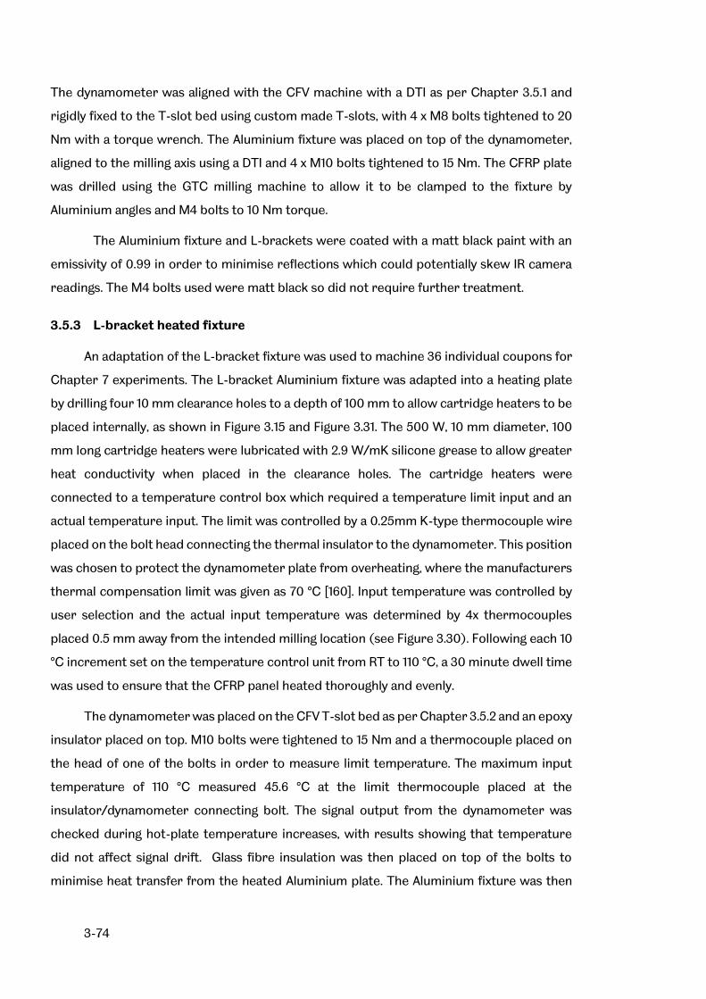
3-74

The dynamometer was aligned with the CFV machine with a DTI as per Chapter 3.5.1 and

rigidly fixed to the T-slot bed using custom made T-slots, with 4 x M8 bolts tightened to 20

Nm with a torque wrench. The Aluminium fixture was placed on top of the dynamometer,

aligned to the milling axis using a DTI and 4 x M10 bolts tightened to 15 Nm. The CFRP plate

was drilled using the GTC milling machine to allow it to be clamped to the fixture by

Aluminium angles and M4 bolts to 10 Nm torque.

The Aluminium fixture and L-brackets were coated with a matt black paint with an

emissivity of 0.99 in order to minimise reflections which could potentially skew IR camera

readings. The M4 bolts used were matt black so did not require further treatment.

3.5.3 L-bracket heated fixture

An adaptation of the L-bracket fixture was used to machine 36 individual coupons for

Chapter 7 experiments. The L-bracket Aluminium fixture was adapted into a heating plate

by drilling four 10 mm clearance holes to a depth of 100 mm to allow cartridge heaters to be

placed internally, as shown in Figure 3.15 and Figure 3.31. The 500 W, 10 mm diameter, 100

mm long cartridge heaters were lubricated with 2.9 W/mK silicone grease to allow greater

heat conductivity when placed in the clearance holes. The cartridge heaters were

connected to a temperature control box which required a temperature limit input and an

actual temperature input. The limit was controlled by a 0.25mm K-type thermocouple wire

placed on the bolt head connecting the thermal insulator to the dynamometer. This position

was chosen to protect the dynamometer plate from overheating, where the manufacturers

thermal compensation limit was given as 70 °C [160]. Input temperature was controlled by

user selection and the actual input temperature was determined by 4x thermocouples

placed 0.5 mm away from the intended milling location (see Figure 3.30). Following each 10

°C increment set on the temperature control unit from RT to 110 °C, a 30 minute dwell time

was used to ensure that the CFRP panel heated thoroughly and evenly.

The dynamometer was placed on the CFV T-slot bed as per Chapter 3.5.2 and an epoxy

insulator placed on top. M10 bolts were tightened to 15 Nm and a thermocouple placed on

the head of one of the bolts in order to measure limit temperature. The maximum input

temperature of 110 °C measured 45.6 °C at the limit thermocouple placed at the

insulator/dynamometer connecting bolt. The signal output from the dynamometer was

checked during hot-plate temperature increases, with results showing that temperature

did not affect signal drift. Glass fibre insulation was then placed on top of the bolts to

minimise heat transfer from the heated Aluminium plate. The Aluminium fixture was then

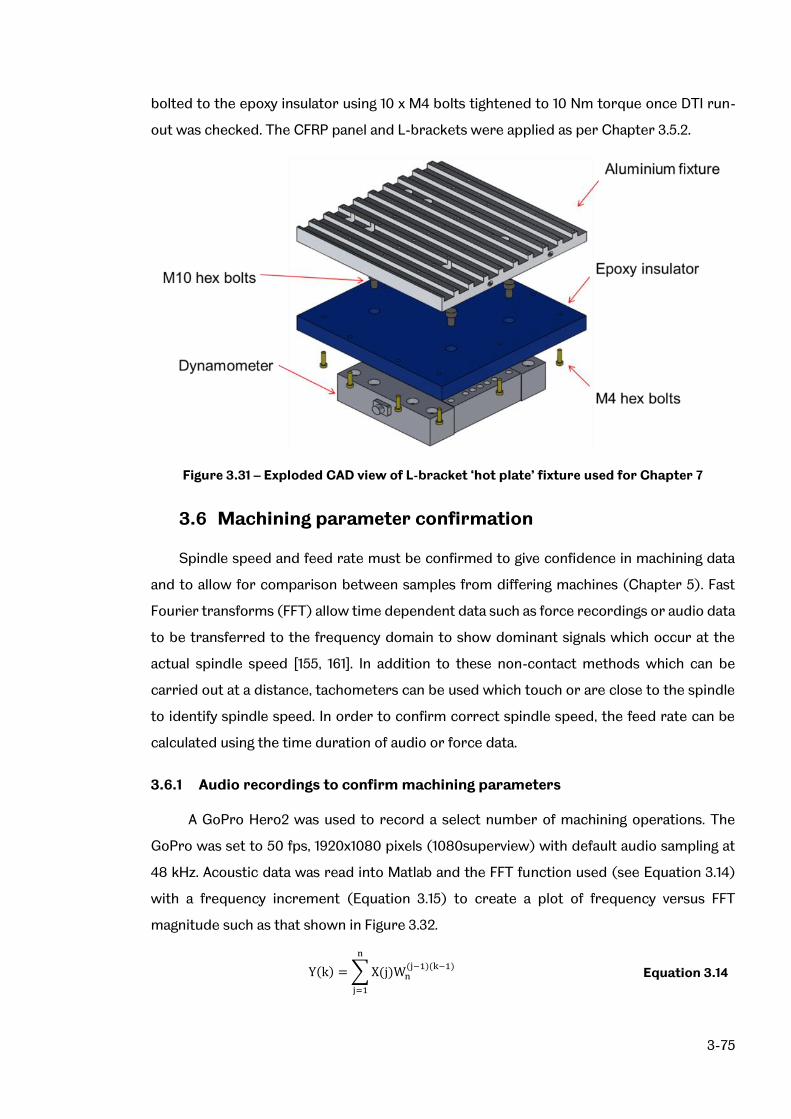
3-75

bolted to the epoxy insulator using 10 x M4 bolts tightened to 10 Nm torque once DTI run-

out was checked. The CFRP panel and L-brackets were applied as per Chapter 3.5.2.

Figure 3.31 – Exploded CAD view of L-bracket ‘hot plate’ fixture used for Chapter 7

3.6 Machining parameter confirmation

Spindle speed and feed rate must be confirmed to give confidence in machining data

and to allow for comparison between samples from differing machines (Chapter 5). Fast

Fourier transforms (FFT) allow time dependent data such as force recordings or audio data

to be transferred to the frequency domain to show dominant signals which occur at the

actual spindle speed [155, 161]. In addition to these non-contact methods which can be

carried out at a distance, tachometers can be used which touch or are close to the spindle

to identify spindle speed. In order to confirm correct spindle speed, the feed rate can be

calculated using the time duration of audio or force data.

3.6.1 Audio recordings to confirm machining parameters

A GoPro Hero2 was used to record a select number of machining operations. The

GoPro was set to 50 fps, 1920x1080 pixels (1080superview) with default audio sampling at

48 kHz. Acoustic data was read into Matlab and the FFT function used (see Equation 3.14)

with a frequency increment (Equation 3.15) to create a plot of frequency versus FFT

magnitude such as that shown in Figure 3.32.

Y(k) = ∑ X(j)Wn(j−1)(k−1)

n

j=1

Equation 3.14

3-76

𝐹𝑟𝑒𝑞𝑢𝑒𝑛𝑐𝑦 𝑖𝑛𝑐𝑟𝑒𝑚𝑒𝑛𝑡 = 𝐹𝑠

𝑙𝑒𝑛𝑔𝑡ℎ (𝑥) Equation 3.15

Where 𝐹𝑆 is the sampling frequency and 𝑙𝑒𝑛𝑔𝑡ℎ (𝑥) is the FFT increment.

Figure 3.32 – Spindle speed confirmation (14,412 RPM) through FFT of GoPro acoustic data

The machining time can be calculated from simply plotting the audio recording signal

as a function of time and determining the start and end of a cut by the change in frequency.

3.6.2 Force recordings to confirm machining parameters

Force data collected through a Kistler dynamometer can be processed using Kistler

Dynoware software to show data in the frequency domain. As an alternative, Matlab has

been chosen to import raw force data in order to understand the process and tailor the FFT

application. The FFT function within Matlab is applied to force data as per Chapter 3.6.1 to

produce figures similar to that shown in Figure 3.32 which plot the dominant frequency thus

allowing spindle speed to be identified. Feed speed is verified by analysing the time length

of the force data.

3.6.3 Tachometer

A Testo 470 tachometer was used to directly record the spindle speed of the GTC

and the Erbauer diamond disc saw. Reflective strips were placed on rotating components

and the laser non-contact function used to record the spindle speed.

3-77

3.7 Cutting force measurement

The reaction forces involved in cutting can be measured using a stationary plate

dynamometer. Kistler dynamometers operate using pre-loaded force piezo electric sensors

for x, y and z force components which sit within 4 sensors located in the dynamometer plate

[162].

3.7.1 Dynamometer

A Kistler 9139AA dynamometer, calibrated annually, was used for machine

comparison trials, initially due to availability and then in further experiments to remain

consistent. The dynamometer was connected to an 8 channel charge amplifier (Kistler type

5070A12100) which was in turn connected to a DAQ system (Kistler Type 5070A12100).

Dynoware version 2.6.5.16 was used to open the raw collected data and then export to

Matlab for post-processing. The dynamometer was attached to the T-slot bed for the ABB

machine using four side clamps. For FTV machining trials, the dynamometer was attached

by two clamps at the rear and a single bar across the front face of the plate for tool clearance

purposes. For the CFV machine, the dynamometer was clamped directly to the T-slot bed

using custom T-slots. All bolts were tightened to 20 Nm using a torque wrench to ensure a

rigid and consistent setup and as per Chapter 3.5 a DTI was used to ensure squareness to

the direction of cutting. Channel sensitivity and ranges were set as per Table 3.8. Measuring

time was set to 100 s and a sample rate of 20 kHz was used. The high sampling rate ensures

that the contact between individual cutting teeth and the workpiece is captured with

sufficient points to produce a curve showing interaction between the cutting edge and the

workpiece. A higher sampling rate would allow a greater observation of the actual analogue

signal however would require larger resources when processing data. The minimum

sampling rate can be expressed as a consequence of individual tooth passing frequency,

𝑓𝑡𝑜𝑜𝑡ℎ, given by Equation 3.16.

𝑓𝑡𝑜𝑜𝑡ℎ =𝑁 × 𝑛

60 Equation 3.16

For 14,412 RPM (Chapter 5) and 8 teeth, the tooth passing frequency is 1,921.6 Hz. Therefore

20 kHz will allow each tooth pass to be mapped by approximately 10 data points from the

dynamometer.

3-78

Table 3.8 – Channel Sensitivity and Ranges

Direction Channels Sensitivity (pC/N) Measuring range (kN)

Fx 1-2 -8.377 0 - 1

Fy 3-4 -4.317 0 - 1

Fz 5-8 -8.371 0 - 1

Whilst the dynamometer is calibrated yearly, prior to attaching the milling fixture to

the dynamometer plate, the dynamometer was checked for correct force interpretation. A

spindle was weighed on scales and then placed on the dynamometer and z forces recorded

(see Figure 3.33 for axis system). Forces in the x and y-direction were checked by attaching

a luggage scale, recording the observed mass and comparing to raw dynamometer results.

Figure 3.33 – Dynamometer force axis system

A force diagram which has been processed for signal drift, typical of all

measurements during this research, is presented in Figure 3.34. The cut occurs at

approximately 11 seconds from the start of dynamometer recording. It can be seen that

forces are greatest in the x direction, opposing the direction of tool feed. Comparatively,

forces in the y direction are smaller and forces in the z-direction are comparatively smaller

still.

3-79

a)

b)

c)

Figure 3.34 – Typical raw force plots for a) Fx (cutting force), b) Fy (tangential force) and c)

Fz (axial) force diagram from machining, prior to UT calculation (Taken from Chapter 5

sample using ABB machine and DIA-BNC tool)

3-80

3.7.2 Dynamometer data

Typically, cutting/radial and tangential forces can be calculated for machining

experiments using Equation 3.17 and Equation 3.18 [6, 163].

𝐹𝑟(𝜙) = 𝐾𝑟𝑐𝑎ℎ(𝜙) + 𝐾𝑟𝑒𝑎 Equation 3.17

𝐹𝑡(𝜙) = 𝐾𝑡𝑐𝑎ℎ(𝜙) + 𝐾𝑡𝑒𝑎 Equation 3.18

Where 𝐾𝑟𝑐 , 𝐾𝑡𝑐, 𝐾𝑟𝑒 and 𝐾𝑡𝑒 are cutting shear force coefficients and edge force coefficients

for radial and tangential directions, 𝜙 is tool rotation angle, ℎ is instantaneous chip thickness

and 𝑎 is depth of cut. For metallic machining operations, a database of these coefficients

exists [164]. For composites this is more complex, especially for multi-directional laminates

and complex tool geometries with dual and opposing helixes, due to the need to calculate

specific cutting energy coefficients through experimentation for each of the ply fibre

orientations and use of mechanistic models to sum these forces [51, 165-170].

The use of radial or tangential forces does not include z force components (along

the length of the tool) which are also a significant factor when using tools with helix angles

which direct forces axially. An alternative to allow for comparison of machines and tools is

to calculate a total power value for each cut. This takes the raw force data in the x, y and z

direction from the dynamometer from the start to the end of the cut.

Data is imported into Matlab and then subject to a drift compensation script to

remove the exact drift of the dynamometer at the time of cutting (typically 3 N). Then a

specific algebraic sum of forces (Nm) is calculated as the integral of the absolute raw force

data as a function of distance cut within Matlab. This is then divided by the total volume of

material removed to provide UT (N/mm2). Whilst UT is understood to have pressure units

and could be expressed as Pa, the original units of N/mm2 will be used throughout this thesis

as a more machining appropriate unit that reflects its derivation. Using this method also has

the added advantage of accounting for slight thickness variations found in the CFRP flexural

samples for Chapter 5 (3.17 – 3.71 mm) and to a lesser extent Chapter 6 and 7 (3.04 – 3.10

mm), as well as capturing heat elements of work which would otherwise not be possible.

The method would also allow machining with different diameter tools to be directly

compared for future experiments. Whilst a DTI has been used to align the cutting edge with

the cutting axis of the machine, alignment error may result in small amounts of cross-talk in

the x and y channels of the dynamometer. By capturing all directional forces using the UT

method, any cross-talk due to outstanding minor alignment issues can be ignored. The total

specific algebraic sum of forces is divided by the volume cut to give UT, as defined in

Equation 3.19.

3-81

𝑈𝑇 =∫ 𝐹𝑥𝑑𝑥 + ∫ 𝐹𝑦𝑑𝑥 + ∫ 𝐹𝑧𝑑𝑥

𝑉 Equation 3.19

Where UT is the total specific power (N/mm2), 𝐹𝑥,𝑦,𝑧 are the forces recorded by the

dynamometer (N), 𝑥 is the distance of the cut (mm) and 𝑉 is the volume of material removed

(mm3).

In addition to the above argument for using a novel metric to capture cutting forces,

it has also been found that observing individual teeth operations is not appropriate for the

DIA-BNC tool. Figure 3.35 a) shows the tooth passing frequency and x-forces for a DIA-MFC

tool, whilst Figure 3.35 b) shows the same plot for a DIA-BNC tool. It is shown that clear

peaks exist for the DIA-MFC plot, which corresponds to the 8 individual teeth. When

compared to the DIA-BNC plot, the burr teeth make it difficult to extract individual force

peaks that correspond to individual teeth. This adds credence to the need to use a novel

metric which can capture forces for cross tool comparisons.

a) b)

Figure 3.35 – Individual tooth passing frequency comparison for a) DIA-MFC tool (showing

clear peaks) and b) DIA-BNC tool at 8000 RPM (less obvious individual tooth peaks due to

discontinuous engagement caused by burr style teeth)

Figure 3.35 also shows that for the DIA-MFC 8 flute, single helix tool at 8000 RPM,

there is a time difference between teeth of 2.34 ± 0.02 x10-4 s. This can be checked against

a theoretical calculation of time passing frequency described by Schmitz and Smith [155];

𝑓𝑡𝑜𝑜𝑡ℎ =𝜑 × 60

N × 360 Equation 3.20

Where 𝜑 is the tool rotational angle. 𝜑 for up milling can be further described as 𝜑𝑒, the exit

angle of the tooth;

3-82

𝜑𝑒 = cos−1 (𝑟 − 𝑎

𝑟) Equation 3.21

𝑟 is the tool radius, in this case 3 mm and 𝑎 is the radial depth of cut which, for a full

immersion cut, is 3 mm. Using the resulting 𝜑𝑒 value of 90°, the tooth passing frequency time

is 1.875x10-3 seconds. Therefore the time between each of the 8 teeth is 2.343x10-4 which

matches the experimental time.

The individual cutting force peaks cannot be used for comparison of DIA-BNC tools

due to the irregular peak but the DIA-HBC4 and DIA-MFC style tools offer easily identifiable

peaks which will be compared in tool wear and tool temperature experiments (Chapter 6

and Chapter 7, respectively)

3.8 Temperature analysis during milling

Following analysis of edge trimmed flexural specimens, it was noted that significant

smearing of the polymer material had occurred. Since the Tg of the material was

determined by DMA as approximately 113 °C, it was postulated that Tg may be exceeded

during the machining process. This would allow the polymer to be smeared across the

surface by the passing tool. In order to capture temperatures during cutting, a trial on the

GTC machine was conducted using an IR camera placed on the spindle and thermocouples

embedded in the CFRP. The learning from this was then incorporated into tool wear and

cutting temperature trials in Chapter 7.

3.8.1 IR camera

An Optris PI 450 was chosen due to its size, which allowed it to be mounted on the

spindle inside the GTC machine. The IR camera was focussed on the tool during the duration

of the cut. For CFV trials, the IR camera was mounted on a tripod on the bed of the machine.

In the CFV layout, the IR camera was focused on the tool at the end of the cut to observe

maximum tool temperature. The camera was also positioned facing the cut edge to allow

observation of the cut surface. This edge observation was only available for a single cut due

to the layout of the fixture. The camera was set to record between 0-250 °C using emissivity

settings given in Table 3.9 which were determined through calibration tests (Chapter 4.5.1).

The stated accuracy of the camera is ± 2 °C.

3-83

Table 3.9 – Emissivity, ε, settings used for tools during machining of CFRP for Chapter 7

BNC DIA-BNC MFC DIA-MFC

0.74 0.93 0.71 0.85

3.8.2 Embedded thermocouples

K-type thermocouples were embedded to a depth of 1.5mm (i.e. half way through

the thickness of the CFRP panels) at four locations 0.5 mm in front of the tool pass and

secured with a glue gun. The holes were drilled prior to experimentation using the GTC

machine with Proxon Micromot 28 864 HSS drills at a speed of 5,000 RPM and a drill feed

of 1 mm/min at the locations shown in Figure 3.30.

During temperature trials conducted on the GTC machine it was noted that

response rate of the thermocouples was slow. As the response rate of the thermocouples

is low they are not used to measure the temperature of cutting but used only to ensure the

correct panel temperature has been reached where the panel is pre-heated before cutting

(Chapter 7) using a PicoLog TC-08 USB thermocouple DAQ set to 60 Hz.

3.9 Post machining analysis

Following machining, the trimmed edges of the flexural samples were observed. As

noted in Chapter 2.4, current methods of surface quality observation using Ra do not

sufficiently capture the true surface quality. Several methods of surface quality analysis have

been completed using areal, SEM and XCT techniques. These methods are currently

considered cutting edge technologies to observe surface defects however, a novel metric is

also presented which utilises epi-fluorescent microscopy (EFM) optical analysis. This

method characterises the area of removed material compared to a theoretically straight

cut. Figure 3.36 shows the location and measurement strategy for focus variation/areal, SEM

and EFM which form part of the surface measurement strategy.

3-84

Figure 3.36 – Measurement strategy for focus variation, SEM and EFM (where focus

variation is captured for both trimmed edges, EFM captures both trimmed edges and SEM

is completed for one side only)

3.9.1 Areal surface measurements

Areal surface measurements involve capturing the 3D surface topography of a

structure in order to apply metrics to an area of interest to categorise surface defects. As

noted in Chapter 2.4, the optical focus variation method takes images at different focal

lengths and stitches these together to create a surface topography. The resulting cloud

point data can be processed using Alicona recommended flow of information [171];

1. Measure machined composite surface

2. Repeatability filtered surface

3. Reference levelled surface

4. Roughness or waviness filtered surface

5. Calculate roughness parameters

The mid-section of each flexural coupon, on each side of the sample, is observed to

allow comparisons to the likely failure area during four-point bend flexural testing. The scan

area is limited to 5 x 3 mm scans for the Alicona SL due to restrictive hardware memory.

In order to observe the planar face of the machined samples, flexural samples were

placed in a 3D printed sample holder which was developed as per Chapter 4.6 and shown in

Figure 3.37. This holder also allowed an automated measurement script to be used which

reduced user input time and decreased user error in location of the samples.

3-85

a) b)

Figure 3.37 – a) 3D printed flexural sample holder and b) holding 32 samples used to assess

large numbers of CFRP machined coupon edges

As per Chapter 3.4.3, the machines used to capture areal information were checked

against known calibration samples. As noted, it is essential that contrast and exposure are

not altered during measurement. Exposure was set to 7.25ms and contrast was set to 0.7.

Vertical resolution of 200 nm and a lateral resolution of 1 μm were used for all specimens

intended to capture surfaces in the 10 x magnification range. These parameters meet the

measurement criteria defined in BS EN ISO 4288 [172] and Alicona guidance [158] which

require vertical resolution, 𝑉𝑟, to be < 1 µm calculated from Equation 3.22 where Rq was found

to be 10.0 ± 0.06 µm (taken from 10 readings).

𝑉𝑟 =𝑅𝑞

15 Equation 3.22

Lateral resolution, 𝐿𝑟, was required to be < 0.01 mm based on a structure length of 1.0 ± 0.03

mm (taken from 10 readings) in order to fully capture the roughness of the surface.

𝐿𝑟 = 𝑠𝑡𝑟𝑢𝑐𝑡𝑢𝑟𝑒 𝑙𝑒𝑛𝑔𝑡ℎ

10

Equation 3.23

Following image capture, the surface was trimmed to an observable area of 5 x 3

mm, removing approximately 0.1 mm from the edges of the sample as shown in Figure 3.38.

The cropping of the captured image removes edge effect characterisation which can

include extrapolation and extensions of the profile [173] which is unwanted during filtration

using the available Alicona software Gaussian filters. The repeatability of the cropped

surface was then measured. This provides a value of repeatability and allows ‘poor’

measurement points, i.e. those with low contrast, high noise due to sensor temperature, or

low texture, to be removed from the analysis if required. This has not been completed for

3-86

any measurements as robust filtration has been used to discount outliers, which may alter

reference plane adjustment, as noted below.

Figure 3.38 – Image cropping to remove areas of dead pixels and minor edge effects

A reference plane to the cropped surface is applied using Robust Gaussian filtration, shown

visually in Figure 3.39.

a)

b)

Figure 3.39 – a) unlevelled surface and b) Robust plane applied to milled surface (Coupon 9-

1-S1) prior to surface quality metric generation

Based on the metrics provided by Alicona to account for hardware temperatures

during data capture, a repeatability threshold can be generated. For all measurements

completed in this thesis, the repeatability threshold for data point heights has been set to a

3-87

95% confidence interval with a mean repeatability of ± 0.030 µm. As noted in Chapter 3.4.3,

this value does not change the overall results of surface metrics.

Following reference plane creation, a Robust Gaussian filter for flat surfaces is

applied to the surface and cut-off value, 𝜆𝑐, is set. Other options for filtering the surface

include [171] [174]:

Gaussian filter for flat surfaces (ISO 16610-61, Linear planar, Order 0). Linear

Gaussian filter without consideration of end-effects at surface borders. This is

considered ideal where the edges of the specimen have not been included in the

cropped image and the dataset axis system has been robustly adjusted to remove

any slope of the part due to incorrect loading onto the machine during image

collection.

Gaussian filter for inclined planar surfaces (ISO 16610-61, Linear planar, Order 1).

With consideration for end effects at surface borders. Can be applied to flat surfaces

but works best for inclined surfaces.

Gaussian filter for arbitrary surfaces (ISO 16610-61, Linear planar, Order 2).

Considers end effects, inclined planar and curved surfaces. It does not perform well

with outliers.

As above but with Robust Gaussian filters (ISO 16610-71). These filters allow the

observation of unexpected surface defects and outliers.

Robust Gaussian filters were chosen due to the possibility of capturing unexpected defects

and outliers which is particularly useful for defects where the fibres are orientated at -45°

to the cutting edge. These defects can cause fibre pull-out leading to distinct peaks and

valleys which could be missed by standard Gaussian filtration [175]. Further to this, the flat

surfaces option (Linear planar, Order 0) was chosen as careful cropping of the image

removed edge effects. This is visually shown in Figure 3.40 where the ‘freak values’

described by Brinkman and Bodschwinna [175] can only be captured by the Robust Gaussian

method. Whilst computationally more complex, this was completed using an automated

script which could be run overnight. BS EN ISO 16610:31 [176] describes the full process of

Robust Gaussian filtration applied to the cloud point data taken with Alicona hardware and

software.

3-88

a) b)

Figure 3.40 – a) Gaussian and b) Robust Gaussian filtration [177] highlighting the ability of

the Robust method to capture random surface artefacts accurately (reproduced under

agreement with DigitalSurf)

After surface levelling, a 𝜆𝑐 filter value was applied to the image before volumetric,

spatial, bearing area and autocorrelation textural parameters are collected from the

software. The full list of parameters measured is given below, in Table 3.10. Some of the

spatial and volumetric parameters are visualised in Figure 3.41.

a) b)

c)

Figure 3.41 – V-parameter visualisation [171] for a) linear areal material ratio curve based

parameters (where 1 = maximal height, 2 = peak area, 3 = 40% of min. slope, 4 = valley area, 5

= minimal height), b) material and void volume parameters (reproduced under agreement

with Alicona Imaging GmbH [171]) and c) spatial parameters (adapted from [106])

3-89

Table 3.10 – Surface quality parameters measured through areal methods [178] Note:

this page has been coloured for quick reference

Symbol Parameter

type

Sub-parameter

type Definition

Sa (μm)

S-parameter

Amplitude

Average height of selected area

Sq (µm) Root-Mean-Square height of selected area

Sp (µm) Maximum peak height of selected area

Sv (µm) Maximum valley depth of selected area

Sz (µm) Maximum height of selected area

S10z (µm) Ten point height of selected area

Ssk Skewness of selected area

Sku Kurtosis of selected area

Sdq Hybrid

Root mean square gradient

Sdr (%) Developed interfacial area ratio

Sal (μm)

Spacing

Auto correlation length: dominated by low or high frequencies

Str Texture aspect ratio: strong or weak dominant

structures

Stdi Miscellaneous Texture direction index

Sk (µm)

V-parameter

Linear areal material ratio

curve

Core roughness depth, Height of the core material

Spk (µm) Reduced peak height, mean height of the peaks

above the core material

Svk (µm) Reduced valley height, mean depth of the

valleys below the core material

Smr1 (%) Peak material component, the fraction of the

surface which consists of peaks above the core material

Smr2 (%) Peak material component, the fraction of the

surface which will carry the load

Vmp (ml/m²) Material volume

Peak material volume of the topographic surface (ml/m²)

Vmc (ml/m²) Core material volume of the topographic

surface (ml/m²)

Vvc (ml/m²)

Void volume

Core void volume of the surface (ml/m²)

Vvv (ml/m²) Valley void volume of the surface (ml/m²)

Vvc/Vmc Ratio of Vvc parameter to Vmc parameter

3-90

𝜆𝑐 is a cut off ratio which separates roughness from the form and waviness of the

measured item. Alicona [158] recommend a 𝜆𝑐 value at least 5 times greater than the Ra value

in order to completely remove the effects of waviness. In addition, BS EN ISO 4288-1996

[172] offers guidance of separating the roughness by providing 𝜆𝑐 values with look-up tables

based on measured Ra and RSM values. The RSM value represents the mean spacing of

profile irregularities i.e. the average length of a single profile element which consists of a

peak and a trough. This has been completed by taking a sample from Chapter 5, 6 and 7, and

assessing the RSM value for a 2D profile.

For Chapter 5 sampled surfaces had Ra roughness values between 0.1 and 2 µm and

an RSM value between 0.013 and 0.04 µm. As per BS EN ISO 4288-1996, a cut-off 𝜆𝑐 value of

0.8 mm was applied. This also met the requirement of 𝜆𝑐 being 5 times greater than Ra [158].

For Chapter 6 and Chapter 7 machined edges, a 𝜆𝑐 value of 2.5 mm was required to fully

remove the effects of waviness.

In addition to more advanced parameter collection using areal techniques, Ra data

was also collected to validate the findings of Duboust et al. [14] and Nwaogu, Tiedje, and

Hansen [90], who propose that stylus parameter trends can be replicated by areal

techniques. The Ra data is collected from the areal measurements within Alicona and not by

a stylus based profilometer method. The Ra is measured to ISO 4288 [172] and ISO 3274 [179]

specifications, with a cut-off wavelength, 𝜆𝑐, of 0.8 mm and a tip radius of 5 μm. Five

measurements are taken in the transverse direction across the full thickness of the

specimen in order to capture all laminate directions (Figure 3.36), i.e. perpendicular to the

direction of feed.

Both Alicona SL and Alicona G5 save cloud point data i.e. x, y and z co-ordinates which

can be accessed and stitched together to form a surface within Measuresuite, proprietary

software provided by Alicona. The scale bar is not adjustable so a custom Matlab code has

been used to recreate the cloud point data and assign customisable scale bars for

comparison of surfaces.

3.9.1.1 Alicona SL

The Alicona SL machine was used to evaluate surface quality in Chapter 5. A single

representative dummy sample was measured 10 times to give an overall Sa measurement

error of 3.71 ± 0.04 µm. There would be a larger deviation if the sample was measured from

different positions as different sampling regions would be observed. All results using the SL

will be considered to have the same error of ± 0.04 µm throughout this work where Sa is

3-91

quoted. This small error is considered appropriate due to the robust methods employed in

user setup and further computational post processing.

3.9.1.2 Alicona G5

The Alicona G5 was used to evaluate surface quality in Chapter 6 and Chapter 7. This

machine was chosen over the previously used Alicona SL due to the ability to not only

capture 360° tool scans but due to the increased bed movement which would allow the

automation of coupon scanning for a larger number of coupons at one time. As per the SL

machine, a single trial sample was repeated 10 times in order to provide an estimation of

repeatability. The error of the measured sample was found to be 4.85 ± 0.03 µm.

3.9.2 Scanning electron microscopy

In order to understand the micro-surface effects of machining, SEM was used to

collect images of areas of interest on the machined edge. SEM uses an electron gun to fire

a focused beam of electrons onto a material. A detector then receives reflected electrons

and the signals are used to produce an image of the surface. Typically, conductive surfaces

are required in order to prevent the electron beam from charging the sample which can

cause thermal damage by allowing an earthing path for the electron beam to pass through

the sample. Non-conductive options such as variable pressure (VP) SEM could be used to

remove the need for conductive coatings. This process was not cost-effective and VP SEM

was not as effective as standard conductive SEM methods at producing clear, high contrast

images.

Flexural specimens were mounted on 32 mm diameter stubs using Electrodag 1415

silver conducting adhesive. The conducting agent was also used along the perimeter of the

mounted coupon on each side up to the top surface to allow an earthing path around the

material to prevent thermal damage. The top surface was sputter gold coated. An FEI Inspect

F SEM was used with the following parameters:

5kV accelerator voltage (between 5-10kV is recommended for carbon fibre

reinforced polymer composites)

3 spot size/probe current (between 3-3.5 spot size is recommended for carbon fibre

reinforced polymer composites)

Contrast was adjusted per image to attain high contrast between areas in and out of focus.

3-92

3.9.3 XCT scanning

XCT is a method which uses X-rays to penetrate the carbon fibre sample and a

detector to capture X-rays which have passed through the sample. As the sample is rotated

through 360°, the detector collects images which can then be stitched together to provide

a 3D image. This can include any damage through the depth of the composite. A high

powered Nikon CT scanner was initially used as a screening method to determine if

through-depth defects were present. Following creation of a novel metric, XCT scanning

proved an ideal method to verify the results of polished samples. Due to prohibitive costs

the Nikon machine could not be used, however a Skyscan XCT scanner was used within the

Mellanby Centre for Bone Research at the Medical School, UoS. The Skyscan machine

operates at a lower cost but without the same high quality resolution. The Skyscan 1172,

Figure 3.42, is a table top machine intended for low density medical media such as bone

samples.

a) b)

Figure 3.42 – a) Skyscan 1172 machine overview and b) mounted sample (67 x 12 x 3 mm)

Voltage was set to 40 kV, current to 149 μA with no filter. The low power nature of

the machine compared to the Nikon CT scanner required the use of all emitted X-rays,

where exposure level is set to 295, with a final pixel size of 7.83 µm. Whilst it may appear

that the Skyscan is able to provide better pixel resolution than the Nikon, the low power

means that the signal to noise ratio is poor due to the lack of penetration of X-rays. This

presents itself within Skyscan images as ‘ghosting’ where voids are filled with noise from

surrounding material. Post-processing of the images was completed using CTvox [180], a

free to download software with limited functionality.

3-93

3.9.4 Novel epi-fluorescent microscopy damage metric

During the investigation into surface quality, it was found that current measurement

techniques are not fully representative of actual damage. In particular, sub-surface damage

caused by fibre pull-out may not be shown using standard areal metrics or SEM analysis.

Whilst XCT scanning can be used to observe these, the method is prohibitive due to the high

cost per scan. Therefore, a novel metric was developed in order to show sub-surface

defects present in CFRP edge milled materials without the need for expensive XCT scanning.

Edge trimmed samples are sectioned (Figure 3.36) and mounted in epoxy resin

infused with fluorescent dye (Figure 3.43). An ultra-violet light source is then used to

observe through depth effects. A Matlab script changes the colour image to a high contrast

greyscale image where a theoretical straight edge is manually applied as a layer to the image

(Figure 3.44). Analysis of pixel threshold levels with automated Otsu thresholding [181] then

yields a binary image of damaged/non-damaged areas. The resulting metric presents a novel

pixel count of the actual area of machining induced damage, which can be interpreted as an

area measurement (µm2) as seen in Figure 3.44. The development of this process is fully

described in Chapter 4.7.

Figure 3.43 – Mounted epi-fluorescent sample to observe through depth defects

3-94

a)

b)

c)

Figure 3.44 – a) Fluorescent image, b) greyscale image and c) binary image resulting from

automatic Otsu thresholding showing through depth/sub-surface damage

An Erbauer diamond disc saw was used to trim samples which were then cold

mounted with Struers Epo-Fix mixed with Epo-Dye in accordance with manufacturer

recommendations [17]. Following a 24 hr RT cure, the specimens were polished using

parameters presented in Table 3.3, with a microscope inspection after each phase to ensure

the samples were sufficiently polished.

3-95

The epi-fluorescent light process is shown in Figure 3.45 and has been chosen to

create a high contrast image, in this case a darkfield image, where the main portion of the

image is dark but areas of interest are illuminated. An Excelitas X-Cite 110 LED light source

is used to provide light with wavelengths between 360-660 nm; ultra-violet (UV) to the

orange/red end of the visible light spectrum. An auramine light cube (type Zeiss 91029) is

housed in a Qioptiq fusion lens system. The cube consists of the following filters

(wavelengths allowed to pass):

AT450/50x excitation filter (420-480 nm). This removes all but UV/blue light.

AT485DC dichroic mirror (>480 nm). This allows the light from the excitation

filter to be reflected at 45° onto the sample.

AT495lp emissivity filter (> 495 nm). This final filter only allows wavelengths

of > 495 nm through to the Pax-it 3MP camera.

The epo-dye pigmentation powder that is mixed with the epoxy resin is formulated

from “Solvent Yellow 43” [182]. Heterocyclic materials such as Solvent Yellow 43 are ideally

suited to fluorescent excitation due to the availability of free electrons due to the aromatic

compound ring structure [183]. These free electrons can be excited to different Jablonski

[184] energy states where the energy excitation is released as fluorescence. The

fluorescence takes advantage of the Stokes shift whereby light of a certain wavelength (in

this case 420-440 nm) is absorbed but then light of a different wavelength is emitted (in this

case > 520 nm, a green light) [185].

Figure 3.45 – Epi-fluorescent light cube filtration system

3-96

The epi-fluorescent microscope system was used at 2x magnification where the

Qioptiq fusion lens system was calibrated against a Pyser-SGI Ltd. graticule using a 1 mm

scale.

3.9.5 Malvern Morphologi G3

During conventional/up milling a discrete piece of material is theoretically removed

from the workpiece. As discussed in Chapter 2.2.2, chip formation for CFRP materials is

different to metallic machining and discontinuous chips are created and the size of these is

fibre orientation dependent. Chips from cutting were collected for Chapter 6 and Chapter

7 experiments in order to analyse chip morphology. This could then determine if tool wear

or cutting temperature changed the size of the machined chips, giving an indication that the

chip formation/cutting method has changed.

Chips were collected and sealed in a bag following every cut. Following collection,

the surface of the CFRP and the jig were cleaned using dust extractors to avoid cross-

contamination of chip samples when different tools and machining temperatures were

used.

The morphology of the composite chips was analysed using a Malvern Morphologi

G3 through a static image analysis method. A volume of 5 mm3 of sample was dispersed

using a dry powder dispersion unit at a pressure of 1 bar and injection time of 10 ms. The

particles were allowed to settle under gravity for 120 s inside the closed unit. The dispersion

parameters were carefully selected to avoid damage to fragile particles whilst ensuring that

agglomerated material was uniformly dispersed. Images were taken automatically at 5x

magnification with the sample illuminated diascopically. Imaged particles with less than 100

pixels were discounted from the shape analysis in order to remove noise, and an average of

50,000 particles were analysed per sample.

The G3 software provides a distribution of particle sizes. For comparison purposes,

the mean and standard deviation of these distributions can be found from Equation 3.24 and

Equation 3.25 respectively where 𝜇 is the mean, 𝑓 is the frequency, 𝑥𝑖 is the mid-point of

each class and 𝜎 is the standard deviation. In order to conduct a statistical comparison of

values, a t-test comparison can be made using the equation given in Equation 3.26, where

𝑁𝐴 or 𝑁𝐵 is the number of particles from dataset A or B. Based on this t-test, a p-value at a

95% confidence interval level can be used to show if a statistical difference between the two

samples exists.

3-97

𝜇 =∑(𝑓 × 𝑥𝑖)

∑ 𝑓 Equation 3.24

𝜎 = √∑ 𝑓 (𝑥𝑖 − 𝜇)2

∑ 𝑓 Equation 3.25

𝑡 =µ̅𝐴 − µ̅𝐵

√𝜎𝐴

2

𝑁𝐴+

𝜎𝐵2

𝑁𝐵

Equation 3.26

Figure 3.46 – Malvern G3 particle analyser with typical chip morphology displayed on

screen

3.10 Flexural testing

Mechanical testing is completed to determine if defects, caused by differing machining

parameters, change the overall mechanical performance of the CFRP material. Flexural

testing was chosen as typical applications of carbon fibre are not in pure tension or

compression. A more realistic operating mode is flexing of the material such as in a wing

spar or in an automotive monocoque tub. As isolated modes of tension, compression or

shear are not typically experienced, a flexural test is more appropriate as this combines the

load cases. In flexural loading the top surface is in compression, the lower surface is in

tension and the middle portion is in shear. In addition, Soutis [186] notes that free edges

under shear may influence the failure of the material. Static testing was chosen as a starting

point and due to the changes in static flexural properties observed in Chapter 5, the need

for fatigue analysis was considered unnecessary.

3-98

Arola and Ramulu [92] performed static four point bend testing for ABWJ, diamond disc

saw and PCD edge milled CFRPs in a [(0/90/45/-45)2(0/90)]s lay-up and found that no bulk

strength difference was apparent. However, the data presented in this study does show a

difference in peak load obtained during bend testing. A later study by Arola and Ramulu [187]

notes that machining defects are a cause of differing mechanical performance with -45°

plies the point of failure within a laminate when flexurally loaded.

Four point bend testing was chosen over three point bend testing due to the larger

region subject to bending moments, shown in Figure 3.47. Three-point bending also

introduces localised stresses underneath the loading nose which can cause premature

failure and could negate the effect of the machined edge [188].

Figure 3.47 – Comparison of force (V) and bending moments (M) in three and four point

bending [189] highlighting the greater quantity of material/trimmed edge under loading

during four point bend loading compared to three point bend loading (Reproduced under

Open Access license of Theses, Dissertations and Senior Projects at UND Scholarly

Commons)

Whilst it is known that compression is highly influenced by machining effects [8, 9],

this requires larger test specimens than the flexural test and is often difficult to conduct

with unwanted buckling and failure at end tab locations [190]. Interlaminar shear tests were

also considered to observe edge effects, however the sample size is known to be very small

(10 mm) and requires a high degree of tolerance (± 0.2 mm) [191] for the machined width

which, at the time of initial investigation, could not be guaranteed with the GTC machine.

Literature [8] has also shown that tensile testing is also prevalent to machine induced edge

effects however, like compression testing, the test specimens are larger than flexural and

are also prone to failure at end tab locations which cannot be correlated to surface quality.

3-99

Therefore, as an initial study it was chosen to machine flexural samples. Following a result

which showed a difference in mechanical properties (Chapter 5) it was decided to continue

using static flexural analysis to observe changes in mechanical performance in Chapter 6

and Chapter 7.

3.10.1 Flexural testing jig

An Aluminium rig was used for Chapter 5 as a low cost option for testing materials.

Following this a Steel rig was obtained and altered to meet ASTM D6272 requirements of 10

mm diameter loading and support noses [192]. The new rig also allows support and loading

span spacing changes where small adjustments are required to account for CFRP thickness

changes. Both mechanical test jigs are shown in Figure 3.48.

a) b)

Figure 3.48 – 4 Point bending rig a) for Chapter 5 and b) for Chapter 6 and Chapter 7

flexural samples

As per ASTM D 6272 [192] the coupons were machined to a nominal width of 12.7mm.

The support span was set to a 16:1 length to thickness ratio and a loading span at half the

support span distance was used. Half load span was used to maximise the amount of

material in shear during testing. The half span allows more of the edge to be subject to shear

than one third loading and is the reason why ASTM D 6272 rather than BS EN ISO 14125 [152]

has been selected for testing. By allowing more of the edge to be in shear, more edge effects

can be captured. For the Aluminium jig used in Chapter 5, a support span of 54.4 mm was

used based on an average panel thickness of 3.4 mm. For the Steel jig used in Chapter 6 and

Chapter 7 the support and load span was adjusted to match the correct thickness of the

sample.

3-100

3.10.2 Flexural testing machine

A Tinius Olsen 5 kN tensile/compression rig was used with a H500L laser

extensometer to measure mid-span deflection. Two reflective strips were used with the

laser extensometer. One was placed under the support span which remained static during

testing. The second was placed at the mid span of the composite at the edge where most

deflection occurred. As the laser takes the leading edges of the two strips, it is essential

that the width of the strip applied to the CFRP coupons is consistent. The strip applied to

the CFRP has been laser cut to a width of 1mm and a length of 3mm. The testing machine

was programmed with the correct crosshead motion, R (mm/min), to allow for constant

strain rates to be applied to individual specimens as per ASTM D6272 Equation 3.27;

𝑅 =0.167 × 𝑧 × 𝑙𝑠𝑝𝑎𝑛

2

𝑑 Equation 3.27

Where 𝑧 is rate of straining of the outer fibres (mm/mm min.) set to 0.01, 𝑙 is the support

span (mm) and 𝑑 is the depth of beam (mm).

Error analysis of the laser extensometer was completed in order to check the

literature stated ± 1 % error value. A reflective strip was placed on the lower and upper

sections of the four-point bend jig and the gauge length measured. The loading head was

then moved closer to the supporting jig and the crosshead motion (captured directly by the

Tinius Olsen machine) was recorded along with the computed laser extensometer reading.

By repeating this test five times, an absolute error of ± 0.97 % exists, which can be applied

to all strain results. Load cell error of ± 0.5% is given by annual calibration of the Tinius Olsen

machine.

3.10.3 Flexural testing result processing

The test machine was run at the crosshead rate of Equation 3.27 until the specimen

ultimate strength was reached. Testing could have continued until eventual complete

fracture but the initial failure propagation was preserved by stopping testing at the ultimate

strength to allow for observation and failure mode comparison. It is noted that CFRP

material does not exhibit plastic deformation and there is little to no yield in the material.

The load displacement curve was calculated using laser extensometer data and flexural

strength calculated as per Equation 3.28.

𝑆 =3 × 𝑃 × 𝑙𝑠𝑝𝑎𝑛

4 × 𝑏 × 𝑑2 Equation 3.28

3-101

Where 𝑆 is maximum fibre stress (MPa), 𝑃 is load (N) given by Tinius Olsen 5k test file and

𝑏 is the width of beam (mm) for each individual specimen. Modulus of elasticity was

calculated using Equation 3.29.

𝐸 =0.17 × 𝑙𝑠𝑝𝑎𝑛

3 × 𝑚

𝑏 × 𝑑3 Equation 3.29

Where 𝐸 is the modulus of elasticity (MPa) and 𝑚 is the gradient of stress vs. strain graph.

This was taken at five locations of the linear portion of the stress-strain curve and averaged;

it was not taken from the origin which would have required toe compensation.

The maximum strain of the material, 𝑟, under half load span is given by Equation 3.30

where 𝐷𝑚𝑖𝑑 is the mid-span deflection measured by laser extensometer.

𝑟 =4.36 × 𝐷𝑚𝑖𝑑 × 𝑑

𝑙𝑠𝑝𝑎𝑛2 Equation 3.30

3.10.4 Digital image correlation

Digital image correlation (DIC) is a full field strain measurement technique which

works using the principal of tracking and measuring displacement of specific areas of

images [193]. Through use of DIC, the strain progression of the machined coupon can be

observed and tracked, with insight into the failure mechanism or area of strain build up

observed.

Samples are sprayed with a speckle pattern and software is able to determine how

these speckles deform up to the point of failure as shown in Figure 3.49. If the sample

pattern is calibrated, the exact amount of deformation between image frames can be

determined and the strain progression on a surface of a sample can be found.

Figure 3.49 – Displacement components of a deformed body, Peters and Ranson [193]

(reproduced under agreement with SPIE and authors)

3-102

2D high speed (HS) DIC has been used to determine if failure mode is altered in

Chapter 6 and Chapter 7. In addition, DIC provided an alternative source of strain data to

compliment values obtained through ASTM D6272.

Prior to testing, the CFRP samples were sprayed white using a household appliance

white spray. Based on the work of Dong and Pan [194], a speckle pattern of approximately 4

µm, equating to 3x3 pixels, was applied using a handheld airbrush. Acrylic black paint, made

up with 50 % volume of paint thinner, was used to create a speckle pattern between 2 to 5

pixels which was deemed appropriate using the magnification of DIC equipment available.

The DIC setup is shown in Figure 3.50 and comprises of:

Miniconstellation 120C28 5000k LED light source. This was set to a 12 µs pulse which

was adequate to achieve correct speckle pattern contrast.

Frasnel lens in order to disperse the light. This was important as the light source

could not be placed directly in front of the sample as it would obscure the camera.

By using the Frasnel lens, the light was effectively dispersed onto the sample without

shadows.

Phantom VEO 410L high speed camera. The camera was set to a 0.2 kHz frequency

in order to capture the sample from the start of loading to the point of specimen

failure in order to show strain progression. This equates to 30,000 images or 3.3

images per second and is limited by camera memory.

Tokina AT-X Pro D 100 mm F2.8 Macro lens at 1.5x magnification with an aperture

size of 8. The lens magnification was chosen to fit the specimen under the loading

noses within the camera image, with aperture size set to allow good contrast of the

speckle pattern. An image size of 1280 x 720 was generated representing a field of

view of 29.5 x 12.1 mm, a spatial resolution of 463 pixels and a strain resolution of 0.21

% (taken from the standard deviation between two unloaded images, Chapter 4).

The lens was placed at 95 mm from the measured surface.

NI DAQ acquisition card and programmable timing unit (PTU) was used to

synchronise the camera shutter and light source triggering.

3-103

Figure 3.50 – 2D HS DIC setup

After camera levelling, the speckle pattern was observed and checked for sufficient

pixel size where 3x3 was deemed adequate. Following this, the DIC setup was calibrated

using a 1 µm graticule (MP1 LaVision calibration plate) placed on the CFRP sample to attain

the correct distance from lens to test location. The graticule was sampled 5 times and

LAVision DAVIS software used to calibrate the setup.

Within the complete image, a specific set of pixels is tracked through deformation

which is known as a subset [195]. DAVIS software used the iterative least squares method

proposed by Pan et al. [196] to track deformation changes in the subset. A subset size of 27

x 27 pixels was chosen as it was found to produce acceptable levels of noise (see Chapter

4.8). A step size of 9 pixels was selected and the correlation mode set relative to the first

image, which was represented by the unloaded specimen, i.e. 0 % strain.

Maximum normal strain was produced to account for both 휀𝑥𝑥 and 휀𝑦𝑦 i.e. the

compression (top) and tension (bottom) sides of the flexural sample where the normal

strain can be given by the eigenvalues of the matrix shown in Equation 3.31 [197].

(휀𝑥𝑥 휀𝑥𝑦

휀𝑦𝑥 휀𝑦𝑦) Equation 3.31

3.11 Health and safety aspects

Prior to the machining of samples, it was ensured that adequate extraction of

machined chips was present. Unlike chips from machining metallics, CFRP chips form small

particulates and during machining can be ejected into the atmosphere. These chips can

remain in the air and are a potential hazard to the machinist. Of the chips collected and

analysed using the method presented in 3.9.5, it was noted that the average length of a chip

3-104

was 20.70 µm whilst the width was measured as 12.97 µm which suggest that significant

health risks were posed during the machining of samples when compared to the data

presented by Haddad et al. [198] in Figure 3.51.

Figure 3.51 – Inhalation of differing particle sizes within the human lung a) the type of

particle and the area of lung penetration and b) visual representation of lung

corresponding to particle size [198] (reproduced under Elsevier license no. 4639270767923)

To minimise risk during machining, the cutting of CFRP has always been conducted

in an enclosed space. The GTC machine has a protective screen fitted whilst FTV and CFV

machines have sliding doorways that prevent direct exposure to chips. The ABB is situated

inside a closed cell so dust exposure is also minimised. A waiting period of 2 minutes

following each cut was always observed, in order to let airborne chips settle onto the bed

of the machine prior to cleaning with extraction.

In addition to minimising direct exposure during the cutting process, extraction has

been used to remove harmful particulates. A Karcher 001 NT 35/1 Tact Te H was used to

filter particulates as small as 1 µm [199] for GTC experimentation. For AMRC based trials a

second level of extraction was used. The Karcher extractor was situated as close to the tool

as possible to act as a local extractor, whilst a Nilfisk T40WPlus LEV Class H extractor was

placed above the cutting zone to act as a global extractor to remove potentially smaller and

lighter particles.

As well as extraction, Alpha Solway C3V FFP3V F/Flat Respiratory disposable masks,

Bolle Cobra eye protection and nitrile gloves were used to ensure adequate protection

against dust when entering the machining environment and handling chips.

3.12 Method summary

A summary of the methods used throughout the experimental Chapters is given in

Table 3.11.

3-105

Table 3.11 – Summary of primary methodologies used in experimental Chapters with

relevant methodology and method development Chapter given where appropriate

Chapter 5 Chapter 6 Chapter 7

CFRP manufacture RTM, no hydraulic

press (Chapter 3.1.3)

RTM, hydraulic press

(Chapter 3.1.3, Chapter 4.1)

Machining

platform

ABB

(Chapter 3.3.2)

FTV

(Chapter 3.3.1)

Erbauer tile saw

(Chapter 3.3.5)

CFV

(Chapter 3.3.4)

Cutting tools

(Chapter 3.4.1)

DIA-BNC

DIA-HBC4

(DIA-)BNC

(DIA-)MFC DIA-BNC

Milling fixtures Toggle clamp fixture

(Chapter 3.5.1, Chapter 4.3.1)

L-bracket fixture

(Chapter 3.5.2, Chapter 4.3.2)

L-bracket heated fixture

(Chapter 3.5.3, Chapter 4.3.3)

In process

monitoring

Dynamometer

(Chapter 3.7)

Dynamometer

(Chapter 3.7)

Dynamometer

(Chapter 3.7)

IR camera

(Chapter 3.8.1, Chapter 4.5)

Post machining

assessment

Areal, Alicona SL

(Chapter 3.9.1.1)

SEM

(Chapter 3.9.2)

EFM

(Chapter 3.9.4, Chapter 4.7)

Areal, Alicona G5

(Chapter 3.9.1.2, Chapter 4.6)

SEM

(Chapter 3.9.2)

EFM

(Chapter 3.9.4, Chapter 4.7)

Malvern Morphologi G3

(Chapter 3.9.5)

Flexural testing Aluminium jig

(Chapter 3.10.1)

Steel jig

(Chapter 3.10.1)

DIC

(Chapter 3.10.4, Chapter 4.8)

3-106

4-107

4 METHOD DEVELOPMENT

This chapter details the significant development of experimental procedures that

have allowed high quality results to be generated. RTM CFRP manufacturing, the machines

used to edge trim, the jigs involved in holding the CFRP workpiece and post-machining

operations have all been subject to methodology improvements.

4.1 CFRP manufacture

Significant efforts have been made to develop the RTM process in order to make

consistent panels in terms of thickness and overall CFRP panel quality. In addition to new

techniques to improve panel thickness, the resins used in the RTM process have been

studied and optimised to lower void content and reduce dry spots of finished CFRP panels.

4.1.1 RTM washout

A trial to understand the variables involved in RTM CFRP manufacture was

completed using a 3 mm mould cavity spacer. A stack of 10 plies in a [(0,90),(+45,-

45),(0,90),(+45,-45),(0,90)]s formation was used to create an expected 2.8 mm thick

specimen. Following curing, after a maximum resin injection pressure of 6 bar, it was found

that the fibres experienced fibre washout/Marcelling [133]. This is where the fibre plies

shear between layers due to resin and/or air pressure motion as shown in Figure 4.1. Fibre

washout was eliminated by creating a dry laminate consisting of 14 plies to give a nominal

thickness of 3.92 mm in a balanced laminate.

Figure 4.1 – Fibre washout from original trial

4-108

4.1.2 RTM panel deflection

As noted in Chapter 3.1.3, the RTM method was selected to produce high quality

CFRP panels with low void content, controllable resin content and consistent panel

thickness compared to alternative methods such as pre-preg manufactured panels.

Following the manufacture and machining of an RTM panel it was noted that the mid-

point was on average 0.470 mm thicker (15.7%) and up to a maximum 0.580 mm thicker

(19.3%) than the outer perimeter of the panel in addition to an overall deviation across the

panel. This suggested that the current mould tool was deflecting under pressure. In line with

more industrial RTM processes, a hydraulic press was designed and implemented to

counteract the 6 bar internal mould tool pressure. Figure 4.2 shows the design of the 20

tonne upstroke hydraulic press which sandwiches the existing RTM tool between 30 mm

Steel supporting plates. This has the advantage of allowing the existing mould tool to be used

without modification. In addition, the current mass of the mould tool can be maintained.

The solution also allows future RTM tools to be designed that are more lightweight and will

rely on the press to limit deflection instead of the mould tool itself.

Figure 4.2 – Hydraulic press with RTM tooling

Finite element analysis (FEA), through 2D shell elements in MSC Patran, was used to

confirm that the proposed solution would remove deformation at the centre of the plates.

The shell elements were suitable for this analysis due to the uniform loading and low

4-109

expected deflection. It is noted that standard FEA limitations apply, namely the

discretisation of loads.

The model comprises of a 360 x 360 mm plate which is the distance between the

bolt centrelines of the current RTM mould tool. Material outside the centreline of the bolt

holes is not considered. For the sake of simplicity, no additional geometry features are

accounted for such as the seal and resin grooves or resin in/out holes. Only one half of the

tool is accounted for as the top and bottom plates are assumed to be identical. Whilst this

could be simplified further by analysing only a quarter of the panel and applying symmetry,

the model is not computationally taxing and such simplifications are not required. Two FEA

models will be considered:

A model where the current 15 mm thick plate is modelled so that the FEA method can

be compared to measured thickness differences and also validated against hand

calculations of expected deflection.

A model where the planned addition of a 30 mm thick plate to the top and bottom

sections which will take the total model thickness to 45 mm.

Analysis uses a standard low carbon Steel with a Poisson’s ratio of 0.3 and a Young’s

modulus of 200 GPa [200]. A 6 bar pressure is applied uniformly across the 360 x 360 mm

panel. Two boundary conditions are applied to the model;

For the current 15 mm thick RTM plate, fixed boundary conditions will be applied to

the perimeter of the model. This is a fair assumption as the 12 bolts and four pins

effectively clamp the mould tool so rotation and translation about the x, y and z axis

is set to zero.

For the proposed solution shown in Figure 4.2, the 45 mm plate (15 mm RTM mould

tool plate + 30 mm supporting/sandwiching plate) is supported by 10 mm thick Steel

sections which connect the supporting plates to the hydraulic press frame. These

two Steel sections are applied across the full width of the panel at 50 and 310 mm

from one end of the plate. The aspect ratio of the 10 mm thick sections is such that

they can be considered fixed and rotation and translation about the x, y and z axis is

set to zero, i.e. the second moment of area is sufficiently large to suggest that

bending will not occur and fixed conditions can be assumed.

Mesh convergence has been considered for both models and has been classed as

converged when the difference between results is less than 1 %. The existing mould tool

4-110

design requires 1,600 elements, whilst 5,184 elements are suitable for the new design for

converged solutions.

In addition to the given FEA solution for the current plate, a hand calculation using

Equation 4.1 [201] has been completed to yield a deflection of 0.206 mm.

𝑦𝑚𝑎𝑥 =𝛼 × 𝑞 × 𝑏4

𝐸 × 𝑡3 Equation 4.1

Using a converged FEA solution, the current plate gives a deflection of 0.214 mm. This

closely matches the hand calculated solution which was used as a check for the FEA

modelling techniques used. The actual experimental thickness difference measured across

three CFRP panels was an average of 0.470 mm or 0.240 mm per mould tool half which

closely matches the FEA and hand calculated deflection. The new design provides an

anticipated deflection of 0.005 mm per mould tool half, or 0.010 mm in total. This represents

a 97.82% reduction in deflection.

a) b)

Figure 4.3 – FEA results (in mm) and boundary conditions for a) original RTM plate and b)

proposed frame with extra plate and support frame

By using this method, consistently flat panels can be made. For the 9 panels

manufactured with this method (Chapter 6 and Chapter 7), a maximum thickness

difference of 0.051 mm from the centre of the panel to the panel peripheral edges was

measured. This suggests that the FEA method was optimistic due to the boundary

conditions of no deflection at the press frame connections. However, whilst the planned

total FEA deflection is not achieved, the panels have a lower and more consistent thickness

4-111

compared to the previous method which is deemed to be a significant improvement for

repeatability of manufacture.

4.1.2.1 Alternative designs

Whilst a hydraulic press was selected to improve the geometric tolerances of CFRP

panels, alternative designs using modifications to the existing mould tool were assessed.

Whilst the advantages of the press are noted, one disadvantage is the cost of £1,600. A lower

cost alternative is to adapt the current mould tool. In order to stiffen the panel, stiffeners

could be welded to the existing plate such as those shown in Figure 4.4. The stiffeners were

accounted for by calculating the second moment of area and by utilising simplistic 1D line

models [201].

a) b) c)

Figure 4.4 – Mould tool alterations showing a) four, b) eight and c) sixteen stiffeners

Stiffeners of various sizes were considered with dimensions, final deflections and

overall mould tool mass given in Table 4.1. Whilst deflection of the panel could be reduced,

the mass increased substantially for all examples. The solution of using a hydraulic press

was therefore considered as the optimal solution and the investment will allow lightweight

RTM tools to be designed in the future.

Table 4.1 – Stiffener numbers, dimensions, panel deflections and complete mould tool mass

No. stiffeners

Stiffener

dimensions

(mm)

Deflection change

from current (%)

Change from

current mass

(%)

4 50 x 10 -92 37

8 15 x 10 -57 22

16 10 x 10 -53 30

4-112

4.1.3 Resin development

Initial resin selection was based on the need to minimise the epoxy and hardener

resin variables described in Chapter 2.1.1.2; namely the removal of unknown compounds

such as diluents, tougheners and accelerators within commercial resins and hardeners. A

resin system which could operate without heating, in addition to a hardener which would

work without the use of an accelerator, was preferred. Diglycidyl-ether-of-bisphenol-A

(DGEBA) was chosen because of its ubiquitous nature within the automotive and aerospace

industry [202], and for its ease of curing with several curing agent options. Epikote 828

(Hexion, UK) was chosen because of the lack of diluents and general availability. TETA was

chosen because of its ability to cure at room temperature. Saleh et al. [135] note that TETA

is a low viscosity aliphatic amine. This group of curing agents uses each aliphatic amine to

react with an epoxy ring to form a hydroxyl group (CH-OH or CH2-OH). The product of this

reaction, in addition to the amine, also reacts with the remaining epoxy rings albeit at a

slower rate than the amine itself.

The stoichiometric equation noted in Equation 3.1 was used to find a mass mixing

ratio of 100:13. Following the resin injection period described in Chapter 3.1.3, no resin was

drawn out of the RTM mould tool towards the resin catch pot. When the panel was cured

at RT for 24 hours, it was found that only the outside of the fibres encased in the mould tool

had been wetted by resin. Further trials used an initial 5 bar pressure in order to quickly

move the DGEBA/TETA resin before its expected gel time of 30 minutes [41], however, no

further permeation of the fabric material was noted. This suggested that the viscosity was

too high for the density of fabric used (200 gsm).

Following this initial trial, a lower viscosity resin was selected. DGEBF (Huntsman PY

306) has a lower viscosity than DGEBA (11,000 versus 1,400 cP [203]) due to the differing

structure where DGEBF lacks the CH3 groups of the DGEBA molecule between the epoxy

rings, as shown in Figure 4.5. As the DGEBF loses the functionality of the CH3 groups, it is

likely that the Tg of the material will decrease due to the ability to rotate around the chain

axis when heated, i.e. the cured DGEBF molecule is less rigid than DGEBA. DMA of the two

materials was completed with a tan delta Tg for DGEBA of 135 °C compared to 115 °C for the

DGEBF material.

4-113

a) b)

Figure 4.5 – a) DGEBA and b) DGEBF epoxy resins

Following the selection of DGEBF due to successful trials, where the resin was able

to fully wet the dry fabric laminate, various curing schedules were trialled in order to

determine the most effective manner of curing RTM CFRP panels. A post cure following the

initial cure was required in order to prevent damage to the RTM tool which contained

elements that could not be heated above 100 °C. The results shown in Table 4.2, obtained

through calculation of Δh and Equation 3.4, show that to achieve a level of 99.998% cure, a

post cure at 130 °C is required. Whilst curing at 100 °C would possibly allow the panel to stay

within the RTM tool during the complete curing cycle, it was deemed that the higher level

of cure would be preferred in order to eliminate further variables during the edge trimming

process, for example local post curing of samples.

Table 4.2 – Tg, Δh and curing results for DGEBF/TETA resins for various curing methods

Cure regime Tg (°C) Δh (J/g) % Cured

Uncured 96.66 -339.78 N/A

RT 72 Hrs 97.62 -191.93 45.764

2 hours at 60°C 97.98 -18.42 59.915

2 hours at 60°C, 2 hours at 100°C 102.48 -0.08 99.977

2 hours at 60°C, 2 hours at 130°C 103.11 -0.01 99.998

4.2 GTC milling machine

A GTC 3D printing machine was adapted to a milling machine configuration with the

intent to create a low cost machining centre without the need for additional technical

4-114

support. Whilst the machine was inappropriate for milling 3 mm thick CFRP, the steps taken

to successfully convert the 3D printing machine into a machine capable of milling CFRP at

low speeds, drilling CFRP and milling of fixtures is still an important advance for the

capability of the research group. The following significant changes were made:

An enclosure was fitted to the machine and electronics moved to an external

area away from CFRP dust, an electrical shorting hazard.

The replacement of x, y, z and spindle controllers and driver boards to a

universal, off-the-shelf standard to allow for easy replacement in case of

failure and compatibility with UniversalGCode sender [204].

The machine enclosure doors were fitted with an interlock safety switch to

stop spindle and axis motion if opened during a machining cycle.

The creation of a vacuum fixture to hold tooling boards to the machine bed.

The introduction of a Hepa filtered dust extractor and on-tool extractor fitting.

4.2.1 Calibration

Whilst ABB, FTV and CFV machines have maintenance schedules and actual spindle

and feed speeds have been checked against dynamometer and audio data, the GTC was

subject to preliminary trials to assess machine performance.

A Testo 470 optical tachometer was used to check spindle input speed against actual

output. A reflective strip was placed onto the top of the spindle motor and measurements

taken. It can be seen from Figure 4.6 that the requested and actual RPM was different. A

cubic quadratic function was used to alter the firmware output voltage of the spindle in

order to account for these differences to allow a range of ±2% between requested and

actual spindle speed. It is also noted from Figure 4.6 that a maximum of 11,000 RPM is

possible for the 400 W brushless DC motor.

4-115

Figure 4.6 – Spindle Motor Test Results

4.2.2 Directional calibration

The directional motion in x, y and z positions was tested using callipers attached to

all axis systems. It was found that the machine was repeatable and accurate to the stepping

motor capability of 0.1 mm which was within necessary requirements. This was not found

to be the case when chatter occurred which changed the expected versus actual positioning

of the axis.

4.2.3 Suitability for CFRP machining

CFRP milling trials using machining parameters produced audible and visible

chatter. The chatter was so extreme that the position of the tool within the working co-

ordinate system was lost and the tool clashed into the milling fixture. Figure 4.7 shows the

results of static tap testing in order to assess machine stability and compare to industrial

machining platforms such as the ABB and FTV. The z direction of the GTC machine is driven

by lead screws whilst the x and y directions (the only directions active in flat edge trims) are

driven by belts. Figure 4.7 a) and b) shows that the stability of the machine changes when

the power of the machine is turned on and off and that, unlike lead screw mechanisms, the

position is not held if a small amount of force is placed upon it. The frequency response at

machining speeds of 9,000 and 14,412 RPM (150 and 240 Hz, respectively) includes areas

where peaks occur, suggesting an unstable process at these cutting speeds. Figure 4.7 c)

1 2 3 4 5 6 7 8 9 10 11 12

0

5000

10000

15000

Inpu

t sp

indle

spe

ed

(R

PM

)

Test

Input spindle speed

Tachometer spindle speed

4-116

and d) show the spindle stability and bed stability of the GTC compared to the FTV and ABB.

It is observed that there is much less stability of both spindle and bed for the GTC machine.

a) b)

c) d)

Figure 4.7 – Stability comparison for a) GTC spindle with power on and off, b) GTC bed with

power on and off, c) various machine spindles and d) various bed stabilities

Whilst Figure 4.7 provides enough evidence to suggest that the machine is not

capable of machining CFRP due to instability, the machined surface of the CFRP coupons

also provides evidence to reject this machining bed for experimental purposes. Surface

topography analysis of the machined CFRP surface is shown in Figure 4.8. This image shows

a clear undulating surface which is visible to the naked eye without the need for further

analysis to show that waviness is large and chatter exists.

100

200

300

400

500

600

700

800

900

1000

1100

1200

0.0

1.0x10-6

2.0x10-6

3.0x10-6

4.0x10-6

5.0x10-6

6.0x10-6

7.0x10-6

8.0x10-6

Mag

nitu

de

(m

/N)

Frequency (Hz)

Power ON X Pos Direction

Power ON Y Pos Direction

Power OFF X Pos Direction

Power OFF Y Pos Direction

Comparison of spindle stability with power on and off

100

200

300

400

500

600

700

800

900

1000

1100

1200

0

1x10-7

2x10-7

3x10-7

4x10-7

5x10-7

6x10-7

7x10-7

Magnitude (

m/N

)

Frequency (Hz)

Power ON X Direction

Power ON Y Direction

Power OFF X Direction

Power OFF Y Direction

Comparison of bed stability with power on and off

100

200

300

400

500

600

700

800

900

1000

1100

1200

1.0x10-6

3.0x10-6

5.0x10-6

7.0x10-6

0.0

2.0x10-6

4.0x10-6

6.0x10-6

8.0x10-6

Mag

nitu

de

(m

/N)

Frequency (Hz)

FTV X Direction

FTV Y Direction

ABB X Direction

ABB Y Direction

GTC X Direction

GTC Y Direction

Comparison of machine spindle stability

100

200

300

400

500

600

700

800

900

1000

1100

1200

0

1x10-7

2x10-7

3x10-7

4x10-7

5x10-7

6x10-7

7x10-7

Mag

nitu

de

(m

/N)

Frequency (Hz)

GTC X Direction

GTC Y Direction

FTV/ABB Jig X Direction

FTV/ABB Jig Y Direction

Comparison of bed/jig stability

4-117

Figure 4.8 – Surface topography of a GTC machined surface

4.3 Milling fixtures

In order to edge trim a specimen from a panel, the milling tool needs to access the

full depth of the composite, requiring the CFRP panel to overhang the milling fixture. Custom

fixtures were thus needed to hold the sample away from the machining bed.

4.3.1 Chapter 5 milling fixture development

Experiments in Chapter 5 were completed using the Aluminium jig with Steel

clamping arms shown in Figure 4.9. This was an existing jig used to machine larger snapshot

coupons, but was adapted to machine flexural samples to the dimensions required in ASTM

D6272. The original jig was created to accept full size coupons which slotted into the

Aluminium cut-out. This was too wide for flexural specimens and it was found that the

flexural coupons could slide in the direction of cutting even when a CFRP pad was added to

prevent movement. Therefore, two Aluminium spacers were fixed to the original jig, which

could be adjusted to accept the pre-trimmed snapshot coupons. The spacers were held by

M4 bolts which were tightened to 5 Nm with a torque wrench. In order to position the

flexural specimens to achieve a 6 mm overhang, to allow the milling tool to pass without

clashing with the jig, the new flexural snapshot sized coupons were placed in front of a CFRP

spacer which was initially trimmed and hand ground to the required size to stop motion in

the y-direction. A CFRP pad was also placed above the flexural snapshot coupons in order

to prevent clamp damage to the flexural specimens to limit motion in the z-direction.

4-118

Figure 4.9 – Clamp based milling jig used for trials in Chapter 5, holding ~125 x 32 x 5 mm

CFRP coupon

4.3.2 Chapter 6 and 7 milling fixture development

Following the experiment in Chapter 5, it was noted that the overhang of the CFRP

was significant and therefore any z-axis related forces through the length of the tool and

spindle could have been translated into small oscillations in the workpiece. Several custom

epoxy based jigs were created in order to improve on the original jig design shown in Figure

4.9.

Figure 4.10 and Figure 4.11 show a design to utilise vacuum suction to hold a CFRP

plate. It was intended that the vacuum bed of the GTC machine could be extended through

an epoxy tooling block (300 x 300 x 30 mm) to the CFRP panel which could then be trimmed.

Ebaboard 1400 (Ebalta, UK) was chosen as a tooling block material due to its heat resistance

up to 89 °C which was less than the expected CFRP temperature during cutting.

4-119

a) b)

Figure 4.10 – Vacuum fixture drawings a) tool path and b) o-ring grooves for holding CFRP

plate

a) b)

Figure 4.11 – a) o-ring grooves to secure panel and b) CFRP plate with lead-in and lead-out

tool paths

During testing of the vacuum fixture it was noted that the CFRP panel was not flat

enough to allow the rubber O-rings to form a seal which would withstand the machining

forces of approximately 10 N (taken from Chapter 5 force calculations). More compliant

nitrile O-rings were tested, but again, the forces during machining exceeded the vacuum

force.

Following testing of vacuum fixtures, it was deemed that a mechanical method of

holding the CFRP plate to the fixture would be more appropriate. The solution, shown in

Figure 4.12, shows a composite panel clamped to the epoxy jig using Aluminium angles.

4-120

Beneath each of the angled brackets, four flexural samples can be produced. The flexural

samples are supported by an island of material which allows a 1 mm overhang on each side.

Figure 4.12 – Proposed jig (with optional dynamometer fixing) supporting 300 x 300 x 3 mm

CFRP

As approximately 10 N of force was generated in the z direction for the previous

experiment, the Aluminium angles were chosen to provide minimal deflection when subject

to this force using beam theory from Young and Budynas [201], with bolts applied every 74

mm along the length. Steel straps were also used as a comparison to the Aluminium angles,

as shown in Table 4.3 (Steel Young’s modulus = 200x109 Pa, Aluminium Young’s modulus =

69x109 Pa, [200]).

𝛿 =𝑤𝑙3

192𝐸𝐼 Equation 4.2 [201]

As the flexural samples are required to be 12.7 mm wide, a 10 mm maximum strap

width was deemed to be acceptable to provide a suitable amount of CFRP overhang. As an

alternative to L-angles, channel and square sections were also considered. Channel sections

exist which would offer uniform support either side of the ‘milling island’ but do not allow

an M4 hex head to fit between the channels. A square section was not chosen because the

bolt force would be applied away from the point of contact, offering less stability. In addition,

the creation of straight holes could not be guaranteed.

4-121

Table 4.3 – Cost and deflection analysis

Support Type Deflection (μm) Cost (£) (/m)

Steel strap (10x2mm) 16 15.64 [205]

Aluminium strap (10x2mm) 46 5.60 [206]

Aluminium angle (15x2mm) 0.30 2.05 [207]

Figure 4.13 – Final GTC milling fixture for preliminary tool wear and temperature trials

showing Aluminium L-brackets and Ebaboard slots for tool clearance

The milling fixture shown in Figure 4.13 was used during preliminary tool wear and

temperature trials. During this trial it was found that the GTC machine was not rigid enough

to offer adequate machining performance. Therefore the designed jig was used on the CFV

3-axis machine available at the AMRC. The larger and more versatile bed space of the CFV

machine allowed the use of a dynamometer plate to capture cutting forces. Whilst this

offered an improvement, the dynamometer plate was smaller than the designed footprint

of the milling fixture causing an overhang.

Whilst the milling fixture was considered rigid when bolted or vacuumed to a bed,

the fixture deflection must be considered when it is bolted to a dynamometer. The largest

load case that can be considered is when the milling fixture is mounting on a Kistler 9139AA

dynamometer where there will be some overhang as shown in Figure 4.14. The maximum

free distance from the bolt to the point of force application is 82.1 mm.

4-122

Figure 4.14 – Overhang when mounted on a dynamometer

Using the following equations, the deflection at this point can be calculated for the Ebaboard

material and a more rigid Aluminium replacement.

𝐼𝑥 = 𝑏ℎ3

12 Equation 4.3

𝛿𝑚𝑎𝑥 =𝑃𝑙3

3𝐸𝐼 Equation 4.4

The expected load, P, is set to 10N (taken from prior experiments). To calculate Ix only a

rectangular section is used where the width is 300 mm and the height is 12 mm. In reality

the setup is more rigid due to the supporting islands and also the connection of the CFRP

plate to each island.

Table 4.4 – Jig Deflections

Material Deflection (µm)

Epaboard 140 10.8

Aluminium 0.639

It can be seen in Table 4.4 that using an Aluminium jig instead of an epoxy tooling

block is preferred due to lower deflection. Where variables need to be minimised and the

dynamics of the material/tool interaction are important, the stiffer Aluminium block is

advantageous and has therefore been used in Chapter 6 and Chapter 7.

4.3.3 Chapter 7 milling fixture development

In addition to the heated fixture details noted in Chapter 3, the temperature

variation across the CFRP panel was also measured in order to ensure even heat

4-123

distribution. Four K-type thermocouples were placed at a depth of 1.5 mm at 0.5 mm from

the planned milling path for each of the machining sample ‘islands’ (setup noted in Figure

3.30). The slow response time of the CFRP to the Aluminium heat input required a 30 minute

dwell time. It was found that a maximum temperature difference of 1.9 °C occurred across

the four thermocouples when the panel was heated to 110 °C.

4.4 Preliminary tool wear trial

The GTC machine was used to investigate a number of key parameters for a

preliminary study of uncoated and coated BNC tool wear. The focus of the study aimed to

answer the following questions;

Can tool wear be measured on a small scale, i.e. cutting up to 1.8 m of cumulative

linear tool distance with tool scanning intervals as small as 75 mm?

Is the Faraz [71] a suitable method to understand tool wear for milling of CFRP?

Can tool wear trials be repeated using the same tool but with different cutting

zones?

4.4.1 Tool wear cutting zones

Figure 4.15 shows the planned tool wear cutting zones. This makes use of one tool

but with three different tool wear cutting areas, reducing the amount of tools required for

a trial.

Figure 4.15 – Tool wear cutting zones for repeated trials

Tool wear was measured using an Alicona SL with a manual rotating stage. This

presented difficulties in that the manual rotating stage could not be finely rotated. Finding

the same tooth and starting point was therefore difficult and having a difference in contrast

4-124

or brightness is known to influence the focus variation method results [156]. As this was the

case an Alicona G5 with a fully automated tool stage, which allowed for fine control of the

tool, was used for tool wear observations in Chapter 6. During this initial trial stage, it was

noted that the tool became duller through continued use. The contrast and brightness

settings that were able to produce high quality results (based on internal quality metrics of

Measuresuite 5.1) for a new tool did not give high quality results in worn tools. Whilst the

settings were altered to allow high quality images of worn tools, the metrics generated from

the two settings would not be comparable. Therefore an intermediate brightness and

contrast setting, which could capture both new and worn tool cuttings edges, was used for

the tool wear experiment in Chapter 6. Similarly, it was found that the same brightness and

contrast setting could not be used for uncoated and coated tools and therefore individual

settings were developed.

Three cutting teeth and three measurements across each tooth were taken for the

GTC trial and the Faraz [71] method (Chapter 3.4.3) of measuring edge radius was applied

using semi-automated Measuresuite 5.1 software. Figure 4.16 shows that towards the tip of

the tool, the cutting edge radius becomes greater, i.e. the tool becomes less sharp towards

the tool tip. This makes the use of a single tool with different zones, instead of using multiple

tools and one cutting zone, unacceptable. The potentially different zone sharpness would

undoubtedly change the cutting forces and damage mechanisms [6, 51, 56]. All experiments

therefore only use the mid-section of the tool, i.e. zone 2 as this offers a mid-range tool

sharpness. Using the same cutting zone also has the advantage of constant stability, where

use of different cutting zones would change the tool flexibility due to differing bending

moments [155].

4-125

Figure 4.16 – Cutting zone sharpness difference showing mean values of 3 readings per

cutting zone with ±1 standard deviation error bars

4.4.2 Tool wear distance

In order to assess if a tool was suitable for a wear trial, the GTC machine was used

to observe coated (DIA-BNC) and uncoated (BNC) tools over a total distance of 1.8 m. The

results of this initial trial, in terms of cutting edge roundness, are shown in Figure 4.17.

Results for the coated tool suggest that limited wear, in terms of edge rounding, has

taken place up to 1.8 m. Therefore a much larger amount of tool wear was planned with 16.2

m possible with the material available.

The uncoated BNC tool initially undergoes a high rate of wear followed by a lower

rate of wear as the tool re-grinds itself into a sharper point. The dulling and sharpening is

then repeated. Due to the limited amount of edge trimming distance used in this initial trial

it was deemed that further sharpening and dulling of the cutting edge would occur. Up to

7.2 m of tool wear for the uncoated tool was therefore planned for Chapter 6.

5.495.18 4.73

20.91

17.11

15.63

Zone 1 Zone 2 Zone 3 Zone 1 Zone 2 Zone 3

Uncoated Coated

0

5

10

15

20

25

Ed

ge r

ad

ius (m

m)

4-126

Figure 4.17 – Change in edge radius for uncoated and coated burr style tool for GTC

development trial showing average of 3 teeth values with ±1 standard deviation error bars

During the generation of results, the cutting edge radius was often difficult to

measure as a single edge was no longer present. The cutting edge separated into two small

edges between the rake and flank intersection, with one of these being the effective edge

which would come into contact with the workpiece. This effective cutting edge radius

increased and decreased as a re-sharpening and dulling cycle occurred. This was difficult

to select using the automated radius generator within Measuresuite software, so a user

drawn radius was used. By investigating the tool less frequently, with longer intervals and

more distance traversed by the tool between measurements, it was hoped that the larger

overall tool wear could be observed instead of a localised re-sharpening/dulling cycle.

Therefore, the study in Chapter 6 uses fewer tool inspection stages, with 1.2 m between

each uncoated tool scan (except in a final scenario where 600 mm was used due to the need

to replicate uncoated/coated tool distances). Coated tools were inspected at a frequency

of 1.2 m but then extended to 1.8, 2.4 and 4.8 m in line with expected tool wear rates. Due to

the difficulty of measuring using the Faraz method, other tool wear methods were explored.

Flank wear was used as this is the predominant method used in industry to measure metallic

milling tool wear [70]. The cutting edge rounding will continue to be investigated but in

addition a cutting edge length parameter will be added to measure the length of the cutting

edge from a point of no wear on the flank and rake faces. Volumetric wear will also be

investigated as described in Chapter 3.4.3. In addition to observing the tool, dynamometer

0 200 400 600 800 1000 1200 1400 1600 1800 2000

0

2

4

6

8

10

12

D R

adiu

s (m

m)

Cumulative linear cutting distance (mm)

Uncoated

Coated

4-127

readings will be used as a measure of tool wear. As this uses actual values with no user

interpretation, the dynamometer values are likely to be more useful to describe tool wear.

4.4.3 Surface quality

The majority of samples obtained through the initial GTC tool wear trial could not

be used with confidence due to the ever present and sometimes extreme chatter of the

GTC. However, the resultant samples were measured using an Alicona SL in order to

observe and understand typical surface quality metrics in a tool wear experiment. Figure

4.18 shows the results of the surface quality and, even with the GTC machine, an increase in

tool wear results in a lower surface quality. It is expected that whilst the uncoated tool has

a sharper starting point, the cutting edge radius will rapidly increase and the tool will

become less sharp. At this point the benefits of coating a tool with a diamond coating should

become apparent as the tool is more durable and stays sharper for a longer duration of

time. The experiment in Chapter 6 uses greater linear tool distances in order to observe

more pronounced tool wear effects. The scatter of results could also be reduced by use of

a more rigid milling fixture and milling machine.

Figure 4.18 – Surface quality in terms of Sa for GTC tool wear trial

4.5 Preliminary temperature trial

In addition to using the GTC machine as a test bed for trial wear, a preliminary study

on cutting temperature was conducted with the aim to answer the following questions;

0 500 1000 1500

0

1

2

3

4

5

6

7

8

9

10

11

Coated Sa

Uncoated Sa

Coated linear fit

Uncoated linear fit

Sa (

µm

)

Linear cutting distance (mm)

4-128

Can the temperature at the tool/workpiece interface be measured using an IR

camera?

Can the temperature generated through the friction of tool and abrasion/cutting be

recorded at 0.5 mm from the tool path by K-type thermocouples?

4.5.1 Infra-red camera settings

Trials to measure temperature were initially performed on the GTC machine using

an Optris PI 450 camera. The camera requires an emissivity value in order to report an

emission temperature of the focal field. In order to set a value, tools were placed onto a hot

plate with the IR camera set to the expected distance during the machining trial as per

Figure 4.19. K-type thermocouples were then placed on the tools at three flute locations and

left until the temperature settled (approx. 10 minutes).

Figure 4.19 – Emissivity calibration with camera set to expected “on machine” distance and

hot plate set to expected cutting temperatures

The emissivity settings of the IR camera were then changed to match the

thermocouple output, ensuring that only the tool on the hot plate was observed, i.e. the

background heat emission was not captured. It can be seen in Figure 4.20 that a wide range

of emissivity values, for the coated and uncoated tools for different tool temperatures,

exists. These errors were due to misalignment of the tools during rotation to ensure even

heat spread. By moving the tools, the rake and flank faces were exposed to the IR camera

aperture and as they reflect light differently (rake face is more reflective compared to flank

face), the emissivity value is therefore different. The selection of an emissivity value, ε, at 180

°C was chosen for Chapter 7 based on GTC machine trials, where a tool temperature of 180

°C was observed. The range of values shows that achieving an accurate IR setup to capture

4-129

expected tool cutting temperatures is difficult. Therefore results should only be treated as

indicative and used for comparison purposes.

Figure 4.20 – Emissivity trials using hot plate and tools with linear fits

As noted above, the reflection of the tools is likely to have played a role in varying the

emissivity settings of the camera. In order to prevent reflection during the experiment, the

Aluminium milling fixture and the supporting brackets were sprayed black using

commercially available stove paint (Rustoleum, UK). Observation and thermocouple

calibration of the coated parts with the IR camera gave ε values of 0.99.

4.5.2 Tool temperature inspection

An Optris PI 450 IR camera was mounted to the GTC machine to observe the tool

(DIA-BNC) during the edge trimming process. It was found that the chip temperature

obscured both the cut edge and the tool, which rendered the spindle placement of the

camera unnecessary. It was also found that the tool could be observed immediately after

the machining phase where no chips obscured the camera and that the tool temperature

was approximately 180 °C. The temperature of the CFRP during machining was recorded by

K-type thermocouple embedded to a depth of 1.5 mm, 0.5 mm away from the cutting path

at four evenly spaced locations. Each of the holes was filled with a conductive paste to

ensure heat conduction to the thermocouple wire. The temperature was recorded for all of

the tool wear trials completed using the GTC machine.

100 150 200 250

0.55

0.60

0.65

0.70

0.75

0.80

0.85

0.90

0.95

1.00

Emissivity values for coated and uncoated tools at varying temperatures

BNC

DIA-BNC

MFC

DIA-MFC

Em

issiv

ity (e)

TC Temp (°C)

4-130

The average temperature results of the four thermocouples and the IR camera are

shown in Figure 4.21. Thermocouple temperatures are much lower than anticipated and

even at 0.5 mm away from the interface are not representative of expected temperatures.

The slow response rate of the thermocouples rendered them unsuitable for cutting

temperature measurements, so only IR camera observations were made during Chapter 7.

It is also observed that the IR temperature shows that the tool temperature does increase

with increased tool wear.

Figure 4.21 – Embedded K-type thermocouples in CFRP plate and IR temperature

measurement of tools at end of cut for GTC tool wear trial using uncoated and coated tools

4.6 Automated focus variation method for trimmed edge

measurements

Chapter 3.9.1 describes Alicona focus variation settings and the reasons behind

selection. The method was developed to allow automated collection and processing of the

trimmed edges of the coupons using IF-Automation 1.0 scripting language. Following the

development of the script to capture a single 5 mm x full thickness (i.e. 3 mm) surface

topography measurement, the script was extended to capture multiple coupon

measurements using loop functions. In order to hold the tools parallel to the objective lens

of the focus variation machine, a custom fixture was designed, which could hold up to 32

samples. This was originally completed as a single row fixture of up to 32 samples shown in

Figure 4.22 but the fixture was found to deflect due to the method of manufacture. The 3D

laser sintering machine (EOS Laser Sintering P100) used to manufacture the sample holder

0 500 1000 1500

0

50

100

150

200

250

Uncoated IR

Coated IR

Uncoated TC

Coated TC

Tem

pe

ratu

re (

°C)

Cumulative linear cutting distance (mm)

4-131

was calibrated in the x and y dimensions but not in the z-direction. Due to the length of the

sample holder required, the part had to be built in a vertical sense which created unequal

spaces between the individual pockets due to the non-calibrated z-axis. Therefore a smaller,

more compact double row version was created as shown in Figure 3.37 using a PLA fed

Ultimaker 2+ 3D printer. It was found that tolerances were not as anticipated and the flat

base curled due to the uneven cooling of the part. Whilst this created a slightly warped part

holder, the fixture solution worked and 32 coupons could be scanned overnight using the

custom code. It is recommended that future coupon holders be milled from a soft PTFE

material, in order to not damage the CFRP material, on the GTC machine.

Figure 4.22 – Single row sample holder

4.7 Novel epi-fluorescent microscopy damage metric

development

An initial experiment to observe through-depth defects was completed using planar

sectioning, cold mounting and polishing parameters noted in Chapter 3.2.3. Due to the initial

study, a novel metric was developed to quantify damage. Various methods were trialled to

create a theoretical straight edge on the sample in order to find a quantity of sub-surface

damage. Following the successful acquisition of a mask which collected an image with

respect to a perfect trimmed edge, various image pixel colour threshold techniques were

used to separate the high contrast darkfield image into damaged and non-damaged areas.

The damage was compared to XCT images in order to verify that the method of preparation

was not adding false damage to the specimens. In order to understand the limitations of the

method, error analysis was completed.

4-132

4.7.1 Initial study

An initial study was conducted to determine if bright and darkfield optical

microscopy of machined coupons would allow the observation of sub-surface defects due

to the machining process. UD coupons were edge trimmed at an orientation of +45° to the

cutting edge with a 12 fluted, 10 mm diameter DIA-BNC tool. Coupons were trimmed using

the original milling fixture noted in Chapter 3.5.1. Following machining, the samples were

mounted and polished as per Chapter 3.2.3 and observed under brightfield and epi-

flourescent darkfield optical methods. The results, as shown in Figure 4.23, showed that the

epi-fluorescent method was able to highlight damage penetrating into the surface due to

high contrast between existing resin and fibre and the fluorescent resin used in the cold

mounting process.

a) b)

Figure 4.23 – a) initial brightfield and b) epi-fluorescent darkfield optical study which

shows sub-surface damage

4.7.2 Theoretical milled edge development

Based on the initial study, which showed that sub-surface damage can be observed

using EFM, a solution to quantify the amount of sub-surface damage was sought. This would

involve the comparison of the damage to a theoretical straight line that would define a

perfect, non-damaged edge. Matlab has several edge detection methods for finding object

boundaries. The current methods work on the principal of finding discontinuities in

brightness [208] and include Sobel, Prewitt, Roberts, Log and Canny algorithms. Gonzalez

and Woods [209] note that the difference between the available Matlab algorithms relates

4-133

to the amount of smoothing and noise suppression of the gradient functions used to

measure the difference between contrasting pixels, i.e. background and foreground. Figure

4.24 shows the results of processing an epi-fluorescent image with Matlab image processing

algorithms to detect an edge.

Original Sobel Prewitt

Roberts Log Canny

Figure 4.24 – Original and example edge sensing image processing routines (Sobel, Prewitt,

Roberts, Log and Canny) which are unable to effectively show the trimmed edge

It can be seen that all the methods fail to detect a distinct edge. This is perhaps due

to the lack of a clear edge as the pixel gradient between bright and dark areas is not well

defined. This is an issue for edge sensing algorithms which require a grey level pixel

transition significantly stronger than the background [209] which, as shown in Figure 4.24,

is not the case. Whilst Gonzalez and Woods recommend pre-smoothing and dilation of

pixels to form a clearer edge, it was decided to manually select the trimmed edge. As the

straight edge can’t be formed by using the furthest left and right points of the edge, defined

by Matlab image processing methods, the straight line was defined by the user. This uses

the Matlab impoly function, allowing a straight line to be drawn across the trimmed edge.

The impoly function requires a closed section to form a new image through a masking

process which is completed by drawing an area of interest once the straight edge has been

defined. Once the polygon mask was created, the masked image was saved as a greyscale

file. The process of drawing a masking region and the resulting masks are shown in Figure

4.25.

4-134

Figure 4.25 – Masking region creation and resulting cropped image for further novel metric

analysis (pixel axis scale)

4.7.3 Threshold development

Once a greyscale image has been created, such as that shown in Figure 4.25, the

image is processed into a binary image showing simple undamaged and damaged areas. The

greyscale image has 256 possible shades per pixel which need to be separated to provide

background (undamaged CFRP) and foreground (damaged CFRP). Manual thresholding can

be completed but this is a subjective process. Figure 4.26 shows the resulting histogram of

pixel colours, where a separation between background and foreground pixels seems

obvious. However, when a smaller scale is applied to the y-axis it can be seen that some

pixels appear at the boundary between background and foreground. Deciding where this

thresholding level should be applied is critical, as the final foreground pixel count is used as

a damage metric. Matlab includes an automated threshold setting which is based on Otsu

thresholding. Otsu is a form of clustering based thresholding where the separation between

pixel/grey level data is maximised [181]. Sezgin and Sankur [210] note that whilst Otsu can be

outperformed by other thresholding methods, it is a frequently used automated

thresholding method which provides acceptable results when subject to their own

experimental data.

If Otsu methods were not available to robustly select a threshold, a large error would

be present due to the low level noise around the threshold noted in Figure 4.26. Based on

an example fabric specimen (Figure 4.30), where Otsu reported a threshold value of 127.50,

an upper and lower threshold bound of 170.0 and 85 was selected (i.e. ± 1/3). This led to an

average damage of 38,781 µm2 with an error of ± 9,496 µm2 in damage results (24 %). This

4-135

is a large variation which highlights the importance of using the automated Otsu method,

which removes human bias in the selection of a threshold.

a) b)

c)

Figure 4.26 – a) typical histogram of binary image showing background and foreground

pixels, b) low level noise around selected threshold of 150 and c) overall pixel number

showing foreground/fluorescent/damage pixels and background pixel which highlights the

potential for incorrectly using a threshold value i.e. false damage

4.7.4 Error analysis

The user error due to theoretical line creation is a source of error which was not

overcome, but the limitations are well understood. A single fabric image (Figure 4.30) was

0 100 200

0

1x106

2x106

3x106

4x106

5x106

No. p

ixels

Threshold value

No. foreground/fluorescent/damage pixels

No. background pixels

Total Pixels

4-136

taken and the theoretical edge applied 10 times. This resulted in an average damage of 38,187

µm2 with a standard deviation error of ± 955.20 µm2 (2.5 %) which is deemed acceptable.

This variation will be applied to all novel damage metric results.

4.7.5 Pixel count development

As a binary image can now be produced, the foreground pixels can be counted and

used as a pixel count to provide a damage metric. The use of a calibrated microscope allows

the pixel size to be known in terms of µm2, which can be applied to give damage in terms of

area. In addition to the area of damage, a maximum depth of damage can be observed by

simple pixel count or through use of Matlab image drawing functions.

4.7.6 Verification of method

The EFM method needs to be verified, by XCT, to ensure that only CFRP edge

trimming processes, and not the trimming process to make EFM samples, account for

measured damage. In addition to observing defects of fabric material used throughout this

thesis, UD laminates at fibre orientations of 0, 90, +45, -45° to the cutting edge have been

trimmed and observed by XCT and EFM. This array of fibre orientations to the cutting edge

will not only allow verification of the EFM method against XCT, but also showcase the

method for measuring UD CFRP materials.

The [((0,90)/(+45,-45))3/(0,90)]s fabric material was processed using the standard

RTM process to create a 3 mm thick cured laminate.

UD laminates were manufactured from twelve layers of MTM46-36%-12KHTS40-

250-300 (Solvay, UK), a high performance toughened epoxy resin pre-preg, in order to

create a specimen of 3 mm thickness. The laminate was cured using the autoclave regime

shown in Table 4.5.

Table 4.5 – MTM46 curing regime

Segment Temperature

target

Temperature

ramp rate

Pressure

(bar)

Pressure

Ramp rate

(bar/min)

Dwell time

(mins)

1 120 2 6.2 0.2 60

2 180 2 6.2 - 60

3 20 3 0 0.5 -

4-137

All materials have been edge trimmed using a full slot up/conventional milling

procedure with a DIA-BNC tool with 500 mm of pre-wear using parameters noted in Table

3.6. Fabric material was machined with the CFV machine whilst UD material was machined

with an XYZ 1060HS VMC 3-axis milling machine, a machine outside the scope of this thesis.

UD samples at +45, 90 and -45° orientation contained uncut burrs which is typical of the

machining process [167]. These burrs were removed prior to XCT as the fibres caused

artefacts in test scans due to image lag and ghosting [211]. XCT was completed using Skyscan

1172 equipment with settings as noted in Chapter 3.9.3. Post-processing of the images was

completed using CTvox, a free to download software with limited functionality, to produce

images such as those shown in Figure 4.27. Comparisons of individual XCT (.tiff) images

were made with a single EFM image to observe if the machined edge damage is replicated.

It is noted that the final image resolution, artefacts and XCT image sample rate may cause

errors in exact visual comparison to EFM images.

Figure 4.27 - 3D XCT scan of UD fibres orientated at 0° to the cutting edge made from 1,879

planar .tiff images to allow comparison to EF method

The results of the EFM verification against XCT images are shown in Figure 4.28. It

can be seen that major areas of damage on the machined edge seen through XCT are

replicated in the EFM images. This is in spite of the resolution of the XCT which is limited by

relatively high distance between scan images compared to fibre diameter, artefacts and

ghosting, all of which do not allow individual fibres to be captured. Importantly, the EFM

images do not exhibit further damage from the processing method.

4-138

Fabric

0°

45°

90°

-45°

Figure 4.28 - Verification of EFM method by comparison with single planar slice XCT

4-139

Visible transverse cracks for 90° fibres can be seen in the EF image in Figure 4.28

and are observed to a less visible extent in the XCT image. This is due to power limitations

in the XCT equipment which does not allow resolution to individual fibre level, in addition

to the production of artefacts, which mask areas of no material. The observation of the exact

plane of damage is unlikely to be achievable without significantly improved XCT resolution,

where more individual planar images can be created to find the exact match to EFM. Future

work should consider using Matlab codes to re-create volume data for greater manipulation

than can be achieved using VoxCT.

The machined edge shown for the -45° XCT sample does not match the EFM image

closely. This may be due to the distance between individual images taken by the XCT

equipment, however the contrast available shows some light greyscale areas which can be

correlated to similar areas in the EFM image.

Low amounts of damage have been exhibited for fibres at 45° to the cutting edge due

to the clean shearing mechanism of the fibres in this orientation. Therefore it is difficult to

verify the EFM method with the resolution limit of the XCT equipment used. However,

further inspection of the trimmed edge shown in Figure 4.29 shows comparable areas of

damage deeper in the specimen.

Figure 4.29 - Further verification of damage to 45° fibres

4.7.7 Machining damage comparison of CFRP materials using novel metric

Figure 4.30 shows the binary images created through use of the novel damage

metric. Figure 4.31 shows the resultant area of damage calculated from pixel count.

4-140

Fabric

0° UD

45° UD

90° UD

-45° UD

Figure 4.30 - Binary images denoting damage obtained through novel EFM metric

calculations

4-141

Figure 4.31 - Novel metric damage results for differing fibre orientations showing large

damage at 90° and for fabric material with error bars defined from error analysis

It can be seen that machining the 90° UD laminate forms the greatest level of

damage. Figure 4.30 shows large scale damage along the length of the fibres/fibre-matrix

interface. The damage occurring during machining of 90° is as described in Wang et al. [52],

with the cutting force causing shear of the fibres and also causing a mode I type opening

along the fibre-matrix interface.

The 45° UD laminate exhibited the least amount of damage when using the novel

metric even compared to the 0° UD laminate which typically exhibit the least amount of

surface damage according to literature [6].

The -45° UD laminate typically exhibits the largest amount of surface damage due to

the fracture below the cutting plane [6] however, results show a low amount of sub-surface

damage compared to 0 and +45° UD laminate samples.

It is noted that the measurements of damage provided by Sheikh-Ahmad [6] and

Wang et al. [52] refer to surface damage and not sub-surface damage. This may account for

the differences observed and highlights the importance of measuring sub-surface defects

which would otherwise not be seen.

The standard fabric material used throughout this thesis shows the second highest

level of sub-surface damage. This may be attributed to machine stability (where CFV

machined the fabric and an XYZ VMC machine was used for UD specimens) which is known

33810

61444489

76623

7557

Fabric 0° +45° 90° -45°

0

20000

40000

60000

80000

100000

Are

a o

f dam

age (

µm

2)

Fibre orientation

4-142

to change the properties of the machined surface [212] or it may be due to the individual ply

orientations being supported by differing fibre orientations in adjacent plies. This may

change the chip formation method and subsequent sub-surface/surface damage. It is also

noted that the fabric material uses 3k fibre tows whilst the UD material is made from 12k

fibre tows which may change the fracture mode causing differing levels of damage. Whilst

these differences are noted and are of interest as they highlight the effectiveness of

measuring sub-surface damage in UD laminates, they are not the focus of this body of work.

4.7.8 Machining damage comparison of an EFM and XCT sample using novel metric

Figure 4.32 compares the binary images of the EFM and XCT methods with damage

results showing a 3.77% increase in damage of EFM compared to XCT. As expected and

observed previously, the lack of high resolution limits small scale damages in addition to

artefacts being generated which mask defects.

a)

b)

Figure 4.32 – Binary image representation of damage for a) EFM and b) XCT images showing

more captured damage through a), the EFM method which captures 3.77% more damage

due to increased resolution

4.7.9 Novel epi-fluorescent microscopy damage metric development summary

Based on the experimental validation results obtained, the following conclusions can

be drawn:

The bulk damage due to the cutting edge is the same between XCT and EFM images.

This suggests that EFM is a suitable alternative to the XCT method.

The EFM method presented is able to identify areas of sub-surface damage which

would not be visible using surface analysis techniques such as stylus or focus

variation microscopy. Further to this the method is able to more accurately measure

subsurface damage than the XCT method.

4-143

By using the EFM method, a novel pixel count metric which accounts for machining

induced damage of CFRP edge trimming has been generated. The novel pixel count

metric is able to provide a value for total damage area compared to a theoretically

straight cut.

Fibres at different orientations to the cutting edge exhibit different sub-surface

damage levels.

The sub-surface damage observed by the limited sample size shows that sub-surface

damage may differ to the typical surface damage mechanisms shown in current

literature.

4.8 Digital image correlation

Substep and step size are important variables within DIC correlation, where substep

refers to the width and height of the box containing, according to Sutton, Orteu and

Schreier [213] at least three speckles. The step is the distance between substep centres,

which defines the grid spacing placed over the substep and is typically set to one third of

the substep size [214].

ImageJ analysis of the sprayed speckle pattern was completed to determine the

substep and step sizes. As noted in literature, this should be at least 3 x 3 pixels but less than

7 x 7 pixels [215]. Reu also notes that speckle density should be approximately 50%. It was

found that the average speckle size by ImageJ processing was 69 pixels through observing

an example image of 500 x 500 pixels. If it was assumed that each individual speckle is

circular, the individual diameter of the speckle is 9 pixels. Based on the aforementioned 3 x

3 rule, a step size of 29 was chosen for analysis to fit three speckles within it (whilst 27 is

exactly the correct step size, 29 was chosen as not all speckles are perfectly circular).

ImageJ also showed that a speckle density of 54.76 % (black) was present in the observed

image.

As noted in Chapter 2, variance and bias errors exist in the DIC method. Variance

error includes the camera noise and matching of pixels during the correlation process. Bias

errors include lens distortion, incorrect camera calibration and out of plane motions which

cannot be captured using the 2D system. Haddadi and Belhabib [216] note that variance

error can be measured through the use of differing the step sizes, which is a function of

pixel size. By completing analysis of different step sizes for 50 static images, prior to loading

of the specimen where no theoretical motion except variance error has occurred, an

optimum step value can be found for the substep size of 27. Figure 4.33 shows the results of

4-144

this analysis where a step size of 9 pixels shows the most stable graph from peak to peak.

The average error was found to be 0.21 % which can be used as a standard deviation for any

presented strain results. Also included are the results of lower and higher substep sizes

which show larger errors.

Figure 4.33 – Rigid body motion error calculated in function of substep and step pixel sizes

Bias errors can be minimised by correct setup such as ensuring good focus,

calibration to a plate, alignment of the lens to the sample and alignment of mechanical test

rig to ensure that out of plane motions are kept to a minimum. The setup of DIC has been

completed to minimise these errors; a rigid 4 point bending jig has been used which has

prevented misalignment of samples. This has been observed through the continual focus

across the whole specimen. Focus of the camera has remained the same for all specimens;

once setup, the samples were positioned using a marker tape which allowed the exact same

placement of samples. A calibration plate (LaVision, UK) was used during initial setup to

ensure that the pixel size could be accurately monitored. The calibration plate was also

sampled 5 times at differing orientations to ensure accuracy.

4.9 Summary

It can be seen that significant work has been completed in order to reduce variables,

and where reduction has not been possible, to understand variables throughout the

manufacture, edge trimming and mechanical testing of CFRP materials.

0.24

0.21

0.24

0.35

0.30

0.0

0.2

0.4

0.6

0.8

% S

tra

in o

f sta

tic c

ells

Substep 27, step size = 7

Substep 27, step size = 9

Substep 27, step size = 11

Substep 15, step size = 5

Substep 36, step size = 12

5-145

5 EFFECTS OF MACHINE STIFFNESS AND CUTTING

TOOL DESIGN ON THE SURFACE QUALITY AND

FLEXURAL STRENGTH OF EDGE TRIMMED CFRP

In this chapter, the results of a design of experiment (DOE) where machine and tool

2-level factors are presented. It was hypothesised that the stability of two different

machines and two different cutting geometries would cause changes in the trimmed edges

of machined coupons and provide different mechanical properties.

An introduction to the hypothesis is presented, which is an extension of the

literature review provided in Chapter 2. The characterisation results of the CFRP panels

used in the experiment and the stability of the two machines is discussed. UT, total specific

power, from dynamometer data is also compared between the DOE factors. Surface

metrics, in terms of areal and SEM analysis, are presented and cross correlated using

ANOVA methods. The mechanical test results are compared and again cross correlated to

dynamometer and areal metrics. Failure analysis of the coupons and finally the results of a

baseline analysis are completed to show differences between milling strategies and to

define a method that produces ‘smooth’ machined edges.

5.1 Introduction

Typically, industry has strict tolerances for machined edge quality. For metallic parts

there is a clear need for a surface roughness measurement due to the link between surface

micro-defects and failure due to crack propagation [217-221]. Ra, the arithmetic mean of the

micro-scale peaks and valleys of a surface, is most frequently used to measure such metallic

surface defects [9, 222]. The Ra measurement parameter has also been used for edge

trimmed CFRP parts, due to availability of equipment and understanding of tribological

aspects of Ra [223]. Montoya et al. [12] note that industry typically require an Ra value of 3.2

µm or less for machined CFRP parts. These CFRP parts do not behave in the same way as

metallic parts due to the use of two differing material phases (fibre and resin) and the

combination of these in an anisotropic manner, for example a 2x2 twill, multi-directional

laminate. This fundamental material difference poses the question of whether Ra is an

adequate surface measurement parameter and if it is able to correctly capture complex

defects that are apparent in edge trimmed components. Recent studies have compared the

use of areal 3D versus 2D parameters and found that 3D offers more appropriate data whilst

also being able to fully replicate data given in 2D stylus analyses [14, 114]. The high number of

5-146

3D parameters available makes the down-selection of a single useful metric more

challenging, but increases the probability of a 3D metric being able to link mechanical

properties where 2D metrics have previously failed [9, 11, 92, 94].

The effect on static or dynamic mechanical performance of an edge trimmed

composite has not been fully explored due to the assumption that composites are able to

arrest any crack growth. Links of either Ra or another surface metric to mechanical

properties are not fully understood [83]. In one of the few studies to link mechanical

performance to surface metrics, Arola and Ramulu [92] performed four point bend testing

for abrasive waterjet, diamond disc and PCD edge milled CFRPs in a [(0/90/45/-

45)2(0/90)]s lay-up and found that no bulk strength difference was apparent through

statistical methods, but the study does show a difference in peak load obtained during bend

testing. A later study by Arola and Ramulu [93] notes that machining defects are a cause of

differing mechanical performance with -45° plies being the point of failure within a laminate

when flexurally loaded. These and other studies [10, 11, 121, 128, 198] observe that Ra does not

fully characterise the machined edge which offers a significant opportunity for further

assessment using 3D areal methods to determine if a link between surface tolerance and

mechanical properties can be made.

Generating different surfaces in terms of Ra has been previously completed using

relatively simple tool geometries [49, 52, 53, 55, 56, 66] such as orthogonal or single helix

angles compared to available products and those used in industry. This chapter focuses on

using more complex geometries such as herringbone and burr style tools. The herringbone

design is intended to direct cutting forces to the centre of the composite instead of

directing it towards a single edge, which can cause significant delamination of the top plies

of the laminate [50, 67]. Burr style tools are being introduced in CFRP milling to reduce

cutting forces and improve feed rates, particularly during roughing operations.

If modern robotic machining is to be considered as a replacement for traditional

elevated gantry style milling machines, there is a clear need to understand the differences

between the surface tolerances achieved using both methods, and more fundamentally, any

differences in mechanical performance of the machined product. This chapter will

therefore observe a robotic milling machine and compare this to a standard 5-axis gantry

machine.

Whilst some work has been conducted to investigate dimensional errors when

machining with robotic machines [224, 225], Slamani, Gauthier and Chatelain [16] are the

only authors to specifically address the effect of surface roughness when comparing parts

5-147

generated from robotic and gantry style machining, noting that Ra surface roughness did

not differ between machines. The study did not use 3D surface parameters which may have

provided additional information for edge trimmed CFRPs. In addition, the effect of different

machines on mechanical performance of the milled parts were not observed.

5.2 Characterisation of manufactured panels

DSC results show that a 99.99 % cure was achieved using the given cure schedule.

This indicates the stoichiometric mixing regime is suitable and the DGEBF freely reacts with

the TETA hardener without a need for additional post curing or chemical additions such as

accelerators.

DMA analysis gives an average tan delta Tg of 115 ± 0.63 °C for all four panels where

the error is taken from standard deviation of the samples. The low standard deviation

indicates that the panel manufacturing process is repeatable.

Optical microscopy shows that all panels have the correct number and orientation

of plies. Table 5.1 shows the average fibre, resin and void content for all manufactured panels

taken from 5 specimens. The void content for all panels is low with an average and standard

deviation of 0.3 ± 0.2 %, respectively for a total of 20 samples.

Table 5.1 – Average laminate content results from 5 samples with ± 1 standard deviation

Fibre Content (%) Resin Content (%) Void Content (%)

Panel 1 52.6 ± 6.8 47.0 ± 6.6 0.4 ± 0.2

Panel 2 57.2 ± 5.5 42.7 ± 5.5 0.1 ± 0.1

Panel 3 55.2 ± 6.9 44.3 ± 6.6 0.5 ± 0.4

Panel 4 52.5 ± 3.3 47.1 ± 3.3 0.4 ± 0.1

Geometric analysis has shown that of the 48 samples machined, the average

thickness of the samples was 3.43 ± 0.13 mm. The average width of the trimmed samples

was 11.87 ± 0.37 mm. The tolerance is taken from the standard deviation of the 48 samples

which are within ASTM D6272 [192] tolerance requirements and accounted for in crosshead

rate calculations for flexural testing.

Overall, it has been shown that the manufacturing process has minimised variables

such as void and cure to improve panel consistency and reduce errors, which could

potentially provide misleading information during machining and post-processing.

5-148

5.3 Static modal tap testing of machine and fixture

The frequency versus magnitude plot for the FTV and ABB machines at the point of

initial tool engagement with the workpiece is shown in Figure 5.1 . There is a clear difference

in machine stability inferred from the frequency response result. Practically, this means that

the FTV is more rigid than the ABB which is expected due to the 3 joints within the robotic

system compared to the relatively stable overhead gantry about which the FTV machine

moves.

Figure 5.1 – Frequency versus magnitude plot showing differences in machine stability

5.4 Dynamometer assessment of cutting forces

Performing an FFT to dynamometer data showed that the correct speed of 14,412

RPM was achieved on both platforms. The cutting speed of 271 m/min was confirmed

separately by observing raw dynamometer forces in the time domain. Figure 5.2 shows that

the average UT, the total specific cutting power, for the FTV is higher than the ABB machine.

This suggests that the tool is held more rigidly against the workpiece for the FTV therefore

more energy can be transferred to the CFRP. This is in agreement with stability analysis that

demonstrates the FTV enables a more rigid setup than the ABB machine. The graph also

shows that UT for the DIA-HBC4 tool is higher than the DIA-BNC tool. This fits with the feed

per tooth values of the tools used, where the DIA-HBC4 tool FPT is double the DIA-BNC tool.

500 1000

0.0

2.0x10-6

4.0x10-6

6.0x10-6

8.0x10-6

Mag

ntiu

de

(m

/N)

Frequency (Hz)

FTV X Direction

FTV Y Direction

ABB X Direction

ABB Y Direction

682Hz716Hz 924Hz

980Hz

5-149

Figure 5.2 - Comparison of UT for machines and tools displaying mean value and ± 1

standard deviation error bars from a minimum of 8 samples per tool

In order to establish the significance of measured parameters to factorial responses

of machine and tool, Minitab has been used to analyse the factorial design against various

parameters. In order to understand the importance of each variable (UT, Sa, Sq etc.) to the

response (machine, tool, machine-tool) further analysis has been completed by creating

Pareto plots. This highlights the relative importance of each response if a relationship to the

variable is present. The Pareto classification of each variable with respect to machine and

tool factors is given in terms of primary, secondary and tertiary relationship.

The ANOVA for UT with respect to machine, tool and machine-tool interactions is

shown in Table 5.2. This shows that there is a statistical link between both machine and tool

factors to UT where machine has the primary Pareto effect. This is in agreement with Figure

5.2 where a change in machine has a greater effect than a change in tool.

3.0

3.6

4.4

5.3

DIA-BNC DIA-HBC4 DIA-BNC DIA-HBC4

ABB FTV

0

1

2

3

4

5

6

UT (

N/m

m2)

5-150

Table 5.2 – ANOVA p-value results and Pareto classification for UT with respect to machine

and tool factors

Key

Significant (<0.05)

p-value from DOE ANOVA

Primary Pareto effect Parameter (Variable)

Machine Tool Machine/Tool

Secondary Pareto effect UT <0.001 <0.001 0.098

Tertiary Pareto effect

5.5 Post machining surface assessment

5.5.1 Focus variation assessment results

Depth profiles obtained through focus variation and the cutting zones of tools used

for both machines are shown in Figure 5.3. It can be seen that the tools impart their

geometries onto the surfaces of the CFRP specimens. The DIA-HBC4 tool presents an

obvious herringbone pattern on the machined surface with an intersection where the two

opposing helixes meet. The DIA-BNC tool shows bands of teeth which are present only in

the ABB machine. This suggests that the reduced stiffness of the robotic process not only in

the x/y plane, but also in the z axis, results in a greater opportunity for non-linear trochoidal

(circular) motion in the tool path. Whilst the stiffness of the robot is known to be highly

transient when reaching to points towards the edge of the working envelope, this result

suggests that even minor positional changes result in a degree of flexibility.

As well as imparting the tool geometry on the surface of the CFRP, the images show

the underlying fibre structure, in particular the -45° fibres. This is due to the chip formation

mechanisms involved in machining this fibre orientation which manifests as fibre pull-out.

This is observed as low areas/valleys, coloured blue, in Figure 5.3.

5-151

Figure 5.3 – Tools and tool geometry corresponding to surface depth images for edge

trimmed specimens a) ABB, DIA-BNC b) ABB, DIA-HBC4 c) FTV, DIA-BNC and d) FTV-HBC4

Complete ANOVA results for focus variation assessments are given in Table 5.3.

When considering statistical links between variable and DOE factors, only Sz and Sal metrics

are able to statistically determine surface differences due to the machine (p-value = 0.035

and 0.007, respectively). The texture direction index, Stdi, is also able to statistically show

differences between machines. Whilst able to show differences, this is a tertiary Pareto

effect and the tool has greater effect on the Stdi parameter (p-value = 0.014). The Stdi metric

also shows tool and machine-tool factors have larger effects (p-value < 0.001 and 0.007

respectively).

5-152

Table 5.3 – ANOVA p-value results and Pareto classification for surface metric

variables with respect to machine and tool factors (Key as per Table 5.2)

p-value from DOE ANOVA

Parameter Group

Sub-Group Parameter (Variable)

Machine Tool Machine/Tool

S-Parameters (based on height and spacing)

Amplitude

Sa (µm) 0.928 0.004 <0.001

Sq (µm) 0.575 <0.001 <0.001

Sp (µm) 0.207 0.007 0.001

Sv (µm) 0.052 <0.001 0.001

Sz (µm) 0.035 <0.001 <0.001

S10z (µm) 0.085 <0.001 <0.001

Ssk 0.075 <0.001 0.037

Sku 0.231 0.024 0.007

Hybrid Sdq 0.244 <0.001 0.008

Sdr (%) 0.390 <0.001 0.006

Spacing Sal (μm) 0.007 0.065 0.102

Str 0.060 0.006 0.029

Miscellaneous Stdi 0.014 <0.001 0.007

V-Parameters (based on

Abbott-Firestone

Curve)

Linear areal material ratio

curve

Sk (µm) 0.817 0.133 <0.001

Spk (µm) 0.191 0.153 0.052

Svk (µm) 0.141 <0.001 0.060

Smr1 (%) 0.084 0.001 0.794

Smr2 (%) 0.778 0.001 0.056

Material volume Vmp (ml/m²) 0.212 0.287 0.045

Vmc (ml/m²) 0.923 0.090 <0.001

Void volume

Vvc (ml/m²) 0.628 0.896 <0.001

Vvv (ml/m²) 0.229 <0.001 0.033

Vvc/Vmc 0.110 <0.001 0.910

As machine is the main contributor to UT, the Sal metric may be able to identify

changes in total cutting forces. As Sal is a metric which is more biased towards waviness

5-153

changes than smaller scale roughness, it is able to show the difference in the machine

stability (presented in Figure 5.1). A higher Sal value means that the surface is dominated by

low frequency, long wavelength components whereas for a lower Sal value, the opposite is

true (high frequency, low wavelength). The FTV has a higher mean Sal value than the ABB

(72.50 versus 65.33 µm, respectively) meaning that the stiffer FTV 5-axis elevated gantry

milling machine generates a lower frequency, longer wavelength topography structure

compared to the 6-axis articulated robotic ABB system, a difference which is statistically

significant between the two machines (p-value = 0.007 as per Table 5.3).

ANOVA results for the machine response also show that Sa, a widely used parameter,

is not statistically significant (p-value = 0.928). This 3D metric analysis is in agreement with

Slamani, Gauthier and Chatelain [16], who note that the equivalent 2D measurement, Ra, is

not different between the two machines used in their study. Whilst there is a stability

difference between the two machines, Sa is not able to differentiate between samples cut

by the two machines. Whilst Sa is unable to statistically show differences between the

machines, the cutting tool and machine-tool combination are statistically significant with p-

values of 0.004 and < 0.001 respectively.

When visually examined, each tool imparts a different topography (see Figure 5.3).

The results in Table 5.3 confirm that this geometry difference is recognised by Sa, Sq, Sp, Sv,

Sz, S10z, Ssk, Sdq, Sdr, Str, Stdi, Svk, Smr1, Smr2, Vvv and Vvc/Vmc parameters (p-value < 0.05).

In addition to using ANOVA to attain links between the measured surface metrics

and the DOE factors (Table 5.2 and Table 5.3), linear regression analysis has been completed

to provide links between UT and flexural strength responses to measured surface metric

variables (Table 5.4), where machine and tool groups are combined.

5-154

Table 5.4 - Linear regression p-value results for UT and flexural strength responses where

surface metric parameters are variables (bold, italic = significant)

Regression P-value

Parameter Group Sub-Group Parameter (Variable)

UT Flexural Strength

S-Parameters (based on height

and spacing)

Amplitude

Sa (µm) 0.920 0.015

Sq (µm) 0.583 0.059

Sp (µm) 0.166 0.273

Sv (µm) 0.060 0.701

Sz (µm) 0.046 0.414

S10z (µm) 0.113 0.381

Ssk 0.004 0.023

Sku 0.015 0.006

Hybrid Sdq 0.084 0.596

Sdr (%) 0.130 0.504

Spacing Sal (μm) <0.001 0.094

Str 0.229 0.319

Miscellaneous Stdi 0.060 0.238

V-Parameters (based on Abbott-Firestone Curve)

Linear areal material ratio

curve

Sk (µm) 0.797 0.02

Spk (µm) 0.023 0.005

Svk (µm) 0.063 0.799

Smr1 (%) 0.005 0.081

Smr2 (%) 0.461 0.707

Material volume Vmp (ml/m²) 0.027 0.004

Vmc (ml/m²) 0.634 0.009

Void volume

Vvc (ml/m²) 0.316 0.009

Vvv (ml/m²) 0.123 0.521

Vvc/Vmc 0.014 0.15

Table 5.4 shows that for UT, the surface metrics Sz, Ssk, Sku, Sal, Spk, Smr1, Vmp and Vvc/Vmc

have p-values < 0.05, showing a statistical link between UT generated and the given surface

5-155

metrics. Sz, an extreme parameter that notes the average of the five highest peaks and five

lowest valleys, decreases as UT increases. This suggests that there are less extreme peaks

and valleys on the machined surface as UT increases. Sku, the Kurtosis, also decreases with

an increase in UT suggesting less sharpness in the overall peaks and valleys of the surface

topography. The Sz and Sku responses are shown in Figure 5.4 as a comparator as all other

responses (Sa, Sq, etc.) increase with corresponding UT increases.

Figure 5.4 – Linear regression fitted plots of UT versus Sz and Sku

An analysis of 2D versus 3D parameters for ABB machined coupons elucidate that 2D

parameters show the same trend as 3D parameters. For example, the DIA-BNC tool provides

a rougher surface with a higher Sa and Ra than the DIA-HBC4 tool. It is noted that 3D

parameters give larger values than the 2D counterparts (Table 5.5). This is expected due to

the increase in measured -45° fibres which have a chip formation method that leaves very

rough surfaces. A traditional stylus would not be able to capture the full amount of damage

present due to its limited tip size and the direction of measurement which could potentially

fail to capture the roughness in -45° fibres. Sa and Sq give similar results to Ra and Rq whilst

other amplitude parameters, S10z, Sp and Sv give much larger differences (from 142 to 208 %

increases) indicating a higher sensitivity to spatial features such as sections of removed

fibre. The 3D parameters take into account the full specimen thickness and a 5 mm width

whilst the 2D evaluation is taken from an average of five readings measured normal to the

fibre direction across the full thickness of the specimen. The data demonstrates that the 3D

2 3 4 5 6

40

60

80

100

120

140

Sz

Sku

Linear fit and ANOVA of SZ

Linear fit and ANOVA of Sku

UT (N/mm2)

SZ (

µm

)

p = 0.046

p = 0.015

0

5

10

15

20

25

Sku

5-156

value is more representative of the surface and the 2D measurements underestimate the

surface roughness, which aligns with findings of previous literature by Duboust et al. [14].

If Sa were to be widely adopted by industry as a replacement for Ra, the acceptable

limit should be increased. For example the acceptable Ra limit of a trimmed surface given by

Montoya, Calamaz, Gehin and Girot [12] is 3.2 µm. In order to have a suitable Sa equivalent,

the Ra value could be increased by 16 % (the average increase between the two tools from

Table 5.5) to provide a new acceptance criteria of 3.71 µm. Only the FTV machine with the

DIA-HBC4 tool would be able to meet this new Sa criterion using the machining parameters

of this experiment. As a cutting speed of 271 m/min was used, this highlights the importance

of following manufacturer’s guidelines; the recommended cutting speed of 100-180 m/min

is likely to yield a much lower Sa value which would be within the newly proposed limit.

Table 5.5 – 3D versus 2D parameter comparison (for all ABB samples)

Parameter Increase from 2D to 3D (%)

2D 3D DIA-BNC DIA-HBC4

Ra Sa 17 15

Rq Sq 19 18

Rt S10z 142 156

Rp Sp 208 172

Rv Sv 154 201

Rsk Ssk 39 74

Rku Sku 59 74

Rdq Sdq 48 50

Rk Sk 31 24

Rpk Spk 15 15

Rvk Svk 15 14

Rmr1 Smr1 -9 -13

Rmr2 Smr2 2 1

5-157

5.5.2 Scanning electron microscopy results

A comparison of specimens with the highest Sa value from each cutting tool and

machine sample set is shown in Figure 5.5 for half the specimen thickness to its mid-line.

Figure 5.5 – SEM micrographs for highest Sa samples from a) FTV, DIA-BNC b) FTV, DIA-

HBC4 c) ABB, DIA-BNC and d) ABB, DIA-HBC4 machine and tool combinations. -45° pullout

shown by large craters, 45° spring back noted by a textured surface, 90° smearing shown by

areas of small matrix agglomerates, 0° surfaces shown by fibre tows with mode I opening

rupture along the fibre/matrix interface

As noted previously in Figure 5.3, the ply orientation with respect to the cutting edge

has a significant effect on the surface structure. Whilst the global view is in line with

expected surfaces from literature sources [6, 51, 53, 56, 66], there is significant matrix

smearing across all fibre orientations as shown in Figure 5.6, with the exception of -45° plies.

5-158

Figure 5.6 – High magnification micrographs of ply orientation defects typical of both ABB

and FTV machines and DIA-BNC and DIA-HBC4 tools (defects identified as per Figure 5.5)

In accordance with Sheikh-Ahmad [6], the cutting mechanics can be conveniently

grouped as Type I, III, IV and V chip formation methods for different ply orientations. Type I

chip formation describes 0° fibre cut through crack propagation ahead of the tool where

the peeled layer then bends and fractures. This has been observed where some fibres have

been bent and not fully snapped, or held in place with resin as shown in Figure 5.6. The fibre

tows also show signs of matrix debonding, where the matrix has been removed from around

the fibre bundles. Type III and IV chip formation, for 45° and 90° fibres respectively, occurs

through compression induced shear across the axis of the fibres followed by interlaminar

shear fracture along the fibre matrix interface. Figure 5.6 shows that the matrix smearing is

5-159

so significant that no fibres in the 90° orientation can be viewed. Whilst matrix smearing has

occurred for the 45° fibre orientations, the underlying rough surface created by the Type III

chip formation appears to be present. The type V chip formation mechanism for -45° fibres

to the cutting edge occurs through macro-fracture ahead of the tool. Compressive stresses

ahead of the cutting tool edge cause fibres and matrix to crack and form a long

discontinuous chip. Type V chip formation causes the largest surface defects, which can be

seen in both Figure 5.5 and Figure 5.6. These images support existing theory [53, 56, 66] that

notes whole tows instead of individual fibres are bent and removed. The existence of the

pull-out in the -45° direction accounts for the increase in 3D parameters compared to 2D

parameters given in Table 5.5. Smr1 and Rmr1 (which account for the fraction of surface that

consists of peaks above the core material) are the exception to this where the change from

2D to 3D results in a decreased value suggesting that less peaks are above the core material.

This can be explained by an increase in available data and therefore the Smr1 value is more

realistic.

Matrix smearing is evident in all but -45° plies for all machine and tool combinations,

which suggests that the thermoset epoxy Tg is exceeded during continuous tool contact.

This is highly significant as smearing may mask potential surface and sub-surface defects,

an observation also made by Kerrigan and O’Donnell [76]. The need for sub-surface

inspection is therefore critical and may offer an explanation to differing flexural strengths;

given that the UT is different between two machines this may have created differing levels

of sub-surface defects which are then hidden from view.

5.6 Flexural Testing Results

The results of flexural testing between the machine and tool DOE variables are

shown in Figure 5.7. Through ANOVA, it can be seen that flexural strength varies between

machines which, as noted in Table 5.6, has a statistically significant relationship (p-value <

0.001). Whilst there are some minor differences due to tools, DOE analysis has shown this

to be statistically non-correlated (p-value of > 0.05). Whilst there is no statistical link

between flexural strength and tool, there is a link between flexural strength and machine-

tool interactions (p-value < 0.001) suggesting that tools do play a role in the flexural strength

but the effect is only apparent in conjunction with machines of different rigidity.

5-160

Figure 5.7 – Comparison of flexural strength and flexural modulus for different machines

and tools displaying mean value and ± 1 standard deviation error bar from a minimum of 8

samples per tool, per machine

Table 5.6 - ANOVA p-value results and Pareto classification for flexural strength and

maximum fibre strain with respect to machine and tool factors (Key as per Table 5.2)

p-value from DOE ANOVA

Parameter (Variable) Machine Tool Machine/Tool

Flexural strength <0.001 0.700 <0.001

Maximum fibre strain <0.001 0.331 0.014

Previously calculated ANOVA results in Table 5.2 show that the total specific cutting

power is statistically different for both machines (p-value < 0.001). The ABB shows a lower

measured UT during cutting than the FTV which can be explained by the stiffness of the

machines; the ABB has 3 mechanical joints, each with a degree of compliance, which absorb

some of the forces instead of transferring to the workpiece. Due to the full immersion

nature of the cutting completed, the compliance is likely to be in the direction of cutting due

to support from the carbon fibre in the direction normal to cutting. This produces surfaces

which lead to higher flexural strengths than the FTV machine.

5-161

Figure 5.7 also shows that flexural modulus does not change for machines and tools

which is an expected result as the stress and strain rates of the material remain the same

during bending and it is only the onset of failure which changes for samples cut by different

machines and to a lesser extent by different tools.

Using the Birmingham 14 parameters, defined by Blunt and Jiang [106], it can be seen

that of the S-parameter subset (defined as height amplitude and spacing based), only the

amplitude parameters are statistically correlated to flexural strength, including the widely

used Sa parameter. Spacing parameters, based on spatial properties, hybrid parameters,

based on both amplitude and spatial properties, and extreme properties based on highest

peaks and depths as well as texture direction, do not correlate to flexural strength. All sub

types within V-parameters (defined as a function of material void and volume within peak,

core and valley zones) show statistical significance. This shows that the v-parameters offer

a wealth of statistical information which correlates to flexural strength.

Further analysis through linear regression correlation between flexural strength and

UT is shown in Table 5.7. It can be seen that flexural strength and UT are statistically linked

(p-value < 0.001). By observing the results from Figure 5.2, it can be seen that the lower UT

of the ABB machine produces higher flexural results. Conversely, the high UT experienced in

the FTV machine produced specimens which exhibited lower flexural strength.

Table 5.7 – Linear regression p-value results for UT with flexural strength and maximum

fibre strain interactions (bold, italic = significant)

Regression P-value

Parameter (Variable) UT

Flexural Strength <0.001

Maximum fibre strain <0.001

The maximum fibre strain shown in Figure 5.8 shows the same trend as the flexural

strength. This gives extra reassurance to the load based results and subsequent statistical

analysis as the strain results rely on the use of mid-point deflection. Results shown in Table

5.4 are closely matched when strain is set as a linear regression response for surface metric

variables. Similarly the flexural strength analysis results in Table 5.6 and Table 5.7 are

replicated.

5-162

Figure 5.8 – Comparison of maximum fibre strain for different machines and tools

displaying mean value and ± 1 standard deviation error bar from a minimum of 8 samples

per tool, per machine

5.7 Comparison to baseline coupon

In addition to ABB and FTV machines, baseline coupons were machined on an

Erbauer diamond disc saw, see Chapter 3.3.5, to create smooth surfaces with none of the

defects associated with cutting tools e.g. pull-out. This expectation of a smoother surface

was quantified with focus variation methods in the form of Sa, Figure 5.9. From observation

of Figure 5.9, it is suggested that the Sa metric is suitable for comparing different machining

process, e.g. tile saw grinding and subtractive machining through milling. But, this metric is

unable to adequately compare for different platforms within the same process, for example

6-axis robotic and 5-axis CNC.

0.015 0.014

0.0120.013

DIA-BNC DIA-HBC4 DIA-BNC DIA-HBC4

ABB FTV

0.010

0.012

0.014

0.016

0.018

Maxim

um

fib

re s

train

5-163

Figure 5.9 – Comparison of Sa for machines, tools and Erbauer tile saw displaying mean

value and ± 1 standard deviation error bar from a minimum of 8 samples per tool, per

machine

Table 5.8 shows the flexural strength of the coupons machined by tile saw and

includes ABB and FTV machines, and tools for comparison. Comparing the flexural strength

across the three machines using ANOVA analysis still indicates that machine is a significant

factor (p < 0.001). The Sa values for the tile saw were low compared to milled coupons and

there is no statistical link between the metric and flexural strength (p > 0.05). The need for

a more suitable metric, for example a sub-surface measurement, which can capture

differences that lead to flexural strength is therefore needed.

Table 5.8 – Average flexural strength for machines and tools

Machine Tool Flexural strength average (MPa)

ABB DIA-BNC 718

ABB DIA-HBC4 679

FTV DIA-BNC 570

FTV DIA-HBC4 642

Tile Saw - 626

3.884.17

4.91

3.47

2.10

DIA-BNC DIA-HBC4 DIA-BNC DIA-HBC4 -

ABB FTV Tile Saw

0

2

4

6

Sa

(µ

m)

5-164

5.8 Failure analysis of flexural specimens

Failure analysis for specimens subject to mechanical testing has been completed

using SEM methods. A typical failure mechanism observed with SEM is shown in Figure 5.10.

Figure 5.10 – Failed specimen (approx. 60 x 12.7 x 5 mm specimen) in mechanical test

jig and SEM micrograph of typical failure mechanism during flexural loading

observed at edge, midway between loading noses

Step 1 (Figure 5.10) of failure occurs as an initial fibre break for all specimens,

regardless of machine or cutting tool, at fibres orientated at 90° to the cutting edge. As the

material is a fabric, both 0 and 90° orientations are exposed at the bottom of the flexural

sample which is experiencing tension due to the flexural load. Failure is likely to occur in the

weaker of the two options, in this case the fibres orientated at 90° to the cutting edge which

allow failure through the matrix. This bypasses the useful tensile strength of the fibre in the

0° orientation through an initial matrix crack followed by failure through the 90° fibre layer

[133]. Following this initial matrix failure at the 90° orientation, delamination between the 0°

and 90° fibres occurs, known as an interlaminar failure (Step 2, Figure 5.10). The crack then

propagates a small distance between the 0 and 90° fibre layers until the 0° fibres fail under

a tensile load (Step 3, Figure 5.10). The crack then propagates along the ply interface with a

large amount of delamination between the 0/90 and 45/-45° plies (Step 4, Figure 5.10).

Optical observation then highlights that the delamination eventually leads to a failure within

the 45 and -45° fibre orientation ply at the intra-ply interface (Step 5.1, Figure 5.10). Focus

variation analysis has shown that pullout in the -45° orientation to the cutting edge

dominates the surface topography (Figure 5.3). It is potentially the size of this pullout which

5-165

determines failure strength between the two orientations plies. In addition to the intra-ply

delamination between the 45 and -45° fibre directions, the bending action of the mechanical

test also produces microcracks which propagate through the 45° layer into the -45° layer

where mass delamination then occurs. The failure mechanism appears to repeat itself due

to the ply stacking sequence. Following the widespread delamination between the 0/90 and

45/-45 plies in Step 3 and eventual fibre failure of the ±45° fibres (Steps 4 and 5), all steps

are then repeated.

Relating the failure mechanism to variables produced by the DOE, machine and tool,

is not possible as all samples exhibited the same failure method without exception. However,

it has been observed in surface topography that the -45° fibres dominate the image. It is

therefore proposed in line with Cartledge [226] and Greenhalgh [227] that the free edge

defects, in this case the -45° ply pullout, influence the mechanical property of the CFRP.

Whilst 0 and 90° fibres fail due to tension, there is a trend for 45 and -45° plies to fail by

delamination until the force becomes so great that the next 0/90° ply breaks through

tension. The tendency to delaminate is exacerbated through the high number of plies and

compaction due to the RTM process where limited resin is able to bond the surfaces. DIC

imaging could be used to try to observe the build-up of strain around failure points however,

due to the instantaneous nature of failure through four point bending testing, this may be

difficult to capture even using HS DIC.

5.9 Conclusions

The flexural strength of coupons machined on the robotic arm is up to 25.9 % (148

MPa) greater than those machined on the elevated gantry (p-value < 0.001). ANOVA shows

that the machine and machine-tool interactions are statistically significant (p-value < 0.001).

Therefore, it is proposed that the damping within the 3 joints of the robotic machine causes

lower UT from the tool to workpiece than the overhead gantry which manifest in a differing

surface topography where more UT transfer adversely affects the flexural strength. Flexural

strength can be predicted using areal metrics, with Sa showing statistically significant links

(p-value < 0.015).

The tool geometry does play a role in the total specific cutting power, UT, of the

machining process (p-value < 0.001) but it does not influence the flexural strength (p-value

> 0.05) directly. However the machine-tool interaction was shown to be statistically

significant (p-value < 0.001). The tool geometry does play a role in generating different

surface metrics with Sa, Sq, Sp, Sv, Sz, S10z, Ssk, Sdq, Sdr%, Str, Stdi, Svk, Smr1, Smr2, Vvv and Vvc/Vmc

metrics all reporting p-values < 0.05 where the response is surface metric and the variable

is the burr and herringbone tool.

5-166

A comparison of 2D and 3D surface parameters shows that 3D parameters follow

the same trends as 2D parameters but report larger values due to the increased observation

area. To provide a suitable limit for Sa, which has not been widely adopted by industry, the

existing Ra limit value could be increased by 16 %.

Total UT during machining should be kept to a minimum where possible to improve

flexural strength. Results show that an increase in UT corresponds to lower flexural strength

values. Practically this can be achieved by lowering feed and speed however there may be a

lower limit which leads to a drop-off in flexural performance which has not yet been

explored. The choice of machine is also an important factor for total UT between tool and

workpiece with the robotic system providing lower UT overall.

Through use of a DOE where machine and tool are set as variables, Sal and Stdi

metrics were able to show the difference in surface topography due to the machine (p-value

< 0.001 and < 0.05 respectively) with mean results suggesting that the robotic machine

generates a higher frequency, lower wavelength topography structure compared to the

robotic machine (72.50 versus 65.33 µm) which matches expectations as the robotic system

was shown to be less stable through static modal tap testing.

SEM analysis concludes that matrix smearing is present due to the low Tg of the

material which obscures defects as well as influencing focus variation results.

5.10 Further work

Whilst this study has shown that there is a link between flexural strength and

surfaces generated through edge trimming using different machines and tools, further work

is required to capture the failure mechanisms at the point of rupture which would allow the

exact nature of the failure defect to be traced and ultimately provide a more detailed link

between surface metrics and defects. This could be completed using DIC methods.

Manufacturers guidance for CVD diamond coated tools show that approximately 60

m of machining can be achieved before a tool change is required [61]. In addition, the tools

are also noted to be above the hardness of PCD tools in references such as Sheikh Ahmad

[6] due to the diamond vapour deposition process which leaves a smoother coating than

PCD, which is more durable. Whilst the above literature shows that tools should be

acceptable for 1.5 m of machining, statistical analysis has shown the distance cut by the tool

does not affect flexural strength or any of the surface quality metrics used in this study.

Table 5.9 shows no statistical correlation between flexural strength, Sa or any other areal

metric observed in this chapter.

5-167

Table 5.9 – Statistical correlation of tool wear against various responses (bold, italic =

significant)

Factor Response P-value

Cumulative cutting distance

Flexural strength 0.455

Sa 0.863

Other metrics >0.05

Whilst tool wear has not affected any results in this Chapter, an observation of tool

cutting edge radius values before and after machining of 1.5 m was completed. The results

in Table 5.10 show that the DIA-BNC tool appears to wear and cutting edge radius increases,

whilst the DIA-HBC4 tool shows a sharper cutting edge. Based on this, the use of tools to

complete larger cutting distances may alter the cutting edge radii and therefore change the

surface topography to such an extent that mechanical performance may be altered. Chapter

6 is used to present the findings of a tool wear trial on surface metrics and mechanical

performance.

Table 5.10 – Tool inspection before and after machining

Radius Values (μm)

Tool Machine Unworn Average Worn Average Difference

DIA-BNC ABB 15.4 20.8 -35%

DIA-BNC FTV 17.9 19.6 -10%

DIA-HBC4 ABB 17.3 16.4 5%

DIA-HBC4 FTV 16.6 15.5 7%

The matrix has been shown to smear across the surface of the trimmed edge as a

result of the machining process. The heat generated during the machining process has not

been captured and the smearing may be a cause for the detrimental mechanical

performance of the more rigid FTV machine which has higher reported UT values. Therefore

the effects of heat will be investigated in Chapter 7.

5-168

This study has shown that current metrics to observe surface quality may not be

capturing defects hidden beneath smeared matrix. Therefore a novel metric has been

devised to inspect sub-surface damage. The results of this are shown in Chapter 8.

6-169

6 EFFECTS OF TOOL COATING AND TOOL WEAR ON THE

SURFACE QUALITY AND FLEXURAL STRENGTH OF

EDGE TRIMMED CFRP

An initial tool wear study, conducted in Chapter 5, showed measurable changes in

the cutting edge of diamond coated CVD tools for a cutting distance of 1.5 m. Whilst this did

not statistically alter any mechanical property results, extending the amount of tool wear

above 1.5 m may cause a change in surface quality to the point where mechanical

performance is altered.

This chapter provides an introduction to tool wear and its relevance to industrial

practices, where tools are often replaced well within the manufacturers recommended tool

interval changes which may not be necessary. CFRP characterisation results are presented

in order to understand differences between the panels used in the tool wear trials. The

dynamometer results are presented along with a range of metrics that analyse tool wear at

intervals during the machining trials. A variety of surface metrics are used to assess tool

wear for two tool geometries in CVD coated and uncoated form. The surface quality of the

machined coupons are inspected using areal methods and a correlation to dynamometer

and tool wear is observed. Further surface analysis is completed by SEM. In addition to

measuring the surfaces, the chips formed during machining trials are inspected. Finally,

mechanical test results are presented and correlated to tool wear and surface quality

metrics, with failure analysis through SEM and DIC methods also completed.

6.1 Introduction

Tool wear was defined as early as 1907 by Taylor [69] as the process of wearing away

of the cutting tool surface which interacted with a metallic workpiece. Edge trimming of

CFRP material is notoriously difficult due to the anisotropic nature of fibre and matrix.

Relatively little, if any, plastic deformation occurs in front of the tool cutting edge and fibres

are directly exposed at the cutting interface [18] which exacerbates tool wear. Tool wear in

the form of edge acuity reduction over time is an important aspect of machining due to the

increase of cutting forces associated with worn tools and subsequent degradation of

surface quality. The link to CFRP surface quality degradation has been rarely explored [18,

91], especially for edge trimming operations with only Duboust et al. [91] utilising areal

surface metrics as a surface comparator.

6-170

Various tool substrates and coatings have been designed to overcome the issue of

high tool wear such as carbides, cemented carbides, coated carbides, ceramics, PCBN and

PCD. Whilst most literature covers carbide and PCD tooling, limited literature exists for CVD

diamond coated tools, especially for edge milling tool wear trials, where CVD is currently

rated as the most hard and durable cutting edge tool type by manufacturers [61].

Standards exist for the measurement of tool wear which primarily focus on flank

wear, VB, as a measure of tool life [172]. VB may not be a suitable metric to measure tool wear

due to the unique tool wear that occurs in the machining of CFRP. To this end Faraz,

Biermann and Weinert [71] created a new metric for measuring tool wear during the drilling

of CFRP material which focused on the cutting edge radius and its progressive increase with

wear. Whilst successfully trialled on drilling, the principle of increased cutting edge radius

due to tool wear could be applied to milling. Typical tool wear measurements rely on the

use of a toolmakers microscope to capture an image at intervals during the tool life to define

VB, amongst other metrics. However, limited studies exist on the use of focus variation to

study the effects of tool wear on CFRP geometry optimised tools.

The correlation of tool wear metrics to dynamometer readings of cutting forces has

not been completed in literature for CFRP edge milling. This may offer insight into the

effects of tool wear on cutting forces. Similarly, there is little data related to the chips of

CFRP material and how these change due to tool wear.

Understanding tool wear and its link to mechanical performance could have

significant consequences. For example, if no link were found, the tools could be used up to

the point of tool failure instead of the current approach of applying a conservative life of the

tool which results in high tooling expenditure. The use of finishing milling, whereby the

material is given a final cutting pass by a finishing tool (eg. DIA-MFC), could also be removed

from the process, saving time and money. Conversely, if tool wear does have an impact on

mechanical performance, limits on tool life should be applied to limit the impact on

mechanical performance.

6.2 Characterisation of CFRP materials

Tg results obtained through DMA are shown in Table 6.1. The results fall within the

limits of the 114.7 – 116.8 °C limits recommended in Chapter 3 which suggest that the panel

is cured within the expected > 99 % range. It is therefore expected that any heat generated

during the machining process will not alter the degree of cure across any of the CFRP panels

6-171

and that surface metrics generated across differing panels will be independent of degree of

cure.

The optical analysis results of manufactured panels are shown in Table 6.1. Panels 5

and 6 were identified as containing high void content. The cause of this was found to be

DGEBF used two and three days after a resin melting process. As the material was not used

immediately after the melting process the epoxy began crystallisation which changed its

flow properties, leading to defects. These defective panels were used only to increase tool

wear and were not used in any surface analysis or mechanical testing.

Table 6.1 – DMA (1 sample per panel, ± 1 standard deviation taken across panels 1-8) and

average laminate content results (5 samples per panel, ± 1 standard deviation taken per

panel). * = used for tool wear only, not for surface or mechanical analysis

Tg (°C) ± 0.70 Fibre Content (%) Resin Content (%) Void Content (%)

Panel 1 115 55.4 ± 2.9 44.5 ± 2.9 0.1 ± 0.1

Panel 2 114.8 56.2 ± 4.3 43.6 ± 4.7 0.2 ± 0.1

Panel 3 115.3 57.4 ± 13.3 42.4 ± 13.2 0.2 ± 0.1

Panel 4 116.2 49.0 ± 4.9 50.8 ± 4.9 0.2 ± 0.1

Panel 5* 116.7 58.5 ± 7.0 39.9 ± 6.2 1.6 ± 2.4

Panel 6* 115.2 50.1 ± 8.2 48.3 ± 8.8 1.6 ± 1.8

Panel 7 114.7 59.7 ± 12.4 40.1 ± 12.3 0.2 ± 0.2

Panel 8 115.1 60.1 ± 3.4 39.8 ± 3.4 0.1 ± 0.1

Optical analysis shows that the number and orientation of plies is as expected. NDE

through thermal heating and cool down inspection using an IR camera did not detect any

defects or areas of low resin content.

Geometric analysis has shown that of the 342 samples machined, the average

thickness of the samples was 3.06 ± 0.047 mm. The average width of the trimmed samples

was 12.60 ± 0.061 mm. The tolerance is taken from the standard deviation of the samples.

6-172

6.3 Dynamometer assessment of cutting forces

Dynamometer readings across all tool wear distances were combined and an

average for each tool was taken to show an overall difference in cutting forces, Figure 6.1.

Uncoated tools (BNC and MFC) completed a total of 7.2 m of machining whilst coated tools

(DIA-BNC and DIA-MFC) completed a total of 16.2 m.

Figure 6.1 – Average dynamometer UT readings displaying mean and ±1 standard deviation

showing low specific cutting forces for the burr style BNC tools compared to the MFC style

coated/uncoated tools (10 samples for uncoated tools, 15 samples for coated tools)

It is observed that the BNC and DIA-BNC burr style tools have lower UT readings than

MFC and DIA-MFC tools. This is in line with expectations as the MFC has a continual tooth

engagement with the workpiece, unlike the BNC which only has a small length of tooth

engagement due to the double helix. Figure 6.1 also highlights that whilst the uncoated tools

completed 7.2 m of machining compared to 16.2 m of machining with a coated tool, the

average cutting forces are comparable. This suggests that the tool wear of the coated tools

is not significant enough to produce higher cutting forces. ANOVA, where UT is set as a

response, with tool set as a four level factor, yields a p-value <0.001 suggesting that the mean

values are significantly different, i.e. the dynamometer response of UT produces statistically

different responses depending on the tool.

9.8

17.0

9.6

18.4

BNC MFC DIA-BNC DIA-MFC

4

6

8

10

12

14

16

18

20

22

24

26

UT (

N/m

m2)

BNC

MFC

DIA-BNC

DIA-MFC

6-173

Figure 6.2 – UT versus cutting distance showing a non-linear trend where specific cutting

force varies for increased tool wear

When the individual specific cutting forces are plotted against the total cumulative

linear tool distance, Figure 6.2, a non-linear trend is observed, with fluctuations in total

specific cutting power. UT appears to increase and decrease during the machining trial

however, it is noted that there is an overall trend of increasing UT with increased tool cutting

distance. This meets the overall expectation that worn tools should produce higher cutting

forces due to less edge acuity. Engdahl [228] also notes that CVD drilling tools produce a

similar variation in thrust force. This suggests that the tool geometry, due to the CVD

coating, is wearing in such a way that forces increase and decrease throughout tool life.

6.3.1 Tooth force diagrams

Individual teeth interactions with the workpiece, observed for the MFC tool at 600

and 7200 mm tool cutting distances, are shown in Figure 6.3. The image shows two teeth

interactions using raw force data in the x-direction (feed direction) for a relatively new tool

at 600 mm. It is noted that the time period between these two peaks matches the expected

theoretical tooth interaction period of 2.34x10-4 s (see Chapter 3.7.2). The force profile of

the worn tool at 7200 mm of tool wear is significantly different. The forces show that instead

of two single and distinct peaks, two peaks with a step in forces are present. This suggests

that the tool geometry has changed to that of low acuity, i.e. the nose radius has increased

0 2000 4000 6000 8000 10000 12000 14000 16000

0

2

4

6

8

10

12

14

16

18

20

22

24

26

28

30

UT (

N/m

m2)

Cumulative linear tool distance (mm)

BNC

DIA-BNC

MFC

DIA-MFC

6-174

significantly and there is some form of step on the nose of the tool. This has been confirmed

in later edge radius measurements in Chapter 6.4.1.

Figure 6.3 – Tooth force diagrams for 2 teeth of an MFC tool at 600 and 7200 mm of linear

cutting distance, showing differing cutting edge profiles due to tool wear

Whilst a comparison of the uncoated MFC tool was possible, an observation of the

individual teeth for the coated MFC tool at start and end of the tool wear trial showed

negligible difference. The burr style tool teeth interaction forces in the x-direction, both

coated and uncoated, could not be separated adequately to observe a comparison between

forces in the feed direction at the start and end of the tool wear trial.

6.4 Tool wear assessment

A number of tool wear assessment techniques have been applied to show that tool

wear does occur for the two tool geometries and coating styles. Tool wear assessment has

been completed as per Table 6.2.

0.0000 0.0002 0.0004 0.0006

600 mm

7200 mm

Time (s)

Forc

e p

rofile

fo

r 6

00

mm

of

too

l w

ear

Forc

e p

rofile

fo

r 7

20

0 m

m o

f to

ol w

ear

6-175

Table 6.2 – Tool inspection points

Inspection cadence (mm) Tool

0 All

1200 All

2400 All

3600 All

4800 All

7200 All

9000 Coated

11400 Coated

16200 Coated

All tool wear assessment methods showed that the tools remained intact and there

was no catastrophic failure of coating or cutting edge which would have adversely changed

the results of surface quality analysis. In addition, the coating was found to be very durable

and did not delaminate from the tool, an issue Sheikh-Ahmad [18] notes due to the

mismatches in thermal expansion coefficients between the diamond film and substrate.

6.4.1 Edge rounding

Whilst challenging, edge rounding measurements have been performed on all tools.

Figure 6.4 shows the cutting edge radius of a worn uncoated MFC tool. It can be seen that

three options for fitting a circle are apparent; the smallest circle captures the nose of the

tool, the second largest circle again captures the nose but with the rake and flank of the

immediate nose also captured, whilst the largest circle captures the rake and flank away

from the cutting edge. All of these options were automatically generated when varying

numbers of data points were selected. It should be noted that the smallest fitted circle was

consistently applied to the data points that make up the cutting nose. As the smallest section

of the cutting edge actually interfaces with the workpiece during machining, it was deemed

the most appropriate selection.

The results of the cutting edge radius inspection are shown in Figure 6.5.

6-176

Figure 6.4 – Worn MFC tool with three options for radius fitting to cutting edge where the

edge profile highlights local flank and rake wearing which has created a sharp cutting edge

a) b)

c) d)

Figure 6.5 – Cutting edge radius for a) BNC, b) DIA-BNC, c) MFC and d) DIA-MFC showing

average and error bars for two flute measurements

0 2000 4000 6000 8000

0

2

4

6

8

10

12

14

16

18

20

22

24

26

28

30 BNC

Linear fit

Edge r

adiu

s (

µm

)

Edge radius

0 5000 10000 15000

0

2

4

6

8

10

12

14

16

18

20

22

24

26

28

30 DIA-BNC

Linear fit

0 2000 4000 6000 8000

0

2

4

6

8

10

12

14

16

18

20

22

24

26

28

30 MFC

Linear fit

Edge r

adiu

s (

µm

)

Cumulative linear tool distance (mm)

0 5000 10000 15000

0

2

4

6

8

10

12

14

16

18

20

22

24

26

28

30 DIA-MFC

Linear fit

Cumulative linear tool distance (mm)

0 2000 4000 6000 8000

0

2

4

6

8

10

12

14

16

18

20

22

24

26

28

30 BNC

Linear fit

Edge r

adiu

s (

µm

)

Edge radius

0 5000 10000 15000

0

2

4

6

8

10

12

14

16

18

20

22

24

26

28

30 DIA-BNC

Linear fit

0 2000 4000 6000 8000

0

2

4

6

8

10

12

14

16

18

20

22

24

26

28

30 MFC

Linear fit

Edge r

adiu

s (

µm

)

Cumulative linear tool distance (mm)

0 5000 10000 15000

0

2

4

6

8

10

12

14

16

18

20

22

24

26

28

30 DIA-MFC

Linear fit

Cumulative linear tool distance (mm)

6-177

It can be seen that the uncoated tools wear rapidly, in line with expectations [18], as

the carbide edge is quickly worn away by the abrasive fibres. Whilst the uncoated tools show

an overall upward trend in edge radius, there are some instances where the cutting edge

radius decreases. This was an unexpected result as it was anticipated that the edge radius

would only increase as tool wear took place. The cutting edge radius decrease can be

explained by the wearing process at both the flank and rake faces. Where a tool cutting edge

became rounded due to wear, a sharpening effect took place as friction wore away both the

rake and flank faces, as shown in Figure 6.4, to create a new, sharper nose. This dulling and

sharpening of the cutting edge appears to be repeated as the wear process continually

evolves the cutting edge radius. There appears to be no observable difference between the

two tool geometries which is expected due to the manufacturing process; the BNC tool

begins as an MFC tool and has a secondary helix ground into the carbide substrate so should

share a similar cutting edge radius. For the coated tools there was an initial increase of the

cutting edge radius. This was expected due to the larger starting radius as a result of the

diamond deposition process upon the originally sharp tool substrate. The cutting edge

radius for both DIA-BNC and DIA-MFC fluctuates during the course of the tool wear trials

suggesting that the cutting edge is constantly dulling and re-sharpening as per the uncoated

tools. That this appears to be happening more frequently than the uncoated tools suggests

that the diamond layers that form the coating are able to slip over each other/shed to allow

this process to occur quickly [228]. It is also noted, in flank wear analysis (Chapter 6.4.2),

that the coated tools have not yet reached a steady state of wear and fluctuations in cutting

forces are therefore likely.

The observation of edge rounding of milling tools is challenging. The variation in the

results makes a statistical analysis difficult and unlikely to yield a significant result. However,

ANOVA is performed with edge radius as a response and tool as a 4 level factor, which

provides a p-value of 0.057 which is not statistically significant. The method is useful to

understand that the actual cutting edge in contact with the workpiece does go through

phases of continual sharpening and dulling. The uncoated tools also show initial high wear

rates which fit with the principles of Vaughn [229] who notes that tool wear occurs initially

at a rapid rate before steady state and final tool failure.

6.4.2 Flank wear

Of the traditional methods to observe tool wear for milling tools, VB, flank wear, is

the most frequently used. Figure 6.6 shows the results of flank wear analysis for the coated

and uncoated tools. As per the edge rounding method, the uncoated tools show high initial

6-178

rates of wear followed by a middle section of linear tool wear, then a rapid flank wear after

4800 mm of machining. The coated tools show significantly less tool wear than the uncoated

counterparts, as expected. For both types of MFC tool there appears to be less flank wear

compared to the two types of BNC tool. The tribological interface between the teeth and

workpiece must be different to change the wear of the flank faces due to the double helix

where each tooth is seeing a larger shock force during teeth-workpiece cycles.

a) b)

c) d)

Figure 6.6 – Flank wear average for a) BNC, b) DIA-BNC, c) MFC and d) DIA-MFC and error

bars for two flute measurements

Flank wear measurement of two opposing teeth was conducted in order to capture

any tool run-out effects. Based on Figure 6.6, there appears to be a larger tooth variation

between BNC types of tool. This must be attributed to the manufacturing process as the

tools were loaded into the same tool holder with run-out consistent across all tool changes.

As noted previously, Vaughn [229] stated that tool wear occurs in three phases; an

initial high rate of wear, a steady state period of wear and finally another rapid tool wear

0 2000 4000 6000 8000

0

20

40

60

80

100

BNC Average

Linear fit

Fla

nk w

ear

(µm

)

0 5000 10000 15000

0

20

40

60

80

100 DIA-BNC Average

Linear fit

Flank wear

0 2000 4000 6000 8000

0

20

40

60

80

100

MFC Average

Linear fit

Fla

nk w

ear

(µm

)

Cumulative linear tool distance (mm)

0 5000 10000 15000

0

20

40

60

80

100

DIA-MFC Average

Linear fit

Cumulative linear tool distance (mm)

0 2000 4000 6000 8000

0

20

40

60

80

100

BNC Average

Linear fit

Fla

nk w

ear

(µm

)

0 5000 10000 15000

0

20

40

60

80

100 DIA-BNC Average

Linear fit

Flank wear

0 2000 4000 6000 8000

0

20

40

60

80

100

MFC Average

Linear fit

Fla

nk w

ear

(µm

)

Cumulative linear tool distance (mm)

0 5000 10000 15000

0

20

40

60

80

100

DIA-MFC Average

Linear fit

Cumulative linear tool distance (mm)

6-179

phase as the tool approaches the end of its life. Figure 6.7 shows the typical tool wear life

curves fitted to BNC and DIA-BNC flank wear. The DIA-BNC tool shows a very high initial rate

of flank wear which is typical of the diamond CVD coating which wears through a process

of diamond layers sliding across each other [228]. The steady state wear appears to be

reached after approximately 1600 mm of machining. Based on this, a tool with 2000 mm of

pre-wear was used during Chapter 7 experiments. The end of steady state tool wear has

not been reached for the coated tool which is in agreement with other CVD wear

experiments where the coating lasts up to 60 m [91]. The uncoated tool appears to pass

through all tool life stages; there is a high rate of initial flank wear as the tool is ground away

from its original geometry and from approximately 1400 mm to 5300 mm the tool goes

through a period of steady state wear. Finally, the tool appears to go through a second

period of rapid wear which fits with Vaughn’s theory of the tool coming to the end of its

usable life.

Figure 6.7 – Typical tool wear curve fitted to tool averages, showing initial high wear rate,

steady state wear and rapid rate tool wear in accordance with Vaughn [229]

6.4.3 Area

Observation of planar slices of data that cut through the tool normal to the shank, to

expose all 8 teeth, has been completed. The area within this cut, for progressive cutting

distance, is shown in Figure 6.8. The method shows an overall decrease in area, which meets

expectations, due to the tool wearing process for all tools. For the MFC and DIA-MFC tools,

6-180

the area appears to increase in some cases. This suggests a poor cleaning technique, likely

to be the rake face, which has not adequately removed CFRP dust/epoxy from the tool

surface. This has not occurred for the burr style tools as the rake face is easier to access

and clean with the ‘bagging sealant’ tacky tape.

Figure 6.8 – Change in area by planar slice tool wear for all tools

In line with previous tool wear measurements, the DIA-BNC tool appears to have a

gradual reduction in area which matches the steady state wear region shown in Figure 6.7.

Similarly, the uncoated BNC tool exhibits the same trend as Figure 6.7 in that area initially

reduces quickly, enters a steady state of tool wear and has a further aggressive wear period

towards the end of the tool life, in this case 7200 mm. Conclusions for the MFC and DIA-

MFC tools are difficult to draw due to the errors in methodology noted.

Whilst there do appear to be some drawbacks to the method, this could easily be

improved for future studies and a more rigorous cleaning regime implemented. For

example, in addition to the tacky tape cleaning to remove CFRP dust chips, warm acetone

could be used in a sonic bath to further remove dried epoxy which has adhered to the tool.

Whilst the methodology section notes that extending this to an infinite number of slices

would be ideal, but is limited due to the inclusion of some dead pixels, extending this method

to further slices would be advantageous.

6.4.4 Length and height of cutting edge

The length of the cutting edge, from the same, unworn points of the rake and flank

face throughout the tool wear experiment, was used as a new and novel metric to assess

0 2000 4000 6000 8000 10000 12000 14000 16000

-0.05

-0.04

-0.03

-0.02

-0.01

0.00

0.01

0.02

0.03

0.04

0.05 BNC

DIA-BNC

MFC

DIA-MFC

D A

rea (

mm

2)

Cumulative linear tool distance (mm)

6-181

tool wear. Figure 6.9 shows the result of this analysis. The length of the uncoated tools again

follows the Vaughn curve where there is an initial decrease in the length as the initial sharp

nose of the tool wears away. This is followed by a steady state wear and then another high

rate of wear as the tool enters the third stage of tool wear (rapid wear prior to failure). The

coated tools show varying results; the DIA-BNC tool has a gradual reduction in length which

corresponds to a regression of the cutting edge with little rake and flank wear compared to

the uncoated tools. The DIA-MFC tool appears to increase in length before decreasing. This

is due to the formation of pockets of wear either side of the cutting edge which gradually

wear away. This was previously noted in the edge rounding method.

Figure 6.9 – Change in length of cutting edge from point of no rake or flank wear

The height of the cutting edge, taken from the baseline drawn between unworn

points of the flank and rake face, was measured with results shown in Figure 6.10. There is

an overall decrease in the height of the cutting edge for all tools. The variation in height of

the cutting edge should remain constant however, as noted for the edge radius method, the

tool is constantly dulling and re-sharpening. Whilst the height of this should always

decrease, the point of the cutting edge nose is constantly moving and often does not lie in

line with the intersection of the rake and flank face, i.e. the cutting edge is not symmetric

about the rake and flank mid-line which explains some of the increases in height of the

cutting nose shown in Figure 6.10.

0 2000 4000 6000 8000 10000 12000 14000 16000

-30

-20

-10

0

10

20

BNC

DIA-BNC

MFC

DIA-MFC

D L

en

gth

(µ

m)

Cumulative linear tool distance (mm)

6-182

Figure 6.10 – Change in height of cutting edge for all tools

Whilst the novel wear metric is successful in showing the overall wear of tools and

provides more information than metrics such as flank wear, it could be further improved to

include more automation where unworn points on the rake and flank face are selected and

the length of the cutting edge automatically calculated. Also the distance of the nose of the

tool to an unworn baseline drawn between the two unworn rake and flank face could be

automatically calculated. By automating, much more data could be processed which would

otherwise be overly time consuming due to the manual nature of selecting points within the

Alicona software.

6.4.5 Tool wear assessment conclusions

Based on the four methods to measure tool wear, it can be stated with confidence

that the tools have worn. In particular, the uncoated tools have begun to enter the rapid tool

wear stage associated with the end of tool life. The hypothesis requirement of increasing

tool wear can therefore be assessed with confidence.

A single metric is not capable of giving the full definition of tool wear. Whilst flank

wear is a convenient method to assess tool wear for CFRP milling tools, it does not assess

the actual cutting nose where the cutting mechanisms take place. The edge rounding

method suggested by Faraz has been applied to milling tools with satisfactory results that

highlight the ever changing nature of the cutting edge, which constantly sharpens and dulls.

This method is difficult to implement and overall wear of the tool can be difficult to observe.

The area method makes use of the 360° tool scanning facilities of a high powered focus

0 2000 4000 6000 8000 10000 12000 14000 16000

-25

-20

-15

-10

-5

0

5

10

BNC

DIA-BNC

MFC

DIA-MFC

D H

eig

ht

(µm

)

Cumulative linear tool distance (mm)

6-183

variation machine but some methodology issues make this a time consuming process to

obtain results compared to all other methods which could employ only single teeth scans

to observe wear. The new metrics of length of cutting edge are time consuming to

implement but again give a satisfactory overall view of the gradual process of tool wear. As

per the planar slicing area method, slices of the image are taken. Where dead pixels occur

the slice must be taken at a different location which potentially changes the results. Large

scale analysis of this method using multiple slices would be an area of future work with the

aim to automate this process and move towards a volumetric type measurement.

6.4.6 Comparison to dynamometer assessment of cutting forces

As noted in Figure 6.2, UT increases as cumulative linear tool distance increases.

Similarly, edge radius analysis shows that the tool cutting edge radius increases and

decreases for uncoated tools. The uncoated tools exhibit an overall increase in cutting edge

radius but coated tools show no overall wear. It is therefore postulated that the cutting edge

radius changes proportionally with UT. UT and cutting edge radius are plotted against each

other for individual tools in Figure 6.11. The overall trend of increase and decrease in UT and

edge radius appears to be shared.

6-184

a) b)

c) d)

Figure 6.11 – UT and cutting edge radius plots for a) BNC, b) DIA-BNC, c) MFC and d) DIA-

MFC tools with dashed lines representing linear regression fits to UT and edge radius data

for the purposes of ANCOVA slope comparison

A proportionality test between UT and edge radius has been completed to determine if the

difference between data points is constant, with results shown in Table 6.3. It can be seen

that the proportionality between the two datasets is relatively constant with a higher

proportionality between burr style BNC tools than MFC style tools. The small standard

deviations of proportionality for the uncoated tools in particular suggests that the two

trends (UT and edge radius) are related.

0 2000 4000 6000 8000

0

5

10

15

20

25

30

BNC

BNC

Linear Fit of "Matching data points only" C"Radius"

Linear Fit of "Matching data points only" B"Specific algebraic sum of forces"

UT (

N/m

m2)

a)

0

5

10

15

20

25

0 5000 10000 15000

0

5

10

15

20

25

30

DIA-BNC

DIA-BNC

Linear Fit of "Matching data points only" E"Radius"

Linear Fit of "Matching data points only" D"Specific algebraic sum of forces"

b)

Ra

diu

s (

µm

)

Equation y = a + b*x

PlotSpecific algebraic sum of force

s

Weight No Weighting

Intercept 7.94822 ± 0.84909

Slope 2.77161E-4 ± 1.0848E-4

Residual Sum of Squares 8.88591

Pearson's r 0.75251

R-Square (COD) 0.56627

Adj. R-Square 0.47952

0

5

10

15

20

25

Equation y = a + b*x

Plot Radius

Weight No Weighting

Intercept 8.10073 ± 2.70217

Slope 5.67363E-4 ± 3.4523E-4

Residual Sum of Squares 89.99554

Pearson's r 0.59222

R-Square (COD) 0.35072

Adj. R-Square 0.22087

0 2000 4000 6000 8000

0

5

10

15

20

25

30

MFC

MFC

Linear Fit of "Matching data points only" G"Radius"

Linear Fit of "Matching data points only" F"Specific algebraic sum of forces"

c)

Cumulative linear tool distance (mm)

UT (

N/m

m2)

Equation y = a + b*x

PlotSpecific algebraic sum of force

s

Weight No Weighting

Intercept 16.22558 ± 2.4604

Slope 3.72191E-4 ± 5.02586E-4

Residual Sum of Squares 36.24338

Pearson's r 0.31439

R-Square (COD) 0.09884

Adj. R-Square -0.08139

0

5

10

15

20

25

Equation y = a + b*x

Plot Radius

Weight No Weighting

Intercept 13.85118 ± 1.81705

Slope 7.32084E-4 ± 3.99375E-4

Residual Sum of Squares 14.89095

Pearson's r 0.67567

R-Square (COD) 0.45653

Adj. R-Square 0.32067

0 5000 10000 15000

0

5

10

15

20

25

30

DIA-MFC

DIA-MFC

Linear Fit of "Matching data points only" H"Specific algebraic sum of forces"

Linear Fit of "Matching data points only" I"Radius"

Cumulative linear tool distance (mm)

d)

Equation y = a + b*x

PlotSpecific algebraic sum of force

s

Weight No Weighting

Intercept 21.11343 ± 2.44868

Slope -1.21035E-4 ± 2.92985E-4

Residual Sum of Squares 89.50321

Pearson's r -0.1663

R-Square (COD) 0.02766

Adj. R-Square -0.1344

0

5

10

15

20

25

Radiu

s (

µm

)

Equation y = a + b*x

Plot Radius

Weight No Weighting

Intercept 10.73611 ± 2.47781

Slope 7.45338E-5 ± 2.96471E-4

Residual Sum of Squares 91.64556

Pearson's r 0.1021

R-Square (COD) 0.01042

Adj. R-Square -0.15451

6-185

Table 6.3 – Proportionality of UT and edge radius data and ANCOVA p-value results for

comparison of linear regression fitted lines for UT and edge radius data (bold, italic =

significant)

Tool Average

proportionality

Standard deviation of

proportionality ANCOVA p-value

BNC 2.07 0.12 0.511

DIA-BNC 1.07 0.22 0.441

MFC 0.97 0.10 0.514

DIA-MFC 0.55 0.11 0.647

In addition to completing a proportionality test to observe if the varying trend

between UT and edge radius is linked, analysis of covariance (ANCOVA) was completed. This

utilises linear regression fits through the UT and edge radius data with respect to cumulative

linear tool distance. Whilst the fits have differing Y intercept points due to the nature of

having two different Y measurements, the slope of these regression fits can be compared

to see if they are statistically different from each other. In this case the null hypothesis states

that the slope of the two lines are not statistically different [230]. ANCOVA analysis has been

completed in Minitab by stipulating a condition interaction term between UT and edge

radius in a standard fitted linear regression model. Through ANCOVA, with a significance

level of 95 %, a comparison of two gradients yields a p-value > 0.05. This requires the null

hypothesis to be accepted, i.e. there is no statistical difference between the slopes of the

two fitted regression lines for UT and edge radius. This elucidates that UT and edge radius

conditions follow the same trend for the cumulative linear tool distance input.

All results shown in Table 6.3 show that the null hypothesis must be accepted and that

there is no statistical difference between the fitted linear regression lines. This analysis

along with the proportionality test show that there is a link between UT and edge radius

which has previously not been shown within literature.

6.5 Post machining surface assessment

6.5.1 Focus variation assessment

Surface metric analysis of four flexural composite samples was completed at the

same tool inspection intervals. The mid-point of each of the samples preceding the tool

6-186

inspection distance were observed and averaged, leading to the x (distance) and y (Sa)

standard deviation plots shown in Figure 6.12.

a) b)

c) d)

Figure 6.12 – Average Sa values for a) BNC, b) DIA-BNC, c) MFC and d) DIA-MFC. y error of ±1

standard deviation with x-error the range from 4 samples, highlighting the variable nature

of Sa with an overall trend of increased Sa for BNC, MFC and DIA-MFC tools and general

decrease in DIA-BNC Sa

The results of Sa plotted against cumulative linear tool distance appear to show a

general increase with tool wear for BNC and DIA-MFC tools. The MFC tool shows only a

minor overall increasing Sa trend. The DIA-BNC tool appears to show decreasing Sa with

increased cumulative linear tool distance. It is also noted that Sa appears to both increase

and decrease as cumulative linear tool distance increases. Whilst this does not meet with

an expectation that Sa should always increase with tool wear, it is noted in Duboust et al. [91]

and also Sheikh-Ahmad and Sridhar [58] tool wear trials that Sa does not always increase

0 2000 4000 6000 8000

0

1

2

3

4

5

6

7

8 BNC

Linear fit

Sa

(µ

m)

0 5000 10000 15000

0

1

2

3

4

5

6

7

8 DIA-BNC

Linear fit

0 2000 4000 6000 8000

0

1

2

3

4

5

6

7

8 MFC

Linear fit

Sa

(µ

m)

Cumulative linear tool distance (mm)

0 5000 10000 15000

0

1

2

3

4

5

6

7

8 DIA-MFC

Linear fit

Cumulative linear tool distance (mm)

0 2000 4000 6000 8000

0

1

2

3

4

5

6

7

8 BNC

Linear fit

Sa

(µ

m)

0 5000 10000 15000

0

1

2

3

4

5

6

7

8 DIA-BNC

Linear fit

0 2000 4000 6000 8000

0

1

2

3

4

5

6

7

8 MFC

Linear fit

Sa

(µ

m)

Cumulative linear tool distance (mm)

0 5000 10000 15000

0

1

2

3

4

5

6

7

8 DIA-MFC

Linear fit

Cumulative linear tool distance (mm)

6-187

linearly, and indeed Sa can decrease as the cutting distance increases. The observation of a

non-linear trend in this data set is exacerbated by the increase in inspection points where

distances between CFRP surface measurements as little as 375 mm have been completed.

Literature around CFRP tool wear notes inspection distances of 7.24 and 202 m by the

aforementioned authors, which is significantly more than this experiment. Therefore, this

trend may not have been observed before.

Work in Chapter 5 has noted that an acceptable Sa limit of 3.71 µm can be adapted

from traditional Ra tolerances set by Montoya et al. [12]. Using this as an acceptability criteria

shows that the results of almost all machining would yield unacceptable surfaces. As the

uncoated tools have a high edge acuity at the start of cutting and are still unable to meet this

Sa requirement, this is not due to tool wear. It is proposed that the high feed rate which is

at the high end of manufacturer’s recommendations, contributes to the high Sa values.

There is an observable difference in surface topography for CFRP coupons edge

trimmed with uncoated tools at the start and end of the tool wear trial, as shown in Figure

6.13.

6-188

Figure 6.13 – Surface height topography at start and end of coated and uncoated BNC and

MFC tool life, noting surface defects caused by differing fibre orientations to the cutting

edge

The surface topography at the start of tool life matches expectations, based on

observations in Chapter 5, as it is dominated by fibres orientated at -45° to the cutting edge.

This damage is observed as large gouges/areas of fibre pull-out where the cutting

mechanism removes whole tows of fibre material. At the end of the tool life for both BNC

and MFC, the cutting mechanism changes significantly such that the 45° fibres protrude

6-189

from the surface. This suggests that significant spring back has occurred where the cutting

edge is unable to shear the fibres; instead the fibres are pushed beneath the cutting edge

and spring back as the tooth passes. Further evidence confirming this effect is shown in

Chapter 6.5.2 and is also in line with literature [52, 53, 55] and in particular that of Girot et

al. [56] who note that a low edge acuity produces significant spring back of 45° fibres. This

has not been previously reported using focus variation methods.

There appears to be limited difference between the surface topography of coupons

machined with new and worn coated DIA-BNC and DIA-MFC tools which is expected given

the aforementioned low rate of overall tool wear. The surface topography results are similar

to those presented in Chapter 5, leading to confidence that the cutting mechanisms of

coated DIA-BNC tools are repeatable even with differing jig setups.

Whilst observable topography defects due to tool wear can be seen for the uncoated

tools in particular, the correlation of all measured areal metrics to tool wear must be

considered for each tool. These results will highlight if any metric is able to capture tool

wear. The results of regression analysis for all tools is shown in Table 6.4, where linear

regression analysis has been used due to the appearance of linear trends in all residual data

scatterplots.

Based on the results from Table 6.4 it can be seen that, even with the varying

dynamometer force noted in Figure 6.2, and varying tool wear in terms of edge rounding, a

number of metrics are able to observe changes on the machined surface with statistical

significance.

6-190

Table 6.4 – Linear regression p-value results for correlation between cumulative linear tool

distance (0-7.2/0-16.2m and 28/36 data points for uncoated and coated tools respectively)

and areal surface metric (bold, italic = significant)

Regression P-value for tool wear

Parameter Group

Sub-Group Parameter (Variable)

BNC DIA-BNC MFC DIA-MFC

S-Parameters (based on height and spacing)

Amplitude

Sa (µm) <0.001 0.009 0.522 <0.001

Sq (µm) <0.001 0.004 0.487 <0.001

Sp (µm) 0.241 0.769 0.384 0.060

Sv (µm) 0.003 0.248 0.007 0.002

Sz (µm) 0.003 0.318 0.045 <0.001

S10z (µm) 0.004 0.039 0.178 0.001

Ssk 0.064 0.022 0.611 0.014

Sku 0.346 0.224 0.304 0.005

Hybrid Sdq 0.724 <0.001 0.257 <0.001

Sdr (%) 0.868 <0.001 0.327 <0.001

Spacing Sal (μm) <0.001 0.725 0.272 <0.001

Str 0.003 0.932 0.980 0.212

Miscellaneous Stdi <0.001 0.826 0.801 0.056

V-Parameters (based on

Abbott-Firestone

Curve)

Linear areal material ratio

curve

Sk (µm) <0.001 0.101 0.085 <0.001

Spk (µm) <0.001 0.029 0.120 0.002

Svk (µm) 0.094 0.002 0.006 <0.001

Smr1 (%) 0.012 0.068 0.066 0.289

Smr2 (%) 0.220 0.138 0.003 0.883

Material volume Vmp (ml/m²) <0.001 0.026 0.105 0.001

Vmc (ml/m²) <0.001 0.050 0.102 <0.001

Void volume

Vvc (ml/m²) <0.001 0.028 0.026 <0.001

Vvv (ml/m²) 0.457 0.002 0.010 <0.001

Vvc/Vmc 0.005 0.518 0.008 0.575

Of the metrics measured, only core void volume, Vvc, a measurement of volume taken

between 10% from the greatest material peak and 20% from the lowest valley (Figure 3.41),

6-191

shows statistically significant links across all four tools. Interestingly, this parameter is

closest to the novel metric parameter (see Chapter 3.9.4 and Chapter 8) which measures

the amount of removed material but the Vvc metric does not have the advantage of observing

sub-surface defects. Further to the shared Vvc metric, for uncoated tools which are known

to have greater tool wear, Sv and Sz metrics are shared where Sv is the maximum valley

depth and Sz, which is an extreme parameter that notes the average of the five highest peaks

and five lowest valleys. These three metrics suggest that for large amounts of tool wear, the

valley structure is changing detrimentally i.e. the valley depth is increasing. This is shown in

Figure 6.13 as the 45° fibres spring back and offer larger peaks which therefore increases

the maximum overall depth of damage.

The surface metrics can be compared to UT to test for any statistical significance, as

per Chapter 5, with results shown in Table 6.5. Due to the high rate of wear only uncoated

tools are assessed to observe links between tool wear, UT and surface metrics. Unlike

Chapter 5, the surface metrics, except for Stdi, are unable to show a statistical relationship

with UT. As the p-value for the analysis is >0.05 for most cases the null hypothesis must be

accepted i.e. there is no link between UT and the given surface metrics.

6-192

Table 6.5 – Linear regression p-value results for correlation between UT and flexural

strength to surface quality (bold, italic = significant)

Regression P-value

BNC MFC

Parameter Group

Sub-Group Parameter (Variable)

UT Flexural Strength

UT Flexural Strength

S-Parameters (based on height and spacing)

Amplitude

Sa (µm) 0.567 0.014 0.630 0.468

Sq (µm) 0.937 0.003 0.419 0.278

Sp (µm) 0.511 0.595 0.219 0.476

Sv (µm) 0.681 0.008 0.926 0.252

Sz (µm) 0.620 0.012 0.895 0.200

S10z (µm) 0.656 0.007 0.742 0.081

Ssk 0.488 0.113 0.542 0.709

Sku 0.904 0.056 0.679 0.747

Hybrid Sdq 0.403 0.008 0.686 0.790

Sdr (%) 0.360 0.016 0.673 0.884

Spacing Sal (μm) 0.554 0.166 0.460 0.257

Str 0.090 0.565 0.269 0.701

Miscellaneous Stdi 0.047 0.394 0.142 0.979

V-Parameters (based on

Abbott-Firestone Curve

Linear areal material ratio

curve

Sk (µm) 0.607 0.005 0.917 0.705

Spk (µm) 0.357 0.218 0.489 0.243

Svk (µm) 0.704 0.395 0.227 0.024

Smr1 (%) 0.194 0.344 0.939 0.025

Smr2 (%) 0.923 0.591 0.888 0.970

Material volume Vmp (ml/m²) 0.396 0.166 0.511 0.298

Vmc (ml/m²) 0.623 0.006 0.867 0.757

Void volume

Vvc (ml/m²) 0.483 0.022 0.871 0.974

Vvv (ml/m²) 0.961 0.161 0.336 0.052

Vvc/Vmc 0.017 0.359 0.872 0.243

6-193

6.5.2 Scanning electron microscopy

Figure 6.14 shows the SEM results for CFRP cut with new and old tools, with 0.1-7.1

and 0.1-16.1 m of tool wear for uncoated and coated tools respectively, for half the specimen

thickness about the mid-plane.

Figure 6.14 – SEM micrographs for trimmed edges using BNC, DIA-BNC, MFC and DIA MFC

at start and end of tool wear trials showing typical defects at 0, 45, 90 and -45° fibre

orientations to the cutting edge (defects identified as per Figure 5.5)

6-194

In line with Chapter 5, the cutting mode mechanisms remain the same for all new

tools. The cutting mechanism changes for the worn uncoated tools with spring back of 45°

fibres to the cutting edge with Type V macro fracture ahead of the tool being less dominant

for worn tools in the -45° orientation to the cutting edge. Whilst focus variation is able to

better represent the surface topography, the micrographs do give an insight into the extra

matrix smearing which has occurred due to tool wear for both uncoated and coated tools.

Striations are also visible in the micrographs of new tools which are not evident in

worn tool cases. This finding is supported by focus variation surface topography images

shown in Figure 6.13 for the uncoated tools only. This could be due to the worn tools

generating more heat (as noted in Figure 6.2) which subsequently causes additional matrix

smearing, thus masking individual teeth grooves.

Figure 6.15 shows high magnification micrographs of typical surfaces machine by

uncoated tools which show the matrix smearing predominantly in the 45 and 90° fibre

orientations which was also evident in Chapter 5. The smearing appears in the form of

agglomerated polymer which hides the fibres. This highlights the importance of

investigating the effect of temperature, an area assessed in Chapter 7, as the Tg of the

material is likely to have been exceeded during cutting.

Figure 6.15 – High magnification micrographs of machined edges, typical of uncoated tools

for a) 0, b) 45, c) 90 and d) -45° to the cutting edge (defects identified as per Figure 5.5)

6-195

6.6 Chip analysis

The results of chip analysis, using the Malvern G3 equipment for particles collected

from uncoated MFC trials, at varying cumulative linear tool distances, is shown in Table 6.6.

The raw data shows little difference between chips collected from a new tool and tool with

7.2 m of cutting distance. Length and width showed an increase of 0.82 µm and 0.31 µm

whilst for aspect ratio, a reduction of 0.01 occurred. Whilst a difference exists between the

new and ultimate worn tool cutting distance, there is as much variation across other

measured samples which potentially limits the usefulness of the data.

Table 6.6 – Mean values for length, width and aspect ratios of particles from milling for

uncoated MFC tool only with standard deviation (with errors at half mean length scale)

Cumulative tool distance (m)

Mean Length (µm) Mean Width (µm) Aspect ratio

New 19.62 ± 0.10 12.84 ± 0.06 0.65 ± 0.01

3.6 21.78 ± 0.11 13.40 ± 0.07 0.62 ± 0.01

6 20.43 ± 0.10 12.84 ± 0.06 0.63 ± 0.01

7.2 20.43 ± 0.10 13.14 ± 0.07 0.64 ± 0.01

Figure 6.16 shows the relationship between chips from differing levels of tool wear.

This visually shows that the distribution of the particles is not substantially different

between tool wear levels. This suggests that even though there is significant tool wear, and

the surface is different as shown in Figure 6.13, the worn tool does not produce significantly

different chips that can be measured by the Malvern G3. The chip formation method still

produces chips which are of similar size, even though the edge acuity of the cutting tools

change throughout the experiment. Whilst contradictory to expectations that a less sharp

cutting edge should produce larger chips, no literature exists regarding the experimentally

observed chip size due to differing cutting edges.

6-196

a) b)

c)

Figure 6.16 - Particle distribution for a) length, b) width and c) aspect ratio of chips

collected from CFRP machined using uncoated MFC tool showing little difference between

samples

6.7 Flexural testing results

The results of flexural strength for samples edge trimmed with increasing tool wear

is presented in Figure 6.17. When a linear fitting model is applied to flexural strength versus

cumulative linear tool distance, the uncoated tools show a decrease in flexural strength as

tool wear increases; a reduction of 10.5 and 7.1 % for BNC and MFC respectively. For both

coated tools the flexural strength appears to increase; 2.2 and 7.2 % for DIA-BNC and DIA-

MFC, respectively where the increase and decrease have been based on the linear fitting

model.

1 10 100 1000

0.0

0.2

0.4

0.6

0.8

1.0

%

Length (µm)

MFC, New

MFC, 3.6m

MFC, 6m

MFC, 7.2m

Length (Tool wear)

1 10 100 1000

0.0

0.2

0.4

0.6

0.8

1.0

1.2

1.4

%Width (µm)

MFC, New

MFC, 3.6m

MFC, 6m

MFC, 7.2m

Width (Tool wear)

0.0 0.5 1.0

0.0

0.1

0.2

0.3

%

Aspect ratio

MFC, New

MFC, 3.6m

MFC, 6m

MFC, 7.2m

Aspect ratio (Tool wear)

6-197

a) b)

c) d)

Figure 6.17 - Flexural strength of coupons machined with a) BNC, b) DIA-BNC, c) MFC and d)

DIA-MFC tools with increasing tool wear showing decrease and increase in flexural strength

for uncoated and coated tools, respectively

Table 6.7 shows the statistical links between tool wear (as cumulative linear tool

distance traversed) and flexural strength which notes that only the uncoated tools have a

statistically significant link. This fits with the knowledge that the tool wear for coated tools

is minimal and therefore unlikely to generate any flexural strength difference.

Whilst Table 6.7 shows the link between tool wear and flexural strength, Table 6.5

shows the link between areal surface metrics and flexural strength. Some metrics are

statistically linked to flexural strength including Sa, Sq, Sv, Sz, S10z, Sdq, Sdr, Sk, Vmc and Vvc for

the BNC tool and Svk and Smr1 for the MFC tool. There are no shared metrics, suggesting that

whilst there are statistically significant relations between the aforementioned metrics, they

0 2000 4000 6000 8000

600

700

800

900

1000

1100

1200

BNC

Linear fit

Fle

xu

ral S

tren

gth

(M

Pa)

Cumulative linear tool distance (mm)

Equation y = a + b*x

Plot Flexural Strength

Weight No Weighting

Intercept 999.5425 ± 20.29232

Slope -0.01142 ± 0.00488

Residual Sum of Squares 54058.35795

Pearson's r -0.44674

R-Square (COD) 0.19958

Adj. R-Square 0.16319

0 2000 4000 6000 8000 10000 12000 14000 16000

600

700

800

900

1000

1100

1200

DIA-BNC

Linear fit

Fle

xura

l S

trength

(M

Pa)

Cumulative linear tool distance (mm)

0 2000 4000 6000 8000

600

700

800

900

1000

1100

1200

MFC

Linear fit

Fle

xu

ral S

tren

gth

(M

Pa)

Cumulative linear tool distance (mm)

0 2000 4000 6000 8000 10000 12000 14000 16000

600

700

800

900

1000

1100

1200

DIA-MFC

Linear fit

Fle

xura

l S

trength

(M

Pa)

Cumulative linear tool distance (mm)

Equation y = a + b*x

Plot Flexural Strength

Weight No Weighting

Intercept 890.31827 ± 18.94617

Slope 0.00423 ± 0.00251

Residual Sum of Squares 98977.30258

Pearson's r 0.30854

R-Square (COD) 0.0952

Adj. R-Square 0.06169

6-198

are only specific to the damage caused on the machined surface by each tool. By observing

surface topography images, these surfaces are known to be different. Whilst individual

metrics are not shared, the volumetric group of metrics is shared, specifically the linear

areal material ratio curve grouping rather than the more ‘popular’ spatial parameter sets

which include Sa. This suggests a volumetric type metric would be useful for linking machine

surface/sub-surface to mechanical properties. It is postulated that using the older, more

simplistic methods (Abbott-Firestone) provide far more valuable results than the so called

‘parameter rash’ [89].

Table 6.7 - Linear regression p-value results for correlation between cumulative linear tool

distance, flexural strength, maximum fibre strain and flexural modulus (bold, italic =

significant)

Regression P-value (tool distance)

Parameter (Variable) BNC DIA-BNC MFC DIA-MFC

Flexural strength 0.029 0.510 0.014 0.110

Maximum fibre strain 0.395 0.595 0.103 0.179

Flexural modulus 0.157 0.292 0.300 0.775

To test if a statistical difference between the two uncoated tool geometries is

present, a t-test has been completed. A two sample t-test of BNC and MFC flexural strength

results gives a p-value of 0.003 which is statistically significant. This is in contrast to Chapter

5 work where the DIA-HBC4 and DIA-BNC tool were only significant in the DoE as part of

machine-tool interactions. When each machine from Chapter 5 is taken individually, the

difference in flexural strength due to tool is statistically significant which supports the

evidence provided here that the different geometry results in different flexural strengths.

As BNC gives an average flexural strength of 958 compared to 921 MPa for the MFC tool it is

suggested that the burr style tool is able to improve results. This is unexpected as it is known

that the MFC tool is used for finishing purposes but it is noted that likely finishing

parameters would be less aggressive in terms of feed rate.

Figure 6.18 shows the results of maximum fibre strain calculations. Unlike Chapter

5, these results do not match the strength results in that they are not considered statistically

significant. If only the uncoated tools are considered, the MFC strain data matches the trend

6-199

of the flexural strength data which is to be expected; for the modulus to remain the same,

the strength and strain have to decrease proportionally. This does not hold true for BNC

data whereby flexural strength decreases and measured laser extensometer strain data

shows a slight upward trend. As modulus data is the same, this suggests that the error in

the laser extensometer readings has affected results. It is considered that of the two

measurement methods, strength measured by load cell and strain measured by laser

extensometer, the strain measurement has the largest error as noted in Chapter 3. Flexural

modulus is also reported as approximately 65 GPa across all tool samples which is

consistent with the findings in Chapter 5, where the modulus was found to be within the

same range across all testing.

a) b)

c) d)

Figure 6.18 - Maximum fibre strain of coupons machined with BNC, DIA-BNC, MFC and DIA-

MFC tools with increasing tool wear

0 2000 4000 6000 8000

0.010

0.012

0.014

0.016

0.018

0.020

BNC

Linear fit

Max.

Fib

re S

train

Cumulative linear tool distance (mm)

Equation y = a + b*x

Plot Max. Fibre Strain

Weight No Weighting

Intercept 0.01545 ± 5.37226E-4

Slope 5.11456E-8 ± 1.2913E-7

Residual Sum of Squares 3.7889E-5

Pearson's r 0.08415

R-Square (COD) 0.00708

Adj. R-Square -0.03805

0 2000 4000 6000 8000 10000 12000 14000 16000

0.010

0.012

0.014

0.016

0.018

0.020

DIA-BNC

Linear fit

Max.

Fib

re S

train

Cumulative linear tool distance (mm)

0 2000 4000 6000 8000

0.010

0.012

0.014

0.016

0.018

0.020

MFC

Linear fit

Max. F

ibre

Str

ain

Cumulative linear tool distance (mm)

0 2000 4000 6000 8000 10000 12000 14000 16000

0.010

0.012

0.014

0.016

0.018

0.020

DIA-MFC

Linear fit

Max.

Fib

re S

train

Cumulative linear tool distance (mm)

6-200

Table 6.8 shows the results of final cross correlation where the UT response is tested

against the variable of flexural strength. It shows that UT is not a successful metric to

measure flexural strength due to tool wear. This is unexpected as the cutting forces in

Chapter 5 were linked to flexural strength. It is suggested that the variation of UT due to the

increase and decrease in cutting edge radius has limited its usefulness to observe flexural

strength changes.

Table 6.8 - Linear regression p-value results for UT with flexural strength interactions for all

tools (bold, italic = significant)

Regression P-value (UT)

Parameter (Variable) BNC DIA-BNC MFC DIA-MFC

Flexural Strength 0.591 0.180 0.490 0.729

6.8 DIC analysis of flexural specimens

DIC testing was used to provide further information regarding the failure of CFRP

coupons under four point bend compression testing. The typical result of the strain

concentrations on the part prior to failure are shown in Figure 6.19. Whilst laser

extensometer data has been used to characterise the failure on the bottom surface due to

tensile loading, the DIC results show that larger strain values occur on the top surface of the

part (for the example shown in Figure 6.19, the compressive strain is 2.26 % whilst the tensile

strain is 1.76 %). The neutral axis shows small amounts of strain which is expected as bending

occurs on either side of the neutral axis. For all DIC results, both tensile and compressive

strains have been observed for comparison to strain results from ASTM D6272. The DIC

image in Figure 6.19 also provides a level of confidence in the alignment of the setup. The

CFRP sample is constantly in focus along its length, showing that the sample is always parallel

to the loading noses. In addition to alignment, this also provides confidence in the DIC image

processing method whereby in-focus speckle patterns are essential to track deformations

accurately.

6-201

Figure 6.19 – Typical strain image showing both top and bottom surface strain

measurements

Results from coated tools showed no discernible difference in strain results.

However, the results from uncoated tool analysis, shown in Figure 6.20, do show a general

overall decrease in maximum strain for both top and bottom plies. The graph shows that

the top plies have the largest decrease in strain compared to bottom plies. The decrease in

strain for both BNC and MFC tools is in line with expectations; as flexural strength has

decreased, a decrease in strain is required to maintain a constant modulus.

Figure 6.20 – Comparison of failure strain for top and bottom edges of uncoated tools

obtained through DIC immediately prior to failure

0 1000 2000 3000 4000 5000 6000 7000

1.5

1.6

1.7

1.8

1.9

2.0

2.1

2.2

2.3

2.4

2.5

BNC Top

BNC Bottom

MFC Top

MFC Bottom

Maxim

um

str

ain

Cumulative tool distance (mm)

6-202

6.9 Failure analysis of flexural specimens

Failure analysis of the coupons shows that the same failure mechanisms from

Chapter 5 are applicable (Figure 5.10). Figure 6.21 shows how the tensile failure occurs at

the bottom ply followed by large scale delamination. Whilst SEM results have been taken,

they offer no further insight to the failure mechanism which has been previously linked

(Chapter 6.5.1) to differing surface topography for coupons machined with worn tools

compared to new tools.

Figure 6.21 – DIC results highlighting failure mechanisms 1) initial tensile failure and 2) large

scale delamination occurring at ±45° ply

6.10 Conclusions

Dynamometer assessment shows that for increasing tool cutting distance, the UT

measure of specific cutting forces increases overall, but is not uniform, suggesting that

cutting forces increase and decrease during a tools life. This is in line with drilling

experiments for CVD coated tools [228] where variations in thrust force have been reported

for increasing tool wear, but has not been previously observed for milling tools. As expected,

the single helix MFC/DIA-MFC tools have higher overall UT values than the double helix burr

style BNC/DIA-BNC tools. Dynamometer data has allowed individual teeth to be assessed

for the MFC tool showing matching tooth passing frequency is comparable to the

theoretically defined passing frequency.

6-203

Tool wear for uncoated and coated tools has been achieved and monitored through

use of traditional flank wear methods. Uncoated tools show high levels of wear which

correspond to the end of tool life. This method is the easiest to obtain compared to more

novel methods such as edge rounding, area of a planar slice of tool showing all teeth, and

length and height of individual teeth. Whilst more complex and subject to larger errors, the

edge rounding method has provided a useful explanation for the increase and decrease of

UT. It is observed that both edge rounding and UT increase and decrease proportionally and

that this proportion has only small standard deviations for all measured points.

As per other tool wear measurement methods, the novel length and height methods

were unable to draw firm conclusions for coated tools. For uncoated tools, the overall

cutting edge length of the tool decreased, suggesting an overall flattening of the edge. This

is not representative of tool wear as edge rounding methods show that the cutting edge

develops into a sharp edge which gradually rounds and then re-sharpens. The height of the

cutting edge shows that edge regression has occurred and regression of the cutting edge

should be incorporated into standard CFRP cutting edge measurement.

Surface topography images from focus variation methods show that the uncoated

tools at the end of life produce differing surfaces compared to surfaces generated with

relatively unworn tools. This is due to the difference in 45° cutting mechanism where the

fibres are pushed beneath the tool cutting edge, only to spring back, as shearing of fibres

occurs further in-front of the cutting edge for worn tools. SEM imaging also confirms this

using focus variation methods.

All measured surface metrics have been statistically tested against tool wear in

terms of cumulative linear cutting distance with only Vvc shown to be statistically linked for

all tool geometries and coatings. Further statistical analysis has attempted to link surface

metrics to UT and flexural strength with limited success for UT. Links between flexural

strength and tool wear exist with Sa, Sq, Sv, Sz, S10z, Sdq, Sdr, Sk, Vmc and Vvc for the BNC tool

and Svk and Smr1 for the MFC tool being statistically significant.

Chip analysis has been inconclusive, with small variations existing between tool wear

distances. Whilst UT and cutting edge radius were linked by proportionality, this was not the

case for the chip length, width or aspect ratio. This proposes that whilst the surface is

topographically different and some surface metrics suggest differences due to tool wear,

the chip formation mechanism is not sufficiently changed to elicit a response in length, width

or aspect ratio of chips with the current methodology.

DIC has been able to observe the failure mechanism of four point bend testing. The

exact point of failure was found to be at the bottom plies, 0/90°, away from areas of high

6-204

material damage i.e. -45° orientated plies. Whilst this was the case, it was observed that the

-45° fibre damage plays a role in the ultimate flexural strength which has been observed

through various metrics including amplitude based areal parameters.

Importantly, a link between tool wear and flexural strength has been observed with

uncoated tools producing a reduction in flexural strength of 10.5 and 7.1 % for BNC and MFC

tools, respectively. For the coated tools, which are more frequently used within a

production environment, the flexural strength did not statistically change suggesting that

the 16.2 m of tool wear was within the tool’s capability to produce acceptable parts in terms

of flexural strength.

Whilst strength has been reduced by using a worn solid carbide tool, this was not

reported in Sa analysis where the worn tool produced similar Sa values to its coated

counterpart. This suggests that measuring the surface of the machined coupon may not be

an adequate method to capture differences.

As tool life has been identified as a critical factor for mechanical performance in

terms of flexural strength, it is imperative that strict limits are placed on tool life used to

machine load bearing structures, e.g. primary aircraft structure. Two uncoated tools, BNC

and MFC, were shown to provide statistically different flexural strengths, whilst coated tools

showed no statistical link for more than twice the machined distance than their uncoated

counterparts.

6.11 Further work

As per Chapter 5, it has been noted that matrix smearing occurs across 45 and 90°

fibres in particular, which is likely to be caused by the Tg of the polymer matrix being

exceeded during machining. An investigation into the effects of heat is presented in Chapter

7.

It has also been stated that whilst a link between tool wear and flexural strength

exists, there are only a limited number of surface metrics which link to flexural strength.

Indeed, there are no shared metrics between BNC and MFC tools that statistically link

surface metrics to flexural strength. There are, however, links between surface metrics and

tool wear with volumetric parameters being particularly useful. Therefore, a new novel

metric which accounts for volumetric losses including sub-surface defects, that potentially

mask machining defects, may be able to link directly to flexural strength for both BNC and

MFC tools.

7-205

7 EFFECTS OF MACHINING TEMPERATURE ON THE

SURFACE QUALITY AND FLEXURAL STRENGTH OF

EDGE TRIMMED CFRP

As noted in Chapter 5 and Chapter 6, matrix smearing was observed on the cut edges

of CFRP samples. It was therefore suggested that the temperature during milling may have

exceeded the material onset Tg during cutting. It is hypothesised that pre-heating the CFRP

panel prior to milling changes the quality of the machined edge and mechanical

performance of the final coupons.

This chapter provides an introduction to the effects of temperature on edge

trimmed surfaces of CFRP. Characterisation results of the CFRP panel, used at different

pre-heating temperatures prior to edge trimming, are presented. The temperature

measurements of the tool are discussed along with cutting forces recorded through a

dynamometer. Surface metric analysis using areal and SEM methods is completed, along

with analysis of chips produced during the trial at different CFRP pre-heating temperatures.

Finally, the results of mechanical testing, correlation to temperature and surface metrics

are presented along with failure analysis of the coupons.

7.1 Introduction

Some damage types encountered during edge trimming operations are dependent

on temperature during cutting [20, 21]. Matrix smearing is a particular issue for CFRP

machining due to the potential for degradation of edge-of-part properties, particularly in

aerospace primary structures. Smearing occurs when the fully cured and cross-linked

polymer resin state softens as it is heated above its Tg. If the glass transition temperature is

exceeded, the polymer matrix softens and under external influence, this can flow. Given

enough pressure during cutting, the matrix can smear over the surface of the cut fibres; a

particular issue for fibres orientated at 45° and 90° to the cutting edge [9, 10].

Whilst numerical methods of observing temperature at the tool-workpiece

interaction zone have been successful [231], experimental analysis has been limited to the

use of thermocouples (TCs) and IR imaging. Whilst steps have been made to improve the

observation of the tool-workpiece interaction zone by embedding TCs in the tool [231-233],

the method does not capture temperature effects at the exact point of interaction without

further numerical analysis. In addition to tool based TCs, embedded TCs in the material

[234] have also been extensively used but, due to poor response rates, the temperature at

7-206

the surface of cutting cannot be captured. IR imaging has also been used to observe cutting

temperatures on the effects of surface quality [235]. IR has the disadvantage of chip ejection

obscuring the trimmed edge and/or the tool when attempting to observe the cutting zone,

with Soler et al. [236] noting that for a 1 mm offset in position from the actual cutting

interface, a 30 % reduction in observed temperature is witnessed.

By changing the temperature difference between tool and workpiece, using a novel

method to adjust the CFRP temperature, a fundamental difference in heat flow will occur.

Wang et al. [22] note that the total heat energy (𝑄𝑡𝑜𝑡𝑎𝑙) in the cutting interface/heat partition

zone is the sum of the workpiece, tool and chip; 𝑄𝐶𝐹𝑅𝑃, 𝑄𝑇𝑜𝑜𝑙 and 𝑄𝐶ℎ𝑖𝑝 heat energies

respectively (Equation 7.1). A change to the temperature of the CFRP workpiece will,

through application of Fourier’s law, result in a different CFRP heat energy, 𝑄𝐶𝐹𝑅𝑃.

𝑄𝑇𝑜𝑡𝑎𝑙 = 𝑄𝐶𝐹𝑅𝑃 + 𝑄𝑇𝑜𝑜𝑙 + 𝑄𝐶ℎ𝑖𝑝 Equation 7.1

The high level of uncertainty of temperature measurement in CFRP machining,

related to instantaneous thermal excitation at the cutting interface and temperatures

generated at different cuttings speeds and feeds, is difficult to study. Therefore, direct

heating of the CFRP panel to change the thermal excitation state of the whole system may

provide additional understanding of the cutting mechanisms and chip formation methods.

The information has the potential to improve milling output to meet increasing CFRP

demand within the composites industry [1].

Whilst chip roots have been analysed using quick-stop techniques [51] and by optical

and scanning electron microscopy analysis [64, 167], it is noted that limited information

exists on analysis of the machined chips themselves, in particular for machining at different

temperatures and for woven CFRP material.

Machining was conducted at different temperatures with a setup to globally exceed

the Tg of CFRP resin during edge milling. As direct observations of workpiece tool

interactions are not experimentally viable options, the effects of differing starting

temperatures of the workpiece material are assessed through dynamometer, focus

variation, SEM and, for the first time, chip analysis methods. The coupons, machined at

different CFRP pre-heating temperatures, are then assessed for mechanical performance

differences.

7.2 Characterisation of CFRP materials

One panel was used for trials with DMA analysis providing a tan delta Tg temperature

of 115.2 ± 0.66 °C, where error is taken from grouped DMA results of Chapter 6 and Chapter

7-207

7. This is within the Tg range, set in Chapter 3.2.2, which states that a cure level of > 99.99 %

with a confidence interval of 95 % is expected.

Optical analysis shows that the panel has an average fibre, resin and void content of

58.2 ± 8.7, 41.6 ± 8.7 and 0.2 ± 0.1 %, respectively, from 5 samples, which is typical of panels

processed with the hydraulic press RTM method described in Chapter 3.1.3.

Geometric analysis has shown, for the 36 coupons machined in this experiment, the

average thickness was 3.08 ± 0.04 mm. The average width of the trimmed samples was 12.59

± 0.03 mm where the tolerance is taken from the standard deviation of the samples. This

highlights the stability of the 3 axis machine used to edge trim the coupons.

Nanoindentation was completed in order to verify that the process of heating the

CFRP plate close to the Tg range, prior to edge trimming, did not alter the material

structure. Merino-Pérez et al. [237] have previously shown how nanoindentation can be used

to measure the micro properties of the matrix which has been subjected to local heating

through machining activities. Each CFRP pre-heating temperature step of 10 °C was subject

to a dwell time of 30 minutes to ensure even heat distribution across the panel. This meant

that when machining at 110 °C, the material had been subject to a period of 4 hours of

increasing temperature, not including removal of previously machined coupons and

collection of chip particles between temperature steps. As thermal ageing is known to be

an issue even in thermoset polymers [237-239], a test to ensure that the mechanical

properties remained consistent was required.

The results of reduced modulus obtained through nanoindentation of resin rich

regions are shown in Figure 7.1. There is a fluctuation in results which is typical of the

nanoindentation process [237] where the main source of error is the relative distance of

fibres underneath the measured resin rich region. A further uncertainty is the visco-elastic

deformation of the epoxy material about the tip whereby the material relaxes around the

indenter tip. Whilst the 5 second indentation dwell period reduces this error, the material

will still deform around the tip, which is again dependent on depth of fibres beneath the

surface of the measured resin rich region.

Whilst there is some fluctuation, the results suggest that the modulus of the material

has not changed during the thermal ramping and dwell periods. ANOVA analysis shows a p-

value of 0.35 which requires the null hypothesis to be accepted i.e. there is no statistical

difference between the mean values. Based on this, the analysis of surfaces and mechanical

testing can be considered as independent from thermal ageing.

7-208

Figure 7.1 – Reduced modulus showing average and ±1 standard deviation of 9 indentations

in samples heated to different temperatures

7.3 Temperature measurements

Following each 300 mm cut, IR observation of the tool was completed. The results of

this are shown in Figure 7.2 for RT (21.65 °C) and 110 °C temperatures.

a) b)

Figure 7.2 – IR tool images of a) 203.5 °C tool temperature when milling at no CFRP pre-

heating and b) 183.0 °C tool temperature when milling at 110°C CFRP pre-heating

temperature, taken as peak temperature in the observation window

The full range of tool temperatures measured by IR is given in Figure 7.3. In order to

observe if there is a trend between data points, linear regression is applied to the data set,

yielding a p-value of <0.001 suggesting a strong statistical link between CFRP temperature

and the maximum tool temperature.

3.94.2

3.5

4.1 4.0 4.2 4.2 4.1

21.65 43.42 50.17 60.48 69.35 79.95 104.43 109.14

0.0

0.5

1.0

1.5

2.0

2.5

3.0

3.5

4.0

4.5

5.0

5.5

6.0

Reduced m

odulu

s (

MP

a)

Temperature (°C)

7-209

Figure 7.3 –IR tool temp., UT and Sa measurements during edge milling of CFRP heated from

RT to 110°C with linear (tool temp., UT) and non-linear (Sa) regression fitting. IR tool temp.

and UT mean values of two samples per temp., Sa mean from eight samples, ±1 standard

deviation presented

It is observed that the tool temperature decreases as the CFRP panel temperature

increases. This suggests that the friction and abrasion at the cutting interface is lowered at

higher cutting temperatures. It is also shown that the tool exceeds the Tg of the material

(115.2 °C) for all CFRP starting temperatures. Whilst the Tg point has been determined as

115.2 ºC through tan delta methods, the onset Tg and start of the transition from glassy to

rubbery can be given by loss or storage onsets [74] which have been calculated as 105.6 °C

and 109.3 °C, respectively. Whilst the heat transfer from the tool to the material is likely to

be minimal due to the high feed rate, it is still likely that the surface of the machined

specimen has exceeded the Tg onset based on SEM analysis in Chapter 5.5.2 and Chapter

6.5.2. Tool temperature may also decrease as the thermal conductivity of CFRP increases at

higher temperatures [240]. This may conduct heat away from the tool and into the specimen

during machining.

The removal of a section of the panel for DMA analysis exposed a small amount of

overhang. Figure 7.4 a) and b) highlights this region, where approximately 1 mm of overhang

from the cutting path was trimmed at a CFRP starting temperature of 50°C. During this trial

0 20 40 60 80 100 120 140

160

170

180

190

200

210

Max.

too

l te

mpe

ratu

re (

IR)

(°C

)

CFRP panel temperature (°C)

0

2

4

6

8

10

12

14

16

18

20

UT (

N/m

m2)

Sa (

µm

)

0

2

4

6

8

10

7-210

the matrix burnt (observed smoke) and left unsupported fibres. This suggests that the Tg

of the material is exceeded and pyrolysis (approx. 305 °C [241]) has been achieved. For

coupons cut in this experiment it is therefore hypothesised that the material behind a larger

tool immersion depth acts as a heat sink, preventing pyrolysis such as that seen in Figure 7.4

b).

a)

b)

Figure 7.4 – a) Up milling configuration for flexural coupons shown in black with red

showing small overhang and b) result of small overhang edge trimming showing fibres

exposed by pyrolysis of the epoxy matrix during CFRP milling at starting temperature of 50

°C

7-211

During development of the setup it was noted that the edges of the trimmed samples

could not be imaged directly. This is due to the positioning of the clamping brackets which

stopped edge-on measurements. However, the first edge at the end of the Aluminium fixture

could be observed (ε set to 0.98 and calibrated with TC). Whilst the chip pile dominates the

IR image and the edge cannot be observed directly, Figure 7.5 highlights the resulting chip

pile immediately (1 frame, ~ 1.26 seconds) after tool passing and chip settling for RT starting

temperature. The chip pile within Figure 7.5 is slightly different due to the chip pile settling

and being disturbed following the completion of the machine cycle.

a)

b)

Figure 7.5 – a) optical image of trimmed edge chip pile and b) corresponding IR image

showing 132 °C chip temperature, ~ 1.26 seconds after tool passing

With the evidence presented in Figure 7.4 and Figure 7.5, it is reasonable to assume

that trimming operations for starting temperatures greater than and equal to RT, will

exceed the material Tg at the cutting interface. The impact of exceeding Tg is explored in

post machining assessment of the coupons.

7.4 Dynamometer assessment of cutting forces

The average UT for each side of coupon cutting is given in Figure 7.3. UT decreases as

temperature increases, with a linear regression model providing a p-value <0.001 suggesting

a strong statistical relationship exists between initial temperature of the CFRP panel and UT.

7-212

As noted previously, the tool appears to be heating less during machining of higher

preheated CFRP which is also supported by Figure 7.3. This suggests that less total specific

power is transferred between tool and workpiece which results in lower tool temperature.

7.5 Post machining surface assessment

7.5.1 Focus variation assessment

Figure 7.3 shows the surface quality, in terms of Sa, for samples milled with different

CFRP starting temperatures. It can be seen that the mean Sa increases with higher CFRP

starting temperatures and the Sa value at 110°C represents an increase of 89.8 % compared

to RT. When cross-correlated with the tool temperature at the end of the cut and the total

specific power of the milling operation, UT, it can be inferred that whilst UT and tool

temperature decrease with higher CFRP starting temperatures, the surface quality

decreases.

The trend of Sa with temperature does not appear linear. Analysis of residuals [242]

has shown that non-linear fitting is most appropriate based on actual S-values recorded

from fitting trials. Non-linear fitting provides an ANOVA p-value of <0.001 which shows a very

strong statistical link between Sa and CFRP heating temperature. Due to the polynomial

relationship of surface quality and CFRP panel temperature, machining at temperatures

lower than RT may not be beneficial. However, keeping the CFRP panel temperature at RT

through cryogenics for example may provide surface quality improvements (in terms of Sa),

in line with literature [243].

Figure 7.6 shows a surface height topography comparison between samples

machined at RT and 110 °C. The surface topography is visually different between samples,

with the samples machined at a CFRP pre-heat temperature of 110 °C showing larger craters

in the -45° fibres to the cutting edge. There is also visual evidence of more frequent high

peaks for 110 °C machined samples, similar to the 45° spring back experienced during worn

tool milling shown in Chapter 6.5.1. Potentially the matrix of the sample has softened when

heated to 110 °C and subject to additional tool temperature (181.6 °C, Figure 7.3), allowing

the 45° fibres to the cutting edge to be bent and compressed prior to springing back once

the tool has passed. The striations of the tool remain, even though the CFRP panel has been

preheated. This suggests that matrix smearing is not enough to blend between teeth

impressions/striations. This also suggests that tool wear has not caused any effect during

this trial. This is expected as tool wear was minimised and is also in line with findings in both

7-213

Chapter 5 and Chapter 6 which show that significant traversing distance for coated tools is

required to make statistical differences in the surface topography.

Figure 7.6 –Surface height topography for a) RT and b) 110 °C CFRP material obtained

through focus variation

As per Chapter 5.5.1 and Chapter 6.5.1, whilst observable effects in surface

topography are visible, the metrics used to interpret the topography must be assessed for

performance. Statistical linking of metric variables to UT and temperature responses has

again been completed by ANOVA analysis through linear and non-linear fitting. Again, as per

previous chapters, both linear and non-linear fitting is considered and in this case, non-

linear results appear to provide more statistical links than linear fitting in some cases.

Where non-linear fitting has been used this is indicated and residual analysis within Minitab

has been completed. Further to this, higher order non-linear fitting has been considered

but has not offered improved statistical correlation between variable and response. The

results of the correlation analysis are shown in Table 7.1.

7-214

Table 7.1 – Linear or non-linear regression p-value results (lowest result shown) for UT,

temperature and flexural strength where surface metric parameters are variables (bold =

significant, bold and italic = 2nd order has greatest significance)

Regression P-value

Parameter Group

Sub-Group Parameter (Variable)

UT Temperature Flexural strength

S-Parameters (based on height and spacing)

Amplitude

Sa (µm) <0.001 <0.001 0.015

Sq (µm) <0.001 <0.001 0.017

Sp (µm) 0.003 0.002 0.445

Sv (µm) <0.001 <0.001 0.017

Sz (µm) <0.001 <0.001 0.039

S10z (µm) <0.001 <0.001 0.044

Ssk 0.004 0.007 0.245

Sku <0.001 <0.001 0.327

Hybrid Sdq <0.001 <0.001 0.012

Sdr (%) <0.001 <0.001 0.015

Spacing Sal (μm) 0.002 0.033 0.407

Str 0.541 0.387 0.972

Miscellaneous Stdi <0.001 <0.001 0.271

V-Parameters (based on

Abbott-Firestone

Curve)

Linear areal material ratio

curve

Sk (µm) <0.001 <0.001 0.044

Spk (µm) <0.001 <0.001 0.148

Svk (µm) <0.001 <0.001 0.090

Smr1 (%) <0.001 <0.001 0.251

Smr2 (%) 0.275 0.175 0.461

Material volume Vmp (ml/m²) <0.001 <0.001 0.160

Vmc (ml/m²) <0.001 <0.001 0.012

Void volume

Vvc (ml/m²) <0.001 <0.001 0.036

Vvv (ml/m²) <0.001 <0.001 0.076

Vvc/Vmc 0.010 0.223 0.750

7-215

Analysis shows that surface metrics offer a very strong statistical correlation to UT.

All metrics with the exception of Str, Smr2 and Vvv/Vvc are able to show mostly non-linear

relationships to UT. These metrics are unable to generate statistically significant links

between UT and surface quality metrics in machine and tool geometry (Chapter 5) and tool

wear (Chapter 6) with the exception of VVc/Vvv (Chapter 5). Smr2 is the peak material

component given as a fraction of the surface which will carry load [96]. This is perhaps not

relevant to CFRP machining because the surface is not one with tribological wear

characteristics. For example this metric may be useful for assessing sliding surfaces

however, the CFRP trimming process does not create surfaces flat enough to generate

significant peaks that would carry load. Str is the texture aspect ratio which gives a measure

of the uniformity of the surface texture [106]. The value is obtained by dividing the fastest

auto-correlation decay by the slowest. Practically, this gives a measure of if the surface has

a strong or weak dominant underlying structure i.e. lay. A value close to 0 indicates that

periodic lay occurs whilst 1 indicates a surface with no dominant underlying characteristics.

Due to the anisotropic nature of composites, this value is likely to be unsuitable as the

differing fibre orientations always provide a machined surface with non-uniform features.

Surface metrics also offer a very strong link to temperature, i.e. when temperature

of the CFRP panel changes prior to milling and therefore the cutting interface temperature

changes, the surface of the coupon changes in an observable way for the metrics highlighted

as statistically significant in Table 7.1. As per the response of UT, Str, Smr2 and Vvv/Vvc are the

only measured metrics unable to quantify a link to temperature.

Where Sa is set to a response, with UT and IR tool temperature set as variables, both

have statistically significant links (p-value <0.001). As Sa increases, the UT and IR tool

temperature decrease as shown in Figure 7.7. This suggests that higher cutting forces could

lead to cleaner cutting of the fibres. An increase in cutting force would also correspond to

an increase in tool temperature which improves results. This is contradictory, however, the

higher cutting tool temperature is a result of increased frictional forces as the matrix is

more rigid, which supports the ‘cleaner’ cutting of fibres. In this case a cleaner cut refers to

the matrix supporting the fibres and allowing the fibres to be sheared closer to the cutting

edge. It can therefore be assumed that higher temperatures in the tool are preferred to a

higher CFRP panel temperature.

7-216

Figure 7.7 – Sa versus UT and IR tool temperature at end of cut showing decreasing UT and IR

tool temperature, detrimentally effecting Sa

7.5.2 Scanning electron microscopy

SEM results for coupons milled at RT, an intermediate CFRP pre-heating

temperature of 60 °C and the largest pre-heating temperature of 110 °C are shown in Figure

7.8. This shows a visible difference in machined surface quality between CFRP panel pre-

heating temperatures. As the SEM method is able to provide high contrast, it is particularly

valuable for observing valleys in machined surfaces. For fibres at -45° to the cutting edge it

can be seen that as CFRP pre-heating temperature increases, the depth of pullout also

increases. This is in line with focus variation results given in Figure 7.6. The SEM method is

not as capable of highlighting the magnitude of peaks due to the spring back effect of fibres

orientated at 45° to the cutting edge, compared to the focus variation method. As a method,

SEM low magnification images such as those shown in Figure 7.8, are not as useful as focus

variation surface topography maps. However, they act as a confirmation of the presence of

valleys in milled surfaces.

4 5 6 7 8

3

4

5

6

7

Sa (µm)

UT (

N/m

m2)

180

190

200

210

Max.

too

l te

mpe

ratu

re (

IR)

(°C

)

7-217

Figure 7.8 – Micrographs at 300 x magnification comparing surface damage when milled at

a) RT, b) 60 and c) 110 °C temperature up to mid-ply (defects identified as per Figure 5.5)

Figure 7.9 – Micrographs at 2500 x magnification at a) 0, b) 45, c) 90 and d) -45° fibre

orientations to the cutting edge for sample milled at 110 °C CFRP pre-heating temperature

(defects identified as per Figure 5.5)

7-218

Micrographs at high magnification for samples milled at 110 °C are shown in Figure

7.9. It can be seen that fibres orientated at 0° to the cutting edge maintain the typical cutting

mechanisms as noted in Chapter 5.5.2 and Chapter 6.5.2, as well as literature [51-53] even

when cut with a high pre-heating temperature.

Figure 7.9 shows that fibres at 45° to the cutting edge show through the smeared

matrix which has not been seen previously. This fits the expectation of fibres being able to

bounce back due to the softer matrix; the matrix has been removed by the cutting edge but

the fibres have been pushed beneath the cutting tool only to spring back and penetrate

above the machined matrix layer. The micrograph additionally shows that matrix smearing

is still occurring even at higher temperatures, even if on a smaller scale, as fibres are still

covered with agglomerated melted polymer.

There may be additional damage beneath the surface which cannot be accounted

for using focus variation or SEM analysis. Fibres at 90° to the cutting edge are no longer

hidden by smeared matrix which was evident in Chapter 5 and Chapter 6 and in RT milling

during this chapter. The fibre ends are exposed suggesting that some fibre bounce back has

occurred due to the softer matrix as the fibres are not held rigidly in place during their

cutting.

Fibres at -45° to the cutting edge show the same trend as previous experiments in

Chapter 5 and Chapter 6 but the depth of damage is amplified due to the softer matrix at

increased temperatures. As the fibres are less well supported, the distance in front of the

tool where macro fracture occurs is increased, leading to deeper valleys of damage.

The SEM results suggest that whilst pre-heat temperature increases and the tool

temperature decreases (Figure 7.3), the overall temperature at the cutting interface must

be increasing. This is the case because of the increase in damage at 45° (spring back due to

softer matrix), 90° (a small degree of bounce back allowing cut fibre ends to be exposed

which was not the case for low temperature milling) and -45° fibre orientations (softer

matrix allowed the shear front to be much deeper meaning that fibres were broken further

beneath the surface).

7.6 Chip analysis

The mean values from chip analysis are shown in Table 7.2. Length and width of chips

increase according to the temperature of milling and statistical t-tests between the groups

all have p-values <0.001, suggesting a high degree of correlation between temperature and

particle size. This suggests that the chip is dominated by fibre material; if the matrix which

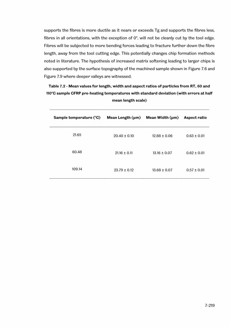
7-219

supports the fibres is more ductile as it nears or exceeds Tg and supports the fibres less,

fibres in all orientations, with the exception of 0°, will not be cleanly cut by the tool edge.

Fibres will be subjected to more bending forces leading to fracture further down the fibre

length, away from the tool cutting edge. This potentially changes chip formation methods

noted in literature. The hypothesis of increased matrix softening leading to larger chips is

also supported by the surface topography of the machined sample shown in Figure 7.6 and

Figure 7.9 where deeper valleys are witnessed.

Table 7.2 - Mean values for length, width and aspect ratios of particles from RT, 60 and

110°C sample CFRP pre-heating temperatures with standard deviation (with errors at half

mean length scale)

Sample temperature (°C) Mean Length (µm) Mean Width (µm) Aspect ratio

21.65 20.40 ± 0.10 12.88 ± 0.06 0.63 ± 0.01

60.48 21.16 ± 0.11 13.16 ± 0.07 0.62 ± 0.01

109.14 23.79 ± 0.12 13.68 ± 0.07 0.57 ± 0.01

7-220

a) b)

c)

Figure 7.10 – Particle distribution for a) length, b) width and c) aspect ratio of chips

collected from CFRP machined at RT, 60 and 110 °C workpiece starting temperatures

7.7 Flexural testing results

Figure 7.11 shows the results of flexural strength taken from four coupons. Whilst the

sample size is understood to be small, there is an observable overall decrease in mean

flexural strength for increased CFRP pre-heating temperature. There is a reduction of 8.7

% in flexural strength between RT and 110 °C machined coupons.

1 10 100 1000

0.0

0.2

0.4

0.6

0.8

1.0

% D

istr

ibu

tion

Length (µm)

22.5°C

60°C

110°C

Length (Temperature only)

1 10 100 1000

0.0

0.2

0.4

0.6

0.8

1.0

1.2

1.4

% D

istr

ibution

Width (µm)

22.5°C

60°C

110°C

Width (Temperature only)

0.0 0.5 1.0

0.0

0.1

0.2

0.3

% D

istr

ibution

Aspect ratio

22.5°C

60°C

110°C

Aspect ratio (temperature only)

7-221

Figure 7.11 – Flexural strength of coupons machined at different temperatures showing

mean values of four samples with ±1 standard deviation

Whilst there is an observable decrease in flexural strength, Table 7.3 shows that

flexural strength is not statistically significant for a confidence level of 95 % (p-value = 0.052)

and the null hypothesis must be accepted; there is no relationship between the flexural

strength and CFRP panel pre-heating temperature. Whilst this must be accepted, it should

be noted that the p-value is close to being statistically linked and a strong correlation

between temperature, UT, and surface metrics are noted. When a confidence level of 90 %

is applied, linear regression shows that a statistical link does exist between temperature

and flexural strength (p-value = 0.045).

Table 7.3 – Linear regression p-value results for correlation between temperature and

flexural strength, maximum fibre strain and flexural modulus (bold, italic = significant)

Regression P-value

Parameter (Variable) Temperature

Flexural strength 0.052

Maximum fibre strain 0.064

Flexural modulus 0.133

965

885 873920 904 887

848 880

21.65 43.42 50.17 60.48 69.35 79.95 104.43 109.14

0

100

200

300

400

500

600

700

800

900

1000

1100

1200

1300

1400

1500

Fle

xura

l str

ength

(M

Pa)

Temperature (°C)

7-222

The direct link between temperature and flexural strength is not statistically

significant but the correlation between surface quality and flexural strength given in Table

7.1 shows that several metrics have statistically significant links. Surface metric variables

including Sa, Sq, Sv, Sz, S10z, Sdq, Sdr, Sk, Vmc, Vvc provide linear statistical correlation to flexural

strength. Some of these parameters fall within the amplitude and hybrid group of areal

parameters which have shown previous links to flexural strength in Chapter 5.5.1.

Volumetric type parameters are also shown to provide statistical links with all categories;

linear areal material ratio curve, material volume and volume categories, providing metrics

which are able to statistically link to flexural strength. The need for a single volume based

metric rather than many different parameters is required, which will be discussed in

Chapter 8.

The likely decrease in flexural strength is due to the increased amount of fibre

pullout in the -45° direction which has been caused by a softening of the matrix, leading to

less support of fibres during the shearing process. Subsequently the fibres have broken

deeper into the surface resulting in an increase in depth of pullout. An increase in depth of

pullout would lead to an increased likelihood of crack propagation.

Relating to previous literature in the field is difficult due to the lack of mechanical

test data, particularly for flexural response. However Morkavuk et al. [244] note a tensile

strength improvement for coupons edge milled cryogenically which fits with the same trend

noted in this study; lower cutting temperatures provided higher strength. The authors note

that cutting at lower temperatures improves the chip formation ability which is also noted

within Table 7.2 which shows lower chip size for lower cutting temperatures.

The maximum fibre strain, calculated using ASTM D6272 methods, is shown in Figure

7.12. The plots show the same trend as flexural strength with larger standard deviations (for

example 12 % for fibre strain but 6 % for flexural strength at RT). This is indicative of the

larger error in the laser extensometer measurement method to formulate strain values

whereas strength is purely a load based criteria. This larger error is reflected in a larger p-

value (0.064), Table 7.3, for ANOVA analysis where temperature response is measured by

maximum fibre strain.

7-223

Figure 7.12 – Maximum fibre strain of coupons machined at different temperatures showing

mean values of four samples with ±1 standard deviation

Figure 7.13 shows the results of flexural modulus for differing CFRP pre-heating

temperatures, which shows little variation in results which is confirmed in Table 7.3 (p-value

= 0.133). This was expected due to the aforementioned cure and nanoindentation results.

This is an important result as it shows no degradation has occurred; the ageing of polymers

is known to change the material modulus due to additional cross linking and then

degradation of the material, as noted in Lèvêque et al. [239] and Maxwell et al. [238].

Figure 7.13 – Flexural modulus of coupons machined at different temperatures showing

mean values of four samples with ±1 standard deviation

0.015

0.014 0.013

0.0150.015 0.015 0.014 0.015

21.65 43.42 50.17 60.48 69.35 79.95 104.43 109.14

0.000

0.002

0.004

0.006

0.008

0.010

0.012

0.014

0.016

0.018

0.020

Maxim

um

fib

re s

train

Temperature (°C)

61.060.2 61.1 60.5 59.0

61.059.3 59.7

21.65 43.42 50.17 60.48 69.35 79.95 104.43 109.14

0

5

10

15

20

25

30

35

40

45

50

55

60

65

70

75

80

85

Fle

xura

l m

odulu

s (

GP

a)

Temperature (°C)

7-224

In order to complete the cross correlation study, whereby UT has been related to

temperature and surface metrics, and surface metrics related to flexural strength, UT must

also be compared to flexural strength. This final cross correlation shows that UT is

statistically linked to flexural strength, as shown in Table 7.4. This is useful as it potentially

means that UT could be used as a metric instead of surface quality metrics for all samples.

Table 7.4 – Linear regression p-value results for correlation between UT and flexural

strength, maximum fibre strain and flexural modulus (bold, italic = significant)

Regression P-value

Parameter (Variable) UT

Flexural strength 0.024

Maximum fibre strain 0.658

7.8 DIC analysis of flexural specimens

The strain of the lower plies in tension during four point bend testing, immediately

prior to failure of the flexural sample, is presented in Figure 7.14. The strain at the top

surface is not provided as the top surface buckled prior to actual ultimate failure of the

specimen from a CFRP pre-heating temperature of > 40 °C. Observation of all camera

frames has shown that, as per previous DIC results, the build-up of strain is proportional to

the increasing load and that the strain builds across the lower plies of the laminate. The

results of the DIC analysis match the expectation, as per Chapter 6.8, that the strain

decreases proportionally with flexural strength whilst the modulus remains constant. Linear

regression through ANOVA shows a statistical link between increasing tool temperature and

the decreasing strain of the flexural sample (p-value = 0.039). Again as per Chapter 6.8, the

DIC strain values follow expectations more closely than the laser extensometer strain

method suggesting more variability in the method than anticipated.

7-225

Figure 7.14 - Failure strain for bottom edge of flexural samples obtained through DIC

immediately prior to failure

DIC results show a build-up of strain across the top and bottom surfaces which is

progressive and in line with the loading of the sample. A high concentration of strain on the

surface was particularly useful to identify top surface buckling which could have otherwise

not been observed.

7.9 Failure analysis of flexural specimens

The same failure mechanism as Chapter 5.8 and Chapter 6.9 (Figure 5.10) occurs in

samples milled at different pre-heating temperatures, as shown in Figure 7.15. However,

prior to the onset of final failure, fibre buckling occurs on the top surface from CFRP

preheating temperatures of 40°C upwards as per Figure 7.16.

0 20 40 60 80 100 120

0.0

0.5

1.0

1.5

2.0

2.5

Maxim

um

str

ain

on b

ottom

surf

ace (

%)

Temperature (°C)

7-226

Figure 7.15 – Failure of CFRP at RT and 110 °C preheat temperatures with buckling of fibres

highlighted for the top surface and locations of 1) initial tensile failure and 2) large scale

delamination occurring at ±45° ply

Figure 7.16 – Typical buckling of 0° fibres at the top surface which started at CFRP

preheating temperatures of 40°C (image of buckling at 100°C)

7-227

Buckling is usually preceded by interfacial debonding/delamination of plies, which

are observed in Figure 7.15, with DIC imaging suggesting that this has occurred in the

interface between 0/90 and ±45° plies. As per Chapter 6.9 it is noted that the delamination

between these two layers is likely due to the large amount of fibre pullout at the -45°

direction which then creates a stress concentration and subsequent failure at the ply

interfaces. Due to the larger thermal energy involved in the cutting process it is proposed

that the softer matrix has allowed increased damage which has resulted in increased stress

concentrations in the interfacial region between -45° and adjacent plies. This increased

stress then allows buckling and delamination in the upper plies during flexural testing. This

hypothesis is supported by the surface topography results (Figure 7.6 and Table 7.1) which

show larger valleys and peaks.

7.10 Conclusions

The effect of increasing the temperature of the CFRP material prior to edge

trimming has been investigated using IR to observe maximum tool temperature, a

dynamometer to observe cutting forces and focus variation and SEM methods to observe

the surface topography and provide areal metrics. Mechanical testing through four-point

bending has been completed and observed with DIC methods. Finally, the chip morphology

has been assessed using optical methods to support the observed machined surface

topography.

Whilst overall flexural strength appears to decrease with increasing temperature,

with a reduction of up to 8.7 % from RT to 110 °C CFRP pre-heating temperature, statistical

analysis shows that this is not significant (p-value = 0.052). Whilst accepted as not significant

at a 95 % confidence interval, the p-value is close to the limit of significance (0.05) and the

general downward trend of flexural strength with increasing CFRP pre-heating temperature

is visible. Whilst a 90 % confidence interval does provide a statistical link between

temperature and flexural strength (p-value = 0.045), the 95 % confidence interval is

accepted as standard [245].

Using the novel experimental technique, it was observed that Sa values of CFRP

preheated to 110 °C increased by 89.8 % compared to RT. A non-linear statistical link (p-

value <0.001) was observed for the trend between Sa and CFRP panel preheating

temperature. Statistical links between variables of dynamometer (UT) and IR tool

temperature immediately after cutting were identified with the response of CFRP panel pre-

heating temperature (p-values <0.001).

7-228

The cutting mechanisms of 45, 90 and -45° fibres orientated to the tool change

significantly with increasing CFRP panel preheating. Unlike RT cutting operations, where

only a small surface layer of matrix is altered by smearing in the 45 and 90° directions,

cutting at elevated CFRP panels temperatures causes global matrix softening. The lower

stiffness matrix is therefore unable to support the fibres close to the cutting edge, leading

to increased fibre bounce back in the 45 and 90° fibre orientation. Whilst pullout of -45°

fibres is evident in RT milling, the fracture zone is further ahead and deeper from the cutting

edge for elevated temperature milling. The difference in cutting mechanism for CFRPs is

reported for the first time through optical chip analysis which shows increases in mean chip

length and width (3.39 and 0.79 µm, respectively) which is statistically different between

CFRP pre-heating temperatures of RT, 60 and 110°C (p-value <0.001).

When Sa was correlated against tool temperature, it was noted that higher tool

temperatures produced an improvement in Sa values. It is proposed that the local effects of

increased tool temperature improve Sa results compared to the global matrix effects of

heating the CFRP panel. This is most likely due to the low heat partition ratio where only 21

% of the heat generated in the cutting process is in the workpiece with the remainder in the

tool and chip according to Liu et al. [78].

Whilst it is observed that lower CFRP preheating allowed improved Sa results, the

effects on sub-surface defects are not understood and XCT or alternative sub-surface

investigations should be completed. Further testing should investigate if cooling of the CFRP

material, or the cutting tool, is able to improve surface quality and mechanical performance.

The use of DIC has allowed the buckling of the CFRP material to be captured which

would otherwise not be observed. This highlights the change in material behaviour at

increased temperature where larger damage occurs that corresponds to larger stress

concentrations at interfacial regions to plies adjacent to -45° orientations in particular.

The novel CFRP heating method and surface observation has provided new insight

into the cutting mechanisms at high temperatures where the Tg of the matrix is exceeded.

7.11 Further work

The onset Tg temperature of the material has been given between 105.6-109.3 °C

(method dependent) which has been reached during the hottest CFRP pre-heat

temperature. Whilst it can be assumed that the temperature at the cutting interface has

exceeded this, future work should exceed the onset Tg in CFRP pre-heating stage to assess

the surface quality and resulting mechanical performance of edge trimmed coupons.

7-229

In addition to further mechanical testing to increase the sample size of data, there

is a requirement to observe sub-surface defects which cannot be observed by current

methods. Whilst matrix smearing appears to be reduced for fibres orientated at 90° to the

cutting edge for increasing pre-heat temperatures, it is still present. The importance of

observing damage in the 90° fibre direction was found to be particularly important during

Chapter 4.7.6. The relative softness of the matrix at high cutting temperatures may allow

even deeper sub-surface defects to be formed which could be observed by a novel pixel

count method that observes through-depth defects.

7-230

8-231

8 NOVEL EPI-FLUORESCENT MICROSCOPY DAMAGE

METRIC RESULTS

This chapter provides novel metric observations of sub-surface defects caused

through different machining variables presented in previous chapters; the effect of machine

stiffness and tool geometry, tool wear and machining temperature. The novel EFM (epi-

fluorescent microscopy) damage metric has been considered necessary due to the

existence of smeared matrix which has potentially hidden sub-surface defects in previous

Chapters. This novel metric, defined in Chapter 3.9.4, with development shown in Chapter

4.7, defines an area of damage of a planar section from a trimmed sample, quantifying the

amount of damage from a theoretically straight edge into the depth of the trimmed surface,

in terms of pixel count.

8.1 Introduction

Previous chapters have explored how areal parameters measure the surface of

CFRP when cut with different machines, tool geometries, tools with different coatings, worn

tools and cutting at increased temperatures. It was highlighted that matrix smearing was an

issue, particularly for 45 and 90° fibres orientated to the cutting edge and that the surface

metrics were unable to detect sub-surface defects due to masking of the region by a layer

of smeared matrix. This was especially prevalent when the pre-heating temperature of the

CFRP was increased. The matrix is no longer rigid which allows fibres to be moved,

potentially resulting in sub-surface defects deeper in the trimmed edge.

8.2 Effect of machine stiffness and tool geometry

The novel EFM metric has been applied to four samples taken from Chapter 5 for

each tool, on each machine, with the results shown in Figure 8.1. It can be seen that the tool

results are in line with expectations; the DIA-HBC4 tool provides a lower amount of sub-

surface damage due to the constant engagement of cutting teeth as opposed to the double

helix nature of the DIA-BNC which has less continual tooth engagement. The FTV machine

was expected to produce a higher surface roughness due to a stiffer system and more

energy transfer as measured through the UT parameter. Whilst this was the case for the

DIA-BNC tool, it was not the case for the DIA-HBC4 tool. Areal surface metric results also

reflected this.

ANOVA analysis has been completed, where the variable is set as the novel metric

and compared to machine, tool and machine/tool factors, with the results shown in Table

8-232

8.1. It can be seen that the novel metric has an improved p-value for the machine factor

however, this is not statistically significant. The novel metric is also unable to show statistical

links between tool and machine/tool factors which may be attributable to the sample size

of collected data. Whilst a comparison has been made with Sa, this may not be appropriate

as the metrics observe very different types of topography. An area of future work could be

to explore these differences and compare an Sa measured area with several planar slices

which are able to show the sub-surface damage of the same area.

Figure 8.1 – Novel EFM damage metric area of damage for ABB and FTV machine platforms

and DIA-HBC4 and DIA-BNC tools displaying mean values from four samples with ±1

standard deviation error

Table 8.1 – ANOVA p-value results for novel EFM damage and areal surface metrics with

respect to machine and tool factors (Key as per Table 5.2)

Parameter (Variable) Machine Tool Machine/Tool

Area of damage (µm2) 0.865 0.064 0.553

Sa (µm) for comparison 0.928 0.004 <0.001

Novel metric results for machine and tool groups are shown in Table 8.2. The results

are in agreement with the Sa metric in that FTV machine and DIA-BNC tool produce more

6350

4242

7444

3509

BNC HBC4 BNC HBC4

ABB FTV

0

2500

5000

7500

10000

12500

Are

a o

f d

am

ag

e (

µm

2)

14412 only

8-233

damage than the ABB machine and DIA-HBC4 tool. Additionally, there is novelty in the

information that sub-surface damage follows the same trend as surface metrics such as Sa.

This information could be used to assess only a single measurement criterion, e.g. Sa, or the

novel metric. There are benefits to each measurement type; Sa is able to characterise a

larger sample area but is unable to account for sub-surface damage hidden by smeared

matrix which can be captured with the novel metric.

Table 8.2 – Results of novel EFM damage metric analysis on machine and tool variables

Novel EFM damage

area (µm2) SD of damage area

Sa average (µm) for

comparison

ABB Machine 5296 2340 3.86

FTV Machine 5758 3820 4.23

DIA-BNC tool 6897 3016 4.18

DIA-HBC4 tool 3928 2239 3.86

Typical machining defects are shown in Figure 8.2. The defects match the

expectation that machining with a DIA-BNC burr style tool causes larger areas of defects

than a DIA-HBC4 tool. Of particular interest are the sub-surface defects which would not be

measured by the areal metric. The sub-surface defect occurs beneath 90° fibres which are

frequently subjected to matrix smearing as per SEM analysis in Chapter 5.5.2, Chapter 6.5.2

and Chapter 7.5.2. The smearing can potentially hide damage if measured by areal means.

The sub-surface defects beneath the 90° plies are concentrated at the 0° interface.

Delamination damage of the 90° fibres is particularly prevalent at the ply interface with the

0° fibre plies which could be attributable to the mismatch between cutting forces that

typically occurs between CFRP plies [226, 227].

8-234

Figure 8.2 – Comparison of novel EFM damage metric area of damage for ABB, FTV, DIA-

BNC, DIA-HBC4 machine and tools (representative damage from each group)

Data is presented in Table 8.3 showing no statistical link between the novel metric,

UT and flexural strength. Whilst this may suggest that the novel metric is limited, as it is

unable to link to flexural strength where Sa could, the small data set is perhaps a factor. As

discussed previously the lack of a statistical link may not be important and the observation

of sub-surface damage may be adequate to add to the knowledge of damage captured by

areal methods, for example.

Table 8.3 – Linear regression p-value results for UT and flexural strength responses for

novel EFM damage metric and Sa variables (bold, italic = significant)

Regression P-value

Parameter (Variable) Novel metric Sa for comparison

UT 0.812 0.920

Flexural strength 0.075 0.015

8-235

Whilst statistical links through ANOVA analysis have been limited, the metric has

been able to identify that sub-surface defects do occur and the area/ply region where this

defect occurs. When compared to the Sa parameter, the overall trends have been repeated

when machine and tool averages are considered. On this basis, it is recommended that this

novel metric is further investigated and the dataset increased.

8.3 Effect of tool wear

The results of applying the novel metric to uncoated BNC and MFC, and coated DIA-

BNC and DIA-MFC tools against cumulative linear tool distance (i.e. tool wear) samples from

Chapter 6 are shown in Figure 8.3. The results show an average upward trend of increasing

damage as the tool wears. This is more obvious in uncoated BNC and MFC tools due to their

higher rate of wear and high initial edge radius, which matches the analysis using the Sa

parameter.

a) b)

c) d)

Figure 8.3 – Novel EFM damage area with increasing cumulative linear tool wear for a) BNC,

b) MFC, c) DIA-BNC and d) DIA-MFC tools with y error of ±1 standard deviation from a

minimum of four samples per data point

0 2000 4000 6000 8000

0

2000

4000

6000

8000

10000

12000

14000 BNC

Linear fit

Are

a o

f d

am

ag

e (

µm

2)

R2=0.056

0 5000 10000 15000

0

2000

4000

6000

8000

10000

12000

14000 DIA-BNC

Linear fit

0 2000 4000 6000 8000

0

2000

4000

6000

8000

10000

12000

14000 MFC

Linear fit

Are

a o

f d

am

ag

e (

µm

2)

Cumulative linear tool distance (mm)

0 5000 10000 15000

0

2000

4000

6000

8000

10000

12000

14000 DIA-MFC

Linear fit

Cumulative linear tool distance (mm)

R2=0.853

0 2000 4000 6000 8000

0

2000

4000

6000

8000

10000

12000

14000 BNC

Linear fit

Are

a o

f d

am

ag

e (

µm

2)

R2=0.056

0 5000 10000 15000

0

2000

4000

6000

8000

10000

12000

14000 DIA-BNC

Linear fit

0 2000 4000 6000 8000

0

2000

4000

6000

8000

10000

12000

14000 MFC

Linear fit

Are

a o

f d

am

ag

e (

µm

2)

Cumulative linear tool distance (mm)

0 5000 10000 15000

0

2000

4000

6000

8000

10000

12000

14000 DIA-MFC

Linear fit

Cumulative linear tool distance (mm)

R2=0.853

8-236

The increase in the novel metric area of damage and areal metric Sa as tool wear

progresses have been subject to linear regression fitting for uncoated tools only due to the

high wear rate. In this case, linear fitting has been chosen due to residual analysis and

resulting S-values. It was found that a better fit could be achieved for the MFC tool with a

non-linear fit but not for the BNC tool. As this was the case, linear fitting was applied for

comparison to the BNC tool and also for results in Chapter 6 which used linear regression

fitting. The results of the goodness-of-fit parameter (R2) resulting from linear regession

fitting for both uncoated tools is shown in Table 8.4. R2 values show that the novel metric

has a similar goodness-of-fit compared to Sa. However, it is noted that for a true

comparison, this value requires a dataset which matches that of the Sa analysis where,

currently, the novel metric is limited by a small number of observed samples.

A comparison of novel metric area of damage images for uncoated tools is shown in

Figure 8.4. It shows the damage compared to a theoretical straight cut and in particular

highlights damage that penetrates beneath the surface. This has potentially been obscured

by smeared matrix when using areal metrics and has not been observed before. As per

Figure 8.3, the average area of damage is similar for both tools (7808 and 8266 µm2 for BNC

and MFC tools, respectively). Sub-surface damage has been detected as a non-continuous

effect from the surface of the MFC example in Figure 8.4. In the plane observed, the defect

appears to be non-continuous but it is likely that the plane below or above that shown links

these two defects.

Table 8.4 – Comparison of linear regression model R2 values for cumulative linear tool wear

against novel metric or Sa

Tool Metric R2 value of linear regression model

BNC Sa for comparison 0.871

Novel metric 0.853

MFC Sa for comparison 0.019

Novel metric 0.056

8-237

Figure 8.4 – Comparison of novel EFM damage area for BNC and MFC tools (from

specimens at largest cumulative linear distance, average damage)

Linear regression p-value analysis comparing the novel metric response to tool wear,

UT and flexural strength variables are shown in Table 8.5.

Table 8.5 – Linear regression p-value results for UT and flexural strength responses for

novel EFM damage area variables (bold, italic = significant)

Regression P-value

BNC MFC

Parameter (Variable) Novel metric Sa (comparison) Novel metric Sa (comparison)

Cumulative linear tool distance

<0.001 <0.001 0.611 0.522

UT 0.048 0.567 0.958 0.630

Flexural strength <0.001 0.014 0.839 0.468

As per Sa, for the MFC tool, the novel metric was unable to show any statistically

significant results. This is perhaps due to the varying nature of cutting edge sharpness as

tool wear progresses, which creates cyclical periods of sharpness and bluntness. When

linear regression fitting is used for the average values of the BNC tool, statistical links are

shown for increasing tool wear, UT and flexural strength. The statistically significant p-values

are an indication that the novel metric, that measures area of damage, is as effective as Sa.

Again, a limiting factor in this statement is the large standard deviation of results which

8-238

needs to be minimised by further application of the novel metric. The large deviation in

results is likely to be due to the fabric nature of the laminate, where every slice will reveal

different quantities of fibre directions. A volumetric approach where more slices are

observed would yield a lower deviation.

8.4 Effect of pre-heating CFRP temperature

Figure 8.5 shows the novel metric area of damage results for specimens machined

at different CFRP pre-heat temperatures as per Chapter 7. Whilst non-linear fitting has been

completed in accordance with residual analysis where S-values suggests that non-linear is

a superior fit, linear fitting at two regions has been shown. It highlights the region between

RT and 70 °C machining where the trend appears linear and the region after this where an

increase in damage is shown. It is hypothesised that at low CFRP pre-heating temperatures

(𝑄𝐶𝐹𝑅𝑃) the heat energy is insignificant compared to the energy input of the tool

temperature during cutting (𝑄𝑇𝑜𝑜𝑙). After 70 °C, the CFRP preheating temperature energy

becomes greater than the tool input energy and the damage, in terms of the novel metric,

increases significantly.

Figure 8.5 – Novel EFM damage area with increasing CFRP pre-heating temperature

compared to traditional areal metric, Sa, from a minimum of four samples with ±1 standard

deviation and R2 values for comparison of raw data fitting

The standard deviation of the area of damage is large except for RT (21.65 °C)

machined specimens where a standard deviation of 89 µm2 occurs. This is in agreement

20 40 60 80 100 120

0

2500

5000

7500

10000

12500

15000

Temperature (°C)

Avera

ge a

rea o

f dam

age (

µm

2)

0

5

10

15

20

Avera

ge S

a (

µm

)Non-linear

R2=0.979

Non-linear

R2=0.972

Double linear

trend

8-239

with Chapters 8.2 and 8.3. As previously discussed, this a shortcoming of the planar slicing

novel metric method where only a single slice of data is observed for an isotropic material.

More analysis is required to fully investigate the proposed hypothesis.

The amount of sub-surface damage changes as a function of temperature. As shown

in Figure 8.5, there is more damage due to increased temperature. Whilst this could be

observed with focus variation surface topography methods as shown in Figure 7.6, Figure

8.6 shows that the novel metric is able to measure damage beneath the surface. It can be

seen that the depth of damage increases with increasing CFRP pre-heat temperature. The

images also highlight that the damage occurs in 90° fibres to the cutting edge at the interface

with 0° fibres. This suggests that the cutting mechanism, as noted in Chapter 7, changes to

allow the 90° fibres to be bent and they cause delamination in the weakest point – at the

interlaminar bond between the two fibre directions.

Figure 8.6 – Evolution of novel EFM damage area. Damage in 0 and 90° fibre orientation

interface is highlighted (images represent largest damage from each group)

Whilst there is an observable difference between the amount of sub-surface

damage, as captured by the novel metric, the relationship to static flexural strength is not

as strong as Sa. Table 8.6 shows a p-value of 0.018 for the novel metric compared to 0.015

for Sa (Table 7.1), where flexural strength is set as the variable. There is less data for the

novel metric which observed 33 samples compared to the Sa evaluation which used 64

samples.

8-240

Table 8.6 also shows that statistical links exist between UT, temperature and flexural

strength, which show that the novel metric is statistically able to characterise changes due

to temperature, cutting forces and the resulting flexural strength. As statistical links do exist,

R2 values for the novel metric and traditional Sa results are plotted in Figure 8.5 to allow for

a goodness-of-fit comparison. It is observed that non-linear regression analysis for both Sa

and novel damage metric data provides high R2 values of 0.972 and 0.979, respectively. This

suggests that both methods are suitable for analysing damage however, the novel metric

has more value in this case as it captures sub-surface damage which is known to be a

significant factor for 90° fibres in particular, as discussed in Chapter 4.7.6. In its current

form, with such high standard deviations, this statement should be treated with caution and

more data should be assessed to reduce the deviations.

Table 8.6 – Non-linear regression p-value results for UT, temperature and flexural strength

variables for novel EFM damage area responses (bold, italic = significant)

Regression P-value

Parameter (Variable) Novel metric Sa for comparison

UT 0.022 <0.001

Temperature <0.001 <0.001

Flexural strength 0.018 0.015

8.5 Conclusions

The use of a novel metric criteria to measure the area of damage has allowed sub-

surface damage to be captured and inspected without the use of expensive XCT methods.

In particular sub-surface damage was captured at the 0/90° interface which would

otherwise not be captured by areal methods due to matrix smearing. This corresponds well

to the DIC/SEM failure analysis which noted that initially tensile failure occurs at the lower

surface of the flexural coupon followed by interlaminar delamination at the 0 and 90° fibre

interfaces. This is caused by sub-surface defects that have now been captured using the

novel pixel count metric.

8-241

8.6 Further work

Whilst an improvement on the areal metric, in terms of visualising damage beneath

matrix smearing, the data set is limited and should be expanded to incorporate a larger

quantity of samples. This can be done through additional polishing of existing samples to

expose new cross sections of sub-surface damage and ideally would be completed through

an automated process. In order to evaluate the number of samples required, margin of

error analysis can be completed using Equation 8.1. This equation is typically utilised prior

to experimentation to determine the required sample size and in this case will use a 95%

confidence interval and a 10% margin of error. Practically the margin of error is the range

of values below and above the sample statistic in the 95% confidence interval range of a

normal distribution.

𝑆 = �̂�(1 − �̂�) (

𝑧12

𝑥𝑒𝑟𝑟𝑜𝑟

)

2

Equation 8.1 [246, 247]

Where 𝑆 is the number of samples, �̂� is the sample proportion set to 0.5 to maximise the

potential error as per [246], 𝑥𝑒𝑟𝑟𝑜𝑟 is the margin of error, taken as 10 %, and 𝑧1

2

is the standard

normal variable, 1.96, taken from a z-table for confidence interval of 95 % [248]. With these

variables in place, it is shown that a minimum of 97 samples are required to complete an

observation with a 10 % margin of error with a 95 % confidence interval. This is much greater

than the number of samples currently observed and highlights a weakness of the novel

metric compared to a more volumetric approach such as XCT where the complete sample

could be observed in a single scan.

8-242

9-243

9 CONCLUSIONS

The main objective of this body of work was to understand if various factors,

including milling machines, milling tools, tool coatings, tool wear and temperature of the

edge milling process, altered mechanical performance of CFRP materials. In addition to

understanding each of the noted variables more thoroughly, in some cases for the first time,

the effects of these variables on surface quality metrics were observed.

The work presented in this thesis has generated novel data in understanding factors

that affect surface quality of the machined part, dynamometer response, mechanics of

cutting and resulting flexural strength of edge trimmed test coupons. The aim of generating

a novel metric to capture previously unseen defects has also been achieved and applied to

all aforementioned variables.

9.1 Conclusions and themes

The main conclusions with respect to flexural strength are;

Flexural strength of CFRP coupons machined using the robotic system is up to 25.9

% (147.5 MPa) greater than those machined on the elevated gantry (p-value < 0.001)

when the same cutting parameters are used. ANOVA shows that the machine and

machine-tool interactions are statistically significant (p-value < 0.001). Therefore, it

is proposed that the damping within the 3 joints of the robotic machine causes lower

cutting forces from the tool to workpiece, in the form of UT, than the overhead

gantry. This manifests in a differing surface topography, where more energy transfer

adversely affects the flexural strength.

The tool geometry (Chapter 5) does play a role in the cutting forces of the machining

process (p-value < 0.001) but it does not influence the flexural strength directly (p-

value > 0.05). However, the machine-tool interaction was shown to be statistically

significant (p-value < 0.001) whilst tool geometry considered in Chapter 6 also shows

a statistical link to flexural strength (p-value = 0.003). Whilst contradictory, it should

be considered that the DOE may not be able to separate the tool response

sufficiently from the statistical model and that when individual machines are

considered, the tools do show statistical differences through two way t-tests (p <

0.001). In both Chapter 5 and Chapter 6 the burr style tool is able to produce

improved flexural strength values compared to continual teeth tools of DIA-HBC4

(Chapter 5, compression router) and DIA-MFC (Chapter 6, single helix router) types.

9-244

A hypothesis is presented whereby the burr style tool and corresponding lower

overall cutting forces are able to produce coupons with higher flexural strengths.

Tool wear of 7.2 m linear cumulative cutting distance in uncoated BNC and MFC tools

produced a reduction in flexural strength of 10.5 and 7.1 % respectively compared to

the flexural strength derived from new tools. This shows that tool life is a significant

factor and should be accounted for in a production environment, i.e. to maintain

flexural strength, worn tools should not be used. For coated tools, which are more

frequently used within a production environment, the flexural strength did not

statistically change suggesting that the 16.2 m of cumulative linear tool wear was not

enough to alter the cutting edge structure and subsequent flexural strength.

Whilst overall flexural strength appears to decrease with increasing temperature

exposure, with a reduction of up to 8.7 % from RT to 110 °C CFRP pre-heating

temperature, a statistical analysis shows that this is not significant (p-value = 0.052).

Whilst accepted as not statistically significant, the p-value is close to the limit of

significance (0.05), and the general downward trend of flexural strength with

increasing CFRP pre-heating temperature is visible.

SEM and DIC analysis has been used to show that the primary failure region of

flexural specimens is at the tensile side of the specimen. However, it is the trimmed

edge quality which lowers the overall flexural strength of the CFRP coupons. In

addition to reducing the overall failure strength, the quality of the trimmed edge also

dictates the failure mechanism of the specimens where interlaminar failure between

0 and 90° fibres occurred and was found to be caused by sub-surface defects which

were measured by a novel EFM pixel based damage metric.

The main conclusions with respect to total specific power, UT, a novel method to

characterise cutting forces that includes x, y and importantly z data, whilst also accounting

for the actual volume of material removed are;

Dynamometer assessment of data has been an invaluable tool to determine the

cause and effect relationship of many of the variables witnessed within this

thesis. The use of UT as a metric instead of cutting and tangential forces has been

well justified, especially due to the complex factors which have different chip

formation methods.

Dynamometer assessment using a DOE in Chapter 5 shows that UT is significant

for machine and tools i.e. UT measurements are able to differentiate between

machines and tools.

9-245

UT was able to show differences in reported mean values for uncoated and

coated BNC and MFC tools within the tool wear study (Chapter 6) (p-value <

0.001). However, the effect of increasing tool wear could not be statistically

measured due to the fluctuation in UT values for different tool wear levels. This

was attributed to rounding edge effects, where cutting teeth continually cycled

through dulling and sharpening phases. As expected, the single helix MFC/DIA-

MFC tools have higher overall UT values than the double helix burr style BNC/DIA-

BNC tools.

UT was a suitable metric to measure the effects of increasing CFRP panel pre-

heating temperature (p-value of <0.001), where temperature is a variable and UT

is a response. UT decreased with increasing CFRP panel temperature which is

attributed to softer matrix and less support for fibres during cutting where

additional spring-back was observed.

Total cutting forces during machining should be kept to a minimum where

possible to improve flexural strength (Chapter 5, Chapter 6 uncoated tools).

However, Chapter 7 shows that whilst cutting forces can be lowered by

increasing the temperature at the workpiece interface during cutting, this can

be detrimental to the flexural strength due to increased amounts of surface/sub-

surface damage.

As a metric to measure flexural strength, UT is statistically significant for Chapter

5 and Chapter 7 and is able to show linear regression trends with high R2 values.

Chapter 6 did not show a link between UT and flexural strength, but this was

expected due to the local sharpening and dulling process caused by cutting edge

radius changes.

The main conclusions with respect to surface quality analysis taken from focus

variation and SEM methods are;

The focus variation method is able to produce 3D and 2D surface topography maps

which are useful to interpret differing levels of damage between tools, tool wear and

CFRP pre-heating temperatures. Little observable differences were noted between

machines, except during trials on the GTC test-bed machine, which induced chatter

on the machined surface. Alongside SEM methods, the focus variation method

allowed observation of cutting mechanisms which correspond to literature.

Previously unseen cutting mechanisms due to tool wear and cutting temperature

were observed with this method.

9-246

Chapter 5 shows that surface metrics can be linked to flexural strength with Sa, Ssk,

Sku, Sk, Spk, Vmp, Vmc and Vvc metrics showing statistically significant links. Statistical

links between flexural strength and tool wear exist (Chapter 6) with significant

metrics Sa, Sq, Sv, Sz, S10z, Sdq, Sdr, Sk, Vmc and Vvc for the BNC tool and Svk and Smr1 for

the MFC tool. Surface metric variables including Sa, Sq, Sv, Sz, S10z, Sdq, Sdr, Sk, Vmc, Vvc

provide linear statistical correlation of flexural strength for investigations into

machining temperature (Chapter 7).

Surface metrics are able to show statistical relationships to static flexural strength

which suggests that only understanding the surface is required. Sub-surface analysis

using a novel EFM pixel based damage model show that defects beyond the surface

do exist. Potentially, fatigue loading may allow the sub-surface EFM method to be

more useful if surface metrics were unable to observe links to fatigue strength.

SEM analysis for all chapters has concluded that matrix smearing is apparent and

that typical cutting mechanisms apply to unworn and RT machining studies. Where

worn tools have been used, fibres at 45° to the cutting edge are pushed beneath the

tool cutting edge only to spring back as the shearing of the fibres occurs further in-

front of the cutting edge, which generates the main surface topography difference.

A hypothesis is generated; where the matrix becomes softer, due to the preheating

temperature increase, the chip formation method changes. This is supported by

chip analysis which shows a general increase in mean length (16.6 %) and width (6.1

%) from RT to 110 °C. Whilst the chip formation method in the 0° orientation to the

cutting edge remains similar, 45° fibres experience a larger degree of spring back as

the fibres are held in place less rigidly as the matrix is softer. Fibres in the 90°

direction also experience spring back although to a lesser extent and the cut ends

of the fibres are visible, which, for RT examples in this and previous chapters, have

been covered by smeared matrix. The large damage in the -45° fibre direction is

exacerbated by the lack of support from the matrix, which becomes more ductile

due to increasing temperatures. The cutting forces are also lowered due to the less

stiff matrix for increasing preheated CFRP panel temperature.

The main conclusions with respect to sub-surface quality analysis taken from a novel

EFM pixel based damage method are;

A novel metric has been developed and validated against XCT for fabric and UD

material, showing that sub-surface damage does exist due to the edge trimming

9-247

process. This solution is not limited to edge trimming and could be used for other

machining practices such as drilling to observe sub-surface defects.

Based on the limited sample size, the novel metric was able to show differences in

averages between machine and tools. These interactions were not found to be

statistically significant, possibly due to the large standard deviation and small sample

size. The statistical link between the novel metric and flexural strength was given as

p-value = 0.075. Whilst not statistically significant, the novel metric was able to

replicate the trends of Sa for different machines and tools. Whilst no statistical link

could be considered limiting, the novel metric was able to show that sub-surface

defects do occur. Of importance was the observation of delamination defects

caused by the machining of 90° fibres, in a fabric material, where penetration into

the depth of the material at the interlaminar area occurs.

With respect to tool wear, the novel metric was able to replicate the trends of Sa for

the uncoated BNC tool and show that the area of damage increased as the amount

of tool wear increased (p-value <0.001). The novel metric was able to statistically

show that as the average area of damage increased, the flexural strength decreased

(p-value <0.001).

When applied to samples from Chapter 8, the novel EFM damage metric was able to

statistically show that as the CFRP pre-heating temperature increased, the area of

damage, which included sub-surface damage, also increased with non-linear

methods providing a p-value of <0.001. The increasing area of damage was also

statistically linked to a decrease in flexural strength with a p-value of 0.018.

Overall the novel EFM damage metric showed the presence of sub-surface defects

which were found to be detrimental to flexural strength in DIC and SEM analysis of

mechanically tested specimens. If the variation in results could be reduced by

increasing sample size, the novel metric would be a worthy replacement of Sa as it

is able to replicate the same trends whilst having the benefit of observing sub-

surface damage.

9.2 Novelty of research

The novelty of this research has been identified as:

Providing a framework to assess manufactured CFRP panels in order to produce

high quality laminates with minimal and accountable variability.

Providing a framework to assess machine stability in order to conduct chatter-free

machining.

9-248

Tool wear for CFRP material is unique and current standards may not capture

representative wear mechanisms. This thesis has used classic flank wear and

adapted more recent methods obtained through literature research to characterise

wear in a new way.

For the first time the effect of machine stability and tool geometry on the machined

surface quality and subsequent mechanical performance are presented.

The effect of tool wear for diamond coated and uncoated carbide tools on cutting

force, surface quality and mechanical performance are assessed and discussed. The

effect of tool wear on mechanical performance is novel. This has significant

ramifications for industry practices where tools are frequently replaced at

considerable expense.

A novel method of investigating the effects of temperature on cutting forces, surface

quality and mechanical performance has been completed, whereby the CFRP panel

is pre-heated before milling. This method has not been previously explored and

results highlight how temperature changes chip morphology, cutting forces, surface

quality and mechanical performance.

Chip analysis of CFRP has been completed for the first time with promising results

highlighting differences in the machining process due to tool wear and cutting

temperature.

A highly novel epi-fluorescent microscopy (EFM) method is presented which is able

to capture defects generated at and below the surface of machined CFRP coupons.

The method is found to be comparable to X-ray computed tomography (XCT) which

is limited by resolution and equipment cost.

The use of current state of the art 3D areal techniques to assess machined surfaces

which have traditionally been inspected using stylus based 2D methods which is

considered an improvement over current literature practices.

In terms of a legacy at The University of Sheffield (UoS), resin transfer moulding

(RTM) equipment has been improved to produce higher quality panels, through the

introduction of a hydraulic press. A table top milling machine has been

commissioned which is capable of milling and drilling of CFRP and is suitable as a

test bed for more rigid industrial machine trials.

9.3 Applicability to industry

Based on the work completed in this thesis, the following recommendations are made

to CFRP machining industry;

9-249

When conducting material qualification programs, the choice of conventional

milling machine (e.g. 3-axis, 5-axis) is critical to the final mechanical strength

values which are used in subsequent design calculations. Industry must select

the appropriate machine that will be used for final part production and not

allow large changes in machine stiffness which would erode the value of

mechanical strength coupon testing.

Similarly, tool geometry and tool wear also plays a role in the mechanical

strength and subsequent design properties. Both should be considered in the

long term production of parts, for example, a change to a different tool

geometry may change the surface and sub-surface quality which would alter

the mechanical strength of the machined part.

A comparison of 2D and 3D surface parameters confirms literature

expectations that 3D parameters follow the same trends as 2D parameters but

report larger values due to the increased observation area. If Sa were to be

widely adopted instead of Ra, the Ra value should be increased by 16 %.

Single metrics should not be used to define the quality of a machined surface.

A raft of parameters which must include with Sa, Sq, Sv, Sz, S10z, Ssk, Sku, Sdq, Sdr,

Sk, Spk, Vmp, Vmc and Vvc metrics. Sub-surface metrics are also vital to giving the

full story of machined edge quality. Where XCT methods are unavailable, a

small section of material could be offcut for EFM analysis.

9.4 Future work

Based on the work conducted in this thesis, several incorporations to CFRP edge

milling operations are suggested.

Milling machines should be tap tested to understand the machine stability. As this is

a known factor in changing the flexural properties, it is recommended that the machine

stability is understood. Further testing into the advantages of damping in machining of

composites could also be undertaken to unlock further mechanical performance

advantages.

The importance of understanding the amount of cure in a material was vital during

temperature trial machining studies. Completing DSC and DMA analysis of the CFRP panels

prior to experiments was important in order to understand any differences that occurred

in the manufacturing process. Similarly understanding the void content is important. An

average of 0.2 % void by volume was observed throughout the thesis which allows the

9-250

surface quality observations and mechanical test results to be considered independent of

voids.

Tensile and compression testing was not conducted due to the need for larger

coupons which would have limited the scope of this thesis. However, these mechanical test

properties should be understood to add to the novel information found in this thesis

regarding correlation of flexural strength to machining parameters. Further samples should

also be tested in order to conclude that initial temperature during CFRP cutting does

statistically affect flexural strength. It is also understood that fatigue of composites with

surface edge defects may exacerbate the issues seen within all of the studies of this thesis

and may yield more obvious defect paths. Larger structural parts, for example stringers or

long beams should also be tested to see if the effects are scaled to actual production

applications.

The polymer selected in this study was a DGEBF/TETA resin system which was

chosen due to its simple handling characteristics and low viscosity to fully impregnate fibres.

The interaction of different matrix systems with the cutting tool would provide additional

data to allow resin systems to be tailored to improve the surface quality and therefore

flexural strength. Less viscous systems with higher Tg, the addition of tougheners and even

uncured polymers could be used to observe the effects on surface and sub-surface damage.

Similarly, the fibre systems could be altered. The T300 fibres used within this study

are widely available and cost effective but, intermediate modulus and high modulus fibres

exist, which would change the generated cutting forces. This could alter tool wear and the

surface/sub-surface finish of the machined composite. A library of information including the

effects of fibre type and/or resin type on tool wear could be invaluable to a design engineer.

Ideally, when cost effective, XCT analysis could be completed with sufficiently high

resolution and within reasonable time frame in order to characterise as much sub-surface

information as possible and link these to mechanical performance. It is hoped that once the

cost of this method has become acceptable, XCT can be a preferred surface metric over

current Ra requirements. Whilst commercial options are available, ‘beam time’ on a light

source synchrotron would be ideal to observe sub-surface defects. The ability to complete

in-situ mechanical testing also offers the chance to observe crack growth for a fatigue based

mechanical testing where the pauses allow CFRP defect capture through XCT between

cycles.

Great care was taken to create a machining solution within UoS and it could be

adapted to allow CFRP edge trimming at typical manufacturer or higher feeds and spindle

9-251

speeds. The belt driven x and y stage should be replaced with a ball screw system which

should improve stability. The machine could then be tap tested as per the method in this

thesis to understand how stable the machine is.

9-252

10-253

10 REFERENCES

[1] P. Farries and C. Eyers, "Aviation CO2 Emissions Abatement Potential from Technology Innovation," Qinetiq, 2008.

[2] "Strategic Research & Innovation Agenda," Advisory Council for Aviation Research and Innovation in Europe (ACARE), 2012.

[3] "Meeting the UK aviation target - options for reducing emissions to 2050," Committee on Climate Change, 2009.

[4] "Towards a 50% more efficient road transport system by 2030," European Road Transport Research Advisory Council (ETRAC), 2010.

[5] "21st Century Truck Partnership Roadmap/Technical White Papers," US Department of Energy, 2006.

[6] J. Sheikh-Ahmad, Machining of polymer composites. Springer, 2008.

[7] R. Teti, "Machining of Composite Materials", CIRP Annals, vol. 51, no. 2, pp. 611-634, 2002, doi: https://doi.org/10.1016/S0007-8506(07)61703-X.

[8] N. Nguyen-Dinh, A. Hejjaji, R. Zitoune, C. Bouvet, and L. Crouzeix, "Machining of FRP Composites: Surface quality, damage, and material integrity: critical review and analysis", in Futuristic composites: Behaviour, characterization and manufacturing, S. S. Sidhu, P. S. Bains, R. Zitoune, and M. Yazdani Eds.: Springer, 2018.

[9] M. Haddad, R. Zitoune, H. Bougherara, F. Eyma, and B. Castanié, "Study of trimming damages of CFRP structures in function of the machining processes and their impact on the mechanical behavior", Composites Part B: Engineering, vol. 57, pp. 136-143, 2014, doi: http://dx.doi.org/10.1016/j.compositesb.2013.09.051.

[10] J. Sheikh-Ahmad, N. Urban, and H. Cheraghi, "Machining Damage in Edge Trimming of CFRP", Materials and Manufacturing Processes, vol. 27, pp. 802-808, 2012, doi: https://doi.org/10.1080/10426914.2011.648253.

[11] P. Ghidossi, M. El Mansori, and F. Pierron, "Edge machining effects on the failure of polymer matrix composite coupons", Composites Part A: Applied Science and Manufacturing, vol. 35, no. 7–8, pp. 989-999, 2004, doi: http://dx.doi.org/10.1016/j.compositesa.2004.01.015.

[12] M. Montoya, M. Calamaz, D. Gehin, and F. Girot, "Evaluation of the performance of coated and uncoated carbide tools in drilling thick CFRP/aluminium alloy stacks", The International Journal of Advanced Manufacturing Technology, vol. 68, no. 9, pp. 2111-2120, 2013, doi: https://doi.org/10.1007/s00170-013-4817-0.

[13] M. Ramulu, C. W. Wern, and J. L. Garbini, "Effect of fibre direction on surface roughness measurements of machined graphite/epoxy composite", Composites Manufacturing, vol. 4, no. 1, pp. 39-51, 1993, doi: http://dx.doi.org/10.1016/0956-7143(93)90015-Z.

[14] N. Duboust et al., "An optical method for measuring surface roughness of machined carbon fibre reinforced plastic composites", Journal of Composite Materials, vol. 51, no. 3, pp. 289-302, 2015, doi: https://doi.org/10.1177/0021998316644849.

[15] M. Slamani and J.-F. Chatelain, "Assessment of the suitability of industrial robots for the machining of carbon-fiber reinforced polymers (CFRPs)", Journal of Manufacturing Processes, vol. 37, pp. 177-195, 2019, doi: https://doi.org/10.1016/j.jmapro.2018.11.022.

[16] M. Slamani, S. Gauthier, and J.-F. Chatelain, "Comparison of surface roughness quality obtained by high speed CNC trimming and high speed robotic trimming for CFRP laminate", Robotics and Computer-Integrated Manufacturing, vol. 42, pp. 63-72, 2016, doi: http://dx.doi.org/10.1016/j.rcim.2016.05.004.

[17] M. Slamani, J.-F. Chatelain, and H. Hamedanianpour, "Influence of machining parameters on surface quality during high speed edge trimming of carbon fiber reinforced polymers",

10-254

International Journal of Material Forming, journal article 2018, doi: 10.1007/s12289-018-1419-2.

[18] J. Sheikh-Ahmad and J. P. Davim, "Tool wear in machining processes for composites", in Machining technology for composite materials, H. Hocheng Ed.: Woodhead Publishing, 2012.

[19] A. Caggiano, V. Lopresto, and R. Teti, "Improved Tool Geometry to Enhance Surface Quality and Integrity in Trimming of CFRP Composite Materials", Procedia CIRP, vol. 66, pp. 187-192, 2017, doi: https://doi.org/10.1016/j.procir.2017.04.001.

[20] M. H. El-Hofy, S. L. Soo, D. K. Aspinwall, W. M. Sim, D. Pearson, and P. Harden, "Factors Affecting Workpiece Surface Integrity in Slotting of CFRP", Procedia Engineering, vol. 19, pp. 94-99, 2011, doi: http://dx.doi.org/10.1016/j.proeng.2011.11.085.

[21] M. H. El-Hofy et al., "Tool Temperature in Slotting of CFRP Composites", Procedia Manufacturing, vol. 10, pp. 371-381, 2017, doi: https://doi.org/10.1016/j.promfg.2017.07.007.

[22] F.-J. Wang, J.-W. Yin, J.-W. Ma, and B. Niu, "Heat partition in dry orthogonal cutting of unidirectional CFRP composite laminates", Composite Structures, vol. 197, pp. 28-38, 2018, doi: https://doi.org/10.1016/j.compstruct.2018.05.040.

[23] D. Foti, "Innovative techniques for concrete reinforcement with polymers", Construction and Building Materials, vol. 112, pp. 202-209, 2016, doi: https://doi.org/10.1016/j.conbuildmat.2016.02.111.

[24] L. E. Murr, "Examples of natural composites and composite structures", Handbook of Materials Structures, Properties, Processing and Performance, pp. 425-449, 2015.

[25] Gurit. "Guide to Composites." Gurit. http://issuu.com/gurit/docs/guide_to_composites_2011/7?e=1086841/1088243 (accessed August, 2016).

[26] C. Soutis, "Fibre reinforced composites in aircraft construction", Progress in Aerospace Sciences, vol. 41, no. 2, pp. 143-151, 2005, doi: https://doi.org/10.1016/j.paerosci.2005.02.004.

[27] "Boeing shares work, but guards its secrets." The Seattle Times. https://archive.seattletimes.com/archive/?date=20070515&slug=787globalbuild15 (accessed June, 2020).

[28] "The A350 XWB "MSN1" forward fuselage takes shape." Airbus. https://www.airbus.com/newsroom/news/en/2011/09/the-a350-xwb-msn1-forward-fuselage-takes-shape.html (accessed June, 2020).

[29] "McLaren to build supercar chassis in Sheffield City Region - bringing £100m boost to UK economy." The University of Sheffield. https://www.sheffield.ac.uk/news/nr/mclaren-sheffield-facility-amrc-innovation-district-100m-uk-economy-1.679675 (accessed June, 2020).

[30] M. F. Ashby, "Chapter 4 - Material Property Charts", in Materials Selection in Mechanical Design (Fourth Edition), M. F. Ashby Ed. Oxford: Butterworth-Heinemann, 2011, pp. 57-96.

[31] S. Thomas, Polymer composites. Volume 1 [electronic resource] (Polymer composites. Volume 1, Macro- and microcomposites). Weinheim: Weinheim : Wiley-VCH, 2012, 2012.

[32] M. M. R. Khan, Y. Gotoh, H. Morikawa, M. Miura, Y. Fujimori, and M. Nagura, "Carbon fiber from natural biopolymer Bombyx mori silk fibroin with iodine treatment", Carbon, vol. 45, no. 5, pp. 1035-1042, 2007, doi: https://doi.org/10.1016/j.carbon.2006.12.015.

[33] S.-J. Park and M.-K. Seo, "Chapter 6 - Element and Processing", in Interface Science and Technology, vol. 18, S.-J. Park and M.-K. Seo Eds.: Elsevier, 2011, pp. 431-499.

[34] M. Inagaki, "Chapter 4 - Carbon Fibers", in New Carbons - Control of Structure and Functions, M. Inagaki Ed. Oxford: Elsevier Science, 2000, pp. 82-123.

10-255

[35] S. G. Burnay and J. V. Sharp, "Defect structure of PAN-based carbon fibres", Journal of Microscopy, vol. 97, no. 1-2, pp. 153-163, 1973, doi: https://doi.org/10.1111/j.1365-2818.1973.tb03770.x.

[36] K. A. M. Vallons, "12 - Fatigue of non-crimp fabric composites", in Fatigue of Textile Composites, V. Carvelli and S. V. Lomov Eds.: Woodhead Publishing, 2015, pp. 275-293.

[37] Toray_Inc.;. "T300 datasheet." https://www.toraycma.com/page.php?id=661 (accessed 03/01/2019, 2019).

[38] B. Ellis, Chemistry and technology of epoxy resins. London: London : Blackie Academic & Professional, 1992, 1993.

[39] L. Penn and H. Wang, "Epoxy resins", in Handbook of Composites: Springer, 1998, pp. 48-74.

[40] M. Boyle, C. Martin, and J. Neuner, "Epoxy resin", Composites Compendium, ASM Handbook FB MVU, Werkstofftechnologien, Kunststofftechnik, 2003.

[41] O. Hara, "Curing Agents for Epoxy Resin", Three Bond Technical News, vol. 10, 1990. [Online]. Available: https://www.threebond.co.jp/en/technical/technicalnews/pdf/tech32.pdf.

[42] K. D. Potter, Resin Transfer Moulding, 1st ed. Chapman & Hall, 1997.

[43] K. D. Potter, "The early history of the resin transfer moulding process for aerospace applications", Composites Part A: Applied Science and Manufacturing, vol. 30, no. 5, pp. 619-621, 1999, doi: http://dx.doi.org/10.1016/S1359-835X(98)00179-1.

[44] T. S. Lundstrom, B. R. Gebart, and C. Y. Lundemo, "Void Formation in RTM", vol. 12, no. 12, pp. 1339-1349, 1993, doi: 10.1177/073168449301201207.

[45] E. Sinkora. "New Tech Helps to Cut Tricky Aerospace Composites." sme. https://www.sme.org/technologies/articles/2018/february/new-tech-helps-cut-tricky-aerospace-composites/ (accessed June, 2020).

[46] J. Lorincz. "Cutting tools must be matched to matrix materials, fiber reinforcements." SME. https://www.sme.org/technologies/articles/2016/august/no-two-cfrp-materials-machine-exactly-alike/ (accessed June, 2020).

[47] M. P. Groover, Principles of Modern Manufacturing. Wiley, 2013.

[48] M. E. Merchant, "Mechanics of the Metal Cutting Process. II. Plasticity Conditions in Orthogonal Cutting", Journal of Applied Physics, vol. 16, no. 6, pp. 318-324, 1945, doi: https://doi.org/10.1063/1.1707596.

[49] K. Colligan and M. Ramulu, "The Effect of Edge Trimming On Composite Surface Plies", American Society of Mechanical Engineers, vol. 5, no. 4, 1992.

[50] W. König, C. Wulf, P. Graß, and H. Willerscheid, "Machining of Fibre Reinforced Plastics", CIRP Annals - Manufacturing Technology, vol. 34, no. 2, pp. 537-548, 1985, doi: http://dx.doi.org/10.1016/S0007-8506(07)60186-3.

[51] A. Koplev, A. Lystrup, and T. Vorm, "The cutting process, chips, and cutting forces in machining CFRP", Composites, vol. 14, no. 4, pp. 371-376, 1983, doi: http://dx.doi.org/10.1016/0010-4361(83)90157-X.

[52] D. H. Wang, M. Ramulu, and D. Arola, "Orthogonal cutting mechanisms of graphite/epoxy composite. Part I: unidirectional laminate", International Journal of Machine Tools and Manufacture, vol. 35, no. 12, pp. 1623-1638, 1995, doi: http://dx.doi.org/10.1016/0890-6955(95)00014-O.

[53] D. H. Wang, M. Ramulu, and D. Arola, "Orthogonal cutting mechanisms of graphite/epoxy composite. Part II: multi-directional laminate", International Journal of Machine Tools and Manufacture, vol. 35, no. 12, pp. 1639-1648, 1995, doi: http://dx.doi.org/10.1016/0890-6955(95)00015-P.

10-256

[54] L. C. Zhang, "Mechanics and Modeling of Machining Polymer Matrix Composites Reinforced by Long Fibers", in Machining Composite Materials, J. P. Davim Ed.: ISTE Ltd and John Wiley & Sons Ltd., 2010.

[55] X. M. Wang and L. C. Zhang, "An experimental investigation into the orthogonal cutting of unidirectional fibre reinforced plastics", International Journal of Machine Tools and Manufacture, vol. 43, no. 10, pp. 1015-1022, 2003, doi: http://dx.doi.org/10.1016/S0890-6955(03)00090-7.

[56] F. Girot, L. N. Lopez De Lacalle, A. Lamikiz, D. Iliescu, and M. E. Gutierrez, "Machinability Aspects of Polymer Matrix Composites", in Machining Composite Materials, J. P. Davim Ed.: ISTE Ltd and John Wiley & Sons Ltd., 2010.

[57] P. S. Sreejith and B. K. A. Ngoi, "Dry machining: Machining of the future", Journal of Materials Processing Technology, vol. 101, no. 1–3, pp. 287-291, 2000, doi: http://dx.doi.org/10.1016/S0924-0136(00)00445-3.

[58] J. Sheikh-Ahmad and G. Sridhar, "Edge Trimming of CFRP Composites with Diamond Coated Tools: Edge Wear and Surface Characteristics", SAE Technical Papers, 2002, doi: https://doi.org/10.4271/2002-01-1526.

[59] J. Y. Sheikh-Ahmad, M. Dhuttargaon, and H. Cheraghi, "New tool life criterion for delamination free milling of CFRP", The International Journal of Advanced Manufacturing Technology, journal article vol. 92, no. 5, pp. 2131-2143, 2017, doi: https://doi.org/10.1007/s00170-017-0240-2.

[60] J. Y. Sheikh-Ahmad, F. Almaskari, and F. Hafeez, "Thermal aspects in machining CFRPs: effect of cutter type and cutting parameters", The International Journal of Advanced Manufacturing Technology, journal article 2018, doi: https://doi.org/10.1007/s00170-018-2881-1.

[61] OSG Aerospace Solutions - Composite, N-109.410.AC.AE(DN), 2014, p. 54.

[62] R. Voss, L. Seeholzer, F. Kuster, and K. Wegener, "Analytical force model for orthogonal machining of unidirectional carbon fibre reinforced polymers (CFRP) as a function of the fibre orientation", Journal of Materials Processing Technology, vol. 263, pp. 440-469, 2019, doi: https://doi.org/10.1016/j.jmatprotec.2018.08.001.

[63] D. Arola, M. Ramulu, and D. H. Wang, "Chip formation in orthogonal trimming of graphite/epoxy composite", vol. 27, no. 2, pp. 121-133, 1996, doi: https://doi.org/10.1016/1359-835X(95)00013-R.

[64] R. Voß, M. Henerichs, F. Kuster, and K. Wegener, "Chip Root Analysis after Machining Carbon Fiber Reinforced Plastics (CFRP) at Different Fiber Orientations", Procedia CIRP, vol. 14, pp. 217-222, 2014, doi: https://doi.org/10.1016/j.procir.2014.03.013.

[65] C. Wang, G. Liu, Q. An, and M. Chen, "Occurrence and formation mechanism of surface cavity defects during orthogonal milling of CFRP laminates", Composites Part B: Engineering, vol. 109, pp. 10-22, 2017, doi: https://doi.org/10.1016/j.compositesb.2016.10.015.

[66] D. H. Wang, M. Ramulu, and C. W. Wern, Orthogonal Cutting Characteristics of Graphite/Epoxy Composite Material (Transactions of NAMRI/SME). 1992, pp. 159-165.

[67] W. G. Konig, P.; Heintze, A.; Okcuand, F.; Justen, S., "New Developments in Drilling and Contouring Composites Containing Kevlar Aramid Fibers", Proceeding on Design and Use of Kevlar Aramid Fiber in Composite Structures, pp. 99-103, 1984.

[68] S. Abrate and D. A. Walton, "Machining of composite materials. Part I: Traditional methods", Composites Manufacturing, vol. 3, no. 2, pp. 75-83, 1992, doi: http://dx.doi.org/10.1016/0956-7143(92)90119-F.

[69] F. W. Taylor, "On the art of cutting metals," The American Society of Mechanical Engineers, Book 1907. Accessed: 2017-11-20.

[70] Tool life testing in milling - Part 2: End milling (ISO 8688-2:1989), ISO 8688-2:1989, ISO, 1988.

10-257

[71] A. Faraz, D. Biermann, and K. Weinert, "Cutting edge rounding: An innovative tool wear criterion in drilling CFRP composite laminates", International Journal of Machine Tools and Manufacture, vol. 49, no. 15, pp. 1185-1196, 2009, doi: https://doi.org/10.1016/j.ijmachtools.2009.08.002.

[72] K. Palanikumar and J. P. Davim, "Assessment of some factors influencing tool wear on the machining of glass fibre-reinforced plastics by coated cemented carbide tools", Journal of Materials Processing Technology, vol. 209, no. 1, pp. 511-519, 2009, doi: http://dx.doi.org/10.1016/j.jmatprotec.2008.02.020.

[73] O. Pecat, R. Rentsch, and E. Brinksmeier, "Influence of Milling Process Parameters on the Surface Integrity of CFRP", Procedia CIRP, vol. 1, pp. 466-470, 2012, doi: http://dx.doi.org/10.1016/j.procir.2012.04.083.

[74] K. P. Menard, Dynamic Mechanical Analysis - A Practical Introduction, Second Edition ed. CRC Press, 2008.

[75] S. Ashworth et al., "Varying CFRP workpiece temperature during slotting: Effects on surface metrics, cutting forces and chip geometry", Procedia CIRP, vol. 85, pp. 37-42, 2019, doi: https://doi.org/10.1016/j.procir.2019.09.021.

[76] K. Kerrigan and G. E. O’Donnell, "On the Relationship between Cutting Temperature and Workpiece Polymer Degradation During CFRP Edge Trimming", Procedia CIRP, vol. 55, pp. 170-175, 2016, doi: https://doi.org/10.1016/j.procir.2016.08.041.

[77] J. L. Merino-Pérez, R. Royer, S. Ayvar-Soberanis, E. Merson, and A. Hodzic, "On the temperatures developed in CFRP drilling using uncoated WC-Co tools Part I: Workpiece constituents, cutting speed and heat dissipation", Composite Structures, vol. 123, pp. 161-168, 2015, doi: http://dx.doi.org/10.1016/j.compstruct.2014.12.033.

[78] J. Liu, G. Chen, C. Ji, X. Qin, H. Li, and C. Ren, "An investigation of workpiece temperature variation of helical milling for carbon fiber reinforced plastics (CFRP)", International Journal of Machine Tools and Manufacture, vol. 86, pp. 89-103, 2014, doi: https://doi.org/10.1016/j.ijmachtools.2014.06.008.

[79] B. Bhushan, "Surface Roughness Analysis and Measurement Techniques", in Modern Tribology Handbook, B. Bhushan Ed., 2001, ch. 2.

[80] L. Blunt, "1 - Introduction: The History and Current State of 3D Surface Characterisation", in Advanced Techniques for Assessment Surface Topography. Oxford: Kogan Page Science, 2003, pp. 1-13.

[81] D. Arola and C. L. Williams, "Estimating the fatigue stress concentration factor of machined surfaces", International Journal of Fatigue, vol. 24, no. 9, pp. 923-930, 2002, doi: http://dx.doi.org/10.1016/S0142-1123(02)00012-9.

[82] S. Shepard, "Thermography of composites", Materials Evaluation, vol. 65, pp. 690-696, 2007.

[83] X. Jiang, P. J. Scott, D. J. Whitehouse, and L. Blunt, "Paradigm shifts in surface metrology. Part I. Historical philosophy", Proceedings of the Royal Society of London A: Mathematical, Physical and Engineering Sciences, 10.1098/rspa.2007.1874 vol. 463, pp. 2049-2070, 2007. [Online]. Available: http://rspa.royalsocietypublishing.org/content/463/2085/2049.abstract.

[84] E. J. Abbott, S. Bousky, and D. Williamson, "The profilometer", Mech. Eng., no. 60, pp. 205-216, 1938.

[85] E. J. Abbott and F. A. Firestone, "Specifying surface quality", Mech. Eng., no. 55, p. 569, 1933.

[86] Geometrical Product Specification (GPS) - Surface Texture: Profile Method - Terms, Definitions and Surface Texture Parameters, BS EN ISO 4287:1998 + A1:2009, B. S. I. (BSI), 1998.

[87] D. J. Whitehouse, "The parameter rash — is there a cure?", Wear, vol. 83, no. 1, pp. 75-78, 1982, doi: http://dx.doi.org/10.1016/0043-1648(82)90341-6.

10-258

[88] S. Lou, S. B. Brown, W. Sun, W. Zeng, X. Jiang, and P. J. Scott, "An investigation of the mechanical filtering effect of tactile CMM in the measurement of additively manufactured parts", Measurement, vol. 144, pp. 173-182, 2019, doi: https://doi.org/10.1016/j.measurement.2019.04.066.

[89] X. Jiang, P. J. Scott, D. J. Whitehouse, and L. Blunt, "Paradigm shifts in surface metrology. Part II. The current shift", Proceedings of the Royal Society of London A: Mathematical, Physical and Engineering Sciences, 10.1098/rspa.2007.1873 vol. 463, no. 2085, pp. 2071-2099, 2007. [Online]. Available: http://rspa.royalsocietypublishing.org/content/463/2085/2071.abstract.

[90] U. C. Nwaogu, N. S. Tiedje, and H. N. Hansen, "A non-contact 3D method to characterize the surface roughness of castings", Journal of Materials Processing Technology, vol. 213, no. 1, pp. 59-68, 2013, doi: http://dx.doi.org/10.1016/j.jmatprotec.2012.08.008.

[91] N. Duboust et al., "Machining of Carbon Fibre: Optical Surface Damage Characterisation and Tool Wear Study", Procedia CIRP, vol. 45, pp. 71-74, 2016, doi: https://doi.org/10.1016/j.procir.2016.02.170.

[92] D. Arola and M. Ramula, "Machining-induced surface texture effects on the flexural properties of a graphite/epoxy laminate", Composites, vol. 25, no. 8, pp. 822-834, 1994, doi: http://dx.doi.org/10.1016/0010-4361(94)90143-0.

[93] D. Arola and M. Ramulu, "Net-shape machining and the process-dependent failure of fiber-reinforced plastics under static loads", Journal of Composites Technology and Research, vol. 20, no. 4, pp. 210-220, 1998.

[94] J. S. Sheikh-Ahmad, A.H., "Effect of Edge Trimming on Failure Stress of Carbon Fibre Polymer Composites", Machining and Machinability of Materials, vol. 13, no. 2/3, 2013, doi: https://doi.org/10.1504/IJMMM.2013.053231.

[95] S. Pomberger, M. Stoschka, and M. Leitner, "Cast surface texture characterisation via areal roughness", Precision Engineering, vol. 60, pp. 465-481, 2019, doi: https://doi.org/10.1016/j.precisioneng.2019.09.007.

[96] K. J. Stout et al., The Development of Methods for the Characterization of Roughness in Three Dimensions. Luxembourg: Commission of the European communities, 1993.

[97] Geometrical Product Specification (GPS) - Surface Texture: Areal - Part 606: Nominal Characteristics of Non Contact (Focus Variation) Instruments, BS EN ISO 25178-606:2015, B. S. I. (BSI), 2015 2015.

[98] The development of methods for the characterisation of roughness in three dimensions, EUR 15178N, Commission-of-the-European-Communities, 1993.

[99] Surface Texture (Surface Roughness, Waviness, and Lay), ASME B46.1, T. A. S. o. M. E. (ASME), 2002.

[100] O. Çolak, C. Kurbanoğlu, and M. C. Kayacan, "Milling surface roughness prediction using evolutionary programming methods", Materials & Design, vol. 28, no. 2, pp. 657-666, 2007, doi: http://dx.doi.org/10.1016/j.matdes.2005.07.004.

[101] J. Peters et al., "Contribution of CIRP to the Development of Metrology and Surface Quality Evaluation during the last fifty years", CIRP Annals - Manufacturing Technology, vol. 50, no. 2, pp. 471-488, 2001, doi: http://dx.doi.org/10.1016/S0007-8506(07)62996-5.

[102] J. L. Yang and J. C. Chen, "A systematic approach for identifying optimum surface roughness performance in end milling operations", Journal of Industrial Technology, vol. 17, no. 2, 2001.

[103] P. G. Benardos and G. C. Vosniakos, "Predicting surface roughness in machining: a review", International Journal of Machine Tools and Manufacture, vol. 43, no. 8, pp. 833-844, 2003, doi: http://dx.doi.org/10.1016/S0890-6955(03)00059-2.

[104] L. D. Todhunter, R. K. Leach, S. D. A. Lawes, and F. Blateyron, "Industrial survey of ISO surface texture parameters", CIRP Journal of Manufacturing Science and Technology, doi: https://doi.org/10.1016/j.cirpj.2017.06.001.

10-259

[105] Geometrical product specifications (GPS) — Surface texture: Areal Part 2: Terms, definitions and surface texture parameters, ISO 25178-2:2012, BSI, 2012.

[106] L. Blunt and X. Jiang, "2 - Numerical Parameters for Characterisation of Topography", in Advanced Techniques for Assessment Surface Topography. Oxford: Kogan Page Science, 2003, pp. 17-41.

[107] R. J. Hocken, N. Chakraborty, and C. Brown, "Optical Metrology of Surfaces", CIRP Annals - Manufacturing Technology, vol. 54, no. 2, pp. 169-183, 2005, doi: http://dx.doi.org/10.1016/S0007-8506(07)60025-0.

[108] R. Danzl, F. Helmli, and S. Scherer, Automatic measurement of calibration standards with arrays of hemi-spherical calottes. 2007, pp. 41-46.

[109] R. H. Danzl, F., Rubert, P.; Prantl, M., "Optical Roughness Measurements on Specially Designed Roughness Standards", Proc. SPIE, vol. 7102, no. 71020M, 2008.

[110] R. H. Danzl, F.; Scherer, S., "Focus Variation - A New Technology for High Resolution Optical 3D Surface Metrology", presented at the The 10th International Conference of the Slovenian Society for Non-Destructive Testing, Ljubljana, Slovenia, 2009. [Online]. Available: http://www.alicona.at/home/fileadmin/alicona/pdfs/FocusVariation_New_technology_for_optical_3D_surface_metrology_10th_InternatConfSlovSoc_2009_01.pdf.

[111] R. H. Danzl, F.; Scherer, S., "Comparison of Roughness Measurements Between a Contact Stylus Instrument and an Optical Measurement Device Based on a Color Focus Sensor", in Technical Proceedings of the 2006 NSTI Nanotechnology Conference and Trade Show, 2006, vol. 3.

[112] L. Newton et al., "Areal topography measurement of metal additive surfaces using focus variation microscopy", Additive Manufacturing, vol. 25, pp. 365-389, 2019, doi: https://doi.org/10.1016/j.addma.2018.11.013.

[113] D. J. Whitehouse, "Comparison Between Stylus and Optical Methods for Measuring Surfaces", CIRP Annals - Manufacturing Technology, vol. 37, no. 2, pp. 649-653, 1988, doi: http://dx.doi.org/10.1016/S0007-8506(07)60762-8.

[114] J. J. Ramsden et al., "The Design and Manufacture of Biomedical Surfaces", CIRP Annals - Manufacturing Technology, vol. 56, no. 2, pp. 687-711, 2007, doi: http://dx.doi.org/10.1016/j.cirp.2007.10.001.

[115] U. Teicher, T. Rosenbaum, A. Nestler, and A. Brosius, "Characterization of the Surface Roughness of Milled Carbon Fiber Reinforced Plastic Structures", Procedia CIRP, vol. 66, pp. 199-203, 2017, doi: https://doi.org/10.1016/j.procir.2017.03.282.

[116] M. L. Herring, J. I. Mardel, and B. L. Fox, "The effect of material selection and manufacturing process on the surface finish of carbon fibre composites", Journal of Materials Processing Technology, vol. 210, no. 6–7, pp. 926-940, 2010, doi: http://dx.doi.org/10.1016/j.jmatprotec.2010.02.005.

[117] Q. Qi, T. Li, P. J. Scott, and X. Jiang, "A Correlational Study of Areal Surface Texture Parameters on Some Typical Machined Surfaces", Procedia CIRP, vol. 27, pp. 149-154, 2015, doi: http://dx.doi.org/10.1016/j.procir.2015.04.058.

[118] A. Townsend, N. Senin, L. Blunt, R. K. Leach, and J. S. Taylor, "Surface texture metrology for metal additive manufacturing: a review", Precision Engineering, vol. 46, pp. 34-47, 2016, doi: http://dx.doi.org/10.1016/j.precisioneng.2016.06.001.

[119] L. Deleanu, C. Georgescu, and C. Suciu, "A comparison between 2D and 3D surface parameters for evaluating the quality of surfaces", The Annals of "Dunarea de Jos" University of Galati Fascicle V: Technologies in Machine Building, vol. 1, no. 1, pp. 5-12, 2012.

[120] E. Uhlmann, F. Sammler, S. Richarz, F. Heitmüller, and M. Bilz, "Machining of Carbon Fibre Reinforced Plastics", Procedia CIRP, vol. 24, no. Supplement C, pp. 19-24, 2014, doi: https://doi.org/10.1016/j.procir.2014.07.135.

10-260

[121] P. Ghidossi, M. E. Mansori, and F. Pierron, "Influence of specimen preparation by machining on the failure of polymer matrix off-axis tensile coupons", Composites Science and Technology, vol. 66, no. 11–12, pp. 1857-1872, 2006, doi: http://dx.doi.org/10.1016/j.compscitech.2005.10.009.

[122] S. C. Wu, T. Q. Xiao, and P. J. Withers, "The imaging of failure in structural materials by synchrotron radiation X-ray microtomography", Engineering Fracture Mechanics, 2017, doi: https://doi.org/10.1016/j.engfracmech.2017.07.027.

[123] B. Yu, R. S. Bradley, C. Soutis, and P. J. Withers, "A comparison of different approaches for imaging cracks in composites by X-ray microtomography", Philosophical Transactions of the Royal Society A: Mathematical, Physical and Engineering Sciences, vol. 374, no. 2071, 2016, doi: https://doi.org/10.1098/rsta.2016.0037.

[124] N. Nguyen-Dinh, R. Zitoune, C. Bouvet, and S. Leroux, "Surface integrity while trimming of composite structures: X-ray tomography analysis", Composite Structures, vol. 210, pp. 735-746, 2019, doi: https://doi.org/10.1016/j.compstruct.2018.12.006.

[125] C. A. Squires, K. H. Netting, and A. R. Chambers, "Understanding the factors affecting the compressive testing of unidirectional carbon fibre composites", vol. 38, no. 4, pp. 481-487, 2007, doi: https://doi.org/10.1016/j.compositesb.2006.08.002.

[126] D. Arola and C. Williams, "Surface Texture, Fatigue, and the Reduction in Stiffness of Fiber Reinforced Plastics", Journal of Engineering Materials and Technology, vol. 124, 2002, doi: https://doi.org/10.1115/1.1416479.

[127] J. Delahaigue, J.-F. Chatelain, and G. Lebrun, "Influence of Cutting Temperature on the Tensile Strength of a Carbon Fiber-Reinforced Polymer", Fibers, vol. 5, no. 4, p. 46, 2017. [Online]. Available: http://www.mdpi.com/2079-6439/5/4/46.

[128] E. Eriksen, "The Influence of Surface Roughness on the Mechanical Strength Properties of Machined Short-Fibre-Reinforced Thermoplastics", Composites Science and Technology, vol. 60, pp. 107-113, 2000.

[129] R. B. Pipes, B. E. Kaminski, and N. J. Pagano, "Influence of the Free Edge upon the Strength of Angle-Ply Laminates", J. M. Whitney Ed. West Conshohocken, PA: ASTM International, 1973, pp. 218-228.

[130] R. B. Pipes, "Moiré Analysis of the Interlaminar Shear Edge Effect in Laminated Composites", Journal of Composite Materials, vol. 5, no. 2, pp. 255-259, 1971, doi: https://doi.org/10.1177/002199837100500211.

[131] J. M. Whitney and C. E. Browning, "Free-Edge Delamination of Tensile Coupons", Journal of Composite Materials, vol. 6, no. 2, pp. 300-303, 1972, doi: https://doi.org/10.1177/002199837200600211.

[132] J. M. Whitney, "Free-Edge Effects in the Characterization of Composite Materials", J. M. Whitney Ed. West Conshohocken, PA: ASTM International, 1973, pp. 167-180.

[133] R. B. Heslehurst, Defects and damage in composite materials and structures. Boca Raton : CRC Press, Taylor & Francis Group, 2014.

[134] S. T. Knox, "A Fundamental Understanding of the Factors Controlling the Chemical Performance of Model Polymer Networks", PhD, The University of Sheffield, 2018. [Online]. Available: http://etheses.whiterose.ac.uk/id/eprint/22715

[135] S. Najat J, A. A. R. Adnan, A. T. Manal, and E. A. Mariam, "A Study Mechanical Properties of Epoxy Resin Cured at Constant Curing Time and Temperature with Different Hardeners", Engineering & Technology Journal, vol. 29, no. 9, pp. 1804-1819, 2011.

[136] L. M. Meng, Y. C. Yuan, M. Z. Rong, and M. Q. Zhang, "A dual mechanism single-component self-healing strategy for polymers", Journal of Materials Chemistry, vol. 20, no. 29, pp. 6030-6038, 2010, doi: https://doi.org/10.1039/C0JM00268B.

[137] Araldite PY 306 TDS, Huntsman.

10-261

[138] Triethylenetetramine - technical grade 60%, S. Aldrich.

[139] RS-Components. "Legris Pneumatic Straight Threaded-to-Tube Adapter, G 1/2 Male, Push In 10 mm." https://uk.rs-online.com/web/p/pneumatic-straight-threaded-to-tube-adaptors/2655769/ (accessed 13/03/2019, 2019).

[140] RS-Components. "RS PRO Nitrile Rubber O-Ring Cord, 3mm Diam. , 8.5m Long." https://uk.rs-online.com/web/p/o-ring-cords/1591490/ (accessed 13/03/2019, 2019).

[141] PicoTechnology. "Improving the accuracy of temperature measurements." https://www.picotech.com/library/application-note/improving-the-accuracy-of-temperature-measurements (accessed 13/03/2019, 2019).

[142] Thermocouples Part 1: EMF specifications and tolerances, BS EN 60584-1-2013, B. Standards, 2013.

[143] PerkinElmer, Differential Scanning Calorimetry (DSC) - A Beginner's Guide: PerkinElmer, 2014. [Online]. Available: http://www.perkinelmer.com/lab-solutions/resources/docs/GDE_DSCBeginnersGuide.pdf.

[144] E. Freire, "Differential Scanning Calorimetry", in Protein Stability and Folding: Theory and Practice, B. A. Shirley Ed. Totowa, NJ: Humana Press, 1995, pp. 191-218.

[145] P. Gabbott, Principles and Applications of Thermal Analysis. Blackwell Publishing, 2008.

[146] PerkinElmer, Dynamic Mechanical Analysis (DMA) A Beginner's Guide: PerkinElmer, Inc., 2013. [Online]. Available: www.perkinelmer.co.uk/CMSResources/.../44-74546GDE_IntroductionToDMA.pdf.

[147] B. S. Hayes and L. M. Gammon, Optical microscopy of fiber-reinforced composites. ASM international, 2010.

[148] Buehler SumMet - The Sum Of Our Experience - A Guide to Materials Preparation & Analysis, 2 ed., 2007.

[149] C. Meola, S. Boccardi, and G. m. Carlomagno, "Chapter 3 - Infrared Thermography Basics", in Infrared Thermography in the Evaluation of Aerospace Composite Materials, C. Meola, S. Boccardi, and G. m. Carlomagno Eds.: Woodhead Publishing, 2017, pp. 57-83.

[150] E. Pérez-Pacheco, J. I. Cauich-Cupul, A. Valadez-González, and P. J. Herrera-Franco, "Effect of moisture absorption on the mechanical behavior of carbon fiber/epoxy matrix composites", Journal of Materials Science, vol. 48, no. 5, pp. 1873-1882, 2013, doi: https://doi.org/10.1007/s10853-012-6947-4.

[151] S. Prabhakaran, V. Krishnaraj, M. Senthilkumar, R. Zitoune, and K. Shankar, "Effect of water absorption on the flexural strength of a green sandwich composite", Materials Testing, vol. 61, no. 4, pp. 369-375, 2019, doi: https://doi.org/10.3139/120.111330.

[152] Fibre-reinforced plastic composites - Determination of flexural properties, BSI, 1998.

[153] M. Khrushchov and E. Berkovich, "Methods of determining the hardness of very hard materials: the hardness of diamond", Industrial diamond review, vol. 11, no. 2, pp. 42-49, 1951.

[154] W. C. Oliver and G. M. Pharr, "An improved technique for determining hardness and elastic modulus using load and displacement sensing indentation experiments", Journal of Materials Research, vol. 7, no. 6, pp. 1564-1583, 1992, doi: https://doi.org/10.1557/jmr.1992.1564.

[155] T. L. Schmitz and K. S. Smith, Machining Dynamics. Springer Verlag, 2008.

[156] W. Kargar, "Surface Quality Investigation for a CFRP Edge Trimmed Component", MSc MSc, Department of Mechanical Engineering, The University of Sheffield, 2015.

[157] F. Hiersemenzel, "Development towards a focus variation based micro-co-ordinate measuring machine", Doctor of Philosophy, Loughborough University, 2014. [Online]. Available: https://dspace.lboro.ac.uk/dspace-jspui/bitstream/2134/14920/3/Thesis-2014-Hiersemenzel.pdf

10-262

[158] Alicona, Alicona's Guide to Optical Roughness Measurement: Alicona, 2015.

[159] L. L. Alhadeff, M. B. Marshall, D. T. Curtis, and T. Slatter, "Protocol for tool wear measurement in micro-milling", Wear, vol. 420-421, pp. 54-67, 2019, doi: https://doi.org/10.1016/j.wear.2018.11.018.

[160] Kistler. "Kistler 9139AA Dynamometer Datasheet." https://www.kistler.com/?type=669&fid=79386&model=document (accessed 2019).

[161] R. Barthorpe and K. Worden, The University of Sheffield. MEC409 Signal Processing.

[162] K. Group. "Cutting force measurements in research and development." https://www.kistler.com/?type=669&fid=539&model=download&callee=frontend (accessed 02/04/2019, 2019).

[163] Y. Karpat and N. Polat, "Mechanistic force modeling for milling of carbon fiber reinforced polymers with double helix tools", CIRP Annals - Manufacturing Technology, vol. 62, no. 1, pp. 95-98, 2013, doi: http://dx.doi.org/10.1016/j.cirp.2013.03.105.

[164] J. Tlusty, Manufacturing processes and equipment. 2000.

[165] J. Sheikh-Ahmad and R. Yadav, Model for predicting cutting forces in machining CFRP. 2008.

[166] L. C. Zhang, H. J. Zhang, and X. M. Wang, "A force prediction model for cutting unidirectional fibre-reinforced plastics", Machining Science and Technology, vol. 5, no. 3, pp. 293-305, 2001, doi: https://doi.org/10.1081/MST-100108616.

[167] H. Hocheng, H. Y. Puw, and Y. Huang, "Preliminary Study on Milling of Unidirectional Carbon Fiber Reinforced Plastics", Composite Manufacturing, vol. 4, pp. 103-108, 1993, doi: https://doi.org/10.1016/0956-7143(93)90077-L.

[168] N. Bhatnagar, N. Ramakrishnan, N. K. Naik, and R. Komanduri, "On the machining of fiber reinforced plastic (FRP) composite laminates", International Journal of Machine Tools and Manufacture, vol. 35, no. 5, pp. 701-716, 1995, doi: https://doi.org/10.1016/0890-6955(95)93039-9.

[169] H. Takeyama and N. Iijima, "Machinability of Glassfiber Reinforced Plastics and Application of Ultrasonic Machining", CIRP Annals, vol. 37, no. 1, pp. 93-96, 1988, doi: https://doi.org/10.1016/S0007-8506(07)61593-5.

[170] A. Ahmadian, "Experimental Model for Predicting Cutting Forces in Machining Carbon Fiber Reinforced Polymer Composites", Master of applied science, Department of Mechanical Engineering, Iran University of Science and Technology, 2013. [Online]. Available: https://dspace.library.uvic.ca/bitstream/handle/1828/10878/Ahmadian_Amirali_MASc_2019.pdf?sequence=1

[171] Alicona, Alicona IF-MeasureSuite Version 5.1: Alicona Imaging GmbH, 2013.

[172] Geometric Product Specification (GPS) — Surface texture — Profile method: Rules and procedures for the assessment of surface texture, BSI.

[173] Geometrical product specifications (GPS) — Filtration Part 28: Profile filters: End effects (ISO 16610-28:2016), BSI, 2016.

[174] Geometrical Product Specification (GPS) - Filtration, B. S. Institution, 2015.

[175] S. Brinkman and H. Bodschwinna, "4 - Advanced Gaussian Filters", in Advanced Techniques for Assessment Surface Topography, L. Blunt and X. Jiang Eds. Oxford: Kogan Page Science, 2003, pp. 63-90.

[176] Geometrical product specifications (GPS). Filtration. Robust profile filters: Gaussian regression filters, BSI, 2016.

[177] DigitalSurf. "Filtration techniques for surface texture." https://guide.digitalsurf.com/en/guide-filtration-techniques.html (accessed March, 2019).

10-263

[178] Geometrical product specifications (GPS) — Surface texture: Areal Part 2: Terms, definitions and surface texture parameters, BSI.

[179] Geometric Product Specifications (GPS) — Surface texture: Profile method — Nominal characteristics of contact (stylus) instruments, BSI.

[180] Bruker;. "Products." https://www.bruker.com/products/microtomography/micro-ct-software/3dsuite.html (accessed July, 2019).

[181] N. Otsu, "A Threshold Selection Method from Gray-Level Histograms", IEEE Transactions on Systems, Man, and Cybernetics, vol. 9, no. 1, pp. 62-66, 1979, doi: https://doi.org/10.1109/TSMC.1979.4310076.

[182] Safety data sheet - Epodye, Struers, 2017. [Online]. Available: https://e-shop.struers.com/US/EN/documents/40300002_Msds_US_English_981052a8d56373f741bfdcd781e56954.aspx

[183] S. G. Streitel, "Fluorescent Pigments (Daylight)", in Kirk‐Othmer Encyclopedia of Chemical Technology, 2000.

[184] A. Jablonski, "Efficiency of anti-Stokes fluorescence in dyes", Nature, vol. 131, no. 3319, p. 839, 1933.

[185] J. W. Lichtman and J.-A. Conchello, "Fluorescence microscopy", Nature methods, vol. 2, no. 12, p. 910, 2005.

[186] B. Yu, R. Blanc, C. Soutis, and P. J. Withers, "Evolution of damage during the fatigue of 3D woven glass-fibre reinforced composites subjected to tension–tension loading observed by time-lapse X-ray tomography", Composites Part A: Applied Science and Manufacturing, vol. 82, pp. 279-290, 2016, doi: http://dx.doi.org/10.1016/j.compositesa.2015.09.001.

[187] M. Ramulu and D. Arola, "The influence of abrasive waterjet cutting conditions on the surface quality of graphite/epoxy laminates", International Journal of Machine Tools and Manufacture, vol. 34, no. 3, pp. 295-313, 1994, doi: http://dx.doi.org/10.1016/0890-6955(94)90001-9.

[188] A. Nishimura, "Effect of radius of loading nose and supports in short beam test fixture on fracture mode and interlaminar shear strength of GFRP at 77 K", AIP Conference Proceedings, vol. 986, no. 1, pp. 50-59, 2008, doi: https://doi.org/10.1063/1.2900391.

[189] A. Amiri, "Experimental Investigation of Fatigue Behavior of Carbon Fiber Composites Using Fully Reversed Four Point Bending Test", Mechanical Engineering, University of North Dakota, 2012. [Online]. Available: https://commons.und.edu/theses/1331/?utm_source=commons.und.edu%2Ftheses%2F1331&utm_medium=PDF&utm_campaign=PDFCoverPages

[190] J. F. Harper, N. A. Miller, and S. C. Yap, "Problems associated with the compression testing of fibre reinforced plastic composites", Polymer Testing, vol. 12, no. 1, pp. 15-29, 1993, doi: https://doi.org/10.1016/0142-9418(93)90023-I.

[191] Fibre-reinforced plastic composites — Determination of apparent interlaminar shear strength by short-beam method, BS EN ISO 14130-1998, BSI, 1998.

[192] Standard Test Method for Flexural Properties of Unreinforced and Reinforced Plastics and Electrical Insulating Materials by Four-Point Bending, ASTM.

[193] W. H. Peters and W. F. Ranson, Digital Imaging Techniques In Experimental Stress Analysis (no. 3). SPIE, 1982, pp. 427-431, 5.

[194] Y. L. Dong and B. Pan, "A Review of Speckle Pattern Fabrication and Assessment for Digital Image Correlation", Experimental Mechanics, vol. 57, no. 8, pp. 1161-1181, 2017, doi: https://doi.org/10.1007/s11340-017-0283-1.

[195] A. F. Cinar et al., "An autonomous surface discontinuity detection and quantification method by digital image correlation and phase congruency", Optics and Lasers in Engineering, vol. 96, pp. 94-106, 2017, doi: https://doi.org/10.1016/j.optlaseng.2017.04.010.

10-264

[196] B. Pan, A. Asundi, H. Xie, and J. Gao, "Digital image correlation using iterative least squares and pointwise least squares for displacement field and strain field measurements", Optics and Lasers in Engineering, vol. 47, no. 7, pp. 865-874, 2009, doi: https://doi.org/10.1016/j.optlaseng.2008.10.014.

[197] LaVision, "Product manual DaVis 10.0 Software," 2019.

[198] M. Haddad, R. Zitoune, F. Eyma, and B. Castanie, "Study of the surface defects and dust generated during trimming of CFRP: Influence of tool geometry, machining parameters and cutting speed range", Composites Part A: Applied Science and Manufacturing, vol. 66, pp. 142-154, 2014, doi: http://dx.doi.org/10.1016/j.compositesa.2014.07.005.

[199] Household and similar electrical appliances - safety, BS EN 60335, B. Standard, 2002.

[200] M. F. Ashby and D. R. H. Jones, Engineering Materials 1: An Introduction to Properties, Applications and Design, Third ed. Elsevier, 2005.

[201] W. C. Young and R. G. Budynas, Roark’s Formulas for Stress and Strain, Seventh ed. 2002.

[202] O. Faruk, J. Tjong, and M. Sain, Lightweight and Sustainable Materials for Automotive Applications. CRC Press, 2017.

[203] High Performance Components, Huntsman. [Online]. Available: http://www.huntsman.com/advanced_materials/Media%20Library/global/files/US%20High%20Performance%20Components%20Sel%20Guide.pdf.

[204] H. Gibson, "Three Axis CNC Milling Machine for Composite Manufacturing Applications", Master of Engineering Masters Thesis, Department of Mechanical Engineering, The University of Sheffield, 2017.

[205] RS-Components. "Tool Steel Rectangular Bar, 500mm x 10mm x 2mm." https://uk.rs-online.com/web/p/steel-rods-bars-tubes-hexagonals/4478839/ (accessed 08/02/2018, 2018).

[206] eBay. "Aluminium Flat Bar / Plate / Strip Many sizes and lengths Aluminium Multivariation." https://www.ebay.co.uk/itm/Aluminium-Flat-Bar-Plate-Strip-Many-sizes-and-lengths-Aluminum-Multivariation-/253125603028 (accessed 08/02/2018, 2018).

[207] eBay. "Aluminium Section Angle Wall Corner Protector." eBay. https://www.ebay.co.uk/itm/Aluminium-Section-Angle-Wall-Corner-Protector-L-Extrusions-Profile-/262933597700 (accessed 08/02/2018, 2018).

[208] D. Ziou and S. Tabbone, "Edge detection techniques-an overview", Pattern Recognition and Image Analysis C/C of Raspoznavaniye Obrazov I Analiz Izobrazhenii, vol. 8, pp. 537-559, 1998.

[209] R. C. Gonzalez and R. E. Woods, Digital Image Processing, 2 ed. Prentice Hall, 1992.

[210] M. Sezgin and B. Sankur, "Survey over image thresholding techniques and quantitative performance evaluation", vol. 13, no. 1, pp. 146-168, 2004, doi: https://doi.org/10.1117/1.1631315.

[211] N. Mail, P. O'Brien, and G. Pang, Lag correction model and ghosting analysis for an indirect conversion flat-panel imager. 2007, p. 2483.

[212] S. Ashworth et al., "Effects of machine stiffness and cutting tool design on the surface quality and flexural strength of edge trimmed carbon fibre reinforced polymers", Composites Part A: Applied Science and Manufacturing, vol. 119, pp. 88-100, 2019, doi: https://doi.org/10.1016/j.compositesa.2019.01.019.

[213] M. A. Sutton, J.-J. Orteu, and H. Schreier, Image Correlation for Shape, Motion and Deformation Measurements: Basic Concepts,Theory and Applications. Springer Publishing Company, Incorporated, 2009, p. 364.

[214] LaVision. "StrainMaster DaVis v10." http://www.camfit.fr/EMcourse/BSSM_DaVis10_DIC_2018%20x3.PDF (accessed August, 2019).

10-265

[215] P. Reu, "All about speckles: Speckle Size Measurement", vol. 38, no. 6, pp. 1-2, 2014, doi: https://doi.org/10.1111/ext.12110.

[216] H. Haddadi and S. Belhabib, "Use of rigid-body motion for the investigation and estimation of the measurement errors related to digital image correlation technique", Optics and Lasers in Engineering, vol. 46, no. 2, pp. 185-196, 2008, doi: https://doi.org/10.1016/j.optlaseng.2007.05.008.

[217] H. Remes et al., "Influence of surface integrity on the fatigue strength of high-strength steels", Journal of Constructional Steel Research, vol. 89, pp. 21-29, 2013, doi: http://dx.doi.org/10.1016/j.jcsr.2013.06.003.

[218] H. K. Akyildiz and H. Livatyali, "Effects of machining parameters on fatigue behavior of machined threaded test specimens", Materials & Design, vol. 31, no. 2, pp. 1015-1022, 2010, doi: http://dx.doi.org/10.1016/j.matdes.2009.07.039.

[219] S. K. Bhaumik, M. Sujata, and M. A. Venkataswamy, "Fatigue failure of aircraft components", Engineering Failure Analysis, vol. 15, no. 6, pp. 675-694, 2008, doi: http://dx.doi.org/10.1016/j.engfailanal.2007.10.001.

[220] B. Li, Y. Shen, and W. Hu, "Casting defects induced fatigue damage in aircraft frames of ZL205A aluminum alloy – A failure analysis", Materials & Design, vol. 32, no. 5, pp. 2570-2582, 2011, doi: http://dx.doi.org/10.1016/j.matdes.2011.01.039.

[221] S. J. Findlay and N. D. Harrison, "Why aircraft fail", Materials Today, vol. 5, no. 11, pp. 18-25, 2002, doi: http://dx.doi.org/10.1016/S1369-7021(02)01138-0.

[222] M. C. Shaw, Metal Cutting Principles, Second ed. Oxford University Press, 2005.

[223] K. Palanikumar, "Analyzing surface quality in machined composites", in Machining technology for composite materials, H. Hocheng Ed.: Woodhead Publishing, 2012, ch. 6.

[224] M. Slamani and I. A. Bonev, "Characterization and experimental evaluation of gear transmission errors in an industrial robot", Industrial Robot: the international journal of robotics research and application, vol. 40, no. 5, pp. 441-449, 2013, doi: https://doi.org/10.1108/IR-07-2012-387.

[225] C. Dumas, A. Boudelier, S. Caro, S. Garnier, M. Ritou, and B. Furet, "Développement d’une cellule robotisée de détourage des composites", Mécanique & Industries, vol. 12, no. 6, pp. 487-494, 2011. [Online]. Available: https://doi.org/10.1051/meca/2011103.

[226] A. Cartledge, "The Fatigue of Carbon Fibre Composites Containing Interlaminar Inkjet Printed Polymer Droplets", 2017.

[227] E. S. Greenhalgh, Failure analysis and fractography of polymer composites. 2009, pp. 1-595.

[228] N. C. Engdahl, "CVD Diamond Coated Rotating Tools for Composite Machining", SAE International, 2006. [Online]. Available: http://www.aerospacemanufacturinganddesign.com/FileUploads/File/Whitepapers/Crystallume_White%20Paper.pdf.

[229] R. L. Vaughn, "Modern Metals Machining Technology", Journal of Engineering for Industry, vol. 88, no. 1, pp. 65-71, 1966, doi: https://doi.org/10.1115/1.3670894.

[230] Minitab. "How to compare regression slopes." https://blog.minitab.com/blog/adventures-in-statistics-2/how-to-compare-regression-lines-between-different-models (accessed 2019).

[231] J. L. Battaglia, O. Cois, L. Puigsegur, and A. Oustaloup, "Solving an inverse heat conduction problem using a non-integer identified model", International Journal of Heat and Mass Transfer, vol. 44, no. 14, pp. 2671-2680, 2001, doi: https://doi.org/10.1016/S0017-9310(00)00310-0.

[232] K. Kerrigan and G. E. O'Donnell, "Temperature Measurement in CFRP Milling using a Wireless Tool-Integrated Process Monitoring Sensor", International Journal of Automation Technology, vol. 7, no. 6, pp. 742-750, 2013.

10-266

[233] K. Kerrigan, J. Thil, R. Hewison, and G. E. O’Donnell, "An Integrated Telemetric Thermocouple Sensor for Process Monitoring of CFRP Milling Operations", Procedia CIRP, vol. 1, pp. 449-454, 2012, doi: http://dx.doi.org/10.1016/j.procir.2012.04.080.

[234] M. A. Davies, T. Ueda, R. M'Saoubi, B. Mullany, and A. L. Cooke, "On The Measurement of Temperature in Material Removal Processes", CIRP Annals, vol. 56, no. 2, pp. 581-604, 2007, doi: https://doi.org/10.1016/j.cirp.2007.10.009.

[235] S. Ghafarizadeh, G. Lebrun, and J.-F. Chatelain, "Experimental investigation of the cutting temperature and surface quality during milling of unidirectional carbon fiber reinforced plastic", Journal of Composite Materials, 2015, doi: https://doi.org/10.1177/0021998315587131.

[236] D. Soler, T. H. C. Childs, and P. J. Arrazola, "A Note on Interpreting Tool Temperature Measurements from Thermography", Machining Science and Technology, vol. 19, no. 1, pp. 174-181, 2015, doi: https://doi.org/10.1080/10910344.2014.991027.

[237] J. L. Merino-Pérez, A. Hodzic, E. Merson, and S. Ayvar-Soberanis, "On the temperatures developed in CFRP drilling using uncoated WC-Co tools Part II: Nanomechanical study of thermally aged CFRP composites", Composite Structures, vol. 123, pp. 30-34, 2015, doi: http://dx.doi.org/10.1016/j.compstruct.2014.12.035.

[238] A. S. Maxwell, W. R. Broughton, G. Dean, and G. D. Sims, "Review of accelerated ageing methods and lifetime prediction techniques for polymeric materials," National Physical Laboratory, 2005.

[239] D. Lévêque, A. Schieffer, A. Mavel, and J.-F. Maire, "Analysis of how thermal aging affects the long-term mechanical behavior and strength of polymer–matrix composites", Composites Science and Technology, vol. 65, no. 3, pp. 395-401, 2005, doi: https://doi.org/10.1016/j.compscitech.2004.09.016.

[240] M. W. Pilling, B. Yates, M. A. Black, and P. Tattersall, "The thermal conductivity of carbon fibre-reinforced composites", Journal of Materials Science, journal article vol. 14, no. 6, pp. 1326-1338, 1979, doi: https://doi.org/10.1007/BF00549304.

[241] X. Gong, Y. Liu, S. Wu, D. Ding, H. Wei, and Z. Guo, "Decomposition mechanisms of cured epoxy resins in near‐critical water", Journal of Applied Polymer Science, vol. 132, no. 11, 2015, doi: https://doi.org/10.1002/app.41648.

[242] Minitab. "Curve fitting with linear and nonlinear regression." https://blog.minitab.com/blog/adventures-in-statistics-2/curve-fitting-with-linear-and-nonlinear-regression (accessed 2018).

[243] R. Domingo, M. M. Marin, and B. d. Agustina, "Study of the roughness of carbon fiber-reinforced composite plates in peripheral cryogenic milling", AIP Conference Proceedings, vol. 2113, no. 1, 2019, doi: https://doi.org/10.1063/1.5112621.

[244] S. Morkavuk, U. Köklü, M. Bağcı, and L. Gemi, "Cryogenic machining of carbon fiber reinforced plastic (CFRP) composites and the effects of cryogenic treatment on tensile properties: A comparative study", Composites Part B: Engineering, vol. 147, pp. 1-11, 2018, doi: https://doi.org/10.1016/j.compositesb.2018.04.024.

[245] J. Antony, Design of Experiments for Engineers and Scientists (Second Edition). Oxford: Elsevier, 2014.

[246] "Determining sample size based on confidence and margin of error." Khan Academy. https://www.khanacademy.org/math/ap-statistics/estimating-confidence-ap/one-sample-z-interval-proportion/v/determining-sample-size-based-on-confidence-and-margin-of-error (accessed October, 2019).

[247] G. M. Clarke and R. E. Kempson, Design and analysis of experiments Arnold, 1997.

[248] J. A. Rice, "Appendix B", in Mathematical statistics and data analysis, Third ed.: Thomson Brooks/Cole, 2007, p. A7.