ONL INE CONTENT GENERAT ION

in MOB ILE GAME APPL ICAT IONS

Adaptation and Personalization for Location-based Game Systems

Dem Fachbereich Elektrotechnik und Informationstechnik

der Technischen Universität Darmstadt

zur Erlangung des akademischen Grades eines

Doktor-Ingenieurs (Dr.-Ing.)

genehmigte Dissertation

von

thomas tregel, m.sc.

Geboren am 21. Januar 1988 in Darmstadt

Vorsitz: Prof. Dr.-Ing. Griepentrog

Referent: Prof. Dr.-Ing. Ralf Steinmetz

Korreferent: Prof. Dr.-Ing. Helmut Hlavacs

Korreferent: PD. Dr.-Ing. Stefan Göbel

Tag der Einreichung: 20. Oktober 2020

Tag der Disputation: 18. Dezember 2020

Hochschulkennziffer D17

Darmstadt 2020

Thomas Tregel, M.Sc.: Online Content Generation in Mobile Applications,Adaptation and Personalization for Location-based Game Systems

Darmstadt, Technische Universität Darmstadt,

Jahr der Veröffentlichung der Dissertation auf TUprints: 2021

Tag der mündlichen Prüfung: 18. Dezember 2020

Dieses Dokument wird bereitgestellt von: This document is provided by:

tuprints, E-Publishing-Service der Technischen Universität Darmstadt.

http://tuprints.ulb.tu-darmstadt.de

tuprints@ulb.tu-darmstadt.de

Bitte zitieren Sie dieses Dokument als: Please cite this document as:

URN: urn:nbn:de:tuda-tuprints-174994

URL: https://tuprints.ulb.tu-darmstadt.de/id/eprint/17499

Die Veröffentlichung steht unter folgender Creative Commons Lizenz:

Namensnennung - Keine Bearbeitungen 4.0 International

https://creativecommons.org/licenses/by-nd/4.0/deed.de

This publication is licensed under the following Creative Commons License:

Attribution-NoDerivatives 4.0 International

https://creativecommons.org/licenses/by-nd/4.0/deed.en

ABSTRACT

Location-aware mobile applications like navigation services or fitness trackers are

inherently incorporated into our everyday life. The success of Ingress and Pokémon GOpopularized the genre of location-based games, even indicating positive health effects

for avid players that voluntarily cover large distances. However, the inconsistent and

area-dependent supply of playable content, combined with superficial cooperation

mechanisms, pose a considerable challenge for novel games in this genre. Furthermore,

a suitable content generation based on real-world location data is complicated by the

heterogeneity of populated areas. Continuously, in these movement-based games an

inflexible mobility integration penalizes players deviating from the game’s intended

style of play.

Online procedural content generation, which creates content during run-time, is

well suited for such scenarios. In numerous application domains, online content gen-

eration is utilized based on individual scenario parameters and contextual user data,

providing personalized outcomes. But the optimization of content availability based

on real-world location data, combined with a dynamic online generation, remains an

open research challenge.

In this thesis,wedesign and implement automatic location-based content generation

mechanisms as our first contribution, which address the aforementioned challenge. We

develop an approach to identify suitable content locations and procedurally derive

game areas. Consequently, we enable cooperation concepts by game area coupling,

providing distinct game areas with similar urban characteristics, even in heteroge-

neous areas. Since movement is the main characteristic of such games, we propose a

mobility personalization strategy as our second contribution. This incorporates a playerrouting approach in urban scenarios focusing on guided virtual reward optimization.

On this basis, we develop a run-time mobility detection utilizing accumulated smart-

phone sensor data as our third contribution. To support this decision-making process,

we employ a combination of accelerometer and location sensor readings to overcome

the limitations of individual data sources for specific mobility types.

Finally, based on our developed GeoVis prototype, we conduct an extensive eval-

uation of our contributions. Therefore, we assess the effectiveness of our content

approach under varying ambient conditions. We show that our location-based con-

tent generation leads to a reliable and flexible content selection in inhabited regions.

Additionally, we demonstrate the utilization of route planning and automatic mobility

detection as suitable mobility personalization strategies. In summary, we show that

our contributions allow novel location-based game systems to create content world-

wide and adapt to application-specific area and mobility characteristics by examining

user mobility data during run-time.

iii

KURZFASSUNG

Standortbezogene mobile Anwendungen wie Navigationsdienste oder Fitnesstracker

sind fest in unser tägliches Leben integriert. Der Erfolg von Ingress und Pokémon GOhat dabei das verwandte Genre der Location-based Games populär gemacht, welches

positive gesundheitliche Auswirkungen für begeisterte Spieler zeigt, die freiwillig

große Entfernungen zurücklegen, um spielbezogene Belohnungen zu erhalten. Das

inkonsistente Angebot an spielbaren Inhalten an verschiedenen Orten, kombiniert mit

oberflächlichen Kooperationsmechanismen, stellt jedoch eine beträchtliche Herausfor-

derung für neuartige Spiele indiesemGenredar.Darüber hinauswird einepraktikable

Inhaltsgenerierung auf der Grundlage von Kartendaten durch die Heterogenität der

besiedelten Gebiete erschwert. Bei diesen bewegungslastigen Spielen benachteiligt ei-

ne unflexible Mobilitätsintegration jene Spieler, die von der beabsichtigten Spielweise

des Spiels abweichen.

Die Online Procedural Content Generation, bei der Inhalte automatisiert zur Laufzeit

erstellt werden, ist für solche Szenarien besonders geeignet. In zahlreichen Anwen-

dungsdomänen wird die Online-Generierung auf Basis individueller Szenariopara-

meter und kontextbezogener Nutzerdaten eingesetzt und liefert dabei personalisierte

Ergebnisse.DieGewährleistungeinerflächendeckendenVerfügbarkeit der generierten

Inhalte inAugmentedReality, kombiniertmit einer dynamischenOnline-Generierung,

wurden bislang nicht erforscht.

In dieser Dissertation erforschen wir ortsbasierte Mechanismen zur automatisier-

ten Generierung von Inhalten. Im ersten Beitrag, der sich mit der flächendeckenden

Verfügbarkeit beschäftigt, entwickeln wir einen Ansatz zur Identifikation geeigneter

Standorte und der prozeduralen Konvertierung in bespielbare Gebiete. Anschließend,

ermöglichen wir den Einsatz von Kooperationskonzepten durch Kopplung dieser Ge-

biete. Daraus resultieren gekoppelte Spielareale, die trotz Heterogenität der realen

Umgebung, Orte mit äquivalenten urbanen Charakteristika auswählen.

Da die Bewegung der Nutzer das zentrale Merkmal solcher Spiele ist, schlagen

wir als zweiten Beitrag eine Strategie zur Personalisierung der Spielermobilität vor.

Diese beinhaltet einen Ansatz zur Routenplanung in urbanen Szenarien um Spieler

bei der Optimierung der virtuellen Belohnungen zu unterstützen. Darauf aufbauend

stellen wir als dritten Beitrag eine automatische Mobilitätserkennung zur Laufzeit vor.

Diese setzt hierfür eine Kombination aus Beschleunigungs- und Standortssensoren

ein, um die Einschränkungen einzelner Datenquellen für bestimmte Mobilitätsarten

zu kompensieren.

Auf der Grundlage unseres entwickelten GeoVis-Prototypen führenwir eine umfas-

sende Evaluierung dieser Beiträge durch. Dazu bewerten wir die Anwendbarkeit un-

serer Inhaltsgenerierung unter verschiedenen Umgebungsbedingungen. Unsere Eva-

luation belegt, dass unsere Mechanismen zu einer zuverlässigen und flexiblen Inhalts-

generierung in bewohnten Regionen führen. Darüber hinaus belegen wir, dass eine

v

RoutenplanungundautomatischeMobilitätserkennungflexibel einsetzbare Strategien

zur Personalisierung der Mobilität sind. Die Beiträge dieser Dissertation ermöglichen

die Erstellung von weltweiten Inhalten für neue Location-based Games, sowie die flexi-

ble anwendungsspezifische Anpassung an aktuelle Gebiets- und Mobilitätsmerkmale

der Nutzer, indem deren Mobilitätsverhalten zur Laufzeit analysiert wird.

vi

ACKNOWLEDGMENTS

To my parents and my friends.

vii

PREV IOUSLY PUBL I SHED MATER IAL

This thesis includes material previously published in scientific journals and confer-

ences. Table 1 summarizes the considered publications for the content of this thesis.

No text in this thesis is directly copied out of these publications. Figures, particularly

those illustrating core concepts or showcasing individual results, have been repli-

cated. Similarly, tables containing conceptual overviews or evaluation data have been

restructured, but their contents have been adopted.

Table 1: Previously published material

Section [242] [237] [239] [240] [238] [241]

Chapter 2: background and related work

Location-based Games 3 3 3 3

Geographic Modeling Systems 3 3 3 3

Procedural Content Generation 3 3 3 3

Mobile Activity Detection 3 3

Chapter 3: online content generation for location-based games

Game Area Construction 3

Area Generation & Quality Assess-

ment

3 3

Game Area Coupling 3

Route Calculation 3 3

Chapter 4: run-time mobility detection

run-time mobility detection 3 3

Chapter 5: geovis: system for adaptive location-based games

Overview of the GeoVis system 3 3

Chapter 6: evaluation

Game Area Quality 3

Coupling Quality 3

Route Quality 3 3

Mobility Detection Quality 3 3

ix

Scientific work is usually the result of a joint team effort. For this thesis’s context,

we address a research area tackling computer science and information technology in

the urban context. Hence, all contributions are the collaborative result of computer

scientists, urban planners, and mobility researchers. Therefore, we will disclose all

contributions of co-authors and contributors, including their affiliations. Whenever

no dedicated affiliation is provided with the first mention, the respective person is or

has been, a colleague at the Technical University of Darmstadt (TU Darmstadt) in the

Multimedia Communications Lab. For the remainder of this thesis, the “we” is used,

referring to each contribution’s collaborative effort.

Following, I detail the chapters that include verbatim and rephrased fragments from

publications or collaborative work. The complete list of my publications, including

those out of this thesis’s scope, is presented in Appendix B.

In general, for each contribution PD Dr.-Ing. Stefan Göbel supervised the whole

process and provided valuable feedback regarding methodology, approach, and final

development. Thus, he is not mentioned for each contribution repeatedly.

Chapter 3, online content generation for location-based games, presents

the design of a Procedural Content Generation (PCG) approach to create game areas

utilized for Location-based Games (LBGs).

I developed the game area construction in collaboration with Lukas Raymann. The

identification of suitable locations inurban areaswas initiatedwithin theUrbanHealth

Games interdisciplinary lecture series and driven by the continuing cooperation with

Prof. Dr.-Ing. Martin Knöll (Faculty of Architecture, Research Group Urban Health

Games, TU Darmstadt) and Marianne Halblaub Miranda (Faculty of Architecture,

Research Group Urban Health Games, TU Darmstadt). I conducted a study with

Lukas Raymann for the resulting content generation approach, which was published

in [242], with all co-authors contributing to the manuscript’s writing.

Following, I elaborated on coupling those generated game areas for multiplayer

purposes in cooperation with Lukas Raymann. Concerning the location-based appli-

cability and location-aware applications, Dr.-Ing Björn Richerzhagen provided valu-

able feedback to improve on, in terms of user movement dynamics and adaptation

flexibility. The approach, evaluated for select game areas, was submitted for publica-

tion [241].

I worked together with Philipp Niklas Müller on the heuristic route-finding and

data integration approach for the route-based movement personalization. We pub-

lished those results, focusing on the algorithmic modeling in [239], with a follow-up

publication in [240] with a focus on a thorough parameter-dependent evaluation. For

both manuscripts, all co-authors contributed to the writing process. Following, I in-

vestigated different distance heuristics based on road networks in collaboration with

Aurel Kilian, which I integrated into the aforementioned system with Philipp Niklas

Müller.

Chapter 4, run-time mobility detection, presents the design of an automatic

mobility detection applicable to smartphone devices. The original idea, with its inte-

gration into mobile game applications, emerged from discussions with Dr.-Ing. Tim

Dutz andwas substantially integrated into the LOEWE IDG (“projectmo.de”) research

x

project [245]. In collaboration with Maja Nöll, I designed an early acceleration-based

mobility detection, which we published in [237]. After exploring possible boundaries

of acceleration-based features, I elaborated purely location-based mobility detection

in the lab course of [146], followed by cooperating with its members Yannik Klein and

Maximilian Ratzke. Concurrently I investigated the possible effect of time tables in

location-based mobility detection with Felix Leber, which we published in [238].

In collaboration with Sanja Tatjana Huhle, I developed a mobility detection ap-

proach incorporating acceleration and location data based on all my previous findings.

Therein, Augusto Garcia-Agundez assisted me with sensor processing insights. Tim

Steuer and Philipp Niklas Müller helped me verify the validity of our machine learn-

ing approach. To identify suitable application setups and sharpen our understanding

of mobility scenarios, I closely worked with the members of “project mo.de” [245],

namely in particular with Prof. Dr.-Ing. Petra K. Schäfer (New Mobility specialist

group, Frankfurt University of Applied Sciences), Andreas Gilbert (New Mobility

specialist group, Frankfurt University of Applied Sciences), Prof. Peter Eckart (Design

Institute forMobility and Logistics, University of Art andDesign Offenbach amMain),

Julian Schwarze (Design Institute for Mobility and Logistics, University of Art and De-

sign Offenbach am Main), and Marianne Halblaub Miranda. In this project, many of

the methods and application areas of our mobility concept have been elaborated and

reviewed for real-world applicability.

Chapter 5, geovis: system for adaptive location-based games, describes the

important aspects of our developed prototypical framework. Therein, the backend

components (Section 5.1.2) were realized with Lukas Raymann, providing requested

OpenStreetMap data on an area-basis. For the mobility recording application pre-

sented in Section 5.2, I reiterated on the application design and the way of data record-

ing, processing, and storage. In accordance with our currently investigated detection

approach, the application needed to be adapted. Since mobility data of different sub-

jects is required for our machine learning process, the application needed to function

on asmanymobile devices as possible (the subjects’ privatemobile device) and needed

to be usable by subjects without constant supervision. With Maja Nöll, I developed

the acceleration-based prototype, with further design inputs by Prof. Dr.-Ing. Petra K.

Schäfer, Andreas Gilbert, Prof. Andrea Krajewski (Interactive Media Design, Darm-

stadt University of Applied Sciences) assisting in screen design and screen navigation

design. With Sanja Tatjana Huhle, closely built upon these results, we developed the

presented prototypical mobility data recording application. The application was then

applied in the “Serious Games” lecture of the summer term 2020, given by PD Dr.-Ing.

Stefan Göbel, accumulating our evaluation dataset.

Chapter 6, evaluation, presents the evaluation of our proposed approaches. For

the game area location identification, Marianne Halblaub Miranda assisted me in the

methodology of urban categorization to select opportune areas with different urban

characteristics. An earlier evaluation was published with Lukas Raymann in [242].

Built upon the collaboration with Lukas Raymann and visualization assistance by

Theo Kastner-Guhl, I evaluated the game area quality (Section 6.2.1) and the cou-

pling quality (Section 6.2.2). Following, for the route personalization evaluation (Sec-

xi

tion 6.2.3), I collaborated with Philipp Niklas Müller. We expanded on our earlier

evaluation published in [239, 240] and further investigated the impact of route-based

distance heuristics. In this part, the idea of comparing different distance heuristic

accuracies arose from my cooperation with Aurel Killian.

For the evaluation of our automatic mobility detection, based on the insights of

our previous work with Maja Nöll, Yannik Klein, Maximilian Ratzke, and Felix Leber

published in [237, 238], I collaborated with Sanja Tatjana Huhle. We developed our

evaluation approach utilizing a combination of different-sized time windows. Philipp

Achenbach, Philipp Niklas Müller, and Augusto Garcia-Agundez assisted me in the

evaluation methodology. I then performed the presented evaluation in collaboration

with Sanja Tatjana Huhle, with valuable feedback by Tim Steuer.

xii

CONTENTS

1 introduction 11.1 Motivation for Procedural Content Generation and Game Adaptation . 2

1.2 Research Challenges . . . . . . . . . . . . . . . . . . . . . . . . . . 3

1.3 Research Goals and Contributions . . . . . . . . . . . . . . . . . . . 4

1.4 Structure of the Thesis . . . . . . . . . . . . . . . . . . . . . . . . . 5

2 background and related work 72.1 Location-based Games . . . . . . . . . . . . . . . . . . . . . . . . . 7

2.1.1 Content and Gameplay . . . . . . . . . . . . . . . . . . . . . 7

2.2 Geographic Modeling Systems . . . . . . . . . . . . . . . . . . . . . 9

2.3 Procedural Content Generation . . . . . . . . . . . . . . . . . . . . 10

2.3.1 Optimization Methods . . . . . . . . . . . . . . . . . . . . . 11

2.4 Mobile Activity Detection . . . . . . . . . . . . . . . . . . . . . . . 12

2.4.1 Automatic Mobility Detection . . . . . . . . . . . . . . . . . . 13

2.4.2 Detection Quality Assessment . . . . . . . . . . . . . . . . . . 16

2.5 Summary and Identified Research Gap . . . . . . . . . . . . . . . . . 17

3 online content generation for location-based games 193.1 Game Area Construction . . . . . . . . . . . . . . . . . . . . . . . . 19

3.1.1 Data Acquisition . . . . . . . . . . . . . . . . . . . . . . . . 23

3.1.2 Geodata Filter . . . . . . . . . . . . . . . . . . . . . . . . . . 23

3.2 Area Generation & Quality Assessment . . . . . . . . . . . . . . . . 26

3.2.1 Area Generation . . . . . . . . . . . . . . . . . . . . . . . . 29

3.3 Game Area Coupling . . . . . . . . . . . . . . . . . . . . . . . . . 33

3.3.1 Game Area Modification and Adaptation . . . . . . . . . . . . 35

3.4 Route Calculation . . . . . . . . . . . . . . . . . . . . . . . . . . . 36

3.4.1 Route Candidate Pruning . . . . . . . . . . . . . . . . . . . . 38

3.4.2 Distance Calculation with possible Road Networks . . . . . . . 39

3.4.3 Route Generation . . . . . . . . . . . . . . . . . . . . . . . . 43

4 run-time mobility detection 494.1 Data Source Selection . . . . . . . . . . . . . . . . . . . . . . . . . 49

4.2 Model Architecture . . . . . . . . . . . . . . . . . . . . . . . . . . 51

4.2.1 Frame Classifier . . . . . . . . . . . . . . . . . . . . . . . . . 52

4.2.2 Classification Approach . . . . . . . . . . . . . . . . . . . . . 53

4.2.3 Data Cleansing . . . . . . . . . . . . . . . . . . . . . . . . . 53

4.2.4 Pre-processing & Training . . . . . . . . . . . . . . . . . . . . 55

4.3 Feature Engineering . . . . . . . . . . . . . . . . . . . . . . . . . . 59

4.3.1 Acceleration Data Features . . . . . . . . . . . . . . . . . . . 60

4.3.2 Location Sensor Data Features . . . . . . . . . . . . . . . . . 63

xiii

xiv contents

4.3.3 External Data Features . . . . . . . . . . . . . . . . . . . . . 64

4.3.4 Delta Features . . . . . . . . . . . . . . . . . . . . . . . . . 66

4.3.5 Meta-Classifier Features . . . . . . . . . . . . . . . . . . . . . 66

5 geovis: system for adaptive location-based games 695.1 Overview of the GeoVis system . . . . . . . . . . . . . . . . . . . . 69

5.1.1 Mobile Application Components . . . . . . . . . . . . . . . . 70

5.1.2 Server Components . . . . . . . . . . . . . . . . . . . . . . . 72

5.2 Prototypical Realization of Mobile Mobility Detection . . . . . . . . . 74

6 evaluation 776.1 Game Area Evaluation Setup and Methodology . . . . . . . . . . . . 77

6.1.1 Location Identification . . . . . . . . . . . . . . . . . . . . . 78

6.1.2 Pokémon GO Locations . . . . . . . . . . . . . . . . . . . . . 79

6.2 Online Generation Quality . . . . . . . . . . . . . . . . . . . . . . . 81

6.2.1 Game Area Quality . . . . . . . . . . . . . . . . . . . . . . . 81

6.2.2 Coupling Quality . . . . . . . . . . . . . . . . . . . . . . . . 90

6.2.3 Route Quality . . . . . . . . . . . . . . . . . . . . . . . . . . 96

6.3 Mobility Detection Quality . . . . . . . . . . . . . . . . . . . . . . . 104

6.3.1 Default Parameter Determination . . . . . . . . . . . . . . . . 105

6.3.2 Feature Set Importance . . . . . . . . . . . . . . . . . . . . . 111

6.3.3 Frame Classifier Importance . . . . . . . . . . . . . . . . . . . 114

6.3.4 Final Model and Comparison to Related Work . . . . . . . . . . 115

7 summary, conclusions, and outlook 1197.1 Summary of the Thesis . . . . . . . . . . . . . . . . . . . . . . . . . 119

7.1.1 Contributions . . . . . . . . . . . . . . . . . . . . . . . . . . 119

7.1.2 Conclusions . . . . . . . . . . . . . . . . . . . . . . . . . . . 120

7.2 Outlook . . . . . . . . . . . . . . . . . . . . . . . . . . . . . . . . 121

bibliography 123

A appendix 147A.1 Additional Insights on Game Area Generation . . . . . . . . . . . . . 147

A.2 Extended Study of Game Area Quality . . . . . . . . . . . . . . . . . 153

A.3 Additional Insights on Coupling Quality . . . . . . . . . . . . . . . . 161

A.4 Extended Study of Route Quality . . . . . . . . . . . . . . . . . . . 166

A.4.1 Route Algorithm Performance . . . . . . . . . . . . . . . . . . 166

A.4.2 Further Round Course Scenario Evaluation . . . . . . . . . . . 170

A.5 Additional Insights on Automatic Mobility Detection . . . . . . . . . 172

A.5.1 Extended Related Work Overview . . . . . . . . . . . . . . . . 172

A.5.2 Mobility Detection Features . . . . . . . . . . . . . . . . . . . 174

A.5.3 Extended Study of Mobility Detection Quality . . . . . . . . . . 177

A.6 List of Acronyms . . . . . . . . . . . . . . . . . . . . . . . . . . . . 187

A.7 Supervised Student Theses . . . . . . . . . . . . . . . . . . . . . . . 189

contents xv

B author’s publications 191

C erklärung laut promotionsordnung 195

1INTRODUCT ION

Mobile entertainment applications are ubiquitous nowadays, enabled by the avail-

ability ofmobile smart devices. Alongside streaming services and socialmedia

applications, mobile games are a continually growing area [40, 63] and an essential

part of the entire games market [259].

Mobile pervasive games, which augment the game with the player’s surroundings,

are part of this mobile gaming culture. Multiple perspectives on pervasive games

are considered in the research community [190], grouped into pervasive technologies

enabling the personalized augmentation of a player’s game world, and cultural im-

plications corresponding to the players’ interaction with the real world, their game

worlds, and one another.

General mobile technical advancement, usually with the support of smart devices,

impacts the area of visualization, like augmented reality applications, and in the

area of constant sensor-based measurements [41], e. g., health parameters or fitness

tracking. For pervasive games, similar technical advancements can be observed, such Technicaladvances

as augmented reality-based games [151, 199, 236] or adaptive exergames [57, 103, 210,

276], games adapting based on, e. g., a player’s physical performance or theirmeasured

biosignals [78].

Cultural implications of pervasive games are broadly reported and researched con-

cerning the impact on the individual and society. Especially Location-based Games Culturalimplications

(LBGs), a typical representative of pervasive games [154], have been extensively re-

searched with their rise in popularity induced by Pokémon GO’s [199] release.

Among many other authors, the World Health Organization draws a significant

connection between physical activity and positive health effects [57, 260]. In a large

cohort study using Pokémon GO, Althoff et al. [5] identified a game-induced increase of

25% in daily step count over 30 days, leading to positive health effects. This effect has Game impacton individualhealth

been independent of gender, age, weight status, and prior activity level. Unlike lead-

ing mobile health applications [5], a lasting long-term effect could not be confirmed,

partially due to missing long-term motivation [263]. Despite physical activity’s high

relevance for a healthy lifestyle, in Germany over 42% of all adults and over 83% of

children must be treated as insufficiently physically active [261], with similar trends

in other regions [5, 42, 57, 261].

Another prominent effect on society is caused by the players’ change in behav-

ior, aiming to find the best location to play in, leading to clustered gatherings and

highly dynamic movement [132, 207, 208, 228]. Implications were diverse, including Game impacton society

the closure of traffic bottlenecks for player safety [218] and sudden player-induced traf-

fic jams [202]. Besides these local effects, real-world game exhibitions and recurring

weekly or monthly virtual game events have an ongoing impact on infrastructure, be

it cellular network strain or region-wide booked-out accommodations [69].

1

2 introduction

An LBG’s main characteristic goal has been reported to be getting people to walk

around outside [114], which is hindered by two factors: Clustered content locations,Implicationsof unbalanced

contentwhich evolved to popular hotspots, promote only stationary gameplay. Additionally,

the imbalance or even lack of available content in non-urban areas, outside of those

hotspots, reduces retention rates, as players cannot play wherever they want.

In this thesis, we tackle these content imbalances by first proposing a Procedural

Content Generation (PCG) system capable of automatically generating LBG content

in desired regions, with the objective of both availability and movement promotion.Utilization ofPCG to handle

contentimbalance

Consecutively, we enrich our approach in terms of personalization and adaptation

options. On the one hand, this includes cooperative content options, emphasizing the

social aspect of pervasive games. On the other hand, we propose mechanisms for

route and movement type adaptation based on automatic mobility detection, since

movement is the main characteristic and primary input of LBGs.

1.1 motivation for procedural content generation and game adaptation

PCG is particularly well suited to apply different content generation approaches to

LBGs: Current day LBGs already utilize those approaches to select automatically

generated content elements, whilst other content creation approaches are based on

manual creation. Current automatic approaches are mostly randomized [54, 150],

while manual approaches require tremendous efforts to cover whole countries, so

games using those are usually limited to distinct places [264]. Utilizing crowd-sourcedPCG fornationwide

contentgeneration

databases [20, 36, 38] is an effective methodology for nationwide content creation. The

high availability leads to players’ freedom of choice to play wherever desired. This

approach is currently limited by the discrepancy in content quality, measured by the

number of available locations in rural or suburban areas compared to urban areas [132].

An effect of nationwide availability is the potential variety of content, fostering

long-term motivation as new areas can be explored. The facilitation of online gen-Contentvariety

eration [235], which is the generation during run-time, further enriches options for

variety and dynamic content adaptation in truly pervasive games.

Further aspects of pervasiveness include the component of social interaction, which

is an integral part of cooperative gameplay. Due to spatial restrictions, multiplayer

options that are commonly observed in entertainment games are either superficial or

force local gameplay [23]. Playing LBGs together in spatially separate places has beenCooperationin spatialseparateplaces

explored in individual prototypes [144, 217], removing the need for interaction locality.

Incorporating such mechanisms into an online PCG approach increases availability,

introduces novel cooperative formats [23], and integrates the social experience into a

game’s core loop [70, 99, 248].

Apart fromoccasional distance-based games [58, 276],whose concept ismore promi-

nent in gamified fitness applications [49, 163], LBGs outline the idea of travel between

distinct content locations. To optimize their virtual reward, players employ route op-

timization approaches, increasing the number of visited locations [6, 270]. This is aVirtualreward

optimizationgeneralization of common routing problems [9, 11, 86, 180, 182] and covers an integral

aspect of LBGs: the coordinated travel between locations. Personalization options are

1.2 research challenges 3

diverse and depend on player goals [107], ranging from time constraints over differ-

ent mobility types to gameplay preferences, requiring a flexible routing approach to

establish a player assistance system in a virtual game area [140].

When it comes to further personalized game adaptation, the user’s mobility plays

a pivotal role, as movement is the primary input for such games [57]. While current

games employ a rudimentary mobility examination based on the player’s current

speed, the research area of automatic mobility detection is diverse. Non-motorized

activities such as walking or cycling are already distinguishable [249] and integrated

into commercial activity or fitness trackers.Distinguishingmotorized activities ismore Mobility per-sonalization

challenging. Two main approaches are trip-based solutions [28, 32, 47, 153, 183, 250,

272], classifying entire trips in hindsight, and sliding window approaches [13, 68, 96,

108, 126, 168, 229, 252], allowing a classification during run-time.

While slidingwindowapproaches fit a personalized game adaptation, the examined

approaches are either limited to particular urban areas [126, 168], require area-specific

data like timetables [229], or cannot be utilized onmodern smartphones [13]. Thus, the

underlying mobility detection needs to be geographically independent and function

on generally available data.

To generate personalized LBG content, location-based generation systems require

i) an automatic game area creation, and ii) individual personalization methods based

on each user’s surroundings. Our system addresses the emerging challenges with the

utilization of PCG, which we explain in the following.

1.2 research challenges

Global location-based game systems pose challenges for the automatic content genera-

tion and further the area-based adaptation and user personalization.We identified the

following research challenges influencing the realization of an online location-based

content generation.

Challenge: Providing comprehensive generation availabilityContent availability is a determining factor for LBG quality. Modeling determining

factors for appropriate game locations, including their automatic provision and inte-

gration, will be required to support a general content generation for LBGs. In contrast

to current games, this should not be limited to urban areas, but emphasize a uniform

distribution across game areas, and provide comparable generation outcomes across

regions. The heterogeneous data needs to be adequately aggregated into high-level

structures to support a flexible selection of content locations. Each selection needs to

be quantifiable according to quality metrics that also allow for comparing different

selection results.

Challenge: Dynamic online generation with personalizationA comprehensive personalization requires dynamic approaches that can be applied

during run-time on amobile device. Such approaches need to combine large quantities

of geographic data entries with individual scenario parameters in a dynamic manner.

4 introduction

Those parameters are either determined by the game scenario or based on contextual

user data [51], which needs to be analyzed. In contrast to static data pre-processing,

a dynamic selection process considers the determined parameters to identify suitable

content or eligible routing objectives. This reduces the number of permutations which

need to be assessed in the process. Consequently, a dynamic online generation is

required to apply on-demand personalization on mobile devices.

Challenge: Differentiation of user mobility in heterogeneous areasIn LBGs, playermobility is pivotal, with different types ofmobility being common. For

mobility-basedadaptation tobe feasible, a contemporarydetectionof theuser’s current

mobility is required. Compared to established trip-based detection approaches, this

requires the feature analysis to operate during run-time, working on time series data.

Here, e. g., the sensor fusion of acceleration and location data, needs to be measured,

processed, and interpreted. While machine learning methods have already been used

for this problem, an area-independent approachwith limitations on exclusive regional

data is needed.

1.3 research goals and contributions

The main goal of this work is to model, design, and evaluate automatic location-

based content generation providing adaptive georeferenced game content, including

mobility personalization. This objective is divided into the following two research

goals.

Research Goal 1: Automatic content generation approaches across geographic regions.To develop promising content generation approaches for LBGs, game areas need to

be modeled, and promising geographic data sources need to be examined. This goal

focuses on three aspects: i) identifying game area content, ii) procedurally deriving

generated areas, and iii) enabling cooperation by game area coupling. The former is

required to derive a suitable content location scheme, allowing the identification of

geographically or culturally relevant locations.Our contributions include an adaptable

game area generation for different game scenarios [242]. The findings are extended by

coupling multiple game areas based on their content locations, aiming for areas with

similar urban characteristics [241].

Research Goal 2: Run-time mobility detection and player mobility guidance.To realize mobility-dependent personalization, we require an approach to infer the

user’s current mobility type automatically. Our focus lies on detecting the mobility

type utilizing a mobile device during run-time. Since content locations are reached

through movement, planned routes allow for personalized gameplay. Consequently,

for personalizedmobility guidance, the user’s currentmobility is utilized to determine

an optimized route according to player preferences.Within our contributions, the goal

is approached in two ways: i) automatic mobility detection [237, 238], and ii) creation

1.4 structure of the thesis 5

of optimized routes with respect to game parameters [239, 240].

This thesis focuses on concepts for the automated generation of location-based game

areas and essential components for adaptation and personalization, like mobility de-

tection. Since we strive to support the creation of LBGs, we do not design an extensive Contentgenerationfocus

game in any form, i. e., we neither design individual game mechanics nor investi-

gate their practical integration into a game’s flow. While we implemented numerous

prototypical games in individual research projects [26, 83, 241], we neither perform

extensive user experience studies nor present a game utilizing an individual techno-

logical concept in the course of this thesis. Since no individual game mechanics are

designed, we refrain from individual adaptation mechanics based on, e. g., the day- Scenario-basedadaptationmechanics

night cycle, seasons, or the local weather. We gauge such adaptation mechanics vital

for immersion and variety, but see no need for further research, as they are already

commonly utilized.

To this end, based on our related work review, we include generation parameters

to allow for customized game area generations. Additional limitations relate to the

utilizedgeographicdata source sincewedonotproposenovel geographicdata systems

nor the systematic inclusion of potentially intriguing socio-cultural aspects. Based on openmap data

While we design our concept for global application, this cannot be thoroughly eval-

uated worldwide for every functional aspect. Due to cultural differences or potentially

diverging infrastructure, divergences may negatively impact the result quality of an

individual approach.

1.4 structure of the thesis

Extending this brief introduction to our primary research goals, we provide the back-

ground and previous work regarding the location-based content generation and mo-

bility detection in Chapter 2. Based on our findings, we propose a location-based

content generation in Chapter 3, addressing game area creation and the coupling of

different game areas to each other. We further describe a routing approach to plan

routes within game area-based LBG scenarios efficiently. In Chapter 4, we develop our

mobility detection, discussing the findings of the respective research area, and realiz-

ing an approach for mobile detection during run-time. We then present our GeoVis

framework in Chapter 5, discussing application components for geodata dissemina-

tion and mobility data acquisition. In Chapter 6, we conduct an in-depth evaluation

of our prototype and its mechanisms for game area generation, personalization, and

mobility detection. Therein, we specifically focus on each component’s quality in ex-

tensive evaluation scenarios, exploring the individual boundaries of applicability. The

thesis is concluded inChapter 7with a brief summary of the core contributions. Finally,

we provide an outlook on potential future work.

2BACKGROUND AND RELATED WORK

This chapterprovidesbackground informationaboutLocation-basedGames (LBGs)

and their underlying systems and discusses the current state-of-the-art regarding

optimization methods in Procedural Content Generation (PCG) and mobile activity

detection. First, we discuss the characteristics of current LBGs in Section 2.1. After-

ward, we provide an insight into the underlying geographic systems in Section 2.2. In

Section 2.3, we investigate the area of PCG, including commonly utilized optimiza-

tion methods. This includes an analysis of current approaches to solve the traveling

salesman problem and the related orienteering problem. Section 2.4 then covers the

research area of automatic mobility detection, including employed data sources and

utilized machine learning approaches. Finally, we conclude this chapter in Section 2.5

with the identified research gap.

2.1 location-based games

LBGs are a typical representative of pervasive games, popularized by the physical

realization of Geocaching [223]. Their main component is the real-world movement

towards pre-defined game locations on a nowadays virtual map, followed by a game-

specific interaction to obtain a virtual reward. They are played outdoors on mobile

devices, with movement being measured by the device’s location sensor. Before the

smartphone era, pervasive games with external location sensors were utilized, laying

the groundwork for today’s LBGs [7, 22, 84, 219].

Building upon outdoor realizations of common board games [219], Kiefer et al. [144]

presented an approach to competitively play those games in two distanced locations

comparing game areas to achieve similar distances for each player. The authors stated

the requirement formore sophisticatedmethods for larger datasets. Further on, spatial

configuration is important when manually created content needs to be relocated to

another location [106, 217], as not only suitable locations need to be identified, but also

opportune paths between locations are required.

2.1.1 Content and Gameplay

In LBGs content is located at set locations, the Points of Interest (PoIs). Those PoIs

usually relate to real-world locations that are, e. g., culturally relevant, particularly

noteworthy, or specifically selected for the respective game [147]. In general there are

three different game types [178]: Structured LBGs contain content, where all game Differentgame types

locations are pre-determined at those PoIs [219]. Unstructured LBGs on the other

hand, contain no pre-defined PoIs [7, 22], or are merely based on distances [276]. Semi-

7

8 background and related work

structured LBGs combine both aspects and are the common approach for current

LBGs.

The data sources for a game’s pre-determined locations vary from game to game

depending on its content focus [150]. A pseudo random content generation selects

PoI locations independent of any real-world association, offering content even in rural

areas, but risking to generate content in unsafe or inaccessible locations [54]. Many

research prototypes, and geographically restricted games, e. g., for tourism [18], utilize

amanual PoI creation inwhich content designersmanually select all suitable locations

and provide respective content. User-generated or crowd-sourced content [223] areDifferentcontent types

a popular choice for current commercial LBGs. This concerns purely user-generated

content as found inGeocaching [223], and crowd-sourcedplatforms for users to submit

candidate PoIs to. The latter are then rated by developers or the community1. For

games based on the largest platform by Niantic [104, 121, 199], a strong discrepancy

in content amount between rural and urban areas has been reported [45], restricting

the opportunities to play for rural areas.

Eligible content locations vary from game to game depending on its specific focus

area, e. g., tourism, advertisement, or awareness. Niantic’s portal network [189] aimsContent datato cover places of cultural relevance in general. Other commercial applications are

based on Foursquare data2or Google Maps services [165].

Content at these locations is typically twofold. Static locations, like PokéStops and

Gyms3in Pokémon GO, provide the players with the necessary resources required for

the collection of game content on a cooldown. Those collectibles, which represent aContent typescoremotivation [99], are located at spawnpoints,which are usually distributed around

PoIs, but do not require a real object reference. These spawn points are also static and

spawn content in recurring intervals.

Long-term motivational components, similar to classical entertainment games, de-

pend on the player type [99, 258, 267]. They include the availability of content, social

aspects (cooperative and competitive), the exploration of an area, and the drive to fur-

ther improve or complete the virtual collection [99, 226]. Social aspects are approachedLBGlong-termmotivation

differently for each game.Whereasmost games offer cooperative [104, 134, 199] or com-

petitive [121, 199] content at PoIs, social gameplay interaction independent from the

players’ position is limited [134, 199, 232], but offers unique multiplayer options.

The cultural impact of LBGs are diverse and have been researched especially for

Pokémon GO due to its high popularity. Since its reported main characterizing goal

is to get people outside walking [114], positive health effects have been thoroughly

researched [5, 110, 149, 254]. The main findings reported a mild increase in physicalGame impacton health

activity, measured by an increase in step count over all age groups [149]. However,

a lasting long-term effect could not be confirmed, as motivation started to decrease

after six weeks [149, 263]. Especially personalization aspects play an essential role in

health-related behavior change [107, 140].

1 https://wayfarer.nianticlabs.com/ (last accessed: October 02, 2020)

2 https://developer.foursquare.com/places (last accessed: October 02, 2020)

3 PokéStops and Gyms are virtual representations of interactable PoIs when players are within the interac-

tion radius of 40m. There, Gyms have the additional functionality of promoting optional asynchronous

player versus player combat.

2.2 geographic modeling systems 9

Induced by the change in player behavior, their movement behavior becomes more

dynamic [132, 208, 228] with diverse occurring implications. Urban areas becoming

gaming hotspots can lead to safety issues [2, 14], traffic jams [202], and trespass-

ing [184]. With the dependence on open cartographic data, users contribute to those Game impacton society

platforms [178], but geographic data vandalism4can also be encountered [133]. Global

game events, on the other hand, have a strong impact on event locations and the sur-

rounding hospitality industry, similar to conventions and exhibitions [69].

2.2 geographic modeling systems

Geographic information (short: geodata) is any “information concerning phenomena

implicitly or explicitly associated with a location relative to the Earth” [125]. The

explicit location association is present, when a location is referenced by coordinates in

a coordinate reference system [123], whereas implicit association relates to locations

referenced by geographic identifiers [124]. Each geographic object has geographic

features modeling its shape, consisting of a combination of the basic forms being

points, curves, surfaces, and solids [122].

Geographic Information Systems (GISs) are used to access, collect, share, and ana-

lyze geographic information [90]. For the global position detection Global Navigation

Satellite Systems, like GPS or Galileo, are used, with signal receivers commonly built

into modern smartphones. To gain access to geodata multiple different sources like

Open Government Data exists, unlike private geodata used by individual companies,

e. g., for navigation. Besides the raw data provided by governments, many online map GIS forgeodata access

services exist, providing detailed data about landscape features, urban structures,

or transport systems. OSM differs from other online maps, like Google Maps5, Bing

Maps6, or Apple Maps

7, as they utilize Volunteered Geographic Information, a form

of user-generated content, to collect and update their data.

To collect, process and analyze geodata in a GIS an efficient form of data storage

and retrieval is important. Allowing this functionality and employing efficient data

structures, discrete global grids perform a division of the Earth’s surface area into grid

cells, often called tessellation [89]. Goodchild [89] identifies three key applications:

georeferencing, spatial indexing, and discretization. Georeferencing within a discrete Geodatastorage

global grid has a distinct allocation of geographic identifiers like a city name, which

otherwise requires additional domain information like a country name. In a linearized

discrete global grid, arbitrary positions can be represented by a single string, encoding

its cell size by the string’s length [89, 91]. The string itself allows for efficient spatial

indexing with its length, the whole string, or parts of it. The discretization maps the

infinite number of geographic locations to a finite amount of grid cells. This also allows

for hierarchical structures to index different cell sizes introducingmultiple granularity

levels [89]. Such hierarchical structures are called a discrete global grid system, which

4 Players are manipulating OpenStreetMap (OSM) data to gain an advantage in the game based on their

knowledge of how certain tags are processed to game content.

5 https://www.google.com/maps (last accessed: April 18, 2020)

6 https://www.bing.com/maps (last accessed: April 18, 2020)

7 https://www.apple.com/ios/maps (last accessed: April 18, 2020)

10 background and related work

is congruentwhen a region of cell level k is a union of regionswith cell level k+ 1 [215].

The geographic coordinates are then represented by the smallest cell, the coordinates

are located in [215].

Map projections, applied to geographic coordinate systems, like the commonly used

WGS84, or the UTM system, transform geographic coordinates in a way to project the

Earth’s surface onto a flat map [173]. This inevitably leads to distortions in shape

and size, commonly depending on the vicinity to the equator. The tessellation orMapprojections

so-called tiling divides the Earth into a grid of geometric shapes and is affected by

the underlying projection, resulting in distorted cells. Common geometric shapes are

triangles, parallelograms [215], and hexagons [172]. For spatial indexing of each cell,

hierarchy-based, curve-based, or coordinate-based indexing schemes are utilized [171].

Depending on the origin point, especially curve-based schemes may result in rotated

cells.

Different approaches can be used tomeasure geographic distances between geodata

locations, depending on the required accuracy. Linear distance models, e. g., utilizing

the Euclidian distance, or the Manhattan distance, measure the distances on a plain,

neglecting the Earth’s curvature. City-wide distances can be calculatedwith high accu-

racies for linear distance models [176]. More accurate, spherical distance calculations,Geographicdistance

measurementare accomplished utilizing the great circle distance [138, 141], like the Haversine dis-

tance [213]. Since the Earth’s surface is not perfectly round, it can be modeled as an

oblate spheroid, taking into account its flattening at the poles. One common formula

for this approach is the iterative Vincenty formula [138, 141].

2.3 procedural content generation

PCG offers an automatic creation of content with the use of algorithms in different ar-

eas of a game or an application [234], optimizing the content according to an objective

function. The application areas are manifold and can be categorized into six groups,

with the most common area being game area generation [109]. For the generation

process, approaches are categorized according to a taxonomy developed by Togelius

et al. [235]. Therein, a content generation is distinguished between online and offline

generation. Online generation happens during run-time and requires no further man-PCG onlinegeneration

ual input. It has the requirement to work in a predictable, reasonable time, and its

results have a predictable level of quality [235]. Offline generation happens during

a game’s development and offers developers options to automate individual content

creation processes with the option to lastly edit and polish the respective results [235].

Online content generation is suitable for content personalization. This personaliza-

tion commonly impacts a game’s difficulty, as individual gameparameters are adjusted

according to the player’s current performance, leading to a different perceived game

experience [221]. According to player experience models this effect can be further em-

phasized, depending on the utilized data sources, even including biosignals into the

generation process [266].

Since game area generation became popular for, e. g., role-playing games, the inte-

gration of real area data became intriguing. To introduce variety and recognition value

2.3 procedural content generation 11

a concept to generate game boards based on openmapdatawas proposed [77]. Further

development translates this approach to different game genres like racing games and

strategy games [95].

Utilizing PCG for LBGs has been proposed based on open map platforms, identi-

fying relevant data and translating it to individual game elements [20, 36]. Resulting ApplyingPCG to LBGs

games are inspired by common board games, introducing the factor of real movement

into the game [38]. To support the development of LBGs and reducing the necessary

effort to identify suitable locations, Google recently introduced a service to obtain

playable locations based on their map data [165].

2.3.1 Optimization Methods

An optimization problem aims to find an ideally optimal solution for a problem in

a given time, which is commonly applied in PCG. Its solution quality is assessed by

a target function, also known as objective function or fitness function [72, 145]. Its

search area, containing all valid solutions, is constrained, with each element having

a neighborhood with other solution candidates. A neighborhood’s solution with the

highest objective function value is the local optimum, while the overall highest value

refers to the global optimum.

Local search [167] is a first heuristic optimization method that searches for a strictly

better solution traversing its neighborhood, which when applied without modifica-

tions optimizes into local optima.

Simulated annealing [1, 145] is a heuristic neighborhood-based approach inspired

by the heart treatment process in material science, hence the temperature parameter

name as controlling parameter. It utilizes probabilistic acceptance criteria for worse Simulatedannealing

generated neighbors depending on the temperature value, allowing it to escape large

local optima in the early iteration process.

Another heuristic neighborhood approach are evolutionary algorithms [72], in-

spired by biological evolution, with solutions represented by individuals and their Evolutionaryalgorithms

fitness. They usually contain the following optimization steps [256]: initial population,

evaluation, selection, reproduction, mutation, and repetition.

Traveling Salesman Problem & Orienteering Problem Solution Approaches

The Traveling Salesman Problem is a well-known optimization problem for finding

the shortest route, visiting all locations in a given location set before returning to the

start location [10, 113, 179, 182]. A common generalization is the Traveling Salesman

Problem with Time Windows, which requires the locations to be visited during an

active time window. The Orienteering Problem, is a combination between the Knap- Commonroute findingproblems

sack Problem and the Traveling Salesman Problem [247]. Its intention is to visit as

many locations as possible or to maximize a score in a given amount of time, which,

in addition can be incorporated with time windows. These problems are in the class

of NP-hard problems and furthermore in NP-complete, meaning it currently cannot

be solved in polynomial time [74, 86, 139, 156].

12 background and related work

For the Traveling Salesman Problem, exact algorithms are nowadays rarely used due

to their comparatively long execution time. The previously employed exact branch andExact solutionapproaches

bound algorithms [17] are mostly replaced by branch and cut algorithms [11, 12], with

the Concorde solver currently performing best [115].

For larger problem instances, approximative algorithms are necessary to keep com-

putation costs low. Early constructive heuristics iteratively add locations [79, 135], with

more recent approaches utilizing local search heuristics [130] like Tabu search [81, 82]

or k-Opt [216] to find an optimum in a neighborhood of valid routes. Both simulatedApproximatesolution

approachesannealing [1, 97, 117, 119, 145] and evolutionary algorithms [72, 243] are among the

best-performing algorithms, utilizing neighborhood structures. Further, more com-

plex, neighborhood-based approaches, like Variable Neighbourhood Search utilize

multiple different neighborhoods for optimization [180].

With the category of ant colony optimization algorithms [53] like BEAM-ACO [166]

and Ant-Q [52] ant behavior is simulated in search for routes to food sources. OtherAlternativeheuristic

approachesheuristic approaches have shown to be applicable to the problem [44, 131], e. g., the

Monte-Carlo search [60], but lack in either scalability or solution quality.

For the lesser-known Orienteering Problem with Time Windows, significantly less

tailored solution approaches exist. A similar problem, with a different name is the

Steiner Traveling Salesman Problem [46, 186], which in fact has a similar goal, withOrienteeringproblemsolutions

the addition of incorporating traffic effects. The employed approaches are similar to

the ones utilized for the Traveling Salesman Problem, using exact algorithms [209],

constructive heuristics [137], or variable neighborhood search [175].

In the context of LBGs the Orienteering Problem has been used for exact optimized

route determination using branch and cut, and branch and bound algorithms [6]. TheLBGOrienteering

problemapplication

approach makes use of the clustered nature of locations to reduce the problem size,

for scalability reasons, resulting into the Clustered Orienteering Problem [9]

A related problem is the Vehicle Routing Problem, which generalized the problem

in the direction of having multiple vehicles minimizing the time for each locationVehicleRoutingproblem

being visited once, as relevant for delivery vehicles [50, 198].

2.4 mobile activity detection

The idea of using mobile phones to distinguish user activities has been around for

more than a decade, which is why the work in this area is diverse. We base our

recap on existing reviews covering the research area [24, 191, 249] to identify relevant

publications, with individual reviews specifying on distinct aspects, like GPS-based

activity detection [262, 265]. Additionally, we included more recent publications, not

yet covered in existing reviews.

The two commonly utilized sensors are the accelerometer and the location sensor.

Acceleration data is measured on three orthogonal axes. Since the sensor is affected by

the Earth’s gravity, its values are usually adjusted for further data processing. LocationBasic sensorsdata is based on a Global Navigation Satellite System. Alongside the device’s position

in latitude and longitude, it contains information about altitude, speed, heading, and

accuracy. The latter describes the measurement’s expected deviation in meters [201].

2.4 mobile activity detection 13

2.4.1 Automatic Mobility Detection

Early approaches in this field have already shown that the fine granular distinction

of human non-motorized activities such as standing, walking, jogging and cycling is

possible. These approaches utilized mobile radio cells8[8, 185, 227] or separate GPS

devices [159]. Today’s approaches [249] are basedmainly on smartphones’ acceleration Non-motorizedmobilitydetection

and location data. Existing commercial products, based on smartphones or fitness

trackers, offer an automatic activity recognition, based on the non-motorized activities,

e. g., Google Fit9, Fitbit

10, or Garmin

11.

Distinguishing between non-motorized activities and motorized transport in gen-

eral has also been investigated in detail [174, 193, 205]. Results, utilizing location and

acceleration data, purely on mobile phones distinguish between the previously men- Motorizedtransportdetection

tioned non-motorized activities andmotorized transportwith an accuracy of 93.6% [205].

Commercial solutions for this use-case already exist, detecting motorized transport

during run-time, e. g., Google Activity Recognition API12, or PathSense

13.

The differentiation of motorized transport modes has also been the subject of sci-

entific investigation for several years, with early works in 2003 [196]. Due to changes

in technical options since then, we will focus on related works from the past decade,

where two distinct approaches arose. First, trip-based approaches that classify entire Distinguish-ing motorizedtransportmodes

trips in retrospect [28, 32, 47, 153, 183, 250, 272], e. g., for a travel diary. The approach fo-

cuses on the segmentation of trips and the assignment of segments to different modes

of transport. Second, sliding window approaches [13, 68, 96, 108, 126, 168, 229, 252]

allow for a transport mode detection during run-time depending on the window size,

and whether processing and classification can be done within the given time frames.

Trip-based approaches are not suitable for detection during run-time, because trips

finish after the data recording is stopped. Nevertheless, the publications are still con-

sidered, as theymay incorporate valuable feature that can help to detect the respective

transport mode. Commercial products for transport mode detection exist that assign Trip-basedunsuitability

specific sections of a route to a mode of transport retroactively, e. g., the Google Maps

Timeline14. This presumably trip-based approach however is not documented.

We provide an extensive overview over the identified, relevant publications in the

area of mobility detection with at least two motorized transport modes, in Table 21.

Here, we discuss prominent characteristics of the analyzed works.

A large number of possible sensors and information sources have been investigated

for the detection of the mode of transport. Thus, there are the classical approaches,

8 Global System for Mobile Communications (GSM)

9 Google Fit for Wear OS - https://wearos.google.com/#stay-healthy (last accessed: July 16, 2020)

10 Fitbit SmartTrack - Auto exercise recognition - https://www.fitbit.com/nl/smarttrack (last accessed:

July 16, 2020)

11 Garmin Fitness-Tracker: vivofit Auto Activity Detection Feature - https://support.garmin.com/en-US/

?faq=bMgN7dg30YAifXASdZjLN9 (last accessed: July 16, 2020)

12 Google Activity Recognition API - https://developers.google.com/location-context/

activity-recognition (last accessed: July 16, 2020)

13 PathSense - https://pathsense.com/ (last accessed: July 16, 2020)

14 Google Maps Timeline - https://support.google.com/maps/answer/6258979?co=GENIE.Platform%

3DDesktop&hl=en (last accessed: July 16, 2020)

14 background and related work

which, as in the case of the differentiation of non-motorized transport modes, rely on

mobile radio cell data, accelerometers, or location data. Additionally, some works addEmployeddata sources

further information sources like georeferenced public transport data [183, 229], sur-

rounding audio analysis [101, 155, 251], nearby device data of Bluetooth andWi-Fi [47,

183] or socioeconomic characteristics, e. g., whether the user owns a car or a public

transport ticket [250].

Standing and walking are recognized with higher accuracies than other mobility

types [28, 32, 96, 126, 229, 250], which is also supported by reviews [191]. The dis-

tinction between motorized modes of transport such as car, bus, and train is far more

challenging [191]. Only few authors [47, 108, 183] included trams in their distinction,Detectedmobility types

which can be due to the scarcity of tram lines in the geographic area their data comes

from. Frequent confusions are reported between tram and bus [47], car and bus [13, 68,275], as well as car and train [32]. It is noticeable that often not all motorized mobility

types are recognized equally well, where one mobility type reports high accuracies,

other detection results are noticeably worse, e. g., car [229], bus [47], tram [183], and

train [32].

Dealing with temporary stops, e. g., stopping at a traffic light or a bus stop, provides

a basis for discussion, whether such stops should be classified as standing. Detailed

information about temporary stops are relevant to distinguish between driving and

standing either inside or outside a vehicle [61]. In the research area of TransportationMode Detection, only few approaches tackle this problem. Trip-based approaches inTemporary

stopsgeneral and slidingwindow approacheswithwindow sizes of severalminutes suggest

that temporary stops are ignored to obtain a continuous trip result. For slidingwindow

approaches with small window sizes [13, 68, 108, 126, 168, 252], this becomes more

relevant, where in some papers [126, 168] standing is not explicitly classified, thereby

bypassing the differentiation between standing in person, and temporary vehicular

stops. Hemminki et al. [108] explicitly describes their handling of stationary segments

within an activity, assigning it to the original activity.

The findings of many existing works are difficult to apply to European conditions

where cities are usually smaller [32]. Related studies often used data collected in

large cities such as Chicago [229], London [28], Tehran [153], Paris [183], Kobe [220],

Istanbul [96] or Shanghai [250, 275]. By contrast, Brunauer et al. [32], collected 322Employeddatasets

hours of data in both European urban and rural areas. Dataset sizes differ largely,

with work, containing only six [229] or twelve [252] hours of data. This leads to

less data variance and less generalizable results [250]. Additionally, unbalanced data

sets were frequently used for training and testing [108, 153, 220, 252, 272, 273], with

walking being disproportionally overrepresented and means of public transportation

being underrepresented.

Classification Approaches

In the area of transportation mode detection, machine learning approaches are com-

monly utilized, especially ensemble algorithms. These approaches train multiple clas-

sifiers and aggregate their results, aiming to reduce classification variance. DecisionEnsemblelearners

tree approaches are frequently used for this. Different methods are utilized to com-

2.4 mobile activity detection 15

bine the individual classifiers in an ensemble learner: Boosting performs a sequential

training by re-weighting training instances each iteration, focusing on false classifica-

tions by increasing their weights [76, 160]. Bagging, for which Random Forests are a

prominent example, construct multiple decision trees independently and report their

results based on a majority vote [160].

Time series classification is a specific classification problem, where a sequence of

time-ordered data needs to be assigned with a class label. A time series is usually Time seriesclassification

separated into smaller series of constant length with a sliding window approach for

processing [255].

With regard to the classification algorithms, particularly decision tree approaches,

notablyRandomForest,were frequently used [47, 220, 229, 275].Many studies, compar- Classificationapproaches

ing different classification concluded Random Forests [96, 126, 168, 250] and decision

tree learners [252] respectively provide the best results for their application. In one

prominent study [108] Boosting was superior to all other approaches. In more recent

studies also deep learning is evaluated [13], but usually without stating training and

classification times.

Recent studies increasingly ignored the concept of feature selection [47, 153, 183,

220, 275]. In its absence, the resulting model may contain features that are irrelevant

to the detection of the transport mode. Since features may contain redundant or Featureselection

correlating information, e. g., standard deviation and variance [108], this may impact

the final model. For large sets of features, or even different sensor groups [183], e. g.,

Bluetooth and Wi-Fi [47], neither the influence of different sensor, nor the usefulness

of individual features was examined.

Employed Features

Features based on the frequency-domain have been rarely used in previousworks. The

accelerometer was often sampled at 25 Hz or more [96, 108, 126, 168, 252], but either

no [96] or only few [108, 126, 252] frequency-domain features are utilized. Even during Frequency-domain

high sampling rates of 35Hz, oftentimes only featureswith low frequencieswere used,

e. g., between 0Hz and 4Hz [252], or below 5Hz [108]. Aşçı andGüvensan [13] suggest

that the inclusion of higher frequency features may lead to a better transport mode

recognition.

External geo-referenced information in conjunction with the user’s location can

improve the detection of running, cycling, and motorized transport modes [191]. Thia-

garajan et al. utilizes features comparing spatio-temporal user datawith timetables and

geodata of bus and subway stops plus their routes [233], in addition to accelerometer-

based features. Stenneth et al. [229] solely rely on location data, integrating live in- Externalgeo-referencedfeatures

formation about bus locations and information about train tracks and bus stops to

differentiate between bus, car, and train. They showed an increase in detection accu-

racy based on the use of those external features. Montoya et al. [183] utilize the user’s

GPS trajectory to compare them with OSM public transport information, to differ-

entiate between motorized mobility types, after detecting a vehicle mode based on

accelerometer data.

16 background and related work

Hanet al. [101] use audio-based features to differentiate betweendifferentmotorized

vehicles, as soon as the movement type is narrowed down to those. Lee et al. [155]

also utilize the microphone to perform run-time classification. In their dataset ofAudioSouth Korean cities they take advantage of unique vibrations and noise patterns of

local public transport engines to train their model. Other approaches use a more

in-depth audio analysis [251], including deep learning approaches (convolutional

neural networks), leading to high training and classification times making run-time

classification infeasible.

2.4.2 Detection Quality Assessment

Thework of Shafique andHato [220] shows that an accurate differentiation of different

motorized transportmodes is feasiblewith an accuracy> 95%with largewindowsizes

(10 min). However, trip-based approaches and approaches with such large window

sizes are not suitable for live detection during run-time. For the examined approaches,Reporteddetection

quality forselected works

we specify their respective macro-averaged prediction accuracy. Compared to the

micro-averaged accuracy, macro-averaging weighs all classes equally, instead of based

on the number of instances [246]. Thus, for an unbalanced dataset, worse macro-

averaged accuracies are likely due to overfitting more represented classes.

To the best of our knowledge Stenneth et al. [229] and Güvensan et al. [96] provide

the only recent works with an implemented and evaluated live detection. The former

approach achieves an accuracy of 91% on a dataset from the city of Chicago with

six different mobility types on 8 features. The latter approach utilized a significantlyLive-detectionresults

larger dataset with with eight mobility types on 348 different features without feature

selection. However, only a macro-averaged accuracy of 79% could be achieved in live

detection. To achieve the specified accuracy of 94%, a post-processing algorithm based

on larger segments is required, which therefore classifies as a trip-based approach

again. For Google’s Application Programming Interface (API), a study shows amacro-

average accuracy of 67% [274], which may change during its active development.

Other works that employ sliding window approaches [47, 68, 108, 126, 168, 252]

are also relevant for this purpose. Particularly promising are those of Jahangiri andSlidingwindowapproachquality

Rakha [126], Lu et al. [168], and Aşçı and Güvensan [13], which all achieve a macro-

averaged accuracy of > 95% while only using inertial sensors. However, for the first

two listed approaches, the number of distinguishable mobility types is small with two

and three respectively.

Jahangiri and Rakha [126] utilize a one second sliding window on time- and

frequency-domain features, and report the spectral entropy as one of the most im-

portant features in their feature selection. Lu et al. [168] also extract features in the

time- and frequency-domain based on each accelerometer axis in five and six second

windows. Thereby they extract, among other things, the so-called Hjorth parame-Individualnotable

employedfeatures

ters [111] from time series analysis. However, they are reported toworsen the detection

performance, since the parameters correlate with other employed features. Spectral

energy features at 1, 2, and 3 Hz achieved a slight accuracy improvement. Aşçı and

Güvensan [13] also use sensor values of each of the three axes, including the resulting

2.5 summary and identified research gap 17

magnitude. Overall they utilize ten features in the time-domain and six features in the

frequency-domain.

2.5 summary and identified research gap

In this thesis,we investigate the concept of online content generation for the application

area of LBGs. These games face considerable challenges regarding its content creation

process due to the heterogeneous data in geographic areas. We examine potential

types of content locations and propose a method enabling comprehensive generation

availability. For this purpose, we develop an online generation approach, procedurally Onlinecontentgeneration forLBGs

selecting suitable PoIs based on developed quality metrics. While approaches in the

literature commonly utilize randomly [54, 150], manually [18], or user-created [189,

223] content, they have insufficient area coverage or fluctuating content quality. Both

aspects limit the creation of new LBGs. The varying area quality further restricts the

comparison of areas, which impedes novel multiplayer options [144, 217].

Beyond that, dynamic online generation utilization allows for methods incorporat-

ing the current game scenario or contextual user data. While static contextual content

adaptation has seen frequent use in current games [104, 134, 199, 232], player-based

adaptation does not occur. With large quantities of suitable game locations to visit

in these games, we propose a personalized mobility guidance to identify optimized

routes offering promising virtual rewards. Since player mobility is pivotal, a contem- Mobility per-sonalization

porary user mobility detection is required, with each possible mobility type having

its unique restrictions. In contrast to established trip-basedmobility detection [47, 153,

183, 275], the current mobility needs to be determined during travel and not in ret-

rospect. While sliding window approaches [13, 68, 96, 168, 229] conceptually offer a

run-time detection, it is rarely realized. Thus, we model a run-time mobility detection

distinguishing between different mobility types, including distinct public transport

vehicles, to allow for a smart mobility-based adaptation during play for content ad-

justment and player safety.

3ONL INE CONTENT GENERAT ION FOR LOCAT ION-BASED

GAMES

Based on our findings in the related work in Chapter 2 and the resulting identified

gap, we introduce an approach utilizing Procedural Content Generation (PCG)

to provide automatically generated game area. We propose a system to automatically

determine appropriate game locations suitable for a Location-based Game (LBG),

including creating structured game areas. Thus, each game area consists of a collection

of content locations, its Points of Interest (PoIs). By developing quality metrics, these

areas become directly comparable, allowing an optimization approach to generate

optimized game areas. At the same time, this allows us to couple game areas together

according to their respective PoI characteristics. A flexible game area coupling enables

the direct comparison of game areas, the transfer and re-localization of content, and

allows for novel multiplayer game concepts. Since PoIs in LBGs offer virtual rewards,

players aim to optimize their pathing through a game area. Consequently, we develop

an approach to determine an optimized route in large game areas to assist players

during gameplay.

In the following, we start with the construction of game areas and the geodata

acquisition in Section 3.1. In Section 3.2, we describe our procedural game area gen-

eration approach to identify suitable PoIs according to proposed quality metrics. In

Section 3.3, we focus on the comparison and coupling of game areas to break the

colocation requirement of current multiplayer LBG systems. In Section 3.4, we pro-

pose a method to find optimized game routes, offering personalized guidance. These

generalized concepts are integrated into our GeoVis platform described in Chapter 5

and systematically evaluated in Chapter 6.

3.1 game area construction

A game area is a part of the game world with which players can interact directly or

with contained objects. Each game area is associated with the real world, is specified

by its geographic coordinates, and contains a distinct set of PoIs. For a given player Game areadefinition

position, a game area is required to retrieve geodata, and game content is generated.

Each PoI is assigned a numerical value representing its quality, which we will further

define in Section 3.2, with higher quality PoIs being selected over lower ones until a

certain number (pn) of selected PoIs is reached.

A first, intuitive, creation approach is to construct the game area as a circle, around

the player’s position. During playermovement, it is notmodified as long as the current

player position remains within the given area. Because the area’s content always

depends on the available geographic data, it would change when an area was moved,

as visualized in Figure 1. Using a discrete global grid system approach, as described

19

20 online content generation for location-based games

in Section 2.2, has multiple advantages over the repeating creation after movement

updates:

First, the content generation process can be costly in terms of required computation

time, or the manual input of a content creator can even be required. By using a

discrete global grid, positions close to each other are assigned to the same grid cell.Locationhandling

Thereby, a small position input change does not change the resulting content, except

for positions crossing cell borders. This allows us to use an identical game area for

similar locations, which leads to higher generation consistency, comparability, and

the option to pre-compute individual aspects of the generation process. Second, as

illustrated in Figure 1, a changing game area can lead to disappearing content when a

player approaches it.

y4

21

1

5

3

2

3

4

21

3

42

1

3

y4

21

1

5

3

2

3

4

21

3

42

1

3

Figure 1: An example of PoI selection during movement. The number in each PoI indicates its

quality, with the two highest quality PoIs being selected within the players circular

game area. Left: the selection of two nearby PoIs with values of 2 and 4. Right:

newly selected PoIs when moving left, leading to the previously selected PoI with

value 2, no longer getting selected. Adapted from [242]

This approach works under the assumption that the player will always be within

the game area. When a player leaves it, a new game area must be loaded to find

game content outside the first area. For that demand, a circle is unsuitable due to

its geometrical shape. Either a new game area would be created with no overlap,

which would result in uncovered areas, or a new game area would be created despite

the overlap, as illustrated in Figure 2. In the latter case, the previous inconsistency

problem could reappear, as real-world areas would be part of multiple distinct game

areas. Areas already covered by another game area would need to take parts of their

generation result into account to keep already generated elements unmodified. With

an increasing number of overlapping areas, the difficulty in generating appropriate

content for the remaining areas rises. A new area would be required to use partial

solutions not optimized for the new area.

If gameareas are shaped to be joinable togetherwithout gaps, theproblemof loading

new game areas can be solved. Good options for this uniform tiling problem [94],

according to Sahr et al. [215], are hexagons, squares, and triangles, as shown in Figure 3.Game areashapes

Unlike hexagons, parallelograms and triangular shapes can be subdivided into four

smaller parallelograms and triangles of similar shape and size. Since, as explained

3.1 game area construction 21

Figure 2: An illustration of tiling challenges for circular game areas. Left: uncovered areas, for

non-overlapping game areas. Right: overlapping game areas, leading to consistency

problems for overlapping game area regions. Adapted from [203]

later, the subdivision into smaller areas is necessary, hexagons are therefore unsuitable

for modeling game areas. This also applies to circles, further preventing them from

being used. Both triangles and parallelograms can be stretched or distorted, which is

necessary to fit onto a sphere. Subsequently, we will use quadrangular shapes since it

is also commonly used in related work, although triangles would also be applicable.

Figure 3: Valid uniform tiling options for game areas: hexagons (left), squares (center) and

triangles (right). Adapted from [203]

Additional game areas can then be generated adjacent to already created ones

whenever a player enters a new game area with no previously generated content,

or in advance when a player approaches the boundary of the current game area, as

shown in Figure 4. By using the adjacency relations and the option to subdivide areas

hierarchically, the Earth can be efficiently covered through georeferencing and spatial

indexing approaches. This ensures that game areas of different players match when

they start in the same cell of the discrete global grid. Whenever a player leaves an

area, the newly entered, adjacent game area becomes active, which should be pre-

computed to avoid gameplay disruptions. The later introduced subdivision of game

areas, among other aspects, leads to a partly local optimization with respect to the

geographic distribution.

Therefore, wewill assume that a procedure based on a quadrangular discrete global

grid is used which maps a position uniquely to a game area. The specific choice of

22 online content generation for location-based games

y4

21

1

5

3

2

3

4

21

3

42

1

3

y4

21

1

5

3

2

3

4

21

3

42

1

3

Figure 4: The example of Figure 1 selecting PoIs during movement utilizing a square discrete

global grid for separation. Adapted from [242]

size and exact shape can be customized for the respective game scenario. For these

game areas, a reasonable size should be chosen based on the game scenario. Smaller

areas are then only locally optimized, likely resulting into bad generation results. This

is especially problematic when the number of potential PoIs is not sufficient to create

a good result, according to the chosen quality metrics. If game areas are too large,Cell mergingapproach

the online game area generation might need too much time to be used in practice as

it needs to process all available geodata in the area. By subdividing these areas in

question, we can use a flexible approach that recursively divides areas with too much

geodata into smaller areas that are processed separately from each other. Afterward,

these areas are merged again, resulting in a solution of combined local optima. The

maximum number of recursive subdivisions thereby poses a trade-off between local

and global optimization, whereby the more subdivisions are performed, the more

locally optimized the resulting game area becomes.

In LBGs, movement is required to change a player’s position. Depending on the

player’s speed, different locations are reachable within a given time. Thereby, we

choose to link the grid cell size to the player’s current mode of movement for two

reasons: If we were to use a static size for different modes of movement, content

would be accessible faster for players on a bicycle or amotorized vehicle. Alternatively,Cell sizeadaptation

keeping the cell size constant and adjusting the location selection tied to the pnparameter accordingly, would negatively influence the location selection approach.

By adapting the number of content locations, the expected time required under a

given mode of transportation to reach the locations would remain similar. A more

suitable approach is to adjust the cell size accordingly and to take that adjusted cell

size into account during content generation. This allows for a personalized online

generation outcome. However, a constant adjustment during gameplay should not be

applied since this affects the underlying grid, leading to possible aforementioned PoI

inconsistencies.

3.1 game area construction 23

3.1.1 Data Acquisition

Based on the player’s current game area, geodata is required to determine content

locations players can interact with within the game. For this purpose, a Geographic

Information System (GIS), which contains the required geospatial data, can be used.

In conjunction with Volunteered Geographic Information, OpenStreetMap (OSM) is

a suitable choice, as it can provide data for all locations worldwide, but may have

fluctuating quality [73]. Geodata of many different types can thus be determined for

any position on Earth using OSM alone. Other online map services such as Google Dataavailability

Maps or Bing Maps specialize in providing maps without making the underlying

geodata freely available. Since geodata available on OSM is freely usable according to

Open Data Commons Open Database License, using a system based on OSM geodata

is opportune and appropriate. Besides, OSM is one of the most researched systems

in geographical science [73] regarding data completeness [31, 67, 112, 188] and both

positional and thematic correctness [31, 73]. Heterogeneous data distribution has been

a problem for all map providers with less available data for rural areas [187].

For individual queries, OSM offers an openly available Application Programming

Interface (API), which allows for a selection of specific tags and tag combinations

in a given target area specified by a bounding box. However, the underlying data is Accessmethods

also freely available, allowing the usage of a custom map server where data can be

pre-processed according to the application requirements.

Each data entry consists of positional information, representing a single geographic

coordinate, or an ordered list of coordinates. For each entry, a list of tags is stated as Data formatkey-value pairs that specify, e. g., the entry’s name or a geographic attribute. Notably,

these geographic attributes can be used to identify specific locations like sidewalks,

town halls, or river banks by filtering for the respective tag combination.

3.1.2 Geodata Filter

Identifying and selecting suitable locations is the core challenge for the content gen-

eration of LBGs. As discussed in Section 2.1.1, each game has a different approach to

select suitable locations and what geographic or cultural attributes make a location

relevant. Our goal is to create a PCG-based approach, allowing the selection of rel-

evant PoIs. In such an approach, it is essential to add customizability regarding the

content selection, to allow the usage in different application scenarios. An appealing

approach existing games that are not limited to a single geographic area have, is that

they regularly distinguish content according to the PoI’s cultural representation like

historical monuments.

In a short analysis, we exemplarily examined different OSM tag groups that have

been deemed relevant by most authors regarding their global data availability. This

is important to allow our approach not to be limited to specific countries or cities. Place ofworshipanalysis

Tags that represent historically relevant locations or places of worship are particularly

suitable for their global and frequent occurrence. Tags representing historic places

and buildings could be found at 1,201,715 locations with a distribution illustrated in

24 online content generation for location-based games

Figure 5: Data distribution of OSM tags for historic places and buildings extracted from

taginfo1.

Figure 5. These locations meet many criteria for good PoI candidates, as they often

represent cultural and architecturally interesting buildings and exist inmost countries.

To apply and group available geodata according to its cultural representation, we

define geodata filters. Each geodata filter contains a set of unique tags required to

identify the particular map features. For the example of places of worship, both large

cathedrals and small chapels are covered by the same category. To distinguish be-Geodata filterdefinition

tween different elements within a filter, priority values can be assigned to individual

tags, indicating an assumed relevance based on the tag’s frequency and cultural mean-

ing [169]. Thereby, cathedrals are assigned a higher priority value than chapels in this

filter.

As described in Section 2.1.1, the difference in content quantity and quality in rural,

suburban, and urban areas in current LBGs is measurable [132] and can negatively

influence player experience and retention [194]. Our goal is to create a set of geodata

filters that represents suitable game locations and is available in rural, suburban, and

urban areas, i. e., is not limited to large cities. We subsequently analyze the availableCreatinggeodata filters

OSM tags and their respective frequency and distribution for suitability in a geodata

filter. Following, we assign a priority value to each filter itself, to introduce an esti-

mated relevance or representativeness for the area. This is led by the previous work of

Lynch [169], identifying prominent locations in an urban landscape, and the assump-

tion that, e. g., a town hall might be more expected to be shown as a PoI within a game,

than the public benches in front of it.

Our analysis focuses on tags and locations, likely to be found in all types of areas

like town halls. Because the frequency of suitable locations in a city center is relatively

high compared to less populated areas, we primarily aim to increase the coverage

in those rural areas. This includes covering corner cases like parks, which have aIncreasecoverage

distinctive characteristic in urban areas. Additional relevant categories are identified

based onNiantic’s guideline for high-quality content in their games [189] and locations

1 https://taginfo.openstreetmap.org/keys/historic (last accessed: August 25, 2020)

3.1 game area construction 25

Table 2: Developed geodata filter and associated OSM tags. Prioritiy values are only noted on

a category basis instead of on a tag basis.

priority category

1 street and footway crossings

2 trees, stones and springs

3 wells, towers and survey points

4 waste disposal and toilets

5 public communication

6 benches

7 pedestrian walkways

8 parks

9 stations and stops for means of transport

10 product shops and services

11 healthcare and social facilities

12 places for food or drinks

13 places for doing sport

14 educational establishments

15 playgrounds

16 mountain peaks

17 huts and other shelters

18 places for picnic or barbecue

19 libraries and public bookcases

20 town halls

21 places of entertainment, arts, culture and tourism

22 places of worship

23 historic places

identified to be of high relevance for players [224]. For matters of direct comparability,

each geodata filter is assigned a unique priority value resulting in a linear order.

Along with the rise in popularity of LBGs with Pokémon GO, reports of trespassing

and play in dangerous areas were reported in the media [184]. In a PCG system that

can generate content worldwide, security and safety restrictions cannot be enforced

manually. We thereby introduce a set of exclusion criteria, where geodata filters are Exclusioncriteria forplayer safety

not applied, leading to no content being generated in these areas. The exclusion criteria

are also integrated with the use of OSM tags, e. g., private access to exclude locations

on private property, company grounds, or military areas. Unsafe locations with no footaccess like highways, or locations in front of police stations, hospitals, or fire brigade

buildings are also excluded.

InTable 2, the resulting geodatafilters are shown,without any claim to completeness. Prototypicallist of filters

The filters can be extended andmodified to cover additional missing areas and corner

cases, not integrated yet. Further details about the developed filters are displayed in

Table 19. Assigning similar priority values to multiple geodata filter categories would

be an option to model an equal relevance of those categories in a scenario.

26 online content generation for location-based games

3.2 area generation & quality assessment

PCG approaches use an objective function to assess generation quality, which assigns

a numerical value to a given generation result. These functions usually consist of a

combination of multiple parameters and metrics.

For our case of location-based content generation, we identify two categories of

relevant metrics. First, the geographic location of a selected location can be assessed.Metriccategories:

geographic &cultural

It may include the quality of the location itself, or, when related to other selected

locations, the geographic location quality of a set of locations. Second, the cultural

meaning of a selected location can be assessed. This again may include a location’s

unique cultural quality or the cultural quality of a set of locations.

Additionally, we differentiate between absolute and relative metrics. Absolute met-

rics are used to assess the quality of an outcome itself. A relative metric, on the otherAbsolute andrelativemetrics

hand, cannot be used on a singular outcome but relates multiple outcomes to each

other. It becomes useful when comparing different candidate outcomes for a subse-

quent generation, or when comparing final generation results to one another.

We identified the following metrics covering the previously presented metric cate-

gories:

Distribution

To allow for gameplay in many places of a game area, a proper PoI distribution is

required. Because the number of selected PoIs is limited to pn, each location should be

meaningful. If PoIs are clustered in a fewareas, players have less available game content

in areas outside of those clusters. Besides, they are tempted to stay in the clustered areas

and only move to another area when the current area no longer suffices. An optimalDistributionmetric

situation would thereby be a uniform distribution within the game area, independent

from the geodata availability. Especially in rural areas or areas verging on city borders,

a uniform distribution is essential to avoid the content problem, which has become

known from Ingress and Pokémon GO. Players have significantly less game content in

remote locations than in cities [45, 132], which also translates to other LBGs [150].

NNI =dobs

dexp

dobs =1

n

n∑i=1

min(di)

dexp = 0.5 ·√a

n

(1)

For the calculation of distribution, we identify three applicable metrics. The Nearest

Neighbor Index (NNI) introduced by Clark and Evans [43], shown in Equation 1, is an

algorithm from spatial statistics, with di representing the nearest neighbor distance

of a location i [158]. It compares the observed mean nearest neighbor distance of each

location (dobs) to the expected mean distance for randomly distributed points (dexp)

3.2 area generation & quality assessment 27

in a given area with surface area a. Therebymin(di) is the nearest neighbor distance

of location i. A resulting index of 1 represents a randomdistribution.When the nearest NearestNeighborIndex

neighbor distance is smaller than expected on a chance basis, with an index below 1,

it is an indication for clustering. If the index becomes larger than 1, it indicates our

targeted uniform distribution. For a sufficiently large location sample size of n > 302,the maximum index value is 2.1491 [43, 93], describing a uniformly distributed set of

points. The theoretical maximum index value in a squared area is 4 for n = 2, where

both points are located in diagonally opposite corners, which is no strong assertion as

the sample size is too small. In practice, the index’s empirical value is likely to range

between 0.33 and 1.67 [93].In a street network environment, the linear NNI is a modification mainly applied to

street networks utilizing the Manhattan distance, also called the city block distance,

instead of the Euclidian distance [157, 158].

A different approach to express the distribution of points in an area is motivated by

the idea of each location having an area of influence around its position. The Voronoi Voronoi areavariation

diagram partitions a set of points into regions, where for each location in a region,

the original point is the closest point of the original set. That way, each point’s area of

influence can be modeled. For clustered points, each Voronoi region is small. Points

outside of clusters, by contrast, have a larger Voronoi region.

Ripley’s K statistic [16, 211] is another alternative clustering index. Rather than

utilizing the single nearest neighbor distance, it is based on the number of PoIs within

a circle with a given radius r around it. This can be compared to an expected number Ripley’s Kfunction

of PoIs within each circle, which isn

areaπr2. Varying r then allows the identification

of clusterings and dispersion at different radii [136].

For our distribution metric we choose the general NNI, since the linear NNI mostly

measures the distribution along, e. g., a street. Thereby, it is not directly applicable

for game areas. As an alternative point distribution measurement, we can utilize the

variance of Voronoi regions’ surface areas with respect to the original area’s size. Distributionmetric choice

Compared to the general NNI it can be applied for smaller PoI amounts, but in

return requires attention for locations near a game area’s border, which we address in

Section 5.1.1. Integrating Ripley’s K into PCG requires a fine-grained understanding of

the expected dispersion characteristics, as dispersion at some radius leads to clustering

at another radius. Additionally, it is particularly affected by area constraints, like

excluded areas or the game area borders. For that reason, we do not employ Ripley’s

K for game area clustering analysis.

Distance

To compare different outcomes based on their PoI distance, we establish a relative

geographic metric, which compares a PoI’s relative position to that of one in another

area. It is another spatial metric, but focuses on the pairwise distance comparison of

locationswithin distinct game areas. Exemplary game areas, visualizing the difference

between both metrics, are shown in Figure 6. We assume a set of pairwise locations,

2 according to the central limit theorem

28 online content generation for location-based games

area2 1

2

3

area1 1

3

2

1

2

3

1

2

3

1

2

3

1

2

3

Figure 6: Three PoI selection examples combining distribution and distance metrics for two

game areas with pn = 3. PoIs with equal numbers are utilized in pairs for the

distance calculation. Good distribution & bad distance (left), bad distribution &

good distance (center), good distribution & good distance (right).

where each location belongs to a different game area. Depending on the individual

game concept, it can be important in an LBG to have players require about the same

time to travel from one PoI to the next one. For each pair, a location mean can be

calculated, where areas are similar, when each PoI is as close as possible to their pair’s

location mean. A pair’s distance is calculated using each PoI’s relative position withinDistancemetric

a game area and calculating the distance between those relative coordinates. Different

distancemetrics can be useddepending on the application scenario, e. g., Euclidiandis-

tance, Manhattan distance, or the individual street network distance using individual

accessibility information. The latter is further investigated in Section 3.4.2.

A pair’s or set’s distance value is calculated with its PoI centroid Cp (Equation 2),

which is relative to the respective game area g’s center.

Cp =1

|pois|·

∑Pg∈pois

2

fmaxDist(g)· Pg (2)

To allow for different-sized game areas, each value is normalized with the term

2fmaxDist(g)

, where fmaxDist(g) returns the maximum possible distance between two

PoIs for game area g. In a quadratic game area, this would be its diagonal length. Be-

cause distances are calculated relative to the area’s center, the normalization quotient

multiplies by two. Thereby, Cp is the location centroid of pois normalized by each

game area’s size.

Dist(areas,pois) =1

|pois|·

∑Pg∈pois

2

fmaxDist(areasg)· ‖−−−→PgCp‖ (3)

3.2 area generation & quality assessment 29

After calculating the normalized centroid Cp, each PoI’s (Pg) average distance to the

centroid is calculated and again normalized according to the game area’s size. An

example is shown in Figure 40 using the Euclidian distance.

Relevance

To point out the cultural relevance of a PoI, we use the geodata filter values introduced

in Section 3.1.2. An intuitive approach is to sum up each selected PoI’s priority value

anddivide it by themaximumpossible priority value. Thatway, game areaswithmany

selected historic places and places of worship have a high relevance metric. Selecting Relevancemetric

a PoI representing a culturally important monument over a park bench results in a

higher relevance value. The monument is potentially more relevant and prominent

for the game area.

However, the metric can be specified in more detail, depending on the application

scenario. In addition to the different priorization of utilized geodata filters, the aspect

of content diversity may be integrated, where the number of different PoI categories

is integrated into the metric. Additionally, focusing solely on individual categories

of, e. g., shop locations would be possible for advertisement or customer acquisition,

similar to approaches in Ingress [15] andPokémonGO [64]. This focus is freely adjustable

where aspects of tourism, health promotion, or education could be prioritized.

Similarity

The cultural similarity can be used to compare different game areas regarding their

PoI composition. It can be used to compare the similarity or difference between two

game areas regarding their data availability and between selected PoI pairs. Like the

distance metric, we assume a set of pair-wise locations, where one location belongs to

one game area, and the other location belongs to another game area. It is calculated as

the ratio between the number pairs with equivalent priority values and all pairs. Thus, Similaritymetric

a high similarity refers to pairs having a similar PoI category, thereby representing

a similar object in the real world. This is important as soon as cultural goals are

integrated into the game concept, e. g., where a player is tasked to visit a certain

number of monuments. In that scenario, game areas with a low similarity would

pose widely different challenges for the players due to the different PoI selection. We

define the similarity as the proportion of PoI tuples with identical relevance. Similar

to the relevance metric, this value comparison can be adjusted to incorporate groups

of categories or focus on individual aspects like tourism.

3.2.1 Area Generation

To distinguish a generation outcome’s quality, an objective function fscore is required,

which assigns a numerical value to it, e. g., for a set of selected PoIs. We construct the

function as a weighted sum of the proposed metrics, with adaptable weights depend-

ing on the application scenario. This corresponds to one consolidated metric. Each

function relates to its respective metric: Dist(A,P) to the distance metric, NNI(A,P)

30 online content generation for location-based games

to the distributionmetric utilizing theNNI, Sim(P) to the similaritymetric, and Rel(P)

to the relevance metric:

fscore(A,P) = ωDist ·Dist(A,P) +ωNNI ·NNI(A,P) +ωSim · Sim(P) +ωRel · Rel(P) (4)

withωDist +ωNNI +ωSim +ωRel = 1.

Each function calculates the arithmetic mean for its values and normalizes it to [0, 1].Objectivefunction

For the NNI this corresponds to the mapping of values in [0.33, 1.67] to [0, 1], as we

limit the metric to its empirical probable values. In our studies, values below 0.33 andabove 1.67were never encountered, but in case of such a scenario, we set the metric to

0 or 1, respectively. The distance metric value space is inverted, as we want to assign

high values to small relative distances and vice versa.

The inputs utilized in Equation 4 are a set of game areas A and the selected PoIs P,

which are a set of tuple-wise PoIs if multiple game areas are to be optimized.

Obtaining a set of selected PoIs is a typical optimization problem found similarly

in PCG systems. Hereby, different solution approaches, according to Section 2.3.1, are

feasible. In this case, an optimal solution often cannot be obtained due to the problem

size. Thus, we do not use exact solution approaches, but rely on heuristics.

Both simulated annealing and evolutionary algorithms are metaheuristics used for

neighborhood-based global optimization and have shown to be well-performing, par-

ticularly for largeproblemsizes [119, 243].Due to their adaptability, they canbe tailored

towards a given problem by freely adjusting optimization parameters, neighborhood

functions, and the objective function. Alternatives like tabu search are reported to scale

poorly and are more likely to be stuck in local optima, requiring new approaches to

compensate. A variable neighborhood search then again allows for multiple differentUtilizingevolutionaryalgorithms

neighborhood types, which may provide feasible generation candidates, when prop-

erly configured.We expect such a configuration to be harder to find andmore inflexible

regarding application scenario changes than simulated annealing or evolutionary al-

gorithms. Additionally, both approaches can utilize the same objective function and

the same neighborhood type, making them interchangeable. In the following, we de-

scribe the approach utilizing an evolutionary algorithm, while a simulated annealing

approach would be similarly applicable.

Area Separation

We can express the number of possible selection outcomes, with the binomial coef-

ficient. In an exemplary scenario of 1,000 candidate locations in an area, we want

to select the pn = 32 best PoIs according to our objective function, resulting in(100032

)≈ 2.30 · 1060 unique options. By subdividing the areas as mentioned in Sec-Problem size

tion 3.1, e. g., into four equal areas and only optimizing within the subarea, the prob-

lem size can be reduced. Assuming a uniform distribution of candidate locations, this

3.2 area generation & quality assessment 31

results in

(2508

)≈ 3.38 · 1014 unique options for each subarea. The general formula for

the total number of possible combinations would be((ps

)gpn

s

)︸ ︷︷ ︸combinations

in subarea 1

·((p

s

)gpn

s

)︸ ︷︷ ︸combinations

in subarea 2

· . . . ·((p

s

)gpn

s

)︸ ︷︷ ︸combinations

in subarea s

=

((ps

)gpn

s

)s

with p being the number of candidate PoIs, s being the number of subareas, g being the

number of game areas (for the case of multiplayer areas), and pn being the selection

goal. While the total number of combinations only decreases slightly, the approach

has one significant side effect: the initial distribution of PoIs is improved, as an equal

number of candidate locations is selected for each equal-sized subarea.

Utilizing an area separation presents an interesting trade-off. By separating a game

area into more subareas the optimization in each subarea becomes increasingly more

manageable. Only a small number of PoIs are selected, strongly reducing the number Areaseparationtrade-off

of unique options. However, this leads to amore locally optimized result. On the other

hand, utilizing less area separation retains the chances to achieve results at or close to

the global optimum at the cost of a larger number of unique options to consider.

Evolutionary Approach

Generating the initial population is the first step in an evolutionary algorithm. In

a recursive approach, we use the hierarchical structure of game areas to subdivide

the area into four equal parts, similar to a quadtree. When the number of possible Initialpopulation

combinations within a subarea is smaller than a chosen threshold of maximum com-

binations, it is not split any further. Thereby, subareas with less available data are not

split anymore, and dense subareas are divided further. Alternatively, a criterion based

solely on the number of remaining candidate PoIs could be used to omit the binomial

calculation. When the area is divided, a random initial population is chosen for each

subarea.

Algorithm1 shows a code fragment for an evolutionary algorithmwith the input of a

set of given game areas and their divisions. Rows 2 to 9 show the previously described

generation of an individual population. For the initial randomized selection, we use

a stochastic acceptance approach. The goal is to integrate metrics based solely on the

PoI’s individual properties into the process, like the relevance metric. By weighting Evolutionalgorithm forareageneration

the selection process, we can address two potential problems. First, we developed

multiple geodata filters that aim to increase data coverage in rural areas to both

increase availability and diversity. However, objects like trees or park benches are

far more common than highly suitable locations like monuments. Thereby, a random

selection on the available data would category-wise be strongly biased towards more

ordinary objects. Second, with a weighted approach, higher relevance categories can

be further emphasized, addressing the relevance metric goals.

A weighted random selection can be made by a “fitness proportionate selection”

(also known as roulette-wheel selection) or stochastic acceptance [162], with either

usually used in the recombination step of an evolutionary algorithm. The latter ap- Selection

32 online content generation for location-based games

Algorithm 1 : Evolution

Input : • A = {area1, . . . ,arean}• Asplit = {({area1,1, . . . ,arean,1},pn,1), . . . , ({area1,h, . . . ,arean,h},pn,h)}

A is a set of n different game areas. Asplit is the subdivision of areas into a set

of pairs. Each pair (Az,pn,z) ∈ Asplit represents a subarea of the original area

in A. pn,z is the number of PoIs that are to be selected.

Output : A set of PoIs {(POI1,1, . . . ,POIn,1), (POI1,2, . . . ,POIn,2), . . .}.

1 I← ∅2 while |I| < pind do3 inew ← ∅4 forall (Az,pn,z) ∈ Asplit do5 Mz ← ∅6 while |Mz| < pn,z do7 Mz ←Mz ∪ {StochasticAcceptance(Az,Mz)}

8 inew ← inew ∪ {(Az,pn,z,Mz)}

9 I← I∪ {inew}

10 forall j ∈ {1, . . . ,pgen} do11 Inew ← Reproduction(I)∪ I12 forall i ∈ Inew do13 Inew ← (Inew \ {i})∪ {Mutation(A, i)}

14 I← ∅15 while |I| < pind do16 MbestUnsel ← ∅17 ibestUnsel ← ∅18 forall i ∈ Inew do19 M← ∪(Az,pn,z,Mz)∈iMz

20 ifMbestUnsel = ∅ or fscore(A,MbestUnsel) < fscore(A,M) then21 MbestUnsel ←M

22 ibestUnsel ← i

23 Inew ← Inew \ {ibestUnsel}

24 I← I∪ {ibestUnsel}

25 Mbest ← ∅26 forall i ∈ I do27 M← ∪(Az,pn,z,Mz)∈iMz

28 ifMbest = ∅ or fscore(A,Mbest) < fscore(A,M) then29 Mbest ←M

30 returnMbest

3.3 game area coupling 33

proach chooses a random individual and accepts its choice based on the individual’s

fitness value compared to the highest available fitness value, repeating the choice

process when rejecting the previous choice.

The reproduction step in row 11 uses the current individuals and creates a number

of prep new individuals. For each subarea, the individuals are evaluated based on

the objective function fscore. The best prep sets for the current subarea are then Reproductionreproduced and input randomly into one of the new individuals. After all subareas

have been processed, the new individuals contain a combination of the best scoring

subarea selections.

The mutation step, also frequently called neighborhood generation, in row 12 to 13

modifies the current individuals to include PoIs, aiming to increase the overall score.

Each subarea in this step compares its result to the local subarea score and the score

of the whole game area. In an iterative process, we perform a replace operation on the Mutationcurrent selection, and evaluate it afterward, until no new global best score could be

reached for a number of iterations pmaxIt. To allow for temporal fscore deteriorations

within the mutation process, mutated selections only worse by a margin of pmaxDec

are kept and further mutated, to possibly escape small local optima.

The replace operation, as our sole neighborhood operation, is the core modification

in a mutation process. Metaheuristic optimization approaches like evolutionary algo-

rithms use these neighborhood operations to generate a new solution candidate, from

a previous one. By replacing one PoI in the current individual, we can reach all valid Replace as soleneighborhoodoperation

solution candidates over a sequence of replace operations. Because the individual im-

pact on the total fscore cannot be directly extracted, we choose to replace a random

PoI instead of using a weighted selection. The newly inserted PoI, however, is again

selected based on stochastic acceptance.Repetition is the last essential part, included in row 10. The whole evolutionary Repetition

approach repeats multiple (pgen) times, independently. Finally, the best generation

outcome is retrieved (row 25 to 29) and returned as result.

The resulting best individual now contains a selection of pn PoIs with an optimized

fscore value.

3.3 game area coupling

Multiplayer options in current location-based games have shown to be either superfi-

cial or force players to play together only locally. One reason for this is the expected

challenge when comparing each player’s surroundings. Two players in distinct areas Multiplayerbalancingchallenge

will find a different PoI representation, aswell as different paths to reach themvia road

networks. Competitive multiplayer approaches would have problems establishing a

fair and level playing field. Cooperative approaches could become biased towards sin-

gular players having far better circumstances for a given task and would be expected

to fulfill most of the group’s work.

Our concept of generated game areas allows us to compare them to each other

directly. When integrated into the selection process, PoIs in one game area can be

selected according to criteria or circumstances present in another one. We introduce

34 online content generation for location-based games

y

{PPOI1,1, . . . ,PPOI1,8}

y

{PPOI2,1, . . . ,PPOI2,9}

. . .

. . .

y

{PPOIn,1, . . . ,PPOIn,7}

fmatch

y y . . . y

{(POI1,1,POI2,1, . . . ,POIn,1), . . . , (POI1,5,POI2,5, . . . ,POIn,5)}

Figure 7: The individual step for the creation of coupled game areas using the example of

three (but potentially n) players. Here, five PoIs are matched with each other,

according to their relative position within each game area. Taken from [241]

the aspect of coupling multiple game areas together. If two or more game areas are

coupled, each selected PoI of one area is mapped to one PoI of every other game

area. Coupled PoIs can be directly compared to each other according to all presentedComparisonallows forcoupling

metrics in Section 3.2.We illustrate the approach in Figure 7, solely based on each PoI’s

relative position within its game area and the resulting selection process. Therefore,

we assumen > 2 players, each in a distinct game area.We aim to find amatch (fmatch)

of their potential PoIs onto those of the other game areas resulting in coupled game

areas with similar PoI characteristics, according to fscore. fmatch is thereby the call

of our evolution algorithm, shown in Algorithm 1, with the input of multiple game

areas and a similar subarea partitioning.

From a game perspective, this approach can be applied in various situations. In a

competitive environment, game areas of players in different locations can be coupled

automatically to provide a balanced, time-limited challenge. Otherwise, in a coop-Gameapplicability

erative environment, players might need to overcome challenges against non-player

characters, with each player contributing to the team’s progress. This enables the

integration of true simultaneous multiplayer concepts for LBGs.

The main objective of this coupling approach is to provide each player with a

game area similar to other players’ game areas, to maintain equal opportunities in a

respective game. In contrast to games with static content, our approach is integratedCoupling goalinto the content selection process, likely resulting in different selected PoIs for one

game area when coupled with different other game areas. The implications are varied.

When generating content for a single game area, the results can be stored and

reused when other players enter the game area, as long as no player-specific param-

eters are integrated into the generation process. When areas are coupled with each

other, they become interdependent, resulting in an at least quadratic growth of possi-

3.3 game area coupling 35

ble generation requests. The more areas are allowed to be coupled, the more possible Pre-computation

game area permutations exist. Singular non-coupled game areas, however, can still be

pre-computed. Because the generation outcomes have the absolute metrics (distribu-

tion and relevance) in common, these results, if available, can be used for the initial

population setup in the coupling evolution process.

Content variety can positively influence user motivation [206], which is one cen-

tral reason PCG approaches are used in current AAA games3. By accepting slight

reductions in content quality, compared to game content designed by professionals, a

PCG approach provides diverse and unpredictable content, like levels or virtual items,

within the game’s rules. In an LBG, players quickly try to find optimal locations or Contentvariety

routes [132] that allow them to play the game as effectively as possible, even though

the optimal gameplay might require highly repetitive actions. We will go into detail

regarding this aspect in Section 3.4.

When coupling game areas, we achieve this variety due to the number of possible

coupling permutations. In the case of fixed social groups or individual coupling that

have already been computed before, the generation result can be reused or recalculated

basedon the application scenario. Thatdependsonwhether great variety or generation

consistency is deemed to bemore important. For our previous singleplayer generation,

variety is only introduced by the algorithm’s variance or when intentionally accepting

slightly unoptimized results.

3.3.1 Game Area Modification and Adaptation

Especially in rural areas, geodata availability and spatial distribution can become a

challenge [150]. Due to fewer potential PoIs, the number of possible selection outcomes

drastically shrinks, up to a pointwhere no good result can be obtained. In our coupling Area rotationand mirroring

process, the only geospatial metric explicitly integrating a PoI’s position is the distance

metric, which, however, uses the relative position. Thereby, we can use area rotations

or area reflections to increase the available possible outcomes. In an example of two

coupled areas, a rotation of one game area might, e. g., overlap residential areas,

where cultural aspects are similar or provide fitting distance-based locations, where

previously none was available.

We illustrate the process of a possible coupling outcome in Figure 8, with numbers

indicating coupled pairings, in their original orientation. Exploring the example from

the origin of area1, it is coupled with area2 with the latter being rotated 90◦ counter-

clockwise. Furthermore,area3’s coupling is the result ofmirroring along its horizontal

axis. Because all game areas are interconnected, the coupling between area2 and

area3 is reflected by both the rotation and the mirroring. As elaborated in Section 2.2, Modificationexample

individual cells in a discrete global grid can already have different orientations due

to the cells’ projection on the Earth’s surface. Because of the usage of quadrangular

game areas instead of circular ones, valid rotations are limited to the four 90◦ steps.

The mirroring is only done on either the horizontal or the vertical axis, as a mirroring

along both axes is similar to a rotation by 180◦.

3 entertainment video games produced by the current major game developers and publishers

36 online content generation for location-based games

area1

1 2

34

area2

41

23

area3

43

21

Figure 8: Illustration how rotation and mirroring of a game area area1 allows for new

possible solutions for game area coupling with another area. Black circles represent

coupled PoIs with equal numbers belonging to the same match. area2 contains 90◦

counter-clockwise rotated matches and area3 was mirrored along the horizontal

axis for the coupling process. Adapted from [203]

Previously, we assumed a constant game area size. For adaptation purposes, it is

useful to modify the size while retaining all previous characteristics as an opportunity

to equalize the scenario for each player. First, similar to the previous aspect, each cell’s

projection in a discrete global grid may vary in size depending on the cell’s absolute

latitude. The closer it is towards the equator, the larger it becomes, depending on

the employed map projection. Second, a core challenge in the context of LBGs isGame arearesizing

each player’s movement speed. Because movement in the real world is required and

is the primary player input, the estimated time needed to reach a location changes

depending on the player’s speed. This becomes evident when comparing one walking

player with another player riding a bike. Therefore, we choose to link the player’s

current type of movement to their game area’s size, as shown in Figure 9. Thus, we

accommodate the difference in expected travel time from one PoI to another, based on

the player’s current or chosen movement type.

Because game areas are created during a game’s or session’s start, a speed value

needs to be set, resulting in a scaling factor. For this, we use a default pedestrianMobility-based gamearea sizes

speed of 5km/h [181] and an estimated cycling speed of 20km/h. This is coherent

with our later evaluation data (Section 6.3) with an average of x = 5.004km/h with

standard deviation s = 1.116km/h for walking, and cycling speeds of x = 20.88km/hand s = 4.248km/h.In an application scenario, these values can be personalized and adjusted to the

individual player. Apart from that, a more complex mobility detection can be utilizedVehiculargame area

sizesto accommodate for players in a car (when not actively driving), or players using

public transport. The latter group poses an additional challenge for content selection

because the players’ movement flexibility is limited to public transport stops and their

fixed routes.

3.4 route calculation

In an LBG, the location-based accumulation of provided content presents the continu-

ing challenge for players expanding their collection. The optimization process to find

3.4 route calculation 37

Figure 9: An example how two game areas of different sizes can be coupled, fokussing on the

geospatial parameters. The coupled PoIs have a similar distribution and relative

distance compared to their area size. Adapted from [241]

content clusters and effectively travel between them is an ongoing process in the player

community. As content locations are usually static, optimized routes, maximizing the Routerelevance forLBGs

likelihood of sought-after content is in high demand. However, creating a personal-

ized route is challenging due to the number of available locations, their intermediate

distance, the associated real-world travel time, and the limited time at the player’s

disposal. Thereby a player has to select which locations to visit, rather than to go

everywhere.

These calculated routes have multiple application scenarios. For newer or inexperi- Applicationareas

enced players, they can teach basic game mechanics, where more experienced players

may use them to customize and improve their gameplay performance, maximizing

their progress. In a tourism environment, users in a foreign citymay plan and perform

their trip according to personalized criteria.

The problem of route-finding in LBGs is a combination of typical player require-

ments and system restrictions. Player requirements are expectations players would Problemdefinition

have towards a desirable route. Then again, system restrictions are imposed on a route

depending on the underlying game mechanics of content locations.

A player would want to start a route at a specific location and time, e. g., directly at

the current location, or pre-planned for a future trip. The time at the player’s disposal

is typically limited, requiring the route to finish before a given point in time at a target

location. This target location can either be equal to the start location, implying a round

walk, or an entirely different location. To optimize the game’s progress, a player aims Playerrequirements

to maximize the visits of viable content locations. The viability or expected value of

a content location changes depending on the game. In Pokémon GO, for example, a

viable location is an active spawn point (a static location, where a Pokémon spawns

in recurring intervals) capable of spawning a sought-after Pokémon. Depending on

38 online content generation for location-based games

the player’s goals, this could be any Pokémon, especially rare ones, or the ones not yet

encountered.

One distinctive game aspect in LBGs is the system of interaction cooldowns or

time-based availability. A cooldown is applied to a PoI after interaction, requiring

the player to wait for a fixed time, until the PoI can be interacted with again. This

motivates constant movement around the area rather than repetitive interaction at a

single location. Time-based availability means that content can be accessed once everySystemrequirements

given time frame, e. g., once for the first 30 minutes of each hour for a location with

a spawn time at minute 0, a spawn time window size of 30 minutes, and a period

length of 60 minutes. This periodicity forces players to go on a round walk to visit

PoIs during their active period. In the context of tourism, this aspect is represented by

a PoI’s opening hours.

Two significant aspects directly dependent on the player determine whether a route

is feasible in practice. First, the estimated retention time for each PoI is required. In

Pokémon GO, the expected time would be how long a player needs to catch a Pokémon

at a given location, which could be either a constant value or be determined based on

statistical player data, if available. Second, the player’s travel speed directly impactsTravelbehavior

the estimated travel time between locations. Again, this can be set to a constant value

based on the desired movement type. A more sophisticated approach can incorporate

advanced route data and traffic conditions such as provided by navigation systems.

Using an infinite period length for a spawn point’s active period and no retention

timewhen arriving at a location, we generalize to the Orienteering Problemwith Time

Windows. Any solution capable of solving our described problem would also be ableComputa-tional

complexityto solve any instance of the Orienteering Problem with Time Windows [139], which

is an NP-hard problem [86]. Thus, similar to our game area generation process in

Section 3.2.1, a metaheuristic approach will be applied in large scenarios.

3.4.1 Route Candidate Pruning

Before a route canbe generated,we applymultiple pre-processing steps to ourproblem

instance. Frequently used values can be pre-calculated, and the number of considered

locations can be reduced to improve performance. Depending on the application

scenarios, the precise specification and the impact of this pre-processing may vary. In

the following, S represents the set of content locations, with S ′ being the pruned set.

The expected value of a content location depends on the player’s preferences, like

the chance of spawning a sought-after Pokémon. Filtering all content locationswith an

expected value of zero leads to a reduction in problem size. Alternatively, particularly

low values that are not expected to be included in an optimized route can also be

filtered according to a given threshold th. If a threshold is used, it needs to be chosenValue-basedpruning

carefully depending on the value calculation, as a significant fraction of available

spawn locations might be filtered out when said threshold is too high. Dynamically

setting the threshold based on, e. g., the median value or another percentile is advised.

S ′ = {s ∈ S|v(s) > th} (5)

3.4 route calculation 39

The value v(s) of a spawn point s includes two parameters: the location’s relevance

r and the probability p to encounter a desired content element at this location. The

relevance can be, e. g., the cultural relevance of a location in the context of tourism, or

the personalized relevance of the content element like a sought-after Pokémon. The Valuecalculation

latter can be either manually specified by the player or automatically derived based on

the player’s collection. In LBGs, the forthcoming content cannot be anticipated due to

its randomness. However, the spawn point’s content behavior can be represented by

probabilities for each possible outcome. When exact probabilities are unknown, LBG

communities established systems to analyze spawn points [200], based on individual

sightings for each spawn period, to deduce spawn probabilities P.

v(s) =

P∑i=1

(pi(s) · ri) (6)

Other LBGs may adjust the value calculation according to its unique properties. Alternativevalue effects

Additionally, external factors could be taken into account, as well. Including location

properties such as noise level or air pollution could skew the route generation towards

more relaxing and healthy routes.

Based on the start location ss, the target location st, the targeted route duration

t, the retention time for each spawn location tr(s) and travel time function d(s1, s2)between two locations (see Section 3.4.2), all the spawn points not reachable by any

viable route can be filtered out. This is done by calculating the path between ss, a Distance-basedpruning

single chosen point, and st, including the retention time at the spawn point. Thereby

we model the accessibility of a location within the route, filtering out all locations that

cannot be part of any route due to the time constraint t.

S ′ = {s ∈ S|d(ss, s) + tr(s) + d(s, st) 6 t} (7)

This filter can be further extended by, e. g., including time windows, or using addi-

tional heuristics to determine spawn locations that are unlikely to be on a good route

based on their distance to other spawn locations. However, the impact of these addi- Possibledistance filterextensions

tions would need to be studied whether the route quality is not negatively affected,

and the reduced problem size justifies the additional pre-processing time. For our

scenario, we choose to use the distance filter shown in Equation 7, because users set

route parameters during run-time, leading to the distance pre-processing also being

done during run-time.

3.4.2 Distance Calculation with possible Road Networks

To estimate travel times between locations, a distance metric is required allowing us to

estimate distances. Ideally, a route service would be used to obtain exact distances on

the road network. Depending on the number of locations and the respective distances

to obtain, this may be not feasible due to the high amount of different routes examined

40 online content generation for location-based games

in a metaheuristic approach. When monitoring citywide traffic or mobile phone data

estimated travel times can be calculated based on the underlying road network [128,

253]. However, this information is not commonly available in LBG scenarios.

A first distance calculation method is to estimate the linear distance between two

spawn locations. For thismethod, the spherical distance (or great circle distance) needs

to be calculated. Alternatively, the geographical coordinates can be converted intomet-

ric coordinates first, and an approximate distance obtained using the linear distance.Lineardistance

For exact spherical distance calculation, the Haversine formula can be used. However,

for small city-wide distances, the difference between the great circle distance and the

linear distance is marginal, with a difference of 0.11% [176]. Even for distances above

2.000km, the linear distance is only off by 0.8%. Thereby we can use a linear distance

metric like the Euclidian distance to approximate distances with less computational

costs using the latitude lat and longitude lng of each coordinate.

d(s1, s2) =√

(lng(s2) − lng(s1))2 + (lat(s2) − lat(s1))2 (8)

Our distance-based pruning filters out spawn points that are not reachable for any

route given the time constraint. Because our goal is to find a route that visits a high

number of valuable points, additional pruning would be required after each step. As

this would evoke additional distance calculations, we employ a grid-based approach

to approximate distances within our pruned set of spawn points. By separating theGridgeneration

remaining area into equal-sized cells according to a discrete global grid, we can assign

each spawn point to a cell. For each cell, its contained spawn locations are stored as

well as its center coordinate. The distances between those grid centers can now be

stored in a grid distance matrix, calculated once after distance-based pruning, and

utilized for a simple lookup to estimate the approximate distance between two points.

A concept that can be used to decrease route calculation times is to use a distance

matrix to lookup distances instead of calculating them. It can be fully calculated

during pre-processing, i. e., all distances of spawn points after pruning are calculated

and stored. Another option is to use it as a cache, where already calculated distances

during run-time are stored for faster retrieval when required again. This distanceDistancematrix

matrix could be incorporated into the dataset instead of being calculated during run-

time, whichwould allow formore refined distancemetrics, possibly including routing

services. A different aspect is that a complete distance matrix has a quadratic growth

with the number of locations, even though a possible symmetry of distances can

be used for time-distance estimations based on pedestrians or cyclists. One possible

run-time improvement is the usage of efficient Many-to-Many [214] route calculation

approaches, to speed up the matrix creation.

Instead of storing distances for all spawn point pairs, we can use our grid distance

matrix to access approximate distances quickly. In a metaheuristic optimization ap-

proach, the neighborhood function generates solution candidates, which, in our case,

are candidates for routes, evaluated based on an objective function. This function,Distance gridwhich we define in Equation 9, can now use the approximate distances to filter far-

3.4 route calculation 41

distancedgrid cells in each iteration. The calculateddistances between spawn locations

are then used to determine the total travel time and the resulting objective value.

Whereas the use of a routing service for exact distance would be beneficial, in a

live environment, this is not feasible because the current distance matrix APIs are

commonly limited in terms of matrix size4, in addition to limited free query rates

5,6,7,

or a total free query quota8. For a pre-defined dataset, this information can be acquired

over time, which is infeasible in a live environment. Because locations close to each Directdistancecalculation:Location toLocation

other most likely have limited required travel times but increase our matrix size

in a naive querying approach, exploiting this proximity can reduce query amounts.

However, the resulting approach is still required to calculate distance beforehand.

Another conceivable approach would be to calculate road network distances only

when presenting the final route. However, a route, calculated with a realistic travel

speed, would rarely fit in the scenario. Reducing the travel speed by a constant factor

to accommodate for longer routes, e. g., by

√2 · d(s1, s2) for the Manhattan distance,

can compensate for this shortcoming. A scenario-specific solution would be able to Region-specific lineardistanceconversion

determine an average detour factor for a given road network, comparing road network

distances to linear distances. By applying this factor to the travel speed, delays caused

by road network-induced detours could be compensated, allowing the route genera-

tion to work on linear distances with reduced travel speeds, bypassing the query limit

problems of routing services.

The following approaches assume that each spawn location can be reached by

traversing the street network. LBGs, in general, employ a so-called interaction distance,

allowing players to interact with game objects in a given radius around them. This Interactiondistance

both compensates for both location sensor inaccuracies, as well as content location

errors, i. e., content placed within buildings instead of in front, where it would be

accessible.

A first approach to reduce our location set size, as illustrated in Figure 10a, is to

map each spawn location to its nearest street crossing. When the content density is Mappinglocations tocrossings:Crossing toCrossing

high, multiple spawn locations are mapped onto one street crossing, reducing the

problem size. This assumes that street crossings are plentiful. The distance between

the spawn location and the street crossing location can be approximated, resulting in

road network distances being required on a crossing to crossing basis.

The nearest street crossing can be calculated by linear distance. Assuming a straight Finding theclosest streetcrossingdistance

road, we can determine the closest location on the street by a scalar projection of the

spawn location onto the street vector. That allows us to determine the distance from

the crossing using the Manhattan distance, representing a player traveling along the

street until being as close as possible to the spawn location.

4 https://developer.tomtom.com/routing-api/routing-api-documentation/matrix-routing Limit:

50x50

5 https://developers.google.com/maps/documentation/distance-matrix Limit: 25x75

6 https://docs.graphhopper.com/#tag/Matrix-API Limit: 50x50

7 https://developer.mapquest.com/documentation/directions-api/route-matrix/post Limit: 25x25

8 https://www.microsoft.com/en-us/maps/distance-matrix Total Limit

42 online content generation for location-based games

street A

street B

street C

½ ½

½

½½½

½ ½½

½½

(a) PoIs mapped onto their

nearest crossing with two

visualized path projections.

street A

street B

street C

½ ½

½

½½½

½ ½½

½½

(b) PoIs mapped onto their

closest street segment.

street A

street B

street C

½ ½

½

½½

½ ½

½

½

½½

(c) PoIs clustered according to a

given interaction radius

illustrated in a dashed circle.

Figure 10: Three different distance heuristics mapping spawn locations to their closest

crossing, closest street segment, or clustering nearby spawn locations.

Because only the distances towards the crossings are saved, these routes include

unnecessary detours. The player is expected to return to the crossing after visiting a

spawn location before advancing any further.

In a refined approach, we use the projected location of each spawn point as our

mapped location, as illustrated in Figure 10b. While still assuming a straight road, weMappinglocations to

streetsegments:

Street to Street

can determine the street segment of our location and store it as a fraction of total street

length. By accessing this parameter, the route distance calculation can determine a

user’s progress on the street and better calculate real distances. While each spawn

location retains a unique position, only real road network distances are required on a

crossing to crossing basis.

According to the crossing link displacement problem presented by Roth [214], in

this scenario, we need to retrieve the shortest route of four candidates. Since each

spawn point is connected to two crossings, there are four possible paths with different

distances when searching for the distance between two spawn points.

A third approach, illustrated in Figure 10c, is independent of the underlying street

network and utilizes the spatial proximity of spawn locations to group them up into

cluster locations. The cluster location is calculated using the coordinate centroid, a

fitting approximation to the geographic midpoint calculation [176]. The clusteringClusteringspawn

locationstakes advantage of the interaction radius concept, where players can interact with

a location from several meters away. The more content clusters exist, the more this

reduces our problem size. We can combine the clustering with one of the previous

3.4 route calculation 43

two approaches to further decrease the problem size. This may be useful when a small

clustering radius is used, or streets contain many clusters, e. g., in rural areas with

long streets without intersections. Since the interaction radius is already common in

LBGs, we decide to utilize a clustering approach and evaluate the impact of the other

two heuristics in terms of distance accuracy and problem size reduction.

3.4.3 Route Generation

Based on our related work analysis, we consider exact solution algorithms to be

currently infeasible for large scenarios. The best-performing exact algorithms for the

Traveling Salesmen Problem, like the Concorde solver, have run-times of more than

three hours per problem instance for instances with 8,000 locations [19, 115]. Among Optimizationalgorithms

the high number of different approximation approaches presented in Section 2.3.1,

we decide to use the two metaheuristic optimization approaches simulated annealing

and evolutionary algorithms. They apply to our problem, similar in nature, which

allows us to compare their solution quality directly. Other popular approaches like

Ant Colony optimization [53] or machine learning approaches [52] require distinct

models optimized to the respective approach. The difference in solution quality could

not be directly attributed to the solution approach, but dependent on the employed

model.

Our selected metaheuristic optimization approaches can utilize the same route rep-

resentation, objective function, and neighborhood function. This allows us to compare

the solution quality based on the selected approach.

Simulated annealing operates with a so-called cooling schedule T at time t, which

influences its convergence properties, with faster cooling leading to faster convergence.

Based on the related work, we choose Tt = Clog(t) [97] with the value C set to the

maximum value v(si) for all spawn locations. This approach directly influences the Simulateannealingmodel

behavior to not get stuck in a local optimum, as it resembles the maximum value a

route can change within one iteration step. Additional algorithm-specfic parameters

include the number of restarts, the number of temperatures per restart, and the number

of runs per temperature.

Similar to our evolutionary algorithm approach in Algorithm 1, we utilize a roulette

wheel selection for a weighted selection of individuals. Instead of having a constant Evolutionaryalgorithmmodel

number of reproductions, only individuals that died are replaced by new ones. The

death rate again depends on a roulette wheel selection with higher death probabilities

for lower objective values, i. e., bad routes are more likely to get replaced in the next

iteration. Similarly, good routes are chosen with a higher probability of being parents

in the reproduction step.

Similar to the general Traveling Salesmen Problem and the Orienteering Problem,

we can fully represent a solution to our problem as a sequence of locations to visit.

Thereby, an optimized arrival time ti for each location li can be determined as follows: Routerepresentation

The expected arrival time tiexp = ti−1 + tr(li−1) + d(li−1, li) is the optimized arrival

time if it is within an active time window, and li has not been visited yet within

that window. Otherwise, ti is equal to the next spawn event, i. e., the earliest time

44 online content generation for location-based games

a time window becomes active again after the expected arrival time tiexp . In our

scenario, the latter represents a player waiting for a given time for a spawn point to

become active again, before moving further along the route. The advantage of this

representation is that every represented route is automatically viable regarding time

window constraints. Our neighborhood function can use simple operations such as

swapping or location removalwithin the sequencewithout checking for the adherence

of time window constraints.

To calculate route arrival and departure times, we need to go through all locations

in order of the route sequence. For each location, we calculate the earliest time it can

be accessed by a player depending on the travel time from the previous location, the

location’s active time window, and whether the player already accessed the location

within the currently active time window. The player-chosen start and end location areTravel timecalculation

arbitrary and can thereby not be mapped to a spawn location. To respect this within

our model, start and target location are integrated into the route sequence at the start

and the end, respectively, without an associated retention time. As a result, the last

location’s expected arrival time represents the route’s total travel time.

To determine the quality of a generation, an objective function froute is required,

which assigns a numerical value to the generated route. For this function, we want toObjectivefunction goals

achieve the following properties:

• We want to maximize the total expected route value vroute, which is the com-

bined sum of its expected location values v(s) (Equation 6).

• To enforce a maximum total travel time, the objective value needs to decrease

significantly, the more the maximum travel time is exceeded.

• To minimize total travel time for routes below the maximum total travel time, a

higher total travel time should lead to a slightly lower objective value for equal

expected route values vroute.

• If the maximum travel time is not exceeded, a higher objective value should be

prioritized over lower total travel time.

The maximum total travel time constraint could be enforced by setting the objec-

tive value to zero when breaking the constraint. However, a slight modification of a

route by the neighborhood function, e. g., removing a single location, can result in

substantial travel time changes. Additionally, we expect an optimized route to haveTravel timeconstraint

a total travel time close to the maximum travel time to reach as many spawn loca-

tions as possible when each spawn point has a similar expected value. Thereby, the

neighborhood function is likely to produce candidates close to the constraint value.

By setting the objective value to zero for any candidate route exceeding the constraint,

we would remove the option to find an optimal route by removing a location in the

sequence or swapping locations, limiting how an optimized route can be achieved in

the metaheuristic process. Instead, we decide to penalize routes that exceed the total

travel time.

3.4 route calculation 45

Figure 11: Route objective function value compared to total route value for routes with

varying total travel time. The maximum total travel time trmax has been set to two

hours. Taken from [240]

We model our objective function as follows:

froute =vroute

1+

√min{troute,trmax}+c·max{0,troute−trmax}

2

trmax

(9)

The objective value scales proportionally with the expected route value vroute in

the nominator. The divisor is at least one and increases with increasing travel time,

resulting in a lowerobjectivevalue.Any travel timeexceeding themaximumtotal travel Objectivefunction

time is squared (max{0, troute − trmax}2), which heavily reduces objective values for

routes exceeding the time constraint. Any time spent before the desired maximum

travel time is only taken into account as a square root (

√min{troute, trmax}) to adhere

to our third desired objective function property. Both properties in the denominator

are normalized by the maximum total travel time trmax . Figure 11 exemplarily shows

the behavior of this function for a desired maximum travel time trmax of 120 minutes.

This assumes that the value of vroute increases proportionally to its travel time troute,

caused by visited spawn locations on the respective route.

The remaining travel time could alternatively be integrated into the nominator

by instead subtracting vmin · min{troute,trmax}

trmaxfrom the expected route value, with

vmin being the smallest available spawn location value. In contrast to Equation 9,

this function would guarantee an increased objective value, when adding additional

locations even for small location values. While this property may be promising, we Alternativeremainingtime model

decide against it in our scenario.As statedduring themodelingof ourvalue calculation,

exact spawn probabilities are typically unknown. Therefore, the individual sighting

46 online content generation for location-based games

reports may contain erroneous data leading tomarginal probability for distinct spawn

events. In this alternative objective function, these locations would be included at any

travel time costs, if available. In practice, this route is unlikely to perform better, be it

because of truly erroneous data or our algorithm being more likely to invest iterations

on routes that only add marginal value at best.

To adjust the severity of penalization for exceeding the maximum total travel time,

we add a factor c to the penalty term. When utilizing c-value close to zero, exceedingPenalizationfactor

the maximum travel time is punished far less, resulting in more of a rough guideline.

Metaheuristic optimization approaches use neighborhood functions to generate

new solution candidates, i. e., new routes. Since all considered solutions are created as

neighbors of previous solution candidates, an optimized solution must be reachable

from the initial solution candidate over neighborhood relations. Like an objectiveNeighborhoodfunction

function, the choice of a neighborhood function can have a substantial effect on the

optimizationperformance. Problem-specificneighborhood functionshavebeen shown

to accelerate the optimizationprocess or even significantly increase the solutionquality

when limiting numbers of iterations [180].

To achieve a complete function space, we design four operations for our neighbor-

hood function:

• Add: A random spawn location s ∈ S is added to the route at a random position.

• Remove: A random spawn location l ∈ L is removed from the route.

• Swap: Two consecutive spawn locations l1, l2 ∈ L from the route are selected,

and their position on the route is swapped.

• Replace: A random spawn location l ∈ L from the route is replaced by a random

spawn location s ∈ S from all spawn locations.

The replace and swap operations are not necessary for our neighborhood function to

reach all viable solution candidates, as they are similar to a series of add and removeoperations. Nevertheless, including them allows for a change in solution candidates

in fewer iterations. We expect these operations to be valuable in the context of local

optima. If a solution candidate represents a route close to the maximum travel time,

an add operation would violate the constraint, while a remove operation would lower

the route value. A swap or a replace operation can address this problem by potentiallyNeighborhoodoperations

allowing routes that are better within one iteration step, e. g., by replacing a low-value

spawn location with a high-value spawn location without a significant increase in

travel time. Limiting our swap operation to consecutive spawn locations has shown

no significant differences in initial tests compared to swapping two arbitrary route

locations. Additionally, adding the replace operation showed no significant gain in so-

lution quality. We assume that the reason for this is the behavior of our metaheuristics

that are already getting out of local optima by occasionally accepting locally worse

neighboring solutions.

A first simple approach would be to choose one neighborhood operation at random

in an iteration step to generate a respective route candidate. However, by weighting

the operations, we can prioritize operations that are more likely to increase the route’s

3.4 route calculation 47

overall quality. Our intention behind this weighting process is to prioritize adding Heuristicallydeterminedneighbor

locations to the route, whist the maximum route time has not been exceeded yet, to

increase the route’s value.When the time constraint is violated, the operation becomes

unavailable.We assign initial weights ofωAdd = 47 ,ωSwap = 2

7 , andωRemove = 17 to

represent our design of a higher likelihood of certain operations. The swap operation

is unavailable for routes of one element.

As described for our distance grid, instead of a full random selection of an added

spawn location, we utilize our grid to filter out spawn locations that would exceed

the time threshold. Because the grid distances are approximations based on the grid

cells’ center, the values can be directly accessed. However, on rare occasions, this

may lead to valid routes becoming unavailable through neighborhood operations.

We consider this acceptable for two reasons. First, filtered out locations are part of a Heuristic addoperation

different cell, where it is unlikely that adding a detour into that cell for a single spawn

location is part of an optimal solution. Second, when most cells are filtered out by this

approach, the current route candidate is close to the maximum travel time. Thereby

local optimization with same-cell distances is still available for use to include minor

modifications.

When calculating route times, information about previously visited spawn locations

is determined to checkwhether an active spawnwindowhas already been visited. This

information can be used in multiple scenarios. For particularly long routes, the route Subroutecalculation

calculation process could be split into subroutes and optimized individually. This

would require us to determine good intermediate locations that are likely to be on an

optimal route at determinable times. While certainly interesting, in practice, it is not

likely to be required to plan a multi-hour-long route with an accuracy of seconds.

A much more likely application scenario is the requirement for route recalculation

during run-time. Delays or quicker advancements, while routing are likely to happen,

due to traffic, road network structure, diverging movement behavior, or different

retention times. In a live environment, the information of previously visited locations

Context-awarerecalculation

can be used to generate a follow-up route, based on the current time and location.

A system that detects deviations from the initially calculated route above a certain

threshold can trigger a recalculation and provide the user with a new valid route.

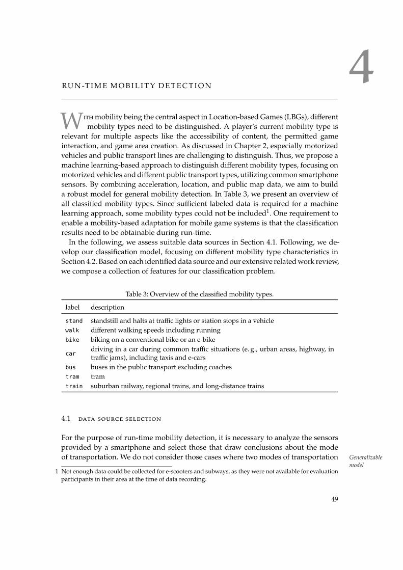
4RUN-T IME MOB IL I TY DETECT ION

With mobility being the central aspect in Location-based Games (LBGs), different

mobility types need to be distinguished. A player’s current mobility type is

relevant for multiple aspects like the accessibility of content, the permitted game

interaction, and game area creation. As discussed in Chapter 2, especially motorized

vehicles and public transport lines are challenging to distinguish. Thus, we propose a

machine learning-based approach to distinguish different mobility types, focusing on

motorizedvehicles anddifferent public transport types, utilizing common smartphone

sensors. By combining acceleration, location, and public map data, we aim to build

a robust model for general mobility detection. In Table 3, we present an overview of

all classified mobility types. Since sufficient labeled data is required for a machine

learning approach, some mobility types could not be included1. One requirement to

enable a mobility-based adaptation for mobile game systems is that the classification

results need to be obtainable during run-time.

In the following, we assess suitable data sources in Section 4.1. Following, we de-

velop our classification model, focusing on different mobility type characteristics in

Section 4.2. Based on each identifieddata source andour extensive relatedwork review,

we compose a collection of features for our classification problem.

Table 3: Overview of the classified mobility types.

label description

stand standstill and halts at traffic lights or station stops in a vehicle

walk different walking speeds including running

bike biking on a conventional bike or an e-bike

cardriving in a car during common traffic situations (e. g., urban areas, highway, in

traffic jams), including taxis and e-cars

bus buses in the public transport excluding coaches

tram tram

train suburban railway, regional trains, and long-distance trains

4.1 data source selection

For the purpose of run-time mobility detection, it is necessary to analyze the sensors

provided by a smartphone and select those that draw conclusions about the mode

of transportation. We do not consider those cases where two modes of transportation Generalizablemodel

1 Not enough data could be collected for e-scooters and subways, as they were not available for evaluation

participants in their area at the time of data recording.

49

50 run-time mobility detection

overlap, such aswalking in amoving tram for ourmodel. Additionally,we refrain from

considering data favoring personalization, e. g., weekday, time of day, or the used start

or destination stop, because this would hurt our approach’s generalized applicability.

Furthermore, this could establish strong privacy concerns.

As noted in Section 2.4.1, the inclusion of external georeferenced information hasPublictransport data

been reported to increase the detection accuracy for the motorized transport modes

car, bus and train. By adding tram information we intend to extend the classification to

further fixed-route transportation modes.

Both audio recording and Bluetooth nearby device data were considered as possible

data sources but turned out to be unsuitable. Audio recordings are too dependent on a

concrete application or public transport operator, e. g., announcements in public trans-

port or car radio. Supplementary noise by music or radio announcements is unrelatedNo audiosignal

integrationto the chosen vehicle and further complicates the distinction. Additionally, distinctive

noises of each mode of transport are hard to generalize [155], and high accuracy audio

analysis might not be processable during run-time on a smartphone [251].

Bluetooth has already been used in previous works [47, 183] to detect changes in the

mode of transport. The detection is based on a change of nearby devices, e. g., smart-Bluetoothnearby devices

phones, fitness trackers, or wireless headphones, which assumes that the devices are

visible or detectable over a longer period of time. The visibility of a Bluetooth device,

usually induced by the pairing mode’s activiation, needs to be manually activated by

the user for most devices, making it unsuitable for our scenario.

The accelerometer for conventional mobile devices distinguishes between hardware

and software sensors. Since the gravitational direction does not influence the mode

of transportation, we include software sensor acceleration data, which is corrected by

gravitational influence. Furthermore, to provide orientation independence, we utilizeAcceleration-based sensor

datathe acceleration vector magnitude |a| of all three axes as the acceleration direction

depends on the device orientation, shown in Equation 10.

|a| =√a2x + a2y + a2z (10)

For location-based sensor data, the position itself cannot be directly used for non-

personalizedmodels. TheW3CGeolocationApplication Programming Interface (API)

standard [201], however, contains additional parameters we include: accuracy, speed,

and heading. We deemed altitude data to not be applicable due to their area depen-Location-based sensor

datadent data. While map data in general provides valuable information, altitude data is

available over individual APIs2, which poses additional challenges regarding query

limits or data accuracy.

In terms of additional location-based data, OpenStreetMap (OSM) provides infor-Location-based external

datamation about the following public transport-related locations: i) the location of bus

and tram stops and train stations including train platforms, ii) the routes of buses,

trams, and trains, and iii) the position of traffic lights.

Information about railway crossings is also available but is similarly tagged like tram

crossings, which does not allow further distinctions. Under the assumption that public

2 https://open-elevation.com (last accessed: September 22, 2020)

4.2 model architecture 51

transport vehicles adhere to these routes and do not take detours due to, e. g., traffic

or diversions, this can be used to improve the differentiation process. Cars driving

along those public transport routes provide an additional challenge, as they might be

mistaken for public transport vehicles given their location trace.

Similar to the extraction of geodata for Points of Interest (PoIs) in Section 3.1.1, we

extract all public transport-related data in a grid-based approach. The assignment of OSM relationtags for publictransport

objects or path segments to a public transport line are stored in OSM relations, which

we can obtain: route=train, route=bus, route=subway, route=tram. This relation-based

method also includes traffic signals affecting the ride.

4.2 model architecture

To determine the type of transport, we use a model trained by supervised machine

learning since our problem is a classification problem. To train and test the model,

we need labeled data, i. e., data consisting of sensor values with the corresponding

transport mode. Since training a model, including data pre-processing and data per- Generalizedmodelarchitecture

sistence, is expensive in computation time and storage capacity, we decide to train a

generalized model on a server. The final model, however, needs to be feasible on a

mobile device for run-time classification.

For time series classification, frames are usually used, each representing a specific

time series interval. Each frame thereby represents an instance, labeledwith a class for Time seriesclassification

classifier training. These instances are generated during pre-processing and contain

features, which we will discuss in Section 4.3.

Ourmain ideahere is to create synthetic instances for training that are later described

as frame instances. An instance is a data segmentwith a fixed length onwhichwewant

to classify themobility type.No temporal coherence ismodeled in these instances other (Frame)instancedefinition

than the ordering of data entries for, e. g., determination of movement direction. Thus,

the features are computed on the whole instance, without distinguishing individual

time segments. Therefore, we treat our problem as a classification problem.

We expect that different features may be relevant, and different frame lengths may

be advantageous for different activities depending on the frame length. Related work

has shown that standing andwalking can already be recognizedwith high accuracy [28,

32, 96, 126, 229, 250], where in contrast, other types of transport are more difficult to

detect. Especially for the differentiation of motorized vehicles among themselves, we Differentframe lengths

expect that longer observed time intervals improve the detection.We assume that short

intervals are advantageous for the differentiation between standing and walking since

these can react quickly to short-term changes. On the other hand, motorized vehicle

usage is unlikely to change on a short-term basis, which is why longer intervals should

be advantageous to detect motorized movement in, e. g., a car, bus, tram, or train.During run-time on a smartphone, we choose to perform a classification in short

time intervals to ensure a timely system response for activity changes. A classification Run-timemobilitydetection

every TC = 5s is a suitable interval, providing the user or the mobile system with an

updatedmobility type prediction. However, the parameter choice entirely depends on

52 run-time mobility detection

Data

Cleansing

Frame

Instances

Over-

sampling

Frame-

Classifier

Training

Meta

Instances

Meta-

Classifier

Training

Figure 12: Overview over the applied mobility model building steps.

the application scenario. A classification every second or every minute is also feasible,

introducing a trade-off between strain on the system and responsiveness.

An overview of the entire process developed in the following is shown in Figure 12.

4.2.1 Frame Classifier

To detect short-term changes in the movement type and at the same time still be able

to distinguish motorized transport modes, we base our concept on intervals of three

different sizes: short (with the interval length TS), medium (TM) and long (TL). For eachCombinationof frame

classifiersinterval size, we train a classifier, which we call frame classifier. To obtain an overall

prediction result based on these three frame classifiers, we employ a meta-classifier

that combines the three classifiers’ outputs into an overall prediction.

We assign different goals to each frame classifier. The short classifier should be

particularly good at distinguishing between standing, walking, and the remaining mo-

bility types, so that it can react to short-term changes in movement. The other two

frame classifiers, on the other hand, should be able to distinguish primarily between

motorized modes of transport. To achieve our goal of recognizing short-term standingShort-termstanding

and differentiate between extended intentional standing, both short and medium classi-

fiers should recognize standing. For the example of a pedestrian or vehicle waiting at

a traffic light, or a bus stopping at a bus stop, the long classifier should continue to

predict the overall, longer-lasting movement type.

This goal requires two labels during the data acquisition process: The main move-

ment type label recorded during data acquisition and, if necessary, in some places, a

secondary, more precise standing label. The latter is only used for special cases suchTemporarystanding label

as stopping at a traffic light or bus stop and is manually assigned to the training data,

based on the route speed and acceleration data, described in detail in Section 4.2.4. It

is important to note that each instance only contains one class label, with the exception

of temporary standing. Thus, the frame length must not be exceedingly long, as this

would introduce possible misclassifications when switching mobility types. Because

the switchover usually requires intermediate standing orwalking, those frame instances

will most likely not contain two distinct vehicular mobility types.

If the short classifier cannot reliably differentiate between movement types, based

on their short frame length, it would be possible to reduce its classification spaces toPossiblereduction of

short classifierthe three labels of standing, walking, and other means of transportation. However, in the

course of this thesis, it has been valuable to integrate all available classes for short.

4.2 model architecture 53

4.2.2 Classification Approach

Among the classical classification algorithms, especially random forests, have led to

the best results in related work [96, 168, 220, 229, 275]. For our described multi-class Employedmachinelearningapproaches

problem, we focus our work on decision tree learners, e. g., Random Tree, Reduced

Error Pruning Tree, or J48, as well as ensemble approaches, e. g., Adaptive Boosting,

or Random Forest.

Under- and overfitting is a severe problem in machine learning. To counteract un-

derfitting, we will identify as many fitting features as possible, for which we suspect

them being relevant for the current transport mode, or features reported in related

work. Thereby, we accept that individual features may overlap or correlate with each

other. Subsequently, to counteract overfitting, we perform a feature selection, reducing Approach tounder- andoverfitting

the features that are ultimately used to those with the greatest relevance. We utilize a

stratified 10-fold cross-validation for the final evaluation, which reduces the variance

between distinct folds as each fold aims to have a similar class distribution. It is impor-

tant to note that the raw data itself contains inaccuracies and noise. Additionally, due

to the manual labeling process, inaccuracies in the transition between standing and a

specific transport type cannot be ruled out, especially if certain sensor values such as

speed are missing in the recording.

4.2.3 Data Cleansing

To collect the required rawdata, an application is required that records the acceleration Dataacquisitionapplication

sensor and location data of a smartphone and labels this data with the corresponding

label, based on user input. We will present this application in Section 5.2.

In our scenario, an activity represents a continuous course of movement of a smart-

phone for a certain type of transport. During data acquisition, the labeled sensor data

is recorded in a continuous data stream. With data coming from different users and Activityseparation

thereby different smartphones, the data stream is separated according to the user de-

vice ID and split into activities. We separate activities, whenever the transport mode

changes according to its label, or two data points are separated by more than a certain

amount of timemaxGap, indicating an interruption of data recording.

The manual assignment of the additional standing label is shown in Figure 13. Due

to latency between the acceleration and velocity data, a precise assignment was not

always possible in all datasets. Whenever velocity data was inaccurate, the manual Manualre-labeling

labels were applied according to acceleration data. If manual labelingwas not possible

due to ambiguous or missing data, we excluded the activity from the training set.

The ambiguity or low quality of location data may also be an indicator for, e. g.,

routes through tunnels. Thus, the respective data is not discarded. For scenarioswhere Ambiguouslocation data

location data is unavailable or the retrieval is not authorized, features based on accel-

eration data can still be used for classification.

According to the Geolocation API, no speed is returned unless it can be deter-

mined [201]. Missing data, however, is reported as having a velocity of 0m/s, being Speed datacleansing

indistinguishable from a true standstill. Thus, we decide to fill inmissing speed values

54 run-time mobility detection

Figure 13: Setting the additional standing label in the marked areas using the velocity data

(top) and the acceleration data (bottom) in an exemplary car dataset entry.

for singular cases based on linear interpolation when both previous and next speed

values are available. This is not applied for the special cases of, e. g., tunnels or when

the location sensor has not yet initialized, as we only want to fill up single missing

values and not replace the whole time series.

To compensate for missing speed data, it would also be possible to calculate the

current speed from the accelerometer values using a Kalman Filter [129]. For a KalmanAccelerationdata

compensationFilter to work reliably, additional parameters like the initial speed would be required,

which is not obtainable from previous speed data when facing the scenario of location

sensor initialization. As a result, we decide against using additional approaches to

compensate for missing speed data.

It is common knowledge that GPS-based location data is prone to errors [27, 126,

177, 229, 233, 275]. In addition to that, there is a latency between the velocity and

acceleration data, which is induced by technical conditions: The acceleration data areDelay and badaccuracy forlocation data

determined directly by a smartphone’s sensor, whereas a sufficiently good GPS signal

from several satellites is necessary for the exact position determination. Furthermore,

inaccuracies of the GPS signal can be observed frequently in the following situations:

i) signal isolation in a building or tunnel, ii) signal distortion by the environment, e. g.,

close to tall buildings, reflecting signals [48], and iii) attenuation of signals through

metal coatings [34, 143] of multi-pane insulating glass inside buildings or trains. The

metal coating attenuates radio waves (including GPS signals) by up to 33 dB, which

4.2 model architecture 55

Figure 14: Windowing to generate frames for short, medium and long for an example without

overlap. For short and medium those frames are removed that are overlapped by a

secondary label (highlighted). In addition, at the end of an activity, the last frame

is removed if it does not reach the specified frame length. Adapted from [116]

corresponds to an almost complete shielding. Such insulating glass is increasingly

used in glass facades, trains, and cars.

During data analysis, we observed these effects, especially during train rides and in

dense urban areas, where location data was less accurate than in open air. In situations

with metal-coated windows in trains, such inaccuracies occur systematically. Instead

of removing these scenarios as reported for other works [183], we retain this data and

expect the location sensor accuracy to be an important feature in these scenarios.

We refrain from threshold-basedfiltering of acceleration and speeddata formultiple

reasons, which is regularly reported in related work, e. g., speeds > 125 km/h [153],

or speeds > 150 km/h [177]. Most of the data has been collected in Germany, which Nospeed-relateddata removal

has no generally valid speed limit, and high-speed trains can also easily exceed the

reported thresholds. In general, we could observe from our data that outliers are

rare. In this scenario an outlier would be a strong deviation from the expected speed

or acceleration values for a given mobility type, e. g., 70 km/h for bikes induced by

incorrect location data. For this reason, we decide to focus on attributes that are more

robust against outliers, e. g., different quantiles, instead of removing them.

4.2.4 Pre-processing & Training

Since instances are needed to train the frame classifiers, we generate frames of the

duration TS, TM, and TL from the time series of the respective activity during pre-

processing, independent from each other. Thereby, a sliding window iterates over the Frameinstancecreation

time series with a certain shift of shifti. Instead of utilizing an overlap solely based

56 run-time mobility detection

on the percentage length of a frame, we include an absolute value of shiftmax into the

calculation, which provides higher overlap for longer frames. To achieve an overlap of

at least 50% for shorter frames, we use the following shift for frames with length Ti:

shifti = min(0.5 · Ti, shiftmax) (11)

Since we want to correctly classify short-term standing, we remove all short and

medium frames that overlapwith such an additional label. Those frames are thenutilized

to train standing classification. For long, we only remove frames that overlapmore thanFramewindowing

70% with a secondary label, which is rare, as it requires either very long stops or

training data where users forgot to stop the recording. Following, we remove intervals

that are shorter than 95% of the specified frame length, which only happens for very

short activities or the last instance of an activity, as shown in Figure 14.

To train our model for frames containing a temporary standing label, we extract the

intervals to pseudo activities with a standing label. Thus, we can frame them withPseudoactivities fortemporarystanding

the same procedure and use them for classifier training, ensuring that our classifiers

are trained to detect temporary standing. The long classifier should be able to identify

the means of transport independent of temporary stops, which is why those frames

containing a temporary stop (if not > 70%) are not removed.

Pre-processing & Training for Frame Classifiers

After separating the data stream into individual frame instances, the previously de-

scribed speed data cleansing is performed, i. e., single missing velocity values are

interpolated. However, we sample acceleration data during data collection at the de-

vice’s maximum possible sampling rate. Thereby, the achieved sampling rate depends

on the particular smartphone and its current workload. Thus, the raw data samplingAccelerometerdata

resamplingrates range from 6.5 Hz in rare cases to 62.5 Hz in normal cases. Therefore, our model

needs to be able to handle diverging sampling rates. For some of the features de-

veloped in Section 4.3, e. g., statistical or frequency spectrum features, it is required

that the data within a frame is equispaced. This can be achieved by evenly sampling

the respective signal in the time domain. For this purpose, a suitable sampling fre-

quency f = 1/T must be determined for each frame. To determine a suitable sampling

frequency, we analyzed our recorded data in terms of time difference between data

measurements using the minimum, average, median, and first quartile.

We could deduce right off that utilizing the minimum time difference, i. e., the

maximum sampling frequency, would not be representative of the data, as it ranged

between 1ms and 7ms. It would have an impact on pre- and live processing perfor-

mance, due to a significant increase in data, without providing much added value in

terms of accuracy as most data would be interpolated. The mean value is also unsuit-Accelerometerdata distance

analysisable, with values between 17ms and 29ms, as it is influenced by outliers. This could

be avoided by using the median, which, however, also has a high range between 17ms

and 27ms. The first quartile had by far the lowest variance in time difference between

14ms and 18ms for our data. Thereby we choose to utilize the first quartile of the time

4.2 model architecture 57

difference between data points as our sampling frequency for the respective frame.

During resampling in equidistance intervals, we utilize the closest sensor value of the

original sample for each new sampling time value.

Due to the nature of the data collection process being split up to multiple users

recording their movement activities of varying durations, the data records are unbal-

anced. This holds true for the number of intervals for each frame classifier. Training Unbalanceddataset

a classifier on an unbalanced set may lead to a biased classifier. Two data sampling

options to avoid biasing a classifier during training are reweighting and resampling.

Reweighting of instances, assigns a weight to each training instance, to compen-

sate for varying class amounts. However, not all algorithms for classifier training and

hardly any algorithms for feature selection can handle weighted instances. Resam- Reweightingandresampling

pling, in contrast, achieves an even class distribution by adding or removing instances.

We choose to use oversampling for each individual frame classifier by multiplying

instances for a balanced dataset. Applying the oversampling process only to the raw

data stream or one selected frame classifier would still lead to unbalanced datasets for

the other frame classifiers because of the individual frame windowing approach, as

shown in Table 4.Undersampling, i. e., leaving out instances to achieve a balanced class

distribution, would impact our approach, as our dataset would be reduced according

to the least represented mobility type.

Table 4: Distribution of instances for each class for the utilized training data for TS = 5s,

TM = 15s, and TL = 90s. The meta-classifier utilizes stepSize = 5s. The exact

number of instances depends on the respective frame length, and the window shift.

frame classifier stand walk bike car bus tram train

short 6,207 10,618 5,185 14,829 5,115 1,793 3,936

medium 2,266 5,082 2,514 7,070 2,199 739 1,826

long 1,135 3,884 2,255 6,704 2,457 1,042 1,578

meta 3,708 5,395 2,650 7,578 2,736 974 2,029

The resampling process is an integral part of machine learning, especially when

there are many initial features. For performance reasons, we have chosen a filtering

approach, and because the alternative wrapper approaches can be prone to overfitting.

In Section 4.2.2,we stated thatwe accept features correlatingwith each other. In feature Featureselection

selection,weuse correlation-based feature selection [98] that preferably selects features

that correlate strongly with the class and as little as possible with other features.

This reduces redundancies between features. There are several approaches to finding

feature subsets, for which we identified four applicable search methods:

• Exhaustive Search [127] checks all possible feature subsets. This leads to a compu-

tationally intensive and impractical selection process, which is why we decided

against this approach.

• Best First search [197] selects features based on their performance and selected

the fewest features in our initial tests.

58 run-time mobility detection

• Evolutionary Search [148], in contrast, selected the most features, and is based

on an evolutionary algorithm employing a heuristic selection.

• Genetic Search [85] uses a random selection algorithm allowing the search in

large search spaces.

Because each of our frame classifiers can contain different features, or at least has a

different task, the employed feature selection search can be different for each classifier.

Meta-pre-processing & Training for the Meta-Classifier

Ourmeta-classifier is designed to combine the predictions of the three frame classifiers,

which is called stacking. For this reason, we perform ameta pre-processing simulating

the activities that determine the frame classifiers’ predictions at the respective points

in time and provide them with the actual label. Thereby, we generate meta instances

with which we train the meta-classifier.

In the meta pre-processing, we iterate over the activities in a certain step size

stepSize, determining the respective three frame classifiers for each step.When choos-

ing the step size, we can relate to the TC parameter, i. e., the time interval, after which a

classification update should be shown to the user. In systems with infrequent updates,

the step size should not be an order of magnitude larger than the length of the short

frame TS, as valuable training opportunities might then be wasted. Similar to the gen-Meta instancecreation

eral pre-processing, frames that have not yet reached at least 90% of their intended

frame length are not used because some features depend on its frame length. Thus,

at the beginning of an activity or recording, there is a phase, where first only short

frames are used, being later supplemented by medium and long frames. This results in

an initialization duration of 0.90 · TL until all frames are used. This also means that the

first classification can be done only after the first short frame, i. e., after TS.

In the case of transitions between different movement types, we introduce the

transitionDuration, which represents a certain amount of time that may pass until

enough data is available to recognize the new movement type. We thereby aim forTransitionduration

a transition duration that is less than a short frame length TS to allow for a respon-

sive classification result. In our meta-classification, for the time of the transition, the

previous label will be treated as the expected classification result. Thus, each frame is

labeled with the movement type that was active during t ′ = t− transitionDuration.

Those transitions also happen in situations where the temporary standing label was

set, like halting at a traffic signal. We choose to design our meta-classifier to detectMeta-classificationfor temporary

standing

these temporary stops. Thereby, each meta-instance is assigned with this temporary

label as the expected prediction class, otherwise the primary label is expected.

Just like the instances for the frame classifiers, the meta instances are unbalanced,

as shown in Table 4. Accordingly, we resample the meta instances before training the

meta-classifier.Meta-instancefeature

selectionThe prediction of ourmeta-classifier solely depends on the output of the three frame

classifiers. This results in a limited amount of features. For feature selection, this allows

for more exhaustive approaches, which we will need to evaluate.

4.3 feature engineering 59

Table 5: Overview over the employed feature categories for mobility detection. A detailed

insight over all features is provided in Tables 22-26.

feature type description of utilized sensors or sources

Statistical features statistical features for acceleration, location sensor speed,

and location accuracy

Measures of dispersion measures of dispersion for acceleration, location sensor

speed, and location accuracy

Time-domain features gravity-adjusted acceleration in time-domain

Frequency-domain features Fourier-transformed gravity-adjusted acceleration

Location sensor information covered distance, heading, and speed features

External map data features OSM map data for public transport stations

Meta-features classification results for each frame classifier

4.3 feature engineering

Feature engineering is the process of developing the most relevant features for the

problem based on the given data [271]. We define features for the three frame lengths Featureengineering

with the intention to map relevant data features to singular values that are usable in

a classification process.

We intend to add features that have either shown a promising impact in relatedwork

or have been used without feature selection, meaning that their individual impact is

unknown to us. In individual cases, we have modified, expanded, or added features, Features fromrelated work

which we state accordingly. The features have been constructed based on the data

sources selected in Section 4.1: acceleration data, location sensor data, and external

location information.

To allow for a better intuitive representation of each feature, we try to only introduce

abbreviations when necessary or when related work commonly uses the given abbre-

viation, e. g., FFT for fast Fourier transform. We choose feature names to allow for a Feature nameabbreviations

sensor-based grouping after alphabetic sorting. Two consistently used abbreviations

from here are accu for the location sensor accuracy, and acce for the accelerometer ac-

celeration vector magnitude (Equation 10). All employed features are shown in detail

in Section A.5.2 with a category overview provided in Table 5.

We start by including basic statistical features commonly used in the relatedwork for

the three data sources of acceleration, geolocation speed, and its accuracy. As noted

before, we accept features correlating with each other at this stage. We present the Basicstatisticalfeatures

developed features in detail in Table 22, which include common individual statistical

values, e. g., mean or commonly used quantiles, and measures of dispersion, e. g.,

variance, and interquartile range. In the recorded sensor data outliers are found with

particularly high values. For that reason, we include the 95% quantile and also utilize

60 run-time mobility detection

an alternative range measurement between the minimum value and the 95% quantile

(RangeTo95).

4.3.1 Acceleration Data Features

Apart from basic statistical features, acceleration data is rich in information, which

is why many authors solely rely on acceleration data [24, 191, 249]. We divide theAccelerationdata

separationidentified features into two groups: features in the time-domain, and features in the

frequency-domain, e. g., following a Fourier transformation. Acceleration data has the

advantage to be readily available in smartphones, as no external signal is required,

and accelerometers are part of the built-in inertial measurement unit. The detailed

resulting features are shown in Table 23.

Acceleration data features in the time-domain

The root mean square (RMS), also known as the quadratic mean, is a simple feature

based on the mean values, with the goal of emphasizing higher values.Root meansquare

acceRMS =

√√√√ 1

n·

n∑i=1

ai2 (12)

Inspired by the normalized spectral energy, which we will develop later in the fre-

quency domain in Equation 17, we propose the normalized acceleration energy, which

in this case is the is the square of the root mean square, and is thereby directly corre-

lated.

acceNormEnergy =1

n·

n∑i=1

ai2 = acceRMS2 (13)

The zero-crossing rate (ZCR) is the rate at which a signal changes its sign. Since we

use the acceleration vector’s magnitude, its value is never negative. For this reason,Zero-crossingrate

we count how often the signal touches the value 0, normalizing it with the number of

signal data points for the given frame. This does not correspond to a true zero-crossing

rate for each individual axis, as all axes need to be zero to result in a magnitude of

zero.

The mean-crossing rate (MCR) works similarly to the zero-crossing rate, except thatMean-crossing

rateit counts the crossings through themean, again normalizing it by the number of signal

data points.

The skewness describes the asymmetry of a frequency distribution and is com-

monly used for probability distributions. It is the third central moment in a frequency

distribution, where the variance is the second central moment. It characterizes theSkewnessasymmetry of the tapering sides of the distribution, with negative values representing

a left-sided skew and positive values a right-sided skew.We calculate the skewness [4,

4.3 feature engineering 61

92] based on the standard deviation SD and the mean value a of data series a with

length n.

acceSkewness =1

n · SD3·

n∑i=1

(ai − a)3

(14)

The kurtosis is a measure of the steepness of a frequency distribution and is the

fourth centralmoment. Thehigher thevalueof thekurtosis, the steeper thedistribution. KurtosisThe lower the value, the more convex the distribution. We, similarly to the skewness,

calculate the kurtosis [4, 92] based on the standard deviation SD and the mean value

a of a data series awith length n.

acceKurtosis =1

n · SD4·

n∑i=1

(ai − a)4

(15)

The slope sign change rate was used by Aşçı and Güvensan [13] without specifying

a formula. We comprehend the feature as the zero-crossing rate of the derivation of Slope signchange rate

a time series. For this reason, we calculate it based on the difference between every

consecutive acceleration value.

Other features we have considered in the time-domain include a peak detection, No peakdetection

which showed no added value over the features used in the evaluation process.

Acceleration data features in the frequency-domain

A representation in the frequency-domain is a commonway to describe a signal or the

course of sensor values. For our discrete data, we use the discrete Fourier transform to DiscreteFouriertransformapplication

calculate the frequency spectrum [225]. A commonly used algorithm for fast discrete

Fourier transform calculation is the Fast Fourier Transform (FFT), which is applicable

since we earlier resampled the sensor values into equispaced segments.

An alternative to resampling the data into equispaced segments would be to use the

FFT for non-equispaced data. The non-equispaced FFT [55, 56] is a generalization of Non-equispacedFFT

the FFT with existing reference implementations by Keiner et al. [142]. This approach

best works for periodic signals, which does not necessarily apply for our data, which

is why we decided to resample our data.

The common FFT implementation expects the number of data points corresponding

to 2n, which does not hold true for our data, which is why the FFT algorithm of

Bluestein [25, 105] is used. According to the Nyquist theorem, the sampling rate Maximummeasuredfrequency

must be at least twice the maximum frequency to be detected [3]. During initial

data collection, reported in Section 4.2.4 identified an average first quartile signal

time difference of 16ms. This corresponds to a sampling rate of 62.5 Hz, leading to

frequencies up to 31.25 Hz being measurable.

To receive the amplitude for a given frequency, we determine themagnitude of each

Fourier coefficient, combining its real-valued component Re(X(fi))with its imaginary

component Im(X(fi)). Fourieramplitude

|X(fi)| =√Re(X(fi))2 + Im(X(fi))2 (16)

62 run-time mobility detection

The DC term in Fourier transformation is the 0 Hz term, i. e., a constant amplitude

wave with zero frequency, with low-frequency noise being close-by. After an initialHigh-passfilter for noise

analysis, we chose a high-pass filter with a cutoff frequency of 0.03 Hz to eliminate

these frequency components. For a signal without any noise, a cutoff frequency of

0 Hz would be sufficient to remove the term.

Since the discrete Fourier transform is calculated in-place, more data points are

obtained for the frequency spectrum, the longer the time series is. Grouping them up

into frequency bins is a commonmethod to retain performance. For each frequency bin,Frequencybins

the maximum frequency component |X(fi)| from the frequency band is selected. We

choose a width of 0.2 Hz for the frequency bins, significantly increasing performance

while retaining as much information as possible.

To calculate meaningful features, the frequency bins are too small. Therefore, we

use frequency bands, which are intervals of the frequency spectrum, each limited by

a lower frequency of fl and an upper frequency of fu. The frequency band is thenFrequencybands

defined as the sum of the Fourier coefficients of the frequency bins between fl and

fu. While arbitrary numbers and band lengths would be possible to use as features,

we determined our resulting frequency band features by inspecting our recorded data

and identifying promising bands. Our list is by no means exhaustive but covers all

frequency bins between 1 Hz and 30 Hz.

In addition to frequency bands, features based on a frequency component’s ampli-

tude |X(fi)| are commonly used. We will use the prefix spectral for these features.

The energy of a coefficient can be calculated by squaring its amplitude. Thereby, weNormalizedspectralenergy

define the normalized spectral energy as the normalized sum of energy coefficients

withN frequency bins. The normalization is required because signals contain different

amounts of frequency bins due to their sample rate.

spectralNormEnergy =1

N·∑i

|X(fi)|2

(17)

The spectral centroid was originally introduced as a feature for speech recogni-

tion [195], where each frequency bin is weighted by its amplitude. It is thereforeSpectralcentroid

defined as the frequencies’ weighted average.

spectralCentroid = fSC =

∑i |X(fi)| · fi∑

i |X(fi)|(18)

The spectral flatness is a measure of a spectrum’s noisiness [62]. It is calculated bySpectralflatness

normalizing the geometric mean of the FFT coefficients by its arithmetic mean [170]

for N frequency bins.

spectralFlatness =N√∏

i |X(fi)|1N

∑i |X(fi)|

(19)

The spectral crest factor is strongly related to the spectral flatness [62]. It is the

ratio of the maximum amplitude coefficient to the root mean square of the amplitude

coefficients [29].Spectral crest

4.3 feature engineering 63

spectralCrest =max(|X(fi)|)√1N ·

∑i |X(fi)|

2(20)

The spectral roll-off has a cut-off frequency that divides the total spectral energy

into a high- and low-frequency band. We choose a ratio of 0.85 between the energy of Spectralroll-off

the low-frequency band and the total spectral energy [62]. This feature can sometimes

correlate with the spectral centroid.

The spectral spread indicates the current effective bandwidth and assesses the

shape’s spectrum in terms of the width distribution around the spectral centroid

fSC [62]. Spectralspread

spectralSpread =

√∑i(fi − fSC)

2 · |X(fi)|2∑i |X(fi)|

2(21)

Similar to the features in the time-domain, we include the skewness and kurtosis in Spectralskewness &kurtosis

the frequency-domain.

4.3.2 Location Sensor Data Features

Features based on the distance traveled were often utilized in related work when

complete trips based on location data were classified [88, 275]. In contrast to the

authors, we apply distance measurements on a frame-basis. In doing so, we normalize Traveldistancecalculation

the distance in terms of time. For distance measurement, we use Vincenty’s inverse

problem formula [138], which models the Earth as an oblate spheroid, presenting a

higher accuracy than models calculating the great circle distance.

Feature-wise we decide to use the traveled distance within the frame, i. e., the

distance between the first and the last location, to utilize the covered distance. For a Traveldistancefeatures

more comprehensive distance estimation, we use the accumulated distance, which is

the sum of distances between consecutive locations. Unlike Zhou et al. [275], we do not

use the maximum distance of the most distant positions for the maximum distance,

but the maximum distance of two consecutive positions. The latter feature is expected

to correlate with the maximum speed feature presented before.

In their work, they also introduce features based on the location sensor’s speed

parameter [275]. They model the ratio of speed measurements that are below a given Travel speedfeatures

threshold. We adopt their features and supplement additional thresholds for higher

speeds, but again apply them to our frames instead of the whole route.

The heading variation is a measure of the frequency of directional changes. Similar

features have already been used in [229, 272, 275]. Using the absolute difference in Headingvariation

heading between consecutive heading data entries, with each entry in [0◦, 180◦], we

can calculate the accumulated change in heading.

Previous publications have shown that enriching vehicle discrimination with fea-

tures for vehicle-specific stopping behavior can be promising [183, 229, 233]. Looking Stoppingbehavior

at the reported stoppingbehavior differences in relatedwork [233] andwhen analyzing

our recorded data, we identify multiple key aspects.

64 run-time mobility detection

• Cars stop mainly at traffic lights or level crossings. The stops at traffic lights are

relatively short.

• Trams stop regularly, but primarily at tram stops. Between two tram stops, in

most cases, we observed a maximum of 90s, with durations between 5s and

30s. This is comparatively short because tram drivers usually do not sell tickets

themselves. In some cities, public transport is given priority at traffic lights. For

this reason, trams in these cities stop at traffic lights less frequently or for shorter

periods than cars.

• Buses can be either city buses or intercity (regional) buses. City buses, like

trams in the corresponding cities, also benefit from public transport priority. In

contrast to trams, a stop can last much longer if the driver sells tickets on the

bus. Differences between city and intercity buses exist in terms of shorter, more

equidistant stop intervals in a city, and higher maximum speeds for intercity

buses due to regional transfer.

• Trains stop less often than trams or city buses, with stops usually taking much

longer than 60s.

Based on this information, we create features based on the number and duration of

recognized stops. Recognizing these stops is independent of the standing classification,meaning that segments identified as stops are not automatically classified as standing.We define a stop as a sequence of speed data that does not exceed a threshold of

maxStopSpeed for more than 2s. A threshold-based approach is chosen, to offset forStop amountand frequency

featuresa potential location sensor drift during a real stop. The duration was chosen, as we

want to avoid treating slow-moving traffic as a sequence of stops. In terms of stop

duration, we choose to group up durations into differently sized bins, with one open-

ended bin containing stops above a duration of minDurationLongStop, representing the

presumable train stops. Because the stop durations are rather long and frames with

a temporary standing label are not used in short and medium training, we apply these

stop features only in the long frame classifier.

4.3.3 External Data Features

Not only the frequency and length of stops may allow conclusions about current

mobility type, but also the positions of these stops. While classifiers without any

station informationmay result in false car classifications, the vicinity towards a nearby

public transport line or a station may increase public transport detection confidence.

For this purpose, we extracted OSM relations for public transport lines, which include

the individual stations. We define a radius stopRadius, specifying the radius aroundPublictransport spot

detectionan OSM node, in whose radius we assign the stop to the public transport stop or

the traffic signal. The definition of a radius is necessary because of location sensor

inaccuracies. Additionally, the locations are represented as single coordinate, whereas

a stop in a public transport vehicle or in a line in front of a traffic light, might deviate

in its distance due to the length of the vehicle or the waiting line. It must be noted

4.3 feature engineering 65

that an OSM node can have several tags, e. g., a location can represent both a bus and

a tram stop at the same time. The information about the exclusiveness of a stop, i. e.,

it only being served by this one means of transport, can be helpful if encoded into a

feature.

For all public transport features included, we make an assumption on the operating

principles in the respective area. We assume that public transport vehicles stop at

pre-defined stations to load or unload passengers, whereby individual stops can be

skipped. During each trip, they follow a fixed route.

In addition to station data, OSM provides detailed route data, which we can use

to compare a user’s movement trajectory to a particular public transport line. Public Publictransportroute retrieval

transport routes are represented by an ordered list of positions, annotated with the

public transport type and in many cases the specific line identifier, e. g., the bus or

train number.

Our goal is to compare the smartphone’s position data with the various routes of

the public transport network. Both routes are continuous in space and time and can Trajectorycomparison

be represented as a trajectory, generally described as a time-sampled and ordered

sequence of data points [87, 118, 230, 231].

To the best of our knowledge, neither live public transport data nor country-wide

public transport timetables are openly available at the time of writing. For individ- Publictransporttimetableavailability

ual transport organizations in Germany, timetable APIs are available3,4,5

. They are,

however, presented in different formats and only cover the country to some degree.

Thereby, we can only compare our route trajectories in the spatial dimension.

Shao et al. [222] describe a trajectory as a discrete image of a continuous polygon

course, which can be generalized to the comparison of two geographic trajectories. Hausdorffdistance

An often used similarity measure of two trajectories in geographical scenarios is the

Hausdorff distance [21, 102, 152, 222], which is a metric for the distance HA↔B of

two non-empty point sets A and B on a plain. It is based on the one-sided Hausdorff

distancehA→B, which describes themaximumdeviation of a point setA froma second

point set B:

hA→B = maxa∈A

(d(a,B)) (22)

d(a,B) = minb∈B

|a− b| (23)

d(a,B) describes the minimum distance between a single point a and a point set B,

according to a given distance metric. Thus, each a ∈ A is at most hA→B away from B.

Because the Hausdorff distance is not symmetric [21], the distance of hB→A (defined

equivalently) is required, to define HA↔B. The two-sided Hausdorff distance HA↔B

is then defined as the maximum of both one-sided distance measurements.

3 https://www.delfi.de/de/strategie-technik/mitglieder/

4 https://www.opendata-oepnv.de

5 https://opendata.rmv.de/site/start.html

66 run-time mobility detection

In our scenario, we want to compare a frame of a whole movement trajectory to a

full public transport route. As a result, only the one-sided Hausdorff distance hA→B

contains the relevant information, as we want to know how much our position data

A diverges from a public transport route B. The inverse case of hB→A is usually notHausdorffdistance

applicationrelevant, because the route is unlikely to be traversed in the given time frame, and it

would expect the user to use the vehicle from the departure stop until the terminal

station. Because hB→A is most likely greater than hA→B, the two-sided Hausdorff

distance HA↔B has a worse distance estimation than hA→B.

The Hausdorff distance only calculates the maximum distance between two routes

independent of their direction. For this reason, before applying it, we have to checkDirection oftravel

whether both trajectories have a similar direction. Two congruent trajectories with

opposite directions would have a very small Hausdorff distance, but would not corre-

spond to the public transport route it is compared to.

To derive concrete features from the information described above, we calculate the

smallest trajectorydistanceper transport type.We consider only routes not excludedbyHausdorfffeatures

travel direction filtering and with a Hausdorff distance below a given cutoffDistance.

If the cutoffDistance is exceeded, the distance calculation is terminated early, and the

public transport route is discarded.

Consequently, we employ a feature for each type of public transport station related

to the smallest Hausdorff distance.

4.3.4 Delta Features

In order to model the temporal course of activities in features, we introduce delta

features for each previously described feature. A delta feature sets a feature value of

the current frame in relation to the feature’s value of the previous frame. If no previous

value exists, the delta feature remains empty. Thereby, we double the number of

available features, where the previous value does not need to be recalculated as their

value has already been determined for the previous frame due to the calculation

happening in sequence.

Since we want to use the short frames to be able to react to short-term activity

changes, and the idea of time dependency opposes this, we do not use delta features

for the short frame classifier.

4.3.5 Meta-Classifier Features

As stated before, we use the results of the three frame classifiers short, medium, and

long to determine the overall prediction results in the form of themeta-classifier result.

Feature-wise we include the individual predictions and each classifier’s prediction

for the previous frame. In ensemble approaches like the Random Forest, the frame

classifiers prediction is determined by a majority voting approach over the individual

Random Tree predictions.

Furthermore, we want to include the outcome of this voting process into our pre-

diction because the uniformity or diversity of the trees’ predictions can be promising.

4.3 feature engineering 67

To provide a measure of prediction reliability, we utilize the proportion between

weights of the trees’ prediction, the overall prediction, and all tree weights. In a non- Meta-classifier scorefeatures

weighted Random Forest approach, this corresponds to the ratio of individual trees

predicting the given class. In an Adaptive Boosting approach, individual trees can be

weighted, requiring the weights to be included in the calculation. We name the result-

ing measure of reliability score, which must not be mistaken for a measurement of

confidence [269]. The higher this score, themore reliable the respective frame classifier

is with its prediction resulting in the features. Additionally, we use the scores of the

previous classification per frame classifier.

This results in twelve features per Meta-instance, which are shown in detail in

Table 26.

5GEOV I S : SYSTEM FOR ADAPT IVE LOCAT ION-BASED GAMES

To assess the performance of our content generation approach and its adaptation

components, we need to implement the respective components for the utilization

with mobile devices. For this purpose, we introduce the GeoVis platform. It combines

a mobile app component operating on each player’s smartphone device with a server

component responsible for game data provision and information processing. Further,

the mobile component incorporates a prototypical visualization to present the pro-

cessed results as a foundation for a fully developed game presentation.

In the following section we provide an overview of the platform, before presenting

details about the mobile application components in Section 5.1.1, and the server com-

ponents in Section 5.1.2. Finally, we discuss the development of a mobile application

utilized to collect mobility data for model building in Section 5.2. In these sections,

we focus on select implementory details for each component to provide additional

insights into the architecture and highlight its design choices.

5.1 overview of the geovis system

In Figure 15, we provide an overview on all system components.

The Android-based mobile application deployed on each player’s smartphone is

the core component of our system. It accumulates local sensor data and processes it Android-based mobileapp

for i) game area creation base on the location sensor utilizing a Global Navigation

Satellite System (GNSS), ii) a repeating mobility detection, and iii) on-demand route

calculation within the game area. The processed data is then fed into the respective

game’s runtime and applied for visualization accordingly.

Our server instance is responsible for request processing,whichmainly concerns the

content generation of game areas. To obtain the requested number of suitable Points Serverinstances fordataprocessing

of Interest (PoIs) it manages its own OpenStreetMap (OSM) database. For mobility

detection, the applied model is created on the server utilizing mobility data recorded

in our user study described in Section 6.3. This incorporates a web application we

utilize for mobility data visualization, data cleansing steps, and model management.

Especially for personalization and run-time adaptation aspects, privacy is a highly

relevant concern. For that reason, we do not communicate personal data to our server.

The only data sent to the server are the game area generation requests. However, these Privacyconcerns forpersonaliza-tion andadaptation

requests only contain the game area identifiers relating to the geographic area the

player is located in. Since these areas are sufficiently large1, the player’s accurate posi-

tion is not communicated. For the route personalization component, the optional PoIs

distances can be downloaded from the server, processing the route on the player’s mo-

1 The commonly used game area size correspond to the sizes utilized in our later evaluation scenario of at

least 0.32km2.

69

70 geovis: system for adaptive location-based games

bile device. For the mobility detection component, the pre-built model is downloaded

from the server once and contains no player-specific data.

Mobile AppÆ

Game Runtime�

Game Data

Visualization

Sensors½

GNSS

Accelerometer

. . .

Processing3

Game AreaCreation

Mobility Detection

Route Calculation

Mobility Web App)

Data Visualization Model Management

Server�

Data Handling

OSM Database (PoIs & Public Transport)

PoI Distances Mobility Data

Processing3

Game Area Content Generation

Mobility Detection Model

Figure 15: Components in the GeoVis platform.

5.1.1 Mobile Application Components

For our rectangular discrete global grid implementation, we utilize the S2 GeometryLibrary2, as it offers the functionality of hierarchical cells with uniform tiling, neighbor

determination, and cell vertex information in anefficientmanner. Furthermore, current

Location-based Games (LBGs) [104, 199] utilize this library for game area provision,

allowing us to compare respective game areas directly. Each cell has a numeric cellS2 Librarylevel up to 31, where an increase in cell level by one corresponds to a division into a

cell’s four children. The largest cells with a level of zero cover the whole globe and

consist of six cells arranged as a cube. Within our evaluation scenario, we will be

exclusively using level 12, 13, and 14 cells, as they have appropriate sizes to cover

inhabited areas matching suitable game areas. Level 14 S2 cells have an average area

of 0.32km2, which is approximately the size of a common park area in cities, and

therefore a suitable size for a LBG game area. Level 13 S2 cells combine their four level

14 children into an area fourfold the size. Then again, level 12 S2 cells combine their

four level 13 children in an area of 16 · 0.32km2 = 5.12km2, which corresponds to the

approximate area of a suburban area. Although possible, utilizing smaller or larger

cell levels would limit our options to either apply the approach to villages when game

areas become too large or select meaningful PoIs when game areas become too small.

The latter example results in areas with hardly any locations to select from.

Due to the nature of geographic projections (see Section 2.2), a cell’s size slightly

varies for similar cell levels depending on its latitude. Cells might be rotated, as cell

2 http://s2geometry.io (last accessed October 10, 2020)

5.1 overview of the geovis system 71

(a) PoI view. (b) Route view.

Figure 16: PoI and public transport route visualization for the city center of Darmstadt. The

PoI view utilizes a pn value of 16. For the route view, all public transport lines

with their respective stations are shown.

identifiers are created based on a space-filling curve, in that case, a Hilbert Curve, and

projected onto the Earth’s surface similar to six faces of a dice. These identifiers allow Cell parentrelation

for an efficient examination and calculation of parent relations between two cells of

different S2 levels3. We utilize this characteristic to split an area into its subcells of

similar sizes during the content generation process described in Section 3.2.1.

For data visualization, we developed a game-like component showing the selected

PoIs with their respective geofilter category on a geographic map. In Figure 16a, an

exemplary view of this component is visualized for the city center of Darmstadt. This Datavisualization

component builds the foundation for a fully developed game presentation and was

utilized in numerous game prototypes [26, 241], which are not within the scope of

this thesis. Since public transport data is separately retrieved for automatic mobility

detection, we show a corresponding data view for Darmstadt in Figure 16b, which has

been utilized for location-based mobility detection [146].

3 https://s2geometry.io/devguide/s2cell_hierarchy.html (last accessed October 10, 2020)

72 geovis: system for adaptive location-based games

5.1.2 Server Components

To reduce our reliance on the uptime and query limits of OSM Application Program-

ming Interfaces (APIs)4, as well as establish caching approaches, we create a data

provision service for all necessary OSM data on a self-hosted server.

Global OSM data is available as .osm.pbf files and updated daily5. This data usually

covers the whole continent but is also individually available for countries. Since coun-

try borders are irrelevant for area separation, we split6the data according to level 6 S2

cells. The chosen cell level shows good filtering times for the further processing steps.

Subsequently, we filter7all restricted areas (see Section 3.1.2). The remaining data isData

provisionthen filtered into two files, with one containing an area’s relevant PoIs covered by our

OSM geodata filters, and one containing all available public transport information

including stations and affected traffic signals. Finally, each resulting file is converted8

into an .o5m file designed for fast processing and data merging.

The resulting data is available with an API requiring the type of content (PoI or

route data), the area of interest specified by a list of S2 cell ids, and for a PoI request

a list of included geodata filter identifier, and the number of requested PoIs pn. DueData APIto this request’s customizability, allowing any desired combination of geodata filters,

the game areas are not pre-calculated. In a game scenario with static parameters,

i. e., designated geodata filters and PoI amounts, game areas can be calculated for

solo gameplay. Then again, for our coupling approach, areas need to be generated

dynamically due to the number of possible area combinations for coupling.

Furthermore, we establish an option to retrieve all OSM public transport data (seePublictransport API

Section 4.3.3) for a given S2 cell.

Both the game area generation (Section 3.2.1) and the game area coupling (Sec-

tion 3.3) is written in javascript, allowing for deployment as a web service for server-Dataprocessing

based calculation and local calculation on a mobile device.

Game Area Distribution Determination

To determine the PoI distribution in a game area, we developed two possible metrics,

with one being the geographic area of each PoI’s Voronoi cell. We calculate an area’sVoronoiduality andopen border

limit

Voronoi diagram using the Delaunay triangulation due to their duality [75]. Voronoi

border cells are known to be open, having edges of infinite length, leading to incalcu-

lable geographic areas. We approach this challenge with two distinct approaches.

Integrating the game area’s geographic borders allows us to limit each Voronoi cell

to them. By examining intersection points between game area borders and VoronoiVoronoi areaborder

integrationcell edges, all open cells can be closed to match the respective borders. An example

for the resulting Voronoi cells adhering to the game areas’ outer borders is shown in

Figure 17.

4 https://overpass-api.de (last accessed October 10, 2020)

5 https://download.geofabrik.de/ (last accessed October 10, 2020)

6 https://wiki.openstreetmap.org/wiki/Osmosis (last accessed October 10, 2020)

7 https://wiki.openstreetmap.org/wiki/Osmfilter (last accessed October 10, 2020)

8 https://wiki.openstreetmap.org/wiki/Osmconvert (last accessed October 10, 2020)

5.1 overview of the geovis system 73

(a) Open Voronoi diagram. (b) Closed Voronoi diagram.

Figure 17: Open and closed Voronoi diagrams for four game areas in London with dots

representing the individual PoIs. The inner borders exceed each area’s individual

borders as neighboring areas exist.

While the former approach works reliably, the resulting Voronoi cell size for all

previously open cells is problematic. PoIs close to the border are restricted, resulting

in significantly smaller area size values. When integrated into an optimization pro-

cess, those content candidates would be more likely to be neglected due to the false

causation between small Voronoi area to likely clustering. In our game area generation Voronoineighborintegration

process, the problem is divided into subcells, which allows us to integrate neighbor-

ing cells’ Voronoi calculations. For border subcells, the neighboring subcells outside

the original game area are also determined to close the Voronoi areas. PoIs close to

the game area border can now calculate their representative cell areas. This results in

the sum of all Voronoi cell areas most likely slightly differing from the game area’s

geographic area, which we deem to not be an issue.

If not otherwise stated, the latter method for Voronoi area calculation is used, if

neighboring data is available.

For the Nearest Neighbor Index (NNI) metric calculation for uniform distribution,

we require nearest neighbor information for all PoIs, which corresponds to a k-Nearest-

Neighbor with k = 1. In three-dimensional space, usually, a k-d tree data structure is Ball treeused,which returns inaccurate results for geographicmeasurements. Therebyweuse a

balltree [192], allowing for a spherical representation including the Haversine distance

for distance measurements.

74 geovis: system for adaptive location-based games

(a) Data collection view with

mobility type selection.

(b) Live classification view with

frame classifier results.

Figure 18: Mobile application for mobility data collection of accelerometer and location data.

Adapted from [116]

5.2 prototypical realization of mobile mobility detection

To record labeled data for mobility detection, we developed a mobile application

depicted in Figure 18a that continuously records the sensor data of the acceleration

and location sensors and stores them with a label chosen by the user. The data isMobility datacollection

stored within a database, which is also responsible for the storing of pre-processing

runs, preliminary classification results, and all trained models.

The live mobility detection, utilizing the final trained model, is integrated into theLive detectionsame application, shown in Figure 18b.

Apart from the recorded acceleration and location sensor data, the external ge-

ographic information is retrieved. For this purpose, we incorporate our OSM data

provision into our processing pipeline, and cache recently retrieved data to reduce the

number of queries. This is particularly useful, as much recorded data originate fromData sourcecombination

the same geographic region. Finally, we cleanse all data from unused information, like

unused OSM relation data or tags.

To analyze the recorded data we set up a Node.js-based platform, depicted in Fig-

ure 19. This allows us to visualize the data of, e. g., acceleration, speed, and routeData analysisand additional

labelingposition and compare individual aspects for each recording. Built-on this analysis, we

identify the temporary stops within each dataset and manually add the temporary

standing label, as shown for the highlighted area.

5.2 prototypical realization of mobile mobility detection 75

Figure 19: Prototypical data analysis view, showing the location sensor’s speed, and the

accelerometer vector magnitude with the route on a map. It is utilized during

development to visualize each recorded dataset, allowing the identification of

special scenarios.

For resampling of instances, classifier training, and feature selection, we integrated

Weka9in our workflow. It provides a multitude of machine learning and data mining

approaches. By using Weka’s command line interface, we automatize and schedule Wekaintegration

the training process. This requires us to convert all data into .arff files, which can be

processed byWeka. TheWeka training process is then multi-threaded, which allowed

us to test more processing-heavy approaches like adaptive boosting.

9 WEKA - The workbench for machine learning https://www.cs.waikato.ac.nz/ml/weka/ (last accessed:

August 04, 2020)

6EVALUAT ION

Based on our GeoVis prototype, we conduct an extensive evaluation of game area

generation, personalization, andmobility detection approaches presented in this

thesis. In Section 6.1, we detail our evaluation methodology and how evaluation data

was gathered and selected. This includes the specification of evaluated locations and

the acquisition of Pokémon GO data for comparison.

Next,weaddress the availability and the correspondingonlinegenerationquality for

the specified locations in Section 6.2.1. This includes all GeoVis components designed

in Chapter 3 and concludes with our route-based personalization approach’s quality

assessment. Consequently, we evaluate the performance of our automatic mobility

detection approach described in Chapter 4.

This evaluation aims to show the applicability of online content generation for

Location-based Games (LBGs) across geographic regions. For quality measurement,

we apply geographic and cultural metrics, as proposed in Chapter 3. Given our re-

search goal, we explore the boundaries of applicability induced by the fluctuating

OpenStreetMap (OSM) data quality and the game areas’ heterogeneity. Furthermore,

we assess the quality of route-based player mobility guidance in a metropolitan game

area to explore virtual reward optimization. Here, we explore the impact of different

distance heuristics and the quality of created routes regarding its expected virtual

reward. Since mobility in LBG game areas is pivotal and different mobility types are

common, we utilize recorded mobility data to evaluate our run-time mobility detec-

tion. Therein, we focus on evaluating detection accuracy and comparing the impact of

employed features and algorithms on our detection model.

Each evaluated component has scenario-specific characteristics and evaluation sce-

nario parameters, which are described in the corresponding section.

6.1 game area evaluation setup and methodology

In this thesis, we utilized box plots, line plots and scatter plot grids to present our

evaluation results. Other kinds of data and result presentation are of tabellaric nature.

We utilize box plots as a method to visualize statistical data and its corresponding

distribution. Figure 20a demonstrated each individual part of a box plot. The box rep-

resents the range between upper (75%) and lower (25%) percentile with the median in

between. The two whiskers show the 1.5-times interquartile range (IQR) as a measure-

ment of dispersion. There, the interquartile range is the range between the upper and Box plotlower percentile. Values outside of this range are statistical outliers and presented as

pluses. When the statistical data consists of multiple subclasses with possible varying

distributions, we provide additional markers with error bars on the box’s right side.

77

78 evaluation

The line plot, shown in Figure 20b, aims to visualize the development for the vari-

ation of one parameter according to a given metric. We apply the parameter on theLine plotx-axis and its respective metric on the y-axis. Different evaluation aspects are shown

in one line plot visualizing their development according to their mean value. For the

main evaluation aspect, the standard deviation is shown accordingly.

As shown in Figure 20c, a scatter plot grid shows scatter plots partitioned according

to one or two parameters on a nominal scale. Thus, each row or column is assignedScatter plotgrid

to one distinct parameter value. Each scatter plot then shows its respective data as a

collection of points, according to two chosen continuousmetrics, aiming to investigate

their correlation. The grid aims to identify parameter-based dependencies in terms of

quantity or metric correlation.

(a) Box plot. (b) Line plot. (c) Scatter plot grid.

Figure 20: Example of utilized plots in this evaluation.

6.1.1 Location Identification

Our goal is to evaluate both the global applicability of our system as well as the

area dependent generation quality. Differentiating between land use characteristics is

important to obtain results about our generation quality for rural and urban areas.

However, an area’s urban category or its land use is not clearly defined.

The National Center for Health Statistics presents an area classification scheme to

differentiate between rural, suburban, and different sizes of metropolitan areas [120]

based on their population size. Comparable classifications can be found for EuropeanPopulation-based land usecharacteriza-

tion

countries as well [33, 80]. In OSM data, administrative boundaries1distinguish be-

1 https://wiki.openstreetmap.org/wiki/Tag:boundary%3Dadministrative (last accessed: September

09, 2020)

6.1 game area evaluation setup and methodology 79

Table 6: Different categories of urban areas based on their population size according to

government classification [120].

Urban category Population size

Medium & Large Metropolitan > 250,000

Urban / Small Metropolitan 50,000 - 250,000

Suburban / Micropoliton 10,000 - 50,000

Rural < 10,000

tween different urban areas, which, however, is inconsistent across and also within

countries.

Urban planners further describe the land use in terms of density, diversity, and

design [39], later followed by destination accessibility and distance to transit [66]. In Alternativeland use char-acterization

censusdata, populationdensity is occasionallyused todifferentiate betweenurbanand

rural areas [244], but the definition of metropolitan or urban areas is not consistent

across countries, which would lead to uneven comparisons when integrating the

reported density. Therefore we utilize a population-based approach to differentiate

between populated areas, as shown in Table 6.

We choose an evaluation approach, where we systematically select distinct areas

around the globe to evaluate. For each continent, excluding Antarctica due to its low

population size, we select five metropolises belonging to distinct countries or at least

to distinct regions to achieve a proficient coverage for the continent. For each of the

remaining three population categories and for each metropolis, we select one location

with the appropriate population size according to accumulated census data [30] in

the metropolis’s broad vicinity. Alternate data sources provided by the European Systematiclocationselection

Commission’s Global Human Settlement Layer [65, 71] have a detailed focus on urban

areas, but lack information about rural areas. We manually select locations instead of

a truly random selection to reduce storage strain for our backend service (Section 5.1.2)

and because OSM data is reported to be more accurate around populated areas [31,

73]. A complete list of evaluated regions can be found in Table 20, with a description

of region-based parameters in Table 7.

6.1.2 Pokémon GO Locations

Pokémon GO provides no open Application Programming Interface (API) for data

acquisition. Early on, libraries2,3

were created by the community. These allow for Pokémon GOscanningapproach

multiple accounts to extract relevant game information about the position of Pokémon,

PokéStops, and Gyms from the communication between their smartphone application

and the game servers. Systematicallywalking around an area allows the programmatic

scanning of its content and learning about the different content locations. Due to the

2 https://github.com/tejado/pgoapi (last accessed: August 14, 2020)

3 https://rocketmap.readthedocs.io/en/develop (last accessed: August 14, 2020)

80 evaluation

Table 7: Different regional parameters employed to described the characteristics of a selected

location.

parameter name parameter description

continentthenameof the continent beingoneof the followng:Africa,Asia,Australia,Europe, North America, South America

areathe metropolitan area’s name the respective selected location is based

on

town the selected area’s name

categorythe urban category being one of the following: Metropolitan, Urban, Sub-urban, Rural

s2cells a list of S2 cells representing the given town

temporary (typically 30 minutes) availability of spawn points each hour, this process

needs to be repeated continuously to extract the exact time a spawn point becomes

active.

Due to the developers’ large efforts to prevent the automatic scanning of areas, the

scan results, aswell as community sitesmaking them available, have not been perfectly

reliable. The scanned information provides an unfair advantage to players, knowingImpact ofscanning onthe players

the exact location of a sought-after Pokémon, which led to a playing style of rushing

to those locations by other means of transportation than walking, conflicting with the

idea of the game [114].

The data, however, is highly interesting to analyze, as it provides an opportunity to

discover the underlying gamemechanics, optimize gameplay for different game areas,

and understandmore about the regional content quality of the game.Other optionswePossibleinformative

value ofscanned areas

will not cover are the impact of the day-night cycle, the game’s weather4, or different

spawn behaviors, e. g., nearby water bodies or different geographic habitats [200].

For our analysis, we obtained two datasets. The first dataset obtained for Berlin5con-

tains data from 32,148 unique spawn points, which we employ for our route-finding

approach described in Section 3.4. The dataset contains no data about Gyms and

PokéStops and is limited to a metropolitan area, which both required us to obtain a

second dataset. Over the course of six months (July 18, 2017 to Jan 22, 2018), we col-Two datasetsacquired ofBerlin and

Rhine-Mainarea

lected all scanned data in the Rhine-Main area, utilizing a community site unavailable

afterward6. During this time, the actively scanned areas changed regularly, allowing

us to accumulate a total of 12,913 Gym and PokéStop locations and 210,769 unique

spawn points. The scanned areas primarily consist of inhabited areas, while some

rural areas are still included, leaving many unscanned areas between cities or towns

without an organized player base.

Because the latter dataset contains only verified content locations and has no data

about scanned areas that contain no content, we cannot know whether an empty cell

4 The game’s weather directly depends on the real-world weather and gets updated at every full hour.

5 https://www.reddit.com/r/pokemongodev/comments/4vckgh/5_million_logged_spawns_over_

multiple_days_for/ (last accessed: August 14, 2020)

6 https://gomap.at (last accessed: March 22, 2018)

6.2 online generation quality 81

is empty because no content is available, or because it was not scanned. This becomes Datasetprocessing

an issue when processing the data to calculate Voronoi areas, as the full neighborhood

integration is required. Otherwise, the Voronoi area would be primarily dependent on

the cell size rather than its area of influence. Therefore, we filter the dataset, including

only areas with a full neighborhood, shown in Table 8. This consequently leads to an

overestimation on mean content locations per cell, as corner areas or scattered cells,

which characteristically have less content, are filtered out. The dataset’s area coverage

is shown in Figure 43.

Table 8: Pokémon GO filtered dataset split by S2 level, including only cells with a fully

occupied neighborhood. Cell counts are reported based on three cell sizes (see

Section 5.1.1). Thereby, each decrease in level corresponds to a fourfold increase in

game area. Thus, the mean number of content locations within a cell increases

accordingly.

S2 level

Gyms and PokéStops Spawn points

cell count Mean Std cell count Mean Std

14 (small cells) 463 9.68 9.22 3366 44.80 28.34

13 411 17.64 21.63 1335 128.05 98.59

12 (large cells) 278 36.43 49.33 383 451.87 323.03

6.2 online generation quality

This sectionwill investigate our online generation approaches’ quality and relate them

to the game data obtained for Pokémon GO. Since the obtained dataset is limited to par-

ticular game areas in Germany, a worldwide quality comparison is not feasible. Hence,

we create individual evaluation scenarios employing the given dataset for comparison.

Additionally, we evaluate generation quality and its parameters independent from the

dataset in detail.

6.2.1 Game Area Quality

To build a dataset for game area quality evaluation, we need to determine a game area

for each selected location. For each location, we select 16 game areas arranged in a

four times four grid, with an S2 level of 14 to cover a quadratic section. On average,

these cells have an area of 0.32km2, depending on their latitude, with each decreasing

level increasing its size by a factor of four. This results in a total selected area of about Game areadataconstruction

16 · 0.32km2 = 5.12km2, which we deemed appropriate to still be able to cover rural

areas and small towns, without the majority of the area being purely environmental.

Since we also want to evaluate our approach for larger cell levels up to level 12, our

grid approach allows us to construct a level 12 game area out of the collective level 14

cells. Because we are not familiar with all selected locations, we select the game areas

82 evaluation

based on our perception while inspecting each area on OSM, especially looking for

prominent indicators like town halls or city centers.

After identifying the game areas, we generate our content for each game area, based

on the pair-wise variation of two game area parameters: the target amount of Points

of Interest (PoIs) pn, and a list of geodata filters. For pn, we vary between 4, 8, 16and 32. For comparison, we include the result containing all available PoIs without

any optimization. For our 23 geodata filters (see Table 2), a large amount of filter

combinations is possible, which is why we construct three groups. The first groupGame areadata

acquisitionincludes all filters between 13 and 23, whichmostly correspond toNiantic’s guidelines

for high-quality content in their games [189]. The second group additionally includes

the filters from 7 to 12, representing locations with shops, relevant societal buildings,

or leisure areas. The final, third group now also incorporates filters 2 to 6 intended for

better coverage in suburban and rural areas. We thereby ignore the street and footway

crossing filter as it turned out to provide too much data for practical use, with over

80% of total potential PoI being attributed to it. While it is always an option to include

this data, the results in terms of PoI distribution lose in explanatory power, since it is

usually possible to select an appropriate location for distribution optimization when

fully ignoring the priority metric.

As a measure of generation completeness, we introduce the metric of pc2t being

the ratio between the number of PoIs in a result and the total target amount pn.

However, this is not a direct measure of generation quality, as it is directly dependent

on underlying potential PoIs. Reasons for an unmet PoI amount goal in some subareasCount-to-target ratio

pc2tare manifold, e. g., excluded company grounds, water bodies, outskirts, insufficiently

tagged OSM areas, or even just the absence of notable locations for the given selected

geodata filters. Henceforth, we utilize pc2t as a criterion for acceptable results, relating

to the number of required PoIs and, in return, the number that can be omitted in some

subareas.

Before analyzing the different aspects of generation quality itself, we evaluate the ap-

plicability of our approach to the different continents and urban categories. Figure 21Dataavailability

shows the number of areas that contain any data according to our filters, indicating an

increase in applicability from 60.42% to 70.52% by utilizing the third geofilter group.

Five full areas7(all 16 cells) led to no PoI, indicating that no OSM data is available for

that region.

In Figures 44-46 we show the impact of problem parameter variation for the pnvalues of 8, 16, and 32, with pc2t thresholds of 0.5 and 0.9, split by continent and

category. This is still no measure of generation quality, but about the applicability

to different regions. Intuitively, for the laxest criteria of pn = 8 and pc2t > 0.5, theWorld stateanalysis

approach is applicable to most regions. By comparing different parameter sets we

identified pairs with an equal coverage, e. g., (pc2t > 0.5; pn = 32) and (pc2t > 0.9;pn = 8). This implies that relaxing the pc2t criterion can allow for a strong increase

in target PoI amount pn when allowing for a more clustered result. This is a feasible

7 SimãoPereira (Rural, Riode Janeiro),Damalliij (Rural,Kairo), Lemode (Rural, Lagos), IgboOra (Suburban,

Lagos), Zhangyan Zhen (Suburban, Shanghai)

6.2 online generation quality 83

Figure 21: Data availability for all examined locations for geodata filter groups 1 and 3. For

each combination of continent and urban category, the number of game areas

containing data of a given filter group is shown with a maximum of 80 (16 · 5). Theresulting availabilities are

11601920 = 60.42% (group 1) and

13541920 = 70.52% (group 3).

option when a slight loss in expected content quality is accepted in favor of a much

higher generation availability.

In the following, we will investigate the value of our proposed distribution metrics.

Since the Nearest Neighbor Index (NNI) is on a continuous scale with an intermediate

value of 1, it is not transparent whether a value represents more of a uniform or

more of a random distribution. Thus, its explanatory power is not intuitively clear. Z-test foruniformdistribution

For that reason, a Z-test was proposed [43, 100, 157, 212] to compare the present

area distribution to a random one. The test relates the differences between the mean

nearest neighbor distances for both distributions (dobs − dexp) to the standard error

of the mean random distance. It is defined as shown in Equation 24 [157, 158]. Here,

n corresponds to the number of PoIs and a to the game area’s surface area.

Z =dobs − dexpSEdexp

SEdexp=

√(4− π) · a4π ·n2

≈ 0.26136√n2

a

(24)

With this Z-test we can quantify the confidence of a spatial distribution actually be-

ing uniformly distributed, rather than randomly. The resulting Z-value represents the

number of standard deviations differing from the mean according to the cumulative

distribution function. Thereby, values above a given threshold apply to the respective

confidence level. Because NNI values below 1, representing a clustered distribution, Translating Zvalues to pvalues

are still possible, we employ a two-tailed test8. Before applying the Z-test, we have to

check each set of nearest neighbor distances for normal distribution, which is usually

done using a Shapiro Wilk Test. When its p-value is> 0.05, the distances are normally

distributed.

8 The respective two-sided confidence level thresholds are defined as follows: |Z| > 1.645 : 90%, |Z| > 1.96 :95%, |Z| > 2.576 : 99%, |Z| > 3.291 : 99.9%.

84 evaluation

Since a game area is constructed utilizing an area subdivision, the NNI can barely

be optimized for scenarios with many empty or partially filled subareas. Thus, we

evaluate the metric’s explanatory power under the assumption of a close to fully filled

areawith pc2t > 0.9. As shown in Table 9, a high number of game areas that suffice the

pc2t requirement achieve NNI values with high confidence levels for not randomly

dispersed. Since all NNI values in this dataset are above one it shows their uniformZ-test resultsdistribution. For the example of pn = 16, this shows that our approach can optimize

game areas for uniform PoI distributions, even though individual subareas could be

filtered out, or inversely contain clusters along streets or at public spaces. In this data,

the decreasing confidence ratios with an increasing pn stand out. We identify two

reasons for this behavior. First, selecting 64 PoIs in a game area of the given size

limits the selection options, since it is unlikely that an area contains many more PoI

candidates. Second, the clustering along streets or public spaces plays a role for large

PoI numbers, leading to small local clusters.

Table 9: NNI significance test against a random distribution for the distribution of game areas

with pc2t > 0.9. All game areas have been generated with equal metric weights

(ωNNI = 0.5,ωRel = 0.5) at S2 level 14. The confidence levels show the accumulated

ratio of areas with at least the respective confidence for a uniform distribution.

pn pc2t > 0.9not

normal

distributed

confidence level

99.9% 99% 95% 90%

Geodata filter group 3

16 31.83% 5.57% 44.08% 60.32% 72.39% 77.03%

32 25.92% 7.12% 27.35% 41.31% 53.56% 59.26%

64 18.46% 9.60% 21.60% 33.60% 44.80% 53.20%

Geodata filter group 1

16 10.17% 6.78% 32.20% 52.54% 63.56% 70.34%

32 4.48% 0.00% 19.23% 36.54% 46.16% 61.54%

To check for a correlation between the Voronoi area and NNI, we calculate its

Spearman’s rank correlation. In correlationmeasures the resulting p-values lead to the

respective confidence levels, e. g., p < 0.05 : 95%. Becausewewant to find a correlationCorrelationbetween NNIand Voronoi

area

between those parameters in general, a game area-specific correlation measure cannot

be used. For the Voronoi’s area measure, we choose its standard deviation, as we

expect the standard deviation to be small for uniformly distributed PoIs.

A Pearson correlation was not applicable for two reasons. First, we could only

confirm the NNI’s normal distribution visually, utilizing a Q-Q plot (quantile-quantile

plot), as the Shapiro Wilk Test is prone to individual outliers on large datasets [59,

204]. For the Voronoi areas this could not be confirmed. Second, the homoscedasticity

constraint is not satisfied, i. e., the variable’s variance is not homogeneous, which we

confirmed in a scatter plot.

6.2 online generation quality 85

Grouping the game areas based on the parameters of category and continent each

exposed no further insights as the results were close to each other and similar in

nature. We obtained a Spearman’s rank correlation of −0.696 with p = 4 · 10−52, Spearman’s

r=-0.696which represents a monotonic decrease of Voronoi standard deviationwith increasing

NNI. Thus, we can utilize the Voronoi standard deviation to compare game areas

where the NNI is not applicable due to the low amount of locations.

Parameter Dependent Area Generation Quality

To assess the overall area generation quality, we investigate the game areas based on

their two utilized metrics, distribution and relevance. Therefore, we employ the NNI

and themean priority value of the selected PoIs, with higher values indicating a better

generation result. As a measure of generation success, all results with pc2t < 0.5 are Game areaqualityscenario:pc2t > 0.5

filtered out, showing only game areas that provided an acceptable number of PoIs.

All game areas are generated with an equal weighting of distribution and relevance

metric (ωNNI = 0.5, ωRel = 0.5), examining the potential trade-off between both

metrics. Further analysis without filtering and for the strictest acceptance criterion

of pc2t > 0.9 can be found in Section A.2. We conclude that pc2t acceptance criteria

should be utilized to avoid low-quality game areas and the effect of a strict criterion. pn = 32 inlevel 14 S2cells

To analyze differences between different geographical areas, we split up our data

based on continents and urban categories, as shown in Figure 22. Each individual

plot contains a scatterplot to visualize the relation between our two metrics and the

utilized geofilter group. For the presented scenario, we choose pn = 32 on the level

14 S2 cells, which is intended to be a challenging target for most game areas.

For geofilter group 1, containing highly relevant locations, we achieve a mean prior-

ity value of 19.5 formetropolitan areas, which is more than 50% higher than that of the

other groups. The difference between groups 2 and 3, however, is remarkably small,

with the difference in means being between 1.0 and 1.9. Additionally, the amount of Nomeaningfuldifferencebetweengroups 2 and3

game areas meeting the constraint is only 4.6% higher for group 3 compared to group

2. Thereby, we deduce that the geofilters included in group 3 accomplish their goal

of providing backup data for sparse areas without having a noticeable negative im-

pact on generation quality. For the NNI, only a marginal difference can be measured

between these groups. This also confirms that the resulting game areas are not filled

with less meaningful PoIs, but include as many meaningful locations as possible.

The characteristics for geofilter group 1 confirm our previous observations that

they are mostly applicable to metropolitan areas. It has to be noted that this does not Generationsuccess ratefor group 1and Europe

exclude meaningful locations, but that game areas exclusively containing these PoIs

are only feasible for metropolitan areas. For urban areas, the generation is successful

in 88% of cases in Europe, dropping to 46% in suburban areas, which is still high given

the requirement of having at least 16 PoIs in an area of about 0.32km2.

As observed before, the generation quality of individual small (level 14) cells may

vary due to excluded areas or a general scarcity of PoIs. Utilizing larger game areas

can bypass these local problems, but may lead to a more clustered solution. Another Cell mergingfor largercustom cells

problem with a naive approach is the static position of larger cells, i. e., a level 12 cell

may not cover a small town, as their borders do not align with each other. Therefore,

86 evaluation

Figure 22: Game area generation quality, split by continent and urban category. Each plot

shows the results for all three geofilter groups, relating the mean priority value to

the Nearest Neighbor Index (NNI). Parameters: pn = 32, pc2t > 0.5.

6.2 online generation quality 87

we evaluate our cell merging approach that merges the content of four quadratically

arranged level 14 cells into one custom level 13 cell and combining four of those custom

level 13 cells into one custom level 12. Thereby, borders canbebetter alignedwith towns

or city center areas. In Figure 23, we show the Voronoi area standard deviation and

the NNI for all three game area sizes. Bymerging the areas, bothmetrics becomemore

stable, with a small decrease in NNI value at the top end, after each merge.

Figure 23: Comparison of different cell sizes for Voronoi area standard deviation and NNI.

The cells are merged for geofilter group 3, pn = 16, pc2t > 0.5.

With similar average mean Voronoi area sizes between 23, 600m2and 25, 400m2

,

the merging process has no major impact on this area metric and shows the effect of

integrating neighbor cells during the calculation. In the example of merging four level

14 cells into one level 13 cell for pn = 16, seven PoIs of each uniformly distributed child

cell are affected by themerging process, as they are located at a cell’s inner border. This

would lead to a significant change in NNI and Voronoi area variance when ignoring

neighboring cells during generation.

Regarding the quality of the merged cells, similar observations for merged level

13 cells can be made as before, shown in Figure 24. In this scenario we want to get

at least 32 PoIs, resulting in pn = 16 for pc2t > 0.5, since four cells are merged. Merged level13 cells

Geofilter groups 2 and 3 each have an average NNI of 1.16 with higher values for

metropolitan areas and mean priority values of 13.2 and 12.5, respectively, having

a smaller difference than the level 14 cells. Similar to before, only 4.8% more group

3 areas are generated than group 2 ones. The merging process can compensate for

lower-performing subareas up to the pn value, which we can see in a rate of 92.6% of

game areas with a merge, meeting the constraint of pc2t > 0.5 for equal parameters.

For the merged level 12 cells, all 16 level 14 cells are merged in one virtual cell. For a

similar goal of getting at least 32 PoIs, this results into pn = 4 for pc2t > 0.5, which are

laxer criteria for each individual level 14 cell. This results in a constantly high mean

NNI of at least 1.33 for all geofilter groups, with mean priority values of 15.8 and 15.3

for groups 2 and 3, as shown in Figure 25. For the merged areas, 82.6% of all game Merged level12 cells

areas meet the constraint of pc2t > 0.5 for equal parameters. Compared to the merged

level 13 cells, 53.5%more game areas are generatedwith at least 32 PoIs when utilizing

these four times larger cells while having a significant increase in generation quality.

88 evaluation

Figure 24: Game area generation quality for merged cells by urban category. Parameters:

pn = 16 for 4 cells, pc2t > 0.5, level = 13.

Figure 25: Game area generation quality for merged cells by urban category. Parameters:

pn = 4 for 16 cells, pc2t > 0.5, level = 12.

We thereby highlight the importance of thoughtful parametrization for the given game

scenario since an increase in game area size drastically increases generation quality at

the cost of content density, which at the end is a design choice to be made for each

individual application scenario.

In Figure 26, we show an exemplary generation result for the metropolitan area of

London, compared with its nearby rural area of Towcester, to visualize the limitations

but also the contributions of our approach. While the London area has a uniform dis-

tribution of high-quality PoIs, due to its 26 times larger data availability, the Towcester

area still allows for a successful content generation in the inhabited area. Every game

area in London meets the generation requirement and selects well distributed PoIs of

high relevance. Towcester, on the other hand, cannot select sufficiently enough PoIsExemplarygeneration

resultin the outer regions, since these areas no longer belong to the town. However, for its

populated area good results are achieved, resulting into an average NNI of 1.18. We

observe similar patterns for less populated areas in other evaluated countries, where

outer regions cannot provide enough PoIs, but game areas around the cultivated area

provide good results. Thus, our approach only provides scattered PoIs in areas of vary-

ing quality for non-populated areas or countryside between towns. This is expected

since we did not create geodata filters focusing on, e. g., highways, fields, or forests.

Additional geodata filters could be designed covering such areas. However, location-

based gameplay in such areas needs to adhere to safety regulations and might not be

generally advisable.

6.2 online generation quality 89

(a) Metropolitan game area London. (b) Rural game area Towcester.

Figure 26: Comparing the game areas of London and nearby rural Towcester. Selected PoIs

for pn = 16 are shown within each of their game areas. Each game area is colored

according to their pc2t values. Green areas indicate pc2t > 0.9, blue areaspc2t > 0.5, and grey areas pc2t < 0.5.

State of the Art Area Quality

In the following, we want to compare our results to retrieved data from Pokémon GOdescribed in Section 6.1.2. Since we determined the direct relation between Voronoi Comparison

to PokémonGO dataset

area and NNI, we will utilize the Voronoi areas here because many areas contain

only few content locations, in which case the NNI would not be meaningful. A clear

identification, towhichurban category a gamedataset cell belongs to, is hardly feasible.

For that reason,we compare against our generateddatasetwithout rural areas, as those

were not included for the game dataset.

For the whole dataset, more than 16 times as many spawn points as Gyms and

PokéStops exist. Even for the densest Gym and PokéStop areas in the dataset, Darm- Differencebetweenspawn pointsand Gyms &PokéStops

stadt, Frankfurt, and Wiesbaden, there still exist at least three times as many spawn

points as Gyms and PokéStops. This is mostly because every Gym and PokéStop has

at least one, typically more, spawn points nearby, with additional spawn points seem-

ingly randomly distributed on the road network.

Comparing the mean number of Gyms and PokéStops in the scanned dataset to our

approach, we achieve an increase from 9.6 to 14.0 for pn = 16, and to 28.0 for pn = 32

for geofilter group 3. The generated area data for geofilter group 1, on the continent

of Europe, and pn = 32 can be compared to the dataset due to the similar area and

90 evaluation

Figure 27: Related work comparison for the Voronoi area of each PoI between Pokémon GOdata and generation results for geofilter group 3. Values for pn = ∞ are shown to

display the variance without any content selection steps.

PoI characteristics. When comparing this data with the dataset, we achieve a mean PoIIncrease inPoIs of 31%for similarparameters

number of 12.6, which is an increase of 31%. This indicates that, by directly embedding

OSM data, Pokémon GO could increase their number of PoIs without changing their

content criteria. Themeannumber of spawnpoints of 44.8 cannot bedirectly compared,

since they are not directly associated with PoIs. By scattering virtual locations around

our PoIs, this could be simulated,which, however, does neither guarantee the locations’

accessibility nor their safety.

The Voronoi area comparison in Figure 27 shows a particularly high variance for

the Pokémon GO related data. The high number of outliers for spawn points indicatesVoronoi areacomparison toPokémon GO

a tendency of many isolated locations with no other content nearby. For our gener-

ated game areas, Africa’s data again confirms that most of its analyzed areas have

significantly fewer PoIs, leading to less content that is also strongly scattered.

To directly assess our approach’s applicability compared to the Pokémon GO dataset,

we generated game areas for each cell with existing corresponding game data in

the dataset. In total, there are 2249 game areas, with 1539 areas containing Gym

or PokéStop data. Since Gyms and PokéStop have similar location demands to ourGenerationavailability forPokémon GO

dataset

geofilter group 1 [189], we can confirm a 98.83% coverage of these game areas for our

generation approach. Investigating the areas where the Pokémon GO dataset contains

only spawn points, i. e., no content related to PoIs represented by Gyms or PokéStop

exists, we achieve an area coverage of 87.61%. Those results corresponds to an increase

in game areas with suitable PoIs from 68.43% for the Pokémon GO dataset to 95.29%

with our generation approach.

6.2.2 Coupling Quality

To evaluate our game area coupling approach, we limit our scenario that we analyze in

detail to game areas in Europe. For game areas outside Europe, thematching is applied

but only discussed on a case-by-case basis. Based on our previous results, we decide

to utilize level 13 S2 cells with pn = 16 and two coupled game areas for our evaluation

6.2 online generation quality 91

Figure 28: Total fscore values for coupled European game areas with our chosen default

weighting (ωDist = 0.35,ωNNI = 0.25,ωSim = 0.05,ωRel = 0.35).

scenario. Since multiple game areas are present for each match, we can employ both

absolute and relative metrics, namely distance, distribution, similarity, and relevance.

Our primary goal is to achieve a geographically well-distributed matching. Due to the

different availability of distinct geofilters in different cultural regions, we choose to

weight the similarity metric lower. The default values for the evaluation are selected

as follows: ωDist = 0.35, ωNNI = 0.25, ωSim = 0.05, ωRel = 0.35, having a larger

focus on geographical metrics.

Weutilize the geofilter group3 to incorporate all categories except street and footway

crossings since its inclusion led to increased scores, but with game areas mainly

consisting of those crossings. The reason for that is the almost universal availability of

crossings, which allows for an optimization of all but one metric, the relevance metric.

We decide against using these crossings because we do not deem a matching mainly

consisting of crossings to be appropriate for LBGs.

Individual Metric Impact

The target function fscore indicates the overall quality of selectedmatches, according to

our fourmetrics. Figure 28 shows the fscore values for all game areas in our evaluation

scenario, with the exception of rural areas, because individual areas could not provide

sufficient PoIs. For all other areas, the respective values are reported, with the location

being abbreviated by the metropolitan area’s first two letters and the urban category

as an index, e. g., Lou for the urban area near London, which is Oxford (see Table 20).

Since every matching is symmetrical, only the triangular matrix is shown.

92 evaluation

As expected, the highest scores are achieved for game areas that are coupled to

themselves, which can occur when players are within the same game area. The higherOverallcouplingresults

values are explained by high expected values in both distance and similarity metric

because, in that scenario, one PoI can be matched to itself, resulting in a value of 1 for

both metrics since position and priority are identical.

Similar to our game area generation, coupled game areas in the metropolitan areas

achieve the highest values due to their significantly higher amount of potential PoIs.

In addition to the impact on the absolute metrics of distribution and relevance, the

wider variety of PoIs allows for shorter relative distances for coupled PoIs and better

options to match PoIs of the same geodata filter.

Despite this advantage, the coupled areas for the other urban categories result in

matching scores with small variations. This shows that the coupling, in general, is ap-

plicable to any area, and still achieves sufficiently high evaluation scores in most cases.

It should be noted that values close to 0.5 do not necessarily represent a mediocre

qualityİn comparison, the relative metrics of distance and similarity are in practice

optimizable to values above 0.9 for all game areas. These values are often unattain-

able for the absolute metrics of distribution and relevance since they depend on the

underlying geodata.Datadependence of

metricsFor a perfect relevance score, each PoIwould need to fit into the category of historical

places, which is unlikely due to the game areas’ heterogeneity. A good coupling

distribution score is, however, already achieved when reaching values well above

0.5, since we normalized the empirical NNI interval of [0.33, 1.67] to [0, 1], therebyrepresenting values with an NNI above 1. Since distribution and relevance metrics are

both heavily weighted, the resulting fscore values are already satisfactory.

Comparing the different urban categories shows a steady decrease in objective

value with decreasing population sizes. However, matching game areas of different

urban categories shows interesting results: coupling with one metropolitan area can

be enough to achieve consistent high values, as it offers lower populated areas more

options to match its PoIs to. To better understand the impact and range of each metric,

we will now examine them in detail. The detailed visualized data is provided in

Section A.3.

A low distance for matched PoIs is necessary so that all players need about the same

time to get from one PoI to the next one. For that reason, we choseωDist accordingly

high. As shown in Figure 53, all urban categories achieve similarly high values, with

suburban areas being slightly lower. Exploring the empirical lower boundary of this

metric by setting ωDist = 0 in Figure 54, and weighting all other metrics equally,

values above 0.4 are still common in more popularized areas. The main reason for thisDistanceimpact

behavior is the game area subdivision limiting the maximum relative distance that

two matched PoIs can have to the diagonal of that subarea. To explore the empirical

upper boundary, we only optimize for distance, setting ωDist = 1, with all other

weights to zero. In that scenario, only values above 0.9 are present when at least one

metropolitan area is in the match. Even in suburban area matchings, enough potential

PoIs are present to optimize this value, showing that very low relative distances can

be achieved for all areas when prioritizing it accordingly.

6.2 online generation quality 93

The difference between the optimized distribution metric (ωNNI = 1) and the ig-

nored metric (ωNNI = 0) in Figure 56 shows the range it can achieve in our scenario.

An optimized distribution reaches NNI values of up to 1.55, while individual lesser

populated areas indicate a clearly clustered result with values below 0.5. According to Distributionimpact

the previously utilized Z-test, all urban and metropolitan matchings have a high like-

lihood of being uniformly distributed. For the default parameterization, in Figure 55,

we observe strictly worse values in suburban areas.

Since our default similarity weight ωSim is small, its values vary in many cases, as

shown in Figure 57. However, compared to ignoring the metric altogether, occasional

improvements can still be observed. Especially areas that are coupledwith themselves

reach high similarity values,which is plausible since priority values are identicalwhen

distance values aremaximized.When themetric is optimized (ωSim = 1), amaximum Similarityimpact

value of 1 can be achieved in many areas, especially in metropolitan areas. It has to

be noted that optimizing this metric is, in many cases, achieved by choosing the most

frequently occurring PoI categories in all game areas. Since these are usually objects of

low relevance, like trees or stones, the respective relevance values are correspondingly

poor. In this example, the mean relevance value is only 0.43.

Together with the distance metric, we assigned the highest weight to the relevance

metric. Nevertheless, only low values can be achieved for many game areas. As shown

in Figure 59, high relevance values mainly occur whenmetropolitan areas are coupled

with one another. This is expected since PoIs with the highest assigned relevance,

historical places, places of worship, and entertainment and tourism places, are far

more common in larger cities. The differences between an optimized relevance metric Relevanceimpact

(ωRel = 1) and an ignoredmetric (ωRel = 0), shown in Figure 60 illustrate theweight’s

notable influence on the resulting quality since the similarity metric occasionally

counteracts high relevance values.

Different Sizes

Game areas of different sizes can be coupled, representing different travel speeds,

e. g., as part of personalization options. To evaluate this approach’s feasibility and

generation quality, we coupled all game areas in our evaluation scenario with fourfold

larger game areas at the same location. Thereby, one-fourth of that area corresponds

to the original area.

The fscore values, shown in Figure 29, show a similar tendency as found for the

default scenario. Couplings which include metropolitan areas result in consistently

high scores, with a maximum value of 0.83 and a mean value of 0.73. Compared to the

default scenario, the scores are impacted by two factors. First, game areas of level 12 Similarfscore values

are four times as large as game areas of level 13 and therefore have about four times

as many potential PoIs, assuming consistent PoI availability. Accordingly, it is more

likely that potential PoIs of high relevance exist, and better distribution and relative

normalized distance values can be obtained. Second, coupling a game area with itself

no longer happens in this scenario, as the game areas have different sizes. The effect

can be observed at the matrix’s main diagonal, which no longer has comparatively

high values. In general, the coupling of game areas of different sizes shows to be

94 evaluation

Figure 29: Total fscore values for coupled European game areas of different sizes. Game areas

in uppercase letters on the x-axis represent game areas with a fourfold larger size

than the areas on the y-axis. Thus, x-axis areas utilize level 12 S2 cells.

feasible. It does not lead to a loss of quality, allowing for a flexible selection of game

area sizes.

Matching more than Two Areas

Our approach is not limited in regard to the amount of coupled game areas. This allows

us to create PoI matches for multiple game areas at once, enabling the realization

of larger multiplayer settings. Since increasing the number of coupled game areas

drastically increases the problem size, we investigate its effects on the coupling quality.

To this end, we gradually increased the number of areas, coupling them in descending

order with respect to population size, according to Table 20, with results shown in

Figure 30.

An expected trend that can be observed is the decrease in overall coupling quality

represented by fscore. For comparison, we also show the resulting values adding areas

in order of their population size, starting with the highest. With an increasing numberReducedscores for

more areasof game areas, the values converge to the total result of 0.42, whereas the coupling

scores are significantly higher when only couplingmetropolitan areas with each other

for the sorted approach.

Analyzing themetric impact shows that the distancemetric ismainly responsible for

the drop in coupling quality. One reason for that behavior is the lack of PoIs in certain

regions due to either filtered out areas or just the absence of any taggedOSM locations.

The similarity values are notably low, which is explained by their low weighting in

6.2 online generation quality 95

Figure 30: Resulting mean fscore and metric values for an increasing number of coupled

game areas, combined in Table 20’s order. The fscore values as “sorted” for

comparison, when combined in descending order with respect to population size,

starting with the highest.

the optimization process. However, the relevance metric is relatively stable, while the

distance metric quickly declines in value. Thus, each PoI matching’s distance has the

highest impact on the fscore when utilizing more than two game areas.

Exemplary Coupling Analysis

In the following, we analyze the coupling of two separate game areas on an exemplary

basis. As shown in Figure 31, we compare the game areas of Madrid and Tokyo. The

distorted shapes result from map projections, which have no impact on our approach

since we normalize each game area’s coordinates. Because both cities have a similar

latitudinal coordinate, the game area sizes only differ slightly (0.97km2and 0.94km2

respectively). Accordingly, this can be equalized by scaling up Tokyo’s area when it is

essential for the game scenario.

The couplingwith pn = 16 achieves a high fscore of 0.78, with anNNI of 1.38, a high

distance score of 0.88, and ameanpriority value of 19.4. It is generatedwithout rotating

or mirroring a game area to make them better visually comparable. Additionally, the

visualization shows the separation of each game area into its four subareas. For the Exceptionallyhigh metricvalues

coupledPoIswith the identifier of 4, the difference in relative position and the resulting

larger distance to one another is notable.While Tokyo’s PoI is close to the northwestern

subarea border, its counterpart in Madrid is displaced southward.

Furthermore, the same PoI in Tokyo negatively influences the NNI since it has a

small nearest neighbor distance to the PoI with the identifier of 12. While both PoIs

represent a restaurant, leading to a good similarity, the associated geofilter priority

value is only 12, not contributing to a high relevance value. We deduce that this

96 evaluation

(a) Coupled PoIs for Madrid. (b) Coupled PoIs for Tokyo.

Figure 31: Coupling the game areas of Madrid and Tokyo with pn = 16. Coupled PoIs are

indicated with the similar number. Both game areas have an equal size, where the

Tokyo game area has a distorted visualization due to the nature of map projections.

individual coupling is subject to a local optimization, where a higher number of

iterations or multiple reruns would potentially yield a better result.

Another important aspect is the accessibility of each location. For the PoIs with

identifiers 13 and 14 in Tokyo, both locations have a river nearby, which is visually

covered by a highway on top of it. While highway PoIs are not selected, the movementContentaccessibility

differenceclose to a river is restricted, as it is only crossable at bridges. Both PoIs are located at

bridges, representingmonuments, but themovement is still affected, as players would

need to plan their trip around these PoIs carefully.

6.2.3 Route Quality

To assess the generated route quality and the scalability of our approach,we utilize ourBerlin datasetwith large

problem sizePokémon GO dataset containing over 5 million automatically registered spawn events

at 32,148 unique spawn locations, spanning over a large area of Berlin with an urban

area of 309km2.

Due to the large problem size, exact solvers like the Concorde solver [115] are not

feasible, which is why no optimal route is calculated for comparison. We instead ana-Generationrun time &

Route qualitylyze different parameter configurations for both employed metaheuristic approaches,

simulated annealing, and evolutionary algorithms. For each approach, results from

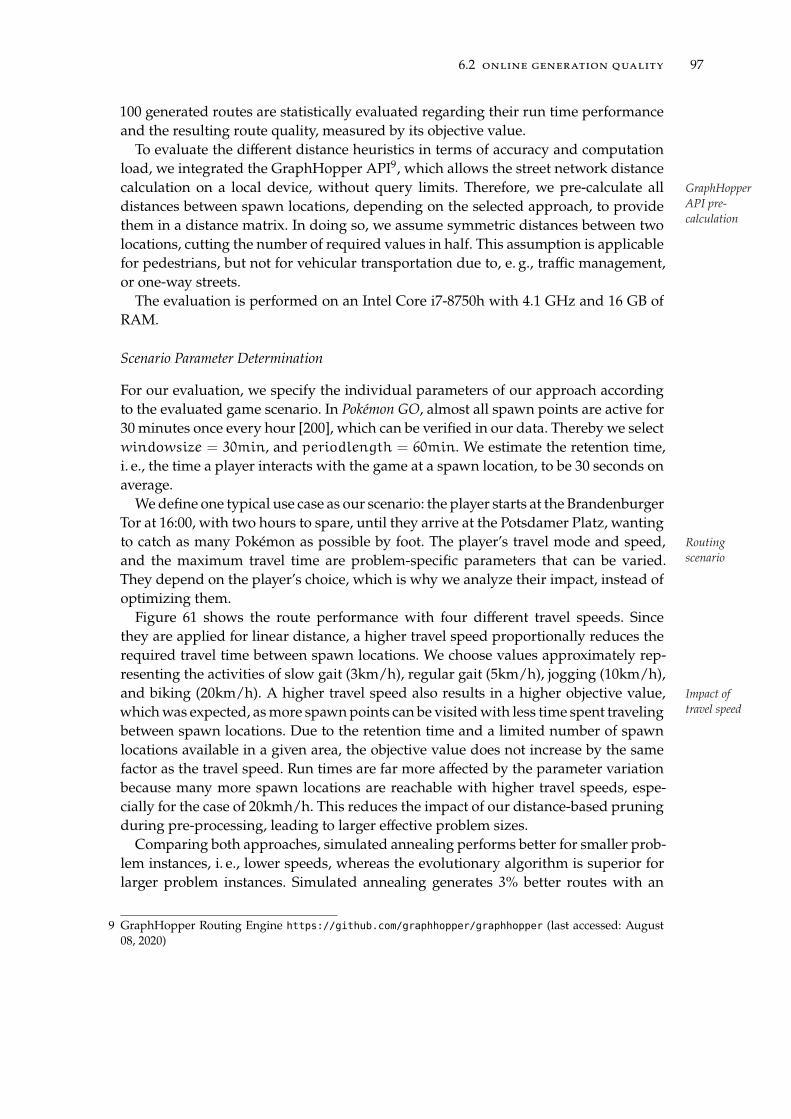
6.2 online generation quality 97

100 generated routes are statistically evaluated regarding their run time performance

and the resulting route quality, measured by its objective value.

To evaluate the different distance heuristics in terms of accuracy and computation

load, we integrated the GraphHopper API9, which allows the street network distance

calculation on a local device, without query limits. Therefore, we pre-calculate all GraphHopperAPI pre-calculation

distances between spawn locations, depending on the selected approach, to provide

them in a distance matrix. In doing so, we assume symmetric distances between two

locations, cutting the number of required values in half. This assumption is applicable

for pedestrians, but not for vehicular transportation due to, e. g., traffic management,

or one-way streets.

The evaluation is performed on an Intel Core i7-8750h with 4.1 GHz and 16 GB of

RAM.

Scenario Parameter Determination

For our evaluation, we specify the individual parameters of our approach according

to the evaluated game scenario. In Pokémon GO, almost all spawn points are active for

30 minutes once every hour [200], which can be verified in our data. Thereby we select

windowsize = 30min, and periodlength = 60min. We estimate the retention time,

i. e., the time a player interacts with the game at a spawn location, to be 30 seconds on

average.

Wedefine one typical use case as our scenario: the player starts at the Brandenburger

Tor at 16:00, with two hours to spare, until they arrive at the Potsdamer Platz, wanting

to catch as many Pokémon as possible by foot. The player’s travel mode and speed, Routingscenario

and the maximum travel time are problem-specific parameters that can be varied.

They depend on the player’s choice, which is why we analyze their impact, instead of

optimizing them.

Figure 61 shows the route performance with four different travel speeds. Since

they are applied for linear distance, a higher travel speed proportionally reduces the

required travel time between spawn locations. We choose values approximately rep-

resenting the activities of slow gait (3km/h), regular gait (5km/h), jogging (10km/h),

and biking (20km/h). A higher travel speed also results in a higher objective value, Impact oftravel speed

whichwas expected, asmore spawnpoints can be visitedwith less time spent traveling

between spawn locations. Due to the retention time and a limited number of spawn

locations available in a given area, the objective value does not increase by the same

factor as the travel speed. Run times are far more affected by the parameter variation

because many more spawn locations are reachable with higher travel speeds, espe-

cially for the case of 20kmh/h. This reduces the impact of our distance-based pruning

during pre-processing, leading to larger effective problem sizes.

Comparing both approaches, simulated annealing performs better for smaller prob-

lem instances, i. e., lower speeds, whereas the evolutionary algorithm is superior for

larger problem instances. Simulated annealing generates 3% better routes with an

9 GraphHopper Routing Engine https://github.com/graphhopper/graphhopper (last accessed: August

08, 2020)

98 evaluation

equal median run time for the case of 3km/h. By contrast, the evolutionary algorithm

achieves 21% better results in 18% less median time for the case of 20km/h, indicating

a better scalability.

Figure 62 shows the route performance with four different maximum travel times.

Again as expected, routes with more time at their disposal achieve higher objective

values. However, the increase in objective value is not linearly proportional to the

increase in time. Between route durations of 30 and 60 minutes, the median objectiveImpact ofmaximumtravel time

value increases by 130%, indicating that clustered spawn points with low travel times

are reached on the route. For two hours, the increase is only 60%, compared to the

100% increase in available time.We observe another increase of only 49% for four hour

routes.

The analyzed data suggests that generated routes with small travel times are likely

closer to the optimal route than larger ones. Additionally, the behavior, again, shows

the impact of larger problem sizes due to their effect on our distance-based pruning.

Therefore, routes should either be limited in maximum travel time, or stronger heuris-

tics need be employed, filtering out more spawn locations that are unlikely to be in

an optimized route. A fitting alternative here is our suggested subroute approach,

splitting the route generation into shorter, more optimized, subroutes.

Comparing both algorithms, the findings reinforce our previous observation that

simulated annealing works slightly better for small problem instances, while the evo-

lutionary algorithm scales better. For large problem instances, the evolutionary algo-

rithm also takes less computation time.

Our pre-processing approach, especially including a distance-based pruning, aims

to significantly decrease the problem instance size. For our default scenario, a decrease

in relevant spawn points by 77% to 7,375 can be achieved, not yet including any

distance heuristics like clustering. The impact of our value-based pruning heavilyPre-processing

impactdepends on the selection of the specific Pokémon. In our tests, even looking for the

most commonPokémon led to a spawnpoint decrease by 99%, indicating that targeting

one individual Pokémon might not be worthwhile in the evaluation scenario, due to

the random spawn behavior.

Heuristic Parameter Determination

We will now compare the different heuristic parameters to determine an optimized

parameter value in our scenario. The algorithmic parameters dependonour evaluation

scenario and especially the problem size, which might not be optimal in a different

scenario. First, we will evaluate the respective impact of our four distance calculation

heuristics.

In Figure 32, we compare the accuracy of our proposed distance calculation ap-

proaches. The goal here was to reduce the number of required routing calculations,

by either utilizing the spawn locations’ geographic relation to the street network or

a proximity-based clustering. We show the absolute and proportionate error the ap-Distanceheuristic

comparisonmethodology

proach introduces, compared to the actual routing information, i. e., the shortest direct

route between two locations. Because routing information is particularly important for

close spawn locations, we confine the analysis to distances within our grid cells. While

6.2 online generation quality 99

Figure 32: Different heuristic distance approaches with their absolute and percentage error

compared to the true route between locations.

distances between far apart points are also relevant, the introduced error becomes

more evident when comparing close spawn locations. Additionally, in an optimized

route, it is far more likely that nearby active spawn points are visited in succession.

The Crossing to Crossing approach resulted in 18,081 relevant locations, which is

a reduction to 56.24% of the original locations. However, on average, its routes were

58.8s longer than the real shortest route between the actual locations, with a median

increase of 20.4s and a high standard deviation of 88.7s. This corresponds to, on Distanceheuristic:Clustering

average, 35.14% longer routes. We can observe many strong outliers, which is because

this heuristic requires going to a location’s closest crossing first, which can be a major

detour in the wrong direction.

The Street to Street approach resulted in 23,860 relevant locations (74.22%). On

average, its routes were 25.2s longer than the real shortest routes with amedian of 4.0sand still a high standard deviation of 60.7s, which corresponds to, on average, 23.7%longer routes.

The clustering approach, with a radius of 40m, resulted in 6,430 clusters containing

21,123 spawn points, leading to 17,455 relevant locations (54.30%). Its routes are, on

average, 0.2s shorter than the real shortest route, with amedian of 0s. Thismedianwas

expected, as it represents the distance calculation for two spawn locations that have

not been clustered, leading to an accurate distance value. The clustering approach

also has a low standard deviation of 7.2s, corresponding to, on average, 0.7% shorter

routes. Thereby the clustering heuristic is superior in both spawn location reduction

and accuracy.

We calculate the proposed average detour factor for all spawn points, indicating

how much longer the real route between two spawn locations is compared to its

linear distance. We select the median value instead of the arithmetic mean, as we

observe strong individual outliers, especially for some close-by spawn points that

are nevertheless accessed from different streets. The resulting distance factor is 1.18, Travel speed =4.24km/h

leading to an optimized median linear travel speed of5km/h1.18 ≈ 4.24km/h for the

dataset and road network of Berlin. This signals that the Manhattan distance would

be an overestimation of a detour factor, which would have been5km/h√

2≈ 3.54km/h.

100 evaluation

RandomSA RandomEA HeuristicSA HeuristicEA

Neighborhood Approach0

200

400

600

800

1000

1200

1400Ru

ntim

e (m

s)

Simulated AnnealingEvolutionary Algorithm

RandomSA RandomEA HeuristicSA HeuristicEA

Neighborhood Approach0

10

20

30

40

50

60

70

80

Obje

ctiv

e Va

lue

Simulated AnnealingEvolutionary Algorithm

Figure 33: Route performance comparison between the utilization of a random neighborhood

function and our heuristic neighborhood function.

Figure 33 shows the performance difference when using either our random neigh-

borhood function or the developed heuristic neighborhood function, forwhichwewill

treat the random neighborhood approach as a baseline. Simulated annealing, here has

the largest gain increasing its objective value by a factor of 2.9. The evolutionary al-Heuristicneighborhood

functiongorithm also has a notable objective value gain, with both approaches reaching an

identical median objective value of 54.3. In terms of run time, the simulated annealing

profits from a significant decrease in run time variance. The evolutionary algorithm

increases its run time variance, leading us to assume that the heuristic neighborhood

grid could still be optimized to achieve high-quality outcomes consistently. The me-

dian run time values are equivalently increased for both algorithms. For the simulated

annealing, we observemedian run times longer by a factor of 2.9 and longer by a factor

of 2.7 for the evolutionary algorithm, respectively. Since the heuristic neighborhood

allows for vastly superior route results, we deem this trade-off acceptable and further

utilize this approach.

Within our algorithm evaluation, provided in detail in Section A.4.1, we assess the

effect of different algorithm-specific parameters on generated route quality and perfor-

mance. Both algorithms are viable when applying them to the problem but performAlgorithm-specific

parametersdifferently depending on the given problem size. We select our default parameters

based on the trade-off between route quality and required run time in our scenario.

A clear better algorithm cannot be determined, as both showed overall comparative

results, with weaknesses in individual scenarios.

For our distance matrix, we evaluated whether linearizing the matrix has an advan-

tage in terms of computation time compared to a two-dimensional array. Because both

approaches performed similarly well, we did not investigate any other storage opti-

mization approaches. Linearizing the matrix has the primary advantage to utilized

the distance symmetry more efficiently, thus saving memory.

Based on our collected data, in most scenarios, the simulated annealing approach

achieves marginally better median results for smaller problem instances, and slightly

6.2 online generation quality 101

LinSA LinEA RouSA RouEA

Optimization Algorithm0

200

400

600

800

1000

1200

1400Ru

ntim

e (m

s)Simulated AnnealingEvolutionary Algorithm

LinSA val LinEA val RouSA val RouEA valOptimization Algorithm

0

10

20

30

40

50

60

70

Obje

ctiv

e Va

lue

Simulated AnnealingEvolutionary Algorithm

Figure 34: Route generation results and their validation, for our evaluation scenario with the

determined default parameters. Linear routes (Lin) are validated based on our

cluster distance matrix, while distance matrix-based routes (Rou) are validated

using a full GraphHopper route.

worse median results for larger problem instances. One notable factor is the con-

sistently higher variance in objective value of the evolutionary algorithm approach,

which can lead to the preference of simulated annealing for its generation consistency.

For simulated annealing, we observe that the number of restarts seems to significantly

decrease its variance in objective value. Its slight scalability issues could be approached

by employing stricter pre-processing filtering to keep the problem size in dimensions

where the approach still performs well.

Route Quality Verification

After determining our default parameter set, we evaluate the approach’s performance

within ourdefined scenario. Since all approaches utilize some sort of heuristic tomodel

the required travel time between two spawn locations, we employ two validation

methods. After a successful route generation, the resulting route gets verified, either

by using the heuristic distance matrix, which is only applicable for generated routes

based on the linear distance or by utilizing it into a GraphHopper API call. For the Routevalidationmethods

latter approach, we expect routes, generated with our distance matrix to become

invalid since the clustering radius, i. e., the interaction radius, is not utilized, leading

to differing travel times. Since it is possible for a route to reach a spawn point before

an active spawn window, small waiting times can be included in each route. Within

our evaluation, we experimented with different wait time approaches for validation,

allowing routes to wait at a spawn point for a maximum fixed time or to wait an

additional amount of time on top of the time scheduled by the route initially. However,

no promising findings were achieved here, with the best approach having no artificial

waiting time alterations.

In our validation process, we observed many routes, becoming slightly longer, lead-

ing to reduced objective values. To allow for a better comparison between generated

102 evaluation

30mLinSA

30mLinEA

30mRouSA

30mRouEA

1hLinSA

1hLinEA

1hRouSA

1hRouEA

Round Course Maximum Travel Time (min)

0

200

400

600

800

1000

1200Ru

ntim

e (m

s)

Simulated AnnealingEvolutionary Algorithm

30mLinSA

v 30mLinEA

v 30mRouSA

30mRouEA

1hLinSA

v 1hLinEA

v 1hRouSA

1hRouEA

Round Course Maximum Travel Time (min)

0

10

20

30

40

50

60

Obje

ctiv

e Va

lue

Simulated AnnealingEvolutionary Algorithm

Figure 35: Modification of our evaluation scenario, simulating a round course for the

duration of 30 minutes and 1 hour. Validated route results are marked with v.

and validated routes, we adjusted the validated routes, to match the maximum time

constraint. Finding and removing those spawn points responsible for the longest de-Cutting rearspawn pointsto adhere to

timeconstraints

tours while still adhering to the subsequent active spawn windows, is a separate

optimization problem. We instead decided to remove the last spawn locations on the

route until the target location can be reached in time, since removing later spawn loca-

tions does not influence earlier ones. The route results with their respective validation

approach are shown in Figure 34.

The results show consistent median objective values between 48 and 51, indicat-

ing that the included detour factor for linear distance calculation results appropriately

compensates for detours. Investigating the validation results shows that the full Graph-

Hopper route validation leads toworse objective value resultswith high variance. ThisRoutevalidation

effectis explained by the employed wait time methodology. Since the route is generated us-

ing thedistancematrix basedon clustered spawn locations, short detours are inevitable

when trying to verify the route visiting each spawn location instead of only its cluster

location. These detours add up until a spawn point has just become inactive when

arriving, leading to an extensive wait time until it becomes active again about 30 min-

utes later. Judging from the median and variance in objective value, this occasionally

affects routes, with most routes being close to the generated ones.

A different application scenario we want to investigate is the route generation for

a round course, i. e., start and target location being the same. The results, shown

in Figure 35, display an interesting behavior compared to our basic scenario. LinearRound coursescenario

distance routes, those validated using our distance matrix, and distance matrix routes

are close in median objective value. The variance in objective value does not increase

to the same extent as our basic scenario, with an outlier rate between 10% and 15%.

Since a threshold-based approach can easily detect an outlier, another route can be

calculated instead.

Similar to our results regarding maximum travel time, in Figure 62, the increase

in objective value is not linearly proportional to the gain in time. Beneath possible

6.2 online generation quality 103

AnyLinSA

AnyLinEA

AnyRouSA

AnyRouEA

#016LinSA

#016LinEA

#016RouSA

#016RouEA

#129LinSA

#129LinEA

#129RouSA

#129RouEA

Sought-after Pokémon

0

250

500

750

1000

1250

1500

1750

2000

Runt

ime

(ms)

Simulated AnnealingEvolutionary Algorithm

AnyLinSA

AnyLinEA

AnyRouSA

AnyRouEA

#016LinSA

#016LinEA

#016RouSA

#016RouEA

#129LinSA

#129LinEA

#129RouSA

#129RouEA

Sought-after Pokémon

0

10

20

30

40

50

60

70

Obje

ctiv

e Va

lue

Simulated AnnealingEvolutionary Algorithm

Figure 36: Route performance for routes when focusing on either every spawn point (Any),

Pidgey (#016), or Magicarp (#129), showing the routes objective value, which does

by no means equate the number of visited spawn points.

scalability issues, the lack of available spawn points could be another reason for this. No linearlyproportionalincrease

Since the player returns to the starting location, individual spawn points on the way

back may have already been visited when no perfect round course is generated.

A reduction of retention time to model experienced players and a variation of

different start times is examined in Section A.4.2. Regarding the employed algorithm,

no additional findings could be deduced. The reduction in retention time led to an

expected increase in objective value, with no major side effects. Varying the start time Modeling ofexperiencedplayers

showed that round courses starting at hh:45, i. e., any desired time 45 minutes into

an hour, seems to be worse than starts at other quarter-hourly times. This is likely to

be caused by the spawn points’ time-limited availability, leading to worse routes, and

shows that a start time analysis for optimized routes can be advantageous.

In Figure 36, we show the route performance when looking for specific Pokémon,

compared with aiming to catch as many Pokémon of arbitrary species as possible, Sought-afterPokémon

i. e., visiting the most spawn points. We look for the particularly common Pokémon

Pidgey (#016), and the water Pokémon Magikarp (#129), whose spawn frequency is

influenced by the vicinity of water bodies.

As expected, we see a substantial decrease in objective value when looking for

specific Pokémon because a spawn point’s value is now resembled by its probability

to spawn the respective sought-after Pokémon. Thereby, scores vary for each spawn Impact ofvalue-basedpruning

location. Additionally, it leads to large numbers of spawn locations being filtered out

during pre-processing, because, according to the dataset, they are unlikely to spawn

the given Pokémon. Due to the random spawn mechanics, the spawned Pokémon

cannot be anticipated, but only predicted based on historical data, always assuming

that spawn mechanics remain unchanged.

For both evaluated Pokémon, we achieve a comparable average objective value, with

simulated annealing routes being very consistent, while the evolutionary algorithm

introduces much more variance, with a higher run time. Since the objective value

depends on the sum of spawn probabilities of each visited spawn point, the objective

104 evaluation

AnyLinSA

AnyLinEA

AnyRouSA

AnyRouEA

#016LinSA

#016LinEA

#016RouSA

#016RouEA

#129LinSA

#129LinEA

#129RouSA

#129RouEA

Sought-after Pokémon

0

10

20

30

40

50

60

70

Num

ber o

f Loc

atio

ns o

n Ro

ute

Simulated AnnealingEvolutionary Algorithm

Figure 37: Number of visited spawn points on the route evaluated in Figure 36.

value results are self-explanatory. In Figure 37, the number of locations on each routeConsistentresults forsimulatedannealing

is shown, which is comparatively close to a default scenario route. The difference for

Magikarp (#129) routes is noticeable, where simulated annealing appears to perform

significantly better for this reduce problem size,withmostly tightly clustered locations

along water bodies.

In an additional evaluation of the rarer Pokémon Bulbasaur (#001), an interesting

phenomenon couldbeobserved.Dependingon themaximumtravel time, the resulting

objective value was either close to zero or well above that. A game mechanic called

nests is responsible for this, where most spawn locations within a park have a high

chance of spawning one specific Pokémon. This changes for each park and on a bi-Looking for arare Pokémon

speciesweeklybasis

10. The resulting route identifiedadistancedBulbasaurnest, traveled there,

passed by its spawn points repeatedly, and returned to the target location, ignoring

almost all spawn locations on its way. This is an expected and realistic behavior for

players looking for a Pokémon with a nearby active nest.

6.3 mobility detection quality

To evaluate our automatic mobility detection, we acquired a dataset utilizing our mo-

bile application recordingmobility data of study participants, described in Section 5.2.

For our data acquisition, 43 participants were asked to record data on their personal

Android smartphones. This led to 65.8 hours of raw data collected in multiple Euro-

pean countries with a cluster point in the Rhine-Main area. The raw data distribution

across the mobility types is not uniformly distributed as participants were asked to

record their daily travels11. Data was collected in urban, suburban, and rural areas, asCollected data

well as during transit between locations, and covers a variety of different situations

such as traffic jams and heavy rush-hours. The smartphone position was not specified

for the recording. It was worn at the body, in a bag, a backpack, smartphone holder in

10 https://thesilphroad.com/atlas (last accessed: August 17, 2020)

11 Recorded data in total: 11.8h stand, 18.5h walk, 4.9h bike, 17.6h car, 5.0h bus, 2.4h tram, and 5.6h train

6.3 mobility detection quality 105

cars, or on bikes. Neither of those locations was compulsory, allowing users to change

their smartphone’s position during travel freely.

All participants were asked to record sessions of at least 10 minutes of length so that

we can investigate our system’s performance over time if it turns out to require a cold

starting phase until prediction quality converges. Thereby we excluded all recordings

shorter than 10 minutes from the dataset. Not all the recorded data was used for Training datasplit

training, as specific datasets were reserved for testing purposes only so that our final

model could be tested with yet unknown data. For the training, we used recordings

of 38.6 hours of data by 23 participants12.

In ourmulti-class classification problem,we use twoprimary qualitymeasurements.

For each examinedmodel, we calculate itsmacro-averaged prediction accuracy, which,

compared to the micro-averaging approach, weights all classes equally [246]. Each

class’s performance is reported using the F1 measure.We select the balanced F-score as

wehavenoparticular emphasis onprecision13or recall

14, as it calculates their harmonic

mean.When recall would require a higher emphasis, the F2 measure would be chosen, Employedqualitymetrics

and conversely, the F0.5 measure for a higher focus on precision. All evaluation runs

use a stratified 10-fold cross-validation15, which provides a similar class distribution

for each fold, as present in the dataset. Finally, an automatic feature selection for

all three frame classifiers is employed to determine all relevant features and their

respective information gain. The data itself is oversampled beforehand to construct a

balanced dataset. Both individual class precision and recall values and evaluation run

confusion matrices were obtained and are provided when relevant.

The evaluation is performed on an Intel Xeon E5-2660 v3 with 2.60GHz and 32 GB

of RAM. Weka is adjusted to use num-decimal-places = 8 as it strongly increases indi-

vidual feature accuracies, compared to its default value 2.

6.3.1 Default Parameter Determination

Simulation Setup

To evaluate the meta-classifier’s performance and the overall system, the recorded

activities are simulated and inserted into our classification system. For this simulation

the recordings are processed in steps of TC = stepSize = 5s. As noted in Table 4.2.4,

we choose a stepSize equal to the time interval TC, after which a classification update

is expected. For each step, the respective frames of the length short, medium and long, Simulationsetup

and their associated features are determined and classified. Finally, the meta-classifier

determines the final prediction and is compared to the actual data label. We choose

a transitionDuration = 2s, representing the transition delay after a change in mo-

bility type. Thereby, we expect the system to predict the previous activity during the

transition period since we assumed that the new activity cannot yet be detected.

12 Training data in total: 5.7h stand, 7.7h walk, 3.9h bike, 11.3h car, 4.9h bus, 1.9h tram, and 3.2h train

13 Precision is the ratio between true positives and the sum of all positives.

14 Recall is the ratio between true positives and the sum of true positives and false negatives.

15 The k-fold cross-validation separates data into k folds and, in each case, trains on k− 1 folds and tests

on the remaining one.

106 evaluation

The shiftmax parameter is relevant to create the frame classifiers during training,

determining the overlap each frame has. Selecting this value is twofold. It concerns the

frame classifiers’ overlap, which is vital for sliding window approaches. Additionally,shiftmax =

5sthe resulting number of frame instances needs to be observed, as a too narrow overlap

can strongly boost computation requirements to infeasible levels. We decide to use

shiftmax = 5s, as it provides us with pre-processing times between one and two

hours, which allowed us to gradually improve on parameter values and later on

analyze further parameter combinations.

For the other introduced parameters, good default valuesmust be determined for an

optimizedmobility type distinguishment. To determine one parameter, we vary one at

a time while keeping all other parameters constant. Subsequently, we select the valueDefaultparameter

determinationmethodology

for which the meta-classifier obtains its maximum accuracy. In earlier experimental

evaluation runs, we narrowed each parameter down to promising value ranges, for

which we now determine its final value. After an optimized parameter has been

determined, it is used in succession.

Since random forests have proven to be promising approaches in related work and

our early evaluation runs, we use it for default parameter determination for both theEarlyalgorithm

usageframe classifiers and the meta-classifier

16. For similar reasons, we use genetic search for

automatic feature selection. Since the number of meta-features is low, we do not use

an automatic feature selection for the meta-classifier.

The frame length variation is especially challenging since different combinations

can have different effects on the overall system. For this reason, we first define all

other parameters by using two parameter setups: We perform an evaluation withEarly framelength

methodologysmall frame lengths for medium and long (TM = 20s and TL = 90s) and one with longer

frames (TM = 30s and TL = 300s), as we assume that different features are more

relevant for different frame lengths, to better assess the effects of parameter selection.

Since affected parameters mainly influence features of the medium and long frames, we

use a fixed length for the short frame of TS = 5s.

Parameter Determination

The S2 level, i. e., the area size for which OSM information is obtained for feature

calculation, is utilized in medium and long frames. However, the S2 level choice hadS2 level = 14no substantial impact on the overall system accuracy, which is why we selected the

smaller level of 14, as less data needs to be obtained and processed. A detailed S2 level

evaluation can be found in Table 27.

The cutoffDistance serves as a threshold, from which point on public transport

routes further away are not considered. The variation of this parameter, however,

had little impact. For the shorter frame setup, a 600m threshold was sufficient, whilecutoffDistance= 800m

for longer frames, 800m showed an improvement. For that reason, we choose to use

cutoffDistance = 800m, with a more detailed evaluation shown in Table 28.

Stop-based features are only calculated for long frames. The maximum stop speed

serves as an upper threshold value, below which a segment is treated as halting.maxStopSpeed= 0.5m/s

16 hyperparameters: 20 iterations; at least 2 instances per leaf; maximum depth of 20

6.3 mobility detection quality 107

The evaluation for the two different scenarios shows small effects of the choice of

maxStopSpeed on the overall system accuracy. Based on the results shown in Table 29,

we select a value of 0.5m/s as it achieved the best results for both scenarios.

The stop radius indicates up towhich range nearby PoIs are considered.When a low

value is chosen, relevant PoIs might be ignored due to the location inaccuracies. When stopRadius =20m

the radius is set too large, stations not relevant for the stop can be included. In Table 30,

we provide detailed results for this parameter, in which we select stopRadius = 20m.

The minimum duration for a long stop helps to identify meaningful stops instead of

stops causedbydense trafficand stop-and-go. Similar to theprevious radiusparameter,

the variation had no significant impact when varying between 6s, 8s, 10s, and 15s. For stopDuration-LongStop =8s

the shorter frame scenario, a stopDurationLongStop of 8s performed best, while for the

longer frame lengths, a value of 15s achieved the best results, although the differences

within the two setups weremarginal (6 0.1%). Since the shorter frame lengths seem to

be more accurate than the longer frame lengths, we choose minDurationLongStop = 8s.

Interval Lengths

After selecting the individual parameter, a preliminary evaluation showed that Adap-

tiveBoostingwith a J48 classifier17performed significantly better for themeta-classifier

than the previous random forest. For that reason, we use this algorithm for frame

length determination, with frame classifier algorithms remaining as previously de-

fined.

We again decide on the optimized parameter based on the meta-classifiers perfor-

mance. Alternatively, the performance of the individual frame classifier could have

been used. However, this would only locally optimize the frame classifier, which we

deemed problematic in individual evaluation runs, where the overall system accuracy

declined when optimizing individual frame performance. Even though all frames are

calculated independently from another, the choice of frame length influences the oth-

ers because the overall system accuracy is a deciding factor. For that reason, we start

with the long frames since we expect them to be more independent from the other two

frames. Subsequently, we determine the short length and, finally, the medium frames,

as the latter serves as a connection between both other frame lengths.

As shown in Table 10, the highest accuracy of the meta-classifier is achieved at

90s. Especially car and bus benefit from a this longer frame length compared to 60s. long framelength = 90s

Although the frame classifier’s accuracy increases for higher frame lengths, the meta-

classifier does not increase simultaneously. We therefore choose TL = 90s.

A similar pattern can be observed for the short frames, as shown in Table 11. While

the frame classifier’s accuracy increases with an increased frame length, the meta- short framelength = 5s

classifier’s accuracy reaches its maximum at TS = 5s and decreases rapidly with

longer frame length. One possible reason would be the detection of temporary stops

becoming worse for longer short frames. Since the results for TS = 4s and TS = 5s are

17 hyperparameters: AdaBoostM1 with 20 iterations; J48 with at least 2 instances per leaf; pruning confi-

dence c = 0.25

108 evaluation

Table 10: Evaluation results for long interval length TL highlighting the selected parameter

value. Parameters: TS = 5s, TM = 20s, s2Level = 14, cutoffDistance = 800m,

maxStopSpeed = 0.5 m/s, stopRadius = 20m, and minDurationLongStop = 8s.

TLaccuracy F1 scores of meta-classifier

meta long stand walk bike car bus tram train

60s 98.37% 99.49% 97.0% 99.5% 99.2% 97.4% 97.5% 99.2% 98.8%

90s 98.48% 99.71% 97.0% 99.5% 99.3% 97.8% 98.0% 99.1% 98.7%

120s 98.45% 99.80% 96.8% 99.4% 99.2% 97.6% 97.9% 99.2% 98.9%

150s 98.44% 99.93% 96.8% 99.5% 98.9% 97.8% 98.0% 99.3% 98.8%

similar, we will consider both frame lengths for medium frame length determination in

the next step.

Table 11: Evaluation results for short interval length TS highlighting the selected parameter

value. Parameters: TM = 20s, TL = 90s, with remaining parameters identical to

Table 10.

TSaccuracy F1 scores of meta-classifier

meta short stand walk bike car bus tram train

3s 98.38% 96.84% 97.2% 99.5% 99.2% 97.6% 97.8% 99.0% 98.3%

4s 98.44% 97.27% 96.9% 99.6% 99.2% 97.6% 98.0% 99.1% 98.7%

5s 98.48% 97.26% 97.0% 99.5% 99.3% 97.8% 98.0% 99.1% 98.7%

6s 96.83% 97.36% 93.9% 98.9% 98.7% 96.2% 95.8% 97.7% 96.6%

Based on the results in Table 12, we can identify a short frame length of TS = 5s

performing better in each scenario. For the medium frame length, the meta-classifiermediumframe length

= 15sreaches its best result for TM = 15s, which is why we select it accordingly.

Algorithms and Feature Selection

Todetermine suitable searchmethods for feature selection,weuse anAdaBoostM1 [76]

with J48 and a Random Forest, selecting the smallest possible feature set with good

detection accuracies. We use the correlation-based feature selection (CfsSubsetEval

in Weka) as an evaluator and define the Random Forest baseline as a full run with

all available features. We expect this baseline to have comparable accuracy to theEmployedfeature

selectionapproach

selection strategies. Our goal is to reduce the number of features required to identify

particularly important features for a mobility type’s detection. For AdaBoostM1, we

do not calculate a baseline because AdaBoost’s training times are already slower by a

factor of 10 to 20 with a reduced number of features.We show the summarized feature

selection results in Table 13, with a more detailed one in Tables 31-33.

6.3 mobility detection quality 109

Table 12: Evaluation results for medium interval length TM highlighting the selected

parameter value. Parameters: TS, and TL defined in Table and remaining parameters

identical to Table 10.

TMaccuracy F1 scores of meta-classifier

meta medium stand walk bike car bus tram train

TS = 4s, TL = 90s

10s 98.39% 98.25% 97.0% 99.6% 99.2% 97.3% 97.7% 99.2% 98.7%

15s 98.48% 98.73% 96.9% 99.5% 99.3% 97.7% 98.1% 99.1% 98.7%

20s 98.44% 99.02% 96.9% 99.6% 99.2% 97.6% 98.0% 99.1% 98.7%

25s 98.35% 99.13% 96.8% 99.6% 99.3% 97.3% 97.8% 99.0% 98.6%

TS = 5s, TL = 90s

10s 98.52% 98.25% 97.2% 99.4% 99.3% 97.8% 97.9% 99.2% 98.9%

15s 98.55% 98.73% 97.2% 99.5% 99.2% 97.8% 98.1% 99.1% 98.9%

20s 98.48% 99.02% 97.0% 99.5% 99.3% 97.8% 98.0% 99.1% 98.7%

25s 99.41% 99.13% 96.9% 99.4% 99.3% 97.6% 97.9% 99.3% 98.6%

The Best First feature selection always results in the fewest selected features, leading

to shorter training times. When analyzing the individual F1 scores, we identified the Best First formedium andlong

differentiation between bus and car being influenced the most by the feature selection.

For both medium and long frames, a Best First selection was the most suitable, as it

required far fewer features with an only slightly worse macro-averaged accuracy. This

leads to a considerable decrease in training time by a factor of three compared to the

baseline allowing for faster iteration during development.

For the short frames, the Genetic Search achieves the best results, requiring only

seven more features. We deliberately omitted delta features for the short classifier GeneticSearch forshort

to react faster to short-term activity changes without being influenced by the previ-

ous frame. A brief evaluation confirms that approach, where although delta features’

inclusion minimally increases the frame classifier’s accuracy, the meta-classifier’s ac-

curacy decreases. For this reason, we retain the exclusion of delta features for the short

frames.

We test five classification algorithms for the frame classifiers, three based on singular

decision trees: J48, REP-Tree, RandomTree, and two ensemble learners: RandomForest

andAdaBoostM1with J48. For each ensemble learning algorithm,we vary the number Algorithmselectionmethodology

of iterations I. We specify both the required training time per fold on our system and

the resulting classifier’s size.

With the detailed results presented in Tables 34-36, we can conclude that ensemble

learners perform significantly better compared to individual decision trees. Especially

the distinction between motorized transport types improves. For the short classifier,

18 hyperparameters: 30 iterations; at least 2 instances per leaf; maximum depth of 30

110 evaluation

Table 13: Evaluation results for feature selection in short, medium, and long frame classifiers,

indicating selected feature counts and frame classifier accuracies. Detailed results

containing individual F1 scores can be found in Tables 31-33.

feature

selection

short medium long

feature

count

accuracy

feature

count

accuracy

feature

count

accuracy

Random Forest with I = 30 18

Baseline 65 97.60% 136 98.77% 180 99.79%

Evolutionary Search 32 97.43% 65 98.83% 84 99.76%

Genetic Search 32 97.59% 48 98.62% 53 99.67%

Best First 25 97.53% 29 98.77% 29 99.73%

AdaBoostM1 with I = 15 and J48

Genetic Search 32 97.66% 48 98.89% 53 99.76%

Best First 25 97.55% 29 98.89% 29 99.81%

the algorithmchoice leads to an improvement inmacro-averagedaccuracy from92.98%

(REP tree) to 97.84% (AdaBoostM1 with J48 with 25 iterations). The differences areAdaBoostM1for frameclassifiers

especially prominent for bus, where the F1 score improves from86.6% to 95.5%. Similar

trends can be observed for medium and long frames. Comparing both ensemble learners,

Adaptive Boosting reaches a higher overall accuracy with the same number of trees,

which are two to three times smaller due to J48’s integrated pruning. Then again,

the required training time is significantly longer compared to equally parametrized

Random Forests. Since the training is only performed once on a server, we choose to

use AdaBoostM1 and select the minimum iteration counts that achieve the highest

accuracy. This is 35 iterations for medium and 30 iterations for long. For the short frame,

we select a lower-than-optimal number of 15 iterations to allow for accelerated training

time and a smaller classifier size.

For the feature selection of the meta-features, the same three search methods were

examined, where each result selected the same five features19, resulting in lower accu-

racies. To identify the least important features, we utilized a feature ranking based onMeta-classifierfeature

selection

each feature’s information gain for its class. The featurewith the least information gain

prevScoreS resulted in no accuracy change and thereby appeared not to be required.

However, we intend to analyze the impact of different feature types next, for which

the removal may impact the feature selection options. For that reason, and because

using all meta-features has no negative impact on the system’s performance, we will

use all meta-features for our classifier.

The selection of a suitable classifier for the frame classifiers has shown that the best

results could be achieved using AdaBoost. We, therefore, use an AdaBoostM1 withMeta-classifieralgorithm

J48 for the meta classifier as well. The best results were achieved with 20 maximum

19 predS, predM, predL, prevPredM, scoreS

6.3 mobility detection quality 111

iterations, where increasing the number of iterations further did not lead to higher

accuracies.

6.3.2 Feature Set Importance

In the following, we examine the influence of different feature sets on the system, in

which we want to identify those feature sets that are essential for the system or, if

possible, identify dispensable components. In Table 14, we present a detailed analysis

of the different sets that can be freely combined for each group. The δ indicator

behaves slightly differently, as it corresponds to the inclusion of delta features for

all utilized features. Each result provided uses the previously determined parameters,

feature selection settings, and algorithm parameterizations in a stratified 10-fold cross-

validation.

Table 14: Different feature sets that can be freely combined.

feature set description

A Features based on the accelerometer in the time-domain.

AF Features based on the accelerometer in both time- and frequency-domain.

L Features based on the location sensor.

LE Features based on the location sensors and additional external information.

δ For each feature in the feature set an additional delta feature is used.

Relevance of delta features

The delta features introduced in Section 4.3.4 are used for medium and long frames

aim to represent the chronological sequence of feature changes. However, results in Negative δfeature effect

Figure 38 show that, in direct comparison, feature sets without delta features perform

equally at best, with the only exception being the LE feature set, i. e., the one without

any acceleration data features.

Going into detail onto changes per movement type, shown in detail in Table 37. For

the example of car, we can observe an interesting tendency comparing AL, ALE, and

LE with and without delta features. By adding external information (ALE, LE), there

is an accuracy gain provided by delta features, whereas the acceleration delta features

alone seem to have a negative effect (A, AF, AL↔ LE) on car classification. A similar

pattern can be observed for bus classification.

Relevance of frequency-domain features

Features based on the frequency spectrum of the accelerometer have been rarely

utilized in relatedwork. Looking at our results, it is noticeable that indirect comparison

these features always contribute to a notable detection improvement: ALE ↔ AFLE

112 evaluation

Figure 38: Meta-classifier macro-averaged accuracy with select combinations of feature sets,

showing the accuracies without delta features. The secondary value represents the

loss or gain in accuracy when including delta features in the respective feature set.

(+0.50%),AL↔ AFL (+0.52%),A↔ AF (+0.92%). Especially the detection of cars andPerformanceincrease

attributed tofrequency-

domainfeatures

buses benefits from the features of the frequency domain, which have been reported to

be particularly challenging in related work. In case location features are missing, the

train detection is also increased by adding the frequency features: A↔ AF (+1.6%).

When analyzing the selected featureswhen frequency-domain features are included,

we observe features based on frequency bands achieving a high information gain.Selectedfrequency-

domainfeatures

Thereby the whole frequency spectrum up to 30 Hz appears to be relevant. One possi-

ble explanation we found is the vibration of combustion engines in vehicles is covered

by a broad frequency spectrum, e. g., 1,800 rounds per minute corresponding to 30

Hz. Additionally notable is that all frames select the features spectral roll-off, spectral

crest, and spectral spread. For the short frame, the spectral skewness is selected. For

the feature set without location features AF, the normalized spectral energy and the

spectral centroid are selected. Thus, all frequency-domain features except the spectral

spread have been utilized.

Relevance of location features

In the related work, location-based features have been frequently used, providedPerformanceincrease

attributed tolocationfeatures

that these approaches rarely combined them with many acceleration-based features.

Whendirectly comparing feature sets including location features,we notice a detection

improvement: AF ↔ AFL (+1.25%), A↔ AL (+0.90%).

According to our results, standing classification benefits the most from location

features, which is likely to be due to features based on speed and distance traveled.

6.3 mobility detection quality 113

Car, bus, and train confusion also improves, whichwe suspect to be due to heading and Improvedconfusion ofmotorizedmobility

location accuracy features. The latter is especially prominent for metal-coated train

windows, which lead to high location accuracy values, i. e., values indicating that a

high location variance is expected. For the location accuracy in AL, the accu95 feature

is selected for short, and the feature accu25 is selected for medium.

Relevance of external information features

Our results are consistent with the findings of Stenneth et al. [229], who showed that

the addition of external geo-referenced information could improve transport mode

detection for location-based systems. When directly comparing features sets with Small externalinformationfeaturesimprovement

external information, we notice only small detection improvements: AFL ↔ AFLE(+0.04%), AL ↔ ALE (+0.06%), L ↔ LE (+0.21%). Thus, when accelerometer-based

features are already utilized, the gain in detection quality is minimal.

It is possible that a model is more valid in general when including external features. Possiblelimitation:local vibrationpatterns

However, we do not know to what extent public transport vehicles in the recorded

datasets have specific vibration patterns and whether they differ from other transport

vehicles in other regions. In this case, a model that supports detection via uniformly

available, external information from OSM could be more generalizable.

In Figure 39, we show an example from our dataset where information about public

transport routes is beneficial.While the classifierwithout any route information results Exemplaryimpact ofpublictransportstationdistance

in a false tram classification, the external feature provides the information that there

is no tram station or tram line nearby, increasing the confidence for bus detection. Incontrast, the addition of public transport routes can also lead to a false prediction, e. g.,

where the proximity to a bus station while passing in a tram might lead to a false busprediction.

When analyzing the selected features when external information features are in-

cluded, we observe that the same four features are always selected: distanceTram, Selectedexternalinformationfeatures

distanceTrain, stopsBusStop and stopsTramStop. For the model without acceleration

data LE, the additional feature of stopsExclTramStop is selected.

(a) Activity without external information (AFL). (b) Activity with external information (AFLE).

Figure 39: Individual activity comparison without and with external information.

114 evaluation

6.3.3 Frame Classifier Importance

To analyze the difference between using the meta concept as a whole and individ-

ual frames, we trained a meta-classifier solely based on one frame classifier feature

(predS, predM, predL). As shown in Table 15, each feature’s accuracy is drastically lower

than the overall accuracy with all meta-features. Among the simple classifiers, the

classifier predM performed best, likely because it can still detect short stops fairly well

and contains relevant location features to distinguish different motorized mobility

types. Since the feature predL does not receive information about temporary stops, it

performs worse in the standing scenario. This factor becomes particularly clear in its

recall value of 45.1% and in conjunction with the vehicles’ precision values. The predM

precision values, especially for tram and train, show the successful training on the

special characteristics of public transport, despite its duration of only TM = 15s. The

contribution of predL, on the other hand, can be seen from its recall values, where it

identifies motorized mobility types particularly well.

Combining these two frames can compensate for each other’s worse precision for

some mobility types and allow the short classifier’s high recall to work for detecting

standing andwalking. Thus, the meta concept combines the advantages of short frames

with those of long frames.

Table 15: Evaluation results of frame classifiers prediction features for AFLE including

precision and recall due to its variation. Precision and recall values are listed in

brackets in that order.

feature

sets

accuracy F1 scores of meta-classifier + (precision, recall)

overall stand walk bike car bus tram train

Meta 98.91% 97.7% 99.6% 99.4% 98.3% 98.5% 99.5% 99.3%

(98.9%,

98.9%)

(97.8%,

97.7%)

(99.7%,

99.5%)

(99.2%,

99.6%)

(98.6%,

98.0%)

(98.6%,

98.4%)

(99.2%,

99.7%)

(99.1%,

99.5%)

predS 91.67% 92.6% 99.6% 97.1% 87.3% 86.1% 87.7% 91.5%

(91.8%,

91.7%)

(89.4%,

96.1%)

(99.2%,

99.2%)

(97.6%,

96.6%)

(83.1%,

92.0%)

(88.5%,

86.1%)

(93.6%,

82.4%)

(91.5%,

91.5%)

predM 93.43% 83.7% 98.9% 97.8% 94.0% 90.5% 93.0% 96.1%

(93.5%,

93.4%)

(82.2%,

85.3%)

(98.6%,

99.3%)

(98.3%,

97.4%)

(93.6%,

94.5%)

(89.8%,

91.3%)

(97.2%,

89.2%)

(95.1%,

97.0%)

predL 90.99% 61.7% 97.8% 98.1% 91.9% 88.8% 95.5% 94.9%

(91.8%,

91.0%)

(97.7%,

45.1%)

(96.2%,

99.5%)

(96.2%,

100%)

(85.7%,

99.0%)

(81.9%,

97.0%)

(92.1%,

99.1%)

(92.7%,

97.2%)

To analyze the importance of each frame in detail, we trained meta-classifiers with

a subset of meta-features. Each subset is grouped by frame classifier length and either

contains one, two, e. g., short and long, or all three groups of meta-classifier features.

6.3 mobility detection quality 115

As shown in Table 16, a system based solely on the long frame would have a

significant loss in accuracy compared to our final system. Especially the detection

quality of standing, and to a degree, car and bus decreases and would have a long

initialization time of 0.9 · TL = 81s. The analysis shows only a marginal difference Frameclassifierimportance

between systems based solely on short or medium frames, with the former performing

slightly better. For the medium frame, especially the differentiation between car and busimproves. Similarly, the accuracy for the other two public transport modes improves,

likely due to the external information features being included in this frame classifier.

Classifiers based on two different frames performed best when including the short

frame, reinforcing its importance for our system. The highest accuracy can only be

achieved by combining all three frame lengths. Especially vehicular mobility types Reliableaccuracy forsystem coldstart

profit from the combination of all three frame lengths with a net gain of at least 0.3%accuracy. The overall high accuracy values show that the system does not inevitably

require the longest frames but can accurately predict the current mobility type early

on while the system is in a cold starting phase.

Table 16: Evaluation results of frame classifiers combinations.

frame

combination

accuracy F1 scores of meta-classifier

overall stand walk bike car bus tram train

short, medium &

long

98.91% 97.7% 99.6% 99.4% 98.3% 98.5% 99.5% 99.3%

short & long 98.63% 97.5% 99.6% 99.1% 97.8% 98.2% 99.2% 99.0%

short & medium 98.60% 97.4% 99.7% 99.2% 97.6% 97.9% 99.4% 99.0%

medium & long 97.97% 94.4% 99.4% 99.2% 97.3% 97.1% 99.3% 99.1%

short 97.57% 97.4% 99.4% 99.0% 95.3% 95.2% 98.2% 98.5%

medium 97.47% 94.1% 99.4% 99.0% 96.4% 96.4% 98.4% 98.7%

long 94.51% 80.3% 98.3% 98.6% 94.3% 94.4% 97.4% 97.1%

6.3.4 Final Model and Comparison to Related Work

The individual F1 scores of our final AFLE model, the confusion matrix, and the

selected features with their information gain are shown in Tables 37-40. Since all Final accuracyof 98.9%

classes are weighted equally, the results are macro-averaged. We achieve a macro-

averaged accuracy of 98.9% on a 10-fold cross-validation for the feature sets of AFLEandAFL, i. e., with and without external features, both excluding delta features. If the

standing class is neglected, the macro-averaged accuracy increases to 99.1%.

Analyzing the AFLE model in detail shows that the lowest accuracy is achieved for

standing. Although standing is fundamentally the easiest to identify, the reason for this

result lies within the transitions to a temporary stand, which make up a large portion

of our data used for the class. On the one hand, these transitions are difficult to detect

116 evaluation

accurately, differing between intentional stops or stop-and-go. On the other hand, theTemporarystandinganalysis

detection is influenced by the quality of our manual labeling. Since these were set

after data recording utilizing acceleration and velocity data, inaccuracies and errors

are likely. Especially since there is a delay between the acceleration and velocity data,

it makes accurate transition labeling more difficult. This can also be observed in the

confusion matrix.

For vehicular transportation, we can detect bus and car with a macro-F1 score of

98.3% and 98.5%, respectively. Tram and train detection works best with a score of

99.5% and 99.3%, respectively. For the confusion matrix, it is noticeable that cars andbikes are confused for one another, which mostly occurs during start-up. One possibleVehicular

mobilityconfusion

explanation for this is the frequent use of e-bikeswithin our training data, which allow

for strong acceleration, and may contain frequency-domain signals on the motor. This

mightmake the distinction between cars and bikesmore difficult. One observation from

related work is the frequent confusion of buses and cars, which we can still confirm for

our data. Another observed confusion is buses being confused for trams. We deem the

distinction between these two types of transport as particularly challenging since, in

our recorded data, buses often travel on roads with integrated tram tracks.

The developed model is rotation invariant since only the acceleration magnitude is

used. Additionally, no personalized data is utilized, and data originates from different

subjects reducing the possible impact of different walking styles. Since we use a shortFinalemployed

featurecharacteristics

length of TS = 5s, the system’s first prediction is obtainable 5 seconds after its

activation. Since only OSM features and no detailed timetables are used, external

information is globally available, if tagged accordingly. Then again, themodel without

any additional external information has been verified to be of equal quality for our

data, allowing us to neglect missing OSM data.

Finally, we have tested our final model’s live detection on a smartphone to ensure

its functionality on a mobile device itself. The resulting models take up an acceptableRun-timemobilitydetection

amount of storage (AFLE : 8.7MB,AFL : 9.1MB), which depends on the number of

employed features and their names’ length. Compared to the reported models in

related work, our model is considerably smaller than 150MB and suitable for mobile

applications.

Table 17: Google Activity Recognition API mapping to mobility type and resulting detection

accuracy.

class Google API accuracy Unknown

stand Still 52% 25%

walk On Foot 87% 12%

bike On Bicycle 31% 45%

car In Vehicle 85% 13%

bus In Vehicle 36% 58%

tram In Vehicle 34% 58%

train In Vehicle 43% 26%

6.3 mobility detection quality 117

We want to compare our final model to existing solutions and related works re-

garding detection accuracy in the following. With the Google Activity Recognition

API [164], Google provides a way to recognize activities without differentiating be-

tweendifferentmotorizedmeans of transport.We recorded theAPI’s predicted activity Comparisonto GoogleActivityRecognitionAPI

for 12.7 hours of our dataset and expect the most similar mobility type to our label as

a prediction result. In Table 17, we show this mapping and the respective prediction

accuracies. It is noticeable that the API often returns Unknown, especially frequent for

bikes, buses, and trams. The best results are achieved forwalkingwith 87% accuracy and

carwith 85% accuracy.

A similar evaluation has been reported in 2018 [35], which stated that the API

only predicted 3% of all cases, which does not hold true anymore, as either the API

itself or its embedding into the Android framework, has been drastically improved. Google APIimprovement

For our data, the API achieves a macro-averaged accuracy of 53%, which is largely

comparable with other earlier studies [274]. We suspect the still large proportion of

Unknown predictions being due to its wide range of users and likely focus on producing

too many false positive predictions.

Table 18: Comparison of our models with results of Stenneth et al. [229] including feature

selection and Aşçı and Güvensan [13]. The F1 scores are calculated from the

authors’ reported precision and recall values. The macro-averaged accuracies are

determined only for the compared classes and thereby differ from our other reports.

model

accuracy

F1 scores

walk bike car bus tram train

Stenneth et al. [229] 90.70% 98.4% 89.2% 81.2% 90.4% - 94.3%

our LE model 97.63% 98.9% 98.6% 95.5% 96.9% 99.4% 98.3%

our LEδmodel 97.92% 99.0% 98.9% 96.1% 97.1% 99.4% 98.5%

Aşçı and Güven-

san [13]

96.45% 97.0% 96.9% 97.1% 94.7% - 96.6%

our AF model 98.09% 99.4% 99.1% 97.6% 97.1% 98.7% 97.2%

Although a direct comparison with related studies is not feasible because the

datasets have not been published in most cases, an accuracy-based comparison per

mobility type is possible. For our comparison, we use the two works with the high- Related workcomparisonmethodology

est reported macro-averaged accuracy from related works, excluding standing, sinceit usually is not reported how temporary stops are handled. Our goal with this is

not to compare the quality of the final model by numbers but to evaluate our meta-

classification concept, so we choose the feature set closest to the work in question.

Stenneth et al. [229] uses a purely location-based approach, including external geo-

graphic information about the public transport network. It should be noted that the Comparison ofLE and LEδ toStenneth et al.

authors used real-time information about the positions of buses, which we cannot

provide. Because they do not use the accelerometer, we decide to use both our LEand LEδmodels for comparison, shown in Table 18. We can significantly increase the

118 evaluation

detection quality of bike, car, bus, and train through our meta-concept. Additionally,

the direct distinction between car and bus works well for our model, where Stenneth

et al. has a strong bias towards bus detection. We deduce that real-time information

on bus positions is unnecessary for our model to detect buseswith high accuracy.

Aşçı and Güvensan [13] use an orientation-dependent model based on the ac-

celerometer, gyroscope, and magnetometer in both time- and frequency-domain in

a recurrent neural network. Since we only use the accelerometer, a comparison withComparison ofAF to Aşçı

and Güvensanour AF model is evident, which is orientation invariant. As shown in the results in

Table 18, their accuracy for cars is slightly higher than ours, whereas we detect busesbetter. Overall, these results suggest that the gyroscope and magnetometer are not re-

quired for mobility detection, and an orientation-invariant model performs similarly

well.

7SUMMARY, CONCLUS IONS , AND OUTLOOK

Concluding our work, we summarize the previous chapters’ content and state our

main contributions in the following. We then draw conclusions based on our

obtained results and discuss potential future work.

7.1 summary of the thesis

In Chapter 1, we described the challenges for an online content generation system

applicable to Location-based Game (LBG) applications. We motivated the advantages

of online generation based on the customizability and personalization of content

towards each individual player. In Chapter 2, we studied existing content creation

approaches regarding their applicability for global content location identification. As

a possible strategy for mobility-based adaptation, we analyzed heuristic route-finding

and automaticmobility detection approaches utilized in different application domains.

Based on our analysis of the state of the art, we presented the following contributions

in our thesis.

7.1.1 Contributions

Chapter 3 contains our first two contributions, focusing on the online content gen-

eration for LBGs. As the first contribution, we propose a globally applicable content

generation with scenario-specific customization options to i) identify and retrieve

promising Points of Interest (PoIs) data for a given region, ii) select a number of PoIs

according to four quality metrics to construct a game area, and iii) couple multiple

game areas based on their available PoIs. The latter option enables the utilization Globalcontentgeneration

of multiplayer gameplay across regions despite the players’ different geographic lo-

cations, aiming for game areas with similar geographical and cultural characteristics.

Furthermore, our approach considers the generation of multiple coupled game areas,

resulting in regularly new game areas providing additional variety for the underlying

game. To determine a suitable selection of PoIs, we solved an optimization problem,

utilizing heuristic approaches, applicable to an online generation scenario.

In Section 3.4, we develop our second contribution, which covers the location-

dependent determination of routes in a city-wide game area, obtaining a route op-

timizing the expected virtual reward during gameplay. Due to the large number and Personalizedrouteoptimization

time-dependent variety of available content locations, we develop a heuristic route-

finding approach to provide personalized mobility guidance for LBG players, aiming

to optimize their gameplay according to their preferences.

In our third contribution, found in Chapter 4, we propose our concept of automatic

mobility detection. Therein, we include the impact of acceleration and location-based

119

120 summary, conclusions, and outlook

mobile device sensor data to extract features allowing the differentiation between

common types of mobility like walking or biking. Furthermore, we provide a detailedRun-timemobilitydetection

differentiation between different vehicularmodes of transportation, particularly focus-

ing on different public transport vehicles. Our concept includes features of different

temporal lengths, specifically designed to detect everyday traffic situations like station

or traffic light stops.

The resultingmobility detection is directly applicable formobility-based adaptation

in LBGs, allowing for a versatile adaptation during run-time. For our previous two

contributions, suitable adaptation options are as follows: game area content and size

can be selected based on accessibility and expected time to reach. Similarly, routes can

be planned, monitored, and adapted according to the given mobility type.

Further, we developed our GeoVis system, described in Chapter 5, as the basis for

our extensive evaluation. For this purpose, we constructed an evaluation scenario and

compared our results to the current state of the art in Chapter 6.

7.1.2 Conclusions

In our extensive evaluation, we analyzed the effects of online location generation for

a mobile game system. We showed that our approach enables the utilization of LBG

content generation nationwide, optimizing the content selection concerning geograph-

ical and cultural quality characteristics. Its selection is freely adaptable for different

application scenarios, providing a flexible foundation for game area generation. For

its basic configuration, we could verify well-distributed game areas, containing cul-

turally relevant PoIs, with viable results even in rural areas. By coupling those gameGoodgeneration

results in allareas

areas together, we subsequently proved the applicability for an innovativemultiplayer

approach. Our proposed coupling approach achieves noteworthy generation results

for our employed metrics and constructs comprehensive PoI matchings, even across

continents. With flexible game area sizes and multi-area matching, we evaluated our

approach’s adaptability to players with different movement conditions and its scala-

bility beyond a two-player setting.

Moreover, we showed the validity of route finding for virtual game reward optimiza-

tion in an LBG. In a game areawith thousands of valid PoIs, where it is yet infeasible to

calculate an optimal solution, we applied heuristic approaches to reliably obtain high-

quality routes. Since linear distances in an urban scenario are infeasible for accurate

measurements, our proposed distance heuristics successfully utilize a clustering to re-

duce the problem size drastically. By verifying those routes using a routing service, weRoute-findingvalidity

prove its suitability in the real-world environment. Our resulting route-finding strat-

egy successfully utilizes the spatial density of locations to find customizable routes

during gameplay. For those, we evaluated different common scenario parameters such

as route duration, target location, movement behavior, and game objective as a generic

way for LBG route customization.

Lastly, we showed the strong performance of our proposed automatic mobility

detection concept for mobile adaptation purposes. By utilizing a combination of dif-

ferent time windows, meaningful features for different movement and vehicle types

7.2 outlook 121

have been identified and integrated into a classification pipeline. Our evaluation re-

sults demonstrated strong classification accuracies for all examined mobility types. Mobilityintegration

The proposed meta-classification approach reached an overall 98.9% accuracy, em-

phasizing the successful combination of time windows with different lengths. We

investigated the different effects of varying sensor sources and feature sets, which

allows for area-specific detection approaches in scenarios where different mobility

distinctions are necessary, or where sensor quality varies.

7.2 outlook

Our presented results motivate the evaluation of location-based applications in differ-

ent scenarioswhere specificPoIs are required. It is particularly intriguing to investigate

long-termmotivational effects in extensive cohort studies, based on the systematic uti-

lization for, e. g., game-based health or culture promotion. Such applications would Studylong-termmotivationaleffects

not only require an interdisciplinary team for realization. They would potentially

also require new content assessment approaches [99] to generate other aspects than

the map layout [109], further utilizing the PoI data for location-specific information

processing.

The presented personalization approaches build the foundation for further research

in the area of mobility-based adaptation. While we proposed them for the application Routing withshiftinglocationproperties

of LBGs, each contribution is applicable in its respective area. Applying our routing

approach to, e. g., (data) delivery services [161], is expected to enable more efficient

delivery schemes for dynamically shifting location properties. Regarding our mobil-

ity detection, we focused on the differentiation of vehicular transportation. A more

human-centered activity or exercise detection, highlighting more precise movement

and adapting accordingly, is an exciting research topic in the Internet of Things and

the quantified-self area [41]. For that purpose, a detailed motion recording is required, Human-centeredexercisedetection

favoring the utilization ofmultiple sensors for fine-granularmotion differentiation [37,

257]. Thus, LBG content can be individually connected with exercises for movement

and health promotion.

Our contributions to the development and systematic evaluation of online content

generation in mobile game applications and its generalization and customization in

the GeoVis platform fuel new and further research questions in the aforementioned

directions.

acknowledgments

The research described in this thesis was co-funded by the LOEWE initiative (Hessen,

Germany) within the IDG “Infrakstruktur - Design - Gesellschaft” project.

B IBL IOGRAPHY

[1] Emile Aarts, Jan Korst, and Wil Michiels. “Simulated Annealing.” In: SearchMethodologies. Ed. by EdmundKBurke andGrahamKendall. Boston,MA,USA:

Springer, 2014. Chap. 10, pp. 265–285. doi: 10.1007/978-1-4614-6940-7_10.

[2] Paula Alavesa, Minna Pakanen, Hannu Kukka, Matti Pouke, and Timo Ojala.

“Anarchy or Order on the Streets: Review Based Characterization of Location

Based Mobile Games.” In: Proc. Annual Symposium on Computer-Human Interac-tion in Play. 2017, pp. 101–113. doi: 10.1145/3116595.3116614.

[3] Jonathan B Allen. “Short Term Spectral Analysis, Synthesis, and Modification

by Discrete Fourier Transform.” In: IEEE Transactions on Acoustics, Speech, andSignal Processing 25.3 (1977), pp. 235–238.

[4] NoorAlmaadeed,MuhammadAsim, SomayaAl-Maadeed,AhmedBouridane,

and Azeddine Beghdadi. “Automatic Detection and Classification of Audio

Events for Road Surveillance Applications.” In: Sensors 18.6 (2018), pp. 1858–

1875. doi: 10.3390/s18061858.

[5] Tim Althoff, Ryen W. White, and Eric Horvitz. “Influence of Pokémon Go

on Physical Activity: Study and Implications.” In: Journal of Medical InternetResearch 18.12 (2016), pp. 1–10. doi: 10.2196/jmir.6759.

[6] Eduardo Álvarez-Miranda, Martin Luipersbeck, and Markus Sinnl. “Gotta (ef-

ficiently) catch them all: Pokémon GOmeets Orienteering Problems.” In: Euro-pean Journal of Operational Research 265.2 (2018), pp. 779–794.

[7] RobAnastasi, Nick Tandavanitj,Martin Flintham,AndyCrabtree,Matt Adams,

Ju Row-Farr, Jamie Iddon, Steve Benford, Terry Hemmings, Shahram Izadi,

and Ian Taylor. “Can You See Me Now? A Citywide Mixed-Reality Gaming

Experience.” In: Proc. 4th Conference on Ubiquitous Computing (UbiComp). 2002,pp. 1–18.

[8] Ian Anderson and Henk Muller. “Practical Activity Recognition using GSM

Data.” In: Proc. 5th International Semantic Web Conference (ISWC). Springer. 2006,pp. 1–8.

[9] Enrico Angelelli, Claudia Archetti, and Michele Vindigni. “The Clustered Ori-

enteering Problem.” In: European Journal of Operational Research 238.2 (2014),

pp. 404–414.

[10] DavidLApplegate, Robert EBixby,VasekChvatal, andWilliam JCook, eds.TheTraveling Salesman Problem: A Computational Study. Princeton, NJ, USA: Prince-

ton University Press, 2006.

123

124 bibliography

[11] Anna Arigliano, Gianpaolo Ghiani, Antonio Grieco, Emanuela Guerriero, and

Isaac Plana. “Time-dependent asymmetric traveling salesman problem with

time windows: Properties and an exact algorithm.” In: Discrete Applied Mathe-matics 261 (2019), pp. 28–39. doi: 10.1016/j.dam.2018.09.017.

[12] Norbert Ascheuer, Matteo Fischetti, and Martin Grötschel. “Solving the Asym-

metric Travelling SalesmanProblemwith timewindowsbybranch-and-cut.” In:

Mathematical Programming90.3 (2001), pp. 475–506.doi:10.1007/s101070100218.

[13] GüvenAşçı andMAmaçGüvensan. “ANovel Input Set for LSTM-based Trans-

port Mode Detection.” In: Proc. 2019 IEEE International Conference on Perva-sive Computing and Communications Workshops (PerCom Workshops). IEEE. 2019,pp. 107–112.

[14] JohnWAyers, Eric CLeas,MarkDredze, Jon-PatrickAllem, JurekGGrabowski,

and Linda Hill. “Pokémon GO – A New Distraction for Drivers and Pedestri-

ans.” In: JAMA Internal Medicine 176.12 (2016), pp. 1865–1866. doi: 10.1001/

jamainternmed.2016.6274.

[15] Sarwat Y Azeem. The promotional potential of Pokemon Go. Available: https://aurora.dawn.com/news/1141509. [Accessed Jul. 31, 2020]. July 2016.

[16] Trevor C Bailey and Anthony C Gatrell, eds. Interactive Spatial Data Analysis.Longman Scientific & Technical, 1995.

[17] Edward K Baker. “An exact algorithm for the time-constrained traveling sales-

man problem.” In: Operations Research 31.5 (1983), pp. 938–945. doi: 10.1287/

opre.31.5.938.

[18] Rafael A Ballagas, Sven G Kratz, Jan Borchers, Eugen Yu, Steffen P Walz, Clau-

dia O Fuhr, Ludger Hovestadt, and Martin Tann. “REXplorer: a mobile, per-

vasive spell-casting game for tourists.” In: Proc. Conference on Human Factors inComputing Systems (CHI). 2007, pp. 1929–1934.

[19] PouyaBaniasadi,VladimirEjov,MichaelHaythorpe, andSergueiRossomakhine.

“A new benchmark set for Traveling salesman problem and Hamiltonian cycle

problem.” In: 2018, pp. 1–21. arXiv: 1806.09285.

[20] GabriellaABBarros. “DataGames: TowardsGeneratingContent using theReal

World.” In:Proc. of Doctoral Symposium of the 9th International and InterdisciplinaryConference on Modeling and Using Context (CONTEXT 2015). 2015, pp. 15–22.

[21] Michael Bartoň, Iddo Hanniel, Gershon Elber, and Myung-Soo Kim. “Precise

Hausdorff Distance Computation between Polygonal Meshes.” In: ComputerAided Geometric Design 27.8 (2010), pp. 580–591.

[22] Steve Benford, Andy Crabtree, Martin Flintham, Adam Drozd, Rob Anastasi,

Mark Paxton, Nick Tandavanitj, Matt Adams, and Ju Row-Farr. “Can You See

Me Now?” In: ACM Transactions on Computer-Human Interaction 13.1 (2006),

pp. 100–133.

bibliography 125

[23] Arpita Bhattacharya, TravisWWindleharth, RioAnthony Ishii, IvyMAcevedo,

Cecilia R Aragon, Julie A Kientz, Jason C Yip, and Jin H Lee. “Group Interac-

tions in Location-Based Gaming: A Case Study of Raiding in Pokémon GO.”

In: Proc. Conference on Human Factors in Computing Systems (CHI). 2019, pp. 1–12.doi: 10.1145/3290605.3300817.

[24] Jacopo Biancat, Chiara Brighenti, and Attilio Brighenti. “Review of Transporta-

tion Mode Detection techniques.” In: EAI Endorsed Transactions on AmbientSystems 1.4 (2014), pp. 1–10. doi: 10.4108/amsys.1.4.e7.

[25] Leo I Bluestein. “A Linear Filtering Approach to the Computation of the Dis-

crete Fourier Transform.” In: IEEE Transactions on Audio and Electroacoustics 18.4(1970), pp. 451–455. doi: 10.1109/TAU.1970.1162132.

[26] Boehringer Ingelheim Accelerator Program. Obesity Game – Lands of Bhur. un-published. 2018.

[27] Adel Bolbol and Tao Cheng. “GPSData Collection Setting For Pedestrian Activ-

ity Modelling.” In: Proc. Geographical Information Science Research UK Conference2010 (GISRUK). 2010, pp. 1–8.

[28] Adel Bolbol, Tao Cheng, Ioannis Tsapakis, and James Haworth. “Inferring

hybrid transportation modes from sparse GPS data using a moving window

SVM classification.” In: Computers, Environment and Urban Systems 36.6 (2012),

pp. 526–537. doi: 10.1016/j.compenvurbsys.2012.06.001.

[29] Stephen Boyd. “Multitone Signals with LowCrest Factor.” In: IEEE Transactionson Circuits and Systems 33.10 (1986), pp. 1018–1022.

[30] Thomas Brinkhoff. City Population. Available: https://www.citypopulation.de. [Accessed Jul. 03, 2020]. 2020.

[31] Maria A Brovelli and Giorgio Zamboni. “ANewMethod for the Assessment of

Spatial Accuracy and Completeness of OpenStreetMap Building Footprints.”

In: International Journal of Geo-Information 7.8 (2018), pp. 289–314. doi: 10.3390/

ijgi7080289.

[32] RichardBrunauer,MichaelHufnagl, Karl Rehrl, andAndreasWagner. “Motion

Pattern Analysis Enabling Accurate Travel Mode Detection from GPS Data

Only.” In: Proc. 16th International IEEE Conference on Intelligent TransportationSystems (ITSC 2013). IEEE. 2013, pp. 404–411.

[33] Bundesinstitut für Bau-, Stadt- und Raumforschung. Raumabgrenzungen undRaumtypen des BBSR. Available: https : / / www . bbsr . bund . de / BBSR / DE /veroeffentlichungen/analysen-bau-stadt-raum/ausgaben/Bd06.html. [Ac-

cessed Sep. 29, 2020]. 2012.

[34] Luc Burnier, Matteo Lanini, Olivia Bouvard, Damiano Scanferla, Abiraam

Varathan, Carine Genoud, Arnaud Marguerit, Bernard Cuttat, Noémie Dury,

Reiner Witte, Andrea Salvadè, and Andreas Schüler. “Energy saving glaz-

ing with a wide band-pass FSS allowing mobile communication: up-scaling

and characterisation.” In: IET Microwaves, Antennas & Propagation 11.10 (2017),

pp. 1449–1455. doi: 10.1049/iet-map.2016.0685.

126 bibliography

[35] Claudia Carpineti, Vincenzo Lomonaco, Luca Bedogni, Marco Di Felice, and

LucianoBononi. “CustomDual TransportationModeDetection by Smartphone

Devices Exploiting Sensor Diversity.” In: Proc. IEEE International Conference onPervasive Computing and Communications Workshops (PerCom Workshops). 2018,pp. 367–372.

[36] AnaMCCarraca. “Procedural ContentGeneration for Location-basedGames.”

PhD thesis. Porto, PT: University of Porto, 2014.

[37] PolonaCaserman, AugustoGarcia-Agundez, Robert Konrad, StefanGöbel, and

Ralf Steinmetz. “Real-time body tracking in virtual reality using aVive tracker.”

In: Virtual Reality 23.2 (2019), pp. 155–168. doi: 10.1007/s10055-018-0374-z.

[38] Irene Celino, Dario Cerizza, Simone Contessa, Marta Corubolo, Daniele Dell’-

Aglio, Emanuele Della Valle, and Stefano Fumeo. “Urbanopoly – a Social and

Location-based Game with a Purpose to Crowdsource your Urban Data.” In:

Proc. International Conference on Privacy, Security, Risk and Trust and InternationalConference on Social Computing. 2012, pp. 910–913.

[39] Robert Cervero and Kara Kockelman. “Travel demand and the 3Ds: Density, di-

versity, and design.” In: Transportation research. Part D, Transport and environment2.3 (1997), pp. 199–219.

[40] StephanieChan.GlobalAppRevenueReached $50Billion in the FirstHalf of 2020,Up23% Year-Over-Year. Available: https://sensortower.com/blog/app-revenue-and-downloads-1h-2020. [Accessed August. 28, 2020]. June 2020.

[41] Eun KChoe, Nicole B Lee, Bongshin Lee,Wanda Pratt, and Julie AKientz. “Un-

derstanding Quantified-Selfers’ Practices in Collecting and Exploring Personal

Data.” In: Proc. Conference on Human Factors in Computing Systems (CHI). 2014,pp. 1143–1152. doi: 10.1145/2556288.2557372.

[42] Yvette Chong, Dean Krishen Sethi, Charmaine Hui Yun Loh, and Fatimah

Lateef. “Going Forward with Pokemon Go.” In: Journal of Emergencies, Trauma,and Shock 11.4 (2018), pp. 243–246. doi: 10.4103/JETS.JETS_87_17.

[43] Philip J Clark and Francis C Evans. “Distance toNearest Neighbor as aMeasure

of Spatial Relationships in Populations.” In: Ecology 35.4 (1954), pp. 445–453.

[44] Kester D Clegg, Julian F Miller, Kieran Massey, and Mike Petty. “Travelling

Salesman Problem Solved ’in materio’ by Evolved Carbon Nanotube Device.”

In: Proc. International Conference on Parallel Problem Solving from Nature. 2014,pp. 692–701.

[45] AshleyColley, Jacob Thebault-Spieker, AllenYLin,DonaldDegraen, Benjamin

Fischman, Jonna Häkkilä, Kate Kuehl, Valentina Nisi, Nuno J Nunes, Nina

Wenig, Dirk Wenig, Brent Hecht, and Johannes Schöning. “The Geography of

Pokémon GO: Beneficial and Problematic Effects on Places andMovement.” In:

Proc. Conference on Human Factors in Computing Systems (CHI). 2017, pp. 1179–1192. doi: 10.1145/3025453.3025495.

bibliography 127

[46] Gérard Cornuéjols, Jean Fonlupt, and Denis Naddef. “The Travelling Salesman

Problem on a Graph and some Related Integer Polyhedra.” In: MathematicalProgramming 33.1 (1985), pp. 1–27.

[47] Vlad C Coroamă, Can Türk, and Friedemann Mattern. “Poster: Exploring the

Usefulness of Bluetooth andWiFi Proximity for Transportation Mode Recogni-

tion.” In:Proc. 2019ACMInternational Joint Conference onPervasive andUbiquitousComputing and the 2019 International Symposium onWearable Computers (UbiCom-p/ISWC 19 Adjunct). ACM. 2019, pp. 37–40. doi: 10.1145/3341162.3343847.

[48] Emanoel Costa. “Simulation of the Effects of Different Urban Environments on

GPS Performance Using Digital ElevationModels and Building Databases.” In:

IEEE Transactions on Intelligent Transportation Systems 12.3 (2011), pp. 819–829.

doi: 10.1109/TITS.2011.2122258.

[49] Victor Cotton and Mitesh S Patel. “Gamification use and design in popular

health and fitness mobile applications.” In:American Journal of Health Promotion33.3 (2019), pp. 448–451. doi: 10.1177/0890117118790394.

[50] George B Dantzig and John H Ramser. “The truck dispatching problem.” In:

Management Science 6.1 (1959), pp. 80–91.

[51] Anind K Dey. “Understanding and Using Context.” In: Personal and UbiquitousComputing 5.1 (2001), pp. 4–7.

[52] Marco Dorigo and Luca M Gambardella. “Ant-Q: A Reinforcement Learning

approach to the traveling salesman problem.” In: Proc. 12th International Confer-ence on Machine Learning (ICML). 1995, pp. 252–260.

[53] Marco Dorigo and Thomas Stützle. “Ant Colony Optimization: Overview and

Recent Advances.” In: Handbook of Metaheuristics. Ed. by Michel Gendreau and

Jean-Yves Potvin. Vol. 272. Cham, CH: Springer, 2019, pp. 311–351. doi: 10.

1007/978-3-319-91086-4_10.

[54] Draconius GO: Catch a Dragon! Elyland LLC. Android, iOS. 2017.

[55] Alok Dutt and Vladimir Rokhlin. “Fast Fourier Transforms for Nonequispaced

Data.” In: SIAM Journal on Scientific Computing 14.6 (1993), pp. 1368–1393.

[56] Alok Dutt and Vladimir Rokhlin. “Fast Fourier Transforms for Nonequispaced

Data, II.” In: Applied and Computational Harmonic Analysis 2.1 (1995), pp. 85–100.

[57] Tim Dutz. “Pervasive Behavior Interventions - Using Mobile Devices for Over-

coming Barriers for Physical Activity.” PhD thesis. Darmstadt, DE: Technische

Universität Darmstadt, 2017.

[58] TimDutz, SandroHardy,MartinKnöll, StefanGöbel, andRalf Steinmetz. “User

Interfaces of Mobile Exergames.” In: Proc. International Conference on Human-Computer Interaction. 2014, pp. 244–255.

[59] George S Easton and Robert E McCulloch. “A Multivariate Generalization of

Quantile-Quantile Plots.” In: Journal of the American Statistical Association 85.410

(1990), pp. 376–386.

128 bibliography

[60] Stefan Edelkamp, Max Gath, Tristan Cazenave, and Fabien Teytaud. “Algo-

rithm and knowledge engineering for the TSPTW problem.” In: Proc. IEEESymposium on Computational Intelligence in Scheduling (SCIS). 2013, pp. 44–51.doi: 10.1109/SCIS.2013.6613251.

[61] Hamid R Eftekhari and Mehdi Ghatee. “An inference engine for smartphones

to preprocess data and detect stationary and transportation modes.” In: Trans-portation Research Part C: Emerging Technologies 69 (2016), pp. 313–327. doi:

10.1016/j.trc.2016.06.005.

[62] Gunnar Eisenberg, ed. Identifikation und Klassifikation von Musikinstrumenten-klängen in monophoner und polyphoner Musik. Göttingen, DE: Cuvillier Verlag,

2008.

[63] Ericsson. Ericsson Mobility Report June 2020. Available: https://www.ericsson.com/en/mobility-report/reports/june-2020. [Accessed August. 28, 2020].

June 2020.

[64] Darrel Etherington. Pokémon GO is officially teaming with Starbucks for 7,800new Gyms and PokéStops. Available: https://techcrunch.com/2016/12/08/pokemon-go-is-officially-teaming-with-starbucks-for-7800-new-gyms-

and-pokestops/. [Accessed Jul. 31, 2020]. Dec. 2016.

[65] European Commission, Joint Research Centre. Atlas of the Human Planet 2018.Tech. rep. Publications Office of the European Union, Dec. 2018. doi: 10.2760/

124503.

[66] Reid Ewing and Robert Cervero. “Travel and the built environment: a meta-

analysis.” In: Journal of the American planning association 76.3 (2010), pp. 265–294.

doi: 10.1080/01944361003766766.

[67] Hongchao Fan, Alexander Zipf, Qing Fu, and Pascal Neis. “Quality assessment

for building footprints data on OpenStreetMap.” In: International Journal ofGeographical Information Science 28.4 (2014), pp. 700–719.doi: 10.1080/13658816.

2013.867495.

[68] Shih-Hau Fang, Hao-Hsiang Liao, Yu-Xiang Fei, Kai-Hsiang Chen, Jen-Wei

Huang, Yu-Ding Lu, and Yu Tsao. “Transportation Modes Classification Using

Sensors on Smartphones.” In: Sensors 16.8 (2016), pp. 1324–1336. doi: 10.3390/

s16081324.

[69] Megan Farokhmanesh. I went to Pokémon Go Fest, and it was a disaster. Available:https : / / www . theverge . com / 2017 / 7 / 25 / 16019404 / pokemon - go - fest -

refunds-disaster-review. [Accessed Sep. 9, 2020]. July 2017.

[70] Ernst Fehr and Urs Fischbacher. “Why social preferences matter–the impact

of non-selfish motives on competition, cooperation and incentives.” In: TheEconomic Journal 112.478 (2002), pp. 1–33.

bibliography 129

[71] Aneta J Florczyk, Christina Corbane, Daniele Ehrlich, Sergio Freire, Thomas

Kemper, LucaMaffenini, Michele Melchiorri, Martino Pesaresi, Panagiotis Poli-

tis, Marcello Schiavina, Filip Sabo, and Luigi Zanchetta. GHSL Data Package2019. Tech. rep. Publications Office of the European Union, Dec. 2019. doi:

10.2760/290498.

[72] David B Fogel. “Evolutionary algorithms in theory andpractice.” In:Complexity2.4 (1997), pp. 26–27.

[73] Cidália Costa Fonte, Vyron Antoniou, Lucy Bastin, Jacinto Estima, Jamal Jokar

Arsanjani, Juan-Carlos Laso Bayas, Linda See, and Rumiana Vatseva. “Assess-

ing VGI data quality.” In: Mapping and the Citizen Sensor. Ed. by Linda See,

Giles Foody, Steffen Fritz, PeterMooney,Ana-MariaOlteanu-Raimond,Cidalia

Maria Parreira da Costa Fonte, Vyron Antoniou, and Cidália Costa Fonte. Lon-

don, GBR: Ubiquity Press, 2017. Chap. 7, pp. 137–163. doi: 10.5334/bbf.g.

[74] Lance Fortnow. “The status of the P versus NP problem.” In: Communicationsof the ACM 52.9 (2009), pp. 78–86.

[75] Steven Fortune. “Voronoi diagrams and Delaunay triangulations.” In: Com-puting in Euclidean Geometry. Ed. by Ding-Zhu Du and Frank Hwang. World

Scientific, 1995. Chap. 6, pp. 225–265. doi: 10.1142/2463.

[76] Yoav Freund and Robert E Schapire. “Experiments with a New Boosting Algo-

rithm.” In: Proc. 13th International Conference on Machine Learning (ICML). 1996,pp. 148–156.

[77] Marie Gustafsson Friberger and Julian Togelius. “Generating Interesting Mo-

nopoly Boards from Open Data.” In: Proc. IEEE Conference on ComputationalIntelligence and Games (CIG). 2012, pp. 288–295.

[78] Augusto Garcia-Agundez Garcia. “Clinical Decision Support Systems with

Game-BasedEnvironments:Monitoring Symptomsof Parkinson’sDiseasewith

Exergames.” (Unpublished doctoral dissertation). PhD thesis. Darmstadt, DE:

Technische Universität Darmstadt, 2020.

[79] Michel Gendreau, Alain Hertz, Gilbert Laporte, and Mihnea Stan. “A Gen-

eralized Insertion Heuristic for the Traveling Salesman Problem with Time

Windows.” In: Operations Research 46.3 (1998), pp. 330–335. doi: 10.1287/opre.

46.3.330.

[80] Geographic Information Science & Analysis Team Rural and Environment Sci-

ence and Analytical Services Division. Scottish Government Urban Rural Classifi-cation 2016. Edinburgh, GBR, 2018.

[81] Fred Glover. “Tabu Search-Part I.” In: ORSA Journal on Computing 1.3 (1989),

pp. 190–206.

[82] Fred Glover. “Tabu Search-Part II.” In: ORSA Journal on Computing 2.1 (1990),

pp. 4–32.

130 bibliography

[83] Stefan Göbel, Alvar Gámez-Zerban, Philipp Müller, Thomas Tregel, Andreas

Gilbert, JasonChristian, andDavidSchmoldt. “SG4Mobility: EducationalGame

for Environment-Friendly Mobility Behaviour.” In: Proc. 13th European Confer-ence on Games Based Learning (ECGBL). Academic Conferences International

Limited. 2019, pp. 261–276. doi: 10.34190/GBL.19.092.

[84] StefanGöbel,Oliver Schneider,DanielHolweg, andUrsulaKretschmer. “GEIST

– Mobile Edutainment with GIS and Interactive Storytelling.” In: Proc. Ubiqui-tous GIS. 2004, pp. 1–6.

[85] David E Goldberg, ed. Genetic Algorithms in Search, Optimization and MachineLearning. Boston, MA, USA: Addison-Wesley Longman Publishing Co., Inc.,

1989.

[86] Bruce L Golden, Larry Levy, and Rakesh Vohra. “The Orienteering Problem.”

In: Naval Research Logistics (NRL) 34.3 (1987), pp. 307–318.

[87] Xuri Gong, ZhouHuang, YaoliWang, LunWu, andYuLiu. “High-performance

spatiotemporal trajectory matching across heterogeneous data sources.” In:

Future Generation Computer Systems 105 (Nov. 2019), pp. 148–161. doi: 10.1016/

j.future.2019.11.027.

[88] Paola A Gonzalez, Jeremy S Weinstein, Sean J Barbeau, Miguel A Labrador,

Philip L Winters, Nevine L Georggi, and Roxana Perez. “Automating mode

detection for travel behaviour analysis by using global positioning systems-

enabled mobile phones and neural networks.” In: IET Intelligent Transport Sys-tems 4.1 (2010), pp. 37–49. doi: 10.1049/iet-its.2009.0029.

[89] Michael F Goodchild. “Discrete Global Grids for Digital Earth.” In: Proc. 1stInternational Conference on Discrete Global Grids. 2000, pp. 1–9.

[90] Michael FGoodchild. “Geographic information systems and science: today and

tomorrow.” In:Annals ofGIS15.1 (2009), pp. 3–9.doi:10.1080/19475680903250715.

[91] Michael FGoodchild and ShirenYang. “Ahierarchical spatial data structure for

global geographic information systems.” In:Computer Vision, Graphics and ImageProcessing: Graphical Models and Image Processing (CVGIP) 54.1 (1992), pp. 31–44.

[92] RichardAGroeneveld andGlenMeeden. “Measuring Skewness andKurtosis.”

In: Journal of the Royal Statistical Society. Series D (The Statistican) 33.4 (1984),

pp. 391–399.

[93] Sanford L Grossbart, Robert A Mittelstaedt, and Gene W Murdock. “Nearest

Neighbor Analysis: Inferring Behavioral Processes From Spatial Patterns.” In:

NA - Advances in Consumer Research 5 (1978), pp. 114–118.

[94] Branko Grünbaum and Geoffrey Colin Shephard, eds. Tilings and Patterns. Mi-

neola, NY, USA: Dover Publications, 1987.

[95] Marie Gustafsson Friberger, Julian Togelius, Andrew Borg Cardona, Michele

Ermacora, Anders Mousten, Martin Møller Jensen, Virgil-Alexandu Tanase,

and Ulrik Brøndsted. “Data Games.” In: Proc. Foundations of Digital Games(FDG). 2013, pp. 1–8.

bibliography 131

[96] M Amaç Güvensan, Burak Dusun, Baris Can, and Hafiza Turkmen. “A Novel

Segment-Based Approach for Improving Classification Performance of Trans-

port Mode Detection.” In: Sensors 18.1 (2018), pp. 87–105. doi: 10 . 3390 /

s18010087.

[97] Bruce Hajek. “Cooling Schedules for Optimal Annealing.” In: Mathematics ofOperations Research 13.2 (1988), pp. 311–329.

[98] Mark A Hall. “Correlation-based Feature Subset Selection for Machine Learn-

ing.” PhD thesis. Hamilton, New Zealand: University of Waikato, 1999.

[99] Juho Hamari, Aqdas Malik, Johannes Koski, and Aditya Johri. “Uses and grat-

ifications of Pokémon Go: why do people play mobile location-based aug-

mented reality games?” In: International Journal of Human–Computer Interaction35.9 (2019), pp. 804–819. doi: 10.1080/10447318.2018.1497115.

[100] Robert Hammond and Patrick S McCullagh, eds. Quantitative Techniques inGeography: An Introduction. Oxford University Press, 1978.

[101] Manhyung Han, La The Vinh, Young-Koo Lee, and Sungyoung Lee. “Compre-

hensive Context Recognizer Based on Multimodal Sensors in a Smartphone.”

In: Sensors 12.9 (2012), pp. 12588–12605. doi: 10.3390/s120912588.

[102] Jean-Francois Hangouet. “Computation of the Hausdorff distance between

plane vector polylines.” In: Proc. AutoCarto Conference. 1995, pp. 1–10.

[103] Sandro Hardy, Stefan Göbel, Michael Gutjahr, Josef Wiemeyer, and Ralf Stein-

metz. “Adaptation Model for Indoor Exergames.” In: International Journal ofComputer Science in Sport 11.1 (2012), pp. 73–85.

[104] Harry Potter: Wizards Unite. Niantic, Inc. Warner Bros. Games San Francisco.

Android, iOS. 2019.

[105] Markus Hegland. “Block Algorithms for FFTs on Vector and Parallel Comput-

ers.” In: Proc. Parallel Computing: Trends and Applications (PARCO). 1993, pp. 129–136.

[106] Thomas Heinz and Christoph Schlieder. “Addressing Spatio-Temporal Ge-

ogame Relocation Issues Using Design Evaluation Heuristics and Agent-based

Simulation.” In: Proc. 11th International Conference on Virtual Worlds and Gamesfor Serious Applications (VS-Games). 2019, pp. 1–4.

[107] Christopher Helf and Helmut Hlavacs. “Apps for life change: Critical review

and solution directions.” In: Entertainment Computing 14 (2016), pp. 17–22. doi:

10.1016/j.entcom.2015.07.001.

[108] Samuli Hemminki, Petteri Nurmi, and Sasu Tarkoma. “Accelerometer-Based

TransportationModeDetection on Smartphones.” In:Proc. 11thACMConferenceon Embedded Networked Sensor Systems (SenSys). ACM. 2013, pp. 1–14. doi: 10.

1145/2517351.2517367.

132 bibliography

[109] MarkHendrikx, SebastiaanMeijer, Joeri VanDer Velden, andAlexandru Iosup.

“Procedural Content Generation for Games: A Survey.” In: ACM Transactionson Multimedia Computing, Communications, and Applications (TOMM) 9.1 (2013),pp. 1–22. doi: 10.1145/2422956.2422957.

[110] KimihiroHino, Yasushi Asami, and Jung Su Lee. “Step Counts ofMiddle-Aged

and Elderly Adults for 10Months Before andAfter the Release of PokémonGO

in Yokohama, Japan.” In: Journal of Medical Internet Research 21.2 (2019), pp. 1–9.doi: 10.2196/10724.

[111] Bo Hjorth. “EEG analysis based on time domain properties.” In: Electroen-cephalography and Clinical Neurophysiology 29.3 (1970), pp. 306–310.

[112] Hartwig H Hochmair, Dennis Zielstra, and Pascal Neis. “Assessing the Com-

pleteness of Bicycle Trail and Lane Features in OpenStreetMap for the United

States.” In: Transactions in GIS 19.1 (2015), pp. 63–81. doi: 10.1111/tgis.12081.

[113] KarlaLHoffman,ManfredPadberg, andGiovanniRinaldi. “Traveling salesman

problem.” In: Encyclopedia of Operations Research andManagement Science. Ed. bySaul I Grass andMichael C Fu. Boston,MA,USA: Springer, 2013, pp. 1573–1578.

doi: 10.1007/978-1-4419-1153-7_1068.

[114] David Hollin. “Origins of Pokémon GO.” Talk at the Animation on Display

(AOD) conference by the technical artist & game designer at Niantic, Inc. Mar.

2017.

[115] Holger H Hoos and Thomas Stützle. “On the empirical scaling of run-time

for finding optimal solutions to the travelling salesman problem.” In: EuropeanJournal of Operational Research 238.1 (2014), pp. 87–94. doi: 10.1016/j.ejor.

2014.03.042.

[116] SanjaHuhle. “LiveModalitydetectionwith SmartphoneSensorsusingMachine

Learning.” Master Thesis. TU Darmstadt, 2020.

[117] Frederick John Humphreys and Max Hatherly, eds. Recrystallization and relatedannealing phenomena. Elsevier, 2012.

[118] Chih-Chieh Hung, Wen-Chih Peng, and Wang-Chien Lee. “Clustering and

aggregating clues of trajectories for mining trajectory patterns and routes.” In:

International Journal on Very Large Data Bases (VLDB) 24.2 (2015), pp. 169–192.

doi: 10.1007/s00778-011-0262-6.

[119] Lester Ingber. “Simulated Annealing: Practice versus Theory.” In:Mathematicaland Computer Modelling 18.11 (1993), pp. 29–57.

[120] DeborahD Ingramand Sheila J Franco. “2013NCHSUrban-Rural Classification

Scheme for Counties.” In:Vital and Health Statistics. Series 2 166 (2014), pp. 1–73.

[121] Ingress. Google Inc. Niantic Labs. Android, iOS. 2013.

[122] ISO Central Secretary. Geographic information – Spatial schema. Standard ISO

19107:2019. Geneva, CH: International Organization for Standardization, 2019.

bibliography 133

[123] ISO Central Secretary. Geographic information – Referencing by coordinates. Stan-dard ISO 19111:2019. Geneva, CH: International Organization for Standardiza-

tion, 2019.

[124] ISO Central Secretary. Geographic information – Spatial referencing by geographicidentifiers. Standard ISO 19112:2019. Geneva, CH: International Organization

for Standardization, 2019.

[125] ISO/TC 211. ISO/TC 211 Multi-Lingual Glossary of Terms. 2020. url: https :

//isotc211.geolexica.org/registers/.

[126] Arash Jahangiri and Hesham A Rakha. “Applying Machine Learning Tech-

niques to TransportationMode Recognition UsingMobile Phone Sensor Data.”

In: IEEE Transactions on Intelligent Transportation Systems 16.5 (2015), pp. 2406–

2417. doi: 10.1109/TITS.2015.2405759.

[127] Anil K Jain, Robert PWDuin, and Jianchang Mao. “Statistical Pattern Recogni-

tion: AReview.” In: IEEE Transactions on Pattern Analysis andMachine Intelligence22.1 (2000), pp. 4–37.

[128] Andreas Janecek, Danilo Valerio, KarinAHummel, Fabio Ricciato, andHelmut

Hlavacs. “The Cellular Network as a Sensor: From Mobile Phone Data to Real-

Time Road TrafficMonitoring.” In: IEEE Transactions on Intelligent TransportationSystems 16.5 (2015), pp. 2551–2572. doi: 10.1109/TITS.2015.2413215.

[129] Soo Jeon and Masayoshi Tomizuka. “Benefits of acceleration measurement in

velocity estimation and motion control.” In: Control Engineering Practice 15.3

(2007), pp. 325–332. doi: 10.1016/j.conengprac.2005.10.004.

[130] David S Johnson and Lyle A McGeoch. “The traveling salesman problem: a

case study.” In: Local Search in Combinatorial Optimization. Ed. by Emile Aarts

and Jan Karel Lenstra. Hoboken, NJ, USA: John Wiley & Sons, 1997. Chap. 8,

pp. 215–310.

[131] Jeff Jones and Andrew Adamatzky. “Computation of the travelling salesman

problem by a shrinking blob.” In: Natural Computing 13.1 (2014), pp. 1–16. doi:

10.1007/s11047-013-9401-x.

[132] Levente Juhász and Hartwig H Hochmair. “Where to catch ‘em all? – a geo-

graphic analysis of Pokémon Go locations.” In: Geo-spatial Information Science20.3 (2017), pp. 241–251. doi: 10.1080/10095020.2017.1368200.

[133] Levente Juhász, Tessio Novack, Hartwig H Hochmair, and Sen Qiao. “Carto-

graphic Vandalism in the Era of Location-Based Games—The Case of Open-

StreetMap and Pokémon GO.” In: ISPRS International Journal of Geo-Information9.4 (2020), pp. 197–216. doi: 10.3390/ijgi9040197.

[134] Jurassic World: Alive. Ludia Inc. Android, iOS. 2018.

[135] Andrew B Kahng and Sherief Reda. “Match twice and stitch: a new TSP tour

construction heuristic.” In: Operations Research Letters 32.6 (2004), pp. 499–509.

doi: 10.1016/j.orl.2004.04.001.

134 bibliography

[136] Stephen P Kaluzny, Silvia C Vega, Tamre P Cardoso, and Alice A Shelly, eds.

S+ SpatialStats: user’s manual for Windows and UNIX. Springer, 1998.

[137] Marisa G Kantor and Moshe B Rosenwein. “The Orienteering Problem with

TimeWindows.” In: Journal of theOperationalResearch Society 43.6 (1992), pp. 629–635. doi: 10.1057/jors.1992.88.

[138] Charles F F Karney. “Algorithms for Geodesics.” In: Journal of Geodesy 87.1

(2013), pp. 43–55. doi: 10.1007/s00190-012-0578-z.

[139] Richard M Karp. “Reducibility among combinatorial problems.” In: 50 Years ofInteger Programming 1958-2008. Springer, 2010, pp. 219–241.

[140] Stephen Karpinskyj, Fabio Zambetta, and Lawrence Cavedon. “Video game

personalisation techniques: A comprehensive survey.” In: Entertainment Com-puting 5.4 (2014), pp. 211–218. doi: 10.1016/j.entcom.2014.09.002.

[141] Hannu Karttunen. “Spherical Astronomy.” In: Fundamental Astronomy. Ed. byHannu Karttunen, Pekka Kröger, Heikki Oja, Markku Poutanen, and Karl J

Donner. Springer, 2016. Chap. 2, pp. 11–45. doi: 10.1007/978-3-540-34144-4.

[142] Jens Keiner, Stefan Kunis, and Daniel Potts. “Using NFFT 3—A Software Li-

brary for Various Nonequispaced Fast Fourier Transforms.” In: ACM Trans-actions on Mathematical Software (TOMS) 36.4 (2009), pp. 1–30. doi: 10.1145/

1555386.1555388.

[143] Ghaffer I Kiani, Lars G Olsson, Anders Karlsson, and Karu P Esselle. “Trans-

mission of infrared and visible wavelengths through energy-saving glass due

to etching of frequency-selective surfaces.” In: IETMicrowaves, Antennas & Prop-agation 4.7 (2010), pp. 955–961. doi: 10.1049/iet-map.2009.0439.

[144] Peter Kiefer, Sebastian Matyas, and Christoph Schlieder. “Playing Location-

based Games on Geographically Distributed Game Boards.” In: Proc. 4th Inter-national Symposium on Pervasive Gaming Applications (PerGames). 2007, pp. 63–71.

[145] Scott Kirkpatrick, C Daniel Gelatt, and Mario P Vecchi. “Optimization by Sim-

ulated Annealing.” In: Science 220.4598 (1983), pp. 671–680. doi: 10 . 1126 /

science.220.4598.671.

[146] Yannik Klein, Felix Klose, Sarah Lettmann, andMaximilian Ratzke. “TrainyMc-

Trainface: Wie heißt mein Zug?” Serious Games Lab Course Report. TU Darm-

stadt, 2018.

[147] Martin Knöll and Magnus Moar. “The Space of Digital Health Games.” In:

International Journal of Computer Science in Sport 11.1 (2012), pp. 1–13.

[148] Krzysztof Krawiec. “Evolutionary Feature Selection and Construction.” In: En-cyclopedia of Machine Learning and Data Mining. Ed. by Claude Sammut and Ge-

offrey IWebb. Boston,MA,USA: Springer, 2016, pp. 353–357. doi: 10.1007/978-

1-4899-7502-7_90-1.

bibliography 135

[149] Samuli Laato, Sonja Hyrynsalmi, Sampsa Rauti, and Erkki Sutinen. “The Ef-

fects Playing Pokémon GO has on Physical Activity -A Systematic Literature

Review.” In: Proc. 53rd Hawaii International Conference on System Sciences. 2020,pp. 3407–3416.

[150] Samuli Laato, Tarja Pietarinen, Sampsa Rauti, and TeemuHLaine. “Analysis of

theQuality of Points of Interest in theMost Popular Location-basedGames.” In:

Proc. 20th International Conference on Computer Systems and Technologies (Comp-SysTech). 2019, pp. 153–160. doi: 10.1145/3345252.3345286.

[151] TeemuHLaine. “Mobile Educational Augmented Reality Games: A Systematic

Literature Review and Two Case Studies.” In: Computers 7.1 (2018), pp. 19–46.

doi: 10.3390/computers7010019.

[152] AS Lakhtin and VN Ushakov. “Minimization of the Hausdorff distance be-

tween convex polyhedrons.” In: Journal of Mathematical Sciences 126.6 (2005),

pp. 1553–1560.

[153] Zahra Ansari Lari and Amir Golroo. “Automated Transportation Mode Detec-

tion Using Smart Phone Applications via Machine Learning: Case StudyMega

City of Tehran.” In:Proc. Transportation Research Board 94th AnnualMeeting. 2015,pp. 1–15.

[154] Lasse Juel Larsen and Gunver Majgaard. “The Concept of the Magic Circle

and the Pokémon GO Phenomenon.” In: Augmented Reality Games I. Ed. byVladimir Geroimenko. Springer, 2019. Chap. 3, pp. 33–50. doi: 10.1007/978-3-

030-15616-9_3.

[155] Sungyong Lee, Jinsung Lee, and Kyunghan Lee. “VehicleSense: A Reliable

Sound-based Transportation Mode Recognition System for Smartphones.” In:

Proc. 18th International Symposium on a World of Wireless, Mobile and MultimediaNetworks (WoWMoM). IEEE. 2017, pp. 1–9.

[156] Jan Karel Lenstra and Alexander H G Rinnooy Kan. “Complexity of vehicle

routing and scheduling problems.” In: Networks 11.2 (1981), pp. 221–227.

[157] Ned Levine. “Crime mapping and the Crimestat program.” In: GeographicalAnalysis 38.1 (2006), pp. 41–56. doi: 10.1111/j.0016-7363.2005.00673.x.

[158] Ned Levine. “CrimeStat III: Distance Analysis I and II.” In: CrimeStat III: ASpatial Statistics Program for the Analysis of Crime Incident Locations (v 3.3). Hous-

tan, TX, USA, and National Institute of Justice, Washington DC, CO, USA: Ned

Levine & Associates, 2010. Chap. 5, pp. 1–42.

[159] Lin Liao, Donald J Patterson, Dieter Fox, and Henry Kautz. “Learning and in-

ferring transportation routines.” In:Artificial Intelligence 171.5-6 (2007), pp. 311–331. doi: 10.1016/j.artint.2007.01.006.

[160] Andy Liaw, MatthewWiener, et al. “Classification and Regression by random-

Forest.” In: R News 2.3 (2002), pp. 18–22.

136 bibliography

[161] Patrick Lieser. “Decentralized Communication Services for Post-Disaster Sce-

narios: Resource Allocation, Prioritization, and Long-Range Communication

Support.” PhD thesis. Darmstadt, DE: Technische Universität Darmstadt, 2019.

[162] AdamLipowski andDorota Lipowska. “Roulette-wheel selection via stochastic

acceptance.” In: Physica A: Statistical Mechanics and its Applications 391.6 (2012),

pp. 2193–2196. doi: 10.1016/j.physa.2011.12.004.

[163] Cameron Lister, Joshua HWest, Ben Cannon, Tyler Sax, and David Brodegard.

“Just a Fad? Gamification in Health and Fitness Apps.” In: Journal of MedicalInternet Research Serious Games 2.2 (2014), pp. 1–12. doi: 10.2196/games.3413.

[164] Google LLC. Google Activity Recognition API. Available: https://developers.google.com/location- context/activity- recognition. [Accessed Jul. 29,

2020]. 2020.

[165] GoogleLLC.GoogleMapsPlatformGamingServices.Available:https://developers.google.com/maps/documentation/gaming. [Accessed Sep. 10, 2020]. 2020.

[166] Manuel López-Ibáñez andChristian Blum. “Beam-ACO for the Travelling Sales-

man Problem with Time Windows.” In: Computers & Operations Research 37.9

(2010), pp. 1570–1583.

[167] Helena R Lourenço, Olivier C Martin, and Thomas Stützle. “Iterated Local

Search.” In: Handbook of Metaheuristics. Ed. by Fred W Glover and Gary A

Kochenberger.NewYork,NY,USA:KluwerAcademicPublishers, 2003.Chap. 11,

pp. 320–353.

[168] Dang-Nhac Lu, Duc-Nhan Nguyen, Thi-Hau Nguyen, and Ha-Nam Nguyen.

“Vehicle Mode and Driving Activity Detection Based on Analyzing Sensor

Data of Smartphones.” In: Sensors 18.4 (2018), pp. 1036–1060. doi: 10.3390/

s18041036.

[169] Kevin Lynch, ed. The Image of the City. Cambridge, MA, USA: MIT Press, 1960.

[170] Nilesh Madhu. “Note on measures for spectral flatness.” In: Electronics Letters45.23 (2009), pp. 1195–1196.

[171] Ali Mahdavi-Amiri, Troy Alderson, and Faramarz F Samavati. “A Survey of

Digital Earth.” In: Computers & Graphics 53 (2015), pp. 95–117. doi: 10.1016/j.

cag.2015.08.005.

[172] Ali Mahdavi-Amiri, Erika Harrison, and Faramarz F Samavati. “Hexagonal

connectivity maps for Digital Earth.” In: International Journal of Digital Earth 8.9(2015), pp. 750–769. doi: 10.1080/17538947.2014.927597.

[173] Derek Hylton Maling, ed. Coordinate Systems and Map Projections. Oxford, UK:

Pergamon Press, 2013.

[174] AndreaMannini andAngeloMaria Sabatini. “On-line Classification of Human

Activity and Estimation of Walk-Run Speed from Acceleration Data using Sup-

port Vector Machines.” In: Proc. 2011 Annual International Conference of the IEEEEngineering in Medicine and Biology Society (EMBS). IEEE. 2011, pp. 3302–3305.

bibliography 137

[175] Renata Mansini, M Pelizzari, and R Wolfer. A granular variable neighbourhoodsearch heuristic for the tour orienteering problem with time windows. Tech. rep. Uni-versity of Brescia, IT, 2006.

[176] Eny Maria, Edy Budiman, Haviluddin, and Medi Taruk. “Measure distance

locating nearest public facilities using Haversine and Euclidean Methods.” In:

Journal of Physics: Conference Series 1450 (2020), pp. 1–7. doi: 10.1088/1742-

6596/1450/1/012080.

[177] Alessio D Marra, Henrik Becker, Kay W Axhausen, and Francesco Corman.

“Multimodal passive tracking of passengers to analyse public transport use.”

In: Proc. 18th Swiss Transport Research Conference (STRC). 2018, pp. 1–24. doi:

10.3929/ethz-b-000264733.

[178] Sebastian Matyas. “Playful Geospatial Data Acquisition by Location-based

Gaming Communities.” In: International Journal of Virtual Reality 6.3 (2007),

pp. 1–10.

[179] Karl Menger. “Untersuchungen über allgemeine Metrik.” In: MathematischeAnnalen 103.1 (1930), pp. 466–501.

[180] Nenad Mladenović, Raca Todosijević, and Dragan Urošević. “An efficient gen-

eral variable neighborhood search for large travelling salesman problem with

timewindows.” In: Yugoslav Journal of Operations Research 23.1 (2013), pp. 19–30.doi: 10.2298/YJOR120530015M.

[181] Betty J Mohler, William B Thompson, Sarah H Creem-Regehr, Herbert L Pick,

and William H Warren. “Visual flow influences gait transition speed and pre-

ferred walking speed.” In: Experimental Brain Research 181.2 (2007), pp. 221–228.doi: 10.1007/s00221-007-0917-0.

[182] Jérôme Monnot and Sophie Toulouse. “The Traveling Salesman Problem and

its Variations.” In: Paradigms of Combinatorial Optimization: Problems and NewApproaches. Ed. by Vangelis T Paschos. Wiley Online Library, 2014. Chap. 7,

pp. 173–214. doi: 10.1002/9781119005353.ch7.

[183] DavidMontoya, SergeAbiteboul, and Pierre Senellart. “Hup-Me: Inferring and

Reconciling a Timeline of User Activity from Rich Smartphone Data.” In: Proc.23rd SIGSPATIAL International Conference on Advances in Geographic InformationSystems. ACM. 2015, pp. 1–4. doi: 10.1145/2820783.2820852.

[184] Kate Motsinger. “Pokémon Go Away: Augmented Reality Games Pose Issues

with Trespass and Nuisance.” In: Sand Diego Law Review 54.3 (2017), pp. 649–

703.

[185] Min Y Mun, Deborah Estrin, Jeff Burke, and Mark Hansen. “Parsimonious

Mobility Classification using GSM and WiFi Traces.” In: Proc. 5th Workshop onEmbedded Networked Sensors (HotEmNets). 2008, pp. 1–5.

[186] Saeideh Dehghan Nasiri. “Vehicle routing on real road networks.” PhD thesis.

Lancaster, UK: Lancaster University, 2014.

138 bibliography

[187] Pascal Neis and Dennis Zielstra. “Recent Developments and Future Trends in

Volunteered Geographic Information Research: The Case of OpenStreetMap.”

In: Future Internet 6.1 (2014), pp. 76–106. doi: 10.3390/fi6010076.

[188] Pascal Neis, Dennis Zielstra, and Alexander Zipf. “The Street Network Evo-

lution of Crowdsourced Maps: OpenStreetMap in Germany 2007–2011.” In:

Future Internet 4.1 (2012), pp. 1–21. doi: 10.3390/fi4010001.

[189] Niantic, Inc. What makes a High-Quality Portal? Available: https://niantic.

helpshift.com/a/ingress/?s=portal- network&f=what- makes- a- high-

quality-portal. [Accessed September. 09, 2020]. 2020.

[190] Eva Nieuwdorp. “The Pervasive Discourse: An Analysis.” In: Computers inEntertainment (CIE) 5.2 (2007), pp. 1–17. doi: 10.1145/1279540.1279553.

[191] Marija Nikolić andMichel Bierlaire. “Review of transportation mode detection

approaches based on smartphone data.” In: Proc. 17th Swiss Transport ResearchConference. 2017, pp. 1–18.

[192] Stephen M Omohundro. Five Balltree Construction Algorithms. Tech. rep. TR-89-063. International Computer Science Institute Berkeley, Nov. 1989.

[193] Melis Oner, Jeffry A Pulcifer-Stump, Patrick Seeling, and Tolga Kaya. “Towards

the run and walk activity classification through step detection - an android ap-

plication.” In: Proc. 2012 Annual International Conference of the IEEE Engineeringin Medicine and Biology Society (EMBS). IEEE. 2012, pp. 1980–1983.

[194] JannePaavilainen,HannuKorhonen,KatiAlha, JaakkoStenros, ElinaKoskinen,

and Frans Mayra. “The Pokémon GO experience: A location-based augmented

reality mobile game goes mainstream.” In: Proc. Conference on Human Factors inComputing Systems (CHI). 2017, pp. 2493–2498. doi: 10.1145/3025453.3025871.

[195] Kuldip K Paliwal. “Spectral subband centroid features for speech recognition.”

In: Proc. IEEE International Conference on Acoustics, Speech and Signal Processing(ICASSP’98). 1998, pp. 617–620.

[196] Donald J Patterson, Lin Liao, Dieter Fox, and Henry Kautz. “Inferring High-

Level Behavior from Low-Level Sensors.” In: Proc. 5th Conference on UbiquitousComputing (UbiComp). Springer. 2003, pp. 73–89.

[197] Judea Pearl. “Informed, Best-First Search: A Way of Using Heuristic Infor-

mation.” In: Heuristics: Intelligent Search Strategies for Computer Problem Solv-ing. Boston, MA, USA: Addison-Wesley Longman Publishing Co., Inc., 1984.

Chap. Basic Heuristic-Search Procedures, pp. 46–55.

[198] Victor Pillac, Michel Gendreau, Christelle Guéret, and Andrés L Medaglia. “A

Review of Dynamic Vehicle Routing Problems.” In: European Journal of Opera-tional Research 225.1 (2013), pp. 1–11. doi: 10.1016/j.ejor.2012.08.015.

[199] Pokémon GO. The Pokémon Company, Nintendo. Niantic, Inc. Android, iOS.

2016.

bibliography 139

[200] Pokémon GOHub. Researching Pokémon GO SpawnMechanics. Available: https:/ / pokemongohub . net / generation - 2 / researching - pokemon - go - spawn -

mechanics. [Accessed Aug. 5, 2020]. 2017.

[201] Andrei Popescu.Geolocation API Specification. Tech. rep. [Accessed Jul. 29, 2020].

World Wide Web Consortium (W3C), 2010.

[202] R. Darren Price. Rare Pokemon Sparks Stampede in Central Park. Available: https://www.nbcnewyork.com/news/local/pokemon-go-players-stampede-new-

york-central-park/642115/. [Accessed Sep. 9, 2020]. July 2016.

[203] Lukas Raymann. “Concepts and Implementation for Cross-Location-based

Games to enable simultaneous Multiplayer.” Master Thesis. TU Darmstadt,

2019.

[204] Nornadiah Mohd Razali, Yap Bee Wah, et al. “Power comparisons of Shapiro-

Wilk, Kolmogorov-Smirnov, Lilliefors and Anderson-Darling tests.” In: Journalof Statistical Modeling and Analytics 2.1 (2011), pp. 21–33.

[205] Sasank Reddy, Min Y Mun, Jeff Burke, Deborah Estrin, Mark Hansen, and

Mani Srivastava. “Using Mobile Phones to Determine Transportation Modes.”

In: ACM Transactions on Sensor Networks (TOSN) 6.2 (2010), pp. 1–27. doi: 10.

1145/1689239.1689243.

[206] Christian Reuter. “Authoring CollaborativeMultiplayer Games - GameDesign

Patterns, Structural Verification, Collaborative Balancing and Rapid Prototyp-

ing.” PhD thesis. Darmstadt, DE: Technische Universität Darmstadt, 2016.

[207] Björn Richerzhagen. “Mechanism Transitions in Publish/Subscribe Systems:

AdaptiveEvent Brokering for Location-basedMobile SocialApplications.” PhD

thesis. Darmstadt, DE: Technische Universität Darmstadt, 2017.

[208] Björn Richerzhagen, Dominik Stingl, Ronny Hans, Christian Gross, and Ralf

Steinmetz. “Bypassing the cloud: Peer-assisted event dissemination for aug-

mented reality games.” In:Proc. 14th IEEE International Conference on Peer-to-PeerComputing. IEEE. 2014, pp. 1–10.

[209] Giovanni Righini andMatteo Salani. “Decremental state space relaxation strate-

gies and initialization heuristics for solving the Orienteering Problem with

Time Windows with dynamic programming.” In: Computers & Operations Re-search 36.4 (2009), pp. 1191–1203. doi: 10.1016/j.cor.2008.01.003.

[210] Ring Fit Adventure. Nintendo. Nintendo Switch. 2019.

[211] Brian D Ripley. “Modelling Spatial Patterns.” In: Journal of the Royal StatisticalSociety: Series B (Methodological) 39.2 (1977), pp. 172–192.

[212] Brian D Ripley, ed. Spatial Statistics. Hoboken, NJ, USA: John Wiley & Sons,

2005. doi: 10.1002/0471725218.

[213] C. Carl Robusto. “The cosine-haversine formula.” In: The AmericanMathematicalMonthly 64.1 (1957), pp. 38–40. doi: 10.2307/2309088.

140 bibliography

[214] Jörg Roth. “Efficient many-to-many path planning and the Traveling Salesman

Problem on road networks.” In: International Journal of Knowledge-based andIntelligent Engineering Systems 20.3 (2016), pp. 135–148. doi: 10 . 3233 / KES -

160339.

[215] Kevin Sahr, DenisWhite, andA Jon Kimerling. “Geodesic Discrete Global Grid

Systems.” In:Cartography and Geographic Information Science 30.2 (2003), pp. 121–134.

[216] Martin WP Savelsbergh. “Local search in routing problems with time win-

dows.” In: Annals of Operations Research 4.1 (1985), pp. 285–305.

[217] SimonScheider andPeterKiefer. “(Re-) LocalizationofLocation-BasedGames.”

In:Geogames andGeoplay. Ed. byOlaAhlqvist andChristophSchlieder. Springer,

2018, pp. 131–159. doi: 10.1007/978-3-319-22774-0_7.

[218] Christian Schiffer.Wenn digital und analog verschmelzen. Available: https://www.deutschlandfunk.de/pokemon-go-wenn-digital-und-analog-verschmelzen.

691.de.html?dram:article_id=361679. [Accessed Sep. 9, 2020]. July 2016.

[219] Christoph Schlieder, Peter Kiefer, and Sebastian Matyas. “Geogames: Design-

ing Location-Based Games from Classic Board Games.” In: IEEE IntelligentSystems 21.5 (2006), pp. 40–46.

[220] Muhammad Awais Shafique and Eiji Hato. “Travel Mode Detection with Vary-

ing Smartphone Data Collection Frequencies.” In: Sensors 16.5 (2016), pp. 716–

739. doi: 10.3390/s1605071.

[221] Noor Shaker, Georgios N Yannakakis, and Julian Togelius. “Towards Auto-

matic Personalized Content Generation for PlatformGames.” In: Proc. ArtificialIntelligence and Interactive Digital Entertainment. 2010, pp. 63–68.

[222] Fei Shao, Songmei Cai, and Junzhong Gu. “A Modified Hausdorff Distance

based Algorithm for 2-Dimensional Spatial Trajectory Matching.” In: Proc. 5thInternational Conference on Computer Science & Education. 2010, pp. 166–172.

[223] Erik B Sherman, ed.Geocaching: Hike and Seek with Your GPS. Berkeley, CA, USA:

Apress, 2004.

[224] Cynthia M Sifonis. “Attributes of Ingress Gaming Locations Contributing to

Players’ Place Attachment.” In: Proc. Annual Symposium on Computer-HumanInteraction in Play. 2017, pp. 569–575. doi: 10.1145/3130859.3131338.

[225] Julius Orion Smith, ed.Mathematics of the Discrete Fourier Transform (DFT): WithAudio Applications. W3K Publishing, 2007.

[226] Heinrich Söbke, Jannicke Baalsrud Hauge, and Ioana A Stefan. “Long-Term

Engagement in Mobile Location-Based Augmented Reality Games.” In: Aug-mented Reality Games I. Ed. by Vladimir Geroimenko. Springer, 2019. Chap. 9,

pp. 129–147. doi: 10.1007/978-3-030-15616-9_9.

bibliography 141

[227] Timothy Sohn, Alex Varshavsky, Anthony LaMarca, Mike Y Chen, Tanzeem

Choudhury, Ian Smith, Sunny Consolvo, Jeffrey Hightower, William G Gris-

wold, and Eyal De Lara. “Mobility Detection Using Everyday GSM Traces.” In:

Proc. International Conference on Ubiquitous Computing. Springer. 2006, pp. 212–224.

[228] Ralf Steinmetz, Melanie Holloway, Boris Koldehofe, Björn Richerzhagen, and

Nils Richerzhagen. “Towards Future Internet Communications - Role of Scal-

ableAdaptiveMechanisms.” In:Proc. 27thAnnual Conference Symbiosis – Synergyof Humans & Technology. 2015, pp. 59–61.

[229] Leon Stenneth, Ouri Wolfson, Philip S Yu, and Bo Xu. “Transportation Mode

Detection using Mobile Phones and GIS Information.” In: Proc. 19th ACMSIGSPATIAL International Conference on Advances in Geographic Information Sys-tems. ACM. 2011, pp. 54–63.

[230] Lu Sun, Wei Zhou, Jian Guan, and You He. “Mining spatial–temporal motion

pattern for vessel recognition.” In: International Journal of Distributed SensorNetworks 14.5 (2018), pp. 1–11. doi: 10.1177/1550147718779563.

[231] Lu Sun, Wei Zhou, Baichen Jiang, and Jian Guan. “A Real-time Similarity

Measure Model for Multi-source Trajectories.” In: Proc. International Conferenceon Computing Intelligence and Information System. 2017, pp. 257–262. doi: 10.

1109/CIIS.2017.60.

[232] The Walking Dead: Our World. Next Games. Android, iOS. 2018.

[233] Arvind Thiagarajan, James Biagioni, Tomas Gerlich, and Jakob Eriksson. “Co-

operative Transit Tracking using Smart-phones.” In: Proc. 8th ACM Conferenceon Embedded Networked Sensor Systems (SenSys). ACM. 2010, pp. 85–98.

[234] Julian Togelius, Georgios N Yannakakis, Kenneth O Stanley, and Cameron

Browne. “Search-based Procedural Content Generation.” In: Proc. EuropeanConference on the Applications of Evolutionary Computation. 2010, pp. 141–150.

[235] Julian Togelius, Georgios N Yannakakis, Kenneth O Stanley, and Cameron

Browne. “Search-Based Procedural Content Generation: A Taxonomy and Sur-

vey.” In: IEEE Transactions on Computational Intelligence and AI in Games 3.3

(2011), pp. 172–186. doi: 10.1109/TCIAIG.2011.2148116.

[236] Thomas Tregel, Tim Dutz, Patrick Hock, Philipp NMüller, Philipp Achenbach,

and Stefan Göbel. “StreetConqAR: Augmented Reality Anchoring in Perva-

sive Games.” In: Proc. 5th Joint International Conference on Serious Games (JCSG).Springer. 2020, pp. 3–16. doi: 10.1007/978-3-030-61814-8_1.

[237] Thomas Tregel, Andreas Gilbert, Robert Konrad, Petra Schäfer, and Stefan

Göbel. “Examining Approaches for Mobility Detection Through Smartphone

Sensors.” In: Proc. 4th Joint International Conference on Serious Games (JCSG).Springer. 2018, pp. 217–228. doi: 10.1007/978-3-030-02762-9_22.

142 bibliography

[238] Thomas Tregel, Felix Leber, and Stefan Göbel. “Incentivise Me: Smartphone-

Based Mobility Detection for Pervasive Games.” In: Proc. 1st Joint InternationalConference on Entertainment Computing and Serious Games (ICEC-JCSG). Springer.2019, pp. 470–476. doi: 10.1007/978-3-030-34644-7_48.

[239] Thomas Tregel, Philipp N Müller, Stefan Göbel, and Ralf Steinmetz. “Where’s

Pikachu: Route Optimization in Location-Based Games.” In: Proc. 10th Interna-tional Conference on Virtual Worlds and Games for Serious Applications (VS-Games).IEEE. 2018, pp. 81–88. doi: 10.1109/VS-Games.2018.8493448.

[240] Thomas Tregel, Philipp N Müller, Stefan Göbel, and Ralf Steinmetz. “Looking

for Charizard: applying the orienteering problem to location-based games.” In:

The Visual Computer (2019), pp. 1–15. doi: 10.1007/s00371-019-01737-z.

[241] Thomas Tregel, Lukas Raymann, and Stefan Göbel. “Match Our Cities: Cross-

Location-Based Games to Enable Simultaneous Multiplayer”. Submitted for

publication.

[242] Thomas Tregel, Lukas Raymann, Stefan Göbel, and Ralf Steinmetz. “Geodata

Classification for Automatic Content Creation in Location-Based Games.” In:

Proc. 3rd Joint International Conference on Serious Games (JCSG). Springer. 2017,pp. 212–223. doi: 10.1007/978-3-319-70111-0_20.

[243] Huai-Kuang Tsai, Jinn-Moon Yang, Yuan-Fang Tsai, and Cheng-Yan Kao. “An

Evolutionary Algorithm for Large Traveling Salesman Problems.” In: IEEETransactions on Systems, Man, and Cybernetics, Part B (Cybernetics) 34.4 (2004),

pp. 1718–1729. doi: 10.1109/TSMCB.2004.828283.

[244] United States Bureau of the Census. “UrbanArea Criteria for the 2010 Census.”

In: Federal Register 76.164 (Aug. 2011), pp. 53029–53043.

[245] University of Art and Design Offenbach am Main. project-mo.de – the mobilitydesign project. Available: https://project-mo.de. [Accessed Sep. 15, 2020].

2020.

[246] Vincent VanAsch.Macro-andmicro-averaged evaluation measures. Tech. rep. Com-

putational Linguistics & Psycholinguistics University of Antwerp, 2013.

[247] Pieter Vansteenwegen, Wouter Souffriau, and Dirk Van Oudheusden. “The

orienteering problem: A survey.” In: European Journal of Operational Research209.1 (2011), pp. 1–10. doi: 10.1016/j.ejor.2010.03.045.

[248] Peter Vorderer, Tilo Hartmann, and Christoph Klimmt. “Explaining the enjoy-

ment of playing video games: the role of competition.” In:Proc. 2nd InternationalConference on Entertainment Computing (ICEC). 2003, pp. 1–9.

[249] Johan Wahlström, Isaac Skog, and Peter Händel. “Smartphone-Based Vehicle

Telematics: A Ten-Year Anniversary.” In: IEEE Transactions on Intelligent Trans-portation Systems 18.10 (2017), pp. 2802–2825. doi: 10.1109/TITS.2017.2680468.

bibliography 143

[250] Bao Wang, Linjie Gao, and Zhicai Juan. “Travel Mode Detection Using GPS

Data and Socioeconomic Attributes Based on a Random Forest Classifier.” In:

IEEE Transactions on Intelligent Transportation Systems 19.5 (2017), pp. 1547–1558.doi: 10.1109/TITS.2017.2723523.

[251] LinWang andDaniel Roggen. “Sound-basedTransportationModeRecognition

with Smartphones.” In: Proc. International Conference on Acoustics, Speech andSignal Processing (ICASSP). IEEE. 2019, pp. 930–934.

[252] Shuangquan Wang, Canfeng Chen, and Jian Ma. “Accelerometer based trans-

portation mode recognition on mobile phones.” In: Proc. 2010 Asia-Pacific Con-ference on Wearable Computing Systems. IEEE. 2010, pp. 44–46. doi: 10.1109/

APWCS.2010.18.

[253] Yilun Wang, Yu Zheng, and Yexiang Xue. “Travel Time Estimation of a Path

using Sparse Trajectories.” In: Proc. 20th International Conference on KnowledgeDiscovery and Data Mining (SIGKDD). 2014, pp. 25–34. doi: 10.1145/2623330.

2623656.

[254] Kazuhiro Watanabe, Norito Kawakami, Kotaro Imamura, Akiomi Inoue, Aki-

hito Shimazu, ToruYoshikawa,HisanoriHiro, YumiAsai, YukoOdagiri, Etsuko

Yoshikawa, and Akizumi Tsutsumi. “Pokémon GO and psychological distress,

physical complaints, and work performance among adult workers: a retrospec-

tive cohort study.” In: Scientific Reports 7.1 (2017), pp. 1–7. doi: 10.1038/s41598-

017-11176-2.

[255] Li Wei and Eamonn Keogh. “Semi-supervised time series classification.” In:

Proc. 12th InternationalConference onKnowledgeDiscovery andDataMining (SIGKDD).2006, pp. 748–753.

[256] ThomasWeise. Global Optimization Algorithm: Theory and Application. Available:http://www.it-weise.de/projects/book.pdf. June 2009.

[257] Tobias Welther. “Complex Three-Dimensional Gesture Detection using IMUs

and Wearables for Sensorfusion with Machine Learning.” Master Thesis. TU

Darmstadt, 2018.

[258] Viktor Wendel. “Collaborative Game-based Learning - Automatized Adapta-

tion Mechanics for Game-based Collaborative Learning using Game Master-

ing Concepts.” PhD thesis. Darmstadt, DE: Technische Universität Darmstadt,

2015.

[259] Tom Wijman. Mobile Revenues Account for More Than 50% of the Global GamesMarket as It Reaches $137.9 Billion in 2018. Available: https://newzoo.com/insights/articles/global-games-market-reaches-137-9-billion-in-

2018-mobile-games-take-half. [Accessed August. 28, 2020]. Apr. 2018.

[260] World Health Organization. “Global recommendations on physical activity for

health.” In: (2010), pp. 1–60.

[261] World Health Organization. Global Health Observatory data repository. Available:https://apps.who.int/gho/data/node.main.A893?lang=en. [Accessed Sep.

09, 2020]. Nov. 2018.

144 bibliography

[262] LinlinWu, Biao Yang, and Peng Jing. “Travel mode detection based onGPS raw

data collected by smartphones: a systematic review of the existing methodolo-

gies.” In: Information 7.4 (2016), pp. 67–85. doi: 10.3390/info7040067.

[263] Ying Xian, Hanzhang Xu, Haolin Xu, Li Liang, Adrian F Hernandez, Tracy Y

Wang, and Eric D Peterson. “An Initial Evaluation of the Impact of Pokémon

GO on Physical Activity.” In: Journal of the American Heart Association 6.5 (2017),

pp. 1–7. doi: 10.1161/JAHA.116.005341.

[264] Feifei Xu, Dimitrios Buhalis, and Jessika Weber. “Serious games and the gam-

ification of tourism.” In: Tourism Management 60.1 (2017), pp. 244–256. doi:

10.1016/j.tourman.2016.11.020.

[265] Xue Yang, Kathleen Stewart, Luliang Tang, Zhong Xie, and Qingquan Li. “A

Review of GPS Trajectories Classification Based on Transportation Mode.” In:

Sensors 18.11 (2018), pp. 3741–3760. doi: 10.3390/s18113741.

[266] Georgios N Yannakakis and Julian Togelius. “Experience-Driven Procedural

Content Generation.” In: IEEE Transactions on Affective Computing 2.3 (2011),

pp. 147–161. doi: 10.1109/T-AFFC.2011.6.

[267] Nick Yee. “Motivations for Play in Online Games.” In: CyberPsychology & behav-ior 9.6 (2006), pp. 772–775.

[268] Meng-Chieh Yu, Tong Yu, Shao-Chen Wang, Chih-Jen Lin, and Edward Y

Chang. “Big Data Small Footprint: The Design of A Low-Power Classifier for

Detecting TransportationModes.” In:Proc. International Conference onVery LargeData Bases (VLDB). 2014, pp. 1429–1440.

[269] Haozhe Zhang, Joshua Zimmerman, Dan Nettleton, and Daniel J Nordman.

“Random forest prediction intervals.” In: The American Statistician (2019), pp. 1–

49. doi: 10.1080/00031305.2019.1585288.

[270] Xinyue Zhang, Jingyi Wang, Yong Li, Riku Jäntti, Miao Pan, and Zhu Han.

“Catching All Pokémon: Virtual Reward Optimization With Tensor Voting

Based Trajectory Privacy.” In: IEEE Transactions on Vehicular Technology 68.1

(2018), pp. 883–892. doi: 10.1109/TVT.2018.2882733.

[271] Alice Zheng and Amanda Casari, eds. Feature Engineering for Machine Learning:Principles andTechniques forData Scientists. Sebastopol, CA,USA:O’ReillyMedia,

Inc., 2018.

[272] Yu Zheng, YukunChen, Quannan Li, Xing Xie, andWei-YingMa. “Understand-

ing Transportation Modes Based on GPS Data for Web Applications.” In: ACMTransactions on the Web (TWEB) 4.1 (2010), pp. 1–36. doi: 10.1145/1658373.

1658374.

[273] Yu Zheng, Quannan Li, Yukun Chen, Xing Xie, and Wei-Ying Ma. “Under-

standing Mobility Based on GPS Data.” In: Proc. 10th Conference on UbiquitousComputing (UbiComp). ACM. 2008, pp. 312–321.

bibliography 145

[274] Mingyang Zhong, JiahuiWen, PeizhaoHu, and Jadwiga Indulska. “Advancing

Android Activity Recognition Service with Markov Smoother.” In: Proc. IEEEInternational Conference on Pervasive Computing and Communications Workshops(PerCom Workshops). 2015, pp. 38–43.

[275] Chaoran Zhou, Hongfei Jia, Jingxin Gao, Lili Yang, Yixiong Feng, and Guang-

dong Tian. “Travel mode detection method based on big smartphone global

positioning system tracking data.” In: Advances in Mechanical Engineering 9.6

(2017), pp. 1–10. doi: 10.1177/1687814017708134.

[276] Zombies, Run! Six to Start. Android, iOS, Windows Phone. 2012.

AAPPENDIX

a.1 additional insights on game area generation

Geodata filters are designed to group location-based OpenStreetMap (OSM) data

according to their similar cultural representation. Each filter contains a set of unique

tags utilized to identify the particular location feature, shown in Table 19. Priority

values represent the expected cultural relevance for that location, with higher values

being more relevant.

Table 19: Developed geodata filter and associated OSM tags. Prioritiy values are only noted

on a category basis instead of on a tag basis.

priority category content

1 street and footway

crossings

2 trees, stones and

springs

natural = spring

rock, stone

tree

3 wells, towers and

survey points

man_made = communications_tower

water_tower

water_well

survey_point, tower

4 waste disposal and

toilets

amenity = waste_basket, waste_disposal, recy-

cling

toilets

building = toilets

5 public

communication

amenity = post_box, post_office

telephone

6 benches amenity = bench

7 pedestrian walk-

ways

highway = pedestrian

8 parks leisure = park

9 stations and stops

for means of

transport

amenity = bicycle_parking, bicycle_rental

charging_station, fuel

highway = rest_area, services

147

148 appendix

priority category content

car_rental, car_wash

amenity = bus_station

railway = halt, station, tram_stop

public_transport = station, stop_position

building = train_station, transportation

highway = bus_stop

10 product shops and

services

craft = *

shop = *

vending *

amenity = atm, bank, bureau_de_change,

marketplace, internet_cafe, vend-

ing_machine

building = kiosk, retail, supermarket

11 healthcare and

social facilities

amenity = dentist

veterinary, animal_shelter

pharmacy

social_facility

social_facility = *

amenity = clinics, community_center, doctors,

kneipp_water_cure

healthcare = *

12 places for food or

drinks

amenity = drinking_water

fast_food

cafe, food_court, ice_cream, restau-

rant, pub, bar, biergarten

13 places for doing

sport

leisure = beach_resort, sauna, swimming_pool,

water_park

amenity = public_bath

leisure = fitness_centre, fitness_station, pitch,

stadium, bowling_alley

amenity = dojo

sport = *

14 educational

establishments

amenity = college, dancing_school, kinder-

garten, language_school, mu-

sic_school, school, university

building = college, kindergarten, school, univer-

sity

15 playgrounds leisure = playground

A.1 additional insights on game area generation 149

priority category content

16 mountain peaks natural = peak

17 huts and other

shelters

leisure = bird_hide

amenity = hunting_stand

shelter

building = hut

tourism = alpine_hut

18 places for picnic or

barbecue

amenity = bbq

leisure = firepit, picnic_table

shelter_type = picnic_shelter

tourism = picnic_site

19 libraries and public

bookcases

amenity = library, public_bookcase

20 town halls amenity = townhall

21 places of

entertainment, arts,

culture and

tourism

amenity = fountain

cinema

man_made = windwill

tourism = museum

information

attraction, viewpoint

artwork, gallery, theme_park, zoo

amenity = arts_center, conference_centre,

events_venue, exhibition_centre,

nightclub, planetarium,

ranger_station, studio, theatre

22 places of worship amenity = place_of_worship

building = cathedral, chapel, church, religious,

shrine, synagogue, temple

man_made = cross, torii

23 historic places building = ruins

man_made = obelisk

historic = *

150 appendix

Distance Calculation Example

The relative distance between a tuple of PoIs utilizes each PoI’s relative positionwithin

its game area to determine their similarity in positioning. Figure 40 shows a simplified

example for one PoI tuple of three equal-sized game areas according to Equation 3.

determine Pg relative to the game area’s center

(00

)for each PoI Pg of a tuple pois = (P1,P2,P3):

area1

P1

(3

−4

)

area2

P2(5

7

)

area3

P3

(4

−3

)

calculate Cp = 1|pois|

·∑

Pg∈pois Pg = 13 ·(( 3

−4

)+(57

)+( 4−3

))=(40

)

area1

P1

Cp

area2

P2

Cp

area3

P3

Cp

calculate ‖−−−→PgCp‖ = ‖

−−−→Pg(40

)‖ for each PoI Pg of pois:

area1

P1

√17

area2

P2√50

area3

P33

Dist({area1,area2,area3}, (P1,P2,P3))

= 13 ·(‖−−−−−→( 3−4

)(40

)‖+ ‖

−−−−→(57

)(40

)‖+ ‖

−−−−−→( 4−3

)(40

)‖)

= 13 ·(‖(14

)‖+ ‖

(−1−7

)‖+ ‖

(03

)‖)

= 13 · (√17+

√50+ 3) ≈ 4, 73139

Figure 40: A simplified example calculating DistMatch({Area1,Area2,Area3}, (P1,P2,P3))for three game areas {Area1,Area2,Area3} without normalization since the game

areas have equal sizes.

A.1 additional insights on game area generation 151

Relative Coordinate Calculation

As a result of geographic projections, game areas and their underlying cells are dis-

torted. For the same reason, cells can already be rotated. To compare the PoIs’ relative

position of one game area to PoIs in other game areas, each PoI’s relative position

within its area is required. With a game area’s center being (0, 0), the relative positionP = (xp,yp) of a geographic point Pg is calculated. We assign the following rela-

tive coordinates to the corner locations: A = (−1,−1), B = (−1, 1), C = (1, 1), andD = (1,−1). Because we know the game area’s geographic location, its corner location

coordinates Ag, Bg, Cg, and Dg are also known.

Because, for these relative coordinates, the distance between adjacent corner loca-

tions is 2, the distance of P to the corner locations A and B can be calculated as

follows:

dA =‖−−−→AgPg‖12‖−−−→AgBg‖

dB =‖−−−→BgPg‖12‖−−−→AgBg‖

As shown in Figure 42, we can now create circles at both corner locations with the

determineddistances as their radius. The intersection pointwithin the game area is the

relative position P. It is calculated based on the Pythagorean theorem: d2A = g2A + h2Aand d2B = (2 − gA)2 + h2A, with gA and hA being the right-angled triangle’s legs.

By substituting h2A and the subsequent transformation, we get gA =d2A−d2

B+4

4 , and

therefore hA =√d2A − g2A. Thus, based on A = (−1,−1), the relative position is

P = (xp,yp) = (−1+ hA,−1+ gA).

A

B

dA

dB

gA

hA(xp,yp)

Figure 41: Finding the relative position Pr = (xp,yp) of a PoI with coordinates P in a game

area it is located in. It is calculated as the intersection point of circles within the

area around A = (−1,−1) and B = (−1, 1) with radii dA and dB. gA and hA are

determined according to the Pythagorean theorem.

152 appendix

The calculated values xp and yp are now relative to the corner locations A and B.Because the game areas are usually not quadratic, these values have to be normalized

according to the area’s stretching and obliqueness. Thus, we determine the adjusted

relative position P ′ = (x ′p,y ′p).D ′ = (x ′D,y ′D) is thepositionofD relative toA, andB,whichwedetermine similar to

our previous approach. The obliqueness is thereby described by the resulting values

of gD ′ and hD ′ . In a quadratic game area, D ′ and D would be equal. All utilized

measurements are visualized in Figure 42.

A

B

D ′

12hD ′

12gD ′

gD ′

hD ′

hA(xp,yp)

12gD ′

Figure 42: Calculation of D ′ analog to Figure 41, for the values of gD ′ and hD ′ . They are used

to normalize the position (xP,yP) for the area’s stretching and obliqueness.

First, we determine x ′p according to the x-axis’s stretching or compression. Since

hD ′ would be 2 in a normalized game area,12hD ′ can be used to normalize hA:

x ′p = −1+hA

12hD ′

=2hAhD ′

− 1

Second, we determine y ′p according to the y-axis’s obliqueness. The proportional

shift along the x-axis according to hD ′ causes a similar proportional shift along the

y-axis according to gD ′ . Therefore, the shift is sy = 12gD ′

(hA

12hD ′

). Applying the shift

of yp alongside the y-axis results in:

y ′p = yp − sy = −1+ gA −1

2gD ′

(hA

12hD ′

)= gA − 1−

gD ′hAhD ′

In conclusion, the relative normalized position of P ′ is:

P ′ =(2hAhD ′

− 1 , gA − 1−gD ′hAhD ′

)

A.2 extended study of game area quality 153

a.2 extended study of game area quality

Game Area Evaluation Data

Figure 43 shows the distribution of our collected Pokémon GO dataset. Since we have

no information on whether a cell contains no data or has not been scanned, we filtered

all cells that contain no fully occupied cell neighborhood. This allows us to assess

the Voronoi areas within each cell reliably. One effect is that this leads to cells at

the dataset’s border are ignored, which characteristically have less content. Thus,

the results will instead be an overestimation regarding content density. The cells

highlighted in blue contain only reliable spawn point data, as the cell either contains

no Gym or PokéStop data, or the neighboring cells are missing this data. Because Gym

and PokéStop data can be accessedmore reliably, this indicated that the corresponding

areas contain no reliable coverage of this content.

Figure 43: Overview map over Pokémon GO locations after cell filtering. Green cells contain a

full content coverage, containing Gyms, PokéStops and spawn points. The blue

cells contain only reliable spawn point data.

154 appendix

Table 20: All evaluated regions based on their urban categories and a continent-based

location selections. Each entry belongs to a different country, increasing the

coverage for each continent.

Metropolitan

area / region

Selected area in metropolitan area’s vicinity

Urban Suburban Rural

Africa

Johannesburg Vanderbijlpark Heidelberg Mooinooi

Kairo Beni Suef Al Ayyat Damalliij

Lagos Ikorodu Igbo Ora Lemode

Abidjan Anyama Akoupé Lopou

Nairobi Naivasha Kenol Isinya

Asia

Tokyo Chigasaka Samukawa Manazuru

Shanghai Chongming Zhangyan Zhen Tongjiang Jiedao

Delhi Bulandshahr Tigri Khera Khurd

Seoul Guri Sohol-eup Yeoncheon

Abu Dhabi Ajman Al Dhaid Al Madam

Australia

Brisbane Sunshine Coast Southport Byron Bay

Sydney Wollongong City Nowra-Bomaderry Moss Vale

Auckland Hamilton New Lynn Silverdale

Wellington Lower Hutt Blenheim Khandallah

Perth Mandurah Rockingham Northam

Europe

London Oxford Bletchley Towcester

Paris Amiens Ozoir-la-Ferrière Montididier

Madrid Guadalajara Tarancón Villarejo de Salvanés

Athen Chalkida Korinth Aliveri

Helsinki Vantaa Kerava Sundsberg

NorthAmerica Los Angeles Victorville California City Helendale

Montreal Saint-Jean-sur-Richelieu Sorel-Tracy Napierville

Calgary Red Deer Okotoks Rocky Mountain House

Kansas City Saint Joseph Blue Springs Cameron

New York City Paterson Morristown Armonk

SouthAmerica Rio de Janeiro Magé Vassouras Simão Pereira

Lima Lurigancho-Chosica Chilca Cocachacra

Santiago de Chile Melipilla Peumo Lo Miranda

Buenos Aires Luján Cañuelas Sulpacha

Bogotá Fusagasugá Cota Restrepo

A.2 extended study of game area quality 155

Game Area Availability with Varying Problem Parameters

In the following, we analyze the number of game areas meeting the requirements of

increasing pn values, i. e., the targeted amount of PoIs and varying pc2t thresholds

between 0.5 and 0.9. For the laxest criteria (pn = 8, pc2t > 0.5), the approach can be

utilized in most regions. It is notable that the parameter sets of (pc2t > 0.5; pn = 32)

and (pc2t > 0.9; pn = 8) have an almost identical coverage, with most contributing

cells being identical. This introduces an interesting trade-off, where by reducing the

pc2t criterion, an increasing PoI amount pn can be requested. Thus, more PoIs get

selected, though allowing for more clustered game areas. Especially for game areas

with larger excluded areas like rivers or highways crossing the area, accepting a locally

more clustered game area is inevitable, when pn still need to bemet. The same applies

for areaswith anon-uniformdistribution of PoI candidates,where it becomes a feasible

content generation option to weigh between reduced expected content quality and an

increase in availability. This effect is observable for the parameter sets of (pc2t > 0.5;pn = 16) and (pc2t > 0.9; pn = 8).

Figure 44: Percentual amount of fully generated game areas for given pc2t and pn = 8 with

geodata filter group 3.

Figure 45: Percentual amount of fully generated game areas for given pc2t and pn = 16 with

geodata filter group 3.

156 appendix

Figure 46: Percentual amount of fully generated game areas for given pc2t and pn = 32 with

geodata filter group 3.

A.2 extended study of game area quality 157

Extended Game Area Quality Evaluation

In addition to our analysis with the pc2t threshold of 0.5, we assess the effect of a

strict threshold of 0.9 and a threshold-less approach. Similar to our evaluation in

Section 6.2.1, we choose pn = 32 on the level 14 S2 cells, presenting an intentionally

challenging target for most game areas. The results are depicted in Figure 47. Subse-

quently, we assess the generation quality for groups of level 14 cells, merged to level

13, respectively level 12 cells, each for a total of 64 PoIs.

Since the pc2t threshold is highly restrictive, there are notably fewer game areas

meeting the required amount of PoIs. For geofilter groups 1, nearly solely European

game areas can be generated with the exception of Lima in South America, also

providing reliable results. We achieve a mean priority value of 20.2, which is more pn = 32 inlevel 14 S2cells

than our previous evaluation, indicating a high availability of places of worship and

historical places in these areas. The difference in mean priority values between groups

2 and 3 is below 1.0 for all non-rural areas. The amount of game areas is 15.5% higher

for group 3 compared to group 2. This shows a good effect of group 3 filters for sparse

areas, increasing the game area availability without a harsh impact on priority values.

For the Nearest Neighbor Index (NNI), a mean value of 1.2 with a standard deviation

of 0.18 can be achieved, showing a good PoI distribution in most game areas.

For the four cells merged into level 13 cells with pn = 16, shown in Figure 48,

the scenario results in at most 64 selected PoIs. With regard to the mean priority Merged level13 cells

values, similar observations can be made like before. However, the NNI significantly

increases to 1.3 with a lower standard deviation of 0.12. Thus, the merging process

in this scenario allows for well-distributed game areas. Additionally, 9.7% more game

areas are generated with geofilter group 3 compared to group 2.

For the 16 cells merged into level 12 cells with pn = 4, shown in Figure 49, the

scenario again results in at most 64 selected PoIs. The mean priority value for groups Merged level12 cells

2 and 3 rises to 17.6 and 16.8, respectively, which is an increase of five compared to

the level 14 cells. However, no suburban or rural area was able to meet the generation

requirements, indicating that the threshold of pc2t > 0.9 is too high for those areas.

For the areas meeting the requirements, particularly high NNI values are achieved

with a mean of 1.45 and a low standard deviation of 0.07.

For the scenario with a pc2t criterion, i. e., all game areas are evaluated. The results, NNIrestrictions forsmall numberof PoIs

shown in Figure 50,match the number of game areas that can provide a game locations

(Figure 21) with one deduction. Since NNI values are only calculatable for at least two

locations, areaswith only one selected PoI are not visualized. Tomeasure the quality of

those game areas, an alternate metric would be required to describe an area’s location

quality.

For the priority value, geofilter group 1 areas achieve mean values of 19.1, while

groups 2 and 3havemeanvalues of 12.8, respectively 11.9, further confirming the small

difference between the two latter groups. In contrast to our previous scenarios, only 1% pn = 32 inlevel 14 S2cells

more game areas were generated when comparing geofilter group 3 to group 2, and

16.7% compared to group 1. This shows that most game areas contain at least one PoI

of high cultural relevance, and almost all areas with OSM data contain at least one PoI

of geofilter group 2. The mean NNI value of 1.16 is similar to the previous scenarios

158 appendix

Figure 47: Game area generation quality, split by continent and urban category. Each plot

shows the results for all three geofilter groups. Parameters: pn = 32, pc2t > 0.9.

A.2 extended study of game area quality 159

Figure 48: Game area generation quality for merged cells by urban category. Parameters:

pn = 16 for 4 cells, pc2t > 0.9, level = 13.

Figure 49: Game area generation quality for merged cells by urban category. Parameters:

pn = 4 for 16 cells, pc2t > 0.9, level = 12.

with a much higher standard deviation of 0.41. Besides the common interpretation of

having a high variance in this metric, it also indicates the metrics instability for small

numbers of locations, discussed in Section 3.2.

For the four cells merged into level 13 cells with pn = 16, shown in Figure 51,

the scenario results in at most 64 selected PoIs. The reduced priority values for this Merged level13 cells

scenario are also visible for these merged cells. However, the NNI behaves differently,

as it is reduced to a mean value of 1.06. This is a good example of the effects when

no pn threshold is utilized. For the example of one well-distributed area and three

areas with low PoI numbers being merged, the process results in a game area with

one cluster and three almost unoccupied subareas.

Only slight improvements are notable for the 16 cells merged into level 12 cells

with pn = 4, shown in Figure 52. It results in an NNI value of 1.12, with a standard Merged level12 cells

deviation of 0.32. Since merging 16 game areas together has a higher probability of

containing more than one well-distributed area than when merging groups of four

areas, the average NNI was expected to be slightly higher. Regardless of this increase,

the values show that the generation process should not be utilized without setting a

pc2t threshold when quality requirements need to be met.

160 appendix

Figure 50: Game area generation quality, split by continent and urban category. Each plot

shows the results for all three geofilter groups. Parameters: pn = 32, pc2t > 0.

A.3 additional insights on coupling quality 161

Figure 51: Game area generation quality for merged cells by urban category. Parameters:

pn = 16 for 4 cells, pc2t > 0, level = 13.

Figure 52: Game area generation quality for merged cells by urban category. Parameters:

pn = 4 for 16 cells, pc2t > 0, level = 12.

a.3 additional insights on coupling quality

Our coupling objective function consists of the weighted sum of four individual met-

rics. In Section 6.2.2, we analyze the individual impact of each metric based on each

chosen weighting. Here, we present the detailed data in our evaluation scenario. Since

an interdependence of these metrics cannot be ruled out, we analyze each metric

within this evaluation scenario with a minimum and a maximum weighting. I. e., we

observe each metric’s values when it is either ignored during generation or when it is

the only relevant metric. The former case depicts the case in which metric values are Individualmetricanalysis

achieved by chance. Additionally, empirical lower and upper boundaries for eachmet-

ric can be derived. Each of these plots shows the data for a full focus on the respective

metric on the left side, and the ignored metric weighting on the right side.

In the following, we visualize each metric’s values with default, minimum, and

maximum weighting. These are: distance (Figure 53, 54), distribution (Figure 55, 56),

similarity (Figure 57, 58), and relevance (Figure 59, 60).

162 appendix

Figure 53: Distance metric values (Dist) with default weighting (ωDist = 0.35) for coupledEuropean game areas.

Figure 54: Distance metric value analysis for coupled European game areas.

Left weights:ωDist = 1,ωNNI = 0,ωSim = 0,ωRel = 0.

Right weights:ωDist = 0,ωNNI =13 ,ωSim = 1

3 ,ωRel =13 .

A.3 additional insights on coupling quality 163

Figure 55: Distribution metric values (NNI) with default weighting (ωNNI = 0.25) forcoupled European game areas.

Figure 56: Distribution metric value analysis for coupled European game areas.

Left weights:ωDist = 0,ωNNI = 1,ωSim = 0,ωRel = 0.

Right weights:ωDist = 13 ,ωNNI = 0,ωSim = 1

3 ,ωRel =13 .

164 appendix

Figure 57: Similarity metric values (Sim) with default weighting (ωSim = 0.05) for coupledEuropean game areas.

Figure 58: Similarity metric value analysis for coupled European game areas.

Left weights:ωDist = 0,ωNNI = 0,ωSim = 1,ωRel = 0.

Right weights:ωDist = 13 ,ωNNI =

13 ,ωSim = 0,ωRel =

13 .

A.3 additional insights on coupling quality 165

Figure 59: Relevance metric values (Rel) with default weighting (ωRel = 0.35) for coupledEuropean game areas.

Figure 60: Relevance metric value analysis for coupled European game areas.

Left weights:ωDist = 0,ωNNI = 0,ωSim = 0,ωRel = 1.

Right weights:ωDist = 13 ,ωNNI =

13 ,ωSim = 1

3 ,ωRel = 0.

166 appendix

a.4 extended study of route quality

For a personalized route, besides the start and target location, the player’s speed

and his route duration can be varied. Since both problem parameters depend on the

player’s choice during run-time, we vary them based on various expected application

scenarios. For the player’s speed, shown in Figure 61, these are typical speeds for

different activities: slow gait (3km/h), regular gait (5km/h), jogging (10km/h), and

biking (20km/h). For the route duration, shown in Figure 62, we select short play

sessions of 30 minutes up to extended routes with 4 hours.

3km/hSA

3km/hEA

5km/hSA

5km/hEA

10km/hSA

10km/hEA

20km/hSA

20km/hEA

Travel Speed (km/h)

0

1000

2000

3000

4000

5000

Runt

ime

(ms)

Simulated AnnealingEvolutionary Algorithm

3km/hSA

3km/hEA

5km/hSA

5km/hEA

10km/hSA

10km/hEA

20km/hSA

20km/hEA

Travel Speed (km/h)

0

20

40

60

80

100

Obje

ctiv

e Va

lue

Simulated AnnealingEvolutionary Algorithm

Figure 61: Route performance for different player travel speeds.

30mSA

30mEA

1hSA

1hEA

2hSA

2hEA

4hSA

4hEA

Maximum Travel Time (min)

0

250

500

750

1000

1250

1500

1750

2000

Runt

ime

(ms)

Simulated AnnealingEvolutionary Algorithm

30mSA

30mEA

1hSA

1hEA

2hSA

2hEA

4hSA

4hEA

Maximum Travel Time (min)

0

20

40

60

80

100

Obje

ctiv

e Va

lue

Simulated AnnealingEvolutionary Algorithm

Figure 62: Route performance for different amounts of maximum travel time.

a.4.1 Route Algorithm Performance

Both routing algorithms have multiple optimization parameters specific to each algo-

rithm. They are associated with the time, space, or the number of tries an algorithm

A.4 extended study of route quality 167

30 300 1500 3000Number of Temperatures

0

2000

4000

6000

8000

10000

Runt

ime

(ms)

30 300 1500 3000Number of Temperatures

0

10

20

30

40

50

60

70

Obje

ctiv

e Va

lue

Figure 63: Simulated annealing parameter evaluation for varying the numbers of

temperatures. The number of iterations is directly tied to the number of

temperatures.

has to optimize its result. They thereby present a trade-off between route quality and

the expected route calculation time.

For the simulated annealing algorithm, we examine how the route quality corre- Simulatedannealingparameters

lates with its generation run time when modifying the number of iterations by either

changing how often the algorithm is restarted or the number of runs between restarts.

Figure 63 shows the algorithm’s performance for different numbers of temperatures

used. The number of temperatures combinedwith the number of runs per temperature

results in the total number of runs. Thus, the run time scales proportionally to the

number of runs. The number of runs per temperature is another potential optimization

parameter. We choose to keep it at a constant 120 runs since we observed in early Number oftemperatures

empirical studies that the determining aspect in our scenario is the total number of

runs.

With an increasing number of temperatures the run time increases more than lin-

early. We believe that this is due to longer routes being more likely to be created after

more runs. These longer routes have a more expensive neighborhood generation and

objective value calculation.

The median route quality increases from 33.6 to 49.9, when going up to 300 tem-

peratures. Further increases for 1,500 temperatures are only 15% and another 7% for

3,000 temperatures. This is expected since an optimal objective value is approached

with an increasing number of runs. Given the large increase in median run time for a

higher number of temperatures, we select 300 temperatures as our default parameter,

generating reasonably close to optimal routes under 1 second.

Figure 64 shows the algorithm’s performance for different numbers of restarts used.

Each restart utilized the best previously generated route as a starting point. Number ofrestarts

The run time scales linearly with the total number of runs with amedian run time of

131ms per run. The increase in route quality is visible for a higher number of restarts.

The median objective value reaches 52.4 for 9 restarts increasing the objective value by

18% compared to runs without a restart.

168 appendix

0 1 5 9Number of Restarts

0

200

400

600

800

1000

1200

1400

1600

Runt

ime

(ms)

0 1 5 9Number of Restarts

0

10

20

30

40

50

60

Obje

ctiv

e Va

lue

Figure 64: Simulated annealing parameter evaluation for varying the numbers of restarts.

1000 10000 50000 100000Number of Generations

0

2000

4000

6000

8000

10000

12000

Runt

ime

(ms)

1000 10000 50000 100000Number of Generations

0

10

20

30

40

50

60

70

Obje

ctiv

e Va

lue

Figure 65: Evolutionary algorithm parameter evaluation for varying numbers of generations.

The number of iterations is directly tied to the number of generations.

We select a default value of 5 restarts to still generate routes under 1 second and

having a notable increase in objective value compared to 0 or 1 restart. We expect

that for each route problem and its associated problem size, an optimal parameter set

exists, maximizing the increase in objective value per increasing run time.

For the evolutionary algorithm, we examine how the route quality correlates withEvolutionaryalgorithmparameters

its generation run time when varying the population parameters of the number of

generations, the population size, and the survival rate of each individual.

Figure 65 shows the evolutionary algorithm’s performance for varying numbers

of generations. This parameter behaves similarly to the number of temperatures in

simulated annealing when increasing the parameter by the same factor. Analog toNumber ofgenerations

simulated annealing, we choose 10,000 generations, which have a median objective

value of 50.2. For the longest run times with 100,000 generations, the evolutionary

algorithm performs worse than simulated annealing, while being slightly better for

short run times.

Figure 66 shows the evolutionary algorithm’s performance for varying populationPopulationsize

sizes. The run time increases slightly more than linearly. However, the objective value

A.4 extended study of route quality 169

10 20 40 80Population Size

0

500

1000

1500

2000

Runt

ime

(ms)

10 20 40 80Population Size

0

10

20

30

40

50

60

Obje

ctiv

e Va

lue

Figure 66: Evolutionary algorithm parameter evaluation for varying population sizes.

0 0.25 0.5 0.75 1Survival Rate

0

250

500

750

1000

1250

1500

1750

2000

Runt

ime

(ms)

0 0.25 0.5 0.75 1Survival Rate

0

10

20

30

40

50

60

70

Obje

ctiv

e Va

lue

Figure 67: Evolutionary algorithm parameter evaluation for varying survival rates.

does not increase much further beyond a population size of 40, with a median value

of 49.4. Therefore, we select the population size of 40 as a default value.

The population size follows a similar trend, like the number of restarts for simu-

lated annealing. Therefore, we expect that there is also an optimal problem-specific

parameter set of the number of generations and population size.

Figure 67 shows the evolutionary algorithm’s performance for varying survival

rates. The survival rate is used to determine the number of individuals surviving a

generation, where all dying individuals are replaced by survivors’ mutations. Survival rateFor the survival rates of 0 and 1, respectively, a median objective value of 2.98

is achieved. This is expected behavior because these survival rates mean that routes

either do not survive the first generation or routes are nevermutated, thus no improve-

ment after the initial random population. For lower survival rates, the neighborhood

generation’s costs are notable. Between the survival rates of 0.75 to 0.5, we have an

increase in median run time by a factor of 2.2 with an increase in median objective

value of 14.3%. When going from 0.5 to 0.25, the median run time increase by a factor

of 1.9 with an increase in median objective value of 16.7%.

170 appendix

30mLinSA

30mLinEA

30mRouSA

30mRouEA

1hLinSA

1hLinEA

1hRouSA

1hRouEA

Farm Round Course Maximum Travel Time (min)

0

200

400

600

800

1000

1200

1400

1600

Runt

ime

(ms)

Simulated AnnealingEvolutionary Algorithm

30mLinSA

v 30mLinEA

v 30mRouSA

30mRouEA

1hLinSA

v 1hLinEA

v 1hRouSA

1hRouEA

Farm Round Course Maximum Travel Time (min)

0

20

40

60

80

Obje

ctiv

e Va

lue

Simulated AnnealingEvolutionary Algorithm

Figure 68: Route performance evaluation for experience players, with a significantly reduced

retention time to 5s, leading to less time spent with the game at each spawn point.

A low survival rate yielding the best objective values can be explained by the

approach of mutations. Because individuals are not randomly discarded after each

generation, but the better routes survive, those routes are also the ones utilized for

mutation.

Eventually, we choose a default survival rate of 0.5 as it provides a good trade-off be-

tween run time and objective value. However, this parameter could also be optimized

according to each individual problem. This results in the evolutionary algorithm hav-

ing three optimization parameters that could be further optimized depending on the

individual problem or the problem size.

a.4.2 Further Round Course Scenario Evaluation

Experienced players in most games tend to optimize their playstyle, achieving goals

faster or getting higher scores. In LBGs, primarily affects the retention time at a spawnReducedretention time

forexperienced

players

point, as players require less time to, e. g., catch a Pokémon, continue walking while

interacting with the spawn point, or utilize techniques to skip recurring game anima-

tions1.

By significantly reducing the retention time to five seconds, we try to model this

behavior, leading tomore available time traveling todifferent spawnpoints. The results

in Figure 68 show the round course routes for routes of 30 and 60 minutes. Compared30% gain inroute quality

forexperienced

players

to our basic round course scenario, an expected increase in mean objective value can

be observed, with an average median increase of 29% for 30 minutes and 31% for 60

minutes for all approaches.

The highest achieved median objective value for 60-minute routes is 66.63. When

assuming an upper bound guess of 70 visited locations, this results in 5 minutes and

50 seconds of retention time, being less than 10% of the total route time.

1 https://www.reddit.com/r/TheSilphRoad/comments/9f3hcy/a_collection_of_known_fast_catch_

methods_and/ (last accessed: August 14, 2020)

A.4 extended study of route quality 171

hh:00LinSA

hh:00LinEA

hh:15LinSA

hh:15LinEA

hh:30LinSA

hh:30LinEA

hh:45LinSA

hh:45LinEA

Start Time

0

200

400

600

800

Runt

ime

(ms)

Simulated AnnealingEvolutionary Algorithm

hh:00LinSA

hh:00LinEA

hh:15LinSA

hh:15LinEA

hh:30LinSA

hh:30LinEA

hh:45LinSA

hh:45LinEA

Start Time

0

5

10

15

20

25

30

35

40

Obje

ctiv

e Va

lue

Simulated AnnealingEvolutionary Algorithm

Figure 69: Route performance evaluation varying the start time in 15 minute intervals.

Due to the nature of spawn time windows, the availability of spawn points at a

given time varies. In Figure 69 we investigate the impact a start at a different time in

an hour has on the generated route. We vary the starting time in quarter-hourly steps Analysis ofquarter-hourlyvariedstarting times

with a maximum travel time of one hour, where longer routes would blur the impact

this variation might have. The chosen notation of hh:15 represents all routes starting

at an arbitrary hour with 15 minutes in. Since spawn points are active for 30 minutes,

we do not expect large variances in route quality.

Interestingly enough, the median objective values of routes starting at hh:00, hh:15, Worsegeneratedroutes whenstarting 45minutes intoan hour

and hh:30 are almost identical. For routes starting at hh:45, we observed a drop in ob-

jective value by up to 6%, indicating that generated routes are worse because narrowly

located spawn points are inactive during that time, or profitable clustered locations

cannot be reached for that starting time within one hour.

172 appendix

a.5 additional insights on automatic mobility detection

a.5.1 Extended Related Work Overview

Table 21: Overview of related work of the last decade distinguishing at least two different

motorized transportation vehicles. When multiple algorithms were used the

selected algorithm is emphasized. Common abbreviations used in this Table are DT

(decision trees), RF (random forest), and CV (cross-validation).

work mobility

types

description

(Sensors, Features, Methods, Algorithms, Remarks)

Feature SelectionApproach (-based)

Run-Time

dataset size

(locations)

macro-averaged

accuracy

(test approach)

Zheng et al.

[272, 273]

(2008, 2010)

walk, bike,

car, bus

S: GPS (standalone)

A: DT & post-processing

R: no resampling or class balancing

FS: 3

A: tripRT: 7

2,000h

(different

cities)

75%

(test dataset)

Wang et al.

[252] (2010)

stand, walk,

bike, car,

bus, subway

S: accelerometer (35 Hz)

F: 23 features (statistical features, frequency feature in [0

Hz, 4 Hz], peak-detection

M: 8s sliding window, no overlap

A: J48 DT, k-NN, SVM

R: no resampling or class balancing with high ratio of

walk data

FS: 3

A: window

RT: 7

12h

(Peking, CHN)

71%

(10-fold CV)

Stenneth

et al. [229]

(2011)

stand, walk,

bike, car,

bus, train

S: GPS + external GIS data

F: 8 features (GPS accuracy, speed, heading, acceleration;

distance to nearest bus or train)

M: 30s sliding window

A: RF

FS: 3

A: window

RT: 3 (server)

6h

(Chicago, USA)

93%

(10-fold CV)

Bolbol et al.

[28] (2012)

walk, bike,

car, bus,

train, sub-

way

S: GPS (0.016 Hz)

F: speed & acceleration

A: SVM

FS: 3

A: tripRT: 7

k.A.

(London, GBR)

74%

(n/a)

Hemminki

et al. [108]

(2013)

stand, walk,

car, bus,

tram, metro,

train

S: accelerometer (60 Hz to 100 Hz)

F: 78 features of time- and frequency-domain (FFT-

coefficients with 2, 3, and 5 Hz)

M: 3 classifiers (stationary, kinematicmotion,motorized)

1.2s sliding window von 1.2s, 50% overlap

A: AdaBoosted DT

R: no resampling or class balancing

FS: 7

A: mixed

RT: n/a

150h

(multiple)

82%

(leave-one-out CV)

Brunauer

et al. [32]

(2013)

walk, bike,

car, bus,

train

S: GPS

F: 54 FeaturesA: multilayer perceptron, logistic Model Trees, C4.5

FS: 3

A: tripRT: 7

322h

(DEU, AUT,

CHE)

93%

(5-fold CV)

Jahangiri

and Rakha

[126] (2015)

walk, run,

bike, car,

bus

S: accelerometer, gyroscope (both 25 Hz)

F: 165 features of time- and frequency-domain, 80 se-

lected

M: 1s sliding window

A: k-NN, SVM, SVM ensemble, DT, Bagging, RF

FS: 3

A: window

RT: 7

25h

(Virginia, USA)

94%

(5-fold CV)

Lari and

Golroo [153]

(2015)

walk, car,

bus

S: GPS

F: 6 features (with GPS-accuracy)

A: RFR: no resampling or class balancing

FS: 7

A: tripRT: 7

n/a

(Teheran, IRN)

91%

(test dataset)

Montoya

et al. [183]

(2015)

stand, walk,

bike, car,

bus, tram,

train

S: GPS (1 Hz), accelerometer (20 Hz), Wi-Fi, Bluetooth,

OSM data & public transport schedule

A: bayesian net

R: evaluation on training data

FS: 7

A: tripRT: 7

43h

(Paris, FRA)

86%

(training dataset)

Fang et al.

[68] (2016)

stand, walk,

run, bike,

motorbike,

car, bus,

metro, train,

high-speed

rail

S: accelerometer, gyroscope, magenetometer

F: 14 features (1 in time- and 13 in frequency-domain)

M: 17.06s sliding window, 75% overlap

two-step approach (non-motorized vs. motorized; then

detailed motorized distinction)

A: SVM (first step), k-NN (second step), DT

FS: 7

A: window

RT: 7

20% of HTC-

dataset [268]≈1,600h

93% (first step)

81% (second step)

(test dataset)

A.5 additional insights on automatic mobility detection 173

work mobility

types

description

(Sensors, Features, Methods, Algorithms, Remarks)

Feature SelectionApproach (-based)

Run-Time

dataset size

(locations)

macro-averaged

accuracy

(test approach)

Shafique

and Hato

[220] (2016)

walk, bike,

car, bus,

train, sub-

way

S: accelerometer, gyroscope (both 10 Hz)

F: 9 features in time-domain (i. a.: pitch, roll, skewness,

kurtosis)

M: 10min sliding window

A: RF (100 trees)

R: no resampling or class balancingwith high ratio (71%)

of walk data

FS: 7

A: tripRT: 7

203h

(Kobe, JPN)

99.89%

(test dataset)

Zhou et al.

[275] (2017)

walk, bike,

e-bike, car,

bus, subway

S: GPS

F: 24 features (speed, acceleration, heading)A: RFR: skip closest 10 data points to activity transitions

FS: 7

A: tripRT: 7

3593 segments

(Shanghai,

CHN)

92%

(test dataset)

Wang et al.

[250] (2017)

walk, bike,

e-bike, car,

bus

S:GPS&socio-economicdata (possession of ticket, bikes,

or cars in household)

A: RF, SVM, artifical neural network

FS: 3

A: tripRT: 7

2740 segments

(Shanghai,

CHN)

81%

(test dataset)

Güvensan

et al. [96]

(2018)

stand, walk,

car, bus,

tram, train,

metro, ferry

S: accelerometer, gyroscope, magnetometer (all 100 Hz)

F: 348 features: 29 features in time-domain for each of 12

sensor axes

M: 60s sliding window, 40% Overlap

post-processing with “healing” algorithm for correction

A: RF, J48, k-NN, Naïve Bayes

R: no resampling or class balancing, feature selection

discarded due to bad results

FS: 7

A: mixed

RT: 3

49h

(Istanbul, TUR)

79% (window)

94% (trip-based)

(test dataset)

Lu et al.

[168] (2018)

walk, bike,

motorbike,

car, bus

S: accelerometer (50 Hz)

M: 5s / 6s sliding window, 75% overlap

F: 27 features (23 in time- and 4 in frequency-domain)

A: RF, Naïve Bayes, J48, SVM, k-NN

R: no resampling or class balancing

FS: 3

A: window

RT: 7

32h

one city

98%

(10-fold CV)

Coroamă

et al. [47]

(2019)

walk, bike,

car, bus,

tram, train

S: GPS, accelerometer, Bluetooth, Wi-Fi

F: 28 GPS features, 16 accelerometer features, 28 vicinity

Bluetooth features, 15 vicinity Wi-Fi features

M: 10s and 120s sliding windows

A: RFR: low accuracy of bus (67.5%)

FS: 7

A: tripRT: 7

153h

(Zürich, CHE)

87%

(test dataset)

Aşçı and

Güvensan

[13] (2019)

stand, walk,

run, bike,

motorbike,

car, bus,

metro, train,

high-speed

rail

S: accelerometer, gyroscope, magnetometer (all 100 Hz)

F: 252 features: 15 features in time- and 6 features in

frequency-domain (i. a.: spectral roll-off, spectral flatness,

kurtosis, skewness) for each of 12 sensor axes

M: 12s window, no overlap

A: long short-term memory (LSTM)

FS: 7

A: window

RT: 7

HTC-

dataset [268]

97%

(training or test

dataset)

174 appendix

a.5.2 Mobility Detection Features

In the following we provide an overview over all employed features for mobility

detection. The features are divided as follows: statistical features in Table 22, time-

and frequency-domain acceleration features in Table 23, location features in Table 24,

OSM-based features in Table 25, and meta-classifier features in Table 26.

Table 22: Developed statistical features based on acceleration, speed, and accuracy.

feature feature name

acceleration speed accuracy

minimum acceMin speedMin accuMin

maximum acceMax speedMax accuMax

arithmetic mean acceMean speedMean accuMean

25% quantile (1st quartile) acce25 speed25 accu25

50% quantile (2nd quartile /

median)

acce50 speed50 accu50

75% quantile (3rd quartile) acce75 speed75 accu75

95% quantile acce95 speed95 accu95

measures of dispersion

variance acceVar speedVar accuVar

range (difference between

min and max)

acceRange speedRange accuRange

difference between min and

95% quantile

acceRangeTo95 speedRangeTo95 accuRangeTo95

interquartile range acceRange25To75 speedRange25To75 accuRange25To75

A.5 additional insights on automatic mobility detection 175

Table 23: Developed acceleration features in the time- and frequency-domain.

feature name feature description

time-domain features

acceRMS root mean squared

acceNormEnergy squared quadratic mean

acceMCR mean-crossing rate

acceZCR zero-crossing rate

acceSlopeSignChangeRate derivation of zero-crossing rate

acceSkewness skewness

acceKurtosis kurtosis

frequency-domain features

acce1To3Hz frequency band with 1Hz < f 6 3Hz

acce3To8Hz frequency band with 3Hz < f 6 8Hz

acce5To8Hz frequency band with 5Hz < f 6 8Hz

acce8To10Hz frequency band with 8Hz < f 6 10Hz

acce10To14Hz frequency band with 10Hz < f 6 14Hz

acce14To20Hz frequency band with 14Hz < f 6 20Hz

acce20To22Hz frequency band with 20Hz < f 6 22Hz

acce22To25Hz frequency band with 22Hz < f 6 25Hz

acce25To30Hz frequency band with 25Hz < f 6 30Hz

spectralNormEnergy normalized spectral energy

spectralCentroidHz centroid of frequency spectrum

spectralSpreadHz width of frequency spectrum

spectralFlatness noisiness of frequency spectrum

spectralCrest spectral crest factor

spectralRollOffHz cut-off frequency between high and low frequency bands

spectralKurtosis spectral kurtosis

spectralSkewness spectral skewness

Table 24: Developed location sensor-based distance and speed features.

feature name feature

travelDistance distance between a frame’s first and last position

travelDistanceAcc accumulated distance between consecutive positions

travelDistanceMax maximum distance of consecutive positions

speedPointRatioStationary ratio of speed values < 0.1m/sspeedPointRatioLow ratio of speed values < 3m/s

speedPointRatioMedium ratio of speed values > 4m/s

speedPointRatioHigh ratio of speed values > 10m/s

headingVar accumulated change in heading

176 appendix

Table 25: Developed external data features based on OSM data.

feature name feature

stopsTrafficSig number of stops at OSM nodes with tag

’highway’ = ’traffic_signals’stopsTrafficSigLong

stopsPubTransportStop number of stops at OSM nodes with tag

’public_transport’ = ’stop_position’stopsPubTransportStopLong

stopsBusStop, similar stopsPubTransportStopwith the additional tag of

either ’bus’ = ’yes’, ’tram’ = ’yes’, or

’train’ = ’yes’stopsBusStopLong,

stopsTramStop,

stopsTramStopLong,

stopsTrainStop,

stopsTrainStopLong

stopsExclBusStop, similar to the respective stop features, with the additional

restriction of the OSM node being an exclusive station for

the respective movement type

stopsExclBusStopLong,

stopsExclTramStop,

stopsExclTramStopLong,

stopsExclTrainStop,

stopsExclTrainStopLong

distanceBus, smallest one-sided Hausdorff distance for the respective

movement type for all nearby public transport routesdistanceTram,

distanceTrain

Table 26: Overview of meta-classifier features.

feature name feature

predS, predM, predLframe classifier prediction for short, medium and

long

prevPredS, prevPredM, prevPredL previous frame classifier’s prediction

scoreS, scoreM, scoreLmeasure of reliability of each frame classifier’s pre-

diction

prevScoreS, prevScoreM, prevScoreL previous frame classifier’s score

A.5 additional insights on automatic mobility detection 177

a.5.3 Extended Study of Mobility Detection Quality

S2 level parameter

The S2 level parameter variation shows no substantial impact on the overall result,

as shown in Table 27. We believe this is because we use the information of all eight

neighboring S2 cells. Thus, the covered area is large enough for all features.

Looking at the results in Table 27, for the setup with the shorter frame durations

in detail, the only difference is the detection of bus. For this type of transport, an S2

level of 13, i. e., a larger cell size containing more information, seems better. For the

evaluation setup with larger frame durations , the only substantial difference exists

for tram, where larger cells perform slightly better.

The differences in accuracy between the two cell sizes are hardly measureable and

can also be cause by the random component of the random forest application. In

terms of OSM data requirement, however, a detrimental difference between the two

cell sizes can be found. For larger cells (s2Level = 13) the processing time required for

pre-processing and meta-pre-processing increases by 50% compared to the smaller

cells (s2Level = 14) in our evaluation setup.

Table 27: Evaluation results for s2Level. Parameters: TS, TM, and TL defined in Table,

cutoffDistance = 1000m, maxStopSpeed = 0.5 m/s, minDurationLongStop = 8s,

and stopRadius = 20m.

s2Level accuracy F1 scores of meta-classifier

meta medium long stand walk bike car bus tram train

TS = 5s, TM = 20s, TL = 90s

13 (large

cells)

98.8% 99.0% 99.7% 97.9% 99.5% 99.5% 97.9% 97.8% 99.4% 99.1%

14 (small

cells)

98.9% 99.0 % 99.7% 98.0% 99.5% 99.6% 98.1% 98.3% 99.5% 99.2%

TS = 5s, TM = 45s, TL = 300s

13 (large

cells)

98.7% 99.6% 99.9% 97.8% 99.6% 99.5% 97.8% 97.8% 99.2% 98.9%

14 (small

cells)

98.6% 99.6% 99.9% 97.9% 99.5% 99.5% 97.6% 97.7% 98.8% 98.9%

Cutoff distance parameter

The cutoffDistance parameter also shows no substantial impact on the overall system

during variation. A small value risks ignoring routes that are considered to be too far

away only due to location sensor inaccuracies mostly prevalent in trains. A large value,

on the other hand, has the disadvantage of longer processing times. According to our

178 appendix

evaluation results shown in Table 28, for the shorter frame lengths an initial distance

of 600m provides the highest accuracy of the entire system. For the longer frames

a trajectory distance of 800m performs better, although the differences between the

individual distances are slightly larger than for the shorter frame lengths. Especially

public transport benefits from the shorter initial distance. Since very good results are

achieved for both scenarios with cutoffDistance = 800m, we choose this value.

Table 28: Evaluation results for cutoffDistance. Parameters: TS, TM, and TL defined in Table,

s2Level = 14, maxStopSpeed = 0.5 m/s, minDurationLongStop = 8s, and

stopRadius = 20m.

cutoff

Distanceaccuracy F1 scores of meta-classifier

meta medium long stand walk bike car bus tram train

TS = 5s, TM = 20s, TL = 90s

600m 98.90% 98.9% 99.8% 98.0% 99.6% 99.6% 98.3% 98.3% 99.2% 99.4%

800m 98.88% 99.0% 99.7% 98.0% 99.6% 99.6% 98.1% 98.2% 99.4% 99.3%

1000m 98.88% 99.0% 99.7% 98.0% 99.5% 99.6% 98.1% 98.3% 99.5% 99.2%

1200m 98.89% 99.0% 99.7% 98.0% 99.6% 99.5% 98.2% 98.3% 99.4% 99.3%

TS = 5s, TM = 45s, TL = 300s

600m 98.58% 99,5% 99.5% 97.9% 99.5% 99.5% 97.6% 97.7% 98.9% 99.0%

800m 98.69% 99.6% 99.9% 98.0% 99.6% 99.5% 97.7% 98.1% 99.0% 99.0%

1000m 98.55% 99.6% 99.9% 97.9% 99.5% 99.5% 97.6% 97.7% 98.8% 98.9%

1200m 98.56% 99.7% 99.9% 97.9% 99.5% 99.5% 97.8% 97.7% 98.8% 98.7%

Stop speed parameter

The stop-based features are calculated exclusively in the long frame. The maxStopSpeed

parameter determines the maximum location sensor speed value that is treated as a

stop. This is required to compensate for potential location sensor inaccuracies and

sensor drift. According to our evaluation results shown in Table 29 for both evaluated

scenarios a speed threshold of 0.5m/s achieves the best results. Similar to the previous

parameter, the differences are small but consistent.

Stop radius parameter

The stopRadius parameter determines the range up to which nearby public transport

stations, lines, or traffic signals are assigned to a stop event. In our evaluation scenario

shown in Table 30, 20 meters turned out to be an optimal value by a small margin.

Thereby, recorded stops canhave adistance of 20meters to a stationor traffic signal, and

still be allocated to it. This parameter can compensate for a public transport station’s

length, vehicle length (especially crucial for trains), and location sensor inaccuracies.

A.5 additional insights on automatic mobility detection 179

Table 29: Evaluation results for maxStopSpeed highlighting the selected parameter value.

Parameters: TS, TM, and TL defined in Table, s2Level = 14,

cutoffDistance = 800m, minDurationLongStop = 8s and stopRadius = 20m.

maxStopSpeedaccuracy F1 scores of meta-classifier

meta long stand walk bike car bus tram train

TS = 5s, TM = 20s, TL = 90s

0.3 m/s 98.72% 99.7% 97.7% 99.3% 99.4% 98.0% 97.9% 99.3% 99.3%

0.5 m/s 98.88% 99.7% 98.0% 99.6% 99.6% 98.1% 98.2% 99.4% 99.3%

0.7 m/s 98.75% 99.7% 97.8% 99.5% 99.5% 98.0% 98.0% 99.2% 99.1%

0.9 m/s 98.82% 99.8% 97.7% 99.5% 99.5% 98.2% 98.1% 99.3% 99.3%

TS = 5s, TM = 45s, TL = 300s

0.3 m/s 98.67% 99.9% 97.9% 99.5% 99.4% 97.8% 98.0% 99.1% 98.9%

0.5 m/s 98.69% 99.9% 98.0% 99.6% 99.5% 97.7% 98.1% 99.0% 99.0%

0.7 m/s 98.53% 99.9% 97.6% 99.5% 99.5% 97.9% 97.6% 98.9% 98.7%

0.9 m/s 98.59% 99.9% 97.7% 99.6% 99.5% 98.0% 97.8% 98.9% 98.7%

Table 30: Evaluation results for stopRadius. Parameters: TS, TM, and TL defined in Table,

s2Level = 14, cutoffDistance = 800m, maxStopSpeed = 0.5 m/s, and

minDurationLongStop = 8s.

stopRadius accuracy F1 scores of meta-classifier

meta long stand walk bike car bus tram train

TS = 5s, TM = 20s, TL = 90s

15m 98.12% 99.78% 97.4% 99.6% 99.2% 96.8% 97.1% 98.6% 98.2%

20m 98.12% 99.77% 97.4% 99.6% 99.2% 96.7% 97.0% 98.8% 98.2%

25m 98.08% 99.77% 97.3% 99.5% 99.2% 96.6% 96.9% 98.8% 98.1%

30m 98.08% 99.76% 97.1% 99.6% 99.2% 96.7% 97.1% 98.8% 98.1%

40m 98.04% 99.76% 97.3% 99.5% 99.2% 96.6% 96.3% 98.7% 98.0%

TS = 5s, TM = 45s, TL = 300s

15m 97.71% 99.92% 97.0% 99.4% 99.0% 96.3% 96.3% 98.0% 97.8%

20m 97.73% 99.95% 97.0% 99.4% 99.0% 96.4% 96.3% 98.2% 97.8%

25m 97.69% 99.87% 96.9% 99.5% 99.1% 96.2% 96.2% 98.1% 97.7%

30m 97.69% 99.92% 97.0% 99.5% 99.0% 96.2% 96.1% 98.1% 97.8%

40m 97.65% 99.85% 96.9% 99.4% 98.9% 96.3% 96.3% 98.0% 97.7%

180 appendix

Feature selection

Tables 31-33 show the detailed feature selection results for each of the three frame

classifiers. We select the feature selection approach based on the trade-off between

feature count and frame classifier accuracy. Since our goal is to reduce the number

of features required to identify particularly important features for each mobility type

and its frame length, we accept slightly lower accuracies for largely reduced feature

counts.

Table 31: Evaluation results for feature selection in short frame classifier, indicating selected

feature count and frame classifier accuracy.

short feature

selection

feature

count

accuracy

short

F1 scores of meta-classifier

stand walk bike car bus tram train

Random Forest with I = 30

Baseline 65 97.60% 98.6% 99.7% 98.8% 94.4% 95.1% 98.6% 97.9%

Evolutionary Search 32 97.43% 98.6% 99.6% 98.7% 94.0% 94.7% 98.3% 98.0%

Genetic Search 32 97.59% 98.6% 99.7% 98.8% 94.5% 95.1% 98.5% 98.0%

Best First 25 97.53% 98.5% 99.7% 98.7% 94.3% 95.1% 98.5% 97.9%

AdaBoostM1 with I = 15 and J48

Genetic Search 32 97.66% 98.7% 99.7% 99.1% 94.7% 95.1% 98.4% 98.0%

Best First 25 97.55% 98.6% 99.7% 98.9% 94.4% 94.8% 98.3% 98.1%

Table 32: Evaluation results for feature selection in medium frame classifier, indicating selected

feature count and frame classifier accuracy.

medium feature

selection

feature

count

accuracy

medium

F1 scores of meta-classifier

stand walk bike car bus tram train

Random Forest with I = 30

Baseline 136 98.77% 99.6% 99.9% 99.5% 96.5% 97.1% 99.8% 99.1%

Evolutionary Search 65 98.83% 99.5% 99.9% 99.4% 96.8% 97.4% 99.8% 99.0%

Genetic Search 48 98.62% 99.6% 99.9% 99.4% 96.0% 96.7% 99.8% 98.9%

Best First 29 98.77% 99.6% 99.9% 99.3% 96.5% 97.3% 99.9% 99.0%

AdaBoostM1 with I = 15 and J48

Genetic Search 48 98.89% 99.7% 99.9% 99.5% 96.8% 97.3% 99.7% 99.3%

Best First 29 98.89% 99.6% 99.9% 99.5% 97.0% 97.5% 99.7% 99.1%

A.5 additional insights on automatic mobility detection 181

Table 33: Evaluation results for feature selection in long frame classifier, indicating selected

feature count and frame classifier accuracy.

long feature

selection

feature

count

accuracy

long

F1 scores of meta-classifier

stand walk bike car bus tram train

Random Forest with I = 30

Baseline 180 99.79% 100% 100% 100% 99.5% 99.4% 99.9% 99.8%

Evolutionary Search 84 99.76% 100% 100% 100% 99.4% 99.4% 99.8% 99.8%

Genetic Search 53 99.67% 100% 100% 100% 99.1% 99.1% 99.8% 99.8%

Best First 29 99.73% 99.9% 100% 100% 99.3% 99.3% 99.9% 99.7%

AdaBoostM1 with I = 15 and J48

Genetic Search 53 99.76% 99.9% 100% 100% 99.3% 99.2% 99.9% 99.7%

Best First 29 99.81% 99.9% 100% 100% 99.5% 99.5% 99.9% 99.7%

182 appendix

Algorithm selection

We evaluate classification algorithms for each frame classifier in Tables 34-36. For

each of the ensemble learning algorithms Random Forest and AdaBoostM1 with J48,

we vary the number of iterations I. The indicated training time is the time required

for one training run on our evaluation system. Because we utilize a 10-fold stratified

cross-validation, ten training runs are conducted.

Table 34: Evaluation of different classification algorithms for the short classifier, evaluating

the number of iterations I for the ensemble learners with Genetic Search.

shortsize

in kB

accuracy

meta

time

F1 scores of meta-classifier

stand walk bike car bus tram train

J48 219 95.00% 8s 96.9% 99.4% 97.9% 90.1% 90.3% 95.2% 95.0%

REP-Tree 121 92.98% 3s 96.5% 99.2% 97.5% 86.4% 86.6% 91.9% 92.8%

Random Tree2

807 95.24% 1s 96.1% 99.4% 97.8% 89.7% 91.5% 97.4% 94.6%

Random Forest

I = 10 6409 97.16% 6s 98.3% 99.6% 98.6% 93.6% 94.5% 98.3% 97.2%

I = 15 9536 97.37% 8s 98.4% 99.7% 98.7% 94.1% 94.8% 98.4% 97.4%

I = 20 12701 97.47% 10s 98.5% 99.7% 98.7% 94.3% 95.0% 98.4% 97.7%

I = 25 15977 97.54% 12s 98.6% 99.7% 98.7% 94.5% 95.1% 98.5% 97.7%

AdaBoostM1 with J48

I = 10 2555 97.55% 90s 98.5% 99.7% 99.0% 94.5% 94.9% 98.3% 97.9%

I = 15 3874 97.66% 152s 98.7% 99.7% 99.1% 94.7% 95.1% 98.4% 98.0%

I = 20 5190 97.81% 186s 98.7% 99.7% 99.1% 95.1% 95.4% 98.5% 98.2%

I = 25 6562 97.84% 203s 98.7% 99.7% 99.1% 95.0% 95.5% 98.6% 98.2%

I = 30 7882 97.88% 297s 98.7% 99.7% 99.2% 95.2% 95.5% 98.6% 98.3%

I = 35 9212 97.93% 313s 98.8% 99.7% 99.2% 95.4% 95.7% 98.6% 98.3%

I = 40 10522 97.94% 347s 98.7% 99.7% 99.2% 95.4% 95.7% 98.6% 98.2%

I = 45 11853 97.95% 364s 98.7% 99.7% 99.2% 95.5% 95.8% 98.6% 98.2%

2 With maximum tree depth of 30, as it provided slightly better results.

A.5 additional insights on automatic mobility detection 183

Table 35: Evaluation of different classification algorithms for the medium classifier, evaluating

the number of iterations I for the ensemble learners with Genetic Search.

mediumsize

in kB

accuracy

meta

time

F1 scores of meta-classifier

stand walk bike car bus tram train

J48 56 97.02% 1s 98.6% 99.6% 98.7% 92.6% 93.7% 98.9% 97.0%

REP-Tree 33 95.74% 1s 98.1% 99.5% 97.9% 90.4% 90.4% 97.8% 96.0%

Random Tree 235 96.84% 1s 98.4% 99.6% 98.6% 92.1% 93.5% 98.9% 96.7%

Random Forest

I = 10 1863 98.50% 1s 99.4% 99.9% 99.3% 95.9% 96.7% 99.6% 98.7%

I = 15 2810 98.58% 2s 99.4% 99.9% 99.4% 96.1% 96.8% 99.8% 98.8%

I = 20 3705 98.61% 2s 99.5% 99.9% 99.3% 96.1% 96.9% 99.8% 98.8%

I = 25 4587 98.76% 3s 99.6% 99.8% 99.3% 96.5% 97.3% 99.9% 98.9%

AdaBoostM1 with J48

I = 10 729 98.87% 21s 99.5% 99.9% 99.4% 97.0% 97.6% 99.7% 99.1%

I = 15 1102 98.89% 32s 99.6% 99.9% 99.5% 97.0% 97.5% 99.7% 99.1%

I = 20 1497 98.98% 43s 99.6% 99.9% 99.5% 97.2% 97.7% 99.7% 99.2%

I = 25 1839 99.01% 53s 99.6% 99.9% 99.5% 97.2% 97.8% 99.7% 99.2%

I = 30 2199 99.06% 56s 99.6% 99.9% 99.6% 97.4% 97.9% 99.8% 99.2%

I = 35 2585 99.09% 75s 99.7% 99.9% 99.5% 97.5% 98.0% 99.8% 99.3%

I = 40 2958 99.07% 96s 99.7% 99.9% 99.5% 97.5% 97.9% 99.8% 99.2%

Table 36: Evaluation of different classification algorithms for the long classifier, evaluating

the number of iterations I for the ensemble learners with Genetic Search.

longsize

in kB

accuracy

meta

time

F1 scores of meta-classifier

stand walk bike car bus tram train

J48 36 98.63% 1s 99.8% 99.9% 99.7% 96.8% 96.7% 98.8% 98.7%

REP-Tree 26 98.12% 1s 99.3% 99.6% 99.4% 96.3% 95.8% 98.6% 97.7%

Random Tree 71 98.91% 1s 99.8% 99.8% 99.6% 97.3% 97.4% 99.4% 99.0%

Random Forest

I = 10 714 99.65% 1s 99.9% 100% 99.9% 99.0% 99.1% 99.9% 99.7%

I = 15 1101 99.67% 1s 99.9% 100% 100% 99.1% 99.1% 99.9% 99.7%

I = 20 1485 99.73% 1s 99.9% 100% 100% 99.3% 99.3% 99.9% 99.7%

I = 25 1825 99.71% 2s 99.9% 100% 100% 99.3% 99.3% 99.9% 99.6%

AdaBoostM1 with J48

I = 10 312 99.80% 15s 100% 100% 100% 99.4% 99.5% 100% 99.8%

I = 15 461 99.81% 19s 99.9% 100% 100% 99.5% 99.5% 99.9% 99.7%

I = 20 611 99.83% 26s 100% 100% 100% 99.6% 99.6% 99.9% 99.7%

I = 25 764 99.83% 36s 99.9% 100% 100% 99.5% 99.6% 99.9% 99.8%

I = 30 894 99.84% 40s 99.9% 100% 100% 99.6% 99.6% 99.9% 99.8%

I = 35 1057 99.84% 47s 99.9% 100% 100% 99.6% 99.6% 99.9% 99.8%

184 appendix

Feature set importance

In Table 14,wedefineddifferent feature sets, eachhaving adistinct feature composition

of sensor and external data sources. In Table 37,weprovide an overviewof each feature

set’s performance, including the F1 scores for each mobility type.

Table 37: Evaluation results for different feature sets. Each feature set is defined in Table 37

and investigated with and without the inclusion of delta features (+δ).

feature

sets

accuracy F1 scores of meta-classifier

meta stand walk bike car bus tram train

AFLE 98.91% 97.7% 99.6% 99.4% 98.3% 98.5% 99.5% 99.3%

+δ -0.07% -0.2% 0.0% -0.1% 0.0% -0.1% +0.1% 0.0%

AFL 98.87% 97.6% 99.7% 99.4% 98.3% 98.5% 99.4% 99.2%

+δ -0.03% -0.1% -0.1% -0.2% 0.0% 0.0% +0.1% +0.1%

ALE 98.41% 97.4% 99.7% 99.2% 96.9% 97.1% 99.3% 99.2%

+δ +0.03% 0.0% -0.1% 0.0% 0.0% +0.3% +0.2% -0.1%

AL 98.35% 97.4% 99.6% 99.3% 96.9% 97.1% 99.1% 99.0%

+δ -0.22% 0.0% 0.0% -0.1% -0.8% -0.5% +0.1% -0.2%

LE 97.81% 97.1% 98.9% 98.6% 95.5% 96.9% 99.4% 98.3%

+δ +0.22% +0.1% +0.1% +0.3% +0.6% +0.2% 0.0% +0.2%

L 97.60% 97.0% 98.8% 98.4% 95.2% 96.5% 98.9% 98.4%

+δ -0.18% 0.0% +0.1% 0.0% -0.4% -0.7% -0.2% -0.1%

AF 97.62% 94.2% 99.4% 99.1% 97.6% 97.1% 98.7% 97.2%

+δ -0.13% -0.1% +0.1% -0.1% -0.4% -0.4% +0.1% -0.1%

A 96.70% 93.9% 99.4% 99.0% 95.1% 95.0% 98.8% 95.6%

+δ -0.31% 0.0% 0.0% -0.3% -0.5% -0.6% -0.2% -0.5%

A.5 additional insights on automatic mobility detection 185

Final model details

In Table 38, we show the confusion matrix of our final AFLE model, with a macro-

averaged accuracy of 98.91%.

Table 39 shows the information gain of each meta-classifier feature. Since no feature

selection was applied, all twelve features are utilized. The predictions of each frame

classifier, and their previous prediction achieved the highest information gain. Our

score features, describing the ratio of individual trees predicting the given class, are

included in the classifier but have less information gain.

Table 40 shows the selected features for each frame classifier, sorted by and their

respective information gain. Especially acceleration-based features in the time- and

frequency-domain are assigned high information gain values. Speed features are also

commonly integrated. Only a few features are selected for external data features, with

two distinct distance-based features and two stop-based features.

Table 38: Meta-classifier confusion matrix in a stratified 10-fold cross-validation for the final

AFLE model.

predicted as

actual class stand walk bike car bus tram train

stand 3496 5 12 20 19 10 18

walk 12 3562 0 2 2 0 2

bike 8 1 3564 7 0 0 0

car 26 3 13 3507 22 4 5

bus 20 2 2 15 3523 12 6

tram 4 0 0 2 1 3571 2

train 7 0 0 3 6 1 3563

Table 39: AFLE model: information gain of meta-features.

information gain and feature

2.26 predM

2.18 predS

2.10 prevPredM

1.99 prevPredS

1.74 predL

1.70 prevPredL

0.58 prevScoreL

0.58 scoreL

0.53 scoreM

0.52 prevScoreM

0.46 scoreS

0.40 prevScoreS

186 appendix

Table 40: AFLE model: information gain of selected features.

short (32 out of 65) medium (26 out of 68) long (25 out of 90)

1.44 acce25

1.43 acce50

1.37 acce5To8Hz

1.35 acce8To10Hz

1.35 acceNormEnergy

1.33 acce10To14Hz

1.28 acceRangeTo95

1.26 acceRange25To75

1.22 acce14To20Hz

1.19 acceVar

1.16 acceRange

1.13 acce3To8Hz

1.11 speedMax

1.09 speed95

1.04 acce20To22Hz

1.04 speed25

1.04 acceMin

1.03 acce1To3Hz

1.00 travelDistance

0.95 travelDistanceAcc

0.91 acceSlopeSignChangeRate

0.69 spectralSpreadHz

0.67 spectralRollOffHz

0.58 accu75

0.54 speedPointRatioLow

0.49 speedPointRatioMedium

0.49 speedRangeTo95

0.33 spectralCrest

0.32 spectralSkewness

0.24 speedPointRatioStationary

0.16 acceZCR

0.12 acceSkewness

1.60 acce25

1.57 acce50

1.52 acce5To8Hz

1.51 acceMean

1.49 acce8To10Hz

1.48 acce10To14Hz

1.40 acceRange25To75

1.33 acce14To20Hz

1.24 acceRange

1.19 acce1To3Hz

1.18 acce22To25Hz

1.13 speedMean

1.10 travelDistance

1.08 acceMin

0.79 spectralSpreadHz

0.76 spectralRollOffHz

0.61 speedPointRatioLow

0.57 accu25

0.56 speedPointRatioMedium

0.51 distanceTram

0.49 speedVar

0.48 spectralCrest

0.45 speedPointRatioHigh

0.29 distanceTrain

0.27 speedPointRatioStationary

0.23 acceZCR

1.80 acce75

1.80 acce50

1.76 acce25

1.75 acceMean

1.70 acce5To8Hz

1.70 acce95

1.69 acce10To14Hz

1.69 acce8To10Hz

1.63 acceRange25To75

1.55 acceVar

1.40 acce25To30Hz

1.40 acce1To3Hz

1.38 acce22To25Hz

1.03 spectralSpreadHz

0.97 spectralRollOffHz

0.88 acceMin

0.84 speedMean

0.66 spectralCrest

0.65 speedPointRatioMedium

0.57 acceSkewness

0.51 speedPointRatioHigh

0.43 distanceTram

0.40 acceZCR

0.20 stopsTramStop

0.14 stopsBusStop

A.6 list of acronyms 187

a.6 list of acronyms

API Application Programming Interface

FFT Fast Fourier Transform

GIS Geographic Information System

LBG Location-based Game

NNI Nearest Neighbor Index

OSM OpenStreetMap

PCG Procedural Content Generation

PoI Point Of Interest

a.7 supervised student theses

Master theses

[1] Johannes Alef. “Design and Implementation of a Content Adaption Algorithm

for Cooperative Role-basedMultiplayer Games.”Master Thesis. TUDarmstadt,

2016.

[2] SanjaHuhle. “LiveModalitydetectionwith SmartphoneSensorsusingMachine

Learning.” Master Thesis. TU Darmstadt, 2020.

[3] Aurel Killian. “Skalierung und Anwendung des Orientierungslaufproblems

auf stadtweite Standorte unter Verwendung realer Straßennetze.” Master The-

sis. TU Darmstadt, 2020.

[4] Sebastian Linsner. “Multifaktorielle Validierung von Sensordaten zur Detek-

tion von Spoofing Angriffen.” Master Thesis. TU Darmstadt, 2017.

[5] Chris Michel. “Automatische Inhaltsadaption durch Nutzerprofilierung für

Ortsbezogene Spiele mit Hilfe von Kontextinformationen.” Master Thesis. TU

Darmstadt, 2017.

[6] Philipp Niklas Müller. “Design and Implementation of an Algorithm for the

Traveling Salesman Problem with TimeWindows for Movement Optimization

in Location-based Games.” Master Thesis. TU Darmstadt, 2017.

[7] Adrian Petschenka. “Concept and Implementation of Adaptationservices for

Cross-Location-basedMultiplayerGames.”Master Thesis. TUDarmstadt, 2019.

[8] Lukas Raymann. “Concepts and Implementation for Cross-Location-based

Games to enable simultaneous Multiplayer.” Master Thesis. TU Darmstadt,

2019.

[9] JannisWeil. “CooperativeMulti-Agent Reinforcement Learning für Role-Based

Games mit Unity.” Master Thesis. TU Darmstadt, 2019.

[10] Tobias Welther. “Complex Three-Dimensional Gesture Detection using IMUs

and Wearables for Sensorfusion with Machine Learning.” Master Thesis. TU

Darmstadt, 2018.

Bachelor theses

[11] Sören Albrecht. “Konzept und Implementierung eines Analyse und Feedback

Moduls zur Laufzeit für rollenbasierte Multiplayer Spiele.” Bachelor Thesis.

TU Darmstadt, 2018.

[12] Florian Baptistella. “Anwendung von Machine Learning auf Musik-basierte

Exergames - Automatisierte Inhaltsgenerierung am Beispiel von Beat Saber.”

Bachelor Thesis. TU Darmstadt, 2019.

[13] Wolfgang Brabänder. “Cooperative Multi-Agent Learning for Role-based Mul-

tiplayer Games using Unity.” Bachelor Thesis. TU Darmstadt, 2018.

189

[14] Sanja Huhle. “Development of adaptable Cooperation Mechanisms for Role-

based Multiplayer Games.” Bachelor Thesis. TU Darmstadt, 2016.

[15] FelixLeber. “EntwicklungundUmsetzungvonAdaptionsansätzendurchSmart-

phone-basierte Kontexterkennung für pervasive Spiele.” Bachelor Thesis. TU

Darmstadt, 2018.

[16] Tamara Liebich. “Regulieren der Anstrengung beim Sport mit Hilfe eines mo-

bilen Spiels und des ambiotex-Fitnessshirts.” Bachelor Thesis. TU Darmstadt,

2018.

[17] Iryna Makovetska. “Analyse und Entwicklung von Spiel- und Aktivierungs-

konzepten zur spielerischen Bewegungsförderung für Adipositaspatienten.”

Bachelor Thesis. TU Darmstadt, 2018.

[18] Maja Nöll. “Erkennung multimodaler Bewegungsmuster anhand von Smart-

phonesensoren.” Bachelor Thesis. TU Darmstadt, 2017.

[19] Thilo Petry. “Konzeption und Umsetzung personalisierte Adaptionskompo-

nenten für rollenbasierte Multiplayerspiele.” Bachelor Thesis. TU Darmstadt,

2019.

[20] LukasRaymann. “Designand Implementationof aGeodataClassificationAlgo-

rithm for Automatic Content Generation in Location-based Games.” Bachelor

Thesis. TU Darmstadt, 2016.

[21] Tim Rieber. “Player and Team Performance Prediction in Competitive Multi-

player Games using League of Legends.” Bachelor Thesis. TU Darmstadt, 2019.

[22] Kai Riemann. “Creation and Verification of Incentives to Increase Interaction

in Location-Based Games.” Bachelor Thesis. TU Darmstadt, 2017.

Student research projects

[23] YannikKlein. “Concept andEvaluation of a LiveModalityDetectionAlgorithm

for Mobile Devices.” Studienarbeit. TU Darmstadt, 2019.

[24] Yannik Klein, Felix Klose, Sarah Lettmann, andMaximilian Ratzke. “TrainyMc-

Trainface: Wie heißt mein Zug?” Serious Games Lab Course Report. TU Darm-

stadt, 2018.

[25] Maximillian Ratzke. “Concept and Evaluation of Live Modality Detection Al-

gorithms with a Simulation Component for Mobile Devices.” Studienarbeit.

TU Darmstadt, 2020.

190

BAUTHOR ’ S PUBL ICAT IONS

main publications

[1] ThomasTregel, JohannesAlef, StefanGöbel, andRalf Steinmetz. “TowardsMul-

tiplayer Content Online Adaptation using Player Roles and their Interactions.”

In: Proc. 11th European Conference on Games Based Learning (ECGBL). Academic

Conferences International Limited. 2017, pp. 677–686.

[2] Thomas Tregel, Tim Dutz, Patrick Hock, Philipp NMüller, Philipp Achenbach,

and Stefan Göbel. “StreetConqAR: Augmented Reality Anchoring in Perva-

sive Games.” In: Proc. 5th Joint International Conference on Serious Games (JCSG).Springer. 2020, pp. 3–16. doi: 10.1007/978-3-030-61814-8_1.

[3] Thomas Tregel, Andreas Gilbert, Robert Konrad, Petra Schäfer, and Stefan

Göbel. “Examining Approaches for Mobility Detection Through Smartphone

Sensors.” In: Proc. 4th Joint International Conference on Serious Games (JCSG).Springer. 2018, pp. 217–228. doi: 10.1007/978-3-030-02762-9_22.

[4] Thomas Tregel, Stefan Göbel, and Ralf Steinmetz. “Role-Based Multiplayer

Content Online Adaptation in Large-Scale Scenarios.” In: Proc. 12th EuropeanConference on Games Based Learning (ECGBL). Academic Conferences Interna-

tional Limited. 2018, pp. 720–729.

[5] Thomas Tregel, Felix Leber, and Stefan Göbel. “Incentivise Me: Smartphone-

Based Mobility Detection for Pervasive Games.” In: Proc. 1st Joint InternationalConference on Entertainment Computing and Serious Games (ICEC-JCSG). Springer.2019, pp. 470–476. doi: 10.1007/978-3-030-34644-7_48.

[6] Thomas Tregel, Philipp N Müller, Stefan Göbel, and Ralf Steinmetz. “Where’s

Pikachu: Route Optimization in Location-Based Games.” In: Proc. 10th Interna-tional Conference on Virtual Worlds and Games for Serious Applications (VS-Games).IEEE. 2018, pp. 81–88. doi: 10.1109/VS-Games.2018.8493448.

[7] Thomas Tregel, Philipp N Müller, Stefan Göbel, and Ralf Steinmetz. “Looking

for Charizard: applying the orienteering problem to location-based games.” In:

The Visual Computer (2019), pp. 1–15. doi: 10.1007/s00371-019-01737-z.

[8] Thomas Tregel, Lukas Raymann, and Stefan Göbel. “Match Our Cities: Cross-

Location-Based Games to Enable Simultaneous Multiplayer”. Submitted for

publication.

[9] Thomas Tregel, Lukas Raymann, Stefan Göbel, and Ralf Steinmetz. “Geodata

Classification for Automatic Content Creation in Location-Based Games.” In:

Proc. 3rd Joint International Conference on Serious Games (JCSG). Springer. 2017,pp. 212–223. doi: 10.1007/978-3-319-70111-0_20.

191

[10] Thomas Tregel, Christian Reuter, Stefan Göbel, and Ralf Steinmetz. “Generat-

ing Multiplayer Games for Interaction Learning using Game Design Patterns.”

In: Proc. 10th European Conference on Games Based Learning (ECGBL). Academic

Conferences International Limited. 2016, pp. 686–695.

[11] Thomas Tregel,MiriamCSchwab, ThanhTungLinhNguyen, PhilippNMüller,

and Stefan Göbel. “Costs to Compete – Analyzing Pay to Win Aspects in Cur-

rent Games.” In: Proc. 5th Joint International Conference on Serious Games (JCSG).Springer. 2020, pp. 177–192. doi: 10.1007/978-3-030-61814-8_14.

co-authored publications

[12] Hagen Becker, Augusto Garcia-Agundez, Philipp N Müller, Thomas Tregel,

André Miede, and Stefan Göbel. “Predicting functional performance via clas-

sification of lower extremity strength in older adults with exergame-collected

data.” In: Journal of NeuroEngineering and Rehabilitation 17.1 (2020), pp. 1–8. doi:

10.1186/s12984-020-00778-z.

[13] PolonaCaserman,ThomasTregel,MarcoFendrich,MoritzKolvenbach,Markus

Stabel, and Stefan Göbel. “Recognition of Full-Body Movements in VR-Based

Exergames Using Hidden Markov Models.” In: Proc. 4th Joint International Con-ference on Serious Games (JCSG). Springer. 2018, pp. 191–203. doi: 10.1007/978-

3-030-02762-9_20.

[14] Augusto Garcia-Agundez, Ann-Kristin Folkerts, Robert Konrad, Polona Caser-

man, Thomas Tregel, Mareike Goosses, Stefan Göbel, and Elke Kalbe. “Recent

advances in rehabilitation for Parkinson’s Disease with Exergames: A System-

atic Review.” In: Journal of NeuroEngineering and Rehabilitation 16.1 (2019), p. 16.

doi: 10.1186/s12984-019-0492-1.

[15] Andreas Gibert, Petra K Schäfer, Thomas Tregel, and Stefan Göbel. “Förderung

von umweltfreundlichen Verkehrsmitteln durch Gamification und Serious Ga-

mes.” In: Neue Dimensionen der Mobilität. Ed. by Heike Proff. Wiesbaden, DE:

Springer, 2020, pp. 745–753. doi: 10.1007/978-3-658-29746-6_58.

[16] Stefan Göbel, Alvar Gámez-Zerban, Philipp Müller, Thomas Tregel, Andreas

Gilbert, JasonChristian, andDavidSchmoldt. “SG4Mobility: EducationalGame

for Environment-Friendly Mobility Behaviour.” In: Proc. 13th European Confer-ence on Games Based Learning (ECGBL). Academic Conferences International

Limited. 2019, pp. 261–276. doi: 10.34190/GBL.19.092.

[17] Robert Konrad, Thomas Tregel, and Stefan Göbel. “Game Design Principles in

a Game Programming Framework.” In: Proc. 4th Joint International Conferenceon Serious Games (JCSG). Springer. 2018, pp. 248–252. doi: 10.1007/978-3-030-

02762-9_26.

192

[18] Marianne Halblaub Miranda, Maria Ustinova, Thomas Tregel, and Martin

Knöll. “MoMe@school – A pilot study on a analytical and participatory tool

for active learning spaces design.” In: Journal of Urban Design and Mental Health3.10 (2017), p. 14. url: https://www.urbandesignmentalhealth.com/journal-

3---mome.html.

[19] Marianne Halblaub Miranda, Maria Ustinova, Thomas Tregel, and Martin

Knöll. ““I spy with my little eye” A child-led Assessment of the School Built

Environment.” In: Proc. ANFA Conference. Academy of Neuroscience for Archi-

tecture. 2018, pp. 1–2.

[20] Marianne Halblaub Miranda, Maria Ustinova, Thomas Tregel, and Martin

Knöll. “Growing up in urban school environments.” In: City at eye level for kids.Ed. by Rosa Danenberg, Vivian Doumpa, and Hans Karssenberg. Rotterdam,

NL: STIPO Publishing, 2018, pp. 281–285.

[21] PhilippNMüller, PhilippAchenbach, AndréMihca Kleebe, Jan Ulrich Schmitt,

Ute Lehmann, Thomas Tregel, and Stefan Göbel. “Flex your muscles: EMG-

based serious game controls.” In: Proc. 5th Joint International Conference on Seri-ous Games (JCSG). Springer. 2020, pp. 230–242. doi: 10.1007/978-3-030-61814-

8_18.

[22] Christian Reuter, Thomas Tregel, Florian Mehm, Stefan Göbel, and Ralf Stein-

metz. “Rapid prototyping formultiplayer serious games.” In: Proc. 8th EuropeanConference on Games Based Learning (ECGBL). Academic Conferences Interna-

tional Limited. 2014, pp. 478–486.

edited books

[23] Stefan Göbel, Augusto Garcia-Agundez, Thomas Tregel, Minhua Ma, Jannicke

Baalsrud Hauge, Manuel Oliveira, TimMarsh, and Polona Caserman, eds. Pro-ceedings of the 4th Joint International Conference on Serious Games (JCSG). Darm-

stadt, DE: Springer, 2018. doi: 10.1007/978-3-030-02762-9.

[24] Stefan Göbel, Robert Konrad, FlorianMehm, Polona Caserman, Thomas Tregel,

and Augusto Garcia-Agundez. “Serious-Games-Forschung und -Lehre in der

Informatik.” In: Games studieren – was, wie, wo? Ed. by Björn Bartholdy, Linda

Breitlauch, André Czauderna, and Gundolf S Freyermuth. Bielefeld, DE: Tran-

script, 2019. Chap. 3, pp. 613–656. doi: 10.14361/9783839440322.

193

CERKLÄRUNG LAUT PROMOT IONSORDNUNG

§8 Abs. 1 lit. c PromO

Ich versichere hiermit, dass die elektronische Version meiner Dissertation mit der

schriftlichen Version übereinstimmt.

§8 Abs. 1 lit. d PromO

Ich versichere hiermit, dass zu einem vorherigen Zeitpunkt noch keine Promotion

versucht wurde. In diesem Fall sind nähere Angaben über Zeitpunkt, Hochschule,

Dissertationsthema und Ergebnis dieses Versuchs mitzuteilen.

§9 Abs. 1 PromO

Ich versichere hiermit, dass die vorliegende Dissertation selbstständig und nur unter

Verwendung der angegebenen Quellen verfasst wurde.

§9 Abs. 2 PromO

Die Arbeit hat bisher noch nicht zu Prüfungszwecken gedient.

Darmstadt, 20. Oktober 2020

Thomas Tregel