One-Step-Ahead Forecastability of GARCH (1,1): A Comparative Analysis of USD-and PKR-Based Exchange...

The Lahore Journal of Economics 18 : 1 (Summer 2013): pp. 1–38

One-Step-Ahead Forecastability of GARCH (1,1): A Comparative Analysis of USD- and PKR-Based Exchange

Rate Volatilities

Abdul Jalil Khan* and Parvez Azim**

Abstract

This study aims to capture volatility patterns using GARCH (1,1) models. It evaluates these models to obtain one-step-ahead forecastabilities by employing four major forecasting evaluation criteria, and compares two different currencies—the Pakistan rupee and the US dollar—as domestic and foreign currency-valued exchange rates, respectively. The results show that using an international vehicle currency is favorable in Pakistan’s context. However, the Kuwaiti dinar, Canadian dollar, US dollar, Singapore dollar, Hong Kong dollar, and Malaysian ringgit are found to be preferable when performing direct international transactions. Using the root mean square errors and mean absolute errors techniques, the study also assess the robustness of measuring one-step-ahead forecasts.

Keywords: Time series analysis, GARCH models, foreign exchange markets, forecasting, exchange rate volatility, Pakistan.

JEL classification: C22, C53, F31, F37, F44.

1. Introduction

Exchange rate volatility became an important issue after the conversion of the exchange rate system from a fixed regime to a flexible one in the 1970s and onward. Many studies have tried to capture the patterns of volatile exchange rates. Since volatility was an important concern in stock markets, various methods were developed to control the effect of volatility. Consequently, when the issue of exchange rate volatility arose, the available literature on testing, estimating, and forecasting volatility allowed researchers to evaluate these techniques within the context of exchange rate fluctuations. This article applies recent volatility techniques to understand volatility patterns and assess the forecasting capacity of volatility models, using various exchange rates.

* PhD Scholar, Government College University, Lahore. ** Dean, Faculty of Arts and Social Sciences, Government College University, Faisalabad.

2 Abdul Jalil Khan and Parvez Azim

We focus on two different exchange rate bases in this study: (i) the Pakistan rupee (PKR) to measure direct or domestic currency-valued exchange rates because all Pakistan’s significant trading partners are considered in choosing a sample; and (ii) the US dollar (USD) to calculate indirect or foreign currency-valued exchange rates because most world transactions in trade, capital movements, and financial dealings are made in US dollars. In addition, the US dollar is universally accepted, given that (i) the US has extensive trade links with the rest of the world, (ii) countries prefer to use it as a currency of foreign exchange reserves, and (iii) it has the capacity to be converted into gold after demonetization.

Most traders and investors involved in the exchange of goods and services internationally prefer to measure their costs and profits in USD terms. Historically, all developing countries have had close connections with the US either in the form of trade and investment or as aid, grants, or loans. This has allowed the countries of the world to agree to use US dollars as an acceptable international currency when making financial transactions with each other. Further, the demonetization of world currencies virtually bound developing countries to accumulate their foreign reserves mainly in US dollars.

However, this does not undermine the importance of local currencies because, as a vehicle currency, the US dollar can affect international transactions by raising risk and introducing volatility, and through recurrent speculative attacks. Moreover, US policies may have a variety of impacts on development in Pakistan. This has made it crucial for Pakistan to reconsider and revise its policies on international transactions and foreign reserve accumulation. Foreign exchange rates are the major player in this case because of the constant decline in the value of domestic currency (see Figure 1). International traders and investors need a stable exchange rate to make consistent future decisions and to keep the burden of international payments manageable.

Analysis of USD and PKR Based Exchange Rates Volatilities

3

Figure 1: Monthly real exchange rate of PKR in terms of USD

In recent research, exchange rate stability is assumed to be the most vital element to ensure the sustainable flow of trade, capital, and foreign reserves (see Esquivel & Larraín, 2002; Bahmani-Oskooee, 2002; Arize, Malindretos, & Kasibhatla, 2003; Crowley & Lee, 2003; Akyüz, 2009). We attempt to add to the literature on exchange rate volatility by using the generalized autoregressive conditional heteroskedasticity or GARCH (1,1) approach. We also explore its effective forecastabilities measured by four main loss functions: the root mean square error (RMSE), mean absolute percent error (MAPE), mean absolute error (MAE), and Theil’s inequality coefficient (TIC).

It is useful to identify those currencies that can be used to finance trade and capital flows with more certainty by using GARCH (1,1) models as an effective volatility proxy. This allows policymakers to choose a better, more stable, currency (either a domestic or international vehicle currency) to finance trade, investment, and the accumulation of foreign exchange reserves. It helps minimize the risk involved in international transactions because of volatile exchange rates, especially when Pakistan engages in bilateral trade with its close trading partners.

This article is organized as follows. Section 2 explains the study’s objectives and the hypothesis to be tested. Section 3 provides a brief literature review describing the empirical foundations of GARCH application. Section 4 describes the sample, data, and estimation procedure

.01

.02

.03

.04

.05

.06

70 73 76 79 82 85 88 91 94 97 00 03 06 09

RERR_USD

Years

Cha

nge

in V

alue

per

Uni

t


used to generate volatility variables. Our results are presented and analyzed in Section 5; and Section 6 gives the major empirical findings, policy implications, and conclusions.

2. Objectives and Hypothesis

The purpose of this study is to gauge the possibilities of using domestic currencies directly—to avoid the given level of risk involved in using a vehicle currency—in bilateral trade to conduct international financial transactions smoothly with reference to Pakistan. The study tries to fill the gap in the literature with regard to the volatile behavior of various currencies within the context of Pakistan by comparing the exchange rates of its most important trading partners and measuring each in PKR and USD terms. No such study has been conducted: most existing studies focus only on Pakistan’s major trading partners fully or partially and compare only a few bilateral exchange rates.

The use of US dollars instead of the domestic currency to perform international transactions can raise issues regarding exchange rate volatility over time. Does the international vehicle currency contribute significantly to the exchange rate volatility of world currencies, and can this be avoided if currencies are exchanged with each other directly without the need for a vehicle currency, i.e., the US dollar?

Further, within the context of Pakistan and its trading partners, there is a need to explore how the exchange of domestic currencies directly against the local currencies of other partners may be more feasible in order to effectively predict future uncertainties that could lead to a volatility hazard during international transactions. This will help decide whether the domestic currency can stabilize the flow of trade and investment or if dependence on a vehicle currency should continue. Our hypothesis is that (i) indirect exchange rates cause a significant rise in volatility compared to domestic rates, and (ii) short-run variations in exchange rates can be forecast more effectively in the case of direct exchange rates.

3. Literature Review

There are many methods for measuring exchange rate volatility, ranging from simple standard deviations to the modern GARCH specifications (see Kumar & Dhawan, 1999; Dell’Ariccia, 1999; Clark, Tamirisa, & Wei, 2004). However, these methodologies have certain flaws. The standard deviations method and its applied versions do not incorporate the phenomenon of “volatility clustering” that is usually


5

observed in financial time series or elements of heteroskedastic variance. The moving averages technique yields a bias due to the arbitrarily selected length of its moving average; it also understates the cost of exchange rate changes due to the substantial smoothing of fluctuations, and the deviations from a trend pass through the level of the rate rather than past changes in the rate (Lanyi & Suss, 1982, p. 538). Finally, annual and semiannual rather than monthly changes can be measured through the variability of effective exchange rates (VEER) with a high level of accuracy along with the effective variability (EV) of exchange rates calculated as the weighted sum of the fluctuations in bilateral exchange rates with proportionally assigned weights according to the total number of transactions in each currency (Lanyi & Suss, 1982, pp. 537–538).

Using realized volatility in terms of absolute percentage changes, the lag of standard deviations, or moving average variances would need to follow the assumption of adaptive expectations strictly, i.e., that future values depend solely on past values. However, exchange rate values are usually contained in the present set of information, consequently giving rise to endogeneity (Wang & Barrett, 2002, p. 4). The autoregressive conditional heteroskedasticity (ARCH) model and its generalized versions (GARCH) are found to be more successful in capturing the nonconstant volatility of time-series data, even in the case of one-step-ahead forecastability, compared to most applied autoregressive integrated moving average (ARIMA) models (Sparks & Yurova, 2006, p. 572).

ARCH and GARCH models have been debated extensively in the literature and are considered more effective in generating proxies for volatility variables because of their ability to capture persistence in “shocks” or “news” components, which are observed mainly in financial time series. These models are also more flexible and accurate than others when applied to long time-series data since they allow more precise estimates of the parameters used (Matei, 2009, p. 62).

The error terms in the ARCH model introduced by Engle (1982) have the capacity to encompass the time-varying variance conditional on the past behavior of the same series. Its enhanced version presented by Bollerslev (1986)—the GARCH variance—is able to generate parsimonious models, i.e., those with few parameters and minimum computational effort (see Bollerslev, Chou, & Kroner, 1992; Bollerslev, Engle, & Nelson, 1994). These models are widely used in financial time-series analysis (see, for example, Kroner & Lastrapes, 1993; Grier & Perry, 2000; Arize, 1998).


Most studies have already proved that GARCH (p,q) application is better than any other method of measuring volatility, especially with first lags, i.e., p = 1 and q = 1. In the recent literature that compares GARCH (1,1) with the higher-lag GARCH (p,q) or even other types of volatility models, the former is found to perform better in most cases (Floros, 2008; Tripathy & Gil-Alana, 2010, pp. 1489–1490; Gozgor & Nokay, 2011, pp. 131–132; Vee, Gonpot, & Sookia, 2011, p. 2). Pacelli (2012) finds that, when using GARCH (1,1), GARCH models can better forecast exchange rate dynamics. Many studies support the idea of using the GARCH approach to proxy volatility, perhaps due to the existence of a nonconstant variance.

Al Samara (2009) explains that real exchange rates can change with monetary variables; the autoregressive components of real exchange rates (i.e., the lags) are also highly influential variable(s), especially within time-series specifications. Asseery and Peel (1991) argue that constructing a proxy for exchange rate volatility using the conditional second moment of the given time series has its own economic relevance. Caporale and Doroodian (1994) apply the GARCH (1,1) specification to generate a proxy for the “volatility” of the real exchange rate. Matei (2009) assesses forecasting techniques and evaluates the superiority of advanced complex models by reviewing the 50 most important studies on this subject. He concludes that, as a forecasting model, GARCH is superior to other models, but is sensitive to the frequency of data and performs better when using high-frequency data (pp. 44–45, 62).

Many studies have put forward models with high forecastabilities (see Andersen, Bollerslev, Diebold, & Labys, 2001; Andersen, Bollerslev, Christoffersen, & Diebold, 2006; Engle, 1982, 2001; Engle & Bollerslev, 1986; Engle & Lee, 1999; Engel, Mark, & West, 2007; Franses & McAleer, 2002; Frimpong & Oteng-Abayie, 2006; French, Schwert, & Stambaugh, 1987). Inherent volatility remains unobserved and evolves stochastically over time. Since the mean and variance of this process is subject to certain conditions, it is referred to as the conditional mean and conditional variance:

yt y(t) for t = 1, 2, 3, … n

Conditional mean: | |

Conditional variance: | | | |

”N = information set” is assumed to incorporate all the relevant information through time lag (t – 1) in the model. If any new information


7

needs to be added to obtain the next interval forecast, then both the mean and conditional variance will deviate in comparison to the next interval mean and variance. The resulting inequality is given as: )(1| ttt yE and

t t12 var(yt ) .

Assuming that the unit of time h = 1 (i.e., h > 0 for discrete intervals) and the exchange rate ERij = price of the currency of the ith country (e.g., PKR) in terms of the currency of the jth country (e.g., USD), then j =

(profit) returns on the currency of the jth country, which is quantified as:

j (t,h) ERij (t) ERij (t h) only if t > 1

Here, risk is represented by the probability of loss in the profit stream from the current period (t) to the last period (h). As a result, modeling the tradeoff between risk and return becomes essential both for traders and investors when designing financial market policies (Andersen et al., 2006, p. 781).

3.1. Status of Exchange Rate Variability in Pakistan

Pakistan has tried to incorporate some reforms within the financial sector over time, such as making stock markets accessible to a large number of investors and following a flexible exchange rate policy. Since 1970, the rupee has depreciated against the dollar on average from PKR 4.78 to PKR 10.34 in the 1970s, to PKR 17.55 in the 1980s, to PKR 46.82 during the 1990s, and up to PKR 87.16 per dollar during the 2000s. This clearly shows the deteriorating status of the Pakistan rupee, which has lost its effective worth more than 18 times against the dollar in the last four decades.

Historically, Pakistan’s foreign exchange system has remained dynamic under fixed and flexible exchange rate regimes. In the beginning, it was pegged to the pound sterling, which continued up to the 1970s in order to keep the exchange rate fixed under the Bretton Woods policy consensus. However, during the early 1970s, the peg-currency (pound sterling) was replaced by the US dollar at PKR 4.76 per USD as an initial exchange rate. The first shock occurred in 1972, when the rupee fell by 56.7 percent in terms of gold. A flexible currency band accommodating fluctuations up to 4.5 percent was introduced to resolve that issue.

From 1981 onward, the exchange rate system shifted from a fixed (pegged) exchange rate to a managed floating system by linking the rupee to


a trade-weighted currencies basket. Later, the introduction of a comprehensive package of exchange and payment reforms in the early 1990s permitted domestic residents to open foreign currency accounts within Pakistan. This policy endorsed the legal conversion of the rupee to other currencies in open markets through licensed “currency dealers”. The process was smoothed after the acceptance of the IMF obligation in Article VIII (2 to 4) of the IMF Articles of Agreement 1994 (Siddiqui, 2009, pp. 83–84).

Multifaceted exchange rate systems were adopted in 1998 under the flexible exchange rate regime, and comprised three major dimensions: a USD-based exchange rate, a floating interbank exchange rate (FIBR), and a composite (a combination of both rates). Local banks were allowed to declare their own daily exchange rates based on market demand and supply conditions for all currencies except the US dollar, where the exchange rate was required to fall within the band prescribed by the State Bank of Pakistan (SBP). However, in 1999, all three parallel systems were replaced by a single unified exchange rate system, where the rupee was allowed to fluctuate within a range of PKR 52.10 and PKR 52.30 against the US dollar. Although in the early 2000s, when band-limit regulations were abandoned to allow the rupee to float freely, exchange rate determination became the responsibility of market forces (Qayyum & Kemal, 2006).

Kumar and Dhawan (1999) analyze the volatility patterns of Pakistan’s export demand from developed countries, and observe that increased exchange rate volatility has an adverse effect on trade. They also find the presence of a ”third-country effect” with the use of an international vehicle currency to be significant. This suggests that “exports from Pakistan could be sold in the markets of Japan and (former West) Germany by reallocating them from USA and UK” since these two countries were prime shareholders in exports from Pakistan and resultantly their currencies were sensitive enough to affect Pakistan’s balance of payments whenever volatility arose in their respective currencies. However, this argument is weakened when we consider Esquivel and Larraín’s (2002) observation that exchange rate volatility in Germany, Japan, and the US leads to higher chances of an exchange rate crisis in developing countries, which were found to be highly susceptible to crisis.


9

4. Data and Methodological Issues

We use data on 28 trading partners of Pakistan1. Initially, 40 countries fulfilled the criteria but due to missing values for important variables such as inflation that are needed to calculate the real exchange rate, we have focused only on 29 countries. The time series of exchange rates is measured in real terms based separately on the US dollar and Pakistan rupee for all sampled countries. The data was taken mainly from the IMF’s International Finance Statistics. Using two different exchange rate values for each country helps us evaluate which currency performs better in bilateral transactions to facilitate trade and capital flows and avoids volatility distortions by assuming that volatility has an unfavorable impact on trade and investment.

4.1. Stationarity

In the case of time-series analysis, classical linear regression models prove invalid when the time series of selected variables is found to be nonstationary. This is due to the existence of temporal trends because time is a continuous variable and becomes the most prominent determinant of change. Therefore, it is essential to address such issues in time-series variable(s) before applying a classical linear regression model, otherwise the estimates of the coefficients of parameters will not be best, linear, unbiased, efficient (BLUE) estimators, and the results may be spurious.

Making any data stationary means its trend component must be eliminated before using such a series in statistical processing and analysis. Thus, any change in the values of the series if caused solely by the time factor will not be left in the series to exaggerate its explanatory power; if any patterns in the series persist, they will be associated with other factors such as ”news” or ”shock” that may have a significant influence on the values of the series. Stationarity can be confirmed through first-(or higher) order differentiation of the series.

In this study, we measure volatility in levels on these grounds: (i) poorly estimated models are obtained in many cases when a series is first-differenced in level or log to estimate the GARCH models2; (ii) since each 1 The major criteria for selecting sample countries is their “relatively significant trade magnitude, i.e., either exports are higher or equal to at least ten million dollars per month on average or imports are more than twenty million US dollars per month on average or both” with Pakistan. 2 Using first differences can soak up long-run variations, which need to be retained to make an effective analysis. Moreover, negative values of R2 and adjusted R2 were obtained, especially for developing country exchange rates, whether measured in terms of USD or PKR. Finally, the log of the sampled series also held elements of nonstationarity in many cases.


exchange rate has already been regressed on its own first lag, temporal components are automatically controlled to an extent; (iii) in all models that were regressed through classical linear regression, the model misspecification hypothesis was rejected by testing the normality of the residuals.

4.2. Estimation Technique

ARCH models allow the error term to capture a time-varying variance that may be conditional on the past behavior of the same series (Engle, 1982). Bollerslev’s (1986) GARCH models are referred to as ”parsimonious models” because they minimize the number of parameters and computational efforts required (see Bollerslev et al., 1992; Bollerslev et al., 1994). Many researchers have used these models to analyze financial time series (see Kroner & Lastrapes, 1993; Grier & Perry, 2000; Arize, 1998).

In this study, the time-series data for each exchange rate series is tested to detect autocorrelation in the series by regressing the selected exchange rate variable for each individual country on its own lag series, using ordinary least squares. The statistical significance of these models confirms the strong link between the current value of the ith country’s exchange rate and its past values. The residuals of these autoregressive models are then analyzed using the Breusch-Pagan-Godfrey serial correlation LM test to determine the existence of white noise, i.e., a zero mean and constant variance. Serial correlation is found in the series when the observed R-squared value proves to be significant on the basis of the chi-squared probability value. The problem of omitted variables is resolved by applying the Ramsey RESET to ensure the model’s stability. This helps us confirm the correct specification of the models for statistically insignificant fitted terms (Asteriou, 2006, pp. 114–128).

After taking the residual series of the estimated lagged model, which was selected on the basis of the significance of all its parameters, we apply the autoregressive procedure to the squared residual series to detect the presence of any remaining ARCH effects. If at least one lag term in this squared residual series is found to be statistically significant, this confirms the presence of ARCH effects. Applying the ARCH/GARCH specification is suitable for addressing the problem of conditional heteroskedasticity, but the Breusch-Pagan-Godfrey heteroskedasticity test is also applied to verify the result.


11

After obtaining a second autoregressive model of residuals for the same series, we generate another residual series—referred to as ”errors of residuals” to differentiate it from original model’s “residual series”. This errors-of-residuals series is tested for the normality of the residuals by observing its mean, skewness, kurtosis, and Jarque-Bera (JB) statistics. Theoretically, the mean and skewness should be equal to 0 and the kurtosis should be equal to 3 with insignificant JB statistics to ensure the presence of white noise or to confirm the normality of the residuals. The existence of white noise ensures the validity and efficiency of the estimated coefficients. The exchange rate series for all the sampled countries are selected by applying this procedure to obtain the most valid and efficient models. The GARCH models are also tested with various lag terms, but in many cases GARCH (1,1) successfully fulfills the criteria used to choose the valid models.

4.3. GARCH (1,1) Model Specification and Application

Bollerslev’s (1986) GARCH (p,q) model introduces autoregressive and moving average components in the nonconstant variance (Irfan, Irfan, & Awais, 2010, p. 1091). Thus, the mean equation applied in our study is

yt a yt1 ut

),0(~/ ttt hNiidu

The generalized variance equation for GARCH (p,q) is

jut j2 ihtii1

pj1

q

where, ht is the nonconstant variance and t is the information set, if j i 1, where j and i must satisfy the nonnegativity condition.

The specific variance equation for GARCH (1,1) is

ht 0 1ut 12 1ht 1

GARCH (1,1) will be stationary only if 1 1 1.

Accordingly, ht as a variance scaling parameter depends on the past values of the “shock”, i.e., the p term, captured by the lagged squared residual term (ut 1

2 ) , and the q term, captured by the lagged variance term


(ht1) , which reflects the component of “history” (the impact of its own past values on the current value). However, if p increases toward infinity, the ARCH (p) specification will become equivalent to the GARCH (1,1) specification. The latter is preferable to a higher-order ARCH that contains a large number of parameters causing a reduction in the degrees of freedom. On the contrary, GARCH (1,1) with a small number of parameters will not cause a great reduction in the degrees of freedom in the model.

GARCH (1,1) models are estimated by imposing a ”variance target” restriction on the constant term (Siddiqui, 2009, p. 90), which usually helps to make the constant term a function of the GARCH parameters and unconditional variance by using ˆ 2 as the unconditional variance of residuals:

1 ∑ ∑ .

This is another way of ensuring stationarity by keeping the sum of the ARCH and GARCH terms smaller than the unit (1 1 1) . This condition proves to be successful in all cases that involve indirectly measured exchange rate volatility models and in most cases for directly measured exchange rate volatility models. Further, it makes the intercept nonconstant by keeping it as a function of the ARCH and GARCH coefficients.

4.4. Methodological Limitations

Additional specifications for the optimization algorithm and error distribution are applied to both currency-based exchange rates; the optimization algorithm is valid according to the Marquardt algorithm in most cases, but according to the Berndt-Hall-Hall-Hausman (BHHH) algorithm in very few cases. One option is to use a normal (Gaussian) error distribution in each model by assuming that the errors follow a normal distribution; this obtains valid estimations. However, this has been replaced by the Student’s t-error distribution or generalized error distribution (GED), where the former specification cannot generate valid estimated models and, consequently, the errors are considered nonnormal.

The Bollerslev-Wooldridge heteroskedasticity-consistent covariance of coefficients restriction is evaluated for each model during estimation but imposed only if the model is significant. Such a restriction essentially “provides correct estimates of the coefficient covariance in the presence of


13

heteroskedasticity of an unknown form;” however, it assumes that serially uncorrelated residuals are obtained through the estimated equation (Agung, 2009, p. 263).

All the models are then compared using the smallest values of the Akaike information criterion (AIC) and Schwarz information criterion (SIC) during estimation to select which is better for each country’s exchange rate if more than one model with given specifications is found to be significant. However, the SIC better evaluates the best given models.3

In the case of conditional variance models, independent variables with “probability values less than 20 percent (or p < 0.20) allowed us to conclude that the concerned variable(s) imparts a significant effect on the dependent variable at 10 percent level of significance” (Agung, 2009, p. 440). In this case, the models are selected using the same guidelines, but by exploiting all the possible options we can identify highly significant models to derive all volatility proxy variables in the form of a GARCH variance series.

5. Results, Analysis, and Limitations

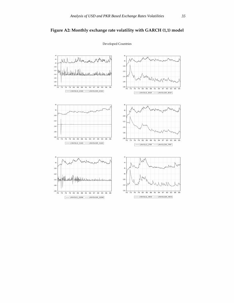
5.1. GARCH (1,1) Model-Based Exchange Rate Volatilities: Graphical Analysis

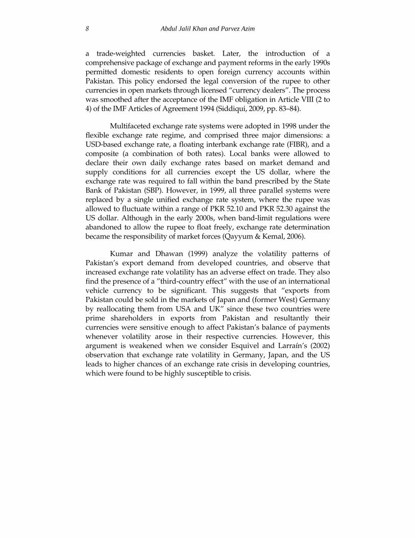
Figure A2 in the Appendix illustrates all GARCH (1,1) based volatilities, giving developed countries’ and developing countries’ exchange rates separately. Each graph shows volatility measured both in terms of foreign (upper line) and domestic currency value (lower line)-based exchange rates. All the volatility variables are compared graphically by taking their respective natural logarithms to smooth any intensities, as observed in some cases.

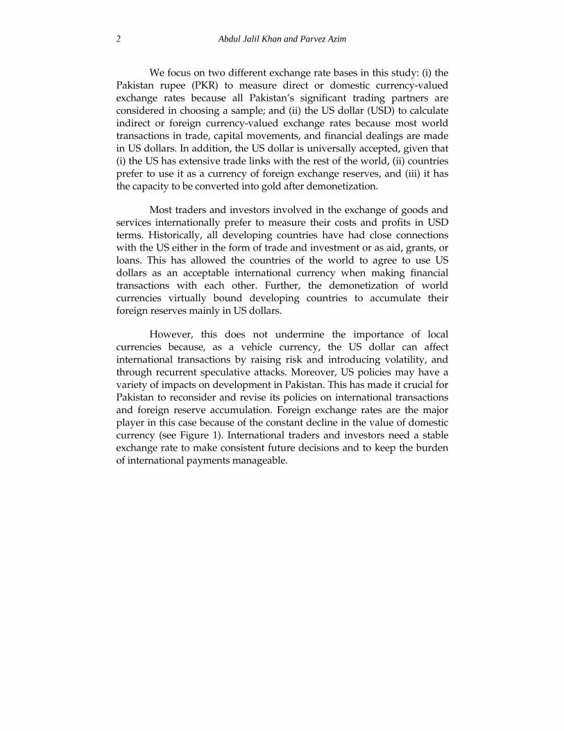
Figure 2 compares the exchange rate volatilities of developed and developing countries; the direct bilateral exchange rates reveal that the standard deviation of volatilities is larger for virtually all developed countries. Since the developed countries included in the sample are those with whom most developing countries have extensive trade links (and that are also major trading partners of Pakistan), short-run forecasting may be required to avoid potential losses in international transactions.

3 The SIC is an alternative to the AIC but “imposes a larger penalty for an additional coefficient used in the model” (Agung, 2009, p. 28). Hence, it is preferred to the AIC.


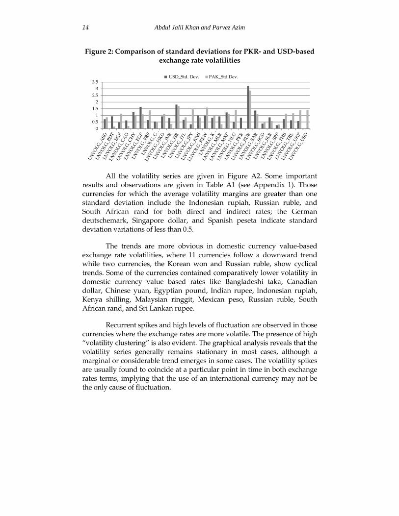
Figure 2: Comparison of standard deviations for PKR- and USD-based exchange rate volatilities

All the volatility series are given in Figure A2. Some important results and observations are given in Table A1 (see Appendix 1). Those currencies for which the average volatility margins are greater than one standard deviation include the Indonesian rupiah, Russian ruble, and South African rand for both direct and indirect rates; the German deutschemark, Singapore dollar, and Spanish peseta indicate standard deviation variations of less than 0.5.

The trends are more obvious in domestic currency value-based exchange rate volatilities, where 11 currencies follow a downward trend while two currencies, the Korean won and Russian ruble, show cyclical trends. Some of the currencies contained comparatively lower volatility in domestic currency value based rates like Bangladeshi taka, Canadian dollar, Chinese yuan, Egyptian pound, Indian rupee, Indonesian rupiah, Kenya shilling, Malaysian ringgit, Mexican peso, Russian ruble, South African rand, and Sri Lankan rupee.

Recurrent spikes and high levels of fluctuation are observed in those currencies where the exchange rates are more volatile. The presence of high “volatility clustering” is also evident. The graphical analysis reveals that the volatility series generally remains stationary in most cases, although a marginal or considerable trend emerges in some cases. The volatility spikes are usually found to coincide at a particular point in time in both exchange rates terms, implying that the use of an international currency may not be the only cause of fluctuation.

00.5

11.5

22.5

33.5

USD_Std. Dev. PAK_Std.Dev.


15

Table 1: Currencies prove consistent segment-wise with respect to all four methods of error measurement and forecastabilities

Forecastability

Exchange rates

Domestic rates (PKR) Foreign rates (USD)

Highly effective (top segment only)

Kuwaiti dinar, Canadian dollar, US dollar

Kuwaiti dinar, Canadian dollar, Singapore dollar

Very good (top and middle)

Hong Kong dollar, Malaysian ringgit

Hong Kong dollar, Malaysian ringgit

Good (middle segment only)

Spanish peseta, Australian dollar, Singapore dollar, Chinese yuan

Spanish peseta, Australian dollar

Fairly (mostly in middle segment)

Egyptian pound Egyptian pound, Dutch guilder

Poorly (lower segment only)

Mexican peso, Japanese yen, Russian ruble, Indonesian rupiah

Japanese yen, Russian ruble, Indonesian rupiah Kenyan shilling, Korean won

Interestingly, the mean of the volatility series is lower for domestic currency-valued exchange rates than for foreign ones. The exchange rate volatility for domestic rates is mostly not normally distributed—it is negatively skewed in the case of the Bangladeshi taka, Canadian dollar, Indian rupee, Malaysian ringgit, and Spanish peseta, and positively skewed for the German deutschmark, Italian lira, Kenyan shilling, Mexican peso, and Sri Lankan rupee.

5.2. GARCH (1,1) Model-Based Exchange Rate Volatilities: Analysis of Results

Since invertible series possess the property of convergence, where the sum of the coefficients of both the ARCH and GARCH terms in the models must be less than unity, all the exchange rate volatilities are evaluated in both currency terms. The conditional distribution of errors is initially assumed to be normal (Gaussian), but we also apply the Student’s t-distribution and GED to obtain valid models. The Marquardt algorithmic option helps achieve convergence in most cases, as compared to the BHHH algorithm. All foreign currency-valued exchange rate series converge earlier than domestic ones.

During estimation, we attempt to construct models by applying the Bollerslev-Wooldridge (1992) method of heteroskedasticity-consistent covariance, which allows the computation of quasi-maximum likelihood covariance and standard errors, usually needed if the residuals fail to


become conditionally normally distributed (Floros, 2008, p. 37). However, in some cases, the normally distributed error does not have this property; those models are then considered fit to generate volatility proxies that contain each parameter of mean and variance equations, which are significant at the 10 percent level.

The significance of all GARCH (1,1)-based volatility models in both currency terms shows that volatility clustering plays an important role in causing monthly changes in the exchange rates. Andersen et al. (2001), who present strong evidence of the volatility clustering impact on daily returns, support this observation. This means that the impact of any kind of “shock” takes more time to taper off.

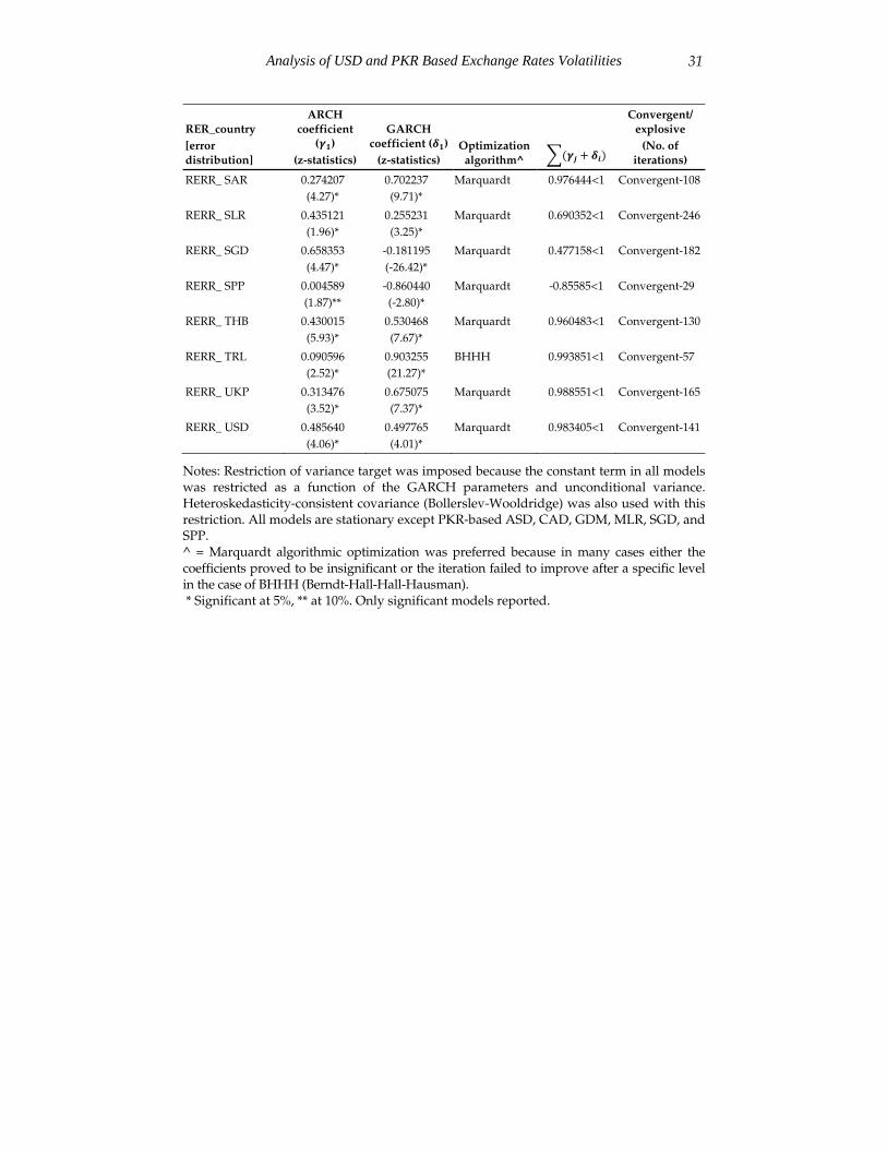
The detailed results for all 28 foreign currency-valued exchange rate volatility models are given in Table A2; the domestic currency-valued exchange rate volatility models are presented in Table A3 (see Appendix 1). Many exchange rate volatility models are found to rapidly converge, requiring a small number of iterations, and are found to be invertible. Most of the foreign currency-valued exchange rate variances remain rapidly convergent compared to domestic ones.

Those exchange rate series that are found to be explosive (with a higher degree of volatility and divergence) include the Indonesian rupiah, Kenyan shilling, Pakistani rupee, and Russian ruble in terms of foreign currency-valued exchange rate volatility; and the Canadian dollar, Indian rupee, Indonesian rupiah, Korean won, and Malaysian ringgit in terms of domestic currency-valued exchange rate volatilities. One of the reasons for this divergence is that the variance-targeted constant term restriction has to be withdrawn to obtain better model specifications with highly significant parameters, but the domestic currency-valued Canadian dollar and Indian rupee exchange rate volatility models remain explosive even in the presence of this restriction.

All foreign currency-valued exchange rate models prove to be significant when estimated assuming a normal (Gaussian) distribution of errors. Exceptions include the Chinese yuan, where the GED needs to be considered, and the Kuwaiti dinar and Egyptian pound, where the Student’s t-error distribution is applied to obtain a valid model. In the same way, we estimate direct exchange rate models assuming a normal (Gaussian) distribution of errors, except for the Bangladeshi taka, Canadian dollar, and Hong Kong dollar, which remain valid and significant assuming a Student’s t-error distribution. The Egyptian pound, Indian rupee, Italian lira, Kenyan shilling, Kuwaiti dinar, and Mexican peso have


17

a GED. This shows that indirect exchange rate volatility models are usually more stable and consistent than direct exchange rate volatility models.

In Tables A2 and A3, the sum of the estimators‘ coefficient values in each GARCH-based conditional volatility model is close to unity, indicating the persistence of volatility shocks. Generally, all the volatility models are found to be highly significant and show positive values for each coefficient of lagged exchange rates in the mean equation. In addition, the coefficient of the lagged conditional variance is also significant and usually has a positive sign but is less than 1, implying that last-period news can still have a significant impact on volatility.

We find evidence of long memory in variances through the large magnitude of the GARCH coefficients, such as for the Bangladeshi taka, Canadian dollar, French franc, Indian rupee, Japanese yen, Malaysian ringgit, Dutch guilder, Spanish peseta, and Turkish lira, in terms of domestic rates. In terms of foreign rates, this is observed in the case of the Belgium franc, Canadian dollar, French franc, German deutschmark, Hong Kong dollar, Japanese yen, Kuwaiti dinar, Dutch guilder, and Spanish peseta. Interestingly, in the case of developed partners, the long memory effect is found to be persistent and more visible.

5.3. Predictability of GARCH (1,1) Model-Based Exchange Rate Volatilities

Four major evaluation criteria (loss functions) are applied to compare the volatility of each currency-based exchange rate including: RMSE, MAE, MAPE, and TIC. The reason for applying all four criteria is to obtain consistent and vigorous results regarding the forecastability of GARCH (1,1)-based exchange rate volatility models.4 The RMSE usually gives more weight to large forecast errors while the MAE gives equal weight to both over- and under-predicted values of volatility forecasts (Vee et al., 2011, p. 10).

The RMSE and MAE also help measure those forecasts that are conditional on the scale of the dependent variables, and allow one to compare relative forecasts for the same series across various models. The minimum forecasting error measured through a given loss function indicates the superior forecasting ability of a particular model. The MAPE and TIC are both scale-independent, where the TIC lies between 0 and 1, with 0 denoting the perfect fit (Ocran & Biekpe, 2007, p. 96). 4 Various studies have applied and tested these criteria to evaluate both the static (short-run) and dynamic (long-run) forecastabilities of time series models (see Vee et al., 2011; Matei, 2009; Frimpong & Oteng-Abayie, 2006; Sparks & Yurova, 2006; Zivot, 2008).


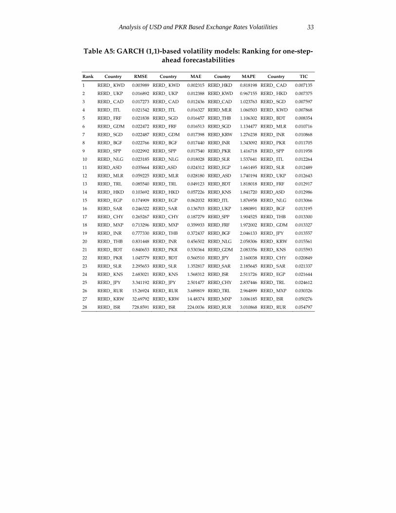
The versatility of these loss functions helps us identify and differentiate between those currencies that have high predictive power and those with poor predictive power. In this case, all the sampled countries are divided into three different segments by assigning each country a rank based on the minimum values obtained through each criterion of evaluation, referred to as the top, middle, and lower segments, respectively. The top segment includes eight countries with the highest position in terms of their respective performance in one-step-ahead forecasts based on each criterion. These countries fall in the “highly effective forecasting” category where robust and effective short-run forecasting of variations in their bilateral exchange rates is possible, especially when Pakistan is a trading partner.

The remaining 20 countries are divided into two equal segments. The middle segment includes the ten countries next in rank by assuming that their currencies can be reasonably well forecast, and so including them in the “very good” category. The lower segment comprises ten other countries at the lowest level of forecastability, which are included in the “poor” category, referring those currencies that perform poorly in forecasting short-run variations in exchange rates. Tables A4 and A5 (Appendix 2) identify all the sampled countries and their respective currencies in each category on the basis of each loss function.

Table 1 shows that roughly the same currencies have consistently acquired the same, or close to the same, rank in the case of each (loss function) evaluation criterion, and remained part of a common segment. Exchange rates are measured using two different bases, i.e., the Pakistan rupee as the domestic and US dollar as the foreign currency value. The consistency of these results shows that GARCH (1,1)-based volatility models strongly help to predict variations in both the Kuwaiti dinar and Canadian dollar, irrespective of the base currency; US dollar exchange rate volatility measured in domestic currency value terms; and Singapore dollar exchange rate volatility measured in foreign currency value terms. Consequently, Pakistan could shield the potentially negative effect on trade and business scenario—usually more sensitive to a volatile currency exchange rate—by using GARCH (1,1) forecasting models when making international transactions primarily through Kuwaiti dinars, Canadian dollars, and US dollars directly.

Using the Hong Kong dollar and Malaysian ringgit is equally good because GARCH (1,1)-based volatilities can effectively capture the uncertain variability in the exchange rates of these currencies, at least in the


19

short run. Further, the ability to predict future variations and uncertainties in exchange rates with a high level of accuracy in the shape of “shocks” or “news” is in great demand by traders and investors. This could be made available through the GARCH (1,1) model in terms of various currencies for traders and investors, especially those from Pakistan, and also for the country’s significant trading partners. The Egyptian pound, Mexican peso, Japanese yen, Russian ruble, and Indonesian rupiah are not, however, considered feasible for conducting direct international transactions due to their poor forecastability and high deviations from the mean.

The overall statistics obtained through the MAE are lower than the RMSE. No perfect-fit models could be obtained based on the TIC statistics because, although the TIC values are close to 0, none of them is equal to 0. Further, the similar ranks assigned to each country/currency according to the given forecasting evaluation criteria clearly reveals that, to an extent, these criteria are reasonably valid substitutes for one another. Hence, they need not be used simultaneously to save time and effort. The RMSE and MAE both assign the same ranks to various exchange rate volatility models, irrespective of the base currencies, and therefore are preferred to the MAPE and TIC when measuring short-run predictive capacity.

6. Major Findings, Policy Implications, and Conclusions

Our main findings are described below.

First, foreign currency-valued exchange rate volatilities converge more rapidly than domestic ones, which implies that the former have a linear structure compared to the latter models in which forecasting is possible and easy.5 Second, volatility spikes remain independent of the base currency used to calculate exchange rate volatilities. This implies that foreign currency-valued exchange rates are not the major cause of various shocks in financial markets.

Third, those exchange rate volatilities that remain explosive in both currency terms are poor at making one-step-ahead forecasts, with the exception of the Canadian dollar. This confirms the first finding that the parameters of explosive models are nonlinear where accurate forecasting is difficult. We can conclude that rapid convergence and stationarity are required to make effective forecasts because those models in which the ARCH and GARCH terms fail to achieve stationarity remain explosive,

5 Rapid convergence shows a linearity of equations with respect to the parameters because linear equation estimation needs only one iteration to converge (SAS Institute, 1999, p. 742).


which can also decrease their forecasting ability. Fourth, various forecasting evaluation criteria are usually consistent in terms of results and consequent rank assignment.

Fifth, the RMSE and MAE are better at assigning ranks to various currencies in the sample according to their respective forecastabilities. Sixth, using an international currency instead of a domestic currency to perform international transactions does not make exchange rates more volatile, therefore contradicting our first hypothesis.

Since policymakers are interested in keeping the exchange rate more certain and less volatile in the future, this purpose may be served in the short run by using GARCH-based exchange rate volatility models because exchange rate series, like other financial time-series, exhibit two main properties: fat tails and volatility clustering.6 Hence, GARCH models, usually with a first lag, are considered suitable for resolving the issues above and helpful in understanding the dynamics of an exchange rate series.

The analysis of two different currency-based exchange rate volatilities has clearly revealed that, at least in the context of Pakistan, the use of US dollars as an international currency is beneficial because it ensures rapid adjustment in exchange rate variations in various currencies without compromising their stability against the Pakistan rupee. The use of an international (vehicle) currency can also have a “third-country effect”, as observed by Cushman, which intensifies the exchange rate volatility because of the “correlation of exchange rate fluctuations” (1986, p. 1226) when developing countries use it instead of their own domestic currency. However, this could not be covered within the scope of this study and should be considered for future research.

The application and comparison of four different loss functions to measure the predictive capacity of various models proves that the RMSE and MAE techniques are superior to other techniques. Since the Kuwaiti dinar, Canadian dollar, US dollar, Singapore dollar, Hong Kong dollar, and Malaysian ringgit can be effectively forecast at least in the short run, they are preferred for international transactions. This helps address uncertainties and the temporal self-dependence of exchange rate volatilities and prevents potential losses in international transactions. Given that the use of an international (vehicle) currency is not the main contributor to volatility, continuing to use the US dollar to conduct international transactions is beneficial for Pakistan with respect to all its significant trading partners. 6 Floros’s (2008) “fat tail” reflected different degrees of leptokurtosis for the same variance.


21

References

Agung, I. G. N. (2009). Time series data analysis using Eviews. Hoboken, NJ: John Wiley & Sons.

Akyüz, Y. (2009). Exchange rate management, growth and stability: National and regional policy options in Asia. Colombo, Sri Lanka: United Nations Development Programme Centre for Asia Pacific. Retrieved from www.hdru.aprc.undp.org/resource_centre/pub_pdfs/P1115.pdf

Al Samara, M. (2009). The determinants of real exchange rate volatility in the Syrian economy (Mimeo). Paris, France: Sorbonne Economic Centre.

Andersen, T. G., Bollerslev, T., Christoffersen, P. F., & Diebold, F. X. (2006). Volatility and correlation forecasting. In G. Elliot, C. W. J. Granger, & A. Timmermann (Eds.), Handbook of economic forecasting (pp. 778–878). Amsterdam: North-Holland.

Andersen, T. G., Bollerslev, T., Diebold, F. X., & Labys, P. (2001). The distribution of realized exchange rate volatility. Journal of the American Statistical Association, 96, 42–55.

Arize, C. A. (1998). The effect of exchange rate on US imports: An empirical investigation. International Economic Journal, 12(3), 31–40.

Arize, A. C., Malindretos, J., & Kasibhatla, K. M. (2003). Does exchange rate volatility depress export flows? The case of LDCs. International Advances in Economics Research, 9(1), 7–19.

Asseery, A., & Peel, D. A. (1991). The effects of exchange rate volatility on exports. Economics Letters, 37(2), 173–177.

Asteriou, D. (2006). Applied econometrics: A modern approach using Eviews and Microfit. New York, NY: Palgrave Macmillan.

Bahmani-Oskooee, M. (2002). Does black market exchange rate volatility deter the trade flows? Iranian experience. Applied Economics, 34(18), 2249–2255.

Bollerslev, T. (1986). Generalized autoregressive conditional heteroskedasticity. Journal of Econometrics, 31(3), 307–327.


Bollerslev, T., Chou, R. Y., & Kroner, K. F. (1992). ARCH modeling in finance: A review of the theory and empirical evidence. Journal of Econometrics, 52, 5–59.

Bollerslev, T., Engle, R. F., & Nelson, D. B. (1994). ARCH models. In R. F. Engle & D. McFadden (Eds.), Handbook of econometrics (vol. 4, pp. 2959–3038). Amsterdam: North Holland.

Caporale, T., & Doroodian, K. (1994). Exchange rate variability and the flow of international trade. Economics Letters, 46, 49–54.

Clark, P., Tamirisa, N., & Wei, S.-J. (2004). A new look at exchange rate volatility and trade flows (Occasional Paper No. 235) Washington, DC: International Monetary Fund.

Crowley, P., & Lee, J. (2003). Exchange rate volatility and foreign investment: International evidence. International Trade Journal, 17(3), 227–252.

Cushman D. O. (1986). Has exchange rate risk depressed international trade? The impact of third-country exchange risk. Journal of International Money and Finance, 5, 361–379.

Dell‘Ariccia, G. (1999). Exchange rate fluctuations and trade flows: Evidence from the European Union. IMF Staff Papers, 46(3), 315–334.

Engle, R. F. (1982). Autoregressive conditional heteroskedasticity with estimates of the variance of UK inflation. Econometrica, 50, 987–1007.

Engle, R. F. (2001). GARCH 101: The use of ARCH/GARCH models in applied econometrics. Journal of Economic Perspectives, 15(4), 157–168.

Engle, R. F., & Bollerslev, T. (1986). Modeling the persistence of conditional variances. Econometric Reviews, 5(1), 1–50.

Engle, R. F., & Lee, G. G. J. (1999). A permanent and transitory component model of stock return volatility. In R. F. Engle & H. White (Eds.), Cointegration, causality, and forecasting: A festschrift in honor of Clive W. J. Granger (pp. 475–497). Oxford, UK: Oxford University Press.

Engel, C., Mark, N. C., & West, K. D. (2007). Exchange rate models are not bad as you think. In Proceedings of the Jacques Polak Annual Research Conference (pp. 1–48). Washington, DC: International Monetary Fund.


23

Esquivel, G., & Larraín, F. (2002). The impact of G-3 exchange rate volatility on developing countries (Working Paper No. 86). Cambridge, MA: Center for International Development.

Floros, C. (2008). Modeling volatility using GARCH models: Evidence from Egypt and Israel. Middle Eastern Finance and Economics, 2, 31–41.

Franses, P. H., & McAleer, M. (2002). Financial volatility: An introduction. Journal of Applied Econometrics, 17, 419–424.

French, K. R., Schwert, G. W., & Stambaugh, R. F. (1987). Expected stock returns and volatility. Journal of Financial Economics, 19(1), 3–29.

Frimpong, J. M., & Oteng-Abayie, E. F. (2006). Modeling and forecasting volatility of returns on the Ghana Stock Exchange using GARCH models (MPRA Paper No. 593). Munich, Germany: University of Munich. Retrieved from http://ssrn.com/abstract=927168

Gozgor, G., & Nokay, P. (2011). Comparing forecasting performances among volatility estimation methods in the pricing of European type currency options of USD-TL and Euro-TL. Journal of Money, Investment and Banking, 19, 130–142

Grier, K. B., & Perry, M. J. (2000). The effect of real and nominal uncertainty on inflation and output growth: Some GARCH-M evidence. Journal of Applied Econometrics, 15(1), 45–58.

Irfan, M., Irfan, M., & Awais, M. (2010). Modeling volatility of short-term interest rates by ARCH family models: Evidence from Pakistan and India. World Applied Sciences Journal, 9(10), 1089–2010.

Kroner, K. F., & Lastrapes, W. D. (1993). The impact of exchange rate volatility on international trade: Reduced form estimates using the GARCH-in-mean model. Journal of International Money and Finance, 12, 298–318.

Kumar, R., & Dhawan, R. (1999). Exchange rate volatility and Pakistan exports to the developing world: 1974–85. World Development, 19(9), 1225–1240.

Lanyi, A., & Suss, E. C. (1982). Exchange rate variability: Alternative measures and interpretation. IMF Staff Papers, 29(4), 527–560.


Matei, M. (2009). Assessing volatility forecasting models: Why GARCH models take the lead. Romanian Journal of Economic Forecasting, 12(4), 42–65.

Ocran, M. K., & Biekpe, N. (2007). Forecasting volatility in sub-Saharan Africa’s commodity markets. Investment Management and Financial Innovations, 4(2), 91–102.

Pacelli, V. (2012). Forecasting exchange rates: A comparative analysis. International Journal of Business and Social Science, 3(10), 145–156.

Qayyum, A., & Kemal, A. R. (2006). Volatility spillover between the stock market and the foreign exchange market in Pakistan (Working Paper No. 2006-7). Islamabad: Pakistan Institute of Development Economics.

SAS Institute. (1999). SAS/ETS user’s guide, version 8. Cary, NC: Author.

Siddiqui, M. A. (2009). Modeling Pak rupee volatility against five major currencies in the perspective of different exchange rate regimes. European Journal of Economics, Finance and Administrative Sciences, 17, 81–96.

Sixty years of US aid to Pakistan: Get the data. (2011, July 11). The Guardian. Retrieved on February 4, 2012, from http://www.guardian.co.uk/global-development/poverty-matters/2011/jul/11/us-aid-to-pakistan

Sparks, J. J., & Yurova, Y. V. (2006). Comparative performance of ARIMA and ARCH/GARCH models on time series of daily equity prices for large companies. In 2006 SWDSI proceedings (pp. 563–573). Chicago, IL: South West Decision Science Institute. Retrieved on August 17, 2011 from http://www.swdsi.org/swdsi06/Proceedings06/Papers/ QM04.pdf

Tripathy, T., & Gil-Alana, L. A. (2010). Suitability of volatility models for forecasting stock market returns: A study on the Indian National Stock Exchange. American Journal of Applied Sciences, 7(11), 1487–1494.

Vee, D. N. C., Gonpot, P. N., & Sookia, N. (2011). Forecasting volatility of USD/MUR exchange rate using a GARCH (1,1) model with GED and student’s t-errors. University of Mauritius Research Journal, 17, 171–214.


25

Wang, K.-L., & Barrett, C. B. (2002). A new look at the trade volumes effects of real exchange rate risk: A rational expectation-based multivariate GARCH-M approach (Working Paper No. 2002-41). Ithaca, NY: Cornell University, Department of Applied Economics and Management. Retrieved on July 2008 from http://papers.ssrn.com/5013/papers.cfm?abstract_id=430422

Zivot, E. (2008). Practical issues in the analysis of univariate GARCH models (Working Paper No. UWEC-2008-03-FC). Seattle, WA: University of Washington, Department of Economics.


Appendix 1

Results of GARCH (1,1)-based volatility models

Table A1: Graphical analysis of GARCH (1,1)-based volatilities

Currency

Average volatility margins (standard

deviation) Trend (frequency of

fluctuations) Highly volatile (spikes)

years (period)

PKR USD PKR USD PKR USD

Australian dollar (ASD)

0.001123 0.033153 No (H)* @Up (H*) 72-74, 77, 83, 85, 86,

08-09

73, 74, 77, 83, 85, 86,

98, 01-02, 09

Bangladeshi taka (BDT)

0.032343 0.725098 No @Down(H) No 75, 85, 90, 01-02, 06-07

Belgian franc (BGF)

0.000796 0.022032 Down (H) No (M) 72-74, 81, 82, 85

Canadian dollar (CAD)

0.00133 0.015067 No Up (L) 72 09

Chinese yuan (CHY)

0.004714 0.196466 @Down (H) @Up (H*) 72-74, 78, 94-95

72, 78, 94

Egyptian pound (EGP)

0.004628 0.102956 No (M) No (H) 72-74, 79-81, 90-92,

03

74-75, 79-81, 90-92, 95,

01, 03-04, 08

French franc (FRF)

0.000941 0.020766 Down (M) No (M) 72-73 No

German deutschmark (GDM)

0.000949 0.021598 No (H*) No (L) 71, 72, 73-74, 81, 84

73

Hong Kong dollar (HKD)

0.004573 0.087218 No (M) @Up (M) 72-74, 80, 81-84, 89-90

73-74, 79-81, 83-84, 05

Indian rupee (INR)

0.02109 0.639649 No @Up (H*) No 92, 93, 95-96

Indonesian rupiah (ISR)

9.773622 390.4742 No (H*) No (H*) 72, 74, 79, 82, 83, 86, 98-99, 01-

02, 09.

70, 72, 73, 79, 83, 86, 97-98, 01,

06, 09

Italian lira (ITL)

0.00083 0.020386 @Down(H*) No (H)* 72-74, 76, 81

74, 76, 85-86, 93, 97,

01, 09

Japanese yen (JPY)

0.140736 3.285553 Down (H) No (M) 72-73, 86, 95, 98

71

Kenyan shilling (KNS)

0.080893 2.369582 No (H*) @Cyclical(H*) 72, 76, 81-82, 93, 95-

96, 98

75, 76, 81-82, 84, 93-

95, 98, 03, 06

Korean won (KRW)

1.233907 21.38206 Cyclical(H*) No (H)* 71-73, 74-75, 76,80-81,

83, 89, 94,

71, 74, 80, 98-99, 01,

08-09


27

Currency

Average volatility margins (standard

deviation) Trend (frequency of

fluctuations) Highly volatile (spikes)

years (period)

96, 98-99, 01, 08-09

Kuwaiti dinar (KWD)

1.79E-04 0.003537 No (M) No (M) 71-74, 79-80, 83

79-80, 89

Malaysian ringgit (MLR)

0.002801 0.039892 No No (H*) 72 73, 75, 80, 92, 94, 98-99

Mexican peso (MXP)

0.014758 0.49483 No (H*) No (H)* 72, 77, 81-83, 86, 88, 95, 98, 09

77, 81-83, 86-87, 95-96,

98, 09

Dutch guilder (NLG)

0.001032 0.022348 Down (L) No (L) 72, 81-82 74, 82, 85-86

Pakistani rupee (PKR)

__ 0.997572 __ No (H*) __ 72, 73, 89, 93, 95, 97,

99,01

Russian ruble (RUR)

0.166004 7.815225 Cyclical (H*)

Cyclical (H*)

72, 82, 92-94, 98-99,

09

72, 92-94, 96, 97, 98-99,

2000-01, 09

South African rand (SAR)

0.005836 0.188274 @Down(H)* Up (H*) 72, 76, 81, 84-86, 98, 02-03, 09

72-73, 76, 84-86, 95,

98, 02-03, 09

Singapore dollar (SGD)

0.001527 0.021871 No (H*) No (M) 71, 72, 75, 79

73-74, 98

Sri Lankan rupee (SLR)

0.077471 1.942905 No (H*) No (H*) 72, 78, 79, 81-82, 90

77-78, 80, 81, 83, 89, 93, 95, 98, 02, 05, 07

Spanish peseta (SPP)

0.001546 0.022663 No No (L) 72* No

Thai Land Baht (THB)

0.025838 0.584162 Down (H*) No (M-H*) 72, 80, 81, 85, 98-99,

2001

81, 85, 98-99, 2001, 07

Turkish lira (TRL)

0.002733 0.078735 Down (M) No (M) 71, 72, 80, 94-95, 01-02

71, 80, 94-95, 01-02

United Kingdom pound (UKP)

0.000735 0.015928 Down (H)* No (H)* 72-73, 81, 84-85, 89, 93, 97, 09

79, 85, 93, 09

United States dollar (USD)

0.000706 __ Down(H)* __ 72 __

Note: Graphs were drawn in logarithmic transformation but the values were used in level in this table, therefore representing the deviation from the mean at the original level of measurement. Level of frequencies: @ = at margin, H = high, M = medium, L = low. * Significantly observable volatility clustering within brackets if compatible with frequency, otherwise placed outside brackets.


Table A2: GARCH (1,1): USD-based models

RER_country

ARCH coefficient

( ) (z-statistics)

GARCH coefficient

( ) (z-statistics)

Optimization algorithm^

Convergent/ explosive

(No. of iterations)

RERD_ASD 0.284651 (4.10)*

0.596191 (5.78)*

Marquardt 0.880842 <1 Convergent-45

RERD_ BGF 0.096275 (2.63)*

0.858712 (16.24)*


RERD_ BDT 0.216256 (4.34)*

0.745320 (10..72)*

Marquardt 0.961576 <1

Convergent-237

RERD_ CAD 0.042615 (2.65)*

0.953193 (51.59)*


Convergent-11

RERD_ CHY [[email protected]]

0.783574 (23.67)*

0.116985 (2.98)*

Marquardt 0.900559<1

Convergent-131

RERD_ EGP [t@10]

0.279262 (17.71)*

0.718244 (44.43)*


Convergent-29

RERD_ FRF 0.107337 (3.82)*

0.868634 (23.89)*


Convergent-19

RERD_ GDM 0.106903 (2.70)*

0.854000 (16.77)*


Convergent-10

RERD_ HKD 0.102602 (4.46)*

0.873107 (37.30)*


Convergent-29

RERD_ INR 0.315616 (7.30)*

0.598453 (9.70)*


Convergent-238

RERD_ ISR 1.787072 (3.36)*

0.165427 (2.61)*

Marquardt, without restricted constant term

1.952499 >1

Explosive-862

RERD_ ITL 0.203095 (4.78)*

0.741284 (12.69)*


Convergent-14

RERD_ JPY 0.058305 (1.79)**

0.904221 (14.08)*

BHHH 0.962526 <1

Convergent-51

RERD_ KNS 0.379841 (2.55)*

0.623122 (5.23)*


1.002963 >1

Explosive-50

RERD_ KRW 0.583274 (3.01)*

0.326481 (1.58) **

BHHH 0.909755 <1

Convergent-43

RERD_ KWD [t@10]

0.081725 (5.86)*

0.906066 (58.20)*


Convergent-74

RERD_ MXP 0.337620 (2.75)*

0.636507 (4.71)*


Convergent-59

RERD_ MLR 0.621868 (7.21)*

0.276835 (2.44)*


Convergent-56

RERD_ NLG 0.094233 (2.79)*

0.867497 (22.51)*


Convergent-13


29

RER_country

ARCH coefficient

( ) (z-statistics)

GARCH coefficient

( ) (z-statistics)

Optimization algorithm^


(No. of iterations)

RERD_ PKR 1.430321 (1.67)**

-0.008884 (-11.79)*


1.421437 >1

Explosive-38

RERD_ RUR 3.682844 (2.46)*

0.076209 (1.68)**


3.759053 >1

Explosive-96

RERD_ SAR 0.279295 (4.01)*

0.705559 (9.46)*


Convergent-33

RERD_ SLR 0.775119 (2.98)*

0.194128 (2.78*)


0.969247 <1

Convergent-30

RERD_ SGD 0.139742 (2.26)*

0.701444 (6.49)*


Convergent-15

RERD_ SPP 0.041490 (1.56)**

0.907352 (16.13)*


Convergent-11

RERD_ THB 0.285579 (1.88)**

0.478501 (3.69)*


0.76408 <1

Convergent-190

RERD_ TRL 0.131245 (20.00)*

0.799107 (76.34)*

Marquardt (without RSE)

0.930352 <1

Convergent-82

RERD_ UKP 0.226794 (5.05)*

0.663268 (8.97)*


Note: ^ = Marquardt algorithmic optimization was applied but where coefficients proved insignificant, BHHH (Berndt-Hall-Hall-Hausman) was tested. Further heteroskedasticity-consistent covariance (Bollerslev-Wooldridge) was used. Constant term in all models was restricted as a function of the GARCH parameters and unconditional variance. All models are stationary except USD-based PKR. * Significant at 5%, ** at 10%.


Table A3: GARCH (1,1): PKR-based models

RER_country [error distribution]

ARCH coefficient

( ) (z-statistics)

GARCH coefficient ( )

(z-statistics) Optimization

algorithm^


(No. of iterations)

RERR_ASD 0.849144 (29.14)*

-0.008907 (-10..29)*


Convergent-51

RERR_ BGF 0.200190 (6.68)*

0.793676 (25.97)*


Convergent-207

RERR_ BDT [Student’s t]

0.014725 (3.60)*

0.979600 (183.7)*


Convergent-17

RERR_ CAD [Student’s t]

0.000876 (3.68)*

0.999913 (6545)*

BHHH 1.000789>1

Explosive-30

RERR_ CHY 0.204335 (4.41)*

0.766797 (12.78)*


Convergent-234

RERR_ EGP [GED]

0.137942 (3.42)*

0.838840 (17.39)*


Convergent-34

RERR_ FRF 0.101547 (8.20)*

0.896949 (71.16)*


Convergent-175

RERR_ GDM 0.626305 (7.13)*

-0.164023 (-30.72)*


Convergent-52

RERR_ HKD [Student’s t]

0.180939 (4.95)*

0.800635 (20.32)*


Convergent-63

RERR_ INR [GED]

0.001626 (3.23)*

0.998588 (1984)*

Marquardt 1.000214>1

Explosive-88

RERR_ ISR 1.662280 (5.58)*

0.174667 (4.24)*

Marquardt, without restriction

1.836947>1

Explosive-30

RERR_ ITL [GED]

0.210044 (3.83)*

0.757048 (11.30)*

Marquardt 0.967092<1 Convergent-101

RERR_ JPY 0.144470 (5.54)*

0.853663 (32.52)


Convergent-104

RERR_ KNS [GED]

0.444142 (7.59)*

0.472030 (6.57)*


Convergent-21

RERR_ KRW 1.809092 (2.06)*

0.379925 (3.00)*

Marquardt, without restriction

2.189017>1

Explosive-63

RERR_ KWD [GED]

0.174085 (3.90)*

0.805181 (15.07)*


Convergent-95

RERR_ MXP [GED]

0.582858 (7.61)*

0.354729 (4.12)*


Convergent-32

RERR_ MLR 0.007827 (5.08)*

-0.622043 (-6.65)*

Marquardt -0.614216<1

Convergent-26

RERR_ NLG 0.099376 (8.37)*

0.899490 (73.67)*


Convergent-197

RERR_ RUR 0.813796 (10.15)*

0.185714 (2.31)*

Marquardt 0.99951<1

Convergent-24


31

RER_country [error distribution]

ARCH coefficient

( ) (z-statistics)

GARCH coefficient ( )

(z-statistics) Optimization

algorithm^


(No. of iterations)

RERR_ SAR 0.274207 (4.27)*

0.702237 (9.71)*


Convergent-108

RERR_ SLR 0.435121 (1.96)*

0.255231 (3.25)*


Convergent-246

RERR_ SGD 0.658353 (4.47)*

-0.181195 (-26.42)*


RERR_ SPP 0.004589 (1.87)**

-0.860440 (-2.80)*

Marquardt -0.85585<1 Convergent-29

RERR_ THB 0.430015 (5.93)*

0.530468 (7.67)*


RERR_ TRL 0.090596 (2.52)*

0.903255 (21.27)*

BHHH 0.993851<1

Convergent-57

RERR_ UKP 0.313476 (3.52)*

0.675075 (7.37)*


Convergent-165

RERR_ USD 0.485640 (4.06)*

0.497765 (4.01)*


Notes: Restriction of variance target was imposed because the constant term in all models was restricted as a function of the GARCH parameters and unconditional variance. Heteroskedasticity-consistent covariance (Bollerslev-Wooldridge) was also used with this restriction. All models are stationary except PKR-based ASD, CAD, GDM, MLR, SGD, and SPP. ^ = Marquardt algorithmic optimization was preferred because in many cases either the coefficients proved to be insignificant or the iteration failed to improve after a specific level in the case of BHHH (Berndt-Hall-Hall-Hausman). * Significant at 5%, ** at 10%. Only significant models reported.


Appendix 2

Ranking of sampled countries/currencies: GARCH (1,1) models-based one-step-ahead forecastabilities

Table A4: GARCH (1,1)-based volatility models: Ranking for one-step-ahead forecastabilities

Rank Country RMSE Country MAE Country MAPE Country TIC

1 RERR_KWD 0.000260 RERR_KWD 0.000104 RERR_HKD 1.539356 RERR_ BDT 0.013929

2 RERR_ UKP 0.001074 RERR_ ITL 0.000510 RERR_MLR 1.633824 RERR_ HKD 0.016957

3 RERR_GDM 0.001183 RERR_ CAD 0.000529 RERR_KWD 1.647312 RERR_ INR 0.017833

4 RERR_ ITL 0.001192 RERR_ USD 0.000543 RERR_BDT 1.667074 RERR_KWD 0.019563

5 RERR_ BGF 0.001228 RERR_GDM 0.000551 RERR_INR 1.700491 RERR_ CAD 0.019992

6 RERR_ USD 0.001273 RERR_ BGF 0.000561 RERR_CAD 1.740250 RERR_ SLR 0.020061

7 RERR_ FRF 0.001274 RERR_ UKP 0.000570 RERR_USD 1.741950 RERR_ MLR 0.020412

8 RERR_ CAD 0.001341 RERR_ SPP 0.000595 RERR_SGD 1.759509 RERR_ USD 0.021910

9 RERR_ NLG 0.001401 RERR_ FRF 0.000675 RERR_KRW 2.000351 RERR_ CHY 0.021970

10 RERR_ SPP 0.001549 RERR_ NLG 0.000720 RERR_THB 2.132959 RERR_ ITL 0.022647

11 RERR_ ASD 0.001810 RERR_ SGD 0.000756 RERR_ITL 2.215917 RERR_ SGD 0.023210

12 RERR_ SGD 0.002009 RERR_ ASD 0.000860 RERR_SLR 2.223079 RERR_ ASD 0.023622

13 RERR_ MLR 0.002806 RERR_ MLR 0.001104 RERR_EGP 2.264776 RERR_GDM 0.023682

14 RERR_ TRL 0.003335 RERR_ TRL 0.001510 RERR_CHY 2.286328 RERR_ BGF 0.024206

15 RERR_ EGP 0.006133 RERR_ EGP 0.002210 RERR_SPP 2.288698 RERR_ THB 0.024546

16 RERR_ CHY 0.006272 RERR_ HKD 0.002780 RERR_KNS 2.319876 RERR_ KNS 0.024589

17 RERR_ HKD 0.006383 RERR_ CHY 0.003171 RERR_ASD 2.373710 RERR_KRW 0.024608

18 RERR_ SAR 0.007620 RERR_ SAR 0.004214 RERR_BGF 2.379223 RERR_ SPP 0.025290

19 RERR_ MXP 0.025347 RERR_ MXP 0.008784 RERR_GDM 2.443351 RERR_ FRF 0.025849

20 RERR_ INR 0.029983 RERR_ INR 0.013485 RERR_MXP 2.574731 RERR_ UKP 0.026213

21 RERR_ BDT 0.032649 RERR_ BDT 0.017255 RERR_JPY 2.584721 RERR_ NLG 0.026428

22 RERR_ THB 0.040099 RERR_ THB 0.018414 RERR_FRF 2.702764 RERR_ SAR 0.026472

23 RERR_ SLR 0.093295 RERR_ SLR 0.047559 RERR_NLG 2.726639 RERR_ JPY 0.027108

24 RERR_ KNS 0.119986 RERR_ KNS 0.050698 RERR_UKP 2.775656 RERR_ EGP 0.029277

25 RERR_ JPY 0.229584 RERR_ JPY 0.094110 RERR_SAR 2.856873 RERR_ TRL 0.035374

26 RERR_ RUR 0.363728 RERR_ RUR 0.155388 RERR_TRL 3.340640 RERR_ MXP 0.039108

27 RERR_KRW 1.448813 RERR_KRW 0.576308 RERR_ISR 3.400326 RERR_ ISR 0.047478

28 RERR_ ISR 14.87059 RERR_ ISR 5.931519 RERR_RUR 5.089294 RERR_ RUR 0.053534


33

Table A5: GARCH (1,1)-based volatility models: Ranking for one-step-ahead forecastabilities

Rank Country RMSE Country MAE Country MAPE Country TIC

1 RERD_ KWD 0.003989 RERD_ KWD 0.002315 RERD_HKD 0.818198 RERD_ CAD 0.007135

2 RERD_ UKP 0.016892 RERD_ UKP 0.012388 RERD_KWD 0.967155 RERD_ HKD 0.007375

3 RERD_ CAD 0.017273 RERD_ CAD 0.012436 RERD_CAD 1.023763 RERD_ SGD 0.007597

4 RERD_ ITL 0.021542 RERD_ ITL 0.016327 RERD_MLR 1.060503 RERD_ KWD 0.007868

5 RERD_ FRF 0.021838 RERD_ SGD 0.016457 RERD_THB 1.106302 RERD_ BDT 0.008354

6 RERD_ GDM 0.022472 RERD_ FRF 0.016513 RERD_SGD 1.134477 RERD_ MLR 0.010716

7 RERD_ SGD 0.022487 RERD_ GDM 0.017398 RERD_KRW 1.276238 RERD_ INR 0.010868

8 RERD_ BGF 0.022766 RERD_ BGF 0.017440 RERD_INR 1.343092 RERD_ PKR 0.011705

9 RERD_ SPP 0.022992 RERD_ SPP 0.017540 RERD_PKR 1.416718 RERD_ SPP 0.011958

10 RERD_ NLG 0.023185 RERD_ NLG 0.018028 RERD_SLR 1.537641 RERD_ ITL 0.012264

11 RERD_ASD 0.035664 RERD_ASD 0.024312 RERD_EGP 1.661495 RERD_ SLR 0.012489

12 RERD_ MLR 0.059225 RERD_ MLR 0.028180 RERD_ASD 1.740194 RERD_ UKP 0.012643

13 RERD_ TRL 0.085540 RERD_ TRL 0.049123 RERD_BDT 1.818018 RERD_ FRF 0.012917

14 RERD_ HKD 0.103692 RERD_ HKD 0.057226 RERD_KNS 1.841720 RERD_ASD 0.012986

15 RERD_ EGP 0.174909 RERD_ EGP 0.062032 RERD_ITL 1.876958 RERD_ NLG 0.013066

16 RERD_ SAR 0.246322 RERD_ SAR 0.136703 RERD_UKP 1.880891 RERD_ BGF 0.013195

17 RERD_ CHY 0.265267 RERD_ CHY 0.187279 RERD_SPP 1.904525 RERD_ THB 0.013300

18 RERD_ MXP 0.713296 RERD_ MXP 0.359933 RERD_FRF 1.972002 RERD_ GDM 0.013327

19 RERD_ INR 0.777330 RERD_ THB 0.372437 RERD_BGF 2.046133 RERD_ JPY 0.013557

20 RERD_ THB 0.831448 RERD_ INR 0.456502 RERD_NLG 2.058306 RERD_ KRW 0.015561

21 RERD_ BDT 0.840653 RERD_ PKR 0.530364 RERD_GDM 2.083356 RERD_ KNS 0.015593

22 RERD_ PKR 1.045779 RERD_ BDT 0.560510 RERD_JPY 2.160038 RERD_ CHY 0.020849

23 RERD_ SLR 2.295653 RERD_ SLR 1.352817 RERD_SAR 2.185645 RERD_ SAR 0.021337

24 RERD_ KNS 2.683021 RERD_ KNS 1.568312 RERD_ISR 2.511726 RERD_ EGP 0.021644

25 RERD_ JPY 3.341192 RERD_ JPY 2.501477 RERD_CHY 2.837446 RERD_ TRL 0.024612

26 RERD_ RUR 15.26924 RERD_ RUR 3.689819 RERD_TRL 2.964899 RERD_ MXP 0.030326

27 RERD_ KRW 32.69792 RERD_ KRW 14.48374 RERD_MXP 3.006185 RERD_ ISR 0.050276

28 RERD_ ISR 728.8591 RERD_ ISR 224.0036 RERD_RUR 3.010868 RERD_ RUR 0.054797


Appendix 3

Descriptive and Graphical results

Figure A1: Descriptive results: Comparison of two currency-based exchange rate volatilities

-20

-15

-10

-5

0

5

10

15 USD_Mean PAK_Mean

0

100

200

300

400

500USD_Kurtosis PAK_Kurtosis

-25

-20

-15

-10

-5

0

5

10 USD_Skewness PAK_Skewness


35

Figure A2: Monthly exchange rate volatility with GARCH (1,1) model

Developed Countries

-20

-18

-16

-14

-12

-10

-8

-6

-4

70 73 76 79 82 85 88 91 94 97 00 03 06 09

LNVOLG_ASD LNVOLGR_ASD

-18

-16

-14

-12

-10

-8

-6

70 73 76 79 82 85 88 91 94 97 00 03 06 09

LNVOLG_BGF LNVOLGR_BGF

-18

-16

-14

-12

-10

-8

-6

70 73 76 79 82 85 88 91 94 97 00 03 06 09

LNVOLG_CAD LNVOLGR_CAD

-18

-16

-14

-12

-10

-8

-6

70 73 76 79 82 85 88 91 94 97 00 03 06 09

LNVOLG_FRF LNVOLGR_FRF

-18

-16

-14

-12

-10

-8

-6

70 73 76 79 82 85 88 91 94 97 00 03 06 09

LNVOLG_GDM LNVOLGR_GDM

-14

-12

-10

-8

-6

-4

-2

70 73 76 79 82 85 88 91 94 97 00 03 06 09

LNVOLG_HKD LNVOLGR_HKD


-16

-14

-12

-10

-8

-6

70 73 76 79 82 85 88 91 94 97 00 03 06 09

LNVOLG_ITL LNVOLGR_ITL

-8

-6

-4

-2

0

2

4

70 73 76 79 82 85 88 91 94 97 00 03 06 09

LNVOLG_JPY LNVOLGR_JPY

-4

-2

0

2

4

6

8

10

12

70 73 76 79 82 85 88 91 94 97 00 03 06 09

LNVOLG_KRW LNVOLGR_KRW

-20

-18

-16

-14

-12

-10

-8

70 73 76 79 82 85 88 91 94 97 00 03 06 09

LNVOLG_KWD LNVOLGR_KWD

-18

-16

-14

-12

-10

-8

-6

70 73 76 79 82 85 88 91 94 97 00 03 06 09

LNVOLG_NLG LNVOLGR_NLG

-18

-16

-14

-12

-10

-8

-6

-4

70 73 76 79 82 85 88 91 94 97 00 03 06 09

LNVOLG_SGD LNVOLGR_SGD

-20

-18

-16

-14

-12

-10

-8

-6

70 73 76 79 82 85 88 91 94 97 00 03 06 09

LNVOLG_SPP LNVOLGR_SPP

-18

-16

-14

-12

-10

-8

-6

-4

70 73 76 79 82 85 88 91 94 97 00 03 06 09

LNVOLG_UKP LNVOLGR_UKP


37

Developing Countries

-10

-8

-6

-4

-2

0

2

4

70 73 76 79 82 85 88 91 94 97 00 03 06 09

LNVOLG_BDT LNVOLGR_BDT

-14

-12

-10

-8

-6

-4

-2

0

2

4

70 73 76 79 82 85 88 91 94 97 00 03 06 09

LNVOLG_CHY LNVOLGR_CHY

-14

-12

-10

-8

-6

-4

-2

0

2

70 73 76 79 82 85 88 91 94 97 00 03 06 09

LNVOLG_EGP LNVOLGR_EGP

-10

-8

-6

-4

-2

0

2

4

70 73 76 79 82 85 88 91 94 97 00 03 06 09

LNVOLG_INR LNVOLGR_INR

-8

-6

-4

-2

0

2

4

6

70 73 76 79 82 85 88 91 94 97 00 03 06 09

LNVOLG_KNS LNVOLGR_KNS

0

4

8

12

16

20

70 73 76 79 82 85 88 91 94 97 00 03 06 09

LNVOLG_ISR LNVOLGR_ISR

-10

-8

-6

-4

-2

0

2

4

70 73 76 79 82 85 88 91 94 97 00 03 06 09

LNVOLG_MXP LNVOLGR_MXP

-20

-16

-12

-8

-4

0

70 73 76 79 82 85 88 91 94 97 00 03 06 09

LNVOLG_MLR LNVOLGR_MLR


Note: In each graph, the upper line represents USD-based and the lower line PKR-based exchange rate volatilities, respectively. The x-axis shows time (monthly) from 1970/71 to 2009–12 and the y-axis shows the variance.

-14

-12

-10

-8

-6

-4

-2

0

2

70 73 76 79 82 85 88 91 94 97 00 03 06 09

LNVOLG_SAR LNVOLGR_SAR

-10

-5

0

5

10

15

70 73 76 79 82 85 88 91 94 97 00 03 06 09

LNVOLG_RUR LNVOLGR_RUR

-10

-8

-6

-4

-2

0

2

4

70 73 76 79 82 85 88 91 94 97 00 03 06 09

LNVOLG_THB LNVOLGR_THB

-6

-4

-2

0

2

4

6

8

70 73 76 79 82 85 88 91 94 97 00 03 06 09

LNVOLG_SLR LNVOLGR_SLR

-20

-16

-12

-8

-4

0

4

8

70 73 76 79 82 85 88 91 94 97 00 03 06 09

LNVOLG_PKR LNVOLGR_USD

-14

-12

-10

-8

-6

-4

-2

70 73 76 79 82 85 88 91 94 97 00 03 06 09

LNVOLG_TRL LNVOLGR_TRL

One-Step-Ahead Forecastability of GARCH (1,1): A Comparative Analysis of USD-and PKR-Based Exchange...

Documents

Transcript of One-Step-Ahead Forecastability of GARCH (1,1): A Comparative Analysis of USD-and PKR-Based Exchange...