econstorMake Your Publication Visible

A Service of

zbwLeibniz-InformationszentrumWirtschaftLeibniz Information Centrefor Economics

Taylor, Stephen J.; Yadav, Pradeep K.; Zhang, Yuanyuan

Working Paper

The information content of implied volatilities andmodel-free volatility expectations: Evidence fromoptions written on individual stocks

CFR working paper, No. 09-07

Provided in Cooperation with:Centre for Financial Research (CFR), University of Cologne

Suggested Citation: Taylor, Stephen J.; Yadav, Pradeep K.; Zhang, Yuanyuan (2009) : Theinformation content of implied volatilities and model-free volatility expectations: Evidence fromoptions written on individual stocks, CFR working paper, No. 09-07

This Version is available at:http://hdl.handle.net/10419/41359

Standard-Nutzungsbedingungen:

Die Dokumente auf EconStor dürfen zu eigenen wissenschaftlichenZwecken und zum Privatgebrauch gespeichert und kopiert werden.

Sie dürfen die Dokumente nicht für öffentliche oder kommerzielleZwecke vervielfältigen, öffentlich ausstellen, öffentlich zugänglichmachen, vertreiben oder anderweitig nutzen.

Sofern die Verfasser die Dokumente unter Open-Content-Lizenzen(insbesondere CC-Lizenzen) zur Verfügung gestellt haben sollten,gelten abweichend von diesen Nutzungsbedingungen die in der dortgenannten Lizenz gewährten Nutzungsrechte.

Terms of use:

Documents in EconStor may be saved and copied for yourpersonal and scholarly purposes.

You are not to copy documents for public or commercialpurposes, to exhibit the documents publicly, to make thempublicly available on the internet, or to distribute or otherwiseuse the documents in public.

If the documents have been made available under an OpenContent Licence (especially Creative Commons Licences), youmay exercise further usage rights as specified in the indicatedlicence.

www.econstor.eu

CFR-Working Paper NO. 09-07

The information content of implied volatilities and model-free volatility

expectations: Evidence from options written on individual

stocks

S.J. Taylor • P.K. Yadav • Y. Zhang

The information content of implied volatilities and model-free

volatility expectations: Evidence from options written on

individual stocks

Stephen J. Taylora, Pradeep K. Yadava,b,d, and Yuanyuan Zhanga,c

a Department of Accounting and Finance, Lancaster University, UK

b Price College of Business, University of Oklahoma, USc Department of Finance and Insurance, Lingnan University, Hong Kong

d Center for Financial Research, University of Cologne, Germany

June 10, 2009

JEL classifications: C22; C25; G13; G14

Keywords: Volatility; Stock options; Information content; Implied volatility; Model-freevolatility expectations; ARCH models

1

The information content of implied volatilities and model-free

volatility expectations: Evidence from options written on

individual stocks

Abstract

The volatility information content of stock options for individual firms is measured using

option prices for 149 U.S. firms and the S&P 100 index. ARCH and regression models are

used to compare volatility forecasts defined by historical stock returns, at-the-money implied

volatilities and model-free volatility expectations for every firm. For one-day-ahead

estimation, a historical ARCH model outperforms both of the volatility estimates extracted

from option prices for 36% of the firms, but the option forecasts are nearly always more

informative for those firms that have the more actively traded options. When the prediction

horizon extends until the expiry date of the options, the option forecasts are more informative

than the historical volatility for 85% of the firms. However, the model-free volatility

expectations are generally outperformed by the at-the-money implied volatilities.

2

1 Introduction

Volatility forecasts extracted from option prices have very often been compared with

forecasts calculated from historical asset prices1. For U.S. stock indices in particular, the

empirical evidence strongly supports the conclusion that option prices provide the most

accurate volatility forecasts; see, for example, Christensen and Prabhala (1998), Fleming

(1998) and Ederington and Guan (2002). Option-based forecasts even outperform the high-

frequency realized volatility measures of Andersen et al (2001, 2003) for U.S. stock indices,

as has been shown by Blair, Poon and Taylor (2001) and Jiang and Tian (2005). In contrast,

there are few published comparisons of volatility forecasts for the stock prices of individual

firms, the most notable being the study of ten U.S. firms by Lamoureux and Lastrapes (1993).

Our first contribution is to compare historical and option-based predictors of future volatility

for a large sample of U.S. firms, namely all 149 firms that have sufficient option price data

included in an OptionMetrics database.

The most recent important innovation in research into volatility forecasts exploits

combinations of option prices that do not rely on any pricing formula. These model-free

forecasts are based upon theoretical results developed by Carr and Madan (1998), Demeterfi,

Derman, Kamal and Zou (1999) and Britten-Jones and Neuberger (2000), which are outlined

in Section 2. For the S&P 500 index, Jiang and Tian (2005) have shown that the model-free

volatility expectation is more highly correlated with future realized volatility than either the

at-the-money implied volatility or the latest measurement of realized volatility calculated

from five-minute returns; furthermore, in multivariate regressions only the model-free

variable has a significant coefficient. Lynch and Panigirtzoglou (2004) also compare the

model-free volatility expectation with historical volatility measured by intraday returns. Their

1 For surveys of equity, foreign exchange and commodity markets, see Poon and Granger (2003) and Taylor(2005).

3

results, for the S&P 500 index, the FTSE 100 index, Eurodollar futures and short sterling

futures, show that the model-free volatility expectation is more informative than high-

frequency returns, but it is a biased estimator of future realized volatility. Our second

contribution is to compare model-free and at-the-money predictors for individual firms. We

provide an empirical strategy which is able to extract model-free information from the few

traded strikes that are usually available for firms.

Model-free volatility expectations have two potential advantages compared with

Black-Scholes implied volatilities. Firstly, they do not depend on any option pricing formula

so assumptions about the volatility dynamics are not required. Secondly, they avoid relying

on a single strike price which is problematic because implieds are far from constant across

strikes. The early version of the VIX volatility index, calculated by the CBOE and

investigated by Blair et al (2001), uses a few near-the-money option prices. This index was

replaced in 2003 by the model-free volatility expectation. Both versions of the VIX index and

relevant theory are discussed by Carr and Wu (2006). In related research, Carr and Wu

(2009) synthesize variance swap rates, which are equivalent to model-free variance

expectations, and show these swap rates are significant when explaining the time-series

movements of realized variance.

This paper compares the information content of three types of volatility forecasts for

149 U.S. firms: historical ARCH forecasts obtained from daily stock returns, the at-the-

money (hereafter ATM) implied volatility and the model-free volatility expectation. We

initially focus on a one-day-ahead forecast horizon and subsequently evaluate forecasts

whose horizons match the relevant option expiry dates, which are chosen to be one month

into the future on average. Our sample also includes the S&P 100 index, to provide

comparisons with the results for our firms and also with previous literature about indices.

4

Our empirical results show that both the model-free volatility expectation and the

ATM implied volatility do contain relevant information about the future volatility of stock

prices. In contrast to previous studies about stock index options, our research into individual

stocks shows that for one-day-ahead prediction neither the ATM implied volatility nor the

model-free volatility expectation is consistently superior to a simple ARCH model for all

firms. It is often best to use an asymmetric ARCH model to estimate the next day’s volatility,

particularly for firms with few traded strikes. However, when the estimation horizon extends

until the end of the option lives, both the volatility estimates extracted from option prices

outperform the historical volatility for a substantial majority of our sample firms.

The ATM implied volatility outperforms the model-free volatility expectation for 87

out of 149 firms when predicting volatility one-day-ahead, and for 89 firms when the forecast

horizon equals the remaining time until the options expire. The relatively unsuccessful

performance of the model-free volatility expectation can not be explained by either selected

properties of the available option data, such as the number of option observations or the range

of option moneyness, or by the trading volume of ATM options compared with all other

options.

The paper is organized as follows. Section 2 introduces three types of volatility

forecasts and explains how the model-free volatility expectation is calculated. The data are

described in Section 3. Section 4 explains the ARCH and regression methodologies that are

used to compare the information content of the historical and option-based volatility

estimates. Section 5 presents the empirical results for one-day-ahead forecasts and option life

forecasts. Cross-sectional comparisons are provided in Section 6, which identify firm-specific

variables which are associated with the best volatility prediction method. Conclusions are

presented in Section 7.

5

2 The volatility forecasting instruments

ARCH models provide a vast variety of historical volatility forecasts, obtained from

information sets tI that contain the history of asset prices up to and including time t ;

examples are provided by Lamoureux and Lastrapes (1993), Blair et al (2001) and Ederington

and Guan (2005). The conditional variance of the next asset return, 1tr , is denoted by

ttt Irh 11 var , which is a forecast of the next squared excess return. An advantage of the

ARCH framework is that maximum likelihood methods can be used to select a specification

for 1th and to estimate the model parameters. However, historical forecasts rely on past

information and are not forward-looking.

Option implied volatilities are forward-looking and essentially contain all the

information, including the historical information, required to infer the market’s risk-neutral

expectation of future volatility. For the risk-neutral measure Q, suppose the price of the

underlying asset tS follows a diffusion process, SdWSdtqrdS )( , where r is the risk-

free rate, q is the dividend yield, tW is a Wiener process and t is the stochastic volatility.

The integrated squared volatility of the asset from time 0 until the forecast horizon T is

defined as T

tT dtV0

2,0 ; it equals the quadratic variation of the logarithm of the price

process because we are here assuming there are no price jumps2. The theoretical analysis of

Carr and Wu (2006) and Carr and Lee (2008) shows that the Black-Scholes ATM implied

volatility for expiry time T represents an accurate approximation of the risk-neutral

expectation of the realized volatility over the same time period, namely TQ VE ,0 .

2 The quadratic variation of )log(S during a time interval is defined as the integrated squared volatility plus the

sum of the squared jumps in )log(S during the interval.

6

Consequently, although the ATM implied volatility is model-dependent it has an economic

interpretation as an approximation to the volatility swap rate.

The concept of the model-free variance expectation is developed in Carr and Madan

(1998), Demeterfi et al (1999), Britten-Jones and Neuberger (2000) and Carr and Wu (2009),

motivated by the development of variance swap contracts. At time 0 a complete set of

European option prices is assumed to exist for an expiry time T; the call and put prices are

respectively denoted by ),( TKc and ),( TKp for a general strike price K. Britten-Jones and

Neuberger (2000) show that the risk-neutral expectation of the integrated squared volatility is

given by the following function of the continuum of European out-of-the-money (hereafter

OTM) option prices:

TF

TF

rTT

Q dKK

TKcdK

K

TKpeVE

,0

0 ,022,0

),(),(2 (1)

where TF ,0 is the forward price at time 0 for a transaction at the expiry time T . We refer to

the right-hand side (RHS) of (1) as the model-free variance expectation and its square root as

the model-free volatility expectation. Dividing, as appropriate, by either T or T defines the

annualized versions of these quantities. As the volatility expectation does not rely on a

specific option pricing formula, the expectation is “model-free”, in contrast to the Black-

Scholes implied volatility.

The key assumption required to derive (1) is that the stochastic process for the

underlying asset price is continuous. When there are relatively small jumps in the stock price

process, Jiang and Tian (2005) and Carr and Wu (2006, 2009), show that the RHS of (1) is an

excellent approximation to the risk-neutral, expected quadratic variation of the logarithm of

the stock price. However, if there is an appreciable risk of an extreme jump, in particular of

default, then the approximation error can be very large.

7

As the model-free expectation defined by (1) is a function of option prices for all

strikes, there is a potential problem arising from the limited number of option prices observed

in practice. This is an important issue when forecasting stock price volatility, because stocks

(unlike stock indices) have few traded strikes. To obtain sufficient option prices to

approximate the integrals in (1) accurately, we must rely on implied volatility curves

estimated from small sets of observed option prices; Jiang and Tian (2007) illustrate the

importance of constructing these curves when estimating the model-free volatility

expectation.

We implement a variation of the practical strategy described by Malz (1997a, 1997b),

who proposed estimating the Black-Scholes implied volatility curve as a quadratic function of

the Black-Scholes delta. The quadratic specification is preferred because it is the simplest

function that captures the basic properties of the volatility smile. Furthermore, there are

insufficient stock option prices to estimate higher-order polynomials.

Delta is defined here by the equations:

))(()( 1,0 KdeFCK rTT (2)

with

T

TKFKd

T

ˆ

ˆ5.0)log()(

2,0

1

.

Following Bliss and Panigirtzoglou (2002, 2004), ̂ is a constant that permits a convenient

one-to-one mapping between and K. In this study, ̂ is the volatility implied by the option

price whose strike is nearest to the forward price, TF ,0 .

The parameters of the quadratic implied volatility function, denoted by , have been

estimated by minimizing the sum of squared errors function:

N

iiiii VIIVw

1

2)),(ˆ( , (3)

8

where N is the number of observed strikes for the firm on the observation day, iIV is the

observed implied volatility and ),(ˆ iiVI is the fitted implied volatility for a strike price iK

which defines i by (2). The minimization is constrained to ensure that the fitted implied

curve is positive for all between 0 and rTe . The squared errors are weighted by

)1( iiiw , so that the most weight is given to near-the-money options; consequently,

extreme strikes (which can have extreme implied volatilities) cannot distort the fitted curves.

One thousand equally spaced values of , that cover the range from 0 to rTe , are

used to calculate strikes K from (2) followed by implied volatilities and finally OTM option

prices3. These OTM prices are used to accurately approximate the integrals in (1).

3 Data

The analyzed option data are obtained from the IvyDB database of OptionMetrics, which

includes price information for all U.S. listed index and equity options, based on daily closing

quotes at the CBOE. The database also includes interest rate curves and dividend

information. Daily stock price data are obtained from CRSP. Our sample period is the 1009

trading days from January 1996 until December 1999.

We use the implied volatilities provided by IvyDB database directly in our study, as

do Carr and Wu (2009) and Zhang, Zhao and Xing (2008). Each implied volatility is

computed from the midpoint of the most competitive bid and ask prices, across all exchanges

on which the option trades, using a binomial tree calculation which takes account of the early

exercise premium and dividends. Whenever matching call and put implieds are available on

3 If either the least call price or the least put price exceeds 0.001 cents then we extend the range of strike pricesto eliminate any error caused by truncating integrals. The extrapolations employ a spacing of 0.01 in moneyness,

defined as TFK ,0 . They continue until the OTM prices are less than 0.001 cents.

9

the same trading day, their average is used which reduces any measurement errors created by

nonsynchronous asset and option prices. All options less than seven days from maturity are

excluded.

Interest rates corresponding to each option’s expiration are obtained by linear

interpolation of the two closest zero-coupon rates derived from BBA LIBOR rates. We

calculate the forward stock price TF ,0 , that has the same expiry date T as options, from the

future value of the current spot price minus the present value of all dividend distributions

until time T. Daily stock returns are continuously compounded and adjusted for dividends.

Two criteria are used to select firms. Firstly, only firms that have options traded

throughout the whole sample period are included. Secondly, a firm must have sufficient

option trading activity to allow us to construct implied volatility curves for at least 989 (i.e.

98%) of the 1009 trading days.

Implied volatilities for at least three strike prices are required to estimate quadratic

curves. Nearest-to-maturity options are usually chosen, but if they provide less than three

implieds we switch to the second nearest-to-maturity. If, however, it is impossible to estimate

the implied volatility curve from the two nearest-to-maturity sets of option contracts, we

regard the day as having missing data4.

A total of 149 firms pass both filters. The number of option price observations during

the sample period varies across firms and years, with the least observations in 1996. The

average number for firm i , denoted iN , equals the number of strike prices used during the

sample period divided by the number of trading days; for those trading days when it is

impossible to construct an implied volatility curve, the number of available strike prices is set

4 The GARCH specification introduced in Section 4.1 requires daily values of the forecasting instruments. Whenit is impossible to estimate the implied volatility curve, we assume both the model-free volatility expectationand the ATM implied volatility are unchanged from the previous trading day.

10

to zero. The minimum, median and maximum values of iN across firms are 3.7, 5.1 and 12.9

respectively. More than a half of the averages iN are between 4.0 and 6.0.

4 Empirical methodology

4.1 Econometric specifications

We investigate the informational efficiency of the model-free volatility expectation and the

ATM implied volatility, firstly when the forecast horizon is one day and secondly when it is

matched with the option’s time to maturity. ARCH models are estimated from daily returns,

while regression models are estimated for a data-frequency that is determined by the

expiration dates of the option contracts. The primary advantages of ARCH models are the

availability firstly of more observations and secondly of maximum likelihood estimates of the

model parameters. A disadvantage of ARCH models, however, is that the time interval

between price observations is short compared with the forecasting horizon that is implicit in

option prices, namely the remaining time until expiry. To learn as much as we can about the

accuracy of volatility estimates derived from the option prices, our study therefore evaluates

both ARCH specifications for the one-day-ahead forecasts and regressions that employ a

forecast horizon equal to the option’s time to maturity.

The general ARCH specification evaluated for daily returns is as follows, and

includes an MA(1) term in the conditional mean equation to capture any first-order

autocorrelation in stock returns:

11

.111

),1,0.(..~,

,

21,

21,

2112

211

1

LLL

sh

diizzh

r

tATMtMFtttt

tttt

ttt

(4)

Here L is the lag operator, th is the conditional variance of the return in period t and 1ts is

1 if 01 t and it is 0 otherwise. The terms 1, tMF and 1, tATM are respectively the

daily estimates of the model-free volatility expectation and the ATM implied volatility,

computed at time 1t by dividing the annualized values by 252 .

We focus on three different volatility models based upon different information sets.

First, the GJR(1,1)-MA(1) model, as developed by Glosten, Jagannathan and Runkle (1993),

only uses historical returns, so 0 . Second, the model that uses the

information provided by model-free volatility expectations alone has

021 . Third, the model that uses information provided by ATM implied

volatilities alone has 021 .

The parameters are estimated by maximizing the quasi-log-likelihood function,

defined by assuming that the standardized returns tz have a normal distribution. To ensure

that the conditional variances of all models remain positive, the constraints 0 , 01 ,

021 , 0 , 0 and 0 are placed on the parameters. Inferences are made

through t ratios, constructed from the robust standard errors of Bollerslev and Wooldridge

(1992). The three special cases listed above are ranked by comparing their log-likelihood

values; a higher value indicates that the information provides a better description of the

conditional distributions of daily stock returns. As we rank specifications which have the

same conditional mean equations, a higher rank indicates a more informative specification of

12

the conditional variance and hence more appropriate forecasts of the next day’s realized

variance.

Similar models with implied volatility incorporated into ARCH models have been

estimated by Day and Lewis (1992) and Blair et al (2001) for the S&P 100 index and by

Lamoureux and Lastrapes (1993) for individual stocks. The GJR(1,1) model is adopted here

because asymmetric volatility effects have been found for individual U.S. firms in previous

studies such as Cheung and Ng (1992) and Duffee (1995).

Univariate and encompassing regressions are estimated for the realized volatility of

each firm, as in the index studies by Canina and Figlewski (1993), Christensen and Prabhala

(1998), Ederington and Guan (2002) and Jiang and Tian (2005). While a univariate

regression can assess the information content of one volatility estimation method, the

encompassing regression addresses the relative importance of competing volatility estimates.

The explained variable in the regression analysis could be volatility, variance or the

logarithm of volatility, as in Jiang and Tian (2005). We find that each of these three variables

provides the same ranks for the forecasting instruments. Here we focus on the logarithm of

volatility, which Andersen et al (2001) show has the advantage of an approximately normal

distribution and hence more reliable inferences.

The most general regression equation is specified as follows:

TtTtATMATMTtMFMFTtHisHisTtRE ,,,,,,,0,, 100log100log100log100log . (5)

The forecast quantity is the realized volatility from time t to time T , denoted by TtRE ,,

and defined by (6) in Section 4.2. The historical volatility forecast, TtHis ,, , is calculated

from the GJR(1,1)-MA(1) model using the information up to time t . The terms TtMF ,, and

TtATM ,, are non-overlapping measures of the model-free volatility expectation and the

ATM implied volatility. Inferences are made using OLS estimates and the robust standard

13

errors of White (1980), which take account of any heteroscedasiticity in the residual terms

Tt, .

4.2 Volatility measures and forecasts

We use daily values of the ATM implied volatility and the model-free volatility expectation

in the estimation of the ARCH models. The ATM implied volatility corresponds to the

available strike price closest to the forward price. The model-free volatility expectation is

calculated after extracting a large number of OTM option prices from an implied volatility

curve as described in Section 2.

To implement regression analysis for option-life forecasts of volatility, both the

model-free volatility expectation and the ATM implied volatility on the trading date that

follows the previous maturity date are selected, so that non-overlapping samples of volatility

expectations are obtained. We are able to use sets of 49 monthly observations, with option

expiry months from January 1996 to January 2000, for the S&P 100 index and 129 of the 149

firms. For each of the remaining 20 firms, the number of observations is 46, 47 or 48 because

of the occasional illiquidity of option trading for some firms. To match the horizon of all the

variables in the regressions with the approximately one-month horizon of the options

information, realized volatility measures and historical volatility forecasts are required for the

remaining lives of the options.

The annualized realized volatility from a day t until the option’s maturity date T is

calculated by applying the well-known formula of Parkinson (1980) to daily high and low

stock prices, such that:

H

i

ititTtRE

lh

H 1

2

,,)2log(4

)]log()[log(252 , (6)

14

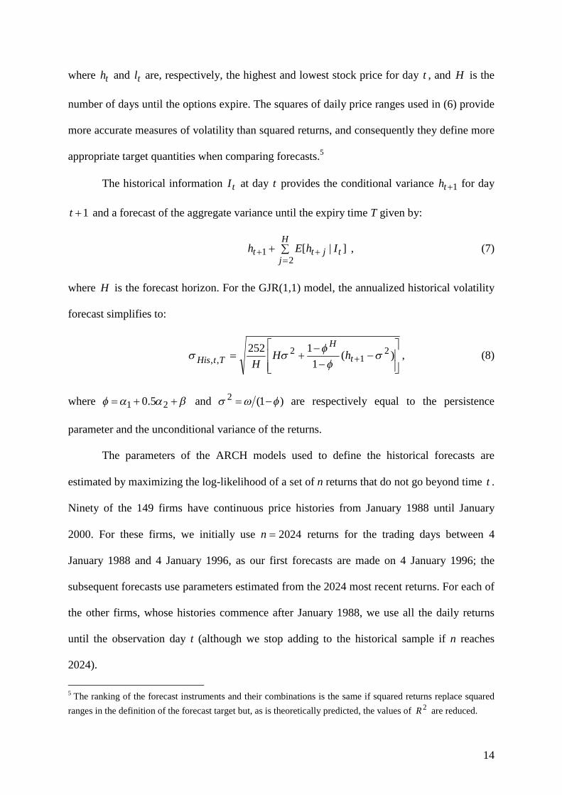
where th and tl are, respectively, the highest and lowest stock price for day t , and H is the

number of days until the options expire. The squares of daily price ranges used in (6) provide

more accurate measures of volatility than squared returns, and consequently they define more

appropriate target quantities when comparing forecasts.5

The historical information tI at day t provides the conditional variance 1th for day

1t and a forecast of the aggregate variance until the expiry time T given by:

H

jtjtt IhEh

21 ]|[ , (7)

where H is the forecast horizon. For the GJR(1,1) model, the annualized historical volatility

forecast simplifies to:

)(

1

1252 21

2,,

t

H

TtHis hHH

, (8)

where 21 5.0 and )1(2 are respectively equal to the persistence

parameter and the unconditional variance of the returns.

The parameters of the ARCH models used to define the historical forecasts are

estimated by maximizing the log-likelihood of a set of n returns that do not go beyond time t .

Ninety of the 149 firms have continuous price histories from January 1988 until January

2000. For these firms, we initially use 2024n returns for the trading days between 4

January 1988 and 4 January 1996, as our first forecasts are made on 4 January 1996; the

subsequent forecasts use parameters estimated from the 2024 most recent returns. For each of

the other firms, whose histories commence after January 1988, we use all the daily returns

until the observation day t (although we stop adding to the historical sample if n reaches

2024).

5 The ranking of the forecast instruments and their combinations is the same if squared returns replace squared

ranges in the definition of the forecast target but, as is theoretically predicted, the values of 2R are reduced.

15

5 Empirical results

5.1 Descriptive statistics

Table 1 presents summary statistics for daily estimates of the model-free volatility

expectation, the ATM implied volatility and their difference. The mean and standard

deviation are first obtained for each firm and the index from time series of volatility

estimates. Then the cross-sectional mean, lower quartile, median and upper quartile values of

each statistic, across the 149 firms, are calculated and displayed.

On average the model-free volatility expectation is slightly higher than the ATM

implied volatility, as also occurs in the study by Jiang and Tian (2005) on S&P 500 index

options. Consequently, the squared ATM implied volatility tends to be a downward biased

measure of the risk-neutral expected variance. The null hypothesis that the ATM implied

volatility is an unbiased estimate of the model-free volatility expectation is rejected for the

index and each of the 149 firms, at the 1% significance level, using the standard test. Table 1

also shows that the two volatility estimates are highly correlated, with the mean and median

of the correlations respectively equal to 0.926 and 0.940. These high values reflect the similar

information that is used to price ATM and OTM options.

Table 2 shows similar summary statistics for the one-month, volatility option-life

forecasts and outcomes. The realized volatility measured by daily high and low prices is

usually lower than the other volatility estimates, because discrete trading (both in time and in

price) induces a downward bias which is explained in Garman and Klass (1980).

Table 3 summarises the correlations between the four one-month volatility measures,

namely the historical forecast of the volatility during the remaining lifetime of a set of option

strikes, the at-the-money forecast, the model-free forecast and the realized volatility given by

16

(6). Across all the firms, the average correlation between the realized volatility and the ATM

implied volatility, the model-free expectation and the historical forecast respectively equals

0.502, 0.492 and 0.344. The highest correlations are between the ATM and the model-free

volatilities, and their average value equals 0.937.

5.2 One-day-ahead forecasts from ARCH specifications

Estimates of parameters

Table 4 provides the summary statistics of the sets of 149 point estimates (their mean,

standard deviation, lower quartile, median, and upper quartile) and the point estimates for the

S&P 100 index, from the three ARCH specifications defined by (4). All the ARCH

parameters are estimated using daily returns from January 1996 to December 1999. The

column headed “5%” contains the percentages of the firm-level estimates out of 149 that are

significantly different from zero at the 5% level.

Panel A summarises estimates for the GJR(1,1)-MA(1) model, which uses previous

stock returns to calculate the conditional variance. The value of 1 measures the symmetric

impact of new information (defined by t ) on volatility while the value of 2 measures the

additional impact of negative information (when 0t ). Approximately 75% of all firms

have a value of 21 that is more than twice the estimate of 1 , indicating a substantial

asymmetric effect for individual stocks. The volatility persistence parameter, assuming

returns are symmetrically distributed, is 21 5.0 . The median estimate of persistence

across the 149 firms equals 0.94.

Panel B provides results for the model which only uses the information contained in

the time series of model-free volatility expectations, 1, tMF . This series is filtered by the

function )1( L . For half of the firms, the estimates of are between 0.48 and 0.85. In

17

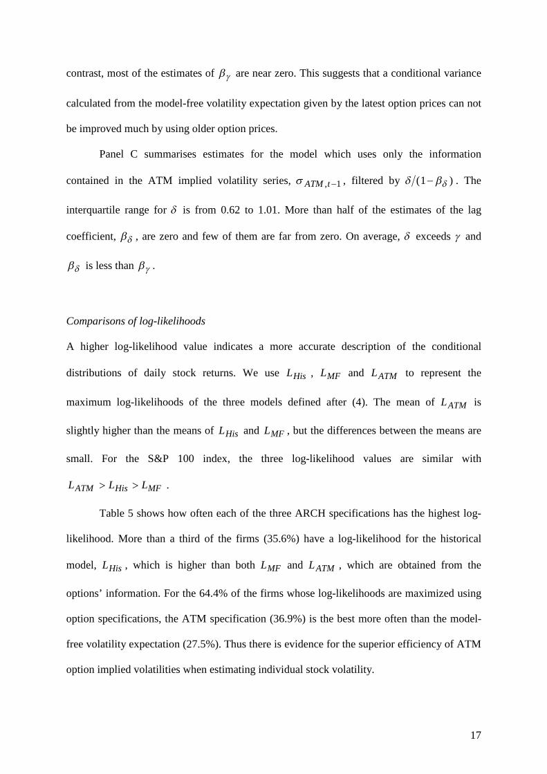
contrast, most of the estimates of are near zero. This suggests that a conditional variance

calculated from the model-free volatility expectation given by the latest option prices can not

be improved much by using older option prices.

Panel C summarises estimates for the model which uses only the information

contained in the ATM implied volatility series, 1, tATM , filtered by )1( . The

interquartile range for is from 0.62 to 1.01. More than half of the estimates of the lag

coefficient, , are zero and few of them are far from zero. On average, exceeds and

is less than .

Comparisons of log-likelihoods

A higher log-likelihood value indicates a more accurate description of the conditional

distributions of daily stock returns. We use HisL , MFL and ATML to represent the

maximum log-likelihoods of the three models defined after (4). The mean of ATML is

slightly higher than the means of HisL and MFL , but the differences between the means are

small. For the S&P 100 index, the three log-likelihood values are similar with

MFHisATM LLL .

Table 5 shows how often each of the three ARCH specifications has the highest log-

likelihood. More than a third of the firms (35.6%) have a log-likelihood for the historical

model, HisL , which is higher than both MFL and ATML , which are obtained from the

options’ information. For the 64.4% of the firms whose log-likelihoods are maximized using

option specifications, the ATM specification (36.9%) is the best more often than the model-

free volatility expectation (27.5%). Thus there is evidence for the superior efficiency of ATM

option implied volatilities when estimating individual stock volatility.

18

The high frequency for the historical specification providing the best description of

one-day-ahead volatility contrasts with the opposite evidence for options written on stock

indices, such as in Blair et al (2001). There are two plausible explanations for why the GJR

model performs the best for so many firms. Firstly, the key difference between the data for

individual stock options and the stock index options is that the latter are much more liquid

than the former. The illiquidity of individual stock options may cause the relative inefficiency

of their implied volatility expectations. When we select the 30 firms with the highest average

option trading volume, the historical volatility performs the best for only 2 firms, the model-

free volatility expectation for 11 firms and the ATM implied volatility for 17 firms. Secondly,

our ARCH specifications are estimated with a horizon of one day, while volatility estimates

from option prices represent the expected average price variation until the end of the option’s

life. The mismatch between the estimation horizon and the option’s time to expiry may

reduce the relative performance of both the model-free volatility expectation and the ATM

implied volatility when they are compared with the GJR(1,1) model.

5.3 Regression results for option-life forecasts

The regression results are for non-overlapping monthly observations, defined so that the

estimation horizon is matched with the option’s time to maturity. Table 6 reports the results

of both univariate and encompassing regressions that explain realized volatility, defined after

(6). As before, Table 6 shows the mean, median, lower and upper quartile of the point

estimates across the 149 firms and the point estimates for the S&P 100 index. The bracketed

number for each parameter is the percentage of firms whose estimates are significantly

different from zero at the 5% level. The last three columns show the summary statistics for

the regression 2R , the adjusted 2R and the sum of squared residuals.

19

We begin our discussion with the results of the univariate regressions summarised by

Table 6. The null hypotheses 0His , 0MF and 0ATM are separately rejected for

70%, 89% and 91% of the firms at the 5% level. The values of 2R are highest for the ATM

implied volatility (mean 0.290), but the values for the model-free volatility expectation are

similar (mean 0.278); the values for historical volatility, however, are much lower (mean

0.179). This evidence suggests that volatility estimates extracted from option prices are much

more informative than historical daily stock returns when the estimation horizons match the

lives of the options. The S&P 100 index forecasts rank in the same order as the firm averages

but the index values of 2R are higher than for most firms.

Table 5 provides the frequency counts that show how often each of the three

univariate forecasts has the highest value of 2R . There are important differences between the

frequencies for one-day-ahead forecasts (left block) and for option-life forecasts (right block).

Only 15.4% of the firms have historical volatility ranking highest for the option-life forecasts,

compared with 35.6% in the left block. Thus, only when the estimation horizon is matched do

we find that the option prices are clearly more informative than the historical daily returns.

Both the model-free volatility expectation and the ATM implied volatility rank as the best

more often in the right block than in the left block. The ATM implied volatility has the best

regression results for 52.4% of the sample firms, while the model-free volatility expectation

performs the best for 32.2%.

We next consider the encompassing regressions with two explanatory variables. Table

6 documents that the bivariate regression models which include the historical volatility

variable increase the average adjusted 2R values slightly from the univariate levels for

option specifications; from 0.290 to 0.319 for the ATM implied volatility and from 0.278 to

0.308 for the model-free (MF) volatility expectation. For 73 firms, the adjusted 2R of the

20

bivariate regression for the historical and MF variables is higher than that of the MF

univariate regression, although the null hypothesis 0His is only rejected for 37 firms at

the 5% level. Similarly, for 71 firms the adjusted 2R of the regression with the historical and

ATM variables is higher than that of the ATM univariate regression and 0His is rejected

for 32 firms at the 5% level. Therefore, for most firms the hypothesis that the historical

volatility is redundant when forecasting future volatility can not be rejected, which may be a

consequence of the informative option prices and/or the small number of forecasts that are

evaluated.

The MF and ATM bivariate regressions have an average adjusted 2R equal to 0.311,

which is fractionally less than the average for the bivariate regressions involving the

historical and the ATM volatilities. This can be explained by the very high correlation

between the model-free volatility expectation and the ATM implied volatility. For most

firms, both the null hypotheses 0MF and 0ATM can not be rejected at the 5% level,

showing that we can not conclude that one option measure subsumes all the information

contained in the other.

Finally, the highest average adjusted 2R , equal to 0.336, occurs when all three

volatility estimates define the explanatory variables in the regression model. Consequently,

the evidence overall favours the conclusion that every volatility estimate contains some

additional information beyond that provided by the other estimates. The mean values of

His , MF and ATM are respectively 0.118, 0.197 and 0.483, suggesting that the ATM

forecasts are the most informative.

6 Cross-sectional comparisons

21

6.1 Variables

None of the volatility estimation methods is consistently more accurate than the others for

most of our sample firms. We now investigate eight firm-specific variables, seeking to

identify variables which are associated with the best volatility estimation method. The

variables and their definitions are summarized in Table 7.

To explain the variation across firms in the performance of volatility estimates from

option prices relative to historical forecasts, the firm’s option trading liquidity is expected to

be the most important factor. The IvyDB database provides the option trading volume,

measured by option contracts, which is a proxy for liquidity. We also consider the firm’s

stock trading volume and its stock market capitalization, because firms with more liquid

stock trading and with larger size tend to have more liquid option trading. We conjecture that

firms with option prices more informative than historical volatilities have relatively high

average values of option trading volume, stock trading volume and market capitalization.

Theoretically the model-free volatility expectation is superior to ATM implied

volatility, as it is model-independent and contains information from a complete set of option

prices. We attempt to explain the generally superior empirical performance of the ATM

implied by using variables that proxy for model-free implementation problems. We consider

the average number of market available strike prices, because more strike prices will enable a

more accurate estimation of the implied volatility curve. According to the simulations in

Jiang and Tian (2005, 2007), the estimation error of the model-free volatility expectation is

higher firstly when the range of available strike prices is small and/or secondly when the

distance between adjacent strike prices is large; we measure these two distance criteria using

the moneyness scale.

The informational efficiency of the model-free volatility expectation relies on the

liquidity of OTM options. Consequently, we also consider the trading volume of ATM

22

options as a proportion of all option trading volume and conjecture that the proportion is

higher for those firms for which the ATM implied volatility outperforms the model-free

volatility expectation. With the same motivation, we also include the trading volume of

intermediate delta options divided by all option trading volume, where intermediate call

deltas are here defined as being between 0.25 rTe and 0.75 rTe .

6.2 Results

The means and standard deviations of each variable across the 149 firms are presented in

Panel A of Table 8.

In Panel B, we show summary statistics and test results for the 16 firms for which the

historical volatility is superior to option prices for both one-day-ahead and option-life

forecasts. These firms define the group called “His>OP”. Here OP refers to both the model-

free volatility expectation and the ATM implied volatility, and the group “His>OP” consists

of all firms that have both “His>MF” and “His>ATM”. Based on similar criteria, there are 72

firms satisfying “OP>His”, which is equivalent to both “MF>His” and “ATM>His”. First, as

expected, the averages of the three option liquidity proxies are lower for the group “His>OP”

than for the group “OP>His”. The standard two-sample t -test rejects the null hypothesis that

the two groups provide observations from a common distribution, at low significance levels;

the t -statistics are –6.30 (option volume), -4.41 (stock volume) and –4.18 (firm size). Second,

the same null hypothesis is also decisively rejected using the average number of traded strike

prices, which can also be considered an option liquidity proxy, as the t -statistic is –5.15.

Panel C compares the 34 firms satisfying “MF>ATM” for both one-day-ahead and

option-life forecasts with the 61 firms satisfying “ATM>MF” for both horizons. These group

sizes emphasize that the ATM implied volatility performs better than the model-free volatility

expectation for more firms across both forecast horizons. The t-statistic for firm size is

23

significant at the 5% level for one-sided tests, and it is significant for the strike price interval

at the 10% level; the firms in the group “MF>ATM” have a lower average size and a wider

average strike price interval which reflects a wider strike price range. Thus we find some

evidence that the theoretical advantages of the model-free volatility expectation are more

likely to be detected when the traded strike prices are more dispersed. We do not find

evidence that the relative trading volumes of ATM or intermediate delta options are

associated with the relative performance of the ATM implied volatility and the model-free

volatility expectation6.

The cross-sectional analysis shows that the relative performance of option prices and

historical methods for forecasting the volatility of individual stocks is strongly associated

with the liquidity of option trading. In contrast, the comparisons between the model-free

volatility expectation and the ATM implied volatility for individual stocks only provide weak

evidence that the dispersion of the strike prices is a relevant explanatory factor.

There are three possible explanations of the relatively unsatisfactory performance of

the model-free volatility expectation. Firstly, our options data might contain measurement

errors from the bid-ask spread and nonsynchronous trading of options and stocks, which

might be more severe for OTM options. The model-free volatility expectation, calculated as a

function of option prices across all strikes, might then contain more noise in total than the

ATM implied volatility. Secondly, the trading of individual stock options, especially OTM,

might have been insufficient to reflect the theoretical advantages of the model-free volatility

expectation; the most liquid options in our study have option trading volumes far below the

levels observed for stock indices. Thirdly, as noted by the referee, the model-free volatility

expectation gives more weight to OTM puts than to OTM calls and it is the puts which reflect

6 Negative conclusions have also been obtained for the average realized volatility, the average risk-neutralskewness and estimates of systematic risk.

24

default risk; however, our firms all survive and hence the observed forecast targets do not

include any exceptional prices when firms fail.

7 Conclusions

This paper provides the first comparison of the information content of three volatility

measures for a large set of U.S. stocks, namely a forecast obtained from historical prices, the

at-the-money implied volatility and the newly-developed model-free volatility expectation.

We find that each of the three volatility estimates contains some, but not all, relevant

information about the future variation of the underlying asset returns.

The consensus from studies about the informational efficiency of U.S. stock index

options is that these option prices are significantly more informative than historical returns

when predicting index volatility. Our analysis of 149 firms shows that a different conclusion

applies to options for individual firms. For one-day-ahead estimation, more than a third of our

firms do not have volatility estimates, extracted from option prices, that are more accurate

than those provided by a simple ARCH model estimated from daily stock returns. When the

prediction horizon extends until the expiry date of the options, the historical volatility

becomes less informative than either the ATM implied volatility or the model-free volatility

expectation for 126 of the 149 firms. Our results also show that both volatility estimates from

option prices are more likely to outperform historical returns when the firm has higher option

trading activity, as measured either by option volume or the number of strikes traded.

The recent interest shown in the model-free volatility expectation is explained by the

few assumptions required to derive the model-free formula. The formula has the limitation,

however, that it is an integral function of a complete set of option prices. As few strikes are

traded for individual firms, we use a quadratic function of a delta quantity to estimate implied

25

volatility curves from which we can derive the required interpolated option prices. Although

the model-free volatility expectation has been conclusively shown to be the most accurate

predictor of realized volatility by Jiang and Tian (2005) for the S&P 500 index, it only

outperforms both the ATM implied volatility and the historical volatility for about one-third

of our sample firms. In contrast, the ATM implied volatility is the method that most often

performs the best. When the ATM implied volatility outperforms the model-free volatility for

a firm, we find that the relative trading volume of ATM options is not significantly higher

than otherwise.

Our paper shows that model-free methods do not realize their theoretical potential for

some assets. The relatively unsatisfactory performance of the model-free volatility

expectation for individual firms can be attributed to the illiquidity of their OTM options,

which reduces the aggregate information content of the available option prices. Compared

with an index, at the firm level fewer strikes are traded, option bid-ask spreads are wider and

recorded option prices are more likely to be nonsynchronous with the price of the underlying

asset.

26

References

Andersen, Torben G., Tim Bollerslev, Francis X. Diebold and Heiko Ebens, 2001, The

distribution of realized stock volatility, Journal of Financial Economics 61, 43-76.

Andersen, Torben G., Tim Bollerslev, Francis X. Diebold and Paul Labys, 2003, Modeling

and forecasting realized volatility, Econometrica 71, 579-625.

Blair, Bevan J., Ser-Huang Poon, and Stephen J. Taylor, 2001, Forecasting S&P 100

volatility: the incremental information content of implied volatilities and high-

frequency index returns, Journal of Econometrics 105, 5-26.

Bliss, Robert R., and Nikolaos Panigirtzoglou, 2002, Testing the stability of implied

probability density functions, Journal of Banking and Finance 26, 381-422.

Bliss, Robert R., and Nikolaos Panigirtzoglou, 2004, Option-implied risk aversion estimates,

Journal of Finance 59, 407-446.

Bollerslev, Tim, and Jeffrey M. Wooldridge, 1992, Quasi-maximum likelihood estimation

and inference in dynamic models with time-varying covariances, Econometric

Reviews 11, 143-179.

Britten-Jones, Mark, and Anthony Neuberger, 2000, Option prices, implied price processes,

and stochastic volatility, Journal of Finance 55, 839-866.

Canina, Linda, and Stephen Figlewski, 1993, The informational content of implied volatility,

Review of Financial Studies 6, 659-681.

Carr, Peter, and Roger Lee, 2008, Robust Replication of Volatility Derivatives, working

paper, New York University and University of Chicago.

Carr, Peter, and Dilip Madan, 1998, Towards a theory of volatility trading, in Robert A.

Jarrow, ed.: Volatility (Risk Books, London), 417-427.

Carr, Peter, and Liuren Wu, 2006, A tale of two indices, Journal of Derivatives 13, 13-29.

27

Carr, Peter, and Liuren Wu, 2009, Variance risk premiums, Review of Financial Studies 22,

1311-1341.

Cheung, Yin-Wong, and Lilian K. Ng, 1992, Stock price dynamics and firm size: an

empirical investigation, Journal of Finance 47, 1985-1997.

Christensen, Bent J., and Nagpurnanand R. Prabhala, 1998, The relation between implied and

realized volatility, Journal of Financial Economics 50, 125-150.

Day, Theodore E., and Craig M. Lewis, 1992, Stock market volatility and the information

content of stock index options, Journal of Econometrics 52, 267-287.

Demeterfi, Kresimir, Emanuel Derman, Michael Kamal, and Joseph Zou, 1999, A guide to

volatility and variance swaps, Journal of Derivatives 6, 9-32.

Duffee, Gregory R., 1995, Stock returns and volatility a firm-level analysis, Journal of

Financial Economics 37, 399-420.

Ederington, Louis H, and Wei Guan, 2002, Measuring implied volatility: Is an average

better? Which average?, Journal of Futures Markets 22, 811-837.

Ederington, Louis H, and Wei Guan, 2005, Forecasting volatility, Journal of Futures Markets

25, 465-490.

Fleming, Jeff, 1998, The quality of market volatility forecasts implied by S&P 100 index

option prices, Journal of Empirical Finance 5, 317-345.

Garman, Mark B., and Michael J. Klass, 1980, On the estimation of security price volatilities

from historical data, Journal of Business 53, 67-78.

Glosten, Lawrence R., Ravi Jagannathan, and David E. Runkle, 1993, On the relation

between the expected value and the volatility of the nominal excess return on stocks,

Journal of Finance 48, 1779-1801.

Heston, Steven L., 1993, A closed-form solution for options with stochastic volatility with

applications to bond and currency options, Review of Financial Studies 6, 327-343.

28

Jiang, George J., and Yisong S. Tian, 2005, The model-free implied volatility and its

information content, Review of Financial Studies 18, 1305.

Jiang, George J., and Yisong S. Tian, 2007, Extracting model-free volatility from option

prices: an examination of the VIX Index, Journal of Derivatives 14, 35-60.

Lamoureux, Christopher G., and William D. Lastrapes, 1993, Forecasting stock-return

variance: toward an understanding of stochastic implied volatilities, Review of

Financial Studies 6, 293-326.

Lynch, Damien P., and Nikolaos Panigirtzoglou, 2004, Option implied and realized measures

of variance, working paper, Bank of England.

Malz, Allan M, 1997a, Estimating the probability distribution of the future exchange rate

from option prices, Journal of Derivatives 5, 18.

Malz, Allan M, 1997b, Option-implied probability distributions and currency excess returns,

Staff Reports 32, Federal Reserve Bank of New York.

Parkinson, Michael, 1980, The extreme value method for estimating the variance of the rate

of return, Journal of Business 53, 61-65.

Poon, Ser-Huang, and Clive W. J. Granger, 2003, Forecasting volatility in financial markets:

a review, Journal of Economic Literature 41, 478-539.

Taylor, Stephen J., 2005, Asset Price Dynamics, Volatility, and Prediction (Princeton

University Press, Princeton).

White, Halbert, 1980, A heteroskedasticity-consistent covariance matrix estimator and a

direct test for heteroskedasticity, Econometrica 48, 817-838.

Zhang, Xiaoyan, Rui Zhao and Yuhang Xing, 2008, What does individual option volatility

smirk tell us about future equity returns?, Journal of Financial and Quantitative

Analysis, forthcoming.

29

Table 1 Summary statistics for daily estimates of volatility from option prices

The cross-sectional statistics are calculated from the means and standard deviations of dailyobservations from time series, which cover the period from January 1996 to December 1999. Thecross-sectional mean, lower quartile ( 1Q ), median ( 2Q ) and upper quartile ( 3Q ) values of each

statistic are reported in the columns, across 149 firms. MF and ATM are daily estimates of the

model-free volatility expectation and the at-the-money implied volatility. The time-series statistics forthe S&P 100 index are reported in the last column.

Firms S&P 100

Mean 1Q 2Q 3Q

Panel A: MF

Mean 0.523 0.371 0.521 0.646 0.225

Std. Dev. 0.123 0.078 0.106 0.131 0.056

Panel B: ATM

Mean 0.486 0.351 0.484 0.610 0.200

Std. Dev. 0.099 0.072 0.094 0.114 0.050

Panel C: ATMMF

Mean 0.036 0.024 0.032 0.043 0.025

Std. Dev. 0.051 0.026 0.035 0.048 0.010

Panel D: Correlation between MF and ATM

Correlation 0.926 0.907 0.940 0.960 0.989

30

Table 2 Summary statistics for historical and option-based measures of volatility

The reported statistics are for monthly observations of annualized measures of volatility. MF , ATM , His and RE are respectively the values of the

model-free volatility expectation, the at-the-money implied volatility, the historical forecast from a GARCH model and the realized volatility calculated fromdaily high and low prices using the formula of Parkinson (1980). All these volatility measures are for the remaining lifetimes of option contracts, which areapproximately one month.

The cross-sectional statistics are calculated from descriptive statistics for monthly observations from time series, which cover the period from January 1996 toDecember 1999. The cross-sectional lower quartile, median and upper quartile values of each statistic are reported in the columns, across 149 firms. The time-series statistics for the S&P 100 index are also reported.

MF ATM His RE

Firms S&P 100 Firms S&P 100 Firms S&P 100 Firms S&P 100

1Q 2Q 3Q 1Q 2Q 3Q 1Q 2Q 3Q 1Q 2Q 3Q

Mean 0.37 0.51 0.64 0.22 0.35 0.49 0.61 0.20 0.32 0.50 0.60 0.15 0.29 0.42 0.54 0.15

Std.Dev. 0.07 0.09 0.11 0.05 0.06 0.09 0.11 0.04 0.05 0.08 0.11 0.04 0.09 0.11 0.15 0.05

Skewness 0.43 0.78 1.12 1.08 0.38 0.70 1.10 0.75 0.69 1.28 2.05 1.59 0.60 1.03 1.45 1.95

Kurtosis 3.37 3.25 4.62 4.90 3.61 3.20 4.52 3.62 3.53 5.71 8.89 6.20 3.08 4.21 5.86 8.09

Max 0.59 0.80 0.98 0.40 0.56 0.71 0.90 0.34 0.52 0.73 0.94 0.32 0.57 0.80 0.99 0.36

Min 0.25 0.36 0.45 0.13 0.23 0.34 0.43 0.12 0.22 0.34 0.46 0.09 0.16 0.22 0.31 0.09

31

Table 3 Summary statistics for the correlations between volatility measures

The summarised correlations are between monthly observations of annualized measures of volatility. MF , ATM , His and RE are respectively the

values of the model-free volatility expectation, the at-the-money implied volatility, the historical forecast from a GARCH model and the realized volatilitycalculated from daily high and low prices using the formula of Parkinson (1980). All these volatility measures are for the remaining lifetimes of optioncontracts, which are approximately one month.

Each correlation is between monthly observations from two time series for the same firm, which cover the period from January 1996 to December 1999. Thecross-sectional mean, lower quartile, median and upper quartile of each set of correlation statistics is calculated across 149 firms. The columns headed S&P100 report the correlations between monthly volatility observations from the index and another time series.

MF ATM His

Firms S&P 100 FirmsS&P

100Firms

S&P

100

Mean 1Q 2Q 3Q Mean 1Q 2Q 3Q Mean 1Q 2Q 3Q

ATM 0.937 0.923 0.952 0.971 0.988

His 0.547 0.373 0.576 0.745 0.892 0.562 0.412 0.577 0.747 0.883

RE 0.492 0.373 0.516 0.627 0.623 0.502 0.377 0.516 0.621 0.624 0.344 0.191 0.343 0.500 0.483

32

Table 4 A summary of the ARCH parameter estimates obtained from 149 firms

Daily stock returns tr are modeled by the ARCH specification: 1 tttr ,

ttt zh , )1,0.(..~ diizt ,LLL

sh

tATMtMFtttt

111

21,

21,

2112

211 , ts is 1 if 0t ,

otherwise ts is zero. MF and ATM are respectively the daily measure of model-free

volatility expectation and the ATM implied volatility. All parameters are estimated bymaximizing the quasi-log-likelihood function. Panel A contains the results for the GJR (1,1)-MA(1) model. Panels B and C respectively show estimates for models that use informationprovided by the model-free volatility expectation and the ATM implied volatility. Cross-sectional means, standard deviations, lower quartiles, medians and upper quartiles arepresented across 149 firms. The column headed 5% shows the percentages of estimates whichare significantly different from zero at the 5% level, using the robust t-ratios of Bollerslev andWooldridge (1992). The last column reports the parameter estimates for the S&P 100 index;the starred estimates are significantly different from zero at the 5% level. HisL , MFL and

ATML are the maximized log-likelihood values of the three models.

Mean Std. Dev. 1Q 2Q 3Q 5% S&P 100

Panel A: the GJR (1,1)-MA (1) model310 0.91 0.96 0.40 0.85 1.42 11.4 0.88*

0.00 0.06 -0.04 0.00 0.04 16.1 0.00510 17.61 28.93 1.57 5.91 17.89 63.8 0.58*

1 0.05 0.07 0.00 0.03 0.06 20.1 0.00

2 0.12 0.20 0.04 0.08 0.13 43.0 0.21* 0.77 0.23 0.66 0.86 0.93 93.3 0.85*

Persistence 0.87 0.18 0.81 0.94 0.98 0.96

HisL 2141 340 1860 2083 2438 3168

Panel B: the ARCH specification that only uses the model-free volatility expectation310 0.77 0.92 0.33 0.73 1.22 12.8 0.75*

0.01 0.05 -0.03 0.00 0.05 17.4 0.05510 10.35 25.16 0.00 0.49 10.15 0.7 0.00

0.65 0.26 0.48 0.71 0.85 50.3 0.58*

0.19 0.26 0.00 0.03 0.34 7.4 0.00

1 0.80 0.19 0.72 0.83 0.90 0.58

MFL 2143 339 1872 2075 2454 3165

Panel C: the ARCH specification that only uses the ATM implied volatility310 0.77 0.91 0.35 0.71 1.23 11.4 0.77*

0.01 0.05 -0.03 0.01 0.05 15.4 0.05510 9.41 22.27 0.00 0.00 7.27 0 0.00

0.81 0.29 0.62 0.88 1.01 42.3 0.73*

0.14 0.24 0.00 0.00 0.20 4.0 0.00

1 0.92 0.22 0.84 0.96 1.04 0.73

ATML 2144 340 1870 2078 2453 3170

33

Table 5 Frequency counts for the variables that best describe the volatility ofstock returns

The counts and percentages show how many of the 149 firms satisfy the ordering stated in thefirst column. For one-day-ahead forecasts, the frequency counts are based on the maximizedlog-likelihood values of the ARCH specifications that respectively use historical daily returns(His), the model-free volatility expectation (MF) and the ATM implied volatility. For option-life forecasts, the frequency counts are based on the explanatory powers of the univariateregressions that contain historical volatility, the model-free volatility expectation and theATM implied volatility.

For one-day-ahead

forecasts

For options’ life

forecasts

Historical is best 53 35.6% 23 15.4%

His>MF>ATM 21 14.1% 12 8.1%

His>ATM>MF 32 21.5% 11 7.4%

Model-free is best 41 27.5% 48 32.2%

MF>ATM>His 38 25.5% 45 30.2%

MF>His>ATM 3 2.0% 3 2.0%

At-the-money is best 55 36.9% 78 52.4%

ATM>MF>His 49 32.9% 61 41.0%

ATM>His>MF 6 4.0% 17 11.4%

34

Table 6 Summary statistics for regression models when the dependent variableis realized volatility

The most general estimated regression model for the logarithm of realized volatility is:

TtRE ,,100ln = 0 + TtHisHis ,,100ln + MF TtMF ,,100ln + ATM TtATM ,,100ln + Tt , ,

where RE , MF , ATM and His respectively refer to the realized volatility calculated

from the formula of Parkinson (1980), the model-free volatility expectation, the at-the-money

option implied volatility and the historical forecast obtained from the GJR-GARCH model

specified in Table 4. The regressions are estimated by OLS for each of the 149 firms in the

sample, from which the cross-sectional mean, lower quartile, median and upper quartile are

calculated for each model coefficient. The numbers in parentheses are the percentages of

firms whose estimates are significantly different from zero at the 5% level. Inferences are

made using standard errors that are robust against heteroscedasticity [White (1980)]. The

rows headed S&P 100 report the regression results for the index; the starred estimates are

significantly different from zero at the 5% level. SSE is the sum of squared errors for the

regression.

0 His MF ATM 2R2.Radj SSE

His Mean 1.344 0.620 0.179 0.162 0.059

1Q 0.250 0.378 0.050 0.030 0.044

2Q 1.288 0.618 0.136 0.117 0.053

3Q 2.312 0.889 0.270 0.254 0.067

(44.3) (69.8)

S&P 100 1.254* 0.538* 0.242 0.226 0.064

MF Mean 0.834 0.731 0.278 0.262 0.052

1Q 0.170 0.594 0.145 0.127 0.038

2Q 0.764 0.749 0.263 0.247 0.047

3Q 1.374 0.887 0.390 0.377 0.064

(24.8) (88.6)

S&P 100 0.092 0.852* 0.426 0.414 0.048

ATM Mean 0.713 0.775 0.290 0.275 0.051

1Q 0.016 0.601 0.155 0.137 0.037

2Q 0.673 0.777 0.284 0.268 0.047

3Q 1.310 0.960 0.396 0.383 0.061

(22.8) (90.6)

S&P 100 0.179 0.852* 0.438 0.426 0.047

35

His + MF Mean 0.607 0.182 0.613 0.308 0.278 0.049

1Q -0.179 -0.016 0.372 0.175 0.140 0.036

2Q 0.501 0.187 0.645 0.290 0.259 0.046

3Q 1.145 0.418 0.812 0.424 0.399 0.062

(12.1) (24.8) (67.1)

S&P 100 -0.062 -0.320 1.180* 0.447 0.423 0.048

His + ATM Mean 0.601 0.127 0.680 0.319 0.289 0.049

1Q -0.257 -0.074 0.477 0.180 0.144 0.036

2Q 0.412 0.154 0.692 0.307 0.277 0.045

3Q 1.125 0.389 0.873 0.425 0.401 0.058

(14.8) (21.5) (73.2)

S&P 100 0.059 -0.358 1.218* 0.465 0.441 0.046

MF + ATM Mean 0.714 0.252 0.519 0.311 0.281 0.049

1Q -0.025 -0.254 0.092 0.170 0.133 0.036

2Q 0.631 0.214 0.576 0.302 0.271 0.046

3Q 1.399 0.676 1.053 0.425 0.400 0.060

(23.5) (11.4) (23.5)

S&P 100 0.185 -0.034 0.886 0.438 0.414 0.048

His+MF+ATM Mean 0.067 0.118 0.197 0.483 0.336 0.292 0.047

1Q 0.003 -0.086 -0.280 0.049 0.196 0.142 0.035

2Q 0.036 0.153 0.138 0.572 0.330 0.285 0.044

3Q 0.157 0.363 0.599 0.983 0.453 0.415 0.057

(13.4) (18.1) (9.4) (18.1)

S&P 100 0.031 -0.363 0.147 1.080 0.465 0.429 0.047

36

Table 7 Definitions of eight firm-specific variables

This table defines eight firm-specific candidate variables, which may be associated with thebest volatility estimation method. The first three variables are plausible variables whencomparing the relative advantages of historical and option-based methods, while theremaining five variables may help to explain when the model-free volatility expectationoutperforms the at-the-money implied volatility.

All variables for each firm are calculated as time-series averages of daily measures fromJanuary 1996 to December 1999. The option-related variables are only calculated from theoption contracts described in Section 3. Moneyness is defined as the option strike pricedivided by the matched forward price.

Variable Definition

TV_OP The natural logarithm of the firm’s average

option trading volume.

TV_Stock The natural logarithm of the firm’s average stock

trading volume.

FirmSize The natural logarithm of the firm’s average size,

measured in thousands of dollars, and calculated

as the number of shares outstanding multiplied

by the closing stock price.

Moneyness Range The maximum moneyness minus the minimum

moneyness.

Strike Prices The number of available option strike prices.

Average Strike Price Interval The average interval between adjacent strike

prices, measured in moneyness units.

TV_ATM/TV_ALL At-the-money option trading volume divided by

total option trading volume.

TV_IntermediateDelta/TV_ALL The trading volume of intermediate delta options

divided by total trading volume, where

intermediate delta options have deltas within the

interquartile range of feasible delta values.

37

Table 8 Comparisons of the firm-specific variables for selected groups of firms

Averages and standard deviations (shown in parentheses) are tabulated for various firm-specific variables, for all firms in Panel A and for selected groups offirms in Panels B and C. MF, ATM and His respectively refer to the model-free volatility expectation, the ATM implied volatility and historical volatilitymethods. The symbol OP refers to both MF and ATM. Panel B shows results for those firms having both option-based methods performing either worse orbetter than His, for both one-day-ahead and option-life forecasts. Panel C covers those firms with MF performing either better or worse than ATM for bothone-day-ahead and option-life forecasts. The t -statistics are for the standard two-sample test of the null hypothesis of equal population means, while the p-values are for one-tail tests.

Firms TV_OP TV_Stock FirmSizeMoneyness

RangeStrikePrices

Average StrikePrice Interval

TV_ATM/TV_ALL

TV_IntermediateDelta/TV_ALL

Panel A: all firms

149 6.18 13.92 22.60 0.39 5.44 0.10 0.42 0.62

(1.42) (1.07) (1.65) (0.11) (1.54) (0.03) (0.06) (0.07)

Panel B: OP versus His

His>OP 16 5.18 13.24 21.81 0.37 4.59 0.11 0.43 0.60(0.90) (1.03) (1.09) (0.11) (0.65) (0.03) (0.06) (0.09)

OP>His 72 6.88 14.46 23.19 0.40 5.96 0.09 0.43 0.64(1.29) (0.85) (1.57) (0.12) (1.77) (0.03) (0.06) (0.04)

t statistic -6.30 -4.41 -4.17 -0.80 -5.15 2.15 0.54 -1.76p value 0.00 0.00 0.00 0.22 0.00 0.02 0.30 0.05

Panel C: MF versus ATM

MF>ATM 34 6.04 13.85 22.18 0.41 5.17 0.11 0.43 0.63(1.43) (1.04) (1.50) (0.11) (1.22) (0.03) (0.06) (0.06)

ATM>MF 61 6.35 14.05 22.86 0.39 5.51 0.10 0.43 0.63(1.32) (0.97) (1.63) (0.12) (1.48) (0.03) (0.06) (0.07)

t statistic -1.04 -0.92 -2.07 0.88 -1.20 1.49 0.11 0.12p value 0.15 0.18 0.02 0.19 0.12 0.07 0.46 0.45

Cfr/Working Paper Series

Centre for Financial Research Look deeper

CFR Working Papers are available for download from www.cfr-cologne.de. Hardcopies can be ordered from: Centre for Financial Research (CFR), Albertus Magnus Platz, 50923 Koeln, Germany.

2009 No. Author(s) Title 09-07 S. J. Taylor , P. K. Yadav,

Y. Zhang The information content of implied volatilities and model-free volatility expectations: Evidence from options written on individual stocks

09-06 S. Frey, P. Sandas The Impact of Iceberg Orders in Limit Order Books

09-05 H. Beltran-Lopez, P. Giot, J. Grammig

Commonalities in the Order Book

09-04 J. Fang, S. Ruenzi Rapid Trading bei deutschen Aktienfonds: Evidenz aus einer großen deutschen Fondsgesellschaft

09-03 A. Banegas, B. Gillen, A. Timmermann, R. Wermers

The Performance of European Equity Mutual Funds

09-02 J. Grammig, A. Schrimpf, M. Schuppli

Long-Horizon Consumption Risk and the Cross-Section of Returns: New Tests and International Evidence

09-01 O. Korn, P. Koziol The Term Structure of Currency Hedge Ratios 2008 No. Author(s) Title 08-12 U. Bonenkamp,

C. Homburg, A. Kempf Fundamental Information in Technical Trading Strategies

08-11 O. Korn Risk Management with Default-risky Forwards

08-10 J. Grammig, F.J. Peter International Price Discovery in the Presence of Market Microstructure Effects

08-09 C. M. Kuhnen, A. Niessen Is Executive Compensation Shaped by Public Attitudes?

08-08 A. Pütz, S. Ruenzi Overconfidence among Professional Investors: Evidence from Mutual Fund Managers

08-07 P. Osthoff What matters to SRI investors?

08-06 A. Betzer, E. Theissen Sooner Or Later: Delays in Trade Reporting by Corporate Insiders

08-05 P. Linge, E. Theissen Determinanten der Aktionärspräsenz auf Hauptversammlungen deutscher Aktiengesellschaften

08-04 N. Hautsch, D. Hess, C. Müller

Price Adjustment to News with Uncertain Precision

08-03 D. Hess, H. Huang, A. Niessen

How Do Commodity Futures Respond to Macroeconomic News?

No. Author(s) Title 08-02 R. Chakrabarti,

W. Megginson, P. Yadav Corporate Governance in India

08-01 C. Andres, E. Theissen Setting a Fox to Keep the Geese - Does the Comply-or-Explain Principle Work?

2007 No. Author(s) Title 07-16 M. Bär, A. Niessen,

S. Ruenzi The Impact of Work Group Diversity on Performance: Large Sample Evidence from the Mutual Fund Industry

07-15 A. Niessen, S. Ruenzi Political Connectedness and Firm Performance:

Evidence From Germany

07-14 O. Korn Hedging Price Risk when Payment Dates are Uncertain 07-13 A. Kempf, P. Osthoff SRI Funds: Nomen est Omen

07-12 J. Grammig, E. Theissen, O. Wuensche

Time and Price Impact of a Trade: A Structural Approach

07-11 V. Agarwal, J. R. Kale On the Relative Performance of Multi-Strategy and Funds of Hedge Funds

07-10 M. Kasch-Haroutounian, E. Theissen

Competition Between Exchanges: Euronext versus Xetra

07-09 V. Agarwal, N. D. Daniel, N. Y. Naik

Why is Santa so kind to hedge funds? The December return puzzle!

07-08 N. C. Brown, K. D. Wei, R. Wermers

Analyst Recommendations, Mutual Fund Herding, and Overreaction in Stock Prices

07-07 A. Betzer, E. Theissen Insider Trading and Corporate Governance: The Case of Germany

07-06 V. Agarwal, L. Wang Transaction Costs and Value Premium

07-05 J. Grammig, A. Schrimpf Asset Pricing with a Reference Level of Consumption: New Evidence from the Cross-Section of Stock Returns

07-04 V. Agarwal, N.M. Boyson, N.Y. Naik

Hedge Funds for retail investors? An examination of hedged mutual funds

07-03 D. Hess, A. Niessen The Early News Catches the Attention: On the Relative Price Impact of Similar Economic Indicators

07-02 A. Kempf, S. Ruenzi, T. Thiele

Employment Risk, Compensation Incentives and Managerial Risk Taking - Evidence from the Mutual Fund Industry -

07-01 M. Hagemeister, A. Kempf CAPM und erwartete Renditen: Eine Untersuchung auf Basis der Erwartung von Marktteilnehmern

2006 No. Author(s) Title 06-13 S. Čeljo-Hörhager,

A. Niessen How do Self-fulfilling Prophecies affect Financial Ratings? - An experimental study -

06-12 R. Wermers, Y. Wu, J. Zechner

Portfolio Performance, Discount Dynamics, and the Turnover of Closed-End Fund Managers

06-11 U. v. Lilienfeld-Toal, S. Ruenzi

Why Managers Hold Shares of Their Firm: An Empirical Analysis

06-10 A. Kempf, P. Osthoff The Effect of Socially Responsible Investing on Portfolio Performance

06-09 R. Wermers, T. Yao, J. Zhao

The Investment Value of Mutual Fund Portfolio Disclosure

No. Author(s) Title 06-08 M. Hoffmann, B. Kempa The Poole Analysis in the New Open Economy

Macroeconomic Framework

06-07 K. Drachter, A. Kempf, M. Wagner

Decision Processes in German Mutual Fund Companies: Evidence from a Telephone Survey

06-06 J.P. Krahnen, F.A. Schmid, E. Theissen

Investment Performance and Market Share: A Study of the German Mutual Fund Industry

06-05 S. Ber, S. Ruenzi On the Usability of Synthetic Measures of Mutual Fund Net-Flows

06-04 A. Kempf, D. Mayston Liquidity Commonality Beyond Best Prices 06-03 O. Korn, C. Koziol Bond Portfolio Optimization: A Risk-Return Approach

06-02 O. Scaillet, L. Barras, R. Wermers

False Discoveries in Mutual Fund Performance: Measuring Luck in Estimated Alphas

06-01 A. Niessen, S. Ruenzi Sex Matters: Gender Differences in a Professional Setting 2005 No. Author(s) Title 05-16 E. Theissen An Analysis of Private Investors´ Stock Market Return

Forecasts

05-15 T. Foucault, S. Moinas, E. Theissen

Does Anonymity Matter in Electronic Limit Order Markets

05-14 R. Kosowski, A. Timmermann, R. Wermers, H. White

Can Mutual Fund „Stars“ Really Pick Stocks? New Evidence from a Bootstrap Analysis

05-13 D. Avramov, R. Wermers Investing in Mutual Funds when Returns are Predictable

05-12 K. Griese, A. Kempf Liquiditätsdynamik am deutschen Aktienmarkt

05-11 S. Ber, A. Kempf, S. Ruenzi

Determinanten der Mittelzuflüsse bei deutschen Aktienfonds

05-10 M. Bär, A. Kempf, S. Ruenzi

Is a Team Different From the Sum of Its Parts? Evidence from Mutual Fund Managers

05-09 M. Hoffmann Saving, Investment and the Net Foreign Asset Position

05-08 S. Ruenzi Mutual Fund Growth in Standard and Specialist Market Segments

05-07 A. Kempf, S. Ruenzi Status Quo Bias and the Number of Alternatives - An Empirical Illustration from the Mutual Fund Industry –

05-06 J. Grammig, E. Theissen

Is Best Really Better? Internalization in Xetra Best

05-05 H. Beltran, J. Grammig, A.J. Menkveld

Understanding the Limit Order Book: Conditioning on Trade Informativeness

05-04 M. Hoffmann Compensating Wages under different Exchange rate Regimes

05-03 M. Hoffmann Fixed versus Flexible Exchange Rates: Evidence from Developing Countries

05-02 A. Kempf, C. Memmel On the Estimation of the Global Minimum Variance Portfolio

05-01 S. Frey, J. Grammig Liquidity supply and adverse selection in a pure limit order book market

2004 No. Author(s) Title 04-10 N. Hautsch, D. Hess Bayesian Learning in Financial Markets – Testing for the

Relevance of Information Precision in Price Discovery

04-09 A. Kempf, K. Kreuzberg

Portfolio Disclosure, Portfolio Selection and Mutual Fund Performance Evaluation

04-08 N.F. Carline, S.C. Linn, P.K. Yadav

Operating performance changes associated with corporate mergers and the role of corporate governance

04-07 J.J. Merrick, Jr., N.Y. Naik, P.K. Yadav

Strategic Trading Behavior and Price Distortion in a Manipulated Market: Anatomy of a Squeeze

04-06 N.Y. Naik, P.K. Yadav Trading Costs of Public Investors with Obligatory and Voluntary Market-Making: Evidence from Market Reforms

04-05 A. Kempf, S. Ruenzi Family Matters: Rankings Within Fund Families and Fund Inflows

04-04 V. Agarwal, N.D. Daniel, N.Y. Naik

Role of Managerial Incentives and Discretion in Hedge Fund Performance

04-03 V. Agarwal, W.H. Fung, J.C. Loon, N.Y. Naik

Liquidity Provision in the Convertible Bond Market: Analysis of Convertible Arbitrage Hedge Funds

04-02 A. Kempf, S. Ruenzi Tournaments in Mutual Fund Families

04-01 I. Chowdhury, M. Hoffmann, A. Schabert

Inflation Dynamics and the Cost Channel of Monetary Transmission

Cfr/University of cologne

Albertus-Magnus-Platz

D-50923 Cologne

Fon +49(0)221-470-6995

Fax +49(0)221-470-3992

Kempf@cfr-Cologne.dewww.cfr-cologne.de