University of South FloridaScholar Commons

Graduate School Theses and Dissertations Graduate School

1-1-2012

On the spatial and temporal variability of upwellingin the southern Caribbean Sea and its influence onthe ecology of phytoplankton and of the Spanishsardine (Sardinella aurita)Digna Tibisay Rueda-RoaUniversity of South Florida, dignarueda@gmail.com

Follow this and additional works at: http://scholarcommons.usf.edu/etdPart of the American Studies Commons, Oceanography Commons, Other Earth Sciences

Commons, and the Other Oceanography and Atmospheric Sciences and Meteorology Commons

This Dissertation is brought to you for free and open access by the Graduate School at Scholar Commons. It has been accepted for inclusion inGraduate School Theses and Dissertations by an authorized administrator of Scholar Commons. For more information, please contactscholarcommons@usf.edu.

Scholar Commons CitationRueda-Roa, Digna Tibisay, "On the spatial and temporal variability of upwelling in the southern Caribbean Sea and its influence on theecology of phytoplankton and of the Spanish sardine (Sardinella aurita)" (2012). Graduate School Theses and Dissertations.http://scholarcommons.usf.edu/etd/4217

On the spatial and temporal variability of upwelling in the southern Caribbean Sea and its

influence on the ecology of phytoplankton and of the Spanish sardine (Sardinella aurita)

by

Digna T. Rueda-Roa

A dissertation submitted in partial fulfillment

of the requirements for the degree of

Doctor of Philosophy

College of Marine Science

University of South Florida

Major Professor: Frank E. Muller-Karger, Ph.D.

Mark Luther, Ph.D.

Ernst Peebles, Ph.D.

David Hollander, Ph.D.

Eduardo Klein, Ph.D.

Jeremy Mendoza, Ph.D.

Date of Approval:

June 18, 2012

Keywords: Ekman Transport, Ekman Pumping, hydroacoustics, CARIACO ocean time

series, Subtropical Underwater

Copyright © 2012, Digna Rueda-Roa

DEDICATION

Dedicated to the health of the oceans! With the deep belief that the better we

know the oceans, the better we can take care of them

I am very touched for the continued and unconditional support that my family has

provided throughout my career. I am also deeply indebted for the continuous help and

support of my extended family at the Institute for Marine Remote Sensing, especially to

Frank Muller-Karger, Laura Lorenzoni, Inia Soto and Enrique Montes with whom I have

shared a significant part of my career and personal life since I started my studies and

research at USF. To all those especial people in my life I also dedicate this work.

.

ACKNOWLEDGEMENTS

This dissertation would not have been possible without the generous opportunity

that my advisor, Frank Muller-Karger, gave me to do my research and to work in the

CARIACO Ocean Time Series Program. I thank him for all his support, encouragement

and continuous feedback. I am grateful to the rest of my committee, Mark Luther, Ernst

Peebles, David Hollander, Eduardo Klein and Jeremy Mendoza, for their expertise and

assistance. I am also grateful to Tal Ezer for providing important suggestions and Matlab

code for satellite wind products. Many Venezuelan colleagues enriched this research. I

want to thank especially Ramón Varela, Yrene Astor, Baumar Marín, Luis Trocoli and

the rest of the CARIACO team, for their support and suggestions. I am in debt to Alina

Achury and José Juan Cárdenas for providing and explaining the hydroacoustics sardine

biomass data; José Alió and Jeremy Mendoza provided guidance, information, and

feedback about the sardine fisheries in Venezuela. The enthusiasm and hard work of

Xiomara Gutierrez (Instituto Socialista de Pesca y Acuicultura) to locate and provide

Spanish sardine capture data is greatly appreciated.

I am grateful to the USF College of Marine Science for the Carl Riggs and the

Robert M. Garrels fellowships. This work was funded by various grants to the CARIACO

project: NSF and NASA, from U.S.A., CONICIT and FONACIT, from Venezuela.

i

TABLE OF CONTENTS

TABLE OF CONTENTS ..................................................................................................... i

LIST OF TABLES ............................................................................................................. iv

LIST OF FIGURES .............................................................................................................v

GENERAL ABSTRACT ................................................................................................... ix

PREAMBLE ........................................................................................................................1 Mid-year upwelling:................................................................................................ 2

Contrasting the eastern and western upwelling areas: ............................................ 3 Upwelling cycle influence on the Spanish sardine spatial distribution .................. 3 Scientific manuscripts ............................................................................................. 4

CHAPTER ONE ..................................................................................................................6

Contribution of Ekman transport and pumping on the mid-year southern

Caribbean Sea upwelling and on phytoplankton biomass .............................................6 1.1 Abstract ............................................................................................................. 6

1.2 Introduction ....................................................................................................... 7

1.3 Methods........................................................................................................... 10 1.3.1 Temperature ..................................................................................... 10 1.3.2 Wind ................................................................................................. 12

1.3.3 Chlorophyll-a ................................................................................... 13 1.3.4 Sea Level .......................................................................................... 15

1.4 Results and Discussion ................................................................................... 15 1.4.1 Persistence and extension of the mid-year upwelling: ..................... 15

1.4.2 Regional Wind speed and wind-curl patterns: ................................. 19 1.4.3 Forcing mechanisms acting along the coast..................................... 26 1.4.4 Effects of the mid-year upwelling on phytoplankton biomass: ....... 31

1.5 Conclusions ..................................................................................................... 39

1.6 Acknowledgements ......................................................................................... 42 1.7 References ....................................................................................................... 42

CHAPTER TWO ...............................................................................................................49 Southern Caribbean Upwelling System: characterization of sea surface

temperature, Ekman forcing and chlorophyll concentration. .......................................49 2.1 Abstract ........................................................................................................... 49 2.2 Introduction ..................................................................................................... 50 2.3 Methods........................................................................................................... 52

ii

2.3.1 Sea Surface Temperature ................................................................. 52

2.3.2 Chlorophyll-a ................................................................................... 53 2.3.3 Wind ................................................................................................. 54

2.4 Results and Discussion ................................................................................... 56

2.4.1 Upwelling foci of the southern Caribbean Sea: ............................... 56 2.4.2 Chlorophyll cycle: ............................................................................ 65 2.4.3 Forcing mechanisms along the coast ............................................... 68 2.4.4 Phytoplankton response to the differences in upwelling

regimes along the southern Caribbean Sea ......................................... 77

2.5 Conclusions ..................................................................................................... 81 2.6 Acknowledgements ......................................................................................... 84 2.7. References ...................................................................................................... 84 2.8 Appendices ...................................................................................................... 89

Appendix A ............................................................................................... 89 Appendix B ............................................................................................... 90

Appendix C ............................................................................................... 91

CHAPTER THREE ...........................................................................................................92 Spatial variability of Spanish sardine (Sardinella aurita) abundance as related to

the upwelling cycle of the southeastern Caribbean Sea ...............................................92

3.1 Abstract ........................................................................................................... 92 3.2 Introduction ..................................................................................................... 93

3.3 Methods........................................................................................................... 99 3.3.1 Study Area: ...................................................................................... 99 3.3.2 Acoustic survey data: ..................................................................... 101

3.3.3 Satellite Sea Surface Temperature and Chlorophyll: ..................... 102

3.3.4 Data analysis: ................................................................................. 104 3.3.5 Upwelling and phytoplankton biomass 2004-2005: ...................... 106

3.4 Results ........................................................................................................... 106

3.4.1 Orinoco River effects: .................................................................... 106 3.4.2 Acoustic cruises: ............................................................................ 107

3.4.3 Upwelling and phytoplankton biomass 2004-2005: ...................... 118 3.5 Discussion ..................................................................................................... 120

3.5.1 Diel variations: ............................................................................... 120 3.5.2 SST gradients: ................................................................................ 121 3.5.3 Spatial distribution related to upwelling: ....................................... 121 3.5.4 Distribution of Schools: ................................................................. 126

3.5.6 Case 2004-2005: ............................................................................ 128 3.6 Conclusions ................................................................................................... 129 3.7 Recommendations ......................................................................................... 131

3.8 Acknowledgements ....................................................................................... 131 3.9 References ..................................................................................................... 132

CHAPTER FOUR ............................................................................................................140 Conclusions ......................................................................................................................140

4.1.1 Mid-year upwelling:....................................................................... 140

iii

4.1.2 Upwelling dynamics along the southern Caribbean Sea................ 141

4.1.3 Influence of the upwelling cycle on the Spanish sardine: .............. 141 4.2.1 Mid-year upwelling:....................................................................... 142 4.2.2 Upwelling dynamics along the southern Caribbean Sea: .............. 143

4.2.3 Influence of the upwelling cycle on the Spanish sardine: .............. 146 4.2.4 Implications: .................................................................................. 149

GENERAL REFERENCES .............................................................................................152

iv

LIST OF TABLES

Table 1.1 Pearson correlation coefficients between weekly time series (2000-

2009) of Chl, SST and wind derived parameters for the western and eastern

upwelling areas. .......................................................................................................... 37

Table 2.1. Comparison between the west (70°-73°W ) and east (63°-65°W)

upwelling areas regarding their long-term coastal averages (and

minimum/maximum values) of satellite products of: wind speed (W),

turbulence (Turb) calculated with W3, alongshore wind speed (alongW),

offshore Ekman Transport due to alongshore wind (offshET), vertical

transport due to Ekman Pumping integrated to 100km offshore (EP100), sea

surface temperature (SST), chlorophyll-a (Chl).. ....................................................... 72

Table 2.2. Comparison of the effect of latitude and of the proportions of along

shore wind (alongW) on the calculation of offshore Ekman Transport (ET) in

the west and east upwelling areas.. ............................................................................. 73

Table 3.1. Comparison of the GAM ‘% deviance explained’ (analogous to

variance in a linear regression) for the univariate models (i.e. comparing

sAsardine with each predictor separated, in bold and shadowed) and for

bivariate models (i.e. comparing sAsardine with the pair of predictors placed

in the column and row). ............................................................................................ 114

v

LIST OF FIGURES

Figure 1.1. Map showing the study area in the southern Caribbean Sea (8-16ºN

and 58-77º W). ............................................................................................................ 12

Figure 1.2. (a): Seasonal changes (1996-2011) in the depth of isotherms in the

upper 150 m at the CARIACO Ocean Time-Series station (10.5°N, 64.66°W,

Figure 1.1). (b): Monthly variations of sea level anomaly at Cumaná

(10.46°N, 64.19°W, see Figure 1.1). .......................................................................... 17

Figure 1.3. (a): Seasonal cycle in sea surface temperature (SST) along the

southern Caribbean Sea coast, calculated with long-term weekly SST means

(1994-2008) derived from satellites (isotherm contours are every 1°C). SST

time series were extracted at 172 coastal stations approximately 13 km

offshore, shown in the map (b) as red dots. ................................................................ 18

Figure 1.4. Long-term seasonal SST cycle of the central-eastern Caribbean Sea

(solid heavy line), and coastal SST averaged for the western and eastern

upwelling areas (broken and thin black lines).. .......................................................... 20

Figure 1.5. Long-term seasonal averages for (a) the wind magnitude (color) and

wind direction (vectors) and for (b) the wind stress curl. ........................................... 21

Figure 1.6. Differences between average June minus average May (2000-2006)

for: (a) SST (°C), (b) wind stress (N m-2

) and (c) wind stress curl (N m-3

).. .............. 23

Figure 1.7. Seasonal cycle in satellite-derived nearshore (~25 km) wind speed

along the southern Caribbean Sea coast, calculated with long-term weekly

means (1999-2008). .................................................................................................... 27

Figure 1.8. Long term means of the upwelling transport (UT) in the western (a)

and eastern (b) upwelling areas due to only cross-shore Ekman transport (ET);

vi

and total UT due to cross-shore Ekman transport plus Ekman pumping

integrated to 100 km offshore (ET+EP). Width of the offshore distance with

positive Ekman pumping values (EP distance). .......................................................... 29

Figure 1.9. (a): Correlation coefficient (r) between weekly time series of satellite

SST and log Chl (1998-2009). (b) Seasonal cycle of spatial normalized Chl

along the southern Caribbean Sea coast, calculated with long-term weekly Chl

means (1998-2009). .................................................................................................... 33

Figure 1.10. Comparison of the long term weekly means of SeaWiFS chlorophyll-

a averaged to 100 km offshore (Chl), Ekman Pumping integrated up to 100

km offshore (EP100km) and depth of the Subtropical Underwater core (traced

with the 22°C isotherm, Iso22) for the western (left) and eastern (right)

upwelling areas. .......................................................................................................... 35

Figure 2.1. Map of the study region (8-16ºN and 58-77º W).. ......................................... 51

Figure 2.2. (a): Seasonal cycle in satellite sea surface temperature (SST) along the

coast of the southern Caribbean Sea upwelling system (isotherms contours

every 1°C), calculated with long-term weekly SST means (1994-2008,

isotherms contours every 1°C). SST time series were extracted at 172 coastal

stations approximately 13 km offshore, shown in the map (b) as red dots. ................ 57

Figure 2.3. Location of the upwelling foci along the southern Caribbean

upwelling system (top: western region, bottom: eastern region).. .............................. 58

Figure 2.4. Dendrogram (Spearman rank correlation r=0.85) showing similarities

in the SST seasonal cycles among the different upwelling foci (Figure 2.3 and

Figure 2.5) and two open sea areas in the central-eastern Caribbean Sea and

the western Tropical Atlantic Ocean (Figure 2.1). ..................................................... 61

Figure 2.5. Comparison of the long-term seasonal SST cycles for upwelling foci

clusters (Figure 2.4) from three large subdivisions of the Southern Caribbean

Upwelling System: (a) west of 73.5°W; (b) western (70-73°W) and eastern

(63-65°W) upwelling areas; and (c) east of 61.7°W.. ................................................. 63

vii

Figure 2.6. Correlation coefficient (r) between weekly time series of satellite SST

and log Chl (top, a) and seasonal cycle of long-term weekly Chl means

(bottom, b) for the period 1998-2009. ........................................................................ 66

Figure 2.7. Long term averages of QuikSCAT-derived wind speed (a), offshore

Ekman Transport (b) and Ekman Pumping (c).. ......................................................... 70

Figure 2.8. Climatological variation of the depth of the Subtropical Underwater

core (traced with the 22ºC isotherm) along the southern Caribbean upwelling

system area, (calculated from the World Ocean Atlas 2005, see location in

Figure 2.1). .................................................................................................................. 74

Figure 2.9. (a) Comparison of correlation coefficients (r) obtained with weekly

climatologies (solid line) and with weekly time series (dashed line) for sea

surface temperature (SST) vs. offshore Ekman Transport (ET) along the coast,

and for the climatologies of SST vs. nearshore wind speed (W) (dotted line).

(b) Rate of change (slope) for the simple regressions of SST vs. W and of SST

vs. the 22°C isotherm depth (iso22) for each grid point along the coast. (c)

Explained variance (R2) for the single regression between SST vs. W (dashed

line), and for the multiple regression of SST vs. W and iso22 (solid line). ................ 75

Figure 2.10. (a) and (b) Long term coastal values means of SST, Chl and wind

speed (W) averaged for (a) the west upwelling area (70-73 ) and (b) the east

upwelling area (63-65°W). (c) Explained variance for the single regression

between Chl vs. SST weekly time series (dashed line), and for the multiple

regression between Chl vs. SST and W (solid line). (d) Rate of changes

(slope) of the parameters SST and W for the multiple regressions of Chl vs.

SST and W. ................................................................................................................. 78

Figure 3.1. The Caribbean Sea (a) and northeastern Venezuela (b). ................................ 95

Figure 3.2. Annual capture of Sardinella aurita in northeastern Venezuela

compared to annual SST averages for the study area. Spanish sardine capture

data from INSOPESCA (2012).. ................................................................................. 96

Figure 3.3. Study area used to calculate the spatial averages for satellite SST

(10°N to 12°N and 61.5°W to 65°W). ..................................................................... 100

viii

Figure 3.4. Averaged SST for each VECEP acoustic cruise (V1 to V8) compared

to the weekly SST climatology (1994-2009). ........................................................... 108

Figure 3.5 Spanish sardine relative abundance index (sAsardine, proportional to

circle size) along the tracks of each VECEP acoustic survey, superimposed on

average SST for each survey period (color coded). .................................................. 109

Figure 3.6. SST histograms calculated from the SSTs extracted along each cruise

track........................................................................................................................... 110

Figure 3.7. (a) Boxplot of sAsardine for each cruise showing that, regardless of

the season, the four first cruises have higher averages than the rest. (b) GAM

analysis of log(sAsardine) vs. hour of measurement. . ............................................. 112

Figure 3.8. Univariate GAM analysis of log(sAsardine) vs. SST, distance from

upwelling foci, and location (longitude, latitude) for: Cool (top, VECEP 5 and

8), Transition (middle, VECEP 4) and weak or “Warm” (bottom, VECEP 1

and 7) upwelling conditions.. .................................................................................... 116

Figure 3.10. Long term (1994-2009) averages of SST and Chl compared to 2005

values.. ...................................................................................................................... 119

ix

GENERAL ABSTRACT

The Southern Caribbean Sea experiences a strong upwelling process along the

coast from about 61°W to 75.5°W and 10-13°N. In this dissertation three aspects of this

upwelling system are examined: (A) A mid-year secondary upwelling that was previously

observed in the southeastern Caribbean Sea between June-July, when land based stations

show a decrease in wind speed. The presence and effects of this upwelling along the

whole southern Caribbean upwelling system were evaluated, as well as the relative

forcing contribution of alongshore winds (Ekman Transport, ET) and wind-curl (Ekman

Pumping, EP). (B) Stronger upwelling occurs in two particular regions, namely the

eastern (63-65°W) and western (70-73°W) upwelling areas. However, the eastern area

has higher fish biomass than the western area (78% and 18%, respectively, of the total

small pelagic biomass of the southern Caribbean upwelling system). The upwelling

dynamics along the southern Caribbean margin was studied to understand those regional

variations on fish biomass. (C) The most important fishery in the eastern upwelling area

off Venezuela is the Spanish sardine (Sardinella aurita). The sardine artisanal fishery is

protected and only takes place up to ~10 km offshore. The effects of the upwelling cycle

on the spatial distribution of S. aurita were studied. The main sources of data were

satellite observations of sea surface temperature (SST), chlorophyll-a (Chl) and wind (ET

and EP), in situ observations from the CARIACO Ocean Time-Series program, sardine

x

biomass from 8 hydroacoustics surveys (1995-1998), and temperature profiles from the

World Ocean Atlas 2005 used to calculate the depth of the Subtropical Underwater core

(traced by the 22°C isotherm). The most important results of the study were as follows:

(A) The entire upwelling system has a mid-year upwelling event between June-

August, besides the primary upwelling process of December-April. This secondary event

is short-lived (~5 weeks) and ~1.5°C warmer than the primary upwelling. Together, both

upwelling events lead to about 8 months of cooler waters (<26°C) and 8-9.5 months of

high Chl (0.35 mg m-3

, averaged from the coast to 100 km offshore) in the region.

Satellite nearshore wind (~25 km offshore) remained high in the eastern upwelling area

(> 6 m s-1

) and had a maximum in the western area (~10 m s-1

) producing high offshore

ET during the mid-year upwelling (vertical transport of 2.4 - 3.8 m3 s

-1 per meter of

coastline, for the eastern and western areas, respectively). Total coastal upwelling

transport was mainly caused by ET (~90%). However, at a regional scale, there was

intensification of the wind curl during June as well; as a result open-sea upwelling due to

EP causes isopycnal shoaling of deeper waters enhancing the coastal upwelling.

(B) The eastern and western upwelling areas had upwelling favorable winds all

year round. Minimum / maximum offshore ET (from weekly climatologies) were 1.52 /d

4.36 m3 s

-1 per meter, for the western upwelling area; and 1.23 / 2.63 m

3 s

-1 per meter, for

the eastern area. The eastern and western upwelling areas showed important variations in

their upwelling dynamics. Annual averages in the eastern area showed moderate wind

speeds (6.12 m s-1

), shallow 22ºC isotherm (85 m), cool SSTs (25.24°C), and

phytoplankton biomass of 1.65 mg m-3

. The western area has on average stronger wind

speeds (8.23 m s-1

) but a deeper 22ºC isotherm (115 m), leading to slightly warmer SSTs

xi

(25.53°C) and slightly lower phytoplankton biomass (1.15 mg m-3

). We hypothesize that

the factors that most inhibits fish production in the western upwelling area are the high

level of wind-induced turbulence and the strong offshore ET.

(C) Hydroacoustics values of Sardinella aurita biomass (sAsardine) and the

number of small pelagics schools collected in the eastern upwelling region off northeast

Venezuela were compared with environmental variables (satellite products of SST, SST

gradients, and Chl –for the last two cruises-) and spatial variables (distance to upwelling

foci and longitude-latitude). These data were examined using Generalized Additive

Models. During the strongest upwelling season (February-March) sAsardine was widely

distributed in the cooler, Chl rich upwelling plumes over the wide (~70km) continental

shelf. During the weakest upwelling season (September-October) sAsardine was

collocated with the higher Chl (1-3 mg m-3

) found within the first 10 km from the

upwelling foci; this increases Spanish sardine availability (and possibly the catchability)

for the artisanal fishery. These results imply that during prolonged periods of weak

upwelling the environmentally stressed (due to food scarceness) Spanish sardine

population would be closer to the coast and more available to the fishery, which could

easily turn into overfishing. After two consecutive years of weak upwelling (2004-2005)

Spanish sardine fishery crashed and as of 2011 has not recovered to previous yield;

however during 2004 a historical capture peak occurred. We hypothesize that this

Spanish sardine collapse was caused by a combination of sustained stressful

environmental conditions and of overfishing, due to the increased catchability of the

stock caused by aggregation of the fish in the cooler coastal upwelling cells during the

anomalous warm upwelling season.

1

PREAMBLE

The Southern Caribbean Sea experiences a strong upwelling process along the

coast from about 61°W to 75.5°W, 10-13°N, area that is called hereafter the ‘southern

Caribbean upwelling system’. This process had been characterized historically as

following a simple seasonal cycle, with strong upwelling occurring between about

December and April every year caused by the seasonal strengthening of the alongshore

Trade Winds (Richards 1960, Herrera and Febres-Ortega 1975, Muller-Karger and

Aparicio 1994, Muller-Karger et al. 2004). This upwelling process maintains a highly

productive ecosystem in the region (e.g. Stromme and Saetersdal 1989). A preliminary

study based on data from the CARIACO Ocean Time-Series program revealed

substantial temporal variation in the upwelling observed in the southeastern Caribbean

Sea. This led to a dissertation to study the spatial extent and the temporal variability of

the upwelling dynamic along the entire southern Caribbean upwelling system. Satellite

imagery was extensively used in this research because of its synoptic coverage and high

temporal resolution. Satellite sea surface temperature was used as a proxy for upwelling,

satellite chlorophyll-a was used as a proxy for phytoplankton biomass, and satellite

marine wind products were used to calculate upwelling due to wind forcing. The research

focused in three main topics, outlined below.

2

Mid-year upwelling:

During a preliminary study using 1996-1998 data from the CARIACO Ocean

Time-Series (10.5°N, 64.67°W, http://www.imars.usf.edu/CAR/), a short, weak

secondary upwelling pulse was found during June-August (Rueda-Roa 2000). Although

previous hydrographic data had indications of this upwelling pulse, the observations were

too short to provide evidence that this mid-year upwelling was part of the normal

upwelling cycle of the southeastern Caribbean Sea. Wind data from coastal

meteorological stations showed a decrease in the wind at the time of this secondary

upwelling (Rueda-Roa 2000, Astor et al. 2003).

The upwelling phenomenon along the southern Caribbean Sea is a complex

process that depends on a number of factors including the geostrophic adjustment of the

Caribbean Current, the distance of the Caribbean Current to the continent, stratification of

the water column, bathymetry, and the local and regional wind patterns. In this work we

focus on the effect of changes in local and regional wind forcing to assess the

contribution of Ekman transport and Ekman Pumping on the seasonality of the upwelling

process, especially during the mid-year upwelling. The following objectives were

proposed: (a) Establish whether the mid-year upwelling is part of the seasonal upwelling

cycle of the southern Caribbean Sea; (b) characterize the mid-year upwelling and its

effect on phytoplankton biomass; and (c) assess the relative contribution of local and

regional along-shore winds and wind curl in forcing the upwelling process. The results of

this study are presented in the first chapter of this dissertation.

3

Contrasting the eastern and western upwelling areas:

The results obtained in the study of the secondary upwelling showed that there are

differences in the dynamics of upwelling in different parts of the southern Caribbean Sea.

The two areas that experience the strongest SST fluctuations are also important fishery

grounds: an eastern upwelling area located between 63°W and 65°W, and a western

upwelling area between 70°W and 73°W. Acoustic fisheries surveys conducted in the

southern Caribbean Sea between 61°W and 74.5°W estimated a total biomass of small

pelagics of 1,580,000 tonnes (Stromme and Saetersdal 1989). More than 95% of that

biomass was concentrated in the eastern and western upwelling areas (78% and 18%

respectively). Due to the importance of upwelling to regional fisheries, the goal of this

chapter was to study the differences in upwelling dynamics of the upwelling foci along

the southern Caribbean Sea margin, with emphasis in the eastern and western upwelling

areas. The results of this study are presented in the second chapter.

Upwelling cycle influence on the Spanish sardine spatial distribution

The Spanish sardine, Sardinella aurita (also called round sardinella), is one of the

most important fish resources in the eastern upwelling area. Spanish sardine catch in this

area of Venezuela represents nearly 90% of the total small pelagic fish catch for the

Caribbean Sea (FAO-FIGIS, 1980-2011). Fishing activities only take place within ~10

km of the shore owing to the artisanal nature of this fishery, which is protected by

Venezuelan law (Freón and Mendoza 2003, González et al. 2005, INAPESCA 2001).

Following two consecutive years of weak upwelling (2004-2005) the Venezuelan Spanish

sardine fishery crashed and, even as of June 2011, has not recovered to previous yields.

4

The economic and social problems that have arisen from the collapse of the Spanish

sardine fishery in this area made clear the need for better fishery management strategies

for this resource. For instance, what may be a reasonable level of exploitation during

years with good recruitment may produce overfishing during years of unfavorable

environmental conditions. The great economic and social importance of Spanish sardine

fishery led to a joint study with Venezuelan fisheries experts to determine how the spatial

distribution of Spanish sardine biomass is related to the upwelling annual cycle. A major

goal was to clarify if Spanish sardine catchability is influenced by the upwelling cycle.

The results of this study are presented in the third chapter.

Chapter four is a summary of the major findings of this dissertation, linking the

observations and conclusions presented in the first three chapters.

Scientific manuscripts

The central part of this dissertation is formed by three multi-authored scientific

papers that are going to be submitted for publication, in a slightly modified form, in

international, peer-reviewed journals in the immediate future.

Chapter 1: Contribution of Ekman transport and pumping on the mid-year

Southern Caribbean upwelling and on phytoplankton biomass, by D. Rueda-Roa, F.

Muller-Karger and T. Ezer.

Chapter 2: Southern Caribbean Upwelling System: characterization of sea surface

temperature, Ekman forcing and chlorophyll concentration, by D. Rueda-Roa and F.

Muller-Karger.

5

Chapter 3: Spatial variability of Spanish sardine (Sardinella aurita) abundance

related to the upwelling cycle in the southeastern Caribbean Sea, by D. Rueda-Roa, J.

Mendoza and F. Muller-Karger.

D. Rueda-Roa and F. Muller-Karger are both affiliated with the University of

South Florida, College of Marine Science, Institute of Marine Remote Sensing. T. Ezer is

affiliated with the Old Dominion University, College of Science, Department of Ocean,

Earth and Atmospheric Sciences. J. Mendoza is affiliated with the Universidad de

Oriente, Instituto Oceanográfico de Venezuela, Department of Fisheries.

6

CHAPTER ONE

Contribution of Ekman transport and pumping on the mid-year southern

Caribbean Sea upwelling and on phytoplankton biomass

1.1 Abstract

The Southern Caribbean Sea experiences a well-known seasonal cycle of strong

coastal upwelling during December-April. Data from the CARIACO Ocean Time-Series,

established in 1995 off northeastern Venezuela (10.50ºN, 64.66ºW), have revealed a

secondary upwelling pulse in June-July, when wind speed over the area is decreasing.

This study examined this secondary upwelling pulse and its effects on phytoplankton

biomass, and evaluated the relative contribution of alongshore winds (Ekman Transport,

ET) and wind-curl (Ekman Pumping, EP) in forcing this phenomenon. Historical sea

level data dating back to 1948, and satellite-derived Sea Surface Temperature (SST from

the AVHRR; 1994-2009) observations revealed that the mid-year upwelling is a normal

feature of the annual upwelling cycle and that it occurs along the entire Southern

Caribbean Sea (from 61 to 75.5°W). This mid-year upwelling is short-lived (~5 weeks)

and ~1.5°C warmer than the primary upwelling; both processes combined lead to about 8

months of cooler waters (< 26°C) at the surface along this continental margin. Stronger

upwelling occurs in two particular regions, the eastern (63-65°W) and western (70-73°W)

upwelling areas. Chlorophyll-a concentrations observed by satellite (SeaWiFS) were

7

averaged from the coast to 100 km offshore (Chl_100km) and were compared with the

values in the central Caribbean Sea (seasonal maximum 0.29 mg m-3

). High Chl_100km

( 0.35 mg m-3

) were present during 8-9.5 months in the western and eastern upwelling

areas, respectively. During June, when the Trade Winds in the south-eastern Caribbean

Sea coast decreased, nearshore satellite wind data from QuikSCAT (~25 km offshore)

remained high in the east region (> 6 m s-1

) and showed an intensification to the west

(peak ~ 10 m s-1

). This strengthening produced high offshore ET during the mid-year

upwelling (vertical transport of 2.4 - 3.8 m3 s

-1 per meter of coastline, for the east and

west region, respectively). In the coastal area total coastal upwelling transport was mainly

caused by ET (~90%); however, at a regional scale, the wind curl intensifies during June.

Over the Caribbean Sea the wind curl exhibits a year-round pattern of positive/negative

EP in the south/north Caribbean Sea that induces open-sea upwelling/downwelling. This

pattern is intensified during June. As a result, EP enhances the coastal upwelling

phenomenon by isopycnal shoaling on the waters feeding the mid-year coastal upwelling,

which is in turn forced by the larger-scale traditional wind-driven Trade Wind blowing

along the coast. Chl_100km and SST showed higher correlations with EP than with ET

indicating the importance of this wind curl effect in the upwelling process of the southern

Caribbean Sea.

1.2 Introduction

The continental margin of much of the southern Caribbean Sea, from Trinidad to

Colombia (i.e. about 61-75.5°W, Figure 1.1), experiences pronounced seasonal upwelling

from December to April caused by Ekman Transport (ET) driven by the Trade Winds

8

(Richards 1960, Herrera and Febres-Ortega 1975, Muller-Karger and Aparicio 1994,

Muller-Karger et al. 2004). Off northeastern Venezuela, the CARIACO Ocean Time-

Series program (10.50ºN, 64.66ºW; Figure 1.1) has studied decadal-scale variability in

upwelling intensity and the impact of this process on productivity, nutrient cycling, and

the sedimentation of particles to the bottom of the Cariaco Basin. CARIACO was

established in November 1995, and has generated a time series of monthly or more

frequent observations. The time series provided sufficient temporal resolution to detect a

short-lived and less intense secondary upwelling event that occurs between June-July

(Rueda-Roa 2000, Astor et al. 2003, Muller-Karger et al. 2004). Previous works

(Fukuoka 1966, Okuda 1975, Febres-Ortega 1975) overlooked this upwelling pulse or

treated it as an anomaly and not as a part of the seasonal upwelling cycle.

The mid-year upwelling coincides with a weakening in wind intensities at land-

based meteorological stations located around northeastern Venezuela (Rueda-Roa 2000,

Astor et al. 2003; Peterson and Haug 2006). This decrease in the local wind stress

suggested that other mechanisms lead to the mid-year event. Here, in addition to the

contribution of ET due to along-shore winds, we explored the contribution of cross-shelf

wind speed gradients in the Caribbean Sea that cause Ekman Pumping (EP) due to curl in

the wind stress (Gill 1982, Oey 1999). Another mechanism for upwelling can be

variations in along-shelf currents (i.e. Caribbean Current) position and/or intensity that

can cause dynamical uplift of colder nutrient-rich waters from the deep ocean onto the

shelf (Tomczak 1998), However, this latter mechanism is usually associated with

turbulent flow and therefore is not the likely cause of the mid-year upwelling, simply

because the expression of the upwelling has an extremely well defined annual periodicity.

9

This remarkable periodicity suggests that we also can discard irregular events such as

tropical storms, random coastal trapped waves, or random eddies as the cause. The

upwelling phenomenon along the southern Caribbean Sea is a complex process that

depends on a number of factors including the geostrophic adjustment of the Caribbean

Current, the distance of the Caribbean Current to the continent, stratification of the water

column, bathymetry, and the local and regional wind patterns. In this work we focus on

the effect of changes in local and regional wind forcing to assess the contribution of

Ekman transport and Ekman Pumping on the seasonality of the upwelling process,

especially during the mid-year upwelling.

The upwelling along the southern Caribbean Sea brings waters rich in nutrients

that produce important phytoplankton blooms and which in turn support significant

fisheries (Stromme and Saetersdal, 1989; Cárdenas and Achury, 2002; Cárdenas, 2003).

More than 60% of the marine fish catch within the Caribbean Sea occurs in these waters

shared between Trinidad, Venezuela and Colombia (FAO 1980-2011). The ultimate

importance of the mid-year upwelling in terms of the regional fisheries is that it serves to

extend the high phytoplankton biomass season in the southern Caribbean Sea.

The objectives of this study were to: a) characterize the mid-year upwelling cycle

off northeastern Venezuela; b) determine the spatial extent of the phenomenon along the

southern Caribbean Sea margin; c) assess the relative contribution of along-shore winds

and wind curl in forcing the upwelling process; d) assess the impact on the length of the

phytoplankton productivity cycle. We used historical observations and satellite-derived

products over the Caribbean Sea for our research, including Sea Surface Temperature

(SST), Chlorophyll-a (Chl), and wind speed and direction.

10

We found that historical sea level records collected at the coast off northeastern

Venezuela trace the mid-year upwelling back to 1948. We also found that this

phenomenon occurs throughout the entire southern Caribbean upwelling system. Our

analysis shows that while coastal meteorological stations display a decrease in wind

intensity in June-July, satellite-derived near-shore winds reveal high wind during this

period along the southern Caribbean Sea coast. Thus, there is Ekman Transport (ET) that

continues after the primary upwelling season into August. The presence of high

phytoplankton biomass in the upwelling system starts on December (due to the principal

upwelling) and it is prolonged through August as a result of the mid-year upwelling pulse

1.3 Methods

1.3.1 Temperature

Historical temperature profiles collected monthly as part of the CARIACO Ocean

Time-Series station at 10.50ºN, 64.66ºW were used (Figure 1.1 and Figure 1.2; see site

details on the hydrography at this location in: Astor et al., 2003; Muller-Karger et al.,

2001; Scranton et al. 2006 and Thunell et al. 2007).

High resolution (pixel size ~1 km2) Sea Surface Temperature (SST) satellite

images collected by the Advanced Very High Resolution Radiometer (AVHRR) were

used to construct weekly SST means over the period 1994-2009 for the southern

Caribbean Sea (8ºN-16ºN, 77ºW-58ºW). Images were collected using a ground-based L-

band antenna located at the University of South Florida (St. Petersburg, Florida, U.S.A.).

SST was derived using the Multi-Channel Sea Surface Temperature split-window

techniques (Walton 1988; Strong and McClain 1984; McClain et al. 1983). The nominal

11

accuracy of AVHRR SST retrievals is in the range of ±0.3 to ±1.0 C (Brown et al. 1985,

Minnett 1991). AVHRR imagery contains false cold pixels as a result of cloud

contamination; to improve data quality we implemented a cloud filter similar to that of

Hu et al. (2009). This was based on a weekly climatology derived for each pixel. All

daily values in the time series larger than 2 standard deviations above the climatology or

1.5 standard deviations below the climatology were discarded. These values were

selected by trial and error and work well for the tropical SSTs in the Caribbean Sea where

the upwelled waters produce the coolest seasonal SST signal in the area. The filtered

daily images were then used to calculate new weekly composites and a new long-term

weekly climatology.

SST time series were extracted from 172 points to analyze the variability of SST

along the continental margin of the southern Caribbean Sea. These points were

distributed along the continental margin, approximately 10 km from the coast, between

Trinidad and the central coast of the Colombian Caribbean Sea (Figure 1.3). Each point

represented an average of the SST in a 5x5 pixel box (~25 km2) centered at each station.

Seasonal SST from the mid-Caribbean Sea basin (Figure 1.1) was contrasted

(Figure 1.4) with seasonal SST from the continental margin along the two main

upwelling regions of the Southern Caribbean Sea (the western upwelling area [70-

72.5°W, 11.3-12.9°N] and the eastern upwelling area [63-65°W, 10-11°N], Figure 1.3).

We also examined SST in the Tropical Atlantic Ocean (30°S to 30°N and 10°W

to 85°W) using lower resolution satellite imagery (~16 km2 pixels, AVHRR Pathfinder

daily gridded observations, level 3, version 5) from the Physical Oceanography

12

Distributed Active Archive Center (PO.DAAC.) at the NASA Jet Propulsion Laboratory,

Pasadena, CA.

Figure 1.1. Map showing the study area in the southern Caribbean Sea (8-16ºN and 58-

77º W). The 1000, 200 and 100 m isobaths are shown (black, dark gray and light gray

lines, respectively). The star shows the location of the CARIACO Ocean Time-Series

station (10.50ºN, 64.66ºW). Sea surface temperature (SST) time series were extracted and

averaged from satellite data covering the central-eastern Caribbean Sea (dashed

rectangle, 15-16 ºN and 63-71 ºW).

1.3.2 Wind

Synoptic surface ocean wind observations (spatial resolution 0.25 degree) for the

period 1999-2008 from NASA’s QuikSCAT satellite were obtained from PO.DAAC.

Away from coastal zones, scatterometer wind retrievals were accurate to better than 2 m

s-1

in speed and 20° in direction, similar to the accuracy of in situ buoy measurements

(Freilich and Dunbar 1999). Due to contamination by radar backscatter from land in the

antenna side lobes, there is at least a ~25 km gap between the QuikSCAT measurements

and the coast (Hoffman and Leidner 2005).

13

QuikSCAT data were used to calculate long-term average wind patterns (Figures

1.5, 1.6 and 1.7), Ekman transport (ET) due to alongshore winds, and Ekman pumping

(EP) due to the wind curl over the Caribbean Sea and the Tropical Atlantic Ocean (5-

30°N and 10-85°W). Daily zonal and meridional QuikSCAT wind speed components (u,

v) were used to estimate the wind stress components (τx, τy and τxy, Bakun 1973) using a

drag coefficient which includes curve fits for low and high wind speeds (Oey et al. 2006

and 2007). To examine ET (m2 s

-1, which is the same as m

3 s

-1 per m of coast or Sv/1,000

km of coast) it was calculated the wind speed along a direction parallel to the coastline

direction (Castelao and Barth 2006) to obtain the alongshore wind stress (Mendo et al.

1987) and the cross-shore ET (Chereskin 1995) at each QuikSCAT grid point closest to

the coast (Figure 1.8). Positive/negative values are used to indicate offshore/onshore ET

(upwelling/downwelling). EP (m s-1

) was calculated based on wind curl estimates

(curl_τxy, Smith 1968) computed from weekly means of wind stress, using one pixel to

the east/west and to the north/south from each QuikSCAT grid point. In the northern

hemisphere, positive wind curl means counterclockwise vorticity that induces upward EP

(upwelling). Total upwelling transport was calculated by adding the cross-shore ET plus

the transport of EP integrated over 100 km offshore per meter of coast (EP100k, m3 s

-1,

Pickett and Paduan, 2003); we found that this distance includes most of the positive EP in

this region.

1.3.3 Chlorophyll-a

We used high resolution (pixel resolution ~1 km2) satellite chlorophyll-a (Chl),

produced with the default NASA chlorophyll algorithm (O’Reilly et al., 2000) from

14

images collected by the ocean color scanner Sea-viewing Wide Field-of-view Sensor

(SeaWiFS). Data were downloaded for the study area from NASA and mapped to a

uniform spatial grid using Matlab routines provided by NASA. Weekly averages of Chl,

from Jan 1998 to Dec 2009, were calculated. Because chlorophyll is approximately log-

normally distributed, we did all our calculations using log[Chl].

Riverine discharge can produce a very strong signal in the satellite derived Chl

product because of its high concentrations of CDOM (Colored Dissolved Organic

Matter). The SeaWiFS default Chl algorithm tends to fail in turbid coastal waters with

high concentrations of CDOM, producing erroneous high estimates of pigment

concentration (Carder et al. 1999). The southern Caribbean Sea waters are influenced by

two large rivers (Orinoco and Magdalena, Figure 1.1) and several other small rivers. In

order to separate the influence of upwelling from the freshwater discharge on Chl levels,

we used a linear regression analysis between weekly SST and log[Chl] time series (1998-

2009, Figure 1.9a).

Weekly Chl climatology were calculated and the coastal values were extracted at

the same 172 coastal stations used for SST (Figure 1.3b). However, because of the high

variability of Chl close to the coast, a larger box was used than for SST (13x13 pixel box

centered at each station) in order to obtain a more robust average. There was a strong

zonal variability in the Chl among the coastal stations, which difficult the visualization of

the phytoplankton biomass due to the mid-year upwelling. A spatial Chl normalization

(i.e. at each station Chl values were normalized by its average Chl, Fig. 9b) was applied

in order to enhance the visualization of the mid-year upwelling contribution on

phytoplankton biomass. A mean Chl concentration was calculated within a 100 km wide

15

cross-shelf (Chl_100km) for the eastern and western upwelling areas (Figure 1.10)

defined in section 2.1 and from the Caribbean Sea mid-basin (Figure 1.1).

1.3.4 Sea Level

Hourly tide gauge records from Punta de Piedras (1992-1999 and 2001; provided

by Fundación La Salle de Ciencias Naturales, Venezuela) were averaged monthly to filter

tidal fluctuations and compared with satellite SST extracted close to the sea level station

(10.74°N and 63.43°W, Figure 1.1). Three decades of monthly sea level anomalies at the

city of Cumaná (Figure 1.1, 1948-1978; data provided by the Instituto Oceanográfico de

Venezuela, Universidad de Oriente) were also analyzed (Figure 1.2b).

1.4 Results and Discussion

1.4.1 Persistence and extension of the mid-year upwelling:

From 1996 to the end of 2011, every year of the CARIACO Ocean Time-Series

showed the mid-year upwelling in northeastern Venezuela (Figure 1.2a). CARIACO data

shows important inter-annual variability in the upwelling cycle, and also a shift in the

upwelling temperature. Remarkably, since 2004 the upwelling phenomenon now brings

warmer waters to the surface (the 19°C isotherm that was located around 150 m depth

before 2004 is now located deeper after 2004, Figure 1.2a). That raised the question of

whether the mid-year upwelling pulse is just a modern feature in the area; to answer that

we needed to analyze older time series records.

Coastal upwelling causes sea level in the study area to drop as a result of

geostrophic adjustment, and also due to cooling of the water (Muller-Karger and Castro

16

1994). Approximately 75% of the variability in monthly sea level at Punta de Piedras was

related to variability in SST (r=0.87, n=93, p< 0.01), indicating that older sea level

records can be used as a proxy for upwelling off northeastern Venezuela. Three decades

of historical monthly sea level anomalies at the city of Cumaná dating back to 1948

clearly showed the occurrence of the mid-year upwelling (Figure 1.1 and Figure 1.2b).

Cooling of coastal waters during June-July is evident in oceanographic data from off

northeastern Venezuela collected as early as the early 1960’s (Fukuoka 1966, Okuda

1975, Febres-Ortega 1975). However, this oceanographic feature was not recognized as

part of the seasonal upwelling cycle because of the low temporal and spatial resolution of

the data at the time. The 30 years of sea-level records and 16 years of hydrographic time

series showing the mid-year upwelling demonstrate that the mid-year upwelling is part of

the annual upwelling cycle off northeastern Venezuela.

The mid-year upwelling is not confined to northeastern Venezuela. Fourteen years

of satellite-derived SST data along the coast of the southern Caribbean Sea revealed that

the mid-year upwelling occurs along the entire margin from 61°W to 75.5°W (Figure

1.3a). These findings agree with the lower SST observed on July for the Colombian

Caribbean Sea coast (Bernal et al. 2006). The seasonal climatology of coastal SST

(Figure 1.3a) shows that mid-year upwelling occurred between June-August at the same

geographic locations as the principal seasonal wind-driven upwelling. However, SST is

typically about 1-2°C warmer than during the principal upwelling period. Overall, the

mean lifetime of the mid-year upwelling was 5.5 weeks ( 2.2 SD, during the period

1994-2009).

17

Figure 1.2. (a): Seasonal changes (1996-2011) in the depth of isotherms in the upper 150

m at the CARIACO Ocean Time-Series station (10.5°N, 64.66°W, Figure 1.1). Isotherms

are separated by 1°C increments; the shaded area identifies the 22-23°C isotherm

interval, to highlight the seasonal upwelling. The mid-year upwelling is marked with

arrows. (b): Monthly variations of sea level anomaly at Cumaná (10.46°N, 64.19°W, see

Figure 1.1). Sea level in this area follows the seasonal sea surface temperature cycle,

including the mid-year upwelling (interval June-July highlighted in bold black).

(a) Monthly temperature profiles at the CARIACO station

150

100

50

De

pth

(m

)

150

100

50

Dep

th (

m)

1996 1997 1998 1999 2000 2001 2002 2003

2004 2005 2006 2007 2008 2009 2010 2011

Time (year)

(b) Monthly Sea Level at Cumaná

SL

an

om

aly

(cm

)D

ep

th (

m)

-30

-20

-10

0

10

20

30

1948 1950 1952 1954 1956 1958 1960 1962 1964 1966 1968 1970 1972 1974 1976 1978

18

Figure 1.3. (a): Seasonal cycle in sea surface temperature (SST) along the southern

Caribbean Sea coast, calculated with long-term weekly SST means (1994-2008) derived

from satellites (isotherm contours are every 1°C). SST time series were extracted at 172

coastal stations approximately 13 km offshore, shown in the map (b) as red dots. Two

main upwelling regions of the southern Caribbean Sea were compared: the western

upwelling area (70-72.5°W) and the eastern upwelling area (63-65°W), identified as

squares in panel (b). The principal upwelling season was synchronous in both areas and

peaked during February-March; the mid-year upwelling peaked around June-July and it

showed a linear lag in time from East to West as shown by slope of red line in panel (a).

Two large areas showed the strongest upwelling signal in the southern Caribbean

Sea (Figure 1.3a). One is located off northeastern Venezuela (63-65°W), and the other off

northwestern Venezuela and northeastern Colombia (70-72.5°W); they are identified

hereafter as the eastern and western upwelling areas, respectively. While the principal

(

a)

(

b)

19

upwelling was synchronous for both upwelling areas, the mid-year upwelling occurred

with a slight lag in time of up to two weeks to the west (see red line in Figure 1.3a, and

Figure 1.4). This lag was then found to be related to a lag in wind conditions, as

discussed below in section 3.4.

Muller-Karger and Castro (1994) inferred that the eastern and the western

upwelling areas had the same seasonal cycle as the Caribbean Sea mid-basin, although

with cooler SST all year round (Figure 1.4). We confirmed this earlier observation with

our longer time series; the SST averages for the eastern and the western upwelling areas

were 1.9°C and 1.3°C cooler than the central Caribbean Sea, respectively.

There is a midyear SST decrease in the central Caribbean Sea concurrent with the

mid-year upwelling, even though northern hemisphere summer should feature warmer

SSTs in the Caribbean Sea. We explore the spatial extent of these regional minima and

their relationship to regional wind changes in more detail in section 3.2.

1.4.2 Regional Wind speed and wind-curl patterns:

The Caribbean Sea experiences strong seasonal changes in wind regimes,

including latitudinal wind gradient (Figure 1.5a). Weaker winds occur along the southern

continental margin of the basin compared to stronger winds in the Caribbean Sea mid-

basin (~13-15ºN). Land-based meteorological stations in eastern Venezuela show mid-

year weakening of wind intensities (Rueda-Roa 2000, Astor et al. 2003). However, in the

Colombian Caribbean Sea and throughout Central America a slight increment in coastal

wind intensity occurs during mid-year. This phenomenon is known as the “Veranillo de

San Juan” (Muller-Karger and Fuentes-Yaco 2000, Arevalo-Martinez et al. 2008).

20

Regional patterns of wind and wind curl were analyzed to understand these geographical

variations and their impact on upwelling and phytoplankton.

Figure 1.4. Long-term seasonal SST cycle of the central-eastern Caribbean Sea (solid

heavy line), and coastal SST averaged for the western and eastern upwelling areas

(broken and thin black lines); see locations in Figure 1.1 and Figure 1.3b. Values were

filtered with a centered 3-week running mean.

Latitudinal gradients in wind intensity lead to a curl in the wind stress (Gill 1982).

The wind-curl was positive in the southern half of the Caribbean Sea, and negative in the

northern half all year round (Figure 1.5b). This latitudinal pattern induces open sea

upwelling in the southern Caribbean Sea and downwelling in the northern Caribbean Sea

throughout the year (Gordon 1967). The strongest seasonal winds over the central

Caribbean Sea occurred from November to July off the coast of Colombia (between 74-

76ºW; Figure 1.5a).

23

24

25

26

27

28

29

0 1 2 3 4 5 6 7 8 9 10 11 12 13

SST

(°C

)

Time (month)

Caribbean

West (70-72.5W)

East (63-65W)

21

Figure 1.5. Long-term seasonal averages for (a) the wind magnitude (color) and wind

direction (vectors) and for (b) the wind stress curl. The southern Caribbean Sea exhibits

year-round positive wind stress curl (upwelling favorable in the northern hemisphere).

Data derived from the NASA QuikSCAT satellite-based sensor (1999-2008).

During May-July there was a longitudinal intensification of the wind along ~14N from

the Tropical North Atlantic Ocean to the western Caribbean Sea, and wind direction

became more aligned with the southern Caribbean Sea coastline (Figure 1.5a). This is

identified as the Caribbean Low-Level-Jet (Amador 1998, Whyte et al. 2008), which

peaks in June-July in the western Caribbean Sea. The Caribbean Low-Level-Jet produced

(

a)

(

b)

22

intensification in the latitudinal wind gradient, which in turn causes a maximum positive

EP from June through August along the entire extent of the southern-central Caribbean

Sea and along the Atlantic side of the South American continent (see May-July in Figure

1.5b). The area of positive wind curl extended far beyond the southern Caribbean Sea

continental slope all year round, ranging from 40 to 190 km offshore, and with a

maximum extension during June through August. During this time, the positive wind curl

reached farther offshore in the eastern upwelling area (average ~130 km) than in the

western one (average ~60 km), probably because the core of stronger winds was closer to

the coast in the last area (Figure 1.5a). The annual average of positive (upwelling

inducing) wind-curl along the southern Caribbean Sea coast (between 62°W to 74°W)

covered an area of 3,345 km2.

The curl of the wind causes significant upwelling in other upwelling systems,

such as off southern California (Oey 1999, Pickett & Paduan 2003) and Cabo Frio, Brasil

(Castelao & Barth 2006). The positive wind curl found beyond the continental slope of

the southern Caribbean Sea upwelling areas (Figure 1.5b) contributes to open-sea

upwelling (Halpern 2002). To explore the possible connections of Tropical Atlantic

Ocean processes with the mid-year SST decrease observed in the central Caribbean Sea

and the mid-year upwelling seen along the southern Caribbean Sea margin (Figure 1.4)

we analyzed SST and wind satellite products in a larger area (30°S to 30°N and 10°E to

85°W). Long term monthly means (2000-2006) were calculated and subtracted the mean

of June minus the mean of May for SST, wind stress magnitude and wind stress curl

(Figure 1.6). The results show that not only does the Caribbean Sea experience a mid-

year SST cooling (Figure 1.4), but that also occurs across the entire tropical North

(

a)

(

b)

23

Figure 1.6. Differences between average June minus average May (2000-2006) for: (a)

SST (°C), (b) wind stress (N m-2

) and (c) wind stress curl (N m-3

). The mid-year

upwelling along the southern Caribbean Sea showed strong negative SST anomalies; in

addition, there was SST cooling along an ocean-wide band across the entire tropical

North Atlantic Ocean roughly between 10-20N. Wind stress and wind stress curl patterns

were congruent to the spatial pattern of SST cooling.

Atlantic Ocean (Figure 1.6a). The normal summer SST increase, owing to the seasonal

warming in the tropical North Atlantic Ocean, was disrupted by a longitudinal band

(between roughly 10°N -20°N) of negative SST anomalies that stretched from Africa to

-80 -70 -60 -50 -40 -30 -20 -105

10

15

20

25

30

-0.1

-0.08

-0.06

-0.04

-0.02

0

0.02

0.04

0.06

0.08

0.1

-80 -70 -60 -50 -40 -30 -20 -105

10

15

20

25

30

-3

-2

-1

0

1

2

3

-80 -70 -60 -50 -40 -30 -20 -105

10

15

20

25

30

-0.03

-0.02

-0.01

0

0.01

0.02

0.03

La

titu

de

( N

)

Longitude ( W)

SST ( C)

Wind Stress

(N m-2)

Wind Stress

Curl (N m-3)

June-May long term means

(a)

(b)

(c)

24

the Caribbean Sea (Figure 1.6a). Indeed, temperatures north of ~20°N continued to

increase during this period (Figure 1.6a). The tropical South Atlantic Ocean also showed

negative SST anomalies caused by the seasonal cooling in the southern hemisphere (data

not presented). The strongest negative SST anomalies were found in the southern

Caribbean upwelling system, indicating that the mid-year upwelling is not an imported

signal but the result of the upwelling of cooler sub-surface waters.

June minus May wind stress (Figure 1.6b) showed a longitudinal belt of increased

magnitude between 10-25°N, and also negative anomalies along its southern edge (5-

10°N). This indicates that during June, the easterlies shifted to a more northerly position

and became more concentrated, in a narrower band of 10° width. Within this band, the

wind direction was intensified to the southwest. The Caribbean Low-Level-Jet in the

western Caribbean Sea was very evident, showing the most intense positive anomaly

values. The eastern coast of Venezuela showed null to slight negative wind stress

anomalies, while the Colombian and Central America Caribbean Sea coasts had positive

anomalies. This agrees with reports from land-based meteorological stations of less

intense winds over the eastern upwelling area (Rueda-Roa 2000, Astor et al. 2003) and

intensification of winds over the western upwelling area ( Muller-Karger and Fuentes-

Yaco 2000, Arevalo-Martinez et al. 2008). Wind stress curl anomalies also had increased

values (i.e. increased positive curl) along a longitudinal ocean-wide band in the tropical

North Atlantic Ocean between about 5-10ºN and in the southern Caribbean Sea (Figure

1.6c), indicating enhanced open sea upwelling in these large areas during June.

The belt of positive anomalies for both the wind stress and wind stress curl was

congruent with the negative SST anomalies along the Tropical North Atlantic Ocean and

25

the Caribbean Sea. Increased wind over the ocean enhances surface mixing and air-sea

fluxes. This, and open sea upwelling as a result of the increased positive wind-curl,

explains the mid-year cooling in the Caribbean Sea and Tropical North Atlantic Ocean.

The mechanistic explanation for this mid-year negative SST ocean-wide band is beyond

the scope of this paper; however, it is worth to highlight some aspects that could have an

association with the genesis of the mid-year upwelling. The southern portion of the North

Atlantic Gyre forms part of the North Equatorial Current that feeds the Caribbean Sea.

The location of the increased wind stress band and the enhanced southwest directionality

might produce an acceleration of the transport to the Caribbean Sea caused by increased

wind-induced surface currents toward the west. This is supported by modeled results of

maximum inflow around June in the southern Antilles passages of Saint Vincent and

Grenada, and a strongest Caribbean Current in the northern hemisphere summer (Johns et

al. 2002). This basin- wide phenomenon can contribute to the mid -year upwelling

observed in the southern Caribbean Sea in three ways. An acceleration of the mean speed

of a current along the continental slope (i.e. the Caribbean Current) would produce rising

isotherms, causing dynamical uplift of colder nutrient-rich waters from the deep ocean

onto the shelf (Tomczak 1998). Another process that enhances the rising of isotherms

during this time frame is the positive wind curl, which reaches its maximum along 10°N

in the Caribbean Sea and the Tropical North Atlantic Ocean (Figure 1.6c and Figure

1.5b). This would produce open-sea upwelling (rising of isotherms) in the southern

Caribbean Sea margin, and also in the waters that feed the Caribbean Current. Another

consideration is the presence of relatively cooler Caribbean Sea surface waters, which

reduces stability of the water column, further facilitating upwelling during mid-year.

26

1.4.3 Forcing mechanisms acting along the coast

In this section, the local effects that coastal ET and coastal EP have on the mid-

year upwelling are examined by contrasting the western and eastern upwelling areas.

Nearshore QuikSCAT satellite wind products were obtained along the coast of the

southern Caribbean Sea using the grid cells closest to the shore (~25 km offshore). It was

assumed that nearshore QuikSCAT data were accurate and useful to obtain reasonable

estimates of upwelling since winds in the region are usually higher than 3m s-1

, which is

the lower threshold above which satellite-derived winds are expected to be more accurate

(Pickett et al. 2003).

Along the southern Caribbean Sea there were three areas with very distinctive

nearshore wind speed regimes (Figure 1.7, see also Figure 1.5a):

1) From 61°W to 66°W: relatively stable and high wind speed from December to July (>

6 m s-1

) and slightly lower wind speed during August-November (4-6 m s-1

).

2) From 69°W to 74°W: stronger winds year round (> 6 m s-1

), with a maximum in

June-July (> 9 m s-1

) and a minimum during September-October (6-7 m s-1

).

3) From 74°W to 76°W: the area of strongest nearshore winds, with a distinctive

maximum during December-April (> 11 m s-1

), a secondary maximum in July (~9 m

s-1

), and a marked minimum during September-October (~5 m s-1

).

Wind speed over the eastern upwelling area was ~26% weaker compared with the

western area (annual wind speed averages 6.2 and 8.3 m s-1

, respectively). However, over

the eastern upwelling area, the winds were more aligned with the coastline, with

alongshore winds only ~9% weaker than over the western upwelling area (annual

alongshore wind averages -5.9 and -6.5 m s-1

, respectively). Mid-year QuikSCAT near-

27

shore winds were high for the eastern upwelling area (Figure 1.7) and indicated sufficient

along-the-coast wind forcing to produce the mid-year upwelling (i.e. speeds > 6 m s-1

sustained over several days). However, land-based meteorological stations show wind

weakening during this time of the year (Rueda-Roa 2000, Astor et al. 2003). Fréon and

Ans (2003) attributed those differences to terrestrial influence and to a latitudinal gradient

in wind speed.

Figure 1.7. Seasonal cycle in satellite-derived nearshore (~25 km) wind speed along the

southern Caribbean Sea coast, calculated with long-term weekly means (1999-2008). The

red line connects the mid-year wind speed maximum along the coast. Notice the

longitudinal variation in the lag in wind intensity toward the west, between 70°W and

73°W.

Between 70° and 73°W there was a lag in the timing of the mid-year peak in wind

intensity. This is a partial explanation for the ~2 week SST lag for the mid-year

upwelling in the western upwelling area relative to that of the east (Figure 1.3a), since the

SST lag increased steadily along the coast toward the west, while the lag in the wind was

28

more irregular or even abrupt (compare red lines in Figure 1.3a and Figure 1.7). Another

possible explanation for the westward lag in timing of the mid-year upwelling could be

the propagation of perturbations along the Caribbean Current. The Caribbean Current is

fastest along the southern boundary of the Venezuela basin, with a mean speed of 80 cm

s-1

(Richardson 2005). Models indicate an intensification of the Caribbean Current during

June-July (Johns et al. 2002). The eastern and western upwelling areas are separated by

~8° of longitude (Figure 1.3), and any perturbation of the Caribbean Current, caused by

speed intensification, would reach the west area in around 12 days. Further studies are

necessary to understand the mechanisms underlying this lag in timing of the upwelling

along the coast toward the west.

Cross-shore Ekman Transport occurred year-round in both the western and

eastern upwelling areas (Figure 1.8), with annual ET averages of 2.74 and 2.06 m3 s

-1 per

meter, respectively. Even the smallest annual values for the western and eastern

upwelling areas were relatively large (1.67 and 1.46 m3 s

-1 per meter, respectively). These

values explain why these areas are always cooler than the mid-Caribbean Sea basin

(Figure 1.4). Our values are consistent with Peru offshore ET averages (1.99 m3 s

-1 per

meter, Bakun 1987; average coastal wind speed of 5.7 m s-1

, Chavez and Messié 2009).

ET values depend on latitude (Coriolis effect), and the upwelling area off Peru is located

at a similar latitudinal range as the southern Caribbean Sea upwelling (6-16°S).

Ekman Pumping integrated through 100 km offshore (EP100km) was also

favorable for upwelling year-round for both areas (annual EP100km means 0.31 and 0.41

m3 s

-1 per meter for the west and east areas, respectively), aside from slightly negative

EP100km during November for the west area (0.02 m3 s

-1 per meter).

29

Total upwelling transport (ET+ EP100km) annual averages were 3.07 and 2.48 m3

s-1

per meter, for the western and eastern upwelling areas respectively (Figure 1.8). For

both areas, higher EP100km contribution to the total upwelling was between December

and August; however, EP100km contribution was smaller in the west area compared to

the east (11% and 20%, respectively). These differences are likely explained by the

annual cycles of positive EP offshore (Figure 1.8). Positive EP values were found farther

offshore in the eastern upwelling area and had a distinctive peak at the end of June

(average 102 km, peak 130 km), while in the west area the peak occurred during

December-January (average 82 km, peak 106 km). Both areas showed high wind forcing

during the mid-year upwelling; at the end of June total upwelling estimates were high in

the east area (2.7 m3 s

-1 per meter), and even peaked in the west area (4.2 m

3 s

-1 per

meter).

Figure 1.8. Long term means of the upwelling transport (UT) in the western (a) and

eastern (b) upwelling areas due to only cross-shore Ekman transport (ET); and total UT

due to cross-shore Ekman transport plus Ekman pumping integrated to 100 km offshore

(ET+EP). Width of the offshore distance with positive Ekman pumping values (EP

distance). Values were filtered with a centered 3-weeks running mean.

These results indicate that in the southern Caribbean Sea, ET was the dominant

upwelling mechanism for the eastern and western areas, including for the mid-year

30

upwelling (Figure 1.8). EP100km upwelling transports were one order of magnitude

smaller than ET. We believe that EP contribution closer to shore may be more important.

There is a ~25 km gap between nearshore QuikSCAT wind and the coastline. Close to

shore there is a significant drop-off in coastal wind speed (Capet et al. 2004); therefore,

nearshore QuikSCAT wind may cause an ET overestimation and EP underestimation

(Pickett and Paduan 2003). Nevertheless, nearshore QuikSCAT total transport estimates

are very robust even if the relative proportions of ET and EP are biased (Pickett and

Paduan 2003). The high mid-year total upwelling transport for both upwelling areas

indicates that the mid-year upwelling is mainly wind-driven and that ET contribution is

very high nearshore. In the open-sea, EP seemed to play an important role during the

mid-year upwelling. The area of positive EP seen expanding between the Southern

Caribbean Sea and the Tropical Atlantic Ocean in May-July (Figure 1.5b and Figure

1.6c) suggested that isopycnal shoaling of the Tropical Atlantic Ocean waters that

connect with the Caribbean Current could perhaps enhance the southern Caribbean Sea

mid-year upwelling. However, no evidence was found of mid-year isotherm shoaling in

longitudinal transects extracted along 5°, 8°, 10° and 12°N, from 0-500 m depth, in 1°x1°

monthly climatological records (World Ocean Atlas 2005) in the Tropical North Atlantic

Ocean. It is possible that both the spatial and historical data density in the World Ocean

Atlas is still low. Therefore, more studies are needed to understand the role of the

midyear EP expansion into the Tropical Atlantic Ocean on the southern Caribbean Sea

mid-year upwelling. Future studies are also needed to help understand the impact of

changes in the intensity of the Caribbean Current, in both time and space, on upwelling

along the southern Caribbean Sea. For example, the Caribbean Current intensifies

31

seasonally with a peak in flow in June-July (Johns et al. 2002, Richardson 2005) which

coincides with the mid-year upwelling. How these seasonal changes are affected by long-

term changes in the intensification or position of the Caribbean Current are important

questions that have relevance to local weather and management of living marine

resources

1.4.4 Effects of the mid-year upwelling on phytoplankton biomass:

SST showed strong inverse correlations with Chl (correlation coefficient, r< -0.4)

in areas where the upwelling plumes extend offshore of the southern Caribbean Sea coast

(dark blue areas in Figure 1.9a). The increased biomass in these plumes is caused by

enhanced phytoplankton growth closer to the surface as a result of increased nutrient

availability in upwelled cooler waters. There is correspondence between the upwelling

plume areas (SST 26°C) and high phytoplankton biomass plumes (Chl 0.4 mg m-3

;

see Muller-Karger et al. 2004, and references therein). Direct and weaker SST vs. Chl

correlations (0 r < 0.4) were found in regions with freshwater influence (e.g. zones 1 to

5 in Figure 1.9a). The most prominent one was the plume of the Orinoco River (zone 1 in

Figure 1.9a). in situ concentrations of chlorophyll-a within the Orinoco River plume are

smaller than the ones obtained from satellite Chl (Varela et al. 2003). This is caused by

the high concentration of CDOM in the Orinoco River plume (Muller-Karger et al. 1989,

Muller-Karger and Aparicio 1994, Odriozola et al. 2007). The surface area of satellite

Chl produced by the pigment-rich river plume and by the upwelling plumes changes

seasonally, with one or the other dominating the region in different seasons. The seasonal

boundary or front between the eastern upwelling plume and the Orinoco River plume was

32

established as the location where no significant SST vs. Chl correlation was observed at p

> 0.01 (indicated in grey color in Figure 1.9a). Around the Orinoco discharge area; this

no-correlation-area coincided with the spatial expansion-contraction of the seasonal

boundary between the upwelling plume and the river plume into the Caribbean Sea traced

manually by Muller-Karger and Varela (1990). The lower negative correlations (> -0.3,

light blue) point out transition areas, where the Chl signal from upwelling is influenced

by freshwater in both time and space.

Coastal Chl concentrations showed large regional variability. The annual means

for the 172 coastal stations extracted using SeaWiFS data ranged from 0.2 to 5.8 mg m-3

.

This high spatial variability made it somewhat difficult to assess the mid-year upwelling

effect on phytoplankton biomass. To address this problem local variability was removed

applying a spatial normalization of Chl; i.e. developing a time series of Chl anomalies by

subtracting the weekly mean value of each station from their annual average (Figure

1.9b). Within the upwelling areas, with no influence from freshwater discharges, higher

Chl (Figure 1.9b) coincided with the principal and the mid-year upwelling (Figure 1.3a).

There was a prolonged Chl maximum between December and April, and a second shorter

maximum between June-July and June-August, for the eastern and western upwelling

areas, respectively. While there was a clear lag in the mid-year upwelling SST minimum

for the eastern and western upwelling areas (Figure 1.3a), that lag is not obvious for the

mid-year Chl peak. However, the more prolonged mid-year Chl peak in the western

upwelling area could be a result of the mid-year upwelling lag in this area. In portions of

the eastern upwelling area (e.g. around ~64°W) the Chl maxima from both the primary

33

Figure 1.9. (a): Correlation coefficient (r) between weekly time series of satellite SST and

log Chl (1998-2009). Non-significant values (p> 0.01) are masked in grey. Upwelling

areas showed strong inverse correlations with phytoplankton biomass, while areas with

freshwater influence showed a direct correlation as a result of their high content in

CDOM. The principal fresh water sources that influenced the satellite Chl were: (1)

Orinoco River, (2) Maracaibo Lake, (3) the Magdalena River and Ciénaga Grande, and

(4) the Sinú river and Canal del Dique. Additionally, other areas showed contamination

of the Chl product very close to the coast because of smaller local freshwater discharges

(5: Tocuyo river, and 6: Tuy River). (b) Seasonal cycle of spatial normalized Chl along

the southern Caribbean Sea coast, calculated with long-term weekly Chl means (1998-

2009). Chl was normalized at each station subtracting its annual Chl average (isolines are

every 1 mg Chl m-3 below or above the annual average at each station). Time series were

extracted at the same coastal stations as for SST (Figure 1.3b). On top of panel B

numbers in brackets show the locations of river discharge occurs, as also shown in panel

(a). The approximate extent of the coastal impact of the plume is indicated by the width

of the brackets around these numbers.

34

and mid-year almost overlap, which reflects the short transition time between the

principal and the mid-year upwelling for that region (Figure 1.3a).

The Chl peak in coastal areas with riverine influence (Figure 1.9b) coincided

roughly with the time of maximum discharges. For example, the Margdalena River

discharge peaks in October-December (Restrepo and Kjerfve, 2000); the Sinú River

peaks in July-November (Lozano-Rivera, 2009); the Orinoco River peaks in July-

September (Aparicio 2003). We found that the Chl/CDOM maximum around the Orinoco

plume started one month earlier (June) than the maximum discharge, as previously

documented by Muller-Karger and Varela (1990) and Hu et al. (2004). The reason for

this could be the influence of other nearby rivers. For example, the Esequibo River (in

Guyana), a large river east of the Orinoco delta, have its peak one month earlier than the

Orinoco River (June-Aug, US Army Corps of Engineers, 1998). Also, the flux of the

Amazon River into the Caribbean Sea peaks in June (Hu et al. 2004).

A weekly time series average of log-Chl was calculated for the longitudinal range

of each upwelling area and up to 100 km offshore (Chl_100km, Figure 1.10 a and b). To

avoid fresh water contamination in the Chl signal, the pixels with SST vs. log-Chl

correlation coefficients -0.3 were filtered out. The eastern upwelling area had higher

Chl_100km than the western area (annual mean 0.55 and 0.37 mg m-3

, respectively).

These values are modest when compared to the four big upwelling systems (ranging from

1.5 mg m-3

in California to 4.3 mg m-3

in NW Africa; Chavez and Messié, 2009).

However, they are high compared to open sea values in the Caribbean Sea mid-basin

(Figure 1.1, annual mean 0.17 mg m-3

), where lower concentrations were found during

most of the year (October to May, 0.13-0.15 mg m-3

) and a peak during June-August

35

(0.18-0.29 mg m-3

). This Chl peak is caused by the dispersal of the Orinoco and Amazon

Rivers into the Caribbean Sea (Muller-Karger and Varela 1990, Hu et al. 2004). The

western and eastern upwelling areas had a Chl_100km maximum during the principal

upwelling (0.58 and 1.27 mg m-3

, respectively) and another Chl_100km peak during the

mid-year upwelling (0.62 and 0.91 mg m-3

, respectively); minimum values occurred

during October-November (0.23 and 0.28 mg m-3

, respectively).

Figure 1.10. Comparison of the long term weekly means of SeaWiFS chlorophyll-a

averaged to 100 km offshore (Chl), Ekman Pumping integrated up to 100 km offshore

(EP100km) and depth of the Subtropical Underwater core (traced with the 22°C isotherm,

Iso22) for the western (left) and eastern (right) upwelling areas. Iso22 calculated from

climatological temperature profiles next to the continental platform between 70-73°W

(west area) and 62-65°W (east area) from the World Ocean Atlas 2005 (1 x 1 degree

resolution). Values were filtered with a centered 3-weeks running mean.

The mid-year upwelling process extended the duration during which cool waters

are present in surface layers of the southern Caribbean. Together, both upwelling

36

processes provided an average of 8.0 and 8.5 months of SSTs 26°C, in the western and

eastern upwelling areas respectively, with a range between 6.2-10 months (e. g. Figure

1.3). The prolonged availability of upwelled waters into the euphotic zone had a direct

effect in phytoplankton biomass throughout the year. High concentrations of Chl_100km

( 0.35 mg m-3

) were present during 8 and 9.5 months on average, for the western and

eastern upwelling areas, respectively. The threshold of Chl_100km 0.35 mg m-3

to

denote high chlorophyll concentrations in the southern Caribbean upwelling system was

selected because it is above the mean seasonal maximum found in the Caribbean Sea

mid-basin (0.29 mg m-3

). The west area showed similar Chl_100km (and coastal Chl)

values for both the principal and the mid-year upwelling events (Figure 1.10a and Figure

1.9b, respectively). Visual analysis of Chl time series maps confirmed that the mid-year

high Chl was not produced by nearby freshwater discharges but were originated at the

upwelling cores, principally at 70.1 and 72.3°W.

Chl_100km had high inverse correlations with SST (Table 1.1), as it is expected

in areas with enhanced primary production due to upwelling. In general, Chl_100km

(Figure 1.10 a and b) also followed the inverse of the SST annual cycle (Figure 1.4).

Better correlations for Chl_100km and SST were usually found with a lag of 1-2 weeks

after the wind products. Higher correlations for both Chl_100km and SST were found

with the total upwelling calculated with ET plus EP100km (Table 1.1). This could be

attributable to offshore EP causing a rise in isopycnals to the depths of the waters feeding

the coastal upwelling. To further examine this idea the depth of the 22°C isotherm

(Iso22) was calculated as an index of the Subtropical Underwater high salinity core in the

37

southern Caribbean Sea (Morrison and Nowlin 1982). We used climatological

temperature profiles extracted from the grid points of the World Ocean Atlas (2005)

closest to the coast at 70-73°W (west area) and 62-65°W (east area). The seasonal

variation of Iso22 depth follows EP100km (Figure 1.10 c and d), especially in the

western upwelling area; this is an indication that offshore EP has an effect on open sea

isopycnal shoaling, enhancing the coastal upwelling.

Table 1.1 Pearson correlation coefficients between weekly time series (2000-2009) of

Chl, SST and wind derived parameters for the western and eastern upwelling areas.

QuikSCAT wind derived parameters: (ET: cross-shore Ekman Transport calculated with

nearshore winds; EPcoast: coastal Ekamn Pumping; EP100km: Ekman Pumping

integrated until 100 km offshore. Chl_100km (SeaWiFS chlorophyll-a averaged until 100

km offshore). SST (AVHRR sea surface temperature close to the coastline). Weekly

averages of each parameter were calculated for the longitudinal range of the western and

the eastern upwelling areas. All correlations were significant (p< 0.01). The best lagged

correlation is presented and the lag of the first variable, in weeks, is indicated between

parentheses.

Variables Western area (70-72.5°W) Eastern area (63-65°W)

Chl_100km vs. SST -0.69 (0) -0.80 (0)

Chl_100km vs. ET 0.44 (+2) 0.40 (+2)

Chl_100km vs. EPcoast 0.21 (+1) 0.27 (0)

Chl_100km vs. ET+EPcoast 0.45 (+2) 0.44 (+2)

Chl_100km vs. EP100km 0.41 (+1) 0.38 (+1)

Chl_100km vs. ET+EP100km 0.50 (+1) 0.54 (+1)

SST vs. ET -0.33 (+2) -0.47 (+1)

SST vs. Epcoast -0.20 (+1) -0.24 (+1)

SST vs. ET+EPcoast -0.34 (+2) -0.51 (+1)

SST vs. EP100km -0.38 (+1) -0.38 (0)

SST vs. ET+EP100km -0.41 (+2) -0.59 (+1)

Our results show increased Chl concentrations during the mid-year upwelling in

the southern Caribbean Sea (Figure 1.9b, Figure 1.10 a and b). In general, seasonal

variations of Chl_100km were tightly coupled with upwelling (SST), except for the

midyear Chl_100km peak at the western upwelling area, with concentrations as high as

38

the principal upwelling and coincident with the local annual wind speed maximum (~10

m s-1

, Figure 1.7). The disproportionally high magnitude of this midyear Chl_100km

peak could be related to the enhanced turbulence at the western upwelling area. The

averaged annual turbulence (calculated as a function of the cube of the wind speed,

Chavez and Messié 2009) was 656 m3 s

-3, which is at the top of the range found in the

four principal upwelling ecosystems of the world’s ocean (from 225 to 610 m3 s

-3,

Chavez and Messié 2009). At the end of June, mean turbulence peaked at 1000 m3 s

-3 in

this area. Near-surface turbulence in nutrient-rich areas has a bottom-up effect on

phytoplankton, increasing the relative importance of autotrophic components and

favoring big-size phytoplankton (Arin et al. 2002, Peters et al. 2006). That seems to be

caused by the suspension of phytoplankton cells in the euphotic zone (especially for the

larger species) and by the turbulent transport of nutrients from the thermocline to the

euphotic zone (Ghosal et al. 2000). This mechanism helps to increase Chl during the mid-

year upwelling at the western upwelling area, when the seasonal Ekman depth reached its

maximum (70 m depth during the second half of June, calculated as Messié et al. 2009).

The mid-year upwelling pulse in the southern Caribbean Sea causes a longer

upwelling season (i.e. from December to August) and, therefore, a more prolonged period

of active nutrient supply into the upwelling system than has been considered previously

(December-May). This knowledge permits a better understanding of the impacts on the

ecology of the organisms living within the upwelling system. For instance, off

northeastern Venezuela the Spanish sardine Sardinella aurita accumulate energy during

the upwelling season and reaches a maximum in the condition factor during August

(Freón et al. 1997). The condition factor (the length-weight relationship) characterizes

39

the relative robustness of a fish; its variations reflect the degree of nourishment and the

state of sexual maturity of the fish. The maximum in S. aurita condition factor is

explained by the high phytoplankton biomass present until August due the mid-year

upwelling; however, it could not be explained with the traditional view of the upwelling

season ending in May.

1.5 Conclusions

A mid-year upwelling pulse was observed to be part of the annual upwelling cycle

of the southeastern Caribbean Sea, as confirmed using 16 years of in situ data from the

CARIACO Ocean Time-Series and historical sea-level records that date back to 1948.

Fourteen years of satellite-derived Sea Surface Temperature (SST) reveal that the mid-

year upwelling occurs along the entire southern margin of the Caribbean Sea from 61°W

to 75.5°W. This short-lived event (~5 weeks) is not as cold as the principal upwelling

event (~1.5°C warmer); yet the effect is that, in combination with the principal upwelling,

cool waters (< 26°C) are present in the euphotic zone of the region for an extended period

(~8 months).

Two large areas with the strongest upwelling signal in the southern Caribbean Sea

were compared: the western (between 70-72.5°W) and the eastern upwelling areas

(between 63-65°W); the latter located off northeastern Venezuela. The principal

upwelling is synchronous in both upwelling areas, but the mid-year upwelling occurs

later in time in the western area by up to approximately two weeks. Two reasons may be

the cause of this lag: (a) One may be related to the wind cycle, which shows a lagged

intensification between 70°W and 73°W. (b) Another possible cause is the propagation of

perturbations along the Caribbean Current that could reach the western upwelling area in

40

about 12 days. It is possible that perturbations of the Caribbean Current during mid-year

take place as the Caribbean Current intensifies. Further studies are necessary to clarify

the mechanisms underlying the longitudinal lag in the mid-year upwelling.

The mid-year upwelling in the southern Caribbean Sea is concurrent with the

development of a cooler band across the entire tropical North Atlantic Ocean during June,

spanning from the Caribbean Sea to the northwestern African coast. This cooling disrupts

the seasonal warming of the tropical North Atlantic Ocean, at a time when the Atlantic

Ocean continues to warm up north of about 20ºN. The strong and concurrent negative

SST anomalies observed along the southern Caribbean Sea coast indicate that the mid-

year upwelling is not a signal imported from the Tropical Atlantic Ocean, but that it is a

process that leads to localized upwelling. This basin-wide, mid-year cooling seems to be

related to wind stress magnitude and wind stress curl patterns.

Although during the middle of the year winds measured on land along the coast

are starting to decline at northeastern Venezuela coastal stations, there is a wind

intensification along ~14N offshore in the Caribbean Sea (the Caribbean Low Level Jet).

This causes winds ~25km offshore to remain high (eastern area), and even peak (western

area) during the northern summer, which produces high offshore Ekman Transport (ET)

during the mid-year upwelling (2.4 and 3.8 m3 s

-1 per meter, respectively).

The Caribbean Sea has a year-round wind-curl latitudinal pattern that produces

positive Ekman Pumping (EP) in the southern Caribbean Sea (open-sea upwelling) and

negative EP in the northern Caribbean Sea (downwelling). This pattern is intensified

during mid-year. Also during this period, positive EP increases along a band from the

southern Caribbean Sea coast throughout the tropical North Atlantic Ocean. This process

41

enhances the mid-year upwelling by the lifting of isotherms in the open sea, and these

waters feed the mid-year upwelling process. The acceleration of the Caribbean Current

during summer could also be related to isotherm uplift during this period, which needs

further investigation.

The mid-year upwelling increases coastal Chlorophyll-a (Chl) along the entire

southern Caribbean upwelling system. Chl, averaged up to 100 km offshore (Chl_100km)

of the western and eastern upwelling areas, shows peaks during the principal upwelling

(0.58 and 1.27 mg m-3

, respectively) and also during the mid-year upwelling (0.62 and

0.91 mg m-3

, respectively). High concentrations of Chl_100km ( 0.35 mg m-3

) were

present during 8 and 9.5 months on average, for the western and eastern upwelling areas,

respectively. In general, Chl_100km annual cycles at both areas were tightly coupled

with upwelling (SST), except for the strong mid-year Chl_100km peak at the western

upwelling area, with concentrations disproportionally higher compared to the SST

cooling. This Chl_100km peak coincides with the local annual wind speed maximum

(~10 m s-1

) and is likely enhanced by mixing of nutrients between the thermocline and

the surface within the euphotic zone by enhanced turbulence in the deeper Ekman spiral

(70 m) occurring during this time-frame.

Nearshore QuikSCAT winds indicate that the mid-year coastal upwelling is

driven mostly (~90%) by offshore Ekman Transport due to alongshore winds. However,

as a result of the inherent coastal gap (~25km) of QuikSCAT products, a higher

contribution of Ekman Pumping closer to the coast is still possible. Open-sea EP

upwelling might enhance the coastal upwelling by the shoaling of isopycnals on the

waters feeding the coastal upwelling. This is supported by the alignment between the

42

annual cycles of EP100km and of the depth of the 22°C isotherm. Further studies are

needed to understand the relationship between those two processes. Higher correlations

of Chl_100km and SST with ET+EP100km, indicate the importance of offshore EP on

the southern Caribbean Sea upwelling process.

1.6 Acknowledgements

This research was carried out under the CARIACO Time-Series program, funded

by: the ‘National Science Foundation’ (NSF, USA, Grants OCE- 0752139, OCE-

9216626, OCE-9729284, OCE-9401537, OCE-9729697, OCE-9415790, OCE-9711318,

OCE-0326268 and OCE 0963028), the ‘National Aeronautics and Space Administration’

(NASA, USA, Grants NAG5-6448 and NAS5-97128), the ‘Consejo Nacional de

Investigaciones Cientificas y Tecnológicas’ (CONICIT, VENEZUELA, Grant 96280221)

and the ‘Fondo Nacional de Investigaciones Científicas y Tecnológicas’ (FONACIT,

Venezuela, Grant 2000001703). We wish to thank the personnel working at Fundación

La Salle, EDIMAR, Venezuela, for their continuous efforts in maintaining the CARIACO

Ocean Time-Series Program and their support of the analyses presented in this

manuscript. We are grateful to Yrene Astor, José Alió and Jeremy Mendoza for their

revisions and commentaries to this manuscript.

1.7 References

Amador JA (1998) A climate feature of the tropical Americas: The trade wind easterly

jet. Tópicos Met. Oceanogr., 5(2): 91-102.

Aparicio R (2003) Review of the oceanographic characteristics on the continental shelf of

northeastern Venezuela [Revisión de las características oceanográficas de la

plataforma nororiental de Venezuela]. Pp. 171-200 In: Frèon P and Mendoza J

43

(eds.) The sardine (Sardinella aurita), its environment and exploitation in Eastern

Venezuela. IRD (Colloques et Séminaires), Paris.

Arevalo-Martinez DL, Franco-Herrera A (2008) Características oceanográficas de la

surgencia frente a la ensenada de Gaira, departamento de Magdalena, época seca

menor de 2006. Bol. Invest. Mar. Cost., 37 (2): 131-162.

Arin L, Marrasé C, Maar M, Peters F, Sala MM, Alcaraz M (2002) Combined effects of

nutrients and small-scale turbulence in a microcosm experiment. I. Dynamics and

size distribution of osmotrophic plankton. Aquatic Microbial Ecology, 29: 51-61.

Astor Y, Muller-Karger F, Scranton MI (2003) Seasonal and interannual variation in the

hydrography of the Cariaco Basin: implications for basin ventilation. Cont. Shelf

Res., 23, 125-144.

Bakun A (1973) Coastal upwelling indices, west coast of North America, 1946-71. U.S.

Dept. of Commerce, NOAA Tech. Rep., NMFS SSRF-671, 103p.

Bakun A (1987) Monthly variability in the ocean habitat off Peru as deduced from

maritime observations, 1953 to 1984. Pp. 46-74 In: Pauly D. and I. Tsukayama

(Eds). The Peruvian Anchoveta and its Upwelling Ecosystem: Three Decades of

Change, ICLARM Conference Proceedings, Instituto del Mar del Peru´

(IMARPE), Deutsche Gesellschaft für Technische Zusammenarbeit (GTZ) and

International Center for Living Aquatic Resources Management (ICLARM). 351

pp.

Bernal G, Poveda G, Roldán P, Andrade C (2006) Patrones de variabilidad de las

temperaturas superficiales del mar en la Costa Caribe Colombiana. Rev. Acad.

Colomb. Cienc., 30 (115): 195-208. 2006.

Brown OB, Brown JW, Evans RH (1985) Calibration of advanced very high resolution

radiometer infrared observations. J. Geophys. Res., 90:11667-11678.

Capet XJ, Marchesiello P, McWilliams JC (2004) Upwelling response to coastal wind

profiles. Geophys. Res. Lett., 31: L13311.

Castelao RM, Barth JA (2006) Upwelling around Cabo Frio, Brazil: The importance of

wind stress curl. Geophys. Res. Lett., 33: L03602.

Chavez FP, Messié MA (2009) comparison of eastern boundary upwelling ecosystems.

Progr. Oceanogr. 83: 80–96.

Chereskin TK (1995) Direct evidence for an Ekman balance in the California Current. J.

Geophys. Res., 100: 18261–18269.

44

Fréon P, Ans L (2003) Comparison between coastal wind data,merchant ship data and sea

surface temperaturein northeastern Venezuela [Comparación de datos de viento

costeros con vientos marítimos y temperatura superficial del mar en el nororiente

de Venezuela] Pp. 233-262 In: Fréon P and Mendoza J (eds.) The sardine

(Sardinella aurita), its environment and exploitation in Eastern Venezuela IRD

(Colloques et Séminaires), Paris.

Fréon P, El Khattabi M, Mendoza J, Guzman R (1997) Unexpected reproductive strategy

of Sardinella aurita off the coast of Venezuela. Mar. Biol., 128, 363–372.

Fukuoka J (1966) Coastal upwelling near Venezuela. 2. Certain periodicities of

hidrographic conditions. Bol. Inst. Oceanogr Univ. Oriente, 5: 84-95.

Freilich MH, Dunbar RS (1999) The accuracy of the NSCAT 1 vector winds:

Comparisons with National Data Buoy Center buoys. J.Geophys. Res., 104,

11231–11246.

Ghosal S, Rogers M, Wray A (2000) The Turbulent Life of Phytoplankton. In: Studying

Turbulence Using Numerical Simulation Databases VIII Proceedings of the 2000

Summer Program. Center forTurbulence Research (Stanford Univ.&NASAAmes

Research Ctr.) VIII, 31–4.

Gill AE (1982) Atmosphere-Ocean Dynamics, Academic Press, San Diego, CA, 662 pp.

Gordon, A. L. 1967: Circulation of the Caribbean Sea. J. Geophys. Res., 72(24): 6207-

6223.

Herrera L, Febres-Ortega G (1975) Kinematics of Me wind-generated velocity field in

the surface waters off eastern Venezuela, Caribbean Sea. Bol. Inst. Oceanogr.

Univ. Oriente, 14(2):165-186.

Hoffman RN, Leidner SM (2005) An introduction to the near-real-time QuikSCAT data.

Weather and Forecasting, 20: 476-493

Hu C, Montgomery ET, Schmitt RW, Muller-Karger FE (2004) The dispersal of the

Amazon and Orinoco River water in the tropical Atlantic and Caribbean Sea:

observation from space and S-PALACE floats. Deep-Sea Res. part II, 51: 1151–

1171.

Hu C, Muller-Karger F, Murch B, Myhre D, Taylor J, Luerssen R, Moses C, Zhang C,

Gramer L, and Hendee J (2009) Building an Automated Integrated Observing

System to Detect Sea Surface Temperature Anomaly Events in the Florida Keys.

IEEE Tran. Geosc. Remote Sens., 47(6):1607–1620.

Johns WE, Townsend TL, Fratantoni DM, Wilson WD (2002) On the Atlantic inflow to

the Caribbean Sea. Deep-Sea Res. part I, 49: 211-243.

45

Locarnini RA, Mishonov AV, Antonov JI, Boyer TP, Garcia HE, (2006) World Ocean

Atlas 2005, Volume 1: Temperature. S. Levitus, Ed. NOAA Atlas NESDIS 61,

U.S. Government Printing Office, Washington, D.C., 182 pp.

http://www.nodc.noaa.gov/OC5/WOA05/pr_woa05.html

Lozano-Rivera P (2009) Mapping suspended sediment concentration using the diffuse

attenuation coefficient Kd and multi spectral and spatiotemporal images in

Caribbean coastal waters of Colombia. Master of Sciences thesis, Enschede, ITC.

McClain EP, Pichel WG, Walton CC, Ahmad Z, Sutton J (1983) Multi-channel

improvements to satellite-derived global sea-surface temperatures. Adv. Space

Res., 2(6):43-47.

Mendo J, Pizarro L, Castillo S (1987) Monthly turbulence and Ekman transport indexes

1953 to 1985, based on local wind records from Trujillo and Callao, Peru. In:

Pauly D, Tsukayama I (eds.) The Peruvian anchoveta and its upwelling

ecosystem: three decades of change. ICLARM Studies and Reviews, 15:75–88.

Minnett PJ (991) Consequences of sea surface temperature variability on the validation

and applications of satellite measurements. J. Geophys. Res., 96(C10): 18475-

18489.

Morrison J M, Nowlin Jr WD (1982) General Distribution of Water Masses Within the

Eastern Caribbean Sea During the Winter of 1972 and Fall of 1973. J. Geophys.

Res., 87(C6): 4207–4229.

Muller-Karger FE, McClain CR, Fisher TR, Esaias WE, Varela R. (1989) Pigment

distribution in the Caribbean Sea: observations from space. Progr. Oceanogr., 23:

23-69.

Muller-Karger FE, Aparicio R (1994) Mesoscale Processes Affecting Phytoplankton

Abundance in the Southern Caribbean Sea. Cont. Shelf Res., 14(2-3): 199-221.

Muller-Karger FE., Varela R (1990). Influjo del Río Orinoco en el Mar Caribe:

observaciones con el CZCS desde el espacio. Mem. Soc. Cien. Nat. La Salle,

50(133–134): 361-390.

Muller-Karger FE, Varela R, Thunell R, Scranton M, Bohrer R, Taylor G, Capelo J,

Astor Y, Tappa E, Ho TY, Walsh JJ (2001) Annual cycle of primary production

in the Cariaco Basin Response to upwelling and implications for vertical export.

J. Geophys. Res., 106: 4527–4542.

Muller-Karger FE, Varela R, Thunell R, Astor Y, Zhang H, Luerssen R, Hu C (2004)

Processes of coastal upwelling and carbon flux in the Cariaco Basin. Deep-Sea

Res. part II, 51: 927–943

46

Muller-Karger FE, Fuentes-Yaco C (2000) Characteristics of Wind-Generated Rings in

the eastern tropical Pacific Ocean. J. Geophys. Res., 105: 1271-1284.

Odriozola AL, Varela R, Hu C, Astor Y, Lorenzoni L, Muller-Karger FE (2007) On the

absorption of light in the Orinoco River plume. Cont. Shelf Res., 27(10-11): 1447-

1464

Oey LY (1999) A forcing mechanism for the poleward flow off the southern California

coast. J. Geophys. Res., 104, 13529 -13539.

Oey LY, Ezer T, Wang DP, Fan SJ, Yin XQ (2006) Loop Current warming by Hurricane

Wilma. Geophys. Res. Let., 33: L08613

Oey LY, Ezer T, Wang DP, Yin XQ, Fan SJ (2007) Hurricane-induced motions and

interaction with ocean currents. Cont. Shelf Res., 27: 1249-1263.

Okuda T (1975) Características hidroquímicas del Golfo de Santa Fe y áreas adyacentes.

Bol. Inst. Oceanog. Univ. Oriente, 14: 251-268.

O'Reilly JE, Maritorena S, Siegel D, O'Brien MC, Toole D, Mitchell BG, Kahru M,

Chavez FP, Strutton P, Cota G, Hooker SB, McClain CR, Carder KL, Muller-

Karger F, Harding L, Magnuson A, Phinney D, Moore GF, Aiken J, Arrigo KR,

Letelier R, and Culver M (2000) Ocean color chlorophyll a algorithms for

SeaWiFS, OC2, and OC4: Version 4. Pp: 9-23 In: Hooker SB and Firestone ER

(eds.) SeaWiFS Postlaunch Technical Report Series, Volume 11, SeaWiFS

Postlaunch Calibration and Validation Analyses, Part 3. NASA, Goddard Space

Flight Center, Greenbelt, Maryland.

Peters F, Arin L, Marrasé C, Berdale Et, Sala MM (2006) Effects of small-scale

turbulence on the growth of two diatoms of different size in a phosphorus-limited

medium. J. Mar. Syst., 61: 134–148.

Peterson LC, Haug GH (2006) Variability in the mean latitude of the Atlantic

Intertropical Convergence Zone as recorded by riverine input of sediments to the

Cariaco Basin (Venezuela). Palaeogeogr. Palaeoclimatol. Palaeoecol., 234(1):

97-113.

Pickett MH, Paduan JD (2003) Ekman transport and pumping in the California Current

based on the U.S. Navy’s high-resolution atmospheric model (COAMPS). J.

Geophys. Res., 108(C10): 3327.

Pickett M H, Tang W, Rosenfeld LK, and Wash CH (2003) QuikSCAT satellite

comparisons with nearshore buoy wind data off the U.S. west coast. J. Atmos.

Oceanic Technol., 20: 1869–1879.

47

Restrepo, J. D., & Kjerfve B. (2000). Magdalena River: Interannual variability (1975-

1995) and revised water discharge and sediment load estimates. J. Hydrology.

235: 137-149.

Richards F (1960) Some chemical and hydrographic observations along the north coast of

South America. Deep-Sea Res., 7: 163-182.

Richardson PL (2005) Caribbean Current and eddies as observed by surface drifters.

Deep-Sea Res., 52: 429-463.

Rueda-Roa D (2001) Variabilidad temporal de la distribución vertical de la biomasa

fitoplanctónica en la Cuenca de Cariaco y sus relaciones con los aspectos

hidrográficos del estrato superficial (1996-1998). Master Thesis to obtain the title

of M.Sc. in Marine Sciences, Univ. de Oriente, 190 pp.

Scranton MI, McIntyre M, Taylor GT, Muller-Karger F, Fanning K, Astor Y (2006)

Temporal variability in the nutrient chemistry of the Cariaco Basin, Pp 139–160

In: Neretin LN (ed.) Past and Present Marine Water Column Anoxia, NATO Sci.

Ser. IV (64): 139–160, Springer, New York.

Smith RL (1968) Upwelling. Oceanogr Mar. Biol. Ann. Rev., 6: 11–46.

Smith R L (1981) A comparison of the structure and variability of the flow field in three

coastal upwelling regions: Oregon, Northwest Africa, and Peru. Pp. 107–118 In:

Richards FA (ed.) Coastal Upwelling, Amer. Geophys. Union.

Strong AE, McClain E (1984) Improved Ocean Surface Temperatures From Space-

Comparisons With Drifting Buoys. Bull. Am. Meteorol. Soc., 85: 138.

Tomczak M (1998): Upwelling dynamics in deep and shallow water; In: Shelf and

Coastal Oceanography, chapter 6, accessed on September 10 2011 at:

http://www.es.flinders.edu.au/~mattom/ShelfCoast/chapter06.html

Thunell R, Benitez-Nelson C, Varela R, Astor Y, Muller-Karger F (2007) Particulate

organic carbon fluxes along upwelling-dominated continental margins: Rates and

mechanisms. Global Biogeochem. Cycles, 21: GB1022,

US Army Corps of Engineers. (1998). Water Resources Assessment of Guyana. Mobile

District & Topographic Engineering Center, US.

Walton CC (1988) Nonlinear Multichannel Algorithms for Estimating Sea Surface

Temperature with AVHRR Satellite Data. J. Appl. Met., 27(2): 115-124.

Whyte FS, Taylor MA, Stephenson TS, Campbell JD (2008) Features of the Caribbean

low level jet. International J. Climatol., 28(1) 119-128.

48

Varela R., Carvajal F., Muller-Karger F (2003). The phytoplankton of the continental

shelf of northeastern Venezuela [El fitoplancton en la plataforma nororiental de

Venezuela]. Pp. 263-294 In: Frèon P and Mendoza J (eds.) The sardine

(Sardinella aurita), its environment and exploitation in Eastern Venezuela. IRD

(Colloques et Séminaires), Paris.

49

CHAPTER TWO

Southern Caribbean Upwelling System: characterization of sea surface

temperature, Ekman forcing and chlorophyll concentration.

2.1 Abstract

The southern Caribbean Sea experiences wind driven coastal upwelling from

about 61° to 75.5°W along approximately 11-12°N. Two particular regions show stronger

upwelling: the ‘eastern area’ between 63-65°W in the eastern Caribbean Sea, and the

‘western area’ between 70-73°W in the central Caribbean. These two areas contain more

than 95% of the small pelagic biomass of the whole southern Caribbean upwelling

system, but with important differences between them (78% and 18% for the eastern and

western area, respectively). To understand those biological differences, we looked into

the upwelling dynamics variations along southern Caribbean upwelling system. The

seasonal cycles of sea surface temperature (SST), chlorophyll-a (Chl) and wind were

examined using synoptic satellite observations along the coastline of the southern

Caribbean Sea, beside of climatological hydrographic data from the NOAA World Ocean

Atlas 2005. Both the western and eastern upwelling areas showed temperature minima

(SST< 26°C) for over six months every year (6.9 and 8.5 months, respectively). The

eastern area featured the lowest average SST (25.24°C) and the highest average Chl (1.65

mg m -3

) in the southern Caribbean upwelling system. The average wind intensity in the

50

eastern area was 6.12 m s -1

, and the 22ºC isotherm depth was on average 85 m. The

western area had stronger average winds (8.23 m s -1

) but the 22ºC isotherm was deeper

(115 m). This led to an average SST of 25.53°C and more moderate average Chl (1.15

mg m -3

). Chlorophyll cycles in the entire region generally followed an inverse and

coherent relationship with SST. However, the western area had a disproportionately high

mid-year Chl maximum concurrent with the wind annual maximum (~10 m s -1

). This is

likely related to localized vertical nutrient flux as a result of the thermocline erosion

caused by wind-driven turbulence during this period. The differences in the upwelling

dynamics between the eastern upwelling area (medium wind speeds, shallower offshore

isotherms, slightly cooler SSTs and higher phytoplankton biomass) compared to the

western upwelling area (higher wind speeds, deeper isotherms, slightly warmer SSTs and

lower phytoplankton biomass) helped explain the higher fish productivity of the eastern

area. We hypothesize that the factors that most inhibits fish production in the western

upwelling area are the high level of turbulence, by inducing strong dispersion of plankton

and larvae, and the stronger offshore transport, by causing offshore loss of eggs and

larvae and the export of nutrients before they are fully used within the coastal upwelling

system.

2.2 Introduction

The Southern Caribbean Sea (Figure 2.1) experiences strong wind-driven coastal

upwelling between approximately January and May (Richards 1960, Herrera and Febres-

Ortega 1975, Muller-Karger and Aparicio 1994, Muller-Karger et al. 2004). The southern

Caribbean upwelling system extends along the continental margin between about 61°W

51

and 74°W from Trinidad and Tobago to Colombia. At least 13 major upwelling foci have

been documented in this region using satellite-derived sea surface temperature (SST)

(Castellanos et al. 2002).

Figure 2.1. Map of the study region (8-16ºN and 58-77º W). The 100 and 200 m isobaths

are shown in increasing shades of gray. SST data was extracted from the central-eastern

Caribbean Sea (top dashed rectangle, 15-16 ºN and 63-71 ºW) and the northwestern

equatorial Atlantic Ocean (right dashed rectangle, 10.5-12.5ºN and 58-60ºW). Grey

squares mark areas where climatological temperature profiles were extracted from the

1x1 degree World Ocean Atlas 2005.

Two particular regions show the cooler upwelling (Rueda-Roa et al. first chapter

in this dissertation): the ‘eastern upwelling area’ located off northeastern Venezuela

between 63°W to 65°W in the eastern Caribbean Sea, and the ‘western upwelling area’

which is located off northeastern Colombia and northwestern Venezuela between 70°W

to 73°W in the central Caribbean. Acoustic fisheries surveys conducted in the southern

Caribbean between 61°W and 74.5°W estimated a total biomass of small pelagics of

1,580,000 tonnes (Stromme and Saetersdal 1989) which includes clupeids, anchovies,

52

carangid, scombrids and barracudas. Nearly all this biomass (95%) is concentrated in the

eastern and western upwelling areas; however, the eastern area had a disproportionally

higher biomass of small pelagics (78%).

Synoptic satellite-derived products allow construction of time series of along-

shore wind stress and wind-curl, which force the upwelling process. The response of the

system was examined using sea surface temperature (SST) and phytoplankton biomass

(satellite Chlorophyll-a concentration or Chl). The seasonal cycles of SST, Chl and wind

products were studied along the entire southern Caribbean upwelling system showing

high regional variability. In this study we focused on the impacts of the wind on

upwelling, fully recognizing that geostrophic processes associated with the Caribbean

Current could also play an important role in the setup of the thermocline along the

southern margin of the Caribbean Sea. We found important differences in the wind

forcing and response of the upwelling between the eastern and western upwelling areas,

which help to explain their differences in fish biomass.

2.3 Methods

2.3.1 Sea Surface Temperature

High resolution (pixel size 1km, resolution ~1 km2) Sea Surface Temperature

(SST) satellite images collected by the Advanced Very High Resolution Radiometer

(AVHRR, National Oceanic and Atmospheric Administration/NOAA) were used to

construct weekly SST means over the period 1994-2008 for the southern Caribbean Sea

(8º-16ºN, 77º-58ºW). Images were collected using a ground-based L-band antenna

located at the University of South Florida (St. Petersburg, Florida, U.S.A.). SST was

53

derived using the Multi-Channel Sea Surface Temperature split-window techniques

(Walton 1988; Strong and McClain 1984; McClain et al. 1983). The nominal accuracy of

AVHRR SST retrievals is in the range of ±0.3 to ±1.0 C (Brown et al. 1985, Minnett

1991). AVHRR imagery contains false cold pixels due to cloud contamination; therefore,

a cloud filter similar to that of Hu et al. (2009) was used to improve data quality. The

filter was based on a weekly climatology derived for each pixel. All daily values in the

time series larger than two standard deviations above the climatology or one standard

deviation below were discarded. These values were selected by trial and error and work

well for the tropical SSTs in the Caribbean Sea where the upwelled waters produce the

coolest seasonal SST signal in the area. The filtered daily images were then used to

calculate new weekly composites and a new long-term weekly climatology.

To analyze the variability of SST along the continental margin of the southern

Caribbean Sea, SST time series were extracted from 172 points distributed along the

coast, approximately 10 km from the coast from Trinidad to the central coast of

Colombian Caribbean Sea (Figure 2.2b). Each point represented an average of the SST in

a 5x5 pixel box (~25 km2) centered at each station.

2.3.2 Chlorophyll-a

We used high resolution (pixel resolution ~1 km2) satellite chlorophyll-a (Chl),

produced with the default NASA chlorophyll algorithm (O’Reilly et al., 2000) from

images collected by the ocean color scanner Sea-viewing Wide Field-of-view Sensor

(SeaWiFS). Data were downloaded for the study area from NASA and mapped to a

uniform spatial grid using Matlab routines provided by NASA. Weekly averages of Chl

54

were calculated from January 1998 to December 2009. Because chlorophyll is

approximately log-normally distributed, all calculations were made using log[Chl].

Riverine discharge can produce a very strong signal in the satellite derived Chl

product because of high concentrations of CDOM (Colored Dissolved Organic Matter).

The SeaWiFS default Chl algorithm fails in turbid coastal waters with high

concentrations of CDOM, producing erroneous high estimates of pigment concentration

(Carder et al. 1999). The southern Caribbean Sea is influenced by two large rivers

(Orinoco and Magdalena, Figure 2.1) and several other small rivers. In order to separate

the influence of upwelling from the freshwater discharge on Chl levels, it was used a

linear regression analysis between weekly SST and log[Chl] time series (1998-2009,

Figure 2.6a). A weekly Chl climatology was calculated and the coastal values were

extracted at the same 172 coastal stations used for SST (Figure 2.2b); but, to obtain

sufficient valid pixels, it was used a larger box than that used for SST (a 13x13 pixel box

centered at each station).

2.3.3 Wind

Synoptic surface ocean wind observations from the NASA QuikSCAT satellite

for the period 1999-2008, gridded to a spatial resolution of 0.25 degrees, were obtained

from the Physical Oceanography Distributed Active Archive Center (PO.DAAC) at the

NASA Jet Propulsion Laboratory. Away from coastal zones, scatterometer wind

retrievals are estimated to be accurate to better than 2 m s -1

in speed and 20° in direction,

similar to the accuracy of in situ buoy measurements (Freilich and Dunbar 1999). Due to

contamination by radar backscatter from land in the antenna side lobes, there is at least a

55

~25-30 km gap between the QuikSCAT measurements and the coast (Hoffman and

Leidner 2005).

QuikSCAT data were used to calculate long-term average wind patterns, Ekman

Transport (ET) due to alongshore winds and Ekman Pumping (EP) due to the wind curl

over the Caribbean Sea and the Tropical Atlantic Ocean (5-30°N and 10-85°W). Daily

zonal and meridional QuikSCAT wind speed components (u,v) were used to estimate the

wind stress components (τx , τy and τxy, Bakun 1973) using a drag coefficient which

includes curve fits for low and high wind speeds (Oey et al. 2006 and 2007). Alongshore

wind speed, in a direction parallel to the direction of the nearest coast, was computed to

examine coastal ET (Castelao and Barth 2006, see details in appendix A). This allowed

computation of the alongshore wind stress (Mendo et al. 1987) and the cross-shore ET

(Chereskin 1995) at each QuikSCAT grid point closest to the coast. Positive/negative

values indicate offshore/onshore ET (upwelling/downwelling). EP was calculated based

on wind curl estimates (curl_τxy, Smith 1968) computed from weekly means of wind

stress, using one pixel to the east/west and to the north/south from each QuikSCAT grid

point. Positive wind curl means counterclockwise vorticity that induces upward EP. Time

series of the suite of nearshore wind products were extracted from the pixels closest to

the coast between longitudes 61°-77°W. More details on the equations used for the wind

products are presented in Appendix A.

56

2.4 Results and Discussion

2.4.1 Upwelling foci of the southern Caribbean Sea:

SST imagery shows that the southern Caribbean upwelling system extends from

the northeastern tip of Trinidad (61°W) to Cartagena, Colombia (75.5°W, Figure 2.2 and

Figure 2.3). A total of 21 recurrent coastal upwelling foci were found (f1 to f21, Figure

2.3). The foci locations are consistent with the 13 major upwelling foci documented by

Castellanos et al. (2002) using SST imagery for 1996. Our longer time series helped

better resolve the location of adjacent foci and identify two additional foci (f1 and f2) in

the western area. Location names for each upwelling focus are presented in Appendix B.

The zone of active coastal upwelling has a characteristic offshore distance

determined by the internal Rossby radius, R = square root (g Δρ/ρ h) / f , which depends

of the mean depth (h = 35 m), the gravity (g = 9.81 m s-2

) adjusted by the ratio between

local vertical density differences and the density (Δρ/ρ: 0.9 kg m-3

/ 1025 kg m-3

, at the

CARIACO time series -between 0 and 35m-), and the coriolis value (f = 2.9x10-5

s-1

). The

southern Caribbean upwelling system showed active coastal upwelling, observed in the

satellite SST images as a band of cold water adjacent to the coast (Figure 2.3), within the

internal Rossby radius for this region (~ 19 km).

To examine the similarity in timing and upwelling intensity between the foci, it

was applied a hierarchical cluster analysis (Pang-Ning et al. 2005) to SST time series

extracted from each upwelling focus (boxes depicted in Figure 2.3). SST time series were

also included from the central-eastern Caribbean Sea and from the northwestern

equatorial Atlantic Ocean (see Figure 2.1). Figure 2.4 shows that upwelling foci located

adjacent to each other have coherent upwelling cycle. A similarity index threshold of 0.1

57

Figure 2.2. (a): Seasonal cycle in satellite sea surface temperature (SST) along the coast

of the southern Caribbean Sea upwelling system (isotherms contours every 1°C),

calculated with long-term weekly SST means (1994-2008, isotherms contours every

1°C). SST time series were extracted at 172 coastal stations approximately 13 km

offshore, shown in the map (b) as red dots. Two regions of interest were compared: the

west upwelling area (70-73°W) and the east area (63-65°W) highlighted by black dotted

line under Figure 2.(a).

(

a)

(

b)

58

Figure 2.3. Location of the upwelling foci along the southern Caribbean upwelling

system (top: western region, bottom: eastern region). The squares show the area used to

extract SST time series and statistics for each upwelling focus (e.g. see Figure 2.5 and

Appendix C).

59

shows seven groups within three larger subdivisions (Spearman rank correlation r=0.85):

(a) two groups in the westernmost region from Barranquilla to Sta. Marta (f1-2 and f3),

located close to the Colombia-Panama gyre, showed the highest dissimilarity with the

other foci; (b) one upwelling focus in the easternmost region off Trinidad (f21) showed

high similarity with the western equatorial Atlantic Ocean annual cycle; and (c), four

groups in the central area showed SST cycles similar to those of the central-eastern

Caribbean Sea. Within them, two groups include numerous upwelling foci with the

lowest SST, and hereafter we refer to these as the western upwelling area (f4-9) located

between 70-73°W, and the eastern upwelling area (f12-18), located between 63-65°W.

The zone of active coastal upwelling has a characteristic offshore distance

determined by the internal Rossby radius, R = square root (g Δρ/ρ h) / f , which depends

of the mean depth (h = 35 m), the gravity (g = 9.81 m s-2

) adjusted by the ratio between

local vertical density differences and the density (Δρ/ρ: 0.9 kg m-3

/ 1025 kg m-3

, at the

CARIACO time series -between 0 and 35m-), and the coriolis value (f = 2.9x10-5

s-1

). The

southern Caribbean upwelling system showed active coastal upwelling, observed in the

satellite SST images as a band of cold water adjacent to the coast (Figure 2.3), within the

internal Rossby radius for this region (~ 19 km).

To examine the similarity in timing and upwelling intensity between the foci, it was

applied a hierarchical cluster analysis (Pang-Ning et al. 2005) to SST time series

extracted from each upwelling focus (boxes depicted in Figure 2.3). SST time series were

also included from the central-eastern Caribbean Sea and from the northwestern

equatorial Atlantic Ocean (see Figure 2.1). Figure 2.4 shows that upwelling foci located

adjacent to each other have coherent upwelling cycle. A similarity index threshold of 0.1

60

shows seven groups within three larger subdivisions (Spearman rank correlation r=0.85):

(a) two groups in the westernmost region from Barranquilla to Sta. Marta (f1-2 and f3),

located close to the Colombia-Panama gyre, showed the highest dissimilarity with the

other foci; (b) one upwelling focus in the easternmost region off Trinidad (f21) showed

high similarity with the western equatorial Atlantic Ocean annual cycle; and (c), four

groups in the central area showed SST cycles similar to those of the central-eastern

Caribbean Sea. Within them, two groups include numerous upwelling foci with the

lowest SST, and hereafter we refer to these as the western upwelling area (f4-9) located

between 70-73°W, and the eastern upwelling area (f12-18), located between 63-65°W.

The upwelling foci SST cycle showed a semiannual cycle (Figure 2.5). The primary

cooling period (principal upwelling) occurred between December and April, typically

showing 2-4 upwelling pulses and peaking during February-March. Around May, there

typically was a slight increase in SST, followed by a secondary cooling in June-August

(midyear upwelling). The highest SST values were observed in September-October

(upwelling relaxation). With exception of f1-f2, the upwelling foci showed cooler SSTs

than the central Caribbean Sea by 1-2°C year-round (Figure 2.5, Appendix C). The

western limit of the upwelling system was 75.5°W. Further west (i.e. to 77°W) the annual

cycle of coastal SST had a brief SST minimum during mid-March (~26°C) and a broad

maximum between mid-April to January (> 27°C), with the highest values around June-

August (> 28°C) and an annual average of 27.4°C.

Of the upwelling foci studied, Barranquilla and Ciénaga, on either side of the

Magdalena River delta (f1 and f2, respectively) had the shortest upwelling season (Jan-

March), the weakest SST decrease, and the highest annual SST means (Figure 2.5a,

61

Figure 2.4. Dendrogram (Spearman rank correlation r=0.85) showing similarities in the

SST seasonal cycles among the different upwelling foci (Figure 2.3 and Figure 2.5) and

two open sea areas in the central-eastern Caribbean Sea and the western Tropical Atlantic

Ocean (Figure 2.1). Upwelling foci are in longitudinal order from the west (bottom) to

the east (top). Foci with SST cycle similar to that of the Caribbean Sea (bold lines)

showed cooler SST. Two homogeneous areas (dashed lines and shaded names) were

contrasted: the western (f4 to f9) and the eastern upwelling areas (f12 to f18)

00.050.10.150.20.250.3

f2

f1

f3

f21

Atlan.

Carib.

f5

f4

f6

f7

f9

f8

f11

f10

f17

f16

f15

f18

f13

f12

f14

f20

f19

Dissimilarity (1-|correlation|)

62

Appendix C). Santa Marta (f3) had relatively small annual SST amplitude (2.8°C) and

showed the most prolonged mid-year upwelling of the region (Figure 2.5a). The most

likely cause of the weaker upwelling in this area is the added water column stability

caused by the Magdalena River discharge and the proximity of the warm and deep

Panama-Colombia Gyre (Bernal et al. 2006). The upwelling off the northern coast of

Trinidad Island (f21) exhibited the second warmest principal upwelling (~25°C, Figure

2.5c, Appendix C). This focus had waters 0.3-0.9°C cooler than the western equatorial

Atlantic Ocean, but during the mid-year upwelling the difference was minimal (~0.15°C).

Although not studied here, some of the islands located in the southern Caribbean Sea

within about 150 km of the coast of Venezuela also showed upwelling activity. An

example is La Tortuga Island (i.e. 10.9°N-65.3°W; Figure 2.3).

The central continental margin area experienced the coolest SST of the whole

southern Caribbean upwelling system. Upwelling foci from the western area (f4-9) had

warmer mean SSTs than those in the east (f12-f18, Figure 2.5b). Their SST cycles

differed by up to 1°C between mid-March to mid-July and between October to November

(significant differences with t-test, p< 0.05). The strongest cooling due to the upwelling

started at both places simultaneously during February with similar SSTs, but it remained

cooler in the eastern upwelling area until July. The mid-year upwelling cooling also

started simultaneously in both the western and eastern areas; however, the western mid-

year SST minimum lagged the one in the east by 1-2 weeks (Figure 2.5b, see also Figure

2.2). During upwelling relaxation (September-October) the western upwelling area

presented the highest SSTs compared to the other upwelling foci (with exception of f1-2).

The highest SST annual amplitude in the western area occurred at foci f5 and f9 (~4°C,

63

Figure 2.5. Comparison of the long-term seasonal SST cycles for upwelling foci clusters

(Figure 2.4) from three large subdivisions of the Southern Caribbean Upwelling System:

(a) west of 73.5°W; (b) western (70-73°W) and eastern (63-65°W) upwelling areas; and

(c) east of 61.7°W. SST cycles from the central-eastern Caribbean Sea and the west

Tropical Atlantic Ocean are presented for comparison (refer to Figure 2.1 and Figure 2.3

for locations).

64

Appendix C). Puerto Cumarebo (f10) and Cabo Codera (f11) are transition zones that

experienced upwelling cycles with characteristics shared between the western and eastern

areas.

The eastern upwelling area experienced the lowest SST values of the region all

year round and a longer principal upwelling (Figure 2.5b). In this region, the Gulf of

Cariaco (f14) experienced the coolest SSTs (Appendix C). This is caused by the

connection of the Gulf of Cariaco to deeper Caribbean Sea waters and the Cariaco Basin

through a submarine canyon (Caraballo 1982). The f19-20 cycle was similar to that of the

eastern group, but with cooler temperatures during the secondary upwelling and the

relaxation period (Appendix C).

In most of the upwelling foci examined along the southern Caribbean, the coldest

waters occur within 1-3 km of the coast and the direction of the surface upwelling plume

was roughly 45° to the right of the prevailing Trade Wind. This is typical for coastal ET

on “deep water conditions” (Tomczak 1998a). At Punta Cardón (f9, Figure 2.3) where

depths were > 30 m upwelling plumes turned 45° to the right of the wind; however, close

to the coast where depths were < 15 m, upwelling plumes extended in the direction of the

wind (to the west). This later is consistent with Tomczak’s (1998b) “inner zone

conditions” where ET is more aligned with the direction of the wind in shallower waters.

At Rio Hacha (f4, Figure 2.3), the surface upwelling plume was 45° to the right of the

wind 7-13 km offshore. However, closer to shore a band of warm water was persistently

seen year round. This area is very shallow, and cooler temperatures were observed only

farther offshore beyond the 10 m isobath. A similar situation, although less prominent,

65

was observed in the area immediately to the south of the central and western Cariaco

Basin (focus f12, Figure 2.3).

2.4.2 Chlorophyll cycle:

There were strong inverse correlations between Chl vs. SST (Pearson correlation

coefficient, r < -0.4, p< 0.01) in the upwelling plumes (dark blue areas in Figure 2.6a).

The higher phytoplankton biomass in the plumes is stimulated by nutrient availability in

upwelled waters (Muller-Karger et al. 2004). Direct and weaker SST-Chl correlations (r<

0.4) were found in regions with freshwater influence (e.g. zones 1 to 5 in Figure 2.6a). In

the Orinoco River plume (zone 1 in Figure 2.6a) satellite Chl is overestimated because of

high CDOM concentrations (Muller-Karger et al., 1989; Muller-Karger and Aparicio

1994; Varela et al. 2003; Odriozola et al., 2007).

The surface area of the upwelling plumes with high Chl and of the high CDOM

river discharge changes seasonally, with one or the other dominating the region in

different seasons. We established the seasonal boundary or front between the eastern

upwelling plume and the Orinoco River plume using the location where no significant

SST-Chl correlation was observed at p> 0.01 (indicated in grey color in Figure 2.6a).

Around the Orinoco discharge region, this no-correlation-area coincided with the spatial

expansion-contraction of the seasonal boundary between the upwelling plume and the

river plume into the Caribbean Sea traced manually by Muller-Karger and Varela (1990).

Low negative correlations (> -0.3, light blue) point to transition areas, where the Chl

signal from upwelling is still influenced by freshwater in both time and space. For

66

Figure 2.6. Correlation coefficient (r) between weekly time series of satellite SST and log

Chl (top, a) and seasonal cycle of long-term weekly Chl means (bottom, b) for the period

1998-2009. (a): Non-significant values (p> 0.01) are masked in grey. Upwelling areas

showed strong inverse correlations with phytoplankton biomass, while areas with

freshwater influence showed a direct correlation with Chl caused by their high content in

CDOM. The principal fresh water sources that influenced the satellite Chl were: (1)

Orinoco River, (2) Maracaibo Lake, (3) the Magdalena River and Ciénaga Grande, and

(4) the Sinú river and Canal del Dique. Other areas showed contamination of the Chl

product very close to the coast due to smaller local freshwater discharges (5: Tocuyo

River, and 6: Tuy River). (b): Time series were extracted at the same coastal stations as

for SST (Figure 2.2b). On top of panel ‘b’ numbers in brackets show the locations where

river discharge occurs, as shown in panel ‘a’. The approximate extent of the coastal

impact of the plume is indicated by the width of the brackets around these numbers.

67

example, the correlation map (Figure 2.6a) showed high interference of the outflow from

Maracaibo Lake between 70° and 71.2°W (Figure 2.2b).

In areas without riverine influence, coastal Chl maxima were coherent with the

upwelling cycle (Figure 2.2a and Figure 2.6b). There was a prolonged Chl maximum

between December-April, and a second shorter maximum between June-July. Annual

means (first peak/second peak) for the west and east upwelling areas were 1.15

(1.33/1.35) mg m -3

and 1.65 (3.19/2.05) mg m -3

, respectively. The western and eastern

upwelling areas had phytoplankton biomass 1 mg Chl m -3

during 7.5 and 10 months,

respectively.

Although in the west upwelling area the mid-year upwelling SST minimum was

~1.5°C warmer than the principal upwelling (Figure 2.5b), this area had similar Chl

maxima during both periods. Visual analysis of the Chl time series maps confirmed that

in this area the mid-year Chl peak was not caused by advection of freshwater discharges

but originated at the upwelling cores.

Time series of log[Chl] and SST along the coast (1998-2009) showed the highest

inverse correlations in the upwelling cores situated far away from freshwater inputs

(Figure 2.6a). for example at ‘a’: 72-73°W (Eq. 1, r= -0.69, p< 0.01) and ‘b’: 64-65°W

(Eq. 2, r= -0.80, p< 0.01). The correlation equations for those areas were:

log(Chl) = -0.135 SST(a) + 3.341 (Eq. 1)

log(Chl) = -0.164 SST(b) + 4.211 (Eq. 2)

Using equation 1 and 2, Chl is similar for both areas at SST=30°C (0.20 mg m-3

);

but at lower SSTs, Chl is higher at 64-65°W (for example, at SST=22°C, Chl is about 2.4

and 4.0 mg m-3

, for areas ‘a’ and ‘b, respectively). Something similar was found by

68

Muller-Karger and Aparicio (1994) with higher variations of Chl with sea level (which

tracks the upwelling) at 63-65°W, compared to 66-68°W. The Subtropical Underwater

feeds the southern Caribbean upwelling system. Therefore it is assumed that, for the

different upwelling foci, waters upwelled with similar SSTs should also have similar

nutrients content. Further analysis, beyond the scope of this study, are necessary to

establish if the waters upwelled in the eastern and western upwelling areas have indeed

the same concentration of nutrients. Another explanation for the phytoplankton

biomass/SST discrepancy between those areas could be related to differences in their

continental shelf width (see Figure 2.1). The eastern upwelling area has a very wide

continental shelf (60-90km, Herrera and Febres 1975), while the continental shelf at the

western upwelling area is narrower (10-40km, Cuello et al. 2007). Upwelling occurring

in wide and relatively shallow continental shelves can generate resuspension and

transport of essential microelements from the benthic boundary layer to the surface,

enhancing phytoplankton productivity (Dale et al. 2002, Huhn et al. 2007).

2.4.3 Forcing mechanisms along the coast

Nearshore QuikSCAT satellite wind products were extracted from the pixels

closest to the shore (~25 km offshore). Along the southern Caribbean Sea three areas

showed distinctive wind speed regimes (Figure 2.7). The area east of 68°W (foci f11-f21)

had relatively stable high wind speed (> 6 m s-1

) from December to July and slightly

lower during August-November (4-6 m s-1

). Between 69° and 74°W (foci f3-f10),

stronger winds (> 6 m s-1

) occurred year round, with a maximum in June-July (> 9 m s-1

)

and a minimum in September-October (6-7 m s-1

). The strongest wind speed occurs from

69

74° to 76°W (foci f1-f2), with maximum during December-April (> 11 m s-1

), a

secondary maximum in July (~9 m s-1

), and a minimum during September-October (~5 m

s-1

). West from 76°W the winds decreased sharply to averages maxima of ~6 m s-1

between January to April and a minimum < 4 m s-1

between May-November.

On average, winds in the western upwelling area were 1.3 times stronger and

offshore ET was 1.5 higher than in the eastern area (Table 2.1). This means that induced

water column turbulence (a function of the cube of the wind speed) was ~2.5 higher in

the western area than in the eastern one (557 and 229 m3 s

-3, respectively). The direction

of the wind with respect to the coast was roughly alongshore along the entire southern

Caribbean Sea margin. The wind direction showed some seasonality. The eastern area

had on average half a year with alongshore winds (~1.7° variation from the alongshore

direction, May-October); during the principal upwelling (November to April) the

direction was more onshore (~12°). The western area had slightly offshore winds (~ -14°)

during the entire year, excepting October-November (~ 0.2°).

Offshore ET due to alongshore winds (Figure 2.7b) was upwelling favorable

(positive) year-round. It closely followed changes in nearshore winds except where the

coast is nearly perpendicular to the predominant wind direction (for example at 65.7°W,

68.3°W, 69.75°W and 71°W). Nearshore EP due to the wind-curl (Figure 2.7c) also

caused positive vertical velocities (upwelling favorable) in both the eastern and western

upwelling areas (at 62-64°W and 72-74.5°W) with minimum values around October. EP

was noisy even after averaging in time, consistent with the findings of Wunsch (2011).

This is in part the result of aliasing caused by the satellite sampling pattern (Milliff and

Morzel 2000). The area west of 72.5°W experiences the strongest positive nearshore EP,

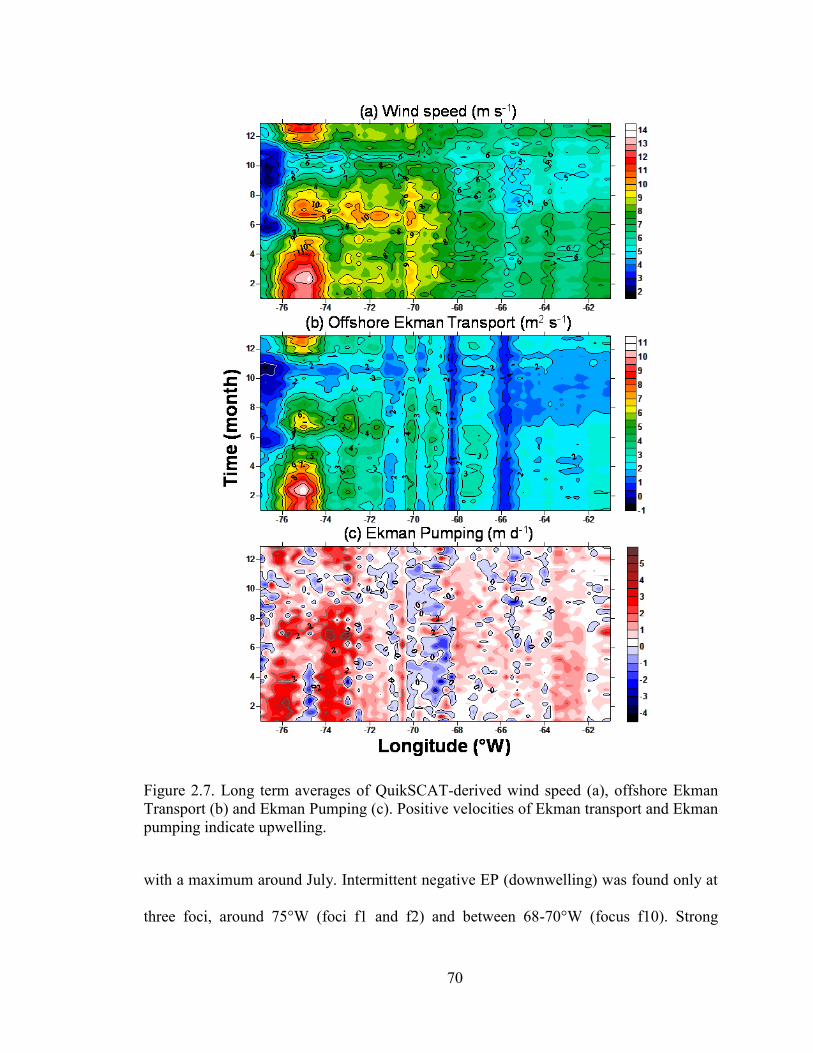
70

Figure 2.7. Long term averages of QuikSCAT-derived wind speed (a), offshore Ekman

Transport (b) and Ekman Pumping (c). Positive velocities of Ekman transport and Ekman

pumping indicate upwelling.

with a maximum around July. Intermittent negative EP (downwelling) was found only at

three foci, around 75°W (foci f1 and f2) and between 68-70°W (focus f10). Strong

71

positive EP also occurs around 76°W; however, in that area surface SST does not suggest

upwelling of deeper cooler waters (Figure 2.2).

On average, winds in the western upwelling area were 1.3 times stronger and

offshore ET was 1.5 higher than in the eastern area (Table 2.1). This means that induced

water column turbulence (a function of the cube of the wind speed) was ~2.5 higher in

the western area than in the eastern one (557 and 229 m3 s

-3, respectively). The direction

of the wind with respect to the coast was roughly alongshore along the entire southern

Caribbean Sea margin. The wind direction showed some seasonality. The eastern area

had on average half a year with alongshore winds (~1.7° variation from the alongshore

direction, May-October); during the principal upwelling (November to April) the

direction was more onshore (~12°). The western area had slightly offshore winds (~ -14°)

during the entire year, excepting October-November (~ 0.2°).

Offshore ET due to alongshore winds (Figure 2.7b) was upwelling favorable

(positive) year-round. It closely followed changes in nearshore winds except where the

coast is nearly perpendicular to the predominant wind direction (for example at 65.7°W,

68.3°W, 69.75°W and 71°W). Nearshore EP due to the wind-curl (Figure 2.7c) also

caused positive vertical velocities (upwelling favorable) in both the eastern and western

upwelling areas (at 62-64°W and 72-74.5°W) with minimum values around October. EP

was noisy even after averaging in time, consistent with the findings of Wunsch (2011).

This is in part the result of aliasing caused by the satellite sampling pattern (Milliff and

Morzel 2000). The area west of 72.5°W experiences the strongest positive nearshore EP,

with a maximum around July. Intermittent negative EP (downwelling) was found only at

three foci, around 75°W (foci f1 and f2) and between 68-70°W (focus f10). Strong

72

positive EP also occurs around 76°W; however, in that area surface SST does not suggest

upwelling of deeper cooler waters (Figure 2.2).

Table 2.1. Comparison between the west (70°-73°W ) and east (63°-65°W) upwelling

areas regarding their long term coastal averages (and minimum/maximum values) of

satellite products of: wind speed (W), turbulence (Turb) calculated with W3, alongshore

wind speed (alongW), offshore Ekman Transport due to alongshore wind (offshET),

vertical transport due to Ekman Pumping integrated to 100km offshore (EP100), sea

surface temperature (SST), chlorophyll-a (Chl). Depth of the 22°C isotherm (Iso22) was

calculated from climatological temperature profiles (1 degree resolution) from the World

Ocean Atlas (2005) extracted at 12.5°N, 72.5°W and 11.5°N-64.5°W for the west and

east upwelling areas, respectively. Values of latitude (Lat) and coriolis are also

compared.

West

East

Average (Minimum : Maximum) Average (Minimum : Maximum)

W (m s-1

) 8.23 (0.13 : 14.39) 6.12 (0.00 : 12.90)

Turb (m3 s

-3) 638 (285 : 1096) 255 (121 : 366)

alongW (m s-1

) -7.00 (-14.38 : 7.48) -5.77 (-12.68 : 6.49)

offshET (m2

s-

1) 3.04 (-3.50 : 11.68) 2.02 (-1.08 : 9.19)

EP100 (m2 s

-1) 0.48 (-10.17 : 7.56) 0.38 (-7.76 : 5.39)

SST(°C) 25.53 (19.93 : 30.53) 25.24 (20.31 : 30.08)

Chl (mg m-3

) 1.15 (0.01 : 23.00) 1.65 (0.02 : 24.56)

Iso22 (m) 115 (87 : 140) 85 (65 : 105)

Lat (°N) 12.23 (11.50 : 12.75) 10.88 (10.25 : 11.25)

Coriolis f (s-1

) 3.09E-5 (2.91E-5 : 3.22E-5) 2.75E-5 (2.60E-5 : 2.85E-5)

The western upwelling area showed a more energetic aeolic system than the

eastern area. ET was ~1.5 times higher in the west upwelling area compared to the

eastern area (Table 2.1, Figure 2.7b). Since wind stress (and ET) is a quadratic function

of the wind, with the mean wind speed for those areas (Table 2.1) we would expect a

higher offshore ET difference (around ~1.8 times higher in the western area instead of

~1.5 times). The upwelling mechanism in the west responds to the transfer of wind

energy less efficiently (Table 2.2). Two factors are responsible for this: (a) Due to the

small difference in latitude (Table 2.1 and Table 2.2) the Coriolis effect is ~10% smaller

in the western area compared to the eastern. (b) The western upwelling area experienced

73

a lower proportion of alongshore winds compared to the eastern area during the year (85

and 94%, respectively, Table 2.1). Therefore, less of the total wind speed energy is

converted to upwelling in the western area compared to the eastern (72 and 89%,

respectively, Table 2.2). Between these two factors, there was a ~28% less effective

transfer from wind to offshore ET in the western area.

Table 2.2. Comparison of the effect of latitude and of the proportions of along shore wind

(alongW) on the calculation of offshore Ekman Transport (ET) in the west and east

upwelling areas. Case 1: the same hypothetical wind speed (W) with 100% alongW was

used for both areas, differing only in their coriolis parameter (from Table 2.1). Case 2, in

top of the differences caused by coriolis, it is added the effect of the typical proportion of

alongW for each upwelling area (from Table 2.1). For each upwelling area it was

calculated the efficiency of the transference of wind to upwelling (wind efficiency)

dividing ET(case 2) by ET(case 1). The differences between the areas on the ET

calculations was obtained dividing ET(west) by ET(east) for each case.

Case Area coriolis W % alongW alongW ET

Wind

efficiency

ET

differences

1 West 3.1E-5 7.00 100 7.00 2.21 case 1: -11%

1 East 2.8E-5 7.00 100 7.00 2.49

2 West 3.1E-5 7.00 85 5.95 1.59 West: 72% case 2: -28%

2 East 2.8E-5 7.00 94 6.58 2.21 East: 89%

Regardless to the higher ET, the western area showed similar or warmer SSTs

than the eastern area (Figure 2.2 and Figure 2.5). To examine the hypothesis that this is

caused by differences in the depth of the upwelling source waters, we studied the

climatological vertical temperature structure of waters in the region (World Ocean Atlas

2005, Locarnini et al. 2006, Figure 2.1). The seasonal variability of the depth of the 22°C

isotherm (Figure 2.8) was extracted, as this temperature traces the Subtropical

Underwater core (Morrison and Nowlin 1982).

The depth of the Subtropical Underwater core (22°C isotherm) showed three

distinctive areas where it behaved consistently; these coincided with the subregions that

74

showed consistent wind speed behavior (Figure 2.7a). The shallowest depths were found

east of 68°W (annual mean 85 m, Figure 2.8); the deepest between 68-74°W (annual

mean 115 m); between 74-76°W the isotherm was slightly shallower (annual mean 109

m). During January to about August-September the 22°C isotherm in the southern

Caribbean Sea was shallower than the rest of the year. EP, integrated up to 100 km

offshore, showed remarkable coincidence with the seasonal cycle of the 22°C isotherm

depth (Figure 1.10 in Rueda-Roa et al. first chapter in this dissertation); which is

explained by the isopycnals rise caused by EP open-sea upwelling.

Figure 2.8. Climatological variation of the depth of the Subtropical Underwater core

(traced with the 22ºC isotherm) along the southern Caribbean upwelling system area,

(calculated from the World Ocean Atlas 2005, see location in Figure 2.1).

We examined the degree of correlation between the climatology of a number of

parameters, including SST, Chl, nearshore wind speed (W), wind direction, offshore ET,

coastal EP, EP integrated up to 100 km offshore (EP100), offshore extension of positive

22°C isotherm depth (m)

Tim

e (

mo

nth

)

Longitude ( W)

-76 -74 -72 -70 -68 -66 -64 -62

2

4

6

8

10

12

70

80

90

100

110

120

130

75

Figure 2.9. (a) Comparison of correlation coefficients (r) obtained with weekly

climatologies (solid line) and with weekly time series (dashed line) for sea surface

temperature (SST) vs. offshore Ekman Transport (ET) along the coast, and for the

climatologies of SST vs. nearshore wind speed (W) (dotted line). (b) Rate of change

(slope) for the simple regressions of SST vs. W and of SST vs. the 22°C isotherm depth

(iso22) for each grid point along the coast. The positions of upwelling foci are shown for

reference (diamonds). (c) Explained variance (R2) for the single regression between SST

vs. W (dashed line), and for the multiple regression of SST vs. W and iso22 (solid line).

Calculations for (b) and (c) were done with weekly climatologies, and only significant

values (p < 0.05) are shown.

76

EP and the 22°C isotherm depth (iso22). All parameters were interpolated to the same

temporal and spatial resolution (1 week and 0.25° of longitude). A comparison of the

correlations using climatological data with those performed with time series data set (for

all the variables but iso22) showed nearly identical shape in their variations along the

coast (see for example Figure 2.9a). However, the values of the correlation coefficients

(r) and the rate of changes (slope) were lower when using time series. Therefore, we

describe proportionality when comparing the correlations of climatology data between

the eastern and western upwelling areas instead of the actual values.

Correlation coefficients for SST vs. ET were very similar as for SST vs. W

(Figure 2.9a). This is due to the high proportion of alongshore wind this area experiences.

However, correlations with W were higher in two regions, at 68-70°W (foci f10) and

65.75-66.5°W (f11). This indicates that these areas experience upwelling under a

different range of wind directions, probably because of local characteristics, e.g. mean

depth or other alongshelf bathymetric variations (Smith 1981, Tomczak 1998b).

The slope of the SST vs. W regression computed for each grid point (Figure 2.9b)

showed that the wind speed had a higher effect on SST in the eastern coastal areas. These

longitudinal differences seem to be related to the increasing depth of upwelling source

waters toward the west, as shown by the slope of the iso22 depth vs. SST (Figure 2.9b).

A multiple regression between the QuikSCAT nearshore wind speed and the

depth of the 22°C isotherm explained coastal SST variability better than a single

regression of SST vs. W (Figure 2.9c). The improvement was especially marked in the

western upwelling area (71-73°W). The deeper position of the Subtropical Underwater

core in that area (~30 m deeper, Figure 2.8) produced higher sensitivity of the SST to the

77

22°C isotherm depth (Figure 2.9b and Figure 2.9c). This also explains the warmer SST

during upwelling (Figure 2.2 and Figure 2.5) in spite of the higher offshore ET (Figure

2.7a and Table 2.1) seen here compared to the eastern area.

The upwelling in the southern Caribbean Sea could be also influenced by

mesoscale geostrophic features which requires further analysis. For example, the

Caribbean Current moves westward and faster (~70 cm s-1

) near the southern boundary of

the southern Caribbean Sea, off the continental shelf-break between 62-72°W (Fratantoni

2001, Centurioni and Niiler 2003); it has a mixed annual/semiannual character with

maxima in spring (Secondary maximum) and summer (highest maximum) and minimum

in fall (Johns et al. 2002). Seasonal variations in the strength and position of the

Caribbean Current could influence the depth of the Subtropical Underwater core. For

instance, the shallowest depth of the 22°C isotherm (August, Figure 2.8) coincides with

the seasonal maximum in the strength of the Caribbean Current.

2.4.4 Phytoplankton response to the differences in upwelling regimes along the southern

Caribbean Sea

Both the eastern and western upwelling areas showed upwelling during more than

half a year (SSTs below 26°C during 6.9 and 8.5 months for the west and east upwelling

areas, respectively, Figure 2.2b). Chl concentrations were about 1.4 times higher in the

eastern area compared to the western (Figure 2.6b, Table 2.1), regardless of their

similarity in SST. In both areas, the Chl cycle was coherent with the SST cycle (Figure

2.10a and 2.10b), with exception of the mid-year Chl peak in the west upwelling area.

The disproportionally high magnitude of the Chl peak in the western area compared to

the corresponding SST is related to the enhanced turbulence in the west upwelling area

78

during that time frame, reaching over 1000 m3

s-3

(Table 2.1, Figure 2.10a). Wind-stress

drives entrainment of colder waters into the mixed layer and leads to further turbulent

Figure 2.10. (a) and (b) Long term coastal values means of SST, Chl and wind speed (W)

averaged for (a) the west upwelling area (70-73 ) and (b) the east upwelling area (63-

65°W). SST values are presented in reverse order for a better comparison with Chl. (c)

Explained variance for the single regression between Chl vs. SST weekly time series

(dashed line), and for the multiple regression between Chl vs. SST and W (solid line). (d)

Rate of changes (slope) of the parameters SST and W for the multiple regressions of Chl

vs. SST and W. Only significant values (p < 0.05) are shown for the correlations.

79

vertical nutrient flux as a result of the erosion of the thermocline (Klein and Coste 1984).

A multiple regression of Chl vs. SST and wind speed (W) time series (Figure 2.10c)

increased considerably the explained variance along the west upwelling area (between

69.5-72°W, and also along 74-76°W) but for the rest of the coastline the values were

similar than for the single regression of Chl vs. SST. Values obtained with W were

similar or slightly higher than the obtained using turbulence (W3) or offshore ET. The

relationship of the wind was directly related with Chl (positive slopes, Figure 2.10d),

confirming that in the western upwelling area, the mid-year Chl was enhanced by

turbulence. During mid-year mixed layers are relatively shallow in that area (between 10-

30m depth for the period of June-July 1997, Andrade 2000), which would make easier

the turbulent entrainment of nutrients from the thermocline erosion.

The eastern upwelling area has four times higher small pelagic biomass than the

western area (Stromme and Saetersdal 1989). The enhanced upwelling in the eastern area

results in a longer season of high Chl (1.6 months longer) and a phytoplankton biomass

that is 1.4 times higher than those in the western area (Figure 2.6b, Table 2.1).

Furthermore, the eastern area shows higher Chl increases at an equivalent lower SST

(upwelling) than the western area (i.e. Eq. 1 and Eq. 2). This seems related to its wider

continental shelf (Figure 2.1). Comparing the upwelling dynamics, the western area had a

more energetic wind field (1.5 higher offshore ET and 2.5 higher turbulence, Table 2.1),

but similar or warmer SSTs than the eastern upwelling area (Table 2.1, Figure 2.5) due to

the deeper position of the Subtropical Underwater core in the western area (Figure 2.8

and Figure 2.9).

80

The ‘optimal environmental window’ theory stresses the importance of a balance

between the upwelling of nutrient-rich water and calm conditions for encouraging

successful clupeoid recruitment (Cury and Roy, 1989). This theory has been successfully

tested and, in the major upwelling ecosystems, clupeoid recruitment is dome-shaped with

the upwelling, turbulence and SST (Cole and McGlade 1998, MacKenzie 2000 and

references therein). The ‘optimal environmental window’ establishes an optimum wind

speed of ~6 m s-1

for recruitment of small pelagics in wind driven upwelling systems

(Cury and Roy, 1989). This is the case for the eastern upwelling area with an annual wind

speed average of 6.2 m s-1

. Above this value turbulence increases, as in the western area

with winds > 8 m s-1

. The effect of turbulence in the biology of the western area was

demonstrated by its effect on Chl (i.e. Figure 2.10) which is not seen for the eastern area.

Since the western area has relatively similar SSTs as the eastern area, the level of

enrichment due to upwelling is also comparable, but the higher offshore ET, and

especially the much higher turbulence, place this upwelling ecosystem in the right

(negative) side of the dome-shaped relationship between the intensity of

upwelling/turbulence and the small pelagics recruitment. Higher turbulence mixes surface

waters dispersing plankton and larvae, which often inhibits successful first feeding

(Lasker 1975, 1978) and reduces the ability of larvae to catch prey (MacKenzie et al.

1994). Higher turbulence also reduces phytoplankton production by mixing cells below

the critical depth (Steele 1974 as cited in Bakun 2010). In addition, stronger offshore

transport may cause the loss of eggs and larvae from their coastal habitat (Parrish et al.

1981) and leads to nutrients being exported before they are fully used within the coastal

upwelling system.

81

Bakun's triad hypothesis (Bakun, 1993, 1996) generalizes three oceanographic

processes in diverse marine systems that can influence recruitment success: (a)

enrichment of the food chain, (b) retention of the eggs and larvae within suitable nursery

areas, and (c) concentration of food particles for the first-feeding larvae and subsequent

development stages. In coastal upwelling systems, enrichment (a) is produced by the

upwelled waters, retention (b) is related to moderate offshore ET, and concentration of

food (c) is related to moderate turbulence. Retention (b) is also influenced by

recirculation due to topography; topographical features minimize offshore transport and

allow retention of eggs and larvae in the favorable coastal habitat (Lett et al. 2006).

Comparing the upwelling plumes extension (Figure 2.3) with the continental shelf extent

(Figure 2.1) it is clear that in the western upwelling area the upwelling plume extends

broadly offshore beyond the continental shelf. However, in the eastern region the

upwelling plumes bathe a wide continental shelf with high topographic complexity (i.e.

the Cariaco Gulf, the Margarita Island and other small islands) that increase and diversify

retention mechanisms for eggs and larvae.

2.5 Conclusions

The southern Caribbean upwelling system (61°W to 75.5°W, 10 to 12.5ºN)

features a strong semiannual SST cycle, with a principal upwelling season between

December and April, a mid-year upwelling during June-August. The weakest upwelling

is seen in during September-October. Satellite Chl shows maxima near specific coastal

upwelling foci. In areas without riverine influence, the coastal Chl maxima are coherent

with the upwelling cycle, showing the same (but inverse) seasonality as SST. Nearshore

82

winds are mainly aligned with the coastline and they are upwelling favorable all year-

round. There are three areas with distinctive wind regimes. (1) The coast east of 68°W

showed relatively stable high wind speed (> 6 m s-1

) from December to July and lower

winds between August-November (4-6 m s-1

). (2) The region between 69-74°W

experienced stronger winds (> 8 m s-1

) year round, with a maximum in June-July (> 9 m

s-1

). (3) The strongest nearshore winds occurred around 74-76°W, with a distinctive

maximum during December-April (> 11 m s-1

) and a marked minimum during

September-October (~5 m s-1

).

The southern Caribbean Sea has 21 upwelling foci. Adjacent upwelling foci tend

to have coherent upwelling cycles. Seven groups of foci can be identified with different

characteristics in their seasonal SST cycle. There are two large sections of coast which

experience the strongest SST decrease and which also are the most important fisheries

grounds: The east upwelling area, between 63-65°W, which showed the lowest SST

(annual mean 25.24°C) and the highest Chl (annual mean 1.65 mg m-3

), moderate winds

(annual mean 6.12 m s-1

), and shallower offshore isotherms (22°C isotherm annual mean

at 85m depth). The west upwelling area, between 74-69.5°W, with stronger winds

(annual mean 8.23 m s-1

) but deeper offshore isotherms (22°C isotherm annual mean at

115 m depth) that limit the upwelled waters to SST similar or higher than in the east area

(annual mean 25.53°C), and with lower Chlorophyll concentrations (annual mean 1.15

mg m-3

). . The western upwelling area has very energetic eolic conditions. However, the

transference of energy from the wind stress to the water column is not as efficient as in

the east area in generating upwelling owing to a lower proportion of alongshore winds

(85 and 94%, for the west and east areas, respectively) and because the western coast is

83

located at a higher latitude. These two factors cause a ~28% less effective transfer of

energy from wind to offshore ET. Regardless, offshore ET in the western upwelling area

is ~1.5 higher than in the eastern area. Chlorophyll cycles are inverse and coherent with

SST cycles, indicating that the increase in phytoplankton biomass is driven by upwelling.

An exception of this is the mid-year Chl peak in the western upwelling area, which is

disproportionately high compared to the SST mid-year upwelling and it is concurrent

with the wind maxima. This midyear Chl maximum is enhanced by wind stress

turbulence which leads to additional entrainment of nutrients from the thermocline.

The differences in the upwelling dynamics between the eastern upwelling area

(medium wind speeds, shallower offshore isotherms, slightly cooler SSTs and higher

phytoplankton biomass) and the western upwelling area (high wind speeds, deeper

isotherms, slightly warmer SSTs and lower phytoplankton biomass) helped explain the

higher fish productivity of the eastern upwelling area (~90% of the southern Caribbean

Sea captures, FAO). The wind speed at the eastern upwelling area (annual mean 6.12 m s-

1) is very close to the optimum wind speed for recruitment of small pelagics (~6 m s

-1,

‘optimal environmental window’ theory), which generates moderate offshore Ekman

Transport and moderate turbulence, that in turn produce the highest recruitment.

Furthermore, the wider continental shelf and higher topographic complexity in the eastern

area increase and diversify retention mechanisms for eggs and larvae. Possibly, the most

important factors that quench secondary production to fish in the western area are the

high degree of turbulence and strong offshore transport. This produces strong dispersion

of plankton and larvae, which in turn would affect larvae feeding and mortality and

export of nutrients, plankton and larvae from the coastal upwelling system.

84

2.6 Acknowledgements

This research was carried out under the CARIACO Time-Series program, funded

by: the National Science Foundation (NSF, USA, Grants OCE- 0752139, OCE-9216626,

OCE-9729284, OCE-9401537, OCE-9729697, OCE-9415790, OCE-9711318, OCE-

0326268 and OCE 0963028), the National Aeronautics and Space Administration

(NASA, USA, Grants NAG5-6448 and NAS5-97128), the Consejo Nacional de

Investigaciones Cientificas y Tecnológicas (CONICIT, VENEZUELA, Grant 96280221)

and the Fondo Nacional de Investigaciones Cientificas y Tecnologicas (FONACIT,

Venezuela, Grant 2000001703). We are in debt to Tal Ezer, who provided important

suggestions and Matlab code for satellite wind products. We wish to thank the personnel

working at Fundación La Salle, EDIMAR, Venezuela, for their continuous efforts in

maintaining the CARIACO Ocean Time-Series Program. We are grateful to Ramón

Varela, Yrene Astor, José Alió and Jeremy Mendoza for their revisions and

commentaries to this manuscript.

2.7. References

Bakun A (1973) Coastal upwelling indices, west coast of North America, 1946-71. U.S.

Dept. of Commerce, NOAA Tech. Rep., NMFS SSRF-671, 103p.

Bakun A (2010) Linking climate to population variability in marine ecosystems

characterized by non-simple dynamics: conceptual templates and schematic

constructs. J. Mar. Syst. 79: 361–373.

Bernal G, Poveda G, Roldán P, Andrade C (2006) Patrones de variabilidad de las

temperaturas superficiales del mar en la Costa Caribe Colombiana. Rev. Acad.

Colomb. Cienc., 30 (115): 195-208.

85

Brown OB, Brown JW, Evans RH (1985) Calibration of advanced very high resolution

radiometer infrared observations. J. Geophys. Res. 90:11667-11678.

Caraballo LF (1982) Golfo de Cariaco. Parte I: Morfología y batimetetría submarina.

Estructura y tectonísmo reciente. Bol. Inst. Oceanogr. Univ. Oriente, 21 (1-2):13-

35.

Castelao RM, Barth JA (2006) Upwelling around Cabo Frio, Brazil: The importance of

wind stress curl. Geophys. Res. Lett., 33, L03602.

Castellanos P, Varela R, Muller-Karger F (2002) Descripción de las areas de surgencia al

sur del Mar Caribe examinadas con el sensor infrarrojo AVHRR. Mem. Soc. Cien.

Nat. La Salle, 154: 55-76.

Centurioni LR,Niiler PP (2003) On the surface currents of the Caribbean Sea. Geophys.

Res. Lett., 30(6): 1279.

Chereskin TK (1995) Direct evidence for an Ekman balance in the California Current. J.

Geophys. Res., 100: 18261-18269.

Cury P, Roy C (1989) Optimal environmental window and pelagic fish recruitment

success in upwelling areas. Canad. J. Fish. Aquatic Sci., 46(4): 670-680.

Dale AW, Prego R (2002) Physico-biogeochemical controls on benthic-pelagic coupling

of nutrient fluxes and recycling in a coastal upwelling system. Mar. Ecol. Prog.

Ser., 235: 15–28.

Fratantoni DM (2001) North Atlantic surface circulation during the 1990's observed with

satellite-tracked drifters. J. Geophys. Res., 106: 22067-22093.

Freilich MH, Dunbar RS (1999) The accuracy of the NSCAT 1 vector winds:

Comparisons with National Data Buoy Center buoys. J. Geophys. Res., 104:

11231- 11246.

Herrera L, Febres-Ortega G (1975) Kinematics of Me wind-generated velocity field in

the surface waters off eastern Venezuela, Caribbean Sea. Bol. Inst. Oceanogr.

Univ. Oriente, 14(2):165-186.

Hoffman RN, Leidner SM (2005) An introduction to the near-real-time QuikSCAT data.

Weather Forecast., 20: 476-493.

Hu C, Muller-Karger F, Murch B, Myhre D, Taylor J, Luerssen R, Moses C, Zhang C,

Gramer L, and Hendee J (2009) Building an Automated Integrated Observing

System to Detect Sea Surface Temperature Anomaly Events in the Florida Keys.

IEEE Trans. Geosc. Remote Sens., 47(6):1607-1620.

86

Huhn K, Paul A, Seyferth M (2007) Modeling sediment transport patterns during an

upwelling event. J. Geophys. Res., 112: C10003.

Klein P and Coste B (1984) Effects of wind-stress variability on nutrient transport into

the mixed layer. Deep Sea Res., 31(1):21-37.

Lasker R (1975) Field criteria for survival of anchovy larvae: the relation between

inshore chlorophyllmaximum layers and successful first feeding. Fish. Bull.U.S.,

73: 453-462.

Lasker R (1978) The relation between oceanographic conditions and larval anchovy food

in the California Current: identification of the factors leading to recruitment

failure. Rapp. P.-v. Réun. - Cons. Int. Explor. Mer, 173, 212-230.

Locarnini RA, Mishonov AV, Antonov JI, Boyer TP, Garcia HE, (2006) World Ocean

Atlas 2005, Volume 1: Temperature. S. Levitus, Ed. NOAA Atlas NESDIS 61,

U.S. Government Printing Office, Washington, D.C., 182 pp.

http://www.nodc.noaa.gov/OC5/WOA05/pr_woa05.html

McClain EP, Pichel WG, Walton CC, Ahmad Z, Sutton J (1983) Multi-channel

improvements to satellite-derived global sea-surface temperatures. Adv. Space

Res., 2(6):43-47.

MacKenzie BR (2000) Turbulence, larval fish ecology and fisheries recruitment: a review

of field studies. Oceanol. Acta, 23(4): 357-375.

MacKenzie BR, Miller TJ, Cyr S, Leggett WC (1994) Evidence for a dome-shaped

relationship between turbulence and larval fish ingestion rates. Limnol.

Oceanogr., 39(8): 1790-1799

Mendo J, Pizarro L, Castillo S (1987) Monthly turbulence and ET indexes 1953 to 1985,

based on local wind records from Trujillo and Callao, Peru. In: Pauly D,

Tsukayama I (ed) The Peruvian anchoveta and its upwelling ecosystem: three

decades of change. ICLARM Studies and Reviews 15:75-88

Milliff RF, Morzel J (2000) The global distribution of the time-average wind-stress curl

from NSCAT. J. Atmosph. Sci., 58(2):109-131.

Minnett PJ (1991) Consequences of sea surface temperature variability on the validation

and applications of satellite measurements. J. Geophys. Res., 96(C10):18475-

18489.

Morrison J M, Nowlin Jr WD (1982) General Distribution of Water Masses Within the

Eastern Caribbean Sea During the Winter of 1972 and Fall of 1973. J. Geophys.

Res., 87(C6), 4207-4229

87

Muller-Karger FE, Aparicio R (1994) Mesoscale Processes Affecting Phytoplankton

Abundance in the Southern Caribbean Sea. Cont. Shelf Res.., 14(2/3): 199-221.

Muller-Karger FE, McClain CR, Fisher TR, Esaias WE, Varela R. (1989) Pigment

distribution in the Caribbean Sea: observations from space. Progr. Oceanogr., 23:

23-69.

Muller-Karger FE, Varela R (1990). Influjo del Río Orinoco en el Mar Caribe:

observaciones con el CZCS desde el espacio. Mem. Soc. Cien. Nat. La Salle,

50(133–134): 361-390.

Muller-Karger FE, Varela R, Thunell R, Astor Y, Zhang H, Luerssen R, Hu C (2004)

Processes of coastal upwelling and carbon flux in the Cariaco Basin. Deep-Sea

Res. part II, 51: 927-943

Oey LY, Ezer T, Wang DP, Fan SJ, Yin XQ (2006) Loop Current warming by Hurricane

Wilma. Geophys. Res. Let., 33: L08613.

Oey LY, Ezer T, Wang DP, Yin XQ, Fan SJ (2007) Hurricane-induced motions and

interaction with ocean currents. Cont. Shelf Res., 27: 1249-1263.

Pang-Ning T, Steinbach M, Kumar V (2005) Introduction to Data Mining. Addison-

Wesley, 1st edition, May 2005.

Parrish RH, Nelson CS, Bakun A (1981) Transport mechanisms and reproductive success

of fishes in the California Current. Biol. Oceanogr., 1: 175-203.

Richards F (1960) Some chemical and hydrographic observations along the north coast of

South America. Deep-Sea Res., 7: 163-182.

Rueda-Roa D, Ezer T, Muller-Karger F (in preparation) Contribution of Ekman transport

and pumping on the mid-year Southern Caribbean upwelling and on

phytoplankton biomass. (First chapter on this dissertation).

Smith RL (1968) Upwelling. Oceanogr. Mar. Biol. Ann. Rev., 6: 11-46.

Smith R L (1981) A comparison of the structure and variability of the flow field in three

coastal upwelling regions: Oregon, Northwest Africa, and Peru. Pp. 107–118. In:

Richards FA (ed.) Coastal Upwelling, Amer. Geophys. Union, 107–118.

Stewart RH (2007) Introduction to Physical Oceanography; R. H. Stewart, Ed; Dept. of

Oceanography, Texas A & M University: College Station: TX, 2002; available

online: http://oceanworld.tamu.edu/resources/ocng_textbook/contents.html.

Strong AE, McClain E (1984) Improved ocean surface temperatures from space-

comparisons with drifting buoys. Bull. Am. Meteorol. Soc., 85: 138.

88

Steele JH (1974) The Stucture of Marine Ecosystems. Harvard Univ. Press, Cambridge,

Mass. 128 pp.

Tomczak M (1998a) Ekman layer dynamics for shallow seas with stratification; in: Shelf

and Coastal Oceanography, chapter 3, accessed on September 10 2011 at:

http://www.es.flinders.edu.au/~mattom/ShelfCoast/chapter03.html

Tomczak M (1998b): Upwelling dynamics in deep and shallow water; in: Shelf and

Coastal Oceanography, chapter 6, accessed on September 10 2011 at:

http://www.es.flinders.edu.au/~mattom/ShelfCoast/chapter06.html

Walton CC (1988) Nonlinear Multichannel Algorithms for Estimating Sea Surface

Temperature with AVHRR Satellite Data. J. Appl. Meteor., 27(2) 115-124.

Wunsch, (2011) The decadal mean ocean circulation and Sverdrup balance. J. Mar. Res.,

69: 1-18.

89

2.8 Appendices

Appendix A

Daily zonal and meridional QuikSCAT wind speed components (u, v respectively,

in m s-1

) were used to estimate the wind stress components (τx = ca ρa |u| u; τy = ca ρa |v| v;

and τxy= ca ρa |W|2, Kg m

-1 s

-2 or N m

-2, Bakun 1973); where ρa is the air density (1.2 kg m

-

3), W is the scalar wind magnitude (W = sqrt(u

2 + v

2), m s

-1), and CD is a drag coefficient

(dimensionless) used by Oey et al. (2006 and 2007) and which includes curve fits for low

and high wind speeds: CD x 103

= 1.2 (W 11 m s-1

; = 0.49 + 0.065 W (11 < W 19 m s-

1), = 1.364 + 0.0234 W - 0.0002 f2 (19 < W 100 m s

-1).

The geographic direction of the wind (Wind) is defined as the angle of the wind

vector (where the wind goes) calculated clockwise from a unitary vector pointing north:

Wind = atan2 (u, v) (180/); 360° is added for negative u values. The coastline angle

(Coast) is defined by the Pacific Fisheries Environmental Laboratory

(http://www.pfeg.noaa.gov/) as the clockwise angle that the landward side of the

coastline makes with a vector pointing north. The coastline angle, Coast = F +

acos(slope/sqrt(1+slope2)) (180/), was obtained for each coast segment of 0.25° of

longitude, calculating the slope of a linear fit for each coast segment with data points at 1

km resolution (Castelao and Barth 2006) and using a factor of F=180° when the land

mass is mainly in the southern/southeastern quadrants and, F=0° when the land mass is

mainly in the northern/ northwestern quadrants.

The alongshore wind stress, τalong-shore= τxy cos(Coast - Wind ) (/180) (in Kg

m-1

s-2

, Mendo et al. 1987) and the cross-shore Ekman volume transport , ETcross-shore =

- τalong-shore / ρw f (in m2 s

-1, Chereskin 1995) were calculated at each QuikSCAT grid point

closest to the coast. We used a seawater density ρw = 1025 kg m-3

and the coriolis

parameter (f= 2Ω sin(), in s-1

) calculated for each wind pixel latitude () with the

angular speed of earth rotation Ω = 7.29211538 x 10-5

(radians/second). Positive cross-

shore ET means offshore transport that induces coastal upwelling.

The relative vorticity of wind stress curl was calculated using the wind stress

components one pixel to the east/west and to the north/south from each grid point:

curl_τxy = ((τy east - τy west)/ x) - (τx north - τx south)/y)), where x and y are the

distance in meters between pixel centers (Kg m-2

s-2

or N m-3

, Stewart 2007). The wind

stress curl was used to calculate the EP vertical velocity, EP = curl_τxy / ρw f, (m s-1

,

Smith 1968). Positive wind curl means counterclockwise vorticity that induces upward

EP.

90

Appendix B

Geographical location of the upwelling foci along the Southern Caribbean Upwelling

System shown in Figure 2.3.

Focus Localization

f1: Barranquilla: from Galerazamba to Río Magdalena, Bolívar and Atlántico

departments, Colombia

f2: Ciénaga: Ciénaga Grande, Magdalena department, Colombia

f3: Sta. Marta: from Tyrona to Río Don Diego (East of Santa Marta), Magdalena

department, Colombia

f4: Río Hacha: from Río Hacha to Manaure, middle sector of the Guajira peninsula, La

Guajira department, Colombia

f5: El Cabo: West from El Cabo, La Guajira department, Colombia

f6: Cabo de la Vela: from Cabo de la Vela to Punta Gallinas, La Guajira department,

Colombia

f7: Punta Gallinas: from Punta Gallinas to Puerto Estrella, La Guajira department,

Colombia

f8: Cabo San Román: from Cabo San Román to Punta Macama, northwest of Paraguaná

Peninsula, state of Falcón, Venezuela

f9: Punta Cardón: Punto Fijo: from Punta Cardón to the entrance of the Golfete de Coro,

west of Paraguaná Peninsula, state of Falcón, Venezuela

f10: Puerto Cumarebo: from Puerto Cumarebo to Campechano, state of Falcón, Venezuela

f11: Cabo Codera: from Marina Grande (Vargas state) to Cabo Codera (state of Miranda),

Venezuela

f12: Unare: north from Laguna de Unare (South of the Cariaco basin), state of Anzoátegui,

Venezuela

f13: Mochima: Between Puerto La Cruz, Cumaná and the west of the Araya Peninsula,

(states of Anzoátegui and Sucre) Venezuela

f14: Golfo de Cariaco: Golfo de Cariaco, state of Sucre, Venezuela

f15: El Guamache: northeast of the Araya peninsula, state of Sucre, Venezuela

f16: Macanao: North of Macanao (from Punta El Faro to Punta de Tigre), northwest of

Margarita island, Venezuela

f17: Manzanillo: from La Salineta to Manzanillo, north of Margarita island, Venezuela

f18: Carúpano: from Guaca to El Morro de Puerto Santo, state of Sucre, Venezuela

f19: Las Galdonas: from Playa Medina to San Juan de Unare, Paria Peninsula, state of

Sucre, Venezuela

f20: Don Pedro: from Ensenada de Mejillones to the easternmost tip of the Paria peninsula,

state of Sucre, Venezuela

f21: Trinidad: North of Trinidad island, Trinidad and Tobago

91

Appendix C

Long term SST averages and standard deviation (in parenthesis) for the different

upwelling foci (Figure 2.3 and Appendix B) for the principal upwelling (February-

March), mid-year upwelling (from June 17 to July 21), SST maximum (September-

October) and annual mean. Averages calculated from weekly SST time series for the

period 1994-2008. *The warm season for the Caribbean Sea and the Atlantic Ocean is

shorter and was calculated for September only. The areas used to extract the averages are

shown in Figures 1 and 3.

Areas Principal

upwelling

Mid-year

upwelling

Low-upwelling

(maximum SST) Annual Mean

f1 25.62 (0.60) 27.53 (0.63) 27.95 (0.74) 26.98 (1.10)

f2 25.58 (0.69) 27.46 (0.67) 28.22 (0.76) 27.06 (1.16)

f3 24.45 (0.79) 25.89 (0.78) 27.25 (0.91) 25.84 (1.30)

f4 24.36 (0.89) 26.21 (0.74) 27.95 (0.69) 26.18 (1.44)

f5 23.68 (0.98) 25.61 (0.87) 27.63 (0.77) 25.70 (1.58)

f6 23.97 (0.88) 25.47 (0.76) 27.55 (0.65) 25.74 (1.42)

f7 24.39 (0.69) 25.79 (0.72) 27.58 (0.63) 25.96 (1.26)

f8 23.95 (0.78) 25.35 (0.76) 27.62 (0.70) 25.77 (1.44)

f9 23.83 (0.89) 25.36 (0.86) 27.78 (0.94) 25.79 (1.59)

f10 24.53 (0.75) 25.31 (0.70) 27.35 (0.68) 25.87 (1.20)

f11 24.09 (0.85) 24.94 (0.85) 27.34 (0.92) 25.60 (1.40)

f12 24.12 (0.91) 25.37 (0.83) 27.61 (0.72) 25.84 (1.41)

f13 23.33 (0.90) 24.94 (0.86) 27.34 (0.80) 25.35 (1.59)

f14 23.11 (0.80) 24.44 (0.87) 26.80 (0.92) 24.93 (1.51)

f15 23.54 (0.74) 24.92 (0.78) 27.13 (0.88) 25.26 (1.46)

f16 23.85 (0.75) 25.36 (0.72) 27.54 (0.75) 25.62 (1.47)

f17 23.45 (0.73) 25.00 (0.74) 27.23 (0.78) 25.26 (1.50)

f18 23.46 (0.70) 24.73 (0.74) 26.86 (0.77) 25.06 (1.38)

f19 23.74 (0.90) 25.04 (0.82) 27.09 (0.75) 25.33 (1.40)

f20 23.42 (0.93) 24.59 (0.90) 26.85 (0.84) 25.04 (1.46)

f21 25.02 (0.64) 25.82 (0.78) 27.52 (0.80) 26.18 (1.08)

Caribbean 26.07 (0.34) 26.87 (0.52) 28.38 (0.40)* 27.14 (0.89)

Atlantic 25.81 (0.50) 25.95 (0.78) 28.10 (0.67)* 26.72 (0.99)

92

CHAPTER THREE

Spatial variability of Spanish sardine (Sardinella aurita) abundance as related to the

upwelling cycle of the southeastern Caribbean Sea

3.1 Abstract

The southeastern Caribbean Sea (10-12°N and 61.5-65°W) is an area of

pronounced seasonal wind-driven upwelling that supports an important Spanish sardine

(Sardinella aurita) fishery that accounts for 90% of the small pelagic fish within the

Caribbean Sea. This artisanal fishery largely takes place in the first ~10 km from shore.

To understand the effects of the upwelling on the spatial patterns of Spanish sardine

distribution, a comparison was made between the number of small pelagics schools

(Schools) and S. aurita biomass (sAsardine) obtained from 8 acoustic surveys (1995-

1998) to satellite-derived products including sea surface temperature (SST, as a proxy for

upwelling), SST gradients (SSTgrad) and chlorophyll-a (Chl, only available for the last

two surveys) and also with distance to upwelling foci and latitude-longitude. Spatially

averaged SSTs for the surveys were similar to long term SST averages for the study area.

The surveys were gruped according to three seasons: strong, weak, and transition

upwelling periods and compared each group’s sAsardine with the environmental

variables using Generalized Additive Models. During the strongest upwelling (February-

March) sAsardine was widely distributed in the cooler, Chl rich upwelling plumes over

93

the ~70 km continental shelf. During the weakest upwelling (September-October)

sAsardine was larger near upwelling foci where Chl concentrations of 1-3 mg m-3

were

observed within the first 10 km of the coast, and avoided distances farther than 30 km

from the upwelling foci. During this season with high riverine discharge, sAsardine

evaded the southeast-northwest haline front formed between clear Caribbean Sea waters

and the turbid Orinoco River plume. Higher coastal concentrations of sAsardine increase

the availability (and possibly the catchability) for the artisanal fishery during the period

of weakest upwelling. Higher numbers of small pelagics schools were found closer to the

shore all year round, which increases catchability regardless of the total stock. We

hypothesize that the 2005 collapse of the S. aurita fishery off northeastern Venezuela was

caused by a combination of sustained stressful environmental conditions (weak upwelling

and warmer water temperatures from 2004 to 2010) and overfishing as a result of the

increased catchability of the stock caused by aggregation of the fish in the cooler coastal

upwelling cells.

3.2 Introduction

The southern Caribbean Sea (Figure 3.1a) is an area of pronounced seasonal

coastal upwelling during the first half of the year (Richards 1960, Herrera and Febres-

Ortega 1975, Muller-Karger and Aparicio-Castro 1994). The nutrient-rich upwelled

waters produce important phytoplankton growth that leads to bountiful fisheries;

especially in the northeastern Venezuelan shelf (Figure 3.1b), which is one of the most

important fishing grounds in the Caribbean Sea. The Spanish sardine, Sardinella aurita

(also called round sardinella), is one of the most important fisheries in this area. Spanish

94

sardine catches in northeastern Venezuela represent nearly 90% of the small pelagic fish

catch for the Caribbean Sea (FAO-FIGIS, 1980-2011). This relatively small shelf area of

23,200 km2 (Figure 3.1b) has a Spanish sardine biomass between 0.6 to 1.3 million tons,

estimated by means of acoustic surveys (Stromme and Saetersdal 1989; Cárdenas and

Achury 2002; Cárdenas 2003). Spanish sardine is an opportunistic filter feeder and its

stomach content has the same composition of plankton as the surrounding surface waters

of the study area (Cervigón 1991; Cellamare and Gómez 2007). In addition to the

plankton richness in this area due to upwelling, the complex topographic features and

wide continental shelf (Figure 3.1b, Fréon and Mendoza 2003), and its characteristic

upwelling dynamics (Rueda-Roa and Muller-Karger, see second chapter in this

dissertation) favor the development of Spanish sardine biomass. Despite the wide

distribution of the Spanish sardine population on the shelf (Figure 3.1b, Cárdenas 2003;

Guzmán et al. 2003), fishing activities only take place in areas close to shore (up to ~10

km from shore) owing to the artisanal nature of the fishery which is protected by

Venezuelan laws (Freón and Mendoza 2003; González et al. 2005, INAPESCA 2001).

Fishermen catch Spanish sardine schools using relatively small boats with traditional

fishing gear like artisanal beach seines without bags or using artisanal purse seines and

operated manually from small boats and from shore.

Fishery management of clupeoid fishes has proven difficult because the high

variability in ocean conditions, such as upwelling, can threaten or enhance the survival of

early life-history stages (Lasker 1975, Cury and Roy 1989, Bakun 1996). Short life cycles

make any fluctuations in recruitment translate rapidly into fluctuations in population size.

A reasonable level of exploitation during years with good recruitment, if unchanged, may

95

Figure 3.1. The Caribbean Sea (a) and northeastern Venezuela (b). (a): Sea surface

temperature (SST) climatology (20-24 February, 1994-2009) of the Caribbean Sea

showing the upwelling in the southern region. The study area (red rectangle) off

northeastern Venezuela shows seasonal upwelling and it is also influenced by the

Orinoco River discharge. (b): Eastern coast of Venezuela bathymetry with known

Sardinella aurita distribution (hatched) and main fishing areas (solid black).

12.0

11.5

11.0

10.5

64.565.5 65.0 64.0 63.5 63.0

Longitude ( W)

La

titu

de ( N

)

(b)

SST

( C)

Known distribution

Main fishing areas

Cumaná

Gulf of Cariaco

Araya PeninsulaParia Peninsula

Margarita I.

Cubagua I. Coche I.

-85 -80 -75 -70 -65 -60

10

15

20

22

23

24

25

26

27

28

29

Caribbean Sea

Atlantic Ocean

Orinoco Delta →

SST

( C)

(a)

96

Figure 3.2. Annual capture of Sardinella aurita in northeastern Venezuela compared to

annual SST averages for the study area. Spanish sardine capture data from INSOPESCA

(2012). SST spatial averages for the study area were calculated excluding the Orinoco

mask (see Figure 3.3). Long term SST average (1994-2009) was 25.9°C.

lead to overfishing during unfavorable environmental conditions and could have

disastrous consequences. Sardine fishery landings off the northeastern Venezuela

(provided by the Venezuelan Government Fisheries and Aquaculture Administration,

INSOPESCA) showed that S. aurita annual landings from 1980 to 1993 were 61,760 tons

in average. After 1994 catches were higher (Figure 3.2) as a result of a higher market

demand (Barrios et al. 2010). However, consecutive years of weak upwelling starting in

2004-2005 (Figure 3.2) have contributed to a crash in the Venezuelan Spanish sardine

fishery. This created great economic havoc which included the closing of several sardine

canneries. As of 2011, the fishery had not recovered to previous yields (34,754 tons in

2011 and maintains the descending trend), which caused the closing of several factories

related to sardine processing (El Nacional newspaper 03/21/2009). The economic and

97

social problems arising from the collapse of the Spanish sardine fishery in this area

highlights the need for better fishery management strategies.

The main objective of this research was to understand the response of S. aurita to

changes in upwelling in the southeastern Caribbean Sea. This information is needed for

competent fishery management. Our first approach was to study the fluctuations in S.

aurita landings in the main fishing areas (Figure 3.1b) and relate them to inter-annual

variation of the strength of the upwelling. Fishery data for S. aurita were compiled by

INSOPESCA, the institute responsible for compiling fishing information and for the

sustainable management of the fishery resources. The main source of the Spanish sardine

fishery data come from the canning factories, which are required to provide INSOPESCA

with a monthly summary of the amount landed in their facilities and the capture area of

the Spanish sardine they purchase. In 2002, the information form to be filled required

much more details and requested data for each transaction, e.g. the total weight (kilos) of

fish bought, name of the provider, place and date of the capture, etc. The forms are sent

to INSOPESCA on paper, from which they extract the monthly summary and add it to the

fishery statistics. We worked with INSOPESCA personnel to transcribe the detailed

information contained on paper into electronic files. These contained the spatial and

temporal resolution needed for the analysis. Unfortunately, it was found that an important

number of forms returned from various canneries or fishing entities over time were

missing and this prevented a systematic study of the fishery patterns using these data.

We needed a way to determine if the spatial patterns of Spanish sardine

distribution are related to the upwelling annual cycle. An analysis of such patterns would

clarify if availability to the fishery is influenced by the upwelling cycle. For this purpose

98

we used data from acoustic surveys that provide historical estimates of fish abundance

and their spatial and temporal distributions in the region (Simmonds et al. 1992). There

have been several hydroacoustics surveys to estimate stock abundance and distribution of

S. aurita off northeastern Venezuela. The series of VECEP program acoustic surveys

performed from 1995 through 1998 was used; which coincided with the availability of

satellite-derived Sea Surface Temperature (SST) imagery. These surveys had been

analyzed using in situ oceanographic data (Cárdenas and Achury 2000), but these data

lacked the synoptic coverage offered by satellite SST. The satellite SST products were

used to define a proxy for upwelling in this study area.

The main finding is that during the upwelling season, Spanish sardine is widely

distributed in the cooler waters of the continental shelf, while during the lowest-

upwelling season the sardine is concentrated closer to the coast in nearshore upwelling

foci that still have cells of cooler waters near the coast. This coastal concentration

increases Spanish sardine availability to the artisanal fishery operating within 10 km of

the coast. The possibility arises that after an anomalous period of weak upwelling,

reproductive output is negatively impacted, and larval survival and recruitment of the

Spanish sardine are negatively affected at the same time that the availability and

catchability is increased. This poses a “perfect-storm” scenario in which overfishing can

occur on an already environmentally strained population.

99

3.3 Methods

3.3.1 Study Area:

The study area (10-12°N and 61.5-65°W; Figure 3.1 and Figure 3.3) is located

along the southeastern boundary of the Caribbean Sea, off northeastern Venezuela, with a

continental shelf roughly oriented east-west. It has a variable continental platform

extension that ranges from 5 to 100 km, with depths between 7-115 m (Freón and

Mendoza 2003). The shelf topography is complex (Figure 3.1b) presenting several

islands, capes, offshore banks, a long and narrow gulf (Gulf of Cariaco) and a deep

depression (Cariaco Basin). The prevailing trade winds along with the coastline

orientation and shelf topography favor year-round wind-induced coastal upwelling in this

region, with seasonal intensification during the time of stronger Trade Winds between

December and April (Richards 1960, Herrera and Febres-Ortega 1975, Muller-Karger

and Aparicio-Castro 1994). A recent analysis of a long record of oceanographic

observations in the area (the CARIACO Ocean Time-Series program) revealed that a

secondary upwelling event occurs every year around July (Rueda-Roa 2001, Astor et al.

2003, Rueda-Roa et al. first chapter in this dissertation). The warmest sea temperatures in

the region occur during September-November; these are ~1°C cooler than SST in the

central Caribbean Sea (Muller-Karger and Aparicio-Castro 1994); this is caused by the

weaker upwelling that occurs during this period (Rueda-Roa and Muller-Karger second

chapter in this dissertation). This continental margin area experiences moderate winds

during July (mean 6.12 m s-1

) and shallow offshore isotherm depths (22°C isotherm mean

depth, 85 m) due to the geostrophic Caribbean Current. This leads to moderate coastal

SST (25.24°C) and moderately high Chl (1.65 mg m-3

). The coastal upwelling area

100

presents relatively high levels of primary production with a high temporal and spatial

variability, ranging from 3 gCm2 d

-1 in coastal upwelling areas to 0.2 gCm

2 d

-1 in other

areas (Varela et al. 1997).

Figure 3.3. Study area used to calculate the spatial averages for satellite SST (10°N to

12°N and 61.5°W to 65°W). (a) SST climatology for February is presented as an example

of upwelling conditions, showing the upwelling foci (blue circles) and the upwelling

plumes, and also the extreme high SSTs in the Gulf of Paria (arrow). (b) Chl climatology

for February shows high levels related to upwelled waters and also high apparent pigment

concentrations in the Orinoco river plume (dotted black line) caused by high levels of

CDOM. (c) Correlation coefficient between weekly SST and Chl time series (1998-

2009). A mask (black polygon) was applied to avoid the inclusion of data from the Gulf

of Paria and the Orinoco plume. The mask was established as the area with no significant

(p> 0.05) or with positive correlations.

101

The Orinoco is the third largest river in the world based on discharge and its

plume extends towards the northwest as it enters the Caribbean Sea (Figure 3.3b). The

strong freshwater discharge from the Orinoco River (Figure 3.3c) adds complexity to the

hydrological and optical environment of the region. Maximum discharge occurs between

July-October (Aparicio-Castro 2003) and the plume extends to its maximum at that time,

reaching as far north into the Caribbean Sea as Puerto Rico (see references in Muller-

Karger et al. 1989).

3.3.2 Acoustic survey data:

Spanish sardine density and spatial distribution were obtained from eight VECEP

program acoustic surveys performed during 1995-1998 with the R/V Hermano Ginés

(Fundación La Salle de Ciencias Naturales), under the Technical Cooperation Programme

for Fishing UE-VECEP ALA 92/43 between the European Union and Venezuela,

Colombia, Ecuador and Peru. Pelagic fish acoustic backscattering strength was measured

with a split-beam echo sounder SIMRAD EK500 at 38 and 120 kHz, and processed using

a digital echo integrator from Agenor (Protechno). A frequency of 120 kHz is the

optimum for the relatively shallow depths around the study area (from 10 to 150 m). The

navigation velocity for the echo-surveys was 10 knots (18.5 km h-1

) and the basic

sampling unit was one nautical mile (1.85 km). Calibrations of the echosounder were

performed before every survey with two copper spheres. More details of the echo survey

methodology can be found in Cárdenas and Achury (2002).

Acoustic backscattering echo ground-truthing was performed with exploratory

fishing using semi-pelagic trawls, and they were used to calculate the Spanish sardine

102

relative abundance index (sAsardine) from the total pelagic acoustic data. For each

cruise, the different proportions of Spanish sardine obtained from all trawls were

averaged within three areas. Exploratory fishing was not possible for some acoustic

survey areas, and the factors used were an average obtained from the other VECEP

surveys. Those Spanish sardine factors varied from 0.1 to 1 with an average of 0.54

(Cárdenas and Achury 2002). Spanish sardine factors were calculated within three

delimited areas (a) The Gulf of Cariaco which features upwelling focus in its

southeastern extreme (Figure 3.3a); this area is considered an important nursery for the

species (Freón et al. 1997). (b) The South Area, from 10.6°N to 11°N (Figure 3.1), and

which shows important upwelling foci along the northern coasts of the Paria and Araya

peninsulas and upwelling plumes extending toward the NW. This area is affected by the

Orinoco River discharge on a seasonal basis (Figure 3.3a) and it presents variable depth,

especially around the western area with the presence of islands and other topographic

features. (c) The North Area, from 11° N to 11.4° N, with deeper waters off northern

Margarita Island. This area has two local upwelling foci situated northeast of Margarita

Island (Figure 3.3a). Open waters to the east of this area receive the input of the

upwelling plumes from the South Area and also the Orinoco River discharge (Figure

3.3b).

3.3.3 Satellite Sea Surface Temperature and Chlorophyll:

Several satellite-derived products were extracted for the study area window

(Figure 3.3). High resolution sea surface temperature (SST) imagery (~1 km2 per pixel)

from the Advanced Very High Resolution Radiometer (AVHRR, National Oceanic and

103

Atmospheric Administration), were collected using a ground-based L-band antenna

located at the University of South Florida (St. Petersburg, Florida, U.S.A.). SST was

derived using the Multi-Channel Sea Surface Temperature (MCSST) split-window

techniques (Walton 1988; Strong and McClain 1984; McClain et al. 1983). The nominal

accuracy of AVHRR SST retrievals is in the range of ±0.3 to ±1.0 C (see also Brown et

al. 1985, Minnett 1991). AVHRR imagery contains false cold pixels caused by cloud

contamination; to improve data quality, a cloud filter similar to that of Hu et al. (2009)

was implemented. The filtered daily images were used to calculate weekly averages and a

long-term weekly SST climatology (1994-2009). Figure 3.4 shows the SST averaged

over the duration of each acoustic survey cruise (V1 to V8) compared to the weekly SST

climatology (1994-2009). Most survey samples were collected well within the expected

range of temperatures for each area and season.

In order to assess whether Spanish sardine has a tendency to aggregate close to

upwelling/thermal fronts or not, SST gradients (SST-gradient) from the SST imagery

covering each acoustic survey were calculated. This was done using the following

equation, where ‘i’ denotes the latitudinal pixel position, and ‘j’, the longitudinal pixel

position:

High resolution (~1 km2 per pixel) satellite Chlorophyll-a (Chl) imagery was

used, produced with the default NASA OC4 chlorophyll algorithm (O’Reilly et al. 2000),

from images collected with the Sea-viewing Wide Field-of-view Sensor. Level 2 images

(with derived geophysical variables at full resolution) were downloaded for the study area

from the Ocean Color web page http://oceancolor.gsfc.nasa.gov/ (Sep 1997 to Dec 2009)

104

and mapped to a uniform space grid scale using Matlab routines provided by NASA.

Weekly Chl time series composites and weekly long term means (1998-2009) were

calculated. Correlations between SST and Chl were used to delimit the area influenced by

upwelling from the area influenced by the Orinoco plume. SeaWiFS Chl was concurrent

only for two acoustic surveys, VECEP 7 and 8, which were carried out during weak and

strong upwelling conditions, respectively.

3.3.4 Data analysis:

For this work the following variables obtained for each VECEP acoustic survey

were used: survey number, sampling time, latitude, longitude, sAsardine, number of

small pelagics schools (Schools) and area of sampling (Area, see section 2.2). At each

nautical mile along the acoustic tracks the following parameters were extracted from the

satellite images: SST, SST-gradient, distance to the nearest upwelling focus (upw-foci,

see location of the upwelling foci in Figure 3.3a), and Chl (for VECEP 7 and 8).

Due to the intrinsic aggregation behavior of sardines, the analysis of the

relationships between sardine biomass and environmental variables is challenging. This

behavior has caused a patchy spatial distribution off South Africa , with a significant

portion (90%) of sardine (Sardinops sagax) biomass located in a small fraction of

acoustic transects (~10%, Barange and Hampton,1997, Barange et al. 2005). For the

VECEP surveys, Cárdenas and Achury (2000) did not find a clear correlation between

Spanish sardine biomass with in situ sea temperature or chlorophyll-a data. This was

likely related to the high proportion of data points with low sAsardine values caused by

their aggregation behavior (see for example Figure 3.5). In order to overcome this

105

problem and visualize the distribution of sAsardine related to the seasonal spatial and

intensity variations in upwelling (SST), histograms of SST and averaged sAsardine and

Schools for each SST bin (0.3°C, Figure 3.6) were used. sAsardine follows a log-normal

distribution; therefore, all analyses were made with its log-transformation.

Generalized Additive Models (GAM) were used to explore the relationship

between sAsardine and different variables. The GAMs analysis were performed using the

‘‘mgcv’’ library (Wood 2006) in the free “R” statistical software (R Development Core

Team 2011). GAMs find predictor-responses relationships without using a specific model

(non-parametric model), allowing the data to reveal possible functional forms. The

GAMs use a link function to establish a relationship between the mean of the response

variable and a ‘‘smoothed’’ function of the explanatory variable(s). They are especially

useful when the relationship between variables is expected to be complex, not easily fit to

standard linear or non-linear models (Hastie and Tibshirani 1990).

The GAM analyses were performed with a Gaussian distribution; this was

appropriate because sAsardine is a continuous variable with a log-normal distribution.

Output plots from GAMs illustrate the non-linear relationship between the response

variable and each predictor. For example, in Figure 3.7b the y-axis represents a relative

scale with zero as the mean effect of the independent variable or predictor (Time) on the

response variable (log[sAsardine]), and positive/negative y-values indicates a

positive/negative effect on the response. The range of the function in the y-axis indicates

the relative importance of each predictor. The black lines at the bottom of the x-axis (the

rugplot) indicate where the data values lie. GAM graphs also show the 95% confidence

limits, which tend to diverge near the extreme of the range for continuous predictors as a

106

consequence of fewer observations (e. g. Figure 3.8). In order to account for the

geographical distribution of sAsardine (e. g. Figure 3.8), a two dimensional smoother

(Guisan et al. 2002) was implemented using the two geographic coordinates as a variable

(Lon, Lat).

3.3.5 Upwelling and phytoplankton biomass 2004-2005:

Spatial averages of SST and Chl were produced for 2004-2005 and compared to

long-term SST and Chl climatologies. Annual spatial averages of SST were then

contrasted with Sardinella aurita annual catch data from INSOPESCA (2012) with the

objective of assessing whether there are long-term associations between particular SST or

Chl regimes and sardine populations (Figure 3.2).

3.4 Results

3.4.1 Orinoco River effects:

The area dominated by the Orinoco River discharge had very high SST (Figure

3.3a) and a strong signal in the Chl product (Figure 3.3b) as a result of high

concentrations of CDOM (Colored Dissolved Organic Matter). The SeaWiFS default Chl

algorithm fails in turbid coastal waters with high concentrations of CDOM, producing

erroneous high estimates of pigment concentration (Carder et al. 1999). The strength and

boundary of the upwelling plume and of the Orinoco plume into the Caribbean Sea

alternate seasonally (Varela et al. 2003). The lower salinity and warmer waters of the

Orinoco plume overlap the dense, cold and high salinity water from the upwelling area.

Correlation coefficients between weekly time series of SST and Chl show a

107

negative/positive relationship in the areas influenced by upwelling/Orinoco plume

(Figure 3.3c). The boundary between these two phenomena was determined as the area

with no significant correlation (p> 0.05) between weekly SST and Chl time series (1998-

2009, Figure 3.3c). The upwelling plume area presented a negative correlation between

SST and Chl; lower SSTs due to upwelling are related with higher Chl concentrations, as

expected. The Orinoco plume, with higher SSTs from the warmer riverine discharge, had

positive correlation with Chl caused by high CDOM and chlorophyll-a concentrations

within the riverine waters. The area with no correlation (Figure 3.3c) is the boundary

where those two phenomena interact in the southeastern Caribbean Sea along the course

of the year. For this work the area covered by the Orinoco plume was masked and this

region was not include in the analyses in order to obtain the spatial SST/Chl averages

related solely to upwelling dynamics (e.g. Figure 3.2, Figure 3.4, Figure 3.10).

3.4.2 Acoustic cruises:

The spatially-averaged SSTs covering the acoustic surveys were very close to the

long-term weekly SST spatial average for the study area (Figure 3.4), although VECEP 1

was warmer than average. Consequently, although the surveys were done during different

years, we think that it is reasonable to analyze them as being part of a typical annual

upwelling cycle (Figure 3.5). The SST histograms show seasonal differences in the

distribution of sAsardine in relation with SST (Figure 3.6). During upwelling, sAsardine

was distributed along all the SSTs bins, which imply a wide spatial distribution in the

broader study area. During months of weaker upwelling (September and October

surveys) sAsardine was concentrated in those fewer pixels showing the coolest SSTs

108

Figure 3.4. Averaged SST for each VECEP acoustic cruise (V1 to V8) compared to the

weekly SST climatology (1994-2009). Spatial SST averages were calculated for the study

area excluding the Orinoco mask (see Figure 3.3). Twice standard deviations are shown

for the SST cruises (bars) and the SST climatology (gray shadowed).

(Figure 3.6). These months had cooler SSTs very close to the coast, particularly off the

coasts of the Araya and Paria peninsulas and in the Gulf of Cariaco (Figure 3.5), and

sAsardine was highest in these areas. On the other hand, the number of small pelagics

schools did not show clear seasonal differences; the numbers of schools was always

higher in areas with cooler SSTs (Figure 3.6). The GAM analysis was performed only

with sAsardine because of its seasonal response.

109

Figure 3.5 Spanish sardine relative abundance index (sAsardine, proportional to circle

size) along the tracks of each VECEP acoustic survey, superimposed on average SST for

each survey period (color coded).

110

Figure 3.6. SST histograms calculated from the SSTs extracted along each cruise track.

For each SST-bin, average log-sAsardine (red line) and the average number of small

pelagic schools (blue line) were calculated and both were scaled to percent. Stars indicate

the SST-bin where 50% of the average sAsardine and school number occurred.

22 24 26 28 300

20

40

JAN 16-27, 1996

22 24 26 28 300

20

40

FEB 10-21, 1997

22 24 26 28 300

20

40

FEB-MAR 23-02, 1998

22 24 26 28 300

20

40

MAR-APR 22-03, 1996

22 24 26 28 300

20

40

APR-MAY 23-04, 1997

22 24 26 28 300

20

40

SEP 15-26, 1995

22 24 26 28 300

20

40

OCT 16-27, 1997

22 24 26 28 300

20

40

NOV-DEC 23-11, 1996

Ave

rag

ed

sA

sa

rdin

e(%

)

Ave

rage

d n

um

be

r o

f sch

ools

(%

)

SS

T h

isto

gra

m (

% d

ata

poin

ts)

Sea Surface Temperature SST (°C)

22 24 26 28 300

20

40

JAN 16-27, 1996

22 24 26 28 300

20

40

FEB 10-21, 1997

22 24 26 28 300

20

40

FEB-MAR 23-02, 1998

22 24 26 28 300

20

40

MAR-APR 22-03, 1996

22 24 26 28 300

20

40

APR-MAY 23-04, 1997

22 24 26 28 300

20

40

SEP 15-26, 1995

22 24 26 28 300

20

40

OCT 16-27, 1997

22 24 26 28 300

20

40

NOV-DEC 23-11, 1996

Ave

rag

ed

sA

sa

rdin

e(%

)

Ave

rage

d n

um

be

r o

f sch

ools

(%

)

SS

T h

isto

gra

m (

% d

ata

poin

ts)

Sea Surface Temperature SST (°C)

111

There were differences among the acoustic surveys with regard to the mean

density of sAsardine along the tracks (Figure 3.7a). The first 4 surveys had significantly

higher averages (ANOVA, p<0.01) and lower variances than the last four surveys. Both

groups of surveys were performed at different phases of the upwelling cycle. This

indicates that the reason was not the seasonal nature of the upwelling but other factors,

including inter-annual variations in upwelling strength, or logistical differences between

surveys or even differences in surveys tracks.

The backscattering strength of sAsardine changed during the day for all the surveys.

Higher backscatter was recorded during night-time (5:30 pm to 5:30 am, Figure 3.7b).

This is further corroborated with day vs. night ANOVA analysis for each survey

(p<0.01). This also shows that night-time data present lower variances than day-time

data. The number of schools also changed during the day, in exactly the opposite pattern

as backscatter, showing higher degree of aggregation during daytime (data not shown).

To account for the differences on sAsardine within surveys and along the day, the data

was normalized adding ‘survey number’ and ‘sampling time’ as factors in the GAM

analyses. The ‘area’ was also added as a factor to account for errors in the sharp

latitudinal delimitation of the three areas used to average the sardine biomass conversion

factors obtained from the exploratory fishing samples (see section 2.2).

GAM analyses can be applied to several independent variables at the same time

(multivariate model) to obtain the best model that explain the variations of the dependent

variable. However, concurvity (the non-linear multicollinearity) could lead GAMs to

produce unstable or even wrong estimates of the covariates’ functional effects (Peng et

al. 2006, Gu et al. 2010). Concurvity occurs when some smooth term in a model could be

112

Figure 3.7. (a) Boxplot of sAsardine for each cruise showing that, regardless of the

season, the four first cruises have higher averages than the rest. (b) GAM analysis of

log(sAsardine) vs. hour of measurement (with cruise number as a factor, p<0.001,

deviance explained 19.2%), showing a daily cycle in the backscattered strength of

sAsardine recorded along the day, as a result of diel changes in aggregation patterns and

vertical migrations.

approximated by one or more of the other smooth terms in the model. The level of

concurvity between the predictors was calculated, giving the ‘estimate’ index (values

between 0 and 1, with 0 indicating no problem, and 1 indicating total lack of

113

identifiability, Wood 2012). The data used in this work had high levels of concurvity with

the geographic coordinates (Lon, Lat): SST (0.78), Chl (0.79), upw-foci (0.91); and from

low to moderate concurvity levels with upw-foci: SST (0.32), Chl (0.20), and with SST:

Chl (0.27). Concurvity in our data set was caused by the spatial stability of the upwelling

foci, the spatial pattern of the upwelling plume dispersion, and by the correlation between

upwelling and phytoplankton biomass.

There were no important differences (Table 3.1) between the GAM ‘deviance

explained’ (analogous to variance in a linear regression) using a univariate model (i.e.

comparing sAsardine with each predictor separated) or using a bivariate model (i.e.

comparing sAsardine with a pair of predictors). In addition, the shape of some predictor

had important changes when analyzed together, as it has been found in other works. For

example, Jablonski and Legey (2004) found an optimal window dome shape relationship

between recruitment with Ekman Transport and with SST when used separated, but the

dome shape was lost when both terms were together. Since the objective was to

understand the relationship of sAsardine with the different variables, and in order to

avoid the problems produced by concurvity, GAM models were calculated for every

parameter separated (see for example Bertrand et al. 2004) and including as factors the

survey number, sampling time and area. An example of the GAM formula for SST is

given below:

gam(log(sAsardine) ~ as.factor (hour) + as.factor (survey) + as.factor (area) + s(SST), data=Veceps

To contrast the differences in sAsardine distribution in the upwelling cycle, three

parts of the cycle were analyzed (see Figure 3.4). (a) The strongest upwelling season

(‘Cool’ conditions, when the seasonal SST minimum occurs between February-March)

was analyzed using VECEP 5 and 8. (b) The weakest upwelling season (‘Warm’

114

conditions, when a seasonal SST maximum is reached between September-October) was

analyzed using VECEP 1 and 7. During the local SST maximum there is still some level

of coastal upwelling, and SST is around 1°C lower than in the central-eastern Caribbean

Sea (i.e. Figure 2.5, Rueda-Roa and Muller-Karger, second chapter in this dissertation).

And (c), the upwelling transition period (‘Transition’ conditions, that occurs during

August and November) was analyzed using VECEP 4 (see Figure 3.4 and Figure 3.5).

Table 3.1. Comparison of the GAM ‘% deviance explained’ (analogous to variance in a

linear regression) for the univariate models (i.e. comparing sAsardine with each predictor

separated, in bold and shadowed) and for bivariate models (i.e. comparing sAsardine with

the pair of predictors placed in the column and row). For both cases ‘sampling time’ and

‘Area’ are included as factors. Predictors used were: location (Lon, Lat), phytoplankton

biomass (Chl), Sea Surface Temperature (SST), and distance to upwelling foci (Foci).

VECEP cruises 8 and 7 are presented because they have Chl data and represent the cool

and warm upwelling conditions, respectively.

Vecep 8 Lon-Lat Chl Foci SST Vecep 7 Lon-Lat Chl Foci SST

Lon-Lat 29.0

Lon-Lat 27.5

Chl 31.0 19.2

Chl 29.1 18.9

Foci 31.1 19.8 19.0

Foci 30.0 21.6 17.4

SST 30.2 23.3 21.7 19.5 SST 28.6 19.0 19.4 16.7

During ‘Cool’ conditions (range of temperature of 22-25.5°C; Figure 3.8a) high

sAsardine was widely distributed (Figure 3.8c), especially north of 11°N. There was

slight lower sAsardine in the Gulf of Cariaco and between the Margarita Island and the

Araya Peninsula. The sAsardine was distributed evenly across the temperature range but

avoided SST < 22.5°C (Figure 3.8a). For VECEP 8, Chl was related to SST linear and

inversely between 22°C and 24°C; at SST > 24°C, Chl had the lowest values and did not

show any correlation with SST (GAM deviance explained 30.4%; data not shown). This

indicates that there was no shortage of phytoplankton in the freshly upwelled waters.

115

During VECEP 8, upwelled waters (Figure 3.5) and Chl (Figure 3.9a) were widely spread

over the continental shelf. The highest Chl was found between 20-35 km from the

upwelling foci (Figure 3.9c). Biomass of sAsardine had two peaks, around 1.1 and 4 mg

m-3

(0.05 and 0.6 log[Chl], Figure 3.9b).

During ‘Transitional’ conditions (range of temperature of 25.4-26.1°C; Figure

3.8d) the highest sAsardine was found inside the Gulf of Cariaco (Figure 3.8f); high

biomasses were also found in the entire study area but with some avoidance of waters

around Margarita Island. There was preference for intermediate SST (25.4-26.1°C, Figure

3.8d). Below and above this preferred temperatures range the effect of SST was not

significant (confidence intervals covered both positive and negative values). For both

’Cool’ and ’Transitional’ conditions, sAsardine was widely dispersed throughout the

distance range from upwelling foci (Figures 8b and Figure 3.8e).

During ‘Warm’ conditions (range of temperature of 25.7-29.1°C; Figure 3.8g)

sAsardine showed a strong avoidance of the northeast region with a south-east/north-west

orientation (Figure 3.8i). This region coincides with the seasonal extension of the

Orinoco plume (Figure 3.3c). sAsardine was concentrated close to the coast of the

mainland and the islands of Cubagua and Coche (between ~63.2-64.2°W) and shoreward

of Margarita Island. sAsardine had high avoidance of areas farther than 32 km from the

upwelling foci (Figure 3.8h). There was a high sAsardine between 25.7-27.7°C. The

range of SST with higher sAsardine coincides with the highest Chl (for VECEP 7) at the

SST interval 26.5-27.7°C (and very low at warmer SST; GAM deviance explained

23.6%, data not shown). During VECEP 7 there was indeed some upwelling with cooler

waters and higher Chl very close to the coast (compare SST and Chl on Figure 3.5 and

116

Figure 3.9a). sAsardine was larger at existing high Chl concentrations (1-2.2 mg m-3

, or

0-0.35 log[Chl] Figure 3.9b) and the highest Chl was found within the first 10 km of the

upwelling foci (Figure 3.9c).

The percentage of sAsardine deviance explained for the three upwelling cases was

always higher for the spatial location (Lon, Lat) than for SST, Chl and upw-foci (ranging

from 12% to 89% higher than the next highest deviance, e.g. Table 3.1, Figure 3.8 and

Figure 3.9). Explained deviances of SST and upw-foci were highest during ‘Warm’

upwelling conditions (~60% higher than during cool conditions), indicating that during

the absence of strong upwelling, these variables exert a higher influence on the Spanish

sardine distribution. SST-gradient was not significant for any of the upwelling conditions

(data not shown). Analyzing each survey separately, SST-gradient was significant only

for VECEP 3 and 6, when there was avoidance of areas with high gradients (> 0.3 and >

0.4 °C km-1

, respectively).

Caption for figure on next page

Figure 3.8. Univariate GAM analysis of log(sAsardine) vs. SST, distance from upwelling

foci, and location (longitude, latitude) for: Cool (top, VECEP 5 and 8), Transition

(middle, VECEP 4) and weak or “Warm” (bottom, VECEP 1 and 7) upwelling

conditions. The y-axes (and the isolines in the map) show relative changes, so that a y-

value of zero is the mean effect of the environmental variable on sAsardine; for

[Longitude, Latitude] positive values are highlighted in red. Each parameter has the same

y-axis scale (isolines for Lat-Lon) for comparing the importance of the fitted terms

between the different upwelling conditions. A rugplot is displayed for SST and foci

distance along the base of each plot (x-axes), where the data values lie; this was omitted

in the maps for clarity. The 95% confidence intervals are grey shaded for SST and foci

distance. All terms were significant (p<0.001) and the percentage of sAsardine ‘deviance

explained’ (analogous to variance in a linear regression) is showed for each term.

117

118

Figure 3.9. Comparison between strong upwelling (left column) and weak upwelling

(right column) for: (a) Satellite Chlorophyll-a (Chl); (b) GAM analysis of log(sAsardine)

vs. log10(Chl); and (c) GAM analysis of log10(Chl) vs. distance from upwelling foci.

The GAM 95% confidence intervals are grey shaded; all the terms were significant

(p<0.001) and the percentage of deviance explained is showed for each term.

3.4.3 Upwelling and phytoplankton biomass 2004-2005:

Spanish sardine landings off northeastern Venezuela had steep increases in two years of

weak upwelling, namely 1998 and 2004 (high annual SSTs in Figure 3.2), followed by an

-65 -64 -63 -6210

11

12

Vecep 7

Oct 1997

-65 -64 -63 -6210

11

12

Vecep 8

Feb-Mar 1998

(a)

(b) log(sAsardina) vs. log(Chl)

-0.5 0.0 0.5

-20

12

log10(Chl)

s(log10(Chl),5.86)

-0.5 0.0 0.5

-20

12

log10(Chl)s(log10(Chl),7.94)

0 10 30 50

-0.3

0.0

0.2

Dist_upw_foci

s(Dist_upw_foci,8.54)

0 10 30 50

-0.3

0.0

0.2

Dist_upw_foci

s(Dist_upw_foci,8.15)

Log10(Chl, mg m-3) Log10(Chl , mg m-3)

Upw. Foci dist. (km) Upw. Foci dist. (km)

19.2% 18.9%

24.5% 17.7%

-65 -64 -63 -6210

11

12

0.01

0.05

0.1

0.5

1

5

10

20

Chl (mg m-3)f(

x)

f(x)

f(x)

f(x)

(c) log(Chl) vs. Foci distance

119

abrupt decline the year after. For 1998, the next upwelling season was a little cooler, and

the period after that (2000-2003) had intense upwelling with SST values lower than the

long term SST average (25.9°C). After two years of low catch, landings started to

increase in 2001, one year after the first intense upwelling (2000). For the 2004 case, the

next year (2005) was even warmer (Figure 3.2 and Figure 3.10), and the warm trend

continued for several years (Figure 3.2) with annual SST above the long term SST

average. Catches declined abruptly in 2005 and as of 2011 had still not recovered.

Figure 3.10. Long term (1994-2009) averages of SST and Chl compared to 2005 values.

Spatial averages for the study area was calculated excluding the Orinoco mask (see

Figure 3.3).

120

The upwelling season of 2005 was irregular and shorter (Figure 3.10). The

principal upwelling had a short peak two months later (April) than average SST

climatology. The mid-year upwelling (Rueda-Roa et al., first chapter in this dissertation)

was much weaker (1.7°C warmer). Very low levels of phytoplankton were present from

December 2004 until March 2005 (Figure 3.10). There was a short Chl peak in April

2005 followed by low Chl during May-June that reached lower values (0.20 mg m-3

) than

the Chl climatology annual minimum (0.25 mg m-3

during October). The lowest annual

Chl was found in October 2005 (0.14 mg m-3

). Conditions during 2004 were warm and

with low phytoplankton, but departures from the SST and Chl climatologies were not as

marked as for 2005 (data not shown).

3.5 Discussion

3.5.1 Diel variations:

The sAsardine backscattering strength (Figure 3.7b) and the number of schools

show diel variations caused by daily vertical migrations and aggregation patterns that are

typical in most small pelagics. The fish school at depth during the day and disaggregate

and ascend to the surface during the night (Mais, 1974). This behavior often results in

“invisible” fish biomass during nigh-time surveys if they are conducted using narrow

beam, downward-projecting hull-mounted echosounder transducers (Cutter and Demer,

2008). However, the VECEP acoustic series used a split-beam echo sounder SIMRAD

EK500 that was able to detect higher and less variable relative densities during night time

(Figure 3.7b). The VECEP results are consistent with those from previous acoustic

surveys in the same study area (Fréon et al. 1993; Cárdenas 2003).

121

3.5.2 SST gradients:

Several small pelagics prefer areas with low SST gradients, keeping away from

thermal fronts (Lanz et al. 2009) and there is little or no tendency to aggregate near fronts

(Agenbag et al. 2003). On the other hand, off northern Chile, Sardinops sagax was

mainly located on the offshore side of thermal fronts and their distribution became wider

towards the ocean (Castillo 1996). Also, in Chile Sardinops sagax prefer oceanic waters

and the frontal zone between these waters and more coastal waters (Castillo et al. 1996),

while the same species is reported to have its main spawning and nursery areas in frontal

zones off Perú (Gutierrez et al. 2007). No significant relationship was found between

sAsardine with SST gradients. Only two surveys, carried out during the upwelling

season, showed some avoidance of elevated gradients, however, this was not evident in

the other three surveys done during the same season. The reasons behind this apparent

lack of thermal front avoidance need to be explored. High food availability at fronts

attracts predators (e.g. fish, squids, etc.) and their presence/absence could be a factor that

influences the distribution of Spanish sardine in this area around thermal fronts.

3.5.3 Spatial distribution related to upwelling:

Our results indicate that from the start of the upwelling season as pulses during

the transition period studied here (VECEP 4, November 23-December 11) to the fully

developed upwelling case, Spanish sardine was broadly distributed in the study area, with

some avoidance of the (cooler) waters closer to the coast. However, its spatial

distribution was completely different during the season of weakest upwelling

122

(September-October). During this time, Spanish sardine was concentrated in the first 10

km from the upwelling foci and avoided areas farther than 30 km from the upwelling foci

(Figure 3.6 and Figure 3.8). These seasonal differences seem related mainly to the level

of spatial dispersion of upwelled waters, and therefore, to phytoplankton biomass along

the seasonal upwelling cycle. During upwelling, cool upwelled waters are widely spread

over the continental shelf (e.g. January to May, Figure 3.5) with its associated abundance

of plankton (e.g. Figure 3.9a); therefore, Spanish sardine can find food in a broad area.

The evasion of the coolest waters with the highest Chl near the coast has been

documented for small pelagics in other areas. In South Africa, Sardinops sagax tends to

concentrate in upwelled waters which have been warmed to14–19 °C (Agenbag et al.

2003). In the Gulf of California, S. sagax (and other small pelagics) prefer moderate Chl

(1.0 to 3.0 mg m-3

) and moderate SST (17–22°C, Lanz et al. 2009). A habitat model for

S. sagax (Zwolinski et al. 20011) indicates that the pacific sardine avoids areas with

higher Chl and lower SST, indicative of freshly upwelled waters, and most often resides

in water with Chl values between 0.3 and 1 mg m m-3

. Zwolinski et al. (2011) suggest

that the reason for the apparent preference for mid-range SST could be inadequate food

for adults in freshly upwelled, cooler, coastal waters and in warmer, oligotrophic, oceanic

waters. During VECEP 8 there was high Chl at the lowest SSTs. The Mediterranean S.

aurita feeds principally on zooplankton (Tsikliras et al. 2005); but in northeastern

Venezuela S. aurita adults feeds largely on phytoplankton (Cellamare and Gomez 2007,

and references therein). Therefore, the evasion of the coolest waters of this stock was not

attributable to shortage of food and may be related to other factors, such as physiological

123

preferences (S. aurita is considered a tropical stenothermic species, Tsikliras and

Antonopoulou 2006).

During the low upwelling season (September-October) coastal waters off

northeastern Venezuela are ~1°C cooler than in the central-eastern Caribbean Sea

(Muller-Karger and Aparicio-Castro 1994); some level of upwelling can be seen very

close to the coast (Figure 3.5) with relatively high phytoplankton biomass (e.g. October

in Figure 3.9a and Figure 3.9c). sAsardine was concentrated in those areas with higher

phytoplankton (Figure 3.9b) and close to the upwelling foci (Figure 3.8h and Figure

3.9c). A seasonal difference in the offshore distance has been reported for other small

pelagics. During warm events the Namibian pilchard (Sardinops sagax) shrinks to small

areas adjacent to the coast where some localized upwelling is maintained (Thomas and

Boyd 1985, as cited in Cole and McGlade 1998). In Perú, the pacific sardine (Sardinops

sagax) is found farther offshore during winter/upwelling (Gutierrez et al. 2007); and, in

the primary stages of El Niño (warm) events, S. sagax migrate towards the coast off Perú

(Ñiquen and Bouchon 2004). In California, S. sagax is compressed along the coast during

summer (non-upwelling), while it is located offshore during upwelling (Demer et al.

2012). When the range of the species shrinks, increased competition for food and higher

levels of cannibalism of eggs and larvae also occurs (Cole and McGlade 1998). In the

southeastern Caribbean, the coastal concentrations of Spanish sardine during warm

conditions increases its availability (and likely also increases its catchability) to the

artisanal fishery that operates within 10 km offshore. This behavior increases sardine

availability during unfavorable environmental conditions (e.g. anomalous lower

upwelling). Thus, it is possible that anomalous years with low upwelling intensities

124

would affect Spanish sardine in two strong ways: affect abundance due to food scarcity

and at the same time increase catchability due to horizontal migrations toward cooler

waters closer to the coast. Understanding when this condition occurs is crucial for proper

fishery management of this small pelagic.

Eggs of S. aurita had been found in the study area between September and April

(Huq 2003) with a maximum during November-January (Ramirez and Huq 1986). This

stock has an unusual reproductive strategy, with the reproductive period uncoupled to the

condition factor (Freón et al. 1997). This stock accumulates energy during the upwelling

season, reaching a maximum in the condition factor during August (Freón et al. 1997), at

the end of the mid-year upwelling (Rueda et al., first chapter in this dissertation). On the

other hand, the reproductive index starts to increase between September-October, peaking

during December-February. This implies that during the low upwelling period a growing

proportion of Spanish sardine with mature gonads are more susceptible to be fished.

The spatial distribution of S. aurita during September-October seemed also

strongly affected by the position of the Orinoco River plume. The maximum discharge of

the Orinoco occurs from July to October (Aparicio-Castro 2003). The seasonal effect of

the Orinoco plume off northeastern Venezuela is delimited by the area of positive or no

significant correlations between SST and Chl (Figure 3.3c). Spanish sardine strongly

avoid this area during September-October (Figure 3.8). It has been previously noted that

this stock has an eastern limit with the western haline front of the Orinoco plume; area

that corresponds also to changes in plankton composition and in plankton biomass

(Varela et al. 2003). Very low numbers of eggs and larvae have been found to the east

(fresher and warmer waters) of this haline front (López 1972). Sardinella aurita is a

125

stenohaline species that avoids low salinity waters (Longhurst 1971). Therefore, there is a

positive correlation between the availability of the species and water cooling, and a

negative correlation with river inflow (Binet 1982). Consequently, during the lowest

upwelling season there are two mechanisms that influence the contraction of S. aurita to

a smaller area: (a) the wider haline front caused by the seasonal higher discharge of the

Orinoco River during this period, that causes a horizontal migration of the stock away

from the haline front and towards the western side of the study area; and (b) localized

cells of upwelling very close to the coast, that produce Spanish sardine concentration

closer to shore. A completely different scenario would occur during July, when the

maximum freshwater extension (Aparicio-Castro 2003) coincides with the mid-year

upwelling pulse (Rueda-Roa et al. first chapter in this dissertation). However, the

acoustic VECEP series did not have cruises during this time frame. Analysis of acoustic

surveys made during this period with concomitant oceanographic satellite products would

help us to understand the distribution of Spanish sardine under two simultaneous, strong

environmental forces with opposite effects: the upwelling, that produces the spread of

Spanish sardine biomass over the continental shelf; and a wider haline front, that would

produce the retreat of the stock to the west of the study area.

The location variable (Lon, Lat) always explained the largest deviance for every

survey in the upwelling cycle (Figure 3.8, Table 3.1). The same has been found for

herring and sprat in the Gulf of Finland (Peltonen et al. 2007). This is the result of several

geographic factors that lead to enhanced upwelling and chlorophyll and that ultimately

influence the distribution of Spanish sardine. Depth could be an important parameter in

the distribution of S. aurita in the southeastern Caribbean Sea, as found for the Japanese

126

anchovy (Engraulis japonicus, Murase et al. 2009), for small pelagic fish in the

Mediterranean (Brown et al 2006; Schismenou et al. 2008), and sardine (Sardinops

sagax) in South Africa (Agenbag 2003). Seabed type could also be important, as found

for the Atlantic herring (Maravelias 1999). In upwelling areas, diet composition of S.

aurita varies with the intensity of upwelling (Tsikliras et al. 2005), and during cessation

of upwelling sardines can feed on detritus (Nieland 1982, as cited in Tsikliras et al.

2005). Sardinella aurita off northeastern Venezuela show benthic feeding during the

‘Warm’ upwelling season (Cellamare and Gomez-Gaspar 2007). Both, bathymetry and

seabed type are spatially distributed factors and they are connected with coastal dynamics

(e.g. circulation); and their inclusion is advisable in future analysis. The discharge of the

Orinoco River caused changes in S. aurita spatial distribution (e.g. Figure 3.3b and 2c)

attributable to the salinity effect on this stenohaline organism (Binet 1982). Therefore,

salinity is another spatially distributed factor important to include in future analysis.

3.5.4 Distribution of Schools:

Without regard of the upwelling season, all surveys had higher numbers of small

pelagic schools in the cooler water range of the surveyed waters closer to the coast

(Figure 3.6). This coastal schooling behavior is not related to the abundance of the

Spanish sardine (sAsardine) close to the coast, and occurred even during the surveys with

the lower sAsardine at cooler coastal SSTs. This nearshore enhanced schooling was also

observed in other 6 acoustic surveys made in the study area during 1985-1989 (Cárdenas

2003). However, no references were found of this schooling behavior in other upwelling

regions. It is now accepted that schooling has a multi-purpose function related to survival

127

to predator attacks, effectiveness of feeding, hydrodynamic advantages, migration,

reproduction, and learning (Fréon et al. 2005 and references therein). An average of

Spanish sardine factor > 0.5 (from exploratory fishing) indicates that more than half of

those schools were S. aurita. In the study area, the schooling preference of Spanish

sardine for the cooler waters available (and hence, in waters with higher levels of

phytoplankton) suggests that schooling is strongly related to food availability. Waters

with high levels of plankton would ensure low levels of intraschool food competition, and

individuals located in the posterior margin of schools would be less affected by plankton

scarcity due to other fishes feeding before them (Fréon and Mendoza 2003). This coastal

schooling behavior also increases catchability of the stock to the artisanal fishery along

the entire year.

For the S. aurita stock in northeastern Venezuela the weakness of the relation

between effort and catch-per-unit-of-effort in tons per set suggests a lack of relationship

between the size of the schools and stock abundance (Freón et al. 2003). In a review

about sustainable exploitation of small pelagic fish, Fréon et al. (2005) explained that

when sardine abundance decreases, it might decrease their area of distribution, which

results in small changes in density within the reduced spatial range. They may continue to

form schools of the same magnitude, although fewer schools would be present. In

northeastern Venezuela, the schools are within the reach of the artisanal fishery year-

round, regardless of actual total biomass. Because the ability of fishers to locate these

schools remains high, catches and catch rates are maintained despite reduced abundance.

As a result, the catchability of the stock increases and catch rates do not decrease

dramatically when the stock declines, until the reduced abundance of schools begins to

128

impact fishing success or the stock even collapses (Fréon et al. 2005). Because higher (or

more concentrated) Spanish sardine biomasses does not necessarily translate into higher

number/size of schools, and because the local fishery is based on the detection and catch

of schools, more studies are necessary to find out if higher coastal availability of Spanish

sardine during lowest upwelling is really translated into higher catchability.

3.5.6 Case 2004-2005:

During adverse conditions, the Peruvian anchoveta experiences drastic declines

and may collapse completely, partly through reduced food supply, and partly through

enhanced vulnerability to fishing pressure caused by aggregation of the fish in the

remaining foraging areas (Overland et al. 2010). We hypothesize that during 1998 and

2004, S. aurita was intensively fished as a result of the high market demand and

increased catchability. As for 1998, catches in the following two years were lower, but

catches started to increase in 2001 following favorable upwelling conditions during 2000

that enhanced recruitment. However, after the historical peak in landings in 2004, the

extremely warm and irregular 2005 upwelling may have exerted added negative pressure

over the population in several ways. Specifically: (1) An extreme shortage of plankton

prey for larvae, postlarvae (from the November-January spawning maxima) and for

juveniles from the 2004 year-class, and this probably caused cohort failure. (2) Shortage

of food for energy storage and posterior gametogenesis in adults. (3) High levels of

catchability throughout 2004 and 2005 (because of the weak upwelling and the presence

of schools close to the coast) and increased fishing pressure caused overfishing of the

environmentally stressed stock. (4) Relatively higher predation pressure due to reduced

129

abundance. (5) Subsequent years of weak upwelling haven’t allowed the population to

recover from the environmental and fishery pressure.

3.6 Conclusions

Correlations of Chl vs. SST were useful to delimit the area of influence of the

seasonal Orinoco river discharge, because of the positive (negative) correlations of Chl

with SST within the warm (cool) waters of the river discharge (upwelling waters).

Seasonal differences were found in the spatial distribution of Sardinella aurita in

relation with the upwelling cycle. During strong upwelling conditions, when cool waters

with high phytoplankton biomass are extensively spread, S. aurita biomass was widely

distributed over the continental shelf. Spanish sardine was broadly distributed in the

study area with higher biomass in the northwest region. The causes of avoidance of

cooler waters (SST < 22.5°C) with higher Chl immediately next to the upwelling foci are

still unclear. During the season of weakest upwelling (September-October), Spanish

sardine biomass was concentrated close to the mainland and islands and tended to be in

the first 30 km from the upwelling foci and higher in the first 10 km. The range of

temperature was 25.7-29.1°C and highest biomass was found below 27.7°C. There was a

very strong evasion of the northeast area that coincides with the seasonal extension of the

Orinoco plume front. During this season there was some level of upwelling with cooler

waters and higher Chl very close to the coast. Spanish sardine densities were larger at the

higher Chl concentrations available (1-3 mg m-3

) located within the first 10 km of the

upwelling foci. During this season, two mechanisms influence the spatial distribution of

Spanish sardine: (a) localized cells of upwelling very close to the coast induce Spanish

130

sardine concentration closer to shore, increasing availability and likely increasing its

catchability for the artisanal fishery that operates up to 10 km offshore; and (b) the

seasonal high discharge of the Orinoco River causes horizontal migration of the stock

toward higher salinity waters west of the haline front. Because the disconnection between

Spanish sardine biomasses and the number/size of schools, more studies are necessary to

find if the higher coastal concentration of Spanish sardine during lowest upwelling is

really translated into higher catchability.

All surveys registered higher numbers of small pelagic schools in the cooler

waters close to the coast, a schooling behavior that seems mainly related to feeding

purposes. This coastal schooling behavior increases catchability of the stock to the

artisanal fishery along the entire year, regardless of the total stock biomass.

Regarding the correlations of Spanish sardine biomass with the different

variables, the percentage of deviance explained for the three upwelling periods was

always higher with location (Lon, Lat). This suggests that there is a strong geographic

control on population dynamics attributable to other factors (beside upwelling and

chlorophyll) such as bathymetry, seabed, salinity, and circulation.

We hypothesize that during 2004 S. aurita was intensively fished in northeastern

Venezuela owing to high market demand and increased catchability. In addition, the

extremely warm and irregular 2005 upwelling exerted added pressure on the population,

and the increased catchability facilitated the overfishing of the environmentally stressed

stock. Following years with weak upwelling hindered the recovery of the stock.

131

3.7 Recommendations

It is important to include spatially-explicit indices of upwelling, such as synoptic

and frequent SST maps from satellite imagery, in fishery management strategies that

require prediction of habitat of Sardinella aurita. Analysis of acoustic surveys jointly

with oceanographic satellite products would helps to understand the distribution of

Spanish sardine. Satellite chlorophyll-a maps would improve our understanding of the

spatial distribution of Spanish sardine related to seasonal food availability and freshwater

input. Small pelagic fish catches seem to have stronger correlations with Chl than with

SST (Lanz et al. 2009).

As for 2011, there has only been one acoustic survey since the last VECEP survey

in 1998. Routinely acoustic surveys along all the upwelling cycle are essential to

understand S. aurita variations in biomass and spatial distribution and their relations with

interannual upwelling variations.

Because of S. aurita coastal schooling preference and their fishery occurring up to

10 km offshore, detailed catch/landing records are essential to understand the spatial and

temporal variability of the number and size of S. aurita schools. The knowledge on the

factors affecting the variability of the schools (related directly with catchability) and of

the stock biomass and distribution would allow a reliable stock assessment and

management.

3.8 Acknowledgements

We are very grateful to Alina Achury (from Fundación La Salle, EDIMAR,

Venezuela) for providing and explaining the VECEP acoustic data; and also to Yrene

132

Astor and Juán José Cárdenas (from the same institution) for discussions concerning that

data set. We warmly thank José Alió and Ramón Guzmán, from INIA (Instituto Nacional

de Investigaciones Agrícolas, Venezuela) for providing fishery data and also very

instructive conversations about the fisheries in Venezuela. The passion and hard work of,

Xiomara Gutierrez (from INSOPESCA, Instituto Socialista de Pesca y Acuicultura) was

an inspiration for this work. We are in debt with her for her efforts in providing detailed

data of Spanish sardine landing. We are also grateful to Luis Gerardo González and

Massimo Ortisi for information from the cannery industry perspective. This research was

carried out under the CARIACO Time-Series program, funded by: the National Science

Foundation (NSF, USA, Grants OCE- 0752139, OCE-9216626, OCE-9729284, OCE-

9401537, OCE-9729697, OCE-9415790, OCE-9711318, OCE-0326268 and OCE

0963028), the National Aeronautics and Space Administration (NASA, USA, Grants

NAG5-6448 and NAS5-97128), the Consejo Nacional de Investigaciones Cientificas y

Tecnológicas (CONICIT, VENEZUELA, Grant 96280221) and the Fondo Nacional de

Investigaciones Científicas y Tecnológicas (FONACIT, Venezuela, Grant 2000001703).

3.9 References

Aparicio-Castro R (2003) Review of the oceanographic characteristics on the continental

shelf of northeastern Venezuela [Revisión de las características oceanográficas

de la plataforma nororiental de Venezuela]. Pp. 171-200 In: Frèon P and

Mendoza J (eds.) The sardine (Sardinella aurita), its environment and

exploitation in Eastern Venezuela. IRD (Colloques et Séminaires), Paris.

Astor Y, Muller-Karger F, Scranton MI (2003) Seasonal and interannual variation in the

hydrography of the Cariaco Basin: implications for basin ventilation. Cont. Shelf

Res., 23, 125-144.

133

Agenbag JJ, Richardson AJ, Demarcq H, Fréon P, Weeks S, Shillington FA (2003)

Estimating environmental preferences of South African pelagic fish species using

catch size- and remote sensing data. Progr. Oceanogr., 59: 275–300

Bakun A (1996) Patterns in the Ocean: Ocean Processes and Marine Population

Dynamics. University of California Sea Grant, San Diego, California, USA, in

cooperation with Centro de Investigaciones Biologicas de Noroeste, La Paz, Baja

California Sur, Mexico. 323 pp.

Barange M, Coetzee JC and Twatwa NM (2005) Strategies of space occupation in

anchovy and sardine in the southern Benguela: the role of stock size and intra-

species competition. ICES J. Marine Science, 62: 645-654.

Barange M and Hampton I (1997) Spatial structure of co-occurring anchovy and sardine

populations from acoustic data: implications for survey design. Fish. Oceanogr.,

6: 94-108.

Bertrand A, Segura M, Gutiérrez M, and Vásquez L (2004) From small-scale habitat

loopholes to decadal cycles: a habitat-based hypothesis explaining fluctuation in

pelagic fish populations off Peru. Fish and Fisheries, 5:296-316

Binet D (1982) Climatic changes related to the Sardinella aurita fishery of the Ivory

Coast and Ghana: A drought-overfishing relationship. Oceanol. Acta, 5(4): 443-

452.

Brown OB, Brown JW, Evans RH (1985) Calibration of advanced very high resolution

radiometer infrared observations. J. Geophys. Res., 90:11667-11678.

Brown,AM, Bellido JM, Valavanis VD and Giráldez A (2006) Investigating the

distribution of small pelagic fish in Spanish Mediterranean waters using

environmental modeling and essential fish habitat mapping. ICES CM 2006/O:13.

ICES ASC Sept 2005, Maastrich (Netherlands)

Cárdenas J (2003) Distribution and quantification of fish biomass on the continental shelf

of Eastern Venezuela, with special emphasis on sardine, as observed using

hydroacustic methods. [Distribución y cuantificación de la biomasa íctica del mar

nororiental venezolano, con énfasis especial en la sardina, determinadas por

medios hidroacústicos]. Pp. 401-423 In: Frèon P and Mendoza J (eds.) The

sardine (Sardinella aurita), its environment and exploitation in Eastern

Venezuela. IRD (Colloques et Séminaires), Paris.

Cárdenas J, and Achury A (2000) Acústica pesquera sobre los recursos marinos del

nororiente de Venezuela: evaluación y seguimiento espacio-temporal del stock de

sardina, Sardinella aurita. Mem. Fundac. La Salle Cien. Nat., 154:39-54.

134

Carder KL, Chen FR, Lee ZP, Hawes SK, Kamykowski D (1999) Semianalytic Moderate

Resolution Imaging Spectrometer algorithms for chlorophyll a and absorption

with bio-optical domains based on nitrate-depletion temperatures. J. Geophys.

Res., 104(C3): 5403- 5421.

Castillo J, Barbieri MA, Espejo M, and Catasti V (2000) Evaluación acústica del

reclutamiento de anchoveta y sardina común en la zona centro-sur de Chile.

Fondo de Investigación Pesquera, Informe Final Proyecto FIP 99-13: 138 pp.

Cellamare M, and Gómez-Gaspar A (2007) Alimentación de la sardina Sardinella aurita

(clupeidae) en el sureste de la isla de Margarita, Venezuela. Bol. Inst. Oceanogr.

Venezuela, Univ. Oriente,, 46 (1): 23-36.

Cervigón F (1991) Los peces marinos de Venezuela.Vol. 1. Fundación Científica Los

Roques. Caracas, Venezuela.

Cole J, and McGlade J (1998) Clupeoid population variability, the environment and

satellite imagery in coastal upwelling systems. Rev. Fish Biol. Fish., 8:445-471

Cury P, and Roy C (1989) Optimal environmental window and pelagic fish recruitment

success in upwelling areas. Canadian J. Fish. Aquat. Sci., 46(4): 670-680.

Cutter GR, Demer DA (2008) California current ecosystem survey 2006. Acoustic cruise

reports for NOAA FSV Oscar Dyson and NOAA FRV David Starr Jordan. OAA

Technical Memorandum NMFS-SWFSC-415, 98pp.

Demer DA, Zwolinski JP, Byers KA, Cutter GR, Renfree JS, Sessions TS, and Macewicz

BJ (2012) Prediction and confirmation of seasonal migration of Pacific sardine

(Sardinops sagax) in the California Current Ecosystem. Fish. Bull., 110(1): 52-70.

El Nacional, 03/21/2009 Enlatadoras trabajan a media máquina porque no hay sardinas.

http://www.guia.com.ve/noticias/?id=37593

FAO- FGIS - Fisheries Global Information System. http://www.fao.org/fishery/figis/en

Fréon P, Cury P, Shannon L, Roy C (2005) Sustainable exploitation of small pelagic fish

stocks challenged by environmental and ecosystem changes: A review. Bull. Mar.

Sci., 76 (2), 385-462.

Fréon P, El Khattabi M, Mendoza J, Guzman R (1997) Unexpected reproductive strategy

of Sardinella aurita off the coast of Venezuela. Mar. Biol., 128, 363–372.

Fréon P, Guzmán R and Aparicio R (2003) Relationships between catch, fishing effort

and coastal upwelling indices in the sardine fishery of Eastern Venezuela.

[Relaciones entre capturas, esfuerzo pesquero y surgencia costera en la

pesquería de sardina del Oriente de Venezuela]. Pp. 451-471 In: Fréon P and

135

Mendoza J (eds.) The sardine (Sardinella aurita), its environment and

exploitation in Eastern Venezuela. IRD (Colloques et Séminaires), Paris.

Fréon P, and Mendoza J (Eds) (2003) The sardine (Sardinella aurita), its environment

and exploitation in eastern Venezuela [La sardina (Sardinella aurita), su medio

ambiente y explotación en el oriente de Venezuela]. Freón and Mendoza

(scientific editors). Colloques et Séminaires. 549 p.

Fréon P, Soria M, Mullon C, and Gerlotto F (1993) Diurnal variation in fish density

estimate during acoustic surveys in relation to spatial distribution and avoidance

reaction. Aquat. Living Resour., 6: 221-234.

Gómez A, Vicent P, Pérez J, and González LW (2006). Captura de sardina Sardinella

aurita en Nueva Esparta (Venezuela) durante 2003. pp. 16-21. En S. Salas, M.A.

Cabrera, J. Ramos, D. Flores y J. Sánchez. (eds). Memorias Primera Conferencia

de Pesquerías Costeras en América Latina y el Caribe. Evaluando, Manejando y

Balanceando Acciones. Mérida, Yucatán, 4-8 Octubre, 2004.

González LW, Salas S. and Eslava N (2005). Caracterización socio-económica de la

pesquería artesanal de la sardina (Sardinella aurita) en el sureste de la Isla de

Margarita, Venezuela. Bol. Centro Invest. Biol.: 39(3) 197 – 216

Gu H, Kenney T, and Zhu M (2010): Partial Generalized Additive Models: An

Information-Theoretic Approach for Dealing With Concurvity and Selecting

Variables. J. Comput. Graph. Stat., 19:3, 531-551

Guisan A, Edwards Jr. TC, and Hastie T (2002) Generalized linear and generalized

additive models in studies of species distributions: Setting the scene. Ecol.

Modell., 157, 89-100.

Gutierrez M, Swartzman G, Bertrand A, and Bertrand S (2007) Anchovy and sardine

spatial dynamics and aggregation patterns in the Humboldt Current ecosystem,

Peru, from 1983-2003. Fish. Oceanogr., 16: 155-168.

Guzmán R, Freón P, and Mendoza J (2003) Spatial and temporal variability of the sardine

fishery in Eastern Venezuela from 1959 to 1989. [La Pesquería de sardina en el

Oriente de Venezuela, su variabilidad espacio-temporal: Periodo 1959-1989]. Pp.

427-450 In: Fréon P and Mendoza J (eds.) The sardine (Sardinella aurita), its

environment and exploitation in Eastern Venezuela. IRD (Colloques et

Séminaires), Paris.

Hastie TJ and Tibshirani RJ (1990) Generalized Additive Models. New York: Chapman

and Hall.

136

Herrera LE and Febres-Ortega G (1975) Kinematics of the wind-generated velocity field

in the surface waters off eastern Venezuela, Caribbean Sea. Bol. Inst. Oceanogr.

Venezuela, Univ. Oriente, 14(2): 165-186.

Hu C, Muller-Karger F, Murch B, Myhre D, Taylor J, Luerssen R, Moses C, Zhang C,

Gramer L, and Hendee J (2009) Building an Automated Integrated Observing

System to Detect Sea Surface Temperature Anomaly Events in the Florida Keys.

IEEE Trans. Geosc. Remote Sens., 47(6):1607–1620.

Huq MF (2003) Review of the fishery biology of sardine (Sardinella aurita

Valenciennes, 1847) in Eastern Venezuela [Estado del conocimiento biológico

pesquero de la sardina, (Sardinella aurita Valenciennes 1847) en el oriente de

Venezuela]. Pp. 331-356 In: Fréon P and Mendoza J (eds.) The sardine

(Sardinella aurita), its environment and exploitation in Eastern Venezuela. IRD

(Colloques et Séminaires), Paris.

INAPESCA (2001). Gaceta Oficial 37323, decreto No. 1524, artículo 21. Ley de Pesca y

Acuicultura. Official J. No. 37323, dated 11/13/2001. Law on Fisheries and

Aquaculture.

INSOPESCA (2012). Producción pesquera de Venezuela durante el período 1996-2011.

Instituto Socialista de la Pesca y la Acuicultura, Ministerio de Agricultura y

Tierras, Caracas.

Jablonski S, and Legey LFL (2004) Quantifying environmental effects on the recruitment

of Brazilian sardine (Sardinella brasiliensis), 1977-1993. Sci. Mar., 68: 385-398.

Lanz E, Nevárez-Martínez, López-Martínez J, and Dworak JA (2009) Small pelagic fish

catches in the Gulf of California associated with sea surface temperature and

chlorophyll. Calif. Coop. Oceanic Fish. Invest. Rep., 50:134–146.

Lasker R (1975) Field criteria for survival of anchovy larvae: the relation between

inshore chlorophyll maximum layers and successful first feeding. Fish. Bull., 73:

453-462.

Longhurst AR (1971) The clupeoid resources of tropical seas. Oceanogr. Mar. Biol. Ann.

Rev., 9: 349-385

López H ( 1972) Distribución y abundancia estimada de huevos de la sardina Sardinella

anchovia en la región Oriental de Venezuela,1968-1969. Proy. Invest. Des. Pesq.

MACPNUD-FAO. Ministerio de Agric. y Cría,Venezuela. Inf. Téc., 46: 1-27.

Mais KF (1974) Pelagic fish surveys in the California Current. State of California,

Resources Agency, Dept. of Fish and Game, Sacramento.

137

Maravelias CD (1999) Habitat selection and clustering of a pelagic fish: effects of

topography and bathymetry on species dynamics. Canad. J. Fish. and Aquatic

Sci., 56(3): 437-450.

Minnett PJ (1991) Consequences of sea surface temperature variability on the validation

and applications of satellite measurements. J. Geophys. Res. 96(C10):18475-

18489.

Muller-Karger, F. E., C. R. McClain, T. R. Fisher, W. E. Esaias, and R. Varela. 1989.

Pigment distribution in the Caribbean Sea: Observations from Space. Progr.

Oceanogr.. 23: 23-69.

Muller-Karger and Aparicio-Castro (1994). Mesoscale processes affecting Phytoplankton

abundance in the southern Caribbean Sea. Cont. Shelf Res., 14(2/3): 199-221

Murase H, Nagashima H, Yonezaki S, Matsukura R, and Kitakado T (2009) Application

of a generalized additive model (GAM) to reveal relationships between

environmental factors and distributions of pelagic fish and krill: a case study in

Sendai Bay, Japan. ICES J. Mar. Sci., 66: 1417–1424.

Ñiquen M, and Bouchon M (2004) Impact of El Niño events on pelagic fisheries in

Peruvian waters. Deep-Sea Res., II, 51: 563-574.

O'Reilly JE, Maritorena S, Siegel D, O'Brien MC, Toole D, Mitchell BG, Kahru M,

Chavez FP, Strutton P, Cota G, Hooker SB, McClain CR, Carder KL, Muller-

Karger F, Harding L, Magnuson A, Phinney D, Moore GF, Aiken J, Arrigo KR,

Letelier R, and Culver M (2000) Ocean color chlorophyll a algorithms for

SeaWiFS, OC2, and OC4: Version 4. Pp: 9-23 In: Hooker SB and Firestone ER

(eds.) SeaWiFS Postlaunch Technical Report Series, Volume 11, SeaWiFS

Postlaunch Calibration and Validation Analyses, Part 3. NASA, Goddard Space

Flight Center, Greenbelt, Maryland.

Overland JE, Alheit J, Bakun A, Hurrell JW, Mackas DL, and Miller AJ (2010) Climate

controls on marine ecosystems and fish populations. J. Mar. Syst., 79(3-4): 305-

315.

Peng RD, Dominici F, Louis TA (2006). Model choice in time series studies of air

pollution and mortality. J. Royal Statist. Soc., series A, 169(2): 179–203.

Peltonen H, Luoto M, Pääkkönen JP, Karjalainen M. Tuomaala A, Pönni J and Viitasalo

M (2007) Pelagic fish abundance in relation to regional environmental variation

in the Gulf of Finland, northern Baltic Sea. ICES J. Mar. Sci., 64: 487–495.

R Development Core Team (2011). R: A language and environment for statistical

computing. R Foundation for Statistical Computing, Vienna, Austria. ISBN 3-

900051-07-0, URL http://www.R-project.org/.`

138

Ramírez I, Huq MF (1986) Aspectos reproductivos de la sardina, Sardinella aurita

Valeciennes, 1847 (Pisces: Clupeidae) del Golfo de Cariaco, estado Sucre,

Venezuela. Bol. Inst. Oceanogr. Venezuela. Univ. Oriente, 25 (1-2): 3-20.

Richards FA (1960). Some chemical and hydrographic observations along the north coast

of South America. I. Cabo Tres Puntas to Curacao including the Cariaco Trench

and the Gulf of Cariaco. Deep-Sea Res., 7(3): 163-182

Rueda-Roa D (2001) Variabilidad temporal de la distribución vertical de la biomasa

fitoplanctónica en la Cuenca de Cariaco y sus relaciones con los aspectos

hidrográficos del estrato superficial (1996-1998). Master Thesis, Programa de

Ciencias Marinas, Univ. de Oriente, Venezuela. 190 pp.

Rueda-Roa D, Ezer T, Muller-Karger F (in preparation) Contribution of Ekman transport

and pumping on the mid-year Southern Caribbean upwelling and on

phytoplankton biomass. (First chapter on this dissertation).

Rueda-Roa and Muller-Karger (in preparation) Southern Caribbean Upwelling System:

characterization of sea surface temperature, Ekman forcing and chlorophyll

concentration. (Second chapter on this dissertation).

Schismenou E, Giannoulaki M, Valavanis VD, Somarakis S (2008). Modelling and

predicting potential spawning habitat of anchovy (Engraulis encrasicolus) and

round sardinella (Sardinella aurita) based on satellite environmental information.

Hydrobiologia, 612: 201-214

Simmonds EJ, Williamson N, Gerlotto F and Aglen A (1992) Acoustic survey design and

analysis procedure: a comprehensive review of current practice. Rapp. Rech.

Collectives Cons. Int. Explor. Mer, 187: 131 p.

Strong AE, McClain E (1984) Improved ocean surface temperatures from space-

comparisons with drifting buoys. Bull. Am. Meteorol. Soc., 85, 138.

Stromme T, Saetersdal G (1989) Surveys of the fish resources in the shelf areas between

Suriname and Colombia 1988. Reports on surveys with RV 'Dr. F. Nansen', Vol 1

Institute of Marine Research, Bergen.

Thomas RM and Boyd AJ (1985) Trends in the Namibian pilchard Sardinops ocellata

fishery in 1984. Colln Scient. Pap. Int. Commn SE Atl. Fish. 12: 181-191.

Tsikliras AC, Antonopoulou E (2006) Reproductive biology of round sardinella

(Sardinella aurita) in the north-eastern Mediterranean. Scientia Marina, 70: 281-

290

139

Tsikliras AC, Torre M, Stergiou KI (2005) Feeding habits and trophic level of round

sardinella (Sardinella aurita) in the northeastern Mediterranean (Aegean Sea,

Greece). J. Biolog. Res., 3: 67-75.

Varela R., Carvajal F., Muller-Karger F (2003). The phytoplankton of the continental

shelf of northeastern Venezuela [El fitoplancton en la plataforma nororiental de

Venezuela]. Pp. 263-294 In: Frèon P and Mendoza J (eds.) The sardine

(Sardinella aurita), its environment and exploitation in Eastern Venezuela. IRD

(Colloques et Séminaires), Paris.

Walton CC (1988) Nonlinear Multichannel Algorithms for Estimating Sea Surface

Temperature with AVHRR Satellite Data. J. Appl. Met., 27(2): 115-124

Wood SN (2006) Generalized Additive Models: an introduction with R. Chapman &

Hall/CRC.

Wood SN (2012) The mgcv Package. Online documentation of R. http://cran.r-

project.org/web/packages/mgcv/mgcv.pdf

Zwolinski, J. P., Emmett, R. L., and Demer, D. A. 2011. Predicting habitat to optimize

sampling of Pacific sardine (Sardinops sagax). ICES J. Mar. Sci., 68: 867–879.

140

CHAPTER FOUR

Conclusions

4.1 Overview of the motivations and Objectives:

The southern Caribbean upwelling system experiences a strong upwelling process

along the coast (from about 61°W to 75.5°W, 10-13°N). This process had been

characterized historically as following a simple seasonal cycle, with strong upwelling

occurring between about December and April every year caused by the seasonal

intensification of the alongshore Trade Winds (Richards 1960, Herrera and Febres-Ortega

1975, Muller-Karger and Aparicio 1994, Muller-Karger et al. 2004). The aim of this

research was to study the dynamics and forcing of this upwelling and how it affects the

seasonal cycle of phytoplankton biomass and the spatial distribution of the Spanish

sardine (Sardinella aurita). This research used synoptic satellite-derived products of sea

surface temperature (SST, as a proxy for upwelling), chlorophyll-a (Chl, as a proxy for

phytoplankton biomass), and satellite wind products (to calculate upwelling due to wind

forcing).

4.1.1 Mid-year upwelling:

Data from the CARIACO Oceanographic Time Series (1996-1998) located off

northeastern Venezuela (10.50ºN, 64.66ºW) documents a mid-year upwelling between

141

June-August, at a time of the year when land-based meteorological stations typically

show a decrease in wind speed (Rueda 2000, Astor et al. 2003). This phenomenon was

acknowledged in some historical oceanography reports as an anomaly and not a regular

and periodic feature of the upwelling cycle. The objectives of this study were to (a)

establish whether the mid-year upwelling is part of the seasonal upwelling cycle of the

southern Caribbean Sea; (b) characterize the mid-year upwelling effect on phytoplankton

biomass; and (c) assess the relative contribution of along-shore winds and wind curl in

forcing the upwelling process.

4.1.2 Upwelling dynamics along the southern Caribbean Sea

The study focuses on the zonal variations observed in the upwelling system of the

southern Caribbean Sea. The strongest upwelling occurs in two separate areas: the eastern

and western upwelling areas at 63-65°W and 70-73°W, respectively at a latitude of

roughly 10-13°N. Both areas have very important fishery resources; however, fish

biomass is more abundant in the eastern upwelling area than in the western area (78%

and 18%, respectively, of the total small pelagic biomass from the southern Caribbean

upwelling system, Stromme and Saetersdal 1989).

4.1.3 Influence of the upwelling cycle on the Spanish sardine:

One of the most important fisheries in the eastern upwelling area is the Spanish

sardine (Sardinella aurita), with around 95% the catches of the whole Caribbean Sea

region. Following two consecutive years of weak upwelling (2004-2005) the Venezuelan

Spanish sardine fishery crashed and hasn’t recovered to previous yields. The fast

142

response of small pelagics populations to environment changes, such as upwelling, led to

the objective of help to understand the response of S. aurita distribution to changes in

upwelling in the southeastern Caribbean Sea. This information is needed for competent

fishery management.

4.2 Main Conclusions and implications?

4.2.1 Mid-year upwelling:

The analysis of historical data from northeastern Venezuela dating back to 1948

(section 1.4.1) established that the mid-year upwelling is not an anomaly but a normal

feature of the upwelling cycle in this area. Fourteen years of synoptic satellite SST over

the Caribbean Sea provided evidence that the mid-year upwelling is part of the annual

upwelling cycle along the entire southern margin of the Caribbean Sea from 61°W to

75.5°W.

The mid-year upwelling is a short-lived event (~5 weeks) and not as cold as the

principal upwelling event (~1.5°C warmer). However, in combination with the principal

upwelling, this phenomenon result in the presence of cool waters (< 26°C) in the euphotic

zone of the region for an extended period of time (~8 months). The mid-year upwelling

stimulates phytoplankton growth, as documented in section 1.4.4. Together the principal

and the mid-year upwelling events enhance phytoplankton biomass for up to 8-9.5

months (i.e. Chl averaged up to 100 km offshore averaged 0.35 mg m-3

for this period).

During the middle of the year, winds measured on land along the coast are

starting a decline. However, satellite estimates of wind speeds ~25km offshore revealed

high wind intensities during this period (section 1.4.3). June-July alongshore winds

143

produce high offshore Ekman Transport (ET) that lead to the mid-year upwelling

(averages of 2.4 and 3.8 m3 s

-1 per meter for the east and west upwelling areas,

respectively). The satellite wind data set shows that the mid-year coastal upwelling is

driven mostly (~90%) by offshore ET due to alongshore winds. However, as a result of

(a) the inherent coastal gap of satellite wind products (~25km, Hoffman and Leidner

2005), and (b) to the significant drop-off in coastal wind speed closer to shore (Capet et

al. 2004), the direct contribution of coastal Ekman Pumping (EP) due to wind-curl could

be significantly higher.

In the open-sea EP upwelling seems to enhance the mid-year upwelling by the

shoaling of isopycnals on the waters feeding the coastal upwelling. During June there is

an intensification of positive EP (open-sea upwelling) along a band from the southern

Caribbean Sea coast throughout the tropical North Atlantic Ocean (section 1.4.2). This

open-sea upwelling is evidenced by the good correlation between the annual cycles of EP

(integrated up to 100 km offshore, EP100km) and of the depth of the 22°C isotherm

along the southern Caribbean Sea. The relevance of EP on the upwelling cycle along the

southern Caribbean Sea is supported by the higher correlations between the time series of

Chl_100km and of SST with EP100km, compared with ET.

4.2.2 Upwelling dynamics along the southern Caribbean Sea:

The southern Caribbean upwelling system features 21 upwelling foci with a

strong semiannual SST cycle: it has a principal upwelling season between December and

April, a mid-year upwelling during June-August and the weakest upwelling during

September-October. Foci adjacent to each other tend to have coherent upwelling cycles.

144

Seven groups of contiguous foci can be identified with different characteristics in their

seasonal SST cycle. Two of those clusters encompass the largest number of foci in

extensive sections of coast: the eastern upwelling area (between 63-65°W) and the

western upwelling area (between 70-73°W). Those two areas experience the strongest

SST decrease of the southern Caribbean upwelling system. Both host very important fish

biomasses.

Nearshore satellite winds are upwelling favorable all year-round along the

southern Caribbean upwelling system. There are three coastal areas with distinctive wind

regimes: moderate wind speed east of 68°W (annual mean 6.3 m s-1

); stronger winds

between 69-74°W all year round (annual mean 8.3 m s-1

); and, strongest wind speed and

highest seasonal range occurs between 74-76°W (annual mean 8.7 m s-1

). Although the

western upwelling area has the strongest winds, the upwelling process is less efficient

compared to the eastern area as a result of the lower proportion of winds aligned

alongshore (85 and 94%, for the western and eastern areas, respectively) and because the

western area is located at a slightly higher latitude/coriolis parameter which causes ~10%

less transference from wind stress to upwelling (see Table 2.2 in chapter 2). Nevertheless,

offshore ET in the western upwelling area is ~1.5 higher than in the eastern area (annual

means of 3 and 2 m2 s

-1, respectively). Those three sub-regions also had differences in the

seasonal variability of the core depth of Subtropical Underwater (using the 22°C isotherm

as a proxy). Subtropical Underwater reaches the shallowest depths east of 68°W (85 m),

it is deepest between 68-74°W (115 m), and has intermediate depths between 74-76°W

(109 m). Coastal SST was better explained by a multiple parameter regression including

nearshore wind speed and the depth of the 22°C isotherm, than with wind alone (Figure

145

2.9). The multiple parameter correlation improvement was especially marked for the

western upwelling area, where the deeper position of the Subtropical Underwater core

(~30 m deeper than in the eastern area) produced higher sensitivity of the SST to the

22°C isotherm depth.

Chl cycles are inversely related and coherent with SST cycles in both the eastern

and the western upwelling areas, indicating that the increase in phytoplankton biomass is

driven by upwelling. An exception of this is the mid-year Chl peak in the western

upwelling area, which is disproportionately high compared to the SST during mid-year

upwelling. The mid-year Chl peak is concurrent with the seasonal maximum in the wind

in the western upwelling area in June-July (> 9 m s-1

). This midyear Chl maximum is

enhanced by high wind stress turbulence which leads to additional entrainment of

nutrients from the thermocline.

Upwelled waters in the eastern upwelling area feature higher phytoplankton

biomass than in the western area. For example, using the correlation equations between

coastal Chl and SST for each area (weekly time series 1998-2009, section 2.4.2), at

SST=22°C Chl is about 4.0 and 2.4 mg m-3

for the eastern and western upwelling areas,

respectively. A possible reason could be related to the wider continental shelf in the

eastern upwelling area (~90km) compared to the western area (10-40km). The higher Chl

in the eastern area could be attributable to the blooming of resuspended cells from the

sediment (Muller-Karger and Aparicio 1994)

The eastern upwelling area featured the lowest SST (annual mean 25.2°C) and the

highest Chl (annual mean 1.7 mg m-3

), moderate winds (annual mean 6.1 m s-1

), and

shallower offshore isotherms (22°C isotherm annual mean at 85m depth). The western

146

upwelling area has stronger winds (annual mean 8.2 m s-1

) but deeper offshore isotherms

(22°C isotherm annual mean at 115 m depth), which lead to upwelling SST similar or

higher than in the eastern area (annual mean 25.5°C), and lower Chlorophyll

concentrations (annual mean 1.1 mg m-3

).

The upwelling dynamics of the eastern upwelling area seems to fit the “optimal

environmental window” for fish recruitment, which explains its higher fish biomasses.

Possibly, the most important factors that quench fish biomass in the western area are the

high degree of turbulence and strong offshore transport. This produces strong dispersion

of plankton and larvae, which in turn would affect larvae feeding and mortality and

export of nutrients, plankton and larvae from the coastal upwelling system.

4.2.3 Influence of the upwelling cycle on the Spanish sardine:

To understand the response of Sardinella aurita to changes in upwelling in the

southeastern Caribbean Sea, capture statistics were examined. Capture data were

provided by the fish cannery industry to the Venezuelan government agency

INSOPESCA, which is responsible for the sustainable management of regional fishing

resources. This information included the total weight of Spanish sardine bought, name of

the provider, and place and date of the capture. These data in principle have adequate

spatial and temporal resolution needed for the analysis. Much effort and time was

devoted with INSOPESCA to the transcription of this information into digital media files.

However, an important number of missing forms prevented a systematic study of

fisheries patterns using these data. To avoid additional loss of information INSOPESCA

is now digitizing the data as soon they obtain it.

147

Next we tried to determine whether the spatial patterns of Spanish sardine

distribution was related to the upwelling annual cycle using historical acoustic biomass

surveys. Fishing activities for S. aurita take place within ~10 km of the shore as this is a

legally-protected artisanal fishery (Freón and Mendoza 2003, González et al. 2005). A

goal was to clarify whether Spanish sardine catchability is influenced by the upwelling

cycle. The data set used was the series of VECEP hydroacoustics surveys (8 surveys) that

estimated stock abundance and distribution of S. aurita off northeastern Venezuela

between 1995 and 1998. These surveys had previously been analyzed using in situ

oceanographic data (Cárdenas and Achury 2000). Here, we augmented these data using

synoptic coverage of environmental parameters offered by satellite. A Sardinella aurita

relative abundance index (sAsardine) and number of small pelagics schools (Schools)

were compared with SST, SST gradients, Chl (only available for the last two surveys),

location (longitude and latitude) and distance to upwelling foci, using histograms and

Generalized Additive Models. Spatially-averaged SSTs for the surveys were similar to

long-term SST averages previously published for the study area. Therefore, surveys were

grouped into strongest (February-March), weakest (September-October) and transition

(November-December) upwelling periods.

There were differences in the spatial distribution of S. aurita in relation with the

upwelling cycle. During the strongest upwelling conditions, sAsardine was widely

distributed in the cooler, Chl rich upwelling plumes that spread over the ~70 km

continental shelf. The distribution pattern was similar for transition conditions. During

the weakest upwelling conditions, sAsardine was more abundant near upwelling foci

where higher Chl (1-3 mg m-3

) was observed within the first 10 km of the coast. During

148

these weak upwelling conditions, the sardines avoided distances farther than 30 km from

the upwelling foci. The weakest upwelling season also presented high riverine discharge.

Spanish sardine avoided the southeast-northwest front between clear Caribbean Sea

waters and the turbid Orinoco River plume (assessed with ocean color satellite images).

When Sardinella aurita is so concentrated near the coast during weak upwelling periods,

their availability to fisheries is increased to the local artisanal fishery, likely increasing

the catchability. Thermal gradients and fronts didn't seem to have an effect in defining

sAsardine or the distribution of schools. In general, the parameter pair describing location

(longitude, latitude) always showed the highest percentage of sAsardine deviance

explained for the three upwelling periods; this suggests a strong geographic control on

population dynamics caused by other factors, beside upwelling and chlorophyll (e.g.

bathymetry, seabed, salinity, and circulation).

Without regard of the upwelling season, higher numbers of small pelagics schools

were always found in the cooler waters closer to the shore all year round. The same

behavior was observed in previous acoustic surveys (6 surveys made between 1985-1989,

Cárdenas 2003). The enhanced coastal schooling is not related to the density of Spanish

sardine close to the coast, and occurred even for surveys with low sAsardine densities

close to the coast. Because the Spanish sardine fishing operations are based in the

localization and catch of schools, this coastal schooling behavior increases catchability

throughout the year, regardless of total stock biomass.

There is therefore a disconnect between Spanish sardine biomass and the number/size

of schools in the region close to the coast, confirming earlier studies by Freón et al.

(2003). More studies are necessary to verify whether higher availability of Spanish

149

sardine closer to the coast during low upwelling conditions is translated into higher

catchability or not. Two historic peaks in the landings of Spanish sardine off northeastern

Venezuela were concurrent with years of weak upwelling (1998 and 2004, Chapter 3,

Figure 3.2); this supports the idea that Spanish sardine concentration closer to the coast

during low upwelling conditions does increase catchability.

We therefore hypothesize that the 2005 collapse of S. aurita fishery off northeastern

Venezuela was caused by a combination of sustained stressful environmental conditions

(weak upwelling and warmer water temperatures from 2004 to 2010) and overfishing due

to the increased catchability of the stock caused by aggregation of the fish in the cooler

coastal upwelling cells.

4.2.4 Implications:

This research presented here shows that the mid-year upwelling pulse in the

southern Caribbean Sea causes a longer upwelling season (i.e. from December to August)

and, therefore, a more prolonged nutrient supply in the upwelling system than considered

previously (December- May). This explains the prolonged period of high phytoplankton

biomass (8 and 9.5 months, for the western and eastern upwelling areas, respectively;

chapters 1 and 2). This knowledge helps to have a better understanding of the ecology of

the organisms living within the upwelling system. For instance, off northeastern

Venezuela the ‘condition factor’ of Sardinella aurita increases steadily from January and

peaks in August (Freón et al. 1997). The traditional view that the upwelling season ends

in May did not explain the higher ‘condition factor’ for sardines several months after the

upwelling season.

150

The phenomenon of upwelling in the southern Caribbean Sea caused by offshore

Ekman Transport produced by the seasonal intensification of the Trade Winds is well

known. Our study finds that Ekman Pumping due to changes in the curl of the wind also

plays an important role in the southern Caribbean upwelling cycle. The higher

correlations between open-sea Ekman Pumping upwelling and both coastal SST and Chl,

compared to Ekman Transport (Chapter 1, Table 1.1), emphasizes the importance of this

mechanism. That could be associated with the effect of open-sea upwelling (due to

Ekman Pumping integrated up to 100 km offshore) in the depth of the core of Subtropical

Underwater; which is supported by the similarity and timing in their annual cycles (i.e.

Figure 1.10).

It is intriguing that upwelled waters with the same SST signature show higher

phytoplankton biomass in the eastern upwelling area than in the western area. The water

source for the upwelling is the same for both areas, namely Subtropical Underwater.

Understanding the ecological dynamics that leads to lower phytoplankton concentrations

in the western area requires further studies.

Along the southern Caribbean upwelling system there are differences in the

upwelling forcing mechanisms of upwelling (i.e. wind field and depth of the Subtropical

Underwater core) and in topography (coastline, geographical features, width of the

continental platform, etc.). They cause the presence of seven groups of contiguous

upwelling foci with similar upwelling characteristics. Therefore, although it is possible to

extrapolate processes within foci from the same group, higher discretion must be exerted

in extrapolation between different groups of foci.

151

Schools of Sardinella aurita off northeastern Venezuela are present throughout

the year closer to the coast. Therefore they are always accessible to the artisanal fishery

regardless of total stock biomass. During periods of weak upwelling S. aurita tends to

further concentrate closer to the coast around upwelling foci. Understanding these

behaviors is of importance for the management of this stock. During prolonged periods of

low upwelling, Spanish sardine populations can be stressed as a result of lower than

normal amount of food. If these stressed populations are then heavily harvested by the

fishery, as a result of their higher concentration closer to the coast, this can lead to

overfishing. Synoptic satellite products of sea surface temperature and chlorophyll-a are

of great use and low cost to monitor upwelling conditions. These tools are helpful in the

decision making process about protective measures for the stock. For example, if the first

half of the year had low upwelling conditions, it is advisable to take precautionary actions

on the Spanish sardine fishery during the second part of the year. Further studies are

needed to find out the threshold values of SST and Chl (during certain interval of time)

that identify environmental stress in the Spanish sardine population. It is also necessary to

formulate the best precautionary regulations for the fishery taking in account the biology

of S. aurita and its behavior during the different phases of the upwelling cycle.

152

GENERAL REFERENCES

Astor Y, Muller-Karger F, Scranton MI (2003) Seasonal and interannual variation in the

hydrography of the Cariaco Basin: implications for basin ventilation. Cont. Shelf

Res., 23, 125-144.

Cárdenas J (2003) Distribution and quantification of fish biomass on the continental shelf

of Eastern Venezuela, with special emphasis on sardine, as observed using

hydroacustic methods. [Distribución y cuantificación de la biomasa íctica del mar

nororiental venezolano, con énfasis especial en la sardina, determinadas por

medios hidroacústicos]. Pp. 401-423 In: Frèon P and Mendoza J (eds.) The

sardine (Sardinella aurita), its environment and exploitation in Eastern

Venezuela. IRD (Colloques et Séminaires), Paris.

Cárdenas J, and Achury A (2000) Acústica pesquera sobre los recursos marinos del

nororiente de Venezuela: evaluación y seguimiento espacio-temporal del stock de

sardina, Sardinella aurita. Mem. Soc. Cien. Nat. La Salle, 154:39-54.

Capet XJ, Marchesiello P, McWilliams JC (2004) Upwelling response to coastal wind

profiles. Geophys. Res. Lett., 31: L13311.

FAO- FGIS - Fisheries Global Information System. http://www.fao.org/fishery/figis/en

Fréon P, El Khattabi M, Mendoza J, Guzman R (1997) Unexpected reproductive strategy

of Sardinella aurita off the coast of Venezuela. Mar. Biol., 128, 363–372.

Fréon P, Guzmán R and Aparicio R (2003) Relationships between catch, fishing effort

and coastal upwelling indices in the sardine fishery of Eastern Venezuela.

[Relaciones entre capturas, esfuerzo pesquero y surgencia costera en la

pesquería de sardina del Oriente de Venezuela]. Pp. 451-471 In: Fréon P and

Mendoza J (eds.) The sardine (Sardinella aurita), its environment and

exploitation in Eastern Venezuela. IRD (Colloques et Séminaires), Paris.

Fréon P, and Mendoza J (Eds) (2003) The sardine (Sardinella aurita), its environment

and exploitation in eastern Venezuela [La sardina (Sardinella aurita), su medio

ambiente y explotación en el oriente de Venezuela]. Colloques et Séminaires,

Paris 549 p.

153

González LW, Salas S. and Eslava N (2005). Caracterización socio-económica de la

pesquería artesanal de la sardina (Sardinella aurita) en el sureste de la Isla de

Margarita, Venezuela. Bol. Centro Invest. Biol.: 39(3) 197 – 216

INAPESCA (2001) Gaceta Oficial 37323, decreto No. 1524, artículo 21. Ley de Pesca y

Acuicultura. Official J. No. 37323, dated 11/13/2001. Law on Fisheries and

Aquaculture.

Hoffman RN, Leidner SM (2005) An introduction to the near-real-time QuikSCAT data.

Weather and Forecasting, 20: 476-493

Muller-Karger FE, Aparicio R (1994) Mesoscale Processes Affecting Phytoplankton

Abundance in the Southern Caribbean Sea. Cont. Shelf Res.. 14(2-3): 199-221.

Muller-Karger FE, Varela R, Thunell R, Astor Y, Zhang H, Luerssen R, Hu C (2004)

Processes of coastal upwelling and carbon flux in the Cariaco Basin. Deep-Sea

Res. II, 51: 927–943

Richards F (1960) Some chemical and hydrographic observations along the north coast of

South America, Deep-Sea Res., 7: 163-182.

Rueda-Roa D (2001) Variabilidad temporal de la distribución vertical de la biomasa

fitoplanctónica en la Cuenca de Cariaco y sus relaciones con los aspectos

hidrográficos del estrato superficial (1996-1998). Master Thesis to obtain the title

of M.Sc. in Marine Sciences, Univ. De Oriente, 190 pp.