arX

iv:1

406.

7035

v1 [

quan

t-ph

] 2

6 Ju

n 20

14

On the Role of Information Theoretic Uncertainty Relations in

Quantum Theory

Petr Jizba∗

FNSPE, Czech Technical University in Prague,

Brehova 7, 115 19 Praha 1, Czech Republic

and

ITP, Freie Universitat Berlin,

Arnimallee 14 D-14195 Berlin, Germany

Jacob A. Dunningham†

Department of Physics and Astronomy,

University of Sussex, Falmer,

Brighton, BN1 9QH UK

Jaewoo Joo‡

School of Physics and Astronomy,

University of Leeds, Leeds LS2 9JT, UK

AbstractUncertainty relations based on information theory for both discrete and continuous distribution

functions are briefly reviewed. We extend these results to account for (differential) Renyi entropy

and its related entropy power. This allows us to find a new class of information-theoretic un-

certainty relations (ITURs). The potency of such uncertainty relations in quantum mechanics is

illustrated with a simple two-energy-level model where they outperform both the usual Robertson–

Schrodinger uncertainty relation and Kraus–Maassen Shannon entropy based uncertainty relation.

In the continuous case the ensuing entropy power uncertainty relations are discussed in the context

of heavy tailed wave functions and Schrodinger cat states. Again, improvement over both the

Robertson–Schrodinger uncertainty principle and Shannon ITUR is demonstrated in these cases.

Further salient issues such as the proof of a generalized entropy power inequality and a geometric

picture of information-theoretic uncertainty relations are also discussed.

PACS numbers: 03.65.-w; 89.70.Cf

Keywords: Information-theoretic Uncertainty Relations; Renyi Entropy; Entropy-power Inequality; Quan-

tum Mechanics

∗Electronic address: p.jizba@fjfi.cvut.cz†Electronic address: J.Dunningham@sussex.ac.uk‡Electronic address: J.Joo@leeds.ac.uk

1

I. INTRODUCTION

Quantum-mechanical uncertainty relations place fundamental limits on the accuracy with

which one is able to measure the values of different physical quantities. This has profound

implications not only on the microscopic but also on the macroscopic level of physical sys-

tems. The archetypal uncertainty relation formulated by Heisenberg in 1927 describes a

trade-off between the error of a measurement to know the value of one observable and the

disturbance caused on another complementary observable so that their product should be

no less than a limit set by ~. Since Heisenberg’s intuitive, physically motivated deduction

of the error-disturbance uncertainty relations [1, 2], a number of methodologies trying to

improve or supersede this result have been proposed. In fact, over the years it have became

steadily clear that the intuitiveness of Heisenberg’s version cannot substitute mathematical

rigor and it came as no surprise that the violation of the Heisenberg’s original relation was re-

cently reported a number of experimental groups, e.g., most recently by the Vienna group in

neutron spin measurements [3]. At present it is Ozawa’s universally valid error-disturbance

relation [35, 36] that represents a viable alternative to Heisenberg’s error-disturbance rela-

tion.

Yet, already at the end of 1920s Kennard and independently Robertson and Schrodinger

reformulated the original Heisenberg (single experiment, simultaneous measurement, error-

disturbance) uncertainty principle in terms of a statistical ensemble of identically prepared

experiments [4–6]. Among other things, this provided a rigorous meaning to Heisenberg’s im-

precisions (“Ungenauigkeiten”) δx and δp as standard deviations in position and momenta,

respectively, and entirely avoided the troublesome concept of simultaneous measurement.

The Robertson–Schrodinger approach has proven to be sufficiently versatile to accommodate

other complementary observables apart from x and p, such as components of angular mo-

menta, or energy and time. Because in the above cases the variance is taken as a “measure of

uncertainty”, expressions of this type are also known as variance-based uncertainty relations

(VUR). Since Robertson and Schrodinger’s papers, a multitude of VURs has been devised;

examples include the Fourier-type uncertainty relations of Bohr and Wigner [17, 18], the

fractional Fourier-type uncertainty relations of Mustard [19], mixed-states uncertainty rela-

tions [29], the angle-angular momentum uncertainty relation of Levy-Leblond [30] and Car-

ruthers and Nietto [31], the time-energy uncertainty relation of Mandelstam and Tamm [32],

Luisell’s amplitude-phase uncertainty relation [33], and Synge’s three-observable uncertainty

relations [34].

Many authors [7–9, 12–14] have, however, remarked that even VURs have many limita-

tions. In fact, the essence of a VUR is to put an upper bound to the degree of concentration

of two (or more) probability distributions, or, equivalently impose a lower bound to the

associated uncertainties. While the variance is often a good measure of the concentration

of a given distribution, there are many situations where this is not the case. For instance,

variance as a measure of concentration is a dubious concept in the case when a distribu-

tion contains more than one peak. Besides, variance diverges in many distributions even

though such distributions are sharply peaked. Notorious examples of the latter are provided

by heavy-tail distributions such as Levy [10, 11], Weibull [11] or Cauchy–Lorentz distribu-

2

tions [11, 15]. For instance, in the theory of Bright–Wigner shapes it has been known for a

long time [16] that the Cauchy–Lorentz distribution can be freely concentrated into an ar-

bitrarily small region by changing its scale parameter, while its standard deviation remains

very large or even infinite.

Another troublesome feature of VURs appears in the case of finite-dimensional Hilbert

spaces, such as the Hilbert space of spin or angular momentum. The uncertainty product

can attain zero minimum even when one of the distributions is not absolutely localized, i.e.,

even when the value of one of the observables is not precisely known [8]. In such a case

the uncertainty is just characterized by the lower bound of the uncertainty product (i.e., by

zero) and thus it only says that this product is greater than zero for some states and equal

to zero for others. This is, however, true also in classical physics.

The previous examples suggest that it might be desirable to quantify the inherent quan-

tum unpredictability in a different, more expedient way. A distinct class of such non-

variance-based uncertainty relations are the uncertainty relations based on information the-

ory. In these the uncertainty is quantified in terms of various information measures —

entropies, which often provide more stringent bound on concentrations of the probability

distributions. The purpose of the present paper is to give a brief account of the existing

information-theoretic uncertainty relations (ITUR) and present some new results based on

Renyi entropy. We also wish to promote the notion of Renyi entropy (RE) which is not yet

sufficiently well known in the physics community.

Our paper is organized in the following way: In Section II, we provide some information-

theoretic background on the Renyi entropy (RE). In particular, we stress distinctions be-

tween the RE for discrete probabilities and RE for continuous probability density functions

(PDF) — the so-called differential RE. In Section III we briefly review the concept of en-

tropy power both for Shannon and Renyi entropy. We also prove the generalized entropy

power inequality. With the help of the Riesz–Thorin inequality we derive in Section IV the

RE-based ITUR for discrete distributions. In addition, we also propose a geometric illustra-

tion of the latter in terms of the condition number and distance to singularity. In Section V

we employ the Beckner–Babenko inequality to derive a continuous variant of the RE-based

ITUR. The result is phrased both in the language of REs and generalized entropy powers.

In particular, the latter allows us to establish a logical link with the Robertson–Schrodinger

VUR. The advantage of ITURs over the usual VUR approach is illustrated in Section VI.

In two associated subsections we first examine the role of a discrete generalized ITUR on a

simple two-level quantum system. In the second subsection the continuous ITUR is consid-

ered for quantum-mechanical systems with heavy-tailed distributions and Schrodinger cat

states. An improvement of the Renyi ITUR over both the Robertson–Schrodinger VUR and

Shannon ITUR is demonstrated in all the cases discussed. Finally in Section VII we make

some concluding remarks and propose some generalizations. For the reader’s convenience

we relegate to Appendix A some of the detailed mathematical steps needed in Sections IIIA

and V.

3

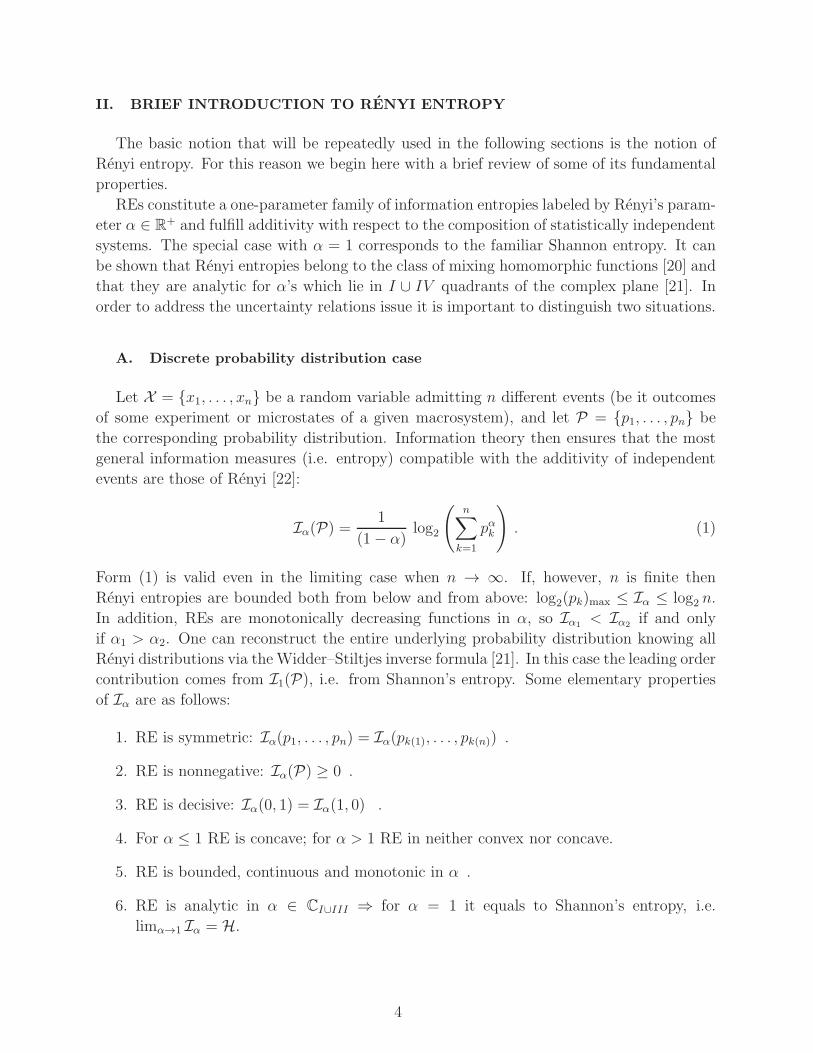
II. BRIEF INTRODUCTION TO RENYI ENTROPY

The basic notion that will be repeatedly used in the following sections is the notion of

Renyi entropy. For this reason we begin here with a brief review of some of its fundamental

properties.

REs constitute a one-parameter family of information entropies labeled by Renyi’s param-

eter α ∈ R+ and fulfill additivity with respect to the composition of statistically independent

systems. The special case with α = 1 corresponds to the familiar Shannon entropy. It can

be shown that Renyi entropies belong to the class of mixing homomorphic functions [20] and

that they are analytic for α’s which lie in I ∪ IV quadrants of the complex plane [21]. In

order to address the uncertainty relations issue it is important to distinguish two situations.

A. Discrete probability distribution case

Let X = {x1, . . . , xn} be a random variable admitting n different events (be it outcomes

of some experiment or microstates of a given macrosystem), and let P = {p1, . . . , pn} be

the corresponding probability distribution. Information theory then ensures that the most

general information measures (i.e. entropy) compatible with the additivity of independent

events are those of Renyi [22]:

Iα(P) =1

(1− α)log2

(

n∑

k=1

pαk

)

. (1)

Form (1) is valid even in the limiting case when n → ∞. If, however, n is finite then

Renyi entropies are bounded both from below and from above: log2(pk)max ≤ Iα ≤ log2 n.

In addition, REs are monotonically decreasing functions in α, so Iα1< Iα2

if and only

if α1 > α2. One can reconstruct the entire underlying probability distribution knowing all

Renyi distributions via theWidder–Stiltjes inverse formula [21]. In this case the leading order

contribution comes from I1(P), i.e. from Shannon’s entropy. Some elementary properties

of Iα are as follows:

1. RE is symmetric: Iα(p1, . . . , pn) = Iα(pk(1), . . . , pk(n)) .

2. RE is nonnegative: Iα(P) ≥ 0 .

3. RE is decisive: Iα(0, 1) = Iα(1, 0) .

4. For α ≤ 1 RE is concave; for α > 1 RE in neither convex nor concave.

5. RE is bounded, continuous and monotonic in α .

6. RE is analytic in α ∈ CI∪III ⇒ for α = 1 it equals to Shannon’s entropy, i.e.

limα→1 Iα = H.

4

Among a myriad of information measures REs distinguish themselves by having a firm oper-

ational characterization in terms of block coding and hypotheses testing. Renyi’s parameter

α is then directly related to so-called β-cutoff rates [25]. RE is used in coding theory [26, 27],

cryptography [28, 37, 38], finance [39, 40] and in theory of statistical inference [22]. In physics

one often uses Iα(P) in the framework of quantum information theory [38, 41, 42].

B. Continuous probability distribution case

Let M be a measurable set on which is defined a continuous probability density function

(PDF) F(x). We will assume that the support (or outcome space) is a smooth but not

necessarily compact manifold. By covering the support with the meshM (l) of d–dimensional

(disjoint) cubes M(l)k (k = 1, . . . , n) of size ld we may define the integrated probability in

k–th cube as

pnk = F(xi)ld , xi ∈M

(l)k . (2)

This defines the mesh probability distribution Pn = {pn1, . . . , pnn}. Infinite precision of

measurements (i.e., when l → 0) often brings infinite information. As the most “junk”

information comes from the uniform distribution En, it is more sensible to consider the

relative information entropy rather than absolute one. In references [21, 22] it was shown

that in the limit n → ∞ (i.e., l → 0) it is possible to define a finite information measure

compatible with information theory axioms. This renormalized Renyi entropy, often known

as differential RE entropy, reads

Iα(F) ≡ limn→∞

(Iα(Pn)− Iα(En)) =1

(1− α)log2

(

∫

MdxFα(x)

∫

Mdx 1/V α

)

. (3)

Here V is the volume ofM . Equation (3) can be viewed as a generalization of the Kullback–

Leibler relative entropy [43]. When M is compact it is possible to introduce a simpler

alternative prescription as

Iα(F) ≡ limn→∞

(Iα(Pn)− Iα(En)|V=1) = limn→∞

(Iα(Pn) +D log2 l)

=1

(1− α)log2

(∫

M

dxFα(x)

)

. (4)

In both previous cases D represents the Euclidean dimension of the support. Renyi entropies

(3) and (4) are defined if (and only if) the corresponding integral∫

MdxFα(x) exists. Equa-

tions (3) and (4) indicate that the asymptotic expansion for Iα(Pn) has the form:

Iα(Pn) = −D log2 l + Iα(F) + o(1) = −D log2 l + Iα(F) + log2 Vn +O(1) .

Here Vn is the covering volume and the symbol O(1) is the residual error which tends to

0 for l → 0. In contrast to the discrete case, Renyi entropies Iα(F) are not generally

positive. In particular, a distribution which is more confined than a unit volume has less

RE than the corresponding entropy of a uniform distribution over a unit volume and hence

yields a negative Iα(F). A paradigmatic example of this type of behavior is the δ-function

5

PDF in which case Iα = − log2 δ(0) = −∞, for all α. Information measures Iα(F) and

Iα(F) are often applied in theory of statistical inference [44–47] and in chaotic dynamical

systems [48–51].

III. ENTROPY POWER AND ENTROPY POWER INEQUALITIES

The mathematical underpinning for most uncertainty relations used in quantum mechan-

ics lies in inequality theory. For example, the wave-packet uncertainty relations are derived

from the Plancherel inequality, and the celebrated Robertson–Schrodinger’s VUR is based on

the Cauchy–Schwarz inequality (and ensuing Parseval equality) [5]. Similarly, Fourier-type

uncertainty relations are based on the Hausdorff–Young inequality [66], etc.

In information theory the key related inequalities are a) Young’s inequality that im-

plies the entropy power inequalities, b) the Riesz–Thorin inequality that determines the

generalized entropic uncertainty relations and c) the Cramer–Rao and logarithmic Sobolev

inequalities that imply Fisher’s information uncertainty principle. In this section we will

briefly review the concept of the entropy power and the ensuing entropy power inequality.

Both concepts were developed by Shannon in his seminal 1948 paper in order to bound

the capacity of non-Gaussian additive noise channels [23]. The connection with quantum

mechanics was established by Stam [67], Lieb [72] and others who used the entropy power

inequality to prove standard VUR.

In the second part of this section we show how the entropy power can be extended into

the RE setting. With the help of Young’s inequality we find the corresponding generalized

entropy power inequality. Related applications to quantum mechanics will be postponed to

Section VIB.

A. Entropy power inequality — Shannon entropy case

Suppose that X is a random vector in RD with the PDF F . The differential (or contin-

uous) entropy H(X ) of X is defined as

H(X ) = I1(F) = −∫

RD

F(x) log2F(x) dx . (5)

The discrete version of (5) is nothing but the Shannon entropy [23], and in such a case it

represents an average number of binary questions that are needed to reveal the value of X .

Actually, (5) is not a proper entropy but rather information gain [21, 22] as can be seen

directly from (4) when the limit α → 1 is taken. We shall return to this point in Section 5.

The entropy power N(X ) of X is the unique number such that [23, 24]

H (X ) = H (XG) , (6)

where XG is a Gaussian random vector with zero mean and variance equal to N(X ), i.e.,

XG ∼ N (0, N(X )1D×D). Eq.(6) can be equivalently rewritten in the form

H (X ) = H(

√

N(X ) · ZG

)

, (7)

6

with ZG representing a Gaussian random vector with the zero mean and unit covariance

matrix. The solution of both (6) and (7) is then

N(X ) =2

2

DH(X )

2πe. (8)

Let X1 and X2 be two independent continuous vector valued random variables of finite

variance. In the case when the Shannon differential entropy is measured in nats (and not

bits) we get for the entropy power

N(X ) =1

2πeexp

(

2

DH(X )

)

. (9)

The differential entropy (8) (as well as (9)) satisfies the so-called entropy power inequality

N(X1 + X2) ≥ N(X1) + N(X1) , (10)

where the equality holds iff X1 and X2 are multivariate normal random variables with pro-

portional covariance matrices [23]. In general, inequality (10) does not hold when X1 and

X2 are discrete random variables and the differential entropy is replaced with the discrete

entropy. Shannon originally used this inequality to obtain a lower bound for the capacity of

non-Gaussian additive noise channels. Since Shannon’s pioneering paper several proofs of

the entropy power inequality have become available [54, 55, 57, 67].

B. Entropy power inequality — Renyi entropy case

In the following we will show how it is possible to extend the entropy power concept to

REs. To this end we first define Renyi entropy power (for simplicity we use nats as units of

information).

Definion III.1 Let p > 1 and let X be a random vector in RD with probability density

F ∈ ℓp(RD). The p-th Renyi entropy power of X is defined as

Np(X ) =1

2πp−p

′/p||F||−2p′/Dp =

1

2πp−p

′/p exp

(

2

DIp(F)

)

, (11)

where p′ is the Holder conjugate of p.

The above form of Np(X ) was probably firstly stated by Gardner [58] who, however, did

not develop the analogy with N(X ) any further. Plausibility of Np(X ) as the entropy power

comes from the following important properties:

Theorem III.1 The p-th Renyi entropy power Np(X ) is a unique solution of the equation

Ip (X ) = Ip(

√

Np(X ) · ZG

)

. (12)

7

With ZG representing a Gaussian random vector with zero mean and unit covariance matrix.

In addition, in the limit p→ 1+ one has Np(X ) → N(X ).

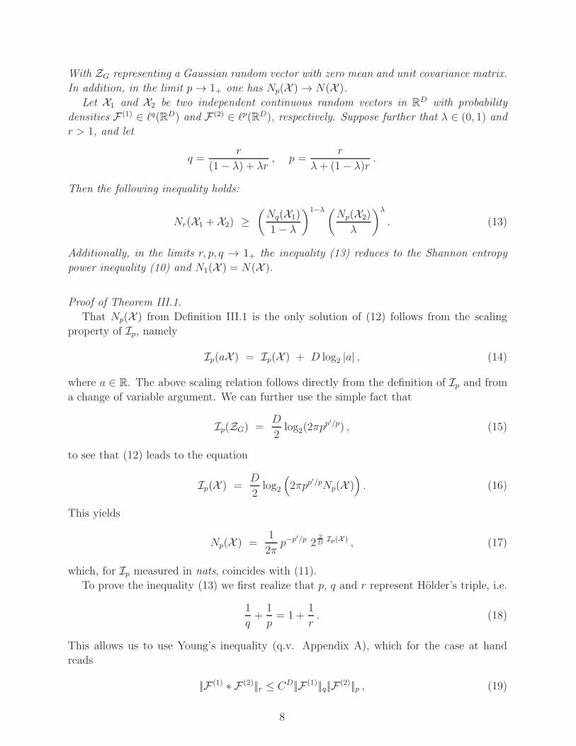
Let X1 and X2 be two independent continuous random vectors in RD with probability

densities F (1) ∈ ℓq(RD) and F (2) ∈ ℓp(RD), respectively. Suppose further that λ ∈ (0, 1) and

r > 1, and let

q =r

(1− λ) + λr, p =

r

λ+ (1− λ)r.

Then the following inequality holds:

Nr(X1 + X2) ≥(

Nq(X1)

1− λ

)1−λ(Np(X2)

λ

)λ

. (13)

Additionally, in the limits r, p, q → 1+ the inequality (13) reduces to the Shannon entropy

power inequality (10) and N1(X ) = N(X ).

Proof of Theorem III.1.

That Np(X ) from Definition III.1 is the only solution of (12) follows from the scaling

property of Ip, namely

Ip(aX ) = Ip(X ) + D log2 |a| , (14)

where a ∈ R. The above scaling relation follows directly from the definition of Ip and from

a change of variable argument. We can further use the simple fact that

Ip(ZG) =D

2log2(2πp

p′/p) , (15)

to see that (12) leads to the equation

Ip(X ) =D

2log2

(

2πpp′/pNp(X )

)

. (16)

This yields

Np(X ) =1

2πp−p

′/p 22

DIp(X ) , (17)

which, for Ip measured in nats, coincides with (11).

To prove the inequality (13) we first realize that p, q and r represent Holder’s triple, i.e.

1

q+

1

p= 1 +

1

r. (18)

This allows us to use Young’s inequality (q.v. Appendix A), which for the case at hand

reads

||F (1) ∗ F (2)||r ≤ CD||F (1)||q||F (2)||p , (19)

8

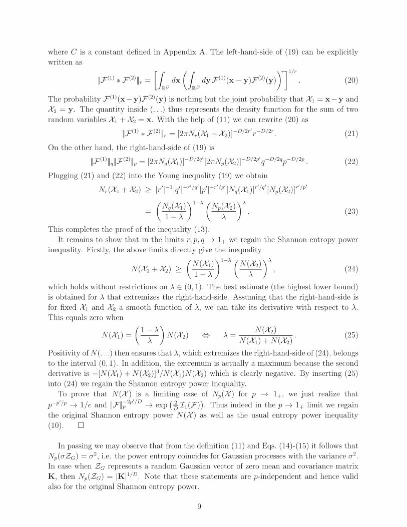
where C is a constant defined in Appendix A. The left-hand-side of (19) can be explicitly

written as

||F (1) ∗ F (2)||r =[∫

RD

dx

(∫

RD

dyF (1)(x− y)F (2)(y)

)r]1/r

. (20)

The probability F (1)(x−y)F (2)(y) is nothing but the joint probability that X1 = x−y and

X2 = y. The quantity inside (. . .) thus represents the density function for the sum of two

random variables X1 + X2 = x. With the help of (11) we can rewrite (20) as

||F (1) ∗ F (2)||r = [2πNr(X1 + X2)]−D/2r′r−D/2r. (21)

On the other hand, the right-hand-side of (19) is

||F (1)||q||F (2)||p = [2πNq(X1)]−D/2q′ [2πNp(X2)]

−D/2p′q−D/2qp−D/2p . (22)

Plugging (21) and (22) into the Young inequality (19) we obtain

Nr(X1 + X2) ≥ |r′|−1|q′|−r′/q′ |p′|−r′/p′ [Nq(X1)]r′/q′ [Np(X2)]

r′/p′

=

(

Nq(X1)

1− λ

)1−λ(Np(X2)

λ

)λ

. (23)

This completes the proof of the inequality (13).

It remains to show that in the limits r, p, q → 1+ we regain the Shannon entropy power

inequality. Firstly, the above limits directly give the inequality

N(X1 + X2) ≥(

N(X1)

1− λ

)1−λ(N(X2)

λ

)λ

, (24)

which holds without restrictions on λ ∈ (0, 1). The best estimate (the highest lower bound)

is obtained for λ that extremizes the right-hand-side. Assuming that the right-hand-side is

for fixed X1 and X2 a smooth function of λ, we can take its derivative with respect to λ.

This equals zero when

N(X1) =

(

1− λ

λ

)

N(X2) ⇔ λ =N(X2)

N(X1) +N(X2). (25)

Positivity ofN(. . .) then ensures that λ, which extremizes the right-hand-side of (24), belongs

to the interval (0, 1). In addition, the extremum is actually a maximum because the second

derivative is −[N(X1) + N(X2)]3/N(X1)N(X2) which is clearly negative. By inserting (25)

into (24) we regain the Shannon entropy power inequality.

To prove that N(X ) is a limiting case of Np(X ) for p → 1+, we just realize that

p−p′/p → 1/e and ||F||−2p′/D

p → exp(

2DI1(F)

)

. Thus indeed in the p → 1+ limit we regain

the original Shannon entropy power N(X ) as well as the usual entropy power inequality

(10). �

In passing we may observe that from the definition (11) and Eqs. (14)-(15) it follows that

Np(σZG) = σ2, i.e. the power entropy coincides for Gaussian processes with the variance σ2.

In case when ZG represents a random Gaussian vector of zero mean and covariance matrix

K, then Np(ZG) = |K|1/D. Note that these statements are p-independent and hence valid

also for the original Shannon entropy power.

9

1

1

b

a

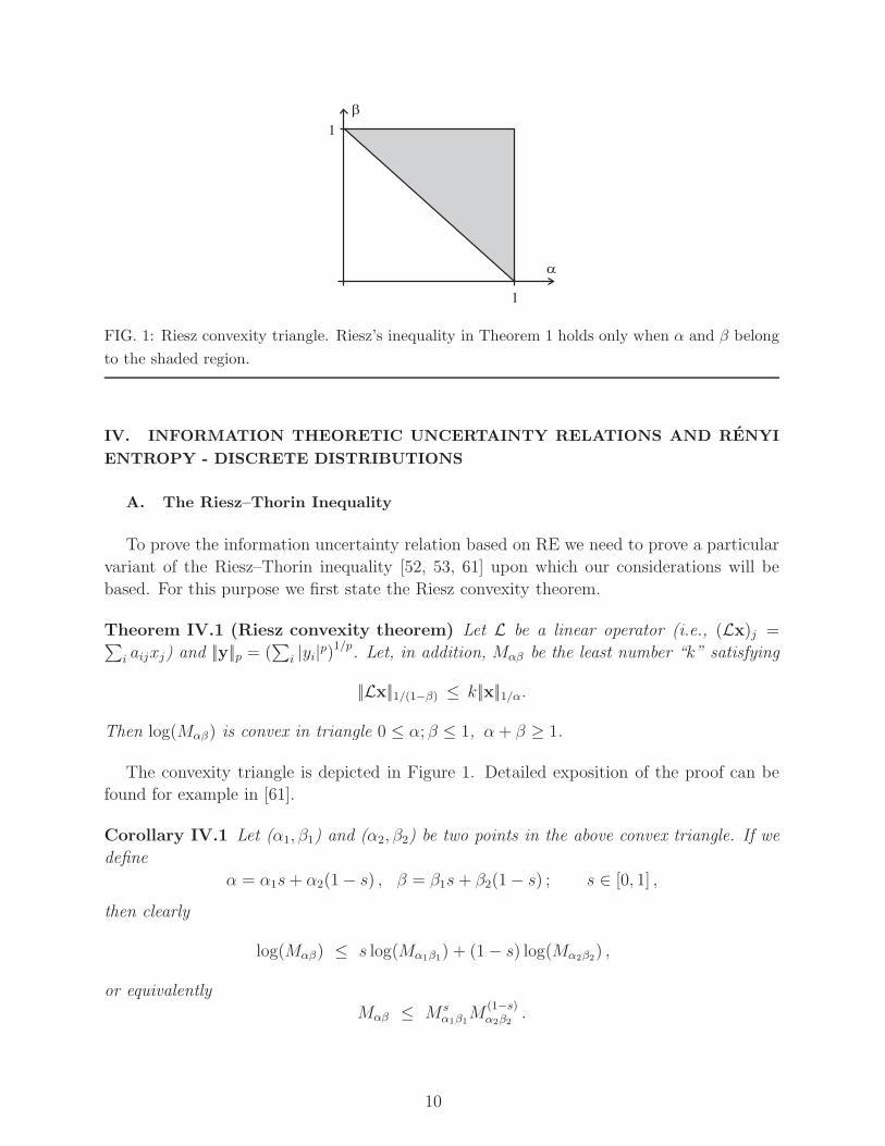
FIG. 1: Riesz convexity triangle. Riesz’s inequality in Theorem 1 holds only when α and β belong

to the shaded region.

IV. INFORMATION THEORETIC UNCERTAINTY RELATIONS AND RENYI

ENTROPY - DISCRETE DISTRIBUTIONS

A. The Riesz–Thorin Inequality

To prove the information uncertainty relation based on RE we need to prove a particular

variant of the Riesz–Thorin inequality [52, 53, 61] upon which our considerations will be

based. For this purpose we first state the Riesz convexity theorem.

Theorem IV.1 (Riesz convexity theorem) Let L be a linear operator (i.e., (Lx)j =∑

i aijxj) and ||y||p = (∑

i |yi|p)1/p. Let, in addition, Mαβ be the least number “k” satisfying

||Lx||1/(1−β) ≤ k||x||1/α.

Then log(Mαβ) is convex in triangle 0 ≤ α; β ≤ 1, α+ β ≥ 1.

The convexity triangle is depicted in Figure 1. Detailed exposition of the proof can be

found for example in [61].

Corollary IV.1 Let (α1, β1) and (α2, β2) be two points in the above convex triangle. If we

define

α = α1s+ α2(1− s) , β = β1s+ β2(1− s) ; s ∈ [0, 1] ,

then clearly

log(Mαβ) ≤ s log(Mα1β1) + (1− s) log(Mα2β2) ,

or equivalently

Mαβ ≤ Msα1β1M

(1−s)α2β2

.

10

Theorem IV.2 (Riesz–Thorin inequality) Suppose that (Lx)j =∑

i ajixi and that

∑

j

|(Lx)j|2 ≤∑

j

|xj|2 .

Then for p ∈ [1, 2] and c ≡ maxi,j |aij |

||Lx||p′ ≤ c(2−p)/p||x||p = c1/pc−1/p′ ||x||p ⇔ c1/p′ ||Lx||p′ ≤ c1/p||x||p ,

holds. Here p and p′ are Holder conjugates, i.e., 1/p+ 1/p′ = 1.

Proof of Theorem IV.2. We shall use the notation α = 1/p, β = 1/q (and the Holder

conjugates p′ = p/(p − 1), q′ = q/(q − 1)). Consider the line from (α1, β1) = (1/2, 1/2) to

(α2, β2) = (1, 1) in the (α, β) plane. This line lies entirely in the triangle of concavity (see

Figure 1). Let us now define

α = α1s + α2(1− s)

= s/2 + (1− s)

= −s/2 + 1 ,

implying s = 2(1− α), and define

β = β1s+ β2(1− s)

= −s/2 + 1 ,

implying β = α. Hence

Mα,α ≤ Msα1β1M

(1−s)α2β2

= M2(1−α)1/2,1/2 M

2α−11,1 . (26)

Note particularly that because s ∈ [0, 1] then α ∈ [1/2, 1] and p ∈ [1, 2]. To estimate

the right hand side of (26) we first realize that M1/2,1/2 ≤ 1. This results from the very

assumption of the theorem, namely that

‖Lx‖22 =∑

j

|(Lx)j|2 ≤∑

j

|xj|2 = ‖x‖22 .

Hence, M1/2,1/2 ≤ k = 1. To find the estimate for M11 we realize that it represents the

smallest k in the relation

||Lx||∞ ≤ k||x||1 .Thus

M11 = maxx 6=0

||Lx||∞||x||1

= maxx 6=0

maxj |(Lx)j|∑

i |xi|≤ max

i,j|aij | ≡ c . (27)

So finally we can write that

Mα,α = M1/p,(1−1/p′) ≤ c2α−1 = c(2−p)/p = c1/pc−1/p′ . �

11

z2

z1

z2

z1

z2

z1

f

x

y

z

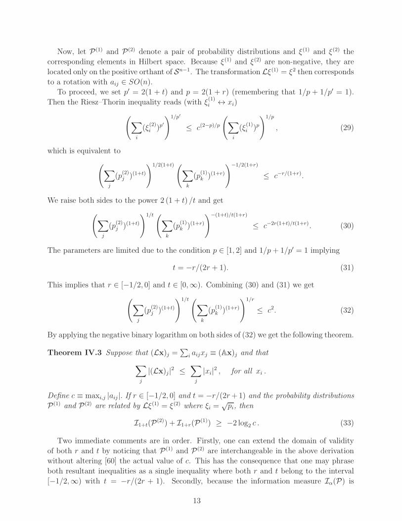
FIG. 2: A statistical system can be represented by points ξ on a positive orthant (Sn−1)+ of the

unit sphere Sn−1 in a real Hilbert space H. The depicted example corresponds to n = 3.

B. Generalized ITUR

To establish the connection with RE let us assume that X is a discrete random variable

with n different values, Pn is the probability space affiliated with X and P = {p1, . . . , pn}is a sample probability distribution from Pn. Normally the geometry of Pn is identified with

the geometry of a simplex. For our purpose it is more interesting to embed Pn in a sphere.

Because P is non–negative and summable to unity, it follows that the square–root likelihood

ξi =√pi exists for all i = 1, . . . , n, and it satisfies the normalization condition

n∑

i=1

(ξi)2 = 1 .

Hence ξ can be regarded as a unit vector in the Hilbert space H = Rn. Then the inner

product

cosφ =

n∑

i=1

ξ(1)i ξ

(2)i = 1− 1

2

n∑

i=1

(

ξ(1)i − ξ

(2)i

)2

, (28)

defines the angle φ that can be interpreted as a distance between two probability distribu-

tions. More precisely, if Sn−1 is the unit sphere in the n-dimensional Hilbert space, then φ

is the spherical (or geodesic) distance between the points on Sn−1 determined by ξ(1) and

ξ(2). Clearly, the maximal possible distance, corresponding to orthogonal distributions, is

given by φ = π/2. This follows from the fact that ξ(1) and ξ(2) are non–negative, and hence

they are located only on the positive orthant of Sn−1 (see Figure 2). The geodesic distance

φ is called the Bhattacharyya distance. The representation of probability distributions as

points on a sphere also has an interesting relation to Bayesian statistics. If we use a uniform

distribution on the sphere as the prior distribution then the prior distribution on probability

vectors in Pn is exactly the celebrated Jeffrey’s prior that has found new justification via the

minimum description length approach to statistics [70].

12

Now, let P(1) and P(2) denote a pair of probability distributions and ξ(1) and ξ(2) the

corresponding elements in Hilbert space. Because ξ(1) and ξ(2) are non-negative, they are

located only on the positive orthant of Sn−1. The transformation Lξ(1) = ξ2 then corresponds

to a rotation with aij ∈ SO(n).

To proceed, we set p′ = 2(1 + t) and p = 2(1 + r) (remembering that 1/p + 1/p′ = 1).

Then the Riesz–Thorin inequality reads (with ξ(1)i ↔ xi)

(

∑

i

(ξ(2)i )p

′

)1/p′

≤ c(2−p)/p

(

∑

i

(ξ(1)i )p

)1/p

, (29)

which is equivalent to

(

∑

j

(p(2)j )(1+t)

)1/2(1+t)(∑

k

(p(1)k )(1+r)

)−1/2(1+r)

≤ c−r/(1+r).

We raise both sides to the power 2 (1 + t) /t and get

(

∑

j

(p(2)j )(1+t)

)1/t(∑

k

(p(1)k )(1+r)

)−(1+t)/t(1+r)

≤ c−2r(1+t)/t(1+r). (30)

The parameters are limited due to the condition p ∈ [1, 2] and 1/p+ 1/p′ = 1 implying

t = −r/(2r + 1). (31)

This implies that r ∈ [−1/2, 0] and t ∈ [0,∞). Combining (30) and (31) we get

(

∑

j

(p(2)j )(1+t)

)1/t(∑

k

(p(1)k )(1+r)

)1/r

≤ c2. (32)

By applying the negative binary logarithm on both sides of (32) we get the following theorem.

Theorem IV.3 Suppose that (Lx)j =∑

i aijxj ≡ (Ax)j and that

∑

j

|(Lx)j|2 ≤∑

j

|xi|2 , for all xi .

Define c ≡ maxi,j |aij |. If r ∈ [−1/2, 0] and t = −r/(2r+1) and the probability distributions

P(1) and P(2) are related by Lξ(1) = ξ(2) where ξi =√pi, then

I1+t(P(2)) + I1+r(P(1)) ≥ −2 log2 c . (33)

Two immediate comments are in order. Firstly, one can extend the domain of validity

of both r and t by noticing that P(1) and P(2) are interchangeable in the above derivation

without altering [60] the actual value of c. This has the consequence that one may phrase

both resultant inequalities as a single inequality where both r and t belong to the interval

[−1/2,∞) with t = −r/(2r + 1). Secondly, because the information measure Iα(P) is

13

always non-negative, the inequality (33) can represent a genuine uncertainty relation only

when c < 1. Note that for A ∈ SO(n) or SU(n) (i.e. for most physically relevant situations)

one always has that c ≤ 1. This is because for such A’s

c = maxi,j

|aik| = ||A||max ≤ ||A||2 =√

λmax(A†A) = 1 . (34)

The last identity results from the fact that all of eigenvalues of A ∈ SO(n) or SU(n) have

absolute value 1.

It needs to be stressed that in the particular case when r = 0 (and thus also t = 0) we

get

H(P(2)) + H(P(1)) ≥ −2 log2 c . (35)

This Shannon entropy based uncertainty relation was originally found by Kraus [71] and

Maassen [9]. A weaker version of this ITUR was also earlier proposed by Deutsch [8].

The reader can see that ITUR (33) which is based on RE provides a natural extension of

the Shannon ITUR (35). In Section VI we shall see that there are quantum mechanical sys-

tems where Renyi’s ITUR improves both on Robertson–Schrodinger’s VUR and Shannon’s

ITUR.

C. Geometric interpretation of inequality (33)

Let us close this section by providing a useful geometric understanding of the inequality

(33). To this end we invoke two concepts known from error analysis. These are, the condition

number and distance to singularity (see, e.g., Refs. [79, 80]).

The condition number κα,β(A) of the non-singular matrix A is defined as

κα,β(A) = ||A||α,β||A−1||β,α , (36)

where, the corresponding (mixed) matrix-valued norm ||A||α,β is defined as

||A||α,β = maxx 6=0

||Ax||β||x||α

. (37)

So, in particular M11 = c from (27) is nothing but ||A||1,∞. Note also that ||A||α,α = ||A||α,which is the usual α-matrix norm. Justification for calling κα,β a condition number comes

from the following theorem:

Theorem IV.4 Let Ax = y be a linear equation and let there be an error (or uncertainty)

δy in representing the vector y, and let x = x + δx solve the new error-hindered equation

Ax = y + δy. The relative disturbance in x in relation to δy fulfills

||δx||α||x||α

≤ κα,β(A)||δy||β||y||β

. (38)

14

Proof of Theorem IV.4. The proof is rather simple. Using the fact that Ax = y and

Ax = y + δy we obtain δx = A−1δy. Taking α-norm on both sides we can write

||δx||α = ||A−1δy||α ≤ ||A−1||β,α||δy||β . (39)

On the other hand, the β-norm of Ax = y yields

||y||β = ||Ax||β ≤ ||A||α,β||x||α ⇔ 1

||x||α≤ ||A||α,β

||y||β. (40)

Combining (39) with (40) we obtain (38). �

From the previous theorem we see that κα,β(A) quantifies a stability of the linear equation

Ax = y, or better the extent to which the relative error (uncertainty) in y influences the

relative error in x. A system described by A and y is stable if κα,β(A) is not too large

(ideally close to one). It is worth of stressing that κα,β(A) ≥ 1. The latter results from the

fact that

||x||β = ||AA−1x||β ≤ ||AA−1||β,β||x||β ≤ ||A||α,β||A−1||β,α||x||β . (41)

In the last step we have used the submultiplicative property of mixed matrix norms.

The second concept — the distance to singularity for a matrix A, is defined as

distα,β(A) ≡ min {||∆A||α,β; A+∆A singular} . (42)

In this connection an important theorem states that the relative distance to singularity is

the reciprocal of the condition number.

Theorem IV.5 For a non-singular matrix A, one has

distα,β(A)

||A||α,β= κα,β(A)

−1 . (43)

Proof of Theorem IV.5. If A + ∆A is singular then there is a vector x 6= 0, such that

(A +∆A)x = 0. Because A is non-singular, the latter is equivalent to x = −A−1∆Ax. By

taking the α-norm we have

||x||α = ||A−1∆Ax||α ≤ ||A−1||β,α||∆Ax||β ≤ ||A−1||β,α||∆A||α,β||x||α , (44)

which is equivalent to

||∆A||α,β||A||α,β

≥ κα,β(A)−1 . (45)

To show that κα,β(A)−1 is a true minimum of the left-hand side of (45) and not mere lower

bound we must show that there exists such a suitable perturbation ∆A which saturates the

inequality. Corresponding ||∆A||α,β will then clearly represent distα,β(A). Consider y such

15

that ||y||β = 1 and ||A−1y||α = ||A−1||β,α, and write z = A−1y. Define further a vector z such

that

max||ζ||α=1

|z∗ · ζ |||z||α

=z∗ · z||z||α

= 1 . (46)

We now introduce the matrix Bi,j = −yiz∗j , which implies Bz/||z||α = −y. Note that B thus

defined fulfills

||B||α,β = max||ζ||α=1

||y(z∗ · ζ)||β||z||α

= ||y||β max||ζ||α=1

|z∗ · ζ |||z||α

= 1 . (47)

Let us set ∆A = B/||z||α. This directly implies that

(A+∆A)A−1y = y +Bz

||z||α= 0 . (48)

So the matrix A+∆A is singular with A−1y being the null vector. Finally note that

||∆A||α,β||A||α,β

=||B||α,β

||z||α||A||α,β=

1

||A−1y||α||A||α,β= κα,β(A)

−1 . �

The connection with the ITUR (33) is established when we observe that the smallest value

of c is (see, Eqs.(27) and (43))

c = ||A||1,∞ = dist1,∞(A)κ1,∞(A) . (49)

Since c ≤ 1, this shows that the ITUR (33) restricts the probability distributions more

the smaller the distance to singularity and/or the lower the stability of the transformation

matrix A is. In practical terms this means that the rotation/transformation within the

positive orthant introduces higher ignorance or uncertainty in the ITUR the more singular

the rotation/transformation matrices are.

V. INFORMATION THEORETIC UNCERTAINTY RELATIONS AND RENYI

ENTROPY - CONTINUOUS DISTRIBUTIONS

Before considering quantum-mechanical implications of Renyi’s ITUR (33), we will briefly

touch upon the continuous-probability analogue of (33). This issue is conceptually far more

delicate than the discrete one namely because it is difficult to find norms for the correspon-

dent (integro-)differential operators L. This in particular does not allow one to calculate

explicitly the optimal bounds in many relevant cases. Fortunately, there is one very im-

portant class of situations, where one can proceed with relative ease. This is the situation

when the linear transform is represented by a continuous Fourier transform, in which case

the Riesz-Thorin inequality is taken over by the Beckner-Babebko inequality [62, 63].

Theorem V.1 (Beckner–Babebko’s theorem) Let

f (2)(x) ≡ f (1)(x) =

∫

RD

e2πix.y f (1)(y) dy ,

16

then for p ∈ [1, 2] we have

||f ||p′ ≤ |pD/2|1/p|(p′)D/2|1/p′ ||f ||p , (50)

or, equivalently

|(p′)D/2|1/p′||f (2)||p′ ≤ |pD/2|1/p||f (1)||p .

Here, again, p and p′ are the usual Holder conjugates. For any F ∈ ℓp(RD) the p-norm ||F ||pis defined as

||F ||p =(∫

RD

|F (y)|p dy)1/p

.

Due to symmetry of the Fourier transform the reverse inequality also holds:

||f ||p′ ≤ |pD/2|1/p|(p′)D/2|1/p′ ||f ||p . (51)

The proof of this theorem can be found in the Appendix. Lieb [64] proved that the inequal-

ity (50) is saturated only for Gaussian functions. In the case of discrete Fourier transforms

the corresponding inequality is known as the (classical) Hausdorff–Young inequality [61, 66].

Analogous manipulations that have brought us from equation (29) to equation (32) will

allow us to cast (50) in the form

(∫

RD

[F (2)(y)](1+t) dy

)1/t(∫

RD

[F (1)(y)](1+r) dy

)1/r

≤ [2(1 + t)]D |t/r|D/2r , (52)

where we have defined the square-root density likelihood as |f(y)| =√

F(y).

When the negative binary logarithm is applied to both sides of (52), then

I1+t(F (2)) + I1+r(F (1)) ≥ −D +1

rlog2(1 + r)D/2 +

1

tlog2(1 + t)D/2 . (53)

Because 1/t+ 1/r = −2, we can recast the previous inequality in the equivalent form

I1+t(F (2)) + I1+r(F (1)) ≥ 1

rlog2[2(1 + r)]D/2 +

1

tlog2[2(1 + t)]D/2 . (54)

This can be further simplified by looking at the minimal value of the RHS of (53) (or (54))

under the constraint 1/t + 1/r = −2. The minimal value is attained for t = −1/2 and

equivalently t = ∞, see Fig. 3, and it is 0 (note t cannot be smaller than −1/2). This in

particular implies that

I1+t(F (2)) + I1+r(F (1)) ≥ 0 . (55)

Inequality (53) is naturally stronger than (55), but the latter is usually much easier to

implement in practical calculations. In addition the RHS of (53) is universal in the sense

that it is t and r independent. The reader should also notice that the zero value of the

17

FIG. 3: Dependence of the RHS of (54) on t provided we substitute for r = −t/(2t + 1). The

minimum is attained for t = −1/2 and t = ∞ (and hence r = ∞ and r = −1/2, respectively) while

maximum is at t = 0+ (and hence for r = 0−).

right-hand side of (55) does not yield a trivial inequality since Iα are not generally positive

for continuous PDFs (q.v. Section 4.2). In fact, from the coarse probability version of (55)

(cf. Eq. (4)) follows

I1+t(P(2)n ) + I1+r(P(1)

n ) ≥ −2D log2 l , (56)

which is clearly a non-trivial ITUR.

Also, notice that in the limit t → 0+ and r → 0− the inequalities (53)-(54) take the

form [86]

H(F (2)) +H(F (1)) ≥ log2

(e

2

)D

, (57)

which coincides with the classical Hirschman conjecture for the differential Shannon entropy

based ITUR [81]. In this connection it should be noted that among all admissible pairs

{r, t}, the pair {0−, 0+} gives the highest value of the RHS in (54). This can be clearly seen

from Fig. 3.

Let us finally observe that when (53)-(54) is rewritten in the language of Renyi entropy

powers it can be equivalently cast in the form

N1+t(F (2))N1+r(F (1)) ≡ N1+t(X )N1+r(Y) ≥ 1

16π2, (58)

or equivalently as

Np/2(X )Nq/2(Y) ≥ 1

16π2, (59)

with p and q being Holder conjugates and the RE measured in bits. Note that in the case

when both X and Y represent random Gaussian vectors then (59) reduces to

|KX |1/D|KY |1/D =1

16π2. (60)

18

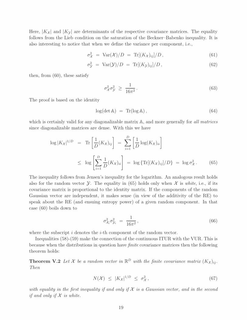
Here, |KX | and |KY | are determinants of the respective covariance matrices. The equality

follows from the Lieb condition on the saturation of the Beckner–Babenko inequality. It is

also interesting to notice that when we define the variance per component, i.e.,

σ2X = Var(X )/D = Tr[(KX )ij ]/D , (61)

σ2Y = Var(Y)/D = Tr[(KY)ij ]/D , (62)

then, from (60), these satisfy

σ2Xσ

2Y ≥ 1

16π2. (63)

The proof is based on the identity

log(detA) = Tr(logA) , (64)

which is certainly valid for any diagonalizable matrix A, and more generally for all matrices

since diagonalizable matrices are dense. With this we have

log |KX |1/D = Tr

[

1

D(KX )ij

]

=

D∑

i=1

[

1

Dlog(KX )ii

]

≤ log

[

D∑

i=1

1

D(KX )ii

]

= log {Tr[(KX )ij]/D} = log σ2X . (65)

The inequality follows from Jensen’s inequality for the logarithm. An analogous result holds

also for the random vector Y . The equality in (65) holds only when X is white, i.e., if its

covariance matrix is proportional to the identity matrix. If the components of the random

Gaussian vector are independent, it makes sense (in view of the additivity of the RE) to

speak about the RE (and ensuing entropy power) of a given random component. In that

case (60) boils down to

σ2Xiσ2Yi

=1

16π2, (66)

where the subscript i denotes the i-th component of the random vector.

Inequalities (58)-(59) make the connection of the continuous ITUR with the VUR. This is

because when the distributions in question have finite covariance matrices then the following

theorem holds:

Theorem V.2 Let X be a random vector in RD with the finite covariance matrix (KX )ij.

Then

N(X ) ≤ |KX |1/D ≤ σ2X , (67)

with equality in the first inequality if and only if X is a Gaussian vector, and in the second

if and only if X is white.

19

The proof of this theorem is based on the non-negativity of the relative Shannon entropy (or

Kullback–Leibler divergence) and can be found, e.g., in Refs. [68, 69]. An important upshot

of the previous theorem is that also for non-Gaussian distributions one has

σ2Xσ

2Y ≥ |KX |1/D|KY |1/D ≥ N(X )N(Y) ≥ 1

16π2, (68)

which saturates only for Gaussian (respective white) random vectors X and Y . This is just

one example where a well-known inequality can be improved by replacing variance by a

quantity related to entropy. In certain cases the last inequality in (68) can be improved by

using Renyi’s entropy power rather than Shannon’s entropy power. In fact, the inequality

N(X )N(Y) ≥ Np/2(X )Nq/2(Y) ≥ 1

16π2, (69)

(with p and q being Holder conjugates) is fulfilled whenever

H(X )− Ip/2(X ) ≥ Iq/2(Y)−H(Y) , (70)

(q ∈ [1, 2] and p ∈ [2,∞)). Note that both sides in (70) are positive (cf. Eq. (4)). Inequal-

ity (70) can be satisfied by a number of PDFs. This is often the case when the PDF F (1)

associated with Y is substantially leptokurtic (peaked) while F (2) (which is related to X )

is platykurtic heavy-tailed PDF. A simple example is the Cauchy–Lorentz distribution [11],

for which we have

f(x) =

√

c

π

√

1

c2 + x2, (71)

f(y) =

√

2c

π2K0(c|y|) , (72)

F (2)(x) =c

π

1

c2 + x2, (73)

F (1)(y) =2c

π2K2

0 (c|y|) . (74)

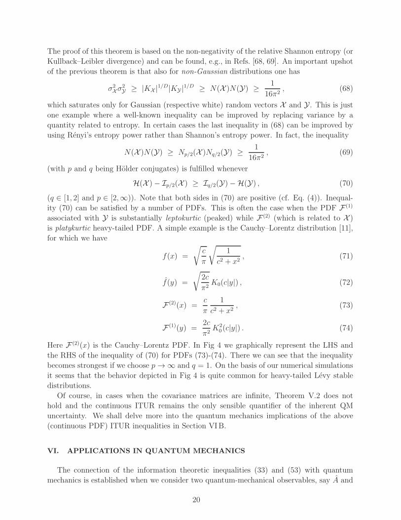
Here F (2)(x) is the Cauchy–Lorentz PDF. In Fig 4 we graphically represent the LHS and

the RHS of the inequality of (70) for PDFs (73)-(74). There we can see that the inequality

becomes strongest if we choose p→ ∞ and q = 1. On the basis of our numerical simulations

it seems that the behavior depicted in Fig 4 is quite common for heavy-tailed Levy stable

distributions.

Of course, in cases when the covariance matrices are infinite, Theorem V.2 does not

hold and the continuous ITUR remains the only sensible quantifier of the inherent QM

uncertainty. We shall delve more into the quantum mechanics implications of the above

(continuous PDF) ITUR inequalities in Section VIB.

VI. APPLICATIONS IN QUANTUM MECHANICS

The connection of the information theoretic inequalities (33) and (53) with quantum

mechanics is established when we consider two quantum-mechanical observables, say A and

20

10 15 20p

0.2

0.4

0.6

0.8

1.0

1.2

D

RHS

LHS

FIG. 4: Graphical representation of the LHS and the RHS of the inequality of (70). ∆ denotes

the difference of entropies on the LHS respective the RHS of (70). The q variable is phrased in

terms of p as q = p/(p − 1). Because the PDF’s involved have no fundamental scale, the ensuing

entropies (and hence ∆) are c independent. Note in particular that the inequality (70) is strongest

for p → ∞ and q = 1.

B, written through their spectral decompositions

A =∑

∫

a|a〉〈a| da , B =∑

∫

b|b〉〈b| db . (75)

Here the integral-summation symbol schematically represents summation over a discrete

part of the spectra and integration over a continuous part of the spectra. States |a〉 and |b〉are proper (for discrete spectrum) and improper (for the continuous spectrum) eigenvectors

of A and B, respectively.

According to the quantum measurement postulate, the probability of obtaining a result

a in a measurement of observable A on a system prepared in the state |φ〉 is given by the

(transition) probability density

F(a) = |〈a|φ〉|2 . (76)

When ai belongs to a discrete spectrum, then the (transition) probability for the result ai is

p(ai) = |〈ai|φ〉|2 . (77)

Similarly for the observable B.

21

A. Discrete probabilities

For the discrete-spectrum the conditions assumed in the Riesz–Thorin inequality (cf.

Theorem IV.2) are clearly fulfilled by setting xi = 〈xi|φ〉, (Lx)j = 〈bj|φ〉 and aij = 〈bj |ak〉.We will now illustrate the utility of Renyi’s ITUR with a toy-model example. To this end we

consider a two-dimensional state |φ〉 of a spin-12particle, and let A and B be spin components

in orthogonal directions, i.e.

|A〉 ≡( |Sx; +〉|Sx;−〉

)

, |B〉 ≡( |Sz; +〉|Sz;−〉

)

. (78)

Because( |Sx; +〉|Sx;−〉

)

=1√2

(

1 1

−1 1

)( |Sz; +〉|Sz;−〉

)

, (79)

we can immediately identify c with 1/√2 (cf. Eq. (35)). Let us now define probability

P = (p, (1 − p)) ≡ (|〈Sx; +|φ〉|2, |〈Sx;−|φ〉|2). Without loss of generality we may assume

that p = maxi P. The question we are interested in is how the knowledge of P restricts

the distribution Q = (q, (1− q)) ≡ (|〈Sz; +|φ〉|2, |〈Sz;−|φ〉|2)? Both distribution cannot be

independent as Shannon’s ITUR

H(P) + H(Q) ≥ −2 log2 c = 1 , (80)

clearly indicates. In fact, inequality (80) can be equivalently phrased in the form

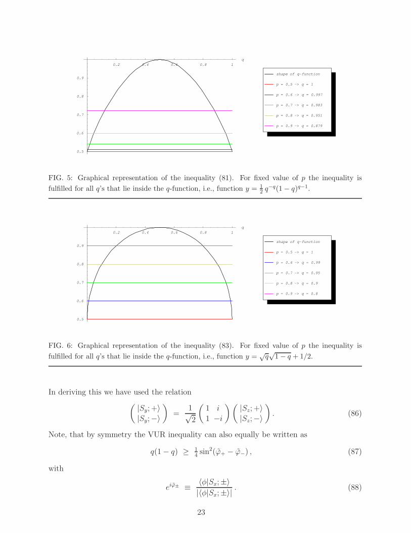
pp(1− p)1−p ≤ 12q−q(1− q)q−1 . (81)

The graphical solution of this equation can be seen on Fig. 5. In case of Renyi’s ITUR we

can take advantage of the fact that the RE is a monotonically decreasing function of its

index and hence the most stringent relation between p and q is provided via Renyi’s ITUR

I∞(P) + I1/2(Q) ≥ −2 log2 c = 1 . (82)

The latter is equivalent to

√q√

1− q + 1/2 ≥ p . (83)

This inequality can be again treated graphically, see Fig. 6. The comparison with the

ordinary Schrodinger–Robertson’s VUR, can easily be made. In fact, we have

〈(△Sx)2〉φ〈(△Sz)2〉φ ≥ ~2

4|〈Sy〉φ|2 ⇔ p(1− p) ≥ 1

4sin2(ϕ+ − ϕ−) , (84)

where the phase ϕ± is defined as

eiϕ± ≡ 〈φ|Sz;±〉|〈φ|Sz;±〉| . (85)

22

0.2 0.4 0.6 0.8 1

q

0.5

0.6

0.7

0.8

0.9

p = 0.9 -> q = 0.879

p = 0.8 -> q = 0.951

p = 0.7 -> q = 0.983

p = 0.6 -> q = 0.997

p = 0.5 -> q = 1

shape of q-function

FIG. 5: Graphical representation of the inequality (81). For fixed value of p the inequality is

fulfilled for all q’s that lie inside the q-function, i.e., function y = 12 q

−q(1 − q)q−1.

0.2 0.4 0.6 0.8 1

q

0.5

0.6

0.7

0.8

0.9

p = 0.9 -> q = 0.8

p = 0.8 -> q = 0.9

p = 0.7 -> q = 0.95

p = 0.6 -> q = 0.99

p = 0.5 -> q = 1

shape of q-function

FIG. 6: Graphical representation of the inequality (83). For fixed value of p the inequality is

fulfilled for all q’s that lie inside the q-function, i.e., function y =√q√

1 − q + 1/2.

In deriving this we have used the relation( |Sy; +〉|Sy;−〉

)

=1√2

(

1 i

1 −i

)( |Sz; +〉|Sz;−〉

)

. (86)

Note, that by symmetry the VUR inequality can also equally be written as

q(1− q) ≥ 14sin2(ϕ+ − ϕ−) , (87)

with

eiϕ± ≡ 〈φ|Sx;±〉|〈φ|Sx;±〉| . (88)

23

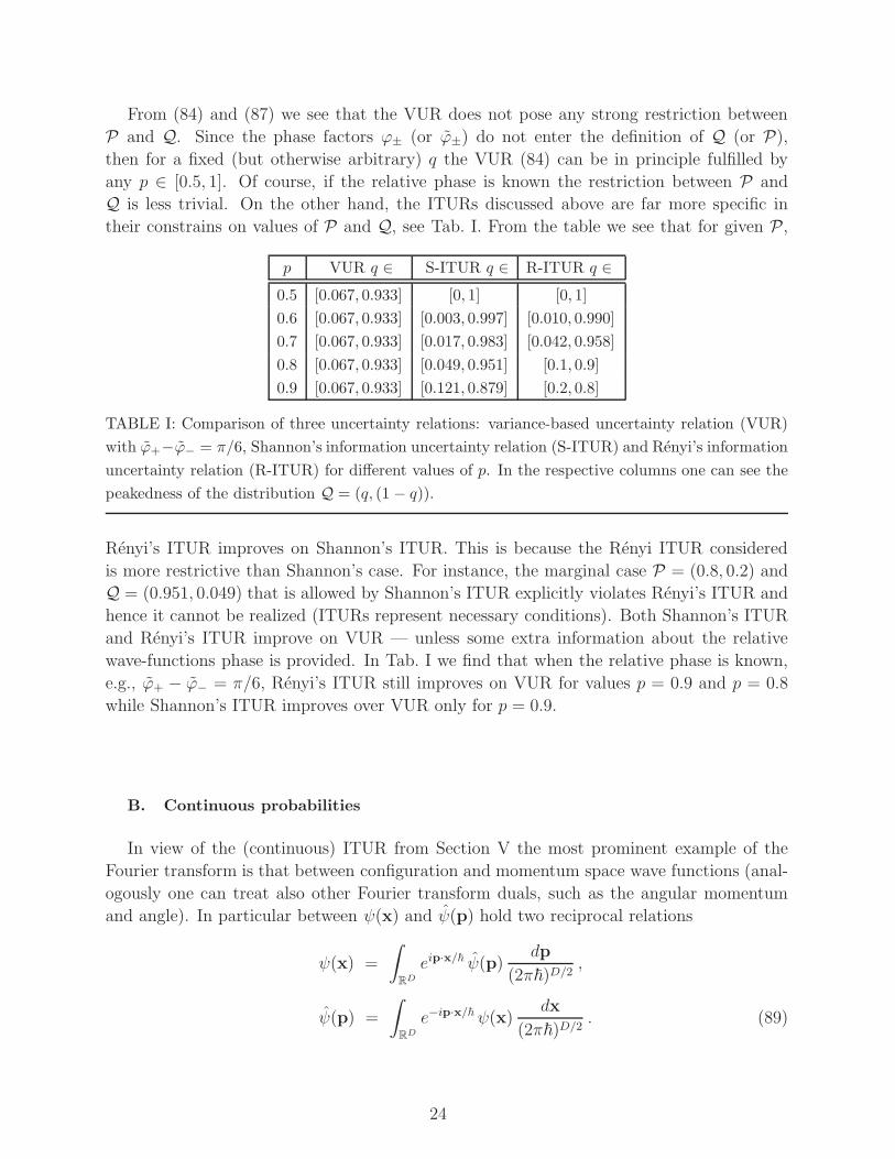
From (84) and (87) we see that the VUR does not pose any strong restriction between

P and Q. Since the phase factors ϕ± (or ϕ±) do not enter the definition of Q (or P),

then for a fixed (but otherwise arbitrary) q the VUR (84) can be in principle fulfilled by

any p ∈ [0.5, 1]. Of course, if the relative phase is known the restriction between P and

Q is less trivial. On the other hand, the ITURs discussed above are far more specific in

their constrains on values of P and Q, see Tab. I. From the table we see that for given P,

p VUR q ∈ S-ITUR q ∈ R-ITUR q ∈0.5 [0.067, 0.933] [0, 1] [0, 1]

0.6 [0.067, 0.933] [0.003, 0.997] [0.010, 0.990]

0.7 [0.067, 0.933] [0.017, 0.983] [0.042, 0.958]

0.8 [0.067, 0.933] [0.049, 0.951] [0.1, 0.9]

0.9 [0.067, 0.933] [0.121, 0.879] [0.2, 0.8]

TABLE I: Comparison of three uncertainty relations: variance-based uncertainty relation (VUR)

with ϕ+−ϕ− = π/6, Shannon’s information uncertainty relation (S-ITUR) and Renyi’s information

uncertainty relation (R-ITUR) for different values of p. In the respective columns one can see the

peakedness of the distribution Q = (q, (1 − q)).

Renyi’s ITUR improves on Shannon’s ITUR. This is because the Renyi ITUR considered

is more restrictive than Shannon’s case. For instance, the marginal case P = (0.8, 0.2) and

Q = (0.951, 0.049) that is allowed by Shannon’s ITUR explicitly violates Renyi’s ITUR and

hence it cannot be realized (ITURs represent necessary conditions). Both Shannon’s ITUR

and Renyi’s ITUR improve on VUR — unless some extra information about the relative

wave-functions phase is provided. In Tab. I we find that when the relative phase is known,

e.g., ϕ+ − ϕ− = π/6, Renyi’s ITUR still improves on VUR for values p = 0.9 and p = 0.8

while Shannon’s ITUR improves over VUR only for p = 0.9.

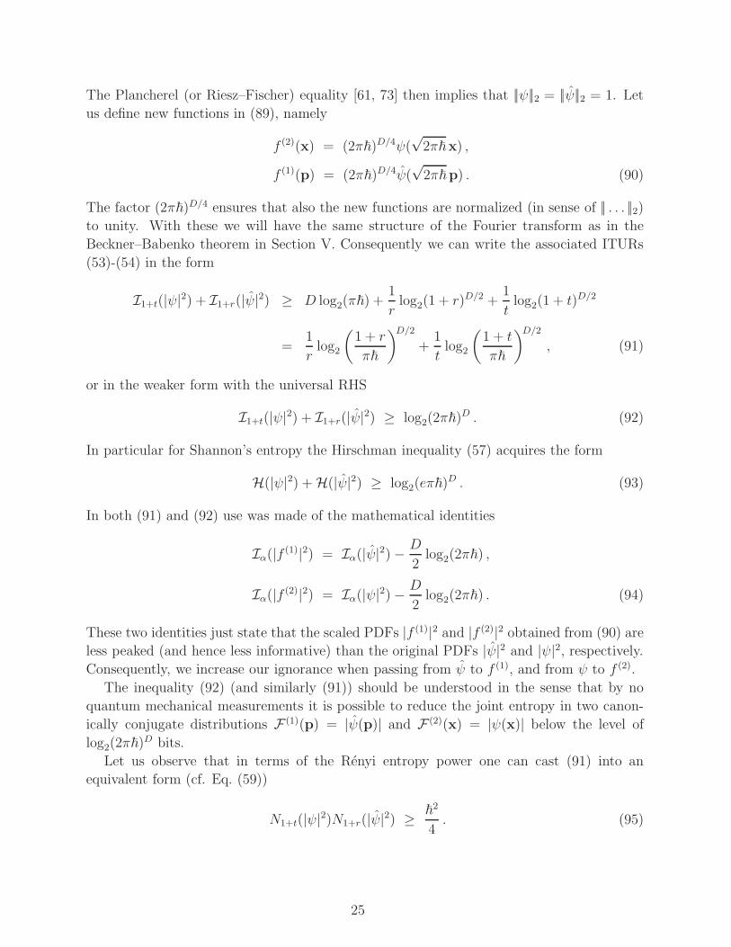
B. Continuous probabilities

In view of the (continuous) ITUR from Section V the most prominent example of the

Fourier transform is that between configuration and momentum space wave functions (anal-

ogously one can treat also other Fourier transform duals, such as the angular momentum

and angle). In particular between ψ(x) and ψ(p) hold two reciprocal relations

ψ(x) =

∫

RD

eip·x/~ ψ(p)dp

(2π~)D/2,

ψ(p) =

∫

RD

e−ip·x/~ ψ(x)dx

(2π~)D/2. (89)

24

The Plancherel (or Riesz–Fischer) equality [61, 73] then implies that ||ψ||2 = ||ψ||2 = 1. Let

us define new functions in (89), namely

f (2)(x) = (2π~)D/4ψ(√2π~x) ,

f (1)(p) = (2π~)D/4ψ(√2π~p) . (90)

The factor (2π~)D/4 ensures that also the new functions are normalized (in sense of || . . . ||2)to unity. With these we will have the same structure of the Fourier transform as in the

Beckner–Babenko theorem in Section V. Consequently we can write the associated ITURs

(53)-(54) in the form

I1+t(|ψ|2) + I1+r(|ψ|2) ≥ D log2(π~) +1

rlog2(1 + r)D/2 +

1

tlog2(1 + t)D/2

=1

rlog2

(

1 + r

π~

)D/2

+1

tlog2

(

1 + t

π~

)D/2

, (91)

or in the weaker form with the universal RHS

I1+t(|ψ|2) + I1+r(|ψ|2) ≥ log2(2π~)D . (92)

In particular for Shannon’s entropy the Hirschman inequality (57) acquires the form

H(|ψ|2) +H(|ψ|2) ≥ log2(eπ~)D . (93)

In both (91) and (92) use was made of the mathematical identities

Iα(|f (1)|2) = Iα(|ψ|2)−D

2log2(2π~) ,

Iα(|f (2)|2) = Iα(|ψ|2)−D

2log2(2π~) . (94)

These two identities just state that the scaled PDFs |f (1)|2 and |f (2)|2 obtained from (90) are

less peaked (and hence less informative) than the original PDFs |ψ|2 and |ψ|2, respectively.Consequently, we increase our ignorance when passing from ψ to f (1), and from ψ to f (2).

The inequality (92) (and similarly (91)) should be understood in the sense that by no

quantum mechanical measurements it is possible to reduce the joint entropy in two canon-

ically conjugate distributions F (1)(p) = |ψ(p)| and F (2)(x) = |ψ(x)| below the level of

log2(2π~)D bits.

Let us observe that in terms of the Renyi entropy power one can cast (91) into an

equivalent form (cf. Eq. (59))

N1+t(|ψ|2)N1+r(|ψ|2) ≥ ~2

4. (95)

25

1. Heavy tailed distributions

If we wish to improve over the Shannon–Hirschman ITUR (57) we should find such a

pair {r, t} which provides a stronger restriction on the involved distributions than Shannon’s

case. In Section V we have already seen that this can indeed happen, e.g., for heavy tailed

distributions. This fact will be now illustrated with Paretian or Levy (stable) distributions.

Such distributions represent, in general, a four parametric class of distributions that replace

the role of the normal distribution in the central limit theorem in cases where the underlying

single event distributions do not have one of the first two momenta. For computational

simplicity (results can be obtained in a closed form) we will consider one of the Levy stable

distributions, namely the Cauchy–Lorentz distribution [11] which can be obtained from the

wave function

ψ(x) =

√

c

π

√

1

c2 + (x−m)2. (96)

The corresponding Fourier transform and respective PDFs are

ψ(p) = e−imp/~√

2c

π2~K0(c|p|/~) , (97)

F (2)(x) =c

π

1

c2 + (x−m)2, (98)

F (1)(p) =2c

π2~K2

0 (c|p|/~) , (99)

and the ensuing Shannon and Renyi entropies are

H(F (1)) = log2(π2~/2c)− 8

π22.8945 , H(F (2)) = log2(4cπ) ,

I1/2(F (1)) = log2(2~/c) , I∞(F (2)) = log2(cπ) . (100)

With these results we can immediately write the associated ITURs, namely

H(F (1)) +H(F (2)) = log2(2π3~)− 8

π22.8945 > log2(eπ~) , (101)

I1/2(F (1)) + I∞(F (2)) = log2(2π~) . (102)

So what can be concluded from these relations? First we notice that the ITUR (102) satu-

rates the inequality (91) while the Shannon ITUR (101) does not saturate the corresponding

Hirschman inequality (93). In fact, if we rewrite (101)-(102) in the language of Renyi entropy

powers, we obtain

N(F (1))N(F (2)) >~2

4, (103)

N1/2(F (1))N∞(F (2)) =~2

4. (104)

26

Since the Renyi ITUR puts a definite constraint between F (2) and F (1) it clearly improves

over the Shannon ITUR (which is less specific). In addition, while (103) indicates that

one could still find another F (2) for a given fixed F (1) that would lower the LHS of the

Shannon entropy power inequality, the relation (104) forbids such a situation to happen

without increasing uncertainty in the Renyi ITUR. By increasing the uncertainty, however,

the definite constraint between F (2) and F (1) will get lost.

It should be stressed, that in general the Renyi ITUR is not symmetric. However, in the

case at hand the situation is quite interesting. One can easily check that I1/2(F (2)) = ∞and I∞(F (1)) = −∞, and so the Renyi ITUR is indeterminate. This result deserves two

comments. First, the extremal values of I1/2(F (2)) and I∞(F (1)) can be easily understood.

From the very formulation of the RE one can see that for α > 1 the non-linearly nature of

the RE tends to emphasize the more probable parts of the PDF (typically the middle parts)

while for α < 1) the less probable parts of the PDF (typically the tails) are accentuated.

In other words, I1/2 mainly carries information on the rare events while I∞ on the common

events. In particular, if one starts from a strongly leptocurtic distribution (such as F (1))

then I∞ effectively works with the PDF that is sharply (almost δ-function) peaked. In this

respect ignorance about the peak is minimal, which in turn corresponds to the minimal RE

which for continuous distributions is −∞. For heavy tailed distributions (such as F (2)) the

RE I1/2 works effectively with a very flat (almost equiprobable) PDF which yields maximal

ignorance about the tail. For continuous distributions the related information of the order

α = 1/2 is thus ∞.

Second, one can make sense of the indeterminate form of the Renyi ITUR by putting

a regulator on the real x axis. In particular we can assume that∫∞

−∞dx . . . 7→

∫ R

−Rdx . . ..

With this we obtain to leading order in R

I1/2(F (2)) = 2 log2

(√

c

πlog(4R2/c2)

)

,

I∞(F (1)) = − log2

(

2c

~π2K2

0(c/R)

)

. (105)

In the associated ITUR the unwanted divergent terms cancel and we end up with the final

result

I1/2(F (2)) + I∞(F (1))R→∞= log2(2π~) , (106)

which again, rather surprisingly, saturates the information bound.

It is also interesting to observe that while the variance in momentum 〈(△p)2〉ψ =

~2π/16c2, the variance in position 〈(△x)2〉ψ = ∞ (which is symptomatic of Levy stable

distributions) and hence the Schrodinger–Robertson VUR is completely uninformative. Sim-

ilar conclusions can be also reached with the Levy–Smirnov distribution which is used in

fractional QM [82, 83] and which can be obtained from the wave function

ψ(x) =( c

2π

)1/4

exp

(

− c4(x−m)−1 +

i

~p0x

)

/(x−m)3/4 . (107)

27

Let us finally note that the meaning of the ITUR (91) (and (92)) is rather different from

the momentum-position VUR. The difference is due to the fact that the two measures of un-

certainty (namely variance and Renyi’s entropy) are left unaltered by very different types of

PDF modifications. While both the variance of a probability distribution and Renyi entropy

are translation invariant (i.e., invariant under the shift of the mean value of the distribution

by a constant), Renyi entropy is, in addition, invariant under the piecewise reshaping of

the wave function. Particularly PDF’s (2)(x) = |ψ(1)(x)|2 and ¯(2)(x) = |ψ(2)(x)|2 with the

wave function

ψ(2)(x) =∑

n∈N

χ[ndx,(n+1)dx] ψ(2)(xσ(n)) , (108)

(χ[a,b] is the indicator function of the interval [a, b] in R and σ(n) is an arbitrary permutation

of the set of all n ∈ N) yield the same Renyi entropy. In other words, Renyi entropy

is invariant under cutting up the original PDF (2)(x) into infinitesimal pieces under the

original curve and reshuffling or separating them in an arbitrary manner. Also the Renyi

entropy for corresponding Fourier transformed wave functions are unchanged when passing

from (1)(p) to ¯(1)(p). This indicates that the corresponding ITUR will not change under

such a reshuffling. This fact will be illustrated in the following subsection.

2. Schrodinger cat states

Another relevant situation when the continuous ITUR improves on the VUR occurs for

coherent state superpositions (CSS), also called Schrodinger cat states. These states have

the form

|CSS±(β)〉 = N±β (|β〉 ± |−β〉) (109)

where |β〉 is the ordinary Glauber coherent state with the amplitude β and

N±β = 1/

√

2(1± e−2β2) , (110)

is the normalization factor. Such states have been created in the laboratory [74] and are

of interest in studies of the quantum to classical transition as well as quantum metrology

[75, 76]. For definiteness we shall consider only the |CSS+(β)〉 state, though the qualitative

statements will equally hold also for |CSS−(β)〉. The operator corresponding to different

phase quadratures of this state is

Xθ = (be−iθ + b†eiθ)/2, (111)

where b† and b are respectively the creation and annihilation operators for a photon in the

coherent state mode. Note that the eigenvalues of these operators are unitless and do not

depend on ~ as was the case with the other examples. We shall be concerned with the

orthogonal quadratures X0 and Xπ/2, which form a pair of conjugate observables with the

28

commutation relation [X0, Xπ/2] = i/2. If we take |x0〉 and |xπ/2〉 to be eigenstates of X0

and Xπ/2 we can represent (109) in these bases as

〈x0|CSS+(β)〉 = N+β (〈x0|β〉 + 〈x0| − β〉)

=2N+

β

π1

4

cosh(√

2βx0

)

exp

[

−1

2x20 − β2

]

, (112)

〈xπ/2|CSS+(β)〉 = N+β

(

〈xπ/2|β〉 + 〈xπ/2| − β〉)

=2N+

β

π1

4

cos(√

2βxπ/2

)

exp

[

−1

2x2π/2

]

. (113)

The corresponding probability distributions

F (2)(x0) = 〈x0|CSS+(β)〉〈CSS+(β)|x0〉 (114)

F (1)(xπ/2) = 〈xπ/2|CSS+(β)〉〈CSS+(β)|xπ/2〉 (115)

can be experimentally accessed with homodyne detections.

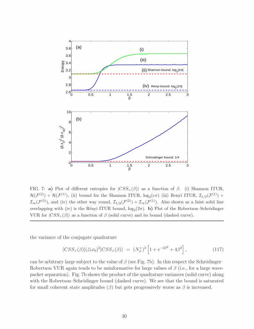
The ensuing values of Shannon and Renyi entropies are depicted in Fig. 7a as functions

of β. Curve (i) is the Shannon ITUR, H(F (2)) +H(F (1)), and the dashed curve (ii) depicts

the bound for the Shannon ITUR, i.e. log2(eπ). We see that the bound is saturated for

small β (as should be expected for a single Gaussian wave packet) and gets worse as β is

increased (and information about the localization worsens), but eventually saturates at some

value above the bound (when two Gaussian wave packets no longer overlap). The plateau

is a consequence of the mentioned fact that the RE is immune to piecewise rearrangements

of the distributions. Namely, a PDF consisting of two well separated wave packets has the

same RE irrespective of the mutual distance. This holds true also for the associated F (1)

PDF.

The other curves are for the Renyi ITURs: (iii) is I1/2(F (1)) + I∞(F (2)) where the

qualitative behavior is similar as in the Shannon case. In this situation we see that the

plateau forms earlier, which indicates that information about the peak part (i.e. I∞) starts

to saturate earlier than in the Shannon entropy case, which democratically takes into ac-

count all parts of the underlying PDF. The dashed curve (iv) is the other way round, i.e.

I1/2(F (2))+I∞(F (1)). The faint solid line overlapping with the dashed line (iv) is the Renyi

entropy bound, log2(2π). We see that both configurations saturate the bound for small β,

but the dashed one saturates the bound for all β. The saturation of the information bound

can be attributed to the interplay between the degradation of information on tthe ail parts

of F (2) carried by I1/2(F (2)) and the gain of information on the central part of F (2) conveyed

by I∞(F (1)). Interestingly enough, the rate of change (in β) for both REs is identical but

opposite in sign thus yielding a β-independent ITUR.

For the same reasons as in the previous subsection the R-ITUR outperforms the S-ITUR.

In addition, we again note that while the variance (∆xπ/2)2 is finite for arbitrary β,

〈CSS+(β)|(△xπ/2)2|CSS+(β)〉 = (N+β )

2[

1 + e−2β2

(1− 4β2)]

, (116)

29

0 0.5 1 1.5 2 2.5 32.6

2.8

3

3.2

3.4

3.6

3.8

4

β

Ent

ropy

0 0.5 1 1.5 2 2.5 30

2

4

6

8

10

β

(∆ x

0)2 (∆ x

π/2)2

(b)

(a)

(ii) Shannon bound: log2(eπ)

(iv) Renyi bound: log2(2π)

(iii)

(i)

Schrodinger bound: 1/4

FIG. 7: a) Plot of different entropies for |CSS+(β)〉 as a function of β. (i) Shannon ITUR,

H(F (2)) + H(F (1)), (ii) bound for the Shannon ITUR, log2(eπ) (iii) Renyi ITUR, I1/2(F (1)) +

I∞(F (2)), and (iv) the other way round, I1/2(F (2)) + I∞(F (1)). Also shown as a faint solid line

overlapping with (iv) is the Renyi ITUR bound, log2(2π). b) Plot of the Robertson–Schrodinger

VUR for |CSS+(β)〉 as a function of β (solid curve) and its bound (dashed curve).

the variance of the conjugate quadrature

〈CSS+(β)|(△x0)2|CSS+(β)〉 = (N+β )

2[

1 + e−2β2

+ 4β2]

, (117)

can be arbitrary large subject to the value of β (see Fig. 7b). In this respect the Schrodinger–

Robertson VUR again tends to be uninformative for large values of β (i.e., for a large wave-

packet separation). Fig. 7b shows the product of the quadrature variances (solid curve) along

with the Robertson–Schrodinger bound (dashed curve). We see that the bound is saturated

for small coherent state amplitudes (β) but gets progressively worse as β is increased.

30

VII. CONCLUSIONS AND OUTLOOK

In this paper we have generalized the information theoretic uncertainty relations that have

been previously developed in Refs. [7–9, 12, 14] to include generalized information measures

of Renyi and RE-based entropy powers. To put some flesh on the bones we have applied

these generalized ITURs to a simple two-level quantum system (in the discrete-probability

case) and to quantum-mechanical systems with heavy-tailed distributions and Schrodinger

cat states (in the continuous-probability case). An improvement of the Renyi ITUR over

both the Robertson–Schrodinger VUR and the Shannon ITUR was demonstrated in all the

aforementioned cases.

In connection with the discrete-probability ITUR we have also highlighted a geometric

interpretation by showing that the lower bound on information content (or uncertainty)

inherent in the ITUR is higher, the smaller is the distance to singularity of the transformation

matrix connecting eigenstates of the two involved observables.

The presented ITURs hold promise precisely because a large part of the structure of

quantum theory has an information theoretic underpinning (see, e.g., Refs. [28, 77]). In

this connection it should be stressed that, ITURs in general should play a central role,

for instance, in quantum cryptography or in the theory of quantum computers, particu-

larly in connection with quantum error-correcting codes, communication and algorithmic

complexities. In fact, information measures such as Renyi’s entropy are used not because

of intuitively pleasing aspects of their definitions but because there exist various (classical

and quantum) coding theorems [26, 39] which endow them with an operational (that is,

experimentally verifiable) meaning. While coding theorems do exist for Shannon, Renyi or

Holevo entropies, there are (as yet) no such theorems for Tsallis, Kaniadakis, Naudts and

other currently popular entropies. The information theoretic significance of such entropies

is thus not obvious, though in the literature one can find, for instance, a Tsallis entropy

based version of the uncertainty relations [78].

Though our reasoning was done in the framework of the classical (non-quantum) in-

formation theory, it is perhaps fair to mention that there exist various generalizations of

Renyi entropies to the quantum setting. Most prominent among theses are Petz’s quasi-

entropies [84] and Renner’s conditional min-, max-, and collision entropy [85]. Nevertheless,

the situation in the quantum context is much less satisfactory in that these generalizations

do not have any operational underpinning and, in addition, they are incompatible with

each other in number of ways. For instance, whereas the classical conditional min-entropy

can be naturally derived from the Renyi divergence, this does not hold for their quantum

counterparts. At present there is no obvious generalization of the Renyi entropy power in

the quantum framework and hence it is not obvious in what sense one should interpret the

prospective ITUR. All these aforementioned issues are currently under active investigation.

Let us finally make a few comments concerning the connection of the entropy power

with Fisher information. Fisher information was originally employed by Stam [67] in his

proof of the Shannon entropy power inequality. Interestingly enough, one can use either the

entropy power inequality or the Cramer–Rao inequality and logarithmic Sobolev inequality

to re-derive the usual Robertson–Schrodinger VUR. While the generalized ITUR presented

31

here can be derived from the generalized entropy power inequality (as both are basically

appropriate restatements of Young’s theorem), the connection with Fisher information (or

some of its generalizations) is not yet known. The corresponding extension of our approach

in this direction would be worth pursuing particularly in view of the natural manner in

which RE is used both in inference theory and ITUR formulation.

Last, but not least, the Riesz–Thorin and Beckner–Babebko inequalities that we have uti-

lized in Sections IV and V belong to a set of inequalities commonly known as Lp-interpolationtheorems [65]. It would be interesting to see whether one can sharpen our analysis from Sec-

tion IV by using the Marcinkiewicz interpolation theorem [65], which in a sense represents

the deepest interpolation theorem. In particular, the latter avoids entirely the Riesz con-

vexity theorem which was key in our proof. Work along these lines is presently in progress.

Acknowledgments

P.J. would like to gratefully acknowledge stimulating discussions with H. Kleinert, P. Har-

remoes and D. Brody. This work was supported by GACR Grant No. P402/12/J077.

Appendix A

In this Appendix we introduce the (generalized) Young inequality and derive some related

inequalities. Since the actual proof of Young’s inequality is rather involved we provide here

only its statement. The reader can find the proof together with further details, e.g., in

Ref. [72].

Theorem A.1 (Young’s theorem) Let q, p, r > 0 represent Holder triple, i.e.,

1

q+

1

p= 1 +

1

r,

and let F ∈ ℓq(RD) and G ∈ ℓp(RD) are two non-negative functions, then

||F ∗ G||r ≥ CD||F||q||G||p , (A1)

for q, p, r ≥ 1 and

||F ∗ G||r ≤ CD||F||q||G||p , (A2)

for q, p, r ≤ 1. The constant C is

C = CpCq/Cr with C2x =

|x|1/x|x′|1/x′ .

Here x and x′ are Holder conjugates. Symbol ∗ denotes a convolution.

32

Young inequality allows to prove very quickly the Hausdorff–Young inequalities which are

instrumental in obtaining various Fourier-type uncertainty relations. In fact, the following

chain of reasons holds

||F ∗ δ||r ≥ CD||F||q||δ||p = CD||F||qV (p−1)/pR . (A3)

Here we have used the fact that for the δ function

||δ||p =[∫

RD

dx δp(x)

]1/p

=

[∫

RD

dx δ(x)δp−1(0)

]1/p

= V(p−1)/pR .

In the derivation we have utilized that

δ(0) =

∫

RD

dx eip·0 = VR .

Subindex R indicates that the volume is regularized, i.e., we approximate the actual volume

of RD with a D-dimensional ball of the radius R, where R is arbitrarily large but fixed. At

the end of calculations we send R to infinity. We should also stress that in (A3) an implicit

assumption was made that q, p, r ≥ 1.

The norm ||F ∗ δ||r fulfills yet another inequality, namely

||F ∗ δ||r =[∫

RD

dx

(∫

RD

dp e−ip·xF(p)

)r ]1/r

≤ ||F||nV 1/n′+1/rR , (A4)

where we have used the Holder inequality

∫

RD

dp e−ip·xF(p) =

∣

∣

∣

∣

∫

RD

dp e−ip·xF(p)

∣

∣

∣

∣

≤ ||F||n ||e−ip·x||n′ = ||F ||nV 1/n′

R ,

with n and n′ being Holder’s conjugates (n ≥ 1).

Comparing (A3) with (A4) gives the inequality

||F ||nV 1/n′+1/rR ≥ CD||F||qV (p−1)/p

R . (A5)

The volumes will mutually cancel provided 1/n′ + 1/r + 1/p = 1, or equivalently, when

1/n′ = 1/q − 2/r. With this we can rewrite (A5) as

||F ||n ≥ CD||F||q ≥ CD||F||n′ . (A6)

The last inequality results from Holder’s inequality:

||F||a ≥ ||F||b when a ≤ b . (A7)

In fact, in the limit r → ∞ the last inequality in (A6) is saturated and Cr→∞→ 1. Conse-

quently we get the Hausdorff–Young inequality in the form

||F ||n ≥ ||F||n′ . (A8)

33

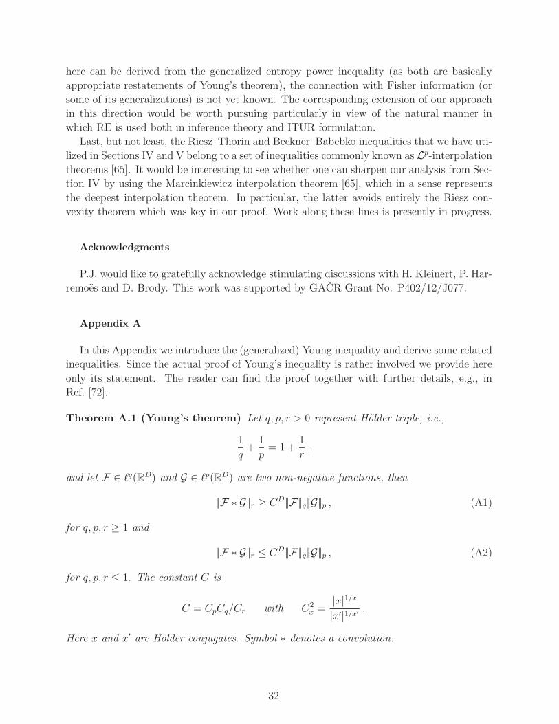
BB CCAA

1.0 1.5 2.0 2.5 3.0x

0.85

0.90

0.95

1.00

1.05

Cx

FIG. 8: Dependence of the constant Cx on the Holder parameter x. When x is between points

B and C, i.e., when x ∈ [1, 2] than Cx ≤ 1. For x ≤ A is Cx also smaller than 1 but such x are

excluded by the fact that x must be ≥ 1.

This inequality holds, of course, only when q ≥ n′ (cf. equation (A7)), i.e., when n ≥q/(q − 1). Since q ≥ 1 we have that n ∈ [1, 2]. Should we have started in our derivation

with F instead of F we would have obtain the reverse inequality

||F||n ≥ ||F||n′ . (A9)

Inequalities, (A8) and (A9) are known as classical Hausdorff–Young inequalities [61]. Note

that in the spacial case when n = 2 we have also n′ = 2 and equations (A8) - (A9) together

imply equality:

||F||2 = ||F ||2 . (A10)

This is known as the Plancherel (or Riesz–Fischer) equality [61, 73].

It should be noted that the Beckner–Babenko inequality from Section 5 improves upon

the Hausdorff–Young inequalities. This is because Cx ≤ 1 for x ∈ [1, 2], see Fig. 8. The

Beckner–Babenko inequality follows easily from Young’s inequality. Indeed, assume that

there exists a (possibly p-dependent) constant k(p) ≤ 1, such that

k(p)||F||p ≥ ||F ||p′ and k(p)||F ||p ≥ ||F||p′ . (A11)

The constant k(p) can be easily found by writing

k(r)||F ∗ G||r ≥ ||FG||r′ ≥ ||F||q′||G||p′ ≥ [k(q′)]−1||F||q[k(p′)]−1||G||p , (A12)

which gives

||F ∗ G||r ≥ [k(r)]−1[k(q′)]−1[k(p′)]−1||F||q||G||p . (A13)

The middle inequality in (A12) is the Holder inequality that is valid for 1/r′ = 1/p′ + 1/q′

(i.e., for 1/p+ 1/q = 1/r + 1). Comparison of (A13) with (A1) gives the equation

[k(r)]−1[k(q′)]−1[k(p′)]−1 = CD = [CqCp/Cr]D = [1/Cq′Cp′Cr]

D . (A14)

34

This is clearly solved with k(p) = CDp . By choosing p ∈ [1, 2] we get improvement over the

Hausdorff–Young inequalities.

[1] W. Heisenberg, Z. Phys. 43 (1927) 172.

[2] W. Heisenberg, The Physical Principles of the Quantum Theory (Dover, New York, 1949).

[3] J. Erhart, S. Sponar, G. Sulyok, G. Badurek, M. Ozawa and Y. Hasegawa, Nature Phys. 8

(2012) 185.

[4] E.H. Kennard, Zeitschrift fur Physik 44 (1927) 326.

[5] H.P. Robertson, Phys. Rev. 34 (1929) 163.

[6] E. Schrodinger, Sitzungsber. Preuss. Acad. Wiss. 24 (1930) 296.

[7] I. Bia lynicky-Birula and J. Mycielski, Commun. Math. Phys. 44 (1975) 129.

[8] D.L. Deutsch, Phys. Rev. Lett. 50 (1983) 631.

[9] H. Maassen and J.B.M. Uffink, Phys. Rev. Lett. 60 (1988) 1103.

[10] P. Levy, Theorie de l’ Addition des Variables Aleatoires (Gauthier-Villars, Paris, 1937 & 1954).

[11] W. Feller, An Introduction to Probability Theory and Its Applications, Vol. II (John Wiley,

London, 1966).

[12] J.B.M. Uffink, Measures of Uncertainty and the Uncertainty Principle, PhD thesis, University

of Utrecht, Januari 1990; http://www.phys.uu.nl/igg/jos/publications/proefschrift.pdf

[13] H.E. Montgomery, Jr., Chemical Educator 7 (2002) 334.

[14] I.I. Hirschman, Jr., Amer. J. Math. 79 (1957) 152.

[15] This distribution is in physics also known as the Breit–Wigner distribution. It is particularly

relevant in nuclear and particle physics, and in spectroscopy.

[16] L. Lyons, Statistics for Nuclear and Particle Physicists (Cambridge University Press, Cam-

bridge, 1989).

[17] P.A.M. Dirac, The principles of Quantum Mechanics (Claredon Pres, Oxford, 1958).

[18] D.L. Donoho and P.B. Stark, SIAM J. Appl. Math. 49 (1989) 906.

[19] D. Mustard, Austral. Math. Soc. Ser. B 33 (1991) 180.

[20] B. Lesche, J. Stat. Phys. 27 (1982) 419.

[21] P. Jizba and T. Arimitsu, Ann. Phys. 312 (2004) 17.

[22] A. Renyi, Probability Theory (North-Holland, Amsterdam, 1970); Selected Papers of Alfred

Renyi, Vol.2 (Akad emia Kiado, Budapest, 1976).

[23] C.E. Shannon A mathematical theory of communication, Bell Syst. Tech. J. 27 (1948) 379;

623.

[24] M.H. Costa, IEEE Trans. Inform. Theory, 31 (1985) 751.

[25] I. Csiszar, IEEE Trans. Inform. Theory 41 (1995) 26.

[26] L.L. Campbell, Informat. Contr. 8 (1965) 423.

[27] M.B. Baer, Renyi to Renyi – source coding under siege, in: Proc., 2006 IEEE Int. Symp. on

Information Theory, July 14, 2006, pp. 1258-1262.

[28] M. Nielsen and I.L. Chuang, Quantum Computation and Quantum Information (Cambridge

Un. Press, Cambridge, 2000).

35

[29] see e.g., V.V. Dodonov, E.V. Kurmyshev and V.I. Man’ko, Phys. Lett. A 79 (1980) 150.

[30] J.M. Levy-Leblond, Ann. Phys. 101 (1976) 319.

[31] P. Carruthers and M.M. Nietto, Rev. Mod. Phys. 40 (1968) 411.

[32] L. Mandelstam and I.G. Tamm, J. Phys. USSR 9 (1945) 249.

[33] W.H. Luisell, Quantum Statistical Theory of Radiation (Wiley, New York, 1973).

[34] J.L. Synge, Proc. R. Society London A 325 (1971) 151.

[35] M. Ozawa, Phys. Rev. A 67 (2003) 042105.

[36] M. Ozawa, J. Opt. B 7 (2005) 672.

[37] C. Cachin, Entropy Measures and Unconditional Security in Cryptography, PhD thesis, ETH

Zurich, May 1997; ftp://ftp.inf.ethz.ch/pub/publications/dissertations/th12187.ps.gz .

[38] C.H Bennett, G. Brassard, C. Crepeau, and U.M. Maurer, IEEE Trans. Inform. Theory 41

(1995) 1915.

[39] P. Jizba, H. Kleinert and M. Shefaat, Physica A 391 (2012) 2971.

[40] P. Jizba and J. Korbel, arXiv:1401.3316 [q-fin.ST].

[41] M. Hayashi, IEEE Trans. Inform. Theory 57 (2011) 3989.

[42] G. Adesso, D. Girolami and A. Serafini, Phys. Rev. Lett. 109 (2012) 190502.

[43] S. Kullback and R. Leibler, Ann. Math. Statist. 22 (1951) 79.

[44] T. Arimitsu and N. Arimitsu, J. Phys. A: Math. Gen. 33 (2000) L235.

[45] T. Arimitsu and N. Arimitsu, Physica A 295 (2001) (2001) 673.

[46] T. Arimitsu and N. Arimitsu, Physica A 305 (2002) 218.

[47] T. Arimitsu and N. Arimitsu, Condens. Matter 14 (2002) 2237.

[48] T.C. Halsey, M.H. Jensen, L.P. Kadanoff, I. Procaccia and B.I. Shraiman, Phys. Rev. A 33

(1986) 1141.

[49] M.H. Jensen, L.P. Kadanoff, A. Libchaber, I. Procaccia and J. Stavans, Phys. Rev. Lett. 55

(1985) 2798.

[50] K. Tomita, H. Hata, T. Horita, H. Mori and T. Morita, Prog. Theor. Phys. 80 (1988) 963.

[51] H.G.E. Hentschel and I. Procaccia, Physica D 8 (1983) 435.

[52] M. Riesz, Acta. Math. 49 (1926) 465.

[53] O. Thorin, Kungl. Fysiogr. Sallsk. i Lund Forh. 8 (1939) 14 (= Medd. Lunds Univ. Mat. Sem.

4 (1939) 1).

[54] T. Cover and J. A. Thomas. Elements of Information Theory, (Wiley, London, 1991).

[55] S. Verdu and D. Guo. IEEE Trans. Inform. Theory 52(2006) 2165.

[56] A. Dembo, IEEE Trans. Inform. Theory 35 (1989) 887.

[57] N.M. Blachman, IEEE Trans. Inform. Theory 11 (1965) 267.

[58] R.J. Gardner, Bull. Amer. Math. Soc. 39 (2002) 355.

[59] S.M. Kay Fundamentals of Statistical Signal Processing, Volume I: Estimation Theory, ( Pren-

tice Hall, New York, 1993).

[60] Note that, since aij ∈ SO(n), then a−1ij = aji and thus maxij |a−1

ij | = c.

[61] G. Hardy, J.E. Littlewood and G. Polya, Inequalities (Cambridge University Press, Cam-

bridge, 1952).

[62] W. Beckner, Ann. of Math. 102 (1975) 159.

[63] K.I. Babenko, Amer. Math. Soc. Transl. Ser. 2 44 (1962) 115.

36

[64] E.H. Lieb, Invent. Math. 102 (1990) 179.

[65] M. Reed and B. Simon, Methods of modern mathematical physics. Vol. XI: Fourier analysis,

selfadjointness, (Academic Press, New York, 1975).

[66] M.E. Andersson, The Hausdorff-Young inequality and Fourier Type, Ph. D. Thesis, Uppsala,

1993.

[67] A. Stam, Inform. Contr. 2 (1959) 101.

[68] A. Dembo and T.M. Cover, IEEE Trans. Inf. Theory, 37 (1991) 1501.

[69] O. Rioul, IEEE Trans. Inf. Theory, 57 (2011) 33.

[70] P. Grunwald, the Minimum Description Length principle (MIT Press, 2007).

[71] K. Kraus, Phys. Rev. D 35 (1987) 3070.

[72] E.H. Lieb, Adv. in Math. 20 (1976) 151.

[73] K. Yosida, Functional Analysis, (Springer Verlag, Berlin, 1968).

[74] M. Brune, E. Hagley, J. Dreyer, X. Maitre, A. Maali, C. Wunderlich, J. M. Raimond, and S.

Haroche, Phys. Rev. Lett. 77 (1996) 4887 .

[75] P.A. Knott, W.J. Munro and J.A. Dunningham, Phys. Rev. A 89 (2013) 053812 .

[76] P.A. Knott, T.J. Proctor, K. Nemoto, J.A. Dunningham, W.J. Munro, arXiv:1405.7198.

[77] C. Brukner and A. Zeilinger, Phys. Rev. Lett. 83 (1999) 3354.

[78] see, e.g., G. Wilk and Z. Wlodarczyk, Phys. Rev. A 79 (2008) 062108.

[79] G.H. Golub and C.F. Van Loan, Matrix Computations, 3rd ed., (John Hopkins University

Press, Baltimore, 1996).

[80] G.W. Steward and J.-G. Sun, Matrix Perturbation Theory, (Academic Press, New York, 1990).

[81] I.I. Hirschman, Jr., Am. J. Math. 79 (1957) 152.

[82] B. Al-Saqabi, L. Boyadjiev and Yu. Luchko, Eur. Phys. J. Special Topics 222 (2013) 1779.

[83] N. Laskin, Phys. Lett. A 268 (2000) 298.

[84] D. Petz, Rep. Math. Phys. 23 (1986) 57.

[85] R. Renner, Security of quantum key distribution, Ph.D. Thesis, ETH Zurich, 2005.

[86] Note that these limits do not contradict the constraint 1/t + 1/r = −2. To see this we go

back to the defining equation 1/[2(1 + t)] + 1/[2(1 + r)] = 1 which is clearly satisfied for the

simultaneous limits t → 0+ and r → 0−.

37