On the Prevalence of Sensor Faults in Real-World Deployments

On the Prevalence of Sensor Faults in Real-WorldDeployments

Abhishek Sharma∗, Leana Golubchik † and Ramesh Govindan∗∗ Computer Science Department

† Computer Science and EE-Systems Departments, IMSCUniversity of Southern California, Los Angeles, CA-90089

(Email: absharma,leana,[email protected])

Abstract—Various sensor network measurement studieshave reported instances of transient faults in sensor read-ings. In this work, we seek to answer a simple question:How often are such faults observed in real deployments? Todo this, we first explore and characterize three qualitativelydifferent classes of fault detection methods. Rule-basedmethods leverage domain knowledge to develop heuris-tic rules for detecting and identifying faults. Estimationmethods predict “normal” sensor behavior by leveragingsensor correlations, flagging anomalous sensor readingsas faults. Finally, learning-based methods are trained tostatistically identify classes of faults. We find that thesethree classes of methods sit at different points on theaccuracy/robustness spectrum. Rule-based methods canbe highly accurate, but their accuracy depends criticallyon the choice of parameters. Learning methods can becumbersome, but can accurately detect and classify faults.Estimation methods are accurate, but cannot classifyfaults. We apply these techniques to four real-world sensordata sets and find that the prevalence of faults as wellas their type varies with data sets. All three methodsare qualitatively consistent in identifying sensor faults inreal world data sets, lending credence to our observations.Our work is a first-step towards automated on-line faultdetection and classification.

I. INTRODUCTION

With the maturation of sensor network software, weare increasingly seeing longer-term deployments of wire-less sensor networks in real world settings. As a result,

This research has been funded by the NSF DDDAS 0540420grant. It has also been funded in part by the NSF Center for Em-bedded Networked Sensing Cooperative Agreement CCR-0120778.This work made use of Integrated Media Systems Center SharedFacilities supported by the National Science Foundation under Co-operative Agreement No. EEC-9529152. Any opinions, findings andconclusions or recommendations expressed in this material are thoseof the author(s) and do not necessarily reflect those of the NationalScience Foundation.

research attention is now turning towards drawing mean-ingful scientific inferences from the collected data [1].Before sensor networks can become effective replace-ments for existing scientific instruments, it is importantto ensure the quality of the collected data. Already,several deployments have observed faulty sensor read-ings caused by incorrect hardware design or impropercalibration, or by low battery levels [2], [1], [3].

Given these observations, and the realization that itwill be impossible to always deploy a perfectly calibratednetwork of sensors, an important research direction forthe future will be automated detection, classification, androot-cause analysis of sensor faults, as well as techniquesthat can automatically scrub collected sensor data toensure high quality. A first step in this direction is anunderstanding of the prevalence of faulty sensor readingsin existing real-world deployments. In this paper, we takesuch a step.

We start by focusing on a small set of sensor faultsthat have been observed in real deployments: single-sample spikes in sensor readings (we call these SHORTfaults, following [2]), longer duration noisy readings(NOISE faults), and anomalous constant offset readings(CONSTANT faults). Given these fault models, ourpaper makes the following two contributions.Detection Methods. We first explore three qualitativelydifferent techniques for automatically detecting suchfaults from a trace of sensor readings. Rule-based meth-ods leverage domain knowledge to develop heuristicrules for detecting and identifying faults. Estimationmethods predict “normal” sensor behavior by leveragingsensor correlations, flagging deviations from the normalas sensor faults. Finally, learning-based methods aretrained to statistically detect and identify classes offaults.

By artificially injecting faults of varying intensity into

sensor datasets, we are able to study the detection perfor-mance of these methods. We find that these methods sitat different points on the accuracy/robustness spectrum.While rule-based methods can detect and classify faults,they can be sensitive to the choice of parameters. Bycontrast, the estimation method we study is a bit morerobust to parameter choices but relies on spatial corre-lations and cannot classify faults. Finally, our learningmethod (based on Hidden Markov Models) is cumber-some, partly because it requires training, but it can fairlyaccurately detect and classify faults. Furthermore, at lowfault intensities, these techniques perform qualitativelydifferently: the learning method is able to detect moreNOISE faults but with higher false positives, while therule-based method detects more SHORT faults, with theestimation method’s performance being intermediate. Wealso propose and evaluate hybrid detection techniques,which combine these three methods in ways that canbe used to reduce false positives or false negatives,whichever is more important for the application.

Evaluation on Real-World Datasets. Armed with thisevaluation, we apply our detection methods (or, in somecases, a subset thereof) to four real-world data sets.The largest of our data sets spans almost 100 days, andthe smallest spans one day. We examine the frequencyof occurrence of faults in these real data sets, usinga very simple metric: the fraction of faulty samplesin a sensor trace. We find that faults are relativelyinfrequent: often, SHORT faults occur once in abouttwo days in one of the data sets that we study, andNOISE faults are even less frequent. We find no spatialor temporal correlation among faults. However, differentdata sets exhibits different levels of faults: for example,in one month-long dataset we found only six instances ofSHORT faults, while in another 3-month long dataset, wefound several hundred. Finally, we find that our detectionmethods incur false positives and false negatives on thesedata sets, and hybrid methods are needed to reduce oneor the other.

Our study informs the research on ensuring dataquality. Even though we find that faults are relativelyrare, they are not negligibly so, and careful attentionneeds to be paid to engineering the deployment and toanalyzing the data. Furthermore, our detection methodscould be used as part of an on-line fault detection andremediation system, i.e., where corrective steps could betaken during the data collection process based on thediagnostic system’s results.

II. SENSOR FAULTS

In this section, we visually depict some faults in sensorreadings observed in real datasets. These examples aredrawn from the same real-world datasets that we useto evaluate the prevalence of sensor faults; we describedetails about these datasets later in the paper. Theseexamples give the reader visual intuition for the kindsof faults that occur in practice, and motivate the faultmodels we use in this paper.

Before we begin, a word about terminology. We usethe term sensor fault loosely. Strictly speaking, whatwe call a sensor fault is really a visually or statisticallyanomalous reading. In one case, we have been able toestablish that the behavior we identified was indeed afault in the design of an analog-to-digital converter. Thatsaid, the kinds of faults we describe below have beenobserved by others as well [2], [1], and that leads us tobelieve that the readings we identify as faults actuallycorrespond to malfunctions in sensors. Finally, in thispaper we do not attempt to precisely establish the causeof a fault.

0 0.5 1 1.5 2 2.5 3

x 105

0

500

1000

1500

2000

2500

Time (seconds)

Se

nso

r R

ea

din

gs

0 1000 2000 3000 4000 5000 6000 7000 8000 90001.5

2

2.5

3

3.5

4

4.5

5

5.5

6x 10

4

Se

nso

r R

ea

din

gs

Sample Number

(a) Unreliable Readings (b) SHORT

Fig. 1. Errors in sensor readings

0 20 40 60 80 1003.248

3.25

3.252

3.254

3.256

3.258

3.26

3.262

3.264

3.266x 10

4

Sample Number

Se

nso

r R

ea

din

gs

0 20 40 60 80 1003.248

3.25

3.252

3.254

3.256

3.258

3.26

3.262

3.264

3.266x 10

4

Sample Number

Se

nso

r R

ea

din

gs

(a) Sufficient voltage (b) Low voltage

Fig. 2. Increase in variance

Figure 1.a shows readings from a sensor reportingchlorophyll concentration measurements from a sensornetwork deployment in lake water. Due to faults inthe analog-to-digital converter board the sensor starts

2

reporting values 4 − 5 times greater than the actualchlorophyll concentration. Similarly, in Figure 1.b, oneof the samples reported by a humidity sensor has avalue that is roughly 3 times the value of the restof the samples, resulting in a noticeable spike in theplot. Finally, Figure 2 shows that the variance of thereadings from an accelerometer attached to a MicaZmote measuring ambient vibration increases when thevoltage supplied to the accelerometer becomes low.

The faults in sensor readings shown in these figurescharacterize the kinds of faults we observed in the fourdata sets from wireless sensor network deploymentswhich we analyze in this paper. We know of two othersensor network deployments [1], [2] that have observedsimilar faults.

In this paper, we explore the following three faultmodels motivated by these examples (further details aregiven in Section IV):

1) SHORT: A sharp change in the measured valuebetween two successive data points (Figure 1.b).

2) NOISE: The variance of the sensor readings in-creases. Unlike SHORT faults that affect a singlesample at a time, NOISE faults affect a number ofsuccessive samples (see Figure 2).

3) CONSTANT: The sensor reports a constant valuefor a large number of successive samples. Thereported constant value is either very high or verylow compared to the “normal” sensor readings(Figure 1.a) and uncorrelated to the underlyingphysical phenomena.

SHORT and NOISE faults were first identified andcharacterized in [2] but only for a single data set.

III. DETECTION METHODS

In this paper, we explore and characterize three qual-itatively different detection methods – Linear Least-Squares estimation (LLSE), Hidden Markov Models(HMM), and a Rule-based method which leverages do-main knowledge (the nature of faults in sensor readings)to develop heuristic rules for detecting and identifyingfaults. The Rule-based methods analyzed in this paperwere first proposed in [2].

Our motivation for considering three qualitatively dif-ferent detection methods is as follows. As one mightexpect, and as we shall see later in the paper, no singlemethod is perfect for detecting the kinds of faults weconsider in this paper. Intuitively, then, it makes sense toexplore the space of detection techniques to understandthe trade-offs in detection accuracy versus the robustnessto parameter choices and other design considerations.

This is what we have attempted to do in a limitedway, and our choice of qualitatively different approachesexposes differences in the trade offs.

A. Rule-based (Heuristic) Methods

Our first class of detection methods uses two intuitiveheuristics for detecting and identifying the fault typesdescribed in Section II.NOISE Rule: Compute the standard deviation of samplereadings within a window N. If it is above a certainthreshold, the samples are corrupted by the NOISE fault.To detect CONSTANT faults, we use a slightly modifiedNOISE rule where we classify the samples as corruptedby CONSTANT faults if the standard deviation is zero.The window size N can be in terms of time or number ofsamples. Clearly, the performance of this rule dependson the window size N and the threshold.SHORT Rule: Compute the rate of change of the physicalphenomenon being sensed (temperature, humidity etc.)between two successive samples. If the rate of change isabove a threshold, it is an instance of a SHORT fault.

For well-understood physical phenomena like temper-ature, humidity etc., the thresholds for the NOISE andSHORT rules can be set based on domain knowledge.For example, [2] uses feedback from domain scientiststo set a threshold on the rate of change of chemicalconcentration in soil.

For automated threshold selection, [2] proposes thefollowing technique:

• Histogram method: Plot the histogram of the stan-dard deviations or the rate of change observed forthe entire time series (of sensor readings) beinganalyzed. If the histogram is multi-modal, select oneof the modes as the threshold.

For the NOISE rule, the Histogram method for auto-mated threshold selection will be most effective when,in the absence of faults, the histogram of standarddeviations is uni-modal and sensor faults affect the mea-sured values in such a way that the histogram becomesbi-modal. However, this approach is sensitive to thechoice of N; the number of modes in the histogram ofstandard deviations depends on N. Figure 3 shows theeffect of N on the number of modes in the histogramcomputed for sensor measurements taken from a real-world deployment. The measurements do not contain asensor fault, but choosing N = 1000 gives a multi-modalhistogram, and would result in false positives.

Selecting the right parameters for the rule-based meth-ods requires a good understanding of reasonable sensorreadings. In particular, a domain expert would have

3

0 5 10 15 20 25 300

10

20

30

40

50

60

70

80

90

Std. Deviation

Fre

quency

5 10 15 20 25 30 350

1

2

3

4

5

6

7

8

9

Std. Deviation

Fre

quency

(a) N = 100 (b) N = 1000

Fig. 3. Histogram Shape

suggested that N = 1000 in our previous example wasan unrealistic choice.

B. An Estimation-Based Method

Is there a method that perhaps requires less domainknowledge in setting parameters? For physical phenom-ena like ambient temperature, light etc. which exhibita diurnal pattern, statistical correlations between sensormeasurements can be exploited to generate estimates forthe sensed phenomenon based on the measurements ofthe same phenomenon at other sensors. Regardless of thecause of the statistical correlation, we can exploit the ob-served correlation in a reasonably dense sensor networkdeployment to detect anomalous sensor readings.

More concretely, suppose the temperature values re-ported by sensors s1 and s2 are correlated. Let t̂1(t2) bethe estimate of temperature at s1 based on the tempera-ture t2 reported by s2. Let t1 be the actual temperaturevalue reported by s1. If |t1 − t̂1| > δ , for some thresholdδ , we classify the reported reading t1 as erroneous. If theestimation technique is robust, in the absence of faults,the estimate error (|t1 − t̂1|) would be small whereas afault of the type SHORT or CONSTANT would cause thereported value to differ significantly from the estimate.

In this paper we consider the Linear Least-Squares Es-timation (LLSE) [4] method as the estimation techniqueof choice. In the real-world, the value t2 at sensor s2

might itself be faulty. In such situations, we can estimatet̂1 based on measurements at more than one sensor.

In general, the information needed for applying theLLSE method may not be available a priori . In applyingthe LLSE method to the real-world data sets, we dividethe data set into a training set and a test set. We computethe mean and variance of sensor measurements, and thecovariance between sensor measurements based on thetraining data set and use them to detect faulty samples inthe test data set. This involves an assumption that, in theabsence of faults or external perturbations, the physical

phenomenon being sensed does not change dramaticallybetween the time when the training and test samples werecollected. We found this assumption to hold for many ofthe data sets we analyzed.

Finally, we set the threshold δ used for detectingfaulty samples based on the LLSE estimation error forthe training data set. We use the following two heuristicsfor determining δ :

• Maximum Error: If the training data has no faultysamples, we can set δ to be the maximum es-timation error for the training data set, i.e. δ =max{|t1 − t̂1| : t1 ∈ T S} where T S is the set of allsamples in the training data set.

• Confidence Limit: In practice, the training data setwill have faults. If we can reasonably estimate, e.g.,from historical information, the fraction of faultysamples in the training data set, (say) p%, we canset δ to be the upper confidence limit of the (1−p)% confidence interval for the LLSE estimationerrors on the training data set.

Finally, although we have described an estimation-based method that leverages spatial correlations, thismethod can equally well be applied by only leveragingtemporal correlations at a single node. By extractingcorrelations induced by diurnal variations at a node, itmight be possible to estimate readings, and thereby de-tect faults, at that same node. We have left an explorationof this direction for future work.

C. A Learning-based Method

For phenomena that may not be spatio-temporallycorrelated, a learning-based method might be more ap-propriate. For example, if the pattern of “normal” sensorreadings and the effect of sensor faults on the reportedreadings for a sensor measuring a physical phenomenonis well understood, then we can use learning-basedmethods, for example Hidden Markov Models (HMMs)and neural networks, to construct a model for the mea-surements reported by that sensor. In this paper we choseHMMs because they are a reasonable representative oflearning based methods that can simultaneously detectand classify sensor faults. Determining the most effectivelearning based method is left for future work.

The states in an HMM mirror the characteristics ofboth the physical phenomenon being sensed as well asthe sensor fault types. For example, based on our charac-terization of faults in Section II, for a sensor measuringambient temperature, we can use a 5-state HMM withthe states corresponding to day, night, SHORT faults,NOISE faults and CONSTANT faults. Such an HMM

4

can capture not only the diurnal pattern of temperaturebut also the distinct patterns in the reported values inthe presence of faults. For brevity, we omit a formaldefinition of HMMs; the interested reader is referredto [5].

D. Hybrid Methods

Finally, observe that we can use combinations ofthe Rule-based, LLSE, and HMM methods to elimi-nate/reduce the false positives or negatives. In this paper,we study two such schemes:

• Hybrid(U): Over two (or more) methods, thismethod identifies a sample as faulty if at least oneof the methods identifies the sample as faulty. Thus,Hybrid(U) is intended for reducing false negatives(it may not eliminate them entirely, since all meth-ods might incorrectly flag a sample to be faulty).However, it can suffer from false positives.

• Hybrid(I): Over two (or more) methods, this methodidentifies a sample as faulty only if both (all) themethods identify the sample as faulty. Essentially,we take an intersection over the set of samplesidentified as faulty by different methods. Hybrid(I)is intended for reducing false positives (again, itmay not eliminate them entirely), but it can sufferfrom false negatives.

Several other hybrid methods are possible. For example,Hybrid(U) can be easily modified so that results fromdifferent methods have different weights in determiningif a measurement is faulty. This would be advantageousin situations where a particular method or heuristic isknown to be better at detecting faults of a certain type. Insituations where it is possible to obtain a good estimateof the correct value of an erroneous measurement, forexample with LLSE, we can use different methods insequence- first correct all the faults reported by onemethod and then use this modified time series of mea-surements as input to another method. We have left theexploration of these methods for future work.

IV. EVALUATION: INJECTED FAULTS

Before we can evaluate the prevalence of faults in real-world datasets using the methods discussed in the pre-vious section, we need to characterize the accuracy androbustness of these methods. To do this, we artificiallyinjected faults of the types discussed in Section II into areal-world data set. Before injecting faults, we verifiedthat the real-world data set did not contain any faults.

This methodology has two advantages. First, injectingfaults into a data set gives us an accurate “ground truth”

R L H U I R L H U I R L H U I R L H U I0

0.2

0.4

0.6

0.8

1

1.2

1.4

1.6

1.8

2x 10

−3

Fra

ctio

n o

f S

am

ple

s w

ith F

au

lts

Intensity = 1.5, 2, 5, 10

DetectedFalse NegativeFalse Positive

Fig. 4. Injected SHORT Faults

that helps us better understand the performance of adetection method. Second, we are able to control theintensity of a fault and can thereby explore the limitsof performance of each detection method as well ascomparatively assess different schemes at low fault in-tensities. Many of the faults we have observed in existingreal data sets are of relatively high intensity; even so, webelieve it is important to understand behavior across arange of fault intensities, since it is unclear if faults infuture data sets will continue to be as pronounced asthose in today’s data sets.

Below, we discuss the detection performance of vari-ous methods for each type of fault. We describe how wegenerate faults in the corresponding subsections. We usethree metrics to understand the performance of variousmethods: the number of faults detected, false negatives,and false positives. More specifically, we use the fractionof samples with faults as our metric, to have a moreuniform depiction of results across the data sets. For thefigures pertaining to this section and Section V, the labelsused for different detection methods are:R: Rule-based,L: LLSE, H: HMM, U:Hybrid(U), and I: Hybrid(I).

A. SHORT Faults

To inject SHORT faults, we picked a sample i andreplaced the reported value vi with v̂i = vi + f × vi. Themultiplicative factor f determines the intensity of theSHORT fault. We injected SHORT faults with intensityf = {2,5,10}. Injecting SHORT faults in this manner(instead of just adding a constant value) does not requireknowledge of the range of “normal” sensor readings.

Figure 4 compares the accuracy of the SHORT rule,LLSE, HMM, Hybrid(U), and Hybrid(I) for SHORTfaults. The horizontal line in the figure represents theactual fraction of samples with injected faults. The four

5

R L H U I R L H U I R L H U I0

0.02

0.04

0.06

0.08

0.1

0.12

0.14

0.16

Fra

ctio

n o

f S

am

ple

s w

ith F

au

lts

Intensity = Low, Medium, High


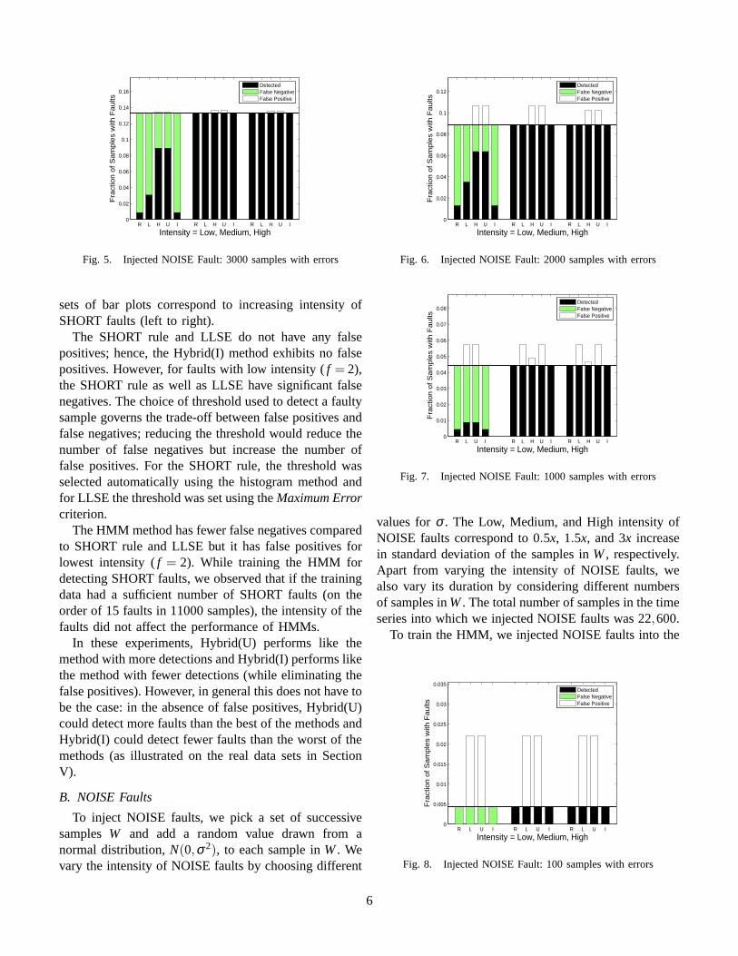
Fig. 5. Injected NOISE Fault: 3000 samples with errors

sets of bar plots correspond to increasing intensity ofSHORT faults (left to right).

The SHORT rule and LLSE do not have any falsepositives; hence, the Hybrid(I) method exhibits no falsepositives. However, for faults with low intensity ( f = 2),the SHORT rule as well as LLSE have significant falsenegatives. The choice of threshold used to detect a faultysample governs the trade-off between false positives andfalse negatives; reducing the threshold would reduce thenumber of false negatives but increase the number offalse positives. For the SHORT rule, the threshold wasselected automatically using the histogram method andfor LLSE the threshold was set using the Maximum Errorcriterion.

The HMM method has fewer false negatives comparedto SHORT rule and LLSE but it has false positives forlowest intensity ( f = 2). While training the HMM fordetecting SHORT faults, we observed that if the trainingdata had a sufficient number of SHORT faults (on theorder of 15 faults in 11000 samples), the intensity of thefaults did not affect the performance of HMMs.

In these experiments, Hybrid(U) performs like themethod with more detections and Hybrid(I) performs likethe method with fewer detections (while eliminating thefalse positives). However, in general this does not have tobe the case: in the absence of false positives, Hybrid(U)could detect more faults than the best of the methods andHybrid(I) could detect fewer faults than the worst of themethods (as illustrated on the real data sets in SectionV).

B. NOISE Faults

To inject NOISE faults, we pick a set of successivesamples W and add a random value drawn from anormal distribution, N(0,σ 2), to each sample in W . Wevary the intensity of NOISE faults by choosing different

R L H U I R L H U I R L H U I0

0.02

0.04

0.06

0.08

0.1

0.12

Fra

ctio

n o

f S

am

ple

s w

ith F

au

lts




R L U I R L H U I R L H U I0

0.01

0.02

0.03

0.04

0.05

0.06

0.07

0.08

Fra

ctio

n o

f S

am

ple

s w

ith F

au

lts




values for σ . The Low, Medium, and High intensity ofNOISE faults correspond to 0.5x, 1.5x, and 3x increasein standard deviation of the samples in W , respectively.Apart from varying the intensity of NOISE faults, wealso vary its duration by considering different numbersof samples in W . The total number of samples in the timeseries into which we injected NOISE faults was 22,600.

To train the HMM, we injected NOISE faults into the

R L U I R L U I R L U I0

0.005

0.01

0.015

0.02

0.025

0.03

0.035

Fra

ctio

n o

f S

am

ple

s w

ith F

au

lts




6

training data. These faults were of the same durationand intensity as the faults used for comparing differentmethods. There were no NOISE faults in the trainingdata for LLSE. For the NOISE rule, N = 100 was used.

Figures 5 (|W | = 3000), 6 (|W | = 2000), 7 (|W | =1000) and 8 (|W |= 100) show the performance of differ-ent methods for NOISE faults with varying intensity andduration. The horizontal line in each figure correspondsto the number of samples with faults.Impact of Fault Duration: The impact of fault durationis most dramatic for the HMM method. For |W | = 100,regardless of the fault intensity, there were not enoughsamples to train the HMM model. Hence, Figure 8 doesnot show HMM results. For |W | = 1000 and low faultintensity, we again failed to train the HMM model. Thisis not very surprising because for short duration (e.g.,|W |= 100) or low intensity faults, the data with injectedfaults is very similar to the data without injected faults.For faults with medium and high intensity or faults withsufficiently long duration, e.g., |W | ≥ 1000, performanceof the HMM method is comparable to those of theNOISE rule and LLSE.

The NOISE rule and LLSE methods are more robust tofault duration than HMMs in the sense that we were ableto derive model parameters for those cases. However, for|W | = 100 and low fault intensity, both the methods failto detect any of the samples with faults. The LLSE alsohas a significant number of false positives for |W | =100 and fault intensity 0.5x. The false positives wereeliminated by the Hybrid(I) method.Impact of Fault Intensity: For medium and high intensityfaults, there are no false negatives for any method. Forlow intensity faults, all the methods have significant falsenegatives. For fault duration and intensities for which theHMM training algorithm converged, the HMM methodgave lower false negatives as compared to the NOISErule and LLSE. However, most of the time the HMMmethod gave more false positives. Hybrid methods areable to reduce the number of false positives or negatives,as intended. High false negatives for low fault intensityarise because the data with injected faults is very similarto the data without faults.

V. FAULTS IN REAL-WORLD DATA SETS

We analyze four data sets from real-world deploy-ments for prevalence of faults in sensor traces. Thesensor traces contain measurements from a variety ofphenomena – temperature, humidity, light, pressure, andchlorophyll concentration. However, all of these phe-nomena exhibit a diurnal pattern in the absence of

outside perturbation or sensor faults.

A. Great Duck Island (GDI) data set

We looked at data collected using 30 weather moteson the Great Duck Island over a period of 3 months [6].Attached to each mote were temperature, light, andpressure sensors, and these were sampled once every 5minutes. Of the 30 motes, the data set contained sampledreadings from the entire duration of the deployment foronly 15 motes. In this section, we present our findingson the prevalence of faults in the readings for these 15motes.

The predominant fault in the readings was of thetype SHORT. We applied the SHORT rule, the LLSEmethod, and Hybrid(I) to detect SHORT faults in light,humidity, and pressure sensor readings. Figure 9 showsthe overall prevalence (computed by aggregating resultsfrom all 15 nodes) of SHORT faults for different sensorsin the GDI data set. The Hybrid (I) technique eliminatesall false positives reported by the SHORT rule or theLLSE method. The intensity of SHORT faults was highenough to detect by visual inspection. This ground-truthis included for reference in the figure under the label V.

It is evident from the figure that SHORT faults arerelatively infrequent. They are most prevalent in the lightsensor data (approximately 1 fault every 2000 samples).Figure 10 shows the distribution of SHORT faults in lightsensor readings across various nodes. SHORT faults donot exhibit any discernible pattern in the prevalence ofthese faults across different sensor nodes; the same holdsfor other sensors, but we have omitted the correspondinggraphs for brevity.

In this data set, NOISE faults were infrequent. Onlytwo nodes had NOISE faults with a duration of about100 samples. The NOISE rule detected it, but the LLSEmethod failed primarily because its parameters had beenoptimized for SHORT faults.

B. INTEL Lab, Berkeley data set

54 Mica2Dot motes with temperature, humidity andlight sensors were deployed in the Intel Berkeley Re-search Lab between February 28th and April 5th,2004 [7]. In this paper, we present the results on theprevalence of faults in the temperature readings (sampledon average once every 30 seconds).

This dataset exhibited a combination of NOISE andCONSTANT faults. Each sensor also reported the volt-age values along with the samples. Inspection of thevoltage values reported showed that the faulty sampleswere well correlated with the last few days of the

7

R L I V R L I V R L I V0

1

2

3

4

5

6x 10

−4

Fra

ctio

n o

f S

am

ple

s w

ith F

au

lts

Light (left), Humidity (Center), Pressure (Right)


Fig. 9. SHORT Faults in GDI data set

101 103 109 111 116 118 119 121 122 123 124 125 126 129 9000

0.1

0.2

0.3

0.4

0.5

0.6

0.7

0.8

0.9

1x 10

−3

Fra

ctio

n o

f S

am

ple

s w

ith F

au

lts

SHORT Faults

Fig. 10. SHORT Faults: Light Sensor, x-axis: Node ID

deployment when the lithium ion cells supplying powerto the motes were unable to supply the voltage requiredby the sensors for correct operation.

The samples with NOISE faults were contiguous intime, and both the NOISE rule and a simple two-stateHMM model identified most of these samples. Figure 11shows that close to 20% of the total temperature samplescollected by all the motes were faulty. Both the NOISE

R H U I0

0.05

0.1

0.15

0.2

0.25

Fra

ctio

n o

f S

am

ple

s w

ith F

au

lts


Fig. 11. Intel data set: Prevalence of Noise faults

101 102 103 106 107 109 110 112 1140

0.05

0.1

0.15

0.2

0.25

0.3

0.35

0.4

Fra

ctio

n of

Sam

ples

with

Fau

lts

Node ID


Fig. 12. NAMOS data set (August): NOISE/CONSTANT faults

rule and the HMM have some false negatives whilethe HMM also has some false positives. For this dataset, we could eliminate all the false positives usingHybrid(I) with the NOISE rule and the HMM. However,the Hybrid(I) incurred more false negatives.

Interestingly, for this dataset, we could not apply theLLSE method to detect NOISE faults. NOISE faultsacross various nodes were temporally correlated, sinceall the nodes ran out of battery power at approximatelythe same time. This breaks an important assumptionunderlying the LLSE technique, that faults at differentsensors are uncorrelated.

Finally, in this data set, there were surprisingly fewinstances of SHORT faults. A total of 6 faults were ob-served for the entire duration of the experiment (Table I).All of these faults were detected by the HMM method,LLSE, and the SHORT rule.

ID # Faults Total # Samples2 1 469154 1 43793

14 1 3180416 2 3460017 1 33786

TABLE IINTEL LAB: SHORT FAULTS, TEMPERATURE

C. NAMOS data set

Nine buoys with temperature and chlorophyll con-centration sensors (fluorimeters) were deployed in LakeFulmor, James Reserve for over 24 hours in August2006 [8]. Each sensor was sampled every 10 seconds.We analyzed the measurements from chlorophyll sensorsfor the prevalence of faults.

The predominant fault was a combination of NOISEand CONSTANT caused by hardware faults in the ADC

8

Station ID # Faults Total # samples3 86 4539621 1 8481841 1 60680

TABLE IISHORT FAULTS IN SENSORSCOPE DATA SET

(Analog-to-Digital Converter) board. Figure 1.a showsthe measurements reported by buoy 103. We applied theNOISE Rule to detect samples with errors. Figure 12shows the fraction of samples corrupted by faults. Thesensor measurements at 4 (out of 9) buoys were affectedby faults in the ADC board and resulted in more than15% of erroneous samples at three of them. Buoy 103was affected the worst, with 35% erroneous samples.We could not apply LLSE and HMM methods becausethere was not enough data to train the models (data wascollected for 24 hours only).

D. SensorScope data set

The SensorScope project is an ongoing outdoor sensornetwork deployment consisting of weather-stations withsensors for sensing several environmental quantities suchas temperature, humidity, solar radiation, soil moisture,and so on [9]. We analyzed the temperature measure-ments reported once every 15 seconds during November,2006 by 31 weather stations deployed on a universitycampus.

We found the occurrence of faults to be the lowest forthis data set. The data from only 3 out of the 31 stationsthat we looked at contained instances of SHORT faults.We identified the faulty samples using the SHORT ruleand the LLSE method. Neither of the methods generatedany false positives. We did not find any instances ofNOISE and CONSTANT faults. Table (II) presents ourfindings from the SensorScope data set.

VI. RELATED WORK

Two recent papers [10], [11] have proposed a declar-ative approach to erroneous data detection and cleaning.StreamClean [10] provides a simple declarative languagefor expressing integrity constraints on the input data.Samples violating these constraints are considered faulty.StreamClean uses a probabilistic approach based onentropy maximization to estimate the correct value ofan erroneous sample. The evaluation in [10] is gearedtowards a preliminary feasibility study and does notuse any real world data sets. Extensible Sensor streamProcessing (ESP) framework [11] provides support for

specifying the algorithms used for detecting and cleaningerroneous samples using declarative queries. This ap-proach works best when the types of faults that can occurand the methods to correct them are known a priori. Thedeclarative queries used for outlier detection in [11] aresimilar to our Rule-based method for SHORT faults. TheESP framework is evaluated using the INTEL Lab dataset [7] and a data set from an indoor RFID networkdeployment.

Koushanfar et al. [12] propose a real-time fault de-tection procedure that exploits multi sensor data fusion.Given measurements of the same source(s) by n sensors,the data fusion is performed (n + 1) times–once withmeasurements from all the sensors and in the rest of theiterations the data from exactly one sensor is excluded.Measurements from a sensor are classified as faulty ifexcluding them improves the consistency of the datafusion results significantly. This approach is similar toour HMM model based fault detection because it requiresa sensor data fusion model. However, it cannot be usedfor applications such as volcano monitoring [3] wheresensor data fusion is not used; but the HMM basedmethod can be. Simulations and data from a small indoorsensor network are used for evaluation in [12]. Data fromreal world deployment are not used.

Elnahrawy et al. [13] propose a Bayesian approachfor cleaning and querying noisy sensors. However, usinga Bayesian approach requires prior knowledge of theprobability distribution of the true sensor readings andthe characteristics of the noise process corrupting thetrue readings. In terms of the prior knowledge and themodels required, the Bayesian approach in [13] is similarto the HMM based method we evaluated in this paper.The evaluation in [13] does not use any real world dataset.

Several papers on real-world sensor network deploy-ments [1], [6], [2], [3] present results on meaningfulinferences drawn from the collected data. However, tothe best of our knowledge, only [2], [3], [1] do a detailedanalysis of the collected data. The aim of [2] is to doroot cause analysis using Rule-based methods for on-linedetection and remediation of sensor faults for a specifictype of sensor network monitoring the presence of ar-senic in groundwater. The SHORT and NOISE detectionrules analyzed in this paper were proposed in [2]. Werneret al. [3] compare the fidelity of data collected using asensor network monitoring volcanic activity to the datacollected using traditional equipment used for monitor-ing volcanoes. Finally, Tolle et al. [1] examine spatio-temporal patterns in micro-climate on a single redwood

9

tree. While these publications thoroughly analyze theirrespective data sets, examining fault prevalence was notan explicit goal. Our work presents a thorough analysisof four different real-world data sets. Looking at differentdata sets also enables us to characterize the accuracyand robustness of three qualitatively different detectionmethods.

VII. SUMMARY, CONCLUSIONS, AND FUTURE WORK

In this paper, we focused on a simple question: Howoften are sensor faults observed in real deployments?To answer this question, we first explored and char-acterized three qualitatively different classes of faultdetection methods (Rule-based, LLSE, and HMMs) andthen applied them to real world data sets. Several othermethods—based on time series, Bayesian filter, neuralnetworks etc.— can be used for sensor fault detection.However, the three methods discussed in this paperare representatives of the larger class of these alternatetechniques. For example, a time series method wouldrely on temporal correlations in measured samples at thesame node whereas the LLSE method relies on temporalas well as spatial correlation across different nodes.Hence, an analysis of the three methods with injectedfaults presented in Section IV, not only demonstrates thedifferences, in terms of accuracy and robustness, betweenthese methods but can also help make an informedopinion about the efficacy of several other methods forsensor fault detection.

We know summarize our main findings. SHORT faultsin real data sets were relatively infrequent but of highintensity. In the GDI data set SHORT faults occurredonce in two days but the faulty sensor values were oftenorders of magnitude higher than the correct value. CON-STANT and NOISE faults were relatively infrequenttoo, but in the INTEL Lab and NAMOS data sets asignificant percentage (between 15− 35%) of sampleswere affected. Such a high percentage of erroneoussamples highlights the importance of automated, on-linesensor fault detection. Except in the INTEL Lab dataset, we found no spatial or temporal correlation amongfaults. In that data set, the faults across various nodeswere temporally correlated because all the nodes ranout of battery power at approximately the same time.Finally, we found that our detection methods incurredfalse positives and false negatives on these data sets, andhybrid methods were needed to reduce one or the other.

Even though we analyzed most of the publicly avail-able real world sensor data sets for faults, it is hard tomake general statements about sensor faults in real worlddeployments based on just four data sets. However, ourresults raise awareness of the prevalence and severity ofthe problem of data corruption and can inform futuredeployments. Overall, we believe that our work opensup new research directions in automated high-confidencefault detection, fault classification, data rectification,and so on. More sophisticated statistical and learningtechniques than those we have presented can be broughtto bear on this crucial area.

REFERENCES

[1] G. Tolle, J. Polastre, R. Szewczyk, D. Culler, N. Turner, K. Tu,S. Burgess, T. Dawson, P. Buonadonna, D. Gay, and W. Hong,“ A Macroscope in the Redwoods,” in SenSys ’05: Proceedingsof the 2nd international conference on Embedded networkedsensor systems. New York, NY, USA: ACM Press, 2005, pp.51–63.

[2] N. Ramanathan, L. Balzano, M. Burt, D. Estrin, E. Kohler,T. Harmon, C. Harvey, J. Jay, S. Rothenberg, and M. Srivastava,“ Rapid Deployment with Confidence: Calibration and FaultDetection in Environmental Sensor Networks,” CENS, Tech.Rep. 62, April 2006.

[3] G. Werner-Allen, K. Lorincz, J. Johnson, J. Lees, and M. Welsh,“ Fidelity and Yield in a Volcano Monitoring Sensor Network,”in Proceedings of the 7th USENIX Symposium on OperatingSystems Design and Implementation (OSDI), 2006.

[4] Linear Least-Squares Estimation. Hutchison & Ross, Strouds-burg, PA, 1977.

[5] L. Rabiner, “ A tutorial on Hidden Markov Models and selectedapplications in speech recognition,” Proceedings of IEEE, vol.77(2), pp. 257–286, 1989.

[6] A. Mainwaring, J. Polastre, R. Szewczyk, and D. C. J. Ander-son, “ Wireless Sensor Networks for Habitat Monitoring ,” inthe ACM International Workshop on Wireless Sensor Networksand Applications (WSNA), 2002.

[7] “ The Intel Lab, Berkeley data set,” http://berkeley.intel-research.net/labdata/.

[8] “ NAMOS: Networked Aquatic Microbial Observing System,”http://robotics.usc.edu/ namos.

[9] “ The SensorScope project,” http://sensorscope.epfl.ch.[10] N. Khoussainova, M. Balazinska, and D. Suciu, “ Towards

Correcting Inpur Data Errors Probabilistically Using IntegrityConstraints,” in Fifth International ACM Workshop on DataEngineering for Wireless and Mobile Access (MobiDE)., 2006.

[11] S. R. Jeffery, G. Alonso, M. J. Franklin, W. Hong, andJ. Widom, “ Declarative Support for Sensor Data Cleaning ,”in Fourth International Conference on Pervasive Computing(Pervasive), 2006.

[12] F. Koushanfar, M. Potkonjak, and A. Sangiovammi-Vincentelli,“ On-line Fault Detection of Sensor Measurements,” in IEEESensors, 2003.

[13] E. Elnahrawy and B. Nath, “ Cleaning and Querying NoisySensors,” in the ACM International Workshop on WirelessSensor Networks and Applications (WSNA), 2003.

10

On the Prevalence of Sensor Faults in Real-World Deployments

Documents

Transcript of On the Prevalence of Sensor Faults in Real-World Deployments