Chapter 37

On the Merging of Heterogeneous Height Data from SRTM,ICESat and Survey Control Monuments for EstablishingVertical Control in Greece: An Initial Assessmentand Validation

D. Delikaraoglou and I. Mintourakis

Abstract Earth surface elevations can be utilized ina variety of applications including e.g., terrain reduc-tions for accurate geoid modeling, assessment of thevertical accuracy of Digital Elevation Models (DEMs),geodetic monitoring and characterization of urbanareas. In this paper we are concerned with the rigorousmerging of heterogeneous height data for providingvertical control in Greece. We assess and validate theaccuracy of 3" ×3" SRTM grid elevations in Greece (a)by using a set of Survey Control Monuments (SCMs),used for geodynamic applications or for conventionalground geodetic control, and (b) by using an elevationdataset derived from the Geoscience Laser AltimeterSystem (GLAS) on the Ice, Cloud, and land ElevationSatellite (ICESat).

In order to conduct a consistent comparison of thesedata sets we studied various datum and calibrationissues, and used geoid undulations derived from thespherical harmonic representations of EGM96 andEGM08. We also used various interpolation schemesto calculate the SRTM grid elevations at the irregu-larly spaced SCMs and the ICESat’s footprint loca-tions. Differences of the SRTM vis-à-vis SCM andICESat elevations will be presented, together with adiscussion of our findings regarding the various effectsthat influence any combination of these height data.The product may provide vertical georeferencing andassociated height accuracy values which are deemeduseful for numerous emerging applications such as

D. Delikaraoglou (�)Department of Surveying Engineering, National TechnicalUniversity of Athens, Zografos 15780, Greecee-mail: ddeli@mail.ntua.gr

environmental monitoring, remote sensing, lidar, anddigital elevation modeling.

37.1 Introduction

Assessing the quality of the DEM datasets is crucialin geoid determinations, where any errors in the digitalelevation models will propagate into the geoid models,e.g., in interpolating free-air gravity anomalies.

The accuracy of a DEM depends on many fac-tors e.g., the number of sampling points and theirspatial distributions, the methods used for interpo-lating surface elevations and the propagated errorsfrom the source data. Nowadays Synthetic ApertureRadar (SAR) data has become a useful source forgenerating accurate DEM datasets since it has highresolution, coverage and accuracy over large areas.The Shuttle Radar Topography Mission (SRTM) of theSpace Shuttle Endeavour, in February 2000, has pro-vided data with 3 arcsec resolution and ±16 m absoluteheight errors (at 90% confidence level), cf. Rodriguezet al. (2005). In January 2003, a new spacebornegeodetic tool was placed into a 600 km, near polarEarth orbit on ICESat, the Geoscience Laser AltimeterSystem (GLAS) – a space-based LIDAR, was installed.GLAS was designed to generate high accuracy pro-files of the polar ice sheets in order to enable detectionof surface change (Zwally et al., 2002). ICESat pro-vides global measurements of elevation, and repeatsmeasurements along nearly-identical tracks which pro-vide new surface elevation grids of the ice sheets andcoastal areas, with greater latitudinal extent and fewerslope-related effects than radar altimetry.

289S.P. Mertikas (ed.), Gravity, Geoid and Earth Observation, International Association of Geodesy Symposia 135,DOI 10.1007/978-3-642-10634-7_37, © Springer-Verlag Berlin Heidelberg 2010

290 D. Delikaraoglou and I. Mintourakis

37.2 Study Area

The topography of Greece, because of its locationat the meeting-point of three continents includes amultitude of high mountains, flat and rolling areas,coastal plains and bays and hundreds of kilometres ofcoastline. The study area covers Greece’s entire terri-tory that exhibits elevations ranging from 0 to 2,900 mabove sea level and terrain slopes ranging on aver-age from 0◦ to 20◦ and on extreme cases rangingup to 87◦.

This study focuses on estimating the mean eleva-tion error in the SRTM DEM using available ICESatdata profiles over Greece, including the islands, aswell as terrestrial discrete elevations at some 25,000Survey Control Monuments (SCMs) which constitutethe larger part of the national geodetic framework.The latter have been established over the last severaldecades using various geodetic techniques, includingtriangulation, Doppler Transit, mobile Satellite LaserRanging, and GPS measurements. The network istherefore very diverse in terms of quality and spatialresolution. Their height above sea level has been deter-mined using spirit and trigonometric leveling, as wellas GPS leveling schemes.

37.3 SCM vs. SRTM Data Comparisons

The main goal of our SRTM vs. SCM elevationcomparison was to answer the following questionspertaining to the SRTM performance over Greece:

1. Does absolute vertical accuracy of the 3′′x3′′ SRTMdata exceed the nominal ±16 m value?

2. How do slope- and aspect-related effects influencethe SRTM data accuracy?

3. Is it possible to increase the accuracy of the SRTMelevation predictions using slope and aspect infor-mation?

To address these questions, we examined the differ-ences (HSCM – HSRTM) between the elevations fromSRTM data interpolated at each SCM location andthe corresponding available SCM elevations which weassumed to be accurate and, thus, used as reference

values. The SRTM DEM refers to mean sea level real-ized by the EGM96 geoid model described by Lemoineet al. (1998).

For the interpolation we used various methods suchas the Near Neighbour (NN), the Inverse Distancesquared Weighting (ID2W) and the Bilinear (BIL)schemes, which are computationally straightforwardand relatively simple to implement. A small num-ber of SCM points (less than 100 points overall) atSRTM voids (Hall et al., 2005) were excluded fromany subsequent evaluation.

Visualization of the computed elevation differ-ences did not reveal any uniform distribution of thediscrepancies. Generally, greater discrepancies wereassociated with rugged terrain, while smaller discrep-ancies were noted at coastal and plain areas, sug-gesting that terrain characteristics (slope and slopedirection) influence the SRTM data. These wellknown effects in the SRTM data have previouslybeen reported and investigated, for example, byMiliaresis and Paraschou (2005). Our analysis showedthat the observed differences at 8,397 points wherethe SRTM-derived slope values were greater than10◦ exhibited almost twice of the mean difference andstandard deviation compared to the corresponding val-ues at the remaining 16,871 points where the slopevalues were ≤ 10◦.

Therefore we analyzed the magnitude of the abso-lute errors in the SRTM data with respect to slopeand aspect characteristics of the landscape at eachSCM point. “Slope” at a SCM point was computedfrom the SRTM grid data as the maximum rate ofchange in the elevation value from its eight neighbor-ing cells. Specifically, we are interested in the angle ofthe slope defined by the so-called “rise” (vertical dis-tance change) and “run” (horizontal distance change)values. The slope values were expressed in integerdegrees between 0◦ and 90◦. We are also interested inthe so-called aspect effect, which related to the SpaceShuttle’s orbit characteristics and is mainly due to theview direction of the imaging radar at the time ofthe data acquisition and depends upon the imaging ofeach point on the Earth’s surface from an ascendingor descending orbit. The “Aspect” value at a point isdefined as the down-slope direction of the maximumrate of change in the elevation value from the cell ofthe said point to its eight neighbors. The angle betweenthe slope direction and North is expressed in integerdegrees between 0◦ and 360◦.

37 Merging of Heterogeneous Height Data from SRTM, ICESat 291

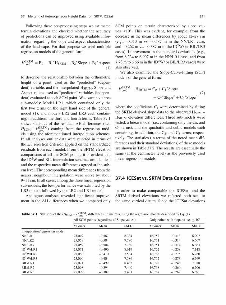
Following these pre-processing steps we estimatedterrain elevations and checked whether the accuracyof predictions can be improved using available infor-mation regarding the slope and aspect characteristicsof the landscape. For that purpose we used multipleregression models of the general form

HSRTMpred = B0 + B1

∗HSRTM + B2∗Slope + B3

∗Aspect(1)

to describe the relationship between the orthometricheight of a point, used as the “predicted” (depen-dent) variable, and the interpolated HSRTM, Slope andAspect values used as “predictor” variables (indepen-dent) evaluated at each SCM point. We examined threesub-models: Model LR1, which contained only thefirst two terms on the right hand side of the generalmodel (1), and models LR2 and LR3 each contain-ing, in addition, the third and fourth terms. Table 37.1shows statistics of the residual �H differences (i.e.,HSCM − HSRTM

pred ) coming from the regression mod-els using the aforementioned interpolation schemes.In all analyses outlier data were rejected in terms ofthe ±3 rejection criterion applied on the standardizedresiduals from each model. From the SRTM elevationcomparisons at all the SCM points, it is evident thatthe ID2W and BIL interpolation schemes are identicaland the respective mean differences agreed at the sub-cm level. The corresponding mean differences from thenearest neighbour interpolation were worse by about9–11 cm. In all cases, among the three linear regressionsub-models, the best performance was exhibited by theLR3 model, followed by the LR2 and LR1 model.

Analogous analyses revealed significant improve-ment in the �H differences when we compared only

SCM points on terrain characterized by slope val-ues ≤10◦. This was evident, for example, from thedecrease in the mean differences by about 12–27 cm(e.g., –0.313 m vs. –0.587 m in the NN/LR1 case,and –0.262 m vs. –0.387 m in the ID2W/ or BIL/LR3cases). Improvement in the standard deviations (e.g.,from 8.334 to 6.907 m in the NN/LR1 case, and from7.78 m to 6.66 m in the ID2W/ or BIL/LR3 cases) werealso observed.

We also examined the Slope-Curve-Fitting (SCF)models of the general form:

HSRTMpred − HSRTM = C0 + C1

∗Slope

+ C2∗Slope2 + C3

∗Slope3(2)

where the coefficients Ci were determined by fittingthe SRTM-derived slope data to the observed HSCM –HSRTM elevation differences. Three sub-models weretested: a linear model (i.e., containing only the C0, andC1 terms), and the quadratic and cubic models eachcontaining, in addition, the C2, and C3 terms, respec-tively. The statistics (in terms of the noted mean dif-ferences and their standard deviations) of these modelsare shown in Table 37.2. The results are essentially thesame (at the centimeter level) as the previously usedlinear regression models.

37.4 ICESat vs. SRTM Data Comparisons

In order to make comparable the ICESat- and theSRTM-derived elevations we referred both sets tothe same vertical datum. Since the ICESat elevations

Table 37.1 Statistics of the (HSCM − HSRTMpred ) differences (in metres), using the regression models described by Eq. (1)

All SCM points (regardless of Slope values) Only points with slope values ≤ 10◦

# Points Mean Std.D. # Points Mean Std.D.

Interpolation/regression modelNN/LR1 25,049 –0.587 8.334 16,752 –0.313 6.907NN/LR2 25,059 –0.504 7.780 16,751 –0.314 6.667NN/LR3 25,059 –0.504 7.780 16,751 –0.314 6.663ID2W/LR1 25,071 –0.496 8.619 16,772 –0.258 7.148ID2W/LR2 25,086 –0.410 7.584 16,763 –0.275 6.780ID2W/LR3 25,090 –0.404 7.586 16,762 –0.273 6.769BIL/LR1 25,071 –0.492 8.462 16,778 –0.246 7.078BIL/LR2 25,098 –0.394 7.440 16,768 –0.260 6.706BIL/LR3 25,099 –0.387 7.431 16,767 –0.262 6.691

292 D. Delikaraoglou and I. Mintourakis

Table 37.2 Statistics of the (HSCM − HSRTMpred ) differences (in metres), using the Slope Curve Fitting models

All SCM points (regardless of Slope values) Only points with slope values ≤ 10◦

# Points Mean Std.D. # Points Mean Std.D.

Interpolation/slope curve fit modelNN/linear 25,060 –0.501 7.857 16,751 –0.316 6.754NN/quadratic 25,060 –0.498 7.872 16,751 –0.316 6.744NN/cubic 25,060 –0.498 7.884 16,751 –0.316 6.744ID2W/linear 25,086 –0.408 7.689 16,762 –0.274 6.914ID2W/quadratic 25,086 –0.407 7.691 16,762 –0.274 6.895ID2W/cubic 25,086 –0.408 7.712 16,762 –0.274 6.892BIL/linear 25,092 –0.394 7.527 16,762 –0.267 6.836BIL/quadratic 25,092 –0.393 7.530 16,762 –0.267 6.817BIL/cubic 25,092 –0.394 7.552 16,762 –0.267 6.815

Table 37.3 Statistical results of the Dh = hIcesat−hSRTM (filtered) differences observed over Greece

Entire sample of data Edited sample

Threshold edit level a(μDh ± a∗ σDh)

Total # ofpoints

Points on land oron land and sea

# of filtered points(% accepted) Mean difference (m) Std deviation (m)

0.50 480,947 Land only 280,526 (58.3%) 0.102 1.5960.75 346,482 (72.0%) 0.128 2.2090.50 1,281,134 Land and sea 1,066,686 (83.3%) –0.031 0.9420.75 1,132,902 (88.4%) –0.015 1.305

are expressed as geometric (ellipsoidal) heights withrespect to the TOPEX ellipsoid, a constant value of0.70 m was subtracted from all elevations in order totransform the ICESat data to the WGS84 ellipsoid. TheSRTM orthometric elevations, referred to the EGM96geoid, were interpolated from the SRTM grid to theICESat footprint locations. These were transformedinto ellipsoidal heights referenced to the WGS84 ellip-soid by adding the geoid undulations NEGM96 com-puted from the EGM96 spherical harmonic coeffi-cients. A constant correction dNEGM96 = –0.53 m wasalso added that enables the EGM96-derived undula-tions to refer to the WGS84 ellipsoid (Lemoine et al.,1998). We made statistical comparisons based on thedifferences Dh = hIcesat − hSRTM from all the avail-able ICESat data over Greece (for convenience wedropped the superscript WGS84, understanding thatboth ellipsoidal height data set now refer to WGS84).The Dh differences can be partially attributed to thedifferent errors inherent in both data sets, such asunaccounted atmospheric effects on the GLAS data,tree canopy effects on the GLAS waveforms, vegeta-tion and terrain slope effects on the SRTM elevations,ICESat and SRTM orbit accuracy, calibration errors

etc. For the computed statistics shown in Table 37.3,we distinguish two data subsets: the first includingICESat footprints only on land, and the second onboth land and sea. Extreme differences (outliers) wereremoved using the following “a∗sigma” edit schemeaccording to the criterion μDh – a ∗ σDh ≤ Dh ≤ μDh +a ∗ σDh, where a is a threshold edit factor (e.g., thelower the value of a, the more data is removed dueto this editing), and μDh and σDh are the mean andstandard deviation of the observed differences com-puted using ICESat elevations only available on land.The values μDh = –0.805 m and σDh = 6.234 m wereconsidered representative enough to be used for allpoints.

In order to more closely examine the ICESat andSRTM elevation datasets, we computed estimatesof “geoid undulations” N = hIcesat − HSRTM as thedifference between the entire set of available ICESatellipsoidal heights and SRTM orthometric heightsinterpolated at the corresponding ICESat footprintlocations. We tested the observed differences dN = N–NReference on land and sea, using reference geoid undu-lations (a) the geoid computed (over land and sea) fromthe EGM96 and EGM08 (Pavlis et al., 2008) spherical

37 Merging of Heterogeneous Height Data from SRTM, ICESat 293

Table 37. 4 Statistics of the differences dN = hICESat – HSRTM – NReference over Greece

Thres-hold edit levela (μDH ± a∗ σDH)

Along-trackfilter (s) # Points Land/sea Ref. model

Mindifference(m)

Maxdifference(m)

Meandifference(m)

Std.deviation(m)

0.75 8.00 283,981 L EGM96 −3.522 1.620 −0.366 0.6361,072,432 L & S −3.522 1.620 −0.507 0.475

739,608 S −2.716 1.0911 −0.551 0.380283,981 L EGM08 −3.202 2.462 0.018 0.688

1,072,432 L & S −3.202 2.462 −0.094 0.481739,608 S −1.926 1.521 −0.125 0.359739,608 S KMSS04 −2.279 1.396 −0.069 0.260

12.00 284,466 L EGM96 −2.615 1.369 −0.395 0.5951,067,593 L & S −2.615 1.369 −0.496 0.469

734,530 S −2.447 0.774 −0.521 0.398284,466 L EGM08 −2.254 2.183 −0.013 0.654

1,067,593 L & S −2.254 2.183 −0.085 0.486734,530 S −1.826 1.150 −0.096 0.393734,530 S KMSS04 −2.145 1.298 −0.040 0.323

0.50 8.00 206,808 L EGM96 −2.016 1.123 −0.389 0.488990,879 L & S −2.677 1.123 −0.520 0.407741,375 S −2.677 0.692 −0.550 0.371206,808 L EGM08 −1.797 1.720 0.017 0.549990,879 L & S −1.797 1.720 −0.100 0.406741,375 S −1.779 1.111 −0.123 0.348741,375 S KMSS04 −1.672 0.868 −0.066 0.245

12.00 206,971 L EGM96 −1.855 0.957 −0.422 0.472985,456 L & S −2.411 0.957 −0.507 0.412735,131 S −2.411 0.639 −0.520 0.387206,971 L EGM08 −1.762 1.529 −0.019 0.537985,456 L & S −1.762 1.529 −0.089 0.424735,131 S −1.672 1.085 −0.094 0.379735,131 S KMSS04 −1.650 1.299 −0.037 0.308

harmonic models, and (b) the KMSS041 global MeanSea Surface model (over the sea). Table 37.4 summa-rizes the statistical results of these comparisons using(i) rejection criteria for noisy data corresponding tothreshold edit levels with a = 0.5 and a = 0.75, and (ii)Gaussian smoothing filters with temporal windows setat 8 12 s, to reduce the sensitivity of the estimated dif-ferences dN to the noise of the ICESat and/or SRTMdata. The chosen temporal windows correspond to awavelength of approximately 60 and 90 km in thealong track ICESat data respectively. We found that themean differences from the combined ICESat/SRTMelevations and the EGM96 geoid undulations range

1 KMSS04 is a combined multi-satellite solution based onaltimetry data from the Geosat, ERS-1 and -2, GFO andTOPEX/Poseidon satellites and is available from the DanishNational Space Centre.

from –36 cm up to –55 cm and from 2 cm up to –12 cmat the EGM08 comparisons. These values are compa-rable with the accuracy of the EGM96 and EGM08gravity field models. Better agreement at the EGM08comparisons is expected since ICESat and SRTM datahave been included in the computation of this EarthGravity Model. We also note that the comparisons ofthe ICESat/SRTM elevations with the KMSS04 solu-tion for the points at sea yield better results, i.e., upto 50% improvement was observed in the mean differ-ences vis-à-vis the respective EGM08 comparisons atthe same points at sea.

37.5 Conclusions

We presented a national scale assessment of the accu-racy of SRTM topographic data using the elevationsfrom a large set of Survey Control Monuments (SCM),

294 D. Delikaraoglou and I. Mintourakis

which are part of the national geodetic networks inGreece and from the available ICESat elevations overGreece and the surrounding seas. Linear regressionanalyses confirmed the strong correlation between theSCM elevations and the SRTM interpolated eleva-tion values and demonstrated that a large part ofthe dominant random errors in the SRTM elevations,which exhibits geographic variability due to changes inthe terrain surface slope and aspect (slope direction),can be recovered using one of the linear regressionmodels we tested. The predictive value of SRTM datafor estimating terrain elevations could be significantlyimproved using SRTM information regarding the slopeand aspect characteristics of the lanscape at the pointsof interest. We demonstrated that the accuracy of theSRTM elevation predictions can exceed the missiongoal of 16 m (at 90% confidence level) by a factor oftwo or more.

This study also examined the elevation values ofthe SRTM 90-m DEM and point wise elevationsfrom ICESat laser altimetry in order to evaluate theircombined use as source of information for regionalgeoid modeling. Using an optimal along-track filter-ing scheme to limit errors and time varying effects onthe elevations of the ICESat footprints on land and/orin the seas surrounding Greece, it was shown that agood correlation exists between the computed (hICESat

– HSRTM) “geoid undulations” and the EGM96- andEGM08- derived geoid models, or the KMSS04 globalmean sea surface.

Future investigations will focus on separating thestudy area into different morphology (hilly plains,mountainous areas, etc.) and land use covers (e.g.,waters, wetlands, forests, bare grounds etc.), to identifydependency of the SRTM/ICESat uncertainties over

different terrain surface types (e.g., areas of low/highrelief and sparse/dense tree cover).

Acknowledgments The authors would like to thank the twoanonymous reviewers of the initial manuscript for their usefulcomments and suggestions

References

Hall, O., G. Falorni, and R.L. Bras (2005). Characterizationand quantification of data voids in the shuttle radar topog-raphy mission data. IEEE Geosci. Remote Sens. Lett., 2(2),177–181.

Lemoine, F.G., S.C. Kenyon, J.K. Factor, R.G. Trimmer, N.K.Pavlis, D.S. Chinn, C.M. Cox, S.M. Klosko, S.B. Luthcke,M.H. Torrence, Y.M. Wang, R.G. Williamson, E.C. Pavlis,R.H. Rapp, and T.R. Olson (1998). The development of thejoint NASA GSFC and the national imagery and mappingagency (NIMA) geopotential model EGM96. NASA Tech.Pub. 1998-206861..Goddard Space Flight Center, Greenbelt,Maryland, USA.

Miliaresis, G.Ch. and C.V.E. Paraschou (2005). Vertical accu-racy of the SRTM DTED level 1 of Crete. Int. J. Appl. EarthObservation Geoinformation, 7(1), 49–59.

Pavlis, N.K., S.A. Holmes, S.C. Kenyon, and J.K. Factor (2008).An earth gravitational model to degree 2160: EGM2008.Presented at the 2008 European Geosciences Union GeneralAssembly. Vienna, Austria, April 13–18.

Rodriguez, E., C.S. Morris, J.E. Belz, E.C. Chapin, J.M. Martin,W. Daffer, and S. Hensley (2005). An assessment ofthe SRTM topographic products. Technical Report JPLD31639, Jet Propulsion Laboratory, Pasadena, California,143 pp.

Zwally, H.J., B. Schutz, W. Abdalati, J. Abshire, C. Bentley,A. Brenner, J. Bufton, J. Dezio, D. Hancock, D. Harding,T. Herring, B. Minster, K. Quinn, S. Palm, J. Spinhirne, andR. Thomas (2002). ICESat’s laser measurements of polarice, atmosphere, ocean, and land. J. Geodynamics, 34(3–4),405–445.