K. Sithamparanathan et al. (Eds.): PSATS 2010, LNICST 43, pp. 370–380, 2010. © Institute for Computer Sciences, Social-Informatics and Telecommunications Engineering 2010

Local Detection of Three-Dimensional Systematic Errors in Satellite DSMs: Case Studies of SRTM and

ASTER in Lombardy

Maria Antonia Brovelli, Xuefei Liu, and Fernando Sansò

DIIAR, Politecnico di Milano, Polo Regionale di Como Via Valleggio 11, 22100 Como, Italy

{maria.brovelli,fernando.sanso}@polimi.it, xuefei.liu@mail.polimi.it

Abstract. In this paper we present a method for detecting three-dimensional systematic errors of Digital Surface Models (DSMs) derived from satellite data. The detection process is realized via a three-dimensional comparison with ref-erence altimetric models of better accuracy, by a matching process based on a 3D geospatial transformation without scale factor correction. The matching process of the two altimetric models is based on the estimation of the six pa-rameters of a geospatial transformation between two 3D surfaces, minimizing the Euclidean distances between the surfaces by least squares method; this pro-cedure does not require the a priori availability of homologous points. The method is applied on comparison of GPS surveys over Lombardy Region of Northern Italy, with SRTM (3 arc sec) and ASTER (1 arc sec) DSMs in the same region; tests of statistical significance are performed confirming, in the latter case, the existing 3D systematic error.

Keywords: DSM, GPS, systematic errors, 3D transformation.

1 Introduction

The Digital Surface Model (DSM) is a topographic representation of the earth’s sur-face that includes buildings, vegetation, roads, as well as natural terrain features. DSMs provide us with a geometrically correct reference frame over which other data layers can be draped. They can also be used as a comparatively inexpensive means to ensure that cartographic products such as topographic line maps, or even road maps, have a much higher degree of accuracy than would otherwise be possible.

Digital surface models may be prepared in a number of ways: field surveys based on Global Positioning System (GPS) represent an optimal choice to produce high accuracy DSMs, yet they are used in few cases because of the high cost; instead, re-mote sensing surveying techniques are frequently used. One powerful technique for generating digital surface models is interferometric synthetic aperture radar (InSAR): two passes of a radar satellite or a single pass if the satellite is equipped with two antennas, like the Shuttle Radar Topography Mission (SRTM) instrumentation. The phase difference information between the SAR images is used to measure precisely

Local Detection of Three-Dimensional Systematic Errors in Satellite DSMs 371

changes in the range, on the sub-wavelength scale, for corresponding points in an image pair. Analysis of the differential phase, and therefore change in distance, be-tween the corresponding pixel centers and the observing antenna can provide informa-tion on terrain elevation. The vertical accuracy of the SRTM-3 generated DSM, with grid spacing of 3 arc-seconds, about 90 m, is stated as 16 m with 90% confidence level [1]. Alternatively, stereoscopic pairs can be employed using the digital image correlation method, where two optical images acquired with different angles taken from the same pass of an airplane or an Earth Observation Satellite, such as the visi-ble and near-infrared (VNIR) band of the Advanced Spaceborne Thermal Emission and Reflection Radiometer (ASTER), an advanced multispectral imager, launched on board NASA’s Terra spacecraft in December, 1999. The viewing geometry of AS-TER is suitable for a global DSM generation with horizontal spatial resolution of 15 m and a near-pixel-size vertical accuracy. Pre-production estimated accuracies for the global product were 20 m at 95% confidence for vertical data and 30 m at 95% confi-dence for horizontal data, with a horizontal posting of 30 m [2].

The exterior quality (i.e. accuracy) of a DSM can be examined through a compari-son with reference elevation data which did not participate in the generation of the DSM. The reference model can be either another DSM or irregularly distributed 3D points, in addition, these data are supposed to possess much better accuracy than the input data( at least one order of magnitude better than the DSM to be examined). In this way, systematic errors of the DSM may be revealed. Researches with a similar approach have been conducted in recent years, for instance, Koch et al. have pub-lished their results in SRTM quality assessment using algorithm based on the spatial similarity transformation [3].

In this paper we focus on the satellite DSM exterior quality evaluation and height accuracy calibration, via comparisons between DSM and GPS surveying data, SRTM- and ASTER-derived DSMs for the Lombardy region, in northern Italy were compared with GPS measurements, systematic errors were detected in these satellite DSMs.

2 Methodology: Least Squares Matching

An accuracy evaluation for a DSM can be performed by comparing it to reference elevation data, which can be either another DSM or irregularly distributed 3D points. The reference elevation data should be characterized by an accuracy of at least one order of magnitude better than the DSM to be examined. Moreover, in order to be compared, the models need to be transformed into a unique datum. For example, local products, usually given in a national datum, should be converted to a global one by a grid-based datum adjustment before they are compared to international models.

If there is only a simple translation between the two models, the classic two-and-a-half-dimensional (2.5D) calibration, which considers merely the average altimetric distance between the models, should be enough. Unfortunately this is not always the case (Figure 1): on the contrary, georeferentiation difference is often tridimensional, i.e. both rotation and translation exist between the two models: systematic errors in elevation data can be recognized to consist of mainly two components, the horizontal, often referred as positional accuracy, and the vertical component or accuracy of the attribute. However, positional and attribute accuracy generally cannot be separated;

372 M.A. Brovelli, X. Liu, and F. Sansò

Fig. 1. From the traditional 2.5 D to the 3D calibration

the error may be due to an incorrect elevation value at the correct location, or a cor-rect elevation for an incorrect location, or certain combination of the two.

Consequently a complete three-dimensional transformation between the two models is indispensable. Since both the DSM and the reference model describe the same ter-rain in the common geodetic datum, the difference between the two models is rather small, thus we can reasonably assume that between the two models there is no scale variation and the rotation is infinitesimal. Therefore DSM calibration methodology is based on the estimation of a spatial Helmert transformation without scale correction, minimizing the Euclidean distances between the surfaces by least squares method.

2, ,( )DSM i REF i

imin P I R p t− + −∑ (1)

in which:

, ,

, , , ,

, ,

, ,DSM i REF i

DSM i DSM i REF i REF i

DSM i REF i

X X

P Y p Y

Z Z

⎡ ⎤ ⎡ ⎤⎢ ⎥ ⎢ ⎥= =⎢ ⎥ ⎢ ⎥⎢ ⎥ ⎢ ⎥⎣ ⎦ ⎣ ⎦

0

0 ,

0

z y x

z x y

y x z

R R T

R R R t T

R R T

−⎡ ⎤ ⎡ ⎤⎢ ⎥ ⎢ ⎥

= − =⎢ ⎥ ⎢ ⎥⎢ ⎥ ⎢ ⎥− ⎣ ⎦⎣ ⎦

Local Detection of Three-Dimensional Systematic Errors in Satellite DSMs 373

, , ,, ,REF i REF i REF iX Y Z are the Cartesian coordinates of reference data with greater

accuracy, while , , ,, ,DSM i DSM i DSM iX Y Z are those of the DSM under examination;

, ,x y zT T T and , ,x y zR R R are the three parameters of translation and the three

parameters of an infinitesimal rotation of the transformation, respectively. Elevation values inside every DSM grid cell can be determined via a bilinear inter-

polation, calculated at the position corresponding to reference model’s planimetrical coordinates. Consequently the DSM vector can be expressed as a function of horizon-tal coordinates of the reference model:

, ,

, ,

, , , ,( , )

DSM i REF i

DSM i REF i

DSM i DSM i bilinear REF i REF i

X X

Y Y

Z Z Z X Y

⎧ =⎪⎪ =⎨⎪

= =⎪⎩

(2)

in which:

,DSM iZ is the interpolated elevation at the position , ,( , )REF i REF iX Y ,

( )bilinearZ i is a bilinear interpolation function, which is then applied at every

reference point position , ,( , )REF i REF iX Y .

Since the homologous points for the calibration process are calculated based on the DSM grid data and at every reference point position , ,( , )REF i REF iX Y , the whole

procedure does not require a priori availability of homologous points. The transformation therefore can be written as follows:

, ,

, ,

, , ,

1

1

( , ) 1

z yGPS i x REF i

GPS i y z x REF i

bilinear REF i REF i y x REF iz

R RX T X

Y T R R Y

Z X Y R R ZT

−⎡ ⎤⎡ ⎤⎡ ⎤ ⎡ ⎤⎢ ⎥⎢ ⎥⎢ ⎥ ⎢ ⎥= + −⎢ ⎥⎢ ⎥⎢ ⎥ ⎢ ⎥⎢ ⎥⎢ ⎥⎢ ⎥ ⎢ ⎥−⎣ ⎦ ⎣ ⎦⎣ ⎦ ⎣ ⎦

(3)

The six parameters ( , ,x y zT T T and , ,x y zR R R ) of the 3D transformation are estimated

by least squares method, adopting equation (3) for all the reference points; potentially existing systematic errors are revealed by examining these parameters. The residuals of the transformation can be considered as either local systematic errors or random ones.

3 Data Overview

The study area of this work lies in Lombardy Region, in the north of Italy, between 44° to 47° North latitude and 8° to 11° East longitude. Lombardy is located in Alpine and Pre-Alpine area, characterized by both smooth plain (Padana Plain) and hard reliefs (Rhaetian Alps and Bergamo Alps). All elevation data used in this work cover all the three distinct natural zones (mountains, hills and plains) in Lombardy region, data coverage is shown in Figure 2.

374 M.A. Brovelli, X. Liu, and F. Sansò

Fig. 2. Data coverage in the study zone

Two kinds of satellite DSMs have been used in this work: the global DSM derived from SRTM (version 4 from the CGIAR-CSI GeoPortal) and the ASTER-derived DSM. The global SRTM DSM has a grid spacing of 3 arc second (approx. 90 m) and the global vertical accuracy is assessed as 16 m with 90% confidence level; while pre-production estimated accuracies for the ASTER global product are 20 m at 95% confidence for vertical data and 30 m at 95% confidence for horizontal data, with a posting interval of 1 arc second (approx. 30 m). Both SRTM and ASTER data are georeferenced in geographic lat/long coordinates in WGS84 horizontal datum, with orthometric heights referenced to the EGM96 geoid [4][5].

On the other side, reference model for the calibration has constituted of 3D sparse points obtained by direct GPS measurements, with vertical and horizontal accuracy of a few centimeters; these points are characterized by stablility and accessiblity with materializations average distance among them of 20 km. GPS data were produced by Lombardy Region - General Department of Land and Urban Planning, Organizational Unit Infrastructure for Spatial Information (Regione Lombardia - Direzione Generale Territorio e Urbanistica - Unità Organizzativa Infrastruttura per l'Informazione Terri-toriale), GPS data are supplied in geographic lat/long coordinates in WGS84 horizon-tal datum, with height referenced to WGS84 ellipsoid.

4 Experiment

4.1 Data Preprocessing

The first part of data elaboration consists in searching the homologous points. As mentioned in previous section, homologous points for the calibration have been calcu-lated automatically based on the DSM grid data and at every reference point position, using a MATLAB®-based module [6].

Local Detection of Three-Dimensional Systematic Errors in Satellite DSMs 375

In this way we obtain the homologous points in the form:

, , ,

, , ,

( , , ), 84 ;

( , , ), 84 / 96 .

GPS i GPS i GPS i

DSM i DSM i DSM i

h referenced to the WGS Ellipsoid

H referenced to the WGS EGM Geoid

ϕ λϕ λ

⎧⎪⎨⎪⎩

The undulation of the geoid N in the study area has been calculated using EGM96, the NASA and NIMA global geopotential model [7], since:

i i ih H N= + (4)

in which: ih is the ellipsoidal height of a point, while iH is the orthometric elevation

of the point; iN expresses the corresponding undulation of the geoid.

So we obtain:

, , ,

, , ,

( , , ), 84 .

( , , )

GPS i GPS i GPS i

DSM i DSM i DSM i

hboth referenced to the WGS Ellipsoid

h

ϕ λϕ λ

⎧⎪⎨⎪⎩

Subsequently all data in geographic coordinates have been converted into geocen-tric Cartesian coordinates:

2

( ) cos cos

( ) cos sin

( (1 ) )sin

i i i i i

i i i i i

i i i i

X N h

Y N h

Z N e h

ϕ λϕ λ

ϕ

⎧ = +⎪⎪ = +⎨⎪

= − +⎪⎩

(5)

in which: 2

222 2

, 1-1- sin

i

i

a bN e

ae ϕ= =

For the WGS84 Earth Ellipsoid: Semi-major axis a= 6 378 137.0000 m Semi-minor axis b≈ 6 356 752.3142 m

Then the data have been converted into a local Cartesian coordinate system via the following 3D rototranslation:

0 0 0

0 0 0 0 0 0

0 0 0 0 0 0

sin cos 0

sin cos sin sin cos

cos cos cos sin sin

i i

i i

i i

x X X

y Y Y

z Z Z

λ λϕ λ ϕ λ ϕ

ϕ λ ϕ λ ϕ

− −⎡ ⎤ ⎡ ⎤ ⎡ ⎤⎢ ⎥ ⎢ ⎥ ⎢ ⎥= − − −⎢ ⎥ ⎢ ⎥ ⎢ ⎥⎢ ⎥ ⎢ ⎥ ⎢ ⎥−⎣ ⎦ ⎣ ⎦ ⎣ ⎦

i (6)

in which: 0 0 0( , , )X Y Z represents the barycenter of the homologous points expressed

in geocentric Cartesian coordinate system, while 0 0( , )ϕ λ are the corresponding geo-

graphic coordinates. As a result, both GPS measurements and the DSM data in homologous points are

expressed in local Cartesian coordinate system:

, , ,

, , ,

( , , ), .

( , , )

GPS i GPS i GPS i

DSM i DSM i DSM i

x y zreferenced to the local Cartesian coordinate system

x y z

⎧⎪⎨⎪⎩

The proposed 3D transformation is based on the hypothesis that the possible hori-zontal errors in DSM would not exceed its grid cell size (this allows us to interpolate

376 M.A. Brovelli, X. Liu, and F. Sansò

the DSM elevation values considering only the four vertices of each pixel in which the GPS measurement falls). This hypothesis has been verified by comparison tests between the satellite DSMs and an available high resolution local LIDAR (Laser Imaging Detection and Ranging) DSM, which covers a significant subpart of Lom-bardy; the accuracy of the LIDAR DSM has been calibrated by GPS Real-Time Ki-nematic measurements in previous work [8]. Satellite DSMs are compared with the local LIDAR DSM at pixel level at an offset position and its adjacent parts (in a few pixels scale); by examining the linear correlation coefficients of the two DSMs and by testing for the significance of correlation coefficient we confirmed that the maximum correlation of both SRTM and ASTER DSM with respected to LIDAR DSM was obtained without shift more than one pixel (In a few cases the actual sample maxi-mum can be displaced by a pixel, yet its value is not significantly different from the one that we find within the pixel).

At this point we can perform the 3D transformation between the GPS data and the DSMs, in local Cartesian coordinate system; the systematic errors between the two models will be detected, by examining the transformation results.

4.2 Comparison of SRTM DSM with GPS Data

The first three-dimensional calibration test is conducted on four SRTM DSM tiles which cover the entire Lombardy region, using the GPS data in the same zone as reference model. The calibration is computed by the least squares estimation on the calculated homolougous points in the previous step.

Table 1 reports the statistics before the transformation estimation: a 2.5D bias of 0.36 m with a standard deviation of 10.33 m has been detected between the SRTM and GPS data.

Table 1. 2.5D statistics of comparison SRTM DSM - GPS measurements

Number of points 608

2.5D bias (m) -0.36

σ (m) 10.33

min (m) -68.53

max (m) 44.57

Table 2 shows the estimated parameters and residuals of the transformation. The

application of the 3D transformation improves the differences standard deviations (from the original 10.33 m to 5.95 m after the transformation). Statistical significance of these residual parameters has been verified by a standard F-test; it turned out that the parameters are slightly significant (empirical Fisher Test: 2.29, theoretical (95%): 2.10), which confirms a systematic difference, however small it is, exists between the SRTM data and the GPS measurements.

Local Detection of Three-Dimensional Systematic Errors in Satellite DSMs 377

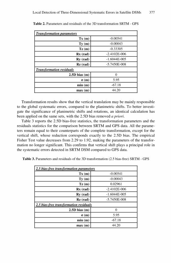
Table 2. Parameters and residuals of the 3D transformation SRTM - GPS

Transformation parameters

Tx (m) -0.00541

Ty (m) -0.00043

Tz (m) -0.33305

Rx (rad) -2.4102E-006

Ry (rad) -1.6044E-005

Rz (rad) -5.7450E-008

Transformation residuals

2.5D bias (m) 0

σ (m) 5.95

min (m) -67.18

max (m) 44.20

Transformation results show that the vertical translation may be mainly responsible

to the global systematic errors, compared to the planimetric shifts. To better investi-gate the significance of planimetric shifts and rotations, an identical calculation has been applied on the same sets, with the 2.5D bias removed a priori.

Table 3 reports the 2.5D bias-free statistics, the transformation parameters and the residuals statistics for the comparison between SRTM and GPS data. All the parame-ters remain equal to their counterparts of the complete transformation, except for the vertical shift, whose reduction corresponds exactly to the 2.5D bias. The empirical Fisher Test value decreases from 2.29 to 1.92, making the parameters of the transfor-mation no longer significant. This confirms that vertical shift plays a principal role in the systematic errors detected in SRTM DSM compared to GPS data.

Table 3. Parameters and residuals of the 3D transformation (2.5 bias-free) SRTM - GPS

2.5 bias-free transformation parameters

Tx (m) -0.00541

Ty (m) -0.00043

Tz (m) 0.02961

Rx (rad) -2.4102E-006

Ry (rad) -1.6044E-005

Rz (rad) -5.7450E-008

2.5 bias-free transformation residuals

2.5D bias (m) 0

σ (m) 5.95

min (m) -67.18

max (m) 44.20

378 M.A. Brovelli, X. Liu, and F. Sansò

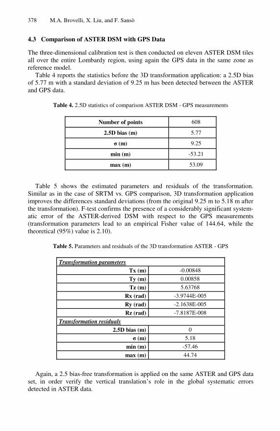
4.3 Comparison of ASTER DSM with GPS Data

The three-dimensional calibration test is then conducted on eleven ASTER DSM tiles all over the entire Lombardy region, using again the GPS data in the same zone as reference model.

Table 4 reports the statistics before the 3D transformation application: a 2.5D bias of 5.77 m with a standard deviation of 9.25 m has been detected between the ASTER and GPS data.

Table 4. 2.5D statistics of comparison ASTER DSM - GPS measurements

Number of points 608

2.5D bias (m) 5.77

σ (m) 9.25

min (m) -53.21

max (m) 53.09

Table 5 shows the estimated parameters and residuals of the transformation.

Similar as in the case of SRTM vs. GPS comparison, 3D transformation application improves the differences standard deviations (from the original 9.25 m to 5.18 m after the transformation). F-test confirms the presence of a considerably significant system-atic error of the ASTER-derived DSM with respect to the GPS measurements (transformation parameters lead to an empirical Fisher value of 144.64, while the theoretical (95%) value is 2.10).

Table 5. Parameters and residuals of the 3D transformation ASTER - GPS

Transformation parameters

Tx (m) -0.00848

Ty (m) 0.00858

Tz (m) 5.63768

Rx (rad) -3.9744E-005

Ry (rad) -2.1638E-005

Rz (rad) -7.8187E-008

Transformation residuals

2.5D bias (m) 0

σ (m) 5.18

min (m) -57.46

max (m) 44.74

Again, a 2.5 bias-free transformation is applied on the same ASTER and GPS data

set, in order verify the vertical translation’s role in the global systematic errors detected in ASTER data.

Local Detection of Three-Dimensional Systematic Errors in Satellite DSMs 379

Table 6 reports the 2.5D bias-free statistics, the transformation parameters and the residuals statistics for the comparison between ASTER and GPS data. All the parame-ters remain equal to their counterparts of the complete transformation, except for the vertical shift, whose reduction corresponds exactly to the 2.5D bias between the two altimetric models. The empirical Fisher Test value has decreased dramatically from 144.64 to 19.23, yet the test result remains positive: transformation parameters are still statistically significant. This result shows that even though the 2.5D bias is largely responsible in the systematic errors in ASTER DSM compared to GPS data, a full three-dimensional transformation is indispensable in order to remove all the sys-tematic errors detected in ASTER DSM.

Table 6. Parameters and residuals of the 3D transformation (2.5 bias-free) ASTER - GPS

2.5 bias-free transformation parameters

Tx (m) -0.00848

Ty (m) 0.00858

Tz (m) -0.12798

Rx (rad) -3.9744E-005

Ry (rad) -2.1638E-005

Rz (rad) -7.8187E-008

2.5 bias-free transformation residuals

2.5D bias (m) 0

σ (m) 5.18

min (m) -57.46

max (m) 44.74

5 Conclusions

This paper shows results of evaluation of the proper georeferencing of a DSM derived from satellite data, by determining its accuracy compared to local GPS measurements of a high accuracy; the algorithm used is based on a spatial similarity transformation without scale variation on the two altimetric data sets which have to be in the same datum. This algorithm does not require any a priori availability of homologous points. Experiments have been conducted on SRTM-derived and ASTER-derived DSM data in Lombardy Region, Northern Italy, both in 2.5D and in complete 3D comparison.

Systematic errors have been detected both in SRTM DSM and in ASTER DSM, compared to GPS data; in both cases vertical shifts play a principal role in the DSM systematic errors. However, three dimensional systematic errors in SRTM DSM are not significant, while in ASTER DSM case, a significant rototranslational systematic error has been confirmed. We can conclude that before the further application of the global ASTER DSM, a complete three-dimensional calibration is necessary.

380 M.A. Brovelli, X. Liu, and F. Sansò

References

1. Jarvis, A., Rubiano, J., Nelson, A., Farrow, A., Mulligan, M.: Practical use of SRTM data in the tropics: comparisons with digital elevation models generated from cartographic data. In: Working document no. 198, Centro Internacional de Agricultura Tropical, CIAT (2004)

2. ASTER GDEM Validation Team (METI/ERSDAC-NASA/LPDAAC-USGS/EROS): AS-TER Global DEM Validation Summary Report (2009)

3. Koch, A., Heipke, C., Lohmann, P.: Quality Assessment of SRTM DTM: methodology and practical results. In: Symposium on Geospatial Theory, Processing and Applications, Ot-tawa (2002)

4. CGIAR Consortium for Spatial Information (CGIAR-CSI), http://srtm.csi.cgiar.org

5. ASTER Global Digital Elevation Model (ASTER GDEM)-Earth Remote Sensing Data Analysis Center (ERSDAC), http://www.ersdac.or.jp

6. Brovelli, M.A., Caldera, S., Liu, X.: 3D comparison of DTMs without the use of homolo-gous points. In: The 6th International Symposium on Digital Earth, Processing, Beijing (2009)

7. Lemoine, F.G., Kenyon, S.C., Factor, J.K., Trimmer, R.G., Pavlis, N.K., Chinn, D.S., Cox, C.M., Klosko, S.M., Luthcke, S.B., Torrence, M.H., Wang, Y.M., Williamson, R.G., Pavlis, E.C., Rapp, R.H., Olson, T.R.: The development of the joint NASA GSFC and NIMA geo-potential model EGM96. NASA/TP-1998-206861. In: Goddard Space Flight Center, Greenbelt, Maryland (1998)

8. Brovelli, M.A., Caldera, S., Liu, X., Sansò, F.: Valutazione dell’accuratezza tridimensionale di un modello digitale del terreno. In: Convegno nazionale SIFET Dalle misure al modello digitale, Mantova, pp. 31–36 (2009)