On the computation of the demagnetization tensor for uniformly magnetized particles of arbitrary...

ARTICLE IN PRESS

Journal of Magnetism and Magnetic Materials 271 (2004) 27–38

*Corresp

412-268-75

E-mail

0304-8853/

doi:10.1016

On the computation of the demagnetization tensor foruniformly magnetized particles of arbitrary shape.

Part II: numerical approach

S. Tandona, M. Beleggiab, Y. Zhub, M. De Graef a,*aDepartment of Materials Science and Engineering, Carnegie Mellon University, 5000 Forbes Avenue, Pittsburgh, PA, 15213-3890, USA

bMaterials Science Department, Brookhaven National Laboratory, Upton, NY 11973, USA

Received 17 July 2003; received in revised form 24 August 2003

Abstract

In Part I, we described an analytical approach to the computation of the demagnetization tensor field for a uniformly

magnetized particle with an arbitrary shape. In this paper, Part II, we introduce two methods for the numerical

computation of the demagnetization tensor field. One method uses a Fourier space representation of the particle shape,

the other starts from the real space representation. The accuracy of the methods is compared to theoretical results for

the demagnetization tensor of the uniformly magnetized cylinder with arbitrary aspect ratio. Example computations are

presented for the hexagonal plate, the truncated paraboloid, and a so-called ‘‘Pac-Man’’ shape, recently designed for

MRAM applications. Finally, the magnetostatic self-energy of a uniformly magnetized regular polygonal disk of

arbitrary order is analyzed. A linear relation is found between the order of the polygon and the critical aspect ratio for

in-plane vs. axial magnetization states.

r 2003 Elsevier B.V. All rights reserved.

PACS: 41.20.Gz; 75.30.Gw; 75.40.Mg

Keywords: Demagnetization tensor field; Shape amplitude; Polygonal disk; Numerical algorithm; Demagnetization energy

1. Introduction

The computation of the magnetic inductioninside and surrounding a uniformly magnetizedparticle of arbitrary shape requires knowledge ofthe demagnetization tensor field, also known asthe point-function demagnetization tensor [1]. In

onding author. Tel.: +1-412-268-8527; fax: +1-

96.

address: [email protected] (M. De Graef).

$ - see front matter r 2003 Elsevier B.V. All rights reserve

/j.jmmm.2003.09.010

Part I of this two-paper series [2], we have shownanalytical computations of the demagnetizationtensor field (DTF) of the cylinder. This is a specialshape for which the equations can be solvedanalytically. In most cases, however, numericalmethods must be used to determine the tensorfield. In this paper, Part II, we will introduce twodifferent numerical procedures for the computa-tion of the DTF. In Section 2, we summarize thetheoretical model for the DTF and relatedquantities, the magnetostatic energy and the

d.

ARTICLE IN PRESS

S. Tandon et al. / Journal of Magnetism and Magnetic Materials 271 (2004) 27–3828

magnetometric demagnetization tensor. Section3.1 deals with a solution method which can beused if an analytical expression for the shapeamplitude is available. We also introduce animproved version of the latter case, in which afilter function is applied in Fourier space tosuppress Gibbs-like oscillations in the real spaceDTF. In Section 3.2, we introduce a numericalprocedure which starts from the shape function ofthe object, and employs numerical fast Fouriertransforms (FFT) to determine the DTF.Throughout this paper, we compare the numericalresults with analytical computations based on theexpression for the DTF of the uniformly magne-tized cylinder of Part I [2]. We conclude the paperwith a computation of the critical aspect ratio forin-plane vs. out-of-plane magnetization for regularpolygonal disks of arbitrary order.

2. Summary of the theoretical model

As shown by Beleggia and De Graef [3], thedemagnetization tensor field for a uniformlymagnetized particle with shape function DðrÞ (alsoknown as characteristic function) can be repre-sented in Fourier space as follows:

NijðkÞ ¼ DðkÞkikj

k2; ð1Þ

where k is the frequency vector, and DðkÞ theshape amplitude (i.e., the Fourier transform of theshape function). In real space, the demagnetizationtensor field is given by the inverse Fourier trans-form of Eq. (1):

NijðrÞ �1

8p3

Zd3k

DðkÞk2

kikjeikr: ð2Þ

The following relations were explicitly derived inRef. [3]:

1. the trace of NijðrÞ is equal to the shape functionDðrÞ;

2. the demagnetization energy can be written interms of the shape amplitude as

Em ¼m0M2

0

16p3

Zd3k

7DðkÞ72

k2ð #m � kÞ2; ð3Þ

with M0 the magnitude of the magnetizationand #m a unit magnetization vector;

3. the volume averaged (or magnetometric) de-magnetization tensor is given by

/NSij ¼1

V

ZV

d3rNijðrÞ

¼1

8p3V

Zd3k

7DðkÞ72

k2kikj ; ð4Þ

where V is the volume of the particle.

3. Numerical methods for the computation of the

demagnetization tensor field

3.1. Starting from the shape amplitude DðkÞ

The shape amplitude DðkÞ can be computedanalytically for many different particle shapes,among others: sphere [4], cylinder [4], truncatedparaboloid [2], Platonic solids [5,6], and so on.When the shape amplitude is used to compute theDTF, one must select a 3D computational grid onwhich the tensor field will be calculated. In mostcases, the use of FFT dictates that the dimensionsof the grid be powers of 2; although such arequirement is no longer necessary when modernFFT algorithms are used (e.g., the FFTW package[7]). Since the shape function is a discontinuousfunction, its Fourier representation always re-quires an infinite support. Truncation of thissupport to a finite computational grid results inthe familiar Gibbs oscillations near all disconti-nuities of the shape function. These oscillations arealso present in the DTF, since the phases of theFourier components NijðkÞ are identical to those ofthe Fourier components DðkÞ: It is possible,however, to propose a Fourier space filter func-tion, gðkÞ; which can be used to suppress the realspace Gibbs oscillations.

The filter function is essentially a piecewisecontinuous cubic polynomial, used primarilyfor image reconstruction by parametric cubicconvolution [8]. The function gðkÞ is given by

gðkÞ ¼ g0ðkÞ þ ag1ðkÞ

ARTICLE IN PRESS

S. Tandon et al. / Journal of Magnetism and Magnetic Materials 271 (2004) 27–38 29

¼3

k2sinc2ðkÞ � sincð2kÞ� �

þ a2

k23sinc2ð2kÞ � 2sincð2kÞ � sincð4kÞ� �

:

ð5Þ

where a is a parameter which can be chosen tooptimize the reconstruction. The optimum valuefor image reconstruction is a ¼ �0:5 [8]. This filterfunction gðkÞ is the one-dimensional (1D) Fouriertransform of the piecewise continuous cubicpolynomial

gðrÞ ¼ g0ðrÞ þ ag1ðrÞ; ð6Þ

with

g0ðrÞ ¼ð27r7þ 1Þð7r7� 1Þ2 7r7o1

0 elsewhere

(ð7Þ

and

g1ðrÞ ¼

7r72ð7r7� 1Þ 7r7o1;

ð7r7� 1Þð7r7� 2Þ2 1o7r7o2;

0 elsewhere:

8><>: ð8Þ

Multiplication of the frequency spectrum of a 1Dfunction with discontinuities with the filter func-tion dramatically reduces the Gibbs phenomenon.As an example, consider the periodic step functionwhich alternates between þ1 and �1: Its Fourierrepresentation is given by

f ðxÞ ¼XNn¼0

An sinðnpxÞ

with

A2n ¼ 0

A2nþ1 ¼4

pð2n þ 1Þ:

8<: ð9Þ

When this series is truncated after 25 termsðn ¼ 25Þ; then the resulting function is shown inFig. 1(a). An overshoot of 9% of the amount ofthe discontinuity occurs, and the function oscil-lates (Gibbs oscillations) around the values 71elsewhere. If the Fourier coefficients are multipliedby the filter function, i.e., An-AngðknÞ; then theresulting reconstructed function is significantlysmoother, as shown for the values a ¼ �0:5; 0.0,and 0.5 in Fig. 1(b)–(d). The inset shows the detailsat the discontinuity, magnified by a factor of 4:When the number of terms is increased to n ¼ 50;

the overshoot remains, and the filtered functionsare shown on the second row of Fig. 1. It is evidentthat the filtered functions more closely approx-imate the step function, and that the reconstruc-tion with a ¼ 0 creates the best approximation.For a ¼ �0:5 a small overshoot remains, whereasa ¼ 0:5 produces significant rounding at thediscontinuity. For the remainder of this paper wewill use the filter function in Eq. (5) with a ¼ 0:The same filter function can be used in threedimensions, provided the length of the frequencyvector k is used for k:

If we denote the tensor function kikj=k2 bykijðkÞ; then, according to Eq. (1), the DTF is givenby

NijðrÞ ¼ F�1 DðkÞkijðkÞ� �

: ð10Þ

If an analytical version of DðkÞ is available, thenthis equation should be replaced by a filteredversion for all numerical work:

NijðrÞ ¼ F�1 DðkÞkijðkÞgð7k7Þ� �

: ð11Þ

To show the validity of the filtering approach,we compare analytical results for the uniformlymagnetized cylinder with computational resultswith and without the filter function. The shapeamplitude for a cylinder with radius R and aspectratio t ¼ d=R; with d the half-height, is given by(Part I and [4]):

DðkÞ ¼ 2VJ1ðk>RÞ

k>RsincðdkzÞ; ð12Þ

where J1ðxÞ is the Bessel function of first order, k>

and kz are the in-plane and orthogonal compo-nents of k; resp., and sincðxÞ � sinðxÞ=x: Fig. 2shows the tensor element Nrrðr; 0Þ for a cylinderwith radius R ¼ 16 (in pixels) and t ¼ 0:75: Thecontinuous curve represents the analytical solu-tion, derived in Part I. The triangles on the left sideof the figure correspond to the tensor elementcomputed using Eq. (10) on a grid of 1283 points.The truncation of the Fourier representation (12)after only 64 different frequencies results in strongGibbs oscillations in the tensor element. Applica-tion of the Fourier filter in Eq. (11) reduces theseoscillations and the resulting tensor element isshown on the right side of Fig. 2. There are onlytwo points, one on either side of the discontinuity,

ARTICLE IN PRESS

0.0

-0.5

-1.0

0.5

1.0

0 0 0 0

uncorrected α = -0.5 α = 0.0 α = 0.5

(a) (b) (c) (d)

0.0

-0.5

-1.0

0.5

1.0

0 0 0 0

uncorrected α = -0.5 α = 0.0 α = 0.5

(e) (f) (g) (h)

n=25

n=50

Fig. 1. (a) and (e) show the reconstruction of series expansion 9 for n ¼ 25 and 50, resp. The other curves are reconstructions using the

filtered Fourier coefficients for three different values of the parameter a: �0:5; 0.0, and 0.5. The insets show a magnified view of the

discontinuity (�4).


for which the numerical value does not agree withthe analytical result. If the number of grid pointswere doubled in each direction, then there wouldstill be two incorrect points on either side of thediscontinuity, but now those points would becloser to the discontinuity. In the limit of acontinuous grid, the numerical result wouldcoincide with the analytical solution. In practice,the number of grid points is determined by theavailable computing memory. The mean deviationbetween the analytical and numerical values forthe tensor elements, excluding the points closest tothe discontinuity, is typically about 0.1% forcomputations that include the filter function,and closer to 1% if the filter function is not used.These numbers are somewhat sensitive to the sizeof the cylinder relative to the size of the computa-tional array. Smaller cylinders result in betteragreement between theoretical values and numer-ical computations.

3.2. Starting from the shape function DðrÞ

Consider a 3D regular grid with N grid pointsalong each axis. Any object for which the insideand outside can be unambiguously defined can berepresented by an array of 1’s and 0’s, correspond-ing to the interior and exterior points, respectively.This is essentially a discrete representation of theshape function DðrÞ: Special topological cases,such as the Klein bottle and other non-orientablesurfaces for which there is no inside or outside,cannot be dealt with in this formalism. The objectneed not be simply connected, so that hollow orshell-like objects can also be treated. One can alsoplace multiple non-connected objects on thediscrete array and compute the demagnetizationtensor field for the set of all objects. Note that thisthen assumes that the magnetization directionused to contract the tensor to obtain the magneticfield, H; must be identical in all objects that make

ARTICLE IN PRESS

0.4

0.2

0.0

-0.2

-0.4

-0.6

-20 -10 0 10 20

Nrr

(r,0

)

r (pixels)

unfiltered filtered

Fig. 2. Comparison between the analytical value of Nrrðr; 0Þ fora cylinder with radius R ¼ 16 and t ¼ 0:75 (solid line), and a

numerical simulation based on the discretized analytical

expression of the shape amplitude in Eq. (12) (left curve). The

Gibbs oscillations are clearly visible. After Fourier space

filtering of the shape amplitude DðkÞ with the function gðkÞ ofEq. (5), the resulting numerical values are indicated by small

diamonds on the right half of the figure. Only the two points

arrowed deviate from the analytical solution; the others are

within 1% of the analytical value.

0.4

0.2

0.0

-0.2

-0.4

-0.6

-20 -10 0 10 20

Nrr

(r,0

)

Standard D(r) Smooth D(r)

r (pixels)

Fig. 3. Comparison between the analytical value of Nrrðr; 0Þ fora cylinder with radius R ¼ 16 and t ¼ 0:75 (solid line), and a

numerical simulation based on the shape function DðrÞ: On the

left side, the shape function was discretized with only two

intensity levels: 0 and 1: On the right, a smoother version of the

shape function was used. The smoothened result should be

compared with the Fourier space filtered result of Fig. 2.


up the complete array. If this is not the case, thenthe demagnetization tensor field must be computedfor each object separately, then contracted withrespect to the magnetization direction for thatobject, and the resulting magnetic field configura-tions for each object added together to obtain themagnetic field for the assembly of objects.

If we assume periodic boundary conditions,then the numerical Fourier transform of the 3Dgrid will approximate the analytical Fourier trans-form for the smaller spatial frequencies, but forhigher spatial frequencies discrepancies will arisebecause of the finite support of the Fourier space.Only frequencies below the Nyquist frequency aremeaningful. An inverse Fourier transform will re-create the original object without Gibbs oscillations,even when this object has discontinuities.

This observation leads to a simple numericalalgorithm for the computation of the DTF on adiscrete 3D grid:

1. create the discrete shape function DðrÞ on thecomputational grid;

2. convert to Fourier space DðkÞ;

3. multiply by the kijðkÞ tensor field;4. transform back to real space to obtain the DTF

NijðrÞ:

As with all periodic continuation problems, caremust be taken to properly select the size of theobject with respect to the size of the computationalgrid. Near the edges of the grid, the values of thetensor field may be affected by the periodicboundary conditions.

As an example, consider the analytical solutionfor the uniformly magnetized cylinder in Part I.For a cylinder with radius R ¼ 16 (pixels) andaspect ratio t ¼ 0:75; the tensor field componentNrrðr; 0Þ is shown as a continuous line in Fig. 3.When the tensor element is computed using theabove algorithm, the function values on the leftside of the figure are obtained (triangles). Theagreement with the analytical solution is rathergood, except at two points close to the disconti-nuity. The numerical result can be improved byconsidering a modified shape function DðrÞ: Themodification consists of a smoothing operation,which is carried out for all grid points that arewithin a certain distance from the object surface.There are many possible smoothing options. Asimple smoothing operation is carried out asfollows: for each grid point located less than Z

ARTICLE IN PRESS


grid spacings from the object surface (either insideor outside the object), the normal distance d to theobject surface is computed. For points on theinside of the object, the distance d is taken to benegative. The shape function value at this gridpoint is then given by

D ¼ cos2 pðdþ ZÞ4Z

�: ð13Þ

This function smoothly goes from 1 inside theobject to 0 outside the object. The tensor elementNrrðr; 0Þ for the smoothed shape function is shownon the right in Fig. 3 (diamonds). The functionvalues are identical to those for the unsmoothedshape function on the left, except for the twopoints near the discontinuity. For these points, thevalues are nearly identical to those obtained usingthe Fourier filtered shape amplitude (see right sideof Fig. 2). The mean deviation between theoreticaland numerical values, excluding the points closestto the discontinuity, is again about 0.1% whenused with the smoothing operation, and closer to1% without smoothing.

4. Example applications

In this section, we will apply the numericalformalisms described in Section 3 to a number ofimportant shapes: the regular hexagonal plate, thetruncated paraboloid, and a ‘‘pacman’’ thin plate.These shapes are shown schematically in Fig. 4(a)–(c). The regular hexagonal plate (Section 4.1) isan important building block for micromagneticsimulations, where it represents the shape of afinite element cell. The truncated paraboloid

z

h=aR2

ar2

(a) (b)

2a

2c

Fig. 4. Schematic illustration of the shapes for which example DTF c

(b) truncated paraboloid and (c) ‘‘pacman’’ particle.

(Section 4.2) approximates the shape of the tip ofa magnetic force microscope. The ‘‘pacman’’ shape(Section 4.3) was recently proposed [9] as a novelshape for a sub-micron NiFe element for magneticrandom access memory (MRAM) applications.We conclude this section with the numericalcomputation of the critical aspect ratio forpolygonal disks.

4.1. The regular hexagonal plate

The shape amplitude of a regular hexagonalplate has been given in Eq. (14) of Part I, and israther complicated. Since there is no straightfor-ward analytical method to compute the real spaceDTF, starting from this shape amplitude, we applythe Fourier space filter function of Eq. (11). Two-dimensional section of the resulting DTF areshown in Fig. 5 for a plate with aspect ratio Z ¼25(computation carried out on a 1283 grid). The top

two rows show a grayscale representation of thetensor field elements for a plane going through thecenter of the hexagonal plate. All images have acommon grayscale from �0:4 (black) to þ0:79(white). The axes in the lower corner of each imageindicate the orientation of the two-dimensionalsection. The bottom two rows show two differentsections (xy and xz) of the eigenvalues of thetensor field, ranked from smallest (l1) to largest(l3). The eigenvalues reveal the true symmetry ofthe tensor field.

4.2. The truncated paraboloid

The shape amplitude of the truncated parabo-loid can be computed analytically, and the explicit

Rr

(c)

ω

R r

R=3r

omputations are shown in Sections 4.1–4.3: (a) hexagonal plate,

ARTICLE IN PRESS

Fig. 5. DTF tensor components (a) and eigenvalues (b) for a

hexagonal plate with c=a ¼ 25: The basis vectors indicate the

orientation of the planar sections; all sections go through the

center of the plate. The eigenvalues are ranked in ascending

order. The intensity ranges [black,white] correspond to

½�0:399; 0:784 (a) and ½�0:399; 0:789 (b).

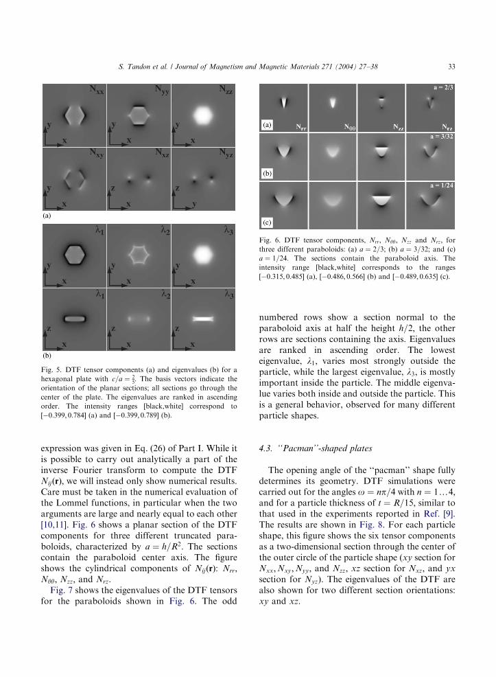
Fig. 6. DTF tensor components, Nrr; Nyy; Nzz and Nrz; forthree different paraboloids: (a) a ¼ 2=3; (b) a ¼ 3=32; and (c)

a ¼ 1=24: The sections contain the paraboloid axis. The

intensity range [black,white] corresponds to the ranges

½�0:315; 0:485 (a), ½�0:486; 0:566 (b) and ½�0:489; 0:635 (c).


expression was given in Eq. (26) of Part I. While itis possible to carry out analytically a part of theinverse Fourier transform to compute the DTFNijðrÞ; we will instead only show numerical results.Care must be taken in the numerical evaluation ofthe Lommel functions, in particular when the twoarguments are large and nearly equal to each other[10,11]. Fig. 6 shows a planar section of the DTFcomponents for three different truncated para-boloids, characterized by a ¼ h=R2: The sectionscontain the paraboloid center axis. The figureshows the cylindrical components of NijðrÞ: Nrr;Nyy; Nzz; and Nrz:

Fig. 7 shows the eigenvalues of the DTF tensorsfor the paraboloids shown in Fig. 6. The odd

numbered rows show a section normal to theparaboloid axis at half the height h=2; the otherrows are sections containing the axis. Eigenvaluesare ranked in ascending order. The lowesteigenvalue, l1; varies most strongly outside theparticle, while the largest eigenvalue, l3; is mostlyimportant inside the particle. The middle eigenva-lue varies both inside and outside the particle. Thisis a general behavior, observed for many differentparticle shapes.

4.3. ‘‘Pacman’’-shaped plates

The opening angle of the ‘‘pacman’’ shape fullydetermines its geometry. DTF simulations werecarried out for the angles o ¼ np=4 with n ¼ 1y4;and for a particle thickness of t ¼ R=15; similar tothat used in the experiments reported in Ref. [9].The results are shown in Fig. 8. For each particleshape, this figure shows the six tensor componentsas a two-dimensional section through the center ofthe outer circle of the particle shape (xy section forNxx;Nxy;Nyy; and Nzz; xz section for Nxz; and yx

section for Nyz). The eigenvalues of the DTF arealso shown for two different section orientations:xy and xz:

ARTICLE IN PRESS

Fig. 7. DTF tensor eigenvalues li (i ¼ 1y3) for the same

paraboloids as in Fig. 6. The horizontal sections in the first,

third and fifth rows, intersect the paraboloid at half height, the

vertical sections in the remaining rows contain the paraboloid

axis. The intensity range [black,white] corresponds to the ranges

½�0:318; 0:511 (a), ½�0:487; 0:705 (b) and ½�0:508; 0:787 (c).


The volumetric demagnetization tensor can becomputed by means of Eq. (4). Fig. 9 shows theeigenvalues of the volumetric demagnetizationfactors as a function of the opening angle o forthe pacman shape of Fig. 4(c) (solid lines), as well

as for a simpler shape where the radius r of theinner circle vanishes (dashed lines) (referred to asPM-I in Ref. [9]). The Nzz demagnetization factoris about 8% smaller for the new ‘‘pacman’’ shape.This is consistent with the results presented inRef. [9]; the ‘‘pacman’’ shape of Fig. 9 shows nomagnetic domain walls, regardless of the value ofthe opening angle o; whereas the shape with r ¼ 0shows a domain with reverse magnetizationsurrounding the sharp corner at the center of theparticle. Rounding of this corner results in asmaller demagnetization field, which favors thesingle domain state of the particle.

4.4. Computation of the critical aspect ratio for

polygonal disks

In Part I, Section 5, we computed analyticallythe demagnetization energy for the uniformlymagnetized cylinder with aspect ratio t ¼ t=2R;with t the cylinder height and R the radius. It wasshown that, if we denote by y the angle betweenthe magnetization direction and the cylinder axis,the demagnetization energy is proportional to anexpression of the following form:

EmðtÞBf1ðtÞð3 cos2 y� 1Þ þ f2ðtÞ cos2 y; ð14Þ

where

f1ðtÞ ¼1

t1

3p�

ffiffiffiffiffiffiffiffiffiffiffiffiffi1� t2

p4

2F11

2;3

2; 2;

1

1þ t2

� �" #; ð15Þ

f2ðtÞ ¼1

2: ð16Þ

The critical aspect ratio tc corresponds to a saddlepoint in the energy (see Fig. 5 in Part I), and can becomputed from the condition 3f1ðtÞ þ f2ðtÞ ¼ 0;which leads to tc ¼ 0:9065 for the cylinder.

The cylinder can be considered as the limitingcase of a series of regular polygonal disks of heightt and order N; for N-N: It was shown byBeleggia et al. [6] that the shape amplitude of aregular polygonal disk of order N can becomputed analytically. The result is given by

DðkÞ ¼ 4icsincðckzÞk2

x þ k2y

XN

p¼1

X3j¼1

kpjsincðmpjÞeinpj ; ð17Þ

ARTICLE IN PRESS

Fig. 8. DTF tensor components and eigenvalues for four different ‘‘pacman’’ shapes. All sections go through the center of the outer

circle of the particle shape. The top six figures for each opening angle o depict sections of the DTF, whereas the bottom two rows

depict two sections of the eigenvalues of the DTF in ascending order.


with

kpj ¼ cpk1 þ spm1; cpk2 � spm2;�aðspkx þ cpkyÞ� �

;

ð18aÞ

mpj ¼ cpm1spk1; cpm2 þ spk2; aðcpkx � spkyÞ� �

; ð18bÞ

npj ¼ mp1;mp2; hðspkx þ cpkyÞ� �

; ð18cÞ

cp ¼ cosðypÞ; sp ¼ sinðypÞ; yp ¼ 2pa; h ¼ a=tana;and a ¼ p=N: The parameters ki and mi are givenby

kj ¼a

2�okx þ ky;okx þ ky

� �; ð19aÞ

mj ¼a

2kx þ oky;�kx þ oky

� �; ð19bÞ

with o ¼ 1=tana:Using Eq. (17), we can compute the magneto-

static energy (3) as a function of the angle y andthe aspect ratio t ¼ c=a of the polygonal disk,where c ¼ t=2; and a is half the edge length. Sinceeach regular polygonal disk has a rotation axis oforder N normal to the disk, the magnetostaticenergy will be invariant with respect to theazimuthal component of the magnetization direc-tion [3]. This in turn means that the angular

ARTICLE IN PRESS

0.5

0.6

0.7

0.8

0.9

1.0

1.1

1.2

3 4 5 6 7 8 9 10 11

N

Cri

tica

l Asp

ect

Rat

io

τc(N) tanα

τc(N) sinα

0.90647

0

1

2

3

4

3 4 5 6 7 8 9 10 11

N

τ c (N

)Numerical Result

Linear Fit

(a)

(b)

Fig. 10. (a) Critical aspect ratio tcðNÞ for regular polygonal

plates of various orders N ; converted to an outer radius value

(top curve) and an inner radius value (bottom curve). The dash-

dotted line is the limit for N-N; i.e., the cylinder, for which

inner and outer radii coincide. (b) Critical aspect ratio as a

function of N ; along with a linear fit (dashed line). The aspect

ratio changes linearly with the order of the polygon for

sufficiently large orders.

60 80 100 120 180140 1600.0

0.2

1.0

0.8

0.6

NxxNyy

Nzz

Opening angle ω

Volu

me

aver

aged

dem

agn

etiz

ati

on

fact

ors

Fig. 9. Comparison between the magnetometric demagnetiza-

tion factors for the ‘‘pacman’’ shape and a simpler shape for

which the radius of the inner circle is equal to zero. The

horizontal axis shows the opening angle, as defined in Fig. 4.


integrations will result in the angular dependenceof the energy on y shown for the cylinder inEq. (14). Therefore, by fitting the energy to theform (14), we obtain both functions fiðtÞ for agiven N: Application of the equation 3f1ðtÞ þf2ðtÞ ¼ 0 then results in the critical aspect ratiotcðNÞ: Note that the definition of the aspect ratioof the polygonal disk involves the thickness andthe edge length, whereas for the cylinder the aspectratio depends on the thickness and the diameter.We can convert from edge length to either theinscribed or the circumscribed diameter by multi-plying the aspect ratio by tan a or sin a; respec-tively. The results of numerical simulations forN ¼ 3y11 are shown in Fig. 10. The top curvecorresponds to tcðNÞtan a; the bottom curve totcðNÞsin a: The dash-dotted line is the analyticalvalue tcðNÞ for the limiting cylinder. It is clearthat the two curves for the outer and inner circleconverge towards each other and to the criticalaspect ratio of the cylinder, when N-N:

When the critical aspect ratio tcðNÞ is plotted vs.N; the linear function shown in Fig. 10b isobtained. This linear behavior can be understoodas follows: for large N; the critical aspect ratio canbe written as

tcðNÞ ¼ c0 þ c1N: ð20Þ

Converting this aspect ratio to either tcðNÞtana ortcðNÞsin a; and taking the limit for N-N we must

obtain the critical aspect ratio tcðNÞ for thecylinder:

limN-N

ðc0 þ c1NÞtan a

sin a

(¼ lim

N-N

c0

Nþ c1

� �p ¼ c1p

¼ tcðNÞ ¼ 0:90647; ð21Þ

ARTICLE IN PRESS


from which follows c1 ¼ 0:90647=p ¼ 0:28854: Alinear fit to the data of Fig. 10b leads to c1 ¼0:29276 and c0 ¼ �0:07806; in reasonable agree-ment with the theoretical result.

5. Summary

We have presented two accurate and fastnumerical methods for the computation of thedemagnetization tensor field, the demagnetizationenergy, and the volumetric demagnetization fac-tors of particles with an arbitrary, finite shape. Ifan analytical expression for the particle shapeamplitude is available, then the DTF can becomputed using a 3D inverse FFT operation. Toeliminate Gibbs oscillations, which occur due tothe intrinsic discontinuous nature of the shapefunction, DðrÞ; we have proposed a Fourier spacefilter function. If no explicit expression for theshape amplitude is available, then the DTF can becomputed starting from a 3D real space array of 0and 1 values, defining the shape of the particle.The formalism can also be applied to thecomputation of magnetostatic self-energy for aparticle with an arbitrary shape. It was shown thatthe critical aspect ratio for the in-plane vs. axialmagnetization states in a regular polygonal diskof arbitrary order varies linearly with the orderN; for sufficiently large N; and converges to thevalue for the cylinder. While both the direct spaceand the Fourier space numerical approaches resultin the same accuracy for the demagnetizationtensor elements, the Fourier space approach hasthe advantage of being fast, provided of coursethat an analytical expression for the shapeamplitude can be found. The direct space ap-proach has the advantage that truly arbitraryshapes can be dealt with in a straightforwardmanner, at the expense of somewhat longercomputation times.

While it is difficult in practice to obtain auniform magnetization in a body of arbitraryshape, accurate knowledge of the DTF for such anobject is desirable, in particular in the case of smallparticles. Below a critical size limit, where theexchange term is largely predominant over otherenergy contributions, all particles will show a

single domain magnetization state. While therewill be small deviations from the uniformlymagnetized state, in particular near edges andcorners, knowledge of the uniformly magnetizedstate is useful as a first order approximation to thereal magnetization state. The computationalmethods described in this paper provide a fastand accurate means to access this information.Regarding magnetocrystalline anisotropy, wherethis effect is not negligible due to the possiblepolycrystalline nature of the particle, we cansimply account for it by specifying the directionof the magnetization along the preferential axis ofthe particle.

The methods proposed in this paper are basedon the use of the fast Fourier transform, for whichmany speed-optimized implementations are avail-able. Given the simplicity and accuracy of themethods, they should find quick acceptance in thecomputational magnetism community, and maywell replace the slower direct space methods,which often require the numerical evaluation oftwo 3D integrals.

Acknowledgements

The authors would like to thank Prof. Y.-K.Hong for making available a preprint on the‘‘Pacman’’-shaped particles. Financial support wasprovided by the US Department of Energy, BasicEnergy Sciences, under contract numbers DE-FG02-01ER45893 and DE-AC02-98CH10886.

References

[1] R. Moskowitz, E. Della Torre, IEEE Trans. Magn. 2

(1966) 739.

[2] S. Tandon, M. Beleggia, Y. Zhu, M. De Graef, J. Magn.

Magn. Mater. (2004), this issue.

[3] M. Beleggia, M. De Graef, J. Magn. Magn. Mater. 263

(2003) L1.

[4] M. Beleggia, Y. Zhu, Philos. Mag. B 83 (2003) 1143.

[5] J. Komrska, W. Neumann, Phys. Stat. Sol (a) 150 (1995)

89.

[6] M. Beleggia, S. Tandon, Y. Zhu, M. De Graef, Philos.

Mag. B 83 (2003) 1143.

10.1016/j.jmmm.2003.09.011

ARTICLE IN PRESS


[7] M. Frigo, S.G. Johnson, FFTW (Fastest Fourier Trans-

form in the West, version 3.0), URL: http://www.fftw.org/,

2003.

[8] S.K. Park, R.A. Schowengerdt, Comput. Vision, Graphics,

Image Process. 23 (1983) 1187.

[9] M.H. Park, Y.K. Hong, S.H. Gee, D.W. Erickson, B.C.

Choi, Appl. Phys. Lett. 83 (2003) 329.

[10] K.D. Mielenz, J. Res. Natl. Inst. Stand. Technol. 103

(1998) 497.

[11] W.H. Press, B.P. Flannery, S.A. Teukolsky, W.T. Vetter-

ling, Numerical Recipes: The Art of Scientific Computing

(Fortran Version), Cambridge University Press,

Cambridge, 1989.

http://www.fftw.org/

On the computation of the demagnetization tensor for uniformly magnetized particles of arbitrary...

Documents

Transcript of On the computation of the demagnetization tensor for uniformly magnetized particles of arbitrary...