On the Choice of Momentum Control Variables and ...

On the Choice of Momentum Control Variables and CovarianceModeling for Mesoscale Data Assimilation

QIN XU

NOAA/National Severe Storms Laboratory, Norman, Oklahoma

(Manuscript received 26 March 2018, in final form 12 September 2018)

ABSTRACT

For mesoscale variational data assimilation with high-resolution observations, there has been an issue

concerning the choice of momentum control variables and related covariancemodeling. This paper addresses

the theoretical aspect of this issue. First, relationships between background error covariance functions for

differently chosen momentum control variables are derived, and different choices of momentum control

variables are proven to be theoretically equivalent in the sense that they lead to the same optimally analyzed

incremental wind field in the limit of infinitely high spatial resolution provided their error covariance func-

tions satisfy the derived relationships. It is then shown that when the velocity potential x and streamfunction

c are used as momentum control variables with their background error autocovariance functions modeled by

single-Gaussian functions, the derived velocity autocovariance functions contain significant negative side-

lobes. These negative sidelobes can represent background wind error structures associated with baroclinic

waves on the synoptic scale but become unrepresentative on the mesoscale. To reduce or remove these

negative sidelobes for mesoscale variational data assimilation, Gaussian functions are used with two types of

modifications to model the velocity covariance functions in consistency with the assumed homogeneity and

isotropy in variational data assimilation. In this case, the random (x, c) background error fields have no

classically valid homogeneous and isotropic covariance functions, but generalized (x, c) covariance functions

can be derived from the modified velocity covariance functions for choosing (x, c) as momentum control

variables. Mathematical properties of generalized covariance functions are explored with physical in-

terpretations. Their important implications are discussed for mesoscale data assimilation.

1. Introduction

The streamfunction c and velocity potential x have

been widely used as momentum control variables in

operational three-dimensional variational data assimi-

lation (3DVar) systems (Lorenc et al. 2000; Wu et al.

2002). A well-recognized advantage for using (x, c) as

momentum control variables in 3DVar is that c can be

linearly related to the mass field via the geostrophy on

the synoptic scale, and this linear relationship can be

built into the background error covariance. In addition,

the x field can be prescribed with a relatively small error

variance to suppress the associated divergent incre-

ments, while the c field (or mass field) can be split into

geostrophically balanced and unbalance parts with a

relatively small error variance prescribed to the unbal-

ance part to suppress the unbalanced increments. The

aforementioned advantages, however, diminish as the

horizontal scale of the analyzed features reduces toward

the mesoscale. Moreover, using (x, c) as momentum

control variables with their background error autoco-

variance modeled by single-Gaussian functions in the

mesoscale range can generate spurious structures in the

analyzed incremental wind field outside and around

areas covered by patched high-resolution observations

(such as those from Doppler radars) as a result of the

presence of significant negative sidelobes in the velocity

autocovariance functions [derived from the (x, c)

Gaussian autocovariance functions]. To avoid this prob-

lem, Gaussian functions were used with simplifications to

model the velocity covariance functions in the recently

developed radar wind analysis system (Xu et al. 2015).

Xie and MacDonald (2012) performed spectral and

numerical analyses to examine various possible analysis

errors that could be potentially introduced by the use of

(x, c), versus the use of the horizontal velocity compo-

nents (u, y) and the use of the vorticity and divergence,

as momentum control variables in 3DVar. In particular,

their analysis of a single velocity observation indicated

that using (x, c) as momentum control variables inCorresponding author: Qin Xu, [email protected]

JANUARY 2019 XU 89

DOI: 10.1175/JAS-D-18-0093.1

For information regarding reuse of this content and general copyright information, consult the AMS Copyright Policy (www.ametsoc.org/PUBSReuseLicenses).

Brought to you by NOAA Central Library | Unauthenticated | Downloaded 09/23/21 09:00 PM UTC

mailto:[email protected]

http://www.ametsoc.org/PUBSReuseLicenses



3DVar can generate erroneous negative sidelobes

around the observation point because (u, y) are de-

rivatives of (x, c). However, since the background error

covariance wasmodeled (implicitly by a single-Gaussian

function or similar type) through applications of a sim-

ple recursive filter in their numerical experiments, the

presence and absence of negative sidelobes were ex-

amined only in terms of choices of momentum control

variables independent of covariance modeling. Thus,

whether and how the concerned negative sidelobes can

be reduced or eliminated by modifying or generalizing

the conventional covariance modeling were not studied

but need to be explored (as shown later in this paper).

Sun et al. (2016) performed real-data experiments to

examine the impacts of different choices of momentum

control variables on limited-area high-resolution data

assimilation and subsequent convective precipitation

forecasting. Their experiments showed that using (x, c),

in comparison with using (u, y), as momentum control

variables in high-resolution radar data assimilation can

result in degraded analysis and forecast. Velocity com-

ponents were also used favorably as momentum control

variables with their background error covariance mod-

eled by single Gaussians and mimicked by recursive

filters in the 3DVar system developed by Gao et al.

(2004, 2013) for real-time radar data assimilation. Since

the aforementioned studies advocated the use of (u, y) in

place of (x, c) as momentum control variables for high-

resolution variational data assimilation, there has been

an issue on the choice of momentum control variables

and related covariance modeling. This issue can be im-

portant for mesoscale variational data assimilation as

well as multiscale variational data assimilation (Xie

et al. 2011; Li et al. 2015; Xu et al. 2016). This paper aims

to address the theoretical aspect of this issue.

The next section derives the relationships between

background error covariance functions for differently

chosen momentum control variables and proves that

different choices of momentum control variables are

theoretically equivalent in the sense that they lead to the

same optimally analyzed incremental wind field in the

limit of infinitely high spatial resolution provided their

error covariance functions satisfy the derived relation-

ships. Section 3 presents typical examples of negative

sidelobes in the velocity autocovariance functions de-

rived from single-Gaussian (x, c) autocovariance func-

tions and explains physically why negative sidelobes can

represent background wind error structures on the

synoptic scale but not on the mesoscale. Section 4 shows

how Gaussian functions can be modified to model the

isotropic canonical-form velocity autocovariance func-

tions with negative sidelobes reduced or removed for

mesoscale variational data assimilation, and explains

how and why (x, c) covariance functions derived by

integrating the modified velocity covariance become

classically invalid but can still be used as generalized

covariance functions for (x, c) chosen as momentum

control variables. Mathematical properties of generalized

covariance functions are further explored with physical

interpretations in appendixes D–F. Conclusions follow

in section 5, where the theoretical findings are summa-

rized with their implications remarked for mesoscale

data assimilation.

2. Equivalence between different choices ofmomentum control variables

a. Relationships between covariance functions fordifferent momentum control variables

The covariance of background wind errors at two

points, say, zi [ (xi, yi, hi)T and zj [ (xj, yj, hj)

T, in the

three-dimensional space (where the vertical coordinate

h is as in the concerned data assimilation system) is a

2 3 2 tensor defined by

Cvv(z

i, z

j)[ hv

ivTj i , (1)

where h(�)i denotes the statistical mean of (�), vi [ v(zi)

[or vj [ v(zj)] is the value of v at z5 zi (or zj), v[ (u, y)T

denotes the background wind error as a random vector

field in z with hvi5 0 (or with hvi subtracted if hvi 6¼ 0),

and (�)T denotes the transpose of (�). The velocity po-

tential x and streamfunction c of v are two random

scalar fields defined by v [ =x 1 k 3 =c, where = [(›x, ›y)

T is the horizontal gradient operator, and k is the

unit vector along the vertical coordinate so k 3 = 5(2›y, ›x)

T is the horizontal gradient operator rotated

counterclockwise by 908.The x and c composed vector field, c [ (x, c)T, is

related to v by v 5 (=, k 3 =)c. Substituting this into

(1) gives

Cvv(z

i, z

j)5 h[(=

i, k3=

i)c

i][(=

j, k3=

j)c

j]Ti

5 (=i,k3=

i)[(=

j,k3=

j)C

cc(z

j, z

i)]T, (2)

where =i (or =j) denotes = applied to zi (or zj), ci [ c(zi),

cj[ c(zj), and Ccc(zi, zj)[ hcicjTi [5hcjciTiT [ Ccc(zj, zi)T]

is the 2 3 2 covariance tensor of c [ (x, c)T with its

two diagonal (or off diagonal) elements defined by

Cxx(zi, zj)[ hxixji andCcc(zi, zj)[ hcicji [orCxc(zi, zj)[hxicji and Ccx(zi, zj) [ hcixji].The divergence and vorticity of v are random scalar

fields that are defined by d[ =� v5 =2x and z [ k � =3v 5 =2c, respectively, where =2 [= � =5 ›2x 1 ›2y is the

horizontal Laplace operator. Their composed vector

90 JOURNAL OF THE ATMOSPHER IC SC IENCES VOLUME 76


field, q [ (d, z)T, is related to c by q 5 =2c. The co-

variance tensor of q is thus related to that of c by

Cqq(z

i, z

j)[ hq

iqTj i5=2

i =2jCcc

(zi, z

j) , (3)

where qi [ q(zi), qj [ q(zj), and =2i (or =

2j ) denotes =

2

applied to zi (or zj).

b. Equivalence between different choices ofmomentum control variables

Using the relationships derived in the previous sec-

tion, we can prove the theoretical equivalence between

the following three different choices of momentum

control variables: (i) v [ (u, y)T in choice 1, (ii) c [(x, c)T in choice 2, and (iii) q[ (d, z)T in choice 3. Here,

by theoretical equivalence we mean the equivalence in

the continuous limit (i.e., the limit of infinitely high

spatial resolution) between optimally analyzed incre-

mental wind fields obtained by using different choices of

momentum control variables with their background

error covariance tensor functions satisfying the rela-

tionships derived in section 2a. Also, to simplify the

notations, the symbols v, c, and q used in the previous

subsection to denote the random-vector error fields are

reused here for the control-variable vector fields.

The cost function for the minimization problem

formulated with each choice of control variables in a

discretized domain of z has the following general in-

cremental form:

J5DaTB21Da1 (HDa2 d)TR21(HDa2 d) , (4a)

where Da 5 a 2 b denotes the state vector of analysis

increment expressed by the chosen control variable, a

(or b) denotes the state vector of analysis (or back-

ground), B denotes the background error covariance

matrix constructed by the error covariance tensor

function of the chosen control variables in the dis-

cretized space of (zi, zj), R denotes the observation error

covariance matrix, d5 y2H(b) denotes the innovation

vector (i.e., observation minus background in the ob-

servation space), y is the observation vector, H denotes

the (nonlinear) observation operator that maps the

model space to the observation space, and H is the lin-

earized H around b. Since the wind observations con-

sidered in this study are linearly related to the model’s

velocity state vector (or velocity field in the continuous

limit), H reduces to H in (4a) for 3DVar. [By extending

H to include the forward model operator, the cost

function in (4a) can be used for perfect-model 4DVar.

In this case, H is nonlinear in general and J in (4a) is

an approximation of its original nonincremental form,

but the approximation can be improved via outer-loop

iterations by updating b to b 1 Da once Da is obtained

from the previous outer loop (see section 3b of Lorenc

2003). Thus, although H becomes nonlinear, (4a) still

can be used with a given b to prove the theoretical

equivalence between the different choices of momen-

tum control variables, because b will be updated also

equivalently in the subsequent outer loop.]

The cost function in (4a) can be transformed into its

dual form (Courtier 1997) in the observation space:

J5 pTHBHTp1 (HBHTp2 d)TR21(HBHTp2d) , (4b)

where p is the transformed control vector related to Da byDa 5 BHTp 5 pTBH. The minimizer of J in the space of

p is given by the solution of =p J 5 2HBHTR21[(R 1HBHT)p 2 d] 5 0 or, equivalently, (HBHT 1 R)p 5 d.

Thus, the minimizer of J in the space of Da is given by

Da5BHTp , (5a)

with p solved from

(HBHT 1R)p5 d . (5b)

In (5b),R and d are independent of the choice of control

variables. As shown in appendix A, HBHT also becomes

independent of the choice of control variables in the

continuous limit and so is the solution of p obtained

from (5a) [also see (A10)]. When p is transformed back

to give Da 5 BHTp for the solutions in the control var-

iable spaces of v, c and q, these solutions satisfy the re-

quired relationships of v5 (=, k3=)c and q5=2c in the

continuous limit [see (A16) and (A22) in appendix A].

This proves the theoretical equivalence between dif-

ferent choices of control variables.

The above proof assumes implicitly that Ccc(z, z0)

is a differentiable and classically valid covariance

tensor function (i.e., to not only satisfy the required

symmetry and positive semidefiniteness but also ap-

proach zero as jz0 2 zj increases unboundedly). This

ensures Cvv(z, z0) and Cqq(z, z

0) are also classically valid

covariance tensor functions, as they are derived from

Ccc(z, z0) via differentiations in (2) and (3), respectively.

The inverse, however, does not hold true. In particular,

the classical validity of Cvv(z, z0) [or Cqq(z, z

0)] cannotensure the classical validity of Ccc(z, z

0) [or Cvv(z, z0)], as

the latter is derived from the former by inverting (2) [or

(3)]. This problem will be revisited later in section 4c.

c. Relationships between homogeneous and isotropiccovariance functions

In variational data assimilation, the random vector

field of background wind error v (or v normalized by its

standard deviation) is assumed to be homogeneous and

JANUARY 2019 XU 91


isotropic in x[ (x, y)T. In this case,Cvv defined in (1) can

be transformed into the following canonical form:

h(li, t

i)T(l

j, t

j)i5R

aC

vvRT

a , (6)

where (li, ti)T [ Ravi, (lj, tj)

T [ Ravj, Ra [[(cosa, 2sina)T, (sina, cosa)T] is the rotational matrix

that rotates the x axis to the direction of r [ xj 2 xi; and

a [ tan21[(yj 2 yi)/(xj 2 xi)] is the angle of the rotation,

measured positively counterclockwise. In the above locally

rotated coordinate system, vi (or vj) is transformed to

(li, ti)T [or (lj, tj)

T] with the l component along r and the

t component perpendicular to r with positive to the left

(see Fig. 1). Since (li, ti)T and (lj, tj)

T are invariant in the

locally rotated coordinate system, their constructed ca-

nonical form of the covariance tensor in (6) is invariant

with respect to translations and rotations of the system of

xi and xj under the above assumed homogeneity and isot-

ropy. This implies that the covariance tensor h(li, ti)T(lj, tj)iis a function of (r, hi, hj) independent of a, where r[ jrj.In this case, Ccc and Cqq reduce to their respective ho-

mogeneous and isotropic forms that are also functions of

(r, hi, hj) independent of a, and the reduced homoge-

neous and isotropic form of (2) recovers (A.1) of Xu and

Wei (2001, hereafter XW).

For the canonical form in (6) to be invariant not only

to horizontal translations and rotations but also to mir-

ror reflections of the system of horizontal points xi and

xj, it is necessary to assumeClt5Ctl5 0 or, equivalently,

Cxc 5 Ccx 5 0 [see (2.6) of XW], where Clt [ hlitji andCtl [ htilji. This assumption is commonly used in varia-

tional data assimilation (see section 5.2 of Daley 1991),

and the validity of this assumption is supported by the

smallness of the estimated c2 x correlation (see Fig. 20

of Hollingsworth and Lonnberg 1986, hereafter HL86)

and the smallness of estimated Clt 5 Ctl (see Fig. 3c of

XW) from radiosonde innovations (observations minus

background values at observation points). With this as-

sumption, Ccc reduces (Cxx, Ccc)diag, and (6) reduces to

(Cll,Ctt)diag 5RaCvvR

Ta , or, equivalently,

Cvv5RT

a(Cll,C

tt)diagR

a, (7)

where Cll [ hlilji, Ctt [ htitji, and (�, �)diag denotes a 23 2

diagonal matrix composed by two diagonal elements

inside of (�, �). The two off-diagonal terms of Cvv in (7)

become zero only when Cll 5 Ctt.

Under the assumed condition of Cxc 5 Ccx 5 0, v

can be partitioned into two uncorrelated parts; that

is, a rotational part defined by vr [ (2›yc, ›xc)T and a

divergent part defined by vd [ (›xx, ›yx)T. Substituting

the partitioned v5 vd 1 vr into (1) gives Cvv 5 Cd 1 Cr,

where Cd [ hvdivTdji and Cr [ hvrivTrji are the covariance

tensors of vd and vr, respectively. The canonical forms of

Cd and Cr can be derived similarly, also as functions of

(r, hi, hj) independent of a, by (Cdll,C

dtt)

diag5RaCdR

Ta

and (Crll,C

rtt)

diag 5RaCrRTa , respectively. Their sum gives

(Cll,Ctt)diag 5 (Cd

ll ,Cdtt)

diag1 (Cr

ll,Crtt)

diag. As shown in (2.14)

of XW, these two canonical forms are related to Cxx

and Ccc, respectively, by

(Cdll,C

dtt)

diag52(›2r , r

21›r)diag

Cxx, (8a)

(Crll,C

rtt)

diag 52(r21›r, ›2r )

diagC

cc. (8b)

Also, under the condition of Cxc 5 Ccx 5 0 with the

assumed homogeneity and isotropy, (3) reduces to

(Cdd,C

zz)diag 5 (›2r 1 r21›

r)2(C

xx,C

cc)diag. (9)

Only homogeneous and isotropic covariance functions

will be considered in the remaining sections, where they

will be treated as functions of r only with (hi, hj) dropped

from the independent variables (r, hi, hj) to simplify the

notations.

3. Negative sidelobes in velocity autocovariancefunctions

a. Negative sidelobes in derived velocityautocovariance functions

When Cxx and Ccc are modeled by Gaussian func-

tions, Cll and Ctt contain negative sidelobes and so do

the two diagonal components of Cvv. To show this, we set

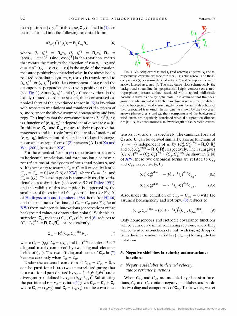
FIG. 1. Velocity errors vi and vj (red arrows) at points xi and xj,

respectively, over the distance of r 5 xj 2 xi (blue arrow), and their l

components (green arrows labeled as li and lj) and t components (green

arrows labeled as ti and tj). The gray curve plots schematically the

background streamline (or geopotential height contour) on a mid-

troposphere pressure surface associated with a typical midlatitude

baroclinic wave on the synoptic scale. It is assumed that the back-

ground winds associated with the baroclinic wave are overpredicted,

so the background wind errors largely follow the same directions of

their associated true winds. In this case, as shown by the two green

arrows (denoted as ti and tj), the t components of the background

wind errors are negatively correlated when the separation distance

r5 jxj2 xij is at and around a half wavelength of the baroclinic wave.



Cxx5s2

xG(r/Lx) , (10a)

Ccc

5s2cG(r/L

c) , (10b)

where G(�) [ exp[2(�)2/2], s2x (or s

2c) denotes the error

variance of x (or c), and Lx (or Lc) denotes the decor-

relation length ofCxx (orCcc). Substituting (10) into the

traces of (8a) and (8b) gives

Cd[Tr(C

d)5Cd

ll 1Cdtt 52(r21›

r1 ›2r )Cxx

5 2s2d[12 r2/(4L2

d)]G(r/ffiffiffi2

pL

d) , (11a)

Cr[Tr(C

r)5Cr

ll 1Crtt 52(r21›

r1 ›2r )Ccc

5 2s2r [12 r2/(4L2

r )]G(r/ffiffiffi2

pL

r) , (11b)

where Tr(�) denotes the trace of (�), s2d 5s2

x/L2x (or

s2r 5s2

c/L2c) is the error variance for each vector com-

ponent of vd (or vr), and

Ld[ [2C

d(r)j

r50]1/2[2=2C

d(r)j

r50]21/2 5L

x/

ffiffiffi2

p

and

Lr[ [2C

r(r)j

r50]1/2[2=2C

r(r)j

r50]21/2 5L

c/

ffiffiffi2

p

are the decorrelation lengths of Cd and Cr, respectively.

Here, the decorrelation length is defined based on the

local curvature of the covariance function at r 5 0 ac-

cording to (4.3.12) of Daley (1991), and =2 5 ›2r 1 r21›ris used for isotropic covariance functions.

Substituting (10) into the sum of (8a) and (8b) gives

Cll5Cd

ll 1Crll 52›2rCxx

2 r21›rC

cc

5s2d(12 r2/2L2

d)G(r/ffiffiffi2

pL

d)1s2

rG(r/ffiffiffi2

pL

r) ,

(12a)

Ctt5Cd

tt 1Crtt 52›2rCcc

2 r21›rC

xx

5s2r (12 r2/2L2

r )G(r/ffiffiffi2

pL

r)1s2

dG(r/ffiffiffi2

pL

d) .

(12b)

From (12), it is easy to see that Cll and Ctt switch to each

other as (s2d, Ld) and (s

2r , Lr) switch, so there is a duality

between Cll and Ctt associated with the switch between

(s2d, Ld) and (s2

r , Lr).

When Lx 5 Lc 5 L and thus Ld 5Lr 5L/ffiffiffi2

pand

s2d/s

2r 5s2

x/s2c, (12) reduces to

Cll5s2[12 (r/L)2(11b)21]G(r/L) , (13a)

Ctt5s2[12 (r/L)2b(11b)21]G(r/L) , (13b)

where b[s2r /s

2d and s2 [s2

d 1s2r 5 (11b)s2

d 5 (11b21)s2

r is the error variance for each vector component

of v. The aforementioned duality between Cll and Ctt is

now associated only with the switch between s2d and s2

r

or, equivalently, the inversion of b. This duality is seen

directly from (13). Owing to this duality, Cll computed

from (13a) for b 5 4, 2, 1, 1/2, and 1/4 are the same as Ctt

computed from (13b) for b 5 1/4, 1/2, 1, 2, and 4, respec-

tively, so they can be plotted compactly by the same set

of five curves, as shown in Fig. 2.

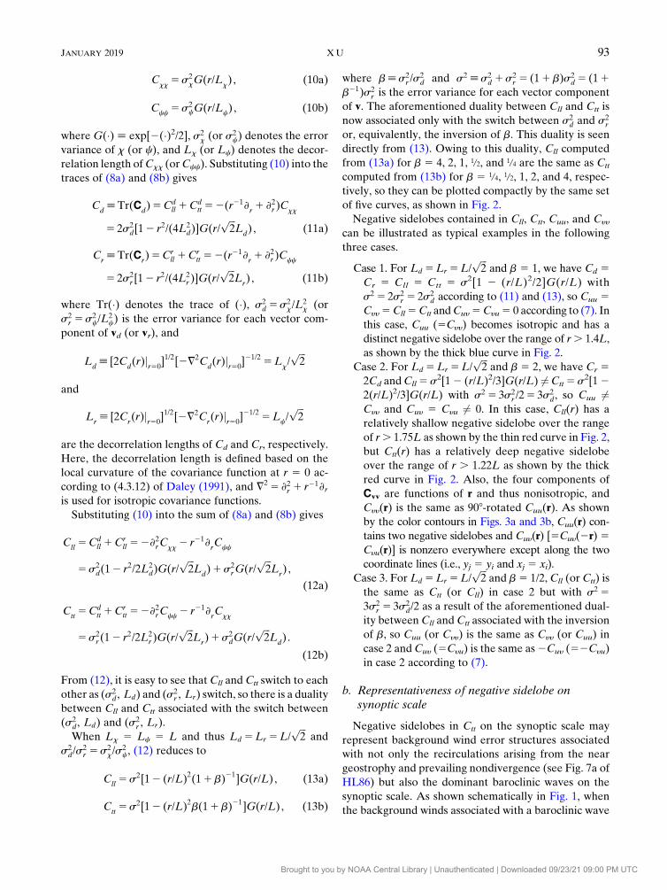
Negative sidelobes contained in Cll, Ctt, Cuu, and Cyy

can be illustrated as typical examples in the following

three cases.

Case 1. For Ld 5Lr 5L/ffiffiffi2

pand b 5 1, we have Cd 5

Cr 5 Cll 5 Ctt 5 s2[1 2 (r/L)2/2]G(r/L) with

s2 5 2s2r 5 2s2

d according to (11) and (13), so Cuu 5Cyy5Cll5Ctt andCuy5Cyu5 0 according to (7). In

this case, Cuu (5Cyy) becomes isotropic and has a

distinct negative sidelobe over the range of r. 1.4L,

as shown by the thick blue curve in Fig. 2.


pand b 5 2, we have Cr 5

2Cd andCll5 s2[12 (r/L)2/3]G(r/L) 6¼Ctt5 s2[122(r/L)2/3]G(r/L) with s2 5 3s2

r /25 3s2d, so Cuu 6¼

Cyy and Cuy 5 Cyu 6¼ 0. In this case, Cll(r) has a

relatively shallow negative sidelobe over the range

of r. 1.75L as shown by the thin red curve in Fig. 2,

but Ctt(r) has a relatively deep negative sidelobe

over the range of r . 1.22L as shown by the thick

red curve in Fig. 2. Also, the four components of

Cvv are functions of r and thus nonisotropic, and

Cyy(r) is the same as 908-rotated Cuu(r). As shown

by the color contours in Figs. 3a and 3b, Cuu(r) con-

tains two negative sidelobes and Cuy(r) [5Cuy(2r)5Cyu(r)] is nonzero everywhere except along the two

coordinate lines (i.e., yj 5 yi and xj 5 xi).


pand b5 1/2, Cll (or Ctt) is

the same as Ctt (or Cll) in case 2 but with s2 53s2

r 5 3s2d/2 as a result of the aforementioned dual-

ity between Cll and Ctt associated with the inversion

of b, so Cuu (or Cyy) is the same as Cyy (or Cuu) in

case 2 and Cuy (5Cyu) is the same as2Cuy (52Cyu)

in case 2 according to (7).

b. Representativeness of negative sidelobe onsynoptic scale

Negative sidelobes in Ctt on the synoptic scale may

represent background wind error structures associated

with not only the recirculations arising from the near

geostrophy and prevailing nondivergence (see Fig. 7a of

HL86) but also the dominant baroclinic waves on the

synoptic scale. As shown schematically in Fig. 1, when

the background winds associated with a baroclinic wave

JANUARY 2019 XU 93


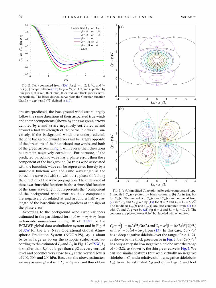
are overpredicted, the background wind errors largely

follow the same directions of their associated true winds

and their t components (shown by the two green arrows

denoted by ti and tj) are negatively correlated at and

around a half wavelength of the baroclinic wave. Con-

versely, if the background winds are underpredicted,

then the background wind errors will be largely opposite

of the directions of their associated true winds, and both

of the green arrows in Fig. 1 will reverse their directions

but remain negatively correlated. Furthermore, if the

predicted baroclinic wave has a phase error, then the t

component of the background (or true) wind associated

with the baroclinic wave can be represented loosely by a

sinusoidal function with the same wavelength as the

baroclinic wave but with (or without) a phase shift along

the direction of the wave propagation. The difference of

these two sinusoidal functions is also a sinusoidal function

of the same wavelength but represents the t component

of the background wind error, so the t components

are negatively correlated at and around a half wave-

length of the baroclinic wave, regardless of the sign of

the phase error.

According to the background wind error variances

estimated in the partitioned form of s2 5s2r 1s2

d from

radiosonde innovations in Fig. 10 of HL86 for the

ECMWF global data assimilation system and in Fig. 6

of XW for the U.S. Navy Operational Global Atmo-

spheric Prediction System (NOGAPS), sr is about

twice as large as sd on the synoptic scale. Also, ac-

cording to the estimated Lr and Ld in Fig. 12 of XW, Lr

is smaller than Ld but larger than Ld/2 at every vertical

level and becomes very close to Ld at the vertical levels

of 900, 500, and 200 hPa. Based on the above estimates,

we may assume b5 4 with Lx 5Lc5 L and thus obtain

Cll5 s2[12 (r/L)2/5]G(r/L) andCtt5 s2[12 4(r/L)2/5]G(r/L)

with s2 5 5s2r /45 5s2

d from (13). In this case, Ctt(r)/s2

has a deep negative sidelobe over the range of r. 1.12L

as shown by the thick green curve in Fig. 2, but Cll(r)/s2

has only a very shallow negative sidelobe over the range

of r. 2.2L as shown by the thin green curve in Fig. 2.We

can see similar features (but with virtually no negative

sidelobe inCll and a relative shallow negative sidelobe in

Ctt) from the estimated Cll and Ctt in Figs. 5 and 6 of

FIG. 3. (a)UnmodifiedCuu(r) plotted by color contours and type-2 modified Cuu(r) plotted by black contours. (b) As in (a), but

for Cyy(r). The unmodified Cuu(r) and Cuy(r) are computed from

(7) with Cll and Ctt given by (13) for b 5 2 and Ld 5Lr 5L/ffiffiffi2

p.

The modified Cuu(r) and Cuy(r) are also computed from (7) but

with Cll and Ctt given by (21) for b 5 2 and Ld 5Lr 5L/ffiffiffi3

p. The

contours are plotted every 0.1s2 but labeled with s2 omitted.

FIG. 2. Cll(r) computed from (13a) for b 5 4, 2, 1, 1/2, and 1/4[orCtt(r) computed from (13b) for b5 1/4, 1/2, 1, 2, and 4] plotted bythin green, thin red, thick blue, thick red, and thick green curves,

respectively. The black dashed curve plots the Gaussian function

G(r/L) [ exp[2(r/L)2/2] defined in (10).



HL86 and Figs. 3a and 3b ofXW.However, sinceCxx and

Ccc are modeled by single-Gaussian functions in (10), the

negative sidelobe of the above derived Ctt/s2 (shown by

the thick green curve in Fig. 2) is about twice as deep as

that of the estimated Ctt(r)/s2 [with Ctt(r)jr50 5 s2] in

Fig. 6 of HL86 or Fig. 3b of XW. Excessively negative

sidelobes of this type (caused in Ctt by using single-

Gaussian functions to model Ccc and Cxx) can be

reduced if Cxx and Ccc are modeled by fat-tailed

Gaussian-weighted mixtures of Gaussians or multiple

Gaussians (see Fig. 1 of Purser et al. 2003b).

c. Unrepresentativeness of negative sidelobe onmesoscale

For mesoscale data assimilation, the background wind

error covariance functions can be estimated from radar

radial-velocity innovations (Xu et al. 2007a, hereafter

X07a; Xu et al. 2007b, hereafter X07b). As an example,

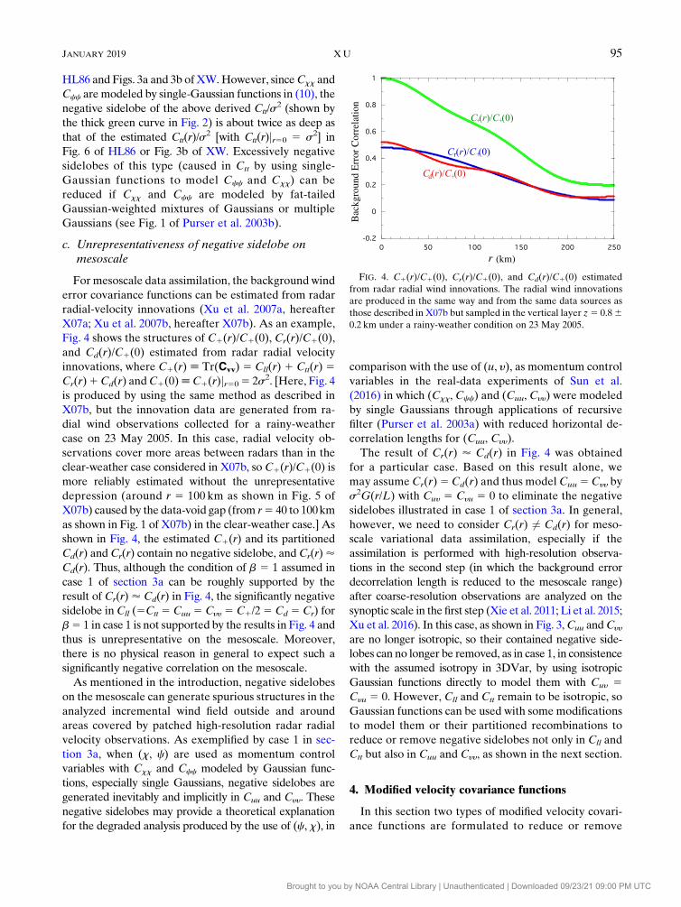
Fig. 4 shows the structures of C1(r)/C1(0), Cr(r)/C1(0),

and Cd(r)/C1(0) estimated from radar radial velocity

innovations, where C1(r) [ Tr(Cvv) 5 Cll(r) 1 Ctt(r) 5Cr(r)1Cd(r) andC1(0)[C1(r)jr505 2s2. [Here, Fig. 4

is produced by using the same method as described in

X07b, but the innovation data are generated from ra-

dial wind observations collected for a rainy-weather

case on 23 May 2005. In this case, radial velocity ob-

servations cover more areas between radars than in the

clear-weather case considered in X07b, so C1(r)/C1(0) is

more reliably estimated without the unrepresentative

depression (around r 5 100 km as shown in Fig. 5 of

X07b) caused by the data-void gap (from r5 40 to 100km

as shown in Fig. 1 of X07b) in the clear-weather case.] As

shown in Fig. 4, the estimated C1(r) and its partitioned

Cd(r) and Cr(r) contain no negative sidelobe, and Cr(r)’Cd(r). Thus, although the condition of b 5 1 assumed in

case 1 of section 3a can be roughly supported by the

result of Cr(r)’ Cd(r) in Fig. 4, the significantly negative

sidelobe inCll (5Ctt 5 Cuu 5 Cyy 5 C1/25 Cd 5 Cr) for

b5 1 in case 1 is not supported by the results in Fig. 4 and

thus is unrepresentative on the mesoscale. Moreover,

there is no physical reason in general to expect such a

significantly negative correlation on the mesoscale.

As mentioned in the introduction, negative sidelobes

on the mesoscale can generate spurious structures in the

analyzed incremental wind field outside and around

areas covered by patched high-resolution radar radial

velocity observations. As exemplified by case 1 in sec-

tion 3a, when (x, c) are used as momentum control

variables with Cxx and Ccc modeled by Gaussian func-

tions, especially single Gaussians, negative sidelobes are

generated inevitably and implicitly in Cuu and Cyy. These

negative sidelobes may provide a theoretical explanation

for the degraded analysis produced by the use of (c, x), in

comparison with the use of (u, y), as momentum control

variables in the real-data experiments of Sun et al.

(2016) in which (Cxx, Ccc) and (Cuu, Cyy) were modeled

by single Gaussians through applications of recursive

filter (Purser et al. 2003a) with reduced horizontal de-

correlation lengths for (Cuu, Cyy).

The result of Cr(r) ’ Cd(r) in Fig. 4 was obtained

for a particular case. Based on this result alone, we

may assume Cr(r)5Cd(r) and thus model Cuu 5Cyy by

s2G(r/L) with Cuy 5 Cyu 5 0 to eliminate the negative

sidelobes illustrated in case 1 of section 3a. In general,

however, we need to consider Cr(r) 6¼ Cd(r) for meso-

scale variational data assimilation, especially if the

assimilation is performed with high-resolution observa-

tions in the second step (in which the background error

decorrelation length is reduced to the mesoscale range)

after coarse-resolution observations are analyzed on the

synoptic scale in the first step (Xie et al. 2011; Li et al. 2015;

Xu et al. 2016). In this case, as shown in Fig. 3,Cuu andCyy

are no longer isotropic, so their contained negative side-

lobes can no longer be removed, as in case 1, in consistence

with the assumed isotropy in 3DVar, by using isotropic

Gaussian functions directly to model them with Cuy 5Cyu 5 0. However, Cll and Ctt remain to be isotropic, so

Gaussian functions can be used with some modifications

to model them or their partitioned recombinations to

reduce or remove negative sidelobes not only in Cll and

Ctt but also in Cuu and Cyy, as shown in the next section.

4. Modified velocity covariance functions

In this section two types of modified velocity covari-

ance functions are formulated to reduce or remove

FIG. 4. C1(r)/C1(0), Cr(r)/C1(0), and Cd(r)/C1(0) estimated

from radar radial wind innovations. The radial wind innovations

are produced in the same way and from the same data sources as

those described in X07b but sampled in the vertical layer z5 0.860.2 km under a rainy-weather condition on 23 May 2005.

JANUARY 2019 XU 95


negative sidelobes concerned in the previous section.

The detailed formulations are presented in the following

subsections.

a. Type-1 modified covariance functions withnegative sidelobes reduced

The results in (13) can be recombined into

C1[C

ll1C

tt5 2s2[12 (r/L)2/2]G(r/L) , (14a)

C2[C

ll2C

tt5 2as2(r/L)2G(r/L) , (14b)

where 2a [ (b 2 1)/(b 1 1) and a is confined within

(21/2, 1/2) because b[s2r /s

2d is confined within (0, ‘).

When the value ofb is inverted, a changes sign and so does

C2 in (14b). This property is tied up with the duality be-

tween Cll and Ctt associated with the inversion of b, as

noted earlier in (13). The normalized function form of

C1 is the same as that forCll (5Ctt) in case 1 and thus also

has a negative sidelobe as shown by the solid blue curve in

Fig. 2. This negative sidelobe can be removed by using

a Gaussian function to model C1 with its decorrelation

length denoted by L1, while C2 is still modeled by (14b)

but with L redenoted by L2, so (14) is modified into

C1[C

ll1C

tt5 2s2G(r/L

1) , (15a)

C2[C

ll2C

tt5 2as2(r/L

2)2G(r/L

2) . (15b)

By changing the notationL1 toL andL2 toffiffiffiffiffiffiffibL

p, (15)

recovers (3.2) of Xu and Gong (2003, hereafter XG).

According to (3.7) of XG, Lr and Ld are related to L1

and L2 by

L2r 5 (11 2a)/(L22

1 1 4aL222 ) , (16a)

L2d 5 (12 2a)/(L22

1 2 4aL222 ) . (16b)

Note that the left-hand side of (16a) [or (16b)] is non-

negative and so is the right-hand side, and 16 2a is also

nonnegative because 2a is confined within (21, 1) as

explained in (14). Thus, L221 6 4aL22

2 must be non-

negative or, equivalently, L22/L

21 cannot be smaller

than min(0, 4a). Furthermore, the autocorrelation func-

tions Cll 5 (C1 1 C2)/2 and Ctt 5 (C1 2 C2)/2 derived

from (15) must be positive semidefinite or, equivalently,

their power spectra must be nonnegative. As shown in

appendix B, this leads to the following additional con-

straints on jaj and L22/L

21:

jaj# am5 e/8 (’0:333 98) , (17a)

2jam/aj[12 (12 ja/a

mj)1/2]#L2

2/L21

# 2jam/aj[11 (12 ja/a

mj)1/2] , (17b)

where e (’2.718 28) is the base of the natural logarithm.

By substituting the Taylor expansion of (1 2 ja/amj)1/2around ja/amj 5 0 into (17b), one can verify that the

admissible range of L22/L

21 increases toward (1, ‘) as

jaj/ 0. As jaj increases from 0 to its upper bound am in

(17a), the admissible range of L22/L

21 in (17b) shrinks

from (1, ‘) to a single point at L22/L

21 5 2.

Mathematically, the covariance functions in (15) can

be constructed with a and L22/L

21 specified within their

respective admissible ranges in (17), but the two physical

parameters Lr and Ld become implicit and cannot be

freely specified. Physically, it is convenient to specify

b[s2r /s

2d, Lr, and Ld first, and then obtain a, L1, and

L2, and this is facilitated by the following relationships

derived from (16a) and (16b):

L2r /L

2d 5b(L2

2/L21 2 4a)/(L2

2/L21 1 4a)

5b[12 8a/(L22/L

21 1 4a)] , (18a)

L21 5 (b1 1)L2

r /(bL2r /L

2d 1 1), (18b)

L22 5 2(b2 1)L2

r /(bL2r /L

2d 2 1), (18c)

where 2a [ (b 2 1)/(b 1 1) is used. Here, b is con-

fined by

1/bm#b#b

m, (19)

where bm 5 (1 1 2am)/(1 2 2am) ’ 5.02 and (17a) is

used.

If b5 1 and thus a5 0, then (18a) givesLr/Ld5 1 and

(18b) gives L1 5 Lr for any given Lr 5 Ld, but (18c)

becomes redundant because a 5 0 and C2 5 0 in (15b)

and L2 is no longer needed. If b 6¼ 1, then L2r /L

2d is

confined by

b[12 8a/(lmn

1 4a)]#L2r /L

2d #b[12 8a/(l

mx1 4a)]

for b. 1 (with a. 0),

b[11 8jaj/(lmx

2 4jaj)]#L2r /L

2d

#b[11 8jaj/(lmn

2 4jaj)] for b, 1 (with a, 0),

wherelmn5 2jam/aj[12 (12 ja/amj)1/2],lmx5 2jam/aj[11(1 2 ja/amj)1/2], and (17) and (18) are used in the deriva-

tion. These conditions lead to L2r /L

2d ,b for b . 1 and

L2r /L

2d .b for b , 1, which ensure L2

2 . 0 in (17b). If

Lr 5Ld 5L/ffiffiffi2

pas assumed in (13), then (18b) gives

L1 5L/ffiffiffi2

pand (18c) gives L2 5 L for any admissible

b in (19).

Modified Cll 5 (C1 1 C2)/2 and Ctt 5 (C1 2 C2)/2

are constructed from C1 and C2 in (15) with Lr 5Ld 5L/

ffiffiffi2

p(and thus L1 5L/

ffiffiffi2

pand L2 5 L). These

modifiedCll andCtt retain the duality associated with the



inversion of b, so they can be plotted compactly by the

five curves in Fig. 5 for five different settings of b as

those in Fig. 2. The unmodified Ctt (5Cll) for b 5 1

plotted by the thick blue curve in Fig. 2 is duplicated by

the thin dashed blue curve in Fig. 5. This unmodified

Ctt (5Cll) has the same decorrelation length and thus the

same curvature at r 5 0 as the modified Ctt (5Cll) for

b 5 1 plotted by the thick blue curve in Fig. 5, but it

decreases rapidly and becomes negative as r increases to

1.4L and beyond, while the modified Ctt (5Cll), given by

s2G(r/L) for b 5 1, stays above zero as r increases un-

boundedly. As shown in Fig. 5, the modifiedCtt for b. 1

still contains a negative sidelobe but its negative side-

lobe is much shallower than that of the unmodified Ctt

for the same value of b. 1 in Fig. 2. Similarly, according

to the duality between Cll and Ctt, the modified Cll for

b , 1 contains a negative sidelobe and its negative

sidelobe is much shallower than that of the unmodified

Cll. Thus, the modifications made to C1 and C2 in (15)

can reduce but not eliminate the negative sidelobe in Ctt

for b . 1 or in Cll for b , 1.

b. Type-2 modified covariance functions with nonegative sidelobe

As shown in (8a), the divergent parts of Cll and Ctt are

defined by Cdll(r)[2›2rCxx(r) and Cd

tt(r)[2r21›rCxx(r),

respectively. Based on these definitions, Cdtt(r) can be

related to Cdll(r) by Cd

tt(r)5 r21Ð r0Cd

ll(r0) dr0 directly with

Cxx(r) dropped from this relationship. Using this re-

lationship, we can set Cdll(r)5s2

dG(r/Ld) and obtain

Cdtt(r)5s2

dE(r/Ld), where

E(r/Ld)[ (L

d/r)

ðr/Ld0

G(r0) dr0 .

Similarly, we can set Crtt(r)5s2

rG(r/Lr) with Crll(r)5

r21Ð r0Cr

tt(r0) dr0 and obtain Cr

ll 5s2rE(r/Lr) for the rota-

tional parts of Cll(r) and Ctt(r) defined in (8b).

Combining the above results gives the type-2 modified

covariance functions defined below:

Cd(r)5s2

d[G(r/Ld)1E(r/L

d)] (20a)

and

Cr(r)5s2

r [G(r/Lr)1E(r/L

r)] , (20b)

or

Cll(r)5s2[G(r/L

d)1bE(r/L

r)]/(b1 1) (21a)

and

Ctt(r)5s2[bG(r/L

r)1E(r/L

d)]/(b1 1), (21b)

where s2 [s2r 1s2

d 5 (11b)s2d as defined in (13). For

Cd (or Cr) in (20) to have the same decorrelation length

as the unmodified Cd (or Cr) in (11), we need to set

Ld 5Lx/ffiffiffi3

p(or Lr 5Lc/

ffiffiffi3

p) as shown in appendix C,

where Lx (or Lc) is the decorrelation length of Cxx (or

Ccc) in (10a) [or (10b)], so Lx/ffiffiffi2

p(or Lc/

ffiffiffi2

p) is the

decorrelation length of the unmodified Cd (or Cr).

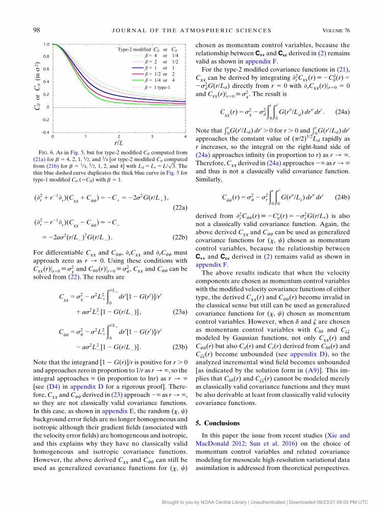
The type-2 modified covariance functions Cll and Ctt

in (21) retain the duality associated with the inversion of

b, so they can be plotted compactly by the five curves

in Fig. 6 for five different settings of b with Lr 5Ld 5L/

ffiffiffi3

p. As shown in Fig. 6, the type-2 modifiedCll and Ctt

contain no negative sidelobe for any given b ($0). Their

derived Cuu (or Cyy) also contains no negative sidelobe

as shown by the black contours (vs the colored contours)

in Fig. 3a for b 5 2. As shown by the thick blue curve in

Fig. 6, the type-2modifiedCtt (5Cll) forb5 1 has the same

decorrelation length and thus the same curvature at r5 0

as the type-1 modified Ctt (5Cll) for b 5 1 (plotted by the

thin dashed blue curve in Fig. 6), but it decreases more

slowly than the type-1 modified Ctt (5Cll) as r increases.

All the type-2 modified covariance functions in Fig. 6 have

fat tails, like the fat-tailed hyper-Gaussians (or multi-

Gaussians) that allow a broader dynamical range of

scales in the analysis increments to be assimilated (Purser

et al. 2003b). This can be an advantage of the type-2

modified covariance functions over the type 1 for varia-

tional data assimilation over a wide mesoscale range.

c. Generalized covariance functions for (x, c)

For the type-1 modified covariance functions in (15),

Cxx and Ccc can be related to C1 and C2, according to

(8), by the following equations:

FIG. 5. As in Fig. 2, but for type-1 modified Cll 5 (C1 1 C2)/2

computed from (15) and (18) for b 5 4, 2, 1, 1/2, and 1/4 [or type-1modified Ctt 5 (C1 2 C2)/2 computed from (15) and (18) for b 51/4, 1/2, 1, 2, and 4] withLd 5Lr 5L/

ffiffiffi2

p. The thin blue dashed curve

duplicates the thick blue curve in Fig. 2 for the unmodified Ctt

(5Cll) with b 5 1.

JANUARY 2019 XU 97


(›2r 1 r21›r)(C

xx1C

cc)52C

1522s2G(r/L

1) ,

(22a)

(›2r 2 r21›r)(C

xx2C

cc)52C

2

522as2(r/L2)2G(r/L

2) . (22b)

For differentiable Cxx and Ccc, ›rCxx and ›rCcc must

approach zero as r / 0. Using these conditions with

Cxx(r)jr50[s2x and Ccc(r)jr50[s2

c, Cxx and Ccc can be

solved from (22). The results are

Cxx5s2

x 2s2L21

ðr/L1

0

dr0[12G(r0)]/r0

1 as2L22[12G(r/L

2)] , (23a)

Ccc

5s2c 2s2L2

1

ðr/L1

0

dr0[12G(r0)]/r0

2 as2L22[12G(r/L

2)] . (23b)

Note that the integrand [12G(r)]/r is positive for r. 0

and approaches zero in proportion to 1/r as r/‘, so theintegral approaches ‘ (in proportion to lnr) as r / ‘[see (D4) in appendix D for a rigorous proof]. There-

fore,Cxx andCcc derived in (23) approach2‘ as r/‘,so they are not classically valid covariance functions.

In this case, as shown in appendix E, the random (x, c)

background error fields are no longer homogeneous and

isotropic although their gradient fields (associated with

the velocity error fields) are homogeneous and isotropic,

and this explains why they have no classically valid

homogeneous and isotropic covariance functions.

However, the above derived Cxx and Ccc can still be

used as generalized covariance functions for (x, c)

chosen as momentum control variables, because the

relationship between Cvv and Ccc derived in (2) remains

valid as shown in appendix F.

For the type-2 modified covariance functions in (21),

Cxx can be derived by integrating ›2rCxx(r)[2Cdll(r)5

2s2dG(r/Ld) directly from r 5 0 with ›rCxx(r)jr50 5 0

and Cxx(r)jr50[s2x. The result is

Cxx(r)5s2

x 2s2d

ðr0

ðr00

G(r00/Ld) dr00 dr0 . (24a)

Note thatÐ r0G(r0/Ld) dr

0 . 0 for r. 0 andÐ r0G(r0/Ld) dr

0

approaches the constant value of (p/2)1/2Ld rapidly as

r increases, so the integral on the right-hand side of

(24a) approaches infinity (in proportion to r) as r / ‘.Therefore,Cxx derived in (24a) approaches2‘ as r/‘and thus is not a classically valid covariance function.

Similarly,

Ccc(r)5s2

c 2s2r

ðr0

ðr00

G(r00/Lr) dr00 dr0 (24b)

derived from ›2rCcc(r)[2Crtt(r)52s2

rG(r/Lr) is also

not a classically valid covariance function. Again, the

above derived Cxx and Ccc can be used as generalized


control variables, because the relationship between

Cvv and Ccc derived in (2) remains valid as shown in

appendix F.

The above results indicate that when the velocity

components are chosen as momentum control variables

with the modified velocity covariance functions of either

type, the derived Cxx(r) and Ccc(r) become invalid in

the classical sense but still can be used as generalized


control variables. However, when d and z are chosen

as momentum control variables with Cdd and Czz

modeled by Gaussian functions, not only Cxx(r) and

Ccc(r) but also Cd(r) and Cr(r) derived from Cdd(r) and

Czz(r) become unbounded (see appendix D), so the

analyzed incremental wind field becomes unbounded

[as indicated by the solution form in (A9)]. This im-

plies that Cdd(r) and Czz(r) cannot be modeled merely

as classically valid covariance functions and they must

be also derivable at least from classically valid velocity

covariance functions.

5. Conclusions

In this paper the issue from recent studies (Xie and

MacDonald 2012; Sun et al. 2016) on the choice of

momentum control variables and related covariance

modeling for mesoscale high-resolution variational data

assimilation is addressed from theoretical perspectives.

FIG. 6. As in Fig. 5, but for type-2 modified Cll computed from

(21a) for b 5 4, 2, 1, 1/2, and 1/4 [or type-2 modified Ctt computed

from (21b) for b 5 1/4, 1/2, 1, 2, and 4] with Ld 5Lr 5L/ffiffiffi3

p. The

thin blue dashed curve duplicates the thick blue curve in Fig. 5 for

type-1 modified Ctt (5Cll) with b 5 1.



In particular, the relationships between background

error covariance functions are derived for three differ-

ent choices of momentum control variables; that is,

(i) the horizontal velocity (u, y), (ii) the velocity po-

tential x and streamfunction c, and (iii) the divergence

d and vorticity z. These different choices of momentum

control variables with their error covariance functions

satisfying the derived relationships are proven to be

theoretically equivalent in the sense that they lead to the

same optimally analyzed incremental wind field in the

continuous limit. As the relationships between covariance

functions are derived in general nonhomogeneous and

nonisotropic forms, the proved theoretical equivalence is

applicable to not only variational data assimilation (with

homogeneous and isotropic background error covariance

formulations) but also ensemble-based data assimilation

(with flow-dependent nonhomogeneous and nonisotropic

background error covariance formulations).

Although the aforementioned different choices of

momentum control variables are equivalent in theory,

they are not equivalent in practical applications, as their

required numerical schemes and computational costs

can be very different for obtaining numerical solutions

in discrete spaces, but this topic is beyond this paper.

Furthermore, their theoretical equivalence requires the

velocity covariance tensor function to be valid in the

classic sense (i.e., to not only satisfy the required sym-

metry and positive semidefiniteness but also approach

zero as the separation distance increases boundlessly).

Note that the classical validity of a (x, c) covariance

tensor function ensures the classical validity of (u, y) and

(d, z) covariance tensor functions, as the latter functions

are derived from the former via differentiations [see (2)

and (3)]. The inverse, however, does not hold true, and

this can limit the (d, z) covariance modeling but not the

choices of control variables (see section 4c). In particu-

lar, when (d, z) are chosen as momentum control vari-

ables with their covariance functionsmodeled byGaussian

functions, the derived velocity covariance functions

become unbounded (see appendix D) and so does the

analyzed incremental wind field. This implies that if

(d, z) are used asmomentum control variables, their error

covariance functions must be derivable from classically

valid velocity covariance functions.

It is also shown in this paper that the (u, y) auto-

covariance functions derived from single-Gaussian

(x, c) autocovariance functions contain significant

negative sidelobes. These negative sidelobes can rep-

resent background wind error structures associated

with the recirculations arising from the near geos-

trophy and prevailing nondivergence as well as with the

dominant baroclinic waves on the synoptic scale, but

they become unrepresentative on the mesoscale (as

shown in sections 3b and 3c). Using (u, y) directly as

independent momentum control variables with their

autocovariance functions modeled by Gaussian func-

tions can remove negative sidelobes, but this velocity

covariance modeling is not consistent with the assumed

isotropy in variational data assimilation in general

[unless Cd 5 Cr or, equivalently, Cll 5 Ctt is further

assumed as shown by case 1 in section 3a].

To solve the above problem, Gaussian covariance

functions are modified in two ways to model the iso-

tropic canonical-form velocity autocovariance func-

tions with negative sidelobes reduced or removed in

consistency with the assumed isotropy for mesoscale

variational data assimilation. In this case, (x, c) co-

variance functions can be derived by integrating the

modified velocity covariance functions and used as

generalized covariance functions for (x, c) chosen as

momentum control variables, although the derived

(x, c) covariance functions are not classically valid as

they approach negative infinity in the limit of infinitely

large separation distance (see section 4c).

When negative sidelobes are reduced or removed in

the modified velocity covariance functions, the velocity

power spectra become nonzero and their derived (x, c)

power spectra become singular at zero wavenumber

[see (E1) in appendix E]. These properties are further

explored mathematically in appendixes E and F, and the

results can be summarized in the following implications

that can be important and/or useful for mesoscale data

assimilation:

1) The zero-wavenumber and near-zero-wavenumber

components in the power spectra of the modified

velocity covariance can represent, to a certain extent,

the synoptic-scale components not represented by

the velocity covariance functions derived from single-

Gaussian mesoscale (x, c) covariance functions.

2) Generalized (x, c) covariance functions derived

from the modified velocity covariance functions

contain unbounded structures, but these unbounded

structures are bounded in a mesoscale domain and

thus can represent, to a certain extent, the synoptic-

scale components [as shown explicitly by the one-

dimensional example in (G8)–(G15) of appendix G].

3) For mesoscale data assimilation, the covariance

structures should be modeled by function forms

more general than single Gaussians. These include

not only the two types proposed in this paper but also

those comprising multiple Gaussians with their de-

correlation lengths ranging up to the synoptic scale

(at which point the presence of negative sidelobes

becomes acceptable). Multi-Gaussians (Purser et al.

2003b) are more flexible and thus can be more

JANUARY 2019 XU 99


accurate than the two types proposed in this paper

for mesoscale data assimilation, especially if the true

covariance can be well estimated and represented

by a multi-Gaussian on the mesoscale and synoptic

scale. Since the true covariances are often largely

unknown or not well estimated on the mesoscale, the

modifications proposed in this paper provide simple

theoretically justifiable choices for mesoscale data

assimilation.

4) Background velocity covariance functions C1 and

C2 represented by spectral expansions can be esti-

mated directly from radar radial wind innovations on

the mesoscale [see (12)–(14) of X07a]. These spec-

tral representations, if well estimated, can be used

directly with their zero-wavenumber components

retained to represent the synoptic-scale components

that are not resolved because of the limited innovation

data coverage. Furthermore, the synoptic-scale com-

ponents represented by the zero-wavenumber compo-

nents can be estimated separately from radiosonde

innovations and then used to replace the zero-

wavenumber components and thus expand the meso-

scale spectral representations to the synoptic scale [as

shown by the one-dimensional example in (G16) with

its two-dimensional extension suggested for real-data

assimilation at the end of appendix G]. In this case,

the geostrophy can be conveniently built into multi-

variate covariance on the synoptic scale.

5) Covariance localizations have been commonly used

for ensemble-based data assimilation. When such an

ensemble-based method is used for mesoscale data

assimilation, the localization radiuses often cover only

small fractions of the mesoscale domain and thus

inevitably eliminate all the large-scale structures be-

yond the localization radiuses. This may partially

explain in theory why a localized flow-dependent

covariance estimated by ensemble perturbations needs

to be combined with prescribed (or preestimated)

covariance with smooth structures well beyond the

localization radiuses via a hybrid approach.

The two types of modified velocity covariance func-

tions formulated in this paper (see sections 4a and 4b)

can be used directly to construct the background co-

variance matrix in 3DVar for mesoscale wind analyses

and data assimilation. In this way the utility in 3DVar

and advantages of the type-2 modified velocity co-

variance functions over their unmodified counterparts

have been demonstrated and evaluated by comparative

experiments with radar radial-velocity observations.

The detailed results were presented in section 5 of Xu

et al. (2017). The modified velocity covariance func-

tions will be incorporated, as enhanced options, into

the recently developed radar wind analysis system (Xu

et al. 2015).

Acknowledgments. The author thanks the anonymous

reviewers for providing constructive and stimulating

comments and suggestions, Li Wei and Kang Nai at the

University of Oklahoma for producing Figs. 3 and 4, and

the support of ONR Grant N000141712375.

APPENDIX A

Equivalence of Different Choices of MomentumControl Variables in the Continuous Limit

a. Cost functional for choice 1 and its minimizer inthe continuous limit

For choice 1, we have Da / v(z) and B / Cvv(z, z0)

[see (1)] in the continuous limit. The space for v(z) can

be completed as a Hilbert space (Courant and Hilbert

1962) [or, specifically, a Sobolev space (Adams 1975) as

shown by the examples in sections 4–5 of Xu (2005)],

denoted by Hv, with the following inner product:

hf(z), g(z)iv[

ðdz

ðdz0f(z)TQ

vv(z, z0)g(z0) , (A1a)

where f(z) and g(z) denote two arbitrary vector func-

tions in Hv, Qvv(z, z0) is the inverse of Cvv(z, z

0) defined[see section 5.3 of Bennett (1992)] by

ðdz0C

vv(z, z0)Q

vv(z0, z00)5 d(z2 z00)I , (A1b)

the integralÐdz is over the entire space of z, and I [

(1, 1)diag. In this case we have

DaTB21Da/

ðdz

ðdz0v(z)TQ

vv(z, z0)v(z0)5 kv(z)k2v

(A2)

in the continuous limit, where kv(z)k2v [ hv(z), v(z)iv is

the squared norm of v(z) in Hv.

Note that HDa is a vector in the observation space

RM of finite dimension M, where M is the total

number of horizontal wind component observations.

The mth element of HDa, denoted by {HDa}m, cor-responds to the mth observed velocity component at

the observation point zm. In the continuous limit of

Da, HDa is still a vector in RM with its mth element

given by

fHDagm/

ðdzd(z

m2 z)rTmv(z)5 hrTmCvv

(zm, z), v(z)i

v,

(A3)



where rm denotes the unit vector along the mth ob-

served horizontal wind component at the observation

point zm. The last step of (A3) is derived by using

d(zm 2 z)rTm 5 rTmÐdz0Cvv(zm, z

0)Qvv(z0, z), according to

(A1b), with the definition of h�, �iv in (A1a). From

(A3), we have

HDa/ hLv(z), v(z)i

v, (A4)

where Lv(z) is aM 3 2 matrix with itsmth row given by

rTmCvv(zm, z).

Substituting (A2) and (A4) into (4a) in the continuous

limit gives

J(v)5 kv(z)k2v 1 (hLv(z), v(z)i

v2 d)T

3R21(hLv(z), v(z)i

v2 d) . (A5)

As a function in Hv, v(z) in (A5) can be expressed in

general by

v(z)5 pTLv(z)1 g

v(z) , (A6)

where p 2 RM is an intermediate vector to be deter-

mined in the observation space and gv(z) is an element

in Hv orthogonal to Lv(z), that is, hgv(z), Lv(z)iv 5 0.

Substituting (A6) into (A5) gives

J(v)5pTPp1 kgv(z)k2

v

1 (Pp2 d)TR21(Pp2d) , (A7)

whereP5 hLv(z),LTv (z)iv is anM3M symmetric matrix

in the observation space with its diagonal (or

off diagonal) element given by rTmCvv(zm, zm)rm [or

rTmCvv(zm, zn)rn] corresponding to the mth observation

(or the paired mth and nth observations).

Clearly, kgv(z)k2v is nonnegative and thus must be zero

if v(z) minimizes J in (A7). This implies that gv(z) is

unrepresented by observations and must be discarded, so

the infinite-dimensional cost functional J(v) in (A7) re-

duces to the following finite-dimensional form:

J5 pTPp1 (Pp2 d)TR21(Pp2 d) . (A8)

The minimizer of J(v) in (A5) is thus given by

v(z)5 pTLv(z)5L

v(z)Tp5�

m

Cvv(z, z

m)r

mpm, (A9)

where pm is the mth component of p, and p is the solu-

tion of the following equation [derived from ›J/›p 5 0

for J in (A8)]:

(P1R)p5 d . (A10)

Here, the advanced method of representer solution for

imperfect-model 4DVar (Bennett 1992, chapter 5) is

simplified for 3DVar (or perfect-model 4DVar) to de-

rive the solution in (A9).

b. Choice 2 and its equivalence to choice 1 in thecontinuous limit

For choice 2, we have a/ c(z) and B/Ccc(z, z0) in

the continuous limit. The space for c(z) can be com-

pleted as a Hilbert space, denoted by Hc, with the

inner product, denoted by h�, �ic, defined similarly to

that in (A1) except that Cvv(z, z0) and Qvv(z, z

0) are

replaced by Ccc(z, z0) and Qcc(z, z

0), respectively. Inthis case, we have

DaTB21Da/ kc(z)k2c , (A11)

fHDagm/

ðdzd(z

m2 z)rTm[(=,k3=)c(z)]5

ðdzrTm[2(=, k3=)d(z

m2 z)I]c(z)

5

ðdzrTm[(=m

, k3=m)d(z

m2 z)I]c(z)5

ðdzrTm

�(=

m, k3=

m)

ðdz0C

cc(z

m, z0)Q

cc(z0, z)

�c(z)

5

ðdz

ðdz0rTm(=m

, k3=m)C

cc(z

m, z0)Q

cc(z0, z)c(z)5 hrTm(=m

,k3=m)C

cc(z

m, z), c(z)i

c. (A12)

In the derivation of (A12), v(z)5 (=, k3 =)c(z) is used in

the first step, integration by parts is used in the second

step, 2(=, k 3 =)d(zm 2 z) 5 (=m, k 3 =m)d(zm 2 z) is

used (see section 2.2 of Lighthill 1958) in the third step,Ðdz0Ccc(zm, z

0)Qcc(z0, z)5 d(zm 2 z)I is used in the fourth

step, and the definition of h�, �ic is used in the last step.

From (A12), we have

HDa/ hLc(z), c(z)i

c, (A13)

where Lc(z) is anM3 2 matrix with itsmth row given by

rTm(=m, k3=m)Ccc(zm, z).

Substituting (A11) and (A13) into (4a) in the contin-

uous limit gives

JANUARY 2019 XU 101


J(c)5 kc(z)k2c 1 [hLc(z), c(z)i

c2 d]T

3R21[hLc(z), c(z)i

c2 d]. (A14)

Similar to v(z) in (A6), c(z) can be expressed by c(z) 5pTLc(z)1 gc(z), where gc(z) is an element inHc orthogonal

to Lc(z). Using this expression together with the rela-

tionship of rTm(=m, k3=m)[(=n, k3=n)Ccc(zn, zm)]Trn 5

rTmCvv(zm, zn)rn derived from (2) or, equivalently,

hLc(z), Lc(z)Tic 5 hLv(z), Lv(z)

Tiv 5 P, the cost functional

in (A14) can be transformed into the same form as that in

(A7) but with kgv(z)k2v replaced by kgc(z)k2c . Again,

kgc(z)k2c is nonnegative and thus must be zero at the mini-

mum of J(c), so gc(z) must be discarded, reducing J(c) to the

same finite-dimensional form as in (A8). Thus, similar to the

solution in (A9), the minimizer of J(c) in (A14) is given by

c(z)5 pTLc(z) , (A15)

with p solved from (A10). According to (2), we

have (=, k3=)[rTm(=m,k3=m)Ccc(zm, z)]T5 (=, k3=)

[(=m,k3=m)Ccc(zm, z)]Trm 5Cvv(z, zm)rm 5 rTmCvv(zm, z),

which gives (=, k 3 =)Lc(z)T 5 Lv(z)

T, so

(=, k3=)c(z)5 (=, k3=)[pTLc(z)]

5 (=, k3=)Lc(z)Tp5L

v(z)Tp5 pTL

v(z) .

(A16)

This proves that c(z) in (A15) is equivalent to v(z)

in (A9).

c. Choice 3 and its equivalence to choice 2 in thecontinuous limit

For choice 3, we have a/ q(z) and B/ Cqq(z, z0) in

the continuous limit. The space for q(z) can be completed

as a Hilbert space, denoted byHq, with the inner product,

denoted by h�, �iq, defined similarly to that in (A1) except

that Cvv(z, z0) and Qvv(z, z

0) are replaced by Cqq(z, z0) and

Qqq(z, z0), respectively. In this case, we have

DaTB21Da/ kq(z)k2q , (A17)

fHDagm/

ðdzd(z

m2 z)rTm[(=, k3=)=22q(z)]5

ðdzrTm[=

22(2=,2k3=)d(zm2 z)I]=22q(z)

5

ðdzrTm[(=m

, k3=m)=22

m d(zm2 z)I]q(z)5

ðdzrTm

�(=

m, k3=

m)=22

m

ðdz0C

qq(z

m, z0)Q

qq(z0 2 z)

�q(z)

5

ðdz

ðdz0rTm(=m

, k3=m)=22

m Cqq(z

m, z0)Q

qq(z0 2 z)q(z)5 hrTm(=m

,k3=m)=22

m Cqq(z

m, z), c(z)i

q, (A18)

where=22 5Ðdx0 lnjx0 2 xj/(2p) is the inverse of=2 [see

(3.1) of Xu et al. 2011], the integralÐdx0 is over the

entire horizontal space of x0, and similarly =22m is the

inverse of =2m. In the derivation of (A18), v(z) 5 (=,

k 3 =)=22q(z) is used in the first step, integration by

parts is used in the second step, =22(2=, k3=)d(zm 2 z)5 (=m, k3 =m)=

22m d(zm 2 z) is used in the

third step,Ðdz0Cqq(zm, z

0)Qqq(z0, z)5 d(zm 2 z)I is used

in the fourth step, and the definition of h�, �iq is used in the

last step. From (A18) we have

HDa/ hLq(z), q(z)i

q, (A19)

where Lq(z) is anM3 2 matrix with itsmth row given by

rTm(=m, k3=m)=22m Cqq(zm, z).

Substituting (A17) and (A19) into (4a) in the contin-

uous limit gives

J(q)5 kq(z)k2q 1 [hLq(z), q(z)i

q2 d]T

3 R21[hLq(z), q(z)i

q2 d]. (A20)

Again, as v(z) in (A6), q(z) can be expressed by q(z) 5pTLq(z) 1 gq(z), where gq(z) is an element in Hq

orthogonal to Lq(z). Using this expression together

with the relationship of rTm(=m, k3=m)=22m [(=n, k3

=n)=22n Cqq(zn, zm)]

Trn 5 rTmCvv(zm, z)rn derived from

(2) and (3) or, equivalently, hLq(z), Lq(z)Tiq 5 hLv(z),

Lv(z)Tiv 5 P, the cost functional in (A20) can be

transformed into the same form as that in (A7) but with

kgv(z)k2v replaced by kgq(z)k2q. Again, kgq(z)k2q is non-

negative, so gq(z) must be discarded, reducing J(q) to

the same finite-dimensional form as in (A8). The mini-

mizer of J(q) in (A20) is thus given by

q(z)5 pTLq(z) (A21)

with p solved from (A10). Note that =22[rTm(=m, k3=m)=

22m Cqq(zm, z)]5 rTm(=m, k3=m)Ccc(zm, z) accord-

ing to (3) or, equivalently, =22Lq(z) 5 Lc(z), so

=22q(z)5=22[pTLq(z)]5 pT=22L

q(z)5 pTL

c(z) .

(A22)



This proves that q(z) in (A21) is equivalent to c(z)

in (A15).

d. Extension to three-dimensional velocityobservations

For simplicity, we have so far considered only hori-

zontal wind observations. This simplification is conven-

tional in operation data assimilation, since operationally

assimilated wind observations are either essentially

horizontal or treated approximately as horizontal ve-

locities. In particular, operationally assimilated radar

radial-component velocity observations are commonly

limited to those scanned at low-elevation angles (nearly

horizontal) and thus treated as horizontal velocities.

However, when radar radial-component velocity ob-

servations scanned at high-elevation angles (.58) are

also assimilated, a bias correction should be made first

to each observed radial-component velocity (often

as a part of data quality control) by subtracting the

projection of precipitate hydrometeors’ downward

terminal velocity (estimated from radar observed re-

flectivity) on the radar beam direction (because it is

the precipitate hydrometeors’ velocity that is mea-

sured by a radar and the precipitate hydrometeors

largely follow the air motion in the horizontal but fall

downward relative to the air motion in the vertical).

The bias-corrected radial-component velocity obser-

vation can be then related, still linearly, to the pro-

jection of the model’s three-dimensional velocity on

the radar beam direction. In this case the theoretical

equivalence between the three different choices of

momentum control variables can be proven in the

same way as shown in the previous subsections except

that the observation operators in (A4), (A13), and

(A19) need to be extended for three-dimensional ve-

locity observations. The detailed extensions are de-

scribed below.

For three-dimensional velocity observations, the two-

dimensional unit vector rm introduced in the previous

subsections should be extended to denote the three-

dimensional unit vector along the mth observed compo-

nent of three-dimensional velocity at the observation point

zm. In this case (A3) is extended to the following form:

fHDagm/

ðdzd(z

m2 z)rTm[v(z)

T,w(z)]T

5 hrTmPmCT

vv(zm, z), v(z)iv ,

where w(z)52r21Ð h0dh0=T[rv(z)] is the vertical veloc-

ity computed from the horizontal velocity v(z) by

vertically integrating the mass continuity equation of

=T(rv) 1 ›h(rw) 5 0 with the boundary condition of

w5 0 at h5 0, r is the pseudodensity associated with the

vertical coordinate h (e.g., r is the air density if height

z is used for h, but r 5 1 if pressure p is used for h),

Pm 5�I,2r21

Ð h0dh0=mr

�Tis a 3 3 2 matrix operator

consisting of the 23 2 identity matrix on the top and the

13 2 row vector operator2r21Ð h0dh0=T

mr on the bottom.

Consequently, the observation operators Lv(z) in (A4),

Lc(z) in (A13), and Lq(z) in (A19) are extended (from

M 3 2 matrices) to M 3 3 matrices with their mth row

given by rTmPmCvv(zm, z), rTmPm(=m, k3=m)Ccc(zm, z),

and rTmPm(=m, k3=m)=22m Cqq(zm, z), respectively.

APPENDIX B

Derivations of (17a) and (17b)

Applying the spectral formulations in (3.2) and (3.3)

of XG to C1(r) and C2(r) in (15) gives

Sll(k)1 S

tt(k)[

ð‘0

C1(r)J

0(kr)r dr5 2s2L2

1G(kL1) ,

(B1a)

Sll(k)2 S

tt(k)[2

ð‘0

C2(r)J

2(kr)r dr

522as2k2L42G(kL

2) , (B1b)

where k 5 jkj, k [ (kx, ky)T is the two-dimensional

vector wavenumber associated with x[ (x, y)T, and J0(�)[or J2(�)] denotes the zero-order (or second-order)

Bessel function of the first kind. Recombining (B1a)

and (B1b) gives

Sll(k)5 2s2L2

1G(kL1)[12 ak2L4

2L221 G(kL

2)/G(kL

1)] ,

(B2a)

Stt(k)5 2s2L2

1G(kL1)[11 ak2L4

2L221 G(kL

2)/G(kL

1)] ,

(B2b)

Here, Sll(k) [or Stt(k)] is the power spectrum associated

with the autocorrelation function Cll 5 (C1 1 C2)/2 [or

Ctt 5 (C1 2 C2)/2] derived from (15).

For Cll and Ctt to be positive semidefinite, Sll(k) and

Stt(k) must be nonnegative. This requires 1$ f (k2)[jajk2L4

2L221 G(kL2)/G(kL1) in (B2). A necessary condi-

tion for this is that L2 . L1, so k2G(kL2)/G(kL1)5k2 exp[2k2(L2

2 2L21)/2]/ 0 as k2 / ‘. For L2 . L1,

one can verify that f(k2) reaches its maximum of

jaj(2/e)L42/(L

21L

22 2L4

1) at the point ofk2 5 2/(L2

2 2L21)

where df(k2)/dk2 5 0. Thus, 1 $ f(k2) can be satisfied

if and only ifL2.L1 and jaj(2/e)L42/(L

21L

22 2L4

1)# 1.

The latter two conditions yield 2jaj(L2/L1)42 e(L2/L1)

21e # 0 or, equivalently,

JANUARY 2019 XU 103


[(L2/L

1)2 2R

2][(L

2/L

1)2 2R

1]# 0, (B3)

where R6 5 2jam/aj[1 6 (1 2 ja/amj)1/2] are the two

roots of 2jaj(L2/L1)42 e(L2/L1)

21 e5 0, and am5 e/8

(’ 0.333 98). Clearly, (B3) can be satisfied if and only if

1$ jaj/am (soR6 can be real) andR2# (L2/L1)2#R1.

This gives the two conditions in (17).

APPENDIX C

Decorrelation Lengths of Cd(r) and Cr(r) in (20)

In the limit of r /0, we have

E(r/Ld)[ r21

ðr0

G(r0/Ld) dr0 /G(r/L

d)/ 1,

(C1)

r21›rE(r/L

d)5 [G(r/L

d)2E(r/L

d)]/r2

/ [2(r/L2d)G(r/L

d)2 ›

rE(r/L

d)]/(2r)

/2L22d /22 r21›

rE(r/L

d)/2 , (C2)

where the L’Hopital’s rule is used. Note that (C2) gives

r21›rE(r/Ld)52L22d /22 r21›rE(r/Ld)/2 as r / 0 or,

equivalently,

r21›rE(r/L

d)/2L22

d /3 as r/ 0. (C3)

Note also that r21›rE(r/Ld)/ ›2rE(r/Ld) as r / 0, so

2=2E(r/Ld)52(›2r 1 r21›

r)E(r/L

d)

/ 2L22d /3 as r/ 0, (C4)

where (C3) is used. It is easy to see that

2=2G(r/Ld)52(›2r 1 r21›

r)G(r/L

d)

5 (2/L2d 2 r2/L4

d)G(r/Ld)

/ 2/L22d as r/ 0: (C5)

Substituting (C1) into (20a) gives

Cd(r)5s2

d[G(r/Ld)1E(r/L

d)]/ 2s2

d as r/ 0: (C6)

Substituting (C4) and (C5) into 2=2(20a)52(›2r 1r21›r)(20a) gives

2=2Cd(r)52s2

d(›2r 1 r21›

r)[G(r/L

d)

1E(r/Ld)]/ 8s2

dL22d /3 as r/ 0: (C7)

The decorrelation length of the modified Cd in (20) is

thus given by

[2Cd(r)j

r50]1/2/[2=2C

d(r)j

r50]1/2 5L

d(3/2)1/2 (C8)

according to (C6) and (C7). The decorrelation length of

the unmodified Cd in (11a) is Lx/ffiffiffi2

p, where Lx is the

decorrelation length ofCxx in (10a).According to (C8), for

the modified Cd in (20a) to have the same decorrelation

length as the unmodified Cd in (11a), we need to set

Ld 5Lx/ffiffiffi3

pfor the modified Cd derived in (20a). Simi-

larly, Lr 5Lc/ffiffiffi3

pfor the modified Cr derived in (20b),

where Lc is the decorrelation length of Ccc in (10b).

APPENDIX D

Cd(r) and Cr(r) Derived from Cdd(r) and Czz(r)Modeled by Gaussian Functions

From (8) we obtain

Cd5Cd

ll 1Cdtt 52(r21›

r1 ›2r )Cxx

,

Cr5Cr

ll 1Crtt 52(r21›

r1 ›2r )Ccc

.

Substituting these into (9) gives

(›2r 1 r21›r)C

d52C

dd, (D1)

(›2r 1 r21›r)C

r52C

zz. (D2)

For Cdd 5s2dG(r/Ld), Cd can be solved from (D1) with

›rCdjr50 5 0 and Cdjr505s2d. The solution is

Cd5s2

d 2s2dLd

ðr/Ld0

dr0[12G(r0)]/r0 . (D3)

Note that 1$ 12G(r)$ 0 and [12G(r)]/r/O(1/r) as

r/‘, so the integral in (D3) approaches ‘ (in proportion

to lnr) as r /‘. A rigorous prof of this is given byð‘0

dr[12G(r)]/r.

ð‘R

dr[12G(r)]/r.

ð‘R

dr(12 1/rb)/r

5 [lnr1 (brb)21]j‘R 5‘ , (D4)

whereG(R)5 1/Rb, soG(r)# 1/rb for r$R. Therefore,

Cd derived from (D1) approaches 2‘ as r / ‘. Simi-

larly, Cr derived from (D2) is also not a classically valid

covariance function.

APPENDIX E

Pseudospectral Representations and GeneralizedCovariance Functions for x and c

By applying the Hankel transformation to (9) with

the identity (›2r 1 r21›r)J0(kr)52k2J0(kr) and applying

the spectral formulations in (2.11) of XW to Sll(k) and

Stt(k) in (B2), we obtain



Sdd(k)/k4 5 S

ll(k)/k2 5 S

xx(k)5S

sg(k)2 S

rg(k) , (E1a)

Szz(k)/k4 5S

tt(k)/k2 5 S

cc(k)5 S

sg(k)1 S

rg(k) . (E1b)

Here, Sdd(k)[Ð ‘0Cdd(r) J0(kr)r dr and Szz(k)[Ð ‘

0Czz(r)J0(kr)r dr are the power spectra of d and z,

respectively, Sxx(k)[Ð ‘0Cxx(r)J0(kr)r dr and Scc(k)[Ð ‘

0Ccc(r)J0(kr)r dr are the power spectra of x and c,

respectively, formally defined as in (2.7) of XW. Also,

Ssg(k) [ s2(L1/k)2G(kL1) is the singular part of Scc(k)

or Sxx(k), and Srg(k)[s2aL42G(kL2) is the regular part

of Scc(k) or the negative of the regular part of Sxx(k).

Note that Ssg(k) / ‘ in proportion to 1/k2 as k / 0,

so Sxx(k) and Scc(k) are not integrable in the wave-

number space and their inverse Hankel transformations

do not converge. This implies that x and c are no longer

homogeneous and isotropic and thus cannot have clas-

sically valid Cxx(r) and Ccc(r). However, k2Sxx(k) 5Sll(k) and k2Scc(k) 5 Stt(k) are integrable, so Sxx(k)

and Scc(k) satisfy the convergence condition for locally

homogeneous and isotropic random fields that have

homogeneous and isotropic increments or gradients [see

(13.34) in Panchev 1971, chapter 3] and thus have valid

structure functions [see (13.4) in Panchev 1971, chapter 3].

The structure functions can be derived for x and c and

then used to formulate Cxx(r) and Ccc(r) by generalizing

the relationship between the covariance and structure

functions established for homogeneous and isotropic ran-

dom fields to locally homogeneous and isotropic random

fields. The detailed derivations are given below for c.

The random background error field z is homogeneous

and isotropic, so it can be represented by the following

stochastic integral of Fourier–Stieltjes:

z(x)5 (2p)21/2

ðexp(ikTx) dZ

z(k) , (E2)

where i5ffiffiffiffiffiffiffi21

pis the imaginary unit, and dZz(k) [

Zz(k 1 dk) 2 Zz(k), where Zz(k) is a complex random

function of k satisfying the following conditions [see

sections 9 and 10 of Yaglom (1962) or section 10 in

chapter 2 of Panchev (1971) for one-dimensional cases]:

hZz(k)i5 0,

h[Zz(k1Dk)2Z

z(k)][Z

z(k0 1Dk0)2Z

z(k0)]*i5 0 for any nonoverlappedDk andDk0,

hjdZz(k)j2i5S

zz(jkj)dk , (E3)

where [�]* denotes the complex conjugate of [�]. With

z(x) given by (E2) in the infinite domain of x, a pseu-

dospectral representation of c(x) can be obtained as a

solution of =2c(x) 5 z(x) in the following general form:

c(x)5 (2p)21/2

ðjkj22[c(k)2 exp(ikTx)] dZ

z(k)1 c

0j ,

(E4)

where j is a random variable independent of dZz(k) with

hji5 0 and hjjj2i5 1, and c(k) and c0 are the constants of

integration. The solution of=2c(x)5 z(x) in (E4) can be

further generalized by changing c(k) and c0 to h(x, k)

and h0(x), respectively, where h(x, k) and h0(x) are ar-

bitrary harmonic functions of x satisfying =2h(x, k) 5 0

and =2h0(x) 5 0. This generalization, however, is ex-

cluded, as it yields no valid structure function.

Unlike the spectral representation of z(x) in (E2), the

pseudospectral representation of c(x) in (E4) contains

nonsinusoidal terms and thus is not purely spectral un-

less c(k)5 c0 5 0 in (E4). In the latter case, c(x) in (E4)

reduces to

cs(x)52(2p)21/2

ðexp(ikTx) dZ

z(k)/jkj2 . (E5)

This pure spectral form is not convergent in the mean-

square sense because of the singularity of Ssg(k) at k5 0.

This problem can be seen from the unbounded variance

of cs(x) derived below,

hjcs(x)j2i5 (2p)21

ðhjdZ

z(k)j2i/jkj4 5 (2p)21

ðdkS

zz(jkj)/jkj4 5

ð‘0

k dkSzz(k)/k4 5

ð‘0

k dk[Ssg(k)1S

rg(k)] , (E6)

where jexp(ikTx)j5 1 is used in the first step, (E3) is

used in the second step, (2p)21Ðdk5

Ð ‘0k dk is used

for the isotropic integrand Szz(jkj)/jkj4 in the third

step, (E1b) is used in the last step, andÐdk denotes

the integration over the entire two-dimensional

wavenumber space of k. It is easy to see that

kSsg(k) / ‘ in proportion to 1/k as k / 0, so the

integral in (E6) does not converge. This implies that

JANUARY 2019 XU 105


the covariance of cs(x) defined by Ccc(x, x0) [hcs(x)cs(x

0)*i is not convergent as jx0 2 xj / 0. The

above problem is also seen for the general pseudo-

spectral representation of c(x) in (E4) unless c(k) 51 as shown later.

On the other hand, the structure function of c(x) in

(E4) defined by Dcc(r) [ hjc(x 1 r) 2 c(x)j2i is con-vergent (clearly to zero) as jrj / 0, regardless of the

values of c(k) and c0. Substituting c(x) in (E4) into the

definition of Dcc(r) gives

Dcc(r)5 (2p)21

ðjexp(ikTr)2 1j2hjdZ

z(k)j2i/jkj4 5 2(2p)21

ðdk[12 cos(kTr)]S

zz(jkj)/jkj4

5 2

ð‘0

k dk[12 J0(kr)]S

zz(k)/k4 5D

sg(r)1D

rg(r) , (E7)

where Dsg(r)[ 2Ð ‘0k dk[12 J0(kr)]Ssg(k) and Drg(r)[

2Ð ‘0k dk[12 J0(kr)]Srg(k). The derivation of (E7) is sim-

ilar to that of (E6) but (2p)21Ðdk cos(kTr)5

Ð ‘0k dkJ0(kr)

is used in addition to (2p)21Ðdk5

Ð ‘0k dk in the third step.

The integral in Drg(r) can be further derived to give

Drg(r)5 2

ð‘0

k dk[12 J0(kr)]s2aL4

2G(kL2)

5 2s2aL22[12G(r/L

2)] . (E8)

Note that 12 J0(kr)/ 0 in proportion to k2 as k/ 0, so

the singularity of Ssg(k) at k 5 0 is offset completely by

1 2 J0(kr) in Dsg(r) and the integral in Dsg(r) is con-

vergent (to a finite value for a given r , ‘). Becauseof this, Drg(r) can be further derived by applying the

Laplace operator (›2r 1 r21›r) first and then its inverse,

denoted by (›2r 1 r21›r)21, to the integral in Dsg(r). This

gives

Dsg(r)5 (›2r 1 r21›

r)21(›2r 1 r21›

r)2

ð‘0

k dk[12 J0(kr)]S

sg(k)5 (›2r 1 r21›

r)212

ð‘0

k dkJ0(kr)s2L2

1G(kL1)

5 (›2r 1 r21›r)212s2G(r/L

1)5 2s2L2

1

ðr/L1

0

dr0[12G(r0)]/r0 , (E9)

where the identity (›2r 1 r21›r)[12 J0(kr)]5 k2J0(kr) is

used in the second step, and the boundary conditions

Dsg(r)5 ›rDsg(r)5 0 at r5 0 are used for the inversion

of (›2r 1 r21›r) in the last step.

By generalizing the relationship between the co-

variance and structure functions established for

homogeneous and isotropic random fields [see

(13.5) in chapter 3 of Panchev (1971)] to locally

homogeneous and isotropic random fields, we ob-

tain the following generalized covariance function

for c(x):

Ccc(r)5C

cc(0)2D

cc(r)/25s2

c 2 [Dsg(r)/21D

rg(r)]/2 ,

(E10)

which recovers the result in (23b). Similarly, from (E1a)

we can derive the following generalized covariance

function for x:

Cxx(r)5s2

x 2Dxx/25s2

x 2 [Dsg(r)2D

rg(r)]/2 , (E11)

which recovers the result in (23a).

Setting c(k) 5 1 can make c(x) in (E4) conver-

gent. In this case, we have c(0) [ c(x)jjxj50 5 c0j

and s2c [ hjc(0)j2i5 c20hjjj2i5 c20, and c(x) is regular-

ized to

c(x)5 (2p)21/2

ð[12 exp(ikTx)] dZ

z(k)/jkj2 1s

cj .

(E12)

The variance of c(x) is then given by

sc(x)2 [ hjc(x)j2i

5s2c 1 (2p)21

ðj12 exp(ikTx)j2hjdZ

z(k)j2i/jkj4

5s2c 1 2(2p)21

ðdk[12 cos(kTx)]S

zz(jkj)/jkj4

5s2c 1 2

ð‘0

k dk[12 J0(kjxj)]S

zz(k)/k4

5s2c 1D

sg(jxj)1D

rg(jxj) , (E13)



whereDsg(jxj) andDrg(jxj) have the same function forms as

those in (E9) and (E8), respectively, except that r is replaced

by jxj. The derivationof (E13) is similar to that in (E7) except

that r is replaced by jxj. The covariance of c(x) is given by

Ccc(x, x0)[ hc(x)c(x0)*i5s2

c 1 (2p)21

ðdk[12 exp(ikTx)2 exp(2ikTx0)1 exp(2ikTr)]S

zz(jkj)/jkj4

5s2c 1 (2p)21

ðdkf[12 cos(kTx)]1 [12 cos(kTx0)]2 [12 cos(kTr)]gS

zz(jkj)/jkj4

5s2c 1 [D

sg(jxj)1D

rg(jxj)]/21 [D

sg(jx0j)1D

rg(jx0j)]/22 [D

sg(r)1D

rg(r)]/2

5Ccc(r)1 [D

sg(jxj)1D

rg(jxj)]/21 [D

sg(jx0j)1D

rg(jx0j)]/2 , (E14)

where r 5 x0 2 x and Ccc(r) is given in (E10). The

derivation of (E14) is similar to that in (E13) ex-

cept thatÐdk sin(kTx)Szz(jkj)/jkj4 5 0 is used in the

second step due to the antisymmetry of sin(kTx)

with respect to jkj5 0 for any given x. When x0 5 x,

Ccc(x, x0) in (E14) recovers sc(x)

2 in (E13). Simi-

larly, we can derive the following covariance function

for x:

Cxx(x, x0)5C

xx(r)1 [D

sg(jxj)2D

rg(jxj)]/2

1 [Dsg(jx0j)2D

rg(jx0j)]/2 , (E15)

where Cxx(r) is given in (E11).

Clearly, the covariance function in (E14) [or

(E15)] is neither homogeneous nor isotropic, and

it consists of three parts: a correlated part given

by Ccc(r) [or Cxx(r)], and two uncorrelated parts

that are functions of jxj and jx0j, respectively. When

these covariance functions are substituted for Ccc 5[Cxx(xi, xj), Ccc(xi, xj)]

diag in (2), their uncorrelated

parts that are independent of xi (or xj) are elimi-

nated by (=j, k 3 =j) [or (=i, k 3 =i)] applied to Ccc.

Thus, the uncorrelated parts do not affect the

analyzed velocity increments from velocity obser-

vations. Furthermore, the unbounded structure in

Ccc(xi, xj) [or Cxx(xi, xj)] becomes bounded over

the mesoscale range and it should represent the

synoptic-scale covariance structures that are local-

ized and thus not fully resolvable on the mesoscale.

As the synoptic-scale covariance structures contain

no uncorrelated part, the uncorrelated parts in

Ccc(xi, xj) [or Cxx(xi, xj)] must be nonrepresentative

and nonphysical. This point is shown explicitly by

the one-dimensional example in (G14) and (G15) of

appendix G.

APPENDIX F

Validity of (2) for Generalized (x, c) CovarianceFunctions

When Cvv and Ccc are homogeneous and isotropic as

assumed in section 2c, (2) reduces to

RTa[Cll

(r),Ctt(r)]diagR

a

5 (=i,k3=

i)f(=

j,k3=

j)[C

xx(r),C

cc(r)]diaggT , (F1)

where Ccc 5 [Cxx(r), Ccc(r)]diag and Cvv 5RT

a[Cll(r),

Ctt(r)]diagRa are used [see (7)]. In this case, as shown

in (12), Cll(r) and Ctt(r) are related to Cxx(r) and

Ccc(r) by

Cll52›2rCxx

2 r21›rC

cc, (F2a)

Ctt52›2rCcc

2 r21›rC

xx. (F2b)

It is easy to see from the derivations in section 4 that

the modified velocity covariance functions [see (15)

and (21)] and their derived covariance functions for

(x, c) [see (23) and (24)] satisfy (F2). Thus, to show

that (2) remains valid for these covariance functions,

we need only to prove that (F2) can be derived

from (F1).

Note that r [ jrj and r [ xj 2 xi 5 (xj 2 xi, yj 2 yi)T,

so

(=j, k3=

j)[C

xx(r),C

cc(r)]diag

5 [(xj2 x

i)/r,k3 (x

j2 x

i)/r]›

r[C

xx(r),C

cc(r)]diag,

(F3)

JANUARY 2019 XU 107


where =ja(r) 5 [(xj 2 xi)/r]›ra(r) is used and a(r)

denotes an arbitrary differentiable function of r.

Substituting (F3) into the right-hand side of (F1)

gives

(=i, k3=

i)f[x

j2 x

i,k3 (x

j2 x

i)][›

rC

xx(r)/r, ›

rC

cc(r)/r]diag]gT

5 f(=0,k3=0)[(xj2 x0)›

rC

xx(r)/r,k3 (x

j2 x0)›

rC

cc(r)/r]Tgj

x05xi

1 f(=i, k3=

i)[›

rC

xx(r)/r, ›

rC

cc(r)/r]diagg[(x

j2 x

i), k3 (x

j2 x

i)]T

52[›rC

xx(r)/r1 ›

rC

cc(r)/r]I2RT

af›r[›rCxx(r)/r, ›

rC

cc(r)/r]diagg(rR

a)

5RTa[2›2rCxx

(r)2 ›rC

cc(r)/r,2›2rCcc

(r)2 ›rC

xx(r)/r]

diagR

a. (F4)

In the above derivation, the gradient operator =0 isapplied to x0 and then x0 is set to xi for the first

term in the first step; [(xj 2 xi)/r, k3 (xj 2 xi)/r]5RTa ,

=ia(r)52[(xj2 xi)/r]›ra(r) and (=0, k3 =0)[(xj2 x0)a(r),

k3 (xj2 x0)b(r)]T52[a(r)1 b(r)]I are used in the second

step, where a(r) and b(r) denote arbitrary differentiable

functions of r and I[ (1, 1)diag; andRTaRa 5 I is used in the

last step. Substituting (F4) back into the right-hand side

of (F1) gives (F2).

APPENDIX G

One-Dimensional Examples of GeneralizedCovariance Functions

Consider a one-dimensional random background er-

ror field y(x) of meridional velocity over the domain of

0 # x # L that represents a global latitude circle. As-

sume that this random field is homogeneous and con-

strained byÐ L0y dx5 0 (say, as a result of the global mass

conservation), so its discrete power spectrum, denoted

by Sn 5 Syy(kn), has no zero-wavenumber component

and its covariance has the following general form:

Cyy(x)5 �

N

1

Sncos(k

nx) , (G1)

where �N

1 denotes the summation over n from 1 to N,

kn 5 ndk, dk 5 2p/L is the global minimum wave-

number, and kN 5 Ndk 5 2p/dx is the maximum

wavenumber resolved by the background grid (spaced

every dx [ L/N). The spectrum representation of y(x)

is then given by

y(x)5 �N

1

[ancos(k

nx)1b

ncos(k

nx)] , (G2)

where an and bn are random variables satisfying

hani 5 hbni 5 hanbni 5 0, hanbn0i 5 0 for n 6¼ n0, and

ha2ni5 hb2ni5Sn/2 [see (2.29) of Yaglom (1962) or (9.1)

in chapter 2 of Panchev (1971)]. It is easy to see that

Cyy(x) [ hy(x0 – x)y(x0)i derived from y(x) in (G2)

recovers (G1).

When Cyy(x) is estimated from coarse-resolution

observation innovations (such as radiosonde innova-

tions sampled over one season), its spectral repre-

sentation in (G1) is coarsened and truncated to the

following form:

Cyy(x)5 �

M

1

Smcos(k

mx) , (G3)

where �M

1 denotes the summation over m from 1 to

M (�N), km 5 mDk, Dk 5 2p/l is the minimum wave-

number, l (, or�L) is the synoptic-scale range covered

by the coarse-resolution innovations, and kM 5 MDk 52p/Dx is the maximum wavenumber resolved by the

coarse-resolution innovations (spaced about every Dx[l/M). Note that Sm in (G3) should estimate and represent

the sum of Sn for (m 2 1/2)Dk , kn # (m 1 1/2)Dk or,

equivalently, (m 2 1/2)L/l , n # (m 1 1/2)L/l in (G1).

However, because kM (52p/Dx) in (G3) is much smaller

than kN (52p/dx) in (G1) and the high-wavenumber

components with kn. 2p/Dx in (G1) are aliased into the

low-wavenumber components sampled and estimated

by Sm in (G3), the estimated sum (by Sm) can become

larger than the true sum and this leads to

Sm. �

n(m)

Sn, (G4)

where �n(m) denotes the summation over n for (m 21/2)L/l , n # (m 1 1/2)L/l. Strictly speaking, a zero-

wavenumber component S0 should be added to the

spectral representation in (G3) to estimate and repre-

sent the sum of Sn for 1# n# Dk/(2dk)5L/(2l) in (G1).

However, since the power spectrum Sn forCyy(x) in (G1)

is peaked around wavenumbers on the synoptic scale

and so is the estimated Sm in (G3), the sum of Sn



estimated by S0, if added in (G3), is very small and thus

can be neglected [see (4.4), Figs. 4 and 6 of XW].

In consistence with Cyy(x) in (G3), the spectrum rep-

resentation of y(x) in (G2) is also coarsened and trun-

cated to

y(x)5 �M

1

[amcos(k

mx)1 b

msin(k

mx)] , (G5)

where am and bm are random variables similar to those

in (G2) but associated with Sm in (G3). The spectrum

representation for the streamfunction c, defined by

›xc 5 y, can be derived by integrating y(x) in (G5),

which gives

c(x)�M

1

[amsin(k

mx)2 b

mcos(k

mx)]/k

m. (G6)

Substituting (G6) into Ccc(x) [ hc(x0 2 x)c(x0)i gives

Ccc(x)5 �

M

1

Smcos(k

mx)/k2

m . (G7)

Note that ›2xCcc(x)52Cyy(x) can be derived by substitut-

ing ›xc 5 y into Cyy(x) [ hy(x0 2 x)y(x0)i as those in

section 2a, and this relationship is satisfied by Ccc(x) in

(G7) with Cyy(x) in (G3).

When Cyy(x) is estimated from high-resolution ob-

servation innovations (such as radar radial velocity in-

novations sampled over a mesoscale time window up to

1/2 day), the spectral representation in (G3) is further

coarsened to

Cyy(x)5 �

M0

0

S0m cos(k0

mx) , (G8)

where �M0

0 denotes the summation over m0 from 0 to

M0 (�N), k0m 5m0Dk0, Dk0 5 2p/l0 is the minimum

wavenumber, l0 (�l) is themesoscale range covered by the

high-resolution innovations, and k0M 5M0Dk0 5 2p/dx0

is the maximum wavenumber resolved by the high-

resolution innovations (spaced about every dx0 5 l0/M0).Note that S0

0 retained by Cyy(x) in (G8) estimates and

represents the sum of Sn for 1# n# Dk0/(2dk)5 L/(2l0)in (G1) and this sum, according to (G4), is over-

estimated by the sum of Sm for 1 # m # Dk0/(2Dk) 5l/(2l0) in (G3), so

S00 ’ �

n0

1

Sn, S

m0[ �

m0

1

Sm, (G9)

where�n01 denotes the summation over n for 1# n# n0,

�m0

1 denotes the summation over m for 1 # m # m0,

n0 [ int[L/(2l0)] � m0 [ int[l/(2l0)] � 1, and int[(�)]denotes the integer part of (�).In consistence with Cyy(x) in (G8), the spectrum repre-

sentation of y(x) in (G2) is also further coarsened to

y(x)5 �M0

0

[a0m cos(k0mx)1 b0

m sin(k0x)] , (G10)

where a0m and b0m are random variables similar to those

in (G2) but associated with S0m in (G8). Integrating

(G10) gives

c(x)5 c0j01 a00x1 �

M0

1

[a0m sin(k0mx)2 b0

m cos(k0mx)]/k

0m ,

(G11)

where c0 is a constant of integration to be specified

[see (G14)], j0 is a random variable independent of

a0m and b0m and satisfying hj0i5 0 and hj20i5 1. Clearly,

c(x) in (G11) is no longer homogeneous and thus

has no classically valid homogeneous covariance, but it

is locally homogeneous (with homogeneous increments or

derivative) and thus has a valid structure function defined

byDcc(x)[ h[c(x0 1 x) 2 c(x0)]2i [see (3.40) of Yaglom

(1962) or (11.6) in chapter 2 of Panchev (1971)].

Substituting c(x) in (G11) into this definition gives

Dcc(x)5 S0

0x2 1 2�

M0

1

S0m[12 cos(k0

mx)]/k02m

5 S00x

2 1 2s02c 2 2�

M0

1

S0m cos(k0

mx)/k02m , (G12)

where s02c [�M0

1 S0m/k

02m is the mesoscale variance resolved

by the sinusoidal terms ofc(x) in (G11). By generalizing the

relationship between the covariance and structure functions

established for homogeneous random fields [see (3.42)

of Yaglom (1962) or (11.9) in chapter 2 of Panchev (1971)]

to locally homogeneous random fields, we obtain the fol-

lowing generalized covariance function for c(x) in (G11):

Ccc(x)5C

cc(0)2D

cc(x)/25Ds2

c 2 S00x

2/2

1 �M0

1

S0m cos(k0

mx)/k02m , (G13)

where Ds2c 5s2

c 2s02c is the residual variance not re-

solved by the sinusoidal terms of c(x) in (G11), and

s2c [Ccc(0) is the total variance of c(x).

Clearly, Ccc(x) in (G13) satisfies ›2xCcc(x)52Cyy(x)

for Cyy(x) in (G8). This relationship or, equivalently,

›x00›x0Ccc(x00 2 x0) 5 Cyy(x

00 2 x0) is also satisfied by the

following covariance function derived directly from the

pseudospectrum representation of c(x) in (G11):

JANUARY 2019 XU 109


Ccc(x0, x00)[ hc(x0)c(x00)i5 c20 1 S0

0(x02 1 x002 2 x2)/2

1 �M0

1

S0m cos(k0

mx)]/k02m

5Ccc(x)1 S0

0x02/21S0

0x002/2 , (G14)

where x5 x00 2 x0, the identity of x0x00 5 (x02 1 x002 2 x2)/2

is used in the first step, and Ccc(x) in (G13) is used by

specifying c20 [Ds2c in the last step. The covariance function

in (G14) consists of three parts: a homogeneously correlated

part given by Ccc(x), and two uncorrelated parts that are

functions of x0 and x00, respectively. The two uncorrelated

parts are contained in the nonsinusoidal part of Ccc(x0, x00),

that is, Ds2c 1 S0

0(x02 1 x002 2 x2)/2. According to (G9), this

nonsinusoidal part should represent �m0

1 Sm cos(kmx)/k2m

and the latter can be estimated by

C0cc

(x)[ (S00/Sm0

)�m0

1

Smcos(k

mx)/k2

m 5 (S00/Sm0

)�m0

1

Sm(1/k2

m2 x2/2!1 x4k2m/4!2 x6k4

m/6!1 � � � )’ S00(a2 x2/2) ,

(G15)

where the Taylor expansion of cos(kmx) is used in the

first step, and Sm0[�m0

1 Sm and a[ (�m0

1 Sm/k2m)/Sm0

are

used in the second step after the expansion is truncated.

The truncation is valid for jxj# l0/2 because 1#m#m0[int[l/(2l0)] and thus jkmxj # p/2 for all cos(kmx) terms in

the summation denoted by�m0

1 . By settingDs2c 5aS0

0, the

truncated expansion in the last step of (G15) gives

the nonsinusoidal part of Ccc(x) in (G13) rather than

Ccc(x0, x00) in (G14). This implies the followings:

(i) Ds2c can be set to aS0

0 with a and S00 estimated from

the coarse-resolution innovations although Ds2c can-

not be estimated by (G8) from the high-resolution

innovations; (ii) S00(x

02 1 x002) inCcc(x0, x00) is nonphysical,

as it can neither represent nor approximate any part of

C0cc(x) in (G15); (iii) Ds2c 2 S0

0x2/2 in Ccc(x) is a valid

approximation of C0cc(x) for jxj# l0/2 in the mesoscale

range; and (iv) C0cc(x) can replace Ds2c 2 S0

0x2/2 in

Ccc(x) with Sm estimated from the coarse-resolution

innovations, so Ccc(x) in (G13) is modified and ex-

panded to the synoptic scale into the following form:

Ccc(x)5C

0cc(x)1 �

M0

1

S0m cos(k0

mx)]/k02m . (G16)

As the high-resolution innovations are sampled over a

mesoscale time window (#0.5 days), the true synoptic-

scale innovation variance is partially attributed to the

innovation mean and thus not fully detectable. This

implies that the true synoptic-scale background error

variance that should be represented by S00 is only par-

tially extracted by S00 from the partially detected in-

novation variance, and this leads to S00 ,�n0

1 Sn instead

of S00 ’�n0

1 Sn in (G9). Thus, when Cyy(x) in (G8) or

Ccc(x) in (G13) or (G16) is used for mesoscale data

assimilation, S00 (estimated from the high-resolution

innovations) may need to be adjusted properly to-

ward (but not to) its upper bound Sm0(estimated from

the coarse-resolution innovations) in (G9). Such an

adjustment may become unnecessary if the mesoscale

data assimilation is performed in the second step

after the background errors are reduced on the syn-

optic scale by analyzing coarse-resolution observations

in the first step via a multistep andmultiscale approach.

The above one-dimensional results can be extended

to the two-dimensional space for real-data assimila-

tion, in which case the truncated one-dimensional

spectral expansions formulated above are replaced

by their respective two-dimensional versions (similar

to those in XW, X07a, and X07b). The detailed for-

mulations are omitted here.

REFERENCES

Adams, R. A., 1975: Sobolev Spaces. Academic Press, 268 pp.

Bennett, A. F., 1992: Inverse Method in Physical Oceanography.

Cambridge University Press, 346 pp.

Courant, R., and D. Hilbert, 1962: Partial Differential Equations. Vol.

II, Methods of Mathematical Physics, Interscience, 830 pp.

Courtier, P., 1997: Dual formulation of four-dimensional varia-

tional assimilation. Quart. J. Roy. Meteor. Soc., 123, 2449–

2461, https://doi.org/10.1002/qj.49712354414.

Daley, R., 1991:AtmosphericDataAnalysis.CambridgeUniversity

Press, 457 pp.

Gao, J., M. Xue, K. Brewster, and K. K. Droegemeier, 2004: A

three-dimensional variational data assimilation method with

recursive filter for Doppler radars. J. Atmos. Oceanic Technol.,

21, 457–469, https://doi.org/10.1175/1520-0426(2004)021,0457:

ATVDAM.2.0.CO;2.

——, and Coauthors, 2013: A real-time weather-adaptive 3DVAR

analysis system for severe weather detections and warn-

ings. Wea. Forecasting, 28, 727–745, https://doi.org/10.1175/

WAF-D-12-00093.1.

Hollingsworth, A., and P. Lonnberg, 1986: The statistical structure

of short-range forecast errors as determined from radiosonde

data. Part I: The wind field. Tellus, 38A, 111–136, https://

doi.org/10.1111/j.1600-0870.1986.tb00460.x.

Li, Z., J. C. McWilliams, K. Ide, and J. D. Farrara, 2015: A multi-

scale variational data assimilation scheme: Formulation and

illustration. Mon. Wea. Rev., 143, 3804–3822, https://doi.org/

10.1175/MWR-D-14-00384.1.



https://doi.org/10.1002/qj.49712354414

https://doi.org/10.1175/1520-0426(2004)021<0457:ATVDAM>2.0.CO;2

https://doi.org/10.1175/1520-0426(2004)021<0457:ATVDAM>2.0.CO;2

https://doi.org/10.1175/WAF-D-12-00093.1

https://doi.org/10.1175/WAF-D-12-00093.1

https://doi.org/10.1111/j.1600-0870.1986.tb00460.x

https://doi.org/10.1111/j.1600-0870.1986.tb00460.x

https://doi.org/10.1175/MWR-D-14-00384.1


Lighthill, M. J., 1958: Introduction to Fourier Analysis and Gen-

eralized Functions. Cambridge University Press, 79 pp.

Lorenc, A. C., 2003: Modeling of error covarinces by 4D-Var data

assimilation. Quart. J. Roy. Meteor. Soc., 129, 3167–3182,https://doi.org/10.1256/qj.02.131.

——, andCoauthors, 2000: TheMetOffice global three-dimensional

variational data assimilation scheme. Quart. J. Roy. Meteor.

Soc., 126, 2991–3012, https://doi.org/10.1002/qj.49712657002.Panchev, S., 1971: Random Functions and Turbulence. Pergamon

Press, 444 pp.

Purser, R. J., W.-S. Wu, D. F. Parrish, and N. M. Roberts, 2003a:

Numerical aspects of the application of recursive filters to

variational statistical analysis. Part I: Spatially homogeneous

and isotropic Gaussian covariances. Mon. Wea. Rev., 131,

1524–1535, https://doi.org/10.1175//1520-0493(2003)131,1524:

NAOTAO.2.0.CO;2.

——, ——, ——, and ——, 2003b: Numerical aspects of the ap-

plication of recursive filters to variational statistical analysis.

Part II: Spatially inhomogeneous and anisotropic general co-

variances. Mon. Wea. Rev., 131, 1536–1548, https://doi.org/

10.1175//2543.1.

Sun, J., H. Wang, W. Tong, Y. Zhang, C.-Y. Lin, and D. Xu, 2016:

Comparison of the impacts of momentum control variables on

high-resolution variational data assimilation and precipitation

forecasting.Mon. Wea. Rev., 144, 149–169, https://doi.org/

10.1175/MWR-D-14-00205.1.

Wu,W.-S., R. J. Purser, andD. F. Parrish, 2002: Three-dimensional

variational analysis with spatially inhomogeneous covari-

ances. Mon. Wea. Rev., 130, 2905–2916, https://doi.org/10.1175/

1520-0493(2002)130,2905:TDVAWS.2.0.CO;2.

Xie, Y., and A. E. MacDonald, 2012: Selection of momen-

tum variables for a three-dimensional variational analysis.

Pure Appl. Geophys., 169, 335–351, https://doi.org/10.1007/

s00024-011-0374-3.

——, S. Koch, J. McGinley, S. Albers, P. E. Bieringer, M. Wolfson,

and M. Chan, 2011: A space–time multiscale analysis system:

A sequential variational analysis approach. Mon. Wea. Rev.,

139, 1224–1240, https://doi.org/10.1175/2010MWR3338.1.

Xu, Q., 2005: Representations of inverse covariances by differen-

tial operators. Adv. Atmos. Sci., 22, 181–198, https://doi.org/

10.1007/BF02918508.

——, and L. Wei, 2001: Estimation of three-dimensional error co-

variances. Part II: Analysis of wind innovation vectors. Mon.

Wea. Rev., 129, 2939–2954, https://doi.org/10.1175/1520-0493(2001)

129,2939:EOTDEC.2.0.CO;2.

——, and J.Gong, 2003: Background error covariance functions for

Doppler radial-wind analysis.Quart. J. Roy. Meteor. Soc., 129,

1703–1720, https://doi.org/10.1256/qj.02.129.

——, K. Nai, and L. Wei, 2007a: An innovation method for esti-

mating radar radial-velocity observation error and back-

ground wind error covariances. Quart. J. Roy. Meteor. Soc.,

133, 407–415, https://doi.org/10.1002/qj.21.

——, ——, ——, H. Lu, P. Zhang, S. Liu, and D. Parrish, 2007b:

Estimating radar wind observation error and NCEP WRF

background wind error covariances from radar radial-velocity

innovations. 22nd Conf. on Weather Analysis and Forecasting/

18th Conf. on Numerical Weather Prediction. Park City, UT,

Amer. Meteor. Soc., 1B.3, https://ams.confex.com/ams/

22WAF18NWP/techprogram/paper_123419.htm.

——, J. Cao, and S. Gao, 2011: Computing streamfunction and

velocity potential in a limited domain. Part I: Theory and

integral formulae. Adv. Atmos. Sci., 28, 1433–1444, https://

doi.org/10.1007/s00376-011-0185-6.

——, L. Wei, K. Nai, S. Liu, R. M. Rabin, and Q. Zhao, 2015: A

radar wind analysis system for nowcast applications. Adv.

Meteor., 2015, 264515, https://doi.org/10.1155/2015/264515.

——, ——, J. Gao, Q. Zhao, K. Nai, and S. Liu, 2016: Multistep vari-

ational data assimilation: Important issues and a spectral approach.

Tellus, 68A, 31110, https://doi.org/10.3402/tellusa.v68.31110.

——, ——, and K. Nai, 2017: Generalized covariance functions

for mesoscale wind analysis and data assimilation. 17th Conf.

on Mesoscale Processes, San Diego, CA, Amer. Meteor.

Soc., 8.7, https://ams.confex.com/ams/17MESO/webprogram/

Paper320236.html.

Yaglom, A. M., 1962: An Introduction to the Theory of Stationary

Random Functions. Dover Publications, 235 pp.

JANUARY 2019 XU 111


https://doi.org/10.1256/qj.02.131

https://doi.org/10.1002/qj.49712657002

https://doi.org/10.1175//1520-0493(2003)131<1524:NAOTAO>2.0.CO;2

https://doi.org/10.1175//1520-0493(2003)131<1524:NAOTAO>2.0.CO;2

https://doi.org/10.1175//2543.1

https://doi.org/10.1175//2543.1



https://doi.org/10.1175/1520-0493(2002)130<2905:TDVAWS>2.0.CO;2

https://doi.org/10.1175/1520-0493(2002)130<2905:TDVAWS>2.0.CO;2

https://doi.org/10.1007/s00024-011-0374-3

https://doi.org/10.1007/s00024-011-0374-3

https://doi.org/10.1175/2010MWR3338.1

https://doi.org/10.1007/BF02918508

https://doi.org/10.1007/BF02918508

https://doi.org/10.1175/1520-0493(2001)129<2939:EOTDEC>2.0.CO;2

https://doi.org/10.1175/1520-0493(2001)129<2939:EOTDEC>2.0.CO;2

https://doi.org/10.1256/qj.02.129

https://doi.org/10.1002/qj.21

https://ams.confex.com/ams/22WAF18NWP/techprogram/paper_123419.htm

https://ams.confex.com/ams/22WAF18NWP/techprogram/paper_123419.htm

https://doi.org/10.1007/s00376-011-0185-6

https://doi.org/10.1007/s00376-011-0185-6

https://doi.org/10.1155/2015/264515

https://doi.org/10.3402/tellusa.v68.31110

https://ams.confex.com/ams/17MESO/webprogram/Paper320236.html

https://ams.confex.com/ams/17MESO/webprogram/Paper320236.html

On the Choice of Momentum Control Variables and ...

Documents

Transcript of On the Choice of Momentum Control Variables and ...