ARTICLE IN PRESS

Journal of the Franklin Institute 345 (2008) 102–118

0016-0032/$3

doi:10.1016/j

�CorrespoE-mail ad

jrincon@ctrl.

www.elsevier.com/locate/jfranklin

On nonlinear systems diagnosis using differential andalgebraic methods

Juan C. Cruz-Victoria�, Rafael Martınez-Guerra,Jose Juan Rincon-Pasaye

Departamento de Control Automatico, CINVESTAV-IPN, A.P. 14-740, C.P. 07360, Mexico, D.F., Mexico

Received 27 September 2005; received in revised form 5 July 2007; accepted 11 July 2007

Abstract

In this paper we tackle the diagnosis problem in nonlinear systems under failure using differential

algebra. Three examples are presented in order to apply the proposed methodology. Numerical

simulations of these examples are presented to illustrate the effectiveness of the suggested approach.

r 2007 The Franklin Institute. Published by Elsevier Ltd. All rights reserved.

Keywords: Diagnosis problem; Differential algebra; Algebraic observability

1. Introduction

Systems diagnosis has been studied for more than three decades, see for instance [1].Reports about its applications to industrial control systems are also numerous [2,3]. Earlyresearch was strongly oriented towards the design of algorithms capable of realizing thefault diagnosis task in linear systems [4,5]. In [6] a review of the observer-based faultdiagnosis approaches for deterministic nonlinear dynamic systems is given, also someschemes extending the well-known diagnosis methods for linear systems to the nonlinearcase. In [7] a direct extension of the unknown input observer (UIO) results in linear systemsto the nonlinear case was considered. This approach takes advantage of the system modelstructure, which is assumed to be in an observable canonical form. An alternative to thenonlinear UIO approach in nonlinear uncertain systems was proposed in [8] where the

2.00 r 2007 The Franklin Institute. Published by Elsevier Ltd. All rights reserved.

.jfranklin.2007.07.001

nding author.

dresses: jccv99@yahoo.com (J.C. Cruz-Victoria), rguerra@ctrl.cinvestav.mx (R. Martınez-Guerra),

cinvestav.mx (J.J. Rincon-Pasaye).

ARTICLE IN PRESSJ.C. Cruz-Victoria et al. / Journal of the Franklin Institute 345 (2008) 102–118 103

presence of modelling uncertainties is not taken into account, however, the reader isreferred to [9,10] where the presence of uncertainties is included using this methodology. In[11] the authors have developed some simple fault detection and isolation observers bydirectly using the results of [12]. Another appealing approach is the one based ondifferential geometric methods [2,3,13–19]. Alternatively some authors have proposedsolutions to the fault detection and identification problem for a nonlinear system class in adifferential and algebraic setting [9,10,20–24]). For instance, in [9,10] an approach has beenconsidered to solve the diagnosis problem. It consists in translating the solvability of theproblem in terms of the algebraic observability of the variable modelling the fault. Theconnection between diagnosability and observability of faults has not been studiedpreviously. However, it is important to note mentions of quite close notions in earlierworks, including input observability [16], fault detectability and distinguishability [25] andfault isolability [26]. The framework in which this paper is conceived is based essentially onthe language of differential algebra. In [23,24,27,28], the methodologies employed for theobserver design only include full order observers without considering uncertaintyestimation. In this paper, the fault dynamics is considered as an uncertainty. In theproposed procedure, the construction of a full order observer is not necessary, instead, areduced-order uncertainty observer is constructed using differential algebraic techniquesapplied to the fault estimation in the diagnosis problem. The main result of this paper is togive conditions on the minimal number of measurements that one need to make a systemdiagnosable and the construction of a methodology for diagnosis in a class of nonlinearsystems using differential algebraic methods. The proposed methodology is applied to ahydraulic system, which was studied before in [29]. Here, a fault estimation of the fault isobtained, meanwhile in [29] the work was limited to fault detection. The class of systemsfor which this methodology can be applied contains systems depending on the inputs andtheir time derivatives in a polynomial form.

The rest of this paper is organized as follows: in Section 2, some basic definitions onobservability and systems diagnosability in a differential algebraic framework areintroduced. Statement of the problem and the diagnosability condition are described inSection 3. In Section 4, two academic examples and the application of the proposedmethodology to a hydraulic system are shown. In Section 5, the construction of a reduced-order uncertainty observer is described. In Section 6, numerical results of examples ofSection 4 are given. Finally, in Section 7 the paper is closed with some concluding remarks.

2. Basic definitions

We start by introducing some basic differential algebra definitions given in[9,10,20–24,27,28,30–32], and references there in.

Definition 1. A differential field extension L=k is given by two differential fields k and L,such that: (i) k is a subfield of L, (ii) the derivation of k is the restriction to k of thederivation of L.

Example. Q, R and C are trivial differential field extensions, where Q � R � C.

Definition 2. An element is said to be differentially algebraic with respect to the field k if itsatisfies a differential algebraic equation with coefficients over k.

ARTICLE IN PRESSJ.C. Cruz-Victoria et al. / Journal of the Franklin Institute 345 (2008) 102–118104

Example. Rheati=R is a differential field extension R � Rheati, x ¼ eat is a solution ofPðxÞ ¼ _x� ax ¼ 0 (a is a constant).

Definition 3. An element is said to be differentially transcendental over k, if and only if, itis not differentially algebraic over k.

Definition 4. Let L=k be a differential field extension. A differential transcendental family,which is the greatest with respect to the inclusion, is called a differentially transcendentalbase of L=k. The cardinality of the base is called the differential transcendence degree ofL=k and is denoted by

difftrd�ðL=kÞ. (1)

Example. Consider the following system:

_x1 ¼ x1 þ x2 þ 2x3,

_x2 ¼ x2 þ x3 þ u,

_x3 ¼ x1, ð2Þ

where u is an input variable which is by definition, differentially transcendental over R.From Eq. (2), it is not hard to obtain the following relationships:

0 ¼ _x3 � x1, (3)

0 ¼ � €x3 þ _x3 þ x2 þ 2x3, (4)

u ¼ _ _ _x3 � 2 €x3 � _x3 þ x3 (5)

then according to Definition 2 and from Eqs. (3) and (4), it can be concluded that x1 and x2

are both differentially algebraic over Rhx3i, since both x1 and x2 satisfy an algebraicpolynomial with coefficients in the differential field Rhx3i. We can see that x3 isdifferentially transcendental over R, since x3 satisfies an algebraic polynomial over Rhui

(see Eq. (5)), and not over R. Then it is concluded that the cardinality of the transcendentalbase of the extension Rhx1;x2;x3i=R related to system (2) is equal to 1 (Definition 4), i.e.

difftrd�Rhx1; x2; x3i=R ¼ 1.

Definition 5. The differential output rank r of a system is equal to the differentialtranscendence degree of the differential extension khyi over the differential field k, i.e.

r ¼ difftrd�khyi=k. (6)

Property 1. The differential output rank r, of a system is smaller or equal to minðm; pÞ:

r ¼ difftrd�khyi=kpminðm; pÞ, (7)

where m; p are the total number of inputs and outputs, respectively.

Definition 6. A system is left-invertible if, and only if, the differential output rank is equalto the total number of inputs, i.e.

r ¼ m.

Property 2 (Fliess [30], Left invertibility). If a system is differentially left-invertible thenthe input u can be recovered from the output by means of a finite number of ordinarydifferential equations.

ARTICLE IN PRESSJ.C. Cruz-Victoria et al. / Journal of the Franklin Institute 345 (2008) 102–118 105

Definition 7. A dynamics is a finitely generated differential algebraic extension G=khui

ðkhu; xi; x 2 GÞ. Any element of G satisfies an algebraic differential equation withcoefficients being rational functions over k in the elements of u and a finite number oftheir time derivatives.

Example. Let consider the input–output system €yþ o2 sinðyÞ ¼ u, equivalent to the system

_x1 ¼ x2,

_x2 ¼ �o2 sinðx1Þ þ u,

y ¼ x1. ð8Þ

System (8) is a dynamics of the form Rhu; yi=Rhui where G ¼ Rhu; yi, y 2 G and k ¼ R.Any solution of Eq. (8) satisfies the following differential algebraic equation:

ðyð3Þ � _uÞ2 þ ð _yðyð2Þ � uÞÞ2 ¼ ðo2 _yÞ2.

Definition 8. Let a subset fu; yg of G in a dynamics G=khui. An element in G is said to bealgebraically observable with respect to fu; yg if it is algebraic over khu; yi. Therefore, astate x is said to be algebraically observable if, and only if, it is algebraically observablewith respect to fu; yg. A dynamics G=khui, with output y in G is said to be algebraicallyobservable if, and only if, the state has this property.

Example. System (8) with output y 2 Rhu; yi is algebraically observable, since x1 and x2

satisfy two differentially algebraic polynomials with coefficients in Rhu; yi, i.e.

x1 � y ¼ 0,

x2 � _y ¼ 0.

3. Statement of the problem

Let consider the class of nonlinear systems described by

_xðtÞ ¼ Aðx; uÞ,

yðtÞ ¼ hðx; uÞ, ð9Þ

where x ¼ ðx1; . . . ;xnÞT2 Rn is a state vector, u ¼ ðu; f Þ ¼ ðu1; . . . ; um�m; f 1; . . . ; f mÞ 2

Rm�m � Rm where u is a known input vector and f is an unknown fault vector, y ¼

ðy1; . . . ; ypÞ 2 Rp is the output, A and h are assumed to be analytical vector functions.

3.1. On the diagnosability condition

In the next paragraphs some concepts concerning to the diagnosability problem will bepresented [9,10].

Definition 9 (Algebraic observability). An element f 2 khui is said to be algebraicallyobservable if f satisfies a differential algebraic equation with coefficients over khu; yi.

Definition 10 (Diagnosability). A nonlinear system described by Eq. (9) is said to bediagnosable if it is possible to estimate the fault f from the system equations and the timehistories of the data u and y, i.e. it is diagnosable if f is algebraically observable withrespect to u and y.

ARTICLE IN PRESSJ.C. Cruz-Victoria et al. / Journal of the Franklin Institute 345 (2008) 102–118106

In other words it is required that each fault component be able to be written as asolution of a polynomial equation in f i and finitely many time derivatives of u and y withcoefficients in k

Hiðf i; u; u�; . . . ; y; y

�; . . .Þ ¼ 0.

Example. Consider the following linear system:

_x1 ¼ x2,

_x2 ¼ �x2 þ f ,

y ¼ x2. ð10Þ

It is not hard to see that system (10) is diagnosable according to Definition 8, that is to say,the fault f in the system is algebraically observable with respect to u and y and satisfies adifferential algebraic polynomial with coefficients in khu; yi as follows:

_yþ y� f ¼ 0.

Rearranging terms the following differential algebraic polynomial is obtained:

f ¼ _yþ y (11)

then, f can be estimated from _y and y. Condition (11) is called the diagnosability condition.

Remark 1. It was already pointed out in [10] that a diagnosable system is not necessarilyobservable, and vice versa. Indeed, the above system is diagnosable, but it is not observablesince x1 is not observable with respect to u and y.

The following result relates the observability and diagnosability conditions.

Theorem 1 (Diop and Martınez-Guerra [10]). If system (9) is observable then it is

diagnosable, if and only if, f is observable with respect to u, y and x.

Remark 2. This is an immediate consequence of the general transitivity property of theobservability condition [10].

The diagnosability conditions of f with respect to u, y and x are generally expected to besimpler than those of f only in terms of u and y. This will be seen in the hydraulic systemexample. In particular, if the system is observable then it is possible to reduce the numberof time derivatives of the data in the fault differential algebraic equation.

3.2. On the minimal number of measurements

The basic practical question is: How many measurements does one need to make asystem diagnosable?. An answer to the question would be a valuable piece of informationto the system expert who wants to optimize the number of sensors for fault detectionpurposes [10].Before starting the main result, an useful lemma concerning the Towers of Differential

Fields Extensions and some definitions are given. This results will be used subsequently inthe proof of Theorem 2.

Lemma 1 (Kolchin [33]). Take K , L, M, differential fields, where K � L �M, then

difftrd�ðM=KÞ ¼ difftrd�ðM=LÞ þ difftrd�ðL=KÞ. (12)

ARTICLE IN PRESSJ.C. Cruz-Victoria et al. / Journal of the Franklin Institute 345 (2008) 102–118 107

Another key result is given in the following proposition:

Proposition 1. The differential transcendence degree of the differential field extension

khu; yi=khui is equal to zero, that is to say

difftrd�khu; yi=khui ¼ 0. (13)

Proof. From Property 1 of the differential output rank, there exist only two cases: r ¼ m

and rom:By applying Lemma 1 to the differential field extension khu; yi=k, it is obtained:

k � khyi � khu; yi,

k � khui � khu; yi,

then

difftrd�khu; yi=k ¼ difftrd�khu; yi=khyi þ difftrd�khyi=k, (14)

difftrd�khu; yi=k ¼ difftrd�khu; yi=khui þ difftrd�khui=k. (15)

Case 1: Let us suppose that r ¼ m, then by Property 2

difftrd�khu; yi=khyi ¼ 0.

Substituting in Eq. (14) this implies that

difftrd�khu; yi=k ¼ m. (16)

From Eqs. (15) and (16) it is obtained:

difftrd�khu; yi=khui þ difftrd�khui=k ¼ m (17)

the following relation is given by definition:

difftrd�khui=k ¼ m,

then

difftrd�khu; yi=khui ¼ 0

and the first part of the proof is concluded.Case 2: Let us consider rom, then ye and yT can be defined such that the output vector

ye is differentially transcendental over the differential field khyi and yT ¼ ½y; ye�, whichmeans that

khyT i ¼ khy; yei

then khy; yT i=khyT i is a differential algebraic extension, that is to say

difftrd�khy; yT i=khyT i ¼ 0 (18)

without loss of generality, we can suppose that

rT ¼ m

or in other way

rT ¼ rþ re ¼ m.

But in Case 1 it was proved that if rT ¼ m, then

difftrd�khyT ; ui=khui ¼ 0

ARTICLE IN PRESSJ.C. Cruz-Victoria et al. / Journal of the Franklin Institute 345 (2008) 102–118108

and from (18) this implies that

difftrd�khu; yi=khui ¼ 0

and the proof is concluded. &

The following theorem corresponds to the main result of this paper.

Theorem 2. System (9) is diagnosable if, and only if, difftrd�khu; yi=khui ¼ m, where m is the

number of components of the fault f.

Proof. By applying Lemma 1 to the differential field extension khu; yi=k, it is obtained:

k � khui � khu; yi � khu; yi

then

difftrd�khu; yi=k ¼ difftrd�khu; yi=khu; yi þ difftrd�khu; yi=khui þ difftrd�khui=k

(19)

on the other hand

k � khui � khui � khu; yi,

difftrd�khu; yi=k ¼ difftrd�khu; yi=khui þ difftrd�khui=khui þ difftrd�khui=k. (20)

from Eqs. (19) and (20) it is obtained:

difftrd�khu; yi=khui ¼ difftrd�khu; yi=khui;þdifftrd�khui=khui � difftrd�khu; yi=khu; yi.

(21)

Using Proposition 1 in Eq. (21)

difftrd�khu; yi=khui ¼ difftrd�khui=khui � difftrd�khu; yi=khu; yi. (22)

From (22), it is now possible to demonstrate Theorem 2.Sufficiency: Let suppose that difftrd�khu; yi=khui is equal to the number of fault

components; since each fault component is differentially transcendental over khui, thendifftrd�khui=khui is also equal to the number of fault components which implies

difftrd�khu; yi=khu; yi ¼ 0,

that is to say, the fault f is algebraic over khu; yi (or f is diagnosable), which concludes thefirst part of the proof.

Necessity: Let f to be diagnosable, this implies that f is algebraic over khu; yi and thefollowing equality is true

difftrd�khu; yi=khui ¼ difftrd�khui=khui. (23)

It is also known that difftrd�khui=khui ¼ m, since all the fault components are by definitiondifferentially transcendental over the differential field khui. Then, the equality (23) can beexpressed as follows:

difftrd�khu; yi=khui ¼ m,

where m is the number of components of the fault f. And the proof is concluded. &

Remark 3. Theorem 2, provides a non-systematic way to determine the diagnosability of aclass of nonlinear systems described by (9). Moreover, the proof gives the necessary

ARTICLE IN PRESSJ.C. Cruz-Victoria et al. / Journal of the Franklin Institute 345 (2008) 102–118 109

number of outputs or sensors ðmÞ needed to construct the differential algebraic equationassociated to the fault.

4. Examples

4.1. Example 1

Consider the following nonlinear system:

_x1 ¼ �x1 þ f 1x32 þ f 2x2x3 þ u,

_x2 ¼ x3 þ f 1,

_x3 ¼ �x32 þ f 2,

y1 ¼ x2,

y2 ¼ x3. ð24Þ

Firstly, the condition given by Theorem 2 is verified.In order to do that, it is necessary to prove that difftrd�Rhu; yi=Rhuia0 (i.e. Rhu; yi=Rhui

is a differential transcendental extension). To this end, a differential algebraic polynomialPðyÞ ¼ 0 is obtained. It should be noted that at least one coefficient must not be in Rhui.The output y is differentially transcendental over Rhui and the differential transcendencedegree is equal to the number of outputs, i.e.

difftrd�khu; yi=khui ¼ 2,

since from (24) it is not hard to obtain:

_y1 � y2 � f 1 ¼ 0,

_y2 þ y31 � f 2 ¼ 0 ð25Þ

with coefficients in Rhui and independents over x.Then, according to Theorem 2, system (24) is diagnosable and each fault component

satisfies the following algebraic equations over khu; yi:

f 1 ¼ _y1 � y2,

f 2 ¼ _y2 þ y31. ð26Þ

4.2. Example 2: hydraulic system

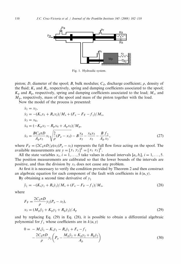
The considered hydraulic system was presented in [5] where the work was limited to faultdetection, meanwhile here, a full estimation of the fault is obtained. The hydraulic systemconsists of a spool valve and a single rod piston acting on an inertial load (see Fig. 1). Theexternal force F e controls the flow entering the head side chamber of the piston from apressure supply Pa: The rod side chamber is always connected to the return pressure Pr.

Then it is necessary to detect, isolate and estimate two faults in this system: a drop of thespool control force F e and an increase of the internal leakage of the piston (which isnormally assumed to be negligible). The following notations will be used: x1, displacementof the spool; x2, velocity of the spool; x3, displacement of the piston; x4, velocity of thepiston; x5, pressure at the head side chamber; f 1, failure mode corresponding to the controlforce; f 2, failure mode corresponding to the internal leakage of the piston; Ap, area of the

ARTICLE IN PRESS

Pr

Pr

Ks

Rs

Kp

RpMp

Pa

Fe

Fig. 1. Hydraulic system.

J.C. Cruz-Victoria et al. / Journal of the Franklin Institute 345 (2008) 102–118110

piston; D, diameter of the spool; B, bulk modulus; Cd, discharge coefficient; r, density ofthe fluid; K s and Rs, respectively, spring and damping coefficients associated to the spool;Kp and Rp, respectively, spring and damping coefficients associated to the load; Ms, andMp, respectively, mass of the spool and mass of the piston together with the load.Now the model of the process is presented:

_x1 ¼ x2,

_x2 ¼ �ðK sx1 þ Rsx2Þ=Ms þ ðF e � FF � f 1Þ=Ms,

_x3 ¼ x4,

_x4 ¼ ð�Kpx3 � Rpx4 þ Apx5Þ=Mp,

_x5 ¼BCdpD

Apx3x1

ffiffiffiffiffiffiffiffiffiffiffiffiffiffiffiffiffiffiffiffiffiffiffi2

rðPa � x5Þ

s� B

x4

x3�

x4x5

x3�

B

Ap

f 2

x3, ð27Þ

where FF ¼ ð2CdpD=rÞx1ðPa � x5Þ represents the full flow force acting on the spool. Theavailable measurements are y ¼ ½ y1 y2 �

T ¼ ½ x1 x3 �T.

All the state variables xi; i ¼ 1; . . . ; 5 take values in closed intervals ½ai; bi�, i ¼ 1; . . . ; 5.The position measurements are calibrated so that the lower bounds of the intervals arepositive, and thus the division by x3 does not cause any problem.At first it is necessary to verify the condition provided by Theorem 2 and then construct

an algebraic equation for each component of the fault with coefficients in khu; yi.By obtaining a second time derivative of y1

€y1 ¼ �ðK sy1 þ Rs _y1Þ=Ms þ ðF e � FF � f 1Þ=Ms, (28)

where

FF ¼2CdpD

ry1ðPa � x5Þ,

x5 ¼ ðMp €y2 þ Kpy2 þ Rp _y2Þ=Ap ð29Þ

and by replacing Eq. (29) in Eq. (28), it is possible to obtain a differential algebraicpolynomial for f 1 whose coefficients are in khu; yi

0 ¼ �Ms €y1 � K sy1 � Rs _y1 þ F e � f 1

�2CdpD

ry1 Pa �

Mp €y2 þ Kpy2 þ Rp _y2

Ap

� �ð30Þ

ARTICLE IN PRESSJ.C. Cruz-Victoria et al. / Journal of the Franklin Institute 345 (2008) 102–118 111

also by replacing y1 and y2 in _x5, the following equation is obtained:

_x5 ¼BCdpD

Apy2

y1

ffiffiffiffiffiffiffiffiffiffiffiffiffiffiffiffiffiffiffiffiffiffiffi2

rðPa � x5Þ

s� B

y�

2

y2

�x5y�

2

y2

�B

Ap

f 2

y2

, (31)

where replacing x5 ¼ ðMpy��

2 þ Kpy2 þ Rpy�

2Þ=Ap, yields

0 ¼ �Mpy���

2 þ Kpy�

2 þ Rpy��

2

Ap� B

y�

2

y2

�B

Ap

f 2

y2

þBCdpDy1

Apy2

ffiffiffiffiffiffiffiffiffiffiffiffiffiffiffiffiffiffiffiffiffiffiffiffiffiffiffiffiffiffiffiffiffiffiffiffiffiffiffiffiffiffiffiffiffiffiffiffiffiffiffiffiffiffiffiffiffiffiffiffiffiffiffiffiffiffi2

rPa �

Mpy��

2 þ Kpy2 þ Rpy�

2

Ap

!vuut

�y�

2ðMpy��

2 þ Kpy2 þ Rpy�

2Þ

Apy2

. ð32Þ

As we can see, the fault components appear explicitly in Eqs. (30) and (32) and it is notpossible to eliminate them, so we conclude that the outputs are differentiallytranscendental over khui (remember that by definition the fault components are notcontained in khui), in fact, for this example, Eqs. (30) and (32) are also the differentialalgebraic polynomials for f 1 and f 2 with coefficients in khu; yi (or diagnosabilityconditions). However, these polynomials depends on second and third time derivatives ofthe output, which are unknown. So, it is not possible to construct a reduced-order observerfor the fault in a direct way. On the other hand, by Theorem 1, it is known that if a systemis observable (see Definition 8) then it is diagnosable if, and only if, f is observable withrespect to u, y and x. It is not hard to see that this system is algebraically observable asfollows:

x1 � y1 ¼ 0,

x2 � _y1 ¼ 0,

x3 � y2 ¼ 0,

x4 � _y2 ¼ 0,

Apx5 � ðMp €y2 þ Kpy2 þ Rp _y2Þ ¼ 0.

From Theorem 1, it is only necessary that each component of the fault be algebraicallyobservable with respect to u, y and x, and it is not hard to see that this condition issatisfied.

It is clear that the differential transcendence degree of Rhu; yi=Rhui ¼ 2, then, from Eq.(27) the following equations are obtained:

f 1 ¼ �Ms _x2 � ðK sy1 þ Rsx2Þ þ F e � FF,

f 2 ¼ �Ap _x5y2

Bþ CdpDy1

ffiffiffiffiffiffiffiffiffiffiffiffiffiffiffiffiffiffiffiffiffiffiffi2

rðPa � x5Þ

s� Apx4 �

Ap

Bx4x5.

ARTICLE IN PRESSJ.C. Cruz-Victoria et al. / Journal of the Franklin Institute 345 (2008) 102–118112

5. Reduced-order uncertainty observer

Let consider system (9). The fault vector f is unknown and it can be assimilated as a statewith uncertain dynamics. Then, in order to estimate it, the state vector is extended to dealwith the unknown fault vector. The new extended system is given by

_xðtÞ ¼ Aðx; uÞ,

_f ¼ Oðx; uÞ,

yðtÞ ¼ hðx; uÞ, ð33Þ

where Oðx; uÞ is a bounded uncertain function.Note that a classic Luenberger observer cannot be constructed because the term Oðx; uÞ

is unknown. Then, the above problem is overcome by using a reduced-order uncertaintyobserver in order to estimate the failure variable f [32].Next lemma describes the construction of a proportional reduced-order observer for Eq.

(33).

Lemma 2. If the following hypotheses are satisfied:

H1:

Oðx; uÞ is bounded, i.e. jOðx; uÞjpN. H2: f ðtÞ is algebraically observable over khu; yi. H3: g is a C1 real-valued function.

Then the system

f:

¼ Kðf � f Þ (34)

is an asymptotic reduced-order observer for system (33), where f denotes the estimate of fault

f and K 2 Rþ determines the desired convergence rate of the observer.

Proof (Sketch). The dynamics of the error eðtÞ can be expressed as

_eðtÞ þ KeðtÞ ¼ Oðx; uÞ. (35)

The solution to the differential equation (35) is given by

eðtÞ ¼ e�Kt e0 þZ t

0

eKtOðtÞdt� �

(36)

with e0 as initial condition Then Eq. (36) yields

jeðtÞj ¼ e�Kt e0 þZ t

0

eKtOðtÞdt� �����

���� (37)

then, by applying the triangle and Schwarz inequalities, the following is obtained:

jeðtÞjpe�Ktje0j þ e�Kt

Z t

0

eKtOðtÞdt����

����and from H1

0pjeðtÞjpe�Ktje0j þ N

Z t

0

e�Kðt�tÞ dt����

����,

ARTICLE IN PRESSJ.C. Cruz-Victoria et al. / Journal of the Franklin Institute 345 (2008) 102–118 113

by solving the integral we have

0pjeðtÞjpe�Ktje0j þN

Kð1� e�KtÞ

�������� (38)

applying the lim sup when t!1 in both sides of (38), we obtain

0p lim supt!1

jeðtÞjp lim supt!1

e�Ktje0j þ lim supt!1

N

Kð1� e�KtÞ

��������,

simplifying

0p lim supt!1

jeðtÞjpN

K

and the proof is completed. &

Remark 4. Sometimes the output time derivatives (which are unknown), appear in thealgebraic equation of the fault, then it is necessary to use an auxiliary variable to avoidusing them.

Corollary. The dynamic system (34) along with

_g ¼ cðx; u; gÞ with g0 ¼ gð0Þ and g 2 C1 (39)

constitute a proportional asymptotic reduced-order fault observer for system (33), where g is a

change of variable which depends on the estimated fault f , and the states variables.

The performance of the reduced-order observer estimator is shown by means ofnumerical simulations.

6. Numerical results

6.1. Example 1

Let consider the nonlinear system (24), where

y1 ¼ x2,

y2 ¼ x3.

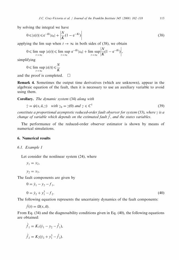
The fault components are given by

0 ¼ _y1 � y2 � f 1,

0 ¼ _y2 þ y31 � f 2. (40)

The following equation represents the uncertainty dynamics of the fault components:

_f ðtÞ ¼ Oðx; uÞ.

From Eq. (34) and the diagnosability conditions given in Eq. (40), the following equationsare obtained:

f:

1 ¼ K1ð _y1 � y2 � f 1Þ,

f:

2 ¼ K2ð _y2 þ y31 � f 2Þ.

ARTICLE IN PRESSJ.C. Cruz-Victoria et al. / Journal of the Franklin Institute 345 (2008) 102–118114

Note that _y1 and _y2 are not available. However, the following auxiliary variables allow tocircumvent this problem. Define

g1 ¼ f 1 � K1y1,

g2 ¼ f 2 � K2y2.

Then, the reduced-order observer is given by

_g1 ¼ �K1g1 � K1y2 � K21y1,

_g2 ¼ �K2g2 þ K2y31 � K2

2y2,

f 1 ¼ g1 þ K1y1,

f 2 ¼ g2 þ K2y2, (41)

where g1; g2 2 C1:The simulation results are obtained with initial conditions g1ð0Þ ¼ g2ð0Þ ¼ 0 and the

observer gains K1 ¼ K2 ¼ 10: Dynamics of the fault components are given by thefollowing equations:

f 1 ¼ 10 sinðte�2:3x1Þ,

f 2 ¼ 10 sinðte�1:4x1Þ.

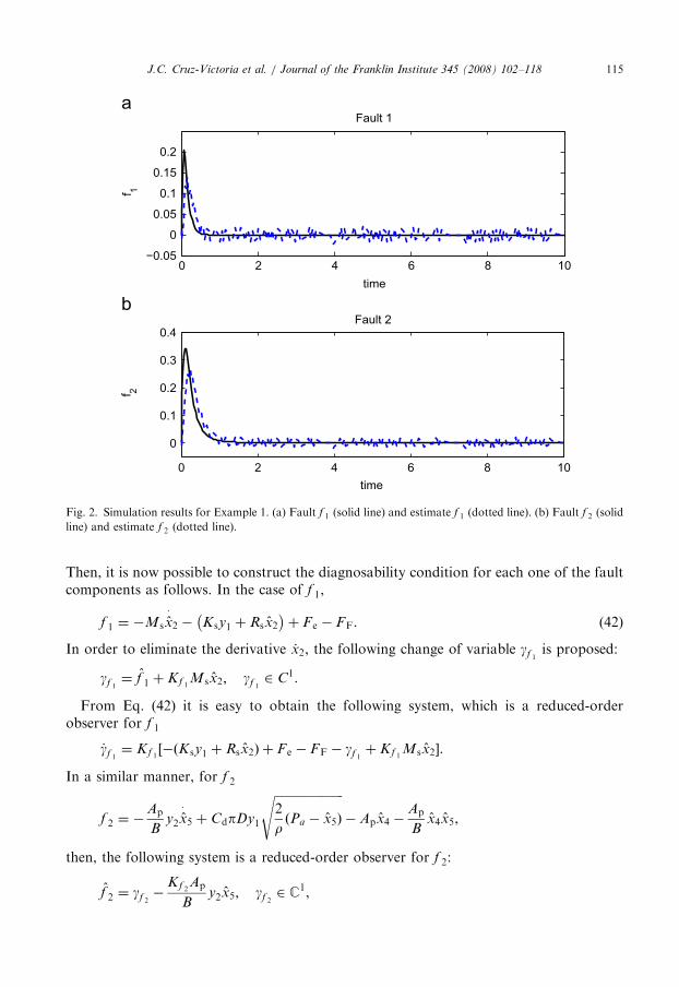
Estimation results are given in Fig. 2. It should be noted that the estimated faults followclosely its corresponding true values even in the presence of measurement noise. The noisecontaminating output measurements is gaussian with zero mean and variance 0.01 and it isbounded within the interval ½�0:001; 0:001�.

6.2. Example 2: hydraulic system

Before constructing the reduced-order observer used for the fault estimation, the statesx2; x4 and x5; must be estimated, so the following reduced-order observer is proposed inthe same way to calculate x2 and x4:

x2 ¼ y:

1 ¼ K1ðy1 � y1Þ,

x4 ¼ y:

2 ¼ K2ðy2 � y2Þ,

and in order to estimate x5 the following system is constructed:

x5 ¼ g5 þK5Mp

Apx4; g5 2 C1,

_g5 ¼ K5 ðKpx3 þ Rpx4Þ=Ap � g5 �K5Mp

Apx4

� �.

ARTICLE IN PRESS

0 2 4 6 8 10

0

0.05

0.1

0.15

0.2

time

f 1

Fault 1

0 2 4 6 8 10

0

0.1

0.2

0.3

0.4

time

f 2

Fault 2

Fig. 2. Simulation results for Example 1. (a) Fault f 1 (solid line) and estimate f 1 (dotted line). (b) Fault f 2 (solid

line) and estimate f 2 (dotted line).

J.C. Cruz-Victoria et al. / Journal of the Franklin Institute 345 (2008) 102–118 115

Then, it is now possible to construct the diagnosability condition for each one of the faultcomponents as follows. In the case of f 1,

f 1 ¼ �Msx�

2 � K sy1 þ Rsx2

� þ F e � FF. (42)

In order to eliminate the derivative _x2, the following change of variable gf 1is proposed:

gf 1¼ f 1 þ Kf 1

Msx2; gf 12 C1.

From Eq. (42) it is easy to obtain the following system, which is a reduced-orderobserver for f 1

_gf 1¼ Kf 1

½�ðK sy1 þ Rsx2Þ þ F e � FF � gf 1þ Kf 1

Msx2�.

In a similar manner, for f 2

f 2 ¼ �Ap

By2x�

5 þ CdpDy1

ffiffiffiffiffiffiffiffiffiffiffiffiffiffiffiffiffiffiffiffiffiffiffi2

rðPa � x5Þ

s� Apx4 �

Ap

Bx4x5,

then, the following system is a reduced-order observer for f 2:

f 2 ¼ gf 2�

Kf 2Ap

By2x5; gf 2

2 C1,

ARTICLE IN PRESS

0 10 20 30 40 50

0

0.02

0.04

0.06

time

f 1Fault 1

0 10 20 30 40 50

0

0.5

1

1.5

2

2.5x 10

time

f 2

Fault 2

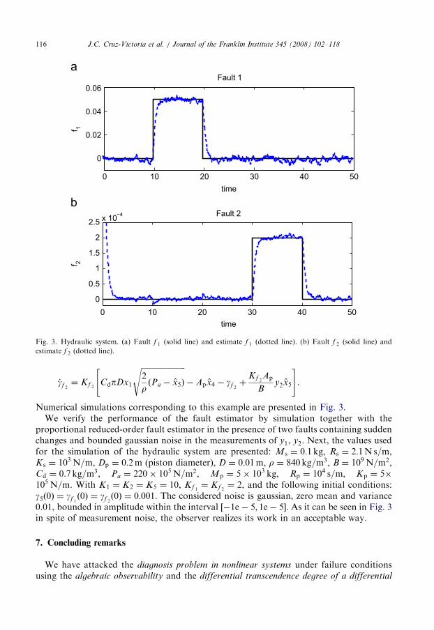
Fig. 3. Hydraulic system. (a) Fault f 1 (solid line) and estimate f 1 (dotted line). (b) Fault f 2 (solid line) and

estimate f 2 (dotted line).

J.C. Cruz-Victoria et al. / Journal of the Franklin Institute 345 (2008) 102–118116

_gf 2¼ Kf 2

CdpDx1

ffiffiffiffiffiffiffiffiffiffiffiffiffiffiffiffiffiffiffiffiffiffiffi2

rðPa � x5Þ

s� Apx4 � gf 2

þKf 2

Ap

By2x5

" #.

Numerical simulations corresponding to this example are presented in Fig. 3.We verify the performance of the fault estimator by simulation together with the

proportional reduced-order fault estimator in the presence of two faults containing suddenchanges and bounded gaussian noise in the measurements of y1, y2. Next, the values usedfor the simulation of the hydraulic system are presented: Ms ¼ 0:1 kg; Rs ¼ 2:1N s=m,K s ¼ 103 N=m, Dp ¼ 0:2m (piston diameter), D ¼ 0:01m, r ¼ 840 kg=m3, B ¼ 109 N=m2,Cd ¼ 0:7 kg=m3, Pa ¼ 220� 105 N=m2, Mp ¼ 5� 103 kg, Rp ¼ 104 s=m, Kp ¼ 5�105 N=m. With K1 ¼ K2 ¼ K5 ¼ 10, Kf 1

¼ Kf 2 ¼ 2, and the following initial conditions:g5ð0Þ ¼ gf 1

ð0Þ ¼ gf 2ð0Þ ¼ 0:001. The considered noise is gaussian, zero mean and variance

0.01, bounded in amplitude within the interval ½�1e� 5; 1e� 5�. As it can be seen in Fig. 3in spite of measurement noise, the observer realizes its work in an acceptable way.

7. Concluding remarks

We have attacked the diagnosis problem in nonlinear systems under failure conditionsusing the algebraic observability and the differential transcendence degree of a differential

ARTICLE IN PRESSJ.C. Cruz-Victoria et al. / Journal of the Franklin Institute 345 (2008) 102–118 117

field extension concepts. A reduced-order uncertainty observer was used to estimate thefault variable. Numerical simulations were presented in order to illustrate the effectivenessof the suggested approach.

References

[1] A.S. Willsky, A survey of design methods for failure detection in dynamic system, Automatica 12 (1976)

601–611.

[2] P.M. Frank, X. Ding, Survey of robust residual generation and evaluation methods in observer-based fault

detection systems, J. Proc. Control 7 (1997) 403–424.

[3] R. Iserman, Process fault detection based on modeling and estimation methods: a survey, Automatica 20 (4)

(1984) 387–404.

[4] P.M. Frank, Fault diagnosis in dynamic systems using analytical and knowledge-based redundancy: a survey,

Automatica 26 (1990) 459–474.

[5] P.M. Frank, X. Ding, Frequency domain approach to optimally robust residual generation and evaluation

for model based fault diagnosis, Automatica 20 (5) (1994) 789–804.

[6] E. Alcorta Garcıa, P.M. Frank, Deterministic nonlinear observer-based approaches to fault diagnosis: a

survey, Control Eng. Practice 5 (1997) 663–670.

[7] Wunnenberg. Observer-based fault detection in dynamic system, Reihe 8, No. 222, VDI-Fortschrittsber.,

VDI-Verlag, Dusseldorf, Germany, 1990.

[8] R. Seliger, P.M. Frank, Robust observer-based fault diagnosis in nonlinear uncertain systems, in: Patton,

Frank, Clark (Eds.), Issues of Fault Diagnosis for Dynamic Systems, Springer, Berlin, 2000, pp. 145–187.

[9] S. Diop, R. Martınez-Guerra, An algebraic and data derivative information approach to nonlinear systems

diagnosis, in: Proceedings of the European Control Conference 2001, Porto, Portugal, ECC01, 2001,

pp. 2334–2339.

[10] S. Diop, R. Martınez-Guerra, On an algebraic and differential approach of nonlinear systems diagnosis, in:

Proceedings of the IEEE Conference of Decision and Control, CDC01, Orlando, FL, USA, pp. 585–589.

[11] N. Viswanadham, R. Srichander, Fault detection using unknown-input observers, Control Theory Adv.

Technol. 3 (1987) 91–101.

[12] P. Kudva, N. Viswanadham, A. Ramakrishna, Observers for linear systems with unknown inputs, IEEE

Trans. Autom. Control 25 (1980) 113–115.

[13] X. Baseville, I.V. Nikoforov, Detection of Abrupt Changes. Theory and Application, Prentice-Hall,

Englewood Cliffs, NJ, 1993.

[14] J. Chen, R.J. Patton, Robust Model-Based Fault Diagnosis for Dynamic Systems, Kluwer Academic

publishers, Boston, 1998.

[15] C. De Persis, A. Isidori, A geometric approach to nonlinear fault detection and isolation, IEEE Trans.

Autom. Control 46 (6) (2001) 853–865.

[16] M.A. Massoumnia, G.C. Verghese, A.S. Willsky, Failure detection and identification, IEEE Trans. Autom.

Control 34 (1989) 316–321.

[17] R.J. Patton, P.M. Frank, R.N. Clark, Fault Diagnosis in Dynamic Systems, Theory and Application,

Prentice-Hall, Englewood Cliffs, NJ, 1989.

[18] M. Staroswiecki, G. Comtet-Varga, Fault detectability and isolability in algebraic dynamic systems, in:

Proceedings of European Control Conference, ECC99, Karlsruhe, Germany, 1999.

[19] F. Szigeti, C.E. Vera, J. Bokor, A. Edelmayer, Inversion based fault detection and isolation, in: Proceedings

of the 40th IEEE Conference Decision Control, Orlando, FL, CDC, 2001, pp. 1005–1010.

[20] M. Fliess, C. Join, H. Mounier, An introduction to nonlinear fault diagnosis with application to a congested

internet router, in: C.T. Abdalah, J. Chiasson (Eds.), Advances in Communication Control Networks,

Lecture Notes in Control and Information Sciences, vol. 308, Springer, Berlin, pp. 327–343.

[21] M. Fliess, C. Join, H. Sira-Ramırez, Robust residual generation for linear fault diagnosis: an algebraic setting

with examples, Int. J. Control 14 (77) (2004) 1223–1242.

[22] C. Join, H. Sira-Ramırez, M. Fliess, Control of an uncertain three-tank system via on-line parameter

identification and fault detection, in: Proceedings of World IFAC Conference, Prague, July 2005.

[23] R. Martınez-Guerra, R. Garrido, A. Osorio Miron, High-gain nonlinear observers for the fault detection

problem: application to a bioreactor, in: A.B. Kurzhanski, A.L. Fradkov (Eds.), IFAC Publications,

ARTICLE IN PRESSJ.C. Cruz-Victoria et al. / Journal of the Franklin Institute 345 (2008) 102–118118

Editorial Elsevier Science Ltd., Amsterdam, Nonlinear Control Systems, vol. 3, pp. 1567–1572, 2002, ISBN

0-08-043560-2.

[24] R. Martınez-Guerra, R. Garrido, A. Osorio Miron, The fault detection problem in nonlinear systems using

residual generators, IMA J. Math. Control Inf. 22 (2005) 119–136.

[25] P.M. Frank, Enhancement of robustness in observer-based fault detection, Int. J. Control 59 (1994) 955–981.

[26] J. Chen, R.J. Patton, H.Y. Zhang, Design of unknown input observers and robust fault detection filters, Int.

J. Control 63 (1996) 85–105.

[27] R. Martınez-Guerra, J. De Leon-Morales, Nonlinear estimators: a differential algebraic approach, Appl.

Math. Lett. 9 (4) (1996) 21–25.

[28] R. Martınez-Guerra, I.R. Ramırez Palacios, E. Alvarado-Trejo, On parametric and state estimation:

application to a simple academic example, in: Proceedings of the IEEE 37th Conference on Decision and

Control, 1998, pp. 764–765.

[29] H. Hammouri, M. Kinnaert, E.H. El Yaagoubi, Observer based approach to fault detection and isolation for

nonlinear systems, IEEE Trans. Autom. Control 44 (1999) 10.

[30] M. Fliess, A note on the invertibility of non-linear input–output differential systems, Syst. Control Lett. 8

(1986) 147–151.

[31] R. Martınez-Guerra, S. Diop, R. Garrido, A. Osorio Miron, Diagnosis of nonlinear systems using a reduced

order fault observer: application to a bioreactor, in: Journees Franco-Mexicaines d’Automatique Appliquee,

IRCCyN, Nantes, France, 12–14, September 2001.

[32] R. Martınez-Guerra, J. Mendoza-Camargo, Observers for a class of Liouvillian and nondifferentially flat

systems, IMA J. Math. Control Inf. 21 (2004) 493–509.

[33] E.R. Kolchin, Differential Algebra and Algebraic Groups, Academic Press, New York, 1973.