On Loss Probabilities in Presence of Redundant Packets and Several Traffic Sources

Performance Evaluation 36–37 (1999) 485–518www.elsevier.com/locate/peva

On loss probabilities in presence of redundant packetsand several traffic sources

Omar Ait-Hellal a,1, Eitan Altman a,Ł,2, Alain Jean-Marie a,2, Irina A. Kurkova b,3

a INRIA Sophia Antipolis, BP 93, 2004 route des Lucioles, 06902 Sophia Antipolis Cedex, Franceb Laboratory of Large Random Systems, Faculty of Mathematics and Mechanics, Moscow State University,

119899 Moscow, Russia

Abstract

We study the effect of adding redundancy to an input stream on the losses that occur due to buffer overflow. We considerseveral sessions that generate traffic into a finite capacity queue. Using multi-dimensional probability generating functions,we derive analytical formulas for the loss probabilities and provide asymptotic analysis (for large n and small or large ²). Ouranalysis allows us to investigate when does adding redundancy decrease the loss probabilities. In many cases, redundancy isshown to degrade the performance, as the gain in adding redundancy is not sufficient to compensate the additional losses dueto the increased overhead. We show, however, that it is possible to decrease loss probabilities if a sufficiently large amount ofredundancy is added. Indeed, we show that for an arbitrary stationary ergodic input process, if ² < 1 then redundancy canreduce loss probabilities to an arbitrarily small value. 1999 Elsevier Science B.V. All rights reserved.

Keywords: Forward error correction; Loss probabilities; Multi-dimensional generating functions; M=M=1=K queue; Stationaryergodic arrival processes

1. Introduction

An important trend in telecommunications is to integrate different type of traffic in a single network.The various traffic types typically have different requirements on quality of services, and in particular,on loss probabilities. Rapid progress in the development of fiber optics allows to achieve a bit error rateof 10�14; information loss is then essentially due to congested nodes and buffer overflow.

Often, a group of consecutive packets are grouped into a frame, and loss of one packet results in theloss of the whole frame. This is the case in ATM where a transport layer protocol (known as AAL)is responsible for this grouping, see e.g. Chapter 5 in [11]. In order to reduce the loss probabilities,

Ł Corresponding author.1 Current address: Departement de Reseaux Informatique, Universite de Liege, Bat. B28, 4000 Liege 1, Belgium.2 E-mail: {altman,ajm}@sophia.inria.fr3 E-mail: [email protected]

0166-5316/99/$ – see front matter 1999 Elsevier Science B.V. All rights reserved.PII: S 0 1 6 6 - 5 3 1 6 ( 9 9 ) 0 0 0 1 7 - 6

486 O. Ait-Hellal et al. / Performance Evaluation 36–37 (1999) 485–518

one may add redundant packets into the frame, so that lost packets can be often reconstructed. Indeed,there exist erasure recovery codes that, by including additional k redundant packets in a frame, enableto reconstruct up to k losses (see [5,10,13,4] and references therein). We note, however, that by addingredundant packets, the workload increases and thus the loss probability of a packet increases.

Adding redundant packets to a frame is quite frequent in networks, especially in the ATM adaptationlayer (AAL), see e.g. [3]. It also plays an important role in several applications on the Internet (see e.g.[2,12]). If the number of redundant packets j that is to be added to a set of n packets is one, the simplestway to do it is by letting the kth bit of the redundant packet be the modulo 2 sum of the kth bit of all npackets. For the case of j ½ 2 there are several known methods, see e.g. [4], or the Reed Solomon code[6]. The procedure of adding redundancy is known as Forward Error Correction (FEC). (This method isin contrast with feedback error correction methods based on retransmissions, which may require longdelays due to the retransmission.)

We analyze the tradeoff between the effects of increase of workload and the recovery of lost packets,and calculate the probability of no more losses than k packets within n consecutive ones in the presenceof k redundant packets. The computations are based on recursive formulas obtained by Cidon, Khamisyand Sidi [5]. We consider the possibility of multiplexing between several sources so that the packetsof a given source to which redundancy is added may be separated in the queue by packets from othersources. This type of models (with more general arrival processes) was studied also in Kawahara et al.[10] who obtain a procedure for the numerical solution. By restricting in this paper to Poisson arrivals,we are able to obtain exact formulas for the loss probabilities.

In [13], the authors have used an approximation based on an assumption of independence betweenconsecutive losses, and shown that redundancy results in decrease of loss probabilities by 10% to 100%.Exact numerical methods based on recursions [5] led to an opposite conclusion, i.e. that redundancycauses increase in loss probabilities. One of the advantages of our analytical approach, together withthe asymptotic approximations which we present, is that they enable to study both qualitative andquantitative behavior of the effect of redundancy in a systematic way. As was already shown in [1,9]for the case of a single source, we show that for both light traffic as well as heavy traffic conditions,redundancy decreases loss probabilities.

In this paper we identify a fundamental property of losses with redundancy. We show that for anyvalue ² smaller than one of the traffic load of sessions to which we wish to add redundancy, addingredundancy in an appropriate way results in arbitrarily small loss probabilities. This property is shownto hold for any stationary ergodic arrival sequence. For the special case of Poisson arrivals we actuallycompute the rate of redundancy that has to be added.

The paper is structured as follows: in Section 2, we describe the model and we set the main results:probability generating function (etc.), the proofs are given in Section 3. The asymptotic analysis ispresented in Section 4. In Section 5, we show that in light traffic, adding redundancy decreases theloss probabilities. Numerical examples which illustrate this improvement are given in Section 6. InSection 7 we show that frame losses can be almost completely eliminated, and we compute the requiredrate of redundancy. In Section 8 we extend some of these results to general arrival and service timedistributions. We conclude with some remarks and future work in Section 9.

O. Ait-Hellal et al. / Performance Evaluation 36–37 (1999) 485–518 487

2. The model and the main results

We consider an M=M=1 queue with a finite buffer of size K served according to the FIFO (first infirst served) discipline. We assume that packets arrive to the queue from S independent sources, i.e. theinter-arrival times and the transmission times of packets from each source are mutually independent.The arrival process from source s, s D 1; 2; : : :; S, is assumed to be Poisson with rate ½s . The overallarrival process to the system is then Poisson with rate ½ ,

PSsD1 ½s . Define ps , ½s=½ and pNs , 1� ps ,

² D ½=¼, ²s D ½s=¼ D ps². We summarize the recursive scheme introduced in [5] for computingPs. j; n/; s D 1; 2; : : :; S which are the probabilities of j losses among n consecutive ones originatingfrom source s. For the system with Poisson arrivals with rate ½ and exponential transmission rate ¼,in steady state, the probability of finding i packets in the system at an arbitrary epoch is given byŠ.i/ D ²i=.

PKlD0 ²

l/. Define Qi .k/ to be the probability that k packets out of i leave the system duringan inter-arrival epoch. We have

Qi .k/ D ²ÞkC1; 0 � k � i � 1;

Qi .i/ D Þi ; where Þ :D .1C ²/�1:(1)

Denote by Ps;ai . j; n/ resp. P Ns;ai . j; n/, i D 0; 1; : : :; K , s D 1; 2; : : :; S, n ½ 1, 0 � j � n, the

probabilities of j losses in a block of n packets coming from source s, given that there are i packets inthe system just before the arrival of the first packet in the block, and just before the arrival of a packetfrom any other source (denoted by Ns), respectively. Since the first packet in the block is arbitrary, wehave

Ps. j; n/ DKX

iD0

Š.i/Ps;ai . j; n/: (2)

The probability that an arbitrary arrival is from source s is equal to ½s=½. The recursive scheme is

Ps;ai . j; 1/ D

(1; j D 0;

0; j ½ 1;i D 0; 1; : : :; K � 1 (3)

Ps;aK . j; 1/ D

(1; j D 1;

0; j D 0; j ½ 2:(4)

For n ½ 2, we have for 0 � i � K � 1 and for i D K , respectively:

Ps;ai . j; n/ D

iC1XkD0

QiC1.k/h

ps Ps;aiC1�k. j; n � 1/C pNs P Ns;aiC1�k. j; n � 1/

i;

Ps;aK . j; n/ D

KXkD0

QK .k/h

ps Ps;aK�k. j � 1; n � 1/C pNs P Ns;aK�k. j � 1; n � 1/

i;

(5)


where P Ns;ai . j; n/ for n ½ 1 is given by

P Ns;ai . j; n/ DiC1XkD0

QiC1.k/h

ps Ps;aiC1�k. j; n/C pNs P Ns;aiC1�k. j; n/

i; 0 � i � K � 1;

P Ns;aK . j; n/ D P Ns;aK�1. j; n/:

(6)

The complexity of these recursions is O.K 2nj/ in arithmetic operations and O.K 2/ in memory space.Next, we state the main results, whose detailed proofs are given in next section. Define:

qs.y; z/ ,1XjD0

1XnD1

y j zn�1 Ps. j; n/:

Let x1.z/ and x2.z/ be the solutions in x of x2 � .1C ²/x C ².pNs C psz/ D 0:

x1.z/ D�

1C ² Cp.1C ²/2 � 4².pNs C psz/

�=2;

x2.z/ D�

1C ² �p.1C ²/2 � 4².pNs C psz/

�=2:

We shall often write simply x1 and x2 for x1.z/ and x2.z/. Both these functions are analytic in thedisk

ýjzj < �.1C ²/2 � 4²Ns

Ð=4²s

. Define, for all k, Žk D xk

1 � xk2 , �k D .pNs C psz/Žk�1 � Žk . Let

RK D�PK

lD0 ²l��1

.

Proposition 1. The probability generating function qs is given by

qs.y; z/ D RK

.1� z/

�²K�1.1� z/[ŽKC1]2

z�K

�1

zŽK � ŽKC1 � ²z�K y

½C R�1

K C²K�1ŽKC1

z�K

�: (7)

Once the probability generating function is obtained by Proposition 1, one can obtain the requiredprobabilities by inverting qs . We focus in the sequel on Ps

² .> j; n/, which is the probability of losingmore than j packets out of n consecutive ones coming from source s. We investigate in particular thecase of j D 0; 1, in order to be able to decide when does including one redundant packet in each frameresults in a decrease of the loss probability.

We shall use the notation [zk] f .z/ to denote the coefficient of zk in the Taylor expansion of thefunction f .z/, i.e. if f .z/ DPk fk zk then [zk] f .z/ D fk .

Corollary 2. The probability of losing more than j packets out of n consecutive packets that arrive fromsource s is

Ps² .> j; n/ D RK²

KC j ðzn�1� jŁ 1

z � 1

�ŽKC1

zŽK � ŽKC1

½��K

zŽK � ŽKC1

�j

: (8)

In the following, we obtain a simple recursion on n, for computing the probabilities Ps² .> j; n/.

Thus, we avoid a recursion on j and a resolution of a set of linear equations of size K for all j and all nrequired in [5].


Define þ, and � as

D 1C ²; þ Dp.1C ²/2 � 4²Ns; � D 4²s

.1C ²/2 � 4²Ns: (9)

Let G D K=2 for K even and .K C 1/=2 otherwise, and set

an D .��/nGX

kDn

�K C 1

2k C 1

��k

n

�þ

�þ

�2k

;

bn D .��/n�1GX

kDn

�K C 1

2k C 1

��k

n

��4 .2k C 1/n

þ.K C 1/.K C 1� 2k/C �þ

��þ

�2k

(we use the convention thatPG

kDn D 0 if n > G).

Corollary 3. For n ½ 1 we have

Ps² .> 0; n/ D RK²

K C 1

a0

n�1XkD1

�bn�k Ps

² .> 0; k/C RK²K ak

Ð: (10)

For j < n, n ½ 1, Ps² .> j; n/ is given by the expression

.�1/ j

A jC1;0

24n�2XkD j

HjC1;n�1�k Ps² .> j; k C 1/C RK²

Kn� j�1X

kD0

R j;k

35 ; (11)

where

Hk;n DkX

rD0

nXmDr

�k

r

�.�1/k�r Ak�r;n�m Br;m�r ;

Rk;n DkX

rD0

nXmD0

�k

r

�.�1/k�r Ak�rC1;n�m Br;m;

with

Ak;n DðznŁ .ŽKC1/

k DnX

mD0

kXrD0

�k

r

�.�1/k�r a0r.KC1/;mb0.k�r/.KC1/;n�m;

Bk;n DðznŁ .ŽK /

k DnX

mD0

kXrD0

�k

r

�.�1/k�r a0r K ;mb0.k�r/K ;n�m;


where

a0k;n D �n�

2

�k kXrD0

�k

r

��þ

�r� .n � r=2/

n!� .�r=2/;

b0k;n D �n�

2

�k kXrD0

�k

r

��þ

�r� .n � r=2/

n!� .�r=2/:

For computing the probabilities Ps² .> 0; n/, we first compute the terms ak and bk , k D 0; : : :; n

which requires O.K n/ arithmetic operations, then we compute the sum, which is a simple recursion onn, with complexity of O.n2/ arithmetic operations and O.K n/ in memory space if we consider that allthe values

�kr

Ð, 0 � r � n, r � k � K=2 remain in memory (and need not be computed). In the case

j > 0, we proceed in the same manner; we first compute the terms a0k;m , b0k;m, k D K C 1; : : :; j .K C 1/,m D 0; : : :; n which requires O.K nj2/ arithmetic operations, after this, we compute the terms Ak;m, Bk;m,k D 1; : : :; j , m D 0; : : :; n with complexity of O. j2n2/, after what, we compute the terms HjC1;m andR j;m , m D 0; : : :; n which requires O. jn2/. Finally, the probabilities are computed from Eq. (11) withcomplexity of O.n2/ arithmetic operations. Thus, the complexity of this procedure is O. j2n2 C K nj2/ inarithmetic operations and O.K 2 j2/ in memory space if we consider, again, that all values

�kr

Ð, 0 � r � k,

K C 1 � k � j .K C 1/ are stored beforehand in the memory and need not be computed.

Remark 4. All the results in [1], who considered a single source, can be obtained as special case of ourresults by substituting 1 for ps .

3. Proof of the main results

Proof of Proposition 1. The following derivation is a generalization of the one given in [1] for the caseof no exogenous flow, i.e. pNs D 0. Define

³ sj;n.x/ ,

KXiD0

xi Ps;ai . j; n/;

³ Nsj;n.x/ ,KX

iD0

xi P Ns;ai . j; n/;

ýs Nsj;n.x/ ,

KXiD0

xih

ps Ps;ai . j; n/C pNs P Ns;ai . j; n/

i; n ½ 1; j ½ 0:

It follows from Eq. (5) that

³ sj;n.x/ D

K�1XiD0

xiiC1XkD0

QiC1.k/h


i

C x KKX

kD0

QK .k/h


i:


Next, we substitute Eq. (1) as well as the definition of ýs Nsj;n.x/ into the last equation. Using the fact

thatýs Nsj;n.0/ D ps Ps;a

0. j; n/C pNs P Ns;a0 . j; n/, we obtain for n ½ 2, j ½ 1:

³ sj;n.x/ D

K�1XiD0

xi

iX

kD0

²ÞkC1h


iC ÞiC1

hps Ps;a

0. j; n � 1/C pNs P Ns;a0 . j; n � 1/

i!

C x K

K�1XkD0

²ÞkC1h


iC ÞK

hps Ps;a

0. j � 1; n � 1/C pNs P Ns;a0 . j � 1; n � 1/

i!

D ²Þ2

1� Þx

�1

Þxýs Ns

j;n�1.x/� .Þx/Kýs Nsj;n�1.Þ

�1/

�� ²Þ2

1� Þx

�1

Þx� .Þx/K

�ýs Ns

j;n�1.0/

C Þ1� .Þx/K

1� Þxýs Ns

j;n�1.0/C Þ².Þx/Kýs Nsj�1;n�1.Þ

�1/C Þ.Þx/Kýs Nsj�1;n�1.0/: (12)

Proceeding similarly as above, we obtain from Eq. (6) for n ½ 1, j ½ 0:

³ Nsj;n.x/ D²Þ2

1� Þx

�1

Þxýs Ns

j;n.x/� .Þx/Kýs Nsj;n.Þ

�1/

�� ²Þ2

1� Þx

�1

Þx� .Þx/K

�ýs Ns

j;n.0/

C Þ1� .Þx/K

1� Þxýs Ns

j;n.0/C Þ².Þx/Kýs Nsj;n.Þ

�1/C Þ.Þx/Kýs Nsj;n.0/: (13)

Define, with some abuse of notation, the generating functions of Ps;ai . j; n/ resp. P Ns;ai . j; n/:

³ s.x; y; z/ ,1XjD0

1XnD1

y j zn�1³ sj;n.x/; resp. ³ Ns.x; y; z/ ,

1XjD0

1XnD1

y j zn�1³ Nsj;n.x/:

Define also, with some abuse of notation, the generating function of ps Ps;ai . j; n/C pNs P Ns;ai . j; n/:

ýs Ns.x; y; z/ ,1XjD0

1XnD1

y j zn�1ýs Nsj;n.x/ D ps³

s.x; y; z/C pNs³ Ns.x; y; z/: (14)

When we fix y and jzj < 1, the three generating functions are polynomials in x , and therefore analyticfunctions. In order to use Eq. (12), which holds only for n ½ 2 and j ½ 1, we note that

1XjD1

1XnD2

y j zn�1³ sj;n.x/ D ³ s.x; y; z/�

1XnD1

zn�1³ s0;n.x/�

1XjD0

y j³ sj;1.x/C ³ s

0;1.x/

D ³ s.x; y; z/� ³ s.x; 0; z/� ³ s.x; y; 0/C ³ s.x; 0; 0/:


From Eqs. (3) and (4) we get

³ s.x; 0; 0/ D 1� x K

1� x; ³ s.x; y; 0/ D 1� x K

1� xC yx K : (15)

In Eq. (15), as well as in the rest of the paper, we consider that for x D 1 and for all K ,.1 � x K /=.1 � x/ D K (in particular, RK D 1=.K C 1/ for ² D 1). From Eq. (12), after substitutingEq. (14), we obtain

³ s.x; y; z/� ³ s.x; 0; z/ D yx K C ²Þ2

1� Þx

1

Þxzðýs Ns.x; y; z/�ýs Ns.x; 0; z/

Ł� ²Þ2

1� Þx.Þx/K z

ðýs Ns.Þ�1; y; z/�ýs Ns.Þ�1; 0; z/

Ł� ²Þ2

1� Þx

�1

Þx� .Þx/K

�zðýs Ns.0; y; z/�ýs Ns.0; 0; z/

ŁC Þ1� .Þx/K

1� Þxzðýs Ns.0; y; z/�ýs Ns.0; 0; z/

ŁC Þ².Þx/K zy

ðýs Ns.Þ�1; y; z/Cýs Ns.0; y; z/

ŁD yx K C ²Þ2

1� Þx

1

Þxzðýs Ns.x; y; z/�ýs Ns.x; 0; z/

ŁC ²Þ.Þx/K

�y � Þ

1� Þx

�z

�ýs Ns.Þ�1; y; z/C 1

²ýs Ns.Þ�1; 0; z/

½C ²Þ

2.Þx/K

1� Þxz

�ýs Ns.Þ�1; 0; z/C 1

²ýs Ns.0; 0; z/

½C� �²Þ2

1� Þx

1

ÞxC Þ

1� Þx

�zðýs Ns.0; y; z/�ýs Ns.0; 0; z/

Ł: (16)

Similarly, from Eq. (13) after substituting Eq. (14), we have

³ Ns.x; y; z/ D ²Þ.Þx/K�

1� Þ

1� Þx

��ýs Ns.Þ�1; y; z/C 1

²ýs Ns.Þ�1; 0; z/

½C ²Þ2

1� Þx

1

Þxýs Ns.x; y; z/C Þ2.x � ²/

.1� Þx/Þxýs Ns.0; y; z/: (17)

By using the relation Þ C ²Þ D 1, we get from Eq. (17) and Eq. (14)

³ Ns.²; y; z/ D ýs Ns.²; y; z/ D ³ s.²; y; z/: (18)

This means that the distributions of the number of the customers in the queues taken at the arrivaltimes of the packets from source s are the same when taken at the arrival times of the other packets(packets coming from other sources Ns). (This is due to the Pasta property.)

We note that in order to establish the proof of Proposition 1, it follows from Eq. (2) that it suffices toobtain ³ s.x; y; z/ at x D ², since

qs.y; z/ D RK³s.²; y; z/: (19)


From Eqs. (16) and (18) we haveð³ s.²; y; z/� ³ s.²; 0; z/

Ł.1� z/ D y²K C z.²Þ/KC1 ðýs Ns.Þ�1; 0; z/�ýs Ns.0; 0; z/

ŁC z.y � 1/.²Þ/KC1 ðýs Ns.Þ�1; y; z/�ýs Ns.0; y; z/

Ł: (20)

In order to compute the function ³ s.²; y; z/ it suffices to compute the functions in the square bracketsas well as ³ s.²; 0; z/. To do that, we first compute ³ s

0;n by proceeding in the same manner as in Eq. (12).Since Ps;a

K .0; n/ D 0 we have

³ s0;n D

²Þ2

1� Þx

1

Þxýs Ns

0;n�1.x/�²Þ2

1� Þx.Þx/Kýs Ns

0;n�1.Þ�1/

C Þ1� .Þx/K

1� Þxýs Ns

0;n�1.0/�²Þ2

1� Þx

�1

Þx� .Þx/K

�ýs Ns

0;n�1.0/:

By taking the generating function of both sides of the above equation and substituting Eq. (15), wecan write

.1� Þx/Þx³ s.x; 0; z/ D 1� x K

1� x.1� Þx/Þx C ²Þ2zýs Ns.x; 0; z/� ²Þ2.Þx/KC1z

ð�ýs Ns.Þ�1; 0; z/C 1

²ýs Ns.0; 0; z/

½C Þ2.x � ²/zýs Ns.0; 0; z/; (21)

from which we get, for x D ², and after substituting Eq. (18)

.1� z/³ s.²; 0; z/ D R�1K�1 � .²Þ/KC1z

�ýs Ns.Þ�1; 0; z/C 1

²ýs Ns.0; 0; z/

½: (22)

From Eqs. (14), (16) and (17) we have�.1� Þx/ Þx � ²Þ2 .pNs C ps z/

Ð ðýs Ns.x; y; z/�ýs Ns.x; 0; z/

ŁD .pNs C psz/

�Þ2.x � ²/Ð ðýs Ns.0; y; z/�ýs Ns.0; 0; z/

ŁC ²Þ.Þx/KC1 ðpNsÞ .² � x/C .y .1� Þx/� Þ/ ps z

Ł �ýs Ns.Þ�1; y; z/C 1

²ýs Ns.0; y; z/

½C ps.1� Þx/Þyx KC1 C ²Þ2.Þx/KC1 .pNs.x � ²/C psz/

�ýs Ns.Þ�1; 0; z/C 1

²ýs Ns.0; 0; z/

½:

(23)

Also, from Eqs. (14) and (17) for y D 0 and Eq. (21) we obtain�.1� Þx/ Þx � ²Þ2 .pNs C ps z/

Ðýs Ns.x; 0; z/

D 1� x K

1� x.1� Þx/Þxps C Þ2.x � ²/ .pNs C psz/ýs Ns.0; 0; z/

C ²Þ2.Þx/KC1 .pNs.x � ²/C psz/

�ýs Ns.Þ�1; 0; z/C 1

²ýs Ns.0; 0; z/

½: (24)


We now apply the ‘kernel method’ for solving the functional equations Eqs. (23) and (24). For eachi D 1; 2; when x D xi .z/, the term that multiplies ýs Ns.x; 0; z/ in the left-hand side of Eq. (24) (thekernel) vanishes. Since ýs Ns.x; 0; z/ is polynomial in x and therefore analytic in x , the left-hand sideof Eq. (24) vanishes at x D xi.z/. Thus by substituting xi for x into Eq. (24), we obtain for eachz two equations with two unknowns: ýs Ns.0; 0; z/ and [ýs Ns.Þ�1; 0; z/ C 1

²ýs Ns.0; 0; z/]. Solving these

equations yields

ýs Ns.Þ�1; 0; z/C 1

²ýs Ns.0; 0; z/ D ps

Þ�.KC1/.x K1 � x K

2 /

x K2 .x2 � ²Ns/.x1 � ²/� x K

1 .x1 � ²Ns/.x2 � ²/; (25)

ýs Ns.0; 0; z/ D ²s

.x1 � ²/.x2 � ²/��1C x K

1 C²sx K

1 .x1 � ²Ns/.x2 � ²/.x K1 � x K

2 /

x K2 .x2 � ²Ns/.x1 � ²/� x K

1 .x1 � ²Ns/.x2 � ²/½:

(26)

We use again the same argument as above, for each i D 1; 2, when x D xi.z/ the term that multipliesýs Ns.x; y; z/�ýs Ns.x; 0; z/ in the left-hand side of Eq. (23), vanishes. Sinceýs Ns.x; y; z/ andýs Ns.x; 0; z/are both analytic in x , after substituting Eqs. (25) and (26) into Eq. (23), for x D xi .z/, we obtaintwo equations with two unknowns: [ýs Ns.Þ�1; y; z/ C 1

²ýs Ns.0; y; z/] and ýs Ns.0; y; z/. Solving these

equations yields

ýs Ns.Þ�1; y; z/C 1

²ýs Ns.0; y; z/

D psÞ�.KC1/

�x K

1 .y.x2 � ²/� 1/� x K2 .y.x1 � ²/� 1/

Ðx K

1 .x2 � ²/ðx1.1� yx2/� ²Ns.1� y/

Ł� x K2 .x1 � ²/

ðx2.1� yx2/� ²Ns.1� y/

Ł : (27)

Finally, by substituting Eqs. (22), (25) and (27) into Eq. (20), we obtain

.1� z/³ s.²; y; z/ D y²K C R�1K�1 C z.y � 1/.²Þ/KC1

�ýs Ns.Þ�1; y; z/C 1

²ýs Ns.0; y; z/

½D y²K C R�1

K�1

C ps z.y � 1/²KC1�x K

1 .y.x2 � ²/� 1/� x K2 .y.x1 � ²/� 1/

Ðx K

1 .x2 � ²/ðx1.1� yx2/� ²Ns.1� y/

Ł� x K2 .x1 � ²/

ðx2.1� yx2/� ²Ns.1� y/

Ł : (28)

In the derivation of the above, we used the following relations: x1x2 D pNs C psz, x1C x2 D 1C ² and²s.1� z/ D .xi � ²/.xi � 1/, i D 1; 2. Moreover, ²�K D ŽK � ŽKC1 since

ŽKC1 D x KC11 � x KC1

2 D x K�11 [Þ�1x1 � ².pNs C ps z/]� x K�1

2 [Þ�1x2 � ².pNs C psz/]

D Þ�1ŽK � ².pNs C psz/ŽK�1 D ŽK � ²�K :

The proposition, finally, follows from Eq. (19). �


Proof of Corollary 2.

Ps² .> j; n/ D RK

ðzn�1Ł 1X

kD jC1

ðykŁ³ s.²; y; z/

D RKðzn�1Ł ²K�1

z�K

ðŽKC1

Ł2ðzŽK � ŽKC1

Ł 1XkD jC1

�²z�K

zŽK � ŽKC1

�k

D RKðzn�1Ł²K

�ŽKC1

zŽK � ŽKC1

½2 1XkD jC1

�²z�K

zŽK � ŽKC1

�k�1

D RKðzn�1Ł²K

�ŽKC1

zŽK � ŽKC1

½2 �²z�K

zŽK � ŽKC1

�j 1

1� ²z�K

zŽK � ŽKC1

:

Eq. (8) is obtained by noting that

zŽK � ŽKC1 � ²z�K D z.ŽK � ²�K /� ŽKC1 D zŽKC1 � ŽKC1 D �.1� z/ŽKC1: �

Proof of Corollary 3. From Eq. (8), it follows that

.zŽK � ŽKC1/jC1

1XnD1

zn�1 Ps² .> j; n/

!D �RK²

K 1

1� zŽKC1 .²z�K /

j : (29)

Particularly, for j D 0, by computing the coefficient of [zn�1] in both sides of Eq. (29), given that[zn�1] f .z/=.1� z/ DPn

kD0[zk] f .z/, we get

ðzn�1Ł .zŽK � ŽKC1/

1XnD1

zn�1 Ps² .> 0; n/

!D

n�1XkD0

ðzn�1�kŁ .zŽK � ŽKC1/ Ps

² .> 0; k C 1/

D ðz0Ł .zŽK � ŽKC1/ Ps² .> 0; n/C

n�1XkD1

ðzn�kŁ .zŽK � ŽKC1/ Ps

² .> 0; k/

D �RK²K ðz0Ł ŽKC1 � RK²

Kn�1XkD1

ðzkŁ ŽKC1:

Eq. (10) follows by noting that an and bn defined below Eq. (9) are given by

an DðznŁ �

2

�K 1p1� �z

ŽKC1;

bn DðznŁ �

2

�K 1p1� �z

.zŽK � ŽKC1/ ;


with

ðz0Ł �

2

�K 1p1� �z

.zŽK � ŽKC1/ Dðz0Ł �

2

�K �1p1� �az

ŽKC1 D �a0:

By proceeding similarly as above, for j > 0, we have

ðzn�1Ł .zŽK � ŽKC1/

jC1

1XnD1

zn�1 Ps² .> j; n/

!D

n�1XkD0

ðzn�1�kŁ .zŽK � ŽKC1/

jC1 Ps² .> j; k C 1/

D .�1/ jC1 ðz0Ł Ž jC1KC1 Ps

² .> j; n/Cn�2XkD j

ðzn�1�kŁ .zŽK � ŽKC1/

jC1 Ps² .> j; k C 1/

D �RK²K

n� j�1XkD0

ðzkŁ ŽKC1 .ŽK � ŽKC1/

j : (30)

Eq. (11) follows from Eq. (30) by setting

HjC1;n ,ðznŁ .zŽK � ŽKC1/

jC1

and

R j;n ,ðznŁ ŽKC1 .ŽK � ŽKC1/

j ;

and noting that Ps² .> j; n/ D 0, for j ½ n. Moreover,

HjC1;n DjC1XkD0

nXmDk

�j C 1

k

�.�1/ jC1�k ðzm�kŁ Žk

K

ðzn�mŁ Ž jC1�k

KC1 :

Thus Hk;n and Rk;n are obtained as functions of Ak;n and Bk;n by using Newton’s binomial, where

Ak;n DðznŁ .ŽKC1/

k D ðznŁ .x KC11 � x KC1

2 /k DkX

rD0

�k

r

�.�1/k�r ðznŁ xr.KC1/

1 x .k�r/.KC1/2

DkX

rD0

nXmD0

�k

r

�.�1/k�r ðzmŁ xr.KC1/

1

ðzn�mŁ x .k�r/.KC1/

2 ;

and Bk;n DðznŁ.ŽK /

k , which is obtained in the same way. Finally, a0k;n and b0k;n in Corollary 3 are thecoefficients

ðznŁ

xk1 and

ðznŁ

xk2 respectively. �


4. Asymptotic behavior

In order to reduce the complexity of calculations of Ps² .> j; n/, we shall approximate it by an

expression QPs² .> j; n/ which we derive below. From Eq. (8) we have

Ps² .> j; n/ D �RK²

K ðzn�1Ł 1

1� z

x KC1

1

x K1 .z � x1/

�zx K

1 .1� x1/

x K1 .z � x1/

�j

C f j .z/

!

D �RK²K ðzn�1Ł 1

1� z

�²Ns

x1 � ²Ns C1

1� x1

��x2 � ²Ns.x1 � ²/

x1 � ²Ns

� j

C f j .z/

!

, QPs² .> j; n/� RK²

K ðzn�1Ł 1

1� zf j .z/:

We show in Proposition A.1 that the termðzn�1

Łf j .z/ can be neglected for large n and n < K

( j D 0; 1) and hence Ps² .> j; n/ ¾D QPs

² .> j; n/, which we compute next.For j D 0; 1, we have

QPs² .> 0; n/ D RK²

K

2.1� ²Ns/ðzn�1Ł � 1

.1� z/2

�1� ² C

p.1C ²/2 � 4²Ns � 4²sz

�� ²Ns

1� ²Ns1

1� z

�1C ²s � ²Ns �

p.1C ²/2 � 4²Ns � 4²s z

�C ²Ns

1� ²Ns1

²Ns � z

�1C ²s � ²Ns �

p.1C ²/2 � 4²Ns � 4²s z

�½, RK²

K ðzn�1Ł 0.z/ (31)

and

QPs² .> 1; n/ D RK²

K

2.1� ²Ns/2ðzn�1Ł � ²s

.1� z/2

�2z � 1� ² C

p.1C ²/2 � 4²Ns � 4²s z

�� ²Ns

1� ²Ns1

1� z

�.1C ²s/

2 C .²Ns � 1/2 � 1� 2²s z � .1C ²s � ²Ns/p.1C ²/2 � 4²Ns � 4²sz

�C ²s²Ns

1� ²Ns1

z � ²Ns�

2z � 1� ² Cp.1C ²/2 � 4²Ns � 4²s z

�C ²3

Ns1� ²Ns

1

z � ²Ns�.1C ²s/

2 C .²Ns � 1/2 �1� 2²sz � .1C ²s � ²Ns/p.1C ²/2 � 4²Ns � 4²sz

�C ²3

Ns.²Ns � z/2

�.1C ²s/

2 C .²Ns � 1/2 � 1� 2²sz � .1C ²s � ²Ns/p.1C ²/2 � 4²Ns � 4²s z

�#

, RK²K

2.1� ²Ns/2ðzn�1Ł0.z/: (32)


Proposition 5. For n ½ 1, for ² fixed, and for n < K , QPs² .> 0; n/ is given by8>>>>>>>>>>>>><>>>>>>>>>>>>>:

RK²K

1� ²Ns

�.1� ²/n C

�²s

1� ² �²s²Ns

1� ²Ns

�C �nO

�n�3=2Ð½ if ² < 1;

1

K C 1

1

ps

��2p

ps C pNsppsn

� pnpπ

�1CO

�1

n

�� pNs

½if ² D 1;

1��

4²2s

².² � 1/3� ²s²Ns².1� ²Ns/

�1

² � 1� ² � 1

.1C ²s � ²Ns/2��

;

ð �n�1 þn�3=2

.1� ²Ns/p

π.1C o .1// if ² > 1

(33)

and QPs² .> 1; n/ is given by8>>>>>>>>>>>>>><>>>>>>>>>>>>>>:

RK²K²s

.1� ²Ns/2�.1� ²/n C ²s C ² � 1

1� ² � ²s²Ns1� ²Ns C �

nO�n�3=2Ð½ if ² < 1;

1

K C 1

1

ps

��2p

ps C 2pNsppsn

� pnpπ

�1CO

�1

n

�� .1C pNs/

½if ² D 1;

1� ²s

1� ²Ns

�4²2

s

².² � 1/3C ²Ns.² � 1/

².1� ²Ns/.1C ²s � ²Ns/�.1C ²s � ²Ns/2.² � 1/2

� ²s

.1C ²s � ²Ns/ C ²2Ns C

4²s²2Ns .1� ²Ns/

.1C ²s � ²Ns/2!!

�n�1þn�3=2

.1� ²Ns/p

π.1C o .1// if ² > 1:

(34)

Proof. From Eq. (31), we get, for ² < 1,

0.z/ D 1.z/C 1� ².1� z/2

1C

s1� 4²s

.1� ²/2 .z � 1/

!

� ²Ns1� ²Ns

1

1� z

1C ²s � ²Ns.1� ²/

s1� 4²s

.1� ²/2 .z � 1/

!

D 1� ².1� z/2

0@2C1XjD1

c j

�4²s

.1� ²/2 .z � 1/

�j1A

� ²Ns1� ²Ns

1

1� z

0@2²s � .1� ²/1XjD1

c j

�4²s

.1� ²/2 .z � 1/

�j1A

C 1.z/ D 2.1� ²/.1� z/2

C�

1

1� ² �²Ns

1� ²Ns

�2²s

1� zC 2.z/C 1.z/;


where

2.z/ D .1� ²/1XjD2

c j

�4²s

.1� ²/2�j

.z � 1/ j�2 C ²Ns.1� ²/1� ²Ns

1XjD1

c j

�4²s

.1� ²/2�j

.z � 1/ j�1:

(35)

2.z/ is analytic at z D 1 and has a singularity of typepž at z D zs ,

�.1C ²/2 � 4²Ns

Ð=4²s .

Therefore, when z is close to zs ,

2.z/ D O

[email protected] ²/2 � 4²Ns4²s

� z

1A :It is easily checked that

1.z/ D ²Ns1� ²Ns

1

²Ns � z

�1C ²s � ²Ns �

p.1C ²/2 � 4²Ns � 4²sz

�D ²Ns.1C ²s � ²Ns/

1� ²Ns1

²Ns � z

1�

s1� 4²s

.1C ²s � ²Ns/2 .z � ²Ns/!

D ²Ns.1C ²s � ²Ns/1� ²Ns

1XjD1

c j

�4²s

.1C ²s � ²Ns/2� j

.z � ²Ns/ j�1: (36)

1.z/ is also analytic at z D ²Ns and for the same argument as above, when z is close to�.1C ²/2 � 4²Ns

Ð=4²s ,

1.z/ D O

[email protected] ²/2 � 4²Ns4²s

� z

1A :In addition to this singularity, 0 is seen to have a pole of degree 2 at z D 1. We get

ðzn�1Ł 0.z/ D 2.1� ²/n C 2²s

�1

1� ² �²Ns

1� ²Ns

�C�

4²s

.1C ²/2 � 4²Ns

�n

O�n�3=2Ð :

This is obtained, by applying Theorem 1 of Flajolet and Odlyzko [8]. This theorem is applicable,since 0.z/ is analytic in the whole complex plan except the segment along the real axis z 2[..1C ²/2 � 4²Ns/=4²s;1[.

For ² D 1 we have

0.z/ D2p

ps

.1� z/3=2C 2pNsp

ps

1

.1� z/1=2C 1.z/

and

1.z/ D 2pNs1XjD1

c j

�1

ps

�j

.z � pNs/ j�1


is analytic at z D pNs and has a singularity o typepž at z D 1 i.e when z is close to 1, 1.z/ D

O�p

1� zÐ. We get

ðzn�1Ł 0.z/ D 2

pps� .n C 1=2/

� .3=2/

1

.n � 1/!C 2pNsp

ps

� .n � 1=2/

� .1=2/

1

.n � 1/!� 2pNs C O

�n�3=2Ð ;

we obtain the corresponding equation in Proposition 5, by using Proposition 1 of [8] as well as the factthat � .3=2/ D 1

2� .1=2/ Dp

π=2:

� .n C 1=2/

� .3=2/

1

.n � 1/!D 2p

π

pn

�1CO

�1

n

��:

For ² > 1 we note that

0.z/ D 2.1� ²Ns/²² � 1

�1

1� z

�� .z/ (37)

where

.z/ D � 1� ².1� z/2

C ²Ns.1C ²s � ²Ns/1� ²Ns

1

1� z� ²Ns.1C ²s � ²Ns/

1� ²Ns1

²Ns � z

C ²Nsp.1C ²/2 � 4²Ns

1� ²Ns1

²Ns � z

s1� 4²s

.1C ²/2 � 4²Nsz � 2.1� ²Ns/²

² � 1

1

1� z

�p.1C ²/2� 4²Ns.1� z/2

s1� 4²s

.1C ²/2� 4²Nsz � ²Ns

p.1C ²/2� 4²Ns

1� ²Ns1

1� z

s1� 4²s

.1C ²/2� 4²Nsz:

When z is close to ..1 C ²/2 � 4²Ns/=4²s , equivalently, as .z � 1/ tends to .1 � ²/2=4²s , also, as.z � ²Ns/ tends to .1C ²s � ²Ns/2=4²s , we have

.z/ D C ²Ns1� ²Ns

4²s

.1C ²s � ²Ns/ �²Ns.1C ²s � ²Ns/

1� ²Ns4²s

.1� ²/2 C2.1� ²Ns/²² � 1

4²s

.1� ²/2

C .² � 1/.4²s/2

.1� ²/4 ��.4²s/

2

.1� ²/4 �4²s²Ns1� ²Ns

�1

.1� ²/2 �1

.1C ²s � ²Ns/2��

ðp.1C ²/2 � 4²Ns

s1� 4²s

.1C ²/2 � 4²Nsz C o

s1� 4²s

.1C ²/2 � 4²Nsz

!:

It follows from [2, p. 219 (2.2)] that

ðzn�1Ł .z/ D � � .4²s/

2

.1� ²/4 �4²s²Ns1� ²Ns

�1

.1� ²/2 �1

.1C ²s � ²Ns/2��

4²s

.1C ²/2 � 4²Ns

�n�1

ðp.1C ²/2 � 4²Ns.n � 1/�3=2

� .�1=2/

�1C O

�1

n

��: (38)


Finally, from Eqs. (31), (37) and (38), we get

QPs² .> 0; n/ D RK²

K

2.1� ²Ns/ðzn�1Ł 0.z/ D 1

1� ²�.KC1/

ðzn�1Ł � 1

1� zC .1� ²/

2².1� ²Ns/ .z/�

D ��

4²2s

².² � 1/3� ²s²Ns².1� ²Ns/

�1

² � 1� ² � 1

.1C ²s � ²Ns/2��

4²s

.1C ²/2 � 4²Ns

�n�1

ðp.1C ²/2 � 4²Nsn�3=2

.1� ²Ns/pπ.1C o .1// :

To obtain QPs² .> 1; n/, we proceed in the similar way. We shall identify the singularities of 0.z/.

From Eq. (32) we have

0.z/ D 1.z/� 2²s

1� z� 2²Ns²s

1� ²Ns C²s.1� ²/.1� z/2

1C

s1� 4²s

.1� ²/2 .z � 1/

!

� ²Ns1� ²Ns

1

1� z

.²Ns � 1/2 C ²2

s � ..²Ns � 1/2 � ²2s /

s1� 4²s

.1� ²/2 .z � 1/

!

D � 2²s

1� z� 2²Ns²s

1� ²Ns C²s.1� ²/.1� z/2

0@2C1XjD1

c j

�4²s

.1� ²/2 .z � 1/

�j1A

� ²Ns1� ²Ns

1

1� z

0@2²2s � ..²Ns � 1/2 � ²2

s /

1XjD1

c j

�4²s

.1� ²/2 .z � 1/

�j1A

C 1.z/ D 2²s.1� ²/.1� z/2

C 2²s

�²s C ² � 1

1� ² � ²s²Ns1� ²Ns

�1

1� z� 2²Ns²s

1� ²Ns C 2.z/C 1.z/;

where

2.z/ D ²s.1� ²/1XjD2

c j

�4²s

.1� ²/2�j

.z � 1/ j�2

C ²Ns.1� ²/.1C ²s � ²Ns/1� ²Ns

1XjD1

c j

�4²s

.1� ²/2�j

.z � 1/ j�1: (39)

2.z/ is analytic at z D 1 and has the same singularities as 2.z/.It is, also, easy to check that

1.z/ D 2²Ns²s

1� ²Ns�1� ²2

NsÐC �2²s � ²2

Ns .1C ²s � ²Ns/Ð ²Ns.1C ²s � ²Ns/

1� ²Ns1XjD1

c j

�4²s

.1C ²s � ²Ns/2�j

ð .z � ²Ns/ j�1 C ²3Ns .1C ²s � ²Ns/2

1XjD2

c j

�4²s

.1C ²s � ²Ns/2� j

.z � ²Ns/ j�2: (40)


1.z/ is analytic at z D ²Ns and has the same singularities as 1.z/. In addition, it has poles at z D 1.For ² D 1

0.z/ D2psp

ps

.1� z/3=2C 2pNs

pps

.1� z/1=2� 2ps.1C pNs/

1� z� 2pNs C 1.z/:

When z is close to 1 1.z/ D O�p

1� zÐ.

We obtain the corresponding equation in Eq. (34) by using the same properties as those used forgetting Eq. (33). The expression for ² > 1 is obtained in similar way as we obtained it for QPs

² .> 0; n/,which establishes the proof. �

Next, we examine the asymptotics of the loss probabilities for small ². For large ² the probabilitiesare close to 1, thus, this last case is of no interest since systems are not supposed to work with such lossprobabilities.

Proposition 6. For n ½ 1, 0 � j < n, we have for small ²

Ps² .> j; n/ D ²K² j

s .n � j CO.²s//:

Proof. For ² small enough, we have Ps² .> j; n/ D ²k²

js .n � j C O.²//, as ² ! 0. The function O.1/

here depends on ² and z and it is uniformly bounded in the disk jzj � h (h > 0 is a small constant) as²! 0.

This implies

ŽKC1

zŽK � ŽKC1D 1

z � 1C O.²/;

ýK

zŽK � ŽKC1D ps C O.²/:

By substituting this into Eq. (8), since RK¾D 1, we can write

Ps² .> j; n/ D ²K² j

s [zn� j�1]

�1

.1� z/2CO.²/

�D ²K² j

s .n � j C O.²//:

(We used the fact that if the function O.1/ D O.z; ²/ is uniformly bounded in the small disk jzj < h as²! 0, all its coefficients [zn]O.z; ²/ are also bounded as ² ! 0.)

In particular Ps² .> 0; n/ D ²k.n C O.²s//, Ps

² .> 1; n/ D ²KC1²s.n � 1C O.²//. �

5. When is it better to add redundancy

In this section we compare the loss probabilities of a whole group of n consecutive packets, whichwe call a block, with and without j additional redundant packets. The group of packets that includesthe original block plus the additional redundant packets (if these are added) is called a frame. We stillassume that the process of arrivals of packets is Poisson. If the number of packets of a frame (containingj C n packets) that reach the destination is at least n then all the packets that have not reached thedestination can be reconstructed. If not, all the packets of the frame are considered to be lost. In thissection we restrict ourselves to the case of j D 0 and j D 1.

Without loss of generality, we may rescale time so that the service rate is one:¼ D 1. We assume thatthe rate at which frames arrive is the same for the two cases and is given by x D pNs x C psx D x 0 C x 00.We distinguish two cases:


(1) Adding redundancy for all sources. Hence, the rate at which packets arrive is ½ D ² D .n C 1/x .(2) Adding redundancy only for source s; the workload is then ½ D ² D nx C x 00 and ²Ns stays the

same.The frame is lost, in both last cases, if and only if more than one packet is lost out of nC1 consecutive

ones coming from source s.We are thus interested in the difference

∆ D(

Psnx .> 0; n/� Ps

.nC1/x.> 1; n C 1/ if all sources add redundancy;

Psnx .> 0; n/� Ps

nxCx 00.> 1; n C 1/ if only source s adds redundancy:

If ∆ > 0 then the redundancy decreases the loss probabilities of frames.

Proposition 7. For any n and K , adding redundancy results in a decrease of the loss probabilities for allx small enough (light traffic regime).

Proof. We consider case 1. Case 2 follows similarly. From Proposition 6 we have Psnx.> 0; n/ D

.nx/K .n CO.nx 00// and

Ps.nC1/x.> 1; n C 1/ D ..n C 1/x/KC1 ps.n C O.nx 00//:

The proof now follows by noting that

limx!0

Ps.nC1/x.> 1; n C 1/

Psnx.> 0; n/

D limx!0

�n C 1

n

�K

.n C 1/psx D 0 < 1: � (41)

6. Numerical examples

We have shown that adding redundancy is profitable in light traffic. A natural question is how smallshould the traffic be in order for this conclusion to hold in practice.

Below, we fix ², ps and obtain a set of n and K for which redundancy will lead to better performanceand for which the loss probability of frames is of a given order (e.g.: 10�8). We shall restrict to a familyof n and K that are inter-related by n ¾D �K , where � is a constant to be determined, and we shallconsider n × 1. In fact, the approximations turn out to be quite accurate even for moderate values of nand K .

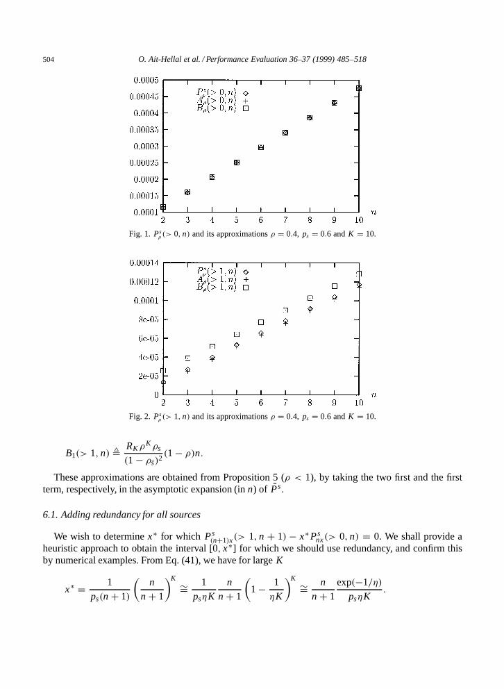
In Fig. 1, we display the values of Ps² .> 0; n/ and its approximations (from Proposition 5):

A0.> 0; n/ , RK²K

.1� ²Ns/�.1� ²/n C ²s

�1

1� ² �²Ns

1� ²Ns

��;

B0.> 0; n/ , RK²K

.1� ²Ns/.1� ²/nin the case K D 10, n � 10, ² D 0:4 and ps D 0:6.

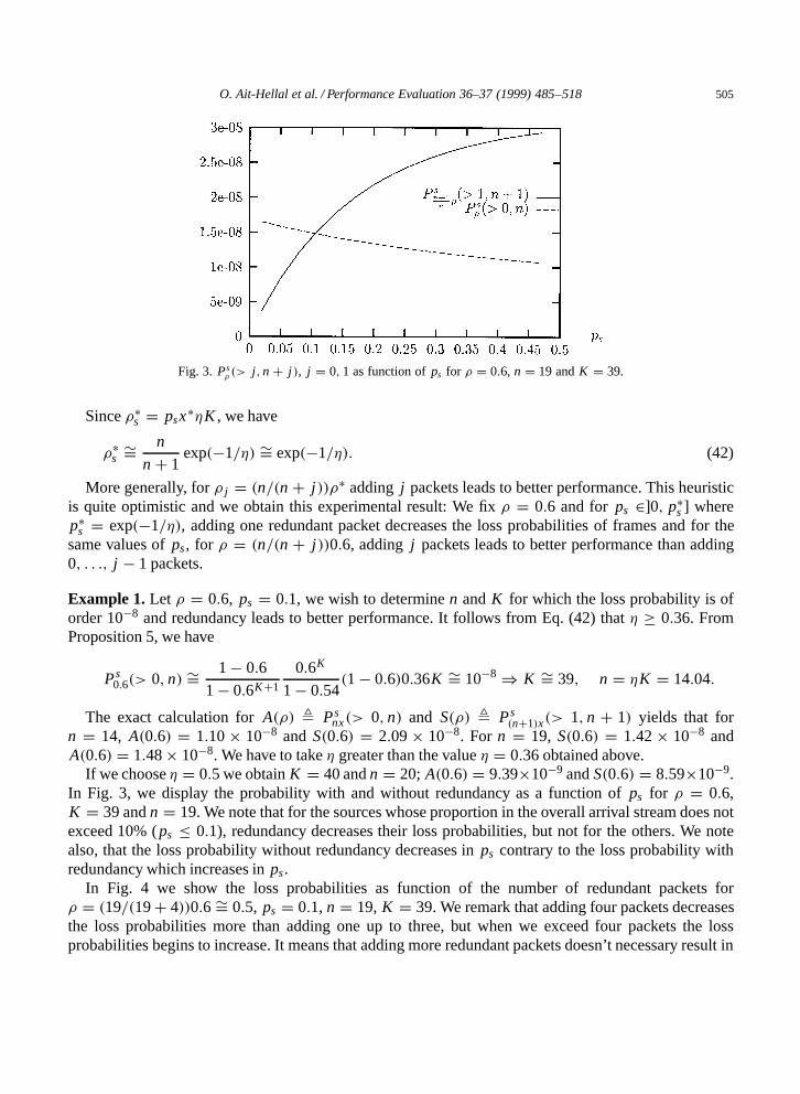
In Fig. 2, we make the same comparison for Ps² .> 1; n/ and

A1.> 1; n/ , RK²K²s

.1� ²Ns/2�.1� ²/n C ² C ²s � 1

1� ² � ²s²Ns1� ²Ns

�;


Fig. 1. Ps² .> 0; n/ and its approximations ² D 0:4, ps D 0:6 and K D 10.

Fig. 2. Ps² .> 1; n/ and its approximations ² D 0:4, ps D 0:6 and K D 10.

B1.> 1; n/ , RK²K²s

.1� ²Ns/2 .1� ²/n:

These approximations are obtained from Proposition 5 (² < 1), by taking the two first and the firstterm, respectively, in the asymptotic expansion (in n) of QPs .

6.1. Adding redundancy for all sources

We wish to determine xŁ for which Ps.nC1/x.> 1; n C 1/ � xŁPs

nx.> 0; n/ D 0. We shall provide aheuristic approach to obtain the interval [0; xŁ] for which we should use redundancy, and confirm thisby numerical examples. From Eq. (41), we have for large K

xŁ D 1

ps.n C 1/

�n

n C 1

�K¾D 1

ps�K

n

n C 1

�1� 1

�K

�K¾D n

n C 1

exp.�1=�/

ps�K:


Fig. 3. Ps² .> j;n C j/, j D 0; 1 as function of ps for ² D 0:6, n D 19 and K D 39.

Since ²Łs D psxŁ�K , we have

²Łs ¾Dn

n C 1exp.�1=�/ ¾D exp.�1=�/: (42)

More generally, for ² j D .n=.n C j//²Ł adding j packets leads to better performance. This heuristicis quite optimistic and we obtain this experimental result: We fix ² D 0:6 and for ps 2]0; pŁs ] wherepŁs D exp.�1=�/, adding one redundant packet decreases the loss probabilities of frames and for thesame values of ps , for ² D .n=.n C j//0:6, adding j packets leads to better performance than adding0; : : :; j � 1 packets.

Example 1. Let ² D 0:6, ps D 0:1, we wish to determine n and K for which the loss probability is oforder 10�8 and redundancy leads to better performance. It follows from Eq. (42) that � ½ 0:36. FromProposition 5, we have

Ps0:6.> 0; n/ ¾D 1� 0:6

1� 0:6KC1

0:6K

1� 0:54.1� 0:6/0:36K ¾D 10�8) K ¾D 39; n D �K D 14:04:

The exact calculation for A.²/ , Psnx.> 0; n/ and S.²/ , Ps

.nC1/x.> 1; n C 1/ yields that forn D 14, A.0:6/ D 1:10 ð 10�8 and S.0:6/ D 2:09 ð 10�8. For n D 19, S.0:6/ D 1:42 ð 10�8 andA.0:6/ D 1:48ð 10�8. We have to take � greater than the value � D 0:36 obtained above.

If we choose � D 0:5 we obtain K D 40 and n D 20; A.0:6/ D 9:39ð10�9 and S.0:6/ D 8:59ð10�9.In Fig. 3, we display the probability with and without redundancy as a function of ps for ² D 0:6,K D 39 and n D 19. We note that for the sources whose proportion in the overall arrival stream does notexceed 10% (ps � 0:1), redundancy decreases their loss probabilities, but not for the others. We notealso, that the loss probability without redundancy decreases in ps contrary to the loss probability withredundancy which increases in ps .

In Fig. 4 we show the loss probabilities as function of the number of redundant packets for² D .19=.19C 4//0:6 ¾D 0:5, ps D 0:1, n D 19, K D 39. We remark that adding four packets decreasesthe loss probabilities more than adding one up to three, but when we exceed four packets the lossprobabilities begins to increase. It means that adding more redundant packets doesn’t necessary result in


Fig. 4. Ps.nC j/²=n.> j; n C j/ as function of j for ² D 0:5, ps D 0:1, n D 19 and K D 39.

a decrease of the loss probabilities. In fact, the adequate number of redundant packets which we shouldadd in order to decrease, as much as possible, the loss probabilities strongly depends on the workloadand the size of frames.

6.2. Adding redundancy only for source s

We are interested by the case when redundancy is added only for the source s. We assume that therate at which frames arrive is the same with and without redundancy. When one redundant packet isadded for source s, we have ½ D ² D nx C psx . We proceed similarly as above, we get for large K

²Łs D exp.�ps=�/: (43)

Example 2. Let ² D 0:8 and ps D 0:1, we wish to determine n and K for which the loss probability isof order 10�9 and redundancy leads to better performance. From Eq. (43) we have � D 0:04 and fromProposition 5 we have

Ps0:8.> 0; n/ ¾D 1� 0:8

1� 0:8KC1

0:8K

1� 0:72.1� 0:8/0:04K ¾D 10�9) K ¾D 90; n D �K ¾D 4:

Exact calculation for A.²/ , Psnx.> 0; n/ and S0.²/ , Ps

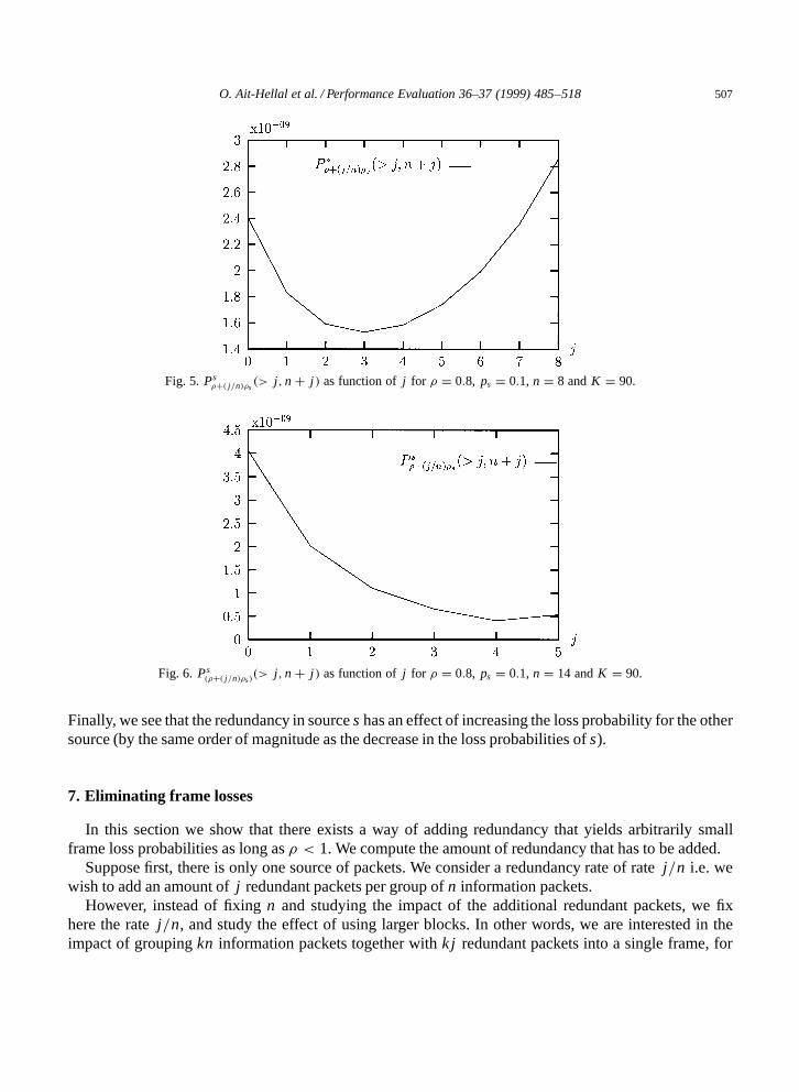
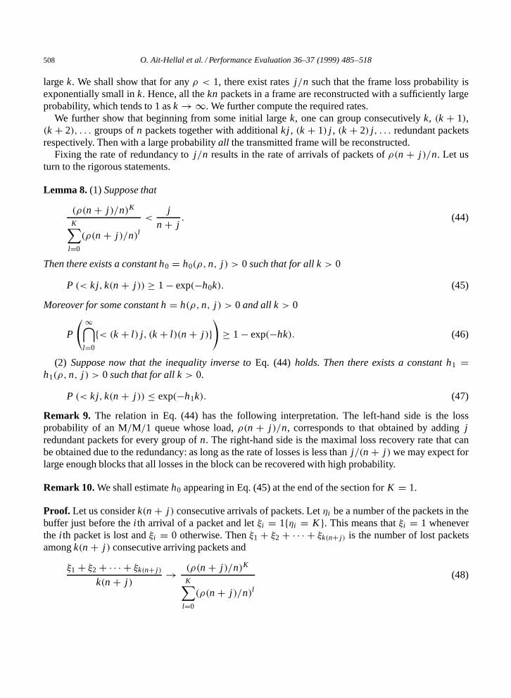
nxCps x .> 1; n C 1/ yields that for n D 4and K D 90, S.0:8/ D 2:67 ð 10�9 and A.²/ D 1:28 ð 10�9 and for n D 7, K D 90 we haveS.0:8/ D 1:86 ð 10�9 and A.²/ D 2:12 ð 10�9, thus for n ½ 7, S.²/ < A.²/. We display in Fig. 5the loss probabilities as function of the number of redundant packets for n D 8, K D 90, ² D 0:8and ps D 0:1. We note that the larger size of frames leads to better performance in the presence ofredundancy. For the same example, by taking n D 14, we reduce the loss probabilities of frames by anorder of 10 when we add 4 redundant packets only for source s (Fig. 6). Note that this improvement hasa negative effect on the other sources.

For the example above, if we consider only two sources s and Ns, we have pNs D 0:9 and P Ns0:8 D2:114ð10�9. When we add 4 redundant packets for s the workload becomes² D 0:8C 4

140:08 D 0:8228,ps D 18

140:1 D 0:1285 and pNs D 1�0:1285 D 0:8715. For these values, we obtain P Ns0:8228 D 2:305ð10�8.


Fig. 5. Ps²C. j=n/²s

.> j; n C j/ as function of j for ² D 0:8, ps D 0:1, n D 8 and K D 90.

Fig. 6. Ps.²C. j=n/²s /

.> j; n C j/ as function of j for ² D 0:8, ps D 0:1, n D 14 and K D 90.

Finally, we see that the redundancy in source s has an effect of increasing the loss probability for the othersource (by the same order of magnitude as the decrease in the loss probabilities of s).

7. Eliminating frame losses

In this section we show that there exists a way of adding redundancy that yields arbitrarily smallframe loss probabilities as long as ² < 1. We compute the amount of redundancy that has to be added.

Suppose first, there is only one source of packets. We consider a redundancy rate of rate j=n i.e. wewish to add an amount of j redundant packets per group of n information packets.

However, instead of fixing n and studying the impact of the additional redundant packets, we fixhere the rate j=n, and study the effect of using larger blocks. In other words, we are interested in theimpact of grouping kn information packets together with k j redundant packets into a single frame, for


large k. We shall show that for any ² < 1, there exist rates j=n such that the frame loss probability isexponentially small in k. Hence, all the kn packets in a frame are reconstructed with a sufficiently largeprobability, which tends to 1 as k !1. We further compute the required rates.

We further show that beginning from some initial large k, one can group consecutively k, .k C 1/,.k C 2/; : : : groups of n packets together with additional k j , .k C 1/ j , .k C 2/ j; : : : redundant packetsrespectively. Then with a large probability all the transmitted frame will be reconstructed.

Fixing the rate of redundancy to j=n results in the rate of arrivals of packets of ².n C j/=n. Let usturn to the rigorous statements.

Lemma 8. (1) Suppose that

.².n C j/=n/K

KXlD0

.².n C j/=n/l<

j

n C j: (44)

Then there exists a constant h0 D h0.²; n; j/ > 0 such that for all k > 0

P .< k j; k.n C j// ½ 1� exp.�h0k/: (45)

Moreover for some constant h D h.²; n; j/ > 0 and all k > 0

P

1\lD0

f< .k C l/ j; .k C l/.n C j/g!½ 1� exp.�hk/: (46)

(2) Suppose now that the inequality inverse to Eq. (44) holds. Then there exists a constant h1 Dh1.²; n; j/ > 0 such that for all k > 0.

P .< k j; k.n C j// � exp.�h1k/: (47)

Remark 9. The relation in Eq. (44) has the following interpretation. The left-hand side is the lossprobability of an M=M=1 queue whose load, ².n C j/=n, corresponds to that obtained by adding jredundant packets for every group of n. The right-hand side is the maximal loss recovery rate that canbe obtained due to the redundancy: as long as the rate of losses is less than j=.n C j/we may expect forlarge enough blocks that all losses in the block can be recovered with high probability.

Remark 10. We shall estimate h0 appearing in Eq. (45) at the end of the section for K D 1.

Proof. Let us consider k.n C j/ consecutive arrivals of packets. Let �i be a number of the packets in thebuffer just before the i th arrival of a packet and let ¾i D 1f�i D K g. This means that ¾i D 1 wheneverthe i th packet is lost and ¾i D 0 otherwise. Then ¾1 C ¾2 C Ð Ð Ð C ¾k.nC j/ is the number of lost packetsamong k.n C j/ consecutive arriving packets and

¾1 C ¾2 C Ð Ð Ð C ¾k.nC j/

k.n C j/! .².n C j/=n/K

KXlD0

.².n C j/=n/l(48)


in probability as k !1 with exponential rate (see below). In fact, the sequence �i forms an irreducibleaperiodic finite Markov chain on the state space f0; 1; : : :; K g. The fraction in the left-hand side ofEq. (48) is the empirical measure of the time spent by this chain at the state K . It is well-known thatit converges in probability to a stationary probability of the state K , which is in the right-hand side ofEq. (48). Assume that Eq. (44) holds. Then we can choose " > 0 such that

.².n C j/=n/K

KXlD0

.².n C j/=n/lC " < j

n C j:

Then for some h0 > 0 (which is a function of ") and all k > 0

P .< k j; k.n C j// D P�¾1 C ¾2 C Ð Ð Ð C ¾k.nC j/ < k j

Ð½ P

0B@¾1 C ¾2 C Ð Ð Ð C ¾k.nC j/

k.n C j/<

.².n C j/=n/K

KXlD0

.².n C j/=n/lC "

1CA½ 1� exp.�h0k/: (49)

The last inequality follows from standard Large deviation arguments, see e.g. section 3.1 in [7]. ThusEq. (45) is proved. The inequality Eq. (47) is derived by the same way from the convergence Eq. (48).

To get Eq. (46) we note that the convergence in Eq. (48) does not depend on an initial distribution,then for all l > 0

P

f< .k C l/ j; .k C l/.n C j/gþþ l�1\

iD0

f< .k C i/ j; .k C i/.n C j/g!½ 1� exp.�h0.k C l//:

Then for some h > 0 and all k > 0

P

1\lD0

f< .k C l/ j; .k C l/.n C j/g!½1Y

lD0

[1� exp.�h0.k C l//] ½ 1� exp.�hk/:

This establishes the proof. �

In the following lemma we show the way to find j for given K > 0, ² < 1 and n such that theproposed strategy is valid, i.e. the inequality Eq. (44) is fulfilled.

Lemma 11. Let us fix K > 0 and ² > 0.If ² ½ 1, the inequality Eq. (44) does not hold for any pair of integers j > 0 and n > 0.If ² < 1, then for all sufficiently large n, we can find an integer j > 0 such that Eq. (44) holds.

Moreover, the minimal j with this property is such that:

j=n < .1� ²/=²; if K > ²=.1� ²/I j=n > .1� ²/=²; if K < ²=.1� ²/:

Proof. Denote by Þ :D j=n. Then, except when ².1C Þ/ D 1, Eq. (44) can be written as

.².1C Þ//K .².1C Þ/� 1/

.².1C Þ//KC1 � 1<

Þ

1C Þ : (50)


This inequality holds for no Þ ½ 0 under the assumption ² ½ 1. If ² < 1, then Eq. (50) implies(²K .1C Þ/KC1 > Þ=.1� ²/;².1C Þ/ > 1;

and

(²K .1C Þ/KC1 < Þ=.1� ²/;².1C Þ/ < 1:

(51)

Let us introduce the function f .Þ/ D ²K .1 C Þ/KC1 � Þ=.1 � ²/, which equals zero whenÞ D 1=² � 1 D .1� ²/=². The systems (51) mean that

f .Þ/ < 0 if Þ < .1� ²/=²I f .Þ/ > 0 if Þ > .1� ²/=²: (52)

ž Assume that K > ²=.1�²/. This amounts to say that f 0 ..1� ²/=²/ > 0. Then in the neighborhoodof Þ D .1 � ²/=², we have Eq. (52). The elementary analysis of f .Þ/ shows that there existsÞ0 < .1 � ²/=², such that f .Þ0/ D 0, f .Þ/ > 0 on [0IÞ0/, f .Þ/ < 0 on .Þ0I .1 � ²/=²/ andf .Þ/ > 0 on ..1� ²/=²I1/. To get Eq. (44), we take Þ 2 .Þ0I1/, or equivalently j 2 .nÞ0I1/.

ž Suppose now that K < ²=.1 � ²/, i.e. in other words f 0 ..1� ²/=²/ < 0. Then Eq. (52) does nothold in the neighborhood of Þ D .1 � ²/=² neither on [0I .1 � ²/=²]. However, there exists someÞ0 > .1� ²/=² such that f .Þ/ > 0 on [Þ0I1/. So, to obtain Eq. (44), we take the minimal integer jon [nÞ0I1/.

Note that for ² > 1 the suggested strategy does not fit at all. �

To complete our investigation, we will also specify the estimation (45) from Lemma 8 in the caseK D 1. The sequence �i forms a Markov chain L on the state space f0; 1g with the matrix of transitionprobabilities:0BBB@

1

1C ².n C j/=n

².n C j/=n

1C ².n C j/=n

1

1C ².n C j/=n

².n C j/=n

1C ².n C j/=n

1CCCA :Let �1; �2; : : : be a sequence of i.i.d. random variables distributed as the time to return to the state

1 starting from it by the chain L. Indeed, E�1 D .1 C ².n C j/=n/.².n C j/=n/�1. Let also �0 be arandom variable distributed as the time to reach the state 1 at the stationary regime. Then, for all Ž > 0such that E exp.Ž�i / <1, i D 0; 1, and all n, j and k by Chernof inequality we have:

P .> k j; .n C j/k/ D P��0 C �1 C Ð Ð Ð C �k j � k.n C j/

Ð� E exp.Ž�0/ .E exp Ž.�1 � .n C j/=j//k j

D E exp.Ž�0/ exp�ð

log.E exp Ž�1/� Ž.n C j/=jŁ

jkÐ: (53)

It is easy to verify that

E exp.Ž�0/ D ².n C j/=n

1C ².n C j/=n � exp Ž; E exp.Ž�1/ D ².n C j/=n exp Ž

1C ².n C j/=n � exp Ž:

Let us assume that Eq. (44) holds, i.e.

j

n C j� ².n C j/=n

1C ².n C j/=n> 0: (54)


Then the function f .Ž/ D � log.E exp Ž�1/C Ž.nC j/=j is increasing on [0; Ž0] and is decreasing on[Ž0; ln.1C ².n C j/=n/], ( f .0/ D 0), where Ž0 D ln .² C n=.n C j//.

The estimation (53) with Ž D Ž0 implies

P .> k j; .n C j/k/ � E exp .Ž0�0/ exp .� j f .Ž0/k/

for all k > 0, where

E exp.Ž0�0/ D ².n C j/=n

1C ².n C j/=n

n C j

j;

f .Ž0/ D � ln

�²

n C j

n

�C n C j

jln

�² C n

n C j

�:

The constant j f .Ž0/ is a Large deviation constant.Let us now proceed with the case of many sources of packets. Suppose, we are interested in

decreasing the losses of frames or of packets issued only from one source s. Hence, we add j redundantpackets from n, originated from s, thus the total rate is ²s.n C j/=n C ²Ns . Let as usual ²s D ½s=¼,²Ns D ½Ns=¼ D .½�½s/=¼. The strategy, that we use, is the same as in the previous case: kn, .kC 1/n; : : :packets from the source s are grouped together with the redundancy of k j , .k C 1/ j; : : : respectively.In the case of one source, only for ² < 1, there is a suitable j to render the strategy profitable. In thecase of many sources, to find such a j , the restriction ²s < 1 remains necessary. However, the inequality² D ²s C ²Ns > 1 is accepted.

Lemma 12. (1) Suppose that

.²s.n C j/=n C ²Ns/K

KXlD0

.²s.n C j/=n C ²Ns/l<

j

n C j: (55)

Then there exists h0 > 0 such that for all k > 0

P .< k j; k.n C j// ½ 1� exp.�h0k/: (56)

Moreover for some h > 0 and all k > 0

P

1\lD0

f< k j; k.n C j/g!½ 1� exp.�hk/: (57)

(2) Suppose that the inequality inverse to Eq. (55) holds. Then for some h1 > 0 and all kP .< k j; k.n C j// � exp.�h1k/.

The proof is completely analogous to the proof of Lemma 8.

Lemma 13. Assume that ²s > 0, ²Ns > 0, K and n are fixed. There exists an integer j satisfying Eq. (55)if and only if ²s < 1.


Proof. The proof is carried out as the proof of Lemma 11. Without going into details, we will point outthe way to find the minimal integer j satisfying Eq. (55).

Denote by Þ :D j=n, then the inequality Eq. (55) is equivalent to the following:

.²s.1C Þ/C ²Ns/K .²s.1C Þ/C ²Ns � 1/

.²s.1C Þ/C ²Ns/KC1 � 1<

Þ

1C Þ ; (58)

except when ²s.1C Þ/C ²Ns D 1. It holds for no Þ ½ 0 if ²s ½ 1.ž Assume that ² D ²s C ²Ns > 1, ²s < 1. Then, to get Eq. (58), we should take Þ satisfying the system8><>:

.²s.1C Þ/C ²Ns/K >Þ

.1� ²s/Þ C 1� ² ;Þ >

²Ns1� ²s

� 1:

There exists minimal Þ0 such that the system holds on .Þ0I1/, i.e. j 2 .nÞ0I1/.ž Assume that ² D 1. Then we have to take Þ satisfying the inequality .1C Þ²s/

K > 1=.1� ²s/.ž Assume now that ² < 1. There are two cases.

If K > ²s=.1 � ²/ then there is the minimal Þ0 < .1 � ²Ns/=²s � 1 D .1 � ²/=²s such that on thesegment .Þ0I .1� ²/=²s/ the inequality

.²s.1C Þ/C ²Ns/K <Þ

.1� ²s/Þ C 1� ²holds. We take j 2 .nÞ0I n.1� ²/=²s/.If K < ²s=.1� ²/ then there exists the minimal Þ0 > .1� ²/=²s such that the inequality

.²s.1C Þ/C ²Ns/K >Þ

.1� ²s/Þ C 1� ²holds on .Þ0I1/. We take j 2 .nÞ0I1/. �

8. General arrivals and service times

We relax in this section the probabilistic assumptions on the distributions of the arrival and serviceprocesses: we consider a stationary ergodic sequence f¦ng; n 2 Z (where Z D f: : :;�2;�1; 0; 1; 2; : : :g)of service times, and a stationary ergodic sequence f−ng; n 2 Z, of interarrival times of packets.

We consider a finite queue with capacity K ½ 1. Define ² , E¦1=E−1.

8.1. Basic idea

We present in this subsection the general idea behind the elimination of losses. Assume that theprocess f−n; ¦ng is already the one observed after we included the redundancy of rate j : for eachinformation packet we added j redundant ones. We denote by ½. j C 1/ the input arrival rate of packets.Assume that this process feeds a finite FIFO queue, and that the joint process of arrivals and queuelength is stationary ergodic.

We call a frame a sequence of . j C 1/k consecutive packets, where k is some parameter. We assumethat all packets from the frame can be recovered if there are no more than jk losses within the frame.


Assume that the following reasonable property is satisfied: as j !1, the output rate (the expectednumber of departures per time unit) from the queue approaches ¼ :D 1=E−1. Fix " > 0 such that² C " < 1 and let j be such that the output rate from the queue is greater than ¼.1 � "/. Then theproportion p j of lost packets satisfies

p j D input rate� output rate

input rate

<. j C 1/½� ¼.1� "/

. j C 1/½D j

j C 1C ² C " � 1

. j C 1/²<

j

j C 1:

Due to the stationarity and ergodicity assumptions, for any Ž > 0, the number of losses within a frameis less than k j .p j C Ž/ with probability that approaches 1 as k !1.

Thus with probability arbitrarily close to one, the actual number of losses per frame will be smallerthan k j by choosing j and k sufficiently large, and all losses in the frame can be recovered.

8.2. Actual redundancy scheme

We restrict here to the case where the service times are i.i.d. and are independent of the interarrivaltimes and K D 1.

We shall assume throughout that ² < 1 before adding redundancy. Under this assumption, we showthat by adding appropriately redundant packets, one can obtain loss probabilities as small as desired. Weassume that the sequence of interarrival times f−ng; n 2 Z of the original information packets (before weadd redundancy) is stationary ergodic.

For some integer k that will be determined later, we call the group of packets number nk C 1; nk C2; : : :; .n C 1/k the nth block of information packets. We shall add jk redundant packets to the eachblock. The . j C 1/k packets which include the original block as well as the additional redundant packetsare called a frame. We assume that the service times of the redundant packets added to a block have thesame distribution as ¦1; ¦n will in fact denote the service time of the nth packet actually served, whetherit is an information packet or a redundant one.

As long as the number of losses in a frame is less than or equal to jk, all the frame (and in particular,the original information packets) can be retrieved at the destination. Define

r D E−1 C E¦1

2. j C 1/

and consider the following transport protocol:(1) Blocking phase: Wait till a whole block of k information packets is generated at the source; as long

as the whole block is not generated, we do not transmit any packet of the block.(2) Framing phase: once all k packets have arrived, we compute the extra jk redundant packets.(3) Transmission phase: Once the whole frame has been generated, all packets of the frame are put in

a transmission buffer. Packets are transmitted from this buffer at a constant rate 1=r , i.e. the timebetween transmission of two consecutive packets is r .

The above protocol requires buffering capability at the source of at least one frame. To make ourprotocol realistic we have to assume thatž The capacity of the transmission buffer at the source is finite.


This implies that losses may occur also due to buffer overflow at the source, and not only at thebuffer inside the network. We shall show that the above protocol can render the total loss probabilitiesarbitrarily small.

Note that congestion at the source occurs typically at periods during which interarrival times areshort. In order to minimize the buffer requirements at the source we shall thus assume thatž we deliberately drop the nth frame at the source if and only if

PkiD1 −nkCi < kr. j C 1/. In that case,

the framing and transmission phase for frame n are not performed.In case that the computation required in the framing phase takes a negligible amount of time, this

assumption on dropping at the source implies that the total buffering required at the source is exactly ofone frame and is thus minimal.

We shall assume that the above protocol has been used for at least one frame before packet 1 istransmitted, and that before it was used, the system was empty.

Theorem 14. With ² < 1, the above protocol results in frame loss probabilities that can be madearbitrarily small by an appropriate choice of k and j .

Proof. Consider an arbitrary frame, say frame 1, and let OT be the time at which the first packet of thatframe arrives to the buffer inside the network. Define

1 ,

kXiD1

¦i C � > jkr

!; 2 ,

kX

iD1

−i < . j C 1/kr

!;

where � is the residual service time in the buffer inside the network at OT (the packet that arrives at thenetwork buffer might find there another packet from some previous frame that is still getting service; theremaining service time of that packet is called �, and it is considered to be zero if there is no such packetat time OT ).

Let " > 0 be an arbitrary small number. One can choose j and k such that P.1/ < " andP.2/ < ". That this choice is possible follows since ² < 1, since P � a:s:

limk!1

1

k

kXiD1

¦i D E¦1 < jr; limk!1

1

k

kXiD1

−i D E−1 > . j C 1/r

and since for all Ž > 0 P.� > kŽ/! 0 as k ! 1. This fact needs some additional explanation (notethat the distribution of � might depend on k and on the number of the frame that we consider). Let OSbe the time at which the last successful packet transmission occurred from the buffer inside the networkbefore time OT . Let An denote the event that the number of packets that were blocked (and thus lost) inthe buffer inside the network during the time interval . OS; OT / was exactly n. n ½ 0. (In the case n D 0the last packet of the previous frame is served.) Then P.f� > kŽg \ An/ � P.¦1 > nr C kŽ/. SinceE¦1 <1,

P.� > kŽ/ �1X

nD0

P.¦1 > nr C kŽ/! 0 as k !1: (59)

On the event N2 (the complement of2) the new frame is not dropped at the transmission buffer.


On N1, the time T till the k first successful transmissions of packets occurs satisfies T � � CPkiD1 ¦i C kr � . j C 1/kr . Thus the number of packets successfully transmitted on the event N1 \ N2

among the first frame is at least k, so that the probability of a successful transmission of the whole firstframe is at least 1� 2". (Indeed, no later than OT C � C r , the first successful transmission in the framebegins, no later than OT C � C ¦1 C 2r , the 2nd successful transmission begins, etc.).

The same argument holds for any frame; since the bound in Eq. (58) is uniform for all frames, thisestablishes the proof. �

9. Discussion

In this paper, we have shown the effect of adding redundancy to losses of packets and of frames dueto overflow in a finite queue. Explicit expressions for the loss probabilities of frames were obtained inthe case of several traffic streams that are multiplexed at the input of a finite buffer. We have obtainedschemes of adding redundancy that may almost eliminate loss probabilities for any given buffer size aslong as the offered load of the traffic to which redundancy is added is lower than 1 (before adding theredundancy). The price to pay is long delays due to the need to consider redundancy of large blocks. Theanalysis of the required delay and the tradeoff between losses and delay are the issue of future work.

Appendix A

We return to the asymptotic behavior of Ps² .> j; n/ and show that the terms [zn�1] f0.z/ and

[zn�1] f1.z/ can be neglected as n!1, n < K .

Proposition A.1. We have

Ps² .> 0; n/ D QPs

² .> 0; n/.1C o.1//; as n!1; n < K (A.1)

Ps² .> 1; n/ D QPs

² .> 1; n/.1C o.1//; as n!1; n < K : (A.2)

Moreover o.1/ is exponentially small in K (there exists 0 < þ < 1: jo.1/j � þK ).

Proof. Let us first prove Eq. (A.1). We have

Ps² .> 0; n/ D �RK²

K [zn�1]1

1� z

x1

z � x1

1� .x2=x1/KC1

1� .x2=x1/K .z � x2/=.z � x1/

D �RK²K [zn�1]

1

1� z

x1

z � x1

�1C .x2=x1/

K ..z � x2/=.z � x1/� x2=x1/

1� .x2=x1/K .z � x2/=.z � x1/

�:

Let us denote for shortness

an�1 D [zn�1]1

z � 1

x1

z � x1;

bn�1 D [zn�1].x2=x1/

K ..z � x2/=.z � x1/� x2=x1/

1� .x2=x1/K .z � x2/=.z � x1/

;


cn�1 D [zn�1]1

1� z

x1

z � x1

.x2=x1/K ..z � x2/=.z � x1/� x2=x1/

1� .x2=x1/K .z � x2/=.z � x1/:

Then QPs² .> 0; n/ D �RK²

K an�1 and by Eq. (33) there are constants C1;C2 > 0 such that

C1 < janj < C2n < C2K : (A.3)

Moreover, Ps² .> 0; n/ D �RK²

K .an�1 C cn�1/, where cn�1 DPn�1

kD0 an�1�kbk . Thus, it suffices toshow that for some 0 < þ < 1

jcnj � janjþK : (A.4)

By virtue of Eq. (A.3)

jcn�1j � C2.K � 1/n�1XkD0

jbk j: (A.5)

Let us now estimate bk . The function

g0.z/ D .x2=x1/K ..z � x2/=.z � x1/� x2=x1/

1� .x2=x1/K .z � x2/=.z � x1/D x K

2 z.x1 � x2/

x1�x K

1 .z � x1/� x K2.z � x2/Ð

is analytic in the disk jzj < 1C " for sufficiently small " > 0. In factž x1 6D 0 for all z, (² 6D 0);ž if z � x1 D 0, then x2.z � x2/ 6D 0;ž the branching point of x1.z/ and x2.z/ is outside the unit disk. The branches x1.z/ and x2.z/ have

been chosen in such a way that jx2.0/j=jx1.0/j < 1. The equality jx2.z/j=jx1.z/j D 1 takes place onlyif Re z D 1C .1� ²/2=4²²Ns > 1. The function jx2.z/j=jx1.z/j being continuous,

infjzj�1C"

þþþþx2.z/

x1.z/

þþþþ D < 1:

Hence for sufficiently large K , x K1 .z � x1/� x K

2 .z � x2/ 6D 0 for all z 2 fz: jzj � 1C "g. In additionfor some C3 > 0, jg0.z/j � C3

K . Then for some C4 > 0,

jbkj Dþþþþ 1

2πi

ZjzjD1C"

g0.z/

zkC1dz

þþþþ � C4 K .1C "/�k :

Therefore, taking into account Eq. (A.5), we have for some 0 < 0 < 1, 0 > ,

jcn�1j � C2.K � 1/ K C4

n�1XkD0

.1C "/�k � K0 :

This estimation together with Eq. (A.3) implies Eq. (A.4) and thus Eq. (A.1) is proved. Let us now


turn to the case j D 1.

Ps² .> 1; n/ D �RK²

K [zn�1]1

1� z

x1

z � x1

z.1� x1/

z � x1

1� .x2=x1/KC1

1� .x2=x1/K .z � x2/=.z � x1/

ð 1� .x2=x1/K .1� x2/=.1� x1/

1� .x2=x1/K .z � x2/=.z � x1/

D �RK²K [zn�1]

1

1� z

x1

z � x1

z.1� x1/

z � x1.1C g1.z/C g2.z// ;

where

g1.z/ Dx K

2

��x K

1 x2.z � x1/2 C 2x KC1

1 .z � x2/.z � x1/� x1x K2 .z � x2/

2�

x1�x K

1 .z � x1/� x K2 .z � x2/

Ð2 ;

g2.z/ D x K2 .x

KC12 � x KC1

1 /.1� x2/.z � x1/2

x1.1� x1/�x K

1 .z � x1/� x K2 .z � x2/

Ð2 :

The functions g1.z/ and g2.z/ are analytic in the disk jzj < 1 C " due to the same arguments as forg0.z/. (The point z D 1, where x1.z/ � 1 D 0 can not be a pole of g2.z/ because of .z � x1/

2 in thenumerator.) Further, the proof of Eq. (A.2) is carried out along the same lines as of Eq. (A.1), so theother details are skipped. �

References

[1] E. Altman, A. Jean-Marie, Loss probabilities for messages with redundant packets feeding a finite buffer, IEEE J.Selected Areas Commun. 16 (5) (1998) 779–787.

[2] J.-C. Bolot, A. Vega Garcia, The case for FEC-based error control for packet audio in the Internet, to appear in ACMMultimedia Systems.

[3] G. Carle, Adaptable error control for efficient provision of reliable services in ATM networks, in: IFIP, WG.6.2Broadband Communication, Proceedings of the First Workshop on ATM Traffic Management, WATM’95, Paris, 1995,pp. 399–406.

[4] N. Cem O Lguz, E. Ayanoglu, Performance analysis of two-level forward error correction for lost cell recovery in ATMnetworks, in: Proc. INFOCOM ’95, pp. 6b.3.1–6b.3.10.

[5] I. Cidon, A. Khamisy, M. Sidi, Analysis of packet loss process in high-speed networks, IEEE Trans. IT 39 (1) (1993)98–108.

[6] G. Clark, J.B. Cain, Error Correcting Coding for Digital Communications, Plenum Press, New York, 1981.[7] A. Dembo, O. Zeitouni, Large Deviations Techniques, Jones and Bartlett, Sudbury, MA, 1993.[8] P. Flajolet and A. Odlyzko, Singularity analysis of generating functions, SIAM J. Disc. Math. 3(2) (1990) 216–240.[9] O. Gurewitz, M. Sidi, I. Cidon, The Ballot Theorem strikes again: packet loss process distribution, manuscript.

[10] K. Kawahara, K. Kumazoe, T. Takine, Y. Oie, Forward error correction in ATM networks: an analysis of cell lossdistribution in a block, in: Proceedings of IEEE INFOCOM ’94, Toronto, Canada, June 1994, pp. 1150–1159.

[11] D. Kofman, M. Gagnaire, Reseaux Haut Debit: Reseaux ATM, Reseaux Locaux et Reseaux Tout-optiques, InterEditions(groupe Masson), Paris, 1996.

[12] J. Nonnenmacher, E. Biersack, D. Towsley, Parity-based loss recovery for reliable multicast transmission, in: Proceed-ings of Sigcom 97, Cannes, France, 1997, pp. 289–299.

[13] N. Shacham, P. McKenney, Packet recovery in high-speed networks using coding and buffer management, in:Proceedings of INFOCOM ’90, San Francisco, CA, 1990, pp. 124–131.


Omar Ait-Hellal ([email protected]) received a DEA degree (French Master de-gree) from University of Versailles, and a Ph.D. degree from University of Nice-Sophia Antipolisin 1995, and 1998 respectively. In November 1998, he joined the Research Unit in Networking atUniversity of Liege for a post-doctoral position. His main interests include FEC, flow control inhigh speed networks and middleware transport protocols.

Eitan Altman received the B.Sc. degree in electrical engineering (1984), the B.A. degree in physics(1984) and the Ph.D. degree in electrical engineering (1990), all from the Technion-Israel Institute,Haifa. In (1990) he further received his B.Mus. degree in music composition in Tel-Aviv University.Since 1990, he has been with INRIA (National Research Institute in Informatics and Control) inSophia Antipolis, France. His current research interests include performance evaluation and controlof telecommunication networks, stochastic control and dynamic games. In recent years, he hasapplied control theoretical techniques in several joint projects with the French telecommunicationscompany – France Telecom.

Alain Jean-Marie obtained his Ph.D. degree in Computer Science from the University of ParisXI at Orsay, France, in 1987. Since then, he has been researcher at the INRIA (French NationalInstitute of Computer Science and Control) in Sophia Antipolis.

Irina Kurkova, born 15=01=1974 in Moscow. In 1996 she graduated from the Department ofMathematics at Moscow State University in Russia. In 1998 she defended her Ph.D. Thesis titled‘Poisson and Martin boundaries for two-dimensional random walks’ at the Chair of Probability ofthe same university. She also has publications on some special queueing networks. Her researchinterests are mainly concerned with both analytic and probabilistic approaches for studing largerandom systems. The joint research presented in this paper was conducted in spring 1998 duringher stay in the MISTRAL group of INRIA Sophia Antipolis. Since April 1999 she is a postdocresearcher at Eurandom, the Netherlands.

On Loss Probabilities in Presence of Redundant Packets and Several Traffic Sources

Documents

Transcript of On Loss Probabilities in Presence of Redundant Packets and Several Traffic Sources