Wireless Netw (2008) 14:277–294

DOI 10.1007/s11276-006-9958-8

On k−coverage in a mostly sleeping sensor networkSantosh Kumar · Ten H. Lai · Jozsef Balogh

Published online: 23 October 2006C© Springer Science + Business Media, LLC 2006

Abstract Sensor networks are often desired to last many

times longer than the active lifetime of individual sensors.

This is usually achieved by putting sensors to sleep for most

of their lifetime. On the other hand, event monitoring appli-

cations require guaranteed k-coverage of the protected region

at all times. As a result, determining the appropriate number

of sensors to deploy that achieves both goals simultaneously

becomes a challenging problem. In this paper, we consider

three kinds of deployments for a sensor network on a unit

square—a√

n × √n grid, random uniform (for all n points),

and Poisson (with density n). In all three deployments, each

sensor is active with probability p, independently from the

others. Then, we claim that the critical value of the func-

tion npπr2/ log(np) is 1 for the event of k-coverage of every

point. We also provide an upper bound on the window of

this phase transition. Although the conditions for the three

deployments are similar, we obtain sharper bounds for the

An earlier version of this paper appeared in the Tenth AnnualInternational Conference on Mobile Computing and Networking(ACM MobiCom), September 25–October 1, 2004, Philadelphia, PA.Major differences from the conference version are in Sections 5, 6,and 7.

S. Kumar (�)Department of Computer Science, University of Memphis,Memphis, TN, USA 38152-3240e-mail: santosh.kumar@memphis.edu

T. H. LaiDepartment of Computer Science and Engineering, Ohio StateUniversity, Columbus, OH, USA 43210e-mail: lai.1@osu.edu

J. BaloghDepartment of Mathematical Sciences, University of Illinois,Urbana, IL, USA 61801e-mail: jobal@math.uiuc.edu

random deployments than the grid deployment, which oc-

curs due to the boundary condition. In this paper, we also

provide corrections to previously published results. Finally,

we use simulation to show the usefulness of our analysis in

real deployment scenarios.

Keywords Sensor network . Deterministic deployment .

Random deployment . Coverage . Connectivity . Power

management

1 Introduction

This work was motivated by a fundamental problem currently

facing the deployment of sensor networks for event monitor-

ing applications such as fire detection, radiation detection,

and intrusion detection. Given an area to be protected, howmany sensors should be deployed so that every point in the

region is continuously covered by at least k active sensors,

and given that the network must last for a specified length of

time? This problem is challenging because individual motes

(a popular device that hosts sensors [10]) can last only 100–

120 hours (4–5 days) on a pair of AA batteries in the fully

active mode [5], while the network is desired to last for sev-

eral months. It is well known that when the motes are in the

sleeping mode, they consume only 0.1% of the energy con-

sumed in the active mode.1 A natural approach to extend the

network’s lifetime is, therefore, to let sensor nodes sleep in

turns. The fraction of time that a node remains active is called

its duty cycle.

Three issues need to be resolved before the above approach

becomes feasible. First, a method is needed to compute the

1 Experimental data shows that motes can last for more than a year ona 1% duty cycle [5].

Springer

278 Wireless Netw (2008) 14:277–294

required duty cycle for individual nodes, given the longevity

requirement of the network. Second, given a duty cycle, each

node needs to determine when to be active and when to enter

the sleeping mode. Third, and the most difficult, we need a

method to determine the appropriate number of sensor nodes

to be deployed that simultaneously achieves the desired goals

of longevity and continuous k-coverage. This is a nontrivial

problem because on the one hand, the economics dictates

minimizing the number of sensors needed in the deployment,

and on the other hand, it is essential to have enough of them

deployed that will guarantee a desired quality of monitoring

for a long enough period of time. The lack of a sound method

for computing the appropriate number of sensors needed of-

ten becomes a cause for concern in actual deployments. In-

deed, it is such a concern that has motivated our work.

Let us address the easier problems of determining an ap-

propriate duty cycle and the sleeping schedule. Consider the

following sleeping scheme, which we call Randomized In-

dependent Sleeping (RIS): Time is divided into periods. Al-

though the length of period is same for all nodes, the start

time of a period need not be synchronized. At the beginning

of a period, each sensor node independently decides whether

to remain awake for this period (with probability p) or go to

sleep (with probability (1 − p)). With this approach, the ex-

pected lifetime of the network will increase by a factor close

to 1/p. Now, given a desired network lifetime and the active

lifetime of individual sensor nodes, it is easy to compute the

value of p, which also happens to be the expected duty cy-

cle of each node. In addition, this approach of uniform duty

cycle will balance the energy consumption in the network.

We note here that the idea of dividing time into peri-

ods and allowing nodes to sleep during some periods has

been explored previously. A sentry-based power manage-

ment scheme was proposed in [12], where an active node is

called a sentry. However, the issue of how to select the sen-

tries dynamically is not addressed there. A scheme for sentry

selection was proposed in [9]. In this scheme, a node backs off

for an interval inversely proportional to its remaining energy

and then uses a communication radius equal to the sensing

radius to inform the neighbors in its sensing range of its in-

tention to become a sentry, if it has not heard such a message

from a neighbor already. Although basing the back-off inter-

val on the remaining energy is a good heuristic to balance the

energy consumption in the network, it does not lead to the

determination of the probability of sentry selection given a

desired network lifetime, unlike the RIS scheme. In addition,

the RIS scheme frees a node from the task of checking with

its neighbors as to whether it should become a sentry or not.

Balancing power consumption is only a desirable crite-

rion. The main goal is to guarantee full coverage with sen-

try nodes. One of the goals of the sentry selection scheme

proposed in [9] is to guarantee 1-coverage with the sentry

nodes. However, if not enough sensors have been deployed,

then the sentry selection scheme of [9] can not guarantee 1-coverage. Similarly, for guaranteeing k-coverage with sentry

nodes, algorithms proposed in [11, 18] can be used by the

nodes to decide (by interacting with their neighbors) if it is

necessary for them to be awake during a period to ensure k-

coverage of every point. But again, if not enough nodes have

been deployed, then there is no way that these algorithms

can guarantee k-coverage. Therefore, the development of a

sound method to compute the appropriate number of sensors

nodes to be deployed so that every node needs to be active

only p fraction of the time and still guarantee k-coverage of

every point in the region, is a fundamental problem currently

facing the deployment of sensor networks for the intrusion

detection application.

In this paper, we develop theories that can be used to an-

swer questions such as these. In addition, our theorems apply

to a variety of scenarios and platforms, other than the one

mentioned above. We consider sleep to be a form of failure.2

The sleeping sensors can be considered as “failed,” for the

duration of their sleep. The added benefit of this model is

that the sleep probability can be readily combined with the

probability of other forms of failure in sensor networks such

as failure to detect events of interest, or packet loss. For a

more extensive list of failures prevalent in sensor networks

deployed for intruder detection, classification and tracking,

we refer the reader to [2]. The problem we address in this

paper is that of developing the critical conditions relating the

number of nodes deployed, their sensing radius, and their

failure probability such that even in the case of failures (or

sleeping, or both), each point in the region is almost always

covered by at least k sensors. We consider three kinds of

deployments: a√

n × √n grid, random uniform (for all n

points), and Poisson (with density n). Considering determin-

istic and random deployments in the same spirit allows us to

make some interesting observations. For example, we find

that the number of sensors needed in the grid deployment

with RIS sleeping is of the same order as that in the random

deployments with RIS sleeping, with a second order differ-

ence due to the boundary condition in the grid deployment.

We would like to briefly mention a few reasons for requir-

ing k-coverage rather than just 1-coverage in applications.

1. In the intruder detection application, for the purposes of

classification, it is necessary to have every intruder de-

tected by not just one sensor, but by at least k sensors [2];

with the value of k depending on the desired accuracy of

classification. The sensing range of some sensors such

as magnetometer depends on the type of intruder, e.g.

2–3 meters for armed personnel and 5–7 meters for cars.

As a result, the number of magnetometers detecting a

2 By failure, we refer to intermittent failures in this paper and not per-manent failures such as fail-stop.

Springer

Wireless Netw (2008) 14:277–294 279

car is significantly higher than those detecting armed

personnel. This fact is used in classifying a car from

armed personnel [2].

2. A multi-hop wireless sensor network exhibits high loss of

packets [2, 20], and so it is necessary to ensure that k or

more sensors detect an intruder to guarantee the reception

of enough detection messages at the base station.

3. k coverage is also needed to mask the false activation of

individual sensors—differentiate the false activation of a

sensor by wind or some other natural phenomenon from

a real intrusion event. As the sensors in a large wireless

sensor network are supposed to be cheap, false activation

is likely to continue to occur in such networks.

4. Yet another reason for having k sensors detect an event

may be to improve the accuracy of tracking (e.g. kcoverage of a target improves the estimate of target

location or its velocity by a factor of√

k, if detection

data are fused in an optimal manner [7]).

The rest of the paper is organized as follows: In Section 2,

we describe our network model, summary of our contribu-

tions, application of our results, and some related work. In

Section 3, we establish a result that we use in most of the

proofs later on. In Section 4, we prove the phase transition

conditions for 1-coverage and k−coverage when the nodes

are deployed in a regular grid. In this section, we also provide

corrections to previously published results [16] on the grid

deployment model. In Sections 5 and 6, we prove similar

conditions when nodes are deployed randomly with uniform

distribution and with Poisson distribution respectively. In

Section 7, we present some results from simulation. Section 8

concludes the paper.

2 Model, contributions, applications, and related work

2.1 The model and the problem definition

We consider a square region of unit area where sensors are

to be deployed according to the following models:� √n × √

n grid deployment of n sensors, where each of the

n grid points hosts a sensor;� random uniform deployment of n sensors, where each of

the n sensors to be deployed has equal likelihood of falling

at any location in the deployment area, independently of

the other sensors.� Poisson deployment with rate n, where sensors are de-

ployed according to a 2-dimensional Poisson process. No-

tice that the number of sensors deployed in this model need

not be exactly n.

We consider a particular point t in time and assume that at

time t each of the deployed sensors is active with probabil-

ity p, independently from the others, and inactive (due to

either failure or sleeping) with probability (1 − p). We as-

sume a disc-based sensing model where each active sensor

has a sensing radius of r ; any object within a disc of radius rcentered at an active sensor is reliably detected by it. A point

in the region is said to be k-covered if it is within the sensing

distance of k or more active sensors. A region is said to be

k-covered if every point in it is k-covered; and is said to be

not k-covered if it contains some non-k-covered point(s).

The problems we address in this paper are the following:

1. What relation among n, r , p, and k would be sufficient to

guarantee that the probability of the entire region being

k-covered approaches 1 as n approaches infinity?

2. What relation among n, r , p, and k would be sufficient

to guarantee that the probability of the region being not

k-covered approaches 1 as n approaches infinity.

The conditions we seek as listed above are referred to as criti-

cal conditions for asymptotic coverage. The condition sought

in 1 is a sufficient condition for asymptotic k-coverage. The

second condition will be a sufficient condition for asymptotic

non-k-coverage (while its negation will provide a necessary

condition for asymptotic k-coverage). The gap between the

two conditions, referred to as a window of phase transition,

is a gray area where the behavior of asymptotic coverage is

uncertain. In seeking critical conditions for asymptotic cov-

erage, it is desired that the window of the phase transition

converge to 0 as fast as possible; the faster the rate of con-

vergence, the sharper the transition. The window of phase

transition is also frequently used as an indicator of the ex-

pected behavior in finite cases.

2.2 Notations and assumptions

We adopt the following notations throughout the paper.� Dr (u): the disc of radius r centered at the point u.� Pr[T ]: the probability that event T occurs.� E[X ]: the expected value of X.� We say that an event T (x) almost always occurs if

limx→∞ Pr[T (x)] = 1. If it is clear which parameter goes

to infinity, then we simply say that Pr[T ] approaches 1.� We write g(x) = o( f (x)) iff limx→∞ g(x)/ f (x) = 0,

g(x) = ω( f (x)) iff limx→∞ g(x)/ f (x) = ∞, and g(x) ≈f (x) iff limx→∞ g(x)/ f (x) = 1.� We use d(u, v) to denote the Euclidean distance between

points u and v.� The parameters r (n), r ′(n), p(n), c(n), and c′(n) are all

functions of n. For ease of readability, we use r , r ′, p, c,

and c′ in their place, while still retaining the meaning that

these are functions of n.� For ease of presentation, we use√

n for �√n and√

� for

�√�. Since our calculations are robust, this does not affect

our results.

Springer

280 Wireless Netw (2008) 14:277–294� We assume lim supn→∞ p(n) < 1, unless stated otherwise.

We also assume that np → ∞ as n → ∞.� We assume r (n) → 0 as n → ∞.

2.3 Contributions

A function φ(np) is slowly growing if it is monotonically

increasing, goes to infinity as n → ∞, and is o(log log(np)).

Throughout this paper, φ(np) always denotes a slowly grow-

ing function. Let

c(n) = npπr2

log(np). (1)

In this paper, we make the following contributions on the

issue of coverage of a square region of the unit area:

1. For the grid deployment, we prove that if there exists

a slowly growing function φ(np) such that c(n) ≥ 1 +[φ(np)(1 + √

p log(np)) + k log log(np)] / log(np), then

all the points in the region are almost always k-covered as

n approaches infinity.

2. We also prove for the grid deployment that if c(n) ≤ 1

− [φ(np)(1 + √p log(np)) + log log(np)] / log(np) for

some (slowly growing function) φ(np), then as n ap-

proaches infinity there almost always exists a point in the

region that is not 1-covered. Certainly, if a point is not

1-covered, then it is not k-covered, as well.

3. For the random uniform deployment, we prove that

if c(n) ≥ 1 + [φ(np) + k log log(np)]/ log(np) for some

φ(np), then all the points in the region are almost always

k covered as n approaches infinity.

4. We also prove for the random uniform deployment that

if c(n) ≤ 1 − [φ(np) + log log(np)]/ log(np) for some

φ(np), then as n approaches infinity there almost always

exists a point in the region that is not 1-covered.

5. For Poisson distribution, we prove the same conditions as

for the uniformly distributed nodes.

6. Finally, we provide corrections to previously published

results. We show that a necessary condition derived in [16]

(Proposition 2.1) does not hold. This also affects the claim

made in [16] that asymptotic connectivity does not imply

asymptotic coverage. This claim now remains open.

Remark 2.1. For the grid deployment, we have accounted for

the boundary condition. In the case of random deployments,

the number of sensors in the disc Dr (u) for any point u is

independent of its location. However, in the grid deployment

model, number of sensors in a disc Dr (u) depends on the

location of u. Therefore, for the grid deployment, we obtain

a coarser estimate for the number of sensors in Dr (u), which

results in the extra term, φ(np)√

p log(np). This indicates

that there is some difference between the deterministic and

random models with respect to coverage.

Notice that both critical functions given by us for the case

of k-coverage and non k-coverage converge to 1. Therefore,

for k-coverage, the critical value of npπr2/ log(np) is 1.

If we were to state our conditions as lim inf c(n) > 1 and

lim sup c(n) > 1, then although they look simpler, they are

not very useful for applications as they do not provide any

information on the rate of convergence. On the other hand,

our conditions provide a window of phase transition that pro-

vides a guidance on what behavior to expect in finite cases.

For instance, for 1-coverage in the random uniform deploy-

ment case, 2[φ(np) + log log(np)]/ log(np) is the window

of phase transition for 1-coverage that converges to 0 as

n → ∞, and at the same time provides useful guidance in

finite cases. Figure 1 illustrates this situation for the proba-

bility of 1-coverage. Simulation results in Section 7 illustrate

this point further with actual results that exhibit a behavior

similar to the one shown in Fig. 1. A more formal discussion

on phase transition can be found in literature on percolation

theory [14] and random graphs [4]

We note that although we are motivated mostly by the need

to find out the number of sensors n to be deployed given p,

r , and k, to achieve k-coverage, our conditions allow the

computation of any one parameter out of n, p, r , and k given

the other three, assuming the number of sensors is large.

Finally, we note that after the events are sensed, the no-

tification needs to be sent to the base station. Consequently,

the network must be connected. For the random uniform de-

ployment, the conditions for k-connectivity has been derived

in [3, 13] when p = 1. These conditions can also be shown

10

0.1

0.2

0.3

0.4

0.5

0.6

0.7

0.8

0.9

1

Pr[

All

Po

ints

1–

Co

vere

d]

c-->

c =

1

–ψ

(np

)

c =

1

+ψ

(np

)

Fig. 1 An illustration of the phase transition window. Let ψ(np) →0 as np → ∞. When c ≤ 1 − ψ(np), our results predict that Pr[Allpoints 1-covered] should approach 0 and when c ≥ 1 + ψ(np), it shouldapproach 1. The gap between 1 − ψ(np) and 1 + ψ(np) is the windowof phase transition; where the behavior of the probability is uncertain

Springer

Wireless Netw (2008) 14:277–294 281

to hold for Poisson distribution. However, it is still an open

issue whether similar conditions can be shown to hold for the

k-connectivity in the case of grid deployment when the sen-

sors are allowed to sleep according to the RIS scheme. A (not

so sharp) sufficient condition for connectivity for all the three

models of deployment considered here can be easily derived

using an earlier published result [18] and our results on k-

coverage. It has been shown earlier [18] that if k-coverage is

guaranteed, then using a communication radius of twice the

sensing radius ensures k-connectivity. Therefore, our suffi-

cient conditions for k-coverage also give sufficient conditions

for k-connectivity, although they are not as sharp as those for

k-coverage.

2.4 Applications of our results

This work was motivated by user requirements of a real

project. As such, our results are applicable to real projects.

Our results can be used both in the initial deployment and

in dynamic reconfiguration after the sensors have been de-

ployed.

2.4.1 Initial deployment� Determining the sensor density: Using our results for k-

coverage, an appropriate value for the number of sensors

can be computed, given the sensing radius (r ), desired life-

time of the network (p), and the level of coverage desired

(k), in order to guarantee that all the points in the region

are k-covered. Using an appropriate value for the level of

coverage (k) will also guarantee the classification of the

intruders.� Tolerating environmental losses: If at the time of deploy-

ment, the probability of missing an event by a sensor is

known, then this probability can be multiplied with the

sleep probability to give a more accurate value of p to be

used in the calculations, which, in turn, will allow for tol-

erance to event detection failures. Similarly, if other loss

behaviors are known to be independently and uniformly

distributed, their probability can be subsumed in p to get

more accurate calculations in real life.

2.4.2 Dynamic reconfiguration

Here, we assume that a network reprogramming service ex-

ists to communicate the values of parameters from the base

station to all the sensors, as is the case with sensor networks

being built today [2].� Changing the level of coverage: The value of k in k-

coverage can be changed dynamically by choosing a differ-

ent value of k when the sensors have already been deployed.

This can be done by distributing a new value of p to the

network corresponding to the new value of k. If it is desired

to have different levels of coverage at different times of the

day, then precomputed values of p can be provided to the

sensors in a one-time communication or by having these

values programmed in them before the deployment.� Increasing the desired lifetime: Consider a scenario where

multiple sensors are mounted on the nodes [10] (which is

usually the case [2, 17]) and it is discovered after the de-

ployment that the network is required to last longer than

was originally planned. Since different sensors have dif-

ferent sensing radius, one way to solve this problem may

be to use only the longer range sensors for full k coverage.

In such a case, a new value of p (a lower one) can be dis-

tributed to the network corresponding to the new value of r .

The nodes can now start sleeping with a higher probability;

making the network last longer.� Dealing with failures at the time of deployment: Consider

a scenario where it is determined after the deployment

that 50% of the sensors have failed due to errors in the

deployment process. If the original value of p was at most

0.5, then it is possible to compute a new value of p using

the reduced value of n, in order to achieve the same level

of coverage. This new value of p can be communicated to

the network and the network can function as was originally

planned except that the network will now have a reduced

lifetime. Additional sensors can be deployed at a later date

in order to compensate for this loss.� Increasing the probability of coverage: After the network

has been deployed, the k-coverage algorithms [11, 18] can

be run on the nodes to improve the probability of coverage.

Similar types of dynamic reconfiguration can be performed

by dynamically changing the value of p. In some types of

sensors, it may be possible to dynamically change the value

of r too.

2.5 Related work

The work closest to ours is [16], where necessary and suf-

ficient conditions for 1-coverage and 1-connectivity are de-

rived when n sensors are deployed in a√

n × √n grid and

each sensor is allowed to fail independently with probability

(1 − p). It is claimed in [16] that lim inf npr2/ log(n) ≥ 1/π

is a necessary condition for 1-coverage (Proposition 2.1

in [16]), which, as to be discussed later in Section 4.3, how-

ever, is not true.

It is also claimed in [16] that lim inf npr2/ log(n) > 4/π

is a sufficient condition for 1-coverage, which in our notation

can be written as

c(n) >4 log(n)

log(np)(2)

Springer

282 Wireless Netw (2008) 14:277–294

where c(n) is as defined in (1). This condition has a stronger

requirement than our sufficient condition for 1-coverage

due to the log(n)/ log(np) term in the numerator instead of

log(np). Another difference between our work and [16] is

that we derive conditions for k-coverage, whereas the work

in [16] focused on 1-coverage. Also, we use different tech-

niques to derive our conditions than the ones used in [16].

Poisson distribution has been studied extensively in the

literature. In [8], the problem of 1-coverage has been ad-

dressed when nodes are always active (i.e. p = 1 in our

model). It is proved (Theorem 3.11 in [8]) that the probabil-

ity of non-coverage is less than min(1, 3(1 + πr2n2)e−πr2n).

As was shown in [6], this results in a sufficient condition for

1-coverage:

nπr2

log n= 1 + φ(n) + log log(n)

log(n).

This condition is a special case of our Theorem 6.1 with

k = 1.

In the same theorem in [8] (as was shown in [6]), it is

also proved that if nπr2/log n ≤ 1 − [φ(n) − log log(n)]/

log(n), then the probability of non-coverage is greater than

1/20. Our sufficient condition for non-coverage (Theo-

rem 6.2) is slightly stronger than this, but our condition guar-

antees non-coverage with probability tending to 1.

In [19], sensors are deployed according to a Poisson dis-

tribution with rate λ in a square region with side length �.

Each sensing disk is assumed to have unit area. It is proved

that the square is almost always k-covered if λ satisfies

λ = log(�2) + (k + 1) log log(�2) + c(�) (3)

and c(�) → ∞. It is also proved that the square is almost

always non-k-covered if λ satisfies (3) and c(�) → −∞.

Although our condition (61) may appear to be better than

the sufficient condition of [19] and appear contradictory to

the sufficient condition for non k-coverage of [19], our suffi-

cient condition for k-coverage is the same as the one derived

in [19] (after careful scaling). We provide the details of how

to transform the results derived under the model used in [19]

to our model of unit square in Section 6, and vice versa.

Since we have shown our result to hold for the regions close

to the boundary (which requires a more difficult proof than

for regions away from the boundary), it shows that the results

of [19] also hold for regions close to the boundary.

The sufficient condition for non-k-coverage derived

in [19] for Poisson distributed nodes is actually stronger than

our condition (62). We conjecture that a similar condition for

non-k-coverage will hold for uniform and grid deployment.

We are not aware of any work on the issue of k-coverage

in the case of random uniform and grid deployment, when

nodes are allowed to fail (and/or sleep).

3 Virtual grid

We start our exploration by showing that if a certain (finite)

set of points in the unit square is k-covered by a sensor net-

work with a certain sensing radius, then the entire region is

k-covered by the same sensor network with a slightly larger

sensing radius. The set of points we will use, denoted by L ,

is the set of all grid-points of a√

� × √� virtual grid on the

unit square region as illustrated in Fig. 2. The L in the next

lemma refers to this set. With this result, whenever wishing

to show the unit square k-covered, we will only need to show

that L , with an appropriate value of �, is k-covered.

Lemma 3.1. Let r , r ′ and � be constants such that r ′ = r −1/

√2�, and let L be the set of all grid points of the

√� × √

�

virtual grid. If L is k-covered by a network with sensingradius r ′, then the entire unit square region is k-covered bythe same network but with sensing radius r .

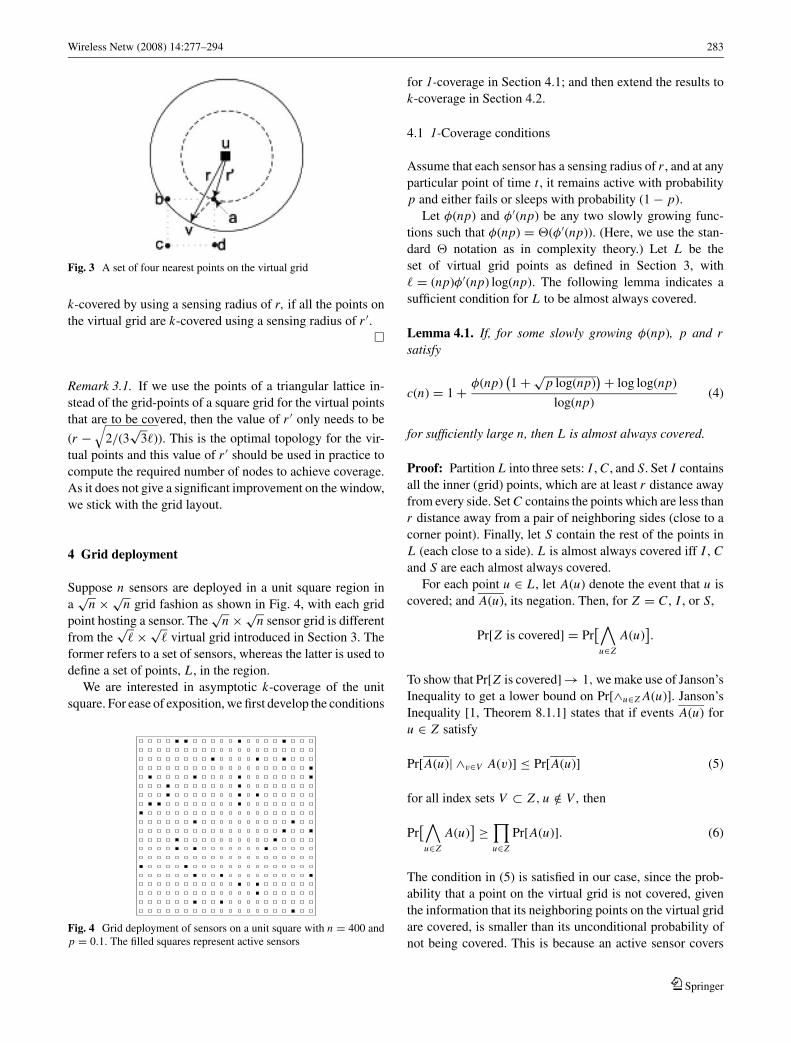
Proof: Let v be an arbitrary point in the square region. With-

out loss of generality, we may assume it is inside the square

formed by some set of four points a, b, c, and d on the virtual

grid as shown in Fig. 3. Also, without loss of generality, we

may assume that it is closest to the point a. By assumption,

there exist at least k active sensors that cover point a. Let

one of these be located at point u as shown in Fig. 3. Then,

d(u, a) < r ′. From triangle inequality,

d(u, v) ≤ d(u, a) + d(a, v) < r ′ + 1√2�

= r.

The same holds for the other active sensors covering point

a. Therefore, we conclude that every point in the region is

Fig. 2 The unit square region tiled with a virtual grid with � = 169points

Springer

Wireless Netw (2008) 14:277–294 283

Fig. 3 A set of four nearest points on the virtual grid

k-covered by using a sensing radius of r, if all the points on

the virtual grid are k-covered using a sensing radius of r ′.�

Remark 3.1. If we use the points of a triangular lattice in-

stead of the grid-points of a square grid for the virtual points

that are to be covered, then the value of r ′ only needs to be

(r −√

2/(3√

3�)). This is the optimal topology for the vir-

tual points and this value of r ′ should be used in practice to

compute the required number of nodes to achieve coverage.

As it does not give a significant improvement on the window,

we stick with the grid layout.

4 Grid deployment

Suppose n sensors are deployed in a unit square region in

a√

n × √n grid fashion as shown in Fig. 4, with each grid

point hosting a sensor. The√

n × √n sensor grid is different

from the√

� × √� virtual grid introduced in Section 3. The

former refers to a set of sensors, whereas the latter is used to

define a set of points, L , in the region.

We are interested in asymptotic k-coverage of the unit

square. For ease of exposition, we first develop the conditions

Fig. 4 Grid deployment of sensors on a unit square with n = 400 andp = 0.1. The filled squares represent active sensors

for 1-coverage in Section 4.1; and then extend the results to

k-coverage in Section 4.2.

4.1 1-Coverage conditions

Assume that each sensor has a sensing radius of r , and at any

particular point of time t , it remains active with probability

p and either fails or sleeps with probability (1 − p).

Let φ(np) and φ′(np) be any two slowly growing func-

tions such that φ(np) = �(φ′(np)). (Here, we use the stan-

dard � notation as in complexity theory.) Let L be the

set of virtual grid points as defined in Section 3, with

� = (np)φ′(np) log(np). The following lemma indicates a

sufficient condition for L to be almost always covered.

Lemma 4.1. If, for some slowly growing φ(np), p and rsatisfy

c(n) = 1 + φ(np)(1 + √

p log(np)) + log log(np)

log(np)(4)

for sufficiently large n, then L is almost always covered.

Proof: Partition L into three sets: I , C , and S. Set I contains

all the inner (grid) points, which are at least r distance away

from every side. Set C contains the points which are less than

r distance away from a pair of neighboring sides (close to a

corner point). Finally, let S contain the rest of the points in

L (each close to a side). L is almost always covered iff I , Cand S are each almost always covered.

For each point u ∈ L , let A(u) denote the event that u is

covered; and A(u), its negation. Then, for Z = C , I , or S,

Pr[Z is covered] = Pr[∧

u∈Z

A(u)].

To show that Pr[Z is covered] → 1, we make use of Janson’s

Inequality to get a lower bound on Pr[∧u∈Z A(u)]. Janson’s

Inequality [1, Theorem 8.1.1] states that if events A(u) for

u ∈ Z satisfy

Pr[A(u)| ∧v∈V A(v)] ≤ Pr[A(u)] (5)

for all index sets V ⊂ Z , u /∈ V, then

Pr[∧

u∈Z

A(u)] ≥

∏u∈Z

Pr[A(u)]. (6)

The condition in (5) is satisfied in our case, since the prob-

ability that a point on the virtual grid is not covered, given

the information that its neighboring points on the virtual grid

are covered, is smaller than its unconditional probability of

not being covered. This is because an active sensor covers

Springer

284 Wireless Netw (2008) 14:277–294

multiple points on the virtual grid. Therefore, Janson’s In-

equality holds here.

Now, Pr[Z is covered] → 1 if∏

u∈Z Pr[A(u)] → 1, which

we establish in the following by considering I , C , and Sseparately. We note that the proof for the three sub-regions

are different and the proof for the sub-region S is the most

challenging one.

Case 1. First consider I , noting that |I | ≤ �. For points u ∈I , event A(u) occurs iff all the sensors in disc Dr (u) are

inactive. The number of sensors that are within disc Dr (u) is

m ≥ ml = πr2n − 2πr√

n. Thus,

Pr[A(u)] = (1 − p)m ≤ (1 − p)ml ≤ e−pml . (7)

It can be easily verified that pml = α log(np), where

α = c −√

4pπc/ log(np). (8)

Therefore,

Pr[A(u)] ≤ e−pml = (np)−α (9)

and

Pr[A(u)] ≥ 1 − (np)−α. (10)

Using Janson’s Inequality (6), the probability that all points

in I are covered is given by

Pr[I is covered] ≥∏i∈I

Pr[A(i)]

≥ (1 − (np)−α)�

≥ exp (−5�(np)−α). (11)

Here we have used the fact that (1 − x) ≥ e−5x if x ≤ 0.99.

Since α → 1 and np → ∞, (np)−α ≤ 0.99 for sufficiently

large n. The right hand side of (11) goes to 1 if the exponent

of e, −5�(np)−α , goes to 0 or, equivalently, if log(�(np)−α)

goes to −∞, which we show below. Using (8), (4) and the

definition � = (np)φ′(np) log(np), we have

log(�(np)−α) = −φ(np) − φ(np)√

p log(np)

+ log(φ′(np)) + √4πc

√p log(np).

The first and the second terms in the right hand side of

the equation dominate the third and the fourth, respectively.

Therefore, log (�(np)−α) → −∞, and Pr[I is covered] → 1.

Case 2. Next, consider C . For u ∈ C , the number of sensors

that are within disc Dr (u) is at least ml/4, where ml is as

defined in Case 1. A similar argument as for (10) results in

Pr[A(u)] ≥ 1 − (np)−α/4. (12)

Note that |C | ≤ 4r2�(1 + 1

r√

�)2 ≤ 8r2�. Proceeding as

in (11) (again using Janson’s Inequality) yields

Pr[C is covered] ≥ exp( − 40r2�(np)−α/4

)≥ exp

(−40elog(r2�(np)−α/4)). (13)

The inner exponent, log(r2�(np)−α/4), can be written as fol-

lows (using (8) and r2� = c log2(np)φ′(np)/π ):

log

(c log2(np)φ′(np)

π

)− c log(np)

4+

√pπc log(np)

4.

The whole expression goes to −∞, forcing the right hand

side of (13) to approach 1.

Case 3. Finally, consider S. We tried to use the inequality

Pr[A(u)] ≥ 1 − (np)−α/2 (cf. (10) and (12)), but as it turned

out, we needed a tighter bound to obtain the desired result.

Let Sl be the set of points in S that are close to the unit

square’s left side. S is almost always covered if Sl is almost

always covered. Label the columns of grid points in Sl from

0 to f − 1, starting with the leftmost column, where f is the

number of columns in Sl . For a grid point u in column j ,

the area of the disc Dr (u) that is within the square region is

more than πr2/2 + jr/√

� and the number of sensors is at

least m j = πr2n/2 + jrn/√

�. Therefore, for a point u ∈ Sl

in column j ,

Pr[A(u)] ≤ (1 − p)m j ≤ e−pm j = (np)−σ j , (14)

where σ j = c/2 + jc/(πr√

�). From (14), the fact (1 −x) ≥ e−5x if x ≤ 0.99, and by observing that (np)−σ ≤ 0.99

for sufficiently large n, it follows that

Pr[A(u)] ≥ 1 − (np)−σ j ≥ exp (−5(np)σ j ).

There are no more than√

� grid points in a column. By

Janson’s Inequality (6), the probability that all the points in

Sl are covered is given by

Pr[∧

u∈Sl

A(u)] ≥

f −1∏j=0

(exp (−5(np)σ j ))√

�

≥ exp

(−5

√�(np)−c/2

f −1∑j=0

w j

)(15)

Springer

Wireless Netw (2008) 14:277–294 285

where

w = (np)−c/(πr√

�) = exp

(−

√c

πφ(np)

).

We have used the relation r√

� = log(np)√

cφ′(np)/π in

obtaining the last equality.

The right hand side of (15) approaches 1 if the exponent

of e goes to 0, which we show in the following. We first

note that since∑ f −1

j=0 w j is the sum of a geometric series and

f → ∞, therefore (1 − w)−1 is a good approximation for

this summation. Using this value, the exponent of e in (15)

can be expressed as

−5 exp((−φ(np) − φ(np)√

p log(np) + log(φ(np)))/2)

1 − exp( −

√c

πφ(np)

) ,

which can be easily shown to converge to 0 using L’Hospital’s

Rule. Consequently, the right hand side of (15) approaches

1. We note that the rate of convergence is the slowest for this

case. �

Remark 4.1. Since the convergence of the bound is the slow-

est for the points close to the sides, it is possible to save some

nodes in the deployment by maintaining a higher density of

nodes on the sides and a lower density in the inner region.

Now, we show that the same condition, (4), ensures asymp-

totic coverage of the unit square.

Theorem 4.1. If, for some slowly growing function φ(np),p and r satisfy

c(n) = 1 + φ(np)(1 + √p log(np)) + log log(np)

log(np)(16)

for sufficiently large n, then the entire unit square region isalmost always covered.

Proof: Let L be the set of virtual grid points introduced in

Section 3, with � = (np)φ(np) log(np); let r ′ = r − 1/√

2�;

and let c′(n) = npπr′2/ log(np). We will show

c′(n) = 1 + φ′(np)(1 + √p log(np)) + log log(np)

log(np)(17)

for some slowly growing function φ′(np) = �(φ(np)). Once

this is proved, then by Lemma 4.1, L is almost always cov-

ered; and then by Lemma 3.1, the unit square region is almost

always covered.

To establish (17), we obtain the following using the defi-

nitions of c′, c, r ′ and �:

c′(n) = c(n)

(1 − 2√

2r2�+ 1

2r2�

)= c(n)

(1 − o

(1

log(np)

))= c(n) − o(c(n))

log(np)(18)

Substituting the equality from (16) in (18) results in

c′(n) = 1 + φ(np)(1 + √p log(np)) − o(c(n)) + log log(np)

log(np)

which is equivalent to

c′(n) = 1 + φ′(np)(1 + √p log(np)) + log log(np)

log(np)

where

φ′(np) = φ(np) − o(c(n)). (19)

This establishes (17) and thereby proves the theorem. �

Corollary 4.1. If, for some slowly growing φ(np), p and rsatisfy

c(n) ≥ 1 + φ(np)(1 + √p log(np)) + log log(np)

log(np)(20)

for sufficiently large n, then the entire unit square region isalmost always covered.

Proof: If c(n) satisfies (20), there exists an rl ≤ r for which

cl(n) = npπr2l / log(np) satisfies (16). The region is almost

always covered when rl is used, and remains so when a larger

sensing radius r is used. �

Corollary 4.2. A simple sufficient condition for asymptoticcoverage of the unit square region is limn→∞ c(n) > 1.

Proof: The right hand side of (17) approaches 1 as n goes

to infinity. Thus, if limn→∞ c(n) > 1, then for any slowly

growing function φ(np), (17) holds for sufficiently large n.

�

We now prove a sufficient condition for asymptotic non-

coverage of the unit square when a sensing radius of r is

used. Such a result is stronger than a mere necessary condi-

Springer

286 Wireless Netw (2008) 14:277–294

tion for (asymptotic) 1-coverage. In the next theorem, c(n)

refers to the same function as defined in (1).

Theorem 4.2. Assume limn→∞ p = 0. If, for some slowlygrowing function φ(np), p and r satisfy

c(n) = 1 − φ(np)(1 + √

p log(np)) + log log(np)

log(np)(21)

for sufficiently large n, then the unit square region is almostalways not 1-covered.

Proof: It suffices to show I , the set of inner grid points as

defined in the proof of Lemma 4.1, to be almost always not 1-covered. (Recall the dimensions of the virtual grid:

√� × √

�,

where � = npφ(np) log(np).)

For any point i ∈ I , let Xi be the indicator random vari-

able of event A(i), i.e. Xi = 1 if i is not 1-covered and 0,

otherwise. Let X be the number of points in I which are not 1-covered. Then, X = X1 + X2 + · · · + X�. I is almost always

not 1-covered iff almost always X > 0. To show that almost

always X > 0, we use Corollary 4.3.4 of [1], which states

that almost always X > 0 if E[X ] → ∞ and � = o(E2[X ]),

where

� =∑u∼v

Pr[A(u) ∧ A(v)].

Here, u ∼ v means that u �= v and A(u) and A(v) are not

independent.

First, we show E[X ] → ∞. The event Au occurs iff all the

sensors in the disc Dr (u) are inactive. The number of sensors

m that are within disc Dr (u) is at most mu = πr2n. Using

the relation c = npπr2/ log(np), we obtain

Pr[A(u)] = (1 − p)m ≥ (1 − p)mu ≈ e−pmu = (np)−c.

(22)

Here, we have used the fact that (1 − x)y ≈ e−yx if y → ∞and x → 0. Now, we compute the expected number of non-

covered points on the virtual grid, E[X ].

E[X ] = � · Pr[A(u)] ≥ �(np)−c = exp(log(�(np)−c)). (23)

Using � = (np)φ(np) log(np), the assumption on cfrom (21), and observing from (22) that (np)−c =exp(−npπr2), the exponent of e in (23) can be rewritten

as follows:

log(�(np)−c) = φ(np)(

1 +√

p log(np))

+ log(φ(np)) + 2 log log(np). (24)

The whole expression on the right hand side of (24) goes to

∞ forcing E[X ] to go to ∞.

Next, we show � = o(E2[X ]). For any two grid points uand v, u ∼ v if the distance between u and v is less than 2r .

For a given point u on the virtual grid, there are two cases

for points v such that u ∼ v: (1) 0 < d(u, v) < r and (2) r ≤d(u, v) < 2r. We compute Pr[A(u) ∧ A(v)], conditioned on

the above two disjoint cases.

Case 1: 0 < d(u, v) < r. It is obvious that Pr[A(u) ∧A(v)] ≤ Pr[A(u)], and thus from (8) and (9) we have

Pr = Pr[A(u) ∧ A(v) | 0 < d(u, v) < r ] ≤ (np)−α. (25)

Case 2: r ≤ d(u, v) < 2r. The area of Dr (u) ∩ Dr (v) is less

than 2πr2/3 − √3r2/2; hence the area of Dr (u) ∪ Dr (v) is

more than 4πr2/3 + √3r2/2, and the number of sensors in

Dr (u) ∪ Dr (v) is more than m2r = 4πr2n/3 when r√

n >

11.67, which trivially holds since r√

n → ∞. Similarly as

in (7), but using the definition of m2r from above, we obtain

P2r ≤ Pr[A(u) ∧ A(v) | r < d(u, v) < 2r ]

≤ (1 − p)m2r ≤ e−pm2r = (np)−4c/3. (26)

For a given point u, there are �r ≈ πr2� points v such that

0 < d(u, v) < r and there are �2r ≈ 3πr2� points v such

that r ≤ d(u, v) < 2r. There are no more than � choices for

selecting the point u. However, because of double counting,

since u ∼ v iff v ∼ u, we have to divide it with 2. Using (25)

and (26), we obtain

� ≤ �

2(�r Pr + �2r P2r )

≤ �

2

(�r (np)−α + �2r (np)−4c/3

). (27)

From (23) and (27), it follows

�

E[X ]2≤ �r (np)−α + �2r (np)−4c/3

2�(np)−2c. (28)

The �r (np)−α term dominates the �2r (np)−4c/3 term in (28).

Therefore, showing that �r (np)−α/(2�(np)−2c) approaches

0, is enough to show that the whole expression on the right

hand side of (28) approaches 0 as n → ∞. Using the relation

�r ≤ log(np)�/(np), which follows since c ≤ 1, we obtain

�r (np)−α

2�(np)−2c≤ log(np)(np)2c−α−1 (29)

Springer

Wireless Netw (2008) 14:277–294 287

Taking the logarithm of the right hand side of (29) and ma-

nipulating it using (8) and (21), we obtain

log(log(np)(np)c−α(np)c−1

)= −φ(np) − φ(np)

√p log(np) + √

4pπc log(np). (30)

The whole expression in the right hand side of (30) goes to

−∞ as n → ∞, thereby forcing the right hand side of (29)

(and hence that of (28)) to approach 0. This proves � =o(E2[X ]).

Now that E[X ] → ∞ and � = o(E2[X ]), we conclude

by Corollary 4.3.4 of [1] that X > 0 almost always. In other

words, almost always there exists a non-covered point in the

region. �

Corollary 4.3. Let limn→∞ p = 0. If, for some slowly grow-ing φ(np), p and r satisfy

c(n) ≤ 1 − φ(np)(1 + √

p log(np)) + log log(np)

log(np)(31)

for sufficiently large n, then the unit square region is almostalways not 1-covered.

Proof: When c(n) satisfies (31), there exists an ru ≥ r for

which cu(n) = npπr2u / log(np) satisfies (21), and so the re-

gion is almost always not 1-covered using ru . This implies

that the region is automatically not 1-covered when a smaller

sensing radius of r is used. �

Corollary 4.4. If limn→∞ p = 0, a simple necessary condi-tion for asymptotic coverage is limn→∞ c(n) ≥ 1.

Proof: Otherwise, if lim c(n) < 1, then (31) would hold (for

any slowly growing φ(np)) and the unit square region would

be almost always not 1-covered. �

4.2 k−Coverage conditions

As a generalization to Theorem 4.1, we derive in this section

a sufficient condition for asymptotic k-coverage. We do not

need a generalization to Theorem 4.2 since a sufficient condi-

tion for non-1-coverage is also a sufficient condition for non-

k-coverage. As before, φ(np) denotes a slowly growing func-

tion, � = (np)φ(np) log(np), and c(n) = npπr2/ log(np).

from 1.

Theorem 4.3. If, for some slowly growing function φ(np),p and r satisfy

c(n) = 1 + φ(np)(1 + √

p log(np)) + k log log(np)

log(np)(32)

for sufficiently large n, then the entire unit square region isalmost always k-covered.

Proof: The proof is similar to that of Theorem 4.1. Thus,

along the same line of reasoning as in that proof, we will

show the following:

Claim 1: If r and p satisfy (32), then r ′ = r − 1/√

2� and psatisfy

c′(n)=1+ φ′(np)(1+√

p log(np))+k log log(np)

log(np), (33)

where c′(n) = npπr′2/ log(np) and φ′(np) is a slowly

growing function such that φ′(np) = �(φ(np)).

Claim 2: If r ′ and p satisfy (33), then L is k-covered using

the reduced sensing radius r ′, where L is the set of grid points

of the√

� × √� virtual grid on the unit square region.

Once these two claims are proved, the theorem will im-

mediately follow from Lemma 3.1.

To see Claim 1, we note that in the proof of Theorem 4.1,

the arguments leading to (18) only uses the definition of cfrom (1) and so it applies in the k-coverage case too. Substi-

tuting the equality from (32) in (18) yields (33) immediately.

To prove Claim 2, we follow the proof of Lemma 4.1

except that now we use Ak(u) in place of A(u), where Ak(u)

is the event that a point u on the virtual grid is not k-covered.

We consider here only the case of I . The proof for sets C and

S can be done with similar modifications as that presented

here for I . Also, for simplicity, we write r ′, c′ and φ′(np)

as r , c and φ(np), respectively. With φ(np) now denoting

φ′(np), we will write the original φ(np) which appears in the

definition of � as φ(np). Thus, � = npφ(np) log(np). Note:

φ(np) = �(φ(np)), from Claim 1.

Let δ > 0 be any constant such that lim supn→∞ p < 1 −δ; such a constant exists since by assumption (Section 2.2),

lim supn→∞ p < 1. Let m be the number of sensors within

disc Dr (u); then m ≤ πr2n.

Let Nr (u) denote the number of active sensors in Dr (u),

and let Pi (u) = Pr[Nr (u) = i]. From (9), we have

P0(u) = (1 − p)m ≤ (np)−α, (34)

where, as defined in (8), α = c − √4pπc/ log(np).

For i ≥ 1, we have

Pi (u) =(

m

i

)pi (1 − p)m−i

≤ (np)−αβ i , (35)

where α is as above and β = ec log(np)/δ. We have applied

(34) and the relation(m

i

) ≤ ( emi )i [1] in obtaining the last

inequality.

Springer

288 Wireless Netw (2008) 14:277–294

The event Ak(u) occurs iff less than k sensors are active

in the disc Dr (u). Therefore,

Pr[Ak(u)] =k−1∑i=0

Pi (u) ≤k−1∑i=0

(np)−αβ i ≈ (np)−αβk−1 (36)

and Pr[Ak(u)] ≥ 1 − (np)−αβk−1. Applying (6) and using

the value of Pr[Ak(u)] in (11), we obtain

Pr[∧

i∈I

Ak(i)] ≥ exp (−5�(np)−αβk−1). (37)

The exponent of e in (37) should go to 0 for the probability

of k-coverage to approach 1. To verify that, we take the log-

arithm of �(np)−αβk−1 (the exponent of e in (37) without the

“−5” factor) and expand it using (33) as well as definitions

of �, α and β. This yields

log(�(np)−αβk−1

) = −φ(np) − φ(np)√

p log(np)

+ log(φ(np)) + (k − 1) log(ec/δ) + √4pπc log(np). (38)

The right hand side of (38) approaches −∞ forcing the right

hand side of (37) to approach 1, which ensures the asymptotic

k-coverage of all the virtual grid-points in I . As mentioned

earlier, the k-coverage of C and S can be proved similarly.

This completes the proof of Claim 2. By Lemma 3.1, we

conclude that all the points in the unit square are almost

always k-covered. �

Corollary 4.5. If, for some slowly growing φ(np), p and rsatisfy

c(n) ≥ 1+ φ(np)(1 + √

p log(np)) + k log log(np)

log(np)(39)

for sufficiently large n, then the entire unit square region isalmost always k-covered.

Note that if a region is not 1-covered then it is not k-covered.

Thus, the conditions established in Theorem 4.2 and Corol-

lary 4.3 for non-1-coverage also hold for non-k-coverage.

4.3 A paradox

Our sufficient condition for asymptotic 1-coverage

(Corollary 4.2) seems to contradict a necessary condition

reported in [16]. In Proposition 2.1 of [16], it is claimed

that if p(n)→0 as n→∞, then a necessary condition for

asymptotic 1-coverage (of the unit square) is given by

lim infn→∞

np(n)r2(n)

log(n)≥ 1

π. (40)

Using our notion of c(n), this (necessary) condition can be

rephrased as

lim infn→∞

c(n) log(np)

log(n)≥ 1 (41)

which evidently contradicts our Corollary 4.2. For instance,

if we let p = 1/√

n and r2 = log(n)/(1.2π√

n), then c(n) =log n/(1.2 log(np)), which approaches infinity; while lim

c(n)log(np)/ log n < 1. By Corollary 4.2, the unit square re-

gion is almost always 1-covered; while by Proposition 2.1 of

[16], it is not. They cannot be both true. To resolve this para-

dox, we wish to point out an unproven claim in the proof

of Proposition 2.1 in [16].3 Thus, when p → 0, the neces-

sity of (40) lacks a proof. We established a simple necessary

condition in Corollary 4.4.

In another proposition in [16], it is claimed that asymp-

totic connectivity does not imply asymptotic coverage.

Proposition 4.1 [16], together with Proposition 2.1 (the con-

dition (40) above), was used to support this claim. Now

that Proposition 2.1 [16] remains unproven, the question of

whether asymptotic connectivity implies asymptotic cover-

age remains open.4

5 Uniform distribution

Under uniform distribution, n nodes are distributed uniformly

over the square region of unit area as illustrated in Fig. 5.

Under this distribution, each node has an equal likelihood of

being at any location in the region; and the probability of a

given node being in any subregion of area R is R.

The proofs for uniform distribution differ from those used

in Section 4 for the grid distribution in the following ways:

1. The proofs will be simpler for uniform distribution—and

so will the obtained conditions—than for the grid deploy-

ment. This is because under the uniform distribution we

3 In the proof of Proposition 2.1, it is shown that the following, (7)in [16], is a necessary condition for asymptotic 1-coverage:

4c(n) log(n)nc(n)πpθ (p)−1 n→∞−→ ∞ (42)

where c(n) = nr2(n)/ log(n) and θ (p) = − log(1 − p)/p. It is thenclaimed that (42) holds only if c(n)πpθ (p) ≥ 1. The latter is shown tohold only if (40) is satisfied; and, therefore, it is concluded that (40)is a necessary condition for 1-coverage. Unfortunately, the aboveclaim is not always true. For instance, if we take p(n) = 1/

√n and

r2 = log(n)/(1.2π√

n) (and thus c(n) = √n/(1.2π )), then the condi-

tion in (42) holds, but c(n)πpθ (p) < 1.4 Proposition 4.1 [16] states that the sensor network is almost always

connected if npe−npπr2

2n→∞−→ 0, which in our notation is equivalent to

limn→∞ c(n) > 2. Since this condition is consistent with our sufficientcondition for coverage (Corollary 4.1) for sufficiently large n, the claimthat asymptotic connectivity does not imply asymptotic coverage re-mains open.

Springer

Wireless Netw (2008) 14:277–294 289

Fig. 5 Random Uniform deployment of sensors on a unit square withn = 400 and p = 0.1. The filled squares represent active sensors

do not have to estimate the number of nodes falling in a

disc Dr (u) (see Remark 2.1).

2. For uniform distribution, the event of coverage (or non-

coverage) of a point u in the region is dependent on the

event of coverage (or non-coverage) of not only the points

located within a distance of 2r from u (so that some sensor

can cover both points) but also on the coverage of points

more than 2r distance from u. This is because if u is not

covered, then the probability of coverage of a point v lo-

cated more than 2r distance from u increases as now all nsensors have a greater likelihood of being in the sensing

range of v, than if one or more of these sensors was cover-

ing u. This observation has at least two implications—(1)

Janson’s Inequality, which was used in the proof of Theo-

rem 4.3 can no longer be used to prove the conditions for

almost always k-coverage in case of uniform distribution,

and (2) establishing that � = o(E[X ]2), as was done in

the proof of Theorem 4.2, is not enough to prove the con-

ditions for almost always non-coverage in case of uniform

distribution.

We use the same virtual grid L as introduced in Section 3.

As in the case of grid deployment, showing L almost always

covered is sufficient to guarantee the almost always coverage

of the entire region. As before, let c(n) = npπr2/ log(np).

Theorem 5.1. Let n sensors be deployed uniformly over aunit square region. If, for some slowly growing φ(np), p andr satisfy

c(n) = 1 + φ(np) + k log log(np)

log(np)(43)

for sufficiently large n, then the unit square region is almostalways k-covered.

Proof: The proof is similar to that of Theorem 4.3. The key

part in that proof is Claim 2. Here, we prove a corresponding

claim: If p and r satisfy

c(n) = 1 + φ(np) + k log log(np)

log(np)(44)

then L is k-covered, where, as before, L contains � grid

points, with � = npφ(np) log(np) and φ(np) = �(φ(np).

Again, we only prove the claim for I . Let A(u), Ak(u),

Nr (u), Pi (u) and β assume the same definition as in the proofs

of Theorems 4.1 and 4.3. For any u ∈ I , with probability

pπr2 each individual sensor falls in Dr (u) and is active.

Therefore, corresponding to (34) and (35), we have

P0(u) = Pr[A(u)] = (1 − pπr2)n ≤ (np)−c (45)

and, for i ≥ 1,

Pi (u) ≤ (np)−cβ i . (46)

Substituting these values in (36) yields

Pr[Ak(u)] ≤ (np)−cβk−1. (47)

Similar to the definition of X in the proof of Theorem 4.2,

let Xk = Xk(1) + Xk(2) + · · · + Xl(�). Here, Xk(i) is an in-

dicator random variable assuming a value of 1 if the vir-

tual grid point i is not k-covered, and 0 otherwise. Now,

E[Xk(u)] = Pr[Ak(u)] ≤ (np)−cβk−1, by using (45). There-

fore, E[Xk] ≤ �(np)−cβk−1. Now, we will use a different

approach to show Pr[∧

i∈I Ak(i)] → 1 than that followed in

the proof of Theorem 4.3, where we used Janson’s Inequal-

ity [1, Theorem 8.1.1]. Since Xk is a nonnegative integral

valued random variable, Pr[Xk > 0] ≤ E[Xk], and therefore,

we have

Pr[∧

i∈I

Ak(i)] = 1 − Pr[Xk > 0]

≥ 1 − (�(np)−cβk−1

). (48)

Now, corresponding to (38), we have (by using (44))

log(�(np)−cβk−1

)= −φ(np) + log(φ(np)) + (k − 1) log (ec/δ) . (49)

The right hand side of (49) approaches −∞ forcing the right

hand side of (48) to approach 1, which implies that all the

grid-points on the virtual are almost always covered. Similar

to Theorem 4.3, we conclude with the help of Lemma 3.1

that all the points in the unit square region are almost always

covered. �

Corollary 5.1. Let n sensors be deployed uniformly over aunit square region. If, for some slowly growing φ(np), p and

Springer

290 Wireless Netw (2008) 14:277–294

r satisfy

c(n) ≥ 1 + φ(np) + k log log(np)

log(np)(50)

for sufficiently large n, then the entire unit square region isalmost always k-covered.

Theorem 5.2. Let n sensors be deployed uniformly over aunit square region, and assume limn→∞ pr2 = 0. If, for someslowly growing φ(np), p and r satisfy

c(n) = 1 − φ(np) + log log(np)

log(np)(51)

for sufficiently large n, then the unit square region is almostalways not 1-covered.

Proof: Let A(u) and X be as defined in the proof of

Theorem 4.2. For points u ∈ I , we observe from (45) that

Pr[A(u)] = p0(u) = (1 − pπr2)n ≈ (np)−c. (52)

Using this value of Pr[A(u)] in (23), the right hand side of (23)

remains the same and so E[X ] → ∞ as n → ∞.

We will use Corollary 4.3.2 from [1] in place of its

Corollary 4.3.4 that was used in the proof of Theorem 4.2.

Corollary 4.3.2 states that if V ar [X ] = o(E[X ]2), then X >

0 almost always. Since X is a sum of indicator random vari-

ables, we can write

Var[X ] ≤ E[X ] +∑i �= j

Cov[Xi , X j ]

= E[X ] +∑

d(i, j)≤2r

Cov[Xi , X j ]

+∑

d(i, j)>2r

Cov[Xi , X j ] (53)

Clearly, E[X ] = o(E[X ]2). As was shown in the proof of

Corollary 4.3.4 in [1],∑

i �= j Cov[Xi , X j ] ≤ �. We will ap-

ply this inequality to the second term in (53) to show that for

the case of d(i, j) ≤ 2r, � = o(E[X ]2) and consequently∑d(i, j)≤2r Cov[Xi , X j ] = o(E[X ]2).

Using the value of Pr[A(u)] from (45), we have corre-

sponding to (25) the following:

Pr = Pr[A(u) ∧ A(v) | 0 < d(u, v) < r ] ≤ (np)−c. (54)

For P2r , we have the same inequality as (26). Using values

from (54) and (26) in (27), we obtain

� ≤ �

2

(�r (np)−c + �2r (np)−4c/3

). (55)

Using the upper bound on � from (55) and the lower bound

on E[X ] from (23) (as was shown earlier it holds for the

uniform distribution as well), in (28), we obtain

�

E[X ]2≤ �r (np)−c + �2r (np)−4c/3

2�(np)−2c. (56)

Thus, using (51), we obtain

log

(log(np)(np)−c

(np)−1−2c

)= −φ(np). (57)

in place of (30). The right hand side of (57) approaches −∞.

Therefore, for the case of d(i, j) ≤ 2r, � = o(E[X ]2) and

consequently∑

d(i, j)≤2r Cov[Xi , X j ] = o(E[X ]2). What re-

mains to be shown for V ar [X ] = o(E[X ]2) to hold is to

show that∑

d(i, j)>2r Cov[Xi , X j ] = o(E[X ]2), which we

now prove.

We notice that

Cov[Xi , X j ] = E[Xi X j ] − E[Xi ]E[X j ]

= Pr[A(i) ∧ A( j)] − Pr[A(i)]Pr[A( j)]. (58)

Applying the equality in (58) to the case of d(i, j) > 2r and

using (52), we get

Cov[Xi , X j ] = Pr[A(i) ∧ A( j)] − Pr[A(i)]Pr[A( j)]

= (1 − 2pπr2)n − (1 − pπr2)2n < 0. (59)

Since Cov[Xi , X j ] < 0 for d(i, j) > 2r, and E[X ] →∞,

∑d(i, j)>2r Cov[Xi , X j ] = o(E[X ]2). This proves that

V ar [X ] = o(E[X ]2), and we conclude from Corollary 4.3.2

in [1] that if (51) holds, then there almost always exists a

non-covered point in the region. In fact, from Corollary 4.3.3

in [1], we can even conclude that almost always X ≈ E[X ].

This completes the proof. �

Corollary 5.2. Let n sensors be deployed uniformly over aunit square region, and assume limn→∞ pr2 = 0. If, for someslowly growing φ(np), p and r satisfy

c(n) ≤ 1 − φ(np) + log log(np)

log(np)(60)

for sufficiently large n, then the unit square region is almostalways not 1-covered.

6 Poisson distribution

In the Poisson model of deployment, number of nodes de-

ployed follows Poisson distribution with rate n. The actual

Springer

Wireless Netw (2008) 14:277–294 291

number of nodes deployed need not be n. Following the

proofs for uniform distribution developed in Section 5, sim-

ilar results for Poisson distribution can be easily derived.

Therefore, in this section we only state the results, and focus

more on showing the equivalence of our condition and that

in [19] for k-coverage under Poisson distribution. We first

state our results.

Theorem 6.1. Let sensors be deployed over a unit squareregion according to a Poisson process with rate n. If, forsome slowly growing φ(np), p and r satisfy

c(n) = 1 + φ(np) + k log log(np)

log(np)(61)

for sufficiently large n, then the entire unit square region isalmost always k-covered.

Theorem 6.2. Let sensors be deployed over a unit squareregion according to a Poisson process with rate n. If, forsome slowly growing φ(np), p and r satisfy

c(n) = 1 − φ(np) + log log(np)

log(np)(62)

for sufficiently large n, then the unit square region is almostalways not 1-covered.

The conditions in the corresponding corollaries are the same

as in Corollary 5.1 and Corollary 5.2.

We now show how to translate the results developed for

the model considered in this paper to the model considered

in [19] and vice versa. In this paper, we model the region as

a unit square with n as the rate of Poisson distribution and rthe sensing radius. (We will assume p = 1, so that np = n.)

In [19], the region was modeled as a square with side length

�, each sensing disk had unit area, and the rate of Poisson

distribution was λ.

If we scale the side length of square from � to unity, then

the rate of Poisson distribution becomes �2λ. Since n is the

rate of Poisson distribution in a unit square in our model,

n = λ�2, (63)

and since the original rate, λ, indicated the expected number

of sensors in a sensing disk, we obtain

nπr2 = λ. (64)

We now show that (61) (with p = 1) is essentially the

same as the condition for k-coverage in [19], which for con-

venience is restated below:

λ = log(�2) + (k + 1) log log(�2) + c(�), (65)

where c(�) → ∞.

Substituting the value of c(n) from (1) in (61) and setting

p = 1, we obtain

nπr2 = log(n) + k log log(n) + φ(n),

which can be restated using (63) and (64) as

λ = log(λ�2) + k log log(λ�2) + φ(λ�2)

= log(�2) + (k + 1) log log(�2)

+ φ(λ�2) + (k + 1)[log log(λ�2) − log log(�2)] (66)

By observing from (66) that log(�2) ≤ λ = O(log(�2)), (66)

can be transformed to (65).

Conversely, (65) can be transformed to (61) as follows:

if c(�) = O(log log log(�2)). Substituting �2 = n/λ and λ =nπr2 from (63) and (64) in (65) yields

nπr2 = log(n) − log(λ) + log log(�2) + k log log(�2) + c(�)

= log(n) + k log log(n) + [c(�)

+ k log log(�2) − k log log(�2 log(�2))]. (67)

Here we have used (64), (65), and the fact that λ � n. If

c(�) = O(log log log(�2)), then (67) is same as (65).

7 Simulation

In this section, we describe how the number of sensors needed

to achieve k-coverage varies with k in analysis and in simu-

lation. We focus on grid deployment as the results for other

deployments are similar.

We use p = 0.2, which means that the network is desired

to last five times the lifetime of an individual sensor. We use

r = 0.04, which implies that the side of the square region of

deployment is 25 times the sensing radius.We first describe the procedure we follow to compute the

number of sensors required to achieve k-coverage in analysis,which we denote by na(k, p, r ), for a given value of k, p,and r. The value of na(k, p, r ) is given by

minn

{npπr2

log(np)≥ 1 + φ(np)

(1 + √

p log(np)) + k log log(np)

log(np)

}.

One issue here is what function to use for φ(np). We discuss

this issue when describing the simulation results later in this

section.

Springer

292 Wireless Netw (2008) 14:277–294

We now describe the procedure to determine the number of

sensors required to achieve k-coverage in simulation, which

we denote by ns(k, p, r ), for a given value of k, p, and r. We

consider the deployment of n sensors in a grid for a particular

value of n. In one iteration, we activate each of these n sensors

with probability p. We then compute the number of virtual

grid points (of which there are � = npφ(np) log(np) of them)

k-covered by the active sensors with a sensing radius of r ′ =r − 1/

√2�. If all points on the virtual grid are covered in

this iteration, we conclude by Lemma 3.1, that all points in

the square are k-covered with the actual sensing radius of rin this interation. We perform 100 iterations for each value

of n. The probability of k coverage is then approximated as

the fraction of interations in which all points in the square

region were k-covered.

In simulation, we vary the number of sensors n, starting

with a value close to na(k, p, r ) and find the minimum value

of n for which the probability of k-coverage is 1. This is the

value of ns(k, p, r ).

Figure 6 shows the values of na(k, p, r ) and ns(k, p, r ).

We make several observations from this figure. First, we see

that the results of analysis closely matches the results of sim-

ulation. Second, there is a sharp increase in the number of

nodes needed to achieve 1-coverage from 0-coverage. But,

the number of nodes needed to achieve 2-coverage is only

marginally more than that needed for 1-coverage. From the

simulation plot in Fig. 6, we see that 15,600 sensors are

needed to achieve 1-coverage. But, deploying only 1,275

more sensors provides 2-coverage. Third, we observe that as

the value of k increases, the curve of na(k, p, r ) becomes

flatter, which indicates that the additional number of nodes

needed to achieve an additional degree of coverage will de-

crease with increasing value of k.

0 2 4 6 8 10 12 140

0.5

1

1.5

2

2.5

3

3.5

4

4.5x 10

4

k

Nu

mb

er

of

No

de

s to

Ach

ieve

k–

Co

vera

ge

na(k,p,r)

ns(k,p,r)

Fig. 6 Number of sensor nodes needed to achieve k-coverage for p =0.2 and r = 0.04 as k is varied

Finally, observe that as the value of k increases, the pre-

dictions of analysis in terms of the number of nodes needed

to achieve k-coverage changes from conservative to liberal.

It means to match the simulation results more closely for

values of k larger than 10, we need to choose a more ap-

propriate value of φ(np). It is the value of φ(np) that largely

determines how closely the analysis will match simulation re-

sults. Here, we chose (log log(np))0.99 as the value of φ(np),

which provided a close match with simulation results for

k ≤ 10. If the value of k is larger than 10, or if the value of ris smaller than 0.04, or if the value of p is smaller than 0.2,

a slower growing function will be a more appropriate choice

for φ(np).

We end this section by discussing the effect of varying

p on the number of nodes needed to achieve k coverage for

a fixed value of k, and r. Notice that in all the conditions

for coverage, n and p appear together so that we can use

n′ = np in all the conditions, as long as the assumptions on

p are met. It means that the conditions for coverage depend on

n′ = n ∗ p.5 Further, for a given value of k and r, the value of

n′ that provides k-coverage with high probability is uniquely

determined. The value of n then can be uniquely determined,

as well, given a value of p by computing n = n′/p. For the

example deployment considered in this section, 1-coverage

is achieved at n = (na(k, p, r )) = 14, 651, when p = 0.2. If

p = 0.1, 1-coverage will be achieved at n = 29, 302.

8 Conclusion

In this paper, we considered the fundamental problem of de-

termining the appropriate number of sensors that are enough

to provide k-coverage of a region when sensors are allowed

to sleep most of their lifetime, which in turn is necessary to

make sensor networks long-lived. We derived critical con-

ditions for these kinds of sensor networks. We showed that

the conditions for deterministic deployment are similar to

the conditions for random deployments. At the same time,

the minor difference in the conditions for these two types

of deployments indicates that the deterministic model with

RIS sleeping is not exactly the same as the random deploy-

ment models with RIS sleeping. We also showed that our

analytical values match closely with simulation results, sup-

porting our claim that our results can be used in real-life

applications for determining the appropriate number of sen-

sors to be deployed, given the area to be covered, the sensing

radius of the sensors, and the desired network lifetime. Fi-

5 In the conditions for coverage for uniform and Poisson distribution,every occurrence of n and p always occur together as n ∗ p, which canbe easily replaced with n′. In the grid deployment case, there is an errorterm

√p log(np). Here p appears alone. This term, however, has only

a marginal effect on the conclusion of this discussion.

Springer

Wireless Netw (2008) 14:277–294 293

nally, the approach of independent sleeping proposed in our

RIS scheme makes the sentry selection task (to ensure k-

coverage) energy-efficient and light-weight because sensors

do not require any interaction with their neighbors.

Acknowledgments The authors would like to thank Anish Arora andMarc E. Posner from the Ohio State University, Jason Hallstrom fromClemson University, and Ho Woo Lee from Sung Kyun Kwan Univer-sity, South Korea for their valuable comments and feedback on an earlierdraft of this paper. Santosh Kumar’s work was partially supported byDARPA contract OSU-RF #F33615-01-C-190. Jozsef Balogh’s workwas partially supported by National Science Foundation grant # DMS0302804 and OTKA grant 049398.

References

1. N. Alon and J.H. Spencer, The probabilistic method, (John Wiley& Sons, 2000).

2. A. Arora et al., Line in the sand: A wireless sensor network fortarget detection, classification, and tracking. Technical report, OSU-CISRC-12/03-TR71, Ohio State University (2003).

3. C. Bettstetter, On the minimum node degree and connectivity ofa wireless multihop network, in: Proceedings of ACM MobiHoc,Lausanne Switzerland (2002) pp. 80–91.

4. B. Bollobas, Random Graphs, (Cambridge University Press 2001).5. Crossbow, Power management and batteries, Application

Notes, Available at http://www.xbow.com/Support/appnotes.htm(2004).

6. P. Gupta and P.R. Kumar, Critical power for asymptotic connectivityin wireless networks, in: IEEE 37th Conference on Decision andControl. Tampa, FL (1998) pp. 1106–1110.

7. D.L. Hall and J. Llinas, Handbook of Multisensor Data Fusion,(CRC Press 2001).

8. P. Hall, Introduction to the Theory of Coverage Processes, (JohnWiley & Sons, 1988).

9. T. He, S. Krishnamurthy, J.A. Stankovic, T. Abdelzaher, L. Luo,R. Stoleru, T. Yan and L. Gu, Energy-efficient surveillance systemusing wireless sensor networks, in: Proceedings of ACM Mobisys,Boston, MA (2004).

10. M. Horton, D.E. Culler, K. Pister, J. Hill, R. Szewczyk and A. Woo,The commercialization of microsensor motes, in: Sensors volumeVol. 19, No. 4, (April 2002) pp. 40–48.

11. C. Huang and Y. Tseng, The coverage problem in a wireless sensornetwork, in: Proceedings of WSNA, San Diego, CA (2003) pp. 115–121.

12. J. Hui, Z. Ren and B.H. Krogh, Sentry-based power managementin wireless sensor networks, in: Proceedings of IPSN, Palo Alto,CA (2003) pp. 458–472.

13. X. Li, P. Wan, Y. Wang and C. Yi, Fault tolerant deployment andtopology control in wireless networks, in: Proceedings of ACMMobiHoc, Annapolis, MD (2003) pp. 117–128.

14. R. Meester and R. Roy, Continuum Percolation, Cambridge Uni-versity Press (1996).

15. S. M. Ross, Introduction to Probability Models, Academic Press(2000).

16. S. Shakkottai, R. Srikant and N.B. Shroff, Unreliable sensor grids:coverage, connectivity and diameter, in: Proceedings of IEEE IN-FOCOM vol. 2, San Francisco, CA (2003) pp. 1073–1083.

17. R. Szewczyk, J. Polastre, A.M. Mainwaring and D.E. Culler,Lessons from a sensor network expedition, in: EWSN, Berlin, Ger-many (2004).

18. X. Wang, G. Xing, Y. Zhang, C. Lu, R. Pless and C. Gill, Inte-grated coverage and connectivity configuration in wireless sensornetworks, in; Proceedings of ACM Sensys, Los Angeles, CA (2003)pp. 28–39.

19. H. Zhang and J. Hou, On deriving the upper bound of α-lifetime forlarge sensor networks, in: Proceedings of ACM MobiHoc, Tokyo,Japan (2004) pp. 121–132.

20. J. Zhao and R. Govindan, Understanding packet delivery perfor-mance in dense wireless sensor networks, in: Proceedings of ACMSensys, Los Angeles, CA (2003) pp. 1–13.

Santosh Kumar is an Assistant Professor in the department of Com-puter Science at the University of Memphis. He received his Ph.D. inComputer Science and Engineering from the Ohio State University in2006, where he was the SBC Presidential Fellow in 2006. He also re-ceived an M.S. in Computer and Information Science from the OhioState University in 2002. He received a B.Tech. in Computer Scienceand Engineering from the Institute of Technology at Banaras Hindu Uni-versity (IT-BHU) in 1998. His current research focuses on the issues ofcoverage and connectivity in wireless sensor networks.

Ten-Hwang Lai is a Professor of Computer Science and Engineer-ing at the Ohio State University. A pioneer of Zen Networking, he isinterested in the art of applying Zen to the teaching and research of pro-tocol design. He served as the program chair of ICPP’98, the generalchair of ICPP’00, the program co-chair of ICDCS’04, and, recently, thegeneral chair of ICDCS’05. He is/was an editor of IEEE Transactionson Parallel and Distributed Systems (TPDS), ACM/Springer WirelessNetworks, Academia Sinica’s Journal of Information Science and En-gineering (JISE), and International Journal of Ad Hoc and UbiquitousComputing.

Springer

294 Wireless Netw (2008) 14:277–294

Jozsef Balogh is an Assistant Professor of Mathematics at the Uni-versity of Illinois at Urbana-Champaign. He received an M.S. fromSzeged University, Hungary in 1995 and a Ph.D. in Mathematics fromthe University of Memphis in 2001. Before joining the University of

Illinois, he held post doctoral positions at AT&T (2001–2002), Prince-ton (2002), and the Ohio State University (2002–2005). His currentresearch interests include Probabilistic Methods in Discrete Mathemat-ics and Extremal Graph Theory.

Springer