This article appeared in a journal published by Elsevier. The attachedcopy is furnished to the author for internal non-commercial researchand education use, including for instruction at the authors institution

and sharing with colleagues.

Other uses, including reproduction and distribution, or selling orlicensing copies, or posting to personal, institutional or third party

websites are prohibited.

In most cases authors are permitted to post their version of thearticle (e.g. in Word or Tex form) to their personal website orinstitutional repository. Authors requiring further information

regarding Elsevier’s archiving and manuscript policies areencouraged to visit:

http://www.elsevier.com/copyright

Author's personal copy

On active disturbance rejection based control design forsuperconducting RF cavities

John Vincent a, Dan Morris a, Nathan Usher a, Zhiqiang Gao b,n, Shen Zhao b,Achille Nicoletti b, Qinling Zheng b

a National Superconducting Cyclotron Laboratory (NSCL), Michigan State University, East Lansing, MI 48824-1321, USAb Center for Advanced Control Technologies, Fenn College of Engineering, Cleveland State University, Cleveland, OH 44115-2214, USA

a r t i c l e i n f o

Article history:

Received 16 February 2011

Received in revised form

11 April 2011

Accepted 18 April 2011Available online 30 April 2011

Keywords:

Active disturbance rejection control

SRF

LLRF

a b s t r a c t

Superconducting RF (SRF) cavities are key components of modern linear particle accelerators. The

National Superconducting Cyclotron Laboratory (NSCL) is building a 3 MeV/u re-accelerator (ReA3)

using SRF cavities. Lightly loaded SRF cavities have very small bandwidths (high Q) making them very

sensitive to mechanical perturbations whether external or self-induced. Additionally, some cavity types

exhibit mechanical responses to perturbations that lead to high-order non-stationary transfer functions

resulting in very complex control problems. A control system that can adapt to the changing perturbing

conditions and transfer functions of these systems would be ideal. This paper describes the application

of a control technique known as ‘‘Active Disturbance Rejection Control’’ (ARDC) to this problem.

& 2011 Elsevier B.V. All rights reserved.

1. Introduction

The National Superconducting Cyclotron Laboratory (NSCL) iscurrently constructing a 3 MeV/u re-accelerator (ReA3), expand-able to 12 MeV/u, using superconducting RF (SRF) cavities [1].The project is cooperatively funded by the Michigan State Uni-versity (MSU) and the National Science Foundation (NSF). Inaddition, MSU has been selected to build the Facility for RareIsotope Beams (FRIB) national user facility that features a 400 kW,200 MeV/u SRF linac requiring over 340 SRF cavities [2]. FRIB isfunded through a cooperative agreement between MSU and theOffice of Nuclear Physics in the Department of Energy (DOE)Office of Science. Maximizing the performance and decreasing theoverall costs of these systems are the ongoing goals of bothprojects.

The control of lightly loaded SRF cavities is an ongoing topic inthe accelerator community due to the extreme sensitivity of thesecavities to disturbances and other detuning forces. A dominantmethod applied is to over-couple these cavities, thereby reducingthe sensitivity by increasing the bandwidth and applying standardproportional-integral-derivative (PID) controls [3]. Adaptive controlalgorithms are sought that can minimize the required drivepower and improve the overall performance of these systems.This paper describes our experience applying a seemingly ideal

solution to this problem known as ‘‘Active Disturbance RejectionControl’’ (ADRC) [4,5].

The nature of many, if not most, control problems is distur-bance rejection, particularly the microphonics problem discussedhere, and the key question in design is how to deal with it. ThePID control strategy, by default, deals with the disturbances in apassive way as it merely reacts to the tracking errors caused bythe disturbances. An alternative, and better, solution is to rejectthe disturbances actively by estimating the disturbances directlyand canceling it out, before it affects the system in a significantway, and this is at the core of ADRC.

In the ADRC design, the disturbance is estimated using the socalled state observer, which is commonly used in the frameworkof modern control theory to estimate the immeasurable internalstates of a system. Note that states, also known as state variables,refer to physical variables of a system, such as current, voltage,temperature, pressure, etc., and state observer, usually imple-mented in a computer algorithm, and uses the input and outputdata of a system, and its model, to reconstruct in real time thevalues of state variables [6].

The uniqueness of the ADRC design is that the total distur-bance, which includes both external disturbances and unknowninternal dynamics, is defined as an extended state of the systemand estimated using a state observer, known as the extendedstate observer (ESO). Unlike the standard state observers, thestate in ESO is extended beyond the regular physical variables toinclude the effects of unknown disturbance and dynamics intheir totality. Once estimated, the total disturbance can be

Contents lists available at ScienceDirect

journal homepage: www.elsevier.com/locate/nima

Nuclear Instruments and Methods inPhysics Research A

0168-9002/$ - see front matter & 2011 Elsevier B.V. All rights reserved.

doi:10.1016/j.nima.2011.04.033

n Corresponding author. Tel.: þ1 216 687 3528; fax: þ1 216 687 5405.

E-mail addresses: z.gao@csuohio.edu, gaocsu@gmail.com (Z. Gao).

Nuclear Instruments and Methods in Physics Research A 643 (2011) 11–16

Author's personal copy

readily canceled by the control signal, transforming elegantly theoriginal system to a disturbance-free one, which can easily becontrolled [4,5].

ARDC is practical because it requires very little knowledgeabout the plant dynamics, which in real systems may be bothunknown and non-stationary. In the case of a linear timeinvariant system, it requires only the knowledge of the relativedegree of the system and an estimation of the high frequencygain [5]. For example, given the general transfer function below(1), the information needed is the relative degree n�m and bm:

GðsÞ ¼bmsðmÞ þbm�1sðm�1Þ þ � � � þb1sþb0

sðnÞ þan�1sðn�1Þ þ � � � þa1sþa0ð1Þ

Additionally, the number of ARDC tuning parameters may bereduced to one [7], further simplifying the control design.

2. ADRC solution for the SRF cavity problem

In accelerator applications, the cavity voltage must be pre-cisely controlled in the presence of vibrations referred to as‘‘microphonics’’. The problem is acute here at NSCL since theReA3 accelerator has been mounted on a balcony, making it evenmore susceptible to microphonic disturbances from the environ-ment. The previously explored adaptive feedforward cancellationmethod [8] is found to be not sufficient in this case. We are thusmotivated to explore more effective disturbance rejection tech-nology beyond a standard PID and our search leads to ADRC.In this section the standard SRF cavity model [9] is first intro-duced, followed by a new problem formulation and the corre-sponding control design. Tuning of the new controller is alsodiscussed.

2.1. Ideal voltage vector I–Q model

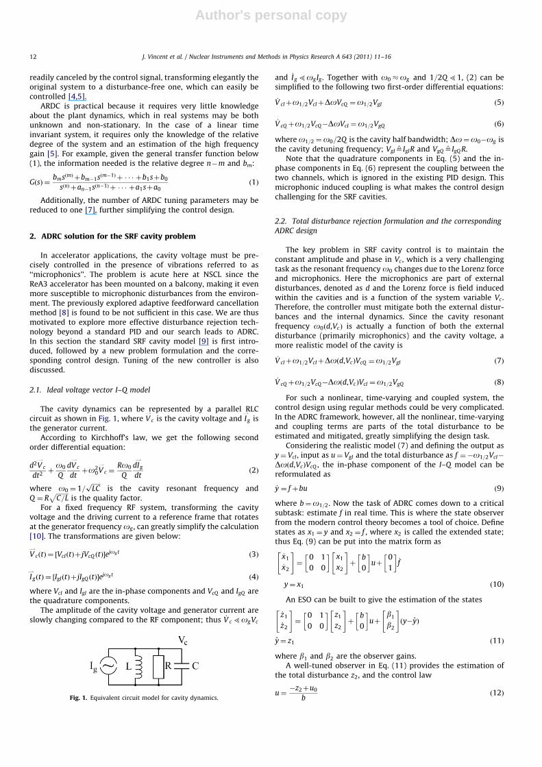
The cavity dynamics can be represented by a parallel RLCcircuit as shown in Fig. 1, where V

,

c is the cavity voltage and I,

g isthe generator current.

According to Kirchhoff’s law, we get the following secondorder differential equation:

d2V,

c

dt2þo0

Q

dV,

c

dtþo2

0V,

c ¼Ro0

Q

dI,

g

dtð2Þ

where o0 ¼ 1=ffiffiffiffiffiffiLCp

is the cavity resonant frequency andQ ¼ R

ffiffiffiffiffiffiffiffiC=L

pis the quality factor.

For a fixed frequency RF system, transforming the cavityvoltage and the driving current to a reference frame that rotatesat the generator frequency og , can greatly simplify the calculation[10]. The transformations are given below:

V,

cðtÞ ¼ ½VcIðtÞþ jVcQ ðtÞ�ejog t ð3Þ

I,

gðtÞ ¼ ½IgIðtÞþ jIgQ ðtÞ�ejog t ð4Þ

where VcI and IgI are the in-phase components and VcQ and IgQ arethe quadrature components.

The amplitude of the cavity voltage and generator current areslowly changing compared to the RF component; thus _V c 5ogVc

and _Ig 5ogIg . Together with o0 �og and 1=2Q 51, (2) can besimplified to the following two first-order differential equations:

_V cIþo1=2VcIþDoVcQ ¼o1=2VgI ð5Þ

_V cQþo1=2VcQ�DoVcI ¼o1=2VgQ ð6Þ

where o1=2 ¼o0=2Q is the cavity half bandwidth; Do¼o0�og isthe cavity detuning frequency; VgI9IgIR and VgQ9IgQ R.

Note that the quadrature components in Eq. (5) and the in-phase components in Eq. (6) represent the coupling between thetwo channels, which is ignored in the existing PID design. Thismicrophonic induced coupling is what makes the control designchallenging for the SRF cavities.

2.2. Total disturbance rejection formulation and the corresponding

ADRC design

The key problem in SRF cavity control is to maintain theconstant amplitude and phase in Vc , which is a very challengingtask as the resonant frequency o0 changes due to the Lorenz forceand microphonics. Here the microphonics are part of externaldisturbances, denoted as d and the Lorenz force is field inducedwithin the cavities and is a function of the system variable Vc .Therefore, the controller must mitigate both the external distur-bances and the internal dynamics. Since the cavity resonantfrequency o0ðd,VcÞ is actually a function of both the externaldisturbance (primarily microphonics) and the cavity voltage, amore realistic model of the cavity is

_V cIþo1=2VcIþDoðd,VcÞVcQ ¼o1=2VgI ð7Þ

_V cQþo1=2VcQ�Doðd,VcÞVcI ¼o1=2VgQ ð8Þ

For such a nonlinear, time-varying and coupled system, thecontrol design using regular methods could be very complicated.In the ADRC framework, however, all the nonlinear, time-varyingand coupling terms are parts of the total disturbance to beestimated and mitigated, greatly simplifying the design task.

Considering the realistic model (7) and defining the output asy¼ VcI , input as u¼ VgI and the total disturbance as f ¼�o1=2VcI�

Doðd,VcÞVcQ , the in-phase component of the I–Q model can bereformulated as

_y ¼ f þbu ð9Þ

where b¼o1=2. Now the task of ADRC comes down to a criticalsubtask: estimate f in real time. This is where the state observerfrom the modern control theory becomes a tool of choice. Definestates as x1 ¼ y and x2 ¼ f , where x2 is called the extended state;thus Eq. (9) can be put into the matrix form as

_x1

_x2

" #¼

0 1

0 0

� �x1

x2

" #þ

b

0

� �uþ

0

1

� �_f

y¼ x1 ð10Þ

An ESO can be built to give the estimation of the states

_z1

_z2

" #¼

0 1

0 0

� �z1

z2

" #þ

b

0

� �uþ

b1

b2

" #ðy�yÞ

y¼ z1 ð11Þ

where b1 and b2 are the observer gains.A well-tuned observer in Eq. (11) provides the estimation of

the total disturbance z2, and the control law

u¼�z2þu0

bð12Þ

Fig. 1. Equivalent circuit model for cavity dynamics.

J. Vincent et al. / Nuclear Instruments and Methods in Physics Research A 643 (2011) 11–1612

Author's personal copy

where u0 is a virtual control signal, reduces the original plant inEq. (9) to a simple integrator plant of the form

_y ¼ u0þðf�z2Þ � u0 ð13Þ

which can be easily controlled using a proportional controller.

u0 ¼ kpðr�z1Þ ð14Þ

Here kp is the controller gain and r is the reference signal.

To simplify the tuning process, the observer gains are chosenas b1 ¼ 2oob and b2 ¼o2

ob to put the poles of the observer at�oob. Similarly the controller gains are chosen as kp ¼oc to putthe pole of the control loop at �oc. oob and oc are called theobserver bandwidth and controller bandwidth, respectively.For further simplification, we can set oob ¼ ð3�10Þoc and oc

becomes the only tuning parameter [7].The control design for the quadrature component can be

carried out similarly by defining y¼ VcQ , u¼ VgQ and f ¼�o1=2

VcQþDoðd,VcÞVcI .

2.3. Amplitude and phase control

As shown above, the cavity dynamics can be clearly describedby the IQ model. However, in the real test environment, the electricfield is normally measured in terms of amplitude and phase. Therelationship between the IQ components and amplitude/phase ismerely a linear coordinate transformation, from Cartesian to polar.For the sake of convenience and without loss of generality, theproposed ADRC solution is implemented to control the amplitudeand phase directly instead of the IQ components, as the transfor-mation does not affect the cavity dynamics. However a difficultyexists in phase control, since the phase can jump between �1801and 1801, which is referred to as the ‘‘wrap-around’’ problem. Theproblem is addressed in more detail in subsection D of Section III,while implementing the ADRC for phase loop.

Two diagrams are given in Figs. 2 and 3 to show the differencebetween the PID and ADRC for amplitude and phase control of thecavity, respectively. In a PID control structure, the amplitude andphase coupling, the disturbance and dynamic uncertainties aredealt with passively in the form of parameter tuning. In the ADRCdesign, however, they are lumped together as the total distur-bance, estimated in real time, and actively canceled out in thecorresponding control signal. In other words, another benefit ofADRC is that two coupled loops, such as the amplitude and phaseloops in this application, are decoupled naturally.

3. Simulation and measured responses

3.1. Simulation model

A MATLAB simulation model is built to test the control design,as shown in Fig. 4. The cavity half bandwidth is 219 rad/s (35 Hz).The sampling rate is 54.6 kHz; the controller and observer

Fig. 2. Diagram of the PID control.

Fig. 3. Diagram of the ADRC control.

Fig. 4. MATLAB simulation model with ADRC control.

J. Vincent et al. / Nuclear Instruments and Methods in Physics Research A 643 (2011) 11–16 13

Author's personal copy

bandwidths are set to 600 and 3000 rad/s, respectively. Forcomparison, a PI controller is tuned with a proportional gain of3 and an integral gain of 5474. The parameters were tuned toachieve the best stable response. The same values were used forsimulations and measurements.

3.2. Hardware implementation

The RF control is implemented on a digital low-level RF con-troller developed at the NSCL. The controller produces a low-level RFoutput at the cavity drive frequency and directly controls the phaseand amplitude of the output. This low-level RF signal is fed into asolid-state linear amplifier and the output of the amplifier is coupledto the cavity. The cavity used for these tests is a SRF quarter waveresonator with a loaded bandwidth of 70 Hz (440 rad/s). Thisparticular cavity is especially susceptible to microphonics becauseits mechanical damper does not work as well as anticipated. Duringthe tests, intermittent microphonics were present, which detunedthe cavity by more than 40 Hz. The discrete implementation of theADRC control algorithm can be found in Ref. [11].

3.3. Simulation and measured results

Step signals were introduced as a reference for both theamplitude and phase components. For the simulations, a constantdetuning frequency of 40 rad/s was used. The simulated andmeasured response curves for a step in amplitude (6-8 MV/m)are shown in Fig. 5. The response curves for a step in phase(75-901) are shown in Fig. 6. With the ADRC controller, theripple and overshoot are greatly reduced.

The steady-state probability density functions for amplitudeand phase are shown in Fig. 7. The steady-state model includes aGaussian detuning frequency, which was varied in order to matchthe measured data.

3.4. Implementation issues

Physical limitations always exist for the actuators. For exam-ple, in the amplitude loop, the output voltage of the amplifier islimited to 0–10 V, which results in a difference between theactual applied and the calculated control signal. In the observerbased design, the control signal is needed for the state estimation.Normally feeding back the control signal that is actually appliedFig. 5. Amplitude step response: simulation (top) and measured (bottom).

Fig. 6. Phase step response: simulation (top) and measured (bottom).

Fig. 7. Steady-state probability density function: simulation (top) and measured

(bottom).

J. Vincent et al. / Nuclear Instruments and Methods in Physics Research A 643 (2011) 11–1614

Author's personal copy

on the real system to the observer will give us a more accurateestimation. It works very well with the amplitude loop.

In the phase loop, however, feeding back the actual appliedcontrol signal gives us unexpected results. The phase outputcannot get to the setpoint in some special cases. A simulationexample for the case is shown in Fig. 8.

The reason for it is that the phase loop is different from theamplitude loop in the sense of how the control signal is handleddue to the physical limitation. In the amplitude loop, the controlsignal is saturated between a lower bound and an upper bound. Inthe phase loop, the 2701 control signal will have the same effectas that of �901 control signal. So a wrap-around method is usedinstead of the saturation method. In the wrap-around method,whenever the control signal goes beyond the range from �1801to 1801, 3601 is added to or subtracted from the control signal tomake it fall back into this range. The effect of the saturation andwrap-around is graphed in Figs. 9 and 10. It is the non-monotonicbehavior of the phase loop that causes the multi-equilibriumpoints of the system, and hence the above problem.

To solve the problem, we first tried the saturation method forthe phase loop to avoid the non-monotonic behavior, but it didnot work. The phase saturates at either the upper limit or thelower limit and cannot recover from the saturation point. This isbecause naturally the phase can approach its setpoint in bothdirections. In the saturation method, we manually block one ofthe directions. So once the phase initially goes in the wrongdirection, it will always saturate.

So we switched back to the wrap-around method that pre-serves the feature of the phase behavior. We finally solved theproblem in simulation by feeding back the calculated control

signal (before the wrap-around) instead of the actually appliedcontrol signal (after the wrap-around) to the ESO. In this way weactually consider the wrap-around effect (adding or subtracting3601 to or from the calculated control signal) as an inputdisturbance, and use the disturbance rejection ability of the ADRCto deal with it. A simulation result is given in Fig. 11 to show theeffectiveness of this method.

The new wrap-around implementation has been tested onseveral superconducting cavities, and it solves the problemsfound in the previous implementations. When running the newdesign, large disturbances do not cause control problems and thephase setpoint can be changed arbitrarily without causing thesaturation problem illustrated in Fig. 8.

4. Conclusion

The initial tests of the ADRC control on a SRF cavity at the NSCLhave shown a significant improvement over the PID control underthe same conditions. We expect that as we continue to work withthe implementation, we may improve the response even further.

Acknowledgments

This work was supported in part by the National ScienceFoundation under Grant no. PHY-06-06007.

References

[1] Oliver Kester, et al., The MSU/NSCL re-accelerator ReA3, in: Proceedings ofthe SRF2009, Berlin, Germany, 2009, pp. 57–61.

Fig. 8. Undesired response for phase loop.

Fig. 9. Saturation effect for amplitude loop.

Fig. 10. Wrap-around effect for phase loop.

Fig. 11. Desired response for phase loop.

J. Vincent et al. / Nuclear Instruments and Methods in Physics Research A 643 (2011) 11–16 15

Author's personal copy

[2] R.C. York, et al., FRIB: a new accelerator facility for the production of rare isotopebeams, in: Proceedings of the SRF2009, Berlin, Germany, 2009, pp. 888–894.

[3] Curt Hovater, RF control of high QL superconducting cavities, in: Proceedingsof the LINAC08, Victoria, BC, Canada, 2008, pp. 704–708.

[4] Z. Gao, Active disturbance rejection control: a paradigm shift in feedbackcontrol system design, in: Proceedings of the American Control Conference,2006, pp. 2399–2405.

[5] J. Han, IEEE Transactions on Industrial Electronics 56 (3) (2009) 900.[6] P.J. Antsaklis, A.N. Michel, Linear Systems, McGraw-Hill Companies Inc., 1997.[7] Z. Gao, Scaling and bandwidth-parameterization based controller tuning, in:

Proceedings of the American Control Conference, 2003, pp. 4989–4996.

[8] T.H. Kandil, et al., Nuclear Instruments & Methods in Physics Research SectionA 550 (2005) 514.

[9] S. Simrock, G. Petrosyan, A. Facco, V. Zviagintsev, S. Andreoli, R. Pa-parella,First demonstration of microphonic control of a superconducting cavity witha fast piezoelectric tuner, in: Proceedings of the 2003 Particle AcceleratorConference, Portland, OR, 2003, pp. 470–472.

[10] M.G. Minty, R.H. Siemann, Nuclear Instruments and Methods in PhysicsResearch Section A 376 (1996) 310.

[11] R. Miklosovic, A. Radke, Z. Gao, Discrete implementation and generalizationof the extended state observer, in: Proceedings of the American ControlConference, 2006, pp. 2209–2214.

J. Vincent et al. / Nuclear Instruments and Methods in Physics Research A 643 (2011) 11–1616