
GENOTOXICITY OF COMMERCIAL PETROL SAMPLES IN CIJLITJRED HUMAN LYMPHOCYTES

545
Volume IX Issue 4(30)
Winter 2014
I.S.S.N. 1843-6110

Journal of Applied Economic Sciences VolumeIX, Issue4 (30) Winter 2014
546
Editorial Board
Editor in Chief Laura ŞTEFĂNESCU
Managing Editor Mădălina CONSTANTINESCU
Executive Editor Ion Viorel MATEI
International Relations Responsible Pompiliu CONSTANTINESCU
Proof – readers Ana-Maria Trantescu - English
Redactors Andreea-Denisa Ionițoiu Cristiana Bogdănoiu Sorin Dincă

Journal of Applied Economic Sciences
Volume IX, Issue 4(30), Winter 2014
547
Editorial Advisory Board
Claudiu Albulescu, University of Poitiers, France, West University of Timişoara, Romania
Aleksander Aristovnik, Faculty of Administration, University of Ljubljana, Slovenia
Muhammad Azam, School of Economics, Finance & Banking, College of Business, Universiti Utara, Malaysia
Cristina Barbu, Spiru Haret University, Romania
Christoph Barmeyer, Universität Passau, Germany
Amelia Bădică, University of Craiova, Romania
Gheorghe Bică, Spiru Haret University, Romania
Ana Bobîrcă, Academy of Economic Science, Romania
Anca Mădălina Bogdan, Spiru Haret University, Romania
Jean-Paul Gaertner, l'Institut Européen d'Etudes Commerciales Supérieures, France
Shankar Gargh, Editor in Chief of Advanced in Management, India
Emil Ghiţă, Spiru Haret University, Romania
Dragoş Ilie, Spiru Haret University, Romania
Elena Doval, Spiru Haret University, Romania
Camelia Dragomir, Spiru Haret University, Romania
Arvi Kuura, Pärnu College, University of Tartu, Estonia
Rajmund Mirdala, Faculty of Economics, Technical University of Košice, Slovakia
Piotr Misztal, Technical University of Radom, Economic Department, Poland
Simona Moise, Spiru Haret University, Romania
Marco Novarese, University of Piemonte Orientale, Italy
Rajesh Pillania, Management Development Institute, India
Russell Pittman, International Technical Assistance Economic Analysis Group Antitrust Division, USA
Kreitz Rachel Price, l'Institut Européen d'Etudes Commerciales Supérieures, France
Andy Ştefănescu, University of Craiova, Romania
Laura Ungureanu, Spiru Haret University, Romania
Hans-Jürgen Weißbach, University of Applied Sciences - Frankfurt am Main, Germany
Publisher:
Spiru Haret University Faculty of Financial Management Accounting Craiova No 4. Brazda lui Novac Street, Craiova, Dolj, Romania Phone: +40 251 598265 Fax: + 40 251 598265
European Research Center of Managerial Studies in Business Administration http://www.cesmaa.eu Email: [email protected] Web: http://cesmaa.eu/journals/jaes/index.php
Journal of Applied Economic Sciences VolumeIX, Issue4 (30) Winter 2014
548
Journal of Applied Economic Sciences
Journal of Applied Economic Sciences is a young economics and interdisciplinary research journal, aimed
to publish articles and papers that should contribute to the development of both the theory and practice in the field of Economic Sciences.
The journal seeks to promote the best papers and researches in management, finance, accounting, marketing, informatics, decision/making theory, mathematical modelling, expert systems, decision system support, and knowledge representation. This topic may include the fields indicated above but are not limited to these.
Journal of Applied Economic Sciences be appeals for experienced and junior researchers, who are interested in one or more of the diverse areas covered by the journal. It is currently published quarterly with three general issues in Winter, Spring, Summer and a special one, in Fall.
The special issue contains papers selected from the International Conference organized by the European Research Centre of Managerial Studies in Business Administration (www.cesmaa.eu) and Faculty of Financial Management Accounting Craiova in each October of every academic year. There will prevail the papers containing case studies as well as those papers which bring something new in the field. The selection will be made achieved by:
Journal of Applied Economic Sciences is indexed in SCOPUS www.scopus.com, CEEOL www.ceeol.org, EBSCO www.ebsco.com, RePEc www.repec.org and in IndexCopernicus www.indexcopernicus.com databases.
The journal will be available on-line and will be also being distributed to several universities, research institutes and libraries in Romania and abroad. To subscribe to this journal and receive the on-line/printed version, please send a request directly to [email protected].
Journal of Applied Economic Sciences
Volume IX, Issue 4(30), Winter 2014
549
Journal of Applied Economic Sciences
ISSN 1843-6110
Table of Contents
Encarnación ÁLVAREZ, Francisco J. BLANCO-ENCOMIENDA,
Juan F. MUÑOZ and Mercedes SÁNCHEZ-GUERRERO
Evaluation of randomized response models for the mean and using data …551
on income and living conditions
Muhammad AZAM, Abdul Qayyum KHAN and Laura ȘTEFĂNESCU
Determinants of stock market development in Romania …561
Süleyman AÇIKALIN and Erginbay UĞURLU
Oil price fluctuations and trade balance of Turkey …571
Alena ANDREJOVSKÁ
Categorisation of the European Union countries in relation to efficiency adjustment …580
of value added tax collection using cluster analysis and multidimensional scalling
Muhammad AZAM and Yusnidah IBRAHIM
Foreign direct investment and Malaysia’s stock market: …591
using ARDL bounds testing approach
Radovan BAČÍK, Róbert ŠTEFKO and Jaroslava GBUROVÁ
Marketing pricing strategy as part of competitive advantage retailers …602
Elena BICĂ
Technical, economic and managerial structures in the field of …608 energy in the vision in the European Union
Tanattrin BUNNAG
The real exchange rate volatility comovements and spillovers …614
in Thailand’s international trade: a multivariate garch approach
2
1
3
5
6
7
8
4

Journal of Applied Economic Sciences VolumeIX, Issue4 (30) Winter 2014
550
Jozef HETEŠ, Ivana ŠPIRENGOVÁ and Michaela URBANOVIČOVÁ
Modelling the demand for new investment credits to the …632 non-financial companies in the Slovak Republic
Petra HORVÁTHOVÁ, Martin ČERNEK and Kateřina KASHI
Ethics perception in business and social practice in the Czech Republic …646
Samuel KORÓNY and Erika ĽAPINOVÁ
Economic aspects of working time flexibility in Slovakia …660
Matúš KUBÁK, Radovan BAČÍK, Zsuzsanna Katalin SZABO and Dominik BARTKO
The efficiency of Slovak universities: a data envelopment analysis …673
Irina A. MARKINA and Antonina V. SHARKOVA
Assessment methodology for resource-efficient development of …687 organizations in the context of the green economy
Patrycja PUDŁO and Stanislav SZABO
Logistic costs of quality and their impact on degree of operating leverage …694
Sawssen ARAICHI and Lotfi BELKACEM
Solvency capital for non life insurance: modelling dependence using copulas …702
Erginbay UĞURLU
Modelling volatility: evidence from the Bucharest Stock Exchange …718
9
10
11
12
13
14
15
16
Journal of Applied Economic Sciences
Volume IX, Issue 4(30), Winter 2014
551
EVALUATION OF RANDOMIZED RESPONSE MODELS FOR THE MEAN AND USING DATA ON INCOME AND LIVING CONDITIONS
Encarnación ÁLVAREZ
Department of Quantitative Methods in Economics and Business
University of Granada, Spain
Francisco J. BLANCO-ENCOMIENDA
Department of Quantitative Methods in Economics and Business
University of Granada, Spain
Juan F. MUÑOZ
Department of Quantitative Methods in Economics and Business
University of Granada, Spain
Mercedes SÁNCHEZ-GUERRERO
Department of Quantitative Methods in Economics and Business
University of Granada, Spain
Abstract:
The surveys on Income and Living Conditions carried out by the statistical agencies of many countries
may contain sensitive questions, which can induce the respondent to give a false answer or no answer. Although
the most common technique to treat this is the imputation, the randomized response techniques can also be
used. In this paper we evaluate the performance of two randomized response models to estimate the population
mean with real data obtained from the 2012 Spanish Survey on Income and Living Conditions. For this purpose,
Monte Carlo simulation studies are carried out. Empirical results indicate that no estimator presents bias when
individuals provide the true answers while the direct estimator presents a large bias when providing false
answers. We also observe that one of the estimators based on randomized response models is more efficient
than the other.
Keywords: sensitive questions, randomized response models, Monte Carlo simulation, survey on income and
living conditions.
JEL Classification: A10, C15, C46, D10
1. Introduction
The statistical agencies of many countries carry out regular surveys in order to analyze the
income and expenditure of households, and other variables related to living conditions. The
information collected in these surveys has multiple applications, such as the calculation of the
National Accounts, the Consumer Price Index (CPI), the poverty indicators such as the poverty line or
the proportion of poor, etc. In this type of survey may be sensitive questions, i.e., questions that by
their nature can induce the respondent to give a false answer or no answered. This fact is usually
treated by imputation, assigning values that are within the possible values taken by the variable with
no response. However, it is also possible to use randomized response techniques.
The purpose of this study is to evaluate the performance of two randomized response models,
described in Section 3, for the problem of estimating the population mean with real data obtained
from the 2012 Spanish Survey on Income and Living Conditions (ES-SILC) and verify if they
produce similar results. For this, Monte Carlo simulation studies are carried out. Results derived from
these simulation studies are shown in Section 4. Finally, this paper concludes with some discussions
in Section 5.
2. Estimation on sensitive questions
A sensitive question is one whose response is susceptible or prone to be modified or not
given, being this change in the response or the lack of it due to the fact that the interviewee, for
personal reasons, does not wish to provide the true answer to the question.
Journal of Applied Economic Sciences VolumeIX, Issue4 (30) Winter 2014
552
To conduct a study containing sensitive questions has numerous consequences. For example,
in the scenario of respondents who provide other responses to sensitive questions, it is obvious that
one of the most important consequences is to obtain results and conclusions different from those that
really should be obtained. Statistically, this results in estimates with a large bias and a significant
decrease in efficiency (see, for instance, Diana and Perry 2010). Regarding the other possible
scenario, the lack of response to sensitive questions, bias in the estimates will appear and, in general,
the results and the conclusions will be less reliable (Hu, Salvucci and Lee 2001; Little and Rubin
2002).
The most used and accepted quantitative techniques for the treatment of answers to sensitive
questions are known as randomized response techniques. These techniques were proposed by Warner
(1965) and consist in using a method of randomization, so that only the respondent knows the result
of the random experiment or the device that generates a random assignment. Based on this result, the
respondent will have to respond the true answer to the sensitive question or another specified random
answer according to the randomized response method used. Therefore, the interviewer has no option
to know the true answer of the respondent, ensuring the anonymity of the real answer, i.e., this
method ensures that the respondents cannot be identified through their responses.
From the work of Warner (1965), many mechanisms, models and techniques have been
proposed in order to increase the privacy protection and reduce both the rate of non-response and the
bias in the estimates. Some important references are: Fox and Tracy (1986), Chaudhuri and Mukerjee
(1988), Mangat and Singh (1990), Hedayat and Sinha (1991), Bhargava and Singh (2000), Chaudhuri
(2004), Shabbir and Gupta (2005), Huang (2006), Saha (2006), etc.
The early works on randomized response techniques used only the information provided by
the variable under study. In sampling practice, the direct techniques to collect information on non-
sensitive characters make massive use of other variables, called auxiliary variables, which can be
used to improve the sampling design or in the estimation phase in order to improve the accuracy in the
estimation of population parameters (see, for example, Cochran 1977; Fernandez and Mayor 1994;
Kish 1965; Särndal, Sweensson and Wretman 1992; Singh 2003). Despite the wide variety of
techniques developed to estimate the parameters in the presence of auxiliary information, in the
literature there are very few methods proposed for the estimation of parameters using together
randomized response techniques and auxiliary variables. Some relevant references in this regard are
Chaudhuri and Mukerjee (1988), Grewal, Bansal and Sidhu (2006) and Bouza (2010). For example,
Zaizai (2006) uses auxiliary information directly at the stage of estimation, improving the Warner
estimator through the ratio method.
Among the applications of the randomized response techniques it is worth noting the
possibility of using them in the Surveys on Household Budget, Income and Living Conditions. These
surveys include questions about income and expenditures, which may be considered as sensitive
questions for certain individuals. In particular, economic variables, such as income, can be given as
quantitative variables, but they can also be classified by intervals. In the latter case, for example, the
interviewee may be tempted to answer a lower income category than that which actually belongs to
him/her. Specifically, in such surveys the quantitative techniques and the models for the estimation of
two parameters might be applied: the proportion of individuals who possess a certain sensitive
attribute and the mean of the variable related to the sensitive question.
On the one hand, with regard to the estimation of the proportion, Warner (1965) was the first
author who proposed that the information provided on the sensible attribute of each respondent was
related to a randomization device. This method assumes a simple random sample with replacement of
size n and an unbiased estimator.
The first alternative to the Warner method, in order to improve the cooperation with the
interviewee, is known as Simmons model. This technique, first proposed by Horvitz, Shah and
Simmons (1967) and later developed by Greenberg et al. (1969), is also based on the simple random
sampling with replacement, but allows the respondent to answer one of two questions posed by the
interviewer.
After these early works, note for example Kim (1978), who selects respondents from
independent subsamples using simple random sampling without replacement; Singh (2003), who
proposes two new randomized response models; and Diana and Perry (2009), who present a
randomized response model based on auxiliary information.

Journal of Applied Economic Sciences
Volume IX, Issue 4(30), Winter 2014
553
On the other hand, regarding the estimation of the mean, the most relevant models are those
proposed by Eichhorn and Hayre (1983) and Bar-Lev, Bobovitch and Boukai (2004); both of them are
described in Section 3. The evaluation of the performance of these randomized response models based
on real data obtained from the 2012 Spanish Survey on Income and Living Conditions is the main
objective of this paper.
Although the randomized response models for the estimation of means proposed by Eichhorn
and Hayre (1983) and Bar-Lev et al. (2004) are the best known and those that we will use to perform
the Monte Carlo simulation studies, other randomized response mechanisms exist in the literature,
such as those proposed by Eriksson (1973), Pollock and Bek (1976), Padmawar and Vijayan (2000),
Gupta, Gupta and Singh (2002), Grewal et al. (2006), Singh and Mathur (2005), Ryu et al. (2006),
Saha (2006), Gjestvang and Singh (2007), Pal (2008), Diana and Perry (2010), etc.
3. Randomized response models to estimate the mean
Let X be the random variable of interest and Z the random variable which denotes the random
number used in a mechanism that generates a code. Thus, the respondent has the option, depending on
the model used, to give a randomized answer using the true value X (the answer to the sensitive
question) and the code or random number Z. The following conditions are assumed:
(C1). The variable X is not negative, that is, X≥0.
(C2). The variables X and Z are independent.
The aim of this section is to estimate the mean of the variable of interest X, i.e., to estimate
. The variance of the variable X can be written as
. Moreover, the mean and the
variance of the variable Z are given by and . Finally, we assume that
(1)
are, respectively, the variation coefficients of the variables X and Z.
3.1 The Eichhorn and Hayre Model
Eichhorn and Hayre (1983) propose an appropriate randomized response model for the
problem of estimating the mean of the variable of interest X. In this method, interviewees can respond
to the sensitive question with a code, which is obtained after multiplying the true value of the variable
of interest by some type of random number, that is, the encoded response provided by the respondent
is given by .
Also, it can be seen that:
(2)
(3)
Let be the coded responses from n individuals interviewed and selected by simple
random sampling with replacement. The estimator of the mean proposed is:
(4)
where is the arithmetic mean of the n coded responses. Eichhorn and Hayre (1983) show
that the estimator is unbiased and its variance is given by:
[
] (5)
It can also be seen that the variance is greater than the variance resulting from a
simple random sample with replacement and non-random response, i.e.
(6)
Journal of Applied Economic Sciences VolumeIX, Issue4 (30) Winter 2014
554
3.2 The Bar-Lev, Bobovitch and Boukai Model
The model proposed by Bar-Lev et al. (2004) combines the randomized response mechanisms
proposed by Warner (1965) and Eichhorn and Hayre (1983). In this model there is an additional
random mechanism that incorporates a new parameter in the model, p, where . The response
provided by the respondent consists as follows: with probability p the individual will respond the true
value to the sensitive question, i.e. X, whereas with probability the interviewee will provide the
randomized code proposed by Eichhorn and Hayre (1983). Mathematically, the randomized response
provided by Bar-Lev et al. (2004) is given by:
{
(7)
In this case, the mean and the variance of the variable Y are given by:
E (Y) = (8)
V (Y) =
[
] (9)
And the estimator of the parameter proposed can be expressed by:
(10)
We can see that the estimator depends on the parameter p. Bar-Lev et al. (2004) show that
is an unbiased estimator and its variance is given by:
V ( / p) =
[ +
(1+ )
(p)] (11)
where:
( )
(12)
Under certain conditions, Bar-Lev et al. (2004) note that the variance of their estimator is
smaller than the variance of the estimator proposed by Eichhorn and Hayre (1983). Also, for
large sample sizes, Bar-Lev et al. (2004) propose a confidence interval for using the
approximation to the normal distribution.
4. Monte Carlo simulations
The Eichhorn and Hayre model and the Bar-Lev et al. one have in common the use of the
variable Z, whose data are generated by any random process. In the present simulation study this
variable Z is generated from two different distributions, but with the same mean and variance: 10 and
4, respectively. As distributions to generate Z, we use the normal and the uniform distributions. Hence
this study also allows ascertaining whether there are significant differences in the behavior of the
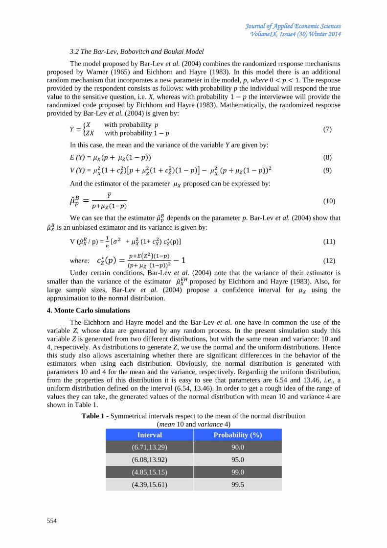
estimators when using each distribution. Obviously, the normal distribution is generated with
parameters 10 and 4 for the mean and the variance, respectively. Regarding the uniform distribution,
from the properties of this distribution it is easy to see that parameters are 6.54 and 13.46, i.e., a
uniform distribution defined on the interval (6.54, 13.46). In order to get a rough idea of the range of
values they can take, the generated values of the normal distribution with mean 10 and variance 4 are
shown in Table 1.
Table 1 - Symmetrical intervals respect to the mean of the normal distribution
(mean 10 and variance 4)
Interval Probability (%)
(6.71,13.29) 90.0
(6.08,13.92) 95.0
(4.85,15.15) 99.0
(4.39,15.61) 99.5
Journal of Applied Economic Sciences
Volume IX, Issue 4(30), Winter 2014
555
From Table 1 we can observe that 90% of the normal distribution values are closer to the
mean than the range of values set in the uniform distribution. Broader intervals are obtained when
considering over 95% of the data from the normal distribution compared with the uniform
distribution.
The Monte Carlo simulation study is based on selecting samples with size { } In
addition, in this study we use two new concepts: F and D. F is the proportion of individuals in
simulation who provide false answers. For example, F = 10% indicates that 10% of individuals in the
sample provide false answers. Meanwhile when an individual gives a false answer D is the difference,
in percentage, between the true response of the individual and the false answer provided to the
interviewer.
In this simulation study we assume that respondents only provide false answers when they
have to respond directly to the sensitive response, i.e., respondents always provide true answers when
a randomized response method is applied. Considering the population from the Spanish Survey on
Income and Living Conditions, as the variable of interest is ‘income’, we will assume that false
answers will be lower than the true ones because it is reasonable to think that an individual declares to
have lower incomes than those which he/she really has, being the opposite situation less likely.
Therefore, if an individual has an income of 1,000 euros and in the interview declares to have an
income of 800 euros, the value of D will be 20%, that is, he/she responds with a difference of 20%
respect to the true value.
The relative bias (RB) and the relative root mean square error (RRMSE) are the empirical
measures used to compare the behavior of the various estimators of the unknown parameter μ. These
measures are defined as
RB =
(13)
RRMSE=√
(14)
where denotes a given estimator of the parameter µ. and are, respectively,
the empirical expectation and the empirical mean square error based on R = 1000 independent
samples selected in the Monte Carlo simulation.
These empirical measures are likely the most used for the problem of evaluating estimators.
For example, these measures have been used by Rao, Kovar and Mantel (1990), Silva and Skinner
(1995), Chen and Sitter (1999), etc. In this study we use the direct estimator , i.e., the sample mean
of the responses obtained from the sensitive question. Alternatively, the estimators and are
also obtained based on randomized response models. For the estimator we consider the values
which also serve to analyze possible differences between the various values of p
that have been considered.
The results from the Monte Carlo simulation study are shown below. Tables 2 and 3 contain
the results from the 2012 Spanish Survey on Income and Living Conditions (ES-SILC) population,
while the results obtained from the normal distribution can be seen in Tables 4 and 5.
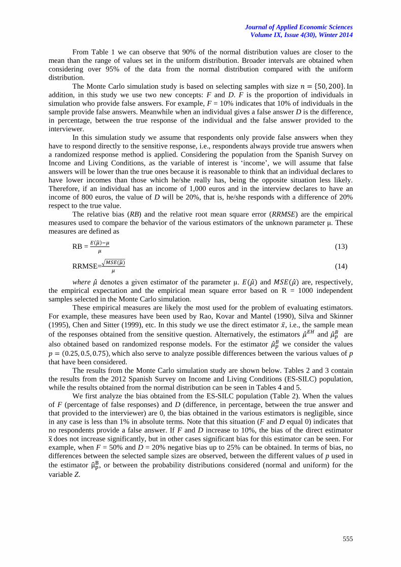
We first analyze the bias obtained from the ES-SILC population (Table 2). When the values
of F (percentage of false responses) and D (difference, in percentage, between the true answer and
that provided to the interviewer) are 0, the bias obtained in the various estimators is negligible, since
in any case is less than 1% in absolute terms. Note that this situation (F and D equal 0) indicates that
no respondents provide a false answer. If F and D increase to 10%, the bias of the direct estimator
does not increase significantly, but in other cases significant bias for this estimator can be seen. For
example, when F = 50% and D = 20% negative bias up to 25% can be obtained. In terms of bias, no
differences between the selected sample sizes are observed, between the different values of p used in
the estimator , or between the probability distributions considered (normal and uniform) for the
variable Z.
Journal of Applied Economic Sciences VolumeIX, Issue4 (30) Winter 2014
556
Table 2 - Relative bias (RB) for the estimators of the mean from the Spanish survey on
income and living conditions population
F D
0 0 0.05 0.04 0.03 -0.12 0.08 -0.04 -0.02 -0.04 -0.06 0.03
0.05 0.01 -0.01 -0.13 0.08 -0.04 -0.07 -0.10 -0.10 0.02
10
5 -0.95 - - - - -1.04 - - - -
10 -1.95 - - - - -2.04 - - - -
20 -4.96 - - - - -5.04 - - - -
20
5 -1.95 - - - - -2.04 - - - -
10 -3.95 - - - - -4.04 - - - -
20 -9.94 - - - - -10.04 - - - -
50
5 -4.95 - - - - -5.04 - - - -
10 -9.97 - - - - -10.04 - - - -
20 -24.97 - - - - -25.02 - - - -
Note: The variable Z is obtained from the uniform distribution (italics) and the normal distribution (bold). The
values of F, D and RB are shown in percentage.
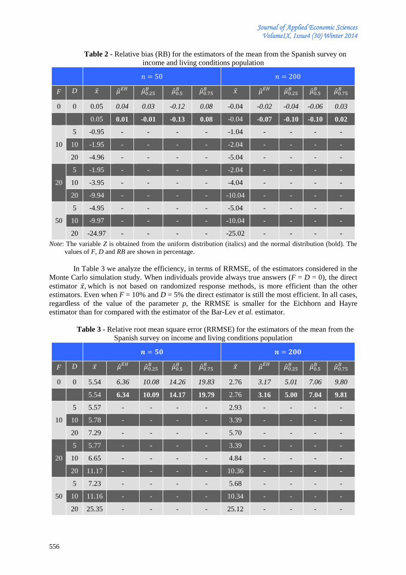
In Table 3 we analyze the efficiency, in terms of RRMSE, of the estimators considered in the
Monte Carlo simulation study. When individuals provide always true answers (F = D = 0), the direct
estimator which is not based on randomized response methods, is more efficient than the other
estimators. Even when F = 10% and D = 5% the direct estimator is still the most efficient. In all cases,
regardless of the value of the parameter p, the RRMSE is smaller for the Eichhorn and Hayre
estimator than for compared with the estimator of the Bar-Lev et al. estimator.
Table 3 - Relative root mean square error (RRMSE) for the estimators of the mean from the
Spanish survey on income and living conditions population
F D
0 0 5.54 6.36 10.08 14.26 19.83 2.76 3.17 5.01 7.06 9.80
5.54 6.34 10.09 14.17 19.79 2.76 3.16 5.00 7.04 9.81
10
5 5.57 - - - - 2.93 - - - -
10 5.78 - - - - 3.39 - - - -
20 7.29 - - - - 5.70 - - - -
20
5 5.77 - - - - 3.39 - - - -
10 6.65 - - - - 4.84 - - - -
20 11.17 - - - - 10.36 - - - -
50
5 7.23 - - - - 5.68 - - - -
10 11.16 - - - - 10.34 - - - -
20 25.35 - - - - 25.12 - - - -
Journal of Applied Economic Sciences
Volume IX, Issue 4(30), Winter 2014
557
Note: The variable Z is obtained from the uniform distribution (italics) and the normal distribution (bold). The
values of F, D and RRMSE are shown in percentage.
Regarding the distributions considered in order to generate the variable Z, we observe that
there is no significant difference, in terms of efficiency, between the results obtained from the normal
distribution and those obtained from the uniform distribution. As expected, all estimators are more
efficient as the sample size increases. Finally, we note that the estimator is more efficient for
smaller values of p.
Note that although the randomized response models may be less efficient than the direct
estimator, we must remember that under the situations discussed in this paper, such estimators based
on random models present a negligible bias, unlike the direct estimator that can present negative
biases up to 25%.
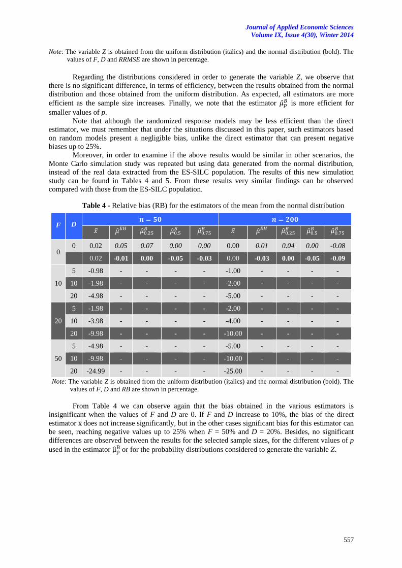
Moreover, in order to examine if the above results would be similar in other scenarios, the
Monte Carlo simulation study was repeated but using data generated from the normal distribution,
instead of the real data extracted from the ES-SILC population. The results of this new simulation
study can be found in Tables 4 and 5. From these results very similar findings can be observed
compared with those from the ES-SILC population.
Table 4 - Relative bias (RB) for the estimators of the mean from the normal distribution
F D
0 0 0.02 0.05 0.07 0.00 0.00 0.00 0.01 0.04 0.00 -0.08
0.02 -0.01 0.00 -0.05 -0.03 0.00 -0.03 0.00 -0.05 -0.09
10
5 -0.98 - - - - -1.00 - - - -
10 -1.98 - - - - -2.00 - - - -
20 -4.98 - - - - -5.00 - - - -
20
5 -1.98 - - - - -2.00 - - - -
10 -3.98 - - - - -4.00 - - - -
20 -9.98 - - - - -10.00 - - - -
50
5 -4.98 - - - - -5.00 - - - -
10 -9.98 - - - - -10.00 - - - -
20 -24.99 - - - - -25.00 - - - -
Note: The variable Z is obtained from the uniform distribution (italics) and the normal distribution (bold). The
values of F, D and RB are shown in percentage.
From Table 4 we can observe again that the bias obtained in the various estimators is
insignificant when the values of F and D are 0. If F and D increase to 10%, the bias of the direct
estimator does not increase significantly, but in the other cases significant bias for this estimator can
be seen, reaching negative values up to 25% when F = 50% and D = 20%. Besides, no significant
differences are observed between the results for the selected sample sizes, for the different values of p
used in the estimator or for the probability distributions considered to generate the variable Z.
Journal of Applied Economic Sciences VolumeIX, Issue4 (30) Winter 2014
558
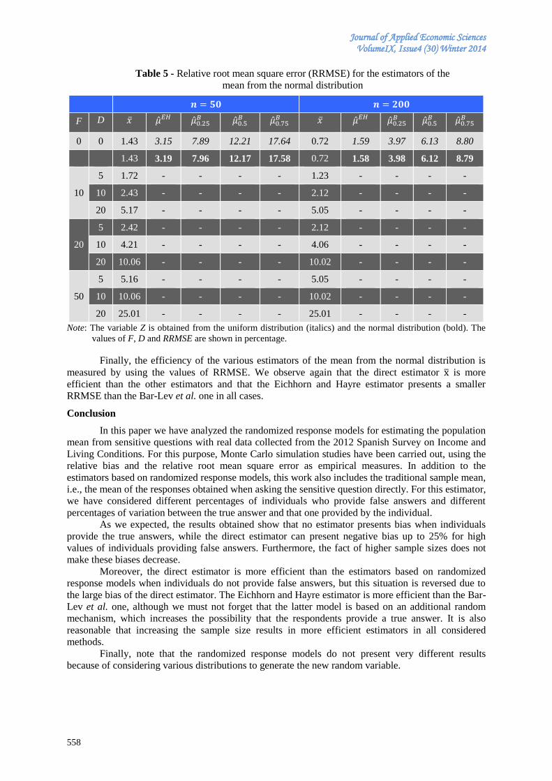
Table 5 - Relative root mean square error (RRMSE) for the estimators of the
mean from the normal distribution
F D
0 0 1.43 3.15 7.89 12.21 17.64 0.72 1.59 3.97 6.13 8.80
1.43 3.19 7.96 12.17 17.58 0.72 1.58 3.98 6.12 8.79
10
5 1.72 - - - - 1.23 - - - -
10 2.43 - - - - 2.12 - - - -
20 5.17 - - - - 5.05 - - - -
20
5 2.42 - - - - 2.12 - - - -
10 4.21 - - - - 4.06 - - - -
20 10.06 - - - - 10.02 - - - -
50
5 5.16 - - - - 5.05 - - - -
10 10.06 - - - - 10.02 - - - -
20 25.01 - - - - 25.01 - - - -
Note: The variable Z is obtained from the uniform distribution (italics) and the normal distribution (bold). The
values of F, D and RRMSE are shown in percentage.
Finally, the efficiency of the various estimators of the mean from the normal distribution is
measured by using the values of RRMSE. We observe again that the direct estimator is more
efficient than the other estimators and that the Eichhorn and Hayre estimator presents a smaller
RRMSE than the Bar-Lev et al. one in all cases.
Conclusion
In this paper we have analyzed the randomized response models for estimating the population
mean from sensitive questions with real data collected from the 2012 Spanish Survey on Income and
Living Conditions. For this purpose, Monte Carlo simulation studies have been carried out, using the
relative bias and the relative root mean square error as empirical measures. In addition to the
estimators based on randomized response models, this work also includes the traditional sample mean,
i.e., the mean of the responses obtained when asking the sensitive question directly. For this estimator,
we have considered different percentages of individuals who provide false answers and different
percentages of variation between the true answer and that one provided by the individual.
As we expected, the results obtained show that no estimator presents bias when individuals
provide the true answers, while the direct estimator can present negative bias up to 25% for high
values of individuals providing false answers. Furthermore, the fact of higher sample sizes does not
make these biases decrease.
Moreover, the direct estimator is more efficient than the estimators based on randomized
response models when individuals do not provide false answers, but this situation is reversed due to
the large bias of the direct estimator. The Eichhorn and Hayre estimator is more efficient than the Bar-
Lev et al. one, although we must not forget that the latter model is based on an additional random
mechanism, which increases the possibility that the respondents provide a true answer. It is also
reasonable that increasing the sample size results in more efficient estimators in all considered
methods.
Finally, note that the randomized response models do not present very different results
because of considering various distributions to generate the new random variable.
Journal of Applied Economic Sciences
Volume IX, Issue 4(30), Winter 2014
559
Acknowledgment
This work is supported by grant P11-SEJ-7090 of the Consejería de Innovación, Ciencia y
Empresa (Junta de Andalucía).
References
[1] Bar-Lev, S.K, Bobovitch, E., Boukai, B. (2004). A note on randomized response models for
quantitative data, Metrika, 60(3): 255-260. http://dx.doi.org/10.1007/s001840300308
[2] Bhargava, M., Singh, R. (2000). A modified randomization device for Warner´s model. Statistica
60(2): 315-321.
[3] Bouza, C.N. (2010). Ranked set sampling using auxiliary variables of a randomized response
procedure for estimating the mean of a sensitive quantitative character. Journal of Modern
Applied Statistical Methods 9(1): 248-254.
[4] Chaudhuri, A. (2004). Christofides´randomized response technique in complex sample survey.
Metrika 60(3): 223-228. http://dx.doi.org/10.1007/s001840300305
[5] Chaudhuri, A., Mukerjee, R. (1988). Randomized Response: Theory and Techniques. New York:
Marcel Dekker.
[6] Chen, J., Sitter, R.R. (1999). A pseudo empirical likelihood approach to the effective use of
auxiliary information in complex surveys. Statistica Sinica, 9(2): 385-406.
[7] Cochran, W.G. (1977). Sampling Techniques. New York: John Wiley & Sons, Inc.
[8] Diana, G., Perry, P.F. (2009). Estimating a sensitive proportion through randomized response
procedures based on auxiliary information. Statistical Papers 50(3): 661-672. http://dx.doi.org/
10.1007/s00362-007-0107-y
[9] Diana, G., Perry, P.F. (2010). New scrambled response models for estimating the mean of a
sensitive quantitative character. Journal of Applied Statistics 37(11): 1875-1890. http://dx.doi.org/
10.1080/02664760903186031
[10] Eichhorn, B., Hayre, L.S. (1983). Scrambled randomized response methods for obtaining
sensitive quantitative data. Journal of Statistical Planning and Inference 7(4): 307-316.
http://dx.doi.org/10.1016/0378-3758(83)90002-2
[11] Eriksson, S.A. (1973). A new model for randomized response. International Statistics Review,
41: 101-113.
[12] Fernández, F.R., Mayor, J.A. (1994). Muestreo en Poblaciones Finitas. Barcelona: P.P.U.
[13] Fox, J.A., Tracy, P.E. (1986). Randomized response: a method for sensitive surveys. London:
SAGE Publications.
[14] Gjestvang, C., Singh, S. (2007). Forced quantitative randomized response model: a new device.
Metrika 66(2): 243-257. http://dx.doi.org/10.1007/s00184-006-0108-1
[15] Greenberg, B.G., Abul-Ela, A., Simmons, W.R., Horvitz, D.G. (1969). The unrelated question
randomized response model: Theoretical frame-work. Journal of the American Statistical
Association 64: 520-539. http://dx.doi.org/ 10.2307/2283636
[16] Grewal, I.S., Bansal, M.L., Sidhu, S.S. (2006). Population mean corresponding to Horvitz-
Thompson´s estimator for multi-characteristics using randomized response technique, Model
Assisted Statistics and Applications, 1(4): 215-220.
[17] Gupta, S., Gupta, B., Singh, S. (2002). Estimation of sensitivity level of personal interview
survey questions. Journal of Statistical Planning and Inference, 100(2): 239-247.
http://dx.doi.org/10.1016/S0378-3758(01)00137-9
[18] Hedayat, A.S., Sinha, B.K. (1991). Design and Inference in finite population sampling. New
York: John Wiley & Sons, Inc.
Journal of Applied Economic Sciences VolumeIX, Issue4 (30) Winter 2014
560
[19] Horvitz, D.G., Shah, B.V., Simmons, W.R. (1967). The unrelated question randomized response
model. Proceedings of Social Statistics Section, American Statistical Association, 65-72.
[20] Hu, M., Salvucci, S., Lee, R. (2001). A study of imputation algorithms. Washington, DC: US
National Center for Education Statistics.
[21] Huang, K. (2006). Estimation of sensitive data from a dichotomous population. Statistical Papers
47(1): 149-156. http://dx.doi.org/ 10.1007/s00362-005-0278-3
[22] Kim, J.L. (1978). Randomized response technique for surveying human populations. Ph.D.
Dissertation. Philadelphia, USA: Temple University.
[23] Kish, L. (1965). Survey Sampling. New York: John Wiley & Sons, Inc.
[24] Little, R.J.A., Rubin, D.B. (2002). Statistical Analysis with Missing Data. New York: John Wiley
& Sons, Inc.
[25] Mangat, N.S., Singh, R. (1990). An alternative randomized response proceures. Biometrika
77(2): 439-442. http://dx.doi.org/10.2307/2336829
[26] Padmawar, V.R., Vijayan, K. (2000). Randomized response revisited. Journal of Statistical
Planning and Inference, 90(2): 293-304. http://dx.doi.org/ 10.1016/S0378-3758(00)00097-5
[27] Pal, S. (2008). Unbiasedly estimating the total of a stigmatizing variable from complex survey on
permitting options for direct or randomized responses. Statistical Papers, 49(2): 157-164.
http://dx.doi.org/ 10.1007/s00362-006-0001-z
[28] Pollock, K.H., Bek, Y. (1976). A comparison of three randomized response models for
quantitative data. Journal of the American Statistical Association, 71: 884-886. http://dx.doi.org/ 10.2307/2286855
[29] Rao, J.N.K., Kovar, J.G., Mantel, H.J. (1990). On estimating distribution functions and quantiles
from survey data using auxiliary information. Biometrika, 77(2): 365-375. http://dx.doi.org/ 10.2307/2336815
[30] Ryu, J.B., Kim, J.M., Heo, T.Y., Park, C.G. (2006). On stratified randomized response sampling.
Model Assisted Statistics and Applications, 1(1): 31-36.
[31] Saha, A. (2006). A generalized two-stage randomized response procedure in complex sample
survey. Australian & New Zealand Journal of Statistics, 48(4): 429-443. http://dx.doi.org/ 10.1111/j.1467-842X.2006.00449.x
[32] Särndal, C.E., Sweensson, B., Wretman, J.H. (1992). Model Assisted Survey Sampling. New
York: Springer-Verlag.
[33] Shabbir, J., Gupta, S. (2005). On modified randomized device of Warner´s model. Pakistan
Journal of Statistics, 21(1): 123-129.
[34] Silva, P.L.D., Skinner, C.J. (1995). Estimating distribution functions with auxiliary information
using poststratification. Journal of Official Statistics, 11(3): 277-294.
[35] Singh, S. (2003). Advanced Sampling Theory with Applications: How Michael ‘Selected’ Amy.
The Netherlands: Springer.
[36] Singh, H.P., Mathur, N. (2005). Estimation of population mean when coefficient of variation is
known using scrambled response technique. Journal of Statistical Planning and Inference,
131(1): 135-144. http://dx.doi.org/10.1016/j.jspi.2004.01.002
[37] Warner, S. (1965). Randomized responses: A survey technique for eliminating evasive survey
bias. Journal of the American Statistical Association, 60: 63-69. http://dx.doi.org/ 10.2307/2283137
[38] Zaizai, Y. (2006). Ratio method of estimation of population proportion using randomized
response technique. Model Assisted Statistics and Applications, 1(2): 125-130.
Journal of Applied Economic Sciences
Volume IX, Issue 4(30), Winter 2014
561
DETERMINANTS OF STOCK MARKET DEVELOPMENT IN ROMANIA
Muhammad AZAM
School of Economics, Finance & Banking
College of Business, Universiti Utara Malaysia
Abdul Qayyum KHAN
Department of Management Sciences,
COMSATS Institute of Information Technology Wah Cantt Campus, Pakistan
Laura STEFANESCU
Faculty of Financial Management Accounting Craiova
Spiru Haret University, Romania
Abstract
This study aims to evaluate the impacts of some central explanatory variables namely Foreign Direct
Investment (FDI), infrastructure facility, saving, inflation, income and energy use on Romanian’s stock market
development measured by market capitalization. For empirical examination, this study used annual time series
data over the period of 1990 to 2013. The study employs various diagnostic tests including normality test,
Pearson correlation test, Park test and DW- test, which shows that there is no problem of skewness and
kurtosis, no problem of heteroscedasticity and no problem of autocorrelation in the model of market
capitalization used for Romania. The Johanson co-integration results indicates that there exists three co-
integrating relationship among the variables. Further, least squares estimate indicates incoming FDI,
infrastructure, saving, energy usage and income are important determinants of Romanian’s stock market in
selected macroeconomic variables used in the study. The empirical findings suggests that management
authorities of Romania needs to formulate prudent macroeconomic stabilization policy in order to encourage
incoming FDI, facilitate physical infrastructure, encourage saving, maintain sustainable energy use. Thus, all
these measures will further develop largely Romanian’s stock market.
Keywords: Stock market development, FDI, GDP, Infrastructure, Romania.
JEL classification: F20, E44, H54, O43, O52
1. Introduction
Generally, it is believed that stable and well-functioning stock market plays important role in
the process of economic growth and development everywhere. Therefore, researchers have exposed
visible interest in various factors determining stock market for different countries. The supporters of
stock market supposed that it perform a better role in the expansion of commerce and industry and
consequently it contributes to the macroeconomic performance of country. The contemporary
theoretical research reveals that long-standing stock market development can bolster economic
growth, whereas, empirical studies be likely to offer some encouragement to this affirmation. In a
study, Demirguc-Kunt and Levine (1996) have shown that utmost stock market indicators are vastly
connected with the development of banking sector. So those countries which have well-developed and
stable stock markets have a tendency to have well-developed banking sector. In a similar vein, study
of Levine and Zervos (1998) indicates that stock market development plays a crucial role in expecting
forthcoming economic growth of a country. According to Levine (1996:7) “Do stock markets affect
overall economic development? Some analysts have viewed stock markets in developing countries as
“Casinos” that have little positive impact on economic growth”.
Caporale et al. (2004) notes that sound stock market facilitates the investors to bypass risk
when capitalizing in promising projects. Moreover, energetic stock markets carry out a conclusive
role in assigning investment to the corporate sector, which will have undeniably a verifiable impact on
the overall economy. Sound stock market provides profitably to total productivity and established
financial markets are usually well-thought-out a vital factor of long-run economic growth (Levine et
al., 2000; Barna and Mura, 2010; Cooray, 2010; Shin, 2013; Al-Qudah, 2014; Kaserer and Rapp
2014). It is therefore, foreseeable that every established stock market will certainly speed up the
suitability of long-term capital for cost-effectively beneficial activities which is mandatory for the
Journal of Applied Economic Sciences VolumeIX, Issue4 (30) Winter 2014
562
encouragement of economic growth and development. In addition, suitable and smooth functioning of
stock market be a sign of an extensive condition for financial sector evolution which is considered a
pre-requisite to contributes to the economic development and provide sound environment to attract
more foreign investors.
It is therefore, important to explore various determinants affects stock market. Though, there
are enormous factors explaining stock market development, however, the main focus of the present
study is more on the impacts of income, inflation, energy, foreign direct investment on stock market
development in the context of Romania.
The study of Brasoveanu et al. (2008) finds a significantly positive relationship between
capital market development and economic growth in Romania on quarterly data from 2000: 1 to 2006:
2. In a study, Barna and Mura (2010) mention that Romanian capital market grown sluggishly starting
since 1995. It is evident, that many years after 1989 Romania had undesirable real rate of Gross
Domestic Product (GDP) growth. While, it is recorded that since 2000, Romania exhibits positive and
desirable economic growth rates associated with the progress of the financial system. Regarding the
importance of capital market, Prime Minister Victor Ponta stated that the existence of solid capital
market is an important part for Romania's development1. The economy of Romania showed a
marvelous performance in 2013, GDP growth rate is estimated to have touched or even surpassed
2.5% in 2013. The performance of Romanian’s capital market remained outstanding and undoubtedly
it is considered best year in the previous five years where some initial public offerings (IPOs) at
highest values. The upward trend is expected to be continued during 2014 also. The capital market
will certainly play a leading role in development of overall Romanian economy. Evidently, a
significant growth of the capital market has been observed in 2013, with two IPOs of state-owned
enterprises. Moreover, the growing involvement of retail investors could be another vital component
in the expansion of Romania’s market2.
The broad aim of this study is to evaluate the influence of some macroeconomic variables
namely FDI inflow, inflation, energy, and infrastructure on Romanian’s stock market. For empirical
analysis, time series data over the period of 1990 to 2013 are used. According to the knowledge of the
authors, therefore is no similar studies exist on the Romania. Moreover, this study is different from
the previous studies in terms of the period length taken into consideration. Several studies have
surveyed the factors affecting stock market through different viewpoints and with different regressors
for different countries. In spite of this, the assortment of regressors with holistic approach used in this
study is emphatically different as compared to the past studies carried out in the context of
Romanian’s stock market determinants. Therefore, the present study will constructively contribute to
the growth of literature on the determinants of stock market for Romania and can be extended to other
countries also.
The rest of the study is structured as follows. Section 2 discusses literature review on the
factors affecting stock market development. Section 3 deals with data sources, and the methodology
used. Section 4 interprets the empirical results. Section 5 concludes the study.
2. Literature review
The existing literature reveals that though empirical studies on the factors determining stock
market development are many but studies in the context of Romanian stock market are very scarce.
Using panel data for fifteen industrial and developing countries during 1980-1995, Garcia and Liu
(1999) discovers that financial intermediary development, real income, saving rate, and stock market
liquidity are the crucial factors influencing stock market capitalization. The study of Wongbangpo and
Sharma (2002) finds that high inflation in Indonesia and Philippine has a long run negative
association between stock prices and money supply, while the money growth in the case of Malaysia,
Singapore and Thailand suggest the positive influence for their stock market during 1985-1996.
Naceur and Ghazouani (2007) carried out an empirical study using unbalanced panel data from
MENA-12 countries. The empirical results reveals that macroeconomic variables such as , credit to
private sector, inflation rate, saving rate, and stock market liquidity are significant factors
1 Romanian National News Agency (2014)
2 Franklin Templeton Investments (2014)
Journal of Applied Economic Sciences
Volume IX, Issue 4(30), Winter 2014
563
determining stock market development in MENA-12 countries. The study of Yartey (2008)
investigates the institutional and macroeconomic factors of stock market development for 42
emerging economies during 1990-2004. The study observes that macroeconomic determinants namely
income level, gross domestic investment, banking sector development, private capital flows, and stock
market liquidity are the key factors determining stock market development in 42 emerging market
countries during the period under the study. Moreover, the empirical findings reveal that political risk,
law and order, and bureaucratic quality are significant factors of stock market development because
they attract the sustainability of exterior finance. The study suggests that analysis also reveals the
determinates detected earlier mentioned as determining stock market in emerging economies can also
describe the stock market development in South Africa.
Similarly, Billmeier and Massa (2009) examines the macroeconomic factors of stock market
capitalization for 17 countries from Middle East and Central Asia. The macroeconomic determinants
considered in the study were an institutional variable, remittances, GDP, gross fixed capital formation
to GDP, inflation change, domestic credit to private sector and to GDP, stock value traded to GDP
and oil price index among explanatory variables. The results indicate institutions and remittances have
significantly positive effect on stock market development, whereas in resource-rich countries, stock
market development is mostly pushed by the oil price. Cherif and Gazdar (2010) examine the
influence of macroeconomic determinants and institutional factors on stock market development for
fourteen Middle Eastern and Northern African (MENA) countries during 1990-2007. The results
show strong effects of income, saving, stock market liquidity and interest rate on equity market
development for MENA-14 countries. While, the study fails to find that institutional environment as
captured by a composite policy risk index is a motivating force for the stock market development in
MENA countries. Al-Halalmeh and Sayah (2010) find that FDI has a significant impact on shares
market value for Jordon over the period of 2006-2009.
Using a panel of country observations assembled for 30 countries over the period of 1960-
2007, Evrim-Mandaci et al. (2013) finds that FDI, foreign remittances and bank credits to private
sector had significantly positive influence on stock market development measured by market
capitalization. In a similar vein, Azam and Ibrahim (2014) observe that FDI inflow, domestic
investment, domestic saving rate, GDP growth rate and inflation rate are important determinants of
Malaysian’s stock market in the selected set of explanatory variables used in the study during 1988 -
2012. Şukruogl and Nalin (2014) observe that monetization ratio and inflation rate have significantly
inverse impacts on stock market development, while income, liquidity ratio, saving rate have
significantly positive impacts on the stock market development for 19 European Countries during
1995-2011. The study of Burca and Batrinca (2014) investigates the factors determining the financial
performance in the Romanian insurance market during 2008-2012, while employing specific panel
data techniques. The empirical findings show the financial leverage in insurance, company size,
growth of gross written premiums, underwriting risk, risk retention ratio and solvency margin are the
main determinants of the financial performance in the Romanian insurance market. Table 1 portrays
brief prior selected empirical studies on the determinants of stock market.
Table 1- Compact previous selected empirical studies on the determinants of stock market
Author (s) Sample periods,
Methodology used
Dependent
variable Independent variables Findings
Şukruogl
and Nalin
(2014)
1995-2011 - 19
European
Countries3 dynamic
panel data
estimation
Stock market
development
GDP, liquidity ratio,
Monetization ratio
turnover ratio, Inflation,
budget balance and saving
rate
Income, Monetization
ratio, liquidity ratio,
saving rate and inflation
effect on stock market
development.
Shahbaz et al. (2013)
1971-2006 -
Pakistan ARDL
Bounds Testing
Approach
Stock market
development
FDI, GNP per capita,
inflation rate and domestic
savings
Results support the
complementary role of
FDI in the stock market
development
3 Austria, Belgium, Bulgaria, Croatia, Czech Republic, Denmark, Finland, France, Germany, Greece, Hungary,
Italy, Latvia, Netherlands, Portugal, Slovenia, Spain, Sweden and United Kingdom
Journal of Applied Economic Sciences VolumeIX, Issue4 (30) Winter 2014
564
Author (s) Sample periods,
Methodology used
Dependent
variable Independent variables Findings
Abdelbaki
(2013)
1990-2007,
Bahrain
ARDL
stock market
development
Inflation, income, banking
system development, stock
market liquidity, private
capital flow investment
and saving
Income, domestic
investment,
banking system
development; private
capital flows and stock
market liquidity
El-Nader
and
Alraimony
(2011)
1990-2011, Jordan
VECM model
stock market
development
Money supply, GDP,
inflation, real exchange
rate, interest rate
Money supply, inflation,
real exchange rate,
interest rate
Kurach
(2010)
1996-2006 - 13
CEE states4
Fixed-effects and
Random-effects
stock market
development
Inflation, Budget balance,
saving rate, Turnover ratio,
liquidity ratio,
Monetization ratio and
GDP per capita
GDP, banking sector
growth, stock market
liquidity, budget balance
are main determinants
Yartey
(2008)
1990- 2004
42 economies
GMM
Stock market
capitalization
Private credit, value
traded, Log GDP per
capita, credit, FDI,
inflation, political risk, law
and order, corruption,
bureaucratic quality and
democratic accountability
Income level, gross
domestic investment,
banking sector
development, private
capital flows, and stock
market liquidity are key
factors
Source: Authors compilation
3. Data description and methodology
Data sources
Annual time series data ranging from 1990 to 2013 is used for empirical investigation. The
data were obtained from the World Development Indicator (2014), the World Bank database
(http://data.worldbank.org/news/release-of-world-development-indicators-2014).
Model Specification
This study adopt a single multivariate framework methodology where market capitalization is
the response variable. Log-linear multiple regression model is used in order to examine the impacts of
various determinants of market capitalization namely FDI, energy usage, inflation rate, saving,
infrastructure proxy used utilization of landline telephone per 1000 people, and GDP on market
capitalization. The proposed model of market capitalization for Romania is given in the following
functional equation:
t t t t t, Infrt, GDPt (3.1)
Equation (3.1) can be written in the following log-linear general market capitalization
function:
MCt = α 0+ α 1FDIt +α2EUgt+ α 3Inft + α4 St + α5 Infrt + α6GDPt+εt (3.2)
Where, α0 is the intercept and t for time period. MC indicates market capitalization, FDI
denote foreign direct investment, EU is energy usage, Inf is inflation, S is saving Infr is infrastructure,
GDP is Gross Domestic product and ε is error term, which shows effect of the other factors. Data are
converted into in log form. The parameters α1, α2, α3, α4, α5 and α6 are the long-run elasticities of all
regressors. Equation 3.2 postulates that all the coefficients signs are predicted would be positive with
exception of inflation rate which expected to exhibit negative coefficient sign.
4 Bulgaria, Croatia, Czech Republic, Estonia, Hungary, Latvia, Lithuania, Poland, Romania, Russian Federation,
Slovak Republic, Slovenia and Ukraine
Journal of Applied Economic Sciences
Volume IX, Issue 4(30), Winter 2014
565
4. Empirical Results
Normality of the Data
It is an important and a necessary process to check the data for its normality before going to
put the data in linear model for its coefficient determination. Histograms and normal probability plot
of regression standardized residuals were obtained and is used here to check the normality. It is a very
simple and easy approach to visually check normality of the data. The results are given in Graph 1 and
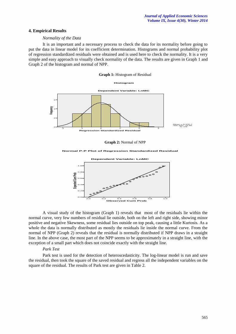
Graph 2 of the histogram and normal of NPP.
Graph 1: Histogram of Residual
Graph 2: Normal of NPP
A visual study of the histogram (Graph 1) reveals that most of the residuals lie within the
normal curve, very few numbers of residual lie outside, both on the left and right side, showing minor
positive and negative Skewness, some residual lies outside on top peak, causing a little Kurtosis. As a
whole the data is normally distributed as mostly the residuals lie inside the normal curve. From the
normal of NPP (Graph 2) reveals that the residual is normally distributed if NPP draws in a straight
line. In the above case, the most part of the NPP seems to be approximately in a straight line, with the
exception of a small part which does not coincide exactly with the straight line.
Park Test
Park test is used for the detection of heteroscedasticity. The log-linear model is run and save
the residual, then took the square of the saved residual and regress all the independent variables on the
square of the residual. The results of Park test are given in Table 2.
Regression Standardized Residual
3210-1-2
Frequ
ency
6
4
2
0
Histogram
Dependent Variable: LnMC
Mean =-9.37E-15Std. Dev. =0.853
N =23
Observed Cum Prob
1.00.80.60.40.20.0
Expe
cted C
um Pr
ob
1.0
0.8
0.6
0.4
0.2
0.0
Normal P-P Plot of Regression Standardized Residual
Dependent Variable: LnMC
Journal of Applied Economic Sciences VolumeIX, Issue4 (30) Winter 2014
566
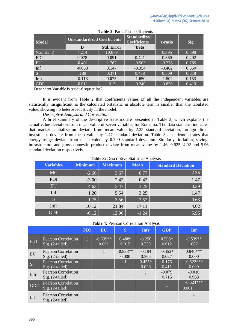
Table 2: Park Test coefficients
Model Unstandardized Coefficients
Standardized
Coefficients t-ratio Sig.
B Std. Error Beta
(Constant) 4.214 10.679 0.395 0.698
FDI 0.078 0.091 0.421 0.860 0.402
EU -0.491 1.767 -0.503 -0.278 0.785
Inf -0.068 0.147 -0.354 -0.462 0.650
S .189 0.371 0.438 0.509 0.618
Infr -0.113 0.075 -1.650 -1.502 0.153
GDP -0.011 .013 -0.240 -0.830 0.419 Dependent Variable is residual square lne2
It is evident from Table 2 that coefficients values of all the independent variables are
statistically insignificant as the calculated t-statistic in absolute term is smaller than the tabulated
value, showing no heteroscedasticity in the model.
Descriptive Analysis and Correlation
A brief summary of the descriptive statistics are presented in Table 3, which explains the
actual value deviation from mean value of seven variables for Romania. The data statistics indicates
that market capitalization deviate from mean value by 2.35 standard deviation, foreign direct
investment deviate from mean value by 1.47 standard deviation. Table 3 also demonstrates that
energy usage deviate from mean value by 0.290 standard deviation. Similarly, inflation, saving,
infrastructure and gross domestic product deviate from mean value by 1.46, 0.625, 4.02 and 5.96
standard deviation respectively.
Table 3: Descriptive Statistics Analysis
Variables Minimum Maximum Mean Standard Deviation
MC -2.66 3.67 0.77 2.35
FDI -3.00 2.42 0.42 1.47
EU 4.63 5.47 3.25 0.29
Inf 1.20 5.54 3.25 1.47
S 1.75 3.56 2.57 0.63
Infr 10.12 21.84 17.11 4.02
GDP -0.12 12.90 -1.24 5.96
Table 4: Pearson Correlation Analysis
FDI EU S Infr GDP Inf
FDI Pearson Correlation
Sig. (2-tailed)
1
-0.639**
0.001
0.488*
0.015
-0.250
0.239
0.505*
0.012
-0.539**
.007
EU Pearson Correlation
Sig. (2-tailed)
1
-0.838**
0.000
-0.194
0.365
-0.452*
0.027
0.846***
0.000
S Pearson Correlation
Sig. (2-tailed)
1
0.455*
0.026
0.176
0.411
-0.522***
0.009
Infr Pearson Correlation
Sig. (2-tailed) 1
-0.079
0.715
-0.010
0.963
GDP Pearson Correlation
Sig. (2-tailed) 1
-0.624***
0.001
Inf Pearson Correlation
Sig. (2-tailed)
1
Journal of Applied Economic Sciences
Volume IX, Issue 4(30), Winter 2014
567
Table 4 illustrates Pearson correlation result for correlation among the six independent
variables used in the study. It is evident from Table 4 that foreign direct investment has statistically
significant relationship with energy usage, saving, gross domestic product and inflation in Romania.
Energy usage has negative and statistically significant connection with gross domestic product and
saving, and positive significant relationship with inflation. It is observed that saving has significant
negative relationship with inflation and significant positive relationship with infrastructure. GDP has
significant negative relationship with inflation.
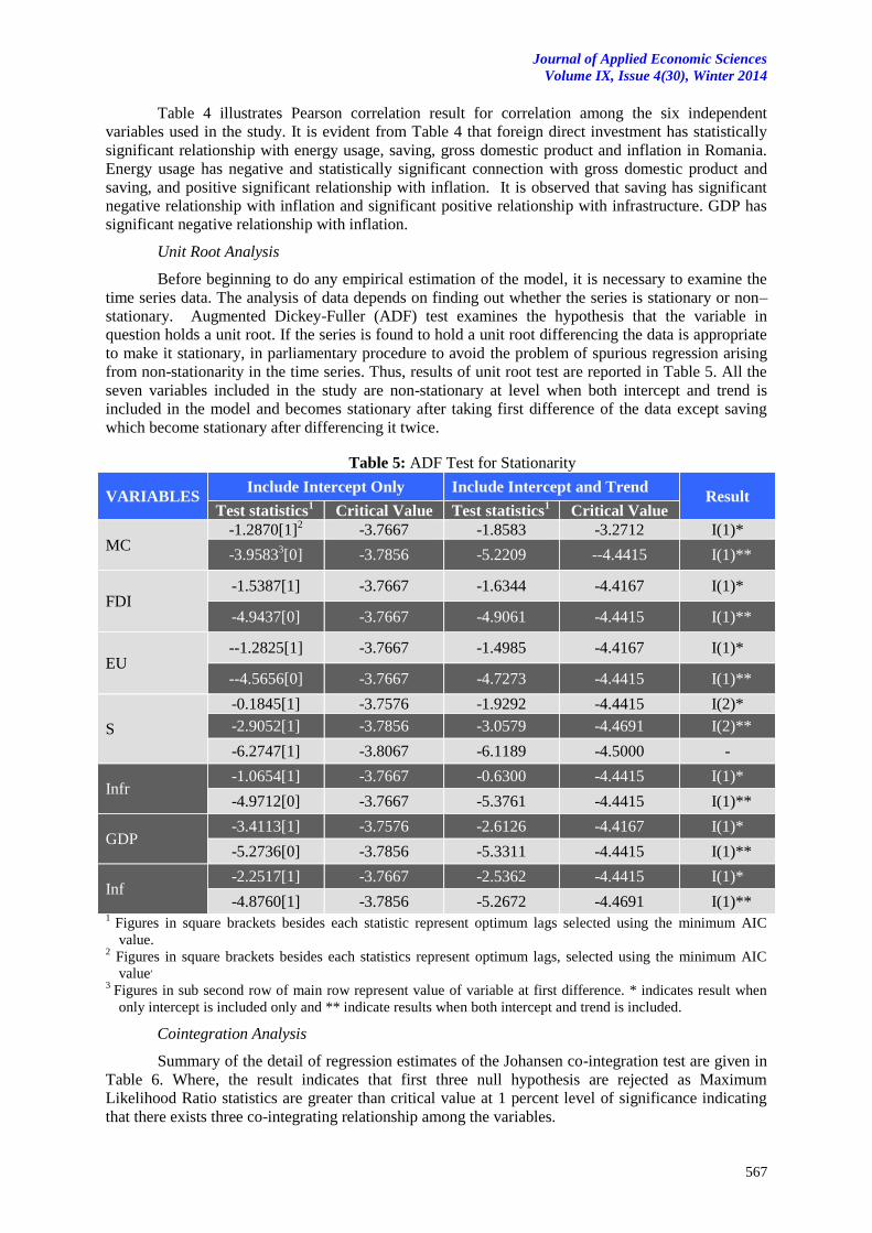
Unit Root Analysis
Before beginning to do any empirical estimation of the model, it is necessary to examine the
time series data. The analysis of data depends on finding out whether the series is stationary or non–
stationary. Augmented Dickey-Fuller (ADF) test examines the hypothesis that the variable in
question holds a unit root. If the series is found to hold a unit root differencing the data is appropriate
to make it stationary, in parliamentary procedure to avoid the problem of spurious regression arising
from non-stationarity in the time series. Thus, results of unit root test are reported in Table 5. All the
seven variables included in the study are non-stationary at level when both intercept and trend is
included in the model and becomes stationary after taking first difference of the data except saving
which become stationary after differencing it twice.
Table 5: ADF Test for Stationarity
VARIABLES Include Intercept Only Include Intercept and Trend
Result Test statistics
1 Critical Value Test statistics
1 Critical Value
MC
-1.2870[1]2
-3.7667 -1.8583 -3.2712 I(1)*
-3.95833[0] -3.7856 -5.2209 --4.4415 I(1)**
FDI -1.5387[1] -3.7667 -1.6344 -4.4167 I(1)*
-4.9437[0] -3.7667 -4.9061 -4.4415 I(1)**
EU
--1.2825[1] -3.7667 -1.4985 -4.4167 I(1)*
--4.5656[0] -3.7667 -4.7273 -4.4415 I(1)**
S
-0.1845[1] -3.7576 -1.9292 -4.4415 I(2)*
-2.9052[1] -3.7856 -3.0579 -4.4691 I(2)**
-6.2747[1] -3.8067 -6.1189 -4.5000 -
Infr
-1.0654[1] -3.7667 -0.6300 -4.4415 I(1)*
-4.9712[0] -3.7667 -5.3761 -4.4415 I(1)**
GDP -3.4113[1] -3.7576 -2.6126 -4.4167 I(1)*
-5.2736[0] -3.7856 -5.3311 -4.4415 I(1)**
Inf -2.2517[1] -3.7667 -2.5362 -4.4415 I(1)*
-4.8760[1] -3.7856 -5.2672 -4.4691 I(1)** 1
Figures in square brackets besides each statistic represent optimum lags selected using the minimum AIC
value. 2 Figures in square brackets besides each statistics represent optimum lags, selected using the minimum AIC
value,
3 Figures in sub second row of main row represent value of variable at first difference. * indicates result when
only intercept is included only and ** indicate results when both intercept and trend is included.
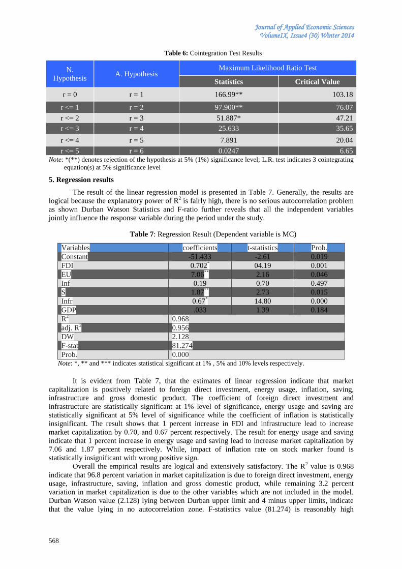
Cointegration Analysis
Summary of the detail of regression estimates of the Johansen co-integration test are given in
Table 6. Where, the result indicates that first three null hypothesis are rejected as Maximum
Likelihood Ratio statistics are greater than critical value at 1 percent level of significance indicating
that there exists three co-integrating relationship among the variables.
Journal of Applied Economic Sciences VolumeIX, Issue4 (30) Winter 2014
568
Table 6: Cointegration Test Results
N.
Hypothesis A. Hypothesis
Maximum Likelihood Ratio Test
Statistics Critical Value
r = 0 r = 1 166.99** 103.18
r ˂= 1 r = 2 97.900** 76.07
r ˂= 2 r = 3 51.887* 47.21
r ˂= 3 r = 4 25.633 35.65
r ˂= 4 r = 5 7.891 20.04
r ˂= 5 r = 6 0.0247 6.65 Note: *(**) denotes rejection of the hypothesis at 5% (1%) significance level; L.R. test indicates 3 cointegrating
equation(s) at 5% significance level
5. Regression results
The result of the linear regression model is presented in Table 7. Generally, the results are
logical because the explanatory power of R2 is fairly high, there is no serious autocorrelation problem
as shown Durban Watson Statistics and F-ratio further reveals that all the independent variables
jointly influence the response variable during the period under the study.
Table 7: Regression Result (Dependent variable is MC)
Variables coefficients t-statistics Prob.
Constant -51.433 -2.61 0.019
FDI 0.702*
04.19 0.001
EU 7.06**
2.16 0.046
Inf 0.19
0.70 0.497
S 1.87**
2.73 0.015
Infr 0.67* 14.80 0.000
GDP .033
1.39 0.184
R2
0.968
adj. R2
0.956
DW 2.128
F-stat 81.274
Prob. 0.000 Note: *, ** and *** indicates statistical significant at 1% , 5% and 10% levels respectively.
It is evident from Table 7, that the estimates of linear regression indicate that market
capitalization is positively related to foreign direct investment, energy usage, inflation, saving,
infrastructure and gross domestic product. The coefficient of foreign direct investment and
infrastructure are statistically significant at 1% level of significance, energy usage and saving are
statistically significant at 5% level of significance while the coefficient of inflation is statistically
insignificant. The result shows that 1 percent increase in FDI and infrastructure lead to increase
market capitalization by 0.70, and 0.67 percent respectively. The result for energy usage and saving
indicate that 1 percent increase in energy usage and saving lead to increase market capitalization by
7.06 and 1.87 percent respectively. While, impact of inflation rate on stock marker found is
statistically insignificant with wrong positive sign.
Overall the empirical results are logical and extensively satisfactory. The R2 value is 0.968
indicate that 96.8 percent variation in market capitalization is due to foreign direct investment, energy
usage, infrastructure, saving, inflation and gross domestic product, while remaining 3.2 percent
variation in market capitalization is due to the other variables which are not included in the model.
Durban Watson value (2.128) lying between Durban upper limit and 4 minus upper limits, indicate
that the value lying in no autocorrelation zone. F-statistics value (81.274) is reasonably high
Journal of Applied Economic Sciences
Volume IX, Issue 4(30), Winter 2014
569
indicating that all the independent variables have joint significance effect on the response variable
which is market capitalization in the study.
Concluding remarks
The main objective of this study is to empirically verify the impacts of some central
explanatory variables namely FDI, infrastructure, saving, inflation, income and energy use on stock
market development of Romania measured by market capitalization. The study used annual time
series data ranging from 1990 to 2013. The study applied various diagnostic tests including normality
test, Pearson correlation test, Park test and DW- test, which shows that there is no problem of
skewness and kurtosis, no problem of heteroscedasticity and no problem of autocorrelation in the
model of market capitalization used for Romania. Data have been checked for stationarity using ADF
test. The Johanson co-integration results indicates that there exists three co-integrating relationship
among the variables. Further, least squares estimate reveals that the impacts of FDI, infrastructure,
saving, energy usage and income on market capitalization are positive and statistically significant.
The results of this study are vigorous and reasonable, therefore, alluring for sound policy
consideration. The findings of the study suggest that policy makers needs to create investment-
friendly environment in order to enhance more FDI inflows into the country, infrastructure
development, saving enhancement techniques, more energy usage but care should be taken to design
energy supply policy appropriately to meet increase energy demand handsomely, all these factors
expand market capitalization.
References
[1] Abdelbaki, H.H. (2013). Causality relationship between macroeconomic variables and stock
market development: Evidence from Bahrain. The International Journal of Business and
Finance Research, 7(1):69–84.
[2] Al-Halalmeh, M.I., Sayah, A.M. (2010). Impact of foreign direct investment on shares market
value in Amman exchange market, American Journal of Economics and Business
Administration, 2(1):35-38.
[3] Al-Qudah, A.M. (2014). Stock exchange development and economic growth: empirical evidence
from Jordan. International Journal of Business and Management, 9(11): 123-138.
[4] Azam, M. and Ibrahim, Y., (2014). Foreign direct investment and Malaysia’s stock market: using
ARDL bounds testing approach. Journal of Applied Economic Sciences, IX, Issue 2(29).
[5] Barna, F., Mura, P.O. (2010). Capital market development and economic growth: the case of
Romania. Annals of the University of Petrosani, Economics, 10(2): 31-42.
[6] Billmeier, A., Massa, I. (2009). What drives stock market development in emerging markets
institutions, remittances, or natural resources?, Emerging Markets Review, 10(1): 23–35.
[7] Brasoveanu, L.O., Dragota, V., Catarama, D., Semenescu, A. (2008). Correlations between capital
market development and economic growth: The case of Romania. Journal of Applied Quantitative
Methods, 3(1): 64–75.
[8] Burca, A-M., Batrinca, G. (2014). The determinants of financial performance in the Romanian
insurance market. International Journal of Academic Research in Accounting, Finance and
Management Sciences, 4(1): 299–308.
[9] Caporale, G. M., Howells, P.G.A, and Soliman, A.M. (2004). Stock market development and
economic growth: the causal linkage, Journal of Economic Development, 29(1): 33-50.
[10] Cherif, M. and Gazdar, K., (2010).Macroeconomic and institutional determinants of stock market
development in MENA region: new results from a panel data analysis. International Journal of
Banking and Finance, 7(1): 139-159.
[11] Cooray, A., (2010). Do stock markets lead to economic growth? Journal of Policy Modeling, 32:
448–460.
Journal of Applied Economic Sciences VolumeIX, Issue4 (30) Winter 2014
570
[12] Demirguc-Kunt, Levine, R. (1998). Stock markets, coportae finance, and economic growth: an
overview. The World Bank Economic Review, 10(2): 223-239.
[13] El-Nader, H. M., Alraimony, A. D. (2013). The macroeconomic determinants of stock market
development in Jordan international. Journal of Economics and Finance, 5(6): 91–103.
[14] Evrim-Mandaci, P., Aktan, B., Kurt-Gumus, G., Tvaronaviciene, M. (2013). Determinants of
stock market development: evidence from advanced and emerging markets in a long span.
Business: Theory and Practice, 14(1): 51-56.
[16] Garcia, V. F., Liu, L. (1999). Macroeconomic determinants of stock market development.
Journal of Applied Economics, II(1): 29-59.
[17] Kaserer, C., Rapp, M. S., (2014). Capital Markets and Economic Growth: Long-Term Trends and
Policy Challenges. Research Report. Retrieved from www.aima.org/...cfm/.../5D6152C4-C9A0-
4FDA-B2DD415168ED658B
[18] Kurach, R. (2010). Stock market development in CEE countries-the panel data analysis.
Ekonomika, 89(3): 20– 29.
[19] Levine, R., Loayza, N., Beck, T. (2000). Financial intermediation and growth: causality and
causes. Journal of Monetary Economics, 46(1): 31-77.
[20] Levine, R. and Zervos, S., (1998). Stock markets, banks, and economic Growth. American
Economic Review, 88: 536–558.
[21] Levine, R. (1996). Stock markets: a spur to economic growth. Finance and Development, 46: 7-
10.
[22] Naceur, S.B., Ghazouani, S. (2007). Stock markets, banks, and economic growth: Empirical
evidence from the MENA region. Research in International Business and Finance, 21: 297–315.
[24] Shahbaz, M., Lean, H.H., Kalim, R. (2013). The impact of foreign direct investment on stock
market development: evidence from Pakistan. Ekonomska Istrazivanja-Economic Research,
26(1):17-32.
[25] Shin, Y. (2013). Financial markets: an engine for economic growth. The Regional Economist,
Federal Reserve Bank of St. Louis, Central of America Economy.
[26] Şukruoğlu, D., Nalin, H.T. (2014). The macroeconomic determinants of stock market
development in selected European countries: dynamic panel data analysis. International Journal
of Economics and Finance, 6(3): 64-71
[27] Wongbangpo, P., Sharma, S.C. (2002). Stock market and macroeconomic fundamental dynamic
interactions: ASEAN-5 countries. Journal of Asian Economics, 13(1): 27-51.
[28] Yartey, C.A. (2008). The determinants of stock market development in emerging economies: is
South Africa Different? International Monetary Fund WP/08/32.
*** Franklin Templeton Investments (2014). Romania on the Right Track. Investment Adventures in
Emerging Markets. Retrieved from http://mobius.blog.franklintempleton.com/2014/
02/06/romania-on-the-right-track-2/
*** Romanian National News Agency (2014). PM Ponta: Strong capital market mandatory for
Romania's development. National Press Agency AGERPRES, 6 Oct 2014. Retrieved from
http://www.agerpres.ro/english/2014/10/06/pm-ponta-strong-capital-market-mandatory-for-
romania-s-development-12-05-07
Journal of Applied Economic Sciences
Volume IX, Issue 4(30), Winter 2014
571
OIL PRICE FLUCTUATIONS AND TRADE BALANCE OF TURKEY
Süleyman AÇIKALIN
Hitit University, FEAS, Department of Economics5, Turkey
Erginbay UĞURLU
Hitit University, FEAS, Department of Economics, Turkey
Abstract:
The relationship between oil price fluctuations and the trade balance of Turkey is the main concern of
this paper. Economic growth performance of Turkey depends on imported capital goods as well as imported oil.
Oil price increases bring a heavy burden for Turkish economy. Therefore, it is important to analyze the effects
of oil price increases on external balances of Turkey. We specifically aim to examine the effects of price
fluctuations of imported oil on Turkey’s trade balance using a structural vector autoregression (VAR) model.
The variables used in this model are imported crude oil price, imports of crude oil, industrial production index,
and trade balance to GDP ratio. Monthly data set for the period of September 2009 - June 2014 is used. The
results show that the oil price shock creates a negative impact on trade balance and this effect continues while
declining in magnitude for more than 10 months. Most of the variation in forecast error of trade balance ratio is
explained by the shock on itself and only a limited variation, around 4%, is explained by oil price shock for a 10
months period.
Keywords: Oil price; trade balance; structural VAR; Turkish Economy.
JEL classification: F14, C32, F41
1. Introduction
The relationship between increasing oil prices and macroeconomic indicators such as
economic growth rate, inflation rate, and external balances has been an important area of study in
economics. The interest on the topic mainly started after the drastic oil price increases experienced
during the oil shocks of 1970s. Initial studies after 1970s focused on the effects of increasing oil
prices on macroeconomic performance of industrialized economies. As expected, it was mainly
concluded that increasing oil prices lowered the GDP growth rate and contributed to the inflation
problem.
Studies showed that the degree of the impact of increasing oil prices on macroeconomic
variables varied over time. Hamilton (1983) showed that while the negative impact of oil prices on
explaining US recession during the period of 1949 – 1972 was significant, its size weakened in 1973 –
1980 period. Later studies argued that not all oil shocks were the same in terms of their nature and
also in terms of their effects on the related economies. Some of these studies agreed that oil shocks of
1970s and early 1980s were supply side shocks while the ones after 1980s including the ones after
2000 were demand side shocks (Archanskia et al., 2012; Hamilton 1983) in which oil prices are
determined endogenously. However, not everyone agreed with this classification. For example, Kilian
(2009) claimed that oil price shock of 1979/1980 should be considered as a result of both supply and
demand shocks which were worked out together. For the oil shocks experienced after 2000 most of
the studies agreed on the opinion that they are not supply side shocks (Archanskaia et al., 2012;
Hamilton, 2009; Kilian 2009). Determining the nature of oil price increase and therefore the nature of
the shocks is important to understand the underlying reasoning behind the shock so that policymakers
could take appropriate precautionary actions for their economies in a timely manner.
The issue of increasing oil prices and oil price fluctuations captured the attention of
economists one more time after the year 2000 as oil prices started to fluctuate considerably one more
time. Small number of studies conducted was on emerging economies during this period. The
response of economic growth rate and inflation rate of oil importing countries to the surge in world oil
prices was one of the research topics of this period (Ghosh, 2009; Barsky and Kilian 2004; Hamilton,
This paper was presented on ICESBA 2014 in Bucharest, Romania.
5 Hitit University, FEAS, Department of Economics, Çorum, 19030, Turkey
Journal of Applied Economic Sciences VolumeIX, Issue4 (30) Winter 2014
572
2005). Studies on the external balances of oil importing countries were very limited in numbers
(Bodenstein et al., 2011; Kilian, L., Rebucci, A., and Spatafora, N., 2009; Narayan et al., 2014).
As Turkey moved to export oriented growth strategy after 1980, trade and current account
balances gained importance in evaluation of Turkey’s economic performance. According to the new
growth strategy, export has become the new engine of growth in Turkey. As an oil importing
developing country, it is widely believed that oil price fluctuations have created significant negative
effects for Turkey. Moreover, Turkish growth experience showed that there is a significant correlation
between economic growth and imports.
This paper is organized as follows. Section 2 reviews the previous literature on oil shocks and
their effects on macroeconomic indicators such as growth rate and external balances. Section 3 gives
brief information about the empirical methodology used in the paper and the main findings. Section 4
includes the concluding remarks.
2. Literature Review
The results of oil shocks for both oil exporting and oil importing countries as well as the main
factors behind oil shocks are studied especially after the oil shocks of 1970s. As the oil price stayed
relatively stable during the period of 1985 to 2000, the interest on the subject was declined. As the
prices started to increase one more time after 2002, the interest on the topic is on the rise again.
Most of the literature consists of studies analyzing the association between external balances
of developed economies such as the US. For example; Kilian (2010) used five variables which are the
percent change of world production of crude oil, the measure of global real economic activity, the real
price of imported crude oil, the real price of gasoline in the US, and the percent growth rate of the
quantity of gasoline consumed in the US. Peersman and Robays (2011), on the other hand, analyzed
the effects of oil price shocks on macroeconomic indicators using various countries. They concluded
that oil price increases create different effects depending on the nature of the increase and results also
differ depending on whether the country is an oil importer or an oil exporter.
Le and Chang (2013) took three different types of countries in their paper. This study
included Malaysia as an oil exporter, Singapore with an oil refinery and Japan as an oil importer
country to see the effects of oil price increase on countries with different economic characteristics
relating oil.
Archanskaia, Creel, and Huert (2012) wanted to determine the driving force behind oil shocks
in 1970-2006 period with the distinction of supply side and demand side shocks in their model. They
argued that while supply side oil shocks have created negative external balance effects, demand
driven oil shocks did not have such negative effects. Kilian and Murphy (2014), on the other hand,
used unobservable shifts in expectations about future oil demand and supply conditions in the demand
for above-ground crude oil inventories. They concluded that traditional estimates of the short-run
price elasticity of oil demand are downward biased because of ignoring the endogeneity of the real
price of oil.
There is a strong dependence on imported oil in case of Turkey and it is believed that this fact
plays a significant role in high trade deficit problem of the country. The issue of oil prices and
economic growth relationship is covered by a number of studies (Erdal et al., 2013; Ozlale and
Pekkurnaz, 2010; Aydın and Acar, 2011; Sozen and Nalbant, 2007; Lise and Van Montfort, 2005).
Erdal et al. (2013) questioned the nature of the energy consumption and economic growth
performance using Granger causality framework. They found a bidirectional relationship between
energy consumption and economic growth for the period of 1970-2006. Similar conclusion was
reached by Lise and Montfort (2005) as they found a co-integration between oil price and GDP for the
period of 1970-2003 and concluded that it possibly shows a bi-directional causality relationship
between these two variables. Irhan, H. B. et al. (2011) could not find any significant effect created by
oil price on Turkey’s trade balance based on 1990-2007 quarterly data using ARDL bounds testing
analyses. Ozlale and Pekkurnaz (2010), after controlling for exchange rate misalignment and output
gap, based on 1999-2008 monthly data, concluded that oil price shocks played a role on affecting
Turkish current account balance but it was short term in nature. Ugurlu and Unsal (2009) studied on
1971-2007 to see the relationship between crude oil import and economic growth for Turkey and
found no long run relationship between these variables.
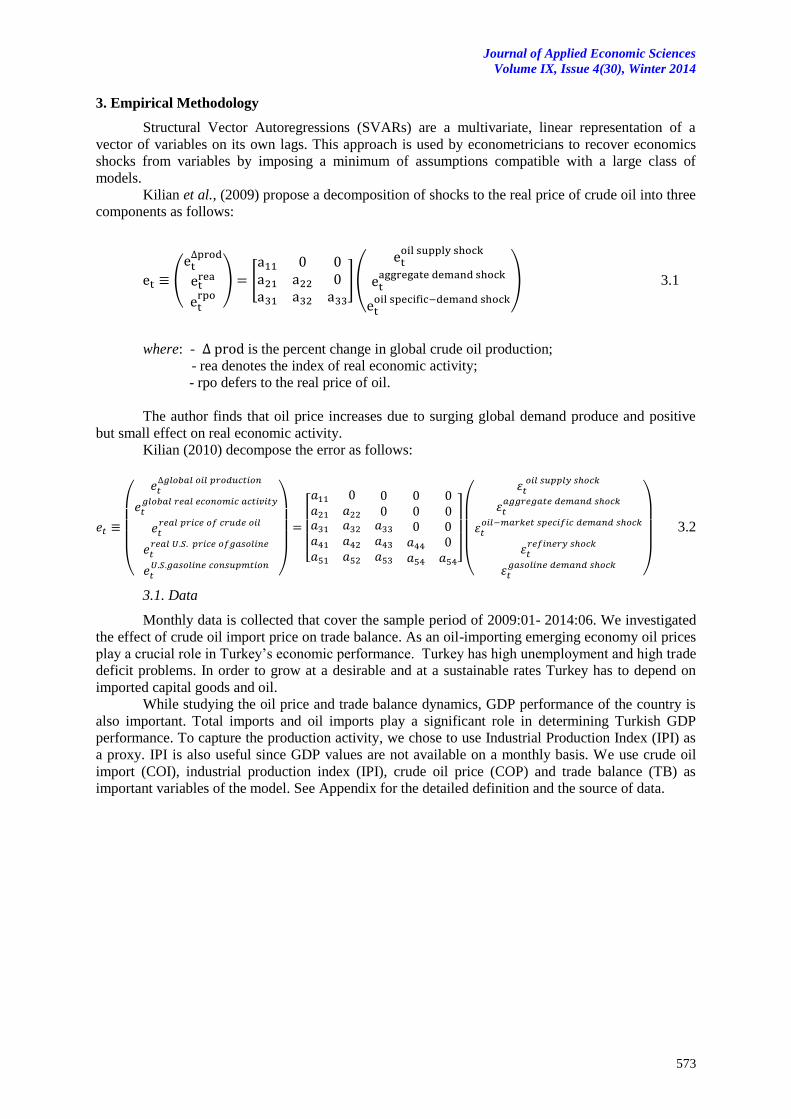
Journal of Applied Economic Sciences
Volume IX, Issue 4(30), Winter 2014
573
3. Empirical Methodology
Structural Vector Autoregressions (SVARs) are a multivariate, linear representation of a
vector of variables on its own lags. This approach is used by econometricians to recover economics
shocks from variables by imposing a minimum of assumptions compatible with a large class of
models.
Kilian et al., (2009) propose a decomposition of shocks to the real price of crude oil into three
components as follows:
(
) [
](
) 3.1
where: - is the percent change in global crude oil production;
- rea denotes the index of real economic activity;
- rpo defers to the real price of oil.
The author finds that oil price increases due to surging global demand produce and positive
but small effect on real economic activity.
Kilian (2010) decompose the error as follows:
(
)
[
]
(
)
3.2
3.1. Data
Monthly data is collected that cover the sample period of 2009:01- 2014:06. We investigated
the effect of crude oil import price on trade balance. As an oil-importing emerging economy oil prices
play a crucial role in Turkey’s economic performance. Turkey has high unemployment and high trade
deficit problems. In order to grow at a desirable and at a sustainable rates Turkey has to depend on
imported capital goods and oil.
While studying the oil price and trade balance dynamics, GDP performance of the country is
also important. Total imports and oil imports play a significant role in determining Turkish GDP
performance. To capture the production activity, we chose to use Industrial Production Index (IPI) as
a proxy. IPI is also useful since GDP values are not available on a monthly basis. We use crude oil
import (COI), industrial production index (IPI), crude oil price (COP) and trade balance (TB) as
important variables of the model. See Appendix for the detailed definition and the source of data.
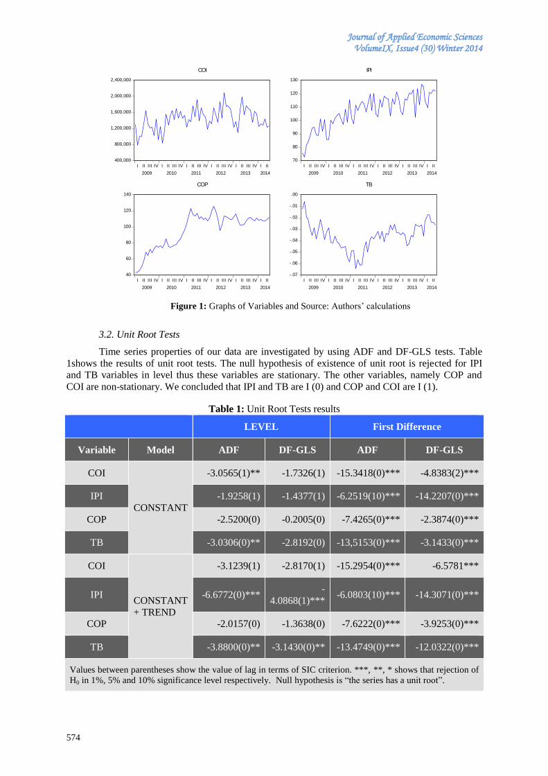
Journal of Applied Economic Sciences VolumeIX, Issue4 (30) Winter 2014
574
400,000
800,000
1,200,000
1,600,000
2,000,000
2,400,000
I II III IV I II III IV I II III IV I II III IV I II III IV I II
2009 2010 2011 2012 2013 2014
COI
70
80
90
100
110
120
130
I II III IV I II III IV I II III IV I II III IV I II III IV I II
2009 2010 2011 2012 2013 2014
IPI
40
60
80
100
120
140
I II III IV I II III IV I II III IV I II III IV I II III IV I II
2009 2010 2011 2012 2013 2014
COP
-.07
-.06
-.05
-.04
-.03
-.02
-.01
.00
I II III IV I II III IV I II III IV I II III IV I II III IV I II
2009 2010 2011 2012 2013 2014
TB
Figure 1: Graphs of Variables and Source: Authors’ calculations
3.2. Unit Root Tests
Time series properties of our data are investigated by using ADF and DF-GLS tests. Table
1shows the results of unit root tests. The null hypothesis of existence of unit root is rejected for IPI
and TB variables in level thus these variables are stationary. The other variables, namely COP and
COI are non-stationary. We concluded that IPI and TB are I (0) and COP and COI are I (1).
Table 1: Unit Root Tests results
LEVEL First Difference
Variable Model ADF DF-GLS ADF DF-GLS
COI
CONSTANT
-3.0565(1)** -1.7326(1) -15.3418(0)*** -4.8383(2)***
IPI -1.9258(1) -1.4377(1) -6.2519(10)*** -14.2207(0)***
COP -2.5200(0) -0.2005(0) -7.4265(0)*** -2.3874(0)***
TB -3.0306(0)** -2.8192(0) -13,5153(0)*** -3.1433(0)***
COI
CONSTANT
+ TREND
-3.1239(1) -2.8170(1) -15.2954(0)*** -6.5781***
IPI -6.6772(0)*** -
4.0868(1)*** -6.0803(10)*** -14.3071(0)***
COP -2.0157(0) -1.3638(0) -7.6222(0)*** -3.9253(0)***
TB -3.8800(0)** -3.1430(0)** -13.4749(0)*** -12.0322(0)***
Values between parentheses show the value of lag in terms of SIC criterion. ***, **, * shows that rejection of
H0 in 1%, 5% and 10% significance level respectively. Null hypothesis is “the series has a unit root”.
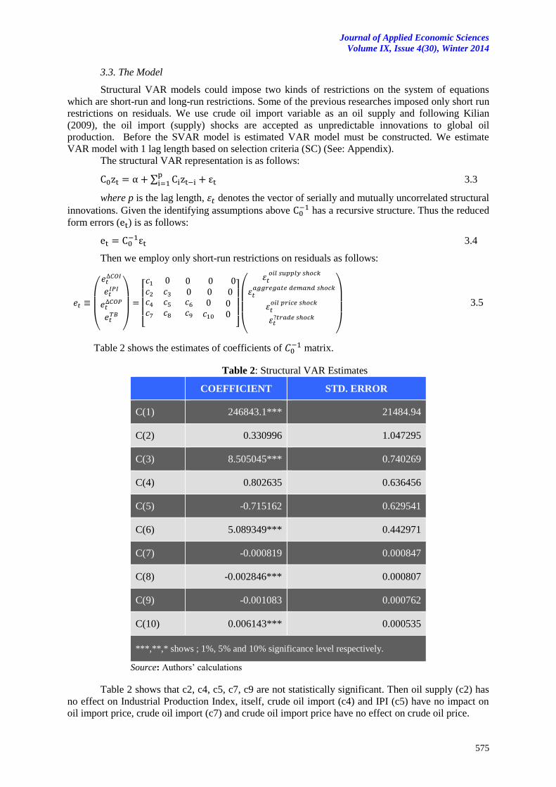
Journal of Applied Economic Sciences
Volume IX, Issue 4(30), Winter 2014
575
3.3. The Model
Structural VAR models could impose two kinds of restrictions on the system of equations
which are short-run and long-run restrictions. Some of the previous researches imposed only short run
restrictions on residuals. We use crude oil import variable as an oil supply and following Kilian
(2009), the oil import (supply) shocks are accepted as unpredictable innovations to global oil
production. Before the SVAR model is estimated VAR model must be constructed. We estimate
VAR model with 1 lag length based on selection criteria (SC) (See: Appendix).
The structural VAR representation is as follows:
∑ 3.3
where p is the lag length, denotes the vector of serially and mutually uncorrelated structural
innovations. Given the identifying assumptions above has a recursive structure. Thus the reduced
form errors ( ) is as follows:
3.4
Then we employ only short-run restrictions on residuals as follows:
(
)
[
]
(
)
3.5
Table 2 shows the estimates of coefficients of matrix.
Table 2: Structural VAR Estimates
COEFFICIENT STD. ERROR
C(1) 246843.1*** 21484.94
C(2) 0.330996 1.047295
C(3) 8.505045*** 0.740269
C(4) 0.802635 0.636456
C(5) -0.715162 0.629541
C(6) 5.089349*** 0.442971
C(7) -0.000819 0.000847
C(8) -0.002846*** 0.000807
C(9) -0.001083 0.000762
C(10) 0.006143*** 0.000535
***,**,* shows ; 1%, 5% and 10% significance level respectively.
Source: Authors’ calculations
Table 2 shows that c2, c4, c5, c7, c9 are not statistically significant. Then oil supply (c2) has
no effect on Industrial Production Index, itself, crude oil import (c4) and IPI (c5) have no impact on
oil import price, crude oil import (c7) and crude oil import price have no effect on crude oil price.
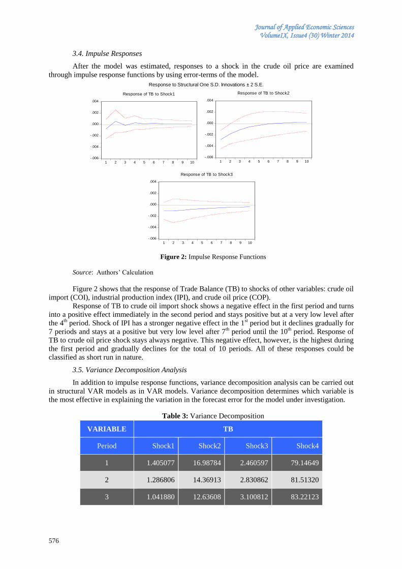
Journal of Applied Economic Sciences VolumeIX, Issue4 (30) Winter 2014
576
3.4. Impulse Responses
After the model was estimated, responses to a shock in the crude oil price are examined
through impulse response functions by using error-terms of the model.
-.006
-.004
-.002
.000
.002
.004
1 2 3 4 5 6 7 8 9 10
Response of TB to Shock1
-.006
-.004
-.002
.000
.002
.004
1 2 3 4 5 6 7 8 9 10
Response of TB to Shock2
-.006
-.004
-.002
.000
.002
.004
1 2 3 4 5 6 7 8 9 10
Response of TB to Shock3
Response to Structural One S.D. Innovations ± 2 S.E.
Figure 2: Impulse Response Functions
Source: Authors’ Calculation
Figure 2 shows that the response of Trade Balance (TB) to shocks of other variables: crude oil
import (COI), industrial production index (IPI), and crude oil price (COP).
Response of TB to crude oil import shock shows a negative effect in the first period and turns
into a positive effect immediately in the second period and stays positive but at a very low level after
the 4th period. Shock of IPI has a stronger negative effect in the 1
st period but it declines gradually for
7 periods and stays at a positive but very low level after 7th period until the 10
th period. Response of
TB to crude oil price shock stays always negative. This negative effect, however, is the highest during
the first period and gradually declines for the total of 10 periods. All of these responses could be
classified as short run in nature.
3.5. Variance Decomposition Analysis
In addition to impulse response functions, variance decomposition analysis can be carried out
in structural VAR models as in VAR models. Variance decomposition determines which variable is
the most effective in explaining the variation in the forecast error for the model under investigation.
Table 3: Variance Decomposition
VARIABLE TB
Period Shock1 Shock2 Shock3 Shock4
1 1.405077 16.98784 2.460597 79.14649
2 1.286806 14.36913 2.830862 81.51320
3 1.041880 12.63608 3.100812 83.22123
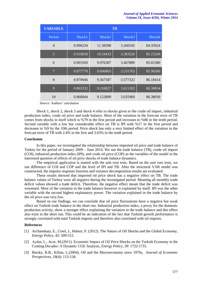
Journal of Applied Economic Sciences
Volume IX, Issue 4(30), Winter 2014
577
VARIABLE TB
Period Shock1 Shock2 Shock3 Shock4
4 0.996234 11.38398 3.260545 84.35924
5 0.919658 10.54433 3.383520 85.15249
6 0.901920 9.976387 3.467889 85.65380
7 0.877778 9.606863 3.531703 85.98366
8 0.870946 9.367587 3.577322 86.18414
9 0.863332 9.216827 3.611302 86.30854
10 0.860844 9.122899 3.635960 86.38030
Source: Authors’ calculation
Shock 1, shock 2, shock 3 and shock 4 refer to shocks given to the crude oil import, industrial
production index, crude oil price and trade balance. Most of the variation in the forecast error of TB
comes from shocks to itself which is %79 in the first period and increases to %86 in the tenth period.
Second variable with a low but considerable effect on TB is IPI with %17 in the first period and
decreases to %9 by the 10th period. Price shock has only a very limited effect of the variation in the
forecast error of TB with 2.4% in the first and 3.63% in the tenth period.
Conclusion
In this paper, we investigated the relationship between imported oil price and trade balance of
Turkey for the period of January 2009 – June 2014. We use the trade balance (TB), crude oil import
(COI), industrial production index (IPI), and crude oil price (COP) as the variables of the model in the
interested question of effects of oil price shocks of trade balance dynamics.
The empirical application is started with the unit root tests. Based on the unit root tests, we
use difference of COI and COP and the level of IPI and TB. After the structural VAR model was
constructed, the impulse response function and variance decomposition results are evaluated.
These results showed that imported oil price shock has a negative effect on TB. The trade
balance values of Turkey were all negative during the investigated period. Meaning all monthly trade
deficit values showed a trade deficit. Therefore, the negative effect meant that the trade deficit was
worsened. Most of the variation in the trade balance however is explained by itself. IPI was the other
variable with the second highest explanatory power. The variation explained in the trade balance by
the oil price was very low.
Based on our findings, we can conclude that oil price fluctuations have a negative but weak
effect on Turkish trade balance in the short run. Industrial production index, a proxy for the domestic
production activity, show a stronger effect explaining the variation in the trade balance and this effect
also exist in the short run. This could be an indication of the fact that Turkish growth performance is
strongly correlated with total Turkish imports and therefore also correlated with oil imports.
References
[1] Archanskaia, E., Creel, J., Hubert, P. (2012). The Nature of Oil Shocks and the Global Economy,
Energy Policy, 42: 509-512.
[2] Aydın, L., Acar, M.(2011). Economic Impact of Oil Price Shocks on the Turkish Economy in the
Coming Decades: A Dynamic CGE Analysis, Energy Policy, 39: 1722-1731.
[3] Barsky, R.B., Kilian, L.(2004). Oil and the Macroeconomy since 1970s, Journal of Economic
Perspectives, 18(4): 115-134.
Journal of Applied Economic Sciences VolumeIX, Issue4 (30) Winter 2014
578
[4] Bodenstein, M., Erceg, C.J, Guerrieri, L. (2011). Oil Shocks and External Adjustment, Journal
of International Economics, 83: 168-184.
[5] Erdal, G, Hilmi, E.H., Esengün, K. (2008). The Causality between Energy Consumption and
Economic Growth in Turkey, Energy Policy, 36: 3838-3842.
[6] Ghosh, S. (2009). Import demand of crude oil and economic growth: Evidence from India,
Energy Policy, 37: 699-702.
[7] Hamilton, J.D. (2006). Oil and the Macroeconomy.” in: Durlauf, D., Blume, L. (Eds.), The New
Palgrave Dictionary of Economics, 2nd
Edition, MacMillan, London.
[8] Hamilton, J.D. (1998). Oil and the Macroeconomy since World War II, The Journal of Political
Economy, 91(2): 228-248.
[9] Irhan, B.H., Alacahan, N.D., Korap, L. (2011). An Empirical Model for the Turkish Trade
Balance: New Evidence from ARDL Bounds Testing Analyse, Ekonometri ve İstatistik, 14: 38-
61.
[10] Kilian, L. (2010). Explaining Fluctuations in Gasoline Prices: A Joint Model of the Global Crude
Oil Market and the U.S. Retail Gasoline Market, The Energy Journal, 31(2): 103-128.
[11] Kilian, L., Rebucci, A., Spatafora, N. (2009). Oil Shocks and External Balances, Journal of
International Economics, 77: 181-194.
[12] Kilian, L. (2009). Not all oil price shocks are alike: Disentangling demand and supply shocks in
the crude oil market, American Economic Review, 99: 1053-1069.
[13] Kilian, L., Murphy, D.P. (2014). The Role of Inventories and Speculative Trading in the Global
Market for Crude Oil, Journal of Applied Econometrics, 29: 454-478.
[14] Le, Thai-Ha, Chang, Y. (2013). Oil Price Changes and Trade Imbalances, Energy Economics,
36: 78-96.
[15] Lise, W., van Moontfort, K. (2005). Energy Consumption and GDP in Turkey: Is There a Co-
integration Relationship. EcoMod 2005, International Conference on Policy Modeling, June 29 –
July 2, Istanbul, Turkey.
[16] Narayan, P.K., Sharma, S., Wai Ching Poon, Westerlund, J. (2014). Do Oil Prices Predict
Economic Growth? New Global Evidence, Energy Economics, 41: 137-146.
[17] Ozlale, U., Pekkurnaz, D. (2010). Oil prices and current account: A structural analysis for the
Turkish economy, Energy Policy, 38: 4489-4496.
[18] Peersman, G., van Robays, I. (2012). Cross Country Differences in the Effects of Oil Shocks,
Energy Economics, 32: 1532-1547.
[19] Sozen, A., Muammer, N. (2007). Situation of Turkey’s Energy Indicators among the EU
Member States, Energy Policy, 35: 4993-5002.
[20] Ugurlu, E., Ünsal, A. (2009). Ham Petrol İthalatı ve Ekonomik Büyüme: Türkiye.” 10th
Symposium on Econometrics Statistics , Erzurum, Turkey.
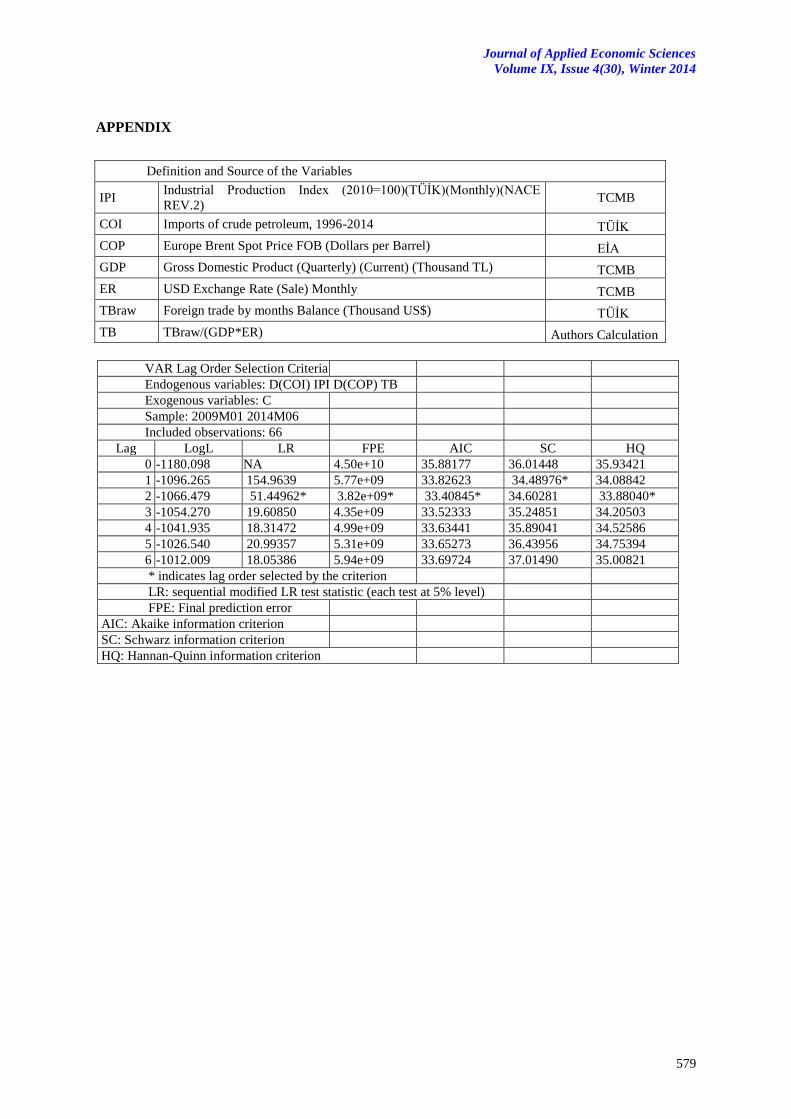
Journal of Applied Economic Sciences
Volume IX, Issue 4(30), Winter 2014
579
APPENDIX
Definition and Source of the Variables
IPI Industrial Production Index (2010=100)(TÜİK)(Monthly)(NACE
REV.2) TCMB
COI Imports of crude petroleum, 1996-2014 TÜİK
COP Europe Brent Spot Price FOB (Dollars per Barrel) EİA
GDP Gross Domestic Product (Quarterly) (Current) (Thousand TL) TCMB
ER USD Exchange Rate (Sale) Monthly TCMB
TBraw Foreign trade by months Balance (Thousand US$) TÜİK
TB TBraw/(GDP*ER) Authors Calculation
VAR Lag Order Selection Criteria
Endogenous variables: D(COI) IPI D(COP) TB
Exogenous variables: C
Sample: 2009M01 2014M06
Included observations: 66
Lag LogL LR FPE AIC SC HQ
0 -1180.098 NA 4.50e+10 35.88177 36.01448 35.93421
1 -1096.265 154.9639 5.77e+09 33.82623 34.48976* 34.08842
2 -1066.479 51.44962* 3.82e+09* 33.40845* 34.60281 33.88040*
3 -1054.270 19.60850 4.35e+09 33.52333 35.24851 34.20503
4 -1041.935 18.31472 4.99e+09 33.63441 35.89041 34.52586
5 -1026.540 20.99357 5.31e+09 33.65273 36.43956 34.75394
6 -1012.009 18.05386 5.94e+09 33.69724 37.01490 35.00821
* indicates lag order selected by the criterion
LR: sequential modified LR test statistic (each test at 5% level)
FPE: Final prediction error
AIC: Akaike information criterion
SC: Schwarz information criterion
HQ: Hannan-Quinn information criterion
Journal of Applied Economic Sciences VolumeIX, Issue4 (30) Winter 2014
580
CATEGORISATION OF THE EUROPEAN UNION COUNTRIES IN RELATION TO EFFICIENCY ADJUSTMENT OF VALUE ADDED TAX
COLLECTION USING CLUSTER ANALYSIS AND MULTIDIMENSIONAL SCALLING
Alena ANDREJOVSKÁ
Faculty of Economics, Technical University of Košice, Slovakia
Abstract:
The issue of the value added tax efficiency is intensively debated these days both at the level of
individual governments, and the level of the European institutions and bodies, as well. The whole Europe is
trying to mobilize and implement effective measures which would be able to improve the collection of taxes
without increasing tax rates. VAT is currently the most harmonized tax, but states still retain some sovereignty
regarding the level of rates, reduced rates and exemptions. Different Tax legislation in the countries, in
combination with the application of its own VAT policy preferences and lack of control of tax administration
causes growing the gap between actual and theoretical base for income taxes. The paper is devoted to the
quantification of VAT system setup from the view of revenue collection efficiency of this tax using cluster
analysis including 27 EU countries. It is also devoted to the identification of countries groups with similar
situation of VAT collection and their common features. In a statistical meta-analysis there are compared several
methodological approaches: variant of agglomerative hierarchical cluster analysis, the outputs of k-means, k-
medoid and also fuzzy c-means method. The results are in qualitative agreement with multidimensional scaling.
Keywords: Value-addeded tax, tax harmonization, tax rate, Cluster analysis, Multidimensional scaling
JEL Classification: C52, H20, H26
1. Introduction
According to (Novysedlák and Palkovičová, 2012) discuss that the primary objective of any
tax system is to provide an efficient collection of taxes through the legislative and institutional
conditions. These two components must operate and complement each other. Successful in tax
legislation and tax administration is the foundation of a good functioning, steady source of income.
Although states on the one hand may have tax legislative treated well, it still does not designate them
to generate a sufficient amount of tax revenue. In the countries there are some obstacles in the form of
bureaucracy, bad practices in the collection of the tax, weak controls, taxes unnecessary complexity in
the form of a large number of legislative exemptions, exceptions and multiple rates application. This
fact is confirmed by several studies, such as (CASE, 2013) and (Reckon LLP, 2009), which findings
concerning the EU countries point to the fact that the growth of VAT revenues not reflect
macroeconomic base applied within this tax. According to estimates of the VAT gap for EU-27
between 2000 and 2011, the average value of the VAT gap ranged at 17% in the Member States,
while the median is 13%. Regardless of the objective reasons causing the gaps, loss of income has a
major influence on economic policy. That is why tax revenue should produce stable income for the
development of public finance and enable the efficient consolidation of public finances without taking
any consolidation measures on the expenditure side.
2. Research objectives and methodology
The main aim of this paper is to create an economically transparent and effective
categorisation of EU countries in relation to efficiency adjustment of VAT collection and to identify
collecting VAT in the countries regarding the efficiency of three indicators (VRR, VPR and G,
theoretically defined in section 4).
To fulfill the main objective there are formulated two hypotheses:
H1: The more advanced economies have effectively set the VAT system, which is
characterized by small gaps in the selection VAT.
H2: Countries with excessive indebtedness or failing countries are separated from the cluster
of developed economies.
Journal of Applied Economic Sciences
Volume IX, Issue 4(30), Winter 2014
581
The analysis is performed in two steps:
1. VRR efficiency indicators, VPR and G take vastly different values, so in the first step of analysis
there has been provided the data transformation performed through conversion to z-scores. Each
item has been standardized/normalized by subtracting the mean and dividing the standard deviation.
Transformation caused achieving a zero value mean and one standard deviation value. They has
been displayed in one of the multidimensional scaling means through procedure cmdscale () and
then evaluated whether the data show signs of clustering or not. The transformed data has been
processed using selected methods for cluster analysis - Ward single linkage clustering, k-means and
k-medoids. To test the quality of clustering, interpretation and validation of data clusters there were
used a methodology silhoutte (Rousseeuw, 1987).
2. Using cluster analysis in the paper there have also been performed categorization of countries with
similar settings tax system. The categorisation has been realised by means of a number of
methodological approaches to data analysis that are based on the concept of the Euclidian metric.
These methods are used to be mentioned mainly in the context of issue of the so called manifold
learning (Rosman, Bronstlin, Bronstein and Kimmel, 2010). We mainly address to the traditional
hierarchical cluster analysis with Ward´s linkage, as well as to application of the methods such as:
k-means; k-medoids; and fuzzy c-means.
For use of these methods, we have chosen the implementation in the R environment. For
hierarchical clustering, it was the standard routine hclust() (R CORE TEAM, 2013); for k-means, we
used the routine kmeans(). Its extension is fuzzy logical variant c-means implemented by means of the
routine cmeans(). Dimensional scaling (also called principal coordinates analysis) has been realised
by means of the routine cmdscale() (Venables and Ripley, 2002).
Data has been collected from Internet databases and statistics provided by the European
Statistical Office of the European Union (Eurostat), OECD reports and IFP.
3. Literature review
Indicator of the efficiency of VAT collection compares a real collection with an efficient one.
Calculated as a share of the actual VAT collection on an effective collection of VAT. VAT collection
efficiency reaches 72% of the EU average. In comparison with Slovakia, there is 57.4%, the results
comes from the survey evaluation of structural indicators, published by (IFP, 2012). (Bodin et al.,
2001) monitored the dependence of the efficiency of VAT expressed as VRR (Vat Revenue Ratio) on
a variety of factors. The authors (Bánociová, Jakubíková and Mihoková, 2012), (Glova, 2013), (Filip,
2009), (McGee Tušan, 2008) determine the VAT revenues as a function of fiscal variables and
economic variables, while fiscal variables considered to be legislatively set and dependent on
economic factors, as well. The authors finds that the growth of VAT rates cause a disproportionately
increase of VRR. (if rate increase by 10% then VRR increase by only 7%). It could conclude that the
growth of rates causes tax evasion, but on the other hand, it could be due to transfer consumpiton
because of the preferences changes regarding goods and services with a lower tax rate, or even the tax
exemption. (Aizenmann and Jinjarak, 2005) found a positive relationship between GDP and VRR,
thus the effectiveness of the VAT system. This variable was also examined in the studies of (Reckon
LLP, 2009), in both cases, however it was statistically insignificant.
Because the calculation of the VAT gap has been monitored for the last 15 years, many
authors like (Sanack, Velloso and Xing, 2010), (Bodin.et al., 2001), (Aizenman and Jinjarak, 2005)
do not focuse on the determinants of tax gaps but they use VAT revenues or VAT performance as a
dependent variable which is given by VRR. The second indicator is the Gap, which determines the
gap between the base and the implicit rate. Both implicit and base VAT rate represent the tax burden.
Implicit rates, however, is the effective tax rate, because as opposed to the base rate reflects the actual
tax burden on consumers. It is structured as an income from all excise taxes and thus not only VAT
but also consumer and environmental related to the total final consumption of households.Goods and
services subjected to excise taxes are more often the subject of tax evasion because overall taxation of
these products is due to other goods and services higher. Just this fact expresses implicit tax rate. The
third studied variable VPR (Vat Productivity Ratio) represents VAT incomes to GDP and it is a part
tax quota, which approximates to the tax burden. It is easily accessible data, which has similar
properties, such as an average rate of VAT throughout the economy. There is a prerequisite for a
positive impact on the VAT gap as with the base and the implicit rate of taxation of consumption. But
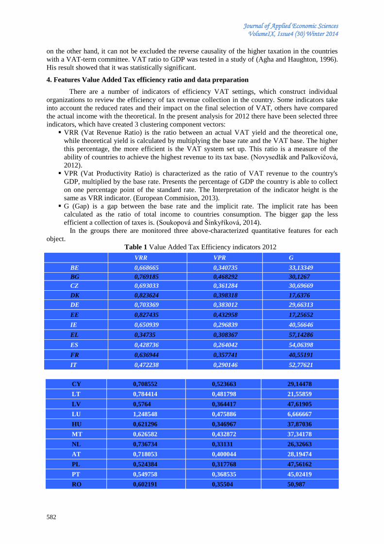
Journal of Applied Economic Sciences VolumeIX, Issue4 (30) Winter 2014
582
on the other hand, it can not be excluded the reverse causality of the higher taxation in the countries
with a VAT-term committee. VAT ratio to GDP was tested in a study of (Agha and Haughton, 1996).
His result showed that it was statistically significant.
4. Features Value Added Tax efficiency ratio and data preparation
There are a number of indicators of efficiency VAT settings, which construct individual
organizations to review the efficiency of tax revenue collection in the country. Some indicators take
into account the reduced rates and their impact on the final selection of VAT, others have compared
the actual income with the theoretical. In the present analysis for 2012 there have been selected three
indicators, which have created 3 clustering component vectors:
VRR (Vat Revenue Ratio) is the ratio between an actual VAT yield and the theoretical one,
while theoretical yield is calculated by multiplying the base rate and the VAT base. The higher
this percentage, the more efficient is the VAT system set up. This ratio is a measure of the
ability of countries to achieve the highest revenue to its tax base. (Novysedlák and Palkovičová,
2012).
VPR (Vat Productivity Ratio) is characterized as the ratio of VAT revenue to the country's
GDP, multiplied by the base rate. Presents the percentage of GDP the country is able to collect
on one percentage point of the standard rate. The Interpretation of the indicator height is the
same as VRR indicator. (European Commision, 2013).
G (Gap) is a gap between the base rate and the implicit rate. The implicit rate has been
calculated as the ratio of total income to countries consumption. The bigger gap the less
efficient a collection of taxes is. (Soukopová and Šinkyříková, 2014).
In the groups there are monitored three above-characterized quantitative features for each
object.
Table 1 Value Added Tax Efficiency indicators 2012
VRR VPR G
BE 0,668665 0,340735 33,13349
BG 0,769185 0,468292 30,1267
CZ 0,693033 0,361284 30,69669
DK 0,823624 0,398318 17,6376
DE 0,703369 0,383012 29,66313
EE 0,827435 0,432958 17,25652
IE 0,650939 0,296839 40,56646
EL 0,34735 0,308367 57,14286
ES 0,428736 0,264042 54,06398
FR 0,636944 0,357741 40,55191
IT 0,472238 0,290146 52,77621
CY 0,708552 0,523663 29,14478
LT 0,784414 0,481798 21,55859
LV 0,5764 0,364417 47,61905
LU 1,248548 0,475886 6,666667
HU 0,621296 0,346967 37,87036
MT 0,626582 0,432872 37,34178
NL 0,736734 0,33131 26,32663
AT 0,718053 0,400044 28,19474
PL 0,524384 0,317768 47,56162
PT 0,549758 0,368535 45,02419
RO 0,602191 0,35504 50,987
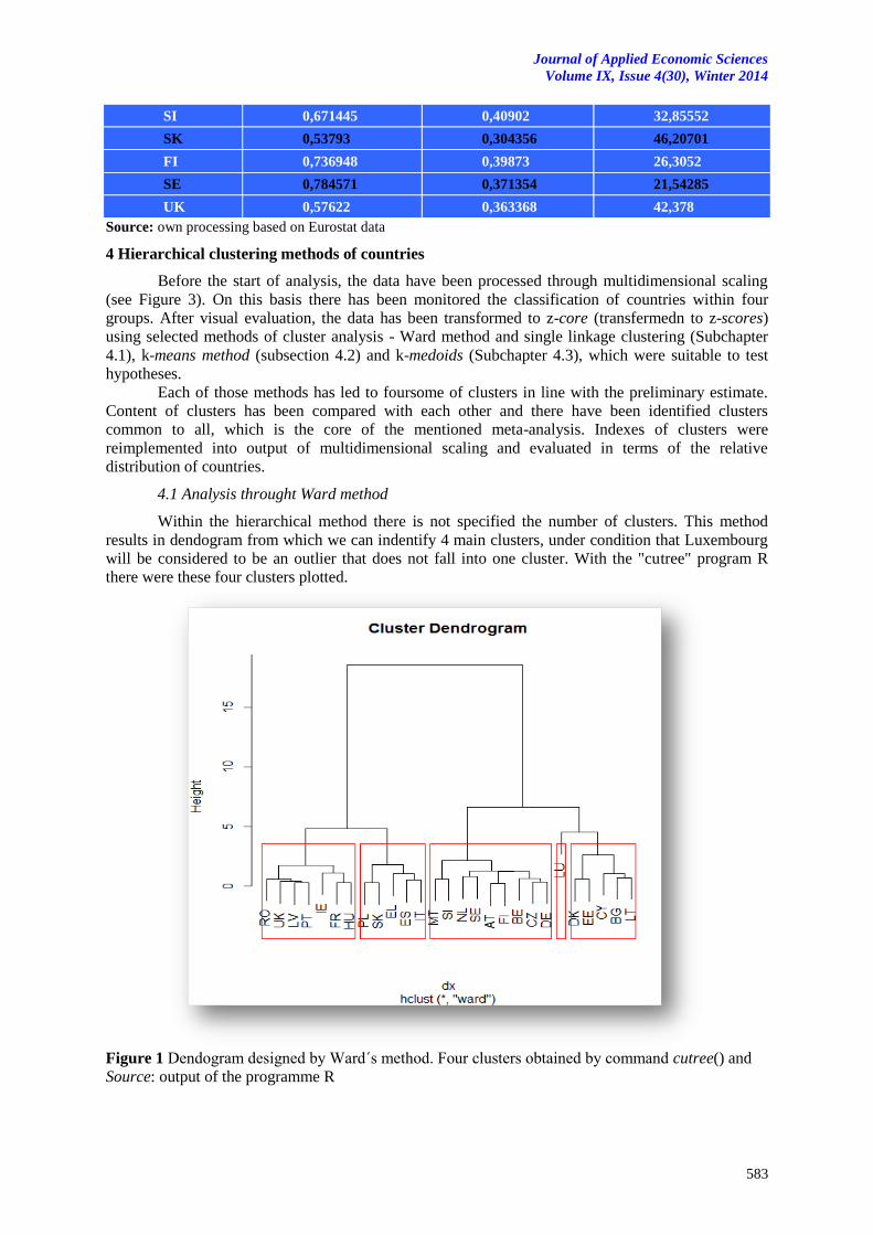
Journal of Applied Economic Sciences
Volume IX, Issue 4(30), Winter 2014
583
Source: own processing based on Eurostat data
4 Hierarchical clustering methods of countries
Before the start of analysis, the data have been processed through multidimensional scaling
(see Figure 3). On this basis there has been monitored the classification of countries within four
groups. After visual evaluation, the data has been transformed to z-core (transfermedn to z-scores)
using selected methods of cluster analysis - Ward method and single linkage clustering (Subchapter
4.1), k-means method (subsection 4.2) and k-medoids (Subchapter 4.3), which were suitable to test
hypotheses.
Each of those methods has led to foursome of clusters in line with the preliminary estimate.
Content of clusters has been compared with each other and there have been identified clusters
common to all, which is the core of the mentioned meta-analysis. Indexes of clusters were
reimplemented into output of multidimensional scaling and evaluated in terms of the relative
distribution of countries.
4.1 Analysis throught Ward method
Within the hierarchical method there is not specified the number of clusters. This method
results in dendogram from which we can indentify 4 main clusters, under condition that Luxembourg
will be considered to be an outlier that does not fall into one cluster. With the "cutree" program R
there were these four clusters plotted.
Figure 1 Dendogram designed by Ward´s method. Four clusters obtained by command cutree() and
Source: output of the programme R
SI 0,671445 0,40902 32,85552
SK 0,53793 0,304356 46,20701
FI 0,736948 0,39873 26,3052
SE 0,784571 0,371354 21,54285
UK 0,57622 0,363368 42,378
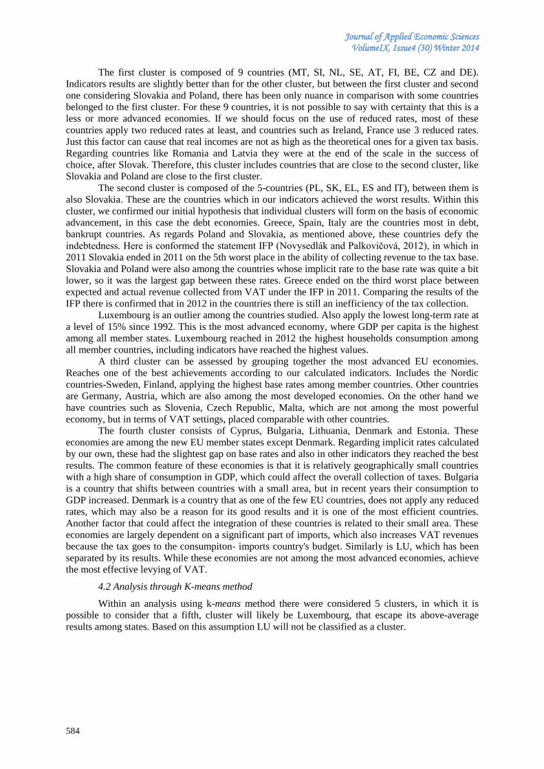
Journal of Applied Economic Sciences VolumeIX, Issue4 (30) Winter 2014
584
The first cluster is composed of 9 countries (MT, SI, NL, SE, AT, FI, BE, CZ and DE).
Indicators results are slightly better than for the other cluster, but between the first cluster and second
one considering Slovakia and Poland, there has been only nuance in comparison with some countries
belonged to the first cluster. For these 9 countries, it is not possible to say with certainty that this is a
less or more advanced economies. If we should focus on the use of reduced rates, most of these
countries apply two reduced rates at least, and countries such as Ireland, France use 3 reduced rates.
Just this factor can cause that real incomes are not as high as the theoretical ones for a given tax basis.
Regarding countries like Romania and Latvia they were at the end of the scale in the success of
choice, after Slovak. Therefore, this cluster includes countries that are close to the second cluster, like
Slovakia and Poland are close to the first cluster.
The second cluster is composed of the 5-countries (PL, SK, EL, ES and IT), between them is
also Slovakia. These are the countries which in our indicators achieved the worst results. Within this
cluster, we confirmed our initial hypothesis that individual clusters will form on the basis of economic
advancement, in this case the debt economies. Greece, Spain, Italy are the countries most in debt,
bankrupt countries. As regards Poland and Slovakia, as mentioned above, these countries defy the
indebtedness. Here is conformed the statement IFP (Novysedlák and Palkovičová, 2012), in which in
2011 Slovakia ended in 2011 on the 5th worst place in the ability of collecting revenue to the tax base.
Slovakia and Poland were also among the countries whose implicit rate to the base rate was quite a bit
lower, so it was the largest gap between these rates. Greece ended on the third worst place between
expected and actual revenue collected from VAT under the IFP in 2011. Comparing the results of the
IFP there is confirmed that in 2012 in the countries there is still an inefficiency of the tax collection.
Luxembourg is an outlier among the countries studied. Also apply the lowest long-term rate at
a level of 15% since 1992. This is the most advanced economy, where GDP per capita is the highest
among all member states. Luxembourg reached in 2012 the highest households consumption among
all member countries, including indicators have reached the highest values.
A third cluster can be assessed by grouping together the most advanced EU economies.
Reaches one of the best achievements according to our calculated indicators. Includes the Nordic
countries-Sweden, Finland, applying the highest base rates among member countries. Other countries
are Germany, Austria, which are also among the most developed economies. On the other hand we
have countries such as Slovenia, Czech Republic, Malta, which are not among the most powerful
economy, but in terms of VAT settings, placed comparable with other countries.
The fourth cluster consists of Cyprus, Bulgaria, Lithuania, Denmark and Estonia. These
economies are among the new EU member states except Denmark. Regarding implicit rates calculated
by our own, these had the slightest gap on base rates and also in other indicators they reached the best
results. The common feature of these economies is that it is relatively geographically small countries
with a high share of consumption in GDP, which could affect the overall collection of taxes. Bulgaria
is a country that shifts between countries with a small area, but in recent years their consumption to
GDP increased. Denmark is a country that as one of the few EU countries, does not apply any reduced
rates, which may also be a reason for its good results and it is one of the most efficient countries.
Another factor that could affect the integration of these countries is related to their small area. These
economies are largely dependent on a significant part of imports, which also increases VAT revenues
because the tax goes to the consumpiton- imports country's budget. Similarly is LU, which has been
separated by its results. While these economies are not among the most advanced economies, achieve
the most effective levying of VAT.
4.2 Analysis through K-means method
Within an analysis using k-means method there were considered 5 clusters, in which it is
possible to consider that a fifth, cluster will likely be Luxembourg, that escape its above-average
results among states. Based on this assumption LU will not be classified as a cluster.
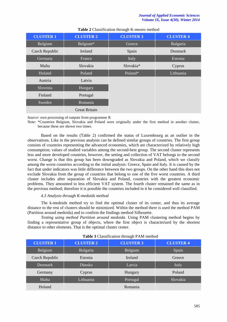
Journal of Applied Economic Sciences
Volume IX, Issue 4(30), Winter 2014
585
Table 2 Classification through K-means method
Source: own processing of outputs from programme R
Note: *Countries Belgium, Slovakia and Poland were originally under the first method in another cluster,
because these are shown two times.
Based on the results (Table 2) confirmed the status of Luxembourg as an outlier in the
observations. Like in the previous analysis can be defined similar groups of countries. The first group
consists of countries representing the advanced economies, which are characterized by relatively high
consumption; values of studied variables among the second-best group. The second cluster represents
less and more developed countries, however, the setting and collection of VAT belongs to the second
worst. Change is that this group has been downgraded as Slovakia and Poland, which we classify
among the worst countries according to the initial analysis: Greece, Spain and Italy. It is caused by the
fact that under indicators was little difference between the two groups. On the other hand this does not
exclude Slovakia from the group of countries that belong to one of the five worst countries. A third
cluster includes after separation of Slovakia and Poland, countries with the greatest economic
problems. They amounted to less efficient VAT system. The fourth cluster remained the same as in
the previous method; therefore it is possible the countries included in it be considered well classified.
4.3 Analysis through K-medoids method
The k-medoids method try to find the optimal cluster of its center, and thus its average
distance to the rest of clusters should be minimized. Within the method there is used the method PAM
(Partition around medoida) and to confirm the findings method Silhouette.
Testing using method Partition around medoida. Using PAM clustering method begins by
finding a representative group of objects, where the first object is characterized by the shortest
distance to other elements. That is the optimal cluster center.
Table 3 Classification through PAM method
CLUSTER 1 CLUSTER 2 CLUSTER 3 CLUSTER 4
Belgium Belgium* Greece Bulgaria
Czech Republic Ireland Spain Denmark
Germany France Italy Estonia
Malta Slovakia Slovakia* Cyprus
Holand Poland Poland* Lithuania
Austria Latvia
Slovenia Hungary
Finland Portugal
Sweden Romania
Great Britain
CLUSTER 1 CLUSTER 2 CLUSTER 3 CLUSTER 4
Belgium Bulgaria Belgium Spain
Czech Republic Estonia Ireland Greece
Denmark Dánsko Latvia Italy
Germany Cyprus Hungary Poland
Malta Lithuania Portugal Slovakia
Holand Romania
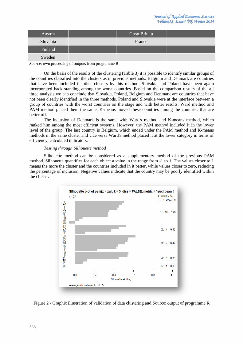
Journal of Applied Economic Sciences VolumeIX, Issue4 (30) Winter 2014
586
Source: own processing of outputs from programme R
On the basis of the results of the clustering (Table 3) it is possible to identify similar groups of
the countries classified into the clusters as in previous methods. Belgium and Denmark are countries
that have been included in other clusters by this method. Slovakia and Poland have been again
incorporated back standing among the worst countries. Based on the comparison results of the all
three analysis we can conclude that Slovakia, Poland, Belgium and Denmark are countries that have
not been clearly identified in the three methods. Poland and Slovakia were at the interface between a
group of countries with the worst countries on the stage and with better results. Ward method and
PAM method placed them the same, K-means moved these countries among the countries that are
better off.
The inclusion of Denmark is the same with Ward's method and K-means method, which
ranked him among the most efficient systems. However, the PAM method included it in the lower
level of the group. The last country is Belgium, which ended under the PAM method and K-means
methods in the same cluster and vice versa Ward's method placed it at the lower category in terms of
efficiency, calculated indicators.
Testing through Silhouette method
Silhouette method can be considered as a supplementary method of the previous PAM
method. Silhouette quantifies for each object a value in the range from -1 to 1. The values closer to 1
means the more the cluster and the countries included in it better, while values closer to zero, reducing
the percentage of inclusion. Negative values indicate that the country may be poorly identified within
the cluster.
Figure 2 - Graphic illustration of validation of data clustering and Source: output of programme R
Austria Great Britain
Slovenia France
Finland
Sweden
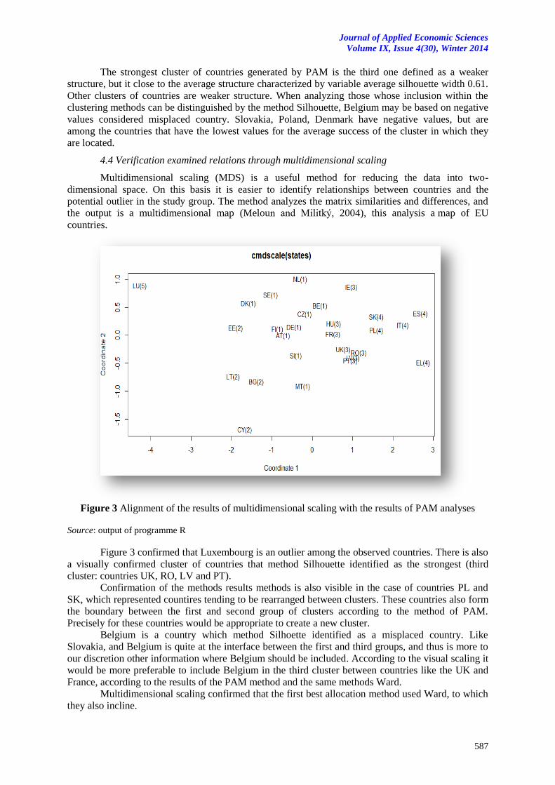
Journal of Applied Economic Sciences
Volume IX, Issue 4(30), Winter 2014
587
The strongest cluster of countries generated by PAM is the third one defined as a weaker
structure, but it close to the average structure characterized by variable average silhouette width 0.61.
Other clusters of countries are weaker structure. When analyzing those whose inclusion within the
clustering methods can be distinguished by the method Silhouette, Belgium may be based on negative
values considered misplaced country. Slovakia, Poland, Denmark have negative values, but are
among the countries that have the lowest values for the average success of the cluster in which they
are located.
4.4 Verification examined relations through multidimensional scaling
Multidimensional scaling (MDS) is a useful method for reducing the data into two-
dimensional space. On this basis it is easier to identify relationships between countries and the
potential outlier in the study group. The method analyzes the matrix similarities and differences, and
the output is a multidimensional map (Meloun and Militký, 2004), this analysis a map of EU
countries.
Figure 3 Alignment of the results of multidimensional scaling with the results of PAM analyses
Source: output of programme R
Figure 3 confirmed that Luxembourg is an outlier among the observed countries. There is also
a visually confirmed cluster of countries that method Silhouette identified as the strongest (third
cluster: countries UK, RO, LV and PT).
Confirmation of the methods results methods is also visible in the case of countries PL and
SK, which represented countires tending to be rearranged between clusters. These countries also form
the boundary between the first and second group of clusters according to the method of PAM.
Precisely for these countries would be appropriate to create a new cluster.
Belgium is a country which method Silhoette identified as a misplaced country. Like
Slovakia, and Belgium is quite at the interface between the first and third groups, and thus is more to
our discretion other information where Belgium should be included. According to the visual scaling it
would be more preferable to include Belgium in the third cluster between countries like the UK and
France, according to the results of the PAM method and the same methods Ward.
Multidimensional scaling confirmed that the first best allocation method used Ward, to which
they also incline.
Journal of Applied Economic Sciences VolumeIX, Issue4 (30) Winter 2014
588
Discussion and conclusions
Through the provided cluster analysis for the EU-27 on the basis of three indicators (VRR,
VPR and G) were identified countries with similar state efficiency of the VAT system. The first two
indicators (VRR and VPR) take into account the efficiency of VAT collection to the tax base and
ability to generate revenue from the one percent rate in relation to GDP. The third indicator (G) is the
gap between the base rate and the implicit rate.
Initial hypotheses H1 and H2 were determined at the beginning of the analysis and assumed
EU countries distribution only by economic advancement and indebtedness, as well.
Hypothesis H1 that advanced economies have effectively set the VAT system can be
considered partially confirmed. For the confirmation of the hypotheses can be considered the third
most important cluster obtained by applying the Ward method. The third cluster of countries unite
advanced economies of the EU, which has been placed on the second best place under monitoring of
the indicators VRR, VPR and G. Cluster was characterized by the following features:
Associates particularly the Nordic countries, which characterize their high-set VAT rates;
With economies such as Germany and Austria have a stable social and economic
environment and strong state legal system. Just these factors may affect the integration of
these countries into a single cluster.
The cluster is demonstrated a significant geographic dependence, as this is the vast majority
of neighboring countries. As the only country of the V4 it was Czech which achieved
comparable results with those countries. It is also a neighboring country with Germany and
Austria;
Hypothesis H1 can be considered partially confirmed as in clusters with developed
economies there were also placed a less efficient economy. First cluster in the method Ward
suggested that it is a advanced and less advanced economies, such as. France, Hungary,
Ireland, Portugal. Their common feature is that they employ more than one reduced rate and
reach the second worst record after bankrupt economies in southern Europe.
France and Ireland are among countries which apply up to 3 reduced rates. According to
many studies, such as. (CASE, 2013) and (Reckon LLP, 2009), this dependence in the use of reduced
rates was confirmed. Working on an analysis of reduced VAT rates and their impact on revenues from
(Borselli, Chiri and Romagnano, 2012), confirms that the reduced rates have a negative impact on the
overall levying of VAT. Specifically, only 60% of total household consumption is taxed at the full
rate. According to a study by Copenhagen Economics: "… From a purely economic point of view is
clearly the best approach one applicable rate of VAT. Less complicated rate structure would clearly
create significant savings by reducing the costs associated with VAT obligations for businesses, both
on the tax administration."
Hypothesis H2 predicted that countries with excessive indebtedness or failing countries are
separated from the cluster of developed economies. That assumption was confirmed as a second
cluster in the Ward method. It was the countries that are characterized by high debt and
mismanagement of the government deficit. The countries have also a tendency less working tax
administration in the form of high corruption. Countries during crises and unrest become non-standard
economies with optimal settings for an inefficient tax administration. The analysis was conducted on
specific countries Italy, Spain and Greece.
This group falls well as Slovakia and Poland. Although it is not the economy that is extremely
indebted, it is neighboring countries within the V4, which are similar economic and legislative setting.
In terms of foreign trade, Poland is an important trading partner for Slovakia. Even just this fact can
have a big impact, that between our economies and Poland in the supply of goods and services may
circumvention of legislation in the form of fraud, and so there is a choice of reducing VAT.
An interesting finding is that the best placed geographically small countries with a high share
of consumption in GDP, which the cluster analysis included the fourth cluster. Achieve the best
results examined indicators, which is mainly due to high consumption, but also that small countries
are largely dependent on the import of what they can greatly increase the revenue from these taxes.
E.g. Estonia, Bulgaria, Lithuania, Cyprus ended for 2012 with a negative balance of trade. This result
confirms that it is the economy that is dependent on the import of goods and services. Denmark is the
country, which in turn ended with an active trade balance. It is a specific country, as the only from
Journal of Applied Economic Sciences
Volume IX, Issue 4(30), Winter 2014
589
EU-27 does not use any reduced rates. This fact in this country plays an important role in the
classification of the economy with the most efficient VAT collection.
Regarding the resetting VAT systems, many organizations set different recommendations and
proposals for action. To (OECD, 2002) increasing rates of individual countries within the
consolidation has its limits, particularly in countries whose base rate is already quite high. With an
increase in rates, the amount of revenue losses expected increases as a result of the application of
reduced rates and tax exemptions. Therefore, the recommends of the reforms to improve the
performance and efficiency of the various VAT systems, among others, the expansion of the tax base,
and the way that goods and services is to reduced rate or zero, will be progressively taxed at the full
rate. The effective VAT system could thus be lower basic rate.
References
[1] Agha, A., Haughton, J. (1996). Designing VAT Systems: Some Efficiency Considerations. The
Review of Economics and Statistics.78 (2): 303–08.
[2] Aizenmann, J., Jinjarak, Y. (2005). The collectin efficiency of the value added tax:theory and
international evidence eScholarship University of California, [Online]. Available at:
http://escholarship.org/uc/item/42d103zh#page [Accessed 2014, May 10].
[3] Bánociová, A., Jakubíková, E., Mihoková, L., (2012) Quantification of evolution dependencies
of the Slovak economy on the changes in tax structure. In: Vitek, L., NEW ROLE OF PUBLIC
FINANCE 2012, Conference: 17th International Conference on New Role of Public Finance
2012, Apr 12-14, Prague, Czech republic.
[4] Bodin, J.P., Ebrill, E.P., Keen, M., Summers, V.P. (2001). The Modern VAT. International
Monetary Fund, [Online]. Available at: http://www.imf.org/external/pubs/nft/2001/VAT/ ©2001
[Accessed 2014, May 10].
[5] Borsello, F., Chiri S., Romagnano E. (2012): Patterns of Reduced VAT Rates in the European,
[Online]. Available at: http://papers.ssrn.com/sol3/papers.cfm?abstract_id=2009320 [Accessed
May 28, 2014].
[6] Filip, P. (2009). Tax competition within the European Union as an opportunity of regional
development. In: Countries of Central and Eastern Europe versus global economic crisis.
Geopolitical Studies Polish Academy of Science, 15: 87-97.
[7] Glova, J. (2013). Determinacia systematickeho rizika kmenovej akcie v modeli casovo-
premenliveho fundamentalneho beta. E+M Ekonomie a Management, 16(2): 139.
[8] McGee, W. R., Tušan, R.( 2008). The Ethics of Tax Evasion: A Survey of Slovak Opinion. In:
Taxation and Public Finance in Transition and Developing Economies. Springer
Science+Business Media, New York, USA. http://dx.doi.org/10.2139/ssrn.932990
[9] Meloun, M., Militký, J. (2004). Statistická analýza experimentálních dat. Praha: ACADEMIA,
960 s. ISBN 80-200-1254-0, in Polish.
[10] Novysedlak, V., Palkovičová, J. (2012). The estimate of the value added tax revenue loss.
Institure for Financial Policy, The Ministry of Finance of the Slovac Republic, [Online].
Available at: http://www.finance.gov.sk/en/Components/CategoryDocuments/sLoad Document.
aspx?categoryId=614&documentId=426 [Accessed 2014, May 9]
[11] Sanack, C, Velloso, R, Xing, J. (2010). Tax Revenue Response to the Business Cycle.
International Monetary Fund Working Paper. [Online]. Available at:
http://www.imf.org/external/ pubs/ft/wp/2010/wp1071.pdf. [Accessed 2014, May 6].
[12] Soukopová , J., Šinkyříková .T. (2014). Standard or Implicit VAT Rate? Proceedings of the 18th
International Conference Current Trends in Public Sector Research. Masaryk University, Brno,
s. 90-98.

Journal of Applied Economic Sciences VolumeIX, Issue4 (30) Winter 2014
590
[13] Rosman,G., Bronstein, M. M., Bronstein, A.M., Kimmel, R. (2010). Nonlinear Dimensionality
Reduction by Topologicalty Constrained Isometric Embedding, International Journal of
Computer Vison, 89(1): 56-68.
[14] Rousseeuw, P.J. (1987). Silhouettes: A graphical aid to the interpretation and validation of
cluster analysis. J. Comput. Appl. Math, 20: 53-65. http://dx.doi.org/10.1016/0377-0427
(87)90125-7
[15] Venables, W.N., Ripley, B.D. (2002). Modern Applied Statistics with S. (cmdscale()). Fourth
Edition. Springer, New York. http://dx.doi.org/10.1007/978-0-387-21706-2
*** CASE (2013). Consumption Tax Trends - 2008 Edition, [Online]. Available at: http://www.oecd.
org/ctp/consumption/consumptiontaxtrends-2008edition.htm. [Accessed 2014, Jun 12].
*** EUROSTAT: Statistic, [Online]. Available at: http://epp.eurostat.ec.europa.eu/portal/page/portal/
statistics/ search_ database [Accessed 20014, May 29].
*** EUROPEAN COMMISION: Study to quantify and analyse the VAT Gap in the EU-27 Member
States. 2013, [Online]. Available at: http://ec.europa.eu/taxation_ customs/resources/documents/
common/publications/ studies/ vat-gap.pdf [Accessed 2014, July 15].
*** R Core Team (2013). R: A language and environment for statistical computing (hclust()). R
Foundation for Statistical Computing, Vienna, Austria.http://stat.ethz.ch/R-manual/R-
devel/library/stats/html/hclust.html
*** IFP: Odhad straty príjmov z dane z pridanej hodnoty, [Online]. Available at:
http://www.skdp.sk/webnew/main.nsf/0/c02c2e40d2bbfbb1c12579cf003462a7/$FILE/EA_DPH
_uniky_FINAL%5B1%5D.pdf [Accessed 2014, Jun 22].
*** OECD (2002). Measuring the Non-Observed Economy: A Handbook. Paris: OECD Publications.
[Online]. Available at: http://www.oecd.org/std/na/1963116.pdf [Accessed 2014, April 28].
*** RECKON LLP (2009). Study to quantify and analyse the VAT gap in the EU-25 Member States.
[Online]. Available at: http://ec.europa.eu/taxation_ customs/resources/documents/ taxation/
taxcooperation/combating tax fraud/reckon_report_sep2009.pdf [Accessed 2014, April 2]

Journal of Applied Economic Sciences
Volume IX, Issue 4(30), Winter 2014
591
FOREIGN DIRECT INVESTMENT AND MALAYSIA’S STOCK MARKET: USING ARDL BOUNDS TESTING APPROACH
Muhammad AZAM
School of Economics, Finance & Banking
College of Business, Universiti Utara Malaysia
Yusnidah IBRAHIM
School of Economics, Finance & Banking
College of Business, Universiti Utara Malaysia
Abstract
The broad aim of the present study is to examine the influence of Foreign Direct Investment (FDI)
inflow and in addition, some other macroeconomic variables namely domestic investment, inflation rate,
domestic saving and GDP on Malaysia’s stock market. This study is based on annual time series data covering
the period ranging from 1988 to 2012. After checking the data for stationarity purpose, an Autoregressive
Distributed Lag (ARDL) bounds testing approach has been employed for parameters estimation. The empirical
results of ARDL bounds testing approach suggest that FDI inflow has a positive influence on the stock market.
It is also found that domestic investment, domestic saving rate, GDP growth rate and inflation variables
influence stock market. The estimated coefficient of FDI is found to be positive, which implies that the policy
makers need to devise a friendly and conducive investment policy in order to enhance FDI inflow and
encourage domestic investment. In addition, inflation rate needs to be controlled and the domestic savings
should be encouraged in order to promote stock market. This study offers prodigious insights on the important
implication of the FDI in stock market. The positive influence of FDI on stock market demonstrates the
complementary role of inflows of FDI in the stock market. This study will certainly contribute to the growth of
literature on the impact of FDI inflows on stock market capitalization.
Keywords: FDI, stock market, ARDL model, Malaysia
JEL codes: C50, F20; G20
Introduction
The importance of financial market, especially stable stock market has been growing largely
at the global level. It is believed that stable stock market is an indicator of sound macroeconomic
performance. The stock market plays a decisive role in the development of the commerce and industry
in any country and consequently it affects the economy of the country to a large extent. Several prior
studies argue that well‐functioning stock market contributes positively to aggregate output (Singh,
1997; Levine et al., 2000; Caporale et al., 2004; Husain, 2006; Yartey, 2008; Adjasi and Biekpe,
2009; Cooray, 2010). In South Asia, the foreign investors have focused on the emerging financial
markets, where the stock market have the potential and provide lucrative environment for the
international investors (Wongbangpo and Sharma, 2002). Hussain (2006) stated that Japan is the most
advanced market followed by East Asia such as China, Korea, Malaysia, Thailand, Singapore, Hong
Kong, Philippines and Indonesia. Among the East Asia, Malaysia has a large equity and bond market
in relation to its Gross Domestic Product (GDP). However, according to Levine (1996) “Do stock
markets affect overall economic development? Some analysts have viewed stock markets in
developing countries as “Casinos” that have little positive impact on economic growth”. In a study,
Sarkar (2007) has shown that there is no relationship between stock market and economic growth.
Foreign capital inflow provides many benefits include contribution to the recipient countries
capital formation and production capacity, modern technology, knowledge and enhance tax revenue.
Therefore, foreign capital inflows have sound effects on the recipient country’s production,
employment, income, balance of payments and economic development and growth (Gumus and
Gungor, 2013). Though, both components of the foreign capital inflows i.e., FDI and portfolio
investment are the paramount variables affecting the stock market. However, the focus of the present
study is mainly to explore the role of FDI along with a few noteworthy factors influencing the
Malaysia’s stock market. In a study, Wang and Shen (1999) have noted that the proponents of foreign
investment claim that due to its stabilization and demonstration effects, it has a vital positive effect on
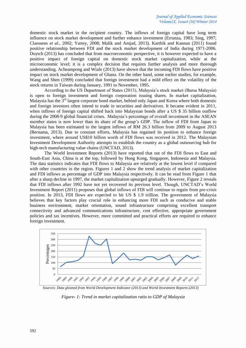
Journal of Applied Economic Sciences VolumeIX, Issue4 (30) Winter 2014
592
domestic stock market in the recipient country. The inflows of foreign capital have long term
influence on stock market development and further enhance investment (Errunza, 1983; Sing, 1997;
Claessens et al., 2002; Yartey, 2008; Malik and Amjad, 2013). Karthik and Kannan (2011) found
positive relationship between FDI and the stock market development of India during 1971-2006.
Doytch (2013) has concluded that from macroeconomic perspective, it is however expected to have a
positive impact of foreign capital on domestic stock market capitalization, while at the
microeconomic level; it is a complex decision that requires further analysis and more thorough
understanding. Acheampong and Wiafe (2013) have shown that the incoming FDI flows have positive
impact on stock market development of Ghana. On the other hand, some earlier studies, for example,
Wang and Shen (1999) concluded that foreign investment had a mild effect on the volatility of the
stock returns in Taiwan during January, 1991 to November, 1995.
According to the US Department of States (2013), Malaysia’s stock market (Bursa Malaysia)
is open to foreign investment and foreign corporation issuing shares. In market capitalization,
Malaysia has the 3rd
largest corporate bond market, behind only Japan and Korea where both domestic
and foreign investors often intend to trade in securities and derivatives. It became evident in 2011,
when inflows of foreign capital shifted back into Malaysian bonds after a US $ 35 billion outflow
during the 2008-9 global financial crises. Malaysia’s percentage of overall investment in the ASEAN
member states is now lower than its share of the group’s GDP. The inflow of FDI from Japan to
Malaysia has been estimated to the largest inflows of RM 26.3 billion from 2009 to August 2013
(Bernama, 2013). Due to constant efforts, Malaysia has regained its position to enhance foreign
investment, where around US$10 billion worth of FDI flows was received in 2012. The Malaysian
Investment Development Authority attempts to establish the country as a global outsourcing hub for
high-tech manufacturing value chains (UNCTAD, 2013).
The World Investment Reports (2013) have reported that out of the FDI flows to East and
South-East Asia, China is at the top, followed by Hong Kong, Singapore, Indonesia and Malaysia.
The data statistics indicates that FDI flows to Malaysia are relatively at the lowest level if compared
with other countries in the region. Figures 1 and 2 show the trend analysis of market capitalization
and FDI inflows as percentage of GDP into Malaysia respectively. It can be read from Figure 1 that
after a sharp decline in 1997, the market capitalization upsurged gradually. However, Figure 2 reveals
that FDI inflows after 1992 have not yet recovered its previous level. Though, UNCTAD’s World
Investment Report (2011) proposes that global inflows of FDI will continue to regain from pre-crisis
position. In 2013, FDI flows are expected to hit US $ 1.9 trillion. The government of Malaysia
believes that key factors play crucial role in enhancing more FDI such as conducive and stable
business environment, market orientation, sound infrastructure comprising excellent transport
connectivity and advanced communications infrastructure, cost effective, appropriate government
policies and tax incentives. However, more committed and practical efforts are required to enhance
foreign investment.
Sources: Data gleaned from World Development Indicator (2013) and World Investment Reports (2013)
Figure- 1: Trend in market capitalization ratio to GDP of Malaysia
0
50
100
150
200
250
300
350
Per
centa
ges
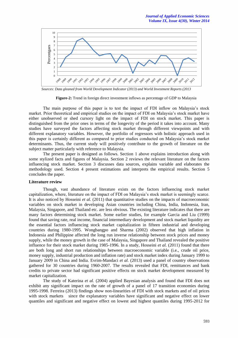
Journal of Applied Economic Sciences
Volume IX, Issue 4(30), Winter 2014
593
Sources: Data gleaned from World Development Indicator (2013) and World Investment Reports (2013
Figure-2: Trend in foreign direct investment inflows as percentage of GDP to Malaysia
The main purpose of this paper is to test the impact of FDI inflow on Malaysia’s stock
market. Prior theoretical and empirical studies on the impact of FDI on Malaysia’s stock market have
either unobserved or shed cursory light on the impact of FDI on stock market. This paper is
distinguished from the prior ones in terms of the longevity of the period it takes into account. Many
studies have surveyed the factors affecting stock market through different viewpoints and with
different explanatory variables. However, the portfolio of regressors with holistic approach used in
this paper is certainly different as compared to prior studies conducted on Malaysia’s stock market
determinants. Thus, the current study will positively contribute to the growth of literature on the
subject matter particularly with reference to Malaysia.
The present paper is designed as follows. Section 1 above explains introduction along with
some stylized facts and figures of Malaysia. Section 2 reviews the relevant literature on the factors
influencing stock market. Section 3 discusses data sources, explains variable and elaborates the
methodology used. Section 4 present estimations and interprets the empirical results. Section 5
concludes the paper.
Literature review
Though, vast abundance of literature exists on the factors influencing stock market
capitalization, where, literature on the impact of FDI on Malaysia’s stock market is seemingly scarce.
It is also noticed by Hosseini et al. (2011) that quantitative studies on the impacts of macroeconomic
variables on stock market in developing Asian countries including China, India, Indonesia, Iran,
Malaysia, Singapore, and Thailand etc. are less obvious. The existing literature indicates that there are
many factors determining stock market. Some earlier studies, for example Garcia and Liu (1999)
found that saving rate, real income, financial intermediary development and stock market liquidity are
the essential factors influencing stock market capitalization in fifteen industrial and developing
countries during 1980-1995. Wongbangpo and Sharma (2002) observed that high inflation in
Indonesia and Philippine affected the long run inverse relationship between stock prices and money
supply, while the money growth in the case of Malaysia, Singapore and Thailand revealed the positive
influence for their stock market during 1985-1996. In a study, Hosseini et al. (2011) found that there
are both long and short run relationships between macroeconomic variable (i.e., crude oil price,
money supply, industrial production and inflation rate) and stock market index during January 1999 to
January 2009 in China and India. Evrim-Mandaci et al. (2013) used a panel of country observations
gathered for 30 countries during 1960-2007. The results revealed that FDI, remittances and bank
credits to private sector had significant positive effects on stock market development measured by
market capitalization.
The study of Katerina et al. (2004) applied Bayesian analysis and found that FDI does not
exhibit any significant impact on the rate of growth of a panel of 17 transition economies during
1995-1998. Ferreira (2013) findings show non-linearities of FDI with stock markets and of oil prices
with stock markets since the explanatory variables have significant and negative effect on lower
quantiles and significant and negative effect on lowest and highest quantiles during 1995-2012 for
0
1
2
3
4
5
6
7
8
9
10
Per
centg
aes
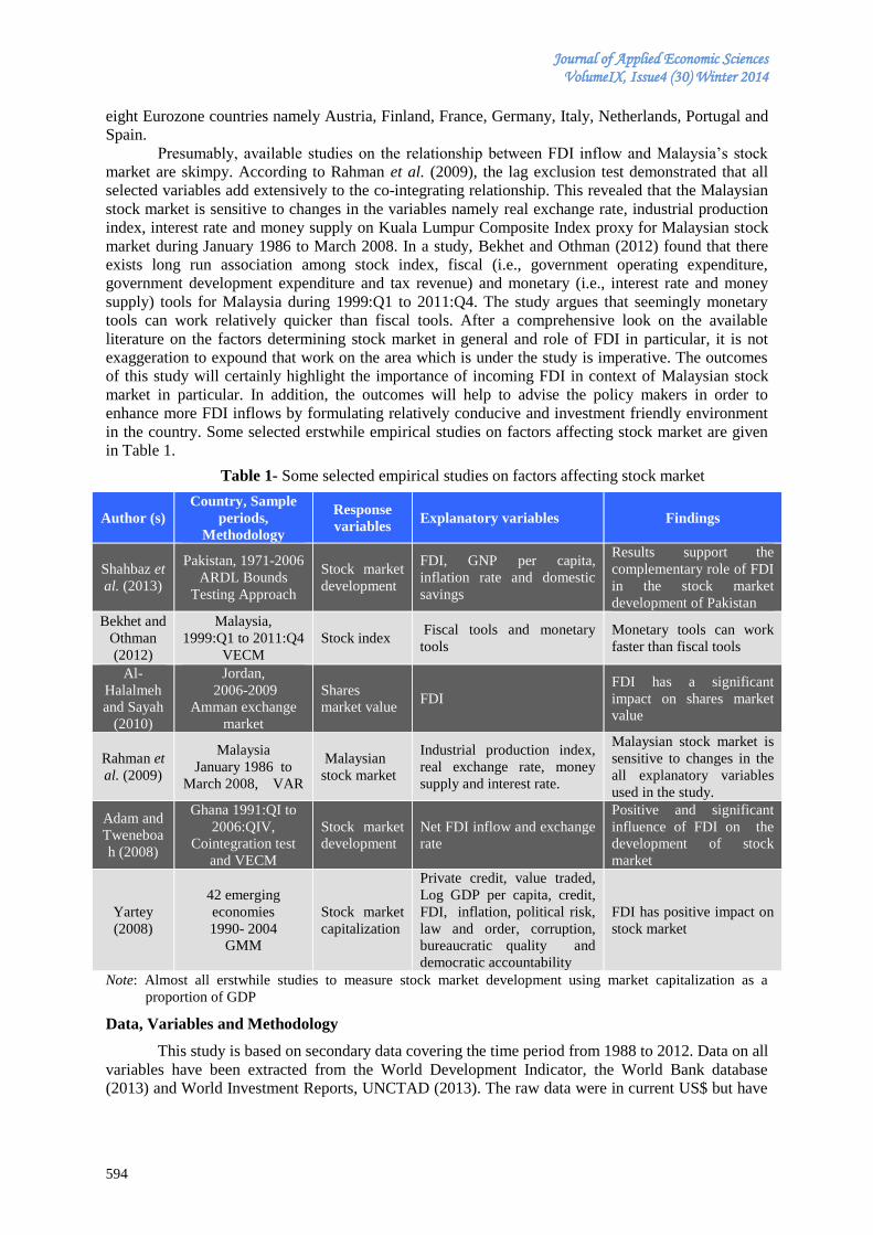
Journal of Applied Economic Sciences VolumeIX, Issue4 (30) Winter 2014
594
eight Eurozone countries namely Austria, Finland, France, Germany, Italy, Netherlands, Portugal and
Spain.
Presumably, available studies on the relationship between FDI inflow and Malaysia’s stock
market are skimpy. According to Rahman et al. (2009), the lag exclusion test demonstrated that all
selected variables add extensively to the co-integrating relationship. This revealed that the Malaysian
stock market is sensitive to changes in the variables namely real exchange rate, industrial production
index, interest rate and money supply on Kuala Lumpur Composite Index proxy for Malaysian stock
market during January 1986 to March 2008. In a study, Bekhet and Othman (2012) found that there
exists long run association among stock index, fiscal (i.e., government operating expenditure,
government development expenditure and tax revenue) and monetary (i.e., interest rate and money
supply) tools for Malaysia during 1999:Q1 to 2011:Q4. The study argues that seemingly monetary
tools can work relatively quicker than fiscal tools. After a comprehensive look on the available
literature on the factors determining stock market in general and role of FDI in particular, it is not
exaggeration to expound that work on the area which is under the study is imperative. The outcomes
of this study will certainly highlight the importance of incoming FDI in context of Malaysian stock
market in particular. In addition, the outcomes will help to advise the policy makers in order to
enhance more FDI inflows by formulating relatively conducive and investment friendly environment
in the country. Some selected erstwhile empirical studies on factors affecting stock market are given
in Table 1.
Table 1- Some selected empirical studies on factors affecting stock market
Author (s)
Country, Sample
periods,
Methodology
Response
variables Explanatory variables Findings
Shahbaz et
al. (2013)
Pakistan, 1971-2006
ARDL Bounds
Testing Approach
Stock market
development
FDI, GNP per capita,
inflation rate and domestic
savings
Results support the
complementary role of FDI
in the stock market
development of Pakistan
Bekhet and
Othman
(2012)
Malaysia,
1999:Q1 to 2011:Q4
VECM
Stock index Fiscal tools and monetary
tools
Monetary tools can work
faster than fiscal tools
Al-
Halalmeh
and Sayah
(2010)
Jordan,
2006-2009
Amman exchange
market
Shares
market value FDI
FDI has a significant
impact on shares market
value
Rahman et
al. (2009)
Malaysia
January 1986 to
March 2008, VAR
Malaysian
stock market
Industrial production index,
real exchange rate, money
supply and interest rate.
Malaysian stock market is
sensitive to changes in the
all explanatory variables
used in the study.
Adam and
Tweneboa
h (2008)
Ghana 1991:QI to
2006:QIV,
Cointegration test
and VECM
Stock market
development
Net FDI inflow and exchange
rate
Positive and significant
influence of FDI on the
development of stock
market
Yartey
(2008)
42 emerging
economies
1990- 2004
GMM
Stock market
capitalization
Private credit, value traded,
Log GDP per capita, credit,
FDI, inflation, political risk,
law and order, corruption,
bureaucratic quality and
democratic accountability
FDI has positive impact on
stock market
Note: Almost all erstwhile studies to measure stock market development using market capitalization as a
proportion of GDP
Data, Variables and Methodology
This study is based on secondary data covering the time period from 1988 to 2012. Data on all
variables have been extracted from the World Development Indicator, the World Bank database
(2013) and World Investment Reports, UNCTAD (2013). The raw data were in current US$ but have
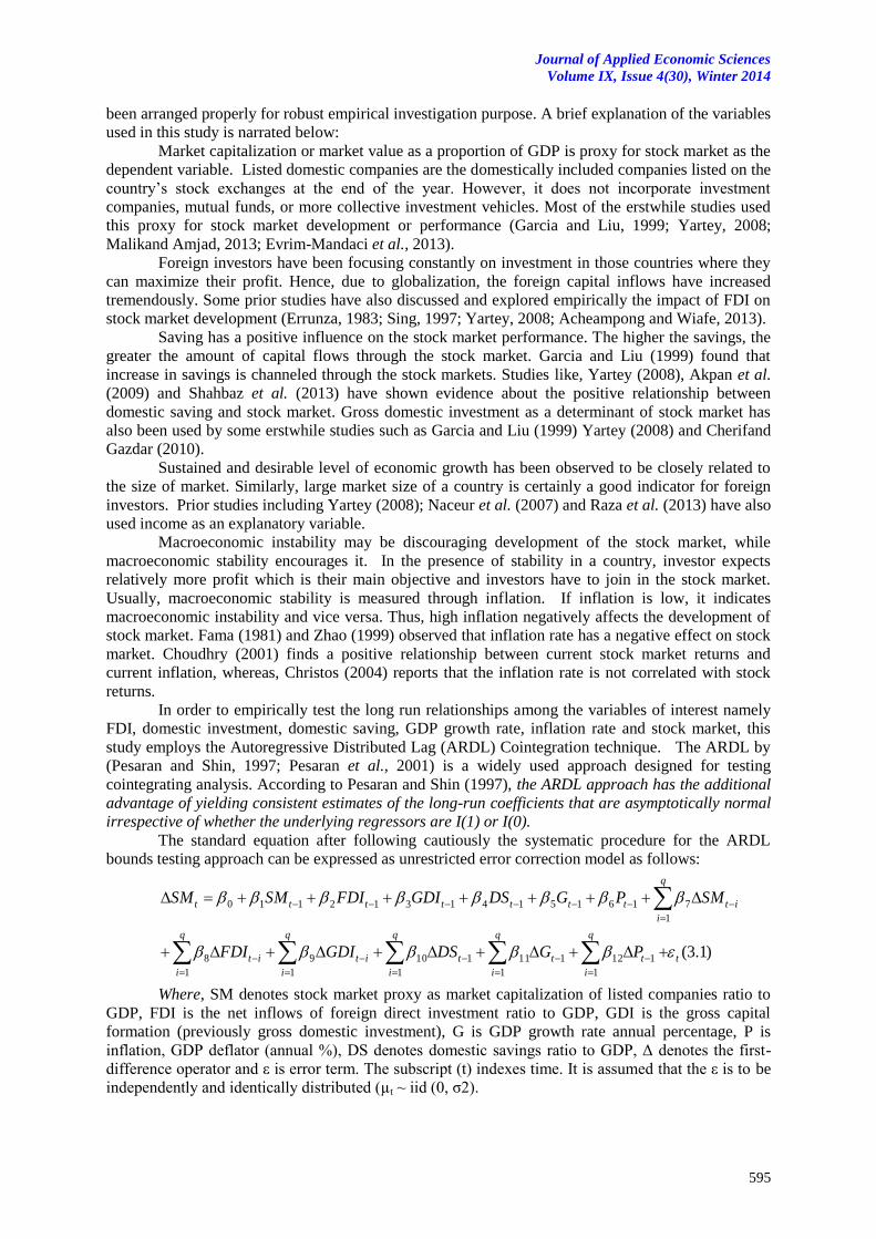
Journal of Applied Economic Sciences
Volume IX, Issue 4(30), Winter 2014
595
been arranged properly for robust empirical investigation purpose. A brief explanation of the variables
used in this study is narrated below:
Market capitalization or market value as a proportion of GDP is proxy for stock market as the
dependent variable. Listed domestic companies are the domestically included companies listed on the
country’s stock exchanges at the end of the year. However, it does not incorporate investment
companies, mutual funds, or more collective investment vehicles. Most of the erstwhile studies used
this proxy for stock market development or performance (Garcia and Liu, 1999; Yartey, 2008;
Malikand Amjad, 2013; Evrim-Mandaci et al., 2013).
Foreign investors have been focusing constantly on investment in those countries where they
can maximize their profit. Hence, due to globalization, the foreign capital inflows have increased
tremendously. Some prior studies have also discussed and explored empirically the impact of FDI on
stock market development (Errunza, 1983; Sing, 1997; Yartey, 2008; Acheampong and Wiafe, 2013).
Saving has a positive influence on the stock market performance. The higher the savings, the
greater the amount of capital flows through the stock market. Garcia and Liu (1999) found that
increase in savings is channeled through the stock markets. Studies like, Yartey (2008), Akpan et al.
(2009) and Shahbaz et al. (2013) have shown evidence about the positive relationship between
domestic saving and stock market. Gross domestic investment as a determinant of stock market has
also been used by some erstwhile studies such as Garcia and Liu (1999) Yartey (2008) and Cherifand
Gazdar (2010).
Sustained and desirable level of economic growth has been observed to be closely related to
the size of market. Similarly, large market size of a country is certainly a good indicator for foreign
investors. Prior studies including Yartey (2008); Naceur et al. (2007) and Raza et al. (2013) have also
used income as an explanatory variable.
Macroeconomic instability may be discouraging development of the stock market, while
macroeconomic stability encourages it. In the presence of stability in a country, investor expects
relatively more profit which is their main objective and investors have to join in the stock market.
Usually, macroeconomic stability is measured through inflation. If inflation is low, it indicates
macroeconomic instability and vice versa. Thus, high inflation negatively affects the development of
stock market. Fama (1981) and Zhao (1999) observed that inflation rate has a negative effect on stock
market. Choudhry (2001) finds a positive relationship between current stock market returns and
current inflation, whereas, Christos (2004) reports that the inflation rate is not correlated with stock
returns.
In order to empirically test the long run relationships among the variables of interest namely
FDI, domestic investment, domestic saving, GDP growth rate, inflation rate and stock market, this
study employs the Autoregressive Distributed Lag (ARDL) Cointegration technique. The ARDL by
(Pesaran and Shin, 1997; Pesaran et al., 2001) is a widely used approach designed for testing
cointegrating analysis. According to Pesaran and Shin (1997), the ARDL approach has the additional
advantage of yielding consistent estimates of the long-run coefficients that are asymptotically normal
irrespective of whether the underlying regressors are I(1) or I(0).
The standard equation after following cautiously the systematic procedure for the ARDL
bounds testing approach can be expressed as unrestricted error correction model as follows:
)1.3(1
1
1
121
1
11110
1
9
1
8
1
71615141312110
t
q
i
t
q
i
t
q
i
tit
q
i
it
q
i
it
q
i
ttttttt
PGDSGDIFDI
SMPGDSGDIFDISMSM
Where, SM denotes stock market proxy as market capitalization of listed companies ratio to
GDP, FDI is the net inflows of foreign direct investment ratio to GDP, GDI is the gross capital
formation (previously gross domestic investment), G is GDP growth rate annual percentage, P is
inflation, GDP deflator (annual %), DS denotes domestic savings ratio to GDP, Δ denotes the first-
difference operator and ε is error term. The subscript (t) indexes time. It is assumed that the ε is to be
independently and identically distributed (µt ~ iid (0, σ2).
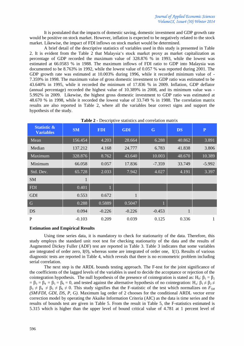
Journal of Applied Economic Sciences VolumeIX, Issue4 (30) Winter 2014
596
It is postulated that the impacts of domestic saving, domestic investment and GDP growth rate
would be positive on stock market. However, inflation is expected to be negatively related to the stock
market. Likewise, the impact of FDI inflows on stock market would be determined.
A brief detail of the descriptive statistics of variables used in this study is presented in Table
2. It is evident from the Table 2 that Malaysia‘s stock market proxy as market capitalization as
percentage of GDP recorded the maximum value of 328.876 % in 1993, while the lowest was
estimated at 66.0583 % in 1988. The maximum inflows of FDI ratio to GDP into Malaysia was
documented to be 8.763% in 1992, while the lowest value of 0.057 % was reported during 2001. The
GDP growth rate was estimated at 10.003% during 1996, while it recorded minimum value of -
7.359% in 1998. The maximum value of gross domestic investment to GDP ratio was estimated to be
43.640% in 1995, while it recorded the minimum of 17.836 % in 2009. Inflation, GDP deflator
(annual percentage) recorded the highest value of 10.389% in 2008, and its minimum value was -
5.992% in 2009. Likewise, the highest gross domestic investment to GDP ratio was estimated at
48.670 % in 1998, while it recorded the lowest value of 33.749 % in 1988. The correlation matrix
results are also reported in Table 2, where all the variables bear correct signs and support the
hypothesis of the study.
Table 2 - Descriptive statistics and correlation matrix
Statistic &
Variables SM FDI GDI G DS P
Mean 156.454 4.203 28.664 6.288 40.862 3.891
Median 137.212 4.168 24.777 6.783 41.838 3.806
Maximum 328.876 8.762 43.640 10.003 48.670 10.389
Minimum 66.058 0.057 17.836 -7.359 33.749 -5.992
Std. Dev. 65.728 2.033 7.942 4.027 4.191 3.397
SM 1
FDI 0.401 1
GDI 0.553 0.672 1
G 0.288 0.5889 0.5047 1
DS 0.094 -0.226 -0.226 -0.453 1
P -0.103 0.209 0.039 0.125 0.336 1
Estimation and Empirical Results
Using time series data, it is mandatory to check for stationarity of the data. Therefore, this
study employs the standard unit root test for checking stationarity of the data and the results of
Augmented Dickey Fuller (ADF) test are reported in Table 3. Table 3 indicates that some variables
are integrated of order zero, I(0), whereas some are integrated of order one, I(1). Results of various
diagnostic tests are reported in Table 4, which reveals that there is no econometric problem including
serial correlation.
The next step is the ARDL bounds testing approach. The F-test for the joint significance of
the coefficients of the lagged levels of the variables is used to decide the acceptance or rejection of the
cointegration hypothesis. The null hypothesis of the presence of cointegration is stated as: H0: β1 = β2
= β3 = β4 = β5 = β6 = 0, and tested against the alternative hypothesis of no cointegration: Ha: β1 ≠ β2 ≠
β3 ≠ β4 ≠ β5 ≠ β6 ≠ 0. This study signifies that the F-statistic of the test which normalizes on FSM
(SM\FDI, GDI, DS, P, G). Maximum lag order of 2 chooses for the conditional ARDL vector error
correction model by operating the Akaike Information Criteria (AIC) as the data is time series and the
results of bounds test are given in Table 5. From the result in Table 5, the F-statistics estimated is
5.315 which is higher than the upper level of bound critical value of 4.781 at 1 percent level of
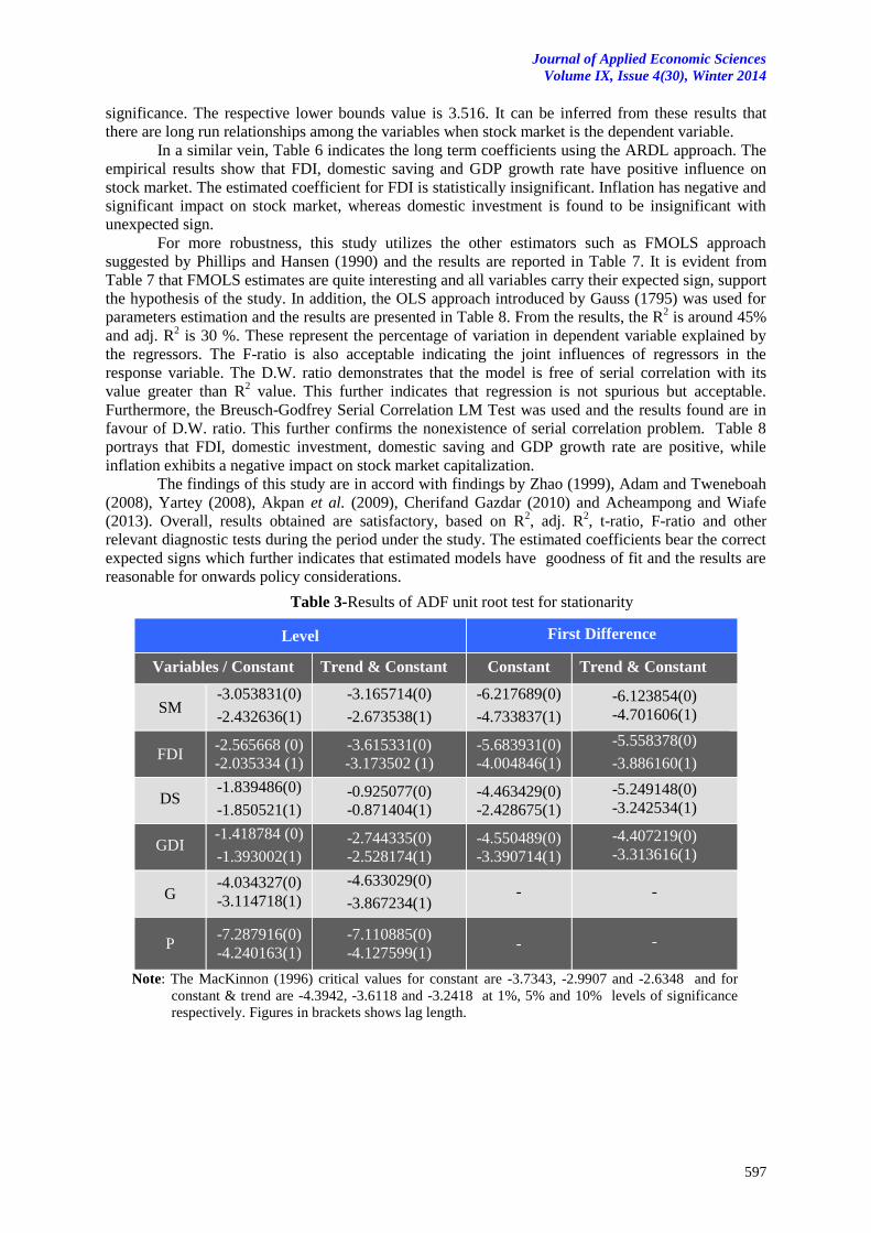
Journal of Applied Economic Sciences
Volume IX, Issue 4(30), Winter 2014
597
significance. The respective lower bounds value is 3.516. It can be inferred from these results that
there are long run relationships among the variables when stock market is the dependent variable.
In a similar vein, Table 6 indicates the long term coefficients using the ARDL approach. The
empirical results show that FDI, domestic saving and GDP growth rate have positive influence on
stock market. The estimated coefficient for FDI is statistically insignificant. Inflation has negative and
significant impact on stock market, whereas domestic investment is found to be insignificant with
unexpected sign.
For more robustness, this study utilizes the other estimators such as FMOLS approach
suggested by Phillips and Hansen (1990) and the results are reported in Table 7. It is evident from
Table 7 that FMOLS estimates are quite interesting and all variables carry their expected sign, support
the hypothesis of the study. In addition, the OLS approach introduced by Gauss (1795) was used for
parameters estimation and the results are presented in Table 8. From the results, the R2 is around 45%
and adj. R2 is 30 %. These represent the percentage of variation in dependent variable explained by
the regressors. The F-ratio is also acceptable indicating the joint influences of regressors in the
response variable. The D.W. ratio demonstrates that the model is free of serial correlation with its
value greater than R2 value. This further indicates that regression is not spurious but acceptable.
Furthermore, the Breusch-Godfrey Serial Correlation LM Test was used and the results found are in
favour of D.W. ratio. This further confirms the nonexistence of serial correlation problem. Table 8
portrays that FDI, domestic investment, domestic saving and GDP growth rate are positive, while
inflation exhibits a negative impact on stock market capitalization.
The findings of this study are in accord with findings by Zhao (1999), Adam and Tweneboah
(2008), Yartey (2008), Akpan et al. (2009), Cherifand Gazdar (2010) and Acheampong and Wiafe
(2013). Overall, results obtained are satisfactory, based on R2, adj. R
2, t-ratio, F-ratio and other
relevant diagnostic tests during the period under the study. The estimated coefficients bear the correct
expected signs which further indicates that estimated models have goodness of fit and the results are
reasonable for onwards policy considerations.
Table 3-Results of ADF unit root test for stationarity
Level First Difference
Variables / Constant Trend & Constant Constant
Trend & Constant
SM -3.053831(0)
-2.432636(1)
-3.165714(0)
-2.673538(1)
-6.217689(0)
-4.733837(1)
-6.123854(0)
-4.701606(1)
FDI -2.565668 (0)
-2.035334 (1)
-3.615331(0)
-3.173502 (1)
-5.683931(0)
-4.004846(1)
-5.558378(0)
-3.886160(1)
DS -1.839486(0)
-1.850521(1)
-0.925077(0)
-0.871404(1)
-4.463429(0)
-2.428675(1)
-5.249148(0)
-3.242534(1)
GDI -1.418784 (0)
-1.393002(1)
-2.744335(0)
-2.528174(1)
-4.550489(0)
-3.390714(1)
-4.407219(0)
-3.313616(1)
G -4.034327(0)
-3.114718(1)
-4.633029(0)
-3.867234(1) - -
P -7.287916(0)
-4.240163(1)
-7.110885(0)
-4.127599(1) - -
Note: The MacKinnon (1996) critical values for constant are -3.7343, -2.9907 and -2.6348 and for
constant & trend are -4.3942, -3.6118 and -3.2418 at 1%, 5% and 10% levels of significance
respectively. Figures in brackets shows lag length.
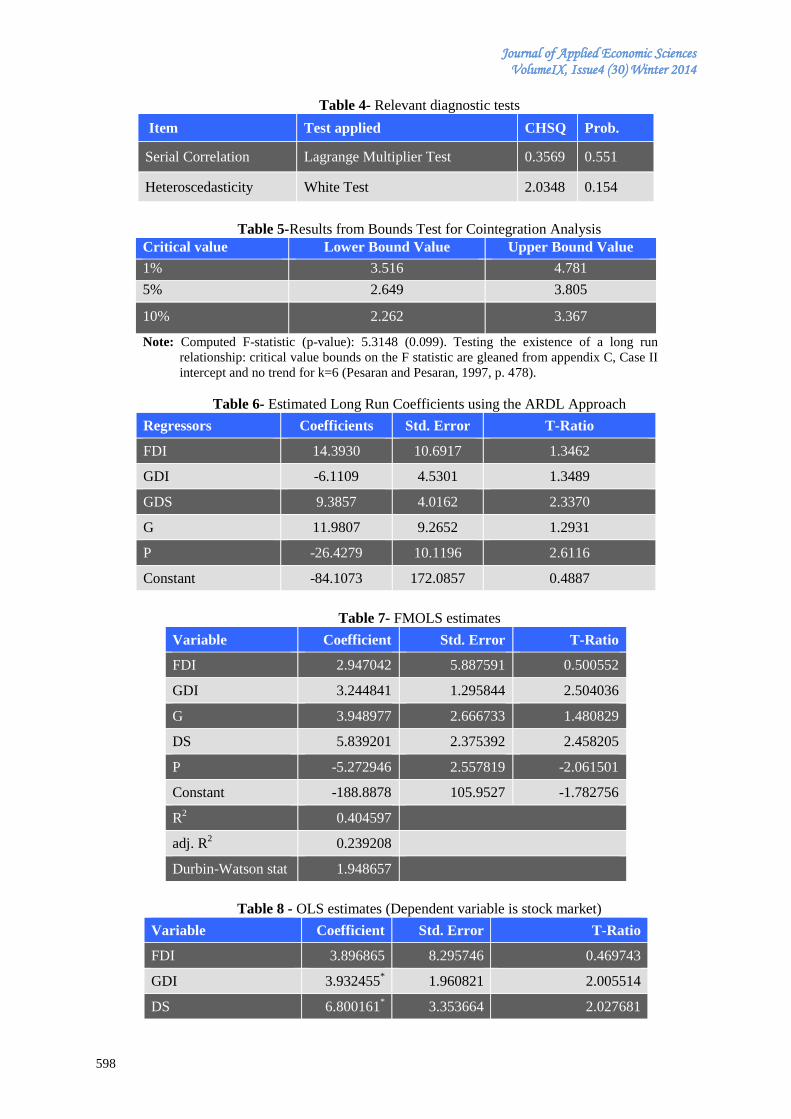
Journal of Applied Economic Sciences VolumeIX, Issue4 (30) Winter 2014
598
Table 4- Relevant diagnostic tests
Item Test applied CHSQ Prob.
Serial Correlation Lagrange Multiplier Test 0.3569 0.551
Heteroscedasticity White Test 2.0348 0.154
Table 5-Results from Bounds Test for Cointegration Analysis
Critical value Lower Bound Value Upper Bound Value
1% 3.516 4.781
5% 2.649 3.805
10% 2.262 3.367
Note: Computed F-statistic (p-value): 5.3148 (0.099). Testing the existence of a long run
relationship: critical value bounds on the F statistic are gleaned from appendix C, Case II
intercept and no trend for k=6 (Pesaran and Pesaran, 1997, p. 478).
Table 6- Estimated Long Run Coefficients using the ARDL Approach
Regressors Coefficients Std. Error T-Ratio
FDI 14.3930 10.6917 1.3462
GDI -6.1109 4.5301 1.3489
GDS 9.3857 4.0162 2.3370
G 11.9807 9.2652 1.2931
P -26.4279 10.1196 2.6116
Constant -84.1073 172.0857 0.4887
Table 7- FMOLS estimates
Variable Coefficient Std. Error T-Ratio
FDI 2.947042 5.887591 0.500552
GDI 3.244841 1.295844 2.504036
G 3.948977 2.666733 1.480829
DS 5.839201 2.375392 2.458205
P -5.272946 2.557819 -2.061501
Constant -188.8878 105.9527 -1.782756
R2 0.404597
adj. R2 0.239208
Durbin-Watson stat 1.948657
Table 8 - OLS estimates (Dependent variable is stock market)
Variable Coefficient Std. Error T-Ratio
FDI 3.896865 8.295746 0.469743
GDI 3.932455*
1.960821 2.005514
DS 6.800161*
3.353664 2.027681
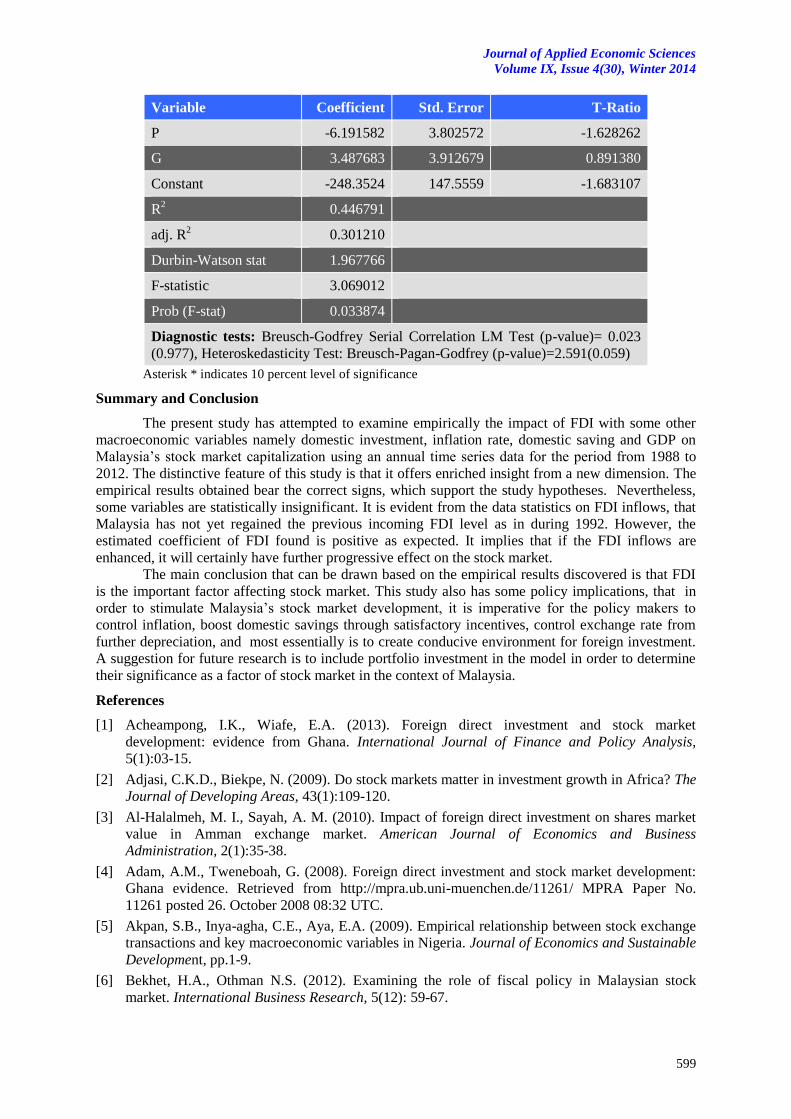
Journal of Applied Economic Sciences
Volume IX, Issue 4(30), Winter 2014
599
Variable Coefficient Std. Error T-Ratio
P -6.191582 3.802572 -1.628262
G 3.487683 3.912679 0.891380
Constant -248.3524 147.5559 -1.683107
R2 0.446791
adj. R2 0.301210
Durbin-Watson stat 1.967766
F-statistic 3.069012
Prob (F-stat) 0.033874
Diagnostic tests: Breusch-Godfrey Serial Correlation LM Test (p-value)= 0.023
(0.977), Heteroskedasticity Test: Breusch-Pagan-Godfrey (p-value)=2.591(0.059)
Asterisk * indicates 10 percent level of significance
Summary and Conclusion
The present study has attempted to examine empirically the impact of FDI with some other
macroeconomic variables namely domestic investment, inflation rate, domestic saving and GDP on
Malaysia’s stock market capitalization using an annual time series data for the period from 1988 to
2012. The distinctive feature of this study is that it offers enriched insight from a new dimension. The
empirical results obtained bear the correct signs, which support the study hypotheses. Nevertheless,
some variables are statistically insignificant. It is evident from the data statistics on FDI inflows, that
Malaysia has not yet regained the previous incoming FDI level as in during 1992. However, the
estimated coefficient of FDI found is positive as expected. It implies that if the FDI inflows are
enhanced, it will certainly have further progressive effect on the stock market.
The main conclusion that can be drawn based on the empirical results discovered is that FDI
is the important factor affecting stock market. This study also has some policy implications, that in
order to stimulate Malaysia’s stock market development, it is imperative for the policy makers to
control inflation, boost domestic savings through satisfactory incentives, control exchange rate from
further depreciation, and most essentially is to create conducive environment for foreign investment.
A suggestion for future research is to include portfolio investment in the model in order to determine
their significance as a factor of stock market in the context of Malaysia.
References
[1] Acheampong, I.K., Wiafe, E.A. (2013). Foreign direct investment and stock market
development: evidence from Ghana. International Journal of Finance and Policy Analysis,
5(1):03-15.
[2] Adjasi, C.K.D., Biekpe, N. (2009). Do stock markets matter in investment growth in Africa? The
Journal of Developing Areas, 43(1):109-120.
[3] Al-Halalmeh, M. I., Sayah, A. M. (2010). Impact of foreign direct investment on shares market
value in Amman exchange market. American Journal of Economics and Business
Administration, 2(1):35-38.
[4] Adam, A.M., Tweneboah, G. (2008). Foreign direct investment and stock market development:
Ghana evidence. Retrieved from http://mpra.ub.uni-muenchen.de/11261/ MPRA Paper No.
11261 posted 26. October 2008 08:32 UTC.
[5] Akpan, S.B., Inya-agha, C.E., Aya, E.A. (2009). Empirical relationship between stock exchange
transactions and key macroeconomic variables in Nigeria. Journal of Economics and Sustainable
Development, pp.1-9.
[6] Bekhet, H.A., Othman N.S. (2012). Examining the role of fiscal policy in Malaysian stock
market. International Business Research, 5(12): 59-67.
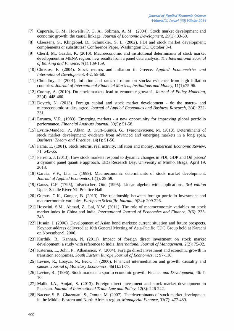
Journal of Applied Economic Sciences VolumeIX, Issue4 (30) Winter 2014
600
[7] Caporale, G. M., Howells, P. G. A., Soliman, A. M. (2004). Stock market development and
economic growth: the causal linkage. Journal of Economic Development, 29(1): 33-50.
[8] Claessens, S., Klingebiel, D., Schmukler, S. L. (2002). FDI and stock market development:
complements or substitutes? Conference Paper, Washington DC. October 3-4.
[9] Cherif, M., Gazdar, K. (2010). Macroeconomic and institutional determinants of stock market
development in MENA region: new results from a panel data analysis. The International Journal
of Banking and Finance, 7(1):139-159.
[10] Christos, F. (2004). Stock returns and inflation in Greece. Applied Econometrics and
International Development, 4-2, 55-68.
[11] Choudhry, T. (2001). Inflation and rates of return on stocks: evidence from high inflation
countries. Journal of International Financial Markets, Institutions and Money, 11(1):75-96.
[12] Cooray, A. (2010). Do stock markets lead to economic growth?, Journal of Policy Modeling,
32(4): 448-460.
[13] Doytch, N. (2013). Foreign capital and stock market development - do the macro- and
microeconomic studies agree. Journal of Applied Economics and Business Research, 3(4): 222-
231.
[14] Errunza, V.R. (1983). Emerging markets - a new opportunity for improving global portfolio
performance. Financial Analysts Journal, 39(5): 51-58.
[15] Evrim-Mandaci, P., Aktan, B., Kurt-Gumus, G., Tvaronaviciene, M. (2013). Determinants of
stock market development: evidence from advanced and emerging markets in a long span,
Business: Theory and Practice, 14(1): 51-56.
[16] Fama, E. (1981). Stock returns, real activity, inflation and money. American Economic Review,
71: 545-65.
[17] Ferreira, J. (2013). How stock markets respond to dynamic changes in FDI, GDP and Oil prices?
a dynamic panel quantile approach. EEG Research Day, University of Minho, Braga, April 19,
2013.
[18] Garcia, V.F., Liu, L. (1999). Macroeconomic determinants of stock market development.
Journal of Applied Economics, II(1): 29-59.
[19] Gauss, C.F. (1795), InBretscher, Otto (1995). Linear algebra with applications, 3rd edition
Upper Saddle River NJ: Prentice Hall.
[20] Gumus, G.K., Gungor, B. (2013). The relationship between foreign portfolio investment and
macroeconomic variables. European Scientific Journal, 9(34): 209-226.
[21] Hosseini, S.M., Ahmad, Z., Lai, Y.W. (2011). The role of macroeconomic variables on stock
market index in China and India. International Journal of Economics and Finance, 3(6): 233-
243.
[22] Husain, I. (2006). Development of Asian bond markets: current situation and future prospects.
Keynote address delivered at 10th General Meeting of Asia-Pacific CDC Group held at Karachi
on November-9, 2006.
[23] Karthik, R., Kannan, N. (2011). Impact of foreign direct investment on stock market
development: a study with reference to India. International Journal of Management, 2(2): 75-92.
[24] Katerina, L., John, P., Athanasios, V. (2004). Foreign direct investment and economic growth in
transition economies. South Eastern Europe Journal of Economics, 1: 97-110.
[25] Levine, R., Loayza, N., Beck, T. (2000). Financial intermediation and growth: causality and
causes. Journal of Monetary Economics, 46(1):31-77.
[26] Levine, R., (1996). Stock markets: a spur to economic growth. Finance and Development, 46: 7-
10.
[27] Malik, I.A., Amjad, S. (2013). Foreign direct investment and stock market development in
Pakistan. Journal of International Trade Law and Policy, 12(3): 226-242.
[28] Naceur, S. B., Ghazouani, S., Omran, M. (2007). The determinants of stock market development
in the Middle-Eastern and North African region. Managerial Finance, 33(7): 477-489.
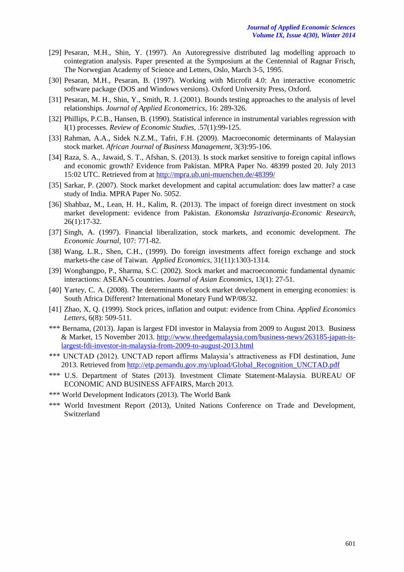
Journal of Applied Economic Sciences
Volume IX, Issue 4(30), Winter 2014
601
[29] Pesaran, M.H., Shin, Y. (1997). An Autoregressive distributed lag modelling approach to
cointegration analysis. Paper presented at the Symposium at the Centennial of Ragnar Frisch,
The Norwegian Academy of Science and Letters, Oslo, March 3-5, 1995.
[30] Pesaran, M.H., Pesaran, B. (1997). Working with Microfit 4.0: An interactive econometric
software package (DOS and Windows versions). Oxford University Press, Oxford.
[31] Pesaran, M. H., Shin, Y., Smith, R. J. (2001). Bounds testing approaches to the analysis of level
relationships. Journal of Applied Econometrics, 16: 289-326.
[32] Phillips, P.C.B., Hansen, B. (1990). Statistical inference in instrumental variables regression with
I(1) processes. Review of Economic Studies, .57(1):99-125.
[33] Rahman, A.A., Sidek N.Z.M., Tafri, F.H. (2009). Macroeconomic determinants of Malaysian
stock market. African Journal of Business Management, 3(3):95-106.
[34] Raza, S. A., Jawaid, S. T., Afshan, S. (2013). Is stock market sensitive to foreign capital inflows
and economic growth? Evidence from Pakistan. MPRA Paper No. 48399 posted 20. July 2013
15:02 UTC. Retrieved from at http://mpra.ub.uni-muenchen.de/48399/
[35] Sarkar, P. (2007). Stock market development and capital accumulation: does law matter? a case
study of India. MPRA Paper No. 5052.
[36] Shahbaz, M., Lean, H. H., Kalim, R. (2013). The impact of foreign direct investment on stock
market development: evidence from Pakistan. Ekonomska Istrazivanja-Economic Research,
26(1):17-32.
[37] Singh, A. (1997). Financial liberalization, stock markets, and economic development. The
Economic Journal, 107: 771-82.
[38] Wang, L.R., Shen, C.H., (1999). Do foreign investments affect foreign exchange and stock
markets-the case of Taiwan. Applied Economics, 31(11):1303-1314.
[39] Wongbangpo, P., Sharma, S.C. (2002). Stock market and macroeconomic fundamental dynamic
interactions: ASEAN-5 countries. Journal of Asian Economics, 13(1): 27-51.
[40] Yartey, C. A. (2008). The determinants of stock market development in emerging economies: is
South Africa Different? International Monetary Fund WP/08/32.
[41] Zhao, X, Q. (1999). Stock prices, inflation and output: evidence from China. Applied Economics
Letters, 6(8): 509-511.
*** Bernama, (2013). Japan is largest FDI investor in Malaysia from 2009 to August 2013. Business
& Market, 15 November 2013. http://www.theedgemalaysia.com/business-news/263185-japan-is-
largest-fdi-investor-in-malaysia-from-2009-to-august-2013.html
*** UNCTAD (2012). UNCTAD report affirms Malaysia’s attractiveness as FDI destination, June
2013. Retrieved from http://etp.pemandu.gov.my/upload/Global_Recognition_UNCTAD.pdf
*** U.S. Department of States (2013). Investment Climate Statement-Malaysia. BUREAU OF
ECONOMIC AND BUSINESS AFFAIRS, March 2013.
*** World Development Indicators (2013). The World Bank
*** World Investment Report (2013), United Nations Conference on Trade and Development,
Switzerland
Journal of Applied Economic Sciences VolumeIX, Issue4 (30) Winter 2014
602
MARKETING PRICING STRATEGY AS PART OF COMPETITIVE ADVANTAGE RETAILERS
Radovan BAČÍK
University of Presov, Faculty of Management, Slovakia
Róbert ŠTEFKO
University of Presov, Faculty of Management, Slovakia
Jaroslava GBUROVÁ
University of Presov, Faculty of Management, Slovakia
Abstract:
The article is focused on pricing policy and marketing pricing strategies applied in the branches of
retail chains in the selected region of Slovakia. An important part of this article is a demonstration of the most
commonly used marketing pricing strategies from the perspective of marketing managers of affiliates of retail
chains operating in the examined region of Slovakia. The aim of this article is to detect and highlight the most
utilized marketing pricing strategy within the surveyed branches of retail chains operating in the North East
of Slovakia. The analysis of variance (ANOVA) and Student two-sample test were used to detect differences
of comparison.
Keywords: pricing policy, marketing pricing strategies, retail trade, competition.
JEL Classification: M30, M31
1. Introduction
For most of history prices were wagered by negotiation between a buyer and a seller.
Negotiation is still a popular discipline in some areas. The idea of setting one price for all buyers was
developed with the beginning of mass retailing in the late 19th century. F. W. Woolwoorth, Tiffany
& Co., John Wanamaker and others advertised "one price policy" because they offered a large number
of items and employed many employees. Traditionally, price acts as a major factor influencing the
choice of the buyer (Kotler and Keller, 2013; Pudło and Gavurová, 2012). Several authors Kotler et
al. (2009), Solomon et al. (2006), Kotler and Keller (2007), Štefko (2003), Gburová (2011) point out
that price decisions and pricing strategies are considered as a highly accented issue that must be to a
large extent handled by marketing. Pricing issue in market conditions is also the specific issue of each
company. Price is an item of the mix marketing; its task together is to with other instruments bring the
company to its marketing objectives (Kita et al., 2010).
Economic fall in recent years caused the "price pressure" for a lot of companies. Price cutting
is not always the best answer, because unnecessary cutting can lead to a profit loss or dangerous price
wars (Užík and Šoltés, 2009; Szabo et al. 2013). This may indicate to customers that a price is more
important than a brand. In pricing companies must carefully consider a number of internal and
external factors while choosing a price, which provides them the biggest competitive advantage on the
selected markets. Pricing decisions are limited by laws and ethical factors (Kotler et al., 2007; Foust,
2003; Gavurová, 2011, 2012). Currently, companies have to face constant price change of their
competitors. The strategy often depends on whether the company produces homogeneous or non-
homogeneous products (Kotler et al., 2009). Pricing must become an integral part of the marketing
strategy of the company and must also comply with corporate and marketing objectives, as well as
other elements of the marketing mix. In addition to these inputs a prices trader has to consider the
demand, price and competition while making decisions about prices (Gavurová et al. 2014; Laucaster
and Massingham, 2010). Making the qualitative pricing strategy requires an understanding of various
situations, considerable background material and results of proven experience in a variety of
situations, which arised during the competition compete. Their use and good theoretical knowledge
are prerequisites for the success of processed procedures in price area of every businessman (Olah et
al., 2009; Šoltés and Gavurová, 2013). Companies usually do not provide the only price, but rather a
pricing structure that reflects the diversity of demand and costs between different regions, the
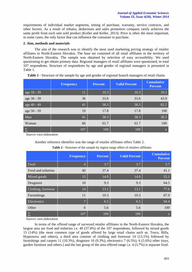
Journal of Applied Economic Sciences
Volume IX, Issue 4(30), Winter 2014
603
requirements of individual market segments, timing of purchase, warranty, service contracts, and
other factors. As a result of rebates, deductions and sales promotion company rarely achieves the
same profit from each unit sold product (Kotler and Keller, 2013). Price is often the most important,
in some cases, the only factor that can influence the consumer to purchase.
2. Aim, methods and materials
The aim of the research was to identify the most used marketing pricing strategy of retailer
affiliates in North-Eastern Slovakia. The base set consisted of all retail affiliates in the territory of
North-Eastern Slovakia. The sample was obtained by selection of easy accessibility. We used
questioning to get obtain primary data. Regional managers of retail affiliates were questioned, in total
107 respondents. Structure of respondents by age and gender of regional managers is presented in
Table 1.
Table 1 - Structure of the sample by age and gender of regional branch managers of retail chains
Frequency Percent Valid Percent Cumulative
Percent
age 18 - 29 11 10.3 10.3 10.3
age 30 - 39 36 33.6 33.6 43.9
age 40 - 49 41 38.3 38.3 82.2
age 50 - 59 19 17.8 17.8 100
Man 41 38.3 38.3 38.3
Woman 66 61.7 61.7 100
∑ 107 100 100 x
Source: own elaboration
Another reference identifier was the range of retailer affiliates offers Table 2.
Table 2 - Structure of the sample by region range offers of retailers affiliates
Frequency Percent Valid Percent Cumulative
Percent
Food 4 3.7 3.7 3.7
Food and toiletries 40 37.4 37.4 41.1
Mixed goods 15 14.0 14.0 55.1
Drugstore 10 9.3 9.3 64.5
Clothing, footwear 14 13.1 13.1 77.6
Furnishings 11 10.3 10.3 87.9
Electronics 7 6.5 6.5 94.4
Other 6 5.6 5.6 100
∑ 107 100 100 x
Source: own elaboration
In terms of the offered range of surveyed retailer affiliates in the North-Eastern Slovakia, the
largest area are food and toiletries i.e. 40 (37.4%) of the 107 respondents, followed by mixed goods
15 (14%) (the most common type of goods offered by large retail chains such as. Tesco, Billa,
Hypernova and others), a third area consists of clothing and footwear 14 (13.1%) followed by
furnishings and carpets 11 (10.3%), drugstore 10 (9.3%), electronics 7 (6.5%), 6 (5.6%) other (toys,
garden furniture and others.) and the last group of the area offered range i.e. 4 (3.7%) is separate food.
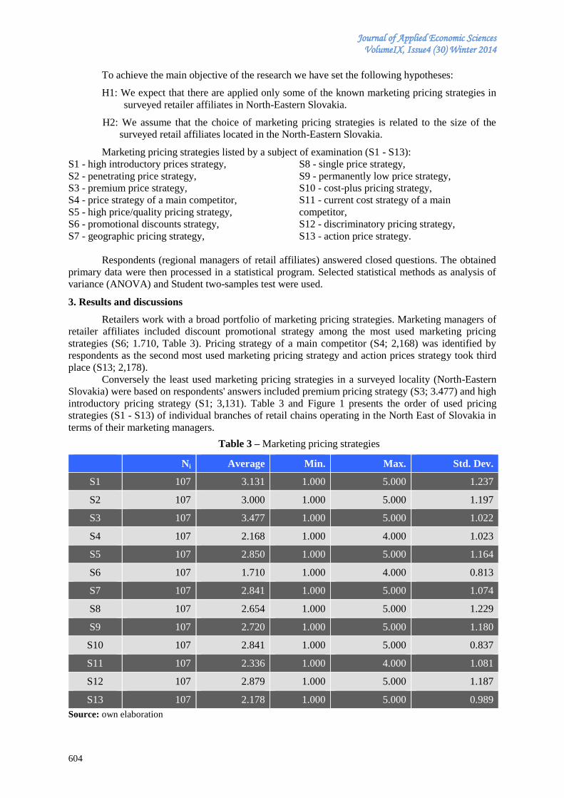
Journal of Applied Economic Sciences VolumeIX, Issue4 (30) Winter 2014
604
To achieve the main objective of the research we have set the following hypotheses:
H1: We expect that there are applied only some of the known marketing pricing strategies in
surveyed retailer affiliates in North-Eastern Slovakia.
H2: We assume that the choice of marketing pricing strategies is related to the size of the
surveyed retail affiliates located in the North-Eastern Slovakia.
Marketing pricing strategies listed by a subject of examination (S1 - S13):
S1 - high introductory prices strategy,
S2 - penetrating price strategy,
S3 - premium price strategy,
S4 - price strategy of a main competitor,
S5 - high price/quality pricing strategy,
S6 - promotional discounts strategy,
S7 - geographic pricing strategy,
S8 - single price strategy,
S9 - permanently low price strategy,
S10 - cost-plus pricing strategy,
S11 - current cost strategy of a main
competitor,
S12 - discriminatory pricing strategy,
S13 - action price strategy.
Respondents (regional managers of retail affiliates) answered closed questions. The obtained
primary data were then processed in a statistical program. Selected statistical methods as analysis of
variance (ANOVA) and Student two-samples test were used.
3. Results and discussions
Retailers work with a broad portfolio of marketing pricing strategies. Marketing managers of
retailer affiliates included discount promotional strategy among the most used marketing pricing
strategies (S6; 1.710, Table 3). Pricing strategy of a main competitor (S4; 2,168) was identified by
respondents as the second most used marketing pricing strategy and action prices strategy took third
place (S13; 2,178).
Conversely the least used marketing pricing strategies in a surveyed locality (North-Eastern
Slovakia) were based on respondents' answers included premium pricing strategy (S3; 3.477) and high
introductory pricing strategy (S1; 3,131). Table 3 and Figure 1 presents the order of used pricing
strategies (S1 - S13) of individual branches of retail chains operating in the North East of Slovakia in
terms of their marketing managers.
Table 3 – Marketing pricing strategies
Ni Average Min. Max. Std. Dev.
S1 107 3.131 1.000 5.000 1.237
S2 107 3.000 1.000 5.000 1.197
S3 107 3.477 1.000 5.000 1.022
S4 107 2.168 1.000 4.000 1.023
S5 107 2.850 1.000 5.000 1.164
S6 107 1.710 1.000 4.000 0.813
S7 107 2.841 1.000 5.000 1.074
S8 107 2.654 1.000 5.000 1.229
S9 107 2.720 1.000 5.000 1.180
S10 107 2.841 1.000 5.000 0.837
S11 107 2.336 1.000 4.000 1.081
S12 107 2.879 1.000 5.000 1.187
S13 107 2.178 1.000 5.000 0.989
Source: own elaboration
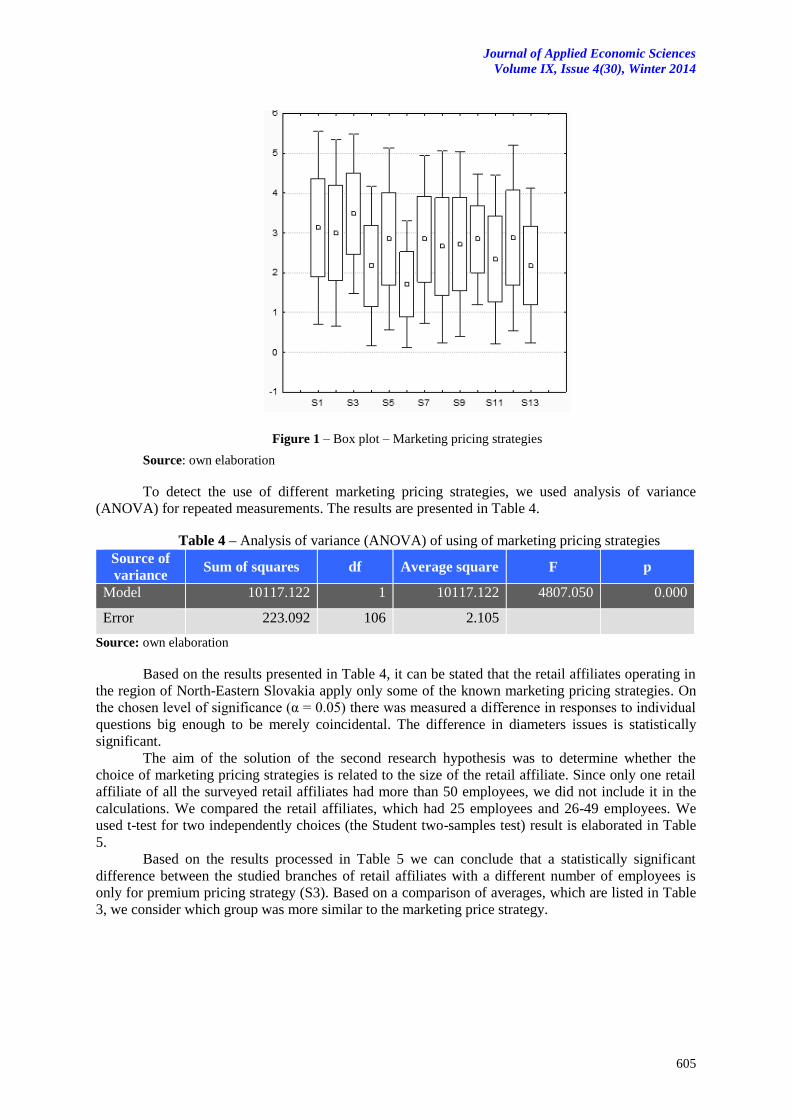
Journal of Applied Economic Sciences
Volume IX, Issue 4(30), Winter 2014
605
Figure 1 – Box plot – Marketing pricing strategies
Source: own elaboration
To detect the use of different marketing pricing strategies, we used analysis of variance
(ANOVA) for repeated measurements. The results are presented in Table 4.
Table 4 – Analysis of variance (ANOVA) of using of marketing pricing strategies
Source of
variance Sum of squares df Average square F p
Model 10117.122 1 10117.122 4807.050 0.000
Error 223.092 106 2.105
Source: own elaboration
Based on the results presented in Table 4, it can be stated that the retail affiliates operating in
the region of North-Eastern Slovakia apply only some of the known marketing pricing strategies. On
the chosen level of significance (α = 0.05) there was measured a difference in responses to individual
questions big enough to be merely coincidental. The difference in diameters issues is statistically
significant.
The aim of the solution of the second research hypothesis was to determine whether the
choice of marketing pricing strategies is related to the size of the retail affiliate. Since only one retail
affiliate of all the surveyed retail affiliates had more than 50 employees, we did not include it in the
calculations. We compared the retail affiliates, which had 25 employees and 26-49 employees. We
used t-test for two independently choices (the Student two-samples test) result is elaborated in Table
5.
Based on the results processed in Table 5 we can conclude that a statistically significant
difference between the studied branches of retail affiliates with a different number of employees is
only for premium pricing strategy (S3). Based on a comparison of averages, which are listed in Table
3, we consider which group was more similar to the marketing price strategy.
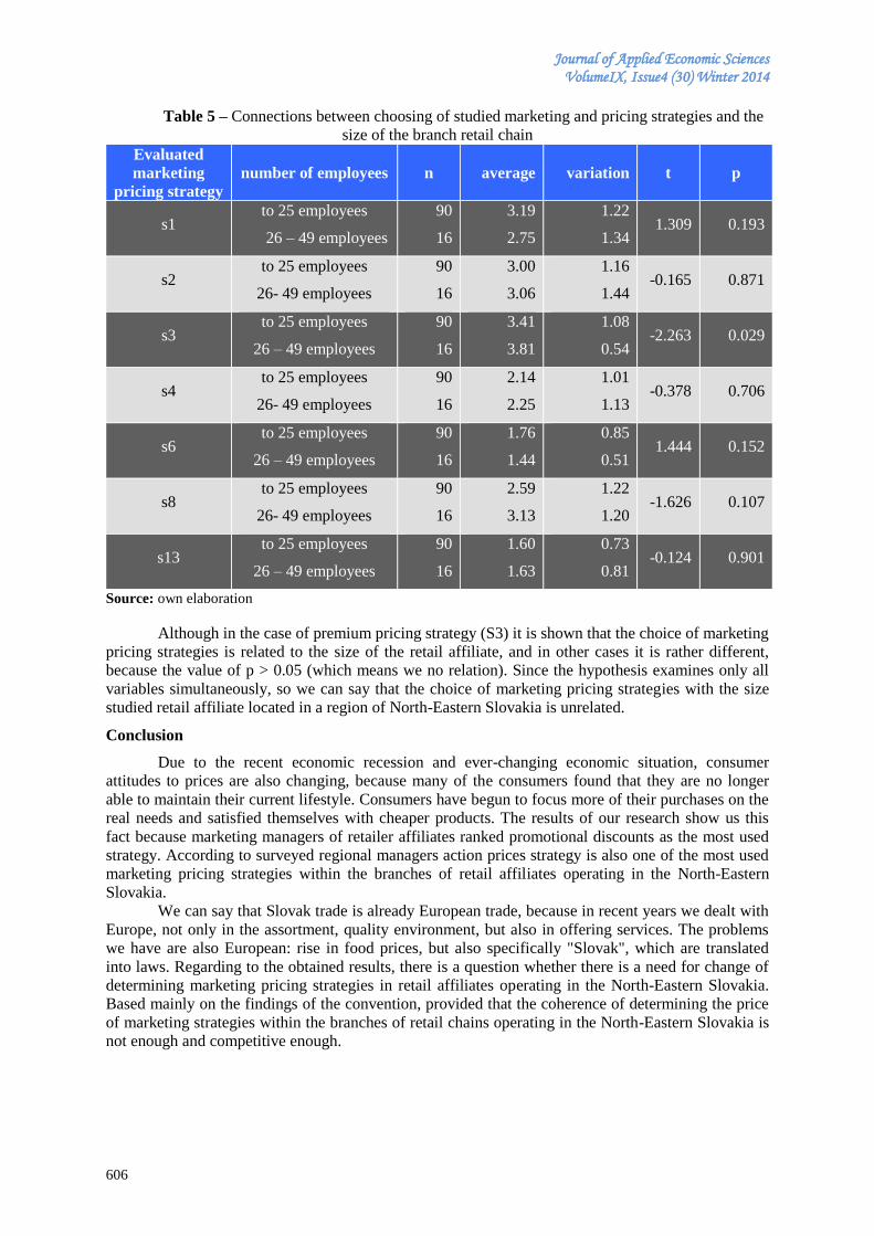
Journal of Applied Economic Sciences VolumeIX, Issue4 (30) Winter 2014
606
Table 5 – Connections between choosing of studied marketing and pricing strategies and the
size of the branch retail chain
Evaluated
marketing
pricing strategy
number of employees n average variation t p
s1 to 25 employees
26 – 49 employees
90
16
3.19
2.75
1.22
1.34 1.309 0.193
s2 to 25 employees
26- 49 employees
90
16
3.00
3.06
1.16
1.44 -0.165 0.871
s3 to 25 employees
26 – 49 employees
90
16
3.41
3.81
1.08
0.54 -2.263 0.029
s4 to 25 employees
26- 49 employees
90
16
2.14
2.25
1.01
1.13 -0.378 0.706
s6 to 25 employees
26 – 49 employees
90
16
1.76
1.44
0.85
0.51 1.444 0.152
s8 to 25 employees
26- 49 employees
90
16
2.59
3.13
1.22
1.20 -1.626 0.107
s13 to 25 employees
26 – 49 employees
90
16
1.60
1.63
0.73
0.81 -0.124 0.901
Source: own elaboration
Although in the case of premium pricing strategy (S3) it is shown that the choice of marketing
pricing strategies is related to the size of the retail affiliate, and in other cases it is rather different,
because the value of p > 0.05 (which means we no relation). Since the hypothesis examines only all
variables simultaneously, so we can say that the choice of marketing pricing strategies with the size
studied retail affiliate located in a region of North-Eastern Slovakia is unrelated.
Conclusion
Due to the recent economic recession and ever-changing economic situation, consumer
attitudes to prices are also changing, because many of the consumers found that they are no longer
able to maintain their current lifestyle. Consumers have begun to focus more of their purchases on the
real needs and satisfied themselves with cheaper products. The results of our research show us this
fact because marketing managers of retailer affiliates ranked promotional discounts as the most used
strategy. According to surveyed regional managers action prices strategy is also one of the most used
marketing pricing strategies within the branches of retail affiliates operating in the North-Eastern
Slovakia.
We can say that Slovak trade is already European trade, because in recent years we dealt with
Europe, not only in the assortment, quality environment, but also in offering services. The problems
we have are also European: rise in food prices, but also specifically "Slovak", which are translated
into laws. Regarding to the obtained results, there is a question whether there is a need for change of
determining marketing pricing strategies in retail affiliates operating in the North-Eastern Slovakia.
Based mainly on the findings of the convention, provided that the coherence of determining the price
of marketing strategies within the branches of retail chains operating in the North-Eastern Slovakia is
not enough and competitive enough.
Journal of Applied Economic Sciences
Volume IX, Issue 4(30), Winter 2014
607
Acknowledgement
The paper was created one of the outputs of the currently ongoing scientific research grant
VEGA 1/0760/13 “Analysis and design of streamlining decision-making processes at the regional
government investment decision-making.”
References
[1] Foust, T. D. (2003). Raising prices won't fly. Retrieved from http://www.businessweek.com/
magazine/content/02_22/b3785051.html.
[2] Gavurová, B. (2011). Systém Balanced Scorecard v podnikovom riadení. (The Balanced
Scorecard System in Enterprise Management). Ekonomický časopis, 59 (2): 163 - 177.
[3] Gavurová, B., (2012). Source Identification of Potential Malfunction of Balanced Scorecard
System and Its Influence on System Function. E+M Ekonomie a management, 15(3): 76 - 90.
[4] Gavurová, B., Šoltés, M., Balloni, A. J. (2014). Ekonomický význam využívania informačno-
komunikačných technológií v systéme zdravotníctva. (The Economic Importance of Using of
ICT in the Health System). Ekonomický časopis. 62(1): 83-104.
[5] Gburová, J. (2011). Marketingové cenové stratégie pobočiek maloobchodných reťazcov
v regióne severovýchodného Slovenska. Bookam, s.r.o. Prešov.
[6] Kita, J. et al. (2010). Marketing. Iura Edition. Bratislava.
[7] Laucaster, G., Massingham, L. (2010). Essentials of Marketing Management. New York.
[8] Kotler, P. et al. (2007). Moderní marketing. Grada Publishing, a.s. Praha.
[9] Kotler, P., Keller, K.L. (2007). Marketing management. Grada Publishing, a.s. Praha.
[10] Kotler, P. et al. (2009). Marketing management. London.
[11] Kotler, P., Keller, K.L. (2013). Marketing management. Grada. Praha.
[12] Oláh, M. et al. (2009). Ceny v marketingu. Elita. Bratislava.
[13] Pudło, P., Gavurová, B. (2012). Experimental learning in higher education, using simulation
games as learning tool. SGEM 2012: 12th International Multidisciplinary Scientific
GeoConference : conference proceedings: Vol. 3: 17-23 June, 2012, Albena, Bulgaria. - Sofia:
STEF92 Technology Ltd., 2012, pp. 1093-1100.
[14] Solomon, R.M. et al. (2006). Marketing očima světových marketingových manažerů. Computer
Press. Brno.
[15] Szabo, Z.K., Šoltés, M., Herman, E. (2013). Innovative Capacity and Performance of Transition
Economies: Comparative Study at the Level of Enterprises. In: E+M Ekonomie a Management,
16 (1): 52-68.
[16] Šoltés, V., Gavurová, B. (2013). Application of the cross impact matrix method in problematic
phases of the Balanced Scorecard system in private and public sector. Journal of Applied
Economic Sciences, 8(1): 99-119.
[17] Štefko, R. (2003). Akademické marketingové inštrumentárium v marketingu vysokej školy. R. S.
Royal Service. Bratislava.
[18] Užík, M., Šoltés, V. (2009). The Effect of Rating Changes on the Value of a Company Listed in
the Capital Market. E + M. Ekonomie a management, 12(1): 49-55.

Journal of Applied Economic Sciences VolumeIX, Issue4 (30) Winter 2014
608
TECHNICAL, ECONOMIC AND MANAGERIAL STRUCTURES IN THE FIELD OF ENERGY IN THE VISION IN THE EUROPEAN UNION
Elena BICĂ
Spiru Haret University, Romania
Faculty of Financial Management and Accounting Craiova
Abstract:
In the global context, emphasis is strongly placed on the attempt to render extractive mining and
energy industry profitable with the help of improved or innovative technologies. Yet, in the field of mining-
energy there occurs a noticeable gap between the operational levels of highly developed, underdeveloped or
emerging countries. The last have more flexible laws related to environment. The development of new
technologies and cooperation to improve the situation of those in operation are topics for technical and
commercial approach, but the demarches were marked by economic, contextual circumstances. Worldwide
including Romania, they require a central qualitative and strategic parameter, in what concerns the the mining
and energy technologies, to be taken into account, namely international competitiveness.
Keywords: energy, efficiency, energy sector, economic development, renewable energy, European strategy,
sustainable energy.
JEL Classification: M12, M54, J53
Introduction
In early 2006 the European Commission launched a broad public debate on the future of the
EU's energy. For Romania as a member state it is particularly important to adapt to the general
framework of Community energy policy. It is marked by three important objectives in the medium
and long term, namely:
increasing the security of energy supply;
increasing competitiveness in the energy field;
reducing environmental impact.
To successfully address these objectives, the European Union aims to establish and implement
a common policy in the field of energy where, traditionally, national competences are very extensive
and the Community instruments are limited.
From this perspective, it should be stressed that EU Member States remain sovereign in
establishing the forms of energy that they want to use. On the other hand, each selection must be
accompanied by the implementation of measures adopted at Community level for that form of energy.
Among the priorities proposed at European level we mention:
The initiation of analysis regarding the long-term energy demand and the way it is
provided;
Elaboration of an action plan for energy efficiency;
The implementation of an action plan regarding biomass;
Development of an interconnection plan and facilitation of the achievement of priority
infrastructure projects which contribute to supply diversification and integration of regional
markets into the EU internal market, recognizing the essential role of economic operators in
these projects;
The improvement of the dialogue on energy between Russia and the EU, including the
ratification by Russia of the Energy Charter Treaty and the finalization of negotiations on
the Transit Protocol;
Development of a strategy to promote the concept of the internal market in EU neighboring
countries;
Ensuring appropriate priorities for the energy sector in FP7 research program;
Improvement of energy markets transparency, particularly in respect of storage capacities
and oil stocks data;
The organization of a European debate about the future of nuclear energy, with accurate
information of European citizens on the current state of energy, advantages and
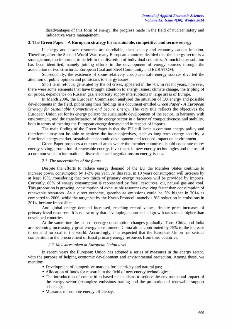
Journal of Applied Economic Sciences
Volume IX, Issue 4(30), Winter 2014
609
disadvantages of this form of energy, the progress made in the field of nuclear safety and
radioactive waste management.
2. The Green Paper - A European strategy for sustainable, competitive and secure energy
If energy and power resources are unreliable, then society and economy cannot function.
Therefore, after the Second World War, many European countries decided that the energy sector is a
strategic one, too important to be left to the discretion of individual countries. A much better solution
has been identified, namely joining efforts in the development of energy sources through the
association of two structures: European Coal and Steel Community and EURATOM.
Subsequently, the existence of some relatively cheap and safe energy sources diverted the
attention of public opinion and politicians to energy issues.
Short term refocus, generated by the oil crises, appeared in the 70s. In recent years, however,
there were some elements that have brought attention to energy issues: climate change, the tripling of
oil prices, dependence on Russian gas, electricity supply interruptions in large areas of Europe.
In March 2006, the European Commission analyzed the situation of EU energy and possible
developments in the field, publishing their findings in a document entitled Green Paper - A European
Strategy for Sustainable Competitive and Secure Energy. The very title reflects the objectives the
European Union set for its energy policy: the sustainable development of the sector, in harmony with
environment, and the transformation of the energy sector in a factor of competitiveness and stability,
both in terms of meeting the European energy demand and in respect of imports.
The main finding of the Green Paper is that the EU still lacks a common energy policy and
therefore it may not be able to achieve the basic objectives, such as long-term energy security, a
functional energy market, sustainable economic development and reduced impact on environment.
Green Paper proposes a number of areas where the member countries should cooperate more:
energy saving, promotion of renewable energy, investment in new energy technologies and the use of
a common voice in international discussions and negotiations on energy issues.
2.1. The uncertainties of the future
Despite the efforts to reduce energy demand of the EU the Member States continue to
increase power consumption by 1-2% per year. At this rate, in 10 years consumption will increase by
at least 10%, considering that two thirds of primary energy resources will be provided by imports.
Currently, 80% of energy consumption is represented by fossil resources: oil, natural gas and coal.
This proportion is growing, consumption of exhaustible resources evolving faster than consumption of
renewable resources. As a direct outcome, greenhouse emissions could be 5% higher in 2014 as
compared to 2006, while the target set by the Kyoto Protocol, namely a 8% reduction in emissions in
2014, became impossible.
And global energy demand increased, reaching record values, despite price increases of
primary fossil resources. It is noteworthy that developing countries had growth rates much higher than
developed countries.
At the same time the map of energy consumption changes gradually. Thus, China and India
are becoming increasingly great energy consummers. China alone contributed by 75% to the increase
in demand for coal in the world. Accordingly, it is expected that the European Union has serious
competition in the procurement of fossil primary energy resources from third countries.
2.2. Measures taken at European Union level
In recent years the European Union has adopted a series of measures in the energy sector,
with the purpose of helping economic development and environmental protection. Among these, we
mention:
Development of competitive markets for electricity and natural gas;
Allocation of funds for research in the field of new energy technologies;
The introduction of competition-based mechanisms to reduce the environmental impact of
the energy sector (examples: emissions trading and the promotion of renewable support
schemes);
Measures to promote energy efficiency.

Journal of Applied Economic Sciences VolumeIX, Issue4 (30) Winter 2014
610
Through these actions, the European Union has clearly demonstrated that it has the political
will to coordinate national efforts in identifying and implementing solutions to energy and
environmental issues. At the time of Green Paper - A European Strategy for Sustainable Competitive
and Secure Energy publication the Union had 25 countries and 450 million consumers of energy. In
January 2007, Romania and Bulgaria's membership number of people increased by another 30
million. In these circumstances, Europe holds significant importance in world energy consumption
and can not be neglected in the international dialogue on the future of energy and environmental
impact of this economic sector. Speaking as "one voice" in this dialogue, the EU is likely to positively
influence other countries to coordinate actions on the conservation of primary energy resources and
reducing the environmental impact of the energy sector. For Unionˊs arguments be convincing it
would have been necessary that policies implemented in Europe in this area be successful and have
tangible results.
Among the targets in the energy field adopted by European Union through binding directives
on Member States we mention:
doubling the share of renewable energy resources in the Union's gross energy consumption
from 6% to 12% in 2015;
increasing the share of electricity produced from renewable resources in total consumption
from 14% to 22% in 2015;
increasing the share of biofuels in transport to 5.75% in 2015; it is also expected to reduce
energy consumption by 20% in 2020.
Using an integrated approach communicated through a "common voice" in the post Kyoto
negotiations, and discussions in the various bodies such as the World Trade Organization will turn
European position in negotiations into not negligible one. Also, an integrated approach to energy
issues and solidarity between Member States will increase the acceptability of European citizens and
national industries to harsh measures that must be implemented in order to achieve the targets.
2.3. Measures proposed by the European Commission
In the Green Paper - A European Strategy for Sustainable Competitive and Secure Energy,
European Commission proposes that, in a number of areas, efforts be coordinated at Community
level, thus avoiding the dissipation of resources through initiatives and actions unrelated at national
level. The identified areas for joint action are:
energy for jobs and development in Europe;
increasing the security and competitiveness of energy supply;
solidarity between Member States;
reducing the impact of energy sector on climate change;
encouraging innovation and research in the field;
relations with third countries.
A series of concrete actions have been identified, such as:
Development of internal electricity market and natural gas.
The process of creating these pan-European markets is in full swing and it should be accelerated
through measures meant to develop new interconnections and a European Network Code, to
promote investments in the field and, last but not least, the possiblility to create a European
Regulator and a European Centre for Energy Networks with roles in managing cross-border trade.
A review of policies on mandatory stocks of oil and gas. The objective of this review is to improve
the response to crisis in the supply of primary energy resources from outside the EU.
A European Energy Observatory, with the effect of increasing transparency on energy demand and
production in member countries.
Improving network security. This objective can be achieved through increased cooperation between
rational network operators and, perhaps, by establishing a new structure in Europe - European
Centre for Energy Networks.
A new mechanism to prepare and ensure solidarity and assistance will be granted to countries in
difficulty as a result of natural disasters affecting energy infrastructure.
A wide debate within the EU on the future of the different energy sources, including issues related
to cost and environmental impact resulting from the use of these sources. As a general goal, through

Journal of Applied Economic Sciences
Volume IX, Issue 4(30), Winter 2014
611
these debates the established European energy mix will meet the criteria of food security in the long
term competitiveness and sustainable development.
An action plan for energy efficiency, with mutually agreed objectives. In addition, it will be
possible to establish an international agreement on energy efficiency.
A roadmap for renewable energy resources, ensuring a predictable framework on measures to
promote these resources at Community level. The measure may include a new target for the share of
renewables in total gross energy consumption in the EU for 2020 and an action plan to reduce
dependence on oil imports.
A strategic plan for technological innovation. Developing research on new energy sources and
improving current technology generation, transmission, distribution and consumption will
contribute to solving current problems of the sector.
A coherent foreign policy at EU level, combining Community and national instruments in dialogue
with third countries on energy issues, including the supply of primary resources imports.
A revision of the EU energy policy. Proposals to this effect were scheduled for presentation to the
European Parliament and the European Council in the spring of 2007, after public debate of the
Green Paper. EU foreign policy proposals aimed at reducing dependence on energy imports, a
roadmap in the field of renewable energy, proposals to develop markets for electricity and natural
gas, the diversification of the energy mix and reduction of the climate impact.
A list of priorities for the construction of new infrastructure elements needed to ensure safe energy
supply: new main natural gas and liquefied natural gas terminals new cross-border power lines.
Reviving the dialogue with Russia, particularly the Energy Charter Transit Protocol.
A European Energy Community Treaty. Based on experience gained through the establishment and
implementation of the Southeast European Energy Community Treaty, the proposed new treaty will
include gradually the neighboring countries of the Union.
A new mechanism at Community level for a rapid and coordinated response to crises affecting the
supply of energy resources of the Member States.
The measures provided in Green Paper - A European Strategy for Sustainable Competitive
and Secure Energy, were publicly debated for nearly a year, the European Commission receiving
1500 written responses from organizations and associations interested in the Union's energy future,
and from ordinary citizens. Following the analysis of these reactions, the Commission published a
coherent package of documents which form a new European Energy Policy. Documents published by
the European Commission under the name,, A new European energy policy ", are built on three ideas:
to demonstrate that the objectives established at the community level in the energy field can
not be achieved with current policies, being necessary to review these policies;
to propose a strategic objective which is the basis for all subsequent energy policy
decisions;
to propose a concrete action plan to achieve the strategic objective.
3. The strategic objective of European energy policy
As a strategic objective the Commission proposed to reduce emissions of greenhouse gases by
20% by 2020. Focus on emissions of greenhouse gases is justified by the fact that the energy sector
contributes a proportion of 800/0 at total emissions. This objective is part of the broader objective
managing climate change and represents a good target for the promotion of renewable subsequent
targets, improving energy efficiency and developing clean technologies. The target of 20% reduction
in emissions of greenhouse gases is a minimum, unilateral commitment of the European Union. The
European Commission believes that if they come to a widely accepted international agreement on
reducing global environmental impact, the EU should increase its target to 30% reduction by 2030
and 60 -80% until 2050.
3.1. Action Plan
In order to achieve the objectives in the common energy policy, the European Commission
has developed a ten-point action plan.
Better use of the domestic energy market. The report of the Commission’s General Directorate
for Competition, resulting from the sectorial analysis on energy, reveals that the expected benefits
from restructuring of the energy sector and the introduction of competition mechanisms have not yet

Journal of Applied Economic Sciences VolumeIX, Issue4 (30) Winter 2014
612
been achieved. The main reasons for this situation are on one hand the existence of a mosaic of
national markets, in each being one or more companies with dominant market power and, on the
other, the limited cooperation between national agencies, mainly, regulators and transmission and
system operators.The proposed measures aimed at creating effective competition with equal
opportunities for all market participants and all energy sources. Action to remove discrimination shall
be taken towards the new entrants and a unitary regulatory mechanism will be created at European
level. Greater attention will be given to consumers whose voice will be listened to by policymakers.
One of the possible ways to achieve this is to create a Charter of European consumers.
Facilitating mutual assistance among Member States in an energy crisis. In this area it is
projected to increase solidarity among the countries that form the European Union in the event of
energy crises. For example, the use of oil stocks achieved by each member will improve. It is
expected that assistance be achieve preventively through active support in diversification of the
energy mix of countries dependent on a single supplier of natural gas or oil.
Improving the mechanisms for marketing the greenhouse effect gas emissions licenses. By
improving the mechanism they intend to transform it into a true catalyst for emissions reduction and a
factor to stimulate investment in clean technologies.Tangible, envisaged measures are presented in a
separate report entitled "Limiting Climate Change to 2 degrees Celsius - Policy Options for Europe
and mankind for 2020 and beyond."
Energy efficiency. Saving energy reduces pollution, energy bills, reduces the need for
investment in new power plants, oil terminals and so on. It is estimated that under current
technological development, up to 20% of energy consumption can be saved. The European
Commission has already launched an Action plan to involve civil society in the joint effort to reduce
energy consumption. This message will also be promoted by the European Union in its dialogue with
international partners to launch a global initiative to increase energy efficiency.
Increasing the proportion of renewable energy sources. All Member States have committed to
support the development of renewable energy: solar, wind, photovoltaic, biomass, biofuels and
geothermal energy, as well as their use in electricity generation and transport. Commitments are still
below the existing potential, and some states do not even realize their commitments. The European
Commission proposes in a Road map, a series of measures to ensure, by its application, the tripling of
share of renewable energy in the energy balance of the Union, from 7% in 2006 to 20% in 2020.
Tehnology. There are many clean and efficient technologies for the production and use of
energy, but they remain marginal because they either are more expensive or are not widely available.
Examples of such technologies are low power light bulbs, solar thermal panels for hot water, hybrid
cars and thermal insulation in the case of buildings. They should strive to reduce the costs of these
technologies. At the same time they must develop new technologies to replace oil and natural gas
shortages or price conditions that are prohibitive for the population.
Clean technologies for fossil fuels. Chiar dacă Uniunea Europeană reuşeşte să-şi modifice
mixul energetic în favoarea surselor regenerabile şi să-şi reducă substanţial consumul de energie, tot
va rămâne dependentă de resursele fosile pentru viitorul previzibil: cărbune, petrol, gaze naturale.
Even if the EU fails to change the energy mix in favor of renewables and to substantially reduce
energy consumption it will still remain dependent on fossil resources - coal, oil, natural gas - for the
foreseeable future. For this reason, it is of general interest to develop technologies that reduce the
carbon dioxide emissions of combustion plants. CO2 capture and storage is a promising solution, but
such technologies are not yet commercially tested.
The safety and security of nuclear energy. More than half of European Union countries use
nuclear energy to produce electricity. About one third of the total of electricity produced Europe
comes from such sources. The decision to use nuclear energy rests with individual Member State
separately. But the EU, according to the rules established by the EURATOM Treaty, has a role in
ensuring the use of nuclear energy in ways that do not endanger life or environment. Achieving high
standards of nuclear safety and non-proliferation of nuclear weapons is the 8th line of action proposed
by the European Commission.
Establishing a common international policy and its utterance in "in a single voice".
Commission proposes several measures expanding globally by promoting them in the international
dialogue. It also intends to create an energy security zone around the Member States as well as the
development of strong partnerships with energy suppliers, based on mutual interest, predictability and
Journal of Applied Economic Sciences
Volume IX, Issue 4(30), Winter 2014
613
equal treatment. The financing conditions and participation in international projects will be improved,
for example, by appointing coordinators for infrastructure projects of European interest. The
European Union will intensify its efforts towards a clean, sustainable and cheap energy technology
transfer to less developed countries.
Improve the understanding of energy issues. To achieve this goal it is expected that the
organization of an Energy Observatory will study among other things, energy trends and investment
needs of the European Union as a whole.
Conclusions
The European Commission's energy policy is to be revised two years after its adoption,
concurrently with the publication of a report on the implementation and results achieved. Through the
energy policy of the European Commission proposed they create a coherent framework for action not
only to ensure the EU's energy future, but also to reduce the impact on environment, particularly, on
climate change. Specific targets are set unilaterally in the Union. This is an example for the rest of the
world states and Europe take the leading role in the fight for a clean and safe planet.
The general objective proposed is also effective on the safety of energy supply in the long
term. Through achieving this goal Europe will reduce exposure to price volatility of fossil energy
resources, will stimulate the development of domestic markets for electricity and gas and encourage
technological development.
Three related objectives emerge from the the overall objective, the European Commission
proposing a target:
Increasing the share of renewables in the total energy mix to 20% in 2020;
Improving energy efficiency by 20% by 2020;
Increasing the share of biofuels in transport to 10% by 2020.
Based on contextual research it is possible to design and implement technical, economic and
managerial restructuring activities in energy complexes.Therefore, the use and future structural
transformation from technical, economic and managerial perspective of the energy sector in the
European Union is an approach characterized by risk estimation and prediction that aims at measuring
and dimensional reduction, of their content, respectively.
References:
[1] Gâf-Deac, I.I. (2007). Legal and Economic Bases of System Resources in the New Economy,
Edition Infomin, Deva.
[2] Jula, D., Jula, N. (2007). Inter-Industries Productivity Gap and the Sercices Employment
Dynamics, Romanian Journal of Economic Forecasting, No. 2/2007.
[3] Mereuţă, C. et al. (2007). A Model to Evaluate the Regional Competitiveness of the EU Regions,
Romanian Journal of Economic Forecasting, No. 3/2007.
[4] Murgescu, B. (2000). Romania and Europe: the Temptation Modernization, Upgrading the Threat,
Alfa Publishing, Bucharest.
[5] Naidin Bică, E. (2010). Contributions to the development of structures econometric model of
technical, economic and managerial type energy-mining complexes and efficiency", PhD thesis
Report for April, Petrosani 2010.
[6] Sârbu, I., Kalamar, F. (2002). Energy optimization, Ed. Matrix Rom, Bucharest.
[7] Sproull, L.S. (1990). Technology and organizations: Integration and opportunities, Technology
and Organization, Jossex-Bass, San Francisco, 1990.
*** Cadre international de classification des Nations Unites pour les reserve/resources, Commission
Economique pour Europe, Comite de Energie, Groupe de Travail du Charbon, Geneva, 1996
*** European Green Paper, COM / 2000/0769.
*** Law no. 243/15 July 2005 on measures of energy complexes to accelerate privatization, Official
Gazette no. 631/19 July 2005.
*** Energy Community Treaty Southeast Europe COM (2002) 321, July 2002.
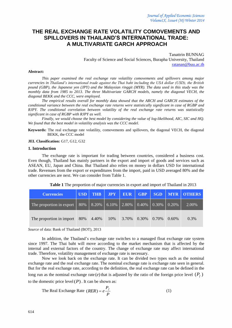
Journal of Applied Economic Sciences VolumeIX, Issue4 (30) Winter 2014
614
THE REAL EXCHANGE RATE VOLATILITY COMOVEMENTS AND SPILLOVERS IN THAILAND’S INTERNATIONAL TRADE:
A MULTIVARIATE GARCH APPROACH
Tanattrin BUNNAG
Faculty of Science and Social Sciences, Burapha University, Thailand
Abstract:
This paper examined the real exchange rate volatility comovements and spillovers among major
currencies in Thailand’s international trade against the Thai baht including the USA dollar (USD), the British
pound (GBP), the Japanese yen (JPY) and the Malaysian ringgit (MYR). The data used in this study was the
monthly data from 1985 to 2013. The three Multivariate GARCH models, namely the diagonal VECH, the
diagonal BEKK and the CCC, were employed.
The empirical results overall for monthly data showed that the ARCH and GARCH estimates of the
conditional variance between the real exchange rate returns were statistically significant in case of RGBP and
RJPY. The conditional correlation between volatility of the real exchange rate returns was statistically
significant in case of RGBP with RJPY as well.
Finally, we would choose the best model by considering the value of log-likelihood, AIC, SIC and HQ.
We found that the best model in volatility analysis was the CCC model.
Keywords: The real exchange rate volatility, comovements and spillovers, the diagonal VECH, the diagonal
BEKK, the CCC model
JEL Classification: G17, G12, G32
1. Introduction
The exchange rate is important for trading between countries, considered a business cost.
Even though, Thailand has mainly partners in the export and import of goods and services such as
ASEAN, EU, Japan and China. But Thailand also relies on money in dollars USD for international
trade. Revenues from the export or expenditures from the import, paid in USD averaged 80% and the
other currencies are next. We can consider from Table 1.
Table 1 The proportion of major currencies in export and import of Thailand in 2013
Source of data: Bank of Thailand (BOT), 2013
In addition, the Thailand’s exchange rate switches to a managed float exchange rate system
since 1997. The Thai baht will move according to the market mechanism that is affected by the
internal and external factors of the country. The change of exchange rate may affect international
trade. Therefore, volatility management of exchange rate is necessary.
Now we look back on the exchange rate. It can be divided two types such as the nominal
exchange rate and the real exchange rate. The nominal exchange rate is exchange rate seen in general.
But for the real exchange rate, according to the definition, the real exchange rate can be defined in the
long run as the nominal exchange rate )(e that is adjusted by the ratio of the foreign price level )( fP
to the domestic price level )(P . It can be shown as:
The Real Exchange Rate P
PeRER
f)( (1)
Currencies USD THB JPY EUR GBP SGD MYR OTHERS
The proportion in export 80% 8.20% 6.10% 2.80% 0.40% 0.30% 0.20% 2.00%
The proportion in import 80% 4.40% 10% 3.70% 0.30% 0.70% 0.60% 0.3%
Journal of Applied Economic Sciences
Volume IX, Issue 4(30), Winter 2014
615
This study covers the conditional volatility and the conditional correlation of Thailand’s
international trade by taking changes in the real exchange rate into consideration. The reason is that
the real exchange rate affects the Thailand’s international trade more than the nominal exchange rate.
And we choose four important exchange rates in the volatility analysis; the USA dollar (USD), the
British pound (GBP), the Japanese yen (JPY) and the Malaysian ringgit (MYR) We can explain more in the next section, which is related to the literature reviews, research
methodology and empirical results.
2. Literature Reviews
A large number of studies find evidence in support of significant comovements in volatility
and spillovers among asset prices. More detail can be found in Bae and Karolyi (1994), Kim and
Rogers (1995), Kim (2003) and Christodoulakis (2007). However, few studies have so far
investigated volatility comovements and spillover among the real exchange rates.
Bollerslev (1990) employed a multivariate GARCH framework to investigate European
exchange rate volatility spillovers. He applied the Constant Conditional Correlation (CCC) to a set of
five weekly European spot exchange rates against the US dollar, namely the Deutsche Mark, the
French franc, the Italian lira, the Swiss franc and the British pound, He found significant
comovements in volatility of these five exchange rates, and by comparing the pre and post European
Monetary System (EMS) periods he found that the comovement were significantly greater in the later
period.
Kearny and Patton (2000) offered an application of the BEKK model, proposed by Engle and
Kloner (1995), to exchange rate volatility spillovers. This approach does not impose the restrictive
assumption of constant conditional correlations through time and offers a very attractive formulation
of volatility spillovers. In addition, it can distinguish between direct volatility spillovers or indirect
spillovers. The currencies investigated by Kearney and Patton included the most important currencies
within the EMS, that is the German mark, the French franc, the Italian lira, the British pound as well
as the European Currency Unit all against the US dollar. Their analysis covered data from April 1979
through to March 1997. The authors found evidence of both direct and indirect volatility transmission
within EMS in both daily and weekly data for the European Currency Unit (ECU), the German mark,
the French franc, the Italian lira and the British pound. In addition, they provided evidence that the
German mark held a dominant position in term of volatility transmission. The German mark was
found to be relatively insulated from outside shocks while transmitting more volatility than the other
currencies. Their results obtained using weekly data were less significant than those on daily data.
This decrease in significant, derived from the temporal aggregation of the data from daily to weekly,
is in the line with the conjecture that markets are more likely a transmit volatility in active phase
rather than in calm ones.
Calvet et al. (2006) employed a Markov-Switching Multifractal (MSM) approach to assess
volatility comovement of the German mark (Euro), the British pound and the Japanese yen against the
US dollar. In addition to the MSM model, the authors applied the Constant Conditional Correlation
(CCC) of Bollerslev (1990) and compared the results from the two models. They found that the MSM
model outperformed the CCC.
The next section describes the research methodology used in this analysis.
3. Research Methodology
Multivariate GARCH Models
The basic idea to extend univariate GARCH models to multivariate GARCH models is that it
is significant to predict the dependence in the comovement of the real exchange rate returns in a
portfolio. To recognize this feature through a multivariate model would generate a more reliable
model than separate univariate models.
In the first place, one should consider what specification of a multivariate GARCH model
should be imposed. On the one hand, it should be flexible enough to state the dynamics of the
conditional variances and covariances. On the other hand, as the number of parameters in a
multivariate GARCH model increase rapidly along with the dimension of the model, the specification
should be parsimonious to simplify the model estimation and also reach the purpose of easy
Journal of Applied Economic Sciences VolumeIX, Issue4 (30) Winter 2014
616
interpretation of the model parameters. However, parsimony may reduce the number of parameters, in
which situation the relevant dynamics in the covariance matrix cannot be captured. So it is important
to get balance between the parsimony and the flexibility when designing the multivariate GARCH
model specification. Another feature that multivariate GARCH models must satisfy is that the
covariance matrix should be positive definite.
Several different multivariate GARCH model formulations have been proposed in the
literature, and the most popular of these are the diagonal VECH, the diagonal BEKK and CCC
models. Each of these is discussed briefly in turn below; for a more detailed discussion, see Kroner
and Ng (1998).
The diagonal VECH model
The first multivariate GARCH model was introduced by Bollerslev, Engle and Wooldridge in
1988, which is called VECH model. It is much general compared to the subsequent formulations. In
the VECH model, every conditional variance and covariance is a function of all lagged conditional
variances and covariances, as well as lagged squared returns and cross-products of returns. The model
can be expressed below:
),()()(11
jt
p
j
jjtjt
q
j
jt HVECHBVECHAcHVECH
(2)
where )( tHVECH is an operator that stacks the columns of the lower triangular part of its
argument square matrix, tH is the covariance matrix of the residuals, N presents the number of
variables, t is the index of the t th observation, c is an 12
)1(
NNvector, jA and jB are
2
)1(
2
)1(
NNNN parameter matrices and is an 1N vector.
The condition for tH is to be positive definite for all t is not restrictive. In addition, the number
of parameters equals to2
)1(
2
1()(
2
NNNNqp , which is large. Furthermore, it demands a
large quantity of computation.
The diagonal VECH model, the restricted version of VECH, was also proposed by Bollerslev,
et al (1988). It assumes the jA and jB in equation (2) are diagonal matrices, which makes it possible
for tH to be positive definite for all t . Also, the estimation process proceeds much smoothly compared
to the complete VECH model. However, the diagonal VECH model with 2
)1()1(
NNqp
parameters is too restrictive since it does not take into account the interaction between different
conditional variances and covariances.
The diagonal BEKK model
To ensure positive definiteness, a new parameterization of the conditional variance matrix tH
was defined by Baba, Engle, Kraft and Kroner (1990) and became known as the BEKK model, which
is viewed as another restricted version of the VECH model. It achieves the positive definiteness of the
conditional variance by formulating the model in a way that is property is implied by model structure.
The form of the BEKK model is as follows:
kjjt
p
j
K
k
kjkjjtjt
q
j
K
k
kjt BHBAACCH
1 11 1
(3)
where kjkj BA , and C are NN parameter matrices, and C is a lower triangular matrix. The
purpose of decomposing the constant term into a product of two triangle matrices is to guarantee the
Journal of Applied Economic Sciences
Volume IX, Issue 4(30), Winter 2014
617
positive semi-definiteness of tH . Whenever 1K , an identification problem would be generated for
the reason that there are not only single parameterizations that can obtain the same representation of
the model.
The first order BEKK model is:
BHBAACCH tttt 111 (4)
The BEKK model also has its diagonal form by assuming kjkj BA , matrices are diagonal. It is
a restricted version of the diagonal VECH model. The most restricted version of the diagonal BEKK
model is the scalar BEKK one with aIA and bIB where a and b are scalars.
Estimation of a BEKK model still bears large computations due to several matrix
transpositions. The number of parameters of the complete BEKK model is2
)1()( 2
NN
KNqp .
Even in the diagonal one, the number of parameters soon reduces to2
)1()(
NNKNqp , but it is
still large. The BEKK form is not linear in parameters, which makes the convergence of the model
difficult. However, the strong point lies in that the model structure automatically guarantees the
positive definiteness of tH . Under the overall consideration, it is typically assumed that
1 Kqp in BEKK form’s application.
The Constant Conditional Correlations (CCC) model
The CCC model was introduced by Bollerslev in 1990 to primarily model the condition
covariance matrix indirectly by estimating the conditional correlation matrix. The conditional
correlation is assumed to be constant while the conditional variances are varying.
Consider the CCC model of Bollerslev (1990):
ttttttt DFyEy ,1 (5)
tttt DDF 1var
where
mtttmttt yyy ,...,1,...,1 , is a sequence of independently and identically
distributed (i.i.d) random vectors, tF is the past information available at time
mhhdiagDt mtt ,,...,, 2/12/1 is the number of returns, and ,,...,1 nt . As
,1 ttttt EFE where ij for ,,...1, mji the constant conditional correlation
matrix of the unconditional shocks, t , is equivalent to the constant conditional covariance matrix of
the conditional shocks, t , from (5), ,,2/1
1 tttttttt QdiagDDD and
,11 tttttt DDQFE where tQ is the conditional covariance matrix.
The CCC model assumes that the conditional variance for each return ,,...,1, mihit follows
a univariate GARCH process, that is:
,,
1
2
,
1
jti
s
j
ijjti
r
j
ijtt hh
(6)
where ij represents the ARCH effect, or short run persistence of shocks to return iji ,
represents the GARCH effect, and
s
j
ij
r
j
ij
11
denotes the long run persistence.

Journal of Applied Economic Sciences VolumeIX, Issue4 (30) Winter 2014
618
Model estimation for multivariate GARCH
Under the assumption of conditional normality, the parameters of the multivariate GARCH
models of any of the above specifications can be estimated by maximizing the log-likelihood function.
)(log2
12log
2)( 1
1
ttt
T
t
t HHTN
(7)
where denotes all the unknown parameters to be estimated, N is the number of the real
exchange rates and T is the number of observations and all other notation is as above. The maximum-
likelihood estimates for is asymptotically normal, and thus traditional procedures for statistical
inference are applicable.
3. The purpose of this study
The purpose is to analyze the real exchange rate volatility comovement and spillovers among
major currencies in Thailand’s international trade against the Thai baht including the USA dollar
(USD), the British pound (GBP), the Japanese yen (JPY) and the Malaysian ringgit (MYR) by using
multivariate GARCH, namely the diagonal VECH, the diagonal BEKK and CCC model and choose
the best way for such analysis.
4. Data
The data used in this study is the monthly data from 1985 to 2013. We will get 348
observations. The data is derived from the Bank of Thailand (BOT). Moreover, data analysis can be
carried out using EVIEWS 8. The real exchange rate return is defined as:
1
logt
tt
RER
RERR (8)
where RERt is the real exchange rate at time t and RERt-1 is the real exchange rate at time t-1.
The Rt of equation (8) will be used in observing the volatility of the real exchange rate between the
selected currencies over the period 1985 to 2013. We can create the variables of the return on the real
exchange rate as follows:
The real exchange rate return of the USA dollar = RUSD, The real exchange rate return of the
British pound = RGBP, The real exchange rate return of the Japanese yen = RJPY and The real
exchange rate return of the Malaysian ringgit = RMYR
In addition, we can show the movement of the monthly real exchange rate returns according
to Figure 1.
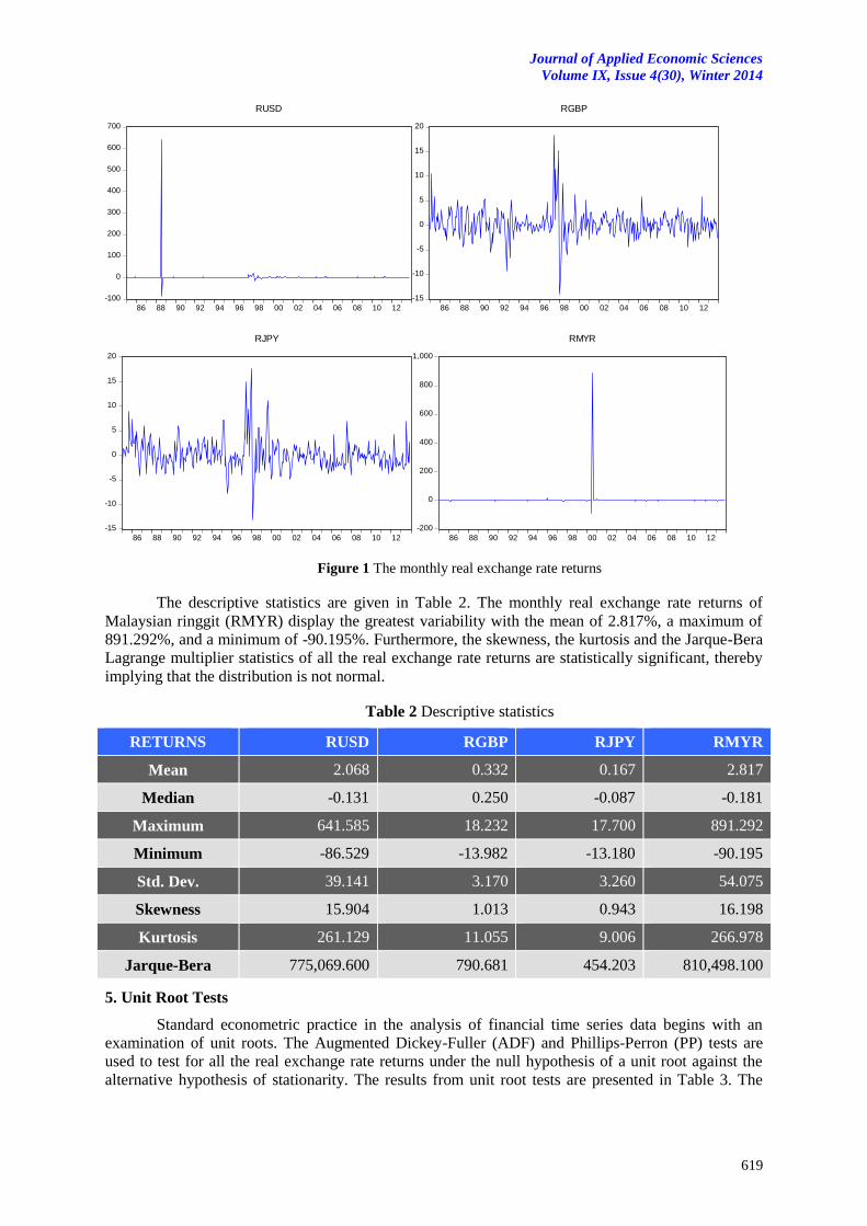
Journal of Applied Economic Sciences
Volume IX, Issue 4(30), Winter 2014
619
-100
0
100
200
300
400
500
600
700
86 88 90 92 94 96 98 00 02 04 06 08 10 12
RUSD
-15
-10
-5
0
5
10
15
20
86 88 90 92 94 96 98 00 02 04 06 08 10 12
RGBP
-15
-10
-5
0
5
10
15
20
86 88 90 92 94 96 98 00 02 04 06 08 10 12
RJPY
-200
0
200
400
600
800
1,000
86 88 90 92 94 96 98 00 02 04 06 08 10 12
RMYR
Figure 1 The monthly real exchange rate returns
The descriptive statistics are given in Table 2. The monthly real exchange rate returns of
Malaysian ringgit (RMYR) display the greatest variability with the mean of 2.817%, a maximum of
891.292%, and a minimum of -90.195%. Furthermore, the skewness, the kurtosis and the Jarque-Bera
Lagrange multiplier statistics of all the real exchange rate returns are statistically significant, thereby
implying that the distribution is not normal.
Table 2 Descriptive statistics
RETURNS RUSD RGBP RJPY RMYR
Mean 2.068 0.332 0.167 2.817
Median -0.131 0.250 -0.087 -0.181
Maximum 641.585 18.232 17.700 891.292
Minimum -86.529 -13.982 -13.180 -90.195
Std. Dev. 39.141 3.170 3.260 54.075
Skewness 15.904 1.013 0.943 16.198
Kurtosis 261.129 11.055 9.006 266.978
Jarque-Bera 775,069.600 790.681 454.203 810,498.100
5. Unit Root Tests
Standard econometric practice in the analysis of financial time series data begins with an
examination of unit roots. The Augmented Dickey-Fuller (ADF) and Phillips-Perron (PP) tests are
used to test for all the real exchange rate returns under the null hypothesis of a unit root against the
alternative hypothesis of stationarity. The results from unit root tests are presented in Table 3. The
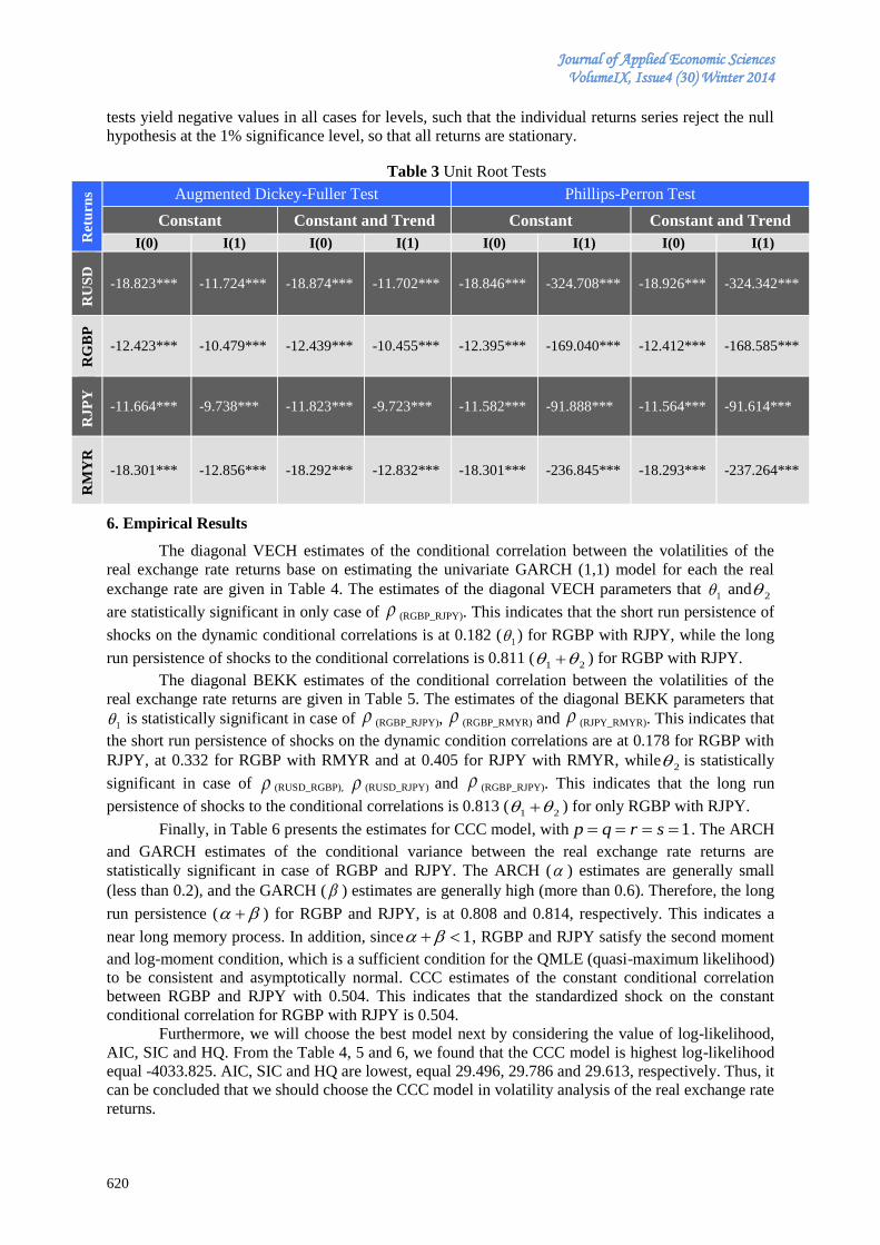
Journal of Applied Economic Sciences VolumeIX, Issue4 (30) Winter 2014
620
tests yield negative values in all cases for levels, such that the individual returns series reject the null
hypothesis at the 1% significance level, so that all returns are stationary.
Table 3 Unit Root Tests
Ret
urn
s Augmented Dickey-Fuller Test Phillips-Perron Test
Constant Constant and Trend Constant Constant and Trend
I(0) I(1) I(0) I(1) I(0) I(1) I(0) I(1)
RU
SD
-18.823*** -11.724*** -18.874*** -11.702*** -18.846*** -324.708*** -18.926*** -324.342***
RG
BP
-12.423*** -10.479*** -12.439*** -10.455*** -12.395*** -169.040*** -12.412*** -168.585***
RJ
PY
-11.664*** -9.738*** -11.823*** -9.723*** -11.582*** -91.888*** -11.564*** -91.614***
RM
YR
-18.301*** -12.856*** -18.292*** -12.832*** -18.301*** -236.845*** -18.293*** -237.264***
6. Empirical Results
The diagonal VECH estimates of the conditional correlation between the volatilities of the
real exchange rate returns base on estimating the univariate GARCH (1,1) model for each the real
exchange rate are given in Table 4. The estimates of the diagonal VECH parameters that 1 and
2
are statistically significant in only case of (RGBP_RJPY). This indicates that the short run persistence of
shocks on the dynamic conditional correlations is at 0.182 (1 ) for RGBP with RJPY, while the long
run persistence of shocks to the conditional correlations is 0.811 (21 ) for RGBP with RJPY.
The diagonal BEKK estimates of the conditional correlation between the volatilities of the
real exchange rate returns are given in Table 5. The estimates of the diagonal BEKK parameters that
1 is statistically significant in case of (RGBP_RJPY), (RGBP_RMYR) and (RJPY_RMYR). This indicates that
the short run persistence of shocks on the dynamic condition correlations are at 0.178 for RGBP with
RJPY, at 0.332 for RGBP with RMYR and at 0.405 for RJPY with RMYR, while2 is statistically
significant in case of (RUSD_RGBP), (RUSD_RJPY) and (RGBP_RJPY). This indicates that the long run
persistence of shocks to the conditional correlations is 0.813 (21 ) for only RGBP with RJPY.
Finally, in Table 6 presents the estimates for CCC model, with 1 srqp . The ARCH
and GARCH estimates of the conditional variance between the real exchange rate returns are
statistically significant in case of RGBP and RJPY. The ARCH ( ) estimates are generally small
(less than 0.2), and the GARCH ( ) estimates are generally high (more than 0.6). Therefore, the long
run persistence ( ) for RGBP and RJPY, is at 0.808 and 0.814, respectively. This indicates a
near long memory process. In addition, since 1 , RGBP and RJPY satisfy the second moment
and log-moment condition, which is a sufficient condition for the QMLE (quasi-maximum likelihood)
to be consistent and asymptotically normal. CCC estimates of the constant conditional correlation
between RGBP and RJPY with 0.504. This indicates that the standardized shock on the constant
conditional correlation for RGBP with RJPY is 0.504.
Furthermore, we will choose the best model next by considering the value of log-likelihood,
AIC, SIC and HQ. From the Table 4, 5 and 6, we found that the CCC model is highest log-likelihood
equal -4033.825. AIC, SIC and HQ are lowest, equal 29.496, 29.786 and 29.613, respectively. Thus, it
can be concluded that we should choose the CCC model in volatility analysis of the real exchange rate
returns.
Journal of Applied Economic Sciences
Volume IX, Issue 4(30), Winter 2014
621
However, we can show the movement of the conditional covariance and the conditional
correlation of the real exchange rate returns in each model according to Figure 2, 3, 4, 5 and 6,
respectively.
7. Multivariate GARCH diagnostic tests
The multivariate GARCH models consist of the diagonal VECH, the diagonal BEKK and the
CCC model. We can diagnostic check on the system residuals to determine efficiency of estimator
according to the Table 7. We found that system residuals have no autocorrelations up to lag 12 and are
not normally distributed. Therefore, it can be concluded that the estimators of multivariate GARCH
model are efficient.
Conclusion
This paper estimated three popular multivariate GARCH models, namely the diagonal VECH,
the diagonal BEKK and CCC model, for the real exchange rate returns of USA dollar (RUSD), British
pound (RGBP), Japanese yen (RJPY) and Malaysian ringgit (RMYR) against the Thai baht. The
empirical results overall for monthly data showed that the ARCH and GARCH estimates of the
conditional variance between the real exchange rate returns are statistically significant in case of
RGBP and RJPY. The conditional correlation between volatility of the real exchange rate returns is
statistically significant in case of RGBP with RJPY as well.
Finally, we will choose the best model by considering the value of log-likelihood, AIC, SIC
and HQ. We found that the best model in volatility analysis is the CCC model. Such results can be
useful as the management the volatility of the real exchange rates for Thailand’s international trade.
References
[1] Bae, K.H. and Karolyi, G.A. (1994). Good News, Bad News and International Spillovers of Stock
Return Volatility between Japan and the U.S. Pacific-Basin Finance Journal, 2: 405-438.
[2] Bollerslev, T. (1990). Modeling the coherence in short-run nominal exchange rates: a Multivariate
generalized ARCH model. Review of Economics and Statistics, 72: 498-505.
[3] Brooks, C. (2002). Introductory Econometrics for Finance. Cambridge University Press.
[4] Calvet, L., Fisher, A.J., and Thompson, S.B. (2006). Volatility Comovements: A Multifrequency
Approach. Journal of Econometrics, 131: 179-215.
[5] Christodoulakis, G.A. (2007). Common Volatility and Correlation Clustering in Asset Returns.
European Journal of Operational Research, 182: 1263-1284.
[6] Edwards, S. and Susmel, R. (2003). Interest rate volatility in emerging markets. Review of
Economics and Statistics, 85: 325-348.
[7] Engle, R.F. (2002). Dynamic Conditional Correlation: A Simple Class of Multivariate GARCH
Models. Journal of Business and Economic Statistics, 37: 827-840.
[8] Kearney, C. and Patton, A.J. (2000). Multivariate GARCH Modeling of Exchange Rate Volatility
Transmission Monetary System. The Financial Review, 41: 29-48.
[9] Kim, S.J. (2003). The Spillover Effects of US and Japanese Public Information News in Advanced
Asia-Pacific Stock Markets. Pacific-Basin Finance Journal, 11: 611-630.
[10] Kroner, K.F. and Ng, V.K. (1998). Modeling Asymmetric Comovement of Asset Returns.
Review of Financial Studies, 11: 122-150.
[11] Kuper, G.H, Lestano. (2007). Dynamic conditional correlation analysis of financial market
interdependence: An application to Thailand and Indonesia. Journal of Asian Economics, 18:
670-684.
[12] Malik, A.K. (2005). European Exchange Rate Volatility Dynamics: An Empirical Investigation.
Journal of Empirical Finance, 12: 187-215.

Journal of Applied Economic Sciences VolumeIX, Issue4 (30) Winter 2014
622
[13] Mojsej, I., Tartaľová, A. (2013). An extreme value approach in exchange rates modeling, Journal
of Advanced Studies in Finance, 2(8): 99-108.
[14] Mussa, M. (2000). The Relationship between the Euro and the Dollar. Journal of Policy
Modeling, 22: 369-379.
[15] Ng, A. (2000). Volatility spillovers effects from Japan and the US to the Pacific-Basin. Journal
of International Money and Finance, 19: 207-233.
[16] Speight, A.E. and McMilan, D.G. (2001). Volatility spillovers in East European Black-Market
Exchange Rates. Journal of International Money and Finance, 20: 367-378.
[17] Tse, Y. (2000). A Test for Constant Correlations in a Multivariate GARCH Model. Journal of
Econometrics, 98: 107-127.
[18] Yang, S.Y. (2005). A DCC analysis of international stock market correlation: The role of Japan
on the Asian Four Tigers. Applied Financial Economics Letters, 1: 89-93.
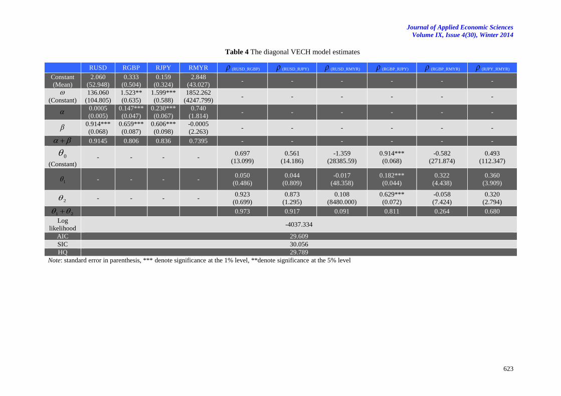
Journal of Applied Economic Sciences
Volume IX, Issue 4(30), Winter 2014
623
Table 4 The diagonal VECH model estimates
Note: standard error in parenthesis, *** denote significance at the 1% level, **denote significance at the 5% level
RUSD RGBP RJPY RMYR (RUSD_RGBP) (RUSD_RJPY) (RUSD_RMYR) (RGBP_RJPY) (RGBP_RMYR) (RJPY_RMYR)
Constant
(Mean)
2.060
(52.948)
0.333
(0.504)
0.159
(0.324)
2.848
(43.027) - - - - - -
(Constant)
136.060
(104.805)
1.523**
(0.635)
1.599***
(0.588)
1852.262
(4247.799) - - - - - -
0.0005
(0.005)
0.147***
(0.047)
0.230***
(0.067)
0.740
(1.814) - - - - - -
0.914***
(0.068)
0.659***
(0.087)
0.606***
(0.098)
-0.0005
(2.263) - - - - - -
0.9145 0.806 0.836 0.7395 - - - - - -
0
(Constant) - - - -
0.697
(13.099)
0.561
(14.186)
-1.359
(28385.59)
0.914***
(0.068)
-0.582
(271.874)
0.493
(112.347)
1 - - - - 0.050
(0.486)
0.044
(0.809)
-0.017
(48.358)
0.182***
(0.044)
0.322
(4.438)
0.360
(3.909)
2 - - - - 0.923
(0.699)
0.873
(1.295)
0.108
(8480.000)
0.629***
(0.072)
-0.058
(7.424)
0.320
(2.794)
21 0.973 0.917 0.091 0.811 0.264 0.680
Log
likelihood -4037.334
AIC 29.609
SIC 30.056
HQ 29.789
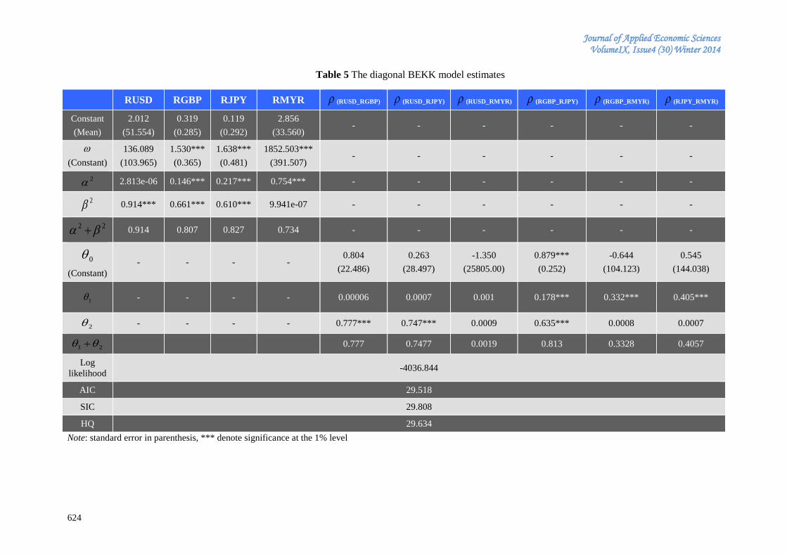
Journal of Applied Economic Sciences VolumeIX, Issue4 (30) Winter 2014
624
Table 5 The diagonal BEKK model estimates
Note: standard error in parenthesis, *** denote significance at the 1% level
RUSD RGBP RJPY RMYR (RUSD_RGBP) (RUSD_RJPY) (RUSD_RMYR) (RGBP_RJPY) (RGBP_RMYR) (RJPY_RMYR)
Constant
(Mean)
2.012
(51.554)
0.319
(0.285)
0.119
(0.292)
2.856
(33.560) - - - - - -
(Constant)
136.089
(103.965)
1.530***
(0.365)
1.638***
(0.481)
1852.503***
(391.507) - - - - - -
2 2.813e-06 0.146*** 0.217*** 0.754*** - - - - - -
2 0.914*** 0.661*** 0.610*** 9.941e-07 - - - - - -
22 0.914 0.807 0.827 0.734 - - - - - -
0
(Constant)
- - - - 0.804
(22.486)
0.263
(28.497)
-1.350
(25805.00)
0.879***
(0.252)
-0.644
(104.123)
0.545
(144.038)
1 - - - - 0.00006 0.0007 0.001 0.178*** 0.332*** 0.405***
2 - - - - 0.777*** 0.747*** 0.0009 0.635*** 0.0008 0.0007
21 0.777 0.7477 0.0019 0.813 0.3328 0.4057
Log
likelihood -4036.844
AIC 29.518
SIC 29.808
HQ 29.634
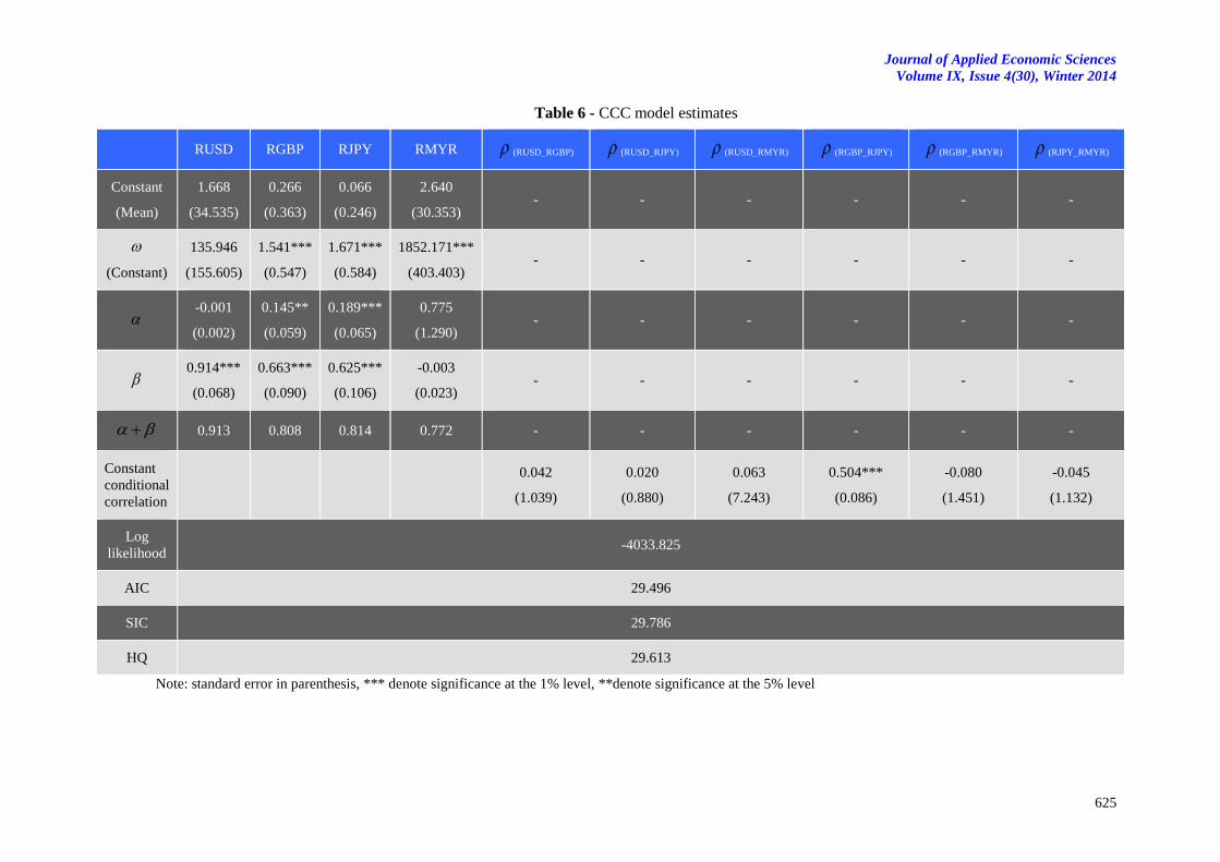
Journal of Applied Economic Sciences
Volume IX, Issue 4(30), Winter 2014
625
Table 6 - CCC model estimates
Note: standard error in parenthesis, *** denote significance at the 1% level, **denote significance at the 5% level
RUSD RGBP RJPY RMYR (RUSD_RGBP) (RUSD_RJPY) (RUSD_RMYR) (RGBP_RJPY) (RGBP_RMYR) (RJPY_RMYR)
Constant
(Mean)
1.668
(34.535)
0.266
(0.363)
0.066
(0.246)
2.640
(30.353) - - - - - -
(Constant)
135.946
(155.605)
1.541***
(0.547)
1.671***
(0.584)
1852.171***
(403.403) - - - - - -
-0.001
(0.002)
0.145**
(0.059)
0.189***
(0.065)
0.775
(1.290) - - - - - -
0.914***
(0.068)
0.663***
(0.090)
0.625***
(0.106)
-0.003
(0.023) - - - - - -
0.913 0.808 0.814 0.772 - - - - - -
Constant
conditional
correlation
0.042
(1.039)
0.020
(0.880)
0.063
(7.243)
0.504***
(0.086)
-0.080
(1.451)
-0.045
(1.132)
Log
likelihood -4033.825
AIC 29.496
SIC 29.786
HQ 29.613
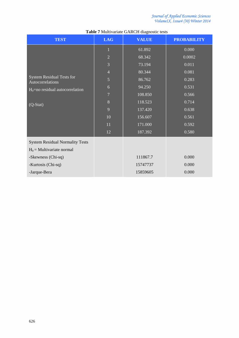
Journal of Applied Economic Sciences VolumeIX, Issue4 (30) Winter 2014
626
Table 7 Multivariate GARCH diagnostic tests
TEST LAG VALUE PROBABILITY
System Residual Tests for
Autocorrelations
H0=no residual autocorrelation
(Q-Stat)
1
2
3
4
5
6
7
8
9
10
11
12
61.892
68.342
73.194
80.344
86.762
94.250
108.850
118.523
137.420
156.607
171.000
187.392
0.000
0.0002
0.011
0.081
0.283
0.531
0.566
0.714
0.638
0.561
0.592
0.580
System Residual Normality Tests
H0 = Multivariate normal
-Skewness (Chi-sq)
-Kurtosis (Chi-sq)
-Jarque-Bera
111867.7
15747737
15859605
0.000
0.000
0.000
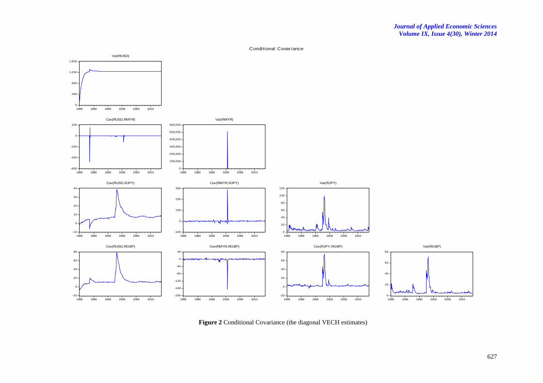
Journal of Applied Economic Sciences
Volume IX, Issue 4(30), Winter 2014
627
0
400
800
1,200
1,600
1985 1990 1995 2000 2005 2010
Var(RUSD)
-600
-400
-200
0
200
1985 1990 1995 2000 2005 2010
Cov(RUSD,RMYR)
0
100,000
200,000
300,000
400,000
500,000
600,000
1985 1990 1995 2000 2005 2010
Var(RMYR)
-10
0
10
20
30
40
1985 1990 1995 2000 2005 2010
Cov(RUSD,RJPY)
-100
0
100
200
300
1985 1990 1995 2000 2005 2010
Cov(RMYR,RJPY)
0
20
40
60
80
100
120
1985 1990 1995 2000 2005 2010
Var(RJPY)
-20
0
20
40
60
80
1985 1990 1995 2000 2005 2010
Cov(RUSD,RGBP)
-200
-160
-120
-80
-40
0
40
1985 1990 1995 2000 2005 2010
Cov(RMYR,RGBP)
-20
0
20
40
60
80
1985 1990 1995 2000 2005 2010
Cov(RJPY,RGBP)
0
20
40
60
80
1985 1990 1995 2000 2005 2010
Var(RGBP)
Conditional Covar iance
Figure 2 Conditional Covariance (the diagonal VECH estimates)
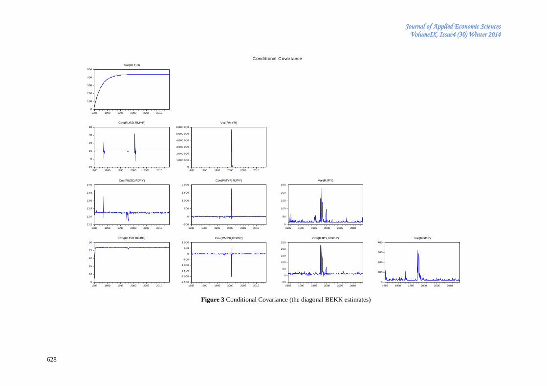
Journal of Applied Economic Sciences VolumeIX, Issue4 (30) Winter 2014
628
0
100
200
300
400
500
1985 1990 1995 2000 2005 2010
Var(RUSD)
-10
0
10
20
30
40
1985 1990 1995 2000 2005 2010
Cov(RUSD,RMYR)
0
1,000,000
2,000,000
3,000,000
4,000,000
5,000,000
6,000,000
1985 1990 1995 2000 2005 2010
Var(RMYR)
11.5
12.0
12.5
13.0
13.5
14.0
1985 1990 1995 2000 2005 2010
Cov(RUSD,RJPY)
-500
0
500
1,000
1,500
2,000
1985 1990 1995 2000 2005 2010
Cov(RMYR,RJPY)
0
50
100
150
200
250
1985 1990 1995 2000 2005 2010
Var(RJPY)
5
10
15
20
25
30
1985 1990 1995 2000 2005 2010
Cov(RUSD,RGBP)
-2,500
-2,000
-1,500
-1,000
-500
0
500
1,000
1985 1990 1995 2000 2005 2010
Cov(RMYR,RGBP)
-50
0
50
100
150
200
250
1985 1990 1995 2000 2005 2010
Cov(RJPY,RGBP)
0
100
200
300
400
1985 1990 1995 2000 2005 2010
Var(RGBP)
Conditional Covar iance
Figure 3 Conditional Covariance (the diagonal BEKK estimates)
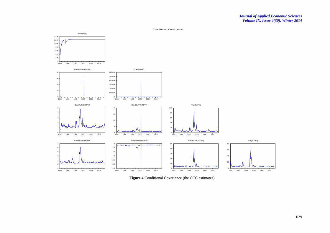
Journal of Applied Economic Sciences
Volume IX, Issue 4(30), Winter 2014
629
0
200
400
600
800
1,000
1,200
1,400
1985 1990 1995 2000 2005 2010
Var(RUSD)
0
20
40
60
80
1985 1990 1995 2000 2005 2010
Cov(RUSD,RMYR)
0
100,000
200,000
300,000
400,000
500,000
600,000
1985 1990 1995 2000 2005 2010
Var(RMYR)
0
1
2
3
4
5
1985 1990 1995 2000 2005 2010
Cov(RUSD,RJPY)
0
10
20
30
40
1985 1990 1995 2000 2005 2010
Cov(RMYR,RJPY)
0
20
40
60
80
100
1985 1990 1995 2000 2005 2010
Var(RJPY)
0
2
4
6
8
10
12
1985 1990 1995 2000 2005 2010
Cov(RUSD,RGBP)
-150
-125
-100
-75
-50
-25
0
1985 1990 1995 2000 2005 2010
Cov(RMYR,RGBP)
0
10
20
30
40
50
1985 1990 1995 2000 2005 2010
Cov(RJPY,RGBP)
0
20
40
60
80
1985 1990 1995 2000 2005 2010
Var(RGBP)
Conditional Covar iance
Figure 4 Conditional Covariance (the CCC estimates)
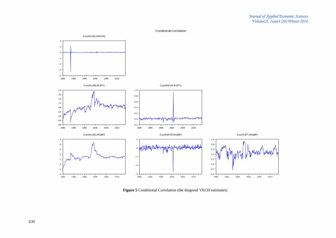
Journal of Applied Economic Sciences VolumeIX, Issue4 (30) Winter 2014
630
-.4
-.3
-.2
-.1
.0
.1
.2
1985 1990 1995 2000 2005 2010
Cor(RUSD,RMYR)
-.08
-.04
.00
.04
.08
.12
.16
.20
.24
1985 1990 1995 2000 2005 2010
Cor(RUSD,RJPY)
-0.2
0.0
0.2
0.4
0.6
0.8
1.0
1985 1990 1995 2000 2005 2010
Cor(RMYR,RJPY)
-.2
-.1
.0
.1
.2
.3
.4
.5
1985 1990 1995 2000 2005 2010
Cor(RUSD,RGBP)
-.3
-.2
-.1
.0
.1
1985 1990 1995 2000 2005 2010
Cor(RMYR,RGBP)
-0.4
-0.2
0.0
0.2
0.4
0.6
0.8
1.0
1985 1990 1995 2000 2005 2010
Cor(RJPY,RGBP)
Conditional Correlation
Figure 5 Conditional Correlation (the diagonal VECH estimates)
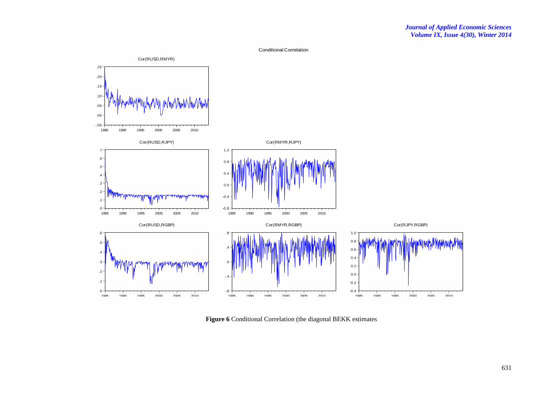
Journal of Applied Economic Sciences
Volume IX, Issue 4(30), Winter 2014
631
-.05
.00
.05
.10
.15
.20
.25
1985 1990 1995 2000 2005 2010
Cor(RUSD,RMYR)
.0
.1
.2
.3
.4
.5
.6
.7
1985 1990 1995 2000 2005 2010
Cor(RUSD,RJPY)
-0.8
-0.4
0.0
0.4
0.8
1.2
1985 1990 1995 2000 2005 2010
Cor(RMYR,RJPY)
.0
.1
.2
.3
.4
.5
.6
1985 1990 1995 2000 2005 2010
Cor(RUSD,RGBP)
-.8
-.4
.0
.4
.8
1985 1990 1995 2000 2005 2010
Cor(RMYR,RGBP)
-0.4
-0.2
0.0
0.2
0.4
0.6
0.8
1.0
1985 1990 1995 2000 2005 2010
Cor(RJPY,RGBP)
Conditional Correlation
Figure 6 Conditional Correlation (the diagonal BEKK estimates
Journal of Applied Economic Sciences
VolumeIX, Issue4 (30) Winter 2014
632
MODELLING THE DEMAND FOR NEW INVESTMENT CREDITS TO THE NON-FINANCIAL COMPANIES IN THE SLOVAK REPUBLIC
Jozef HETEŠ
Technical University of Košice, Slovakia
Faculty of Economics, Department of Banking and Investment
Ivana ŠPIRENGOVÁ
Technical University of Košice, Slovakia
Faculty of Economics, Department of Banking and Investment
Michaela URBANOVIČOVÁ
Technical University of Košice, Slovakia
Faculty of Economics, Department of Banking and Investment
Abstract:
This article deals with modelling the demand for new investment credits to the non-financial
companies in Slovakia. The main aim is to analyze what indicators determine the demand for new investment
credits using Autoregressive distributed lag modelling approach to cointegration analysis. The time period
under consideration lasts from January 2009 to September 2013. Applied econometric analysis has
confirmed the existence of the long-run relationship between the examined variables. We have shown that
the index of industrial production, cost of loans and inflation rate are important determinants of the
investment credit to the non-financial companies in Slovakia. The employed ARDL approach to
cointegration enabled us to examine the long-run and short-run relationships among the variables of
interest. The signs of the coefficients indicate that the estimated function is a demand function for the
investment credit to the non-financial corporations. Both the CUSUM and CUSUMQ tests confirm the
stability of the estimated long-run coefficients of the demand function.
Keywords: new investment credits, non-financial institutions, demand for investment credits, bounds test,
ARDL approach to cointegration
JEL Classification: G21; G31; C22
1. Introduction
Credit developments carry significant information about both economic and financial
activity. First of all, changes in credit provide signals about the availability and demand for funds
supporting (or deterring) the investment and spending decisions of the private non-financial sector.
This is particularly the case where bank lending is one of the major sources of non-financial
corporations financing. Credit developments may thus contain useful information for forecasting
an economic activity and monetary developments. In addition, from a monetary policy perspective,
the credit market potentially plays a propagating role in the process of transmitting changes in
monetary policy to the real side of the economy. Loans are also the major component of banks’
asset side of their balance sheet and hence they represent a significant counterpart to the monetary
aggregates. As a result, corporate lending is an important measure to consider for the regular
assessment of the monetary policy stance. Detailed knowledge about the various structural factors
determining corporate loan developments is therefore crucial for understanding monetary
developments and, ultimately, for the setting of monetary policy.
Most previous studies have either modelled credit to the private sector as a whole
(Hofmann, 2001; Hulsewig, 2003; Calza et al., 2003; Gambacorta and Rossi, 2007) or business
lending for individual euro area countries (Bridgen and Mizen, 1999 and 2004; Kakes, 2000). In
the case of Slovakia the analysis of the determinants for household credits is studied e.g. by
Vokorkosová and Peller (2013). Furthermore, in our analysis, we exploit a dataset of credits to the
non-financial companies in the Slovak Republic.

Journal of Applied Economic Sciences VolumeIX, Issue4 (30) Winter 2014
633
2. Review of the literature
Modelling the credit demand is currently an object of interest in many studies. Various
authors have used different techniques to specify the real demand for credit. Some of them analyze
the credit market using the total volume of granted credits by monetary financial institutions (MFI)
in a country to all sectors in the economy as a dependent variable. Others focus on chosen
segments of credit market such as mortgage, investment or consumer credits granted to private
sector or to households. Identification strategy of significant factors influencing demand for credits
depends on the data which have been applied by authors, e.g. identification based on aggregate
date or micro-level data.
According to the most studies the economic activity variable (e.g. real GDP or industrial
production index as a proxy for GDP), financing cost (e.g. interest rates or bank lending rates) and
inflation rate are considered to be the main determinants affecting credit demand. It does not seem
to be consensus in the literature about what impact has the economic growth on credit demand.
Some empirical findings point to a positive relation (Bernanke, Blinder, 1988) and some of them
to a negative relation (Friedman et al., 1993). It is also difficult to estimate relation between credit
demand and inflation rate in advance. Some empirical studies indicate a positive relation (Calza,
2003) and some of them a negative relation (Cuthbertson, 1985). The negative relationship
between the demand for credits and their cost appears to be more consensual.
Bernanke and Blinder (1988) present a simple formal model for illustrating the bank
lending channel which is a variant of the IS-LM model. In this model they suggest that the loan
demand equation takes the following form:
),,(
yiLLd (1)
where dL represents the loan demand, the interest rate on loans, i the interest rate on
bonds and y denotes GDP.
Kashyap and Stein (1995) investigate bank lending behavior using the individual bank
data. In their model assuming that there is a single, homogeneous economy-wide loan market,
demand for credits should be a function of the loan rate r, as well as general economic condition
denoting by Y. Thus, a linear representation of aggregate credit demand is:
krYLd (2)
Ehrmann (2001) examines bank lending based on a simple version of the Bernanke and
Blinder’s model (1988). His demand for loan dL is given by equation:
l
d ipyL 321 (3)
where y refers to the aggregate real output, p to the price level, li to the interest rate on
loans and 1 ,
2 , 3 are positive coefficients.
Calza et al. (2001) emphasizes that “the analysis of the demand for loans to the private
sector in the euro area is limited to a relatively small set of explanatory variables representing
general economic activity and the cost of loans.” He estimates the empirical model based on the
long-run relationship specified in semi log-linear form which can be written as follow:
LTSTGDPLOANS 321 (4)
where: LOANS and GDI stand for logarithms of loans to the private sector and GDI both
in real terms, ST and LT represent the real short-term and long-term interest rates
respectively.
His econometrical investigation shows that in the cointegration equation, the coefficients
of real short-term and long-term interest rates have negative signs, which confirms that the
employed model is describing a demand phenomenon. On the other side, plus sign of the GDP
coefficient indicates positive relationship between granted loans and economic activity. In 2003
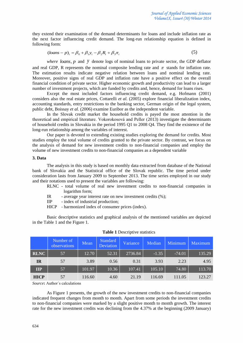
Journal of Applied Economic Sciences VolumeIX, Issue4 (30) Winter 2014
634
they extend their examination of the demand determinants for loans and include inflation rate as
the next factor influencing credit demand. The long-run relationship equation is defined in
following form:
tttt Ryploans 3210)( (5)
where ploans, and y denote logs of nominal loans to private sector, the GDP deflator
and real GDP, R represents the nominal composite lending rate and stands for inflation rate.
The estimation results indicate negative relation between loans and nominal lending rate.
Moreover, positive signs of real GDP and inflation rate have a positive effect on the overall
financial condition of private sector. Higher economic growth and productivity can lead to a larger
number of investment projects, which are funded by credits and, hence, demand for loans rises.
Except the most included factors influencing credit demand, e.g. Hofmann (2001)
considers also the real estate prices, Cottarelli et al. (2005) explore financial liberalization index,
accounting standards, entry restrictions to the banking sector, German origin of the legal system,
public debt, Boissay et al. (2006) examine Euribor as the independent variable.
In the Slovak credit market the household credits is payed the most attention in the
theoretical and empirical literature. Vokorokosová and Peller (2013) investigate the determinants
of household credits in Slovakia in the period 1995 Q1 to 2008 Q4. They find the existence of the
long-run relationship among the variables of interest.
Our paper is devoted to extending existing studies exploring the demand for credits. Most
studies employ the total volume of credits granted to the private sector. By contrast, we focus on
the analysis of demand for new investment credits to non-financial companies and employ the
volume of new investment credits to non-financial companies as a dependent variable
3. Data
The analysis in this study is based on monthly data extracted from database of the National
bank of Slovakia and the Statistical office of the Slovak republic. The time period under
consideration lasts from January 2009 to September 2013. The time series employed in our study
and their notations used to present the variables are following:
RLNC - total volume of real new investment credits to non-financial companies in
logarithm form;
IR - average year interest rate on new investment credits (%);
IIP - index of industrial production;
HICP - harmonized index of consumer prices (index).
Basic descriptive statistics and graphical analysis of the mentioned variables are depicted
in the Table 1 and the Figure 1.
Table 1 Descriptive statistics
Number of
observations Mean
Standard
Deviation Variance Median Minimum Maximum
RLNC 57 12.70 52.31 2736.84 -1.35 -74.01 135.29
IR 57 3.89 0.56 0.31 3.93 2.23 4.95
IIP 57 101.97 10.36 107.41 105.10 74.80 113.70
HICP 57 116.60 4.60 21.19 116.69 111.05 123.27
Source: Author´s calculations
As Figure 1 presents, the growth of the new investment credits to non-financial companies
indicated frequent changes from month to month. Apart from some periods the investment credits
to non-financial companies were marked by a slight positive month to month growth. The interest
rate for the new investment credits was declining from the 4.37% at the beginning (2009 January)
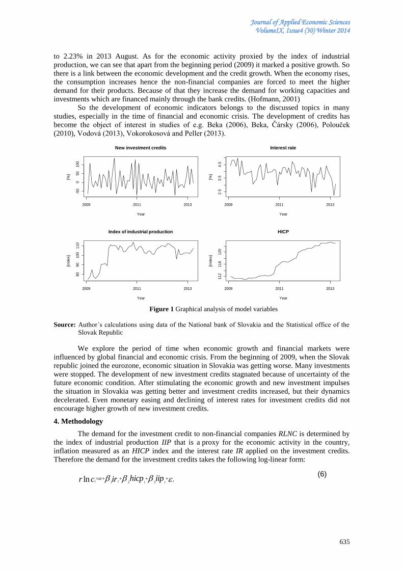
Journal of Applied Economic Sciences VolumeIX, Issue4 (30) Winter 2014
635
to 2.23% in 2013 August. As for the economic activity proxied by the index of industrial
production, we can see that apart from the beginning period (2009) it marked a positive growth. So
there is a link between the economic development and the credit growth. When the economy rises,
the consumption increases hence the non-financial companies are forced to meet the higher
demand for their products. Because of that they increase the demand for working capacities and
investments which are financed mainly through the bank credits. (Hofmann, 2001)
So the development of economic indicators belongs to the discussed topics in many
studies, especially in the time of financial and economic crisis. The development of credits has
become the object of interest in studies of e.g. Beka (2006), Beka, Čársky (2006), Polouček
(2010), Vodová (2013), Vokorokosová and Peller (2013).
Figure 1 Graphical analysis of model variables
Source: Author´s calculations using data of the National bank of Slovakia and the Statistical office of the
Slovak Republic
We explore the period of time when economic growth and financial markets were
influenced by global financial and economic crisis. From the beginning of 2009, when the Slovak
republic joined the eurozone, economic situation in Slovakia was getting worse. Many investments
were stopped. The development of new investment credits stagnated because of uncertainty of the
future economic condition. After stimulating the economic growth and new investment impulses
the situation in Slovakia was getting better and investment credits increased, but their dynamics
decelerated. Even monetary easing and declining of interest rates for investment credits did not
encourage higher growth of new investment credits.
4. Methodology
The demand for the investment credit to non-financial companies RLNC is determined by
the index of industrial production IIP that is a proxy for the economic activity in the country,
inflation measured as an HICP index and the interest rate IR applied on the investment credits.
Therefore the demand for the investment credits takes the following log-linear form:
ttttt iiphicpircr
321ln (6)
New investment credits
Year
[%]
2009 2011 2013
-50
050
100
Interest rate
Year
[%]
2009 2011 2013
2.5
3.5
4.5
Index of industrial production
Year
[index]
2009 2011 2013
80
90
100
110
HICP
Year
[index]
2009 2011 2013
112
116
120
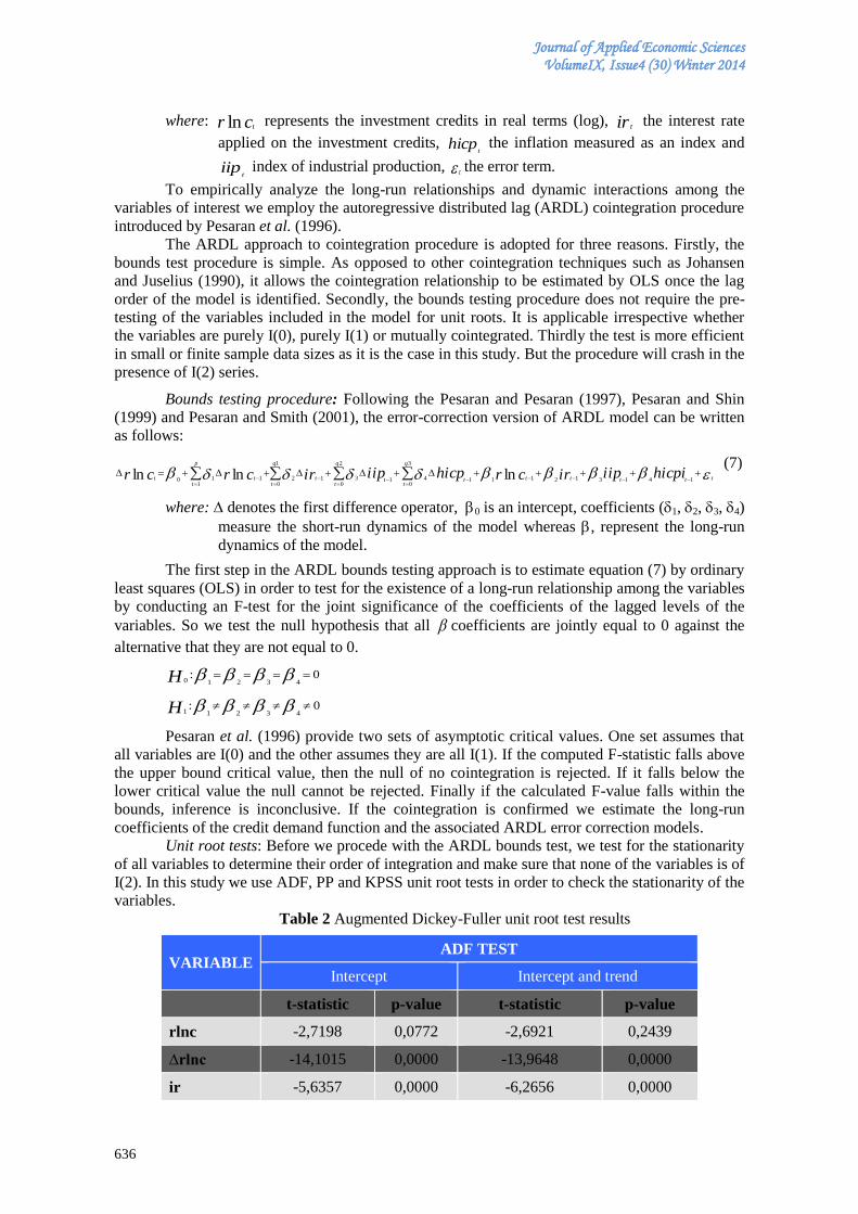
Journal of Applied Economic Sciences VolumeIX, Issue4 (30) Winter 2014
636
where: cr tln represents the investment credits in real terms (log), ir t the interest rate
applied on the investment credits, hicpt the inflation measured as an index and
iipt index of industrial production, t the error term.
To empirically analyze the long-run relationships and dynamic interactions among the
variables of interest we employ the autoregressive distributed lag (ARDL) cointegration procedure
introduced by Pesaran et al. (1996).
The ARDL approach to cointegration procedure is adopted for three reasons. Firstly, the
bounds test procedure is simple. As opposed to other cointegration techniques such as Johansen
and Juselius (1990), it allows the cointegration relationship to be estimated by OLS once the lag
order of the model is identified. Secondly, the bounds testing procedure does not require the pre-
testing of the variables included in the model for unit roots. It is applicable irrespective whether
the variables are purely I(0), purely I(1) or mutually cointegrated. Thirdly the test is more efficient
in small or finite sample data sizes as it is the case in this study. But the procedure will crash in the
presence of I(2) series.
Bounds testing procedure: Following the Pesaran and Pesaran (1997), Pesaran and Shin
(1999) and Pesaran and Smith (2001), the error-correction version of ARDL model can be written
as follows:
ttttt
q
t
q
t
q
tttt
p
ttt hicpiiipircrhicpiipircrcr
14131211
1
0
2
0
3
0141312
1110 lnlnln
(7)
where: denotes the first difference operator, 0 is an intercept, coefficients (1, 2, 3, 4)
measure the short-run dynamics of the model whereas , represent the long-run
dynamics of the model.
The first step in the ARDL bounds testing approach is to estimate equation (7) by ordinary
least squares (OLS) in order to test for the existence of a long-run relationship among the variables
by conducting an F-test for the joint significance of the coefficients of the lagged levels of the
variables. So we test the null hypothesis that all coefficients are jointly equal to 0 against the
alternative that they are not equal to 0.
0:43210 H
0:43211 H
Pesaran et al. (1996) provide two sets of asymptotic critical values. One set assumes that
all variables are I(0) and the other assumes they are all I(1). If the computed F-statistic falls above
the upper bound critical value, then the null of no cointegration is rejected. If it falls below the
lower critical value the null cannot be rejected. Finally if the calculated F-value falls within the
bounds, inference is inconclusive. If the cointegration is confirmed we estimate the long-run
coefficients of the credit demand function and the associated ARDL error correction models.
Unit root tests: Before we procede with the ARDL bounds test, we test for the stationarity
of all variables to determine their order of integration and make sure that none of the variables is of
I(2). In this study we use ADF, PP and KPSS unit root tests in order to check the stationarity of the
variables.
Table 2 Augmented Dickey-Fuller unit root test results
VARIABLE ADF TEST
Intercept Intercept and trend
t-statistic p-value t-statistic p-value
rlnc -2,7198 0,0772 -2,6921 0,2439
∆rlnc -14,1015 0,0000 -13,9648 0,0000
ir -5,6357 0,0000 -6,2656 0,0000
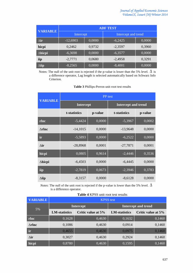
Journal of Applied Economic Sciences VolumeIX, Issue4 (30) Winter 2014
637
VARIABLE ADF TEST
Intercept Intercept and trend
∆ir -12,6903 0,0000 -6,2425 0,0000
hicpi 0,2462 0,9732 -2,3597 0,3960
∆hicpi -6,3698 0,0000 -6,3577 0,0000
iip -2,7771 0,0680 -2,4958 0,3291
∆iip -8,2565 0,0000 -8,4001 0,0000
Notes: The null of the unit root is rejected if the p-value is lower than the 5% level. is
a difference operator, Lag length is selected automatically based on Schwarz Info
Criterion.
Table 3 Phillips-Perron unit root test results
VARIABLE
PP test
Intercept Intercept and trend
t-statistics p-value t-statistics p-value
rlnc -5,4424 0,0000 -5,3967 0,0002
∆rlnc -14,1015 0,0000 -13,9648 0,0000
ir -5,5893 0,0000 -6,2522 0,0000
∆ir -28,8968 0,0001 -27,7871 0,0001
hicpi 0,0805 0,9614 -2,4446 0,3536
∆hicpi -6,4503 0,0000 -6,4445 0,0000
iip -2,7819 0,0673 -2,3946 0,3783
∆iip -8,3157 0,0000 -8,6128 0,0000
Notes: The null of the unit root is rejected if the p-value is lower than the 5% level.
is a difference operator.
Table 4 KPSS unit root test results
VARIABLE KPSS test
5% Intercept Intercept and trend
LM-statistics Critic value at 5% LM-statistics Critic value at 5%
rlnc 0,1628 0,4630 0,1632 0,1460
∆rlnc 0,1086 0,4630 0,0914 0,1460
ir 0,4655 0,4630 0,0975 0,1460
∆ir 0,3027 0,4630 0,2924 0,1460
hicpi 0,8780 0,4630 0,1595 0,1460
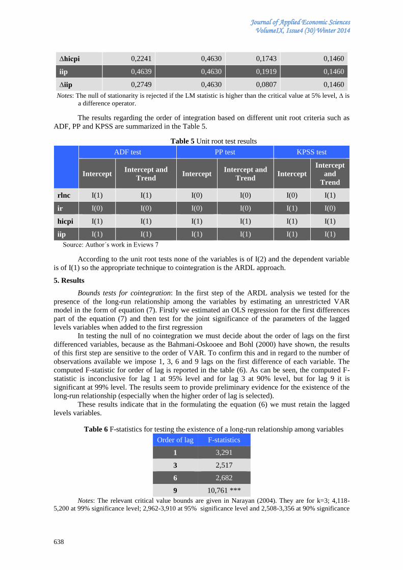
Journal of Applied Economic Sciences VolumeIX, Issue4 (30) Winter 2014
638
∆hicpi 0,2241 0,4630 0,1743 0,1460
iip 0,4639 0,4630 0,1919 0,1460
∆iip 0,2749 0,4630 0,0807 0,1460
Notes: The null of stationarity is rejected if the LM statistic is higher than the critical value at 5% level, is
a difference operator.
The results regarding the order of integration based on different unit root criteria such as
ADF, PP and KPSS are summarized in the Table 5.
Table 5 Unit root test results
ADF test PP test KPSS test
Intercept Intercept and
Trend Intercept
Intercept and
Trend Intercept
Intercept
and
Trend
rlnc I(1) I(1) I(0) I(0) I(0) I(1)
ir I(0) I(0) I(0) I(0) I(1) I(0)
hicpi I(1) I(1) I(1) I(1) I(1) I(1)
iip I(1) I(1) I(1) I(1) I(1) I(1)
Source: Author´s work in Eviews 7
According to the unit root tests none of the variables is of I(2) and the dependent variable
is of I(1) so the appropriate technique to cointegration is the ARDL approach.
5. Results
Bounds tests for cointegration: In the first step of the ARDL analysis we tested for the
presence of the long-run relationship among the variables by estimating an unrestricted VAR
model in the form of equation (7). Firstly we estimated an OLS regression for the first differences
part of the equation (7) and then test for the joint significance of the parameters of the lagged
levels variables when added to the first regression In testing the null of no cointegration we must decide about the order of lags on the first
differenced variables, because as the Bahmani-Oskooee and Bohl (2000) have shown, the results
of this first step are sensitive to the order of VAR. To confirm this and in regard to the number of
observations available we impose 1, 3, 6 and 9 lags on the first difference of each variable. The
computed F-statistic for order of lag is reported in the table (6). As can be seen, the computed F-
statistic is inconclusive for lag 1 at 95% level and for lag 3 at 90% level, but for lag 9 it is
significant at 99% level. The results seem to provide preliminary evidence for the existence of the
long-run relationship (especially when the higher order of lag is selected).
These results indicate that in the formulating the equation (6) we must retain the lagged
levels variables.
Table 6 F-statistics for testing the existence of a long-run relationship among variables
Order of lag F-statistics
1 3,291
3 2,517
6 2,682
9 10,761 ***
Notes: The relevant critical value bounds are given in Narayan (2004). They are for k=3; 4,118-
5,200 at 99% significance level; 2,962-3,910 at 95% significance level and 2,508-3,356 at 90% significance
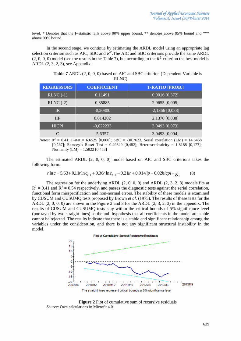
Journal of Applied Economic Sciences VolumeIX, Issue4 (30) Winter 2014
639
level. * Denotes that the F-statistic falls above 90% upper bound, ** denotes above 95% bound and ***
above 99% bound.
In the second stage, we continue by estimating the ARDL model using an appropriate lag
selection criterion such as AIC, SBC and .The AIC and SBC criterions provide the same ARDL
(2, 0, 0, 0) model (see the results in the Table 7), but according to the criterion the best model is
ARDL (2, 3, 2, 3), see Appendix.
Table 7 ARDL (2, 0, 0, 0) based on AIC and SBC criterion (Dependent Variable is
RLNC)
REGRESSORS COEFFICIENT T-RATIO [PROB.]
RLNC (-1) 0,11491 0,9016 [0,372]
RLNC (-2) 0,35885 2,9655 [0,005]
IR -0,20800 -2,1366 [0,038]
IIP 0,014202 2,1370 [0,038]
HICPI -0,022233 3,0493 [0,073]
C 5,6357 3,0493 [0,004]
Notes: R2 = 0.41; F-stat = 6.6525 [0,000]; SBC = -30.7623, Serial correlation (LM) = 14.5468
[0,267]; Ramsey´s Reset Test = 0.49349 [0,482]; Heteroscedasticity = 1.8188 [0,177];
Normality (LM) = 1.5822 [0,453]
The estimated ARDL (2, 0, 0, 0) model based on AIC and SBC criterions takes the
following form:
ttt hicpiiipircrcrcr 02,0014,021,0ln36,0ln11,063,5ln 21 (8)
The regression for the underlying ARDL (2, 0, 0, 0) and ARDL (2, 3, 2, 3) models fits at
R2 = 0.41 and R
2 = 0.54 respectively, and passes the diagnostic tests against the serial correlation,
functional form misspecification and non-normal errors. The stability of these models is examined
by CUSUM and CUSUMQ tests proposed by Brown et al. (1975). The results of these tests for the
ARDL (2, 0, 0, 0) are shown in the Figure 2 and 3 for the ARDL (2, 3, 2, 3) in the appendix. The
results of CUSUM and CUSUMQ tests stay within the critical bounds of 5% significance level
(portrayed by two straight lines) so the null hypothesis that all coefficients in the model are stable
cannot be rejected. The results indicate that there is a stable and significant relationship among the
variables under the consideration, and there is not any significant structural instability in the
model.
Figure 2 Plot of cumulative sum of recursive residuals Source: Own calculations in Microfit 4.0
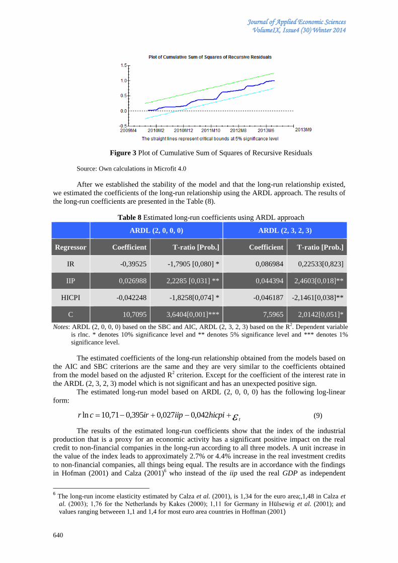
Journal of Applied Economic Sciences VolumeIX, Issue4 (30) Winter 2014
640
Figure 3 Plot of Cumulative Sum of Squares of Recursive Residuals
Source: Own calculations in Microfit 4.0
After we established the stability of the model and that the long-run relationship existed,
we estimated the coefficients of the long-run relationship using the ARDL approach. The results of
the long-run coefficients are presented in the Table (8).
Table 8 Estimated long-run coefficients using ARDL approach
ARDL (2, 0, 0, 0) ARDL (2, 3, 2, 3)
Regressor Coefficient T-ratio [Prob.] Coefficient T-ratio [Prob.]
IR -0,39525 -1,7905 [0,080] * 0,086984 0,22533[0,823]
IIP 0,026988 2,2285 [0,031] ** 0,044394 2,4603[0,018]**
HICPI -0,042248 -1,8258[0,074] * -0,046187 -2,1461[0,038]**
C 10,7095 3,6404[0,001]*** 7,5965 2,0142[0,051]*
Notes: ARDL (2, 0, 0, 0) based on the SBC and AIC, ARDL (2, 3, 2, 3) based on the R2. Dependent variable
is rlnc. * denotes 10% significance level and ** denotes 5% significance level and *** denotes 1%
significance level.
The estimated coefficients of the long-run relationship obtained from the models based on
the AIC and SBC criterions are the same and they are very similar to the coefficients obtained
from the model based on the adjusted R2 criterion. Except for the coefficient of the interest rate in
the ARDL (2, 3, 2, 3) model which is not significant and has an unexpected positive sign.
The estimated long-run model based on ARDL (2, 0, 0, 0) has the following log-linear
form:
thicpiiipircr 042,0027,0395,071,10ln (9)
The results of the estimated long-run coefficients show that the index of the industrial
production that is a proxy for an economic activity has a significant positive impact on the real
credit to non-financial companies in the long-run according to all three models. A unit increase in
the value of the index leads to approximately 2.7% or 4.4% increase in the real investment credits
to non-financial companies, all things being equal. The results are in accordance with the findings
in Hofman (2001) and Calza (2001)6 who instead of the iip used the real GDP as independent
6 The long-run income elasticity estimated by Calza et al. (2001), is 1,34 for the euro area;,1,48 in Calza et
al. (2003); 1,76 for the Netherlands by Kakes (2000); 1,11 for Germany in Hülsewig et al. (2001); and
values ranging betweeen 1,1 and 1,4 for most euro area countries in Hoffman (2001)

Journal of Applied Economic Sciences VolumeIX, Issue4 (30) Winter 2014
641
variable as a proxy for the economic activity. They also found the positive relation between credit
and real GDP. The difference between the value of the iip coefficient in our study and the
coefficients of GDP in other studies that is a bit lower than ours may be caused by the fact that we
use the iip variable as a proxy for the economic activity while Calza (2001, 2003) uses GDP
variable. Also we focus only on the investment credits to non-financial companies while Calza et
al. (2001, 2003) deals with the total loans to private sector in the euro area. Our findings of this
positive relation between these two variables in the case of Slovakia may support the argument
that a strong economic growth in the long-run may lead to a higher demand for the investment
credits from the non-financial companies to fund their investment decisions. As regards the long-
run coefficient of the interest rate, it has an expected significant negative sign. From the estimated
value of the ir coefficient it seems that in the long-run the investment credit is affected mostly by
the changes in the interest rate than by the changes in other variables. The rise of the interest rate
by 1 percentage point leads to approximately 39 % decrease in the volume of the real investment
credits. This indicates that the cost of loans proxied by the nominal interest rate seems to be the
most important determinant of the investment credits demand in the long-run. In our study we
found a support for the existence of a negative relationship between the real investment credits and
inflation because the coefficient of inflation is negative and significant7. A unit increase/(decrease)
in the HICP index value leads to a 4.2% decrease/(increase) in the investment credits.
After estimating the long-run model, the estimates of the short-run dynamic coefficients
selected by the AIC, SBC and R2 are presented in the Tables 9 and 10. The adjusted, R
2 are 0.53
and 0.63 for these models respectively, suggesting that such error correction models fit the data
reasonably well. The coefficients of the error correction terms in ARDL (2, 0, 0, 0) and ARDL (2,
3, 2, 3) model are both negative and highly significant. This reinforces our findings of
cointegration as provided by the F-test.
Table 9 Error correction representation for selected ARDL (2, 0, 0, 0)
model based on AIC and SBC
Regressor Coefficient T-ratio [Prob.]
rlnc (-1) -0,35885 -2,9655 [0,005] ***
IR -0,20800 -2,1366 [0,038] **
IIP 0,014202 2,1370 [0,038] **
HICPI -0,022233 -1,8336 [0,073] *
C 5,6357 3,0493 [0,004] ***
ecm (-1) -0,52624 -3,5763 [0,001] ***
Notes: ecm = rlnc + 0,395ir – 0,0267iip + 0,0422hicpi – 10.7095C. Dependent variable is rlnc,
=0.53, R-Bar-Squared = 0.48390, F-stat = 10.9386 [0,000], SBC = -30.7623, DW-statistic
= 1.9854, SER = 0.3635, RSS = 6,3422; * denotes 10% significance level, ** denotes 5%
significance level and *** 1% significance level
The estimated short-run model will be in the following form:
ttt ecmhicpiiipircrcr 11 53,0022,0014,021,0ln36,064,5ln (10)
Where ecm is the error correction term which is given as:
ecm = rlnc + 0,395ir – 0,0267iip + 0,0422hicpi – 10,7095C (11)
7 The sign of the long-run coefficient of inflation cannot be determined apriori. There are argumets in
support of a positive relationship (Howells and Hussein, 1999), but also the arguments in support of
negative relationship between the two variables. (Cuthbertson, 1985)
Journal of Applied Economic Sciences VolumeIX, Issue4 (30) Winter 2014
642
The coefficient of the lagged error correction term reveals how quickly/slowly variables
return to the equilibrium and it must be significant and negative for establishing cointegration. The
absolute value of the coefficient of the error correction term indicates the speed of adjustment to
restore equilibrium and negative sign shows convergence in the short-run dynamic model. The
estimated ecm coefficient in our model has expected negative and significant sign of -0.53. The
value of this coefficient implies a fairly high speed of adjustment to equilibrium after a shock from
the previous period. This means that approximately 53% of disequilibria from the previous
month´s shock converge to the long-run equilibrium in the next month.
As can be seen from the table (9) the growth rate of the real credit to non-financial
companies in the short-run is affected mainly by the one lagged real credit variable which
coefficient is highly significant and negative. What means that the one percent rises in the real
credit in previous month will cause approximately 0.35 percent decline in the real credit next
month. The real investment credit to non-financial companies is in the short-run also negatively
affected by the interest rate and inflation and positively by the index of industrial production.
Conclusions
This study employed the bounds test (ARDL) approach to cointegration to examine the
long-run and short-run relationships between the real investment credit to non-financial
companies, the interest rate, the index of industrial production and the inflation rate. The main aim
of the study is to estimate the demand for the real investment credit to non-financial companies
and find out the indicators that have an impact on the demand for the credit to non-financial
companies in Slovakia. By applying the cointegration technique we were able to find out that the
variables of interest put in the demand function (6) are bound together in the long-run. The
estimated error correction term was also highly significant and negative confirming the existence
of the long-run relationship among the variables of interest. Both CUSUM and CUSUMQ tests
confirm the stability of the long-run coefficients of the investment credit demand function. The
results also indicate that the economic activity, cost of loans and inflation rate are important
determinants of credit demand to non-financial companies in Slovakia. This implies that the
growing economic activity will enhance the investment credit demand from non-financial
companies while the rise of the cost of loans and inflation will reduce the investment credit
demand in Slovakia.
References
[1] Beka, J. and Čársky, R. (2006). Úvery nefinančným spoločnostiam a ich úverové podmienky,
Biatec, 14(2): 5-7.
[2] Beka, J. (2006). Vývoj úverov domácnostiam a úrokové sadzby z nových úverov
domácnostiam, Biatec, 14(7):12-18.
[3] Bernanke, B., Blinder, A. (1988). Credit money and aggregate demand, The American
Economic Review, 78(2): 435-439.
[4] Boissay, F., et al. (2006). Is lending in Central and Eastern Europe developing too fast?
Financial Development, Integration and Stability: Evidence from Central, Eastern and South-
Eastern Europe. Cheltenham: Edward Elgar Publishing Limited.
[5] Bridgen, A., Mizen, P. (1999). Money, Credit and Investment in the UK corporate sector, Bank
of England working paper, No. 100, http://www.bankofengland.co.uk/archive/
Documents/historicpubs/workingpapers/1999/wp100.pdf
[6] Calza, A. Gartner, C. and Sousa, J. (2001). Modelling the demand for loans to the private
sector in the euro area, Applied Economics, 35(1): 107-117.
[7] Calza, A. et al. (2003). Aggregate loand to the euro area private sector, ECB Working paper,
No. 202, http://www.ecb.europa.eu/pub/pdf/scpwps/ecbwp202.pdf
Journal of Applied Economic Sciences VolumeIX, Issue4 (30) Winter 2014
643
[8] Cottarelli, C. et al. (2005). Early birds, late risers, and sleeping beauties: Bank credit growth to
the private sector in Central and Eastern Europe and in the Balkans, Journal of Banking &
Finance, 29(1): 83-104.
[9] Cuthbertson, K. (1985). Sterling bank lending to UK industrial and commercial companies,
Oxford Bulletin of Economics and Statistics, 47(2): 91-118.
[10] Ehrman, M. (2001). Financial systems and the role of banks in monetary policy transmission
in the euro area, ECB working paper, No. 105, https://www.ecb.europa.eu/pub/pdf/scpwps/
ecbwp105.pdf
[11] Friedman, B.M., et al. (1993). Economic activity and the short-term credit markets: Analysis
of prices and quantities, Brookings Papers on Economic Activity, 24(2): 193-283.
[12] Gambacorta, L., Rossi, C. (2007). Modelling Bank Lending in the Euro Area: A non-linear
approach, Temi di discussion del Servizio Studi di Banca d'Italia, No.650 file:///C:/Users/
EKF/Downloads/en tema_650.pdf
[13] Hofmann, B. (2001). The determinants of private sector credit in industrialised countries: do
property prices matter? Bank of international settlements: Working paper No. 108,
http://www.bis.org/publ/work108.pdf
[14] Hülsewig, O. (2003). Bank Behaviour, Interest rate Targeting and Monetary Policy
Transmission, Würzburg Economic Papers No. 43, http://econstor.eu/bitstream/10419/48467/
1/378423606.pdf
[15] Kakes, J. (2000). Monetary Transmission in Europe: the Role of Financial Markets and
Credit, Edward Elgar Publishing Limited, Cheltenham, http://www.google.sk/books?hl
=sk&lr=&id=3x8tQFBlOy8C&oi=fnd&pg=PR7&dq=KAKES,+J.+Monetary+Transmission+
in+Europe:+the+Role+of+Financial+Markets+and+Credit&ots=Yogw1rAu4R&sig=KR_cZ2
gL5puGaakB_sbbiOmdWcM&redir_esc=y#v=onepage&q&f=false
[16] Kashyap, A.K., Stein, J.C. (1995). The impact of monetary policy on bank balance sheets,
Carnegie-Rochester Conference Series on Public Policy, 42: 151-195.
[17] Pesaran, H.M. et al. (1999). Bounds testing approaches to the analysis of long-run
relationships, Journal of Applied Econometrics, 16: 289-326.
[18] Vokorokosová, R., Peller, F. 2013 Credit to households. What impacts the growth in
Slovakia?, Journal of Economics, 61(3): 223-234.
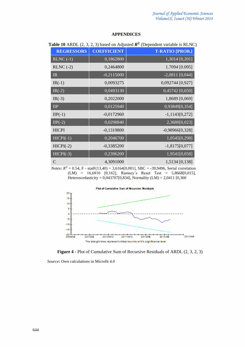
Journal of Applied Economic Sciences VolumeIX, Issue4 (30) Winter 2014
644
APPENDICES
Table 10 ARDL (2, 3, 2, 3) based on Adjusted (Dependent variable is RLNC)
REGRESSORS COEFFICIENT T-RATIO [PROB.]
RLNC (-1) 0,1862800 1,3014 [0,201]
RLNC (-2) 0,2464800 1.7094 [0.095]
IR -0,2115000 -2,0811 [0,044]
IR(-1) 0,0093275 0,092744 [0,927]
IR(-2) 0,0493130 0,45742 [0,650]
IR(-3) 0,2022000 1,8689 [0,069]
IIP 0,0125940 0,93849[0,354]
IIP(-1) -0,0172960 -1,1143[0,272]
IIP(-2) 0,0298840 2,3680[0,023]
HICPI -0,1319800 -0,98966[0,328]
HICPI(-1) 0,2046700 1,0545[0,298]
HICPI(-2) -0,3385200 -1,8175[0,077]
HICPI(-3) 0,2396200 1,9541[0,058]
C 4,3091000 1,5134 [0,138]
Notes: = 0.54, F - statF(13,40) = 3,6164[0,001], SBC = -39,9496, Serial correlation
(LM) = 16,6810 [0,162], Ramsey´s Reset Test = 5,8668[0,015],
Heteroscedasticity = 0,043707[0,834], Normality (LM) = 2,0411 [0,360
Figure 4 - Plot of Cumulative Sum of Recursive Residuals of ARDL (2, 3, 2, 3)
Source: Own calculations in Microfit 4.0
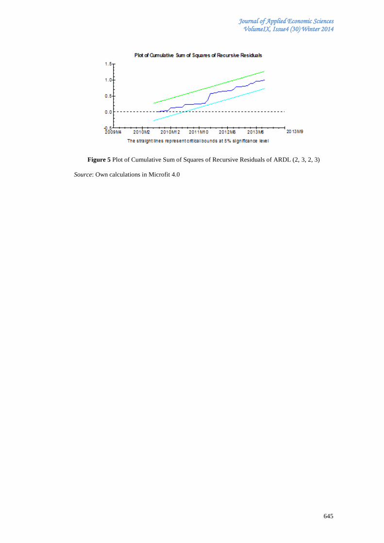
Journal of Applied Economic Sciences VolumeIX, Issue4 (30) Winter 2014
645
Figure 5 Plot of Cumulative Sum of Squares of Recursive Residuals of ARDL (2, 3, 2, 3)
Source: Own calculations in Microfit 4.0
Journal of Applied Economic Sciences VolumeIX, Issue4 (30) Winter 2014
646
ETHICS PERCEPTION IN BUSINESS AND SOCIAL PRACTICE IN THE CZECH REPUBLIC
Petra HORVÁTHOVÁ
VŠB – Technical University of Ostrava, Czech Republic
Martin ČERNEK
VŠB – Technical University of Ostrava, Czech Republic
Kateřina KASHI
VŠB – Technical University of Ostrava, Czech Republic
Abstract:
Business ethics, as a part of so called applied ethics, has been dynamically gaining on importance.
Pushing the idea of applying ethics in the Czech business environment has started in the mid-90s of 20th
century. Since that time the business ethics has made a huge progress and its Czech representatives and
promoters have done a significant amount of work in this area. On the other hand, it is necessary to
objectively admit, that there are still many managers, businessmen, students and people who have doubts
about the legitimacy of business ethics and they consider it as unreal and illusory in the market environment.
Therefore, main objective of this paper is to contribute to the knowledge, understanding, current status, level
of perception’s awareness of ethics and morality in business and social spheres based on both theoretical
analysis and resource bases, and own empirical research.
Keywords: business ethics, applied ethics, corporate social responsibility, Czech society, pilot survey,
qualitative analysis.
JEL Classification: M140
1. Introduction
Much of the growing importance of business ethics was caused by the membership of
Czech Republic in the European Union, which very intensively supports ethical behavior and
corporate governance of European enterprises with the aim to increase their competitiveness in a
global measure. The initiator of promoting ethical behavior can be also the representatives of
business sphere. Entrepreneurs’ growing interest about ethical and social audits, implementation of
ethical codex and other methods and tools of business ethics has various causes: pressure of
foreign partners, requirement for foreign investment, changes in customer’s attitudes, company’s
culture of foreign parent company, requirement of quality and stable employees, requirement for
long-term business relations, pressure of supranational institutions and state and total pressure of
society and public opinion (Bowie, 2013; Andriof, McIntosh, 2001; Kline, 2010; Schminke, 2010;
Kunz, 2012; Trevino, Nelson, 2011).
If the main aim of entrepreneurship is to maximize profits then it is impossible not to
encounter in practice the irresponsibility, performance orientation and motivation, increase need of
money and consumption etc. We meet with ethics resp. with its disobeying practically every day.
Large-scale media and mass media are informing us daily about law violations, but also about the
facts and situations which are not clearly stated in law but they are generally known and violating
these rules/laws is considered unethical and immoral.
Many managers and business owners are asking themselves whether there is any sense in
dealing with ethical and moral aspects of business. It is generally said that you either behave
consistently ethically and morally, but in this case you do not have much chance of success at the
market, or you are successful, efficient, and competitive, simply you are earning money, but ethics
is a luxury for you, it is a luxury good. Ethics, morality and success in business do not mix. This is
then related to overall increase in corruption, economic crime and other social and socio-
pathological phenomena. However, now in a time of falling economic results of enterprises and
overall companies’ deterioration, enterprises and companies are more interested in ethical aspects,
tracking the causes and consequences of its absence not only in interpersonal relationships, but
Journal of Applied Economic Sciences VolumeIX, Issue4 (30) Winter 2014
647
especially in the business and commercial sphere. The importance of applying ethics in business
and management is discussed very often, different views are presented as to why and how
important is ethics in business, why ethics is a necessary prerequisite for the future development in
all areas of social existence. The importance of business and management ethics is becoming more
urgent and necessary as the globalization’s process is coming to its peak. Here, we are dealing with
overcoming up to now respected opinions and searching for ways to form new interpersonal
relationships and creating more dignified business environment. Tendencies, trends and topicality
of this problematic are suggested by the fact that many various ethical conferences, seminars,
trainings, symposia etc. are being organized. At the same time they discover and promote
approaches which state that especially linking business ethics and enterprises’ social responsibility
belongs among one of the competitive advantage on the market and represents the image of
corporate culture (Bailey, Burch, 2005; Caroll, 2008; Blowfield, Murray, 2008; Duarte, Diniz,
2013).
Currently we can, with certainty, characterize several basic foundations (Kuldová, 2012,
Collins, 2012):
Many institutions and organizations that support the implementation of business ethics
in the Czech Republic were established, they promote the idea of ethical behavior.
They compile rankings of ethical companies, present particular examples on how to do
business ethically, they execute research and gather concrete contributions of ethical
behavior.
Consulting companies which help the enterprises to apply concrete tools and methods
of business ethics organize seminars and provide training in the area of business ethics.
Cooperation of private and non-profit sector has intensified. The amount of concrete
social and environmental project is continuously growing.
Conferences, meetings of representatives from state, private companies, non-profit
sectors and academics are being held; the aim is to support and promote development
of business ethics in Czech Republic.
Many researches, in the area of business ethics and company’s corporate governance,
which evaluate current state and point out trends and development direction, were
executed in the Czech Republic.
Teaching business ethics takes place at most of Czech universities.
There are more and more companies that actively apply ethical principles of business
and permanently sustainable development.
More Czech customers are interested in ethical and responsible behavior of companies
whose products they are buying.
This pilot survey follows and in fact complements current, already executed investigations
in the field of business ethics and social practice. We work on the assumption that it is not possible
to comprehensively and methodologically cover the problem only based on a single study or
partial empirical research. Therefore, it is necessary to perceive the results (findings) as
complementary. The structure and content of the research is based on the work of Čaník, Řezbová,
Zavrel (2006), Putnová, Seknička (2007), Dytrt et al. (2011), Remišová (2011), Kuldová (2012),
Kunz (2012), etc.
2. Problem formulation
Executed research, data processing and overall interpretation represent a qualitative
approach. The sense of applying qualitative research is, in our case, to uncover and understand
phenomena legitimacy, which cannot be uncovered by quantitative research. By the qualitative
research approach we are getting closer to the essence of researched phenomena. Qualitative
research has a much bigger ability to reveal legitimacy, and actual links of researched reality.
Under the term qualitative research we understand any research whose results are not
achieved by statistic procedures, or other types of quantification (Trevino, Nelson, 2011; Ritchie,
Lewis, 2003). In social sciences the term qualitative research refers to a research which is aimed at
how individuals and groups see, understand and interpret the world. According to other criteria the
Journal of Applied Economic Sciences VolumeIX, Issue4 (30) Winter 2014
648
qualitative research can be referred to as a research which does not utilize statistical methods and
techniques.
Due to the content type, objectives and overall purpose of the empirical investigation the
following technique was selected – questions about attitudes (questionnaire).
For results’ interpretation was used so called adjusted relative frequency, which means that
percentage of respondents who marked relevant answer from total amount of given answers for
particular question. It is very difficult to say how would the respondents answered if they did not
register the question and therefore did not continue with answering.
As it was already mentioned, the questions that could not have been evaluated
quantitatively are interpreted verbally. During the evaluation logical methods of scientific work
were used, including exploration method based on semantic operationalization (abstraction,
concretization, generalization, analysis, synthesis, induction and deduction).
307 respondents participated in the empirical pilot research (survey). Basic condition for
participation in the survey was permanent employment of the respondent (economically active).
Because of the researches’ problem objective the respondents’ experience with ethical aspects in
working environment is fundamental. Individual questionnaires were delivered personally through
instructed assistants. This research sample surveyed 129 men (42%) and 178 women (58%).
The educational structure of respondents: in standardized empirical research the
educational structure of researched sample belongs among fundamental history data. Thus
inductively is drawn the a priori relationship between the respondent’s education and inherent
values by the credibility of data provided. This structure shows that only 3.6% of respondents have
primary education, 30.3% secondary education and more than 66% of respondents have a
university education, which should be perceived as positive.
The distribution of respondents by region: It is more than understandable, given the place
of the personal distribution of questionnaires, that half of the respondents are from the Moravian-
Silesian Region. However, the percentage of respondents from other regions is by no means
insignificant. For methodologically ideal case (statistically representative sample) it would be
necessary to ensure sufficient number of respondents in all regions, so that it would be possible to
create an overall picture of the study population. It would also be interesting to see the relationship
between individual representation in the regions and their testimonies. However, in this study this
was not the aim.
3. Problem solution
Based on the empirical survey (questionnaire survey) respondents were asked a total of 25
research questions that tried as much as possible to explore given issue. Research questions were
divided into two thematic areas. First set of questions identified common ethical aspects associated
with business operations. Second set of questions surveyed the ethical aspects of business in the
respondents’ own department.
3.1. Ethical Aspects of Business in General
Question No. 1. Do you think it is important to consider ethics in business?
The vast majority of respondents 95% agree that it is important to consider ethics
in business. Other research also confirms that the interest (especially from stakeholders) to ensure
that the businesses behave and act ethically is eminent. Likewise it can be assumed that vast
majority of the population would claim that it is important to deal with ethical aspects of business,
nevertheless the overall level (practice) shows completely different facts.
Question No. 2. Do you think that businesses in the Czech Republic behave ethically?
The results show that more than 60% of respondents believe that businesses in the Czech
Republic behave rather unethically. Only 18% of respondents claim that firms behave rather
ethically. 14% unequivocally say that businesses in the Czech Republic do not behave ethically.
5% of respondents are not able to assess the situation. Only two percent say that business conduct
is ethical.
Journal of Applied Economic Sciences VolumeIX, Issue4 (30) Winter 2014
649
Question No. 3. What do you think about the situation of ethics in business in the Czech
Republic?
The question was formulated in terms whether the situation of ethical climate in business
in Czech Republic is improving or worsening or remaining the same. 18% say that the situation is
still the same, it does not develop. It is also interesting that 14% of respondents feel that the
situation of ethics in business is getting better. 10% of respondents cannot evaluate this situation
and only two percent of respondents do not care, they are not interested at all in the issues of
business ethics.
Question No. 4. According to your opinion what is the situation in the Czech Republic in
terms of compliance with business ethics in comparison with other countries (European
Union)?
Here, of course, it can be assumed that respondents can credibly and adequately assess the
situation of business ethics in comparison with other countries. Nevertheless, even this information
provides some relevant facts. More than half of the respondents perceived the situation in
comparison with foreign countries as rather worse. 15% of respondents believe that this situation is
certainly worse. 13% consider this level as comparable and the same number of respondents could
not adequately assess this problem. Further, none of the respondents chose (on the scale) the
possibility that the ethics situation in comparison with foreign countries is definitely better.
However, 4% of respondents reported that the ethics situation in the Czech Republic seems to
them rather better than abroad. Of course, this fact would have to be more developed and it would
be necessary to find out why the respondents have this opinion, more precisely based on what.
Question No. 5. Which companies in your opinion often behave ethically?
57% of respondents think that the level of ethical climate is better in multinational
companies and organizations, which basically corresponds directly with the results of Question 4.
21% of respondents are not able to assess the situation. 13% think that state enterprises with public
participation are more likely to behave ethically. 9% say that ethical behavior is more common in
private companies and enterprises.
Question No. 6. Do you think that ethical behavior in business has some importance
(benefits)?
65% of respondents say unequivocally that ethics in business activities is important. More
than a quarter of the people surveyed have some doubts about the importance of ethics in business,
but they still think it is needed. Five percent of respondents are not able to assess the importance
and the value of ethics in business. 3% percent of the people surveyed have a doubt about the
importance and benefit of ethics in business. Only one percent stated that ethics in business has no
meaning or benefit. However, even this one percent is significant due to the examined problematic
and thematic interest.
Question No. 7. What do you think derives from ethical business? (max. 5 options)
Here, the respondents reported specific benefits associated with ethics in business. For
better clarity and focus it was possible to only state maximum five reasons. Among the major
reasons belong: company reputation, strengthening corporate culture, keeping skilled employees,
competitiveness. Other less significant reasons are: increasing product quality, sales growth and
profit growth. Interestingly, the respondents did not mention as the main reasons for ethical
business: reducing risks in the company, reduce costs, increase employees’ work efficiency, etc.
The results correspond with the results of previous surveys and other research.
Question No. 8. Do you agree with the opinion that ethical behavior is beneficial for
company in a long term?
More than half of respondents 54% state, that ethical behavior is definitely beneficial for
company in a long term. 35% of respondents are not directly convinced about this fact. 6% of
respondents state that even in the long term perspective the ethical behavior is not beneficial for

Journal of Applied Economic Sciences VolumeIX, Issue4 (30) Winter 2014
650
company. Two percent of respondents are not able to assess this situation. In case of low
percentage representation of negatively perceived opinions these responses are significant. It
cannot be proven how the answers would look like if the question was given for a short time
horizon.
Question No. 9. What are the biggest ethical problems in the Czech Republic? (max. 5
options)
Here again, respondents had the opportunity to present up to five most serious ethical
problems in business today. It was more than likely that respondents would indicate currently the
most acute ethical issues. Here, clearly and understandably "reigns" the problem of corruption and
bribery (86%). Then follows: unfair treatment of employees, unfair sales and marketing practices,
financial fraud, non-commercial conditions or poor quality products and services.
Question No. 10. What do you consider as the main factors of successful business in the
Czech Republic? (max. 5 options)
The respondents consider as the greatest factor (condition) of successful business in the
Czech the quality of the product. However, it is interesting that in the previous question 9 poor
quality products and services represent only 21%. Furthermore, it is about prestige and reputation
of the company, innovation, clear corporate strategy, network of contacts and friends or corporate
culture. Ethics in business as a factor of increasing success in business is seen only by 18%
respondents. The possibility to write their own factors for success in business was utilized by only
two respondents, their answers were: production flexibility and quality marketing strategy.
Although the percentage is not very significant, it provides very interesting and practical opinions
and suggestions.
Question No. 11. Based on your opinion in what area (sector) is unethical behavior taking
place most often?
Based on respondents it is clear, and it is quite understandable and logical that the
unethical behavior is taking place in profitable sector. Nonprofit sector is based on respondents
participating in unethical company’s behavior by more than 17%. Eight percent of respondents do
not know or they are not able to assess this situation. The results are more than comprehensible
because the environment where all of the company’s activities are aimed at profit’s creation and
achieving expected “bottom line” the unethical behavior will be taking place more often.
Everywhere where “you dealing with money” the people have a tendency to behave differently
than in situations in which the people have a free choice of decision and where you cannot lose
anything.
Question No. 12. Based on your opinion in what area (sector) is the unethical behavior
taking place most often?
It is the same question as the previous one, however in this case it is asking for the ratio of
unethical behavior or companies, organizations or institutions from the point of view of its ratio on
its management. More than half of respondents state that unethical behavior is taking place more
often in organizations with state participation 57%. On the contrary, 24% of respondents are
convinced that especially private sector is the place with the biggest ethical problems. 11% states
that the highest level of unethical behavior is in the public sphere. The rest of the respondents 8%
cannot evaluate this situation.
Question No. 13. In what industry (sector) do you think is the highest level of corruption?
(max. 5 options).
The highest level of corruption is obviously seen in the political sphere 78% since it is a
sphere which represents the largest share of all decision-making and management processes within
the state apparatus. Politics and its representatives have a major impact on the fundamental level of
morality in society. Another problem sectors are: construction 65%, health services 50%,
transportation 43% and industry 42%, etc. Due to our problematic it cannot be overlooked that
12% of the respondents see corruption also in professional sport. Given the characteristics,
Journal of Applied Economic Sciences VolumeIX, Issue4 (30) Winter 2014
651
importance, factors and the role of professional sport in society, which we discussed in detail in the
theoretical part, these results are quite understandable.
Question No. 14. Which feasible change would improve the ethics of the business in the
Czech Republic?
More than half of the respondents claim that a fundamental change to increase the overall
ethical and moral climate in the Czech Republic must be made in a people’s way of thinking.
Further, a lower percentage changes seen are: consistent law enforcement (14%), compliance with
existing standards and regulations (12%) and consistent control (9%). Other less significant
changes seen are: amending, supplementing existing laws or changing people. Even the results of
this survey somewhat correspond to the results of other studies.
3.2. Ethical Aspects of Business Activity at Individuaů´s Workplace
Question No. 15. How many employees does the company where you work have?
By asking this anamnestic question we are examining and in fact confirming the relation
between the number of employees and the rate of ethics in an organization. Generally it is stated
that the more employees organization have the more unethical practices are taking place. It is
given especially by organizational structure, certain level of personnel complexity and anonymity,
several levels of delegating authority, fulfilling working and functional roles etc. The highest
number of employees (30%), work in an organization, which has up to 10employees. 22% of
respondents work in an organization with 11 to 50 employees. Because of place of questionnaire’s
distribution (Moravian-Silesian region) it is understandable that more than 16% of respondents
work in an organization that has more than 500 employees; they are most probably industrial
companies. Further, 13% respondents work in an organization with 51 to 200 employees and 12%
work in organization with 201 to 500 employees. Only 7% of employees work (do business)
individually.
Question No. 16. How can you describe your company?
This question is finding out the origin of organization’s ownership. Main aim of this
question was to find the connection between ethics level in organization and its origin. In the
context of question 4 we can assume that with growing level of foreign capital the ethics level is
higher. However, this cannot be proven without further analysis. In our case 61% of respondents
work in an organization with purely Czech capital. 30% work in an organization which is a part of
a multinational corporation and 9% in a company with foreign investor.
Question No. 17. Do you consider the behavior of your business to be ethical?
It is interesting that more than half of the respondents 51% considered the behavior of
firms, organizations in which they work rather ethical. 30% of respondents believe that they are
working in a company that is clearly behaving ethically. 12% of respondents admitted that the
company in which they work, behaves rather unethically. 6% percent is convinced that their
company certainly does not behave ethically. One percent of respondents are unable to assess the
situation, they do not know.
Question No. 18. Are values and rules of conduct clearly defined in your company?
45% of respondents say that their company has clearly and transparently determined
values, rules of conduct and behavior. 28% of respondents state that the organization has probably
these values and rules stated somewhere. Similarly, 17% of respondents say that the organization
for which they work does not have clearly defined values and rules of behavior. 8% is sure that
their organization does not have these rules.
Question No. 19. Do any internal ethical regulations exist in your company?
This question confirms predetermined hypothetical assumption that respondents perceive
the presence of written and clearly defined rules of conduct and unwritten, informally abided
forms of behavior and communication as contradictory. Although in a previous question almost

Journal of Applied Economic Sciences VolumeIX, Issue4 (30) Winter 2014
652
half of respondents stated that organization in which they work have clearly determined values and
rules of conduct; one quarter thinks that that they probably have these rules but almost 60% report
that their organizations have only unwritten code of ethics and one fourth of respondents is not
sure. 15% of respondents are aware of the fact that they do not have any formal ethical rules or
standards. Aforementioned Code of Ethics is registered by only less than two percent of
respondents.
Question No. 20. Do penalties/punishments for violating ethical rules exist in your
company?
The logic is that if an organization does not have any formal ethical rules or clearly stated
values of behavior, it cannot require obedience of these rules nor it can punish possible violation of
these rules. Less than 40% of respondents stated that their organization has an existing punishment
for violating ethical rules. 33% are not sure and 28% say that they do not execute such
penalties/punishments. It can be assumed that if the employees do not have any official rules,
standards or set values of ethical conduct, they will rather comply with general, internal, informal
ways of communication and habits.
Question No. 21. Has your company ever dealt with violation of the Code (rules) by
penalties or punishments?
Here you can get a number of possible interpretations. 43% of respondents stated that they
were not aware about any penalties or punishments given by the organization to the violators of the
Code. 32% respondents state that their company has never handled such a violation. Only 18% of
respondents stated that their company has dealt with the violations of Code by some penalties or
punishments. The respondents had the opportunity to mention specific measure(s) which were
used in their company. Proposed solutions for violating the Code, the respondents reported only
two options: dismissal 4% and fine 3%.
Question No. 22. Have you ever been a direct witness to situation in which your colleague
behaved unethically?
We admit that this question might be perceived by respondents as very sensitive. However,
we noticed that 38% of the respondents witnessed unethical behavior of their colleagues. Almost
60% of respondents did not encounter such problem. Due to the presented theoretical relationship
and background it cannot be overlooked that 3% of respondents do not know what it means to act
unethically. This fact confirms so far presented opinions that citizens really do not know what
exactly ethical and unethical behavior is.
Question No. 23. If you were a witness to this or you would find out about this, what would
you do?
This question directly responds to the positive answer of the respondents for question 23.
Almost 70% of respondents say that if they witnessed or found out about colleague’s unethical
behavior they would have pointed it out to him/her. Only 10% of respondents would notify their
supervisor. 21% of respondents would not bother with this issue at all. The question is what
behavior and based on what would be more appropriate; how to react, how to respond, what
behavior is expected by the colleagues and what by supervisors, and most importantly what does
the person expect from himself/herself.
Question No. 24. In your opinion, how should be potential unethical behavior of employee
handled?
Here, respondents could choose from a variety of possible solutions for unethical behavior
in the organization. Interviewees answered very cunningly in most cases, almost 64% said that the
solution of impropriety should be chosen according to the nature and gravity of the offense. You
cannot punish various unethical behaviors by one universal way. Less than 13% of respondents
would solve unethical conduct of an employee by talking to them about it. Only 8% of respondents
would solve this issue by financial penalties. However, practice shows that especially financial
penalty is the strongest stimulus in behavior change, especially in Czech national environment.
Journal of Applied Economic Sciences VolumeIX, Issue4 (30) Winter 2014
653
Question No. 25. Have you ever come across the CSR concept (Corporate social
responsibility of companies)?
This last question was supposed to find out general knowledge about realized corporate
social responsibility concept of companies and organizations; this concept is a specific practical
application of ethics in entrepreneurial and managerial activities. Although CSR concept is not any
novelty even in Czech environment, more than half of respondents 56% do not know what CSR
concept means. On the contrary 34% state that they know what it is and only 10% of respondents
state that it is a part of strategic approach of their organization.
3.3. Findings
Based on qualitative analysis of empirical survey data the following partial findings were
found:
Almost absolute majority of respondents claim that it is very important and significant to
deal with ethics in business and managerial activity. Equally the respondents claim that ethics in
business has its legitimate contributions. The respondents are also convinced that ethical behavior
is worth for companies in a long-term horizon. It is more than positive, that respondents evaluate
the task, significance and function of ethics in common practice is such way, nevertheless it often
remains in the “sympathies” to the ethics. Other, not completely academic, however apposite
expression would be that everyone only talks and discusses the ethics although no one does
anything that would improve this situation at least a bit.
The respondents consider the behavior of business subject in the CR as rather unethical. It
is also alarming that the respondents perceive this situation in future as worsening. It is very
difficult to say what has caused this situation. Certainly some role is played by the current level of
political corruption and instability, continuously progressing state of economic recession, total
worsening of interpersonal relationships etc. this impression is also confirmed especially in the
confrontation with foreign, not only business environment which has been evaluated by the
respondents on a higher level. In this case we could consider how the respondents would react and
what they would probably say in case of heretic question: „By what concrete activities, attitudes
or behavior have you contributed to the increase of ethics at your workplace or outside?, or
„What would you, yourself do in order to make the whole picture of ethics in the society better?“
The respondents claim that the situation in the context of ethics in business continues to
deteriorate and that business subject in the CR are behaving rather unethically. Within the
evaluation and assessment of organization’s ethics in which the respondents work they are less
critical. They claim that especially their firm is behaving ethically. Certain contradictoriness of
these expressions can be assigned to the anonymity of answers. The respondent has a tendency to
express his/her opinion on general, social question more honestly. In the context of evaluating their
close and concrete surroundings the respondents seem to be more tolerant.
In the context of ethics in the companies and organizations it was found that the ethical
and moral level is higher in the environment of international or supranational corporations. As it
was already mentioned the level of ethical climate in foreign companies is generally perceived at a
higher level. This is apart from others given by certain long-term social, political, economic and
cultural development.
Over a sixty percent of respondents work in organization with solely Czech capital. This
with the fact that there is a higher ethics in a foreign company has some predicative value. From
this fact we can derive that if the respondents worked in organizations with mostly foreign capital
(investors) we would assume higher level of ethics, more precisely higher perception of ethics and
ethics evaluation.
In series of questions we found that unethical behavior occurs more in the profitable and
state subjects. As state enterprise we consider organization where the state is at least a co-owner.
The private and state spheres are meeting here. In this environment the respondents perceive the
highest rate of unethical behavior.
Potential benefits of ethical behavior of firms and organizations completely correspond
with other, previously executed researches and studies. According to respondents, among essential
reasons for implementing ethics into business are: company’s reputation, strengthening company’s
Journal of Applied Economic Sciences VolumeIX, Issue4 (30) Winter 2014
654
culture, sustaining competent employees and competitiveness. Among other, less significant
reasons are: increasing product’s quality, sales growth or profit growth. To what extent are these
reasons legitimate and important for company’s efficient operation remains a question. It is certain
that mentioned reasons are directly connected to the total value system of society.
Among the fundamental ethical problems not only in business environment but in the
whole society the respondents perceive: corruption and bribery. This is (considering various social
environments) the most spread social-pathologic phenomena. Other registered problems include:
dishonest treatment of employees, unfair business and marketing practices, financial frauds, not
abiding business conditions or low quality goods and services.
The highest level of corruption is evidently perceived in the sphere of politics (78%).
Other problematic sectors include: construction (65%), health care (50%), transportation (43%)
and industry (42%) etc. This corresponds with a current corruption perception index (CPI) with the
rating 4.4. The rate of this index ranks Czech Republic within EU countries and other developed
countries at the bottom of the trend.
Due to our problematic it is not insignificant that more than 12 % of respondents perceive
corruption in a professional sport. Due to the facts mentioned in theoretical part of this work these
results are quite understandable. It is certain that in comparison with the corruption, bribery level
and other unethical behaviors, the sector of professional sport is perceived by the respondents as
less significant. However, this can be caused by personal lower level of interest about this
problematic. Nevertheless, in the area of professional sport we can find as serious and spread
manifestation of unethical behavior and corruption as in other more significant sectors.
More than half of respondents claim that a significant change to increase total ethical and
moral climate in the CR include the way of people’s thinking and politics (57%). This up to a
certain level depends on a political culture. The way the representatives of politic life behave the
same way we, the citizen behave. Further, less perceived change is: strict law enforcement,
obedience of current norms and rules or consistent control. What is very interesting is the fact that
increasing ethics in Czech society is, not according to the results, a question of time (continuous
development of society change) but a fundamental and radical change is desirable.
According to respondents product’s quality is considered as the highest factor (condition)
of successful business in the CR. Further it is: company’s prestige, innovations, clear company’s
strategies, network of contacts and acquaintances or company’s culture. The research’s result only
confirms the need, significance and a sense for increasing company’s culture in firms and
enterprises. This corresponds with a urgent need for the implementation of various ethical tools
into the business sphere. Ethics in business itself as a factor of increasing the business success is
perceived only by 18% of respondents.
Ethical rules, values or better said presence of ethical codex are rather an exception in the
analyzed firms. A possible sanction for breaking something that really does not exist is very
difficult. The research indirectly confirmed the dependence between the company size and
existence of ethical codex. With large companies (approx. above 300 employees) we can more
often assume the presence of internal ethical documents. Equally the connection between ethical
codex and the company’s origin is confirmed. The more foreign capital is present the higher is the
existence of ethical codex.
Entrepreneurial subjects in the CR solve the violation of ethical rules and norms with
difficulties. Respondents, themselves admit in many cases that they are not aware of any case
where their employer, supervisor, management solved some violation of ethical codex in the past.
This can be caused by the fact that there are not any ethical wrongdoings or this problematic is not
taken into account. Only in exceptional cases the unethical behavior was punished by a fine or
even dismissal. We confirm only the fact that business subjects and other organizations in CR do
not know how to proceed when ethical rules are violated. This problematic is especially
complicated if concrete ethical rules are not determined.
Another, also serious finding is that more than half of the respondents do not know, do not
have an idea what CSR concept (Corporate social responsibility) represents. Concurrently this
concept is typical examples of applying ethics into business and managerial work.

Journal of Applied Economic Sciences VolumeIX, Issue4 (30) Winter 2014
655
3.4. Recommendation for practice
Based on the results of own research and according to previously realized and in content
similar research it can be stated that from various reasons we are still encountering large level of
unpreparedness of company’s and organization’s management for certain innovation in ethic
environment. Based on long-term observation of own practice, personal contacts and contacts with
other academics it can be stated that main reasons for lack of interest in ethics in business from the
management point of view are:
There is an insufficient, general knowledge about content, meaning, sense and place of
ethics in economics, business and managerial work. This fact was also confirmed not
only by this empirical study but also by other research studies.
Company’s management is afraid of implementing ethics into company’s culture. They
cannot imagine what is connected with implementing ethics into business (advantages,
benefits but also costs and expenditures). They are resisting uncertain, not examined
forms of innovations and changes.
By implementing ethics into business, in fact, we are violating working but also life
style of management (well- known practices of leading and managing). It is necessary to
completely change, adjust existing way of communication, organization and
management.
Management is risking the disapproval and impatience with the results of ethical tools
implementation into company culture from the view of shareholders. Management is worried that
they will not be able to mobilize and positively stimulate employees for a needed cooperation.
Management very often encourages creative abilities of their subordinates and they overestimate
organizational meaning of their own routine work. All work meetings, classical business meetings
or workshops are led more in order to divide work tasks and activities. Management is mostly
concentrated on observing effects, processes and outputs which can be quantified. It is very
difficult to calculate, show and summarize the level of moral, polite and correct behavior. Ethics
and morale are not a part of aggregate macroeconomic model which has its own exact,
mathematical basis (maybe unfortunately).
Implementing ethics into business requires complex and systematic approach, but the
problem is to create it and personally ensure it. In the practice, there is an approach based on
resolution such as: “…so from now on we will behave ethically and morally! “definitely does not
exist.
Management lives under the assumptions that everything about what they have to make a
decision, they also understand; it is very often happening even in super effective organizations
where this is considered as the most important phenomenon. Only “enlightened” management can
publicly admit that they are not specialists for all areas pertaining to the functioning and operation
of the company.
The management is not personally convinced that ethical behavior is going to pay off. This
is completely logical and understanding approach, meaning that each cost (investment) of
company is spent in order to receive later profit or return from it.
Management, in its ethical behavior, is not supported by a general public. Nevertheless, if
the feedback, public support, transparent need and willingness of company to be a part of ethical
environment are missing, then the business subject does not have any interest in these changes.
In order to increase the level of ethical climate in companies and organizations it is
necessary that the management (if interested):
takes responsibility for processes of developing company’s ethics, culture, business
negotiation ethics and behavior of whole organization,
uses consultancy and external company’s services for ensuring company’s policies and
programs development,
is more responsible for implementing ethical principles and standards into
entrepreneurial activities of company,
systematically monitors ethical state of company,
is responsible for creating internal documents (code of ethics), directives and principles
of business ethics,

Journal of Applied Economic Sciences VolumeIX, Issue4 (30) Winter 2014
656
is responsible for ethical behavior training for employees,
is the contact person in case of ethical problems and dilemmas,
investigates in the context of violating ethics, complaints and sanctions,
accepts and solves remarks of company’s management and employees in the area of
ethics,
updates implemented company’s ethical documents,
plans, organizes, manages and controls projects in the area of ethics and social corporate
responsibility,
controls the compliance between company’s values, objectives and strategy with
projects in the area of ethics and CSR,
ensures measurement, evaluation and reporting of organization’s ethical state,
is communication, organizational, operational link among employees, stakeholders and
company’s management in the area of ethics and CSR,
integrates ethical aspects to other subsidiaries after merger or acquisition.
Conclusion
From the executed empirical investigation we have found partial, specific findings:
Almost absolute majority of respondents say that it is very important and significant to
deal with ethics in business and management activities. Similarly, the respondents contended that
ethics in business has its justifiable benefits. They also believe that ethical behavior will pay off to
the companies and organization in the long term horizon. It is more than positive that respondents
evaluate the role and the importance of ethics in social practice; however, it still remains more or
less as the "sympathy" for ethics. Another, not entirely academic, but an apt expression is that
everybody talks and discusses about ethics and its importance but nobody really does anything
about it, more precisely nobody does anything that would at least partially improve this situation.
Respondents consider the behavior of enterprises in the Czech Republic rather unethical.
It is also very worrying that respondents perceive this situation in the future as deteriorating. It is
difficult to say what has caused this situation. Certainly, the level of current political corruption
and instability, ongoing economic recession, overall deterioration of interpersonal relationships
etc. contributed to this problem. This impression is also confirmed especially in the comparison
with foreign countries; it is not only the business environment that the respondents evaluated at
much higher level. Here comes into consideration the fact, how would the respondents react or
what they would most probably mention in case of “heretical” question, such as: “By what specific
activities, attitudes or behavior did they contribute to increase ethical behavior at their workplace
or elsewhere?, or “What did you (yourself) do to make whole picture of ethics in society different,
better?”.
Respondents claim that the situation in the context of ethics in business continues to
deteriorate, and the Czech Republic’s businesses are behaving rather unethically. The evaluation
and assessment of the level of ethics in organization, in which the respondents work, are less
critical. They claim that their own company is behaving ethically. A certain inconsistency of these
observations can be attributed to a certain level of anonymous answers. Respondents have the
tendency to answer general, social questions more sincerely. Within the context of assessing their
surrounding and specific environment the respondents are more tolerant.
In the context of ethics in companies and organizations, it was found that the ethical and
moral level is higher in international or multinational corporations. As already mentioned, the
degree of ethical climate in foreign companies is generally perceived at higher level. This is among
other things due to a certain long-term social, political, economic and cultural development.
Over sixty percent of respondents work in an organization with purely Czech capital, this
with the respect to the fact that higher level of ethics is perceived in foreign companies. From this
information we can derive that if the respondents worked in an organization with mostly foreign
capital (investor) we could assume higher level of ethics, resp. perception of level and ethic’s
evaluation.
From the series of questions it was found out that there is a higher occurrence of unethical
behavior in profitable and state organizations. By state company we understand organization in
Journal of Applied Economic Sciences VolumeIX, Issue4 (30) Winter 2014
657
which the state is at least co-owner. The private and state sectors are colliding here. In this
environment the respondents perceive the highest level of unethical behavior.
Potential benefits of ethical behavior of companies and organizations fully correspond
with other, previously carried out research and studies. Among the major reasons for the
introduction of ethics in business, according to respondents is: company reputation, strengthening
corporate culture, keeping skilled employees, competitiveness. Other less significant reasons are:
increasing product quality, sales growth and profit growth. How much are these reasons justified
and important for effective company’s operation remains a question.
Among the major ethical problems not only in the business environment, but in society as
a whole, respondents perceive: corruption and bribery. This belongs (with respect to various social
environments) to the most common socio- pathological phenomenon. Further problems were also
registered: unfair treatment of employees, unfair sales and marketing practices, financial fraud,
failure to comply with terms and conditions or poor quality of products and services.
The highest level of corruption is obviously seen in the political sphere 78%. Others
troubled sectors include: construction 65%, health services 50%, transportation 43% and industry
42%, etc. this basically corresponds to the current Corruption Perception Index (CPI) with a rating
of 4.4. The rate of this index ranks the Czech Republic in the EU and other developed countries at
the bottom of the trend.
More than half of the respondents claim that a fundamental change to increase the overall
ethical and moral climate in the Czech Republic is in the way of thinking, politics, and people
57%. This is largely associated with the political culture in general. So, the way the leaders present
their image of ethical and moral patters of political life, the same way we, the citizens follow this
pattern. Next, a lower percentage in changes is: rigorous enforcement of law, respect for existing
norms and laws and consistent control. Interestingly, the improvement in ethics in Czech society is
not, based on the results, a question of time (continual development of social changes) but
necessary, fundamental, radical change is required.
As the greatest factor (condition) of successful business in the Czech respondents consider
the quality of the product. Interesting is that in the previous question No. 9 poor quality products
and services are with only 21%. Furthermore, it is about prestige and reputation of the company,
innovation, clear corporate strategy, network of contacts and friends or corporate culture. The
survey results only confirm the need, importance and sense of increasing company cultures in
companies and organizations. This corresponds with necessary need to implement various ethical
tools into business sphere. Actual business ethics as a factor of increasing success in business sees
only 18% of respondents.
Ethic rules, values or better the presence of ethical codex are rather an exception in the
analyzed companies. Potential sanctions and penalties for breaching something which basically
does not exist is very difficult. Research indirectly confirmed dependence between company’s size
and code of ethics. In large companies (approx. more than 300 employees) the presence of internal
ethics document can be assumed more often. At the same time, the relation between code of ethics
and company’s origin is proven. The more the foreign capital is present the higher is the
probability of ethical codex existence.
Business entities in the Czech Republic deal with violations of ethical rules and standards
with difficulties. Respondents, themselves admit in most cases that they are not aware that their
employer, supervisor, or management had ever dealt with ethical code violation. This may be due
to the fact that de facto none ethical wrongdoing occurred or the issue is not specifically addressed.
Only in exceptional cases unethical behavior was punished by a penalty, or even dismissal. This
confirms the fact that some businesses, but also other organizations in the Czech Republic do not
know how to proceed when ethical rules are disobeyed. This problematic is especially complicated
if specific ethical directives are not implemented.
Next, also very important findings are that more than half of the respondents do not know,
what CSR concept (Corporate social responsibility) means or what it represents. But in fact this
concept is a typical example of ethics’ application into business and managerial work. Based on
the survey and its results it is evident that a radical change in terms of improving the ethical
climate and moral awareness or corporate management is necessary. The situation is urgent.
Journal of Applied Economic Sciences VolumeIX, Issue4 (30) Winter 2014
658
Managers should lead their companies in current market conditions to prosperity. This obviously
will not happen without problems which they have to solve responsibly, they have to decide about
them and they have to be held responsible for their decisions. Objective, responsible and ethical
managerial decisions are complicated. Defined rules (phases) for ethical decision making within
the organization can help the managers in their decision making (Čaník, Řezbová, 2006; Putnová,
2007).
Applying ethics into business is not a fashionable trend although it can seem like this. It is
some kind of “revitalization” of correct, transparent and responsible business which should
become necessary condition for success – to become competitive. Managerial ethics increases
business’ transparency and it helps to overcome uncertainty in decision making about strategic
goals in the context of economic and social phenomenon. Mentioned problematic of consumption
does not have to be a fundamental social problem if it is “managed” in the context of economic
responsibility.
In the context of other surveys we have to, unfortunately, admit that interest of
management in implementing ethics into business is rather formal and it has never been high. It is
necessary to realize that ethics and morality, more precisely its level is not an issue only for that
particular company or institution but it reflects total level of ethical climate of society. It is
abundantly clear and understandable that the goal of every company/enterprise is to satisfy the
market requirements, fulfill economic objectives in the context of further development or
sometimes even survive in the market, efficiently use existing capacity and anticipated sources of
new investment and de facto continuous process of innovation support as a means of
competitiveness. It is assumed that all this is happening in the context of ethics, morality and good
governance procedures. But the reality is somewhat different. Many cases can be found and
documented where strictly adhered ethics in business and managerial work "got" the company into
bankruptcy, the competitive failure. It is not possible to be so short-sighted that we did not realize
that the academic environment provides a place; space and time to deal with ethics, morality,
conscience and other noble themes. There is a space to explore and investigate. The market
environment is competitive fight where businesses battle for survival is definitely not the ideal
environment for ethical "experiments ".
Nevertheless, we cannot accept the American slogan "Whatever is good business is good
ethics." And yet we still believe that it is possible to "do" business fairly, honestly, solidly and still
effectively. Due to the very theme and content of the work it is in principle more than undignified,
degrading and desperate, that we have to deal and solve the question of ethics and morality. It
should be a natural thing!
There is a clear connection between the problematic of knowledge of management,
companies, organizations and total level of morale in the society. Otherwise said, company’s
management but also their employees are a part of complete reflection of morale profile of a given
company. From this point of view the analysis of ethics in business is fundamental.
Company’s management responsibility creates some added value in the life of whole
society. It increases not only the total level of a domestic company’s good name, but in current,
globalized, geo-economic place and also the position in international context. It cannot be ignored
or underestimated if the companies realize their social role, significance and in what rate do they
participate on total increase of national wealth. Logical connection among wealth, company’s
prosperity and wealth and prosperity of society is evident. Nevertheless, it should not be done for
any price. In ethics and morality the liberal statement: laissez-faire cannot be applied. As a success
in business we should not consider only production prices increase and company’s cost decrease.
If we talk about responsible and wanted results from business, then we think about all
organization’s activities which do not reduce their duties in case of satisfying the stakeholder’s
interests.
Ethics and its meaning in business and managerial work have been discussed for quite a
long time; in our country as well as in many other developed economies. The meaning of ethics,
resp. the interest in it is growing. This is especially due to the development of science, technology
and information technology, which in the context of globalization presumes development of

Journal of Applied Economic Sciences VolumeIX, Issue4 (30) Winter 2014
659
international cooperation. This development and building mutual relations is not possible without
systematic ethical base.
Acknowledgement
This paper was supported within Student Grant Competition of the Faculty of Economics,
VŠB-Technical University of Ostrava – Project No. SP 2014/126 and within Operational
Programme Education for Competitiveness Project No. CZ.1.07/2.3.00/20.0296.
References
[1] Andriof Jörg and Malcolm McIntosh, Perspectives on Corporate Citizenship. Greenleaf
Publishing, 2001.
[2] Bailey John and Mary Burch, Ethics for Behavior Analysts: A Practical Guide to the Behavior
Analyst Certification board Guidelines for Responsible Conduct. Lawrence Erlbaum
Associates, 2005.
[3] Blowfield Mick and Alan Murray, Corporate responsibility - a critical introduction. Oxford
University Press, 2008.
[4] Bowie Norman, Business Ethics in the 21st Century. Springer, 2013.
[5] Caník Petr a Libuše Rezbová a Tomáš Zavrel, Metody a nástroje podnikatelské etiky.
[Methods and Tools of Business Ethics]. Oeconomica, 2006.
[6] Caroll Archie B. and Ann K. Buchholtz, Business and Society: Ethics and Stakeholder
Management. South-Western College Publishing, 2008.
[7] Collins Denis, Business Ethics: How to Design and Manage Ethical Organizations. John
Wiley & Sons, 2012.
[8] Duarte Nelson and Francisco Diniz, “Management Behaviour on Planning, Cooperation and
Competition,” WSEAS Transactions on Business and Economics 10 (2013): 105-114.
[9] Dytrt Zdenek et al., Manažerská etika v otázkách a odpovědích. [Managerial Ethics in
Questions and Answers]. Computer Press, 2011.
[10] Kline John M., Ethics for International Business: Decision-Making in a Global Political
Economy. Second Edition. Routledge, 2010.
[11] Kramer Roderick M. and Ann E. Tenbrunsel and Max H. Bazerman, Social Decision Making:
Social Dilemmas, social Values, and Ethical Judgments. Psychology Press, 2009.
[12] Kuldová, L. (2012). Nový pohled na společenskou odpovědnost firem: strategická CSR. [New
view on Companies’ Corporate Governance: Strategic CSR]. NAVA, 2012.
[13] Kunz, V. (2012). Společenská odpovědnost firem. [Company’s Corporate Responsibility].
Grada, 2012.
[14] Seknička P., Putnová, A., Uhlář, P. (2006). Etické řízení ve firmě. [Ethical Management in a
Firm], Grada.
[15] Remišová, A. (2011). Etika a ekonomika. [Ethics and Economy]. Kalligram.
[16] Ritchie, J., Lewis, J. (2003). Qualitative Research Practise: A Guide for Social Science
Students and Researchers. Sage Publications.
[17] Schminke, M. (2010). Managerial Ethics: Managing the Psychology of Morality. Creighton
University.
[18] Strauss, A., Corbin, J. (1998). Basic of Qualitative Research: Techniques and Procedures for
Developing Grounded Theory. Sage Publications, 1998.
[19] Trevino, L.K., Nelson, K.A. (2011). Managing Business Ethics: Straight Talk About How To
Do It Right. Fifth Edition. John Wiley & Sons.
Journal of Applied Economic Sciences VolumeIX, Issue4 (30) Winter 2014
660
ECONOMIC ASPECTS OF WORKING TIME FLEXIBILITY IN SLOVAKIA
Samuel KORÓNY
Faculty of Economics, Matej Bel University, Banská Bystrica, Slovakia
Erika ĽAPINOVÁ
Faculty of Economics, Matej Bel University, Banská Bystrica, Slovakia
Abstract:
The paper presents the results of the research held on flexibilization of labour and promoting
reconciliation of work and family life in Slovakia. Data collection was done by questionnaire survey on a
sample of over 400 respondents (parents of minor children) in the Central Slovakia (Banska Bystrica
region). Data were analysed by data mining methods (frequency and cross tables, decision trees) in SPSS.
We tested the dependence of responses to questions about flexibility of working time and contractual
arrangement from economic indicator of work (occupational), sector of economic activity, ownership
(public and private owned companies) and their impact on working conditions. The aim of the paper is to
identify critical factors of influence on working time organization from the first named group of factors of
influence (work, production process organization, sector of economic activity and occupation specifications)
with intention to support implementation of positive working time flexibility in Slovakia and another post-
socialist countries of Central and Eastern Europe facing problems in this area.
Keywords: working time flexibility, factors of influence at sectorial, occupational and company level,
decision trees.
JEL Classification: J22, C38
1. Introduction
Economic factors (at sectorial, occupational, company level) cannot be considered in
isolation. At the same time with economic characteristics of production process it must be taken
into account the influence of socio-demographic structure of workers on working condition,
especially working time organization. Both above-mentioned groups of factors (on the employers-
site and on the workers-site) that determine working time organization at company level are
influenced by national and sector characteristics (legislation, culture, norms formal and informal,
collective bargaining etc.), too.
On the basis of own research results and on the basis on data analysis from Eurostat,
European Foundation of Working and Living Conditions (Eurofound) in Dublin and from Institute
for the Study of Labour (IZA) in Bonn we make conclusions about key factors of influence on
working time flexibility from economic area (at company, sector of economic activity and
occupation level) to improve practical implementation of positive working time flexibility in
Slovakia and other countries of the Central and Eastern Europe.
In the second part we describe the assumption of the research of problematic working time
flexibility at company level.
2. Determinants of working time flexibility at company level
At beginning of the paper we explain some basic concepts of working time flexibility
within the purview of the production process, sector of economic activity specifics or
professions/occupations specifics (managerial, technical or administrative staff; white-collar and
blue-collar staff; managers, professionals, technicians and associate professionals, clerks, service
workers and shop and market sales workers, skilled manual workers, elementary occupations,
armed forces). We distinguish between working time flexibility and employment or contractual
arrangements flexibility (indefinite/open-ended or fixed-term employment contracts, non-
employment contract, self-employment/freelancers, agency contracts etc.).
Working time flexibility means all forms of working time schedules except traditional
standard fixed-time working day. It is more or little regular or irregular, long and short varying

Journal of Applied Economic Sciences VolumeIX, Issue4 (30) Winter 2014
661
working hours over a day, week, month or even an entire year (for example flexible daily starting
and finishing times, working time accounts (called time banking also) with accumulation of paid
time off in hours, days or longer periods (sabbatical or early retirement), compressed workweeks
(number of working hours cumulated in fewer working days), annualised hours (averaging of
working hours over extended periods of time) (Messenger, 2011).
Work duration, scheduling, discretion and short-term flexibility over working time
consider Van Houten, G. et al. (2014) as four dimensions of working time quality. We focus on
internal numerical flexibility (so called working time flexibility) according typology by Atkinson
(1984) or Atkinson and Meager (1986) (Wallace, 2003). We use designation company or
establishment for employers´ organization, because we mean different scale of employers – from
business companies to non-profit or public sector establishments.
We observe mutual dependence of impact between character of production process and
work and between working time organization. The term “correlates” were used in the Survey
about working time flexibility of European Foundation for Improvement of Working and Living
Conditions (Chung, H. et al. 2007) and we agree on correlation between different company
profiles and the types of working time organization.
Valeyre, A. et al. (2009) identify following work organisation types: ‘discretionary
learning’, ‘lean production’, ‘Taylorist’, and ‘traditional’ or ‘simple structure’ forms of work
organization. According to authors the forms of work organisation depend on sector of economic
activity or occupational category. For instance, discretionary learning forms of work organisation
are highly developed in the services sectors, while lean production and Taylorist forms are most
frequent in the manufacturing industries. In terms of occupational category, ‘traditional’ or ‘simple
structure’ forms of work organisation are particularly characteristic among service and sales
workers as well as unskilled workers, while discretionary learning forms are more prevalent
among senior managers, professionals and technicians. The demographic characteristics of
workers are also important: for example, discretionary learning forms are more frequent among
older workers, while Taylorist forms mainly concern younger workers. At the same time, lean
production forms are characterised by an overrepresentation of men, while traditional or simple
structure forms are characterised by a higher presence of women.
Another characteristics of production process, that affect the organization of working time,
are operating/office hours (Delsen, L. et al. 2009), regularity and uniformity of workload,
seasonality of production process, autonomy of work, task rotations, multitasking, multiskilling,
business cycle, fluctuations in demand for production/services of company.
Working time organization (part-time work, overtime work, night work, weekend work,
shift work, Saturday work, Sunday work) and its flexibility at the enterprise level is determined not
only by business objectives (production proces characteristics, variations in workload within
working day – irregular working hours, part-time work, flexible working hours) but also by
company practices (ownership company/establishment (public vs. private), company culture,
formal and informal arrangements about working condition and working time organization. On the
other hand working time organization is affected by workers’ needs and preferences (in the sphere
of work, family and private life, civic engagement) that are diverse across companies. Company-
oriented flexibility emphasises practices that focus on the company´s operational needs and/or the
preferences of its customers (overtime, non-standard work schedules (Messenger, 2011). Type of
working time flexibility that meets the operational needs of companies represent for example
overtime, flexibility oriented towards workers needs is represented by flexi-time schemes with
some degree of control over their work schedules. Clear boundaries can not be identified between
employers-oriented and workers-oriented flexibility. Moreover workers-oriented flexibility
contributes to the company productivity and competitiveness and to the societal and
macroeconomic prosperity - concept of „decent work“.
The Decent Work concept was formulated by the ILO’s constituents – governments and
employers and workers – as a means to identify the Organization’s major priorities. It is based on
the understanding that work is a source of personal dignity, family stability, peace in the
community, democracies that deliver for people, and economic growth that expands opportunities
for productive jobs and company development. Decent Work reflects priorities on the social,
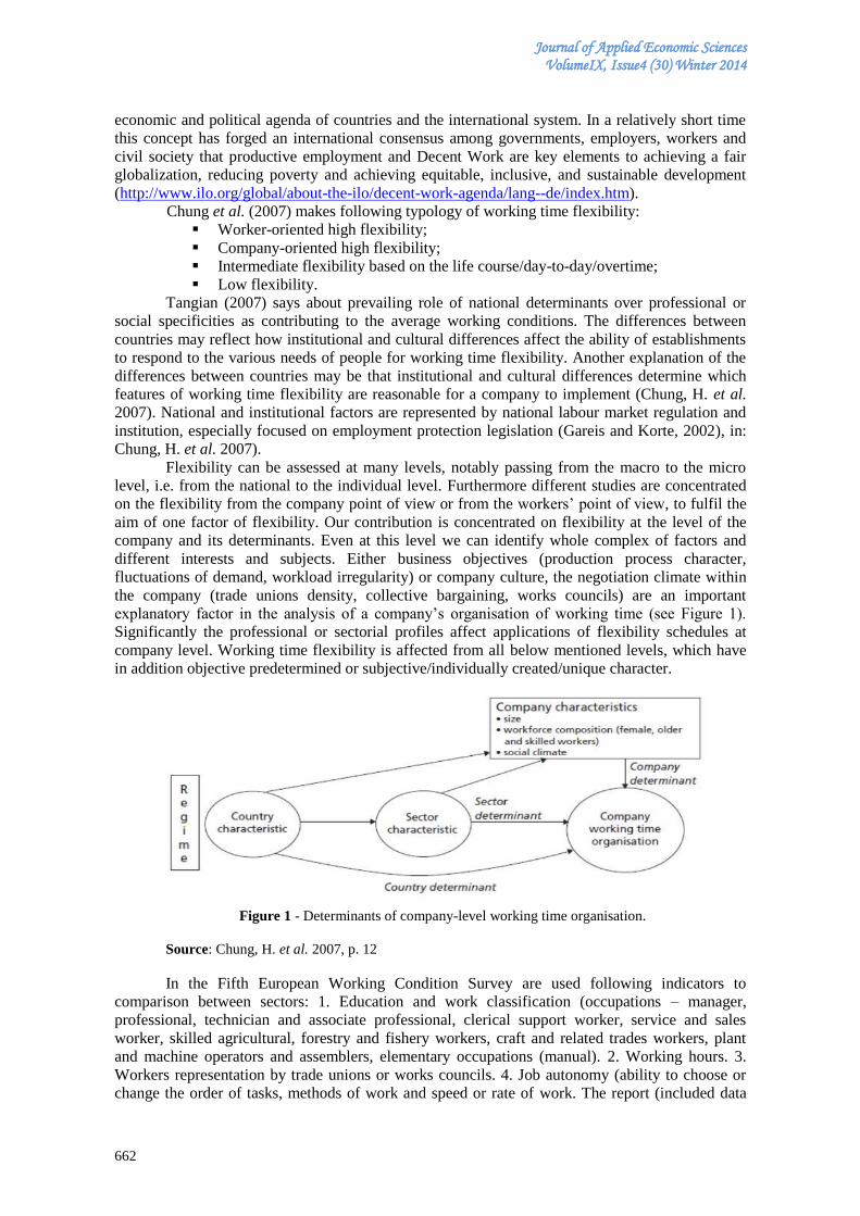
Journal of Applied Economic Sciences VolumeIX, Issue4 (30) Winter 2014
662
economic and political agenda of countries and the international system. In a relatively short time
this concept has forged an international consensus among governments, employers, workers and
civil society that productive employment and Decent Work are key elements to achieving a fair
globalization, reducing poverty and achieving equitable, inclusive, and sustainable development
(http://www.ilo.org/global/about-the-ilo/decent-work-agenda/lang--de/index.htm).
Chung et al. (2007) makes following typology of working time flexibility:
Worker-oriented high flexibility;
Company-oriented high flexibility;
Intermediate flexibility based on the life course/day-to-day/overtime;
Low flexibility.
Tangian (2007) says about prevailing role of national determinants over professional or
social specificities as contributing to the average working conditions. The differences between
countries may reflect how institutional and cultural differences affect the ability of establishments
to respond to the various needs of people for working time flexibility. Another explanation of the
differences between countries may be that institutional and cultural differences determine which
features of working time flexibility are reasonable for a company to implement (Chung, H. et al.
2007). National and institutional factors are represented by national labour market regulation and
institution, especially focused on employment protection legislation (Gareis and Korte, 2002), in:
Chung, H. et al. 2007).
Flexibility can be assessed at many levels, notably passing from the macro to the micro
level, i.e. from the national to the individual level. Furthermore different studies are concentrated
on the flexibility from the company point of view or from the workers’ point of view, to fulfil the
aim of one factor of flexibility. Our contribution is concentrated on flexibility at the level of the
company and its determinants. Even at this level we can identify whole complex of factors and
different interests and subjects. Either business objectives (production process character,
fluctuations of demand, workload irregularity) or company culture, the negotiation climate within
the company (trade unions density, collective bargaining, works councils) are an important
explanatory factor in the analysis of a company’s organisation of working time (see Figure 1).
Significantly the professional or sectorial profiles affect applications of flexibility schedules at
company level. Working time flexibility is affected from all below mentioned levels, which have
in addition objective predetermined or subjective/individually created/unique character.
Figure 1 - Determinants of company-level working time organisation.
Source: Chung, H. et al. 2007, p. 12
In the Fifth European Working Condition Survey are used following indicators to
comparison between sectors: 1. Education and work classification (occupations – manager,
professional, technician and associate professional, clerical support worker, service and sales
worker, skilled agricultural, forestry and fishery workers, craft and related trades workers, plant
and machine operators and assemblers, elementary occupations (manual). 2. Working hours. 3.
Workers representation by trade unions or works councils. 4. Job autonomy (ability to choose or
change the order of tasks, methods of work and speed or rate of work. The report (included data
Journal of Applied Economic Sciences VolumeIX, Issue4 (30) Winter 2014
663
from 33 sectors of economic activity) captures the diversity between sectors in terms of working
conditions and job quality. Likewise it considers sector perspective as highly relevant to the
improvement of working conditions. Many interventions to improve working conditions are
organised and implemented at this level. We mentioned differences within sectors, too. Those are
across groups of workers within the sector (Van Houten, G. et al. 2014).
Overview of irregular and atypical working hours by sectors of economic activity brings
the Fifth European Working Conditions Survey in overview report “Working conditions and job
quality: Comparing sectors in Europe” (Van Houten, et al. 2014). Agriculture stands out regarding
irregular working hours. Atypical hours are particularly prevalent in food and beverage services,
agriculture, accommodation, the arts, entertainment and recreation sector. Financial services, the
metal industry, and legal and accounting activities are among the sectors with the smallest shares
of workers reporting atypical working hours. The study provides a comparison of the organization
of work (teamwork and team autonomy, multitasking and multiskilling, etc.
For more information see identification of sectorial profiles on working conditions, trends
and differences between country clusters by Jettinghoff, K. and Houtman, I. (2009). The authors of
the study note, that in the level of the company the working time schedules are affected by those
specific profiles of sector and parallel by the socio-demographic factors (structure of workers –
gender, age, education, employment status). It explains differences in working conditions within
sector, too.
In 2004–2005 the European Foundation for the Improvement of Living and Working
Conditions launched a large-scale survey in companies in 21 European countries to tackle pressing
data deficit: the Establishment Survey on Working Time (Chung, et al. 2007). The study seeks to
explore and explain the main determinants of the different systems for organising working time in
the workplace. More specifically, the research aims first to identify a typology and its correlates of
different company ‘profiles’ in terms of the types of working time arrangements and work–life
balance policies in place. The study analyses which of the company characteristics determine the
flexibility profile of a company. Main objective of the survey was to construct and validate an
overarching typology of such practices and arrangements in European companies in order to
examine its cross-national variation, determine its main correlates and explore whether distinct
flexible working time profiles can be seen to have different performance outcomes. The study
covers public and private establishments from virtually all sectors of economic activity, with the
exception of ‘agriculture’, ‘forestry’, ‘private households’ and ‘extraterritorial organisations’. In
these sectors, the number of companies employing 10 or more workers is negligible in the
countries surveyed.
Flexibility profile of an organisation is related to its known characteristics, such as its line
of business, the size and composition of its workforce and its geographical location. Due to the
different sector characteristics, services sectors (NACE G–O) are usually seen to need and provide
more flexibility than industry sectors (NACE C–F). The public type of ownership is also
considered to have more arrangements for work–life balance needs of workers than the private
type. Although larger establishments have more scope for introducing different types of flexibility,
smaller establishments require various options to adapt to changes. While bigger establishments
have formalised arrangements, smaller establishments have informal arrangements which might be
more efficient in providing various working time flexibility options. The share of women and older
workers as well as the skill composition within the workforce may be additional aspects that need
to be examined, state Chung, H. et al. (2007). The authors conclude that not only country, but also
sector, size and workforce composition are deciding factors in whether an establishment uses a
certain working time arrangement or not. In addition, as is the case in relation to early retirement,
the economic or employment situation of the companies may also be another factor that might
affect the organisation of working time. A further element which is examined in this research is the
social climate within establishments.
Multivariate analysis of the typology of working time flexibility realised by Chung, H. et
al. (2007) confirmed the following results: Services sector has higher numbers of the high-
flexibility types of companies, both worker and company oriented. This sector also has some
degree of the life course and day-to-day types of moderately flexible companies. Conversely, the
Journal of Applied Economic Sciences VolumeIX, Issue4 (30) Winter 2014
664
industry sector shows a higher proportion of companies with less flexibility, namely the overtime
and low-flexibility type of companies. This may have to do with the fact that establishments in the
services sector, which have less standardised work processes, have more opportunities to
reorganise their working times. The distribution of flexibility types between the services and
industry sectors could also be due to the fact that some forms of working time flexibility – such as
unusual working and opening hours – are needed in the services sector to suit customer needs
(Chung, H. et al. 2007).
The comparison of the private and public sectors displays, the public sector companies
appear to be more concerned to meet workers’ needs in facilitating work–life balance options, by
providing more flexible working time arrangements for their workers.
The marginal effects for the sector of economic activity show that flexibility profiles also
vary considerably between sectors. The manufacturing industries and the mining and quarrying
sector are the reference categories for this set of indicators. The construction sector can be
characterised by an overrepresentation of the low-flexibility type of companies. The typical
worker-oriented high-flexibility sectors include public administration, financial intermediation,
real estate, renting and business activities, electricity, gas and water supply and other community,
social and personal services. Health and social work stands out as the company-oriented high-
flexibility sector, with a higher probability of 20 percentage points of companies being of this type
than in the manufacturing industries and mining and quarrying. However, the transport, storage
and communication sector and the hotels and restaurants sector also show a relatively large
percentage of this type of company. The life course oriented moderately flexible types of
companies are overrepresented in the education sector. The day-to- day flexibility type accounts
for the lowest amount of all establishments. Therefore, the variation across sectors is also lower
than for the other types of companies. Nevertheless, the day-to-day flexibility type of company is
overrepresented in the hotels and restaurants sector, and in the other community, social and
personal services sector. The type of companies for which working time flexibility mainly
concerns overtime is most frequently found in the manufacturing industries and the transport,
storage and communication sector. Overall, more organisations with a higher-flexibility profile
operate in the services sector, while more companies with a lower-flexibility profile are in industry
(Chung, H. et al. 2007).
According to company size, high-flexibility (both in terms of those that are more focused
on company needs and those that are more focused on workers’ needs) types is greater among
larger establishments, numbers of low-flexibility companies are substantially larger in the smaller
company categories. Companies that are part of multi-site organisations more often belong to one
of the two most flexible types of establishments.
The relationship between workload variations and the type of working time flexibility is
also interesting. Establishments that experience variations of workload – whether these are short-
run or long-run fluctuations – are more likely to have a company-oriented high-flexibility profile
and less likely to have a low-flexibility profile. The effect vanishes, however, if it concerns long-
term fluctuations that are not predictable. If short-term variations are unpredictable, then raise the
probability of being a company with overtime arrangements.
Over mentioned characteristics is business/production process-oriented. Following
characteristics is workers-structure oriented. Flexibility options that are geared more towards the
needs of workers exist to a greater extent in companies with a large proportion of skilled workers,
while company-oriented flexibility and low flexibility are more common in companies in which
the percentage of skilled workers is low. Arrangements perform better in attracting and
maintaining a skilled workforce. The age composition of the workforce has little relation to the
flexibility profile of the establishment. Companies with a larger percentage of young workers are,
however, significantly more likely to have a company-oriented high-flexibility profile and less
likely to be low-flexibility organisations (Chung, H. et al. 2007).
Measurable indicators of working time flexibility from the data analysis from Eurostat,
European Foundation of Working and Living Conditions (Eurofound) in Dublin (see Van Houten,
G. et al. 2014; Chung, H. et al. 2007) and from Institute for the Study of Labour (IZA) in Bonn
(Eichhorst, W. et al. 2013) were compared to our own research results.
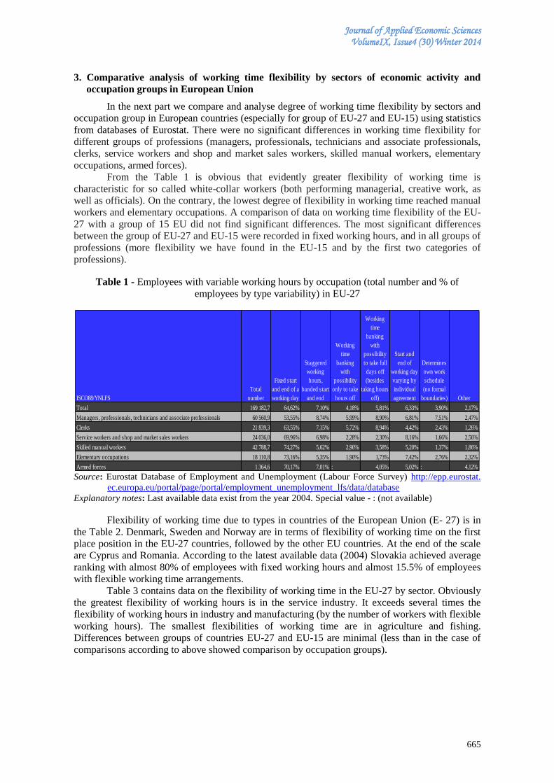
Journal of Applied Economic Sciences VolumeIX, Issue4 (30) Winter 2014
665
3. Comparative analysis of working time flexibility by sectors of economic activity and
occupation groups in European Union
In the next part we compare and analyse degree of working time flexibility by sectors and
occupation group in European countries (especially for group of EU-27 and EU-15) using statistics
from databases of Eurostat. There were no significant differences in working time flexibility for
different groups of professions (managers, professionals, technicians and associate professionals,
clerks, service workers and shop and market sales workers, skilled manual workers, elementary
occupations, armed forces).
From the Table 1 is obvious that evidently greater flexibility of working time is
characteristic for so called white-collar workers (both performing managerial, creative work, as
well as officials). On the contrary, the lowest degree of flexibility in working time reached manual
workers and elementary occupations. A comparison of data on working time flexibility of the EU-
27 with a group of 15 EU did not find significant differences. The most significant differences
between the group of EU-27 and EU-15 were recorded in fixed working hours, and in all groups of
professions (more flexibility we have found in the EU-15 and by the first two categories of
professions).
Table 1 - Employees with variable working hours by occupation (total number and % of
employees by type variability) in EU-27
Source: Eurostat Database of Employment and Unemployment (Labour Force Survey) http://epp.eurostat.
ec.europa.eu/portal/page/portal/employment_unemployment_lfs/data/database
Explanatory notes: Last available data exist from the year 2004. Special value - : (not available)
Flexibility of working time due to types in countries of the European Union (E- 27) is in
the Table 2. Denmark, Sweden and Norway are in terms of flexibility of working time on the first
place position in the EU-27 countries, followed by the other EU countries. At the end of the scale
are Cyprus and Romania. According to the latest available data (2004) Slovakia achieved average
ranking with almost 80% of employees with fixed working hours and almost 15.5% of employees
with flexible working time arrangements.
Table 3 contains data on the flexibility of working time in the EU-27 by sector. Obviously
the greatest flexibility of working hours is in the service industry. It exceeds several times the
flexibility of working hours in industry and manufacturing (by the number of workers with flexible
working hours). The smallest flexibilities of working time are in agriculture and fishing.
Differences between groups of countries EU-27 and EU-15 are minimal (less than in the case of
comparisons according to above showed comparison by occupation groups).
ISCO88/YNLFS
Total
number
Fixed start
and end of a
working day
Staggered
working
hours,
banded start
and end
Working
time
banking
with
possibility
only to take
hours off
Working
time
banking
with
possibility
to take full
days off
(besides
taking hours
off)
Start and
end of
working day
varying by
individual
agreement
Determines
own work
schedule
(no formal
boundaries) Other
Total 169 182,7 64,62% 7,10% 4,18% 5,81% 6,33% 3,90% 2,17%
Managers, professionals, technicians and associate professionals 60 560,9 53,55% 8,74% 5,99% 8,90% 6,81% 7,51% 2,47%
Clerks 21 839,3 63,55% 7,15% 5,72% 8,94% 4,42% 2,43% 1,26%
Service workers and shop and market sales workers 24 036,0 69,96% 6,98% 2,28% 2,30% 8,16% 1,66% 2,56%
Skilled manual workers 42 788,7 74,27% 5,62% 2,90% 3,58% 5,20% 1,37% 1,86%
Elementary occupations 18 110,8 73,16% 5,35% 1,90% 1,73% 7,42% 2,76% 2,32%
Armed forces 1 364,6 70,17% 7,01% : 4,05% 5,02% : 4,12%
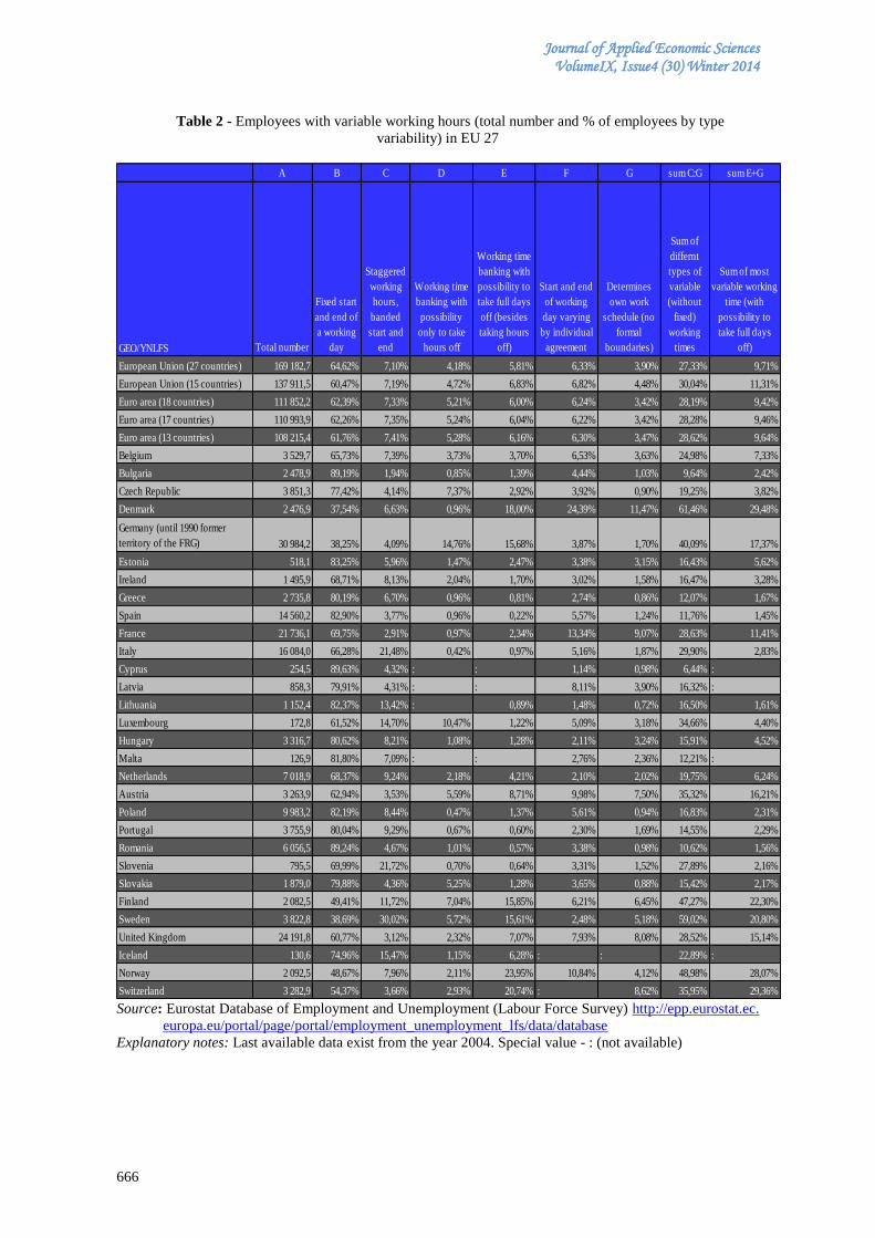
Journal of Applied Economic Sciences VolumeIX, Issue4 (30) Winter 2014
666
Table 2 - Employees with variable working hours (total number and % of employees by type
variability) in EU 27
Source: Eurostat Database of Employment and Unemployment (Labour Force Survey) http://epp.eurostat.ec.
europa.eu/portal/page/portal/employment_unemployment_lfs/data/database
Explanatory notes: Last available data exist from the year 2004. Special value - : (not available)
A B C D E F G sum C:G sum E+G
GEO/YNLFS Total number
Fixed start
and end of
a working
day
Staggered
working
hours,
banded
start and
end
Working time
banking with
possibility
only to take
hours off
Working time
banking with
possibility to
take full days
off (besides
taking hours
off)
Start and end
of working
day varying
by individual
agreement
Determines
own work
schedule (no
formal
boundaries)
Sum of
differnt
types of
variable
(without
fixed)
working
times
Sum of most
variable working
time (with
possibility to
take full days
off)
European Union (27 countries) 169 182,7 64,62% 7,10% 4,18% 5,81% 6,33% 3,90% 27,33% 9,71%
European Union (15 countries) 137 911,5 60,47% 7,19% 4,72% 6,83% 6,82% 4,48% 30,04% 11,31%
Euro area (18 countries) 111 852,2 62,39% 7,33% 5,21% 6,00% 6,24% 3,42% 28,19% 9,42%
Euro area (17 countries) 110 993,9 62,26% 7,35% 5,24% 6,04% 6,22% 3,42% 28,28% 9,46%
Euro area (13 countries) 108 215,4 61,76% 7,41% 5,28% 6,16% 6,30% 3,47% 28,62% 9,64%
Belgium 3 529,7 65,73% 7,39% 3,73% 3,70% 6,53% 3,63% 24,98% 7,33%
Bulgaria 2 478,9 89,19% 1,94% 0,85% 1,39% 4,44% 1,03% 9,64% 2,42%
Czech Republic 3 851,3 77,42% 4,14% 7,37% 2,92% 3,92% 0,90% 19,25% 3,82%
Denmark 2 476,9 37,54% 6,63% 0,96% 18,00% 24,39% 11,47% 61,46% 29,48%
Germany (until 1990 former
territory of the FRG) 30 984,2 38,25% 4,09% 14,76% 15,68% 3,87% 1,70% 40,09% 17,37%
Estonia 518,1 83,25% 5,96% 1,47% 2,47% 3,38% 3,15% 16,43% 5,62%
Ireland 1 495,9 68,71% 8,13% 2,04% 1,70% 3,02% 1,58% 16,47% 3,28%
Greece 2 735,8 80,19% 6,70% 0,96% 0,81% 2,74% 0,86% 12,07% 1,67%
Spain 14 560,2 82,90% 3,77% 0,96% 0,22% 5,57% 1,24% 11,76% 1,45%
France 21 736,1 69,75% 2,91% 0,97% 2,34% 13,34% 9,07% 28,63% 11,41%
Italy 16 084,0 66,28% 21,48% 0,42% 0,97% 5,16% 1,87% 29,90% 2,83%
Cyprus 254,5 89,63% 4,32% : : 1,14% 0,98% 6,44% :
Latvia 858,3 79,91% 4,31% : : 8,11% 3,90% 16,32% :
Lithuania 1 152,4 82,37% 13,42% : 0,89% 1,48% 0,72% 16,50% 1,61%
Luxembourg 172,8 61,52% 14,70% 10,47% 1,22% 5,09% 3,18% 34,66% 4,40%
Hungary 3 316,7 80,62% 8,21% 1,08% 1,28% 2,11% 3,24% 15,91% 4,52%
Malta 126,9 81,80% 7,09% : : 2,76% 2,36% 12,21% :
Netherlands 7 018,9 68,37% 9,24% 2,18% 4,21% 2,10% 2,02% 19,75% 6,24%
Austria 3 263,9 62,94% 3,53% 5,59% 8,71% 9,98% 7,50% 35,32% 16,21%
Poland 9 983,2 82,19% 8,44% 0,47% 1,37% 5,61% 0,94% 16,83% 2,31%
Portugal 3 755,9 80,04% 9,29% 0,67% 0,60% 2,30% 1,69% 14,55% 2,29%
Romania 6 056,5 89,24% 4,67% 1,01% 0,57% 3,38% 0,98% 10,62% 1,56%
Slovenia 795,5 69,99% 21,72% 0,70% 0,64% 3,31% 1,52% 27,89% 2,16%
Slovakia 1 879,0 79,88% 4,36% 5,25% 1,28% 3,65% 0,88% 15,42% 2,17%
Finland 2 082,5 49,41% 11,72% 7,04% 15,85% 6,21% 6,45% 47,27% 22,30%
Sweden 3 822,8 38,69% 30,02% 5,72% 15,61% 2,48% 5,18% 59,02% 20,80%
United Kingdom 24 191,8 60,77% 3,12% 2,32% 7,07% 7,93% 8,08% 28,52% 15,14%
Iceland 130,6 74,96% 15,47% 1,15% 6,28% : : 22,89% :
Norway 2 092,5 48,67% 7,96% 2,11% 23,95% 10,84% 4,12% 48,98% 28,07%
Switzerland 3 282,9 54,37% 3,66% 2,93% 20,74% : 8,62% 35,95% 29,36%
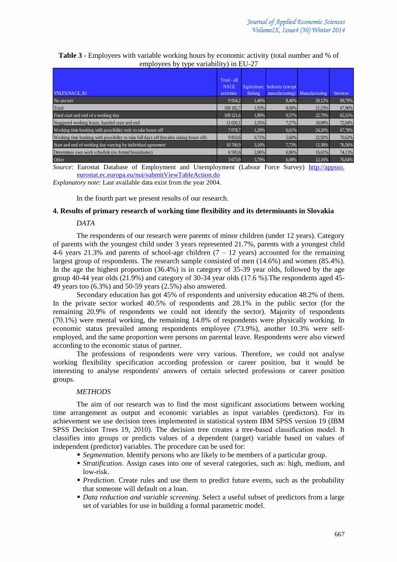
Journal of Applied Economic Sciences VolumeIX, Issue4 (30) Winter 2014
667
Table 3 - Employees with variable working hours by economic activity (total number and % of
employees by type variability) in EU-27
Source: Eurostat Database of Employment and Unemployment (Labour Force Survey) http://appsso.
eurostat.ec.europa.eu/nui/submitViewTableAction.do
Explanatory note: Last available data exist from the year 2004.
In the fourth part we present results of our research.
4. Results of primary research of working time flexibility and its determinants in Slovakia
DATA
The respondents of our research were parents of minor children (under 12 years). Category
of parents with the youngest child under 3 years represented 21.7%, parents with a youngest child
4-6 years 21.3% and parents of school-age children (7 – 12 years) accounted for the remaining
largest group of respondents. The research sample consisted of men (14.6%) and women (85.4%).
In the age the highest proportion (36.4%) is in category of 35-39 year olds, followed by the age
group 40-44 year olds (21.9%) and category of 30-34 year olds (17.6 %).The respondents aged 45-
49 years too (6.3%) and 50-59 years (2.5%) also answered.
Secondary education has got 45% of respondents and university education 48.2% of them.
In the private sector worked 40.5% of respondents and 28.1% in the public sector (for the
remaining 20.9% of respondents we could not identify the sector). Majority of respondents
(70.1%) were mental working, the remaining 14.8% of respondents were physically working. In
economic status prevailed among respondents employee (73.9%), another 10.3% were self-
employed, and the same proportion were persons on parental leave. Respondents were also viewed
according to the economic status of partner.
The professions of respondents were very various. Therefore, we could not analyse
working flexibility specification according profession or career position, but it would be
interesting to analyse respondents' answers of certain selected professions or career position
groups.
METHODS
The aim of our research was to find the most significant associations between working
time arrangement as output and economic variables as input variables (predictors). For its
achievement we use decision trees implemented in statistical system IBM SPSS version 19 (IBM
SPSS Decision Trees 19, 2010). The decision tree creates a tree-based classification model. It
classifies into groups or predicts values of a dependent (target) variable based on values of
independent (predictor) variables. The procedure can be used for:
Segmentation. Identify persons who are likely to be members of a particular group.
Stratification. Assign cases into one of several categories, such as: high, medium, and
low-risk.
Prediction. Create rules and use them to predict future events, such as the probability
that someone will default on a loan.
Data reduction and variable screening. Select a useful subset of predictors from a large
set of variables for use in building a formal parametric model.
YNLFS/NACE_R1
Total - all
NACE
activities
Agriculture;
fishing
Industry (except
manufacturing) Manufacturing Services
No answer 9 954,2 1,46% 8,40% 20,12% 69,79%
Total 169 182,7 1,93% 8,68% 21,23% 67,90%
Fixed start and end of a working day 109 321,6 1,89% 9,57% 22,79% 65,51%
Staggered working hours, banded start and end 12 020,1 2,35% 7,27% 18,08% 72,04%
Working time banking with possibility only to take hours off 7 078,7 1,29% 6,61% 24,20% 67,78%
Working time banking with possibility to take full days off (besides taking hours off) 9 833,6 0,71% 5,60% 22,92% 70,62%
Start and end of working day varying by individual agreement 10 706,9 3,10% 7,73% 12,38% 76,56%
Determines own work schedule (no formal boundaries) 6 593,6 2,06% 6,86% 16,61% 74,13%
Other 3 673,9 3,79% 6,08% 12,16% 76,64%
Journal of Applied Economic Sciences VolumeIX, Issue4 (30) Winter 2014
668
Interaction identification. Identify relationships that belong to specific subgroups and
specify them in a formal parametric model.
Category merging and discretizing continuous variables. Recode group predictor
categories and continuous variables with minimal loss of information.
The decision tree methods available in SPSS are:
CHAID. Chi-squared Automatic Interaction Detection. At each step, CHAID chooses the
independent (predictor) variable that has the strongest interaction with the dependent variable.
Categories of each predictor are merged if they are not significantly different with respect to the
dependent variable (Kass, 1980).
CRT. Classification and Regression Trees. CRT splits the data into segments that are as
homogeneous as possible with respect to the dependent variable. A terminal node in which all
cases have the same value for the dependent variable is a homogeneous, "pure" node (Breiman
et al. 1984).
QUEST. Quick, Unbiased, Efficient Statistical Tree. A method that is fast and avoids other
methods’ bias in favour of predictors with many categories. QUEST can be specified only if the
dependent variable is nominal (Loh – Shih, 1997).
In our case the CRT model produced best results with default parameters (only prior
probabilities where set to equal to increase the number of correct classifications in case of
flexible time arrangements). If we want to take into account the employer viewpoint for
comparison of working time arrangements then we should use some benchmarking method like
balanced scorecard (Gavurová 2011, 2012; Šoltés, Gavurová, 2013).
RESULTS
Our tree diagram (depicted in the Figure 2) shows that using the CRT model, the economic
status is the best predictor of working time arrangement. Right terminal node contains 50 cases of
maternal leave respondents, of household respondents and of self-employed persons. The
proportion of flexible time arrangement in the node is 60.0%. In the left node the proportion of
flexible time arrangement is 30.2%, which is significantly lower than the proportion in the right
node. The left node has got 348 cases of persons with other economic activities: unemployed,
employed and parental leave. For these cases the next best predictor is the sector. More flexible
working conditions in self-employment profession can be explained by character of work (like
below by mental working workers), it is mostly managerial, administrative and creative work
(compare Eichhorst, 2013). People at maternity or parental leave filled flexibility of working time
schedules in their last job.
If the sector is public or missing (left terminal node, n = 149) then proportion of flexible
time arrangement is 39.6%. The respondents working in private or ambiguous sectors (right node,
n = 199) has got proportion of flexible time arrangement 23.1%. For them CRT model includes
paid work during parental leave as another predictor. In the left terminal node the proportion of
flexible time arrangement is 33.8% (paid work during parental leave and blank (missing) cases, n
= 71). Comparable results about differences between flexibility of working time in private and
public sector companies are also in international research studies (Eichhorst, 2013; Chung,
Kerkhofs, Ester, 2007). Reasons are not only character of production process and of operating
hours, regularity of work without fluctuations, but also density of trade unions and coverage by
collective arrangements. Predominant flexibility of working time for persons/mothers especially
working during parental leave can be explained by following. They are mostly high skilled
workers, for who is typical independent/autonomous creative work, which allows for a high degree
of positive (workers-oriented) working time flexibility. At the same time, their employers are
interested in the earliest return of these persons in the labor market (to prevent loss of skills) and
therefore generate flexible working conditions for them.
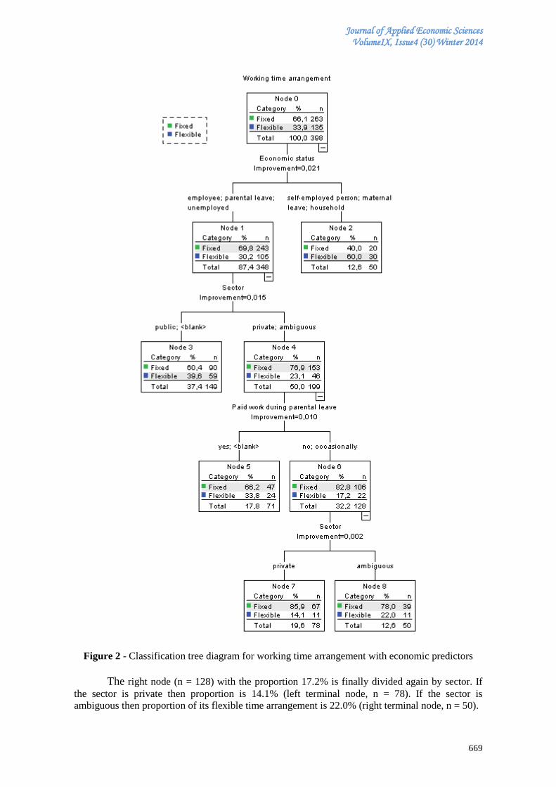
Journal of Applied Economic Sciences VolumeIX, Issue4 (30) Winter 2014
669
Figure 2 - Classification tree diagram for working time arrangement with economic predictors
The right node (n = 128) with the proportion 17.2% is finally divided again by sector. If
the sector is private then proportion is 14.1% (left terminal node, n = 78). If the sector is
ambiguous then proportion of its flexible time arrangement is 22.0% (right terminal node, n = 50).

Journal of Applied Economic Sciences VolumeIX, Issue4 (30) Winter 2014
670
The classification (Table 4) shows that the CRT model classifies only 60.8% of the
respondents correctly in spite of surrogate predictors usage. It is caused mainly by missing values
in following variables: the sector (10.6% of missing values and 20.9% of ambiguous cases which
are questionable) and work type (15.1% of missing values) and also by involution of only
economic variables in our tree model.
Table 4 - Classification matrix of CRT model of the working time arrangement
OBSERVED
PREDICTED
Fixed Flexible Percent Correct
Fixed 153 110 58,20%
Flexible 46 89 65,90%
Overall
Percentage 50,00% 50,00% 60,80%
Importance (relative and absolute) of all five economic predictors involved in CRT model
is depicted in Figure 3. We can see that the most important economic predictor due to working
time arrangement is the economic status of the respondent. The next one is sector with slightly
smaller relative importance (76%). Then follow paid work during parental leave (43%) and sector
(29%). The last predictor – economic status of respondents’ partner is negligible though formally
significant (1%).
Figure 3 – Importance of economic predictors involved in CRT model of working time
arrangement
Now we can make some conclusions.
Journal of Applied Economic Sciences VolumeIX, Issue4 (30) Winter 2014
671
Conclusion
The aim of our paper was to identify critical factors of influence on working time
organization from the first named group of factors of influence (work, production process
organization, sector of economic activity and occupation specifications). Not only business
objectives (production process character, fluctuations of demand, workload irregularity), but also
company’s culture, the negotiation climate within the company (trade unions density, collective
bargaining, works councils) are an important explanatory factors in the analysis of a company’s
organisation of working time, as well as professional or sectorial profiles affect significantly
applications of flexibility schedules at company level. The group of economic factors cannot be
considered in isolation. With economic characteristics of production process it must be taken into
account influence of socio-demographic structure of workers on working condition, especially
working time organization. The differences between countries may reflect how institutional and
cultural differences affect application of working time flexibility in practice. Slovakia and
countries of the Central and Eastern Europe are countries with lower levels of working time
flexibility, particularly of positive (workers-oriented) flexibility of working time schedules.
Reasons are not only objective (determined by nature of production process, sectorial or
occupational specifications), but also subjective behaviour at level of individual employer
(business culture, by willingness to negotiation about working conditions improvement) and
workers structure (by skills, age, occupations and by their individual preferences and needs).
Evidently, all these factors have influence on resulting flexibility of working time schedules. We
specify key factors of influence at company level with the intention to support implementation of
positive working time flexibility in practice of Slovak companies and in companies in other post-
socialist countries of the Central and Eastern Europe facing problems in this area.
Acknowledgment
This research paper was supported by grant VEGA No. 1/0991/12 “Determinants of use of
a flexible approach work from the view of the family and their implementation in the social
system” of the Scientific Grant Agency of the Ministry of Education of the Slovak Republic.
References
[1] Breiman, L. et al. (1984). Classification and Regression Trees, New York, Chapman & Hall.
[2] Chung, H. et al. (2007). Working time flexibility in European companies. Establishment
Survey on Working Time 2004 – 2005, Dublin, European Foundation for the Improvement of
Living and Working Conditions, 74 p., http://www.eurofound.europa.eu/pubdocs/2007/39/
en/1/ef0739en.pdf
[3] Delsen, L. et al. (2009). Comparative Analyses of Operating Hours and Working Times in the
European Union. Heidelberg, Physica Verlag, A Springer Company, 213 p., http://books.
google.sk/books?id=NkMEG16YbasC&pg=PA22&lpg=PA22&dq=flexible+working+hours+
by+economic+activity&source=bl&ots=wWIMCo5i2-&sig=t2UnKnslJFOSCCrcIXDA58b5-
r4&hl=sk&sa=X&ei=dWQhVLfWIMSwO5DbgLAD&ved=0CDoQ6AEwAw#v=onepage&q
=flexible%20working%20hours%20by%20economic%20activity&f=false
[4] Eichhorst, W. et al. (2013). Non-Standard Employment across Occupations in Germany: The
Role of Replaceability and Labour Market Flexibility. Discussion Paper No. 7662, Bonn, IZA
(The Institute for the Study of Labor), 34 p, http://ftp.iza.org/dp7662.pdf
[5] Gavurová, B. (2011). Systém Balanced Scorecard v podnikovom riadení. (The balanced
scorecard system in enterprise management), Ekonomický časopis, 59 (2):163-177.
[6] Gavurová, B. (2012). Source Identification of Potential Malfunction of Balanced Scorecard
System and Its Influence on System Function, E+M Ekonomie a Management, 15(3): 76-90.
[8] Jettinghoff, K., Houtman, I. (2009). A sector perspective on working conditions, Dublin,
European Foundation for the Improvement of Working and Living Conditions, 30 p.
[9] Kass, G. (1980). An exploratory technique for investigating large quantities of categorical
data, Applied Statistics, 29(2): 119–127, http://dx.doi.org/10.2307/2986296
Journal of Applied Economic Sciences VolumeIX, Issue4 (30) Winter 2014
672
[10] Kümmerling, A., Lehndorff, S. (2007). Extended and unusual working hours in European
Companies. Establishment Survey on Working Time 2004 – 2005, Dublin, European
Foundation for the Improvement of Living and Working Conditions, 65 p.
[11] Loh, W.Y., Shih, Y.S. (1997). Split selection methods for classification trees, Statistica
Sinica, 7: 815–840.
[12] Messenger, J.C. (2011). Working time trends and developments in Europe.Cambridge
Journal of Economics, 35: 295–316 http://pat61skarlib.squat.gr/files/2011/11/ EUROPE_
WORKING_TIME.pdf, http://dx.doi.org/10.1093/cje/beq022
[13] Šoltés, V., Gavurová, B. (2013). Application of the cross impact matrix method in
problematic phases of the Balanced Scorecard system in private and public sector. Journal of
Applied Economic Sciences, 8(1): 99-119, http://www.cesmaa.eu/journals/jaes/jaes_issues.
php
[14] Tangian, A. (2007). Analysis of the third European survey on working conditions with
composite indicators, European Journal of Operational Research, 181(1): 468 - 499.
http://dx.doi. org/10.1016/j.ejor.2006.05.038
[16] Valeyre, A. et al. (2009). Working conditions in the European Union: Work organization,
Luxembourg, Office for Official Publications of the European Communities, 74 p., http://
www.eurofound.europa.eu/publications/htmlfiles/ef0862.htm
[17] Van Houten, G. et al. (2014). Working conditions and job quality: Comparing sector in
Europe – Overview report, Dublin, Eurofound (European Foundation for the Improvement of
Living and Working Condition, 66 p., http://www.eurofound.europa.eu/publications/
htmlfiles/ef1384.htm
[18] Wallace, C. (2003). Work Flexibility in Eight European Countries: A Cross-national
Comparison, Czech Sociological Review, 39(6): 773 – 794, http://sreview.soc.cas.cz/uploads/
e827ac95aae18ae44848de8fdd846104c4ff0aea509_63Wall21.pdf
*** IBM SPSS Decision Trees 19 (2010).
*** http://epp.eurostat.ec.europa.eu/portal/page/portal/employment_unemployment_lfs/introd
uction
*** http://www.ilo.org/global/about-the-ilo/decent-work-agenda/lang--de/index.htm
Journal of Applied Economic Sciences VolumeIX, Issue4 (30) Winter 2014
673
THE EFFICIENCY OF SLOVAK UNIVERSITIES: A DATA ENVELOPMENT ANALYSIS8
Matúš KUBÁK Technical University of Košice, Faculty of Economics
9, Slovak Republic
Radovan BAČÍK
University of Prešov in Prešov, Faculty of Management10
, Slovak Republic
Zsuzsanna Katalin SZABO
Faculty of Economics, Law and Administrative Sciences11
, Tg.Mures, Romania
Dominik BARTKO
University of Prešov in Prešov, Faculty of Management9, Slovak Republic
Abstract:
We run Data Envelopment Analysis to study technical efficiency of faculties in the Slovak Republic.
Our dataset come from Academic Ranking and Rating Agency. Inputs for our analysis are Education,
Attractiveness of study and Doctoral studies. Output variables in our study are Research and Grants. Our
finding shows that there exist serious differences in effectiveness of faculties. The most serious imbalances
are within Economic Sciences group, Technical Sciences group, Theological Sciences and Group of Arts. On
the other hand, the most balanced situation is within the Natural Sciences group, Medical Sciences Group
and Agricultural Sciences Group.
Keywords: Data Envelopment Analysis, Slovak universities, efficiency of faculties.
JEL Classification: C14, I21
1. Introduction
Efficiency of schools is a crucial factor that can lead an educational system towards
economic efficiency. In this paper, we look closer on the technical efficiency of universities in
Slovak Republic using Data Envelopment Analysis. The issue of efficiency of universities is quite
complex, because of the fact, that higher education is, apart of certain exceptions, public good,
thus one cannot orient in pursuance of market price. In Slovakia, private and public universities
coexist. Both of them have different goals. Whereas public universities aim to carry on own
research and development, private universities are aiming on profit maximization. Despite of the
fact, that Slovak Republic is a relatively small country, we can find here 20 public universities, 3
state colleges, 13 private colleges and 4 foreign universities. In this paper we present data
envelopment analysis, which works with 24 universities, 109 faculties, among which 103 are
public ones and 6 are private faculties. Our dataset comes from independent Slovak civil
association Academic Ranking and Rating Agency report for 2013. Our study use as input
variables: Education, Attractiveness of study and Doctoral studies. Output variables in our study
are Research and Grants.
The aim of the study is to examine the efficiency of faculties based on their scientific
specialization. Paper is organized as follows: in next part literature review is proposed. Afterwards
materials and methods are described precisely. Subsequently, results of the analysis are presented.
Final part of the paper is devoted to discussion and conclusion.
8 Research reported in this paper was supported by VEGA 1/0726/14.
9 Němcovej 32, 040 01, Košice, Slovak Republic
10 Konštantínova 16, 080 01, Prešov, Slovak Republic
11 N. Iorga Street, No.1, 540088, Tg.Mureș, Romania
Journal of Applied Economic Sciences VolumeIX, Issue4 (30) Winter 2014
674
2. Literature review
Abbott and Doucouliagos found that regardless of the output-input mix, Australian
universities as a whole recorded high level of efficiency relative to each other. Nazarko et al. use
subsidies as the input and the number of students and scientific grants are treated as the output.
Authors showed that the majority of the universities in Poland possess reserves in technical and
allocative efficiency. Bayraktar et al. run Data Envelopment Analysis to measure the relative
efficiency of quality management practices in Turkish public and private universities. Authors
showed that private universities with higher levels of quality management efficiency on
stakeholder-focus indicators achieved better performance in terms of fulfilling the expectations of
their stakeholders. Sav run an analysis on a dataset consisting of 331 public universities in USA.
Author found that tuition dependency promotes inefficiency while increased government funding
yields efficiency gains. Another finding of the study is that investment income appears to have a
slight negative effect, albeit statistically weak. Results of the study reveal that public university
efficiencies have improved over time. Agasisti and Dal Bianco run Data Envelopment Analysis on
58 Italian public universities. Authors found that the majority of universities perform well for
various input and output specifications. Afonso and Santos run Data Envelopment Analysis on
Portuguese Public Universities. In this study inputs are the number of teachers and universities'
spending while the outputs are the undergraduate success rate and on the number of doctoral
dissertations. Authors identified well performing universities and those which do not perform well.
Agasisti and Johnes use Data Envelopment Analysis to compute the technical efficiency of Italian
and English higher education institutions. Authors´ results show that institutions in England are
more efficient than those in Italy when comparing jointly their performances. Authors also look at
the evolution of technical efficiency scores over a four‐year period, and find that Italian
universities are improving their technical efficiency while English universities are obtaining stable
scores. Agasisti and Pérez-Esparrells employ Data Envelopment Analysis to analyze efficiency of
Italian and Spanish universities. Authors found that Italian universities are relatively more efficient
than those in Spain. Afonso and Aubyn showed on a dataset consisting of OECD countries, that
efficiency in education is in some cases linked to efficiency in the health sector. Breu and Raab
measure relative efficiency of the top 25 universities in the United States. Authors find that the
most prestigious universities always generate the highest level of satisfaction among students. The
authors suggest that university expenditures should be aimed more at increasing levels of
efficiency, rather than to improve the perceived quality. Jeck and Sudzina run Data Envelopment
Analysis on a dataset consisting of 96 faculties in the Slovak Republic. Authors use teaching staff
as input variable and number of graduates, publications in Current Contents Connect® and number
of patents as output variables. The authors found that one half of faculties in the Slovak Republic
are effective. Authors found no differences in efficiency caused by the location of faculties.
Authors also argue that 21 faculties do not reach economies of scale, thus are too big. Some other
studies related to state of Slovak educational system can be found in following publications
(Gavurová, 2011), (Bednarova, et al. 2014), (Pudło, Gavurová, 2012) (Pudło, Gavurová, 2013) and
(Hudec, 2003). This study provides many abundant ideas for next researches and for using of
complementary methods to measure efficiency, effectiveness and economy. The future in the use
of effectiveness methods will require more views in the evaluation of economic phenomena and
thus the evaluation of outcomes of several methods (Gavurová, 2011), Gavurová, 2012), (Šoltés,
Gavurová, 2013), (Szabo, Šoltés, Herman, 2013) and (Užík, Šoltés, 2009).
3. Materials and methods
Data Envelopment Analysis is one of the mostly used methods to assess the technical
efficiency of entities. Its basic idea consists in enveloping positions of the monitored entities with a
line called efficiency frontier. All entities not present at this line are considered as inefficient. This
method does work under the condition that at least two entities must be compared and at least one
of them is always effective. Effective one lies on the efficiency frontier. Others may be inefficient
and inefficiency is then measured as the distance from the efficiency frontier. DEA includes
several types of models, the most used models are:
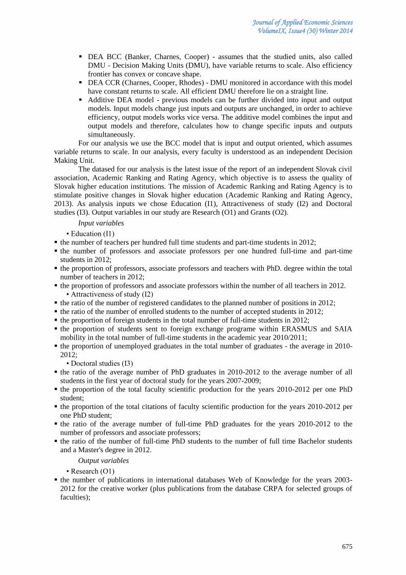
Journal of Applied Economic Sciences VolumeIX, Issue4 (30) Winter 2014
675
DEA BCC (Banker, Charnes, Cooper) - assumes that the studied units, also called
DMU - Decision Making Units (DMU), have variable returns to scale. Also efficiency
frontier has convex or concave shape.
DEA CCR (Charnes, Cooper, Rhodes) - DMU monitored in accordance with this model
have constant returns to scale. All efficient DMU therefore lie on a straight line.
Additive DEA model - previous models can be further divided into input and output
models. Input models change just inputs and outputs are unchanged, in order to achieve
efficiency, output models works vice versa. The additive model combines the input and
output models and therefore, calculates how to change specific inputs and outputs
simultaneously.
For our analysis we use the BCC model that is input and output oriented, which assumes
variable returns to scale. In our analysis, every faculty is understood as an independent Decision
Making Unit.
The datased for our analysis is the latest issue of the report of an independent Slovak civil
association, Academic Ranking and Rating Agency, which objective is to assess the quality of
Slovak higher education institutions. The mission of Academic Ranking and Rating Agency is to
stimulate positive changes in Slovak higher education (Academic Ranking and Rating Agency,
2013). As analysis inputs we chose Education (I1), Attractiveness of study (I2) and Doctoral
studies (I3). Output variables in our study are Research (O1) and Grants (O2).
Input variables
• Education (I1)
the number of teachers per hundred full time students and part-time students in 2012;
the number of professors and associate professors per one hundred full-time and part-time
students in 2012;
the proportion of professors, associate professors and teachers with PhD. degree within the total
number of teachers in 2012;
the proportion of professors and associate professors within the number of all teachers in 2012.
• Attractiveness of study (I2)
the ratio of the number of registered candidates to the planned number of positions in 2012;
the ratio of the number of enrolled students to the number of accepted students in 2012;
the proportion of foreign students in the total number of full-time students in 2012;
the proportion of students sent to foreign exchange programe within ERASMUS and SAIA
mobility in the total number of full-time students in the academic year 2010/2011;
the proportion of unemployed graduates in the total number of graduates - the average in 2010-
2012;
• Doctoral studies (I3)
the ratio of the average number of PhD graduates in 2010-2012 to the average number of all
students in the first year of doctoral study for the years 2007-2009;
the proportion of the total faculty scientific production for the years 2010-2012 per one PhD
student;
the proportion of the total citations of faculty scientific production for the years 2010-2012 per
one PhD student;
the ratio of the average number of full-time PhD graduates for the years 2010-2012 to the
number of professors and associate professors;
the ratio of the number of full-time PhD students to the number of full time Bachelor students
and a Master's degree in 2012.
Output variables
• Research (O1)
the number of publications in international databases Web of Knowledge for the years 2003-
2012 for the creative worker (plus publications from the database CRPA for selected groups of
faculties);
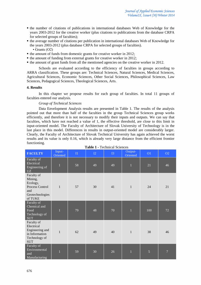
Journal of Applied Economic Sciences VolumeIX, Issue4 (30) Winter 2014
676
the number of citations of publications in international databases Web of Knowledge for the
years 2003-2012 for the creative worker (plus citations to publications from the database CRPA
for selected groups of faculties);
the average number of citations per publication in international databases Web of Knowledge for
the years 2003-2012 (plus database CRPA for selected groups of faculties).
• Grants (O2)
the amount of funds from domestic grants for creative worker in 2012;
the amount of funding from external grants for creative worker in 2012;
the amount of grant funds from all the mentioned agencies on the creative worker in 2012.
Schools are evaluated according to the efficiency of faculties in groups according to
ARRA classification. These groups are: Technical Sciences, Natural Sciences, Medical Sciences,
Agricultural Sciences, Economic Sciences, Other Social Sciences, Philosophical Sciences, Law
Sciences, Pedagogical Sciences, Theological Sciences, Arts.
4. Results
In this chapter we propose results for each group of faculties. In total 11 groups of
faculties entered our analysis.
Group of Technical Sciences
Data Envelopment Analysis results are presented in Table 1. The results of the analysis
pointed out that more than half of the faculties in the group Technical Sciences group works
efficiently, and therefore it is not necessary to modify their inputs and outputs. We can say that
faculties, which have not reached a value of 1, the effective threshold, are close to this limit in
input-oriented model. The Faculty of Architecture of Slovak University of Technology is in the
last place in this model. Differences in results in output-oriented model are considerably larger.
Clearly, the Faculty of Architecture of Slovak Technical University has again achieved the worst
results and its value is only 0.16, which is already very large distance from the efficient frontier
functioning.
Table 1 - Technical Sciences
FACULTY Input-
Oriented I1 I2 I3
Output-
Oriented O1 O2
Faculty of
Electrical
Engineering of
UZ
1 58 49 49 1 21 46
Faculty of
Mining,
Ecology,
Process Control
and
Geotechnologies
of TUKE
1 57 30 41 1 24 21
Faculty of
Chemical and
Food
Technology of
SUT
1 79 48 70 1 100 72
Faculty of
Electrical
Engineering and
in Information
Technology of
SUT
1 62 49 40 1 38 46
Faculty of
Environmental
and
Manufacturing
1 59 30 26 1 5 7
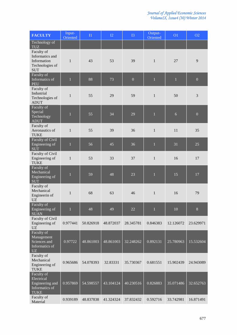
Journal of Applied Economic Sciences VolumeIX, Issue4 (30) Winter 2014
677
FACULTY Input-
Oriented I1 I2 I3
Output-
Oriented O1 O2
Technology of
TUZ
Faculty of
Informatics and
Information
Technologies of
SUT
1 43 53 39 1 27 9
Faculty of
Informatics of
PEU
1 88 73 0 1 1 0
Faculty of
Industrial
Technologies of
ADUT
1 55 29 59 1 50 3
Faculty of
Special
Technology
ADUT
1 55 34 29 1 6 0
Faculty of
Aeronautics of
TUKE
1 55 39 36 1 11 35
Faculty of Civil
Engineering of
SUT
1 56 45 36 1 31 25
Faculty of Civil
Engineering of
TUKE
1 53 33 37 1 16 17
Faculty of
Mechanical
Engineering of
SUT
1 59 48 23 1 15 17
Faculty of
Mechanical
Engineerin of
UZ
1 68 63 46 1 16 79
Faculty of
Engineering of
SUAN
1 48 49 22 1 10 8
Faculty of Civil
Engineering of
UZ
0.977441 50.826918 48.872037 28.345781 0.846383 12.126072 23.629971
Faculty of
Management
Sciences and
Informatics of
UZ
0.97722 48.861003 48.861003 32.248262 0.892131 25.780963 15.532604
Faculty of
Mechanical
Engineering of
TUKE
0.965686 54.078393 32.83331 35.730367 0.681551 15.902439 24.943089
Faculty of
Electrical
Engineering and
Informatics of
TUKE
0.957869 54.598557 43.104124 40.230516 0.826883 35.071486 32.652763
Faculty of
Material 0.939189 48.837838 41.324324 37.832432 0.592716 33.742981 16.871491
Journal of Applied Economic Sciences VolumeIX, Issue4 (30) Winter 2014
678
FACULTY Input-
Oriented I1 I2 I3
Output-
Oriented O1 O2
Science and
technology in
Trnava of SUT
Faculty of
Metallurgy of
TUKE
0.908422 63.784136 34.520033 39.970565 0.74187 44.482203 33.963559
Faculty of
Manufacturing
Technologies of
TUKE
0.901764 47.793468 51.400523 39.152423 0.605656 28.068733 34.673141
Faculty of
Architecture of
SUT
0.865421 47.598131 49.321495 23.366355 0.161487 12.384899 24.769799
Group of Natural Sciences
Results of Data Enveloping Analysis of Natural Sciences group are presented in Table 2.
One can see that according to this analysis, group of Natural Sciences as a whole has reached one
of the best results in both models. Only one faculty has not achieved the effective border. It is the
Faculty of Natural Sciences of Comenius University in Bratislava, which is nevertheless very close
to the optimum boundary.
Table 2 - Natural Sciences
FACULTY Input-
Oriented I1 I2 I3
Output-
Oriented O1 O2
Faculty of Ecology
and Environmental
Sciences of TUZ
1 61 43 45 1 16 36
Faculty of
Mathematics,
Physics and
Informatics of
CUB
1 83 76 86 1 100 88
Faculty of Natural
Sciences of UCMT 1 77 54 45 1 35 9
Faculty of Natural
Sciences of CPUN 1 61 70 41 1 27 23
Faculty of Natural
Sciences of UMB 1 62 54 41 1 21 17
Faculty of Science
of PJSUK 1 94 60 72 1 79 70
Faculty of Natural
Sciences of CUB 0.987026 72.052885 63.992788 64.944712 0.95261 62.984848 62.984848
Group of Medical Sciences
Results of Data Envelopment Analysis for Medical Sciences are depicted in Table 3. The
analysis shows that in the Medical Sciences group, the majority of faculties work on the efficient
frontier. Beyond this limit are only the Faculty of Public Health of the Catholic University in
Ruzomberok and the Faculty of Medicine of Comenius University in Bratislava.
Table 3 - Medical Sciences
FACULTY Input-
Oriented I1 I2 I3
Output-
Oriented O1 O2
Faculty of Social
Sciences and Health Care
of CPUN
1 53 35 36 1 65 10
Faculty of Health Care of
UPP 1 42 48 0 1 8 19
Faculty of Health Care 1 68 33 47 1 29 24
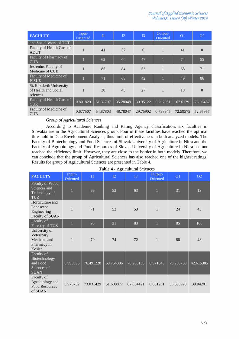
Journal of Applied Economic Sciences VolumeIX, Issue4 (30) Winter 2014
679
FACULTY Input-
Oriented I1 I2 I3
Output-
Oriented O1 O2
and Social Work of TUT
Faculty of Health Care of
ADUT 1 41 37 0 1 41 0
Faculty of Pharmacy of
CUB 1 62 66 47 1 74 55
Jessenius Faculty of
Medicine of CUB 1 85 84 53 1 65 71
Faculty of Medicine of
PJSUK 1 71 68 42 1 49 86
St. Elizabeth University
of Health and Social
sciences
1 38 45 27 1 10 0
Faculty of Health Care of
CUR 0.801829 51.31707 35.28049 30.95122 0.207061 67.6129 23.06452
Faculty of Medicine of
CUB 0.677507 54.87803 48.78047 29.75902 0.798945 72.59575 52.65957
Group of Agricultural Sciences
According to Academic Ranking and Rating Agency classification, six faculties in
Slovakia are in the Agricultural Sciences group. Four of these faculties have reached the optimal
threshold in Data Envelopment Analysis, thus limit of effectiveness in both analyzed models. The
Faculty of Biotechnology and Food Sciences of Slovak University of Agriculture in Nitra and the
Faculty of Agrobiology and Food Resources of Slovak University of Agriculture in Nitra has not
reached the efficiency limit. However, they are close to the border in both models. Therefore, we
can conclude that the group of Agricultural Sciences has also reached one of the highest ratings.
Results for group of Agricultural Sciences are presented in Table 4.
Table 4 - Agricultural Sciences
FACULTY Input-
Oriented I1 I2 I3
Output-
Oriented O1 O2
Faculty of Wood
Sciences and
Technology of
TUZ
1 66 52 63 1 31 13
Horticulture and
Landscape
Engineering
Faculty of SUAN
1 71 52 53 1 24 43
Faculty of
Forestry of TUZ 1 95 31 83 1 85 100
University of
Veterinary
Medicine and
Pharmacy in
Košice
1 79 74 72 1 88 48
Faculty of
Biotechnology
and Food
Sciences of
SUAN
0.993393 76.491228 69.754386 70.263158 0.971845 79.230769 42.615385
Faculty of
Agrobiology and
Food Resources
of SUAN
0.973752 73.031429 51.608877 67.854421 0.881201 55.605928 39.04281
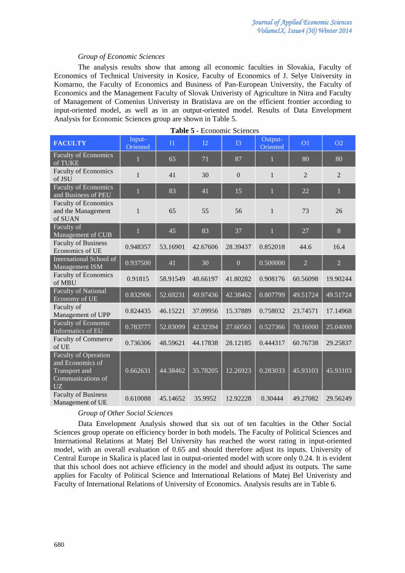
Journal of Applied Economic Sciences VolumeIX, Issue4 (30) Winter 2014
680
Group of Economic Sciences
The analysis results show that among all economic faculties in Slovakia, Faculty of
Economics of Technical University in Kosice, Faculty of Economics of J. Selye University in
Komarno, the Faculty of Economics and Business of Pan-European University, the Faculty of
Economics and the Management Faculty of Slovak Univeristy of Agriculture in Nitra and Faculty
of Management of Comenius Univeristy in Bratislava are on the efficient frontier according to
input-oriented model, as well as in an output-oriented model. Results of Data Envelopment
Analysis for Economic Sciences group are shown in Table 5.
Table 5 - Economic Sciences
FACULTY Input-
Oriented I1 I2 I3
Output-
Oriented O1 O2
Faculty of Economics
of TUKE 1 65 71 87 1 80 80
Faculty of Economics
of JSU 1 41 30 0 1 2 2
Faculty of Economics
and Business of PEU 1 83 41 15 1 22 1
Faculty of Economics
and the Management
of SUAN
1 65 55 56 1 73 26
Faculty of
Management of CUB 1 45 83 37 1 27 8
Faculty of Business
Economics of UE 0.948357 53.16901 42.67606 28.39437 0.852018 44.6 16.4
International School of
Management ISM 0.937500 41 30 0 0.500000 2 2
Faculty of Economics
of MBU 0.91815 58.91549 48.66197 41.80282 0.908176 60.56098 19.90244
Faculty of National
Economy of UE 0.832906 52.69231 49.97436 42.38462 0.807799 49.51724 49.51724
Faculty of
Management of UPP 0.824435 46.15221 37.09956 15.37889 0.758032 23.74571 17.14968
Faculty of Economic
Informatics of EU 0.783777 52.83099 42.32394 27.60563 0.527366 70.16000 25.04000
Faculty of Commerce
of UE 0.736306 48.59621 44.17838 28.12185 0.444317 60.76738 29.25837
Faculty of Operation
and Economics of
Transport and
Communications of
UZ
0.662631 44.38462 35.78205 12.26923 0.283033 45.93103 45.93103
Faculty of Business
Management of UE 0.610088 45.14652 35.9952 12.92228 0.30444 49.27082 29.56249
Group of Other Social Sciences
Data Envelopment Analysis showed that six out of ten faculties in the Other Social
Sciences group operate on efficiency border in both models. The Faculty of Political Sciences and
International Relations at Matej Bel University has reached the worst rating in input-oriented
model, with an overall evaluation of 0.65 and should therefore adjust its inputs. University of
Central Europe in Skalica is placed last in output-oriented model with score only 0.24. It is evident
that this school does not achieve efficiency in the model and should adjust its outputs. The same
applies for Faculty of Political Science and International Relations of Matej Bel Univeristy and
Faculty of International Relations of University of Economics. Analysis results are in Table 6.
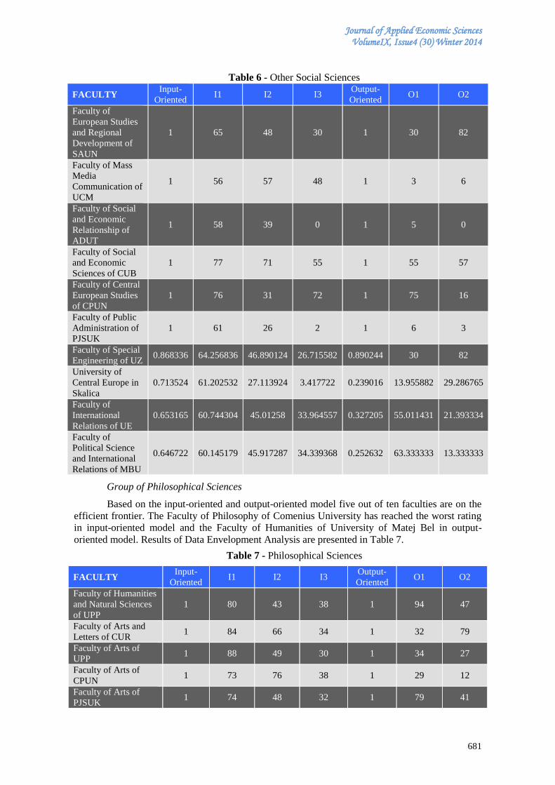
Journal of Applied Economic Sciences VolumeIX, Issue4 (30) Winter 2014
681
Table 6 - Other Social Sciences
FACULTY Input-
Oriented I1 I2 I3
Output-
Oriented O1 O2
Faculty of
European Studies
and Regional
Development of
SAUN
1 65 48 30 1 30 82
Faculty of Mass
Media
Communication of
UCM
1 56 57 48 1 3 6
Faculty of Social
and Economic
Relationship of
ADUT
1 58 39 0 1 5 0
Faculty of Social
and Economic
Sciences of CUB
1 77 71 55 1 55 57
Faculty of Central
European Studies
of CPUN
1 76 31 72 1 75 16
Faculty of Public
Administration of
PJSUK
1 61 26 2 1 6 3
Faculty of Special
Engineering of UZ 0.868336 64.256836 46.890124 26.715582 0.890244 30 82
University of
Central Europe in
Skalica
0.713524 61.202532 27.113924 3.417722 0.239016 13.955882 29.286765
Faculty of
International
Relations of UE
0.653165 60.744304 45.01258 33.964557 0.327205 55.011431 21.393334
Faculty of
Political Science
and International
Relations of MBU
0.646722 60.145179 45.917287 34.339368 0.252632 63.333333 13.333333
Group of Philosophical Sciences
Based on the input-oriented and output-oriented model five out of ten faculties are on the
efficient frontier. The Faculty of Philosophy of Comenius University has reached the worst rating
in input-oriented model and the Faculty of Humanities of University of Matej Bel in output-
oriented model. Results of Data Envelopment Analysis are presented in Table 7.
Table 7 - Philosophical Sciences
FACULTY Input-
Oriented I1 I2 I3
Output-
Oriented O1 O2
Faculty of Humanities
and Natural Sciences
of UPP
1 80 43 38 1 94 47
Faculty of Arts and
Letters of CUR 1 84 66 34 1 32 79
Faculty of Arts of
UPP 1 88 49 30 1 34 27
Faculty of Arts of
CPUN 1 73 76 38 1 29 12
Faculty of Arts of
PJSUK 1 74 48 32 1 79 41
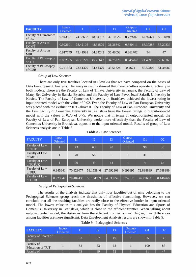
Journal of Applied Economic Sciences VolumeIX, Issue4 (30) Winter 2014
682
FACULTY Input-
Oriented I1 I2 I3
Output-
Oriented O1 O2
Faculty of Humanities
of UZ 0.943371 74.52632 48.94737 32.10526 0.779707 67.97424 55.14891
Faculty of Arts of
UCMT 0.922601 78.42105 48.31579 31.36842 0.380411 66.37288 55.20339
Faculty of Arts on
MBU 0.917749 73.41991 64.24242 35.48052 0.361702 94 47
Faculty of Philosophy
of TU 0.862385 76.75229 45.70642 34.75229 0.545762 71.45978 58.63366
Faculty of Philosophy
of CUB 0.741553 73.41379 64.41379 35.51724 0.46741 85.57804 51.34682
Group of Law Sciences
There are only five faculties located in Slovakia that we have compared on the bases of
Data Envelopment Analysis. The analysis results showed that three faculties operate effectively in
both models. These are the Faculty of Law of Trnava University in Trnava, the Faculty of Law of
Matej Bel University in Banska Bystrica and the Faculty of Law Pavol Jozef Safarik University in
Kosice. The Faculty of Law of Comenius University in Bratislava achieved the lowest rating in
input-oriented model with the value of 0.92. Even the Faculty of Law of Pan European University
was placed with the evaluation 0.95 above it. The Faculty of Law of Pan European University and
the Law Faculty of Comenius University in Bratislava have the lowest ratings in output-oriented
model with the values of 0.70 of 0.75. We notice that in terms of output-oriented model, the
Faculty of Law of Pan European University works more effectively than the Faculty of Law of
Comenius University in Bratislava, opposite to the input-oriented model. Results of group of Law
Sciences analysis are in Table 8.
Table 8 - Law Sciences
FACULTY Input-
Oriented I1 I2 I3
Output-
Oriented O1 O2
Faculty of Law
of TUT 1 73 63 90 1 96 38
Faculty of Law
of MBU 1 70 56 0 1 31 9
Faculty of Law
of PJSUK 1 90 49 64 1 71 67
Faculty of Law
of PEU 0.945641 70.923077 58.153846 27.692308 0.699695 72.888889 27.688889
Faculty of Law
of CUB 0.923342 79.407435 56.164709 64.633959 0.74817 76.79602 60.146766
Group of Pedagogical Sciences
The results of the analysis indicate that only four faculties out of nine belonging to the
Pedagogical Sciences group reach the thresholds of effective functioning. However, we can
conclude that all the teaching faculties are really close to the effective border in input-oriented
model. The lowest value in this analysis has the Faculty of Physical Education and Sports of
Comenius University in Bratislava, which is close to the efficient frontier. When talking about
output-oriented model, the distances from the efficient frontier is much higher, thus differences
among faculties are more significant. Data Envelopment Analysis results are shown in Table 9.
Table 9 - Pedagogical Sciences
FACULTY Input-
Oriented I1 I2 I3
Output-
Oriented O1 O2
Faculty of Sports of
UPP 1 83 37 19 1 25 39
Faculty of
Education of TUT 1 82 53 62 1 100 87
Faculty of 1 73 69 52 1 31 47
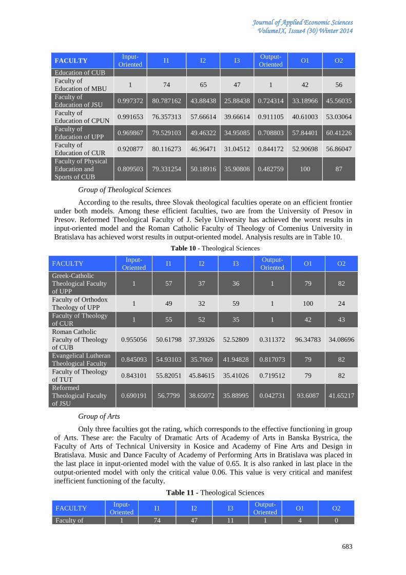
Journal of Applied Economic Sciences VolumeIX, Issue4 (30) Winter 2014
683
FACULTY Input-
Oriented I1 I2 I3
Output-
Oriented O1 O2
Education of CUB
Faculty of
Education of MBU 1 74 65 47 1 42 56
Faculty of
Education of JSU 0.997372 80.787162 43.88438 25.88438 0.724314 33.18966 45.56035
Faculty of
Education of CPUN 0.991653 76.357313 57.66614 39.66614 0.911105 40.61003 53.03064
Faculty of
Education of UPP 0.969867 79.529103 49.46322 34.95085 0.708803 57.84401 60.41226
Faculty of
Education of CUR 0.920877 80.116273 46.96471 31.04512 0.844172 52.90698 56.86047
Faculty of Physical
Education and
Sports of CUB
0.809503 79.331254 50.18916 35.90808 0.482759 100 87
Group of Theological Sciences
According to the results, three Slovak theological faculties operate on an efficient frontier
under both models. Among these efficient faculties, two are from the University of Presov in
Presov. Reformed Theological Faculty of J. Selye University has achieved the worst results in
input-oriented model and the Roman Catholic Faculty of Theology of Comenius University in
Bratislava has achieved worst results in output-oriented model. Analysis results are in Table 10.
Table 10 - Theological Sciences
FACULTY Input-
Oriented I1 I2 I3
Output-
Oriented O1 O2
Greek-Catholic
Theological Faculty
of UPP
1 57 37 36 1 79 82
Faculty of Orthodox
Theology of UPP 1 49 32 59 1 100 24
Faculty of Theology
of CUR 1 55 52 35 1 42 43
Roman Catholic
Faculty of Theology
of CUB
0.955056 50.61798 37.39326 52.52809 0.311372 96.34783 34.08696
Evangelical Lutheran
Theological Faculty 0.845093 54.93103 35.7069 41.94828 0.817073 79 82
Faculty of Theology
of TUT 0.843101 55.82051 45.84615 35.41026 0.719512 79 82
Reformed
Theological Faculty
of JSU
0.690191 56.7799 38.65072 35.88995 0.042731 93.6087 41.65217
Group of Arts
Only three faculties got the rating, which corresponds to the effective functioning in group
of Arts. These are: the Faculty of Dramatic Arts of Academy of Arts in Banska Bystrica, the
Faculty of Arts of Technical University in Kosice and Academy of Fine Arts and Design in
Bratislava. Music and Dance Faculty of Academy of Performing Arts in Bratislava was placed in
the last place in input-oriented model with the value of 0.65. It is also ranked in last place in the
output-oriented model with only the critical value 0.06. This value is very critical and manifest
inefficient functioning of the faculty.
Table 11 - Theological Sciences
FACULTY Input-
Oriented I1 I2 I3
Output-
Oriented O1 O2
Faculty of 1 74 47 11 1 4 0
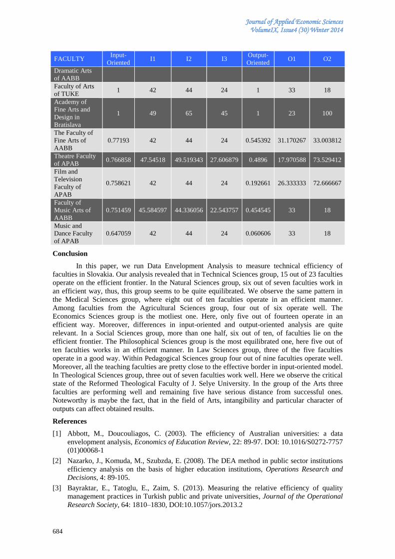
Journal of Applied Economic Sciences VolumeIX, Issue4 (30) Winter 2014
684
FACULTY Input-
Oriented I1 I2 I3
Output-
Oriented O1 O2
Dramatic Arts
of AABB
Faculty of Arts
of TUKE 1 42 44 24 1 33 18
Academy of
Fine Arts and
Design in
Bratislava
1 49 65 45 1 23 100
The Faculty of
Fine Arts of
AABB
0.77193 42 44 24 0.545392 31.170267 33.003812
Theatre Faculty
of APAB 0.766858 47.54518 49.519343 27.606879 0.4896 17.970588 73.529412
Film and
Television
Faculty of
APAB
0.758621 42 44 24 0.192661 26.333333 72.666667
Faculty of
Music Arts of
AABB
0.751459 45.584597 44.336056 22.543757 0.454545 33 18
Music and
Dance Faculty
of APAB
0.647059 42 44 24 0.060606 33 18
Conclusion
In this paper, we run Data Envelopment Analysis to measure technical efficiency of
faculties in Slovakia. Our analysis revealed that in Technical Sciences group, 15 out of 23 faculties
operate on the efficient frontier. In the Natural Sciences group, six out of seven faculties work in
an efficient way, thus, this group seems to be quite equilibrated. We observe the same pattern in
the Medical Sciences group, where eight out of ten faculties operate in an efficient manner.
Among faculties from the Agricultural Sciences group, four out of six operate well. The
Economics Sciences group is the motliest one. Here, only five out of fourteen operate in an
efficient way. Moreover, differences in input-oriented and output-oriented analysis are quite
relevant. In a Social Sciences group, more than one half, six out of ten, of faculties lie on the
efficient frontier. The Philosophical Sciences group is the most equilibrated one, here five out of
ten faculties works in an efficient manner. In Law Sciences group, three of the five faculties
operate in a good way. Within Pedagogical Sciences group four out of nine faculties operate well.
Moreover, all the teaching faculties are pretty close to the effective border in input-oriented model.
In Theological Sciences group, three out of seven faculties work well. Here we observe the critical
state of the Reformed Theological Faculty of J. Selye University. In the group of the Arts three
faculties are performing well and remaining five have serious distance from successful ones.
Noteworthy is maybe the fact, that in the field of Arts, intangibility and particular character of
outputs can affect obtained results.
References
[1] Abbott, M., Doucouliagos, C. (2003). The efficiency of Australian universities: a data
envelopment analysis, Economics of Education Review, 22: 89-97. DOI: 10.1016/S0272-7757
(01)00068-1
[2] Nazarko, J., Komuda, M., Szubzda, E. (2008). The DEA method in public sector institutions
efficiency analysis on the basis of higher education institutions, Operations Research and
Decisions, 4: 89-105.
[3] Bayraktar, E., Tatoglu, E., Zaim, S. (2013). Measuring the relative efficiency of quality
management practices in Turkish public and private universities, Journal of the Operational
Research Society, 64: 1810–1830, DOI:10.1057/jors.2013.2
Journal of Applied Economic Sciences VolumeIX, Issue4 (30) Winter 2014
685
[4] Sav, G.T. (2013). Effects of Financial Source Dependency on Public University Operating
Efficiencies: Data Envelopment Single-Stage and Tobit Two-Stage Evaluations, Review of
Economics and Finance, 3(1): 63-73.
[5] Agasisti, T., Dal Bianco, A. (2006). Data envelopment analysis to the Italian university
system: theoretical issues and policy implications, International Journal of Business
Performance Management, 8(4): 344-367. DOI: 10.1504/IJBPM.2006.009613
[6] Afonso, A., Santos, M. (2008). A DEA Approach to the Relative Efficiency of Portuguese
Public Universities, Portuguese Journal of Management Studies, 13(1): 67-87.
[7] Agasisti, T., Johnes, G. (2009). Beyond frontiers: comparing the efficiency of higher
education decision-making units across more than one country, Education Economics, 17(1):
59-79. DOI:10.1080/09645290701523291
[8] Agasisti, T., Pérez-Esparrells, C. (2010). Comparing efficiency in a cross-country
perspective: the case of Italian and Spanish state universities, Higher Education, 59(1): 85-
103. DOI: 10.1007/s10734-009-9235-8
[9] Afonso, A, ST. Aubyn, M. (2005). Non-parametric Approaches to Education and Health
Expenditure Efficiency in the OECD, Journal of Applied Economics, 8(2): 227-246.
[10] Breu, T.M., Raab, R. L. (1994). Effciency and perceived quality of the nation's top 25
national universities and national liberal arts colleges: an application of data envelopment
analysis to higher education, Socio-Economic Planning Sciences, 28(1): 33-45. DOI: 10.1016
/0038-0121(94)90023-X
[11] Jeck, T., Sudzina, F. (2009). Relatívna efektívnosť univerzít na Slovensku, Úloha univerzít
v regionálnom rozvoji, pp. 84-93., ISBN 978-80-7097-791-0.
[12] Gavurova, B. (2011). Kritické aspekty vysokého školstva na Slovensku, International
Scientific Herald, 3(2): 70-84.
[13] Bednarova, L., Vavrek, R., Vozarova-Kravcakova, I., Kotulic, R., Adamisin, P., Kubak, M.,
Gonos, J., Nemec, J., Dubravska, M., Sira, E. (2014). LMS Moodle as a Communication
Tool of the Students in the Study Programs Environmental Management, Management and
Tourism, Hotel and Spa Industry, Ecology, economics, education and legislation, Conference
Proceedings: 14th
international multidisciplinary scientific geoconference SGEM 2014, 3:
647-653. DOI: 10.5593/SGEM2014/B53/S22.086
[14] Pudło, P., Gavurová, B. (2012). Experimental learning in higher education, using simulation
games as learning tool, SGEM 2012: 12th International Multidisciplinary Scientific
GeoConference: conference proceedings, 17-23 June, 2012, Albena, Bulgaria, Sofia: STEF92
Technology Ltd., 3: 1093-1100.
[15] Pudło, P., Gavurová, B. (2013). Experimental teaching methods in higher education -
practical application, in: SGEM 2013: 13th International Multidisciplinary Scientific
Geoconference: Ecology, Economics, Education and Legislation. 16-22 June, Albena,
Bulgaria. - Albena: STEF92 Technology Ltd., 2: 423-428.
[16] Hudec, O. (2003). Universities - Their New Role in Regional Development?, E+M Ekonomie
a Management, 6: 71-75.
[17] Gavurová, B. (2011). Systém Balanced Scorecard v podnikovom riadení, Ekonomický
časopis, 59(2): 163-177.
[18] Gavurová, B. (2012). Source Identification of Potential Malfunction of Balanced Scorecard
System and Its Influence on System Function, E+M Ekonomie a management, 15(3): 76-90.
[19] Šoltés, V., Gavurová, B. (2013). Application of the cross impact matrix method in
problematic phases of the Balanced Scorecard system in private and public sector, Journal of
Applied Economic Sciences, 8 (1): 99-119.
[20] Szabo, Z.K., Šoltés, M., Herman, E. (2013). Innovative Capacity and Performance of
Transition Economies: Comparative Study at the Level of Enterprises, E+M Ekonomie a
Management, 16(1): 52-68.

Journal of Applied Economic Sciences VolumeIX, Issue4 (30) Winter 2014
686
[21] Užík, M., Šoltés, V. (2009). The Effect of Rating Changes on the Value of a Company Listed
in the Capital Market, E + M Ekonomie a management, 12(1): 49-55.
[22] Banker, R.D., Charnes, A., Cooper, W.W. (1984). Some Models for Estimating Technical and
Scale Inefficiencies in Data Envelopment Analysis, Management Science, 30: 1078–1092,
DOI: 10.1287/mnsc.30.9.1078
[23] Charnes, A.; Cooper W.W., Rhodes, E. (1978). Measuring the efficiency of decision-making
units, European Journal of Operational Research, 2: 429–444. DOI: 10.1016/0377-
2217(78)90138-8
*** Academic Ranking and Rating Agency. 2013. Hodnotenie fakúlt vysokých škôl 2013,
available at: http://www.arra.sk/sites/arra.sk/files/file/ARRA_Sprava_2013.pdf
Journal of Applied Economic Sciences VolumeIX, Issue4 (30) Winter 2014
687
ASSESSMENT METHODOLOGY FOR RESOURCE-EFFICIENT DEVELOPMENT OF ORGANIZATIONS IN THE CONTEXT OF THE
GREEN ECONOMY
Irina A. MARKINA
Poltava National Technical Yuri Kondratuyk University, Poltava, Ukraine
Antonina V. SHARKOVA
Federal State Budgetary Education Institution of Higher Professional Education
“Financial University under the Government of the Russian Federation”, Moscow, Russia
Abstract:
The paper deals with the problem of forming comprehensive methodology for determining the level
of economic, social and environmental performance of all organizations. The system of indicators that allow
an individual to make a forecast of the development of economy under the conditions of its transition from
“brown” to a “green” one is proposed by authors. These indicators can be grouped into three categories:
indicators of economic transformation, indicators of progress and well-being, and indicators of resource
efficiency. An assessment methodology for resource-efficient development at the macro level was created in
accordance with the international standard of the Global Reporting Initiative and methodology for
sustainable development of the industrial organizations. This methodology is based on specific categories of
indicators of organization’s sustainable development, such as the indicators of economic sustainability,
social sustainability and environmental sustainability. The main stages in the formation and implementation
of the methodology in the performance of an organization are presented in the given paper.
Keywords: green economy, brown economy, sustainable development, ecology, green economy indicators.
JEL Classification: Q01, Q57
1. Introduction
A shift towards a green economy defined the beginning of a new stage of the development
of our society, when the existing paradigm is replaced by a new paradigm for the low carbon
energy, necessary for sustainable economic development. In recent decades the most prominent
scientists, experts and politicians regard the priority task to ensure a comprehensive and balanced
development of civilization, as defined by the main task in twenty-first century. The overcoming
of the modern society ecological crisis, as well as improving of the ecological state of the
environment and resource management requires immediate transition to sustainable ecological and
socio-economic development, like in most technologically advanced countries all over the world.
Nowadays particular attention is paid to the search for possible solutions to the urgent problems of
eco-economic theory and to the formation of a modern paradigm of economic and environmental
management, grounding on the “green” economy. The development of methodology and
conceptual principles of sustainable development is no less important than economic education in
the context of myriad of global transformational and environmental challenges faced by certain
countries, regions and continents. It should be mentioned that “green” economy as a system of
economic activities ensures agreeable combination of three components of sustainable economic,
environmental and social development.
2. Main text
Since the mid 90-ies of XX century in many developed countries monitoring of sustainable
development of the economy has become an effective tool in the field of corporate governance.
However, in transition economies work in this area is complicated due to the lack of developed
and introduced methodological guidelines and systems of indicators of sustainable development,
which could form the basis of the national economy green development (Podvorskaya, 2012).
Moreover, when evaluating the performance of sustainable development of an organization, as a
rule, there are particular problems associated with the lack of information support for monitoring.
These problems are as follows: incomplete information, timeliness of its receipt, which, of course,
Journal of Applied Economic Sciences VolumeIX, Issue4 (30) Winter 2014
688
complicate an evaluation of sustainable development of industrial organizations, but can be used
for a variety of research in order to improve the process of evaluation.
The concept of sustainable development was offered by the United Nations and is reflected
in the documents of the United Nations Conference on Environment and Development, held in Rio
de Janeiro, Brazil (1992). The main result of the Conference was the creation of a new global
partnership for sustainable development, which recognizes the common approach to the issues of
environmental protection and socio-economic development. In this regard, scientists and
politicians consider sustainable development as the development, which meets the needs of the
present without compromising the ability of future generations to meet their own needs (Keating,
1993). Achieving sustainable development in any country is impossible without the achievement
of sustainable development of its individual regions, and sustainable development of any region, in
turn, is impossible without the effective functioning of organizations in the region. Thus, not only
the governments are engaged in the creation of national strategies for sustainable development, but
also the largest transnational corporations are paying a lot of attention to the development and
implementation of their own corporate plans for sustainable development. The nature of these
plans is to ensure that these corporations could overcome the directly proportional relationship
between the level of economic development and the level of negative impact of their production
performance on the environment (Kenneth, 2010).
The issue of the green economic development has become increasingly important area of
investigation over the last decade. Our empirical analysis of the theoretical approaches to creating
a system of indicators of the development of an organization in the emerging of a green economy
showed that they need further development (Galushkina, 2011), (Musina, 2012) and (Yamchuk,
2013). Moreover, with the rapid development of market mechanisms there is a problem, associated
with the need to develop a system of indicators for the analysis of sustainable development of
organizations in the transition to a green economy. No less important problem is the practical
application of a single mechanism, able to ensure the sustainability of enterprises at different
stages of their life cycles. All this together defines the purpose of our study.
At the present stage of transformational changes, economists and political scientists
developed a number of techniques that can be used to carry out the forecast level of economic
development, provided its transition from “brown” to “green” economy. The most common of
these procedures are as follows: disaggregation model sequence, computational model of general
equilibrium, macro-econometric models and system dynamics models (Pearce, Atkinson, 1993).
But these techniques are mainly used for the analysis at the short and medium period financial
planning and are not suitable for incorporation in the whole of a variety of economic,
environmental and social growth indicators. The most general system of indicators to measure the
level of greening the economy at the macro level is the system, proposed by The United Nations
Environment Programme (UNEP), which has defined three principal directions for the work on
green economy indicators:
Indicators of economic transformation. A green economy is first and foremost about
transforming the way economies grow. It requires huge investments capital to shift towards low
carbon, clean, waste minimizing, resource efficient and ecosystem, enhancing activities. The main
indicators of economic transformation include the major shift in investments. Certain existing
classifications in the national accounts, such as environmental goods and services sector,
developed by Eurostat, provide an appropriate starting point for measuring transformation to a
green economy, alongside various initiatives, especially in the private sector, to control green
investment flows.
Indicators of resource efficiency. A key benefit of economic transformation, apart from
expected net increase in income and jobs in the medium and long term period, is improved
resource efficiency in relative or absolute terms. Fundamental indicators include those on the use
of materials, energy, water, land, changes to ecosystems and emissions of dangerous substances,
related to economic activity. The International Panel on Sustainable Resource Management has
proposed optimal indicators to capture some of these impacts, which can provide a framework for
further performance in this area. The incentive is given to this area by the EU’s 2020 Strategy for a
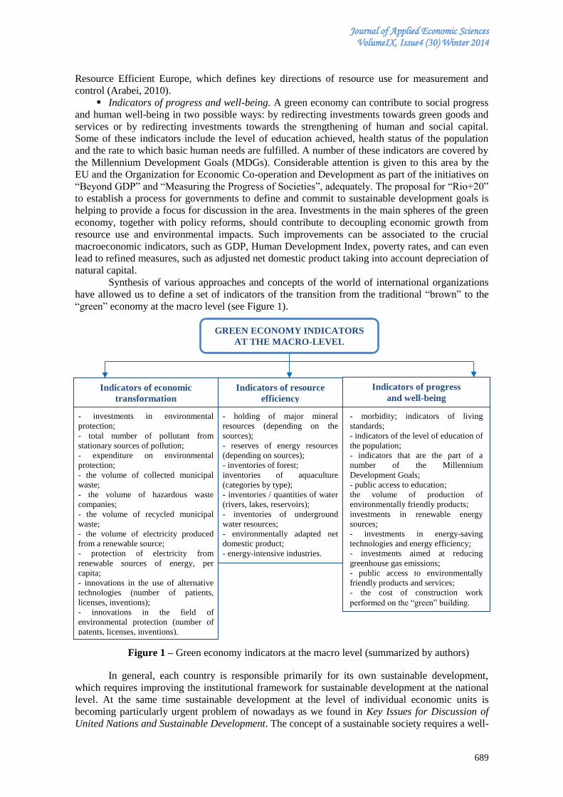
Journal of Applied Economic Sciences VolumeIX, Issue4 (30) Winter 2014
689
Resource Efficient Europe, which defines key directions of resource use for measurement and
control (Arabei, 2010).
Indicators of progress and well-being. A green economy can contribute to social progress
and human well-being in two possible ways: by redirecting investments towards green goods and
services or by redirecting investments towards the strengthening of human and social capital.
Some of these indicators include the level of education achieved, health status of the population
and the rate to which basic human needs are fulfilled. A number of these indicators are covered by
the Millennium Development Goals (MDGs). Considerable attention is given to this area by the
EU and the Organization for Economic Co-operation and Development as part of the initiatives on
“Beyond GDP” and “Measuring the Progress of Societies”, adequately. The proposal for “Rio+20”
to establish a process for governments to define and commit to sustainable development goals is
helping to provide a focus for discussion in the area. Investments in the main spheres of the green
economy, together with policy reforms, should contribute to decoupling economic growth from
resource use and environmental impacts. Such improvements can be associated to the crucial
macroeconomic indicators, such as GDP, Human Development Index, poverty rates, and can even
lead to refined measures, such as adjusted net domestic product taking into account depreciation of
natural capital.
Synthesis of various approaches and concepts of the world of international organizations
have allowed us to define a set of indicators of the transition from the traditional “brown” to the
“green” economy at the macro level (see Figure 1).
Figure 1 – Green economy indicators at the macro level (summarized by authors)
In general, each country is responsible primarily for its own sustainable development,
which requires improving the institutional framework for sustainable development at the national
level. At the same time sustainable development at the level of individual economic units is
becoming particularly urgent problem of nowadays as we found in Key Issues for Discussion of
United Nations and Sustainable Development. The concept of a sustainable society requires a well-
GREEN ECONOMY INDICATORS
AT THE MACRO-LEVEL
- investments in environmental
protection;
- total number of pollutant from
stationary sources of pollution;
- expenditure on environmental
protection;
- the volume of collected municipal
waste;
- the volume of hazardous waste
companies;
- the volume of recycled municipal
waste;
- the volume of electricity produced
from a renewable source;
- protection of electricity from
renewable sources of energy, per
capita;
- innovations in the use of alternative
technologies (number of patients,
licenses, inventions);
- innovations in the field of
environmental protection (number of
patents, licenses, inventions).
- holding of major mineral
resources (depending on the
sources);
- reserves of energy resources
(depending on sources);
- inventories of forest;
inventories of aquaculture
(categories by type);
- inventories / quantities of water
(rivers, lakes, reservoirs);
- inventories of underground
water resources;
- environmentally adapted net
domestic product;
- energy-intensive industries.
- morbidity; indicators of living
standards;
- indicators of the level of education of
the population;
- indicators that are the part of a
number of the Millennium
Development Goals;
- public access to education;
the volume of production of
environmentally friendly products;
investments in renewable energy
sources;
- investments in energy-saving
technologies and energy efficiency;
- investments aimed at reducing
greenhouse gas emissions;
- public access to environmentally
friendly products and services;
- the cost of construction work
performed on the “green” building.
Indicators of economic
transformation
Indicators of resource
efficiency
Indicators of progress
and well-being
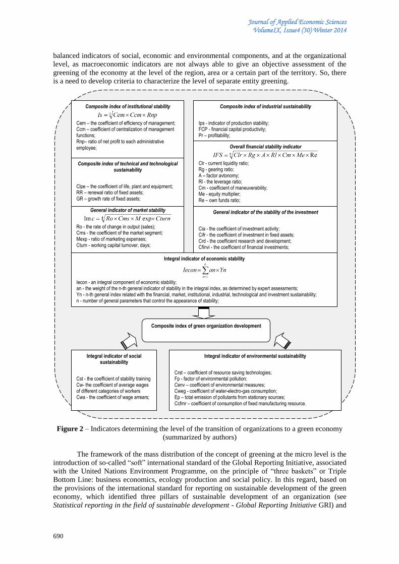
Journal of Applied Economic Sciences VolumeIX, Issue4 (30) Winter 2014
690
balanced indicators of social, economic and environmental components, and at the organizational
level, as macroeconomic indicators are not always able to give an objective assessment of the
greening of the economy at the level of the region, area or a certain part of the territory. So, there
is a need to develop criteria to characterize the level of separate entity greening.
Figure 2 – Indicators determining the level of the transition of organizations to a green economy
(summarized by authors)
The framework of the mass distribution of the concept of greening at the micro level is the
introduction of so-called “soft” international standard of the Global Reporting Initiative, associated
with the United Nations Environment Programme, on the principle of “three baskets” or Triple
Bottom Line: business economics, ecology production and social policy. In this regard, based on
the provisions of the international standard for reporting on sustainable development of the green
economy, which identified three pillars of sustainable development of an organization (see
Statistical reporting in the field of sustainable development - Global Reporting Initiative GRI) and
Composite index of green organization development
Integral indicator of economic stability
Iecon - an integral component of economic stability; an - the weight of the n-th general indicator of stability in the integral index, as determined by expert assessments; Yn - n-th general index related with the financial, market, institutional, industrial, technological and investment sustainability; n - number of general parameters that control the appearance of stability;
Overall financial stability indicator
Clr - current liquidity ratio; Rg - gearing ratio; A – factor avtonomy; Rl - the leverage ratio; Cm - coefficient of maneuverability; Me - equity multiplier; Re – own funds ratio;
General indicator of market stability
Ro - the rate of change in output (sales); Cms - the coefficient of the market segment; Mexp - ratio of marketing expenses; Cturn - working capital turnover, days;
Composite index of institutional stability
Cem – the coefficient of efficiency of management; Ccm – coefficient of centralization of management functions; Rnp– ratio of net profit to each administrative
employee;
Composite index of industrial sustainability
Ips - indicator of production stability; FCP - financial capital productivity; Pr – profitability;
Composite index of technical and technological sustainability
Clpe – the coefficient of life, plant and equipment; RR – renewal ratio of fixed assets; GR – growth rate of fixed assets;
General indicator of the stability of the investment
Cia - the coefficient of investment activity; Cifr - the coefficient of investment in fixed assets; Crd - the coefficient research and development; Cfinvi - the coefficient of financial investments;
Integral indicator of social sustainability
Cst - the coefficient of stability training Cw- the coefficient of average wages of different categories of workers Cwa - the coefficient of wage arrears;
Integral indicator of environmental sustainability
Crst – coefficient of resource saving technologies; Fp - factor of environmental pollution; Cenv – coefficient of environmental measures; Cweg - coefficient of water-electro-gas consumption; Ep – total emission of pollutants from stationary sources; Ccfmr – coefficient of consumption of fixed manufacturing resource.
Journal of Applied Economic Sciences VolumeIX, Issue4 (30) Winter 2014
691
taking into account the methodology for sustainable development of an industrial organization,
proposed (Homyachenkova, 2010) which is based on the principles of operation of the business to
ensure the transformation of the internal environment of an organization for the purpose of self-
preservation and reproduction of social and economic processes, we proposed a methodology of
determining the extent of greening on the macro level. This methodology is based on the
relationship of the interrelated set of indicators for sustainable development of an organization (see
Figure 2).
As can be seen from Figure 2, in the proposed method the economic stability of the
enterprise combines several parameters: financial, market, organizational, industrial, technical and
technological, investment sustainability, each of which corresponds to a number of indicators.
Under each type of the sustainability of an organization is a general indicator of sustainability. The
integral indicator of economic stability is calculated by summing the weighting of each type of
economic stability. The distribution of the weight of each factor, of course, is a subjective factor in
the assessment, which is present only in the calculation of economic sustainability. However, in
the case of expansion of the system performance and, therefore, the scope of evaluation of
sustainable development, in particular, social and environmental components will be able to
introduce the factor of peer review and other components of sustainable development of an
organization. This dynamic system can be considered stable only in the case where all the elements
are in a balanced state.
One of the most important elements of an organization as a production system is
considered to be the staffs who act as a basis to assess the social sustainability of the organization.
As an integral part of the green economy, social stability of the organization reflects the degree of
social protection of its staff, the proportion of staff participation in the profits and in the
management of production, stability in maintaining employment and so on, as in Sustainability
Reporting Guidelines. 2014. In a broad sense, social sustainability provides attracting of
organization’s staff to the various social processes. In determining the degree of social stability, it
is necessary to allocate three important indicators: staff stability coefficients, coefficients of
average wages of different categories of workers and the debt ratio on wages.
The main goal of sustainable development management of an organization is to achieve a
harmonious relationship between the economic, social and ecological functional areas. Moreover,
the influence of organizations on the environment is a separate component of their functional
structures. Environmentally sustainable organization accounts for the possibility of integrated
solutions to economic and environmental issues in their investment decisions, as well as in
determining the level of consumption of limited natural capital in the production process. In order
to analyze the environmental sustainability we developed a set of the following indicators: the
coefficient of resource-saving technologies, the ratio of pollution factor of environmental
protection measures, the ratio of water-electricity-gas-consumption, ratio of emissions from
stationary sources and the coefficient of consumption of fixed production resource.
The use of resource-saving technologies contributes positively to the increase in the degree
of environmental sustainability of an organization. That is why in the process of determining the
integral indicator of environmental sustainability special emphasis should be given to the
coefficient of resource-saving technologies, which is the ratio between the level of the cost of
alternative technologies and the net profit of the organization. Thus, in terms of repetitive
production cycles in each industrial organization the adverse consequences, related with the
economic, social and environmental instability, may suffer.
The proposed method of greening an organization belongs to the category management
processes, which implement in some interconnected stages.
Step 1: Formation of management framework for greening of a certain organization is a
purposeful process, which provides for setting and achieving certain goals. The first step is to
formulate a strategy, objectives, functions, principles and techniques of business management, as
well as to specify the subject and object management within the organizational concept of
transition to a green economy, and to promote economic and social development in the framework
of the existing environmental paradigm. The formation of a strategy for the development of green
businesses requires the use of the approaches defined in international recommendations for public
Journal of Applied Economic Sciences VolumeIX, Issue4 (30) Winter 2014
692
reporting on sustainable development as was related in The Living Planet Report. 2010. It follows
a series of problems that need to be formalized by the relationship between economic and non-
economic indicators to determine their actual and normative values as well as to perform
structuring problems by constructing particular decision trees.
Step 2: Qualitative and quantitative analysis of external and internal stability factors on the
basis of indicators of the current state and development of the organization for the purpose of early
warning of danger and the development of the necessary measures aimed at greening activities. In
a second step is necessary to choose specific techniques of monitoring needed to analyze the level
of greening of an organization. Analysis of the key factors on the sustainable development of the
organization should be carried out in the following order: 1) qualitative and quantitative
determination of the effect of internal and external social, environmental, economic and risk
factors on the economic performance of the organization; 2) qualitative and quantitative
determination of the influence of factors of economic activity indicators for sustainable
development of the organization.
Step 3: Evaluation and analysis of the level of development of the greening of an
organization. At this stage it is necessary to define a specific set of indicators and composite index
of green organization development. The proposed algorithm for analyzing the correspondence
between the economic activities of the organization and its green development tasks should be
based on the state of the financial and economic indicators and indicators of sustainable
development (Tsarev, 2006).
Step 4: As a result of analysis and assessment of the level of greening activities of a certain
business unit, it identifies the need for the development and conduct of administrative decisions
and recommendations with targets, functions, principles and methods of control. A list of
recommendations to guide organizations to improve their stability in a volatile market environment
can be developed on the basis of the results of the main trends of greening business area analysis.
Step 5: Making statements. Information should be presented in the form of public
reporting, developed on the basis of the methodology and technology of the balanced scorecard
(BSC) and international guidelines for public reporting on sustainable development. Such an
important information should be distributed to all participants in the process and be available to
both external and internal users.
Conclusion
As a result of the research, we developed a methodology for assessing the level of
greening of organizations, which is distinguished by the presence of the complex analysis of
sustainable development and the possibility of obtaining composite index based on a set of
indicators. Forming mechanism of the transition from a brown to a green economy by this
technique, the organization will be able to direct the economic activities in such a way as to meet
the international requirements of sustainable development, to address social, environmental and
risky task, ensuring that in the end, their competitiveness and viability. The implementation of the
proposals presented in this paper will contribute to solving the problems of rational use of natural
resources, improve the environmental, physical and spiritual quality of life of citizens, improving
environmental safety. A promising direction for research on this issue is the differentiation of
indicators of greening the various areas of economic activity, through which it is possible to
determine the readiness of organizations to function under conditions of ecological and socio-
economic space and test the proposed methodology.
References
[1] Arabei, E. (2010). The new European strategy “Europe 2020”, http://eulaw.ru/content/307
(accessed October 28, 2014)
[2] Galushkina, T. (2011). “Green” vector of the economy of Ukraine, Economist Ukrainian
Journal, 11: 4–7.
[3] Homyachenkova, N. (2010). Modern aspects of monitoring sustainable development of
industrial enterprises: methodology and practice. Economic Studies, Center of Economic
Research, No. 2, http://www.erce.ru/internet-magazine/magazine/18/298 (accessed November

Journal of Applied Economic Sciences VolumeIX, Issue4 (30) Winter 2014
693
1, 2014)
[4] Keating, M. (1993). The Earth Summit’s Agenda for Change: a plain language version of
Agenda 21 and the other Rio agreements (Geneva: the Centre for Our Common Future),
https://www.iisd.org/rio+5/agenda/ (accessed October 28, 2014)
[5] Kenneth, M. (2010). What Green Economics? An age of global transformation – An Age of
Green Economics, The Green Economics Institute, http://www.greeneconomics.org.uk/
page857.html (accessed October 27, 2014)
[6] Musina, L. (2012). Green technology and innovation as a driver of economic growth: public
policy and development prospects. Scientific and Technical Information, 4: 22–28.
[7] Pearce D., Atkinson G. (1993). Capital theory and the measurement of sustainable
development: an indicator of “weak” sustainability, Ecological Economics, 8(2): 103 – 108,
http://dx.doi.org/10.1016/0921-8009(93)90039-9
[8] Podvorskaya, K. (2012). Formation of a system of indicators for sustainable development of
the enterprise (for example, Timber Company), Ecological Bulletin: Scientific and Practical
Journal, 3 (21): 60–70.
[9] Tsarev, S. (2006). The place and role of investment planning for the sustainability of the
enterprise, Scientific Bulletin of Murmansk State Technical University, 9: 686–689.
[10] Yamchuk, A. (2013). Green industrial growth as an alternative model of economic
development: international and national aspects, Scientific and Technical Information, 4: 13–
20.
*** Statistical reporting in the field of sustainable development. Global Reporting Initiative (GRI),
https://www.globalreporting.org/reporting/Pages/default.aspx (accessed October 28, 2014).
*** Sustainability Reporting Guidelines. (2014). Global Corporate Register reporting initiative,
http://www.corporateregister.com/?d=1 (accessed October 28, 2014).
*** The Living Planet Report. (2010). Biodiversity, biocapacity and development: Report of the
World Wildlife Fund of the Living Planet. Gland, Switzerland: WWF: 92, http://www.foot
printnetwork.org/press/LPR2010.pdf (accessed October 27, 2014)
*** United Nations and sustainable development. Key issues for discussion. Industry,
http://www.un.org/ru/development/sustainable/industry.shtml (accessed November 1, 2014).
Journal of Applied Economic Sciences VolumeIX, Issue4 (30) Winter 2014
694
MANAGING THE STRUCTURE OF QUALITY COSTS IN CONTEXT OF ACHIEVE "DUAL EMPHASIS"
Patrycja PUDŁO
Higher Vocational State School in Sanok, Department of Economics, Poland
Abstract
Article deals with economical aspects of costs of quality (CoQ). Literature review showed that,
improve of quality can increase level of sales, achieving benefits of "revenue emphasis", decrease costs
achieving benefits of "costs emphasis", simultaneous achieving both effects called "dual emphasis". It also
showed that, "dual emphasis" is hard to achieve. That is why the aim of the paper is to show how modeling
the structure of CoQ can influence on "dual emphasis".
Key words: costs of quality, dual emphasis, revenue emphasis, costs emphasis, DOL, DFL, continual
improvement.
JEL Classification: L 15, M 21
1. Introduction
One of the most important dilemmas, which should be take into consideration by
management of present companies is to find effective ways of understand management in turbulent
environment. One of this ways can be rational approach to problematic of quality. Demand for
quality is the single most critical factor for companies to survive in the global marketplace. Quality
is a wide definition refers to all processes in company. That is why improvements/deteriorations of
quality have influence on effectiveness of all company. Quality should be managed
comprehensively throughout the company. The concept of Total Quality Management (TQM) has
been developed as a result of intense global competition. TQM has significant relationship with
business performance (Ahmad et al., 2012). Appropriate improvement of pro-quality actions is
possible by measuring impact of quality on company efficiency. One of the tools which measure
effects pro-quality actions are costs of quality (CoQ). There are many definitions and divisions of
quality costs. In group of total costs of quality are costs of good quality and poor quality. The main
principle of quality management is to minimize total costs of quality, thanks to removing costs of
poor quality (Juran, 1988). Removing costs of poor quality often causes increase of costs of good
quality. Changes in structure of total costs of quality have influence on value of total costs.
Minimizing total cost is basic assumption of “costs emphasis”. In conditions of sharp competition,
customers want to buy products of high quality at a low price. “Revenue emphasis” puts pressure
on increase customer satisfaction and what follows increase of sales. In order to maximize profit,
companies should combine these two models to achieve “dual emphasis”.
2. Literature review
Continuous improvement refers to both incremental and breakthrough improvement in
organizational performance (Linderman, et al. 2004). Improvement can result in such things as
improved customer value, reduction of defects and errors, improved productivity, improved cycle
time performance safety, and motivation (Evans, Lindsay, 2001) (Gavurová, 2011). This often
occurs through the adherence to a stepwise problem solving approach consisting of number of
steps for problem contextualization, problem analysis, solution generation, and lessons learned
(Kamsu-Foguem B., et al. 2008). The problem-solving approach focuses on a characterization of
cognitive processes in reasoning tasks and cognitive considerations deal with knowledge
capitalization on certain structural and processing regularities that give strength to generalizations
(Patel et al. 2001) (Gavurová, 2011). Problem solving methods play a significant role in
knowledge acquisition and engineering, since their abstract knowledge level is valuable to achieve
goals of tasks by applying domain knowledge with the sequential process of searching for a
solution path (Kamsu-Foguem, Rigal, Mauget, 2013).
Many quality improvement (QI) programs including six sigma, design for six sigma, and
kaizen require collection and analysis of data to solve quality problems. Due to advances in data
Journal of Applied Economic Sciences VolumeIX, Issue4 (30) Winter 2014
695
collection systems and analysis tools, data mining (DM) has widely been applied for QI in
manufacturing (Köksal, Batmaz, Testik, 2011). Quality problems may involve several input and
output variables that are not easy to model and/or optimize (Šoltés, Gavurová, 2013). As Yang and
Trewn (2004) point out, data mining (DM) and knowledge discovery in databases (KDD) have
been successfully used for solving QI and control problems involving multivariate data in various
stages of product/process life cycles (Köksal, Batmaz, Testik, 2011).
Ahmad (2012) pointed out that, research on TQM, Lean production, TPM and SPC
investigated the implementation and their impact in isolation. Lean production, TPM and SPC
have similar goals: continuous improvement, waste reduction and improving performance
(Teeravaraprug, Kitiwanwong, Saetong, 2011) (Gavurová, Šoltés, Balloni, 2014). These practices
are a comprehensive set of manufacturing improvement practices directed towards improving
business performance. Lean production eliminates waste through inventory control and reduction
time delay of process (Fullerton, Wempe, 2009). TPM helps maximize equipment performance
and prevents break-down (Breja, Banwet, Iyer, 2011) and TQM aims to maintain and improve
product quality and business performance. Furthermore, SPC is a monitoring process to ensure
process is under control and stable (Juran, 1998).
Continual improvement is also one of principles of quality management. It is also well
known that continuous improvement of quality product/services is related with changes in level
and structure of total costs of quality and total costs. LNC research underlines that, there are many
different definitions of the Cost of Quality available, and many are lacking in scope or precision.
Often these definitions have not kept up with the times and don't account for software costs, supply
chain interactions, or more as related LNC research, Cost of Quality Definition, 2012. Mizla,
Pudło (2012) pointed out that, CoQ are costs that are associated not only in exact products but also
in whole processes. Total costs of quality contain two main groups. First group contains costs of
good quality (CoGQ), the second costs of poor quality (CoPQ). Essentially, the CoGQ relates to
costs incurred to assure quality in products and prevent poor quality. The CoPQ is a measurement
of the failure costs incurred in producing the product (LNC research, Cost of Quality Definition,
2012). CoQ is usually understood as the sum of conformance plus non-conformance costs, where
cost of conformance is the price paid for prevention of poor quality, and cost of nonconformance is
the cost of poor quality caused by product and service failure (Tawfek et al. 2012) (Grzebyk, M.
2010). Mizla, Pudło (2012) adds that CoQ can have fixed or variable character, they can be
devided into fixed costs of quality FCoQ and variable costs of quality VCoQ. The most widely
used model/approach of costs of quality is: P-A-F scheme, Crosby’s model, process cost model,
intangible costs for quality costing, collecting quality costs by department, method based on a team
approach, life cycle model (Štefko, Bačík, Fedorko, 2013) (Feigenbaum, 1956) (Crosby, 1979)
(Ross, 1977) (Marsh, 1989) (Pudło, 2007) (Fajczak – Kowalska, 2004). ABC model is alternative
approach, which can be used to identification from products quantity and localization of quality
costs, and in consequence helps to management of costs in more effective way. Long – term goal
of ABC method is eliminate worthless activities and continuous processes and quality
improvement to create zero defects. Connection between model of quality costs and ABC model is
create common data base, which delivers information about different costs. No matter which
quality costing approach is used, the main idea behind the CoQ analysis is the linking of
improvement activities with associated costs and customer expectations, thus allowing targeted
action for reducing quality costs and increasing quality improvement benefits. Therefore, a
realistic estimate of CoQ, which is the appropriate tradeoff between the levels of conformance and
non-conformance costs, should be considered an essential element of any quality initiative and a
crucial issue for any manager. A number of organizations are now seeking both theoretical advice
and practical evidence about quality related costs and the implementation of quality costing
systems (Schiffauerova, Thomson, 2006). Managing the structure of total quality costs (TCoQ)
influences on the level of total costs and customer satisfaction will improve quality of
products/service/processes influences changes in total quality costs. The changes in value of total
costs of quality are affected in two main variants of changes, increase of TCoQ, decreases TCoQ.
No change in value of TCoQ, do not mean that, changes do not appear. Increase in CoGQ can
cause decrease in CoPQ without changes in value of TCoQ. Customer expectations and
Journal of Applied Economic Sciences VolumeIX, Issue4 (30) Winter 2014
696
competition is increasing. Quality attributes and price are basic elements that determine the value
of sales. If customer has to choose between two products of the same quality and different prices,
choose the one that is cheaper (Cole, Mogab, 1995) (Pudło, 2007). From one hand, the company,
which wants to offer the customer a lower price, will reduce costs, from other hand, clients want
high quality products, and investments in quality very often generate increase costs. That is why
company has to deal with “cost emphasis” and “revenue emphasis”.
Rust et al. (2002) emphasis that, the “cost emphasis” focuses on the efficiency of the
firm’s processes. General cost reduction efforts (e.g., downsizing) do not necessarily improve
efficiency, but quality efforts that reduce costs always do. Successful programs tend to increase the
productivity of quality efforts by reducing the input (labor and materials) required to produce a
unit of output. These improvements can be incremental (continuous improvement) or
discontinuous (process reengineering); in either case, the focus is internal and the goal is to reduce
costs. Customer satisfaction improvements are sought only indirectly, through such results as
increased reliability or lower prices. Cost reduction programs thus transfer their savings to the
bottom line directly. Methods of quantifying cost reductions are referred to as “cost of quality”
programs. Cost emphasis has an internal focus designed to introduce operations and systems that
reduce costs via standardization, efficiency improvements, and defect reduction. This approach is
typically the domain of accounting and operations management. Examples of such programs
include six sigma, total quality management (TQM), and statistical process control (SPC) (Mittal,
Anderson, Sayrak, Tadikamalla, 2005). Revenue emphasis to quality profitability focuses
externally - on customer perceptions and attitudes that will lead to more sales.
Therefore, programs emphasize improving quality by addressing the issues that have the
greatest impact on over-all customer satisfaction. These programs may occasionally lower costs,
but more often costs rise as the firm delivers a higher level of quality that meets customer needs.
This approach is typically the domain of marketing. The revenue emphasis is exemplified in
programs designed to introduce and modify products and services to exceed customer
expectations, to retain consumers, and improve sales to already retained customers. The dual
emphasis argues that financial benefits accrue to firms from simultaneous cost reductions via
efficiencies and revenue enhancements via customer satisfaction improvements. Rust et al. (2002)
caution that in practice a dual emphasis is very difficult to implement because the efficiency and
revenue enhancement perspectives stem from very different organizational philosophies. The cost
emphasis is internally focused toward the firm's operations and is designed to promote efficiencies
that lower costs. The revenue emphasis is externally focused toward satisfying the firm's
consumers and is designed to increase revenues via spending on customers. If achieved
successfully, the dual emphasis should produce the best results with respect to profitability through
simultaneously increasing revenues and decreasing costs, especially in the long run. This dis-
tinction between the long-term and short-term impact is very important from a financial standpoint
(Rust, Moorman, Dickson, 2002) (Mittal, Anderson, Sayrak, Tadikamalla, 2005). Mittal et al.
(2005) find that the association between customer satisfaction and long-term financial performance
is positive and relatively stronger for firms that successfully achieve a dual emphasis, successfully
achieving both customer satisfaction and efficiency simultaneously. Investigation of Swaminathan
et al. (2014) suggest that merging firms should not take a myopic perspective of only wresting
efficiencies (as the finance literature suggests). Rather, merging firms should focus on
simultaneously improving customer satisfaction and improving efficiency to maximize long-term
firm value.
3. Methodology
Literature review showed that in practice dual emphasis is very difficult to implement
because, the efficiency and revenue enhancement perspectives stem from very different
organizational philosophies. The cost emphasis is internally focused toward the firm's operations
and is designed to promote efficiencies that lower costs. The revenue emphasis is externally
focused toward satisfying the firm's consumers and is designed to increase revenues via spending
on customers (Rust, Moorman, Dickson, 2002) (Mittal, Anderson, Sayrak, Tadikamalla, 2005).
Research of Pudło (2007, 2008, 2009) on Polish and Slovak companies confirmed that in
Journal of Applied Economic Sciences VolumeIX, Issue4 (30) Winter 2014
697
researched companies (small and medium size) more common companies use or “cost emphasis”
or “revenue emphasis,” 72% of companies, "dual emphasis" uses 28% of companies. The aim of
this article was to show how managing the structure of CoQ can influence on “dual emphasis”.
Author propose model which is trying to explain and show how companies can achieve "dual
emphasis" and thus provide a methodological guide for enterprises, which want to increase their
profits by ensuring quality and simultaneous use of both approaches. Presented model assumes:
improving of quality products/services generate costs,
generated cost are called costs of quality CoQ,
CoQ are classified into FCoQ and VCoQ,
improving of quality products/services can cause no change, increase, decrease of total
costs of quality,
changes in structure of total costs of quality can cause no change in value of total costs
changes in value of FCoQ and VCoQ have influence on value of DOL (degree of
operating leverage), DFL (degree of financial leverage)
DOL can be calculated from equation 1 (Mizla, Pudło, 2012):
)()(
)(
FIXpFIXkVARpVARkS
VARpVARkSDOL
(1)
where: S – value of sales;
VAR k –total variable quality costs;
VAR p – other variable costs;
FIXk – total fixed quality costs;
FIXp – other fixed costs.
DFL can be calculated from equation 2:
PFKFFIXpFIXkVARpVARkS
FIXpFIXkVARpVARkSDFL
)]()[(
)]()[( (2)
where: - KF – interest expense;
- PF – interest income.
Improvements of quality products/services may be financed from own capital and
foreign capital
4. Result and discussion
Model presented in Figure 1, due to classification of CoQ on FCoQ and VCoQ combines
the two concepts "cost emphasis" and "revenue emphasis". So that companies can achieve "dual
emphasis". Activities in area of quality generate costs, managing the value and structure of CoQ
should minimize PCoQ. Activities undertaken to minimize PCoQ can cause increase of GCoQ e.g.
decrease wastes (VCoQ) as a result of purchase machine (FCoQ), decrease of GCoQ, e.g. buying
warehouse management system, which is prevention cost in category of FLCOQ, can decrease
failure costs, which appears during errors in completing of orders in warehouse and decrease cost
of labor in warehouse (FCoQ).
Ruhupatty, et al. (2014) underlines that cost of quality that is mostly due to internal and
external failures indicate that the pursuit of quality may have failed. Ideally the bulk of quality cost
should be in prevention. Only effective prevention can minimize failure costs. Changes in
categories of CoQ in final can increase, decrease or do not have any change in total CoQ.
Classification CoQ on FCoQ and VCoQ allows to measure influence them value and structure on
EBIT (earnings before interest and taxes), because changes in total CoQ affect total fixed cost and
total variable costs. According to Business Excellence (2014) normally, quality-related costs run in
the range of 10 to 30 percent of sales or 25 to 40 percent of operating expenses. Some of these
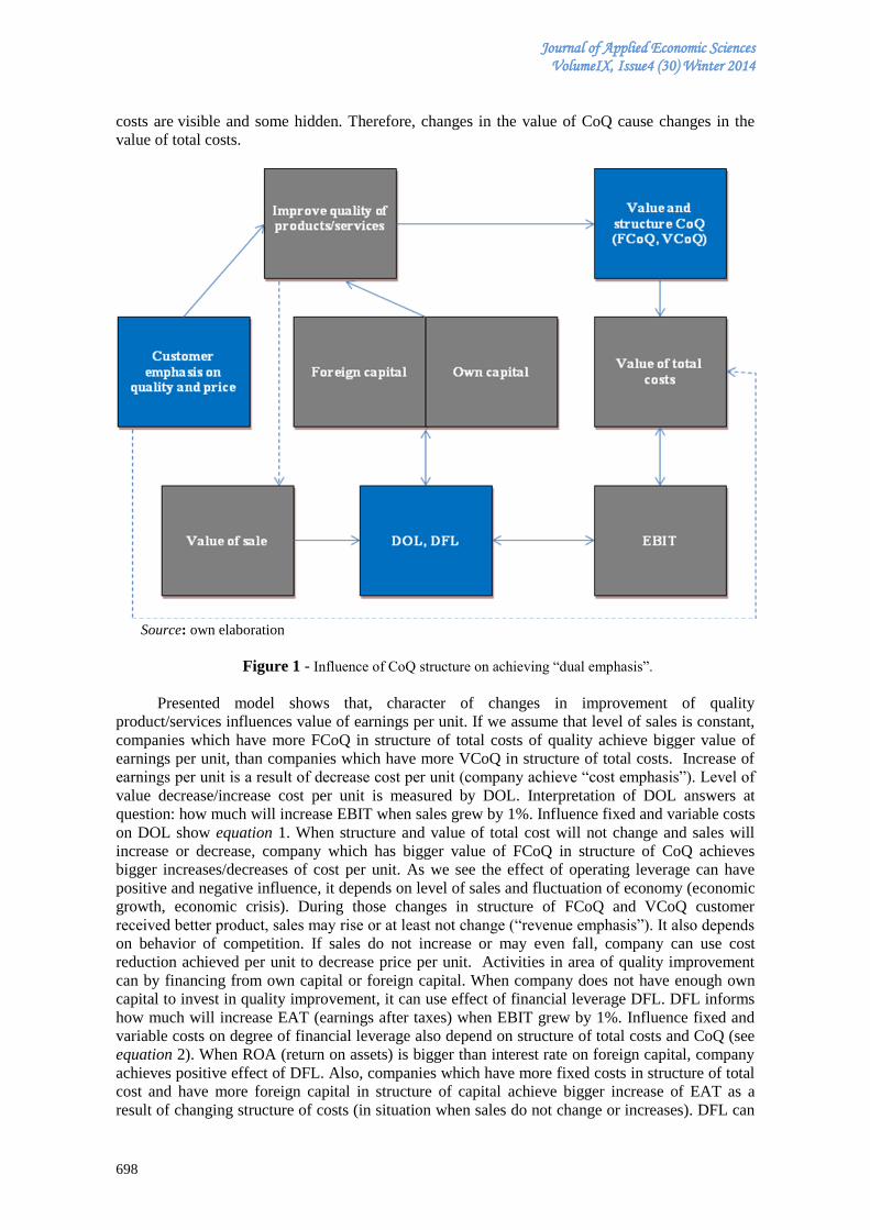
Journal of Applied Economic Sciences VolumeIX, Issue4 (30) Winter 2014
698
costs are visible and some hidden. Therefore, changes in the value of CoQ cause changes in the
value of total costs.
Source: own elaboration
Figure 1 - Influence of CoQ structure on achieving “dual emphasis”.
Presented model shows that, character of changes in improvement of quality
product/services influences value of earnings per unit. If we assume that level of sales is constant,
companies which have more FCoQ in structure of total costs of quality achieve bigger value of
earnings per unit, than companies which have more VCoQ in structure of total costs. Increase of
earnings per unit is a result of decrease cost per unit (company achieve “cost emphasis”). Level of
value decrease/increase cost per unit is measured by DOL. Interpretation of DOL answers at
question: how much will increase EBIT when sales grew by 1%. Influence fixed and variable costs
on DOL show equation 1. When structure and value of total cost will not change and sales will
increase or decrease, company which has bigger value of FCoQ in structure of CoQ achieves
bigger increases/decreases of cost per unit. As we see the effect of operating leverage can have
positive and negative influence, it depends on level of sales and fluctuation of economy (economic
growth, economic crisis). During those changes in structure of FCoQ and VCoQ customer
received better product, sales may rise or at least not change (“revenue emphasis”). It also depends
on behavior of competition. If sales do not increase or may even fall, company can use cost
reduction achieved per unit to decrease price per unit. Activities in area of quality improvement
can by financing from own capital or foreign capital. When company does not have enough own
capital to invest in quality improvement, it can use effect of financial leverage DFL. DFL informs
how much will increase EAT (earnings after taxes) when EBIT grew by 1%. Influence fixed and
variable costs on degree of financial leverage also depend on structure of total costs and CoQ (see
equation 2). When ROA (return on assets) is bigger than interest rate on foreign capital, company
achieves positive effect of DFL. Also, companies which have more fixed costs in structure of total
cost and have more foreign capital in structure of capital achieve bigger increase of EAT as a
result of changing structure of costs (in situation when sales do not change or increases). DFL can
Journal of Applied Economic Sciences VolumeIX, Issue4 (30) Winter 2014
699
have also negative effect, when company have more fixed costs in structure of total cost and sales
decreasing, companies with bigger value of foreign capital have bigger decrease of EAT.
It is also necessary to add, that improve quality of product/service it is possible to achieve
in two ways, continual improvement, investing into quality. Continual improvement, understood as
small changes, which improve quality and do not cause big changes in value of total costs rather
changes in structure of total costs of quality. Literature review shows that this approach is achieved
thanks to using company potential (mainly human capital), methods and techniques of quality
management. Changes in structure of CoQ as a result of continuous improvement may cause
changes in prevention costs. Prevention activities can replace one another, eg. external training are
replaced by internal training, which improve workers knowledge and consequently reduce the
level of errors caused by workers. Investing into quality author understands as spending money on
improve quality/service e.g. buying new machines, technologies, cars, warehouse. Those
investments can by financing from own and foreign capital. Taking into account the level of actual
and future sales, management can change structure of capital and use effect of financial leverage.
Analysis of presented model allows company achieve “dual emphasis”, thanks to modeling of
structure of total CoQ as a result of change in area of quality improvement, thanks to using
company potential through better organizing of activities or investing into quality can achieve
lower costs per unit (costs emphasis). Deliver customers better quality products without changing
or lowering price can increase sales “revenue emphasis”.
Conclusion
Activities in area of quality generate costs of quality (CoQ). Literature review shows that
there are many definitions and classifications of CoQ. The aim of this article was to show how
managing the structure of CoQ can influence “dual emphasis”. Traditional classification of CoQ
divides them on prevention cost, appraisal costs and failure costs are not enough to fulfill the aim.
Classification of CoQ on FCoQ and VCoQ showed how changes in improve quality
product/services on EBIT and level of cost per unit. Modeling the structure of CoQ allows from
one hand lowering cost per unit “cost emphasis” from another hand fulfill customer expectations,
which leads to increase sales “revenue emphasis”. In consequences company achieves “dual
emphasis”. Achieved effect of “dual emphasis” depends on directions of changes: continuous
improvement, investing into quality and changes in individual groups of CoQ, quality and price
products of competition, fluctuation of economy.
References
[1] Ahmad, M.F., Zakuan, N., Jusoh, A., Takala, J. (2012). Relationship of TQM and Business
Performance with Mediators of SPC, Lean Production and TPM. International Congress on
Interdisciplinary Business and Social Science 2012, Social and Behavioral Sciences, 65:186-
191, DOI: 10.1016/j.sbspro.2012.11.109
[2] Breja, S.K., Banwet, D.K., Iyer, K.C. (2011). Quality strategy for transformation: a case
study. The TQM Journal, 23(1):5-20. DOI: 10.1108/17542731111097452
[3] Cepelova, A., Poloucek, S. (2003). Application of strategic methods for evaluation of
portfolio banking products. Ekonomický časopis, 51(6):699 – 707.
[4] Cole, W. E., Mogab, J. W. (1995). The economics of TQM, Clashing paradigms in the Global
Market. Blackwell business.
[5] Crosby, P.B. (1979). Quality is Free, McGraw-Hill.
[6] Evans, J.R., Lindsay, W.M. (2001). The management and control of quality (5th Ed.). South
Western, Cincinnati, OH.
[7] Fajczak – Kowalska, A. (2004). Koszty jakości i ich rachunek. Problemy jakości. 8:33-35.
[8] Feigenbaum, A.V. (1956). Total quality control. Harvard Business Review. 34(6):93-101.
Journal of Applied Economic Sciences VolumeIX, Issue4 (30) Winter 2014
700
[9] Fullerton, R.R., Wempe, W.F. (2009). Lean manufacturing, non-financial performance
measures, and financial performance. International Journal of Operations & Production
Management. 29(3):214-240. DOI: 10.1108/01443570910938970
[10] Gavurová, B. (2011). The Balanced Scorecard System in Enterprise Management. (Systém
Balanced Scorecard v podnikovom riadení). Ekonomický časopis. 59(2):163-177.
[11] Gavurová, B. (2012). Source Identification of Potential Malfunction of Balanced Scorecard
System and Its Influence on System Function. E+M Ekonomie a management, 15(3):76-90.
[12] Gavurová, B., Šoltés, M., Balloni, A.J. (2014). The Economic Importance of Using of ICT in
the Health System (Ekonomický význam využívania informačno-komunikačných technológií
v systéme zdravotníctva). Ekonomický časopis. 62(1): 83-104.
[13] Grzebyk, M. (2010). Determinants influencing the competitiveness of local government units.
Edited by: Jedlicka, P. Conference: International Scientific Conference on Hradec
Economical Days 2010 - Economic Development and Management of the Region Location.
February 02-03, in Czech Republic.
[14] Köksal, G., Batmaz, I., Testik, M.C. (2011). A review of data mining applications for quality
improvement in manufacturing industry. Expert Systems with Applications, 38(10):13448–
13467. DOI: 10.1016/j.eswa.2011.04.063
[15] Juran, J.M. (1998). Juran s Quality Handbook. McGraw Hill.
[16] Juran, J.M. (1988). Juran’s quality control handbook. McGraw Hill.
[17] Kamsu-Foguem, B., Coudert, T., Geneste, L., Beler, C. (2008). Knowledge formalization in
experience feedback processes: An ontology-based approach. Computers in Industry,
59(7):694–710. DOI: 10.1016/j.compind.2007.12.014
[18] Kamsu-Foguem, B., Rigal, F., Mauget, F. 2013. Mining association rules for the quality
improvement of the production process. Expert Systems with Applications, 40(4):1034–1045.
DOI: 10.1016/j.eswa.2012.08.039
[19] Linderman, K., Schroeder, R.G., Zaheer, S., Liedtke, C., Choo, A.S. (2004). Integrating
quality management practices with knowledge creation processes. Journal of Operations
Management, 22(6):589–607. DOI: 10.1016/j.jom.2004.07.001
[20] Marsh, J. (1989). Process modeling for quality improvement. Proceedings of the Second
International Conference on Total Quality Management. London, IFS Publications.
[21] Mittal, V., Anderson, E.W., Sayrak, A., Tadikamalla, P. (2005). Dual Emphasis and the
Long-Term Financial Impact of Customer Satisfaction. Marketing Science 24(4):544-555,
DOI: 10.1287/mksc.1050.0142
[22] Mizla, M., Pudło P. (2012). Štruktúra nákladov kvality a citlivosť podnikov na výkyvy
ekonomiky. E + M. Ekonomie a management, Liberec, 15(1):44-56.
[23] Patel, V.L., Arocha, J.F., Kaufman, D.R. (2001). A primer on aspects of cognition for
medical informatics. Journal of the American Medical Informatics Association, 8(4):324–
343.
[24] Pudło, P. (2008). A Review of research on the definitions and models of quality costs. Acta
oeconomica Cassoviensia. PHF EU Košice, 1(2):13-27.
[25] Pudło, P. (2009). Ekonomické aspekty riadenia kvality vplyv štruktúry nákladov na kvalitu na
zisk- economic aspects of quality management, influence of costs of quality on profit. PhD
diss., University of Economics in Bratislava.
[26] Pudło, P. (2007). Influence investing into quality on structure total costs. Teoretické aspekty
prierezových ekonomík IV. Ekónom, Bratislava, Slovakia.

Journal of Applied Economic Sciences VolumeIX, Issue4 (30) Winter 2014
701
[27] Robison, J. (1997). Integrate quality cost concepts into team problem-solving efforts. Quality
Progress. 30(3):25.
[28] Ross, D.T. (1977). Structured analysis (SA): A language for communicating ideas. IEEE
Transactions on Software Engineering, SE-3(1):16-34
[29] Rust, R.T., Moorman Ch. Dickson P.R. (2002). Getting Return on Quality: Revenue
Expansion, Cost Reduction, or Both?. Journal of Marketing, 66:7–24. DOI:
10.1509/jmkg.66.4.7.18515
[30] Schiffauerova, A., Thomson, V. (2006). A review of research on cost of quality models best
practices. Interantional Juranal of Quality and Reliability Management. 23(4): 13-15.
DOI: 10.1108/02656710610672470
[31] Swaminathan, V., Groening, Ch., Mittal, V., Thomaz, F. (2014). How Achieving the Dual
Goal of Customer Satisfaction and Efficiency in Mergers Affects a Firm’s Long-Term
Financial Performance. Journal of Service Research. 17(2):182-194. DOI:
10.1177/1094670513510196
[32] Šoltés, V. , Gavurová, B. (2013). Application of the cross impact matrix method in
problematic phases of the Balanced Scorecard system in private and public sector. Journal of
Applied Economic Sciences, 8(1):99-119. URL: http://www.cesmaa.eu/journals
/jaes/jaes_issues.php.
[33] Štefko, R., Bačík, R., Fedorko, R. (2013). Spending on social media as part of marketing
budgets. Polish journal of management studies. 8:243-250.
[34] Tawfek, H.S., El-Deen, H., Mohammed, H., Razek, M.E.A. (2012). Assessment of the
expected cost of quality (COQ) in construction projects in Egypt using artificial neural
network model. HBRC journal. 8:132–143. DOI: 10.1016/j.hbrcj.2012.09.009
[35] Teeravaraprug, J., Kitiwanwong, K., Saetong, N. (2011). Relationship model and supporting
activities of JIT, TQM and TPM. Songklanakarin Journal of Science and Technology.
33(1):101-106
[36] Yang, K., Trewn, J. (2004). Multivariate statistical methods in quality management. McGraw
- Hill.
*** Business Excellence. The way business should be done. Costs of quality, 2014,
http://www.bexcellence.org/Cost-Of-Quality.html
*** LNC research, Cost of Quality Definition, 2012 http://blog.lnsresearch.com/blog/bid/
124741/Cost-of-Quality-Definition
Journal of Applied Economic Sciences VolumeIX, Issue4 (30) Winter 2014
702
SOLVENCY CAPITAL FOR NON LIFE INSURANCE: MODELLING DEPENDENCE USING COPULAS
Sawssen ARAICHI
Laboratory Research for Economy, Management and Quantitative Finance
Institute of High Commercial Studies of Sousse, University of Sousse, Tunisia
Laboratory of Actuarial and Financial Sciences, University Claude Bernard Lyon 1, France
Lotfi BELKACEM
Laboratory Research for Economy, Management and Quantitative Finance
Institute of High Commercial Studies of Sousse, University of Sousse, Tunisia
Abstract:
The aim of this article is to improve the internal model of the solvency 2 framework, by assessing a
solvency capital for non life insurance portfolio, taking into account potential dependencies between insured
risks. We used two stochastic models and a simulation technique to determine the distribution of reserve.
Then we modelled the dependence using several copulas and the best one was selected using a goodness of
fit test. Finally we evaluated the solvency capital in the dependent and independent case. By comparing the
results, we highlighted the effect of dependence on solvency capital of the insurance company.
Keywords: solvency capital requirement, reserves, claims dependence, copulas functions, goodness of fit
test, simulation methods.
JEL Classification: C13, G17, G22
1. Introduction
Plenty actuarial research in recent years has focused on the solvency of the insurance
companies. Indeed, insurance company must have a level of liability (equities and technical
reserve), which allows it to be solvent in future years. Historically, the insurance companies were
sufficiently capitalized compared to their engagements: the markets were controlled and less
volatile. Furthermore the correlation between the risks of insurance was not considered. Recently,
we remark that the claims increased and the legal environment became more uncertain: the Lothar
storm in 1999 and the disaster of the World Trade Center in 2001 were responsible of a number of
insolvency among various lines of business: damage, catastrophes, industrial accidents, trading
losses, civil responsibility. Also, some situations are observed almost every day, as for example, in
auto insurance, accidents may involve several insured at once in a collision. These events proved
that the risks of insurance could be dependent, and this dependence can bind liabilities or assets of
insurance. Thus, control of risk has become essential. One way is to consider dependence between
insured risks. For example, linear correlation is frequently used in practice as a measure of
dependence notably by the solvency 2 framework see (Commission 2010). However, it cannot
capture the non-linear dependence relationships that exist between different risks, especially when
extreme events are highly dependent between lines of business.
Recently, several actuarial studies have applied copulas functions to fully capture a wide
range of dependence structure amongst different insured risks. (Frees and Valdez 1998) have
proposed copula function to measure dependence between risks of insurance, and to evaluate the
loss of life mortality, the loss of adjustment expenses and reinsurance contract pricing. Moreover
(Frees and Wang 2006) have used copulas for estimating the credibility of aggregate loss. In
addition, (Kaishev and Dimitrova 2006) have shown the importance of copulas in reinsurance.
(Antonin and Benjamin 2001) also used copulas to assess the amount of the reserve, they provided
a model which combined at the same time the theory of copula and the theory of credibility in
order to detect better the dependence between the lines of business. Furthermore, (Belguise and
Levi 2002), (Faivre 2002) and (Cadoux and Loizeau 2004) have shown that the model with
copulas allows for an aggregation of risks and evaluates a capital higher than when assuming
independence. Similarly, (Krauth 2007) has modeled the dependence using three models
(bootstrap, common shock and copulas) to assess the amount of insurance reserves. In addition,
Journal of Applied Economic Sciences VolumeIX, Issue4 (30) Winter 2014
703
(Bargés et al. 2009) evaluated the capital allocation for the overall portfolio using the TVaR as a
measure of risk and a FGM copula. More recently (Zhao and Zhou 2010) have applied semi
parametric copula models to individual level insurance claims data to forecast loss reserves, and
(Shi and Frees 2011) have investigated the aggregate insurance loss reserving data with bivariate
copulas and linear models. Besides, (Diers et al. 2012) have shown the flexibility of a Berntein
copula to model a several lines of business. Moreover (Zhang and Dukic 2013) have introduced a
Bayesian multivariate model based on the use of parametric copula to model dependencies
between various lines of insurance claims.
All studies mentioned above have considered copulas functions as a powerful tool to
resolve the problem of dependence between insurance risks. However, the new solvency 2
frameworks launched in 2001 which is the basis framework for the European insurance market,
consider the correlation coefficient to measure dependence and to aggregate risks. Or this measure
is insufficient to capture the non linear dependence of insurance risks.
For that, the purpose of this work consists, to model the structure of dependence between
underwriting risks of non life portfolio of a Tunisian insurance company, and to assess the
solvency capital requirement (SCR) by the new solvency 2 approaches. Indeed this paper is
primarily motivated to show the importance of the internal model of the Solvency 2 framework
compared to the standard model, and to extend the internal model by including copula approach in
assessing reserves and capital.
On the basis of this framework, we consider in this paper, two models, the standard model
and the internal model of Solvency 2, the last one is investigated in two cases; the independence
and the dependence case in which a copula approach is used to model the structure of dependence.
A goodness of fit test for copula was implemented to select the best one for the data and a
simulation method of conditional distribution of the copula is applied to include dependence in the
internal model.
The paper is organized as follows. Section 2 presents the Solvency 2 framework. In
Section 3 we present reserving models. In section 4 we provide the copulas functions. Section 5
reports the empirical results. Some comparisons with other papers are discussed in section 6,
followed by concluding remarks and some open questions in Section 7.
2. Solvency 2 framework
Solvency 2 provides a practical tool to evaluate the Solvency Capital requirement (SCR)
for insurance companies in order to manage their risks (reserve risk, premium risk, catastrophe
risk...). Two models were proposed: the standard model and the internal model. These models take
the advantage of evaluating liabilities in stochastic way, contrary to Solvency 1, which evaluates
liabilities with deterministic methods.
In this paper, we focus on reserve risk, which results from fluctuations in the timing and
amount of claims payment. We present here models of SCR for reserve risk, for two lines of
business denoted by k and l, but the models can be generalized for more lines of business.
Standard model
The European Insurance and Occupational Pension Authority (EIOPA) see (Commission
2010) defines a common standard formula for all the insurance companies in order to manage their
risks.
The SCR is defined as
( )aggregate total totalSCR V (2.1)
where:0.995N is the quantile of the
standard normal distribution.
2
0.995
2
exp( log( 1))( ) 1
1
total
total
total
N
Journal of Applied Economic Sciences VolumeIX, Issue4 (30) Winter 2014
704
is the overall standard deviation of the
insurance portfolio, and k, l are the standard
deviations of reserve risk respectively, for the line
of business k and the line of business l fixed by the EIOPA see Table 7 in Appendix B. Vtotal = Vk
+ Vi is the total estimate of technical reserve, which is the amount of claims would rationally pay
to settle the obligations, Vk and Vl are respectively the best estimate of reserve for the line of
business k and the line of business l.
Internal model
The EIOPA recommends the use of an internal model adapted to the risks, which are really
supported by the insurer. Capital reserve risk equation for the line of business k, is given by:
99.5%
k
k kSCR VaR BE (2.2)
where 99.5%
kVaR is the Value at Risk of the line of business k at confidence level 99, 5%.
kBE is the best estimate of the total reserves of the line of business k.
This best estimate must be calculated by at least two models using actuarial techniques
(see Section 3). After computing an SCR for each line of business, we evaluate the aggregate SCR
obtained by:
,
,
agregate k l k l
k l
SCR Corr SCR SCR (2.3)
where: Corrk,l is the correlation matrix of the two lines of business, and SCRk, SCRl are
the solvency capital requirement respectively for the line of business k and the line of business l.
3. Best estimate models
We present here two classical models for evaluating Best Estimate of reserve risk; the
Stochastic Chain Ladder model and the Generalized Linear Model.
3.1 Stochastic Chain Ladder model
Chain Ladder model is the traditional and the straightforward technique to estimate future
claims amounts see (Mack, 1993) and (Mack, 1994). This technique is applied to cumulative
claims data. We assume that the data consist of a triangle of incremental claims,
: 1....... ; 1........ 1ijy i n j n i
i: refers to the row, and indicate the accident year.
j: refers to the column, and indicate the delay year (or development year).
We assume that these incremental claims are independent. Then, the cumulative claims
data are obtained by:
1
,
1
j
ij i j ik
k
C y y
(3.1)
The Chain Ladder methods consist of forecasting the future claims Ci,j, by estimating a
development factors as
, 1
1
,
1
n j
i j
ij n j
i j
i
C
C
1 1j n
(3.2)
,2, 1
1 n
total k l k l k l
k ltotal
Corr V VV
Journal of Applied Economic Sciences VolumeIX, Issue4 (30) Winter 2014
705
Then, the conditional expected loss, which is the best estimate of the future claims are:
, 1 ,1( | ......... )i j i ij j ijE C C C C
(3.3)
For 1 i n and 1 j n , we have
2
, 1 ,1( \ ......... )i j i ij ij jV C C C C , with j
is the
volatility of the development year defined as 2
, 12
1
1
1
n ji j
j ij j
i ij
CC
n j C
(3.4)
The amount of the expected reserves ).....( ,1,1,, jiiininii CCCCRE is estimated by:
, , 1i i n i n iR C C (3.5)
Thus the best estimate of the total amount of reserves is:
1
n
i
i
R R
.
The uncertainty on the estimation of reserves can be measured by:
212
, 21
,
1
1 1( )
nk
i i n n kk n i k ik
j k
j
mse R CC
C
(3.6)
In alternative measure of uncertainty is the standard error ( ) ( )i ise R mse R and the
coefficient of variation ( )i
secv
E R .
Chain Ladder method is considered as the standard reserving model for reserve estimation.
However, this method presents several disadvantages. In fact, it assumes a linear relationship in
claims between the development years; it multiply a claim in development year j by a factor j to
obtain a future claim in development year j + 1, so the risk of accumulated errors is important.
Also, this method does not take into account the various change in the inflation, law.
3.2 Generalized Linear Model
In alternative model to the Stochastic Chain Ladder model was proposed by (Nelder and
Wedderburn 1972), the Generalized Linear Model (GLM). Contrary to Chain Ladder technique,
this method is applied to incremental data ,i jy .
We assume that the response variable ,i jy are independent and belong to the exponential
family distributions defined as
, , ,
, , ,
,
( )( , ) exp ( , )
( )
i j i j i j
i j i j i j
i j
y bf y c y
a
(3.7)
where , ( )i ja , ,( )i jb and ,( , )i jc y are functions specified in advance, ,i j is a
parameter related to the mean and scale parameter related to the variance. For more details we
refer the readers to (McCullagh and Nelder, 1989).
We denote the best estimate of claims amounts as 1
, ,( ) ( )ij i j i jE y b and
'
, , ,( ) ( ) ( ).i j i j i jV y V b
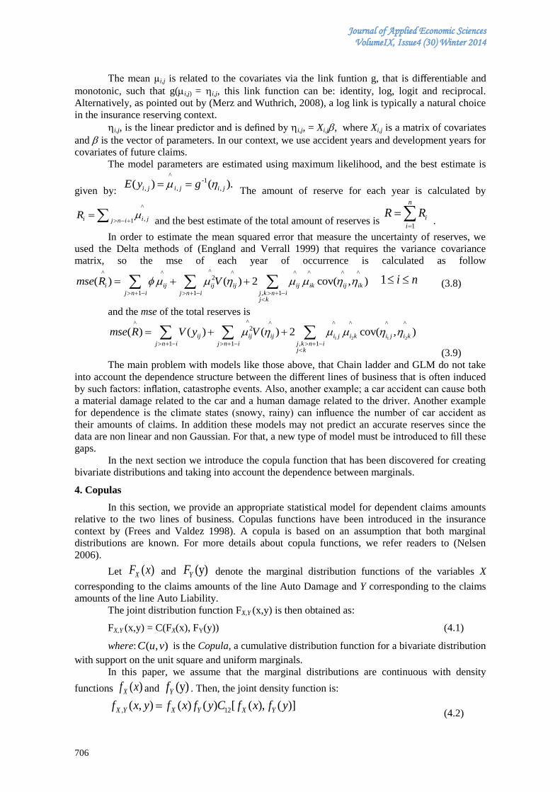
Journal of Applied Economic Sciences VolumeIX, Issue4 (30) Winter 2014
706
The mean µi,j is related to the covariates via the link funtion g, that is differentiable and
monotonic, such that g(i,j) = i,j, this link function can be: identity, log, logit and reciprocal.
Alternatively, as pointed out by (Merz and Wuthrich, 2008), a log link is typically a natural choice
in the insurance reserving context.
i,j, is the linear predictor and is defined by i,j, = Xi,j, where Xi,j is a matrix of covariates
and is the vector of parameters. In our context, we use accident years and development years for
covariates of future claims.
The model parameters are estimated using maximum likelihood, and the best estimate is
given by:
^-1
,, ,( ) ( ).i ji j i jE y g The amount of reserve for each year is calculated by
^
,1i i jj n iR
and the best estimate of the total amount of reserves is
1
n
i
i
R R
.
In order to estimate the mean squared error that measure the uncertainty of reserves, we
used the Delta methods of (England and Verrall 1999) that requires the variance covariance
matrix, so the mse of each year of occurrence is calculated as follow^^ ^ ^ ^ ^ ^ ^2
1 1 , 1
( ) ( ) 2 cov( , )i ij ij ij ij ik ij ik
j n i j n i j k n ij k
mse R V
ni 1 (3.8)
and the mse of the total reserves is
1 2 1 2
^^ ^ ^ ^ ^ ^2
1 1 , 1
( ) ( ) ( ) 2 cov( , )ij ij ij i j i k i j i k
j n i j n i j k n ij k
mse R V y V
(3.9)
The main problem with models like those above, that Chain ladder and GLM do not take
into account the dependence structure between the different lines of business that is often induced
by such factors: inflation, catastrophe events. Also, another example; a car accident can cause both
a material damage related to the car and a human damage related to the driver. Another example
for dependence is the climate states (snowy, rainy) can influence the number of car accident as
their amounts of claims. In addition these models may not predict an accurate reserves since the
data are non linear and non Gaussian. For that, a new type of model must be introduced to fill these
gaps.
In the next section we introduce the copula function that has been discovered for creating
bivariate distributions and taking into account the dependence between marginals.
4. Copulas
In this section, we provide an appropriate statistical model for dependent claims amounts
relative to the two lines of business. Copulas functions have been introduced in the insurance
context by (Frees and Valdez 1998). A copula is based on an assumption that both marginal
distributions are known. For more details about copula functions, we refer readers to (Nelsen
2006).
Let ( )XF x and (y)YF denote the marginal distribution functions of the variables X
corresponding to the claims amounts of the line Auto Damage and Y corresponding to the claims
amounts of the line Auto Liability.
The joint distribution function FX,Y (x,y) is then obtained as:
FX,Y (x,y) = C(FX(x), FY(y)) (4.1)
where: ( , )C u v is the Copula, a cumulative distribution function for a bivariate distribution
with support on the unit square and uniform marginals.
In this paper, we assume that the marginal distributions are continuous with density
functions ( )Xf x and (y)Yf . Then, the joint density function is:
, 12( , ) ( ) ( ) [ ( ), ( )]X Y X Y X Yf x y f x f y C f x f y (4.2)

Journal of Applied Economic Sciences VolumeIX, Issue4 (30) Winter 2014
707
where: 12
( , )( , )
C u vC u v
u v
The conditional distribution function of |Y X x is:
\ 1( \ ) [ ( ), ( )]Y X X YF y x C F x F y (4.3)
where: 1
( , )( , )
C u vC u v
u
In the insurance context, (Frees and Valdez 1998) provide a number of copulas. In each
case the parameter α measures the degree of association. In the present work, we used several
copulas in order to select the appropriate one that describes the structure of dependence between
the two lines of business.
We investigate the Achimedean copulas and their survival copulas, which are more
appropriate to insurance data than elliptical copulas, because elliptical copulas are generally
applied to symmetric distributions.
Gumbel
This copula models a positive dependence and represents the risks which are more
concentrated in the upper tail. It is defined as
))ln((-lnu)-exp(),(1
vvuC 1 (4.4)
where: is the parameter dependence. The Gumbel copula has upper tail dependence 1
2 2U , but no lower tail dependence.
Fank
This copula models both positive and negative dependence, but it has no tail dependence,
it is defined as - u1 ( 1)( 1)
( , ) - ln 1 0( 1)
ve eC u v
e
(4.5)
Clayton
This copula models positive dependence. Unlike to the Gumbel copula, it represents the
risks which are more concentrated in the lower tail, so it correlates small losses. It is defined as
1
-( , ) (u 1) [ 1, ) \{0}C u v v
(4.6)
The Clayton copula has lower tail dependence 0U and
1
2L
.
Rotated Gumbel
It is the survival copula of the Gumbel copula, it is defined by:
( , ) 1 (1 ,1 ; ) [1, )GC u v u v C u v
(4.7)
where: GC is the Gumbel copula.
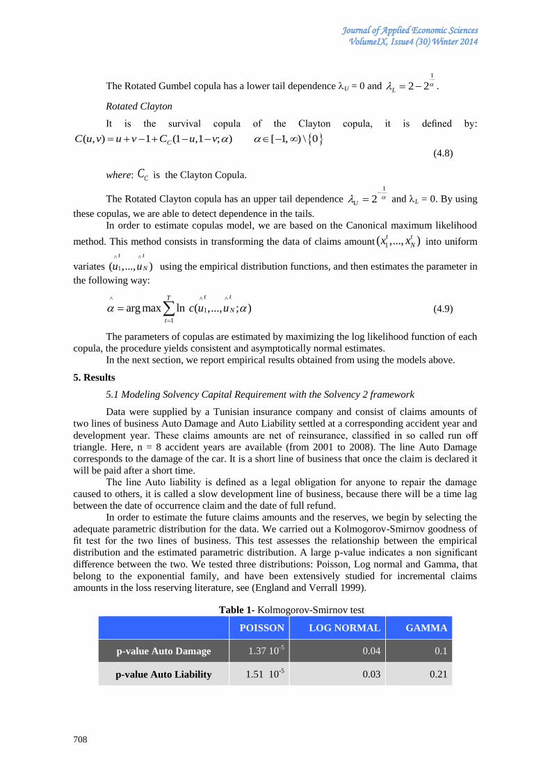
Journal of Applied Economic Sciences VolumeIX, Issue4 (30) Winter 2014
708
The Rotated Gumbel copula has a lower tail dependence U = 0 and
1
2 2L .
Rotated Clayton
It is the survival copula of the Clayton copula, it is defined by:
( , ) 1 (1 ,1 ; ) [ 1, ) \ 0CC u v u v C u v
(4.8)
where: CC is the Clayton Copula.
The Rotated Clayton copula has an upper tail dependence
1
2U
and L = 0. By using
these copulas, we are able to detect dependence in the tails.
In order to estimate copulas model, we are based on the Canonical maximum likelihood
method. This method consists in transforming the data of claims amount 1( ,..., )t t
Nx x into uniform
variates ^ ^
1( ,..., )t t
Nu u using the empirical distribution functions, and then estimates the parameter in
the following way:
^ ^ ^
1
1
arg max ln ( ,..., ; )t tT
N
t
c u u
(4.9)
The parameters of copulas are estimated by maximizing the log likelihood function of each
copula, the procedure yields consistent and asymptotically normal estimates.
In the next section, we report empirical results obtained from using the models above.
5. Results
5.1 Modeling Solvency Capital Requirement with the Solvency 2 framework
Data were supplied by a Tunisian insurance company and consist of claims amounts of
two lines of business Auto Damage and Auto Liability settled at a corresponding accident year and
development year. These claims amounts are net of reinsurance, classified in so called run off
triangle. Here, n = 8 accident years are available (from 2001 to 2008). The line Auto Damage
corresponds to the damage of the car. It is a short line of business that once the claim is declared it
will be paid after a short time.
The line Auto liability is defined as a legal obligation for anyone to repair the damage
caused to others, it is called a slow development line of business, because there will be a time lag
between the date of occurrence claim and the date of full refund.
In order to estimate the future claims amounts and the reserves, we begin by selecting the
adequate parametric distribution for the data. We carried out a Kolmogorov-Smirnov goodness of
fit test for the two lines of business. This test assesses the relationship between the empirical
distribution and the estimated parametric distribution. A large p-value indicates a non significant
difference between the two. We tested three distributions: Poisson, Log normal and Gamma, that
belong to the exponential family, and have been extensively studied for incremental claims
amounts in the loss reserving literature, see (England and Verrall 1999).
Table 1- Kolmogorov-Smirnov test
POISSON LOG NORMAL GAMMA
p-value Auto Damage 1.37 10-5
0.04 0.1
p-value Auto Liability 1.51 10-5
0.03 0.21
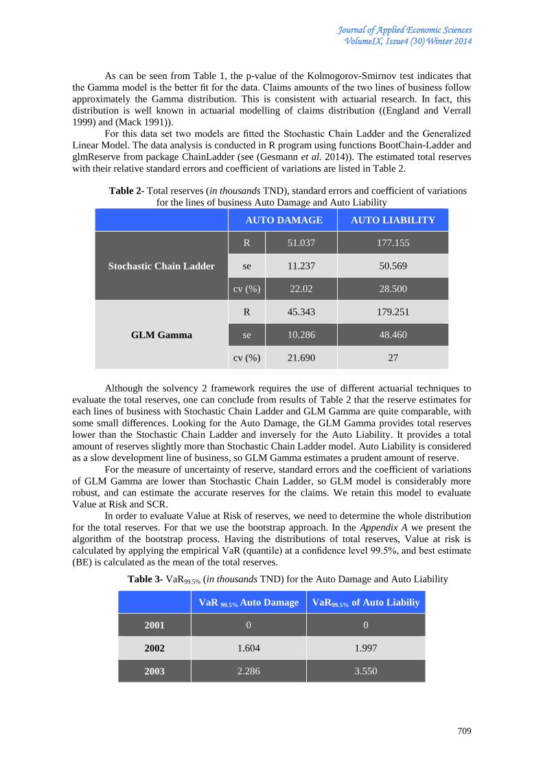
Journal of Applied Economic Sciences VolumeIX, Issue4 (30) Winter 2014
709
As can be seen from Table 1, the p-value of the Kolmogorov-Smirnov test indicates that
the Gamma model is the better fit for the data. Claims amounts of the two lines of business follow
approximately the Gamma distribution. This is consistent with actuarial research. In fact, this
distribution is well known in actuarial modelling of claims distribution ((England and Verrall
1999) and (Mack 1991)).
For this data set two models are fitted the Stochastic Chain Ladder and the Generalized
Linear Model. The data analysis is conducted in R program using functions BootChain-Ladder and
glmReserve from package ChainLadder (see (Gesmann et al. 2014)). The estimated total reserves
with their relative standard errors and coefficient of variations are listed in Table 2.
Table 2- Total reserves (in thousands TND), standard errors and coefficient of variations
for the lines of business Auto Damage and Auto Liability
AUTO DAMAGE AUTO LIABILITY
Stochastic Chain Ladder
R 51.037 177.155
se 11.237 50.569
cv (%) 22.02 28.500
GLM Gamma
R 45.343 179.251
se 10.286 48.460
cv (%) 21.690 27
Although the solvency 2 framework requires the use of different actuarial techniques to
evaluate the total reserves, one can conclude from results of Table 2 that the reserve estimates for
each lines of business with Stochastic Chain Ladder and GLM Gamma are quite comparable, with
some small differences. Looking for the Auto Damage, the GLM Gamma provides total reserves
lower than the Stochastic Chain Ladder and inversely for the Auto Liability. It provides a total
amount of reserves slightly more than Stochastic Chain Ladder model. Auto Liability is considered
as a slow development line of business, so GLM Gamma estimates a prudent amount of reserve.
For the measure of uncertainty of reserve, standard errors and the coefficient of variations
of GLM Gamma are lower than Stochastic Chain Ladder, so GLM model is considerably more
robust, and can estimate the accurate reserves for the claims. We retain this model to evaluate
Value at Risk and SCR.
In order to evaluate Value at Risk of reserves, we need to determine the whole distribution
for the total reserves. For that we use the bootstrap approach. In the Appendix A we present the
algorithm of the bootstrap process. Having the distributions of total reserves, Value at risk is
calculated by applying the empirical VaR (quantile) at a confidence level 99.5%, and best estimate
(BE) is calculated as the mean of the total reserves.
Table 3- VaR99.5% (in thousands TND) for the Auto Damage and Auto Liability
VaR 99.5% Auto Damage VaR99.5% of Auto Liabiliy
2001 0 0
2002 1.604 1.997
2003 2.286 3.550
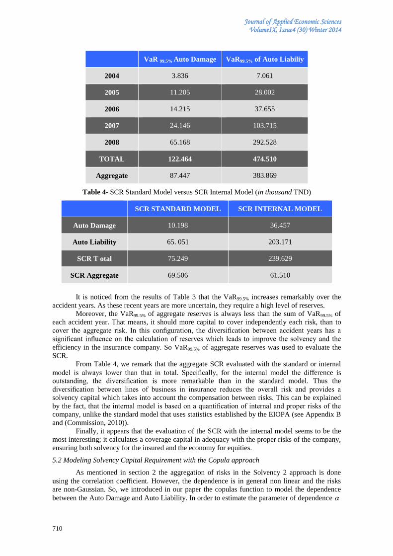
Journal of Applied Economic Sciences VolumeIX, Issue4 (30) Winter 2014
710
VaR 99.5% Auto Damage VaR99.5% of Auto Liabiliy
2004 3.836 7.061
2005 11.205 28.002
2006 14.215 37.655
2007 24.146 103.715
2008 65.168 292.528
TOTAL 122.464 474.510
Aggregate 87.447 383.869
Table 4- SCR Standard Model versus SCR Internal Model (in thousand TND)
SCR STANDARD MODEL SCR INTERNAL MODEL
Auto Damage 10.198 36.457
Auto Liability 65. 051 203.171
SCR T otal 75.249 239.629
SCR Aggregate 69.506 61.510
It is noticed from the results of Table 3 that the VaR99.5% increases remarkably over the
accident years. As these recent years are more uncertain, they require a high level of reserves.
Moreover, the VaR99.5% of aggregate reserves is always less than the sum of VaR99.5% of
each accident year. That means, it should more capital to cover independently each risk, than to
cover the aggregate risk. In this configuration, the diversification between accident years has a
significant influence on the calculation of reserves which leads to improve the solvency and the
efficiency in the insurance company. So VaR99.5% of aggregate reserves was used to evaluate the
SCR.
From Table 4, we remark that the aggregate SCR evaluated with the standard or internal
model is always lower than that in total. Specifically, for the internal model the difference is
outstanding, the diversification is more remarkable than in the standard model. Thus the
diversification between lines of business in insurance reduces the overall risk and provides a
solvency capital which takes into account the compensation between risks. This can be explained
by the fact, that the internal model is based on a quantification of internal and proper risks of the
company, unlike the standard model that uses statistics established by the EIOPA (see Appendix B
and (Commission, 2010)).
Finally, it appears that the evaluation of the SCR with the internal model seems to be the
most interesting; it calculates a coverage capital in adequacy with the proper risks of the company,
ensuring both solvency for the insured and the economy for equities.
5.2 Modeling Solvency Capital Requirement with the Copula approach
As mentioned in section 2 the aggregation of risks in the Solvency 2 approach is done
using the correlation coefficient. However, the dependence is in general non linear and the risks
are non-Gaussian. So, we introduced in our paper the copulas function to model the dependence
between the Auto Damage and Auto Liability. In order to estimate the parameter of dependence
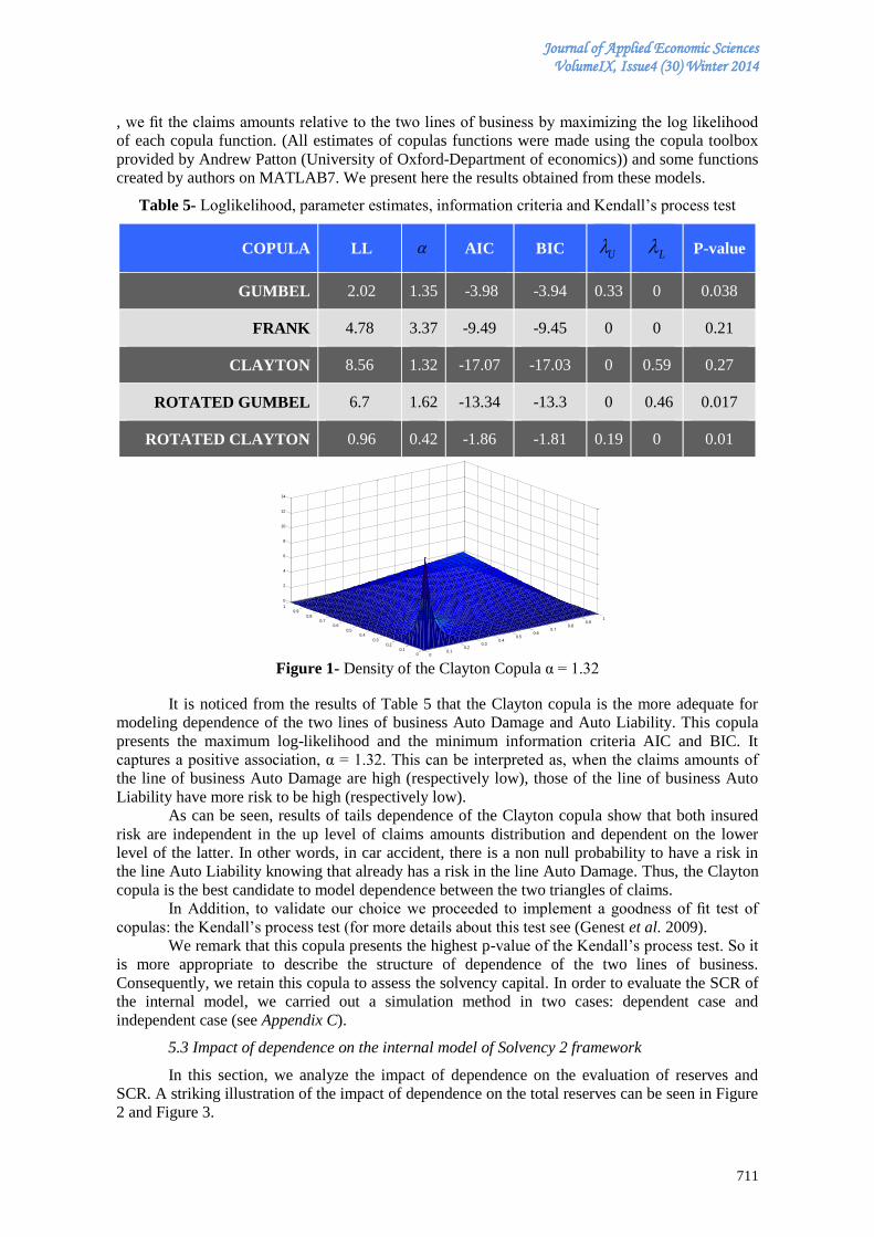
Journal of Applied Economic Sciences VolumeIX, Issue4 (30) Winter 2014
711
, we fit the claims amounts relative to the two lines of business by maximizing the log likelihood
of each copula function. (All estimates of copulas functions were made using the copula toolbox
provided by Andrew Patton (University of Oxford-Department of economics)) and some functions
created by authors on MATLAB7. We present here the results obtained from these models.
Table 5- Loglikelihood, parameter estimates, information criteria and Kendall’s process test
COPULA LL AIC BIC U L P-value
GUMBEL 2.02 1.35 -3.98 -3.94 0.33 0 0.038
FRANK 4.78 3.37 -9.49 -9.45 0 0 0.21
CLAYTON 8.56 1.32 -17.07 -17.03 0 0.59 0.27
ROTATED GUMBEL 6.7 1.62 -13.34 -13.3 0 0.46 0.017
ROTATED CLAYTON 0.96 0.42 -1.86 -1.81 0.19 0 0.01
Figure 1- Density of the Clayton Copula α = 1.32
It is noticed from the results of Table 5 that the Clayton copula is the more adequate for
modeling dependence of the two lines of business Auto Damage and Auto Liability. This copula
presents the maximum log-likelihood and the minimum information criteria AIC and BIC. It
captures a positive association, α = 1.32. This can be interpreted as, when the claims amounts of
the line of business Auto Damage are high (respectively low), those of the line of business Auto
Liability have more risk to be high (respectively low).
As can be seen, results of tails dependence of the Clayton copula show that both insured
risk are independent in the up level of claims amounts distribution and dependent on the lower
level of the latter. In other words, in car accident, there is a non null probability to have a risk in
the line Auto Liability knowing that already has a risk in the line Auto Damage. Thus, the Clayton
copula is the best candidate to model dependence between the two triangles of claims.
In Addition, to validate our choice we proceeded to implement a goodness of fit test of
copulas: the Kendall’s process test (for more details about this test see (Genest et al. 2009).
We remark that this copula presents the highest p-value of the Kendall’s process test. So it
is more appropriate to describe the structure of dependence of the two lines of business.
Consequently, we retain this copula to assess the solvency capital. In order to evaluate the SCR of
the internal model, we carried out a simulation method in two cases: dependent case and
independent case (see Appendix C).
5.3 Impact of dependence on the internal model of Solvency 2 framework
In this section, we analyze the impact of dependence on the evaluation of reserves and
SCR. A striking illustration of the impact of dependence on the total reserves can be seen in Figure
2 and Figure 3.
00.1
0.20.3
0.40.5
0.60.7
0.80.9
1
00.1
0.20.3
0.40.5
0.60.7
0.80.9
1
0
2
4
6
8
10
12
14
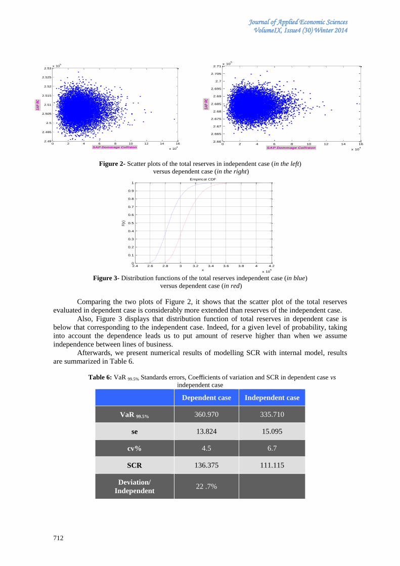
Journal of Applied Economic Sciences VolumeIX, Issue4 (30) Winter 2014
712
Figure 2- Scatter plots of the total reserves in independent case (in the left)
versus dependent case (in the right)
Figure 3- Distribution functions of the total reserves independent case (in blue)
versus dependent case (in red)
Comparing the two plots of Figure 2, it shows that the scatter plot of the total reserves
evaluated in dependent case is considerably more extended than reserves of the independent case.
Also, Figure 3 displays that distribution function of total reserves in dependent case is
below that corresponding to the independent case. Indeed, for a given level of probability, taking
into account the dependence leads us to put amount of reserve higher than when we assume
independence between lines of business.
Afterwards, we present numerical results of modelling SCR with internal model, results
are summarized in Table 6.
Table 6: VaR 99.5% Standards errors, Coefficients of variation and SCR in dependent case vs
independent case
Dependent case Independent case
VaR 99.5% 360.970 335.710
se 13.824 15.095
cv% 4.5 6.7
SCR 136.375 111.115
Deviation/
Independent 22 .7%
0 2 4 6 8 10 12 14 16
x 104
2.66
2.665
2.67
2.675
2.68
2.685
2.69
2.695
2.7
2.705
2.71x 10
5
SAP Dommage Collision
SA
P R
C
2.4 2.6 2.8 3 3.2 3.4 3.6 3.8 4 4.2
x 105
0
0.1
0.2
0.3
0.4
0.5
0.6
0.7
0.8
0.9
1
x
F(x)
Empirical CDF
0 2 4 6 8 10 12 14 16
x 104
2.49
2.495
2.5
2.505
2.51
2.515
2.52
2.525
2.53x 10
5
SAP Dommage Collision
SA
P R
C
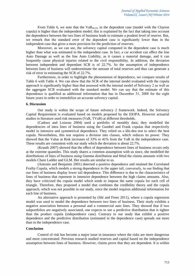
Journal of Applied Economic Sciences VolumeIX, Issue4 (30) Winter 2014
713
From Table 6, we note that the VaR99.5% in the dependent case (model with the Clayton
copula) is higher than the independent model; this is explained by the fact that taking into account
the dependence between the two lines of business leads to estimate a prudent level of reserve. But,
we remark that the standard error of the dependent case is significantly lower than in the
independent case that gives a more precision for the prediction of reserves.
Moreover, as we can see, the solvency capital computed in the dependent case is much
higher than what was estimated in the independent case. In fact, a car accident can affect the line
Auto Damage as well as the line Auto Liability, as it causes a material damage, and it can
frequently cause physical injuries related to the civil responsibility. In addition, the deviation
between independent and dependant SCR is of 22.7%. So the assumption of independence
between lines of business will underestimate the amount of total reserves and thus can generate a
risk of error in estimating the SCR of 22.7%.
Furthermore, in order to highlight the phenomenon of dependence, we compare results of
Table 6 with Table 4. We can show that the SCR of the internal model evaluated with the copula
approach is significantly higher than that assessed with the internal model of Solvency 2 as well as
the aggregate SCR evaluated with the standard model. We can say that the estimate of this
dependence is qualified as additional information that has in December 31, 2008 for the eight
future years in order to immobilize an accurate solvency capital.
6. Discussion
Our study is within the scope of future solvency 2 framework. Indeed, the Solvency
Capital Requirement is evaluated based on models proposed by the EIOPA. However actuarial
studies in literature used risk measures (VaR, TVaR) at different thresholds.
(Cadoux and Loizeau 2004) used a portfolio of monthly data; they modelled the
dependencies of intra lines of business using the Gumbel and Frank copulas that respectively
model in intensive and symmetrical dependence. They relied on a khi-deu test to select the best
copula. Nevertheless, this test requires a division into classes, which reduces its power. They
showed that the Value at Risk increases of 33% to 41% from the VaR in the independence case.
These results are consistent with our study which the deviation is about 22.7%.
(Krauth 2007) showed that the effect of dependence between lines of business occurs only
at the extreme quantiles. This study shares a common assumption with us since, she modelled the
distributions of lines of business using Gamma distribution and fitted the claims amounts with two
models Chain Ladder and GLM. Her results are similar to us.
(Antonin and Benjamin 2001) detected a positive dependence and retained the Correlated
Frailty Copula, which models a strong dependence in the upper tail, conversely, to our finding that
our lines of business display lower tail dependence. This difference is due to the characteristics of
lines of business that represent in intensive dependence between the high claims amounts. Also,
they have criticized the copula model which tends to impose the same copula for each cell of
triangle. Therefore, they proposed a model that combines the credibility theory and the copula
approach, which was not possible in our study, since the model requires additional information for
each line of business.
An alternative approach is presented by (Shi and Frees 2011), where a copula regression
model was used to model the dependence between two lines of business. Their study exhibits a
negative association between a personal and a commercial auto lines. They showed that if two
subportfolios are negatively associated, one expects to see a predictive distribution that is tighter
than the product copula (independence case). Contrary to our study that exhibit a positive
dependence and the predictive distribution (estimated in the dependence case) spreads out more
than in the independence case.
Conclusion
Control of risk has become a major issue in insurance where the risks are more dangerous
and more concentrated. Previous research studied reserves and capital based on the independence
assumption between lines of business. However, claims prove that they are dependent. It is within
Journal of Applied Economic Sciences VolumeIX, Issue4 (30) Winter 2014
714
the framework of assessing a solvency capital requirement including dependence structure that is
the objective of our study.
We carried out an analysis of a non life portfolio consists of two lines of business Auto
Damage and Auto Liability. We assessed the SCR by the two models proposed by Solvency 2 and
we noticed that the aggregate SCR of the internal model is lower than the SCR in total, and this is
due to diversification effect and compensation between risks. This result illustrates a potential
benefits for in insurance company since, it reduces the cost of capital. An important implication of
this observation is that the insurer might consider expanding the Auto Damage or shrinking the
Auto Liability to take best advantage of the diversification effect. Thus, we retained the internal
model that provides a capital an adequacy of the proper risks of the company. The main
contribution in this paper is to improve the internal model chosen. As innovative; we propose to
introduce the copula approach in the internal model. The analysis between the two lines of
business revealed a structure of dependence at the lower tail distribution described by the Clayton
copula. The evaluation of the SCR showed that taking into account the dependence increases the
solvency capital as well as the precision on reserves (minimum standard error). So our study
provides a model to assess the accurate reserve and SCR for the insurance companies that are
adapted to the characteristic of lines of business and suggest that evaluating SCR with the copula
approach is more appropriate.
This study is a first step of modeling dependence between two lines of business. Future
work should therefore include several lines of business. Also, an important question is to
determine the dependence between claims of the one run off triangle. Finally, and after assessing
the SCR, it is interesting to conduct an adequate allocation of the latter to evaluate the performance
of each line of business.
References
[1] Antonin, G., Benjamin, S. (2001). Effets de la dépendance entre différentes branches sur le
calcul des provisions. Astin Bulletin.
[2] Bargés, M., Cossette, H., Marceau, E. (2009). TVaR-based capital allocation with copulas.
Insurance: Mathematics and Economics, 45(3): 348-361. doi:10.1016/j.insmatheco.
2009.08.002
[3] Belguise, O., Levi, C. (2002). Tempêtes: Etude des dépendances entre les branches
automobile et incendie à l'aide de la théorie des copulas. Bulletin Français d'Actuariat.
[4] Cadoux, D. and Loizeau, J.-M. (2004). Copules et dépendances: application pratique la
dtermination du besoin en fonds propres d'un assureur non vie. Astin Bulletin.
[5] Cherubini, U., Luciano, E., and Vecchiato, W. (2004). Copula Methods in Finance, Wiley,
Chichester.
[6] Diers, D., Eling, M., and Marek, S.D. (2012). Dependence modeling in non-life insurance
using the Bernstein copula, Insurance: Mathematics and Economics, 50(3): 430-436,
doi:10.1016/j.insmatheco.2012.02.007
[7] England, P. and Verrall, R.( 1999). Analytic and bootstrap estimates of prediction errors in
claims reserving. Insurance: Mathematics and Economics, 25(3): 281-293, doi:10.1016/
S0167-6687(99)00016-5
[8] Faivre, F. (2002). Copula: A New Vision for Economic Capital and Application to a Four
Line of Business Company. Astin Bulletin.
[9] Frees, E.W., Valdez, E.A. (1998). Understanding relationships using copulas. North
American Actuarial Journal, 2(1): 1-25, DOI: 10.1080/10920277.1998.10595667
[10] Frees, E.W., Wang, P. (2006). Copula credibility for aggregate loss models. Insurance:
Mathematics and Economics, no 38(2): 360-373, doi:10.1016/j.insmatheco.2005.10.004,
http://www.sciencedirect.com/science/article/pii/ S01676687050- 0140X

Journal of Applied Economic Sciences VolumeIX, Issue4 (30) Winter 2014
715
[11] Genest, C., Rmillard, B., Beaudoin, D. (2009). Goodness-of-fit tests for copulas: A review
and a power study. Insurance: Mathematics and Economics, 44(2): 199-213, doi:10.1016/
j.insmatheco.2007.10.005
[12] Gesmann, M., Murphy, D., Zhang, W. (2014). Statistical methods and models for the
calculation of outstanding claims reserves in general insurance. Technical report, R Core
team.
[13] Kaishev, V.K., Dimitrova, D.S. (2006). Excess of loss reinsurance under joint survival
optimality. Insurance: Mathematics and Economics, 39(3): 376-389, doi:10.1016/
j.insmatheco.2006.05.005.
[14] Krauth, G. (2007). Provisionnement et corrélation entre branches. Master’s thesis,
Concervatoire National des Arts et Metiers.
[15] Mack, T. (1991). A simple parametric model for rating automobile insurance or estimating
ibnr claims reserve. Astin Bulletin.
[16] Mack, T. (1993). Distribution-free calculation of the standard error of chain ladder reserve
estimates. Astin Bulletin.
[17] Mack, T. (1994). Which stochastic model is underlying the chain ladder method?, Insurance:
Mathematics and Economics, 15(2-3): 133-138, doi:10.1016/0167-6687(94)90789-7
[18] McCullagh, P., Nelder, J.A. (1989). Generalized Linear Models. Chapman and Hall/CRC, 2nd
Edition.
[19] Merz, M., Wuthrich, M. V. (2008). Prediction error of the multivariate chain ladder reserving
method. North American Actuarial Journal, 12(2):175-197, DOI: 10.1080/10920277.
2008.10597509
[20] Nelder, J., Wedderburn, R. (1972). Generalized linear models. Journal of the Royal Statistical
Society.
[21] Nelsen, R. (2006). An Introduction to Copulas. Springer; 2nd
Edition.
[22] Shi, P., Frees, E.W. (2011). Descendent loss reserving using copulas. Astin Bulletin - Journal
of the International Actuarial Association, 41(2): 449-486, http://dx.doi.org/10.2143/
AST.41.2.2136985
[23] Zhang, Y., Dukic, V. (2013). Predicting multivariate insurance loss payments under the
bayesian copula framework, Journal of Risk and Insurance, 80(4): 691-919, http://dx.doi.org/
10.1111/ j.1539-6975.2012.01480.x
[24] Zhao, X., Zhou, X. (2010). Applying copula models to individual claim loss reserving
methods. Insurance: Mathematics and Economics, 46(2): 290-299, doi:10.1016/j.insmatheco.
2009.11.001.
*** Commission, E. (2010). Qis5 technical specifications. Technical report, Financial Institution
Insurance and Pensions.
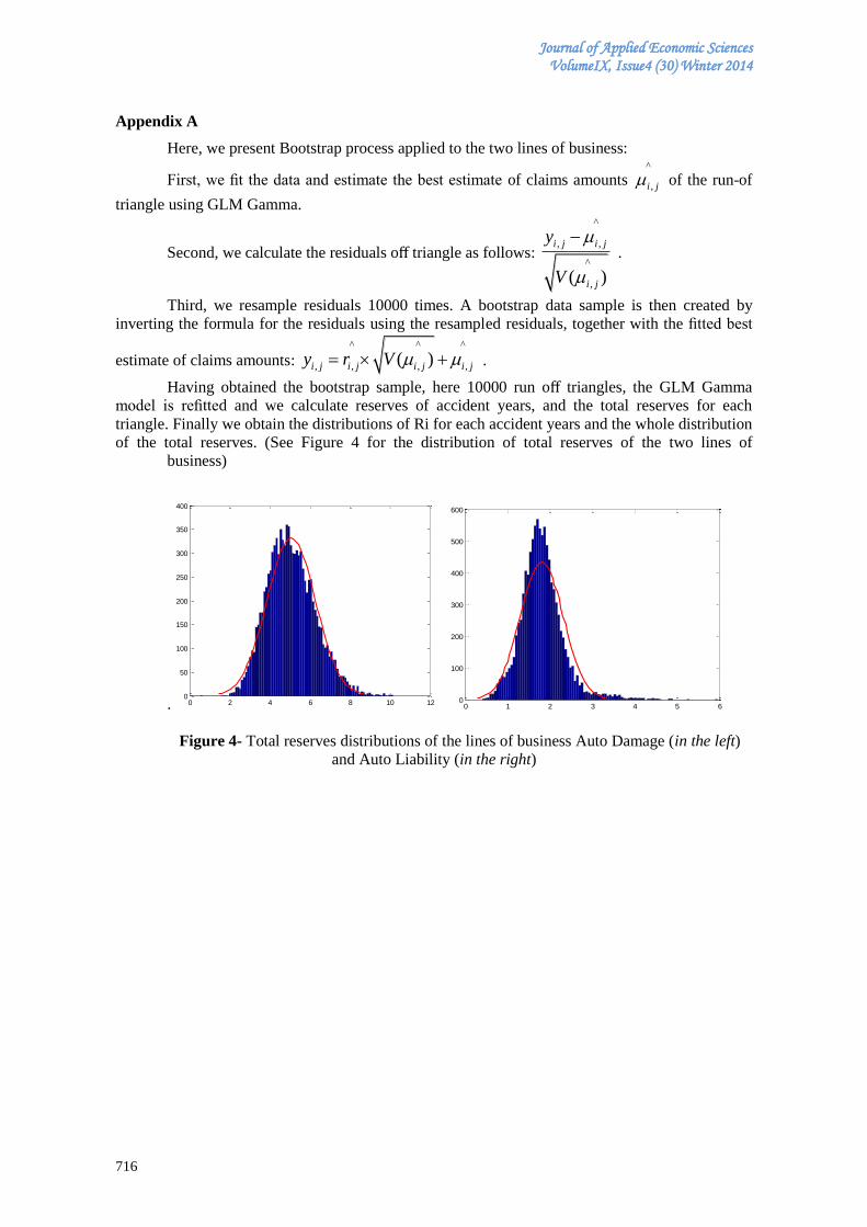
Journal of Applied Economic Sciences VolumeIX, Issue4 (30) Winter 2014
716
Appendix A
Here, we present Bootstrap process applied to the two lines of business:
First, we fit the data and estimate the best estimate of claims amounts ^
,i j of the run-of
triangle using GLM Gamma.
Second, we calculate the residuals off triangle as follows:
^
, ,
^
,( )
i j i j
i j
y
V
.
Third, we resample residuals 10000 times. A bootstrap data sample is then created by
inverting the formula for the residuals using the resampled residuals, together with the fitted best
estimate of claims amounts: ^ ^ ^
, , , ,( )i j i j i j i jy r V .
Having obtained the bootstrap sample, here 10000 run off triangles, the GLM Gamma
model is refitted and we calculate reserves of accident years, and the total reserves for each
triangle. Finally we obtain the distributions of Ri for each accident years and the whole distribution
of the total reserves. (See Figure 4 for the distribution of total reserves of the two lines of
business)
.
Figure 4- Total reserves distributions of the lines of business Auto Damage (in the left)
and Auto Liability (in the right)
0 2 4 6 8 10 12
x 104
0
50
100
150
200
250
300
350
400
0 1 2 3 4 5 6
x 105
0
100
200
300
400
500
600
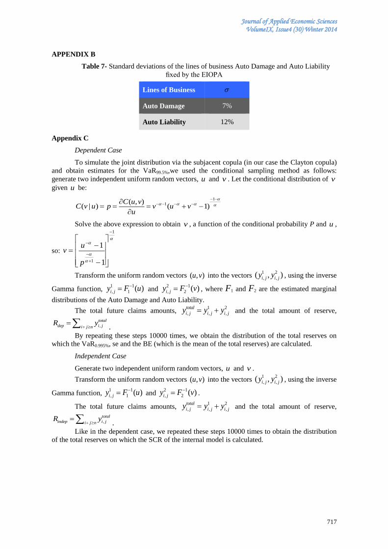
Journal of Applied Economic Sciences VolumeIX, Issue4 (30) Winter 2014
717
APPENDIX B
Table 7- Standard deviations of the lines of business Auto Damage and Auto Liability
fixed by the EIOPA
Lines of Business
Auto Damage 7%
Auto Liability 12%
Appendix C
Dependent Case
To simulate the joint distribution via the subjacent copula (in our case the Clayton copula)
and obtain estimates for the VaR99.5%,we used the conditional sampling method as follows:
generate two independent uniform random vectors, u and v . Let the conditional distribution of v
given u be:
1
1( , )( | ) ( 1)
C u vC v u p v u v
u
Solve the above expression to obtain v , a function of the conditional probability P and u ,
so:
1
1 1
1
p
uv
Transform the uniform random vectors ( , )u v into the vectors 1 2
, ,( , )i j i jy y , using the inverse
Gamma function, 1 1
, 1 ( )i jy F u and 2 1
, 2 ( )i jy F v , where F1 and F2 are the estimated marginal
distributions of the Auto Damage and Auto Liability.
The total future claims amounts, 1 2
, , ,
total
i j i j i jy y y
and the total amount of reserve,
,
total
dep i ji j nR y
.
By repeating these steps 10000 times, we obtain the distribution of the total reserves on
which the VaR0.995%, se and the BE (which is the mean of the total reserves) are calculated.
Independent Case
Generate two independent uniform random vectors, u and v .
Transform the uniform random vectors ( , )u v into the vectors 1 2
, ,( , )i j i jy y , using the inverse
Gamma function, 1 1
, 1 ( )i jy F u and 2 1
, 2 ( )i jy F v .
The total future claims amounts, 1 2
, , ,
total
i j i j i jy y y and the total amount of reserve,
,
total
indep i ji j nR y
.
Like in the dependent case, we repeated these steps 10000 times to obtain the distribution of the total reserves on which the SCR of the internal model is calculated.
Journal of Applied Economic Sciences VolumeIX, Issue4 (30) Winter 2014
718
MODELLING VOLATILITY: EVIDENCE FROM THE BUCHAREST
STOCK EXCHANGE
Erginbay UĞURLU
Hitit University, FEAS, Department of Economics12
, Turkey [email protected]
Abstract:
Financial series tend to be characterized by volatility and this characteristic affects both financial
series of developed markets and emerging markets. Because of the emerging markets have provided major
investment opportunities in last decades their volatility has been widely investigated in the literature. The
most popular volatility models are the Autoregressive Conditional Heteroscedastic (ARCH) or Generalized
Autoregressive Conditional Heteroscedastic (GARCH) models. This paper aims to investigate the volatility
of Bucharest Stock Exchange, BET index as an emerging capital market and compare forecasting power for
volatility of this index during 2000-2014. To do this, this paper use GARCH, TARCH, EGARCH and
PARCH models against Generalized Error distribution. We estimate these models then we compare the
forecasting power of these GARCH type models in sample period. The results show that the EGARCH is the
best model by means of forecasting performance.
Keywords: stock returns; volatility; GARCH models; emerging markets.
JEL classification: C13, C32 C51, C52, G17
1. Introduction
The conditional variance of financial time series is important for measuring risk and
volatility of these series. Conditional distributions of high-frequency returns of financial data have
excess of kurtosis, negative skewness, and volatility pooling and leverage effects. Volatility of
stock exchange indices and forecasting of their volatility have enormously increasing literature for
both investors and academicians. The prices of financial securities have constant inconsistency and
their returns over the various periods of time are notably volatile and complicated to forecast. The
modelling volatility started with the Autoregressive Conditional Heteroskedasticity (ARCH)
model, introduced by (Engle, 1982) and generalized by (Bollerslev, 1986) in GARCH model.
Although ARCH and GARCH models capture volatility clustering and leptokurtosis, they fail to
model the leverage effect. After these two papers, various types of GARCH models were proposed
to solve this problem such as the Exponential GARCH (EGARCH) model , the Threshold GARCH
(TARCH) model and the Power ARCH (PARCH) model.
Aim of this paper is to investigate the volatility and of Bucharest Stock Exchange, namely
Bucharest Exchange Trading Index (BET) as an emerging capital market for the last decade. Also
we aim to compare forecasting power of GARCH-type models to find the relevant GARCH-type
model for BET. We investigate the forecasting performance of GARCH, EGARCH, TARCH and
PARCH models together with the Generalized Error Distribution (GED).
Bucharest Exchange Trading Index (BET) is a capitalization weighted index which was
developed with a base value of 1000 as of September 22, 1997. BET is the first index developed
by the BSE and comprised of the most liquid 10 stocks listed on the Bucharest Stock
Exchange BSE tier 1. Currently, the Bucharest Stock Exchange calculates and publishes a few
indices: BET, BET-C, BET-FI, ROTX, BEX-XT, BET-NG, RASDAQ-C, RAQ-I, RAQ-II. BET.
(Pele et al., 2013; Bloomberg, 2013)
Investigating volatility of returns of stock markets and comparing forecasting accuracy of
returns of stock markets have achieved attractiveness all over the world. Because of aim of the
paper we focused on paper about European and emerging stock markets.
This paper is adopted the paper which is entitled as “Modelling Volatility: Evidence from the Bucharest
Stock Exchange” that was presented in The International Conference on Economic Sciences and Business
Administration (ICESBA 2014), 24 October 2014, Bucharest, Romania 12
Corum, 19030, Turkey
Journal of Applied Economic Sciences VolumeIX, Issue4 (30) Winter 2014
719
(Emerson et al., 1997), (Shields, 1997), and (Scheicher, 1999) investigates Polish stock
returns. (Scheicher, 2001), (Syriopoulos, 2007) and (Haroutounian and Price, 2010) analyze the
emerging markets in Central and Eastern Europe. (Vošvrda and Žıkeš, 2004) is another research
about the Czech, Hungarian and Polish stock markets. (Rockinger and Urga, 2012) make a model
for transition economies and established economies. (Ugurlu et al., 2012) and (Thalassinos et al.
2013) investigate the forecasting performance of GARCH-type model to European Emerging
Economies and Turkey and Czech Republic stock exchange respectively.
This paper is organized as follows. Section 2 describes the volatility models which are
used in this paper. Section 3 shows empirical application results. Section 4 contains summary of
the paper and some concluding remarks.
2. Method
In this section we review the GARCH-type models which are used in the empirical
application section of this paper.
Engle (1982) developed Autoregressive Conditional Heteroscedastic (ARCH) model.
ARCH models based on the variance of the error term at time t depends on the realized values of
the squared error terms in previous time periods. The model is specified as:
(2.1)
0, (2.2)
∑
(2.3)
This model is referred to as ARCH(q), where q refers to the order of the lagged squared
returns included in the model. (Bollerslev, 1986) and (Taylor, 1986) proposed the GARCH(p,q)
random process. The process allows the conditional variance of variable to be dependent upon
previous lags; first lag of the squared residual from the mean equation and present news about the
volatility from the previous period which is as follows:
p
i
q
j
itiitit u1 1
22
0
2 (2.4)
All parameters in variance equation must be positive and ∑ ∑
is expected to
be less than one but it is close to 1. If the sum of the coefficients equals to 1 it is called an
Integrated GARCH (IGARCH) process.
(Nelson, 1991) proposed the Exponential GARCH (EGARCH) model as follows:
∑ ( |
|
) ∑ (
)
(2.5)
In the equation represent leverage effects which accounts for the asymmetry of the
model. While the basic GARCH model requires the restrictions the EGARCH model allows
unrestricted estimation of the variance. If it indicates presence of leverage effect which
means that leverage effect bad news increases volatility.
Threshold GARCH (TARCH) model was developed by (Zakoian, 1994). In TARCH
model the leverage effect is expressed in a quadratic form as follows:
∑
∑
∑
(2.6)
where: {
The effect of the represents the good news and represents the bad news
have different outcomes on the conditional variance. The impact of the news is asymmetric and the
leverage effects exist when .
The power-ARCH (PARCH) specification proposed by (Ding et al., 1993) generalises the
transformation of the error term in the models as follows:
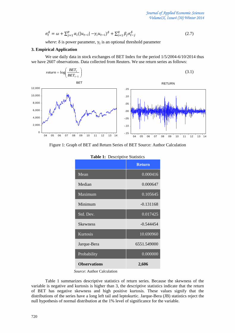
Journal of Applied Economic Sciences VolumeIX, Issue4 (30) Winter 2014
720
∑ | |
∑
(2.7)
where: is power parameter, is an optional threshold parameter
3. Empirical Application
We use daily data in stock exchanges of BET Index for the period 1/5/2004-6/10/2014 thus
we have 2607 observations. Data collected from Reuters. We use return series as follows:
1
logt
t
BET
BETreturn (3.1)
0
2,000
4,000
6,000
8,000
10,000
12,000
04 05 06 07 08 09 10 11 12 13 14
BET
-.15
-.10
-.05
.00
.05
.10
.15
04 05 06 07 08 09 10 11 12 13 14
RETURN
Figure 1: Graph of BET and Return Series of BET Source: Author Calculation
Table 1: Descriptive Statistics
Return
Mean 0.000416
Median 0.000647
Maximum 0.105645
Minimum -0.131168
Std. Dev. 0.017425
Skewness -0.544454
Kurtosis 10.690960
Jarque-Bera 6551.549000
Probability 0.000000
Observations 2,606
Source: Author Calculation
Table 1 summarizes descriptive statistics of return series. Because the skewness of the
variable is negative and kurtosis is higher than 3, the descriptive statistics indicate that the return
of BET has negative skewness and high positive kurtosis. These values signify that the
distributions of the series have a long left tail and leptokurtic. Jarque-Bera (JB) statistics reject the
null hypothesis of normal distribution at the 1% level of significance for the variable.
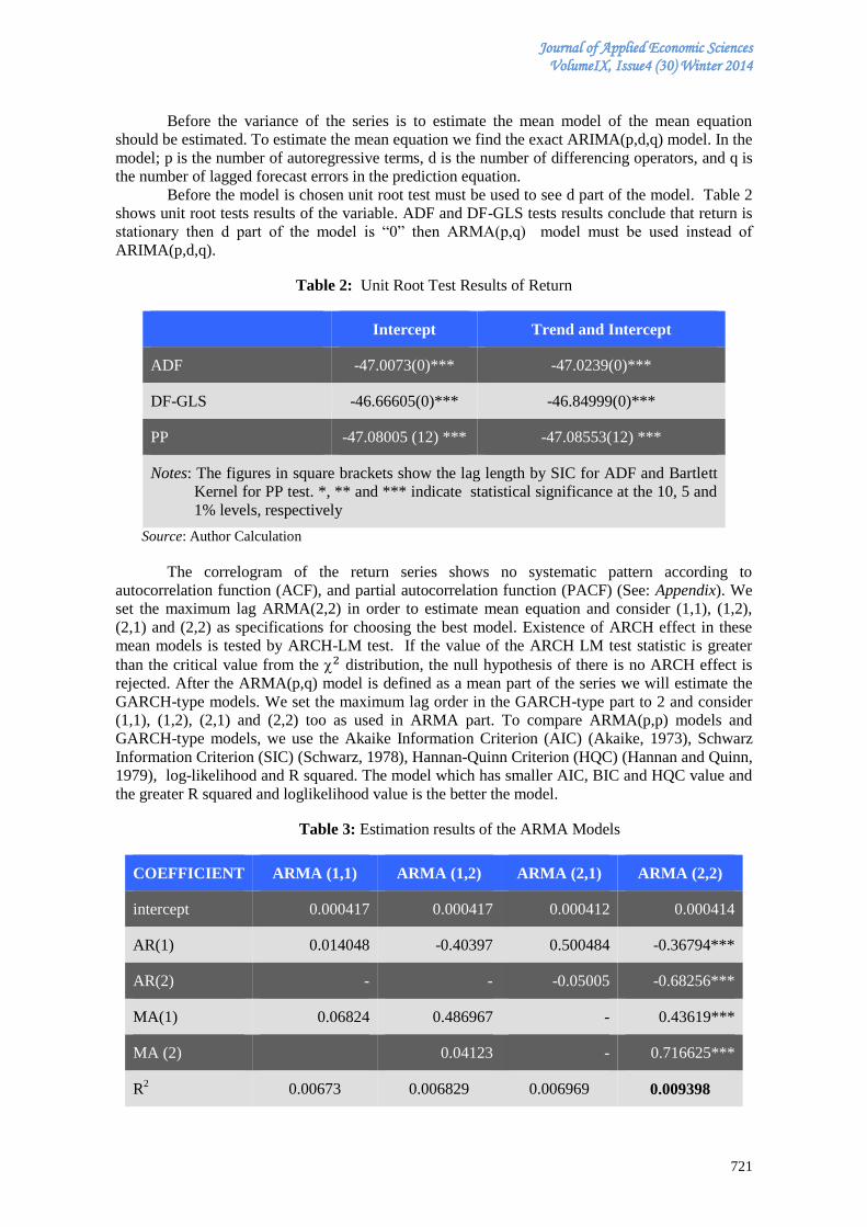
Journal of Applied Economic Sciences VolumeIX, Issue4 (30) Winter 2014
721
Before the variance of the series is to estimate the mean model of the mean equation
should be estimated. To estimate the mean equation we find the exact ARIMA(p,d,q) model. In the
model; p is the number of autoregressive terms, d is the number of differencing operators, and q is
the number of lagged forecast errors in the prediction equation.
Before the model is chosen unit root test must be used to see d part of the model. Table 2
shows unit root tests results of the variable. ADF and DF-GLS tests results conclude that return is
stationary then d part of the model is “0” then ARMA(p,q) model must be used instead of
ARIMA(p,d,q).
Table 2: Unit Root Test Results of Return
Intercept Trend and Intercept
ADF -47.0073(0)*** -47.0239(0)***
DF-GLS -46.66605(0)*** -46.84999(0)***
PP -47.08005 (12) *** -47.08553(12) ***
Notes: The figures in square brackets show the lag length by SIC for ADF and Bartlett
Kernel for PP test. *, ** and *** indicate statistical significance at the 10, 5 and
1% levels, respectively
Source: Author Calculation
The correlogram of the return series shows no systematic pattern according to
autocorrelation function (ACF), and partial autocorrelation function (PACF) (See: Appendix). We
set the maximum lag ARMA(2,2) in order to estimate mean equation and consider (1,1), (1,2),
(2,1) and (2,2) as specifications for choosing the best model. Existence of ARCH effect in these
mean models is tested by ARCH-LM test. If the value of the ARCH LM test statistic is greater
than the critical value from the distribution, the null hypothesis of there is no ARCH effect is
rejected. After the ARMA(p,q) model is defined as a mean part of the series we will estimate the
GARCH-type models. We set the maximum lag order in the GARCH-type part to 2 and consider
(1,1), (1,2), (2,1) and (2,2) too as used in ARMA part. To compare ARMA(p,p) models and
GARCH-type models, we use the Akaike Information Criterion (AIC) (Akaike, 1973), Schwarz
Information Criterion (SIC) (Schwarz, 1978), Hannan-Quinn Criterion (HQC) (Hannan and Quinn,
1979), log-likelihood and R squared. The model which has smaller AIC, BIC and HQC value and
the greater R squared and loglikelihood value is the better the model.
Table 3: Estimation results of the ARMA Models
COEFFICIENT ARMA (1,1) ARMA (1,2) ARMA (2,1) ARMA (2,2)
intercept 0.000417 0.000417 0.000412 0.000414
AR(1) 0.014048 -0.40397 0.500484 -0.36794***
AR(2) - - -0.05005 -0.68256***
MA(1) 0.06824 0.486967 - 0.43619***
MA (2) 0.04123 - 0.716625***
R2 0.00673 0.006829 0.006969 0.009398
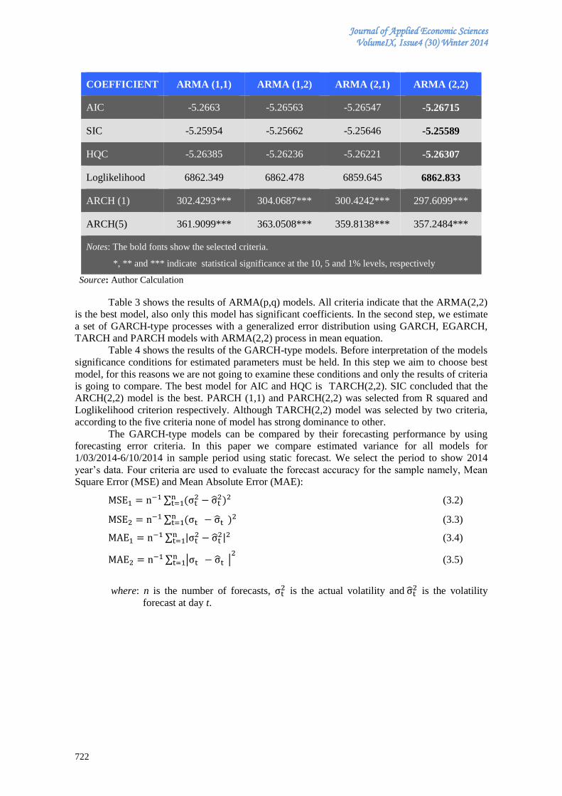
Journal of Applied Economic Sciences VolumeIX, Issue4 (30) Winter 2014
722
COEFFICIENT ARMA (1,1) ARMA (1,2) ARMA (2,1) ARMA (2,2)
AIC -5.2663 -5.26563 -5.26547 -5.26715
SIC -5.25954 -5.25662 -5.25646 -5.25589
HQC -5.26385 -5.26236 -5.26221 -5.26307
Loglikelihood 6862.349 6862.478 6859.645 6862.833
ARCH (1) 302.4293*** 304.0687*** 300.4242*** 297.6099***
ARCH(5) 361.9099*** 363.0508*** 359.8138*** 357.2484***
Notes: The bold fonts show the selected criteria.
*, ** and *** indicate statistical significance at the 10, 5 and 1% levels, respectively
Source: Author Calculation
Table 3 shows the results of ARMA(p,q) models. All criteria indicate that the ARMA(2,2)
is the best model, also only this model has significant coefficients. In the second step, we estimate
a set of GARCH-type processes with a generalized error distribution using GARCH, EGARCH,
TARCH and PARCH models with ARMA(2,2) process in mean equation.
Table 4 shows the results of the GARCH-type models. Before interpretation of the models
significance conditions for estimated parameters must be held. In this step we aim to choose best
model, for this reasons we are not going to examine these conditions and only the results of criteria
is going to compare. The best model for AIC and HQC is TARCH(2,2). SIC concluded that the
ARCH(2,2) model is the best. PARCH (1,1) and PARCH(2,2) was selected from R squared and
Loglikelihood criterion respectively. Although TARCH(2,2) model was selected by two criteria,
according to the five criteria none of model has strong dominance to other.
The GARCH-type models can be compared by their forecasting performance by using
forecasting error criteria. In this paper we compare estimated variance for all models for
1/03/2014-6/10/2014 in sample period using static forecast. We select the period to show 2014
year’s data. Four criteria are used to evaluate the forecast accuracy for the sample namely, Mean
Square Error (MSE) and Mean Absolute Error (MAE):
∑
(3.2)
∑ (3.3)
∑ |
| (3.4)
∑ | |
(3.5)
where: n is the number of forecasts, is the actual volatility and
is the volatility
forecast at day t.
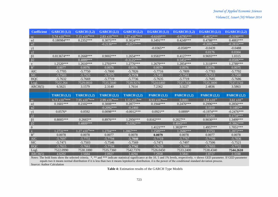
Journal of Applied Economic Sciences
VolumeIX, Issue4 (30) Winter 2014
723
Table 4: Estimation results of the GARCH Type Models
Coefficient GARCH (1,1) GARCH (1,2) GARCH (2,1) GARCH (2,2) EGARCH (1,1) EGARCH (1,2) EGARCH (2,1) EGARCH (2,2)
5.74 x10⁻⁶
*** 7.15 x10⁻⁶
*** 2.83 x10⁻⁶
*** 1.27 x10⁻⁶
*** -0.6169*** -0.6795*** -0.4672*** -0.3190***
α1 0.180984*** 0.2352*** 0.3075*** 0.3024*** 0.3491*** 0.4249*** 0.4788*** 0.4883***
α2 -0.2130*** -0.2577*** -0.2091*** -0.2816***
1 -0.0365** -0.0500** -0.0439 -0.0488
2 0.0176 0.0304
β1 0.813674*** 0.2668*** 0.9002*** 1.2654*** 0.9583*** 0.4127*** 0.9693*** 1.0315
β2 0.4889*** -0.3125**** 0.5451*** -0.0506***
v 1.2520*** 1.2610*** 1.2703*** 1.2776*** 1.2679*** 1.2854*** 1.3118*** 1.2789***
R2 0.0077 0.0076 0.0076 0.0076 0.0079 0.0076 0.0076 0.0075
AIC -5.7705 -5.7750 -5.7800 -5.7826 -5.7716 -5.7809 -5.7783 -5.7792
SIC -5.7503 -5.7525 -5.7575 -5.7578 -5.7491 -5.7561 -5.7513 -5.7500
HQC -5.7632 -5.7669 -5.7719 -5.7736 -5.7635 -5.7719 -5.7685 -5.7686
Logl. 7522.264 7529.0810 7535.5840 7539.9270 7524.6460 7537.7430 7535.3800 7537.5710
ARCH(5) 6.5621 3.1579 2.3140 1.7614 7.2362 3.3227 2.4836 3.5863
TARCH (1,1) TARCH (1,2) TARCH (2,1) TARCH (2,2) PARCH (1,1) PARCH (1,2) PARCH (2,1) PARCH (2,2)
6.73 x10⁻⁶
*** 7.95 x10⁻⁶
*** 2.99 x10⁻⁶
*** 1.15 x10⁻⁶
** 8.93 x10⁻⁶
*** 0.0001 2.84 x10⁻⁵
3.61 x10⁻⁶
α1 0.1601*** 0.2102*** 0.3008*** 0.2877*** 0.1944*** 0.2476*** 0.2996*** 0.2856***
α2 -0.2092*** -0.2460 0.1010 0.1485**
1 0.0576* 0.0592 0.0098*** -0.0012*** 0.0921** 0.0899* -0.1974*** -0.2476***
2 0.1264 0.1734***
β1 0.8005*** 0.2665** 0.8976*** 1.2956*** 0.8162*** 0.2827** 0.9030*** 1.3499***
β2 0.4809*** -0.3392*** 0.4843*** -0.3862***
δ 1.4121*** 1.3828*** 1.4957*** 1.7051***
v 1.2731*** 1.27 x10⁻⁶
*** 1.2704*** 1.2867*** 1.2589*** 1.2680*** 1.2753 1.2872***
R2 0.0078 0.0078 0.0077 0.0078 0.0079 0.0078 0.0077 0.0078
AIC -5.7697 -5.7751 -5.7794 -5.7840 -5.7719 -5.7767 -5.7799 -5.7836
SIC -5.7471 -5.7503 -5.7546 -5.7569 -5.7471 -5.7497 -5.7506 -5.7521
HQC -5.7615 -5.7661 -5.7704 -5.7742 -5.7629 -5.7669 -5.7693 -5.7722
Logl. 7522.0990 7530.1880 7535.7360 7542.7370 7526.0450 7533.2400 7538.4340 7544.2610
ARCH(5) 4.6202 2.5684 2.0927 1.4294 7.2958 3.5841 2.8717 2.3598 Notes: The bold fonts show the selected criteria. *, ** and *** indicate statistical significance at the 10, 5 and 1% levels, respectively. v shows GED parameter. If GED parameter
equals two it means normal distribution if it is less than two it means leptokurtic distribution. δ is the power of the conditional standard deviation process.
Source: Author Calculation
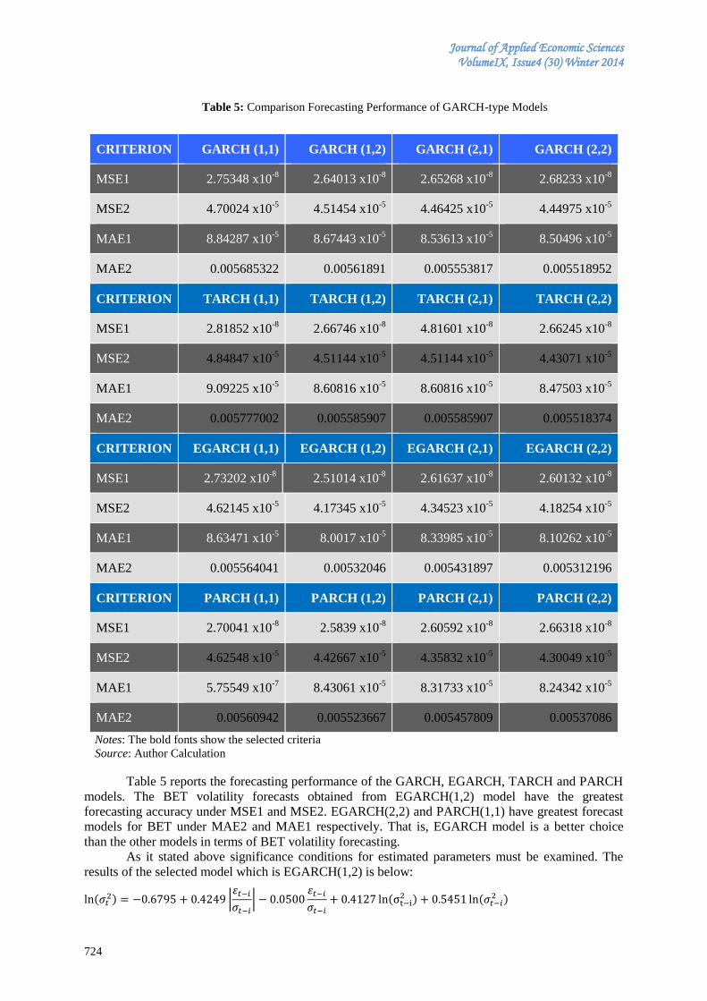
Journal of Applied Economic Sciences VolumeIX, Issue4 (30) Winter 2014
724
Table 5: Comparison Forecasting Performance of GARCH-type Models
CRITERION GARCH (1,1) GARCH (1,2) GARCH (2,1) GARCH (2,2)
MSE1 2.75348 x10⁻⁸
2.64013 x10⁻⁸
2.65268 x10⁻⁸
2.68233 x10⁻⁸
MSE2 4.70024 x10⁻⁵
4.51454 x10⁻⁵
4.46425 x10⁻⁵
4.44975 x10⁻⁵
MAE1 8.84287 x10⁻⁵
8.67443 x10⁻⁵
8.53613 x10⁻⁵
8.50496 x10⁻⁵
MAE2 0.005685322 0.00561891 0.005553817 0.005518952
CRITERION TARCH (1,1) TARCH (1,2) TARCH (2,1) TARCH (2,2)
MSE1 2.81852 x10⁻⁸
2.66746 x10⁻⁸
4.81601 x10⁻⁸
2.66245 x10⁻⁸
MSE2 4.84847 x10⁻⁵
4.51144 x10⁻⁵
4.51144 x10⁻⁵
4.43071 x10⁻⁵
MAE1 9.09225 x10⁻⁵
8.60816 x10⁻⁵
8.60816 x10⁻⁵
8.47503 x10⁻⁵
MAE2 0.005777002 0.005585907 0.005585907 0.005518374
CRITERION EGARCH (1,1) EGARCH (1,2) EGARCH (2,1) EGARCH (2,2)
MSE1 2.73202 x10⁻⁸
2.51014 x10⁻⁸
2.61637 x10⁻⁸
2.60132 x10⁻⁸
MSE2 4.62145 x10⁻⁵
4.17345 x10⁻⁵
4.34523 x10⁻⁵
4.18254 x10⁻⁵
MAE1 8.63471 x10⁻⁵
8.0017 x10⁻⁵
8.33985 x10⁻⁵
8.10262 x10⁻⁵
MAE2 0.005564041 0.00532046 0.005431897 0.005312196
CRITERION PARCH (1,1) PARCH (1,2) PARCH (2,1) PARCH (2,2)
MSE1 2.70041 x10⁻⁸
2.5839 x10⁻⁸
2.60592 x10⁻⁸
2.66318 x10⁻⁸
MSE2 4.62548 x10⁻⁵
4.42667 x10⁻⁵
4.35832 x10⁻⁵
4.30049 x10⁻⁵
MAE1 5.75549 x10⁻⁷
8.43061 x10⁻⁵
8.31733 x10⁻⁵
8.24342 x10⁻⁵
MAE2 0.00560942 0.005523667 0.005457809 0.00537086
Notes: The bold fonts show the selected criteria
Source: Author Calculation
Table 5 reports the forecasting performance of the GARCH, EGARCH, TARCH and PARCH
models. The BET volatility forecasts obtained from EGARCH(1,2) model have the greatest
forecasting accuracy under MSE1 and MSE2. EGARCH(2,2) and PARCH(1,1) have greatest forecast
models for BET under MAE2 and MAE1 respectively. That is, EGARCH model is a better choice
than the other models in terms of BET volatility forecasting.
As it stated above significance conditions for estimated parameters must be examined. The
results of the selected model which is EGARCH(1,2) is below:
|
|

Journal of Applied Economic Sciences VolumeIX, Issue4 (30) Winter 2014
Except the coefficient of leverage effect is significant in 5% level rest of the coefficients are
statistically significant in 1% level (Table 4). The leverage effect is negative and significant means
that leverage effect bad news increase volatility in Bucharest Stock Exchange Trading Index (BET).
Conclusion
The first aim of the paper is to estimate the volatility model of Bucharest Exchange Trading
Index (BET) by using GARCH, EGARCH, TARCH and PARCH models. The second aim is to
compare forecasting performance of the used GARCH-type models to find best model for return of the
BET.
The empirical application was started with interpretation of descriptive statistics. The results
show excess of kurtosis, negative skewness and normality of distribution of the return series. Before
the GARCH-type models were selected the ARMA models estimated to modelling the mean of the
series using several criteria.
It is found that ARMA(2,2) model is the best model for investigated variable. Based on the
ARMA model GARCH-type models were estimated. We compared the forecasting performance of
several GARCH-type models using GED distribution for the return of BET. We found that the
EGARCH(1,2) model is the most promising for characterizing the behaviour of the return of BET. In
other words EGARCH model is more useful than the other models which are used in this paper for
Bucharest Exchange Trading Index returns. Also the EGARCH(1,2) model shows that Bucharest
Exchange Trading Index has leverage effect.
References
[1] Bollerslev, T. (1986). Generalized Autoregressive Conditional Heteroskedasticity, Journal of
Econometrics, 3(3): 307-327.
[2] Ding, Z., Granger, Clive, W.J., Engle, R.F. (1993). A long memory property of stock market
returns and a new model, Journal of Empirical Finance, 1(1): 83-106.
[3] Thalassinos, E., Muratoğlu, Y., Uğurlu E. (2013). Comparison of Forecasting Volatility in the
Czech Republic Stock Market , International Journal of Economics & Business Administration I-
4:, in print.
[4] Uğurlu, E., Thalassinos, E., Muratoğlu Y. (2012). Modeling Volatility in the Stock Markets using
GARCH Models: European Emerging Economies and Turkey, Paper presented at the Annual
International Meeting for International Conference on Applied Business and Economics, Nicosia,
Cyprus, October 11- 13, 2012.
[5] Emerson, R., Hall, S., Zelweska-Mitura, A. (1997). Evolving Market Efficiency with an
Application to Some Bulgarian Shares, Economics of Planning, 30: 75-90.
[6] Engle, R.F. (1982). Autoregressive Conditional Heteroskedasticity with Estimates of the Variance
of UK Inflation, Econometrica, 50: 987–1008.
[7] Haroutounian, M.K., Price, S. (2001). Volatility in the Transition Markets of Central Europe,
Applied Financial Economics, 11: 93-105.
[8] Nelson, D.B. (1991). Conditional Heteroskedasticity in Asset Returns: A New Approach,
Econometrica, 59(2): 347-370.
[9] Pelea, D.T., Mazurencu-Marinescu, M., Nijkampb, P. (2013). Herding Behaviour, Bubbles and
Log Periodic Power Laws in Illiquid Stock Markets A Case Study on the Bucharest Stock
Exchange, Tinbergen Institute Discussion Paper, 109/VIII.
[10] Rockinger, M., Urga, G. (1999). Time Varying Parameters Model to Test for Predictability and
Integration in Stock Markets of Transition Economies, Cahier De Recherche Du Groupe Hec
635.
[11] Scheicher, M. (2001). The Comovements of Stock Markets in Hungary, Poland and The Czech
Republic, International Journal of Finance and Economics, 6: 27–39.

Journal of Applied Economic Sciences VolumeIX, Issue4 (30) Winter 2014
726
[12] Scheicher, M. (1999). Modeling Polish Stock Returns, Helmenstein, C. Edition, Capital Markets
in Transition Economies. Cheltenham, UK: Edward Edgar, 417–437.
[13] Shields, K.K. (1997). Stock Return Volatility on Emerging Eastern European Markets, The
Manchester School Supplement, 1997: 118–138.
[14] Syriopoulos, T. (2007). Dynamic Linkages Between Emerging European And Developed Stock
Markets: Has the EMU Any Impact?, International Review of Financial Analysis, 16: 41-60.
[15] Taylor, S.J. (1986). Modelling Financial Time Series, John Wiley & Sons Publishing.
[16] Vošvrda, M., Žikeš, F. (2004). An Application of The GARCH-t Model On Central European
Stock Returns, Prague Economic Papers, 1: 26-39
[17] Zakoian, J-M. (1994). Threshold Heteroskedastic Models, Journal of Economic Dynamics and
Control, 18(5): 931–952.
*** Bucharest Stock Exchange Trading Index, last modified October 1, 2014, http://www.bloomberg.
com/quote/BET:IND
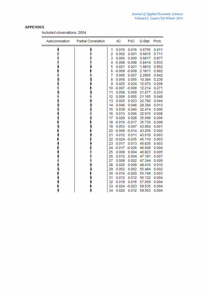
Journal of Applied Economic Sciences VolumeIX, Issue4 (30) Winter 2014
APPENDIX

Journal of Applied Economic Sciences VolumeIX, Issue4 (30) Winter 2014
728
ISSN 1843-6110
Copyright © 2022 FDOKUMEN