
Office 2010 Excel cursus
119
-
Upload
arteveldehs -
Category
Documents
-
view
1 -
download
0
Transcript of Office 2010 Excel cursus

Excel 2010 course
T E R E O S
L e n n a r t . d u b o i s @ t e r e o s . c o m
+ 3 2 5 3 7 3 3 2 9 8
Dubois, Lennart

Lennart Dubois 1 Excel 2010 course
Table of content: 1 Introduction to Excel ............................................................................................................................. 7
1.1 What is Excel? ............................................................................................................................... 7
1.2 User interface ................................................................................................................................ 7
1.3 A few key words ............................................................................................................................ 8
1.3.1 Active Cell .............................................................................................................................. 8
1.3.2 File Tab .................................................................................................................................. 8
1.3.3 Formula Bar ........................................................................................................................... 8
1.3.4 Name Box .............................................................................................................................. 8
1.3.5 Column Letters ...................................................................................................................... 8
1.3.6 Row Numbers ........................................................................................................................ 8
1.3.7 Sheet Tabs ............................................................................................................................. 8
1.3.8 Quick Access Toolbar ............................................................................................................ 9
1.3.9 Ribbon ................................................................................................................................... 9
1.4 The ribbon in depth ...................................................................................................................... 9
1.4.1 General use ........................................................................................................................... 9
1.1.1 Excel 2010 Ribbon overview of the Tabs ............................................................................ 10
1.4.2 Special tabs ......................................................................................................................... 10
1.4.3 Create your own tab ........................................................................................................... 11
1.4.4 10 things you should know about ribbon customization .................................................... 12
1.5 Options within Excel 2010 .......................................................................................................... 14
1.5.1 How to open “Options” ....................................................................................................... 14
1.5.2 Some of the new options .................................................................................................... 16
1.6 Formatting a worksheet in Excel ................................................................................................. 16
1.6.1 Working with columns and rows ........................................................................................ 16
1.6.2 Excel headers and footers ................................................................................................... 18
1.6.3 Format cells ......................................................................................................................... 19
1.6.4 Freeze pane ......................................................................................................................... 20
1.6.5 Merge & centre ................................................................................................................... 21
1.6.6 Wrap Text ............................................................................................................................ 22
1.6.7 Selection of multiple cells ................................................................................................... 22

Lennart Dubois 2 Excel 2010 course
1.6.8 Adjust Sheet tabs ................................................................................................................ 23
1.6.9 Sort ...................................................................................................................................... 24
1.6.10 Filter .................................................................................................................................... 26
2 Functions and formulas....................................................................................................................... 29
2.1 Formulas ..................................................................................................................................... 29
2.1.1 What are formulas? ............................................................................................................ 29
2.1.2 Using operators in formulas ................................................................................................ 29
2.1.3 Relative & Absolute Cell References ................................................................................... 31
2.1.4 Checking formulas with an error......................................................................................... 31
2.2 Functions ..................................................................................................................................... 33
2.2.1 What are functions? ............................................................................................................ 33
2.2.2 The formula tab ................................................................................................................... 33
2.2.3 Insert a function .................................................................................................................. 34
2.2.4 The function wizard ............................................................................................................ 35
2.2.5 Several functions explained ................................................................................................ 36
2.2.6 Search functions .................................................................................................................. 42
2.2.7 List of all the functions ........................................................................................................ 43
2.3 Linking formula’s and functions .................................................................................................. 43
2.3.1 Between different worksheets ........................................................................................... 43
2.3.2 Between different books .................................................................................................... 45
2.3.3 Consolidate data ................................................................................................................. 46
3 Conditional formatting ........................................................................................................................ 48
3.1 What is conditional formatting? ................................................................................................. 48
3.2 How do we apply conditional formatting? ................................................................................. 48
3.3 Data bars, Color scales and Icon sets .......................................................................................... 49
3.4 How to manage Conditional Formatting .................................................................................... 50
3.5 How to delete Conditional Formatting ....................................................................................... 50
4 Tips and tricks within Excel ................................................................................................................. 52
4.1 What is new in Excel 2010? ........................................................................................................ 52
4.1.1 Sparklines ............................................................................................................................ 52
4.1.2 Slicers .................................................................................................................................. 52
4.1.3 Improved Tables & Filters ................................................................................................... 52

Lennart Dubois 3 Excel 2010 course
4.1.4 New Screenshot Feature: .................................................................................................... 53
4.1.5 Paste Previews .................................................................................................................... 53
4.1.6 Improved Conditional Formatting: ..................................................................................... 53
4.1.7 Customize Pivot Tables Quickly .......................................................................................... 54
4.1.8 Customize Add-ins from Developer Ribbon ........................................................................ 54
4.1.9 Customize Ribbons and define your own Ribbons ............................................................. 54
4.1.10 One File Menu to Rule them all .......................................................................................... 55
4.2 Quick access toolbar (QAT) ......................................................................................................... 55
4.2.1 Adding a command to the QAT ........................................................................................... 55
4.3 Export / import changes to the ribbon ....................................................................................... 56
4.4 The new copy-paste options ....................................................................................................... 56
4.4.1 Transpose your selection .................................................................................................... 56
4.4.2 Drag and drop a selection ................................................................................................... 57
4.5 Printing in Excel ........................................................................................................................... 57
4.6 (Select) range options ................................................................................................................. 59
4.7 Protect your worksheet and workbook ...................................................................................... 59
4.7.1 Protect a workbook ............................................................................................................. 59
4.7.2 Protect a worksheet ............................................................................................................ 60
4.8 Working with templates ............................................................................................................. 60
4.9 Creating your own template ....................................................................................................... 61
4.10 Separate content of one cell ....................................................................................................... 62
4.11 Showing only a few rows & columns in Excel ............................................................................. 64
5 Shortcuts ............................................................................................................................................. 65
5.1 Keyboard functions buttons........................................................................................................ 65
5.2 Some of the most important shortcuts: ..................................................................................... 65
6 Data tables .......................................................................................................................................... 67
6.1 How to create table from a bunch of data? ................................................................................ 67
6.1.1 Change table formatting without lifting a finger ................................................................ 68
6.1.2 Add Zebra Lines to Tables without doing Donkey Work ..................................................... 68
6.1.3 Tables come with Data Filters and Sort Options by default ............................................... 69
6.1.4 Bye, bye cell references, welcome structured references .................................................. 69
6.1.5 Make Calculated Columns with ease .................................................................................. 69

Lennart Dubois 4 Excel 2010 course
6.1.6 Total your Tables without writing one formula .................................................................. 70
6.1.7 Convert table back to a range, if you ever need to ............................................................ 70
6.1.8 Export Tables to Pivot Tables .............................................................................................. 70
6.1.9 Print Tables Alone, without all the other stuff around ....................................................... 71
7 Charts .................................................................................................................................................. 72
7.1 Sorts of graphs ............................................................................................................................ 72
7.1.1 Column Chart ...................................................................................................................... 72
7.1.2 Line Graphs ......................................................................................................................... 72
7.1.3 Pie Chart .............................................................................................................................. 72
7.1.4 Bar Graph ............................................................................................................................ 72
7.1.5 Area Chart ........................................................................................................................... 73
7.1.6 Scatter Graphs ..................................................................................................................... 73
7.1.7 Surface Charts ..................................................................................................................... 73
7.2 Formatting your graph ................................................................................................................ 73
7.3 Change chart type ....................................................................................................................... 74
7.4 switch row/column ..................................................................................................................... 75
7.5 Moving a chart to a new sheet ................................................................................................... 75
7.6 Edit / change data ....................................................................................................................... 75
7.7 Edit / change axis ........................................................................................................................ 76
7.8 Add an extra axis ......................................................................................................................... 76
7.9 Save a template........................................................................................................................... 77
7.9.1 Save a chart as a chart template ......................................................................................... 78
7.9.2 Apply a chart template ........................................................................................................ 78
7.9.3 Apply a chart template to an existing chart ........................................................................ 78
7.9.4 Remove or delete a chart template .................................................................................... 78
7.10 Create an interactive chart ......................................................................................................... 79
8 PivotTable ........................................................................................................................................... 83
8.1 Example uses of Pivot Tables ...................................................................................................... 83
8.2 Excel Pivot Table Tutorial: How to create your first pivot table ................................................. 84
8.3 Some useful tips on Excel Pivot Tables ....................................................................................... 85
9 Developer tools ................................................................................................................................... 86
9.1 How to show the developer tab in the ribbon ............................................................................ 86

Lennart Dubois 5 Excel 2010 course
9.2 A Bird’s Eye View Of The Developer Tab’s Options .................................................................... 86
9.3 Code ............................................................................................................................................ 86
9.4 Add-in .......................................................................................................................................... 87
9.5 Controls ....................................................................................................................................... 87
9.6 XML ............................................................................................................................................. 87
9.7 Modify ......................................................................................................................................... 87
10 Macros ............................................................................................................................................ 88
10.1 What is a macro? ........................................................................................................................ 88
10.1.1 Enable macros when the Message Bar appears ................................................................. 88
10.1.2 Enable macros in the Backstage view ................................................................................. 88
10.1.3 Change macro settings in the Trust Center ........................................................................ 89
10.1.4 Macro settings explained .................................................................................................... 89
10.2 Record a macro ........................................................................................................................... 90
10.3 Edit a macro ................................................................................................................................ 91
10.3.1 Create a command button .................................................................................................. 91
10.3.2 Create and Assign the Macro .............................................................................................. 91
11 Visual Basic editor ........................................................................................................................... 94
11.1 To create a new blank workbook ................................................................................................ 94
11.2 Making Macros Accessible .......................................................................................................... 95
11.3 To create a button for a macro on the Quick Access Toolbar .................................................... 95
11.4 A Real-World Example ................................................................................................................ 95
11.4.1 Learning about Objects ....................................................................................................... 95
11.4.2 Using the Macro Recorder .................................................................................................. 96
11.4.3 To use the Macro Recorder as a starting point to your solution ........................................ 96
11.4.4 To record a macro that renames a worksheet .................................................................... 96
11.4.5 Modifying the Recorded Code ............................................................................................ 97
11.4.6 Looping ................................................................................................................................ 98
11.4.7 Useful Renaming ................................................................................................................. 99
11.4.8 Checking for Empty Cells ................................................................................................... 100
11.4.9 Variable Declarations ........................................................................................................ 100
11.4.10 Comments ..................................................................................................................... 101
12 More Things that You Can Do with VBA ....................................................................................... 102

Lennart Dubois 6 Excel 2010 course
12.1 Importance of Being Open ........................................................................................................ 102
12.2 Charts ........................................................................................................................................ 102
12.3 UserForms ................................................................................................................................. 104
13 User forms ..................................................................................................................................... 106
13.1 Introduction .............................................................................................................................. 106
13.2 About the Project ...................................................................................................................... 106
13.3 Build the Form ........................................................................................................................... 106
13.3.1 Insert a New UserForm ..................................................................................................... 106
13.3.2 Rename the UserForm and Add a Caption ....................................................................... 107
13.3.3 Add a TextBox Control and a Label ................................................................................... 107
13.3.4 Add the Remaining Controls ............................................................................................. 109
13.3.5 Create the ComboBox List ................................................................................................. 110
13.3.6 Check the Tab Order ......................................................................................................... 111
13.4 Write the VBA Code .................................................................................................................. 111
13.4.1 Coding the Cancel Button ................................................................................................. 111
13.4.2 Coding the OK Button ....................................................................................................... 112
13.4.3 Coding the Clear Button .................................................................................................... 114
13.4.4 Compile, Test and Save the Finished UserForm ............................................................... 114
13.5 A Macro to Open the UserForm ............................................................................................... 115
13.5.1 Manually Opening the Form ............................................................................................. 115
13.5.2 Opening the Form Automatically ...................................................................................... 115
13.6 Complete Code Listing for the UserForm ................................................................................. 116
Lennart Dubois 7 Excel 2010 course
1 Introduction to Excel
1.1 What is Excel?
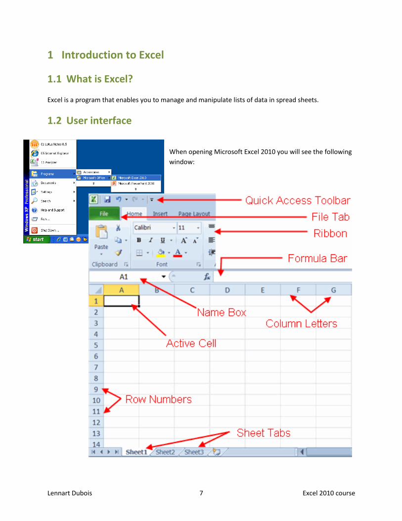
Excel is a program that enables you to manage and manipulate lists of data in spread sheets.
1.2 User interface
When opening Microsoft Excel 2010 you will see the following
window:

Lennart Dubois 8 Excel 2010 course
1.3 A few key words
1.3.1 Active Cell
The active cell is recognized by its black outline. Data is always entered into the active cell. Different
cells can be made active by clicking on them with the mouse or by using the arrow keys on the
keyboard.
1.3.2 File Tab
The File tab is new to Excel 2010 - Sort of. It is a replacement for the Office Button in Excel 2007 which
was a replacement for the file menu in earlier versions of Excel.
Like the old file menu, the File tab options are mostly related to file management such as opening new
or existing worksheet files, saving, printing, and a new feature -saving and sending Excel files in PDF
format.
1.3.3 Formula Bar
Located above the worksheet, this area displays the contents of the active cell. It can also be used for
entering or editing data and formulas.
1.3.4 Name Box
Located next to the formula bar, the Name Box displays the cell reference or the name of the active cell.
1.3.5 Column Letters
Columns run vertically on a worksheet and each one is identified by a letter in the column header.
1.3.6 Row Numbers
Rows run horizontally in a worksheet and are identified by a number in the row header.
Together a column letter and a row number create a cell reference. Each cell in the worksheet can be
identified by this combination of letters and numbers such as A1, F456, or AA34.
1.3.7 Sheet Tabs
By default there are three worksheets in an Excel file.
The tab at the bottom of a worksheet tells you the name of the worksheet - such as Sheet1, Sheet2 etc.
Switching between worksheets can be done by clicking on the tab of the sheet you wish to access.

Lennart Dubois 9 Excel 2010 course
Renaming a worksheet or changing the tab colour can make it easier to keep track of data in large
spread sheet files.
1.3.8 Quick Access Toolbar
This customizable toolbar allows you to add frequently used commands. Click on the down arrow at the
end of the toolbar to display the toolbar's options.
1.3.9 Ribbon
The Ribbon is the strip of buttons and icons located above the work area. The Ribbon is organized into a
series of tabs - such as File, Home, and Formulas. Each tab contains a number of related features and
options. First introduced in Excel 2007, the Ribbon replaced the menus and toolbars found in Excel 2003
and earlier versions.
1.4 The ribbon in depth
1.4.1 General use
You can hide or show the ribbon and its content by double clicking a tab.

Lennart Dubois 10 Excel 2010 course
For more options regarding a group you click on the dialog box Launcher. The window to the right will
appear and represents the “font group”. The result will vary depending in which group you select the
dialog box launcher.
1.1.1 Excel 2010 Ribbon overview of the Tabs
Ribbon Tab
Name
Command Groups Dialog Box
Shortcut
Home Clipboard, Font, Alignment, Styles, Cells, and Editing Ctrl+Shift+F (Font)
Insert Tables, Illustrations, Charts, Sparklines, Filter, Links, Text, and
Symbols
*
Page Layout Themes, Page Setup, Scale to Fit, Sheet Options, and Arrange *
Formulas Function Library, Defined Names, Formula Editing, and
Calculation
*
Data Get External Data, Connections, Sort and Filter, Data Tools,
and Outline
*
Review Proofing, Language, Comments, and Changes *
View Workbook Views, Show, Zoom, Window, and Macros *
1.4.2 Special tabs
When working with Excel 2010 you will notice there are situational
tabs added to your ribbon after selecting certain objects. For
example, when inserting a shape, you get the tab you see on the
right (drawing tools).
There are multiple situational tabs that contain all the information
you need to alter and work with the certain objects. For example
when adding:
Pictures, chards, PivotTables,

Lennart Dubois 11 Excel 2010 course
1.4.3 Create your own tab
Starting Excel 2010, you can finally customize the ribbon user interface and define your
own tabs or groups. This can be a huge productivity boost for people using MS Office
applications.
1. Right click on ribbon area and select “customize ribbon” option.
2. Now, add a new tab (or group or both). Do not forget to rename the new tab! 3. Add a few commands (or buttons) to your new ribbon 4. Click ok and you have a sparkling new ribbon ready.

Lennart Dubois 12 Excel 2010 course
1.4.4 10 things you should know about ribbon customization
This is how the ribbon customization screen looks.
I have highlighted 10 items on the screen. Read the 10 points to master ribbon customization.
1. Use New Tab button to create a new ribbon tab. 2. Use New Group button to add a new group of commands to an existing or new ribbon. 3. Rename button helps you to change the name of an existing custom group or tab. 4. Once you add a group / tab, you have to select it to add items to that group / tab. 5. You can choose the type of commands you want to add to your ribbon tab / group. You can also
add any macros as well (sweet!). 6. Now select the command you want to add to your group 7. Click on “Add” button to add the command to your ribbon tab / group. 8. You can use “Remove” button to remove any commands from custom tabs / groups. 9. Use the up / down arrow buttons to move your ribbon tab / group up or down. (For eg. you can
move your custom tab to first, ie before home tab). 10. You can export your ribbon customizations and re-use them in other computers (both ribbon
and QAT settings will be exported).

Lennart Dubois 13 Excel 2010 course
Ribbon and QAT Customization – Few Tips:
Use “Hide Command Labels” option to shrink your ribbon groups.
Note, this only applies on custom created tabs!
See the below illustration to understand what I mean.
Customize tool ribbon tabs to save a ton of time:
By default, when you go to “customize ribbon” screen, you only see main tabs. But you can also
customize tool specific tabs. For example. I only use a handful of chart formatting options and all
of these are spread across 3 different tabs – design, layout and format. So I combined all the
options I use regularly to come up with a simple ribbon tab like this:

Lennart Dubois 14 Excel 2010 course
As you can guess, the above ribbon tab appears only when I am formatting a chart.
Add groups of commands to QAT:
You can now add a group of commands (for eg. all alignment options) to Quick Access Toolbar
to improve your productivity.
Minimize ribbon with a click:
Press the ^ icon you see next to help icon to instantly collapse / expand ribbon. You can also use
CTRL+F1 keyboard shortcut to do the same.
Ribbon Customization Gotchas!
While ribbon customization is a great move ahead for Excel in particular and Office apps in general,
there are a few gotchas. Beware of the following to avoid un-necessary troubles.
When you add a group or tab, excel doesnt ask you for a name. Make sure you click on “rename”
button to change the name to something you remember.
You cannot add commands to an existing excel defined group. You can however add groups to
existing ribbons.
The ribbon and QAT customizations you do are local to your installation of excel only. You have to
export the customizations and import them before they work on other comps.
1.5 Options within Excel 2010
1.5.1 How to open “Options”
This item is found in the backstage view
In order to open it, you select “Options”

Lennart Dubois 15 Excel 2010 course
The Backstage view – Exposed
Lennart Dubois 16 Excel 2010 course
1.5.2 Some of the new options
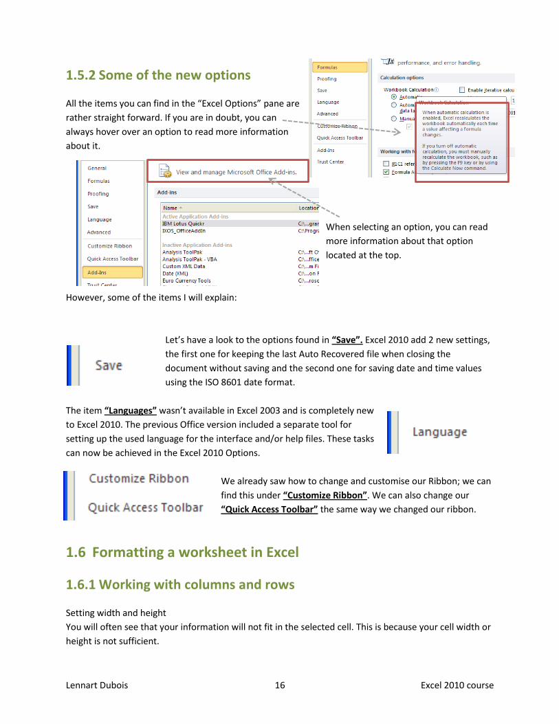
All the items you can find in the “Excel Options” pane are
rather straight forward. If you are in doubt, you can
always hover over an option to read more information
about it.
When selecting an option, you can read
more information about that option
located at the top.
However, some of the items I will explain:
Let’s have a look to the options found in “Save”. Excel 2010 add 2 new settings,
the first one for keeping the last Auto Recovered file when closing the
document without saving and the second one for saving date and time values
using the ISO 8601 date format.
The item “Languages” wasn’t available in Excel 2003 and is completely new
to Excel 2010. The previous Office version included a separate tool for
setting up the used language for the interface and/or help files. These tasks
can now be achieved in the Excel 2010 Options.
We already saw how to change and customise our Ribbon; we can
find this under “Customize Ribbon”. We can also change our
“Quick Access Toolbar” the same way we changed our ribbon.
1.6 Formatting a worksheet in Excel
1.6.1 Working with columns and rows
Setting width and height
You will often see that your information will not fit in the selected cell. This is because your cell width or
height is not sufficient.

Lennart Dubois 17 Excel 2010 course
You can solve this problem using one of the following methods:
Dragging the column or row to the desired width / height
You can drag the column or row manually:
Selecting the column or row and setting the width /height
You select the desired column or row; right click the top or left title bar and select Column Width or
Row Height.
Double clicking the column or row in order to set the width / height
automatically

Lennart Dubois 18 Excel 2010 course
1.6.2 Excel headers and footers
If you want to add additional information about the book you are working with you can add a header or
footer.
If we select this option we can add a range of options to our header/footer. All of these options are
found in the special tab “Header&Footer Tools”:
In the header you can see an example of each option. Note, the bold and underlined text is not a part of
the options!
Also, when you do not fill in anything the “page number” and “number
of pages” will be respectively be “#” and “0”. This because there is
nothing active on the page! This will change when you add text or
numbers:
Lennart Dubois 19 Excel 2010 course
1.6.3 Format cells
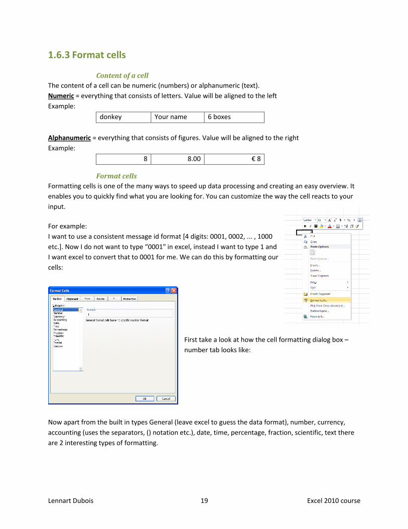
Content of a cell
The content of a cell can be numeric (numbers) or alphanumeric (text).
Numeric = everything that consists of letters. Value will be aligned to the left
Example:
donkey Your name 6 boxes
Alphanumeric = everything that consists of figures. Value will be aligned to the right
Example:
8 8.00 € 8
Format cells
Formatting cells is one of the many ways to speed up data processing and creating an easy overview. It
enables you to quickly find what you are looking for. You can customize the way the cell reacts to your
input.
For example:
I want to use a consistent message id format [4 digits: 0001, 0002, ... , 1000
etc.]. Now I do not want to type “0001″ in excel, instead I want to type 1 and
I want excel to convert that to 0001 for me. We can do this by formatting our
cells:
First take a look at how the cell formatting dialog box –
number tab looks like:
Now apart from the built in types General (leave excel to guess the data format), number, currency,
accounting (uses the separators, () notation etc.), date, time, percentage, fraction, scientific, text there
are 2 interesting types of formatting.

Lennart Dubois 20 Excel 2010 course
Special: Used for phone number, zip code, social security number formats depending on the locale you
select. For eg. for US they would be phone number [xxx-xxx-xxxx], ssn [xxx-xx-xxxx], zipcode[xxxxx,
xxxxx-xxxx].
Custom: Used for creating your own cell formatting structure. This is a bit like regular expressions but in
entire microsoftish way. Any cell custom format code will be divided in to 4 parts: positive numbers ;
negative numbers ; zeros ; text. If your formatting codes have less number of parts (say 1 or 2 or 3) excel
will use some common sense to find out which ones are for what.
Below you can find an overview of how to apply a range of cell formats:
1.6.4 Freeze pane
If you want to keep your titles or subjects visible while
scrolling through your data you can freeze them! This can
be done under view > window > freeze panes.
Select the cell in which you want to freeze your titles and
subjects, go to view > window > freeze panes and select
“Freeze Panes”. You can now scroll through your data without losing your titles and subjects.
Lennart Dubois 21 Excel 2010 course
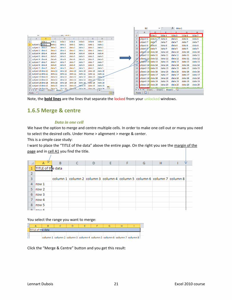
Note, the bold lines are the lines that separate the locked from your unlocked windows.
1.6.5 Merge & centre
Data in one cell
We have the option to merge and centre multiple cells. In order to make one cell out or many you need
to select the desired cells. Under Home > alignment > merge & center.
This is a simple case study:
I want to place the “TITLE of the data” above the entire page. On the right you see the margin of the
page and in cell A1 you find the title.
You select the range you want to merge:
Click the “Merge & Centre” button and you get this result:

Lennart Dubois 22 Excel 2010 course
Data in multiple cells
Select all the cells where your data is located. (All the cells need to be in one area in one column).
Adjust the column width so that you can fit all contents in one cell. (Basically make
it wide enough)
Select Home Ribbon > Fill > Justify
Merge cells now.
The text from selected cells will be re-arranged in top-most cell. If you see the text spreading 2 rows,
just make the column wider and repeat the process.
But wait, this technique has some limitations,
It doesn’t work if the selected cells have numbers or formulas
It only works for cells in a single column, if the cells are spread across several columns, justify
will not work.
It requires a lot of steps.
1.6.6 Wrap Text
If you do not want to merge the cells (take up multiple cells), you can “wrap” the text inside the cell. This
will heighten your cell but will put all the data inside.
Select the cell and click “Wrap Text”. This is the result:
1.6.7 Selection of multiple cells

Lennart Dubois 23 Excel 2010 course
What is “cell range”?
A range of cells are all, with the emphasis on “all”, adjacent or
non-adjacent cells that are selected. This collection of cells,
considered as a whole, is called a cell range or “range” for short.
What can we do with a range?
We use a range in formula’s and functions, a list, … and it consists
of the letter and number. In the image we can see the range in the
formula bar.
Selecting multiple cells
Drag the range of cells with your mouse or keyboard (using the shift and arrow-buttons) to select your range.
If you want to select individual cells that are not next to each other, you hold in the CTRL button and click on the desired cells.
Give a name to a range
If you want to give a name to the range you have selected you can easily apply this in the name box.
This can have any name you like and you can see and select all names under the arrow.
If you want to edit the names, you find the manager under: Formulas > Defined Names > Name
manager.
1.6.8 Adjust Sheet tabs

Lennart Dubois 24 Excel 2010 course
When starting Excel 2010 you will see 3 standard tabs in the bottom left corner with the names sheet 1,
2 and 3.
You can rename a sheet by double clicking or right clicking the sheet and select “rename”. The other
options regarding the sheets are also in this menu:
1.6.9 Sort
Excel is designed to work with large amounts of data. In order to structure this data we use a database.
A database is a collection of records. Those records contain fields.
To demonstrate this:
OrderDate Region Rep Item Units Cost Total
Excel considers each row as a “record”, and each column as a field.
Sorting data has become easy in Excel 2010. To sort your data (either text or
numbers) you select the cells you want to order and click Home > Editing > Sort
& Filter.
Move or copy your sheet to either this
book or another (active) book.
Open the VBa code behind this sheet.
or
Protect your sheet with at the level you
want with a password.
Record
Field

Lennart Dubois 25 Excel 2010 course
Sorting numbers or dates:
Sorting names:
Even when you want to sort your data over multiple columns Excel offers you this option.
Sorting multiple columns (custom sort):
Select a cell within your range, go to home > editing > sort & filter > Custom Sort. This will give you the
option to sort with multiple criteria. Remember, you have the option to define whether your data has
headers or not!

Lennart Dubois 26 Excel 2010 course
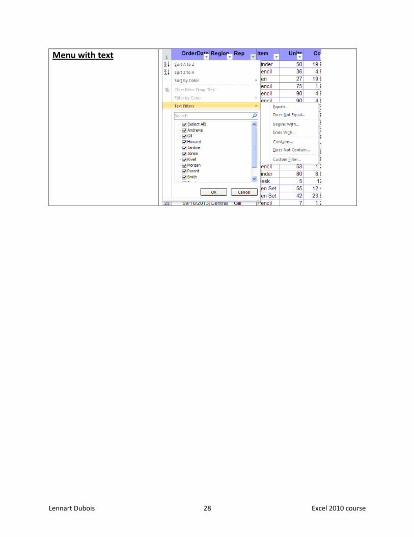
1.6.10 Filter
A second database function is to filter data. By filtering data we can only
show the items which meet a certain criteria or condition.
The first thing you need to do is placing your cursor in the range you want
to filter. The second is to click on the filter button (home > editing > Sort &
Filter > Filter)
After clicking “Filter” you will see buttons next to your headers:
These buttons will present you with a drop-down menu where you can sort
your data or filter it. This drop-down menu takes your values into account!

Lennart Dubois 27 Excel 2010 course
Menu with dates Note that you can add specific filters on your data filter (eg. Equals, before, after, …) The filter option also gives you an overview per year / month.
Menu with numbers You can add certain parameters or condition to your filter (eg. Greater than, less than, …)
Lennart Dubois 28 Excel 2010 course
Menu with text

Lennart Dubois 29 Excel 2010 course
2 Functions and formulas
2.1 Formulas
2.1.1 What are formulas?
A formula is used when we want to calculate something. A formula
always starts with the “equals” sign (=). For example: we want to
calculate the sum of cell A1 and A2:
(A3: we press “=” and click the cell A1, type “+” and click the cell A2)
We do not have to work with the cell reference, we can just
calculate with numbers as well (see cell A4)
2.1.2 Using operators in formulas
An operator is a symbol or instruction that manipulates expressions in a formula. For example, the plus
(+) operator tells Excel to add one expression to another. There are four types of operators:
The Different Types of Operators in Excel
Type Character Operation Example
Mathematical + (plus sign) Addition =A2+B3
– (minus sign) Subtraction or negation =A3–A2 or –C4
* (asterisk) Multiplication =A2*B3
/ Division =B3/A2
% Percent (dividing by 100) =B3%
^ Exponentiation =A2^3
Comparison = Equal to =A2=B3
> Greater than =B3>A2
< Less than =A2<B3
>= Greater than or equal to =B3>=A2
<= Less than or equal to =A2<=B3
<> Not equal to =A2<>B3

Lennart Dubois 30 Excel 2010 course
Text & Concatenates (connects) entries to produce
one continuous entry
=A2&” “&B3t
Reference : (colon) Range operator that includes =SUM(C4:D17)
, (comma) Union operator that combines multiple
references into one reference
=SUM(A2,C4:D17,B3)
(space) Intersection operator that produces one
reference to cells in common with two
references
=SUM(C3:C6 C3:E6)
Most of the time, you’ll rely on the mathematical or arithmetic operators when building formulas in
your spreadsheets that don’t require functions because these operators actually perform computations
between the numbers in the various cell references and produce new mathematical results.
The comparison operators, on the other hand, produce only the logical value TRUE or the logical value
FALSE, depending on whether the comparison is accurate.
The single text operator (the so-called ampersand) is used in formulas to join together two or more text
entries (an operation with the highfalutin’ name concatenation).
You most often use the comparison operators with the IF function when building more complex
formulas that perform one type of operation when the IF condition is TRUE and another when it is
FALSE. You use the concatenating operator (&) when you need to join text entries that come to you
entered in separate cells but that need to be entered in single cells (like the first and last names in
separate columns).
When you build a formula that combines different operators, Excel follows the set order of operator
precedence. When you use operators that share the same level of precedence, Excel evaluates each
element in the equation by using a strictly left-to-right order.
Natural Order of Operator Precedence in Formulas
Precedence Operator Type / Function
1 - Negation
2 % Percent
3 ^ Exponentiation
4 * and / Multiplication and Division
5 + and - Addition and Subtraction
6 & Concatenation
7 =, <, >, <=, >=, <> All Comparison Operators

Lennart Dubois 31 Excel 2010 course
2.1.3 Relative & Absolute Cell References
When using formulas (and soon functions) your argument is a cell
or a range of cells. A cell (or range of cells) is unique because of
its reference to the column and row.
You can find the cell address when selecting cells in the Name
box.
As soon as you know this, you can build a formula or function. Ex: =A2*B2.
When we copy this formula, the references to those cells will shift accordingly.
For example:
We have a formula =A2*B2 in cell C2. When we copy the cell C2 to C3, the copied formula will
automatically adjust. The formula in C3 will be: =A3*B3
A B C
1
2 2 3 =A2*B2
3 =A3*B3
This is what we call relative cell reference. The reference to the cells are relative with respect to the
formula or function, they change accordingly.
However, when you refer to a cell that should remain the same when copied, you should make this cell
reference absolute! This is done by adding a dollar sign ($) before the column and row. The cell
reference with the ($) sign will remain the same, the cell reference without the dollar sign will act
normal (= shift with the movement of the copied cell).
A fast way to assign dollar signs is pressing F4 when your cursor is in the right cell reference. Pressing F4
again will alternate between making the row or column absolute. Pressing F4 a fourth time will return
the reference to normal.
A B C
1
2 2 3 =$A$2*B2
3 =$A$2*B3
2.1.4 Checking formulas with an error
If Excel 2010 can't properly calculate a formula that you enter in a cell, the program displays an error
value in the cell as soon as you complete the formula entry. Excel uses several error values, all of which
begin with the number sign (#).
Result
C2 = 5
C3 = 0
Lennart Dubois 32 Excel 2010 course
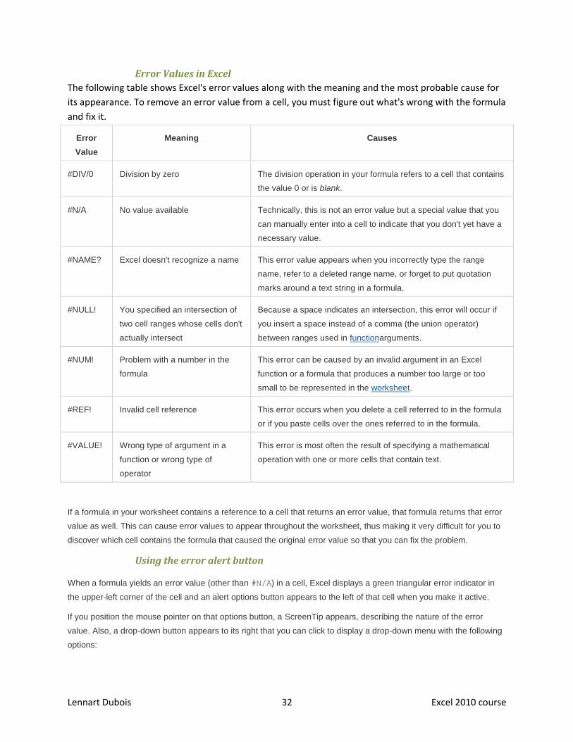
Error Values in Excel
The following table shows Excel's error values along with the meaning and the most probable cause for
its appearance. To remove an error value from a cell, you must figure out what's wrong with the formula
and fix it.
Error
Value
Meaning Causes
#DIV/0 Division by zero The division operation in your formula refers to a cell that contains
the value 0 or is blank.
#N/A No value available Technically, this is not an error value but a special value that you
can manually enter into a cell to indicate that you don't yet have a
necessary value.
#NAME? Excel doesn't recognize a name This error value appears when you incorrectly type the range
name, refer to a deleted range name, or forget to put quotation
marks around a text string in a formula.
#NULL! You specified an intersection of
two cell ranges whose cells don't
actually intersect
Because a space indicates an intersection, this error will occur if
you insert a space instead of a comma (the union operator)
between ranges used in functionarguments.
#NUM! Problem with a number in the
formula
This error can be caused by an invalid argument in an Excel
function or a formula that produces a number too large or too
small to be represented in the worksheet.
#REF! Invalid cell reference This error occurs when you delete a cell referred to in the formula
or if you paste cells over the ones referred to in the formula.
#VALUE! Wrong type of argument in a
function or wrong type of
operator
This error is most often the result of specifying a mathematical
operation with one or more cells that contain text.
If a formula in your worksheet contains a reference to a cell that returns an error value, that formula returns that error
value as well. This can cause error values to appear throughout the worksheet, thus making it very difficult for you to
discover which cell contains the formula that caused the original error value so that you can fix the problem.
Using the error alert button
When a formula yields an error value (other than #N/A) in a cell, Excel displays a green triangular error indicator in
the upper-left corner of the cell and an alert options button appears to the left of that cell when you make it active.
If you position the mouse pointer on that options button, a ScreenTip appears, describing the nature of the error
value. Also, a drop-down button appears to its right that you can click to display a drop-down menu with the following
options:

Lennart Dubois 33 Excel 2010 course
Help on This Error: Opens an Excel Help window with information on the type of error value in the active cell
and how to correct it.
Show Calculation Steps: Opens the Evaluate Formula dialog box, where you can walk through each step in
the calculation to see the result of each computation.
Ignore Error: Bypasses error checking for this cell and removes the error alert and Error options button from it.
Edit in Formula Bar: Activates Edit mode and puts the insertion points at the end of the formula on the Formula
bar.
Error Checking Options: Opens the Formulas tab of the Excel Options dialog box, where you can modify the
options used in checking the worksheet for formula errors.
If you're dealing with a worksheet that contains many error values, you can use the Error Checking button in the
Formula Auditing group on the Ribbon's Formulas tab to locate each error.
2.2 Functions
2.2.1 What are functions?
Functions are pre-defined formulas which preform operations with one or more values in the correct
order. The most common functions are SUM and Average, but there are a whole lot more! I will try to
incorporate the most important ones, but there are functions so specific that I cannot cover them all.
2.2.2 The formula tab
In the ribbon we can find a tab “formulas”. There we find different categories:
The first button is “AutoSum” (also found in the home tab under “Editing”):
Sum Calculates the sum of the selected range.
Average Calculates the average of the selected range.
Count Numbers Counts the amount of numbers in the selected range.
Max Returns the largest value in a set of values.
Min Returns the smallest number in a set of values.

Lennart Dubois 34 Excel 2010 course
Next to “autosum” we find a range of other options like recently used functions, financial functions,
logical functions, etc.
2.2.3 Insert a function
When we want to insert a function, we select the cell where our
result should come. There we click on the “autosum” icon under
start. This will auto complete our function:
Building stones of a function:
Explanation equal sign Name of the function Arguments between brackets
function = SUM (Number1,[number2], …)
Range of numbers (Bold =mandatory!)
2nd argument, not needed because between [ ] brackets
Possibility to add more arguments
If you are not satisfied with the proposed range Excel gives you, you can always change it in the
following ways:
1. By using the mouse to click and drag over the cells you want to count.
2. By dragging the frame that is around the currently selected cells
3. Manually inputting the cells or range you want.
After pressing Enter you will see the result of your function:
If you want to update or change your function in a later stage,
you can double click the cell and following the steps above to
change your range.
Lennart Dubois 35 Excel 2010 course
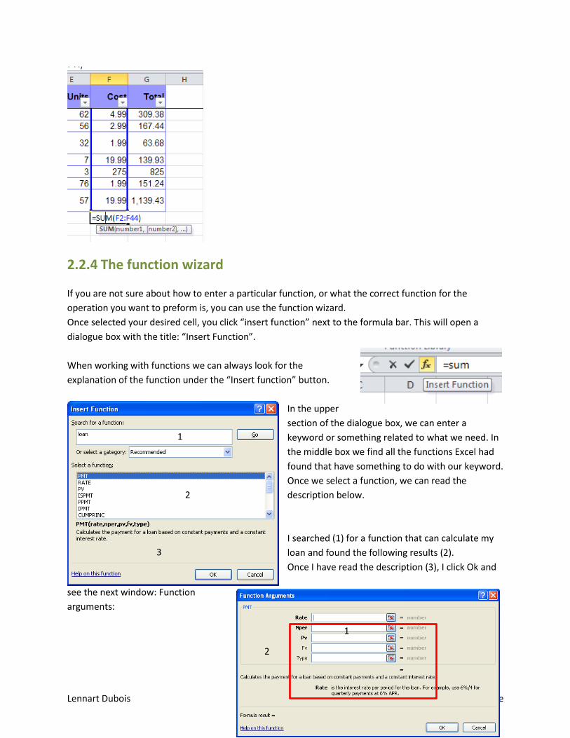
2.2.4 The function wizard
If you are not sure about how to enter a particular function, or what the correct function for the
operation you want to preform is, you can use the function wizard.
Once selected your desired cell, you click “insert function” next to the formula bar. This will open a
dialogue box with the title: “Insert Function”.
When working with functions we can always look for the
explanation of the function under the “Insert function” button.
In the upper
section of the dialogue box, we can enter a
keyword or something related to what we need. In
the middle box we find all the functions Excel had
found that have something to do with our keyword.
Once we select a function, we can read the
description below.
I searched (1) for a function that can calculate my
loan and found the following results (2).
Once I have read the description (3), I click Ok and
see the next window: Function
arguments:
1
3
1
2
2

Lennart Dubois 36 Excel 2010 course
In this dialogue box we can see the arguments (1) needed in order to get a result. The arguments in bold
(2) have to be filled in; the others are optional (3). When selecting an argument, you can see the
description (4) at the bottom.
We will fill in the arguments that are needed and press ok:
And get the following result:
2.2.5 Several functions explained
Min/max
These functions are used to display the minimum or maximum of a range. After selecting your cell, you
can find the function in the “autosum” dropdown menu in the start ribbon. This will automatically select
a range. If you want to re-edit this you can drag the range or drag the edge of the blue bounding box.
3
4

Lennart Dubois 37 Excel 2010 course
Average
We use the average function to calculate the average of all the cells in our range. A fast way to use this
function is via the drop-down menu under the “autosum” button.
Count
In general: the function “count” and everything that has to do with it will count the amount of cells in a
range that meet the condition(s). There are a few functions that work with “count”:
function Example explanation
COUNT =COUNT(F1:F100) Counts the number of cells in a range that contain numbers.
COUNTBLANK =COUNTBLANK(F1:F100) Counts the number of empty cells in a specified range of cells.
COUNTA =COUNTA(F1:F100) Counts nonblank cells in the field (column) or records in the database that match the conditions you specify.
COUNTIF =COUNTIF(F1:F100, “> 0”) Count the number of cells within a range that meet the given condition.
COUNTIFS =COUNTIFS(E4:E8;">4000";A4:A8;"=test") Counts the number of cells specified by a given set of conditions or criteria.
Left / right
The LEFT function returns the first character(s) of a string. For example:
Cell A1 contains the name: John Doe
If we want to separate the first name from the family name, we do this with the LEFT function. In the
cell B1 we type: =LEFT(A1, 4). This will result in the following:
The first argument in our function is the cell reference (the text we want to edit)
The second argument in our function is the number of characters we want to “cut”, in our case 4.
The result in B1 is the first 4 characters from the cell A1.
Lennart Dubois 38 Excel 2010 course
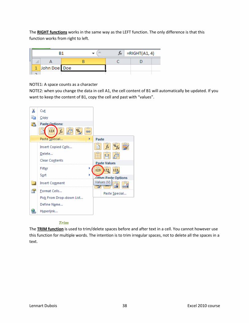
The RIGHT functions works in the same way as the LEFT function. The only difference is that this
function works from right to left.
NOTE1: A space counts as a character
NOTE2: when you change the data in cell A1, the cell content of B1 will automatically be updated. If you
want to keep the content of B1, copy the cell and past with “values”.
Trim
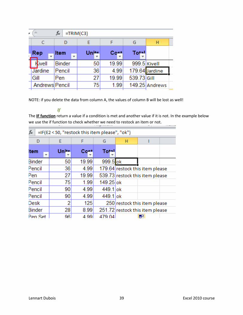
The TRIM function is used to trim/delete spaces before and after text in a cell. You cannot however use
this function for multiple words. The intention is to trim irregular spaces, not to delete all the spaces in a
text.
Lennart Dubois 39 Excel 2010 course
NOTE: if you delete the data from column A, the values of column B will be lost as well!
If
The IF function return a value if a condition is met and another value if it is not. In the example below
we use the if function to check whether we need to restock an item or not.

Lennart Dubois 40 Excel 2010 course
1. What we do is check with a Boolean operator (eg. <, >, =, …) whether a condition is met.
2. We fill in an argument if the logical test is true
3. We fill in an argument if the logical test is false.
Sumif
The SUMIF function adds the content of the cells together if they meet a certain condition. In the
example below we want to check how much is sold of a specific item.
1. My range is the items in my list (column D)
2. The criteria are the 5 sorts of items listen in column H
3. A sum is made with the positive results of my criteria and my items.
1.
2.
3.

Lennart Dubois 41 Excel 2010 course
Concatenate
With the concatenate function we can combine text from multiple cells. For example, the first names
and last names of our contacts are put in 2 separate columns. We want to put the names in 1 column.
There are 2 ways of doing this:
NOTE: the selected cells do not contain a space! You will have to add one yourself. This by adding the
textual string: “ “.
The arguments are put as
separate text.
You create your own text
string with Boolean
operators.

Lennart Dubois 42 Excel 2010 course
2.2.6 Search functions
VLookup
With the VLOOKUP function we search a database based on a predefined value in a column.
For example: a customer has a question about his purchase. He would like to know who sold him the
item. The only thing our customer knows is the OrderId on his ticket. We’ll have to look through the
entire list before we find what we are looking for… or, we use the VLOOKUP function:
1. We type our ticket number in the cell J4. This will be our “lookup value”.
2. Then we give the range in which we want to look (the first column always has to be the column
in which our lookup value should be).
3. Once the function has found a match, it will give the value of the column you select. In our case
the fourth column or the name of the representative.
4. By adding the “TRUE” or “FALSE” logical value to our function we look for either the exact match
(FALSE) or something that resembles our search value (TRUE).

Lennart Dubois 43 Excel 2010 course
Hlookup
With the HLOOKUP function we search data based on a predefined value in a row.
For example: we want to calculate the commission of a sales representative. Each bracket / range has
his own percentage (represented in red). The function will automatically detect that we work with
brackets / ranges and will go to the next value when the condition is met. An example is F6. The value is
1.499 and therefor still 5% instead of 7%
2.2.7 List of all the functions
The following list will give an overview of all the functions available in Excel + explanation:
http://www.techonthenet.com/excel/formulas/
2.3 Linking formula’s and functions
2.3.1 Between different worksheets
An advantage of a linked formula is when we change data in our workbook, the linked cells are updated
with the latest information. When you have data on several sheets and you want to summarize it on a
general sheet you create an extra sheet and make all your calculations with the original sheets. As
always we start by typing in “=” to start our formula or function.
We want to know the total amount of sold items.
Row 1
Row 2

Lennart Dubois 44 Excel 2010 course
Each region has its own sheet:
So we need to add all the sold items together for each sheet:
We take the sum of our total columns of each sheet. As you can see in the formula each sheet is
represented and the range on the sheet is behind the exclamation mark:
function Name of the sheet
Range within the sheet
Name of the sheet
Range within the sheet
Name of the sheet
Range within the sheet
Step-by-step approach:
steps Result
- Select the cell you want
- Type “=” and your function (SUM)
- Go to the sheet you want and select your
range.

Lennart Dubois 45 Excel 2010 course
- Press “,” and add the next argument.
- Repeat and end with “)” =SUM(west!H2:H7,east!H2:H14,central!H2:H25)
Now if we want to calculate how many items and how much each representative has sold. We can do
this with the COUNTIF and the SUMIF function. For each sheet we add a “+” between the calculations.
You will find the solution below:
2.3.2 Between different books
If you want to gather data from different workbooks, you can follow the same actions as above.
Note1: The workbooks have to be open and you have to select the data from the different workbooks.
Note2: the workbooks mentioned in the formula or functions are listed in square brackets or with the
extensions and with absolute cell references.

Lennart Dubois 46 Excel 2010 course
2.3.3 Consolidate data
Another way to consolidate data from different worksheets is
with the command “Merge” the command “Merge” works
best when the layout of the different workbooks are equal.
First you open all the workbooks you want to merge and
select the cell where you want them to be. In the ribbon tab
“data” you will find the option “Consolidate”.
In the upper section of the dialogue box you can chose from
different functions. Underneath you can select your range. Once you are done selecting, you click add.
This will add the first reference to your list. Continue this way for the other references you want to add:

Lennart Dubois 47 Excel 2010 course

Lennart Dubois 48 Excel 2010 course
3 Conditional formatting
3.1 What is conditional formatting?
By making use of conditional formatting we can edit the layout of cells that match the condition we give
based on the content of the cell.
In other words, we visually analyse our data using conditions and in that way identify any problems.
For example, if the value of a cell is less than 1000, the cell is coloured red.
3.2 How do we apply conditional formatting?
The first thing we do is to select the range where we want to
apply the formatting. In our case we select the total column.
This reflects the total amount sold by a representative.
Note: to quickly select the column you can use the keyboard
shortcut CTRL + Shift + arrow down when you selected the
first value in the column.
After selecting the range, we want to apply the conditional
formatting. To do so, go to the home tab and select the
“Conditional Formatting” button in the ribbon. This will give
you a drop down menu with different formatting capabilities
divided into categories.
The first 2 options are rather straight forward:
You apply a certain layout to the cell when the condition you
made is met.
Lennart Dubois 49 Excel 2010 course
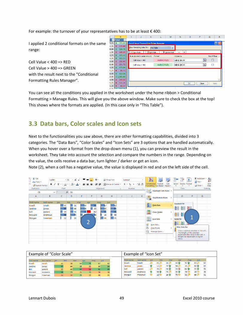
For example: the turnover of your representatives has to be at least € 400:
I applied 2 conditional formats on the same
range:
Cell Value < 400 => RED
Cell Value > 400 => GREEN
with the result next to the “Conditional
Formatting Rules Manager”.
You can see all the conditions you applied in the worksheet under the home ribbon > Conditional
Formatting > Manage Rules. This will give you the above window. Make sure to check the box at the top!
This shows where the formats are applied. (In this case only in “This Table”).
3.3 Data bars, Color scales and Icon sets
Next to the functionalities you saw above, there are other formatting capabilities, divided into 3
categories. The “Data Bars”, “Color Scales” and “Icon Sets” are 3 options that are handled automatically.
When you hover over a format from the drop-down menu (1), you can preview the result in the
worksheet. They take into account the selection and compare the numbers in the range. Depending on
the value, the cells receive a data bar, turn lighter / darker or get an icon.
Note (2), when a cell has a negative value, the value is displayed in red and on the left side of the cell.
Example of “Color Scale” Example of “Icon Set”
1 2

Lennart Dubois 50 Excel 2010 course
3.4 How to manage Conditional
Formatting
To manage the conditional formats you applied you go to the tab
Home > Conditional Formatting > Manage Rules.
This option will show you a dialogue box in which all conditions
are presented.
Make sure you have selected the right option for showing
formatting rules (1)!
Here we see 4 conditions applied on the range =$C$3:$H$7. If I
want to change the condition, I have to edit the rule after
selecting it.
In my case I want to edit the “Icon Set”. When I press “Edit Rule…” I can change the values assigned to
the icons:
3.5 How to delete Conditional Formatting
1

Lennart Dubois 51 Excel 2010 course
To delete the conditions you can just press or select where you want to delete the applied
conditions and then click the option “Clear Rules”:
Lennart Dubois 52 Excel 2010 course
4 Tips and tricks within Excel
4.1 What is new in Excel 2010?
There are a ton of new and cool features in Excel 2010. My favorite new features are:
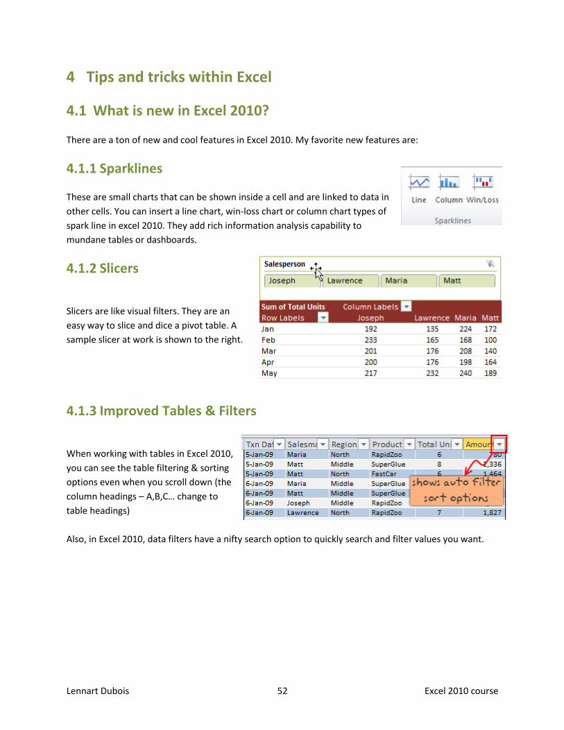
4.1.1 Sparklines
These are small charts that can be shown inside a cell and are linked to data in
other cells. You can insert a line chart, win-loss chart or column chart types of
spark line in excel 2010. They add rich information analysis capability to
mundane tables or dashboards.
4.1.2 Slicers
Slicers are like visual filters. They are an
easy way to slice and dice a pivot table. A
sample slicer at work is shown to the right.
4.1.3 Improved Tables & Filters
When working with tables in Excel 2010,
you can see the table filtering & sorting
options even when you scroll down (the
column headings – A,B,C… change to
table headings)
Also, in Excel 2010, data filters have a nifty search option to quickly search and filter values you want.

Lennart Dubois 53 Excel 2010 course
4.1.4 New Screenshot Feature:
Now, using Excel (or any other Office 2010 app) you can grab a screenshot of any open window. This
could be very useful for those of us in teaching industry as you can quickly embed screenshots in to your
teaching material (like slides or documents).
4.1.5 Paste Previews
There are a ton of cool paste features buried in the Paste Special Options in earlier versions of Excel. MS
has bought all these to fore-front with Paste Previews feature in Office 2010.
4.1.6 Improved Conditional Formatting:
Excel 2010 added a lot of simple but effect improvements to
conditional formatting. One of my favourites is the ability to
have solid fill in a cell based on the value in it. This provides an
easy way to create in-cell bar charts.

Lennart Dubois 54 Excel 2010 course
4.1.7 Customize Pivot Tables Quickly
Now you can easily change pivot table summary type and calculation types from Pivot Table “Options”
ribbon in a click (learn how to do this in Excel 2007 and earlier).
Also you can do what-if analysis on Pivots (I am yet to try this feature).
4.1.8 Customize Add-ins from Developer Ribbon
In Excel 2007, if you want to customize or add a new add-in, you have to circumnavigate cape of good
hope. But Excel 2010 makes it a pleasant experience again. There are two buttons, right on developer
ribbon tab using which you can quickly add, change any add-ins.
(also, it seems like developer ribbon is turned on by default, which is pretty cool.)
4.1.9 Customize Ribbons and define your own Ribbons
One the most beautiful and powerful features about Office products is that you can customize them as
you want. You could easily add menus, change labels, and define toolbars the way you like to work. It
made us feel a little powerful and awesome. Then, for some reason, MS removed most of these
customizations in Office 2007 leaving us frustrated and powerless. Thankfully, they restored some of

Lennart Dubois 55 Excel 2010 course
that in Office 2010. In this version of office, you can easily add new ribbons or customize existing ribbons
(by adding new groups of tools).
4.1.10 One File Menu to Rule them all
One of the biggest changes in Excel 2007 is
Office Button. It wasn’t immediately clear for
most of us, how we should save or work with
existing files as everything was hidden behind
the office button. Office 2010 rectified that
problem beautifully by restoring “File” menu.
But the engineers at MS didn’t stop there.
They also added a host of other powerful
features to the file menu and branded it as
“backstage view”.
4.2 Quick access toolbar (QAT)
The quick access toolbar gives you the opportunity to preform actions and
commands with one click. Standard, Excel starts with “Save”, “Undo” and
“Redo” on the toolbar.
You cannot disable the toolbar but you can change its position. On that aspect however, there are only a
few options as to where you can put it:
1. The default setting, above the ribbon
2. Under the ribbon
To place the toolbar under the ribbon you right-click any command and
select the option: “show Quick Access Toolbar below the Ribbon”.
To put it back above the ribbon, the same options are available.
4.2.1 Adding a command to the QAT
To add a command to the QAT you click on the arrow on the right of the
toolbar. This will give you a few standard commands to enable or disable.
For example: new, open, e-mail, quick print, …
If you want to add an item that is not in the list, you select the option “More
Commands…”
This option is also available under the file tab > options > QAT

Lennart Dubois 56 Excel 2010 course
Note! If you want to add an item that is in the ribbon, you right-click it and select “Add to QAT”.
4.3 Export / import changes to the ribbon
When you have taken the time to customise your Ribbon or QAT and
want to use these setting on another computer, you can export them.
In the “Customize Ribbon” or “Quick Access Toolbar” option pane
under Customization, there is an option “Import/Export”.
If you are exporting, you create an
Exported Office UI file. This file
remembers your settings and enables
you to put the settings on other
computers.
To import this file you do the same steps as mentioned above but you select the “Import customization
file”.
4.4 The new copy-paste options
New in Excel 2010 is that we see a preview of the copied or cut cells. Click the arrow
under “Paste” and a drop-down menu appears showing the different paste options.
When you move the cursor over the different options we see the possible result
appearing in the worksheet.
The same thing works when you right-click the cell you want to
past to and look under the “Paste Special” option.
4.4.1 Transpose your selection

Lennart Dubois 57 Excel 2010 course
When you have a range that is horizontal but you need it vertical (or visa-versa) you use the “Paste
Special” > “Transpose”.
For example, you have put your titles in a vertical list but need them in a horizontal list in order to place
the content underneath them. You select your vertical list and copy it, you right-click the destination and
select transpose.
4.4.2 Drag and drop a selection
We can also move cells by simply selecting and dragging them. After you have selected your desired
range, you hover over the edge of the selection until it changes into a four-arrowed cursor, you click and
drag to the desired spot.
Note! If the target area is not empty your action will delete the target area and replace it by your
selection.
If you do not wish to overwrite the current data, you can also put it in between the data by pressing shift
while dragging your selection.
For more options you right-click your selection and then drag it. At your
destination you will get a menu with several options.
4.5 Printing in Excel
By pressing CTRL + P you print your current sheet. But before you actually give the task to the printer
you can check whether everything is ok in the print preview.
Let’s go over the window together:
1. The print button
2. the standard printer
3. the settings regarding your sheet:
a. print your current sheet, some of the sheets, the entire workbook, …
b. which page you want to print
c. whether the pages are collated or uncollated
d. the orientation of the page (portrait or landscape)
e. what size you are printing (standard A4)
f. what margins are applied
g. what scale is used
4. the actual preview of the page
5. number of pages
6. zoom to page and view margins

Lennart Dubois 58 Excel 2010 course
If your sheet is bigger than 1 sheet in width, you will print 2
sheets (make sure you check before printing! Easy way is to
check the pages at number 5.). If you want to change the
range of your printing area you can by selecting the view
tab > page break preview. Your view changes and the edges
of your printing range will become blue lines. If you have
more than one page, the blue lines become dotted and the
number of the page is indicated as well. To change your
range you drag the dotted lines to the desired range.
Note! When you do this you apply a scaling! This will make
your content smaller!
In order to remove the settings you
cancel the scaling in the print preview or
you reset the print area under the tab
“Page Layout”.
1
2
3
4
5 6

Lennart Dubois 59 Excel 2010 course
4.6 (Select) range options
Whether we are working with a big or small worksheet, it is
sometimes useful to know the sum, average, min, max, count,
of certain rows or columns. To find out, we do not wish to
always calculate these numbers. Instead, we can use the “Auto
calculation” function within Excel.
The Auto calculation function is located at the bottom of your
Excel windows and counts with your selection.
By default, Excel displays “Average”, “Sum” and “Count”
To change (or add) options to your status bar you right-click on
it and you will see the following menu:
You can add whatever functionality you like and it will be displayed at the
bottom of your page in the status bar.
In the red box you find the calculations possible within this menu.
4.7 Protect your worksheet and workbook
If you do not want your data to be changed or edited, you can protect your workbook or a worksheet.
This will disable or protect your worksheets with a password.
4.7.1 Protect a workbook
In order to protect your workbook you go to Review
> Changes > Protect Workbook > Protect Workbook.
There you can protect your entire
workbook with a password to
prevent unwanted changes.
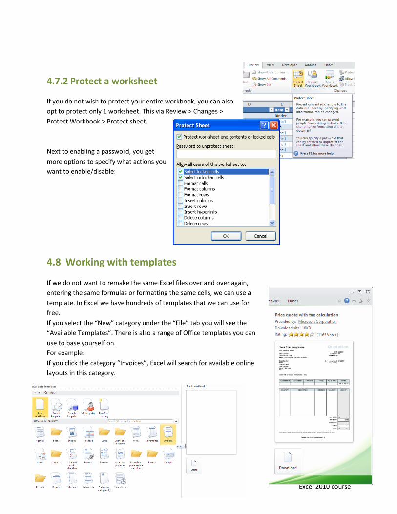
Lennart Dubois 60 Excel 2010 course
4.7.2 Protect a worksheet
If you do not wish to protect your entire workbook, you can also
opt to protect only 1 worksheet. This via Review > Changes >
Protect Workbook > Protect sheet.
Next to enabling a password, you get
more options to specify what actions you
want to enable/disable:
4.8 Working with templates
If we do not want to remake the same Excel files over and over again,
entering the same formulas or formatting the same cells, we can use a
template. In Excel we have hundreds of templates that we can use for
free.
If you select the “New” category under the “File” tab you will see the
“Available Templates”. There is also a range of Office templates you can
use to base yourself on.
For example:
If you click the category “Invoices”, Excel will search for available online
layouts in this category.

Lennart Dubois 61 Excel 2010 course
You can preview the templates in the right window and download them when you have found your
match.
When you are done downloading, Excel opens your file and you can edit it:
When you are happy with the end result you can just save it and everything will be there.
4.9 Creating your own template
Once you downloaded your template or create one yourself you would want to reuse it as a template.
We’ll have to save it on our computer as a template:
Go to the tab file > save as. The
dialogue box will ask you a file
name and type. You enter your
file name and the type of file
(or extension) which will be
Excel Template (“*.xltx”). Once
you have selected this
extension, Excel will
automatically place your file in
the right folder within the
templates.
Press save and close Excel.

Lennart Dubois 62 Excel 2010 course
When you want to open your template again, you
go to File > New > My templates.
This will open a window where all your templates
are stored.
4.10 Separate content of one cell
As an example, I will divide the content of the column “Name” into First name and Last name. When you
want to split up cells, the first thing you have to do is add extra columns. The amount of columns is
equal to the amount of possible values you return.
In order to do so, you select your
data and go to the data tab > text to
columns
In the dialogue box you select “Delimited” and click next. In the next window you select how the text
will be separated. In our case it will be a space. You will see a preview at the bottom of the page. The
final step enables you what the format will be of the final result and where it will be placed.

Lennart Dubois 63 Excel 2010 course
As you might have noticed, there was a name with more than 2
parts. The 3th part will end up (and overwrite) the 3th column.

Lennart Dubois 64 Excel 2010 course
4.11 Showing only a few rows & columns in Excel
Hide:
Step 1: Select the column from which you want to hide.
Step 2: Press CTRL+Shift+Right Arrow to select all the columns till XFD.
Step 3: Right click and hide
Step 4: Select the row from which you want to hide.
Step 5: Press CTRL+Shift+Down Arrow to select all rows until 2^20
Step 6: Hide the rows too. And you are done!
Unhide:
Step 1: Select the last visible row (column)
Step 2: Then while keeping mouse clicked, drag it down as if you are selecting more rows (columns) in to the blank area.
Step 3: Then right click and unhide.
Your
content!

Lennart Dubois 65 Excel 2010 course
5 Shortcuts
5.1 Keyboard functions buttons
List of all the shortcuts there are in Excel:
http://www.shortcutworld.com/en/win/Excel_2010.html
5.2 Some of the most important shortcuts:
Undo/redo shortcuts
Undo CTRL + Z
Redo CTRL + Y
Work with clipboard
Copy content of selected cells CTRL + C
Cut content of selected cells CTRL + X
Paste content from clipboard into selected cell CTRL + V
Actions
Save CTRL + S
Open CTRL + O
Close CTRL + W
Select all CTRL + A
Edit inside cells
Start a new line in the same cell Alt + Enter
Complete a cell entry and move up in the selection Shift + Enter
Cancel a cell entry Esc
Insert current date CTRL + ; (semicolon)
Insert current time CTRL + Shift + ; (semicolon)
Function
Turn on extension of selection with arrow keys
without having to keep pressing shift.
F8
Save as F12
Movement and Selection
Move to the edge of next data region CTRL + arrow keys
Move o the beginning of a row in a worksheet Home
Extend the selection by one cell Shift + arrow keys

Lennart Dubois 66 Excel 2010 course
Extend the selection to the last cell with content in
row or Colom
CTRL + shift + arrow keys
Cancel selection Esc

Lennart Dubois 67 Excel 2010 course
6 Data tables
Excel table is a series of rows and columns with related data that is managed independently.
Excel tables, (known as lists in excel 2003) is a very powerful and supercool feature that you
must learn if your work involves handling tables of data.
What is an excel table?
Table is your way of telling excel, “look, all this data from A1 to E25 is related. The
row 1 has table headers. Right now we just have 24 rows of data. But I can add more
later!”
When you make a table (more on this in a sec) you can easily add more rows to it
without worrying about updating formula references, formatting options, filter
settings etc.
6.1 How to create table from a bunch of data?
To create an excel table, all you have to do is select a range of cells and press the table button
under the Insert tab.
See this simple tutorial:

Lennart Dubois 68 Excel 2010 course
6.1.1 Change table formatting without lifting a finger
Excel has some great pre-defined table formatting options. Just select any cell in your table and
change the table formatting by going to “format as table” button in the home ribbon.
If you are bored with the predefined formats, you can easily define your own table formatting
color schemes and apply them.
6.1.2 Add Zebra Lines to Tables without doing Donkey Work
When you create a table, zebra lines come as a bonus. And when you add new rows to the table,
excel takes care of zebra lining or banding automatically. You can turn on / off the banded rows
feature from “design ribbon tab” as well.
That means you don’t need to use conditional formatting or manually format alternative rows in
different color.
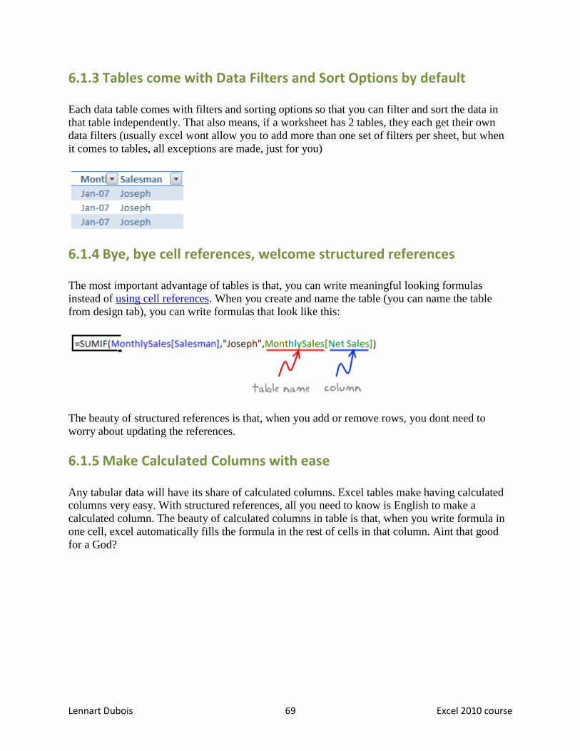
Lennart Dubois 69 Excel 2010 course
6.1.3 Tables come with Data Filters and Sort Options by default
Each data table comes with filters and sorting options so that you can filter and sort the data in
that table independently. That also means, if a worksheet has 2 tables, they each get their own
data filters (usually excel wont allow you to add more than one set of filters per sheet, but when
it comes to tables, all exceptions are made, just for you)
6.1.4 Bye, bye cell references, welcome structured references
The most important advantage of tables is that, you can write meaningful looking formulas
instead of using cell references. When you create and name the table (you can name the table
from design tab), you can write formulas that look like this:
The beauty of structured references is that, when you add or remove rows, you dont need to
worry about updating the references.
6.1.5 Make Calculated Columns with ease
Any tabular data will have its share of calculated columns. Excel tables make having calculated
columns very easy. With structured references, all you need to know is English to make a
calculated column. The beauty of calculated columns in table is that, when you write formula in
one cell, excel automatically fills the formula in the rest of cells in that column. Aint that good
for a God?
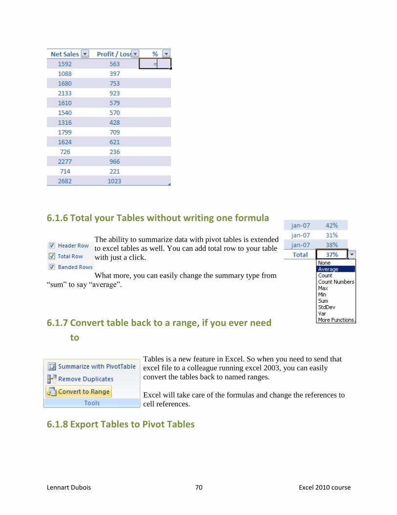
Lennart Dubois 70 Excel 2010 course
6.1.6 Total your Tables without writing one formula
The ability to summarize data with pivot tables is extended
to excel tables as well. You can add total row to your table
with just a click.
What more, you can easily change the summary type from
“sum” to say “average”.
6.1.7 Convert table back to a range, if you ever need
to
Tables is a new feature in Excel. So when you need to send that
excel file to a colleague running excel 2003, you can easily
convert the tables back to named ranges.
Excel will take care of the formulas and change the references to
cell references.
6.1.8 Export Tables to Pivot Tables

Lennart Dubois 71 Excel 2010 course
What good is a bunch of data when you can analyze it? That is where
Pivot tables come in to picture. Thankfully, you don’t need to do
much. Just click a button and your table goes to pivot table.
6.1.9 Print Tables Alone, without all the other stuff
around
Select the table, hit CTRL+P and select “Table” for
“print what?” and you will be able to print the tables
alone. This is far easier and cooler than trying to adjust
print settings when you are printing tabular data.

Lennart Dubois 72 Excel 2010 course
7 Charts In order to insert a chart we first select the data
we want to use, than select the “insert” tab in
the ribbon. In the chart group we find different
types of charts.
Depending on the data you want to visualize in
your chart, certain types are more suitable than
others. By clicking on the icons you will get a
dropdown menu with all the options regarding
that chart.
After selecting the chart you want, it will appear
in the middle of your worksheet.
7.1 Sorts of graphs
7.1.1 Column Chart
The Column chart is one of the most commonly used chart type and is
used to show the changes in data over a period of time or illustrate
comparisons among items.
7.1.2 Line Graphs
Line Graphs are mainly used to plot changes in data over time. The
best example of this chart type can be the weekly change in
temperature.
7.1.3 Pie Chart
The Pie Chart is very useful when you wish to emphasize on a
significant element in the data. It represents data in the form of a pie.
7.1.4 Bar Graph
A bar graph illustrates comparisons among individual items.

Lennart Dubois 73 Excel 2010 course
7.1.5 Area Chart
An area chart displays the magnitude of change over time.
7.1.6 Scatter Graphs
The Scatter Graph and Line chart are almost similar, but the scatter
graph is displayed with a scribble line whereas the line graph uses
connected lines to display data.
7.1.7 Surface Charts
A surface chart comes in handy if you are to determine the optimum
combination between two sets of data.
7.2 Formatting your graph
After selecting the chart, three additional tabs appear in
the ribbon. With those tabs we can change the design,
layout and the format of our graph. A default graph
contains a vertical (value) axis (V) on the left and a
horizontal (category) axis (H) at the bottom. On the right, you will find the legend (L).
In the Chart Tools > Design > Chart
Layouts group you can edit the standard
layout to pre-determined layout. In the
pop-up menu (click the more button
) you will find different formats with
different settings. If you are happy with
your settings you can still manually adjust
the individual settings.

Lennart Dubois 74 Excel 2010 course
For example, the first option will add a title to our chart.
Another instance will move the legend underneath the chart title.
There is also an instance which adds the used data underneath the
graph.
All the preloaded formats can save us a lot of time, but you can, if you
wish, manually add or remove the items on your chart as well.
To add more options (e.g. labels, axes, …) you go to the chart tools >
layout tab. All options are located under the “Labels”, “Axes”,
“Background” and “Analysis” groups.
In these groups you can select how the items are visualized and who it will behave according to the data
which is in your graph.
7.3 Change chart type
We can change the type of chart at any time. To do so, select the chart and go to “Chart Tools” >
“design” tab > “type” > “change chart type” button
This will open the “change chart type” dialog box which contains two parts.
In the left part we find the different categories. In the right part we find the different types

Lennart Dubois 75 Excel 2010 course
7.4 switch row/column
It has been made very easy to switch the rows and columns. To do so,
there is a button in the design tab > data > Switch row/column.
7.5 Moving a chart to a new sheet
By default, a chart is placed as an object in the same worksheet as the selected
data. We can move it to another sheet by clicking on the button “move chart” in the
design tab under location.
This opens a window where we can select where we would like to place the chart.
This can be either a new sheet or an existing sheet. We can also change the name of
the chart. By default our chart is called
“Chart1”
We can also resize our chart by dragging
the dots on the side of our object or at the
format tab under the size group.
7.6 Edit / change data
You can create a chart on its own
chart sheet or on a worksheet. In
both ways the chart is linked to the
source data on the worksheet, which
means the chart is updated when you

Lennart Dubois 76 Excel 2010 course
update the worksheet data. In order to set the chart to change while the values of some particular cells
changes, right-click the chart and choose the Select Data option, and then select, and add the fields that
you wish to include in this process.
7.7 Edit / change axis
When you want to change the lay-out or values of an axis,
you can modify them by right clicking on the axis or
selecting it and clicking the “format selection” button
under chart tools > Format.
In the dialogue box you find all the options to manipulate the
selected axis. Ranging from the axis options to the layout:
7.8 Add an extra axis
When you create your chart, you will only have 1 horizontal axis for all the data you selected. It is
possible that the sets of data are not in the same range as the other. If this is the case, it would be handy
to insert a new axis for both sets. Not only can you set 2 horizontal axis, but change the representation
of the entire data.
First off, this is a normal chart with 2 sets of data and only 1 horizontal axis:
€ -
€ 500.00
€ 1,000.00
€ 1,500.00
€ 2,000.00
€ 2,500.00
200720092011
Sales (m€)
Costs (m€)
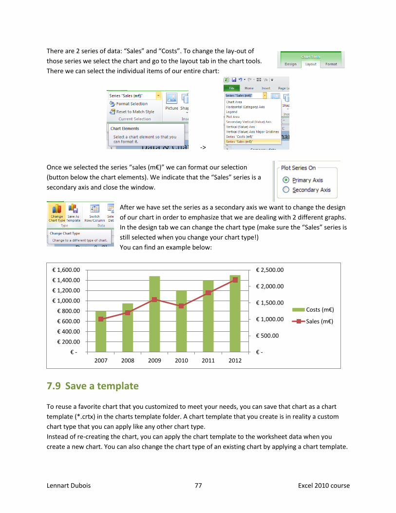
Lennart Dubois 77 Excel 2010 course
There are 2 series of data: “Sales” and “Costs”. To change the lay-out of
those series we select the chart and go to the layout tab in the chart tools.
There we can select the individual items of our entire chart:
->
Once we selected the series “sales (m€)” we can format our selection
(button below the chart elements). We indicate that the “Sales” series is a
secondary axis and close the window.
After we have set the series as a secondary axis we want to change the design
of our chart in order to emphasize that we are dealing with 2 different graphs.
In the design tab we can change the chart type (make sure the “Sales” series is
still selected when you change your chart type!)
You can find an example below:
7.9 Save a template
To reuse a favorite chart that you customized to meet your needs, you can save that chart as a chart
template (*.crtx) in the charts template folder. A chart template that you create is in reality a custom
chart type that you can apply like any other chart type.
Instead of re-creating the chart, you can apply the chart template to the worksheet data when you
create a new chart. You can also change the chart type of an existing chart by applying a chart template.
€ -
€ 500.00
€ 1,000.00
€ 1,500.00
€ 2,000.00
€ 2,500.00
€ -
€ 200.00
€ 400.00
€ 600.00
€ 800.00
€ 1,000.00
€ 1,200.00
€ 1,400.00
€ 1,600.00
2007 2008 2009 2010 2011 2012
Costs (m€)
Sales (m€)
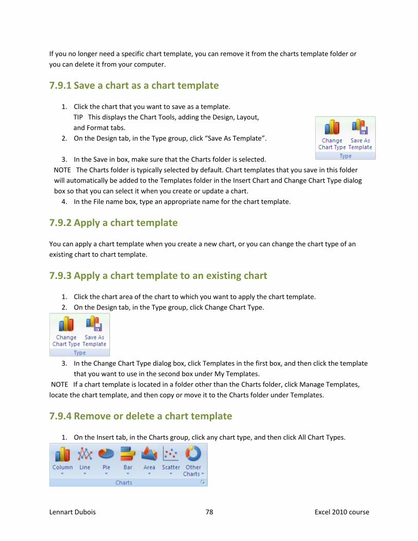
Lennart Dubois 78 Excel 2010 course
If you no longer need a specific chart template, you can remove it from the charts template folder or
you can delete it from your computer.
7.9.1 Save a chart as a chart template
1. Click the chart that you want to save as a template.
TIP This displays the Chart Tools, adding the Design, Layout,
and Format tabs.
2. On the Design tab, in the Type group, click “Save As Template”.
3. In the Save in box, make sure that the Charts folder is selected.
NOTE The Charts folder is typically selected by default. Chart templates that you save in this folder
will automatically be added to the Templates folder in the Insert Chart and Change Chart Type dialog
box so that you can select it when you create or update a chart.
4. In the File name box, type an appropriate name for the chart template.
7.9.2 Apply a chart template
You can apply a chart template when you create a new chart, or you can change the chart type of an
existing chart to chart template.
7.9.3 Apply a chart template to an existing chart
1. Click the chart area of the chart to which you want to apply the chart template.
2. On the Design tab, in the Type group, click Change Chart Type.
3. In the Change Chart Type dialog box, click Templates in the first box, and then click the template
that you want to use in the second box under My Templates.
NOTE If a chart template is located in a folder other than the Charts folder, click Manage Templates,
locate the chart template, and then copy or move it to the Charts folder under Templates.
7.9.4 Remove or delete a chart template
1. On the Insert tab, in the Charts group, click any chart type, and then click All Chart Types.

Lennart Dubois 79 Excel 2010 course
TIP You can also click the Dialog Box Launcher next to Charts in the Charts group on the Insert tab.
2. Click Manage Templates.
3. Do one of the following:
To remove the chart template from the Charts folder, drag it to the folder where you want to
store it.
To delete the chart template from your computer, right-click it, and then click Delete.
7.10 Create an interactive chart
Imagine you have a worksheet with lots of charts. And you want to make it look neat & clean.
Solution?
Simple, create an interactive chart so that your users can pick one of many charts and see them.
0. This is the date we will be working with:
1. First create all the charts you want and place them in
separate locations in your worksheet. Let’s say your charts
look like this:
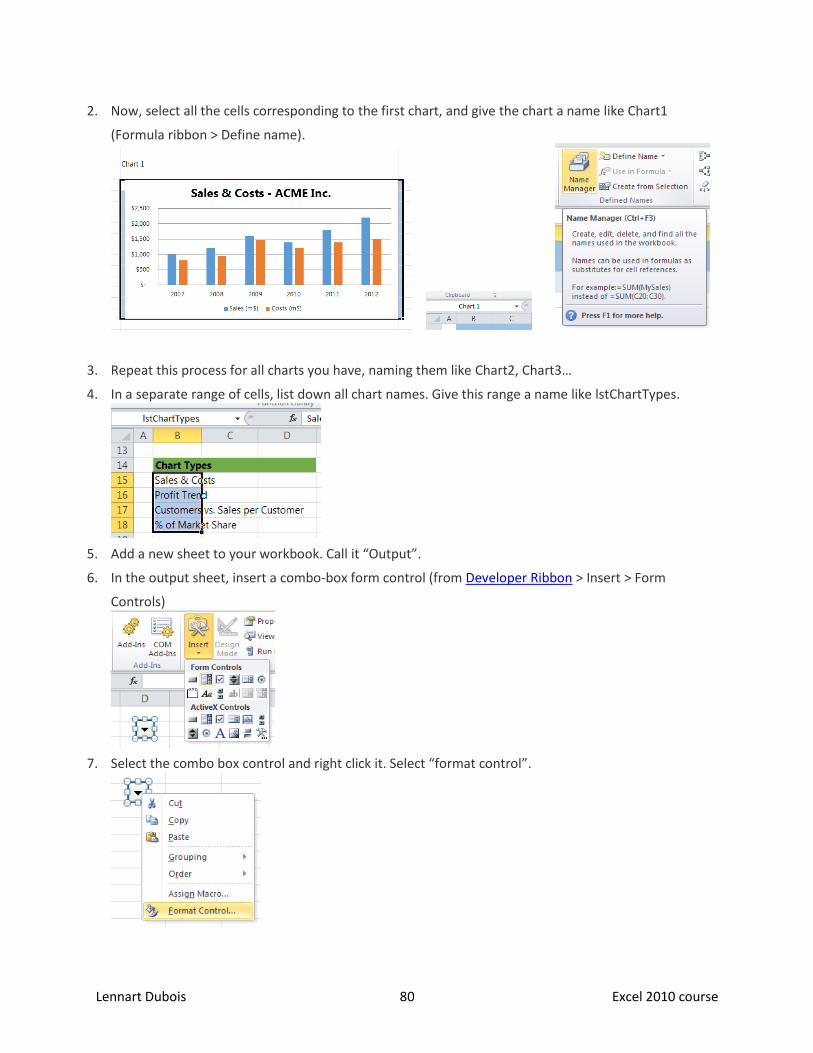
Lennart Dubois 80 Excel 2010 course
2. Now, select all the cells corresponding to the first chart, and give the chart a name like Chart1
(Formula ribbon > Define name).
3. Repeat this process for all charts you have, naming them like Chart2, Chart3…
4. In a separate range of cells, list down all chart names. Give this range a name like lstChartTypes.
5. Add a new sheet to your workbook. Call it “Output”.
6. In the output sheet, insert a combo-box form control (from Developer Ribbon > Insert > Form
Controls)
7. Select the combo box control and right click it. Select “format control”.
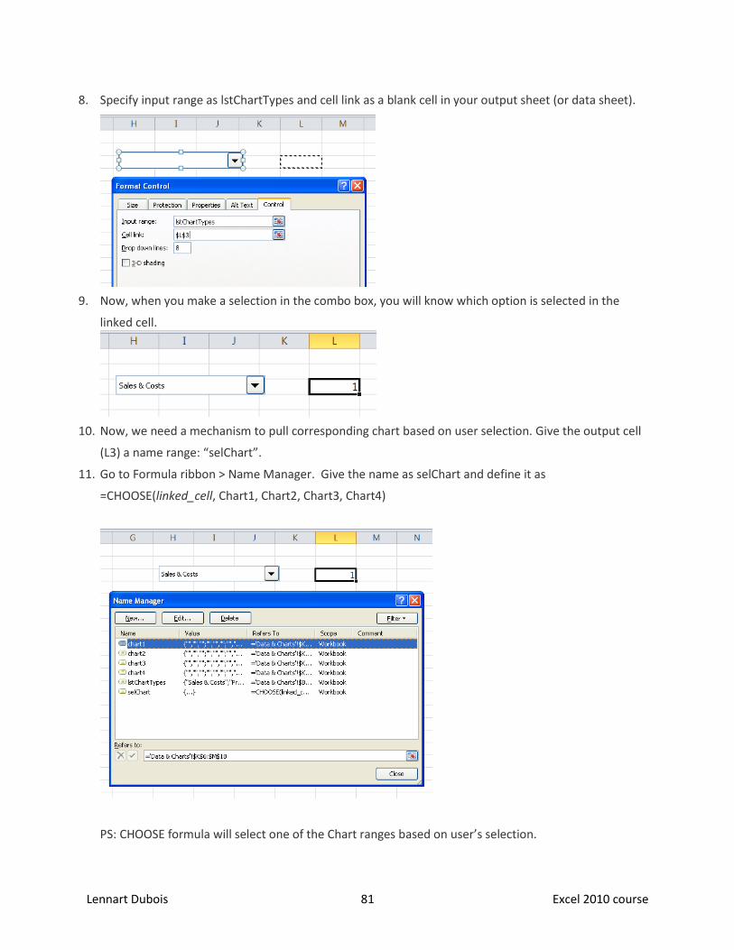
Lennart Dubois 81 Excel 2010 course
8. Specify input range as lstChartTypes and cell link as a blank cell in your output sheet (or data sheet).
9. Now, when you make a selection in the combo box, you will know which option is selected in the
linked cell.
10. Now, we need a mechanism to pull corresponding chart based on user selection. Give the output cell
(L3) a name range: “selChart”.
11. Go to Formula ribbon > Name Manager. Give the name as selChart and define it as
=CHOOSE(linked_cell, Chart1, Chart2, Chart3, Chart4)
PS: CHOOSE formula will select one of the Chart ranges based on user’s selection.

Lennart Dubois 82 Excel 2010 course
12. Now, go back to data & charts sheet. Select Chart1 range. Press CTRL+C to copy it.
13. Go to Output sheet and paste it as linked picture (Right click > Paste Special > Linked Picture)
14. This will insert a linked picture of Chart 1.
15. Now, click on the picture, go to formula bar, type =selChart and press enter
NOTE! You have to type “=selChart” entirely! Do not select it from the drop-down menu.
16. Move the image around, position it nicely next to the combo box.
17. If you want to remove the corresponding number with your chart you can edit the colour of you text
in that cell to white!
End result:

Lennart Dubois 83 Excel 2010 course
8 PivotTable Excel pivot tables are very useful and powerful feature of MS Excel. They can be used to summarize,
analyse, explore and present your data.
In plain English, it means, you can take the sales data with columns like salesman, region and product-
wise revenues and use pivot tables to quickly find out how products are performing in each region.
In this tutorial, we will learn what is a pivot table and how to make a pivot table using excel.
Click here to see a video tutorial of making pivot tables in excel
One more Pivot Table Video Tutorial
8.1 Example uses of Pivot Tables
As I said before pivot tables are very powerful and useful. There are numerous uses of pivot tables.
Here are some example uses of pivot tables:
Summarizing data like finding the average sales for each region for each product from a product sales data table.
Listing unique values in any column of a table [learn more] Creating a pivot report with sub-totals and custom formats Making a dynamic pivot chart Filtering, sorting, and drilling-down data in the reports without writing one formula or macro. Transposing data – i.e. moving rows to columns or columns to rows. Linking data sources outside excel and be able to make pivot reports out of such data.

Lennart Dubois 84 Excel 2010 course
8.2 Excel Pivot Table Tutorial: How to create your first pivot table
Let us make your first pivot table. We will use example data in the following format. Download the excel pivot tables tutorial workbook with the data.
Step 1: Select the data Select the data range from which you want to make the pivot table.
Step 2: Go to Insert ribbon and click on new Pivot table option To insert a new pivot table in to your spread sheet, go to Insert ribbon and click pivot table icon and select pivot table option.
Step 3: Select the target cell where you want to place the pivot table. For starters, select New worksheet. Excel will display a pivot table wizard where you can specify the pivot table target location etc. Select “New worksheet” option and your pivot table will be placed in newly created worksheet.
Step 4: Make your first pivot report
The pivot report UI is very intuitive and sandbox like. To make powerful analysis, all you have to do is
drag and drop fields in to the pivot table grid area.
The pivot report is divided in to header and body sections. You can
drag and drop the fields you want in each area. The body itself
contains three parts. Rows, Columns and Cells. You can use any
fields in these areas too.
For the above sample data, I have set this criteria:
And the outcome is this pivot report.

Lennart Dubois 85 Excel 2010 course
It might be a bit difficult to understand how this works. But believe me, if you have seen any reports or
worked with any other reporting systems, then the idea of pivot tables, pivot reports and pivot charts
becomes quite simple to you.
You can use the excel pivot table features to make a more complicated pivot report like this in no
time.
8.3 Some useful tips on Excel Pivot Tables
You can apply any formatting to the pivot tables. MS Excel has some very good pivot table formats (and they are better in Excel 2010).
You can easily change the pivot table summary formulas. Right click on pivot table and select “summarize data by” option.
You can also apply conditional formatting on pivot tables although you may want to be a bit careful as pivot tables scale in size depending on the data.
Whenever the original data from which pivot tables are constructed, just right click on the pivot table and select “Refresh Data” option.
If you want to drill down on a particular summary value, just double click on it. Excel will create a new sheet with the data corresponding to that pivot report value. (This is extremely useful)
Making a pivot chart from a pivot table is very simple. Just click on the pivot chart icon from tool bar or Options ribbon area and follow the wizard.

Lennart Dubois 86 Excel 2010 course
9 Developer tools
9.1 How to show the developer tab in the ribbon
When starting Excel, you will notice that the developer tool is not in the ribbon. To enable it, you will
have to go to File > Options > customise ribbon > developer tools. This will enable the developer tab.
9.2 A Bird’s Eye View Of The Developer Tab’s Options
The Developer tab contains different useful options for developers. All of the available options of the
developer tab are categorized into the following five:
Code
Add-In
Controls
XML
Modify
9.3 Code
The Code section contains different options. The Visual
Basic option lets you launch the Visual Basic
Editor, Macros launches the list of all the created/recorded
Macros, Record Macro lets you create a new Macro. The Macro
Security options lets you play with the security aspects of the
Macro.

Lennart Dubois 87 Excel 2010 course
9.4 Add-in
The Add-Ins option lets you enable Excel’s Add-Ins like the Solver, COM Add-
Ins options enables the COM add-in which is useful for developers as it aids in
writing common object models.
9.5 Controls
It includes functionality to add the user-interface controls like
ActiveX controls to your Excel spread sheet. You can move
between Code and Design Mode, and can play with the Control’s
Properties and run Dialog.
9.6 XML
The XML portion contains useful options for XML coding in
Excel. It provides options to write XML source code, Import
and Export XML files, Map and refresh your XML data.
9.7 Modify
The Modify section contains the Document Panel option only.

Lennart Dubois 88 Excel 2010 course
10 Macros
10.1 What is a macro?
A macro is a series of commands that you can use to automate a repeated task, and can be run when
you have to perform the task.
10.1.1 Enable macros when the Message Bar appears
When you open a file that has macros, the yellow Message Bar appears with a shield icon and
the Enable Content button. If you know the macro, or macros, are from a reliable source, use the
following instructions:
On the Message Bar, click Enable Content.
The file opens and is a trusted document.
The following image is an example of the Message Bar when macros are in the file.
10.1.2 Enable macros in the Backstage view
Another method to enable macros in a file is via the Microsoft Office Backstage view, the view that
appears after you click the File tab, when the yellow Message Bar appears. The yellow bar means that
the document you are trying to open contains a macro.
Click the File tab.
In the Security Warning area, click Enable Content.
Under “Enable All Content”, click “always enable this document's active content”.
The file becomes a trusted document.
The following image is an example of Always enable this document's active content and Advanced
Options.

Lennart Dubois 89 Excel 2010 course
10.1.3 Change macro settings in the Trust Center
Macro settings are located in the Trust Center. However, if you work in an organization, the system
administrator might have changed the default settings to prevent anyone from changing settings.
IMPORTANT When you change your macro settings in the Trust Center, they are changed only for
the Office program that you are currently using. The macro settings are not changed for all your Office
programs.
1. Click the File tab.
2. Click Options.
3. Click Trust Center, and then click Trust Center Settings.
4. In the Trust Center, click Macro Settings.
5. Make the selections that you want.
6. Click OK.
The following image is the Macro Settings area of the Trust Center.
10.1.4 Macro settings explained
Disable all macros without notification Macros and security alerts about macros are disabled.
Disable all macros with notification Macros are disabled, but security alerts appear if there are macros
present. Enable macros on a case-by-case basis.
Disable all macros except digitally signed macros Macros are disabled, but security alerts appear if
there are macros present. However, if the macro is digitally signed by a trusted publisher, the macro
runs if you have trusted the publisher. If you have not trusted the publisher, you are notified to enable
the signed macro and trust the publisher.
Enable all macros (not recommended, potentially dangerous code can run) All macros run. This setting
makes your computer vulnerable to potentially malicious code.
Trust access to the VBA project object model Disallow or allow programmatic access to the Visual Basic
for Applications (VBA) object model from an automation client. This security option is for code written
to automate an Office program and manipulate the VBA environment and object model. It is a per-user
and per-application setting, and denies access by default, hindering unauthorized programs from

Lennart Dubois 90 Excel 2010 course
building harmful self-replicating code. For automation clients to access the VBA object model, the user
running the code must grant access. To turn on access, select the check box.
10.2 Record a macro
Follow these steps to record a macro:
1. Choose Record Macro in the Code group of the Developer tab.
The Record Macro dialog box appears.
2. Type a name for the macro in the Macro Name text box.
The first character of the macro name must be a letter, and the name cannot contain spaces or
cell references. Macro names are not case-sensitive.
3. (Optional) Assign a Shortcut Key.
If you select a shortcut key already used in Excel, the macro shortcut key overrides the Excel
shortcut key while the workbook that contains the macro is open.
4. From the Store Macro In drop-down list, select where you want to store the macro:
This Workbook: Save the macro in the current workbook file.
New Workbook: Create macros that you can run in any new workbooks created during the
current Excel session.
Personal Macro Workbook: Choose this option if you want the macro to be available
whenever you use Excel, regardless of which worksheet you're using.
5. (Optional) Type a description of the macro in the Description text box.
Use the Record Macro dialog box to begin creating a macro.
6. Click OK.

Lennart Dubois 91 Excel 2010 course
The Record Macro option on the Developer tab changes to Stop Recording.
7. Perform the actions you want to record.
Excel records your steps exactly — such as (Select cell C3) — but you can also record the steps
relative to any current cell — such as (Go up one row and insert a blank line). To do so, click the Use
Relative References button on the Developer tab. You can turn the Use Relative References feature
on and off as needed when recording the macro.
8. Choose Stop Recording in the Code group of the Developer tab.
The macro recorder stops recording keystrokes and the macro is complete.
10.3 Edit a macro
10.3.1 Create a command button
You can now click on the Developer tab which has been placed next to the View tab.
1. Click on Insert.
2. Click on Command Button in the ActiveX Controls section.
3. Now you can drag a command button on your worksheet.
10.3.2 Create and Assign the Macro
Now it is time to create a macro (a piece of code) and assign it to the command button.
1. Right click on CommandButton1.
2. Click on View Code.

Lennart Dubois 92 Excel 2010 course
3. The Visual Basic Editor appears. Place you cursor between 'Private Sub CommandButton1_Click()' and
'End Sub'.
4. For example, add the following code line:
Range("A1").Value = "Hello"
This macro places the word Hello into cell A1.
5. Close the Visual Basic Editor.

Lennart Dubois 93 Excel 2010 course
6. Before you click the command button on the sheet, make sure Design Mode is deselected. You can do
this by clicking on Design Mode again.
Result when you click the command button on the sheet:
You can see the macro you created in the VBA editor as well. The code that you generated can be
copy/pasted into your “private sub” to apply your recorded actions.
In this case I made the cell bold with a yellow background and a red text colour.
Which resulted in the above code. Now you can copy/paste the code into your “private sub” button.
When you click your commandbutton1 you apply
the macro!
The possibilities are endless! Everything you can
record with a macro you can use in your code!

Lennart Dubois 94 Excel 2010 course
11 Visual Basic editor
This following procedure shows you how to create a new blank workbook in which to store your
macros. You can then save the workbook in the .xlsm format.
11.1 To create a new blank workbook
1. Click the Macros button on the Developer tab.
2. In the Macro dialog box that appears, type, Hello under Macro Name.
3. Click the Create button to open the Visual Basic Editor with the outlines of a new macro already
typed in.
VBA is a full-featured programming language with a correspondingly full-featured programming
environment. Here, we will only examine those tools that you use to get started with programming, and
that excludes most of the tools in the Visual Basic Editor. With this said, close the Propertieswindow on
the left side of the Visual Basic Editor, and ignore the two dropdown lists that appear above the code.
The Visual Basic Editor:
The Visual Basic Editor contains the following code.
VB
Sub Hello()
End Sub
Sub stands for Subroutine, which you can define for now as "macro". Running the Hello macro runs any
code that is between Sub Hello() and End Sub.
Now edit the macro so that it looks similar to the following code.
VB
Sub Hello()
MsgBox ("Hello, world!")
End Sub
Go back to the Developer tab in Excel and click the Macros button again.
Select the Hello macro in the list that appears and then click Run to display a small message box that
contains the text, "Hello, world!"

Lennart Dubois 95 Excel 2010 course
You just created and implemented custom VBA code in Excel. Click OK in the message box to close it and
finish running the macro.
If the message box does not appear, check your macro security settings and restart Excel.
11.2 Making Macros Accessible
You can also get to the Macros dialog box from the View tab, but if you use a macro frequently, you
might find it more convenient to access it with a keyboard shortcut or a Quick Access Toolbar button.
To create a button for the Hello macro on the Quick Access Toolbar, use the following procedure.
The following procedure describes how to make a button for a macro on the Quick Access Toolbar:
11.3 To create a button for a macro on the Quick Access Toolbar
1. Click the File tab.
2. Click Options to open the Excel Options dialog box, and then click Quick Access Toolbar.
3. In the list under Choose commands from:, choose Macros. Find the text that is similar
to Book1!Hello in the list that appears and select that text.
4. Click the Add >> button to add the macro to the list on the right side, and then click
the Modify… button to select a button image to associate with the macro.
5. Click OK. You should see your new button on the Quick Access Toolbar above the File tab.
6. Now you can quickly run your macro at any time without using the Developer tab—give it a try.
11.4 A Real-World Example
Suppose that you have a workbook that contains lists on a large number of worksheets and that you
want to change the name of each worksheet to match the heading of the list on that worksheet. Not
every worksheet has a list on it, but if it does, the heading is in cell B1, and if it does not, cell B1 is blank.
The names of worksheets without lists should be left alone.
Ordinarily, this could be a complex task that involves looking at each worksheet to see if it has a list,
copying the name if it does, clicking the worksheet tab, and then pasting in the new name. Instead of
performing all of those steps manually, use Excel VBA to rename the sheets automatically.
11.4.1 Learning about Objects
To solve a VBA programming problem, you must first find out which objects the code will manipulate. To
research that information, an essential tool is the Excel Object Model Reference, which is part of the
Excel 2010 Developer Reference on the Microsoft Developer Network (MSDN).
These reference materials will be updated for Excel 2012.
Figure 3. Excel Object Model Reference on MSDN

Lennart Dubois 96 Excel 2010 course
The first step is to find out how to manipulate the particular objects that you need to work with to
accomplish your task; for example, worksheets, worksheet names, cells, and cell contents. In Excel,
there are at least two ways to approach the problem:
Go directly to the Object Model Reference.
Record some of the actions that you want to automate, see how the recorded code manipulates
the objects, and then go to the Object Model Reference for more information.
Opinions vary on which approach is preferable, but for now, try using the Macro Recorder first.
11.4.2 Using the Macro Recorder
Sometimes a simple recorded macro is all you need; in these cases, you do not even have to look at the
code. More often, recording alone is not enough. Instead, it is a starting point in the following process.
11.4.3 To use the Macro Recorder as a starting point to your
solution
1 Record the actions that you want to code.
2 Review the code and find the lines that perform those actions.
3 Delete the rest of the code.
4 Modify the recorded code.
5 Add variables, control structures, and other code that the Macro Recorder cannot record.
6 Begin your investigation by recording a macro that renames a worksheet to New Name. You can
then use the recorded macro to develop your own macro that renames multiple worksheets based
on their contents.
11.4.4 To record a macro that renames a worksheet
1 Click Record Macro on the Developer tab.

Lennart Dubois 97 Excel 2010 course
2 Name the macro RenameWorksheets, rename Sheet1 to New Name, and click Stop Recording.
3 Go to the Developer or View tab, click the Macros button, and choose Edit to open the Visual Basic
Editor.
The code in the Visual Basic Editor should look similar to the following.
VB
Sub RenameWorksheets()
'
' RenameWorksheets Macro
'
'
Sheets("Sheet1").Select
Sheets("Sheet1").Name = "New Name"
End Sub
The first four lines after the Sub line are comments. Any line that begins with an apostrophe is a
comment and has no effect on what the macro does. The main uses for comments are the following:
To make the code easier to understand, not just for you, but for anyone else who might need to
modify the code later.
To temporarily disable a line of code (called commenting it out).
The four comments in this recorded macro serve neither purpose, so delete them.
The next line uses the Select method to select the Sheet1 member of the Sheets collection object. In
VBA code, it is not generally necessary to select objects before manipulating them, even though that is
what the Macro Recorder does. In other words, this line of code is redundant, so you can delete it as
well.
The last line of the recorded macro modifies the Name Property of the Sheet1 member of
the Sheets collection. This is the line to keep.
After you make your changes, the recorded code should now look like the following.
VB
Sub RenameWorksheets()
Sheets("Sheet1").Name = "New Name"
End Sub
Manually change the sheet called New Name back to Sheet1, then run the macro. The name should
change back to New Name.
11.4.5 Modifying the Recorded Code
Now it is time to research the Sheets collection that the Macro Recorder used. The Sheets topic in the
Object Model Reference includes the following text.
"The Sheets collection can contain Chart or Worksheet objects. If you need to work with sheets of only
one type, see the object topic for that sheet type."

Lennart Dubois 98 Excel 2010 course
You are only working with Worksheets, so change the code to the following.
VB
Sub RenameWorksheets()
Worksheets("Sheet1").Name = "New Name"
End Sub
11.4.6 Looping
One limitation of the code up to this point is that it only makes a change to one worksheet. You could
add another line for each worksheet that you want to rename, but what if you do not know how many
worksheets there are, or what their current names are? You need a way to apply some rulefor
each sheet in the workbook.
VBA has a construction called a For Each loop that is ideal. The For Each loop examines each item in a
collection object such as Worksheets and can be used to take an action (like change a name) to some or
all of those items.
For more information about the For Each loop, see the VBA Language Reference. Click "Visual Basic
Conceptual Topics", then "Using For Each...Next Statements". Also, be aware that the VBA Language
Reference, like the Object Model Reference, will amply repay the time that you spend browsing it, and is
an excellent place to look for ideas if you get stuck working on code.
Using the third example in the "Using For Each...Next Statements" topic, edit the macro so that it looks
similar to the following code.
VB
Sub RenameWorksheets()
For Each myWorksheet In Worksheets
myWorksheet.Name = "New Name"
Next
End Sub
myWorksheet is a variable; that is, what it represents varies. In this case, the myWorksheet variable
successively represents each worksheet in theWorksheets collection. You do not have to
use myWorksheet; you could use "x", "ws", "WorksheetToRenameAfterTheContentsOfCellB1", or (with a
few restrictions) almost any name that you want. A good rule of thumb is to use variable names that are
long enough to remind you of what the variable stands for, but not so long as to clutter the code.
If you run the macro in its current state, it produces an error because Excel requires each worksheet in a
workbook to have a unique name, but the following line instructs Excel to give every worksheet the
same name.
VB
myWorksheet.Name = "New Name"
To correct the line so that you can verify that the For Each loop works, change the line to the following.

Lennart Dubois 99 Excel 2010 course
VB
myWorksheet.Name = myWorksheet.Name & "-changed"
Instead of trying to give each worksheet the same name, this line changes the current name of each
worksheet (myWorksheet.Name) to the current name with "-changed" appended to it.
11.4.7 Useful Renaming
The macro is getting close to something that might actually solve the problem at hand. What you need
now is a way to take information from the worksheets themselves—specifically from cell B1 on each
worksheet—and put that information into the names of the worksheets.
This time, instead of using the Macro Recorder to find out how to refer to a cell, take a guess and see if
using the Cell object will work. It is a good guess, but if you open the Object Model Reference and search
for the Cell object, you find that there is no Cell object! There is a CellFormat object though.
The CellFormat object topic includes the following code in the first code sample.
VB
' Set the interior of cell A1 to yellow.
Range("A1").Select
It turns out that you use Range to specify a range of cells or just one individual cell. Again, you do not
need the .Select portion, but you do need to find out how to refer to the contents of the Range object,
as opposed to the Range object itself. If you go to the Range object topic, you can read that Range has
both Methods and Properties. The contents of a Range is a thing, not an action, so it would probably be
a Property. If you scan down through the list, you can see the Value property. So, try the following.
VB
Sub RenameWorksheets()
For Each myWorksheet In Worksheets
myWorksheet.Name = myWorksheet.Range("B1").Value
Next
End Sub
You get an error if you run this on a workbook that contains worksheets where B1 is empty, because an
empty Range has a Value of "" (an empty text string), which is not a legal worksheet name. It is about
time to create some sample data anyway. Make the three sheets in the workbook look similar to the
figure below, and then run the macro.
Figure 4. Sample data for the RenameWorksheets macro

Lennart Dubois 100 Excel 2010 course
The worksheet names should change accordingly.
11.4.8 Checking for Empty Cells
As noted earlier, the macro fails if any of the B1 cells in the workbook are empty. Instead of manually
checking every worksheet, you can code the macro to do it for you. Before the myWorksheet.Name line,
add the following line of code.
VB
If myWorksheet.Range("B1").Value <> "" Then
And after the myWorksheet.Name line add the following text.
VB
End If
This is called an If…Then statement. The If…Then statement instructs Excel to do whatever is on the lines
between the If line and the End If line, but only if the condition in the If line is met. In the example, the
following line specifies the condition to meet.
VB
myWorksheet.Range("B1").Value <> ""
The <> means "is not equal to", and the quotation marks with nothing between them represent an
empty text string; that is, no text at all. Therefore, whatever lines of code come between the If and the
End If will only be executed if the value in B1 is not equal to nothing; that is, if there is text in cell B1.
For more information about the If…Then statement, see the VBA Language Reference. (The full name is
"If…Then…Else statement", where Else is an optional component.)
11.4.9 Variable Declarations
Another improvement that you should make to the macro is to put a declaration of
the myWorksheet variable at the start of the macro.
VB

Lennart Dubois 101 Excel 2010 course
Dim myWorksheet As Worksheet
Dim is short for "Dimension", and Worksheet is the type of this particular variable. This statement tells
VBA what kind of entity myWorksheetrepresents. Note that after you type As, the Visual Basic Editor
displays a popup that lists all the available variable types. That is an example of IntelliSense technology;
that is, the Visual Basic Editor responds to what it determines you are trying to do and offers a list of
appropriate options. You can choose an option from the list or just continue typing.
Although variable declarations are not required in VBA, using them is strongly recommended! Variable
declarations make it much easier to keep track of your variables and to track down bugs in the code.
Also, be aware that if you declare a variable with an object type (like Worksheet), IntelliSense displays
an appropriate list of properties and methods associated with that object if you use the object variable
later in the macro.
11.4.10 Comments
The macro is complex enough now to include some comments that remind you what the code is doing.
The number of comments to use is partly a matter of personal style, but in general, too many comments
are better than too few. Code usually needs to be modified and updated over time. Without comments,
it can be hard to understand what is going on in the code, especially if the person who modifies the code
is not the same person who wrote it in the first place. Adding comments for the If condition and for the
line that renames the worksheets, results in the following code.
VB
Sub RenameWorksheets()
Dim myWorksheet As Worksheet
For Each myWorksheet In Worksheets
'make sure that cell B1 is not empty
If myWorksheet.Range("B1").Value <> "" Then
'rename the worksheet to the contents of cell B1
myWorksheet.Name = myWorksheet.Range("B1").Value
End If
Next
End Sub
To test the macro, rename the worksheets back to Sheet1, Sheet2, and Sheet3 and delete the contents
of cell B1 on one or more of the worksheets. Run the macro to verify that it renames the worksheets
that have text in cell B1 and leaves the other worksheets alone. The macro works for any number of
worksheets, with any combination of populated and empty B1 cells.

Lennart Dubois 102 Excel 2010 course
12 More Things that You Can Do with VBA This section looks at a few more things that you can do with VBA in Excel 2010. The examples in this
section are designed to give you a sense of the capabilities of VBA instead of focusing on specific real-
world scenarios. You might find it helpful to review the information in the Object Model Reference
about the objects in each step as you work through the examples.
12.1 Importance of Being Open
A good way to learn programming in general, and Excel VBA in particular, is a strategy where you try
something, get it to work, and then ask yourself questions such as:
What could I try next?
What do I want to learn first, given how I want to use VBA?
What might just be fun or interesting to know?
What am I curious about?
The reader is strongly encouraged to investigate whatever avenues open up on the path to knowledge.
12.2 Charts
One common task in Excel is to create a chart based on a range of cells. Create a new macro
called AssortedTasks and then type the following text in the Visual Basic Editor.
VB
Dim myChart As ChartObject
Add a line to create the chart object and assign the myChart variable to it.
VB
Set myChart = ActiveSheet.ChartObjects.Add(100, 50, 200, 200)
The numbers in the parentheses determine the position and size of the chart. The first two numbers are
the coordinates of the top left corner, and the second two numbers are the width and height.
Create a new blank worksheet and run the macro. The chart it creates is useless because the chart has
no data. Delete the chart that you just created, and add the following lines to the end of the macro.
VB
With myChart
.Chart.SetSourceData Source:=Selection
End With
This is a common pattern in VBA programming. First, you create an object and assign it to a variable,
then you use the With…End With construction to do things with the object. The example code instructs
the chart to use the current selection for its data. (Selection is a value for the Source parameter of

Lennart Dubois 103 Excel 2010 course
the SetSourceData method, not a value of an object property, so VBA syntax requires that you use a
colon and an equal sign (:=) instead of just an equal sign (=) to assign the value.)
Type some numbers in cells A1:A5, select the cells, and then run the macro. The chart shows up as the
default type, a bar chart.
Figure 5. Bar chart created by using VBA
If you do not like the bar chart, you can change it to some other kind of chart by using code that is
similar to the following.
VB
With myChart
.Chart.SetSourceData Source:=Selection
.Chart.ChartType = xlPie
End With
xlPie is an example of a built-in constant, also known as an enumerated constant. There are many of
these throughout Excel, and they are exhaustively documented. For more information about built-in
constants, see the Enumerations section of the Object Model Reference. For example, the constants for
chart types are listed under "XlChartType Enumeration".
You can modify the data. For example, try adding this line right after the variable declaration.
VB

Lennart Dubois 104 Excel 2010 course
Application.ActiveSheet.Range("a4").Value = 8
You can get input from the user, and use that input to modify the data.
VB
myInput = InputBox("Please type a number:")
Application.ActiveSheet.Range("a5").Value = myInput
Finally, add the following lines to the end of the macro.
VB
ActiveWorkbook.Save
ActiveWorkbook.Close
The complete macro should now look something like the following.
VB
Sub AssortedTasks()
Dim myChart As ChartObject
Application.ActiveSheet.Range("a4").Value = 8
myInput = InputBox("Please type a number:")
Application.ActiveSheet.Range("a5").Value = myInput
Set myChart = ActiveSheet.ChartObjects.Add(100, 50, 200, 200)
With myChart
.Chart.SetSourceData Source:=Selection
.Chart.ChartType = xlPie
End With
ActiveWorkbook.Save
ActiveWorkbook.Close
End Sub
Verify that cells A1:A5 are still selected, run the macro, type a number in the input box, and then
click OK. The code saves and closes the workbook. Reopen the workbook and note the change to the pie
chart.
12.3 UserForms
The previous section showed how to use a simple input box to get input from the user. In addition to the
corresponding message box that displays information, VBA provides extensive capabilities that you can
use to create custom dialog boxes, to code controls that are placed directly on worksheets, or to
manipulate the dialog boxes that are built in to Excel. For more information about these capabilities,
see Controls, Dialog Boxes, and Forms in the Excel 2010 Developer Reference.
This section completes this introductory look at Excel VBA by taking a quick look at UserForms.
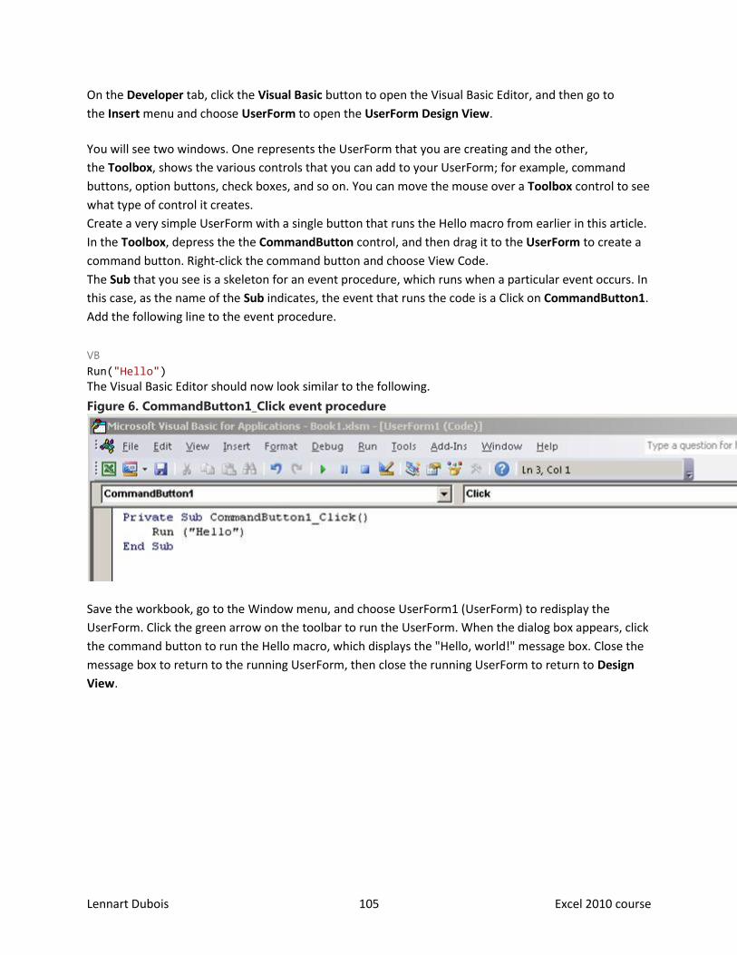
Lennart Dubois 105 Excel 2010 course
On the Developer tab, click the Visual Basic button to open the Visual Basic Editor, and then go to
the Insert menu and choose UserForm to open the UserForm Design View.
You will see two windows. One represents the UserForm that you are creating and the other,
the Toolbox, shows the various controls that you can add to your UserForm; for example, command
buttons, option buttons, check boxes, and so on. You can move the mouse over a Toolbox control to see
what type of control it creates.
Create a very simple UserForm with a single button that runs the Hello macro from earlier in this article.
In the Toolbox, depress the the CommandButton control, and then drag it to the UserForm to create a
command button. Right-click the command button and choose View Code.
The Sub that you see is a skeleton for an event procedure, which runs when a particular event occurs. In
this case, as the name of the Sub indicates, the event that runs the code is a Click on CommandButton1.
Add the following line to the event procedure.
VB
Run("Hello")
The Visual Basic Editor should now look similar to the following.
Figure 6. CommandButton1_Click event procedure
Save the workbook, go to the Window menu, and choose UserForm1 (UserForm) to redisplay the
UserForm. Click the green arrow on the toolbar to run the UserForm. When the dialog box appears, click
the command button to run the Hello macro, which displays the "Hello, world!" message box. Close the
message box to return to the running UserForm, then close the running UserForm to return to Design
View.

Lennart Dubois 106 Excel 2010 course
13 User forms
13.1 Introduction
A UserForm is a custom-built dialog box that you build using the Visual Basic Editor. while this example
works in Excel you can use the same techniques to create a UserForm in any of the Microsoft Office
programs that support VBA. With a UserForm you can create a user-friendly interface for your workbook
or document, making data entry more controllable for you and easier for the user.
13.2 About the Project
This chapter shows you how to build a simple UserForm for entering
personal expenses data on to a worksheet in Excel. The work is divided
into two main sections: building the form itself and then writing the VBA
code to make it work. The finished UserForm will look something like
this:
13.3 Build the Form
Start Excel and open the Visual Basic Editor (keyboard shortcut: [Alt]+[F11]). You will need to use both
the Project Explorer and the Properties Window so if they are not visible open them from the View
menu.
HINT: When building your UserForm try to avoid double-clicking on anything (unless the instructions tell
you to do so) because this sometimes opens the form's code window. If you do this accidentally simply
close the code window by clicking its Close button, or switch back to the UserForm design window with
the keyboard shortcut [Control]+[Tab].
13.3.1 Insert a New UserForm
Make sure that the current workbook (e.g.
VBAProject (Book1)) is selected in the
Project Explorer then open the Insert Menu
and choose UserForm. When you do this a
new, blank UserForm appears in the code
window of the Visual Basic Editor and a
corresponding entry appears in the Project
Explorer.
The Project Explorer shows a new folder
named Forms containing the new UserForm
which has been given the name UserForm1.

Lennart Dubois 107 Excel 2010 course
You should also see the Toolbox. If it is not visible click anywhere on the new UserForm (the Visual Basic
Editor hides the toolbox when it thinks you are working elsewhere) and if it still does not appear open it
from the View menu.
The UserForm has a dotted border around it. On the border, in the lower-right corner and halfway along
the bottom and right sides of the form, are small white squares. These are the resizing handles. You can
use the mouse to drag these handles to make the UserForm the required size. The grid of dots on the
form is to help you easily align items you place there.
13.3.2 Rename the UserForm and Add a Caption
A single project can include many UserForms so it is a good idea to give each one a meaningful name.
With the UserForm selected find the Name property in the Properties Window (it is normally the first
item in the list) and change it frmExpenses. Then change the Caption property to Staff Expenses Claim.
The Project Explorer now displays the UserForm's new name and the Title Bar of the form immediately
changes to show the new caption.
When naming forms and their controls remember that you must not include spaces in the name, or
use any of the VBA "reserved words" (i.e. those keywords that are part of the VBA language such
as "Date").
13.3.3 Add a TextBox Control and a Label
The controls are the items, such as textboxes, comboboxes and command
buttons, that will be placed on the form. The standard selection of controls is
represented by buttons on the Toolbox. Point at a Toolbox button to see a
tooltip showing the name of the control.
Add a TextBox control to the form by clicking on the TextBox button in the
Toolbox then clicking somewhere near the centre of the form. As with the
UserForm itself any control that you place on the form shows a dotted border and resizing handles when
the item is selected (click on any item to select it).

Lennart Dubois 108 Excel 2010 course
You can change the size and shape of a control either by dragging the resizing handles (the mouse
pointer will change to a double-headed arrow ) or by changing the values of its Height and Width
properties in the Properties Window. To move a control drag the dotted border at a point between
resizing handles (the mouse pointer will show a four-headed arrow) or change the values of its Top and
Left properties.
Drag the textbox to a point near the top of the UserForm and about halfway across the form.
Each control should have a meaningful name so that when you write the code you can easily identify it.
This one currently has the name TextBox1. Use the Properties Window to change its name to
txtFirstName.
HINT: It is helpful when naming controls to add a prefix describing the type of control ("txt" for textbox,
"cbo" for combobox etc.). This reminds you what type of control it is when you are working in the code.
It forces the names to appear together when displayed in a list. It also lets you use words that are
otherwise reserved (e.g. txtDate instead of Date).
Now use the toolbox to place a Label control on the form. To change the caption of the label you can
either type directly on to the label or you can change its Caption property in the Properties Window.
Change the label's caption to First Name:.
Change the TextAlign property of the label to 3-fmTextAlignRight then double-click the lower-right
corner resizing handle to snap the label to fit the text. Drag the label to a position just to the left of the
FirstName textbox.
When you move controls around by dragging them they snap to points on the grid. Whilst this is a useful
feature, sometimes you need to position objects more accurately. You will notice that you cannot place
the label exactly level with the center of the textbox. The grid forces it to be too high or too low. Use the
Properties Window to subtract (or add as necessary) 3 units from the Top property of the label so that it
is correctly positioned in relation to the textbox.

Lennart Dubois 109 Excel 2010 course
It isn't necessary to give the label a different name because, in this project, you will not be referring to it
in the code, although in other circumstances you might want to do so.
13.3.4 Add the Remaining Controls
Use the same techniques to add the remaining controls to the form. You need to add four textboxes, a
combobox (a textbox with a drop-down list), a checkbox and three command buttons. Here is a list of
the remaining controls you need to add and their properties:
TextBox ................ Name: txtLastName
Label..................... Caption: Last Name:
ComboBox ............ Name: cboDepartment
Label..................... Caption: Department:
TextBox ................ Name: txtDate
Label..................... Caption: Date:
TextBox ................ Name: txtAmount
Label..................... Caption: Amount:
CheckBox.............. Name: chkReceipt, Caption: Receipt?
TextBox ................ Name: txtDescription, Height: 45, Width: 132, Scrollbars: 2-fmScrollbarsVertical
Label..................... Caption: Description:
CommandButton ... Name: cmdOK, Caption: OK
CommandButton ... Name: cmdClear, Caption: Clear
CommandButton ... Name: cmdCancel, Caption: Cancel
HINT: At any time you can check exactly how the UserForm will look in use by pressing the [F5] key on
your keyboard or clicking the Run button on the Visual Basic Editor Toolbar. Doing this will open the
UserForm in its host program (in this case Excel). To return to the Visual Basic Editor, close the UserForm
by clicking the close button [x] in its upper-right corner.
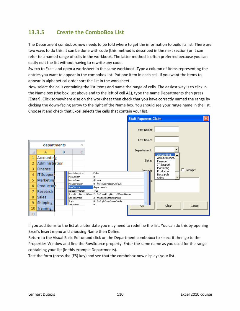
Lennart Dubois 110 Excel 2010 course
13.3.5 Create the ComboBox List
The Department combobox now needs to be told where to get the information to build its list. There are
two ways to do this. It can be done with code (this method is described in the next section) or it can
refer to a named range of cells in the workbook. The latter method is often preferred because you can
easily edit the list without having to rewrite any code.
Switch to Excel and open a worksheet in the same workbook. Type a column of items representing the
entries you want to appear in the combobox list. Put one item in each cell. If you want the items to
appear in alphabetical order sort the list in the worksheet.
Now select the cells containing the list items and name the range of cells. The easiest way is to click in
the Name box (the box just above and to the left of cell A1), type the name Departments then press
[Enter]. Click somewhere else on the worksheet then check that you have correctly named the range by
clicking the down-facing arrow to the right of the Name box. You should see your range name in the list.
Choose it and check that Excel selects the cells that contain your list.
If you add items to the list at a later date you may need to redefine the list. You can do this by opening
Excel's Insert menu and choosing Name then Define.
Return to the Visual Basic Editor and click on the Department combobox to select it then go to the
Properties Window and find the RowSource property. Enter the same name as you used for the range
containing your list (in this example Departments).
Test the form (press the [F5] key) and see that the combobox now displays your list.

Lennart Dubois 111 Excel 2010 course
13.3.6 Check the Tab Order
Many people when working in a form like to move around from control to control by clicking the [Tab]
key on their keyboard. The order in which the tab key moves you around a form is initially defined by
the order in which you placed the controls on the form.
Run the form (open it in Excel) and, starting from the FirstName textbox, press the [Tab] key repeatedly
and check that it takes you through the form in a logical order. If you want to change the order close the
form and in the Visual Basic Editor open the View menu and choose Tab Order. Here you can move
items up and down the list to control the behavior of the [Tab] key in the form.
13.4 Write the VBA Code
The design of the form is now finished. The next job is to write the VBA code to power it. The code is
needed to power the three command buttons…
13.4.1 Coding the Cancel Button
The Cancel button is the simplest one to code. It needs to do the same job as the built-in close button
([x]) in the upper right corner of the form.
Double-click the cmdClose command button (or right-click it and choose View Code) to open the
UserForm's code module. The Visual Basic Editor will have written the Sub and End Sub lines of the
button's Click event for you. Place your cursor in the empty line between these lines, press your [Tab]
key then enter the line:
Unload Me
Your code should look like this (Listing 1):
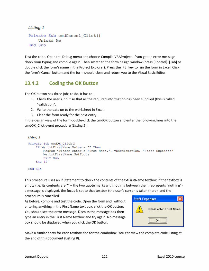
Lennart Dubois 112 Excel 2010 course
Test the code. Open the Debug menu and choose Compile VBAProject. If you get an error message
check your typing and compile again. Then switch to the form design window (press [Control]+[Tab] or
double click the form's name in the Project Explorer). Press the [F5] key to run the form in Excel. Click
the form's Cancel button and the form should close and return you to the Visual Basic Editor.
13.4.2 Coding the OK Button
The OK button has three jobs to do. It has to:
1. Check the user's input so that all the required information has been supplied (this is called
"validation".
2. Write the data on to the worksheet in Excel.
3. Clear the form ready for the next entry.
In the design view of the form double-click the cmdOK button and enter the following lines into the
cmdOK_Click event procedure (Listing 2):
This procedure uses an If Statement to check the contents of the txtFirstName textbox. If the textbox is
empty (i.e. its contents are "" – the two quote marks with nothing between them represents "nothing")
a message is displayed, the focus is set to that textbox (the user's cursor is taken there), and the
procedure is cancelled.
As before, compile and test the code. Open the form and, without
entering anything in the First Name text box, click the OK button.
You should see the error message. Dismiss the message box then
type an entry in the First Name textbox and try again. No message
box should be displayed when you click the OK button.
Make a similar entry for each textbox and for the combobox. You can view the complete code listing at
the end of this document (Listing 8).

Lennart Dubois 113 Excel 2010 course
In addition to checking that an entry is present, it is also sometimes necessary to check that the entry is
correct. Enter the following statements (Listing 3). They use the IsNumeric() function to check that the
value in the txtAmount textbox is a number (and not something else such as text); and the IsDate()
function to check that the value in the txtDate textbox is a date.
Now, having reached a point where all the required entries are present and correct, it's time to write the
entries on to the worksheet. This code involves using a variable to hold the number of rows of data on
the worksheet.
Make an empty line at the top of the current procedure, immediately after the statement Private Sub
cmdOK_Click() and enter the line:
I have assumed that the entries are going to be made on Sheet1 of the current workbook, starting in cell
A1. You might like to prepare the worksheet by typing a row of headings in the top row. The code will
work the same way if there are headings or not.
Return to the end of your code and enter the new line:
This statement counts how many rows of data are included in the region that includes cell A1 and stores
that number in the RowCount variable. Now enter the lines that write the date on to the worksheet
(Listing 4):
The code uses a number of similar statements to write the value of each control into a cell. Each cell is
identified by its position relative to cell A1 by using the VBA Offset property. This requires two numbers,

Lennart Dubois 114 Excel 2010 course
the first representing the number of rows away from cell A1 (which is held in the RowCount variable),
the second representing the number of columns away from cell A1 (which is written into the code as a
number).
Note that the DateValue() function is used to change the date entry into a real date (rather than a date
represented as text) before passing it to Excel.
The value of a checkbox is expressed as "TRUE" or "FALSE" so, because I wanted to see "Yes" or "No" on
the worksheet, the code uses an If Statement to make the required entry.
Finally a timestamp is written into the last column using the Format() function to specify how the exact
time, as supplied by the Now() function, is displayed. Now is a good time to compile and test the code
again.
To complete the procedure, after the data has been written to the worksheet, the form needs to be
emptied. This requires another variable to be entered at the top of the procedure:
This variable represents the controls on the worksheet and will be used in the following loop which visits
each control, checks to see if it is a textbox or a combobox, and if it is it sets the control's value to an
empty string (""). If the control is a checkbox it sets its value to False Enter the following lines (Listing 5):
Compile and test the code again. If any errors occur then check that your typing is exactly as
shown here.
13.4.3 Coding the Clear Button
The function of this button is to clear the form manually if the user wishes to do so. It uses exactly the
same procedure as the last part of the OK button's procedure, so double-click the cmdClearbutton to
create its click event procedure and enter the code shown in Listing 5. You can copy the code from the
OK button's procedure to save time.
13.4.4 Compile, Test and Save the Finished UserForm
That completes the coding of the form. Compile and test the code. If you are satisfied that the form is
working correctly save the file. The job is almost finished. All that remains is to create a macro to open
the form.

Lennart Dubois 115 Excel 2010 course
13.5 A Macro to Open the UserForm
As you have seen, it is easy to open the UserForm from the Visual Basic Editor, but the person who is
going to use this tool needs an easy way to open the form from Excel. There are several ways to do this,
all involving a macro containing the very simple statement:
13.5.1 Manually Opening the Form
This statement can be included in a macro that the user can call from the usual menu. To create this
macro first go to the Visual Basic Editor's Insert menu and choose Module to add a standard module to
the workbook containing the UserForm. Enter the following code into the new module's code window
(Listing 6):
The first line is optional. It tells Excel to switch to Sheet1. But, since the code that writes the data on to
the worksheet specifies the worksheet by name, it could be omitted and the data would still be written
in the correct place.
The user can run this macro from the menu in the usual way (Tools > Macro > Macros) or you could
assign it to a custom menu item, toolbar button, a button on the worksheet or a drawing object.
13.5.2 Opening the Form Automatically
You can make use of one of Excel's built-in event procedures to open the UserForm automatically when
the workbook is opened. In the Visual Basic Editor locate and double-click the ThisWorkbookmodule in
the Project Explorer. This module exists to hold macros specific to the workbook itself.
At the top of the code window there are two drop-down lists. The left-hand one will currently read
General. Open the list and choose Workbook. The Visual Basic Editor automatically creates the
Workbook_Open macro for you. Any code you place in this macro will be executed automatically when
the workbook opens. (If you want to see what else you can do here take a look at the other items on the
right-hand list.) Complete the macro code as follows (Listing 7):

Lennart Dubois 116 Excel 2010 course
13.6 Complete Code Listing for the UserForm
Here is a complete listing of the code in the UserForm's code module (Listing 8)
Listing 8
Private Sub cmdCancel_Click()
Unload Me
End Sub
Private Sub cmdClear_Click()
' Clear the form
For Each ctl In Me.Controls
If TypeName(ctl) = "TextBox" Or TypeName(ctl) = "ComboBox" Then
ctl.Value = ""
ElseIf TypeName(ctl) = "CheckBox" Then
ctl.Value = False
End If
Next ctl
End Sub
Private Sub cmdOk_Click()
Dim RowCount As Long
Dim ctl As Control
' Check user input
If Me.txtFirstName.Value = "" Then
MsgBox "Please enter a First Name.", vbExclamation, "Staff Expenses"
Me.txtFirstName.SetFocus
Exit Sub
End If
If Me.txtLastName.Value = "" Then
MsgBox "Please enter a Last Name.", vbExclamation, "Staff Expenses"
Me.txtFirstName.SetFocus
Exit Sub
End If
If Me.cboDepartment.Value = "" Then
MsgBox "Please choose a Department.", vbExclamation, "Staff Expenses"
Me.txtFirstName.SetFocus
Exit Sub
End If
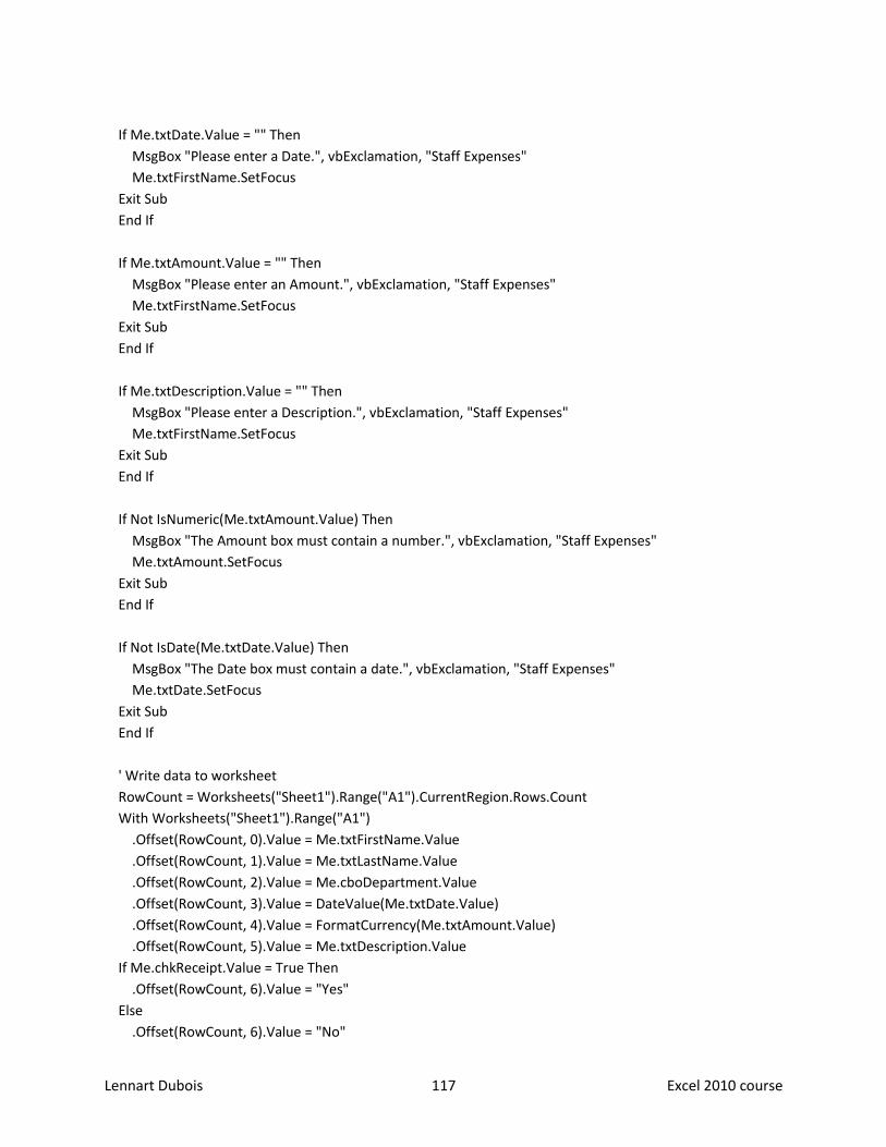
Lennart Dubois 117 Excel 2010 course
If Me.txtDate.Value = "" Then
MsgBox "Please enter a Date.", vbExclamation, "Staff Expenses"
Me.txtFirstName.SetFocus
Exit Sub
End If
If Me.txtAmount.Value = "" Then
MsgBox "Please enter an Amount.", vbExclamation, "Staff Expenses"
Me.txtFirstName.SetFocus
Exit Sub
End If
If Me.txtDescription.Value = "" Then
MsgBox "Please enter a Description.", vbExclamation, "Staff Expenses"
Me.txtFirstName.SetFocus
Exit Sub
End If
If Not IsNumeric(Me.txtAmount.Value) Then
MsgBox "The Amount box must contain a number.", vbExclamation, "Staff Expenses"
Me.txtAmount.SetFocus
Exit Sub
End If
If Not IsDate(Me.txtDate.Value) Then
MsgBox "The Date box must contain a date.", vbExclamation, "Staff Expenses"
Me.txtDate.SetFocus
Exit Sub
End If
' Write data to worksheet
RowCount = Worksheets("Sheet1").Range("A1").CurrentRegion.Rows.Count
With Worksheets("Sheet1").Range("A1")
.Offset(RowCount, 0).Value = Me.txtFirstName.Value
.Offset(RowCount, 1).Value = Me.txtLastName.Value
.Offset(RowCount, 2).Value = Me.cboDepartment.Value
.Offset(RowCount, 3).Value = DateValue(Me.txtDate.Value)
.Offset(RowCount, 4).Value = FormatCurrency(Me.txtAmount.Value)
.Offset(RowCount, 5).Value = Me.txtDescription.Value
If Me.chkReceipt.Value = True Then
.Offset(RowCount, 6).Value = "Yes"
Else
.Offset(RowCount, 6).Value = "No"

Lennart Dubois 118 Excel 2010 course
End If
.Offset(RowCount, 7).Value = Format(Now, "dd/mm/yyyy hh:nn:ss")
End With
End Sub


