1

Introduction to Excel Yitzchak Rosenthal

WorksheetsExcel’s main screen is called a “worksheet”.

Each worksheet is comprised of many boxes, called “cells”.

2

Organize InformationYou can organize information by typing a single piece of data into each cell. (see next slides)

3

How to Enter

Information

4

Selecting a Cell

5

“Select” a cell by clicking on it once (don’t double click).

You can move from cell to cell with the arrow keys or by pressing the “Enter” key.

Entering Information / The Formula Bar

6

To enter information in a cell, just start typing.

When you are done either◦ Press the Enter Key◦ Press an arrow key◦ Click on the “check button” (only visible when entering data into a cell)

The information in the selected cell is also displayed in the “formula bar” above the worksheet.

Double Click to Modify a Cell

To modify the contents of a cell double click on the cell.

Then use the right, left arrow keys and the Insert and Delete keys to modify the data. Or you click F2.

When you are done: Press the Enter key or

Click on the check box.

7

Double click to change “hi there” to “hello there”

Names of Rows, Columns and

Cells

8

Column Names (letters) & Row Names (numbers)

9

The columns of the worksheet are named with letters

The rows are named with numbers

Selected Cell

Cell Names (ex. B4)

10

The name of a cell is a combination of the Letter Of The Column that the cell is in followed by the Number Of The Row that the cell is in.

Example: the selected cell in the picture is named B4 (NOT 4B)

Excel automatically shows the the name of the currently selected cell in the “name box” (located above the worksheet).

The letter must come first (i.e. B4, NOT 4B) and there may NOT be any spaces between the letter and the number.

Name Box Select

ed Cell

Longggggggg Data

11

Information that is “too wide” for a cellThe word “Name” is in cell A5

The words “Hours Worked” are in cell B5 (NOT in cell C5). However, since the information is too wide for cell B5, it looks like it extends into cell C5.

You can determine that the information is really only IN cell B5 by selecting cell B5 and looking at the formula bar and then selecting cell C5 and looking at the formula bar.

12

“Hours Worked” is in cell B5 (look at formula bar)

“Hours Worked” is NOT in cell C5 (formula bar is empty)

Information that is “Chopped Off” If there is information in the cell to the right, then the original cell still contains all of the data, but the data appears to be “chopped off”.

13

• You can see the complete data by selecting the cell and looking in the formula bar.

Change the Width of a Column or the Height of a Row

14

Make a column widerTo make Column B wider, point the cursor to the column separator between columns B and column C.

The cursor changes to a “Double headed arrow”.

Now, click the left mouse button and without letting go of the button, drag the separator to the right to make the column wider (or to the left to make the column narrower).

15

Column is now wider

Drag column separator to the right

Getting the Exact WidthTo get the “exact” width, double click on the separator instead of dragging it.

16

Column is now EXACTLY the correct width

Double click here

Resizing a RowMake a row taller or shorter by dragging the separator between the rows.

Click and drag here to resize row 5.

17

Row is now taller

Putting an “Enter” inside a cell

To add a new line inside a cell◦ Double click inside the cell where you want the new line.

◦ Press Ctrl-Enter (i.e. hold down the Ctrl key and press Enter while still holding down Ctrl).

◦ When you are done editing, press Enter (without holding down Ctrl) to accept the changes.

18

Step 1: Originally “Hours Worked” is on one line.

Step 2: Double click to edit cell and then press Ctrl-Enter

Step 3: Press Enter (without Ctrl) to accept the changes.

Basic Formatting(e.g. bold, colors, fonts, etc)

19

Formatting Cells

20

Select one or more cells and then click on any of the formatting buttons (see below) to change the formatting of the selected cells.

Formatting buttons:

font name

font size

bold italics

underline

center & merge cells

(will explain later)

center

right justify

left justify

These change the way numbers are displayed in cells. (these don’t affect

words).

show as currency (ex. 1000.507 becomes

$1000.50)

show with commas (e.g. 12345 becomes

12,345)show as percent (ex. 0.5 becomes

50%)

remove indent

show fewer decimal points (ex. 10.507 is displayed as

10.51)show more decimal points (ex. 10.507 is displayed as

10.5070)indent within cellput border around

cell(s)color of cellcolor of

text in cell

click on downward pointing

arrows for other colors and border

styles

click on downward pointing

arrows for other font names and

sizes

Example – unformatted worksheet

21

Unformatted worksheet – see next slide for formatting.

Example –making cells bold Click on cell A1 and drag to cell A3. Then press the Bold button to make cells A1,A2,A3 bold.

You could also press the font or background color buttons to change the color or apply any other formatting you like (this is not shown below).

22

Other Ways of Selecting More Than One CellTo select a large range of cells, click on the upper left cell in the range. Then hold the shift key and click on the lower right cell in the range.

You can select different “non-contiguous” areas of cells by holding down the Ctrl key while clicking and dragging. 23

Selecting Non-Contiguous Ranges

Click and drag to select the first range.

Ctrl-click and drag to select additional ranges

24

(This cell is also selected even though it appears white).

Selecting entire Rows, entire Columns or all cells on the worksheet.To select an entire column, click on the letter for the column header. To select several columns, click on the header for the first column and drag to the right.

To select an entire row, click on the number for the row header. To select several rows, click on the header for the first row and drag down.

To select all of the cells on the spreadsheet, click on the upper left hand corner of the spreadsheet (where the column headers meet the row headers)

25

Select Entire Columns/Rows/Worksheet

26

To select ENTIRE COLUMN Bclick on “B” column header

To select COLUMNS B,C,Dclick on “B” column header and drag to

right

To select COLUMNS B,C and F,G,H ◦ click on “B” column header, drag to

right,◦ then Ctrl-Click on “F” column header and

drag right

To select ENTIRE ROW 2click on “2” row header

To select ROWS 2,3 and 5,6,7◦ click on “2” row header, drag down, ◦ then Ctrl-Click on “5” row header and

drag down

To select ENTIRE WORKSHEET click on select worksheet button (in corner between “1” and “A” buttons)

Click

Click

dragClick

drag

Click and drag downthen Ctrl-Click and drag down

Click

dragCtrl-Click

Click

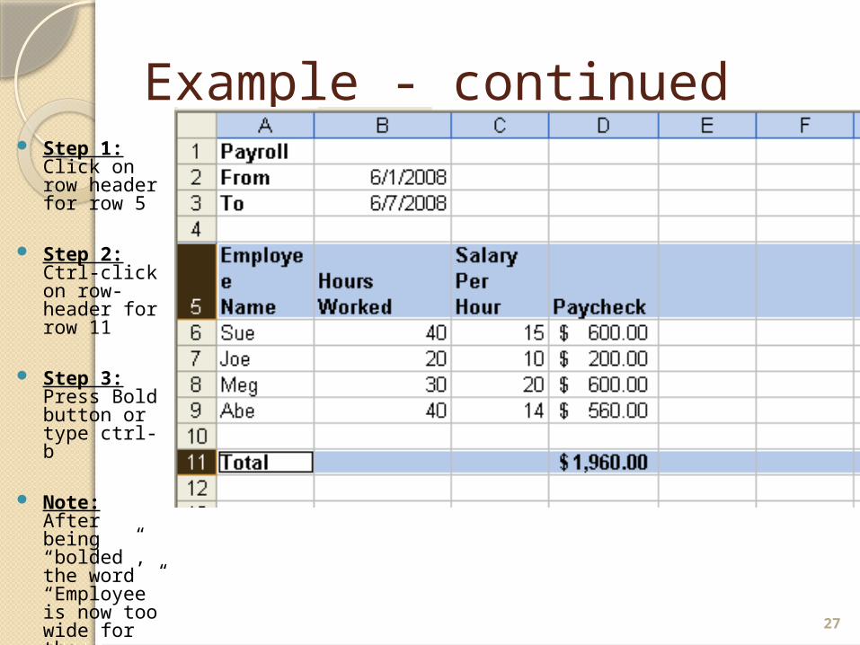
Example - continued

27

Step 1: Click on row header for row 5

Step 2: Ctrl-click on row-header for row 11

Step 3: Press Bold button or type ctrl-b

Note: After being “bolded”,the word “Employee” is now too wide for the column, so make the column wider if necessary (this step is not shown).

More Advanced Formatting

28

FormulasThe bread and butter of Excel

29

Excel FormulasYou must have an equals sign ( = ) as the first character in a cell that contains a formula.

The = sign tells excel that the contents of the cell is a formula

Without the = sign, the formula will not calculate anything. It will simply display the text of the formula.

30

Formulas - correct

31

formula with = sign

After pressing ENTER

Missing = sign

32

Missing = sign!Before pressing enter

After pressing ENTER (no change - not a function)

Types of operationsYou can use any of the following operations in a formula:operation symbol exampleaddition: + =a1+3subtraction: - =100-b3multiplication: * =a1*b1division: / =d1/100exponentiation ^ =a2^2negation - =-a2+3(same symbol as subtraction)

33

Explicit (literal) values and cell references

You can use both explicit values and cell references in a formula

An explicit value is also called a literal value

◦Formula with only cell references: =a1*b1

◦Formula with only literal values: =100/27

◦Formula with both cell references and literal values:

=a1/10034