Microsoft Excel Step by Step (Office 2021 and Microsoft 365)

http://www.facebook.com/share.php?u=http://www.informIT.com/title/9780137564279

http://twitter.com/?status=RT: download a free sample chapter http://www.informit.com/title/9780137564279

https://plusone.google.com/share?url=http://www.informit.com/title/9780137564279

http://www.linkedin.com/shareArticle?mini=true&url=http://www.informit.com/title/9780137564279

http://www.stumbleupon.com/submit?url=http://www.informit.com/title/9780137564279/Free-Sample-Chapter

Joan LambertCurtis Frye

Microsoft ExcelStep by Step(Office 2021 and Microsoft 365)

Microsoft Excel Step by Step (Office 2021 and Microsoft 365)Published with the authorization of Microsoft Corporation by: Pearson Education, Inc.

Copyright © 2022 by Pearson Education, Inc.

All rights reserved. This publication is protected by copyright, and permission must be obtained from the publisher prior to any prohibited reproduction, storage in a retrieval system, or transmission in any form or by any means, electronic, mechanical, photocopying, recording, or likewise. For information regarding permissions, request forms, and the appropriate contacts within the Pearson Education Global Rights & Permissions Department, please visit www.pearson.com/permissions.

No patent liability is assumed with respect to the use of the information contained herein. Although every precaution has been taken in the preparation of this book, the publisher and author assume no responsibility for errors or omissions. Nor is any liability assumed for damages resulting from the use of the information contained herein.

ISBN-13: 978-0-13-756427-9 ISBN-10: 0-13-756427-9

Library of Congress Control Number: 2021949813

ScoutAutomatedPrintCode

TrademarksMicrosoft and the trademarks listed at http://www.microsoft.com on the “Trademarks” webpage are trademarks of the Microsoft group of companies. All other marks are property of their respective owners.

Warning and DisclaimerEvery effort has been made to make this book as complete and as accurate as possible, but no warranty or fitness is implied. The information provided is on an “as is” basis. The author, the publisher, and Microsoft Corporation shall have neither liability nor responsibility to any person or entity with respect to any loss or damages arising from the information contained in this book or from the use of the programs accompanying it.

Special SalesFor information about buying this title in bulk quantities, or for special sales opportunities (which may include electronic versions; custom cover designs; and content particular to your business, training goals, marketing focus, or branding interests), please contact our corporate sales department at [email protected] or (800) 382-3419.

For government sales inquiries, please contact [email protected].

For questions about sales outside the U.S., please contact [email protected].

Editor-in-ChiefBrett Bartow

Executive EditorLoretta Yates

Sponsoring EditorCharvi Arora

Development EditorKate Shoup

Managing EditorSandra Schroeder

Senior Project EditorTracey Croom

Project Editor/Copy EditorDan Foster

Technical EditorLaura Acklen

IndexerValerie Haynes Perry

ProofreaderSusan Festa

Editorial Assistant Cindy Teeters

Cover DesignerTwist Creative, Seattle

Compositor Danielle Foster

http://www.pearson.com/permissions

http://www.microsoft.com

mailto:[email protected]



Pearson’s Commitment to Diversity, Equity, and InclusionPearson is dedicated to creating bias-free content that reflects the diversity of all learners. We embrace the many dimensions of diversity, including but not limited to race, ethnicity, gender, socioeconomic status, ability, age, sexual orientation, and religious or political beliefs.

Education is a powerful force for equity and change in our world. It has the potential to deliver opportunities that improve lives and enable economic mobility. As we work with authors to create content for every product and service, we acknowledge our responsibility to demonstrate inclusivity and incorporate diverse scholarship so that everyone can achieve their potential through learning. As the world’s leading learn-ing company, we have a duty to help drive change and live up to our purpose to help more people create a better life for themselves and to create a better world.

Our ambition is to purposefully contribute to a world where:

■ Everyone has an equitable and lifelong opportunity to succeed through learning.

■ Our educational products and services are inclusive and represent the rich diversity of learners.

■ Our educational content accurately reflects the histories and experiences of the learners we serve.

■ Our educational content prompts deeper discussions with learners and moti-vates them to expand their own learning (and worldview).

While we work hard to present unbiased content, we want to hear from you about any concerns or needs with this Pearson product so that we can investigate and address them.

Please contact us with concerns about any potential bias at https://www.pearson.com/report-bias.html.

https://www.pearson.com/report-bias.html

v

ContentsAcknowledgments . . . . . . . . . . . . . . . . . . . . . . . . . . . . . . . . . . . . . . . . . . . . . . . . . . . . . . . xiiAbout the author . . . . . . . . . . . . . . . . . . . . . . . . . . . . . . . . . . . . . . . . . . . . . . . . . . . . . . . . . xii

i Introduction . . . . . . . . . . . . . . . . . . . . . . . . . . . . . . . . . . . . . . . . . . . . . . . . . . . xiii

Who this book is for . . . . . . . . . . . . . . . . . . . . . . . . . . . . . . . . . . . . . . . . . . . . . . . . . . . . . . xiiiThe Step by Step approach . . . . . . . . . . . . . . . . . . . . . . . . . . . . . . . . . . . . . . . . . . . . . . . . xiiiFeatures and conventions . . . . . . . . . . . . . . . . . . . . . . . . . . . . . . . . . . . . . . . . . . . . . . . . . xivDownload the practice files . . . . . . . . . . . . . . . . . . . . . . . . . . . . . . . . . . . . . . . . . . . . . . . xv

Sidebar: Adapt exercise steps . . . . . . . . . . . . . . . . . . . . . . . . . . . . . . . . . . . . . . . . . xxE-book edition . . . . . . . . . . . . . . . . . . . . . . . . . . . . . . . . . . . . . . . . . . . . . . . . . . . . . . . . . . xxiiGet support and give feedback . . . . . . . . . . . . . . . . . . . . . . . . . . . . . . . . . . . . . . . . . . . xxii

Errata and support . . . . . . . . . . . . . . . . . . . . . . . . . . . . . . . . . . . . . . . . . . . . . . . . . . xxiiStay in touch . . . . . . . . . . . . . . . . . . . . . . . . . . . . . . . . . . . . . . . . . . . . . . . . . . . . . . . . xxii

Part 1: Create and format workbooks

1 Set up a workbook . . . . . . . . . . . . . . . . . . . . . . . . . . . . . . . . . . . . . . . . . . . . . . .3

Create workbooks . . . . . . . . . . . . . . . . . . . . . . . . . . . . . . . . . . . . . . . . . . . . . . . . . . . . . . . . . 4Modify workbooks . . . . . . . . . . . . . . . . . . . . . . . . . . . . . . . . . . . . . . . . . . . . . . . . . . . . . . . 10Modify worksheets . . . . . . . . . . . . . . . . . . . . . . . . . . . . . . . . . . . . . . . . . . . . . . . . . . . . . . . 15Merge and unmerge cells . . . . . . . . . . . . . . . . . . . . . . . . . . . . . . . . . . . . . . . . . . . . . . . . . 20Customize the Excel app window . . . . . . . . . . . . . . . . . . . . . . . . . . . . . . . . . . . . . . . . . . 22

Manage the ribbon . . . . . . . . . . . . . . . . . . . . . . . . . . . . . . . . . . . . . . . . . . . . . . . . . . . 23Manage the Quick Access Toolbar . . . . . . . . . . . . . . . . . . . . . . . . . . . . . . . . . . . . . 28Customize the status bar . . . . . . . . . . . . . . . . . . . . . . . . . . . . . . . . . . . . . . . . . . . . . . 33Change the magnification level of a worksheet . . . . . . . . . . . . . . . . . . . . . . . . . 35Arrange multiple workbook windows . . . . . . . . . . . . . . . . . . . . . . . . . . . . . . . . . . 36

vi

Skills review . . . . . . . . . . . . . . . . . . . . . . . . . . . . . . . . . . . . . . . . . . . . . . . . . . . . . . . . . . . . . . 38Practice tasks . . . . . . . . . . . . . . . . . . . . . . . . . . . . . . . . . . . . . . . . . . . . . . . . . . . . . . . . . . . . 39

2 Work with data and Excel tables . . . . . . . . . . . . . . . . . . . . . . . . . . . . . . . . . . 41

Enter and revise data . . . . . . . . . . . . . . . . . . . . . . . . . . . . . . . . . . . . . . . . . . . . . . . . . . . . . 42Manage data by using Flash Fill . . . . . . . . . . . . . . . . . . . . . . . . . . . . . . . . . . . . . . . . . . . 46Move data within a workbook . . . . . . . . . . . . . . . . . . . . . . . . . . . . . . . . . . . . . . . . . . . . . 48

Sidebar: Quickly access data-formatting commands . . . . . . . . . . . . . . . . . . . . 52Find and replace data. . . . . . . . . . . . . . . . . . . . . . . . . . . . . . . . . . . . . . . . . . . . . . . . . . . . . 53Correct and fine-tune data . . . . . . . . . . . . . . . . . . . . . . . . . . . . . . . . . . . . . . . . . . . . . . . . 57Define Excel tables . . . . . . . . . . . . . . . . . . . . . . . . . . . . . . . . . . . . . . . . . . . . . . . . . . . . . . . 62Skills review . . . . . . . . . . . . . . . . . . . . . . . . . . . . . . . . . . . . . . . . . . . . . . . . . . . . . . . . . . . . . . 67Practice tasks . . . . . . . . . . . . . . . . . . . . . . . . . . . . . . . . . . . . . . . . . . . . . . . . . . . . . . . . . . . . 68

3 Perform calculations on data . . . . . . . . . . . . . . . . . . . . . . . . . . . . . . . . . . . . . 71

Name data ranges . . . . . . . . . . . . . . . . . . . . . . . . . . . . . . . . . . . . . . . . . . . . . . . . . . . . . . . . 72Sidebar: Operators and precedence . . . . . . . . . . . . . . . . . . . . . . . . . . . . . . . . . . . 76

Create formulas to calculate values . . . . . . . . . . . . . . . . . . . . . . . . . . . . . . . . . . . . . . . . 76Summarize data that meets specific conditions . . . . . . . . . . . . . . . . . . . . . . . . . . . . . 83Copy and move formulas . . . . . . . . . . . . . . . . . . . . . . . . . . . . . . . . . . . . . . . . . . . . . . . . . 87Create array formulas . . . . . . . . . . . . . . . . . . . . . . . . . . . . . . . . . . . . . . . . . . . . . . . . . . . . . 90Find and correct errors in calculations . . . . . . . . . . . . . . . . . . . . . . . . . . . . . . . . . . . . . 92Configure automatic and iterative calculation options . . . . . . . . . . . . . . . . . . . . . . 96Skills review . . . . . . . . . . . . . . . . . . . . . . . . . . . . . . . . . . . . . . . . . . . . . . . . . . . . . . . . . . . . . . 99Practice tasks . . . . . . . . . . . . . . . . . . . . . . . . . . . . . . . . . . . . . . . . . . . . . . . . . . . . . . . . . . . 100

vii

4 Change workbook appearance . . . . . . . . . . . . . . . . . . . . . . . . . . . . . . . . . .103

Format cells . . . . . . . . . . . . . . . . . . . . . . . . . . . . . . . . . . . . . . . . . . . . . . . . . . . . . . . . . . . . . 104Define and manage cell styles . . . . . . . . . . . . . . . . . . . . . . . . . . . . . . . . . . . . . . . . . . . . .110Apply and modify workbook themes . . . . . . . . . . . . . . . . . . . . . . . . . . . . . . . . . . . . . .113Apply and modify table styles . . . . . . . . . . . . . . . . . . . . . . . . . . . . . . . . . . . . . . . . . . . .115Make numbers easier to read . . . . . . . . . . . . . . . . . . . . . . . . . . . . . . . . . . . . . . . . . . . . .119Change the appearance of data based on its value . . . . . . . . . . . . . . . . . . . . . . . . 122Add images to worksheets . . . . . . . . . . . . . . . . . . . . . . . . . . . . . . . . . . . . . . . . . . . . . . . 129Skills review . . . . . . . . . . . . . . . . . . . . . . . . . . . . . . . . . . . . . . . . . . . . . . . . . . . . . . . . . . . . . 132Practice tasks . . . . . . . . . . . . . . . . . . . . . . . . . . . . . . . . . . . . . . . . . . . . . . . . . . . . . . . . . . . 133

Part 2: Analyze and present data

5 Manage worksheet data . . . . . . . . . . . . . . . . . . . . . . . . . . . . . . . . . . . . . . . . 137

Filter data ranges and tables . . . . . . . . . . . . . . . . . . . . . . . . . . . . . . . . . . . . . . . . . . . . . 138Summarize filtered data . . . . . . . . . . . . . . . . . . . . . . . . . . . . . . . . . . . . . . . . . . . . . . . . . 143

Sidebar: Randomly select list rows . . . . . . . . . . . . . . . . . . . . . . . . . . . . . . . . . . . . 149Enforce data entry criteria . . . . . . . . . . . . . . . . . . . . . . . . . . . . . . . . . . . . . . . . . . . . . . . 150Skills review . . . . . . . . . . . . . . . . . . . . . . . . . . . . . . . . . . . . . . . . . . . . . . . . . . . . . . . . . . . . . 156Practice tasks . . . . . . . . . . . . . . . . . . . . . . . . . . . . . . . . . . . . . . . . . . . . . . . . . . . . . . . . . . . 157

6 Reorder and summarize data . . . . . . . . . . . . . . . . . . . . . . . . . . . . . . . . . . . . 159

Sort worksheet data . . . . . . . . . . . . . . . . . . . . . . . . . . . . . . . . . . . . . . . . . . . . . . . . . . . . . 160Sort data by using custom lists . . . . . . . . . . . . . . . . . . . . . . . . . . . . . . . . . . . . . . . . . . . 166Outline and subtotal data . . . . . . . . . . . . . . . . . . . . . . . . . . . . . . . . . . . . . . . . . . . . . . . . 168Skills review . . . . . . . . . . . . . . . . . . . . . . . . . . . . . . . . . . . . . . . . . . . . . . . . . . . . . . . . . . . . . 172Practice tasks . . . . . . . . . . . . . . . . . . . . . . . . . . . . . . . . . . . . . . . . . . . . . . . . . . . . . . . . . . . 173

viii

7 Combine data from multiple sources . . . . . . . . . . . . . . . . . . . . . . . . . . . . . 175

Look up data from other locations . . . . . . . . . . . . . . . . . . . . . . . . . . . . . . . . . . . . . . . . 176Locate information in the same row (VLOOKUP) . . . . . . . . . . . . . . . . . . . . . . . 177Locate information in the same column (HLOOKUP) . . . . . . . . . . . . . . . . . . . 179Locate information anywhere (XLOOKUP) . . . . . . . . . . . . . . . . . . . . . . . . . . . . 182

Link to data in other locations . . . . . . . . . . . . . . . . . . . . . . . . . . . . . . . . . . . . . . . . . . . . 185Consolidate multiple sets of data . . . . . . . . . . . . . . . . . . . . . . . . . . . . . . . . . . . . . . . . . 188Skills review . . . . . . . . . . . . . . . . . . . . . . . . . . . . . . . . . . . . . . . . . . . . . . . . . . . . . . . . . . . . . 190Practice tasks . . . . . . . . . . . . . . . . . . . . . . . . . . . . . . . . . . . . . . . . . . . . . . . . . . . . . . . . . . . .191

8 Analyze alternative data sets . . . . . . . . . . . . . . . . . . . . . . . . . . . . . . . . . . . .193

Define and display alternative data sets . . . . . . . . . . . . . . . . . . . . . . . . . . . . . . . . . . . 194Forecast data by using data tables . . . . . . . . . . . . . . . . . . . . . . . . . . . . . . . . . . . . . . . . 199Identify the input necessary to achieve a specific result . . . . . . . . . . . . . . . . . . . . 202Skills review . . . . . . . . . . . . . . . . . . . . . . . . . . . . . . . . . . . . . . . . . . . . . . . . . . . . . . . . . . . . . 204Practice tasks . . . . . . . . . . . . . . . . . . . . . . . . . . . . . . . . . . . . . . . . . . . . . . . . . . . . . . . . . . . 205

9 Create charts and graphics . . . . . . . . . . . . . . . . . . . . . . . . . . . . . . . . . . . . . 207

Create standard charts . . . . . . . . . . . . . . . . . . . . . . . . . . . . . . . . . . . . . . . . . . . . . . . . . . . 208Create combo charts . . . . . . . . . . . . . . . . . . . . . . . . . . . . . . . . . . . . . . . . . . . . . . . . . . . . 215Create specialized charts . . . . . . . . . . . . . . . . . . . . . . . . . . . . . . . . . . . . . . . . . . . . . . . . . 216

Hierarchy charts . . . . . . . . . . . . . . . . . . . . . . . . . . . . . . . . . . . . . . . . . . . . . . . . . . . . . 217Statistic charts . . . . . . . . . . . . . . . . . . . . . . . . . . . . . . . . . . . . . . . . . . . . . . . . . . . . . . 218Scatter charts . . . . . . . . . . . . . . . . . . . . . . . . . . . . . . . . . . . . . . . . . . . . . . . . . . . . . . . 220Stock charts . . . . . . . . . . . . . . . . . . . . . . . . . . . . . . . . . . . . . . . . . . . . . . . . . . . . . . . . . 221Map charts. . . . . . . . . . . . . . . . . . . . . . . . . . . . . . . . . . . . . . . . . . . . . . . . . . . . . . . . . . 222

Customize chart appearance . . . . . . . . . . . . . . . . . . . . . . . . . . . . . . . . . . . . . . . . . . . . . 226Identify data trends . . . . . . . . . . . . . . . . . . . . . . . . . . . . . . . . . . . . . . . . . . . . . . . . . . . . . 233Summarize data by using sparklines . . . . . . . . . . . . . . . . . . . . . . . . . . . . . . . . . . . . . . 235Illustrate processes and relationships . . . . . . . . . . . . . . . . . . . . . . . . . . . . . . . . . . . . . 238

ix

Insert and manage shapes . . . . . . . . . . . . . . . . . . . . . . . . . . . . . . . . . . . . . . . . . . . . . . . 244Sidebar: Insert mathematical equations . . . . . . . . . . . . . . . . . . . . . . . . . . . . . . . 248

Skills review . . . . . . . . . . . . . . . . . . . . . . . . . . . . . . . . . . . . . . . . . . . . . . . . . . . . . . . . . . . . . 249Practice tasks . . . . . . . . . . . . . . . . . . . . . . . . . . . . . . . . . . . . . . . . . . . . . . . . . . . . . . . . . . . 250

10 Create PivotTables and PivotCharts . . . . . . . . . . . . . . . . . . . . . . . . . . . . . 253

Analyze data dynamically in PivotTables . . . . . . . . . . . . . . . . . . . . . . . . . . . . . . . . . . 254Filter, show, and hide PivotTable data . . . . . . . . . . . . . . . . . . . . . . . . . . . . . . . . . . . . . 262Edit PivotTables . . . . . . . . . . . . . . . . . . . . . . . . . . . . . . . . . . . . . . . . . . . . . . . . . . . . . . . . . 270Format PivotTables . . . . . . . . . . . . . . . . . . . . . . . . . . . . . . . . . . . . . . . . . . . . . . . . . . . . . . 273Create dynamic PivotCharts . . . . . . . . . . . . . . . . . . . . . . . . . . . . . . . . . . . . . . . . . . . . . . 277Skills review . . . . . . . . . . . . . . . . . . . . . . . . . . . . . . . . . . . . . . . . . . . . . . . . . . . . . . . . . . . . . 280Practice tasks . . . . . . . . . . . . . . . . . . . . . . . . . . . . . . . . . . . . . . . . . . . . . . . . . . . . . . . . . . . 281

Part 3: Collaborate and share in Excel

11 Print worksheets and charts . . . . . . . . . . . . . . . . . . . . . . . . . . . . . . . . . . . . 285

Add headers and footers to printed pages . . . . . . . . . . . . . . . . . . . . . . . . . . . . . . . . 286Prepare worksheets for printing . . . . . . . . . . . . . . . . . . . . . . . . . . . . . . . . . . . . . . . . . . 291

Fit your worksheet contents to the printed page . . . . . . . . . . . . . . . . . . . . . . . 292Change page breaks in a worksheet . . . . . . . . . . . . . . . . . . . . . . . . . . . . . . . . . . 295Change the page printing order for worksheets . . . . . . . . . . . . . . . . . . . . . . . 297

Print worksheets . . . . . . . . . . . . . . . . . . . . . . . . . . . . . . . . . . . . . . . . . . . . . . . . . . . . . . . . 297Print parts of worksheets . . . . . . . . . . . . . . . . . . . . . . . . . . . . . . . . . . . . . . . . . . . . . . . . 300Print charts . . . . . . . . . . . . . . . . . . . . . . . . . . . . . . . . . . . . . . . . . . . . . . . . . . . . . . . . . . . . . 302Skills review . . . . . . . . . . . . . . . . . . . . . . . . . . . . . . . . . . . . . . . . . . . . . . . . . . . . . . . . . . . . . 304Practice tasks . . . . . . . . . . . . . . . . . . . . . . . . . . . . . . . . . . . . . . . . . . . . . . . . . . . . . . . . . . . 305

x

12 Automate tasks and input . . . . . . . . . . . . . . . . . . . . . . . . . . . . . . . . . . . . . . 307

Enable and examine macros. . . . . . . . . . . . . . . . . . . . . . . . . . . . . . . . . . . . . . . . . . . . . . 308Set macro security levels in Excel . . . . . . . . . . . . . . . . . . . . . . . . . . . . . . . . . . . . . 309Examine macros . . . . . . . . . . . . . . . . . . . . . . . . . . . . . . . . . . . . . . . . . . . . . . . . . . . . . 312

Create and modify macros . . . . . . . . . . . . . . . . . . . . . . . . . . . . . . . . . . . . . . . . . . . . . . . 315Run macros . . . . . . . . . . . . . . . . . . . . . . . . . . . . . . . . . . . . . . . . . . . . . . . . . . . . . . . . . . . . . 317

Assign a macro to a Quick Access Toolbar button . . . . . . . . . . . . . . . . . . . . . . 318Assign a macro to a shape . . . . . . . . . . . . . . . . . . . . . . . . . . . . . . . . . . . . . . . . . . . 320Run a macro when a workbook opens . . . . . . . . . . . . . . . . . . . . . . . . . . . . . . . . 321

Present information and options as form controls . . . . . . . . . . . . . . . . . . . . . . . . . 322Skills review . . . . . . . . . . . . . . . . . . . . . . . . . . . . . . . . . . . . . . . . . . . . . . . . . . . . . . . . . . . . . 332Practice tasks . . . . . . . . . . . . . . . . . . . . . . . . . . . . . . . . . . . . . . . . . . . . . . . . . . . . . . . . . . . 333

13 Work with other Microsoft 365 apps . . . . . . . . . . . . . . . . . . . . . . . . . . . . 335

Combine Excel, Word, and PowerPoint content . . . . . . . . . . . . . . . . . . . . . . . . . . . . 336Link from Excel to a document or presentation . . . . . . . . . . . . . . . . . . . . . . . . 336Embed file content . . . . . . . . . . . . . . . . . . . . . . . . . . . . . . . . . . . . . . . . . . . . . . . . . . 338

Create hyperlinks from worksheets . . . . . . . . . . . . . . . . . . . . . . . . . . . . . . . . . . . . . . . 340Copy or link to charts . . . . . . . . . . . . . . . . . . . . . . . . . . . . . . . . . . . . . . . . . . . . . . . . . . . . 346Skills review . . . . . . . . . . . . . . . . . . . . . . . . . . . . . . . . . . . . . . . . . . . . . . . . . . . . . . . . . . . . . 348Practice tasks . . . . . . . . . . . . . . . . . . . . . . . . . . . . . . . . . . . . . . . . . . . . . . . . . . . . . . . . . . . 349

14 Collaborate with colleagues . . . . . . . . . . . . . . . . . . . . . . . . . . . . . . . . . . . . .351

Manage comments . . . . . . . . . . . . . . . . . . . . . . . . . . . . . . . . . . . . . . . . . . . . . . . . . . . . . . 352Protect workbooks and worksheets . . . . . . . . . . . . . . . . . . . . . . . . . . . . . . . . . . . . . . 356Finalize workbooks . . . . . . . . . . . . . . . . . . . . . . . . . . . . . . . . . . . . . . . . . . . . . . . . . . . . . . 362Save workbook content as a PDF file . . . . . . . . . . . . . . . . . . . . . . . . . . . . . . . . . . . . . . 364Create and distribute workbook templates . . . . . . . . . . . . . . . . . . . . . . . . . . . . . . . . 365Skills review . . . . . . . . . . . . . . . . . . . . . . . . . . . . . . . . . . . . . . . . . . . . . . . . . . . . . . . . . . . . . 368Practice tasks . . . . . . . . . . . . . . . . . . . . . . . . . . . . . . . . . . . . . . . . . . . . . . . . . . . . . . . . . . . 369

xi

Part 4: Perform advanced analysis

15 Perform business intelligence analysis . . . . . . . . . . . . . . . . . . . . . . . . . . 373

Manage the Excel Data Model . . . . . . . . . . . . . . . . . . . . . . . . . . . . . . . . . . . . . . . . . . . 374Sidebar: Power View data visualizations . . . . . . . . . . . . . . . . . . . . . . . . . . . . . . . 375

Define relationships between data sources . . . . . . . . . . . . . . . . . . . . . . . . . . . . . . . . 380Manage data by using Power Pivot . . . . . . . . . . . . . . . . . . . . . . . . . . . . . . . . . . . . . . . 384Display data on timelines . . . . . . . . . . . . . . . . . . . . . . . . . . . . . . . . . . . . . . . . . . . . . . . . 391Import data by using Power Query . . . . . . . . . . . . . . . . . . . . . . . . . . . . . . . . . . . . . . . 395Skills review . . . . . . . . . . . . . . . . . . . . . . . . . . . . . . . . . . . . . . . . . . . . . . . . . . . . . . . . . . . . .400Practice tasks . . . . . . . . . . . . . . . . . . . . . . . . . . . . . . . . . . . . . . . . . . . . . . . . . . . . . . . . . . . 401

16 Create forecasts and visualizations . . . . . . . . . . . . . . . . . . . . . . . . . . . . . . 403

Create forecast worksheets . . . . . . . . . . . . . . . . . . . . . . . . . . . . . . . . . . . . . . . . . . . . . .404Linear forecasting . . . . . . . . . . . . . . . . . . . . . . . . . . . . . . . . . . . . . . . . . . . . . . . . . . .404Exponential smoothing forecasting . . . . . . . . . . . . . . . . . . . . . . . . . . . . . . . . . . .404

Define and manage measures . . . . . . . . . . . . . . . . . . . . . . . . . . . . . . . . . . . . . . . . . . . . 410Define and display key performance indicators . . . . . . . . . . . . . . . . . . . . . . . . . . . . 412Create 3D data maps . . . . . . . . . . . . . . . . . . . . . . . . . . . . . . . . . . . . . . . . . . . . . . . . . . . . 416Skills review . . . . . . . . . . . . . . . . . . . . . . . . . . . . . . . . . . . . . . . . . . . . . . . . . . . . . . . . . . . . . 421Practice tasks . . . . . . . . . . . . . . . . . . . . . . . . . . . . . . . . . . . . . . . . . . . . . . . . . . . . . . . . . . . 422

Appendix Keyboard Shortcuts . . . . . . . . . . . . . . . . . . . . . . . . . . . . . . . . . . . . . . . . . . 425Excel for Microsoft 365 keyboard shortcuts . . . . . . . . . . . . . . . . . . . . . . . . . . . 425Excel function key commands . . . . . . . . . . . . . . . . . . . . . . . . . . . . . . . . . . . . . . . . 432Microsoft 365 app keyboard shortcuts . . . . . . . . . . . . . . . . . . . . . . . . . . . . . . . . 434

Glossary . . . . . . . . . . . . . . . . . . . . . . . . . . . . . . . . . . . . . . . . . . . . . . . . . . . . . . . . . . . . . . . . 441Index . . . . . . . . . . . . . . . . . . . . . . . . . . . . . . . . . . . . . . . . . . . . . . . . . . . . . . . . . . . . . . . . . . . 447

AcknowledgmentsEvery book represents the combined efforts of many individuals. Curt Frye wrote the original versions of this book and provided a solid starting point for this edition. I’m thankful to Loretta Yates for the opportunity to provide readers with informa-tion about Excel 2021 and Excel for Microsoft 365, and to Charvi Arora for keeping things on track. Kate Shoup and Laura Acklen provided valuable developmental and technical feedback. It was a pleasure to work once again with Dan Foster, who did so much more than simply copyedit this book and contributed greatly to the quality of the content. Thanks also to Danielle Foster for laying out the content, Scout Festa for proofreading it, and Valerie Haynes Perry for indexing it.

As always, many thanks and all my love to my divine daughter, Trinity Preppernau.

About the authorJoan Lambert has worked closely with Microsoft technologies since 1986, and in the training and certification industry since 1997, guiding the translation of technical information and requirements into useful, relevant, and measurable resources for people seek-ing certification of their computer skills or who simply want to get things done efficiently. She has written more than 50 books about Windows, Office, and SharePoint technologies, including dozens

of Step by Step books and five generations of Microsoft Office Specialist certification study guides. Students who use the GO! with Microsoft Office textbook products may overhear her cheerfully demonstrating Office features in the videos that accompany the series.

A native of the Pacific Northwest, Joan has had the good fortune to live in many parts of the world. She currently resides with her family—one daughter, two dogs, two cats, and seven chickens—in the Beehive State, where she enjoys the majestic mountain views every day…from her office chair.

i

xiii

IntroductionWelcome! This Step by Step book has been designed so you can read it from the begin-ning to learn about Excel for Microsoft 365 (or Microsoft Excel 2021) and then build your skills as you learn to perform increasingly specialized procedures. Or, if you prefer, you can jump in wherever you need guidance for performing tasks. The how-to steps are delivered crisply and concisely—just the facts. You’ll also find informative graphics that support the instructional content.

Who this book is forMicrosoft Excel Step by Step (Office 2021 and Microsoft 365) is designed for use as a learn-ing and reference resource by people who want to use Excel to manage data, perform calculations, create useful analyses and visualizations, generate forecasts, and discover insights into their operations. The book content is designed to be useful for people who are upgrading from earlier versions of Excel and for people who are discovering Excel for the first time.

The Step by Step approachThe book’s coverage is divided into parts representing general Excel skill sets. Each part is divided into chapters representing skill set areas, and each chapter is divided into topics that group related skills. Each topic includes expository information followed by generic procedures. At the end of the chapter, you’ll find a series of practice tasks you can complete on your own by using the skills taught in the chapter. You can use the practice files available from this book’s website to work through the practice tasks, or you can use your own files.

xiv

Introduction

Features and conventionsThis book has been designed to lead you step by step through tasks you’re likely to want to perform in Excel. The topics are all self-contained, so you can start at the beginning and work your way through all the procedures or reference them indepen-dently. If you have worked with a previous version of Excel, or if you complete all the exercises and later need help remembering how to perform a procedure, the follow-ing features of this book will help you locate specific information:

■ Detailed table of contents Browse the listing of the topics, sections, and sidebars within each chapter.

■ Chapter thumb tabs and running heads Identify the pages of each chapter by the thumb tabs on the book’s open fore edge. Find a specific chapter by number or title by looking at the running heads at the top of even-numbered (verso) pages.

■ Topic-specific running heads Within a chapter, quickly locate the topic you want by looking at the running heads at the top of odd-numbered (recto) pages.

■ Practice tasks page tabs Easily locate the practice tasks at the end of each chapter by looking for the full-page stripe on the book’s fore edge.

■ Detailed index Look up coverage of specific tasks and features in the index at the back of the book.

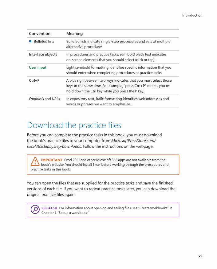
You can save time when reading this book by understanding how the Step by Step series provides procedural instructions and auxiliary information and identifies on-screen and physical elements that you interact with. The following table lists content formatting conventions used in this book.

Convention Meaning

TIP This reader aid provides a helpful hint or shortcut to simplify a task.

IMPORTANT This reader aid alerts you to a common problem or provides information necessary to successfully complete a procedure.

SEE ALSO This reader aid directs you to more information about a topic in this book or elsewhere.

1. Numbered steps Numbered steps guide you through generic procedures in each topic and hands-on practice tasks at the end of each chapter.

xv

Introduction

Convention Meaning

■ Bulleted lists Bulleted lists indicate single-step procedures and sets of multiple alternative procedures.

Interface objects In procedures and practice tasks, semibold black text indicates on-screen elements that you should select (click or tap).

User input Light semibold formatting identifies specific information that you should enter when completing procedures or practice tasks.

Ctrl+P A plus sign between two keys indicates that you must select those keys at the same time. For example, “press Ctrl+P” directs you to hold down the Ctrl key while you press the P key.

Emphasis and URLs In expository text, italic formatting identifies web addresses and words or phrases we want to emphasize.

Download the practice filesBefore you can complete the practice tasks in this book, you must download the book’s practice files to your computer from MicrosoftPressStore.com/Excel365stepbystep/downloads. Follow the instructions on the webpage.

IMPORTANT Excel 2021 and other Microsoft 365 apps are not available from the book’s website. You should install Excel before working through the procedures and

practice tasks in this book.

You can open the files that are supplied for the practice tasks and save the finished versions of each file. If you want to repeat practice tasks later, you can download the original practice files again.

SEE ALSO For information about opening and saving files, see “Create workbooks” in Chapter 1, “Set up a workbook.”

http://MicrosoftPressStore.com/Excel365stepbystep/downloads

http://MicrosoftPressStore.com/Excel365stepbystep/downloads

xvi

Introduction

The following table lists the files available for use while working through the practice tasks in this book.

Chapter Folder File

Part 1: Create and format workbooks

1: Set up a workbook Excel365SBS\Ch01 CreateWorkbooks.xlsx

CustomizeRibbonTabs.xlsx

MergeCells.xlsx

ModifyWorkbooks.xlsx

ModifyWorksheets.xlsx

2: Work with data and Excel tables Excel365SBS\Ch02 CompleteFlashFill.xlsx

CreateExcelTables.xlsx

EnterData.xlsx

FindValues.xlsx

MoveData.xlsx

ResearchItems.xlsx

3: Perform calculations on data Excel365SBS\Ch03 AuditFormulas.xlsx

BuildFormulas.xlsx

CreateArrayFormulas.xlsx

CreateConditonalFormulas.xlsx

NameRanges.xlsx

SetIterativeOptions.xlsx

4: Change workbook appearance Excel365SBS\Ch04 AddImages.xlsx

CreateConditionalFormats.xlsx

DefineStyles.xlsx

FormatCells.xlsx

FormatNumbers.xlsx

ModifyTableStyles.xlsx

ModifyThemes.xlsx

phone.jpg

xvii

Introduction

Chapter Folder File

Part 2: Analyze and present data

5: Manage worksheet data Excel365SBS\Ch05 FilterData.xlsx

SummarizeValues.xlsx

ValidateData.xlsx

6: Reorder and summarize data Excel365SBS\Ch06 CustomSortData.xlsx

OutlineData.xlsx

SortData.xlsx

7: Combine data from multiple sources

Excel365SBS\Ch07 ConsolidateData.xlsx

CreateDataLinks.xlsx

FleetOperatingCosts.xlsx

LookupData.xlsx

8: Analyze alternative data sets Excel365SBS\Ch08 CreateScenarios.xlsx

DefineDataTables.xlsx

PerformGoalSeekAnalysis.xlsx

9: Create charts and graphics Excel365SBS\Ch09 CreateCharts.xlsx

CreateComboCharts.xlsx

CreateSparklines.xlsx

CreateSpecialCharts.xlsx

CustomizeCharts.xlsx

IdentifyTrends.xlsx

InsertShapes.xlsx InsertSmartArt.xlsx

10: Create PivotTables and PivotCharts

Excel365SBS\Ch10 CreatePivotCharts.xlsx

CreatePivotTables.xlsx

EditPivotTables.xlsx

FilterPivotTables.xlsx

FormatPivotTables.xlsx

xviii

Introduction

Chapter Folder File

Part 3: Collaborate and share in Excel

11: Print worksheets and charts Excel365SBS\Ch11 AddHeaders.xlsx

ConsolidatedMessenger.png

PrepareWorksheets.xlsx

PrintCharts.xlsx

PrintParts.xlsx

PrintWorksheets.xlsx

12: Automate tasks and input Excel365SBS\Ch12 AssignMacros.xlsm

ExamineMacros.xlsm

InsertFormControls.xlsm

RecordMacros.xlsm

13: Work with other Microsoft 365 apps

Excel365SBS\Ch13 CreateHyperlinks.xlsx

EmbedWorkbook.xlsx

LevelDescriptions.xlsx

LinkCharts.xlsx

LinkFiles.xlsx

LinkWorkbooks.pptx

ReceiveLinks.pptx

14: Collaborate with colleagues Excel365SBS\Ch14 CreateTemplate.xlsx

DistributeFiles.xlsx

FinalizeWorkbooks.xlsx

ManageComments.xlsx

ProtectWorkbooks.xlsx

xix

Introduction

Chapter Folder File

Part 4: Perform advanced analysis

15: Perform business intelligence analysis

Excel365SBS\Ch15 AnalyzePowerPivotData.xlsx

CreateQuery.xlsx

DefineModel.xlsx

DefineRelationships.xlsx

DisplayTimelines.xlsx

ManagePowerQueryData.xlsx

16. Create forecasts and visualizations

Excel365SBS\Ch16 CreateForecastSheets.xlsx

CreateKPIs.xlsx

CreateMaps.xlsx

DefineMeasures.xlsx

xx

Introduction

Adapt exercise stepsThis book contains many images of the Excel user interface elements (such as the ribbon and the app window) that you’ll work with while performing tasks in Excel on a Windows computer. Unless we’re demonstrating an alternative view of content, the screenshots shown in this book were captured on a horizontally oriented display at a screen resolution of 1920 × 1080 and a magnification of 100 percent. If your settings are different, the ribbon on your screen might not look the same as the one shown in this book. As a result, exercise instructions that involve the ribbon might require a little adaptation.

Simple procedural instructions use this format:

■ On the Insert tab, in the Illustrations group, select the Chart button.

If the command is in a list, our instructions use this format:

1. On the Home tab, in the Editing group, select the Find arrow and then, in the Find list, select Go To.

If differences between your display settings and ours cause a button to appear differ-ently on your screen than it does in this book, you can easily adapt the steps to locate the command. First select the specified tab, and then locate the specified group. If a group has been collapsed into a group list or under a group button, select the list or button to display the group’s commands. If you can’t immediately identify the button you want, point to likely candidates to display their names in ScreenTips.

xxi

Introduction

Multistep procedural instructions use this format:

1. To select the paragraph that you want to format in columns, triple-click the paragraph.

2. On the Layout tab, in the Page Setup group, select the Columns button to display a menu of column layout options.

3. On the Columns menu, select Three.

On subsequent instances of instructions that require you to follow the same process, the instructions might be simplified in this format because the working location has already been established:

1. Select the paragraph that you want to format in columns.

2. On the Columns menu, select Three.

The instructions in this book assume that you’re selecting on-screen content and user interface elements on your computer by clicking (with a mouse, touchpad, or other hardware device) or tapping a touchpad or the screen (with your finger or a stylus).Instructions refer to Excel user interface elements that you click or tap on the screen as buttons, and to physical buttons that you press on a keyboard as keys, to conform to the standard terminology used in documentation for these products.

When the instructions tell you to enter information, you can do so by typing on a con-nected external keyboard, tapping an on-screen keyboard, or even speaking aloud, depending on your computer setup and your personal preferences.

xxii

Introduction

E-book editionIf you’re reading the e-book edition of this book, you can do the following:

■ Search the full text

■ Print

■ Copy and paste

You can purchase and download the e-book edition from the Microsoft Press Store at MicrosoftPressStore.com/Excel365stepbystep/detail.

Get support and give feedbackWe’ve made every effort to ensure the accuracy of this book and its companion content. We welcome your feedback.

Errata and supportIf you discover an error, please submit it to us at MicrosoftPressStore.com/Excel365stepbystep/errata. We’ll investigate all reported issues, update download-able content if appropriate, and incorporate necessary changes into future editions of this book.

For additional book support and information, please visit MicrosoftPressStore.com/Support.

For assistance with Microsoft software and hardware, visit the Microsoft Support site at support.microsoft.com.

Stay in touchLet’s keep the conversation going! We’re on Twitter at twitter.com/MicrosoftPress.

http://MicrosoftPressStore.com/Excel365stepbystep/detail

http://MicrosoftPressStore.com/Excel365stepbystep/errata

http://MicrosoftPressStore.com/Support

http://support.microsoft.com

http://twitter.com/MicrosoftPress

http://MicrosoftPressStore.com/Excel365stepbystep/errata

http://MicrosoftPressStore.com/Support

3Perform calculations on data

In this chapter■ Name data ranges

■ Create formulas to calculate values

■ Summarize data that meets specific conditions

■ Copy and move formulas

■ Create array formulas

■ Find and correct errors in calculations

■ Configure automatic and iterative calculation options

Excel workbooks provide an easy interface for storing and organizing data, but Excel can do so much more than that. Using the built-in functions, you can easily perform a variety of calculations—from simple tasks such as calculating totals to complex financial calcula-tions. Excel can report information such as the current date and time, the maximum value or number of blank cells in a data set, and the cells that meet specific condi-tions, and it can use this information when performing calculations. To simplify the process of referencing cells or data ranges in your calculations, you can name them. Excel provides guidance for creating formulas to perform calculations and for identifying and fixing any errors in the calculations.

This chapter guides you through procedures related to naming data ranges, creating formulas to calculate values, summarizing data in one or more cells, copy-ing and moving formulas, creating array formulas, troubleshooting issues with formula calculations, and configuring automatic and iterative calculation options.

71

Name data rangesWhen you work with large amounts of data, it’s often useful to identify groups of cells that contain related data. For example, you might have a worksheet for a delivery service in which:

■ Each column of data summarizes the number of packages handled during one hour of the day.

■ Each row of data represents a region that handled packages.

Worksheets often contain logical groups of data

Instead of specifying a cell or range of cells individually every time you want to refer-ence the data they contain, you can name the cell or cells—in other words, create a named range. For example, you could group the packages handled in the Northeast region during all time periods into a range named Northeast. Whenever you want to use the contents of that range in a calculation, you can reference Northeast instead of $C$3:$I$3. That way, you don’t need to remember the cell range or even the work-sheet it’s on.

Select a group of cells to create a named range

TIP Range names can be simple or complex. In a workbook that contains different kinds of data, a more descriptive name such as NortheastVolume can help you remem-

ber the data the range includes.

Chapter 3: Perform calculations on data

72

3

If you have a range of data with consistent row or column headings, you can create a series of ranges at one time instead of having to create each individually.

By default, when you create a named range, its scope is the entire workbook. This means that you can reference the name in a formula on any worksheet in the work-book. If a workbook contains a series of worksheets with the same content—for example, sales data worksheets for each month of a year—you might want to set the scope of ranges on those worksheets to the worksheet instead of to the workbook.

After you create a named range, you can edit the name, the cells the range includes, or the scope in which the range exists, or delete a range you no longer need, in the Name Manager.

Manage named ranges in the Name Manager

TIP If your workbook contains a lot of named ranges, tables, or other objects, you can filter the Name Manager list to locate objects more easily.

To create a named range

1. Select the cells you want to include in the named range.

2. In the Name Box, next to the formula bar, enter a name for your named range.

Or

1. Select the cells you want to include in the named range.

2. On the Formulas tab, in the Defined Names group, select Define Name.

Name data ranges

73

3. In the New Name dialog, do the following:

a. In the Name box, enter a name for the range. The name must begin with a letter or underscore and may not contain spaces.

b. If you want to restrict the range to use on a specific worksheet, select that worksheet in the Scope list.

c. If you want to provide additional information to help workbook users identify the range, enter a description of up to 255 characters in the Comment box.

d. Verify that the Refers to box includes the cells you want to include in the range.

e. Select OK.

To create a series of named ranges from data with headings

1. Select the cells that contain the headings and data you want to include in the named ranges.

2. On the Formulas tab, in the Defined Names group, select Create from Selection.

3. In the Create Names from Selection dialog, select the checkbox next to the location of the heading text from which you want to create the range names.

Name ranges by any outer row or column in the selection

4. Select OK.

To open the Name Manager

■ On the Formulas tab, in the Defined Names group, select Name Manager.


74

3

To change the name of a named range

1. Open the Name Manager.

2. Select the range you want to rename, and then select Edit.

3. In the Edit Name dialog, in the Name box, change the range name, and then select OK.

To change the cells in a named range


2. Select the range you want to edit, and then do either of the following:

In the Refers to box, change the cell range.

Select Edit. In the Edit Name dialog, in the Refers to box, change the cell range, and then select OK.

To change the scope of a named range

1. Select the range you want to change the scope of and note the range name shown in the Name Box.

2. On the Formulas tab, in the Defined Names group, select Define Name.

3. In the New Name dialog, do the following:

a. In the Name box, enter the existing range name that you noted in step 1.

b. In the Scope list, select the new scope.

c. If you want to provide additional information to help workbook users iden-tify the range, enter a description of up to 255 characters in the Comment box.

d. Verify that the Refers to box includes the cells you want to include in the range.

e. Select OK.

To delete a named range


2. Select the range you want to delete, and then select Delete.

3. In the Microsoft Excel dialog prompting you to confirm the deletion, select OK.

Name data ranges

75

Create formulas to calculate valuesAfter you enter data on a worksheet and, optionally, define ranges to simplify data references, you can create formulas to performs calculations on your data. For exam-ple, you can calculate the total cost of a customer’s shipments, figure the average number of packages for all Wednesdays in the month of January, or find the highest and lowest daily package volumes for a week, month, or year.

You can enter a formula directly into a cell or into the formula bar located between the ribbon and the worksheet area.

Every formula begins with an equal sign (=), which tells Excel to interpret the expres-sion after the equal sign as a calculation instead of as text. The formula that you enter after the equal sign can include simple references and mathematical operators, or it can begin with an Excel function. For example, you can find the sum of the numbers in cells C2 and C3 by using the formula =C2+C3. You can edit formulas by selecting the cell and then editing the formula in the cell or in the formula bar.

Operators and precedenceWhen you create an Excel formula, you use the built-in functions and arith-metic operators that define operations such as addition and multiplication. The following table displays the order in which Excel evaluates mathematical operations.

Precedence Operator Description

1 - Negation

2 % Percentage

3 ^ Exponentiation

4 * and / Multiplication and division

5 + and – Addition and subtraction

6 & Concatenation


76

3

If two operators at the same level, such as + and –, occur in the same equa-tion, Excel evaluates them from left to right.

For example, Excel evaluates the operations in the formula = 4 + 8 * 3 – 6 in this order:

1. 8 * 3 = 24

2. 4 + 24, with a result of 28

3. 28 – 6, with a final result of 22

You can control the order in which Excel evaluates operations by using paren-theses. Excel always evaluates operations in parentheses first.

For example, if the previous equation were rewritten as = (4 + 8) * 3 – 6, Excel would evaluate the operations in this order:

1. (4 + 8), with a result of 12

2. 12 * 3, with a result of 36


In a formula that has multiple levels of parentheses, Excel evaluates the expressions within the innermost set of parentheses first and works its way out. As with operations on the same level, expressions at the same parenthet-ical level are evaluated from left to right.

For example, Excel evaluates the formula = 4 + (3 + 8 * (2 + 5)) – 7 in this order:

1. (2 + 5), with a result of 7

2. 7 * 8, with a result of 56




Create formulas to calculate values

77

You can perform mathematical operations on numbers by using the mathematical operators for addition (+), subtraction (–), multiplication (*), division (/), negation (-), and exponentiation (̂ ). You can perform other operations on a range of numbers by using the following Excel functions:

■ SUM Returns the sum of the numbers.

■ AVERAGE Returns the average of the numbers.

■ COUNT Returns the number of entries in the cell range.

■ MAX Returns the largest number.

■ MIN Returns the smallest number.

These functions are available from the AutoSum list, which is in the Editing group on the Home tab of the ribbon and in the Function Library group on the Formulas tab. The Function Library is also where you’ll find the rest of the Excel functions, organized into categories.

Excel includes a wide variety of functions

The Formula AutoComplete feature simplifies the process of referencing functions, named ranges, and tables in formulas. It provides a template for you to follow and suggests entries for each function argument. Here’s how it works:

1. As you begin to enter a function name after the equal sign, Excel displays a list of functions matching the characters you’ve entered. You can select a function from the list and then press Tab to enter the function name and the opening parenthesis in the cell or formula bar.


78

3

Select a function from the list

2. After the opening parenthesis, Excel displays the arguments that the selected function accepts. Bold indicates required arguments and square brackets enclose optional arguments. You can simply follow the prompts to enter or select the necessary information, and then enter a closing parenthesis to finish the formula.

Excel prompts you for required and optional information

3. To reference a named range, table, or table element, start entering the name (or an opening square bracket to indicate a table element) and Excel displays a list of options to choose from.

TIP You can reference a series of contiguous cells in a formula by entering the cell range or by dragging through the cells. If the cells aren’t contiguous, hold

down the Ctrl key and select each cell.


79

Excel displays the available table elements

SEE ALSO For information about using keyboard shortcuts to select cell ranges, see the appendix, “Keyboard shortcuts.”

If you’re creating a more complex formula and want extra guidance, you can assemble the formula in the Insert Function dialog. All the Excel functions are available from within the dialog.

Create formulas in the Insert Function dialog

If you’re uncertain which function to use, you can search for one by entering a simple description of what you’d like to accomplish. Selecting any function displays the func-tion’s arguments and description.


80

3

Activate any field to display a description of the argument

After you select a function, Excel displays an interface in which you can enter all the function arguments. The complexity of the interface depends on the function.

Whether you enter a formula directly or assemble it in the Insert Function dialog, you can reference data in cells (A3) or cell ranges (A3:J12), in named ranges (Northeast), or in table columns (TableName[ColumnName]). For example, if the Northeast range refers to cells C3:I3, you can calculate the average of cells C3:I3 by using the formula =AVERAGE(Northeast).

To create a formula manually

1. Select the cell in which you want to create the formula.

2. In the cell or in the formula bar, enter an equal sign (=).

3. If the formula will call a function, enter the function name and an open-ing parenthesis to begin the formula and display the required and optional arguments.

4. Enter the remainder of the formula:

Reference cells by entering the cell reference or selecting the cell.

Reference cell ranges by entering the cell range or dragging across the range.

Reference named ranges and tables by entering the range or table name.

Reference table elements by entering [ after the table name, selecting the element from the list, and then entering ].


81

5. If the formula includes a function, enter the closing parenthesis to end it.

6. Press Enter to enter the formula in the cell and return the results.

To open the Insert Function dialog

■ On the formula bar, to the left of the text entry box, select the Insert Function button (fx).

■ On the Formulas tab, in the Function Library group, select Insert Function.

■ Press Shift+F3.

To locate a function in the Insert Function dialog

■ In the Search for a function box, enter a brief description of the operation you want to perform, and then select Go.

Or

1. In the Or select a category list, select the function category.

2. Scroll down the Select a function list to the function.

To create a formula in the Insert Function dialog

1. Open the Insert Function dialog.

2. Select the function you want to use in the formula, and then select OK.

3. In the Function Arguments dialog, enter the function’s arguments, and then select OK.

To reference a named range in a formula

■ Enter the range name in place of the cell range.

To reference an Excel table column in a formula

■ Enter the table name followed by an opening bracket ([), the column name, and a closing bracket (]).


82

3

Summarize data that meets specific conditionsAnother use for formulas is to display messages when certain conditions are met. This kind of formula is called a conditional formula. One way to create a conditional formula in Excel is to use the IF function. Selecting the Insert Function button next to the formula bar and then choosing the IF function displays the Function Arguments dialog with the fields required to create an IF formula.

The Function Arguments dialog for an IF formula

When you work with an IF function, the Function Arguments dialog displays three input boxes:

■ Logical_test The condition you want to check.

■ Value_if_true The value to display if the condition is met. This could be a cell reference, or a number or text enclosed in quotes.

■ Value_if_false The value to display if the condition is not met.

Summarize data that meets specific conditions

83

The following table displays other conditional functions you can use to summarize data.

Function Description

AVERAGEIF Finds the average of values within a cell range that meet a specified criterion

AVERAGEIFS Finds the average of values within a cell range that meet multiple criteria

COUNT Counts the cells in a range that contain numerical values

COUNTA Counts the cells in a range that are not empty

COUNTBLANK Counts the cells in a range that are empty

COUNTIF Counts the cells in a range that meet a specified criterion

COUNTIFS Counts the cells in a range that meet multiple criteria

IFERROR Displays one value if a formula results in an error and another if it doesn’t

SUMIF Adds the values in a range that meet a single criterion

SUMIFS Adds the values in a range that meet multiple criteria

To create a formula that uses the AVERAGEIF function, you define the range to be examined for the criterion, the criterion, and, if required, the range from which to draw the values. As an example, consider a worksheet that lists each customer’s ID number, name, state, and total monthly shipping bill. If you want to find the average order of customers from the state of Washington (abbreviated in the worksheet as WA), you can create the formula =AVERAGEIF(C3:C6, “WA”, D3:D6).

Sample data that illustrates the preceding example

The AVERAGEIFS, SUMIFS, and COUNTIFS functions extend the capabilities of the AVERAGEIF, SUMIF, and COUNTIF functions to allow for multiple criteria. For example, if you want to find the sum of all orders of at least $100,000 placed by companies in Washington, you can create the formula =SUMIFS(D2:D5, C2:C5, “=WA”, D2:D5, “>=100000”).


84

3

The AVERAGEIFS and SUMIFS functions start with a data range that contains values that the formula summarizes. You then list the data ranges and the criteria to apply to that range. In generic terms, the syntax is =AVERAGEIFS(data_range, criteria_range1, criteria1[,criteria_range2, criteria2...]). The part of the syntax in brackets (which aren’t used when you create the formula) is optional, so an AVERAGEIFS or SUMIFS formula that contains a single criterion will work. The COUNTIFS function, which doesn’t per-form any calculations, doesn’t need a data range; you just provide the criteria ranges and criteria. For example, you could find the number of customers from Washington who were billed at least $100,000 by using the formula =COUNTIFS(C2:C5, “=WA”, D2:D5, “>=100000”).

You can use the IFERROR function to display a custom error message instead of relying on the default Excel error messages to explain what happened. For example, you could create this type of formula to employ the VLOOKUP function to look up a customer’s name in the second column of a table named Customers based on the customer identification number entered into cell G8. That formula might look like this: =IFERROR(VLOOKUP(G8,Customers,2,FALSE),”Customer not found”). If the function finds a match for the customer ID in cell G8, it displays the customer’s name; if not, it displays the text “Customer not found.”

TIP The last two arguments in the VLOOKUP function tell the formula to look in the Customers table’s second column and to require an exact match. For more information

about the VLOOKUP function, see “Look up data from other locations” in Chapter 7, “Combine data from multiple sources.”

To summarize data by using the IF function

■ Use the syntax =IF(logical_test, value_if_true, value_if_false) where:

logical_test is the logical test to be performed.

value_if_true is the value the formula returns if the test is true.

value_if_false is the value the formula returns if the test is false.

To count cells that contain numbers in a range

■ Use the syntax =COUNT(range), where range is the cell range in which you want to count cells.

Summarize data that meets specific conditions

85

To count cells that are non-blank

■ Use the syntax =COUNTA(range), where range is the cell range in which you want to count cells.

To count cells that contain a blank value

■ Use the syntax =COUNTBLANK(range), where range is the cell range in which you want to count cells.

To count cells that meet one condition

■ Use the syntax =COUNTIF(range, criteria) where:

range is the cell range that might contain the criteria value.

criteria is the logical test used to determine whether to count the cell.

To count cells that meet multiple conditions

■ Use the syntax =COUNTIFS(criteria_range1, criteria1, criteria_range2, criteria2,…) where for each criteria_range and criteria pair:

criteria_range is the cell range that might contain the criteria value.

criteria is the logical test used to determine whether to count the cell.

To find the sum of data that meets one condition

■ Use the syntax =SUMIF(range, criteria, sum_range) where:


criteria is the logical test used to determine whether to include the cell.

sum_range is the range that contains the values to be included if the range cell in the same row meets the criterion.

To find the sum of data that meets multiple conditions

■ Use the syntax =SUMIFS(sum_range, criteria_range1, criteria1, criteria_range2, criteria2,…) where:

sum_range is the range that contains the values to be included if all criteria_range cells in the same row meet all criteria.




86

3

To find the average of data that meets one condition

■ Use the syntax =AVERAGEIF(range, criteria, average_range) where:



average_range is the range that contains the values to be included if the range cell in the same row meets the criterion.

To find the average of data that meets multiple conditions

■ Use the syntax =AVERAGEIFS(average_range, criteria_range1, criteria1, criteria_range2, criteria2,…) where:

average_range is the range that contains the values to be included if all criteria_range cells in the same row meet all criteria.



To display a custom message if a cell contains an error

■ Use the syntax =IFERROR(value, value_if_error) where:

value is a cell reference or formula.

value_if_error is the value to be displayed if the value argument returns an error.

Copy and move formulasAfter you create a formula, you can copy it and paste it into another cell. When you do, Excel changes the formula to work in the new cells. For instance, suppose you have a worksheet in which cell C7 contains the formula =SUM(C2:C6). If you copy cell C7 and paste the copied formula into cell D7, Excel enters =SUM(D2:D6). Excel knows to change the cells used in the formula because the formula uses a relative reference—a reference that can change if the formula is copied to another cell. Relative references are written with just the cell row and column—for example, C14.

Copy and move formulas

87

Relative references are useful when you summarize rows of data and want to use the same formula for each row. As an example, suppose you have a worksheet with two columns of data, labeled Sale Price and Rate, and you want to calculate a sales representative’s commission by multiplying the two values in a row. To calculate the commission for the first sale, you would enter the formula =A2*B2 in cell C2.

Use formulas to calculate values such as commissions

Selecting cell C2 and dragging the fill handle down through cell C7 copies the formula from cell C2 into each of the other cells. Because you created the formula by using relative references, Excel updates each cell’s formula to reflect its position relative to the starting cell (in this case, cell C2). The formula in cell C7, for example, is =A7*B7.

Copying formulas to other cells to summarize additional data

When you enter a formula in a cell of an Excel table column, Excel automatically copies the formula to the rest of the column and updates any relative references in the formula.


88

3

If you want a cell reference to remain constant when you copy a formula to another cell, use an absolute reference by inserting a dollar sign ($) before the column letter and row number or a mixed reference by inserting a dollar sign before either the column letter or row number.

TIP In addition to using an absolute reference, another way to ensure that your cell ref-erences don’t change when you copy a formula to another cell is to select the cell that

contains the formula, copy the formula’s text in the formula bar, press the Esc key to exit cut-and-copy mode, select the cell where you want to paste the formula, and press Ctrl+V. Excel doesn’t change the cell references when you copy your formula to another cell in this manner.

One quick way to change a cell reference from relative to absolute is to select the cell reference in the formula bar and then press F4. Pressing F4 cycles a cell reference through the four possible types of references:

■ Relative columns and rows (for example, C4)

■ Absolute columns and rows (for example, $C$4)

■ Relative columns and absolute rows (for example, C$4)

■ Absolute columns and relative rows (for example, $C4)

To copy a formula without changing its cell references

1. Select the cell that contains the formula you want to copy.

2. In the formula bar, select the formula text.

3. Press Ctrl+C.

4. Select the cell in which you want to paste the formula.

5. Press Ctrl+V.

6. Press Enter.

To move a formula without changing its cell references


2. Point to the edge of the selected cell until the pointer changes to a black four-headed arrow.

3. Drag the outline to the cell where you want to move the formula.

Copy and move formulas

89

To copy a formula and change its cell references


2. Press Ctrl+C.

3. Select the cell in which you want to paste the formula.

4. Press Ctrl+V.

To create relative and absolute cell references

1. Enter a cell reference into a formula.

2. Do either of the following:

Enter a $ in front of a row or column reference you want to make absolute.

Select within the cell reference, and then press F4 to advance through the four possible combinations of relative and absolute row and column references.

Create array formulasMost Excel formulas calculate values to be displayed in a single cell. For example, you could add the formulas =B1*B4, =B1*B5, and =B1*B6 to consecutive worksheet cells to calculate shipping insurance costs based on the value of a package’s contents.

A worksheet with data to be summarized by an array formula

Instead of entering the same formula in multiple cells one cell at a time, you can enter a formula in every cell in the target range at the same time by creating an array for-mula. To calculate package insurance rates by multiplying the values in the cell range B4:B6 by the insurance rate in cell B1, you select the target cells (C4:C6) and enter


90

3

the formula =B1*B4:B6. Note that you must select a range of the same shape as the values you’re using in the calculation. (For example, if the value range is three columns wide by one row high, the target range must also be three columns wide by one row high.) If you enter the array formula into a range of the wrong shape, Excel displays duplicate results, incomplete results, or error messages, depending on how the target range differs from the value range.

When you press Ctrl+Shift+Enter, Excel creates an array formula in the selected cells. The formula appears within a pair of braces to indicate that it is an array formula.

An array formula calculates multiple results

IMPORTANT You can’t add braces to a formula to make it an array formula. You must press Ctrl+Shift+Enter to create it.

To create an array formula

1. Select the cells in which you want to display the formula results.

2. In the formula bar, enter the array formula.

3. Press Ctrl+Shift+Enter.

To edit an array formula

1. Select every cell that contains the array formula.

2. In the formula bar, edit the array formula.

3. Press Ctrl+Shift+Enter to re-enter the formula as an array formula.

Create array formulas

91

Find and correct errors in calculationsIncluding calculations in a worksheet gives you valuable answers to questions about your data. As is always true, however, it’s possible for errors to creep into your formu-las. With Excel, you can find the source of errors in your formulas by identifying the cells used in a specific calculation and describing any errors that have occurred. The process of examining a worksheet for errors is referred to as auditing.

Excel identifies errors in several ways. The first way is to display an error code in the cell that contains the formula generating the error.

A warning triangle and pound sign indicate an error

When the active cell generates an error, Excel displays an Error button next to it. Pointing to the button displays information about the error, and selecting the button displays a menu of options for handling the error.

The following table explains the most common error codes.

Error code Description

##### The column isn’t wide enough to display the value.

#VALUE! The formula has the wrong type of argument, such as text in a cell where a numerical value is required.

#NAME? The formula contains text that Excel doesn’t recognize, such as an unknown named range.

#REF! The formula refers to a cell that doesn’t exist, which can happen whenever cells are deleted.

#DIV/0! The formula attempts to divide by zero.


92

3

Another technique you can use to find the source of formula errors is to ensure that the appropriate cells are providing values for the formula. You can identify the source of an error by having Excel trace a cell’s precedents, which are the cells with values used in the active cell’s formula. You can also audit your worksheet by identifying cells with formulas that use a value from a particular cell. Cells that use another cell’s value in their calculations are known as dependents, meaning that they depend on the value in the other cell to derive their own value. They are identified in Excel by tracer arrows. If the cells identified by the tracer arrows aren’t the correct cells, you can hide the arrows and correct the formula.

Tracing a cell’s dependents

If you prefer to have the elements of a formula error presented as text in a dialog, you can use the Error Checking tool to locate errors one after the other. You can choose to ignore the selected error or move to the next or the previous error.

Identify and manage errors from the Error Checking window

TIP You can have the Error Checking tool ignore formulas that don’t use every cell in a region (such as a row or column). To do so, on the Formulas tab of the Excel Options

dialog, clear the Formulas Which Omit Cells In A Region checkbox. Excel will no longer mark these cells as an error.

Find and correct errors in calculations

93

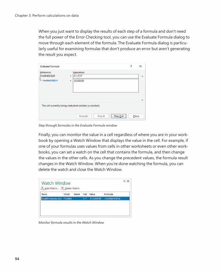
When you just want to display the results of each step of a formula and don’t need the full power of the Error Checking tool, you can use the Evaluate Formula dialog to move through each element of the formula. The Evaluate Formula dialog is particu-larly useful for examining formulas that don’t produce an error but aren’t generating the result you expect.

Step through formulas in the Evaluate Formula window

Finally, you can monitor the value in a cell regardless of where you are in your work-book by opening a Watch Window that displays the value in the cell. For example, if one of your formulas uses values from cells in other worksheets or even other work-books, you can set a watch on the cell that contains the formula, and then change the values in the other cells. As you change the precedent values, the formula result changes in the Watch Window. When you’re done watching the formula, you can delete the watch and close the Watch Window.

Monitor formula results in the Watch Window


94

3

To display information about a formula error

1. Select the cell that contains the error.

2. Point to the error indicator next to the cell to display information about the error.

3. Select the error indicator to display options for correcting or learning more about the error.

To identify the cells that a formula references

1. Select the cell that contains the formula.

2. On the Formulas tab, in the Formula Auditing group, select Trace Precedents.

To identify formulas that reference a specific cell

1. Select the cell.

2. In the Formula Auditing group, select Trace Dependents.

To remove tracer arrows

■ In the Formula Auditing group, do one of the following:

To remove all the arrows, select the Remove Arrows button (not its arrow).

To remove only precedent or dependent arrows, select the Remove Arrows arrow, and then select Remove Precedent Arrows or Remove Dependent Arrows.

To evaluate a formula one calculation at a time

1. Select the cell that contains the formula you want to evaluate.

2. In the Formula Auditing group, select Evaluate Formula.

3. In the Evaluate Formula dialog, select Evaluate. Excel replaces the underlined calculation with its result.

4. Do either of the following:

Select Step In to move forward by one calculation.

Select Step Out to move backward by one calculation.

5. When you finish, select Close.

Find and correct errors in calculations

95

To change error display options

1. Display the Formulas page of the Excel Options dialog.

2. In the Error Checking section, select or clear the Enable background error checking checkbox.

3. Select the Indicate errors using this color button and select a color.

4. Select Reset Ignored Errors to return Excel to its default error indicators.

5. In the Error checking rules section, select or clear the checkboxes next to errors you want to indicate or ignore, respectively.

To watch the values in a cell range

1. Select the cell range you want to watch.

2. In the Formula Auditing group, select the Watch Window button.

3. In the Watch Window dialog, select Add Watch.

4. In the Add Watch dialog, confirm the cell range, and then select Add.

To delete a watch

1. Select the Watch Window button.

2. In the Watch Window dialog, select the watch you want to delete.

3. Select Delete Watch.

Configure automatic and iterative calculation optionsExcel formulas use values in other cells to calculate their results. If you create a for-mula that refers to the cell that contains the formula, the result is a circular reference.

Under most circumstances, Excel treats a circular reference as a mistake for two rea-sons. First, most Excel formulas don’t refer to their own cell, so a circular reference is unusual enough to be identified as an error. The second, more serious consideration is that a formula with a circular reference can slow down your workbook. Because Excel repeats, or iterates, the calculation, you must set limits on how many times the app repeats the operation.


96

3

You can control how often Excel recalculates formulas. Three calculation options are avail-able from the Formulas tab and from the Formulas page of the Excel Options dialog.

You can modify the iterative calculation options Excel uses

The calculation options work as follows:

■ Automatic recalculates a worksheet whenever a value that affects a formula changes. This is the default setting.

■ Automatic Except for Data Tables recalculates a worksheet whenever a value changes but doesn’t recalculate data tables.

■ Manual recalculates formulas only when you tell Excel to do so.

You can also use options in the Calculation Options section to allow or disallow itera-tive calculations (repeating calculations of formulas that contain circular references). The default values (a maximum of 100 iterations and a maximum change per iteration of 0.001) are appropriate for all but the most unusual circumstances.

To manually recalculate the active workbook

■ On the Formulas tab, in the Calculation group, select Calculate Now.

■ Press F9.

To manually recalculate the active worksheet

■ In the Calculation group, select the Calculate Sheet button.

Configure automatic and iterative calculation options

97

To set worksheet calculation options

■ Display the worksheet whose calculation options you want to set.

■ On the Formulas tab, in the Calculation group, select Calculation Options, and then select Automatic, Automatic Except for Data Tables, or Manual.

To enable iterative calculations

1. Open the Excel Options dialog and display the Formulas page.

2. In the Calculation options section, select the Enable iterative calculation checkbox.

3. In the Maximum Iterations box, enter the maximum iterations allowed for a calculation.

4. In the Maximum Change box, enter the maximum change allowed for each iteration.

5. Select OK.


98

3

Skills reviewIn this chapter, you learned how to:

■ Name data ranges

■ Create formulas to calculate values

■ Summarize data that meets specific conditions

■ Copy and move formulas

■ Create array formulas

■ Find and correct errors in calculations

■ Configure automatic and iterative calculation options

Skills review

99

Practice tasksBefore you can complete these tasks, you must copy the book’s practice files to your computer. The practice files for these tasks are in the Excel365SBS\Ch03 folder. You can save the results of the tasks in the same folder.

Name data rangesOpen the NameRanges workbook in Excel, and then perform the following tasks:

1. Create a named range named Monday for the V_101 through V_109 values (found in cells C4:C12) for that weekday.

2. Edit the Monday named range to include the V_110 value for that column.

3. Select cells B4:H13 and create a batch of named ranges for V_101 through V_110, using the row headings as the range names.

4. Delete the Monday named range.

Create formulas to calculate valuesOpen the BuildFormulas workbook in Excel, and then perform the following tasks:

1. On the Summary worksheet, in cell F9, create a formula that displays the value from cell C4.

2. Edit the formula in cell F9 so it uses the SUM function to find the total of values in cells C3:C8.

3. In cell F10, create a formula that finds the total expenses for desktop software and server software.

4. Edit the formula in F10 so the cell references are absolute references.

5. On the JuneLabor worksheet, in cell F13, create a SUM formula that finds the total of values in the JuneSummary table’s Labor Expense column.

100

Chapter 3

Summarize data that meets specific conditionsOpen the CreateConditionalFormulas workbook in Excel, and then perform the fol-lowing tasks:

1. In cell G3, create an IF formula that tests whether the value in F3 is greater than or equal to 35,000. If it is, display Request discount; if not, display No discount available.

2. Copy the formula from cell G3 to the range G4:G14.

3. In cell I3, create a formula that finds the average cost of all expenses in cells F3:F14 where the Type column contains the value Box.

4. In cell I6, create a formula that finds the sum of all expenses in cells F3:F14 where the Type column contains the value Envelope, and the Destination column contains the value International.

Create array formulasOpen the CreateArrayFormulas workbook in Excel, and then perform the following tasks:

1. On the Fuel worksheet, in cells C11:F11, enter the array formula =C3*C9:F9.

2. Edit the array formula you just created to read =C3*C10:F10.

3. On the Volume worksheet, in cells D4:D7, create the array formula =B4:B7*C4:C7.

Find and correct errors in calculationsOpen the AuditFormulas workbook in Excel, and then perform the following tasks:

1. Set a watch on the value in cell C19.

2. Display the precedents for the formula in cell C7.

3. Hide the tracer arrows.

4. Use the Error Checking dialog to identify the error in cell C20.

5. Show the tracer arrows for the error.

6. Hide the arrows, and then change the formula in cell C20 to =C12/D20.

101

Practice tasks

7. Use the Evaluate Formula dialog to step through the formula in cell C20.

8. Delete the watch you created in step 1.

Configure automatic and iterative calculation optionsOpen the SetIterativeOptions workbook in Excel, and then perform the following tasks:

1. On the Formulas tab, in the Calculation group, select the Calculation Options button, and then select Manual.

2. In cell B6, enter the formula =B7*B9, and then press Enter.

3. Note that this result is incorrect because the Gross Savings value minus the Savings Incentive value should equal the Net Savings value, which it does not.

4. Press F9 to recalculate the workbook and read the message box indicating that you have created a circular reference.

5. Select OK.

6. Use options in the Excel Options dialog to enable iterative calculation.

7. Close the Excel Options dialog and recalculate the worksheet.

8. Change the workbook’s calculation options back to Automatic.

102

Chapter 3

447

Indexaspect ratio, explained, 441auditing, explained, 441AutoCalculate feature, 143–144, 148, 441. See also

calculationsAutoComplete feature, 43–44, 46, 441AutoFill feature, 44–46, 441AutoRepublish feature, explained, 441AutoSum feature, 78, 411AVERAGE function, 78, 143AVERAGEIF function, 84, 87AVERAGEIFS function, 84–85, 87

BBackstage view

explained, 441Microsoft 365 app keyboard shortcuts, 436using, 5–7using for printed worksheets, 292

bin, explained, 441Bing search engine, 58blank worksheets, creating, 12. See also worksheetsBody and Heading fonts, changing, 109bold formatting, 117, 426, 430borders, applying, 105, 107–108, 426, 431box-and-whisker charts, 219, 441brackets ([]), using with columns in formulas, 82browser, explained, 441bubble charts, 220Button form control, 323buttons

activating, 427adding to Quick Access Toolbar, 28–29explained, 441macro access through, 328–329reordering on Quick Access Toolbar, 32

Ccalculated columns. See also columns

adding to data sources, 388creating, 411

calculating values, 76–82worksheets, 433

Numbers2-D map charts, 2232-D pie charts, 2103-D data maps, creating, 416–421, 4243-D pie charts, 2103-D references, 186, 4413-D shading, applying to form controls, 327

Symbols##### error code, 92+ (addition) operator, precedence of, 76, 78[] (brackets), using with columns in formulas, 82& (concatenation) operator, precedence of, 76/ (division) operator, precedence of, 76, 78^ (exponentiation) operator, precedence of, 76, 78* (multiplication) operator, precedence of, 76, 78- negation operator, precedence of, 76, 78% (percentage) operator, precedence of, 76‘ (single quote), using with workbook names, 186– (subtraction) operator, precedence of, 76, 78

Aabsolute references, 89, 441. See also relative

referencesactions, undoing and restoring, 59active cell. See also cells

designating, 48editing, 432explained, 441

active tab, selecting, 427add-ins, 376, 441addition (+) operator, precedence of, 76, 78AGGREGATE function, 143–144, 147, 149alignment, explained, 441Alt key. See keyboard shortcutsanimating geographic data, 419arguments. See also Function Arguments dialog

displaying descriptions of, 81explained, 441using with functions, 79

array formulas, creating, 90–91, 101. See also formulasArrow keys. See keyboard shortcutsascending order, sorting values in, 386

448

Index

calculation options, configuring, 96–98, 102calculations, finding and correcting errors in,

92–96. See also AutoCalculate featurecategory axis, explained, 441cell background color, applying or changing, 106cell border, applying and removing, 107–108cell data, picking from lists, 46cell notes, adding and editing, 432cell ranges

converting tables to, 66copying to Clipboard, 51cutting to Clipboard, 51explained, 441moving, 50pasting, 51–52previewing before pasting, 52selecting, 429

cell references, 185–188, 441cell styles, defining and managing, 110–113, 133cells. See also active cell; header cells

changing attributes of, 106copying, 430counting, 85–86dependents, 93editing contents of, 55entering values in, 43, 45–46excluding from tables, 62–63explained, 441formatting, 104–109, 133, 430–431inserting, 19locking and unlocking, 358, 360merging and unmerging, 20–22, 40moving, 20, 430navigating, 428–429referencing in formulas, 79selecting, 79tracing precedents of, 93

cells and cell ranges, selecting, 50cells styles, explained, 441chart appearance, customizing, 226–233, 251chart elements

displaying and hiding, 231selecting and formatting, 231

Chart Filters, 229, 232chart layouts, applying, 230chart styles, applying, 228–230chart templates, applying, 232–233chart types

hierarchy, 217–218map, 222–226overview, 216

scatter, 220–221statistic, 218–220stock, 221–222

charts. See also dynamic PivotChartsaccessing, 53color palettes, 228color schemes, 231copying and pasting, 346–347, 350creating, 208–215, 250–251, 433displaying and hiding elements in, 227dual axis, 215–216explained, 441formatting, 227layouts, 210linking to, 346–347, 350moving in worksheets, 214printing, 302–303, 306resizing, 214selecting, 229trendlines, 234–235

Check Box form control, 323, 326, 329–330checkbox, explained, 442circular reference, explained, 442Clipboard, cutting and copying data to, 49closing

Excel, 432workbooks, 9

color of background, applying or changing, 106. See also fill color

color of fonts, changing, 105color of text, changing, 107color palettes, selecting for charts, 228color scales, 123, 442color schemes, charts, 231colors, selecting for themes, 114colors for tabs, changing for worksheets, 14column and row values, switching in charts, 213column width, modifying, 15–18columns. See also calculated columns

adding to tables, 65deleting, 18, 389explained, 442filtering, 139, 386–387hiding and unhiding, 19inserting, 18referencing in formulas, 82reformatting, 387–388renaming, 388repeating on printed pages, 302selecting, 51

449

Index

columns and rowsdeleting, 16inserting, 16

COM add-in, disabling, 378Combo Box form control, 323, 327, 442combo charts, creating, 215–216, 250, 442.

See also chartscommand buttons, assigning macros to, 325commands

adding to Quick Access Toolbar, 31controlling display of, 29moving to, 427opening lists for, 427removing from Quick Access Toolbar, 33repeating, 432

comments, managing, 352–355, 369concatenation (&) operator, precedence of, 76conditional formatting, 53, 123–129, 274–276, 442.

See also formattingconditional functions, using to summarize data, 84.

See also functionsconfidence interval, 409, 442consolidating sets of data, 188–190, 192context menus, 112, 426, 442control group, 442copies, printing, 299Copy Cells option, 45copying

cell ranges to Clipboard, 51cells, 430formulas, 430items, 48–49or linking to charts, 346–347, 350and moving formulas, 87–90and moving worksheets, 11and pasting charts, 346–347, 350sorting levels, 165worksheets, 13

COUNT function, 78, 84–85, 143, 146COUNTA function, 84, 86, 146COUNTBLANK function, 84, 86COUNTIF function, 85–86COUNTIFS function, 84–85Ctrl key. See keyboard shortcutsCtrl+Enter, using to enter values in cells, 43–44Currency format, 431custom lists, sorting data by, 166–167. See also

list rowscutting and copying data to Clipboard, 49Cycle SmartArt graphics, 239

Ddata. See also worksheet data

changing appearance of, 122–129, 134correcting and fine-tuning, 57–61, 69displaying on timelines, 391–394, 402entering and revising, 42–46, 68finding and replacing, 53–57, 69importing using Power Query, 395–400integrating into Excel Data Model, 379linking to, 185–188, 191looking up, 176–184, 191managing with Flash Fill, 46–47, 68managing with Power Pivot, 384–390, 401–402moving in workbooks, 48–53, 69organizing for PivotTables, 260organizing into levels, 170–171outlining, 168–172, 174plotting in charts, 211, 213subtotaling, 168–172, 174summarizing, 83–87, 101summarizing in tables, 63summarizing to meet conditions, 83–87, 101summarizing using sparklines, 235–238, 251

data analysis. See PivotTablesdata bars, 123, 442data connections, creating with Power Query,

395–400data consolidation, 442data entry

canceling, 42enforcing criteria, 150–156, 158techniques, 43–44

Data Model. See Excel Data Modeldata ranges

filtering, 138–143, 157finding values in, 143naming, 72–75, 100

data series, controlling, 43data sets

consolidating, 188–190defining and displaying, 194–198, 205

data sourcescalculated columns, 388defining relationships between, 380–384, 401

data tablesexplained, 442forecasting data with, 199–202, 205

data trends, identifying, 233–235, 251data-formatting commands, accessing, 52–53data validation, 150–156

450

Index

date and time, entering, 430–431deleting

3D maps, 420cell borders, 108cell formatting, 108–109columns, 16, 18, 389, 426comments, managing, 354conditional formatting, 129custom cell styles, 113custom table styles, 119custom themes, 115fields from PivotTables, 261form controls, 332images, 132KPIs (key performance indicators), 415macros, 317measures, 412named ranges, 75page breaks, 296passwords, 359–361personal information, 363queries in Power Query, 400relationships between tables, 384rows, 18, 426shapes, 249sorting rules, 165timelines, 394tracer arrows, 95validating circles, 156watches, 96worksheets, 15

delimiter, explained, 442dependents, explained, 442descending order, sorting values in, 386Developer tab, displaying on ribbon, 313, 326dictionary, adding words to, 61digital certificate, 442digital signature, 442distribute, explained, 442#DIV/0! error code, 92division (/) operator, precedence of, 76, 78Document Inspector, 362, 442document properties, defining values for, 8.

See also propertiesdocuments, linking to, 336–338doughnut charts, 210Drop-Down list, picking from, 43–44dynamic PivotCharts, creating, 277–280, 282, 444.

See also charts

Eemail messages, creating hyperlinks for, 344–345embed, explained, 442embedding file content, 338–340equations, building, 248error alerts, configuring, 155Error Checking window, 93–94, 433error code, explained, 442errors in calculations, finding and correcting, 92–96,

101–102Evaluate Formula window, 94even and odd pages, headers and footers on, 290Excel

closing, 432combining Word and PowerPoint content,

336–340, 349incorporating earlier versions of, 11

Excel app windowarranging workbook windows, 36–38customizing, 40customizing status bar, 33–34magnification level of worksheets, 35–36managing Quick Access Toolbar, 28–33managing ribbon, 23–28

Excel Data Modeladding tables to, 378creating PivotTables from, 389–390deleting tables from, 389displaying, 379managing, 374–380, 401views, 382

Excel Help task pane, 432Excel Options dialog, opening, 25, 109, 311Excel tables. See tablesexponential smoothing forecasting, 403–410, 442exponentiation (̂ ) operator, precedence of, 76, 78extend mode, 433

FF key commands, 432. See also keyboard shortcutsfields, explained, 442file content, embedding, 338–340files

linking to, 337–338saving, 5

fill color, choosing, 107, 426. See also color of background

Fill Days, Weekdays options, 45Fill Down command, 431

451

Index

Fill Formatting Only option, 45fill handle

explained, 442using, 43, 45

Fill Series option, 44–45, 443Fill Without Formatting option, 45filtered data, summarizing, 143–150filtering. See also Sort & Filter menu

data ranges and tables, 138–143PivotTables, 262–268, 281values in columns, 386–387

filtersclearing, 142explained, 443

finalizing workbooks, 362–363Find & Select menu, displaying, 55finding. See also searching information

and correcting errors in calculations, 101–102and replacing data, 53–57

Flash Fill option, 45–47focus, moving to commands on ribbon, 427font color, changing, 105fonts, changing, 109footers and headers, adding, 286–291, 305, 443FORECAST functions, 404–410forecast values, calculating, 409forecast worksheets, creating, 404–409, 422forecasting data, 199–202, 205foreign key, 443form controls

aligning, 331alternative text for, 332controlling, 332deleting, 332grouping, 331moving, 330resizing, 332selecting, 330types, 323using, 322–332, 334

format, explained, 443Format Control dialog, 324formatting. See also conditional formatting

applying, 52–53cells, 104–109, 133, 430–431chart elements, 227, 231finding and replacing, 57PivotTables, 273–277, 282

formatting controls, displaying, 105Formula AutoComplete feature, 78–80, 443

Formula barexplained, 443hiding and unhiding, 28

formulas. See also array formulascopying and moving, 87–90, 430creating, 80–82creating to calculate values, 76–82, 100explained, 443hiding, 360monitoring results of, 94recalculating, 97–98rechecking, 433stepping through, 94

Function Arguments dialog, 83. See also argumentsFunction key commands, 432. See also keyboard

shortcutsfunctions. See also conditional functions; Insert

Function dialogaccessing, 78, 82AGGREGATE, 143–144, 146–147, 149AVERAGE, 78, 143AVERAGEIF function, 84, 87AVERAGEIFS function, 84–85, 87COUNT, 78, 84–85, 143, 146COUNTA, 84, 86, 146COUNTBLANK, 84, 86COUNTIF, 85–86COUNTIFS, 84–85explained, 443FORECAST.ETS(), 404–410FORECAST.ETS.CONFINT(), 404–410FORECAST.ETS.SEASONALITY(), 404–410FORECAST.LINEAR(), 404HLOOKUP, 176, 179–182IF, 83, 85IFERROR, 84–85, 87inserting, 432MAX, 146MEDIAN, 146MIN, 146MODE.SNGL, 146PRODUCT, 146RAND, 149RANDBETWEEN, 149STDEV.P, 146STDEV.S, 146SUBTOTAL, 143–144, 146–147SUM, 78, 143–144, 146SUMIF, 85–86SUMIFS, 84–86

452

Index

functionsVAR.P, 146VAR.S, 146VLOOKUP, 176–179XLOOKUP, 85, 176–179, 182–184

funnel charts, 222

GGeneral number format, 431geographic data

3D mapping, 416–421charting, 223

Go To actions, 427, 432Goal Seek, 443graphs. See chartsgridlines, hiding and unhiding, 28, 324Group Box form control, 323–324groups of cells, connecting, 50

Hheader cells, 145, 443. See also cellsheaders and footers, adding, 286–291, 305Heading and Body fonts, changing, 109Help feature, 432hiding

command labels on Quick Access Toolbar, 31ribbon tab, 26worksheets, 14

hiding and unhidingcolumns and rows, 19, 426formula bar, 28gridlines, 28row and column headings, 28

hierarchy charts, 217–218Hierarchy SmartArt graphics, 239histograms

combining with line charts, 218–219explained, 443

HLOOKUP function, 176, 179–182Home key. See keyboard shortcutsHTML (Hypertext Markup Language), 443hyperlinks

creating from worksheets, 340–346, 349–350displaying targets of, 345editing, 346explained, 443inserting, 341, 431

Iicon sets, 123, 443iconography, adding to worksheets, 131icons, assigning macros to, 320–321IF function, working with, 83, 85IFERROR function, 84–85, 87images

adding to worksheets, 129–132, 134editing in headers and footers, 289–290

importingdata using Power Query, 395–400, 402Quick Access toolbar, 33

Insert dialog, opening, 16, 20, 430Insert Function dialog, 80, 82. See also functionsinserting

cells, 19columns and rows, 18

Intelligent Services feature, 58italicizing text, 430

Kkeyboard shortcuts. See also F key commands;

Microsoft 365 app keyboard shortcutsarray formulas, 91bold formatting, 426borders, 426cell ranges, 429center-align cell contents, 426closing workbooks, 9, 426context menus, 426Copy, 51, 89–90, 426Cut, 51, 426Delete columns, 426Delete rows, 426entering values in cells, 43–44fill color, 426Find, 56formatting cells, 430–431Go To actions, 427Hide columns, 426Hide rows, 426hyperlinks, 341Insert Function dialog, 82Macro dialog, 313navigating worksheet cells, 428–429opening workbooks, 426Paste, 51, 89–90, 426, 430

453

Index

Print, 294Redo, 426Replace, 56restoring actions, 59ribbon, 427Save, 363, 426Save As dialog, 7spelling checker, 59–60tables with default formatting, 65Undo, 426undoing actions, 59Visual Basic Editor, 313–314Zoom in and out, 426

KPIs (key performance indicators)defining and displaying, 412–415, 423–424explained, 443using, 403

LLabel form control, 323labels

setting apart, 104using with worksheets, 21

landscape mode, 443languages, translating words in, 58–59, 61LARGE operation, 146–147line charts, 218–219, 233linear forecasting, 404, 407linking

to charts, 346–347, 350to data, 185–188, 191to documents or presentations, 336–338to files, 337–338

links, explained, 443list box, explained, 443List Box form control, 323, 326–327list rows, selecting randomly, 149. See also custom

listsList SmartArt graphics, 239Live Preview feature, 49, 443location data, tagging entries as, 224–225location statistics, adding, 225–226locked cell, explained, 444locking and unlocking cells, 358, 360looking up data, 176–184, 191

MMacro dialog, 313, 433macros

accessing through buttons, 328assigning, 325assigning to icons, 320–321assigning to Quick Access Toolbar buttons,

318–319assigning to shapes, 320–321creating and modifying, 315–317, 333deleting, 317editing, 317enabling and examining, 333examining, 312–315explained, 444recording, 315running, 317–322, 333–334security levels, 309–312security settings, 311stepping through, 313–314using, 308–309

magnification level, changing for worksheets, 35–36

mailto hyperlink, 444map charts, 222–226mathematical equations, inserting, 248mathematical operations, 76–78Matrix SmartArt graphics, 239MAX function, 78, 146maximizing windows, 433measures, defining and managing, 410–412, 423, 444MEDIAN function, 146menus, opening, 427Merge and Center, 444merging and unmerging cells, 20–22, 40, 112Microsoft 365 app keyboard shortcuts. See also

keyboard shortcutsactions, 439Backstage view, 436dialogs, 435–436edit boxes within dialogs, 435–436finding and replacing, 439help, 440keyboard focus, 437–438Open and Save As dialogs, 436panes and galleries, 438–439ribbon, 437tables, 438windows, 434

454

Index

MIN function, 78, 146minimizing workbooks, 433MODE.SNGL function, 146Move command, 432moving

cell ranges, 50cells, 430and copying worksheets, 11data in workbooks, 48–53in the ribbon, 427shapes, 245

multiplication (*) operator, precedence of, 76, 78

N#NAME? error code, 92Name Manager, 73, 75named range, explained, 444named ranges

creating, 72–75referencing in formulas, 82

navigating worksheet cells, 428–429negation operator (-), precedence of, 76, 78Normal font, changing, 109notes, inserting, 430, 432number formats, 431numbers, improving readability of, 119–122, 134numeric options, displaying in spin boxes, 328numerical values, summarizing, 140

Oobjects, hiding and displaying, 431odd and even pages, headers and footers on, 290Office.com SmartArt graphics, 239OneDrive service, 444opening workbooks, 8, 426operators and precedence, 76–77Option Button control, 323, 326, 330, 444orientation, specifying for printing, 294outline border, applying, 431outline symbols, displaying and hiding, 431outlining data, 168–172, 174

Ppage breaks, changing in worksheets, 295–296page printing order, changing, 297Page Setup dialog, opening, 297

Pareto charts, 218–219, 444passwords, using, 356–359Paste gallery, 49Paste Name dialog, 432Paste Options, 49, 444Paste Special dialog, 49, 52pasting cell ranges from Clipboard, 51pasting content, 430PDF files, saving workbook content as, 364–365percentage (%) operator, precedence of, 76Percentage format, 431PERCENTILE.EXC operation, 146–147PERCENTILE.INC operation, 146–147personal information, removing, 363Pick From List, 444Picture SmartArt graphics, 239pie charts, 210pivot, explained, 444PivotCharts, creating, 277–280, 282, 444. See also

chartsPivotTable data

showing and hiding, 262–270, 281using in formulas, 273

PivotTables. See also summarizingactivating for editing, 261adding fields to, 261banded rows, 277conditional formatting, 274–276creating, 256–257, 260–261creating from Data Model, 389–390cross-tabular format, 259custom styles, 275deferring updates, 262displaying and hiding, 261editing, 270–273, 282explained, 444features, 254–255filtering, 262–268, 281formatting, 273–277, 282grand totals, 272KPIs (key performance indicators), 415levels of detail, 268number formats, 275organizing data for use in, 260and PivotCharts, 278–280pivoting, 261placing fields in, 257–258removing fields from, 261renaming, 272reorganizing, 256, 259

http://Office.com

455

Index

slicers, 269–270styles, 276–277subtotals, 272using, 281Value Field Settings dialog, 272–273

plotting data in charts, 211, 213portrait mode, 444Power BI Desktop, 375Power Pivot

clearing filters from, 387closing, 380features, 374managing data with, 384–390switching to Excel, 379using, 376–377, 401–402using to create relationships, 381

Power Queryfeatures, 374importing data with, 395–400using, 402

Power View data analysis tool, 375PowerPoint, combining with Excel and Word

content, 336–340, 349precedent, explained, 444presentations, linking to, 336–338primary key, 176, 380–384, 444print area, defining and adding, 301print preview, displaying, 298printed pages, fitting worksheet contents to,

292–294printing

charts, 302–303, 306copies, 299orientation, 294parts of worksheets, 300–301, 306preparing worksheets for, 291–297, 305worksheet errors, 299worksheets, 297–299, 306

printing order, changing, 297Process SmartArt graphics, 239processes and relationships, illustrating, 238–244, 252PRODUCT function, 146properties. See also document properties

assigning, 6customizing, 9explained, 444

Protect Sheet dialog, 357–358Pyramid SmartArt graphics, 239

QQUARTILE.EXC operation, 146–147QUARTILE.INC operation, 146–147queries. See Power QueryQuick Access Toolbar

adding macros to, 318–319explained, 444exporting to files, 33managing, 28–33resetting, 33

Quick Analysis feature, 52–53, 431, 444

RRAND function, 149RANDBETWEEN function, 149range, explained, 444recommended chart, 444recommended PivotTable, 444Record Macro dialog, opening, 315Redo action, 426#REF! error code, 92refresh, explained, 444Relationship SmartArt graphics, 239relationships

creating between tables, 380–384explained, 444illustrating, 238–244, 252

relative references, 87–88, 445. See also absolute references

removing. See deletingrenaming

columns, 388PivotTables, 272ribbon elements, 27tables, 66, 389worksheets, 12

replacing and finding data, 53–57resizing

charts, 214headers and footers, 291images, 131–132shapes, 246–247tables, 63timelines, 394

results, specifying, 202–203, 206

456

Index

ribbonaccessing and managing, 427adding commands to, 27collapsing, 26controlling display of, 23–25customizing, 27displaying and hiding, 432expanding, 26, 427explained, 445hiding, 26managing, 23–28navigating, 427removing elements from, 28reordering command groups on, 26reordering tabs on, 25resetting, 28

ribbon configurationexporting to files, 33importing from files, 33

ribbon elements, renaming, 27row and column headings, hiding and unhiding, 28row and column values, switching in charts, 213row height, modifying, 15–17rows

adding to tables, 65deleting, 18explained, 445hiding and unhiding, 19inserting, 18maximum number of, 53repeating in printed pages, 302selecting, 50

rows and columnsdeleting, 16inserting, 16

SSave As dialog, 7, 433saving

content as PDF files, 364–365, 370copies of workbooks, 7–8files, 5workbooks, 363, 426

scale, explained, 445scatter charts, 220–221scenarios, applying, 194–198, 445schema, explained, 445scientific number format, 431Scroll Bar form control, 323

search filterapplying, 140, 142explained, 445

searching information, 58. See also finding seasonally repetitive patterns, calculating, 410selecting cell ranges, 429selection filter, explained, 445series axis, explained, 445shapes

adding text to, 245, 247assigning macros to, 320–321deleting, 249inserting and managing, 244–249moving, 245using in SmartArt graphics, 241–244

sharing, explained, 445sheet tab, explained, 445Shift key. See keyboard shortcutsshortcut menu, displaying, 433single quote (‘), using with workbook names, 186Size command, 433Slicer, explained, 445slides, inserting content in, 340SMALL operation, 146–147Smart Lookup feature, 58, 61SmartArt graphics, 238–244Solver, explained, 445sort, explained, 445Sort & Filter menu, displaying, 162sorting. See also filtering

using custom lists, 166–167, 173–174values, 386worksheet data, 160–165, 167, 173

sorting levels, copying, 165sorting rules, deleting, 165spaces, including in workbook names, 186sparklines

accessing, 53explained, 445summarizing data with, 235–238, 251

spelling checker, 59–60, 431–432spin box

displaying numeric options in, 328explained, 445form control, 323–325

Start screen, 4–5statistic charts, 218–220status bar, customizing, 33–34STDEV functions, 146stock charts, 221–222stock images, adding to worksheets, 131

457

Index

strikethrough formatting, applying and removing, 431submenus, moving to, 427SUBTOTAL function, 143–145, 146–147, 149subtotaling data, 168–172, 174subtotals, explained, 445subtraction (–) operator, precedence of, 76, 78SUM function, 78, 143–144, 146SUMIF function, 85–86SUMIFS function, 84–86summarizing. See also PivotTables

data, 63, 101data to meet conditions, 83–87, 101data using sparklines, 235–238, 251filtered data, 143–150, 157numerical values, 140

sunburst charts, 217, 445

Ttab colors, changing for worksheets, 14Tab key. See keyboard shortcutsTable AutoExpansion feature, 63table styles, applying and modifying, 115–119, 134tables

accessing, 53adding columns and rows to, 65adding to Excel Data Model, 378converting to cell ranges, 66creating, 64–65, 431creating relationships between, 380–384with default formatting, 65defining, 62–66, 70excluding cells from, 62–63expanding and contracting, 65explained, 442filtering, 138–143, 157renaming, 66, 389resizing, 63summarizing data in, 63Table row, 63–64Total row, 65

templatesbasing workbooks on, 7creating and distributing, 365–368, 370explained, 445

textadding to shapes, 245, 247changing color, 107changing font, 106changing size, 106italicizing, 430

themes, applying and modifying, 113–115, 133, 445thesaurus, looking up words in, 61threaded comments, inserting, 430time and date, entering, 430–431timelines, displaying data on, 391–394, 402, 445tips, turning on and off, 433tool tab, explained, 445tool tabs, 27Top 10 filter, explained, 445Total row, adding to tables, 63–65Totals, accessing, 53tracer arrows

explained, 446removing, 95

translating text, 61treemap charts, 217, 446trendlines

explained, 446using with charts, 234–235

Trust Center dialog, opening, 311Tufte, Edward, 236

Uunderlining text, 430Undo action, 426Undo Table AutoExpansion feature, 63

Vvalidating data, 150–156validation rule, explained, 446value axis, explained, 446#VALUE! error code, 92values

calculating, 76–82, 100entering in cells, 43, 45–46extending series of, 45finding in worksheets, 56replacing with values, 56

variables, using with data tables, 199–202VAR functions, 146VBA (Visual Basic for Applications), 433, 446Visual Basic Editor, accessing, 313–314VLOOKUP function, 85, 176–179, 182–184

WWatch Window, using with formulas, 94, 96watches, explained, 446waterfall charts, 221, 446

458

Index

webpages, creating hyperlinks to, 342–343What-If Analysis

explained, 446selecting, 201

window size, restoring, 432windows

maximizing, 433opening in workbooks, 37–38switching between, 432

Word, combining with Excel and PowerPoint content, 336–340, 349

wordsadding to dictionary, 61looking up in thesaurus, 61translating into languages, 58–59

workbook display, changing, 38workbook names, using single quotes (‘) with, 186Workbook Statistics dialog, 431workbook themes, applying and modifying,

113–115, 133, 445workbook views, displaying, 37workbook windows, arranging, 36–38workbooks

adding worksheets to, 10closing, 9creating, 4–9, 39displaying, 12finalizing, 362–363, 370minimizing, 433modifying, 10–15, 39moving and copying, 11moving data in, 48–53opening, 8, 426opening windows in, 37–38protecting, 356–361, 369renaming, 12repositioning, 11saving, 363, 426saving copies of, 7–8switching to, 37

worksheet area, maximizing, 26worksheet data, sorting, 160–165, 167, 173.

See also dataworksheet errors, printing, 299

worksheets. See also blank worksheetsadding images to, 129–132, 134adding to workbooks, 10calculating, 433changing magnification levels, 35–36changing tab colors, 14copying, 13Create A Copy checkbox, 11deleting, 15explained, 446finding values in, 56hiding and unhiding, 14hyperlinking, 340–346, 349–350inserting, 432–433modifying, 15–20, 39–40moving to workbooks, 13moving within workbooks, 12–13page breaks, 295–296page printing order, 297preparing for printing, 291–297, 305printing, 297–299, 306printing parts of, 300–301, 306protecting, 356–361, 369scaling for printing, 294zooming in and out of, 35–36

Xx-axis, explained, 446XLOOKUP function, 85, 176–179, 182–184.xlsb extension and macro, 308.xlsm extension and macro, 308.xlsx extension and macro, 308.xltm extension and macro, 309.xltx extension and macro, 309XML (Extensible Markup Language), 446

Yy-axis, explained, 446

Zz-axis, explained, 446zoom in and out, 35–36, 426

Microsoft Excel Step by Step (Office 2021 and Microsoft 365)

Documents

Transcript of Microsoft Excel Step by Step (Office 2021 and Microsoft 365)