Heritability, selection, and the1

response to selection in the presence2

of phenotypic measurement error:3

effects, cures, and the role of4

repeated measurements5

6

Quantitative genetic analyses require extensive measurements of phe-7

notypic traits, a task that is often not trivial, especially in wild pop-8

ulations. On top of instrumental measurement error, some traits may9

undergo transient (i.e. non-persistent) fluctuations that are biologically10

irrelevant for selection processes. These two sources of variability, which11

we denote here as measurement error in a broad sense, are possible causes12

for bias in the estimation of quantitative genetic parameters. We illus-13

trate how in a continuous trait transient effects with a classical measure-14

ment error structure may bias estimates of heritability, selection gradi-15

ents, and the predicted response to selection. We propose strategies to16

obtain unbiased estimates with the help of repeated measurements taken17

at an appropriate temporal scale. However, the fact that in quantitative18

genetic analyses repeated measurements are also used to isolate perma-19

nent environmental instead of transient effects, requires a re-assessment20

of the information content of repeated measurements. To do so, we21

propose to distinguish “short-term” from “long-term” repeats, where the22

former capture transient variability and the latter the permanent effects.23

We show how the inclusion of the corresponding variance components in24

quantitative genetic models yields unbiased estimates of all quantities of25

interest, and we illustrate the application of the method to data from a26

Swiss snow vole population.27

1

Keywords: animal model, breeder’s equation, error variance, permanent envi-28

ronmental effects, quantitative genetics, Robertson-Price identity.29

2

Introduction30

Quantitative genetic methods have become increasingly popular for the study of31

natural populations in the last decades, and they now provide powerful tools to in-32

vestigate the inheritance of characters, and to understand and predict evolutionary33

change of phenotypic traits (Falconer and Mackay, 1996; Lynch and Walsh, 1998;34

Charmantier et al., 2014). At its core, quantitative genetics is a statistical approach35

that decomposes the observed phenotype P into the sum of additive genetic effects A36

and a residual component R, so that P = A+R. For simplicity, non-additive genetic37

effects, such as dominance and epistatic effects, are ignored throughout this paper,38

thus the residual component can be thought of as the sum of all environmental ef-39

fects. This basic model can be extended in various ways (Falconer and Mackay, 1996;40

Lynch and Walsh, 1998), with one of the most common being P = A+PE+R, where41

PE captures dependent effects, the so-called permanent environmental effects, while42

R captures the residual, independent variance that remains unexplained. Permanent43

environmental effects are stable differences among individuals above and beyond the44

permanent differences due to additive genetic effects. In repeated measurements of45

an individual, these effects create within-individual covariation. To prevent inflated46

estimates of additive genetic variance, these effects must therefore be modeled and47

estimated (Lynch and Walsh, 1998; Kruuk, 2004; Wilson et al., 2010).48

This quantitative genetic decomposition of phenotypes is not possible at the in-49

dividual level in non-clonal organisms, but under the crucial assumption of inde-50

pendence of genetic, permanent environmental, and residual effects, the phenotypic51

variance at the population level can be decomposed into the respective variance52

components as σ2P = σ2

A + σ2PE + σ2

R. These variance components can then be used53

to understand and predict evolutionary change of phenotypic traits. For example,54

the additive genetic variance (σ2A) can be used to predict the response to selection55

using the breeder’s equation. It predicts the response to selection RBE of a trait z56

(bold face notation denotes vectors) from the product of the heritability (h2) of the57

trait and the strength of selection (S) as58

RBE = h2 · S (1)

(Lush, 1937; Falconer and Mackay, 1996), where h2 is the proportion of additive59

genetic to total phenotypic variance60

h2 =σ2A

σ2P

, (2)

and S is the selection differential, defined as the mean phenotypic difference between61

selected individuals and the population mean or, equivalently, the phenotypic covari-62

3

ance σp(z,w) between the trait (z) and relative fitness (w). Besides the breeder’s63

equation, evolution can be predicted using the secondary theorem of selection, ac-64

cording to which evolutionary change is equal to the additive genetic covariance of65

a trait with relative fitness, that is,66

RSTS = σa(z,w) (3)

(Robertson, 1966; Price, 1970). Morrissey et al. (2010) and Morrissey et al. (2012)67

discuss the differences between the breeder’s equation and the secondary theorem of68

selection in detail. A major difference is that in contrast to RBE, RSTS only estimates69

the population evolutionary trajectory, but does not measure the role of selection in70

shaping this evolutionary change.71

One measure of the role of selection is the selection gradient, which quantifies the72

strength of natural selection on a trait. For a normally distributed trait (z), it is73

given as the slope βz of the linear regression of relative fitness on a phenotypic trait74

(Lande and Arnold, 1983), that is,75

βz =σp(z,w)

σ2p(z)

, (4)

where σ2p(z) denotes the phenotypic variance of the trait, for which we only write76

σ2P when there is no ambiguity about what trait the phenotypic variance refers to.77

The reliable estimation of the parameters of interest (h2, σp(z,w), σa(z,w) and78

βz) and the successful prediction of evolution as RBE or RSTS, require large amounts79

of data, often collected across multiple generations and with known relationships80

among individuals in the data set. For many phenotypic traits of interest, data81

collection is often not trivial, and multiple sources of error, such as phenotypic mea-82

surement error, pedigree errors (wrong relationships among individuals), or non-83

randomly missing data may affect the parameter estimates. Several studies have84

discussed and addressed pedigree errors (e.g. Keller et al., 2001; Griffith et al.,85

2002; Senneke et al., 2004; Charmantier and Reale, 2005; Hadfield, 2008) and prob-86

lems arising from missing data (e.g. Steinsland et al., 2014; Wolak and Reid, 2017).87

In contrast, although known for a long time (e.g. Price and Boag, 1987), the ef-88

fects of phenotypic measurement error on estimates of (co-)variance components89

have received less attention (but see e.g. Hoffmann, 2000; Dohm, 2002; Macgregor90

et al., 2006; van der Sluis et al., 2010; Ge et al., 2017). In particular, general solu-91

tions to obtaining unbiased estimates of (co-)variance parameters in the presence of92

phenotypic measurement error are lacking.93

In the simplest case, and the case considered here, phenotypic measurement error94

is assumed to be independent and additive, that is, instead of the actual phenotype95

4

z, an error-prone version96

z? = z + e , e ∼ N(0, σ2emI) (5)

is measured, where e denotes an error term with independent correlation structure97

I and error variance σ2em (see p.121 Lynch and Walsh, 1998). As a consequence,98

the observed phenotypic variance of the measured values is σ2p(z

?) = σ2p(z) + σ2

em ,99

and thus larger than the actual phenotypic variance. The error variance σ2em thus100

must be disentangled from σ2p(z) to obtain unbiased estimates of quantitative ge-101

netic parameters. However, most existing methods for continuous trait analyses that102

acknowledged measurement error have modeled it as part of the residual component,103

and thus implicitly as part of the total phenotypic value (e.g. Dohm, 2002; Macgre-104

gor et al., 2006; van der Sluis et al., 2010). This means that in the decomposition105

of a phenotype P = A + PE + R, measurement error is absorbed in R, thus σ2em106

is absorbed by σ2R. This practice effectively downwardly biases measures that are107

proportions of the phenotypic variance, in particular h2 and βz. To see why, let us108

denote the biased measures as h2? and β?z . The biased version of heritability is then109

given as110

h2? =σ2A

σ2P + σ2

em

≤ σ2A

σ2P

, (6)

because under the assumption taken here that measurement error is independent111

of the actual trait value, measurement error is also independent of additive genetic112

differences and therefore leaves the estimate of the additive genetic variance σ2A113

unaffected. This was already pointed out e.g. by Lynch and Walsh (p.121, 1998) or114

Ge et al. (2017). Equation (6) directly illustrates that h2? is attenuated by a factor115

λ = σ2P/(σ

2P +σ2

em), denoted as reliability ratio (e.g. Carroll et al., 2006). Using the116

same argument, one can show that β?z = λβz, but also R?BE = λRBE, as will become117

clear later.118

To obtain unbiased estimates of h2, βz, or any other quantity that depends on119

unbiased estimates of σ2P , it is thus necessary to disentangle σ2

em from the actual phe-120

notypic variance σ2P , and particularly from its residual component σ2

R. Importantly,121

however, purely mechanistic measurement imprecision is often not the only source122

of variation that may be considered irrelevant for the mechanisms of inheritance and123

selection in the system under study. Here, we therefore follow Ge et al. (2017) and124

use the term“transient effects” for the sum of measurement errors plus any biological125

short-term changes of the phenotype itself that are not considered relevant for the126

selection process, briefly denoted as “irrelevant fluctuations” of the actual trait.127

As an example, if the trait is the mass of an adult animal, repeated measurements128

within the same day are expected to differ even in the absence of instrumental error,129

5

simply because animals eat, drink and defecate (for an example of the magnitude130

of these effects see Keller and Van Noordwijk, 1993). Such short-term fluctuations131

might not be of interest for the study of evolutionary dynamics, if the fluctuations do132

not contribute to the selection process in a given population. Under the assumption133

that these fluctuations are additive and independent among each other and of the134

actual trait value, they are mathematically indistinguishable from pure measurement135

error. In the remainder of the paper, we therefore do not introduce a separate136

notation to discriminate between (mechanistic) measurement error and biological137

short-term fluctuations, but treat them as a single component (e) with a total“error”138

variance σ2em . Consequently, we may sometimes refer to “measurement error” when139

in fact we mean transient effects as the sum of measurement error and transient140

fluctuations.141

The aim of this article is to develop general methods to obtain unbiased estimates142

of heritability, selection, and response to selection in the presence of measurement143

error and irrelevant fluctuations of a trait, building on the work by Ge et al. (2017).144

We start by clarifying the meaning and information content of repeated phenotypic145

measurements on the same individual. The type of phenotypic trait we have in146

mind is a relatively plastic trait, such as milk production or an animal’s mass, which147

are expected to undergo changes across an individual’s lifespan that are relevant148

for selection. We show that repeated measures taken over different time intervals149

can help separate transient effects from more stable (permanent) environmental and150

genetic effects. We proceed to show that based on such a variance decomposition151

one can construct models that yield unbiased estimates of heritability, selection, and152

the response to selection. We illustrate these approaches with empirical quantitative153

trait analyses of body mass measurements taken in a population of snow voles in154

the Swiss alps (Bonnet et al., 2017).155

Material and methods156

Short-term and long-term repeated measurements157

Table 1 gives an overview of how the different parameters considered here are (or158

are not) affected by the presence of measurement error. In order to retrieve unbi-159

ased estimates of all quantities given in Table 1, we must be able to appropriately160

model and estimate the measurement error variance σ2em , which can be achieved161

with repeated measurements. These repeated measurements must be taken in close162

temporal vicinity, that is, on a time scale where the focal trait is not actually un-163

dergoing any phenotypic changes that are relevant for selection. We introduce the164

notion of a measurement session for such short-term time intervals. In other words,165

6

a measurement session can be defined as a sufficiently short period of time during166

which the investigator is willing to assume that the residual component is constant.167

On the other hand, measurements are often repeated across much longer periods of168

time, such as months, seasons, or years, during which phenotypic change is not ex-169

pected to be solely due to transient effects, and the resulting trait variation is often170

relevant for selection. Thus, long-term repeats, taken across different measurement171

sessions, help separating permanent environmental effects from residual components172

(e.g. Wilson et al., 2010).173

The distinction between short-term and long-term repeats, and thus the definition174

of a measurement session, may not always be obvious or unique for a given trait.175

In the introduction we employed the example of an animal’s mass that transiently176

fluctuates within a day. Depending on the context, such fluctuations might not be177

of interest, and the “actual” phenotypic value would correspond to the average daily178

mass. A reasonable measurement session could then be a single day, and within-day179

repeats can thus be used to estimate σ2em . If however any fluctuations in body mass180

are of interest, irrespective of how persistent they are, much shorter measurement181

sessions, such as seconds or minutes, would be appropriate to ensure that only the182

purely mechanistic measurement error variance is represented by σ2em .183

Repeated measurements in the animal model184

In the following we show how measurement error can be incorporated in the key185

tool of quantitative genetics, the animal model, a special type of (generalized) linear186

mixed model, which is commonly used to decompose the phenotypic variance of a187

trait into genetic and non-genetic components (Henderson, 1976; Lynch and Walsh,188

1998; Kruuk, 2004).189

Let us assume that phenotypic measurements of a trait are blurred by measure-190

ment error following model (5), and that measurements have been taken both across191

and within multiple measurement sessions, as indicated in Figure 1a. Denoting by192

z?ijk the kth measurement of individual i in session j, it is possible to fit a model that193

decomposes the trait value as194

z?ijk = µ+ x>ijkβ + ai + idi +Rij + eijk , (7)

where µ is the population intercept, β is a vector of fixed effects and xijk is the vector195

of covariates for measurement k in session j of animal i. The remaining components196

are the random effects, namely the breeding value ai with dependency structure197

(a1, . . . , an)T ∼ N(0, σ2AA), an independent, animal-specific permanent environmen-198

tal effect idi ∼ N(0, σ2PE), an independent Gaussian residual term Rij ∼ N(0, σ2

R),199

and an independent error term eijk ∼ N(0, σ2em) that absorbs any transient effects200

7

captured by the within-session repeats. The dependency structure of the breeding201

values ai is encoded by the additive genetic relatedness matrix A (Lynch and Walsh,202

1998), which is traditionally derived from a pedigree, but can alternatively be cal-203

culated from genomic data (Meuwissen et al., 2001; Hill, 2014). The model can be204

further expanded to include more fixed or random effects, such as maternal, nest or205

time effects, but we omit such terms here without loss of generality. Importantly,206

model (7) does not require that all individuals have repeated measurements in each207

session in order to obtain an unbiased estimate of the variance components in the208

presence of measurement error. In fact, even if there are, on average, fewer than209

two repeated measurements per individual within sessions, it may be possible to210

separate the error variance from the residual variance, as long as the total number211

of within-session repeats over all individuals is reasonably large. We will in the212

following refer to model (7) as the “error-aware” model.213

If, however, a trait has not been measured across different time scales (i.e. either214

only within or only across measurement sessions), not all variance components are215

estimable. In the first case, when repeats are only taken within a single measurement216

session for each individual, as depicted in Figure 1b, an error term can be included217

in the model, but a permanent environmental effect cannot. The model must then218

be reduced to219

z?ik = µ+ x>ikβ + ai +Ri + eik , (8)

thus it is possible to estimate the error variance σ2em and to obtain unbiased esti-220

mates of σ2A and h2, while the residual variance σ2

R then also contains the permanent221

environmental variance. In the second case, when repeated measurements are only222

available from across different measurement sessions, as illustrated in Figure 1c, the223

error variance cannot be estimated. Instead, an animal-specific permanent environ-224

mental effect can be added to the model, which is then given as225

z?ij = µ+ x>ijβ + ai + idi +Rij (9)

for the measurement in session j for individual i. Interestingly, this last model mir-226

rors the types of repeats that motivated quantitative geneticists to isolate σ2PE, which227

may otherwise be confounded not only with σ2R, but also with σ2

A. This occurs be-228

cause the repeated measurements across sessions induce an increased within-animal229

correlation (i.e. a similarity) that may be absorbed by σ2A if not modeled appropri-230

ately (Kruuk and Hadfield, 2007; Wilson et al., 2010).231

8

Measurement error and selection232

Selection occurs when a trait is correlated with fitness, such that variations in the233

trait values lead to predictable variations among the same individuals in fitness.234

The leading approach for measuring the strength of directional selection is the one235

developed by Lande and Arnold (1983), who proposed to estimate the selection236

gradient βz as the slope of the regression of relative fitness w on the phenotypic237

trait z238

w = α + βz · z + ε , (10)

with intercept α and residual error vector ε. This model can be further extended to239

account for covariates, such as sex or age. If the phenotype z is measured with error240

(which may again encompass any irrelevant fluctuations), such that the observed241

value is z? = z + e with error variance σ2em as in (5), the regression of w against242

z? leads to an attenuated version of βz (Mitchell-Olds and Shaw, 1987; Fuller, 1987;243

Carroll et al., 2006). Using that βz = σp(z,w)

σ2p(z)

, σ2p(z

?) = σ2p(z) + σ2

em , and the244

assumption that the error in z? is independent of w, simple calculations show that245

the error-prone estimate of selection is246

β?z =σp(z

?,w)

σ2p(z

?)=

σp(z,w)

σ2p(z) + σ2

em

≤ βz .

Hence, the quantity that is estimated is β?z = λβz with λ = σ2p(z)/(σ2

p(z) + σ2em),247

thus βz suffers from exactly the same bias as the estimate of heritability (see again248

Table 1). To obtain an unbiased estimate of selection it may thus often be necessary249

to account for the error by a suitable error model. Such error-aware model must250

rely on the same type of short-term repeated measurements as those used in (7) or251

(8), but with the additional complication that z is now a covariate in a regression252

model, and no longer the response. In order to estimate an unbiased version of βz253

we therefore rely on the interpretation as an error-in-variables problem for classical254

measurement error (Fuller, 1987; Carroll et al., 2006). To this end, we propose to255

formulate a Bayesian hierarchical model, because this formulation, together with the256

possibility to include prior knowledge, provides a flexible way to model measurement257

error (Stephens and Dellaportas, 1992; Richardson and Gilks, 1993). To obtain an258

error-aware model that accounts for error in selection gradients, we need a three-259

level hierarchical model: The first level is the regression model for selection, and260

the second level is given by the error model of the observed covariate z? given its261

true value z. Third, a so-called exposure model for the unobserved (true) trait value262

is required to inform the model about the distribution of z, and it seems natural263

to employ the animal model (9) for this purpose. Again using the notation for an264

individual i measured in different sessions j and with repeats k within sessions, the265

9

formulation of the three-level hierarchical model is given as266

wij = α + βzzij + x>ijβ + εij , εij ∼ N(0, σ2

ε ) Selection model (11)

z?ijk = zij + eijk , eijk ∼ N(0, σ2em) Error model (12)

zij = µ+ x>ijβ + ai + idi +Rij , Rij ∼ N(0, σ2

R) Exposure model (13)

where wij is the measurement of relative fitness for individual i, usually taken only267

once per individual and having the same value for all measurement sessions j, β is268

a vector of fixed effects, xij is the vector of covariates for animal i in measurement269

session j, βz is the selection gradient, and α and εij are respectively the intercept270

and the independent residual term from the linear regression model. The classical271

independent measurement error term is given by eijk. This formulation as a hier-272

archical model gives an unbiased estimate of the selection gradient βz, because the273

lower levels of the model properly account for the error in z by explicitly modelling274

it. It might be helpful to see that the second and third levels are just a hierarchical275

representation of model (7). Model (11)-(13) can be fitted in a Bayesian setup, see276

for instance Muff et al. (2015) for a description of the implementation in INLA (Rue277

et al., 2009) via its R interface R-INLA.278

Note that model (11) is formulated here for directional selection. Although the279

explicit discussion of alternative selection mechanisms, such as stabilizing or disrup-280

tive selection, is beyond the scope of the present paper, we note that error modelling281

for these cases is straightforward: The only change is that the linear selection model282

(11) is replaced by the appropriate alternative, for example by including quadratic283

or any other kind of non-linear terms (e.g. Fisher, 1930; Lande and Arnold, 1983).284

Moreover, (11) can be replaced by any other regression model, for example by one285

that accounts for non-normality of fitness (see e.g. Morrissey and Sakrejda, 2013;286

Morrissey and Goudie, 2016). Similarly, it is conceptually straightforward to replace287

the Gaussian error and exposure models, if there is reason to believe that the normal288

assumptions for the error term eijk or the residual term Rij are unrealistic, for ex-289

ample if z is a count or a binary variable. In fact, equation (10) to estimate selection290

does not actually assume a specific distribution for z, however the interpretation of291

βz as a directional selection gradient to predict evolutionary change may be lost for292

non-Gaussian traits (Lande and Arnold, 1983). Finally and importantly, although293

multivariate selection is not covered in the present paper, it is possible to extend294

the hierarchical model (11)-(13) to the multivariate case.295

10

Measurement error and the response to selection296

The breeder’s equation297

Evolutionary response to a selection process on a phenotypic trait can be predicted298

either by the breeder’s equation (1) or by the Robertson-Price identity (3), and these299

two approaches are equivalent only when the respective trait value (in the univariate300

model) is the sole causal factor affecting fitness (Morrissey et al., 2010, 2012). Even301

if the breeder’s equation is formulated for multiple traits, the implicit assumption302

still is that all correlated traits causally related to fitness are included in the model.303

Given that fitness is a complex trait that usually depends on many unmeasured304

variables (Møller and Jennions, 2002; Peek et al., 2003), it is not surprising that305

the breeder’s equation is often not successful in predicting evolutionary change in306

natural systems (Hadfield, 2008; Morrissey et al., 2010), in contrast to (artificial)307

animal breeding situations, where, thanks to the control over the process, all the308

traits affecting fitness are known and included in the models (Lush, 1937; Falconer309

and Mackay, 1996; Roff, 2007).310

To understand how transient effects affect the estimate of RBE = h2 · S, we must311

understand how the components h2 and S are affected. We have seen that h2? = λh2.312

On the other hand, the selection differential S? = σp(z?,w) is an unbiased estimate313

of σp(z,w), because under the assumption of independence of the error vector e and314

fitness w,315

σp(z?,w) = σp(z + e,w) = σp(z,w) + σp(e,w)︸ ︷︷ ︸

=0

= σp(z,w) . (14)

Consequently, the bias in h2? directly propagates to the estimated response to selec-316

tion, that is, R?BE = λRBE (Table 1).317

The Robertson-Price identity318

Response to selection can also be predicted using the secondary theorem of selec-319

tion. Specifically, the additive genetic covariance of the relative fitness w and the320

phenotypic trait z, σa(w, z) can be estimated from a bivariate animal model. If321

interest centers around the evolutionary response of a single trait, the model for the322

response vector including the (error-prone) trait values z? and relative fitness values323

w is bivariate with324 [z?

w

]= µ+Xβ + Da+ Zr , (15)

where µ is the intercept vector, β the vector of fixed effects, X the corresponding325

design matrix, D is the design matrix for the breeding values a, and Z is a design326

11

matrix for additional random terms r. These may include environmental and/or327

error terms, depending on the structure of the data, that may correspond to the328

univariate cases of equations (7) - (9) or again to other random terms such as329

maternal or nest effects. The actual component of interest is the vector of breeding330

values, which is assumed multivariate normally distributed with331

a =

[a(z?)

a(w)

]∼ N

(0,

[σ2a(z

?)A σa(w, z?)A

σa(w, z?)A σ2

a(w)A

]), (16)

where a(z?) and a(w) are the respective subvectors for the trait and fitness, and A332

is the relationship matrix derived from the pedigree. An estimate of the additive333

genetic covariance σa(w, z?) is extracted from this covariance matrix. An inter-334

esting feature of the additive genetic covariance, and consequently estimates of the335

response to selection using the STS, is that it is unbiased by independent error in the336

phenotype. This can be seen by reiterating the exact same argument as in equation337

(14), but replacing the phenotypic with the genetic covariance.338

We confirmed all these theoretical expectations with a simulation study, where339

we analysed the effects of measurement error on the estimates of interest by adding340

error terms with different variances to the phenotypic traits. Details and results of341

the simulations are given in Appendix 2, while the code for their implementation is342

reported in Appendix 3.343

Example: Body mass of snow voles344

The empirical data we use here stem from a snow vole population that has been mon-345

itored between 2006 and 2014 in the Swiss Alps (Bonnet et al., 2017). The genetic346

pedigree is available for 937 voles, together with measurements on morphological347

and life history traits. Thanks to the isolated location, it was possible to monitor348

the whole population and to obtain high recapture probabilities (0.924 ± 0.012 for349

adults and 0.814 ± 0.030 for juveniles). Details of the study are given in Bonnet350

et al. (2017).351

Our analyses focused on the estimation of quantitative genetic parameters for the352

animals’ body mass (in grams). The dataset contained 3266 mass observations from353

917 different voles across 9 years. Such measurements are expected to suffer from354

classical measurement error, as they were taken with a spring scale, which is prone355

to measurement error under field conditions. In addition, the actual mass of an356

animal may contain irrelevant within-day fluctuations (eating, defecating, digestive357

processes), but also unknown pregnancy conditions in females, which cannot reliably358

be determined in the field. Repeated measurements were available, both recorded359

within and across different seasons. In each season two to five “trapping sessions”360

12

were conducted, which each lasted four consecutive nights. Although this definition361

of measurement session was based purely on operational aspects driven by the data362

collection process, we used this time interval to estimate σ2em . It is arguably possible363

that four days might be undesirably long, and that variability in such an interval364

includes more than purely transient effects, but the data did not allow for a finer365

time-resolution. However, to illustrate the importance of the measurement session366

length, we also repeated all analyses with measurement sessions defined as a calendar367

month, which is expected to identify a larger (and probably too high) proportion of368

variance as σ2em . The number of 4-day measurement sessions per individual was on369

average 3.02 (min = 1 , max = 24) with 1.15 (min = 1, max = 3) number of short-370

term repeats on average, while there were 2.37 (min = 1 , max = 13) one-month371

measurement sessions on average, with 1.41 (min = 1, max = 6) short-term repeats372

per measurement session.373

Heritability374

Bonnet et al. (2017) estimated heritability using an animal model with sex, age,375

Julian date (JD), squared Julian date and the two-way and three-way interactions376

among sex, age and Julian date as fixed effects. The inbreeding coefficient was in-377

cluded to avoid bias in the estimation of additive genetic variances (de Boer and378

Hoeschele, 1993). The breeding value (ai), the maternal identity (mi) and the per-379

manent environmental effect explained by the individual identity (idi) were included380

as individual-specific random effects.381

If no distinction is made between short-term (within measurement session) and382

long-term (across measurement sessions) repeated measurements, the model that we383

denote as the naive model is given as384

z?ijk = µ+ x>ijkβ + ai +mi + idi +Rijk , (17)

where z?ijk is the mass of animal i in measurement session j for repeat k. This model385

is prone to underestimate heritability, because it does not separate the variance σ2em386

from the residual variability, and σ2em is thus treated as part of the total phenotypic387

trait variability. To isolate the measurement error variance, the model expansion388

z?ijk = µ+ x>ijkβ + ai +mi + idi +Rij + eijk ,

with Rij ∼ N(0, σ2R) and eijk ∼ N(0, σ2

em) leads to what we denote here as the389

error-aware model. Under the assumption that the length of a measurement session390

was defined in an appropriate way, and that the error obeys model (5), this model391

yields an unbiased estimate of h2, calculated asσ2A

σ2A+σ2

M+σ2PE+σ2

R(in agreement with392

13

Bonnet et al., 2017), where σ2em is explicitly estimated and thus not included in393

the denominator. Both models were implemented in MCMCglmm and are reported394

in Appendix 4. Inverse gamma priors IG(0.01, 0.01), parameterized with shape and395

rate parameters, were used for all variances in all models, while N(0, 1012) (i.e.396

default MCMCglmm) priors were given to the fixed effect parameters. Analyses were397

repeated with varying priors on σ2em for a sensitivity check, but results were very398

robust (results not shown).399

Selection400

Selection gradients were estimated from the regression of relative fitness (w) on body401

mass (z?). Relative fitness was defined as the relative lifetime reproductive success402

(rLRS), calculated as the number of offspring over the lifetime of an individual,403

divided by the population mean LRS. The naive estimate of the selection gradient404

was obtained from a linear mixed model (i.e. treating rLRS as continuous trait),405

where body mass, sex and age were included as fixed effects, plus a cohort-specific406

random effect. The error-aware version of the selection gradient βz was estimated407

using a three-layer hierarchical error model as in (11)-(13) that also included an408

additional random effect for cohort in the regression model. Sex and age were also409

included as fixed effects in the exposure model, plus breeding values, permanent410

environmental and a residual term as random effects. The hierarchical model used411

to estimate the error-aware βz was implemented in INLA and is described in Appendix412

1, with R code given in Appendix 5. Again, IG(0.01, 0.01) priors were assigned to413

all variance components, while independent N(0, 102) priors were used for all slope414

parameters. Since rLRS is not actually a Gaussian trait, p-values and CIs of the415

estimate for βz from the linear regression model are, however, incorrect. Although416

recent considerations indicate that selection gradients could directly be extracted417

from an overdispersed Poisson model (Morrissey and Goudie, 2016), we followed418

the original analysis of Bonnet et al. (2017) and extracted p-values from an over-419

dispersed Poisson regression model with absolute LRS as a count outcome, both420

for the (naive) model without error modelling and for the hierarchical error model,421

where the linear model (13) was replaced by an overdispersed Poisson regression422

model (see Appendices 1 and 5 for the model description and code for both models).423

Response to selection424

Response to selection on body mass was estimated with rLRS using the breeder’s425

equation (1) and the secondary theorem of selection (3), both for the naive and426

the error-aware versions of the model. The naive and error-aware versions of RBE427

were estimated by substituting either the naive h2? or the error-aware estimates of428

14

h2 into the breeder’s equation, where the selection differential was calculated as429

the phenotypic covariance between mass and rLRS. On the other hand, RSTS was430

estimated from the bivariate animal model, implemented in MCMCglmm using the431

same fixed and random effects as those in equation (17). Again IG(0.01, 0.01) priors432

were used for the variance components. No residual component was included for the433

fitness trait, as suggested by Morrissey et al. (2012), and its error variance was fixed434

at 0, because no error modelling is required. Appendix 6 contains the respective R435

code.436

Results437

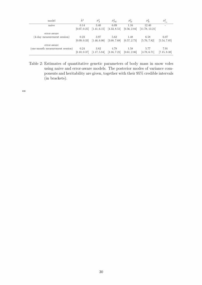
Heritability438

As expected from theory (Table 1), transient effects in the measurements of body439

mass biased some, but not all, quantitative genetic estimates in our snow vole exam-440

ple (Table 2). The estimates and confidence intervals of the additive genetic variance441

σ2A, as well as the permanent environmental variance σ2

PE and the maternal variance442

(denoted as σ2M) were only slightly corrected in the error-aware models. Residual443

variances, however, were much lower when measurement error was accounted for in444

the models. The measurement error model separated residual and transient (error)445

variance so that σ2R + σ2

em corresponded approximately to σ2R from the naive model.446

The overestimation of the residual variance resulted in estimates of heritability that447

were underestimated by nearly 40% when measurement error was ignored (h2 = 0.14448

in the naive model and h2 = 0.23 in the error-aware model).449

As expected, the estimated measurement error variance is larger when a mea-450

surement session is defined as a full month (σ2em = 7.91) than as a 4-day interval451

(σ2em = 6.07, Table 2), because the trait then has more time and opportunity to452

change. As a consequence, heritability is even slightly higher (h2 = 0.24) when the453

longer measurement session definition is used. This example is instructive because it454

underlines the importance of defining the time scale at which short-term repeats are455

expected to capture only transient, and not biologically relevant variability of the456

phenotypic trait. In the case of the mass of a snow vole, most biologists would prob-457

ably agree that changes in body mass over a one-month measurement session may458

well be biologically meaningful (i.e. body fat accumulation, pregnancy in females,459

etc.), while it is less clear how much of the fluctuations within a 4-day measurement460

session are transient, and what part of it would be relevant for selection. Within-461

day repeats might be the most appropriate for the case of mass, since within-day462

variance is likely mostly transient, but because the data were not collected with the463

intention to quantify such effects, within-day repeats were not available in sufficient464

15

numbers in our example data set.465

Selection466

As expected, estimates of selection gradients (βz) obtained with the measurement467

error models provided nearly 40% higher estimates of selection than the naive model468

(Table 3). The two measurement session lengths yielded similar results. With469

and without measurement error modelling, the p-values of the zero-inflated Poisson470

models confirmed the presence of selection on body mass in snow voles (p < 0.001471

in all models).472

Response to selection473

In line with theory, estimates of the response to selection using the breeder’s equation474

were nearly 40% higher when transient effects were incorporated in the quantitative475

genetic models using 4-day measurement sessions (RBE = 0.10 in the naive model476

and RBE = 0.16 in the error-aware model; Table 4). As in the case of heritability, the477

one-month measurement session definition resulted in even slightly higher estimates478

of the response to selection (RBE = 0.17). In contrast, response to selection mea-479

sured by the secondary theorem of selection RSTS did not show evidence of bias, and480

the error-aware model with a 4-day measurement session definition estimated the481

same value (RSTS = −0.17) as the naive model (Table 4). With a one-month mea-482

surement session, we obtained a slightly attenuated value (RSTS = −0.14), although483

the difference was small in comparison to the credible intervals (Table 4).484

This example illustrates that the breeder’s equation is generally prone to under-485

estimation of the selection response in real study systems when measurement error486

in the phenotype is present (Table 1). The results also confirm that estimates for487

response to selection may differ dramatically between the breeder’s equation and the488

secondary theorem of selection approach. As already noticed by Bonnet et al. (2017),489

the predicted evolutionary response derived from the breeder’s equation points in490

the opposite direction in the snow vole data than the estimate derived from the491

secondary theorem of selection (e.g. naive estimates RBE = 0.10 vs. RSTS = −0.17,492

with non-overlapping credible intervals; Table 4).493

Discussion494

This study addresses the problem of measurement error and transient fluctuations495

in continuous phenotypic traits in quantitative genetic analyses. We show that mea-496

surement error and transient fluctuations can lead to substantial bias in estimates of497

several important quantitative genetic parameters, including heritability, selection498

16

gradients and the response to selection (Table 1). We introduce modelling strategies499

to obtain unbiased estimates in these parameters in the presence of measurement500

error and transient fluctuations. These strategies rely on the distinction between501

variability from stable effects that are part of the biologically relevant phenotypic502

variability, and transient effects, which are the sum of mechanistic measurement er-503

ror and biological fluctuations that are considered irrelevant for the selection process.504

We argue that ignoring the distinction between stable and transient effects may not505

only lead to an underestimation of the heritability due to inflated estimates of the506

residual variance, σ2R, but also to bias in the estimates of selection gradients and the507

response to selection. Measurements of the same individual repeated at appropriate508

time scales allow the variance from such transient effects to be partitioned, and thus509

prevent such bias.510

How can repeated measurements be used to prevent an underestimation of her-511

itability, selection, and response to selection, while permanent environment effects512

are required in quantitative genetic models of repeated measures to avoid an upward513

bias of σ2A and, hence, an overestimation of h2 (Wilson et al., 2010)? The fact that514

repeated measurements are used to prevent opposite biases in heritability estimates515

makes it apparent that the information content in what is termed“repeated measure-516

ments” in both cases is very different. The crucial aspect is that it matters at which517

temporal distance the repeats were taken, and that the relevance of this distance518

depends on the kind of trait under study. Repeats taken on the same individual519

at different life stages (“long-term” repeats, e.g. across what we call measurement520

sessions here) can be used to separate the animal-specific permanent environmental521

effect from both genetic and residual variances. On the other hand, repeats taken522

in temporal vicinity (“short-term” repeats, e.g. within a measurement session) help523

disentangle any transient from the residual effects. Only by modelling both types of524

repeats, that is, across different relevant time scales, is it practically feasible to sep-525

arate all variance components. To do so, the quantitative genetic model for the trait526

value, typically the animal model, needs extension to three levels of measurement527

hierarchy (equation (7)): the individual (i), the measurement session (j within i)528

and the repeat (k within j within i). As highlighted with the snow vole example, it529

may not always be trivial to determine, in a particular system, an appropriate dis-530

tinction between short-term and long-term repeats, and consequently how to define531

a measurement session. This decision must be driven by the definition of short-term532

variation as a variation that is not “seen” by the selection process (see e.g. Price533

and Boag, 1987, p. 279 for a similar analogy), in contrast to persistent effects that534

are potentially under selection. This distinction ultimately depends on the trait, on535

the system under study and on the research question that is asked, because some536

traits may fluctuate on extremely short time scales (minutes or days), while others537

17

remain constant across an entire adult’s life.538

The application to the snow vole data, where we varied the measurement session539

length from four days to one month, illustrated that longer measurement sessions540

automatically capture more variability, that is, the estimated error variance σ2em541

increased. Consequently, unreasonably long measurement sessions may lead to over-542

corrected estimates of the parameters of interest. On the other hand, considering543

measurement sessions that are too short may lead to an insufficient number of within-544

session repeats, or they may fail to identify transient variability that is biologically545

irrelevant. This makes clear that a careful definition of measurement session length546

is important already at the design stage of a study.547

If one is uncertain whether repeated measurements capture effects relevant to se-548

lection or not, would averaging over repeats result in better estimates of quantitative549

genetic measures? Averaging methods have been proposed specifically to reduce bias550

that emerges due to measurement error and transient effects (Carbonaro et al., 2009;551

Zheng et al., 2016). While averaging will alleviate bias by reducing the error variance552

in the mean, it will not eliminate it completely. This can be seen from the fact that553

averaging over K within-session repeats for all animals and measurement sessions,554

the variance σ2em is reduced to σ2

em = σ2em/K, assuming independence of the error555

term. Unless K is large, σ2em will not approach zero. Moreover, this practice only556

works if all animals have the same number of repeats within all measurement ses-557

sions, but it will not work in the unbalanced sampling design so common in studies558

of natural populations.559

Our method approaches the problem of measurement error and transient fluc-560

tuations by assuming a dichotomous distinction between short-term and long-term561

repeats. An alternative perspective of within-animal repeated measurements could562

take a continuous view, recalling that repeated measurements are usually correlated,563

even when taken across long time spans, and that the correlation increases the closer564

in time the measurements were taken. A more sophisticated model could thus take565

into account that the residual component in the model changes continuously, and566

introduce a time-dependent correlation structure instead of simply distinguishing567

between short-term and long-term repeats. Such a model might be beneficial if568

repeats were not taken in clearly defined measurement sessions, although such a569

temporal correlation term introduces another level of model complexity, and thus570

entails other challenges.571

It may sometimes not be possible to take multiple measurements on the same572

individual, or to repeat a measurement within a session. However, it may still be573

feasible to include an appropriate random effect in the absence of short-term repeats,574

provided that knowledge about the error variance is available, e.g. from previous575

studies that used the same measurement devices, from a subset of the data, or from576

18

other “expert” knowledge. The Bayesian framework is ideal in this regard, because577

it is straightforward to include random effects with a very strong (or even fixed)578

prior on the respective variance component. Such Bayesian models provide error-579

aware estimates that are equivalent to those illustrated in Table 1, but with the580

additional advantage that posterior distributions naturally reflect all uncertainty581

that is present in the parameters, including the uncertainty that is incorporated in582

the prior distribution of the error variance.583

Measurement error and transient fluctuations bias some, but not all quantitative584

genetic inferences. When σ2em > 0, the naive estimates of h2, βz and RBE are585

attenuated by the same factor λ < 1, but other components, such as the selection586

differential S or RSTS, are not affected (Table 1). The robustness of the secondary587

theorem of selection to measurement error can certainly be seen as an advantage588

over the breeder’s equation. Nevertheless, the Robertson-Price identity does not589

model selection explicitly, and thus says little about the selective processes. The590

Robertson-Price equation can be used to check the consistency of predictions made591

from the breeder’s equation, but the breeder’s equation remains necessary to test592

hypothesis about the causal nature of selection (Morrissey et al., 2012; Bonnet et al.,593

2017). Another quantity that is unaffected by independent transient effects, which594

we however did not further elaborate on here, is evolvability, defined as the squared595

coefficient of variation I = σ2A/z

2, where z denotes the mean phenotypic value596

(Houle, 1992). Evolvability is often used as an alternative to heritability, and is597

interpreted as the opportunity for selection (Crow, 1958). Not only σ2A, but also z can598

be consistently estimated using z?, namely because the expected values E[z?] = E[z]599

due to the independence and zero mean of the error term. For completeness, we600

added evolvability to Table 1.601

A critical assumption of our models was that the error components are indepen-602

dent of the phenotypic trait under study, but also independent of fitness or any603

covariates in the animal model or the selection model. While the small changes in604

RSTS that we observed in the snow vole application with one-month measurement605

sessions could be due to pure estimation stochasticity, an alternative interpretation606

is that the measurement error in the data are not independent of the animal’s fitness.607

At least two processes could lead to a correlation between the measurement error in608

mass and fitness in snow voles. First, pregnant females will experience temporally609

increased body mass, and we expect the positive deviation from the true body mass610

to be correlated with fitness, because a pregnant animal is likely to have a higher611

expected number of offspring over its entire lifespan. And second, some of the snow612

voles were not fully grown when measured, and juveniles are more likely to survive if613

they keep growing, so that deviations from mean mass over the measurement session614

period would be non-randomly associated with life-time fitness.615

19

So far, we have focused on traits that can change relatively quickly throughout616

the life of an individual, such as body mass, or physiological and behavioral traits.617

Traits that remain constant after a certain age facilitate the isolation of measure-618

ment error, because the residual variance term is then indistinguishable from the619

error term, given that a permanent environmental (i.e. individual-specific) effect is620

included in the model. In such a situation it is sufficient to estimate σ2R, which then621

automatically corresponds to the measurement error variance, while σ2PE captures622

all the environmental variability. However, not many traits will fit that description.623

The majority of traits, even seemingly stable traits such as skeletal traits, are in fact624

variable over time (Price and Grant, 1984; Smith et al., 1986).625

We have shown that dealing appropriately with measurement error and transient626

fluctuations of phenotypic traits in quantitative genetic analyses requires the inclu-627

sion of additional variance components. Quantitative genetic analyses often differ in628

the variance components that are included to account for important dependencies629

in the data (Meffert et al., 2002; Palucci et al., 2007; Kruuk and Hadfield, 2007;630

Hadfield et al., 2013). Besides the importance of separating the right variance com-631

ponents, it has been widely discussed which of the components are to be included in632

the denominator of heritability estimates, although the focus has been mainly on the633

proper handling of variances that are captured by the fixed effects (Wilson, 2008;634

de Villemereuil et al., 2018). We hope that our treatment of measurement error in635

quantitative genetic analyses sparks new discussions of what should be included in636

the denominator when heritability is calculated.637

The methods presented in this paper have been developed and implemented for638

continuous phenotypic traits. Binary, categorical or count traits may also suffer639

from measurement error, which is then denoted as misclassification error (Copas,640

1988; Magder and Hughes, 1997; Kuchenhoff et al., 2006), or as miscounting error641

(e.g. Muff et al., 2018). Models for non-Gaussian traits are usually formulated in a642

generalized linear model framework (Nakagawa and Schielzeth, 2010; de Villemereuil643

et al., 2016) and require the use of a link function (e.g. the logistic or log link). In644

these cases, it will often not be possible to obtain unbiased estimates of quantitative645

genetic parameters by adding an error term to the linear predictor as we have done646

here for continuous traits. Obtaining unbiased estimates of quantitative genetic647

parameters in the presence of misclassification and miscounting error will require648

extended modelling strategies, such as hierarchical models with an explicit level for649

the error process.650

We hope that the concepts and methods provided here serve as a useful starting651

point when estimating quantitative genetics parameters in the presence of measure-652

ment error or transient, irrelevant fluctuations in phenotypic traits. The proposed653

approaches are relatively straightforward to implement, but further generalizations654

20

are possible and will hopefully follow in the future.655

21

Supporting information:656

Appendix 1: Supplementary text and figures (pdf)657

Appendix 2: Supplementary text and figures for simulation study (pdf)658

Appendix 3: R script for the simulation and analysis of pedigree data659

Appendix 4: R script for heritability in snow voles660

Appendix 5: R script for selection in snow voles661

Appendix 6: R script for response to selection in snow voles.662

References663

Bonnet, T., P. Wandeler, G. Camenisch, and E. Postma (2017). Bigger is fitter?664

Quantitative genetic decomposition of selection reveals an adaptive evolution de-665

cline of body mass in a wild rodent population. PLOS Biology 15, e1002592.666

Carbonaro, F., T. Andrew, D. A. Mackey, T. L. Young, T. D. Spector, and C. J.667

Hammond (2009). Repeated measures of intraocular pressure result in higher her-668

itability and greater power in genetic linkage studies. Investigative Ophthalmology669

and Visual Science 50, 5115–5119.670

Carroll, R. J., D. Ruppert, L. A. Stefanski, and C. M. Crainiceanu (2006). Measure-671

ment error in nonlinear models, a modern perspective. Boca Raton: Chapman672

and Hall.673

Charmantier, A., D. Garant, and L. E. B. Kruuk (2014). Quantitative Genetics in674

the Wild. Oxford: Oxford University Press.675

Charmantier, A. and D. Reale (2005). How do misassigned paternities affect the676

estimation of heritability in the wild? Molecular Ecology 14, 2839–2850.677

Copas, J. B. (1988). Binary regression models for contaminated data (with dis-678

cussion). Journal of the Royal Statistical Society. Series B (Statistical Methodol-679

ogy) 50, 225–265.680

Crow, J. F. (1958). Some possibilities for measuring selection intensities in man.681

Human Biology 30, 1–13.682

de Boer, I. J. M. and I. Hoeschele (1993). Genetic evaluation methods for populations683

with dominance and inbreeding. Theoretical Applied Genetics 86, 245–258.684

22

de Villemereuil, P., M. B. Morrissey, S. Nakagawa, and H. Schielzeth (2018). Fixed685

effect variance and the estimation of the heritability: Issues and solutions. Journal686

of Evolutionary Biology 31, 621–632.687

de Villemereuil, P., H. Schielzeth, S. Nakagawa, and M. B. Morrissey (2016). General688

methods for evolutionary quantitative genetic inference from generalized mixed689

models. Genetics 204, 1281–1294.690

Dohm, M. R. (2002). Repeatability estimates do not always set an upper limit to691

heritability. Functional Ecology 16, 273–280.692

Falconer, D. S. and T. F. C. Mackay (1996). Introduction to Quantitative Genetics.693

Burnt Mill, Harlow, Essex, England: Pearson.694

Fisher, R. A. (1930). The Genetical Theory of Natural Selection. Oxford, UK:695

Oxford University Press.696

Fuller, W. A. (1987). Measurement Error Models. New York: John Wiley & Sons.697

Ge, T., A. J. Holmes, R. L. Buckner, J. W. Smoller, and M. Sabuncu (2017). Her-698

itability analysis with repeat measurements and its application to resting-state699

functional connectivity. PNAS 114, 5521–5526.700

Griffith, S. C., I. P. F. Owens, and K. A. Thuman (2002). Extrapair paternity701

in birds: a review of interspecific variation and adaptive function. Molecular702

Ecology 11, 2195–2212.703

Hadfield, J. D. (2008). Estimating evolutionary parameters when viability selection704

is operating. Proceedings of the Royal Society of London B: Biological Sciences,705

The Royal Society 275, 723–734.706

Hadfield, J. D., E. A. Heap, F. Bayer, E. A. Mittell, and N. M. Crouch (2013).707

Disentangling genetic and prenatal sources of familial resemblance across ontogeny708

in a wild passerine. Evolution 67, 2701–2713.709

Henderson, C. R. (1976). A simple method for computing the inverse of a numerator710

relationship matrix used in prediction of breeding values. Biometrics 32, 69–83.711

Hill, W. G. (2014). Applications of population genetics to animal breeding, from712

Wright, Fisher and Lush to genomic prediction. Genetics 196, 1–16.713

Hoffmann, A. A. (2000). Laboratory and field heritabilities: Lessons from714

Drosophila. In T. Mousseau, S. B., and J. Endler (Eds.), Adaptive Genetic Vari-715

ation in the Wild. New York, Oxford: Oxford Univ Press.716

23

Houle, D. (1992). Comparing evolvability and variability of quantitative traits.717

Genetics 130, 195–204.718

Keller, L. F., P. R. Grant, B. R. Grant, and K. Petren (2001). Heritability of719

morphological traits in Darwin’s Finches: misidentified paternity and maternal720

effects. Heredity 87, 325–336.721

Keller, L. F. and A. J. Van Noordwijk (1993). A method to isolate environmental722

effects on nestling growth, illustrated with examples from the Great Tit (Parsus723

major). Functional Ecology 7, 493–502.724

Kruuk, L. E. B. (2004). Estimating genetic parameters in natural populations using725

the ’animal model’. Philosophical Transactions of the Royal Society B: Biological726

Sciences 359, 873–890.727

Kruuk, L. E. B. and J. D. Hadfield (2007). How to separate genetic and environ-728

mental causes of similarity between relatives. Journal of Evolutionary Biology 20,729

1890–1903.730

Kuchenhoff, H., S. M. Mwalili, and E. Lesaffre (2006). A general method for dealing731

with misclassification in regression: The misclassification SIMEX. Biometrics 62,732

85–96.733

Lande, R. and S. J. Arnold (1983). The measurement of selection on correlated734

characters. Evolution 37, 1210–1226.735

Lush, J. L. (1937). Animal breeding plans. Ames, Iowa: Iowa State College Press.736

Lynch, M. and B. Walsh (1998). Genetics and Analysis of Quantitative Traits.737

Sunderland, MA: Sinauer Associates.738

Macgregor, S., B. K. Cornes, N. G. Martin, and P. M. Visscher (2006). Bias, precision739

and heritability of self-reported and clinically measured height in Australian twins.740

Human Genetics 120, 571–580.741

Magder, L. S. and J. P. Hughes (1997). Logistic regression when the outcome is742

measured with uncertainty. American Journal of Epidemiology 146, 195–203.743

Meffert, L. M., S. K. Hicks, and J. L. Regan (2002). Nonadditive genetic effects in744

animal behavior. The American Naturalist 160 Suppl 6, S198–S213.745

Meuwissen, T. H. E., B. J. Hayes, and M. E. Goddard (2001). Prediction of total746

genetic value using genome-wide dense marker maps. Genetics 157, 1819–1829.747

24

Mitchell-Olds, T. and R. G. Shaw (1987). Regression analysis of natural selection:748

statistical inference and biological interpretation. Evolution 41, 1149–1161.749

Møller, A. and M. D. Jennions (2002). How much variance can be explained by750

ecologists and evolutionary biologists? Oecologia 132 (4), 492–500.751

Morrissey, M. B. and I. B. J. Goudie (2016). Analytical results for directional and752

quadratic selection gradients for log-linear models of fitness functions. bioRxiv .753

https://www.biorxiv.org/content/early/2016/02/22/040618.754

Morrissey, M. B., L. E. B. Kruuk, and A. J. Wilson (2010). The danger of applying755

the breeder’s equation in observational studies of natural populations. Journal of756

Evolutionary Biology 23, 2277–2288.757

Morrissey, M. B., D. J. Parker, P. Korsten, J. M. Pemberton, L. E. B. Kruuk, and758

A. J. Wilson (2012). The prediction of adaptive evolution: empirical application759

of the secondary theorem of selection and comparison to the breeder’s equation.760

Evolution 66, 2399–2410.761

Morrissey, M. B. and K. Sakrejda (2013). Unification of regression-based methods762

for the analysis of natural selection. Evolution 67 (7), 2094–2100.763

Muff, S., M. A. Puhan, and L. Held (2018). Bias away from the Null due to mis-764

counted outcomes? A case study on the TORCH trial. Statistical Methods in765

Medical Research. In press.766

Muff, S., A. Riebler, L. Held, H. Rue, and P. Saner (2015). Bayesian analysis767

of measurement error models using integrated nested Laplace approximations.768

Journal of the Royal Statistical Society, Applied Statistics Series C 64, 231–252.769

Nakagawa, S. and H. Schielzeth (2010). Repeatability for Gaussian and non-770

Gaussian data: a practical guide for biologists. Biological Reviews of the Cam-771

bridge Philosophical Society 85, 935–956.772

Palucci, V., L. R. Schaeffer, F. Miglior, and V. Osborne (2007). Non-additive ge-773

netic effects for fertility traits in Canadian Holstein cattle. Genetics Selection774

Evolution 39, 181–193.775

Peek, M. S., A. J. Leffler, S. D. Flint, and R. J. Ryel (2003). How much variance is776

explained by ecologists? Additional perspectives. Oecologia 137 (2), 161–170.777

Price, G. R. (1970). Selection and covariance. Nature 227, 520–521.778

Price, T. D. and P. T. Boag (1987). Selection in natural populations of birds. In779

F. Cooke, , and P. Buckley (Eds.), Avian Genetics, pp. 257 – 287. Academic Press.780

25

Price, T. D. and P. R. Grant (1984). Life history traits and natural selection for781

small body size in a population of Darwin’s Finches. Evolution 38, 483–494.782

Richardson, S. and W. R. Gilks (1993). Conditional independence models for epi-783

demiological studies with covariate measurement error. Statistics in Medicine 12,784

1703–1722.785

Robertson, A. (1966). A mathematical model of the culling process in dairy cattle.786

Animal Science 8, 95–108.787

Roff, D. A. (2007). A centennial celebration for quantitative genetics. Evolution 61,788

1017–1032.789

Rue, H., S. Martino, and N. Chopin (2009). Approximate Bayesian inference for790

latent Gaussian models by using integrated nested Laplace approximations (with791

discussion). Journal of the Royal Statistical Society Series B (Statistical Method-792

ology) 71, 319–392.793

Senneke, S. L., M. D. MacNeil, and L. D. Van Vleck (2004). Effects of sire misiden-794

tification on estimates of genetic parameters for birth and weaning weights in795

Hereford cattle. Journal of Animal Science 82, 2307–2312.796

Smith, J. N. M., P. Arcese, and D. Schulter (1986). Song sparrows grow and shrink797

with age. AUK 103, 210–212.798

Steinsland, I., C. T. Larsen, A. Roulin, and H. Jensen (2014). Quantitative genetic799

modeling and inference in the presence of nonignorable missing data. Evolution 68,800

1735–1747.801

Stephens, D. A. and P. Dellaportas (1992). Bayesian analysis of generalised linear802

models with covariate measurement error. In J. M. Bernardo, J. O. Berger, A. P.803

Dawid, and A. F. M. Smith (Eds.), Bayesian Statistics 4. Oxford Univ Press.804

van der Sluis, S., M. Verhage, D. Posthuma, and C. V. Dolan (2010). Phenotypic805

complexity, measurement bias, and poor phenotypic resolution contribute to the806

missing heritability problem in genetic association studies. PLOS One 5, e13929.807

Wilson, A. J. (2008). Why h2 does not always equal VA/VP? Journal of Evolutionary808

Biology 21, 647–650.809

Wilson, A. J., D. Reale, M. N. Clements, M. B. Morrissey, E. Postma, C. A. Walling,810

L. E. B. Kruuk, and D. H. Nussey (2010). An ecologist’s guide to the animal model.811

Journal of Animal Ecology 79, 13–26.812

26

Wolak, M. E. and J. M. Reid (2017). Accounting for genetic differences among813

unknown parents in microevolutionary studies: how to include genetic groups in814

quantitative genetic animal models. Journal of Animal Ecology 86, 7–20.815

Zheng, Y., R. Plomin, and S. von Stumm (2016). Heritability of intraindividual816

mean and variability of positive and negative affect: genetic analysis of daily817

affect ratings over a month. Psychological Science 27, 1611–1619.818

27

Figures819

Figure 1: Schematic representation of three study designs, where one individual is820

measured a) multiple times across multiple measurement sessions, b) multiple times821

in one single measurement measurement session, or c) one single time across multi-822

ple measurement sessions. Only case a) allows to disentangle the measurement error823

variance σ2em and the permanent environmental effects σ2

PE from σ2R, while case b)824

allows to separate only the measurement error variance and case c) only allows to825

disentangle permanent environmental effects.826

827

28

Tables828

829

Parameter Effect of ME Biased parameterσ2A unbiased -

σ2PE unbiased -σ2R biased σ2

R + σ2e

h2 biased λh2

βz biased λβzσp(z,w) = S unbiased -

σa(z,w) = RSTS unbiased -RBE biased λRBE

I unbiased -

Table 1: Overview of the effects of measurement error and transient fluctuations(ME) in a quantitative trait on important quantitative genetic parameters.The table indicates for each parameter whether it is biased or unbiased. Forbiased parameters the quantities are given that are estimated when ignoringtransient effects in the quantitative genetic models. λ is the reliability ratio,

defined as λ =σ2P

σ2P+σ2

em. For notation see the main text.

29

model h2 σ2A σ2

PE σ2M σ2

R σ2em

naive 0.14 3.40 6.09 1.16 12.40 -[0.07, 0.25] [1.41, 6.15] [4.33, 8.51] [0.56, 2.84] [11.78, 13.21]

error-aware(4-day measurement session) 0.23 3.97 5.62 1.48 6.58 6.07

[0.09, 0.33] [1.46, 6.06] [3.68, 7.68] [0.57, 2.73] [5.76, 7.82] [5.54, 7.05]

error-aware(one-month measurement session) 0.24 3.82 4.78 1.58 5.77 7.91

[0.10, 0.37] [1.17, 5.84] [3.16, 7.21] [0.61, 2.86] [4.78, 6.71] [7.15, 8.38]

Table 2: Estimates of quantitative genetic parameters of body mass in snow volesusing naive and error-aware models. The posterior modes of variance com-ponents and heritability are given, together with their 95% credible intervals(in brackets).

830

30

model βz p-value

naive 0.065 < 0.001

error-aware(4-day measurement session) 0.104 < 0.001

error-aware(one-month measurement session) 0.104 < 0.001

Table 3: Estimates of selection gradients (βz) for body mass in snow voles, derivedfrom naive (ML estimate) and error-aware models (posterior means). Forboth types of models, Bayesian p-values were derived from zero-inflatedPoisson regressions.

31

model RSTS 95% CI RBE 95% CI

naive −0.17 [−0.54, 0.18] 0.10 [0.05, 0.17]

error-aware(4-day measurement session) −0.17 [−0.51, 0.19] 0.16 [0.06, 0.23]

error-aware(one-month measurement session) −0.14 [−0.53, 0.17] 0.17 [0.07, 0.26]

Table 4: Response to selection for body mass in snow voles (posterior modes and95% credible intervals) estimated with the breeder’s equation (RBE) andwith the secondary theorem of selection (RSTS). Results are shown for thenaive and the error-aware models.

32