Generated using version 3.2 of the official AMS LATEX template

Ocean circulation under globally glaciated Snowball Earth1

conditions: steady state solutions2

Yosef Ashkenazy ∗

Ben-Gurion University, Midreshet Ben-Gurion, Israel

3

Hezi Gildor

The Fredy and Nadine Herrmann Institute of Earth Sciences, The Hebrew University of Jerusalem, Jerusalem, Israel

4

Martin Losch

Alfred-Wegener-Institut, Helmholtz-Zentrum fur Polar- und Meeresforschung, Bremerhaven, Germany

5

Eli Tziperman

Dept. of Earth and Planetary Sciences and School of Engineering and Applied Sciences, Harvard University, Cambridge, MA, USA

6

∗Corresponding authors’ address: Yosef Ashkenazy, Department of Solar Energy and Environmental

Physics, BIDR, Ben-Gurion University, Midreshet Ben-Gurion, 84990, Israel.

E-mail:ashkena@bgu.ac.il;

Eli Tziperman, Dept. of Earth and Planetary Sciences and School of Engineering and Applied Sciences,

Harvard University; 20 Oxford St, Cambridge, MA, 02138, USA.

E-mail:eli@eps.harvard.edu

1

ABSTRACT7

Between ∼750 to 635 million years ago, during the Neoproterozoic era, the Earth experienced8

at least two significant, possibly global, glaciations, termed “Snowball Earth”. While many9

studies have focused on the dynamics and the role of the atmosphere and ice flow over the10

ocean in these events, only a few have investigated the related associated ocean circulation,11

and no study has examined the ocean circulation under a thick (∼1 km deep) sea-ice cover,12

driven by geothermal heat flux. Here, we use a thick sea-ice flow model coupled to an ocean13

general circulation model to study the ocean circulation under Snowball Earth conditions.14

We first investigate the ocean circulation under simplified zonal symmetry assumption and15

find (i) strong equatorial zonal jets, and (ii) a strong meridional overturning cell, limited16

to an area very close to the equator. We derive an analytic approximation for the latitude-17

depth ocean dynamics and find that the extent of the meridional overturning circulation cell18

only depends on the horizontal eddy viscosity and β (the change of the Coriolis parameter19

with latitude). The analytic approximation closely reproduces the numerical results. Three-20

dimensional ocean simulations, with reconstructed Neoproterozoic continents configuration,21

confirm the zonally symmetric dynamics, and show additional boundary currents and strong22

upwelling and downwelling near the continents.23

1

1. Introduction24

The Neoproterozoic Snowball events are perhaps the most drastic climate events in25

Earth’s history. Between 750 and 580 million years ago (Ma), the Earth experienced at26

least two major, possibly global, glaciations (e.g., Harland 1964; Kirschvink 1992; Hoffman27

and Schrag 2002; Macdonald et al. 2010; Evans and Raub 2011). During these events (the28

Sturian and Marinoan ice ages), ice extended to low latitudes over both ocean and land. It29

is still debated whether the ocean was entirely covered by thick ice (“hard” Snowball) (e.g.,30

Allen and Etienne 2008; Pierrehumbert et al. 2011), perhaps expect very limited regions of31

sea-ice free ocean, e.g., around volcanic islands (Schrag et al. 2001) (that could have pro-32

vided a refuge for photosynthetic life during these periods), or whether the tropical ocean33

was partially ice free or perhaps covered by thin ice (“soft” Snowball) (e.g., Yang et al.34

2012c).35

The initiation, maintenance, and termination of such a climatic condition pose a first-36

order problem in ocean and climate dynamics. One may argue that the Snowball state was37

predicted by simple energy balance models (EBMs) (Budyko 1969; Sellers 1969). Snowball38

dynamics also provide a test-case for our understanding of the climate system as manifested39

in climate models. Therefore, in recent years, these questions have been the focus of nu-40

merous studies and attempts to simulate these climate states using models with different41

levels of complexity. The role and dynamics of atmospheric circulation and heat trans-42

port, CO2 concentration, cloud feedbacks, and continental configuration have been studied43

(Pierrehumbert 2005; Le-Hir et al. 2010; Donnadieu et al. 2004a; Pierrehumbert 2002, 2004;44

Le-Hir et al. 2007). Recently, the effect of clouds, as well as the role of atmospheric and45

oceanic heat transports in the initiation of Snowball Earth events was studied; these studies46

were based on atmospheric GCMs and used different setups and configurations including47

different CO2 concentrations, different continental configurations, and different sea-ice dy-48

namics (Yang et al. 2012c,b,a; Voigt and Abbot 2012; Abbot et al. 2012). It was concluded,49

e.g., that sea-ice dynamics has important role in the initiation of Snowball events (Voigt50

2

and Abbot 2012). Additionally, perceived difficulties in exiting a Snowball state by a CO251

increase alone motivated the study of the role of dust over the Snowball ice cover (Abbot52

and Pierrehumbert 2010; Le-Hir et al. 2010; Li and Pierrehumbert 2011; Abbot and Halevy53

2010).54

A simple scaling calculation of balancing geothermal heat input into the ocean with heat55

escaping through the ice by diffusion leads to an estimated ice thickness of 1 km. The ice56

cover is expected to slowly deform and flow toward the equator to balance for sublimation57

(and melting at the bottom of the ice) at low latitudes and snow accumulation (and ice58

freezing at the bottom of the ice) at high latitude. The flow and other properties of such59

thick ice over a Snowball ocean (“sea glaciers”, Warren et al. 2002) were examined in quite60

a few recent studies (Goodman and Pierrehumbert 2003; McKay 2000; Warren et al. 2002;61

Pollard and Kasting 2005; Campbell et al. 2011; Tziperman et al. 2012; Pollard and Kasting62

2006; Warren and Brandt 2006; Goodman 2006; Lewis et al. 2007). Snowball Earth global63

ice cover is an extreme example within a range of multiple ice cover equilibrium states,64

which have been studied in a range of simple and complex models (e.g., Langen and Alexeev65

2004; Rose and Marshall 2009; Ferreira et al. 2011). In contrast to these many studies of66

different climate components during Snowball events, the ocean circulation during Snowball67

events has received little attention. Most model studies of a Snowball climate used an ocean68

mixed layer model only (Baum and Crowley 2001; Crowley and Baum 1993; Baum and69

Crowley 2003; Hyde et al. 2000; Jenkins and Smith 1999; Chandler and Sohl 2000; Poulsen70

et al. 2001b; Romanova et al. 2006; Donnadieu et al. 2004b; Micheels and Montenari 2008).71

The studies that used full ocean General Circulation Models (GCMs) concentrated on the72

ocean’s role in Snowball initiation and aftermath (Poulsen et al. 2001a; Poulsen and Jacob73

2004; Poulsen et al. 2002; Sohl and Chandler 2007), or other aspects of Snowball dynamics74

in the presence of oceanic feedback (Voigt et al. 2011; Le-Hir et al. 2007; Yang et al. 2012c;75

Ferreira et al. 2011; Marotzke and Botzet 2007; Lewis et al. 2007; Voigt and Marotzke 2010;76

Abbot et al. 2011; Lewis et al. 2004, 2003). Yet none of these studies employing ocean77

3

GCMs accounted for the combined effects of thick ice cover flow and driving by geothermal78

heating. Ferreira et al. (2011) simulated an ocean under a moderately thick (200 m) ice cover79

with no geothermal heat flux, and calculated a non steady-state solution with near-uniform80

temperature and salinity. They described a vanishing Eulerian circulation together with81

strongly parameterized eddy-induced high latitude circulation cells.82

With both the initiation (Kirschvink 1992; Schrag et al. 2002; Tziperman et al. 2011)83

and termination (Pierrehumbert 2004) of Snowball events still not well understood, and the84

question of hard vs. soft Snowball still unresolved (Pierrehumbert et al. 2011), our focus here85

is the steady state ocean circulation under a thick ice cover (hard Snowball). By examining86

ocean dynamics under such an extreme climatic state, we aim to better understand the87

relevant climate dynamics, and perhaps even provide constraints on the issues regarding soft88

vs. hard Snowball states.89

To study the 3D ocean dynamics under a thick ice cover, it is necessary to have a two-90

dimensional (longitude and latitude) ice-flow model, and this was recently developed by91

Tziperman et al. (2012), based on the ice-shelf equations of Morland (1987) and MacAyeal92

(1997), extending the 1D model of Goodman and Pierrehumbert (2003). This model is93

coupled here to the MITgcm (Marshall et al. 1997). Another challenge in studying the 3D94

ocean dynamics under a thick ice cover is that thick ice with lateral variations of hundreds of95

meters (as under Snowball conditions) poses a numerical challenge as standard ocean models96

cannot handle ice that extends through several vertical layers; we use the ice-shelf model of97

Losch (2008), which allows for this. An alternative, vertically scaled coordinates, was used98

by Ferreira et al. (2011).99

This paper expands on results briefly reported in Ashkenazy et al. (2013) (hereafter100

AGLMST), and we report the details of the steady state ocean dynamics under a thick ice101

(Snowball) cover, analytically and numerically, when both geothermal heating and a thick ice102

flow are taken into account. We find the ocean circulation to be quite far from the stagnant103

pool envisioned in some early studies, and very different from that in any other period in104

4

Earth’s history. In particular, the stratification is very weak as might be expected (Ferreira105

et al. 2011), and is dominated by salinity gradients due to melting and freezing of ice; we106

find a meridional overturning circulation that is confined to the equatorial region, significant107

zonal equatorial jets, and strong equatorial meridional overturning circulation (MOC).108

The paper is organized as follows. We first describe the models and configurations used109

in this study (section 2). We then present the results of the latitude-depth ocean model110

coupled to a 1D (latitude) ice-flow model when geothermal heating is taken into account111

(section 3). Analytically approximated solutions of the 2D, latitude-depth ocean model are112

then presented (section 4). Section 5 presents sensitivity runs to study the robustness of113

both the numerical results and the analytical approximations, followed by the steady state114

results of a 3D ocean model coupled to a longitude-latitude 2D ice-flow model in section 6.115

The results are discussed and summarized in section 7.116

2. Model description117

a. Ice-flow model118

The ice-flow model solves for the ice depth and velocity over an ocean as a function of119

longitude and latitude, in the presence of continents (Tziperman et al. 2012). The model120

extends the 1D model of Goodman and Pierrehumbert (2003), which was based on the Weert-121

man (1957) formula for ice shelf deformation. Because this specific formulation cannot be122

extended to ice flow in two horizontal dimensions, we instead used the ice-shelf approxima-123

tion (Morland 1987; MacAyeal 1997) that can be extended to two dimensions. The ice-shelf124

approximation implies a depth-independent ice velocity, and in addition, the vertical tem-125

perature profile within the ice is assumed to be linear (Goodman and Pierrehumbert 2003).126

The temperature at the upper ice surface and surface ice sublimation and snow accumulation127

are prescribed from the energy balance of Pollard and Kasting (2005) and are assumed to be128

constant in time. The temperature and melting/freezing rates at the bottom of the ice are129

5

calculated by the ocean model. The model’s spatial resolution is set to that of the ocean,130

and the model is run in either 1D (latitude only) or 2D configurations, depending on the131

ocean model used; it is typically 1-2◦.132

b. The ocean model—MITgcm133

We used the Massachusetts Institute of Technology general circulation model (MITgcm,134

Marshall et al. 1997), a free-surface, primitive equation ocean model that uses z coordinates135

with partial cells in the vertical axis; we use a longitude-latitude grid. To account for the thick136

ice, we used the ice-shelf package of the MITgcm (Losch 2008) that allows ice thicknesses137

that span many vertical layers. Parameter values followed Losch (2008). The ocean was138

forced at the bottom with a spatially variable (but constant in time) geothermal heat flux.139

The equation of state used here (Jackett and McDougall 1995) was tuned for the present140

day ocean, while the temperature and salinity we used to simulate Snowball conditions were141

somewhat outside this range. Sensitivity tests, using mean present day salinity and mean142

salinity that is two times larger than the present day value, showed no sensitivity of the results143

for the circulation. The ocean model was run at two different configurations, including a144

zonally symmetric 2D configuration and a near-global 3D configuration, described as follows.145

1) Latitude-depth configuration146

In the 2D runs, the spatial resolution was 1◦ with 32 vertical levels spanning a depth147

of 3000 m, with vertical level thicknesses (from top to bottom) of 920, 15×10, 12, 17, 23,148

32, 45, 61, 82, 110, 148, 7×200 m; the uppermost level was entirely within the ice. The149

steady state ice thickness was calculated by the ice model to be approximately 1 km with150

lateral variations of less than 100 m. The latitudinal extent of the 2D configuration was from151

84◦S to 84◦N with walls specified at these boundaries to avoid having to deal with the polar152

singularity of the spherical coordinates. The bathymetry was either flat or had a Gaussian153

6

ridge centered at φ0 with a height of h0 = 1500 m and width√

2σ=7◦:154

h(φ) = h0e−(φ−φ0)2/(2σ2). (1)

In the standard configuration, the ridge was located at φ0 = 20◦N, to schematically represent155

paleoclimatic estimates of more tectonic divergence zones in the Northern Hemisphere (NH).156

We choose the bottom geothermal heat flux to have the same form of Eq. (1) such that it157

is proportional to the height of the ridge (Stein and Stein 1992). The maximal geothermal158

heating was four times larger than the background, with a spatial mean value of 0.1 W/m2,159

as for present day; in the standard 2D run presented below, the maximal geothermal heat160

was ∼0.3 W/m2 while the background geothermal heat, far from the ridge, was ∼0.08 W/m2.161

The mean value of 0.1 W/m2 was based on the mean present day oceanic geothermal heat162

fluxes, given in Table 4 of Pollack et al. (1993).163

The lateral and vertical viscosity coefficients were 2×104m2 s−1 and 2×10−3m2 s−1. The164

lateral and vertical tracer diffusion coefficients were 200 m2 s−1 and 10−4m2 s−1. To be165

conservative, the horizontal viscosity and diffusion coefficients were chosen to be larger than166

those estimated based on eddy resolving runs presented in AGLMST. Static instabilities167

in the water column were removed by increasing the vertical diffusion to 10 m2 s−1. Their168

large values required an implicit scheme for solving the diffusion equations. We note that169

our simulations do not incorporate the effect of vertical diffusion of momentum which was170

shown to be important in atmospheric dynamics under Snowball Earth conditions (Voigt171

et al. 2012).172

For efficiency, we used the tracer acceleration method of Bryan (1984), with a tracer173

time step of 90 minutes and a momentum time step of 18 minutes. We did not expect major174

biases due to the use of this approach as time-independent forcing was used here.175

7

2) 3D configuration176

The domain of the 3D configuration was 84◦S to 84◦N, again with walls specified at these177

boundaries, with a horizontal resolution of 2◦. The ocean depth was 3000 m, and there were178

73 levels in the vertical direction with thicknesses (from top to bottom) of: 550 m, 57 layers179

of 10 m each, 14, 20, 27, 38, 54, 75, 105, 147, and then 7 layers of 200 m each. In a steady180

state, the upper 33 levels were inside the ice — the high 10 m depth resolution was needed181

to resolve the relatively small variations in ice thickness. We used a reconstruction of the182

land configuration at 720 Ma of Li et al. (2008). The standard run used a flat ocean bottom,183

reflecting the uncertainty regarding Neoproterozoic bathymetry. To address this uncertainty,184

we showed sensitivity experiments to bathymetry using prescribed Gaussian sills and ridges185

of 1 km height.186

The average geothermal heat flux was 0.1 W m−2, as in the 2D case. The 720 Ma config-187

uration of Li et al. (2008) also included estimates of the location of divergence zones (ocean188

ridges). In these locations, the geothermal heat flux was up to four times the background;189

we also presented sensitivity runs with uniform geothermal heat flux and with additional190

geothermal heat flux at the ocean ridges.191

The horizontal and vertical viscosity coefficients were 5×104m2 s−1 and 2×10−3m2 s−1,192

respectively. The lateral and vertical diffusion coefficients for both temperature and salinity193

were 500 m2 s−1 and 10−4m2 s−1. As in the 2D configuration, the implicit vertical diffusion194

scheme was used with an increased diffusion coefficient of 10 m2 s−1 in the case of statically195

unstable stratification. The tracer acceleration method (Bryan 1984) was used in these runs196

with a tracer time step of three hours and a momentum time step of 20 minutes.197

c. Initial conditions198

The initial ice thickness, both for the 2D and 3D ocean runs, was chosen with a balance199

between the geothermal heat flux of 0.1 W m−2 and the mean atmospheric temperature of200

8

-44◦C in mind. As the 3D ocean model runs were highly time consuming, we choose an201

initial ice-depth that is closer to the final steady state, instead of initiating the ocean model202

with an uniform ice-depth. The initial ice depth was calculated by running the much faster203

ice-flow model for thousands of years to a steady state when assuming zero melting at its204

base. For the zonally symmetric 2D ocean runs, the initial ice depth for the ocean model205

was chosen to be uniform in space.206

Recent estimates of the mean ocean salinity in Snowball states lie somewhere between207

the present day value of ∼35 and two times this value (∼70) (although see Knauth 2005),208

based on the assumption that the ocean’s Neoproterozoic salt content prior to the Snowball209

events was similar to present day values and that the mean ocean water depth was about210

two kilometers, about half of present day values. This is based on an assumed 1 km sea level211

equivalent land ice cover (Donnadieu et al. 2003; Pollard and Kasting 2004) and 1 km ice212

cover over the ocean. We chose (somewhat arbitrarily) an initial salinity of 50. The initial213

temperature was set to be uniform and equal to the freezing temperature based on an ice214

depth of 1 km and the initial salinity described above, following Losch (2008),215

Tf = (0.0901− 0.0575Sf )o − 7.61× 10−4pb, (2)

where Sf is the freezing salinity (in our case, the initial salinity), and pb is the pressure at216

the bottom of the ice and is given in dBar. For an ice depth of 1 km and a salinity of 50, we217

obtained an initial temperature of about −3.55◦C. For salinities of 35 and 70, we obtained218

freezing temperatures of ≈ −2.7◦C and ≈ −4.7◦C, respectively.219

d. Coupling the models220

The ice and ocean models were asynchronously coupled, each run for 300 years at a time.221

The ice thickness was fixed during the ocean run, at the end of which the melting rate at222

the base of the ice and the freezing temperature, calculated at each horizontal location by223

the ocean model, were passed to the ice-flow model. The ice model was then run to update224

9

the ice-thickness. The simulation ended after both models reached a steady state. Typically,225

more than 30 ice-flow-ocean coupling steps (9,000 years) were required.226

3. Zonally-averaged fields and MOC using a latitude-227

depth ocean model228

The ice thickness, the bottom freezing rate of the ice together with the atmospheric snow229

accumulation minus sublimation, and the ice velocity of the 2D configuration at steady230

state were already presented in AGLMST. The ice surface temperature and the net surface231

accumulation rate are symmetric about the equator (following Pollard and Kasting 2005),232

but the ice depth, the freezing rate at the bottom of the ice (calculated by the ocean model),233

and the ice velocity are not, because the enhanced geothermal heat flux over the ridge at234

20◦N leads to thinner ice, larger melting, and a smaller ice velocity in the NH. The bottom235

ice melting rate is maximal in two locations: (i) 20◦N due to the maximum geothermal236

heating, and (ii) at the equator due to the strong ocean dynamics (as will be shown below).237

The ice thickness is around 1150 m on average, and varies over a range of only about 80238

m. This small variation is due to the efficiency of the ice flow in homogenizing ice thickness239

(Goodman and Pierrehumbert 2003). The small variations in ice-thickness are consistent240

with previous studies (Tziperman et al. 2012; Pollard and Kasting 2005).241

The density, and the vertical derivative of the density are plotted in Fig. 1a,b while the242

oceanic potential temperature and salinity of AGLMST are presented in the top panels of243

Fig. 2. Variations in temperature, salinity, and density are ∼0.3◦C, ∼0.5, and ∼0.3 kg/m3,244

respectively. The ocean temperature is low because the high pressure at the bottom of the245

(∼1 km) thick ice and the high salinity (∼49.5) reduce the freezing temperature. The small246

variations in temperature at the top of the ocean (bottom of the ice), the large variations247

in surface salinity, the similarity between the density and salinity fields, and an analysis248

based on a linearized equation of state all indicate that changes in density are dominated by249

10

salinity variations. The changes in salinity are brought about by melting over the enhanced250

geothermal heat flux in the NH: the warmest water is close to the warm ridge, and the251

freshest water is located above the top of the ridge.252

A notable feature of the solution is the vertically well-mixed water column, except in the253

vicinity of the geothermally heated ridge and the equator, where a very weak stratification254

exists. This weak stratification is associated with melt water at the base of the ice as a255

result of the enhanced heating there. This is also related to the zonal jets that are discussed256

below and in the next section. The nearly vertically homogeneous potential density is used257

to simplify the analytic analysis in the next section.258

The zonal, meridional, vertical velocities, and the MOC, are shown in Fig. 1c,d and in259

the top panel of Fig. 2. Surprisingly, the counterclockwise circulation is concentrated around260

the equator, while velocities away from the equator, including over the ridge and enhanced261

heating, are very weak. This result is explained in the next section. The simulated currents262

are not small, as one would naively expect from a “stagnant” ocean under Snowball Earth263

conditions (Kirschvink 1992), and the intensity of the circulation is close to that of the264

present day.265

Several additional features of the solution are worth noting: (i) there are two relatively266

strong and opposite (anti-symmetric) jets (of a few cm s−1) in the zonal velocity, u (top267

panel of Fig. 2). At the surface, we observe a westward current north of the equator and268

an eastward current south of the equator. The meridional velocity (Fig. 1c) is symmetric269

around the equator, with negative (southward) direction at the top of the ocean and positive270

(northward) direction at the bottom of the ocean. (ii) The zonal and meridional velocities271

are maximal (minimal) at the top and the bottom of the ocean, change sign with depth,272

and vanish at the middle of the ocean. (iii) Both the zonal and meridional velocities decay273

away from the equator where the zonal velocity decays much slower than the meridional274

and vertical velocities. (iv) The MOC (top panel of Fig. 2) stream function, implied by the275

vertical and meridional velocities, is largest at the equator and concentrated close to the276

11

equator. (v) The vertical velocity w (Fig. 1d) is upward (positive) north of the equator,277

downward (negative) south of the equator, vanishes at the equator and maximal at mid278

ocean depth.279

4. The dynamics of the equatorial MOC and zonal jets280

Our goal in this section is to explain the dynamical features listed in the previous section.281

We consider the steady state, zonally symmetric (x-independent) hydrostatic equations. For282

simplicity, we use a Cartesian coordinate system centered at the equator with an equatorial β-283

plane approximation. Then, following the numerical simulations, the advection and vertical284

viscosity terms can be neglected from the momentum equations (not shown). Apart from the285

fact that they are found to be small in the numerical simulation, the momentum advection286

terms and the vertical viscosity may be shown to be small based on scaling arguments (see287

Appendix). Based on the numerical results presented in section 3 and Fig. 1a, the density288

is assumed to be independent of depth and the meridional density (pressure) gradient is289

assumed to be approximately constant near the equator.290

The dominant momentum balances are found to be291

−βyv = νhuyy, (3)

βyu = −py/ρ0 + νhvyy, (4)

pz = −gρ, (5)

where y and z are the meridional and depth coordinates, u and v are the zonal and meridional292

velocities, β = df/dy (where f is the Coriolis parameter), νv and νh are the vertical and293

horizontal eddy-parameterized viscosity coefficients, ρ is the density, ρ0 is the mean ocean294

density, and g is the gravity constant. Vertically integrating the hydrostatic equation and295

differentiating with respect to y we find that py = −ρyg(z + F (y)), where z = 0 is defined296

12

to be at the ocean-ice interface and F (y) is an arbitrary function of y so that,297

βyu =1

ρ0g(z + F (y))ρy + νhvyy. (6)

It is possible to show that F (y) = H/2, by depth-integrating Eqs. (3),(6), using the fact that298

the integrated meridional velocity should be zero due to the mass (or volume) conservation,299

and by assuming that the depth-integrated zonal velocity vanishes at y → ±∞1.300

Eqs. (3) and (4) may be solved in terms of Airy functions, but we instead solve them301

separately for the off-equatorial and equatorial regions and then match the two solutions,302

leading to a more informative solution. As shown in AGLMST, for the off-equatorial region,303

the viscosity term in Eq. (4) is negligible compared to the Coriolis term, leading to304

uoe =g(z +H/2)ρy

βρ0

1

y. (7)

This leads, based on Eq. (3), to the following meridional velocity away from the equator,305

voe = −2g(z +H/2)νhρyβ2ρ0

1

y4, (8)

where the subscript “oe” stands for “off-equatorial”. Based on Eqs. (7), (8), it is clear that:306

(i) both the zonal (u) and meridional (v) velocities decay away from the equator, where v307

decays much faster than u; (ii) u is anti-symmetric about the equator, while v is symmetric;308

and (iii) both u and v change signs at the mid-ocean depth, z = −H/2.309

In the equatorial region, the Coriolis term is negligible in the meridional momentum310

balance, while it still balances eddy viscosity in the zonal momentum equation, so that311

Eqs. (3, 4) become312

νhue,yy + βyve = 0, (9)

1

ρ0g(z +H/2)ρy + νhve,yy = 0, (10)

1The integration of Eqs. (3),(6) leads to −βyV = νhUyy = 0 and hence U = ρygH(F (y)−H/2)/(ρ0βy)

where U ,V are the vertically integrated velocities. Thus V = 0 and U must be a linear function of y. Since

U must vanish when y → ±∞, F (y) = H/2 and hence U = 0 for every y.

13

where the subscript “e” denotes the equatorial solution. These balances were verified from313

the numerical solution, and it was found that the eddy viscosity term indeed varies linearly in314

latitude around the equator. Continuing to assume, for simplicity, that the pressure gradient315

term is approximately constant in latitude near the equator, the solution is a second-order316

polynomial for v and a fifth-order polynomial for u. Requiring that the equatorial and317

off-equatorial solutions match continuously at some latitude y0 one finds,318

ue =gβρy(z +H/2)

40ρ0ν2hy50

[y5

y50+

(40ν2h3β2y60

− 10

3

)y3

y30+

(80ν2h3β2y60

+7

3

)y

y0

], (11)

ve = −gρy(z +H/2)

2ρ0νhy20

(y2

y20+

4ν2hβ2

1

y60− 1

). (12)

It is clear that ue is anti-symmetric in latitude, while ve is symmetric, as in the off-equatorial319

region. The matching point between the off-equatorial and the equatorial velocities, y0, can320

be found by requiring that the derivative of the zonal velocity is continuous at y0 as well,321

giving,322

y0 = 401/6

(νhβ

). (13)

Using y0, the overall solution is323

u(y) =

gβρy(z+H/2)

40ρ0ν2hy50

(y5

y50− 3y

3

y30+ 3 y

y0

), |y| < y0

g(z+H/2)ρyβρ0

1y, |y| ≥ y0

(14)

324

v(y) =

gρy(z+H/2)

2ρ0νhy20

(910− y2

y20

), |y| < y0

−2g(z+H/2)νhρyβ2ρ0

1y4, |y| ≥ y0

(15)

The vertical velocity can be found from the continuity equation325

w(y) =

gρy

2ρ0νh

((z +H/2)2 − H2

4

)y, |y| < y0

−4gνhρyβ2ρ0

((z +H/2)2 − H2

4

)1y5, |y| ≥ y0

(16)

Note that w is not continuous at y0.326

The half-width of the MOC cell, y1, can be estimated by finding the location at which327

the meridional velocity vanishes and is328

y1 =3√10y0. (17)

14

The maximum meridional velocity vmax is found at the equator, either at the top or the329

bottom of the ocean as330

vmax =9gρyH

40ρ0νhy20. (18)

The mean meridional velocity within the MOC cell boundaries is331

〈v〉 =2

3vmax. (19)

The maximal zonal velocity umax can be shown to be either at the surface or bottom of the332

ocean with a value of333

umax ≈ 0.44vmax, (20)

at y∗ = ±y0√

(9−√

21)/10 ≈ ±0.66y0.334

The MOC stream function ψ(y, z) can be found by integrating v(y, z) = −ψz as335

ψ(y, z) =gρy

4ρ0νhy20

(y2

y20− 9

10

)((z +H/2)2 − H2

4

), (21)

such that the stream function vanishes at the top (z = 0) and bottom (z = −H) of the336

ocean. The maximum of the stream function is at mid-ocean depth at the equator (i.e.,337

y = 0 and z = −H/2) and is found to be338

ψmax =H

4vmax. (22)

The stream function MOC, in Sv, is obtained by multiplying the above stream function by339

the Earth’s perimeter.340

The solution presented above accounts for nearly all the characteristics of the numerical341

properties listed at the end of section 3. Namely: (i) the zonal velocity is anti-symmetric in342

latitude (vanishing at the equator), and the meridional velocity is symmetric (maximal at343

the equator); (ii) horizontal velocities obtain their maximum absolute value at the bottom344

and the top of the ocean and change signs with depth; (iii) velocities decay away from the345

equator, and the decay is faster for the meridional velocity; (iv) the meridional extent of the346

MOC cell and its maximal value at the mid-depth at the equator are well predicted; and347

15

(v) vertical velocity shows upwelling north of the equator, downwelling south of the equator,348

zero at the equator, and the maximal vertical velocity at the mid-depth of the ocean. The349

length scale associated with the dynamics depends on the horizontal viscosity and the β350

Coriolis parameter. While β is well defined, the horizontal viscosity is unknown for Snowball351

conditions. In our simulations, we used a value that is comparable to present day values for352

1◦ resolution models; for larger horizontal viscosity, the approximations above (neglecting353

the advection terms and vertical viscosity) become even more accurate. Horizontal viscosity354

that is consistent with mixing length estimates, based on a high resolution, eddy resolving355

1/8 of a degree calculations for the Snowball ocean AGLMST, yielded a higher value.356

While the extent of the MOC cell is well constrained (by νh and β), its magnitude and the357

magnitude of the velocities depend on the meridional density gradient, ρy, which we assumed358

to be roughly constant and specified (from the numerical solution) near the equator. We now359

attempt to develop a rough approximation for this density gradient, completing the above360

discussion.361

We integrate the time independent, zonally symmetric, salinity equation (vS)y+(wS)z =362

κvSzz + κhSyy from bottom to top and from the southern boundary of the MOC cell (i.e.,363

from y = −y1 given in Eq. (17)) to the equator (y = 0), where we assume vS ≈ 0 and364

κhSy ≈ 0 at the southern edge of the MOC cell. We then use the surface boundary conditions365

−κvSz = S0q/ρ0 where q is the freshwater flux due to ice melting/ freezing (in kg m−2 s−1),366

finding H−1∫dz(vS−κhSy) = H−1

∫dy qS0/ρ0 = (y1/H)qS0/ρ0; here we assume a constant367

melting rate difference, q, over the MOC cell. Since the salinity contribution to density368

variations dominates that of the temperature, we can multiply the equation by βSρ0 (where369

βS = 7.73× 10−4 is the haline coefficient) to find an equation for the potential density,370

1

H

∫ 0

−Hdz(κhρy − vρ) ≈ κhρy − vmax(ρyy1) = βSS0qy1/H ≈

βSS0Mδ

λH, (23)

where vmax is the maximal meridional velocity (18). The freshwater flux over the MOC cell371

may be related to the difference between the maximal geothermal heating and that of the372

equator, δ (in W m−2) as follows: q ≈Mδ/(y1λ), where λ = 334000 J kg−1 is the latent heat373

16

of fusion and M is the distance between the central heating and the equator. The above is374

based on the ice-shelf equations of the MITgcm (Losch 2008). Since vmax depends on ρy, it375

is necessary to solve a quadratic equation to find ρy2. Following the above, we obtain the376

following expression for ρy,377

ρy =10ρ0κhβ

27gH

(1−

√1 +

27δgMβSS0

5λκ2hρ0β

). (24)

5. Sensitivity tests of the 2D solution378

We now present the results of sensitivity experiments for the latitude-depth 2D ocean379

configuration, having two objectives in mind: (1) to examine the robustness of the results380

discussed above, and (2) to examine the predictive power and accuracy of the analytic381

approximations presented in section 4.382

a. Sensitivity of the 2D numerical solution383

The latitude-depth profiles of the temperature, salinity, meridional velocity, and the MOC384

of the standard run and of the following sensitivity experiments are shown in Fig. 2 (from385

the top row downward). All experiments started from the standard case described in section386

3, with modifications from that configuration as follows,387

i. Without a ridge. The geothermal heating is as in the standard case.388

ii. With the ridge and the geothermal heating centered at the equator.389

iii. Same as ii, including enhanced equatorial heating, but without the ridge.390

2It is possible to find the velocities when the density gradient is parabolic (ρ = γρy2) rather than linear.

In this case, in off-equatorial regions, the meridional velocity is zero, while the zonal velocity is constant

and equals to gz/γρ/βρ0. Such an approximation is useful when geothermal heating is concentrated at the

equator, a situation that, most probably, does not resemble Snowball conditions.

17

iv. With the ridge and geothermal heating located at 40◦N instead of 20◦N.391

v. With mean geothermal heating of 0.075 W/m2 instead of 0.1 W/m2.392

There are several common characteristics to the steady state solutions in all experiments.393

First, the spatial variations in ice thickness do not exceed 100 m. Second, the temperature394

and salinity are nearly independent of depth. Third, the ocean circulation is centered around395

the equator, where the MOC cell is only a few degrees of latitude wide. Fourth, the zonal396

velocity close to the bottom has an opposite sign from the zonal velocity at the top of the397

ocean. All the above features are similar to those of the standard run and in agreement with398

the analytic approximations presented in section 4. This indicates that the solutions shown399

and analyzed above are indeed robust and represent a wide range of geometries and forcing400

fields.401

As expected, the warmest and freshest waters are located close to the location of en-402

hanced geothermal heating. Still, the equatorial ocean response (velocities and MOC) is403

not sensitive to the location of the ridge or geothermal heating once the heating is located404

outside the tropics (top, fourth, and bottom rows of Fig. 2). This is expected from the ana-405

lytic approximation, presented above, that basically depends on the density gradient across406

the equator, which does not change dramatically when the ridge and heating are located at407

different latitudes outside the equatorial region.408

However, when the ridge and/or geothermal heating are located exactly at the equator409

(second and third rows of Fig. 2), the density gradient exactly at the equator is almost410

zero, and the equatorial water depth is affected by the ridge. In these cases, the zonal411

velocity does not change signs across the equator, as in all the other, off-equatorial heating412

experiments. This is consistent with a parabolic density profile, which may be analyzed413

similarly to the linear profile discussed in section 4. The zonal and meridional velocities still414

change signs with depth in this case, and are still limited to near the equator. Moreover, the415

MOC in the absence of an equatorial ridge (third row of Fig. 2) is about four times larger416

compared to the case with the equatorial ridge (second row of Fig. 2), consistent with the417

18

analytic approximation [Eqs. (21),(22)] that predicts that the MOC intensity will increase as418

a function of the water depth at the equator. In the case of equatorial heating, the system is419

symmetric, and the MOC can be either clockwise (second row of Fig. 2) or counterclockwise420

(third row of Fig. 2). We did not observe a solution with two equatorial MOC cells in these421

2D latitude-depth experiments, although in principle such a situation may be possible.422

When the mean geothermal heating is reduced from 0.1 to 0.075 W/m2 (bottom row of423

Fig. 2), the ice becomes thicker by about 25% and the circulation is weaker compared to the424

standard case, due to the weaker meridional density gradient that results from the weaker425

geothermal heating gradients.426

In addition to the above experiments, we also performed an experiment without a ridge427

and with uniform geothermal heating; these changes led to an MOC cell of ∼8 Sv, sig-428

nificantly weaker than the standard case. This experiment suggests that the atmospheric429

temperature, which is now the only source of meridional gradients in melting and freezing,430

is responsible for about one quarter of the MOC intensity, as the circulation with local-431

ized geothermal heating is about 35 Sv. When using uniform atmospheric temperature and432

uniform geothermal heating, the circulation vanishes. We also initialized the model with433

present day salinity (35 ppt) and two times the present day salinity (70 ppt), and obtained a434

circulation that is similar to the standard run; these salinity sensitivity experiments suggest435

that the dynamics of Snowball ocean do not strongly depend on the mean salinity.436

b. A broader exploration of parameter space437

To examine the range of applicability of the analytic approximations presented in section438

4, we used an idealized configuration and large parameter variations, covering and exploring439

a large regime in the parameter space.440

In the reference experiment of this set, the ice thickness was kept constant in time and441

space (i.e., the ocean was not coupled to the ice-flow model); the ice thickness was set to442

1124 m so that the base of the ice was 1124×ρi/ρw = 1011 m, as heat diffusion through this443

19

ice thickness exactly balances a mean geothermal heat flux of 0.1 W/m2, based on a globally444

averaged ice-surface temperature; we used a flat ocean bottom (no ridge), a geothermal445

heat flux as for the standard case discussed above with the difference between the maximal446

heating and background heating of ∆Q = 0.225 W/m2 (i.e., mean geothermal heating of447

0.1 W/m2 with enhanced heating concentrated around 20◦N, at which the maximal heating448

is four times larger than the background), a horizontal viscosity of νh = 2 × 105 m2 s−1, a449

vertical viscosity of νv = 2 × 10−3 m2 s−1, horizontal and vertical diffusion coefficients of450

temperature and salinity of κh = 2000 m2 s−1 and κv = 2× 10−4 m2 s−1, and an ocean depth451

of H =2000 m. We used a latitude-depth configuration with a meridional extent from 84◦S452

to 84◦N and 2◦ resolution (the edge grid points are assumed to be land points); 21 vertical453

levels were used, with an upper level, completely embedded within the ice, having thickness454

of 1 km and additional 20 levels, each of them 100 m thick. The different experiments were455

run until a steady state was reached.456

We performed the following experiments, all starting from the reference experiment de-457

scribed above with the following modifications,458

1. Reference experiment as described above.459

2. Ten times deeper ocean, 10H.460

3. Ten times shallower ocean, H/10.461

4. Uniform geothermal heat flux, ∆Q = 0.462

5. Difference between the maximal geothermal heat flux and the background of 3∆Q ≈ 0.608463

W/m2; the maximum heat flux is 18 times larger than the background.464

6. Rotation that is 1/4 of the Earth’s rotation; i.e., the β-plane coefficient becomes β/4.465

7. Rotation that is 1/9 of Earth’s rotation; i.e., the β-plane coefficient becomes β/9.466

8. Sixteen times larger horizontal viscosity coefficient, 16νh.467

20

9. Four times smaller horizontal viscosity coefficient, νh/4.468

10. Four times larger horizontal diffusion coefficient, 4κh.469

11. Four times smaller horizontal diffusion coefficient, κh/4.470

12. Sixteen times larger horizontal viscosity coefficient, 16νh, and four times larger horizontal471

diffusion coefficient, 4κh.472

13. Four times larger horizontal viscosity coefficient, 4νh, and four times larger horizontal473

diffusion coefficient, 4κh.474

14. Ten times smaller vertical diffusion coefficient, κv/10.475

15. Four times smaller horizontal viscosity coefficient, νh/4, and a four times smaller horizon-476

tal diffusion coefficient, κh/4.477

The results of these numerical experiments are compared with the analytical scaling solu-478

tions in Fig. 3. As the horizontal eddy viscosity becomes larger, the analytic approximations479

become more accurate, as the neglected momentum advection terms become even smaller480

than the horizontal eddy viscosity term. Four measures were considered: maximum zonal481

velocity, maximum meridional velocity, maximum MOC, and half-width of the MOC cell.482

All four measures yielded a good correlation between numerical experiments and analytic483

expressions with a correlation coefficient higher than or equal to 0.87, pointing to a good484

correspondence between the analytic approximations and the numerical results. Yet, there485

are systematic quantitative biases in the analytic results relative to the numerical solutions.486

The predicted maximal zonal velocity is more than two times smaller than the numerical one,487

while the predicted maximal meridional velocity is about 30% larger than the numerical one.488

In the analytic approximation, the maximal zonal velocity is 44% of the maximal meridional489

velocity, while in the numerical simulations, the maximal zonal velocity is larger than 67%490

of the maximal meridional velocity. Similarly, the predicted maximal MOC is 30% larger491

than the numerical one. The difference between the numerical and analytic approximations492

21

may be attributed to the terms neglected in the analytic approximation, to the piece-wise493

analytic solution (solving for the equatorial and off-equatorial regions instead of solving for494

both simultaneously using Airy and hypergeometrical functions), and to the assumption of495

a linear latitudinal density gradient.496

We found a relatively high correlation coefficient of 0.95 for the comparison between497

the half-width of the MOC cell of the numerical results and the numerical approximation.498

Still, the MOC cell width is larger in the numerical results by about 50%. According to499

the analytic approximation, the half-width in the MOC cell only depends on the horizontal500

viscosity and the β parameter (i.e., it is proportional to (νh/β)1/3)–other parameters, such501

as the density gradient, ρy, which may be associated with larger uncertainties, do not appear502

in the expression for the width of the MOC cell. This high correlation coefficient strengthens503

the first part of the analytic approximation, which can be obtained once a specific density504

gradient ρy is given.505

Our scaling estimate of the density gradient ρy (Eq. 24) leaves room for improvement.506

Yet, overall, the analytic approximations provide a reasonable estimate, within factor 2, of507

the numerical solutions.508

6. 3D ocean model solution with a reconstructed Neo-509

proterozoic continental configuration510

We proceed to describe steady solutions of the 3D near-global ocean model coupled to511

the 2D ice flow model. Our objective is to examine if and how the insights obtained above,512

using the 2D ocean model, change due to the added dimension and presence of continents.513

We can also examine a more realistic geothermal forcing, and study the sensitivity to the514

geothermal heating and bathymetry that are not well constrained by observations.515

22

a. Reference state516

For the simulation using the 3D ocean model coupled to the 2D ice flow model, we517

followed the configuration described in section 2. Our standard 3D run included enhanced518

localized geothermal heating along spreading centers following Li et al. (2008), as indicated519

by the solid black contour line in Fig. 4.520

The ice thickness and velocity field are shown in Fig. 4a. The ice is generally thicker than521

1 km. As in Tziperman et al. (2012), the ice is thinner in the constricted sea area between522

the land masses, both due to the ice sublimation and melting there (see below) and due to523

the reduced ice flow into this region due to the friction with the land masses. The differences524

in ice thickness can reach 240 m, significantly more than in the 1D case without continents525

(Campbell et al. 2011; Tziperman et al. 2012). As expected, the general ice flow is directed526

from the high latitudes towards the equator (i.e., from snow/ice accumulation areas to ice527

sublimation/melting areas) with a velocity of up to 35 m y−1 in the region of the constricted528

sea.529

The temperature, salinity, and density fields close to the base of the ice cover are shown530

in Fig. 4. The warmest and freshest waters are found within the constricted sea area (Fig. 4),531

due to the enhanced warming and melting in this region associated with the localized geother-532

mal heating. Thus, the surface water is lighter in this region (bottom right panel of Fig. 4).533

As in the 2D simulation described in section 3, temperature and salinity are almost inde-534

pendent of depth in most areas, except very close to the ice in the constricted sea area. This535

confirms the assumption of a vertically uniform density used in the analytic derivations of536

section 4, as well as the assumption of density variations, mostly in the meridional direction.537

The differences in temperature, salinity, and density in the 3D simulations are smaller than538

those of the 2D simulations. This is a result of the zonally restricted region of enhanced539

geothermal heating, relative to the latitudinal band of heating prescribed in the 2D case.540

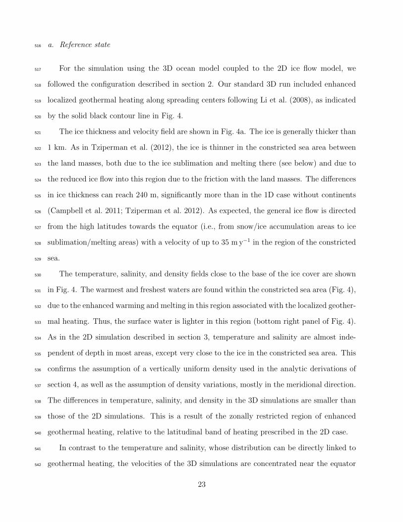
In contrast to the temperature and salinity, whose distribution can be directly linked to541

geothermal heating, the velocities of the 3D simulations are concentrated near the equator542

23

(Fig. 5), similar to the zonally symmetric 2D results (Figs. 1,2). The continents do not543

inhibit the formation of strong equatorial zonal jets. Also similar to the 2D results, and as544

predicted by the analytic expressions, the zonal and meridional velocities change signs with545

depth and the vertical velocity does not. Yet, the latitudinal symmetry properties of the 3D546

run are somewhat different from those of the 2D standard run shown in Fig. 1 and the top547

panel of Fig. 2, as further discussed below.548

Fig. 5 shows that the continents have some effect on the currents — currents, in particular549

the equatorial zonal jets, that either encounter the continents or flow away from them lead550

to boundary currents and to upwelling and downwelling close to the continents. The weak551

salinity stratification over the enhanced geothermal heating regions allows some heating of552

the deep water to occur, and the upwelling of warmer, geothermally heated, bottom water553

near the continents. The latter can lead to enhanced melting, especially at high model554

resolution (AGLMST). However, the coarse resolution of the current model, the absence555

of detailed continental-shelf bathymetry, and the inability of our ice-flow model to handle556

bottom bathymetry do not allow us to draw more specific conclusions on the implications for557

the existence of open water (a potential refuge for photosynthetic life) due to this upwelling.558

A very close similarity between the zonally symmetric model and the more realistic-559

geometry 3D simulation is seen in the zonal mean temperature, salinity and velocity fields560

of the 3D run (Fig. 6). The tracers are vertically well mixed and are almost independent of561

depth; where the ocean is weakly stratified, there is a “cap” of fresh and warm water due562

to the heating and melting in the vicinity of the geothermal heating. The temperature and563

salinity range in the ocean interior are only about 0.15 ◦C and 0.05 ppt, respectively, leading564

to a density range of 0.06 kg m−3.565

The zonal mean velocities (Fig. 6) are concentrated around the equator as in the 2D case,566

but their latitudinal symmetry properties are somewhat different from those of the standard567

2D run, described in sections 3 and 4 and shown in Fig. 2. It is possible to see two opposite568

zonal jets at the equator, just below the ice. However, below these jets, the zonal velocity569

24

converges into a single symmetric jet that is similar to the one in the equatorially heated case570

shown in Fig. 2. The zonal jet changes its sign with depth as before. The meridional velocity571

also exhibits a different symmetry compared to the standard 2D simulations in Figs. 1,2.572

In the 3D case, the meridional velocity is almost symmetric in latitude just below the ice573

and becomes anti-symmetric below that, indicating the presence of two opposite MOC cells574

with poleward velocity at the upper ocean. The meridional velocity also changes sign with575

depth. The vertical velocity is consistent with the equatorial cells formed by the meridional576

velocity, with rising motion at the equator.577

The two MOC cells (Fig. 7) – a southern, counterclockwise cell, with a maximum flux of578

15 Sv and a northern, clockwise cell, with a maximum flux of 20 Sv – are weaker than in the579

standard 2D run (section 3 and Figs. 1,2), although the range of the stream function of 36580

Sv is similar to that seen in the 2D standard run. The extent of the cells is several degrees581

latitude, as for the standard 2D run, and as predicted by the analytic approximation. We582

will show below that the presence of the two cells is a result of the presence of continents.583

b. 3D sensitivity to bathymetry and geothermal heat flux distribution584

The bathymetry of the Neoproterozoic is poorly constrained, and in order to examine585

the robustness of our results with respect to this factor, we performed three additional586

3D-ocean/2D-ice-flow sensitivity runs based on the standard 3D run described in previous587

subsection a: Run (i) uses a uniform geothermal heat flux of 0.1 W m−2, run (ii) has a 1 km588

high sill between the continents around the constricted sea area, and run (iii) has the same589

sill as run (ii) and additional zonal and meridional mid-ocean ridges that are also regions of590

enhanced geothermal heating (the mean geothermal heat flux is again 0.1 W m−2).591

A summary of the results (potential density and MOC) of the three experiments is shown592

in Fig. 8. In experiment (i), the freshest water is not in the vicinity of the constricted sea593

(as in the standard case shown in Fig. 4), but at the low latitudes of the open ocean, due594

to the elimination of the enhanced melting region within the constricted sea. Because we595

25

removed the differential geothermal heating, the difference in density is smaller compared596

to the standard case. The zonal mean potential density is almost uniform with depth, as597

for the 2D and 3D results presented above. The MOC is concentrated around the equator598

as before; the details of the MOC are different though, due to the uniform heat flux. The599

existence of two cells in both the standard 3D run and in Experiment (i) confirms that the600

existence of two MOC cells is due to the presence of the continents rather than the locally601

enhanced geothermal heat flux in the standard run.602

The additional sill of 1 km height between the continents in Experiment (ii) leads to a603

similar circulation and density pattern as for the 3D standard run (middle row of Fig. 8),604

although the MOC is weaker because the bottom water circulation is blocked in the region605

of the constricted sea. The presence of sills also alters the location of the freshest water.606

One expects mid-ocean ridges to have extents that are roughly similar to those of the607

present day. Experiment (iii), with such ridges specified, in necessarily arbitrary locations,608

and with enhanced geothermal heat flux over these ridges, resulted in a circulation and609

density field that are similar to the standard 3D run (bottom panels of Fig. 8). Here,610

however, the MOC cell is stronger due to the larger heating in the NH (over the high NH611

latitude ridge).612

Finally, an additional 3D run, similar to the standard 2D run (discussed in section 3),613

with no continents and with a global configuration, led to results that were almost identical614

to those of the 2D standard run.615

7. Summary and conclusions616

We find that the steady circulation under a thick (∼1000 m) ice cover in a Snowball617

Earth scenario is composed of an equatorial MOC and zonal jets. The MOC amplitude is618

comparable to the present day North Atlantic MOC, yet is restricted to within a couple of619

degrees latitude around the equator. These results are supported by 2D (latitude-depth) and620

26

3D simulations with an ocean GCM. These are found to be robust with respect to geometry621

and forcing parameters, and are consistent with analytical approximations derived from the622

equations of motion. The analytic solution indicates that a horizontal equatorial density623

gradient leads to a pressure gradient that, in turn, drives the MOC and zonal jets. Eddy624

viscosity plays an important role in these dynamics, determining the meridional extent of625

the MOC.626

Given that the temperature, salinity and density are essentially vertically uniform in627

nearly all locations, due to convective instability driven by the geothermal heat flux, we chose628

not to use eddy parameterizations developed for the very different modern-day ocean (Gent629

and McWilliams 1990). Instead, we use a simple formulation with constant strictly horizontal630

and vertical eddy coefficients. The horizontal eddy viscosity and eddy mixing coefficients631

are smaller than the ones predicted by a high resolution eddy resolving run (AGLMST); the632

results of that runs confirm our results. Note that larger viscosity and diffusion coefficients633

lead to a better agreement with the analytical prediction. An alternative approach was634

taken by Ferreira et al. (2011) (their appendix C), who used the GM scheme and found635

strong eddy-driven high latitude meridional cells, different from the equatorial circulation636

found here. While their run is not at a steady state due to the lack of geothermal heat flux637

and their ice cover is only 200 m thick, these results are very interesting and suggest that638

further study of the role of eddies in a Snowball ocean is worthwhile. Such a study, in a639

dynamical regime very far from that of the present-day ocean, may lead to new insights on640

eddy dynamics that may enrich our understanding of ocean dynamics in modern conditions641

as well.642

An important goal of studying snowball ocean circulation is to aid geologists and geo-643

chemists in the interpretation of the geological, geochemical and paleontological record.644

Geochemical studies sometimes assume that the ocean was stagnant and not well mixed.645

The first important lesson from the present study is that one expects the ocean to be well646

mixed in the vertical nearly everywhere, as indicated by the vertically uniform tempera-647

27

ture and salinity profiles, due to the geothermal heat flux. The second related lesson is648

the presence of a relatively strong zonal circulation and meridional overturning circulation649

which would have together further mixed the ocean horizontally and vertically. Ferreira650

et al. (2011) also found a very weak stratification and strong MOC cells, although at higher651

latitudes rather than at the equator as found here. But it does seem that the snowball ocean652

needs to be thought of as well mixed rather than stagnant, and that one cannot assume the653

deep water to be disconnected from the surface ocean. It is, admittedly, difficult to come654

up with additional specific insights that are directly relevant to the observed record, and655

it may take future geochemical studies to explore the consequences of the circulation and656

stratification reported here. It is worth noting that much of the present study dealt with the657

large scale ocean circulation in deep ocean basins, while the preserved geological record is658

mostly from shelf and shallow areas that have not been subducted by now. We do note that659

our study identifies strong tendency for near-coast upwelling and downwelling, as a result660

of a combination of the weak stratification and the encounter of horizontal (mostly zonal)661

currents and land masses, and this may have some geological relevance as well.662

Acknowledgments.663

We thank Aiko Voigt and an anonymous reviewer for their most helpful comments. This664

work was supported by NSF Climate Dynamics, P2C2 Program, grant ATM-0902844 (ET,665

YA) and NSF Climate Dynamics Program, grant ATM-0917468 (ET). ET thanks the Weiz-666

mann Institute for its hospitality during parts of this work. YA thanks the Harvard EPS667

Department for a most pleasant and productive sabbatical visit.668

28

APPENDIX669

670

Scaling of idealized 2D configuration671

We start from the β-plane momentum equations under the assumptions of steady state672

(i.e., ∂t = 0 and zonal symmetry ∂x = 0)673

vuy + wuz − βyv = νhuyy + νvuzz, (A1)

vvy + wvz + βyu = − 1

ρ0py + νhvyy + νvvzz, (A2)

It is possible to switch to nondimensional variables as follows: y = (νh/β)1/3y, z = Hz674

(H is the depth of the ocean), p = gHρy(νh/β)1/3p, u = (gHρy)/(ρ0β2/3ν

1/3h )u, v =675

(gHρy)/(ρ0β2/3ν

1/3h )v, w = (gH2ρy)/(ρ0β

1/3ν2/3h )w, where the hat indicates nondimensional676

variables. Then Eqs. (A1)-(A2) become:677

ε1vuy + ε1wuz − yv = uyy + ε2uzz, (A3)

ε1vvy + ε1wvz + yu = −py + vyy + ε2vzz. (A4)

where678

ε1 =gHρyρ0βνh

� 1, (A5)

ε2 =νv

H2β2/3ν1/3h

� 1, (A6)

are small parameters under our choice of parameters, ≈ 8 × 10−3, ≈ 2 × 10−5 respectively.679

Thus, it is possible to neglect the advection and vertical viscosity terms from the momentum680

equations.681

29

682

REFERENCES683

Abbot, D., A. Voigt, and D. Koll, 2011: The Jormungand global climate state and implica-684

tions for Neoproterozoic glaciations. J. Geophys. Res., 116, D18 103.685

Abbot, D. S. and I. Halevy, 2010: Dust aerosol important for snowball earth deglaciation.686

J. Climate, 23 (15), 4121–4132.687

Abbot, D. S. and R. T. Pierrehumbert, 2010: Mudball: Surface dust and snowball earth688

deglaciation. J. Geophys. Res., 115.689

Abbot, D. S., A. Voigt, M. Branson, R. T. Pierrehumbert, D. Pollard, G. Le Hir, and D. D.690

Koll, 2012: Clouds and Snowball Earth deglaciation. Geophys. Res. Lett., 39, L20 711.691

Allen, P. A. and J. L. Etienne, 2008: Sedimentary challenge to snowball earth. Nature692

Geoscience, 1, 817.693

Ashkenazy, Y., H. Gildor, M. Losch, F. A. Macdonald, D. P. Schrag, and E. Tziperman, 2013:694

Dynamics of a Snowball Earth ocean. Nature, 495, 90–93, doi:10.1038/nature11 894.695

Baum, S. and T. Crowley, 2001: Gcm response to late precambrian (similar to 590 ma)696

ice-covered continents. Geophys. Res. Lett., 28 (4), 583–586, doi:10.1029/2000GL011557.697

Baum, S. and T. Crowley, 2003: The snow/ice instability as a mechanism for rapid climate698

change: A Neoproterozoic Snowball Earth model example. Geophys. Res. Lett., 30 (20),699

doi:10.1029/2003GL017333.700

Bryan, K., 1984: Accelerating the convergence to equilibrium of ocean-climate models. J.701

Phys. Oceanogr., 14, 666–673.702

30

Budyko, M. I., 1969: The effect of solar radiatin variations on the climate of the earth.703

Tellus, 21, 611–619.704

Campbell, A. J., E. D. Waddington, and S. G. Warren, 2011: Refugium for surface life on705

Snowball Earth in a nearly-enclosed sea? A first simple model for sea-glacier invasion.706

Geophys. Res. Lett., 38, 10.1029/2011GL048 846.707

Chandler, M. A. and L. E. Sohl, 2000: Climate forcings and the initiation of low-latitude ice708

sheets during the Neoproterozoic Varanger glacial interval. J. Geophys. Res., 105 (D16),709

20 737–20 756.710

Crowley, T. and S. Baum, 1993: Effect of decreased solar luminosity on late Precambrian711

ice extent. J. Geophys. Res., 98 (D9), 16 723–16 732, doi:10.1029/93JD01415.712

Donnadieu, Y., F. Fluteau, G. Ramstein, C. Ritz, and J. Besse, 2003: Is there a conflict713

between the Neoproterozoic glacial deposits and the snowball Earth interpretation: an714

improved understanding with numerical modeling. Earth Planet. Sci. Lett., 208 (1-2),715

101–112.716

Donnadieu, Y., Y. Godderis, G. Ramstein, A. Nedelec, and J. Meert, 2004a: A ’snow-717

ball Earth’ climate triggered by continental break-up through changes in runoff. Nature,718

428 (6980), 303–306.719

Donnadieu, Y., G. Ramstein, F. Fluteau, D. Roche, and A. Ganopolski, 2004b: The impact720

of atmospheric and oceanic heat transports on the sea-ice-albedo instability during the721

Neoproterozoic. Clim. Dyn., 22 (2-3), 293–306.722

Evans, D. A. D. and T. D. Raub, 2011: Neoproterozoic glacial palaeolatitudes: a global723

update. The Geological Record of Neoproterozoic Glaciations, E. Arnaud, G. P. Halverson,724

and G. Shields-Zhou, Eds., London, Geological Society of London, Vol. 36, 93–112.725

31

Ferreira, D., J. Marshall, and B. E. J. Rose, 2011: Climate determinism revisited: multiple726

equilibria in a complex climate model. J. Climate, 24, 992–1012.727

Gent, P. R. and J. C. McWilliams, 1990: Isopycnal mixing in ocean circulation models. J.728

Phys. Oceanogr., 20 (1), 150–155.729

Goodman, J. C., 2006: Through thick and thin: Marine and meteoric ice in a ”Snowball730

Earth” climate. Geophys. Res. Lett., 33 (16).731

Goodman, J. C. and R. T. Pierrehumbert, 2003: Glacial flow of floating marine ice in732

”Snowball Earth”. J. Geophys. Res., 108 (C10).733

Harland, W. B., 1964: Evidence of late Precambrian glaciation and its significance. Problems734

in Palaeoclimatology, A. E. M. Nairn, Ed., John Wiley & Sons, London, 119–149, 180–184.735

Hoffman, P. and D. Schrag, 2002: The snowball Earth hypothesis: testing the limits of global736

change. Terra Nova, 14 (3), 129–155, doi:10.1046/j.1365-3121.2002.00408.x.737

Hyde, W. T., T. J. Crowley, S. K. Baum, and W. R. Peltier, 2000: Neoproterozoic ’snowball738

earth’ simulations with a coupled climate/ice-sheet model. Nature, 405, 425–429.739

Jackett, D. R. and T. J. McDougall, 1995: Minimal adjustment of hydrographic profiles to740

achieve static stability. J. Atmos. Ocean Tech., 12 (4), 381–389.741

Jenkins, G. and S. Smith, 1999: Gcm simulations of snowball earth conditions during the742

late proterozoic. Geophys. Res. Lett., 26 (15), 2263–2266, doi:10.1029/1999GL900538.743

Kirschvink, J. L., 1992: Late Proterozoic low-latitude glaciation: the snowball Earth. The744

Proterozoic Biosphere, J. W. Schopf and C. Klein, Eds., Cambridge University Press,745

Cambridge, 51–52.746

Knauth, L., 2005: Temperature and salinity history of the Precambrian ocean: implications747

for the course of microbial evolution. Paleonogr. Paleoclim. Paleoecol., 219, 53–69.748

32

Langen, P. L. and V. A. Alexeev, 2004: Multiple equilibria and asymmetric climates in the749

ccm3 coupled to an oceanic mixed layer with thermodynamic sea ice. Geophys. Res. Lett.,750

31, L04 201.751

Le-Hir, G., Y. Donnadieu, G. Krinner, and G. Ramstein, 2010: Toward the snowball earth752

deglaciation... Clim. Dyn., 35 (2-3), 285–297, doi:10.1007/s00382-010-0748-8.753

Le-Hir, G., G. Ramstein, Y. Donnadieu, and R. T. Pierrehumbert, 2007: Investigating754

plausible mechanisms to trigger a deglaciation from a hard snowball Earth. Comptes rendus755

- Geosci., 339 (3-4), 274–287, doi:10.1016/j.crte.2006.09.002.756

Lewis, J., M. Eby, A. Weaver, S. Johnston, and R. Jacob, 2004: Global glaciation in the757

neoproterozoic: Reconciling previous modelling results. Geophys. Res. Lett., 31 (8), doi:758

10.1029/2004GL019725.759

Lewis, J. P., A. J. Weaver, and M. Eby, 2007: Snowball versus slushball Earth: Dynamic760

versus nondynamic sea ice? J. Geophys. Res., 112.761

Lewis, J. P., A. J. Weaver, S. T. Johnston, and M. Eby, 2003: Neoproterozoic ”snowball762

Earth”: Dynamic sea ice over a quiescent ocean. Paleoceanography, 18 (4).763

Li, D. and R. T. Pierrehumbert, 2011: Sea glacier flow and dust transport on Snowball764

Earth. Geophys. Res. Lett., 38, 10.1029/2011GL048 991.765

Li, Z. X., et al., 2008: Assembly, configuration, and break-up history of Rodinia: A synthesis.766

Precambrian Res., 160, 179–210.767

Losch, M., 2008: Modeling ice shelf cavities in a z-coordinate ocean general circulation768

model. J. Geophys. Res., 113, C08 043.769

MacAyeal, D., 1997: EISMINT: Lessons in ice-sheet modeling. Tech. rep., University of770

Chicago, Chicago, Illinois.771

33

Macdonald, F. A., et al., 2010: Calibrating the Cryogenian. Science, 327 (5970), 1241–1243.772

Marotzke, J. and M. Botzet, 2007: Present-day and ice-covered equilibrium states in a773

comprehensive climate model. Geophys. Res. Lett., 34, L16 704.774

Marshall, J., A. Adcroft, C. Hill, L. Perelman, and C. Heisey, 1997: A finite-volume, incom-775

pressible Navier Stokes model for studies of the ocean on parallel computers. J. Geophys.776

Res., 102, C3, 5,753–5,766.777

McKay, C. P., 2000: Thickness of tropical ice and photosynthesis on a snowball Earth.778

Geophys. Res. Lett., 27 (14), 2153–2156.779

Micheels, A. and M. Montenari, 2008: A snowball Earth versus a slushball Earth: Results780

from Neoproterozoic climate modeling sensitivity experiments. Geosphere, 4 (2), 401–410.781

Morland, L., 1987: Unconfined ice-shelf flow. Dynamics of the West Antarctic Ice Sheet,782

C. van der Veen and J. Oerlemans, Eds., D. Reidel, Boston.783

Pierrehumbert, R. T., 2002: The hydrologic cycle in deep-time climate problems. Nature,784

419 (6903), 191–198.785

Pierrehumbert, R. T., 2004: High levels of atmospheric carbon dioxide necessary for the786

termination of global glaciation. Nature, 429 (6992), 646–649.787

Pierrehumbert, R. T., 2005: Climate dynamics of a hard snowball Earth. J. Geophys. Res.,788

110 (D1).789

Pierrehumbert, R. T., D. S. Abbot, A. Voigt, and D. Koll, 2011: Climate of the neoprotero-790

zoic. Ann. Rev. of Earth and Planet. Sci., 39, 417–460.791

Pollack, H., S. Hurter, and J. Johnson, 1993: Heat flow from the Earth’s interior: analysis792

of the global data set. Rev. Geophys., 31, 267–280.793

34

Pollard, D. and J. Kasting, 2004: Climate-ice sheet simulations of Neoproterozoic glaciation794

before and after collapse to Snowball Earth. Geophysical Monograph series, 146, 91–105.795

Pollard, D. and J. F. Kasting, 2005: Snowball Earth: A thin-ice solution with flowing sea796

glaciers. J. Geophys. Res., 110 (C7).797

Pollard, D. and J. F. Kasting, 2006: Reply to comment by Stephen G. Warren and Richard798

E. Brandt on “Snowball Earth: A thin-ice solution with flowing sea glaciers”. J. Geophys.799

Res., 111 (C9), doi:10.1029/2006JC003488.800

Poulsen, C., R. T. Pierrehumbert, and R. L. Jacobs, 2001a: Impact of ocean dynamics on the801

simulation of the Neoproterozoic “snowball Earth”. Geophys. Res. Lett., 28, 1575–1578.802

Poulsen, C. J. and R. L. Jacob, 2004: Factors that inhibit snowball Earth simulation. Pale-803

oceanography, 19 (4).804

Poulsen, C. J., R. L. Jacob, R. T. Pierrehumbert, and T. T. Huynh, 2002: Testing paleo-805

geographic controls on a Neoproterozoic snowball Earth. Geophys. Res. Lett., 29 (11).806

Poulsen, C. J., R. T. Pierrehumbert, and R. L. Jacob, 2001b: Impact of ocean dynamics807

on the simulation of the Neoproterozoic ”snowball Earth”. Geophys. Res. Lett., 28 (8),808

1575–1578.809

Romanova, V., G. Lohmann, and K. Grosfeld, 2006: Effect of land albedo, co2, orography,810

and oceanic heat transport on extreme climates. Climate of the Past, 2 (1), 31–42.811

Rose, B. E. J. and J. Marshall, 2009: Ocean heat transport, sea ice, and multiple climate812

states: Insights from energy balance models. J. Atmos. Sci., 66 (9), 2828–2843.813

Schrag, D. P., R. A. Berner, P. F. Hoffman, and G. P. Halverson, 2002: On the initiation of814

a snowball Earth. Geochemistry Geophysics Geosystems, 3, doi:10.1029/2001GC000219.815

Schrag, D. P., P. F. Hoffman, W. Hyde, et al., 2001: Life, geology and snowball earth.816

NATURE-LONDON-, 306–306.817

35

Sellers, W., 1969: A global climate model based on the energy balance of the Earth-818

atmosphere system. J. Appl. Meteorol., 8, 392–400.819

Sohl, L. E. and M. A. Chandler, 2007: Reconstructing Neoproterozoic palaeoclimates using820

a combined data/modelling approach. Deep-Time Perspectives on Climate Change: Mar-821

rying the Signal from Computer Models and Biological Proxies, M. M. Williams, A. M.822

Hatwood, J. Gregory, and D. N. Schmidt, Eds., Geological Society, Micropalaeontological823

Society Special Publication #2, 61–80.824

Stein, C. A. and S. Stein, 1992: A model for the global variation in oceanic depth and heat825

flow with lithospheric age. Nature, 359, 123–129.826

Tziperman, E., D. S. Abbot, Y. Ashkenazy, H. Gildor, D. Pollard, C. Schoof, and D. P.827

Schrag, 2012: Continental constriction and sea ice thickness in a Snowball-Earth scenario.828

J. Geophys. Res., 117 (C05016), 10.1029/2011JC007 730.829

Tziperman, E., I. Halevy, D. T. Johnston, A. H. Knoll, and D. P. Schrag, 2011: Biologically830

induced initiation of Neoproterozoic Snowball-Earth events. Proc. Natl. Acad. Sci. U.S.A.,831

108 (37), 15 09115 096, doi/10.1073/pnas.1016361 108.832

Voigt, A. and D. S. Abbot, 2012: Sea-ice dynamics strongly promote Snowball Earth initia-833

tion and destabilize tropical sea-ice margins. Clim. Past, 8, 2079–2092.834

Voigt, A., D. S. Abbot, R. T. Pierrehumbert, and J. Marotzke, 2011: Initiation of a Marinoan835

Snowball Earth in a state-of-the-art atmosphere-ocean general circulation model. Clim.836

Past, 7, 249–263, doi:10.5194/cp-7-249-2011.837

Voigt, A., I. M. Held, and J. Marotzke, 2012: Hadley cell dynamics in a virtually dry snowball838

earth atmosphere. J. Atmos. Sci., 69 (1), 116–128.839

Voigt, A. and J. Marotzke, 2010: The transition from the present-day climate to a modern840

Snowball Earth. Climate Dynamics, 35 (5), 887–905.841

36

Warren, S. G. and R. E. Brandt, 2006: Comment on “Snowball Earth: A thin-ice solution842

with flowing sea glaciers” by David Pollard and James F. Kasting. J. Geophys. Res.,843

111 (C9), 10.1029/2005JC003 411.844

Warren, S. G., R. E. Brandt, T. C. Grenfell, and C. P. McKay, 2002: Snowball Earth: Ice845

thickness on the tropical ocean. J. Geophys. Res., 107 (C10).846

Weertman, J., 1957: Deformation of floating ice shelves. J. Glaciology, 3 (21), 38–42.847

Yang, J., W. P. Peltier, and Y. Hu, 2012a: The initiation of modern soft and hard Snowball848

Earth climates in CCSM4. Clim. Past, 8, 907918.849

Yang, J., W. P. Peltier, and Y. Hu, 2012b: The initiation of modern soft snowball and hard850

snowball climates in CCSM3. part i: The inuences of solar luminosity, CO2 concentration,851

and the sea ice/snow albedo parameterization. J. Climate, 25, 2711–2736.852

Yang, J., W. R. Peltier, and Y. Hu, 2012c: The initiation of modern “soft snowball” and853

“hard snowball” climates in CCSM3. part ii: Climate dynamic feedbacks. J. Climate,854

25 (8), 2737–2754, doi:10.1175/JCLI-D-11-00190.1.855

37

List of Figures856

1 (a) Density (kg m−3), (b) the depth derivative of the density (kg m−4), (c)857

meridional velocity v (cm s−1), and (d) vertical velocity w (cm s−1), at steady858

state of the latitude-depth standard run. The white area at the top of the plot859

represents the ice cover and the white area at the bottom of the panels indi-860

cates the ridge that has enhanced geothermal heating. The thick contour line861

in panels a,b represents the zero contour line of panel b, separating the stable862

stratification around the equator from the unstable stratification elsewhere.863

Note that the significant circulation is confined to the equatorial regions. 41864

2 A summary of the latitude-depth 2D profiles of the sensitivity experiments.865

The four columns show the temperature, salinity, zonal velocity, and MOC866

(presented between 40◦S and 40◦N). The contour line in the first and second867

columns separates the vertically stable ocean regions from the unstable ones868

while the contour line in the third column indicates the zero velocity. First869

row: standard run, after AGLMST. Second row: same as standard run but870

without the ridge (the geothermal heat flux is as in the standard case). Third871

row: same as standard but with ridge and enhanced heating placed at the872

equator. Fourth row: same as second row but without the ridge (yet with873

an enhanced equatorial heating). Fifth row: same as standard run but with874

ridge and enhanced heating centered at 40◦N. Sixth row: same as standard875

but with mean geothermal heat flux of 0.075 W/m2 instead of 0.1. 42876

38

3 The analytic approximations vs. the numerical results for the experiments877

described in the text (Experiment 4 of uniform geothermal heating and uni-878

form ice-surface temperature is not presented as it resulted, as expected, in a879

stagnant ocean). Top left: maximum zonal velocity (cm s−1). Top right: maxi-880

mum meridional velocity (cm s−1). Bottom left: maximum MOC (Sv) Bottom881

right: half-width of the MOC cell (degree latitude). The solid line shows the882

linear regression where the correlation coefficients are 0.88, 0.87, 0.87, and883

0.95, for the top-left, top-right, bottom-left, and bottom-right panels, respec-884

tively. The dashed line indicates the “identity” line. When assuming that885

the regression lines cross the (0,0) point the slopes of the curves are 0.56,886

1.47, 1.63, and 0.63 for the top-left, top-right, bottom-left, and bottom-right887

panels, respectively–the correlation coefficients are the same as the above. 43888

4 Results of the 3D standard run. Ice thickness and ice velocity (top left panel),889

potential temperature (top right panel), salinity (bottom left panel), and den-890

sity (bottom right panel), all under the ice, at a depth of 1.2 km. The black891

solid contour line indicates the location of geothermal heating. Ice-depth892

temperature and salinity are after AGLMST. 44893

5 Circulation in the standard 3D run. Zonal (upper panels), meridional (middle894

panels), and vertical (bottom panels) velocities, near the ice bottom (at a895

depth of 1.1 km, left panels) and at 2.9 km (right panels). 45896

6 Zonal averages of the 3D standard run of potential temperature (top left),897

salinity (middle left), density (bottom left), zonal velocity (top right), merid-898

ional velocity (middle right), and vertical velocity (bottom right). Solid con-899

tour lines indicate positive values while dashed contour lines indicate negative900

values. 46901

7 The MOC of the 3D standard run. 47902

39

8 Results of the 3D sensitivity experiments. Density at a depth of 2.5 km (left903

panels), zonal mean density (middle column panels), and MOC (right panels),904

for standard run but with uniform geothermal heating (upper panels), as for905

standard run but with sills (middle row panels), and as for standard run906

but with sills and geothermally heated ridges (bottom panels). The dashed907

contour lines indicate fresher water. The thick solid contour lines indicate the908

location of the geothermal heating. 48909

40

Fig. 1. (a) Density (kg m−3), (b) the depth derivative of the density (kg m−4), (c) meridionalvelocity v (cm s−1), and (d) vertical velocity w (cm s−1), at steady state of the latitude-depthstandard run. The white area at the top of the plot represents the ice cover and the whitearea at the bottom of the panels indicates the ridge that has enhanced geothermal heating.The thick contour line in panels a,b represents the zero contour line of panel b, separatingthe stable stratification around the equator from the unstable stratification elsewhere. Notethat the significant circulation is confined to the equatorial regions.

41

Fig. 2. A summary of the latitude-depth 2D profiles of the sensitivity experiments. The fourcolumns show the temperature, salinity, zonal velocity, and MOC (presented between 40◦Sand 40◦N). The contour line in the first and second columns separates the vertically stableocean regions from the unstable ones while the contour line in the third column indicatesthe zero velocity. First row: standard run, after AGLMST. Second row: same as standardrun but without the ridge (the geothermal heat flux is as in the standard case). Third row:same as standard but with ridge and enhanced heating placed at the equator. Fourth row:same as second row but without the ridge (yet with an enhanced equatorial heating). Fifthrow: same as standard run but with ridge and enhanced heating centered at 40◦N. Sixthrow: same as standard but with mean geothermal heat flux of 0.075 W/m2 instead of 0.1.

42

A

0 0.5 1 1.50

0.5

1

1.5

Num

eric

al re

sults 1.

2. 10H3. 0.1H5. ~3∆Q6. β/47. β/98. 16νh

Max. u (cm/s)

A

0 0.5 1 1.50

0.5

1

1.59. νh/410. 4κh11. κh/412. 16νh, 4κhA

13. 4νh, 4κh14. 0.1κv15. νh/4, κh/4

Max. v (cm/s)

A

0 100 200 300Analytical approximation

0

100

200

300

Num

eric

al re

sults

Max. MOC (Sv)A

0 5 10Analytical approximation

0

5

10

MOC half width (degrees)

0.72

1.46

0.69

2.14

Fig. 3. The analytic approximations vs. the numerical results for the experiments describedin the text (Experiment 4 of uniform geothermal heating and uniform ice-surface temperatureis not presented as it resulted, as expected, in a stagnant ocean). Top left: maximum zonalvelocity (cm s−1). Top right: maximum meridional velocity (cm s−1). Bottom left: maximumMOC (Sv) Bottom right: half-width of the MOC cell (degree latitude). The solid line showsthe linear regression where the correlation coefficients are 0.88, 0.87, 0.87, and 0.95, forthe top-left, top-right, bottom-left, and bottom-right panels, respectively. The dashed lineindicates the “identity” line. When assuming that the regression lines cross the (0,0) pointthe slopes of the curves are 0.56, 1.47, 1.63, and 0.63 for the top-left, top-right, bottom-left,and bottom-right panels, respectively–the correlation coefficients are the same as the above.

43

1

11

11111111

11

1

11111111111

1

11111

111

111

111111

11

1111111111111

11111111

Fig. 4. Results of the 3D standard run. Ice thickness and ice velocity (top left panel),potential temperature (top right panel), salinity (bottom left panel), and density (bottomright panel), all under the ice, at a depth of 1.2 km. The black solid contour line indicatesthe location of geothermal heating. Ice-depth temperature and salinity are after AGLMST.

44

Fig. 5. Circulation in the standard 3D run. Zonal (upper panels), meridional (middlepanels), and vertical (bottom panels) velocities, near the ice bottom (at a depth of 1.1 km,left panels) and at 2.9 km (right panels).

45

Fig. 6. Zonal averages of the 3D standard run of potential temperature (top left), salinity(middle left), density (bottom left), zonal velocity (top right), meridional velocity (middleright), and vertical velocity (bottom right). Solid contour lines indicate positive values whiledashed contour lines indicate negative values.

46

Fig. 7. The MOC of the 3D standard run.

47

Fig. 8. Results of the 3D sensitivity experiments. Density at a depth of 2.5 km (left panels),zonal mean density (middle column panels), and MOC (right panels), for standard run butwith uniform geothermal heating (upper panels), as for standard run but with sills (middlerow panels), and as for standard run but with sills and geothermally heated ridges (bottompanels). The dashed contour lines indicate fresher water. The thick solid contour linesindicate the location of the geothermal heating.

48