Occurrence, Transport and Fate of Persistent Organic ...

Occurrence, Transport and Fate of Persistent

Organic Pollutants in the Global Ocean

Presencia, Transporte y Destino de Contaminantes Orgánicos Persistentes en el Océano Global

Belén González-Gaya

Aquesta tesi doctoral està subjecta a la llicència Reconeixement- NoComercial – SenseObraDerivada 3.0. Espanya de Creative Commons. Esta tesis doctoral está sujeta a la licencia Reconocimiento - NoComercial – SinObraDerivada 3.0. España de Creative Commons. This doctoral thesis is licensed under the Creative Commons Attribution-NonCommercial-NoDerivs 3.0. Spain License.

Occurrence, Transport and Fate ofPersistent Organic Pollutants

in the Global Ocean

Belén González GayaBarcelona, 2015

Universitat de BarcelonaPrograma de Doctorat en Ciències del Mar

PhD ThesisOccurrence, Transport and Fate of

Persistent Organic Pollutants in the Global Ocean

Belén González GayaPrograma de Doctorat en Ciències del Mar

Universitat de BarcelonaBarcelona, 2015

Occ

urre

nce,

Tra

nspo

rt a

nd F

ate

of P

ersi

sten

t Org

anic

Pol

luta

nts

in th

e G

loba

l Oce

an B

elén

Gon

zále

z G

aya

201

5

Occurrence, Transport and Fate of

Persistent Organic Pollutants in the Global Ocean

Presencia, Transporte y Destino de

Contaminantes Orgánicos Persistentes en el Océano Global


Barcelona, 2015

Memòria presentada per Belén González Gaya per optar al grau de doctor

per la Universitat de Barcelona

Programa de Doctorat en Ciències del Mar

La Doctoranda


Los directores

Dr. Jordi Dachs

Dra. Begoña Jiménez

El Tutor

Dr. Miquel Canals

“Por diferentes motivos se marchan los hombres a los confines abandonados del

mundo. A algunos les impele solamente el afán de aventuras, otros sienten una intensa

sed de saber, los terceros obedecen a la seductora llamada de unas voces quedas, al

encanto misterioso de lo desconocido que les aleja de los senderos rutinarios de la vida

cotidiana.”

Ernest Shackleton, 1901.

“Water and air, the two essential fluids on which all life depends, have become global

garbage cans.”

Jacques-Yves Cousteau, 1910.

Agradecimientos

Por fin, tras cientos de horas de muflar, pesar, limpiar, acondicionar, envolver, de no dormir,

de mareos y risas, de viajes, de mal de tierra, de más viajes, del Atlántico y el Índico, de pescar,

filtrar, subir y bajar escaleras oxidadas, de cambiar escobillas y fusibles, de baker, de extraer,

purificar, reducir (sobretodo metanol) e inyectar, de cuantificar (de eso sí que han sido horas,

mare de Deu de Monsterrat), de hacer excels (cuyo límite hemos llegado a rebasar), de

escribir, corregir, escribir y volver a empezar, de difundir lo que hacemos (a grandes y chicos,

desde las Ramblas al Pacífico, pasando por Móstoles), de recorrerme la A2, y, sobre todo, de

aprender… por fin puedo enfrentarme a estas últimas líneas. Líneas para resumir lo que no

caben en 5 años de vida, toda la gratitud y la emoción que se produce durante este “pequeño-

gran” trabajo.

Por empezar por el principio, gracias a Jordi y a Begoña por confiar en mí para esta aventura.

Nunca olvidaré mi primera conversación telefónica con una voz de fuerte acento Catalán, en

los pasillos de mi antiguo trabajo, y la posterior reunión en el IQOG con una investigadora que

me proponía medir la contaminación de los siete mares… Moltes gràcies, Jordi, por tu eficacia,

tu apoyo incondicional y tus sabios consejos. No creo que pudiese encontrar un tutor en el

mundo con más sustancia que exprimir que tú. Algún día yo también cumpliré nuestro sueño

de “vespa blanca”. Gracias Bego por ponerme los pies en la tierra, por tus contactos, viajes y tu

paciencia. Porque una caña sirve tanto para celebrar como para apaciguar. Creo haberme

llevado lo mejor de vosotros y espero habéroslo dado todo también.

En el IDAEA todo lo aprendí. De mis predecesores, Naiara, Ana y Cristóbal, tuve los ejemplos a

seguir y las pautas de lo que funciona y lo que no funciona. Mil gracias por la paciencia y

aguantar todas las preguntas de novata. Espero haber estado a la altura. De mis coetáneos me

llevo lo mejor; horas de labo y despacho regadas de chistes malos, radio a todo trapo y

comidas al solete. MariCarmen, te quiero siempre espalda contra espalda, porque todo el

apoyo que nos hemos dado no se escribe en una línea, sino que se demuestra tras años de

esfuerzo, trapillo, vestidos rojos y cereales. ¡Eres una campeona! Ha sido genial compartir el

despacho con nuestro chileno preferido, ¿eh? Gracias también a mis niñas, Lauri y Gemma, sin

vosotras esto no hubiera sido igual. ¡Porque haya mucho más fernet para brindar! Sin duda,

gracias a Mari Jose, por la calidad de su trabajo dentro del labo y por su apoyo y creatividad

fuera de él. Junto a MC, ¡habéis hecho que Barcelona tenga más colores para mí! Te deseo

toda la suerte del mundo. De las nuevas generaciones mención especial a Paulo y a Mariana,

por currar tanto, por crear un labo nuevo y porque todo ese buen rollo sea el motor de mil

descubrimientos. Gracias por hacerme sentir que he aprendido cosas durante estos años y soy

capaz de ayudar a los demás. No me olvido tampoco de los postdocs a los que pisar los

talones: Javi, Maria, y en especial por su ayuda y consejos a Linda y a Elena. ¡Grazie i graciès!

Agradecerle también a la gente de la quinta planta hacerme un huequito siempre a la hora del

café; a Marta, a mis 3 adorables portus, a Eli, Maria, Denis, Mel y a los capos de la

ecotoxicología. ¡Ya llevaré pastas cuando defienda! También gracias al combo hoquei-quimico

por mezclar curro y deporte, y permitirme conocer a más gente dentro del IDAEA; Quique,

Viky, Cayo, Oscar (you left my heart frozen), ¡espero encontraros en todas las SETACs y Dioxins

del mundo para petarlo!

Mi segunda casa, que en realidad fue la primera, el IQOG, ha sido la “otra cara de la moneda”

de mi doctorado. Gracias en genérico por darme siempre una nueva perspectiva, cada labo

tiene sus misterios y sus trucos. Me siento afortunada por haber podido aprender de ambos.

Gracias, gracias y mil gracias a Pepelu. Por nuestras conversaciones eternas y risas sin control,

por ser mi colega en el curro, en los bares, en alta mar y en la montaña. Por todo lo que hemos

compartido, y lo que nos queda. Por nuestra bohemian rapsody. Gracias a Juan, mi mejor

profe de analítica, con el toque de ironía y sensibilidad perfecto. ¡Te debo mucho! Gracias a

Miren por sus bailes, nuestros viajes y nuestras futuras colaboraciones. ¡Por el carbaZole

symposium en Iruña! Gracias especiales también a María, que no es sólo mi compañera de

trabajo, es mi colega. Por tu apoyo incondicional y nuestra conexión total (y gracias a Pitu por

su asesoramiento!). Gracias a todos los demás por permitirme aprender siempre de vosotros.

Porque todo aquel que haya conocido allí ha influido en mi aprendizaje, especialmente a

Sagrario (artista!!!) y Lourdes por su cercanía.

Gracias a toda la gente que participó en ese gran proyecto llamado Malaspina. Tanto a la gente

que muestreó conmigo como a los que lo hicieron por mí, o para cumplir sus propios objetivos,

llegando todos juntos a un conocimiento más profundo de nuestro océano. No quiero poner

nombres por temor a que me falte alguien, pero de todo corazón, gracias, porque este viaje

cambió mi vida.

Nunca hubiera llegado hasta aquí sin mi formación previa en Mallorca, Buenos Aires, Napoles,

Wageningen, y la Autonoma de Madrid. Gracias, por tanto, a la gente de la Roca, de capital,

Mardel y Bariloche, a todos mis italianos (mi manchate!), a la Wage-people con la que descubrí

la ciencia y la malegría, a mis ambientólogos locos. Sois todos parte de esto.

Gracias a la gente que nada tiene que ver con esta investigación pero que hace que quieras

celebrar con ellos las cosas buenas de esta aventura y que penan contigo las cosas malas. A las

seitonas y seitones en Barcelona, a mis amigas de toda la vida, a los isla planeros, a esas

personas que te llaman y te preguntan sin tener muy claro lo que haces, pero se interesan por

ti no obstante.

Gracias por encima de todo a mis padres porque siempre me han ayudado, animado y

apoyado sin reticencias, aunque eso supusiera poner entre nosotros miles de kilómetros.

Espero que estéis tan orgullosos de mí como lo estoy yo de vosotros. Eskerrik asko a mi

“nueva” familia por cada momento, no he podido sentirme más cuidada en vuestra casa.

Gracias a mi compañero, a mi colegui, a mi más mejor amigo, a la persona con la que lo he

compartido todo durante estos años. Sin ti nada sería. Mundu propioa sortzeko gai izan

garelako…

Belén

3

TABLE OF CONTENTS

List of Acronyms 5

Longhurst provinces 8

List of tables and figures 9

Abstracts 13

Chapter 1. General Introduction 19

Pollution in the Open Ocean: Persistent Organic Pollutants and “not so

Persistent” Pollutants 21

Environmental Fate and Dynamics of POPs 23

Atmospheric processes 25

Water column processes 30

Case studies in the Malaspina expedition: PAHs and PFASs 32

Polycyclic Aromatic Hydrocarbons (PAHs) 34

Perfluoroalkylated Substances (PFASs) 38

Aim and Outline of this thesis 41

References 47

Chapter 2. Results 55

1. Field Measurements of the Atmospheric Dry Deposition Fluxes and

Velocities of Polycyclic Aromatic Hydrocarbons to the Global Oceans 57

References 80

2. High Atmosphere-Ocean Exchange of Semivolatile Aromatic Hydrocarbons

85

References 105

3. Perfluoroalkylated Substances in the Global Tropical and Subtropical

Surface Oceans 109

References 130

4. Oceanic Transport and Sinks of Perfluoroalkylated Substances 135

References 157

4

5. Cycling of Polycyclic Aromatic Hydrocarbons in the Surface Open Ocean

161

References 184

Summary of Results 187

Chapter 3. General Discussion 195

Global Occurrence 199

PAHs 199

PFASs 202

Partitioning of PAHs and PFASs in the environmental compartments and

Implications for their Global Fate 203

PAHs occurrence in atmospheric gas and aerosol phases 203

PAHs and PFASs occurrence in seawater’s dissolved and particulate phases 205

Global fluxes and budgets of PAHs and PFASs in the Open Ocean 208

PAHs and SALCs 209

PFASs 212

References 215

Chapter 4. General Conclusions 221

Annexes 227

Subchapter 1 Supporting Information A1





5

List of Acronyms

List of the acronyms and abbreviations used in this thesis:

∆H Bond enthalpy ∆S Absolute entropy ABL Atmospheric boundary layer B Biomass BCF Bioconcentration factor C Carbon CA Aerosol phase concentration CDD Deposited aerosol phase concentration CG Gas phase concentration CGf Final gas phase concentration CGi Initial gas phase concentration Chls Surface chlorophyll concentration CLRTAP Convention on Long-Range Transboundary Air Pollution COP Contaminantes orgánicos persistentes CP Particulate phase concentration CPlankton Plankton phase concentration CTD Conductivity, Temperature, Depth (device) CTW Truly dissolved phase concentration CW Dissolved phase concentration D Diffusivity DA Diffusivity coefficient in the air Datm Atmospheric degradation DCM Dichloromethane DCM Deep chlorophyll maximum DDT Dichlorodiphenyltrichloroethane DL Detection limit DOC Dissolved organic carbon DP Dechlorane Plus EI Electronic impact EPA Environmental Protection Agency ESI Electrospray ionization fA Air fugacity FAW Air-water exchange flux FDD Dry deposition flux FDD coarse Coarse aerosol dry deposition flux FDD fine Fine aerosol dry deposition flux FEddy Eddy diffusive fluxes FFecal Fecal pellets sinking fluxes FOC Organic carbon flux FOM Organic matter flux FPhyto Phytoplankton sinking flux FSettling Biological pump sinking flux fW Water fugacity

6

FWD Wet deposition flux GC-MS Gas chromatography Mass spectrometry H’ Henry’s law constant HCB Hexachlorobenzene HCHs Hexachlorocyclohexanes HPLC High Performance Liquid Chromatography Hx Hexane IDL Instrument detection limit IQL Instrument quantification limit k Inverse of e-folding time kA Mass transfer coefficients in air kAW Air-water mass transfer rate kDOC Dissolved organic carbon partition coefficient KOC Organic carbon partition coefficient kOH Rate constant for OH radical reaction KOW Octanol water partition coefficient kW Mass transfer coefficients in water Kρ Eddy diffusivity LRET Long range environmental transport m Slope (here used for CPlankton versus Biomass relation) MDL Mixed deep layer MeOH Methanol MQL Method quantification level MRM Multiple reaction monitoring N Nitrogen OC Organic carbon OCPs Organochlorinated pesticides OECD Organization for Economic Co-operation and Development p0 Precipitation rate PAHs Polycyclic aromatic hydrocarbons PBDEs Polybrominated diphenyl ethers PCBs Polychlorinated biphenyls PCDD/Fs Polychlorinated dibenzo-p-dioxins and furans PFASAs Perfluoroalkylated sulfonamides PFASs Perfluoroalkylated substances PFCAs Perfluoroalkylated carboxylic acids PFCs Perfluorinated compounds PFSAs Perfluoroalkylated sulfonic acids PL Vapor pressure POC Particulate organic carbon POPs Persistent organic pollutants PP Polypropylene PUF Polyurethane foam PVC Polyvinyl chloride QA/QC Quality Assurance/Quality Control QL Quantification limits R Gases constant

7

REACH Registration, Evaluation, Authorization and restriction of Chemicals SALCs Semivolatile aromatic-like compounds SC Schmidt number SIM Selected ion monitoring SOA Secondary organic aerosols SOCs Semivolatile organic compounds SPE Solid phase extraction t time T Temperature TSP Total solid phase U10 Wind speed at 10 meters height UCM Unresolved complex mixture UNECE United Nations Economic Commission for Europe UNEP United Nations Environment Programme UPLC-MS/MS Ultra performance liquid chromatography coupled to tandem mass

spectrometry vD Dry deposition velocity vDc Coarse aerosol dry deposition velocity vDf Fine aerosol dry deposition velocity VOCs Volatile organic compounds wP Washout ratio z Depth Γ Mixing efficiency δ13C ‰ of 13C isotope δ15N ‰ of 15N isotope ε Dissipation rate of turbulent kinetic energy

8

Longhurst provinces

Chronologically ordered provinces that Malaspina 2010 cruise crossed correspond to: N. Atlantic Subtropical Gyre Province East (NASE) N. Atlantic Tropical Gyre Province (NATR) Western Tropical Atlantic Province (WTRA) South Atlantic Gyral Province (SATL) Benguela Current Coastal Province (BENG) E. Africa Coastal Province (EAFR) Indian S. Subtropical Gyre Province (ISSG) Australia-Indonesia Coastal Province (AUSW) S. Subtropical Convergence Province (SSTC) E. Australia Coastal Province (AUSE) S. Pacific Subtropical Gyre Province (SPSG) Pacific Equatorial Divergence Province (PEQD) N. Pacific Equatorial Countercurrent Province (PNEC) N. Pacific Tropical Gyre Province (NPTG) Caribbean Province (CARB)

9

List of tables and figures

CHAPTER 1. General Introduction

Figure I.1. Schematic view of POPs processes in the global Ocean.

Figure I.2. Schematic draw of dry deposition.

Figure I.3. Schematic draw of wet deposition.

Figure I.4. Schematic draw of diffusive air-water exchange.

Figure I.5. Schematic draw of atmospheric degradation.

Figure I.6. Schematic draw of physical transport processes in the water column.

Figure I.7. Schematic draw of biological transport processes in the water column.

Figure I.8. Malaspina 2010 circumnavigation track.

Figure I.9. PAHs global production.

Figure I.10. National annual emissions rate of EPA’s 16 regulated PAHs.

Table I.1. PAHs physicochemical properties.

Figure I.11. PFCs production and use timeline.

Figure I.12. PFO and related substances global production (tons y-1).

Table I.2. PFASs physicochemical properties.

Figure I.13. Schematic view of processes reviewed in Chapter 1.





CHAPTER 2. Results

Graphical Abstract 1.

Figure 1.1. Maps of (a) PAHs concentration in suspended aerosols (ng m-3), (b) dry deposition

flux of PAHs measured for the coarse fraction of aerosols (ng m-2d-1), and (c) dry deposition flux

of PAHs measured for the fine fraction of aerosols (ng m-2d-1).

Table 1.1. Comparison of the dry deposition fluxes (ng m-2d-1) measured in this work with those

reported for marine and coastal sites.

Figure 1.2. PAHs distribution pattern of concentrations (ng g-1) in suspended aerosols (upper

panels), coarse (middle panels) and fine fraction (lower panels) of deposited aerosols.

Figure 1.3. Dry deposition velocity (cm s-1) for Fluoranthene, Benzo (a) Pyrene and Benzo (ghi)

Perylene determined from the measured dry deposition fluxes and concentrations in

suspended aerosols.

10

Figure 1.4. Dry deposition velocity (cm s-1) versus vapor pressure (Log(Pa)) for the target PAHs.

Figure 1.5. Concentrations in fine deposited aerosols (ng g-1) versus wind velocity (m s-1) for the

target PAHs.


Figure 2.1. Concentration of PAHs in the gas phase (upper panel), aerosol phase (middle panel)

and dissolved water phase (bottom panel).

Figure 2.2. Global measurements of the 2 more relevant processes affecting PAHs exchange in

the open ocean: dry deposition fluxes for the 28 analyzed compounds (Top panel) and net

diffusive fluxes for 3 representative compounds (bottom panel).

Figure 2.3. Dry deposition (FDD) and net diffusive (FAW) fluxes averaged per month for the

Atlantic, Pacific and Indian Oceans.

Figure 2.4. Atmosphere-ocean exchange of carbon associated to semivolatile aromatic

hydrocarbons (SALCs, figures in red), and Σ28PAHs (figures in black).

Figure 2.5. Overlaid chromatograms of a gas phase sample are shown in the top and dissolved

phase sample in the bottom. In blue the total ion chromatogram (TIC) of the total aromatic

fraction obtained by GC-MS in full scan mode and in red the TIC obtained by GC-MS in SIM

mode of the analyzed ions.


Figure 3.1. Global distribution of PFASs in the tropical and subtropical oceans. Upper panel

shows the PFSA concentrations, central panel shows the PFCA concentrations and lower panel

shows the PFASA concentrations.

Figure 3.2. Relative contribution of the individual PFASs for each oceanic hemispherical sub

basin.

Figure 3.3. Comparison of the surface seawater concentration ranges of PFOS and PFOA

measured during the Malaspina 2010 expedition with those reported in previous studies.

Figure 3.4. Temporal trend of PFOA concentrations in the northern hemisphere in the Atlantic

and Pacific oceans and the fitted linear temporal trend.


Figure 4.1. Global distribution of PFASs in the tropical and subtropical oceans at the DCM.

Upper panel shows the PFSA concentrations, central panel shows the PFCA concentrations and

lower panel shows the PFASA concentrations.

Figure 4.2. PFASs Log concentrations at the surface versus DCM (pg L-1).

11

Figure 4.3. PFOS and PFOA modelled versus measured concentrations (pg L-1) at the DCM

depth.

Figure 4.4. Fluxes assessed for PFOS and PFOA; turbulent fluxes (FEddy) on the top and biological

pump fluxes on the bottom (FPhyto and FFecal).

Table 4.1. Annual mean export of PFASs due to turbulent fluxes (FEddy) and biological pump

fluxes (FSettling).


Figure 5.1. PAHs global concentration in the dissolved phase (pg L-1) (upper panel), particulate

phase (ng gC-1) (middle panel) and plankton (ng gdw-1) (bottom panel).

Figure 5.2. Average concentrations and standard deviation of PAHs in the aerosol, gas,

dissolved, particulate and plankton phase for the different oceanic basins.

Figure 5.3. Correlation between LogKOC (left) and LogCP (right) versus LogPOC.

Figure 5.4. Correlation between the theoretical CP* calculated from the reported CG and real CP

measured.

Figure 5.5. PAH concentrations in plankton (CPlankton) versus plankton biomass (top panel).

Slopes from the relationship between concentrations in plankton and biomass (m) versus the

hydrophobicity of the compound (KOW) (bottom panel).

Figure 5.6. Biological pump fluxes for the algal settling flux (FPhyto) (top panel), and the fecal

settling flux (FFecal) (bottom panel).

CHAPTER 3. General Discussion

Figure D.1. Global distribution of oceanic concentrations of PAHs in the gas, aerosol, dissolved,

particulate and plankton phases.

Figure D.2. Global concentration of PFSAs (blue colors) and PFCAs (red colors) in the surface

seawater (5 m depth, top) and at the deep Chlorophyll maximum (DCM, bottom).

Figure D.3. KP-air (L kgTSP-1) for four representative PAHs.

Figure D.4. PAHs profile for gas (CG) and aerosol (CA) phases.

Figure D.5. KOC (L kgPOC-1) for four representative PAHs.

Figure D.6. PAHs profile for dissolved (CW) and particulate (CP) phases.

Figure D.7. PAHs and SALCs global fluxes.

Figure D.8. PFASs global fluxes.

13

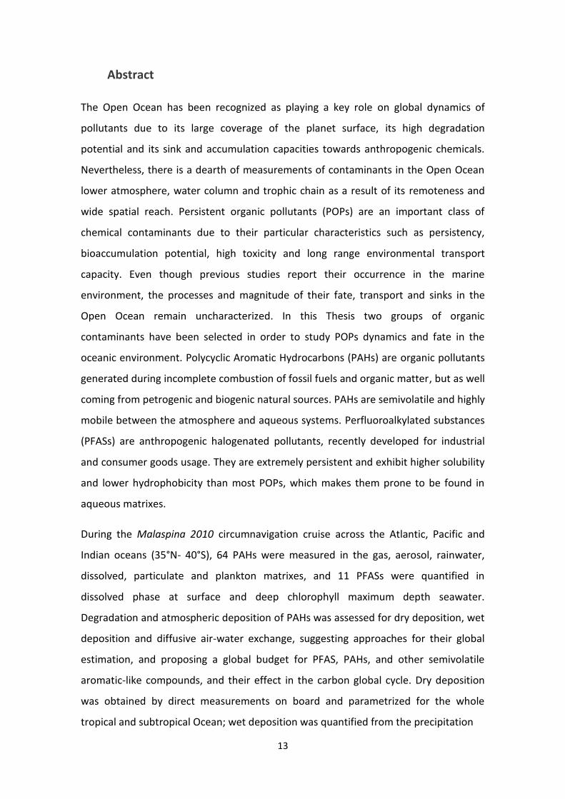
Abstract

The Open Ocean has been recognized as playing a key role on global dynamics of

pollutants due to its large coverage of the planet surface, its high degradation

potential and its sink and accumulation capacities towards anthropogenic chemicals.

Nevertheless, there is a dearth of measurements of contaminants in the Open Ocean

lower atmosphere, water column and trophic chain as a result of its remoteness and

wide spatial reach. Persistent organic pollutants (POPs) are an important class of

chemical contaminants due to their particular characteristics such as persistency,

bioaccumulation potential, high toxicity and long range environmental transport

capacity. Even though previous studies report their occurrence in the marine

environment, the processes and magnitude of their fate, transport and sinks in the

Open Ocean remain uncharacterized. In this Thesis two groups of organic

contaminants have been selected in order to study POPs dynamics and fate in the

oceanic environment. Polycyclic Aromatic Hydrocarbons (PAHs) are organic pollutants

generated during incomplete combustion of fossil fuels and organic matter, but as well

coming from petrogenic and biogenic natural sources. PAHs are semivolatile and highly

mobile between the atmosphere and aqueous systems. Perfluoroalkylated substances

(PFASs) are anthropogenic halogenated pollutants, recently developed for industrial

and consumer goods usage. They are extremely persistent and exhibit higher solubility

and lower hydrophobicity than most POPs, which makes them prone to be found in

aqueous matrixes.

During the Malaspina 2010 circumnavigation cruise across the Atlantic, Pacific and

Indian oceans (35°N- 40°S), 64 PAHs were measured in the gas, aerosol, rainwater,

dissolved, particulate and plankton matrixes, and 11 PFASs were quantified in

dissolved phase at surface and deep chlorophyll maximum depth seawater.

Degradation and atmospheric deposition of PAHs was assessed for dry deposition, wet

deposition and diffusive air-water exchange, suggesting approaches for their global

estimation, and proposing a global budget for PFAS, PAHs, and other semivolatile

aromatic-like compounds, and their effect in the carbon global cycle. Dry deposition

was obtained by direct measurements on board and parametrized for the whole

tropical and subtropical Ocean; wet deposition was quantified from the precipitation

14

rainwater gathered during the cruise; and diffusive exchange was calculated from the

measured PAHs concentrations in the gas and dissolved phases, concurrently with the

environmental parameters affecting volatilization and absorption (temperature, wind

speed, salinity, dissolved organic carbon among others). Moreover, vertical

distribution processes and influencing parameters in the surface mixed layer of the

water column were assessed for PAHs and PFASs. Processes evaluated for PAHs

include the vertical fluxes associated to the organic matter sinking (biological pump),

biomass dilution, planktonic degradation, and air-water-particle exchange. For PFASs,

the biological pump and eddy diffusive fluxes (based on turbulence eddy diffusion

coefficients measured concurrently to the PFASs sampling) were assessed empirically

for the first time in literature. The analysis of the complex feedback established

between atmospheric depositional fluxes and the diffusive, degradative and biological

pumps fluxes in the marine water column at a global scale is also covered.

Furthermore, a wide array of understudied environmental parameters are reviewed as

plausible factors affecting POPs fate in the Open Ocean, and a proposal of the research

directions to follow and missing gaps to be filled is done. Amongst the innovative

outcomes of this study, it can be highlighted the comprehensive sampling covering the

tropical and subtropical global oceans, and the large amount of experimentally

determined processes and influencing factors in order to better understand the global

fate of chemical organic pollutants in the Open Ocean.

15

Resumen

El Océano Abierto está reconocido como un ambiente clave en la dinámica global de la

contaminación debido a que representa un gran porcentaje de la superficie terrestre,

su alto potencial de degradación y su capacidad como sumidero de sustancias químicas

antropogénicas. A pesar de ello, hay una carencia de medidas de contaminantes en la

atmósfera, la columna de agua y el plancton oceánico como resultado de su difícil

acceso y amplitud espacial. Los contaminantes orgánicos persistentes (COP) son un

importante grupo de contaminantes químicos caracterizados por ser persistentes,

bioacumulables, tóxicos y susceptibles de sufrir transporte a larga distancia. Aunque

estudios previos documentan su existencia en el medio ambiente marino, los procesos

y la magnitud de su comportamiento, capacidad de transporte y sumidero en el

Océano abierto no están caracterizados. En esta Tesis dos grupos de contaminantes

orgánicos han sido seleccionados para ilustrar la dinámica de los COP y su destino en el

medio ambiente oceánico. Los hidrocarburos aromáticos policíclicos (PAHs, por sus

siglas en inglés) son contaminantes orgánicos generados durante la combustión

incompleta de combustibles fósiles y de materia orgánica, o provenientes de fuentes

petrogénicas o biogénicas naturales. Son semivolátiles y altamente móviles entre la

atmósfera y los sistemas acuosas debido a sus propiedades fisicoquímicas Las

sustancias perfluoroalquiladas (PFASs, por sus siglas en inglés) son contaminantes

halogenados antropogénicos emergentes desarrollados recientemente para usos

industriales y en productos de consumo. Son extremadamente persistentes y exhiben

mayor solubilidad y menor hidrofobicidad que otros COP, lo que les hace susceptibles

de hallarse en matrices acuosas.

Durante la campaña de circunnavegación Malaspina 2010 a través de los océanos

Atlántico, Pacífico e Índico (35°N- 40°S), se midieron 64 PAHs en las matrices gas,

aerosol, agua de lluvia, disuelto, particulado y en el plancton; y 11 PFAS se

cuantificaron en la fase disuelta de agua marina superficial y de la profundidad del

máximo de clorofila. La degradación y la deposición atmosférica de los PAHs se

evaluaron mediante las medidas de deposición seca, deposición húmeda e intercambio

difusivo aire-agua, sugiriéndose métodos para su cuantificación global y

proponiéndose un cómputo global para estos contaminantes y otros compuestos

16

semivolátiles aromáticos, así como su efecto en el ciclo del carbono. La deposición seca

se obtuvo directamente de medidas durante la campaña y fue parametrizada para

todo el Océano tropical y subtropical; la deposición húmeda se cuantificó con agua de

lluvia recogida durante la navegación; y el intercambio difusivo se estimó con las

concentraciones de PAHs de las fases gas y disuelta, medidas simultáneamente con

parámetros ambientales que afectan a la volatilización y la absorción de estos

compuestos (temperatura, velocidad del viento, salinidad y carbono orgánico disuelto,

entre otras). Asimismo, se midieron los procesos de distribución vertical y los

parámetros que afectan a las concentraciones de PAHs y PFASs en la capa de mezcla

superficial de la columna de agua. Los procesos examinados para PAHs incluyen los

flujos verticales asociados con la sedimentación de materia orgánica (bomba

biológica), la biodilución, la degradación planctónica, y el equilibrio aire-agua-partícula.

Para las PFASs, la bomba biológica y los flujos difusivos turbulentos (basados en

medidas de los coeficientes de difusión turbulenta simultáneas con el muestreo de

PFASs) fueron medidos empíricamente por primera vez en la literatura. El análisis de

los complejos efectos retroactivos establecidos entre los flujos de deposición y los

procesos de degradación, difusión y la bomba biológica a escala global también ha sido

abordado. De la misma forma, un amplio espectro de parámetros ambientales se ha

revisado para dilucidar posibles factores que pudieran afectar al destino de los COP en

el Océano Abierto, y se proponen una serie de líneas de investigación y necesidades

prioritarias para su futura investigación. Entre los aspectos más innovadores de esta

Tesis destacan la enorme cobertura espacial del Océano Global en sus zonas tropicales

y subtropicales, y la gran cantidad de procesos de transporte determinados de manera

empírica junto a sus factores determinantes, con el objeto de poder mejorar el

conocimiento sobre el comportamiento y destino final de los contaminantes químicos

orgánicos en el Océano Abierto.

17

Resum

L'Oceà Obert s'ha descrit com un ambient clau en la dinàmica global de la

contaminació degut al seu gran percentatge de cobertura de la superfície terrestre, el

seu alt potencial de degradació i la seva capacitat com a embornal i acumulador de

substàncies químiques antropogèniques. Tot i això, hi ha una manca de mesures de

contaminants a l'atmosfera, a la columna d'aigua i al plàncton oceànic com a resultat

del seu difícil accés i de l’amplitud espacial. Els contaminants orgànics persistents

(COP) són substàncies químiques no degradables, bioacumulatives, tòxiques per als

humans i els ecosistemes, i susceptibles de patir transport a llarga distància. Encara

que hi ha estudis previs que reporten la seva existència en el medi ambient marí, els

processos i la magnitud del seu transport i embornal en l'Oceà Obert no està

caracteritzada. En aquesta tesi dos exemples de grups de contaminants orgànics han

estat seleccionats per il·lustrar la dinàmica dels COP i el seu destí en el medi ambient

oceànic. Els hidrocarburs aromàtics policíclics (PAHs) són contaminants orgànics

generats durant la combustió incompleta de combustibles fòssils i de matèria orgànica,

o provinents de fonts petrogèniques o biogèniques naturals. Tot i que els PAHs no són

considerats COP ja que són degradables en el medi, han estat descrits com nocius per

als ecosistemes, es troben de manera ubiqua en el medi ambient i mostren nivells

creixents en algunes regions a causa de l'augment de les seves fonts antropogèniques.

Són compostos semivolàtils, altament mòbils entre l'aire i l'aigua com a resultat de les

seves característiques fisicoquímiques. Les substàncies perfluoroalquilades (PFASs) són

contaminants halogenats antropogènics de recent creació per al seu ús industrial i en

productes de consum com aïllants i tensioactius. Són extremadament persistents i

exhibeixen major solubilitat i menor hidrofobicitat que altres COP, fet que els fa

susceptibles de trobar-se en matrius aquoses.

Durant la campanya de circumnavegació Malaspina 2010 a través dels oceans Atlàntic,

Pacífic i Índic (35 ° N-40 ° S), 64 PAHs van ser mesurats en les matrius; gas, aerosol,

aigua de pluja, fracció dissolta, fracció particulada i en el plàncton, i 11 PFASs van ser

identificats en la fase dissolta d'aigua marina superficial i de la profunditat del màxim

de clorofil·la. La degradació i la deposició atmosfèrica dels PAHs van ser avaluades

mitjançant la mesura de la deposició seca, deposició humida i Intercanvi difusiu aire-

18

aigua, suggerint mètodes per a la seva quantificació global i proposant un còmput

global per a aquests contaminants, i altres compostos semivolàtils aromàtics, així com

el seu acoplament amb el cicle del carboni orgànic. La deposició seca es va obtenir

directament de mesures durant la campanya i va ser parametritzada per tot l'Oceà

tropical i subtropical; la deposició humida es va quantificar gràcies a l'aigua de pluja

recollida durant la navegació; i l'Intercanvi difusiu va ser estimat amb les

concentracions dels PAHs mesurades en les fases gas i dissolta, preses simultàniament

amb paràmetres ambientals que afecten la volatilització i l'absorció d'aquests

compostos (temperatura, velocitat del vent, salinitat, carboni orgànic dissolt, entre

d'altres). A més a més, es van mesurar els processos de distribució vertical i els

paràmetres que afectaven a la capa de mescla superficial de la columna d'aigua per als

PAHs i PFASs. Els processos examinats per a PAHs inclouen els fluxos verticals associats

amb la sedimentació de matèria orgànica (bomba biològica), la biodilució, degradació

planctònica, i l'equilibri aire-aigua-partícula. Per a les PFASs, la bomba biològica i els

fluxos difusius turbulents (basats en mesures dels coeficients de difusió turbulenta

simultànies amb el mostreig de PFASs) van ser mesurats empíricament per primera

vegada en la literatura. L'anàlisi dels complexos efectes retroactius establerts entre els

fluxos de deposició i els processos de degradació, difusió i la bomba biològica a escala

global també ha estat abordat. De la mateixa manera, un ampli espectre de

paràmetres ambientals ha estat revisat per dilucidar possibles factors que puguin

afectar al destí dels COP en l'Oceà Obert, i es proposen una sèrie de línies

d'investigació i necessitats prioritàries per a la seva futura investigació. Entre els

aspectes més innovadors d'aquesta tesi es poden destacar l'enorme cobertura espacial

de l'Oceà Global a les seves zones tropicals i subtropicals, i la gran quantitat de

processos de transport determinats de manera empírica juntament amb els seus

factors determinants, per tal de poder identificar el destí final dels contaminants

orgànics persistents en l'Oceà Obert.

19

Chapter 1

General Introduction


20


21

Pollution in the Open Ocean: Persistent Organic Pollutants and “not so

Persistent” Pollutants

The Open Ocean remains as one the most fruitful and unexplored ecosystem on Earth

yet if its extension covers more than three quarters of the Earth’s surface. It provides

the primary source of oxygen to our atmosphere and holds the first place as a sink for

substances like CO2, carbon, and of course, pollutants. Recent studies have dealt with

the resilience capacity of the ocean, and if it would be possible to reach the tipping

point from which its physico-chemical properties and natural biogeochemical cycles

will not sustain life any more 1, 2. Global change threatens in the Ocean are associated

with i) ice melting in the poles and freshening of the oceanic waters, ii) oceanic

currents modification with effects in the heat global transfer, iii) acidification, iv)

ecosystems functioning and biodiversity alterations (both alien species proliferation

and extinction of others) and v) pollution 3.

The chemical alteration of the global Open Ocean has been recently considered for few

emerging issues, like the plastic debris accumulation 4-6 or acidification 7, but other

types of chemical pollution had not been assessed at a planetary scale, even if more

than 2000 organic pollutants have been already reported in marine waters 8.

Moreover, this list is increasing exponentially nowadays with the production and

release of new chemicals with still unknown effects in the environment. Indeed,

chemical risk is one of the global dangers to which we are unaware, according to

Rockstrom et al., who defines it as an earth-system process yet to explore at a global

scale 9.

In order to identify priority chemicals there is an established Risk criteria which

includes i) production volume, ii) usage profile and iii) their physico-chemical

properties 10. Taking into account these premises, there is a particular group of

pollutants that have been classified of major concern, as they fulfill all the

requirements, the so called Persistent Organic Pollutants (POPs). Those are organic

chemicals that:

- Are persistent since they do not degrade over long periods of time once

released into the environment


22

- Bioaccumulate and biomagnify in the trophic chains

- Are toxic to both humans and wildlife

- Are prone to long-range environmental transport (LRET) and deposition

Consequently, POPs pose a threat to the environment and to human health all over

the globe. Due to the international concern regarding these chemicals, the United

Nations Environment Program (UNEP) promoted the adoption in 2001 of the

Stockholm Convention to protect human health and the environment from POPs 11. On

it, 12 priority substances were initially regulated by controlling all their life cycle, from

their production, use and consumption to their removal and waste disposal products.

Nowadays, this list of pesticides, industrial chemicals and unintentional products has

grown, nevertheless, it is still incomplete taking into account the myriads of toxics

fulfilling those requirements released every year to our ecosystems. Other regional

regulatory tools affecting POPs are the United States Environmental Protection

Agency’s (EPA) Toxic Release Inventory 12, the Canadian Environmental Protection Act

13, and The European Union’s regulation on Registration, Evaluation, Authorization,

and Restriction of Chemicals (REACH) 14.

The legacy POPs more extensively studied in the literature are the polychlorinated

biphenyls (PCBs), organochlorinated pesticides (OCPs) such as

dichlorodiphenyltrichloroethane (DDT), hexachlorocyclohexanes (HCHs) and

hexachlorobenzene (HCB) and other by-products of industrial processes or

combustion, such as polychlorinated dibenzo-p-dioxins and dibenzofurans (PCDD/Fs).

Among the new emerging contaminants, defined as chemicals that are not currently or

have been only recently regulated, other halogenated contaminants are arising, like

polybrominated compounds (such as polybrominated diphenyl ethers (PBDEs) and

Dechlorane Plus (DP)) or perfluoroalkylated substances (PFASs). Traditionally, much

attention has been paid as well to the polycyclic aromatic hydrocarbons (PAHs), which

are not as recalcitrant as POPs, but because of their toxicity, bioaccumulation tendency

in low trophic levels (e.g. in plankton), and susceptibility to undergo long-range

atmospheric transport are of great concern globally 15. Indeed, PAHs are not listed in

the Stockholm Convention but are included in the Aarhus Protocol of the United

Nations Economic Commission for Europe (UNECE) 16 and the Convention on Long-


23

Range Transboundary Air Pollution (CLRTAP) 17. Based on the previous considerations,

in this thesis PAHs will be referred to as POPs in its most general sense.

Although the regulations on the use and production of those chemicals and the

potentially new ones launched into the marked, their continuous use and still

unknown toxic effect for the ecosystem’s health requires further research to

understand their fate and behavior in the global environment. Most of the studies

dealing with POPs in the last decades focus on ecotoxicological and health effects and

assess their occurrence at limited regional scales. However, there is a big gap in the

knowledge of POPs global fate 18, even though in the last years some studies are

emphasizing the significance of global dynamics and the role of the ocean on the

global distribution and sink of these pollutants 18, 19.

Environmental Fate and Dynamics of POPs

A combination of local, regional and long range transport is responsible of the POPs

distribution in the global environment. The POPs potential to undergo LRET explains

why they can be found in remote areas, which is even favored by their persistency.

Already in the 60s, the dispersion of halogenated persistent contaminants was

reported 20, 21, and also at that decade, popular concern for these pollutants caused

the “Silent Spring” revolution 22, starting a social movement towards chemical

environmental awareness at global scale supported by the scientific community. Up to

date several studies assessing global transport and accumulation processes to remote

polar and oceanic regions have been undertaken 18, 23-25, suggesting all of them a need

for further research on physico-chemical properties, good monitoring approaches and

global understanding of processes 18, 23, 26.

The distribution of POPs in the environment may occur either in the atmosphere or in

the water systems, or under a combination of both (soils and other environmental

matrixes are considered as reservoirs 27). The presence of POPs in both environmental

compartments is a matter of concern itself, as the uptake from atmosphere and the

water are the two main paths of bioconcentration, and subsequent biomagnification


24

through the trophic chains, leading to a potential risk for wildlife and humans 28.

Moreover, the spread of pollution is accelerated and intensified in these highly

dynamic media.

Figure I.1. Schematic view of POPs processes in the Global Ocean.

The potential fate and behavior of a given contaminant depends on their physico-

chemical properties and environmental variables. It has been reported that

mobilization occurs in pulses of deposition and volatilization, what is called the

“grasshopper effect” 19. In each stage of the cycle, POPs may suffer from different

degradation (like photolysis or OH reactions in the atmosphere, or biodegradation in

soils or the water column) and/or accumulation processes (sequestration by soot in

the atmosphere or bioaccumulation over a food web, for instance) that affects their

occurrence, fate, toxicity and bioavailability. The grasshopper effect is mainly

regulated by temperature and the biological pump, and it is a distillation global process

towards the cold poles, where POPs have been reported to accumulate 29-31.

Nevertheless, other ambient factors like sources, precipitation, organic matter

sorption, or the presence of secondary sources modify the global distribution of POPs.


25

Therefore, the total perspective of processes and their interrelations in the global

Ocean is highly complex (Figure I.1) depending on many environmental factors and

multi-media equilibria.

Atmospheric processes

Most POPs are semivolatile compounds which once released into the environment

distribute over the atmosphere and spread at regional and global scale through a

variety of deposition processes, chemical partition and interchanging fluxes with the

ocean or soils 19, 32, 33. Atmospheric deposition of POPs has been assessed in remote

areas like the Open Ocean and polar seas 34-40 but not on a planetary scale except for

few seminal works 25. The main entrance of POPs to the ocean is reported to be the

atmosphere 41, 42, even if riverine inputs or run-off may be of particular relevance for

some compounds like pesticides and PFASs in coastal areas 43, 44.

The atmospheric deposition processes considered are dry deposition, wet deposition

and air-water diffusive fluxes (Figure I.1). These processes have different relative

importance on pollution loading depending on environmental parameters

(temperature, wind speed, aerosol abundance and organic matter content,

precipitation rates, organic matter content of the surface water, salinity, density, etc.)

and also on the physicochemical properties of the contaminant (volatility, solubility,

hydrophobicity, shoot sorption, etc.). The gas-particle partition of the pollutant will

determine which of the process will have a higher relevance in its total atmospheric

deposition 45. POPs mainly partitioned to aerosols (like PAHs, the more toxic dioxins

and furans, organophosphorus flame retardants and plasticizers, PBDEs and DPs) due

to their low-medium volatility are prone to enter the open ocean via dry deposition.

Contrarily, those POPs mainly found in the gas phase (like volatile PAHs, PCBs and

HCHs) would be more affected by diffusive fluxes between the low atmosphere and

the surface ocean.

Dry deposition in the open ocean consists in the direct load of pollutants adsorbed

onto marine aerosols. The settling of these particles is a generalized process over the

ocean surface, and even if the concentration of aerosols in the remote ocean


26

atmosphere is low there is a continuous production and renewal of these active

elements 46 and their chemical characteristics (organic carbon content) makes them an

effective attaching surface for low vapor pressure POPs. The dry deposition flux had

been poorly described in the open ocean so far, being only characterized in the

Mediterranean Sea 47-49 and some parts of the Atlantic Ocean 41, 50, 51. Previous works

described that dry deposition fluxes will depend on the concentration of contaminants

in the aerosol fraction and the velocity of settling of that aerosol (Figure I.2), and may

be affected by wind speed and other physico-chemical properties of the water that

could enhance the aerosol affinity to the oceanic surface. Dry deposition fluxes (FDD)

can be calculated from

FDD = vD·CA [I.1]

where CA is the aerosol phase concentration and vD is the deposition velocity of the

specific aerosol-bound chemical 51.

Figure I.2. Schematic draw of dry deposition.

Wet deposition is associated with the precipitation events that accelerate the entrance

of pollution in the Open Ocean by a “washing process” of the atmosphere. In the

tropical ocean, precipitation is mainly due to rain, but in higher latitudes or coastal

areas fog, snow and hail should be considered as well. It consists on a double step

equilibria: on the one hand each raindrop is chemically equilibrated with the gas phase

concentration of organic pollutants through diffusion, and on the other, the rain

sweeps the suspended particulate matter in the low atmosphere and enhances the

entrance of hydrophobic compounds attached to the aerosol into the open ocean 45.


27

The wet deposition flux (FWD) of POPs into the ocean can be calculated from a two

terms equation,

𝐹𝑊𝐷 = 𝑝0 (𝐶𝐺

𝐻′+ 𝑤𝑝 𝐶𝐴) [I.2]

where p0 is the precipitation rate, and multiplies a “gaseous equilibria” term, based on

the concentration of the pollutant in the gas phase (CG) and the Henry’s Law constant

(H’), and a “scavenging” term, based on the washout ratio (wp) and the concentration

in the aerosol phase (Figure I.3).

Wet deposition is a very relevant entrance pathway of organic pollution to the ocean;

nevertheless it is an episodic event very difficult to extrapolate spatially and

temporally. It is also very intense during the first moments, but once that the fast

removal of pollution has occurred it rapidly dilutes its strength as a transport vector

since the atmosphere has become depleted in POPs. It has been assessed for

compounds like PCBs42, 52, 53, PAHs49, 54, 55 and PFASs56-58, but again limited to regional

areas, and only modeled at a global scale42.

Figure I.3. Schematic draw of wet deposition.

Diffusive exchange between the atmosphere and the surface ocean appears to be the

major diffuse entrance of POPs into the marine environment 42, 59. Among the

interchanging processes it is the most reported one for many legacy halogenated

pollutants 39, 47, 53, 60 and hydrocarbons 61-64 and it is becoming a hot topic for the

emerging contaminants, even if few information in the Open Ocean can be found yet

65-67.


28

The direction of the air-water exchange depends on the fugacity of the chemical in air

and water. Fugacity is the “the escaping tendency” of a substance from a media, and

each POP will exhibit a particular fugacity from air and water according to its chemical

properties and environmental conditions. Therefore the fugacity from the air (fA) and

the fugacity from the water (fW) phases will be,

𝑓𝐴 = 𝐶𝐺 𝑅 𝑇 [I.3]

𝑓𝑊 = 𝐶𝑊 𝐻′𝑅 𝑇 [I.4]

It is based on the concentration of the compound in the matrix (CG in gas or CW in

water), the gases constant R, the dimensionless Henry’s Law constant H’, and on

temperature (T). The net air-water diffusive flux is always from high to low fugacity,

and there is a net equilibrium if air and water POP fugacities are similar in magnitude.

Diffusive fluxes are estimated from a fugacity gradient and a mass transfer coefficient,

which depend on a wide array of environmental parameters. Air-water flux (FAW,

Figure I.4) can be calculated from the concentration of the POP in the air and in the

water as follows,

𝐹𝐴𝑊 = 𝑘𝐴𝑊 (𝐶𝐺

𝐻′− 𝐶𝑊) [I.5]

Where H’ is the Henry’s Law constant of the compound (salinity and temperature

corrected) and kAW is the air-water mass transfer rate. In turn, this rate is estimated

using the two film resistance model, and thus it is dependent on the mass transfer

coefficients in each phase (kA and kW for the air and water, respectively),

1

𝑘𝐴𝑊=

1

𝑘𝐴 𝐻′+

1

𝑘𝑊 [I.6]

To calculate the particular kA and kW of a certain pollutant (kA,POP and kW,POP),

empirically determined coefficients for H2O in the air (kA,H2O)and CO2 in the water

(kW,CO2)are used as comparison standards. Then in the air,

𝑘𝐴,𝑃𝑂𝑃 = 𝑘𝐴,𝐻2𝑂 (𝐷𝐴,𝑃𝑂𝑃

𝐷𝐴,𝐻2𝑂)

0.61

[I.7]


29

being 𝑘𝐴,𝐻2𝑂 = 0.2 𝑈10 + 0.3, where DA is the diffusivity coefficient in the air and U10 is

the wind speed at 10 m height of the air-ocean interphase.

The same way in the water,

𝑘𝑊,𝑃𝑂𝑃 = 𝑘𝑊,𝐶𝑂2 (𝑆𝐶,𝑃𝑂𝑃

𝑆𝐶,𝐶𝑂2)

−0.5

[I.8]

being 𝑘𝑊,𝐶𝑂2 = 0.24 𝑈102 + 0.061 𝑈10 and 𝑆𝐶,𝐶𝑂2 the Schmidt number at 298 K,

related with the diffusion of a substance in a liquid depending on the fluid viscosity,

600 for the CO2.

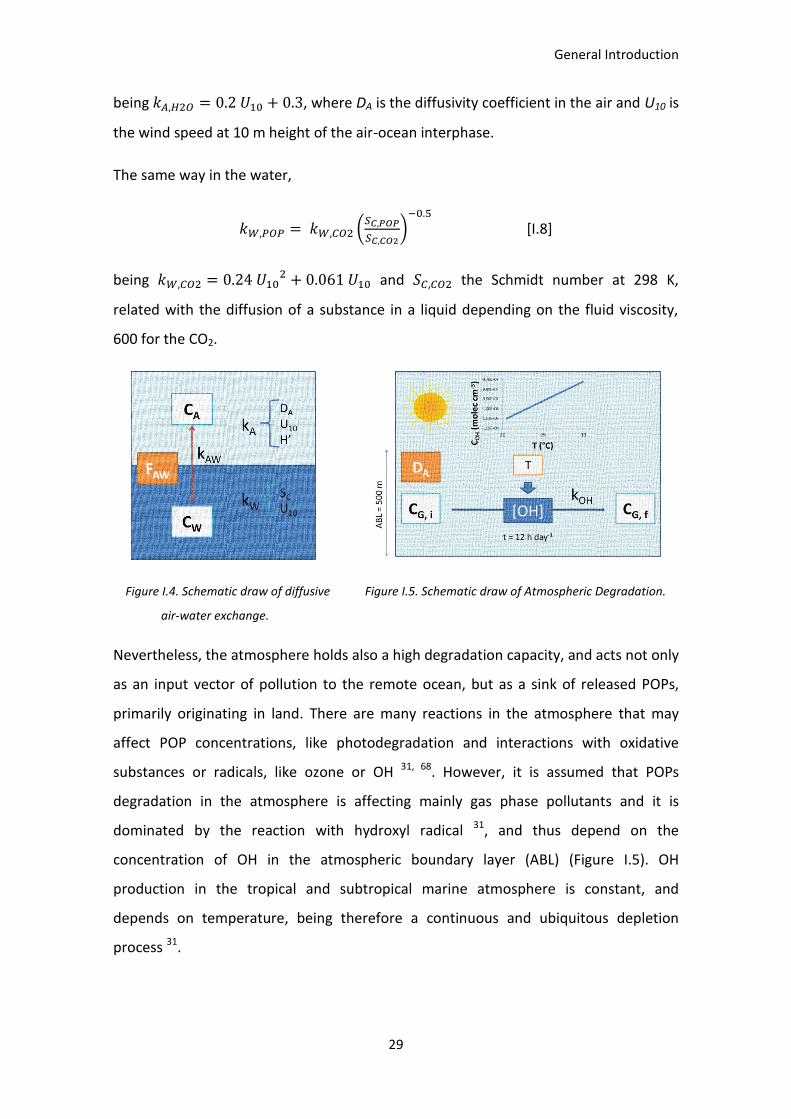
Figure I.4. Schematic draw of diffusive Figure I.5. Schematic draw of Atmospheric Degradation.

air-water exchange.

Nevertheless, the atmosphere holds also a high degradation capacity, and acts not only

as an input vector of pollution to the remote ocean, but as a sink of released POPs,

primarily originating in land. There are many reactions in the atmosphere that may

affect POP concentrations, like photodegradation and interactions with oxidative

substances or radicals, like ozone or OH 31, 68. However, it is assumed that POPs

degradation in the atmosphere is affecting mainly gas phase pollutants and it is

dominated by the reaction with hydroxyl radical 31, and thus depend on the

concentration of OH in the atmospheric boundary layer (ABL) (Figure I.5). OH

production in the tropical and subtropical marine atmosphere is constant, and

depends on temperature, being therefore a continuous and ubiquitous depletion

process 31.


30

Water column processes

There are direct loads of POPs from inland waters via either run-off or through riverine

discharges (Figure I.6). Run-off mainly depends on continental precipitation regimes

(quite important in tropical and subtropical areas), temperature, vegetation cover and

land use, and it has been recently turned into a research topic of interest due to the

suggested future scenarios of climate change 69, 70. Riverine discharge has been more

extensively studied in the past due to the habitual connection between rivers, harbors

and human emplacements, with the consequent effects of POPs on human health and

activities 71-73. Moreover, industrial activities and waste water treatment plants usually

spill in riverine systems affecting as well pollution loading into the coastal marine

environment 74-76. However, POPs entrance through direct coastal inputs has a much

lower effect on the open ocean concentrations when compared to atmospheric inputs

and, thus, those processes are out of the scope of this thesis. Nevertheless, it should

be taken into account that for some POP families, such as PFASs, it has been suggested

that riverine inputs account for a main input to the marine environment 77, 78.

Ocean currents are an effective vector for transport of substances like oxygen 79, salts

80, nutrients 81 and heat 82 at a planetary scale. Equally, organic pollutants prone to be

found in the dissolved water phase (like ionic PFASs) are reported to be affected by

water masses transport 44, 83-85. Nevertheless, most POPs are highly hydrophobic and

semivolatile and it can be assumed that they will not be affected directly by oceanic

circulation, but mainly by atmospheric deposition and other processes, like

phytoplankton blooms in upwelling areas, effects on air-water exchange due to ocean

currents temperature, and organic matter cycling influence on air-water dis-equilibria.

Moreover, the latitudinal area covered in this thesis (tropical and subtropical oceans)

does not include the main marine subduction areas, placed in higher latitudinal strips

85, and therefore this process is out of the scope of this work (Figure I.6).

Dispersion in the deep ocean due to turbulent kinetics is another physical transport

which has received little attention (Figure I.6). It is based on Fick’s laws of diffusion,

which explain diffusion caused by turbulent fluxes 86 by,

𝐹𝐸𝑑𝑑𝑦 = −𝐷 𝜕𝐶𝑤

𝜕𝑧 [I.9]


31

where Cw is the seawater concentration of the target substance, z is depth, and D is the

eddy diffusivity. Diffusivity has been estimated in literature from differences in the

microscale temperature or density of the water 87, 88, being this coefficient is the main

parameter to measure turbulence in the ocean. Turbulence, caused by macro and

micro scale movement of the ocean and wind shear, has been used to explain diffusion

of dissolved substances like nutrients and oxygen in the open ocean 89-91, but up to the

moment has had very low application in POPs distribution 83 and thus it is a research

field yet to explore 87.

Figure I.6. Schematic draw of physical transport processes in the water column.

Interactions of POPs with organic matter in the water column are relevant processes

affecting their fate in the Open Ocean (Figure I.7). POPs are rapidly sorpt onto

particulate organic matter, if not entering the water directly attached to aerosols, and

once there, they are susceptible to suffer physical or biological alteration. Among

these processes; dilution, fast air-water-particle equilibrium, degradation, settling

(biological pump), or bioaccumulation and biomagnification have been described to

modify POPs concentrations in the marine water column and have a plausible effect on

global fate of these compounds18, 23. Studies regarding these processes have been

conducted in lakes and coastal areas92, 93, confined seas64, 94 and in polar regions37, 39, 95,

but for many of these processes there is a lack of a global assessments of their

relevance.


32

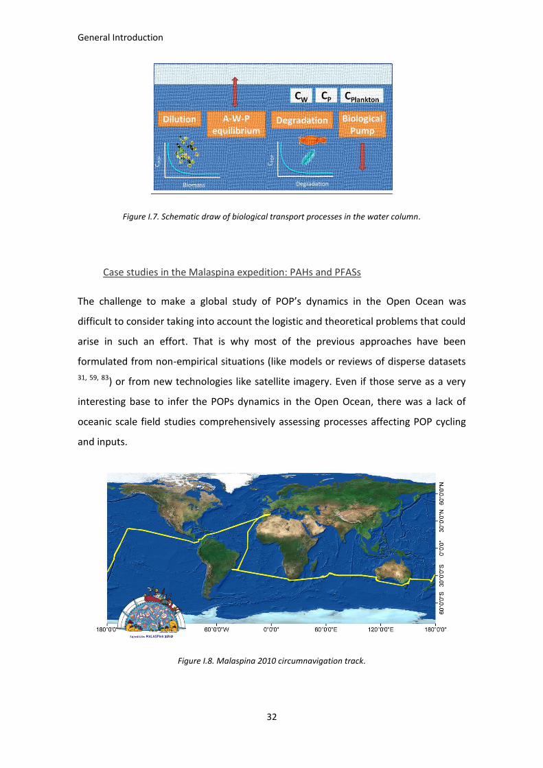
Figure I.7. Schematic draw of biological transport processes in the water column.

Case studies in the Malaspina expedition: PAHs and PFASs

The challenge to make a global study of POP’s dynamics in the Open Ocean was

difficult to consider taking into account the logistic and theoretical problems that could

arise in such an effort. That is why most of the previous approaches have been

formulated from non-empirical situations (like models or reviews of disperse datasets

31, 59, 83) or from new technologies like satellite imagery. Even if those serve as a very

interesting base to infer the POPs dynamics in the Open Ocean, there was a lack of

oceanic scale field studies comprehensively assessing processes affecting POP cycling

and inputs.

Figure I.8. Malaspina 2010 circumnavigation track.


33

The Malaspina 2010 circumnavigation cruise (Figure I.8) was an optimal framework to

hold such an ambitious objective. This interdisciplinary project linked many of the

oceanographic sciences, like physical oceanography, biogeochemistry, chemical

pollution, optics, phytoplankton science (production and metabolism), microbial

biodiversity and functions and zooplankton science among others. This conjunction

created myriads of measurements and data sets that could be interrelated in order to

get a holistic view of the Global Ocean. It lasted 7 months and crossed all the tropical

and subtropical oceans between 40° North and 30° South, making it possible to

measure concentrations and fluxes of the pollutants of interest all around the globe

with a daily resolution. By crossing this information with other measured parameters

during the circumnavigation (like chemical properties or meteorological data) it is

possible to infer the potential influence of some processes not evaluated so far in the

field in terms of POP cycling.

The key processes of distribution and interchange between the atmosphere and the

water surface were evaluated for the main POPs families during the development of

this work, like dioxins, PCBs and some halogenated pesticides. Nevertheless, in this

thesis, two particular groups of organic pollutants, PAHs and PFASs, were selected as

target contaminants to asses POPs dynamics and fate in the open ocean. The first are

semivolatile compounds (considered together with POPs even if they are susceptible

to degradation) with a wide range of volatility and hydrophobicity, what makes them

very interesting in order to asses atmosphere- seawater exchange. The second, PFASs,

are ionic emerging POPs whose chemical characteristics (like much lower

hydrophobicity compared with other POPs, and non-volatility) will serve as an example

to show processes of mobility and diffusion within the water column in the Open sea.


34

Polycyclic Aromatic Hydrocarbons (PAHs)

Polycyclic Aromatic Hydrocarbons are

probably the more abundant and widely

distributed carcinogens in the Earth 96, and

they are present in our proximate

environments 15, 97 but also in remote areas

like the open ocean and polar regions 98 36,

99-101. They come mainly from incomplete

combustion of fossil fuels and organic

matter and are related as well to

petrogenic and biogenic processes. Even if

they have been described to be occurring naturally, due to wildfires, volcanoes 102 and

organic matter degradation in soils 103, the predominant vies is that the main actual

global emission is due to anthropogenic activities, being biofuel consumption the main

global source and the principal producing countries China (114 Gg y-1), India (90 Gg y-1)

and United States (32 Gg y-1) (Figures I.9 and I.10) 104.

Figure I.10. National annual emissions rate of EPA’s 16 regulated PAHs (modified from Zang et al 2009).

The EPA suggested a priority list of 16 compounds (those indicated in Figures I.9 and

I.10 and Table I.1) as of particular toxicological and environmental concern. Among

them, there are the seven PAH compounds classified as probable human carcinogens:

benzo[a]anthracene, benzo[a]pyrene, benzo[b]fluoranthene, benzo[k]fluoranthene,

chrysene, dibenz[a,h]anthracene, and indeno[1,2,3-cd]pyrene 12. The persistence and

Figure I.9. PAHs global production (modified

from Zang et al. 2009).


35

toxicity of PAHs is related with the MW (Table I.1) and with the isomeric structure 105.

However, the higher occurrence of other non-as-toxic compounds or those having a

bigger LRET potential make other PAHs of high interest as well. The chemical

properties of each considered PAH in this thesis are included in Table I.1 and show the

wide range of volatility, hydrophobicity, and persistence these compounds may

exhibit. Indeed, the reported array of their semi volatility and partitioning tendency to

soot and organic carbon, makes PAHs as a good case study of organic pollutants being

subject to a number of different biotic and abiotic processes, and for assessing global

transport and exchange between air-water-biota in the open ocean.


36

Table I.1. PAHs physicochemical properties

MW

[g mol-1

]

Log

KOA

Log

KOW

KOH

[cm-3

molec-1

s-1

]

-∆H

[kJ

mol-1

]

∆S

[kJ

mol-1

K-1

]

Naphthalene*

128 5.1a 3.33

i 1.9 10

-11 -19.29

d 0.054

d

Methyl-

naphthalenes 142 5.79

b 3.87

j 4.1 10

-11 -42.4

m 0.11

m

Dimethyl-

naphthalenes 156

4.42

j 6 10

-11 -48.69

d

Acenaphtylene*

152 6.52 c 3.62

i 1.1 10

-10 -52.2

m 0.131

m

Acenaphtene*

153 6.31 d 3.92

i 5.8 10

-11 -51.9

m 0.133

m

Fluorene*

166 6.83 d 4.21

i 1.3 10

-11 -48.8

m 0.118

m

Dibenzothiophene

184 7.24 e 4.38

k 1.4 10

-11 -21.6

n 0.056

o

Methyl-

dibenzothiophenes 198

1.3 10

-11

Dimethyl-

dibenzothiophenes 212

Phenanthrene*

178 7.22 e 4.57

i 1.3 10

-11 -47.3

m 0.106

m

Methyl-

phenanthrenes

192 7.49 e 4.99

i 8 10

-12 -35.4

m 0.067

m

Dimethyl-

phenanthrenes

206 8.03 e

7.7 10

-12

Anthracene*

178 7.55 d 4.68

i 1.1 10

-11 -46.8

m 0.106

m

Fluoranthene*

202 8.61 d 5.23

i 9.1 10

-12 -38.7

m 0.07

m

Pyrene*

202 8.75 d 5.11

i 8.6 10

-12 -42.9

m 0.084

m

Methyl-pyrenes

216

5.45

i


37

Dimethyl-pyrenes

230

Benzo[ghi]

fluoranthene

226

-5.35 n

Benzo[a]

anthracene* 228 9.5

a 5.91

i 6.9 10

-12 -66.4

m 0.159

m

Chrysene*

228 10.4 a 5.81

i 7.7 10

-12 -100.9

m 0.268

m

Methyl-chrysenes

242

Benzo[b]

fluoranthene*

252 11.19 f 6.2

i

-19.6

n 0.056

d

Benzo[k]

fluoranthene* 252 11.19

f 6.2

i

-19.6

n 0.056

d

Benzo[e] pyrene

252 11.13 f 6.12

i

-16.57

d 0.036

d

Benzo[a] pyrene*

252 11.56

g 6.13

i

-25.61

d 0.032

d

Perylene

252 11.7 h 5.84

i

-31.88

d 0.057

d

Indeno[1,2,3-cd]

pyrene*

276 12.43 g 6.65

i

-21.51

d 0.056

d

Dibenzo[a,h]

anthracene* 278 12.59

g 6.86

i

-31.16

d 0.057

d

Benzo[ghi]

perylene*

276 12.55 g 6.22

i

-17.37

d 0.031

d

a Wania & Mackay 1996,

b Hiatt 2014,

c Ma et al 2010,

d Mackay book 2006,

e Lehndorff and Schwark

2009, f Finizio et al. 1997,

g Odabasi 2006,

h Mackay and Callcot 1998,

i Bukhard EST 2000,

j Mackay book

1992, k Blum et al 2011,

l Keyte et al 2013,

m Bamford 1999,

n Acree and Chickos 2010,

o Ramirez-

Verduzco et al 2007. *included in the EPA priority list.


38

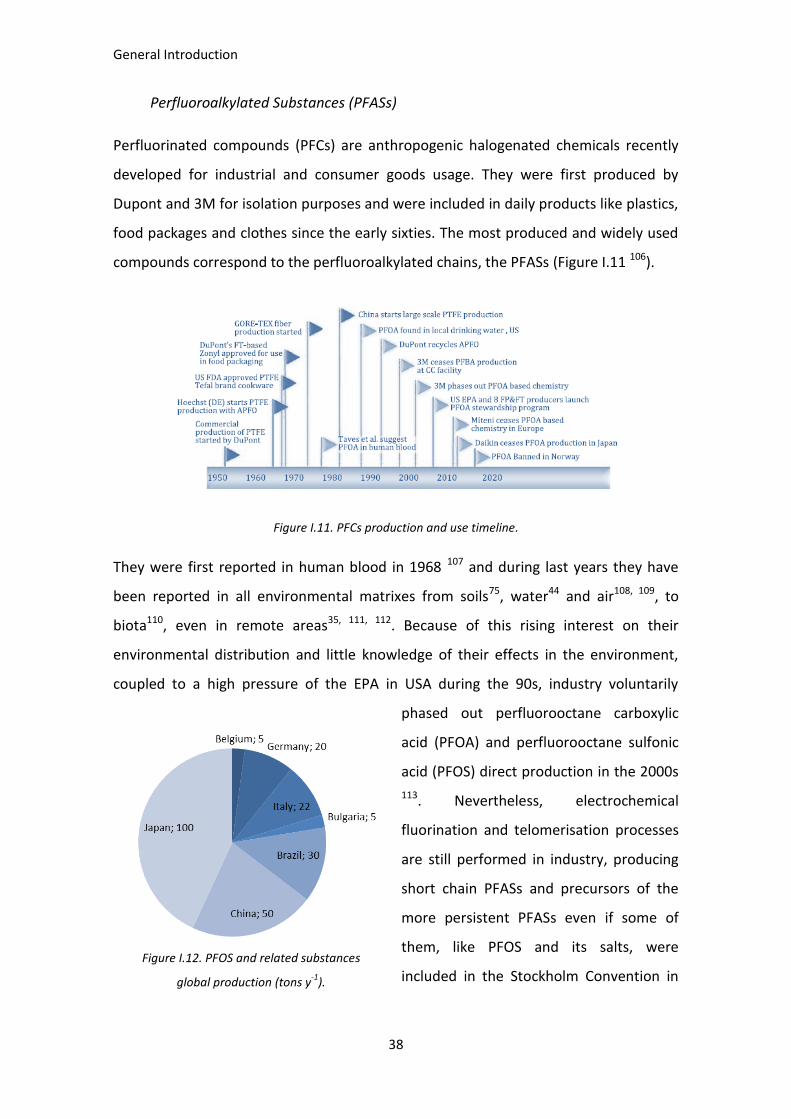
Perfluoroalkylated Substances (PFASs)

Perfluorinated compounds (PFCs) are anthropogenic halogenated chemicals recently

developed for industrial and consumer goods usage. They were first produced by

Dupont and 3M for isolation purposes and were included in daily products like plastics,

food packages and clothes since the early sixties. The most produced and widely used

compounds correspond to the perfluoroalkylated chains, the PFASs (Figure I.11 106).

Figure I.11. PFCs production and use timeline.

They were first reported in human blood in 1968 107 and during last years they have

been reported in all environmental matrixes from soils75, water44 and air108, 109, to

biota110, even in remote areas35, 111, 112. Because of this rising interest on their

environmental distribution and little knowledge of their effects in the environment,

coupled to a high pressure of the EPA in USA during the 90s, industry voluntarily

phased out perfluorooctane carboxylic

acid (PFOA) and perfluorooctane sulfonic

acid (PFOS) direct production in the 2000s

113. Nevertheless, electrochemical

fluorination and telomerisation processes

are still performed in industry, producing

short chain PFASs and precursors of the

more persistent PFASs even if some of

them, like PFOS and its salts, were

included in the Stockholm Convention in Figure I.12. PFOS and related substances

global production (tons y-1

).


39

2009 114. There is little information about the generating volume of the producing

countries and emplacement of the sources. The more complete studies found to date

are the Organization for Economic Cooperation and Development (OECD) reports in

which only direct production of PFOS is compulsory informed for some countries, but

not for other fluorinated compounds extensively used in pesticides formulations,

firefighting foams, photographic industry and aviation industry 115. According to the

report from 2009, the top annual producers in 2003 were Japan, China and Brazil

(Figure I.12), even if previous to that year USA was by far the main producer and

consumer reaching in year 2000 more than 3500 tons of annual production 113.

PFASs consist on a fully fluorinated carbon chain, which makes them highly stable due

to the strong fluoride-carbon bond, and an alkylated ionic “head” which gives them the

amphipathic character. In particular PFOS and PFOA, the 8 carbons (C) sulphonic acid

and carboxylic acid, respectively, have been reported all over the planet in all kind of

environmental matrixes 44, 110, 116-119. These ionic families, perfluoroalkylated sulfonic

and carboxylic acids (PFSAs and PFCAs, respectively) are the more persistent and toxic

among the PFASs, and even if long chain and 8C compounds are raising general

concern, shorter chain compounds are still being used in the growing industry of

surfactants 44. Among the neutral PFASs, fluorotelomer alcohols, sulfonamides

(PFASAs) and fluorotelomer aldehydes are the more relevant precursors of PFSAs and

PFCAs 114, and recently they have become also target pollutants in environmental

research as they are more volatile and have high LRET potential 74, 108, 120-122. In this

thesis, PFSAs, PFCAs and PFASAs were selected for assessing their occurrence and

cycling in the Open Ocean. Their properties affecting chemical dynamics are

summarized in Table I.2. Of special interest is the fact that they have a particular

organic matter affinity, as they are not as lipophilic as other POPs but they have been

described as proteinophilic 123. There are few studies reporting their occurrence in the

open ocean at big spatial scale 35, 112, 124-126, even less giving concentrations through the

deep water column 84 and none to date assessing their fate in the open ocean relating

them with organic matter cycling. Therefore the data provided in this thesis are novel

and of high interest for the better understanding of these pollutants in the remote

Oceanic environment.


40

Table I.2. PFASs physicochemical properties.

Compound Acronym Molecule Chain

length (n) MW

[g mol-1] Log

KOA127

Log KOW

127 Log

KPW127

BAF128

Perfluoro-1-octanesulfonamide

PFOSA

7 498 8.4 6.3 -

N-methylperfluoro-1-octansulfonamide

N-MePFOSA 7 512

Perfluoro-n-butanoic acid PFBA

3

Perfluoro-n-pentanoic acid PFPA 4

Perfluoro-n-hexanoic acid PFHxA 5 312

Perfluoro-n-heptanoic acid PFHpA 6 363 5.9 3.8 2

Perfluoro-n-octanoic acid PFOA 7 413 6.3 4.6 2.5 292

Perfluoro-n-nonanoic acid PFNA 8 463 6.6 5.5 3.1 1650

Perfluoro-n-decanoic acid PFDA 9 512 6.8 6.4 3.8 765

Perfluoro-n-undecanoic acid PFUnDA 10

7.1 7.4 4.5

Perfluoro-n-dodecanoic acid PFDoDA 11

7.4 8.1 5

Perfluoro-n-tridecanoic acid PFTrDA 12

8.8 9 5.6

Perfluoro-n-tetradecanoic acid PFTeDA 13

Perfluoro-n-hexadecanoic acid PFHxDA 15

Perfluoro-n-octadecanoic acid PFODA 17

Perfluoro-butanesulfonate PFBS

3 298

Perfluoro-hexanesulfonate PFHxS 5 399

58

Perfluoro-heptanesulfonate PFHpS 6 449

Perfluoro-octanesulfonate PFOS 7 499 7.8 5.3 3 169

Perfluoro-decanesulfonate PFDS 9

Perfluoro-dodecanesulfonate PFDoDS 11


41

Aim and Outline of this thesis

The general aim of this thesis is to assess the occurrence of POPs cycling in the global

tropical and subtropical Open Oceans, focusing on PAHs and PFASs.

The specific objectives are

- To determine PAHs occurrence in gas, aerosol, dissolved, particulate and

planktonic phases, and PFAS in dissolved phase from the global Open Ocean.

- To quantify POPs fluxes between the different environmental compartments.

- To study physical and trophic factors that affect POPs entrance in the plankton.

- To evaluate the relevance of semivolatile aromatic hydrocarbons (containing

PAHs and other aromatic compounds) as a source of semivolatile organic

carbon to the ocean.

The results obtained are presented in different chapters, depending on the

contaminant family and the processes evaluated, as briefly described below:


42

Chapter 1: Field measurements of the Atmospheric Dry Deposition Fluxes and Velocities

of Polycyclic Aromatic Hydrocarbons to the Global Oceans. Published in Environmental

Science and Technology, 2014.

In the first chapter, as illustrated in Figure I.13, the empirical measurements of PAHs

dry deposition done during the Malaspina 2010 circumnavigation cruise are presented.

PAHs velocities of deposition in coarse and fine aerosol are obtained separately and at

a global scale resolution. Moreover, the directly quantified fluxes measured

concurrently with other physicochemical and meteorological parameters, allowed to

suggest an empirical parametrization of the velocity of deposition. The given equation

allow to predict the dry depositional velocities of semivolatile organic compounds to

the global Oceans by measuring the target compound concentration in the aerosol

phase, its vapor pressure, the wind speed and the chlorophyll concentration of the

water where the aerosol is deposing.

Figure I.13. Schematic view of processes evaluated in Chapter 1.


43

Chapter 2: High Atmosphere-Ocean Exchange of Semivolatile Aromatic Hydrocarbons.

Submitted.

This Chapter describes all the measured and calculated depositional fluxes and fading

processes in the atmospheric boundary layer over the tropical and subtropical global

Oceans (Figure I.14). Diffusive exchange, wet deposition, dry deposition and

atmospheric degradation (OH radical oxidation) are calculated from the measured 64

PAHs congener’s concentrations in the gas, aerosol, rainwater and dissolved phases in

the Open Ocean. Furthermore, an estimation of the semivolatile aromatic-like

compounds (SALCs) concentration is done in the gaseous and dissolved phases and the

diffusive exchange for them is calculated, as it appeared to be the highest magnitude

flux affecting their fate. An estimation of the total carbon entrance to the Open Ocean

due to these organic compounds, PAHs and SALCs, is also emphasized in order to

suggest their account in the global carbon budgets calculations.



44

Chapter 3: Perfluoroalkylated Substances in the Global Tropical and Subtropical Surface

Oceans. Published in Environmental Science and Technology, 2014.

PFASs occurrence in surface ocean waters is reported in this Chapter for the Atlantic,

Indian and Pacific oceans. Eleven congeners of two ionic families (perfluoroalkyl

carboxylic acids and perfluoroalkyl sulfonic acids) and two neutral precursors

(perfluoroalkyl sulfonamides) were identified and quantified. Their global occurrence

and the potential factors affecting their distribution patterns are discussed including

the distance to coastal regions, oceanic subtropical gyres, currents and biogeochemical

processes.

Figure I.15. Schematic view of processes evaluated Chapter 3.


45

Chapter 4: Oceanic Transport and Sinks of Perfluoroalkylated Substances. To be

submitted.

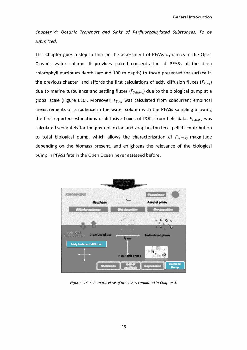
This Chapter goes a step further on the assessment of PFASs dynamics in the Open

Ocean’s water column. It provides paired concentration of PFASs at the deep

chlorophyll maximum depth (around 100 m depth) to those presented for surface in

the previous chapter, and affords the first calculations of eddy diffusion fluxes (FEddy)

due to marine turbulence and settling fluxes (FSettling) due to the biological pump at a

global scale (Figure I.16). Moreover, FEddy was calculated from concurrent empirical

measurements of turbulence in the water column with the PFASs sampling allowing

the first reported estimations of diffusive fluxes of POPs from field data. FSettling was

calculated separately for the phytoplankton and zooplankton fecal pellets contribution

to total biological pump, which allows the characterization of FSettling magnitude

depending on the biomass present, and enlightens the relevance of the biological

pump in PFASs fate in the Open Ocean never assessed before.



46

Chapter 5: Cycling of Polycyclic Aromatic Hydrocarbons in the Surface Open Ocean. In

preparation.

The role of plankton and organic suspended particles in PAHs distribution and fate in

the Open Ocean is an unresolved issue. In this Chapter it is described the measured

PAHs concentration in the dissolved, particulate and plankton phases during the

Malaspina 2010 circumnavigation. Concentration dependence on organic carbon and

physicochemical properties of the PAHs (particularly hydrophobicity) is evaluated.

Furthermore, a review of the previously suggested processes regulating PAH

concentrations in the water column is done, including biodilution, air-water-particle

equilibria, and the degradative and biological pumps (Figure I.17). This last is calculated

separately for the zooplankton and phytoplankton sinking matter, for the first time in

literature, allowing an estimation of the sinking fluxes of PAHs in the Open Ocean and

suggesting directions for future research.



47

REFERENCES

1. Hughes, T. P.; Bellwood, D. R.; Folke, C.; Steneck, R. S.; Wilson, J., New paradigms for supporting the resilience of marine ecosystems. Trends in Ecology & Evolution 2005, 20, (7), 380-386. 2. Côté, I. M.; Darling, E. S., Rethinking ecosystem resilience in the face of climate change. PLoS biology 2010, 8, (7), e1000438. 3. Doney, S. C.; Ruckelshaus, M.; Emmett Duffy, J.; Barry, J. P.; Chan, F.; English, C. A.; Galindo, H. M.; Grebmeier, J. M.; Hollowed, A. B.; Knowlton, N.; Polovina, J.; Rabalais, N. N.; Sydeman, W. J.; Talley, L. D., Climate Change Impacts on Marine Ecosystems. Annual Review of Marine Science 2012, 4, (1), 11-37. 4. Cózar, A.; Echevarría, F.; González-Gordillo, J. I.; Irigoien, X.; Úbeda, B.; Hernández-León, S.; Palma, Á. T.; Navarro, S.; García-de-Lomas, J.; Ruiz, A.; Fernández-de-Puelles, M. L.; Duarte, C. M., Plastic debris in the open ocean. Proceedings of the National Academy of Sciences of the United States of America 2014, 111, (28), 10239-10244. 5. Andrady, A. L., Microplastics in the marine environment. Marine Pollution Bulletin 2011, 62, (8), 1596-1605. 6. Law, K. L.; Moret-Ferguson, S.; Maximenko, N. A.; Proskurowski, G.; Peacock, E. E.; Hafner, J.; Reddy, C. M., Plastic accumulation in the North Atlantic subtropical gyre. Science 2010, 329, (5996), 1185-8. 7. McCulloch, M.; Falter, J.; Trotter, J.; Montagna, P., Coral resilience to ocean acidification and global warming through pH up-regulation. Nature Climate Change 2012, 2, (8), 623-627. 8. Dachs, J.; Méjanelle, L., Organic Pollutants in Coastal Waters, Sediments, and Biota: A Relevant Driver for Ecosystems During the Anthropocene? Estuaries and Coasts 2010, 33, (1), 1-14. 9. Rockstrom, J.; Steffen, W.; Noone, K.; Persson, A.; Chapin, F. S.; Lambin, E. F.; Lenton, T. M.; Scheffer, M.; Folke, C.; Schellnhuber, H. J.; Nykvist, B.; de Wit, C. A.; Hughes, T.; van der Leeuw, S.; Rodhe, H.; Sorlin, S.; Snyder, P. K.; Costanza, R.; Svedin, U.; Falkenmark, M.; Karlberg, L.; Corell, R. W.; Fabry, V. J.; Hansen, J.; Walker, B.; Liverman, D.; Richardson, K.; Crutzen, P.; Foley, J. A., A safe operating space for humanity. Nature 2009, 461, (7263), 472-475. 10. (ECHA), E. C. A., EU criteria for risk assessment of persistance, bioaccumulation and toxicity of chemicals. In European Parliament and of the Council on the Registration, E., Authorisation and Restriction of Chemicals (REACH), Ed. Official Journal of the European Union, 2014. 11. UNEP, U. N. E. P., Report of the Conference of the Parties of the Stockholm Convention on Persistent Organic Pollutants on the work of its fourth meeting. In United Nations Environment Programme: Stockholm Convention on Persistent Organic Pollutants. Geneva, 2009; p p. 112. 12. EPA Toxic Release Inventory Program. (2015). 13. Canada, G. o. Canadian Environmental Protection Act. 14. Agency, E. C. Registration, Evaluation, Authorization, and Restriction of Chemicals (REACH) Program. 15. Menzie, C. A.; Potocki, B. B.; Santodonato, J., Exposure to carcinogenic PAHs in the environment. Environmental science & technology 1992, 26, (7), 1278-1284. 16. UNECE The 1998 Aarhus Protocol on Persistant Organic Pollutants (POPs). 17. UNECE, Protocol to the 1979 Convention on Long Range Transboundary Air Pollution on Persistent Organic Pollutants (POPs). In Europe, U. N. E. C. f., Ed. UN: http://www.unece.org/env/lrtap/pops_h1.html, 1998.


48

18. Lohmann, R.; Breivik, K.; Dachs, J.; Muir, D., Global fate of POPs: Current and future research directions. Environmental Pollution 2007, 150, (1), 150-165. 19. Wania, F.; MacKay, D., Peer Reviewed: Tracking the Distribution of Persistent Organic Pollutants. Environmental Science & Technology 1996, 30, (9), 390A-396A. 20. Risebrough, R.; Rieche, P., Polychlorinated biphenyls in the global ecosystem. Nature 1968, 220, 1098-1102. 21. Tatton, J.; Ruzicka, J., Organochlorine pesticides in Antarctica. Nature 1967, 215, 346-348. 22. Carson, R., Silent spring. Houghton Mifflin Harcourt: 2002. 23. Dachs, J.; Lohmann, R.; Ockenden, W. A.; Méjanelle, L.; Eisenreich, S. J.; Jones, K. C., Oceanic biogeochemical controls on global dynamics of persistent organic pollutants. Environmental Science and Technology 2002, 36, (20), 4229-4237. 24. Wania, F., Assessing the potential of persistent organic chemicals for long-range transport and accumulation in polar regions. Environmental science & technology 2003, 37, (7), 1344-1351. 25. Iwata, H.; Tanabe, S.; Sakai, N.; Tatsukawa, R., Distribution of persistent organochlorines in the oceanic air and surface seawater and the role of ocean on their global transport and fate. Environmental Science & Technology 1993, 27, (6), 1080-1098. 26. Kannan, K., Perfluoroalkyl and polyfluoroalkyl substances: current and future perspectives. Environmental chemistry 2011, 8, (4), 333-338. 27. Sweetman, A. J.; Valle, M. D.; Prevedouros, K.; Jones, K. C., The role of soil organic carbon in the global cycling of persistent organic pollutants (POPs): interpreting and modelling field data. Chemosphere 2005, 60, (7), 959-972. 28. Hageman, K. J.; Bogdal, C.; Scheringer, M., Chapter 11 - Long-Range and Regional Atmospheric Transport of POPs and Implications for Global Cycling. In Comprehensive Analytical Chemistry, Eddy, Y. Z., Ed. Elsevier: 2015; Vol. Volume 67, pp 363-387. 29. Gouin, T.; Mackay, D.; Jones, K. C.; Harner, T.; Meijer, S. N., Evidence for the “grasshopper” effect and fractionation during long-range atmospheric transport of organic contaminants. Environmental Pollution 2004, 128, (1–2), 139-148. 30. Beyer, A.; Wania, F.; Gouin, T.; Mackay, D.; Matthies, M., Temperature Dependence of the Characteristic Travel Distance. Environmental Science & Technology 2003, 37, (4), 766-771. 31. Jurado, E.; Dachs, J., Seasonality in the "grasshopping" and atmospheric residence times of persistent organic pollutants over the oceans. Geophysical Research Letters 2008, 35, (17). 32. Scheringer, M.; Salzmann, M.; Stroebe, M.; Wegmann, F.; Fenner, K.; Hungerbühler, K., Long-range transport and global fractionation of POPs: insights from multimedia modeling studies. Environmental Pollution 2004, 128, (1), 177-188. 33. Castro-Jiménez, J.; Dachs, J.; Eisenreich, S. J., Chapter 8 - Atmospheric Deposition of POPs: Implications for the Chemical Pollution of Aquatic Environments. In Comprehensive Analytical Chemistry, Eddy, Y. Z., Ed. Elsevier: 2015; Vol. Volume 67, pp 295-322. 34. Ahrens, L.; Shoeib, M.; Del Vento, S.; Codling, G.; Halsall, C., Polyfluoroalkyl compounds in the Canadian Arctic atmosphere. Environmental Chemistry 2011, 8, (4), 399-406. 35. Benskin, J. P.; Muir, D. C.; Scott, B. F.; Spencer, C.; De Silva, A. O.; Kylin, H.; Martin, J. W.; Morris, A.; Lohmann, R.; Tomy, G.; Rosenberg, B.; Taniyasu, S.; Yamashita, N., Perfluoroalkyl acids in the Atlantic and Canadian Arctic Oceans. Environmental Science & Technology 2012, 46, (11), 5815-23. 36. Friedman, C. L.; Zhang, Y.; Selin, N. E., Climate change and emissions impacts on atmospheric PAH transport to the arctic. Environmental Science and Technology 2014, 48, (1), 429-437. 37. Galbán-Malagón, C.; Berrojalbiz, N.; Ojeda, M. J.; Dachs, J., The oceanic biological pump modulates the atmospheric transport of persistent organic pollutants to the Arctic. Nature communications 2012, 3, 862.


49

38. Galbán-Malagón, C.; Cabrerizo, A.; Caballero, G.; Dachs, J., Atmospheric occurrence and deposition of hexachlorobenzene and hexachlorocyclohexanes in the Southern Ocean and Antarctic Peninsula. Atmospheric Environment 2013, 80, 41-49. 39. Galbán-Malagón, C. J.; Del Vento, S.; Cabrerizo, A.; Dachs, J., Factors affecting the atmospheric occurrence and deposition of polychlorinated biphenyls in the Southern Ocean. Atmospheric Chemistry and Physics 2013, 13, (23), 12029-12041. 40. Morales, L.; Dachs, J.; Gonzalez-Gaya, B. n.; Hernan, G.; Abalos, M.; Abad, E., Background Concentrations of Polychlorinated Dibenzo-p-Dioxins, Dibenzofurans, and Biphenyls in the Global Oceanic Atmosphere. Environmental science & technology 2014, 48, (17), 10198-10207. 41. Jurado, E.; Jaward, F. M.; Lohmann, R.; Jones, K. C.; Simó, R.; Dachs, J., Atmospheric dry deposition of persistent organic pollutants to the atlantic and inferences for the global oceans. Environmental Science and Technology 2004, 38, (21), 5505-5513. 42. Jurado, E.; Jaward, F.; Lohmann, R.; Jones, K. C.; Simó, R.; Dachs, J., Wet deposition of persistent organic pollutants to the global oceans. Environmental Science and Technology 2005, 39, (8), 2426-2435. 43. Bucheli, T. D.; Müller, S. R.; Heberle, S.; Schwarzenbach, R. P., Occurrence and behavior of pesticides in rainwater, roof runoff, and artificial stormwater infiltration. Environmental Science & Technology 1998, 32, (22), 3457-3464. 44. Ahrens, L.; Bundschuh, M., Fate and effects of poly- and perfluoroalkyl substances in the aquatic environment: A review. Environmental Toxicology and Chemistry 2014, 33, (9), 1921-1929. 45. Bidleman, T. F., Atmospheric processes. Environmental Science and Technology 1988, 22, (4), 361-367. 46. Fitzgerald, J. W., Marine aerosols: A review. Atmospheric Environment. Part A. General Topics 1991, 25, (3–4), 533-545. 47. Castro-Jiménez, J.; Eisenreich, S. J.; Ghiani, M.; Mariani, G.; Skejo, H.; Umlauf, G.; Wollgast, J.; Zaldívar, J. M.; Berrojalbiz, N.; Reuter, H. I.; Dachs, J., Atmospheric occurrence and deposition of polychlorinated dibenzo-p-dioxins and dibenzofurans (PCDD/Fs) in the open mediterranean sea. Environmental Science and Technology 2010, 44, (14), 5456-5463. 48. Demircioglu, E.; Sofuoglu, A.; Odabasi, M., Particle-phase dry deposition and air-soil gas exchange of polycyclic aromatic hydrocarbons (PAHs) in Izmir, Turkey. Journal of Hazardous Materials 2011, 186, (1), 328-335. 49. Birgül, A.; Tasdemir, Y.; Cindoruk, S. S., Atmospheric wet and dry deposition of polycyclic aromatic hydrocarbons (PAHs) determined using a modified sampler. Atmospheric Research 2011, 101, (1-2), 341-353. 50. Gigliotti, C. L.; Totten, L. A.; Offenberg, J. H.; Dachs, J.; Reinfelder, J. R.; Nelson, E. D.; Glenn, T. R. t.; Eisenreich, S. J., Atmospheric concentrations and deposition of polycyclic aromatic hydrocarbons to the Mid-Atlantic East Coast region. Environmental Science & Technology 2005, 39, (15), 5550-9. 51. Del Vento, S.; Dachs, J., Atmospheric occurrence and deposition of polycyclic aromatic hydrocarbons in the northeast tropical and subtropical Atlantic Ocean. Environmental Science and Technology 2007, 41, (16), 5608-5613. 52. Günindi, M.; Tasdemir, Y., Wet and dry deposition fluxes of polychlorinated biphenyls (PCBs) in an urban area of Turkey. Water, Air, and Soil Pollution 2011, 215, (1-4), 427-439. 53. Park, J. S.; Wade, T. L.; Sweet, S. T., Atmospheric deposition of PAHs, PCBs, and organochlorine pesticides to Corpus Christi Bay, Texas. Atmospheric Environment 2002, 36, (10), 1707-1720. 54. Tsapakis, M.; Apostolaki, M.; Eisenreich, S.; Stephanou, E. G., Atmospheric deposition and marine sedimentation fluxes of polycyclic aromatic hydrocarbons in the eastern Mediterranean basin. Environmental Science and Technology 2006, 40, (16), 4922-4927.


50

55. Cavalcante, R. M.; Sousa, F. W.; Nascimento, R. F.; Silveira, E. R.; Viana, R. B., Influence of urban activities on polycyclic aromatic hydrocarbons in precipitation: Distribution, sources and depositional flux in a developing metropolis, Fortaleza, Brazil. Science of the Total Environment 2012, 414, 287-292. 56. Barton, C. A.; Kaiser, M. A.; Russell, M. H., Partitioning and removal of perfluorooctanoate during rain events: the importance of physical-chemical properties. Journal of Environmental Monitoring 2007, 9, (8), 839-46. 57. Kwok, K. Y.; Taniyasu, S.; Yeung, L. W.; Murphy, M. B.; Lam, P. K.; Horii, Y.; Kannan, K.; Petrick, G.; Sinha, R. K.; Yamashita, N., Flux of perfluorinated chemicals through wet deposition in Japan, the United States, and several other countries. Environmental Science & Technology 2010, 44, (18), 7043-9. 58. Taniyasu, S.; Yamashita, N.; Moon, H. B.; Kwok, K. Y.; Lam, P. K.; Horii, Y.; Petrick, G.; Kannan, K., Does wet precipitation represent local and regional atmospheric transportation by perfluorinated alkyl substances? Environment International 2013, 55, 25-32. 59. Jurado, E.; Lohmann, R.; Meijer, S.; Jones, K. C.; Dachs, J., Latitudinal and seasonal capacity of the surface oceans as a reservoir of polychlorinated biphenyls. Environmental Pollution 2004, 128, (1-2), 149-162. 60. Zhang, L.; Lohmann, R., Cycling of PCBs and HCB in the surface ocean-lower atmosphere of the open pacific. Environmental Science and Technology 2010, 44, (10), 3832-3838. 61. Gigliotti, C. L.; Brunciak, P. A.; Dachs, J.; Glenn Iv, T. R.; Nelson, E. D.; Totten, L. A.; Eisenreich, S. J., Air-water exchange of polycyclic aromatic hydrocarbons in the New York-New Jersey, USA, Harbor Estuary. Environmental Toxicology and Chemistry 2002, 21, (2), 235-244. 62. Lohmann, R.; Klanova, J.; Pribylova, P.; Liskova, H.; Yonis, S.; Bollinger, K., PAHs on a west-to-east transect across the tropical Atlantic Ocean. Environmental Science and Technology 2013, 47, (6), 2570-2578. 63. Nizzetto, L.; Lohmann, R.; Gioia, R.; Jahnke, A.; Temme, C.; Dachs, J.; Herckes, P.; Di Guardo, A.; Jones, K. C., PAHs in air and seawater along a North-South Atlantic transect: Trends, processes and possible sources. Environmental Science and Technology 2008, 42, (5), 1580-1585. 64. Castro-Jiménez, J.; Berrojalbiz, N.; Wollgast, J.; Dachs, J., Polycyclic aromatic hydrocarbons (PAHs) in the Mediterranean Sea: Atmospheric occurrence, deposition and decoupling with settling fluxes in the water column. Environmental Pollution 2012, 166, 40-47. 65. Möller, A.; Xie, Z.; Caba, A.; Sturm, R.; Ebinghaus, R., Occurrence and air-seawater exchange of brominated flame retardants and Dechlorane Plus in the North Sea. Atmospheric Environment 2012, 46, 346-353. 66. Cetin, B.; Odabasi, M., Air-water exchange and dry deposition of polybrominated diphenyl ethers at a coastal site in Izmir Bay, Turkey. Environmental science & technology 2007, 41, (3), 785-791. 67. Kim, S. K.; Kannan, K., Perfluorinated acids in air, rain, snow, surface runoff, and lakes: relative importance of pathways to contamination of urban lakes. Environmental Science & Technology 2007, 41, (24), 8328-34. 68. Keyte, I. J.; Harrison, R. M.; Lammel, G., Chemical reactivity and long-range transport potential of polycyclic aromatic hydrocarbons - a review. Chemical Society Reviews 2013, 42, (24), 9333-9391. 69. Paul, A. G.; Hammen, V. C.; Hickler, T.; Karlson, U. G.; Jones, K. C.; Sweetman, A. J., Potential implications of future climate and land‐cover changes for the fate and distribution of persistent organic pollutants in Europe. Global Ecology and Biogeography 2012, 21, (1), 64-74. 70. Balbus, J. M.; Boxall, A.; Fenske, R. A.; McKone, T. E.; Zeise, L., Implications of global climate change for the assessment and management of human health risks of chemicals in the natural environment. Environmental Toxicology and Chemistry 2013, 32, (1), 62-78.


51

71. Guan, Y.-F.; Wang, J.-Z.; Ni, H.-G.; Zeng, E. Y., Organochlorine pesticides and polychlorinated biphenyls in riverine runoff of the Pearl River Delta, China: Assessment of mass loading, input source and environmental fate. Environmental Pollution 2009, 157, (2), 618-624. 72. Paul, A. G.; Scheringer, M.; Hungerbühler, K.; Loos, R.; Jones, K. C.; Sweetman, A. J., Estimating the aquatic emissions and fate of perfluorooctane sulfonate (PFOS) into the river Rhine. Journal of Environmental Monitoring 2012, 14, (2), 524-530. 73. Verhaert, V.; Covaci, A.; Bouillon, S.; Abrantes, K.; Musibono, D.; Bervoets, L.; Verheyen, E.; Blust, R., Baseline levels and trophic transfer of persistent organic pollutants in sediments and biota from the Congo River Basin (DR Congo). Environment international 2013, 59, 290-302. 74. Ahrens, L.; Shoeib, M.; Harner, T.; Lee, S. C.; Guo, R.; Reiner, E. J., Wastewater treatment plant and landfills as sources of polyfluoroalkyl compounds to the atmosphere. Environmental Science & Technology 2011, 45, (19), 8098-105. 75. Zareitalabad, P.; Siemens, J.; Hamer, M.; Amelung, W., Perfluorooctanoic acid (PFOA) and perfluorooctanesulfonic acid (PFOS) in surface waters, sediments, soils and wastewater - A review on concentrations and distribution coefficients. Chemosphere 2013, 91, (6), 725-32. 76. Hwang, I.-K.; Kang, H.-H.; Lee, I.-S.; Oh, J.-E., Assessment of characteristic distribution of PCDD/Fs and BFRs in sludge generated at municipal and industrial wastewater treatment plants. Chemosphere 2012, 88, (7), 888-894. 77. Ahrens, L.; Felizeter, S.; Ebinghaus, R., Spatial distribution of polyfluoroalkyl compounds in seawater of the German Bight. Chemosphere 2009, 76, (2), 179-84. 78. Ahrens, L.; Gerwinski, W.; Theobald, N.; Ebinghaus, R., Sources of polyfluoroalkyl compounds in the North Sea, Baltic Sea and Norwegian Sea: Evidence from their spatial distribution in surface water. Marine Pollution Bulletin 2010, 60, (2), 255-60. 79. Jaccard, S. L.; Galbraith, E. D., Large climate-driven changes of oceanic oxygen concentrations during the last deglaciation. Nature Geosciences 2012, 5, (2), 151-156. 80. Curry, R.; Dickson, B.; Yashayaev, I., A change in the freshwater balance of the Atlantic Ocean over the past four decades. Nature 2003, 426, (6968), 826-829. 81. Levitus, S.; Conkright, M. E.; Reid, J. L.; Najjar, R. G.; Mantyla, A., Distribution of nitrate, phosphate and silicate in the world oceans. Progress in Oceanography 1993, 31, (3), 245-273. 82. Stein, C. A.; Stein, S., A model for the global variation in oceanic depth and heat flow with lithospheric age. Nature 1992, 359, (6391), 123-129. 83. Lohmann, R.; Jurado, E.; Dijkstra, H. A.; Dachs, J., Vertical eddy diffusion as a key mechanism for removing perfluorooctanoic acid (PFOA) from the global surface oceans. Environ Pollut 2013, 179, 88-94. 84. Yamashita, N.; Taniyasu, S.; Petrick, G.; Wei, S.; Gamo, T.; Lam, P. K.; Kannan, K., Perfluorinated acids as novel chemical tracers of global circulation of ocean waters. Chemosphere 2008, 70, (7), 1247-55. 85. Lohmann, R.; Jurado, E.; Pilson, M. E. Q.; Dachs, J., Oceanic deep water formation as a sink of persistent organic pollutants. Geophysical Research Letters 2006, 33, (12). 86. Bramhall, G., Fick's laws and bound-water diffusion. Wood science 1976, 8, (3), 153-161. 87. Jurado, E.; Zaldívar, J.-M.; Marinov, D.; Dachs, J., Fate of persistent organic pollutants in the water column: Does turbulent mixing matter? Marine pollution bulletin 2007, 54, (4), 441-451. 88. Fernández-Castro, B.; Mouriño-Carballido, B.; Benítez-Barrios, V. M.; Chouciño, P.; Fraile-Nuez, E.; Graña, R.; Piedeleu, M.; Rodríguez-Santana, A., Microstructure turbulence and diffusivity parameterization in the tropical and subtropical Atlantic, Pacific and Indian Oceans during the Malaspina 2010 expedition. Deep Sea Research Part I: Oceanographic Research Papers 2014, 94, (0), 15-30. 89. Mouriño-Carballido, B., Eddy-driven pulses of respiration in the Sargasso Sea. Deep Sea Research Part I: Oceanographic Research Papers 2009, 56, (8), 1242-1250.


52

90. McGillicuddy Jr, D. J.; Anderson, L. A.; Bates, N. R.; Bibby, T.; Buesseler, K. O.; Carlson, C. A.; Davis, C. S.; Ewart, C.; Falkowski, P. G.; Goldthwait, S. A.; Hansell, D. A.; Jenkins, W. J.; Johnson, R.; Kosnyrev, V. K.; Ledwell, J. R.; Li, Q. P.; Siegel, D. A.; Steinberg, D. K., Eddy/Wind interactions stimulate extraordinary mid-ocean plankton blooms. Science 2007, 316, (5827), 1021-1026. 91. Riser, S. C.; Johnson, K. S., Net production of oxygen in the subtropical ocean. Nature 2008, 451, (7176), 323-325. 92. Nizzetto, L.; Gioia, R.; Li, J.; Borga, K.; Pomati, F.; Bettinetti, R.; Dachs, J.; Jones, K. C., Biological pump control of the fate and distribution of hydrophobic organic pollutants in water and plankton. Environmental science & technology 2012, 46, (6), 3204-3211. 93. Hoepffner, N.; Dowell, M.; Schrimpf, W., Status and requirements for climate change research in European regional seas. Climate Change Impacts on the Water Cycle, Resources and Quality 2006, 25, 64. 94. Berrojalbiz, N.; Dachs, J.; Ojeda, M. J.; Valle, M. C.; Castro-Jiménez, J.; Wollgast, J.; Ghiani, M.; Hanke, G.; Zaldivar, J. M., Biogeochemical and physical controls on concentrations of polycyclic aromatic hydrocarbons in water and plankton of the Mediterranean and Black Seas. Global Biogeochemical Cycles 2011, 25, (4). 95. Galbán-Malagón, C. J.; Berrojalbiz, N.; Gioia, R.; Dachs, J., The "degradative" and "biological" pumps controls on the atmospheric deposition and sequestration of hexachlorocyclohexanes and hexachlorobenzene in the North Atlantic and Arctic Oceans. Environmental Science and Technology 2013, 47, (13), 7195-7203. 96. Harvey, R. G., Polycyclic aromatic hydrocarbons: chemistry and carcinogenicity. CUP Archive: 1991. 97. Harner, T.; Bidleman, T. F., Octanol-air partition coefficient for describing particle/gas partitioning of aromatic compounds in urban air. Environmental Science & Technology 1998, 32, (10), 1494-1502. 98. Gonzalez-Gaya, B.; Zuniga-Rival, J.; Ojeda, M. J.; Jimenez, B.; Dachs, J., Field measurements of the atmospheric dry deposition fluxes and velocities of polycyclic aromatic hydrocarbons to the global oceans. Environmental Science & Technology 2014, 48, (10), 5583-92. 99. Ma, Y.; Xie, Z.; Yang, H.; Möller, A.; Halsall, C.; Cai, M.; Sturm, R.; Ebinghaus, R., Deposition of polycyclic aromatic hydrocarbons in the North Pacific and the Arctic. Journal of Geophysical Research: Atmospheres 2013, 118, (11), 5822-5829. 100. Cabrerizo, A.; Galban‐Malagón, C.; Del Vento, S.; Dachs, J., Sources and fate of polycyclic aromatic hydrocarbons in the Antarctic and Southern Ocean atmosphere. Global Biogeochemical Cycles 2014, 28, (12), 1424-1436. 101. Lohmann, R.; Gioia, R.; Jones, K. C.; Nizzetto, L.; Temme, C.; Xie, Z.; Schulz-Bull, D.; Hand, I.; Morgan, E.; Jantunen, L., Organochlorine pesticides and PAHs in the surface water and atmosphere of the North Atlantic and Arctic Ocean. Environmental science & technology 2009, 43, (15), 5633-5639. 102. Blumer, M., Polycyclic aromatic compounds in nature. Scientific American 1976, (234), 35-45. 103. Cabrerizo, A.; Dachs, J.; Moeckel, C.; Ojeda, M. J.; Caballero, G.; Barcelo, D.; Jones, K. C., Ubiquitous net volatilization of polycyclic aromatic hydrocarbons from soils and parameters influencing their soil-air partitioning. Environmental Science & Technology 2011, 45, (11), 4740-7. 104. Zhang, Y.; Tao, S., Global atmospheric emission inventory of polycyclic aromatic hydrocarbons (PAHs) for 2004. Atmospheric Environment 2009, 43, (4), 812-819. 105. Hylland, K., Polycyclic aromatic hydrocarbon (PAH) ecotoxicology in marine ecosystems. Journal of Toxicology and Environmental Health A 2006, 69, (1-2), 109-23. 106. Land, M.; de Wit, C. A.; Cousins, I. T.; Herzke, D.; Johansson, J.; Martin, J. W., What is the effect of phasing out long-chain per-and polyfluoroalkyl substances on the concentrations


53

of perfluoroalkyl acids and their precursors in the environment? A systematic review protocol. A systematic review protocol. Environmental Evidence 2015, 4, 3. 107. Taves, D. R., Evidence that there are Two Forms of Fluoride in Human Serum. Nature 1968, 217, (5133), 1050-1051. 108. Barber, J. L.; Berger, U.; Chaemfa, C.; Huber, S.; Jahnke, A.; Temme, C.; Jones, K. C., Analysis of per- and polyfluorinated alkyl substances in air samples from Northwest Europe. Journal of Environmental Monitoring 2007, 9, (6), 530-541. 109. Jahnke, A.; Berger, U.; Ebinghaus, R.; Temme, C., Latitudinal gradient of airborne polyfluorinated alkyl substances in the marine atmosphere between Germany and South Africa (53 degrees N-33 degrees S). Environmental Science & Technology 2007, 41, (9), 3055-61. 110. Houde, M.; De Silva, A. O.; Muir, D. C.; Letcher, R. J., Monitoring of perfluorinated compounds in aquatic biota: an updated review. Environmental Science & Technology 2011, 45, (19), 7962-73. 111. González-Gaya, B.; Dachs, J.; Roscales, J. L.; Caballero, G.; Jiménez, B., Perfluoroalkylated Substances In The Global Tropical And Subtropical Surface Oceans. Environmental Science & Technology 2014, 48, (22), 13076-13084. 112. Zhao, Z.; Xie, Z.; Moller, A.; Sturm, R.; Tang, J.; Zhang, G.; Ebinghaus, R., Distribution and long-range transport of polyfluoroalkyl substances in the Arctic, Atlantic Ocean and Antarctic coast. Environmental Pollution 2012, 170, 71-7. 113. Carloni, D. OECD Report Perfluorooctane Sulfonate (PFOS) Production and Use: Past and Current Evidence; Report for UNIDO: 2009. 114. Buck, R. C.; Franklin, J.; Berger, U.; Conder, J. M.; Cousins, I. T.; de Voogt, P.; Jensen, A. A.; Kannan, K.; Mabury, S. A.; van Leeuwen, S. P., Perfluoroalkyl and polyfluoroalkyl substances in the environment: terminology, classification, and origins. Integrated environmental assessment and management 2011, 7, (4), 513-41. 115. OECD Results of survey on Production and use of PFOS, PFAS and PFOA, related substances and products/mixtures containing these substances; ORGANISATION FOR ECONOMIC CO-OPERATION AND DEVELOPMENT: Paris 2004, 2005. 116. Ahrens, L.; Yeung, L. W.; Taniyasu, S.; Lam, P. K.; Yamashita, N., Partitioning of perfluorooctanoate (PFOA), perfluorooctane sulfonate (PFOS) and perfluorooctane sulfonamide (PFOSA) between water and sediment. Chemosphere 2011, 85, (5), 731-7. 117. Armitage, J. M.; Schenker, U.; Scheringer, M.; Martin, J. W.; Macleod, M.; Cousins, I. T., Modeling the global fate and transport of perfluorooctane sulfonate (PFOS) and precursor compounds in relation to temporal trends in wildlife exposure. Environmental science & technology 2009, 43, (24), 9274-80. 118. Busch, J.; Ahrens, L.; Xie, Z.; Sturm, R.; Ebinghaus, R., Polyfluoroalkyl compounds in the East Greenland Arctic Ocean. Journal of Environmental Monitoring 2010, 12, (6), 1242-6. 119. Butt, C. M.; Berger, U.; Bossi, R.; Tomy, G. T., Levels and trends of poly- and perfluorinated compounds in the arctic environment. Science of the Total Environment 2010, 408, (15), 2936-65. 120. Benskin, J. P.; Ahrens, L.; Muir, D. C.; Scott, B. F.; Spencer, C.; Rosenberg, B.; Tomy, G.; Kylin, H.; Lohmann, R.; Martin, J. W., Manufacturing origin of perfluorooctanoate (PFOA) in Atlantic and Canadian Arctic seawater. Environmental Science & Technology 2012, 46, (2), 677-85. 121. Ellis, D. A.; Martin, J. W.; De Silva, A. O.; Mabury, S. A.; Hurley, M. D.; Sulbaek Andersen, M. P.; Wallington, T. J., Degradation of fluorotelomer alcohols: a likely atmospheric source of perfluorinated carboxylic acids. Environ Sci Technol 2004, 38, (12), 3316-21. 122. Taniyasu, S.; Kannan, K.; So, M. K.; Gulkowska, A.; Sinclair, E.; Okazawa, T.; Yamashita, N., Analysis of fluorotelomer alcohols, fluorotelomer acids, and short- and long-chain perfluorinated acids in water and biota. Journal of chromatography. A 2005, 1093, (1-2), 89-97. 123. Ng, C. A.; Hungerbühler, K., Bioaccumulation of Perfluorinated Alkyl Acids: Observations and Models. Environmental Science & Technology 2014, 48, (9), 4637-4648.


54

124. Ahrens, L.; Barber, J. L.; Xie, Z.; Ebinghaus, R., Longitudinal and latitudinal distribution of perfluoroalkyl compounds in the surface water of the Atlantic Ocean. Environmental Science & Technology 2009, 43, (9), 3122-7. 125. Cai, M.; Zhao, Z.; Yin, Z.; Ahrens, L.; Huang, P.; Cai, M.; Yang, H.; He, J.; Sturm, R.; Ebinghaus, R.; Xie, Z., Occurrence of perfluoroalkyl compounds in surface waters from the North Pacific to the Arctic Ocean. Environmental Science & Technology 2012, 46, (2), 661-8. 126. Wei, S.; Chen, L. Q.; Taniyasu, S.; So, M. K.; Murphy, M. B.; Yamashita, N.; Yeung, L. W.; Lam, P. K., Distribution of perfluorinated compounds in surface seawaters between Asia and Antarctica. Marine Pollution Bulletin 2007, 54, (11), 1813-8. 127. Kelly, B. C.; Ikonomou, M. G.; Blair, J. D.; Surridge, B.; Hoover, D.; Grace, R.; Gobas, F. A. P. C., Perfluoroalkyl contaminants in an arctic marine food web: Trophic magnification and wildlife exposure. Environmental Science and Technology 2009, 43, (11), 4037-4043. 128. Loi, E. I.; Yeung, L. W.; Taniyasu, S.; Lam, P. K.; Kannan, K.; Yamashita, N., Trophic magnification of poly- and perfluorinated compounds in a subtropical food web. Environmental Science & Technology 2011, 45, (13), 5506-13.

55

Chapter 2

Results

Results 1

56

Results 1

57

1. Field Measurements of the Atmospheric Dry Deposition Fluxes and

Velocities of Polycyclic Aromatic Hydrocarbons to the Global

Oceans

Belén González-Gaya1,2, Javier Zúñiga-Rival1, María José Ojeda1, Begoña Jiménez2,

and Jordi Dachs1*

1 Department of Environmental Chemistry, Institute of Environmental Assessment and

Water Research, IDAEA-CSIC; Barcelona, Catalunya, Spain.

2 Department of Instrumental Analysis and Environmental Chemistry, Institute of

Organic Chemistry, IQOG-CSIC; Madrid, Spain.

Corresponding Author email: [email protected]

Environ. Sci. Technol., 2014, 48 (10), pp 5583–5592 DOI: 10.1021/es500846p

Publication Date (Web): April 11, 2014 Copyright © 2014 American Chemical Society

mailto:[email protected]

Results 1

58

ABSTRACT

The atmospheric dry deposition fluxes of 16 polycyclic aromatic hydrocarbons (PAHs)

have been measured, for the first time, in the tropical and subtropical Atlantic, Pacific

and Indian Oceans. Depositional fluxes for fine (0.7-2.7 µm) and coarse (>2.7 µm)

aerosol fractions were simultaneously determined with the suspended aerosol phase

concentrations, allowing the determination of PAH deposition velocities (vD). PAHs dry

deposition fluxes (FDD) bound to coarse aerosols were higher than those of fine

aerosols for 83% of the measurements. Average FDD for total (fine + coarse) 16PAHs

(sum of 16 individual PAHs) ranged from 8.33 ng m-2d-1 and 52.38 ng m-2d-1. Mean FDD

for coarse aerosol’s individual PAHs ranged between 0.13 ng m-2d-1 (Perylene) and 1.96

ng m-2d-1 (Methyl Pyrene), and for the fine aerosol fraction these ranged between 0.06

ng m-2d-1 (Dimethyl Pyrene) and 1.25 ng m-2d-1 (Methyl Chrysene). The estimated

deposition velocities went from the highest mean vD for Methyl Chrysene (0.17-13.30

cm s-1), followed by Dibenzo(ah)Anthracene (0.29-1.38 cm s-1), and other high MW

PAHs to minimum values of vD for Dimethyl Pyrene (<0.00-0.04 cm s-1) and Pyrene

(<0.00-0.06 cm s-1). Dry depositional processes depend on the concentration of PAHs in

the suspended aerosol, but also on physicochemical properties and environmental

variables (vapor pressure, wind speed and on the affinity of aerosols for depositing to

the sea surface). Empirical parameterizations are proposed to predict the dry

depositional velocities of semivolatile organic compounds in the global oceans.


Results 1

59

INTRODUCTION

Atmospheric deposition is the main vector for the entrance of semivolatile organic

compounds to the Global Oceans 1-4. The gas-particle partitioning of the chemical

determines which of the different depositional processes dominates the overall

atmospheric deposition 5. Some persistent organic pollutants (POPs), such as

polychlorinated biphenyls (PCBs) or hexachlorocyclohexanes, are mainly, but not only,

6,7 found in the gas-phase, and therefore diffusive air-water exchange estimates

support the idea that this is the main process driving their deposition to the surface

ocean 7-9. On the contrary, many polycyclic aromatic hydrocarbons (PAHs) and

polychlorinated dibenzo-p-dioxins and furans (PCDD/Fs) are mainly found in the

aerosol phase due to their low vapor pressure and strong sorption to aerosols 10-13.

Therefore, high MW PAHs, with more than four aromatic rings, and PCDD/Fs are

mainly removed from the atmosphere by dry deposition 1,11,12,14,15. Similarly, dry

deposition of aerosol bound POPs will be the dominant depositional process for other

chemicals with analogous properties, such as organophosphorus flame retardants and

plasticizers 16, polybrominated diphenyl ethers and other brominated flame retardants

17,18, and dechlorane plus 19-21. Wet deposition by rain and snow is another

depositional process which is very efficient removing gas- and aerosol-phase organic

compounds from the atmosphere, but its importance is limited to some specific

oceanic regions and time periods 2.

To the best of our knowledge, there has been only one previous effort to measure the

dry deposition fluxes (FDD, ng m-2d-1) of semi-volatile organic compounds in the open

ocean 22, and very few at coastal sites 23-27. Hence, the magnitude of FDD is usually

estimated from the measured aerosol phase concentrations (CA, ng m-3) by,

𝐹𝐷𝐷 = 864𝑣𝐷𝐶𝐴 [1.1]

Where vD (cm s-1) is the deposition velocity of the specific aerosol-bound chemical, and

864 is a unit conversion factor. vD is a function of wind speed, the size distribution of

aerosols, atmospheric stability and relative humidity among other factors. In the case

of the marine environment, the occurrence of a surface microlayer with reduced

surface tension and higher hydrophobicity due to organic compounds and lipids

Results 1

60

floating at surface also increases the values of vD 23. A number of early theoretical

studies addressed the parameterization of vD 28,29, which have been used in many

studies focusing on the deposition of semi-volatile organic compounds 1,30,31.

Field estimates of vD can be obtained from the simultaneous determination of FDD and

CA using equation [1.1]. There are few measures of vD, 22,32-36 with vD ranging from 0.1

to 0.8 cm s-1 in coastal or terrestrial areas. Higher values of vD have been observed in

urban/industrial areas due to the presence of large aerosols, with faster depositional

velocities due to gravitational processes (sedimentation (settling by gravity) or

impaction processes 37), coming from anthropogenic sources 33. However, there is only

one study that experimentally studied vD for the open marine environment, and it was

carried out in the subtropical NE Atlantic 22, with vD ranging from 0.08 to 0.3 cm s-1.

These estimations have been used in the literature to estimate the dry deposition

fluxes of PAHs and other POPs in various oceanic regions 13,14,16-18,21. Because of the

scarcity of previous measures of dry deposition fluxes and vD values for semivolatile

organic compounds, there is a need for further field measurements in order to

understand the factors affecting vD over the ocean and to obtain a more precise range

of vD values in this environment.

PAHs are ubiquitous in the environment and have been included in the Convention on

Long Range Transboundary Air Pollution Protocol on Persistent Organic Pollutants 38.

Moreover, due to their chemical characteristics, PAHs are susceptible of partitioning

between gas and particle phases in the atmosphere, their concentrations are higher

than for other organic pollutants in the oceanic atmosphere, and can be used as

surrogates of the depositional processes affecting aerosol-bound organic compounds.

The objectives of this work are: i) to report a coherent dataset of field measurements

of dry deposition fluxes of PAHs for the global oceans, ii) to estimate the vD values for

individual PAH compounds from the simultaneous determination of FDD and CA, iii) to

assess the factors, such as the chemical vapor pressure, wind speed and aerosol size,

influencing vD values.

Results 1

61

MATERIALS AND METHODS

Sampling strategy

Samples were collected during the Malaspina 2010 cruise performed from December

14th, 2010 to July 14th, 2011 on board of RV Hespérides. The cruise completed a

circumnavigation covering all the tropical and temperate oceans between 35°N and

40°S in seven consecutive transects: Cadiz (Spain) - Rio de Janeiro (Brazil) – Cape Town

(South Africa) – Perth (Australia) – Sydney (Australia) – Auckland (New Zealand) –

Honolulu (Hawaii, USA) – Cartagena de Indias (Colombia) – Cartagena (Spain) (Figure

1.1).

A total of 12 field experiments measuring the dry deposition fluxes of PAHs were

carried out during the circumnavigation cruise (see Figure 1.1 and table S1.1 for

positions and ancillary data) using the sampling methodology described elsewhere

22,23. Briefly, FDD measures were obtained by exposing to the atmosphere stainless-

steel trays (0.4m x 0.3 m x 0.1 m) filled with three liters of surface seawater collected

at 4 m depth from the continuous pumping system of the ship. Seawater was

previously pre-filtered with a GF/F filter (0.7 µm pore size, Whatman) and a sterile

cellulose nitrate filter (0.2 µm pore size, Whatman) in order to remove marine particles

(bacteria, phytoplankton, detritus, aerosols, etc.). The trays were previously cleaned

with acetone and seawater. The dry deposition samplers were deployed on the upper

deck, over the bridge of the ship, for a time period of 3-4 days, after which the final

volume of water was measured and filtered consecutively over a pre combusted 2.7

µm pore size GF/D filter (Whatman) for the aerosol coarse size fraction, and over a 0.7

µm pore size GF/F filter (Whatman) for the fine size fraction. Filters were kept folded in

aluminum foil and zip bags at -20°C during the cruise until their analysis in the

laboratory.

Samples of suspended aerosol (n = 29) were taken using a high volume air sampler

placed on the upper deck, over the bridge, in the top front part of the boat to minimize

contamination from the ship exhaust. Furthermore, a wind vane was connected to the

Results 1

62

electric power system in order to allow sampling only when the wind was coming from

the bow to avoid any perturbation of the sample by the ship emissions. The air

sampling flux was set at 40 m3 hour-1 and the volumes sampled ranged between 525

and 1982 m3 of air per filter (Table S1.2). The suspended aerosols were collected on

pre-combusted (450°C for 24 hours) quartz microfiber filters (QM/A, Whatman), which

after sampling were kept folded in aluminum foil and zip bags at -20°C during the

cruise until their analysis in the laboratory. The 29 air samples were taken

simultaneously to the dry deposition measurements and in order to determine vD

values, the concentrations were weighted to the air volume sampled in order to obtain

a mean value of suspended aerosol phase PAH concentration in the atmosphere per

each measure of the dry deposition flux.

Sample extraction and instrumental analysis

All atmospheric samples for suspended aerosols and deposited coarse and fine

particles were freeze-dried overnight, weighted and Soxhlet extracted with

dichloromethane: methanol (DCM: MeOH) (2:1, v/v) for 24 hours. 25 ng of recovery

standard (Semivolatile Internal Standard Mix©, Dr. Ehrenstorfer by Supelco),

containing Chrysene-d12and Perylene-d12 were added to each sample to estimate

losses during the extraction and fractionation processes. After a solvent exchange to

hexane (Hx), the extract was fractionated on 3 g of 3% chromatography grade quality

water deactivated alumina on a chromatography column with a top layer of anhydrous

sodium sulfate. A first fraction of 5 mL Hx was eluted (containing the more apolar

compounds not analyzed here) and then a 12 mL DCM:Hx (2:1) fraction which

contained the target PAHs. The second fraction was concentrated and solvent

exchanged to isooctane in a rotavapor system and further concentrated under a gentle

stream of nitrogen.

The instrumental analysis of PAHs was performed through an Agilent 6890 Series gas

chromatographer coupled with a mass spectrometer Agilent 5973 (GS-MS) operating

in selected ion monitoring (SIM) and electron impact mode (EI). The GC system used an

Agilent DB-5MS column (30 m, 0.25 mm internal diameter, 0.25 μm film thickness).

Results 1

63

2 µL of sample were injected in split less mode. The initial GC oven temperature was

set at 90°C. It was risen up to 175°C at a rate of 6°C per minute and hold for 4 minutes.

Then the temperature increasing rate slowed to 3°C per minute until 235°C. After, the

heating rate was switched to 8°C per minute and hold for 8 minutes. At last, with the

same rate, the temperature reached 315°C during 4 minutes. The quantification

followed the internal standard procedure, using a mix of Pyrene-d10 and Benzo-b-

Fluoranthrene-d12 (Dr. Ehrenstorfer, Supelco) added to the samples prior to injection.

Since dry deposition may not be the dominating depositional process for the low MW

PAHs, and in order to avoid sampling artifacts of the lighter compounds due to gas

diffusive exchange 22, only PAHs with four or more aromatic rings were considered in

this study. The target compounds were; Fluoranthrene (Flu), Pyrene (Pyr) ,

Methylpyrene (MePyr, as the sum of 5 isomers), Dimethylpyrene (DMePyr, as the sum

of 8 isomers), Benzo(ghi)Fluoranthrene (B(ghi)Fluo), Benzo(a)Anthracene (B(a)Anthr),

Chrysene (Chry), Methylchrysene (MeChry, as the sum of 2 isomers),

Benzo(b)Fluoranthrene, Benzo(k)Fluoranthrene (both isomers are given together,

B(b+k)Fluo), Benzo(e)Pyrene (B(e)Pyr), Benzo(a)Pyrene (B(a)Pyr), Perylene (Per),

Indeno(1,2,3-cd)Pyrene (I(cd)Pyr), Dibenzo(a,h)Anthracene (DB(ah)Anthr) and

Benzo(ghi)Perylene (B(ghi)Per). More information on their identification ions,

retention times and MS method is given in the supplementary info (Table S1.3).

Organic Carbon (OC) was quantified in the settled particles during the dry deposition

measurements. Filters were first lyophilized and a weighted portion of each of them

was homogenized and acidified with hydrochloric acid at 7% to remove the

carbonaceous inorganic fraction. Then it was vortexed repeatedly and pH adjusted

with chromatography quality water. After a last lyophilization for 24 hours, OC was

measured using a Pregl-Dumas (dynamic flash combustion) modified method, using

helium as carrier gas, in an Elemental Microanalyzer (A7) model Flash 2000 39.

Results 1

64

Quality assurance and control

The quality of the dry deposition measurements was assessed with 2 field blanks and 3

laboratory blanks. In the same manner, the extraction method for the suspended

aerosols was assessed through 9 laboratory blanks and 6 field blanks. Field blanks were

obtained from GF/F and GF/D filters placed in the filtration system during the sampling

campaign (for settled aerosol) and clean QM/A filters placed in the high volume

sampler for a minute (in the case of suspended aerosol), and processed in the

laboratory together with the real samples. The laboratory blanks were extracted

simultaneously to the processed aerosol filters to evaluate any contamination during

sample treatment in the laboratory. The detection limit (DL) was set as the inferior

limit of the calibration curve (0.02 ng for all compounds). Quantification limit (QL)

corresponds to mean blank level of the sample class evaluated. The levels for all native

PAHs in the blanks were under the measured levels for 100% of the samples of

suspended and coarse deposited aerosols, and for 99.4% of fine fraction deposited

aerosol samples (as a mean percentage of all individual compounds). Concentrations in

aerosols samples were not subtracted for the concentration in the blanks. Mean

surrogate recoveries in dry deposition samples were 78% for Chrysene-d12 and 114%

for Perylene-d12. Recoveries of the Suspended Aerosol samples ranged between 92%

for Chrysene-d12 and 101% for Perylene-d12. PAHs concentrations were corrected by

the recoveries of Chrysene-d12. Complete information on blank levels, DL and QL and

recoveries is given through the tables of Annex 2.

Statistical analysis

Statistical analysis was performed using SPSS Statistics® version 21.0 (IBM Corp.©).

Kolmogorov-Smirnov test were run to assure normality of the data, which was not

encountered (p<0.05). Non-Parametric statistics were thus applied for the

comparisons and correlations within the data.

Results 1

65

Back Trajectories

Back Trajectories were calculated using the NOAA Hysplit model online at 3 heights

(30, 200 and 500 meters) using GDAS Meteorological data from the sampled period

(Figure S1.1). In addition, back trajectories were also estimated for the upper boundary

layer and above (800 and 2000 masl, Figure S1.2).

Results 1

66

RESULTS AND DISCUSSION

Dry Deposition Fluxes of PAHs

Dry deposition fluxes (ng m-2d-1) were calculated from the measured mass of PAHs in

the deposited aerosols and the time of exposure of the deposition samplers for each

measurement per exposed area of the sampler. Figure 1.1b and figure 1.1c show the

spatial variability of FDD for the coarse (bigger than 2.7 µm) and the fine (between 0.7

and 2.7 µm) fraction of deposited aerosols, respectively, and compound and sample

specific values are given in Table S1.8.

Overall, PAHs dry deposition was higher for the coarse than fine aerosols in the open

ocean by a mean factor of 4. Only in two measurements in south and equatorial Pacific

Ocean, the deposition fluxes of the fine fraction of aerosol-bound PAHs were higher

than for larger aerosols. Average FDD for total (fine + coarse) 16PAHs ranged from 8.33

ng m-2d-1 to 52.38 ng m-2d-1. Mean FDD for coarse aerosol’s individual PAHs ranged

between 0.13 ng m-2 d-1 (Per) and 1.96 ng m-2 d-1 (MePyr), while for the fine fraction,

FDD ranged between 0.06 ng m-2 d-1 (DMePyr) and 1.25 ng m-2 d-1 (MeChry) (Figure

S1.3). Higher FDD were observed in the southern tropical Atlantic which is associated to

higher aerosol-phase PAH concentrations, presumably influenced by emissions from

off-Africa and off-South America as indicated by the back trajectories. In addition,

there is a relevant increase in the PAHs depositional fluxes in the fine fraction’s PAHs in

the central North Pacific sample due to a possible influence of the Hawaiian

archipelago adjacent to the sampling area and an influence of air masses from East

Asia in the upper boundary layer.

Results 1

67

Figure 1.1. Maps of (a) PAHs concentration in suspended aerosols (ng m-3

), (b) dry deposition flux of

PAHs measured for the coarse fraction of aerosols (ng m-2

d-1

), and (c) dry deposition flux of PAHs

measured for the fine fraction of aerosols (ng m-2

d-1

).

Results 1

68

Table 1.1 shows the comparison of the measured FDD with those reported in the

literature for marine sites (essentially coastal). The deposition fluxes reported here are

significantly lower (factor of 2-8) than those reported for the NE Atlantic Ocean 22, a

region affected by high concentrations of PAHs and other POPs from west Africa 40 as

well as those reported in coastal sites with predominantly maritime air masses

affecting the depositional processes 41. Unexpectedly, similar values have been

reported in a terrestrial location in Toronto 36 and in the Corpus Christy Bay (FL, USA)

42. The measured FDD in the open ocean are more than an order of magnitude lower

than those reported for the coastal NE Mediterranean sea 23, and other coastal sites

25,43-47 (Table 1.1).

FDD for aerosols (particles) ranged between 0.15 and 0.86 g m-2d-1 in the fine fraction,

and 0.28 and 1.25 g m-2d-1 for the coarse particles (Figure S1.4). The depositional fluxes

of individual PAHs were not correlated with the dry deposition of aerosols, which may

indicate that dry deposition of PAHs is not determined by the amount of deposited

matter, but by the origin and concentrations of the deposited aerosols, and

presumably by the amount of carbonaceous aerosols due to the strong affinity of PAHs

to organic matter and specially aerosol soot carbon 10. Soot carbon could not be

determined in the deposited aerosols, but OC concentrations ranged from <0.23% to

3.34% of the particle mass (Table S1.9). Nevertheless there is not a statistically

significant correlation of PAH concentrations in settled aerosols with OC

concentrations. PAHs with more than five rings are likely to be adsorbed to aerosol

soot carbon. PAHs with 4 rings also show a strong association with soot carbon, but

because they concentrations are higher in the gas phase 21, they could dynamically

partition to marine primary and secondary organic aerosols.

Results 1

69

Table 1.1. Comparison of the dry deposition fluxes (ng m-2

d-1

) measured in this work with those reported for marine and coastal sites.

Sampling site Sampling

environment Sampling

period Fluo Pyr

B (a) Anthr

Chry B (b) Fluo B (k) Fluo

B (e) Pyr

B (a) Pyr

Per I (123-cd) Pyr

DB(ah) Anthr

B (ghi) Per

total Reference

(ng m

-2day

-1)

Miami, Florida,

USA coastal and

mangrove area Jun 1994 – Mar 1995

- - - - - - - - - - - - 800,00 Lang et al 2002

Corpus Christi Bay, Texas, USA

industrialized bay and harbor

Ago 1998 - Sep 1999

0,014 (+Pyr)

- 0,01 0,04 0,05 0,03 0,03 0,03 0,02 0,04 0,01 0,04 0,13-2,95 Park et al 2002

Tampa, Florida, USA

coastal near urban area

May - Aug 2002

1870,00 650,00 10,00 60,00 30,00 10,00 - 10,00

10,00 10,00 20,00 11500,00 Poor et al 2004*

Finokalia, Creta Island Greece

coastal area Sep 2001 - Jul 2002

6,60 3,30 4,00 9,50 5,10 2,90 2,90 1,80 1,50 0,70 0,40 0,70 58,00 Tsapakis et al 2006

Bursa,Turkey industrial coastal

city Aug 2004 - May 2005

400,00 225,00 100,00 280,00 100,00 90,00 - 70,00 - 70,00 20,00 125,00 1480,00 Tasdemir&Esen 2007

NW Atlantic Ocean

open ocean May - Jun 2003

5,75 8,24 2,44 4,31 12,31

(+B(k)Fluo) - 6,63 3,84 0,00 5,90 0,00 8,94 58,55 Del Vento et al 2007a

NW Mediterranean

urban coastal area Jul 2002 - Dec 2003

- - - - - - - - - - - - 60-230 Del Vento et al 2007b

Guangzhou, Pearl River Delta,

China urban coastal area

Apr 2001-Mar 2002

215,49 152,32 39,63 143,32 93,15 69,52 - 37,99 - 82,65 - 104,51 938,57 Li et al 2009

Bursa,Turkey suburban Aug 2004 - May 2005

90,00 65,00 25,00 55,00 25,00 18,00 - 7,00 - 9,00 4,00 20,00 318,00 Esen el at 2010

Izmir,Turkey suburban May 2003 - May 2004

615,00 815,00 132,00 237,00 441,00 170,00 - 154,00 - 313,00 393,00 242,00 8160,00 Demircioglu et al 2011

Izmir,Turkey urban May 2003 - May 2004

732,00 428,00 78,00 350,00 162,00 94,00 - 66,00 - 90,00 34,00 113,00 4286,00 Demircioglu et al 2011

Bursa,Turkey industrial coastal

city Sep 2008 - Jun 2009

1600,00 1100,00 100,00 300,00 100,00 100,00 - <100 - <100 <100 <100 3300,00 Birgul et al 2011

Toronto, Ontario, Canada

urban terrestrial area

Jun 2012 - Jan 2013

7,58 7,37 1,82 4,58 8,32 3,34 - 4,57 1,09 6,27 1,01 5,41 51,35 Eng et al 2014

Global ocean open tropical

ocean Dec 2010 - Jun 2011

0,84 0,71 1,13 0,89 1,6067

(+B(k)Fluo) - 0,52 2,04 0,17 1,55 1,36 1,00 16,93 This study

*Flux of gaseous phase is included in this study.

Results 1

70

Concentrations of PAH in deposited and suspended aerosols

FDD values depend on several factors, but primary on the chemical concentrations in

the aerosol phase, and it is necessary to assess both suspended and deposited aerosol

as different PAHs distributional patterns may occur (Figure 1.2). PAH concentrations

were higher in the coarse than in the fine deposited aerosols. Concentrations (CDD) of

16PAHs in coarse particles ranged from 35.26 ng g-1 to 1129.74 ng g-1, while for fine

aerosol these ranged between 14.23 ng g-1 and 264.25 ng g-1 16PAHs (Table S1.10 and

Figure S1.5). The highest concentrations of all individual compounds were found in the

Atlantic Ocean for the coarse fraction, in particular west of the Canary Islands,

influenced by Saharan winds and air masses for which there are previous reports of

high PAHs levels 21,48, followed by the Pacific and Indian Oceans consecutively.

However, due to the large variability within oceanic basins, there are no statistically

significant differences between the concentrations of individual compounds, nor for

16PAHs, between the Atlantic, Indian and Pacific oceans. In the fine fraction, with less

variability between basins, the higher PAHs levels were found in the Pacific Ocean

followed by Atlantic and then Indian oceans, with no significant differences between

oceans neither (Figures 1.1 and 1.2).

Figure 1.2 shows the PAHs congeners’ profiles for the deposited coarse and fine

fractions in the three oceanic basins (middle and inferior panels). In general, there is a

higher abundance of the high MW PAHs than in suspended aerosols consistently for

the Atlantic, Pacific and Indian oceans. This is probably due to the high affinity of soot

aerosols to the marine surface microlayer, which is rich in hydrophobic organic

compounds. Nevertheless, this different concentration of individual PAHs in fine and

coarse aerosols according to molecular weight is less severe in large sized aerosols,

due to the affinity of lower MW PAHs to the coarser fraction of particles 24,25. In

addition, methylated PAHs are found predominantly in the coarse fraction for the

Atlantic Ocean (51.15 ng g-1 MePyr and 29.07 ng g-1 MeChry), while in the fine fraction,

B(a)Pyr, DB(ah)Ant, I(cd)Pyr and B(b+k)Flu register the highest concentrations (14.66

ng g-1, 13.18 ng g-1, 12.47 ng g-1 and 12.09 ng g-1, respectively). In the Pacific Ocean, the

fine and coarse deposited aerosols show similar patterns with higher average

concentrations of MeChry (27.09 ng g-1) and B(a)Pyr (22.11 ng g-1) followed by other

Results 1

71

heavier compounds in the coarse fraction, as well as 32.82 ng g-1 and 21.36 ng g-1 for

MeChry and B(a)Pyr, respectively, in the fine fraction. In the only sampling event for

the Indian Ocean, there is a reverse trend in the PAH profile, being the unique dry

deposition measurement where concentrations of some individual compounds in the

fine aerosols are higher than in the coarse aerosols. The highest concentrations in the

Indian ocean are for B(a)Pyr (12.94 ng g-1 and 23.55 ng g-1 in coarse and fine fractions)

and for MeChry (11.98 ng g-1 and 22.37 ng g-1 in coarse and fine fractions).

Figure 1.2. PAHs distribution pattern of concentrations (ng g-1

) in suspended aerosols (upper panels),

coarse (middle panels) and fine fraction (lower panels) of deposited aerosols.

Generally, there were several measures of PAHs in suspended aerosols for each dry

deposition measurement (Table S1.11 and Figure S1.6). Therefore, in order to obtain

vD from equation [1.1], PAHs concentrations in the aerosol phase gathered

simultaneously to each dry deposition measurement were averaged depending on the

sampled volume for each measurement. Figure 1a shows the suspended aerosol phase

concentrations of PAHs corresponding to each dry deposition measurement. The mean

CA of individual PAHs in suspended aerosols are shown in Figure 1.2. 16PAHs

Results 1

72

concentrations in suspended aerosols ranged between 0.06 ng m-3 and 6.52 ng m-3.

This high variability is particularly observed in the Atlantic Ocean, with the highest

concentrations of PAHs found off-shore Brazil, whereas the lowest concentrations are

observed in the central south Atlantic. High PAH concentrations were also described in

the NE Atlantic in previous reports 22 and in the measurements on this study.

Unexpectedly, the sampling event for the Indian Ocean revealed the highest mean

PAHs concentrations in the aerosol phase (given as ng g-1, Figure 1.2).This is due to the

first of the four suspended aerosols samples used to average the concentration during

the time period when the dry deposition was measured, whose PAHs concentrations

were anomalously high (Figure S1.6). It could have been caused by facilitated transport

from distant sources due to the strong winds during this sampling period. Moreover,

there is a particular switch of the direction of the wind during this sampling event since

BT analysis showed that air masses were coming predominantly from Southeast Asia

instead than from the south 49 (Figure S1.2). High levels of atmospheric PAHs have

been reported in South and Southeast Asia. This region is responsible of half of the

world PAHs emissions since 2007 50. Therefore, this abrupt change in wind direction

could have affected the levels of the aerosol sampled, enhancing the PAHs content.

Conversely, PAH concentrations and variability in the Atlantic are slightly greater than

those measured in the Pacific atmosphere for all individual compounds.

Concerning the abundance of individual PAHs (Figure 1.2a), Flu, Pyr and methylated

Pyr were the most abundant PAHs in the suspended aerosol; on average 17.8% and

16.0% of 16PAHs corresponds to Flu and Pyr, respectively, followed by Chry (7.8%),

B(b+k)Flu (8.5%) and B(a)Anthr (6.9%) (see profile in Figure S1.7). Flu global maximal

concentrations were found in the Atlantic Ocean, in particular near the South

American coastal area. Even though the back trajectories in the low atmosphere

(Figure S1.1) indicate that the air masses in that region were coming from the Central

Atlantic, upper air masses show different origins, coming from the Brazilian coastal

region, directly related with a heavier pollution with industrial and urban pollution

uprising PAHs levels (Figure S1.2) 51,52. Pyr followed a very similar pattern, with slightly

lower concentrations than Flu in all samples except for the measurement taken in the

central Indian Ocean.

Results 1

73

The measured concentrations in suspended aerosols reported here are in the same

range of those reported previously in Atlantic 22,48, Pacific53 and Indian 40 tropical and

subtropical areas, but higher than the concentrations given in some studies 54,55. The

PAHs concentrations in suspended aerosol were between one and two orders of

magnitude higher than the deposited aerosol concentrations, suggesting there is a

pool of aerosols with high PAH content that is not efficiently deposited to the ocean.

Dry Deposition Velocities

Figure 1.3. Dry deposition velocity (cm s-1

) for Fluoranthene, Benzo (a) Pyrene and Benzo (ghi) Perylene

determined from the measured dry deposition fluxes and concentrations in suspended aerosols.

Dry deposition velocities for all individual PAHs were calculated with the field

measured FDD and CA using equation [1.1] (Table S1.12). Higher mean vD corresponded

to MeChry (0.17-13.30 cm s-1) followed by DB(ah)Anthr (0.29-1.38 cm s-1), and other

high MW PAHs. Values reported in the few previous studies in the Atlantic Ocean 22

(0.08 to 0.3 cm s-1), coastal sites 22,32-36 (0.01 and 0.8 cm s-1) or in models 1 (0.01 and

0.8 cm s-1) fall in the same range than those estimated here. Nevertheless, calculated

velocities for large urban sites or industrial areas are far higher 33,56. Highest vD were

found in the North Pacific Ocean, followed by the Atlantic (showing no substantial

statistical differences among north and south hemispheres). The lowest values of vD

are those from the South Pacific and Indian Oceans (Figure 1.3) and for lower MW

compounds.

Previous studies have suggested that there is a direct relation between PAHs MW (and

other MW dependent chemical properties, like vapor pressure, PL) and vD. For

Results 1

74

example, higher MW PAHs were reported as more susceptible to attach to finer

aerosols in polluted areas 22,56, but this trend is not always observed for coastal and

marine atmospheres 22,23 nor in this study. Figure 4 shows the correlations between PL

and vD for individual PAHs (Table S1.13) for each sampling event. For 10 out of the 12

sampling events, vD is inversely correlated with Log(PL), with higher values of vD for the

high MW PAHs (p<0.05 or p<0.01) (Table S1.14). Lower values of PL are characteristic

of the more hydrophobic PAHs. This suggests that higher MW PAHs are mainly

deposited with either larger aerosols which have a faster vD due to gravity, or attached

to hydrophobic aerosols, for example soot carbon, that exhibit higher deposition

velocity. Fine particles do not deposit due to gravity (they are suspended in air), but

due to the collisions to the marine surface. At higher wind speed there is more

turbulence and thus more collisions. In addition, the number of collisions that result in

a deposited aerosol increase at lower surface tension and higher hydrophobicity of the

surface microlayer22. This stickiness of the surface microlayer is due to organic

substances with surfactant and hydrophobic properties that in the open oceans are

mainly biogenic 23,57,58. Hydrophobic aerosols will be as well specially enriched with the

more hydrophobic organic compounds such as high MW PAHs due to chemical affinity,

and this sub-population of aerosols (presumably soot carbon) would be particularly

prone to be deposited to the surface ocean. The abundance of high MW PAHs in

suspended aerosols is generally small, suggesting that concentration of high MW PAHs

is low in the accumulation mode aerosols (0.5-1.2 µm), which dominate the suspended

aerosol population 37, also corroborated with the higher concentration of these

compounds found in the coarse fraction (over 2.7 um) of the dry deposited aerosol. In

addition, the higher the PL, the higher the fraction of the chemical in the gas phase.

This means that for PAHs with higher PL, gas-particle partitioning processes play a

bigger role, and PAH may partition from the gas phase preferably to the fine particles,

which dominate the number and surface size distribution of aerosols 37. Over the

ocean, a large fraction of fine particles may be marine secondary organic aerosols.

Contrariwise, high MW PAHs are unlikely to be present in the gas phase due to their

strong association to aerosol soot carbon, and deposit faster as stated before. It is also

possible that other processes specific of the marine environment, such as resuspension

of marine aerosols, etc., may also affect the depositional velocities of PAHs.

Results 1

75

Figure 1.4. Dry deposition velocity (cm s-1

) versus vapor pressure (Log(Pa)) for the target PAHs. 1-12 Dry

deposition samples code: blue in north Atlantic, green in south Atlantic, purple Indian, orange south

Pacific and red north Pacific. Statistical significances are shown: ns means not significant, * means

p<0.05 (bilateral) and ** means p<0.01 (bilateral).

Figure 1.5. Concentrations in fine deposited aerosols (ng g-1

) versus wind velocity (m s-1

) for the target

PAHs. Statistical significances are shown: ns means not significant, * means p<0.05 (bilateral) and **

means p<0.01 (bilateral).

Models predict that wind speed (U10) also affects the values of vD for fine aerosols

because an increased turbulence close to the air-water interface enhances the

efficiency of the depositional process by increasing the number of collisions of aerosols

with the surface. Wind speed does influence to a lesser extent the deposition of coarse

aerosols because dry deposition of large aerosols is mainly driven by gravity 1,3.

Results 1

76

Average U10 (Table S1.12) for the dry deposition sampling periods was positively

correlated with aerosol concentration in the fine fraction for all the PAHs analyzed

(except for DMePyr and MeChry) (Figure 1.5, Table S1.15), but not for the coarse

fraction in any case. Additionally, by calculating the fine particles deposition velocity

(vDf) obtained from Equation [1.1] for the fine particles FDD (FDD fine), it is found as well a

positive correlation (p<0.05) between vDf and U10 for all target PAHs (but for MeChry

and B(ghi)Per) (Table S1.16). These results support the theoretical predictions of higher

deposition of fine aerosols at high wind speeds. Furthermore, the slope of vD for the

fine fraction when plotted against PL is as well inversely correlated with U10 (p<0.05)

(Table S1.17); meaning that with fast wind speeds over the ocean there is a stronger

gradient in vD values between low and high MW PAHs, and therefore fast winds favors

the relative deposition of high MW PAHs versus low MW PAHs.

Predicting Dry Deposition fluxes for semivolatile organic compounds to the oceans

Most field studies only measure the concentrations of organic compounds in

suspended aerosols, but not the dry deposition fluxes. In addition environmental fate

and transport models require of appropriate parameterization of vD to predict the

depositional fluxes. In order to formulate a parameterization for the 3 measured

deposition velocities for PAHs (vDf, vDc (coarse) and vD) as a function of chemical and

environmental factors (PL, U10 and the existence of an hydrophobic microlayer over the

sea surface), a multiple parameter least squares regression was applied to the data set

(Table S1.18). As stated in the previous section, vDf is correlated with PL and wind

speed for each of the measurements (Figure 1.5, Table S1.15). The stickiness of the

surface due to biogenic organic compounds lowering the surface tension and

increasing the surface hydrophobicity is accounted by using chlorophyll a

concentrations as a surrogate of the biological source of these compounds (for

example exudates from phytoplankton). The chlorophyll concentrations were

measured in surface waters (Chls). The following equation is proposed for predicting vDf

values,

𝐿𝑜𝑔 (𝑣𝐷𝑓) = −0.287(±0.060)𝐿𝑜𝑔 (𝑃𝐿) + 0.442(±0.115)𝑈10 ∗ 𝐶ℎ𝑙𝑠 − 3.269(±0.307) [1.2]

Results 1

77

with a significance of p<0.001 for all parameters and R2=0.23 (Table S1.18) (U10 [m s-1]

and Chls [mg m-3]). Equation [1.2] reflects decreasing depositional velocities for

compounds with higher PL and with low U10 and Chls, as theoretically stated in models

and previously discussed.

For the coarse particles deposition, vDc depends as well on the vapor pressure of the

target compound and the interaction between wind speed and chlorophyll

concentration in the ocean surface by (R2= 0.50, p<0.001),

𝐿𝑜𝑔(𝑣𝐷𝑐) = −0.253(±0.047) 𝐿𝑜𝑔 (𝑃𝐿) + 0.337(±0.090) 𝑈10 ∗ 𝐶ℎ𝑙𝑠 − 2.973(±0.240) [1.3]

Regarding vD, originated from fine and coarse aerosol depositional flux concurrently, it

can be predicted by ,

𝐿𝑜𝑔(𝑣𝐷) = −0.261(±0.038) 𝐿𝑜𝑔 (𝑃𝐿) + 0.387(±0.074) 𝑈10 ∗ 𝐶ℎ𝑙𝑠 − 3.082(±0.197) [1.4]

Equation 1.4 (R2 = 0.37 and p<0.001) would be a good approximation for calculating

dry depositional velocities for semi-volatile compounds over the open ocean surface

from known parameters (PL, U10 and Chls) and when atmospheric concentrations are

measured using high volume samplers not discriminating aerosols of different size. U10

and Chls can be easily measured or estimated from satellite products, but in case that

U10 or Chls were not available, the following parameterizations could be used,

𝐿𝑜𝑔 (𝑣𝐷𝑓) = −0.287(±0.063) 𝐿𝑜𝑔 (𝑃𝐿) − 2.798(±0.296) [1.5]

𝐿𝑜𝑔 (𝑣𝐷𝑐) = −0.253(±0.049) 𝐿𝑜𝑔 (𝑃𝐿) − 2.614(±0.231) [1.6]

𝐿𝑜𝑔 (𝑣𝐷) = −0.261(±0.042 )𝐿𝑜𝑔 (𝑃𝐿) − 2.670(±0.198) [1.7]

which significances are all p<0.001 and R2= 0.139, 0.172 and 0.229 respectively for

equations [1.5], [1.6] and [1.7] (Table S1.19).

The usefulness of equations [1.2] to [1.7] can be observed if the error made when

using a single value of vD versus the measured vD from this work is compared with the

error made when using equation [1.4] for predicting vD (or deposition fluxes). For

instance, the mean vD in this study is of 0.12 cm s-1. If this value is used to predict the

dry deposition fluxes of individual PAHs, there will be an average error of 1800%.

Results 1

78

Conversely, if equation [1.4] is used to predict the dry deposition velocities and fluxes

from the suspended aerosol PAH concentrations, the mean error is of a factor of 3

(335%). Therefore, the error in estimating the dry deposition fluxes for individual PAHs

at different locations is reduced by a factor of 5.

It is evident that the atmospheric input of PAHs and other organic pollutants to the

Ocean need to be further studied, and that part of the variability of the measured dry

deposition fluxes cannot be yet predicted from the empirical parameterizations.

Further research should focus on a better characterization of the size distribution of

aerosols, the chemical composition of the surface microlayer and aerosols, and other

processes affecting the dry deposition of organic compounds to the ocean.

Results 1

79

ACKNOWLEDGMENTS

We acknowledge the support of RV Hespérides staff and UTM technicians during the

cruise. This work was funded by the Spanish Government through the Malaspina 2010

project. B.G and J.Z acknowledges a predoctoral fellowship from the BBVA Foundation

and Chilean government, respectively. Thanks to Ana Maria Cabello, Pilar Rial, Prof.

Marta Estrada, Prof. Mikel Latasa, Prof. Francisco Rodríguez and Prof. Patrizija Mozetič

for the Chlorophyll measurements during Malaspina cruise.

Results 1

80

REFERENCES

1 Jurado, E. et al. Atmospheric dry deposition of persistent organic pollutants to the atlantic and inferences for the global oceans. Environmental Science and Technology 38, 5505-5513 (2004).

2 Jurado, E. et al. Wet deposition of persistent organic pollutants to the global oceans. Environmental Science and Technology 39, 2426-2435 (2005).

3 Jurado, E., Dachs, J., Duarte, C. M. & Simó, R. Atmospheric deposition of organic and black carbon to the global oceans. Atmospheric Environment 42, 7931-7939 (2008).

4 Farrington, J. W. & Takada, H. Persistent organic pollutants (POPs), polycyclic aromatic hydrocarbons (PAHs), and plastics: Examples of the status, trend, and cycling of organic chemicals of environmental concern in the ocean. Oceanography 27, 196-213 (2014).

5 Bidleman, T. F. Atmospheric processes. Environmental Science and Technology 22, 361-367 (1988).

6 Galbán-Malagón, C. J., Del Vento, S., Cabrerizo, A. & Dachs, J. Factors affecting the atmospheric occurrence and deposition of polychlorinated biphenyls in the Southern Ocean. Atmospheric Chemistry and Physics 13, 12029-12041 (2013).

7 Galbán-Malagón, C., Cabrerizo, A., Caballero, G. & Dachs, J. Atmospheric occurrence and deposition of hexachlorobenzene and hexachlorocyclohexanes in the Southern Ocean and Antarctic Peninsula. Atmospheric Environment 80, 41-49 (2013).

8 Jurado, E., Lohmann, R., Meijer, S., Jones, K. C. & Dachs, J. Latitudinal and seasonal capacity of the surface oceans as a reservoir of polychlorinated biphenyls. Environmental Pollution 128, 149-162 (2004).

9 Galbán-Malagón, C., Berrojalbiz, N., Ojeda, M. J. & Dachs, J. The oceanic biological pump modulates the atmospheric transport of persistent organic pollutants to the Arctic. Nature communications 3, 862 (2012).

10 Dachs, J. & Eisenreich, S. J. Adsorption onto aerosol soot carbon dominates gas-particle partitioning of polycyclic aromatic hydrocarbons. Environmental Science and Technology 34, 3690-3697 (2000).

11 Gigliotti, C. L. et al. Air-water exchange of polycyclic aromatic hydrocarbons in the New York-New Jersey, USA, Harbor Estuary. Environmental Toxicology and Chemistry 21, 235-244 (2002).

12 Gigliotti, C. L. et al. Atmospheric concentrations and deposition of polycyclic aromatic hydrocarbons to the Mid-Atlantic East Coast region. Environmental Science & Technology 39, 5550-5559 (2005).

13 Lohmann, R., Gioia, R., Eisenreich, S. J. & Jones, K. C. Assessing the importance of ab- and adsorption to the gas-particle partitioning of PCDD/Fs. Atmospheric Environment 41, 7767-7777 (2007).

14 Castro-Jiménez, J., Berrojalbiz, N., Wollgast, J. & Dachs, J. Polycyclic aromatic hydrocarbons (PAHs) in the Mediterranean Sea: Atmospheric occurrence, deposition and decoupling with settling fluxes in the water column. Environmental Pollution 166, 40-47 (2012).

15 Castro-Jiménez, J. et al. Atmospheric occurrence and deposition of polychlorinated dibenzo-p-dioxins and dibenzofurans (PCDD/Fs) in the open mediterranean sea. Environmental Science and Technology 44, 5456-5463 (2010).

16 Möller, A. et al. Organophosphorus flame retardants and plasticizers in airborne particles over the Northern Pacific and Indian Ocean toward the polar regions: Evidence for global occurrence. Environmental Science and Technology 46, 3127-3134 (2012).

Results 1

81

17 Xie, Z., Möller, A., Ahrens, L., Sturm, R. & Ebinghaus, R. Brominated flame retardants in seawater and atmosphere of the Atlantic and the southern ocean. Environmental Science and Technology 45, 1820-1826 (2011).

18 Möller, A., Xie, Z., Sturm, R. & Ebinghaus, R. Polybrominated diphenyl ethers (PBDEs) and alternative brominated flame retardants in air and seawater of the European Arctic. Environmental Pollution 159, 1577-1583 (2011).

19 Möller, A., Xie, Z., Caba, A., Sturm, R. & Ebinghaus, R. Occurrence and air-seawater exchange of brominated flame retardants and Dechlorane Plus in the North Sea. Atmospheric Environment 46, 346-353 (2012).

20 Möller, A., Xie, Z., Cai, M., Sturm, R. & Ebinghaus, R. Brominated flame retardants and dechlorane plus in the marine atmosphere from Southeast Asia toward Antarctica. Environmental Science and Technology 46, 3141-3148 (2012).

21 Möller, A., Xie, Z., Sturm, R. & Ebinghaus, R. Large-Scale Distribution of Dechlorane Plus in Air and Seawater from the Arctic to Antarctica. Environmental Science & Technology 44, 8977-8982, doi:10.1021/es103047n (2010).

22 Del Vento, S. & Dachs, J. Atmospheric occurrence and deposition of polycyclic aromatic hydrocarbons in the northeast tropical and subtropical Atlantic Ocean. Environmental Science and Technology 41, 5608-5613 (2007).

23 del Vento, S. & Dachs, J. Influence of the surface microlayer on atmospheric deposition of aerosols and polycyclic aromatic hydrocarbons. Atmospheric Environment 41, 4920-4930 (2007).

24 Demircioglu, E., Sofuoglu, A. & Odabasi, M. Particle-phase dry deposition and air-soil gas exchange of polycyclic aromatic hydrocarbons (PAHs) in Izmir, Turkey. Journal of Hazardous Materials 186, 328-335 (2011).

25 Birgül, A., Tasdemir, Y. & Cindoruk, S. S. Atmospheric wet and dry deposition of polycyclic aromatic hydrocarbons (PAHs) determined using a modified sampler. Atmospheric Research 101, 341-353 (2011).

26 Günindi, M. & Tasdemir, Y. Wet and dry deposition fluxes of polychlorinated biphenyls (PCBs) in an urban area of Turkey. Water, Air, and Soil Pollution 215, 427-439 (2011).

27 Esen, F., Tasdemir, Y. & Cindoruk, S. S. Dry deposition, concentration and gas/particle partitioning of atmospheric carbazole. Atmospheric Research 95, 379-385 (2010).

28 Slinn, S. A. & Slinn, W. G. N. Predictions for particle deposition on natural waters. Atmospheric Environment - Part A General Topics 14, 1013-1016 (1980).

29 Williams, M. M. R. On a generalization of the Telford equation for aerosols. Annals of Nuclear Energy 9, 499-508 (1982).

30 Ondov, J. M. Influence of temporal changes in relative humidity on size and dry depositional fluxes of aerosol particles bearing trace elements Atmospheric Deposition of Contaminants to the Great Lakes and Coastal Waters. Precedings from a Session at the SETAC 15th Annual Meeting 30 October-4 November 1994. (1994).

31 Chang, K. F., Fang, G. C., Lu, C. & Bai, H. Estimating PAH dry deposition by measuring gas and particle phase concentrations in ambient air. Aerosol Air Quality Research 3, 41-51 (2003).

32 Holsen, T. M. & Noll, K. E. Dry deposition of atmospheric Particles: Application of current models to ambient data. Environmental Science Technology 26, 1807-1815 (1992).

33 Bozlaker, A., Muezzinoglu, A. & Odabasi, M. Atmospheric concentrations, dry deposition and air-soil exchange of polycyclic aromatic hydrocarbons (PAHs) in an industrial region in Turkey. Journal of Hazardous Materials 153, 1093-1102 (2008).

34 Bozlaker, A., Odabasi, M. & Muezzinoglu, A. Dry deposition and soil–air gas exchange of polychlorinated biphenyls (PCBs) in an industrial area. Environmental Pollution 156, 784-793, doi:10.1016/j.envpol.2008.06.008 (2008).

Results 1

82

35 Esen, F., Sıddık Cindoruk, S. & Tasdemir, Y. Bulk deposition of polycyclic aromatic hydrocarbons (PAHs) in an industrial site of Turkey. Environmental Pollution 152, 461-467, doi:10.1016/j.envpol.2007.05.031 (2008).

36 Eng, A., Harner, T. & Pozo, K. A Prototype Passive Air Sampler for Measuring Dry Deposition of Polycyclic Aromatic Hydrocarbons. Environmental Science & Technology Letters, doi:10.1021/ez400044z (2014).

37 Seinfeld, J. H. & Pandis, S. N. Atmospheric Chemistry and Physics: From Air Pollution to Climate Change. 2nd ed. edn, (Wiley-Interscience, 2006).

38 UNECE. (ed United Nations Economic Commision for Europe) (UN, http://www.unece.org/env/lrtap/pops_h1.html, 1998).

39 Cabrerizo, A., Dachs, J. & Barceló, D. Development of a soil fugacity sampler for determination of air - soil partitioning of persistent organic pollutants under field controlled conditions. Environmental Science and Technology 43, 8257-8263 (2009).

40 Xu, Y. et al. The spatial distribution and potential sources of polycyclic aromatic hydrocarbons (PAHs) over the Asian marginal seas and the Indian and Atlantic Oceans. Journal of Geophysical Research D: Atmospheres 117 (2012).

41 Tsapakis, M., Apostolaki, M., Eisenreich, S. & Stephanou, E. G. Atmospheric deposition and marine sedimentation fluxes of polycyclic aromatic hydrocarbons in the eastern Mediterranean basin. Environmental Science and Technology 40, 4922-4927 (2006).

42 Park, J. S., Wade, T. L. & Sweet, S. T. Atmospheric deposition of PAHs, PCBs, and organochlorine pesticides to Corpus Christi Bay, Texas. Atmospheric Environment 36, 1707-1720 (2002).

43 Lang, Q., Zhang, Q. & Jaffé, R. Organic aerosols in the Miami area, USA: Temporal variability of atmospheric particles and wet/dry deposition. Chemosphere 47, 427-441 (2002).

44 Poor, N. et al. Atmospheric concentrations and dry deposition rates of polycyclic aromatic hydrocarbons (PAHs) for Tampa Bay, Florida, USA. Atmospheric Environment 38, 6005-6015 (2004).

45 Tasdemir, Y. & Esen, F. Dry deposition fluxes and deposition velocities of PAHs at an urban site in Turkey. Atmospheric Environment 41, 1288-1301 (2007).

46 Li, J., Cheng, H., Zhang, G., Qi, S. & Li, X. Polycyclic aromatic hydrocarbon (PAH) deposition to and exchange at the air–water interface of Luhu, an urban lake in Guangzhou, China. Environmental Pollution 157, 273-279, doi:10.1016/j.envpol.2008.06.039 (2009).

47 Esen, F., Tasdemir, Y. & Siddik Cindoruk, S. Determination of mass transfer rates and deposition levels of polycyclic aromatic hydrocarbons (PAHs) using a modified water surface sampler. Atmospheric Pollution Research 1, 177-183 (2010).

48 Garrison, V. H. et al. Persistent organic contaminants in Saharan dust air masses in West Africa, Cape Verde and the eastern Caribbean. Science of The Total Environment 468–469, 530-543, doi:10.1016/j.scitotenv.2013.08.076 (2014).

49 Draxler, R. R. a. R., G.D. (NOAA Air Resources Laboratory, College Park, MD, access via NOAA ARL READY Website (http://www.arl.noaa.gov/HYSPLIT.php), 2013).

50 Shen, H. et al. Global atmospheric emissions of polycyclic aromatic hydrocarbons from 1960 to 2008 and future predictions. Environmental Science and Technology 47, 6415-6424 (2013).

51 Cavalcante, R. M., Sousa, F. W., Nascimento, R. F., Silveira, E. R. & Viana, R. B. Influence of urban activities on polycyclic aromatic hydrocarbons in precipitation: Distribution, sources and depositional flux in a developing metropolis, Fortaleza, Brazil. Science of the Total Environment 414, 287-292 (2012).

52 Vasconcellos, P. C., Souza, D. Z., Magalhães, D. & Da Rocha, G. O. Seasonal variation of n-alkanes and polycyclic aromatic hydrocarbon concentrations in PM10 samples

Results 1

83

collected at urban sites of São Paulo State, Brazil. Water, Air, and Soil Pollution 222, 325-336 (2011).

53 Inomata, Y. et al. Source contribution analysis of surface particulate polycyclic aromatic hydrocarbon concentrations in northeastern Asia by source–receptor relationships. Environmental Pollution 182, 324-334, doi:10.1016/j.envpol.2013.07.020 (2013).

54 Jaward, F. M., Barber, J. L., Booij, K. & Jones, K. C. Spatial distribution of atmospheric PAHs and PCNs along a north–south Atlantic transect. Environmental Pollution 132, 173-181, doi:10.1016/j.envpol.2004.03.029 (2004).

55 Lohmann, R. et al. PAHs on a west-to-east transect across the tropical Atlantic Ocean. Environmental Science and Technology 47, 2570-2578 (2013).

56 Vardar, N., Odabasi, M. & Holsen, T. M. Particulate dry deposition and overall deposition velocities of polycyclic aromatic hydrocarbons. Journal of Environmental Engineering 128, 269-274 (2002).

57 Kujawinski, E. B., Farrington, J. W. & Moffett, J. W. Evidence for grazing-mediated production of dissolved surface-active material by marine protists. Marine Chemistry 77, 133-142 (2002).

58 Cunliffe, M. et al. Sea surface microlayers: A unified physicochemical and biological perspective of the air-ocean interface. Progress in Oceanography 109, 104-116 (2013).

85

2. High Atmosphere-Ocean Exchange of Semivolatile Aromatic

Hydrocarbons

Belén González-Gaya1,2, María-Carmen Fernández-Pinos1, Laura Morales1, Esteban

Abad1, Benjamí Piña1, Laurence Mejanelle3, Carlos Duarte4,5, Begoña Jiménez2, Jordi

Dachs1*


Water Research (IDAEA-CSIC), Barcelona, Catalonia, Spain.


Organic Chemistry (IQOG-CSIC), Madrid, Spain.

3 Laboratory of Ecogeochemistry of Benthic Environments, Université Pierre et Marie

Curie, Bagnuls sur Mer, France.

4 Department of Global Change Research, Mediterranean Institute for Advanced

Studies (IMEDEA-CSIC), Esporles, Mallorca, Spain.

5 Division of Biological and Environmental Sciences and Engineering, Red Sea Research

Center, King Abdullah University of Science and Technology, Thuwal, Saudi Arabia.

*Corresponding author email: [email protected]

Submitted


Results 2

86

ABSTRACT

Polycyclic aromatic hydrocarbons (PAHs), and other semivolatile aromatic-like

compounds (SALCs), are an important and ubiquitous fraction of organic matter, with

numerous sources such as incomplete combustion of fossil fuels, oil spills, and other

anthropogenic and biogenic sources 1-5. PAHs have been previously described in the

oceanic atmosphere, seawater, sediments and biota, including remote regions 2,4,6,7.

However, their occurrence, fluxes and relevance at a planetary scale have been poorly

assessed for the open ocean. Here we report the first global assessment of the

occurrence and of the atmosphere-ocean fluxes of 64 PAHs and total SALCs. PAHs

were ubiquitously found in the Atlantic, Pacific and Indian oceans, with gas phase

concentrations of a few ng m-3 for the most abundant compounds (phenanthrene and

alkylated phenanthrenes), and of hundreds of pg L-1 in surface seawater (with

phenanthrene, pyrene and fluoranthene being the most abundant compounds). The

global net diffusive atmospheric input and dry deposition of PAHs to the global ocean

is estimated at 0.09 Tg month-1, four folds the total PAH inputs from the Deep Horizon

oil spill 1. The resolved PAH input to the global ocean accounts for 1 Tg C y-1,

comparable to ocean-atmosphere carbon fluxes of isoprene and other biogenic volatile

organic compounds 8. SALC concentrations account for averaged 10000 ng C m-3 in the

gas phase and 870 ng C L-1 in the surface seawater, with a large contribution of an

aromatic unresolved complex mixture (UCM). These large concentrations drive global

inputs of carbon to the Atlantic, Pacific and Indian Oceans of 430 Tg C y-1, around 16%

of the oceanic CO2 uptake 9.


Results 2

87

INTRODUCTION

There is a growing interest in the quantification of ocean-atmosphere and land-

atmosphere exchange of organic compounds 8,10-15, but besides some earlier efforts,

this has been largely limited to volatile organic compounds (VOCs) such as methane,

ethane, isoprene and other low molecular weight organic compounds with high

volatility 8,11. Atmospheric deposition is small for VOCs, for which the atmosphere is an

ultimate sink. Conversely, semivolatile organic compounds (SOCs) tend to be deposited

to oceans following atmospheric transport 16. Recent studies suggest a large

contribution of SOCs in the overall air-sea and air-land exchanges of carbon 10,13-15, but

these remain uncharacterized.

PAHs, originated from incomplete combustion of biomass, fossil fuels, oil spills,

diagenesis of organic matter and other biogenic sources 1,2,4,5, are among the abundant

known semivolatile organic compounds in the environment 4,17,18. PAHs have raised

significant concern due to their known toxic effects on biota and humans 3 coupled

with their ubiquitous occurrence 19. PAHs are globally redistributed through cycles of

atmospheric transport and deposition/volatilization due to their semivolatility 2,6,7,16,20.

Once deposited in the oceanic water column, PAHs enter the oceanic carbon

biogeochemical cycle including accumulation in the marine food web, biotic and

abiotic degradation and settling of the more refractory PAHs to deep waters and

sediments 4,17,18. However, the air-sea exchange of PAHs has only been assessed in

limited marine regions, mainly coastal or semi-confined seas 18,20,21. In addition,

previous assessments quantified only a small fraction of the total PAHs present in the

environment. Thus, we conducted a global assessment of air-sea exchange of a large

number of PAHs and other SALCs in the open ocean to ascertain whether the resulting

inputs represent a significant source of pollutants and semi-volatile organic carbon to

the oceans.

Results 2

88


Sampling strategy

All samples were collected during the Malaspina 2010 circumnavigation cruise on

board of the RV Hespérides from December 2010 until July 2011. The sampling

campaign crossed the north and south basins of the Atlantic and Pacific oceans, as well

as the Indian Ocean, between 35°N and 40°S, navigating all the tropical and subtropical

oceanic gyres 22. A total of 108 gas, 108 aerosols, 68 seawater samples and 11 wet

deposition events were collected over the 3 oceanic basins.

Air samples (concurrent gas and aerosol phases) were taken as explained elsewhere

2,6,18 with high volume samplers located above the bridge. The high volume samplers

were connected to a wind vane in order to allow sampling only when the wind was

coming from the bow to avoid any perturbation of the sample by the ship emissions.

The mean air volume sampled was 824 m3 (525 - 1982 m3) per sample. The marine

aerosols were first collected on precombusted quartz microfiber filters (QM/A,

Whatman), and the gas phase compounds were retained over precleaned

polyurethane foams (PUF). After sampling, all filters and PUFs were kept folded in

aluminum foil and zip bags at −20 °C.

Water samples were taken from the continuous intake of surface (4 m) seawater of the

research vessel and directly transferred to the sampling system, in which the water

was filtered on precombusted GF/F filters (Whatman), and afterwards, the dissolved

phase compounds were retained on XAD-2 sorbent kept in stainless-steel columns at a

controlled flow. The average volume of water filtered was 239 L (69-391 L). XAD-2

columns were stored at 4°C until their extraction in the laboratory as described

elsewhere 23.

Wet deposition samples were gathered exposing over the boat bridge a pre-cleaned

stainless funnel attached to a Pyrex bottle during rain events. Rain water was solid

phase extracted using HLB Oasis (3cc, 60mg) cartridges on board using a slightly

modified protocol by Berrojalbiz et al 23. Briefly, cartridges were preconditioned with 3

Results 2

89

mL Hexane (Hx), 3 mL Hx:Dichloromethane (DClM) (1:2), 3 mL Methanol(MeOH):DClM

(1:2) and 3 mL of HPLC quality water. Then, the sample was loaded (previously spiked

with a recovery standard) using a vacuum system until dryness. Then, it was eluted

with 3 mL Hx, 6 mL Hx: DClM (1:2) and 6 mL MeOH: DClM (1:2) and the extracts were

preserved frozen until their analysis in the laboratory.

PAHs analysis and quantification

Aerosol, gas and dissolved phase samples were analyzed as described elsewhere

4,6,18,23. HLB extracts from the rain water samples were further purified over 3 g of

activated silica. All sample extracts were fractionated in three fractions (aliphatic,

aromatic, polar), and PAHs and SALCs were determined in the aromatic fraction. 64

individual PAHs were quantified. These were: Naphthalene, Methylnaphthalenes (sum

of 2 isomers), Dimethylnaphthalenes (sum of 6 isomers), Acenaphtylene, Acenaphtene,

Fluorene, Dibenzothiophene, Methyldibenzothiophenes (sum of 3 isomers),

Dimethyldibenzothiopenes (sum of 5 isomers), Phenanthrene, Methylphenantrenes

(sum of 4 isomers), Dimethylphenanthrenes (sum of 7 isomers), Anthracene,

Fluoranthene, Pyrene, Methylpyrenes (sum of 5 isomers), Dimethylpyrenes (sum of 8

isomers), Benzo[ghi]fluoranthene, Benzo[a]Anthracene, Chrysene, Methylchrysenes

(sum of 3 isomers), Benzo[b+k]fluoranthene (sum of 2 isomers), Benzo[e]Pyrene,

Benzo[a]Pyrene, Perylene, Indeno[1,2,3-cd]Pyrene, Dibenzo[a,h]anthracene,

Benzo[ghi]perylene. In the text and figures, we refer to 28 PAHs as we report the sum

of concentrations of 64 alkylated and parental PAHs.

PAHs quantification was performed with an Agilent 6890 Series gas chromatograph

coupled to a mass spectrometer Agilent 5973 (GC-MS) operating in selected ion

monitoring (SIM) and electron impact mode (EI) as described elsewhere 6. The

quantification followed the internal standard procedure (using anthracene-d10, pyrene-

d10, p-terphenyl-d14, and benzo[b]fluoranthene-d12) and measured concentrations

were corrected with recovery of perdeuterated standards (acenaphtene-d10,

phenanthrene-d10, chrysene-d12, and perylene-d12) added before the extraction of the

samples.

Results 2

90

Quantification of the total semivolatile aromatic-like compounds

A subset of ten pairs of gas and dissolved phase samples taken simultaneously were

analyzed for the determination of SALCs. The aromatic fraction extracts were injected

in the same GC-MS, using the same column and chromatographic conditions than for

PAHs, but operating the mass detector in full scan mode (m/z from 50 to 500). The

total ion current was integrated including resolved and unresolved compounds in the

quantification; it is thus largely composed by the UCM. The chromatogram was divided

in six retention time windows (Figure 2.5) around six individual PAHs which were used

as quantification standard for the total SALCs in that chromatographic retention time

window: 1) for more volatile compounds using Acenaphtene as reference standard, 2)

for more semivolatile 3 ring aromatic hydrocarbons, using Phenanthrene, 3) lighter 4

ring hydrocarbons, using Pyrene, 4) heavier 4 rings, using Chrysene, 5) 5 aromatic ring

hydrocarbons using Benzo[a]pyrene and 6) heavier 5 rings hydrocarbons, using

Dibenzo[a,h]anthracene as reference standard. Concentrations were surrogate

recovery corrected, such as in the PAHs quantification. Since it is possible that the

response factors when using GC-MS may vary from chemical to chemical, the

quantification of the SALCs has a higher uncertainty than the quantification of PAHs.

However, the response factor for aromatic compounds, independently of their

chemical structure, will not vary by more than a factor of 2, and the total uncertainty

for the integration of the thousands compounds quantified as SALCs will likely be lower

than a factor of 2.

The aromatic fraction of environmental samples is operationally defined as to ensure a

good recovery of targeted PAHs during the analysis of these compounds. When

abundant, the total lipid extract interferes with the purification (separation) of PAHs

through matrix effects. In order to counteract these matrix effects, the aromatic

fraction usually extends over a considerable range in polarity than strictly that of PAHs,

and other neutral lipids than PAHs occur in the so called “aromatic fraction”, or “PAH

fraction”. The extension in polarity used by various authors to isolate the PAHs and

aromatic fraction is slightly variable. The mixture eluting the PAHs may vary from

Hx:DClM 30% (this work) 2,6,18 to pure DClM 24. In our samples, fatty acid methyl esters

Results 2

91

(mostly C16 and C18) were identified in the second fraction of the gas and the marine

dissolved phase. In the dissolved phase, slightly more polar compounds, such as

aliphatic alcohols (primarily C14), were also identified. Aliphatic hydrocarbons were

not present in neither the gas nor the dissolved phase as they eluted completely in the

first, or aliphatic, fraction (see above). Therefore we refer to the sum of identified and

non-identified resolved compounds, and non-resolved compounds of the second

fraction as SALCs, and they might also include short-chain waxes, aldehydes and some

alcohols. However, most of the SALC mass corresponds to the unresolved aromatic

UCM.

In environmental samples, unresolved compounds are present in all fractions of

different polarities 24. In the aliphatic hydrocarbon fraction, this UCM is dominant in

some sediment samples and have been extensively studied, quantified and qualified 25.

The UCM in the aliphatic hydrocarbon fraction is composed by alkyl substituted and/or

cyclic hydrocarbons 26,27. The UCM of the PAHs fraction is more seldom analyzed and

include alkyl cyclic compounds (tertralin) and polycyclic hydrocarbons with a carbonyl

substituent (indane) 28. Lately, the UCM in polar fractions, eluted by mixtures including

methanol, has been tentatively characterized and it is constituted by N, O and S-

substituted branched PAHs 29,30. The aliphatic and polar unresolved compounds were

not quantified in this work.

Quality Assurance and Control

Laboratory and field blanks, recoveries and analytical limits were determined for each

phase. Aerosol sample blanks and recoveries are included in González-Gaya et al 6.

Breakthroughs of gas phase compounds were checked in 6 split PUFs samples (one per

ocean basin). On average, 77% of total PAHs were present in the first half and 23% in

the second half. The second half contained mainly 2-3 ring PAHs. For the gas phase 5

field blanks and 7 laboratory blanks were collected; dissolved phase blanks included 5

field blanks and 8 laboratory blanks, all extracted in batches with the rest of the

samples to evaluate the analytical procedure. For the gas phase, mean Σ64PAHs was 10

ng per sample in the field blanks and 10 ng per sample in the laboratory blanks.

Results 2

92

Equally, for the dissolved phase, mean Σ64PAHs was 14 ng per sample and 4 ng per

sample in the field and laboratory blanks respectively (Table S2.2). Measured PAHs in

all analyzed field samples were above field and laboratory blanks concentrations, and

thus, those were not subtracted from the quantified PAH amounts. Median recoveries

of the perdeuterated PAHs used as surrogates in dissolved phase samples were: 52%

Acenaphtene-d10, 60% Phenanthrene-d10, 69% Chrysene-d12 and 93% of Perylene-d12.

All concentrations in the different matrixes were surrogate recovery corrected. The

detection limit (DL) was set as the inferior limit of the calibration curve (0.02 ng for all

compounds). Quantification limit (QL) corresponds to the mean blank level of each

sample phase.

Estimation of atmospheric deposition and degradation fluxes

Dry deposition fluxes (FDD, ng m-2d-1) were calculated per each individual compound

from the measured aerosol phase concentrations (CA, ng m-3) by,

FDD = 864·vD·CA [2.1]

where vD (cm s-1) is the deposition velocity of the specific aerosol-bound chemical, and

864 is a unit conversion factor. The values of vD where measured for 12 time periods in

which deposited and suspended particles were collected simultaneously as reported in

Gonzalez-Gaya et al 6. This allowed deriving an empirical equation for the prediction of

vD,

𝐿𝑜𝑔(𝑣𝐷) = −0.261 𝐿𝑜𝑔 (𝑃𝐿) + 0.387 𝑈10 · 𝐶ℎ𝑙𝑠 − 3.082 [2.2]

Where PL is the subcooled liquid vapor pressure of the PAH, U10 is the wind speed at 10

m height, and Chls is the surface chlorophyll concentration. Equation [2.2] allowed

estimating vD for each compound and sampling period depending on the chemical

vapor pressure of every compound and the environmental conditions. Based on the

calculated vD and the measured CA, FDD where obtained from equation [1.1] per each

PAH and sampling period.

Results 2

93

The wet deposition flux (FWD, ng m-2d-1) of PAHs was estimated from the PAH

concentrations quantified in the collected rainwater, and the precipitated water

volume per time period and surface, for each one of the 11 rain events that occurred

during the Malaspina 2010 cruise.

The air-water diffusive fluxes (FAW, ng m-2d-1) for PAHs were estimated in the

traditional manner as,

FAW = kAW (𝐶𝐺

𝐻′− 1000 𝐶𝑇𝑤) [2.3]

Where CG and CTW are the measured concentrations in the gas (ng m-3) phase and the

truly dissolved phase concentration (ng L-1), respectively, H’ is the temperature

dependent dimensionless Henry’s Law constant taken from elsewhere 31 and corrected

by salinity, and kAW is the air-water mass transfer rate (m d-1) estimated using the two

film model and taking into account the non-linear influence of wind speed as described

elsewhere 24.

Truly dissolved phase concentrations used in equation [2.3] were estimated from the

measured dissolved phase concentrations (CW, ng L-1) by,

CTW = (𝐶𝑊

1+𝑘𝐷𝑂𝐶 𝐷𝑂𝐶) [2.4]

where kDOC is 10% the value of the octanol water partition coefficient (KOW) and DOC is

the dissolved organic carbon. Gross fluxes of absorption and volatilization correspond

to the first and second term of equation [2.3]. Total accumulated fluxes for the

Atlantic, Pacific and Indian oceans were obtained by multiplying the average basin flux

by the surface area of the respective basin.

The diffusive air-water exchange fluxes of SALCs were estimated for each one of the six

retention time windows quantified in the chromatogram (Figure 2.5) and using the

physical-chemical properties of the major PAHs eluting in that time window. It is

possible that H’ values for some of the aromatic compounds contributing to SALCs are

significantly different (different solubility in water rather than different vapor

pressure) than those used for the diffusive fluxes calculations. Nevertheless, it is

reasonable to assume that the average physical chemical properties of the aromatic

Results 2

94

compounds contributing to SALCs are similar than those of PAHs since they were

eluted in the same mid-polarity fraction during the fractionation of the extract

(hydrophobicity), and moreover, because they show similar retention times on the GC-

MS system (volatility). Uncertainty was calculated using values of H’ one third and

triple of those used for a representative PAH for each of the chromatographic

intervals. Plausible maximum and minimum variation fluxes using those H’ are pointed

in Table S2.3. We do not provide the dry deposition fluxes of SALCs due to the minor

role of dry deposition to the overall atmospheric deposition as demonstrated for

individual PAHs. The fluxes reported as carbon assume an average 80% of carbon in

the total mass of SALCs.

The atmospheric degradation fluxes (Datm) of PAHs in the oceanic boundary

atmosphere were estimated by,

𝐷𝑎𝑡𝑚 =(𝐶𝐺𝑓−𝐶𝐺𝑖)𝐴𝐵𝐿

𝑡 [2.5]

where CGi is the measured gas phase concentration at the initial time (ng m-3), CGf is the

final concentration (ng m-3) after certain time in a supposed closed system, t is the

time period considered (averaged 12 hours of light per day in tropical and subtropical

areas), and ABL is the mean height of the atmospheric boundary layer (500 m). CGf was

estimated from,

Ln (𝐶𝐺𝑖

𝐶𝐺𝑓) = kOH [OH] t [2.6]

where kOH is the PAH dependent rate constant for reaction with OH radicals 19, [OH] is

the concentration of hydroxyl radicals in the considered mixed layer, dependent on

temperature (T, °C) 32and estimated from

[OH] = (0.5 + 4 (T-273.15)) 105 [2.7]

We do not provide the atmospheric degradation fluxes of SALCs due to major

uncertainties in their kOH values.

Results 2

95

RESULTS AND DICUSSION

108 gas, 108 aerosol, and 68 dissolved seawater phase samples from the lower

atmosphere and surface waters were sampled in the Atlantic, Pacific and Indian

Oceans during the Malaspina 2010 circumnavigation expedition 22 (Figure 2.1). 64

individual PAHs, corresponding to 28 parent and isomer groups of alkylated PAHs,

were analyzed (mean concentrations of individual PAHs per ocean is showed in Table

S2.1). Gas phase concentrations (ng m-3) were highest in the North Atlantic Ocean,

with mean Σ64 PAHs CG (as the sum of all measured compounds) of 41 ng m-3. The

mean CG did not differ significantly in the South Atlantic, Indian and Pacific oceans, but

concentrations were higher in oceanic regions close to continents (Figure 2.1, top

panel). Aerosol phase PAH concentrations (ng m-3) were significantly higher in the

Indian Ocean with a mean Σ64 PAHs of 10 ng m-3 (Figure 2.1 middle panel), associated

with air mass back trajectories from Southern Asia. The global distribution of PAHs in

the surface ocean shows a lower variability in concentrations than that in the

atmosphere. Dissolved phase (ng L-1) oceanic basin average concentrations of Σ64 PAHs

ranged from 3.5 ng L-1 (North Atlantic) to 2 ng L-1 (Indian Ocean). Higher CW was also

observed close to continents than at the center of the oceanic basins, with the highest

concentrations of PAHs found adjacent to the South American and South African

coasts (Figure 2.1, bottom panel).

The relative abundance of individual PAHs in the gas, aerosol and dissolved seawater

phases depends on the hydrophobicity and volatility of each chemical, as reflected in

the PAH profiles measured (Figure S2.1). The gas and dissolved phase were dominated

by low MW PAHs. In the gas phase, phenanthrene (global mean 6.1 ng m-3), its

methylated forms (methyl-phenanthrenes 5.7 ng m-3 , dimethyl-phenanthrenes 2.1 ng

m-3), and dibenzothiophene (DBT) and its methylated forms (0.7 n m-3 for DBT, 2.5 n m-

3 methyl-DBTs, and 4.2 n m-3 dimethyl-DBTs) accounted for more than 70% of Σ64 PAHs.

There was a larger abundance of the high MW PAHs, such as chrysene (global mean

0.2 n m-3) and benzo[a]anthracene (global mean 0.2 n m-3) in the aerosol phase. In the

seawater dissolved phase, fluoranthene and pyrene were the more abundant PAHs

(global means of 0.3 and 0.4 ng L-1).

Results 2

96

Figure 2.1. Concentration of PAHs in the gas phase (upper panel), aerosol phase (middle panel) and

dissolved water phase (bottom panel). Colored bar represents the sum of the 28 quantified parent and

alkylated PAHs, being each individual color noted in the bottom legend (from green, the lightest PAHs, to

red, the heaviest PAHs).

The measured CG, CA and CW fall within the range of previously reported

concentrations for individual PAHs in the marine environment 4,7,17,18, but here we

report the occurrence of a larger number of individual PAHs, and therefore, greater

total concentrations.

Results 2

97

Dry deposition of aerosol-bound PAHs (ng m-2 d-1), is the main depositional process for

PAHs with 5 or more aromatic rings 20. Average FDD for Σ64PAHs ranged from 1 ng

m−2d−1 (in the open ocean) to almost 2500 ng m−2d−1 (near the coasts of South Africa

and Australia, Figure 2.2), with this variability depending mainly on the concentration

of PAHs in the suspended aerosol, but also on the variables affecting the deposition

velocities such as the chemical vapor pressure and wind speed.

Wet deposition fluxes (µg m-2 d-1) of Σ64PAHs for the 11 rain events that occurred

during the Malaspina Circumnavigation were in the order of hundreds to 5000 µg m-2

d-1 (Figure S2.2). Wet deposition is an efficient scavenging process of atmospheric gas

and aerosol phase semivolatile organic compounds. However, rain events are sporadic,

and of lower global relevance than the other depositional processes 33.

Diffusive air-water fluxes are the main process driving the exchange of the lighter

SALCs present in marine samples, such as 2-4 aromatic ring PAHs 20. We estimated the

net diffusive air-water exchange (ng m-2 d-1) by applying the two-film resistance model

13 to the measured gas and dissolved phase concentrations. There was a net input from

the atmosphere to the ocean for most PAHs, except for the more volatile compounds

such as parent and alkylated naphthalenes and DBTs which represent between 27 to

46% of Σ64 PAHs (Figure 2.2 and S2.3).

The integrated monthly FAW fluxes (Tg month-1) of the 5-6 ring PAHs were in the same

order of magnitude than FDD fluxes in all sampled basins, except in the Indian Ocean

where dry deposition fluxes were higher (Figure 2.3). For the other 3-4 rings PAHs, FAW

was up to 3 orders of magnitude greater than FDD in all oceans. The global gross

volatilization and gross absorption of Σ64 PAHs were 0.042 Tg month-1, 0.132 Tg month-

1, respectively, resulting in a net input of atmospheric Σ64 PAHs to the ocean of 0.090

Tg month-1 (Figure S2.3), 90 times larger than the global dry deposition of aerosol-

bound PAHs estimated at 0.001 Tg month-1.

Results 2

98

Figure 2.2. Global measurements of the 2 more relevant processes affecting PAHs exchange in the open

ocean: Dry deposition fluxes for the 28 analyzed compounds (Top panel) and net diffusive fluxes for 3

representative compounds (bottom panel). In upper panel, colored bar represents the sum of the 28

quantified compounds, being each individual color noted in the bottom legend (from green, the lightest

PAHs, to red, the heaviest PAHs). In bottom panel downwards bars indicate net deposition into the

ocean, and upwards bars net volatilization of the compounds.

For comparison, the collapse of the Deepwater Horizon drilling rig in the Gulf of

Mexico in 2010, the largest accidental oil spill to the ocean, delivered an estimated

input of 2.1·1010 g of PAHs to the ocean 1. The monthly net diffuse input of PAHs to the

ocean estimated here is 4-fold larger than the reported Deepwater Horizon PAHs

release to the ocean, thus indicating that the annual atmospheric input of PAHs to the

ocean amounts to about 50 Deepwater Horizon accidents. This comparison confirms

the important role that diffuse fluxes play at a global scale on the overall atmosphere-

ocean exchange of semivolatile organic compounds.

Results 2

99

Figure 2.3. Dry deposition (FDD) and net diffusive (FAW) fluxes averaged per month for the Atlantic, Pacific

and Indian Oceans.

In addition to the amount of PAHs transferred to the ocean, PAHs are also degraded

during their atmospheric transport due to reaction with OH radicals 19. The estimated

degradation fluxes (ng m-2 d-1) over the oceanic atmosphere (Figure S2.4) account for

and additional sink of 0.18 Tg month-1 of Σ64 PAHs. The large PAHs net deposition to

the ocean and atmospheric sink must be supported by large global PAH sources,

mainly from continental origin. The increase of total global atmospheric emissions has

been reported for the last century, mainly due to the use of fossil and bio fuels, and

wildfires 5. Potential biogenic sources may also be ubiquitous from land 2.

Results 2

100

Figure 2.4. Atmosphere-ocean exchange of carbon associated to semivolatile aromatic hydrocarbons

(SALCs, figures in red), and Σ28PAHs (figures in black).

When extrapolated annually, and expressed as carbon fluxes, the global annual input

of Σ64PAHs to the ocean is estimated to be 0.87 Tg C y-1 (Figure 2.4). This flux is of

comparable magnitude to the estimated oceanic volatilization flux of some VOCs such

as isoprene (1.1 to 1.29 Tg C y-1), or dimethyl sulfur (2.8 Tg C y-1), but still lower than

most estimates of the oceanic sink of oxygenated VOCs such as methanol (0.3 to 101

Tg C y-1) and acetone (0.7 to 67 Tg C y-1) 8,11. However, the measured fluxes of Σ64 PAHs

only account for a small fraction of the total SALCs present in the gas and dissolved

phases. There are hundreds, if not thousands, of other SALCs, including oxygenated

PAHs, Nitro-PAHs, halogenated-PAHs, and even the not yet resolved and identified

aromatic compounds 24,29. When analyzed by gas chromatography coupled to mass

spectrometry, the aromatic fraction of a gas or dissolved water sample comprises

hundreds of other compounds than targeted PAHs. These semivolatile compounds of

similar polarity as aromatic hydrocarbons, appear on chromatograms as resolved

compounds over a large hump referred to as unresolved complex mixture 24,29 which

includes the majority of SALCs (Figure 2.5). The SALCs are semi volatile organic

compounds of middle polarity, thus propitious to exchange between air and water.

Results 2

101

We quantified the total gas and dissolved phase SALC concentrations and estimated

their fluxes for a representative subset of paired samples. Dissolved and gas phase

concentrations of SALCs ranged between 360 and 1900 ng C L-1 and between 2000 and

47000 ng C m-3, respectively. The SALC concentrations in the dissolved and gas phase

are between 100 and 7000 times larger than the Σ64PAH concentrations, with this

difference being highest for the gas samples (Figure S2.5). The estimated average net

diffusive flux of SALCs from the atmosphere to the ocean is of 4.3 mg C m-2 d-1 (0.36

mmol C m-2 d-1), which is of comparable magnitude to the reported air-sea CO2 fluxes 9.

The global diffusive gross absorption and volatilization fluxes of SALCs are of 512 Tg C

y-1 and 83 Tg C y-1 respectively, resulting in a net input of organic carbon to the

Atlantic, Pacific and Indian oceans of 429 Tg C y-1 (Figure 2.4). This input is larger than

the reported 244 Tg C y-1 for dry and wet deposition of organic carbon to the global

oceans 34. The global net uptake of atmospheric CO2 by the ocean is of 2700 Tg C y-1 9,

seven fold higher than the estimated SALC net fluxes. Furthermore, there are other

fractions of semivolatile organic matter (aliphatic UCM, polar UCM)29 with yet

unquantified inventories and fluxes which may be playing a role in the global

biogeochemical cycles. This work supports previous claims from studies using

alternative approaches 13-15 suggesting an important role of atmospheric fluxes of SOCs

to the ocean as a component of the marine organic carbon budget.

Results 2

102

Figure 2.5. Overlaid chromatograms of a gas phase sample (A) and dissolved phase sample (B). In blue

the total ion chromatogram (TIC) of the total aromatic fraction obtained by GC-MS in full scan mode and

in red the TIC obtained by GC-MS in SIM mode of the analyzed ions. Quantification groups and standards

are 1) from retention time 6 to 12.38 minutes using Acenaphtene, 2) from 12.38 to 28 minutes using

Phenanthrene, 3) from 28 to 37.5 minutes using Pyrene, 4) from 37.5 to 39 minutes using Chrysene, 5)

from 39 to 46.5 minutes using Benzo[a]pyrene and 6) from 46.5 to 56 minutes using

Dibenzo[a,h]anthracene as reference standard..

Results 2

103

These large inputs and outputs of SALCs in the open ocean have important implications

in the Earth Sciences which have not hitherto been accounted for 35. Many PAHs are

known to be efficiently degraded by bacteria in marine waters 4, and thus, atmospheric

inputs of PAHs and other SALCs could fuel ocean respiration 13. Furthermore, the

presence of a sustained and sizable diffusive input of SALCs and PAHs to the ocean

could condition marine microbial communities for the capacity to degrade these

compounds, thereby allowing rapid degradation of these compounds when introduced

from point sources, such as oil spills 36. In addition, some PAHs have been described as

precursors of secondary organic aerosols (SOA) 37, and the large volatilization fluxes of

some SALCs could play an important role on SOA formation and other atmospheric

chemistry processes. Conversely, some PAHs and the UCM can also have toxic effects

on the oceanic food webs 3,29.

Whereas PAHs are natural components of the environment, increasing fossil fuel use

have led to a major growth in PAH inputs during the anthropocene 5. The results

presented here show that diffusive PAH and SALC contributions from the atmosphere

to the ocean represent a key perturbation of the oceanic carbon cycle and potentially

marine food webs, which remains largely unexplored and requires urgent research

efforts.

Results 2

104

AKNOWLEDGEMENTS

This work was funded by the Spanish Government through the Malaspina 2010

project. We acknowledge the support of RV Hesperides staff and UTM technicians

during the cruise. B.G-G. and M-C. F-P. acknowledge predoctoral fellowships from the

BBVA Foundation and CSIC. Diana García, Gemma Caballero and María J. Ojeda are

acknowledged for collaborating in the laboratory work.

Results 2

105

REFERENCES

1 Reddy, C. M. et al. Composition and fate of gas and oil released to the water column during the Deepwater Horizon oil spill. Proceedings of the National Academy of Sciences 109, 20229-20234, doi:10.1073/pnas.1101242108 (2012).

2 Cabrerizo, A. et al. Ubiquitous net volatilization of polycyclic aromatic hydrocarbons from soils and parameters influencing their soil-air partitioning. Environmental Science & Technology 45, 4740-4747, doi:10.1021/es104131f (2011).

3 Hylland, K. Polycyclic aromatic hydrocarbon (PAH) ecotoxicology in marine ecosystems. Journal of Toxicology and Environmental Health A 69, 109-123, doi:10.1080/15287390500259327 (2006).

4 Berrojalbiz, N. et al. Biogeochemical and physical controls on concentrations of polycyclic aromatic hydrocarbons in water and plankton of the Mediterranean and Black Seas. Global Biogeochemical Cycles 25 (2011).

5 Zhang, Y. & Tao, S. Global atmospheric emission inventory of polycyclic aromatic hydrocarbons (PAHs) for 2004. Atmospheric Environment 43, 812-819, doi:10.1016/j.atmosenv.2008.10.050 (2009).

6 Gonzalez-Gaya, B., Zuniga-Rival, J., Ojeda, M. J., Jimenez, B. & Dachs, J. Field measurements of the atmospheric dry deposition fluxes and velocities of polycyclic aromatic hydrocarbons to the global oceans. Environmental Science & Technology 48, 5583-5592, doi:10.1021/es500846p (2014).

7 Ma, Y. et al. Deposition of polycyclic aromatic hydrocarbons in the North Pacific and the Arctic. Journal of Geophysical Research: Atmospheres 118, 5822-5829, doi:10.1002/jgrd.50473 (2013).

8 Carpenter, L. J., Archer, S. D. & Beale, R. Ocean-atmosphere trace gas exchange. Chemical Society Reviews 41, 6473-6506, doi:10.1039/c2cs35121h (2012).

9 Le Quéré, C. et al. Global carbon budget 2013. Earth System Science Data 6, 235-263, doi:10.5194/essd-6-235-2014 (2014).

10 Park, J.-H. et al. Active Atmosphere-Ecosystem Exchange of the Vast Majority of Detected Volatile Organic Compounds. Science 341, 643-647, doi:10.1126/science.1235053 (2013).

11 Yang, M. et al. Air–sea fluxes of oxygenated volatile organic compounds across the Atlantic Ocean. Atmospheric Chemistry and Physics 14, 7499-7517, doi:10.5194/acp-14-7499-2014 (2014).

12 Goldstein, A. H. & Galbally, I. E. Known and unexplored organic constituents in the earth's atmosphere. Environmental Science & Technology 41, 1514-1521 (2007).

13 Dachs, J. et al. High atmosphere‐ocean exchange of organic carbon in the NE subtropical Atlantic. Geophysical research letters 32 (2005).

14 Hauser, E. J., Dickhut, R. M., Falconer, R. & Wozniak, A. S. Improved method for quantifying the air‐sea flux of volatile and semi‐volatile organic carbon. Limnology and Oceanography: Methods 11, 287-297 (2013).

15 Ruiz-Halpern, S. et al. Ocean–atmosphere exchange of organic carbon and CO 2 surrounding the Antarctic Peninsula. Biogeosciences 11, 2755-2770 (2014).

16 Lohmann, R., Breivik, K., Dachs, J. & Muir, D. Global fate of POPs: Current and future research directions. Environmental Pollution 150, 150-165 (2007).

17 Cabrerizo, A., Galban‐Malagón, C., Del Vento, S. & Dachs, J. Sources and fate of polycyclic aromatic hydrocarbons in the Antarctic and Southern Ocean atmosphere. Global Biogeochemical Cycles 28, 1424-1436 (2014).

18 Castro-Jiménez, J., Berrojalbiz, N., Wollgast, J. & Dachs, J. Polycyclic aromatic hydrocarbons (PAHs) in the Mediterranean Sea: Atmospheric occurrence, deposition

Results 2

106

and decoupling with settling fluxes in the water column. Environmental Pollution 166, 40-47 (2012).

19 Keyte, I. J., Harrison, R. M. & Lammel, G. Chemical reactivity and long-range transport potential of polycyclic aromatic hydrocarbons - a review. Chemical Society Reviews 42, 9333-9391, doi:10.1039/C3CS60147A (2013).


21 Nizzetto, L. et al. PAHs in air and seawater along a North-South Atlantic transect: Trends, processes and possible sources. Environmental Science and Technology 42, 1580-1585 (2008).

22 Duarte, C. M. Seafaring in the 21St Century: The Malaspina 2010 Circumnavigation Expedition. Limnology and Oceanography Bulletin 24, 11-14, doi:10.1002/lob.10008 (2015).

23 Berrojalbiz, N. et al. Accumulation and Cycling of Polycyclic Aromatic Hydrocarbons in Zooplankton. Environmental Science & Technology 43, 2295-2301, doi:10.1021/es8018226 (2009).

24 White, H. K., Xu, L., Hartmann, P., Quinn, J. G. & Reddy, C. M. Unresolved complex mixture (UCM) in coastal environments is derived from fossil sources. Environmental science & technology 47, 726-731 (2013).

25 Farrington, J. W. & Quinn, J. G. “Unresolved Complex Mixture” (UCM): A brief history of the term and moving beyond it. Marine Pollution Bulletin 96, 29-31, doi:10.1016/j.marpolbul.2015.04.039 (2015).

26 Sutton, P. A., Lewis, C. A. & Rowland, S. J. Isolation of individual hydrocarbons from the unresolved complex hydrocarbon mixture of a biodegraded crude oil using preparative capillary gas chromatography. Organic Geochemistry 36, 963-970, doi:10.1016/j.orggeochem.2004.11.007 (2005).

27 Ventura, G. T. et al. Analysis of unresolved complex mixtures of hydrocarbons extracted from Late Archean sediments by comprehensive two-dimensional gas chromatography (GC×GC). Organic Geochemistry 39, 846-867, doi:10.1016/j.orggeochem.2008.03.006 (2008).

28 Booth, A. M., Scarlett, A. G., Lewis, C. A., Belt, S. T. & Rowland, S. J. Unresolved Complex Mixtures (UCMs) of Aromatic Hydrocarbons: Branched Alkyl Indanes and Branched Alkyl Tetralins are present in UCMs and accumulated by and toxic to, the mussel Mytilus edulis. Environmental Science & Technology 42, 8122-8126, doi:10.1021/es801601x (2008).

29 Melbye, A. G. et al. Chemical and toxicological characterization of an unresolved complex mixture‐rich biodegraded crude oil. Environmental Toxicology and Chemistry 28, 1815-1824 (2009).

30 Donkin, P., Smith, E. L. & Rowland, S. J. Toxic Effects of Unresolved Complex Mixtures of Aromatic Hydrocarbons Accumulated by Mussels, Mytilus edulis, from Contaminated Field Sites. Environmental Science & Technology 37, 4825-4830, doi:10.1021/es021053e (2003).

31 Bamford, H. A., Poster, D. L. & Baker, J. E. Temperature dependence of Henry's law constants of thirteen polycyclic aromatic hydrocarbons between 4°C and 31°C. Environmental Toxicology and Chemistry 18, 1905-1912 (1999).

32 Jurado, E. & Dachs, J. Seasonality in the "grasshopping" and atmospheric residence times of persistent organic pollutants over the oceans. Geophysical Research Letters 35 (2008).


Results 2

107

34 Jurado, E., Dachs, J., Duarte, C. M. & Simó, R. Atmospheric deposition of organic and black carbon to the global oceans. Atmospheric Environment 42, 7931-7939 (2008).

35 Sarmiento, J. L. Ocean biogeochemical dynamics. (Princeton University Press, 2013). 36 King, G. M., Kostka, J. E., Hazen, T. C. & Sobecky, P. A. Microbial Responses to the

Deepwater Horizon Oil Spill: From Coastal Wetlands to the Deep Sea. Annual Review of Marine Science 7, 377-401, doi:doi:10.1146/annurev-marine-010814-015543 (2015).

37 Chan, A. W. H. et al. Secondary organic aerosol formation from photooxidation of naphthalene and alkylnaphthalenes: implications for oxidation of intermediate volatility organic compounds (IVOCs). Atmospheric Chemistry and Physics 9, 3049-3060 (2009).

109

3. Perfluoroalkylated Substances in the Global Tropical and

Subtropical Surface Oceans

Belén González-Gaya1,2, Jordi Dachs2, Jose L. Roscales1, Gemma Caballero2, Begoña

Jiménez1*

1Department of Instrumental Analysis and Environmental Chemistry, Institute of

Organic Chemistry, Spanish National Research Council (IQOG-CSIC), Juan de la Cierva 3,

28006 Madrid, Spain.

2Department of Environmental Chemistry, Institute of Environmental Assessment and

Water Research (IDAEA-CSIC), Jordi Girona 18-26, 08034 Barcelona, Catalunya, Spain.

*Corresponding author. Email: [email protected]

Environ. Sci. Technol., 2014, 48 (22), pp 13076–13084 DOI: 10.1021/es503490z

Publication Date (Web): October 17, 2014 Copyright © 2014 American Chemical Society


Results 3

110

ABSTRACT

In this study, perfluoroalkylated substances (PFASs) were analyzed in 92 surface

seawater samples taken during the Malaspina 2010 expedition which covered all the

tropical and subtropical Atlantic, Pacific and Indian oceans. Nine ionic PFASs including

C6-C10 perfluoroalkyl carboxylic acids (PFCAs), C4 and C6-C8 perfluoroalkyl sulfonic

acids (PFSAs) and two neutral precursors perfluoroalkyl sulfonamides (PFASAs), were

identified and quantified. The Atlantic Ocean presented the broader range in

concentrations of total PFASs (131-10900 pg L-1, median 645 pg L-1, n=45) compared to

the other oceanic basins, probably due to a better spatial coverage. Total

concentrations in the Pacific ranged from 344 to 2500 pg L-1 (median=527 pg L-1, n=27)

and in the Indian Ocean from 176 to 1976 pg L-1 (median=329, n=18). Perfluorooctane

sulfonic acid (PFOS) was the most abundant compound, accounting for 33% of the

total PFASs globally, followed by perfluorodecanoic acid (PFDA, 22%) and

perfluorohexanoic acid (PFHxA, 12%), being the rest of the individual congeners under

10% of total PFASs, even for perfluorooctane carboxylic acid (PFOA, 6%). PFASAs

accounted for less than 1% of the total PFASs concentration. This study reports the

ubiquitous occurrence of PFCAs, PFSAs and PFASAs in the global ocean, being the first

attempt, to our knowledge, to show a comprehensive assessment in surface water

samples collected in a single oceanic expedition covering tropical and subtropical

oceans for the first time.

The potential factors affecting their distribution patterns were assessed including the

distance to coastal regions, oceanic subtropical gyres, currents and biogeochemical

processes. Field evidence of biogeochemical controls on the occurrence of PFASs was

tentatively assessed considering environmental variables (solar radiation,

temperature, chlorophyll a concentrations among others), and these showed

significant correlations with some PFASs, but explaining small to moderate

percentages of variability. This suggests that a number of physical and biogeochemical

processes collectively drive the oceanic occurrence and fate of PFASs in a complex

manner.

Results 3

111


Results 3

112

INTRODUCTION

PFASs, such as PFCAs and PFSAs have received increasing worldwide attention due to

their global distribution and toxic properties 1. PFASs are ubiquitous, being found in

densely populated areas 2 or the remote poles 3,4, in a huge variety of environmental

compartments and ecosystems 5-7. Many PFASs have also been stated as

bioaccumulative and susceptible to biomagnification 8-10, thus meeting the criteria of

persistent organic pollutants (POPs). PFOS, its salts and perfluorooctane sulfonyl

fluoride were added in 2009 by the Fourth Conference of Parties to the Stockholm

Convention on POPs 11. In spite of this, many PFASs and volatile precursors are still

being produced 12.

The high stability of the Fluorine-Carbon bond makes PFASs extremely persistent in the

environment. In addition, PFASs have higher water solubility and lower lipophilicity

when compared to other legacy POPs, thus the processes driving the long range

transport and cycling of ionic PFASs are different than those described for more

hydrophobic pollutants, for instance the polychlorinated biphenyls 13,14. The neutral

and more volatile PFASs like the fluorotelomer alcohols and PFASAs undergo

atmospheric transport 15,16, which after oxidation in the atmosphere reach remote

oceanic and continental regions through dry/wet deposition 17-19. However, direct

transport by oceanic water masses is thought to be the main vector for the global

transport of the ionic PFASs from source regions, as suggested for PFOA and PFOS 20-23.

Besides, the open-ocean is presumably the main final global sink for the most

persistent ionic species 20,24. Nevertheless, many uncertainties exist on the main

drivers of their global distribution, including the influence of source regions, currents

and biogeochemical cycles, such as the biological pump and degradative processes.

There are a number of previous studies on the occurrence of PFASs in the oceans 25-27,

focusing primarily on long-chain PFCAs and PFSAs, especially PFOA and PFOS, and

recently other non-ionic species, for instance PFASAs 28,29. Any potential comparison of

levels between oceanic basins or subregions can be strongly biased due to differences

in the analytical and sampling procedures of the different assessments. For this reason,

a global comprehensive data set of measurements on surface water samples collected

in a single oceanic expedition, for the different oceanic regions, can provide a unique

Results 3

113

data set to identify the major known or still unknown biogeochemical and physical

processes driving the PFASs occurrence in the global ocean.

Therefore, the objectives of this study were i) to provide, for the first time, an

assessment of the occurrence of PFCAs, PFSAs and PFASAs in the surface water of all

the tropical and subtropical oceans sampled during the Malaspina 2010 expedition

and analyzed using the same protocols, and ii) to assess the relative influence of

coastal regions, subtropical oceanic gyres and the physical and biogeochemical

controls affecting the occurrence of PFASs in the global tropical and subtropical

oceans.

Results 3

114

MATERIAL AND METHODS

Sampling

A total of 92 surface seawater samples were collected during the Malaspina 2010

expedition performed from December 14th, 2010 to July 14th, 2011 on board of the

research vessel Hespérides. The cruise completed a circumnavigation covering all the

tropical and temperate oceans between 35°N and 40°S in eight consecutive transects:

Cadiz (Spain) - Rio de Janeiro (Brazil) – Cape Town (South Africa) – Perth (Australia) –

Sydney (Australia) – Auckland (New Zealand) – Honolulu (Hawaii, USA) – Cartagena de

Indias (Colombia) – Cartagena (Spain). During the cruise, all the oceanic gyres (north

and south Atlantic and Pacific, and south Indian oceans), and the coastal regions out of

territorial waters were sampled (SI, Table S3.1).

Surface seawater at 3 m depth was sampled with a polyvinyl chloride (PVC) 30 L Niskin

bottle and 1 L was collected in a polypropylene (PP) bottle, previously rinsed with

methanol and washed 3 times with seawater from the Niskin bottle immediately

before sample collection. The PP bottle was fully filled in order to avoid the loss of

volatile species to the trapped air 30.

Sample treatment and instrumental analysis

The extraction method was based on a previously reported procedure 31 with minor

modifications. Briefly, samples were extracted on board by solid phase extraction using

OASIS WAX cartridges and kept during the cruise at -20 °C until their further treatment

in the laboratory (Details in SI, Text S3.1).

The instrumental analysis was performed using a Waters Acquity Ultra Performance

Liquid Chromatography system coupled with a Waters XEVO TQS, triple-quadrupole

mass spectrometer (UPLC-MS/MS). To further reduce instrumental contamination, a

C18 hold-up column available as a PFC kit analysis from Waters®, was installed on the

aqueous solvent line just before the mixing chamber.

Results 3

115

A 10 µL aliquot of each sample was injected onto an Acquity UPLC BEH C18 column

(1.7 um, 2.1 x 50 mm; Waters®) maintained at 50 ºC. Separation was achieved by the

use of a gradient mobile phase of water and methanol with a constant 1% of

acetonitrile buffer at a flow rate of 400 µl/min. Electrospray negative ionization (ESI)

was used with the mass spectrometer operating in the multiple-reaction-monitoring

(MRM) mode. Ionization and collision cell parameters were optimized for each

individual analyte (SI, Table S3.2). Each sample was injected in triplicate. A calibration

curve was made with 10 points from 0.001 pg to 100 pg injected on column. The

quantification followed the internal standard procedure, using the labeled compounds

indicated in Table S3.2. Of the 21 target analytes, 9 ionic PFASs (C6-C10 PFCAs and C4,

C6-C8 PFSAs) and two neutral PFASAs precursor compounds, perfluorooctane

sulfonamide (PFOSA) and N-methyl perfluorooctane sulfonamide (N-MePFOSA) were

identified and quantified.

Quality assurance and quality control

Fluorinated materials (e.g. Teflon®, Gore-Tex®, etc.) were avoided during the sampling

and analysis. Field blank samples of the Niskin bottle were carried out with

chromatography-grade water after washing the Niskin bottle with methanol and

chromatography-grade water. Then, the Niskin field blanks were obtained subtracting

the levels of PFASs present in the chromatographic-grade water not in contact with the

bottle. Laboratory blanks consisted on a) chromatographic-grade water (accounted for

field blanks), b) SPE-extracted chromatographic-grade water and c) the reagents used

for analysis. There were no substantial differences among field and laboratory blanks b

and c, showing a negligible contamination effect by neither the Niskin bottle nor the

sample treatment method (details in SI, Table S3.3).

The method detection limit (MDL) and method quantification limit (MQL) were

calculated as the mean of instrument detection limit (IDL) and instrumental

quantification limit (IQL) (automatically calculated through iteration of all the analyzed

samples and standards by MassLynx software package, Waters®) of 20 random

samples plus the standard deviation. MDL ranged from 0.01 to 4.89 pg L-1 and MQL

Results 3

116

ranged from 0.01 to 10.25 pg L-1. The mean recovery of the labeled surrogates ranged

between 72% for PFNA-13C5 and 149% for PFHxA-13C4. Concentrations were not

corrected by surrogate recoveries. Matrix spikes tests with PFHxA-2C13, PFHxS-2O18,

PFOA-4C13,PFNA-5C13, PFOS-4C13, PFDA-2C13, following the same extraction and analysis

procedures, resulted in recoveries of 96±24%. See SI, Table S3.3 for details on MDL,

MQL, and recoveries.

Back Trajectories and statistical analysis.

Atmospheric back trajectories were calculated with the NOAA Hysplit model online at

3 different heights (30, 200 and 500 meters) using GDAS Meteorological data from the

sampling dates (SI, Figure S3.1). SPSS Statistics version 21.0 (IBM Corp.®) was used for

non-parametric statistical analysis (see normality test results in Table S3.4, SI).

Results 3

117


Hemispheric and oceanic-basin occurrence of PFASs

The global median surface seawater concentration for the sum of all the analyzed

compounds (ΣPFAS) was 1180 ± 1860 pg L-1. In the northern hemisphere the median

concentration was 708 ± 831 pg L-1, while in the southern hemisphere the median

concentration was 1620 ± 488 pg L-1. The Atlantic Ocean presented the broader

concentrations range of ΣPFAS (131-10900 pg L-1, median 645 pg L-1, n=45) compared

to the other ocean basins. Total concentrations in the Pacific ranged from 344 to 2500

pg L-1 (median=527 pg L-1, n=27), and in the Indian Ocean from 176 to 1980 pg L-1

(median=329, n=18). Therefore, the Atlantic Ocean shows the highest concentrations

globally, presenting as well a higher variability in concentrations, in accordance with

previous studies (SI, Tables S3.5 and S3.6). This may be due to the fact that the

sampling coverage of the Atlantic included a larger latitudinal and coastal transects

versus open ocean gradients. Nevertheless, the Malaspina cruise did not cover the

north west Pacific, where PFASs concentrations have been reported in the same range

or even higher 20 than the maximum found in this study.

Figure 3.1 shows the global distribution of PFCAs, PFSAs and PFASAs in surface

seawater in all the tropical and subtropical oceans. There are significant differences in

the relative contribution and concentrations of the three PFAS families in the different

oceanic basins. Ionic PFASs were present in all the samples analyzed, while PFOSA and

N-Me-PFOSA were only found in 49.4% and 61.8% of the samples, respectively. The

median concentration of ΣPFASAs was 0.38 pg L-1, thus significantly lower (T-test,

p<0.05) than ionic PFASs concentrations. The global median concentrations for the two

ionic groups were 595 pg L-1 and 189 pg L-1 for ΣPFCAs and ΣPFSAs, respectively, with a

different global distribution (Figure 3.1).

Results 3

118

Figure 3.1. Global distribution of PFASs in the tropical and subtropical oceans. Upper panel shows the

PFSA concentrations, central panel shows the PFCA concentrations and lower panel shows the PFASA

concentrations. Note that the concentrations of PFSAs and PFCAs in the South Atlantic Ocean are shown

with a different scale in the separated square sub-panels.

The inter-oceanic comparison showed no significant differences for ΣPFCAs, while

ΣPFSAs showed statistically higher concentrations in the South Atlantic Ocean (Kruskal-

Wallis, p<0.01), and PFASAs were significantly more abundant in the Pacific (Kruskal-

Wallis, p<0.01). The higher abundance in the South Atlantic may be influenced by a

better coverage of continent-influenced regions, such as the area in front of Brazil, in

comparison to the Pacific Ocean where more remote regions from potential sources

were sampled. The fact that PFASAs, presumably airborne, have mainly been found in

the northern hemisphere, would be consistent with the described direct release to the

atmosphere by the fluoropolymer manufacturing sites, which are largely located in

Results 3

119

USA, Belgium, France, Italy, Japan and into a lesser extent in China, Russia and India

24,32,33. The low levels of PFASAs, suggest that these are either degraded before they

are deposited to seawater, and/or they are volatilized/degraded during oceanic

transport 34.

Figure 3.2 shows the relative contribution of PFCAs, PFSAs and PFASAs depending on

hemispheres and oceanic basins. On average, PFOS contributed a 33% of the total

PFASs (from 64% in South Atlantic to 16% in North Atlantic), followed by PFDA (22%),

and PFHxA (12%), being the rest of the individual congeners under 10%, with PFOA

contributing 6% and PFASAs accounting for less than 1% of the total PFASs

concentration. There was a significantly higher concentration of PFSAs (Kruskal-Wallis,

p<0.004) in the southern hemisphere, a higher concentration of PFASAs in the

northern hemisphere (Kruskal-Wallis, p<0.01) and no hemispheric differences for

PFCAs. The most often reported PFASs, such as PFOA and PFOS, show a concentration

variability of several orders of magnitude depending on the ocean basin. PFOA and

PFOS concentrations in the North Atlantic (PFOA with a median of 44 pg L-1 and PFOS

with a median of 59 pg L-1; the South Atlantic medians were 58 pg L-1 and 742 pg L-1

respectively), Pacific (median 25 pg L-1 of PFOA; 101 pg L-1 PFOS) and Indian oceans

(median 23 pg L-1 of PFOA; and 89 pg L-1 of PFOS) were not substantially different than

those previously reported (Figure 3.3 and SI, Table S3.5) 4,26,35-37. However, most

surveys of PFASs in the Pacific Ocean correspond to coastal waters from east Asian

countries 20,31,36,38,39. Since China and other south east Asian countries are the major

consumers of many fluorinated products 32, there is a huge range of concentrations

between few nanograms per liter of PFOS and PFOA reported in coastal Japanese and

Chinese waters, 31,39,40 to the picograms per liter concentrations in the center of the

Pacific oceanic gyres. There are few previous reports of PFAS concentrations for the

southern Indian Ocean, and these are limited to coastal surveys in Australia 41, or

further north in the South East Asia 42,43 with seawater concentrations similar to those

measured during the Malaspina 2010 expedition. Concentrations of other individual

PFASs measured in this work are also in agreement with those reported in previous

studies (SI, Table S3.6).

Results 3

120

Figure 3.2. Relative contribution of the individual PFASs for each oceanic hemispherical sub basin.

Sample sizes correspond to: north Atlantic n=25, south Atlantic n=22, north Pacific n=19, south Pacific

n=8 and Indian Ocean n=18.

Figure 3.3. Comparison of the surface seawater concentration ranges of PFOS and PFOA measured

during the Malaspina 2010 expedition with those reported in previous studies. 1) Theobald et

al.(2007a)44

, 2) Ahrens et al. (2009a)27

, 3) Zhao et al (2012)4, 4) Benskin et al (2012)

26, 5) Yamashita

et al.(2005)31

, 6) Yamashita et al.(2008)20

, 7) Wei et al.(2007)42

, 8) Cai et al. (2012b)37

, *) this study.

The bars extend from the minimum to the maximum reported values on a logarithmic scale.

Results 3

121

Coastal versus open ocean occurrence of PFASs in the global ocean

PFAS concentrations in coastal waters have been reported to be 1–2 orders of

magnitude higher than in open-ocean waters 12,45,46. Moreover, their sources in the

marine environment have been identified to be mostly terrestrial through wastewaters

and riverine inputs, and directly linked to population density 12,29,47. This is consistent

with decreasing concentrations from the coasts towards the open ocean (Figure 3.1).

None of the sampling sites was located within the 12 miles of territorial waters, so we

refer as coastal sites those that are at a distance that can range from tens of miles to

more than 200 miles from the coast.

Of special interest are the high levels of PFOS found along the Brazilian coast

compared with much lower concentrations in the North Atlantic Ocean, or the center

of the sub-Atlantic gyre (Figure 3.1 and SI, Table S3.5). The particularly high PFOS

concentrations ranging from 3240 to 6560 pg L-1 found near Brazil have not been

reported before in this region (Figure 3.1). Nevertheless, previous studies have

reported higher levels of PFOS in the south Atlantic compared to the north Atlantic 26.

Sulfluramid (N-ethyl perfluorooctane sulfonamide) is extensively used as a pesticide in

Brazil, which can be transformed to PFOS via different degradation pathways 26,48. The

declared consumption of Sulfuramid in 2004 was of 20.58 tons, increasing up to about

30 tons year-1 in 2007 32. Nonetheless, the high concentration plume detected covering

a large oceanic region gives a calculated total mass of PFASs superior to the reported

pesticide use in Brazil. In addition, PFAS surface concentrations were not correlated

with the surface salinity during the Malaspina cruise, thus, without a direct apparent

riverine influence. Therefore, other contributions, including atmospheric contributions

of PFOS may need to be considered. The air mass backtrajectories (SI, Figure S3.1) for

the lower troposphere had an oceanic origin (from the East), however, in the upper

boundary layer (800 m), air masses were coming from the coastal zone of Espirito

Santo and Rio de Janeiro states, among the more populated and developed in Brazil 49.

Additionally, January coincides with the rainfall period 50 and before and during the

sampling activities, several extreme rain events occurred, facilitating scavenging of gas

phase fluorinated precursors and aerosol bound ionic PFASs by wet deposition 17. Dry

deposition of aerosol bound PFASs could also be a source to surface waters from the

Results 3

122

upper boundary layer, which cannot be quantified here, even if it has been reported to

be of major relevance for other pollutants in the Open Ocean 51. Nevertheless, the

great amount of PFSAs quantified in the south Atlantic is still a surprising novelty which

would deserve further research based on a more comprehensive sampling approach in

the area which was out of the scope of this work.

In the Indian Ocean, there was a clear coastal-open ocean gradient of concentrations,

with concentrations of PFASs, mainly PFOS and PFDA, of more than 1500 pg L-1 in the

Australian coast to 200 pg L-1 in open seawater. The influence of Hawaii and the

Caribbean islands and continents was also noticeable in the Pacific and Atlantic oceans

concentrations, mainly regarding PFCAs and PFSAs (Figure 3.1 and SI, Table S3.5).

Potential influence of the oceanic currents and gyres and biogeochemical processes on

PFASs occurrence in the global ocean

Despite the coastal influence on PFAS concentrations in the open ocean, sometimes

the maximum concentrations are not found in the sampling site closest to the

continental shelf. In the regions affected by the Benguela and Brazilian currents along

the South African and Brazilian coasts (SI, Figure S3.2), the maximum concentrations,

especially for PFCAs and PFOS, are observed in the sampling points strongly affected

by the currents, but not in the sites closest to the continental shelf (Figure 3.1). It is

possible that these well delimitated currents transport PFASs from other source

regions, contributing more than the adjacent continental shelf, and/or that there is

lower dilution within the currents.

The influence of oceanic currents driving an important variability in concentrations,

especially of PFCAs, is also observed around the equator, where for both the Pacific

and Atlantic oceans there are South, North and Counter Equatorial currents (SI, Figure

S3.2). For instance, total PFAS levels are higher in the Atlantic Equator (due to the

counter current flowing from South American coast) compared with contiguous

sampling stations. In the southern hemisphere, the decrease of PFAS concentrations at

higher latitudes may be influenced by the adjacent Antarctic Circumpolar Current with

Results 3

123

low concentration of these pollutants 20,26. In addition, primary emissions of

fluorinated compounds from south African countries are generally low 7,26.

The central areas of the subtropical oceanic gyres are known to accumulate

“swimmer” pollutants, like plastic debris, driven by the oceanic currents transporting

the contaminants 52-55. Ionic PFASs, behaving as swimmers, show a slight increase in

concentrations, especially for PFCAs, in the central areas of the Indian, north Pacific

and north and south Atlantic oceans, which is consistent with oceanic currents

accumulating PFASs in the center of the oceanic gyres. This accumulation is not

observed for semivolatile POPs which can be volatilized driven by the higher

temperatures 56. Therefore, more research should be done to analyze the gyres’

relative influence on PFASs accumulation depending on the compound volatility and

environmental drivers.

Biogeochemical processes, such as sinking of organic matter and biodegradation, are

known to control the occurrence of hydrophobic POPs in the water column 57 58, but its

influence is presumably of lower importance for the less hydrophobic PFASs.

Nevertheless, PFASs have been reported to enter food webs in aquatic environments

from the Poles59-61 to the subtropical regions10,62 and therefore organic matter and

biota may influence their global distribution. Longhurst provinces 63, account for the

geographical variability of biogeochemical and physical processes (SI, Table S3.1 and

Table S3.7). Figure S3.3 (SI) shows the concentration of PFOA, PFOS, and the ratio

PFOA/PFOS in the Longhurst oceanic provinces sampled during the Malaspina 2010

Expedition. There is an important and significant variability in the PFOA/PFOS ratio

(Figure S3.3 middle panel) among the Longhurst provinces (ANOVA, p<0.001). The

highest PFOS concentrations and lowest PFOA/PFOS ratios are observed in the

Benguela (BENG) and South Atlantic gyre (SATL) provinces, followed by the North

Pacific Equatorial Countercurrent (PNEC). The highest PFOA/PFOS ratios were found in

the northern hemisphere provinces, with a particular relevance of the North Atlantic

Subtropical Gyre Province East (NASE) and North Atlantic Tropical Gyre Province

(NATR). Generally, the variability of PFOA and PFOS and their ratio seems most

probably related to proximity to source regions and currents, in addition to the

intrinsic biogeochemical characteristics considered by the Longhurst provinces. The

Results 3

124

PFOA/PFOS ratios were generally lower than 1 when averaged per biogeochemical

province (Figure S3.3, SI), or averaged per oceanic subbasin (Figure 3.2). Other recent

studies have described higher concentrations of PFOS than PFOA in some oceanic

regions, as shown in Figure 3.3. Higher median concentration of PFOS were found in

the north and south Atlantic by Theobald et al.64 and by Ahrens et al. 27, respectively.

Ahrens et al. also described higher PFOS than PFOA concentrations in the South

Atlantic and Southern Ocean 35. Zhao et al 4 reported higher PFOS than PFOA medians

in the middle and south Atlantic. Yamashita 20 reported higher PFOS than PFOA

concentrations in the Equatorial Pacific ocean, while Benskin et al 26 did not encounter

a higher PFOS median in their north-south transects in 2008 and 2009, but PFOS

concentrations were higher than PFOA in some regions, especially where PFOS was

maximum, as observed for the South Atlantic. Wei et al. 42 reported as well higher

PFOS concentrations compared to PFOA in remote areas, particularly in the south east

Indian and Southern Oceans. The overall trend is that most observations of higher

PFOS than PFOA are in the southern hemisphere and equatorial oceans, and also for

the remote locations. This contrasts with higher PFOA/PFOS ratios usually observed in

many studies of PFAS in the northern hemisphere 20,26,27and other regions. In our

study, the sampling sites showing PFOA/PFOS higher than 1 were also from the

Northern hemisphere. It is possible that the source regional variability plays an

important role explaining the relative predominance of PFOS versus PFOA.

Nevertheless, the specific processes affecting their fate and transport once released in

the environment may be of particular interest regarding their presence and relative

abundance in the remote areas.

The physico-chemical and biological processes affecting the fate of PFASs have been

poorly described, especially for the open ocean. However, biodegradation, adsorption

to settling organic matter (biological pump), and photodegradation have shown to be

relevant for other organic pollutants 65. PFASAs and other ionic PFASs precursors can

degrade through photolysis and/or biotransformation processes 34,60. On the contrary,

no biodegradation has been described for most ionic PFASs under aerobic or anaerobic

conditions 66-69. Nevertheless, PFOS and PFOA have been reported to degrade

anaerobically in sewage sludge 66, having PFOS a fastest removal rate than PFOA 70. In

Results 3

125

any case, defluorination of a perfluorinated compound has only appeared to occur

within explicit chemical conditions (molecule conformation, pH and sulfur limiting

conditions being the most relevant) which cannot be extrapolated to the open ocean

68. Nevertheless, due to the huge marine bacterial and functional diversity, the

relevance of biodegradation cannot be disregarded and should be further studied.

The biological pump is an effective process to remove organic pollutants 58,65, but

PFOS, PFOA and other PFASs have low hydrophobicities, even though it could be

relevant for the longer chain substances. There are potential non-hydrophobicity

driven bioconcentration processes in phytoplankton and other organic matter pools

for ionic compounds 9,71,72. PFASs have been recently stated as proteinophilic

compounds in biological tissues 61, 73. The partition coefficient of PFASs depends on

carbon chain length, pH and organic carbon fraction 74,75. PFSAs and PFASAs have a

higher tendency to partition to organic matter than PFCAs, and indeed, PFCAs with

shorter chains (less than seven carbons) have been found only in the dissolved phase,

but not in suspended matter 76. Significant non-parametric correlations were found

between concentrations of individual or total PFASs versus chlorophyll a

concentrations and bacterial biomass measured at each sampling station, but generally

explaining a small fraction of the variability (SI, Table S3.8). For instance PFOS and

PFOA do correlate (p<0.05) with chlorophyll a concentrations and bacterial biomass,

suggesting a potential role of the biological pump and/or unknown degradative

pathways decreasing their dissolved phase concentrations, processes that require

further research.

The concentrations of some PFASs showed a significant correlation with the measured

light intensity during the sampling periods (ΣPFSAs, p<0.05 and ΣPFASAs p<0.01, SI,

Table S3.9). A large variability of PFAS concentrations, including the sampling stations

with the maximum concentrations of some PFASs, was observed at the low solar

radiated areas (SI, Figure S3.4), suggesting a potential role of photodegradation. PFOS

photodegradation in water has been experimentally confirmed and it depends on UV

wavelength and pH. Laboratory experiments showed that 68% of PFOS is lost after 10

days of UV exposition under certain conditions, 77 even though these loss rates cannot

be extrapolated to the field conditions 78. Alternatively, the recent study from Taniyasu

Results 3

126

et al.79 shows that photolytic degradation of perfluorinated compounds may occur in

the natural environment under high solar radiation intensities. Photodegradation

reduces mainly the concentration of long chain fluorochemicals, but also of PFOS, thus

the amount of short PFBS and PFBA could increase due to their formation. This may

cause that radiation is not directly correlated with the total amount of PFASs, even if it

is influencing the marine surface concentrations as reported. Indeed, the positive

correlation found between PFOS and radiation may arise from the fact that long chain

PFASs are degrading and forming more PFOS.

Temperature can affect the degradation processes, but also the partitioning, and it is

related to the water mass. PFCAs and PFASAs are significantly positively correlated

with surface water temperature (p<0.01, Kendall-Tau non-parametric coefficients, SI,

Table S3.8). PFOS is also significantly correlated with water temperature (p<0.01) using

non-parametric coefficients to avoid a bias by source locations overprint (SI, Figure

S3.5 and Table S3.8). This suggests that temperature is an important environmental

variable of the processes affecting the fate of PFASs in surface water. However the

relative importance of the specific processes driving these correlations cannot be

elucidated here.

Time-trends of PFASs in the surface global ocean

Even though field studies dealing with PFASs in the open ocean only expand for one

decade, the assessment of potential temporal trends of PFASs in surface oceanic water

could be attempted for the Atlantic Ocean (SI, Table S3.6). Nevertheless, a high

variability of the sampled areas, seasonal variations, sampling and analytical

techniques, among other factors, introduce a non-negligible uncertainty in this

assessment. In the north Atlantic, a decreasing tendency in surface seawater

concentrations has been described for total PFSAs 4. Conversely, the shorter chain

PFSAs have increased in the north Atlantic 27,31,. On the contrary, the concentration

range of total PFCAs have remained constant during the last decade in the north

Atlantic, excluding long chain compounds which show higher values for the field

studies performed since 2008 4,26 (SI, Table S3.6).

Results 3

127

Figure 3.4 shows a decreasing tendency of PFOA concentrations in the northern

hemisphere (both in Atlantic and Pacific oceans) for the last decade. Fitting this data

set to,

𝐿𝑛 (𝐶𝑡

𝐶0) = −𝑘 𝑡 + 𝑐𝑜𝑛𝑠𝑡𝑎𝑛𝑡 [3.1]

Where t is the year, we obtain that k (inverse of e-folding time) equals 0.12, and thus

the time needed to reduce the concentration to half of the initial value is of 5.8 years.

This decrease, only observed for the Northern Atlantic, suggests that dilution by

homogenization of the concentrations in this basin, removal to deeper waters, or

biotic or abiotic degradation, may have become important drivers once primary

emissions have been reduced. The lower decrease in PFOA concentrations observed in

the Pacific ocean may be due to a different evolution of the potential sources directly

affecting the Pacific basin (like increasing instead of decreasing production in Asian

countries), or to a higher uncertainty due to a fewer number of measurements in the

open Pacific ocean.

Figure 3.4. Temporal trend of PFOA concentrations in the northern hemisphere in the Atlantic and

Pacific oceans and the fitted linear temporal trend. Data from Yamashita et al.(2005)31

, Ahrens et al.

(2009a)27

, Ahrens et al. (2010), Zhao et al (2012)4, and Benskin et al (2012)

26.

Results 3

128

PFSAs can undergo photo- and maybe bacterial degradation in seawater 68, 77,79,80 ,

therefore, the lower concentrations of PFOS in the north Atlantic, the Canary Island

region, and the westerly current north of equator, reported here in comparison to

other studies, may reflect the phasing out of its peak in production and use in the

northern hemisphere regions after 2009, when it was banned 11. This would indicate

that once primary emissions are reduced; there are significant losses of PFOS either by

eddy diffusion and the biological or degradative pumps; which is not appreciated in

other short chain compounds with higher recent emissions.

This study shows the ubiquitous occurrence of PFCAs, PFSAs and PFASAs in the global

ocean, being the first attempt, to our knowledge, to show a comprehensive

assessment in surface water samples collected in a single oceanic expedition covering

tropical and subtropical oceans and using consistently the same sampling and

analytical procedures. Nevertheless, more and new fluorinated products are being

added to the market 12 and the main processes affecting their fate remain largely

unknown, even though, presumably, it is a complex interaction of many factors and

processes what drives their global distribution. Therefore, more research is needed to

explain PFASs fate and behavior in the global ocean, which is presumably their main

sink.

Results 3

129

ACKNOWLEDGEMENTS

This work was funded by the Spanish Ministry of Economy and Competitiveness

(Circumnavigation Expedition Malaspina 2010: Global Change and Biodiversity

Exploration of the Global Ocean. CSD2008-00077). BBVA Foundation is acknowledged

for its economic support of the PhD fellow granted to B. González-Gaya. CSIC and

MAGRAMA are also acknowledged for additional financial support. Thanks to Ana

Maria Cabello, Pilar Rial, Prof. Marta Estrada, Prof. Mikel Latasa, Prof. Francisco

Rodríguez and Prof. Patrizija Mozetič for the surface Chlorophyll measurements. Ana

Gomes, Prof. Josep M. Gasol (ICM-CSIC), and the rest of the people on board

measuring bacterial abundances are also acknowledged, as well Dr. Pepe Salgado (IIM-

CSIC) for discussions on water masses.

Results 3

130

REFERENCES

1 Lindstrom, A. B., Strynar, M. J. & Libelo, E. L. Polyfluorinated compounds: past, present, and future. Environmental Science & Technology 45, 7954-7961, doi:10.1021/es2011622 (2011).

2 Sakurai, T. et al. Spatial, phase, and temporal distributions of perfluorooctane sulfonate (PFOS) and perfluorooctanoate (PFOA) in Tokyo Bay, Japan. Environmental Science & Technology 44, 4110-4115, doi:10.1021/es1007609 (2010).

3 Butt, C. M., Berger, U., Bossi, R. & Tomy, G. T. Levels and trends of poly- and perfluorinated compounds in the arctic environment. Science of the Total Environment 408, 2936-2965, doi:10.1016/j.scitotenv.2010.03.015 (2010).

4 Zhao, Z. et al. Distribution and long-range transport of polyfluoroalkyl substances in the Arctic, Atlantic Ocean and Antarctic coast. Environmental Pollution 170, 71-77, doi:10.1016/j.envpol.2012.06.004 (2012).

5 Martin, J. W. et al. Collection of airborne fluorinated organics and analysis by gas chromatography/chemical ionization mass spectrometry. Analytical chemistry 74, 584-590 (2002).

6 Stock, N. L., Furdui, V. I., Muir, D. C. & Mabury, S. A. Perfluoroalkyl contaminants in the Canadian Arctic: evidence of atmospheric transport and local contamination. Environmental Science & Technology 41, 3529-3536 (2007).

7 Jahnke, A., Berger, U., Ebinghaus, R. & Temme, C. Latitudinal gradient of airborne polyfluorinated alkyl substances in the marine atmosphere between Germany and South Africa (53 degrees N-33 degrees S). Environmental Science & Technology 41, 3055-3061 (2007).

8 Fernandez-Sanjuan, M. et al. Screening of perfluorinated chemicals (PFCs) in various aquatic organisms. Analytical and bioanalytical chemistry 398, 1447-1456, doi:10.1007/s00216-010-4024-x (2010).

9 Houde, M., De Silva, A. O., Muir, D. C. & Letcher, R. J. Monitoring of perfluorinated compounds in aquatic biota: an updated review. Environmental Science & Technology 45, 7962-7973, doi:10.1021/es104326w (2011).

10 Loi, E. I. et al. Trophic magnification of poly- and perfluorinated compounds in a subtropical food web. Environmental Science & Technology 45, 5506-5513, doi:10.1021/es200432n (2011).

11 UNEP, U. N. E. P. p. 112 (United Nations Environment Programme, Stockholm Convention on Persistent Organic Pollutants. Geneva, 2009).

12 Ahrens, L. Polyfluoroalkyl compounds in the aquatic environment: a review of their occurrence and fate. Journal of Environmental Monitoring 13, 20-31, doi:10.1039/c0em00373e (2011).


14 Nizzetto, L. et al. Past, present, and future controls on levels of persistent organic pollutants in the global environment. Environmental Science and Technology 44, 6526-6531 (2010).

15 Li, J. et al. Perfluorinated compounds in the asian atmosphere. Environmental Science and Technology 45, 7241-7248 (2011).

16 Ahrens, L., Shoeib, M., Del Vento, S., Codling, G. & Halsall, C. Polyfluoroalkyl compounds in the Canadian Arctic atmosphere. Environmental Chemistry 8, 399-406 (2011).

17 Barton, C. A., Kaiser, M. A. & Russell, M. H. Partitioning and removal of perfluorooctanoate during rain events: the importance of physical-chemical

Results 3

131

properties. Journal of Environmental Monitoring 9, 839-846, doi:10.1039/b703510a (2007).

18 Kwok, K. Y. et al. Flux of perfluorinated chemicals through wet deposition in Japan, the United States, and several other countries. Environmental Science & Technology 44, 7043-7049, doi:10.1021/es101170c (2010).

19 Taniyasu, S. et al. Does wet precipitation represent local and regional atmospheric transportation by perfluorinated alkyl substances? Environment International 55, 25-32, doi:10.1016/j.envint.2013.02.005 (2013).

20 Yamashita, N. et al. Perfluorinated acids as novel chemical tracers of global circulation of ocean waters. Chemosphere 70, 1247-1255, doi:10.1016/j.chemosphere.2007.07.079 (2008).

21 Armitage, J. M., MacLeod, M. & Cousins, I. T. Modeling the global fate and transport of perfluorooctanoic acid (PFOA) and perfluorooctanoate (PFO) emitted from direct sources using a multispecies mass balance model. Environmental Science & Technology 43, 1134-1140 (2009).

22 Stemmler, I. & Lammel, G. Pathways of PFOA to the Arctic: variabilities and contributions of oceanic currents and atmospheric transport and chemistry sources. Atmospheric Chemistry and Physics 10, 9965-9980, doi:10.5194/acp-10-9965-2010 (2010).

23 Lohmann, R., Jurado, E., Dijkstra, H. A. & Dachs, J. Vertical eddy diffusion as a key mechanism for removing perfluorooctanoic acid (PFOA) from the global surface oceans. Environ Pollut 179, 88-94, doi:10.1016/j.envpol.2013.04.006 (2013).

24 Prevedouros, K., Cousins, I. T., Buck, R. C. & Korzeniowski, S. H. Sources, fate and transport of perfluorocarboxylates. Environmental Science & Technology 40, 32-44 (2006).

25 Benskin, J. P. et al. Perfluorinated acid isomer profiling in water and quantitative assessment of manufacturing source. Environmental Science & Technology 44, 9049-9054, doi:10.1021/es102582x (2010).

26 Benskin, J. P. et al. Perfluoroalkyl acids in the Atlantic and Canadian Arctic Oceans. Environmental Science & Technology 46, 5815-5823, doi:10.1021/es300578x (2012).

27 Ahrens, L., Barber, J. L., Xie, Z. & Ebinghaus, R. Longitudinal and latitudinal distribution of perfluoroalkyl compounds in the surface water of the Atlantic Ocean. Environmental Science & Technology 43, 3122-3127 (2009).

28 Ahrens, L., Felizeter, S. & Ebinghaus, R. Spatial distribution of polyfluoroalkyl compounds in seawater of the German Bight. Chemosphere 76, 179-184, doi:10.1016/j.chemosphere.2009.03.052 (2009).

29 Benskin, J. P. et al. Manufacturing origin of perfluorooctanoate (PFOA) in Atlantic and Canadian Arctic seawater. Environmental Science & Technology 46, 677-685, doi:10.1021/es202958p (2012).

30 van Leeuwen, S. P. & de Boer, J. Extraction and clean-up strategies for the analysis of poly- and perfluoroalkyl substances in environmental and human matrices. Journal of chromatography. A 1153, 172-185, doi:10.1016/j.chroma.2007.02.069 (2007).

31 Yamashita, N. et al. A global survey of perfluorinated acids in oceans. Marine Pollution Bulletin 51, 658-668, doi:10.1016/j.marpolbul.2005.04.026 (2005).

32 Carloni, D. OECD Report Perfluorooctane Sulfonate (PFOS) Production and Use: Past and Current Evidence. (Report for UNIDO, 2009).

33 Ring, K., Kalin, T. & Kishi, A. Fluoropolymers. (CEH Marketing Research Report 2002, Menlo Park CA, 2002).

34 Ellis, D. A. et al. Degradation of fluorotelomer alcohols: a likely atmospheric source of perfluorinated carboxylic acids. Environ Sci Technol 38, 3316-3321 (2004).

Results 3

132

35 Ahrens, L., Xie, Z. & Ebinghaus, R. Distribution of perfluoroalkyl compounds in seawater from northern Europe, Atlantic Ocean, and Southern Ocean. Chemosphere 78, 1011-1016, doi:10.1016/j.chemosphere.2009.11.038 (2010).

36 Cai, M. et al. Spatial distribution of per- and polyfluoroalkyl compounds in coastal waters from the East to South China Sea. Environmental Pollution 161, 162-169, doi:10.1016/j.envpol.2011.09.045 (2012).

37 Cai, M. et al. Occurrence of perfluoroalkyl compounds in surface waters from the North Pacific to the Arctic Ocean. Environmental Science & Technology 46, 661-668, doi:10.1021/es2026278 (2012).

38 Taniyasu, S. et al. Analysis of fluorotelomer alcohols, fluorotelomer acids, and short- and long-chain perfluorinated acids in water and biota. Journal of chromatography. A 1093, 89-97, doi:10.1016/j.chroma.2005.07.053 (2005).

39 So, M. K. et al. Perfluorinated compounds in coastal waters of Hong Kong, South China, and Korea. Environmental Science & Technology 38, 4056-4063 (2004).

40 Taniyasu, S., Kannan, K., Horii, Y., Hanari, N. & Yamashita, N. A survey of perfluorooctane sulfonate and related perfluorinated organic compounds in water, fish, birds, and humans from Japan. Environmental Science and Technology 37, 2634-2639 (2003).

41 Thompson, J. et al. Perfluorinated alkyl acids in water, sediment and wildlife from Sydney Harbour and surroundings. Marine Pollution Bulletin 62, 2869-2875, doi:10.1016/j.marpolbul.2011.09.002 (2011).

42 Wei, S. et al. Distribution of perfluorinated compounds in surface seawaters between Asia and Antarctica. Marine Pollution Bulletin 54, 1813-1818, doi:10.1016/j.marpolbul.2007.08.002 (2007).

43 Guruge, K. S., Taniyasu, S., Yamashita, N. & Manage, P. M. Occurrence of perfluorinated acids and fluorotelomers in waters from Sri Lanka. Marine Pollution Bulletin 54, 1667-1672, doi:10.1016/j.marpolbul.2007.05.021 (2007).

44 Theobald, N., Gerwinski, W., Caliebe, C. & Haarich, M. Vol. Project 202 22 213 (Federal Environmental Agency, Germany, 2007).

45 Ahrens, L., Gerwinski, W., Theobald, N. & Ebinghaus, R. Sources of polyfluoroalkyl compounds in the North Sea, Baltic Sea and Norwegian Sea: Evidence from their spatial distribution in surface water. Marine Pollution Bulletin 60, 255-260, doi:10.1016/j.marpolbul.2009.09.013 (2010).

46 Kim, S. K. & Kannan, K. Perfluorinated acids in air, rain, snow, surface runoff, and lakes: relative importance of pathways to contamination of urban lakes. Environmental Science & Technology 41, 8328-8334 (2007).

47 Pistocchi, A. & Loos, R. A map of European emissions and concentrations of PFOS and PFOA. Environmental Science & Technology 43, 9237-9244, doi:10.1021/es901246d (2009).

48 Armitage, J. M. et al. Modeling the global fate and transport of perfluorooctane sulfonate (PFOS) and precursor compounds in relation to temporal trends in wildlife exposure. Environmental science & technology 43, 9274-9280, doi:10.1021/es901448p (2009).

49 Instituto Brasileiro de Geografia e Estatística, 2014). 50 BBC. Weather Average Conditions: Rio de Janeiro, Brazil, 2012). 51 Gonzalez-Gaya, B., Zuniga-Rival, J., Ojeda, M. J., Jimenez, B. & Dachs, J. Field

measurements of the atmospheric dry deposition fluxes and velocities of polycyclic aromatic hydrocarbons to the global oceans. Environmental Science & Technology 48, 5583-5592, doi:10.1021/es500846p (2014).

52 Andrady, A. L. Microplastics in the marine environment. Marine Pollution Bulletin 62, 1596-1605, doi:10.1016/j.marpolbul.2011.05.030 (2011).

Results 3

133

53 Engler, R. E. The Complex Interaction between Marine Debris and Toxic Chemicals in the Ocean. Environmental Science & Technology 46, 12302-12315, doi:10.1021/es3027105 (2012).

54 Law, K. L. et al. Plastic accumulation in the North Atlantic subtropical gyre. Science 329, 1185-1188, doi:10.1126/science.1192321 (2010).

55 Cózar, A. et al. Plastic debris in the open ocean. Proceedings of the National Academy of Sciences of the United States of America 111, 10239-10244 (2014).

56 Nizzetto, L., Lohmann, R., Gioia, R., Dachs, J. & Jones, K. C. Atlantic ocean surface waters buffer declining atmospheric concentrations of persistent organic pollutants. Environmental Science and Technology 44, 6978-6984 (2010).

57 Galbán-Malagón, C. J., Berrojalbiz, N., Gioia, R. & Dachs, J. The "degradative" and "biological" pumps controls on the atmospheric deposition and sequestration of hexachlorocyclohexanes and hexachlorobenzene in the North Atlantic and Arctic Oceans. Environmental Science and Technology 47, 7195-7203 (2013).


59 Martin, J. W. et al. Identification of Long-Chain Perfluorinated Acids in Biota from the Canadian Arctic. Environmental Science and Technology 38, 373-380 (2004).

60 Tomy, G. T. et al. Fluorinated organic compounds in an Eastern arctic marine food web. Environmental Science and Technology 38, 6475-6481 (2004).

61 Kelly, B. C. et al. Perfluoroalkyl contaminants in an arctic marine food web: Trophic magnification and wildlife exposure. Environmental Science and Technology 43, 4037-4043 (2009).

62 Xu, J., Guo, C. S., Zhang, Y. & Meng, W. Bioaccumulation and trophic transfer of perfluorinated compounds in a eutrophic freshwater food web. Environmental Pollution 184, 254-261 (2014).

63 Longhurst, A. R. in Ecological Geography of the Sea (Second Edition) 103-114 (Academic Press, 2007).

64 Theobald, N., Gerwinski, W. & Jahnke, A. Occurrence of perfluorinated organic acids in surface sea-water of the East Atlantic Ocean between 53º north and 30ºsouth. SETAC Europe Annual Meeting (2007).

65 Dachs, J. et al. Oceanic Biogeochemical Controls on Global Dynamics of Persistent Organic Pollutants. Environmental Science & Technology 36, 4229-4237, doi:10.1021/es025724k (2002).

66 Schröder, H. F. Determination of fluorinated surfactants and their metabolites in sewage sludge samples by liquid chromatography with mass spectrometry and tandem mass spectrometry after pressurised liquid extraction and separation on fluorine-modified reversed-phase sorbents. Journal of chromatography. A 1020, 131-151 (2003).

67 Sáez, M., De Voogt, P. & Parsons, J. R. Persistence of perfluoroalkylated substances in closed bottle tests with municipal sewage sludge. Environmental Science and Pollution Research 15, 472-477 (2008).

68 Fromel, T. & Knepper, T. P. Biodegradation of fluorinated alkyl substances. Reviews of environmental contamination and toxicology 208, 161-177, doi:10.1007/978-1-4419-6880-7_3 (2010).

69 Parsons, J. R., Sáez, M., Dolfing, J. & de Voogt, P. Vol. 196 53-71 (2008). 70 Meesters, R. J. W. & Schröder, H. F. Perfluorooctane sulfonate - A quite mobile anionic

anthropogenic surfactant, ubiquitously found in the environment. Water Science and Technology 50, 235-242 (2004).

Results 3

134

71 Kannan, K. et al. Perfluorinated compounds in aquatic organisms at various trophic levels in a Great Lakes food chain. Arch Environ Contam Toxicol 48, 559-566, doi:10.1007/s00244-004-0133-x (2005).

72 Haukas, M., Berger, U., Hop, H., Gulliksen, B. & Gabrielsen, G. W. Bioaccumulation of per- and polyfluorinated alkyl substances (PFAS) in selected species from the Barents Sea food web. Environmental Pollution 148, 360-371, doi:10.1016/j.envpol.2006.09.021 (2007).

73 Xia, X., Rabearisoa, A. H., Jiang, X. & Dai, Z. Bioaccumulation of perfluoroalkyl substances by daphnia magna in water with different types and concentrations of protein. Environmental Science and Technology 47, 10955-10963 (2013).

74 Higgins, C. P. & Luthy, R. G. Sorption of perfluorinated surfactants on sediments. Environmental Science & Technology 40, 7251-7256 (2006).

75 Ahrens, L., Yeung, L. W., Taniyasu, S., Lam, P. K. & Yamashita, N. Partitioning of perfluorooctanoate (PFOA), perfluorooctane sulfonate (PFOS) and perfluorooctane sulfonamide (PFOSA) between water and sediment. Chemosphere 85, 731-737, doi:10.1016/j.chemosphere.2011.06.046 (2011).

76 Ahrens, L. et al. Distribution of polyfluoroalkyl compounds in water, suspended particulate matter and sediment from Tokyo Bay, Japan. Chemosphere 79, 266-272, doi:10.1016/j.chemosphere.2010.01.045 (2010).

77 Yamamoto, T., Noma, Y., Sakai, S. & Shibata, Y. Photodegradation of perfluorooctane sulfonate by UV irradiation in water and alkaline 2-propanol. Environmental Science & Technology 41, 5660-5665 (2007).

78 Giri, R. R., Ozaki, H., Okada, T., Taniguchi, S. & Takanami, R. Factors influencing UV photodecomposition of perfluorooctanoic acid in water. Chemical Engineering Journal 180, 197-203 (2012).

79 Taniyasu, S., Yamashita, N., Yamazaki, E., Petrick, G. & Kannan, K. The environmental photolysis of perfluorooctanesulfonate, perfluorooctanoate, and related fluorochemicals. Chemosphere 90, 1686-1692 (2013).

80 Buck, R. C. et al. Perfluoroalkyl and polyfluoroalkyl substances in the environment: terminology, classification, and origins. Integrated environmental assessment and management 7, 513-541, doi:10.1002/ieam.258 (2011).

135

4. Oceanic Transport and Sinks of Perfluoroalkylated Substances

González-Gaya B 1,2*, Jurado E. 2, Fernández-Castro B. 3, Mouriño-Carballido B. 3,

Siegel D.A. 4, Dachs J 2, Jiménez B 1


Organic Chemistry of the Spanish National Research Council (IQOG-CSIC), Juan de la

Cierva 3, 28006 Madrid, Spain.


Water Research of the Spanish National Research Council (IDAEA-CSIC), Jordi Girona

18-26, 08034 Barcelona, Catalonia, Spain.

3 Vigo University, Vigo, Pontevedra, Spain.

4 Earth Research Institute and Department of Geography, University of California,

Santa Barbara, California, USA.

* Corresponding author email [email protected]

To be submitted


Results 4

136

ABSTRACT

Perfluoroalkylated substances (PFASs) dynamics at the open ocean is an unresolved

issue at a global scale. At the Malaspina 2010 circumnavigation cruise, 21 PFASs were

measured at the deep chlorophyll maximum (around 100 m depth) alongside physical

and biological parameters influencing their chemistry, in order to elucidate their

vertical transport along the water column. The samples were taken at the Atlantic,

Pacific and Indian Oceans between 35°N and 40°S, providing the first synoptic global

sampling and allowing a direct comparison between oceanic basins at surface and

subsurface in the mixed layer. The vertical transport of PFASs was assessed empirically

for eddy Diffusion and settling fluxes of organic matter bound PFASs (Biological pump).

The eddy diffusion coefficients in the photic water column were measured

concurrently with the PFASs concentrations, allowing the first reported estimation of

PFASs diffusive fluxes from field data. The biological pump fluxes were calculated

based on bioconcentration factors of the selected PFASs and organic carbon export

from the mixed layer. The phytoplankton and zooplankton contribution to the

biological pump fluxes were estimated separately; zooplankton influence dominates

over the phytoplankton, according to our measurements. Moreover, the biological

pump vertical transport of PFASs is of higher magnitude than turbulent diffusion,

except in regions with strong water column eddy diffusion.


Results 4

137

INTRODUCTION

Perfluoroalkylated substances (PFASs) are persistent synthetic compounds, receiving

rising concern worldwide due to their increasing use and therefore widespread

occurrence as environmental contaminants. PFASs are ubiquitous and can reach

remote regions, including the open oceans 1-5. Although earlier studies reported PFASs

occurrence in the marine environment, including assessments at oceanic scale 6-8, and

inter oceanic comparisons 1,5,9,10, the understanding of their fate still represent an

important scientific challenge 11. Neutral PFASs can be atmospherically transported

and deposited globally 12-14, while for ionic PFASs, such as perfluorooctane carboxylic

acids (PFCAs) and perfluorooctane sulfonic acids (PFSAs), marine currents are thought

to be the main transport vector to remote areas 15. Among those, perfluorooctane

carboxylic acid (PFOA) and perfluorooctane sulfonic acid (PFOS) are frequently

assessed 4. Moreover, atmospheric deposition of ionic PFASs is feasible after their

neutral precursors are degraded in the atmosphere 14,16,17, but the relevance of this

input to the ocean has been poorly constrained. Once in the oceanic water column

their residence times and their global fate is still uncertain due to their particular

chemical properties (e.g high water solubility and lipophobicity) compared to other

Persistent Organic Pollutants (POPs) 11.

Most previous assessments of PFAS in the marine environment report concentrations

for surface waters 6,18, while the transport routes (horizontally and vertically) as well as

the potential biogeochemical controls on their occurrence have received little

attention. In addition, the magnitude of the oceanic sinks of PFASs remain largely

uncharacterized 15,19,20. Nevertheless, the potential relevance of the ocean as an

ultimate sink of PFASs has been suggested 4. To date, a limited number of studies focus

on the PFASs vertical transport and their water column distributions in the marine

environment. A remarkable attempt was published by Yamashita and coworkers. 15,

who reported the concentrations’ vertical profiles, from the surface down to several

thousand meters depth, at 9 locations from North Atlantic, South Pacific and offshore

Japan. Their study showed PFOA and PFOS concentrations generally higher at surface

compared to deep waters, consistent with these chemicals being introduced at surface

through riverine inputs and atmospheric deposition. Nevertheless, the database was

Results 4

138

based on PFOS and PFOA measured during several independent research cruises

between 2002 and 2006, which may enhance variability due to sampling

methodologies. Subsequently, this database was used to test the relevance of vertical

transport by eddy Diffusion as a process affecting PFOA depletion from surface marine

waters and driving their transport to the deep ocean 21. The study suggested that

vertical eddy diffusion was an oceanic sink with a magnitude three fold larger than

subduction of water masses, previously suggested to be important as a sink for other

organic pollutants 22 and PFASs 2. Both, vertical transport by eddy diffusion and

subduction of water masses, are part of the “physical pump”. Lohmann and coworkers

also noted the scarce information on the efficiency of vertical mixing due to the limited

field derived data sets of eddy diffusion coefficients, as well the limited knowledge on

the occurrence of PFASs for many oceanic regions, especially in the Indian and Pacific

Oceans.

On the other hand, the Biological pump may be taking part in the removal processes of

PFASs in surface tropical oceans as it has been described as a key factor driving POP

concentrations in remote areas, being able to trap the pollutants and change water

and even air concentrations in the Arctic 23,24, the Antarctica 25,26 and in other marine

environments 27. As pollutants with high octanol- water partition coefficient (Kow) tend

to accumulate in the organic matter in the water column, the vertical settling of these

particles drives a sinking flux of hydrophobic POPs. PFASs sorb onto particulate matter

in aquatic systems, 8,28 even if to a lower extend, and may be affected by this settling

process. There are some studies about bioaccumulation of PFASs in biota, including

planktonic organisms 29-31, but attention has been given mainly to their toxicity or

transfer through food webs. The potential role of the biological pump on the removal

of PFAS from surface waters has not been assessed so far.

Based on the previous considerations, the removal fluxes caused by turbulent diffusion

in the water column (physical pump) and by sorption to biomass with subsequent

sinking (biological pump), as it occurs for other POPs, are the two main processes

potentially affecting the superficial depletion of PFASs, which deserve further

evaluation. For this purpose, our study is based on the Malaspina 2010

circumnavigation cruise, which allowed field measurements of 21 PFAS, including

Results 4

139

PFCAs, PFSAs and perfluoroalkyl sulfonamides (PFASAs), at surface and at the deep

chlorophyll maximum (DCM) depth, concurrently with in-situ measurements of the

eddy diffusion coefficients in the photic zone of the water column 32. To our

knowledge, this research represents the first synoptic estimation of PFASs eddy

diffusive fluxes and settling fluxes derived from field measurements and climatologies

at a global scale.

Therefore, the objective of this work is to assess for a wide range PFASs the removal

fluxes from the superficial ocean through i) the evaluation of their spatial and vertical

concentrations in the global tropical and subtropical Open Ocean and ii) the

quantification of vertical turbulent diffusion and the biological pump affecting PFASs,

as the main settling mechanism for oceanic POPs.

Results 4

140

MATERIAL AND METHODS

Sampling

PFASs and eddy diffusivities were measured during the Malaspina 2010

circumnavigation cruise with RV Hespérides from December 14, 2010 to July 14, 2011,

providing the first global sampling of PFASs in the tropical and subtropical Atlantic,

Pacific and Indian Oceans. The surface seawater concentrations of PFASs have been

discussed in a companion work 1. In addition, 89 water samples at the DCM depth

were taken in the north and south basins of the Atlantic and Pacific Oceans and in the

Indian Ocean between 35°N and 40°S (Figure 4.1), allowing to assess the vertical

distribution of PFASs globally. The DCM depth oscillated between 20 and 160 m during

the circumnavigation cruise, depending on the transparency and nutrients content in

the water column 33. The DCM was chosen because it is where the concentration of

phytoplanktonic biomass is at its maximum, and it has been reported to be an area of

special interest regarding biological processes 34-36. One liter of seawater from the

DCM depth was sampled in 30 L Niskin bottles attached to an oceanographic rosette

coupled with a CTD device (conductivity, temperature, depth), which allowed the

detection of the DCM depth precisely. The water was then transferred to 1L

polypropylene bottles for its subsequent concentration in the laboratory. All the

sampling stations, localizations and depths for DCM samples are included in the

Supplementary Info (SI, Table S4.1).

Sample treatment & Instrumental Analysis

The samples were analyzed following the same protocols used for surface water

samples as described in Gonzalez-Gaya et al. and its supplementary info 1. Briefly, after

collection, water samples were filtered using glass fiber filters (GF/F, 0.7 µm) and

spiked with a mixture of 13C labeled C4,6,8-12 PFCAs and 18O C6 and 13C C8 PFSAs. The

filtrate was concentrated on solid phase extraction OASIS WAX cartridges and kept at -

20°C during the cruise until their further treatment in the laboratory.

Results 4

141

After the elution and concentration of the extract, the instrumental analysis was

performed using a Waters Acquity Ultraperformance Liquid Chromatography system

coupled with a Waters XEVO TQS, triple-quadrupole mass spectrometer (UPLC-MS/MS)

with the mass spectrometer operating in the multiple-reaction-monitoring (MRM)

mode. Separation was achieved on an Acquity UPLC BEH C18 Column (1.7 µm, 1.0 x 50

mm; Waters Corp.). Electrospray negative ionization (ESI) was used. Three labeled (13C)

PFSAs and PFCAs, and one deuterated (D) PFASA were used as injection standard for

an internal standard quantification. Of the 21 target PFASs analyzed, 9 ionic PFASs (C6-

C10 PFCAs and C4, C6-C8 PFSAs) and 2 neutral PFASAs precursor compounds

(perfluorooctane sulfonamide (PFOSA) and N-methyl perfluorooctane sulfonamide (N-

MePFOSA)) were consistently identified. Therefore, the present study if focused on

these 11 compounds.

Quality Assurance/Quality Control

Each sample was injected in triplicate and all the detection and quantification limits

(DL, QL) were calculated as explained elsewhere 1. Niskin field blanks and laboratory

blanks (chromatographic-grade water, SPE-extracted chromatographic-grade water

and of the reagents used for analysis) were analyzed simultaneously with the sample

batches, and give no significant signals of the target compounds in both blanks types,

being the concentrations found of few pg per sample 1. Recoveries for the DCM water

samples ranged from 76% for perflourononane carbolxilic acid PFNA 13C5 to 142% for

perfluorohexane sulfonic acid PFHxS 18O2 (SI, table S4.2). Additional details on QA/QC

are reported in González-Gaya et al 2014 1.

Estimation of Eddy vertical Diffusion of PFASs

The oceanic sink due to vertical eddy diffusion was calculated for individual PFASs with

a one dimension diffusion model as described elsewhere 21. Briefly, the estimation of

the turbulent flux (FEddy, ng m-2d-1) is based on the Fick’s first law,

Results 4

142

𝐹𝐸𝑑𝑑𝑦 = −𝐾𝜌 𝜕𝐶𝑤

𝜕𝑧 [4.1]

where Cw (ng m-3) is the PFASs seawater concentration, z is depth, and Kρ is the eddy

diffusivity (m2 d-1). In the model, it is assumed that no PFASs pollution was present in

the marine surface in the initial time step (Cw0 =0, t0 = 1970) and that the flux is

unidirectional coming from the surface towards the deep ocean, driven uniquely by

eddy diffusion. T0 was selected as the moment when the production of

perfluorochemicals started to be relevant, but the oceanic concentrations were still

likely to be negligible 37. The concentrations are allowed to increase until reaching the

CW values measured for the surface ocean in 2011. Time steps are lapsed in Δt = 0.5

years and the resolution of the water column is of 1 m depth. Details on the

integration method are given by Lohmann et al. 21, except that for the Kρ values. Kρ was

calculated from in-situ measurements during the Malaspina cruise 32 by,

𝐾𝜌 = Γ ε

𝑁2 [4.2]

where N2 (s−2) is the squared buoyancy frequency, Γ is the mixing efficiency described

by Osborn 38 and modified as described in Fernandez-Castro et al. 32, and ε (W kg-1) is

the dissipation rate of turbulent kinetic energy measured by a microstructure

turbulence profiler launched during the sampling campaign. It was deployed,

immediately after the water sampling for PFASs analysis, at 50 stations with a profile

resolution of one ε measurement per meter between 0 to 300 m depth. From 2 to 6

profiles were obtained in each station, being the ε used here an averaged value. When

the ε records were not available, Kρ was obtained from hydrographic and

meteorological data by using the K-profile parameterization described by Fernandez-

Castro et al 32. The estimated FEddy are based on the surface concentrations recorded

during the sampling cruise 1 and the Kρ averaged per meter over the water column of

each sampling point. Fluxes are given for 9 ionic species (C6-10 PFCAs and C4, 6-8 PFSAs)

as their detection in the global sampling campaign was consistent, allowing their

comparison in all the tropical and subtropical oceans.

Results 4

143

Settling fluxes of PFAS due to the Biological pump

The settling flux (FSettling) associated with the settling of organic matter bound PFASs

(biological pump) was estimated by,

𝐹𝑆𝑒𝑡𝑡𝑙𝑖𝑛𝑔 = − 𝐹𝑂𝑀 𝐵𝐶𝐹 𝐶𝑊 = −(𝐹𝑃ℎ𝑦𝑡𝑜 + 𝐹𝐹𝑒𝑐𝑎𝑙)𝐵𝐶𝐹 𝐶𝑊 [4.3]

where FOM (ng m-2 s-1) is the flux of organic matter that settles out of the mixed layer to

the deep ocean with an algal matter flux component (FPhyto) and a zooplankton related

matter flux component (FFecal), Cw (ng L-1) is the concentration of PFASs measured in

the DCM during the Malaspina 2010 sampling cruise, and BCF is the bioconcentration

factor of the given PFASs in plankton (phytoplankton and fecal).

We assume that FOM is 1.8 times the flux of organic carbon (FOC, ng m-2s-1) exported

from the mixed layer 39. FOC is taken from the recently described climatology of export

fluxes of organic carbon in the global oceans by Siegel and coworkers 40. This

climatology separates the contribution to FOC from phytoplankton from those derived

from zooplankton fecal pellets of organic matter (last term of equation [4.3]).

Therefore, both, the phytoplankton and zooplankton contribution to the biological

pump fluxes were estimated separately for the first time, as previous estimates of

POPs fluxes due to the biological pump considered one unique settling flux of organic

matter. Even if there is no available data for PFASs, fecal pellets have been reported to

accumulate persistent organic pollutants 41 42,43.

The BCF values for PFASs accumulation in plankton were taken from the literature 30.

In order to estimate the two components of the settling flux of PFAS, we assume that

the PFAS’s BCFs of phytoplankton is of equal magnitude than the fecal pellet-water

partition coefficient for PFASs (Equation [4.3]).


SPSS Statistics version 21.0 (IBM Corp.) was used for nonparametric statistical analysis

as the measured concentration of individual PFASs where not normally distributed (see

normality test results in SI, Table S4.3).

Results 4

144


Global occurrence of PFASs in the deep chlorophyll maximum depth

The Atlantic Ocean showed the highest average concentrations (as the sum of all the

measured compounds, ΣPFASs) at DCM; followed by the Pacific and the Indian Ocean.

Average concentrations found in the Northern hemisphere were lower than values

found in the Southern hemisphere (Figure 4.1, and SI, Table S4.4), mainly due to the

high concentrations found near Brazil, South Africa and West Australia. It is remarkable

the high abundance of PFOS, as 39% of the total average PFASs concentration,

perfluorodecanoic acid (PFDA) 17%, and perfluorohexanoic acid (PFHxA) 12%. The

relative contribution of the remaining compounds was under 10%, with PFOA,

contributing 5% to ΣPFASs measured at the DCM (SI, Figure S4.1). The PFASs pattern

found at the DCM depth resembles that described previously for the corresponding

surface waters 1 for most oceans basins with the exception of the North Atlantic

Ocean. In this case, PFCAs were predominant at the surface, meanwhile PFCAs and

PFSAs had similar occurrence at the DCM depth, as PFOA and PFDA were highly

reduced with depth.

Regarding global occurrence for the three PFAS families, PFSAs showed a clear coastal

gradient, with the highest concentrations in the South Atlantic Ocean, near the

Brazilian coast as observed previously at surface 1 (Figure 4.1, top panel). PFCAs

followed a similar spatial occurrence pattern, even if the highest concentrations were

not found in the Brazilian coasts, but near West Africa in the North Atlantic gyre, and

close to the East and West coasts of the Indian Ocean transect (Figure 4.1, middle

panel). PFASAs concentrations (Figure 4.1, bottom panel) were 2 or 3 orders of

magnitude lower than the other two ionic families and very close to the analytical

method DL. Neutral compounds have been reported here for the first time in deep

waters, although their detection was possible in 60% of the samples and mostly in the

Northern hemisphere. Their chemical characteristics, such as high volatility and lower

persistence, and lower abundances in the southern hemisphere could be influencing

these results 6.

Results 4

145

Figure 4.1. Global distribution of PFASs in the tropical and subtropical oceans at the DCM. Upper panel shows

the PFSA concentrations, central panel shows the PFCA concentrations and lower panel shows the PFASA

concentrations. Note that the concentrations of PFSAs and PFCAs in the South Atlantic Ocean are shown with a

different scale in the separated square sub-panels.

The concentration spatial patterns of PFASs at DCM were similar to those found at

surface previously 1, even though the concentration ranges at DCM were much smaller

than that of surface samples. Indeed, PFAS concentrations at DCM are positively

correlated with those at surface, being significant this correlation for all analyzed

compounds, except for the PFHxA (Figure 4.2 and SI, Table S4.5). Surface

concentrations of individual PFASs were generally higher than at the DCM for most

samples (surface/DCM ratio was over 0.8 in 75 out of 92 samples, and between 0.8

and 1.2 in 26 out of 92 samples), (SI, Figure S4.2 and Table S4.4) likely due to different

factors (e.g. regional strength of removal processes, influence of oceanic circulation,

Results 4

146

and different historical/ongoing emissions). Assuming a main superficial income of

PFASs pollution, it seems that in some areas the factors affecting surface depletion are

more intense than in others. Also the amount of pollution seems to be relevant; for

instance, in areas with a very low surface PFASs concentration, like the central Pacific

Ocean, there are many stations where PFAS concentrations at DCM are higher than at

surface or in the same range, most likely due to a similar level of the individual

contaminants in both layers, close to the baseline concentrations. Conversely, DCM

total concentration is also higher than at surface in areas with extremely high

concentrations combined with intense removal fluxes (as described later in this paper),

like in the Central America, South African and Australian coasts (SI, Figure S4.2).

Therefore, it is relevant to assess the magnitude and spatial distribution of the eddy

diffusion and settling fluxes due to the biological pump on PFAS in order to understand

their vertical distribution.

Figure 4.2. PFASs Log concentrations at the surface versus DCM (pg L-1

).

Vertical eddy diffusion fluxes of PFASs

Kρ ranged from 5.07 m2s-1 in surface areas of the North Atlantic (with strong turbulent

events, like a storm, which enhanced diffusion) to 3.53·10-7 m2s-1 in the deepest areas

of the measured mixed layer, causing the latter a very slow diffusion typical from the

inner parts of the ocean 32 (SI, Figure S4.3).

Results 4

147

The application of the one dimensional model using the measured eddy diffusion

coefficients allowed predicting the vertical profile of CW in the water column, and

therefore, it was possible to calculate a theoretical value of CW at the DCM depth. To

test the model's goodness-of-fit we compared the measured field concentration of

PFASs at the DCM with those obtained from the model at the same depth (Figure 4.3).

In general, there was a good agreement in the order of magnitude between the model

and the measured field concentration at DCM. However, the model usually

underestimated the measured concentrations (ranging the mean absolute error from

13 pg L-1 for perfluoroheptane acid (PFHpS) to 324 pg L-1 for PFOS) (SI, Table S4.6). In

the South Atlantic Ocean, where maximal concentrations were found at surface 1,

there is more dissimilarity between modeled and measured concentrations (SI, Figure

S4.4). This may be also a consequence of different past or ongoing PFASs loadings from

the surrounding areas and potential unknown vertical transport mechanisms.

Therefore, extreme PFASs concentrations seem to be a factor influencing the model

predictive potential. Likewise, the chemical properties of each individual PFAS may be

a matter of interest, as the fit of every congener is different (SI, Table S4.6 and Figure

S4.4).

Figure 4.3. PFOS and PFOA modelled versus measured concentrations (pg L-1

) at the DCM depth.

Results 4

148

The calculated turbulent fluxes were obtained computing the modeled concentrations

in the water column. FEddy generally decreased with depth because microstructure

turbulence is 1-3 orders of magnitude lower in the deep ocean than in the mixing layer

of the open ocean at tropical and subtropical latitudes 32. FEddy at the surface were

generally higher, up to 4 orders of magnitude, than at the DCM. An inversion of

turbulence fluxes intensity (higher at the DCM) only occurred consistently for all

analyzed compounds at 5 sampling stations (placed in the Brazilian coast, in the Pacific

Equatorial Countercurrent and near the Caribbean sea) corresponding to areas where

situations like to coastal vicinity, lateral water mass intrusion, internal waves or salt-

fingers occur, causing increased interior shear areas as reported by Fernandez-Castro

et al. 32.

FEddy at surface oscillated between 2.92·10-8 and 5.42·10-2 ng m-2day-1 for PFOS and

between 3.24·10-8 and 9.11·10-4 ng m-2day-1 for PFOA (SI, Table S4.7 and Figure S4.5).

FEddy at DCM depth ranged between 1.53·10-5 and 1.96·10-2 for PFOS and between

1.28·10-3 and 1.08·10-6 ng m-2day-1 for PFOA (Figure 4.4 and SI, Table S4.7). The

turbulent fluxes calculated by Lohmann et al. for PFOA are in the same order of

magnitude and exhibit as well those broad ranges depending on the location 21. FEddy

calculated for other PFAS are displayed in Table S4.7 at the SI, and were logically lower

for the less abundant PFASs (e.g. PFHpS and PFNA). The PFOS eddy diffusion flux was

one order of magnitude superior to PFOA due to the higher concentrations of PFOS.

Even at the maximal measured Kρ for PFOS, eddy diffusion will disperse 7 ng m-2y-1 of

PFOS from the oceanic surface, being thus a flux of small magnitude.

The PFOS and PFOA annual removal fluxes for the global tropical and subtropical

surface oceans are of 2.3 and 0.2 tons per year, respectively. Yamasita et al. reported a

rate of 620 Kg year-1 for PFOS and 1460 Kg year-1 for PFOA due to deep water

formation globally, which is of comparable magnitude taking into account the few

areas where deep water subduction occurs. Likewise, Lohmann and coauthors

estimated a total amount of PFOA removed from the top 100 m of the global ocean by

turbulence as 664 tons from 1970 to 2009, which attends for a mean of 17 tons per

year, 85 times our calculated values for this compound. Nevertheless, they assume an

error of their estimations of eddy diffusivity of several orders of magnitude, as they

Results 4

149

were not field derived. Therefore, they provide a range of the estimated PFOA export

from 1.5 tons to 4818 tons since 1970, being then our values within their estimations.

Moreover, they also estimated the mean deep water formation flux for PFOA as 220

tons (80-360 tons). The mean annual sinking according to these calculations would be

5.6 tons, being our calculations of FEddy in the range of the minimum fluxes due to

subduction according to Lohmann 21.

Eddy diffusion is not constant over the open ocean at a fixed depth. For instance, at

the DCM depth very high FEddy was recorded for PFOS at the east South Atlantic,

probably due to elevated concentrations of the pollutant coupled with an intense

internal turbulence caused by upwelling waters. Besides, high FEddy peaks for PFOA in

selected points of West African coasts in the North Atlantic Ocean were found,

probably associated with a significant occurrence of PFOA (Figure 4.4). Shallower areas

(like Tasmanian straight), upwelling water (near South African west coast) and natural

stratification of the mixed layer (for instance due to riverine discharge or cold water

intrusions) among other processes, affect the intensity of the turbulence 32 as reflected

in our measurements.

At surface, turbulence is even more variable (SI, Figure S4.4) depending mostly on

meteorological events (rain, wind, etc.) that may be episodic and thus difficult to

generalize. Indeed, the extremely high variability of instantaneous turbulent fluxes at

the surface ocean have already been reported 21. Therefore, the turbulent fluxes

obtained correspond to a snapshot of the diffusion occurred during the Malaspina

2010 circumnavigation. Moreover, the influence of turbulence alone does not fully

explain the concentrations found at depth, being other sinking processes able to have

an important influence on PFASs behavior.

Results 4

150

Figure 4.4. Fluxes assessed for PFOS and PFOA; turbulent fluxes (FEddy) on the top and biological pump

fluxes on the bottom (FPhyto and FFecal). Bars with ≈ symbol have been manually diminished by a factor of

10 in order to ease the global comparison of all the measurements.

Results 4

151

Settling Fluxes due to the Biological Pump

Settling fluxes due to the biological pump were calculated for the 5 ionic PFASs (C8-10

PFCAs and C6,8 PFSAs) for which their BCF data in the marine phytoplankton were

available 30. Bioconcentration onto organic matter will deplete PFASs from the

dissolved water phase and export them out from the surface mixed layer. The

magnitude of these fluxes is related to the chemical BCF, the concentration at the

DCM, and the magnitude of FOC. The BCF is positively correlated with the FSettling

(Equation 4.3, Figure S4.6); consequently, PFASs with high BCF, such as PFNA and

PFDA, will be more affected by the removal through the biological pump. The global

organic carbon sinking fluxes have been poorly described due to a high variability on a

temporal and regional scale, coupled to a not clear definition of what kind of organic

matter should be taken into account to quantify the sinking processes and the

difficulties to empirically measure it 44-46. Traditionally, the biological pump effect on

POPs has been calculated based on estimation of FOC from chlorophyll a concentrations

39, however it is now possible to quantify organic carbon fluxes associated to plankton

through different methods and parametrizations 46,47. Siegel et al. 40 modeled global

oceanic carbon export from the euphotic layer individually for algae (FOC Phyto) and

zooplankton fecal matter (FOC Fecal) on a monthly basis in a one by one degree global

grid. Based on these estimations, we used the corresponding monthly average export

for the sampled positions to obtain the FOC to calculate the sinking fluxes (SI, Table

S4.8).

The global export of organic carbon is correlated with the concentrations of PFASs at

the surface, at DCM depth and with the ratio between them in a complex manner. For

instance, the surface PFOA concentration is significantly reduced with increased FOC by

phytoplankton (p<0.05), by fecal matter (p<0.05) and as a total OC flux (p<0.05). Also

PFOS concentrations at surface and DCM were negatively correlated with

phytoplankton FOC (p<0.01). Moreover, the phytoplanktonic fraction of export of

organic carbon was negatively correlated with the ratio of surface/DCM concentrations

for PFOS and for 3 PFCAs (p<0.05), including PFOA, meaning that for those compounds

the concentration decrease with depth was correlated with the biological pump

strength.

Results 4

152

Algal sinking fluxes ranged from 10-8 ng m-2 day-1 for PFHxS, with a low KOW, up to 10-2

ng m-2 day-1 for PFNA and PFDA, long chain PFCAs that have much higher KOW 48.

Sinking fluxes attributed to zooplankton fecal pellets ranged between 10-6 ng m-2 day-1

for PFHxS and 10-1 ng m-2 day-1 for PFOS, PFNA and PFDA. Even if hydrophobicity is

positively correlated with the perfluoroalkyl chain length, PFSAs exhibit a higher

partition to organic matter than PFCAs, showing PFOS a similar KOW than larger

carboxylate chains 4,49 and therefore comparable sinking fluxes by the biological pump

(SI, Table S4.9).

Fluxes associated with the zooplankton fecal matter were found to be higher than

those associated only with phytoplankton for the measured concentrations of PFASs at

DCM depth (Figure 4.4 and SI, Table S4.9). The settling fluxes of fecal pellets are thus

relevant for PFASs, as previously described for other POPs. Conversely, the

zooplankton eggs production, included in some studies as a contribution to total

planktonic export of POPs 43,50, may enhance the FSettling particularly due to the

tendency of PFASs to bind to albumin 51. Moreover, as zooplankton undergoes a

vertical daily migration, it could be playing an additional role as well. For other

hydrophobic POPs, such as polychlorinated biphenyls, their bioconcentration in

zooplankton is driven by water-lipid partitioning, whereas for PFASs, it is possible that

water-protein partitioning gets more influence 51. During its vertical migration, PFASs

will partition at surface and at depth, and since the concentrations are lower at deeper

waters, this could induce an additional flux as suggested for other organic pollutants

43,52,53 which cannot be estimated here as we have no information on the kinetics of

these partitioning processes for PFASs in the open deep ocean.

PFOS adsorption to organic carbon is higher than PFOA’s, Log KOW 5.3 and 4.6,

respectively 54 and thus its sinking fluxes due to the biological pump were found to be

at least one order of magnitude greater, even if a higher concentration of PFOS is

affecting as well. Total median FSettling (algal and zooplankton) at the DCM depth for

PFOS was 4.54·10-3 and for PFOA 8.25·10-4 ng m-2 day-1. They differed not only on their

rates of export from the surface, but on the global patterns (Figure 4.4). PFOS’ higher

FSettling was recorded in the South Atlantic Ocean basin, principally near the Brazilian

coast, where the concentration of this compound has been reported to be extremely

Results 4

153

high 1,20. PFOA’s FSettling was also intense in the Atlantic Ocean, even if the maximum

level of export was found near Central America West coast. Indeed in that area, high

concentrations of PFOA coincide with significant phytoplankton abundances 55 which

made the biological pump to be especially relevant. Moreover, the relative importance

of the algal sinking fluxes is remarkable at that zone.

Hence, in general zooplankton contribution to the biological pump is highly significant,

but the particular case of each PFASs and well as the algal abundance should be taken

into account when calculating the export of PFASs from the mixed layer associated

with biomass sinking.

Global sinking and PFASs fate

Vertical turbulent diffusion fluxes are generally low, being the maximum values

generally associated to extraordinary events of mixing. Sinking fluxes due to the

biological pump, several orders of magnitude higher than the turbulent fluxes, seem to

dominate the removal processes in the water column according to our estimations

(Figure 4.4 and SI, Tables S4.7 and S4.9). Nevertheless, both removal processes are

slow, in spite of the considerable uncertainty in their estimation, resulting in long

residence times of PFASs in the surface ocean. A mean PFASs concentration in the

mixed layer (between surface and DCM) can be calculated to obtain an averaged

inventory of PFASs in the global marine euphotic zone of the water column. With the

calculated turbulent and sinking fluxes and the averaged inventory, we can estimate a

mean residence time for the analyzed compounds; PFOS mean residence time in the

mixed layer would be of 27000 years, more than the 17000 years calculated for PFOA,

before they are removed from the surface by eddy diffusion and the biological pump.

The estimated mean FEddy plus FSettling for the individual compounds would range from

0.1 ng m-2 per year for PFHxS to 4 ng m-2 of annual export for PFDA (Table 4.1).

The more complete assessment on production rates of PFASs is the OECED survey from

2005, reporting almost 100 tons of PFOS and related substances produced in Japan in

2003, followed by China and Brazil with 50 and 30 tons respectively during the same

Results 4

154

year 56. More recent studies endorse China a total production of more than 200 tons of

PFASs in 2006 57. Hence, the production seems to be growing on a much higher rate

than rate at which the environment is able to receive and transfer PFASs to the inner

areas of the deep ocean. Therefore, unless there are other still unidentified relevant

removal processes, the surface ocean will remain as a key reservoir of PFASs for

millenniums.

Table 4.1. Annual mean export of PFASs due to turbulent fluxes (FEddy) and biological pump fluxes (FSettling).

PFHxS PFOS PFOA PFNA PFDA

(ng m-2 year-1)

Mean FEddy 0.07 0.36 0.05 0.07 0.22

Mean FSettling 0.06 1.66 0.30 2.32 3.82

Total 0.13 2.02 0.35 2.39 4.04

Assuming both processes accounted here, the turbulent fluxes and the biological

pump, the decay of PFASs from ocean’s surface is still not fully described. Firstly, the

regions where a higher biological pump export occurs, like Northern Atlantic and

Pacific Oceans, Southern Ocean and upwelling areas, like near the western coast of

South America 58, have not been assessed. Therefore, the global means of FSettling could

be much higher than those here reported.

Conversely, export of organic matter and particles from the continental shelfs towards

the Open Ocean, through dense shelf water cascading, has been recently reported to

transfer PFASs to deep-sea ecosystems 59. Therefore, the fluxes of organic and

inorganic material in the inner parts of the water column should be assessed further to

obtain a total budget of PFASs entrances to the marine environment. Eventually, the

formation of deep oceanic water will also deplete PFASs from the global ocean surface.

The latter is only relevant at certain regions of the North Atlantic and Southern oceans

not sampled during the Malaspina cruise, where the thermohaline circulation provokes

the sinking of cooled and less saline water masses.60. Other plausible process affecting

environmental removal of PFASs from the marine surface is photodegradation,

recently reported for a few compounds, but only under precise conditions difficult to

reach in the oceanic environment 61 and called into question by Wang and

Results 4

155

collaborators 62. Likewise, biodegradation has not been reported yet for these

chemicals 63-66. Nevertheless, surface/DCM concentrations ratio for PFOA, for PFCAs,

(p<0.01) and for the total PFASs (p<0.05) correlated with some bacterial activity

concurrently measured during the sampling (Pep Gasol, direct communication). Also

some correlations were found with other microbiological parameters, like bacterial

size or total bacteria carbon content (p<0.05), which supports the idea that the

biological activity of the mixed layer of the global ocean could be playing a still

unknown but maybe important role in PFASs fate, which needs further research.

More extensive field data of marine turbulence would be needed to confirm FEddy of

PFASs in yet unexplored parts of the ocean. Conversely, even if this study provides the

first synoptic approach to the topic at a global scale and with a strong empirical base,

more development of the biological pump effects studies is also required. Moreover,

the role of marine biota in the biological pump and other processes should be

characterized further. Considering the new fluorinated compounds being created as

substitutes 2, the full understanding of PFASs fate in the open Global Ocean, is a

complex issue that needs further research.

Results 4

156

AKNOWLEDGEMENTS

This work was funded by the Spanish Ministry of Economy and Competitiveness

(Circumnavigation Expedition Malaspina 2010: Global Change and Biodiversity

Exploration of the Global Ocean. CSD2008-00077). BBVA Foundation is acknowledged

for its economic support of the PhD fellow granted to B. González-Gaya. CSIC and

MAGRAMA are also acknowledged for additional financial support. Thanks to the staff

from the Physics Block in the Malaspina 2010 circumnavigation for the water

turbulence measurements. Ana Gomes, Prof. Josep M. Gasol (ICM-CSIC), and the rest

of the people on board measuring bacterial abundances are also acknowledged.

Sagrario Calvarro is acknowledged for the instrumental help with UPLC-MS/MS.

Results 4

157

REFERENCES

1 González-Gaya, B., Dachs, J., Roscales, J. L., Caballero, G. & Jiménez, B. Perfluoroalkylated Substances In The Global Tropical And Subtropical Surface Oceans. Environmental Science & Technology 48, 13076-13084, doi:10.1021/es503490z (2014).

2 Ahrens, L. Polyfluoroalkyl compounds in the aquatic environment: a review of their occurrence and fate. Journal of Environmental Monitoring 13, 20-31, doi:10.1039/c0em00373e (2011).

3 Lindstrom, A. B., Strynar, M. J. & Libelo, E. L. Polyfluorinated compounds: past, present, and future. Environmental Science & Technology 45, 7954-7961, doi:10.1021/es2011622 (2011).

4 Ahrens, L. & Bundschuh, M. Fate and effects of poly- and perfluoroalkyl substances in the aquatic environment: A review. Environmental Toxicology and Chemistry 33, 1921-1929 (2014).




8 Ahrens, L. et al. Distribution of polyfluoroalkyl compounds in water, suspended particulate matter and sediment from Tokyo Bay, Japan. Chemosphere 79, 266-272, doi:10.1016/j.chemosphere.2010.01.045 (2010).



11 Buck, R. C. et al. Perfluoroalkyl and polyfluoroalkyl substances in the environment: terminology, classification, and origins. Integrated environmental assessment and management 7, 513-541, doi:10.1002/ieam.258 (2011).

12 Jahnke, A., Berger, U., Ebinghaus, R. & Temme, C. Latitudinal gradient of airborne polyfluorinated alkyl substances in the marine atmosphere between Germany and South Africa (53 degrees N-33 degrees S). Environmental Science & Technology 41, 3055-3061 (2007).


14 Del Vento, S., Halsall, C., Gioia, R., Jones, K. & Dachs, J. Volatile per-and polyfluoroalkyl compounds in the remote atmosphere of the western Antarctic Peninsula: an indirect source of perfluoroalkyl acids to Antarctic waters. Atmospheric Pollution Research 3, 450-455 (2012).


Results 4

158




19 Prevedouros, K., Cousins, I. T., Buck, R. C. & Korzeniowski, S. H. Sources, fate and transport of perfluorocarboxylates. Environmental Science & Technology 40, 32-44 (2006).



22 Lohmann, R., Jurado, E., Pilson, M. E. Q. & Dachs, J. Oceanic deep water formation as a sink of persistent organic pollutants. Geophysical Research Letters 33, doi:10.1029/2006gl025953 (2006).



25 Galbán-Malagón, C., Cabrerizo, A., Caballero, G. & Dachs, J. Atmospheric occurrence and deposition of hexachlorobenzene and hexachlorocyclohexanes in the Southern Ocean and Antarctic Peninsula. Atmospheric Environment 80, 41-49 (2013).



28 Boulanger, B., Peck, A. M., Schnoor, J. L. & Hornbuckle, K. C. Mass budget of perfluorooctane surfactants in Lake Ontario. Environmental Science and Technology 39, 74-79 (2005).

29 Houde, M. et al. Fractionation and bioaccumulation of perfluorooctane sulfonate (PFOS) isomers in a Lake Ontario food web. Environmental Science & Technology 42, 9397-9403 (2008).

30 Loi, E. I. et al. Trophic magnification of poly- and perfluorinated compounds in a subtropical food web. Environmental Science & Technology 45, 5506-5513, doi:10.1021/es200432n (2011).

31 Powley, C. R., George, S. W., Russell, M. H., Hoke, R. A. & Buck, R. C. Polyfluorinated chemicals in a spatially and temporally integrated food web in the Western Arctic. Chemosphere 70, 664-672, doi:10.1016/j.chemosphere.2007.06.067 (2008).

32 Fernández-Castro, B. et al. Microstructure turbulence and diffusivity parameterization in the tropical and subtropical Atlantic, Pacific and Indian Oceans during the Malaspina 2010 expedition. Deep Sea Research Part I: Oceanographic Research Papers 94, 15-30, doi:10.1016/j.dsr.2014.08.006 (2014).

Results 4

159

33 Huisman, J., Thi, N. N. P., Karl, D. M. & Sommeijer, B. Reduced mixing generates oscillations and chaos in the oceanic deep chlorophyll maximum. Nature 439, 322-325 (2006).

34 Cullen, J. J. The deep chlorophyll maximum: comparing vertical profiles of chlorophyll a. Canadian Journal of Fisheries and Aquatic Sciences 39, 791-803 (1982).

35 Longhurst, A. R. & Harrison, W. G. The biological pump: profiles of plankton production and consumption in the upper ocean. Progress in Oceanography 22, 47-123 (1989).

36 Weinbauer, M. G. Ecology of prokaryotic viruses. FEMS microbiology reviews 28, 127-181 (2004).

37 Paul, A. G., Jones, K. C. & Sweetman, A. J. A First Global Production, Emission, And Environmental Inventory For Perfluorooctane Sulfonate. Environmental Science & Technology 43, 386-392, doi:10.1021/es802216n (2009).

38 Osborn, T. R. Estimates of the Local Rate of Vertical Diffusion from Dissipation Measurements. Journal of Physical Oceanography 10, 83-89, doi:10.1175/1520-0485(1980)010<0083:EOTLRO>2.0.CO;2 (1980).


40 Siegel, D. A. et al. Global assessment of ocean carbon export by combining satellite observations and food-web models. Global Biogeochemical Cycles 28, 2013GB004743, doi:10.1002/2013GB004743 (2014).

41 Lipiatou, E., Marty, J.-C. & Saliot, A. Sediment trap fluxes of polycyclic aromatic hydrocarbons in the Mediterranean Sea. Marine Chemistry 44, 43-54, doi:10.1016/0304-4203(93)90005-9 (1993).

42 Dachs, J., Bayona, J. M., Fowler, S. W., Miquel, J. C. & Albaigés, J. Vertical fluxes of polycyclic aromatic hydrocarbons and organochlorine compounds in the western Alboran Sea (southwestern Mediterranean). Marine Chemistry 52, 75-86 (1996).


44 Boyd, P. et al. Measuring biogenic carbon flux in the ocean. Science 275, 554-555 (1997).

45 Boyd, P. & Trull, T. Understanding the export of biogenic particles in oceanic waters: is there consensus? Progress in Oceanography 72, 276-312 (2007).

46 Henson, S. A., Sanders, R. & Madsen, E. Global patterns in efficiency of particulate organic carbon export and transfer to the deep ocean. Global Biogeochemical Cycles 26 (2012).

47 Lima, I. D., Lam, P. J. & Doney, S. C. Dynamics of particulate organic carbon flux in a global ocean model. Biogeosciences 11, 1177-1198, doi:10.5194/bg-11-1177-2014 (2014).

48 Armitage, J. M., Macleod, M. & Cousins, I. T. Comparative assessment of the global fate and transport pathways of long-chain perfluorocarboxylic acids (PFCAs) and perfluorocarboxylates (PFCs) emitted from direct sources. Environmental science & technology 43, 5830-5836 (2009).

49 Wang, Z., MacLeod, M., Cousins, I. T., Scheringer, M. & Hungerbühler, K. Using COSMOtherm to predict physicochemical properties of poly- and perfluorinated alkyl substances (PFASs). Environmental Chemistry 8, 389-398, doi:10.1071/EN10143 (2011).

50 Nizzetto, L. et al. Biological pump control of the fate and distribution of hydrophobic organic pollutants in water and plankton. Environmental science & technology 46, 3204-3211 (2012).

Results 4

160

51 Ng, C. A. & Hungerbühler, K. Bioaccumulation of Perfluorinated Alkyl Acids: Observations and Models. Environmental Science & Technology 48, 4637-4648, doi:10.1021/es404008g (2014).

52 Frouin, H. et al. Partitioning and bioaccumulation of PCBs and PBDEs in marine plankton from the Strait of Georgia, British Columbia, Canada. Progress in Oceanography 115, 65-75 (2013).

53 Pućko, M. et al. Importance of Arctic zooplankton seasonal migrations for α-hexachlorocyclohexane bioaccumulation dynamics. Environmental Science and Technology 47, 4155-4163, doi:10.1021/es304472d (2013).

54 Kelly, B. C. et al. Perfluoroalkyl contaminants in an arctic marine food web: Trophic magnification and wildlife exposure. Environmental Science and Technology 43, 4037-4043 (2009).

55 Royer, S. J., Mahajan, A. S., Galí, M., Saltzman, E. & Simó, R. Small-scale variability patterns of DMS and phytoplankton in surface waters of the tropical and subtropical Atlantic, Indian, and Pacific Oceans. Geophysical Research Letters 42, 475-483, doi:10.1002/2014GL062543 (2015).

56 OECD. Results of survey on Production and use of PFOS, PFAS and PFOA, related substances and products/mixtures containing these substances. (ORGANISATION FOR ECONOMIC CO-OPERATION AND DEVELOPMENT, Paris 2004, 2005).

57 Carloni, D. OECD Report Perfluorooctane Sulfonate (PFOS) Production and Use: Past and Current Evidence. (Report for UNIDO, 2009).

58 Honjo, S., Manganini, S. J., Krishfield, R. A. & Francois, R. Particulate organic carbon fluxes to the ocean interior and factors controlling the biological pump: A synthesis of global sediment trap programs since 1983. Progress in Oceanography 76, 217-285 (2008).

59 Sanchez-Vidal, A. et al. Delivery of unprecedented amounts of perfluoroalkyl substances towards the deep-sea. Science of The Total Environment 526, 41-48, doi:10.1016/j.scitotenv.2015.04.080 (2015).

60 Rahmstorf, S. Ocean circulation and climate during the past 120,000 years. Nature 419, 207-214 (2002).

61 Taniyasu, S., Yamashita, N., Yamazaki, E., Petrick, G. & Kannan, K. The environmental photolysis of perfluorooctanesulfonate, perfluorooctanoate, and related fluorochemicals. Chemosphere 90, 1686-1692 (2013).

62 Wang, Z., Cousins, I. T. & Scheringer, M. Comment on “The environmental photolysis of perfluorooctanesulfonate, perfluorooctanoate, and related fluorochemicals”. Chemosphere 122, 301-303 (2015).


64 Zhang, X. J., Lai, T. B. & Kong, R. Y. Biology of fluoro-organic compounds. Topics in current chemistry 308, 365-404, doi:10.1007/128_2011_270 (2012).

65 Liou, J.-C., Szostek, B., DeRito, C. & Madsen, E. Investigating the biodegradability of perfluorooctanoic acid. Chemosphere 80, 176-183 (2010).

66 Liu, J. & Avendaño, S. M. Microbial degradation of polyfluoroalkyl chemicals in the environment: a review. Environment international 61, 98-114 (2013).

161

5. Cycling of Polycyclic Aromatic Hydrocarbons in the Surface

Open Ocean

Belén González-Gaya 1,2*, María-Carmen Fernández-Pinos 1 ,Cristóbal Galbán-

Malagón 1, Antonio Bode 3, Montserrat Vidal 4, Begoña Jiménez 2, and Jordi Dachs 1


Water Research, IDAEA-CSIC; Barcelona, Catalunya, Spain.


Organic Chemistry, IQOG-CSIC; Madrid, Spain.

3 Spanish Oceanography Institute; A Coruña, Spain.

4 Department of Ecology, Barcelona University; Barcelona, Catalunya, Spain.

*Corresponding Author email: [email protected]

In preparation


Results 5

162

ABSTRACT

Polycyclic Aromatic Hydrocarbons (PAHs) are organic pollutants coming from

anthropogenic origins (incomplete combustion and fossil fuels) but also from natural

sources. Their occurrence in marine environments has been widely reported but most

studies focused to the effects that such substances may have in wildlife or ecosystems

health. Conversely, some reports have been conducted about their dynamics, mainly

originated in continental areas and reaching remote areas due to their long range

transport potential, being the Open Ocean a relevant sink at a global scale. Moreover,

PAHs degradation in the water column and the oceanic sink through the sequestration

of pollutants by biomass and particles, and subsequent settling (biological pump), have

been pointed to strongly affect PAHs occurrence in some marine environments. The

assessment of these processes and the identification of the key parameters affecting

them at a global scale is the purpose of this work. During the Malaspina 2010

circumnavigation cruise, which sailed the Atlantic, Pacific and Indian oceans between

35°N and 40°S simultaneous water and plankton samples were taken. PAHs occurrence

was analyzed for 64 individual congeners; in surface dissolved water phase

concentration ranged from 0.2 to 11.0 ng L-1, in particulate surface phase from 8.0 to

4700 ng gdw-1 and in plankton phase from 11.0 to 7700 ng gdw

-1. Correlations versus

total suspended particles and biomass showed a relevant influence of the air-water-

particles equilibria for surface samples, and an effective removal by degradation and

the biological pump in the mixed layer. Biological pump fluxes were estimated

separately for the phytoplankton and zooplanktonic fecal sinking matter, being the last

1 order of magnitude higher. Total biological pump fluxes showed to remove an annual

amount of 0.008 Tg of PAHs at a planetary scale. Therefore, it is a very relevant process

in the global budget of these pollutants even if the complexity of their governing

mechanisms needs still to be fully understood.

Results 5

163


Results 5

164

INTRODUCTION

Polycyclic Aromatic Hydrocarbons (PAHs) are generated during incomplete combustion

of fossil fuels and organic matter, in addition to accidental oil spills and biogenic

sources 1-3. They cause carcinogenic and toxic effects in biota, and have been proved to

be harmful for ecosystems 4. Moreover, PAHs are ubiquitous in the environment. Due

to their physicochemical properties, PAHs partition to all environmental matrixes and

are found at proximate and remote sites from primary anthropogenic sources 3,5,6.

Earlier assessments of PAHs in the marine environment have focused on their

occurrence in sediments 7-10 and in surface waters 11-14, with few reports of the PAH

occurrence and cycling in different matrixes in the surface (top 200 m) of the marine

environment 13,15,16. PAHs reach the Open Ocean by atmospheric deposition

5,17(Chapter 2). Once PAHs enter the water column by diffusive air-water exchange and

dry/wet deposition, they move into the organic matter cycle by partitioning to

particulate organic carbon (POC), accounting bacteria, phytoplankton and zooplankton

as important pools. In addition, part of this particulate matter, mainly aggregates of

organic matter, fecal pellets, and dead cells, will settle to the deep ocean (biological

pump), favoring an oceanic sink of PAHs 7,8,10,17-19. However, it has been observed that

atmospheric inputs of PAHs are two orders of magnitude higher than their sinking

fluxes 17,20, thus pointing out to important degradation processes in the water column.

This degradation is mostly due to bacteria and zooplankton 16,21. Even though these

earlier works were performed at the Mediterranean and Black Sea, it is possible that a

similar scenario occurs for the global ocean. As the atmosphere-ocean exchange of

PAHs is remarkable, the cycling/degradation in the water column and how they

partition to particles and plankton are important processes for understanding the

regional and global environmental fate and sinks of this family of organic pollutants.

These degradative processes, together with the biological pump will be responsible for

the oceanic sink of PAHs.

Previously, the degradative potential in surface waters has been determined by

comparison of settling fluxes and atmospheric inputs of PAHs 17,20, and by the patterns

of PAHs in plankton samples. Accumulation of PAHs and other organic pollutants in

phyto- and zooplankton is important as an introduction vector of pollution into oceanic

Results 5

165

food webs, and also as supporting contaminants levels in sinking particles (Biological

pump). Nevertheless, there is a dearth of measurements of PAHs in oceanic plankton

and particulate matter, and of the assessment of their role in the oceanic cycling of

these pollutants. In general, previous studies have been undertaken from an

ecotoxicological point of view and report effects of PAHs in marine wildlife 22-24 and

plankton 25-27. Earlier works on PAHs and other persistent organic pollutants (POPs)

have described a complex interaction between plankton and contaminants which

includes the influence of biomass dilution, air-water-biomass exchange and the

biological pump 16,28-31. All these processes drive the occurrence of organic pollutants

in water and biota from proximate and remote marine regions 31-35 (Chapter 4).

Biomass dilution is explained by the lower concentrations in plankton depleted into

large amounts of plankton biomass, largely in very productive areas 36-38. Also trophic

dilution through marine food webs has been described 39. Air-water exchange can

counteract this biomass dilution by supplying POPs to surface waters, when they are

depleted of pollutants. Nevertheless, this exchange plays a relevant role at a global

scale mostly in the ocean surface, being not that significant along the whole water

column 16. The biological pump fluxes are significant modifying plankton phase

concentrations when the sinking fluxes due to organic matter settling are higher than

the air-water-plankton exchange, mainly for highly hydrophobic POPs that strongly

attach to organic matter and at deeper depths than surface 16.

The objectives of this work are therefore, i) to report the largest dataset available for

PAHs in the dissolved phase, particulate phase and plankton from the Atlantic, Pacific

and Indian oceans, and ii) to elucidate the biogeochemical and physical controls that

drive their occurrence in the water column, as well their accumulation in surface

particles and photic zone plankton in the Open Ocean.

Results 5

166


Sampling strategy

All samples were gathered during the Malaspina 2010 circumnavigation cruise

between December 2010 and July 2011 on board of the Hesperides research vessel.

The sampling campaign crossed the north and south basins of the Atlantic and Pacific

oceans as well as the Indian Ocean, between 35°N and 40°S, covering all the tropical

and subtropical oceanic gyres (Figure 5.1). Water samples (n = 69) were taken from the

subsurface (4 m) using the continuous water sampling systems of the boat, during one-

day transects in alternate days. Particles were retained over precombusted GF/F filters

(0.7 µm pore size, Whatman) and the dissolved pollutants were concentrated in XAD-2

resin placed on stainless columns after the filtration. Mean filtration volume was 239 L

(ranging from 69 to 391 L). Columns and filters were kept at 4°C and -20°C respectively

until their further treatment in the laboratory after the cruise. Concurrently, plankton

samples (n = 71) were gathered in 50 um mesh size vertical trawl, from 20 m deeper

than the deep chlorophyll maximum depth (DCM; see Chapter 4 SI for a detailed list of

the DCM depths), and were immediately filtered (GF/D, 1.7 µm pore size, Whatman)

and kept at -20°C, as done in other studies 16, until their analysis in the laboratory after

the circumnavigation. Emplacement and time of sampling for water sampling transects

and for plankton trawls are noted in Table S5.1, and in Table S5.2, respectively in the

supplementary information (SI).

PAH analysis and quantification

Dissolved phase, particulate phase, and plankton samples were analyzed following a

slightly modified protocol previously reported 16,17 (Chapter 2). Prior to the extraction,

a mix of deuterated PAHs (Acenaphtene D10, Phenanthrene D10, Chrysene D12, and

Perylene D12) was added as a recovery standard. Briefly, the XAD-2 resin was washed

sequentially with methanol (MeOH) and dichloromethane (DClM), which were liquid-

Results 5

167

liquid extracted with hexane (Hx) and further purified on a sulfate column and

fractionated on an alumina column.

Filters containing the particulate and plankton samples were freeze dried and soxhlet

extracted overnight with DClM/MeOH (2:1) and DCl/Hx (1:1), respectively. Particulate

phase samples were further purified and fractioned over an alumina column. Plankton

samples were purified and fractioned over a combined silica and alumina column.

Further details are provided in the SI (Text S5.1).

The aromatic fractions underwent the instrumental analysis for 64 individual PAHs,

that was carried out on an Agilent 6890 Series gas chromatograph coupled with a mass

spectrometer Agilent 5973 (GS-MS) operating in selected ion monitoring (SIM) and

electron impact mode (EI) as described elsewhere 5 (Chapter 2). The quantification

followed the internal standard procedure, using a mix of Anthracene-d10, Pyrene-d10,

P-therpenyl-d14 and Benzo[b]fluoranthene-d12 added to the samples prior to injection.

The 64 PAHs identified and quantified were grouped in 28 parent and isomer clusters.

Quality Assurance and Quality Control

Laboratory and field blanks, recoveries and analytical limits were controlled and

fulfilled standard QA/QC constraints. The detection limit (DL) was set as the inferior

limit of the calibration curve (0.02 ng for all compounds). The quantification limit (QL)

corresponds to the mean blank level of each sample phase.

Dissolved phase blanks and recoveries are reported elsewhere (Chapter 2). Particulate

phase blanks (4 field blanks and 7 laboratory blanks) were concurrently extracted and

analyzed with the field samples. The average total pg found per blank was one order of

magnitude lower than the PAHs measured at the samples. Average recoveries were

76% for Perylene D12, for which all given concentrations have been surrogate recovery

corrected. See Table S5.3 in the SI for complete QA/QC information. 4 field blanks and

7 laboratory blanks were concurrently extracted and analyzed with plankton samples.

The average total pg found per blank was as well one order of magnitude lower than

the measured samples. Moreover, plankton samples breakthrough was evaluated by

Results 5

168

doing a second extraction of five random samples and between 81% and 100% of each

single PAHs was extracted in the first batch. Recoveries of the deuterated PAHs ranged

between 25% for Acenaphthene D10 and 102% for Perylene D12. All concentrations

have been surrogate recovery corrected with the proper standard (Table S5.4 in the

SI).

Organic Carbon in particles and plankton

POC has been reported to affect binding and therefore occurrence and bioavailability

of PAHs in marine environments 35. POC was measured during Malaspina 2010

circumnavigation concurrently with the water phase sampling. Total suspended matter

was trapped onto GF/F filters (0.7 µm pore size, Whatman), dried overnight (60°C) and

exposed to HCl (35%) vapors to remove carbonates. Combustion catalyzed with V2O5

was performed with an elemental analyzer (Carlo Erba 1108) and quantification of OC

was done through gas chromatography coupled with a thermic conductivity detector 40

(complete data set in Table S5.5).

The spatial variability of biomass and stable isotopes in plankton size fractions was

studied in concurrent samples to the plankton phase to determine nitrogen and

carbon sources. Samples for isotopes analysis were collected by 40 mm mesh size

vertical tows along the upper 200 m of the water column. Sampling was always

performed right after the plankton phase collection, during the local early morning

time. Filtrate was separated into five size fractions (40 - 200, 200 - 500, 500 - 1000,

1000 - 2000 and over 2000 mm mesh size) by filtration over nylon sieves and removing

the large gelatinous organisms found. Aliquots for each size fraction were collected on

glass-fiber filters, dried (60°C, 48 h) and stored in a desiccator. The determination of

biomass (dry weight), carbon and nitrogen content and natural abundance of stable

carbon and nitrogen isotopes was performed after the circumnavigation. Isotope

analysis was accomplished with an elemental analyzer (Carlo Erba CHNSO 1108)

coupled to an isotope-ratio mass spectrometer (Finnigan Mat Delta Plus). Further

analytical details can be consulted elsewhere 41. Total carbon and nitrogen data is

included in Table S5.6.

Results 5

169

The biological pump

The contribution of the export of PAHs from the ocean surface due to sorption to

organic matter and subsequent sinking (biological pump) was evaluated from the

plankton phase samples taken during the Malaspina 2010 circumnavigation. Biological

pump calculations follow the same procedure than those in Chapter 4, by using Siegel

and coworker’s global climatology of organic carbon export from the surface mixed

layer (FOC) 42. The reported monthly averaged FOC during the sampling was used to

estimate the organic matter flux (FOM, assuming that it is 1.8 times FOC 32) due to

phytoplankton (FPhyto, gC m-2day-1) and to zooplankton associated pellets (FFecal, gC m-

2day-1) separately (Table S5.7, SI). Therefore, the biological pump fluxes (FSettling, ng m-

2day-1) is given by,

𝐹𝑆𝑒𝑡𝑡𝑙𝑖𝑛𝑔 = − 𝐹𝑂𝑀 𝐶𝑃𝑙𝑎𝑛𝑘𝑡𝑜𝑛 = −(𝐹𝑃ℎ𝑦𝑡𝑜 + 𝐹𝐹𝑒𝑐𝑎𝑙)𝐶𝑃𝑙𝑎𝑛𝑘 [5.1]

where CPlankton (ng gC-1) is the concentration of PAHs measured in plankton normalized

by organic carbon content. We assume that the concentrations in plankton are

representative of the concentrations in phytoplankton and fecal pellets. The calculated

biological pump fluxes shape the biggest database reported for PAHs at a global scale

and moreover, this is the first time that phytoplankton and fecal contribution are

estimated individually at such spatial resolution.


Statistical analysis was performed using SPSS Statistics (21.0 IBM Corp.). Kolmogorov-

Smirnov test were run to assure normality of the data, which was found for most

compounds (24 and 20 out of 28 in dissolved and particulate phases, respectively)

(p>0.05). PAH concentrations in plankton were not normally distributed though.

Nevertheless, logarithmic transformation of the data gave a statistically normalized

distribution (p>0.05). Parametric statistics were thus applied for the comparisons and

correlations within the data.

Results 5

170


PAH concentrations in oceanic water

Dissolved phase concentrations (CW) for all measured PAHs have been briefly reported

in Chapter 2 (concentrations can be found in Table S5.8 in the SI). Total Σ64PAHs

concentration ranged between 0.2 and 10.6 ng L-1, with an average value of 2.7 ng L-1

in the open ocean. The more abundant individual PAHs were fluoranthene and pyrene

(average 0.3 and 0.4 ng L-1 respectively) (Figure 5.2). CW is relatively homogeneous

globally when compared to atmospheric concentrations (Chapter 2), with no significant

differences of Σ64PAHs concentrations for the sampled oceanic subbasins.

Nevertheless, decreasing concentration gradients were found from continents towards

central tropical gyres, especially in the South Atlantic and Indian Oceans (Figure 5.1).

Concentrations of PAHs in remote oceanic areas have been rarely described. In the

North Atlantic and Arctic oceans, Lohmann and collaborators 12 showed values ranging

from tens to hundreds pg L-1 for individual measured PAHs, which are in the lowest

values of our concentrations, corresponding with the decreasing latitudinal gradient

that they report. Similar low values are reported in the same area by Schulz-Bull 43.

Another study by Lohmann 13 in the tropical western area of Atlantic Ocean provided

values for phenanthrene (Phe), fluoranthene and pyrene between 32 to 1400 pg L-1, 13

to 190 pg L-1 and 25 to 240 pg L-1, respectively, which are in the range of our

measurements for the same oceanic basin. Besides, the western Atlantic covered by

Nizzetto 11, reported also values in the same order of magnitude for individual PAHs,

even if they provide lower total concentrations as they considered only 10 individual

PAHs. Conversely, given upper ranges of this work coincide with those reported in the

Mediterranean by Berrojalbiz et al 16.

Results 5

171

Figure 5.1. PAHs global concentration in the dissolved phase (pg L-1

) (upper panel), particulate phase (ng

gC-1

) (middle panel) and plankton (ng gdw-1

) (bottom panel). Marked sample (≈) has been reduced by 10

fold to adjust the bars size.

Results 5

172

Particulate phase total concentrations (CP) ranged between 7.7 and 4700 ng gdw-1

(global mean 270 ng gdw-1). The more abundant compounds were found to be

dibenzothiophene (DBT, 14 ng gdw-1) ant its methylated forms (dimethyl-DBT and

methyl-DBT at 42 and 31 mean ng gdw-1 respectively), naphthalenes (Naph) (25 and 15

ng gdw-1 for methyl-Naph and Naph) and phenanthrenes (22 and 19 ng gdw

-1 methyl-Phe

and Phe), being always the methylated forms more abundant (Figure 5.2, Table S5.9,

SI). The relative abundance of individual congeners in the subbasins sampled was

comparable (Figure S5.1, SI). However, total concentrations were significantly higher

(p<0.05) in the Indian Ocean than in the rest of the subbasins. This is even more patent

when the obtained concentrations are corrected by measured POC in the water

column, as this correction modulates the higher presence of PAHs for sampling periods

with higher particulate organic matter concentrations (Figure 5.1). Highest POC was

recorded near continental areas, reaching maximal concentrations near Central

America’s west coast and near South Africa, contrasting with the particularly

oligotrophic center of the oceanic subtropical gyres, with low POC concentrations.

Therefore, after normalizing CP by POC, a high PAHs contamination arises, for instance,

in the central Indian Ocean (Figure 5.1). High concentrations of PAHs have been

reported in the Indian Ocean in the marine aerosol 5, which may act as the main entry

vector to the open ocean for some PAHs as suggested in previous works 44. Similar

concentrations in particulate phase in the Atlantic Ocean (particularly those of high

MW PAHs) were reported as well by Nizzetto et al 11, even if slightly lower volumetric

concentrations are given by Lohmann in the western part of the North and South

Atlantic Ocean 13, in the range of few pg L-1, when the mean values for individual

compounds reported in this work are from few to tens pg L-1. On the other hand, the

concentrations reported in the Mediterranean Sea 16 are between the same range and

one order of magnitude higher than the concentrations found in the open ocean for

individual PAHs.

Results 5

173

Figure 5.2. Average concentrations and standard deviation of PAHs in the aerosol, gas, dissolved,

particulate and plankton phase for the different oceanic basins.

Results 5

174

PAHs occurrence in oceanic plankton

All 64 selected PAHs were found ubiquitously in plankton (Table S5.10, SI), being the

Phe and its methylated forms (methyl-Phe, dimethyl-Phe) the most abundant

congeners (1000 ng gdw-1, 260 ng gdw

-1 and 280 ng gdw-1 respective medians) (Figure

5.2). Relevant concentrations of lighter PAHs were also found, being the profiles

similar to the dissolved phase profile (Figure 5.2). The relative abundance of the

individual PAHs was not significantly different among the oceanic sub basins (Figure

S5.2, SI). Only in South Atlantic Ocean, a lower percentage of Phe and methyl-Phe and

higher occurrence of 2-ring and volatile PAHs was observed. Concurrently, the PAHs

plankton phase concentrations (CPlankton) was higher in the South Atlantic Ocean

(median ∑64PAHs 140 ng gdw-1) followed by North Atlantic Ocean (median ∑64PAHs 130

ng gdw-1), with particularly high Cplankton in the Brazilian and West African coasts

proximities (Figure 5.1). Lowest concentrations were found in the Indian Ocean

(median ∑64PAHs 100 ng gdw-1) and large regions of the Pacific Ocean. The CPlankton

found are between one and two orders of magnitude lower than the average values in

the Mediterranean Sea for individual compounds, even if the maximum records

reported here, in coastal Atlantic areas, are of the same order of magnitude 16.

Particle-water partition of PAHs and controls on surface particle phase concentrations

The coefficient of partition (KOC) between the dissolved and the particulate phases of

the surface water was calculated by,

𝐾𝑂𝐶 = 𝐶𝑃

𝐶𝑊 [5.2]

where CP is the PAH concentration in the particulate phase corrected by POC (ng kgPOC-

1) and CW is the concentration in the dissolved phase (ng L-1). KOC ranged from 104 to

108 L Kg-1 and its values were larger for the higher MW PAHs (Figure S5.3, SI). The

particular chemical properties of a PAH, namely hydrophobicity as measured by the

octanol-water partition coefficient (KOW) and the environmental conditions (like

temperature) influence the partition in the water phase 32,45.

Results 5

175

KOC and CP are affected by the amount of present particles (total suspended particles,

TSP, or organic matter as measured by the POC in the water column). The dependence

between the obtained KOC values and POC during the Malaspina 2010 cruise exhibits a

potential decreasing correlation (statistically significant for 17 out of 28 congeners,

p<0.05) (Figure 5.3, left). In general, for the more hydrophobic compounds (higher

KOW) Koc decreased faster with growing POC than for the lighter compounds,

confirming a decrease of the CP/CW ratio if the particles are enriched in organic carbon.

This trend follows the pattern described before for POPs in plankton, where higher

concentrations are observed at sites with lower organic matter, and lower

concentrations are observed at sites with higher POC. This is probably due to a

biomass (or organic carbon) dilution, but since the more hydrophobic compounds

show a stronger dependence, it may indicate that this biomass dilution is modulated

by air-water exchange and settling flues of POC 16,31. Likewise, CP is also negatively

correlated with POC (Figure 5.3, right) (statistically significant for 4 out of 28

congeners, p<0.05).

Both the dissolved and particulate samples were taken close to the surface, and thus it

is reasonable to consider that the PAH concentrations in the particulate phase are

influenced by the levels of PAHs in the gas phase (CG). By assuming air-water-particle

equilibria, it is possible to predict a CP* value (concentrations in particles equilibrated

with the gas phase) from the measured CG (Chapter 2) by,

𝐶𝑃∗ =

𝐶𝐺 𝐾𝑂𝐶

𝐻′ [5.3]

where KOC values were estimated as described above, and H’ is Henry’s Law constant

temperature and salinity corrected as explained elsewhere (Chapter 2). Figure 5.4

shows the predicted CP* versus the measured CP where it can be observed that there is

a significant positive correlation (p<0.01) for 25 out 28 compounds. It is not significant

for the heavy PAHs Dibenzo[a,h]anthracene and Benzo[ghi]perylene, which enter the

ocean mainly by dry deposition and not by diffusive exchange 5. Even though there are

correlations between predicted and measured CP, the predicted values are a factor

between 2 and 10 higher than the measured CP. This indicated that generally, the

surface water was undersaturated respect to atmospheric PAHs, which is consistent

Results 5

176

with the net air to water diffusive flux measured for most sampling periods and

individual compounds during the Malaspina 2010 circumnavigation (Chapter 2). Thus,

the accumulation of PAHs in surface particulates reflects the levels found in the

atmosphere, even if they are not equilibrated, but other processes may modulate their

concentrations, such as dilution with POC. Overall, it is remarkable that even though

CW and CP were measured close to the surface, these are not equilibrated with the

atmosphere, which suggests a fast kinetics of the partitioning, maybe degradation and

other controls of water column concentrations.

Figure 5.3. Correlation between LogKOC (left) and LogCP (right) versus LogPOC. Statistical significance is

noted per each PAH by * (p<0.05) and ** (p<0.01).

Figure 5.4. Correlation between the theoretical CP* calculated from the reported CG and real CP

measured. Statistical significance is noted per each PAH ** (p<0.01).

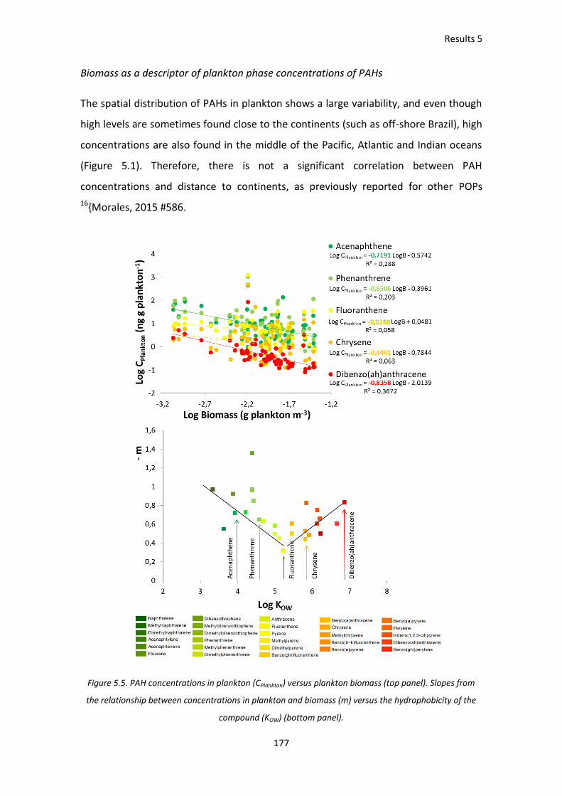
Results 5

177

Biomass as a descriptor of plankton phase concentrations of PAHs

The spatial distribution of PAHs in plankton shows a large variability, and even though

high levels are sometimes found close to the continents (such as off-shore Brazil), high

concentrations are also found in the middle of the Pacific, Atlantic and Indian oceans

(Figure 5.1). Therefore, there is not a significant correlation between PAH

concentrations and distance to continents, as previously reported for other POPs

16{Morales, 2015 #586.

Figure 5.5. PAH concentrations in plankton (CPlankton) versus plankton biomass (top panel). Slopes from

the relationship between concentrations in plankton and biomass (m) versus the hydrophobicity of the

compound (KOW) (bottom panel).

Results 5

178

Similarly to the influence of POC on surface particle phase PAH concentrations (see

above), previous works have identified that biomass is a key descriptor of the spatial

and temporal variability of organic pollutants in the marine environment

16,28,29{Morales, 2015 #586}. For the photic zone, which comprises waters directly

influenced by atmospheric inputs, and deeper ones, which are isolated from

atmospheric inputs by the thermocline, the concentration dilution at high biomass

abundance is an important process driving the occurrence of PAHs 16. There is a

decrease of the concentrations at higher biomass, especially for the more hydrophobic

compounds as they partition to the organic matter and are faster removed from the

water column by settling particles. This trend is also observed for PAHs from the global

oceans (Figure 5.5, top panel). Berrojalbiz and coworkers 16 described the effects that

plankton abundance may have on pollutants concentration by

C Plankton = a B –m [5.4]

where CPlankton (ng gdw-1) is the concentration of the pollutant in the planktonic phase

and B is the plankton biomass (mg m-3). The negative correlations between CPlankton and

B were significant for all PAHs (p<0.05, see Figure 5.5, top panel, for 5 examples).

However, the slope (m) of this relationship is different for each individual compound

(Table S5.11, SI). Figure 5.5 (bottom panel) shows that m values are lowest for PAHs

with middle hydrophobicities (log KOW around 5-6). Conversely, m values are larger for

the least and most hydrophobic PAHs. Indeed, m values are significantly correlated

with KOW (p<0.05).

The dependence of CPlankton on biomass reflects the different processes driving PAH

concentrations in the water column, and the conceptual framework for the

interpretations of these complex trends has been introduced elsewhere 16. One key

process is biomass dilution. This is especially important below the thermocline since it

is isolated from the atmosphere. Biomass dilution results in lower concentrations at

high biomass, but this effect is independent of the chemical hydrophobicity 16.

Therefore, even though biomass dilution may be affecting the concentrations of PAHs,

there are other processes driving the trends depicted in Figure 5.5 as they appeared to

be somehow related to KOW. The biological pump is the main process regulating the

Results 5

179

PAH concentrations in the water column if the sinking fluxes of PAHs are higher than

their air-water exchange. If PAHs are adsorbed to organic matter and those particles

rapidly settle to the deep ocean, the surface ocean is depleted of PAHs. This process is

responsible for the high m values of the more hydrophobic PAHs, but the less

hydrophobic compounds are scarcer affected by this process. It can be said that the

increasing tendency of the right part of the –m versus KOW plot, is therefore due to the

biological pump effects (Figure 5.5, bottom). Conversely, air-water exchange tends to

replenish the water column due to chemical equilibria, and this flux is faster for the

lighter PAHs in the Open Ocean (Chapter 2). This would lead to lower values of m for

the lower MW PAHs. However, PAHs with low MW show large m values (Figure 5.5).

Probably, air-water exchange is not able to counterbalance PAH depletion in the entire

photic zone, down to DCM. Degradation of PAHs is another plausible process affecting

depletion in the water column, being a relevant process for low MW PAHs, which have

been described to be metabolized by bacteria and plankton in the ocean 21. Therefore,

the m values for the lowest MW PAHs are consistent with efficient degradation in the

water column. Probably, large biomass indicates a large zooplankton community, and

maybe also a larger bacterial population, which efficiently degrade some of the PAHs.

A higher amount of biomass may induce biotransformation of the lower MW PAHs, but

will not affect the intermediate and high MW compounds as they are not so

susceptible to be degraded 21. Therefore, the decreasing tendency of –m for the low

KOW PAHs (Figure 5.5, bottom) can be explained by degradative processes affecting the

lower MW compounds.

No statistical correlation was found between CPlankton and δN15, suggesting that the

trophic level did not influence significantly the occurrence of PAHs. This is consistent

with the narrow range of trophic positions for the plankton samples (from 1.2 to 1.9),

and the equilibrium partitioning between the dissolved phase and both phytoplankton

and zooplankton (concentrations are independent of the relative proportion of

phytoplankton and zooplankton).

Results 5

180

Oceanic sink of PAHs due to the biological pump

As the biological pump appeared to be a relevant removal path of PAHs from the

surface mixed layer, the biological pump settling fluxes were calculated for all the

sampled areas and analyzed PAHs (Figure 5.6, Table S5.12, SI).

Figure 5.6. Biological pump fluxes for the algal settling flux (FPhyto) (top panel), and the fecal settling flux

(FFecal) (bottom panel). Marked bars (≈) have been reduced by a factor of 10 in order to ease the global

comparison of all the measurements.

Export of total measured PAHs due to the phytoplankton sinking fluxes are in the order

of tens ng m-2day-1, and maximal fluxes are found in the eastern part of the North

Atlantic basin and near South African coasts (Figure 5.6, top). Fecal sinking fluxes for

total PAHs were in the order of magnitude of hundreds of ng m-2day-1, and the largest

export rates were found as well in the Atlantic Ocean, but with higher fluxes in the

southern basin (Figure 5.6, bottom). Therefore, the sinking fluxes due to fecal pellets

Results 5

181

export are one order of magnitude higher than those due to algae communities, as

reported elsewhere for other organic compounds in the Open Ocean (Chapter 4).

Previous measurements and estimations of the sinking fluxes for PAHs in marine areas

have been undertaken. In the Mediterranean Sea, reported as a highly polluted basin

due to the surrounding developed countries, and to its semi-enclosed character,

Lipiatou 7, Dachs 8, Raoux46, Tsapakis 20, Deyme 10 and Castro 17 described sinking fluxes

in the range of the higher rates here obtained for the open ocean (hundreds of ng m-

2day-1), even if they generally considered less PAH congeners. Probably, in the

Mediterranean Sea, the individual PAHs sinking rates are higher than in the open

ocean due to the higher PAH concentrations reported in particles and plankton 16,17.

Other studies near North American coasts (at heavily polluted areas) 47,48 reported

sinking rates even in the order of μg m-2day-1, which were not found in this study as

the remote open ocean does not hold such great concentrations. Moreover, the

biological pump has been described as an effective removal process also for other

POPs in remote areas; for instance in the Arctic, α and γ HCHs biological pump fluxes

were between 10-1 and 10-2 ng m-2day-1 28, in the range of the fluxes detected for

individual PAHs in the middle of the oligotrophic open ocean (Table S5.12, SI).

Conversely, perfluoroalkylated substances sinking fluxes have been estimated to range

between 10-8 and 10-1 ng m-2 day-1, due to the low hydrophobicity of these

compounds, and thus their low tendency to partition to settling particles, and

considerable lower environmental concentrations (Chapter 4).

The average estimated flux for the Σ64PAHs was of 82.5 ng m-2day-1, standing for a total

of 0.008 Tg of PAHs per year sinking out the tropical and subtropical surface oceans.

Moreover, the more productive oceanic areas, like northern and southern oceans and

upwelling zones near continental margins, have not been accounted in this work, and

thus, total global means of the biological pump settling fluxes may be even higher than

those reported here (Chapter 4). This sinking flux is of the same magnitude than the

estimated global dry deposition flux of PAHs in the Open Ocean 5, but still, there are 2

orders of magnitude higher entrance fluxes of PAHs through diffusive exchange

(Chapter 2). Also previous reports in the Mediterranean Sea estimate that total

atmospheric entrance of PAHs is far higher than what its accounted to sink due to the

Results 5

182

Biological pump 17,20, pointing to unrevealed rates of degradation on the water column

which need to be further assessed.

There is strong evidence that the plankton does influence PAHs cycling at a global

scale, and that the open ocean is an important sink for PAHs. Both, the biological pump

and degradation are process affecting PAHs removal, availability and fate. The

complexity of the results demonstrates that the characterization of the planktonic

food webs, the organic matter and the parameters influencing the kinetics needs

further research in order to fully understand the role of biomass in POPs global cycling.

Results 5

183

ACKNOWLEDGEMENTS

The authors thank the support of RV Hespérides staff and UTM technicians during the

cruise. This work was funded by the Spanish Government through the Malaspina 2010

project Consolider-Ingenio 2010 program (CSD2008-00077). B.G-G. and M-C.-F-P.

acknowledge pre-doctoral fellowships from the BBVA Foundation and Spanish National

Research Council (CSIC), respectively. Staff from the Biogeochemical Block from the

Malaspina 2010 circumnavigation is acknowledged for the organic carbon

measurements. Staff from the Plankton Block from the Malaspina 2010

circumnavigation is acknowledged for the plankton carbon and nitrogen

measurements.

Results 5

184

REFERENCES


2 Reddy, C. M. et al. Composition and fate of gas and oil released to the water column during the Deepwater Horizon oil spill. Proceedings of the National Academy of Sciences 109, 20229-20234, doi:10.1073/pnas.1101242108 (2012).

3 Cabrerizo, A. et al. Ubiquitous net volatilization of polycyclic aromatic hydrocarbons from soils and parameters influencing their soil-air partitioning. Environmental Science & Technology 45, 4740-4747, doi:10.1021/es104131f (2011).

4 Harvey, R. G. Polycyclic aromatic hydrocarbons: chemistry and carcinogenicity. (CUP Archive, 1991).


6 Ma, Y. et al. Deposition of polycyclic aromatic hydrocarbons in the North Pacific and the Arctic. Journal of Geophysical Research: Atmospheres 118, 5822-5829, doi:10.1002/jgrd.50473 (2013).

7 Lipiatou, E., Marty, J.-C. & Saliot, A. Sediment trap fluxes of polycyclic aromatic hydrocarbons in the Mediterranean Sea. Marine Chemistry 44, 43-54, doi:10.1016/0304-4203(93)90005-9 (1993).


9 Dachs, J. & Méjanelle, L. Organic Pollutants in Coastal Waters, Sediments, and Biota: A Relevant Driver for Ecosystems During the Anthropocene? Estuaries and Coasts 33, 1-14, doi:10.1007/s12237-009-9255-8 (2010).

10 Deyme, R. et al. Vertical fluxes of aromatic and aliphatic hydrocarbons in the Northwestern Mediterranean Sea. Environmental Pollution 159, 3681-3691, doi:10.1016/j.envpol.2011.07.017 (2011).


12 Lohmann, R. et al. Organochlorine pesticides and PAHs in the surface water and atmosphere of the North Atlantic and Arctic Ocean. Environmental science & technology 43, 5633-5639 (2009).


14 Farrington, J. W. & Takada, H. Persistent organic pollutants (POPs), polycyclic aromatic hydrocarbons (PAHs), and plastics: Examples of the status, trend, and cycling of organic chemicals of environmental concern in the ocean. Oceanography 27, 196-213 (2014).

15 Dachs, J., Bayona, J. M., Raoux, C. & Albaigés, J. Spatial, Vertical Distribution and Budget of Polycyclic Aromatic Hydrocarbons in the Western Mediterranean Seawater. Environmental Science & Technology 31, 682-688, doi:10.1021/es960233j (1997).


17 Castro-Jiménez, J., Berrojalbiz, N., Wollgast, J. & Dachs, J. Polycyclic aromatic hydrocarbons (PAHs) in the Mediterranean Sea: Atmospheric occurrence, deposition

Results 5

185

and decoupling with settling fluxes in the water column. Environmental Pollution 166, 40-47 (2012).

18 Gustafsson, Ö., Gschwend, P. M. & Buesseler, K. O. Using 234Th disequilibria to estimate the vertical removal rates of polycyclic aromatic hydrocarbons from the surface ocean. Marine Chemistry 57, 11-23, doi:10.1016/S0304-4203(97)00011-X (1997).

19 Bouloubassi, I. et al. PAH transport by sinking particles in the open Mediterranean Sea: A 1 year sediment trap study. Marine Pollution Bulletin 52, 560-571, doi:10.1016/j.marpolbul.2005.10.003 (2006).

20 Tsapakis, M., Apostolaki, M., Eisenreich, S. & Stephanou, E. G. Atmospheric deposition and marine sedimentation fluxes of polycyclic aromatic hydrocarbons in the eastern Mediterranean basin. Environmental Science and Technology 40, 4922-4927 (2006).


22 Douben, P. E. PAHs: an ecotoxicological perspective. (John Wiley & Sons, 2003). 23 Meador, J., Stein, J., Reichert, W. & Varanasi, U. in Reviews of environmental

contamination and toxicology 79-165 (Springer, 1995). 24 Hylland, K. Polycyclic aromatic hydrocarbon (PAH) ecotoxicology in marine ecosystems.

Journal of Toxicology and Environmental Health A 69, 109-123, doi:10.1080/15287390500259327 (2006).

25 Echeveste, P., Agustí, S. & Dachs, J. Cell size dependent toxicity thresholds of polycyclic aromatic hydrocarbons to natural and cultured phytoplankton populations. Environmental Pollution 158, 299-307, doi:10.1016/j.envpol.2009.07.006 (2010).

26 Echeveste, P., Agustí, S. & Dachs, J. Cell size dependence of additive versus synergetic effects of UV radiation and PAHs on oceanic phytoplankton. Environmental Pollution 159, 1307-1316 (2011).

27 Barata, C., Calbet, A., Saiz, E., Ortiz, L. & Bayona, J. M. Predicting single and mixture toxicity of petrogenic polycyclic aromatic hydrocarbons to the copepod Oithona davisae. Environmental Toxicology and Chemistry 24, 2992-2999 (2005).


29 Frouin, H. et al. Partitioning and bioaccumulation of PCBs and PBDEs in marine plankton from the Strait of Georgia, British Columbia, Canada. Progress in Oceanography 115, 65-75 (2013).

30 Morales, L. et al. Background Concentrations of Polychlorinated Dibenzo-p-Dioxins, Dibenzofurans, and Biphenyls in the Global Oceanic Atmosphere. Environmental science & technology 48, 10198-10207 (2014).

31 Morales, L. et al. Oceanic Sink and Biogeochemical controls on the Accumulation of Polychlorinated dibenzo-p-Dioxins, Dibenzofurans, and Biphenyls in Plankton. Environmental Science & Technology, doi:10.1021/acs.est.5b01360 (2015).




Results 5

186

35 Gioia, R. et al. in Persistent Pollution – Past, Present and Future (eds Markus Quante, Ralf Ebinghaus, & Götz Flöser) Ch. 8, 111-139 (Springer Berlin Heidelberg, 2011).

36 Chiuchiolo, A. L., Dickhut, R. M., Cochran, M. A. & Ducklow, H. W. Persistent Organic Pollutants at the Base of the Antarctic Marine Food Web. Environmental Science & Technology 38, 3551-3557, doi:10.1021/es0351793 (2004).

37 Del Vento, S. & Dachs, J. Prediction of uptake dynamics of persistent organic pollutants by bacteria and phytoplankton. Environmental Toxicology and Chemistry 21, 2099-2107, doi:10.1002/etc.5620211013 (2002).

38 Dachs, J., Eisenreich, S. J. & Hoff, R. M. Influence of eutrophication on air-water exchange, vertical fluxes, and phytoplankton concentrations of persistent organic pollutants. Environmental Science and Technology 34, 1095-1102 (2000).

39 Wan, Y., Jin, X., Hu, J. & Jin, F. Trophic dilution of polycyclic aromatic hydrocarbons (PAHs) in a marine food web from Bohai Bay, North China. Environmental science & technology 41, 3109-3114 (2007).

40 Moreno-Ostos, E. Expedición de circunnavegación Malaspina 2010. Cambio global y exploración de la biodiversidad del océano. Libro blanco de métodos y técnicas de trabajo oceanográfico (Consejo Superior de Investigaciones Científicas 2012).

41 Mompeán, C. et al. Spatial patterns of plankton biomass and stable isotopes reflect the influence of the nitrogen-fixer Trichodesmium along the subtropical North Atlantic. Journal of Plankton Research 35, 513-525, doi:10.1093/plankt/fbt011 (2013).

42 Siegel, D. A. et al. Global assessment of ocean carbon export by combining satellite observations and food-web models. Global Biogeochemical Cycles 28, 2013GB004743, doi:10.1002/2013GB004743 (2014).

43 Schulz-Bull, D. E., Petrick, G., Bruhn, R. & Duinker, J. C. Chlorobiphenyls (PCB) and PAHs in water masses of the northern North Atlantic. Marine Chemistry 61, 101-114, doi:10.1016/S0304-4203(98)00010-3 (1998).


45 Berrojalbiz, N. et al. Persistent organic pollutants in Mediterranean seawater and processes affecting their accumulation in plankton. Environmental science & technology 45, 4315-4322 (2011).

46 Raoux, C. et al. Particulate Fluxes of Aliphatic and Aromatic Hydrocarbons in Near-shore Waters to the Northwestern Mediterranean Sea, and the Effect of Continental Runoff. Estuarine, Coastal and Shelf Science 48, 605-616, doi:10.1006/ecss.1998.0458 (1999).

47 Ko, F.-C., Sanford, L. P. & Baker, J. E. Internal recycling of particle reactive organic chemicals in the Chesapeake Bay water column. Marine Chemistry 81, 163-176, doi:10.1016/S0304-4203(03)00027-6 (2003).

48 Adhikari, P. L., Maiti, K. & Overton, E. B. Vertical fluxes of polycyclic aromatic hydrocarbons in the northern Gulf of Mexico. Marine Chemistry 168, 60-68, doi:10.1016/j.marchem.2014.11.001 (2015).

Summary of Results

187

Summary of Results

Through chapters 1-5 presented in this Thesis, the fate and dynamics of two families of

organic pollutants, polycyclic aromatic hydrocarbons (PAHs) and perfluoroalkylated

substances (PFASs), have been studied in the global Open Ocean. The assessed

processes include atmospheric deposition to the remote ocean, distribution along the

water column horizontally and vertically, and interactions with the plankton as the first

link to the oceanic food chain. The present research is circumscribed to the Malaspina

2010 circumnavigation, and covers the tropical and subtropical regions (35°N - 40°S) of

the Atlantic, Pacific and Indian Oceans.

In Chapter 1 the direct input of PAHs to the Open Ocean via dry deposition is assessed.

The study provides a collection of 12 direct measurements of dry deposition fluxes

(FDD) in the Atlantic, Indian and Pacific oceans. The assortment of coarse (>2.7 μm) and

fine (0.7 – 2.7 μm) deposited marine aerosol collected allowed to quantify the FDD to

the Open Ocean surface for 16 individual PAHs. Average FDD for total (fine + coarse)

16PAHs (sum of 16 individual PAHs) ranged from few ng m-2d-1 to around 50 ng m-2d-1.

PAHs FDD bound to coarse aerosols were higher than those of fine aerosols for the 80%

of the measurements and compounds. Coarse aerosol’s FDD for individual PAHs ranged

between an average of 10-1 ng m-2d-1 to 2 ng m-2d-1. Fine aerosol fraction’s FDD ranged

between an average of 10-2 ng m-2d-1 to 1 ng m-2d-1, being in all cases the fluxes for

high MW PAHs of higher magnitude than those for the more volatile compounds.

Concentrations of PAHs were measured in the suspended aerosol (CA) concurrently

with the FDD. 16PAHs concentrations in suspended aerosols ranged between 10-2 ng m-

3 and few ng m-3 and were maximal in the Indian Ocean, where highly polluted marine

aerosols were found. The PAHs velocity of deposition (vD) was calculated from the

measured FDD and the CA, ranging from 10-3 to 1 cm s-1, being faster the deposition of

high MW PAHs. The empirical vD was found to be significantly affected by the chemical

properties of the PAHs, like the vapor pressure (PL) of the congener, and the

environmental conditions, like wind speed (U10, which enhances turbulence and favors

aerosol collisions with the marine surface) and chlorophyll concentration in the surface

water (Chls, which increases stickiness of the ocean by lowering the surface tension

and increasing hydrophobicity). According to these 3 factors, a parametrized equation

Summary of Results

188

is proposed to predict vD in the coarse and fine fractions as well as the deposition

velocity for the total aerosols. This empirical equation reduces by a factor of 5 the

error of calculating FDD with fixed vD values, as traditionally reported in the literature.

Moreover, this equation would be a good approximation for calculating dry

depositional velocities for other semi-volatile compounds over the open ocean surface

from known parameters (PL, U10 and Chls) when atmospheric concentrations are

measured.

The other main atmospheric input fluxes of chemical pollutants into the Open Ocean,

wet deposition and diffusive exchange, are assessed for PAHs in Chapter 2. In this

chapter it is also evaluated the extent of all the measured deposition fluxes and the

implication of the total entrance of PAHs and other semivolatile aromatic-like

compounds (SALCs) to the ocean on the carbon cycle. 64 PAHs and total SALCs were

identified and ubiquitously found in the Atlantic, Pacific and Indian oceans, with gas

phase concentrations (CG) of a few ng m-3 for the most abundant compounds, aerosol

concentration of tens of pg m-3, and of hundreds of pg L-1 in surface seawater (CW). CG

was maximal in the North Atlantic and revealed a dominance of the more volatile PAHs

in the gas phase. Contrarily, CA highest records were found in the Indian Ocean with a

higher occurrence of PAHs with 4 or more aromatic rings. Total PAHs CW was less

variable in all the sampled oceans, compared with the atmosphere, being in the range

of hundreds of pg L-1 in surface seawater. Nevertheless, in the 3 environmental phases,

a decreasing concentration gradient was observed from continental margins to the

open ocean. Dry deposition fluxes for the Open Ocean were calculated from the CA

measured and the vD estimated from the parametrization explained in Chapter 1.

Average FDD for Σ64PAHs ranged from 1 ng m−2d−1 (in the Open Ocean) to almost 2500

ng m−2d−1 (in the west and east margins of the Indian Ocean). Rain water was gathered

during the 11 precipitation events that occurred during the Malaspina 2010 cruise, and

showed concentrations of hundreds to ten thousands ng L-1 of Σ64PAHs. The associated

wet deposition fluxes (FWD) were calculated to be in the order of hundreds to 5000 µg

m-2 d-1. Net diffusive air-water exchange (FAW) was estimated from the measured CG

and CW by applying a two-film resistance model. FAW showed a net input of most PAHs

to the ocean, except for some of the more volatile compounds, ranging from hundreds

Summary of Results

189

of ng m−2d−1 Σ64PAHs volatilizing from the surface ocean to tens of thousands of ng

m−2d−1 being absorbed. The global wet deposition is difficult to extrapolate spatially

and temporally, due to its episodic character. Conversely, the comparison between

total FAW and FDD integrated monthly for all the tropical and subtropical oceans

revealed that the global gross volatilization and gross absorption of Σ64PAHs were

0.042 Tg month-1 and 0.132 Tg month-1, respectively, resulting in a net input of

atmospheric Σ64PAHs to the ocean of 0.090 Tg month-1, 90 times larger than the global

FDD of aerosol-bound PAHs estimated at 0.001 Tg month-1. When extrapolated

annually, and expressed as carbon fluxes, the global annual input of Σ64PAHs to the

ocean is estimated to be 0.873 Tg C y-1. Moreover, by accounting not only PAHs, but

the whole unresolved complex mixture of SALCs (whose concentrations in the

dissolved and gas phase are between 100 and 7000 times larger than the Σ64PAH

concentrations) the input of organic carbon to the Open Ocean is even greater.

According to our estimations, the global diffusive gross absorption and volatilization

fluxes of SALCs are of 512 Tg C y-1 and 83 Tg C y-1, respectively, resulting in a net input

of organic carbon to the Atlantic, Pacific and Indian oceans of 429 Tg C y-1. Therefore,

this first and unique report of global fluxes input of PAHs, SALCs and associated carbon

to the Open Ocean suggests that atmospheric diffuse deposition of those organic

pollutants is a key process influencing the global carbon cycle.

Once in the water column, the pollutants suffer as well from other horizontal and

vertical transport processes. Chapters 3 and 4 cope with the occurrence and dynamics

of PFASs within the water column. Chapter 3 reports the occurrence of 11 PFASs

congeners including ionic perfluoroalkyl carboxylic acids (PFCAs), perfluoroalkyl

sulfonic acids (PFSAs) and neutral perfluoroalkyl sulfonamides (PFASAs) in surface

waters. The global mean CW of Σ11PFASs was in the order of hundreds to thousands of

pg L-1, even if the single concentrations for individual congeners showed broad ranges

(from thousand pg L-1 for the more abundant compounds like perfluorooctane sulfonic

acid (PFOS), to concentrations very close to the detection limit of 10-2 pg L-1). The

Atlantic Ocean exhibited the highest concentrations, found in southern basin for most

compounds, but for the neutral precursors, which occurred mostly in the northern

hemisphere and at very low concentrations. On average, PFOS contributed a 33% to

Summary of Results

190

total PFASs (ranging from 64% in the South Atlantic to 16% in the North Atlantic),

followed by perfluorodecanoic acid (22%), and perfluorohexanoic acid (12%). The

mean concentrations for the remaining congeners was under 10%, with even

perfluorooctane carboxylic acid (PFOA) contributing 6% and PFASAs accounting for less

than 1% to total PFASs concentration. Cw in coastal waters was higher than those

found in the center of the subtropical gyres, suggesting a continental origin of the

pollutants. Of special interest is the high abundance of PFOS found in surface waters

near Brazil, never reported previously at such concentrations in that region, for which

riverine and atmospheric inputs (probably wet deposition) are suggested. The high

concentrations found in other areas (like nearby the equator in the Pacific and Atlantic

oceans) are attributed to global distribution by oceanic currents, which may transport

and accumulate ionic PFASs in certain locations of the Global Ocean. The influence of

biogeochemical and physicochemical processes, like adsorption to organic matter,

biodegradation, or photodegradation is evaluated as well. According to our results and

previous studies, biological pump fluxes could significantly affect PFASs

concentrations, even if they had not been assessed previously to this Thesis. Time

trends for some PFAS congeners are evaluated for the Northern Hemisphere, through

a comparison of a reviewed dataset of PFAS concentrations in the oceanic

environment. For instance, a general decrease of PFOA is observed in the North

Atlantic and Pacific Oceans, with an estimated e-fold time (the time needed to reduce

the concentration to 1/e of the initial value) of 5.8 years. However, the main processes

affecting PFASs fate remain largely unknown, even though, presumably, it is a complex

interaction of many factors and processes driving their global distribution. Therefore,

PFASs fate and behavior in the Open Ocean, as their presumably main sink, merit

further research.

Chapter 4 intends to further understand PFASs fate in the Open Ocean by evaluating

their sinking processes and vertical distribution. For that purpose, a global database of

concentrations in the mixed layer at the deep chlorophyll maximum depth (DCM,

around 100 m) is given. The DCM is an area of special interest regarding biological

processes. Concentrations at DCM were concurrently measured with other physical

and biological parameters influencing their occurrence and discussed. To our

Summary of Results

191

knowledge, the vertical transport of PFASs has been assessed empirically for eddy

diffusion fluxes and for settling fluxes of organic matter bound PFASs (biological pump)

here for the first time. As found for surface CW, concentrations measured at the DCM

showed maximal values in the South Atlantic basin with a very similar contribution of

individual compounds to total PFASs concentration. PFOS accounted for 39% to the

total PFASs concentration followed by perfluorodecanoic acid (17%) and

perfluorohexanoic acid (12%), being the contribution of the remaining compounds

under 10% (including PFOA, which mean contribution was 5%). A clear coast - Open

Ocean decreasing concentrations was found as well for all the PFASs analyzed, as

occurred for surface seawater. DCM CW showed less variability between oceanic basins

than PFAS concentrations measures at surface seawater. However, they were

significantly positively correlated. Vertical eddy diffusion fluxes (FEddy) were calculated

from measured eddy diffusivity parameters (Kρ) concurrently with the PFAS

concentrations along the Malaspina 2010 circumnavigation, and modelled on the

mixed layer of the Open Ocean. The application of this one dimensional model

predicted the vertical profile of CW in the water column, and therefore, it was possible

to calculate a theoretical value of CW at the DCM depth. The modeled CW was generally

of the same order of magnitude than the real measured value. The calculated FEddy at

the surface were between 4 orders of magnitude higher and of comparable values

than at the DCM. FEddy at surface oscillated between 10-8 and 10-2 ng m-2day-1 for PFOS

and between 10-8 and 10-3 ng m-2day-1 for PFOA. FEddy at DCM depth ranged between

10-5 and 10-2 for PFOS and between 10-3 and 10-6 ng m-2day-1 for PFOA. At the maximal

measured Kρ, eddy diffusion will only disperse around 7 ng m-2 of PFOS per year, being

thus a flux of small magnitude. Nevertheless, as turbulent diffusion is a continuous and

ubiquitous process it should be accounted at a global scale. For instance, PFOS and

PFOA annual removal fluxes for the global tropical and subtropical surface Oceans

would be of 2.3 and 0.2 tons per year, respectively. Settling fluxes due to the biological

pump (FSettling) were calculated for 5 ionic PFASs (C8-10 PFCAs and C6,8 PFSAs) using the

measured surface CW, bioconcentration factors (BCF) from literature and a database of

global export of organic matter (FOC) from the mixed layer. Fluxes were calculated for

organic matter sinking related to phytoplankton (FPhyto) and to zooplankton fecal

pellets export (FFecal). FPhyto ranged from an order of magnitude of 10-8 ng m-2 day-1 up

Summary of Results

192

to 10-2 ng m-2 day-1 per individual congener. Individual PFASs FFecal oscillated between

10-6 ng m-2 day-1 and 10-1 ng m-2 day-1. The magnitude of the flux was positively

correlated with the hydrophobicity of the particular compound. FFecal were found to be

about one order of magnitude higher than those associated only with phytoplankton.

Moreover, FSettling seem to dominate the removal processes in the water column

according to our calculations, several orders of magnitude higher than the turbulent

fluxes calculated for all the analyzed compounds. The mean residence time of PFASs in

the surface Open Ocean was calculated with the measured inventory in the mixed

layer and considering the both removal processes quantified; being 27000 years for

PFOS and 17000 years for PFOA. According to the actual production rates of PFASs and

the estimated fluxes affecting their occurrence, the surface Open Ocean will remain a

reservoir of these pollutants for millenniums. Nevertheless, other biological

unrevealed processes not considered in the present study may be occurring in remote

or deep areas of the ocean, and further research is needed to fully understand PFASs

global behavior at the long-term.

The interactions of POPs with organic matter in the water column and the effects of

their accumulation in marine food webs are among the unstudied processes occurring

in the global oceanic environment. Chapter 5 reviews the role of organic carbon and

plankton on PAHs cycling in the Open Ocean and particularly focuses on the effects

that total suspended particles (TSP) and biomass (B) may have on PAHs concentration

in the surface mixed layer. 64 PAHs were simultaneously measured in dissolved and

particulate phases (CP) of surface water, and in plankton pools of the total mixed layer

(CPlankton). Σ64PAHs ranged between 10-1 and 10 ng L-1 in the dissolved water phase,

between 10 and 103 ng gdw-1 in the particulate phase and between 10 and 104 ng gdw

-1

in the plankton phase. The PAHs congeners occurrence profile was not significantly

different between the 3 matrixes, even if intermediate volatility PAHs were more

abundant in the particulate phase. Contrarily, total concentrations differed in their

global occurrence; maximal CW were recorded in south Atlantic coastal areas (with no

significant differences among basins even though), CP was maximal in the Indian Ocean

and CPlankton was the highest in different sampling spots along the Atlantic Ocean, near

the European and Brazilian coasts. Partition coefficients (KOC) at the oceanic surface

Summary of Results

193

were obtained for the water phase from CW and CP, and ranged from 104 to 108 L Kg-1,

with bigger ratios for higher MW PAHs. KOC and CP negatively correlated with

particulate organic carbon (POC) found in the TSP, at different rates for the individual

PAHs, thus, the partition and occurrence in the particles are affected by a POC dilution,

but also modulated by other processes depending on hydrophobicity (like air-water

exchange or the biological pump). Similarly, PAHs concentration in the surface

particulate phase appeared to be influenced by the PAHs found in the gas phase.

Indeed, the suggested situation occurring at surface waters is that there is a fast air-

water-particle exchange governing PAHs occurrence at surface waters (dissolved and

particulate phases). This equilibrium/exchange depends on CG, KOC and the Henry’s Law

constant. Theoretical CP calculated assuming air-water-particle equilibrium, positively

correlated with measured CP confirming the plausibility of this situation. Conversely at

deeper depths of the mixed photic layer, CPlankton was significantly affected by the B

present in the water column; higher amounts of biomass resulted in decreased

concentrations of PAHs. The slope (m) of this correlation was characteristic for each

individual PAH, and turned to be dependent on their hydrophobicity (KOW). For less

hydrophobic compounds there is a decrease of the slope with increasing KOW; thus, the

low hydrophobic congeners are more affected by B than intermediate PAHs. These

results attend for degradative processes, as the low KOW are faster and easier degraded

than the intermediate MW PAHs by bacteria, detoxifying phytoplankton processes and

zooplankton metabolization. From medium to high KOW PAHs, m increased with higher

hydrophobicity, and therefore, the more hydrophobic PAHs are further affected by B

abundance. In this case, the governing process is the biological pump, as the more

hydrophobic PAHs are faster and stronger adsorbed onto organic matter. Thus, their

concentration and removal from surface water is driven by the settling of these

particles. Biological pump fluxes were calculated for PAHs from CPlankton and literature

reported organic carbon export fluxes, separately for algae (FPhyto) and zooplankton

fecal pellets (FFecal). Export of total measured PAHs due to FPhyto are in the order of tens

ng m-2day-1, and maximal fluxes are found in the eastern part of the North Atlantic

basin and near South African coasts. FFecal for total PAHs were in the order of

magnitude of hundreds of ng m-2day-1, and the largest export rates were found as well

in the Atlantic Ocean, but in the southern basin. The average calculated total fluxes for

Summary of Results

194

the Σ64PAHs was of 82.5 ng m-2day-1, standing for a total of 0.008 Tg of PAHs per year

sinking out the tropical and subtropical surface oceans, which may be even greater

taking into account the highly productive marine areas not assessed in this thesis (e.g.

higher latitudinal and upwelling areas). Also the degradative processes seem to be of

interest, especially for the lower MW PAHs, and should be fully characterized and

quantified in the Open Ocean in the future. Therefore, there is evidence that the

plankton does influence PAHs cycling at a global scale, and that the role of the Open

Ocean as a pollutants sink depends on an extraordinary manner on the organic matter

and plankton cycling in the water column.

195

Chapter 3

General Discussion

General Discussion

197

General Discussion

This Thesis evaluates the occurrence of two families of organic pollutants, polycyclic

aromatic hydrocarbons (PAHs) and perfluoroalkylated substances (PFASs) in the Global

tropical and subtropical Oceans. In addition, we have evaluated the role that

atmospheric deposition and biogeochemical cycling has on the occurrence and fate of

PAHs and PFAS. The processes influencing these Persistent Organic Pollutants (POPs)

fate and distribution in the marine environment were assessed taking into account the

contrasting physicochemical properties of PAHs and PFASs. The empirical description

and characterization of the processes affecting these two examples of POP’s fate in the

Global Ocean aims to help to elucidate as well global dynamics of other pollutants with

similar properties. For instance, the parametrization proposed to calculate dry

deposition velocity 1 has been successfully applied to dioxins and furans (PCDD/Fs),

dioxin-like polychlorinated biphenyls (PCBs) 2, and organophosphorus flame retardants

3. As well, it is noteworthy that it has been verified the relevance of the biological

pump as a key regulator of PAHs and PFASs distribution in the Open Ocean, as already

suggested for other POPs in earlier works 4-7.

This discussion will integrate all the measurements performed in the Atlantic, Indian

and Pacific Oceans, and will assess the status of the sampled areas regarding PAHs and

PFASs pollution. We aim to integrate in this discussion the processes evaluated in the

several chapters of the thesis, and thus compare the occurrence, transport and fate of

the two families of POPs. In 1988 Bidleman showed that the gas-particle partition of

organic semivolatile compounds controls their behavior and deposition process in the

atmosphere 8. Likewise, in the water column, transport and fate will depend on the

phase where the target compound is predominantly found 9. Therefore, the discussion

Chapter will review as well the obtained partition coefficients found in the atmosphere

for PAHs and in the water for PAHs and PFASs, in order to assess which are the

governing processes affecting their fate in the Open Ocean. As a final point, a global

budget of the quantified PAHs, SALCs and PFASs including all the reported processes is

done; highlighting not only what has been assessed in this Thesis but the missing gaps

in the global fate of PAHs and PFAS, which provide information for other POPs.

General Discussion

198

Figure D.1. Global distribution of oceanic concentrations of PAHs in the gas, aerosol, dissolved,

particulate and plankton phases.

General Discussion

199

Global Occurrence

PAHs

Figure D.1 presents Σ64PAHs concentrations measured in the 5 environmental

compartments studied in the global Ocean. The relative abundance of the different

PAHs in the gas, aerosol, dissolved, particulate and planktonic phases depends on the

hydrophobicity and volatility of each chemical, and is also affected by the sources and

magnitude of transport and degradation processes. Therefore, the resulting global

occurrence is a combination of physicochemical properties of PAHs and the

environmental cycling of these compounds.

Gas phase concentrations were within the same range in all the sampled oceans. No

significant differences were found between Oceans, even if the North Atlantic

exhibited the highest concentrations, and generally PAHs stand out near continental

shelf margins. Contrarily, aerosol phase PAH concentrations were maximal in the

Indian Ocean and statistically different from the rest of the oceanic basins. Also high

concentrations were found in the NE Atlantic. Few previous records of PAHs in the

Open Ocean atmosphere can be found; on the one hand because they are mostly

related with human activity and some PAHs can be degraded during transport and

once in the water column. Therefore, most studies on PAHs are performed in urban

and coastal areas 10-13. On the other hand, self-contamination of samples has been

frequently detected by boat fumes, and make difficult their sampling in remote

oceanic areas 14. Nevertheless, the previous available measurements exhibit individual

PAHs concentrations within the range of our study in the Atlantic Northern basin 15-17,

showing as well the peaks near North African coasts. Regarding the Indian Ocean, no

previous sampling campaigns covered the longitudinal transect at ~30°S, and the

comparison stands with data sets from much northern and coastal regions 18.

However, those indicate a large PAHs load from Asian margins and support the high

concentrations measured during the Malaspina 2010 circumnavigation, which

presumably are due to air masses in the upper troposphere originating in Southern

East Asia.

General Discussion

200

Likewise, dissolved phase PAHs concentrations were not statistically different between

the sampled Oceans. The highest concentrations were measured in the Atlantic

continental margins, both in the North and South basins, being particularly high in the

southern Atlantic. The particulate phase significant larger concentrations were found

in the Indian Ocean, with some remarkable peaks as well in NE Atlantic. This seems

consistent with the higher aerosol phase concentrations in these basins. Conversely,

PAH concentrations in the plankton phase showed very variable concentrations, with

the highest occurrence in the Atlantic Ocean, reflecting the dynamic character of this

environmental compartment. Concentrations in the plankton phase, with samples

integrating the photic zone do not reflect the proximity to continents, but

biogeochemical controls such as biomass dilution and settling fluxes, as discussed in

Chapter 5. Water (dissolved phase) concentrations are correlated with those in the

atmosphere, confirming the effective transfer of PAHs through diffuse air-water

exchange. Most of previous studies about PAHs in seawater have focused in coastal

regions and semi enclosed bays or seas 13,19-22, as occurred with atmospheric

assessments. The few existing reports in open waters 14,15,17, are in the range of our

measurements both for the dissolved phase and the particulate, as reviewed in

Chapter 5. Studies of PAHs in plankton are even scarcer. The available data set from

the Mediterranean basin 19 ranges from the same level (our maximal CPlankton measured

in the Atlantic Ocean) to 3 orders of magnitude higher (the lowest records recorded in

Indian and South Pacific Oceans) than our Open Ocean concentrations, as this semi-

closed sea is reported to be further polluted with PAHs due to proximate land sources

13.

General Discussion

201

PFASs

Figure D.2 shows the total concentrations measured for ionic PFSAs and PFCAs

ubiquitously found at surface and DCM depth of the Open Ocean.

PFCAs total abundance in all sampled oceans was superior to PFSAs at marine surface,

but in the South Atlantic basin, and their global distribution showed remarkable

different patterns. In surface seawater, the interoceanic comparison revealed no

significant differences for ΣPFCAs, while ΣPFSAs showed statistically higher

concentrations in the South Atlantic Ocean. However, the maximal concentrations for

PFCAs were as well recorded in the South Atlantic basin. Similarly to the PAHs

distribution, high concentration peaks occurred in NE Atlantic, near African coasts,

particularly high for PFCAs. Data from previous studies for individual PFASs are in the

same order of magnitude than those measured in the Atlantic Ocean during the

Malaspina 2010 circumnavigation 23-26. Nevertheless, the range of our measurements

is wider than those previously described, probably due to a higher sampling coverage

of the oceanic basin. Contrarily, the comparison with earlier reports in the Indian and

Pacific Oceans 27-30 shows that our measurements are in the lower concentration

ranges, as those studies focus mainly in coastal regions from Asian countries, which

exponentially increase the PFASs loads 31.

PFAS concentration patterns found in surface and DCM depth seawater were quite

similar in terms of the range of concentrations, even though concentrations were

higher at surface at most of the sampling sites. Nevertheless, there is a general

increase of PFSAs concentrations at the subsurface and thus, their contribution to total

PFASs is of similar magnitude than PFCAs at depth, with the exception of the South

Atlantic Ocean, where the PFSAs relative concentration is larger, as observed at the

surface. Only two studies were found dealing with PFAS concentrations in seawater at

depths different than surface 28,32, and using the same global data set. The lower

concentrations reported for PFOS and PFOA are in the range of the individual PFASs

found in the Open Ocean in this Thesis. Conversely, their registers for Labrador Sea,

General Discussion

202

Figure D.2. Global concentration of PFSAs (blue colors) and PFCAs (red colors) in the surface seawater (5

m depth, top) and at the deep Chlorophyll maximum (DCM, bottom).

Middle Atlantic Ocean and Japan Sea come near the mid-high concentrations found in

DCM samples in the present study, even if those do not exceed the concentrations

found near Brazilian and West African coasts in this study.

General Discussion

203

Partitioning of PAHs and PFASs in the environmental compartments and

implications for their Global Fate

PAHs occurrence in atmospheric gas and aerosol phases

The considered atmospheric processes affecting PAHs (dry and wet deposition, air-

water diffusive exchange and degradation) are universal vectors of transport, transfer

and transformation of POPs in the Open Ocean’s lower atmosphere which depend on

the chemical properties of the substances and environmental parameters 8,9. The

partition (KP-air) of a contaminant between the aerosol and the gaseous phase will

determine the key process affecting its transference to the ocean; dry deposition will

predominate if the pollutant is prone to be attached to aerosols while diffusive

exchange will dominate if the pollutant is found mainly on the gaseous phase. Wet

deposition will affect concentrations in both matrixes as the rain water is equilibrated

with the gas concentration, and precipitation will scavenge aerosols affecting

atmospheric gas and aerosol phase organic compounds occurrence 8. Moreover, the

susceptibility to be photo chemically degraded in the atmosphere is also dependent on

the phase where the POP is found 33-36. Therefore, the atmospheric fate of organic

pollutants is exceptionally reliant on the aerosol-gas equilibria.

According to our measurements for PAHs, KP-air obtained as the ratio between the

aerosol concentration (CA) and the gas concentration (CG) is shown in Figure D.3 for

some representative compounds at the Global Oceans. It can be observed that the

more volatile compounds (like phenanthrene) reflect low KP-air and therefore, they are

mainly present in the gas phase and will be more susceptible to atmospheric

degradation, as there is a higher rate of reaction with OH radical in the gaseous form

33. Meanwhile, heavier compounds exhibit a greater partition to marine aerosol and

will be degraded on a lesser extent but preferably transferred to the ocean through dry

deposition. The highest partition to the aerosol fraction for all PAHs was found in the

central Indian basin and near the Australian southern coast. Besides, the high ΣPAHs CA

found in the Indian Ocean and the large dry deposition fluxes measured there 1

General Discussion

204

facilitate the entrance of high MW PAHs (like perylene) in this particular ocean (Figure

D.3), not previously assessed in the literature.

Figure D.3. KP-air (L kgTSP-1

) for four representative PAHs.

The partition is the reflection of the concentrations of the different PAHs measured in

the gas and aerosol phases, whose profiles (as mean abundances of individual PAHs in

each matrix) are displayed in Figure D.4.

Figure D.4. PAHs profile for gas (CG) and aerosol (CA) phases.

PAHs pollution in the aerosol accounted for only 9.8% of total PAHs found in the

atmosphere, even if the relative presence of higher MW compounds is larger in this

phase than on the gas phase. On the contrary, the intermediate to high volatile

compounds were largely present in the gas phase, holding more than 90% of the total

PAHs measured in the oceanic atmosphere. The dominance of the atmospheric

General Discussion

205

concentrations in the gas phase has been reported previously in the Open Ocean 15,

and moreover, in some studies the aerosol pollution is even neglected in the total

atmospheric occurrence of PAHs 17.Therefore, the majority of PAHs will be affected by

transport processes occurring mainly in the gas phase (diffusive exchange,

degradation); meanwhile the more recalcitrant PAHs attached to the marine aerosol

will be prone to be carried over the ocean with suspended atmospheric particles and

affected by different processes (dry deposition). This is confirmed by the magnitude of

the calculated fluxes presented in Chapter 2; diffusive exchange accounts for 99% of

the total PAHs entrance to the Open Ocean, while dry deposition only stands for less

than 1% of the PAHs input to the Global Oceans.

PAHs and PFASs occurrence in seawater’s dissolved and particulate phases

The presence of POPs either in the dissolved or particulate phase of the Open Ocean

seawater will be affected by different factors leading their distribution and fate. For

PAHs, several processes have been reviewed and calculated in Chapter 5; like biomass

dilution, degradation, biological pump, effects of the air-water diffusive exchange, etc.

Regarding PFASs, even if here there is a lack of direct measurements of concentrations

in the particulate phase, an estimation of the particulate fraction fate has been

conducted in Chapter 4. Effectively, as reported here and in other works, the biological

pump is a key regulator of POPs occurrence in remote areas 4,5, affecting pollutants in

the particulate phase fate. On the other hand distribution of POPs in the dissolved

phase will be more affected by other processes in the Open Ocean, like water masses

subduction or turbulent diffusion 32,37.

Figure D.5. KOC (L kgPOC-1

) for four representative PAHs.

General Discussion

206

PAH’s organic carbon-water partition as given by KOC in the water phase is discussed in

Chapter 5. The main drivers of partition act on a complex manner; the chemical

equilibrium between particulate organic matter and water is affected by a wide array

of variables like gas-water exchange, temperature, the composition of the particulate

organic matter and several others that will modify the final concentration of PAHs.

According to our measurements of dissolved (Cw) and particulate concentrations (CP) in

surface waters for four representative PAHs (Figure D.5), there is a higher ratio of

pollutants in the particulate phase in the Indian Ocean, as found in the atmosphere,

and in the North Atlantic eastern margins. The Northeast Atlantic highest

concentrations, and higher partition to particles of the more hydrophobic compounds,

were previously discussed by Nizzetto and coworkers 17, concluding that African

emissions would explain such occurrence of PAHs at high concentrations. Moreover,

other POPs, such as brominated flame retardants 38 and polychlorinated naphthalenes

39 were also highly abundant in that area. Conversely, PAHs occurrence in the Indian

Ocean seawaters, with high partition to the particulate phase and high concentrations

reported in Chapter 5, would be explained by the high concentrations measured as

well in the atmosphere and intense depositional fluxes 1 for that area. Besides, likewise

in the atmosphere, higher partition coefficients correspond for the more hydrophobic

compounds (like perylene) in all the sampled Oceans. Nevertheless, the differences

between the individual PAHs KOC in the water are much lower than in the atmosphere,

showing narrower ranges.

Due to a low concentration of total particles in the oligotrophic ocean 40, PAHs are

more abundant in the dissolved than on the particulate phase, as found in the

atmosphere. Nevertheless, the proportion of PAHs in the water column particles is

slightly higher than in the aerosol, as 11% of total measured PAHs are found on the

particles versus the 89% found dissolved in the water. This is probably due to the

stronger binding forces in an aqueous solution that attach PAHs to organic matter

more than those in the air 41, and to the degradation of low MW PAHs in the water

column. The dissolved phase contained a higher relative concentration of the

intermediate and more volatile congeners, whereas the particulate fraction holds a

higher proportion of the more hydrophobic compounds (Figure D.6). Therefore,

General Discussion

207

biomass dilution and the biological pump, processes ruling the concentration of PAHs

in the organic matter will mainly affect the more hydrophobic congeners. Contrarily,

dissolved pollutants (like low MW PAHs and most ionic PFASs) will undergo other

distribution processes within the water column.

Figure D.6. PAHs profile for dissolved (CW) and particulate (CP) phases.

PFASs have been reported to be present in both dissolved and particulate phases in

aquatic environments, depending the partition on the amount of suspended solids,

and the density and organic content of those (analogously as for PAHs) 42. Due to the

low concentrations of suspended solids in the Open Ocean and their lesser

hydrophobicity compared with other POPs, PFASs like PFOS, PFOA and PFOSA have

been reported to be found mainly in the dissolved phase 42. Indeed, the calculated

turbulent fluxes presented in Chapter 4 proved to successfully explain part of the

occurrence of dissolved PFASs at depth in the water column. Nevertheless, according

to our measurements and calculations, the biological pump is also a relevant removal

process in the tropical and subtropical Open Ocean, playing even a larger role than

eddy diffusion at a global scale for PFASs removal from the Open Ocean surface. This

means that the occurrence of PFASs in the particulate phase deserve further research,

as there is a need of more empirical measurements in the Open Ocean. A recent work

has reported the occurrence of PFASs in settling particles in the NE Mediterranean sea,

in this case, high fluxes were found due to dense shelf water cascading 43, a

mechanism different than the biological pump estimated for the Open Ocean.

General Discussion

208

In addition, the occurrence of pollutants trapped onto organic matter influences their

bioavailability to marine biota. PAHs are typically metabolized within the planktonic

food web 44, and bioaccumulation is not so relevant, but degradation dominates in the

Open Ocean. The length and complexity of the food web and the persistence of the

particular PAHs 44 are factors influencing this process 45. Lighter compounds are easily

degraded, meanwhile the more recalcitrant PAHs are prone to be accumulated in the

organic matter and therefore redistributed in the water column by the biological

pump, as explained in Chapter 5. Conversely, Higgins described that the sediment-

associated PFASs can be easier accumulated in aquatic food chains 46 and also Martin

reported further accumulation of those pollutants when they are found on sediments

and particles of the water column, as they are then bioavailable to benthic and filtering

organisms, than in the dissolved phase 47. The degradation of those POPs has not been

reported to date, but bioaccumulation and biomagnification48-50 turn as an additional

process (and risk) to the PFASs fate in the Open Ocean yet to be fully characterized.

Global fluxes and budgets of PAHs and PFASs in the Open Ocean

At a global scale, all the processes and factors evaluated are interconnected within a

dynamic coupling of various processes. The partitioning among the different phases

(gas, aerosol, water, particles) strive to put the concentrations at equilibrium. On the

other hand, there are a number of processes such as dry/wet deposition, biological

pump, biomass dilution, advection, etc, that can drive the concentrations away from

equilibrium. For instance, a biomass growth on a certain area may drive a decrease of

pollution into the water column and a consequent enhanced diffusive flux from the

atmosphere towards the Ocean. All the feedbacks and side-effects involved are not

fully quantified, and even to a lesser extent at an oceanic global scale. Nevertheless,

the data and discussion provided here enlightens the magnitude of the processes

affecting PAHs and PFASs distribution and the balance among them which may provide

new insights about the total budgets and governing parameters for the POPs

distribution and fate in the global Open Ocean.

General Discussion

209

An important challenge for this Thesis was to have a first understanding on the global

budget for PAHs in the marine lower atmosphere and surface mixed layer, and even an

estimation of the occurrence and fate of other aromatic-like compounds (Chapter 2).

These results highlight a potential yet unknown perturbation of the global

biogeochemical cycling of organic matter which could influence the balance of the

oceanic carbon cycle. Moreover, regarding the emerging PFASs in the mixed layer,

their fate in the Global Ocean was analyzed for the first time based on direct field

measurements (Chapter 4).

PAHs and SALCs

The annual global balance for PAHs and SALCs considering all the analyzed transport

and transformation processes is shown in Figure D.7. Among all the PAHs present in

the atmosphere, a high fraction of them is directly degraded via oxidative reactions

with OH radical 33, as discussed in Chapter 2. In the oceanic lower atmosphere,

accounting the mean inventory measured over the Atlantic, Pacific and Indian oceans,

there is a degradation of near 2.2 Tg y-1 of the 64 PAHs identified and quantified. This

atmospheric sink is approximately two times bigger than the global Open Ocean

entrance through diffuse fluxes (FAW and FDD), but it only affects the lighter and

degradable compounds. The preferential degradation of the low MW compounds may

account for a distillation process towards remote areas, even if this was not observed

in our measurements, probably due to the volatilization registered from marine

surface in the central areas of the oceanic tropical basins (Chapter 2). Contrarily, this

differential degradation and consequent distillation effect is evident for other non-

biogenic POPs, like PCBs. The lower hydrophobic PCBs show shorter residence times in

intertropical regions due to the OH radical attack, and as they are not produced in the

Open Ocean, the remote areas exhibit lower concentrations of lighter PCBs 51 even if

they are potentially more mobile 52. The degradation rates for PCBs are estimated to

be 0.008 Tg y-1, 3 orders of magnitude lower than those calculated here for PAHs, but

also much larger than the calculated sinks for the Open Global Ocean for PCBs, 240

tons y-1 53. Assuming the higher persistence of PCBs and the much lower environmental

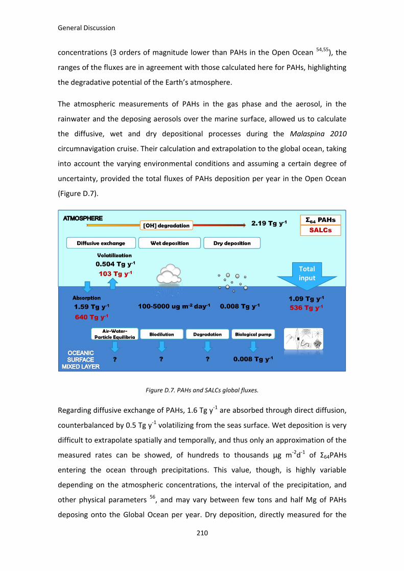
General Discussion

210

concentrations (3 orders of magnitude lower than PAHs in the Open Ocean 54,55), the

ranges of the fluxes are in agreement with those calculated here for PAHs, highlighting

the degradative potential of the Earth’s atmosphere.

The atmospheric measurements of PAHs in the gas phase and the aerosol, in the

rainwater and the deposing aerosols over the marine surface, allowed us to calculate

the diffusive, wet and dry depositional processes during the Malaspina 2010

circumnavigation cruise. Their calculation and extrapolation to the global ocean, taking

into account the varying environmental conditions and assuming a certain degree of

uncertainty, provided the total fluxes of PAHs deposition per year in the Open Ocean

(Figure D.7).

Figure D.7. PAHs and SALCs global fluxes.

Regarding diffusive exchange of PAHs, 1.6 Tg y-1 are absorbed through direct diffusion,

counterbalanced by 0.5 Tg y-1 volatilizing from the seas surface. Wet deposition is very

difficult to extrapolate spatially and temporally, and thus only an approximation of the

measured rates can be showed, of hundreds to thousands µg m-2d-1 of Σ64PAHs

entering the ocean through precipitations. This value, though, is highly variable

depending on the atmospheric concentrations, the interval of the precipitation, and

other physical parameters 56, and may vary between few tons and half Mg of PAHs

deposing onto the Global Ocean per year. Dry deposition, directly measured for the

General Discussion

211

first time with such a resolution, appeared to be as well a relevant process influencing

PAHs input onto the marine surface for the high MW PAHs. Even if the calculated

global fluxes are 3 orders of magnitude lower than the diffusion exchange, the 0.008

Tg y-1 of PAHs entering the Open Ocean with settling aerosols are twice the European’s

year 2000 emission of the 16 EPA’s regulated PAHs 57, thus an unneglectable quantity.

As stated previously, the magnitude of each depositional process depends on each

POPs family class, specifically on their physical-chemical properties. For instance, PCBs

are mainly affected by diffusive exchange fluxes as PAHs do, while for PCDD/Fs, those

are in the range of wet deposition fluxes. Indeed, wet deposition accounts for 40-75%

of the total deposition of PCDD/Fs to the Open Ocean, inducing particularly the

entrance of the hepta- and octa- congeners, but for PCBs it does not represent more

than 35% of total input 56. Dry deposition fluxes for PCBs and PCDD/Fs stand for an

estimated 15% of total flux, and reported to be significant in areas with high wind

speeds and high concentrations of marine aerosols 56. Nevertheless, in a recent study

of PCDD/Fs and dioxin-like-PCBs in the open global ocean conducted as well during the

Malaspina 2010 cruise, it is calculated a dry deposition global input of 360 Kg y-1 and

900 Kg y-1 respectively 2, much lower than previous estimates 58 and thus, pointing to

diffusive fluxes as the main vector of entrance of POPs into the Open Ocean 2, as

occurs for PAHs according to our measurements.

The processes causing the sequestration of PAHs and their transfer to the deep ocean

by the biological pump are of the same range of their dry deposition fluxes (Figure

D.7). Virtually, the same amount of PAHs that enter to the ocean with settling aerosol

will continue their sinking to the deep ocean (0.008 Tg y-1). Other studies show the

evidence of the correlation between biological pump fluxes and atmospheric inputs in

temperate and polar oceans for PCBs, PCDD/Fs and halogenated pesticides 4,5,59,60.

Moreover, in mid to high latitudes air-to-water fluxes are enhanced by the high settling

fluxes of the abundant primary producers in these rich areas, as described for PCBs

and hydrophobic dioxins 9. Those fluxes range within several orders of magnitude and

depend on the amount of suspended biomass, POP concentrations, chemical affinities

and other key environmental factors. Settling fluxes have been described to regulate

pollutants dynamics between the atmosphere and the water oceanic ecosystem, down

General Discussion

212

to the deep ocean. There and even in shallower areas of the water column, dilution,

degradation and other transformation processes will take part at an uncertain rates (at

least at a global scale and for the myriads of pollutants present in the ocean 61), leaving

the Open Ocean as a global sink of pollutants with many open questions about the

global risk for the marine ecosystems.

In 2004 there was a global estimated production of 530 Gg y-1 of the 16 EPA’s

regulated PAHs by anthropogenic sources 57. The concentrations and fluxes here

calculated are far larger, of 900 Gg yr-1 entering into the Open Ocean though dry

deposition and diffusive exchange. This could be explained by an underestimation of

the global anthropogenic production, to a large biogenic production of PAHs not

accounted, and also to the fact that the more recalcitrant PAHs do accumulate and

cycle in the Open Ocean for long time once they have been produced and released into

the environment. Nevertheless, it is obvious that the resilience of the Open Ocean and

its degradative and sink potential for PAHs is enormous, even if it seems that the real

total loads of PAHs to the environment are poorly constrained.

PFASs

The global budget for the emerging fluorinated pollutants assessed in this Thesis, the

PFASs, is still more uncertain to date than that of PAHs (Figure D.8). No degradation of

those compounds has been reported neither in the atmosphere, nor by any organism

in the ocean (in other aerobic or anaerobic ecosystems) 62. Moreover, the atmospheric

inputs to the Ocean have largely being omitted in earlier studies, and are just starting

to be considered in the literature. These remained out of the scope of this thesis. Some

approaches attempted to estimate the relevance of the deposition process and origin

of the PFASs in remote marine areas and lakes through a characterization of the ratios

and isomer profiles of the congeners measured in water 63-65. Only few studies suggest

a temperature dependent occurrence of some volatile compounds, like

perfluoroalkylated sulfonamides, in the remote Arctic indicating a plausible diffusive

exchange with ocean or ice, and mentioning partition to aerosol 66,67. Further, others

correlated the presence of PFASs and their precursors in air, water and sediments in

General Discussion

213

Arctic lakes assuming atmospheric transport 68. But a precise description and

quantification of their fluxes has not been conducted to date in the Open Ocean. Wet

deposition has been tentatively assessed by Taniyasu et al. in Japan and North Pacific

rain and snow 69 and by coworkers based on land measurements 70 and showed an

effective flux of PFASs deposition which should be studied further and characterized

for the Open Ocean. Riverine and run-off contributions have been estimated for some

specific regions 71-73, but there is a lack of total inputs measurements at a global scale,

which may vary exceptionally depending on the river basin and the sources, riverine

discharges and seasonal fluxes 74.

Figure D.8. PFASs global fluxes.

Nonetheless, the inventory provided here for the tropical and subtropical surface

ocean for the target PFASs and the calculated sinking fluxes to the mesopelagic ocean

are examples of the most updated research on this topic. The previously reported eddy

diffusion transport for PFOA by Lohmann et al 32 has been completed and recalculated

here by using direct turbulence measurements concurrently with the PFASs

concentrations along the 3 sampled oceans in the Malaspina 2010 circumnavigation. It

was calculated also for 9 PFASs other than PFOA, with a total contribution of 93.8 tons

of the 9 selected PFASs diffusing out of the surface mixed layer annually (76.1 tons y-1

attend for the 5 PFASs for which also biological pump export was calculated, Figure

General Discussion

214

D.8). No much attention has been paid previously to turbulence affecting POPs

transport in the Ocean; only Jurado et al 75 explicitly assessed the relevance of this

process by modeling PCBs fate in the costal marine water column. Likewise in our

results for PFASs, they concluded that turbulent mixing helps to predict real

concentration of POPs in the water column, where may be other processes playing a

role depending on the particular environmental conditions.

Biological pump estimations were done for the first time for the 5 more abundant

PFASs found in the open ocean during the Malaspina 2010 expedition. The settling flux

turned to be 100 times higher than the eddy diffusion flux calculated for those 5 PFASs

(Figure D.8). The almost 900 tons of PFASs sinking per year into the ocean in

aggregates of organic matter or by turbulent diffusion, may have unknown effects in

the deep marine ecosystems, as the deep ocean will remain as a reservoir for

millenniums due to PFASs persistence. However other processes occurring in the open

ocean may also play a key role, like biomass dilution, equilibration with the

atmosphere (for neutral PFASs), ejection with sea spray aerosol, and thus with a

potential reemission of the PFASs if the concentrations in the water are large enough,

or even the non-yet discovered degradation in the deep ocean. Therefore, more

research is still needed to fully understand the behavior of all the emerging

perfluorinated pollutants in the Global Ocean, considering the relevant processes

proposed here.

The significance that anthropogenic POPs pollution, considering the huge amounts of

compounds constantly produced and their coupling with global biogeochemical cycles

can only be better understood if the processes affecting POPs fate in the Global Ocean

are comprehensively studied.

General Discussion

215

REFERENCES


2 Morales, L. et al. Background Concentrations of Polychlorinated Dibenzo-p-Dioxins, Dibenzofurans, and Biphenyls in the Global Oceanic Atmosphere. Environmental science & technology 48, 10198-10207 (2014).

3 Castro Jiménez, J., Casal, P., González Gaya, B., Pizarro, M. & Dachs, J. Organophosphate ester (OPE) flame retardants and plasticizers in the atmosphere over the Global Oceans. Organohalogen Compounds 76, 364-367 (2014).




7 Nizzetto, L. et al. Biological pump control of the fate and distribution of hydrophobic organic pollutants in water and plankton. Environmental science & technology 46, 3204-3211 (2012).

8 Bidleman, T. F. Atmospheric processes. Environmental Science and Technology 22, 361-367 (1988).


10 Bozlaker, A., Muezzinoglu, A. & Odabasi, M. Atmospheric concentrations, dry deposition and air-soil exchange of polycyclic aromatic hydrocarbons (PAHs) in an industrial region in Turkey. Journal of Hazardous Materials 153, 1093-1102 (2008).

11 Demircioglu, E., Sofuoglu, A. & Odabasi, M. Particle-phase dry deposition and air-soil gas exchange of polycyclic aromatic hydrocarbons (PAHs) in Izmir, Turkey. Journal of Hazardous Materials 186, 328-335 (2011).

12 Vardar, N., Odabasi, M. & Holsen, T. M. Particulate dry deposition and overall deposition velocities of polycyclic aromatic hydrocarbons. Journal of Environmental Engineering 128, 269-274 (2002).

13 Castro-Jiménez, J., Berrojalbiz, N., Wollgast, J. & Dachs, J. Polycyclic aromatic hydrocarbons (PAHs) in the Mediterranean Sea: Atmospheric occurrence, deposition and decoupling with settling fluxes in the water column. Environmental Pollution 166, 40-47 (2012).

14 Lohmann, R. et al. Organochlorine pesticides and PAHs in the surface water and atmosphere of the North Atlantic and Arctic Ocean. Environmental science & technology 43, 5633-5639 (2009).



General Discussion

216


18 Xu, Y. et al. The spatial distribution and potential sources of polycyclic aromatic hydrocarbons (PAHs) over the Asian marginal seas and the Indian and Atlantic Oceans. Journal of Geophysical Research D: Atmospheres 117 (2012).




22 Law, R., Dawes, V., Woodhead, R. & Matthiessen, P. Polycyclic aromatic hydrocarbons (PAH) in seawater around England and Wales. Marine pollution bulletin 34, 306-322 (1997).

23 Theobald, N., Gerwinski, W. & Jahnke, A. Occurrence of perfluorinated organic acids in surface sea-water of the East Atlantic Ocean between 53º north and 30ºsouth. SETAC Europe Annual Meeting (2007).








31 González-Gaya, B., Dachs, J., Roscales, J. L., Caballero, G. & Jiménez, B. Perfluoroalkylated Substances In The Global Tropical And Subtropical Surface Oceans. Environmental Science & Technology 48, 13076-13084, doi:10.1021/es503490z (2014).


33 Keyte, I. J., Harrison, R. M. & Lammel, G. Chemical reactivity and long-range transport potential of polycyclic aromatic hydrocarbons - a review. Chemical Society Reviews 42, 9333-9391, doi:10.1039/C3CS60147A (2013).

34 Koester, C. J. & Hites, R. A. Photodegradation of polychlorinated dioxins and dibenzofurans adsorbed to fly ash. Environmental Science & Technology 26, 502-507, doi:10.1021/es00027a008 (1992).

General Discussion

217

35 Wania, F. & Daly, G. L. Estimating the contribution of degradation in air and deposition to the deep sea to the global loss of PCBs. Atmospheric Environment 36, 5581-5593, doi:10.1016/S1352-2310(02)00693-3 (2002).

36 Raff, J. D. & Hites, R. A. Deposition versus Photochemical Removal of PBDEs from Lake Superior Air. Environmental Science & Technology 41, 6725-6731, doi:10.1021/es070789e (2007).

37 Lohmann, R., Jurado, E., Pilson, M. E. Q. & Dachs, J. Oceanic deep water formation as a sink of persistent organic pollutants. Geophysical Research Letters 33, doi:10.1029/2006gl025953 (2006).

38 Xie, Z., Möller, A., Ahrens, L., Sturm, R. & Ebinghaus, R. Brominated flame retardants in seawater and atmosphere of the Atlantic and the southern ocean. Environmental Science and Technology 45, 1820-1826 (2011).

39 Jaward, F. M., Barber, J. L., Booij, K. & Jones, K. C. Spatial distribution of atmospheric PAHs and PCNs along a north–south Atlantic transect. Environmental Pollution 132, 173-181, doi:10.1016/j.envpol.2004.03.029 (2004).

40 Siegel, D. A., Dickey, T. D., Washburn, L., Hamilton, M. K. & Mitchell, B. G. Optical determination of particulate abundance and production variations in the oligotrophic ocean. Deep Sea Research Part A. Oceanographic Research Papers 36, 211-222, doi:10.1016/0198-0149(89)90134-9 (1989).

41 Mackay, D. & Callcott, D. in PAHs and Related Compounds Vol. 3 / 3I The Handbook of Environmental Chemistry (ed AlasdairH Neilson) Ch. 8, 325-345 (Springer Berlin Heidelberg, 1998).

42 Ahrens, L., Yeung, L. W., Taniyasu, S., Lam, P. K. & Yamashita, N. Partitioning of perfluorooctanoate (PFOA), perfluorooctane sulfonate (PFOS) and perfluorooctane sulfonamide (PFOSA) between water and sediment. Chemosphere 85, 731-737, doi:10.1016/j.chemosphere.2011.06.046 (2011).

43 Sanchez-Vidal, A. et al. Delivery of unprecedented amounts of perfluoroalkyl substances towards the deep-sea. Science of The Total Environment 526, 41-48, doi:10.1016/j.scitotenv.2015.04.080 (2015).


45 D'Adamo, R., Pelosi, S., Trotta, P. & Sansone, G. Bioaccumulation and biomagnification of polycyclic aromatic hydrocarbons in aquatic organisms. Marine Chemistry 56, 45-49, doi:10.1016/S0304-4203(96)00042-4 (1997).

46 Higgins, C. P., McLeod, P. B., MacManus-Spencer, L. A. & Luthy, R. G. Bioaccumulation of Perfluorochemicals in Sediments by the Aquatic Oligochaete Lumbriculus variegatus. Environmental Science & Technology 41, 4600-4606, doi:10.1021/es062792o (2007).

47 Martin, J. W., Whittle, D. M., Muir, D. C. G. & Mabury, S. A. Perfluoroalkyl Contaminants in a Food Web from Lake Ontario. Environmental Science & Technology 38, 5379-5385, doi:10.1021/es049331s (2004).

48 Haukas, M., Berger, U., Hop, H., Gulliksen, B. & Gabrielsen, G. W. Bioaccumulation of per- and polyfluorinated alkyl substances (PFAS) in selected species from the Barents Sea food web. Environmental Pollution 148, 360-371, doi:10.1016/j.envpol.2006.09.021 (2007).

49 Houde, M. et al. Fractionation and bioaccumulation of perfluorooctane sulfonate (PFOS) isomers in a Lake Ontario food web. Environmental Science & Technology 42, 9397-9403 (2008).

50 Houde, M., De Silva, A. O., Muir, D. C. & Letcher, R. J. Monitoring of perfluorinated compounds in aquatic biota: an updated review. Environmental Science & Technology 45, 7962-7973, doi:10.1021/es104326w (2011).

General Discussion

218

51 Jurado, E. & Dachs, J. Seasonality in the "grasshopping" and atmospheric residence times of persistent organic pollutants over the oceans. Geophysical Research Letters 35 (2008).

52 Wania, F. & MacKay, D. Peer Reviewed: Tracking the Distribution of Persistent Organic Pollutants. Environmental Science & Technology 30, 390A-396A, doi:10.1021/es962399q (1996).

53 Anderson, P. N. & Hites, R. A. OH Radical Reactions: The Major Removal Pathway for Polychlorinated Biphenyls from the Atmosphere. Environmental Science & Technology 30, 1756-1763, doi:10.1021/es950765k (1996).

54 Gioia, R. et al. Factors Affecting the Occurrence and Transport of Atmospheric Organochlorines in the China Sea and the Northern Indian and South East Atlantic Oceans. Environmental Science & Technology 46, 10012-10021, doi:10.1021/es302037t (2012).

55 Lohmann, R., Klanova, J., Kukucka, P., Yonis, S. & Bollinger, K. PCBs and OCPs on a East-to-West Transect: The Importance of Major Currents and Net Volatilization for PCBs in the Atlantic Ocean. Environmental Science & Technology 46, 10471-10479, doi:10.1021/es203459e (2012).



58 Lohmann, R., Jurado, E., Dachs, J., Lohmann, U. & Jones, K. C. Quantifying the importance of the atmospheric sink for polychlorinated dioxins and furans relative to other global loss processes. Journal of Geophysical Research: Atmospheres 111, n/a-n/a, doi:10.1029/2005JD006923 (2006).

59 Berrojalbiz, N. et al. Persistent organic pollutants in Mediterranean seawater and processes affecting their accumulation in plankton. Environmental science & technology 45, 4315-4322 (2011).

60 Castro-Jiménez, J. et al. Atmospheric occurrence and deposition of polychlorinated dibenzo-p-dioxins and dibenzofurans (PCDD/Fs) in the open mediterranean sea. Environmental Science and Technology 44, 5456-5463 (2010).



63 Simcik, M. F. & Dorweiler, K. J. Ratio of perfluorochemical concentrations as a tracer of atmospheric deposition to surface waters. Environmental Science & Technology 39, 8678-8683 (2005).

64 Benskin, J. P. et al. Perfluorinated acid isomer profiling in water and quantitative assessment of manufacturing source. Environmental Science & Technology 44, 9049-9054, doi:10.1021/es102582x (2010).



67 Shoeib, M., Harner, T. & Vlahos, P. Perfluorinated Chemicals in the Arctic Atmosphere. Environmental Science & Technology 40, 7577-7583, doi:10.1021/es0618999 (2006).

General Discussion

219

68 Stock, N. L., Furdui, V. I., Muir, D. C. & Mabury, S. A. Perfluoroalkyl contaminants in the Canadian Arctic: evidence of atmospheric transport and local contamination. Environmental Science & Technology 41, 3529-3536 (2007).

69 Taniyasu, S. et al. Does wet precipitation represent local and regional atmospheric transportation by perfluorinated alkyl substances? Environment International 55, 25-32, doi:10.1016/j.envint.2013.02.005 (2013).


71 Ahrens, L., Felizeter, S. & Ebinghaus, R. Spatial distribution of polyfluoroalkyl compounds in seawater of the German Bight. Chemosphere 76, 179-184, doi:10.1016/j.chemosphere.2009.03.052 (2009).


73 Cai, M. et al. Spatial distribution of per- and polyfluoroalkyl compounds in coastal waters from the East to South China Sea. Environmental Pollution 161, 162-169, doi:10.1016/j.envpol.2011.09.045 (2012).

74 Ahrens, L. & Bundschuh, M. Fate and effects of poly- and perfluoroalkyl substances in the aquatic environment: A review. Environmental Toxicology and Chemistry 33, 1921-1929 (2014).

75 Jurado, E., Zaldívar, J.-M., Marinov, D. & Dachs, J. Fate of persistent organic pollutants in the water column: Does turbulent mixing matter? Marine pollution bulletin 54, 441-451 (2007).

221

Chapter 4

General Conclusions

General Conclusions

223

General Conclusions

The general aim of this work, as stated in the introductory chapter, was to assess the

occurrence of POPs cycling in the global tropical and subtropical oceans, focusing on

PAHs and PFASs. The results obtained in this Thesis, according to the specific

objectives, contribute to the further advance in the knowledge on this issue, and a

summary of the main conclusions per each objective are presented below.

- To determine the occurrence of PAHs in gas, aerosol, dissolved, particulate and

planktonic phases, and PFAS in the dissolved phase from the global Open

Ocean.

Both POPs families were detected worldwide in the tropical and subtropical Open

Ocean, with different total concentrations and distribution patterns depending on

their production sources, governing transport processes, chemical properties and

decaying rates.

In general, PAHs were homogeneously distributed in gas and dissolved

phases; meanwhile Indian Ocean revealed very high concentrations of PAHs

in the aerosol and particulate phases. The highest PAHs concentration in

the plankton phase was detected in the Atlantic Ocean.

PFASs were dominated by PFCAs at the surface, and more balanced

between the PFCAs and PFSAs at DCM depth, even if concentrations at both

depths are correlated. PFOSAs where rarely detected, mainly in the

northern hemisphere. The highest concentration of PFASs by far was found

in the Atlantic Ocean, particularly near Brazilian coasts followed by North

East Atlantic margins.

- To quantify the POPs fluxes between the different environmental

compartments.

Depositional fluxes of PAHs in the Open Ocean were dominated by diffusive

exchange, followed by wet deposition and dry deposition. This last, even if of lower

magnitude, is relevant for the heavier PAHs at global scale. Atmospheric

General Conclusions

224

degradation accounted for a large sink for the more volatile PAHs.

PAHs dry deposition fluxes bound to coarse aerosols were higher than

those of fine aerosols in the Open Ocean.

Dry deposition velocities (vD) were higher for higher MW PAHs, due to their

chemical affinities to aerosol organic matter.

The chemical properties of the compound and environmental factors

(aerosol size, wind speed, phytoplankton presence in the water column,

among others) have a great impact on dry deposition. Through a

parameterization of those is possible to predict vD with an error 5 times

smaller than that obtained when using a fixed vD value from the literature,

as it accounts for environmental conditions.

Dry deposition was especially relevant in the Indian Ocean.

Wet deposition is very intense but limited to certain periods and areas in

the Open Ocean for PAHs.

Diffusive atmospheric deposition of PAHs and other semivolatile aromatic-

like compounds to the global oceans is much larger than expected, and

account for a significant source of carbon to the Open Ocean that should be

further studied.

Diffusive global exchange occurred on a higher extent in the Pacific Ocean

due to its large surface.

In the water column, the biological pump resulted to be the main sinking process

governing PAHs and PFASs fate in the Open Ocean. Degradation was also important

for low MW PAHs, and other processes like dilution for PAHs and eddy diffusive

fluxes for PFAS are also relevant and should be further studied.

Eddy diffusive fluxes allow an estimation of the subsurface concentrations

of some PFASs, even if other processes may be affecting the pollutants

transport and their sinking in the Open Ocean.

The biological pump is an oceanic sink flux not previously reported for

PFASs, showing an effective removal of pollutants from the surface. Fecal

pellets associated fluxes were of higher magnitude than those associated

with phytoplankton.

General Conclusions

225

The biological pump fluxes, several orders of magnitude higher than eddy

diffusion fluxes, dominated the removal processes for PFASs, dependent on

the physicochemical properties of the compound, the turbulence in the

water column and the biomass abundance and sinking rates.

According to the temporal trends observed and the estimated residence

times of PFASs, the Open Ocean will act as a reservoir of these pollutants

for extremely long periods. Nevertheless, other processes of deposition and

transport in the water phase may take part and need to be as well assessed

to elucidate PFASs fate at a global scale in the Open Ocean.

Water-particle partition was higher for the high MW PAHs and turned to be

dependent on particulate organic carbon with a negative correlation, at a

higher extent for the more hydrophobic compounds. Also particulate phase

concentration was correlated with the particulate organic carbon. This air-

water-particle exchange governs the occurrence and transport/degradation

of PAHs in the surface ocean.

Air-water-particle transfer of PAHs was confirmed for superficial particulate

phase concentrations, even if the phases were not in equilibria, causing a

net diffusive flux towards the Ocean.

Zooplankton fecal pellet settling was one order of magnitude higher than

the biological pump due to settling phytoplankton. This process is a very

effective sink for PAHs from the euphotic surface ocean, and should be

further characterized according to sinking matter composition.

The reported atmospheric deposition is not totally counterbalanced by the

settling fluxes for PAHs, thus, the degradative pump and other sink

processes in the Open Ocean should be further assessed.

- To study physical and trophic factors that affect POPs entrance in the plankton.

Hydrophobicity and the biomass concentration resulted to be the governing

parameters for PAHs occurrence in the oceanic plankton. The amount of plankton

biomass in the water column negatively correlated with the measured PAHs

concentrations, modulated by the hydrophobicity of each particular compound.

For the lighter PAHs there was a decreasing rate of biomass influence with

increasing hydrophobicity. As their occurrence is governed by degradation,

the lightest are more affected than the intermediate PAHs, which are less

General Conclusions

226

prone to be biotransformed.

For the intermediate and heavier compounds, there was an increasing rate

of biomass dependence with higher hydrophobicity. The biological pump

drives these PAHs occurrence in the plankton, and therefore, the heavier

compounds (more hydrophobic) are more intensively affected at higher

biomass occurrence.

Biomass dilution, air-water-particle exchange, degradation, and the

biological pump are playing a role in the PAHs occurrence in plankton, and

thus governing the POPs entrance in the lower levels of the trophic chains

in the Open Ocean.

Following the trends suggested here, degradation rates and in-situ sinking

fluxes should be assessed further in order to fully understand the entrance

of pollution into marine food webs.

- To evaluate the relevance of semivolatile aromatic hydrocarbons (containing

PAHs and other aromatic compounds) as a source of semivolatile organic

carbon to the Open Ocean.

PAHs and other semivolatile aromatic-like compounds (SALCs) present in the Open

Ocean lower atmosphere and surface water account for a significant portion of the

total Organic Carbon at global scale.

Their transport and deposition fluxes to the Open Ocean are vectors of

carbon cycling of the same order of magnitude than other’s organic

substances already accounted in the global budgets.

Future work should focus on alternative approach of Organic Carbon

measurements and characterization in order to add PAHs and SALCs, and

probably other fractions of semivolatile organic compounds to better

understand the processes governing the occurrence and fluxes of

semivolatile organic compounds in the marine carbon cycle.

227

Annexes

A1

1. FIELD MEASUREMENTS OF THE ATMOSPHERIC DRY

DEPOSITION FLUXES AND VELOCITIES OF POLYCYCLIC

AROMATIC HYDROCARBONS TO THE GLOBAL OCEANS

Supporting Information

Belén González-Gaya1,2, Javier Zúñiga-Rival1, María José Ojeda1, Begoña

Jiménez2, and Jordi Dachs1*



A2

INDEX

Table S1.1, Ancillary and meteorological information for the dry deposition

measurements.

Table S1.2, Ancillary and meteorological information for the suspended aerosols

samples.

Figure S1.1, Air mass back trajectories for the low atmosphere.

Figure S1.2, Air mass back trajectories for the upper atmospheric boundary layer. Back

trajectories are shown for two characteristic dry deposition samples (Samples 4 and 7).

Table S1.3, Information on the Mass Spectrometer method.

Table S1.4, Field blanks for the dry deposited aerosols samples.

Table S1.5, Field blanks for the suspended aerosol samples.

Table S1.6, Surrogate recoveries for the dry deposited aerosol samples.

Table S1.7, Surrogate recoveries for the suspended aerosol samples.

Table S1.8, Dry deposition fluxes (FDD) measured for aerosols (g m-2d-1) and PAHs (ng

m-2d-1).

Figure S1.3, Mean dry deposition fluxes (FDD) for individual PAHs in the coarse and

fine deposited fractions (ng m-2d-1).

Figure S1.4, Aerosol dry deposition fluxes (FDD) in the Global Oceans (g m-2d-1).

Table S1.9, Organic Carbon concentrations in the deposited particles (OC%) and their

dry deposition fluxes ( FDD OC; mg m-2day-1).

Table S11.0, Concentrations of PAHs in dry deposited fine and coarse aerosols (CDD,

ng g-1).

Figure S1.5, PAHs Concentration in dry deposited aerosol (CDD, ng g-1) for the a) fine

fraction and b) coarse fraction.

Table S1.11, Concentrations of individual PAHs in the suspended aerosols (CA, ngm-3).

Figure S1.6, Concentrations of PAHs in suspended aerosol (CA, ng m-3) in the Global

Oceans.

Figure S1.7, Individual PAHs profile in suspended aerosols (CA, ng m-3).

Table S1.12, Estimated dry deposition velocity (vD, cm s-1) of suspended aerosol-bound

PAHs.

Table S1.13, Vapor pressures (PL) for individual PAHs used in this work.

Table S1.14, Spearman correlation data between PAHs dry deposition velocity (vD, cm

s-1) for each sampling period versus compound specific vapor pressure (PL).

A3

Table S1.15, Spearman correlations between PAHs concentration in the fine fraction of

the dry deposited aerosols (CDDfine) and wind speed (U10).

Table S1.16, Spearman correlations between PAHs dry deposition flux associated to

fine particles (FDfine) and wind speed (U10).

Table S1.17, Pearson’s correlation between PAHs dry deposition velocity slopes when

plotted against vapor pressure (slope VDfine) versus wind speed (U10).

Table S1.18. Parameterization of the deposition velocity (vD) versus physic and

biochemical parameters using least squares multiple parametric linear regression.

Table S1.19, Parameterization of the deposition velocity (vD) versus specific vapor

pressure (PL) using least squares multiple parametric linear regression.

A4

Table S1.1, Ancillary and meteorological information for the dry deposition measurements.

Sta

tio

n

Sa

mp

le

Transect Day Hour Longitude Latitude Coarse

particles >2.7 µm

Fine particles

2.7-0.7 µm

Mean Wind

Velocity

Instant Wind

Velocity

Air Temp.

Humidity Solar

Radiation Atmospheric

Pressure

(UTC) (°E) (°N) (g day-1

) (g day-1

) (m s-1

) (m s-1

) (ºC) (%) (W m-2

) (mmHg)

10 1 initial 26/12/2010 12:00 -26.040 14.494 0 0

12 1 final 28/12/2010 12:05 -26.014 9.565 0.0597 0.0430 7.31 8.71 25.30 67.54 214.65 1003.15

17 2 initial 02/01/2011 21:00 -27.544 -3.464 0 0

19 2 final 04/01/2011 13:00 -29.356 -7.200 0.2432 0.1349 8.26 9.33 26.40 74.62 220.35 1000.30

22 3 initial 07/01/2011 12:00 -32.382 -13.704 0 0

24 3 final 09/01/2011 18:00 -34.714 -18.607 0.1101 0.0891 7.87 9.08 25.81 69.47 404.71 1004.80

25 4 initial 10/01/2011 11:13 -35.800 -19.900 0 0

26 4 final 11/01/2011 14:26 -37.400 -22.800 0.0407 0.0355 8.71 11.57 26.64 71.21 380.68 1001.69

29 5 initial 21/01/2011 18:00 -29.995 -25.448 0 0

31 5 final 23/01/2011 19:00 -23.584 -26.583 0.1499 0.1036 6.34 7.00 24.14 73.99 427.01 1011.01

33 6 initial 25/01/2011 19:45 -17.205 -27.706 0 0

35 6 final 27/01/2011 16:45 -11.792 -28.598 0.1029 0.0649 5.13 5.83 22.58 68.15 472.62 1013.86

58 7 initial 02/03/2011 09:15 79.775 -29.827 0 0

60 7 final 04/03/2011 16:28 87.907 -29.717 0.0483 0.0279 6.36 6.98 21.48 69.41 271.52 1011.08

85 8 initial 23/04/2011 18:55 -174.489 -15.902 0 0

87 8 final 25/04/2011 18:59 -172.659 -11.209 0.0453 0.0257 5.88 6.57 27.92 73.94 220.35 1003.28

95 9 initial 03/05/2011 18:40 -164.425 6.980 0 0

97 9 final 05/05/2011 18:19 -162.413 11.593 0.0818 0.0707 9.73 10.78 26.30 77.84 340.11 1000.98

115 10 initial 28/05/2011 14:00 -115.773 13.765 0 0

116 10 final 29/05/2011 19:00 -113.264 13.185 0.0517 0.0326 3.81 4.81 25.04 63.99 452.94 1001.37

120 11 initial 02/06/2011 16:10 -102.462 10.761 0 0

121 11 final 03/06/2011 20:00 -99.224 10.034 0.0340 0.1269 5.03 5.75 27.08 75.43 306.89 1002.51

0 12 initial 24/06/2011 14:00 -62.958 16.483 0 0

0 12 final 25/06/2011 21:00 -59.580 17.508 0.2175 0.0413 6.58 7.245 28.12 72.32 353.86 1007.59

* Meteorological data is used for calculations; therefore it is averaged for the measurement (whole exposition event) with data steps of second to minutes depending on the attribute.

A5

Table S1.2, Ancillary and meteorological information for the suspended aerosols samples.

The correspondence of these samples with the simultaneous measurements of dry deposition is also indicated.

Station Dry Dep sample corresp.

Transect

Date Time Longitude Latitude Sampled Volume

Aerosol Concentration

Mean Wind

velocity

Instant Wind

velocity

Air Temp

. Humidity

Solar Radiation

Atmospheric Pressure

(UTC) (° E) (° N) (m3) (mg m

-3) (m s

-1) (m s

-1) (°C) (%) (W m

-2) (mmHg)

11 1 initial 26/12/2010 13:30 -26.031 14.504

6.92 9.09 22.80 66.20 276.17 1005.53

final 28/12/2010 13:00 -26.025 9.567 945 0.087 7.94 9.69 25.58 65.18 865.98 1005.16

12 1 initial 28/12/2010 13:15 -26.027 9.565

5.41 6.04 21.94 65.18 1160.88 1012.91

final 29/12/2010 21:55 -25.994 6.405 767 0.244 8.44 9.99 26.35 61.1 599.16 1001.83

17 2 initial 02/01/2011 12:00 -27.331 -3.028

5.70 6.07 21.94 67.42 1179.60 1012.73

final 03/01/2011 13:15 -28.181 -4.823 945 0.073 7.29 8.31 26.44 62.12 786.40 1001.83

18 2 and 3 initial 08/01/2011 19:02 -33.755 -16.559

2.68 3.72 20.61 75.89 351.07 1012.18

final 08/01/2011 12:30 -33.429 -15.809 960 0.163 10.26 11.51 26.64 74.87 0.00 1000.72

23 3 initial 08/01/2011 17:30 -33.623 -16.283

6.72 7.38 20.80 74.56 79.57 1012.36

final 09/01/2011 22:30 -35.142 -19.424 632 0.067 8.32 10.12 27.12 72.52 950.23 1000.72

24 4 initial 09/01/2011 23:00 -35.189 -19.514

9.08 11.32 21.56 61.20 636.61 1012.36

final 10/01/2011 20:45 -36.353 -21.835 525 0.133 8.39 9.20 27.41 72.52 1146.84 1000.72

25 4 initial 10/01/2011 21:15 -36.385 -21.904

6.52 7.17 27.02 76.71 0.00 1004.42

final 11/01/2011 20:45 -38.077 -23.382 275 0.331 5.42 7.20 27.12 64.67 383.83 1004.42

30 5 initial 20/01/2011 22:40 -31.479 -25.191

7.60 8.15 27.89 75.00 0.00 1002.02

final 21/01/2011 13:10 -30.167 -25.402 1339 0.086 4.22 4.86 26.54 63.85 1029.81 1005.71

31 5 initial 22/01/2011 13:35 -27.528 -25.877

7.73 8.53 27.89 74.05 0.00 1001.28

final 23/01/2011 22:00 -22.978 -26.684 1149 0.050 2.83 3.32 26.73 67.32 865.98 1004.42

33 6 initial 25/01/2011 18:40 -17.441 -27.666

6.16 6.71 26.64 81.40 0.00 1001.28

final 26/01/2011 20:30 -13.636 -28.328 940 0.028 5.27 6.17 25.19 71.81 0.00 1005.16

34 6 initial 26/01/2011 21:10 -13.487 -28.353

9.86 10.86 26.64 79.36 0.00 1000.72

final 27/01/2011 18:20 -11.452 -28.707 617 0.056 5.54 6.76 25.19 70.28 0.00 1005.34

57 7 initial 01/03/2011 13:15 77.418 -29.883

6.87 7.99 24.62 64.47 800.44 1004.79

final 03/03/2011 6:05 82.625 -29.799 1982 0.018 8.79 9.47 25.10 69.57 1245.14 1012.18

A6


Transect



Mean Wind

velocity

Instant Wind

velocity

Air Temp

. Humidity

Solar Radiation


(UTC) (° E) (° N) (m3) (mg m

-3) (m s

-1) (m s

-1) (°C) (%) (W m

-2) (mmHg)

58 7 initial 01/03/2011 6:00 76.061 -29.886

5.99 7.32 25.00 62.53 500.86 1000.54

final 03/03/2011 5:35 82.618 -29.800 927 0.035 6.38 7.05 22.80 76.50 0.00 1013.10

59 7 initial 03/03/2011 6:10 82.628 -29.801

4.69 5.44 24.81 62.73 285.53 1000.72

final 04/03/2011 6:20 86.256 -29.748 889 0.037 5.53 6.20 23.18 64.06 346.39 1013.65

60 7 initial 04/03/2011 5:58 86.252 -29.746

8.05 9.97 26.16 66.61 215.32 999.06

final 05/03/2011 5:00 89.433 -29.671 871 0.039 5.95 6.46 22.04 74.77 0.00 1012.84

85 8 initial 23/04/2011 13:15 -174.731 -16.341

2.96 3.35 26.06 79.87 248.08 1002.57

final 24/04/2011 12:30 -173.616 -14.028 672 0.047 5.81 6.18 22.23 73.95 0.00 1014.02

86 8 initial 24/04/2011 12:45 -173.598 -13.990

5.95 6.53 28.57 70.38 547.67 100.17

final 26/04/2011 12:15 -172.420 -10.069 582 0.071 3.70 4.02 22.80 63.14 294.89 1011.99

95 9 initial 03/05/2011 11:00 -164.578 6.515

5.87 6.65 28.28 71.50 809.80 1004.23

final 03/05/2011 20:15 -164.431 6.976 618 0.106 4.26 4.59 21.66 69.67 0.00 1013.28

95 9 initial 03/05/2011 20:20 -164.430 6.978

6.35 7.94 28.08 72.12 0.00 1000.54

final 04/05/2011 20:15 -163.581 9.227 902 0.118 2.63 2.92 21.75 65.38 4.67 1012.54

96 9 initial 04/05/2011 20:30 -163.582 9.227

5.76 6.71 28.28 69.87 60.84 999.99

final 05/05/2011 18:00 -162.411 11.592 1088 0.112 2.41 2.61 21.66 65.08 0.00 1012.73

114 10 initial 27/05/2011 21:45 -118.426 14.449

6.12 7.30 27.70 78.54 276.17 100.72

final 28/05/2011 22:50 -115.712 13.765 857 0.074 3.36 3.56 20.80 67.53 0.00 1012.54

115 10 initial 28/05/2011 23:15 -115.627 13.762

6.12 7.30 27.70 78.54 276.17 100.72

final 30/05/2011 0:05 -112.528 13.008 800 0.046 3.85 4.16 20.80 68.04 0.00 1012.36

120 11 initial 02/06/2011 21:48 -101.628 10.610

5.68 6.14 26.93 82.52 1305.99 1004.79

final 03/06/2011 22:30 -98.714 9.951 853 0.035 1.36 1.51 20.04 83.13 23.40 1013.47

120 11 initial 02/06/2011 16:45 -102.468 10.761

6.77 7.39 27.79 79.05 393.20 100.72

final 04/06/2011 0:20 -98.328 9.878 916 0.065 6.00 6.53 20.33 78.95 0.00 1013.84

121 11 initial 03/06/2011 23:50 -98.433 9.898

5.37 6.26 27.60 80.28 781.72 1003.86

final 04/06/2011 23:00 -95.274 9.216 883 0.030 7.82 8.74 19.95 78.24 0.00 1010.33

122 11 initial 04/06/2011 23:00 -95.274 9.216

4.01 4.37 29.73 66.61 1118.75 1007

final 05/06/2011 15:40 -93.139 8.792 551 0.090 5.33 7.06 20.23 89.56 0.00 999.80

A7


Transect



Mean Wind

velocity

Instant Wind

velocity

Air Temp

. Humidity

Solar Radiation


(UTC) (° E) (° N) (m3) (mg m

-3) (m s

-1) (m s

-1) (°C) (%) (W m

-2) (mmHg)

122 11 initial 04/06/2011 20:20 -95.796 9.330

7.35 7.95 27.99 73.54 177.87 1009.59

final 07/06/2011 17:30 -87.839 7.174 789 0.024 7.29 8.05 20.14 74.97 0.00 1010.14

0** 12 initial 24/06/2011 16:25 -62.491 16.577

7.69 8.52 27.41 72.93 60.84 1008.3

final 25/06/2011 13:00 -59.831 17.427 818 0.075 4.34 4.94 21.85 68.24 0.00 1004.60

131 12 initial 25/06/2011 10:20 -59.829 17.427

11.05 12.25 27.5 72.52 332.34 1009.77

final 26/06/2011 11:00 -57.812 18.064 820 0.069 5.56 6.24 22.04 66.71 1179.60 1012.73

* Meteorological data is not used for calculations, therefore only starting and ending values are included.

** No station (no stop) was done when this sample was gathered.

A8

Figure S1.1, Air mass back trajectories for the low atmosphere.

The back trajectories were calculated using the NOAA Hysplit model for the 12 end locations of the Dry Deposition measures. Blue lines

correspond to the 48 hours backwards trajectories of the air masses at 30, 200 and 500 meters above sea level.

A9

Figure S1.2, Air mass back trajectories for the upper atmospheric boundary layer. Back trajectories are shown for two characteristic

dry deposition samples (Samples 4 and 7).

In sample 4 (located in east south Atlantic, offshore Brazil), some of upper air masses are originated in Brazilian inland and coastal zone,

facilitating then the distribution of industrial and urban (particularly heavily populated in this area) aerosols along the entire air column by

deposition. Left panel shows the air masses during the sampling at 800 m above sea level for this sample.

Sample 7 (located in the central Indian Ocean) was affected by a previous strong storm and wind coming from Southern East Asia, especially in

the upper layers of the lower atmosphere above the boundary layer (2000 m). The central panel shows the 96 hours back trajectories and it can

be observed starting points of the trajectories coming from the south and southwest. Right panel shows the evolution of the air masses during

two previous days of the sampling at 800 m, showing as well upper intrusion of South East originated air masses, particularly at the heights of

low clouds formation and from the North East.

Brazil South

Atlantic

Ocean

Indian Ocean Indian Ocean

Au

stralia

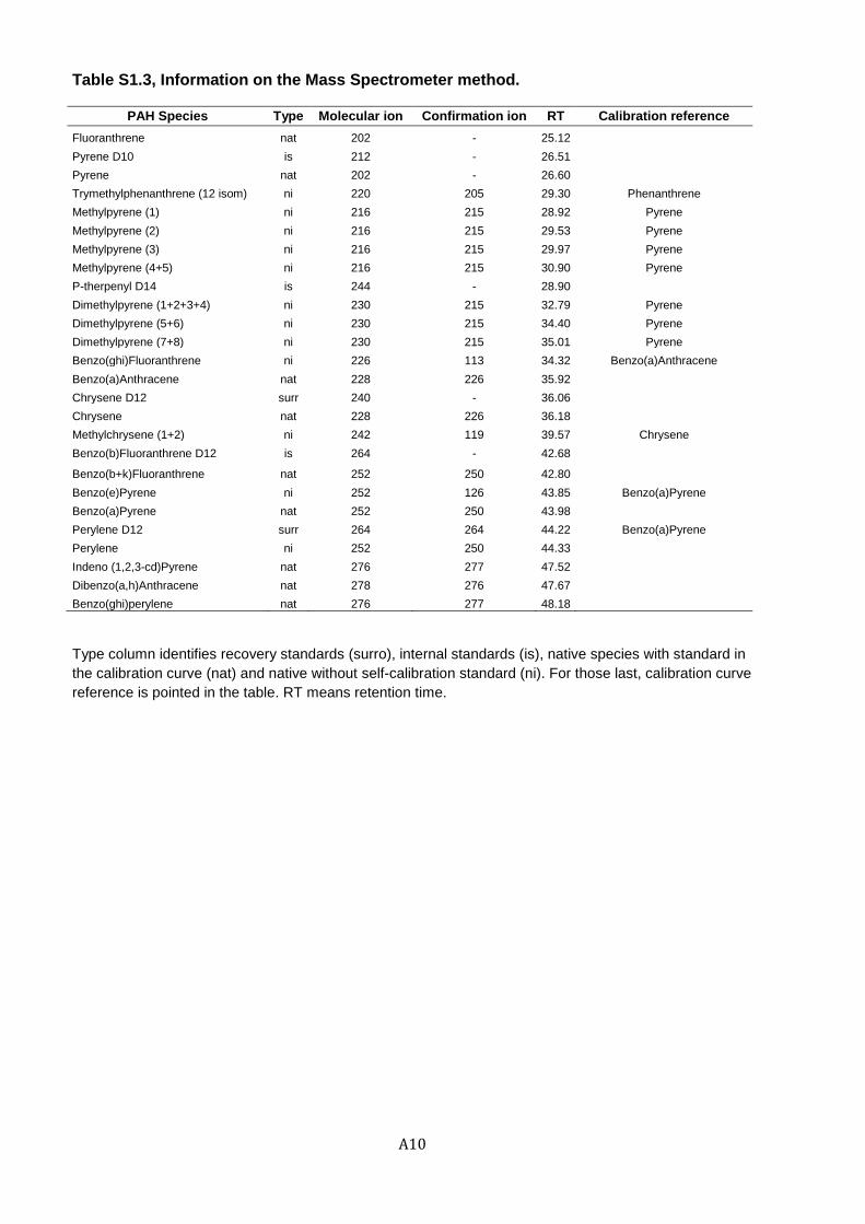
A10

Table S1.3, Information on the Mass Spectrometer method.

PAH Species Type Molecular ion Confirmation ion RT Calibration reference

Fluoranthrene nat 202 - 25.12 Pyrene D10 is 212 - 26.51 Pyrene nat 202 - 26.60 Trymethylphenanthrene (12 isom) ni 220 205 29.30 Phenanthrene

Methylpyrene (1) ni 216 215 28.92 Pyrene



Methylpyrene (4+5) ni 216 215 30.90 Pyrene

P-therpenyl D14 is 244 - 28.90 Dimethylpyrene (1+2+3+4) ni 230 215 32.79 Pyrene

Dimethylpyrene (5+6) ni 230 215 34.40 Pyrene

Dimethylpyrene (7+8) ni 230 215 35.01 Pyrene

Benzo(ghi)Fluoranthrene ni 226 113 34.32 Benzo(a)Anthracene

Benzo(a)Anthracene nat 228 226 35.92 Chrysene D12 surr 240 - 36.06 Chrysene nat 228 226 36.18 Methylchrysene (1+2) ni 242 119 39.57 Chrysene

Benzo(b)Fluoranthrene D12 is 264 - 42.68

Benzo(b+k)Fluoranthrene nat 252 250 42.80 Benzo(e)Pyrene ni 252 126 43.85 Benzo(a)Pyrene

Benzo(a)Pyrene nat 252 250 43.98 Perylene D12 surr 264 264 44.22 Benzo(a)Pyrene

Perylene ni 252 250 44.33 Indeno (1,2,3-cd)Pyrene nat 276 277 47.52 Dibenzo(a,h)Anthracene nat 278 276 47.67 Benzo(ghi)perylene nat 276 277 48.18

Type column identifies recovery standards (surro), internal standards (is), native species with standard in

the calibration curve (nat) and native without self-calibration standard (ni). For those last, calibration curve

reference is pointed in the table. RT means retention time.

A11

Table S1.4, Field blanks for the dry deposited aerosols samples.

DL Blank coarse

Blank fine

Samples over QL coarse

Samples over QL

fine

(ng/sample) (ng/sample) (ng/sample) (%) (%)

Fluoranthene 0.02 0.02 0.05 94 100

Pyrene 0.02 0.01 0.05 100 91

Methylpyrene 0.02 0.00 0.00 100 100

Dimethylpyrene 0.02 0.00 0.00 100 100

Benzo(ghi)Fluoranthene 0.02 0.00 0.00 100 100

Benzo(a)Anthracene 0.02 0.10 0.14 100 100

Chrysene 0.02 0.02 0.06 100 100

Methylchrysene 0.02 0.36 1.88 100 100

Benzo(b+k)Fluoranthene 0.02 0.28 0.00 100 100

Benzo(e)Pyrene 0.02 0.00 0.00 100 100

Benzo(a)Pyrene 0.02 0.35 0.54 100 100

Perylene 0.02 0.00 0.00 100 100

Indeno(1,2,3-cd)Pyrene 0.02 0.00 0.00 100 100

Dibenzo(a,h)Anthracene 0.02 0.00 0.00 100 100

Benzo(ghi)perylene 0.02 0.00 0.00 100 100

A12

Table S1.5, Field blanks for the suspended aerosol samples.

DL Lab Blank

Field Blank

Samples over QL

(ng/sample) (ng/sample) (ng/sample) (%)

Fluoranthene 0.02 nd 0.02 100

Pyrene 0.02 nd 0.05 100

Methylpyrene 0.02 nd nd 100

Dimethylpyrene 0.02 nd 0.23 100

Benzo(ghi)Fluoranthene 0.02 nd nd 100

Benzo(a)Anthracene 0.02 nd 0.25 100

Chrysene 0.02 nd 0.02 100

Methylchrysene 0.02 nd 0.12 97

Benzo(b+k)Fluoranthene 0.02 nd 1.16 100

Benzo(e)Pyrene 0.02 nd nd 100

Benzo(a)Pyrene 0.02 nd nd 100

Perylene 0.02 nd nd 100

Indeno(1,2,3-cd)Pyrene 0.02 nd nd 100

Dibenzo(a,h)Anthracene 0.02 nd nd 100

Benzo(ghi)Perylene 0.02 nd nd 100

A13

Table S1.6, Surrogate recoveries for the dry deposited aerosol samples.

Station

Aerosol fraction

Chrysene D12 Perylene D12

(initial-final)

% recovery % recovery

1 10-12 coarse 112.5 121.0

fine 59.0 104.9

2 17-19 coarse 63.0 112.1

fine 51.0 89.2

3 22-24 coarse 521.3* 340.7*

fine 64.2 118.4

4 25-26 coarse 120.8 203.0

fine 42.9 77.7

5 29-31 coarse 184.7 147.0

fine 78.3 124.3

6 33-35 coarse 70.0 128.3

fine 70.8 124.7

7 58-60 coarse 69.7 112.8

fine 56.2 65.7

8 85-87 coarse 21.2 28.2

fine 41.9 78.6

9 95-97 coarse 79.8 129.4

fine 69.2 120.3

10 115-116 coarse 75.1 128.1

fine 0.0** 0.0**

11 120-121 coarse 84.6 140.0

fine 139.1 114.7

12 0-0 coarse 81.8 136.3

fine 0.0* 0.0*

* 13 coarse sample was spiked wrongly due to an error during the extraction process

**fine aerosol 10 and 12 samples were not surrogate marked

Both anomalies did not account for the mean calculations.

0

50

100

150

200

coar

se

fin

e

coar

se

fin

e

coar

se

fin

e

coar

se

fin

e

coar

se

fin

e

coar

se

fin

e

coar

se

fin

e

coar

se

fin

e

coar

se

fin

e

coar

se

fin

e

coar

se

fin

e

coar

se

fin

e

1 2 3 4 5 6 7 8 9 10 11 12

Surr

oga

te r

eco

very

(%

)

Dry Deposition Measurement

Chrysene D12

Perylene D12

A14

Table S1.7, Surrogate recoveries for the suspended aerosol samples.

Dry Deposition correspondence

Station Sample Chrysene D12 Perylene D12

% recovery % recovery

1 11 MH013K011FPOP 95.20 101.14

2 17 MH019K017FPOP 109.73 110.93

3 23 MH025K023FPOP 87.90 88.84

4 24 MH026K024FPOP 119.17 114.29

4 25 MH027K025FPOP 102.86 100.03

5 30 MH039K030FPOP 119.03 123.68

5 31 MH040K031FPOP 122.74 129.47

6 33 MH042K033FPOP 102.86 105.31

6 34 MH043K034FPOP 127.75 134.19

7 36 MH045K036FPOP 71.82 75.50

7 37 MH046K037FPOP 102.38 95.45

7 38 MH047K038FPOP 114.25 132.73

8 40 MH049K040FPOP 107.08 132.29

8 41 MH050K041FPOP 40.16 48.45

9 57 MH077K057FPOP 93.91 112.13

9 58 MH078K058FPOP 67.06 64.05

9 59 MH079K059FPXX 97.96 105.01

9 60 MH080K060FPOP 120.16 130.47

10 85 MH129K085FPOP 94.37 112.47

10 86 MH130K086FPOP1 97.45 109.26

11 95 MH139K095FPOP1 88.44 116.07

11 95 MH139K095FPOP3 95.10 109.89

11 96 MH140K096FPOP2 91.45 108.27

12 114 MH163K114FPOP1 100.18 110.34

12 115 MH164K115FPOP1 96.83 104.74

13 120 MH169K120FPOP1 72.50 82.58

13 120 MH169K120FPOP2 92.60 119.51

13 121 MH170K121FPOP1 91.98 104.60

13 122 MH171K122FPOP1 90.17 103.18

13 122 MH171K122FPOP2 93.32 121.11

14 000 MH192K000FPOP1 104.25 117.28

14 131 MH193K131FPOP1 102.59 115.35

0

50

100

150

11

17

23

25

31

34

37

40

57

59

85

95

96

11

5

12

0

12

2

Surr

oga

te r

eco

very

(%

)

Station

Chrysene D12

Perylene D12

A15

Table S1.8, Dry deposition fluxes (FDD) measured for aerosols (g m-2d-1) and PAHs (ng m-2d-1).

Sam

ple

Aero

so

l

fracti

on

Part

icle

s

Flu

o

Pyr

MeP

yr

DM

eP

yr

B(g

hi)

Flu

o

B (

a)

An

thr

Ch

ry

MeC

hry

B (

b+

k)

Flu

o

B(e

)Pyr

B (

a)P

yr

Per

I(1,2

,3-c

d)

Pyr

DiB

(a,h

)

An

thr

B(g

hi)

Per

∑16PAHs

(g m-2

day-1

) (ng m-2

day-1

)

1 coarse 2.22 5.90 15.00 19.29 3.35 0.00 0.00 0.00 0.00 3.11 3.08 15.33 0.00 0.00 4.46 3.76 3.08

fine 0.07 0.00 0.19 0.21 1.12 0.43 0.23 0.21 0.11 0.30 0.14 0.07 0.09 0.07 0.39 0.14 0.73

2 coarse 0.29 0.04 0.25 0.60 0.62 0.44 0.55 0.39 0.12 0.67 0.62 0.60 0.66 0.34 0.66 0.87 1.45

fine 0.16 0.00 0.14 0.19 0.70 0.29 0.23 0.19 0.09 0.60 0.50 0.21 0.13 0.14 0.74 0.52 0.92

3 coarse 0.03 1.03 0.09 0.17 0.14 0.16 0.06 0.16 0.02 0.18 0.07 2.28 0.49 0.02 0.34 0.62 2.07

fine 0.08 0.00 0.07 0.10 0.37 0.15 0.12 0.09 0.04 0.19 0.10 0.04 0.02 0.05 0.37 0.07 0.63

4 coarse 0.21 1.04 1.59 2.10 0.92 0.02 0.31 0.32 0.07 0.92 0.73 3.50 0.36 0.44 0.71 1.06 6.00

fine 0.16 0.00 0.29 0.33 1.67 0.66 0.42 0.33 0.16 0.69 0.35 0.16 0.15 0.19 1.72 0.35 1.60

5 coarse 0.06 0.18 0.25 0.46 0.48 0.14 0.13 0.18 0.05 0.32 0.38 0.58 0.28 0.08 0.38 0.58 2.07

fine 0.04 0.00 0.12 0.14 0.72 0.26 0.15 0.10 0.07 0.25 0.13 0.04 0.01 0.05 0.31 0.07 0.83

6 coarse 0.05 0.06 0.14 0.25 0.23 0.17 0.09 0.09 0.04 0.19 0.10 0.03 0.03 0.20 0.34 0.06 1.36

fine 0.13 0.13 0.13 0.13 0.57 0.21 0.11 0.09 0.06 0.14 0.08 0.04 0.03 0.06 0.33 0.07 0.79

7 coarse 0.05 0.20 0.15 0.24 0.45 0.32 0.29 0.22 0.05 0.29 0.17 0.15 0.13 0.06 0.28 0.22 0.74

fine 0.03 0.00 0.04 0.07 0.14 0.09 0.08 0.07 0.04 0.08 0.05 0.03 -0.01 0.05 0.33 0.06 0.73

8 coarse 0.98 9.47 0.00 7.26 2.01 0.00 0.00 0.00 0.00 0.00 0.87 0.00 0.00 1.94 0.00 0.00 0.00

fine 0.04 0.00 0.08 0.10 0.22 0.13 0.10 0.07 0.05 0.12 0.09 0.05 0.00 0.09 0.49 0.11 0.88

9 coarse 0.04 0.18 0.15 0.21 0.27 0.37 0.94 1.97 0.07 1.14 0.89 0.41 0.45 0.24 1.07 1.42 1.70

fine 0.04 0.00 0.15 0.26 0.71 0.40 0.47 0.44 0.09 0.47 0.39 0.41 0.32 0.17 0.86 0.82 4.37

10 coarse 0.07 0.12 0.11 0.15 0.54 0.30 0.22 0.16 0.07 0.30 0.19 0.17 0.12 0.09 0.54 0.24 1.43

fine 0.00 0.00 0.00 0.00 0.02 0.00 0.00 0.02 0.15 0.02 0.00 0.00 0.00 0.00 0.04 0.00 0.00

11 coarse 0.09 1.42 0.18 0.25 0.93 0.38 0.29 0.28 0.09 0.54 0.22 0.22 0.16 0.12 0.51 0.31 1.96

fine 0.27 4.55 0.39 0.56 0.35 0.00 0.00 0.00 0.00 0.12 0.00 0.00 0.00 0.00 0.00 0.00 3.57

12 coarse 0.09 0.00 0.14 0.26 0.75 0.40 0.46 0.37 0.09 1.09 0.82 0.36 0.45 0.18 0.93 1.09 1.57

fine 0.00 0.00 0.00 0.00 0.00 0.00 0.00 0.00 0.00 0.00 0.00 0.00 0.00 0.00 0.00 0.00 0.00

A16

Figure S1.3, Mean dry deposition fluxes (FDD) for individual PAHs in the coarse and fine

deposited fractions (ng m-2d-1).

0

1

2

3

4

5

6

7

F DD (

ng

m-2

day

-1)

mean coarse

mean fine

A17

Figure S1.4, Aerosol dry deposition fluxes (FDD) in the Global Oceans (g m-2d-1).

d

A18

Table S1.9, Organic Carbon concentrations in the deposited particles (OC%) and their dry

deposition fluxes (FDD OC; mg m-2d-1)

Sample OC

(% mass in sample)

coarse fine

1 0.56 0.37

2 0.00* 0.00*

3 0.56 0.23

4 3.34 0.95

5 0.00* 0.00*

6 0.68 0.69

7 0.64 0.48

8 1.53 0.97

9 0.00* 0.60*

10 1.74 2.11

11 1.19 0.79

12 1.19 0.38

* The value is set to 0.00% when the value was detection limit (<0.10%)

d

A19

Table S1.10, Concentrations of PAHs in dry deposited fine and coarse aerosols (CDD , ng g-1) S

am

ple

Aero

so

l

Fra

cti

on

Pa

rtic

le

Flu

o

Py

r

Me

Py

r

DM

eP

yr

B (

gh

i) F

luo

B (

a)

An

thr

Ch

ry

Me

Ch

ry

B (

b+

k)

Flu

o

B (

e)

Py

r

B (

a)

Py

r

Pe

r

I (1

,2,3

-cd

)Py

r

DB

(a

,h)

An

thr

B (

gh

i) P

er

∑1

6P

AH

s

(g) (ng g

-1)

1 coarse 0.0825 75.390 74.709 371.537 nd nd 108.113 91.053 74.722 53.025 nd 60.375 nd 76.489 72.567 71.763 1129.74

2 fine 0.0674 9.037 4.178 1.992 2.558 2.018 11.486 4.047 21.700 22.160 2.861 28.068 1.250 25.033 26.271 8.941 171.601

2 coarse 0.1915 5.844 5.380 5.235 5.746 2.967 5.735 7.580 12.579 20.017 9.028 25.194 2.665 10.437 9.647 5.896 133.951

fine 0.0956 10.528 8.775 3.576 2.208 2.479 12.914 9.039 16.069 24.603 9.514 29.929 4.349 25.071 22.374 11.157 192.584

3 coarse 0.1948 2.092 0.830 26.332 5.698 0.238 3.878 7.106 23.920 2.298 3.002 5.013 0.464 1.470 1.376 1.272 84.989

fine 0.1681 2.550 1.311 0.493 0.282 0.684 4.892 0.986 8.488 7.998 0.252 9.538 0.443 9.064 9.551 2.994 59.525

4 coarse 0.1061 9.668 7.726 36.835 3.734 4.665 7.421 11.138 63.074 13.662 12.796 25.229 3.192 26.039 5.212 25.722 256.114

fine 0.0760 10.101 5.097 2.398 2.132 2.839 25.278 5.209 23.483 30.016 5.179 36.399 2.147 34.376 32.086 15.093 231.832

5 coarse 0.0924 6.851 7.974 12.331 5.862 1.608 8.034 12.389 43.820 6.958 5.505 11.028 1.924 6.943 nd 6.768 137.994

fine 0.0674 7.315 3.654 1.203 0.251 1.560 8.978 2.073 24.076 16.995 0.491 19.516 1.241 18.709 19.581 6.244 131.886

6 coarse 0.2883 1.223 0.650 0.207 0.175 1.319 2.202 0.391 8.841 8.222 0.049 5.026 0.290 nd 5.143 1.523 35.262

fine 0.1660 1.610 0.960 0.503 0.318 0.621 3.731 0.762 8.931 7.034 nd 8.499 0.362 nd 8.813 2.600 44.702

7 coarse 0.1422 4.748 2.826 2.465 2.036 0.968 4.552 3.544 11.982 9.959 3.007 12.941 1.093 10.823 10.817 4.680 86.442

fine 0.0755 2.338 1.647 0.992 nd 1.673 9.932 1.812 22.373 19.406 nd 23.553 0.540 nd nd 7.161 90.993

8 coarse 0.0977 nd 17.738 nd nd 39.736 nd nd nd nd nd nd nd nd nd nd 57.474

fine 0.0498 4.855 3.487 1.909 nd 3.532 19.741 4.328 35.437 40.503 0.659 48.707 1.703 46.476 nd 15.071 226.362

9 coarse 0.0824 13.655 10.698 4.897 5.385 2.915 12.784 16.983 20.323 18.577 8.945 23.894 1.526 16.707 16.416 6.669 180.374

fine 0.0638 7.222 5.999 6.369 4.982 2.641 13.214 12.602 67.565 25.025 13.380 36.010 4.661 25.666 25.068 13.844 264.248

10 coarse 0.0545 6.655 4.210 3.783 2.736 2.070 12.015 5.327 31.678 23.290 3.701 28.473 3.052 24.716 25.676 8.953 186.335

fine 0.0389 0.689 nd nd nd nd 1.210 nd nd nd nd 0.728 nd nd nd 11.600 14.228

11 coarse 0.0423 15.419 6.324 6.453 4.574 3.385 14.725 8.853 56.381 28.402 8.565 36.093 2.812 29.367 30.161 13.844 265.358

fine 0.1534 0.969 nd nd nd nd nd nd 28.293 nd nd nd nd nd nd nd 29.263

12 coarse 0.0587 23.897 17.948 7.902 9.827 3.941 20.398 24.007 34.639 31.650 25.605 45.955 7.180 32.201 25.380 21.500 332.031

fine 0.0485 nd nd nd nd nd nd nd nd nd nd nd nd nd nd nd nd

A20

Figure S1.5, PAHs concentration in dry deposited aerosol (CDD, ng g-1) for the a) fine

fraction and b) coarse fraction.

a

)

b

)

A21

Table S1.11, Concentrations of individual PAHs in the suspended aerosols (CA, ng m-3) D

ry D

ep

me

as

ure

Sta

tio

n

Vo

l

sa

mp

led

Aero

so

l

Flu

o

Py

r

Me

tPy

r

DM

e P

yr

B (

gh

i)

Flu

o

B (

a)

An

thr

Ch

ry

Me

Ch

ry

B(b

) F

luo

B(k

) F

luo

B (

e)

Py

r

B (

a)

Py

r

Pe

r

I (1

,2,3

-

cd

)Py

r

DB

(a,h

)

An

thr

B (

gh

i) P

er

∑1

6P

AH

s

(m

3) (mg m

-3) (ng m

-3)

1 11 945 0.087 0.207 0.185 0.077 0.116 0.034 0.085 0.083 0.001 0.074 0.024 0.057 0.035 0.010 0.027 0.016 0.039 1.069

2 17 945 0.073 0.071 0.062 0.014 0.045 0.017 0.025 0.026 0.001 0.021 0.006 0.020 0.008 0.003 0.007 0.003 0.011 0.339

3 23 632 0.067 0.474 0.404 0.090 0.311 0.181 0.305 0.294 0.005 0.256 0.080 0.218 0.148 0.044 0.087 0.048 0.129 3.073

4 24 525 0.133 0.126 0.111 0.022 0.086 0.027 0.043 0.045 0.002 0.034 0.010 0.026 0.014 0.005 0.019 0.005 0.022 0.596

4 25 275 0.331 0.365 0.381 0.102 0.532 0.004 0.155 0.227 0.005 0.094 0.023 0.079 0.032 0.011 0.021 0.009 0.035 2.077

5 30 1339 0.086 0.059 0.047 0.011 0.038 0.014 0.019 0.022 0.001 0.026 0.007 0.021 0.007 0.003 0.015 0.003 0.021 0.313

5 31 1149 0.050 0.040 0.031 0.015 0.031 nd 0.015 0.015 0.001 0.012 0.003 0.009 0.005 0.001 0.004 0.002 0.005 0.189

6 33 940 0.028 0.052 0.040 0.017 0.039 0.017 0.016 0.019 0.001 0.014 0.004 0.011 0.005 0.003 0.004 0.002 0.005 0.249

6 34 617 0.056 0.072 0.057 0.026 0.066 0.001 0.026 0.029 0.001 0.021 0.006 0.016 0.005 0.002 0.005 0.002 0.006 0.342

7 33 1982 0.018 0.010 0.012 0.003 0.025 0.001 0.002 0.004 0.001 0.003 0.001 0.004 0.001 nd 0.001 nd 0.003 0.071

7 37 927 0.035 0.501 0.613 0.448 0.834 0.131 0.907 0.858 0.013 0.662 0.194 0.481 0.335 0.092 0.174 0.007 0.272 6.524

7 59 889 0.037 0.114 0.114 0.001 0.002 nd 0.120 0.115 nd 0.116 0.106 0.001 0.111 nd 0.116 0.120 0.109 1.145

7 60 871 0.039 0.061 0.092 0.028 0.191 0.066 0.018 0.028 0.007 0.021 0.004 0.027 0.010 0.003 0.007 0.003 0.024 0.592

8 85 672 0.047 0.067 0.059 0.016 0.075 0.001 0.060 0.066 0.002 0.078 0.021 0.072 0.021 0.009 0.026 0.012 0.041 0.625

8 86 582 0.071 0.059 0.050 0.022 0.042 0.001 0.025 0.023 0.001 0.022 0.007 0.016 0.009 0.003 0.005 0.002 0.008 0.295

9 95 618 0.106 0.105 0.089 0.037 0.062 0.032 0.039 0.037 0.001 0.033 0.009 0.028 0.015 0.005 0.011 0.005 0.015 0.522

9 96 902 0.118 0.016 0.016 0.008 0.013 nd 0.010 0.008 nd 0.010 0.002 0.009 0.003 0.002 0.004 0.001 0.005 0.108

9 114 1088 0.112 0.026 0.024 0.012 0.022 0.011 0.016 0.015 nd 0.016 0.005 0.015 0.010 0.003 0.006 0.003 0.010 0.194

10 114 857 0.074 0.028 0.024 0.012 0.021 0.011 0.014 0.012 0.001 0.014 0.004 0.012 0.005 0.002 0.005 0.002 0.007 0.173

10 115 800 0.046 0.051 0.043 0.016 0.034 nd 0.016 0.020 0.001 0.014 0.003 0.011 0.005 0.001 0.003 0.001 0.004 0.224

11 120 853 0.035 0.050 0.042 0.016 0.035 0.011 0.014 0.019 0.001 0.016 0.005 0.012 0.006 0.002 0.006 0.002 0.008 0.243

11 120 916 0.065 0.046 0.040 0.017 0.028 nd 0.015 0.017 0.001 0.013 0.004 0.011 0.006 0.002 0.004 0.002 0.005 0.211

11 121 883 0.030 0.023 0.031 0.010 0.065 0.001 0.005 0.008 0.002 0.007 0.002 0.009 0.003 0.001 0.003 0.001 0.008 0.181

A22

Dry

De

p

me

as

ure

Sta

tio

n

Vo

l

sa

mp

led

Aero

so

l

Flu

o

Py

r

Me

tPy

r

DM

e P

yr

B (

gh

i)

Flu

o

B (

a)

An

thr

Ch

ry

Me

Ch

ry

B(b

) F

luo

B(k

) F

luo

B (

e)

Py

r

B (

a)

Py

r

Pe

r

I (1

,2,3

-

cd

)Py

r

DB

(a,h

)

An

thr

B (

gh

i) P

er

∑1

6P

AH

s

11 122 551 0.090 0.100 0.086 0.033 0.063 0.001 0.034 0.040 0.001 0.034 0.009 0.028 0.010 0.002 0.014 0.003 0.021 0.477

11 122 789 0.024 0.071 0.065 0.028 0.049 0.027 0.024 0.030 nd 0.022 0.007 0.018 0.011 0.003 0.007 0.003 0.010 0.375

12 0 818 0.075 0.007 0.010 0.004 0.020 0.001 0.002 0.002 0.001 0.002 0.001 0.002 0.001 nd 0.001 nd 0.002 0.055

12 131 820 0.069 0.048 0.042 0.018 0.028 nd 0.013 0.014 0.001 0.011 0.003 0.010 0.005 0.002 0.004 0.002 0.005 0.205

Figure S1.6, Concentrations of PAHs in suspended aerosol (CA, ng m-3) in the Global Oceans

A23

Figure S1.7, Individual PAHs profile in suspended aerosols (CA, ng m-3).

Bars show the standard deviation (SD) of the deposition measures in the signed ocean. Indian

Ocean only holds one measurement, thus with no SD bar.

0,00

0,05

0,10

0,15

0,20

0,25

CA (

ng

m-3

)

Atlantic

Indian

Pacific

A24

Table S1.12, Estimated dry deposition velocity (vD, cm s-1) of suspended aerosol-bound PAHs

Sam

ple

Flu

o

Pyr

MeP

yr

DM

eP

yr

B (

gh

i)

Flu

o

B (

a)

An

thr

Ch

ry

MetC

hry

B (

b+

k)

Flu

o

B (

e)

Py

r

B (

a)

Py

r

Per

I (1

,2,3

-

cd

)Pyr

DB

(a,h

)

An

thr

B (

gh

i)

Per

(cm s-1

)

1 0.019 0.020 0.232 0.001 0.002 0.066 0.054 3.016 0.035 0.002 0.114 0.005 0.170 0.287 0.097

2 0.021 0.021 0.068 0.020 0.033 0.065 0.063 2.860 0.159 0.094 0.630 0.199 0.425 1.069 0.142

3 0.001 0.000 0.030 0.002 0.000 0.003 0.003 0.634 0.003 0.001 0.009 0.002 0.011 0.020 0.003

4 0.009 0.006 0.086 0.002 0.039 0.034 0.015 2.941 0.056 0.041 0.283 0.073 0.286 0.467 0.151

5 0.013 0.015 0.056 0.010 0.019 0.047 0.041 5.315 0.042 0.020 0.236 0.077 0.113 0.330 0.046

6 0.006 0.005 0.004 0.001 0.028 0.038 0.006 2.831 0.101 0.000 0.347 0.035 0.000 0.940 0.099

9 0.003 0.002 0.002 0.001 0.003 0.004 0.002 0.368 0.008 0.002 0.025 0.005 0.019 0.197 0.009

10 0.002 0.016 0.002 0.000 0.146 0.018 0.004 1.095 0.034 0.001 0.124 0.014 0.171 0.000 0.039

11 0.073 0.063 0.084 0.043 0.060 0.151 0.200 13.301 0.197 0.138 0.722 0.214 0.642 1.378 0.198

12 0.007 0.005 0.012 0.004 0.018 0.045 0.014 2.701 0.064 0.017 0.288 0.097 0.264 1.015 0.148

13 0.008 0.003 0.007 0.002 0.010 0.018 0.009 2.632 0.029 0.012 0.111 0.029 0.106 0.351 0.030

14 0.029 0.024 0.025 0.019 0.028 0.078 0.089 0.177 0.110 0.126 0.472 0.214 0.448 0.852 0.234

00,10,20,30,40,50,6

Mea

n v

D (

cm s

-1) ≈

A25

Table S1.13, Vapor pressures (PL) for individual PAHs used in this work.

Compound PL

[Pa]

Fluoranthrene 0.00598

Pyrene

Benzo(g,h,i)fluoranthrene 0.00000755

Benzo(a)anthracene

Chrysene 0.00017

Benzo(b+k)fluoranthrene 0.00000896

Benzo(e)pyrene

Benzo(a)pyrene 0.0000059

Perylene 0.00000488

Dibenzo(a,h)anthracene 0.000000344

Benzo(g,h,i)perylene 0.000000428

Adapted from Lei et al. 20021, Super-cooled Liquid vapor Pressure at 25ºC.

1 Lei, Y. D.; Chankalal, R.; Chan, A.; Wania, F., Supercooled liquid vapor pressures of the polycyclic aromatic hydrocarbons. Journal of Chemical and Engineering Data 2002, 47, (4), 801-806.

A26

Table S1.14, Spearman correlation data between PAHs dry deposition velocity

(vD) for each sampling period versus compound specific vapor pressure (PL)

Rho Spearman test Log(PL)

vD 1

P -.382

Sig. (two-tailed) .247

N 11

vD 2

P -.827**


N 11

vD 3

P -.627*


N 11

vD 4

P -.936**


N 11

vD 5

P -.736**


N 11

vD 6

P -.709*


N 11

vD 7

P -.755**


N 11

vD 8

P -.127


N 11

vD 9

P -.673*


N 11

vD 10

P -.900**


N 11

vD 11

P -.882**


N 11

vD 12

P -.827**


N 11 **. Correlation is significant at level 0.01 (two-tailed).

A27

*. Correlation is significant at level 0.05 (two-tailed).

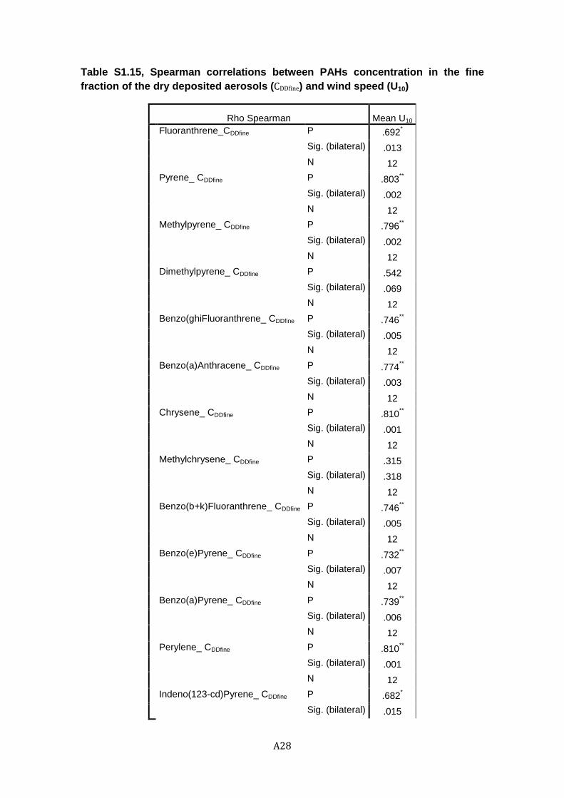
A28

Table S1.15, Spearman correlations between PAHs concentration in the fine

fraction of the dry deposited aerosols (CDDfine) and wind speed (U10)

Rho Spearman Mean U10

Fluoranthrene_CDDfine P .692*

Sig. (bilateral) .013

N 12

Pyrene_ CDDfine P .803**


N 12

Methylpyrene_ CDDfine P .796**


N 12

Dimethylpyrene_ CDDfine P .542


N 12

Benzo(ghiFluoranthrene_ CDDfine P .746**


N 12

Benzo(a)Anthracene_ CDDfine P .774**


N 12

Chrysene_ CDDfine P .810**


N 12

Methylchrysene_ CDDfine P .315


N 12

Benzo(b+k)Fluoranthrene_ CDDfine P .746**


N 12

Benzo(e)Pyrene_ CDDfine P .732**


N 12

Benzo(a)Pyrene_ CDDfine P .739**


N 12

Perylene_ CDDfine P .810**


N 12

Indeno(123-cd)Pyrene_ CDDfine P .682*


A29


N 12

Dibenzo(ah)Anthracene_ CDDfine P .689*


N 12

Benzo(ghi)Perylene_ CDDfine P .627*


N 12

**. Correlation is significant at level 0.01 (two-tailed).


A30

Table S1.16, Spearman correlations between PAHs dry deposition flux

associated to fine particles (FDDfine) and wind speed (U10)


Fluoranthrene_ FDDfine

P .657*


N 12

Pyrene_ FDDfine

P .657*


N 12

Methylpyrene_ FDDfine

P .664*


N 12

Dimethylpyrene_ FDDfine

P .618*


N 12

Benzo(ghi)Fluoranthrene_ FDDfine

P .695*


N 12

Benzo(a)Anthracene_ FDDfine

P .649*


N 12

Chrysene_ FDDfine

P .638*


N 12

Methylchrysene_ FDDfine

P .523


N 12

Benzo(b+k)Fluoranthrene_ FDDfine

P .644*


N 12

Benzo(e)Pyrene_ FDDfine

P .692*


N 12

Benzo(a)Pyrene_ FDDfine

P .601*


N 12

Perylene_ FDDfine

P .678*


N 12

Indeno123cdpyrene_ FDDfine

P .702*


N 12

Dibenzoahanthracene_ FDDfine

P .591*


N 12

A31


Benzoghiperylene_ FDDfine

P .326


N 12


A32

Table S1.17, Pearson’s correlation between PAHs dry deposition velocity slopes

when plotted against vapor pressure (slope VDDfine) versus wind speed (U10)

Slopes are obtained from S14 per each measurement. In this case parametric statistics

are applied as the slope is already normalized within the logarithmic plotting in S14.

Pearson correlation Mean U10

Slope

P -.638*


N 12


Table S1.18, Parameterization of the deposition velocity versus physic and

biochemical parameters using least squares multiple parametric linear

regression.

Parameters include: vapor pressure (LogPL), wind speed (U10) and chlorophyll a

concentrations ate the sea surface (Chls). The term U10xChls accounts for the

interaction of wind speed and chlorophyll a concentration at surface.

Coefficients

Model Not standardized

Coefficients

Standardized

Coefficients

t Sig. R square B Typical Error β

1

(Constant) -3.082 .197 -15.656 .000 .365a

LogPL -.261 .038 -.479 -6.826 .000

U10xChls .387 .074 .368 5.243 .000

a. Dependent Variable: logvD

Coefficients


Coefficients

Standardized

Coefficients


1

(Constant) -3.269 .307 -10.645 .000 .227b

LogPL -.287 .060 -.373 -4.819 .000

U10xChls .442 .115 .297 3.840 .000

b. Dependent Variable: logvDfine

Coefficients


Coefficients

Standardized

Coefficients


1 (Constant) -2.973 .240 -12.402 .000 .503

c

LogPL -.253 .047 -.415 -5.450 .000

A33

U10xChls .337 .090 .285 3.749 .000

c. Dependent Variable: logvDcoarse

Table S1.19, Parameterization of the deposition velocity (vD) versus vapor

pressure (PL) using least squares multiple parametric linear regression.

Coefficient a

Model Not standardized Coefficients Standardized

Coefficients


1 (Constant) -2.670 .198 -13.483 .000 .229

LogPL -.261 .042 -.479 -6.222 .000

a. Dependent Variable: logvD

Coefficient b


Coefficients


1 (Constant) -2.798 .296 -9.452 .000 .139

LogPL -.287 .063 -.373 -4.583 .000

b. Dependent Variable: logvDfine

Coefficient c


Coefficients


1 (Constant) -2.614 .231 -11.339 .000 .172

LogPL -.253 .049 -.415 -5.196 .000

c. Dependent Variable: logvDcoarse

A35

2. HIGH ATMOSPHERE-OCEAN EXCHANGE OF SEMIVOLATILE

AROMATIC HYDROCARBONS


Belén González-Gaya1,2, María-Carmen Fernández-Pinos1, Laura Morales1,

Esteban Abad1, Benjamí Piña1, Laurence Mejanelle3, Carlos Duarte4,5,

Begoña Jiménez2, Jordi Dachs1*

*Corresponding author email: [email protected]

A36

Index

Table S2.1. Mean concentrations of PAHs per ocean in each analyzed matrix

Table S2.2. Mean concentrations of PAHs in dissolved and gas phase blanks

Table S2.3. Calculated uncertainty for SALCs Diffusive fluxes according to Henry’s

constant (H’)

Figure S2.1. Mean PAHs profile in each matrix analyzed; gas, aerosol and dissolved

phase

Figure S2.2. Wet deposition fluxes

Figure S2.3. Ocean basin averaged gross volatilization and absorption fluxes, and

net diffusive fluxes

Figure S2.4. Degradation of PAHs in the atmosphere by reaction with OH radical

Figure S2.5. Mean concentrations of total aromatics and the quantified fraction of

PAHs in gas and water samples for the six retention time intervals quantified

A37

Table S2.1. Mean concentrations of PAHs per ocean in each analyzed matrix

Gas Phase (ng m-3) Aerosol Phase (ng m-3) Dissolved Phase (ng L-1)

Atlantic North

Atlantic South

Pacific North

Pacific South

Indian Atlantic North

Atlantic South

Pacific North

Pacific South


Atlantic South

Pacific North

Pacific South

Indian

Naphthalene 0.072 0.105 0.080 0.144 0.179 0.001 0.001 0.000 0.001 0.004 0.029 0.018 0.019 0.031 0.024

Methylnaphthalenes 0.000 0.000 0.000 0.000 0.000 0.001 0.009 0.000 0.001 0.001 0.131 0.140 0.062 0.110 0.074

Dimethylnaphthalenes 0.146 0.730 0.041 1.120 0.470 0.001 0.001 0.000 0.001 0.001 0.289 0.133 0.150 0.270 0.150

Acenaphtylene 0.198 0.144 0.176 0.135 0.086 0.003 0.004 0.005 0.007 0.020 0.030 0.146 0.004 0.001 0.001

Acenaphtene 0.048 0.085 0.059 0.076 0.112 0.000 0.001 0.000 0.001 0.005 0.135 0.058 0.043 0.043 0.022

Fluorene 0.368 0.434 0.132 0.329 0.366 0.003 0.004 0.002 0.003 0.017 0.195 0.192 0.083 0.083 0.056

Dibenzothiophene 1.130 1.060 0.489 0.784 0.779 0.003 0.003 0.002 0.002 0.018 0.123 0.160 0.042 0.044 0.040

Methyldibenzothiophenes 6.330 2.410 2.260 1.670 1.120 0.024 0.042 0.029 0.030 0.167 0.145 0.185 0.101 0.109 0.081

Dimethyldibenzothiopenes 10.500 3.930 4.230 3.780 2.840 0.074 0.088 0.112 0.114 0.729 0.115 0.151 0.125 0.140 0.088

Phenanthrene 9.360 9.380 5.400 9.510 8.710 0.051 0.084 0.036 0.042 0.348 0.458 0.387 0.325 0.326 0.212

Methylphenantrenes 5.180 2.960 2.200 3.660 1.910 0.036 0.024 0.030 0.053 0.333 0.287 0.324 0.285 0.293 0.223

Dimethylphenanthrenes 2.260 1.380 1.050 2.070 1.060 0.043 0.045 0.053 0.067 0.507 0.139 0.164 0.147 0.154 0.108

Anthracene 1.860 1.780 1.050 1.370 1.420 0.028 0.101 0.047 0.020 0.130 0.045 0.049 0.033 0.035 0.025

Fluoranthene 1.340 0.828 0.674 1.700 0.908 0.058 0.090 0.041 0.067 0.631 0.349 0.417 0.353 0.393 0.274

Pyrene 0.862 0.565 0.476 1.640 0.662 0.059 0.078 0.035 0.065 0.587 0.401 0.477 0.407 0.495 0.295

Methylpyrenes 0.278 0.226 0.102 0.208 0.244 0.029 0.023 0.013 0.024 0.320 0.052 0.085 0.043 0.042 0.061

Dimethylpyrenes 0.127 0.162 0.052 0.092 0.127 0.072 0.079 0.035 0.075 0.730 0.022 0.037 0.014 0.011 0.020

Benzo[ghi]fluoranthene 0.122 0.081 0.109 0.120 0.114 0.019 0.015 0.007 0.035 0.165 0.016 0.018 0.015 0.015 0.012

Benzo[a]anthracene 0.079 0.073 0.048 0.061 0.082 0.059 0.041 0.014 0.055 0.799 0.026 0.038 0.008 0.019 0.041

Chrysene 0.141 0.126 0.063 0.104 0.121 0.076 0.048 0.020 0.077 0.806 0.016 0.016 0.010 0.011 0.007

Methylchrysenes 0.037 0.043 0.025 0.021 0.027 0.049 0.012 0.010 0.039 0.612 0.007 0.011 0.003 0.003 0.010

Benzo[b+k]fluoranthenes 0.051 0.026 0.056 0.190 0.283 0.142 0.048 0.022 0.097 1.227 0.003 0.010 0.002 0.002 0.002

Benzo[e]pyrene 0.014 0.022 0.018 0.035 0.024 0.078 0.032 0.014 0.061 0.725 0.006 0.008 0.004 0.004 0.003

A38

Gas Phase (ng m-3) Aerosol Phase (ng m-3) Dissolved Phase (ng L-1)

Atlantic North

Atlantic South

Pacific North

Pacific South


Atlantic South

Pacific North

Pacific South


Atlantic South

Pacific North

Pacific South

Indian

Benzo[a]pyrene 0.033 0.045 0.070 0.063 0.071 0.028 0.016 0.006 0.026 0.377 0.002 0.011 0.002 0.002 0.002

Perylene 0.010 0.007 0.020 0.026 0.040 0.009 0.005 0.002 0.008 0.107 0.001 0.007 0.001 0.001 0.001

Indeno[1,2,3-cd]pyrene 0.005 0.016 0.005 0.007 0.004 0.060 0.014 0.007 0.037 0.167 0.050 0.072 0.042 0.030 0.036

Dibenzo[a,h]anthracene 0.004 0.014 0.007 0.010 0.006 0.010 0.005 0.001 0.007 0.115 0.064 0.093 0.060 0.043 0.045

Benzo[ghi]perylene 0.004 0.003 0.002 0.010 0.001 0.084 0.019 0.011 0.053 0.396 0.017 0.028 0.016 0.014 0.014

Σ64 PAHS 40.589 26.635 18.887 28.961 21.750 1.103 0.933 0.556 1.067 10.044 3.151 3.433 2.400 2.722 1.927

A39

Table S2.2. Mean concentrations of PAHs in the gas and dissolved phase

blanks

Gas Phase Dissolved Phase

Field blank mean

(total ng)

Laboratory blank mean

(total ng)

Field blank mean

(total ng)

Laboratory blank mean

(total ng)

Naphthalene 0.82 0.98 0.91 0.96

Methylnaphthalenes 0.00 0.00 0.35 0.32

Dimethylnaphthalenes 0.40 0.00 0.49 0.38

Acenaphtylene 0.15 0.09 0.08 0.05

Acenaphtene 0.09 0.47 0.04 0.03

Fluorene 0.05 0.41 0.12 0.08

Dibenzothiophene 0.04 0.09 0.09 0.04

Methyldibenzothiophenes 0.41 0.23 0.48 0.20 Dimethyldibenzothiopenes 0.13 1.91 0.56 0.19

Phenanthrene 0.14 0.18 0.72 0.58

Methylphenantrenes 0.16 0.47 0.69 0.22

Dimethylphenanthrenes 0.12 0.32 0.49 0.16

Anthracene 0.14 0.33 0.31 0.02

Fluoranthene 0.22 0.44 0.28 0.18

Pyrene 0.21 0.35 0.33 0.22

Methylpyrenes 0.01 0.00 0.26 0.13

Dimethylpyrenes 0.03 0.00 0.13 0.04

Benzo[ghi]fluoranthene 0.35 0.75 0.64 0.02

Benzo[a]anthracene 0.08 0.26 0.15 0.13

Chrysene 0.07 0.12 0.09 0.08

Methylchrysenes 0.13 0.00 0.04 0.02

Benzo[b+k]fluoranthenes 0.02 1.98 0.03 0.04

Benzo[e]pyrene 0.65 0.32 0.01 0.04

Benzo[a]pyrene 3.06 0.00 0.08 0.03

Perylene 1.27 0.00 0.11 0.05

Indeno[1,2,3-cd]pyrene 1.01 0.00 1.83 0.07

Dibenzo[a,h]anthracene 0.32 0.00 3.88 0.26

Benzo[ghi]perylene 0.00 0.00 0.80 0.02

Σ64PAHs 10.09 9.72 14.01 4.55

A40

Table S2.3. Calculated uncertainty for SALCs Diffusive fluxes according to

Henry’s constant (H’)

The results are for H’ values 3 times higher and 3 times lower than the H’ values

corresponding to the individual PAH selected for each analysis time window and used

to quantify SALCs.

Mean total SALCs flux

(ng m-2d-1)

H’ 1/3 H’ x3

Absorption flux -8,13 106 -4,02 106

Volatilization flux 4,61 105 1,84 106

Net flux -7,67 106 -2,18 106

A41

Figure S2.1. Mean PAH profile in each matrix analyzed; gas (top), aerosol (middle) and dissolved phase (bottom panel)

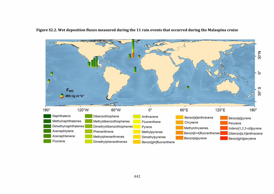
A42

Figure S2.2. Wet deposition fluxes measured during the 11 rain events that occurred during the Malaspina cruise

A43

Figure S2.3. Ocean basin averaged gross volatilization (top) and absorption

(middle) fluxes, and net diffusive fluxes (bottom) of PAHs

A44

Figure S2.4. Degradation of PAHs in the atmosphere by reaction with OH radicals

A45

Figure S2.5. Mean concentrations of total aromatics, id SALCs (blue) and of

targeted PAHs (red) in gas (top) and dissolved water (bottom) samples for

the six retention time intervals quantified

A47

3. PERFLUOROALKYLATED SUBSTANCES IN THE GLOBAL

TROPICAL AND SUBTROPICAL SURFACE OCEANS


Belén González-Gaya1,2, Jordi Dachs2, Jose L. Roscales1, Gemma

Caballero2, Begoña Jiménez1*

*Corresponding author. Email: [email protected]


A48

INDEX

Table S3.1. Stations and positional information of the sampling points

Text S3.1. Details of sample treatment

Table S3.2. MS/MS parameters for the target compounds

Table S3.3. Details of laboratory and field blanks, MDLs, MQLs (pg/L) and %

recoveries of the 9 target compounds

Figure S3.1. Air mass back trajectories for the upper atmospheric boundary layer in the

South Atlantic coastal sites

Table S3.4. Concentration Normality test

Table S3.5. Individual and ∑PFAS concentration (pg/L) in surface ocean water samples

obtained for the Malaspina 2010 expedition

Table S3.6. Comparison of PFAS concentrations (pg/L) in surface seawaters from

different ocean basins including values from the present study

Figure S3.2. Schematics of the global oceanic currents and the Malaspina 2010

cruise track

Table S3.7. Biogeochemical parameters measured at each sampling station retrieved

from the meteorological station or from the continuous surface seawater measurement

system

Figure S3.3. PFOA and PFOS in the different oceanic biogeochemical provinces

Table S3.8. Non parametric statistical correlations between PFAS concentrations

and biological parameters (chlorophyll a concentrations and bacterial biomass)

Figure S3.4. Solar radiation influence on PFASs concentration

Figure S3.5. Temperature influence on PFASs concentration

Table S3.9. Non parametric statistical correlations between PFAS concentrations

and solar radiation and water and air temperature

References

A49

Table S3.1. Stations and positional information of the sampling points

Leg* Station Ocean Longhurst

Province** Day UTC time Longitude Latitude

1 2 Atlantic NASE 17/12/2010 8:17 -12.782 34.003

1 3 Atlantic NASE 19/12/2010 7:15 -17.285 29.686

1 5 Atlantic NASE 21/12/2010 13:00 -21.028 25.005

1 7 Atlantic NATR 23/12/2010 12:10 -23.453 21.447

1 8 Atlantic NATR 24/12/2010 10:30 -24.304 20.26

1 9 Atlantic NATR 25/12/2010 11:30 -26.01 16.143

1 11 Atlantic NATR 27/12/2010 8:19 -26.005 14.519

1 12 Atlantic WTRA 28/12/2010 8:44 -25.994 9.564

1 13 Atlantic WTRA 29/12/2010 8:12 -25.996 7.326

1 14 Atlantic WTRA 30/12/2010 8:15 -26.033 5.011

1 15 Atlantic WTRA 31/12/2010 8:55 -26.032 2.472

1 17 Atlantic WTRA 02/01/2011 8:05 -27.327 -3.03

1 18 Atlantic WTRA 03/01/2011 11:30 -28.174 -4.773

1 20 Atlantic SATL 05/01/2011 9:20 -30.189 -9.11

1 21 Atlantic SATL 06/01/2011 9:15 -31.412 -11.568

1 23 Atlantic SATL 08/01/2011 9:18 -33.412 -15.824

1 24 Atlantic SATL 09/01/2011 9:34 -34.675 -18.399

1 26 Atlantic SATL 11/01/2011 9:20 -36.987 -23.021

2 28 Atlantic SATL 20/01/2011 9:00 -33.095 -24.852

2 29 Atlantic SATL 21/01/2011 9:00 -30.131 -25.4

2 30 Atlantic SATL 22/01/2011 9:00 -27.589 -25.863

2 31 Atlantic SATL 23/01/2011 9:00 -24.243 -26.424

2 32 Atlantic SATL 24/01/2011 9:00 -21.431 -26.901

2 33 Atlantic SATL 25/01/2011 9:00 -18.091 -27.55

2 34 Atlantic SATL 26/01/2011 9:00 -14.789 -28.101

2 37 Atlantic SATL 29/01/2011 9:00 -5.401 -29.687

2 38 Atlantic SATL 30/01/2011 9:00 -2.448 -30.239

2 39 Atlantic SATL 31/01/2011 8:30 0.956 -30.879

2 40 Atlantic SATL 01/02/2011 7:30 3.727 -31.296

2 41 Atlantic SATL 02/02/2011 9:00 6.786 -31.772

2 42 Atlantic BENG 03/02/2011 8:45 9.417 -32.104

2 43 Atlantic BENG 04/02/2011 8:35 12.749 -32.791

2 44 Atlantic BENG 05/02/2011 8:40 15.474 -33.297

3 46 Indian EAFR 14/02/2011 5:11 27.546 -34.837

3 47 Indian EAFR 15/02/2011 5:32 31.083 -34.446

3 49 Indian ISSG 17/02/2011 5:10 37.001 -33.881

3 50 Indian ISSG 18/02/2011 5:20 39.88 -33.532

3 52 Indian ISSG 24/02/2011 3:30 61.458 -30.053

3 53 Indian ISSG 25/02/2011 3:40 63.248 -27.976

3 55 Indian ISSG 27/02/2011 3:00 69.414 -29.363

3 57 Indian ISSG 01/03/2011 2:00 76.086 -29.906

A50



3 58 Indian ISSG 02/03/2011 2:00 79.607 -29.834

3 60 Indian ISSG 04/03/2011 2:15 86.262 -29.756

3 63 Indian ISSG 07/03/2011 1:00 96.395 -29.582

3 64 Indian ISSG 08/03/2011 1:05 99.998 -29.907

3 66 Indian AUSW 10/03/2011 1:20 107.211 -30.812

3 67 Indian AUSW 11/03/2011 1:15 110.18 -31.154

4 70 Indian SSTC 20/03/2011 22:30 120.846 -36.644

4 71 Indian SSTC 21/03/2011 22:55 124.874 -37.345

4 73 Indian SSTC 24/03/2011 22:15 131.541 -38.548

4 75 Indian SSTC 25/03/2011 21:00 138.768 -39.86

4 77 Pacific AUSE 28/03/2011 19:50 150.426 -38.671

4 78 Pacific AUSE 29/03/2011 19:52 150.991 -36.685

5 82 Pacific SPSG 20/04/2011 17:20 -178.212 -23.376

5 84 Pacific SPSG 22/04/2011 16:55 -175.848 -18.554

5 86 Pacific SPSG 24/04/2011 18:23 -173.397 -13.533

5 88 Pacific SPSG 26/04/2011 19:15 -172.323 -9.46

5 90 Pacific PEQD 28/04/2011 17:05 -170.781 -5.733

5 92 Pacific PEQD 30/04/2011 17:07 -168.357 -1.304

5 94 Pacific PEQD 02/05/2011 15:40 -165.805 3.821

5 97 Pacific PNEC 05/05/2011 17:06 -162.422 11.6

5 99 Pacific NPTG 07/05/2011 16:30 -159.442 17.977

6 102 Pacific NPTG 15/05/2011 16:16 -153.42 21.571

6 103 Pacific NPTG 16/05/2011 13:12 -150.366 21.067

6 106 Pacific NPTG 19/05/2011 16:15 -141.617 19.902

6 107 Pacific NPTG 20/05/2011 16:10 -138.966 19.279

6 109 Pacific NPTG 22/05/2011 15:05 -133.262 18.057

6 110 Pacific NPTG 23/05/2011 15:18 -130.595 17.404

6 112 Pacific NPTG 25/05/2011 15:10 -124.508 15.914

6 113 Pacific NPTG 26/05/2011 15:10 -121.995 15.311

6 114 Pacific NPTG 27/05/2011 14:15 -118.773 14.529

6 116 Pacific PNEC 29/05/2011 14:15 -113.27 13.195

6 117 Pacific PNEC 30/05/2011 14:15 -110.392 12.493

6 120 Pacific PNEC 02/06/2011 14:15 -102.448 10.757

6 121 Pacific PNEC 03/06/2011 13:15 -99.251 10.083

6 123 Pacific PNEC 05/06/2011 13:10 -93.148 8.764

6 124 Pacific PNEC 06/06/2011 12:35 -90.362 8.142

6 125 Pacific PNEC 07/06/2011 13:10 -87.947 7.221

7 128 Atlantic CARB 21/06/2011 11:07 -71.703 14.184

7 129 Atlantic CARB 22/06/2011 11:05 -69.289 15.073

7 131 Atlantic NATR 25/06/2011 10:10 -59.829 17.428

7 132 Atlantic NATR 26/06/2011 10:20 -57.81 18.065

7 134 Atlantic NATR 28/06/2011 9:05 -52.629 20.013

7 135 Atlantic NATR 29/06/2011 9:35 -50.143 20.805

A51



7 137 Atlantic NATR 01/07/2011 14:03 -44.539 22.869

7 138 Atlantic NATR 02/07/2011 8:15 -41.912 23.736

7 140 Atlantic NASE 04/07/2011 8:11 -35.274 26.111

7 141 Atlantic NASE 05/07/2011 8:05 -32.89 26.918

7 143 Atlantic NASE 07/07/2011 7:25 -26.952 28.875

7 144 Atlantic NASE 08/07/2011 7:14 -23.693 29.966

7 146 Atlantic NASE 10/07/2011 6:00 -17.26 32.088

7 147 Atlantic NASE 11/07/2011 6:10 -14.65 32.875

*”Leg” term corresponds with transects: (1) Cadiz (Spain) – Rio de Janeiro (Brazil, (2) Rio de

Janeiro (Brazil) – Cape Town (Republic of South Africa), (3) Cape Town (Republic of South

Africa) – Perth (Australia), (4) Perth (Australia) – Sydney (Australia), (5) Sydney (Australia) –

Honolulu (Hawaii, USA), (6) Honolulu (Hawaii, USA) – Cartagena de Indias (Colombia), (7)

Cartagena de Indias (Colombia) – Cartagena (Spain).

**Longhurst Provinces acronyms corresponds to: North Atlantic Subtropical Gyral Province

East (NASE), North Atlantic Tropical Gyral Province (NATR), Western Tropical Atlantic

Province (WTRA), South Atlantic Gyral Province (SATL), Benguela Current Coastal Province

(BENG), East Africa Coastal Province (EAFR), Indian South Subtropical Gyre Province

(ISSG), Australia-Indonesia Coastal Province (AUSW), South Subtropical Convergence

Province (SSTC), East Australia Coastal Province (AUSE), South Pacific Subtropical Gyre

Province (SPSG), Pacific Equatorial Divergence Province (PEQD), North Pacific Equatorial

Countercurrent Province (PNEC), North Pacific Tropical Gyre Province (NPTG), Caribbean

Province (CARB).

A52

Text S3.1. Details of sample treatment

Reagents and standards

All the solvents and solutions used were of analytical grade. Methanol, acetone and

water (LiChrosolv) were purchased from Merk. Acetonitrile was purchased from Fluka

and acetic acid (HPLC) from Scharlab. Ammonia (30% for analysis) and Ammonium

acetate (solid PRS) were provided by Panreac. Glass fiber filters (GF/F, 0.7 µm pore

size) were supplied by Whatman. OASIS WAX cartridges (150 mg, 6 cc, 30 µm) were

supplied by Waters.

The native standard solution used was made of C4-C14, C16 and C18 PFCAs and C4, C6-

C8, C10 and C12 PFSAs acquired as a mix solution (PFAC-MXB commercial solution),

plus the perfluorooctane sulfonamide (PFOSA) and N-methyl perfluorooctane

sulfonamide (N-MePFOSA). The recovery standard solution contained 13

C labeled

C4,6,8-12 PFCAs, 18

O C6 and 13

C C8 PFSAs (MPFAC-MXA commercial solution). The

injection standard consisted of a mixture of PFOA 13

C8, PFOS 13

C8, 3D-N-MePFOSA

and PFUnDA 13

C7. All standards were supplied by Wellington Laboratories (Ontario,

Canada).

Sample treatment

Immediately after sampling, seawater samples were filtered through pre-combusted

glass fiber filters. Samples were spiked with a solution containing seven 13

C labelled

PFCAs, and two 18

O and 13

C labelled PFSAs. Samples were extracted on board by solid

phase extraction using OASIS WAX cartridges. The cartridges were conditioned with 4

mL methanol, 4 mL ammonia 0.1% in methanol and 4 mL of chromatographic-grade

water. Then, the sample was loaded and vacuum extracted at a constant slow flow. The

cartridges were then washed with 4 mL of chromatographic-grade water to remove salts

and matrix impurities, dried under vacuum aspiration for 30 minutes and kept at -20 ºC

during the cruise folded in aluminum foil and zip PP bags, until their elution in the

laboratory. After unfreezing, each cartridge was pH conditioned with 4 mL of

ammonium acetate buffer 25 mM at pH 4 and vacuum dried to remove all aqueous

phase. The target compounds were eluted with 4 mL methanol and 4 mL ammonia 0.1%

in methanol, concentrated under a gentle nitrogen flux down to 0.3 mL and then,

transferred to self-filtration PP vials (Mini-UniPrep Syringeless Filters vials, Whatman).

A53

Table S3.2. MS/MS parameters for the target compounds

Compound Acronym RT Parent

Ion

Quan

Ion

Conf

Ion

Cone

Voltage

Collision

Energy Q1

Collision

Energy Q2

Dwell

time

Perfluoro-butanesulfonate PFBS 2.33 298 79 98.8 40 30 28 0.110

Perfluoro-n-hexanoic acid PFHxA 3.09 312 268 118.9 10 8 19 0.023

Perfluoro-n-[1,2-13C2]hexanoic acid *PFHxA 13C2 3.1 314 269 119 10 9 14 0.023

Perfluoro-n-heptanoic acid PFHpA 3.8 362.9 318.8 169 10 10 16 0.023

Perfluoro-hexanesulfonate PFHxS 3.87 398.9 79.7 98.9 45 33 33 0.020

Perfluoro-1-hexane[18O2]sulfonate *PFHxS 18O2 3.88 402.9 102.9 83.8 45 33 35 1.000

Perfluoro-n-octanoic acid PFOA 4.32 412.9 368.8 168.9 10 10 17 0.030

Perfluoro-n-[1,2,3,4-13C4]octanoic acid *PFOA13C4 4.32 416.9 371.8 172 10 9 16 0.030

Perfluoro-n-[13C8]octanoic acid # PFOA13C8 4.32 420.8 375.8 172 10 10 18 0.030

Perfluoro-heptanesulfonate PFHpS 4.34 448.8 79.8 98.8 55 40 42 2.000

Perfluoro-n-nonanoic acid PFNA 4.72 462.8 418.9 218.9 10 10 15 2.000

Perfluoro-n-[1,2,3,4,5-13C5]nonanoic acid *PFNA 13C5 4.75 467.9 422.7 219 10 10 14 1.000

Perfluoro-1-octanesulfonamide PFOSA 5.24 497.9 77.8 168.7 42 40 24 1.000

Perfluoro-octanesulfonate PFOS 4.75 498.8 79.8 98.9 25 40 39 0.020

Perfluoro-1-[1,2,3,4-13C4]octanesulfonate *PFOS 13C4 4.76 502.8 79.8 98.8 25 42 36 1.000

Perfluoro-[13C8]octanesulfonate #PFOS 13C8 4.76 506.8 79.8 98.8 25 40 34 0.016

Perfluoro-n-decanoic acid PFDA 5 512 468.8 269 15 10 21 0.050

Perfluoro-n-[1,2-13C2]decanoic acid *PFDA 13C2 5.08 514 469.8 219 15 8 18 0.050

N-methylperfluoro-1-octansulfonamide N-MePFOSA 5.56 511.9 168.9 219 35 26 23 8.000

N-methyl-d3-perfluoro-1-

octanesulfonamide

#d3-N-

MePFOSA 5.58 514 169 218.9 35 27 25 5.000

Perfluoro-n-[1,2-13C2]undecanoic acid *PFUnDA 13C2 5.28 564 519 269 15 10 18 1.000

Perfluoro-n-[1,2,3,4,5,6,7-13C7]undecanoic

acid #PFUnDA 13C7 5.24 569 524 219 15 12 18 8.000

*recovery standards, # injection standards.

A54

Table S3.3. Details of laboratory and field blanks, MDLs, MQLs (pg/L) and % recoveries of the 9 target compounds

n PFBS PFHxA PFHpA PFHxS PFOA PFHpS PFNA FOSA PFOS N-MeFOSA PFDA

Laboratory blanks

Chromatography water 3 8.33 3.67 7.00 0.50 5.67 18.1 28.7 nd 4.33 2.74 12.7

SPE- extracted Chromatography water 4 12.0 3.00 8.00 0.37 13.0 3.16 14.0 nd 4.75 3.25 25.0

Reagents 4 6.00 2.75 7.37 0.00 5.25 1.96 8.12 nd 3.25 2.62 8.50

Field blanks

Niskin bottle 3 7.00 4.00 1.33 3.00 14.7 0.00 58.7 0.00 3.00 0.00 1.33

MDL AND MQL

MDL

0.32 2.75 1.75 0.59 0.01 0.49 0.01 0.01 0.06 0.02 0.659

MQL

1.17 10.2 5.31 1.90 0.80 1.70 0.29 0.01 0.42 0.02 1.07

Recoveries

Standard

PFHxA -13C2 PFHxS -18O2 PFOA -13C4 PFNA -13C5 PFOS -13C4 PFDA -13C2

Average Recovery %

149

137 96

72

79

97

A55

Figure S3.1 Air mass back trajectories for the upper atmospheric boundary layer in the

South Atlantic coastal sites

At the sampling locations in east south Atlantic, offshore Brazil, some of upper air masses are

originated in Brazilian inland and coastal zone according to the GDAS Meteorological data

provided by NOAA1, facilitating then the distribution of industrial and urban (particularly

heavily populated in this area2) air masses and possible increase of PFASs precursors over the

ocean.

Left panel shows the air masses during the sampling at 800 m above sea level for this area at the

time the sampling campaign was ongoing. Left upper coastline corresponds to Brazilian coast.

Brazil South Atlantic Ocean

A56

Table S3.4. Concentration Normality test

Normality Test

Kolmogorov-Smirnova Shapiro-Wilk

Statistic df Sig. Statistic df Sig.

PFBS ,168 92 ,000 ,817 92 ,000

PFHxA ,236 92 ,000 ,736 92 ,000

PFHpA ,158 92 ,000 ,829 92 ,000

PFHxS ,348 92 ,000 ,391 92 ,000

PFOA ,220 92 ,000 ,666 92 ,000

PFHpS ,328 92 ,000 ,472 92 ,000

PFNA ,366 92 ,000 ,434 92 ,000

FOSA ,286 92 ,000 ,750 92 ,000

PFOS ,337 92 ,000 ,413 92 ,000

NMeFOSA ,262 92 ,000 ,719 92 ,000

PFDA ,372 92 ,000 ,319 92 ,000

∑PFCAs ,352 92 ,000 ,393 92 ,000

∑PFSAs ,322 92 ,000 ,409 92 ,000

∑PFOSAs ,268 92 ,000 ,739 92 ,000

∑allPFASs ,320 92 ,000 ,509 92 ,000

a. Significance Lilliefors corrected

Since all distributions were not normal, non-parametric statistics was applied.

A57

Table S3.5. Individual and ∑PFAS concentration (pg/L) in surface ocean water samples obtained for the Malaspina 2010 expedition

Station PFBS PFHxA PFHpA PFHxS PFOA PFHpS PFNA PFOSA PFOS N-

MePFOSA PFDA ∑PFAS

2 81.7 68.3 50.1 18.2 82.1 23.1 274 nd 61.4 0.255 633 1290

3 34.5 47.7 23.3 8.39 45.8 0.572 31.2 nd 14.8 nd 148 354

5 80.2 33.4 67.1 10.8 145 0.664 1670 nd 43.6 nd 1080 3130

7 26.4 10.8 18.0 7.30 41.7 4.18 53.8 nd 56.3 1.25 296 516

8 36.2 20.9 13.2 6.44 35.2 8.54 30.0 nd 43.0 nd 159 353

9 46.9 38.4 32.3 6.59 102 188 1270 nd 74.9 0.270 1190 2940

11 68.4 15.0 11.0 5.45 21.7 8.35 46.1 nd 29.0 nd 80.2 285

12 64.3 18.7 13.4 5.54 32.2 3.33 42.0 nd 76.2 0.030 84.7 340

13 67.1 18.3 63.4 23.3 129 6.54 847 nd 124 nd 2720 4000

14 38.5 32.0 36.4 11.2 66.5 2.80 318 nd 118 0.390 519. 1140

15 6.59 28.2 7.27 1.27 33.9 1.34 37.4 nd 22.0 nd 161 299

17 269 154 32.0 1420 132 308 30.2 2.47 6560 nd 1330 9040

18 139 138 16.5 652 77.0 183 22.1 0.300 4250 nd 154 5630

20 154 142 14.3 366 60.7 96.9 32.8 0.740 3420 nd 193 4480

21 249 87.1 125 717 282 91.8 825 nd 3240 nd 1540 7150

23 100 40.0 69.8 125 131 18.0 1010 nd 793 nd 3940 6230

24 118 51.2 17.3 140 60.9 33.4 494 0.210 1240 0.090 8750 10900

26 5.29 6.27 5.46 31.1 18.5 6.57 7.36 nd 310 0.150 109 500

28 18.6 52.7 17.1 46.5 66.6 16.2 263 nd 952 nd 200 1630

29 67.0 nd 106 226 167 45.8 110 nd 2730 nd 61.3 3510

30 36.0 83.5 21.4 123 77.4 37.2 21.1 nd 2340 nd 12.0 2750

31 nd nd 55.0 84.0 36.0 26.6 nd 9.00 1680 9.00 129 2080

32 107 nd 38.9 67.4 106 9.90 600 nd 689 nd 322 1940

33 91.7 nd 20.1 35.1 54.2 6.88 245 nd 584 nd 89.6 1130

35 39.6 5.07 13.4 51.7 32.2 8.50 8.71 nd 569 nd 5.03 733

A58



37 nd nd 6.50 15.5 29.3 2.25 5.65 nd 239 nd 6.41 305

38 70.9 nd 17.1 69.0 38.8 7.76 20.7 nd 492 nd 15.9 732

39 12.6 0.840 3.36 46.9 24.0 2.07 9.57 nd 305 nd 4.72 409

40 106 0.060 19.1 79.9 29.6 4.41 8.58 nd 368 nd 3.50 620

41 48.0 51.0 101 82.0 55.0 40.4 45.0 6.00 692 9.00 nd 1250

42 34.3 7.11 14.3 88.7 66.7 11.3 22.0 nd 845 nd 12.3 1100

43 25.2 3.60 27.8 90.4 39.2 6.52 20.5 nd 419 nd 12.6 645

44 41.9 1.65 6.02 35.7 23.4 2.07 8.45 nd 302 nd 3.20 424

46 7.32 3.69 5.71 5.60 21.1 3.67 31.6 nd 83.8 nd 166 329

47 11.9 6.77 6.28 6.65 17.6 2.50 48.8 nd 64.7 nd 386 551

49 19.3 18.5 5.99 6.00 10.8 1.96 8.51 nd 46.8 nd 62.8 181

50 26.1 12.1 9.71 14.2 18.7 2.33 20.7 nd 88.5 nd 70.9 263

52 109 17.4 5.60 7.94 16.4 1.47 14.3 nd 53.9 nd 58.9 285

53 49.3 23.5 7.36 12.9 24.4 3.25 8.83 nd 91.9 nd 56.5 278

55 9.63 29.9 6.95 6.46 22.2 1.38 14.8 nd 48.0 nd 99.7 239

57 10.8 21.3 10.4 5.90 42.1 2.42 119 nd 48.8 nd 562 823

58 45.0 20.7 9.66 6.36 33.5 1.56 118 nd 51.0 nd 471 757

60 46.5 17.7 7.29 4.90 43.0 7.44 91.1 nd 274 nd 249 742

63 nd nd 45.0 1nd 11.0 0.138 33.0 3.00 64.0 3.00 nd 519

64 124 nd 4.75 6.46 21.2 0.828 18.0 nd 126 nd 73.5 374

66 91.3 nd 19.1 22.8 55.8 4.92 120 0.300 328 0.480 1030 1680

67 51.3 51.0 33.0 52.7 59.8 nd 60.7 nd 511 nd 1160 1980

70 20.7 30.4 4.05 8.78 24.2 3.98 10.8 nd 129 0.360 12.9 245

71 31.6 nd nd 5.50 12.9 1.67 7.35 nd 102 0.260 14.3 176

74 4.71 nd nd 8.60 25.7 4.19 33.5 nd 250 0.350 102 429

75 10.2 14.7 9.20 3.89 26.2 3.07 69.6 nd 50.5 0.350 292 480

A59



77 13.7 47.0 6.90 8.35 23.2 2.58 24.7 nd 95.6 0.180 33.6 256

78 nd nd nd nd nd nd nd nd nd nd nd 0.00

82 110 nd 3.12 13.4 35.1 3.33 17.3 nd 146 0.400 43.2 372

84 109 143 132 2.31 17.0 nd nd nd 74.1 0.300 145 622

86 15.0 39.0 54.0 nd 16.0 2.16 87.0 6.00 52.0 9.00 nd 640

88 nd 9.00 61.0 nd 24.0 4.82 46.0 6.00 159 1nd 637 967

90 nd nd 149 11.0 35.0 71.2 13.0 6.00 174 15.0 78.0 552

92 9.00 nd 164 8.00 33.0 4.80 33.0 6.00 105 9.00 183 585

94 4.50 nd 134 11.0 45.0 117 71.0 9.00 218 nd 233 852

97 nd 24.0 27.0 7.00 25.0 96.2 13.0 6.00 nd 9.00 22.0 489

99 61.5 121 68.1 169 94.0 5.90 243 2.51 232 2.84 1500 2500

102 49.4 55.8 44.3 12.4 32.0 12.4 22.1 2.33 216 3.71 42.9 493

103 31.1 nd 35.4 178 41.2 nd 22.7 2.61 112 3.49 44.1 470

106 115 nd 107 70.0 34.8 nd 18.8 2.07 119 2.58 26.8 497

107 79.6 nd 138 36.2 23.3 nd 12.7 2.47 101 2.95 15.9 413

109 50.8 134 37.7 89.5 42.4 16.9 39.0 3.01 110 3.22 47.0 573

110 56.0 75.2 84.2 476 31.0 nd 27.9 2.01 46.0 2.87 22.5 824

112 88.0 73.9 52.5 24.6 30.8 nd 12.6 2.25 79.5 3.55 8.48 376

113 34.2 104 120 144 25.4 nd 9.38 3.24 69.6 2.85 14.8 527

114 41.3 208 90.0 300 34.4 15.6 6.90 3.29 158 2.83 36.6 896

116 34.2 nd 34.6 132 20.9 18.0 7.11 2.60 64.2 3.46 42.0 359

117 23.7 257 49.6 63.5 24.6 5.27 3.91 2.84 76.3 3.25 38.0 548

120 36.6 296 122 79.2 21.9 nd 4.47 2.75 58.2 3.16 11.3 636

121 30.6 136 45.0 50.7 13.0 3.03 nd 3.30 45.8 2.97 13.3 344

123 72.5 184 77.7 32.4 19.9 9.44 nd 2.97 41.1 2.75 62.5 505

124 74.0 nd 49.0 7.00 17.0 161 nd 3.00 76.0 3.00 44.0 444

A60



125 38.0 193 9.00 4.00 14.0 39.1 1.50 3.00 56.0 3.00 14.0 375

128 53.0 nd 12.0 5.00 27.0 0.201 19.0 4.00 88.0 5.00 147 360

129 47.0 41.0 36.0 5.00 28.0 20.3 7.00 3.00 104 6.00 74.0 371

131 174 9.00 41.0 12.0 24.0 0.201 9.00 5.00 191 8.00 307 780

132 23.0 nd 61.5 2.00 11.0 0.201 nd 3.00 27.0 3.00 nd 131

134 17.0 155 15.0 4.00 nd 0.201 nd 3.00 16.0 3.00 3.00 236

135 23.0 61.5 32.0 4.00 34.0 0.201 nd 3.00 16.0 3.00 nd 207

137 23.0 nd 31.0 15.0 36.0 0.201 19.0 3.00 47.0 3.00 12.0 189

138 22.0 18.0 7.50 8.00 32.0 9.03 13.0 3.00 nd 3.00 8.00 184

140 25.0 82.0 48.0 3.00 52.0 nd nd 3.00 66.0 3.00 11.0 313

141 35.0 51.0 39.0 nd 44.0 28.0 19.0 3.00 76.0 3.00 13.0 311

143 32.0 nd 41.0 3.00 44.0 6.91 14.0 3.00 59.0 5.00 18.0 226

144 nd 25.5 66.0 13.0 71.0 15.5 24.0 9.00 69.0 9.00 nd 302

146 27.0 nd 79.0 19.0 63.0 38.9 nd 3.00 71.0 3.00 6.00 330

147 nd 192 69.0 3.00 45.0 nd nd 3.00 nd 3.00 6.00 441

Ocean [median]

Atlantic 39.6 33.4 27.8 21.1 45.0 8.35 30.0 3.00 191 3.00 99.5 645

Indian 45.4 121 61.0 32.4 25.4 12.4 15.2 3.00 101 3.16 42.9 527

Pacific 20.0 14.7 6.90 6.65 23.2 2.42 24.7 0.000 88.5 0.000 99.7 329

Hemisphere [median]

North 38.2 55.8 42.6 11.2 33.9 8.35 21.1 3.00 69.3 3.00 42.9 708

South 40.8 22.4 16.5 15.5 33.0 4.80 30.1 4.50 274 0.400 109 1620

[median]

Total 39.1 38.4 32.0 12.9 33.5 6.21 23.3 3.00 101 3.00 73.8 1180

nd: non-detected

A61

Table S3.6. Comparison of PFAS concentrations (pg/L) in surface seawaters from different ocean basins including values from the present study

Location Position Year PFBS PFHxS PFOS PFBA PFPA PFHxA PFHpA PFOA PFNA PFDA PFUnDA PFOSA N-Me

FOSA

ARTIC AND GREENLAND

Labrador Sea (deep water)3 56ºN-52º W 2004-06 na na 9-12 na na na na 55-75 na na na na na

Labrador Sea (coastal) 4

2008 na 2.3-10 24-73 na na na na 8-182 <mdl na na na na

North Sea 5 60ºN-7ºE 2004 na na 25 na na na na 300 na na na na na

Greenland Sea 6 75-80ºN 2004 na <2-20 12-32 na na na na 25-80 na na na na na

Norwegian Sea6 72-75ºN 2005 na 5-16 25-80 na na na na 45-60 na na na na na

Northwest Atlantic (east of

Newfoundland)7 2007 na na <10 na na <5.7 na 40-81 <5.1 na na na na

East Greenland Arctic Ocean8 67.5–80.4ºN 2009 nd nd-14.5 nd-38.0 nd nd nd-22.0 nd-26.9 nd-120 nd na na nd-300 na

Labrador sea/ Davis strait/ North

Baffin Bay9 59-77º N 2008 na nd-15 nd-39 na na 0.4-26 na 21-41 nd-13 na na na na

Canadian Artic Archipielago9 87-124º N 2005 na nd-19 nd-32 na na 3-65 na 6-54 2-47 na na na na

Beaufort Sea/ Chukchi Sea/

Bering Strait9 137-169º N 2005 na nd15 9-27 na na 11-45 na 26-39 5-13 na na na na

Chukchi Sea and Artic Ocean10 39-76ºN 2010 na <66 <21-53 na na <27-28 na <20-67 <22-51 na na na na

ATLANTIC

North Atlantic Ocean11 >40º N 2002-03 na 4.1-6.1 8.6-36 na na na na 160-338 15-36 na na na na

Middle Atlantic Ocean11 40-0ºN 2002-03 na 2.6-12 37-73 na na na na 100-439 na na na na na

German Bight5

2004 na na 250-7000 na na na na 3000-13000 na na na na na

German Bight12

2003-05 na na 280-3100 na na na na 540-5900 na na na na na

West Baltic Sea12


East North to South Atlantic

Ocean13 53ºN-30ºS 2007 na na <14-170 na na na na <17-90 na na na na na

North Atlantic Ocean7

2007 <1.6-60 nd <10-291 na na <5.7-127 <5.9-104 <4.0-229 <5.1-107 na na <17-307 na

Middle Atlantic Ocean7

2007 <1.6 nd <10-60 na na <5.7 <5.9-9.7 <4.0-87 <5.1-35 na na <17-60 na

A62


FOSA

South Atlantic Ocean14

2007 <1.6 nd <10 na na <5.7 <5.9 <4.0 <5.1 na na <17-53 na

German Bight14


Norwegian Sea15

2008 nd nd nd nd nd nd nd 10-nd nd nd na nd na

Norwegian Coast15

2008 nd-90 nd-30 nd nd nd 200-310 nd-210 70-350 10-40 nd na 120-280 na

Open North sea15

2008 nd-70 nd nd-70 nd nd nd nd 20-70 40-50 nd na nd-70 na

German Coast15

2008 10-6510 nd-280 nd-2260 nd-4730 nd-380 nd-1180 nd-580 80-3020 50-370 nd-170 na nd-380 na

Riber Elbe15

2008 3490-5270 320-500 4090-6160 nd-400 370-470 1660-2560 700-940 4360-4810 690-1160 240-850 na 500-780 na

Baltic Sea15

2008 260-880 nd-610 nd-350 nd-440 nd-120 120-270 60-260 250-4550 100-420 nd na nd-460 na


2007 <1.6-45 nd <10-114 na nd <5.7-88 na <4.0-209 <5.1-100 nd nd na na


2008 <4.4-20 13-27 54-116 na 30-74 38-54 na 87-154 24-39 12-37 20-39 na na


2010 <51 <6.5-39 <20-90 na 16-77 40-79 na <13-110 13-38 <21 <13 na na


2007 <1.6 nd <10-60 na nd <5.7 na <4.0-87 <5.1-35 nd nd na na


2008 <4.4-17 8.1-14 62-77 na 21-35 20-31 na 49-70 4.4-25 19-35 26-30 na na


2010 <51 <6.5-12 40-50 na <13-32 33-38 na <13 <12-16 <21 <1 na na


2007 <1.6 nd <10 na nd <5.7 na <4.0 <5.1 nd nd na na


2008 <4.4-13 <4.1-17 <11-72 na <14-24 <3.0-26 na <5.2-62 <3.0 <5.5-27 <11-28 na na


2010 <51 <6.5 <20-45 na <13 <5.9 na <13-15 <12 <21 <13 na na

East Atlantic9 27-46º N 2009 na 11-36 61-192 na na 47-110 na 96-259 26-70 na na na na

East coast U.S.A.9 38-41º N 2009 na 13-51 46-191 na na 53-150 na 80-252 48-131 na na na na

Western Atlantic9 3-37º N 2007 na 1-7 13-32 na na 14-75 na 17-49 4-27 na na na na

Mid to Southeeastern Atlantic9 3-21º S 2009 na 2-5 18-30 na na 18-75 na 17-30 5-19 na na na na

Southwest Atlantic (not

including Rio de la Plata)9 5-52º S 2007 na nd-8 18-45 na na 3-17 na 3-26 2-15 na na na na

Northeast Atlantic Ocean (this

study) 35-0º N 2011 0-174 0-188 0-23 15-191 nd nd 0-192 7-79 11-145 0-1669 0-2722 0-9 0-9

Southwest Atlantic Ocean (this study)

0-40º S 2011 0-269 2-308 16-1420 239-6558 nd nd 0-154 3-125 19-282 6-1013 3-8751 0-9 0-9

A63


FOSA

PACIFIC

Tokyo Bay, Japan11


Coastal Hong Kong, China11


Coastal South Corea11


South China Sea11


Coastal area of Japan17

2002 na na <2500-59000 na na na na na na na na na na

West Pacific Ocean11

2002-03 na 2.2-2.8 54-78 na na na na 136-142 na na na na na

Central to East Pacific Ocean11

2002-03 na 0.1-1.6 1.1-20 na na na na 15-62 1.0-16 na na na na

Central to East Pacific Ocean (deep water 4000m)11

2002-03 na 0.4-0.6 3.2-3.4 na na na na 45-56 na na na na na

Coastal South Corea18


Perl River Delta, China18


Hong Kong, China18


South Pacific Ocean3

2004 na na <5-11 na na na na <5-11 na na na na na

Dalian coast, China19

2006 na na <100-2300 na na na na 170-38000 na na na na na

Central and South Pacific

Ocean20 2007 <25 <5 <5-21 na na <5 <5 <5-7.0 <5 na na <5 na

East to South China Sea21

2010 23.0-941.0 na <20.7-70.3 na <20.3-439.0 <27.2-304 <11.3-422.0 37.5-1542.0 <22.5-37.9 na na na na

Northwest Pacific and Bering Sea22

39-79ºN 2010 na <66 <21-60 na na <27 na <20-100 <22-70 na na na na

North Pacific Ocean (this study) 35-0º N 2011 0-115 0-161 4-476 41-260 nd nd 0-296 9-138 13-94 0-243 8-1503 2-9 3-10

South Pacific Ocean (this study) 0-40º S 2011 0-110 0-71 2-13 52-174 nd nd 0-143 3-164 16-35 0-87 43-637 0-6 0-15

Caribbean Sea (this study)

2011 47-53 0-20 5-5 88-104 nd nd 0-41 12-36 27-28 7-19 74-147 3-4 5-6

INDIAN

Sri Lanka (coastal lakes)23

2005 <16-1180 <16-1140 650-44000 na na 330-2170 260-2030 1070-12400 230-610 110-500 18-130 <16-7500 na

Indian Ocean20

2007? <5 <5 <5-8.6 na na <5 <5 <5-11 <5 na na na na

Indian Ocean (this study) 0-40º S 2011 7-124 0-7 5-53 47-511 nd nd 0-51 5-45 11-60 9-120 57-1156 0-3 0-3

Australian coast (this study) 0-40º S 2011 0-32 0-4 0-9 0-250 nd nd 0-47 0-9 0-26 0-70 0-292 0-0 0-0

A64


FOSA

ANTARCTIC

Antarctic region20

2007 <1(5)-2.9 <1(5) 5.1-22.6 na na <5 <5 <5 <5 na na na na

Fildes and King George22 62ºS 2011 <8.3-11.3 na na <64.1-79.7 25.1-82.2 56.6-360 <5.6-28.1 81-15096 na na <10.5-43.2 <40.3-46.4 na

na: not analyzed; nd: not detected

A65

Figure S3.2. Schematics of the global oceanic currents and the Malaspina 2010 cruise track

Warm currents are displayed in red. Cold currents correspond to the blue ones. Black line is the cruise track during the Malaspina 2010 expedition.

A66

Table S3.7. Biogeochemical parameters measured at each sampling station retrieved from the meteorological station or from the continuous surface

seawater measurement system

Station

Air

temperature

(ºC)

Humidity-

(%)

Solar radiation

(w/ m2)

Salinity

(PSU)

Water

Temperature

(ºC)

Fluorescence

(adim)

Conductivity

(S/m)

Water

density

(Kg/m3)

2 17.96 87.72 0 36.3827 19.3434 0.0488 48.9349 25.9908

3 19.28 70.48 46.8 36.9057 21.1895 0.0391 51.5265 25.8947

5 22.99 64.77 767.68 36.9370 23.1915 0.0415 53.7231 25.3493

7 23.18 64.36 341.7 36.9783 25.0572 0.0391 55.8105 24.8215

8 23.47 51.51 276.17 36.6332 25.5721 0.0366 55.9087 24.4016

9 24.62 63.55 322.98 36.3869 26.9941 0.0366 57.1210 23.7669

11 24.72 70.08 0 35.7813 27.4287 0.0366 56.7450 23.1705

12 25.29 65.89 42.12 35.4439 27.8767 0.0366 56.7493 22.7710

13 26.06 69.97 0 35.4009 28.3027 0.0391 57.1442 22.5990

14 26.44 76.6 14.03 35.5171 28.5429 0.0440 57.5688 22.6070

15 26.35 74.05 196.59 35.6446 27.9858 0.0440 57.1516 22.8864

17 25.96 73.95 4.67 36.0982 27.9917 0.0415 57.8022 23.2257

18 27.21 70.69 940.87 36.3231 27.7474 0.0391 57.8540 23.4749

20 25.58 78.75 117.02 36.5988 27.8583 0.0000 58.3649 23.6463

21 26.54 68.24 355.75 36.8678 27.6718 0.0000 58.5380 23.9098

23 26.06 64.98 271.49 37.2380 27.8186 0.0000 59.2219 24.1406

24 23.09 78.34 79.57 37.2265 27.7199 0.0000 59.0955 24.1643

26 25.96 76.71 98.29 36.6801 26.9831 0.0000 57.5165 23.9914

28 25.1 82.11 102.97 36.6345 27.1598 0.0000 57.6471 23.9002

29 24.33 71.61 135.74 36.5812 26.0425 0.0000 56.3508 24.2155

30 22.42 89.15 70.21 36.4865 25.6802 0.0000 55.8275 24.2571

31 23.18 77.73 402.56 36.4102 24.6138 0.0000 54.5709 24.5268

A67

Station

Air

temperature

(ºC)

Humidity-

(%)

Solar radiation

(w/ m2)

Salinity

(PSU)

Water

Temperature

(ºC)

Fluorescence

(adim)

Conductivity

(S/m)

Water

density

(Kg/m3)

32 22.71 69.06 440.01 36.2004 23.9521 0.0000 53.5829 24.5665

33 22.61 67.22 117.02 36.2058 23.7886 0.0000 53.4153 24.6191

35 22.52 67.73 472.77 36.5073 23.8035 0.0000 53.8259 24.8432

37 22.04 68.14 496.18 36.1066 22.6482 0.0000 52.0732 24.8762

38 21.56 62.43 828.53 35.9812 22.8164 0.0000 52.0902 24.7326

39 21.94 65.79 365.11 35.9319 21.7726 0.0000 50.9276 24.9914

40 20.33 81.4 538.31 35.7931 21.5748 0.0000 50.5458 24.9409

41 20.8 74.67 1240.46 35.7748 21.3115 0.0000 50.2478 24.9998

42 19.76 93.54 365.11 35.8058 21.315 0.0000 50.2903 25.0225

43 20.71 88.64 449.37 35.4656 20.9058 0.0000 49.4419 24.8755

44 20.9 77.52 1006.41 35.5409 21.0717 0.0000 49.7070 24.8875

46 25.1 79.56 243.4 35.2933 26.3909 0.0073 54.9561 23.1340

47 23.28 77.73 397.88 35.5106 23.7084 0.0073 52.4190 24.1159

49 22.61 56.61 145.1 35.6274 23.8482 2.0000 52.7195 24.1631

50 20.99 57.02 196.59 35.5671 24.4647 2.0024 53.2903 23.9337

52 22.04 61.3 177.87 0.0000 0.0000 0.0000 0.0000 0.0000

53 22.42 87.52 145.1 35.2860 26.3192 1.7314 54.8700 23.1511

55 21.75 92.52 159.15 35.4577 25.6305 1.7436 54.3761 23.4955

57 21.85 66.91 46.8 35.6690 24.9659 1.7900 53.9571 23.8592

58 21.56 67.53 276.17 36.0047 23.5609 1.8462 52.9098 24.5338

60 21.56 72.63 552.35 35.9466 22.8594 1.8828 52.0912 24.6940

63 20.8 56.71 60.84 35.7717 22.1645 1.9267 51.1361 24.7595

64 20.04 57.94 407.24 35.5304 22.1143 1.9683 50.7770 24.5903

66 20.9 55.39 173.19 35.5737 23.4565 2.0317 52.2369 24.2377

67 20.99 61.92 711.5 35.4728 23.3919 2.1001 52.0376 24.1801

A68

Station

Air

temperature

(ºC)

Humidity-

(%)

Solar radiation

(w/ m2)

Salinity

(PSU)

Water

Temperature

(ºC)

Fluorescence

(adim)

Conductivity

(S/m)

Water

density

(Kg/m3)

70 14.19 74.87 42.12 35.3687 18.4103 2.4542 46.7689 25.4535

71 14.19 81.09 60.84 35.4493 18.6765 2.3687 47.1349 25.4481

74 13.53 61.1 84.25 35.2497 16.9175 2.4176 45.1250 25.7265

75 12.88 83.74 4.67 35.1478 16.4225 3.2063 44.5144 25.7647

77 20.33 75.38 0 35.5502 22.0825 3.0965 50.7689 24.6143

78 20.33 73.14 0 0.0000 0.0000 0.0000 0.0000 0.0000

82 23.57 62.12 0 35.2816 27.0522 1.5507 55.6413 22.9153

84 26.16 82.52 0 34.5453 28.9403 1.5897 56.5867 21.7449

86 28.66 72.93 617.88 34.9384 29.6889 1.6313 57.9544 21.7883

88 27.79 76.81 14.03 35.2433 29.542 1.8071 58.2450 22.0668

90 27.5 78.34 28.08 35.3715 28.7436 3.1209 57.5748 22.4309

92 27.41 80.17 524.26 35.4516 27.9378 3.8266 56.8256 22.7568

94 26.83 76.3 0 34.9893 27.996 5.3309 56.2294 22.3901

97 23.66 83.03 93.61 34.5525 26.7716 3.8486 54.3265 22.4554

99 20.71 87.62 0 0.0000 0.0000 0.0000 0.0000 0.0000

102 22.04 75.69 32.76 34.9421 24.9412 2.2662 52.9533 23.3171

103 21.66 71.81 0 34.5712 24.4214 2.2271 51.9172 23.1932

106 19.95 84.15 37.44 34.6146 23.8118 2.1050 51.3476 23.4068

107 21.47 77.83 159.15 34.7804 22.762 2.1978 50.4856 23.8369

109 20.04 69.46 9.35 34.8413 22.3751 2.2637 50.1670 23.9932

110 20.14 63.14 65.53 34.8462 22.058 2.3175 49.8484 24.0862

112 21.85 68.44 107.65 34.6703 23.8151 2.5128 51.4245 23.4480

113 22.32 71.3 42.12 34.5075 24.5749 2.4908 51.9900 23.0991

114 22.61 71.91 131.06 34.4197 25.2931 2.4542 52.6113 22.8153

116 24.72 65.59 201.27 34.0548 28.4774 2.7082 55.3923 21.5299

A69

Station

Air

temperature

(ºC)

Humidity-

(%)

Solar radiation

(w/ m2)

Salinity

(PSU)

Water

Temperature

(ºC)

Fluorescence

(adim)

Conductivity

(S/m)

Water

density

(Kg/m3)

117 26.25 67.93 98.29 34.1531 29.1432 2.8278 56.2274 21.3828

120 27.41 73.24 46.8 33.4412 29.6864 3.2869 55.7415 20.6667

121 27.21 77.73 149.78 33.8554 29.4574 3.3895 56.1170 21.0543

123 26.83 83.85 98.29 34.3193 28.1317 8.0244 55.4135 21.8420

124 25.19 85.07 23.4 34.2250 28.5718 5.2625 55.7364 21.6266

125 26.54 82.52 177.87 34.1586 28.1704 8.4737 55.2233 21.7087

128 27.89 79.36 23.4 35.5559 29.2159 1.8510 58.3503 22.4115

129 28.18 78.75 65.53 35.5043 29.2817 1.7460 58.3463 22.3506

131 27.5 72.52 32.76 35.5153 29.4255 1.8217 58.5174 22.3103

132 27.21 73.24 60.84 35.5783 29.031 1.7314 58.1833 22.4903

134 26.25 74.77 0 36.7524 28.1236 1.8095 58.8748 23.6747

135 25.58 78.13 42.12 37.0479 27.5184 1.8388 58.6207 24.0955

137 26.73 65.18 1128.11 37.0533 27.0288 1.9585 58.0851 24.2581

138 23.95 66.71 0 37.4466 26.4516 1.9805 57.9858 24.7396

140 23.09 75.58 42.12 37.6315 24.8824 2.0977 56.4885 25.3695

141 22.71 68.65 9.35 37.4785 24.3872 2.1758 55.7374 25.4043

143 20.14 88.44 23.4 37.3438 22.9963 2.4127 54.0341 25.7152

144 20.23 64.36 0 36.9525 21.6126 2.5324 52.0386 25.8127

146 20.14 80.99 0 36.7039 21.8145 2.8987 51.9435 25.5669

147 19.66 84.66 0 36.7783 21.6044 3.2332 51.8120 25.6824

A70

Figure S3.3. PFOA and PFOS in the different oceanic biogeochemical provinces

Upper panel shows mean and minimum and maximums records of PFOA and PFOS

(pg/L) and medium panel PFOA/PFOS ratio mean, minimum and maximum records per

Longhurst province. Map draws Longhurst 2010 biogeochemical provinces and

sampling points in red dots. Chronologically ordered provinces Malaspina cruise

crossed correspond to: N. Atlantic Subtropical Gyre Province East (NASE), N. Atlantic

Tropical Gyre Province (NATR), Western Tropical Atlantic Province (WTRA), South

Atlantic Gyral Province (SATL), Benguela Current Coastal Province (BENG), E. Africa

Coastal Province (EAFR), Indian S. Subtropical Gyre Province (ISSG), Australia-

Indonesia Coastal Province (AUSW), S. Subtropical Convergence Province (SSTC), E.

Australia Coastal Province (AUSE), S. Pacific Subtropical Gyre Province (SPSG),

Pacific Equatorial Divergence Province (PEQD), N. Pacific Equatorial Countercurrent

Province (PNEC), N. Pacific Tropical Gyre Province (NPTG), Caribbean Province

(CARB). NASE, NATR and PNEC have been divided into west and east as they were

crossed in different areas and periods during the campaign.

A71

Table S3.8. Non parametric statistical correlations between PFAS concentrations and

biological parameters (chlorophyll a concentrations and bacterial biomass)

Non Parametric Correlations CHLTotal (mgm-

3) BacterialBiomass(µgCl1)

Ta

u_

b K

en

da

ll

∑PFSAs

Correlation -,077 -,100

Sig. (bilateral) ,319 ,194

N 78 79

∑PFCAs

Correlation ,057 -,104


N 78 79

∑PFASAs

Correlation ,203* ,125


N 78 79

∑PFASs



N 78 79

PFOS

Correlation -,151 -,163*


N 78 79

PFOA

Correlation -,195* -,206

**


N 78 79

Rho

Sp

ea

rman

∑PFSAs



N 78 79

∑PFCAs

Correlation ,076 -,149


N 78 79

∑PFASAs

Correlation ,279* ,181


N 78 79

∑PFASs



N 78 79

PFOS

Correlation -,228* -,242

*


N 78 79

PFOA

Correlation -,294** -,276

*


N 78 79

** p< 0,01 (bilateral).* p <0,05 (bilateral).

A72

Figure S3.4. Solar radiation influence on PFASs concentration

Total PFSAs and PFCAs in the upper panel and PFOS and PFOA in the bottom panel.

0

1000

2000

3000

4000

5000

6000

7000

8000

9000

10000

0

1000

2000

3000

4000

5000

6000

7000

8000

9000

0 200 400 600 800 1000 1200 1400

PFC

As

con

cen

trat

ion

(p

g/L)

PFS

As

Co

nce

ntr

atio

n (

pg/

L)

Solar Radiation (wm-2)

ΣPFSAs ΣPFCAs

0

50

100

150

200

250

300

0

1000

2000

3000

4000

5000

6000

7000

0 200 400 600 800 1000 1200 1400

PFO

A c

on

cen

trat

ion

(p

g/L)

PFO

S C

on

cen

trat

ion

(p

g/L)

Solar Radiation (wm-2)

PFOS PFOA

A73

Figure S3.5. Temperature influence on PFASs concentration

Total PFSAs and PFCAs in the upper panels and PFOS and PFOA in the bottom panels; air

temperature on the left and water temperature on the right.

0

2000

4000

6000

8000

10000

0

1000

2000

3000

4000

5000

6000

7000

8000

9000

10 20 30P

FCA

s co

nce

ntr

atio

n (

pg/

L)

PFS

As

Co

nce

ntr

atio

ns

(pg/

L)

Air Temperature (ºC) ΣPFSAs ΣPFCAs

0

2000

4000

6000

8000

10000

0

1000

2000

3000

4000

5000

6000

7000

8000

9000

15 20 25 30

PFC

As

con

cen

trat

ion

(p

g/L)

PFS

As

on

cen

trat

ion

(p

g/L)

Water Temperature (ºC)

ΣPFSAs ΣPFCAs

0

50

100

150

200

250

300

0

1000

2000

3000

4000

5000

6000

7000

10 20 30

PFO

A c

on

cen

trat

ion

(p

g/L)

PFO

S C

on

cen

trat

ion

s (p

g/L)

Air Temperature (ºC)

PFOS PFOA

0

50

100

150

200

250

300

0

1000

2000

3000

4000

5000

6000

7000

15 20 25 30

PFO

A c

on

cen

trat

ion

(p

g/L)

PFO

S co

nce

ntr

atio

n (

pg/

L)

Water Temperature (ºC) PFOS PFOA

A74

Table S3.9. Non parametric statistical correlations between PFAS concentrations and

solar radiation and water and air temperature

Non parametric Correlations Solar Radiation

Wm-2

Air temp.

ºC

Water temp

ºC

Ta

u_

b K

en

da

ll

ΣPFCAs

Correlation -,037 ,182* ,196**

Sig. (bilateral) ,610 ,011 ,006

N 92 92 89

ΣPFSAs

Correlation ,165* -,016 -,035

Sig. (bilateral) ,021 ,821 ,630

N 92 92 89

ΣPFOSAs

Correlation -,262** ,217** ,243**

Sig. (bilateral) ,001 ,004 ,001

N 92 92 89

PFOA

Correlation -.031 -.079 -.101

Sig. (bilateral) .663 .270 .160

N 92 92 89

PFOS

Correlation .179* -.017 .345**

Sig. (bilateral) .013 .881 .000

N 92 92 92

Rho

Sp

ea

rman

ΣPFCAs

Correlation -,044 ,269** ,294

**

Sig. (bilateral) ,675 ,010 ,005

N 92 92 89

ΣPFSAs

Correlation ,253* -,030 -,062

Sig. (bilateral) ,015 ,773 ,566

N 92 92 89

ΣPFOSAs

Correlation -,357** ,297

** ,338

**

Sig. (bilateral) ,000 ,004 ,001

N 92 92 89

PFOA

Correlation -.039 -.112 -.138

Sig. (bilateral) .712 .287 .198

N 92 92 89

PFOS

Correlation .272** -.030 -.101

Sig. (bilateral) .009 .778 .346

N 92 92 89

*. p< 0,05 (bilateral). **. p< 0,01 (bilateral).

A75

REFERENCES

1. Draxler, R. R. a. R., G.D., HYSPLIT (HYbrid Single-Particle Lagrangian Integrated Trajectory) Model. In NOAA Air Resources Laboratory, College Park, MD: access via NOAA ARL READY Website (http://www.arl.noaa.gov/HYSPLIT.php), 2013. 2. Carloni, D., Perfluorooctane Sulfonate (PFOS) Production and Use: Past and Current Evidence. 2009. 3. Yamashita, N.; Taniyasu, S.; Petrick, G.; Wei, S.; Gamo, T.; Lam, P. K.; Kannan, K., Perfluorinated acids as novel chemical tracers of global circulation of ocean waters. Chemosphere 2008, 70, (7), 1247-55. 4. Rosenberg, B.; DeLaronde, J.; MacHutchon, A.; Stern, G.; Spencer, C.; Scott, B.; Lopez, E.; Muir, D.; Gregg, T., Spatial and vertical distribution of perfluorinated compounds in Canadian Arctic and sub-Arctic ocean water. Organohalogen Compounds 2008, 70, 386– 389. 5. Caliebe, C.; Gerwinski, W.; Hühnerfuss, H.; Theobald, N., Occurrence of perfluorinated organic acids in the water of the North Sea. Organohalogen Compd. 2004, 66, 4074-4078. 6. Caliebe, C.; Gerwinski, W.; Theobald, N.; Hühnerfuss, H., Occurrence of perfluorinated 465 organic acids in the water of the North Sea and Arctic

North Atlantic. In Poster presented at Fluoros, Toronto, Canada., 2005. 7. Ahrens, L.; Barber, J. L.; Xie, Z.; Ebinghaus, R., Longitudinal and latitudinal distribution of perfluoroalkyl compounds in the surface water of the Atlantic Ocean. Environ Sci Technol 2009, 43, (9), 3122-7. 8. Busch, J.; Ahrens, L.; Xie, Z.; Sturm, R.; Ebinghaus, R., Polyfluoroalkyl compounds in the East Greenland Arctic Ocean. J Environ Monit 2010, 12, (6), 1242-6. 9. Benskin, J. P.; Muir, D. C.; Scott, B. F.; Spencer, C.; De Silva, A. O.; Kylin, H.; Martin, J. W.; Morris, A.; Lohmann, R.; Tomy, G.; Rosenberg, B.; Taniyasu, S.; Yamashita, N., Perfluoroalkyl acids in the Atlantic and Canadian Arctic Oceans. Environ Sci Technol 2012, 46, (11), 5815-23. 10. Cai, M.; Zhao, Z.; Yin, Z.; Ahrens, L.; Huang, P.; Cai, M.; Yang, H.; He, J.; Sturm, R.; Ebinghaus, R.; Xie, Z., Occurrence of perfluoroalkyl compounds in surface waters from the North Pacific to the Arctic Ocean. Environ Sci Technol 2012, 46, (2), 661-8. 11. Yamashita, N.; Kannan, K.; Taniyasu, S.; Horii, Y.; Petrick, G.; Gamo, T., A global survey of perfluorinated acids in oceans. Mar Pollut Bull 2005, 51, (8-12), 658-68. 12. Theobald, N.; Gerwinski, W.; Caliebe, C.; Haarich, M., Validation meth PFCs in water sediments and biota. In Federal Environmental Agency: Germany, 2007; Vol. Project 202 22 213. 13. Theobald, N.; Gerwinski, W.; Jahnke, A. In Occurrence of perfluorinated organic acids in surface sea-water of the East Atlantic Ocean between 53º north and 30ºsouth., Poster presentation at the SETAC Europe Annual Meeting 20–24 May 2007 in Porto, Portugal., 2007; 2007. 14. Ahrens, L.; Felizeter, S.; Ebinghaus, R., Spatial distribution of polyfluoroalkyl compounds in seawater of the German Bight. Chemosphere 2009, 76, (2), 179-84. 15. Ahrens, L.; Gerwinski, W.; Theobald, N.; Ebinghaus, R., Sources of polyfluoroalkyl compounds in the North Sea, Baltic Sea and Norwegian Sea: Evidence from their spatial distribution in surface water. Mar Pollut Bull 2010, 60, (2), 255-60. 16. Zhao, Z.; Xie, Z.; Moller, A.; Sturm, R.; Tang, J.; Zhang, G.; Ebinghaus, R., Distribution and long-range transport of polyfluoroalkyl substances in the Arctic, Atlantic Ocean and Antarctic coast. Environ Pollut 2012, 170, 71-7. 17. Taniyasu, S.; Kannan, K.; Horii, Y.; Hanari, N.; Yamashita, N., A survey of perfluorooctane sulfonate and related perfluorinated organic compounds in water, fish, birds, and humans from Japan. Environmental Science and Technology 2003, 37, (12), 2634-2639.

http://www.arl.noaa.gov/HYSPLIT.php)

A76

18. So, M. K.; Taniyasu, S.; Yamashita, N.; Giesy, J. P.; Zheng, J.; Fang, Z.; Im, S. H.; Lam, P. K., Perfluorinated compounds in coastal waters of Hong Kong, South China, and Korea. Environ Sci Technol 2004, 38, (15), 4056-63. 19. Ju, X.; Jin, Y.; Sasaki, K.; Saito, N., Perfluorinated Surfactants in Surface, Subsurface Water and Microlayer from Dalian Coastal Waters in China. Environmental Science & Technology 2008, 42, (10), 3538-3542. 20. Wei, S.; Chen, L. Q.; Taniyasu, S.; So, M. K.; Murphy, M. B.; Yamashita, N.; Yeung, L. W.; Lam, P. K., Distribution of perfluorinated compounds in surface seawaters between Asia and Antarctica. Mar Pollut Bull 2007, 54, (11), 1813-8. 21. Cai, M.; Zhao, Z.; Yang, H.; Yin, Z.; Hong, Q.; Sturm, R.; Ebinghaus, R.; Ahrens, L.; Cai, M.; He, J.; Xie, Z., Spatial distribution of per- and polyfluoroalkyl compounds in coastal waters from the East to South China Sea. Environ Pollut 2012, 161, 162-9. 22. Cai, M.; Yang, H.; Xie, Z.; Zhao, Z.; Wang, F.; Lu, Z.; Sturm, R.; Ebinghaus, R., Per- and polyfluoroalkyl substances in snow, lake, surface runoff water and coastal seawater in Fildes Peninsula, King George Island, Antarctica. J Hazard Mater 2012, 209-210, 335-42. 23. Guruge, K. S.; Taniyasu, S.; Yamashita, N.; Manage, P. M., Occurrence of perfluorinated acids and fluorotelomers in waters from Sri Lanka. Mar Pollut Bull 2007, 54, (10), 1667-72.

A78

4. OCEANIC TRANSPORT AND SINKS OF

PERFLUOROALKYLATED SUBSTANCES


González-Gaya B 1,2*, Jurado E. 2, Fernández-Castro B. 3, Mouriño-

Carballido B. 3, Siegel D.A. 4, Dachs J 2, Jiménez B 1

* Corresponding author [email protected]


A79

INDEX

Table S4.1. Stations, positional information and sampling dates of the DCM water

samples

Table S4.2. Surrogate recoveries of the DCM samples

Table S4.3. Normality test for the individual PFASs concentrations

Table S4.4. Individual and total concentration (pg L-1) in DCM ocean water samples

and total concentration (pg L-1) of surface water samples 1

Figure S4.1. Relative contribution of the individual PFASs at the DCM for each oceanic

sub basin

Table S4.5. Non parametric correlation coefficients and significances for individual

PFASs between surface and DCM concentrations

Figure S4.2. Comparison of PFASs concentration at surface and DCM water samples

Figure S4.3. Eddy diffusion coefficients (Kρ, m2s

-1) at the surface and DCM depth

Table S4.6. Mean relative error of modeled DCM concentration (pg L-1

)

Figure S4.4. Relative error of modelled DCM concentration per sub basin

Table S4.7. Turbulent fluxes (FEddy, ng m-2

day-1

)

Figure S4.5. Turbulent fluxes at Surface for PFOS and PFOA (FEddy, ng m-2

day-1

)

Figure S4.6. Relation between DCM concentrations and FSettling on a logarithmic scale

for PFASs with different BCF

Table S4.8. Organic Carbon Sinking fluxes (FOC, mg C m-2

day-1

)

Table S4.9. Biological pump fluxes (FSettling, ng m-2

day-1

)

A80

Table S4.1. Stations, positional information and sampling dates of the DCM water

samples

Leg* Station Ocean Day UTC

Time Longitude Latitude

DCM

Depth

(m)

1 3 Atlantic 12/19/2010 10:30 -17.285 29.686 98

1 7 Atlantic 12/23/2010 12:40 -23.456 21.456 88

1 8 Atlantic 12/24/2010 10:30 -24.36 20.275 45

1 9 Atlantic 12/25/2010 12:40 -26.018 16.165 75

1 11 Atlantic 12/27/2010 11:53 -26.021 14.514 65

1 12 Atlantic 12/28/2010 10:25 -26.001 9.563 88

1 13 Atlantic 12/29/2010 10:20 -26.011 7.33 55

1 14 Atlantic 12/30/2010 10:35 -26.035 5.021 120

1 15 Atlantic 12/31/2010 10:55 -26.071 2.503 80

1 17 Atlantic 1/2/2011 11:17 -27.348 -3.024 75

1 18 Atlantic 1/3/2011 11:25 -28.167 -4.785 110

1 20 Atlantic 1/5/2011 11:19 -30.191 -9.069 150

1 21 Atlantic 1/6/2011 12:45 -31.465 -11.647 150

1 23 Atlantic 1/8/2011 11:50 -33.435 -15.801 152

1 24 Atlantic 1/9/2011 12:50 -34.669 -18.411 130

1 26 Atlantic 1/11/2011 11:48 -37.001 -23.054 125

2 28 Atlantic 1/20/2011 11:11 -33.366 -24.795 120

2 29 Atlantic 1/21/2011 10:50 -30.151 -25.402 120

2 30 Atlantic 1/22/2011 11:30 -27.591 -25.847 130

2 31 Atlantic 1/23/2011 11:00 -24.257 -26.409 140

2 32 Atlantic 1/24/2011 11:00 -21.433 -26.892 125

2 33 Atlantic 1/25/2011 11:05 -18.084 -27.556 120

2 34 Atlantic 1/26/2011 10:35 -14.792 -28.079 150

2 37 Atlantic 1/29/2011 10:30 -5.424 -29.675 110

2 38 Atlantic 1/30/2011 10:30 -2.441 -30.256 105

2 39 Atlantic 1/31/2011 16:00 1.475 -30.949 110

2 40 Atlantic 2/1/2011 10:40 3.841 -31.317 70

2 41 Atlantic 2/2/2011 10:45 6.752 -31.771 85

2 42 Atlantic 2/3/2011 10:40 9.92 -32.274 72

2 43 Atlantic 2/4/2011 10:35 12.734 -32.771 48

2 44 Atlantic 2/5/2011 10:50 15.479 -33.307 55

3 46 Indian 2/14/2011 8:52 27.494 -34.863 93

3 47 Indian 2/15/2011 7:03 31.05 -34.464 80

3 49 Indian 2/17/2011 8:52 36.981 -33.868 87

3 50 Indian 2/18/2011 6:42 39.872 -33.526 125

3 52 Indian 2/24/2011 5:30 61.483 -30.053 130

3 53 Indian 2/25/2011 6:00 63.259 -27.972 130

3 55 Indian 2/27/2011 5:00 69.424 -29.355 130

3 57 Indian 3/1/2011 5:00 76.066 -29.892 140

3 58 Indian 3/2/2011 4:30 79.612 -29.824 130

3 60 Indian 3/4/2011 4:57 86.252 -29.747 150

A81

3 63 Indian 3/7/2011 3:20 96.416 -29.571 114

3 64 Indian 3/8/2011 3:15 99.999 -29.897 113

3 66 Indian 3/10/2011 3:50 107.25 -30.81 100

3 67 Indian 3/11/2011 2:20 110.22 -31.12 130

4a 70 Indian 3/20/2011 0:55 120.866 -36.634 100

4a 71 Indian 3/21/2011 1:50 124.878 -37.281 75

4a 73 Indian 3/24/2011 0:20 131.592 -38.515 70

4a 75 Indian 3/25/2011 22:21 138.791 -39.853 60

4a 77 Pacific 3/28/2011 23:54 150.436 -38.699 60

4a 78 Pacific 3/29/2011 22:16 150.949 -36.779 80

5 82 Pacific 4/20/2011

-178.24 -23.346 110

5 84 Pacific 4/22/2011

-175.864 -18.562 89

5 86 Pacific 4/24/2011

-173.397 -13.533 105

5 88 Pacific 4/26/2011

-172.367 -9.455 115

5 90 Pacific 4/28/2011

-170.816 -5.732 100

5 92 Pacific 4/30/2011

-168.385 -1.289 65

5 94 Pacific 5/2/2011

-165.734 3.943 80

5 97 Pacific 5/5/2011

-162.398 11.657 89

5 99 Pacific 5/7/2011

-159.443 17.982 140

6 102 Pacific 5/15/2011 19:56 -153.43 21.577 140

6 103 Pacific 5/16/2011 19:56 -150.442 21.063 105

6 106 Pacific 5/19/2011 18:47 -141.635 19.917 125

6 107 Pacific 5/20/2011 19:40 -138.977 19.287 130

6 109 Pacific 5/22/2011 18:30 -133.324 18.075 125

6 110 Pacific 5/23/2011 18:20 -130.634 17.39 110

6 112 Pacific 5/25/2011 17:48 -124.523 15.916 40

6 113 Pacific 5/26/2011 15:10 -121.998 15.31 137

6 114 Pacific 5/27/2011 15:35 -118.776 14.528 88

6 116 Pacific 5/29/2011 18:10 -113.267 13.187 70

6 117 Pacific 5/30/2011 18:50 -110.373 12.475 124

6 120 Pacific 6/2/2011 15:54 -102.459 10.76 37

6 121 Pacific 6/3/2011 15:25 -99.253 10.07 43

6 123 Pacific 6/5/2011 17:20 -93.143 8.809 24

6 124 Pacific 6/6/2011 15:10 -90.341 8.153 23

6 125 Pacific 6/7/2011 15:10 -87.9 7.207 20

7 128 Atlantic 6/21/2011 14:15 -71.772 14.226 97

7 129 Atlantic 6/22/2011 14:52 -69.384 15.068 95

7 131 Atlantic 6/25/2011 13:50 -59.833 17.427 90

7 132 Atlantic 6/26/2011 13:20 -57.845 18.094 160

7 134 Atlantic 6/28/2011 12:30 -52.691 20.014 130

7 135 Atlantic 6/29/2011 12:45 -50.178 20.79 135

7 137 Atlantic 7/1/2011 12:36 -44.531 22.862 137

7 138 Atlantic 7/2/2011 11:05 -41.918 23.766 130

7 140 Atlantic 7/4/2011 11:07 -35.324 26.111 140

7 141 Atlantic 7/5/2011 10:40 -32.924 26.925 150

7 143 Atlantic 7/7/2011 9:50 -26.97 28.874 120

A82

7 144 Atlantic 7/8/2011 10:33 -23.71 29.978 100

7 146 Atlantic 7/10/2011 9:20 -17.286 32.084 110

7 147 Atlantic 7/11/2011 9:30 -14.678 32.846 90

*”Leg” term corresponds with transects: (1) Cadiz (Spain) – Rio de Janeiro (Brazil, (2) Rio de

Janeiro (Brazil) – Cape Town (Republic of South Africa), (3) Cape Town (Republic of South

Africa) – Perth (Australia), (4) Perth (Australia) – Sydney (Australia), (5) Sydney (Australia) –

Honolulu (Hawaii, USA), (6) Honolulu (Hawaii, USA) – Cartagena de Indias (Colombia), (7)

Cartagena de Indias (Colombia) – Cartagena (Spain).

A83

Table S4.2. Surrogate recovery data in DCM samples

Standard

PFHxA -13C2

PFHxS -18O2

PFOA -13C4

PFNA -13C5

PFOS -13C4

PFDA -13C2

Average Recovery

%

140

142 96

76

82

87

A84

Table S4.3. Normality test for the individual PFASs concentrations

Normality Test

Kolmogorov-Smirnova Shapiro-Wilk

Statistic gf Sig. Statistic gf Sig.

S_PFBS ,168 92 ,000 ,817 92 ,000

S_PFHxA ,236 92 ,000 ,736 92 ,000

S_PFHpA ,158 92 ,000 ,829 92 ,000

S_PFHxS ,348 92 ,000 ,391 92 ,000

S_PFOA ,220 92 ,000 ,666 92 ,000

S_PFHpS ,328 92 ,000 ,472 92 ,000

S_PFNA ,366 92 ,000 ,434 92 ,000

S_FOSA ,286 92 ,000 ,750 92 ,000

S_PFOS ,337 92 ,000 ,413 92 ,000

S_NMeFOSA ,262 92 ,000 ,719 92 ,000

S_PFDA ,372 92 ,000 ,319 92 ,000

S_∑PFCAs ,352 92 ,000 ,393 92 ,000

S_∑PFSAs ,322 92 ,000 ,409 92 ,000

S_∑PFOSAs ,268 92 ,000 ,739 92 ,000

S_∑PFASs ,320 92 ,000 ,509 92 ,000

DCM_PFBS ,216 92 ,000 ,651 92 ,000

DCM_PFHxA ,258 92 ,000 ,697 92 ,000

DCM_PFHpA ,225 92 ,000 ,700 92 ,000

DCM_PFHxS ,324 92 ,000 ,428 92 ,000

DCM_PFOA ,155 92 ,000 ,772 92 ,000

DCM_PFHpS ,314 92 ,000 ,519 92 ,000

DCM_PFNA ,347 92 ,000 ,333 92 ,000

DCM_FOSA ,261 92 ,000 ,631 92 ,000

DCM_PFOS ,367 92 ,000 ,290 92 ,000

DCM_NMeFOSA ,253 92 ,000 ,683 92 ,000

DCM_PFDA ,326 92 ,000 ,468 92 ,000

DCM_∑PFCAs ,281 92 ,000 ,503 92 ,000

DCM_∑PFSAs ,345 92 ,000 ,326 92 ,000

DCM_∑PFOSAs ,269 92 ,000 ,713 92 ,000

DCM_∑PFASs ,289 92 ,000 ,458 92 ,000

a. Significance Lilliefors corrected

S attends for Surface samples concentrations and DCM for the DCM ones.

Since all distributions were not normal, non-parametric statistics was applied.

A85

Table S4.4. Individual and total PFAS concentrations (pg L-1

) in DCM ocean water samples and total PFAS concentrations (pg L-1

) in surface

water samples 1

station PFBS PFHxS PFHpS PFOS PFHxA PFHpA PFOA PFNA PFDA PFOSA N-MePFOSA ΣPFASs

DCM

ΣPFASs

surface

2 No sample 1290

3 95.9 18.8 67.6 524 66.2 89.0 186 1050 2120 nd 0.18 4220 355

5 No sample 3130

7 No sample 516

8 32.5 8.54 27.4 99.0 11.9 37.4 78.5 363 1230 nd 0.36 1890 353

9 50.0 6.88 5.36 37.2 19.0 11.3 33.1 27.7 72.9 nd nd 263 2940

11 68.0 7.14 24.6 34.2 46.4 11.9 32.0 24.9 50.5 nd nd 300 285

12 119 5.10 2.34 74.3 90.4 25.3 51.4 254 525 nd nd 1150 340

13 9.40 4.88 2.86 53.2 26.8 15.7 38.1 123 489 nd 0.39 763 4000

14 25.8 6.88 2.22 55.1 45.1 14.1 44.0 139 643 nd nd 975 1140

15 4.62 2.65 1.34 16.2 26.4 6.33 22.2 22.4 97.9 nd nd 200 300

17 95.3 316 85.4 3400 249 8.47 53.2 25.0 144 0.82 nd 4370 9040

18 106 193 56.3 1910 100 9.37 34.9 27.7 64.5 nd nd 2500 5630

20 24.0 681 108 9580 12.0 21.0 77.0 40.0 149 17.0 3.00 10700 4480

A86


DCM

ΣPFASs

surface

21 57.8 140 96.4 1620 32.3 12.8 54.0 18.4 96.6 nd nd 2130 7150

23 56.3 134 25.7 844 30.8 6.15 23.4 15.0 148 nd 0.03 1280 6230

24 83.9 138 27.7 902 51.5 19.7 49.2 84.3 629 nd 0.03 1990 10900

26 10.8 53.9 14.5 509 11.0 6.99 26.9 33.7 769 0.03 0.11 1440 500

28 26.9 21.3 5.34 404 nd 4.02 20.3 5.91 37.7 nd nd 526 1630

29 103 36.2 6.83 506 17.7 16.1 43.2 90.5 78.9 nd nd 898 3510

30 40.2 92.5 20.9 1340 71.0 10.3 46.1 45.1 14.4 nd nd 1680 2750

31 85.6 55.6 8.63 667 6.03 40.9 81.4 384 110 nd nd 1440 2090

32 62.76 14.58 1.835 189.6 nd 4.900 18.47 24.57 29.35 nd nd 346.1 1941

33 480.0 50.00 18.40 1101 39.00 54.00 32.00 10.00 nd 6.000 9.000 1799 1127

35 46.14 19.22 4.083 319.0 nd 8.490 18.38 4.240 4.770 nd nd 424.3 733.2

37 32.18 19.76 2.172 220.2 nd 10.76 23.28 8.460 6.560 nd nd 323.4 304.9

38 72.33 40.81 4.583 275.2 nd 5.930 27.82 9.320 7.960 nd nd 443.9 732.3

39 59.33 18.89 2.729 209.2 nd 6.380 19.78 7.610 1.080 nd nd 325.0 409.2

40 67.80 31.98 1.068 277.0 nd 10.21 20.75 9.580 4.590 nd nd 422.9 619.6

41 39.49 44.08 6.870 325.0 3.060 10.78 31.59 14.99 6.160 nd nd 482.0 1249

42 68.67 34.57 2.199 332.0 2.970 3.340 19.76 12.80 4.840 nd nd 480.7 1102

A87


DCM

ΣPFASs

surface

43 148.7 77.36 8.695 547.0 13.29 6.720 34.35 9.200 4.250 nd nd 849.4 644.6

44 14.07 20.48 1.330 337.2 nd 3.120 25.52 13.28 3.380 nd nd 418.5 424.2

46 14.33 15.47 2.449 76.82 2.490 11.70 21.32 43.86 268.9 nd nd 457.3 328.8

47 15.31 8.890 2.571 49.36 6.260 11.69 20.53 60.87 285.4 nd nd 460.9 551.4

49 3.340 10.10 1.686 55.65 10.17 6.180 18.71 15.46 63.36 nd 0.060 184.7 180.6

50 24.03 6.240 1.535 31.13 8.145 9.550 24.33 102.2 757.0 nd nd 964.1 263.2

52 36.72 9.330 2.971 102.0 8.895 4.040 18.34 20.20 152.1 nd nd 354.6 285.3

53 51.03 10.72 2.059 60.54 40.50 6.830 16.18 8.850 10.21 nd nd 206.9 278.0

55 3.540 7.600 1.623 68.77 36.45 5.400 10.95 7.170 46.71 nd nd 188.2 239.0

57 18.33 9.480 2.201 55.33 20.64 3.800 12.38 13.76 138.3 nd nd 274.3 823.3

58 No sample 757.5

60 29.08 8.040 1.652 124.5 nd 7.040 24.17 42.63 143.1 nd nd 380.2 741.8

63 133. 7 10.98 2.193 159.4 22.51 7.190 19.64 74.68 189.5 nd nd 619.7 519.1

64 32.00 25.00 0.138 215.0 69.00 nd 19.00 59.00 415.0 6.000 3.000 843.1 373.8

66 255.0 32.97 10.80 458.0 51.52 16.93 43.72 58.40 154.1 0.300 nd 1082 1676

67 167.0 33.00 nd 631.0 nd 175.0 40.00 124.0 2193 18.00 15.00 3396 1976

70 14.47 5.340 2.340 84.61 22.59 0.900 20.11 8.340 13.75 nd 0.290 172.7 245.3

A88


DCM

ΣPFASs

surface

71 8.360 4.210 1.711 85.48 nd nd 14.94 4.570 10.48 nd 0.230 130.0 176.0

74 29.30 8.570 1.524 146.1 13.95 8.540 34.29 88.21 109.5 nd 0.255 440.2 429.0

75 23.68 5.270 1.519 59.37 36.33 7.350 21.54 33.46 100.3 nd 0.230 289.0 479.7

77 82.54 16.32 3.206 197.6 21.24 6.405 31.64 94.02 64.67 nd 0.240 517.9 255.6

78 14.17 11.02 5.759 121.9 7.8 nd 34.56 14.38 34.90 nd 0.250 244.8 No sample

82 120.3 15.03 3.835 200.5 30.47 3.540 33.26 16.59 40.71 nd 0.350 464.5 372.2

84 nd 7.000 130.62 185.0 75.00 nd 25.00 47.00 335.0 6.000 9.000 819.6 622.2

86 nd nd 2.155 357.0 85.50 34.50 31.00 19.00 109.0 6.000 9.000 653.2 640.2

88 3.000 14.00 4.978 102.0 nd 106.0 24.00 32.00 353.0 6.000 9.000 654.0 966.8

90 nd 6.000 42.24 227.0 18.0 156.0 21.00 6.000 34.00 6.000 18.00 534.3 552.2

92 15.00 7.500 13.70 264.0 nd 116.0 44.00 16.00 140.0 6.000 9.000 631.2 584.8

94 26.07 137.2 39.97 220.4 nd 29.63 32.68 16.27 61.81 2.890 3.160 570.1 852.2

97 8.770 24.21 2.960 108.9 nd 37.10 28.81 48.33 323.6 2.230 2.750 587.7 489.6

99 116.4 96.30 226.0 232.9 nd 120.1 59.43 28.49 185.3 2.690 2.710 1070 2503

102 140.8 124.2 14.50 145.5 nd 13.35 39.20 24.88 98.19 2.610 3.250 606.5 493.1

103 41.75 48.43 nd 85.89 217.0 49.70 27.79 23.75 22.53 2.220 3.140 522.2 470.4

106 27.43 37.15 nd 121.8 nd 25.85 18.52 16.78 18.67 2.540 2.790 271.6 496.8

A89


DCM

ΣPFASs

surface

107 66.29 22.56 55.36 128.3 129.2 30.19 20.96 17.69 10.84 2.850 3.310 487.5 412.6

109 26.84 125.8 4.713 102.1 nd 33.66 34.66 40.59 21.74 2.100 3.030 395.2 572.7

110 43.84 72.91 nd 134.4 nd 15.51 32.76 13.02 35.85 2.630 2.660 353.6 823.7

112 29.52 19.05 19.71 103.4 94.42 44.96 22.80 19.93 35.73 3.290 3.150 396.0 376.3

113 25.57 nd 13.91 68.24 139.1 86.41 8.380 nd 7.940 2.510 3.050 355.1 526.5

114 nd nd 19.02 86.00 nd 50.00 40.00 17.00 29.00 6.000 9.000 256.0 895.9

116 34.94 71.91 nd 91.88 nd 84.09 17.28 11.61 5.250 3.045 3.630 323.6 359.4

117 17.99 36.32 10.39 26.53 nd 26.90 5.330 nd 15.46 2.500 2.740 144.2 548.3

120 nd 6.000 12.29 20.00 96.00 147.0 17.00 9.000 22.00 6.000 9.000 344.3 635.6

121 51.17 nd 3.991 59.80 182.6 114.4 21.92 0.450 nd 2.360 2.610 439.3 344.1

123 145.3 3.000 0.201 60.00 nd nd 102.0 18.00 84.00 3.000 3.000 418.5 505.4

124 54.00 8.000 0.201 24.00 nd 10.50 19.00 3.000 13.00 3.000 3.000 137.7 443.7

125 34.00 8.000 44.10 136.00 141.0 51.00 12.00 nd nd 3.000 4.000 433.1 374.5

128 75.00 5.000 0.201 69.00 nd 36.00 30.00 12.00 164.1 3.000 5.000 399.3 360.1

129 36.00 14.00 54.06 126.0 108.0 12.00 50.00 15.00 106.0 4.000 7.000 532.1 371.3

131 144.1 25.00 51.21 257.6 nd 39.00 34.00 18.00 nd 5.000 12.00 586.0 780.0

132 19.00 3.000 6.425 33.00 nd 15.00 43.00 15.00 nd 3.000 3.000 140.4 130.7

A90


DCM

ΣPFASs

surface

134 29.00 2.000 0.201 19.00 nd 16.50 52.00 15.00 3.000 3.000 3.000 142.7 235.9

135 28.00 13.00 0.201 32.00 nd 52.00 51.00 16.00 6.000 3.000 3.000 204.2 206.7

137 18.00 7.000 5.033 44.00 43.50 29.00 48.00 18.00 8.000 3.000 3.000 226.5 189.2

138 21.00 12.00 0.201 40.00 144.0 nd 54.00 16.00 10.00 3.000 3.000 303.2 183.5

140 14.00 7.000 0.201 47.00 nd 24.00 13.00 5.000 15.00 3.000 3.000 131.2 313.0

141 21.00 6.000 nd 29.00 33.00 19.00 53.00 16.00 3.000 3.000 3.000 186.0 311.0

143 17.00 nd nd 34.00 43.50 30.00 38.00 20.00 8.000 3.000 3.000 196.5 226.0

144 28.00 3.000 nd 31.00 73.50 58.00 45.00 18.00 13.00 3.000 3.000 275.5 302.0

146 28.00 3.000 8.046 53.00 nd 25.00 63.00 18.00 7.000 3.000 3.000 211.1 330.0

147 17.00 3.000 nd 37.00 nd 18.00 79.00 32.00 8.000 3.000 3.000 200.0 441.0

nd: non detected

A91

Figure S4.1. Relative contribution of the individual PFASs at the DCM for each oceanic sub

basin

A92

Table S4.5. Non parametric correlation coefficients and significances for individual PFASs

between surface and DCM concentrations

Compound Correl. Coeff. Sig.

PFBS .332 .000**

PFHxS .445 .000**

PFHpS .245 .001**

PFOS .588 .000**

PFHxA .113 .124

PFHpA .393 .000**

PFOA .261 .000**

PFNA .271 .000**

PFDA .435 .000**

FOSA .577 .000**

NMeFOSA .572 .000**

Non-parametric Kendall’s Tau **. P< 0,01 (bilateral).

*. P< 0,05 (bilateral).

A93

Figure S4.2. Comparison of PFASs concentration at surface and DCM water samples

A94

Figure S4.3. Eddy diffusion coefficients (Kρ, m2s

-1) at the surface and DCM depth

Top panel shows the value of Kρ at 15 m, corresponding to the surface diffusivity (shallower

diffusivity is not considered due to variability induced by non-diffusion processes like waves and

wind shear). Bottom panel shows the value of Kρ at 105 m, close to the mean DCM depth during

Malaspina 2010 campaign.

Bars with ≈ symbol have been diminished by a factor of 10 in order to ease the global comparison of

all the measurements.

A95

Table S4.6. Mean relative error of modeled DCM concentration (pg L-1

)

Mean

error

PFBS 38.37

PFHxS 39.01

PFHpS 13.66

PFOS 323.51

PFHxA 13.91

PFHpA 21.53

PFOA 23.11

PFNA 51.69

PFDA 145.95

PFOSA 1.96

N-MePFOSA 2.24

A96

Figure S4.4. Relative error of modelled DCM concentration per sub basin

A97

Table S4.7. Turbulent fluxes (FEddy, ng m-2

day-1

)

Sta

tion

Surface Turbulent Fluxes

DCM Turbulent Fluxes

PFBS PFBS PFHxS PFHpS PFOS PFOA PFHpA PFHxA PFNA

PFBS PFHxS PFHpS PFOS PFOA PFHpA PFHxA PFNA PFDA

3 8,85 10-4 8,85 10-4 3,81 10-4 8,62 10-6 3,81 10-4 5,98 10-4 5,98 10-4 2,16 10-4 8,03 10-4

9,67 10-4 2,35 10-4 1,61 10-5 4,16 10-4 1,28 10-3 6,53 10-4 1,34 10-3 8,76 10-4 4,16 10-3

7 3,73 10-4 3,73 10-4 7,95 10-4 1,36 10-5 7,95 10-4 2,55 10-4 2,55 10-4 1,03 10-4 7,60 10-4

1,00 10-4 2,77 10-5 1,59 10-5 2,14 10-4 1,58 10-4 6,85 10-5 4,09 10-5 2,04 10-4 1,13 10-3

13 5,86 10-7 5,86 10-7 1,08 10-6 1,26 10-6 1,08 10-6 5,53 10-7 5,53 10-7 2,03 10-7 7,39 10-6

2,07 10-4 7,17 10-5 2,01 10-5 3,82 10-4 3,99 10-4 1,95 10-4 5,63 10-5 2,61 10-3 8,39 10-3

17 2,22 10-3 2,22 10-3 5,42 10-2 6,40 10-6 5,42 10-2 2,64 10-4 2,64 10-4 1,17 10-2 2,49 10-4

8,01 10-4 2,88 10-3 6,24 10-4 1,96 10-2 2,68 10-4 9,53 10-5 3,12 10-4 9,00 10-5 3,98 10-4

20 2,04 10-6 2,04 10-6 4,52 10-5 3,44 10-5 4,52 10-5 1,89 10-7 1,89 10-7 4,84 10-6 4,32 10-7

2,75 10-6 6,54 10-6 1,73 10-6 6,10 10-5 1,08 10-6 2,56 10-7 2,53 10-6 5,84 10-7 3,45 10-6

23 3,21 10-4 3,21 10-4 2,54 10-3 3,94 10-6 2,54 10-3 2,24 10-4 2,24 10-4 4,00 10-4 3,25 10-3

7,03 10-6 8,76 10-6 1,26 10-6 5,56 10-5 9,17 10-6 4,90 10-6 2,80 10-6 7,11 10-5 2,77 10-4

29 9,20 10-5 9,20 10-5 3,75 10-3 3,40 10-6 3,75 10-3 1,45 10-4 1,45 10-4 3,11 10-4 1,51 10-4

3,49 10-6 1,18 10-5 2,38 10-6 1,42 10-4 8,70 10-6 5,50 10-6 - 5,73 10-6 3,19 10-6

32 4,97 10-4 4,97 10-4 3,19 10-3 3,31 10-5 3,19 10-3 1,80 10-4 1,80 10-4 3,12 10-4 2,78 10-3

5,00 10-5 3,14 10-5 4,60 10-6 3,20 10-4 4,94 10-5 1,81 10-5 - 2,79 10-4 1,50 10-4

37 - - 3,03 10-4 4,40 10-6 3,03 10-4 8,22 10-6 8,22 10-6 1,97 10-5 7,16 10-6

- 3,00 10-5 4,36 10-6 4,63 10-4 5,67 10-5 1,26 10-5 - 1,09 10-5 1,24 10-5

38 1,56 10-4 1,56 10-4 1,08 10-3 2,84 10-5 1,08 10-3 3,77 10-5 3,77 10-5 1,52 10-4 4,56 10-5

2,64 10-4 2,57 10-4 2,89 10-5 1,83 10-3 1,45 10-4 6,38 10-5 - 7,72 10-5 5,91 10-5

40 1,06 10-3 1,06 10-3 3,65 10-3 8,15 10-7 3,65 10-3 1,89 10-4 1,89 10-4 7,92 10-4 8,51 10-5

1,48 10-4 1,11 10-4 6,12 10-6 5,10 10-4 4,11 10-5 2,65 10-5 8,32 10-8 1,19 10-5 4,85 10-6

41 1,05 10-4 1,05 10-4 1,51 10-3 3,54 10-4 1,51 10-3 2,20 10-4 2,20 10-4 1,79 10-4 9,84 10-5

2,87 10-4 4,90 10-4 2,41 10-4 4,13 10-3 3,28 10-4 6,00 10-4 3,05 10-4 2,69 10-4 7,16 10-4

43 3,53 10-4 3,53 10-4 5,86 10-3 4,39 10-6 5,86 10-3 3,89 10-4 3,89 10-4 1,27 10-3 2,87 10-4

3,63 10-4 1,30 10-3 9,38 10-5 6,03 10-3 5,65 10-4 4,00 10-4 5,16 10-5 2,95 10-4 1,82 10-4

44 1,08 10-5 1,08 10-5 7,77 10-5 8,03 10-6 7,77 10-5 1,55 10-6 1,55 10-6 9,19 10-6 2,18 10-6

2,70 10-4 2,30 10-4 1,33 10-5 1,95 10-3 1,51 10-4 3,88 10-5 1,06 10-5 5,45 10-5 2,06 10-5

46 1,22 10-6 1,22 10-6 1,40 10-5 1,54 10-5 1,40 10-5 9,52 10-7 9,52 10-7 9,34 10-7 5,27 10-6

3,58 10-5 2,74 10-5 1,79 10-5 4,10 10-4 1,03 10-4 2,79 10-5 1,80 10-5 1,55 10-4 8,12 10-4

47 2,11 10-6 2,11 10-6 1,14 10-5 7,92 10-6 1,14 10-5 1,11 10-6 1,11 10-6 1,18 10-6 8,61 10-6

5,18 10-5 2,89 10-5 1,09 10-5 2,81 10-4 7,66 10-5 2,73 10-5 2,94 10-5 2,12 10-4 1,68 10-3

50 2,22 10-6 2,22 10-6 7,53 10-6 9,78 10-6 7,53 10-6 8,26 10-7 8,26 10-7 1,21 10-6 1,76 10-6

9,15 10-5 4,97 10-5 8,17 10-6 3,10 10-4 6,55 10-5 3,40 10-5 4,23 10-5 7,27 10-5 2,48 10-4

53 4,49 10-6 4,49 10-6 2,92 10-8 1,75 10-5 8,38 10-6 6,71 10-7 6,71 10-7 1,17 10-6 8,05 10-7

2,30 10-4 6,02 10-5 1,52 10-5 4,29 10-4 1,14 10-4 3,44 10-5 1,10 10-4 4,13 10-5 2,64 10-4

55 1,62 10-6 1,62 10-6 8,38 10-6 5,82 10-6 8,07 10-6 1,17 10-6 1,17 10-6 1,09 10-6 2,48 10-6

3,22 10-5 2,16 10-5 4,62 10-6 1,60 10-4 7,41 10-5 2,32 10-5 9,99 10-5 4,94 10-5 3,33 10-4

57 1,75 10-5 1,75 10-5 8,07 10-6 9,14 10-6 7,88 10-5 1,68 10-5 1,68 10-5 9,52 10-6 1,93 10-4

2,88 10-5 1,57 10-5 6,42 10-6 1,30 10-4 1,12 10-4 2,76 10-5 5,66 10-5 3,17 10-4 1,49 10-3

58 4,16 10-6 4,16 10-6 7,88 10-5 5,95 10-6 4,71 10-6 8,93 10-7 8,93 10-7 5,88 10-7 1,09 10-5

1,36 10-4 1,93 10-5 4,72 10-6 1,55 10-4 1,01 10-4 2,93 10-5 6,27 10-5 3,59 10-4 1,43 10-3

60 4,23 10-6 4,23 10-6 4,71 10-6 3,37 10-5 2,49 10-5 6,63 10-7 6,63 10-7 4,45 10-7 8,28 10-6

1,41 10-4 1,48 10-5 2,25 10-5 8,31 10-4 1,30 10-4 2,21 10-5 5,36 10-5 2,76 10-4 7,56 10-4

63 6,69 10-6 6,69 10-6 2,49 10-5 7,00 10-7 2,14 10-5 1,51 10-5 1,51 10-5 3,35 10-6 1,10 10-5

9,82 10-5 4,91 10-5 6,80 10-7 3,14 10-4 5,40 10-5 2,21 10-4 - 1,62 10-4 1,62 10-3

64 2,50 10-5 2,50 10-5 2,14 10-5 3,97 10-6 2,54 10-5 9,61 10-7 9,61 10-7 1,31 10-6 3,64 10-6

5,66 10-4 2,96 10-5 3,79 10-6 5,75 10-4 9,71 10-5 2,18 10-5 - 8,26 10-5 3,37 10-4

70 3,67 10-6 3,67 10-6 2,54 10-5 3,90 10-5 2,29 10-5 7,20 10-7 7,20 10-7 1,56 10-6 1,92 10-6

2,04 10-4 8,68 10-5 3,93 10-5 1,28 10-3 2,39 10-4 4,00 10-5 3,01 10-4 1,07 10-4 1,28 10-4

71 3,97 10-5 3,97 10-5 2,29 10-5 1,15 10-6 1,28 10-4 - - 6,90 10-6 9,22 10-6

4,07 10-4 7,07 10-5 2,15 10-5 1,32 10-3 1,65 10-4 - - 9,45 10-5 1,84 10-4

74 9,58 10-7 9,58 10-7 1,28 10-4 2,76 10-5 5,08 10-5 - - 1,75 10-6 6,82 10-6

4,11 10-5 7,50 10-5 3,65 10-5 2,18 10-3 2,24 10-4 - - 2,92 10-4 8,91 10-4

A98

Sta

tion

Surface Turbulent Fluxes

DCM Turbulent Fluxes

PFBS PFBS PFHxS PFHpS PFOS PFOA PFHpA PFHxA PFNA

PFBS PFHxS PFHpS PFOS PFOA PFHpA PFHxA PFNA PFDA

75 1,77 10-6 1,77 10-6 5,08 10-5 2,35 10-5 8,72 10-6 1,59 10-6 1,59 10-6 6,71 10-7 1,20 10-5

1,05 10-4 3,99 10-5 3,15 10-5 5,18 10-4 2,68 10-4 9,43 10-5 1,50 10-4 7,13 10-4 2,99 10-3

77 7,06 10-5 7,06 10-5 8,72 10-6 6,02 10-6 4,94 10-4 3,57 10-5 3,57 10-5 4,32 10-5 1,28 10-4

1,40 10-4 8,54 10-5 2,64 10-5 9,77 10-4 2,37 10-4 7,05 10-5 4,81 10-4 2,52 10-4 3,43 10-4

82 5,54 10-4 5,54 10-4 4,94 10-4 7,48 10-6 7,33 10-4 1,57 10-5 1,57 10-5 6,72 10-5 8,68 10-5

2,33 10-4 2,83 10-5 7,02 10-6 3,08 10-4 7,40 10-5 6,59 10-6 - 3,65 10-5 9,12 10-5

88 - - 7,33 10-4 8,83 10-6 1,34 10-4 5,15 10-5 5,15 10-5 8,44 10-6 3,88 10-5

- 1,23 10-6 5,95 10-7 1,96 10-5 2,96 10-6 7,52 10-6 1,11 10-6 5,67 10-6 7,85 10-5

90 - - 1,34 10-4 9,88 10-5 3,34 10-4 2,86 10-4 2,86 10-4 2,11 10-5 2,49 10-5

- 3,13 10-5 2,03 10-4 4,95 10-4 9,96 10-5 4,24 10-4 - 3,70 10-5 2,22 10-4

94 3,06 10-5 3,06 10-5 3,34 10-4 7,58 10-5 1,48 10-3 9,11 10-4 9,11 10-4 7,48 10-5 4,83 10-4

1,92 10-6 4,70 10-6 4,99 10-5 9,32 10-5 1,92 10-5 5,73 10-5 - 3,03 10-5 9,96 10-5

97 - - 1,48 10-3 2,20 10-6 1,55 10-3 1,61 10-4 1,61 10-4 4,17 10-5 7,74 10-5

- 3,31 10-5 4,54 10-4 1,23 10-3 1,18 10-4 1,28 10-4 1,13 10-4 6,14 10-5 1,04 10-4

102 3,54 10-5 3,54 10-5 1,55 10-3 6,06 10-5 1,55 10-4 3,17 10-5 3,17 10-5 8,86 10-6 1,58 10-5

4,37 10-5 1,09 10-5 1,10 10-5 1,91 10-4 2,83 10-5 3,92 10-5 4,93 10-5 1,95 10-5 3,79 10-5

103 5,69 10-5 5,69 10-5 1,55 10-4 - 2,05 10-4 6,48 10-5 6,48 10-5 3,26 10-4 4,15 10-5

3,42 10-4 1,96 10-3 - 1,23 10-3 4,53 10-4 3,89 10-4 - 2,49 10-4 4,85 10-4

107 3,02 10-4 3,02 10-4 2,05 10-4 - 3,85 10-4 5,23 10-4 5,23 10-4 1,37 10-4 4,82 10-5

2,24 10-4 1,02 10-4 - 2,86 10-4 6,57 10-5 3,89 10-4 - 3,58 10-5 4,50 10-5

109 3,45 10-5 3,45 10-5 3,85 10-4 1,86 10-4 7,45 10-5 2,56 10-5 2,56 10-5 6,07 10-5 2,65 10-5

3,04 10-5 5,35 10-5 1,01 10-5 6,57 10-5 2,54 10-5 2,25 10-5 7,99 10-5 2,33 10-5 2,81 10-5

112 1,32 10-4 1,32 10-4 7,45 10-5 - 1,19 10-4 7,87 10-5 7,87 10-5 3,68 10-5 1,89 10-5

5,78 10-5 1,61 10-5 - 5,22 10-5 2,02 10-5 3,45 10-5 4,85 10-5 8,29 10-6 5,57 10-6

116 2,33 10-4 2,33 10-4 1,19 10-4 1,33 10-5 4,38 10-4 2,36 10-4 2,36 10-4 9,03 10-4 4,85 10-5

1,55 10-4 6,01 10-4 8,17 10-5 2,91 10-4 9,46 10-5 1,57 10-4 - 3,22 10-5 1,90 10-4

117 5,19 10-5 5,19 10-5 4,38 10-4 2,41 10-6 1,67 10-4 1,09 10-4 1,09 10-4 1,39 10-4 8,58 10-6

1,73 10-5 4,65 10-5 3,86 10-6 5,59 10-5 1,80 10-5 3,63 10-5 1,88 10-4 2,86 10-6 2,78 10-5

121 3,86 10-5 3,86 10-5 1,67 10-4 4,57 10-7 5,79 10-5 5,68 10-5 5,68 10-5 6,41 10-5 -

3,20 10-5 5,30 10-5 3,17 10-6 4,79 10-5 1,36 10-5 4,70 10-5 1,43 10-4 - 1,39 10-5

123 1,60 10-4 1,60 10-4 5,79 10-5 2,01 10-7 9,06 10-5 1,71 10-4 1,71 10-4 7,15 10-5 -

2,70 10-5 1,21 10-5 3,52 10-6 1,53 10-5 7,42 10-6 2,89 10-5 6,86 10-5 - 2,33 10-5

124 7,67 10-5 7,67 10-5 9,06 10-5 1,42 10-5 7,88 10-5 5,08 10-5 5,08 10-5 7,25 10-6 1,04 10-5

2,57 10-4 2,43 10-5 5,58 10-4 2,64 10-4 5,90 10-5 1,70 10-4 - 3,47 10-5 1,53 10-4

125 4,15 10-5 4,15 10-5 7,88 10-5 1,42 10-6 6,11 10-5 9,83 10-6 9,83 10-6 4,37 10-6 1,64 10-6

1,26 10-4 1,33 10-5 1,30 10-4 1,86 10-4 4,65 10-5 2,99 10-5 6,41 10-4 4,98 10-6 4,65 10-5

128 8,75 10-5 8,75 10-5 6,11 10-5 3,83 10-7 1,45 10-4 1,98 10-5 1,98 10-5 8,25 10-6 3,14 10-5

1,27 10-4 1,20 10-5 4,80 10-7 2,10 10-4 6,46 10-5 2,87 10-5 - 4,54 10-5 3,51 10-4

131 4,93 10-4 4,93 10-4 1,45 10-4 1,90 10-8 5,43 10-4 1,16 10-4 1,16 10-4 3,40 10-5 2,55 10-5

2,17 10-5 1,50 10-6 2,50 10-8 2,39 10-5 2,99 10-6 5,12 10-6 1,12 10-6 1,12 10-6 3,83 10-5

134 5,70 10-6 5,70 10-6 5,43 10-4 3,12 10-7 5,36 10-6 5,03 10-6 5,03 10-6 1,34 10-6 -

2,90 10-5 6,82 10-6 3,42 10-7 2,73 10-5 3,41 10-5 2,56 10-5 2,64 10-4 - 5,12 10-6

137 1,08 10-5 1,08 10-5 5,36 10-6 9,16 10-7 2,20 10-5 1,45 10-5 1,45 10-5 7,04 10-6 8,91 10-6

1,38 10-5 9,00 10-6 1,20 10-7 2,82 10-5 2,16 10-5 1,86 10-5 - 1,14 10-5 7,20 10-6

140 5,89 10-5 5,89 10-5 2,20 10-5 - 1,55 10-4 1,13 10-4 1,13 10-4 7,07 10-6 4,71 10-5

1,20 10-5 1,44 10-6 - 3,17 10-5 2,50 10-5 2,31 10-5 3,94 10-5 9,61 10-6 5,29 10-6

143 5,96 10-5 5,96 10-5 1,55 10-4 3,59 10-5 1,10 10-4 7,63 10-5 7,63 10-5 5,58 10-6 2,61 10-5

1,56 10-4 1,46 10-5 3,36 10-5 2,87 10-4 2,14 10-4 1,99 10-4 - 6,80 10-5 8,75 10-5

146 1,11 10-8 1,11 10-8 1,10 10-4 7,99 10-5 2,92 10-8 3,24 10-8 3,24 10-8 7,85 10-9 8,20 10-9

5,51 10-5 3,88 10-5 7,94 10-5 1,45 10-4 1,29 10-4 1,61 10-4 - 4,08 10-5 1,22 10-5

Zero values (-) attend for a null turbulence due to; i) a concentration of the compound under LOD, ii) a depletion of the quantified compound because of the calculated

ongoing diffusion iii) a diminution of the measured concentration too low for appreciating a variation and thus quantifying a flux, or iv) to a missing value of the eddy

diffusion coefficients.

A99

Figure S4.5. Turbulent fluxes at Surface for PFOS and PFOA (FEddy, ng m-2

day-1

)

Bars with ≈ symbol have been manually diminished by a factor of 10 in order to ease the

global comparison of all the measurements.

A100

Figure S4.6. Relation between DCM concentrations and FSettling on a logarithmic scale for

PFASs with different BCF

BCFs have been taken from Loi et al. 2

A101

Table S4.8. Organic Carbon Sinking fluxes (FOC, mg C m-2

day-1

)

Station Foc Phyto Foc Fecal Total Foc

2 5.24 26.46 31.69

3 2.96 29.67 32.63

5 5.10 44.04 49.14

7 6.33 50.92 57.25

8 6.66 53.92 60.58

9 11.44 79.24 90.67

11 10.97 79.32 90.29

12 8.59 53.54 62.14

13 11.07 62.89 73.96

14 13.67 68.05 81.72

15 9.01 61.34 70.35

17 2.06 55.28 57.34

18 1.18 55.16 56.35

20 0.21 35.79 36.00

21 0.14 28.64 28.78

23 0.27 34.78 35.05

24 0.49 43.92 44.41

26 0.75 43.42 44.16

28 0.38 35.40 35.78

29 0.47 34.28 34.75

30 0.53 34.63 35.16

31 0.24 27.45 27.69

32 0.16 27.52 27.67

33 0.10 24.45 24.55

35 0.10 21.18 21.28

37 0.05 19.25 19.30

38 0.07 22.31 22.38

39 0.09 26.72 26.80

40 0.13 25.39 25.52

41 0.21 24.16 24.36

42 0.31 25.52 25.82

43 0.79 31.31 32.10

44 2.43 41.23 43.65

46 4.19 51.01 55.20

47 2.27 43.36 45.64

49 0.97 38.63 39.60

50 0.60 38.37 38.97

52 0.25 20.81 21.06

53 0.87 31.25 32.13

55 0.21 19.01 19.22

57 0.18 16.96 17.14

58 0.18 16.80 16.99

60 0.19 18.87 19.05

A102


63 0.19 15.44 15.63

64 0.28 18.69 18.97

66 0.95 29.11 30.06

67 0.98 39.81 40.79

70 3.70 41.98 45.68

71 2.68 39.25 41.93

74 7.24 48.63 55.87

75 9.13 49.80 58.92

77 20.73 88.53 109.26

78 13.10 71.47 84.56

82 1.28 37.85 39.13

84 2.46 43.32 45.79

86 0.50 40.06 40.56

88 0.49 39.62 40.11

90 2.26 54.41 56.67

92 10.59 97.14 107.73

94 9.42 74.90 84.32

97 0.63 34.73 35.36

99 0.68 36.79 37.47

102 0.60 42.10 42.70

103 0.54 40.18 40.72

106 0.53 37.63 38.17

107 0.39 36.94 37.33

109 0.30 32.96 33.26

110 0.79 35.81 36.60

112 0.61 40.84 41.45

113 1.75 44.82 46.57

114 1.20 42.84 44.04

116 2.91 52.96 55.87

117 3.56 56.49 60.04

120 3.53 48.01 51.54

121 5.88 52.70 58.58

123 33.00 127.11 160.11

124 48.62 176.16 224.78

125 21.84 93.34 115.18

128 4.34 52.20 56.54

129 4.77 48.64 53.41

131 3.34 46.50 49.84

132 1.25 32.82 34.06

134 0.37 20.85 21.22

135 0.26 19.01 19.27

137 0.40 18.24 18.64

138 0.24 14.19 14.43

140 0.14 12.17 12.31

141 0.14 13.44 13.58

A103


143 0.19 14.87 15.07

144 0.26 16.58 16.84

146 0.64 28.07 28.71

147 0.69 26.17 26.86

All the values are extracted from Siegel et al. 3 database at the corresponding locations and month.

A104

Table S4.9. Biological pump fluxes (FSettling, ng m-2

day-1

)

Station

PFHxS

PFOS

PFOA

PFNA

PFDA

Algae Fecal

Algae Fecal

Algae Fecal

Algae Fecal

Algae Fecal

2

3 5.80 10-6

5.82 10-5

4.72 10-4

4.74 10-3

2.88 10-4

2.89 10-3

9.24 10-3

9.27 10-2

8.62 10-3

8.65 10-2

5

7

8 5.94 10-6

4.81 10-5

2.01 10-4

1.62 10-3

2.75 10-4

2.23 10-3

7.18 10-3

5.81 10-2

1.13 10-2

9.12 10-2

9 8.22 10-6

5.69 10-5

1.30 10-4

8.98 10-4

1.99 10-4

1.38 10-3

9.40 10-4

6.51 10-3

1.15 10-3

7.95 10-3

11 8.18 10-6

5.91 10-5

1.14 10-4

8.24 10-4

1.85 10-4

1.34 10-3

8.13 10-4

5.88 10-3

7.63 10-4

5.51 10-3

12 4.58 10-6

2.85 10-5

1.94 10-4

1.21 10-3

2.32 10-4

1.45 10-3

6.48 10-3

4.03 10-2

6.22 10-3

3.87 10-2

13 5.64 10-6

3.20 10-5

1.79 10-4

1.02 10-3

2.22 10-4

1.26 10-3

4.05 10-3

2.30 10-2

7.45 10-3

4.23 10-2

14 9.82 10-6

4.89 10-5

2.29 10-4

1.14 10-3

3.16 10-4

1.58 10-3

5.65 10-3

2.81 10-2

1.21 10-2

6.02 10-2

15 2.49 10-6

1.70 10-5

4.43 10-5

3.02 10-4

1.05 10-4

7.16 10-4

6.00 10-4

4.09 10-3

1.21 10-3

8.27 10-3

17 6.79 10-5

1.82 10-3

2.13 10-3

5.71 10-2

5.75 10-5

1.55 10-3

1.53 10-4

4.10 10-3

4.07 10-4

1.09 10-2

18 2.38 10-5

1.11 10-3

6.86 10-4

3.20 10-2

2.17 10-5

1.01 10-3

9.74 10-5

4.54 10-3

1.05 10-4

4.90 10-3

20 1.49 10-5

2.54 10-3

6.11 10-4

1.04 10-1

8.49 10-6

1.45 10-3

2.49 10-5

4.25 10-3

4.30 10-5

7.34 10-3

21 2.04 10-6

4.19 10-4

6.87 10-5

1.41 10-2

3.96 10-6

8.13 10-4

7.62 10-6

1.57 10-3

1.85 10-5

3.81 10-3

23 3.80 10-6

4.88 10-4

6.96 10-5

8.93 10-3

3.33 10-6

4.28 10-4

1.21 10-5

1.55 10-3

5.53 10-5

7.10 10-3

24 7.00 10-6

6.31 10-4

1.34 10-4

1.21 10-2

1.26 10-5

1.14 10-3

1.22 10-4

1.10 10-2

4.22 10-4

3.80 10-2

26 4.20 10-6

2.44 10-4

1.16 10-4

6.72 10-3

1.06 10-5

6.14 10-4

7.47 10-5

4.34 10-3

7.91 10-4

4.60 10-2

28 8.37 10-7

7.86 10-5

4.64 10-5

4.36 10-3

4.01 10-6

3.77 10-4

6.62 10-6

6.21 10-4

1.96 10-5

1.84 10-3

29 1.78 10-6

1.30 10-4

7.25 10-5

5.27 10-3

1.07 10-5

7.79 10-4

1.27 10-4

9.21 10-3

5.12 10-5

3.73 10-3

30 5.13 10-6

3.34 10-4

2.17 10-4

1.41 10-2

1.29 10-5

8.39 10-4

7.12 10-5

4.64 10-3

1.05 10-5

6.85 10-4

31 1.36 10-6

1.59 10-4

4.77 10-5

5.57 10-3

1.01 10-5

1.17 10-3

2.68 10-4

3.13 10-2

3.56 10-5

4.16 10-3

32 2.38 10-7

4.19 10-5

9.03 10-6

1.59 10-3

1.52 10-6

2.67 10-4

1.14 10-5

2.01 10-3

6.32 10-6

1.11 10-3

33 5.47 10-7

1.28 10-4

3.51 10-5

8.19 10-3

1.76 10-6

4.11 10-4

3.11 10-6

7.26 10-4

0

0

35 1.95 10-7

4.25 10-5

9.43 10-6

2.06 10-3

9.38 10-7

2.05 10-4

1.22 10-6

2.67 10-4

6.38 10-7

1.39 10-4

A105

Station

PFHxS

PFOS

PFOA

PFNA

PFDA

Algae Fecal

Algae Fecal

Algae Fecal

Algae Fecal

Algae Fecal

37 1.09 10-7

3.97 10-5

3.55 10-6

1.29 10-3

6.48 10-7

2.36 10-4

1.33 10-6

4.84 10-4

4.78 10-7

1.74 10-4

38 2.88 10-7

9.50 10-5

5.65 10-6

1.87 10-3

9.88 10-7

3.26 10-4

1.87 10-6

6.18 10-4

7.40 10-7

2.45 10-4

39 1.73 10-7

5.27 10-5

5.58 10-6

1.70 10-3

9.12 10-7

2.78 10-4

1.98 10-6

6.04 10-4

1.30 10-7

3.97 10-5

40 4.38 10-7

8.48 10-5

1.11 10-5

2.14 10-3

1.43 10-6

2.77 10-4

3.73 10-6

7.23 10-4

8.29 10-7

1.60 10-4

41 9.48 10-7

1.11 10-4

2.04 10-5

2.39 10-3

3.42 10-6

4.01 10-4

9.17 10-6

1.08 10-3

1.75 10-6

2.05 10-4

42 1.11 10-6

9.21 10-5

3.11 10-5

2.57 10-3

3.20 10-6

2.65 10-4

1.17 10-5

9.70 10-4

2.05 10-6

1.70 10-4

43 6.41 10-6

2.53 10-4

1.32 10-4

5.21 10-3

1.43 10-5

5.65 10-4

2.17 10-5

8.55 10-4

4.65 10-6

1.83 10-4

44 5.19 10-6

8.81 10-5

2.49 10-4

4.23 10-3

3.26 10-5

5.53 10-4

9.58 10-5

1.63 10-3

1.13 10-5

1.92 10-4

46 6.77 10-6

8.24 10-5

9.79 10-5

1.19 10-3

4.70 10-5

5.72 10-4

5.46 10-4

6.65 10-3

1.55 10-3

1.89 10-2

47 2.11 10-6

4.02 10-5

3.41 10-5

6.51 10-4

2.45 10-5

4.68 10-4

4.11 10-4

7.84 10-3

8.93 10-4

1.70 10-2

49 1.02 10-6

4.07 10-5

1.64 10-5

6.54 10-4

9.50 10-6

3.80 10-4

4.44 10-5

1.77 10-3

8.43 10-5

3.37 10-3

50 3.93 10-7

2.50 10-5

5.71 10-6

3.63 10-4

7.71 10-6

4.91 10-4

1.83 10-4

1.16 10-2

6.29 10-4

4.00 10-2

52 2.46 10-7

2.03 10-5

7.85 10-6

6.46 10-4

2.44 10-6

2.01 10-4

1.52 10-5

1.25 10-3

5.30 10-5

4.36 10-3

53 9.79 10-7

3.50 10-5

1.61 10-5

5.76 10-4

7.44 10-6

2.66 10-4

2.30 10-5

8.21 10-4

1.23 10-5

4.39 10-4

55 1.67 10-7

1.51 10-5

4.39 10-6

3.98 10-4

1.21 10-6

1.09 10-4

4.47 10-6

4.05 10-4

1.35 10-5

1.22 10-3

57 1.79 10-7

1.68 10-5

3.05 10-6

2.85 10-4

1.18 10-6

1.10 10-4

7.39 10-6

6.93 10-4

3.45 10-5

3.23 10-3

58

60 1.58 10-7

1.58 10-5

7.13 10-6

7.15 10-4

2.39 10-6

2.40 10-4

2.38 10-5

2.39 10-3

3.71 10-5

3.72 10-3

63 2.16 10-7

1.77 10-5

9.15 10-6

7.49 10-4

1.95 10-6

1.59 10-4

4.18 10-5

3.42 10-3

4.92 10-5

4.03 10-3

64 7.26 10-7

4.88 10-5

1.82 10-5

1.22 10-3

2.78 10-6

1.87 10-4

4.87 10-5

3.28 10-3

1.59 10-4

1.07 10-2

66 3.26 10-6

1.00 10-4

1.32 10-4

4.06 10-3

2.17 10-5

6.69 10-4

1.64 10-4

5.05 10-3

2.01 10-4

6.18 10-3

67 3.36 10-6

1.37 10-4

1.87 10-4

7.64 10-3

2.05 10-5

8.37 10-4

3.59 10-4

1.47 10-2

2.95 10-3

1.20 10-1

70 2.06 10-6

2.34 10-5

9.52 10-5

1.08 10-3

3.91 10-5

4.44 10-4

9.16 10-5

1.04 10-3

7.00 10-5

7.95 10-4

71 1.18 10-6

1.73 10-5

6.98 10-5

1.02 10-3

2.11 10-5

3.08 10-4

3.64 10-5

5.33 10-4

3.87 10-5

5.66 10-4

74 6.48 10-6

4.35 10-5

3.22 10-4

2.16 10-3

1.30 10-4

8.76 10-4

1.90 10-3

1.27 10-2

1.09 10-3

7.33 10-3

75 5.02 10-6

2.74 10-5

1.65 10-4

8.99 10-4

1.03 10-4

5.64 10-4

9.07 10-4

4.95 10-3

1.26 10-3

6.87 10-3

77 3.53 10-5

1.51 10-4

1.25 10-3

5.32 10-3

3.45 10-4

1.47 10-3

5.79 10-3

2.47 10-2

1.85 10-3

7.88 10-3

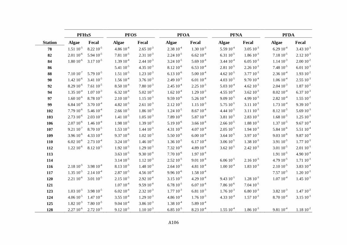
A106

Station

PFHxS

PFOS

PFOA

PFNA

PFDA

Algae Fecal

Algae Fecal

Algae Fecal

Algae Fecal

Algae Fecal

78 1.51 10-5

8.22 10-5

4.86 10-4

2.65 10-3

2.38 10-4

1.30 10-3

5.59 10-4

3.05 10-3

6.29 10-4

3.43 10-3

82 2.01 10-6

5.94 10-5

7.81 10-5

2.31 10-3

2.24 10-5

6.62 10-4

6.31 10-5

1.86 10-3

7.18 10-5

2.12 10-3

84 1.80 10-6

3.17 10-5

1.39 10-4

2.44 10-3

3.24 10-5

5.69 10-4

3.44 10-4

6.05 10-3

1.14 10-3

2.00 10-2

86 5.41 10-5

4.35 10-3

8.12 10-6

6.53 10-4

2.81 10-5

2.26 10-3

7.48 10-5

6.01 10-3

88 7.10 10-7

5.79 10-5

1.51 10-5

1.23 10-3

6.13 10-6

5.00 10-4

4.62 10-5

3.77 10-3

2.36 10-4

1.93 10-2

90 1.42 10-6

3.41 10-5

1.56 10-4

3.76 10-3

2.49 10-5

6.01 10-4

4.03 10-5

9.70 10-4

1.06 10-4

2.55 10-3

92 8.29 10-6

7.61 10-5

8.50 10-4

7.80 10-3

2.45 10-4

2.25 10-3

5.03 10-4

4.62 10-3

2.04 10-3

1.87 10-2

94 1.35 10-4

1.07 10-3

6.32 10-4

5.02 10-3

1.62 10-4

1.29 10-3

4.55 10-4

3.62 10-3

8.02 10-4

6.37 10-3

97 1.60 10-6

8.78 10-5

2.10 10-5

1.15 10-3

9.59 10-6

5.26 10-4

9.09 10-5

4.99 10-3

2.82 10-4

1.55 10-2

99 6.84 10-6

3.70 10-4

4.82 10-5

2.61 10-3

2.12 10-5

1.15 10-3

5.75 10-5

3.11 10-3

1.73 10-4

9.39 10-3

102 7.79 10-6

5.46 10-4

2.66 10-5

1.86 10-3

1.24 10-5

8.67 10-4

4.44 10-5

3.11 10-3

8.12 10-5

5.69 10-3

103 2.73 10-6

2.03 10-4

1.41 10-5

1.05 10-3

7.89 10-6

5.87 10-4

3.81 10-5

2.83 10-3

1.68 10-5

1.25 10-3

106 2.07 10-6

1.46 10-4

1.98 10-5

1.39 10-3

5.19 10-6

3.66 10-4

2.66 10-5

1.88 10-3

1.37 10-5

9.67 10-4

107 9.21 10-7

8.70 10-5

1.53 10-5

1.44 10-3

4.31 10-6

4.07 10-4

2.05 10-5

1.94 10-3

5.84 10-6

5.51 10-4

109 3.96 10-6

4.33 10-4

9.37 10-6

1.02 10-3

5.50 10-6

6.00 10-4

3.64 10-5

3.97 10-3

9.03 10-6

9.87 10-4

110 6.02 10-6

2.73 10-4

3.24 10-5

1.46 10-3

1.36 10-5

6.17 10-4

3.06 10-5

1.38 10-3

3.91 10-5

1.77 10-3

112 1.22 10-6

8.12 10-5

1.92 10-5

1.29 10-3

7.32 10-6

4.89 10-4

3.62 10-5

2.42 10-3

3.01 10-5

2.01 10-3

113

3.63 10-5

9.30 10-4

7.70 10-6

1.97 10-4

1.91 10-5

4.90 10-4

114 3.14 10-5

1.12 10-3

2.52 10-5

9.01 10-4

6.06 10-5

2.16 10-3

4.79 10-5

1.71 10-3

116 2.18 10-5

3.98 10-4

8.13 10-5

1.48 10-3

2.64 10-5

4.81 10-4

1.00 10-4

1.83 10-3

2.10 10-5

3.83 10-4

117 1.35 10-5

2.14 10-4

2.87 10-5

4.56 10-4

9.96 10-6

1.58 10-4

7.57 10-5

1.20 10-3

120 2.21 10-6

3.01 10-5

2.15 10-5

2.92 10-4

3.15 10-5

4.29 10-4

9.43 10-5

1.28 10-3

1.07 10-4

1.45 10-3

121 1.07 10-4

9.59 10-4

6.78 10-5

6.07 10-4

7.86 10-6

7.04 10-5

123 1.03 10-5

3.98 10-5

6.02 10-4

2.32 10-3

1.77 10-3

6.81 10-3

1.76 10-3

6.80 10-3

3.82 10-3

1.47 10-2

124 4.06 10-5

1.47 10-4

3.55 10-4

1.29 10-3

4.86 10-4

1.76 10-3

4.33 10-4

1.57 10-3

8.70 10-4

3.15 10-3

125 1.82 10-5

7.80 10-5

9.04 10-4

3.86 10-3

1.38 10-4

5.89 10-4

128 2.27 10-6

2.72 10-5

9.12 10-5

1.10 10-3

6.85 10-5

8.23 10-4

1.55 10-4

1.86 10-3

9.81 10-4

1.18 10-2

A107

Station

PFHxS

PFOS

PFOA

PFNA

PFDA

Algae Fecal

Algae Fecal

Algae Fecal

Algae Fecal

Algae Fecal

129 6.97 10-6

7.11 10-5

1.83 10-4

1.86 10-3

1.25 10-4

1.28 10-3

2.13 10-4

2.17 10-3

6.96 10-4

7.10 10-3

131 8.72 10-6

1.21 10-4

2.62 10-4

3.64 10-3

5.97 10-5

8.31 10-4

1.79 10-4

2.49 10-3

132 3.90 10-7

1.03 10-5

1.25 10-5

3.29 10-4

2.81 10-5

7.42 10-4

5.55 10-5

1.46 10-3

134 7.64 10-8

4.35 10-6

2.11 10-6

1.21 10-4

1.00 10-5

5.70 10-4

1.63 10-5

9.29 10-4

1.51 10-6

8.61 10-5

135 3.47 10-7

2.58 10-5

2.49 10-6

1.85 10-4

6.86 10-6

5.10 10-4

1.22 10-5

9.03 10-4

2.11 10-6

1.57 10-4

137 2.92 10-7

1.33 10-5

5.35 10-6

2.44 10-4

1.01 10-5

4.60 10-4

2.13 10-5

9.75 10-4

4.40 10-6

2.01 10-4

138 2.95 10-7

1.78 10-5

2.86 10-6

1.73 10-4

6.67 10-6

4.03 10-4

1.12 10-5

6.74 10-4

3.24 10-6

1.95 10-4

140 1.05 10-7

8.89 10-6

2.05 10-6

1.74 10-4

9.78 10-7

8.31 10-5

2.13 10-6

1.81 10-4

2.96 10-6

2.51 10-4

141 8.84 10-8

8.42 10-6

1.25 10-6

1.19 10-4

3.93 10-6

3.74 10-4

6.71 10-6

6.39 10-4

5.83 10-7

5.55 10-5

143 2.01 10-6

1.54 10-4

3.88 10-6

2.97 10-4

1.16 10-5

8.83 10-4

2.14 10-6

1.64 10-4

144 8.11 10-8

5.19 10-6

2.44 10-6

1.56 10-4

6.13 10-6

3.92 10-4

1.39 10-5

8.86 10-4

4.64 10-6

2.97 10-4

146 2.02 10-7

8.79 10-6

1.04 10-5

4.53 10-4

2.13 10-5

9.29 10-4

3.44 10-5

1.50 10-3

6.21 10-6

2.71 10-4

147 2.16 10-7

8.20 10-6

7.77 10-6

2.95 10-4

2.87 10-5

1.09 10-3

6.56 10-5

2.49 10-3

7.61 10-6

2.88 10-4

A108

REFERENCES

1. González-Gaya, B.; Dachs, J.; Roscales, J. L.; Caballero, G.; Jiménez, B., Perfluoroalkylated Substances In The Global Tropical And Subtropical Surface Oceans. Environmental Science & Technology 2014, 48, (22), 13076-13084. 2. Loi, E. I.; Yeung, L. W.; Taniyasu, S.; Lam, P. K.; Kannan, K.; Yamashita, N., Trophic magnification of poly- and perfluorinated compounds in a subtropical food web. Environ Sci Technol 2011, 45, (13), 5506-13. 3. Siegel, D. A.; Buesseler, K. O.; Doney, S. C.; Sailley, S. F.; Behrenfeld, M. J.; Boyd, P. W., Global assessment of ocean carbon export by combining satellite observations and food-web models. Global Biogeochemical Cycles 2014, 28, (3), 2013GB004743.

A110

5. CYCLING OF POLYCYCLIC AROMATIC HYDROCARBONS

IN THE SURFACE OPEN OCEAN


Belén González-Gaya 1,2*, María-Carmen Fernández-Pinos 1, Cristóbal

Galbán-Malagón 1, Antonio Bode 3, Montserrat Vidal 4, Begoña Jiménez 2,

and Jordi Dachs 1



A111

INDEX

Table S5.1. Sampling: Ancillary data for water sample’s transects

Table S5.2. Sampling: Ancillary data for Plankton samples

Text S5.1. Materials and Methods

Table S5.3. Blanks (total pg per sample) and Surrogate recoveries (%) for

particulate phase samples

Table S5.4. Blanks (total pg per sample), Breakthroughs and Surrogate recoveries

(%) for plankton samples

Table S5.5. Particulate Organic Carbon (POC, μM) at surface (5 m depth)

Table S5.6. Carbon, Nitrogen and estimated Trophic position for plankton samples

Table S5.7. Organic carbon export from the surface mixed layer due to

phytoplankton (FOC-Phyto), zooplankton pellets (FOC-Fecal) and total fluxes (FOC) (mgC

m-2day-1)

Table S5.8. Dissolved phase measured PAHs concentrations (ng L-1)

Table S5.9. Particulate phase measured PAHs concentrations (ng gdw-1)

Figure S5.1. Relative abundance of PAHs in the particulate phase

Table S5.10. Plankton phase measured PAHs concentrations (ng gdw-1)

Figure S5.2. Relative occurrence of individual PAHs in plankton per subbasin (%)

Figure S5.3. KOC in surface waters for some representative PAHs

Table S5.11. Slopes fitted to the field data of CPlankton versus biomass

Table S5.12. Biological pump fluxes

A112

Table S5.1. Sampling: Ancillary data for water sample’s transects

Initial Final

Station Volume filtered

(L)

Particles dry weight

(g) Date

Time (UTC)

Longitude Latitude

Date Time (UTC)

Longitude Latitude

1 169.50 0.3626 16/12/10 11:45 -9.564 35.195 16/12/10 21:10 -11.173 34.580

0 192.00 0.3115 18/12/10 8:50 -15.158 31.823 18/12/10 22:10 -16.600 30.370

4 165.60 0.3587 20/12/10 10:51 -19.102 28.311 20/12/10 22:13 -20.125 26.452

6 240.88 0.3154 22/12/10 8:41 -22.247 23.255 22/12/10 21:24 -22.658 22.633

8 211.11 0.3522 24/12/10 8:55 -24.316 20.260 24/12/10 18:30 -24.974 19.063

10 345.21 0.6808 26/12/10 8:15 -26.005 14.519 26/12/10 22:08 -25.999 13.660

12 391.30 0.2067 28/12/10 8:46 -25.994 9.563 28/12/10 21:15 -26.014 8.571

14 259.26 0.3246 30/12/10 8:35 -26.033 5.012 30/12/10 20:15 -25.998 3.695

16 277.96 0.4133 01/01/11 9:28 -26.019 0.269 01/01/11 20:05 -26.481 -1.140

18 237.88 0.3146 03/01/11 9:31 -28.168 -4.780 03/01/11 20:45 -28.709 -5.954

20 367.50 0.3023 05/01/11 9:00 -30.187 -9.125 05/01/11 18:20 -30.443 -13.443

22 323.11 0.2686 07/01/11 9:43 -32.378 -13.735 07/01/11 20:40 -32.659 -14.263

24 272.31 0.2502 09/01/11 9:01 -34.671 -18.399 09/01/11 22:12 -35.114 -19.369

26 161.56 0.3467 11/01/11 9:45 -36.980 -23.002 11/01/11 20:50 -38.086 -23.374

27 240.75 0.2512 18/01/11 13:45 -39.661 -23.694 19/01/11 12:28 -37.530 -24.104

28 317.16 0.2969 19/01/11 14:36 -37.522 -24.105 20/01/11 12:00 -33.485 -24.789

29 185.79 - 20/01/11 13:00 -33.443 -24.781 20/01/11 21:45 -31.647 -25.155

30 249.90 0.2746 21/01/11 0:45 -31.070 -25.272 21/01/11 17:45 -30.049 -25.439

34 170.87 0.3394 24/01/11 15:38 -21.148 -26.999 26/01/11 0:12 -16.224 -27.884

37 355.70 0.4088 27/01/11 0:45 -10.446 -28.881 28/01/11 16:45 -7.588 -29.374

41 68.73 0.3001 01/02/11 1:10 2.954 -31.172 01/02/11 19:00 4.913 -31.498

42 148.18 0.2686 01/02/11 20:45 5.304 -31.555 02/02/11 21:37 8.036 -32.020

43 147.93 0.401 02/02/11 23:08 8.349 -32.074 04/02/11 2:00 12.440 -32.754

44 229.95 0.367 04/02/11 2:30 12.520 -32.769 04/02/11 20:00 13.463 -32.919

45 214.25 0.2988 04/02/11 20:45 13.637 -32.951 05/02/11 18:30 16.751 -33.479

0 118.67 0.393 12/02/11 7:58 20.976 -35.167 12/02/11 19:50 23.790 -35.099

46 289.95 0.3184 14/02/11 6:25 27.543 -34.836 14/02/11 18:48 29.637 -34.596

48 251.18 0.3367 16/02/11 5:30 33.709 -34.176 16/02/11 18:14 35.500 -33.998

50 358.00 0.3585 18/02/11 5:25 39.880 -33.532 18/02/11 18:14 41.684 -33.369

0 186.65 0.3491 20/02/11 4:00 54.284 -31.781 20/02/11 17:34 55.536 -31.495

0 154.38 0.3047 22/02/11 6:00 58.943 -30.852 22/02/11 14:14 61.458 -30.053

53 213.96 0.3418 25/02/11 3:00 63.247 -27.979 25/02/11 17:00 65.051 -27.899

55 337.09 0.3422 27/02/11 4:24 69.420 -29.360 27/02/11 16:25 70.811 -29.333

57 177.53 0.3404 01/03/11 3:03 76.079 -29.904 01/03/11 15:19 77.898 -29.879

59 226.99 0.3134 03/03/11 3:07 82.624 -29.810 03/03/11 15:22 84.578 -29.777

61 266.53 0.3278 05/03/11 2:55 89.466 -29.677 05/03/11 16:59 91.679 -29.666

63 343.13 0.3118 07/03/11 1:36 96.400 -29.579 08/03/11 1:40 99.998 -29.905

65 216.90 0.2707 09/03/11 2:00 103.311 -30.332 09/03/11 16:05 105.848 -30.635

67 187.85 0.3392 11/03/11 0:10 110.179 -31.154 11/03/11 13:44 112.038 -31.361

74 219.69 0.4088 24/03/11 0:25 110.180 -31.154 24/03/11 12:02 137.546 -39.648

A113

Initial Final

Station Volume filtered

(L)

Particles dry weight

(g) Date

Time (UTC)

Longitude Latitude

Date Time (UTC)

Longitude Latitude

0 266.09 0.2869 09/04/11 0:30 156.778 -33.911 09/04/11 11:50 159.463 -33.985

80 242.00 0.3548 17/04/11 22:12 177.743 -30.970 18/04/11 8:17 179.143 -28.406

83 222.63 0.2935 21/04/11 19:14 -176.935 -20.602 22/04/11 6:51 -176.364 -19.796

85 256.00 0.3054 23/04/11 20:08 -174.497 -15.889 24/04/11 5:50 -174.102 -15.038

88 269.45 0.309 25/04/11 23:39 -172.736 -11.201 26/04/11 8:25 -172.560 -10.646

92 319.32 0.3518 29/04/11 21:35 -169.462 -3.398 30/04/11 10:32 -168.669 -1.872

95 206.91 0.3427 02/05/11 23:48 -165.403 4.622 03/05/11 9:40 -164.674 6.290

98 242.86 0.3093 05/05/11 22:20 -162.259 11.921 06/05/11 9:40 -161.379 13.758

104 271.17 0.2944 16/05/11 16:00 -150.360 21.066 17/05/11 6:30 -149.556 20.938

106 270.44 0.2942 18/05/11 15:30 -145.208 20.344 19/05/11 4:42 -146.308 20.085

108 207.28 0.2675 20/05/11 15:45 -138.966 19.279 21/05/11 3:11 -138.110 19.079

110 196.26 0.3285 22/05/11 14:55 -133.262 18.053 23/05/11 7:30 -131.486 17.582

112 197.44 0.2908 24/05/11 14:40 -127.569 16.624 25/05/11 4:30 -125.962 16.248

114 300.72 0.2819 26/05/11 14:45 -121.996 15.311 27/05/11 4:37 -120.109 14.845

116 255.68 0.3796 28/05/11 13:30 -115.768 13.771 29/05/11 4:00 -114.664 13.529

118 211.57 0.3135 30/05/11 13:35 -110.393 12.497 31/05/11 3:06 -109.574 12.321

121 283.11 0.3744 02/06/11 12:35 -102.447 10.757 03/06/11 2:10 -100.838 10.428

124 262.15 0.4244 05/06/11 12:50 -93.148 8.760 06/06/11 1:00 -91.917 8.482

126 257.84 0.3702 07/06/11 11:45 -87.960 7.224 08/06/11 1:00 -86.393 6.630

0 219.00 0.2999 11/06/11 15:15 -78.946 9.779 12/06/11 3:35 -76.588 10.160

129 224.57 0.3154 22/06/11 10:13 -69.291 15.075 22/06/11 23:36 -68.229 15.325

0 258.22 0.3278 24/06/11 11:55 -63.363 16.415 25/06/11 1:04 -60.863 17.082

133 198.50 0.3766 27/06/11 10:20 -55.160 19.020 27/06/11 23:40 -53.689 19.720

136 244.82 0.3138 30/06/11 9:05 -47.785 21.731 30/06/11 23:40 -45.908 22.374

138 246.74 0.3178 02/07/11 7:30 -41.908 23.736 02/07/11 22:45 -39.832 24.458

140 290.41 0.3162 04/07/11 7:35 -35.268 26.111 04/07/11 23:00 -34.037 26.532

142 251.45 0.2989 06/07/11 6:35 -29.671 27.981 06/07/11 21:43 -28.192 28.455

144 177.06 0.2584 08/07/11 6:45 -23.691 29.967 08/07/11 21:27 -22.053 30.507

146 249.09 0.2084 10/07/11 5:43 -17.262 32.083 10/07/11 20:20 -16.101 32.453

A114

Table S5.2. Sampling: Ancillary data for Plankton samples

Station Date Time (UTC)

Longitude Latitude Total dry weight (g)

Biomass (g m

-3)

1 16/12/10 11:45 -9.530 35.165 1.07 4.73 10-3

0 19/12/10 8:50 -17.285 29.686 1.11 5.46 10-3

6 22/12/10 8:41 -22.244 23.256 1.34 7.89 10-3

8 24/12/10 8:55 -24.304 20.260 1.96 1.45 10-2

10 26/12/10 8:15 -26.005 14.519 3.48 3.85 10-2

12 28/12/10 8:46 -25.994 9.564 2.25 1.47 10-2

14 30/12/10 8:35 -26.033 5.011 3.42 2.08 10-2

16 01/01/11 9:28 -26.019 0.270 5.42 4.00 10-2

18 03/01/11 9:31 -28.174 -4.773 1.94 1.04 10-2

20 05/01/11 9:00 -30.189 -9.110 1.98 6.50 10-3

22 07/01/11 9:43 -32.378 -13.729 1.57 5.79 10-3

24 09/01/11 9:01 -34.675 -18.399 3.14 1.23 10-2

26 11/01/11 9:45 -35.975 -21.090 0.74 2.35 10-3

27 19/01/11 13:45 -36.223 -24.314 0.28 1.15 10-3

28 20/01/11 14:36 -33.095 -24.852 0.17 1.15 10-3

29 21/01/11 13:00 -30.131 -25.400 3.23 2.04 10-2

30 22/01/11 0:45 -27.589 -25.863 3.11 1.96 10-2

0 23/01/11 - -24.243 -26.424 2.10 1.16 10-2

34 26/01/11 15:38 -14.789 -28.101 1.74 6.40 10-3

37 30/01/11 0:45 -5.401 -29.687 0.32 1.81 10-3 41 02/02/11 1:10 6.786 -31.772 3.73 3.00 10-2 42 03/02/11 20:45 9.417 -32.104 2.19 1.38 10-2 43 04/02/11 23:08 12.749 -32.791 2.13 1.05 10-2

44 05/02/11 2:30 15.474 -33.297 0.27 3.93 10-3

45 13/02/11 - 25.558 -35.139 2.03 2.00 10-2

46 14/02/11 6:25 27.546 -34.837 4.01 2.15 10-2

48 16/02/11 5:30 33.724 -34.172 2.32 1.25 10-2

50 18/02/11 5:25 39.880 -33.532 0.15 9.73 10-4

52 24/02/11 - 61.458 -30.053 2.21 1.00 10-2

53 25/02/11 3:00 63.248 -27.976 0.19 8.42 10-4

55 27/02/11 4:24 69.414 -29.363 0.87 5.51 10-3

57 01/03/11 3:03 76.086 -29.906 1.80 1.06 10-2

59 03/03/11 3:07 82.624 -29.810 1.82 1.08 10-2

61 05/03/11 2:55 89.478 -29.681 0.86 6.32 10-3

63 07/03/11 1:36 96.395 -29.582 1.71 1.16 10-2

65 09/03/11 2:00 103.309 -30.333 1.82 1.34 10-2

67 11/03/11 0:10 110.180 -31.154 3.65 1.79 10-2

74 24/03/11 0:25 135.224 -39.225 1.00 1.04 10-2

0 09/04/11 0:30 159.057 -33.976 0.41 7.29 10-3

79 17/04/11 - 176.016 -34.056 1.89 1.12 10-2

83 21/04/11 19:14 -177.417 -21.442 2.40 1.41 10-2

85 23/04/11 20:08 -174.488 -15.903 0.60 3.39 10-3

A115

Station Date Time (UTC)

Longitude Latitude Total dry weight (g)

Biomass (g m

-3)

88 26/04/11 23:39 -172.323 -9.460 0.81 4.54 10-3

92 30/04/11 21:35 -168.357 -1.304 1.47 9.60 10-3

95 03/05/11 23:48 -164.427 6.978 3.24 2.94 10-2

98 06/05/11 22:20 -160.861 15.017 1.43 6.47 10-3

103 16/05/11 16:00 -150.366 21.067 3.36 1.53 10-2

105 18/05/11 15:30 -145.212 20.341 4.41 1.86 10-2

106 19/05/11 - -141.617 19.902 2.09 9.15 10-3

107 20/05/11 15:45 -138.966 19.279 3.05 1.28 10-2

109 22/05/11 14:55 -133.262 18.057 3.35 1.58 10-2

111 24/05/11 14:40 -127.627 16.617 4.04 1.91 10-2

113 26/05/11 14:45 -121.995 15.311 4.46 1.95 10-2

115 28/05/11 13:30 -115.775 13.760 5.76 3.08 10-2

116 29/05/11 - -113.270 13.195 3.22 1.52 10-2

117 30/05/11 13:35 -110.392 12.493 2.27 9.25 10-3

118 31/05/11 - -108.046 11.992 4.23 3.11 10-2

120 02/06/11 12:35 -102.448 10.757 2.23 1.58 10-2

123 05/06/11 12:50 -93.148 8.764 4.41 3.47 10-2

125 07/06/11 11:45 -87.947 7.221 4.61 3.88 10-2

129 22/06/11 10:13 -69.289 15.073 3.43 1.68 10-2

131 25/06/11 - -59.829 17.428 4.07 2.18 10-2

133 27/06/11 10:20 -55.160 19.020 1.60 5.90 10-3

136 28/06/11 - -52.629 20.013 1.79 6.81 10-3

136 30/06/11 9:05 -47.790 21.742 1.02 4.02 10-3

138 02/07/11 7:30 -41.912 23.736 1.24 7.80 10-3

140 04/07/11 7:35 -35.274 26.111 0.16 8.79 10-4

142 06/07/11 6:35 -29.673 27.983 0.46 2.71 10-3

144 08/07/11 6:45 -23.693 29.966 1.75 7.95 10-3

146 10/07/11 5:43 -17.260 32.088 1.26 6.78 10-3

A116

Text S5.1. Materials and Methods

Dissolved samples

XAD-2 resin was extracted secuentialy with 200 mL of methanol (MeOH) and 300

mL of dichloromethane (DClM) pumped contrariwise to the sampling direction

flux, in order to facilitate the extraction and avoid preferent pathways. Both

elutants were kept separated and were surrogate recovery spiked. After a rotary

evaporator reduction, the MeOH fraction was liquid-liquid extracted with hexane

(Hx, 30 mL) on a decanting funnel three times. Both phases were further purified

over a anhidrous sulfate muffled open funnel; first the MeOH phase and the MeOH

was discarded and then the Hx phase which was kept and additionally washed

with Hx. This elutant was mixed with the DClM phase, reduced down to Hx and

fractioned over an alumina column (3 g, 90% deactivated alumina with a 1 cm

sulfate top layer, packed with Hx). Fractioning was set with 5 mL Hx for the the

first fraction of alifatic compounds, 12 mL Hx/DClM (1:2) for the second fraction

containing the aromatic compounds, and 15 mL MeOH/DClM (1:2) for other polar

compounds. Fractions 1 and 2 were reduced under a gentle nigrogen stream and

solvent changed to isooctane down to 100 uL.

Particulate samples

Filters containing the particulate samples were freeze dried, weighted and soxhlet

extracted overnight with DClM/MeOH (2:1). The extract was concentrated on a

rotary evaporator system and solvent changed to isooctane. Then, samples were

further purified and fractioned over an alumina column (3 g, 90% deactivated

alumina with a 1 cm sulfate top layer, packed with Hx). Fractioning was set with 6

mL Hx for the the first fraction of alifatic compounds, 12 mL Hx/DClM (3:1) for the

second fraction containing the aromatic compounds, 35 mL DClM for

organophosphate esters on a third fraction, and a last fraction of 15 mL

DClM/MeOH (2:1) for other products. Fractions 1, 2 and 3 were reduced under a

gentle nitrogen stream and solvent changed to isooctane down to 100 uL.

Plankton samples

Plankton filters were freeze dried, weighted and soxhlet extracted overnight with

DCl/Hex (1:1). Plankton samples were purified and fractioned over a combined

silica and alumina column (top 1 cm sulphate, intermediate 5 g muffled neutral

silica, and bottom 3 g, 90% deactivated alumina, packed with Hx). Fractioning was

set with 25 mL Hx for the the first fraction of alifatic compounds, 40 mL Hx/DClM

(3:1) for the second fraction containing the aromatic compounds, 20 mL

DClM/Acetone (70:30) for organophosphate esters on a third fraction and a last

fraction of 25 mL DClM/MeOH (2:1) for other polar compounds. Fractions 1, 2 and

3 were reduced under a gentle nigrogen stream and solvent changed to isooctane

down to 100 uL.

A117

Table S5.3. Blanks (total pg per sample) and Surrogate recoveries (%) for

particulate phase samples

Mean laboratory

blank

Mean field blank

Surrogate recovery

(n=7) (n=4)

(n=69)

Naphthalene 0.154 0.165

Dimethylnaphthalenes 0.057 0.053

Methylnaphthalenes 0.000 0.000

Acenaphtylene 0.038 0.045

Acenaphtene 0.112 0.242

Fluorene 0.095 0.295

Dibenzothiophene 0.049 0.098

Methyldibenzothiophenes 0.174 0.341

Dimethyldibenzothiopenes 0.214 0.356

Phenanthrene 0.433 1.016

Methylphenantrenes 0.303 0.345

Dimethylphenanthrenes 0.222 0.248

Anthracene 0.047 0.049

Fluoranthene 0.336 0.370

Pyrene 0.130 0.173

Methylpyrene 0.051 0.068

Dimethylpyrene 0.000 0.085

Benzo(ghi)fluoranthene 0.069 0.070

Benzo(a)anthracene 0.134 0.201

Chrysene 0.069 0.079

Methylchrysenes 0.000 0.056

Benzo(b+k)fluoranthenes 0.164 0.165

Benzo(e)pyrene 0.076 0.096

Benzo(a)pyrene 0.011 0.080

Perylene 0.097 0.101 Perylene D12 76.2

Indeno(1,2,3-cd)pyrene 0.045 0.095

Dibenzo(a,h)anthracene 0.062 0.089

Benzo(ghi)perylene 0.058 0.095

All samples have been surrogate recovery corrected by Perylene D12.

A118

Table S5.4. Blanks (total pg per sample), Breakthroughs and Surrogate recoveries

(%) for plankton samples

Mean laboratory

blank

Mean field blank

Mean 1st Breakthrough

extraction

Surrogate recovery

(n=7) (n=4) (n=5)

(n=71)

Naphthalene 0.006 0.185 81.1

Methylnaphthalenes 0.027 0.838 85.4 Dimethylnaphthalenes 0.012 0.942 96.0 Acenaphtylene 0.000 0.030 90.7 Acenaphtene D10 25.1

Acenaphtene 0.013 0.418 99.0 Fluorene 0.004 0.069 91.7 Dibenzothiophene 0.000 0.000 100.0 Methyldibenzothiophenes 0.002 0.000 87.5 Dimethyldibenzothiopenes 0.000 0.000 93.7 Phenanthrene 0.015 0.264 97.4 Phenanthene D10 41.9

Methylphenantrenes 0.004 0.196 97.0 Dimethylphenanthrenes 0.007 0.000 99.3 Anthracene 0.000 0.067 85.6 Fluoranthene 0.036 0.128 97.4 Pyrene 0.026 0.275 95.6 Methylpyrenes 0.000 0.000 100.0 Dimethylpyrenes 0.000 0.000 100.0 Benzo(ghi)fluoranthene 0.000 0.037 100.0 Benzo(a)anthracene 0.114 0.120 96.1 Chrysene 0.021 0.015 95.4 Chrysene D12 70.1

Methylchrysenes 0.000 0.000 100.0 Benzo(b+k)fluoranthenes 0.120 0.000 94.2 Benzo(e)pyrene 0.000 0.078 93.3 Benzo(a)pyrene 0.000 0.000 100.0 Perylene 0.000 0.000 100.0 Perylene D12 102.4

Indeno(1,2,3-cd)pyrene 0.071 0.000 100.0 Dibenzo(a,h)anthracene 0.281 0.000 100.0 Benzo(ghi)perylene 0.148 0.000 99.7

All samples have been surrogate recovery corrected by the indicated deuterated standard.

A119

Table S5.5. Particulate organic carbon (POC, μM) at surface (5 m depth)

Station POC

1 1.9

0 1.7

4 1.6

6 1.7

8 1.7

10 2.2

12 2.3

14 2.4

16 2.0

18 2.3

20 2.3

22 1.5

24 2.2

26 2.5

27 2.5

28 2.5

29 1.6

30 3.4

34 3.4

37 1.8

41 1.8

42 1.7

43 3.3

44 4.3

45 4.3

0 6.1

46 2.2

48 1.6

50 1.4

0 1.3

0 1.2

53 2.4

55 0.9

57 0.9

59 1.0

61 0.9

63 1.1

65 4.4

67 2.3

74 2.4

0 -

80 2.2

Station POC

83 3.7

85 2.7

88 1.7

92 1.4

95 2.0

98 1.4

103 4.6

105 1.6

107 2.7

109 2.4

111 1.4

113 1.3

115 2.5

117 1.9

120 2.3

123 4.9

125 9.3

0 2.3

129 2.2

0 1.7

133 -

136 2.0

138 1.6

140 1.7

142 1.3

144 1.8

146 4.5

A120

Table S5.6. Carbon, Nitrogen and estimated trophic position for plankton samples

Station N biomass C biomass C:N d15N d13C Trophic

position*

(mg N m-3) (mg C m-3) (molar) (‰) (‰)

1

3

6

8

10 1.56 6.43 4.81 4.95 -19.57 1.58

12

14

16

18

20

22

24

25

27

28

29 2.78 11.66 4.88 1.92 -19.77

30

31

35 1.09 4.30 4.60 5.87 -21.43 1.29

37

39 2.07 9.86 5.56 8.42 -18.34 1.57

42

43

44

45 2.77 10.89 4.58 6.55 -19.07 1.43

46 2.13 8.46 4.64 4.92 -20.09 1.70

48 1.11 5.65 5.94 4.38 -21.78 1.80

50 0.50 2.46 5.81 4.85 -17.75 1.41

52 1.90 7.19 4.43 4.68 -20.86 1.17

53 2.32 9.09 4.57 3.75 -20.87 1.27

55 1.47 5.50 4.37 4.76 -20.96 1.24

57 1.71 6.64 4.54 5.59 -21.08 1.46

59 1.07 4.39 4.78 8.86 -21.24 1.43

61 1.88 7.42 4.60 6.59 -20.93 1.55

63 1.54 6.14 4.64 8.19 -21.30 1.21

65 1.88 6.96 4.32 3.53 -22.29 1.20

67 1.40 5.86 4.88 3.92 -20.54 1.89

74 2.24 8.72 4.54 12.61 -20.30 1.64

4b1

79 1.96 7.13 4.25 6.88 -20.69 1.31

83 1.98 8.05 4.76 1.68 -19.88 1.66

85 1.29 5.11 4.61 2.27 -19.08 1.44

A121

Station N biomass C biomass C:N d15N d13C Trophic

position*

(mg N m-3) (mg C m-3) (molar) (‰) (‰)

88 1.65 6.13 4.33 12.65 -19.33 1.72

92 2.13 8.10 4.44 3.57 -19.42 1.57

95 7.36 27.90 4.43 6.26 -19.83 1.70

98 0.86 3.86 5.25 8.11 -19.48 1.88

103 2.08 7.84 4.40 8.12 -20.36 1.42

105 2.04 8.07 4.61 4.45 -20.36 1.60

106 1.39 5.39 4.52 7.92 -20.81 1.45

107 1.79 6.88 4.49 8.76 -20.92 1.52

109 2.47 9.60 4.54 8.16 -20.40 1.65

111 2.56 10.21 4.65 10.25 -20.80 1.91

113 2.43 9.37 4.50 10.48 -20.91 1.68

115 3.13 12.09 4.51 10.38 -21.01 1.45

116 2.03 8.33 4.79 8.68 -21.76 2.12

117 2.30 9.18 4.66 9.68 -20.62 1.50

118 2.50 9.76 4.56 10.43 -20.59 1.76

120 3.54 15.30 5.05 9.49 -19.32 1.50

123 5.42 20.02 4.31 6.75 -21.45 1.63

125 6.28 24.29 4.51 5.10 -21.34 1.80

129 3.10 12.14 4.57 1.11 -18.50 1.73

131 1.38 5.40 4.58 1.87 -18.97 1.66

133 1.70 6.73 4.61 0.39 -19.25 1.49

134 1.99 7.97 4.67 0.30 -18.52 1.56

136 1.56 6.18 4.63 0.69 -19.36 1.32

138 1.48 6.21 4.90 1.04 -19.24 1.77

140 1.12 4.72 4.94 1.52 -20.41 1.64

142 1.08 4.16 4.51 2.59 -21.33 1.44

144 1.92 7.40 4.49 3.36 -21.44 1.66

145 1.97 7.72 4.58 3.21 -21.76 1.70

*Trophic position attends for the estimated TP of the plankton Fraction 500-1000 mm calculated by

(δN15500-1000 - δN15

40-200/3.4)-1.5.

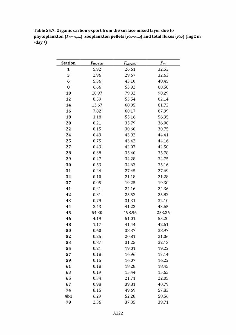
A122

Table S5.7. Organic carbon export from the surface mixed layer due to

phytoplankton (FOC-Phyto), zooplankton pellets (FOC-Fecal) and total fluxes (FOC) (mgC m-

2day-1)

Station FOCPhyto FOCFecal FOC

1 5.92 26.61 32.53

3 2.96 29.67 32.63

6 5.36 43.10 48.45

8 6.66 53.92 60.58

10 10.97 79.32 90.29

12 8.59 53.54 62.14

14 13.67 68.05 81.72

16 7.82 60.17 67.99

18 1.18 55.16 56.35

20 0.21 35.79 36.00

22 0.15 30.60 30.75

24 0.49 43.92 44.41

25 0.75 43.42 44.16

27 0.43 42.07 42.50

28 0.38 35.40 35.78

29 0.47 34.28 34.75

30 0.53 34.63 35.16

31 0.24 27.45 27.69

34 0.10 21.18 21.28

37 0.05 19.25 19.30

41 0.21 24.16 24.36

42 0.31 25.52 25.82

43 0.79 31.31 32.10

44 2.43 41.23 43.65

45 54.30 198.96 253.26

46 4.19 51.01 55.20

48 1.17 41.44 42.61

50 0.60 38.37 38.97

52 0.25 20.81 21.06

53 0.87 31.25 32.13

55 0.21 19.01 19.22

57 0.18 16.96 17.14

59 0.15 16.07 16.22

61 0.18 18.28 18.45

63 0.19 15.44 15.63

65 0.34 21.71 22.05

67 0.98 39.81 40.79

74 8.15 49.69 57.83

4b1 6.29 52.28 58.56

79 2.36 37.35 39.71

A123

Station FOCPhyto FOCFecal FOC

83 2.31 41.33 43.65

85 1.00 38.23 39.23

88 0.49 39.62 40.11

92 10.59 97.14 107.73

95 7.46 69.10 76.56

98 0.62 33.67 34.30

103 0.54 40.18 40.72

105 0.36 38.43 38.79

106 0.53 37.63 38.17

107 0.39 36.94 37.33

109 0.30 32.96 33.26

111 0.46 33.09 33.55

113 1.75 44.82 46.57

115 2.02 51.62 53.64

116 2.91 52.96 55.87

117 3.56 56.49 60.04

118 3.95 55.09 59.04

120 3.53 48.01 51.54

123 33.00 127.11 160.11

125 21.84 93.34 115.18

129 4.77 48.64 53.41

131 3.34 46.50 49.84

133 0.74 24.20 24.94

134 0.37 20.85 21.22

136 0.15 16.35 16.50

138 0.24 14.19 14.43

140 0.14 12.17 12.31

142 0.21 15.32 15.53

144 0.26 16.58 16.84

146 0.64 28.07 28.71

A124

Table S5.8. Dissolved phase measured PAHs concentrations (ng L-1)

Sta

tio

n

Na

ph

tha

len

e

Me

thy

lna

ph

tha

len

es

Dim

eth

yln

ap

hth

ale

ne

s

Ace

na

ph

tyle

ne

Ace

na

ph

ten

e

Flu

ore

ne

Dib

en

zoth

iop

he

ne

Me

thy

ldib

en

zoth

iop

he

ne

s

Dim

eth

yld

ibe

nzo

thio

pe

ne

s

Ph

en

an

thre

ne

Me

thy

lph

en

an

tre

ne

s

Dim

eth

ylp

he

na

nth

ren

e s

An

thra

cen

e

Flu

ora

nth

en

e

Py

ren

e

Me

thy

lpy

ren

e s

Dim

eth

ylp

yre

ne

s

Be

nzo

(gh

i)fl

uo

ran

the

ne

Be

nzo

(a)a

nth

race

ne

Ch

ryse

ne

Me

thy

lch

ryse

ne

s

Be

nzo

(b+

k)f

luo

ran

the

ne

s

Be

nzo

(e)p

yre

ne

Be

nzo

(a)p

yre

ne

Pe

ryle

ne

Ind

en

o(1

,2,3

-cd

)py

ren

e

Dib

en

zo(a

,h)a

nth

race

ne

Be

nzo

(gh

i)p

ery

len

e

∑6

4 P

AH

s

1 0.132 0.575 1.15 0.016 0.542 0.555 0.132 0.118 0.099 0.888 0.339 0.123 0.088 0.237 0.278 0.035 0.018 0.013 0.019 0.017 0.006 0.006 0.007 0.004 0.000 0.019 0.031 0.023 5.47

0 0.024 0.136 0.428 0.010 0.271 0.426 0.096 0.097 0.085 0.635 0.239 0.103 0.070 0.185 0.218 0.028 0.013 0.014 0.016 0.011 0.004 0.004 0.006 0.002 0.001 0.025 0.036 0.022 3.21

4 0.031 0.117 0.313 0.013 0.189 0.571 0.102 0.106 0.093 0.723 0.312 0.126 0.057 0.247 0.280 0.033 0.013 0.013 0.026 0.013 0.005 0.003 0.006 0.001 0.001 0.025 0.037 0.009 3.47

6 0.154 0.558 1.03 0.046 0.488 0.433 0.095 0.111 0.101 0.541 0.271 0.126 0.049 0.235 0.281 0.062 0.035 0.012 0.140 0.026 0.036 0.005 0.017 0.006 0.003 0.018 0.025 0.010 4.91

8 0.000 0.000 0.017 0.024 0.007 0.000 0.007 0.009 0.012 0.000 0.000 0.000 0.000 0.001 0.001 0.034 0.052 0.000 0.004 0.000 0.007 0.000 0.000 0.000 0.001 0.001 0.001 0.000 0.180

10 0.002 0.000 0.122 0.006 0.067 0.294 0.071 0.100 0.094 0.528 0.303 0.130 0.068 0.306 0.368 0.042 0.018 0.009 0.057 0.014 0.004 0.003 0.006 0.002 0.001 0.013 0.015 0.004 2.65

12 0.001 0.017 0.109 0.042 0.034 0.148 0.094 0.088 0.084 0.316 0.251 0.106 0.062 0.236 0.303 0.040 0.020 0.052 0.008 0.018 0.012 0.002 0.008 0.003 0.001 0.012 0.014 0.006 2.09

14 0.022 0.000 0.000 0.304 0.401 0.000 1.07 0.694 0.108 0.604 0.000 0.115 0.027 0.318 0.352 0.199 0.095 0.000 0.000 0.038 0.013 0.000 0.000 0.000 0.000 0.011 0.012 0.000 4.39

16 0.000 0.000 0.000 0.911 0.090 0.000 1.73 0.629 0.137 0.326 0.000 0.044 0.000 0.000 0.000 0.267 0.000 0.000 0.082 0.021 0.044 0.000 0.000 0.050 0.000 0.000 0.000 0.000 4.34

18 0.000 0.033 0.192 0.060 0.067 0.124 0.122 0.115 0.128 0.238 0.451 0.172 0.058 0.376 0.516 0.067 0.035 0.017 0.052 0.023 0.023 0.005 0.015 0.005 0.001 0.016 0.019 0.008 2.94

20 0.000 0.001 0.008 0.001 0.006 0.048 0.015 0.049 0.061 0.129 0.156 0.089 0.014 0.216 0.276 0.032 0.013 0.010 0.023 0.011 0.003 0.003 0.006 0.001 0.001 0.037 0.048 0.010 1.27

22 0.002 0.007 0.046 0.020 0.019 0.061 0.039 0.059 0.068 0.119 0.182 0.081 0.027 0.202 0.259 0.031 0.011 0.012 0.022 0.009 0.004 0.002 0.004 0.002 0.001 0.009 0.009 0.004 1.31

24 0.000 0.010 0.000 0.000 0.428 0.000 0.301 0.114 0.000 0.000 0.000 0.000 0.109 0.000 0.023 0.198 0.155 0.000 0.000 0.000 0.070 0.000 0.000 0.000 0.000 0.000 0.000 0.000 1.41

26 0.019 0.000 0.000 0.000 0.219 0.000 2.28 1.54 0.301 0.000 0.000 0.000 0.281 0.312 0.209 0.252 0.091 0.000 0.000 0.000 0.145 0.000 0.000 0.005 0.000 0.000 0.026 0.000 5.67

27 0.011 0.130 0.163 0.005 0.028 0.123 0.035 0.100 0.128 0.303 0.347 0.241 0.042 0.414 0.495 0.138 0.138 0.023 0.066 0.080 0.138 0.012 0.060 0.019 0.002 0.021 0.020 0.013 3.29

28 0.003 0.028 0.081 0.004 0.016 0.089 0.038 0.124 0.172 0.313 0.358 0.202 0.042 0.469 0.535 0.083 0.029 0.017 0.061 0.019 0.006 0.004 0.006 0.003 0.002 0.028 0.041 0.007 2.78

A125

Sta

tio

n

Na

ph

tha

len

e

Me

thy

lna

ph

tha

len

es

Dim

eth

yln

ap

hth

ale

ne

s

Ace

na

ph

tyle

ne

Ace

na

ph

ten

e

Flu

ore

ne

Dib

en

zoth

iop

he

ne

Me

thy

ldib

en

zoth

iop

he

ne

s

Dim

eth

yld

ibe

nzo

thio

pe

ne

s

Ph

en

an

thre

ne

Me

thy

lph

en

an

tre

ne

s

Dim

eth

ylp

he

na

nth

ren

e s

An

thra

cen

e

Flu

ora

nth

en

e

Py

ren

e

Me

thy

lpy

ren

e s

Dim

eth

ylp

yre

ne

s

Be

nzo

(gh

i)fl

uo

ran

the

ne

Be

nzo

(a)a

nth

race

ne

Ch

ryse

ne

Me

thy

lch

ryse

ne

s

Be

nzo

(b+

k)f

luo

ran

the

ne

s

Be

nzo

(e)p

yre

ne

Be

nzo

(a)p

yre

ne

Pe

ryle

ne

Ind

en

o(1

,2,3

-cd

)py

ren

e

Dib

en

zo(a

,h)a

nth

race

ne

Be

nzo

(gh

i)p

ery

len

e

∑6

4 P

AH

s

29 0.001 0.000 0.000 0.010 0.000 0.065 0.051 0.099 0.129 0.216 0.338 0.124 0.027 0.347 0.401 0.044 0.021 0.018 0.021 0.014 0.007 0.003 0.006 0.003 0.001 0.024 0.032 0.013 2.02

30 0.008 0.041 0.087 0.004 0.017 0.048 0.018 0.057 0.074 0.147 0.170 0.098 0.027 0.225 0.229 0.041 0.020 0.007 0.025 0.015 0.016 0.003 0.009 0.003 0.001 0.015 0.015 0.004 1.42

34 0.001 0.000 0.036 0.004 0.000 0.029 0.030 0.041 0.059 0.130 0.213 0.101 0.020 0.272 0.305 0.037 0.012 0.019 0.015 0.007 0.005 0.002 0.003 0.002 0.001 0.030 0.032 0.008 1.42

41 0.010 0.052 0.197 0.011 0.016 0.198 0.100 0.214 0.225 0.526 0.568 0.302 0.074 0.699 0.715 0.111 0.082 0.045 0.048 0.043 0.063 0.008 0.032 0.011 0.007 0.085 0.096 0.033 4.57

42 0.217 0.144 0.000 1.307 0.000 1.063 2.02 0.684 0.579 0.481 0.000 0.294 0.000 0.557 0.628 0.859 0.502 0.000 0.413 0.000 0.150 0.067 0.000 0.146 0.128 0.143 0.109 0.097 10.6

43 0.000 1.77 1.19 0.000 0.000 1.15 1.52 0.000 0.000 0.082 0.000 0.298 0.000 0.127 0.127 0.112 0.000 0.000 0.149 0.000 0.048 0.151 0.000 0.187 0.000 0.286 0.255 0.203 7.65

44 0.010 0.024 0.089 0.003 0.019 0.063 0.031 0.085 0.098 0.244 0.241 0.135 0.020 0.291 0.297 0.029 0.009 0.006 0.016 0.008 0.002 0.002 0.003 0.001 0.001 0.006 0.007 0.002 1.74

45 0.003 0.007 0.028 0.000 0.005 0.013 0.007 0.024 0.039 0.054 0.069 0.052 0.005 0.098 0.102 0.013 0.005 0.003 0.003 0.004 0.002 0.001 0.002 0.000 0.001 0.007 0.011 0.002 0.559

0 0.017 0.032 0.067 0.000 0.009 0.032 0.019 0.054 0.066 0.158 0.402 0.075 0.020 0.189 0.210 0.023 0.009 0.010 0.006 0.007 0.004 0.001 0.004 0.003 0.004 0.016 0.023 0.014 1.47

46 0.000 0.054 0.151 0.000 0.000 0.000 0.154 0.160 0.000 0.000 0.000 0.000 0.000 0.055 0.077 0.445 0.142 0.000 0.493 0.000 0.107 0.000 0.000 0.000 0.000 0.014 0.000 0.009 1.86

48 0.021 0.086 0.180 0.000 0.029 0.058 0.029 0.075 0.101 0.227 0.226 0.128 0.022 0.298 0.304 0.035 0.012 0.010 0.008 0.009 0.002 0.002 0.004 0.001 0.001 0.023 0.029 0.014 1.93

50 0.001 0.010 0.026 0.000 0.002 0.027 0.020 0.064 0.079 0.174 0.216 0.109 0.018 0.271 0.275 0.032 0.010 0.006 0.013 0.008 0.002 0.002 0.003 0.001 0.001 0.009 0.014 0.004 1.40

0 0.024 0.078 0.136 0.004 0.024 0.059 0.035 0.078 0.094 0.221 0.205 0.102 0.025 0.270 0.267 0.037 0.013 0.011 0.010 0.006 0.003 0.001 0.002 0.001 0.001 0.018 0.026 0.013 1.76

0 0.012 0.041 0.119 0.005 0.000 0.044 0.041 0.071 0.101 0.161 0.164 0.101 0.025 0.235 0.239 0.039 0.013 0.013 0.009 0.006 0.005 0.001 0.003 0.001 0.002 0.030 0.036 0.009 1.53

53 0.000 0.000 0.000 0.000 0.000 0.037 0.017 0.050 0.077 0.145 0.191 0.106 0.021 0.278 0.275 0.030 0.012 0.012 0.014 0.008 0.003 0.002 0.004 0.002 0.001 0.015 0.020 0.010 1.33

55 0.032 0.095 0.174 0.003 0.039 0.064 0.033 0.075 0.097 0.247 0.229 0.115 0.028 0.292 0.318 0.033 0.010 0.007 0.010 0.009 0.002 0.003 0.004 0.003 0.001 0.008 0.010 0.004 1.94

57 0.042 0.146 0.262 0.002 0.043 0.073 0.036 0.083 0.097 0.270 0.233 0.111 0.033 0.320 0.357 0.030 0.009 0.013 0.005 0.008 0.002 0.002 0.003 0.002 0.001 0.059 0.079 0.017 2.34

59 0.007 0.024 0.069 0.002 0.015 0.064 0.028 0.070 0.079 0.209 0.199 0.104 0.019 0.251 0.285 0.034 0.009 0.020 0.008 0.006 0.002 0.001 0.003 0.001 0.001 0.144 0.170 0.032 1.86

A126

Sta

tio

n

Na

ph

tha

len

e

Me

thy

lna

ph

tha

len

es

Dim

eth

yln

ap

hth

ale

ne

s

Ace

na

ph

tyle

ne

Ace

na

ph

ten

e

Flu

ore

ne

Dib

en

zoth

iop

he

ne

Me

thy

ldib

en

zoth

iop

he

ne

s

Dim

eth

yld

ibe

nzo

thio

pe

ne

s

Ph

en

an

thre

ne

Me

thy

lph

en

an

tre

ne

s

Dim

eth

ylp

he

na

nth

ren

e s

An

thra

cen

e

Flu

ora

nth

en

e

Py

ren

e

Me

thy

lpy

ren

e s

Dim

eth

ylp

yre

ne

s

Be

nzo

(gh

i)fl

uo

ran

the

ne

Be

nzo

(a)a

nth

race

ne

Ch

ryse

ne

Me

thy

lch

ryse

ne

s

Be

nzo

(b+

k)f

luo

ran

the

ne

s

Be

nzo

(e)p

yre

ne

Be

nzo

(a)p

yre

ne

Pe

ryle

ne

Ind

en

o(1

,2,3

-cd

)py

ren

e

Dib

en

zo(a

,h)a

nth

race

ne

Be

nzo

(gh

i)p

ery

len

e

∑6

4 P

AH

s

61 0.018 0.048 0.108 0.000 0.019 0.038 0.018 0.047 0.067 0.131 0.147 0.086 0.017 0.231 0.261 0.028 0.009 0.010 0.007 0.007 0.002 0.001 0.002 0.001 0.001 0.023 0.033 0.007 1.37

63 0.023 0.078 0.173 0.003 0.037 0.087 0.037 0.088 0.103 0.288 0.250 0.131 0.027 0.319 0.348 0.032 0.009 0.010 0.008 0.006 0.002 0.001 0.002 0.001 0.001 0.020 0.030 0.010 2.12

65 0.024 0.034 0.108 0.000 0.000 0.105 0.052 0.128 0.142 0.379 0.383 0.172 0.043 0.400 0.428 0.050 0.019 0.019 0.016 0.014 0.005 0.002 0.004 0.002 0.002 0.036 0.052 0.019 2.64

67 0.129 0.337 0.550 0.000 0.087 0.119 0.062 0.146 0.177 0.454 0.402 0.207 0.056 0.548 0.598 0.051 0.017 0.021 0.008 0.013 0.004 0.003 0.005 0.002 0.002 0.083 0.096 0.033 4.21

74 0.016 0.050 0.125 0.000 0.020 0.028 0.016 0.035 0.044 0.119 0.106 0.075 0.015 0.149 0.178 0.018 0.006 0.014 0.003 0.004 0.001 0.001 0.001 0.001 0.001 0.041 0.059 0.015 1.14

0 0.012 0.038 0.098 0.000 0.017 0.026 0.018 0.044 0.063 0.136 0.128 0.075 0.014 0.203 0.276 0.024 0.007 0.007 0.004 0.007 0.002 0.002 0.003 0.001 0.001 0.025 0.033 0.008 1.27

80 0.068 0.285 0.480 0.004 0.066 0.092 0.044 0.091 0.117 0.309 0.250 0.131 0.034 0.319 0.394 0.030 0.009 0.012 0.005 0.008 0.002 0.002 0.003 0.001 0.001 0.033 0.052 0.019 2.86

83 0.033 0.090 0.293 0.002 0.046 0.108 0.052 0.131 0.166 0.386 0.359 0.189 0.045 0.484 0.568 0.047 0.013 0.018 0.017 0.012 0.003 0.003 0.005 0.002 0.001 0.032 0.048 0.016 3.17

85 0.026 0.091 0.263 0.000 0.046 0.100 0.052 0.132 0.173 0.394 0.356 0.184 0.045 0.461 0.583 0.051 0.013 0.016 0.033 0.013 0.003 0.002 0.004 0.002 0.001 0.027 0.041 0.013 3.12

88 0.030 0.085 0.301 0.000 0.053 0.105 0.055 0.136 0.182 0.408 0.365 0.197 0.043 0.502 0.643 0.055 0.013 0.016 0.049 0.013 0.003 0.003 0.005 0.002 0.001 0.030 0.046 0.014 3.36

92 0.016 0.067 0.181 0.000 0.028 0.066 0.044 0.118 0.141 0.320 0.301 0.151 0.031 0.391 0.504 0.043 0.011 0.019 0.009 0.012 0.004 0.003 0.004 0.002 0.001 0.030 0.039 0.013 2.55

95 0.024 0.070 0.171 0.000 0.031 0.065 0.043 0.120 0.148 0.325 0.336 0.176 0.033 0.461 0.574 0.046 0.012 0.023 0.009 0.014 0.003 0.004 0.006 0.002 0.002 0.081 0.100 0.037 2.91

98 0.045 0.133 0.269 0.005 0.038 0.087 0.060 0.152 0.221 0.457 0.445 0.191 0.029 0.504 0.605 0.068 0.023 0.016 0.009 0.015 0.006 0.003 0.006 0.003 0.003 0.022 0.035 0.015 3.47

103 0.019 0.057 0.118 0.003 0.047 0.083 0.032 0.068 0.081 0.250 0.202 0.091 0.017 0.232 0.260 0.032 0.010 0.011 0.012 0.007 0.002 0.002 0.003 0.001 0.001 0.022 0.029 0.008 1.70

105 0.010 0.025 0.071 0.005 0.030 0.073 0.031 0.071 0.108 0.246 0.200 0.117 0.030 0.215 0.243 0.032 0.015 0.013 0.008 0.012 0.004 0.003 0.003 0.001 0.001 0.038 0.046 0.015 1.67

107 0.013 0.054 0.124 0.003 0.042 0.077 0.029 0.071 0.097 0.235 0.215 0.127 0.027 0.230 0.261 0.033 0.011 0.015 0.007 0.008 0.003 0.001 0.003 0.002 0.001 0.048 0.063 0.020 1.82

109 0.005 0.027 0.096 0.005 0.035 0.094 0.038 0.084 0.105 0.306 0.237 0.127 0.022 0.280 0.299 0.043 0.011 0.013 0.007 0.008 0.002 0.002 0.003 0.001 0.001 0.047 0.077 0.010 1.98

111 0.005 0.031 0.089 0.004 0.032 0.081 0.032 0.073 0.085 0.261 0.202 0.106 0.024 0.240 0.268 0.028 0.008 0.018 0.005 0.006 0.002 0.001 0.003 0.001 0.001 0.050 0.068 0.019 1.75

A127

Sta

tio

n

Na

ph

tha

len

e

Me

thy

lna

ph

tha

len

es

Dim

eth

yln

ap

hth

ale

ne

s

Ace

na

ph

tyle

ne

Ace

na

ph

ten

e

Flu

ore

ne

Dib

en

zoth

iop

he

ne

Me

thy

ldib

en

zoth

iop

he

ne

s

Dim

eth

yld

ibe

nzo

thio

pe

ne

s

Ph

en

an

thre

ne

Me

thy

lph

en

an

tre

ne

s

Dim

eth

ylp

he

na

nth

ren

e s

An

thra

cen

e

Flu

ora

nth

en

e

Py

ren

e

Me

thy

lpy

ren

e s

Dim

eth

ylp

yre

ne

s

Be

nzo

(gh

i)fl

uo

ran

the

ne

Be

nzo

(a)a

nth

race

ne

Ch

ryse

ne

Me

thy

lch

ryse

ne

s

Be

nzo

(b+

k)f

luo

ran

the

ne

s

Be

nzo

(e)p

yre

ne

Be

nzo

(a)p

yre

ne

Pe

ryle

ne

Ind

en

o(1

,2,3

-cd

)py

ren

e

Dib

en

zo(a

,h)a

nth

race

ne

Be

nzo

(gh

i)p

ery

len

e

∑6

4 P

AH

s

113 0.005 0.018 0.062 0.002 0.025 0.046 0.027 0.068 0.078 0.231 0.208 0.111 0.027 0.266 0.302 0.038 0.010 0.012 0.005 0.009 0.002 0.001 0.003 0.002 0.001 0.055 0.071 0.012 1.70

115 0.003 0.017 0.075 0.004 0.018 0.083 0.040 0.096 0.110 0.300 0.252 0.129 0.033 0.302 0.341 0.046 0.025 0.015 0.007 0.008 0.003 0.001 0.003 0.001 0.002 0.013 0.037 0.009 1.97

117 0.013 0.035 0.110 0.004 0.047 0.074 0.039 0.096 0.112 0.329 0.275 0.146 0.033 0.372 0.425 0.042 0.012 0.014 0.009 0.010 0.002 0.002 0.004 0.002 0.001 0.045 0.065 0.012 2.33

120 0.016 0.045 0.128 0.003 0.043 0.080 0.046 0.109 0.120 0.361 0.312 0.160 0.042 0.425 0.475 0.045 0.012 0.015 0.007 0.011 0.002 0.003 0.004 0.002 0.001 0.043 0.060 0.011 2.58

123 0.027 0.096 0.248 0.002 0.076 0.107 0.058 0.139 0.152 0.439 0.363 0.188 0.055 0.462 0.534 0.044 0.013 0.015 0.007 0.012 0.003 0.003 0.005 0.002 0.001 0.037 0.054 0.016 3.16

125 0.065 0.197 0.389 0.006 0.100 0.124 0.067 0.173 0.208 0.478 0.462 0.242 0.052 0.603 0.703 0.062 0.017 0.017 0.010 0.015 0.004 0.004 0.006 0.003 0.002 0.048 0.079 0.030 4.17

0 0.025 0.135 0.347 0.007 0.108 0.170 0.092 0.207 0.216 0.631 0.541 0.262 0.057 0.722 0.902 0.068 0.013 0.018 0.078 0.028 0.005 0.005 0.008 0.004 0.002 0.052 0.079 0.024 4.81

129 0.001 0.000 0.000 0.004 0.000 0.080 0.052 0.114 0.084 0.406 0.286 0.151 0.036 0.434 0.540 0.063 0.022 0.019 0.026 0.020 0.004 0.003 0.005 0.002 0.001 0.028 0.035 0.013 2.43

0 0.074 0.263 0.457 0.006 0.098 0.163 0.086 0.220 0.222 0.618 0.588 0.290 0.066 0.737 0.912 0.068 0.022 0.029 0.031 0.029 0.006 0.006 0.010 0.005 0.001 0.075 0.086 0.035 5.20

133 0.005 0.062 0.131 0.008 0.039 0.065 0.035 0.098 0.126 0.275 0.274 0.137 0.030 0.378 0.460 0.039 0.012 0.015 0.012 0.013 0.003 0.004 0.005 0.002 0.001 0.027 0.037 0.011 2.30

136 0.001 0.013 0.054 0.020 0.000 0.128 0.051 0.127 0.157 0.401 0.335 0.165 0.036 0.440 0.463 0.043 0.011 0.016 0.014 0.012 0.005 0.004 0.009 0.001 0.002 0.147 0.199 0.042 2.90

138 0.001 0.011 0.059 0.017 0.000 0.126 0.054 0.132 0.152 0.397 0.339 0.168 0.045 0.468 0.474 0.060 0.013 0.036 0.011 0.013 0.007 0.004 0.007 0.002 0.001 0.305 0.344 0.064 3.31

140 0.003 0.027 0.101 0.001 0.017 0.068 0.038 0.094 0.113 0.289 0.252 0.128 0.026 0.334 0.352 0.036 0.008 0.013 0.012 0.010 0.003 0.002 0.004 0.001 0.001 0.059 0.082 0.017 2.10

142 0.016 0.185 0.348 0.002 0.065 0.098 0.043 0.104 0.116 0.345 0.281 0.130 0.030 0.345 0.360 0.030 0.008 0.014 0.006 0.010 0.002 0.003 0.004 0.001 0.001 0.058 0.082 0.015 2.70

144 0.017 0.081 0.151 0.001 0.030 0.065 0.035 0.082 0.094 0.262 0.247 0.106 0.024 0.302 0.316 0.027 0.007 0.007 0.006 0.007 0.002 0.002 0.003 0.002 0.001 0.005 0.013 0.002 1.90

146 0.019 0.175 0.393 0.004 0.066 0.123 0.049 0.109 0.117 0.376 0.303 0.142 0.041 0.350 0.356 0.027 0.007 0.009 0.006 0.009 0.003 0.002 0.003 0.002 0.001 0.011 0.018 0.003 2.73

A128

Table S5.9. Particulate phase measured PAHs concentrations (ng gdw-1)

Sta

tio

n

Na

ph

tha

len

e

Dim

eth

yln

ap

hth

ale

ne

s

Me

thy

lna

ph

tha

len

es

Ace

na

ph

tyle

ne

Ace

na

ph

ten

e

Flu

ore

ne

Dib

en

zoth

iop

he

ne

Me

thy

ldib

en

zoth

iop

he

ne

s

Dim

eth

yld

ibe

nzo

thio

pe

ne

s

Ph

en

an

thre

ne

Me

thy

lph

en

an

tre

ne

s

Dim

eth

ylp

he

na

nth

ren

es

An

thra

cen

e

Flu

ora

nth

en

e

Py

ren

e

Me

thy

lpy

ren

es

Dim

eth

ylp

yre

ne

s

Be

nzo

(gh

i)fl

uo

ran

the

ne

Be

nzo

(a)a

nth

race

ne

Ch

ryse

ne

Me

thy

lch

ryse

ne

s

Be

nzo

(b+

k)f

luo

ran

the

ne

s

Be

nzo

(e)p

yre

ne

Be

nzo

(a)p

yre

ne

Pe

ryle

ne

Ind

en

o(1

,2,3

-cd

)py

ren

e

Dib

en

zo(a

,h)a

nth

race

ne

Be

nzo

(gh

i)p

ery

len

e

Σ6

4P

AH

s

1 2.20 0.666 0.000 0.747 2.40 4.66 3.35 7.37 5.70 8.29 4.82 3.05 0.353 2.07 2.90 0.152 0.680 0.756 1.07 0.908 0.229 2.19 1.79 0.971 0.636 0.339 0.472 1.22 60.0

0 58.6 53.9 0.000 0.269 0.765 0.898 0.366 1.26 1.76 4.16 2.78 2.18 0.380 3.40 3.36 0.500 0.995 0.672 1.45 1.03 0.597 2.74 1.73 1.14 1.01 2.46 0.622 1.67 151

4 1.98 0.082 0.000 0.214 0.520 0.840 0.514 1.71 1.92 3.05 2.18 1.70 0.192 1.89 3.65 0.166 0.799 0.410 0.886 0.665 0.270 1.13 1.00 0.622 0.469 1.31 0.384 0.923 29.5

6 201 185 0.000 0.317 4.57 1.99 0.393 1.39 1.59 3.07 2.91 2.81 0.426 3.42 3.55 0.748 0.966 0.784 1.44 0.934 0.534 2.80 1.42 0.962 1.02 4.26 0.694 2.48 432

8 129 120 0.000 0.560 2.35 2.20 0.725 2.48 2.79 4.13 4.16 3.80 0.436 2.87 3.53 0.682 1.63 0.651 1.09 0.885 0.804 2.82 1.13 0.846 1.03 4.72 0.506 2.36 299

10 1.54 0.332 0.000 0.414 1.60 1.42 1.10 4.54 4.93 4.93 17.7 14.5 3.11 2.51 3.38 0.198 0.995 3.65 0.707 0.712 1.90 1.95 0.953 0.632 0.746 3.00 0.722 3.36 81.5

12 3.48 0.572 0.000 0.599 2.76 5.09 1.45 5.19 6.17 8.09 11.6 16.9 1.07 6.38 7.66 0.729 1.88 10.1 1.71 1.36 12.0 4.17 3.11 1.97 2.84 8.63 0.690 1.70 128

14 11.8 0.411 0.000 0.697 3.99 1.76 0.644 2.60 2.97 4.61 6.45 11.5 0.736 4.78 4.93 0.307 1.56 1.01 1.26 1.03 5.82 2.77 1.85 1.49 1.61 6.20 0.467 1.78 85.0

16 1.44 0.233 0.000 0.353 0.840 1.25 0.545 2.07 8.45 3.46 5.85 14.9 0.651 5.04 5.58 0.156 3.28 0.610 2.27 1.58 4.14 4.91 3.22 2.85 1.68 6.80 0.599 4.34 87.1

18 2.18 0.143 0.000 0.535 1.41 0.862 0.787 2.83 3.70 2.78 5.43 9.74 0.562 2.62 3.25 0.357 0.989 0.540 1.21 0.843 0.771 2.18 1.55 1.27 0.809 1.23 0.641 1.42 50.7

20 0.082 0.061 0.000 0.262 1.03 0.539 0.374 1.38 2.28 2.26 5.53 5.25 0.688 2.78 3.13 0.269 0.900 0.521 1.05 0.731 0.661 2.10 1.43 1.05 0.841 0.693 0.623 1.30 37.8

22 0.919 0.673 0.000 0.404 1.28 1.65 0.505 1.44 3.51 3.73 3.78 3.79 0.446 5.25 6.24 0.594 1.57 0.975 2.18 1.17 2.31 4.05 2.56 2.16 1.51 5.03 1.12 3.68 62.5

24 2.75 0.331 0.000 0.427 1.39 1.03 0.653 1.81 1.77 2.75 2.94 2.76 0.391 2.58 2.26 0.399 0.802 3.52 1.27 0.707 0.473 2.29 1.37 1.12 0.926 1.05 0.597 1.11 39.5

26 1.19 0.366 0.000 0.300 0.441 1.17 0.335 0.594 3.25 12.5 2.99 2.40 0.441 3.32 3.18 0.324 0.519 0.000 0.000 0.000 0.452 1.80 1.18 1.40 1.29 3.24 0.634 4.78 48.0

27 1.40 0.282 0.000 0.734 5.05 1.37 0.597 1.23 1.45 10.6 6.05 8.05 0.987 4.06 3.99 0.427 0.796 0.761 2.03 1.45 0.698 2.96 1.92 1.61 0.969 0.662 0.678 1.28 62.0

28 2.20 0.320 0.000 0.505 8.32 4.77 0.851 2.43 2.71 6.38 4.66 4.49 0.443 2.24 2.90 0.211 0.671 0.644 1.07 0.762 0.557 2.30 1.29 1.04 0.827 0.681 0.565 1.09 54.9

A129

Sta

tio

n

Na

ph

tha

len

e

Dim

eth

yln

ap

hth

ale

ne

s

Me

thy

lna

ph

tha

len

es

Ace

na

ph

tyle

ne

Ace

na

ph

ten

e

Flu

ore

ne

Dib

en

zoth

iop

he

ne

Me

thy

ldib

en

zoth

iop

he

ne

s

Dim

eth

yld

ibe

nzo

thio

pe

ne

s

Ph

en

an

thre

ne

Me

thy

lph

en

an

tre

ne

s

Dim

eth

ylp

he

na

nth

ren

es

An

thra

cen

e

Flu

ora

nth

en

e

Py

ren

e

Me

thy

lpy

ren

es

Dim

eth

ylp

yre

ne

s

Be

nzo

(gh

i)fl

uo

ran

the

ne

Be

nzo

(a)a

nth

race

ne

Ch

ryse

ne

Me

thy

lch

ryse

ne

s

Be

nzo

(b+

k)f

luo

ran

the

ne

s

Be

nzo

(e)p

yre

ne

Be

nzo

(a)p

yre

ne

Pe

ryle

ne

Ind

en

o(1

,2,3

-cd

)py

ren

e

Dib

en

zo(a

,h)a

nth

race

ne

Be

nzo

(gh

i)p

ery

len

e

Σ6

4P

AH

s

29 4.57 0.260 0.000 0.637 9.62 3.42 0.713 1.92 2.16 5.44 4.68 6.00 0.676 1.88 3.10 0.216 0.622 0.575 1.09 0.802 0.783 2.11 1.16 0.907 0.752 0.681 0.494 0.783 56.1

30 6.93 0.200 0.000 0.770 10.9 2.07 0.575 1.41 1.62 4.50 4.70 7.50 0.908 1.52 3.31 0.220 0.573 0.505 1.11 0.841 1.01 1.92 1.03 0.779 0.677 0.680 0.423 0.479 57.2

34 11.2 0.454 0.000 0.911 8.63 2.05 1.96 7.07 8.39 6.84 4.43 3.53 1.38 1.63 1.78 0.576 0.534 0.412 0.762 0.449 0.311 0.943 0.639 0.512 0.505 0.439 0.362 0.559 67.2

1.59 0.252 0.000 0.775 5.31 4.29 6.29 30.2 35.0 14.1 11.5 8.00 1.19 1.93 2.75 0.162 0.598 0.294 0.844 0.388 0.544 1.03 1.02 0.325 0.328 1.59 0.447 2.29 133

37 7.30 0.243 0.000 0.989 8.46 2.06 0.800 2.49 2.25 3.46 1.61 1.87 0.846 0.708 1.32 0.000 0.337 0.315 0.684 0.299 0.401 1.16 1.78 0.283 0.475 0.675 0.235 0.247 41.3

41 0.503 0.554 0.000 0.180 1.17 0.139 0.000 0.547 0.319 0.124 0.000 0.511 0.186 0.000 0.000 0.000 0.104 0.000 0.000 0.000 0.000 1.70 0.000 0.282 0.000 1.07 0.000 0.367 7.75

42 14.8 37.5 0.000 6.54 10.2 117 12.2 39.2 42.4 22.7 7.90 15.0 4.16 2.20 2.30 6.86 23.7 19.4 0.000 0.000 0.000 3.57 5.08 1.15 10.3 0.000 1.92 1.52 408

43 2.57 0.284 0.000 0.204 1.91 5.35 0.243 0.654 0.764 3.24 2.67 2.41 0.229 1.62 1.42 0.229 0.435 0.294 0.703 0.516 0.322 1.32 0.763 0.592 0.466 0.355 0.374 0.679 30.6

44 0.357 0.124 0.000 0.196 1.18 5.33 0.202 0.771 1.29 4.27 16.0 8.31 1.89 2.69 2.21 0.265 0.517 0.389 0.991 0.703 0.578 1.71 1.16 0.924 0.640 0.397 0.468 1.03 54.5

45 1.13 0.365 0.000 0.321 0.817 7.59 0.975 3.25 4.92 5.23 6.16 5.97 0.779 2.34 2.26 0.206 0.781 0.000 0.000 0.000 0.756 1.58 1.34 1.33 1.20 1.69 0.519 1.66 53.2

0 0.415 1.02 0.000 0.454 0.860 2.78 5.18 32.6 48.7 9.98 57.89 17.5 2.10 4.81 5.20 0.324 2.07 0.465 1.26 0.962 2.03 4.50 1.50 1.06 1.56 5.56 0.414 4.65 216

46 29.9 13.0 0.000 49.3 170 187 191 668 635 350 397 260 23.3 226 192 10.0 41.6 33.2 114 94.3 35.5 273 179 1534 95.1 43.4 55.7 165 4690

48 0.433 1.08 0.000 0.848 2.40 3.61 3.09 8.62 6.04 5.07 8.65 9.58 0.875 3.65 2.76 0.154 0.923 0.532 1.80 1.22 1.30 4.79 2.33 1.76 1.79 2.54 0.978 4.80 81.6

50 40.8 333 0.000 8.42 22.3 36.31 29.2 70.7 78.4 18.8 14.0 0.000 6.05 0.000 0.000 0.000 0.000 0.000 0.000 7.24 0.000 2.97 0.000 4.42 5.35 3.08 0.000 4.73 686

0 0.935 0.141 0.000 0.690 1.27 0.838 0.724 2.17 2.23 2.25 8.47 8.69 1.40 1.74 1.04 0.175 0.427 0.348 0.731 0.534 0.900 1.32 0.650 0.543 0.542 1.18 0.369 0.492 40.8

0 36.7 33.3 0.000 0.482 0.491 11.8 2.64 15.6 15.5 1.02 1.98 0.000 0.488 5.42 5.12 0.000 13.2 0.000 13.5 7.08 0.000 6.65 4.57 3.96 5.35 0.711 1.21 4.19 191

53 65.4 860 0.000 8.86 49.9 51.5 120 56.6 14.6 15.3 0.000 52.5 21.2 0.000 6.96 35.0 25.6 19.8 46.2 27.5 0.000 3.72 0.000 3.09 5.94 2.03 0.000 4.59 1500

55 3.00 3.86 0.000 2.20 5.49 8.54 16.8 92.7 158 32.8 68.9 70.1 3.31 10.3 17.1 0.478 2.89 1.54 3.43 2.52 1.86 7.52 3.62 3.10 2.32 2.61 1.55 2.84 529

A130

Sta

tio

n

Na

ph

tha

len

e

Dim

eth

yln

ap

hth

ale

ne

s

Me

thy

lna

ph

tha

len

es

Ace

na

ph

tyle

ne

Ace

na

ph

ten

e

Flu

ore

ne

Dib

en

zoth

iop

he

ne

Me

thy

ldib

en

zoth

iop

he

ne

s

Dim

eth

yld

ibe

nzo

thio

pe

ne

s

Ph

en

an

thre

ne

Me

thy

lph

en

an

tre

ne

s

Dim

eth

ylp

he

na

nth

ren

es

An

thra

cen

e

Flu

ora

nth

en

e

Py

ren

e

Me

thy

lpy

ren

es

Dim

eth

ylp

yre

ne

s

Be

nzo

(gh

i)fl

uo

ran

the

ne

Be

nzo

(a)a

nth

race

ne

Ch

ryse

ne

Me

thy

lch

ryse

ne

s

Be

nzo

(b+

k)f

luo

ran

the

ne

s

Be

nzo

(e)p

yre

ne

Be

nzo

(a)p

yre

ne

Pe

ryle

ne

Ind

en

o(1

,2,3

-cd

)py

ren

e

Dib

en

zo(a

,h)a

nth

race

ne

Be

nzo

(gh

i)p

ery

len

e

Σ6

4P

AH

s

57 6.41 112 0.000 3.26 20.7 26.6 51.7 21.2 41.8 6.38 13.3 83.1 29.0 0.000 18.7 165 26.3 24.5 11.7 0.000 29.0 1.78 2.84 3.67 1.41 0.796 0.000 0.000 701

59 474 96.7 0.000 18.5 0.000 40.1 383 136 66.3 91.2 97.6 201 64.3 0.000 11.1 4.36 0.000 25.3 7.40 7.29 0.000 8.94 0.000 3.73 0.000 3.16 2.75 0.000 1740

61 26.0 30.8 0.000 0.390 0.000 2.10 6.35 6.44 5.94 6.69 14.0 7.01 2.20 2.06 1.58 0.000 1.33 0.382 0.763 1.06 0.950 1.57 0.414 0.468 1.08 3.12 0.429 1.39 125

63 0.443 1.17 0.000 0.295 3.74 2.55 1.26 2.87 3.55 13.4 8.86 3.68 0.407 2.51 1.90 0.196 0.505 0.402 0.862 0.567 0.462 2.00 0.670 0.548 0.691 2.04 0.392 0.480 56.4

65 0.260 1.36 0.000 0.217 1.87 2.11 2.21 7.14 11.8 30.0 26.3 14.8 0.547 6.65 5.65 0.297 0.708 0.475 0.905 0.548 0.539 1.11 0.648 0.502 0.672 1.14 0.454 0.543 119

67 0.347 0.783 0.000 0.196 1.12 2.08 1.21 3.41 4.68 12.2 9.14 4.82 0.336 2.48 1.83 0.199 0.675 0.340 0.811 0.378 0.520 2.46 0.804 0.721 0.878 3.58 0.371 2.40 58.8

74 0.652 0.428 0.000 0.143 0.404 0.967 0.327 1.13 2.10 2.62 1.71 1.31 0.755 1.51 1.09 0.141 0.583 0.239 0.522 0.295 0.445 1.29 0.764 0.744 0.747 2.33 0.271 1.95 25.5

0 0.578 0.513 0.000 0.207 0.591 1.36 0.423 1.44 2.94 3.60 4.32 2.95 0.470 3.10 2.64 0.218 1.12 0.431 0.928 1.04 0.682 1.05 1.13 0.607 1.21 2.69 0.756 2.95 39.9

80 0.679 0.673 0.000 0.181 0.277 1.57 0.501 2.03 3.61 4.32 3.17 2.02 0.369 2.44 1.88 0.183 0.672 0.325 0.877 0.501 0.512 6.22 2.17 0.546 1.05 2.02 0.399 1.79 41.0

83 0.453 1.32 0.000 0.185 1.35 4.03 9.37 72.9 140 37.7 47.7 43.1 5.94 5.18 10.2 0.142 1.86 0.433 1.03 0.718 0.918 4.76 1.64 0.817 1.23 2.83 0.826 2.85 400

85 0.364 0.578 0.000 0.371 0.367 2.58 3.51 16.4 21.4 19.6 8.66 5.51 0.515 2.54 2.67 0.149 0.907 0.351 0.696 0.506 0.443 5.22 1.96 0.397 1.27 1.86 0.804 4.03 104

88 0.308 1.18 0.000 0.563 0.855 2.57 6.18 32.9 48.1 24.1 16.8 12.2 0.665 2.65 3.32 0.158 0.615 0.369 0.624 0.387 0.476 1.53 0.489 0.356 0.528 1.56 0.306 0.349 160

92 0.092 0.528 0.000 0.452 0.478 2.30 2.92 9.59 10.5 13.0 5.53 4.13 0.399 2.04 2.31 0.154 0.526 0.361 0.744 0.518 0.869 1.81 0.632 0.516 0.632 1.05 0.283 0.438 62.7

95 0.213 0.240 0.000 0.426 1.211 1.57 3.21 16.3 21.6 12.5 13.7 7.35 0.577 1.91 2.13 0.162 0.459 0.292 0.560 0.388 0.960 7.00 0.400 0.352 0.565 1.07 0.280 0.371 95.7

98 0.204 0.284 0.000 0.275 0.404 2.49 9.65 61.1 107 27.6 33.4 30.7 0.688 3.81 7.91 0.149 1.35 0.401 0.789 0.580 0.534 1.53 0.624 0.552 0.651 0.990 0.394 0.550 295

103 0.724 0.825 0.000 0.380 1.382 3.28 4.19 20.9 30.8 19.7 20.6 16.5 1.79 3.48 2.67 0.000 1.21 0.554 0.758 0.659 0.979 1.52 0.563 0.528 1.44 2.22 0.846 1.93 141

105 0.755 0.598 0.000 0.375 0.742 4.40 10.5 54.4 71.7 23.0 21.2 13.8 0.766 2.99 3.51 0.193 1.21 0.499 0.930 0.658 0.533 1.57 0.663 0.535 0.939 2.10 0.764 1.89 221

109 3.10 0.000 0.000 0.322 0.000 1.26 0.255 0.787 1.19 40.3 2.29 0.742 37.4 0.940 0.148 0.527 1.10 1.04 0.290 0.256 0.316 0.295 0.000 0.553 1.51 1.24 0.000 2.14 97.4

A131

Sta

tio

n

Na

ph

tha

len

e

Dim

eth

yln

ap

hth

ale

ne

s

Me

thy

lna

ph

tha

len

es

Ace

na

ph

tyle

ne

Ace

na

ph

ten

e

Flu

ore

ne

Dib

en

zoth

iop

he

ne

Me

thy

ldib

en

zoth

iop

he

ne

s

Dim

eth

yld

ibe

nzo

thio

pe

ne

s

Ph

en

an

thre

ne

Me

thy

lph

en

an

tre

ne

s

Dim

eth

ylp

he

na

nth

ren

es

An

thra

cen

e

Flu

ora

nth

en

e

Py

ren

e

Me

thy

lpy

ren

es

Dim

eth

ylp

yre

ne

s

Be

nzo

(gh

i)fl

uo

ran

the

ne

Be

nzo

(a)a

nth

race

ne

Ch

ryse

ne

Me

thy

lch

ryse

ne

s

Be

nzo

(b+

k)f

luo

ran

the

ne

s

Be

nzo

(e)p

yre

ne

Be

nzo

(a)p

yre

ne

Pe

ryle

ne

Ind

en

o(1

,2,3

-cd

)py

ren

e

Dib

en

zo(a

,h)a

nth

race

ne

Be

nzo

(gh

i)p

ery

len

e

Σ6

4P

AH

s

111 0.021 0.187 0.000 0.165 0.290 0.377 0.400 1.99 2.45 1.41 3.04 1.76 0.254 2.08 1.36 0.202 0.536 0.353 0.801 0.456 0.420 0.790 0.618 0.480 0.956 1.91 0.396 1.36 25.1

113 0.367 0.123 0.000 0.211 0.913 1.72 4.76 46.6 118 18.3 43.5 54.8 1.20 7.38 15.3 0.000 4.34 0.637 0.808 0.911 1.32 1.23 0.964 0.481 2.33 2.10 0.378 0.710 330

115 0.415 0.341 0.000 0.155 0.453 0.461 0.619 3.85 6.01 1.77 5.25 3.76 0.246 2.35 1.75 0.143 0.722 0.618 0.650 0.427 0.481 2.08 0.714 0.623 1.06 0.819 0.537 1.32 37.6

117 0.211 0.250 0.000 0.179 0.429 0.609 2.64 25.8 66.8 7.64 21.9 29.6 0.545 5.80 8.36 0.190 2.77 0.556 1.01 0.823 0.715 1.78 0.841 0.825 0.800 1.63 0.000 0.509 183

120 0.425 0.393 0.000 0.200 0.564 1.20 0.680 2.36 2.23 4.42 5.38 3.17 0.400 2.19 1.80 0.143 0.486 0.321 0.785 0.481 0.557 1.96 1.19 0.586 1.20 0.820 0.641 2.88 37.4

125 0.111 2.61 0.000 0.000 0.000 2.17 3.81 38.7 50.1 24.0 39.7 20.9 0.874 5.05 8.71 0.122 7.00 0.329 0.776 0.628 3.07 1.77 1.37 1.06 1.67 0.644 0.000 3.93 219

129 0.130 0.706 0.000 0.000 0.672 3.49 2.44 17.3 18.3 18.6 15.3 9.53 0.605 2.69 2.23 0.198 0.667 0.000 0.679 0.870 0.809 1.43 1.04 0.556 1.78 1.42 0.607 2.03 104

0 0.166 0.438 0.000 0.285 0.822 1.25 5.05 49.7 112 27.5 32.9 38.5 0.645 3.72 9.31 0.271 2.93 0.000 0.000 0.477 0.350 0.697 0.530 0.297 0.434 0.658 0.000 0.297 289

133 0.384 0.147 0.000 0.313 1.57 1.24 3.06 16.3 20.9 13.6 15.9 11.7 0.732 2.54 2.18 0.182 0.553 1.13 0.893 0.893 0.620 1.12 0.605 0.616 0.693 0.484 0.301 0.398 98.9

1.25 0.651 0.000 0.196 1.62 2.22 4.16 47.4 120 20.7 35.0 43.2 0.315 6.46 13.4 0.329 1.93 7.64 0.744 1.01 0.968 7.16 4.50 0.946 1.48 0.823 0.834 3.32 328

136 0.924 0.063 0.000 0.328 1.31 1.34 5.44 49.6 110 25.4 49.0 48.7 1.79 6.54 10.0 0.249 1.61 0.000 1.04 0.495 0.939 1.37 0.608 0.638 0.645 0.612 0.367 0.573 319

138 0.715 0.157 0.000 0.435 1.95 2.00 8.64 69.6 139 38.9 58.4 48.4 1.59 8.20 10.56 0.325 1.32 0.509 1.29 0.771 1.20 1.63 0.852 0.825 0.919 0.745 0.445 0.656 400

140 0.329 0.150 0.000 0.416 2.29 1.79 3.77 23.8 36.7 17.8 29.4 20.6 1.65 3.681 4.19 0.244 0.531 0.471 1.38 0.854 1.10 2.00 1.11 0.969 1.03 0.631 0.367 0.686 158

142 0.681 0.086 0.000 0.311 0.947 1.28 3.05 18.5 27.4 11.9 29.1 18.0 1.55 2.77 2.98 0.261 0.530 0.468 1.33 0.553 1.23 1.89 1.18 0.969 1.10 0.543 0.371 0.800 130

144 0.496 0.833 0.000 0.327 1.44 2.48 3.35 17.8 22.1 11.0 15.6 8.48 1.14 2.62 2.39 0.176 0.748 0.580 0.982 1.44 0.788 1.53 0.785 0.500 0.000 1.30 0.953 1.25 101

146 0.160 0.191 0.000 0.271 0.906 1.56 8.94 92.8 198 39.3 70.5 64.4 2.05 8.14 15.8 0.387 3.52 0.740 2.02 1.28 1.33 2.76 1.91 1.66 1.22 1.35 0.510 1.74 523

A132

Figure S5.1. Relative abundance of PAHs in the particulate phase

0%

10%

20%

30%

40%

50%

60%

70%

80%

90%

100%

AtlanticNorth

AtlanticSouth

PacificNorth

PacificSouth

Indian

Benzo(ghi)peryleneDibenzo(a,h)anthraceneIndeno(1,2,3-cd)pyrenePeryleneBenzo(a)pyreneBenzo(e)pyreneBenzo(b+k)fluoranthenesMethylchryseneChryseneBenzo(a)anthraceneBenzo(ghi)fluorantheneDimethylpyrenesMethylpyrenesPyreneFluorantheneAnthraceneDimethylphenanthrenesMethylphenantrenesPhenanthreneDimethyldibenzothiopenesMethyldibenzothiophenesDibenzothiopheneFluoreneAcenaphteneAcenaphtyleneTrimethylnaphthalenesMethylnaphthalenesDimethylnaphthalenesNaphthalene

A133

Table S5.10. Plankton phase measured PAHs concentrations (ng gdw-1)

Sta

tio

n

Nap

hth

ale

ne

Me

thyl

nap

hth

ale

ne

s

Dim

eth

yln

aph

thal

en

es

Ace

nap

hty

len

e

Ace

nap

hte

ne

Flu

ore

ne

Dib

en

zoth

iop

he

ne

Me

thyl

dib

en

zoth

iop

he

ne

s

Dim

eth

yld

ibe

nzo

thio

pe

ne

s

Ph

en

anth

ren

e

Me

thyl

ph

en

antr

en

es

Dim

eth

ylp

he

nan

thre

ne

s

An

thra

cen

e

Flu

ora

nth

en

e

Pyr

en

e

Me

thyl

pyr

en

es

Dim

eth

ylp

yre

ne

s

Be

nzo

(gh

i)fl

uo

ran

the

ne

Be

nzo

(a)a

nth

race

ne

Ch

ryse

ne

Me

thyl

chry

sen

e

Be

nzo

(b+k

)flu

ora

nth

en

es

Be

nzo

(e)p

yre

ne

Be

nzo

(a)p

yre

ne

Pe

ryle

ne

Ind

en

o(1

,2,3

-cd

)pyr

en

e

Dib

en

zo(a

,h)a

nth

race

ne

Be

nzo

(gh

i)p

ery

len

e

Σ 64P

AH

s

1 1.77 3.63 9.42 0.958 11.6 5.51 3.76 29.2 76.6 37.0 111 190 2.91 19.0 17.2 9.73 19.3 1.77 4.54 8.42 10.4 7.59 4.55 2.77 2.59 3.87 1.21 5.08 602

3 0.818 1.31 4.12 0.389 8.97 4.60 2.34 14.2 21.4 19.8 29.1 28.4 1.46 8.53 6.61 1.67 3.19 0.526 1.84 2.57 2.21 4.12 2.20 1.35 0.839 1.41 0.677 1.97 177

6 16.7 87.2 65.1 0.350 6.02 2.21 0.070 0.369 0.874 5.70 7.84 14.2 0.424 50.9 40.8 1.31 2.50 0.623 50.5 52.1 2.58 30.1 4.74 2.56 1.23 4.58 1.30 4.50 459

8 34.6 26.0 40.3 0.707 19.5 5.58 0.000 32.6 10.8 72.5 98.0 32.9 0.342 33.7 15.8 0.262 0.753 0.163 0.261 12.3 0.505 9.66 0.441 0.222 0.165 0.216 0.244 2.72 451

10 6.56 20.2 16.3 8.96 21.6 30.0 0.000 25.0 26.0 117 264 79.7 68.5 35.3 9.92 0.300 0.599 0.106 11.0 11.1 0.548 8.52 9.74 0.266 0.156 0.218 0.189 0.342 789

12 14.1 27.3 49.1 6.21 25.3 26.7 0.000 0.179 0.226 95.3 97.3 22.0 20.0 10.1 8.02 0.334 0.451 0.125 0.219 0.225 0.237 9.76 0.325 0.248 0.253 0.000 0.272 0.088 434

14 5.23 22.2 10.6 50.5 2.99 28.8 0.000 0.078 0.032 3.17 5.78 7.34 0.177 10.1 8.23 0.355 0.684 0.110 11.0 10.4 0.461 6.64 9.78 0.171 0.148 0.178 0.172 0.345 213

16 0.283 0.397 1.69 0.214 3.09 0.614 0.000 0.029 0.000 0.984 0.879 1.10 0.119 0.768 0.213 0.092 0.246 0.051 0.108 0.204 0.250 0.628 0.276 0.119 0.103 0.107 0.137 0.197 13.1

18 3.06 4.24 8.32 0.475 7.22 1.96 0.266 1.25 1.84 4.18 4.49 5.00 0.374 4.52 1.10 0.322 0.649 0.137 0.355 0.551 0.614 1.18 0.450 0.248 0.232 0.250 0.239 0.355 56.4

20 0.500 0.598 1.47 0.102 0.987 0.793 0.281 1.71 2.35 3.83 5.00 4.30 0.330 7.86 0.861 0.194 0.427 0.134 0.378 0.479 0.413 1.47 0.589 0.329 0.320 0.329 0.295 0.420 37.2

22 0.319 0.618 3.39 0.216 6.95 2.39 0.385 1.64 1.97 9.23 16.0 19.0 0.533 8.78 3.77 1.43 1.93 0.330 1.64 2.66 1.68 3.78 1.93 0.767 0.690 1.28 0.536 1.41 95.5

24 0.205 0.436 2.22 0.201 4.08 1.10 1.10 11.3 108 7.34 38.9 284 2.23 4.34 8.84 14.7 44.1 1.95 2.63 9.14 21.3 3.82 3.15 0.926 0.421 1.69 0.467 3.96 583

25 2.24 3.03 7.96 0.517 9.59 3.08 0.390 2.31 3.71 8.10 8.367 10.3 0.847 8.57 2.46 0.571 1.07 0.311 0.552 0.906 0.984 2.72 0.887 0.575 0.436 0.230 0.570 0.573 83.6

27 57.7 117 96.6 2.94 90.7 28.9 1.55 6.13 6.30 32.0 25.1 14.3 3.72 9.64 5.92 2.00 3.45 1.30 2.00 3.35 3.83 7.57 3.99 1.92 1.39 0.196 0.000 1.17 574

28 141 177 136 3.86 120 90.5 8.57 40.2 46.5 119 93.7 67.7 7.60 17.0 19.4 4.40 8.86 1.83 3.90 5.96 9.48 16.0 8.23 4.16 2.62 2.96 3.54 6.42 1270

29 0.147 0.221 0.976 0.149 2.67 0.921 0.000 0.070 0.016 3.17 2.98 3.33 0.312 6.38 1.68 0.342 0.473 0.238 0.379 0.514 0.376 0.961 0.418 0.220 0.323 0.183 0.184 0.485 28.3

30 1.65 3.50 6.50 0.107 1.98 1.16 0.147 0.879 1.39 2.86 3.36 2.68 0.328 9.51 0.721 0.206 0.247 0.076 0.226 0.233 0.219 0.636 0.214 0.211 0.154 0.086 0.132 0.150 40.8

A134

Sta

tio

n

Nap

hth

ale

ne

Me

thyl

nap

hth

ale

ne

s

Dim

eth

yln

aph

thal

en

es

Ace

nap

hty

len

e

Ace

nap

hte

ne

Flu

ore

ne

Dib

en

zoth

iop

he

ne

Me

thyl

dib

en

zoth

iop

he

ne

s

Dim

eth

yld

ibe

nzo

thio

pe

ne

s

Ph

en

anth

ren

e

Me

thyl

ph

en

antr

en

es

Dim

eth

ylp

he

nan

thre

ne

s

An

thra

cen

e

Flu

ora

nth

en

e

Pyr

en

e

Me

thyl

pyr

en

es

Dim

eth

ylp

yre

ne

s

Be

nzo

(gh

i)fl

uo

ran

the

ne

Be

nzo

(a)a

nth

race

ne

Ch

ryse

ne

Me

thyl

chry

sen

e

Be

nzo

(b+k

)flu

ora

nth

en

es

Be

nzo

(e)p

yre

ne

Be

nzo

(a)p

yre

ne

Pe

ryle

ne

Ind

en

o(1

,2,3

-cd

)pyr

en

e

Dib

en

zo(a

,h)a

nth

race

ne

Be

nzo

(gh

i)p

ery

len

e

Σ 64P

AH

s

31 1.64 4.83 8.59 0.079 2.22 1.82 0.000 0.032 0.029 4.26 5.37 6.97 0.435 7.63 5.70 0.805 1.37 0.535 0.601 1.14 2.54 1.19 0.786 0.350 0.303 0.303 0.281 1.35 62.4

34 3.55 11.5 18.7 0.528 5.41 2.40 0.000 0.083 0.039 3.89 5.45 5.93 0.720 3.91 3.52 1.34 1.12 0.470 1.97 2.14 1.40 3.55 1.94 1.49 0.653 1.42 0.544 1.59 87.9

37 176 128 63.2 1.00 58.1 17.4 1.047 4.66 5.80 29.4 26.2 24.2 2.50 11.7 8.26 1.86 3.46 1.05 2.90 5.82 4.43 11.2 4.79 2.23 1.66 2.90 1.95 3.42 744

41 0.875 1.15 1.67 0.121 5.69 2.24 0.075 0.133 0.062 25.2 7.71 5.03 3.37 32.4 23.4 5.84 1.84 2.31 16.0 14.7 3.93 20.3 10.5 9.67 2.79 11.8 3.30 8.66 221

42 7.53 23.3 47.1 0.319 8.42 18.3 0.089 0.740 1.11 23.8 16.3 40.8 1.92 8.59 9.57 3.44 8.33 1.72 2.98 6.75 9.06 6.30 3.39 1.52 0.472 2.95 0.840 4.44 266

43 2.27 9.55 20.5 0.135 2.79 6.73 0.000 0.092 0.099 2.17 2.08 2.48 0.335 4.48 1.70 0.336 0.394 0.226 0.341 1.36 0.676 1.73 0.588 0.232 0.412 0.528 0.282 0.557 64.8

44 117 72.6 30.9 0.766 20.8 9.05 0.527 3.78 5.90 24.1 20.9 22.3 2.83 12.2 8.51 1.58 4.69 1.12 1.65 3.06 4.64 8.95 3.05 1.89 1.41 0.464 1.88 2.06 473

45 11.1 9.18 8.55 0.624 6.88 4.83 1.00 5.05 7.06 19.0 28.3 48.6 2.15 9.26 10.77 3.72 6.62 2.31 3.49 6.68 6.11 7.08 4.48 2.60 0.721 3.63 0.931 6.38 235

46 1.14 1.38 2.60 0.124 4.45 0.960 0.105 0.576 1.04 2.75 2.94 6.31 0.386 1.33 0.936 0.360 1.04 0.168 0.396 0.995 0.819 1.22 0.519 0.273 0.240 0.468 0.150 0.498 35.2

48 1.78 4.49 15.2 0.505 11.9 5.86 0.856 5.40 8.09 23.6 88.2 185 11.1 4.72 9.43 7.87 20.6 1.55 1.75 4.93 10.7 2.74 1.88 0.749 0.257 1.12 0.331 2.60 435

50 14.9 24.4 33.2 1.31 20.4 3.69 0.000 2.76 1.72 18.3 12.7 9.64 6.00 9.41 3.77 0.940 1.24 1.43 2.13 2.19 2.35 19.5 7.17 6.04 3.89 0.000 5.19 4.12 231

52 0.128 0.249 1.13 0.191 3.99 1.22 0.000 0.177 0.150 2.48 1.49 1.66 0.535 1.32 0.350 0.095 0.234 0.093 0.162 0.176 0.254 1.15 0.414 0.328 0.227 0.000 0.280 0.189 18.8

53 1.95 6.35 25.9 2.25 39.1 18.8 1.76 10.1 11.8 59.3 50.0 32.2 5.53 7.48 6.86 1.43 1.80 0.970 1.98 2.01 1.73 10.6 2.87 2.27 1.92 0.000 2.42 1.16 313

55 0.236 1.01 2.95 0.174 2.17 0.901 0.000 0.065 0.158 5.33 4.28 4.04 0.529 1.41 0.865 0.257 0.478 0.247 0.412 0.507 0.663 2.34 0.771 0.530 0.431 0.049 0.535 0.520 32.1

57 0.254 0.306 1.33 0.115 3.15 0.705 0.000 0.027 0.058 1.85 1.51 1.13 0.261 0.467 0.304 0.134 0.154 0.092 0.149 0.186 0.250 1.12 0.327 0.200 0.210 0.000 0.254 0.076 14.9

59 1.21 0.948 1.49 0.151 3.78 0.809 0.000 0.125 0.192 2.41 2.13 1.68 0.310 0.675 0.393 0.093 0.169 0.097 0.157 0.241 0.336 1.07 0.307 0.207 0.198 0.000 0.251 0.083 20.5

61 2.23 7.52 28.2 0.829 40.7 8.60 0.000 0.412 0.189 13.8 15.3 21.6 2.52 2.20 2.10 1.49 5.25 0.504 0.988 1.79 4.43 3.94 2.08 0.713 0.537 0.592 0.680 1.39 172

63 2.96 4.00 5.86 0.255 9.08 1.43 0.000 0.126 0.039 6.63 5.46 5.37 0.474 1.75 1.45 0.316 0.662 0.295 0.517 0.782 1.07 1.68 0.799 0.337 0.246 0.211 0.334 0.572 55.0

A135

Sta

tio

n

Nap

hth

ale

ne

Me

thyl

nap

hth

ale

ne

s

Dim

eth

yln

aph

thal

en

es

Ace

nap

hty

len

e

Ace

nap

hte

ne

Flu

ore

ne

Dib

en

zoth

iop

he

ne

Me

thyl

dib

en

zoth

iop

he

ne

s

Dim

eth

yld

ibe

nzo

thio

pe

ne

s

Ph

en

anth

ren

e

Me

thyl

ph

en

antr

en

es

Dim

eth

ylp

he

nan

thre

ne

s

An

thra

cen

e

Flu

ora

nth

en

e

Pyr

en

e

Me

thyl

pyr

en

es

Dim

eth

ylp

yre

ne

s

Be

nzo

(gh

i)fl

uo

ran

the

ne

Be

nzo

(a)a

nth

race

ne

Ch

ryse

ne

Me

thyl

chry

sen

e

Be

nzo

(b+k

)flu

ora

nth

en

es

Be

nzo

(e)p

yre

ne

Be

nzo

(a)p

yre

ne

Pe

ryle

ne

Ind

en

o(1

,2,3

-cd

)pyr

en

e

Dib

en

zo(a

,h)a

nth

race

ne

Be

nzo

(gh

i)p

ery

len

e

Σ 64P

AH

s

65 0.780 1.08 1.85 0.126 2.23 1.23 0.000 0.057 0.065 5.89 2.67 2.52 0.233 1.35 0.739 0.152 0.150 0.135 0.235 0.395 0.313 1.18 0.384 0.209 0.168 0.060 0.231 0.127 25.2

67 0.577 1.26 4.87 0.395 3.17 4.61 0.000 0.104 0.141 1.81 1.48 1.34 0.333 0.948 0.206 0.135 0.123 0.051 0.127 0.127 0.164 0.644 0.182 0.416 0.468 0.301 0.279 0.067 24.8

74 1.33 4.38 16.9 1.35 43.2 12.0 0.000 0.706 0.563 18.0 18.1 9.52 2.63 1.00 0.703 0.447 0.273 0.149 0.264 0.275 0.320 2.44 0.633 0.426 0.469 0.000 0.581 0.127 138

4b1 0.102 2.00 8.98 0.705 10.7 5.38 0.171 0.866 1.65 32.6 28.4 39.4 1.54 13.4 8.95 2.19 4.42 2.01 3.19 7.97 4.92 8.17 4.26 2.40 1.12 2.25 1.34 3.19 202

79 0.022 0.317 2.68 0.324 6.41 3.59 0.139 0.686 1.14 7.55 5.80 7.11 0.646 2.30 2.08 0.401 0.798 0.372 0.921 1.34 0.905 2.28 1.25 0.976 0.441 1.02 0.389 1.21 53.2

83 0.683 0.824 1.63 0.161 2.83 0.627 0.166 0.604 0.797 4.82 1.71 1.92 0.268 6.23 11.9 0.091 0.235 0.991 0.171 0.266 0.226 0.850 0.396 0.232 0.157 0.023 0.175 0.349 40.0

85 1.66 0.000 0.000 51.4 0.000 40.6 0.000 0.000 0.000 0.000 0.000 0.000 0.000 2.40 2.61 0.000 0.000 5.57 0.000 0.000 0.000 26.2 0.000 0.000 5.07 0.000 0.000 2.95 138

88 0.308 1.49 5.49 0.494 18.4 4.06 0.000 0.565 0.284 19.5 67.4 160 9.48 4.12 8.92 7.57 21.9 1.93 2.08 4.72 12.1 4.44 2.73 0.913 0.585 0.549 0.707 2.98 364

92 1.44 2.80 7.66 0.490 13.4 4.49 0.583 2.84 4.38 10.6 9.29 16.8 1.45 5.00 2.62 1.03 2.93 0.836 1.96 3.01 6.21 4.37 2.25 1.12 0.516 1.58 0.687 2.37 114

95 0.005 0.064 0.944 0.999 8.27 1.80 0.000 0.130 0.000 4.86 6.50 12.8 0.619 3.16 1.66 0.786 1.97 0.242 0.875 1.19 1.57 2.71 0.829 0.890 0.282 1.45 1.13 1.58 57.3

98* 12.4 27.2 41.8 4.68 443 419 37.1 54.6 27.6 1040 238 144 119 1250 850 159 52.4 69.9 517 486 103 463 254 253 69.4 270 83.6 219 7710

103 0.350 0.62 1.66 0.153 4.19 0.583 0.065 0.355 0.684 4.15 4.19 5.70 0.271 2.11 2.36 0.750 1.41 0.428 0.432 0.752 0.841 0.887 0.538 0.255 0.095 0.355 0.218 0.738 35.4

105 0.000 0.000 0.000 0.000 0.000 0.000 0.000 0.000 0.000 0.000 0.000 0.000 0.000 0.000 0.000 0.000 0.000 0.000 0.000 0.000 0.000 0.000 0.000 0.000 0.000 0.000 0.000 0.000 0.000

106 3.84 4.05 7.03 0.484 13.5 3.39 0.136 0.843 1.13 9.70 8.25 9.89 0.743 3.58 2.36 0.494 1.13 0.318 0.567 1.11 1.73 1.92 0.840 0.403 0.448 0.157 0.440 0.468 82.0

107 1.13 1.75 3.95 0.261 8.27 1.52 0.292 1.23 4.22 8.81 9.04 30.0 1.42 4.58 4.75 2.28 8.62 0.958 1.45 2.81 6.96 2.29 1.60 0.556 0.508 1.11 0.378 2.40 114

109 0.174 1.01 3.74 0.164 6.45 0.916 0.121 0.574 0.733 3.90 3.92 5.95 0.418 4.55 1.10 0.290 0.784 0.134 0.214 0.632 0.912 0.809 0.348 0.217 0.097 0.107 0.182 0.260 38.9

111 0.625 0.830 1.41 0.335 2.88 0.400 0.019 0.186 0.011 4.90 4.53 5.11 0.517 6.52 4.69 0.677 0.986 0.497 1.67 2.40 1.44 1.89 0.923 0.354 0.346 0.509 0.223 0.558 45.9

113 0.234 0.262 0.645 0.052 1.60 0.249 0.008 0.153 0.026 1.16 0.950 1.22 0.216 9.35 0.233 0.054 0.167 0.055 0.094 0.151 0.258 0.431 0.136 0.108 0.068 0.000 0.124 0.064 18.3

A136

Sta

tio

n

Nap

hth

ale

ne

Me

thyl

nap

hth

ale

ne

s

Dim

eth

yln

aph

thal

en

es

Ace

nap

hty

len

e

Ace

nap

hte

ne

Flu

ore

ne

Dib

en

zoth

iop

he

ne

Me

thyl

dib

en

zoth

iop

he

ne

s

Dim

eth

yld

ibe

nzo

thio

pe

ne

s

Ph

en

anth

ren

e

Me

thyl

ph

en

antr

en

es

Dim

eth

ylp

he

nan

thre

ne

s

An

thra

cen

e

Flu

ora

nth

en

e

Pyr

en

e

Me

thyl

pyr

en

es

Dim

eth

ylp

yre

ne

s

Be

nzo

(gh

i)fl

uo

ran

the

ne

Be

nzo

(a)a

nth

race

ne

Ch

ryse

ne

Me

thyl

chry

sen

e

Be

nzo

(b+k

)flu

ora

nth

en

es

Be

nzo

(e)p

yre

ne

Be

nzo

(a)p

yre

ne

Pe

ryle

ne

Ind

en

o(1

,2,3

-cd

)pyr

en

e

Dib

en

zo(a

,h)a

nth

race

ne

Be

nzo

(gh

i)p

ery

len

e

Σ 64P

AH

s

115 0.258 0.415 0.884 0.080 2.08 0.377 0.000 0.088 0.184 0.657 0.664 0.967 0.098 2.69 0.169 0.042 0.126 0.042 0.053 0.080 0.171 0.320 0.093 0.060 0.058 0.000 0.081 0.045 11.0

116 1.62 1.35 3.25 0.183 5.62 1.20 0.156 0.870 1.01 2.85 1.95 1.88 0.375 6.99 0.293 0.077 0.184 0.050 0.085 0.118 0.236 0.441 0.132 0.090 0.082 0.005 0.121 0.065 32.5

117 0.408 0.552 1.01 0.067 1.53 0.163 0.000 0.275 0.393 1.03 1.33 2.29 0.257 4.42 0.520 0.108 0.376 0.081 0.156 0.218 0.462 0.611 0.216 0.217 0.119 0.007 0.162 0.113 17.4

118 2.64 3.54 4.99 0.261 8.59 1.43 0.025 0.174 0.169 2.57 1.81 2.17 0.271 2.51 3.12 0.135 0.357 0.349 0.148 0.254 0.571 0.471 0.267 0.119 0.178 0.063 0.109 0.234 39.6

120 0.563 1.06 2.19 0.066 1.85 0.368 0.037 0.213 0.220 9.21 7.16 6.56 0.191 4.78 1.24 0.184 0.372 0.172 0.177 0.848 0.515 0.962 0.317 0.182 0.160 0.064 0.234 0.140 40.5

123 0.192 0.274 0.689 0.100 1.05 0.364 0.000 0.031 0.036 6.18 1.85 2.05 0.086 1.26 0.378 0.108 0.292 0.063 0.169 0.311 0.410 0.522 0.216 0.127 0.132 0.058 0.123 0.118 17.3

125 0.569 0.529 0.750 0.075 1.40 0.312 0.000 0.070 0.109 2.15 3.43 7.41 0.400 0.810 0.913 0.538 2.20 0.202 0.391 0.628 1.85 0.729 0.494 0.235 0.114 0.132 0.130 0.434 27.5

129 0.000 0.000 0.154 23.6 137 49.9 0.000 1.04 0.349 5.72 41.0 23.8 1.04 1.24 1.17 0.605 0.189 0.124 0.509 1.42 0.796 1.13 0.714 0.334 0.148 0.597 0.467 0.700 294

131 0.181 0.801 3.37 0.146 4.85 1.55 0.154 0.761 1.13 10.6 3.68 4.19 0.378 2.43 1.52 0.217 0.623 0.200 0.547 1.17 0.886 1.13 0.661 0.197 0.133 0.272 0.184 0.381 42.5

133 0.000 0.285 2.15 0.238 6.59 1.70 0.000 0.327 0.490 3.80 4.06 4.70 0.494 7.04 0.785 0.179 0.334 0.138 0.379 0.494 0.348 1.32 0.395 0.266 0.234 0.000 0.267 0.141 37.3

134 2.50 5.78 13.0 0.259 10.7 1.82 0.419 2.30 1.71 7.94 4.63 4.53 0.903 7.99 0.806 0.179 0.370 0.115 0.171 0.283 0.389 0.855 0.229 0.167 0.183 0.000 0.363 0.084 70.6

136 0.585 2.66 6.83 0.461 10.0 2.28 0.131 0.424 0.597 4.45 3.16 3.41 0.640 2.40 0.600 0.000 0.000 0.000 0.250 0.279 0.000 1.43 0.000 0.260 0.000 0.000 0.000 0.051 41.3

138 3.86 3.23 4.64 0.332 10.2 2.01 0.026 0.514 0.835 6.44 4.72 3.66 0.697 2.17 0.851 0.224 0.550 0.144 0.293 0.310 1.15 1.57 0.365 0.325 0.280 0.618 0.443 0.555 53.9

140 15.3 13.6 25.9 2.12 71.8 15.1 0.000 1.76 1.14 99.0 34.4 27.2 3.03 10.2 5.94 1.35 1.03 1.18 1.85 5.53 2.10 11.7 3.15 0.000 2.25 0.000 0.000 0.164 368

142 2.42 2.48 4.87 0.413 11.1 3.37 0.000 0.798 0.579 15.6 9.34 9.01 1.10 4.99 2.24 0.689 0.367 0.281 0.705 0.748 0.576 3.73 0.853 0.644 0.753 0.000 0.000 0.000 79.7

144 0.398 0.621 1.60 0.315 2.91 1.45 0.512 3.52 10.5 7.49 11.4 25.78 0.675 6.57 6.95 1.97 10.2 1.29 4.23 6.38 13.3 6.69 6.28 4.09 1.05 4.87 2.03 6.50 150

145 0.273 0.599 1.58 0.116 2.17 1.00 0.000 0.108 0.160 2.16 1.19 1.31 0.214 0.963 0.393 0.183 0.387 0.135 0.324 0.514 0.808 1.52 0.592 0.330 0.276 0.000 0.000 0.137 17.8

*Sample 98 has been diminished by 10 fold in graphics.

A137

Figure S5.2. Relative occurrence of individual PAHs in plankton per oceanic

subbasin (%)

0%

10%

20%

30%

40%

50%

60%

70%

80%

90%

100%

AtlanticNorth

AtlanticSouth

PacificNorth

PacificSouth

Indian

Benzo(ghi)peryleneDibenzo(a,h)anthraceneIndeno(1,2,3-cd)pyrenePeryleneBenzo(a)pyreneBenzo(e)pyreneBenzo(b+k)fluoranthenesMethylchrysenesChryseneBenzo(a)anthraceneBenzo(ghi)fluorantheneDimethylpyrenesMethylpyrenesPyreneFluorantheneAnthraceneDimethylphenanthrenesMethylphenantrenesPhenanthreneDimethyldibenzothiopenesMethyldibenzothiophenesDibenzothiopheneFluoreneAcenaphteneAcenaphtyleneTrimethylnaphthalenesMethylnaphthalenesDimethylnaphthalenesNaphthalene

A138

Figure S5.3. KOC in surface waters for some representative PAHs

A139

Table S5.11. Slopes fitted to the field data of CPlankton versus Biomass

m

Naphthalene -1.59

Dimethylnaphthalenes -1.32

Methylnaphthalene -1.48

Acenaphtylene -0.87

Acenaphtene -0.88

Fluorene -1.10

Dibenzothiophene -1.46

Methyldibenzothiophenes -1.26

Dimethyldibenzothiopenes -1.29

Phenanthrene -1.02

Methylphenantrenes -1.11

Dimethylphenanthrenes -1.03

Anthracene -0.96

Fluoranthene -1.20

Pyrene -1.25

Methylpyrenes -1.14

Dimethylpyrenes -1.04

Benzo(ghi)fluoranthene -0.98

Benzo(a)anthracene -1.16

Chrysene -1.19

Methylchrysenes -0.94

Benzo(b+k)fluoranthenes -1.15

Benzo(e)pyrene -1.09

Benzo(a)pyrene -1.08

Perylene -1.11

Indeno(1,2,3-cd)pyrene -1.10

Dibenzo(a,h)anthracene -0.97

Benzo(ghi)perylene -1.23

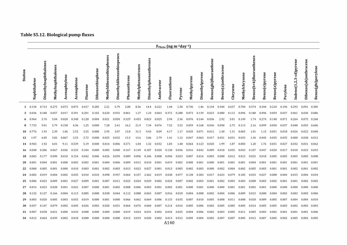
A140

Table S5.12. Biological pump fluxes

FPhyto (ng m-2day-1)

Sta

tio

n

Na

ph

tha

len

e

Dim

eth

yln

ap

hth

ale

ne

s

Me

thy

lna

ph

tha

len

es

Ace

na

ph

tyle

ne

Ace

na

ph

ten

e

Flu

ore

ne

Dib

en

zoth

iop

he

ne

Me

thy

ldib

en

zoth

iop

he

ne

s

Dim

eth

yld

ibe

nzo

thio

pe

ne

s

Ph

en

an

thre

ne

Me

thy

lph

en

an

tre

ne

s

Dim

eth

ylp

he

na

nth

ren

es

An

thra

cen

e

Flu

ora

nth

en

e

Py

ren

e

Me

thy

lpy

ren

e

Dim

eth

ylp

yre

ne

Be

nzo

(gh

i)fl

uo

ran

the

ne

Be

nzo

(a)a

nth

race

ne

Ch

ryse

ne

Me

thy

lch

ryse

ne

Be

nzo

(b+

k)f

luo

ran

the

ne

s

Be

nzo

(e)p

yre

ne

Be

nzo

(a)p

yre

ne

Pe

ryle

ne

Ind

en

o(1

,2,3

-cd

)py

ren

e

Dib

en

zo(a

h)a

nth

race

ne

Be

nzo

(gh

i)p

ery

len

e

1 0.134 0.713 0.275 0.073 0.875 0.417 0.285 2.21 5.79 2.80 8.36 14.4 0.221 1.44 1.30 0.736 1.46 0.134 0.344 0.637 0.784 0.574 0.344 0.210 0.196 0.293 0.091 0.385

3 0.036 0.180 0.057 0.017 0.391 0.201 0.102 0.620 0.932 0.861 1.27 1.24 0.063 0.372 0.288 0.073 0.139 0.023 0.080 0.112 0.096 0.180 0.096 0.059 0.037 0.061 0.030 0.086

6 0.964 3.76 5.04 0.020 0.348 0.128 0.004 0.021 0.050 0.329 0.453 0.823 0.025 2.94 2.36 0.076 0.144 0.036 2.92 3.01 0.149 1.74 0.274 0.148 0.071 0.264 0.075 0.260

8 7.733 9.01 5.79 0.158 4.36 1.25 0.000 7.28 2.41 16.2 21.9 7.34 0.076 7.52 3.52 0.059 0.168 0.036 0.058 2.75 0.113 2.16 0.099 0.050 0.037 0.048 0.055 0.606

10 0.776 1.93 2.39 1.06 2.55 3.55 0.000 2.95 3.07 13.8 31.3 9.43 8.09 4.17 1.17 0.035 0.071 0.012 1.30 1.31 0.065 1.01 1.15 0.031 0.018 0.026 0.022 0.040

12 1.97 6.85 3.82 0.867 3.53 3.72 0.000 0.025 0.032 13.3 13.6 3.06 2.79 1.41 1.12 0.047 0.063 0.017 0.031 0.031 0.033 1.36 0.045 0.035 0.035 0.000 0.038 0.012

14 0.943 1.92 4.01 9.11 0.539 5.19 0.000 0.014 0.006 0.571 1.04 1.32 0.032 1.83 1.48 0.064 0.123 0.020 1.99 1.87 0.083 1.20 1.76 0.031 0.027 0.032 0.031 0.062

16 0.048 0.286 0.067 0.036 0.525 0.104 0.000 0.005 0.000 0.167 0.149 0.187 0.020 0.130 0.036 0.016 0.042 0.009 0.018 0.035 0.043 0.107 0.047 0.020 0.017 0.018 0.023 0.033

18 0.065 0.177 0.090 0.010 0.154 0.042 0.006 0.026 0.039 0.089 0.096 0.106 0.008 0.096 0.023 0.007 0.014 0.003 0.008 0.012 0.013 0.025 0.010 0.005 0.005 0.005 0.005 0.008

20 0.001 0.004 0.001 0.000 0.002 0.002 0.001 0.004 0.006 0.009 0.012 0.010 0.001 0.019 0.002 0.000 0.001 0.000 0.001 0.001 0.001 0.004 0.001 0.001 0.001 0.001 0.001 0.001

22 0.000 0.005 0.001 0.000 0.010 0.003 0.001 0.002 0.003 0.013 0.023 0.027 0.001 0.013 0.005 0.002 0.003 0.000 0.002 0.004 0.002 0.005 0.003 0.001 0.001 0.002 0.001 0.002

24 0.002 0.019 0.004 0.002 0.035 0.010 0.010 0.098 0.937 0.064 0.337 2.462 0.019 0.038 0.077 0.128 0.383 0.017 0.023 0.079 0.185 0.033 0.027 0.008 0.004 0.015 0.004 0.034

25 0.006 0.023 0.009 0.001 0.027 0.009 0.001 0.007 0.011 0.023 0.024 0.029 0.002 0.024 0.007 0.002 0.003 0.001 0.002 0.003 0.003 0.008 0.003 0.002 0.001 0.001 0.002 0.002

27 0.014 0.023 0.028 0.001 0.022 0.007 0.000 0.001 0.002 0.008 0.006 0.003 0.001 0.002 0.001 0.000 0.001 0.000 0.000 0.001 0.001 0.002 0.001 0.000 0.000 0.000 0.000 0.000

28 0.132 0.127 0.166 0.004 0.113 0.085 0.008 0.038 0.044 0.112 0.088 0.063 0.007 0.016 0.018 0.004 0.008 0.002 0.004 0.006 0.009 0.015 0.008 0.004 0.002 0.003 0.003 0.006

29 0.003 0.020 0.005 0.003 0.055 0.019 0.000 0.001 0.000 0.066 0.062 0.069 0.006 0.133 0.035 0.007 0.010 0.005 0.008 0.011 0.008 0.020 0.009 0.005 0.007 0.004 0.004 0.010

30 0.037 0.147 0.079 0.002 0.045 0.026 0.003 0.020 0.031 0.064 0.076 0.060 0.007 0.214 0.016 0.005 0.006 0.002 0.005 0.005 0.005 0.014 0.005 0.005 0.003 0.002 0.003 0.003

31 0.007 0.038 0.021 0.000 0.010 0.008 0.000 0.000 0.000 0.019 0.024 0.031 0.002 0.034 0.025 0.004 0.006 0.002 0.003 0.005 0.011 0.005 0.003 0.002 0.001 0.001 0.001 0.006

34 0.012 0.064 0.039 0.002 0.018 0.008 0.000 0.000 0.000 0.013 0.019 0.020 0.002 0.013 0.012 0.005 0.004 0.002 0.007 0.007 0.005 0.012 0.007 0.005 0.002 0.005 0.002 0.005

A141

37 0.062 0.022 0.045 0.000 0.020 0.006 0.000 0.002 0.002 0.010 0.009 0.008 0.001 0.004 0.003 0.001 0.001 0.000 0.001 0.002 0.002 0.004 0.002 0.001 0.001 0.001 0.001 0.001

41 0.008 0.015 0.010 0.001 0.052 0.020 0.001 0.001 0.001 0.231 0.070 0.046 0.031 0.296 0.214 0.053 0.017 0.021 0.146 0.134 0.036 0.185 0.096 0.088 0.026 0.108 0.030 0.079

42 0.014 0.085 0.042 0.001 0.015 0.033 0.000 0.001 0.002 0.043 0.029 0.074 0.003 0.015 0.017 0.006 0.015 0.003 0.005 0.012 0.016 0.011 0.006 0.003 0.001 0.005 0.002 0.008

43 0.017 0.158 0.073 0.001 0.021 0.052 0.000 0.001 0.001 0.017 0.016 0.019 0.003 0.034 0.013 0.003 0.003 0.002 0.003 0.010 0.005 0.013 0.005 0.002 0.003 0.004 0.002 0.004

44 4.50 1.19 2.80 0.030 0.802 0.350 0.020 0.146 0.228 0.930 0.807 0.862 0.109 0.469 0.329 0.061 0.181 0.043 0.064 0.118 0.179 0.345 0.118 0.073 0.055 0.018 0.073 0.080

45 1.99 1.53 1.65 0.112 1.23 0.866 0.180 0.906 1.27 3.41 5.07 8.73 0.386 1.66 1.93 0.668 1.19 0.414 0.626 1.20 1.10 1.27 0.804 0.467 0.129 0.651 0.167 1.14

46 0.022 0.050 0.026 0.002 0.085 0.018 0.002 0.011 0.020 0.053 0.056 0.121 0.007 0.025 0.018 0.007 0.020 0.003 0.008 0.019 0.016 0.023 0.010 0.005 0.005 0.009 0.003 0.010

48 0.008 0.070 0.021 0.002 0.055 0.027 0.004 0.025 0.038 0.109 0.409 0.859 0.051 0.022 0.044 0.036 0.095 0.007 0.008 0.023 0.050 0.013 0.009 0.003 0.001 0.005 0.002 0.012

50 0.006 0.014 0.010 0.001 0.009 0.002 0.000 0.001 0.001 0.008 0.005 0.004 0.003 0.004 0.002 0.000 0.001 0.001 0.001 0.001 0.001 0.008 0.003 0.003 0.002 0.000 0.002 0.002

52 0.000 0.001 0.000 0.000 0.003 0.001 0.000 0.000 0.000 0.002 0.001 0.001 0.000 0.001 0.000 0.000 0.000 0.000 0.000 0.000 0.000 0.001 0.000 0.000 0.000 0.000 0.000 0.000

53 0.000 0.004 0.001 0.000 0.006 0.003 0.000 0.001 0.002 0.009 0.007 0.005 0.001 0.001 0.001 0.000 0.000 0.000 0.000 0.000 0.000 0.002 0.000 0.000 0.000 0.000 0.000 0.000

55 0.000 0.001 0.000 0.000 0.001 0.000 0.000 0.000 0.000 0.002 0.002 0.002 0.000 0.001 0.000 0.000 0.000 0.000 0.000 0.000 0.000 0.001 0.000 0.000 0.000 0.000 0.000 0.000

57 0.000 0.001 0.000 0.000 0.002 0.000 0.000 0.000 0.000 0.001 0.001 0.001 0.000 0.000 0.000 0.000 0.000 0.000 0.000 0.000 0.000 0.001 0.000 0.000 0.000 0.000 0.000 0.000

59 0.001 0.001 0.001 0.000 0.003 0.001 0.000 0.000 0.000 0.002 0.001 0.001 0.000 0.000 0.000 0.000 0.000 0.000 0.000 0.000 0.000 0.001 0.000 0.000 0.000 0.000 0.000 0.000

61 0.001 0.008 0.002 0.000 0.011 0.002 0.000 0.000 0.000 0.004 0.004 0.006 0.001 0.001 0.001 0.000 0.001 0.000 0.000 0.000 0.001 0.001 0.001 0.000 0.000 0.000 0.000 0.000

63 0.002 0.004 0.003 0.000 0.006 0.001 0.000 0.000 0.000 0.004 0.004 0.003 0.000 0.001 0.001 0.000 0.000 0.000 0.000 0.001 0.001 0.001 0.001 0.000 0.000 0.000 0.000 0.000

65 0.001 0.002 0.001 0.000 0.003 0.001 0.000 0.000 0.000 0.007 0.003 0.003 0.000 0.002 0.001 0.000 0.000 0.000 0.000 0.000 0.000 0.001 0.000 0.000 0.000 0.000 0.000 0.000

67 0.003 0.026 0.007 0.002 0.017 0.025 0.000 0.001 0.001 0.010 0.008 0.007 0.002 0.005 0.001 0.001 0.001 0.000 0.001 0.001 0.001 0.003 0.001 0.002 0.003 0.002 0.001 0.000

74 0.023 0.294 0.076 0.024 0.753 0.210 0.000 0.012 0.010 0.313 0.315 0.166 0.046 0.017 0.012 0.008 0.005 0.003 0.005 0.005 0.006 0.042 0.011 0.007 0.008 0.000 0.010 0.002

4b1 0.001 0.094 0.021 0.007 0.112 0.056 0.002 0.009 0.017 0.341 0.297 0.412 0.016 0.140 0.094 0.023 0.046 0.021 0.033 0.083 0.051 0.085 0.045 0.025 0.012 0.024 0.014 0.033

79 0.000 0.018 0.002 0.002 0.043 0.024 0.001 0.005 0.008 0.050 0.039 0.047 0.004 0.015 0.014 0.003 0.005 0.002 0.006 0.009 0.006 0.015 0.008 0.006 0.003 0.007 0.003 0.008

83 0.005 0.012 0.006 0.001 0.021 0.005 0.001 0.004 0.006 0.035 0.013 0.014 0.002 0.045 0.087 0.001 0.002 0.007 0.001 0.002 0.002 0.006 0.003 0.002 0.001 0.000 0.001 0.003

85 0.002 0.000 0.000 0.061 0.000 0.048 0.000 0.000 0.000 0.000 0.000 0.000 0.000 0.003 0.003 0.000 0.000 0.007 0.000 0.000 0.000 0.031 0.000 0.000 0.006 0.000 0.000 0.004

88 0.000 0.004 0.001 0.000 0.012 0.003 0.000 0.000 0.000 0.013 0.044 0.104 0.006 0.003 0.006 0.005 0.014 0.001 0.001 0.003 0.008 0.003 0.002 0.001 0.000 0.000 0.000 0.002

92 0.033 0.173 0.063 0.011 0.303 0.101 0.013 0.064 0.099 0.239 0.210 0.379 0.033 0.113 0.059 0.023 0.066 0.019 0.044 0.068 0.140 0.099 0.051 0.025 0.012 0.036 0.016 0.054

95 0.000 0.013 0.001 0.014 0.117 0.025 0.000 0.002 0.000 0.069 0.092 0.181 0.009 0.045 0.023 0.011 0.028 0.003 0.012 0.017 0.022 0.038 0.012 0.013 0.004 0.020 0.016 0.022

98 0.023 0.078 0.051 0.009 0.829 0.785 0.069 0.102 0.052 1.94 0.446 0.269 0.223 2.33 1.59 0.297 0.098 0.131 0.967 0.910 0.193 0.866 0.475 0.474 0.130 0.505 0.157 0.410

103 0.001 0.003 0.001 0.000 0.008 0.001 0.000 0.001 0.001 0.008 0.008 0.011 0.001 0.004 0.004 0.001 0.003 0.001 0.001 0.001 0.002 0.002 0.001 0.000 0.000 0.001 0.000 0.001

105 0.000 0.000 0.000 0.000 0.000 0.000 0.000 0.000 0.000 0.000 0.000 0.000 0.000 0.000 0.000 0.000 0.000 0.000 0.000 0.000 0.000 0.000 0.000 0.000 0.000 0.000 0.000 0.000

106 0.006 0.011 0.007 0.001 0.022 0.006 0.000 0.001 0.002 0.016 0.013 0.016 0.001 0.006 0.004 0.001 0.002 0.001 0.001 0.002 0.003 0.003 0.001 0.001 0.001 0.000 0.001 0.001

A142

107 0.001 0.005 0.002 0.000 0.011 0.002 0.000 0.002 0.006 0.012 0.012 0.039 0.002 0.006 0.006 0.003 0.011 0.001 0.002 0.004 0.009 0.003 0.002 0.001 0.001 0.001 0.000 0.003

109 0.000 0.003 0.001 0.000 0.006 0.001 0.000 0.001 0.001 0.003 0.003 0.005 0.000 0.004 0.001 0.000 0.001 0.000 0.000 0.001 0.001 0.001 0.000 0.000 0.000 0.000 0.000 0.000

111 0.001 0.002 0.001 0.001 0.004 0.001 0.000 0.000 0.000 0.008 0.007 0.008 0.001 0.010 0.007 0.001 0.002 0.001 0.003 0.004 0.002 0.003 0.001 0.001 0.001 0.001 0.000 0.001

113 0.002 0.004 0.002 0.000 0.010 0.002 0.000 0.001 0.000 0.008 0.006 0.008 0.001 0.061 0.002 0.000 0.001 0.000 0.001 0.001 0.002 0.003 0.001 0.001 0.000 0.000 0.001 0.000

115 0.002 0.008 0.004 0.001 0.019 0.003 0.000 0.001 0.002 0.006 0.006 0.009 0.001 0.025 0.002 0.000 0.001 0.000 0.000 0.001 0.002 0.003 0.001 0.001 0.001 0.000 0.001 0.000

116 0.015 0.031 0.013 0.002 0.054 0.012 0.001 0.008 0.010 0.027 0.019 0.018 0.004 0.067 0.003 0.001 0.002 0.000 0.001 0.001 0.002 0.004 0.001 0.001 0.001 0.000 0.001 0.001

117 0.003 0.007 0.004 0.000 0.010 0.001 0.000 0.002 0.003 0.007 0.009 0.015 0.002 0.029 0.003 0.001 0.002 0.001 0.001 0.001 0.003 0.004 0.001 0.001 0.001 0.000 0.001 0.001

118 0.060 0.113 0.080 0.006 0.195 0.032 0.001 0.004 0.004 0.058 0.041 0.049 0.006 0.057 0.071 0.003 0.008 0.008 0.003 0.006 0.013 0.011 0.006 0.003 0.004 0.001 0.002 0.005

120 0.004 0.014 0.007 0.000 0.012 0.002 0.000 0.001 0.001 0.060 0.047 0.043 0.001 0.031 0.008 0.001 0.002 0.001 0.001 0.006 0.003 0.006 0.002 0.001 0.001 0.000 0.002 0.001

123 0.020 0.071 0.028 0.010 0.108 0.037 0.000 0.003 0.004 0.636 0.191 0.211 0.009 0.129 0.039 0.011 0.030 0.007 0.017 0.032 0.042 0.054 0.022 0.013 0.014 0.006 0.013 0.012

125 0.036 0.047 0.033 0.005 0.088 0.020 0.000 0.004 0.007 0.135 0.215 0.465 0.025 0.051 0.057 0.034 0.139 0.013 0.025 0.039 0.116 0.046 0.031 0.015 0.007 0.008 0.008 0.027

129 0.000 0.002 0.000 0.281 1.64 0.595 0.000 0.012 0.004 0.068 0.488 0.283 0.012 0.015 0.014 0.007 0.002 0.001 0.006 0.017 0.009 0.013 0.009 0.004 0.002 0.007 0.006 0.008

131 0.004 0.082 0.019 0.004 0.118 0.038 0.004 0.018 0.027 0.257 0.089 0.102 0.009 0.059 0.037 0.005 0.015 0.005 0.013 0.029 0.022 0.028 0.016 0.005 0.003 0.007 0.004 0.009

133 0.000 0.003 0.000 0.000 0.008 0.002 0.000 0.000 0.001 0.004 0.005 0.005 0.001 0.008 0.001 0.000 0.000 0.000 0.000 0.001 0.000 0.002 0.000 0.000 0.000 0.000 0.000 0.000

134 0.001 0.007 0.003 0.000 0.006 0.001 0.000 0.001 0.001 0.004 0.003 0.003 0.001 0.004 0.000 0.000 0.000 0.000 0.000 0.000 0.000 0.000 0.000 0.000 0.000 0.000 0.000 0.000

136 0.000 0.001 0.000 0.000 0.002 0.000 0.000 0.000 0.000 0.001 0.001 0.001 0.000 0.000 0.000 0.000 0.000 0.000 0.000 0.000 0.000 0.000 0.000 0.000 0.000 0.000 0.000 0.000

138 0.002 0.002 0.002 0.000 0.005 0.001 0.000 0.000 0.000 0.003 0.003 0.002 0.000 0.001 0.000 0.000 0.000 0.000 0.000 0.000 0.001 0.001 0.000 0.000 0.000 0.000 0.000 0.000

140 0.001 0.001 0.001 0.000 0.003 0.001 0.000 0.000 0.000 0.005 0.002 0.001 0.000 0.000 0.000 0.000 0.000 0.000 0.000 0.000 0.000 0.001 0.000 0.000 0.000 0.000 0.000 0.000

142 0.001 0.001 0.001 0.000 0.003 0.001 0.000 0.000 0.000 0.004 0.002 0.002 0.000 0.001 0.001 0.000 0.000 0.000 0.000 0.000 0.000 0.001 0.000 0.000 0.000 0.000 0.000 0.000

144 0.000 0.001 0.000 0.000 0.001 0.001 0.000 0.002 0.005 0.004 0.006 0.013 0.000 0.003 0.003 0.001 0.005 0.001 0.002 0.003 0.007 0.003 0.003 0.002 0.001 0.002 0.001 0.003

146 0.000 0.002 0.001 0.000 0.002 0.001 0.000 0.000 0.000 0.002 0.001 0.001 0.000 0.001 0.000 0.000 0.000 0.000 0.000 0.001 0.001 0.002 0.001 0.000 0.000 0.000 0.000 0.000

A143

FFecal (ng m-2day-1)

Sta

tio

n

Na

ph

tha

len

e

Dim

eth

yln

ap

hth

ale

ne

s_

Me

thy

lna

ph

tha

len

es

Ace

na

ph

tyle

ne

Ace

na

ph

ten

e

Flu

ore

ne

Dib

en

zoth

iop

he

ne

Me

thy

ldib

en

zoth

iop

he

ne

s

Dim

eth

yld

ibe

nzo

thio

pe

ne

s

Ph

en

an

thre

ne

Me

thy

lph

en

an

tre

ne

s

Dim

eth

ylp

he

na

nth

ren

es

An

thra

cen

e

Flu

ora

nth

en

e

Py

ren

e

Me

thy

lpy

ren

e

Dim

eth

ylp

yre

ne

Be

nzo

(gh

i)fl

uo

ran

the

ne

Be

nzo

(a)a

nth

race

ne

Ch

ryse

ne

Me

thy

lch

ryse

ne

Be

nzo

(b+

k)f

luo

ran

the

ne

s

Be

nzo

(e)p

yre

ne

Be

nzo

(a)p

yre

ne

Pe

ryle

ne

Ind

en

o(1

.2.3

-cd

)py

ren

e

Dib

en

zo(a

h)a

nth

race

ne

Be

nzo

(gh

i)p

ery

len

e

1 0.600 3.20 1.24 0.326 3.93 1.87 1.28 9.92 26.2 12.6 37.6 64.6 0.991 6.45 5.85 3.31 6.57 0.601 1.54 2.86 3.52 2.58 1.55 0.942 0.881 1.31 0.410 1.73

3 0.358 1.80 0.571 0.170 3.92 2.01 1.03 6.22 9.34 8.64 12.7 12.4 0.636 3.73 2.89 0.729 1.39 0.230 0.806 1.13 0.967 1.80 0.961 0.590 0.367 0.615 0.296 0.860

6 7.76 30.3 40.5 0.163 2.80 1.03 0.033 0.172 0.406 2.65 3.65 6.62 0.197 23.7 19.0 0.611 1.16 0.290 23.5 24.2 1.20 14.0 2.203 1.19 0.570 2.13 0.606 2.09

8 62.6 72.9 46.9 1.28 35.3 10.1 0.000 58.9 19.5 131 177 59.4 0.618 60.9 28.5 0.474 1.36 0.294 0.471 22.3 0.913 17.5 0.797 0.401 0.298 0.390 0.442 4.91

10 5.61 13.9 17.2 7.66 18.5 25.6 0.000 21.4 22.2 100 226 68.2 58.5 30.1 8.48 0.256 0.512 0.090 9.37 9.46 0.468 7.28 8.33 0.227 0.134 0.187 0.162 0.292

12 12.2 42.7 23.8 5.40 22.0 23.2 0.000 0.155 0.197 82.9 84.7 19.1 17.4 8.81 6.97 0.290 0.393 0.109 0.191 0.195 0.206 8.49 0.283 0.216 0.220 0.000 0.237 0.077

14 4.69 9.54 20.0 45.4 2.69 25.8 0.000 0.070 0.029 2.84 5.19 6.59 0.159 9.08 7.38 0.319 0.614 0.099 9.89 9.32 0.413 5.96 8.774 0.154 0.132 0.160 0.154 0.310

16 0.370 2.20 0.518 0.279 4.04 0.803 0.000 0.038 0.000 1.29 1.15 1.44 0.156 1.00 0.279 0.120 0.321 0.067 0.141 0.267 0.327 0.820 0.360 0.156 0.134 0.139 0.179 0.257

18 3.04 8.26 4.21 0.471 7.17 1.95 0.264 1.24 1.82 4.15 4.46 4.96 0.372 4.49 1.10 0.319 0.644 0.135 0.352 0.547 0.609 1.17 0.447 0.246 0.230 0.248 0.237 0.352

20 0.206 0.605 0.247 0.042 0.407 0.327 0.116 0.706 0.968 1.58 2.06 1.77 0.136 3.24 0.355 0.080 0.176 0.055 0.156 0.197 0.171 0.605 0.243 0.136 0.132 0.136 0.122 0.173

22 0.092 0.977 0.178 0.062 2.00 0.689 0.111 0.472 0.567 2.66 4.59 5.46 0.154 2.53 1.09 0.412 0.554 0.095 0.471 0.764 0.485 1.09 0.555 0.221 0.199 0.368 0.154 0.407

24 0.160 1.73 0.341 0.157 3.19 0.859 0.859 8.84 84.5 5.74 30.4 222 1.75 3.40 6.91 11.5 34.5 1.52 2.06 7.15 16.7 2.99 2.46 0.724 0.329 1.33 0.365 3.10

25 0.372 1.32 0.503 0.086 1.59 0.511 0.065 0.383 0.615 1.34 1.39 1.70 0.141 1.42 0.408 0.095 0.178 0.052 0.092 0.150 0.163 0.452 0.147 0.095 0.072 0.038 0.095 0.095

27 1.34 2.24 2.72 0.068 2.11 0.671 0.036 0.142 0.146 0.744 0.584 0.331 0.087 0.224 0.138 0.046 0.080 0.030 0.046 0.078 0.089 0.176 0.093 0.045 0.032 0.005 0.000 0.027

28 12.4 11.9 15.6 0.340 10.6 7.97 0.755 3.54 4.10 10.5 8.25 5.96 0.670 1.49 1.71 0.388 0.780 0.161 0.343 0.525 0.835 1.41 0.724 0.366 0.231 0.261 0.312 0.565

29 0.222 1.48 0.334 0.225 4.04 1.39 0.000 0.106 0.024 4.80 4.50 5.04 0.472 9.66 2.54 0.518 0.715 0.360 0.573 0.778 0.569 1.45 0.632 0.333 0.488 0.278 0.278 0.733

30 2.42 9.55 5.14 0.157 2.91 1.70 0.215 1.29 2.03 4.20 4.94 3.94 0.482 14.0 1.06 0.303 0.362 0.112 0.332 0.341 0.321 0.933 0.315 0.309 0.226 0.126 0.194 0.220

31 0.849 4.438 2.50 0.041 1.14 0.941 0.000 0.017 0.015 2.20 2.77 3.60 0.225 3.94 2.94 0.416 0.706 0.277 0.310 0.589 1.31 0.616 0.406 0.181 0.156 0.156 0.145 0.697

34 2.63 13.9 8.54 0.391 4.01 1.78 0.000 0.061 0.029 2.88 4.04 4.39 0.534 2.90 2.61 0.995 0.833 0.348 1.46 1.59 1.04 2.63 1.44 1.11 0.484 1.05 0.404 1.18

37 22.4 8.04 16.2 0.128 7.39 2.22 0.133 0.593 0.737 3.73 3.34 3.08 0.318 1.49 1.05 0.236 0.440 0.133 0.368 0.740 0.563 1.42 0.609 0.284 0.211 0.369 0.247 0.435

A144

41 0.939 1.79 1.23 0.130 6.10 2.40 0.080 0.142 0.066 27.1 8.26 5.39 3.61 34.72 25.1 6.26 1.98 2.48 17.1 15.7 4.22 21.7 11.2 10.4 2.99 12.6 3.53 9.28

42 1.13 7.03 3.49 0.048 1.26 2.74 0.013 0.111 0.166 3.56 2.44 6.09 0.287 1.28 1.43 0.514 1.25 0.256 0.445 1.01 1.35 0.941 0.506 0.227 0.071 0.441 0.125 0.663

43 0.689 6.21 2.90 0.041 0.846 2.04 0.000 0.028 0.030 0.659 0.630 0.751 0.102 1.36 0.517 0.102 0.120 0.069 0.104 0.413 0.205 0.526 0.178 0.070 0.125 0.160 0.085 0.169

44 76.4 20.3 47.6 0.502 13.6 5.93 0.346 2.48 3.86 15.8 13.7 14.6 1.86 7.96 5.58 1.04 3.07 0.735 1.08 2.01 3.04 5.86 2.00 1.24 0.926 0.304 1.23 1.35

45 7.29 5.62 6.04 0.410 4.52 3.18 0.658 3.32 4.64 12.5 18.6 32.0 1.42 6.08 7.08 2.45 4.35 1.52 2.29 4.39 4.01 4.66 2.95 1.71 0.474 2.39 0.612 4.19

46 0.267 0.608 0.322 0.029 1.04 0.224 0.025 0.134 0.243 0.640 0.685 1.47 0.090 0.309 0.218 0.084 0.243 0.039 0.092 0.232 0.191 0.285 0.121 0.064 0.056 0.109 0.035 0.116

48 0.293 2.50 0.737 0.083 1.95 0.963 0.141 0.887 1.33 3.88 14.5 30.5 1.82 0.777 1.55 1.29 3.38 0.254 0.288 0.810 1.759 0.451 0.309 0.123 0.042 0.183 0.054 0.428

50 0.407 0.906 0.665 0.036 0.558 0.101 0.000 0.075 0.047 0.499 0.345 0.263 0.164 0.257 0.103 0.026 0.034 0.039 0.058 0.060 0.064 0.532 0.196 0.165 0.106 0.000 0.141 0.113

52 0.007 0.059 0.013 0.010 0.209 0.064 0.000 0.009 0.008 0.130 0.078 0.087 0.028 0.069 0.018 0.005 0.012 0.005 0.008 0.009 0.013 0.060 0.022 0.017 0.012 0.000 0.015 0.010

53 0.010 0.135 0.033 0.012 0.204 0.098 0.009 0.053 0.061 0.309 0.260 0.168 0.029 0.039 0.036 0.007 0.009 0.005 0.010 0.010 0.009 0.055 0.015 0.012 0.010 0.000 0.013 0.006

55 0.008 0.102 0.034 0.006 0.075 0.031 0.000 0.002 0.005 0.183 0.147 0.139 0.018 0.049 0.030 0.009 0.016 0.008 0.014 0.017 0.023 0.080 0.026 0.018 0.015 0.002 0.018 0.018

57 0.012 0.065 0.015 0.006 0.154 0.034 0.000 0.001 0.003 0.090 0.073 0.055 0.013 0.023 0.015 0.007 0.008 0.004 0.007 0.009 0.012 0.054 0.016 0.010 0.010 0.000 0.012 0.004

59 0.086 0.106 0.067 0.011 0.268 0.057 0.000 0.009 0.014 0.171 0.151 0.119 0.022 0.048 0.028 0.007 0.012 0.007 0.011 0.017 0.024 0.076 0.022 0.015 0.014 0.000 0.018 0.006

61 0.063 0.792 0.211 0.023 1.14 0.241 0.000 0.012 0.005 0.386 0.429 0.605 0.071 0.062 0.059 0.042 0.147 0.014 0.028 0.050 0.124 0.110 0.058 0.020 0.015 0.017 0.019 0.039

63 0.156 0.308 0.210 0.013 0.478 0.075 0.000 0.007 0.002 0.349 0.287 0.283 0.025 0.092 0.076 0.017 0.035 0.016 0.027 0.041 0.056 0.088 0.042 0.018 0.013 0.011 0.018 0.030

65 0.059 0.139 0.081 0.010 0.168 0.093 0.000 0.004 0.005 0.444 0.202 0.190 0.018 0.102 0.056 0.011 0.011 0.010 0.018 0.030 0.024 0.089 0.029 0.016 0.013 0.005 0.017 0.010

67 0.126 1.07 0.277 0.087 0.694 1.01 0.000 0.023 0.031 0.396 0.325 0.294 0.073 0.208 0.045 0.030 0.027 0.011 0.028 0.028 0.036 0.141 0.040 0.091 0.103 0.066 0.061 0.015

74 0.141 1.79 0.465 0.143 4.59 1.28 0.000 0.075 0.060 1.91 1.92 1.01 0.279 0.106 0.075 0.048 0.029 0.016 0.028 0.029 0.034 0.259 0.067 0.045 0.050 0.000 0.062 0.013

4b1 0.009 0.781 0.174 0.061 0.927 0.468 0.015 0.075 0.143 2.84 2.47 3.43 0.134 1.16 0.779 0.190 0.384 0.175 0.277 0.693 0.428 0.711 0.370 0.209 0.098 0.196 0.116 0.277

79 0.002 0.283 0.033 0.034 0.676 0.379 0.015 0.072 0.120 0.796 0.611 0.749 0.068 0.243 0.219 0.042 0.084 0.039 0.097 0.141 0.095 0.240 0.132 0.103 0.046 0.107 0.041 0.128

83 0.089 0.213 0.108 0.021 0.370 0.082 0.022 0.079 0.104 0.630 0.224 0.250 0.035 0.813 1.56 0.012 0.031 0.129 0.022 0.035 0.029 0.111 0.052 0.030 0.020 0.003 0.023 0.046

85 0.076 0.000 0.000 2.34 0.000 1.85 0.000 0.000 0.000 0.000 0.000 0.000 0.000 0.110 0.119 0.000 0.000 0.254 0.000 0.000 0.000 1.19 0.000 0.000 0.231 0.000 0.000 0.135

88 0.016 0.290 0.079 0.026 0.974 0.215 0.000 0.030 0.015 1.03 3.57 8.46 0.501 0.218 0.472 0.400 1.16 0.102 0.110 0.250 0.642 0.235 0.144 0.048 0.031 0.029 0.037 0.158

92 0.299 1.59 0.580 0.101 2.78 0.930 0.121 0.588 0.906 2.19 1.93 3.48 0.300 1.04 0.542 0.214 0.606 0.173 0.407 0.624 1.29 0.906 0.467 0.231 0.107 0.327 0.142 0.491

95 0.001 0.124 0.008 0.131 1.08 0.236 0.000 0.017 0.000 0.637 0.852 1.68 0.081 0.413 0.218 0.103 0.258 0.032 0.115 0.156 0.206 0.354 0.109 0.117 0.037 0.189 0.148 0.207

98 1.25 4.24 2.76 0.475 45.0 42.6 3.77 5.54 2.80 105 24.2 14.6 12.1 126 86.4 16.1 5.32 7.09 52.5 49.4 10.5 47.0 25.8 25.7 7.05 27.4 8.49 22.2

103 0.049 0.233 0.087 0.022 0.590 0.082 0.009 0.050 0.096 0.584 0.589 0.803 0.038 0.297 0.332 0.106 0.198 0.060 0.061 0.106 0.118 0.125 0.076 0.036 0.013 0.050 0.031 0.104

105 0.000 0.000 0.000 0.000 0.000 0.000 0.000 0.000 0.000 0.000 0.000 0.000 0.000 0.000 0.000 0.000 0.000 0.000 0.000 0.000 0.000 0.000 0.000 0.000 0.000 0.000 0.000 0.000

106 0.442 0.808 0.466 0.056 1.54 0.390 0.016 0.097 0.130 1.12 0.948 1.14 0.085 0.411 0.272 0.057 0.129 0.037 0.065 0.128 0.198 0.221 0.097 0.046 0.052 0.018 0.051 0.054

107 0.140 0.490 0.216 0.032 1.03 0.188 0.036 0.153 0.523 1.09 1.12 3.72 0.176 0.568 0.589 0.282 1.07 0.119 0.180 0.348 0.862 0.284 0.198 0.069 0.063 0.137 0.047 0.298

A145

109 0.017 0.365 0.098 0.016 0.629 0.089 0.012 0.056 0.072 0.380 0.382 0.580 0.041 0.444 0.107 0.028 0.076 0.013 0.021 0.062 0.089 0.079 0.034 0.021 0.009 0.010 0.018 0.025

111 0.069 0.157 0.092 0.037 0.320 0.044 0.002 0.021 0.001 0.544 0.503 0.568 0.057 0.725 0.521 0.075 0.110 0.055 0.186 0.267 0.160 0.210 0.103 0.039 0.038 0.057 0.025 0.062

113 0.039 0.108 0.044 0.009 0.268 0.042 0.001 0.026 0.004 0.194 0.159 0.204 0.036 1.57 0.039 0.009 0.028 0.009 0.016 0.025 0.043 0.072 0.023 0.018 0.011 0.000 0.021 0.011

115 0.061 0.210 0.098 0.019 0.492 0.089 0.000 0.021 0.044 0.156 0.157 0.229 0.023 0.637 0.040 0.010 0.030 0.010 0.012 0.019 0.041 0.076 0.022 0.014 0.014 0.000 0.019 0.011

116 0.282 0.565 0.235 0.032 0.978 0.210 0.027 0.151 0.175 0.496 0.340 0.328 0.065 1.22 0.051 0.013 0.032 0.009 0.015 0.021 0.041 0.077 0.023 0.016 0.014 0.001 0.021 0.011

117 0.042 0.104 0.056 0.007 0.157 0.017 0.000 0.028 0.040 0.106 0.136 0.235 0.026 0.453 0.053 0.011 0.038 0.008 0.016 0.022 0.047 0.063 0.022 0.022 0.012 0.001 0.017 0.012

118 0.834 1.58 1.12 0.082 2.72 0.452 0.008 0.055 0.053 0.812 0.572 0.686 0.086 0.793 0.986 0.043 0.113 0.110 0.047 0.080 0.181 0.149 0.085 0.038 0.056 0.020 0.035 0.074

120 0.050 0.195 0.094 0.006 0.165 0.033 0.003 0.019 0.020 0.821 0.638 0.585 0.017 0.426 0.110 0.016 0.033 0.015 0.016 0.076 0.046 0.086 0.028 0.016 0.014 0.006 0.021 0.013

123 0.076 0.273 0.109 0.040 0.417 0.144 0.000 0.012 0.014 2.45 0.734 0.813 0.034 0.498 0.150 0.043 0.116 0.025 0.067 0.123 0.163 0.207 0.086 0.050 0.052 0.023 0.049 0.047

125 0.153 0.201 0.142 0.020 0.375 0.084 0.000 0.019 0.029 0.578 0.920 1.99 0.107 0.218 0.245 0.145 0.592 0.054 0.105 0.169 0.496 0.196 0.133 0.063 0.031 0.035 0.035 0.116

129 0.000 0.019 0.000 2.87 16.7 6.06 0.000 0.127 0.042 0.695 4.98 2.89 0.126 0.150 0.142 0.073 0.023 0.015 0.062 0.173 0.097 0.138 0.087 0.041 0.018 0.072 0.057 0.085

131 0.061 1.14 0.271 0.050 1.639 0.523 0.052 0.258 0.381 3.58 1.25 1.42 0.128 0.821 0.513 0.074 0.211 0.068 0.185 0.397 0.300 0.384 0.224 0.067 0.045 0.092 0.062 0.129

133 0.000 0.082 0.011 0.009 0.252 0.065 0.000 0.013 0.019 0.145 0.155 0.180 0.019 0.269 0.030 0.007 0.013 0.005 0.014 0.019 0.013 0.051 0.015 0.010 0.009 0.000 0.010 0.005

134 0.080 0.418 0.185 0.008 0.343 0.058 0.013 0.074 0.055 0.255 0.148 0.145 0.029 0.256 0.026 0.006 0.012 0.004 0.005 0.009 0.012 0.027 0.007 0.005 0.006 0.000 0.012 0.003

136 0.011 0.131 0.051 0.009 0.191 0.044 0.003 0.008 0.011 0.085 0.060 0.065 0.012 0.046 0.011 0.000 0.000 0.000 0.005 0.005 0.000 0.027 0.000 0.005 0.000 0.000 0.000 0.001

138 0.124 0.149 0.104 0.011 0.327 0.065 0.001 0.016 0.027 0.207 0.151 0.117 0.022 0.070 0.027 0.007 0.018 0.005 0.009 0.010 0.037 0.050 0.012 0.010 0.009 0.020 0.014 0.018

140 0.062 0.105 0.055 0.009 0.292 0.062 0.000 0.007 0.005 0.403 0.140 0.111 0.012 0.042 0.024 0.005 0.004 0.005 0.008 0.023 0.009 0.048 0.013 0.000 0.009 0.000 0.000 0.001

142 0.044 0.088 0.045 0.007 0.199 0.061 0.000 0.014 0.010 0.280 0.168 0.162 0.020 0.090 0.040 0.012 0.007 0.005 0.013 0.013 0.010 0.067 0.015 0.012 0.014 0.000 0.000 0.000

144 0.013 0.051 0.020 0.010 0.093 0.046 0.016 0.113 0.335 0.240 0.364 0.826 0.022 0.211 0.223 0.063 0.327 0.041 0.136 0.204 0.426 0.214 0.201 0.131 0.034 0.156 0.065 0.208

146 0.012 0.070 0.027 0.005 0.096 0.044 0.000 0.005 0.007 0.096 0.053 0.058 0.010 0.043 0.017 0.008 0.017 0.006 0.014 0.023 0.036 0.067 0.026 0.015 0.012 0.000 0.000 0.006

A146

FSettling (ng m-2day-1)

Sta

tio

n

Na

ph

tha

len

e

Dim

eth

yln

ap

hth

ale

ne

s_

Me

thy

lna

ph

tha

len

es

Ace

na

ph

tyle

ne

Ace

na

ph

ten

e

Flu

ore

ne

Dib

en

zoth

iop

he

ne

Me

thy

ldib

en

zoth

iop

he

ne

s

Dim

eth

yld

ibe

nzo

thio

pe

ne

s

Ph

en

an

thre

ne

Me

thy

lph

en

an

tre

ne

s

Dim

eth

ylp

he

na

nth

ren

es

An

thra

cen

e

Flu

ora

nth

en

e

Py

ren

e

Me

thy

lpy

ren

es

Dim

eth

ylp

yre

ne

s

Be

nzo

(gh

i)fl

uo

ran

the

ne

Be

nzo

(a)a

nth

race

ne

Ch

ryse

ne

Me

thy

lch

ryse

ne

Be

nzo

(b+

k)f

luo

ran

the

ne

s

Be

nzo

(e)p

yre

ne

Be

nzo

(a)p

yre

ne

Pe

ryle

ne

Ind

en

o(1

.2.3

-cd

)py

ren

e

Dib

en

zo(a

h)a

nth

race

ne

Be

nzo

(gh

i)p

ery

len

e

1 0.734 3.92 1.51 0.398 4.80 2.29 1.56 12.1 31.8 15.4 45.9 79.0 1.21 7.89 7.15 4.04 8.03 0.734 1.89 3.50 4.31 3.15 1.89 1.15 1.08 1.61 0.502 2.11

3 0.393 1.98 0.628 0.187 4.32 2.21 1.13 6.84 10.3 9.50 14.0 13.7 0.700 4.10 3.18 0.801 1.53 0.253 0.886 1.24 1.06 1.98 1.06 0.649 0.403 0.676 0.326 0.946

6 8.72 34.0 45.6 0.183 3.15 1.16 0.037 0.193 0.457 2.98 4.10 7.45 0.222 26.6 21.3 0.687 1.31 0.326 26.4 27.3 1.35 15.7 2.48 1.34 0.641 2.39 0.681 2.35

8 70.3 81.9 52.6 1.44 39.6 11.3 0.000 66.2 21.9 147 199 66.8 0.694 68.4 32.0 0.533 1.53 0.331 0.530 25.0 1.03 19.6 0.896 0.451 0.335 0.438 0.496 5.52

10 6.38 15.9 19.6 8.72 21.0 29.2 0.000 24.3 25.3 114 257 77.6 66.6 34.3 9.65 0.292 0.583 0.103 10.7 10.8 0.533 8.29 9.48 0.259 0.152 0.213 0.184 0.332

12 14.2 49.5 27.6 6.27 25.5 26.9 0.000 0.180 0.228 96.2 98.3 22.2 20.2 10.2 8.09 0.337 0.456 0.126 0.221 0.227 0.239 9.85 0.328 0.250 0.256 0.000 0.275 0.089

14 5.64 11.5 24.0 54.5 3.23 31.0 0.000 0.084 0.035 3.41 6.23 7.92 0.191 10.9 8.87 0.383 0.738 0.119 11.9 11.2 0.496 7.15 10.5 0.185 0.159 0.192 0.185 0.372

16 0.418 2.49 0.586 0.315 4.57 0.907 0.000 0.043 0.000 1.45 1.30 1.63 0.176 1.13 0.315 0.136 0.363 0.076 0.159 0.302 0.370 0.927 0.407 0.176 0.151 0.158 0.203 0.290

18 3.10 8.43 4.30 0.481 7.32 1.99 0.270 1.26 1.86 4.24 4.56 5.06 0.380 4.59 1.12 0.326 0.658 0.138 0.360 0.559 0.622 1.19 0.456 0.252 0.235 0.254 0.242 0.359

20 0.208 0.608 0.248 0.042 0.410 0.329 0.116 0.710 0.974 1.59 2.08 1.78 0.137 3.26 0.357 0.080 0.177 0.056 0.157 0.199 0.171 0.608 0.244 0.136 0.133 0.136 0.122 0.174

22 0.092 0.982 0.179 0.062 2.01 0.693 0.111 0.474 0.570 2.67 4.62 5.49 0.154 2.54 1.09 0.414 0.557 0.095 0.473 0.768 0.487 1.09 0.557 0.222 0.200 0.370 0.155 0.409

24 0.162 1.75 0.344 0.159 3.23 0.869 0.869 8.94 85.4 5.81 30.7 225 1.77 3.43 6.99 11.7 34.9 1.54 2.08 7.23 16.8 3.02 2.49 0.732 0.333 1.34 0.369 3.13

25 0.378 1.34 0.512 0.087 1.62 0.519 0.066 0.389 0.626 1.37 1.41 1.73 0.143 1.45 0.415 0.096 0.181 0.052 0.093 0.153 0.166 0.460 0.150 0.097 0.074 0.039 0.096 0.097

27 1.36 2.27 2.75 0.069 2.13 0.678 0.036 0.144 0.148 0.751 0.590 0.335 0.087 0.226 0.139 0.047 0.081 0.031 0.047 0.079 0.090 0.178 0.094 0.045 0.033 0.005 0.000 0.028

28 12.5 12.1 15.8 0.343 10.7 8.06 0.763 3.58 4.14 10.6 8.34 6.02 0.677 1.51 1.73 0.392 0.788 0.163 0.347 0.531 0.844 1.43 0.732 0.370 0.233 0.263 0.315 0.572

29 0.225 1.50 0.339 0.229 4.09 1.41 0.000 0.107 0.024 4.86 4.56 5.11 0.478 9.79 2.57 0.525 0.725 0.365 0.581 0.789 0.577 1.47 0.641 0.337 0.495 0.281 0.282 0.743

30 2.456 9.693 5.22 0.159 2.96 1.72 0.219 1.31 2.07 4.26 5.01 4.00 0.489 14.2 1.08 0.308 0.368 0.113 0.337 0.347 0.326 0.948 0.320 0.314 0.230 0.128 0.197 0.223

31 0.856 4.476 2.52 0.041 1.15 0.949 0.000 0.017 0.015 2.22 2.80 3.63 0.227 3.97 2.97 0.419 0.712 0.279 0.313 0.594 1.32 0.621 0.409 0.182 0.158 0.158 0.146 0.703

34 2.64 13.9 8.58 0.393 4.03 1.79 0.000 0.061 0.029 2.90 4.06 4.41 0.537 2.91 2.62 0.999 0.837 0.350 1.47 1.59 1.04 2.64 1.45 1.11 0.487 1.06 0.405 1.186

37 22.5 8.06 16.3 0.128 7.41 2.22 0.134 0.594 0.739 3.74 3.35 3.09 0.319 1.49 1.05 0.237 0.441 0.134 0.369 0.742 0.564 1.42 0.610 0.284 0.212 0.370 0.248 0.436

A147

41 0.947 1.80 1.24 0.131 6.15 2.42 0.081 0.144 0.067 27.3 8.33 5.44 3.64 35.0 25.3 6.31 1.99 2.50 17.3 15.9 4.25 21.9 11.3 10.5 3.02 12.8 3.56 9.36

42 1.14 7.11 3.53 0.048 1.27 2.77 0.013 0.112 0.168 3.60 2.47 6.17 0.291 1.30 1.45 0.520 1.26 0.259 0.450 1.02 1.37 0.952 0.512 0.230 0.071 0.446 0.127 0.671

43 0.706 6.37 2.97 0.042 0.868 2.09 0.000 0.028 0.031 0.676 0.646 0.770 0.104 1.39 0.530 0.104 0.123 0.070 0.106 0.423 0.210 0.539 0.183 0.072 0.128 0.164 0.088 0.173

44 80.9 21.5 50.4 0.532 14.4 6.28 0.366 2.63 4.09 16.7 14.5 15.9 1.96 8.43 5.90 1.10 3.25 0.778 1.14 2.13 3.22 6.21 2.12 1.31 0.981 0.322 1.31 1.43

45 9.28 7.15 7.69 0.522 5.76 4.04 0.838 4.23 5.91 15.9 23.7 40.7 1.80 7.75 9.01 3.12 5.54 1.93 2.92 5.59 5.11 5.93 3.75 2.18 0.603 3.04 0.779 5.34

46 0.289 0.658 0.348 0.031 1.12 0.242 0.027 0.145 0.263 0.693 0.742 1.59 0.097 0.335 0.236 0.091 0.263 0.042 0.100 0.251 0.207 0.309 0.131 0.069 0.060 0.118 0.038 0.126

48 0.301 2.57 0.758 0.085 2.01 0.990 0.145 0.912 1.37 3.99 14.9 31.3 1.87 0.798 1.59 1.33 3.47 0.262 0.296 0.833 1.81 0.463 0.317 0.127 0.044 0.188 0.056 0.440

50 0.413 0.920 0.675 0.036 0.567 0.102 0.000 0.077 0.048 0.506 0.351 0.267 0.166 0.261 0.104 0.026 0.034 0.040 0.059 0.061 0.065 0.540 0.199 0.167 0.108 0.000 0.144 0.114

52 0.007 0.060 0.013 0.010 0.211 0.064 0.000 0.009 0.008 0.131 0.079 0.088 0.028 0.070 0.019 0.005 0.012 0.005 0.009 0.009 0.013 0.061 0.022 0.017 0.012 0.000 0.015 0.010

53 0.010 0.139 0.034 0.012 0.209 0.101 0.009 0.054 0.063 0.318 0.268 0.172 0.030 0.040 0.037 0.008 0.010 0.005 0.011 0.011 0.009 0.057 0.015 0.012 0.010 0.000 0.013 0.006

55 0.008 0.103 0.035 0.006 0.075 0.031 0.000 0.002 0.005 0.185 0.148 0.140 0.018 0.049 0.030 0.009 0.017 0.009 0.014 0.018 0.023 0.081 0.027 0.018 0.015 0.002 0.019 0.018

57 0.013 0.065 0.015 0.006 0.155 0.035 0.000 0.001 0.003 0.091 0.074 0.056 0.013 0.023 0.015 0.007 0.008 0.005 0.007 0.009 0.012 0.055 0.016 0.010 0.010 0.000 0.013 0.004

59 0.087 0.107 0.068 0.011 0.271 0.058 0.000 0.009 0.014 0.173 0.152 0.120 0.022 0.048 0.028 0.007 0.012 0.007 0.011 0.017 0.024 0.076 0.022 0.015 0.014 0.000 0.018 0.006

61 0.063 0.800 0.213 0.023 1.15 0.243 0.000 0.012 0.005 0.390 0.433 0.611 0.071 0.062 0.059 0.042 0.149 0.014 0.028 0.051 0.126 0.112 0.059 0.020 0.015 0.017 0.019 0.039

63 0.158 0.312 0.213 0.014 0.484 0.076 0.000 0.007 0.002 0.353 0.291 0.286 0.025 0.093 0.077 0.017 0.035 0.016 0.028 0.042 0.057 0.089 0.043 0.018 0.013 0.011 0.018 0.030

65 0.060 0.142 0.082 0.010 0.171 0.094 0.000 0.004 0.005 0.451 0.205 0.193 0.018 0.103 0.057 0.012 0.011 0.010 0.018 0.030 0.024 0.091 0.029 0.016 0.013 0.005 0.018 0.010

67 0.130 1.09 0.284 0.089 0.711 1.04 0.000 0.023 0.032 0.405 0.333 0.301 0.075 0.213 0.046 0.030 0.028 0.012 0.029 0.029 0.037 0.145 0.041 0.093 0.105 0.068 0.063 0.015

74 0.164 2.09 0.541 0.167 5.35 1.49 0.000 0.087 0.070 2.22 2.23 1.18 0.325 0.124 0.087 0.055 0.034 0.018 0.033 0.034 0.040 0.301 0.078 0.053 0.058 0.000 0.072 0.016

4b1 0.010 0.875 0.195 0.069 1.04 0.524 0.017 0.084 0.161 3.18 2.77 3.84 0.150 1.30 0.873 0.213 0.431 0.196 0.310 0.777 0.479 0.796 0.415 0.234 0.109 0.219 0.130 0.311

79 0.002 0.300 0.036 0.036 0.719 0.402 0.016 0.077 0.128 0.846 0.650 0.796 0.072 0.258 0.233 0.045 0.089 0.042 0.103 0.150 0.101 0.255 0.140 0.109 0.049 0.114 0.044 0.136

83 0.094 0.225 0.114 0.022 0.390 0.086 0.023 0.083 0.110 0.665 0.236 0.264 0.037 0.858 1.65 0.013 0.032 0.137 0.024 0.037 0.031 0.117 0.055 0.032 0.022 0.003 0.024 0.048

85 0.078 0.000 0.000 2.40 0.000 1.90 0.000 0.000 0.000 0.000 0.000 0.000 0.000 0.113 0.122 0.000 0.000 0.261 0.000 0.000 0.000 1.226 0.000 0.000 0.238 0.000 0.000 0.138

88 0.017 0.294 0.080 0.026 0.986 0.217 0.000 0.030 0.015 1.04 3.61 8.56 0.507 0.221 0.477 0.405 1.18 0.103 0.111 0.253 0.650 0.238 0.146 0.049 0.031 0.029 0.038 0.160

92 0.332 1.76 0.643 0.112 3.09 1.03 0.134 0.652 1.01 2.43 2.14 3.86 0.333 1.15 0.601 0.237 0.672 0.192 0.451 0.692 1.43 1.005 0.518 0.257 0.119 0.362 0.158 0.544

95 0.001 0.137 0.009 0.145 1.20 0.261 0.000 0.019 0.000 0.706 0.944 1.86 0.090 0.458 0.241 0.114 0.286 0.035 0.127 0.173 0.228 0.393 0.120 0.129 0.041 0.210 0.163 0.229

98 1.28 4.32 2.81 0.484 45.8 43.4 3.84 5.64 2.85 107 24.6 14.9 12.3 129 87.9 16.4 5.42 7.22 53.4 50.3 10.7 47.9 26.3 26.2 7.18 27.9 8.65 22.6

103 0.050 0.236 0.088 0.022 0.598 0.083 0.009 0.051 0.098 0.591 0.597 0.814 0.039 0.301 0.336 0.107 0.201 0.061 0.062 0.107 0.120 0.127 0.077 0.036 0.014 0.051 0.031 0.105

105 0.000 0.000 0.000 0.000 0.000 0.000 0.000 0.000 0.000 0.000 0.000 0.000 0.000 0.000 0.000 0.000 0.000 0.000 0.000 0.000 0.000 0.000 0.000 0.000 0.000 0.000 0.000 0.000

106 0.448 0.819 0.472 0.056 1.57 0.395 0.016 0.098 0.132 1.13 0.961 1.15 0.087 0.417 0.276 0.058 0.131 0.037 0.066 0.130 0.201 0.224 0.098 0.047 0.052 0.018 0.051 0.055

107 0.141 0.495 0.219 0.033 1.04 0.190 0.037 0.155 0.529 1.10 1.13 3.76 0.178 0.574 0.595 0.285 1.08 0.120 0.181 0.352 0.871 0.287 0.201 0.070 0.064 0.139 0.047 0.301

A148

109 0.017 0.368 0.099 0.016 0.635 0.090 0.012 0.056 0.072 0.383 0.386 0.585 0.041 0.448 0.108 0.029 0.077 0.013 0.021 0.062 0.090 0.080 0.034 0.021 0.010 0.011 0.018 0.026

111 0.070 0.159 0.094 0.038 0.324 0.045 0.002 0.021 0.001 0.552 0.510 0.576 0.058 0.735 0.528 0.076 0.111 0.056 0.188 0.271 0.162 0.213 0.104 0.040 0.039 0.057 0.025 0.063

113 0.041 0.112 0.046 0.009 0.278 0.043 0.001 0.027 0.005 0.201 0.166 0.212 0.038 1.63 0.041 0.009 0.029 0.010 0.016 0.026 0.045 0.075 0.024 0.019 0.012 0.000 0.022 0.011

115 0.063 0.218 0.102 0.020 0.511 0.093 0.000 0.022 0.045 0.162 0.164 0.238 0.024 0.662 0.042 0.010 0.031 0.010 0.013 0.020 0.042 0.079 0.023 0.015 0.014 0.000 0.020 0.011

116 0.297 0.596 0.248 0.034 1.03 0.221 0.029 0.160 0.185 0.523 0.359 0.346 0.069 1.28 0.054 0.014 0.034 0.009 0.016 0.022 0.043 0.081 0.024 0.017 0.015 0.001 0.022 0.012

117 0.044 0.110 0.060 0.007 0.167 0.018 0.000 0.030 0.043 0.112 0.145 0.249 0.028 0.481 0.057 0.012 0.041 0.009 0.017 0.024 0.050 0.067 0.024 0.024 0.013 0.001 0.018 0.012

118 0.893 1.69 1.20 0.088 2.91 0.484 0.009 0.059 0.057 0.870 0.613 0.735 0.092 0.850 1.06 0.046 0.121 0.118 0.050 0.086 0.193 0.160 0.091 0.040 0.060 0.021 0.037 0.079

120 0.054 0.210 0.101 0.006 0.177 0.035 0.004 0.020 0.021 0.881 0.684 0.628 0.018 0.458 0.118 0.018 0.036 0.016 0.017 0.081 0.049 0.092 0.030 0.017 0.015 0.006 0.022 0.013

123 0.096 0.344 0.137 0.050 0.525 0.182 0.000 0.016 0.018 3.09 0.924 1.02 0.043 0.627 0.189 0.054 0.146 0.032 0.084 0.156 0.205 0.261 0.108 0.063 0.066 0.029 0.061 0.059

125 0.189 0.249 0.175 0.025 0.462 0.103 0.000 0.023 0.036 0.713 1.14 2.45 0.133 0.268 0.303 0.178 0.731 0.067 0.129 0.208 0.612 0.242 0.164 0.078 0.038 0.044 0.043 0.144

129 0.000 0.021 0.000 3.15 18.3 6.66 0.000 0.139 0.047 0.763 5.46 3.17 0.139 0.165 0.155 0.081 0.025 0.016 0.068 0.190 0.106 0.151 0.095 0.045 0.020 0.080 0.062 0.093

131 0.066 1.22 0.290 0.053 1.76 0.561 0.056 0.276 0.408 3.83 1.33 1.52 0.137 0.880 0.550 0.079 0.226 0.073 0.198 0.426 0.321 0.411 0.240 0.071 0.048 0.099 0.067 0.138

133 0.000 0.085 0.011 0.009 0.260 0.067 0.000 0.013 0.019 0.150 0.160 0.185 0.019 0.277 0.031 0.007 0.013 0.005 0.015 0.019 0.014 0.052 0.016 0.010 0.009 0.000 0.011 0.006

134 0.082 0.425 0.189 0.008 0.349 0.059 0.014 0.075 0.056 0.259 0.151 0.148 0.029 0.261 0.026 0.006 0.012 0.004 0.006 0.009 0.013 0.028 0.007 0.005 0.006 0.000 0.012 0.003

136 0.011 0.132 0.051 0.009 0.193 0.044 0.003 0.008 0.012 0.086 0.061 0.066 0.012 0.046 0.012 0.000 0.000 0.000 0.005 0.005 0.000 0.028 0.000 0.005 0.000 0.000 0.000 0.001

138 0.126 0.151 0.105 0.011 0.332 0.066 0.001 0.017 0.027 0.210 0.154 0.119 0.023 0.071 0.028 0.007 0.018 0.005 0.010 0.010 0.038 0.051 0.012 0.011 0.009 0.020 0.014 0.018

140 0.063 0.107 0.056 0.009 0.296 0.062 0.000 0.007 0.005 0.408 0.142 0.112 0.012 0.042 0.024 0.006 0.004 0.005 0.008 0.023 0.009 0.048 0.013 0.000 0.009 0.000 0.000 0.001

142 0.044 0.089 0.045 0.008 0.202 0.061 0.000 0.015 0.011 0.284 0.170 0.164 0.020 0.091 0.041 0.013 0.007 0.005 0.013 0.014 0.011 0.068 0.016 0.012 0.014 0.000 0.000 0.000

144 0.013 0.052 0.020 0.010 0.095 0.047 0.017 0.114 0.341 0.244 0.370 0.839 0.022 0.214 0.226 0.064 0.333 0.042 0.138 0.208 0.433 0.218 0.204 0.133 0.034 0.159 0.066 0.211

146 0.012 0.072 0.027 0.005 0.098 0.045 0.000 0.005 0.007 0.098 0.054 0.059 0.010 0.044 0.018 0.008 0.018 0.006 0.015 0.023 0.037 0.069 0.027 0.015 0.013 0.000 0.000 0.006

Occurrence, Transport and Fate of Persistent Organic ...

Documents

Transcript of Occurrence, Transport and Fate of Persistent Organic ...