Obstructions and Algorithms for Graph Layout Problems
332
National and Kapodistrian University of Athens School of Science, Department of Mathematics Obstructions and Algorithms for Graph Layout Problems Dimitris Zoros PhD Thesis Supervised by Prof. Dimitrios M. Thilikos July, 2017
-
Upload
khangminh22 -
Category
Documents
-
view
2 -
download
0
Transcript of Obstructions and Algorithms for Graph Layout Problems

National and Kapodistrian University of AthensSchool of Science, Department of Mathematics
Obstructions and Algorithms forGraph Layout Problems
Dimitris Zoros
PhD Thesis
Supervised by
Prof. Dimitrios M. Thilikos
July, 2017


ABSTRACT
Modern Graph Theory is heavily influenced by the seminal work of N.Robertson and P. Seymour, known as Graph Minors. Through this work,a wealth of structural, combinatorial, as well as algorithmic, results hasbeen introduced, in a series of papers having as ultimate goal to give an af-firmative answer to Wagner’s Conjecture. In this doctoral thesis we focuson the study of Obstruction Sets, one of the most important combinatorialconcepts of this theory. In particular, we study the combinatorics and thealgorithmic and computability aspects of graph obstructions and their re-lation to graph parameters emerging from Graph Layouts, Vertex DeletionProblems, and Graph Searching Problems. We consider several partial or-dering relations on graphs such as minors, immersions, and contractions.Our study includes results on the existence and the computability of ob-struction sets, combinatorial bounds on their size, and their interplay withparameterized complexity and kernelization.


ΠΕΡΙΛΗΨΗ
Η σύγχρονη Θεωρία Γραφημάτων έχει επηρεαστεί σε μεγάλο βαθμόαπό την δουλειά των N. Robertson και P. Seymour. Μέσα απόαυτήν, πληθώρα από δομικά, συνδυαστικά, καθώς και αλγοριθμικάαποτελέσματα εισήχθηκαν, σε μία σειρά από εργασίες που είχε απώτεροστόχο την απόδειξη της εικασίας του Wagner. Σε αυτή την διδακτορικήδιατριβή επικεντρωνόμαστε στην μελέτη των Συνόλων Παρεμπόδισης,μία από τις σημαντικότερες συνδυαστικές έννοιες αυτής της θεωρίας.Πιο συγκεκριμένα, μελετάμε την συνδυαστική και αλγοριθμική πτυχή,καθώς και την υπολογισιμότητα, των γραφημάτων παρεμπόδισης, σεσχέση με παραμέτρους γραφημάτων που πηγάζουν από Διατάξειςσε Γραφήματα, Προβλήματα Διαγραφής Κορυφών και ΠροβλήματαΑνίχνευσης Γραφημάτων. Η μελέτη αυτή είναι βασισμένη σε σχέσειςμερικής διάταξης γραφημάτων, όπως τα ελάσσονα, οι εμβυθίσεις και οισυνθλίψεις. Η μελέτη μας περιλαμβάνει αποτελέσματα σχετικά με τηνύπαρξη και υπολογισιμότητα των συνόλων παρεμπόδισης, συνδυαστικάφράγματα στο μέγεθος τους, καθώς και την αλληλεπίδρασή τους με τηνΠαραμετρική Πολυπλοκότητα και την Πυρηνοποίηση.


PREFACE
Having read the abstract of this thesis I am sure you must be eagerto find out what this story will involve. Unavoidably, we have to makea short intermission. I would like to grab this opportunity to show myappreciation and admiration to some people that guided me, or at leastaccompanied me, in my journey since I first decided that studying Math-ematics is what I am “destined” to do. (This probably happened when Iwas in my early teens, but do not be afraid! I would not start thankingpeople I met in the 90’s.)
When I finally had the opportunity to get in the amphitheaters andclassrooms of the Department of Mathematics of the National and Kapodis-trian University of Athens (NKUA), I was completely amazed by the worldthat unfolded right in front of my eyes. Mathematics have the ability tofascinate or to intimidate a young person. I was lucky enough not to beintimidated. I am very happy that I finally decided to give it a try, as itwas an experience that changed the way I think and the way I perceive theworld around me.
Many people continuously tried to persuade me to get back to my stud-ies. My family and friends most certainly tried the most. When I finally

returned, my main motivation was Νίκη. She always supports me morethan I could ever ask for, and this is why I gladly dedicate this thesis, aswell as everything I ever accomplished, to her. I am more than blessed tohave her in my life.
I also wish to dedicate this work to my best buddy in the whole world,little Χάρης, who made the last seven years of my life much more inter-esting and fun. Deep inside my heart, I hope this will be an inspiration forhim to pursue a similar path. I feel I am very fortunate to have been giventhis opportunity and hope the same for him.
Νίκη and Χάρης make every single second of my life worth it and I ammore than grateful to them for this. It would be great if I could express allmy love and the appreciation I have for them in words, but I know that thiscannot ever be possible (certainly not in the finite space I must operate).
I would like to sincerely thank my advisor Prof. Dimitrios M. Thilikos,who has been instructing my studies almost since the beginning. I amvery glad to know him for almost ten years now and, most importantly,to consider him my friend as well as my mentor. He always helped mein any possible way, without ever waiting for something in return. Thisgoes to show that, not only is he a pronounced scientist and a charismaticteacher, but also a great person.
Other than prof. Dimitrios M. Thilikos, the persons that were the clos-est to me during my studies, and always showed the utmost interest in myprogress, are the other two members of my Three-Member committee:Prof. Stavros G. Kolliopoulos and Prof. Evaggelos Raptis. I should notneglect to mention at this point Prof. Lefteris M. Kirousis, member of mySeven-Member committee, who also showed equal, if not more, interestin my work. Their guidance was very important for me and, certainly, Iwould not have made it this far without it.
I warmly thank the other three members of my Seven-Member com-mittee, Prof. Michael C. Dracopoulos, Prof. Ioannis Mourtos, and Prof.

Leonidas Pitsoulis who took a substantial amount of time from their busyschedules to assist me with their remarks and suggestions on this thesis.Their comments were always instructive and, undoubtedly, made this the-sis as good as it would possibly be.
I was very fortunate to be given the opportunity to participate in thefollowing research programs:
- From Graph Theory to Matroids: Algorithmic Issues and Applica-tions1, whose scientific coordinator was Prof. Leonidas Pitsoulis.
- Inference on Markov Random Fields: Complexity and Algorithms2,whose scientific coordinator was Prof. Lefteris M. Kirousis.
The benefits I received from this participation were extremely importantfor my studies. Without trying to be melodramatic, were it not for thefinancial support I received through these programs, it would be almostimpossible to continue my research. Therefore, I will always be indebtedto the two coordinators, Prof. Lefteris M. Kirousis and Prof. LeonidasPitsoulis.
In my research I was privileged to work with some very talented re-searchers, who helped me broaden my horizons. Our collaboration culmi-nated in the publication of some interesting piece of work. It would notbe an exaggeration if I were to say that I learned more from them thanany textbook I ever read. I would like to kindly thank each and every oneof them: Micah J Best, Dimitris Chatzidimitriou, Dr. Archontia C. Gi-annopoulou, Prof. Arvind Gupta, Prof. Menelaos I. Karavelas, SpyridonManiatis, Clément Requilé, Iosif Salem, and Prof. Dimitrios M. Thilikos.
With some of the above we were really close and I feel I should addi-tionally thank them for all the good times we had. A special “thank you”
1 Co-funded by the Greek Ministry of Education and the European Union “Thales”’.2 Co-funded by the Greek Ministry of Education and the European Union “Academic
and Research Excellence”.

must go to Dr. Archontia C. Giannopoulou, and Spyridon Maniatis, twoof my closest and dearest friends, for their kindness and tolerance in my –rather extensive list of – flaws. I would also like to express my admirationfor Dr. Archontia C. Giannopoulou, who is a brilliant scientist, and hasalways been one of my most reliable (and pleasant) collaborators.
I should not neglect to give credit to the Graduate Program in Logic,Algorithms and Computation (μΠλ∀), as it was the place where I receivedthe majority of knowledge I later used in my research. I want to publiclyacknowledge the fact that Prof. Yiannis Moschovakis and Prof. CostasDimitracopoulos were my sources of inspiration in my first “steps”, to-gether with Prof. Dimitrios M. Thilikos, and that I feel am honored tohave been a student at their courses. It is very unfortunate that this pro-gram is now finishing its operation after 21 years of excellent academicoffer.
Finally, I would like to give a special mention to our unprecedented,uncommon, uncustomary, unconventional, and (most certainly) unortho-dox research group, Graphka, whose hideout is the room 116 of the De-partment of Mathematics of NKUA. Graphka, for its lucky members, issomething beyond a research group, as we always feel free to express andto discuss our philosophical and political views in its premises. I hope Iwill never forget the great memories we created in the (purposely alwayshermetically) closed doors of room 116.
Dimitris ZorosKaisariani, 16/07/2017

CONTENTS
1 Introduction 11.1 Why Graphs? . . . . . . . . . . . . . . . . . . . . . . . 11.2 The Background . . . . . . . . . . . . . . . . . . . . . . 4
1.2.1 Graph parameters . . . . . . . . . . . . . . . . . 41.2.2 Partial ordering relations on graphs . . . . . . . 71.2.3 Obstructions . . . . . . . . . . . . . . . . . . . 8
1.3 The Foreground . . . . . . . . . . . . . . . . . . . . . . 91.3.1 Monotone kernels . . . . . . . . . . . . . . . . . 91.3.2 Obstructions for unions of classes . . . . . . . . 121.3.3 d-cutwidth . . . . . . . . . . . . . . . . . . . . 131.3.4 Connected searching . . . . . . . . . . . . . . . 14
1.4 Some Remarks on the Structure . . . . . . . . . . . . . 151.5 The Papers . . . . . . . . . . . . . . . . . . . . . . . . 181.6 Not Included in This Thesis . . . . . . . . . . . . . . . . 19
2 Basic Definitions 212.1 Sets And Functions . . . . . . . . . . . . . . . . . . . . 212.2 Graphs . . . . . . . . . . . . . . . . . . . . . . . . . . . 222.3 Contractions, Minors and Immersions . . . . . . . . . . 262.4 Well Quasi Orderings and Obstruction Sets . . . . . . . 29
i

CONTENTS
2.5 Wagner’s (?) Conjecture . . . . . . . . . . . . . . . . . 312.6 Graph Minors . . . . . . . . . . . . . . . . . . . . . . . 352.7 Logic . . . . . . . . . . . . . . . . . . . . . . . . . . . 38
2.7.1 Monadic Second-Order logic . . . . . . . . . . . 382.7.2 Counting Monadic Second-Order logic . . . . . 41
3 Parameterized Complexity 433.1 Classic Complexity Theory . . . . . . . . . . . . . . . . 443.2 Fixed Parameter Tractable Algorithms . . . . . . . . . . 463.3 Kernelization . . . . . . . . . . . . . . . . . . . . . . . 513.4 Optimization Graph Problems and Their Properties . . . 53
4 Graph Parameters 574.1 Layout Parameters . . . . . . . . . . . . . . . . . . . . 58
4.1.1 Treewidth . . . . . . . . . . . . . . . . . . . . . 594.1.2 Pathwidth . . . . . . . . . . . . . . . . . . . . . 634.1.3 Cutwidth . . . . . . . . . . . . . . . . . . . . . 644.1.4 Linearwidth . . . . . . . . . . . . . . . . . . . . 65
4.2 Graph Modification Parameters . . . . . . . . . . . . . . 664.2.1 Parameters defined from parameters . . . . . . . 68
5 d-dimensional Cutwidth 735.1 Graph Embeddings . . . . . . . . . . . . . . . . . . . . 745.2 Properties of d-cutwidth . . . . . . . . . . . . . . . . . 785.3 Algorithmic Remarks About d-cutwidth . . . . . . . . . 855.4 Conclusion . . . . . . . . . . . . . . . . . . . . . . . . 87
6 Obstructions For Unions of Classes 896.1 Computation of Obstruction Sets . . . . . . . . . . . . . 916.2 Computing Immersion Obstruction Sets . . . . . . . . . 94
6.2.1 An extension of MSO . . . . . . . . . . . . . . 966.3 Width Bounds for Immersion-closed Graph Classes . . . 100
6.3.1 Linkages . . . . . . . . . . . . . . . . . . . . . 1016.4 Conclusion . . . . . . . . . . . . . . . . . . . . . . . . 106
ii

CONTENTS
7 Monotone Kernels 1097.1 Protrusions . . . . . . . . . . . . . . . . . . . . . . . . 1117.2 Boundaried Gaphs and FII . . . . . . . . . . . . . . . . 1137.3 Main Theorem . . . . . . . . . . . . . . . . . . . . . . 1157.4 Consequences of Theorem 7.3.1 . . . . . . . . . . . . . 116
7.4.1 More on optimization problems . . . . . . . . . 1167.4.2 Background: a master theorem for linear kernels 1187.4.3 Consequences on kernels. . . . . . . . . . . . . 1217.4.4 Consequences on obstructions . . . . . . . . . . 1247.4.5 Consequences for EPTAS . . . . . . . . . . . . 129
7.5 Setting up the Proof . . . . . . . . . . . . . . . . . . . . 1297.5.1 Graph decompositions . . . . . . . . . . . . . . 1307.5.2 Rooted trees . . . . . . . . . . . . . . . . . . . 1327.5.3 Pair collections . . . . . . . . . . . . . . . . . . 1337.5.4 Boundaried graphs cont. . . . . . . . . . . . . . 1357.5.5 The functions used in the proof . . . . . . . . . 1397.5.6 Tree-decompositions of boundaried graphs . . . 1407.5.7 A lemma on the compression of admissible pairs 150
7.6 The Algorithm . . . . . . . . . . . . . . . . . . . . . . 1547.6.1 Finding a transition pair . . . . . . . . . . . . . 1557.6.2 A boundaried graph compression algorithm . . . 1647.6.3 An algorithm for finding a rich protrusion . . . . 1677.6.4 Finding and compressing a null-transition pair . 172
7.7 Constructibility . . . . . . . . . . . . . . . . . . . . . . 1867.7.1 An exercise on Computability . . . . . . . . . . 186
7.8 Conclusion . . . . . . . . . . . . . . . . . . . . . . . . 189
8 Graph Searching 1918.1 Edge, Node and Mixed Search . . . . . . . . . . . . . . 1938.2 Monotonicity . . . . . . . . . . . . . . . . . . . . . . . 1978.3 Connected Graph Searching . . . . . . . . . . . . . . . 1998.4 Width Parameters and Search Numbers . . . . . . . . . 2018.5 Obstructions Sets . . . . . . . . . . . . . . . . . . . . . 202
8.5.1 “Distance” to bounded search number . . . . . . 204
iii

CONTENTS
9 Connected Graph Searching 2059.1 Preliminary Definitions and Results . . . . . . . . . . . 206
9.1.1 Connected search for rooted graphs . . . . . . . 2089.1.2 Expansions . . . . . . . . . . . . . . . . . . . . 2099.1.3 Contractions . . . . . . . . . . . . . . . . . . . 2199.1.4 Cut-vertices and blocks . . . . . . . . . . . . . . 221
9.2 Obstructions for Graphs With cms/cmms at Most 2 . . . 2259.2.1 Proof strategy . . . . . . . . . . . . . . . . . . . 2279.2.2 Basic structural properties . . . . . . . . . . . . 2289.2.3 Fans . . . . . . . . . . . . . . . . . . . . . . . . 2349.2.4 Spine-degree and central blocks . . . . . . . . . 2359.2.5 Directional obstructions . . . . . . . . . . . . . 2419.2.6 Putting things together . . . . . . . . . . . . . . 251
9.3 General Obstructions for cmms . . . . . . . . . . . . . . 2529.4 Conclusion . . . . . . . . . . . . . . . . . . . . . . . . 258
Appendices 263
A Some nice figures of obstructions! 265
Bibliography 273
List of Symbols 297
Glossary of Terms 305
iv

LIST OF FIGURES
2.1 The seven bridges of Königsberg. . . . . . . . . . . . . 252.2 The graph formed from the seven bridges of Königsberg. 252.4 The set Ci | i ≥ 1 of all cycles is an infinite anti-chain
for ≤, ≤in. . . . . . . . . . . . . . . . . . . . . . . . . . 292.5 The set K2,i | i ≥ 1 is an infinite anti-chain for ≤c. . . 302.6 An antichain for ≤tp. . . . . . . . . . . . . . . . . . . . 302.7 The two obstructions for planar graphs. . . . . . . . . . 33
4.1 A tree-decomposition of a tree. . . . . . . . . . . . . . . 614.2 The graphs of obs≤m(tw, 3). . . . . . . . . . . . . . . . . 63
5.1 A graph and its “embedding” in a straight line (for displaypurposes we replace the line segments of edges with arcs). 74
5.2 A graph with 2-cutwidth 3. . . . . . . . . . . . . . . . . 77
7.1 Notice that for every i ∈ [l] the set ∂G(Ri) contains thevertices of Ri that are incident to vertices of X0 and that∂G(Ri) ⊆ NG(Xi). . . . . . . . . . . . . . . . . . . . . 112
7.2 The vertical pairs (x2, y2), (x3, y3) and (x4, b) are non-inerfering. Notice that a and y1 are not (a, b)-aligned. . . 135
v

LIST OF FIGURES
7.3 A boundaried graphG = (G,X, λ) and a tree-decompositionD = (T, χ, r) of it. Notice that Vq contains the vertices ofthe three bags inside the dotted curve. . . . . . . . . . . 141
7.4 The transformation of Lemma 7.5.7. . . . . . . . . . . . 1447.5 An (α, β)-tree-decomposition of a boundaried graph G. . 1477.6 The replacement of G2 by G′
2 in G1. . . . . . . . . . . . 1517.7 The boundaried graphs in Lemma 7.5.12. . . . . . . . . 1527.8 The transformations of Lemma 7.6.3. . . . . . . . . . . 1597.9 An example of gohigherT,r(v, µ). . . . . . . . . . . . . . 1647.10 A is an augmented connected component for (G, Y ). . . 1687.11 The set Vu, the sub-trees and the vertices defined in the
proof of Lemma 7.6.14, where u = f(T, r). . . . . . . . 1767.12 The first step of pre-processing of the algorithm of Lemma
7.6.15. . . . . . . . . . . . . . . . . . . . . . . . . . . . 1817.13 The last two steps of pre-processing of the algorithm of
Lemma 7.6.15. . . . . . . . . . . . . . . . . . . . . . . 1827.14 The main transformation of the algorithm of Lemma 7.6.15.183
8.1 A graph with es(T ) = ms(T ) = 2 and ns(T ) = 3. . . . . 1968.2 The graph W . . . . . . . . . . . . . . . . . . . . . . . . 2018.3 The set obs≤m(es, 2). . . . . . . . . . . . . . . . . . . . 203
9.1 The enhancement of the rooted graph triple (G, u1, u2, u3,u3, u4, u5). . . . . . . . . . . . . . . . . . . . . . . . 208
9.2 glue(G1,G2,G3,G4,G5). . . . . . . . . . . . . . . . . . 2129.3 An outerplanar graph and its blocks. The cut-vertices are
hexagonal and the outer vertices are squares. Inner andhaploid faces are denoted by “i” and “h” respectively. Thereare, in total, four inner vertices (all belonging to the es-sential block on the right) and, among them only the tri-angular one is not an haploid vertex. The white hexago-nal vertices are the light cut-vertices while the rest of thehexagonal vertices are the heavy ones. . . . . . . . . . . 223
9.4 The set O1. . . . . . . . . . . . . . . . . . . . . . . . . 2249.5 Some of the sets of graphs in Definition 9.2.1. . . . . . . 226
vi

LIST OF FIGURES
9.6 An example for the proof of Lemma 9.2.4.3. . . . . . . . 2299.7 An example for the proof of Lemma 9.2.4.4. . . . . . . . 2309.8 An example for the proof of Lemma 9.2.4.5. . . . . . . . 2319.9 An example for the proof of Lemma 9.2.4.6. . . . . . . . 2319.10 The set A contains five r-graphs, each of the form (G,
v, v). . . . . . . . . . . . . . . . . . . . . . . . . . 2349.11 A graph G and the blocks B0, B1, . . . , B3, and B4. The
cut-vertices in A1 = c1, . . . , c4 are the grey circularvertices, the vertices in A2 are the white square verticesand the vertices in A3 are the dark square vertices. . . . . 240
9.12 A graph G, the extended extremal blocks B∗0 and B∗
4 theextended central blocks B∗
1 , B∗2 , and B∗
3 and the rootedgraphs F1, F2 and F4 (F3 is the graph consisting only ofthe vertex c3, doubly rooted on c3). . . . . . . . . . . . . 241
9.13 The set of rooted graphs L containing three rooted graphseach of the form (G, v, u). . . . . . . . . . . . . . . 242
9.14 The set of rooted graphs B containing 12 rooted graphseach of the form (G, ∅, v). . . . . . . . . . . . . . . . 244
9.15 The set of rooted graphs C containing six rooted graphseach of the form (G, v, ∅). . . . . . . . . . . . . . . . 248
9.16 The left graph belongs to OBr(2) and the right to OBr(3). 254
A.1 The graphs of obs≤m(lw, 2). . . . . . . . . . . . . . . . . 266A.2 The set obs≤m(ms, 2). . . . . . . . . . . . . . . . . . . . 267A.3 The first part of the set obs≤m(ns, 3). . . . . . . . . . . . 268A.4 The second part of the set obs≤m(ns, 3). . . . . . . . . . 269A.5 The third part of the set obs≤m(ns, 3). . . . . . . . . . . . 270A.6 The forth part of the set obs≤m(ns, 3). . . . . . . . . . . 271
vii


Μὰ εὐτυχῶς ἠ ζωὴ δὲν ἀκούει ποτὲ τοὺς φρόνιμους νοικοκυραίους·
γι’ αὐτὸ καὶ πάει μπροστά. Γι’ αὐτὸ ξεφύγαμε ἀπὸ τὸ φυτὸ καὶ πηδήξαμε
στὸ ζῶο κι ἀπὸ τὸ ζῶο στὸν ἄνθρωπο· καὶ τώρα, άπὸ τὸν ἄνθρωπο τὸ
σκλάβο, στὸν ἐλεύτερο. Ἕνας κόσμος πάλι καινούριος γεννιέται μὲ ὅλους
τοὺς πόνους καὶ τὰ αἵματα τοῦ τοκετοῦ.
Νίκος Καζαντζάκης [195]
But fortunately life does not heed the sensible bourgeois mind, and
that is why it can forge ahead; that is why we have surged beyond the
plant to the animal, and from the animal to the human being. And now
from the enslaved human being, we are evolving into the free one. A new
world is being begotten again with all the blood of birth.
Nikos Kazantzakis [196]

LIST OF FIGURES

CHAPTER 1
INTRODUCTION
1.1 Why Graphs?A Graph1 is a combinatorial “structure” that can be used to represent any-thing from networks to functions and from partial ordering relations toMarkov chains. There are simple graphs, directed graphs, multi-graphs,hyper-graphs, finite or infinite graphs. In Graph Theory we can definepaths, circles, trees, forests, cliques, grids or hyper-grids, among manyother notions [10–15]. This diversity of concepts and “applications” hasmade Graph Theory very popular in almost every field of research in the,
1By the term “graph” (formally defined in Section 2.2) we do not mean the graphicalrepresentation of functions (which in fact can also be seen as representations of –infinite–graphs). This double use of the term may be confusing. When Graph Theory and itsapplications became popular in Greece, some computer scientists (mainly in the 80’s)probably considered that an “hellenization” of the english word “graph” (which actuallyoriginates from the greek word «γράφημα») would be more convenient for the (finite)combinatorial use. Therefore for quite some time they called them «γράφος». Of coursethis is very reminiscent of some (few) of the Greek immigrants to the U.S.A. who, af-ter their repatriation, used to call a car «κάρο» (“horse cart” in english), spontaneouslyapplying the same principle.
1
1.1. WHY GRAPHS?
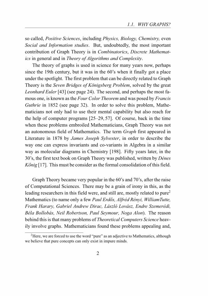
so called, Positive Sciences, including Physics, Biology, Chemistry, evenSocial and Information studies. But, undoubtedly, the most importantcontribution of Graph Theory is in Combinatorics, Discrete Mathemat-ics in general and in Theory of Algorithms and Complexity.
The theory of graphs is used in science for many years now, perhapssince the 19th century, but it was in the 60’s when it finally got a placeunder the spotlight. The first problem that can be directly related to GraphTheory is the Seven Bridges of Königsberg Problem, solved by the greatLeonhard Euler [43] (see page 24). The second, and perhaps the most fa-mous one, is known as the Four Color Theorem and was posed by FrancisGuthrie in 1852 (see page 32). In order to solve this problem, Mathe-maticians not only had to use their mental capability but also reach forthe help of computer programs [25–29, 57]. Of course, back in the timewhen these problems embroiled Mathematicians, Graph Theory was notan autonomous field of Mathematics. The term Graph first appeared inLiterature in 1878 by James Joseph Sylvester, in order to describe theway one can express invariants and co-variants in Algebra in a similarway as molecular diagrams in Chemistry [198]. Fifty years later, in the30’s, the first text book on Graph Theory was published, written by DénesKőnig [17]. This must be consider as the formal consolidation of this field.
Graph Theory became very popular in the 60’s and 70’s, after the raiseof Computational Sciences. There may be a grain of irony in this, as theleading researchers in this field were, and still are, mostly related to pure2
Mathematics (to name only a few Paul Erdős, Alfréd Rényi, WilliamTutte,Frank Harary, Gabriel Andrew Dirac, László Lovász, Endre Szemerédi,Béla Bollobás, Neil Robertson, Paul Seymour, Noga Alon). The reasonbehind this is that many problems of Theoretical Computers Science heav-ily involve graphs. Mathematicians found these problems appealing and,
2Here, we are forced to use the word “pure” as an adjective to Mathematics, althoughwe believe that pure concepts can only exist in impure minds.
2

CHAPTER 1. INTRODUCTION
thus, decided first to “communicate” and then to collaborate with com-puter scientists in order to tackle them.
Nowadays, scientists that do research in Graph Theory come frommany different disciplines of science. Some of the most common areMathematics, Computer Science, and Economics. This proved to be verybeneficial for the rapid development of Graph Theory, as techniques andideas from a variety of contexts can be put to the test in order to solve agreat deal of problems.
Of course, our point of view in this doctoral thesis will be the Mathe-matical one. To make it a little more precise, we study Graph Theory fromthe Combinatorial, Logical, and Algorithmic perspective.
This thesis studies a series of Graph-Width Parameters, defined usingVertex or Edge Layouts (see Chapter 4). As a starting point we will re-view one of the major breakthroughs in Graph Theory, namely the resultsin the Graph Minors series of papers ( [65–87]) (see Section 2.6). Oneof the most omnipresent concepts of this theory is the notion of an Ob-struction (or a minimal forbidden graph, see Section 2.4). Our main focusis the introduction and development of techniques for the characteriza-tion and the computation of Obstruction Sets for these layout parameters.This includes the study of Vertex Removal problems on width parameters(see Section 4.2.1) and the the detection of obstruction sets for variants ofGraph SearchingGames (Chapters 8 and 9), which are prominent versionsof graph layout parameters.
To conclude, the two main scopes of this thesis are:
- Graph Parameters (With emphasis to graph layout parameters andgraph searching numbers.)
- Obstruction Sets (Their finiteness and their computation.)
Starting from the next Section, we will – progressively – get into the par-ticulars.
3

1.2. THE BACKGROUND
1.2 The Background
A graph G is a pair of sets (V,E), where the second set contains two-subsets of the first. Therefore, the set E indicates the elements of V thatare “related” in some sense. This analogy immediately leads to a hugevariety of structures and notions that can be represented by graphs. Inthe early years of Graph Theory this was the main motivation to considergraphs. Researchers used them to capture the abstract essence behind acertain structure or notion, and find its abstract properties.
From the Mathematician’s point of view, Graph Theory is not nec-essarily “application driven”, meaning that we study the properties ofgraphs, graph parameters and graph classes without considering the struc-tures they may represent. Researchers in this field, no matter what theirbackground is, consider graphs as their main mathematical object and fo-cus on methods and technics introduced in the scope of this theory or,more generally, in the scope of other fields of Discrete Mathematics andAlgorithms.
In this thesis, we follow the above approach to Graph Theory. Theresults we present may apply in a variety of contexts, but our motivationis not their applications. We examine these results mainly due to theirtheoretical interest (and “beauty”).
Let us briefly present the basic – connected – components of this the-sis.
1.2.1 Graph parameters
From Chapter 4 and on, we study (mainly) graph parameters. A graphparameter is a function p returning for each graph a nonnegative number(see Definition 4.0.1). Graph parameters usually fall into two main cate-gories: (A) parameters that can be defined using layouts on graphs, i.e.,orderings of vertices or edges (Section 4.1, see also [22]), and (B) graph
4

CHAPTER 1. INTRODUCTION
modification parameters (Section 4.2).
(A) Layout parameters
The most famous layout parameter is undoubtedly treewidth (Section 4.1.1)(and of course pathwidth, see Section 4.1.2). First defined in [33], andhaving more than 7 equivalent definitions [20], treewidth is a central no-tion of Modern Graph Theory (some – of the many – surveys on treewidthare [16, 18–21, 23]). Treewidth belongs to the family of graph width pa-rameters which serve as measures of resemblance (topological or geo-metrical) of a graph to a particular graph family. For instance treewidth(denoted by tw) measures the degree in which a graph can be seen as atree, i.e., it has the topological structure of a tree, and pathwidth (denotedby pw) as a path. Treewidth and pathwidth can be thought of as measuresof the global connectivity of graphs. Another parameter in the same fam-ily is carving-width or cutwidth, cw (see Section 4.1.3 and Chapter 5), thatmeasures the global, edge-connectivity of a graph.
The second type of layout parameters that we examine in the context ofthis thesis is the Search Numbers of Search Game variations (Chapters 8,9). Graph Searching involves a team of mobil agents (usually thought ofas searchers, pursuers or even cops), that aims at capturing a set of escap-ing agents (usually thought of as fugitives or robbers) that hide in somekind of network, represented by a graph. There are many different vari-ations of this set-up, stemming from the different abilities or restrictionsthe two parts may have (see [95–98] for instance). The basic versions ofgraph searching (Fugitive search games to be more precise) we will focuson are Edge search, Node search, and Mixed search.
Given a search game variation, its search number is equal to the mini-mum number of “searchers” needed to guarantee the capture of the “fugi-tive” via a deterministic search strategy.
Graph searching has gained much attention in the last 30 years or so,
5

1.2. THE BACKGROUND
due to its enormous list of applications [95–98] . As many of the classicwidth parameters (treewidth, pathwidth, and linearwidth for instance) canalso be defined through some variant of graph searching (Section 8.4), itprovides us with an alternative – game theoretical – way to approach theproperties of these parameters.
(B) Graph Modification parameters
This is a more general family of parameters. A graph modification param-eter p measures the minimum number of times we have to apply an oper-ation on a graph in order to obtain a new graph that has a certain property(Definition 4.2.3). The most well studied such parameters are the mini-mum vertex cover (page 67), the minimum feedback vertex set (page 67)and the “planarity” parameter (page 67). All these parameters are vertex-deletion parameters. We can use as modification operations edge dele-tions, edge contractions (and all other operations defined in Section 2.3),or even additions of vertices or edges. Basically, we can use any set ofoperations that can modify the graph. A consequence of this variety of dif-ferent possibilities is that many interesting graph problems (minimizationproblems to be exact) emerge from these parameters.
In this thesis we focus on vertex deletion parameters because they en-compass the following subcategory:
“Distance” to some bounded parameter
These parameters are defined using a “host” parameter. Let p be a param-eter (it doesn’t matter if it is a layout or a modification parameter), andr a nonnegative integer. We can define a parameter measuring the mini-mum number of vertex deletions one have to make in a graph G, so as thevalue of p in the new graph will become at most r (Section 4.2.1 ). Theseparameters have the potential to mix the two aforementioned categories
6

CHAPTER 1. INTRODUCTION
together and create many interesting problems. Their study is one of the“collateral” targets of this thesis.
1.2.2 Partial ordering relations on graphs
Graph modification can also be used to define partial ordering relationson graphs. The most known are the subgraph relation, where a graph His a subgraph of G if it can be obtained after the removal of some edgesand/or vertices ofG, and the minor relation, whereH is a minor ofG, if itcan be obtained from a subgraph ofG after the contractions of some edges(Section 2.3). Two equally interesting relations are the (weak) immersionrelation where H is obtained form a subgraph of G after some edge lifts,and the contraction relation where H is obtained after the contraction ofsome edges of G (Section 2.3).
For any given graph class C and partial ordering relation ⪯, there aretwo very important questions emerging:
(A) Is C closed under ⪯ (or ⪯-closed), i.e., does it hold that for anygiven graph G ∈ C, for every graph H ⪯ G, H ∈ C?
(B) (If C is a infinite class) is C well-quasi ordered with respect of ⪯,i.e., for every infinite subset of C do there exist two graphs, say Hand G, such that H ⪯ G?
We are interested to know the answer to these questions for classescontaining graphs whose value of the parameter we examine is boundedby some positive integer. Let G be the class of all graphs and G[p, k] theclass of all graphs G such that p(G) ≤ k.
The first question is typically easy to be answered. The second isone of the most difficult questions in Graph Theory. For instance, theproof that G is well-quasi ordered under the minor relation, known as theRobertson–Seymour Theorem or the Graph Minors Theorem, took Neil
7

1.2. THE BACKGROUND
Robertson and Paul Seymour almost 30 years to be written, and extendsto 23 papers ([65–87], see also [64] ).
From the Graph minors series we also know that G is well-quasi or-dered under the (weak) immersion relation. Unfortunately, this is not truefor the other two relations, the subgraph and the contraction relations.
The importance of questions (A) and (B) above, is discussed in thenext Section.
1.2.3 Obstructions
Given a graph class C that is ⪯-closed, we denote by obs⪯(C) the set ofminimal graphs, with respect of ⪯, not belonging to C. This set is calledthe obstruction set of C with respect of ⪯ (Section 2.4). Observe that forany graphG for which there exists a graphO ∈ obs⪯(C), such thatO ⪯ G,we can immediately conclude that G /∈ C, as, if G were in C, then also Owould be in C. This set, in a sense can characterize C by forbidding somegraphs.
As G is well-quasi ordered under the minor (≤m) and the (weak) im-mersion (≤im) relation, this yields that the sets obs≤m(C) and obs≤im(C)will be finite for every minor or immersion-closed graph class C. Thus,we have a finite Forbidden graph characterization or Kuratowski char-acterization3 for these classes. This characterization is completely “inde-pendent” from every combinatorial, topological or geometrical propertiesC may have, and therefore, can be (almost4) trivially used to device algo-rithms that check whether a graph belongs to C or not. The only thing wehave to check is whether the graph contains some graph of the obstructionset as minor (or immersion).
3Named after Kazimierz Kuratowski who gave the first such characterization, i.e., theone characterizing planar graphs as those that do not contain K5 or K3,3 as topological-minors [51].
4We also need a minor checking (Theorem 2.6.2) and an immersion checking algo-rithm (Theorem 2.6.3).
8

CHAPTER 1. INTRODUCTION
The bad news are that the proof of the Robertson–Seymour Theorem,as well as its immersion counterpart, are not, and cannot be, constructive[88]. This roughly means that we know the obstruction sets are finitebut there is no way, using the Graph Minors, to design an algorithm thatfinds them. Unavoidable, we have to improvise for each and every graphclass, or to find massive classification technique in order to enlarge thecomputability horizon of this theory. The “central” target in this thesis isto contribute to this direction.
1.3 The Foreground
Here we study the existence of finite Kuratowski characterizations forclasses of graphs with bounded width parameters. As far as the minor orthe immersion relation is concerned, the question is not if such characteri-zation exists, but whether it can be computed, and which are the necessaryrequirements for this to happen.
We present the results in this thesis, starting with the minor orderingrelation. Then, we move on to the immersion and contraction relations.
1.3.1 Monotone kernels
Much work has been devoted to finding the necessary conditions for thecomputability of obstruction sets for the minor relation in the last decades[77,80,85–87,92,123,125]. In Chapter 7 we consider minor-closed graphparameters that meet two additional conditions:
- they are Protrusion decomposable, and
- they have Finite Integer Index (FII).
(We formally define this properties in Sections 7.1 and 7.2.)
9

1.3. THE FOREGROUND
One of the results presented in this thesis is that, when a minor-closedparameter p has these properties and its value drops by a constant factor ifwe do some local transformation to a graph, then the size of the graphs inobs≤m(G[p, k]) is linearly bounded by k. Moreover, when p is computableand the FII property is constructive (for more on this “delicate” issue seeSection 7.7), the set obs≤m(G[p, k]) becomes computable.
The central theorem of Chapter 7 can be stated as follows:
Theorem 7.3.1. For every graph parameter p that has FII, is computable,protrusion decomposable, and minor-closed, there is a constant cp and apolynomial algorithm that given a graph G, outputs a graph G′ such that
1. G′ ≤m G,
2. p(G′) = p(G), and
3. the size of G′ is at most cp · p(G).
Using this theorem we can draw some very interesting conclusionsabout the existence of linear kernels for Graph optimization problems.A kernelization algorithm for a parameterized graph problem5 – or, sim-ply, a kernel – is a polynomial-time algorithm that transforms every in-stance (G, k) of the problem to an equivalent one (G′, k′), where the sizeof G′ and the integer k′ depend exclusively on the parameter k (Defini-tion 3.3.1). Ideally this dependency is linear (and therefore we have alinear kernel). Theorem 7.3.1 proves the existence of linear kernels foroptimization graph problems where p is the function returning the “size”of the optimal solution of an instance (see Definition 7.4.1). Properties 1.and 2. of Theorem 7.3.1 give two additional properties to these kernels:
5A parameterized problem can be seen as a subset of Σ∗×N where we have instancesof the form (x, k), i.e., a word (an instance in the “classic” sense) and an integer k, whichis the parameter of the problem. In parameterized graph problems x encodes a graph.Section 3.2 contains all the details.
10

CHAPTER 1. INTRODUCTION
- They are minor monotone, i.e., G′ ≤m G.
- They are parameter invariant, i.e., k′ = k.
Such kernels present independent interest as, apart from their impli-cation to obstruction sets (Section 7.4.4), they can also accelerate knownapproximation schemes (Section 7.4.5). We will not present the conse-quences of the existence of such kernels here (we do so in Chapter 7), aswe do not want to overwhelm the reader with definitions right form theintroduction. Here we will only discuss the following result.
“Distance” to bounded parameter
Let as use as “host” the parameter p, and define the family of vertex re-moval parameters (p, r)-dist, r ∈ N, where, for very graph G = (V,E):
(p, r)-dist(G) = mink | ∃S ⊆ V such that |S| ≤ k and p(G \ S) ≤ r
(Definiton 4.2.4)
Combining the fact that theF-Covering minimization problems (Sec-tion 4.2.1 and SubSection 7.4.2) admit linear, minor monotone and param-eter invariant kernels, with properties of these problems recently proved[174,175], we can show that the obstructions of the set obs≤m(G[(p, r)-dist,k]), r, k ∈ N, that are H-topological-minor free6 for some graph H , canbe computed, when p is a minor-closed, computable parameter, such that
- for a non-connected graph the value of p is equal to the maximumvalue of its connected components (Definition 7.4.10), and
- its value in grids is not bounded (Definition 4.2.6).
6A graphG isH-topological-minor free ifH cannot be obtained fromG after a seriesof vertex and/or edge deletion and vertex dissolution.
11

1.3. THE FOREGROUND
(Theorem 7.4.3)
A large family of parameters having the properties needed for Theo-rem 7.4.3 described above, is the graph searching numbers. For exam-ple, let us examine the search numbers of the three aforementioned vari-ations: es for the Edge search, ns for the Node search, and ms for theMixed search. We prove that, for every r, k ∈ N, we can compute the ob-structions of the sets obs≤m(G[•, k)], where • ∈ (ns, r)-dist, (es, r)-dist,(ms, r)-dist, that are H-topological minor-free, for some graph H (Sec-tion 8.5.1).
1.3.2 Obstructions for unions of classes
As we said in the beginning of the previous section, obstructions for theminor relation have been extensively studied. A quite interesting resultis the fact that if we are given the obstruction sets for two minor-closedgraph classes, say C1 and C2 then we can compute the obstruction set forthe class C1 ∪ C2 [123, 125]. This implies that the constructibility of theGraph Minors Theory is “closed” with respect to the union operation.
In Chapter 6 we deal with the counterpart of this problem for the im-mersion relation. We build on the machinery introduced by Isolde Adler,Martin Grohe and Stephan Kreutzer in [123], for computing minor ob-struction sets, and prove the existence of an algorithm computing the im-mersion obstruction set of a graph class C with the following properties:
- C is immersion-closed (of course),
- it has an MSO-description7, and
- an upper bound on the treewidth of the subgraph-minimal graphscontaining obstructions of C is known.
7I.e., There exist a Monadic Second-Order logic formula ϕC such that G ∈ C if andonly if ϕC is true for G (Definition 2.7.5).
12

CHAPTER 1. INTRODUCTION
(Corollary 6.2.2)
Taking this last property into consideration, we prove that there existsa uniform upper bound on the treewidth of the subgraph-minimal graphsthat do not belong to the union of two immersion-closed graph classes,whose immersion obstruction sets are known (Lemma 6.3.3). This resultmakes use of an extension of the Unique Linkage Theorem of Kawara-bayashi and Wollan [89].
Combining this bound with the aforementioned algorithm, we can showthat the immersion obstruction set of the union of two graph classes canbe computed, provided that the two immersion obstruction sets are known(and given) to us.
1.3.3 d-cutwidth
Our motivation to look into cutwidth under the immersion relation prism,is the fact that it is not a minor-closed parameter (e.g., [22]).
We noticed that cutwidth can be seen as the “unidimensional” versionof a “multidimensional” parameter, called d-cutwidth (we denote it bycwd, where d stands for the dimension of the space we work on) (see Def-initions 5.1.1 and 5.1.2 and Theorem 5.1.1). 1-cutwidth (i.e., cutwidth) isdefined as the minimum over all possible vertex layouts, of the maximumcost a layout may have (Definition 4.1.6). The cost of a layout is definedas the number of edges crossing a cutting point in this layout (we will referto this point as the “cut”). In d-cutwidth we extend the notion of vertexlayouts, which can be seen as embeddings in a straight line segment, toembeddings in Rd (see Section 5.1). Moreover, we define the “cut” as theinterSection of hyperplanes of Rd with this embedding.
We have to postpone the formal definitions until Chapter 5, as theyprobably are out of the scope of this introduction as well. In Chapter 5we will prove some of the properties d-cutwith has (we gathered them inTheorem 5.4.1), and discuss the difficulties posed by the fact that embed-
13

1.3. THE FOREGROUND
dings in Rd contain points that may have some irrational coordinates (seeSection 5.3). Hence, the discretization of these embeddings is manda-tory if we want to examine the Computational Complexity of finding thed-cutwidth of a graph.
To conclude that, as we indeed proved, this parameter is immersion-closed, therefore the classes G[cwd, k], for every d, k ∈ N, admit a finiteforbidden immersions characterization. Yet, we do not have any idea ofdevising an algorithm producing these characterizations. Notice that ifwe find such an algorithm, then there is no need to discretize embeddingsto compute the d-cutwidth of a graph. A consequence of our results isthat checking whether the d-cutwidth of a graph is at most k can be done(non-constructively8) in linear time (Proposition 5.3.1).
1.3.4 Connected searching
The case where the question of the existence of finite Kuratowski charac-terization is meaningful is when we consider the contraction relation. Aswe already mentioned, G is not well-quasi ordered under the contractionrelation (an infinite anti-chain for this relation is depicted in Figure 2.5),which means that a contraction-closed graph class C may not (and typi-cally do not9) have a finite such characterization. Then...
Why should we ever bother trying to find obstruction sets ofcontraction-closed classes?
Let us get back to graph searching numbers. We are particularly in-terested in the Mixed search variant where the part of the graph that is
8As the computation of the immersion obstruction sets for cwd – in general – is notconstructive.
9Other than the contraction obstruction sets in [1,2] the only (non-trivial) example inliterature of finite such set is the set in [128], characterizing planar graphs. In [99, 132]we can see examples of infinite contraction obstruction sets.
14

CHAPTER 1. INTRODUCTION
restricted for the fugitive is connected (see Section 8.3). In this way,searchers can communicate safely with each other through this area andcoordinate their efforts. This variant, known as Connected search, hasrecently gained much attention [1, 2, 100, 107].
The search number of this game, is neither minor- nor immersion-closed, because the deletion of edges may “disconnect” the graph. In thiscase the connected search number of the new graph will be infinite. Inter-estingly enough, it is contraction-closed. This motivated us to investigatethe possibility of finding forbidden contractions characterizations for theclasses of graphs of bounded connected search numbers.
In Chapter 9 we prove that the set of forbidden contractions, char-acterizing the class C of graphs that can be searched using at most twosearchers10, using only connected search strategies, is finite and consistsof 177 graphs. Moreover, we managed to identify every graph in this set.We will describe these graphs, alongside with the restrictions they imposeon C. One of these restrictions is the direction the searchers must use totraverse the graph. We will show that this direction plays a very importantrole for the success of their search strategy towards capturing the fugitive.As a matter of fact, the majority of forbidden graphs in this set are thereto fix the course along an imaginary axis of the graph the searchers mustfollow to achieve their goal.
1.4 Some Remarks on the StructureIn Chapter 2 we introduce the main notations that concern anything fromsets, function and logic formulas to graphs. After this, we present thestory behind the Robertson–Seymour Theorem. This story starts with thefirst Kuratowski characterization, namely the chatarcterization of planar
10Two may be too little, but it seems really hard to extend our results for k ≥ 3. Thereason is that, even if we know that the obstruction set for some k ∈ N is indeed finite,this set would contain more than 22
Ω(k)
graphs (see Section 9.3).
15
1.4. SOME REMARKS ON THE STRUCTURE
graphs as the graphs that are K5 and K3,3 topological-minor free, and ac-companies Graph Theory ever since.
The problems we consider solving algorithmically in the context ofthis thesis belong to the class NP. In Chapter 3 we will look deeper intothe structural properties of the instances that such problems may have.This motivated the definition of multivariable measures of complexity.To be more precise, we investigate these problems from the Parameter-ized Complexity [139–143] point of view. In this complexity theory wedistinguish a structural measure of the input, other than its size. This mea-sure is called the parameter of the problem and, accordingly, the problemis a parameterized problem. The challenge is to design algorithms thattake into consideration that, in most practical cases, the parameter is small(much smaller than the size of the input) and thus we may tolerate somesuper-polynomial contribution of the parameter in the running time of thealgorithms. This parameterized viewpoint reveals a more accurate pictureon the complexity status of the problems.
In this chapter we also present the concept of Kernelization algorithmsand define graph optimization problems.
Chapter 4 consists of the definitions of the graph parameters we con-sider. As the searching numbers have independent interest, we chose notto give their definitions in this chapter, but present them in a separatechapter instead (see Chapter 8).
We also choose to do the same with d-cutwidth. We moved its defini-tion to Chapter 5, where we will have room to set the necessary notation,as well as to discuss its properties in detail.
The first11 computability result for obstruction sets we present, con-cerns the union of immersion-closed graph classes, where their respective
11To be precise, this will be the second such result. In Section 4.2.1, where we discussthe “distance” to bounded parameters, we present some preliminary and already knownresults.
16

CHAPTER 1. INTRODUCTION
obstruction sets are known. It is presented in Chapter 6. Although in theintroduction we chose to look first at obstruction sets for the minor re-lation, we feel it would be better to familiarize the reader of this thesiswith the question of computation of these sets, using the more instructiveproofs of Chapter 6, rather than the technical proofs of Chapter 7.
Chapter 7 may contain a wealth of notions and technics, but, on thedownside, it may be a little difficult to follow. We broke the proof ofTheorem 7.3.1 into small parts, and give some intuition whenever thiswas possible. Here, we will further discuss optimization problems andkernels.
The last two chapters of this thesis are devoted to Graph Searching.Chapter 8 starts with a short historical retrospection of graph searchinggames, more precisely Fugitive search games, and the definition of theirbasic variations. Then we present two important notions: Monotonicityand Connectivity, and discuss the connection between search numbers and– the already defined in Chapter 4 – layout parameters.
In Chapter 9 we present our work on connected graph searching. Again,the proofs presented here contain a lot of details and case analysis, butmuch effort has been made to guide the reader through this proof.
We close this – introductory – chapter by presenting a list of publica-tions that are (or are not) based on parts of this thesis. Then we get intobusiness!
17

1.5. THE PAPERS
1.5 The PapersThe part of our research presented in this thesis was published in the fol-lowing papers (chronologically ordered):
[4] Archontia C. Giannopoulou, Iosif Salem, and Dimitris Zoros,Effective Computation of Immersion Obstructions for Unions ofGraph Classes, Journal of Computer and System Sciences, Volume80, Issue 1, pp. 207–216, 2014.
This publication is based on parts of Chapters 2, 4, and 6.
[5] Archontia C. Giannopoulou, Iosif Salem, and Dimitris Zoros,Effective Computation of Immersion Obstructions for Unions ofGraph Classes, Scandinavian Workshop on Algorithm Theory(SWAT 2012), pp. 165-176, 2012.
This paper is a preliminary version of [4].
[1] Micah J Best, Arvind Gupta, Dimitrios M. Thilikos, andDimitris Zoros, Contraction Obstructions for Connected GraphSearching, Discrete Applied Mathematics, Volume 209, pp. 27–47,2016.
This publication is based on parts of Chapters 2, 8, and 9.
[2] Micah J Best, Arvind Gupta, Dimitrios M. Thilikos, andDimitris Zoros, Contraction Obstructions for Connected GraphSearching, 9th International Colloquium on Graph Theory and Com-binatorics (ICGT 2014), 2014.
This paper is a preliminary version of [1].
[6] Menelaos I. Karavelas, Spyridon Maniatis, Dimitrios M.Thilikos, and Dimitris Zoros, Geometric Extensions of Cutwidth
18

CHAPTER 1. INTRODUCTION
in any Dimension, 9th International Colloquium on Graph Theoryand Combinatorics (ICGT 2014), 2014.
This paper is based on parts of Chapters 2, 3, 4, and 5.
[3] Dimitris Chatzidimitriou, Dimitrios M. Thilikos, and DimitrisZoros,Parameter Invariant, Minor-monotoneKernels, UnpublishedManuscript, Submitted to: 12th International Symposium on Pa-rameterized and Exact Computation (IPEC 2017), 2017.
This paper is based on parts of Chapters 2, 3, 4, and 7.
1.6 Not Included in This Thesis
As the scope of this thesis contains mainly two notions, Obstruction Setsand Graph Layouts, the following paper seems to be out of scope. Never-theless, we should not avoid mentioning it.
[7] Dimitris Chatzidimitriou, Archontia C. Giannopoulou,Spyridon Maniatis, Clément Requilé, Dimitrios M. Thilikos,and Dimitris Zoros, Fixed Parameter Algorithms for CompletionProblems on PlanarGraphs, 41st International Symposium on Math-ematical Foundations of Computer Science (MFCS 2016), 2016.
There were two preliminary versions of this paper:
[8] Dimitris Chatzidimitriou, Archontia C. Giannopoulou,Spyridon Maniatis, Clément Requilé, Dimitrios M. Thilikos,and Dimitris Zoros, Fixed Parameter Algorithms for CompletionProblems on PlanarGraphs, Algorithmic Graph Theory on the Adri-atic Coast (AGTAC 2015), 2015.
19

1.6. NOT INCLUDED IN THIS THESIS
[9] Dimitris Chatzidimitriou, Archontia C. Giannopoulou,Clément Requilé, Dimitrios M. Thilikos, and Dimitris Zoros,AFixed Parameter Algorithm for Plane Subgraph Completion, 13thCologne-Twente Workshop on Graphs & Combinatorial Optimiza-tion (CTW 2015), 2015.
20

CHAPTER 2
BASIC DEFINITIONS
In this Chapter we will give the basic definitions and fix the notation weplan to use throughout this thesis. Although we are going to present thebasic notations in a casual way, we will not compromise the formalityneeded for this occasion. Before we get into graphs, we have to talk aboutsets and functions.
2.1 Sets And FunctionsWe use the logic symbols ∧,∨,¬,→,⇒,⇔,∈, \,∪ and ∩ in the standardway1, and, occasionally, use N for the set of natural numbers (N+ for theset of natural numbers), Z for the set of integers (Z+ for the set of positiveintegers) and R for the set of real numbers (R+ for the set of positive realnumbers).
To keep the notation as short as possible we will write [n] instead of1, . . . , n, n ∈ N.
1We may slightly deviate from the “standard” and write ∪F1, . . . , Fn and∩F1, . . . , Fn instead of F1 ∪ · · · ∪ Fn and F1 ∩ · · · ∩ Fn.
21

2.2. GRAPHS
Given a set S, we denote by 2S the set of all subsets of S and by(S2
)the set of all subsets of S with cardinality 2.
Given a function f : A→ B and a set S, we define f |S = (x, f(x)) |x ∈ S ∩ A and f \ S = (x, f(x)) | x ∈ A \ S. Moreover, we alwaysassume that a function σ : A→ B is also defined on 2A so that for S ⊆ A,σ(S) = σ(x) | x ∈ S. We denote by ∅ the empty set and by ∅ theempty function, i.e., ∅ : ∅ → ∅.
2.2 GraphsA graph is a pair G = (V,E) of sets where E consists of two-subsets ofV . The set V is the vertex set and the set E the edge set of G. We willrefer to the elements of these two sets as vertices and edges respectively.Throughout this thesis we will depict the vertices of a graph as black dots(in some cases we will use additional shapes to distinguish some specialvertices) and the edges as line segment (usually straight) connecting theirendpoints, i.e., the two elements of V that constitute the edge. Later,in Chapter 5, we will discuss about embeddings of graphs in Euclideanspaces and somehow justify why we chose this way to depict graphs.
Given a graph G, when we do not explicitly state the names of itsvertex and edge set, we will denote them as V (G) and E(G) respectively.The two basic “measures” of a graph is the number of vertices n(G) =
|V (G)| (we may sometimes use |G| instead, or just n when the contextmakes clear that it represents n(G)) and the number of edges m(G) =
|E(G)|. In the following Chapters we will see numerous other measuresof a graph, measuring – loosely speaking – its “width”.
If S ⊆ V (G) we call graph G[S] = (S,u, v ∈ E(G) | u, v ∈ S
)
the subgraph of G induced by S. Accordingly, given a set F ⊆ E(G) wecall graph G[F ] = (
∪e∈F e, F ) the subgraph of G induced by F and we
denote by V (F ) the set of vertices inG[F ]. We denote byG\S the graphG[V (G) \ S].
22

CHAPTER 2. BASIC DEFINITIONS
Let u ∈ V (G) be a vertex of a graph G. We adapt the standard no-tations for the (open) neighbourhood and the degree of u, that is the setof all vertices connected with u by an edge, denoted by NG(u), and thecardinality of this set, denoted by degG(u). Moreover, for S ⊆ V (G) wedefine NG(S) = ∪u∈SNG(u). The closed neighbourhood of S in G isNG[S] = S ∪NG(S). We also define ∂G(S) to be the set of all vertices ofS that are incident to edges not in G[S].
A path of length k ≥ 1 is a graph P = (V,E) where V = u0, u1, . . . ,uk and E = u0, u1, u1, u2, . . . , uk−1, uk. In this case we saythat u0 and uk are the ends of P or, in other words, that P connects u0and uk (we may refer to P as a (u0, uk)-path). All other vertices of P areinternal vertices.Two paths are edge-disjoint if they do not share commonedges and vertex-disjoint if they do not share common vertices.
A closed path, i.e., the graph C = (V,E) with V = u1, u2, . . . , ukand E = u1, u2, u2, u3, . . . , uk−1, uk, uk, u1, is also called acycle of length k ≥ 1.
A graph G is connected if for every two vertices u, v ∈ V (G), Gcontains a path connecting them.
IfG is not connected and V1, . . . , Vk are the maximal, under the subsetrelation, vertex sets that induce connected graphs, then we define G[Vi],1 ≤ i ≤ k, to be the connected components of G.
Let G be a graph with at least three vertices. G is 2-connected if forevery two vertices u, v ∈ V (G),G contains two paths with u and v as endsthat meet only at their ends (i.e., apart from u, v they are vertex-disjoint).
If G is not 2-connected, then the maximal vertex sets that induce 2-connected graphs are the 2-connected components, or blocks, of G.
A vertex of a graph is isolated if it has degree 0 and pendant if it hasdegree at most 1. Accordingly, an edge e is pendant if one of its endpointsis pendant. If both endpoints of e are pendant, then we say that e is anisolated edge.
Let u and v be two vertices ofG. The distance of u to v is the minimum
23
2.2. GRAPHS
length of a path in G, having u and v as ends.If a graph G does not contain a cycle, of any length, then it is called a
forest. In addition, if G is connected then it is called a tree.Let T be a tree. The leaves of T are its vertices that have degree at
most 1. The set of leafs of T is denoted by Leaf(T ).Given a tree T and two distinct vertices a, b of V (T ) we denote by aTb
the – unique – path in T connecting a and b.A clique of k ≥ 1 vertices, or k-clique, is the graphKk =
(u1, . . . , uk,
ui, uj | 1 ≤ i < j ≤ k)
. For two disjoint sets A,B, of cardinalityk, l respectively, we define the graph Kk,l = (A ∪ B,
u, v | u ∈
A and v ∈ B).
The line graph of a graphG, denoted byL(G), is the graph (E(G), X),where X = e1, e2 ⊆ E(G) | e1 ∩ e2 = ∅ ∧ e1 = e2.
Let F be a set of edges not sharing common endpoints with each other.If ∪e∈F e = V (G), then F is a perfect matching of the vertices of G.
Given two graphs G1 = (V1, E1) and G2 = (V2, E2) we define theirunion to be the graph G1 ∪ G2 = (V1 ∪ V2, E1 ∪ E2). When V1 andV2 are disjoint, we refer to this union as the disjoint union of G1 and G2
(we denote this fact by G1 + G2). The lexicographic product G1 × G2
is the graph with V (G1 × G2) = V (G1) × V (G2) and E(G1 × G2) =
(x, y), (x′, y′) | (x, x′ ∈ E(G1)) ∨ (x = x′ ∧ y, y′ ∈ E(G2)).Given a k ∈ N+, we define the (k× k)-grid as the graph Pk−1×Pk−1
and we denote it by ⊞k.Two graphs, say G and G′ are isomorphic if there exists a bijection
ϕ : V (G) → V (G′) such that u, v ∈ E(G) ⇔ ϕ(u), ϕ(v) ∈ E(G′)
for every u, v in V (G). In this case, function ϕ is an isomorphism.
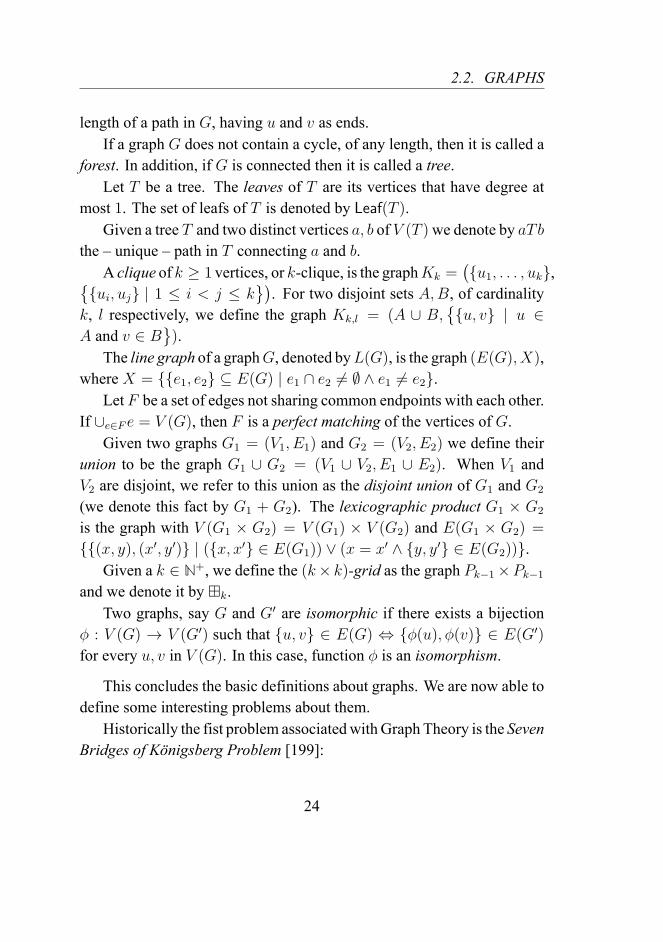
This concludes the basic definitions about graphs. We are now able todefine some interesting problems about them.
Historically the fist problem associated with Graph Theory is the SevenBridges of Königsberg Problem [199]:
24

CHAPTER 2. BASIC DEFINITIONS
Figure 2.1: The seven bridges of Königsberg.
Can all seven bridges of Königsberg (Figure 2.1) be traversedin a single trip without doubling back, with the additional re-quirement that the trip ends in the same place it began?
In terms of Graph Theory the question is whether the underlying graph(Figure 2.2), where bridges correspond to edges, has an Eulerian cycle. In1736 Leonhard Euler gave an answer to this problem, hence, we have thefirst Theorem of Graph Theory appearing in literature:
a
b
c
d
Figure 2.2: The graph formed from the seven bridges of Königsberg.
Theorem 2.2.1 (Euler, 1736 [43]). A connected graph has an euleriancycle if and only if every vertex has even degree.
25

2.3. CONTRACTIONS, MINORS AND IMMERSIONS
Königsberg has lost two of its seven bridges during World War II andlater, in 1945, was named Kaliningrad after Mikhail Kalinin (МихаилИванович Калинин)2. Sadly, World War II not only changed the nameof the problem, but also changed its solution, as – it may still not admit anEulerian cycle – it now admits an Eulerian path [194].
In the following Chapters we will discuss many more problems in thefield of Graph Theory, and see their solutions and the techniques involvedin them. Before we proceed in this endeavour we have to establish ournotation and get a glimpse of some central results.
2.3 Contractions, Minors and ImmersionsThere are many different operations locally transforming a graph to a newgraph, the most common of which are the following:
\u : The deletion of a vertex u ∈ V (G) tranforms G to graph G \ u =
(V (G) \ u, e ∈ E(G) | u /∈ e) (see Figure 2.3a).
\e : The deletion of an edge e ∈ E(G) transforms G to graph G \ e =
(V (G), E(G) \ e) (see Figure 2.3b).
/e : The edge contraction of e = u, v (or just the contraction of u, v)is the operation that deletes this edge, adds a new vertex xuv and
2But why Stalin named Königsberg, the birth place of the great Immanuel Kant, afterKalinin, a man with no real power or influence? According to Milan Kundera’s bookThe Festival of Insignificance [197] Kalinin had a bladder problem that forced him tourinate at very frequent intervals. Stalin, being aware of this fact, would intentionallyslow down his story telling. Out of respect, poor Kalinin would remain sitting during thewhole story, thereby intensifying his bladder problem. It was only when Kalinin wouldfinally give up, shaming himself in front of the other Congress members, that Stalinwould bring his anecdotes to a close. This undoubtedly proves Kalinin’s devotion to hisleader, who later acknowledging this fact named Königsberg after him. This story maynot seem legit but, at least to me, is very amusing. What make things even more particularis that Königsberg is still called Kaliningrad, but, for instance, Leningrad changed backto Saint Petersburg in 1991 and Stalingrad was named Volgograd in 1962.
26

CHAPTER 2. BASIC DEFINITIONS
x
(a) The deletion of x.
e
(b) The deletion of e.
u
vxuv
(c) The contraction of u, v to xuv.
x
y
ze
e1
e2x
y
z
(d) The lift of e1 and e2 to e.
connects this vertex to all the neighbours of u and v (if some mul-tiple edges are created we delete them). G/e is the graph obtained(see Figure 2.3c). Moreover, if an endpoint of e, say u, has degree2 then the contraction of e is also called dissolution of vertex u. Wedenote by G/u the graph obtained.
Lifts: The lift of two edges e1 = x, y and e2 = x, z to an edge eis the operation of removing e1 and e2 from G and then adding theedge e = y, z in the resulting graph. Notice that if y, zwasalready present in G, then this operation creates a multiple edgebetween y and z (this is the only exception throughout this thesiswhere multiple edges are allowed, see Figure 2.3d for an example).
Based on these operations we can define various relations on graphs(consequently, these relations can define partial orderings on graphs, someof which we discuss in the next Section). In a nutshell, let H and G betwo graphs, then:
• H is a subgraph of G if it can be obtained after a series of vertexand edge deletions on G. We denote it by H ≤ G.
27

2.3. CONTRACTIONS, MINORS AND IMMERSIONS
• H is a spanning subgraph of G if it can be obtained after a series ofedge deletions on G. We denote it by H ≤sp G.
• H is an induced subgraph of G if it can be obtained after a series ofvertex deletions on G. We denote it by H ≤in G.
• H is a contraction of G if it can be obtained after a series of edgecontractions on G. We denote it by H ≤c G.
• H is a topological-minor of G if it can be obtained after a series ofvertex deletions, edge deletions and vertex dissolutions on G. Wedenote it by H ≤tp G.
• H is a minor of G if it can be obtained after a series of vertex dele-tions, edge deletions and edge contractions on G. We denote it byH ≤m G.
• H is an (weak) immersion if it can be obtained from a subgraph ofG by lifting some edges3. We denote it by H ≤im G.
Although these definitions of minors, contractions and immersions arevery intuitive and, perhaps, easier to grasp, sometimes it is much moreconvenient to use the – more formal – definitions given in Section 6.2 ofChapter 6.
Definition 2.3.1. We say that a graphG isH-minor-free (H-topological-minor-free) if it does not contain H as a minor (topological-minor). Wealso say that a graph class C is H-minor-free (H-topological-minor-free)if all of its members are H-minor-free (H-topological-minor-free).
3In other words: If there is an injective mapping f : V (H) → V (G) such that, forevery edge u, v ∈ E(H) there is a path from f(u) to f(v) in G, and for any twodistinct edges of E(H) the corresponding paths in G are edge-disjoint. If, in addition,these paths are internally disjoint from f(V (H)), then H is a strong immersion of G.
28

CHAPTER 2. BASIC DEFINITIONS
· · ·C3 C4 C5
Figure 2.4: The set Ci | i ≥ 1 of all cycles is an infinite anti-chain for≤, ≤in.
2.4 WellQuasiOrderings andObstruction SetsIn the previous Section we defined six relations between graphs. These re-lations are quasi-orderings, in other words, reflexive and transitive. Someof them are called well-quasi-orderings, not according to someone’s pref-erences, but according to – loosely speaking – the extent in which they are“partial”. The following definition will make this make sense:
Definition 2.4.1. A quasi-ordering⪯ is awell-quasi-ordering on a setX(of graphs in our case) if and only if for every infinite sequence x0, x1, . . .in X there exist two elements, say xi and xj , such that xi ⪯ xj .
One can prove that a ⪯ is well-quasi-ordering on X if and only ifX contains neither an infinite anti-chain, i.e., an infinite set of elementsnot comparable under ⪯, nor an infinite sequence x0, x1, . . . such thatx0 ≻ x1 ≻ · · · (in other words an infinite strictly decreasing sequence).Using this proposition one can show that the class of all graphs, denotedby G, is not well-quasi-ordered under≤,≤in (Figure 2.4),≤c (Figure 2.5)and ≤tp (Figure 2.6).
Definition 2.4.2. Let C ⊆ G be a class of graphs and⪯ a quasi-orderingon graphs. C is ⪯-closed (or closed under taking of ⪯) if and only if forevery G ∈ C and H ∈ G, with H ⪯ G, it also holds that H ∈ C.
We will focus mainly on minor-closed, contraction-closed and im-mersion-closed graph classes. An example of a graph class closed under
29

2.4. WELL QUASI ORDERINGS AND OBSTRUCTION SETS
· · ·K2,1 K2,2 K2,3
Figure 2.5: The set K2,i | i ≥ 1 is an infinite anti-chain for ≤c.
· · ·
Figure 2.6: An antichain for ≤tp.
all these relations is the class of planar graphs that will be defined shortly(and redefined in Section 9.1.4 of Chapter 9).
Definition 2.4.3. Let C be a graph class closed under taking of ⪯. Wedenote by obs⪯(C) the set of all graphs in G \ C that are minimal withrespect to ⪯, and we call this set obstruction set (or just obstructions) forC under ⪯.
Some few words to make the name used for obs⪯(C) clear: Given agraph G, as C is ⪯-closed, if we can find a graph O ∈ obs⪯(C) suchthat O ⪯ G, this will verify that G /∈ C. Therefore, we can check if agraph belongs to C using the graphs of obs⪯(C). This test by no meansconstitutes an algorithm, as obs⪯(C) may be infinite (Example 2.4.1), sowe will have to make infinite many checks. Furthermore, even when thisset is finite, there may not exist a polynomial time algorithm checking iftwo graphs are related under ⪯, thus, this test will not be efficient.
Let us see some examples of obstraction sets.
Example 2.4.1. Let T be the graph class of all trees. As we saw before,a graph is a tree if and only if it does not contain a cycle as a subgraph
30
CHAPTER 2. BASIC DEFINITIONS
(or induced subgraph). Therefore, the obstruction set of T under ≤ (≤in
respectively) is the set Ci | i ≥ 1 of all cycles (see Figure 2.4), aninfinite set.
Example 2.4.2. The obstruction set of T under ≤m contains only thegraph C3. First observe that every graph in G \ T contains a cycle, sayC, as a minor. We can further contract the edges of C until we obtain C3.This is the minor minimal graph in G \ T because if we delete a vertex oran edge, or contract an edge, we will obtain a tree (a path of length 2 inthe first two cases and a path of length 1 in the last case).
2.5 Wagner’s (?) Conjecture
All the observations discussed in the previous Section would not be ofmuch use – in many respects – if it wasn’t for Graph Minors ( [65–87]),a much celebrated series of papers written by Neil Robertson and PaulSeymour. In this series, working towards proving Wagner’s Conjecture,the authors introduced many useful tools that eventually, forever changedGraph Theory and Combinatorics.
We start this Section by stating Wagner’s Conjecture:
Conjecture 2.5.1 (4Wagner, maybe in 1970 and perhaps in [93]). Theclass G of all graphs is well-quasi-ordered under the minors relation.
Notice that if G does not contain an infinite anti-chain, with respect of≤m, or an infinite strictly decreasing sequence, as this conjecture implies,then for every subclass C ⊆ G closed under taking of minors, the classG \ C would contain a finite number of minor-minimal graphs. Thus, thefollowing is a direct corollary of this conjecture:
4Now known as the the Robertson – Seymour Theorem (see Theorem 2.6.1).
31

2.5. WAGNER’S (?) CONJECTURE
Corollary 2.5.1. For every minor-closed graph class C the obstructionset obs≤m(C) is finite.
Actually, Claus Wagner insisted that he never made this conjecture! Ofcourse he was familiar with this problem and talk about it with his studentsback in the 60’s [13]. The main reason why we attribute this conjecture tohim is because Robertson and Seymour do so (in [84] they cited [93]).
The story starts in the 30’s, with Wagner’s PhD thesis, where he wastrying to prove the Four Color Theorem:
Given a map (formally defined as a separation of the planeinto regions) we can color all countries (the regions) so thatevery two adjacent countries have different colors, using atmost four colors.
To define this Theorem formally we need to introduce the notions ofplanar graphs and graph coloring.
Definition 2.5.1. A plane graph is a pair Γ = (V,E) of sets where:
1. V ⊆ R2,
2. every e ∈ E is an arc between two points of V ,
3. different arcs of E have different endpoints, and
4. the interior of an arc e ∈ E, i.e., the set consisted of every pointbelonging to e other than the two endpoints, does not contain a pointin V or a point of an other arc of E.
Notice that every plane graph Γ = (V,E) defines a (abstract) graph,denoted by G(Γ), by ignoring the position of the points in V and identi-fying the arcs of E by the set of their endpoints. For simplicity, we willrefer to the points of V as vertices and to the arcs of E as edges.
32

CHAPTER 2. BASIC DEFINITIONS
K5 K3,3
Figure 2.7: The two obstructions for planar graphs.
Definition 2.5.2. For every plane graph Γ = (V,E) we call the regionsof R2 \V ∪ (
∪e∈E e) faces of Γ and we denote this set by F (Γ). The only
unbounded face in F (Γ) is the outer face, hence the other faces are innerfaces.
Definition 2.5.3. An (abstract) graph G is planar if and only if thereexists a plane graph Γ such that G(Γ) is isomorphic to G.
Definition 2.5.4. A (proper) vertex coloring (or just coloring) of a graphG that uses k colors is a function f : V (G)→ [k] such that for every edgeu, v ∈ E(G), f(u) = f(v).
The formal definition of the Four Color Theorem is the following:
Theorem 2.5.1 (Four Color Theorem5). Every planar graph is 4-colorable.
Wagner’s approach was to try to completely bypass topology and givea combinatorial proof. He tried to classify the K5-minor free graphs andprove that they are 4-colorable. As the class ofK5-minor-free graphs con-tains all planar graphs (a consequence of Theorem 2.5.2), this would im-ply that all planar graphs are 4-colorable. Wagner’s efforts accumulatedto the following theorem that was proven in 1937 [94] and is – rightfully– bearing his name.
5First proven in 1976 by Kenneth Appel and Wolfgang Haken with the use of a com-puter [25–29].
33

2.5. WAGNER’S (?) CONJECTURE
Theorem 2.5.2 (Wagner, 1937 [94]). A graph G is planar if and only ifneitherK5 ≤m G nor K3,3 ≤m G (Figure 2.7).
Unfortunately for Wagner, this theorem succeed in characterizingK5-minor-free graphs but failed to take “planarity”, and Topology in general,out of the picture. Wagner’s “failure” had great consequences in the devel-opment of Graph Theory. First of all, it inspired Hardwiger’s Conjecture,still “one of the deepest unsolved problems in graph theory” [38]:
Conjecture 2.5.2 (Hardwiger, 1943 [45]). If all colorings of a graphGuse at least k colors, then Kk ≤m G.
It also inspired the notion of Tree-decompositions (Definition 4.1.3) acentral notion in modern Graph Theory, and fundamental for the proof ofRobertson–Seymour Theorem (Theorem 2.6.1).
Last but not least, consider the class of all planar graphs, say P . Itis straightforward to see that P is closed under minors. What Wagnerproved was that the obstruction set obs≤m(P) is finite and contains onlytwo graphs.
Notice that this is an extremely elegant way to define planar graphs:not only it is simple but also it is purely combinatoric. This definitionof a graph class through the set of its “forbidden graphs”, known as For-bidden graph characterization or Kuratowski characterization after Kaz-imierz Kuratowski6, can be considered as the first results in the field ofGraph Minors. It motivated researchers to find such characterizations forother graph classes, using the quasi-orderings defined previously. We willtalk more about this in the following Section.
6Kuratowski proved in 1930 a lighter version of Theorem 2.5.2 for topological mi-nors [51]. But, since this was the first forbidden graph characterization, such character-ization often bears Kuratowski’s name. Interestingly, the same result had been alreadyproven independently by the Soviet Mathematician Lev Semyonovich Pontryagin (ЛевСемёнович Понтрягин) around 1927. However, the proof of Pontryagin has never beenpublished. This recommends that the – somewhat more politically correct – way to namethis theorem is “Kuratowski-Pontryagin Theorem”.
34

CHAPTER 2. BASIC DEFINITIONS
2.6 Graph MinorsRobertson and Seymour published the proof of Wagner’s Conjecture in2004. It is known as Robertson–Seymour Theorem or Graph Minors The-orem.
Theorem 2.6.1 (Robertson–Seymour Theorem, 2004 [84]). The class Gof all graphs is well-quasi-ordered under the minor relation.
This theorem immediately guarantees that there exists a finite forbid-den minors characterization for every graph class, closed under taking ofminors. But, given a minor closed graph class C is it possible to find thischaracterization? In other words, assume that we are given a finite repre-sentation of C, can we compute obs≤m(C)? In this Section we will discusssome of the algorithmic implications of this theorem and try to give ananswer to this question. This will pave the way for the following chapteron Parameterized Complexity.
Before getting any further, we have to stress that we assume the readeris familiar with the notion of algorithm, the time complexity of algorithmsand the big O notation.
In this thesis we will heavily use “tools” from the Graph Minors “tool-set”, more specifically, we will use some structures and parameters de-fined in the Graph Minors series, alongside with some of their major re-sults. The first algorithmic result we will need was published in 1995 [77].Consider the following two problems:
H-Minor-ContainmentInput: A graph G.Question: Is H ≤m G?
C-MembershipInput: A graph G.Question: Is G ∈ C?
35

2.6. GRAPH MINORS
Theorem 2.6.2 (Robertson and Seymour, 1995 [77]). There exist an al-gorithm –with running timeO(n3) – deciding theH-Minor-Containment,where n = n(G).7
Combining Theorem 2.6.1 with Theorem 2.6.2 one can see that, if Cis a minor-closed graph class, the C-Membership problem has an O(n3)
algorithm, provided that obs≤m(C) is known (just run |obs≤m(C)|-timesthe algorithm for H-Minor-Containment problem, one for each H ∈obs≤m(C), and, if all answers are negative then G ∈ C, otherwise G /∈C). The only thing missing to have an affirmative answer to the questionposed in the beginning of this Section is an algorithm that will producethe obstruction set. Here is where things stop being so favourable for us:Theorem 2.6.1 is not – and cannot be – constructive [88]. To formallyexplain this, we have to dive deep into Logic and this – almost certainly –will take us off our track. Therefore, we will only say that, as the Axiomof Choice is used in the proof of the Graph Minors Theorem8 we cannotdraw an algorithm from it that, taking a minor closed graph class C asinput, will compute obs≤m(C). In [88] Friedman, Robertson and Seymourshowed that we cannot prove the Graph Minors Theorem without usingcertain variants of the axiom of choice, hence we will never find such analgorithm in general.
Although we do not know a – universally applicable – method to com-pute the obstruction sets, our research is by no means hopeless, as for somespecific graph classes this may be possible by applying ad hoc methods.
In Section 2.4 we saw that a “Graph Minors” type of theorem is notpossible for ≤,≤in and ≤c, as G is not well-quasi-ordered under theserelations. But what about the immersion relation?
Conjecture 2.6.1 (Weak Immersions Conjecture, Nash-Williams, 1963[91]). The class G of all graphs is well-quasi-ordered under the weak im-
7A reminder: We will occasionally use n instead of n(G) and m instead of m(G).8Actually Kruskal’s Tree Theorem is used, which in turn uses the Axiom of Choice.
36

CHAPTER 2. BASIC DEFINITIONS
mersion relation.
Conjecture 2.6.2 (Strong Immersions Conjecture, Nash-Williams, 1965[90]). The class G of all graphs is well-quasi-ordered under the strongimmersion relation.
Both these conjecture was made by Crispin St. John Alvah Nash-Williams in the sixties. The first one was resolved after 45 years in thelast paper of the Graph Minors series [87]. It is indeed true. For the sec-ond one, in [87] Robertson and Seymour remark that:
“It seemed to us at one time that we had a proof of the stronger[conjecture], but even if it was correct it was very much morecomplicated, and it is unlikely that we will write it down.”
Therefore, we reached the same conclusion as in the minor relation:
Corollary 2.6.1. For every immersion-closed graph class C the obstruc-tion set obs≤im(C) is finite.
One year after the publication of the proof of this conjecture, a cubictime algorithm was given by Grohe, Kawarabayashi, Marx, and Wollanfor the following problem:
H-Immersion-ContainmentInput: A graph G.Question: Is H ≤im G?
Theorem 2.6.3 (Grohe, Kawarabayashi, Marx, and Wollan, 2011 [179]).There exist an algorithm – with running time O(|G|3) – deciding the H-Immersion-Containment.
This theorem applies only for the weak immersions relation9 and is analmost direct corollary of the following.
9The authors of [179] conjecture that there exists such an algorithm for the strongimmersion relation as well. Yet, it still eludes us.
37

2.7. LOGIC
Theorem 2.6.4 (Grohe, Kawarabayashi, Marx, and Wollan, 2011 [179]).For every fixed graph H , there exist an algorithm – with running timeO(|G|3) – that decides if H is a topological-minor of G.
Thus, for an immersion-closed10 graph class C there exist aO(n3) timealgorithm deciding the C-Membership problem, under the condition thatobs≤im(C) is known.
Much effort has been made to find the necessary conditions to makethe computation of the forbidden minors, or forbidden immersions, possi-ble, for a variety of graph classes (a good start for those who want to learnmore about this are [52, 123, 125, 127, 192, 193]). In Chapter 6 we willargue that when C is immersion-closed, MSO expressible and an explicitbound on the treewidth of the≤-minimal graphs of G\C can be computed,there exists an algorithm computing obs≤im(C). There are still some thingsmissing before we are able to formally express this result. In the followingcouple of Chapters we plan to complete the definitions required to do it.
2.7 Logic
Let us recall some definitions from Monadic Second-Order Logic (MSO).An extended introduction to Logic can be found in [186, 188]11. We willtake a shortcut and immediately present the syntax of MSO of graphs.
2.7.1 Monadic Second-Order logic
Definition 2.7.1. We call signature τ = R1, . . . , Rn any finite set ofrelation symbols Ri of any (finite) arity denoted by ar(Ri).
10For now on, when we just say immersion we mean weak immersion.11It is highly advised for the reader to revise the basic notions of logic before getting
any further in this Section.
38

CHAPTER 2. BASIC DEFINITIONS
Definition 2.7.2. A τ -structureA = (A,RA1 , . . . , R
An) consists of a finite
universeA, and the interpretation of the relation symbolsRi of τ inA, thatis, for every i, RA
i is a subset of Aar(Ri).
The syntax of Monadic Second-Order logic of graphs includes the log-ical connectives ∨, ∧, ¬,↔,→, variables for vertices, edges, sets of ver-tices, and sets of edges, the quantifiers ∀, ∃ that can be applied to thesevariables, the signature τG = V,E, I where:
1. V has arity one and represents the set of vertices of a graph G,
2. E has arity one and represents the set of edges of G, and
3. I = (v, e) | v ∈ e and e ∈ E(G) the incidence relation,
and equality of variables. We denote the language of graphs by LG .
Definition 2.7.3. An MSO-formula is defined recursively from atomicformulas (i.e., expressions of the form Ri(x1, x2, . . . , xar(Ri)) or of theform x = y, where xj , j ≤ ar(Ri), x and y are variables) by using theBoolean connectives ¬,∧,∨,→, and existential (∃) or universal (∀) quan-tification over individual variables and sets of variables.
Notice that in LG the atomic formulas are of the form V (u), E(e),X(u), Y (e), and I(u, e), where u and e are vertex and edge variablesrespectively, X is a vertex-set variable, and Y is an edge-set variable.Furthermore, quantification takes place over vertex or edge variables orvertex-set or edge-set variables.
Definition 2.7.4. A graph structure G = (V (G) ∪ E(G), V G, EG, IG)
is a τG-structure, which represents the graph G = (V,E).
From now on, we will abuse the notation and treat G and G as if theywere the same structure.
39
2.7. LOGIC
Definition 2.7.5. A graph class C is MSO-definable if there exists anMSO-formula ϕC , in the language of graphs, such that
G ∈ C if and only if G |= ϕC,
i.e., ϕC is true in the graph structure G representing G (if this is the casewe will say that G is a model of ϕC).
To make this clear let us see an example (which we will later use inthe proofs of Lemma 6.2.2 and Observation 6.3.1):
Lemma 2.7.1. The class of graphs that contain a fixed graph H as animmersion is MSO-definable.
Proof. Let V (H) = v1, v2, . . . , vn and E(H) = e1, e2, . . . , em. Letalso ϕH be the following formula.
ϕH = ∃E1, E2, . . . , Em ∃x1, x2, . . . , xn[(∧i∈[n]
V (xi))
∧(∧j∈[m]
Ei ⊆ E(H))
∧(∧i =j
xi = xj) ∧ (∧p =q
Ep ∩ Eq = ∅)
∧(∧
er=vk,vl∈E(H)
path(xk, xl, Er))],
where path(x, y, Z) is the MSO-formula stating that:
“The edges in Z form a path from x to y.”
This can be done by saying that every vertex v incident to an edge in Z iseither incident to exactly two edges of Z or to exactly one edge, with thefurther condition that v = x or v = z (notice that these conditions also
40

CHAPTER 2. BASIC DEFINITIONS
imply the connectivity of the graph induced by the edges of Z). Thus,path(x, y, Z) can be expressed in MSO by the following formula:
path(x, y, Z) = [(x = y) ∧ ∃p, q(Z(p) ∧ Z(q) ∧ I(x, p) ∧ I(y, q)
∧∀p′ ∈ Z(I(x, p′)→ p = p′)
∧∀q′ ∈ Z(I(y, q′)→ q = q′))
∧∀w(V (w) ∧ w = x ∧ w = y
∧∃q1(Z(q1) ∧ I(w, q1))
→ ∃q2, q3(Z(q2) ∧ Z(q3) ∧ q2 = q3
∧I(w, q2) ∧ I(w, q3)))
∧∀p1, p2, p3(Z(p1) ∧ Z(p2) ∧ Z(p3)
∧∃m(V (m) ∧ I(u, p1) ∧ I(u, p2) ∧ I(u, p3))
→∨i=j
(pi = pj))]
It is easy to verify that ϕH is the desired formula.
2.7.2 Counting Monadic Second-Order logic
If, in addition to the features of Monadic Second-Order logic, we alsohave atomic formula “testing” whether the cardinality of a set is equal to qmodulo r, where q and r are integers such that 0 ≤ q < r and r ≥ 2, thenwe have an extension of MSO, called Counting Monadic Second-Orderlogic (CMSO).
More precisely, CMSO is MSO enriched with the following atomicformula for every set S:
41

2.7. LOGIC
cardq,r(S) = true if and only if |S| = q mod r
As far as “expressibility” is concerned, CMSO is more powerful thanMSO, as there exist graph properties that can be defined in CMSO but notin MSO [191].
Definition 2.7.6. A graph class C is CMSO-definable if there exists aCMSO-formula ϕC , in the language of graphs, such that G ∈ C if andonly if G |= ϕC .
We will see some examples of CMSO formulas in the following Sec-tion (Example 3.4.1 and 3.4.2). More information about CMSO (and MSOin general) can be found in [31, 190, 191] and of course [184].
42

CHAPTER 3
PARAMETERIZED COMPLEXITY
The meta-algorithmic result of the existence of a cubic time algorithmdeciding the C-membership problem for a minor-closed graph class C,broadened the perspectives towards the understanding of NP-hard prob-lems. It was actually at that point when it became clear that, with theintroduction of more variables when measuring the complexity of a prob-lem, there seems to be “different levels of hardness” between problems inNP [138]. To set a working hypothesis let us define two more problems.
A vertex cover of a graph G is a set S ⊆ V (G) such that for very edgeu, v ∈ E(G) either u ∈ S or v ∈ S.
k-Vertex CoverInput: A graph G.Question: Does G contain a vertex cover of size k?
Recall the definition of coloring (Definition 2.5.4).
43

3.1. CLASSIC COMPLEXITY THEORY
k-ColoringInput: A graph G.Question: Can G be colored using k colors?
Notice that, for the k-Vertex Cover problem, the class of graphsadmitting a vertex cover of size at most k is closed under taking of mi-nors. Therefore, for every fixed k there is a cubic time algorithm decidingwhether a graph has a vertex cover of size k (of course there exist way bet-ter algorithms for this problem, the algorithms in [161,162] for instance).However, no similar result can be expected for the k-Coloring problem,as it is known to be NP-hard for every fixed k ≥ 3 [187]. Hence, al-though both problems belong to NP, the k-Coloring problem seems tobe inherently more difficult than the k-Vertex Cover problem.
The observation of this gap in the time complexity of NP-hard prob-lems facilitated the development of Parameterized Complexity Theory[139–143] by Fellows and Downey [167, 168] , which has proven to be avery powerful theory and has majorly advanced during the past decades(see [24, 153, 154, 164, 165]).
Our starting point for this Chapter will be Classic Complexity Theory.
3.1 Classic Complexity Theory
Let Σ∗ be the set of all strings or words of a finite alphabet Σ. A classicproblem Π is a language over Σ, that is a set Π ⊆ Σ∗. The inputs orinstances of Π are the words of Σ∗. We call an input w ∈ Σ∗ Yes-instanceif w ∈ Π and No-instance if w /∈ Π.
As we are mainly interested in graph problems we will implicitly usea representation of graphs and a function mapping this representation towords of an alphabet. For instance, we can use a binary representation ofa graph. In this way we can think of graphs as being words in 0, 1∗ and
44

CHAPTER 3. PARAMETERIZED COMPLEXITY
problems as being subsets of G.To make the notation more intuitive, we will describe classic problems
less formally, following the way we have defined problems so far:
Π
Input: w ∈ Σ∗.Question: Is w ∈ Π?
Whenever we say that there exists an algorithm solving a problem Π,we mean that there exist a Turing machine that takes as input the input ofΠ and returns a “Yes” or “No” answer to the question of the problem.
The time complexity of an algorithm is the number of steps needed forthe corresponding Turing machine to finish its computation and output ananswer. To establish a measure of time complexity we count this num-ber of steps as a function of the size of the input word, i.e., the numberof its symbols. For a word w we will denote its size as |w|. In classicComplexity Theory we are interested in the worst-case analysis of thetime complexity of an algorithm. Therefore, we only focus on the timerequired for an algorithm to give us an answer in the worst possible input.
To express how well an algorithm performs, as far as time complexityis concerned, we will use the Big O notation.
As already mentioned, in this thesis we examine only graph problems.Therefore, it is more suited to measure the performance of an algorithmas a function of the size of the graph that was given to us as input. If nototherwise stated, the input size will be the number of vertices of the inputgraph.1
The biggest open question in classical Complexity Theory is whether1Of course one cannot ignore the fact that a graph may contain n vertices but in real-
ity needs approximately n2 symbols to be expressed in some data structure. Moreover,each different data structure has its own advantages and disadvantages when it comes tomanipulating a graph. We will avoid getting that deep in data structures as we are onlyinterested in how algorithms perform in a higher level.
45

3.2. FIXED PARAMETER TRACTABLE ALGORITHMS
P is equal to NP or not. P contains the problems that can be solved inpolynomial time, i.e., needing O(nc) time steps in order to be solved, forsome constant c. NP on the other hand, contains the problems that canbe “verified” in polynomial time, that is, if someone were to give us acertificate of a solution we could then run a polynomial time algorithmand compute the answer of the problem. Up to now, no-one knows theanswer, although the vast majority2 of computer scientists is convincedthat these sets are not equal and that there exist problems in NP that donot admit polynomial time algorithms (obviously P ⊆ NP).
There exist some problems in NP that are – in a sense – the most dif-ficult of all: If one of these problems were to admit a polynomial timealgorithm, then all problems in NP would also admit such an algorithm.These problems are called NP-hard. The NP-hard problems that belongto NP are called NP-complete problems.
Polynomial time algorithms are commonly fast and very useful forthe applications. Hence, when a problem is proven to be NP-completethis means that its almost certainly hard – at least all the great minds ofTheoretical Computer Science believe so – and no-one can find a feasiblesolution to it (see pages 2,3 of [187]). Researchers came to terms withthis fact and try hard to find other methods to tackle these problems. Aparadigm of a way to look the difficulty of an NP-complete problem in theeyes and try to find algorithms that will perform good despite not beingpolynomial, will be described in the following Section.
3.2 Fixed Parameter Tractable AlgorithmsThe framework of classical complexity theory has a drawback. In manyproblems, when measuring their difficulty only in terms of the input size,
2We stress here that the “vast majority vote” does not imply “truth” in mathematics(while this might be the case in other circumstances).
46

CHAPTER 3. PARAMETERIZED COMPLEXITY
we may overlook some structural properties of the input. Using thesestructural properties we could be able to design feasible algorithms. Thisbecomes clearer if we consider graph problems, and the fact that the “size”of a graph tells almost nothing about the properties of the graph. To backthis thought up, we are going to define a different way of measuring thecomplexity of a problem. First, we will distinguish a secondary measure-ment of the input that governs the computation complexity of the problem.Then, we will define the time complexity of an algorithm in a multivariateway, meaning that we will count the time steps needed for an algorithm tooutput a result as a function, not only of the size of the input, but also asa function of these measurements. The way these two variables are cor-related in the time complexity of an algorithm yields different complexityclasses.
Let us introduce some notation.
Definition 3.2.1. Let Σ be a finite alphabet. A polynomial time com-putable function3 κ : Σ∗ → N is a parameterization of Σ∗.
In this new theory we consider problems where we are given as inputa pair consisted of an input in the classic sense, a word, and the valueof the parameterization, an integer 4, and we are asked to decide whethersome property holds. These type of problems can be formally defined asfollows.
Definition 3.2.2. Let Σ be a finite alphabet. A parameterized problemover Σ consists of a classic problem Π ⊆ Σ∗ and a parameterization κof Σ∗. We will denote this problem as p-Π to indicate that this is theparameterized version of Π. The instances of p-Π are pairs of the form(w, κ(w)) ∈ Σ∗ × N.
3By that we mean that there exists a (known) Turing Machine that can compute theoutput of this function in polynomially-many steps (on the size of the input word).
4We will refer to this parametrization as the parameter of the problem.
47

3.2. FIXED PARAMETER TRACTABLE ALGORITHMS
Let p-Π be a parameterized problem. The Yes-instance of p-Π are thepairs (w, κ(w)) ∈ Σ∗ × N that belong to p-Π and the No-instance allother pairs, as usual. In what follows, if there is no particular reason tomention the function κ, we will denote an instance as (w, k), meaning thatk = κ(w).
We will measure the time complexity of a parameterized problem asa function of the input size and the value of the parameter. Similarly tothe case of Classic Complexity, we are interested only in the worst-caseanalysis of algorithms. To make the two parts of a parameterized problemclear, we will use the following representation:
p-ΠInput: (w, κ(w)) ∈ Σ∗ × N.Parameter: κ : Σ∗ → N.Question: Is (w, κ(w)) ∈ p-Π?
The idea behind measuring the complexity of a problem as a func-tion of the input size and the parameter, stems from the fact that in manyproblems where the parameter is small – a lot smaller than the size ofthe input – simple exponential algorithms (in the classic complexity setup) can perform exceptionally well. For instance, let us parametrize thek-Vertex Cover problem by the constant function k. The best known al-gorithm solving this problem runs in O(1.2738k + k · n) steps [161,162].For small values of k this is an extremely feasible algorithm.
If you are not still persuaded – and you mustn’t – think of the possibleways the parameter and the input size can be combined when measuringthe complexity of a problem. For running times such as O(f(k) · nc) oreven O(nf(k)), where f is just a computable function and c a constant, forevery single value of k, the parameter, we have a polynomial algorithm onn, the input size. The real “tough” problems in parametrized complexityhave running times such as O(kn), where even for constant k we get an
48

CHAPTER 3. PARAMETERIZED COMPLEXITY
exponential algorithm.
I think we had enough hand having so far (too much for my likings),so let us go through the definitions.
Definition 3.2.3. Let p-Π be a parametrized problem over Σ and κ :
Σ∗ → N its parameterization. An algorithmA is fixed parameter tractable,or an FPT-algorithm, if there exist a computable function f : N→ N anda polynomial p such that for every w ∈ Σ∗ the running time ofA on inputw is:
O(f(κ(w)) · p(|w|))
That is potentially exponential on the parameter but polynomial on thesize of the input.
Definition 3.2.4. A parametrized problem p-Π is fixed parameter tractableif it admits an FPT-algorithm deciding it.
For our convenience, we call such problems FPT-problems. To addmore to the overuse of FPT:
Definition 3.2.5. We define FPT to be the class of all FPT-problems.
To get a grasp on these definitions we need some examples. Let usreview Paragraph 2.6 and give parametrizations of the problems describedthere. First of all, we have to stress that
Minor-ContainmentInput: Two graphs H and G.Question: Is H ≤m G?
and
Immersion-ContainmentInput: Two graphs H and G.Question: Is H ≤im G?
49

3.2. FIXED PARAMETER TRACTABLE ALGORITHMS
are NP-complete problems5. We will give a parameterization of theseproblems by defining κ : G → N to be the number of vertices of H:6
p-Minor-ContainmentInput: Two graphs H and G.Parameter: n(H).Question: Is H ≤m G?
p-Immersion-ContainmentInput: Two graphs H and G.Parameter: n(H).Question: Is H ≤im G?
We saw that if C is a minor-closed (immersion-closed) graph class thenobs≤m(C) (obs≤im(C) respectively) is a finite set of graphs, a set that char-acterizes C. Let us focus first in the minor case and assume that the setobs≤m(C) = O1, . . . , O|obs≤m (C)| is known. Moreover let us look deeperin the algorithm of Theorem 2.6.2:
Theorem 3.2.1 (Robertson and Seymour, 1995 [77] ). There exist anO(f(k) · n3) algorithm deciding the p-Minor-Containment problem,where k = n(H).
The function f in the running time of this algorithm is a horrible, yetcomputable function. Therefore, this algorithm is not feasible, but, as wesaw before, it yields a cubic algorithm for the C-Membership problem
5This can be proven in the following way: Take for instance H to be a cycle withn(G) vertices. Then H ≤m G if and only if G contains a Hamiltonian cycle, thus theHamiltonian Cycle problem can be reduced to the Minor-Containment problem (formore informations check [187]). To prove that Minor-Containment ∈ NP take ascertificate the function ψ of Definition 6.2.2.
6Also we have two graphs as input, in essence two words. To be consistent with ourframework, we have to code these two words as one. Then we decode it to take the firstword in order to compute the parameter.
50

CHAPTER 3. PARAMETERIZED COMPLEXITY
with O(|obs≤m(C)| · f(k) ·n3) running time, where k = maxn(O) | O ∈obs≤m(C).
The same thing holds for the immersion case:
Theorem 3.2.2 (Grohe, Kawarabayashi, Marx, and Wollan, 2011 [179]).There exist anO(f(k)·n3) algorithm deciding the p-Immersion-Contain-ment problem.
Again, this algorithm was not meant to be used in real life applications,as f is rather cumbersome, but it is of great significance from a theoreticalpoint of view.
For the purposes of this thesis we will only concider parameterizedgraph problems:
Definition 3.2.6. A parameterized problem p-Π is a (parameterized)Graph problem if in every instance (w, k) ∈ Σ∗ × N, w encodes a graph.For simplicity we will denote the instances of such problems by (G, k) ∈G × N, where G is the graph encoded by the word of the input.
Every so often we have to focus on problems defined on graphs thathave specific properties (planar graphs for instance). Therefore, we mustdefine the restriction of a problem to a ceratin graph class.
Definition 3.2.7. Let C ⊆ G be a class of graphs. The restriction of aparameterized problem p-Π to C, is defined as
p-Π ⋒ C = (G, k) ∈ G × N | (G, k) ∈ p-Π and G ∈ C.
3.3 KernelizationIn this Section we will define the class FPT again, this time using kernels.To give you an idea of what we are about to present, Kernelization is a typeof pre-processing in the input, after which we have a reduced “equivalent”
51

3.3. KERNELIZATION
instance, the kernel. This kernel, as the name suggests, is the hard part ofthe input, i.e., the part that contains all the information needed to decideif this instance is a Yes-instance or a No-instance. The fact that the size ofthe kernel is reduced (usually it is bounded by a polynomial on the valueof the parameter) gives us the ability to solve the problem in FPT time.
Definition 3.3.1. Let p-Π be a parameterized problem over Σ and κ :
Σ∗ → N its parameterization. Let also g be a computable, increasing func-tion. We say that Π admits a kernel of size g if there exists a computablefunction (an algorithm if you prefer) K : Σ∗ → Σ∗, called kernelization(algorithm) for p-Π, or, in short, a kernelization, that given w ∈ Σ∗ out-puts, in time polynomial in |w|+ κ(w), a w′ ∈ Σ∗ such that
(a) w ∈ Π if and only if w′ ∈ Π , and
(b) max|w′|, κ(w′) ≤ g(κ(w)).
When g(k) = kO(1) or g(k) = O(k) then we say that p-Π admits apolynomial or linear kernel respectively.
We often abuse the notation and call the output of a kernelization al-gorithm, the “reduced” equivalent instance K(w), also a kernel.
The following Theorem shows that a decidable problem7 p-Π is FPTif and only p-Π admits a kernelization.
Theorem 3.3.1 (Theorem 1.39 of [142]). For every parameterized prob-lem p-Π, the following are equivalent:
1. p-Π ∈ FPT.
2. p-Π is decidable and admits a kernelization.7Π is decidable if there exist a Turing machine that for every input w ∈ Σ∗ stops and
returns Yes if w ∈ Π and No if w /∈ Π
52

CHAPTER 3. PARAMETERIZED COMPLEXITY
Kernelization has evolved to a prominent area of parameterized com-putation and initiated numerous techniques and methodologies, especiallyfor problems related to graphs [145, 147].
In Chapter 7 we will present a (meta-)theorem that proves the existenceof linear kernels for a large class of problems. In addition to being linear,these kernels have the two properties defined in Definition 3.3.2 and 3.3.3.These properties are important for our purposes as they make the computa-tion of obstruction sets possible, for graph classes defined form problemsadmitting such kernels. This is one of the extremely rare instances wherekernels yield obstruction sets (the only other examples are [169, 171]).
Definition 3.3.2. Let p-Π be a parameterized graph problem and ⪯ apartial ordering relation on graphs. We say that a kernelization algorithmfor p-Π is ⪯-monotone if, given an instance (G, k) it outputs an instance(G′, k′), where G′ ⪯ G.
When taking as ⪯ the minor relation (as we plan to do in Chapter 7),we define minor-monotone kernelization algorithms.
Definition 3.3.3. Let p-Π be a parameterized problem. We say that a ker-nelization algorithm for p-Π is parameter-invariant if, given an instance(w, k) it outputs an instance (w′, k′), where k = k′.
Being consistent with the aforementioned abuse of notation, we callthe corresponding kernels ⪯-monotone and parameter-invariant respec-tively.
3.4 Optimization Graph Problems and TheirProperties
The vast majority of problems we will consider in this thesis are Opti-mization problems, where we want to minimize or maximize a quantity.To formally define them we will need some definitions.
53

3.4. OPTIMIZATION GRAPH PROBLEMS AND THEIR PROPERTIES
Definition 3.4.1. An annotated graph is a pair (G,S)whereG is a graphand S ⊆ V (G).
Definition 3.4.2. A vertex subset certifying function f (or certifyingfunction for short) is a computable function which takes as input an anno-tated graph (G,S) and outputs true or false. We say that the function f isCMSO-definable if there is a CMSO-formula on annotated graphs ϕ suchthat f(G,S) = true if and only if (G,S) |= ϕ.
We can define in the same way edge subset certifying functions butwe will not. We will focus on vertex subset minimization or maximizationproblems.
Definition 3.4.3. A (vertex subset) minimization/maximization problemp-Π is a parameterized problem on graphs for which there exists a certi-fying function f such that for every (G, k) ∈ G × N it holds that
(G, k) ∈ p-Π ⇐⇒ ∃S ⊆ V (G) : |S| ≶ k and f(G,S) = true
where ≶ is interpreted as≤ for minimization problems and as≥ for max-imization problems. Such problems are also called optimization graphproblems (or just optimization problems, as we will only consider graphproblems).
When the certifying function f is CMSO-definable, we say that p-Π isa min-CMSO problem or a max-CMSO problem, depending on whetherp-Π is a minimization or a maximization problem. For simplicity, we willcall such problems CMSO-definable optimization problems.
Example 3.4.1. The aforementioned – but not formally defined – param-eterized version of k-Vertex Cover, where the parameter is k:
54

CHAPTER 3. PARAMETERIZED COMPLEXITY
p-Vertex CoverInput: A graph G and a k ∈ N .Parameter: k.Question: Does G contain a vertex cover of size ≤ k?
is a min-CMSO problemThis holds because p-Vertex Cover is a minimization problem, and
the function f that, given an instance (G, k), certifies whether a set S ⊆V (G) is a vertex cover of G of size at most k, can be defined in CMSO asfollows:
f(G,S) = [∀e∀u∀v(E(e) ∧ I(u, e) ∧ I(v, e)
→ S(u) ∨ S(v))]
∧ϕ≤k(S)
where
ϕ≤k(S) = card0,1(S) ∨ card0,2(S) ∨ · · · ∨ card0,k(S),
i.e., ϕ≤k(S) = true if and only if |S| ≤ k.
Example 3.4.2. An independent set of a graph G is a subset S ⊆ V (G)
where no two vertices u, v ∈ S are connected with an edge. Let us definethe following parameterized problem:
p-Independent SetInput: A graph G and a k ∈ N .Parameter: k.Question: Does G contain an independent set of size ≥ k?
p-Independent Set is a max-CMSO problem, as in this problem we want
55

3.4. OPTIMIZATION GRAPH PROBLEMS AND THEIR PROPERTIES
to maximize the size of an independent set, and the function f which,given an instance (G, k), certifies whether a set S ⊆ V (G) is an indepen-dent set of G of size at least k, can be defined in CMSO as follows:
f(G,S)=[∀u∀v(V (u) ∧ V (v) ∧ S(u) ∧ S(v)
→ ¬∃e(E(e) ∧ I(u, e) ∧ I(v, e)))]
∧ϕ≥k(S)
whereϕ≥k(S) = ¬ϕ≤k(S) ∨ card0,k(S),
i.e., ϕ≥k(S) = true if and only if |S| ≥ k.
We will discuss about optimization problems again in Section 7.4.1,where we will define some of their properties.
56

CHAPTER 4
GRAPH PARAMETERS
All results presented in Chapters 5 to 9 are directly related to some graphparameter and the classes containing the graphs where the value of thisparameter is bounded.
Definition 4.0.1. A graph parameter is a function p : G → N. Thedominion of p is the set of graphs where p is defined. We denote it bydom(p). We say that p is computable if there exists an algorithm thatgiven a graph G, either outputs that G ∈ dom(p) or outputs the value ofp(G).
Definition 4.0.2. Given a graph parameter p and an integer k ∈ Nwe define the graph class G[p, k] which contains all graphs G ∈ G thatp(G) ≤ k.
To keep the notation as simple as possible, instead of obs⪯(G[p, k]) wewill write obs⪯(p, k), where⪯ is a partial relation on graphs, p a parameterand k ∈ N.
Example 4.0.1. Let ∆ : G → N be the function where ∆(G) = maxdegG(u) | u ∈ V (G). This parameter is equal to the maximum degree
57

4.1. LAYOUT PARAMETERS
of the vertices of a graph. We can further define the graph class G[∆, k]that contains all graphs with maximum degree at most k.
Definition 4.0.3. Given a graph parameter p and a quasi-ordering re-lation ⪯ on graphs, we say that p is ⪯-closed if and only if G[p, k] is⪯-closed for every k ∈ N. In other words, for two graphs H,G whereH ⪯ G, it holds that p(H) ≤ p(G).
Example 4.0.2. ∆ is ≤,≤in and ≤im closed but not ≤c and ≤m closed.
Some very well known – and extensively studied – graph parametersare the minimum Vertex Cover, the maximum Independent Set, the Chro-matic Number, the minimum Feedback Vertex Set etc.
The vast majority of graph parameters fall too two categories: Thosewho can be defined using layouts and those that can be defined using mod-ifications of the graph. In this thesis we will focus mainly on graph lay-outs parameters, and a special case of graph modification parameters,which has the potential to blend these two categories together (see Para-graph 4.2.1).
4.1 Layout Parameters
In this Section we attempt to familiarize the reader with the most importantparameters of the first kind, i.e., those that can be defined using layoutsin graphs. A layout is an orderings of the vertices or the edges of thegraph. This type of parameters are also known as width parameters. Asthe name suggests, they are used to measure the “width” of a graph. Asabstract graphs are combinatorial and not geometrical structures, the term“width” is a little misleading. In Graph Theory the width of a graph usu-ally indicates the degree this graph “resembles” a certain family of graphs,trees or paths for instance.
58

CHAPTER 4. GRAPH PARAMETERS
One very interesting fact is that these “width” parameters are relatedto Graph Searching parameters, or Graph Search numbers. As a matterof fact, using graph searching games we can give an alternative – gametheoretic – definition of these parameters. The main reason why there issuch a connection is that both, “width” parameters and search numbers,are based on layouts.
Although our main focus is on layouts, for completion, we also givethe most commonly used definitions of these parameters. More often thannot, the mainstream definition is based on graph decompositions.
We start by making the term “layout” more precise.
Definition 4.1.1. A vertex (edge) layout of a graph G is a bijection σ :
V (G)→ [|V (G)|] (respectively σ : E(G)→ [|E(G)|]).
4.1.1 Treewidth
A central notion in modern Graph Theory is treewidth, a graph parame-ter which measures in what extent a graph has the topological structureof a tree ( [16, 18–21, 23]). The tree-structure is very useful to set-up dy-namic programming [35], a.k.a., the “sledgehammer” of the algorithmscraft [185]. In many cases, we can use this tree-structure to design poly-nomial algorithms for problems that are NP-complete in general graphs,i.e., graphs with unbounded treewidth [19]. Therefore, small treewidthmay be a basic ingredient for many important algorithmic results in GraphTheory.
There are several different definitions of this parameter, stemmingfrom a variety of graph-theoretical notions. For instance, in Theorem 1of [20] we can see 7 equivalent ways to define treewidth. In this thesis wewill see two of the definition in [20], and an additionally definition throughvertex layouts, namely the Tree Vertex Separation number [18,105]. In or-
59

4.1. LAYOUT PARAMETERS
der to define tree vertex separation number, we need to fix some notation.
We denote byLV(G) the set of all vertex layouts of a graphG. Given aσ ∈ LV(G), σ(u) = i is the position of u ∈ V (G) in σ and σi = σ−1(i) =
u. For two vertices u, v ∈ V (G), we write u <σ v if σ(u) < σ(v). Wealso define
σ<i = u ∈ V (G) | σ(u) < i
and, in a similar way, the sets σ≤i, σ>i and σ≥i.For every i ∈ [|V (G)|] we define the tree-supporting set of position i
as follows:
Stσ(i) = u ∈ V (G) | σ(u) < i and there exists a path with u, σi asends, whose internal vertices belong to σ>i
Each layout σ is assigned with some cost. We define:
costt(G, σ) = max|Stσ(i)| | i ∈ [|V (G)|]
Definition 4.1.2 (Dendris, Kirousis, and Thilikos, 1997 [105]). The treevertex separation number of a graphG is tvs(G) = mincostt(G, σ) | σ ∈LV(G).
The second definition of treewidth we will see is the “classic” defini-tion, given by Robertson and Seymour [67].
Definition 4.1.3. A tree-decomposition of a graph G is a pair (T,B),where T is a tree and B : V (T ) → 2V (G) is a function that maps everyvertex v ∈ V (T ) to a subset Bv of V (G) (we may refer to these sets asbags and to the vertices of T as nodes) such that:
(i) for every edge e of G there exists a vertex t in T such that e ⊆ Bt,
(ii) for every v ∈ V (G), if r, s ∈ V (T ) and v ∈ Br∩Bs, then for everyvertex t on the unique path between r and s in T , v ∈ Bt and
60

CHAPTER 4. GRAPH PARAMETERS
a
b
c d
e
f
g
h
i
T
a
b, c
a, cc, d
d, e
e, f
d, g
g, h
g, i(T,B)
Figure 4.1: A tree-decomposition of a tree.
(iii) ∪v∈V (T )Bv = V (G).
The width of a tree-decomposition (T,B) is
width(T,B) = max|Bv| − 1 | v ∈ V (T )
and the treewidth of a graphG, denoted by tw(G), is the minimum width(T,B), a tree-decomposition (T,B) of G can have.
Notice the−1 on the definition of width. As our intension for treewidthis to measure the degree a graph resembles a tree, it makes sense for a treeto have treewidth one. Given a tree T , see Figure 4.1 for instance, wecan define a tree-decompositions (T,B) of T (yes, we use T itself for thedecomposition) as shown in Figure 4.1. In order to satisfy property (i)of the definition above, the edges of E(T ) must be contained in the setsBu, u ∈ V (T ), therefore some of them must have at least two elements.Thus, we have to subtract one from the width of a decomposition in orderto achieve treewidth equal to one.
Example 4.1.1. An easy exercise is to prove that tw(⊞r) = r, for everyr ≥ 1.
Tree vertex separation number and treewidth measure the same thing,as the following theorem suggests.
61
4.1. LAYOUT PARAMETERS
Theorem 4.1.1 (Dendris, Kirousis, and Thilikos, 1997 [105]). Let G bea graph. Then tvs(G) = tw(G).
The G[tw, k]-Membership problem is well known to be NP-complete[30] but, if we parametrize it by k, as tw is closed under taking of minors,the Graph Minors provide us with an FPT-algorithm. This algorithm hasrunning time O(f(k) · n3), for a computable function f , which can beimproved, using results of the Graph Minors, to O(f(k) · n2) [77]. Theproblem is that, we know such an algorithm exists, as the obstruction setfor G[tw, k] is finite, but we do not know a way to compute this set.
Thankfully, we have a constructive, linear time FPT-algorithm [34,37]for the parametrized problem of checking whether the treewidth of a graphis at most the size of the parameter.
Theorem 4.1.2 (Bodlaender, 1996 [34]). Let G be a graph. There existan O(f(k) · n) algorithm for a computable function f , that decides iftw(G) ≤ k and if so, outputs a tree-decomposition of width at most k.
Let us see how the minor-obstruction sets for treewidth look like, fork ≤ 3. The first two are easy to see, the third is significantly more com-plicated [124, 134].
Observation 4.1.1.
1. obs≤m(tw, 1) = K3
2. obs≤m(tw, 2) = K4
3. obs≤m(tw, 3) = K5, K2,2,2,W8, K2 × C5 (see Figure 4.2)
We close this paragraph with a trivial observation, which we will uselater in this thesis.
Observation 4.1.2. IfG is a graph and S = v ∈ V (G) | degG(v) = 0then tw(G) = tw(G \ S).
62
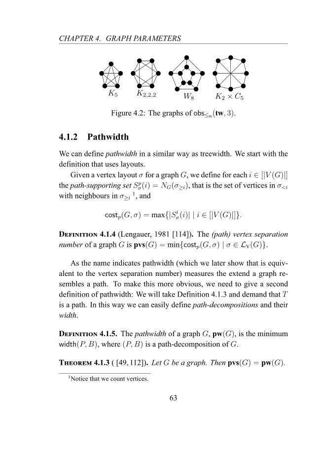
CHAPTER 4. GRAPH PARAMETERS
K5 K2,2,2 W8 K2 × C5
Figure 4.2: The graphs of obs≤m(tw, 3).
4.1.2 Pathwidth
We can define pathwidth in a similar way as treewidth. We start with thedefinition that uses layouts.
Given a vertex layout σ for a graphG, we define for each i ∈ [|V (G)|]the path-supporting set Spσ(i) = NG(σ≥i), that is the set of vertices in σ<iwith neighbours in σ≥i 1, and
costp(G, σ) = max|Stσ(i)| | i ∈ [|V (G)|].
Definition 4.1.4 (Lengauer, 1981 [114]). The (path) vertex separationnumber of a graph G is pvs(G) = mincostp(G, σ) | σ ∈ LV(G).
As the name indicates pathwidth (which we later show that is equiv-alent to the vertex separation number) measures the extend a graph re-sembles a path. To make this more obvious, we need to give a seconddefinition of pathwidth: We will take Definition 4.1.3 and demand that Tis a path. In this way we can easily define path-decompositions and theirwidth.
Definition 4.1.5. The pathwidth of a graph G, pw(G), is the minimumwidth(P,B), where (P,B) is a path-decomposition of G.
Theorem 4.1.3 ( [49, 112]). Let G be a graph. Then pvs(G) = pw(G).
1Notice that we count vertices.
63

4.1. LAYOUT PARAMETERS
The definition of pathwidth was introduced in the Graph Minors se-ries [65] and has several equivalent definitions (e.g., Theorem 2 of [20]).In Chapter 8 we define a search game, namely node search, with searchnumber equivalent to pathwidth plus one.
The G[pw, k]-Membership problem is NP-complete [30, 48, 53, 56],but when parametrized with k, it admits a linear FPT-algorithm [34, 37](basically it is the algorithm for treewidth).
We also must mention that pathwidth is a minor closed parameter. Wepresent the obstruction sets for obs≤m(pw, k), k ≤ 2, in Chapter 8 (seeExample 8.5.1, Theorem 8.5.4), using the node search number.
4.1.3 Cutwidth
Cutwidth, as treewidth and pathwidth, is a min-max parameter. It mea-sures the minimum, over all vertex layouts, of the maximum number ofedges between any prefix of a layout and its complement suffix. It is alsoclosely related to the vertex separation number. Let us see why:
Definition 4.1.6. Given a vertex layout σ of a graph G, the cut at posi-tion i, denoted by ∂G(σ, i), is the set of crossover edges of G having oneendpoint in σ≤i and one in σ>i2. The width of σ is equal to
costc(G, σ) = max|∂G(σ, i)| | i ∈ [|V (G)|]
and the cutwidth of G is cw(G) = mincostc(G, σ) | σ ∈ LV(G).
Example 4.1.2. See Figure 5.1. The vertex layout σ : a, b, c, d → [4]
with σ(a) = 1, σ(b) = 2, σ(c) = 3, and σ(d) = 4 of the graph G depictedhere has costc(G, σ) = 3.
The next observation follows immediately from the definitions.2Now, we count edges.
64

CHAPTER 4. GRAPH PARAMETERS
Observation 4.1.3. If G is a graph then cw(G) ≥ pw(G).
The G[cw, k]-Membership is an NP-complete problem known in liter-ature as the Minimum Cut Linear Arrangement problem [187]. Fromthe parameterized complexity point of view, the same problem is fixedparameter tractable, as an algorithm that checks whether cw(G) ≤ k inf(k) · n steps was given in [59]. Cutwidth has been extensively studiedboth from its combinatorial (see [39, 50, 126]) as well as its algorithmicpoint of view [40, 55, 58, 62].
Notice that a vertex layout is – in essence – a mono-dimensional lineararrangement of the vertices of a graph G. In Chapter 5 we will see howwe can arrange the vertices of G in Euclidean spaces of any dimension,and the way to define the “cut” in these spaces. This will lead to a naturaldefinition of a multi-dimensional geometric extension of cutwidth, the d-cutwidth. In Theorem 5.2.3 we will prove that this extension, and, as aconsequence, cutwidth as well, is an immersion-closed parameter.
4.1.4 Linearwidth
The last layout parameter we define in this Chapter is linearwidth. Wedefine some more in Chapter 8, namely the search numbers of searchgames and, then, one more in Chapter 9, which measures the minimumcost of an expansion (see Definitions 9.1.8 and 9.1.11).
Linearwidth uses edge layouts, therefore, before we give the defini-tion, we need to review our notation and rewrite it using edges instead ofvertices.
We denote by LE(G) the set of all edge layouts of a graph G. Given aσ ∈ LE(G), σ(e) = i is the position of e ∈ E(G) in σ and σi = σ−1(i) =
e. For e1, e2 ∈ E(G) we will write e1 <σ e2 if σ(e1) < σ(e2). Finally,we define
σ<i = ∪e∈E(G)|σ(e)<ie
65

4.2. GRAPH MODIFICATION PARAMETERS
and accordingly the sets σ≤i, σ>i, σ≥i. Notice that these are vertex sets.
Definition 4.1.7. LetG be a graph and σ an edge layout of it. We definefor every i ∈ [|E(G)|] the line-supporting set Slσ(i) = σ≤i ∩ σ i, and
costl(G, σ) = max|Slσ(i)| | i ∈ [|E(G)|].
The linearwidth of a graph G is lw(G) = mincostp(G, σ) | σ ∈ LE(G)(if |E(G)| = 1, then lw(G) = 0).
Linearwidth was introduced by Thomas in 1996 [61] and is closely re-lated to the notion of crusades, a way to describe mixed search, introducedby Bienstock and Seymour in [102,120]. The G[lw, k]-Membership prob-lem was proven to be NP-complete [120] and, in the Parameterized Com-plexity point of view, when parametrized by k, this problem admits a lin-ear time FPTalgorithm. This algorithm appeared in [103] and is construc-tive: For any k it can construct an optimal edge arrangement with cost atmost k, if one exists.
Linearwidth is also a minor closed parameter [120]. The only obstruc-tion sets known for the graph class G[lw, k] are for k = 1, 2. For k = 1 itconsists of K3 and the tree of Figure 8.1. For k = 2, its size is 52 and isgiven in the following theorem.
Theorem 4.1.4 (Thilikos, 2000 [120]). The obstruction set obs≤m (lw, 2)consists of the 52 graphs shown in Figure A.1 (i.e., the first figure of theappendix).
4.2 Graph Modification Parameters
We start with two definitions.
Definition 4.2.1. A graph property P is a subset P of G.
66

CHAPTER 4. GRAPH PARAMETERS
Definition 4.2.2. A graph modification operation is any operation thatmodifies a graph G to a graph G′.
These definitions are as general as a definition may possible be. Def-inition 4.2.2 for instance, includes not only the local transformations wesaw in Section 2.3, but also includes the operations of adding edges orvertices to a graph: The subdivision of a graph G, where we exchangesome edges of G with paths, is a graph modification operation.
Definition 4.2.3. A parameter p is a graph modification parameter (orsimply a modification parameter) if there exists a property P ⊆ G and aset of modification operations M , such that, for every graph G, p(G) isequal to the minimum number of times we have to apply an operation ofM to G, in order to obtain a graph in P .
Example 4.2.1. Let P be the property of “not having any edge”, i.e.,P = G = (V,E) | E = ∅, and let M contain only the vertex deletion.Then, we can define the parameter vc which is equal to the minimum sizea vertex cover of a graph may have.
Example 4.2.2. Let P be the property of “not having any cycles”, i.e.,P = G | G is a forest, and let M contain only the vertex deletion.Then, we can define the parameter fv which is equal to the minimum sizea feedback vertex set3 of a graph may have.
Example 4.2.3. Let P be the property of “being planar”, i.e., P = G |G is planar, and let M contain only the edge deletion. Then, we can de-fine the “planarity” parameter pl which is equal to the minimum numberof edges we have to delete from a graph in order to make it planar.
The first two parameters we saw in these examples, belong to a subcat-egory of modification parameters, the vertex-deletion parameters. Moreexamples of this category are presented in the following Section.
3A feedback vertex set of a graph is a set of vertices whose removal leaves a graphwithout cycles.
67

4.2. GRAPH MODIFICATION PARAMETERS
The modification parameters lead naturally to minimazation problems,known in literature as Graph Modification problems (see [144, 146, 148]for some surveys). Let p be a modification parameter we can define thefollowing problem:
k-p-ModificationInput: A graph G .Question: Is p(G) ≤ k ?
and its parameterized version:
p-p-ModificationInput: A graph G and a k ∈ N .Parameter: k.Question: Is p(G) ≤ k ?
An example is the p-Vertex Cover:
p-Vertex CoverInput: A graph G and a k ∈ N .Parameter: k.Question: Is vc(G) ≤ k?
4.2.1 Parameters defined from parameters
We will now define graph modification parameters – vertex deletion pa-rameters to be precise – that are defined using a “host” parameter. Thishost parameter may well be a layout parameter (as in the case of Chap-ter 8).
Definition 4.2.4. Let p be a graph parameter and r ∈ N. We define the
68
CHAPTER 4. GRAPH PARAMETERS
function (p, r)-dist : G → N, such that
(p, r)-dist(G) = mink | ∃S ⊆ V (G) such that |S| ≤ k and p(G\S) ≤ r.
Notice that this function is also a graph parameter. It measures thenumber of vertices we have to delete from a graph in order for the valueof p to drop down to r or less. Therefore, if we consider the propertyPr = G | p(G) ≤ r, we can see that (p, r)-dist is a modificationparameter. Later in this thesis we will refer to these parameters as distanceto p parameters.
Example 4.2.4. Every cycle C has (tw, 1)-dist(C) = 1.
Definition 4.2.5. Given a graph parameter p and two integers r, k ∈ N.We define the graph class G[(p, r)-dist, k] that contains all graphs G ∈ Gfor which there exists a set S ⊆ V (G) of at most k vertices, such thatp(G \ S) ≤ r.
We also define the following parameterized problem:
(p, r)-DistanceInput: A graph G and a k ∈ N .Parameter: k.Question: Is (p, r)-dist(G) ≤ k?
The following is an immediate consequence of the definitions.
Observation 4.2.1. Let p be a minor closed parameter. Then for everyr ∈ N, (p, r)-dist is also a minor closed parameter.
According to this observation we can include the (p, r)-Distance prob-lem in the following more general category of problems:
69

4.2. GRAPH MODIFICATION PARAMETERS
F-Covering 4
Input: A graph G and a k ∈ N .Parameter: k.Question: Does there exist S ⊆ V (G) such that |S| ≤ k and G \S
contains no graph from F as a minor?
where F is a finite set of graphs.
Notice first that, given a minor closed parameter p and a positive inte-ger r, the set obs≤m(p, r) is finite (this of course, is due to Theorem 2.6.1).Take asF in theF-Covering problem the set obs≤m(p, r) and observe thatthe (p, r)-Distance problem is, in this case, equivalent to the obs≤m(p, r)-Covering problem. Therefore the following holds.
Observation 4.2.2. If p is minor closed parameter, then for every r ∈ Nthe (p, r)-Distance problem is the obs≤m(p, r)-Covering problem.
Definition 4.2.6. Let p be a parameter. We say that p is big in grids ifp(⊞r)→∞, when r →∞.
Lemma 4.2.1. Let p be a minor closed parameter that is big in grids. Thenfor every r ∈ N, obs≤m(p, r) contains a planar graph.
Proof. Notice that, as p is big in grids, there exists a c ∈ N such thatp(⊞c) > r. Thus, there exist an obstruction O ∈ obs≤m(p, r) such thatO ≤m ⊞c, and, consequently, O is planar.
Definition 4.2.7. For a finite set of graphs F , we denote by GF ,k theclass of graphs containing all graphs G for which there exists a subsetS ⊆ V (G), of size at most k, such that G \ S contains no graph from Fas a minor.
The following proposition bounds the size of the graphs in the obstruc-tion set for GF ,k.
4These problems are also known as F-Deletion.
70

CHAPTER 4. GRAPH PARAMETERS
Proposition 4.2.1 (Theorem 3 in [171, 172]). Let k ∈ N. For everyfinite set F ⊆ G, such that F contains at least one planar graph, everygraph in obs≤m(GF ,k) has size polynomial in k.
Using Proposition 4.2.1 we can bound the size of the graphs in obs≤m
((p, r)-dist, k).
Theorem 4.2.1. Let r, k ∈ N and let p be a minor closed parameterthat is big in grids. Then every graph in obs≤m((p, r)-dist, k) has sizepolynomial in k.
Proof. We will prove that for every r ∈ N, obs≤m(p, r) satisfies the prop-erties of Proposition 4.2.1. As p is minor closed, from Theorem 2.6.1, weknow that obs≤m(p, r) is finite. From Lemma 4.2.1 it holds that obs≤m(p, r)contains a planar graph. From Proposition 4.2.1, taking F = obs≤m(p, r),we conclude that every graph in obs≤m(GF ,k) has polynomial size in k.The claim holds as obs≤m(GF ,k) = obs≤m((p, r)-dist, k).
Observation 4.2.3. Notice that Theorem 4.2.1 would also be true if, in-stead of asking that p is big in grids, we demand that for every r ∈ N,obs≤m(p, r) contains at least one planar graph.
Proposition 4.2.2. Letp be a computable parameter as in Theorem 4.2.1.If additionally this polynomial bound on the size of the graphs in obs≤m
((p, r)-dist, k), for some k ∈ N, is known, then obs≤m((p, r)-dist, k) canbe computed.
Indeed, let g be that polynomial. We can check for every graph Gof size at most g(k) whether (p, r)-dist(G) > k (notice that since p iscomputable, (p, r)-dist is also computable) and whether for every properminor G′ of G, (p, r)-dist(G′) ≤ k. In this way we can compute obs≤m
((p, r)-dist, k).
71

4.2. GRAPH MODIFICATION PARAMETERS
72

CHAPTER 5
D-DIMENSIONAL CUTWIDTH
Let us reconsider the definition of cutwidth and give a rough picture ofwhat we are going to see in this Chapter. We can imagine that vertexlayouts are “embeddings” of a graph in a straight line, in the followingway: We assign to each vertex a unique point and each edge is given a linesegment with ends the points assign to its endpoints (these line segmentsmay contain more points assigned to vertices than their two ends)1. If we“cut” this line in some point not assigned to vertices, for instance point 1in Figure 5.1, and count the line segments assigned to edges that containthis point, we can simulate the cut at a position of Definition 4.1.6. Tomake this clear, let us look closer at Figure 5.1. The embedding depictedcorresponds to the vertex layout σ : a, b, c, d → [4] with σ(a) = 1,σ(b) = 2, σ(c) = 3, and σ(d) = 4 and the “cut” at the point 1 of the linecorresponds to the cut at position 2.
This observation give us the motivation to consider embeddings inspaces of higher dimensions, generalizing in this way the notion of cutwidth.
1We will postpone the details for a while, because we need to set the framework first.However, we feel that it will be helpful for the reader to follow this train of thought.
73

5.1. GRAPH EMBEDDINGS
−1 0 1, 5 3
a b c d
a
b
c
d
1
Figure 5.1: A graph and its “embedding” in a straight line (for displaypurposes we replace the line segments of edges with arcs).
In this Chapter we will introduce a multi-dimensional geometric ex-tension of cutwidth, namely the d-dimensional cutwidth (or, simply, d-cutwidth) that – roughly – instead of mono-dimensional linear arrange-ments of a graph G, considers embeddings of G in the d-dimensional Eu-clidean space Rd. We will define the d-cutwidth of such an embeddingto be the maximum number of edges that can be intersected by a hyper-plane of Rd. Then, the d-cutwidth of G, denoted by cwd(G), will be theminimum d-cutwidth over all such embeddings.
5.1 Graph Embeddings
We start with some definitions. To keep it short, we assume that the readeris familiar with the basic notions of Real Analysis and Analytic Geometry.
Definition 5.1.1. Every (d− 1)-dimensional subspace Π of a d-dimen-sional space X is a hyperplane of X .
Here, we are interested in hyperplanes of Rd (subspaces isomorphic toRd−1). Let Π be a hyperplane in Rd, then there are a0, a1, . . . , ad ∈ R such
74

CHAPTER 5. D-DIMENSIONAL CUTWIDTH
that Π = (x1, . . . , xd) ∈ Rd | a1x1 + · · · + adxd + a0 = 0. We denoteby H(d) the set of all hyperplanes of Rd.
Definition 5.1.2. A hypersphere, S(c, r), with center c and radius r inRd is the set (x1, . . . , xd) ∈ Rd |
∑di=1(xi − ci)2 = r2.
We denote by S(d) the set of all hyperspheres of Rd.
Definition 5.1.3. A continuous function C : [0, 1] → Rd is a curve ofRd with ends C(0) and C(1). The other points of C constitute its interior.
Definition 5.1.4. LetG = (V,E) be a graph. An embedding ofG in theeuclidean space Rd, denoted by Ed(G), is a tuple (f, C), where f : V → Rd
is an injection, mapping the vertices of G to Rd and C = Ce | e ∈ E isa set of curves of Rd with the following properties:
1. for every e = u, v ∈ E, the ends of Ce are f(u) and f(v)
2. for all x ∈ (0, 1) and for all v ∈ V it holds that Ce(x) = f(v).
For simplicity, we may sometimes refer to the elements of f(V ) andC as the vertices and edges of Ed(G) respectively.
Definition 5.1.5. LetG be a graph. An embedding Ed(G) = (f, C), ofGin Rd, is an essential-embedding if for every positive integer i ≤ d and forevery subset S of V with |S| ≥ i, the dimension of the subspace definedby f(u) | u ∈ S is i− 1.
We denote by Ed(G) the set of all essential-embeddings of G in Rd.
For instance, an embedding of a path in R2 where all vertices lay onthe same line is not an essential embedding. In an essential embeddingof a path, every three vertices must not belong to the same line. We haveto get to all this fuss about essential embeddings, because when we cutnon-essential embeddings with hyperplanes we may miss some edges: Ifwe embed the whole path in a line then every hyperplane will cross at
75
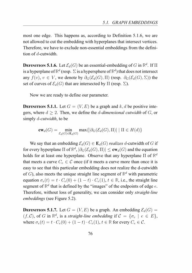
5.1. GRAPH EMBEDDINGS
most one edge. This happens as, according to Definition 5.1.6, we arenot allowed to cut the embedding with hyperplanes that intersect vertices.Therefore, we have to exclude non-essential embeddings from the defini-tion of d-cutwidth.
Definition 5.1.6. Let Ed(G) be an essential-embedding of G in Rd. If Πis a hyperplane of Rd (resp. Σ is a hypersphere of Rd) that does not intersectany f(v), v ∈ V , we denote by ∂G(Ed(G),Π) (resp. ∂G(Ed(G),Σ)) theset of curves of Ed(G) that are intersected by Π (resp. Σ).
Now we are ready to define our parameter.
Definition 5.1.1. Let G = (V,E) be a graph and k, d be positive inte-gers, where d ≥ 2. Then, we define the d-dimensional cutwidth of G, orsimply d-cutwidth, to be
cwd(G) = minEd(G)∈Ed(G)
max|∂G(Ed(G),Π)| | Π ∈ H(d)
We say that an embedding Ed(G) ∈ Ed(G) realizes d-cutwidth of G iffor every hyperplane Π of Rd, |∂G(Ed(G),Π)| ≤ cwd(G) and the equationholds for at least one hyperplane. Observe that any hyperplane Π of Rd
that meets a curve Ce ∈ C once (if it meets a curve more than once it iseasy to see that this particular embedding does not realize the d-cutwidthof G), also meets the unique straight line segment of Rd with parametricequation σe(t) = t · Ce(0) + (1 − t) · Ce(1), t ∈ R, i.e., the straight linesegment of Rd that is defined by the “images” of the endpoints of edge e.Therefore, without loss of generality, we can consider only straight-lineembeddings (see Figure 5.2).
Definition 5.1.7. Let G = (V,E) be a graph. An embedding Ed(G) =(f, C), of G in Rd, is a straight-line embedding if C = σe | e ∈ E,where σe(t) = t · Ce(0) + (1− t) · Ce(1), t ∈ R for every Ce ∈ C.
76

CHAPTER 5. D-DIMENSIONAL CUTWIDTH
a
b
c d
R2
Figure 5.2: A graph with 2-cutwidth 3.
Notice that every straight line embeding Ed(G) = (f, C) is fully de-fined by the function f , i.e., the points assigned to the vertices, therefore,for simplicity, from now on we will omit C.
As we described in the beginning of this Chapter, we will use the no-tation of Definition 5.1.1 and give an equivalent definition of cutwidth.
Definition 5.1.8. Let G = (V,E) be a graph. An embedding of G inR, denoted E1(G), is a tuple (f, I), where f : V → R is an injection,mapping the vertices ofG to R and I = (f(u), f(v)) ⊂ R | u, v ∈ Eis a set of open intervals of R. Given an embedding E1(G) = (f, I), wedenote by ∂G(E1(G), x) the set of intervals of I in which x belongs.
Definition 5.1.2. Let G = (V,E) be a graph and k a positive integer.We define the 1-cutwidth of G to be
cw1(G) = minE1(G)
max|∂G(E1(G), x)| | x ∈ R.
It is straightforward to see that the above definition of cutwidth isequivalent to the definition given in Chapter 4.
Theorem 5.1.1. For every graph G, cw1(G) = cw(G).
77

5.2. PROPERTIES OF D-CUTWIDTH
Observe that, in the case of cw1, hyperplanes degenerate to subspacesof R of dimension 1 – that is points of course – and our demand of essentialembeddings is expressed by our demand of injective functions. Therefore,d-cutwidth is the intuitive generalization of the notion of cutwidth in anydimension d ≥ 2.
In the rest of this Chapter we will present some properties of d-cutwidthand discuss some algorithmic remarks.
5.2 Properties of d-cutwidth
First we have to give the following definition, as it will be used in someof the proofs of this Section.
Definition 5.2.1. Given a point x = (x1, . . . , xd) in Rd and a hyperplaneΠ = (x1, . . . , xd) ∈ Rd | a1x1 + · · · + adxd + a0 = 0, the verticalprojection of x on Π is the point y = y1, . . . , yd ∈ Rd where
yi = xi − aia1x1 + · · ·+ adxd + a0
a12 + · · ·+ ad2, i ∈ 1, . . . , d.
The first two properties we will prove, show us that for every d ∈ N,d-cutwidth is a non-trivial graph parameter.
Proposition 5.2.1. For every graph G and every d ≥ 1,
cwd(G) ≤ cwd+1(G).
Proof. Let G = (V,E) be a graph, and let Ed+1(G) = f be an embeddingof G in Rd+1 that realizes cwd+1(G). Let Π0 be a hyperplane of Rd+1
such that, for every e ∈ E, Π0 is not vertical to σe. We vertically projectEd+1(G) on Π0, which gives us an embedding Ed(G) of G in Rd, as therestriction of f in Rd satisfies the conditions of a graph embedding.
78

CHAPTER 5. D-DIMENSIONAL CUTWIDTH
Assume that there exists a hyperplane Π in Rd that intersects Ed(G)more than cwd+1(G) times. Then we can construct a new hyperplane Π′
in Rd+1 that intersects Ed+1(G) more than cwd+1(G) times. This hyper-plane Π′ is the hyperplane vertical to Π that passes through Π. But thisfact leads to a contradiction, since any hyperplane in Rd+1 can intersectEd+1(G) at most cwd+1(G) times. Hence, our assumption that Π′ existsis false, i.e., every hyperplane in Rd intersects Ed(G) at most cwd+1(G)
times. Therefore, cwd(G) ≤ cwd+1(G).
Proposition 5.2.2. For every d ≥ 1, cwd(Pd) = d, where by Pn wedenote the path of length n.
Proof. Let Ed(Pd) be an essential straight line-embedding of Pd = (V,E)
in Rd, where V = v1, . . . , vd+1 and E = vi, vi+1 | i ∈ 1, . . . , d −1. Consider the midpoints mi of σi,i+1, for every i ∈ 1, . . . , d− 1.These d points of Rd define a hyperplane of Rd that intersects all edges ofEd(Pd). Thus cwd(Pd) ≥ d and as |E(Pd)| = d we derive that cwd(Pd) =
d.
Let us now compare d-cutwidth with cutwidth and see some inequal-ities that hold for them.
Theorem 5.2.1. For every graph G and every d ≥ 2 we have:
cwd(G) ≤ d · cw(G).
Proof. Consider the d-dimensional curve C with parametric equation
C(t) := (t, t2, t3, . . . , td), t ∈ R.
Consider an ordering of the nodes of G that realizes the cutwidth of G.Embed a node vi of G to the point pi = C(ti), for an appropriate valueti. By “appropriate” we mean that, if a node vi is after a node vj inthe cutwidth ordering, then the parametric value ti corresponding to vi
79

5.2. PROPERTIES OF D-CUTWIDTH
is strictly greater than the parameter value tj corresponding to node vj .Now embed an edge eij = (vi, vj) of G by connecting the points pi andpj on C with the minimum length arc of C connecting these points.
Consider a generic hyperplane Π with equation a1x1 + a2x2 + . . . +
adxd + a0 = 0, where, for all i, ai ∈ R. Π can cut C at at most d points.To see that, we need to solve the system of equations:
a1x1 + a2x2 + . . .+ adxd + a0 = 0,
xi = ti, i = 1, . . . , d
for t.This gives the polynomial equation q(t) := a0 + a1t + a2t
2 + . . . +
adtd = 0, in t of maximum degree d. Since q(t) = 0 has at most d
real roots, we deduce that Π intersects C at at most d points. At eachpoint of intersection at most cw(G) edges of the embedding of G passthrough that point. Hence, Π intersects at most d · cw(G) edges of G, i.e.,cwd(G) ≤ d cw(G).
Notice that, from Proposition 5.2.2 it holds that for every d ≥ 1,cwd(Pd) = d, thus cwd(Pd) = d·cw1(Pd). This proves that the inequalityof Theorem 5.2.1 can be tight.
Corollary 5.2.1. ForG = Pd the inequality of Theorem 5.2.1 becomesan equation.
We will now define a variant of d-cutwidth, which, instead of hyper-planes, implement hyperspheres to create the “cuts”.
Definition 5.2.1. Let G = (V,E) be a graph and k, d be positive inte-gers, where d ≥ 2. Then we define the spherical d-dimensional cutwidthof G, or simply spherical d-cutwidth, to be
scwd(G) = minEd(G)∈Ed(G)
max|∂G(Ed(G),Σ)| | Σ ∈ S(d)
80

CHAPTER 5. D-DIMENSIONAL CUTWIDTH
Let see the connection between these two parameters.
Proposition 5.2.3. For every graph G and any d ≥ 2 we have:
cwd(G) ≤ scwd(G) ≤ (d+ 1) cw(G).
Proof. The left-most inequality is obvious. For every embedding Ed(G)of G in Rd, the number of intersections of Ed(G) with a generalized hy-persphere (of an appropriate center and radius) in Rd is greater or equalto the number of intersections of Ed(G) with a hyperplane in Rd. Hence,cwd(G) ≤ scwd(G).
Now consider the curve C(t) = (t, t2, . . . , td), with t ∈ Rd, and con-sider the ordering of the nodes of G that realizes cw(G). We embed thei-th node vi of G, in this ordering, to the point pi = C(i). We embed anedge eij = (vi, vj) of G by connecting the points pi and pj on C with theminimum length arc of C connecting these points.We claim that this curve has at most d+1 intersections with a generalizedhypersphere S in Rd. If S is actually a plane then we can simply apply theargumentation presented in the proof of Theorem 5.2.1. Suppose now thatS is a true hypersphere, and let
∑di=1(xi − ai)2 + a0 = 0 be the equation
of S, where, for all i, ai ∈ R. Consider the following system of equations:
d∑i=1
(xi − ai)2 + a0 = 0,
xi = ti, i = 1, . . . , d.
The intersections of S with the aforementioned embedding of G in C isbounded by the number of real solutions of the system above, for which tis positive. Solving this system for t we get a polynomial equation for t,namely:
d∑i=1
(ti − ai)2 + a0 = 0.
81

5.2. PROPERTIES OF D-CUTWIDTH
Expanding the above equation we get:
d∑i=1
a2i − 2d∑i=1
aiti +
d∑i=1
a2i + a0 = 0,
which can be rewritten as:
d∑i=1
t2i − 2
⌊ d2⌋∑
i=1
a2it2i − 2
⌈ d2⌉∑
i=1
a2i−1t2i−1 +
d∑i=1
a2i + a0 = 0.
It is fairly easy to verify that the above equation can actually be rewrittenas:
d∑i=⌊ d
2⌋+1
t2i +d∑i=1
(1 + (−1)i
2− 2ai
)ti +
d∑i=1
a2i + a0 = 0.
By Descartes’ rule of signs, the number of positive real roots of this poly-nomial is bounded above by the number of sign variations in the sequenceof its (non-zero) coefficients. Taking a close look at this polynomial, weobserve that its first d−⌊d
2⌋ non-zero coefficients are equal to 1, which im-
plies that the number of sign variations in the sequence of its coefficientsis fully determined by the last d + 2 coefficients. A sequence of d + 2
real numbers can have at most d+ 1 sign variations, hence the number ofpositive real roots of this polynomial is at most d+ 1.
To finalize the proof, since any hypersphere in Rd intersects with Cat most d + 1 times, we conclude that the maximum number of intersec-tions of the embedding of G in C is at most (d + 1) cw(G). Therefore,scwd(G) ≤ (d+ 1) cw(G).
Proposition 5.2.4. For every graph G and every d ≥ 1 we have:
cwd+1(G) ≤ scwd(G).
82

CHAPTER 5. D-DIMENSIONAL CUTWIDTH
Proof. Consider a graph G and an embedding Ed(G) in Rd for whichscwd(G) is attained. Let us identify Rd with the hyperplane xd+1 = 0
in Rd+1 and consider the unit hypersphere Sd in Rd+1 centered at the ori-gin. Let Σ : Rd → Sd be the stereographic projection from Rd to theunit hypersphere Sd in Rd+1, and define Ed+1(G) to be the image of Ed(G)through the stereographic projection Σ, i.e., Ed+1(G) = Σ(Ed(G)).
Assume that there exists a hyperplane Π in Rd+1 that cuts Ed+1(G)
more than scwd(G) times. Let S be the intersection of Π with Sd andlet S ′ be the inverse image of S with respect to the stereographic pro-jection, i.e., S ′ = Σ−1(S). Since S is a hypersphere laying on Sd, S ′ iseither a hyperplane or hypersphere in Rd. Since the stereographic projec-tion preserves intersections, we deduce that S ′ intersects Ed(G) more thanscwd(G) times. But this contradicts the definition of Ed(G), which impliesthat our assumption that Π cuts Ed+1(G) more than scwd(G) times is false.Hence, we found an embedding of G in Rd+1, for which the maximumnumber of intersections with any hyperplane in Rd+1 is at most scwd(G).Therefore, cwd+1(G) ≤ scwd(G).
Let us now push the inequality of Theorem 5.2.1 a little further.
Theorem 5.2.2. For any graph G,
cw3(G) ≤ 2 cw2(G).
Proof. Let G be a graph and consider an ordering of the nodes of G thatrealizes cw(G).
Consider an axis-aligned ellipse E centered at the origin with its x-axis being greater than its y-axis (e.g., the ellipse 4x2 + y2 − 4 = 0).Embed the nodes of G on the positive half of E, denoted as E1/2, that ison the half-ellipse that lies on the positive halfplane with respect to thex-axis, in such a way so that their x-coordinates preserve the ordering. Inother words, given two nodes vi and vj of G, such that vi precedes vj in
83

5.2. PROPERTIES OF D-CUTWIDTH
the node ordering, then xi < xj . Let us call E2(G) the above-mentionedembedding.
Given a generalized circle C on the plane, C can cut the half-ellipseE1/2 at most two times. Hence we found an embedding of G in R2 suchthat any generalized circle C in R2 intersects this embedding at most 2 ·cw(G) times. In other words, scw2(G) ≤ 2 cw(G). Using the resultsfrom Propositions 5.2.1 and 5.2.4 we conclude that:
cw3(G) ≤ scw2(G) ≤ 2 cw(G) ≤ 2 cw2(G),
which is what we wanted to prove.
Cutwidth is not a minor closed parameter but it is immersion closed [22].We will prove that the same holds for d-cutwidth.
Theorem 5.2.3. Let G = (V,E) be a graph and H be an immersion(strong immersion) of G. For every d ≥ 1, cwd(H) ≤ cwd(G).
Proof. Let Ed(G) be an an embedding of G in Rd that realizes cwd(G).Let H ′ be a subgraph of G. Then, given Ed(G) = (f, C), we define anembedding Ed(H ′) = (fH′ , CH′) of H ′ in Rd, where fH′ is the restrictionof f to V (H ′) and CH′ = ce ∈ C | e ∈ E(H ′). Observe that everyhyperplane of Rd that intersected l ≤ cwd(G) edges of Ed(G) intersects atmost l edges of Ed(H ′), therefore cwd(H) ≤ cwd(G).
We will next prove that ifH is the result of one lift of edges e1 = u, vand e2 = v, w of E, then cwd(H) ≤ cwd(G). Clearly, for any hyper-plane R of Rd its corresponding numbers |∂H(Ed(H), R)| and |∂G(Ed(G),R)| can differentiate only due to the intersections of R with edges e, e1and e2. Let E(H) ∋ e = u,w be the resulting edge of the lift. LetΠ ∈ H(d) be a hyperplane that does not intersect f(v), ∀v ∈ V . If Πintersects e (more accurately, the straight line segment that represents ein the embedding in Ed(G)), then Π separates Rd into two halfspaces (i.e.,subspaces of dimension d), namely A and B. Assume, without loss of
84

CHAPTER 5. D-DIMENSIONAL CUTWIDTH
generality, that u ∈ A and w ∈ B. Then, as Π does not intersect f(v),either v ∈ A or v ∈ B, which means that either Π intersects e1 or Π in-tersects e2 in Ed(G). Therefore, |∂H(Ed(H),Π)| ≤ |∂G(Ed(G),Π)|. Thesame holds trivially for the case that Π does not intersect e. Therefore,cwd(H) ≤ cwd(G). Summing up the above we get that, for every graphH that is the result of some (or maybe none) vertex deletions, edge dele-tions and edge lifts of G, cwd(H) ≤ cwd(G), which is what we stated.Notice that the above proof implies the same relation between a graph Gand a strong immersion H of G.
5.3 Algorithmic Remarks About d-cutwidthAs a consequence of the Nash-Williams Conjecture’s proof in [87], for ev-ery positive integer k, the class of weak immersion minimal graphs withd-cutwidth bigger than k contains a finite set of graphs. Notice that thisclass is exactly obs≤im(cwd, k), i.e., the immersion obstruction set for d-cutwidth at most k. This fact, combined with Theorem 5.2.3, implies thatcwd(G) ≤ k if and only if none of the graphs in obs≤im(cwd, k) is con-tained in G as an immersion, thus, the graphs of obs≤im(cwd, k) character-ize graphs with d-cutwidth at most k.
Moreover, according to Theorem 3.2.2, checking whether an n-vertexgraph contains as an immersion some k-vertex graph H , can be done inf(k)·n3 steps, for some computable function f . As a consequence, check-ing whether cwd(G) ≤ k can be done in |obs≤im(cwd, k)| ·f(k) ·n3 steps2.This running time can become linear (on n) using the inequality of Theo-rem 5.2.1.
Proposition 5.3.1. For every k and d, there exists a linear (on n) timealgorithm that, given a graph G, decides whether cwd(G) ≤ k or not.
2To be precise, the f(k) factor in the running time of this algorithm is in fact f(n(O))where O is the graph in obs≤im(cwd, k) having the most vertices.
85

5.3. ALGORITHMIC REMARKS ABOUT D-CUTWIDTH
Indeed, the algorithm first checks whether cw(G) ≤ k, using the lineartime algorithm in [59]. If the answer is negative, then from Lemma 5.2.1we can safely report that cwd(G) > k. If not, then, as it holds thatpw(G) ≤ cw(G) (see e.g. [59]), G has a path decomposition with widthat most k and , according to [37] such a decomposition can be found inlinear time. Therefore, we can then check whether some of the graphs inobs≤im(cwd, k) is contained in G as an immersion in f(k) · n steps, usingdynamic programming for instance.
Unfortunately, the algorithm above is non-constructive as we have noother knowledge about the set obs≤im(cwd, k), except from the fact that itis finite. Whether we can obtain a constructive f(k) · n steps algorithmfor d-cutwidth remains an open problem.
Another way to prove Proposition 5.3.1 is to express d-cutwidth inMSO, observe that for every graph G it holds that
tw(G) ≤ pw(G) ≤ cw(G) ≤ cwd(G)
(this follows from the definition of treewidth and pathwidth, Observa-tion 4.1.3, and Proposition 5.2.1), and use Courcelle’s Theorem:
Theorem 5.3.1 (Courcelle, 1990 [189]). Every graph property definablein MSO of graphs can be decided in linear time on graphs of boundedtreewidth.
This algorithm goes as follows:
Step 1: Use the algorithm of Theorem 4.1.2 and check whether the inputgraph G has tw(G) > k. If so, return No and stop.
Step 2: (As tw(G) ≤ k we can implement Theorem 5.3.1.) Run thealgorithm of Theorem 5.3.1 and check if cwd(G) ≤ k.
The problem with this approach is that in order to express d-cutwidthin MSO we have to define embeddings in MSO, which in term involvesdiscretizing Rd.
86

CHAPTER 5. D-DIMENSIONAL CUTWIDTH
5.4 ConclusionWhat we did in this Chapter was to define d-cutwidth, a multi-dimensionalgeometric extension of cutwidth and then proved some of its properties.Theorem 5.4.1 states the most important of them.
Theorem 5.4.1. The following hold:i. d-cutwidth is immersion closed.ii. For every graph G and every d ≥ 1, cwd(G) ≤ cwd+1(G).
iii. For every graph G and every d ≥ 1, cwd(G) ≤ d · cw(G).iv. For every graph G, cw3(G) ≤ 2 · cw2(G).v. For every k and d, there exists a linear (on n) time algorithm that,given a graph G, decides whether cwd(G) ≤ k or not.
Some interesting open problems and suggestions for future work aboutthis parameter are the following:
• Is the problem of checking for a graph G whether cwd(G) ≤ k NP-complete? This seems to be very difficult as – in a sense – we haveto find the right way to discretize Rd in order to define equivalentclasses of embeddings and make their number finite. If we do notaccomplish that, there is no hope of finding certificates of polyno-mial size.
• Finding a constructive algorithm for checking whether cwd(G) ≤ k,for d ≥ 2, as we discussed in the previous Section, is an insistingopen problem.
• It would be very interesting if we extended Theorem 5.4.1 (iv) andproved that cwd+1(G) ≤ f(d) · cwd(G), for some function f .
• We used hyperplanes and hyperspheres to “cut” embeddings ofgraphs. We are very curious to find out what happens when weuse other geometrical objects for this purpose.
87

5.4. CONCLUSION
88

CHAPTER 6
OBSTRUCTIONS FOR UNIONS OF CLASSES
Let us take a moment to briefly recapitulate what we have discussed sofar. In Chapter 2 we presented the Graph Minors Theory. We argued thatit constitutes a vital part of modern Combinatorics, as many theorems thatwere proven – and techniques that were introduced – in its context, areof great significance, not only in Algorithmics and the theory of Param-eterized Complexity, but in Structural Graph Theory as well. The mostprominent results in Graph Minors Theory, supporting this point, are theExcluded Grid Theorem [92], the Structural Theorems in [77, 80] and theIrrelevant Vertex Technique in [86]. Some further examples of algorithmicapplications, can be found in [165, 179].
While the minor partial ordering has been extensively studied through-out the last decades [77, 80, 85–87, 92, 123, 125], the immersion orderinghas only recently gained more attention [42, 137, 179]. In Chapter 2 wesaw one of the fundamental results concerning this relation, the proof ofNash-Williams’ Conjecture (the weak version). As Corollary 2.6.1 indi-cates, a graph class C that is closed under taking of immersions, can becharacterized by a finite family obs≤im(C) of forbidden immersions.
89

Some examples of graph classes for which such characterizations arepossible, are the class Et of graphs that admit a (proper) edge-coloringthat uses at most t ∈ N colors such that for every two edges of the samecolor every path between them contains an edge of greater color (for moreinformation, see [36]) and the classWk of graphs whose carving-width isat most k, k ∈ N, (for more information see [151]). Another example –we plan to study extensively – is the classes G[cwd, k] for d ≥ 2 and k ≥ 0
(see Chapter 5).
Furthermore, in Theorem 2.6.3, we saw that there exists an algorithm– with running time O(|V (G)|3) – that decides whether a graph H is animmersion of a graph G (where the hidden constants depend only on H).Combining this algorithm with the forbidden immersions characterizationone can prove that it can be decided – in cubic time – whether a graphbelongs to C or not.
This – meta-algorithmic – result for an immersion-closed graph classC assumes that the family obs≤im(C) is known. Of course, the finiteness ofobs≤im(C) directly implies that this family of graphs is computable. How-ever, an algorithm for the computation of obs≤im(C) would also require adescription of the family. Therefore, while the existence of an algorithmcomputing the immersion obstruction set of an immersion-closed graphclass C is affirmed, the construction of such an algorithm is, in general,elusive.
To make matters even worse, recall that the proofs of Theorem 2.6.1and Conjecture 2.6.1 are non-constructive (see [88]). This means thatthis proofs do not provide us with a generic algorithm that would allowsus to identify the obstruction sets for every minor or immersion-closedgraph class. Even when we work with fixed graph classes, this task canbe extremely challenging, as such a set may contain a huge number ofgraphs [129] and no general upper bound on its cardinality is known otherthan its finiteness.
90

CHAPTER 6. OBSTRUCTIONS FOR UNIONS OF CLASSES
6.1 Computation of Obstruction Sets
The issue of the computability of obstruction sets for minors and im-mersions was raised by Fellows and Langston [192, 193] and the chal-lenges against computing obstruction sets soon became clear. In particu-lar, in [193] Fellows and Langston showed that the problem of determiningobstruction sets from machine descriptions of minor-closed graph classesis recursively unsolvable1 (which directly holds for the immersion order-ing as well). Moreover, in [127] Courcelle, Downey and Fellows provedthat the obstruction set of a minor-closed graph class cannot be computedwhen only a description of the minor-closed graph class in MSO is known.Thus, the following is a natural open problem:
Identify the information needed in order to make it possible tocompute the obstruction set obs≤im(C) of an immersion-closedgraph class C.
In other words, our goal is to look for theorems able to delimit thecomputability horizon of obstruction sets for the immersion relation.
Several methods have been proposed towards tackling the non-con-structiveness of these sets (see, for example, [125, 192]) and the problemof algorithmically identifying minor obstruction sets has been extensivelystudied [52, 123, 125, 127, 192, 193]. In [125], it was proven that the ob-struction set of a minor-closed graph class C which is the union of twominor-closed graph classes C1 and C2 whose obstruction sets are givencan be computed under the assumption that there is at least one tree thatdoes not belong to C1 ∩ C2, and in [123] it was shown that the aforemen-tioned assumption is not really necessary. This also lead to an interestingquestion:
1I.e., there does not exist a Turing Machine that takes as input the descriptions of aminor-closed graph class C and outputs obs≤m(C).
91

6.1. COMPUTATION OF OBSTRUCTION SETS
What kind of Set Theory operations2 on two immersion closedgraph classes C1 and C2, for which the sets obs≤im(C1) andobs≤im(C2) are known, make the computation of obs≤im(C12 C2)possible2?
In this Chapter we deal with the problem of computing obs≤im(C) forfamilies of graph classes C that are constructed by finite unions of im-mersion-closed graph classes. Observe that the union and the intersectionof two immersion-closed graph classes are also immersion-closed, hencetheir obstruction sets are of finite size. It is also easy to see that, given theobstruction sets of two immersion-closed graph classes, the obstructionset of their intersection can be computed in a trivial way (it is just theunion of the two immersion obstruction sets).
However, in general, while the combination of a machine descriptionof an immersion-closed graph class C, that is, an algorithm deciding themembership of a graph in C, combined with an upper bound on the sizeof the obstructions makes the computation of obs≤im(C) possible, neitherthe machine description of the class nor the upper bound alone are suffi-cient information. Moreover, as mentioned before, no generic procedureis known for computing such an upper bound. Thus, the problem of com-puting the obstruction set of the union of two immersion-closed graphclasses is not trivial at all.
Our final goal for this Chapter is to prove that there exist an algorithmthat, given the obstruction sets of two immersion-closed graph classes,outputs the obstruction set of their union. Our approach is based on thederivation of a uniform upper bound on the tree-width of the subgraph-minimal graphs that do not belong to an immersion-closed graph class C.We will build on the machinery introduced by Isolde Adler, Martin Groheand Stephan Kreutzer in [123] for computing minor obstruction sets. To
2Provided, of course, that C12 C2 is also immersion-closed.
92

CHAPTER 6. OBSTRUCTIONS FOR UNIONS OF CLASSES
be more precise, the algorithm we are going to present needs an MSO-description of an immersion-closed graph class C (instead of a machine de-scription) and an upper bound on the tree-width of the subgraph-minimalgraphs that contain an obstruction of C (instead of an upper bound on thesize of the obstructions of C).
To fulfil this goal, we will adapt the results on [123] so as to per-mit the computation of the obstruction set of any immersion-closed graphclass C, under the aforementioned conditions. We present this algorithmin Lemma 6.2.2, with which we conclude the computability part of thisChapter.
The next step is to give a combinatorial result proving a uniform upperbound on the tree-width of the subgraph-minimal graphs that do not be-long to the union of two immersion-closed graph classes, whose obstruc-tion sets are known. These combinatorial proofs make use of a suitableextension of theUnique Linkage Theorem ofKen-ichi Kawarabayashi andPaul Wollan [89], which, in turn, is an improvement of the Vital LinkageTheorem of Robertson and Seymour in [85, 86]. In particular, notice thata subgraph-minimal graphG not belonging to an immersion-closed graphclass C contains an immersion obstruction for C, that is, there is a set ofterminals that are joined by edge-disjoint paths3 which make use of allthe vertices and edges of G. As G is subgraph-minimal, this implies thatthese edge-disjoint paths of G correspond to vertex-disjoint paths in itsline graph which also form a unique linkage (both the definition of Link-ages and the Unique Linkage Theorem will be presented in Section 6.3 ).Then, the Unique Linkage Theorem, allows us to prove a bound on thetree-width of the line graph ofG and consequently, to the tree-width ofG.
The reader is advised to have this proof sketch in mind when go intothe details.
3Remember that we are always referring to weak immersions.
93

6.2. COMPUTING IMMERSION OBSTRUCTION SETS
6.2 Computing Immersion Obstruction Sets
As we mentioned before, to make everything work we need the followingcombinatorial lemma.
Lemma 6.2.1. There exists a computable function f : N → N such thatthe following holds. Let H and G be graphs such that H ≤im G. If G′ isa minimal subgraph of G with H ≤im G′ then tw(G′) ≤ f(|E(H)|).
We are not going into the details of the the proof of Lemma 6.2.1,as we will later prove a stronger statement of it (Lemma 6.3.3). Insteadwe will continue by giving the necessary definitions in order to prove theanalogue of Lemma 3.1 in [123] for the immersion ordering. We first givemore formal definitions of the contraction, minor, and immersion relation.
Definition 6.2.1. Let H and G be two graphs. H is a contraction of Gif there exists a surjection ϕ : V (G)→ V (H) such that:
(1) for every vertex v ∈ V (H), G[ϕ−1(v)] is connected, and
(2) for every two distinct vertices u, v ∈ V (G), it holds that v, u ∈E(G) if and only if the graph H[ϕ−1(v) ∪ ϕ−1(u)] is connected.
If furthermore H is not isomorphic to G, we say that H is a propercontraction of G.
Observe that function ϕ indicates the edges of E(G) we will contractin order to obtain H . There are the edges of G[ϕ−1(v)], for v ∈ V (H).
Definition 6.2.2. LetH andG be two graphs. H is a minor ofG if thereis a function ψ : V (H)→ 2V (G) such that:
(1) for every v ∈ V (H), Bv = G[ψ(v)] is connected, and
94

CHAPTER 6. OBSTRUCTIONS FOR UNIONS OF CLASSES
(2) for any two distinct vertices v, w ofH ,Bv andBw share no commonvertex, and for every edge u, v ∈ E(H), there is an edge inGwithone endpoint in Bv and one in Bu.
The graph obtained by the union of all Bv, v ∈ V (H), and the edgesbetweenBv andBu in G, where v, u ∈ E(H), is called aminor model ofH inG. This graph is obtained from G after the deletion of some verticesand edges. We can further contract the edges of G[Bv], v ∈ V (H), toobtain H as a minor of G. A model with minimal number of vertices andedges is called minimal minor model.4
In Section 7.5.4 we will give another – more general – definition ofthe minor relation.
Definition 6.2.3. Let H and G be two graphs. H is an immersion of Gif there exists an injective function ψ : V (H)→ V (G), such that:
(1) for every edge u, v ∈ E(H), there is a path from ψ(u) to ψ(v) inG, and
(2) for any two distinct edges of H the corresponding paths in G areedge-disjoint.
Moreover, if these paths are vertex disjoint from ψ(V (H)), then wesay that H is a strong immersion of G. The function ψ indicates the endsof the paths we will lift in order to obtain H as an immersion of G. It iscalled an immersion model of H in G and a model with minimal numberof vertices and edges is called minimal immersion model.
To facilitate the proofs in this Chapter we have to establish an orderingbetween finite sets of graphs.
4Notice that we could define the minor relation for the two graphs by removing in thesecond property of Definition 6.2.1 the demand that if u, v /∈ E(H) then G[ϕ−1(v)∪ϕ−1(u)] is not connected, but we chose not to.
95

6.2. COMPUTING IMMERSION OBSTRUCTION SETS
Definition 6.2.4. For two finite sets of graphs, say F1 and F2, we willwrite F1 ≤ F2 if and only if:
1.∑G∈F1
|V (G)| <∑H∈F2
|V (H)| or
2.∑G∈F1
|V (G)| =∑H∈F2
|V (H)| and∑G∈F1
|E(G)| ≤∑H∈F2
|E(H)|.
We now state a theorem which plays a crucial role in the proof ofthe algorithm for the computation of immersion obstructions for generalimmersion-closed graph classes.
Theorem 6.2.1 (Arnborg, Lagergren, and Seese, 1991 [31]). For everypositive integer k, it is decidable given an MSO-formula whether it is sat-isfied by a graph G whose tree-width is upper bounded by k.
In [123], Adler, Grohe and Kreutzer provide the tools that will allowus to use Theorem 6.2.1 to compute the obstruction sets of minor-closedgraph classes, when an upper bound on the tree-width of the subgraph-minimal graphs not belonging to a minor-closed graph class is known andan MSO-description of the graph class can be computed.
In this Chapter we will adapt the machinery of [123] to the immersionordering and provide a generic technique to compute immersion obstruc-tion sets when an explicit value of such upper bound on the tree-width isknown.
Moreover, in Section 6.3 we will obtain such a – computable – up-per bound on the tree-width for the case where C = C1 ∪ C2 and C1, C2are immersion-closed graph classes whose obstruction sets are given, andtherefore show that obs≤im(C) can be computed.
6.2.1 An extension of MSO
For convenience, we consider the extension of the signature τG to a signa-ture τex that pairs the representation of a graph G with the representation
96

CHAPTER 6. OBSTRUCTIONS FOR UNIONS OF CLASSES
of one of its tree-decompositions.
Definition 6.2.5. IfG is a graph and T = (T,B) is a tree-decompositionof G, τex is the signature that consists of the relation symbols V,E, I ofτG , and four more relation symbols VT , ET , IT and B.A tree-dec-expansion of G and T , is a τex-structure
Gex = (V (G) ∪ E(G) ∪ V (T ) ∪ E(T ),V Gex , EGex , IGex , V Gex
T , EGexT , IGex
T , BGex)
where V GexT = V (T ) represents the node set of T , EGex
T = E(T ) the edgeset of T , IGex
T = (v, e) | v ∈ e∩V (T ) ∧ e ∈ E(T ) the incidence relationin T and BGex = (t, v) | t ∈ V (T ) ∧ v ∈ Bt ∩ V (G).
Let Tk be the class of graphs of tree-width at most k. We denote by CTkthe class of tree-dec expansions consisting of a graph G with tw(G) ≤ k,and a tree decomposition (T,B) of G of width(T,B) ≤ k.
Proposition 6.2.1 (Adler, Grohe, and Kreutzer, 2008 [123]).
1. Let G be a graph and (T,B) a tree decomposition of it with width(T,B) ≤ k. Then the tree-width of the tree-dec expansion of G isat most k + 2.
2. There is an MSO-sentence ϕCTk such that for every τex-structureG,G |= ϕCTk if and only if G ∈ CTk .
Notice that by Theorem 6.2.1, for every k ≥ 0, it is possible to decideif an MSO-formula is satisfied in a graphG of tw(G) ≤ k. An immediatecorollary of this result and Proposition 6.2.1 is the following.
Corollary 6.2.1. It can be decided, for every k, if an MSO-formula ϕis satisfied in some G ∈ CTk .
97

6.2. COMPUTING IMMERSION OBSTRUCTION SETS
Theorem 6.2.2 (Adler, Grohe, and Kreutzer, 2008 [123]). For every k ≥0, there is an MSO-sentence ϕTk such that for every tree-dec expansionG ∈ CTl of G, for some l ≥ k, it holds that G |= ϕTk if and only iftw(G) = k.
The algorithm of Lemma 6.2.2 can be applied not only to MSO defin-able graph classes, but also to Layer-wise MSO definable classes:
Definition 6.2.6. A graph class C is layer-wise MSO-definable, if forevery k ∈ N we can compute an MSO-formula ϕk such that G ∈ C andtw(G) ≤ k if and only if G |= ϕk, where G ∈ CTk is a tree-dec expansionof G.
Definition 6.2.7. Let C be an immersion-closed graph class. The widthof C, denoted by width(C), is the minimum positive integer k such that forevery graph G /∈ C there is a graph G′ ≤ G with G′ /∈ C and tw(G′) ≤ k.
We have to stress here that Lemma 6.2.1 ensures that the width of animmersion-closed graph class is well-defined.
Observation 6.2.1. If C1 is an immersion-closed graph class then thefollowing holds. For every graph G /∈ C1, there exists a graph G′ ≤ G
such that G′ /∈ C1 and tw(G′) ≤ maxf(|E(H)|) | H ∈ obs≤im(C1),where f is the function of Lemma 6.2.1.
We are now able to present an algorithm analogue to that of Lemma3.1 in [123], but in our case for the immersion ordering.
Lemma 6.2.2. There exists an algorithm that, given an upper bound l ≥ 0
on the width of a layer-wise MSO-definable class C, and a computablefunction f : N→ MSO such that for every positive integer k, f(k) = ϕk,where ϕk is the MSO-formula defining C ∩ Tk, it computes obs≤im(C).
Proof. In order to prove the Lemma it is enough to prove the following.
98
CHAPTER 6. OBSTRUCTIONS FOR UNIONS OF CLASSES
Claim 1. For any finite family of graphsF = F1, . . . , Fn, it is decidablewhether the following two conditions are unsatisfiable for any graph G.
G ∈ C and there exists an F ∈ F such that F ≤im G (6.1)G /∈ C and for every F ∈ F , F ≰im G (6.2)
To see that the above claim is enough, first notice that if F is a finitefamily of graphs for which the conditions (6.1) and (6.2) are unsatisfiablethen F is a forbidden immersion characterization of C, that is, a graphG belongs to C if and only if it does not contain any of the graphs in Fas an immersion. By definition, obs≤im(C) is the minimum such familyaccording to the ≤-relation (Definition 6.2.4).
Thus, if Claim 1 holds, we can find the set obs≤im(C) by enumerating,according to ≤ (see Definition 6.2.4), all the finite families of graphs Fand deciding, for each one of them, if the conditions (6.1) and (6.2) areunsatisfiable.
Proof of Claim 1. Let G be a graph in C such that F ≤im G, for someF ∈ F . Lemma 6.2.1 implies that there exists a graph G′ ≤ G suchthat tw(G′) ≤ f(|E(F )|) and F ≤im G′, where f is the function ofLemma 6.2.1. Observe thatG′ ∈ C. Thus, (6.1) is satisfiable if and only ifthere exists a graph in C, whose tree-width is bounded from maxf(|E(F )|)| F ∈ F, that satisfies it, where f is the computable function of Lemma6.2.1. Let ϕC be the formula defining C ∩ Tk in CTk , and ϕF =
∨F∈F ϕF ,
where ϕF is the formula from Lemma 2.7.1 and k = maxf(|E(F )|) |F ∈ F. Notice that there exists some graph G ∈ C that models ϕF ifand only if ϕC∧ϕF is satisfiable for someG′ ∈ CTk . From Corollary 6.2.1,this is decidable.
LetG /∈ C be a graph such thatF ≰im G, for everyF ∈ F . Recall thatthe width of a graph class C is the minimum positive integer k such that forevery graph G /∈ C there is a G′ ≤ G with G′ /∈ C and tw(G′) ≤ k. Thus,G contains a subgraph G′ with tree-width at most w such that G′ /∈ C,
99

6.3. WIDTH BOUNDS FOR IMMERSION-CLOSED GRAPH CLASSES
where w is computable by Lemma 6.2.1. Observe that F ≰im G′, forevery F ∈ F . If ϕ′
C is the MSO-sentence defining C ∩ Tw (given bythe hypothesis), then there exists a graph G /∈ C such that F ≰im G,for every F ∈ F if and only if ¬ϕ′
C ∧ ¬ϕF is satisfiable in CTw . Thedecidability of whether ¬ϕ′
C ∧ ¬ϕF is satisfiable in CTw follows, again,from Corollary 6.2.1.
As Claim 1 holds, the lemma follows.
Corollary 6.2.2. There is an algorithm that given an MSO formula ϕand k ∈ N, so that ϕ defines an immersion closed-graph class C of widthat most k, computes the obstruction set of C.
Notice that a direct proof of Corollary 6.2.2 would be enough for ourgoal for this Chapter, which is to prove Theorem 6.3.2 . However, asLemma 6.2.2 provides a more general framework regarding the construc-tiveness of immersion obstruction sets, it is worth to be mentioned.
Although Lemma 6.2.2 provides an algorithm for computing the ob-struction set of any immersion-closed graph class C, given that the con-ditions stated are satisfied, this result is generic and there is no uniformway for computing either an upper bound on the width of C or an MSO-description of C.
In the next Section, we will prove some combinatorial lemmata andthen conclude that if C1 and C2 are two immersion-closed graph classeswhose obstruction sets are known then the width of C1 ∪ C2 can be com-puted and hence, the set obs≤im(C1 ∪ C2) is computable.
6.3 WidthBounds for Immersion-closedGraphClasses
Our goal for this Section is to give an upper bound on the width of thegraph class C1 ∪ C2, where C1 and C2 are immersion-closed graph classes
100

CHAPTER 6. OBSTRUCTIONS FOR UNIONS OF CLASSES
and their obstruction sets are known. This will directly imply the proof ofLemma 6.2.1. To do this, we will first prove a generalization of the UniqueLinkage Theorem, appeared in the Graph Minors series [85]. Then wewill introduce the notion of an r-approximate edge-linkage and work onthe subgraph-minimal graphs not belonging to C1 ∪ C2.
Finally, as it is trivial to compute an MSO-description of C1∪C2 whenwe are given the sets obs≤im(C1) and obs≤im(C2), we will show that theobstruction set of C1 ∪ C2 is computable.
6.3.1 Linkages
We start with a series of definitions.
Definition 6.3.1. Let r be a positive integer. An r-approximate linkagein a graph G is a family L of paths with distinct endpoints in G suchthat for every r + 1 distinct paths P1, P2, . . . , Pr+1 in L, it holds that∩i∈[r+1] V (Pi) = ∅. These paths are the components of the linkage.
Definition 6.3.2. Let (α1, α2, . . . , αk) and (β1, β2, . . . , βk) be elementsof V (G)k, that is k-tuples of vertices of V (G). An r-approximate link-age L, consisting of the paths P1, P2, . . . , Pk, links (α1, α2, . . . , αk) and(β1, β2, . . . , βk) if Pi is a path with endpoints αi and βi, for every i ∈ [k].
Definition 6.3.3. Given a r-approximate linkage L for a graph G, wedefine the order of L to be equal to the number of its paths. We call anr-approximate linkage of order k, r-approximate k-linkage. When r = 1,such a family of paths is simply called linkage.
Definition 6.3.4. Two r-approximate k-linkagesL andL′ are equivalentif for every component P of L there exists a component P ′ of L′ with thesame endpoints. An r-approximate linkageL of a graphG is called uniqueif for every linkage L′ that is equivalent to L, V (L) = V (L′).
101

6.3. WIDTH BOUNDS FOR IMMERSION-CLOSED GRAPH CLASSES
Definition 6.3.5. A linkage L in a graph G is called vital if there is noother linkage in G joining the same pairs of vertices.
In [85], Robertson and Seymour proved a theorem which is known asThe Vital Linkage Theorem. This theorem provides an upper bound forthe tree-width of a graph G that contains a vital k-linkage L such thatV (L) = V (G), where the bound depends only on k. A stronger statementof the Vital Linkage Theorem was recently proved by Kawarabayashi andWollan [89], where instead of asking for the linkage to be vital, it asksfor it to be unique. Notice here that a vital linkage is also unique. As insome of the proofs in this Chapter (for instance, the proof of Lemma 6.3.1)we deal with unique but not necessarily vital linkages we make use of theVital Linkage Theorem in its latter form stated below.
Theorem 6.3.1 (Unique Linkage Theorem, 2010 [89]). There exists acomputable function w : N → N such that the following holds: Let L bea (1-approximate) k-linkage inG with V (L) = V (G). If L is unique thentw(G) ≤ w(k).
Lemma 6.3.1. There exists a computable function f : N → N such thatthe following holds. Let G be a graph that contains a 2-approximate k-linkage L such that V (L) = V (G). If L is unique, then tw(G) ≤ f(k).
Proof. LetG be a graph that contains a unique 2-approximate k-linkage Lwith V (L) = V (G) that linksA = (α1, α2, . . . , αk) andB = (β1, β2, . . . ,
βk) in G. Denote by T the set A ∪B and consider the graph Gb with
V (Gb) = V ((G \ T )×K2) ∪ TE(Gb) = E((G \ T )×K2) ∪ t, t′ | t, t′ ∈ T ∧ t, t′ ∈ E(G)
∪t, (v, x) | t ∈ T ∧ x ∈ V (K2) ∧ v ∈ V (G)
∧t, v ∈ E(G),
where V (K2) = 1, 2. It is easy to see that Gb contains a k-linkage thatlinks A and B. Let G′ be a minimal induced subgraph of Gb that contains
102

CHAPTER 6. OBSTRUCTIONS FOR UNIONS OF CLASSES
a k-linkage L′ that links A and B. From Theorem 6.3.1, it follows that
tw(G′) ≤ w(k). (6.3)
From now on we work towards proving thatG ≤m G′. In order to achievethis, we prove the following two claims for G′.
Claim 2. IfL′ is a k-linkage inG′ that linksA andB then for every vertexv ∈ V (G) \ T no path of L′ contains both (v, 1) and (v, 2).
Proof of Claim2. Towards a contradiction, assume that for some vertexv ∈ V (G)\T , there exists a (t, t′)-pathP ofL′ that contains both (v, 1) and(v, 2). Without loss of generality, assume also that (v, 1) appears before(v, 2) in P . Let y be the successor of (v, 2) in P and notice that y = (v, 1).From the definition of Gb and the fact that G′ is an induced subgraph ofGb, y, (v, 1) ∈ E(G′) \ E(L′). By replacing the subpath of P from(v, 1) to y with the edge (v, 1), y, we obtain a linkage in G′ \ (v, 2) thatlinks A and B. This contradicts to the minimality of G′.
Claim 3. IfL′ is a k-linkage inG′ that linksA andB then for every vertexv ∈ V (G) \ T , V (L′) ∩ (v, 1), (v, 2) = ∅.
Proof of Claim3. Assume, in contrary, that there exists a linkage L′ in G′
and a vertex x ∈ V (G) \ T such that L′ links A and B and V (L′) ∩(x, 1), (x, 2) = ∅. Claim 2 ensures that, after contracting the edges(v, 1), (v, 2), v ∈ V (G) \ T (whenever they exist), the correspondingpaths compose a 2-approximate k-linkage L′ of G \ x that links A andB. This is a contradiction to the assumption that L is unique. Thus, theclaim holds.
Recall that T ⊆ V (G′) and that G′ is an induced subgraph of Gb.Claim 3 implies that we may obtain G from G′ by contracting the edges(v, 1), (v, 2) for every v ∈ V (G) \ T (whenever they exist). As G ≤m
G′, from (6.3), it follows that, tw(G) ≤ w(k).
103

6.3. WIDTH BOUNDS FOR IMMERSION-CLOSED GRAPH CLASSES
We remark that, the previous lemma holds for any graph G that con-tains an r-approximate k-linkage. This can be seen by substituting (G \T )×K2 with (G \ T )×Kr in its proof.
The following lemma provides an upper bound on the tree-width of agraph G, given an upper bound on the tree-width of its line graph L(G).
Lemma 6.3.2. IfG is a graph and k is a positive integer with tw(L(G)) ≤k then tw(G) ≤ 2k + 1.
Proof. Notice that, from Observation 4.1.2, we may assume that G doesnot contain isolated vertices. Suppose that G is graph such that L(G) ad-mits a tree decomposition of width at most k and recall that every vertexof L(G) corresponds to an edge of G. We construct a tree decompositionT = (T,B) of G from a tree decomposition TL of L(G) by replacing ineach bag of TL every vertex of L(G) by the endpoints of the correspond-ing edge in G. It is easy to verify that this is a tree decomposition of G.Therefore, tw(G) ≤ 2k + 1.
Before we proceed to the next lemma, we need to introduce the notionof an r-approximate k-edge-linkage in a graph.
Definition 6.3.6. An r-approximate edge-linkage in a graphG is a fam-ily of pathsE inG such that for every r+1 distinct paths P1, P2, . . . , Pr+1
in E, it holds that ∩i∈[r+1]E(Pi) = ∅. We call these paths the componentsof the edge-linkage.
Definition 6.3.7. Let (α1, α2, . . . , αk) and (β1, β2, . . . , βk) be elementsof V (G)k. We say that an r-approximate edge-linkage E, consisting ofthe paths P1, P2, . . . , Pk, links (α1, α2, . . . , αk) and (β1, β2, . . . , βk) if Piis a path with endpoints αi and βi, for every i ∈ [k].
Definition 6.3.8. Given a r-approximate edge-linkage E for a graph G,we define the order of E to be equal to the number of its paths. We call
104

CHAPTER 6. OBSTRUCTIONS FOR UNIONS OF CLASSES
an r-approximate edge-linkage of order k, r-approximate k-edge-linkage.When r = 1, we call such a family of paths, an edge-linkage.
Lemma 6.3.3. There exists a computable function r such that the follow-ing holds. Let G1, G2 and G be graphs such that Gi ≤im G, i = 1, 2. If G′
is a minimal subgraph of G where Gi ≤im G′, i = 1, 2, then
tw(G′) ≤ r(|E(G1)|, |E(G2)|).
Proof. Let G′ be a minimal subgraph of G such that Gi ≤im G′, i = 1, 2.Recall that the edges of Gi compose a ki-edge-linkage Ei in G, whereki = |E(Gi)|, i = 1, 2. Furthermore, observe that the paths of E1 and E2
constitute a 2-approximate k-edge-linkage E of G, where k = k1 + k2.Indeed, notice that in contrary to linkages, we do not require the paths thatare forming edge-linkages to have different endpoints. The minimality ofG′ implies that
∪P | P ∈ E = G′. Denote by A = (vi1 , vi2 , . . . , vik)
and B = (vj1 , vj2 , . . . , vjk) the vertex sets that are edge-linked by E in G′
and let G be the graph with
V (G) = V (G′) ∪ uiq | q ∈ [k] ∪ ujq | q ∈ [k],E(G) = E(G′) ∪ tiq | q ∈ [k] ∪ tjq | q ∈ [k],
where the vertices uiq and ujq , q ∈ [k] are new, tiq = uiq , viq, q ∈ [k]
and tjq = ujq , vjq, q ∈ [k].Consider the line graph of G, L(G), and notice that E corresponds
to a 2-approximate k-linkage L from AL to BL in L(G), where AL =
(ti1 , ti2 , . . . , tik) and BL = (tj1 , tj2 , . . . , tjk). This is true as, from theconstruction of G, all the vertices in AL and BL are distinct. The mini-mality of G′ yields that V (L) = V (L(G)) and implies that L is unique.From Lemma 6.3.1, we obtain that tw(L(G)) ≤ f(k). Therefore, fromLemma 6.3.2, we get that tw(G) ≤ p(f(k)), where p is the function ofLemma 6.3.2. Finally, as G′ ≤ G, tw(G′) ≤ r(k1, k2), where r(k1, k2) =
105

6.4. CONCLUSION
p(f(k1 + k2)).
Notice that Lemma 6.2.1 follows from Lemma 6.3.3 when we set G2
to be the empty graph.To conclude with the necessary conditions for Lemma 6.2.2 we have
to show that given two immersion-closed graph classes C1 and C2 theimmersion-closed graph class C1 ∪ C2 is layer-wise MSO-definable.
Observation 6.3.1. Let C1 and C2 be immersion-closed graph classes,then C = C1 ∪ C2 is a layer-wise MSO-definable class defined, for everyk ≥ 0, by the formula
ϕk =
∧G∈obs≤im (C1)
¬ϕG
∨ ∧H∈obs≤im (C2)
¬ϕH
∧ ϕCTk
where ϕG and ϕH is the formula described in the proof of Lemma 2.7.1,and ϕCTk the formula of Proposition 6.2.1.
We are now able to prove the main result of this Section.
Theorem 6.3.2. Let C1 and C2 be two immersion-closed graph classes. Ifthe sets obs≤im(C1) and obs≤im(C2) are given, then the set obs≤im(C1 ∪ C2)is computable.
Proof. Observation 6.3.1, provides us with an MSO-description of theimmersion-closed graph class C1∪C2, and Lemma 6.3.3 gives us an upperbound on the width of C1∪C2. Therefore, Lemma 6.2.2 is applicable.
6.4 ConclusionIn Chapter 2 we mentioned the fact that Robertson and Seymour claimedthat the class of graphs is also well-quasi-ordered under the strong immer-sion ordering [87]. However, a full proof of this result has not appeared
106

CHAPTER 6. OBSTRUCTIONS FOR UNIONS OF CLASSES
so far. The combinatorial results we discussed in this chapter, namely,the upper bounds on the width of a graph class, also hold for the strongimmersion ordering. Thus, if the claim of Robertson and Seymour is trueand eventually proven, the obstruction set of the union of two stronglyimmersion-closed graph classes, whose obstruction sets are given, canalso be computed.
Finally, it was proven by Courcelle, Downey and Fellows [127] thatthe obstruction set of a minor-closed graph class C cannot be computed byan algorithm whose input is a description of C as an MSO-formula. Whenwe consider the immersion relation, the computability of the obstructionset of an immersion-closed graph class C, given solely an MSO descriptionof C, remains an open problem.
107

6.4. CONCLUSION
108

CHAPTER 7
MONOTONE KERNELS
In this Chapter we introduce the concepts of parameter-invariant andmin-or-monotone kernels for optimization problems. Our approach (beingconsistent with our main focus in this thesis) will be “parameter-centered”,meaning that our central Theorem (Theorem 7.3.1) is stated using param-eters instead of problems. In order for it to be applied to an optimizationproblem p-Π, and prove the existence of a linear kernel, we use the pa-rameter pp-Π that measures the size of the optimal solution for p-Π (seeSubsection 7.4.1). Theorem 7.3.1 demands that the parameter – in ad-dition to being computable and minor-closed – satisfies the condition ofbeing Protrusion decomposable and of having Finite Integer Index. Theseextra conditions, if met from the parameter pp-Π, imply the existence oflinear kernels (for p-Π) that have the desirable kernel properties we planto introduce in this Chapter.
The first concerns the monotonicty of a kernel for a graph problem,with respect to some ordering relation on graphs (see Definition 3.3.2).A typical example of an ≤in-monotone (or induced subgraph-monotone)kernel is the size 2k kernel for the p-Vertex Cover problem in [157].
109

Also, induced subgraph-monotone kernels have been defined and studiedin [150]. For our purposes here, ⪯ in Definition 3.3.2 will be the minorrelation, and, thus, in addition to Conditions (a) and (b) in Definition 3.3.1,we demand that the following condition is satisfied:
(c) G′ ≤m G.
I.e., we demand that the graph in the returned instance is a minor of thegraph of the input instance and we restrict our attention to minor-closedproblems on graphs. We should mention that the notion ofminor-monotoni-city of kernels appeared also in [183], but for kernels of exponential size.
The second kernel property is the parameter invariance property ofDefinition 3.3.3:
(d) k′ = k.
Here we demand that the parameter of the input instance remains in-variant. This condition applies to the general definition of kernelizationand does not require that the parameterized problem in question is a graphproblem.
Parameter-invariant kernels should not be confused with proper ker-nels, defined in [150], where it is demanded that k′ ≤ k, i.e., the parame-ter only decreases in the new equivalent instance. This property is muchweaker than parameter invariance 1. A slightly more general version ofkernelization is strict kernelization, defined in [170] which demands thatk′ ≤ k + c for some constant c. Actually it is mentioned in [150]/ [170]that a parameterized problem admits an FPT algorithm if and only if itadmits a proper/strict kernelization. However, as we will see, enforcingparameter-invariance needs much more effort.
1It follows from the results in [155] that all linear kernels emerging from the appli-cation of Proposition 7.4.1 in page 119 – “a master Theorem for linear kernels” – areproper.
110

CHAPTER 7. MONOTONE KERNELS
A similar notion to parameter invariant-kernels, and – in a sense –more general concept, is the one of α-approximate kernels where, for ev-ery c ≥ 1, a c-approximate solution to the preprocessed instance can beturned, in polynomial time, into a cα-approximate solution to the origi-nal instance. α-approximate kernels have been recently introduced in thesoon-to-be-seminal work of [181] and established an important link be-tween kernelization and approximation algorithms. Under this vewpoint,parameter-invariant kernels can be seen as α-approximate kernels whereα = 1.
In this chapter we will present some of the consequences kernels sat-isfying (c) and (d) have. The first (presented in Section 7.4.4) is of com-binatorial nature: These kernels make the computation of obstruction setspossible, for minor closed parameters, whose value drops in a constantfactor when we do a local transformation to a graph, such as a vertex/edgedeletion or an edge contraction (we can say informally that they “behave”in the normal – intuitive – way, see Definition 7.4.9 for more details).
The second is algorithmic. The existence of such kernels acceleratesthe running time of known EPTAS for several graph optimization prob-lems from f(1/ϵ) · nO(1) to nO(1) + f(1/ϵ) · OPTO(1) (see Section 7.4.5for more details).
Because of the “size” of this Chapter, and the fact that it contains manyand diverse notions, we will divide it into small steps that eventually leadto the proof of Theorem 7.3.1 – our final goal.
The first milestone is to define protrusion decompositions and the FIIproperty, in order to have the notation set and be able to state this theorem.
7.1 ProtrusionsDefinition 7.1.1. LetG be a graph and letR ⊆ V (G).We say thatR is aβ-protrusion ofG if max|∂G(R)|, tw(G[R]) ≤ β.An (α, β)-protrusion
111

7.1. PROTRUSIONS
X0
X1
X2
Xl−1
Xl
...
Rl
∂G(Rl)
NG(X1)
Figure 7.1: Notice that for every i ∈ [l] the set ∂G(Ri) contains the verticesof Ri that are incident to vertices of X0 and that ∂G(Ri) ⊆ NG(Xi).
decomposition of a graphG is a partition P = X0, X1, . . . , Xℓ of V (G)
such that
(1) maxℓ, |X0| ≤ α,
(2) for every i ∈ [ℓ], the set Ri = NG[Xi] is a β-protrusion of G and
(3) for every i ∈ 1, . . . , ℓ, NG(Xi) ⊆ X0.
We call the sets Ri, i ∈ [ℓ], the protrusions of P and the set X0 the coreof P (see Figure 7.1).
Definition 7.1.2. We say that a parameter p is protrusion decomposable,if there exists some c > 0 such that:
∀G ∈ dom(p), G has a (c · p(G), c)-protrusion decomposition (7.1)
112

CHAPTER 7. MONOTONE KERNELS
We denote by dec(p) the minimum c for which (7.1) is true and we call itprotrusion decomposability constant of p.
7.2 Boundaried Gaphs and FIIDefinition 7.2.1. A labeling of a graph G is any injective function λ :
V (G)→ N.
Definition 7.2.2. Let t ∈ N. A t-boundaried graph is a triple G =
(G,X, λ) where G is a graph, X ⊆ V (G), |X| = t, and λ is a labellingof G. We call X the boundary of G and we call the vertices of X theboundary vertices of G. We also callG the underlying graph of G and theinteger t = |X| the boundary size of G.
Definition 7.2.3. We say that G is a boundaried graph if there exists apositive integer t such that G is a t-boundaried graph.
We denote V (G) = V (G), E(G) = E(G), and |G| = |G|.
Definition 7.2.4. We define B(t) as the set of all t-boundaried graphsand we set B(≤t) =
∪t′∈0∪[t] B(t′).
We also define T (≤t) to be the set of all boundaried graphs in B(≤t)
whose underlying graph has treewidth at most t− 1.
Definition 7.2.5. Given a t-boundaried graph G = (G,X, λ), we definethe label normalising function of G, ψG : X → [t] such that for eachv ∈ X ,
ψG(v) = |u ∈ X | λ(u) ≤ λ(v)|.
Note that, as λ is an injective function, ψG is a bijection. Given a boundaryvertex v of G, we call ψG(v) the index of v.
Definition 7.2.6. We define the frontier graph HG of G as follows:
HG = ([t], (ψGq(x), ψG(y) | x, y ∈ E(G[X])).
113

7.2. BOUNDARIED GAPHS AND FII
We say that two t-boundaried graphs G1 and G2 are compatible if HG1 =
HG2 (not just isomorphic).
Definition 7.2.7. Let G1 = (G1, X1, λ1) and G2 = (G2, X2, λ2) be twot-boundaried graphs. We define the gluing operation ⊕ such that
(G1, X1, λ1)⊕ (G2, X2, λ2)
is the graph G obtained by taking the disjoint union of G1 and G2 andthen, for each i ∈ [t], identifying the vertex ψ−1
G1(i) and the vertex ψ−1
G2(i)
(i.e., we identify boundary vertices of the same index).
Keep in mind that G1 ⊕ G2 is a graph and not a boundaried graph.Moreover, the operation⊕ requires both boundaried graphs to have bound-aries of the same size.
Definition 7.2.8. Let p be a graph parameter and t ∈ N. Let Gi =
(Gi, Xi, λi) ∈ B(≤t), i ∈ [2]. We say that G1 ≡p,t G2 if G1 and G2 areboth t′-boundaried graphs for some t′ ∈ 0 ∪ [t], they are compatible,and
∃cG1,G2 ∈ Z ∀F ∈ B(t′), p(G1 ⊕ F) = p(G2 ⊕ F) + cG1,G2 (7.2)
If in the above definition for some i ∈ [2] the graph Gi⊕F ∈ dom(p),we assume that p(Gi ⊕ F) =∞.
It is easy to observe that≡p,t is an equivalence relation on the setB(≤t).
Moreover, one of the equivalence classes of this relation is the set, denotednull(p), of all boundaried graphs whose underlying graph does not belongin dom(p).
Definition 7.2.9. We say that a graph class R is a t-representative col-lection for≡p,t if it contains one member of each of its equivalence classes,except from null(p). Given a G ∈ B(≤t) we define repp(G) to be the(unique) boundaried graph G′ inR such that G′ ≡p,t G.
114

CHAPTER 7. MONOTONE KERNELS
Definition 7.2.10. We say that p has Finite Integer Index (FII) if ≡p,t
has a finite set of equivalence classes for every t, i.e., the number of itsequivalence classes of ≡p,t, depends on p and t only.
Definition 7.2.11. Given that p has FII, we define cardp(t) to be thenumber of equivalence classes of ≡p,t for each t ∈ N.
7.3 Main TheoremTo specify the dependencies of the constants hidden inside the Big O weintroduce the following notation.
Definition 7.3.1. Let p, q ∈ N with p ≥ 2 and 0 < q < p, let f : Np →N, and let g : Nq → N. We say that
f(x1, . . . , xp) = Oxq ,...,xp(g(x1, . . . , xq))
if there is a function h : Np−q → N such that
f(x1, . . . , xp) = O(h(xq, . . . , xp) · g(x1, . . . , xp−1)).
We can now state our main goal for this Chapter (this is our secondmilestone). We plan to prove the following:
Theorem 7.3.1. For every graph parameter p that has FII, is computable,protrusion decomposable, and minor-closed, there is a constant cp and apolynomial algorithm that given a graph G ∈ dom(p), outputs a graphG′ such that
1. G′ ≤m G,
2. p(G′) = p(G), and
3. |G′| ≤ cp · p(G).
115

7.4. CONSEQUENCES OF THEOREM 7.3.1
Moreover, this algorithm runs in Ocp(|G|2c+2) steps where c = dec(p) isthe protrusion decomposability constant of p.
The constant cp is defined in Section 7.5.5, and is a combination ofmany functions.
Theorem 7.3.1 proves the existence of such an algorithm, but is notconstructive, i.e., it cannot provide us with an algorithm that takes as in-put a parameter p, satisfying its specification, and outputs an algorithmcomputing the constant cp and the graph G′. The problem is that the al-gorithm Theorem 7.3.1 provide us with, needs to know a representativecollection for ≡p,t, or at least cardp must be a computable function (seeLemma 7.7.1).
The importance of Theorem 7.3.1 is suggested from its applicationspresented in the next Section.
7.4 Consequences of Theorem 7.3.1
In order to reach our third milestone for this Chapter, which is to presentsome of the consequences of Theorem 7.3.1, we have to get a little deeperinto optimization problems.
7.4.1 More on optimization problems
Let us define some more properties an optimization problem may have.We already mentioned the function pp-Π which give us the value of theparameter in the optimal solution.
Definition 7.4.1. Given an optimization problem p-Πwe define the (par-tial) function pp-Π that given a graph G, outputs
pp-Π(G) = •k | (G, k) ∈ p-Π
116

CHAPTER 7. MONOTONE KERNELS
where • is interpreted as min or max depending whether p-Π is a mini-mization or a maximization problem.
Notice that pp-Π is not defined when k | (G, k) ∈ p-Π is an emptyset.
Definition 7.4.2. We define solp-Π to be a (partial) function that, givenas an input a graph G, returns a set S of size pp-Π(G) such that f(G,S) =true, and is not defined if no such set S exists.
The functions pΠ and solΠ have the same domain.
Definition 7.4.3. Let p-Π be an optimization probem. We say that p-Πis minor-closed if pp-Π is minor-closed. Moreover, we say that p-Π isminor-bidimensional if the following conditions hold:
1. p-Π is minor closed.
2. ∃δ ∈ R+ ∃k0 ∈ N ∀k ≥ k0,pp-Π(⊞k)
k2≥ δ.
Definition 7.4.4. Let p be a parameter. We say that p is treewidth modu-lable if there are constants c1 and c2 such that for every graphG ∈ dom(p)there is a S ⊆ V (G) such that |S| ≤ c1 · p(G) and tw(G \ S) ≤ c2.
Definition 7.4.5. Let p-Π be an optimization problem. We say that p-Πis treewidth modulable if pp-Π is treewidth modulable.
Definition 7.4.6. Let f : Z+ → Z+ be a function. We say that anoptimization problem p-Π is f -separable if for any graph G and subsetL ⊆ V (G) such that |∂G(L)| ≤ t, it holds that
|solp-Π(G) ∩ L| − f(t) ≤ pp-Π(G[L]) ≤ |solp-Π(G) ∩ L|+ f(t).
p-Π is called separable if there exists a function f such that p-Π is f -separable. Moreover, p-Π is called linearly separable if there exists aconstant c such that p-Π is c · t-separable.
117

7.4. CONSEQUENCES OF THEOREM 7.3.1
Definition 7.4.7. We say that an optimization problem p-Π is protrusiondecomposable if pp-Π is protrusion decomposable.
Definition 7.4.8. We say that an optimization problem p-Π has FII ifpp-Π has FII.
7.4.2 Background: a master theorem for linear kernels
A “couple” of testbed problem
Let us make some remarks on kernelization. Unfortunately, not all prob-lems that admit FPT-algorithms also admit polynomial –or, ideally, linear–kernels. In many cases, it is unavoidable to restrict the graph classes whereproblems are defined in order to permit the design of such kernels.
We will use as a testbed the family ofF-Covering problems (see Sec-tion 4.2.1), where F contains connected graphs and at least one of themis planar. Notice that this problems is a minimization graph problem. In-deed, the corresponding subset certifying function is f where f(G,S) istrue if and only if some graph in F is a minor of G \ S.F-Covering belongs in the more general class of p-p-Modification
porblem, where p is a modification parameter (see Section 4.2). Also itcan generate several known problems, depending on the choice of the setof F . For instance, we can obtain p-Vertex Cover (for F = K2),p-Feedback Vertex Set (when F = K3), and p-Vertex Outerpla-narization (when F = K4, K2,3). In [171, 172], it was proven thatF-Covering admits a polynomial kernel of size kcF where cF is a pa-rameter depending on the defining class2 F . An interesting question thatemerged is whether a kernel of size cF · kO(1) exists, that is uniformlypolynomial with respect to the contribution of F . This question has beenanswered negatively in [177] (based on standard complexity assumptions)for certain, but not all, instantiations of F .
2Here F can also contain graphs that are not connected.
118

CHAPTER 7. MONOTONE KERNELS
Problem properties for linear kernels
The results in [177] indicate that, if we insist on the derivation of lin-ear kernels for F-Covering, we should restrict instances to certain graphclasses. In this direction, a series of meta-algorithmic results have beendeveloped in [155, 174–176, 180], for a wide family of graph problems,when restricted either to H-minor free graphs or to H-topological minorfree graphs.
Notice that F-Covering is minor-closed. It is also well known thatF-Covering is treewidth-modulable (e.g., [155, 180]).
The meta-algorothmic results in [155, 174, 175, 180] are based on thefollowing master theorem.
Proposition 7.4.1 ( [155]). Let p-Π ⊆ G×N be an optimization problem.If p-Π is protrusion-decomposable and has FII, then p-Π admits a linearkernel.
The property of having FII was defined in [152] (see also [149, 155,156,191]) and has been extensively used in several meta-algorirthmic re-sults in parameterized complexity and kernelization [155, 174, 175, 180].The family of graph problems that have FII is quite extended. Conditionsthat yield the FII property have been proposed in [155] and more recentlyin [175] where it was proven that FII can be implied by other (more easyto be checked) problem properties, such as the separability and the ex-pressibility in CMSO. The proof of Proposition 7.4.1 is based on the factthat the FII property enables the existence of protrusion replacers that arealgorithmic procedures permitting the replacement of parts of the inputgraph, of an instance (G, k), by smaller ones [155]. Each replacementis done in a way that the new instance created after this replacement isequivalent to the initial one. The protrusion decomposability guaranteesthat when these replacements are not any more possible, the equivalentinstance consists of a graph of size O(k) and a parameter k′ ≤ k.
119

7.4. CONSEQUENCES OF THEOREM 7.3.1
It has been noticed that very few problems are protrusion decompos-able in general, therefore Proposition 7.4.1 is typically applied to prob-lems restricted to special classes of graphs. In [174, 175] a series of addi-tional combinatorial requirements where given for p-Π in order to guaran-tee protrusion-decomposablility for H-minor free graphs (and thus makeProposition 7.4.1 applicable to more problems). These conditions wererelated to the separability property and to the Bidimensionality Theory(Proposition 7.4.2, see [174, 175, 182] for more details). Also, in [180]it was proven that when restricted to H-topological minor free graphs,treewidth-modulable problems became also protrusion-decomposable (Pro-position 7.4.3). Therefore, if C is a class of H-topological minor freegraphs, for someH , then the fact that p-Π is treewidth-modulable and hasFII, implies that p-Π⋒C admits a linear kernel. This statement applies for awide variety of problems. For instance, it is known that F-Covering hasFII (see [155,180]). This fact, together with the treewidth-modulability ofF-Covering, implies that the restriction ofF-Covering toH-topologicalminor-free graphs admits a linear kernel.
Another example of the applicability of Proposition 7.4.1 is the fol-lowing:
F-PackingInput: A graph G and a k ∈ N .Parameter: k.Question: Does G contain k disjoint graphs, each containing a
graph in F as a minor?
Again, we consider this problem for sets F that contain connectedgraphs where at least one of them is planar. F-Packing is a maximizationgraph problem: The subset certifying function is f , where f(G,S) is trueif and inly if G contains a collection of disjoint graphs, each containingsome of the graphs inF as a minor and each containing at most one of the
120

CHAPTER 7. MONOTONE KERNELS
vertices in S. In a sense, F-Packing is dual to F-Covering.
Similarly to the case of F-Covering, this problem, restricted to H-minor-free graphs, has FII and is treewidth-modulable [155]. Therefore,using Proposition 7.4.1, this restriction admits a linear kernel [155, 174,175].
We could add more examples of the applicability of Proposition 7.4.1here, however we restrict our attention toF-Covering andF-Packing asthey are already able to produce many known graph problems and, also,they are minor-closed, which is a requirement of Theorem 7.3.1.
Having presented the necessary background, and hinted what the mo-tivation behind the results in this Chapter is, we can finally put Theo-rem 7.3.1 in the picture. Theorem 7.3.1 yields the following – more pow-erful – version of Proposition 7.4.1, for minor-closed graph problems.
Theorem 7.4.1. Let p-Π be an optimization problem that is minor-closed,has FII, and is protrusion decomposable. Then p-Π admits a linear kernelthat is parameter-invariant and minor-monotone.
Notice that the only additional demand in order to make the kernelsof Proposition 7.4.1 minor-monotone and parameter-invariant is minor-closedness. Interestingly, in the proof of Theroem 7.3.1, minor-closednessis necessary for proving, not only the minor-monotonicity (as someonewould probably expect), but also the parameter-invariance.
The proof of Theorem 7.4.1, as well as some other consequences onkernels, is discussed in the following Section.
7.4.3 Consequences on kernels.
As mentioned above, Theorem 7.4.1 is an easy corollary of Theorem 7.3.1.Let us see why.
121

7.4. CONSEQUENCES OF THEOREM 7.3.1
Proof of Theorem 7.4.1. The definition of optimization problems impliesthat pp-Π is computable. Notice that the conditions of Theorem 7.3.1 aresatisfied, therefore there exists an algorithm that given a n-vertex graphG, outputs – in polynomial on n number of steps – a graph G′ wherepp-Π(G) = pp-Π(G
′), G′ ≤m G, and |G′| = O(pp-Π(G)). This meansthat for every instance (G, k) ∈ G × N, (G, k) ∈ p-Π if and only if(G′, k) ∈ p-Π, therefore this algorithm is a parameter-invariant kerneliza-tion. Moreover as G′ ≤m G it is also minor monotone.
In the previous Section, we mentioned some of the following results.
Proposition 7.4.2 (Lemma 3.2 of [174] and Lemma 3.6 of [175]). Letp-Π be an optimization problem and let C be a graph class that is H-minor-free for some graph H . If p-Π is
1. minor-bidimensional,
2. CMSO-definable, and
3. linearly separable,
then p-Π ⋒ C is treewidth modulable.
Proposition 7.4.3 ( [180]). Let p-Π be an optimization problem and letC be a graph class that isH-topological minor-free for some graphH . Ifp-Π is treewidth modulable then p-Π ⋒ C is protrusion decomposable.
Proposition 7.4.4 (Theorem 4.4 of [175]). If an optimization problemp-Π is CMSO-definable and separable, then it has FII.
We are now able to investigate the prerequisites for the existence ofminor-monotone and parameter invariant kernels. Theorem 7.4.1 has thefollowing corollaries.
Corollary 7.4.1. Let p-Π be an optimization problem and let C be agraph class that is H-minor-free for some graph H . If p-Π is
122

CHAPTER 7. MONOTONE KERNELS
1. minor-bidimensional,
2. CMSO-definable, and
3. linearly separable,
then p-Π ⋒ C admits a linear, minor-monotone, and parameter-invariantkernel.
Proof. Let p-Π′ = p-Π⋒ C. The fact that C is CMSO-definable and Con-dition 2, implies that Condition 2 holds for p-Π′ as well. Notice also thatconditions 1 and 3 hold for p-Π′ as well. CMSO-definability and sepa-rability of p-Π′ together with Proposition 7.4.4 imply that p-Π′ has FII.As p-Π′ is minor-bidimensional, p-Π′ is also minor-closed. Moreover,the minor-bidimensionality of p-Π′ and the linear-separability of p-Π′ im-ply that p-Π′ is treewidth modulable, because of Proposition 7.4.2. FromProposition 7.4.3 on p-Π′ we derive that p-Π′ is protrusion decomposable.Finally, the result follows from Theorem 7.4.1.
Using a subset of the arguments of the above proof we also derive thefollowing – slightly more general – corollary.
Corollary 7.4.2. Let p-Π be an optimization problem and let C be agraph class that is H-topological minor-free for some graph H . If p-Π is
1. minor-closed,
2. treewidth modulable,
3. CMSO-definable, and
4. separable,
then p-Π ⋒ C admits a linear, minor-monotone, and parameter-invariantkernel.
123

7.4. CONSEQUENCES OF THEOREM 7.3.1
7.4.4 Consequences on obstructions
c-normal parameters
In order to exploit Theorem 7.4.1 for computing obstruction sets, it is nec-essary that the parameters we use Theorem 7.4.1 on, behave in a “normal”way. “Normal” in this set-up is defined as follows.
Definition 7.4.9. Let p be a graph parameter and c ≥ 1 a constant. Wesay that p is c-normal for
- vertex deletions if for every graph G ∈ dom(p) and every x ∈V (G), p(G \ x) ≥ p(G)− c,
- edge deletions if for every graph G ∈ dom(p) and every e ∈ E(G),p(G \ e) ≥ p(G)− c, and
- edge contractions if for every graph G ∈ dom(p) and every e ∈E(G), p(G/e) ≥ p(G)− c.
Furthermore, we say that p is normal if there exists a constant c ≥ 1 suchthat p is c-normal for some of the above operations3.
All parameters defined so far are (trivially) normal. Let us see an ex-ample.
Example 7.4.1. Treewidth and pathwidth are 1-normal for vertex dele-tions. We will prove the treewidth case. Let x be a vertex of a graph G,and assume that tw(G\x) < tw(G)−1. This means that there exist a tree-decomposition (T,B) ofG\xwith width(T,B) ≤ tw(G)−2. Notice thatthe tree-decomposition (T,B′), where, for every t ∈ V (T ),B′
t = B∪x,is a tree-decomposition of G with width(T,B′) ≤ tw(G) − 1, a contra-diction.
3We may also say that p is c-normal, without explicitly stating the local transforma-tion, as – in all known cases – it does not matter what this transformation is.
124

CHAPTER 7. MONOTONE KERNELS
In this Section we will prove that a minor-monotone and parameter-invariant kernel for a minor-closed problem p-Π, can make the computa-tion of the set obs≤m(pp-Π, k) possible, as long as pp-Π is a normal param-eter. The rationale supporting this stems from the following lemma.
Lemma 7.4.1. Let p-Π be an minor-closed optimization problem that ad-mits a kernel of size g that is minor-monotone and parameter-invariant.For every graphG there is a graphG′ such thatG′ ≤m G, |G′| ≤ g(pp-Π(G)),and pp-Π(G
′) = pp-Π(G).
Proof. Let G be a graph and let pp-Π(G) = ℓ. Notice that (G, ℓ) ∈ p-Π.We distinguish two cases.
Case 1: p-Π is a minimization problem. We observe that (G, ℓ−1) ∈ p-Π.As p-Π admits a minor-monotone and parameter-invariant kernel of sizeg, if we run the kernelization algorithm with input (G, ℓ − 1) the outputis a pair (G′, ℓ′) where ℓ′ = ℓ − 1, G′ ≤m G, and |G′| ≤ g(ℓ − 1). As(G, ℓ− 1) ∈ p-Π we also have that (G′, ℓ− 1) ∈ p-Π. The latter impliesthat pp-Π(G
′) ≥ ℓ because p-Π is a minimization problem. Moreover, aspp-Π is minor-closed, then pp-Π(G
′) ≤ ℓ, therefore pp-Π(G′) = ℓ.
Case 2: p-Π is a maximization problem. We observe that (G, ℓ) ∈ p-Π.As p-Π admits a minor-monotone and parameter-invariant kernel of sizeg, if we run the kernelization algorithm with input (G, ℓ) the output is apair (G′, ℓ′) where ℓ′ = ℓ, G′ ≤m G, and |G′| ≤ g(ℓ). As (G, ℓ) ∈ p-Π wealso have that (G′, ℓ) ∈ p-Π. The latter implies that pp-Π(G
′) ≥ ℓ, becausep-Π is a maximization problem. Moreover, as pp-Π is minor-closed, thenpp-Π(G
′) ≤ ℓ, therefore pp-Π(G′) = ℓ.
Theorem 7.4.2. Let p-Π be an minor-closed optimization problem thatadmits a kernel of size g that is minor-monotone and parameter-invariant.If pp-Π is c-normal then obs≤m(pp-Π, k) is computable and, for every k ∈ N,each graph in obs≤m(pp-Π, k) has at most g(k − c) vertices
125

7.4. CONSEQUENCES OF THEOREM 7.3.1
Proof. We will prove that for every G ∈ obs≤m(pp-Π, k), |G| ≤ g(k − c).Since p-Π is an optimization problem it follows that pp-Π is computable.Thus, we can check for every graph G of size at most g(k − c) whetherpp-Π(G) > k and whether for every proper minor G′ of G, pp-Π(G
′) ≤ k,and, in this way, compute G ∈ obs≤m(pp-Π, k).
Let G′ be a graph obtain from G according to Lemma 7.4.4. SinceG ∈ obs≤m(pp-Π, k) andG′ is a minor ofGwith pp-Π(G
′) = pp-Π(G) > k,it follows that G = G′. Therefore |G| ≤ g(pp-Π(G)).
We assume that pp-Π is c-normal for vertex deletions (the same argu-ment holds for edge deletions or edge contractions), and let u ∈ V (G).Then, it holds that
pp-Π(G)− c ≤ pp-Π(G \ u)
and, asG is a minor minimal graph with pp-Π greater than k andG\u ≤m
G, we conclude thatpp-Π(G \ u) ≤ k.
This implies that pp-Π(G) ≤ k − c. Hence |G| ≤ g(pp-Π(G)) ≤ g(k −c).
Theorem 7.4.1 can help us specify the properties an optimization prob-lem p-Π must have to make the computation of obs≤m(pp-Π, k) possible.
Corollary 7.4.3. Let p-Π be an optimization problem that is minor-closed, has FII, and is protrusion decomposable. Then, if pp-Π is normal,then obs≤m(pp-Π, k) is computable and each graph in obs≤m(pp-Π, k) has atmost O(k) vertices.
This corollary also provides some knowledge on the graphs of the setobs≤m (pp-Π, k) when p-Π is the F-Covering problem. As it is provedin [171,172], each graph in obs≤m(pp-Π, k) has at most kcF vertices wherecF is a constant depending only on the class F . An interesting open prob-lem – that is somehow parallel to the problem of the size of the best kernel
126

CHAPTER 7. MONOTONE KERNELS
for p-Π (examined in [177]) – is whether this upper bound can be reducedto cF · kO(1). Theorem 7.4.1, combined with the results in [180], impliesthat for every H , each of the H-topological minor-free obstructions inobs≤m(pp-Π, k) has at most cF · k vertices, for some computable constantcF . Similar conclusions can be derived when p-Π is the F-Packing prob-lem, but now for H-minor free graphs (using results in [44, 155]).
Distance to p parameters
Recall the modification parameter (p, r)-dist, which is defined using the“host” parameterp (see Definition 4.2.4). We will implement Theorem 7.4.1to compute the subset of obs≤m((p, r)-dist, k) containing H-topologicalminors-free graphs, for some graph H .
Definition 7.4.10. Let p be a parameter, and let CG be the set containingthe connected-components of a graph G.
- p is a max-parameter if p(G) = maxp(C) | C ∈ CG.
- p is a sum-parameter if p(G) =∑
C∈CG p(C).
Example 7.4.2. A characteristic max-parameter is tw and a characteristicsum-patrameter is vc.
We have to mention that – typically – layout parameters are max-parameters and vertex removal parameters are sum-parameters.
Definition 7.4.11. A setF of graphs is connected if and only if all graphsin F are connected.
Proposition 7.4.5 (Lemma 8.4 in [155]). Let F be a connected set ofgraphs, that contains at least one planar graph. Then the F-Coveringproblem has FII.
We now present two theorems similar to Theorem 4.2.1.
127

7.4. CONSEQUENCES OF THEOREM 7.3.1
Theorem 7.4.3. Let r, k ∈ N and let p be a minor closed, computable,max-parameter that is big in grids. And let C be a graph class that isH-topological minor-free, for some graph H . Then the set
obs≤m((p, r)-dist, k) ∩ C
can be computed.
Proof. Let r ∈ N and let p-Π be the (p, r)-Distance problem. First weprove that p-Π ⋒ C satisfies the properties of Theorem 7.4.1.
p-Π is trivially minor closed. Notice that, from Observation 4.2.2, p-Πis the obs≤m(p, r)-Covering problem. Therefore, it suffices to show thatobs≤m(p, r)-Covering has FII and for this, according to Proposition 7.4.5,it suffices to show that obs≤m(p, r) is connected and contains a planargraph. obs≤m(p, r) is connected because p is a max-parameter, thereforeevery minor-minimal graphG with p(G) > r must be connected. Since pis also big in grids, from Lemma 4.2.1, it follows that obs≤m(p, r) containsa planar graph.
We will now prove that p-Π is treewidth modulable. Given a graphG, from the definitions of (p, r)-dist and pp-Π, we know that there exist aset S ⊆ V (G), of size at most pp-Π(G), such that p(G \ S) ≤ r. FromLemma 4.2.1 it holds that obs≤m(p, r) contains a planar graph, say O. Asp(G\S) ≤ r,G\S does not containO as a minor, therefore, from [69,92]there exist a constant N such that tw(G \ S) ≤ N .
Since p-Π ⋒ C is also treewidth modulable, using Proposition 7.4.3,we can show that p-Π ⋒ C is protrusion decomposable. Therefore, fromTheorem 7.4.1 p-Π ⋒ C admits a linear kernel that is parameter-invariantand minor-monotone.
Given a graph G and a vertex x ∈ V (G), notice that pp-Π(G \ x) =
pp-Π(G)− 1. Therefore, pp-Π is 1-normal for vertex deletions. Therefore,we can implement Theorem 7.4.2 for p-Π ⋒ C and conclude that obs≤m
((p, r)-dist, k) ∩ C can be computed.
128

CHAPTER 7. MONOTONE KERNELS
7.4.5 Consequences for EPTASParameterized complexity and Approximation algorithms have recentlycame together, producing very interesting results [158–160, 166, 173].
Definition 7.4.12 (Cesati and Trevisan, 1997 [159]). An Efficient Poly-nomial Time Approximation Scheme (EPTAS in short) for a parameter-ized graph problem p-Π is a collection of algorithms (varying for differ-ent values of ϵ) that, for every ϵ > 0, return an (1 + ϵ)-approximation (or(1− ϵ)-approximation, depending on whether p-Π is a minimization or amaximization problem) of pp-Π(G) in f(1/ϵ) · |G|O(1) steps, where f issome computable function.
A direct consequence of Theorem 7.4.1 is the following.
Theorem 7.4.4. Let p-Π ⊆ G × N be an optimization graph problem. Ifp-Π is minor-closed, protrusion-decomposable, and has FII, and an EP-TAS running in f(1/ϵ)·|G|O(1) steps, then p-Π has also anEPTAS runningin |G|O(1) + f(1/ϵ) ·OPTO(1) steps, where OPT = pp-Π(G).
Notice that for the derivation of the theorem above, the parameter-invariance property is only required. In [173], a powerful meta-algorithmicresult yielded the existence of EPTAS for a wide family of minor-closedproblems on H-minor free graphs. In fact, the results in [173] alreadyproved that the corresponding graph problems are protrusion decompos-able. This way, Theorem 7.4.4 provides some acceleration of the runningtimes of the meta-algorithmic framework of [173], for minor-closed prob-lems, including all problems that can be expressed by F-Covering andF-Packing.
7.5 Setting up the ProofThe main idea of the proof of Theorem 7.3.1 is to find parts of the graphthat can be “compressed” without changing the value of p, and that are
129

7.5. SETTING UP THE PROOF
large enough so that eventually the size of the graph will decrease signifi-cantly. To do this, we have to define new types of graph decompositions,as well as boundaried graph decompositions. Then, we have to distinguishpairs of vertices in these decompositions that make the aforementionedcompression possible.
To set-up the proof (milestone number four) we need to introducemany different combinatorial notions.
7.5.1 Graph decompositions
Definition 7.5.1. Let (T, χ) be a tree-decomposition of a graph G. Wesay that (T, χ) is lean if for every t ∈ N, every pair u1, u2 ∈ V (T ), andevery Zi ⊆ χ(ui), i ∈ [2], where |Z1| = |Z2|, it holds that
- either there exists an edge e = w1, w2 ∈ E(iT j) such thatχ(w1)∩χ(w2) < t,
- or there exists a collection of t internally vertex-disjoint paths in Gbetween Z1 and Z2.
Proposition 7.5.1 ( [32, 60]). Every graph G has a lean tree-decompo-sition of width tw(G).
Definition 7.5.2. Let (T, χ) be a tree-decomposition of a graph G. Wesay that (T, χ) is small if ∀i, j ∈ E(T ), χ(i) \ χ(j) = ∅ and χ(j) \χ(i) = ∅.
We need a series of lemmata on tree-decompositions. For the proof ofthe following, we copy [142, Lemma 11.9].
Lemma 7.5.1. There exists an algorithm that, given a graph G and a(lean) tree-decomposition (T, χ) of G of width at most tw(G), returns– in O(|G|) steps – a small (and lean) tree-decomposition (T ′, χ′) of G ofwidth at most tw(G), where |T ′| ≤ |G|.
130

CHAPTER 7. MONOTONE KERNELS
Proof. In order to make D small we apply the following transformation:If for some edge e = a, b of T , it holds that χ(a) ⊆ χ(b), then letD = (T ′, χ′), where T ′ = T \ e and χ′ = χ \ (a, χ(a)). It is easyto verify that if D is lean, this transformation creates again a lean tree-decomposition. Moreover, when this transformation cannot be appliedany more, the resulting decomposition is small. The fact that a smalltree-decomposition of G does not have more than |G| nodes follows byinduction on the number of vertices ofG and using the fact that the bag ofevery leaf in a small tree-decomposition contains an element not containedin any other bag.
Definition 7.5.3. An (α, β)-protrusion decompositionP = X0, X1, . . . ,
Xℓ of a graph G is tight if for all i ∈ [ℓ], ∂G(Ri) = NG(Xi).
Lemma 7.5.2. If a graph G has an (α, β)-protrusion decomposition P =
X0, X1, . . . , Xℓ, then it also have a tight (α, β)-protrusion decomposi-tion.
Proof. LetP = X0, X1, . . . , Xℓ be an (α, β)-protrusion decompositionof G. Recall that Ri = NG[Xi], i ∈ [ℓ]. For every i ∈ [ℓ], we set Zi =NG(Xi)\∂G(Ri) and observe that the setsZ1, . . . , Zℓ are pairwise disjoint.Indeed, this follows from the fact that, for each i ∈ [ℓ], each vertex in Ziis incident only with edges in G[Ri]. For the same reason, none of thesevertices can be a vertex of some ∂G(Rj), j ∈ [ℓ]. We conclude that∪
i∈[ℓ]
(Zi ∩ ∂G(Ri)) = ∅. (7.3)
We define X ′i = Xi ∪ Zi, i ∈ [ℓ], and observe that
NG[X′i] = NG[Xi] and (7.4)
NG(X′i) = ∂G(Ri) (7.5)
131

7.5. SETTING UP THE PROOF
We also define
X ′0 = X0 \
∪i∈[ℓ]
Zi. (7.6)
We claim thatP ′ = X ′0, X
′1, . . . , X
′ℓ is also an (α, β)-protrusion decom-
position of G. As the sets in the collection Z1, . . . , Zℓ, X1, . . . , Xℓ aremutually disjoint we obtain that P ′ is a partition of V (G). As X ′
0 ⊆ X0,Condition 1 holds. (7.4) and the fact that Ri = NG(Xi) is a β-protrusiondecomposition ofG, imply Condition 2. To prove Condition 3, recall firstthat ∂G(Ri) ⊆ NG(Xi) ⊆ X0. Combining this fact with (7.3) and (7.6),we obtain that ∂G(Ri) ⊆ X ′
0. From (7.5), we deduce that NG(X′i) ⊆ X ′
0
and, therefore, the claim holds.From (7.4) and (7.5) we get the additional property that ∀i ∈ [ℓ],
NG(X′i) = ∂G(NG[X
′i]), therefore P ′ is tight.
7.5.2 Rooted trees
We will work towards proving Theorem 7.3.1 on rooted trees defined froma graph decomposition. Let us set the necessary notation.
Definition 7.5.4. A rooted tree is a pair (T, r) where T is a tree andr ∈ V (T )
We denote by Leaf(T, r) the set of all leaves of T that are differentthan r.
Definition 7.5.5. Let (T, r) be a rooted tree. Given two vertices a, b ofT , we write a ≤T,r b to denote that a ∈ V (rTb) and, in this case, we saythat b is a descendant of a in (T, r). We also write a =T,r b to denote thatneither a ≤T,r b nor b ≤T,r a is true and, in this case, we say that a andb are uncomparable in (T, r). Moreover, we write a <T,r b to denote thata =T,r b and a ≤T,r b.
132

CHAPTER 7. MONOTONE KERNELS
Definition 7.5.6. Let (T, r) be a rooted tree. Given some q ∈ V (T ), wedenote the set of descendants of q in (T, r) as descT,r(q). The children ofa vertex q ∈ T , in (T, r) are the vertices in descT,r(q) that are adjacent toq and are denoted as childT,r(q).
Definition 7.5.7. A rooted tree (T, r) is binary if every vertex of T hasat most two children.
Definition 7.5.8. Let (T, r) be a rooted tree, and let v ∈ V (T ). Thedepth of v in (T, r) is |V (rTv)| and is denoted by depthT,r(v). Also theheight of v in (T, r) is defined as heightT,r(v) = max|V (vT l)| | l ∈Leaf(T, r).
7.5.3 Pair collections
The first type of pairs in a rooted tree we consider is – the rather simple –vertical pairs.
Definition 7.5.9. Let (T, r) be a rooted tree. We say that a pair (a, b) ofV (T )× V (T ) is a vertical pair of (T, r) if a <T,r b
4. We call a (resp. b)the upper (resp. the lower) vertex of (a, b). If a, b is an edge of T , then(a, b) is an edge-pair.
Definition 7.5.10. The inner part of a vertical pair (a, b) of (T, r) is
innerT,r(a, b) = b ∪ (descT,r(a)) \ descT,r(b)
The outer part of (a, b) is defined as
outerT,r(a, b) = a, b ∪ (V (T ) \ innerT,r(a, b)).
The capacity of (a, b) is defined as capacityT,r(a, b) = |innerT,r(a, b)|.4Notice that in a vertical pair (a, b), a and b should be different vertices.
133

7.5. SETTING UP THE PROOF
Notice that in the tree T [innerT,r(a, b)] the vertex b is a leave, and thatouterT,r(a, b) ∩ innerT,r(a, b) = a, b (see Figure 7.2).
Definition 7.5.11. Two vertical pairs (a, b) and (a′, b′) of (T, r) are non-interfering if a =T,r a
′ or b <T,r a′, or b′ <T,r a (see Figure 7.2).
Definition 7.5.12. A pair collection of (T, r) is a set C of pairwise non-interfering vertical pairs of T. The minimum (resp. maximum) capacity ofC is the minimum (resp. maximum) capacity of a vertical pair in C.
Definition 7.5.13. If (a, b) is a vertical pair of (T, r), the (a, b)-com-pression of (T, r) is the rooted tree (T ′, r) where T ′ is obtained from T ifwe remove all vertices in innerT,r(a, b) \ a, b, identify a and b, and callthis vertex a again. We denote this new rooted tree by (T, r) \ (a, b).
Observation 7.5.1. If (T, r) is a binary rooted tree, then (T, r) \ (a, b)is also a binary rooted tree.
Definition 7.5.14. Let (a, b) be a vertical pair of (T, r) andx, y ∈ innerT,r(a, b) (x and y are not necessarily distinct). We say that x and y are (a, b)-aligned if either V (xTy) ⊆ V (aTb) or V (xTy) ∩ V (aTb) ⊆ x, y (seeFigure 7.2).
Notice that in every vertical pair (a, b), a and b are (a, b)-aligned.
The following lemma shows us the size of the capacity a pair (a, b)must have in order to be sure that it contains an (a, b)-aligned pair.
Lemma 7.5.3. Let (T, r) be a rooted binary tree and let (a, b) be a verticalpair of (T, r). For every d ≥ 2, if (a, b) has capacity
(d− 2) · 2d−2 + 1,
then there are x, y ∈ innerT,r(a, b) such that x and y are (a, b)-aligned and|xTy| ≥ d.
134

CHAPTER 7. MONOTONE KERNELS
b
innerT,r(a, b)
outerT,r(a, b)
x4
r
a
y2
T
y3
x2
y1
x3
Figure 7.2: The vertical pairs (x2, y2), (x3, y3) and (x4, b) are non-inerfering. Notice that a and y1 are not (a, b)-aligned.
Proof. We set Y = T [innerT,r(a, b)].Observe that (Y, a) is a rooted graphwhere b ∈ Leaf(Y, a).
If |aY b| ≥ d then a and b are the required vertices of innerT,r(a, b).Suppose then that |aY b| ≤ d − 1. Let Y1, . . . , Yz be the connected
components of Y \ E(aY b). Each Yi is a binary tree whose root is somevertex of aY b that has only one child. Clearly, as b ∈ Leaf(Y, a) and|aY b| ≤ d − 1, it holds that z ≤ d − 2. Also the vertices of Y1, . . . , Yzform a partition of V (Y ). This means that one, say Yi, of Y1, . . . , Yz hasat least 1+2d−2 vertices. As Yi is binary and its root has only one child, itfollows thatYi contains a pathP on d vertices. Let x and y be its endpoints.We obtain that |xY y| ≥ d. The lemma follows as the endpoints x and yare (a, b)-aligned.
7.5.4 Boundaried graphs cont.
Recall the definitions of Section 7.2. Here, we focus on the relation ≡p,t
and present an algorithm which will later allow us to calculate the “cost”
135

7.5. SETTING UP THE PROOF
of an (a, b)-compression (Lemma 7.5.4). By cost we mean the change inthe value of the parameter p. As we want to keep this value unchanged,we will have to look for pairs that have zero cost.
Definition 7.5.15. We define the transposition function transpp that re-ceives as inputs pairs (G1,G2) of boundaried graphs, where, G1 ≡p,t G2
and Gi ∈ null(p), i ∈ [2], and outputs the constant cG1,G2 in the equa-tion (7.2).
Notice that, demanding Gi ∈ null(p), i ∈ [2], guaranties that transpp(G1,G2) is an integer.
Observation 7.5.2. Let p be a graph parameter and t ∈ N.The followinghold:
1. ∀G1,G2 ∈ B(t), transpp(G1,G2) = transpp(G2,G1)
2. ∀G1,G2,G3 ∈ B(t), transpp(G1,G3) = transpp(G1,G2) + transpp(G2,G3)
Lemma 7.5.4. Let p be a computable graph parameter that has FII. Forevery t ∈ N, there exists an algorithm that, given a G ∈ B(≤t), outputsH = repp(G) and transpp(H,G).
Proof. Let R be a t-representative collection for ≡p,t.We prove first thatthere is an algorithm that, with inputH,G ∈ B(≤t), checks whetherH ≡p,t
G in Ot(1) steps. For this, we claim first that (7.2) is equivalent to thefollowing:
∃cG,H ∈ Z ∀B ∈ R ∩ B(t′), p(G⊕ B)− p(H⊕ B) = cG,H (7.7)
Given that (7.2) ⇔ (7.7), we check H ≡p,t G as follows: Check firstwhether the underlying graphs of H and G both belong in the domain
136

CHAPTER 7. MONOTONE KERNELS
of p (this is possible as p is computable), second, check whether H arecompatible t′-boundaried graphs, for some t′ ∈ 0 ∪ [t], and, finally,check whether (7.7) is correct (instead of (7.2)). Notice that (7.7) can bechecked in Ocardp(t),|H|,|G|(1) steps.
The “(7.2)⇒ (7.7)” direction is a direct consequence of the definitionof ≡p,t and the fact that R ∩ B(t) ⊆ B(t). To prove the “(7.2) ⇐ (7.7)”direction, observe first that for every F ∈ B(t′), there exists some BF ∈R ∩ B(t′) such that F ≡p,t BF. This, together with the definition of ≡p,t
means that:
∀F ∈ B(t′) ∃BF ∈ R ∩ B(t′) ∃cF,BF ∈ Z ∀B ∈ B(t′) :
p(F⊕ B)− p(BF ⊕ B) = cF,BF (7.8)
By applying (7.8) for B = G and B = H, we have that:
∀F ∈ B(t′) ∃BF ∈ R ∩ B(t′) ∃cF,BF ∈∈ Z :
p(F⊕G)− p(BF ⊕G) = cF,BF (7.9)∀F ∈ B(t′) ∃BF ∈ R ∩ B(t′) ∃cF,BF ∈ Z :
p(F⊕H)− p(BF ⊕H) = cF,BF (7.10)
From (7.9) and (7.10), we deduce the folowing:
∀F ∈ B(t′) ∃BF ∈ R ∩ B(t′) :
p(F⊕G)− p(BF ⊕G) = p(F⊕H)
− p(BF ⊕H) (7.11)
We now apply (7.7) for B = BF:
∃cG,H ∈ Z, p(G⊕ BF)− p(H⊕ BF) = cG,H (7.12)
137
7.5. SETTING UP THE PROOF
Combining (7.11) and (7.12) we have:
∃cG,H ∈ Z ∀F ∈ B(t′) ∃BF ∈ R,p(F⊕G)− p(F⊕H) = cG,H (7.13)
By simplyfying (7.13), we obtain:
∃cG,H ∈ Z ∀F ∈ B(t′), p(F⊕G)− p(F⊕H) = cG,H (7.14)
which is equivalent to (7.2).
Observe now that as p is computable, there exists an algorithm thatchecks whether (7.7) is correct for some H ∈ R that is compatible withG. The algorithm then returns such a boundaried graph H, along with thevalue transpp(H,G) = cG,H.
This lemma is the reason why Theorem 7.3.1 is not constructive. In thefirst line of the proof we assume thatR is given to us. Unfortunately, thereis no known general way to compute a t-representative collection givenonly the parameter p and a t ∈ N. However, if cardp is a computablefunction we can compute for every t ∈ N a t-representative collection, asLemma 7.7.1 shows us.
We close this Section with a couple more definitions.
Definition 7.5.16. Let G = (G,X, λ) be a boundaried graph and S ⊆V (G). We define the boundaried graph G′ = G \ S such that G′ =
(G′, X ′, λ′), G′ = G \ S, X ′ = X \ S, and λ′ = λ|X′ .
Definition 7.5.17. Let G1 = (G1, X1, λ1) and G2 = (G2, X2, λ2) betwo t-boundaried graphs. We say that G1 is a minor of G2, denoted byG1 ≤m G2, if there is a function σ : V (G1)→ 2V (G2) where
(1) ∀x, y ∈ V (G1), x = y ⇒ σ(x) ∩ σ(y) = ∅,
138

CHAPTER 7. MONOTONE KERNELS
(2) ∀x ∈ V (G1), G2[σ(x)] is connected,
(3) ∀x, y ∈ E(G1), G2[σ(x) ∪ σ(y)] is connected, and
(4) ∀i ∈ [t], ψ−1G2(i) ∈ σ(ψ−1
G1(i)).
Notice that if G1 ≤m G2, then HG2 is a spanning subgraph of HG1 .Also notice that the graph H is a minor of G if (H, ∅,∅) ≤m (G, ∅,∅).
7.5.5 The functions used in the proof
The constant cp of Theorem 7.3.1 is defined from the following functions.
Definition 7.5.18. Given a graph parameter p that has FII, we define thefunctions τp, θp, µp, δp, ξp : N→ N such that:
τp(x) = maxp(G) | G is a graph in dom(p) where |G| ≤ x,θp(x) = (cardp(x) · x! + 1)x+1,
µp(x) = (θp(x)− 2) · 2θp(x)−2 + 1,
δp(x) = x((4x · µp(x)− 1)2 + 4x · µp(x)), andξp(x) = τp(x · (24x·µp(x)−1 − 1)).
Definition 7.5.19. Given a graph parameter p that has FII, we define theconstant cp to be
cp = (δp(2 · dec(p)) · (2 · dec(p) · ξp(2 · dec(p)) + 1) + dec(p)).
Notice that the function cardp is involved in the definition of cp. Thisis the reason why cp cannot be constructively computed in Theorem 7.3.1.
Unfortunately, from now on, the reader will have to come back to thisSection many time.
139

7.5. SETTING UP THE PROOF
7.5.6 Tree-decompositions of boundaried graphs
In this Section we extend the definitions of treewidth and lean tree-decom-positions to boundaried graphs. Also, we introduce a couple of new tree-decompositions for boundaried graphs, namely binary and rooted tree-decompositions. Then we prove some basic properties of these decompo-sitions.
Definition 7.5.20. Let G = (G,X, λ) be a boundaried graph. A tree-decomposition of G is a triple D = (T, χ, r) where (T, χ) is a tree-decomposition of G and r is a vertex of T such that χ(r) = X. Thewidth of a tree-decomposition D = (T, χ, r) is the width of the tree-decomposition (T, χ). The treewidth of a boundaried graph G is the min-imum width over all its tree-decompositions and is denoted by tw(G).
To make the proofs shorter we will use some “abbreviations”. LetD = (T, χ, r) be a tree-decomposition of a boundaried graph G:
• For each q ∈ V (T ), we set tq = |χ(q)| and we denote the corre-sponding frontier graph by Hq = HGq .
• We set Tq = T [descT,r(q)] and we denote by Gq the tq-boundariedgraph (Gq, χ(q), λq) where
Gq = G[∪
q′∈V (Tq)
χ(q′)] and λq = λ|V (Gq).
Notice that if a, b ∈ V (T ) and a ≤T,r b, then Gb is a subgraph of Ga.
We also set:
• Vq = V (Gq),
• Vq = Vq \ χ(q),
• Gq = G \ Vq,
140

CHAPTER 7. MONOTONE KERNELS
X
X G
r
q
Gq
Gq
χ(q)
χ(q)
Dq = (Tq, χq, q)
Vq
Figure 7.3: A boundaried graph G = (G,X, λ) and a tree-decompositionD = (T, χ, r) of it. Notice that Vq contains the vertices of the three bagsinside the dotted curve.
and we define the tq-boundaried graph Gq = (Gq, χ(q), λq), where λq =λ|V (Gq)
, for q ∈ V (T ). Notice that Gq and Gq are compatible and thatGq ⊕Gq = G.
Finally, for every q ∈ V (T ), we use the notation V q = V (Gq), χq =χ|Vq , and Dq = (Tq, χq, q) and observe that Dq is a tree-decomposition ofGq (see Figure 7.3).
Definition 7.5.21. We say that a tree-decomposition D = (T, χ, r) of aboundaried graph G is lean if (T, χ) is lean. D = (T, χ, r) is a binarytree-decomposition if (T, r) is a binary tree and for every edge-pair (i, j),if |χ(i)| = |χ(j)|, then Gj is a proper subgraph of Gi, i.e., |Gj| < |Gi|.
Lemma 7.5.5. Let G be a boundaried graph and let D = (T, χ, r) be atree-decomposition of G of width ≤ t− 1. Then |G| ≤ t · |T |.
Proof. Notice that a set of n = |G| vertices is covered by |T | sets, the bagsof D, each of size at most t. As each bag of D covers at most t vertices, itfollows that n ≤ t · |T | as required.
141

7.5. SETTING UP THE PROOF
Lemma 7.5.6. Let G be a boundaried graph and let D = (T, χ, r) be abinary tree-decomposition of G. Then |T | ≤ 4 · |G|.
Proof. The proof is based on the fact that a binary tree-decompositionD = (T, χ, r) ofG can be transformed to a decompositionD′ = (T ′, χ′, r)
with the following properties:
A. T ′ is a binary tree.
B. If some vertex t of T has two children t1 and t2, then χ′(t) =
χ′(t1) = χ′(t2).
C. If some vertex t of T has one child t′, then either |χ′(t)\χ′(t′)| = 1
or |χ′(t′) \ χ′(t)| = 1.
A tree-decomposition as above is called nice and it is known that|T ′| ≤ 4 · |G| (e.g., [16]). It now remains to provide a way to transform(T, χ, r) to a nice tree-decomposition of G – of the same width – where|T | ≤ |T ′|. For this, we apply the following transformations as long asthis is possible.
1. If t ∈ V (T ), t has two children and for one of them, say t′, it holdsthat χ(t′) = χ(t), then subdivide the edge t, t′ and, if tnew is thesubdivision vertex, set χ(vnew) = χ(t).
2. If for some edge-pair (t, t′) of T it holds that |χ(t) ∩ χ(t′)| < min|χ(t)|, |χ(t′)|, then subdivide the edge t, t′ and, if tnew is thesubdivision vertex, set χ(vnew) = χ(t) ∩ χ(t′).
3. If for some edge t, t′ of T there are at least two vertices, a anda′, in χ(t) \ χ(t′), then subdivide the edge t, t′ and, if tnew is thesubdivision vertex, set χ(vnew) = χ(t′) ∪ a.
Let (T ′, χ′, r) be the resulting tree-decomposition of G. Clearly T ′ isbinary, therefore property A holds. Property B follows by the fact that
142

CHAPTER 7. MONOTONE KERNELS
Transformation 1 cannot be applied any more and Property C follows be-cause transformations 2 and 3 cannot be applied any more. Therefore(T ′, χ′, r) is a nice tree-decomposition, as required.
Lemma 7.5.7. There exists an algorithm that, given a boundaried graphG and a (lean) tree-decomposition D = (T, χ, r) of G with width at mostk ∈ N, outputs, in O(|G|) steps, a (lean) binary tree-decomposition of G– of width at most k – that has at most 2 · |G| − 1 nodes.
Proof. Because of Lemma 7.5.1 we can assume that (T, χ) is small, andthat T has at most |G| nodes. Clearly it holds that:
∀x, y ∈ E(T ), χ(x) \ χ(y) = ∅ and χ(y) \ χ(x) = ∅ (7.15)
Let B be the set of vertices of T that have more than 2 children inT. For each b ∈ B we apply the following transformation on D. Letb1, . . . , bs be the children of b in (T, r). We set D′ = (T ′, χ′, r) where:
- T ′ is obtained by T after removing the edges b, bi, i ∈ 2, . . . , s,adding the new vertices b′2, . . . , b′s−1, the edge b, b′2, the edgesb′i, b′i+1, i ∈ 2, . . . , s− 2, the edges bi, b′i, i ∈ 2, . . . , s− 1and the edge b′s−1, bs (see Figure 7.4), and
- χ′ = χ ∪ (b′i, χ(b)) | i ∈ 2, . . . , s− 1.
We call D′ = (T ′, χ′, r) the tree-decomposition of G that is obtainedafter applying the above transformation for every b ∈ B. Notice thatT is a binary tree and that the width of D′ is equal to the width of D.Also, it is easy to observe that the number of new nodes is upper boundedby the number of leaves of T , therefore the number of nodes of the newdecomposition cannot increase more than double. Moreover, it can beeasily verified that if D is lean, then D′ is lean as well.
Notice that D satisfied Condition (7.15) before the application of theabove transformation. Moreover, for every vertical pair (a, b) where Con-dition (7.15) is still true after the transformation, it holds that |Gb| < |Ga|.
143

7.5. SETTING UP THE PROOF
b
b1 b2 bs
b
bsbs−1
b′s−1
b′2b1
b2
Figure 7.4: The transformation of Lemma 7.5.7.
If Condition (7.15) is not any more true for some vertical pair (x, y),created after the application of the above transformation, then (x, y) ∈(b′i, b′i+1) | i ∈ 2, . . . , s− 2 for some b ∈ B (here we denote b′2 = b).In this case, χ(b′i) = χ(b), i ∈ 2, . . . , s − 1. But then b′i has anotherchild, that is bi, where both χ(bi) \ χ(b′i) and χ(b′i) \ χ(bi) are non-empty,because both χ(bi)\χ(b) and χ(b)\χ(bi) where initially non-empty. Thisimplies that if χ(b′i) = χ(b′i+1), Vb′i+1
⊊ Vb′i then |Gb′i+1| < |Gb′i
| as re-quired. Therefore D′ is a binary tree-decomposition.
Notice now that the number of new nodes of D′ is equal to∑v∈V≥3
(degT (v)− 2),
where V≥3 is the number of vertices in T with more than 2 children. It iseasy to observe that∑
v∈V≥3
(degT (v)− 2) ≤ Leaf(T, r) ≤ |T | − 1.
Therefore, |T ′| ≤ 2 · |T | − 1 ≤ 2 · |G| − 1.
Lemma 7.5.8. Let G = (G,X, λ) be a boundaried graph where G[X] isa clique and tw(G) ≤ t− 1. Then G has a lean binary tree-decomposition
144
CHAPTER 7. MONOTONE KERNELS
D = (T, χ, r) – with width at most t − 1 – where χ(r) = X and |T | ≤2 · |G|.
Proof. From Proposition 7.5.1, G has a lean tree-decomposition (T, χ)
of width tw(G). As G[X] is a clique, all vertices of X will go in thesame “bag” of (T, χ). Let q ∈ V (T ) such that X ⊆ χ(q) and set G′ =
(G,χ(q), λ). Notice that (T, χ, q) is a lean tree-decomposition of G′ ofwidth tw(G). From Lemma 7.5.7, (T, χ, q) can be transformed to a leanbinary tree-decomposition D = (T ′, χ′, q) of width tw(G), such that T ′
has at most 2 · |G′| − 1 = 2 · |G| − 1 nodes. Recall that χ′(q) = χ(q).
In the case where χ(q) = X , D is the required lean binary tree de-composition of G and we are done.
In the case where X ⊊ χ(q), rename q to qold, add in T a new vertexqnew along with the edge q, qnew, set χ = χ∪ (qnew, X) and rename qnew
to q. Notice that, as X ⊊ χ(q), after this modification D remains a leanbinary tree-decomposition of G of width tw(G).
Lemma 7.5.9. There exists an algorithm that, given a boundaried graphG = (G,X, λ) and a tree-decomposition D = (T ′, χ′) of G′ = G \X , ofwidth tw(G′), constructs, in O(|G|) steps a binary tree-decomposition ofG – of width at most tw(G′)+|X| – with at most 2·(|G|−|X|)+tw(G′)+1
nodes.
Proof. Pick any vertex r of T ′ and let S = χ′(r). Clearly D′ = (T ′, χ′, r)
is a rooted tree-decomposition ofG′ = (G′, S, λ\X). From Lemma 7.5.7,there is an algorithm that transforms D′ to a binary tree-decompositionD′′ = (T ′′, χ′′, r) ofG′ of width tw(G′) and 2·|G′| = 2·(|G|−|X|) nodes,in O(|G′|) steps. We update χ′′ so that for every q ∈ V (T ′′), χ′′(q) =
χ′′(q) ∪ X. Clearly, the new D′′ is a binary rooted tree-decompositionof G, where χ′′(r) = S ∪X.
Let s = |S| and pick a colection A1, . . . , As of subsets of S ∪X suchthat X = As ⊊ As−1 ⊊ · · · ⊊ A1 ⊊ S ∪X. We use D′′ = (T ′′, χ′′, r) in
145

7.5. SETTING UP THE PROOF
order to construct a binary tree-decomposition D+ = (T+, χ+, r+) of Gof width tw(G′) as follows.
Let T+ be the disjoint union of T ′′ and a path on s vertices q1, . . . , qs.The construction of T+ is completed by adding the edge r, q1. We alsoset r+ = qs. Finally we set χ+ = χ′′ ∪ (qi, Ai) | i ∈ [s] and noticethatD+ = (T+, χ+, r+) is a binary tree-decomposition of G – of width atmost tw(G′)+ |X| – and with at most 2 · (|G|− |X|)+ tw(G′)+1 nodes,as |S| ≤ tw(G′) + 1
Lemma 7.5.10. Let G = (G,X, λ) ∈ B(≤t). There exists an algorithmthat checks whether tw(G) ≤ t − 1, and if so, outputs a binary tree-decomposition of G – of width at most t− 1 – in Ot(|G|) steps.
Proof. LetG′ be the graph obtained fromG after adding all edges missingfrom G[X], i.e, G′[X] is a clique of |X| vertices. We use the algorithm ofTheorem 4.1.2 to check whether G′ has treewidth at most t− 1.
If the answer is affirmative, then this algorithm computes a tree-decom-position (T ′, χ′) of G′, with width at most t− 1, in linear time. As G′[X]
is a clique there exists a r′ ∈ V (T ′) such that χ′(r′) ⊇ X . Let r′′ be avertex not in V (T ′). We define the tree T ′′ = (V (T ′) ∪ r′′, E(T ′) ∪r′′, r′) and the tree-decomposition D′′ = (T ′′, χ′′, r′′) of G, whereχ′′ = χ′ ∪ (r′′, X). Notice that D′′ was width at most t− 1.
On the other hand, if the answer of the algorithm is negative, thatmeans there is no tree-decomposition of G′ with width t − 1, and, there-fore, there is no tree-decomposition of G with width at most t− 1 either.
UsingD′′ and the algorithm of Lemma 7.5.7 we can compute a binarytree-decomposition of G, say D = (T, χ, r), with width at most t− 1, inOt(|G|) steps.
Definition 7.5.22. Let G = (G,X, λ) be a boundaried graph and letD = (T, χ, r) be a tree-decomposition of G. Given α, β ∈ N, we say thatD is an (α, β)-tree-decomposition of G if the following conditions hold(see Figure 7.5):
146

CHAPTER 7. MONOTONE KERNELS
χ(r) = X
r
r(1)
r(2)
r(s)D(s)
D(2)
D(1)
∂G(V (Gr(1)))
Figure 7.5: An (α, β)-tree-decomposition of a boundaried graph G.
(1) |χ(r)| ≤ α,
(2) if r(1), . . . , r(s) is the set of children of r in (T, r), then s ≤ α,
(3) ∀h ∈ [s], D(h) = (Tr(h) , χr(h) , r(h)) is a binary tree-decom-position
of Gr(h) of width at most β,
(4) ∀h ∈ [s], χ(r(h)) = ∂G(V (Gr(h))), and
(5) for each i, j ∈([s]2
), χ(r(i)) = χ(r(j)).
We also define tq, Hq, Tq, Gq, Vq, Vq, Gq and Dq, for every q ∈ V (T ),as we did in the case of tree-decompositions.
(α, β)-tree-decompositions can be related to (α, β)-protrusion decom-positions in the following way.
147

7.5. SETTING UP THE PROOF
Lemma 7.5.11. Let G be a graph that has an (α, β)-protrusion decom-position. Then there exists some boundaried graph G, whose underly-ing graph is G, such that G has a (α, 2β)-tree-decomposition of at most1 + 2 · |G|+ α · β + α nodes.
Proof. LetP = X0, X1, . . . , Xℓ be an (α, β)-protrusion decompositionof G. From Lemma 7.5.2, we may assume that P is tight, i.e.,
∀i ∈ [ℓ], NG(Xi) = ∂G(NG[Xi]). (7.16)
Recall that Ri = NG[Xi], |∂G(Ri)| ≤ β and tw(G[Ri]) ≤ β, i ∈ [ℓ].
We set Gi = G[Xi], i ∈ [ℓ] and, as Xi ⊆ Ri, we obtain that tw(Gi) ≤tw(G[Ri]), i ∈ [ℓ]. Notice that the vertex sets of the graphs in G1, . . . , Gℓ
are pairwise disjoint, therefore:
∀I ⊆ [ℓ], tw(∪i∈I Gi) ≤ β (7.17)
We say that Gi ∼ Gj if and only if ∂G(Ri) = ∂G(Rj). Clearly, ∼ definesan equivalence relation. Let G1, . . . ,Gs be the partition of G1, . . . , Gℓinto the equivalence classes of ∼ .
For h ∈ [s], we set G(h) = ∪ Gh and observe that, because of 7.17,tw(G(h)) ≤ β. Also, we set
G(h)
= G[V (G(h)) ∪ Z(h)],
where Z(h) is the common open neighbourhood, in G, of all the vertexsets of the graphs in G(h), h ∈ [s]. From (7.16), Z(h) = ∂G(V (G
(h))).
As each Z(h) is some of the sets in ∂G(R1), . . . , ∂G(Rℓ), taking intoaccount (7.16), we have that |Z(h)| ≤ β, h ∈ [s].
Let λ be some labelling of G. We set, for every h ∈ [s],
G(h) = (G(h), Z(h), λ|
V (G(h)
))
148

CHAPTER 7. MONOTONE KERNELS
and t(h) = |Z(h)|. Recall that t(h) ≤ β, h ∈ [s]. From Lemma 7.5.9, eachG(h) has a binary tree-decomposition D(h) = (T (h), χ(h), r(h)) of width atmost tw(G(h)) + t(h) ≤ 2 · β and at most
2 · (|G(h)| − |Z(h)|) + tw(G(h)) + 1 ≤ 2 · (|G(h)| − |Z(h)|) + β + 1
nodes.
We now construct a tree-decompositionD = (T, χ, r) ofG as follows.To construct the tree T we take the disjoint union of T (1), . . . , T (s), thenwe add a new vertex r and we make r adjacent with r(1), . . . , r(s). Wethen define χ = (r,X0) ∪ χ(1) ∪ · · · ∪ χ(s). Notice that D is a tree-decomposition of G. We claim that D is an (α, 2 · β)-decomposition.
Taking into account that T (h) = Tr(h) and G(h) = Gr(h) , h ∈ [ℓ], it iseasy to verify that D is an (α, β)-decomposition of G of at most
1 +∑h∈[s]
(2 · (|G(h)| − |Z(h)|) + β + 1) = 1 + 2 ·∑h∈[s]
(|G(h)| − |Z(h)|)
+∑h∈[s]
(β + 1)
≤ 1 + 2 · |G|+ α · (β + 1)
nodes. Moreover, Condition 1 follows as |χ(r)| = |X0| ≤ α. Condition2 follows from the fact that s is the number of equivalence classes of ∼,which is at most ℓ ≤ α. Condition 3 follows directly by the constructionof D. For Condition 4 it is enough to observe that for every h ∈ [s],χ(r(h)) = Z(h) = ∂G(V (G
(h))) = ∂G(V (Gr(h))). As χ(r(h)) = Z(h),
and, by their definition, all sets in Z(1), . . . , Z(s) are pairwise distinct,Condition 5 is satisfied.
149

7.5. SETTING UP THE PROOF
7.5.7 A lemma on the compression of admissible pairs
We move on and define the type of pairs satisfying the properties thatallow us to compress “parts” of a boundaried graph. But first we have todefine what such a “part” is and then, how can we compress it.
Definition 7.5.23. Let Gi = (Gi, Xi, λi), i ∈ [2] be two boundariedgraphs. We say that G2 is a part of G1 if G2 is a subgraph of G1 such thatV (G2) is the union of some of the connected components of G1 \X2 thatdo not contain vertices of X1 and λ1|V (G2) = λ2.
Definition 7.5.24. Let G2 = (G2, X2, λ2) and G′2 = (G′
2, X′2, λ
′2) be
boundaried graphs. We say that G′2 and G2 are strongly compatible if they
are compatible, and λ′2(V (G2)) ⊆ λ2(V (G2)).
Definition 7.5.25. Let Gi = (Gi, Xi, λi), i ∈ [2] and G′2 = (G′
2, X′2, λ
′2)
be boundaried graphs. If G2 is a part of G1 and G2 and G′2 are strongly
compatible, we define the replacement of G2 by G′2 in G1 as the bound-
aried graph G′1 = (G′
1, X′1, λ
′1) where
- G′1 = (G1 \ (V (G2) \X2), X2, λ \ (V (G2) \X2))⊕G′
2,
- X ′1 = X1, and
- λ′1 = (λ1 \ (λ2 \ (V (G2) \X2))) ∪ λ′2.
Definition 7.5.26. Let G = (G,X, λ) be a boundaried graph and letD = (T, χ, r) be a binary tree-decomposition ofG of width at most t− 1.
We say that a vertical pair (a, b) of (T, r) is compressible for (G, D) if Ga
and Gb are compatible.
Definition 7.5.27. Given a vertical pair (a, b) that is compressible for(G, D), we define the (a, b)-compression of the pair (G, D) as the pair(G′, D′) where G′ = (G′, X, λ′) is the replacement of Ga by Gb in G,D = (T ′, χ′, r), T ′ = T \ (a, b), and χ′ = χ|V (T ′).
150

CHAPTER 7. MONOTONE KERNELS
X1
X2 X ′2
G′2
G2
G1
X1
X ′2
G′2
G′1
Figure 7.6: The replacement of G2 by G′2 in G1.
Notice that if D is a binary tree-decomposition of G, then D′ is againa binary tree-decomposition of G.
Definition 7.5.28. Let G = (G,X, λ) be a boundaried graph and letD = (T, χ, r) be a binary tree-decomposition of G of width at most t− 1.
Let t ∈ N and p be a graph parameter that has FII. We say that a verticalpair (a, b) of (T, r) is ≡p,t-admissible for (G, D) if (a, b) is compressiblefor (G, D) and Ga ≡p,t Gb.
The following Lemma is crucial for the proofs in this Chapter, as itshows some useful properties of the replacement on admissible pairs.
Lemma 7.5.12. Let p be a graph parameter that has FII and let t ∈ N. LetG = (G,X, λ) be a boundaried graph and let D = (T, χ, r) be a rootedtree-decomposition of G of width at most t − 1. Let (i1, i2) be an ≡p,t-admissible pair for (G, D) where Gi1 ≡p,ti1 Gi2 and let i3 ∈ V (T ) suchthat i2 ≤T,r i3. Let also Gnew = (Gnew, Xnew, λnew) be a boundaried graphthat is strongly compatible with Gi3 and Gi3 ≡p,ti3 Gnew and let G′
iibe the
replacement of Gi3 by Gnew in Gii , for i ∈ [2]. Then the following hold:
1. G′i1≡p,ti1 G
′i2
,
151

7.5. SETTING UP THE PROOF
X
χ(i1)
χ(i2)
Xnew
G′i1
G′i2
Gnew
BCE
CE
E
G
X
χ(i1)
χ(i2)
χ(i3)
Gi1
Gi2
Gi3
BCD
CDD
C
B
A A
Figure 7.7: The boundaried graphs in Lemma 7.5.12.
2. transpp(G′i1,G′
i2) = transpp(Gi1 ,Gi2),
3. Gi2 ≡p,t G′i2
, and
4. transpp(Gi2 ,G′i2) = transpp(Gi3 ,Gnew).
Proof. We define (see Figure 7.7):
B = Gi1 ∩Gi2 C = Gi2 ∩Gi3 D = Gi3
BCE = G′i1
CE = G′i2
BCD = Gi1
CD = Gi2 D = Gi3 E = Gnew.
If A = (A, Y, λ) is some ti1-boundaried graph, we denote ABC =
(A∪B ∪C, χ(i3), λ′), where we insist that V (A)∩V (Gi1) = Y = χ(i1)
and we pick λ′ as some vertex labelling ofA∪B∪C such that λ|χ(i3) ⊆ λ′.
Similarly, if A = (A, Y, λ) is some ti1-boundaried graph, we denoteAC = (A∪C, χ(i3), λ′),where we insist thatV (A)∩V (Gi2) = Y = χ(i2)
and we pick λ′ as some vertex labelling ofA∪B∪C such that λ|χ(i3) ⊆ λ′.
152
CHAPTER 7. MONOTONE KERNELS
We also set ABCD = A ⊕ BCD, ACD = A ⊕ CD, ABCE =
A⊕ BCE, and ACE = AC⊕ E. Clearly:
ABCD = ABC⊕ D (7.18)ACD = AC⊕ D (7.19)
ABCE = ABC⊕ E (7.20)ACE = AC⊕ E (7.21)
Finally we set t = ti1 = ti2 , t′ = ti3 = |Xnew|, c1,2 = transpp(Gi1 ,Gi2),and c3,4 = transpp(Gi3 ,Gnew).
The proof is based on the following observations:
Gi1 ≡p,t Gi2 means that
∀A ∈ B(t), p(A⊕Gi1) = p(A⊕Gi2) + c1,2 ⇐⇒∀A ∈ B(t), p(ABCD) = p(ACD) + c1,2 (7.22)
Gi3 ≡p,t′ Gnew means that
∀S ∈ B(t′), p(S⊕Gi3) = p(S⊕Gnew) + c3,4 ⇐⇒∀S ∈ B(t′), p(S⊕ D) = p(S⊕ E) + c3,4 (7.23)
We apply (7.23) for all S ∈ ABC | A ∈ B(t′),
∀A ∈ B(t), p(ABC⊕ D) = p(ABC⊕ E) + c3,4(7.18),(7.20)⇐⇒
∀A ∈ B(t), p(ABCD) = p(ABCE) + c3,4 (7.24)
From (7.22) and (7.24), we obtain that
∀A ∈ B(t), p(ABCE) = p(ACD) + c1,2 − c3,4 (7.25)
153

7.6. THE ALGORITHM
We apply (7.23) for all S ∈ (AC | A ∈ B(t′),
∀A ∈ B(t), p(AC⊕ D) = p(AC⊕ E) + c3,4(7.19),(7.21)⇐⇒
∀A ∈ B(t), p(ACD) = p(ACE) + c3,4 (7.26)
From (7.25) and (7.26) we conclude that
∀A ∈ B(t), p(ABCE) = p(ACE) + c1,2(7.20),(7.21)⇐⇒
∀A ∈ B(t), p(A⊕ BCE) = p(A⊕ CE) + c1,2
which implies that BCE ≡p,t′ CE and transpp(BCE,CE) = c1,2, as re-quired.
Notice now that (7.26) can be rewritten as:
∀A ∈ B(t), p(A⊕ CD) = p(A⊕ CE) + c3,4 (7.27)
From (7.27) we obtain that CD ≡p,t CE and transpp(CD,CE) = c3,4.
Also, (7.23) implies that transpp(D,E) = c3,4.Therefore transpp(CD,CE)= transpp(D,E), thus Gi2 ≡p,t G′
i2and transpp(Gi2 ,G′
i2) = transpp(Gi3 ,
Gnew).
7.6 The AlgorithmWe reached are penultimate milestone. Here, we present the bits and partsof the algorithm in the proof of Theorem 7.3.1.
This algorithm uses two main subroutines: The algorithm of Lemma7.6.9 and the algorithm of Lemma 7.6.15. The former detects a (β, f)-rich protrusion of G for some β and f that depend on p. This detectionrequires O(n2β) guesses for the root Y . For each such guess, we grouptogether to a single set R all connected components with boundary Y andtreewidth at most β and then we check whether |R| > p(G[R])·f(β). The
154

CHAPTER 7. MONOTONE KERNELS
computation of p(G[R]) can be done in O(n) steps using the FII property(Lemma 7.6.6). Therefore we can detect such a rich protrusion, if oneexists, in O(n2β+1) steps.
7.6.1 Finding a transition pair
The type of pairs we want to compress are null transition pairs. We willpostpone the definition of null transition pairs until Section 7.6.4, as wemust first present some general technics.
Definition 7.6.1. Let p be a graph parameter that has FII. Let also Gbe a boundaried graph and let D = (T, χ, r) be a (α, β)-rooted tree-decomposition of G. We say that a vertical pair (a, b) of (T, r) is a transi-tion pair of (G, D) if (a, b) is ≡p,t-admissible and Gb ≤m Ga.
As an important step towards the proof of Theorem 7.3.1, we show thatif a vertical pair (a, b) has “big enough” capacity, then we can rearrangethe part of D that corresponds to the “inner territory” of (a, b) so that itnow contains some transition pair (a′, b′) (Lemma 7.6.4). The proof ofthis result makes extensive use of some suitable variants of the conceptsof lean and linked tree decompositions introduced in [32, 60].
Lemma 7.6.1. Let p be a graph parameter that has FII and let t ∈ N. LetalsoG be a boundaried graph,D = (T, χ, r) be a binary tree-decompositionof G – of width at most t − 1 – and (a, b) be a transition pair of (G, D).
If (G′, D′) is the (a, b)-compression of the pair (G, D) then G′ ≤m G,|G′| < |G|, G′ ≡p,t G and transpp(G,G′) = transpp(Ga,Gb).
Proof. The fact that G′ ≤m G follows from the fact that Ga and Gb arecompatible, thus, the corresponding frontier graphs Ha and Hb are equal,and the fact that Gb ≤m Ga.
Moreover, |G′| < |G| follows from the definition of a binary tree-decomposition.
155

7.6. THE ALGORITHM
To prove that G′ ≡p,t G and that transpp(G,G′) = transpp(Ga,Gb), itis enough to apply Lemma 7.5.12 for G and D, by setting i1 = r, i2 = r,i3 = a, and Gnew = Gb.
We declared in Theorem 7.3.1 that the graph obtained after the com-pression will be a minor of the input graph. To achieve this, we need tomake sure that the part of the graph to be compressed will contain somevertex disjoint paths that can be contracted and yield a minor. We intro-duce the notions ofWeak leanness and Linkedness of a tree-decomposition,that make a tree-decomposition locally lean, and, therefore, provide uswith these disjoint paths.
Definition 7.6.2. LetD = (T, χ, r) be a tree-decomposition of a bound-aried graph G = (G,X, λ). Given a vertical pair (a, b) of T , we say thatD is weakly (a, b)-lean forG if for every x, y ∈ innerT,r(a, b), such that xand y are (a, b)-aligned, and every s ∈ N, it holds that
- either there are s vertex disjoint paths between χ(x) and χ(y) in G,
- or there is an edge q, q′ ∈ E(xTy) such that |χ(q) ∩ χ(q′)| < s.
Definition 7.6.3. LetD = (T, χ, r) be a tree-decomposition of a bound-aried graphG = (G,X, λ) and (a, b) a vertical pair of T . D is (a, b)-linkedif for every x, y ∈ innerT,r(a, b), such that x and y are (a, b)-aligned, andevery s ∈ N, it holds that
- either there are s vertex disjoint paths between χ(x) and χ(y) in G,
- or there is an vertex w ∈ V (xTy) such that |χ(w)| < s.
Lemma 7.6.2. Let G = (G,A, λ) be a boundaried graph where G[A] isa clique, let B ⊆ V (G) where G[B] is a clique, and let D = (T, χ, r)
be a lean binary tree-decomposition of G such that T has a leaf l whereχ(l) = B. Let also G′ be a graph obtained by removing from G edgesthat belong in E(G[A]) or in E(G[B]). Then D is weakly (r, l)-lean forG′ = (G′, A, λ).
156

CHAPTER 7. MONOTONE KERNELS
Proof. Let P = rT l and let T1, . . . , Tz be the connected components ofT \E(P ). Recall that if x and y are (r, l)-aligned, then they both belong toone of P, T1, . . . , Tz. In any case, we have to prove that, if χ(x) and χ(y)are joined by a collection Q = Q1, . . . , Qz of pairwise vertex disjointpaths of G, then they are also joined by the same collection of paths inG′. We chooseQ, so that V (∪Q) is minimized. This minimization forceseach internal vertex of a path inQ to belong in χ(h) for some h ∈ V (xTy)
but not in χ(x) ∪ χ(y).Suppose that some edge e = i, j of some path Q ∈ Q1, . . . , Qz
does not exist in G′. Clearly, the endpoints of e belong in one, say A,of A and B. Also, w.l.o.g., we assume that i is the vertex of i, j thatis closer to r in T and, again w.l.o.g., that i is an endpoint of i, j thatdoes not belong in χ(x) (by the choice of Q it is not possible that both iand j belong in χ(x) or to χ(y)). We now claim that i ∈ χ(h) for someh ∈ V (xTy) \ x. Indeed, as we already mentioned, this holds when iis an internal vertex of Q while if i is not an internal vertex, then i shouldbelong in χ(y). We conclude that i belongs both in χ(r) and χ(y) and asx ∈ V (rTy), i ∈ χ(x), a contradiction to the choice of i. Therefore alledges of the paths in Q are also edges of G′.
The algorithm in the next lemma can make the subtree of a tree-decom-position between the vertices of a vertical pair linked.
Lemma 7.6.3. For every t ∈ N, there is an algorithm with the followingspecifications:
Pair Linking AlgorithmInput: A quadruple (G, D, a, b) where:
1. G is a boundaried graph,2. D = (T, χ, r) is a binary tree-decomposition ofG of widthat most t− 1, and3. (a, b) is a vertical pair of (T, r).
157

7.6. THE ALGORITHM
Output: A binary tree-decomposition D′ = (T ′, χ′, r) where:1. (a, b) is a vertical pair of (T ′, r),2. outerT ′,r(a, b) = outer(T,r)(a, b),3. χ|outerT ′,r(a,b)
= χ|outer(T,r)(a,b),4. D′ is (a, b)-linked, and5. capacity(T ′,r)(a, b) ≥ 1
4t· capacityT,r(a, b).
Moreover, this algorithm runs inOt,c(1) steps where c = capacityT,r(a, b).
Proof. Let I = innerT,r(a, b) and keep in mind that capacityT,r(a, b) =
|I|. Let A = χ(a) and B = χ(b). Let J = G[∪x∈I χ(x)] and let J be
the graph obtained from J if we make all pairs of vertices in A adjacentand all pairs of vertices in B adjacent, i.e., both A and B induce cliquesin J. Let J = (J,A, λ|I). Let also D∗ = (T ∗, χ∗, a), where T ∗ = T [I]
and χ∗ = χ|I . Observe that D∗ is a binary tree-decomposition of J ofwidth ≤ t − 1. From Lemma 7.5.5, |J | = |J | ≤ t · |I| ≤ t · c, wherec = capacityT,r(a, b).
From Lemma 7.5.8 there exists a lean binary tree-decompositionsD• =
(T •, χ•, a) of J, with width at most t − 1, such that χ•(a) = A and|T •| ≤ 2 · |J| ≤ 2 · t · c. Notice that D• can be found in O|J|(1) = Ot,c(1)
steps.We name b the vertex of T • that has the biggest possible depth and
B ⊆ χ(b). Our target is to modify D• so that b will be a leaf of T • andχ•(b) = B. To this aim, we assume that b is not a leaf of T • and applymodifications according to the following case analysis:
Case 1: B ⊊ χ(b) and b has at most one child in T •, rename b to bold inD• and add in T • a new vertex bnew along with the edge bold, bnew (seeFigure 7.8, Case 1). Finally, set χ• = χ• ∪ (bnew, B) and rename bnew to b.Notice that, as B ⊊ χ•(bold), this modification creates again a lean binarytree-decomposition of J.Case 2: If B = χ(b) and b has one child d in T •, we copy the transfor-
158

CHAPTER 7. MONOTONE KERNELS
Case 1b bold bnew
Case 2b bold bnew
d d
Case 3b bold
bnew
d′
d
d′b′new
d
Figure 7.8: The transformations of Lemma 7.6.3.
mation of Case 1 (see Figure 7.8, Case 2). Notice that as χ(d) cannot be asubset of χ(b), the new decomposition D• is again a lean binary decom-position of J.Case 3: b has two children d and d′ in T •.We remove the edges b, d andb, d′ rename b to bold in D• and add two new vertices bnew and b′new, andthe edges bold, bnew, b′new, d
′, bold, b′new, and b′new, d (see Figure 7.8,
Case 3). We set χ• = χ• ∪ (bnew, B), (b′new, χ•(b))and then we rename
bnew to b. Observe that the fact that χ(d) is not a subset of χ(b) and χ(d′)is not a subset of χ(b) in the original D•, the “new” D• is again a leanbinary decomposition of J.
After the above modifications, we have that b is indeed a leaf of T •.
Also, these modifications may add at most 2 more nodes in D•. Now weare in position to apply Lemma 7.6.2 on J, B, D•, b, and J and obtainthat D• is a binary tree-decomposition that is weakly (a, b)-lean for J =
(J,A, λ|I).We now construct D′ = (T ′, χ′, r) by setting T ′ = (T \ I) ∪ T •, and
χ′ = χ|V (G)\I ∪χ•. As b is a leaf of T •, D′ is a binary tree-decompositionof G with width at most the width of D. Moreover, D′ is a binary tree-decomposition that is weakly (a, b)-lean for G.
159

7.6. THE ALGORITHM
We will transform D′ to a tree-decomposition that is (a, b)-linked forG by applying the following transformation for every edge-pair (x, y) of(T •, a):
If |χ′(x) ∩ χ′(y)| < min|χ′(x)|, |χ′(y)|, then remove x, y from T ′,add a new vertex vx,y and the edges x, vx,y and vx,y, y and set χ′ =
χ′ ∪ (vx,y, χ′(x)∩ χ′(y)).
This transformation makesD′ (a, b)-linked while it does not harm the sta-tus of D′ of being a binary tree-decomposition.
To prove the last property, first observe that capacityT,r(a, b) = |T ∗|.AsD∗ = (T ∗, χ∗, a) is a binary tree-decomposition of J, from Lemma 7.5.6it holds that:
|T ∗| ≤ 4 · |J| ⇒ |J| ≥ |T ∗|/4 (7.28)
Now notice that capacity(T ′,r)(a, b) ≥ |T •|, as we may add some verticesto T ′ when transforming T • to an (a, b)-linked tree-decomposition. FromLemma 7.5.5, it holds that |T •| ≥ |J|/t. Combining this with (7.28) weconclude that |T •| ≥ |T ∗|/(4 · t).
Proposition 7.6.1 ( [130,131]). Let t, y be positive integers, and letw ∈Σ∗, where Σ is an alphabet whose symbols are the numbers in [t]. If |w| ≥yt, then there is a number t′ ∈ [t] and a subword u ofw such that all lettersin u are at least t′ and u contains the number t′ at least y times.
The following Lemma give us an algorithm that finds a transition pairin a “locally linked” tree-decomposition of sufficient capacity.
Lemma 7.6.4. Let p be a graph parameter that is computable and has FII.For every t ∈ N, there is an algorithm that receives as input a boundariedgraph G, a binary tree-decomposition D = (T, χ, r) of G, and a verticalpair (a, b) of (T, r) such that
1. D has width at most t− 1,
160

CHAPTER 7. MONOTONE KERNELS
2. capacityT,r(a, b) ≥ µp(t), and
3. D is (a, b)-linked,
and outputs a transition pair (a′, b′) for (G, D)where a′, b′ ∈ innerT,r(a, b).Moreover, this algorithm runs in Ot,c(1) steps, where c = heightT,r(a).
Proof. We set θ = θp(t). From Lemma 7.5.3 and the definition of µp,there are x, y ∈ innerT,r(a, b) such that x and y are (a, b)-aligned and|xTy| ≥ θ = (cardp(t) · t! + 1)t+1. Let P = xTy and keep in mind thatall vertices of P belong in innerT,r(a, b).
Let ⟨q1, . . . , qθ⟩ be the vertices of P ordered in the way they appear inP , starting from q1 = x. We see the sequence w = ⟨|χ(q1)|, |χ(q1)|, . . . ,|χ(qθ)|⟩ as a word on the alphabet Σ = 0 ∪ [t]. As θ = (cardp(t) · t! +1)t+1, from Proposition 7.6.1, there is some t′ ∈ 0∪ [t], a pair i′, j′ ∈ [θ]
and a set I ⊆ i′, i′ + 1, . . . , j′ such that
A. |χ(qi′)|, |χ(qi′+1)|, . . . , |χ(qj′)| ≥ t′,
B. |I| ≥ cardp(t) · t! + 1, and
C. for all f ∈ I, |χ(qf )| = t′.
Let σ : Gqh | h ∈ I → R such that σ(Gqh) = repp(Gqh). As |I| ≥cardp(t) · t! + 1 and t ≥ t′, there is a set I ′ ⊆ I where |I ′| = t′! + 1
and such that all graphs in Gqh | h ∈ I ′ are equivalent with respect to≡p,t. LetW = ⟨p1, . . . , p|I′|⟩ be the vertices of I ′ ordered in the way theyappear in P.
AsD is (a, b)-linked, and because ofA andC, for every i, j ∈ [t′!+1],the vertices of χ(pi) and the vertices of χ(pj) are connected in Gpi bya collection Qi,j of t′ internally vertex-disjoint paths. For every i, j ∈[t′! + 1], i ≤ j, we define the bijection κi,j : [t′] → [t′] such that foreach m ∈ [t], it holds that the vertices ψ−1
Gpi(m) and ψ−1
Gpj(m) are the two
endpoints of some path in Qi,j (recall that ψGpiand ψGpj
are the label
161

7.6. THE ALGORITHM
normalising functions of Gpi and Gpj respectively). Notice that if qi, qj ,and qh are vertices inW where i ≤ j ≤ h, then, κi,h = κi,j κj,h. As [t′]has t′! different permutations, there exist i, j ∈ [t!+1], i < j such that κi,jis the identity mapping. This means that Qi,j contains t′ vertex-disjointpaths P1, . . . , Pt′ in Gpi , from χ(pi) to χ(pj), such that the endpoints ofeach path are equally indexed. Let a′ = pi and b′ = pj . We assume that form ∈ [t′], Pm is the path with endpoints ψ−1
Ga′(m) and ψ−1
Gb′(m). It remains
to show that Gb′ ≤m Ga′ .To prove this, we define the injective function µ : V (Gb′)→ V (Ga′),
where:
µ(v) =
V (PψGb′
(v)) if v ∈ χ(b′)v if v ∈ Vb′ = Vb′ \ χ(b′)
Intuitively, Gb′ can be obtained from Ga′ if we remove all vertices in Va′ \Vb′ that do not belong in some of the paths in Qi,j = P1, . . . , Pt′ andthen, for each h ∈ [t′] contract the path Ph to its endpoint in χ(w), i.e., thevertex of χ(w) that has index h.
Notice that the pair (pi, pj) can be found algorithmically insideGa andDa, given that the function σ is computable and this is possible becauseof Lemma 7.5.4.
The algorithm of Lemma 7.6.5 takes the transition pair the algorithmof Lemma 7.6.4 outputs and compresses it.
Lemma 7.6.5. Let p be a graph parameter that is computable and has FII.For every t ∈ N, there is an algorithm with the following specifications:
Pair Compression AlgorithmInput: A quadruple (G, D, a, b) where:
1.G is a boundaried graph,2. D = (T, χ, r) is a binary tree-decomposition ofG of widthat most t− 1, and
162

CHAPTER 7. MONOTONE KERNELS
3. (a, b) is a vertical pair of (T, r) where 4t · µp(t) ≤capacityT,r(a, b).
Output: A triple (G′, D′, ℓ) where:1. G ≡p,t G′,2. |G′| < |G|,3. G′ ≤m G,4. D′ = (T ′, χ′, r) is a binary tree-decomposition of G′ ofwidth at most t− 1, and5. the value ℓ = transpp(G,G′).
Moreover, if (x, y) is a transition pair where (x, y) ∈ outerT,r(a, b), then(x, y) is also a transition pair of (G′, D′) and transpp(Gx,Gy) = transpp(G′
x,G′y). This algorithm runs in Ot,c(1) steps, where c = heightT,r(a).
Proof. The algorithm applies first the algorithm of Lemma 7.6.3 on (G, D,a, b) and constructs a binary tree-decompositionD∗ = (T ∗, χ∗, r)with thespecifications of Lemma 7.6.3. Notice that
capacity(T ∗,r)(a, b) ≥1
4t· capacityT,r(a, b) ≥ µp(t).
Next applies the algorithm of Lemma 7.6.4 in order to find a transitionpair (a′, b′) of (G, D∗), where a′, b′ ∈ inner(T ∗,r)(a, b). Let (G′, D′) bethe (a′, b′)-compression of the pair (G, D∗). By Lemma 7.6.1, G′ ≤m G,|G′| < |G|, G′ ≡p,t G, and transpp(G,G′) = transpp(Ga′ ,Gb′). Noticethat
transpp(G,G′) = transpp(Ga′ ,G′b′) = transpp(Ga′ ,H)+transpp(H,Gb′),
where H = repp(Ga′) = repp(G′b′). We now use Lemma 7.5.4 to com-
pute H, transpp(Ga′ ,H) and transpp(H,Gb′) in Ot,c(1) steps. Therefore,transpp(G,G′) can be computed in Ot,c(1) steps.
The last statement of the lemma is straightforward in the case where
163

7.6. THE ALGORITHM
Depth: 0
1
2
3
4
5
6
7
r
T
vgohigherT,r(v, 4)
gohigherT,r(v, 15)
Figure 7.9: An example of gohigherT,r(v, µ).
a ∈ desc(T,t)(y) as, in this case, Gx = G′x. Suppose now that a ∈ desc(T,t)
(y). We apply Lemma 7.5.12 on G and D′ for i1 = x, i2 = y, i3 = a′
and Gnew = Gb′ and we obtain that transpp(Gx,Gy) = transpp(G′x,G′
y)
as required.
7.6.2 A boundaried graph compression algorithm
Definition 7.6.4. Let (T, r) be a rooted tree. If v ∈ (T ) and µ ∈ N, wedenote by gohigherT,r(v, µ) the unique vertex u of T where
- v ∈ descT,r(u) and
- minµ, depthT,r(v)− depthT,r(u) is maximized.
(See Figure 7.9 for an example.)
The next algorithm is a big step towards proving Theorem 7.3.1. Itcan compress a boundaried graph to a size depending on the width of thedecomposition we are given as input, and the number of the equivalenceclasses of≡p,t. This algorithm runs in time proportional to the size of ourgraph.
164

CHAPTER 7. MONOTONE KERNELS
Lemma 7.6.6. Let p be graph parameter that is computable and has FII.For every t ∈ N, there is an algorithm with the following specifications:
Boundaried Graph Compression AlgorithmInput: A pair (G, D) where:
1.G = (G,X, λ) is a boundaried graph, and2. D = (T, χ, r) is a binary tree-decomposition of G ofwidth at most t− 1.
Output: A pair (G′, z) where:1. G ≡p,t G′,2. G′ ≤m G, and3. |G′| ≤ t · (24t·µp(t)−1 − 1),4. tw(G′) ≤ t− 1, and5. the value z = transpp(G,G′).
Moreover, the running time of this algorithm is Ot(|G|).
Proof. The algorithm is the following:
Step 1: First we set some variables:
- G = G,
- D = D, and
- z = 0 (at the end this variable will be equal to transpp(G,G′)).
Let D = (T , χ, r), and G = (G,X, λ). Let also µ = 4t · µp(t).
Step 2: Let y be a leaf of T with maximum height and letw = gohigher(T ,r)(y, µ).
Step 3: If height(T ,r)(w) ≤ µ − 1, i.e., the height of T is at most µ − 1,then output G′ = G and z and stop. As T is a binary tree, we have that|T | ≤ 2(µ−1) − 1, therefore, from Lemma 7.5.5, |G′| ≤ t · (2(µ−1) − 1).
165

7.6. THE ALGORITHM
Step 4: If height(T ,r)(w) = µ, then notice that |Tw| ≤ 2µ − 1, whereTw = T [descT ,r(w)]. Thus, from Lemma 7.5.5, |Gw| ≤ t · (2µ − 1).
Let l be a leaf of Tw that is in distance µ − 1 from w in Tw and noticethat the vertical pair (w, l) has capacity at least µ and at most 2µ − 1. Let(G′, D′, ℓ) be the output of the algorithm of Lemma 7.6.5 when it runswith input (G, D, w, l). As the part of D that has changed in D′ concernsonly vertices of Gw, the computation of (G′, D′, ℓ) can be done in Ot(1)
steps. Keep also in mind that G′ ≤m G, |G′| < |G|, G ≡p,t G′ andℓ = transpp(G, G′).
Step 5: Set G = G′, D = D′, and z = z + ℓ, and go to Step 2.
Notice that each of the steps of the algorithm above is repeated less than|G| times and that it returns a pair (G′, z) where G′ ≤ G,G ≡p,t G′,|G′| ≤ t · (2µ− 1), tw(G′) ≤ t− 1, and z = transpp(G,G′). As each steptakes Ot(1) steps, the algorithm runs in Ot(|G|) steps.
We can use the Boundaried Graph Compression Algorithm to devicea linear algorithm computing the value of a (computable) parameter pthat has FII, for boundaried graphs. The hidden constants depend on thetreewidth and the number of the equivalence classes of ≡p,t.
Lemma 7.6.7. Let p be a graph parameter that has FII and let t ∈ N. LetG,G′ ∈ T (≤t), where G ≡p,t G′. Then p(G) = p(G′) + transpp(G,G′)
where G and G′ are the underlying graphs of G and G′.
Proof. Let t′ be the boundary size ofG andG′.We denoteG = (G,X, λ).The fact that G ≡p,t G′ implies that:
∀F ∈ B(t′), p(G⊕ F)− p(G′ ⊕ F) = transpp(G,G′) (7.29)
We apply (7.29) for F = B = (G[X], X, λX). Notice that G⊕B = G andG′ ⊕ B = G′. Therefore p(G) = p(G′) + transpp(G,G′).
166

CHAPTER 7. MONOTONE KERNELS
Lemma 7.6.8. Let t ∈ N, p be a graph parameter that is computable andhas FII. There is an algorithm that, given a G = (G,X, λ) ∈ T (≤t),outputs p(G) in Ot(|G|) steps.
Proof. First we compute a binary tree-decomposition D = (T, χ, r) ofG, with width at most t − 1, in Ot(|G|) steps using the algorithm ofLemma 7.5.10. Then, by running the algorithm of Lemma 7.6.6, with in-putG andD, we obtain – inOt(|G|) steps – someG′ ∈ T (t), whereG ≡p,t
G′, |G′| ≤ t · (24t·µp(t)−1 − 1), together with the value of transpp(G,G′).
From Lemma 7.6.7, p(G) = p(G′) + transpp(G,G′). As
|G′| ≤ t · (24t·µp(t)−1 − 1) = Ot(1),
p(G′), and therefore p(G), can be computed in Ot(1) steps.
7.6.3 An algorithm for finding a rich protrusion
Let us formally define what a rich protrusion is.
Definition 7.6.5. Let p be a graph parameter and f : N → N be somecomputable function. Let also β ∈ N, a graph G along with a labelingλ : V (G)→ N of G, and R ⊆ V (G). We denote Y = ∂G(R) and we saythat R is a (β, f)-rich protrusion of G for p if:
(1) |Y | ≤ β and the boundaried graph (G[R], Y, λ|R) has treewidth atmost β,
(2) Y = NG(R \ Y ),
(3) the set R is maximal with respect to (1) and (2),
(4) |R| > p(G[R]) · f(β).
Notice that, in the above definition, R is a β-protrusion of G.
167

7.6. THE ALGORITHM
A
Y C
G
Figure 7.10: A is an augmented connected component for (G, Y ).
Definition 7.6.6. Let G be a graph and Y ⊆ V (G). We say that a graphA is an augmented connected component for (G, Y ) if there is some con-nected component C of G \ Y such that A = G[Y ∪ V (C)] (see Fig-ure 7.10). We denote by A(G, Y ) the set containing the vertex set of theaugmented connected components for (G, Y ).
The use of the algorithm of Lemma 7.6.9 is self-explanatory.
Lemma 7.6.9. Let p be a graph parameter that is computable and has FII.Let also f : N→ N be a computable function. There is an algorithm withthe following specifications:
Rich Protrusion Finding AlgorithmInput: A graph G and a β ∈ N.
Output: Either a (β, f)-rich protrusion ofG for p, or reports that sucha (β, f)-rich protrusion does not exist.
This algorithm runs in Oβ(|G|β+1) steps.
Proof. Let λ be a labelling of G. The algorithm considers the set Y ofall possible subsets of V (G) of at most β vertices. For every Y ∈ Y , let
168

CHAPTER 7. MONOTONE KERNELS
AY be the set containing every R ∈ A(G, Y ) where NG(R \ Y ) = Y
and tw(G[R], Y, λ|R) ≤ β (to check whether the treewidth is at most β,we can use the algorithm of Lemma 7.5.10). Also, let RY = ∪AY forY ∈ Y .The collectionR = RY , Y ∈ Y can be constructed inOβ(|G|β)steps. Also, every (β, f)-rich protrusion ofG for p should belong inR− =
RY \ Y, Y ∈ Y. The only thing remaining for the algorithm to check iswhether for some R ∈ R, |R| > p(G[R]) · f(β). This can be done usingLemma 7.6.8. If such an R is found, it is a (β, f)-rich protrusion for p,otherwise report that G has no (β, f)-rich protrusion for p.
Our next step is to prove that if G does not have rich protrusions, then|G| = O(p(G)). For this, we already know that G has a (O(p(G)), 2β)-rooted tree-decomposition (Lemma 7.5.11) and we prove that∑
i∈[s]
p(Gr(i)) ≤ p(G) +O(1),
where childrenT,r(r) = r(1), . . . , r(s) (Lemma 7.6.10). Notice that asG does not contain any rich protrusion and, as each Gr(i) can be seen assuch a protrusion, we have that |Gr(i) | = O(p(Gr(i))). This, together withthe previous inequality and the fact that |G| =
∑i∈[s] |Gr(i)| + O(p(G))
imply that |G| = O(p(G)) (see Lemma 7.6.11). We conclude that if Gdoes not have rich protrusions, its size is already linear on the value of theparameter p on G.
Lemma 7.6.10. Let p be a graph parameter that has FII. Let also G =
(G,X, λ) be boundaried graph and let D = (T, χ, r) be an (α, β)-tree-decomposition of G. If childrenT,r(r) = r(1), . . . , r(ℓ), then∑
i∈[ℓ]
p(Gr(i)) ≤ p(G) + α · ξp(β).
Proof. From Lemma 7.6.6, for every i ∈ [ℓ], there is a graph G′r(i)
where
169

7.6. THE ALGORITHM
Gr(i) ≡p,β G′r(i)
, G′r(i)≤m Gr(i) , and |G′
r(i)| ≤ m, where m = β ·
(24β·µp(β)−1 − 1). We also set li = transpp(Gr(i) ,G′r(i)), i ∈ [ℓ]. From
Lemma 7.6.7
p(Gr(i)) = li + p(G′r(i)) ≤ li + τp(|G′
r(i)|) ≤ li + τp(m),
therefore:
∑i∈[ℓ]
p(Gr(i)) ≤∑i∈[ℓ]
(li + τp(m))
= (∑i∈[ℓ]
li) + ℓ · τp(m)
≤ (∑i∈[ℓ]
li) + α · τp(m)
= (∑i∈[ℓ]
li) + α · ξp(β) (7.30)
It holds that for every i ∈ [ℓ]:
∀F ∈ B(tr(i)
), p(Gr(i) ⊕ F)− p(G′r(i) ⊕ F) = li (7.31)
Let G(0) = G. We set:
F0 = (G(0), χ(r0)), λ|G(0)) \ Vr(0) , G(1) = F0 ⊕G′r(0)
F1 = (G(1), χ(r(1)), λ|G(1)) \ Vr(1) , G(2) = F1 ⊕G′r(1)
. . .
Fℓ−1 = (G(ℓ−1), χ(r(ℓ−1)), λ|G(ℓ−1)) \ Vr(ℓ−1) , G(ℓ) = Fℓ−1 ⊕G′r(ℓ−1)
If we repetitively apply (7.31) for i ∈ [ℓ] and F = Fi, we have thatp(G(i)) = p(G(i−1)) − li. Combining these equalities altogether we con-
170

CHAPTER 7. MONOTONE KERNELS
clude thatp(G)−
∑i∈[ℓ]
li = p(G(ℓ)) ≥ 0.
Therefore,∑
i∈[ℓ] li ≤ p(G).This, together with (7.30), completes the proof of the lemma.
Lemma 7.6.11. Let p be a graph parameter that has FII and is protrusiondecomposable. Let also c = dec(p) and f : N→ N be a computable func-tion. For every graph G, if G does not contain any (2c, f)-rich protrusionW for p, then |G| ≤ d · p(G), where d = (f(2c) · (c · ξp(2c) + 1) + c).
Proof. According to the definition of protrusion decomposability in (7.1),G has a (c · p(G), c)-protrusion decomposition. Let λ be a labeling of G.From Lemma 7.5.11 G is the underlying graph of some boundaried graphG = (G,X, λ) that has a (c ·p(G), 2c)-tree-decompositionD = (T, χ, r).
We consider such a (c · p(G), 2c)-tree-decomposition D so that χ(r)is minimized. Let r(1), . . . , r(ℓ) be the set of children of r in (T, r).
A consequence of the minimality of χ(r) and Conditions (4) and (5) ofthe definition of an (a, b)-tree-decomposition, is that property (3) in thedefinition of a (2c, f)-rich protrusion is satisfied for all Vr(i) , i ∈ [ℓ].
As none of Vr(i) can be a (2c, f)-rich protrusion of G for p, we deducethat:
∀i ∈ [ℓ], |Gr(i) | ≤ p(Gr(i)) · f(tr(i)) (7.32)
From Lemma 7.6.10 it holds that:∑i∈[ℓ]
p(Gr(i)) ≤ p(G) + c · p(G) · ξp(2c)
= p(G) · (1 + c · ξp(2c)) (7.33)
Using (7.32) and (7.33) we deduce
171
7.6. THE ALGORITHM
|G| ≤ |X|+∑i∈[ℓ]
|Gr(i) |
≤ c · p(G) + f(2c) ·∑i∈[ℓ]
p(Gr(i))
≤ c · p(G) + f(2c) · p(G) · (1 + c · ξp(2c))
≤ (f(2c) · (c · ξp(2c) + 1) + c) · p(G)
which gives the claimed upper bound.
7.6.4 Finding and compressing a null-transition pair
What remains now is to deal with the case where a rich protrusion R
is detected. Notice that R is the vertex set of some boundaried graphH = (H, Y, λ) that has a binary rooted tree decomposition D = (T, χ, r)
of width O(1). Following the methodology of [155], one could replacein G the boundaried graph H by a smaller “protrusion” H′. This indeedgives a smaller equivalent instance (G′, k′), however, we do not have anyguaranty that G′ will be a minor of G and that k′ = k, as it is required forTheorem 7.3.1. In order to enforce these additional properties, we followanother approach, the algorithm of Lemma 7.6.15, that intuitively con-sists of “compressing” the protrusion than “replacing” it with somethingsmaller.
Let us define the aforementioned null transition pair.
Definition 7.6.7. Let G be a boundaried graph and D = (T, χ, r) a(α, β)-tree-decomposition of it. The potential of a transition pair (a, b) of(G, D) is defined to be
potential(G,D)(a, b) = transpp(Ga,Gb).
172
CHAPTER 7. MONOTONE KERNELS
If the potential of a transition pair (a, b) is 0, the we say that (a, b) is a nulltransition pair.
Definition 7.6.8. A transition collection of (G, D) is a pair collectionP of (T, r) consisting of transition pairs of (G, D). The potential of P ,denoted by potential(G,D)(P), is the sum of the potentials of the pairs ofP .
Bounding potentials
Let H be a rich protrusion, the tree T in its tree decomposition is bigenough to guarantee the existence of a pair collection C of more thanp(G) transition pairs. For each such pair the value transpp(Ha,Hb) ex-presses how much the parameter k should be reduced while producing anequivalent instance because of an (a, b)-compression. Using the fact thatp is a minor-closed parameter, we prove that this value is never negative(Lemma 7.6.13). Therefore the potential of C is also non-negative. Noticethat this is the only point in the proof that we use the minor-closedness ofp.
We next prove that if we apply all (a, b)-compressions in C (in anyorder) the total reduction of the parameter in the produced equivalent in-stance will be at least the potential of C (the proof is strongly based on thefact that the pairs in C are mutually non-interfering). As this total reduc-tion cannot be bigger than p(G) we conclude that at least one of the pairin C is a null-transition pair.
Lemma 7.6.12. Let p be a graph parameter that has FII and let t ∈ N. LetalsoG be a boundaried graph andD = (T, χ, r) a binary tree-decompositionof G of width at most t. For every transition collection P of (G, D), itholds that potential(G,D)(P) ≤ p(G).
Proof. Notice that the lemma is obvious when potential(G,D)(P) = 0.
173

7.6. THE ALGORITHM
Assume now that the lemma holds for every choice of (G, D) and Pwith potential(G,D)(P) < k, where k ∈ N+. Let P be a transition col-lection of (G, D) where potential(G,D)(P) = k > 0. Clearly, P containssome non-null-transition pair (a, b). We set t = ta = tb. Assume thatℓ = potential(G,D)(a, b) = transpp(Ga,Gb) and keep in mind that ℓ > 0.
We set P ′ = P \ (a, b).Let (G′, D′) be the (a, b)-compression of (G, D).
Claim 4. potential(G′,D′)(P ′) = k − ℓ.
Proof of Claim 4. We partition P in three sets. Let Pdown contain all thepairs (i, j) ∈ P such that i ∈ childrenT,r(b), let Pside contains all the pairs(i, j) ∈ P such that i =T,r a and let Pup contains all the pairs (i, j) ∈ Psuch that i ≥T,r a. The fact that all pairs P are pairwise non-interfearingpairs of (T, r), implies that Pdown,Pup,Pside is a partition of P ′.
Notice that if (x, y) ∈ Pdown∪Pside, thenG′x = Gx,G′
y = Gy, thereforepotential(G′,D′)(x, y) = potential(G,D)(x, y).
Suppose now that (x, y) ∈ Pup. We apply Lemma 7.5.12 on G bysetting i1 = x, i2 = y, i3 = a, and Gnew = Gb and deduce that G′
x ≡p,t G′y
and transpp(G′x,G′
y) = transpp(Gx,Gy). This implies that
potential(G′,D′)(x, y) = potential(G,D)(x, y).
Thus, as the potentials of the pairs in P ′ do not change, we conclude that:
potential(G′,D′)(P ′) = potential(G,D)(P)− potential(G,D)(a, b)
= k − ℓ
The induction hypothesis, along with the claim above, shows that:
174

CHAPTER 7. MONOTONE KERNELS
p(G′) ≥ k − ℓ (7.34)
Recall now that Ga ≡p,t Gb and G′a = Gb. This implies that Ga ≡p,t G′
a
and that transpp(Ga,G′a) = ℓ. We have:
∀F ∈ B(t), p(Ga ⊕ F)− p(G′a ⊕ F) = ℓ (7.35)
By applying (7.35) for F = Ga and taking into account that Ga⊕Ga = G
and G′a ⊕ Ga = G′, we conclude that p(G′) = p(G) − ℓ. This, together
with (7.34), implies that k ≤ p(G) as required.
Lemma 7.6.13. Let p be a graph parameter that has FII and is minor-closed and let t ∈ N. If G is a boundaried graph, D is a binary rootedtree-decomposition of G, and (a, b) is a transition pair of (G, D), thenpotential(G,D)(a, b) ≥ 0.
Proof. Let Q = repp(Ga) = repp(Gb). Recall that potential(G,D)(a, b) =
transpp (Ga,Gb). It remains to prove that transpp(Ga,Gb) ≥ 0.
Let t′ = ta = tb and H = (Ha, χ(a), λa). Notice that Ga ⊕ H = Ga
and Gb ⊕H = Gb. Recall that Ga ≡p,t Gb implies that:
∀F ∈ B(t′), p(Ga ⊕ F)− p(Gb ⊕ F) = transpp(Ga,Gb) (7.36)
By applying (7.36) for F = H, we have that
transpp(Ga,Gb) = p(Ga)− p(Gb).
Recall that Gb ≤m Ga. As p is minor closed, it holds that p(Gb) ≤ p(Ga)
and the lemma follows.
We now prove a combinatorial lemma asserting that, if T is the tree in abinary tree decomposition ofG such that |T | > c·p(G), for some constant
175

7.6. THE ALGORITHM
Vu
T
r
rL rR
u
uL uR
Figure 7.11: The set Vu, the sub-trees and the vertices defined in the proofof Lemma 7.6.14, where u = f(T, r).
c ≥ 1, then T contains a pair collection of size bigger than p(G) andcapacity “big enough” so as to guarantee the existence of a pair collectionof more than p(G) transition pairs. As we prove, such a collection C canbe constructed in O(n) steps.
Lemma 7.6.14. There exists an algorithm that, takes as input a rootedbinary tree (T, r) and an integer z ≥ 2, and outputs – in Oz(|T |) steps– a pair collection that has minimum capacity at least z and maximumcapacity at most 2z − 1, and numbers more than
|T |+ 1
(z − 1)2 + z
elements.
Proof. In our proof we “arrange” T so that for every two leafs of T theone in the left is the one of the bigest depth.
176

CHAPTER 7. MONOTONE KERNELS
Let f be a function that takes as input a rooted binary tree (T, r) andfinds a vertex u such that:
- capacity(T,r)(r, u) ≥ z,
- rTu is the leftmost such path in T , and
- |V (rTu)| is the minimum possible,
or outputs null when there is no such vertex in T . Notice that if f(T, r) =null then |T | ≤ z − 1. As we only need to check the leftmost part of thetree and the vertices that have distance at most z from r, f runs in Oz(1)
steps.We denote the left child of a vertex u by uL and the right by uR. We
also define the set
Vu =∪
v∈V (rTu)
childrenT,r(v) \ (V (rTu) ∪ childrenT,r(u))
(see Figure 7.11). Notice that, if u is the output of f , then |Vu| ≤ z − 1.We define a pair collection C(T, r) using the following recursive for-
mula:
C(T, r) =
C(Tf(T,r)L , f(T, r)L)∪ , if |T | > z and
C(Tf(T,r)R , f(T, r)R)∪
∧v∈Vf(T,r)
|Tv| ≤ z − 1
(r, f(T, r))
C(TrL , rL) ∪ C(TrR , rR) , if |T | > z and∨
v∈Vf(T,r)|Tv| ≥ z
(r, f(T, r)) , if |T | = z
∅ , if |T | < z
177

7.6. THE ALGORITHM
It is straightforward to show that the pairs inC(T, r) are non-interferingand have capacity at least z. Let a(T, r) be the number of elements ofC(T, r). This number can be computed from the following recurrencerelation:
a(T, r) =
a(Tf(T,r)L , f(T, r)L)+ , if |T | > z and
a(Tf(T,r)R , f(T, r)R)+
∧v∈Vf(T,r)
|Tv| ≤ z − 1
1
a(TrL , rL) + a(TrR , r
R) , if |T | > z and∨v∈Vf(T,r)
|Tv| ≥ z
1 , if |T | = z
0 , if |T | < z
Claim 5. We claim that:
a(T, r) ≥ |T |+ 1
(z − 1)2 + z
Proof of Claim 5. The proof of this claim is by induction:Clearly, if |T | = z,C(T, r) contains only one pair, namely (r, f(T, r)),
thus a(T, r) = 1. As z+1/((z− 1)2+ z) for z ≥ 2 is at most 1 the claimholds.
Let |T | > z and let u = f(T, r). We assume that the claim holds forevery tree with at most |T | − 1 vertices. We distinguish two cases:
Case 1: If∧v∈Vu
|Tv| ≤ z − 1, then:
178

CHAPTER 7. MONOTONE KERNELS
a(T, r) = a(TuL , uL) + a(TuR , u
R) + 1
≥ |TuL |+ 1
(z − 1)2 + z+|TuR |+ 1
(z − 1)2 + z+ 1
≥ |TuL|+ |TuR |+ 2
(z − 1)2 + z+ 1
Notice that |TuL |+ |TuR | ≥ |T | − (|Vu| · (z − 1) + |rTu|) ≥ |T | − ((z −1) · (z − 1) + z) (see Figure 7.11). Therefore:
a(T, r) ≥ |T | − (z − 1)2 − z + 2
(z − 1)2 + z+ 1
=|T |+ 2
(z − 1)2 + z
>|T |+ 1
(z − 1)2 + z
Case 2: If∨v∈Vf(T,r)
|Tv| ≥ z then:
a(T, r) = a(TrL , rL) + a(TrR , r
R)
≥ |TrL |+ 1
(z − 1)2 + z+|TrR |+ 1
(z − 1)2 + z
=|T | − 1 + 2
(z − 1)2 + z
=|T |+ 1
(z − 1)2 + z
179

7.6. THE ALGORITHM
Hence, the claim holds for every case.
Notice that, for every pair (x, y) ∈ C(T, r), as we always pick y suchthat xTxy is the leftmost and |(xTxy)| the minimum possible, it followsthat (x, y) has capacity at most 2z − 1. Also notice that the definition ofC(T, r) provides a dynamic programming algorithm that computes thiscollection in Oz(|T |) steps.
The second main component of the algorithm of Theorem 7.3.1 is theprocedure in the following lemma. We have to stress that to keep the run-ning time of this algorithm linear we have to repetitively apply a bottom-up “compression” on a rich protrusion, that simultaneously “scans”, “re-vises”, and “compresses” it, alongside with its tree decomposition. To doso, it uses theBoundaried Graph Compression Algorithm of Lemma 7.6.6.This enforces that we are only processing parts of the graph of constantsize. This procedure takes time proportional to the size of the rich protru-tion, i.e., O(n) steps.
Lemma 7.6.15. Let p be a graph parameter that is computable, has FII, andis minor-closed. For every t ∈ N, there is an algorithm with the followingspecifications:
Protrusion Compression AlgorithmInput: A graph G∗ and a (t, δp)-rich protrusion R of G∗ for p.
Output: A graph G∗∗ where:1. |G∗∗| < |G∗|,2. G∗∗ ≤m G∗, and3. p(G∗∗) = p(G∗).
This algorithm runs in Ot(|G∗|) steps.
180

CHAPTER 7. MONOTONE KERNELS
G∗
G
r
ZStep 1 Step 2
T
Z
Figure 7.12: The first step of pre-processing of the algorithm of Lemma7.6.15.
Proof. Recall that δp(x) = x((4x ·µp(x)− 1)2+4x ·µp(x)). We set Z =
∂G∗(R), G = G∗[R], and G = (G,Z, λ|R) where λ is a some labelling ofG. As R is a (t, δp)-rich protrusion of G∗ for p, |R| ≥ δp(t) · p(G), thusp(G) = O(|R|) = O(|G|). We will do some pre-processing in G thatconsists of 3 steps.
First the algorithm constructs a binary tree-decomposition of G – ofwidth t− 1 – using the algorithm of Lemma 7.5.10 (see Figure 7.12, Step1). This pre-processing takes Ot(|G|) steps. Let D = (T, χ, r) be thisbinary tree-decomposition of G.
Notice that |T | ≥ |R|/t, because of Lemma 7.5.5. We use the algo-rithm of Lemma 7.6.14, in order to find in T a pair collection Q of (T, r)of mininum capacity z = 4t · µp(t) and maximum capacity α = 2z − 1
(see Figure 7.13, Step 2), where:
181

7.6. THE ALGORITHM
r
T
Z
a1
b1
a2
b2
a3
b3
r
T ′
Z
a1
b1
a2
b2
a3
b3
Step 3
(a1, b1)-linked
(a2, b2)-linked
(a3, b3)-linked
Step 2
Figure 7.13: The last two steps of pre-processing of the algorithm ofLemma7.6.15.
|Q| ≥ |T |+ 1
(z − 1)2 + z>
|T |(z − 1)2 + z
≥ |R|t((z − 1)2 + z)
=|R|
t((4t · µp(t)− 1)2 + 4t · µp(t))
=|R|δp(t)
≥ p(G)
We assume that Q = (a1, b1), . . . , (as, bs) where we know that s ≥p(G) + 1.
For every i ∈ [s], we run first the algorithm of Lemma 7.6.3 for every(ai, bi) ∈ Q and obtain a binary tree-decomposition D′ = (T ′, χ′, r) of G– of width at most t− 1 – such that, for every i ∈ [s], D′ is (ai, bi)-linked
182

CHAPTER 7. MONOTONE KERNELS
Tb
r
T
a
b
Tnew
r
T ′
a
b
G′a
Figure 7.14: The main transformation of the algorithm of Lemma 7.6.15.
and capacity(T ′,r)(ai, bi) ≥ 14t· z ≥ µp(t)(see Figure 7.13, Step 3). As
α = Ot(1), D′ can be constructed in Ot(|G|) steps.From Lemma 7.6.4, we know that each innerT ′,r(ai, bi), i ∈ [s] con-
tains a vertical pair (a′i, b′i) that is a transition pair for (G, D′). Let Q′ =
(a′1, b′1), . . ., (a′s, b′s) be such a collection of transition pairs for (G, D′)
(here, we use Lemma 7.6.4 in order to prove the existence ofQ′ but we donot construct it). From Lemma 7.6.12, |Q′| = s > p(G) ≥ potential(G,D′)
(Q′), therefore |Q′| > potential(G,D′)(Q′). From Lemma 7.6.13, all tran-sition pairs in Q′ are of non-negative potential, therefore Q′ contains atleast one null-transition pair, say (a, b). Clearly (a, b) is a vertical pair ofT ′ where a, b belong in the same innerT ′,r (ai, bi) for some i ∈ [s]. Whatremains is to find such a null-transition pair (a, b) in Ot(|G|) steps. Wedo this by applying on (G, D′) the following procedure, that makes use ofthe algorithm of Lemma 7.6.6:
Step 1: Set µ = µp(t), G = G, D = D′, and Q = Q. We denoteD = (T , χ, r).
Step 2: Let (a, b) ∈ Q such that b has maximum height in (T , r). Runthe algorithm of Lemma 7.6.6 with input Gb and Db and let Gnew be the
183

7.6. THE ALGORITHM
output. Notice that Gnew and Gb are strongly compatible, as in the algo-rithm of Lemma 7.6.6 the vertices ofGnew originate from (equally labeled)vertices of Gb. The algorithm considers the graph G′ that is constructedby replacing Gb by Gnew in G and as tw(Gnew) ≤ t− 1 it builds a binarytree-decomposition Dnew = (Tnew, χnew, b) and combines it with D− =
(T \ descT ,r(b), χ \ descT ,r(b), b) to create a binary tree-decompositionD′ = (T ′, χ′, r) of G′ (see Figure 7.14). Notice that Q is a pair collectionof G′ as well. Moreover, if for some j ∈ [s], (aj, bj) is a null-transitionpair in G, then it is also a null-transition pair in G′ as well. This follows ifwe apply Lemma 7.5.12 by setting G = G, i1 = aj , i2 = bj , i3 = b, andGnew = Gnew.We now consider all pairs (x, y) where x, y ∈ innerT ′,r(a, b)
and check, with the help of Lemma 7.5.4 whether one, say (x, y), of themis a null-transition pair (see Figure 7.14). If this is the case, return (x, y)
and stop. Clearly, as the capacity of (a, b) is Ot(1) and as |Gnew| = Ot(1)
and using Lemma 7.5.5, we conclude that |G′a| = Ot(1). Therefore the
algorithm checks whether there is a null-transition pair in innerT ′,r(a, b)
in Ot(1) steps.
Step 3: If the previous step does not output a null-transition pair, then setG = G′, D = D′, and Q = Q \ (a, b), and go to Step 2.
The algorithm above applies a bottom-up “compression” on G and D′
and whenever it detects some pair inQ it checks – inOt(1) steps – whetherits inner set contains some null-transition pair. As we have a guarantee thatsuch a pair exists in (G, D′) the algorithm will finally find it. The totalnumber of compressions is proportional to the part of T ′ that does notbelong in the inner set of some pair inQ. Therefore, the above procedureruns in Ot(|G|) steps, as required.
Let now (x, y) be a null-transition pair for (G, D′) and let (G′, D′′)
be the (x, y)-compression of (G, D′). From Lemma 7.6.1 we deduce thatG′ ≤m G, |G′| < |G|,G′ ≡p,t G and transpp(G,G′) = transpp(Gx,Gy) =
0.
184

CHAPTER 7. MONOTONE KERNELS
Let F = G∗ \ Vr, i.e., F contains all vertices of G∗ except from thenon-boundary vertices of G. We set F = (G∗[F ], χ′(r), λ|F ) and observethat G∗ = F⊕G. Let G∗∗ = F⊕G′. From |G′| < |G| and G′ ≤m G, weobtain |G∗∗| < |G∗|, G∗∗ ≤m G∗. Moreover, G′ ≡p,t G implies that:
∀B ∈ B(tr), p(G⊕ B)− p(G′ ⊕ B) = transpp(G,G′) (7.37)
By setting B = F in (7.37), we obtain that p(G∗) − p(G∗∗) = 0 and thelemma follows.
The proof of Theorem 7.3.1
We conclude that after detecting a rich protrusion in G, we can detectin O(n) steps a null transition pair (a, b) and after applying a (a, b)-com-pression to it we can “compress”G to a new graphG′ that is a proper minorof G and has p(G′) = p(G). As this compression cannot be applied formore than n steps, we finally construct an equivalent instance inO(n2c+2)
steps.
Proof of Theorem 7.3.1. The algorithm is the following:
Step 1: Apply the algorithm of Lemma 7.6.9 with inputG, β = 2 ·dec(p)and f = δp. If this algorithm outputs that G does not contain any (β, f)-pair for p, then set G′ = G, output G′, and stop. In this case, fromLemma 7.6.11, |G| ≤ cp · p(G) (recall that cp = (δp(2 · dec(p)) · (2 ·dec(p) · ξp(2 · dec(p)) + 1) + dec(p))).
Step 2: If the algorithm of the previous step outputs a (β, f)-rich protru-sion W of G for p, then apply the algorithm of Lemma 7.6.15 for G andW and output a graphG′ whereG′ ≤m G, |G′| < |G|, and p(G′) = p(G).
Step 3: Set G = G′ and go to Step 1.
185

7.7. CONSTRUCTIBILITY
Notice that the algorithm above outputs a graph G′ that is a minor ofthe initial graph G.
Also p(G′) = p(G) and |G′| ≤ cp · (p(G′)) ≤ cp · (p(G)), as p isminor-closed. As steps 1 and 2 cannot be applied more than |G| times,step 1 takesOcp(|G|2·dec(p)+1) steps (using Lemma 7.6.9), and step 2 takesOβ(|G|) steps (Lemma 7.6.15), the total running time isOcp(|G|2·dec(p)+2).
7.7 Constructibility
We wish to make some short comments on the constructibility of the re-sults presented in this Chapter. In general, the FII property does not im-ply that the algorithms in Proposition 7.4.1, as well as in 7.3.1 and Theo-rems 7.4.1, can be constructed. The same also holds for the constants ofTheorem 7.4.2.
To construct the algorithm one needs to be able to construct a set of rep-resentatives for the equivalence classes of the relation≡p,t or – at least – ofsome refinement of it. This is typically possible when the problem in ques-tion can be expressed in CMSO logic or when some dynamic program-ming algorithm can solve the problem in graphs of bounded treewidth.For instance, this is possible for several families of problems includingF-Covering and F-Packing.
7.7.1 An exercise on Computability
Before we wrap this Chapter up, we will show that it is not necessary tobe given a representative collection for the algorithm of Theorem 7.3.1 towork. We can instead compute such a collection, provided that cardp is acomputable function.
186
CHAPTER 7. MONOTONE KERNELS
Lemma 7.7.1. Let p be a graph parameter. If p is computable, has FII,and cardp is computable, then there exists an algorithm that given a t ∈ N,outputs a t-representative collection for ≡p,t .
Proof. Let k ≥ t. We define the class of boundaried graphs
G(t)k = (G,X, λ) ∈ B(t) | |G| ≤ k and λ : V (G)→ [k].
We also define the equivalence relation ≡kp,t, where G1 ≡kp,t G2 if andonly if G1,G2 ∈ G(t)k , are compatible, and
∃c ∈ Z ∀F ∈ G(t)k , p(G1 ⊕ F) = p(G2 ⊕ F) + c
We will prove that for G1,G2 ∈ G(t)k , if G1 ≡kp,t G2, then G1 ≡p,t G2.From the fact that G1 ≡kp,t G2 and the definition of ≡kp,t we conclude thatfor every c ∈ Z there exists F ∈ G(t)k such that p(G1⊕F) = p(G2⊕F)+c.As G(t)k ⊆ B(t), it holds that
∀c ∈ Z ∃F ∈ B(t), p(G1 ⊕ F) = p(G2 ⊕ F) + c
Therefore G1 ≡p,t G2.
Also notice that, for two boundaried graphs G1,G2 ∈ G(t)k , if thereexist F,F′ ∈ G(t)k such that:
p(G1 ⊕ F)− p(G2 ⊕ F) = p(G1 ⊕ F′)− p(G2 ⊕ F′)
then G1 ≡kp,t G2. To prove this, assume that G1 ≡kp,t G2. From thedefinitions of ≡kp,t there exists a c ∈ Z such that
p(G1 ⊕ F) = p(G2 ⊕ F) + c, andp(G1 ⊕ F′) = p(G2 ⊕ F′) + c.
187
7.7. CONSTRUCTIBILITY
Therefore
p(G1 ⊕ F)− p(G2 ⊕ F) = p(G1 ⊕ F′)− p(G2 ⊕ F′) = c,
a contradiction.
The algorithm that computes a representative collectionR for ≡p,t, isthe following:
Step 1: Compute cardp(t). Let ℓ = cardp(t) and set k = t.
Step 2: Check for every S ⊆ G(t)k with |S| = ℓ whether for every twoboundaried graphs Gi,Gj ∈ S there exist F,F′ ∈ G(t)k such that
p(Gi ⊕ F)− p(Gj ⊕ F) = p(Gi ⊕ F′)− p(Gj ⊕ F′).
If such a set, sayR, exists, return it and stop, otherwise set k = k+1 andgo to Step 2.
Assume that this algorithm stops and that R is its output. Then Rcontains cardp(t) boundaried graphs that are not equivalent with respect of≡kp,t, hence not equivalent with respect of≡p,t. ThusR is a representativecollection for ≡p,t.
The last thing missing is to prove that this algorithm will eventuallystop. Since p has FII it holds that cardp(t) ∈ N, therefore, for a represen-tative collectionR for ≡p,t there exists a k ≥ t such thatR ⊆ G(t)k . Thus,the algorithm will stop after it examines the set G(t)k′ , where k′ ≥ k is suchthat for every two boundaried graphs Gi,Gj ∈ R there exist F,F′ ∈ G(t)k′such that
p(Gi ⊕ F)− p(Gj ⊕ F) = p(Gi ⊕ F′)− p(Gj ⊕ F′).
Therefore,R will be computed in a finite number of steps.
188

CHAPTER 7. MONOTONE KERNELS
7.8 ConclusionIn this chapter we introduced the concept of parameter-invariant and minor-monotone kernels and saw how can these kernels be used to compute ob-struction sets for a variety of parameters.
An interesting question is whether the above framework can be ex-tended so as to yield approximation kernels (as they were recently definedin [181]) for more general problems.
Notice that the running time of our kernels (Theorem 7.4.1 and The-orem 7.3.1) is O(|G|2c+2) steps where c = dec(p). We believe that withthe use of the randomized contraction technique (introduced in [163]), itis possible to implement a faster guess of rich protrusions and drop thisrunning time to f(c)·nO(1) (similar ideas have recently been used in [178]).
An issue related to minor-monotone kernels is at which point poly-nomial kernelization for minor-closed problems implies – or is impliedfrom – polynomial bounds to the corresponding obstructions. An im-portant problem in this direction is to optimally bound the size of thegraphs in obs≤m(pp-Π, k), when p-Π is the F-Covering problem. Ac-cording to [171, 172], each graph in this set has size O(kc), where c is aconstant depending (non-constructively) to the classF (actually the resultof [171, 172] does not even demand the graphs in F to be connected). Aconsequence of Theorem 7.4.1 is that allH-topological minor free graphsin obs≤m(pp-Π, k) are of size at most c · k, where c depends (construc-tively) to the choice of F . This motivates us to conjecture that the generalbound can be dropped to c · kO(1). This would come in contrast to the fact(proved in [171, 172]) that there are no (polynomial) kernels of this sizefor the F-Covering problem, for certain instantiations of F .
189

7.8. CONCLUSION
190

CHAPTER 8
GRAPH SEARCHING
Graph Searching is considered to be a flourishing branch of Graph The-ory that has a wealth of applications. On top of this, it provides us witha descriptive way to define many combinatorial notions and problems. Ina nutshell, “classic” Graph Searching or Guaranteed Search can be de-scribed as follows:
We find ourselves in a network of corridors, or tunnels, cross-ing one another (these crossings correspond to vertices of agraph and tunnels to its edges). This network is the “board”of a two player game. The first player controls an evadingentity1 hiding somewhere in this network. The second playerhas at his disposal a set of mobile agents or pursuers2. Ineach round of the game the two players move their ”pieces”through this network. The goal of the first player is to evadecapture. On the opposite side, the second player tries to guar-
1You may think of this entity as an evader, a fugitive, an explorer or even a robber.2Usually called searchers or – in the robber paradigm – cops.
191

antee this capture, deterministically, without any probabilis-tic assumptions.
The first formulation of Graph Searching was given by Parsons backin 1976 [116], based on an idea of R. Breisch published in a speleologymagazine in 1967 [104]. The “speleotopological” problem described byBreisch in that paper had to do with an unfortunate explorer, lost in a net-work of caves, and a team of rescuers that were trying to locate him. Thequestion asked was “Is it possible to find the minimum number of rescuersneeded to guarantee that the explorer will be found, deterministically andindependently of his moves (even if he mistakenly make the worst possiblemove in every given time of the search)?”.
Nikolai Petrov (Николaй Петрoв) came across this problem (and someof Parsons’ results) in 1982, doing research in a completely different field3.He gave a second definition of this problem based on his formalism andframework [117]. In 1989 Petr Golovach (Пётр Головач) proved thatthese two definitions are equivalent and proposed a third, which later be-came the standard [108, 109].
Graph searching has an enormous number of variations, most of whomare motivated by problems in practice, and can be defined by slightlychanging the capabilities of the evading entity or its pursuers. These appli-cations grabbed the attention from researchers following many differentdisciplines such as Discrete Mathematics, Computer Science and – even– Artificial Intelligence. It also provided us with a formal, mathematicalway to describe the notions of persecution, escape, threatening, and – aswe will see in Chapter 9 – sense of direction.
In the following Section we give the definition of Golovach, and thenpresent some of the most important variations.
3Petrov studied graph searching as a natural restriction of differential games in Eu-clidian spaces like the cossacks and the robber game [118] and the princess and themonster problem [110].
192

CHAPTER 8. GRAPH SEARCHING
8.1 Edge, Node and Mixed SearchWe are given a graph G, without multiple edges and loops, where thegame will be played. When the game begins (i.e., there are no searchersin the graph) player number one choses an edge and places the fugitive4.Then player number two places a number of his searchers on the verticesof G. In the classic scenario, both the fugitive and the searchers can onlymove to neighbour edges and vertices, that is, along a path connected theircurrent position to their new position.
According to the capabilities of the fugitive and the way an edge isconsidered “searched” or “cleaned” we can define many different searchgames. To get a rough idea, we present some of the characteristics a fugi-tive may have:
- He may be lazy or inert: He is forced to move only when a searcherthreatens him, that is, a searcher approaches his position. Contrarily,he may be agile: He moves on each and every round of the game.
- He may be visible by the searchers, or invisible to them.
- He may have bounded speed: He can traverse a bounded numberof edges in each round. Or, he may have unbounded speed: He canmove to every edge of the graph, provided of course that this edgeis connected with his current position.
The fugitive is captured if at some point he resides on an edge e andone of the following capturing cases occurs.
A: Both endpoints of e are occupied by a searcher.
B: A searcher slides along e, i.e., a searcher is moved from one end-point of the edge to the other endpoint.
4Unless otherwise stated, we adopt the fugitive vs. searchers scenario.
193

8.1. EDGE, NODE AND MIXED SEARCH
A search strategy on a graphG is a finite sequenceS containing movesof the following types.
p(v): placing a new searcher on a vertex v,
r(v): deleting a searcher from a vertex v,
s(v, u): sliding a searcher lactated on vertex v along the edge v, uand placing it on u.
We will start with a fugitive who is agile and omniscient, i.e., he movesat any time in the most favourable – for him – position and is invisible,thus, the searchers strategy can be given “in advance”, as it does not de-pend on the moves of the fugitive during it, but only on the graph.
Given a search S, we denote by E(S, i) the set of edges that are cleanafter applying the first i steps of S , where by “clean” we mean that thesearch strategy can guarantee that none of its edges will be occupied bythe fugitive after the i-th step. More formally:
- we set E(S, 0) = ∅ and
- in step i > 0 we define E(S, i) as follows: First consider the setQi containing all the edges in E(S, i − 1) plus the edges of E(i)
the set of edges that are cleaned after the i-th move because of theapplication of cases A, B or both (this will give us three variations,which will be defined shortly). Notice that E(i) may be empty. Inparticular, it may be non-empty in case the i-move is a placementmove, will always be empty in case the i-th move is a removal moveand will surely be non-empty in case the i-th move is a sliding move.In the third case, the edge along which the sliding occurs is calledthe sliding edge ofE(i). Then, the setE(S, i) is defined as the set ofall edges in Qi minus those for which there is a path starting fromthem and finishing in an edge not in Qi. This expresses the fact
194

CHAPTER 8. GRAPH SEARCHING
that the agile and omniscient fugitive could use any of these pathsin order to occupy again some of the edges in Qi.
Definition 8.1.1. In case E(S, i) ⊂ Qi, we say that the i-th move is arecontamination-move.
Notice that in such a case we have thatE(S, i−1) ⊆ E(S, i). We willdiscuss recontamination extensively in the following Section. The objectof a search game is to clear all edges.
Definition 8.1.2. We call a search S complete if at some step all edgesof G are clean, i.e., E(S, i) = E(G) for some i.
Now we can define the three major variations of, the so called, Fugitivesearch games.
Definition 8.1.3 (Golovach, 1989 [108, 109]). When an edge can bycleaned only after the application of case A, then he have Edge search orGraph sweeping.
Definition 8.1.4 (Kirousis and Papadimitriou, 1985 [111, 112]). Whenan edge can by cleaned only after the application of case B and searcherscannot slide along an edge, then he have Node search.
Definition 8.1.5 (Bienstock and Robertson, 1991 [102]). When an edgecan by cleaned after the application of both cases, then he have Mixedsearch5.
According to the search game we are playing we call a search strategyS edge search strategy, node search strategy or mixed search strategy.
In Fugitive search games we are interesting to guarantee the captureof the fugitive, i.e., define a complete search strategy, using the smallerpossible number of searchers. Therefore, we define the cost of a searchstrategy S on a graph G, denoted by costG(S), as the maximum numberof searchers occupying vertices of G at the same time during S .
5We should stress that in this variation searchers can slide along edges.
195

8.1. EDGE, NODE AND MIXED SEARCH
T
Figure 8.1: A graph with es(T ) = ms(T ) = 2 and ns(T ) = 3.
Definition 8.1.6. Let G be a graph. The edge search number of G is
es(G) = mincostG(S) | S is a complete edge search strategy for G.
The node search number of G is
ns(G) = mincostG(S) | S is a complete node search strategy for G.
The mixed search number of G is
ms(G) = mincostG(S) |S is a complete mixed search strategy for G.
If E(G) = ∅ then es(G) = ns(G) = ms(G) = 0.
Example 8.1.1. The tree T of Figure 8.1 has es(T ) = ms(T ) = 2 butns(T ) = 3.
It is straight forward – from the definitions – that there exists someconnection between these three search numbers. For instance, notice thatmixed search unifies edge search and node search, as an edge search, ornode search strategy S is also a mixed search strategy. Thus, for everygraph G it holds that ms(G) ≤ ns(G) and ms(G) ≤ es(G). Moreover,one can use an extra searcher to simulate the sliding move along an edgeto transform node search strategies to edge strategies and vice versa. Allthese facts are put together in the following observation.
Observation 8.1.1. For every graph G, the following are true:
196

CHAPTER 8. GRAPH SEARCHING
(i) ns(G)− 1 ≤ es(G) ≤ ns(G) + 1
(ii) ms(G) ≤ es(G) ≤ ms(G) + 1
(iii) ms(G) ≤ ns(G) ≤ ms(G) + 1
8.2 Monotonicity
Let us get back to the issue of recontamination in a search strategy. As thefugitive is agile and invisible, he can be everywhere in the graph. Let usthink of him as a poisonous gas that has filled the whole graph. Then thepurpose of the mobile agents is to clean this graph. They clean each edge,according to A or B, and when they occupy some vertex, they block thegas from entering in an edge having for endpoint this vertex. Of course,when they leave a vertex that is adjacent to uncleaned edges, they are notguarding it any more and – inevitably – a part of the graph that used to beclean now is recontaminated with the gas.
With what we have seen so far, as a search strategy that has somerecontamination moves in it is still a search strategy, it must be clear thatrecontamination seems to be helpful for the searchers6! In this Section weplan to disprove it, but first we need to fix some notation and define threeadditional search numbers.
Definition 8.2.1. A search strategy S (edge, node or mixed) is calledmonotone if it does not contain any recontamination-moves.
Definition 8.2.2. Let G be a graph. The monotone edge search number
6We may be forced to clear multiple times the same edges but, by putting constrains ina search strategy we immediately get an upper bound in the search number. Remember,we are only interested in the number of searchers used and not in the time a search maytake.
197

8.2. MONOTONICITY
of G is
mes(G) = mincostG(S) | S is a complete monotone edge searchstrategy for G.
The monotone node search number of G is
mns(G) = mincostG(S) | S is a complete monotone node searchstrategy for G.
The monotone mixed search number of G is
mms(G) = mincostG(S) | S is a complete monotone mixed searchstrategy for G.
If E(G) = ∅ then mes(G) = mns(G) = mms(G) = 0.
The first proof of the monotonicity of a search game, i.e., a proof thatfor every non-monotone strategy S – with costG(S) = k – there exists amonotone strategy S ′ with costG(S ′) ≤ k, was given in 1983 by AndreaLaPaugh, but was publish ten years later.
Theorem 8.2.1 (Lapaugh, 1993 [113]). For every graph G, es(G) =
mes(G).
The second was given by Lefteris Kirousis (Λευτέρης Κυρούσης) andChristos Papadimitriou (Χρήστος Παπαδημητρίου) in 1986.
Theorem 8.2.2 (Kirousis and Papadimitriou, 1986 [112]). For everygraph G, ns(G) = mns(G).
The third one, which concerned the monotonicity of mixed search, wasgiven by Daniel Bienstock and Paul Seymour in 1991, in the same paperthey defined this game.
198

CHAPTER 8. GRAPH SEARCHING
Theorem 8.2.3 (Bienstock and Seymour, 1991 [102]). For every graphG,ms(G) = mms(G).
To sum up, monotonicity holds for the three basic games we defined.In 2003, Fedor V. Fomin (фёдор фомин) and Dimitrios M. Thilikos (Δη-μήτριος Θηλυκός) gave a min–max theorem that unified – and extend –all these monotonicity results [106]. Nevertheless, monotonicity does nothold in general. We will see an example in the next Section.
8.3 Connected Graph SearchingIn many applications, searchers need to communicate with each otherthrough a safe channel. Imagine for instance a network of computers in-fected by a virus. Sending messages to not infected computers will helpa lot towards eliminating this virus, as you can coordinate your efforts. Itis mandatory that the information exchanged will never reach an infectedcomputer. In this example the “safe channel” is the part of the networkthat has already been cleaned.
Let us get back to graphs and the fugitive vs. searchers paradigm.Searchers need to communicate through the clean part of the graph and,in order for this communication to be safe – or, in other words, for thefugitive not being able to intersect it – the clean part of the graph mustbe connected. This concept of connectivity in graph searching was intro-duced in [100]. Let us make it more precise.
Definition 8.3.1. Let G be a graph and S a search strategy (edge, nodeor mixed). S is connected if and only if for every step i of S , E(S, i)induces a connected subgraph of G.
We can – once more – revise the definitions of the three basic searchgames and allow only connected search strategies. In this way, we can de-fine connected edge search, connected node search, and connected mixed
199

8.3. CONNECTED GRAPH SEARCHING
search, as well as their corresponding search numbers (denoted by ces, cnsand cms). We have to stress that these numbers are also defined in dis-connected graphs, but in this case their value is infinite.
We can even take it one step further and allow only connected andmonotone strategies. We can then define connected and monotone searchgames and their search numbers (denoted by cmes, cmns and cmms). But,as was the case in the previous Section, if the connected variations ofsearch games are monotone, by doing this we will not introduce somenew parameters. Hence, a very interesting question emerges:
Does monotonicity hold for connected graph searching?
Other than the case of edge search we do not know the answer.
Theorem 8.3.1 (Yang, Dyer, and Alspach, [122]). LetW be the graph ofFigure 8.2, where every circle with the number i on the center, representsthe clique of i vertices Ki, and the double lines between two cliques Ki
and Kj represent a perfect matching between their vertices, if i = j, orbetween Ki and a subgraph of Kj , if i < j. It holds that ces(W ) = 281
but cmes(W ) = 290.
This counter-example shows that, as far as connected edge search isconcerned, searching a graph in a non-monotone way may be favourablefor the searchers part. On the other hand, there are some graph classeswhere connected edge search is a monotone search game, trees for in-stance.
Theorem 8.3.2 (Barière, Flocchini, Fomin, Fraigniaud, Nisse, Santoro,and Thilikos [100]). For every tree T , ces(T ) = cmes(T ).
Connected graph searching poses another difficulty. ces, cns, cms aswell as ces, cns, cmms are not minor-closed parameters. This followsfrom the fact that deleting an edge form a graph may disconnect it and,thus, the graph obtained may have infinite connected search number.
200

CHAPTER 8. GRAPH SEARCHING
Figure 8.2: The graph W .
8.4 Width Parameters and Search NumbersAs we mentioned in Chapter 4, search numbers and width parameters areclosely related. As a matter of fact, in most cases for each width parameterthere exists an equivalent search number. To give you a rough idea why,think of a search strategy as an ordering of the edges being cleaned or thevertices visited by searchers. This can define an edge or vertex layout.Our goal is to minimize the number of searchers in the worst possiblescenario, this leads to a min-max parameter, like the width parameter wedefined.
Let us see some examples.
Theorem 8.4.1. For every graph G, ns(G) = pw(G) + 1.
The above follows by combining two results about interval-thickness,the first by Kirousis and Papadimitriou [111] and the second by Rolf H.Möhring [54].
201

8.5. OBSTRUCTIONS SETS
Theorem 8.4.2 (Thilikos, 2000 [120]). For every graph G, lw(G) ≤ms(G) ≤ lw(G) + 1.
The node search game variation where the fugitive is visible but lazywas first studied by Nick Dendris (Νικόλαος Δενδρής), Lefteris Kirousis,and Dimitrios Thilikos [105]. We denote by ilns(G) the minimum numberof searchers that can guarantee the capture of a fugitive in this game, onthe graphG. This search number can characterize the treewidth of a graph,providing us with a third definition of this parameter.
Theorem 8.4.3 (Dendris, Kirousis, and Thilikos, 1997 [105]). For everygraph G, ilns(G) = tw(G) + 1.
8.5 Obstructions SetsBefore moving any further, it would be useful to pointing out that:
Theorem 8.5.1. For every integer k ≥ 1, the graph classes G[es, k],G[ns, k], and G[ms, k] are closed under ≤,≤in,≤c and ≤m.
This can be proven independently or by using the associated widthparameters of these search numbers (and Observation 8.1.1). For con-nected search, the classes with bounded search number are only closedunder takings of contractions, as the deletion of a vertex or an edge may“disconnect” the graph.
Finding obstruction sets for classes with bounded graph search numberis a difficult endeavour. For small search numbers – really small, 1 and 2for instance – some of these sets may be trivial. Bur then, thinks get verycomplicated.
Example 8.5.1.
1. obs≤m(ns, 1) contains only the graph (u, v, u, v).
202

CHAPTER 8. GRAPH SEARCHING
2. obs≤m(ns, 2) = K3, T, where T is shown in Figure 8.1.
3. obs≤m(ns, k), obs≤m(cns, k), and obs≤m(cmns, k), for k = 1, 2 areequal.
4. obs≤m(es, 1) = obs≤m(ces, 1) = obs≤m(cmes, 1) = obs≤m(ms, 1) =obs≤m(cms, 1) = obs≤m(cmms, 1) = K3, K1,3.
Theorem 8.5.2 (Megiddo, Hakimi, Garey, Johnson, and Papadimitriou,[115]). The obstruction set obs≤m(es, 2) consists of the 3 graphs shown inFigure 8.3.
Figure 8.3: The set obs≤m(es, 2).
Theorem 8.5.3 (Takahashi, Ueno, and Kajitani, [136]). The obstructionset obs≤m (ms, 2) consists of the 36 graphs shown in Figure A.2.
Theorem 8.5.4 (Kinnersley and Langston, [133]). The obstruction setobs≤m (ns, 3) consists of the 110 graphs shown in Figures A.3, A.4, A.5and A.6.
This is as far as our knowledge goes about obstruction sets for graphclasses with bounded search numbers. In Chapter 9 we will make a smallstep forward and prove that obs≤c(cms, 2) and obs≤c(cmms, 2) are finiteand that both consist of the same 177 graphs [1]7.
7We have to stress that these are contraction obstructions, thus there is no generalproof that the obstruction sets would be finite
203

8.5. OBSTRUCTIONS SETS
8.5.1 “Distance” to bounded search number
In this Section we will discuss the obstructions sets for the distance tosearch number parameters, i.e., (ns, r)-dist, (es, r)-dist and (ms, r)-dist,for some r ∈ N.
Observation 8.5.1. ns, es and ms are all big in grids.
Proof. Notice that, for every graph G, it holds that
tw(G) ≤ pw(G) ≤ ns(G)
(this follows from the definition of tw and pw, and Theorem 8.4.1),and that
ns(G) ≤ es(G) ≤ ms(G) + 1
(this follows from Observation 8.1.1).Therefore, as tw(⊞r) = r (Example 4.1.1), it holds that ns(⊞r) ≥ r,
es(⊞r) ≥ r and ms(⊞r) ≥ r − 1.
The following is an immediate corollary of Theorem 4.2.1 (using The-orem 8.5.1 and Observation 8.5.1).
Corollary 8.5.1. For every k, r ∈ N, the graphs in obs≤m(•, r), where• ∈ (ns, r)-dist, (es, r)-dist, (ms, r)-dist, have size bounded by k.
Since ns, es and ms are computable and – by definition – max param-eters, the following is a direct corollary of Theorem 7.4.3 (again, usingTheorem 8.5.1 and Observation 8.5.1).
Corollary 8.5.2. Let r, k ∈ N and let C be a graph class that is H-topological minor-free, for some graph H . Then the set obs≤m (•, k) ∩ C,where • ∈ (ns, r)-dist, (es, r)-dist, (ms, r)-dist, can be computed.
204

CHAPTER 9
CONNECTED GRAPH SEARCHING
In this chapter we are interested in obstruction characterizations for graphswith bounded connected (monotone) mixed search number. While we sawthat ms is closed under taking of minors, this is not the case for cms andcmms, where the connectivity requirement applies. From Robertson –Seymour Theorem [84], the ≤m-obstruction set for the class of graphswith ms at most k is always finite. Recall that this set for k = 1 consistsof 2 graphs, and for k = 2 of 36 graphs [119]. However, no such forbiddengraph characterizations of the classes with bounded connected (monotone)mixed search number exists.
As we will see, cms and cmms are closed under takings of contrac-tions, but, unfortunately, graphs are not well-quasi-ordered with respectto the contraction relation (see Figure 2.5), therefore, there is no guar-antee that the contraction obstruction set for cms or cmms is finite forevery positive integer k ≥ 2 (the finiteness of this set is straightforward ifk = 1 as obs≤c(cmms, 1) = K3, K1,3). In this Chapter we completelyresolve the case where k = 2. We will show that obs≤c(cmms, 2) =
obs≤c(cms, 2) and prove that this set is finite by providing all 177 graphs
205

9.1. PRELIMINARY DEFINITIONS AND RESULTS
it contains. The proof is based on a series of lemmata that confine thestructure of graphs with connected and monotone mixed search number atmost 2.
We should stress that, in contrary to the case of ms, the direction ofsearching is crucial for cms and cmms. This makes the detection of thecorresponding obstruction sets more elaborated, as special kind of obstruc-tions are required in order to enforce a certain sense of direction in thesearch strategy. For this reason, the proof makes use of a more generalvariant of the mixed search strategy that forces the searchers to start from,and finish to, specific sets of vertices. Obstructions for this more generaltype of searching are combined in order to form the required obstructionsfor cmms.
At the end of this chapter we will present a double exponential lowerbound on the size of the contraction obstruction set for the classes withbounded connected and monotone search number. Of course, this lowerbound is only meaningful for the classes where this obstruction set is finite.If this is the case for some k > 2, this lower bound shows us that the sizeof obs≤c(cmms, k) will be huge.
9.1 Preliminary Definitions and ResultsInstead of describing search strategies by explicitly stating each move ofthe searchers in any given round, it is much easier to describe it using anequivalent graph parameter. More often than not, this parameter can bedefined using graph layouts. This is what we are going to do for connected(monotone) mixed search.
The following definition will be very useful.
Definition 9.1.1. Let A be a set and letA = ⟨a1, . . . , ar⟩ be an orderingofA. We denote by prefsec(A) the ordering ⟨A0, . . . , Ar⟩ of subsets ofA,where A0 = ∅ and for i = 1, . . . , r, Ai = a1, . . . , ai.
206

CHAPTER 9. CONNECTED GRAPH SEARCHING
Definition 9.1.2. Let A1 and A2 be two disjoint orderings of A, we de-note by A1 A2 the concatenation of these two orderings.
In order to define an extension of the connected search game we haveto define some new structures and fix some more notation.
Definition 9.1.3. A rooted graph triple, or, for simplicity, a rooted graph,is an ordered triple (G,S in, Sout) whereG is a connected graph and S in andSout are subsets of V (G) 1. If G = (G,S in, Sout) then we also say that Gis the graph G in-rooted at S in and out-rooted at Sout.
Definition 9.1.4. Given a rooted graph G = (G,S in, Sout), we definerev(G) = (G,Sout, S in).
Definition 9.1.5. Given a rooted graph G = (G,S in, Sout), where
S in = vin1 , . . . , v
in|Sin| and Sout = vout
1 , . . . , vout|Sout|,
we define its enhancement as the graph enh(G,S in, Sout) obtained fromG
after adding two vertices uin and uout and the edges in the sets
E in = vin1 , u
in, . . . , vin|Sin|, u
in
andEout = vout
1 , uout, . . . , vout|Sout|, u
out
(See Figure 9.1).
From now on, we will refer to the vertices uin, uout as the vertex ex-tensions of enh(G,S in, Sout) and the edge sets E in and Eout as the edgeextensions of enh(G,S in, Sout).
1 We stress that Sin and Sout are not necessarily disjoint sets.
207
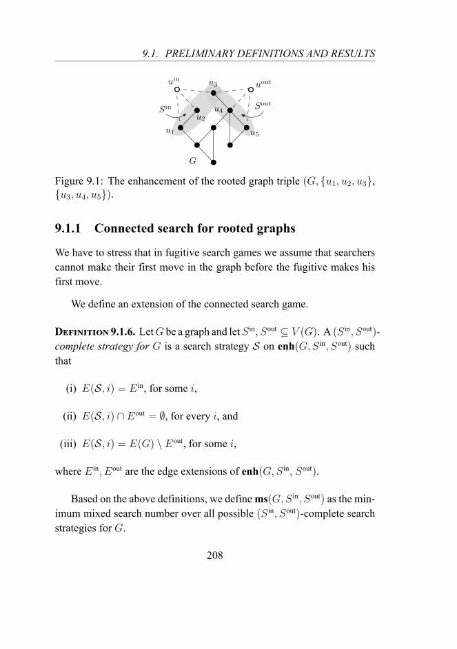
9.1. PRELIMINARY DEFINITIONS AND RESULTS
Sin Sout
uinuout
u1
u2
u3
u4
u5
G
Figure 9.1: The enhancement of the rooted graph triple (G, u1, u2, u3,u3, u4, u5).
9.1.1 Connected search for rooted graphs
We have to stress that in fugitive search games we assume that searcherscannot make their first move in the graph before the fugitive makes hisfirst move.
We define an extension of the connected search game.
Definition 9.1.6. LetG be a graph and letS in, Sout ⊆ V (G). A (S in, Sout)-complete strategy for G is a search strategy S on enh(G,S in, Sout) suchthat
(i) E(S, i) = E in, for some i,
(ii) E(S, i) ∩ Eout = ∅, for every i, and
(iii) E(S, i) = E(G) \ Eout, for some i,
where E in, Eout are the edge extensions of enh(G,S in, Sout).
Based on the above definitions, we define ms(G,S in, Sout) as the min-imum mixed search number over all possible (S in, Sout)-complete searchstrategies for G.
208

CHAPTER 9. CONNECTED GRAPH SEARCHING
Similarly, we definemms(G,S in, Sout) and cmms(G,S in, Sout)where,in the case of connected searching, we additionally demand that S in in-duces a connected subgraph of G. Notice that ms(G) = ms(G, ∅, ∅) andthat this equality also holds for mms and cmms.
9.1.2 Expansions
Now we introduce a graph parameter equivalent to the search game de-fined in the previous paragraph. This parameter is defined using layoutsof edge sets.
Definition 9.1.7. Given a graph G and a set F ⊆ E(G), we define theboundary of F as follows:
∂G(F ) = (∪e∈F
e) ∩ (∪
e∈E(G)\F
e)
Definition 9.1.8. LetG be a graph and letE1 andE2 be subsets ofE(G).An (E1, E2)-expansion of G is an ordering E = ⟨A1, . . . , Ar⟩ where:
(1) For i ∈ 1, . . . , r − 1, E1 ⊆ Ai ⊆ E(G) \ E2.
(2) For i ∈ 1, . . . , r − 1, |Ai+1 \ Ai| ≤ 1.
(3) A1 = E1.
(4) Ar = E(G) \ E2.
Definition 9.1.9. LetG be a graph and letE1 andE2 be subsets ofE(G).An (E1, E2)-expansion of G is connected if, in addition to conditions (1)to (4), the following condition also holds:
(5) For i ∈ 1, . . . , r, G[Ai] is connected.
209

9.1. PRELIMINARY DEFINITIONS AND RESULTS
Definition 9.1.10. Let G be a graph and let E1 and E2 be subsets ofE(G). An (E1, E2)-expansion of G is monotone if, in addition to condi-tions (1) to (4), the following condition also holds:
(6) A1 ⊆ · · · ⊆ Ar.
Definition 9.1.11. Let i ∈ 1, . . . , r − 1. The cost of an expansion Eat position i is defined as costG(E , i) = |∂G(Ai)|+ qi where qi is equal to1 if one of the following holds:
- |Ai| ≥ 2 and Ai \ Ai−1 contains a pendant edge of G
- Ai consists of only one edge that is an isolated edge of G.
If none of the above two conditions hold then qi is equal to 0. The costof the expansion E , denoted as costG(E), is the maximum cost of E amongall positions i ∈ 1, . . . , r − 1.
Our parameter, denoted by p(G,S in, Sout) 2, is defined to be the min-imum cost that an (E in, Eout)-expansion of enh(G,S in, Sout) may have,where E in, Eout are the edge extensions of enh(G, S in, Sout).
We also define mp(G,S in, Sout) (if we consider only monotone (E in,
Eout)-expansions) and cmp(G,S in, Sout) (if we consider connected mono-tone (E in, Eout)-expansions). We finally define cmp(G) = cmp(G, ∅, ∅).
Lemma 9.1.1. Let (G,S in, Sout) be a rooted graph and let S in1 ⊆ S in and
Sout1 ⊆ Sout, whereG[Sin] is a connected subgraph of G. Then cmp(G,S in
1 ,
Sout1 ) ≤ cmp(G,S in, Sout).
Proof. Let E in, Eout and E in1 , E
out1 be the edge extensions of enh(G,S in,
Sout) and enh(G,S in1 , S
out1 ) respectively. Notice that, as S in
1 ⊆ S in andSout1 ⊆ Sout, E in
1 ⊆ E in and Eout1 ⊆ Eout.
2Due to lack of inspiration we do not give a distinct name to this parameter...
210

CHAPTER 9. CONNECTED GRAPH SEARCHING
Let E = ⟨A1, . . . , Ar⟩ be an monotone and connected (E in, Eout)-expansion of enh(G,S in, Sout), with cost at most k.
As G[S in] is a connected subgraph of G, for every vertex of S in \ S in1
there exists a path connecting it with a vertex of S in1 that only uses vertices
of S in. We define the following edge sets:
• E11 contains all edges that have a vertex ofS in
1 and a vertex ofS in\S in1
as endpoints. Let V1 = (∪e∈E1
1e) \ S in
1 , then E21 contains all edges
that have both endpoints in V1.
• E1j contains all edges that have a vertex of Vj−1 and a vertex of S =
S in \ (S in1 ∪ (
∪l=1...,j−1 Vl)) as endpoints. Let Vj = (
∪e∈E1
je) \ S,
then E2j contains all edges that have both endpoints in Vj .
For each edge set Eij , 1 ≤ j ≤ d and i ∈ 1, 2, where d is the
maximum distance between a vertex of S in \S in1 to some vertex in S in
1 , wedefine arbitrarily an edge ordering Lij . We then define an ordering E1 ofedge sets as follows:
• A′1 = (A1 \ E in) ∪ E in
1
• A′
1+l = A′
1+l−1 ∪ Al for l = 1, . . . , |E11 |, where ⟨A1, . . . , A|E1
1 |⟩ =
prefsec(L11)
• A′
1+|E11 |+l
= A′
1+|E11 |+l−1
∪Al, for l = 1, . . . , |E21 |, where ⟨A1, . . . , A|E2
1 |⟩= prefsec(L2
1)
• A′
1+|E11 |+|E2
1 |+···+|E1j−1|+|E2
j−1|+l= A
′
1+|E11 |+|E2
1 |+···+|E1j−1|+|E2
j−1|+l−1∪ Al,
for l = 1, . . . , |E1j |, where ⟨A1, . . . , A|E1
j |⟩ = prefsec(L1j)
• A′
1+|E11 |+|E2
1 |+···+|E1j−1|+|E2
j−1|+|E1j |+l
=A′
1+|E11 |+|E2
1 |+···+|E1j−1|+|E2
j−1|+|E1j |+l−1
∪ Al, for l = 1, . . . , |E2j |, where ⟨A1, . . . , A|E2
j |⟩ = prefsec(L2j)
211

9.1. PRELIMINARY DEFINITIONS AND RESULTS
Sin1
Sin2
Sin3
Sin4
Sin5
Sout1
Sout2 Sout
3
Sout4
Sout5
G1 G2 G3 G4 G5
Figure 9.2: glue(G1,G2,G3,G4,G5).
Let s = |E11 | + |E2
1 | + · · · + |E1d | + |E2
d |. Notice that there exist al0 ∈ 2, . . . , r such that A′
1+s = (Al0 \ E in) ∪ E in1 . We define a second
ordering E2 of edge sets as follows: A′
1+s+l = (Al0+l \ E in) ∪ E in1 for
l = 1, . . . , r − l0.Clearly, E ′ = E1 E2 satisfies conditions (1) to (4) and therefore is an
(E in1 , E
out1 )-expansion of enh(G,S in
1 , Sout1 ). Moreover, the monotonicity
and connectivity of E ′ follows from the monotonicity and connectivity ofE .
Notice that, for every i ∈ 1, . . . , r, ∂G(Ai) = ∂G((Ai \ E in) ∪ E in1 )
therefore costG(E ′, i) ≤ costG(E , i). From this we conclude that E ′ hascost at most k.
We need an operation that will “glue together” rooted graphs by iden-tifying their “in” and “out” roots.
Definition 9.1.12. Let G1, . . . ,Gr be rooted graphs such that Gi =
(Gi, Sini , S
outi ) where V (Gi)∩V (Gi+1) = Sout
i = S ini+1, i ∈ 1, . . . , r−1.
We define, glue(G1, . . . ,Gr) = (G1∪· · ·∪Gr, Sin1 , S
outr ) (see Figure 9.2).
Lemma 9.1.2. Let G1, . . . ,Gr be rooted graphs such that Gi = (Gi, Sini
,Souti ) where V (Gi) ∩ V (Gi+1) = Sout
i = S ini+1, i ∈ 1, . . . , r − 1. Then
cmp(glue(G1, . . . ,Gr)) ≤ maxcmp(Gi) | i ∈ 1, . . . , r.
212

CHAPTER 9. CONNECTED GRAPH SEARCHING
Proof. Let E ini , E
outi be the edge extensions and Ei = ⟨Ai1, . . . , Aili⟩ be an
monotone and connected (E ini , E
outi )-expansion of enh(Gi, S
ini , S
outi ), for
every i ∈ 1, . . . , r. Clearly E = ⟨A11, . . . , A
1l1, A1
l1∪ A2
2, . . . , A1l1∪
A2l2, . . . , (∪1≤i<rA
ili) ∪ Ar2, . . . , (∪1≤i<rA
ili) ∪Arlr⟩ is an (E in
1 , Eoutr )-ex-
pansion of glue(G1, . . . ,Gr) and, as expansions Ei, i ∈ 1, . . . , r aremonotone and connected, conditions (5) and (6) hold.
We observe that costG1∪···∪Gr(E) ≤ maxcostG1(E1), . . . , costGr(Er),therefore cmp (glue(G1, . . . ,Gr)) ≤ maxcmp(Gi) | i ∈ 1, . . . , r.
Now we show the equivalence of our search game number to the pa-rameter defined above.
Lemma 9.1.3. For every graphG, cmms(G,S in, Sout) = cmp(G,S in, Sout).
Proof. Assume that G∗ = enh(G,S in, Sout) has a complete search strat-egy S satisfying conditions (i) – (iii) with cost at most k. We construct anedge ordering of E(G) as follows.
Observe that, because of the monotonicity of S, E(i) = E(S, i) \E(S, i−1). For every i ∈ 1, . . . , |S|, we define Li by taking any order-ing of the setE(i) and insisting that, ifE(i) contains some sliding edge, thisedge will be the first edge of Li. Let E = ⟨A0, . . . , Ar⟩ be the sequence ofprefixes of L1 . . .L|S|, including the empty set (that isA0 = ∅). Noticethat, because of Condition (i), As = E in for some s ∈ 1, . . . , |S|, and,because of Condition (iii), At = E(G) \ Eout, for some t ∈ 1, . . . , |S|.We now claim that E ′ = ⟨As, . . . , At⟩ is an (E in, Eout)-expansion of G∗.Indeed, Condition (1) holds because of Condition (ii) and Conditions (2)– (4) hold because of the construction of E ′. Moreover, the connectivityand the monotonicity of E ′ follow directly from the connectivity and themonotonicity of S.
It remains to prove that the cost of E ′ is at most k. For each j ∈0, . . . , |E ′| we define ij such that the unique edge in Aj \ Aj−1 is anedge in E(ij) and we define hj such that Ahj \ Ahj−1 contains the fist
213

9.1. PRELIMINARY DEFINITIONS AND RESULTS
edge of Lij . Notice now that the cost of E ′ at positions hj to j is upperbounded by the cost of E ′ at position hj . Therefore, it is enough to provethat the cost of E ′ at position hj is at most k. Recall that this cost is equalto |∂G(Ahj)|+ qhj . We distinguish two cases:
Case 1. If qhj = 0, then the cost of E ′ at position hj is equal to |∂G(Ahj)|.As S is monotone, all vertices in ∂G(Ahj) should be occupied by searchersafter the ij-th move of S and therefore the cost of E ′ at position hj is atmost k.
Case 2. If qhj = 1, then the ij-th move of S is either the placement of asearcher on a pendant vertex x or the sliding of a searcher along a pendantedge y, x towards its pendant vertex x. In both cases, x ∈ ∂G(Ahj)
and all vertices in ∂G(Ahj) should be occupied by searchers after the ij-thmove. In the first case, there are in total at least |∂G(Ahj)| + 1 searcherson the graph and we are done. In the second case, we observe that, dueto monotonicity, ∂G(Ahj) = ∂G(Ahj−1) \ y. As after the (hj − 1)-thmove all vertices of ∂G(Ahj−1) were occupied by searchers, we obtain that|∂G(Ahj)| ≤ k − 1 and thus the cost of E ′ at position hj is at most k.
Now assume that there exist a monotone and connected (E in, Eout)-expansion of G∗, say E = ⟨A1, . . . , Ar⟩, with cost at most k. We canadditionally assume that E is properly monotone; this can be done by dis-carding additional repetitions of a set in E .
Moreover, starting from E , we can construct a monotone and con-nected (E in,Eout)-expansion ofG∗, with cost at most k, say E ′ = ⟨A′
1, . . . ,
A′r⟩, with the following additional property:
Expansion property: For every i ∈ 1, . . . , r − 1 for which V (A′i) ⊂
V (A′i+1), A′
i contains all edges of G∗ with both endpoints in V (A′i).
This can be accomplished by a series of appliances of the following
214

CHAPTER 9. CONNECTED GRAPH SEARCHING
rule:
Rule: Let V (Ai) ⊂ V (Ai+1) for some i and let L = ⟨e1, . . . , en⟩ bean ordering of the edges E(G∗) \ Ai with both endpoints in V (Ai). Forevery j ≤ i define A′
j = Aj . Then, define A′i+1 = Ai ∪ e1, A′
i+2 =
Ai∪e1, e2 and so on, untilA′i+n = Ai∪e1, . . . , en. Finally, for every
j ≥ i+ n, define A′j = Aj ∪ e1, . . . , en.
One can easily check that, after every application of this rule, the con-structed sequence of edge sets is indeed an (E in, Eout)-expansion of G∗
and, furthermore, it is monotone and connected. Notice that, for j =
1, . . . , n, ∂G∗(A′i+j) ⊆ ∂G∗(Ai) and for j ≥ i+n, |∂G∗(A′
j)| ≤ |∂G∗(Aj)|.Moreover, if |Ai| ≥ 2 and Ai \ Ai−1 contains a pendant edge of G∗ thenfor every j ∈ 1, . . . , n, |A′
i+j| ≥ 2 and A′i+j \A′
i+j−1 contains the samependant edge of G∗, hence the cost of E ′ is at most k (notice that if Aiconsists of only one edge that is an isolated edge ofG∗ then there does notexist an edge in E(G∗) \ Ai with both endpoints in V (Ai), therefore wedo not need to apply this rule).
For the rest of the proof, we consider that the Expansion property holdsfor the given (E in, Eout)-expansion of G∗.
Our target is to define a (S in, Sout)-complete monotone search strategyS of G∗ with cost at most k.
The first |S in| moves of S will be p(uin) and the next |S in| will bes(uin, vin
i ). We denote this sequence of moves by S0. Notice that E(S ,2|S in|) = A1.
For every vertex u in the set V ∗ = V (G∗) \ S in \ uout, we define luto be the first integer in 1, . . . , r such that u ∈ V (Alu).
Let L = ⟨u1, . . . , u|V ∗|⟩ be an ordering of V ∗ such that i ≤ j whenlui ≤ luj . Notice that, for each i ∈ 1, . . . , |V ∗|, the vertex ui is anendpoint of the unique edge ei in Alui−1 \ Alui and let vi be the otherendpoint of ei. Notice that, due to the connectivity and the monotonicityof E , vi ∈ ∂G∗(Alui−1). We also observe that ui is pendant if and only
215

9.1. PRELIMINARY DEFINITIONS AND RESULTS
if ui ∈ ∂G∗(Alui ). We define E ′ = e1, . . . , e|V ∗| and we call a set Aj ,j ∈ 1, . . . , r, crucial if and only if |Aj−1 ∩ E ′| < |Aj ∩ E ′|.
For each i ∈ 1, . . . , |V ∗|, we define a sequence Si of moves as fol-lows: If vi ∈ ∂G∗(Alui ) then the first move of Si is p(ui), otherwise itis s(vi, ui). The rest of the moves in Si are the removals – one by one– of the searchers in ∂G∗(Alui−1) \ ∂G∗(Alui ). Then, we define S =
S0 S1 · · · S|V ∗|.Notice that, according to the expansion property, all edges of the sets
Aj , for j = 1, . . . , lu1 have both endpoints in S in. Moreover, for every i ∈1, . . . , |V ∗| − 1 all edges of the sets Aj , for j = lui , . . . , lui+1− 1, haveboth endpoints inV (Alui ) and all edges of the setsAj , for j = lu|V ∗| , . . . , r,have both endpoints in V (Alu|V ∗|
).
First we show that the following claim is true:
Claim 6. For everyAj , j ∈ 1, . . . , r, the vertices of ∂G∗(Aj) are exactlythe vertices occupied by searchers after the last move of Smj
, where mj
is the index of the edge in (A ∩ E ′) \ (Aj−1 ∩ E ′), where A is the firstcrucial set of E such that Aj ⊆ A.
Proof of Claim 6. Clearly, this is true for A1 = E in. Assume that it holdsfor Aj′ .
We will show that the vertices in ∂G∗(Aj′+1) are exactly the verticesoccupied by searchers after the last move of Smj′+1
.If Aj′+1 is not crucial then ∂G∗(Aj′+1) ⊆ ∂G∗(Aj′) and mj′+1 = mj′ ,
therefore Claim 6 holds.Now, if Aj′+1 is crucial and emj′+1
= (Aj′+1 ∩ E ′) \ (Aj′ ∩ E ′),then vmj′+1
∈ ∂G∗(Aj′) and, therefore, must be occupied by a searcher.We distinguish three cases:
Case 1. If vmj′+1∈ ∂G∗(Aj′+1) and umj′+1
∈ ∂G∗(Aj′+1), then ∂G∗(Aj′+1)
= ∂G∗(Aj′) ∪ umj′+1 and the first move in Smj′+1
will be p(umj′+1).
216
CHAPTER 9. CONNECTED GRAPH SEARCHING
Case 2. If vmj′+1∈ ∂G∗(Aj′+1) and umj′+1
∈ ∂G∗(Aj′+1) then ∂G∗(Aj′+1)
= ∂G∗(Aj′).
Case 3. If vmj′+1∈ ∂G∗(Aj′+1), then ∂G∗(Aj′+1) = (∂G∗(Aj′)\vmj′+1
)∪umj′+1
, and the first move in Smj′+1will be s(vmj′+1
, umj′+1).
Observe that in all three cases the Claim 6 holds.
Let VS(i) be the set of vertices already visited by searchers after the i-th move of S, and let VS = ⟨VS(1), . . . , VS(r)⟩. Notice that this sequenceis monotone and that if the i-th move belong to the subsequence Sj , thenVS(i) = V (Aluj ). We must next prove the following:
Claim 7. For every i ∈ 1, . . . , |S|, all edges of G∗[VS(i)] are clean.
Proof of Claim 7. Clearly, the claim is true for i ∈ 1, . . . , 2 · |S in|. As-sume that it holds for some i ∈ 2 · |S in|+ 1, . . . , r, we will show that alledges of G∗[VS(i + 1)] are clean. We must distinguish three cases aboutthe (i+ 1)-th move:
Case 1. It is a removal, say r(u). Notice that G∗[VS(i+ 1)] = G∗[VS(i)],therefore the Claim will not be true if r(u) is a recontamination move. Inthis case, there exist an edge connecting u with a vertex not in VS(i), sayv. As u ∈ ∂G∗(Aluj−1) \ ∂G∗(Aluj ), for some j ∈ 1, . . . , |V ∗|, all edgeswith u as endpoint must belong to Aluj , therefore u, v ∈ Aluj . ButVS(i) = V (Aluj ), a contradiction.
Case 2. It is a placement of searcher say p(u). By the definition of S, thereexist an edge u, v, where v is a vertex in VS(i). Notice that, accordingto our search game, all such edges are clean after p(u), thus all edges ofG∗[VS(i+ 1)] are clean.
217

9.1. PRELIMINARY DEFINITIONS AND RESULTS
Case 3. It is a slide, say s(vj, uj), for some j ∈ 1, . . . , |V ∗|. As in theprevious case,G∗[VS(i+1)] contains all edges ofG∗[VS(i)] and additionalall edges with uj as the first endpoint and a vertex v ∈ VS(i) as the other.According to our search game, after the i-th move there must be searcherin vj , therefore due to Claim 6, vj ∈ ∂G∗(Aluj ). Notice that, the Claimwill not be true if s(vj, uj) is a recontamination move, i.e., there exist anedge connecting vj with a vertex, say u, not in VS(i) = V (Aluj ). Asvj ∈ ∂G∗(Aluj ), all edges with u as endpoint must belong to Aluj , there-fore vj, u ∈ Aluj , a contradiction.
In all three cases we saw that after the (i + 1)-th move of S all edgesof G∗[VS(i+ 1)] are clean, therefore Claim 7 is true.
We will now prove that S is a (S1, S2)-complete strategy for G∗.Clearly, Condition (i) holds for every strategy starting with S0. More-
over, Condition (ii) holds as vout is not a vertex of V ∗ and therefore, noplacement on uout or sliding towards uout appears inS . Notice that, accord-ing to Claim 7, for every i ∈ 1, . . . , |V ∗|−1,E(S, |S0· · ·Si−1|+1) =
· · · = E(S, |S0 · · · Si−1| + |Si|) = Alui+1−1, and that for i = |V ∗|,E(S, |S0 · · · S|V ∗||) = Ar, therefore Condition (iii) holds.
By the definition of S , it is clear that S is a connected search strategy,moreover, according to Claim 7, S is monotone.
It remains to prove that S has cost at most k. For the first 2|S in|moves, we use |S in| = costG∗(E , 1) ≤ k searchers. Assume that af-ter j moves exactly k searchers are occupying vertices of G∗ and thatthe (j + 1)-th move is p(ui), for some i ∈ i, . . . , |V ∗|. Then the ver-tices in ∂G∗(Alui−1) are exactly the vertices occupied by the k searchers,therefore |∂G∗(Alui−1)| = k. Observe that, if ui is not pendant, then∂G∗(Alui ) = ∂G∗(Alui−1)∪ ui, therefore |∂G∗(Alui )| = k + 1, a contra-diction and if ui is pendant then ∂G∗(Alui ) = ∂G∗(Alui−1) and the cost ofE at position lui is |∂G∗(Alui )| + 1 = k + 1, again a contradiction. Thus,for every move of S at most k searchers are occupying vertices ofG∗.
218

CHAPTER 9. CONNECTED GRAPH SEARCHING
9.1.3 Contractions
As we consider rooted graphs instead of regular graphs, we need to givenew definitions for the contraction and minor relations, that will still beconsistent with the definitions we gave in Chapter 6. We may define themfor rooted graphs at first, but then, by taking S in
1 = Sout1 = ∅, we will
restrict them to graphs.
Definition 9.1.13. Let (G1, Sin1 , S
out1 ) and (G2, S
in2 , S
out2 ) be rooted graphs.
We say that (G1, Sin1 , S
out1 ) is a (rooted) contraction of (G2, S
in2 , S
out2 ) and
we denote this fact by (G1, Sin1 , S
out1 ) ≤c (G2, S
in2 , S
out2 ) if there exists a
surjection ϕ : V (G2)→ V (G1) such that:
(1) for every vertex v ∈ V (G1), G2[ϕ−1(v)] is connected,
(2) for every two distinct vertices u, v ∈ V (G1), it holds that v, u ∈E(G1) if and only if the graph G2[ϕ
−1(v) ∪ ϕ−1(u)] is connected,
(3) ϕ(S in2 ) = S in
1 , and
(4) ϕ(Sout2 ) = Sout
1 .
We will often write (G1, Sin1 , S
out1 ) ≤ϕc (G2, S
in2 , S
out2 ) to make clear
that the function certifying the contraction relation is ϕ. Notice that G1 isa contraction of G2 if (G1, ∅, ∅) ≤c (G2, ∅, ∅).
We can define the (rooted) minor relation for two rooted graphs byremoving in the second property the demand that if u, v /∈ E(G1)
then G2[ϕ−1(v) ∪ ϕ−1(u)] is not connected. We denote the minor rela-
tion by (G1, Sin1 , S
out1 ) ≤m (G2, S
in2 , S
out2 ). Notice that G1 is a minor of G2
if (G1, ∅, ∅) ≤m (G2, ∅, ∅).
Lemma 9.1.4. If (G1, Sin1 , S
out1 ) and (G2, S
in2 , S
out2 ) are rooted graphs and
(G1, Sin1 , S
out1 ) ≤c (G2, S
in2 , S
out2 ), then cmp(G1, S
in1 , S
out1 )) ≤ cmp(G2, S
in2 ,
Sout2 )).
219

9.1. PRELIMINARY DEFINITIONS AND RESULTS
Proof. Suppose that E = ⟨A1, . . . , Ar⟩ is a monotone (E in2 , E
out2 )-expan-
sion of G∗2 = enh(G2, S
in2 , S
out2 ) with cost at most k. Our target is to
construct a monotone (E in1 , E
out1 )-expansion of G∗
1 = enh(G1, Sin1 , S
out1 )
with cost at most k.Let ϕ be a function where (G1, S
in1 , S
out1 ) ≤ϕc (G2, S
in2 , S
out2 ). We con-
sider an extension ψ of ϕ that additionally maps uin2 to uin
1 and uout2 to uout
1 .Notice that the construction of ψ yields the following:
(G∗1, S
in1 ∪ uin
1 , Sout1 ∪ uout
1 ) ≤ϕc (G∗2, S
in2 ∪ uin
2 , Sout2 ∪ uout
2 )
Given an edge f = x, y ∈ E(G1) we consider the setEf containingall edges of G2 with one endpoint in ψ−1(x) and one endpoint in ψ−1(y).We now pick – arbitrarily – an edge in Ef and we denote it by ef . Wealso set E ′ = ef | f ∈ E(G1). Then it is easy to observe that E ′ =⟨A1 ∩ E ′, . . . , Ar ∩ E ′⟩ is a connected expansion of G∗
1 and that the costof E ′ at step i is no bigger than the cost of E at the same step, wherei ∈ 1, . . . , r − 1.
Lemma 9.1.5. If G1 and G2 are two graphs and G1 ≤c G2, then cms(G1)
≤ cms(G2).
Proof. First observe that, if this is the case, any contraction of G2 can bederived by applying a finite number of edge-contractions of some edgesin E(G2).
It suffices to prove that the lemma holds if G1 is obtained by the con-traction of edge e = u, v ∈ E(G1) to vertex xuv. Let S be a connectedsearch strategy for G2 that – in any step – uses at most k searchers. Basedon S we will construct a search strategy S ′ for G1. Let i be an integer in1, . . . , |S|. We distinguish eight cases:
Case 1: If the i-th move of S is p(x) for some vertex x /∈ u, v, then thenext move of S ′ will be p(x).
220

CHAPTER 9. CONNECTED GRAPH SEARCHING
Case 2: If the i-th move of S is r(x) for some vertex x /∈ u, v, then thenext move of S ′ will be r(x).
Case 3: If the i-th move of S is s(x, y) for some vertices x, y /∈ u, v,then the next move of S ′ will be s(x, y).
Case 4: If the i-th move of S is p(u) or p(v), then the next move of S ′
will be p(xuv).
Case 5: If the i-th move of S is r(u) or r(v), then the next move of S ′ willbe r(xuv).
Case 6: If the i-th move of S is s(z, u) or p(z, v) for some vertex z, thenthe next move of S ′ will be s(z, xuv).
Case 7: If the i-th move of S is s(u, z) or p(v, z) for some vertex z, thenthe next move of S ′ will be s(xuv, z).
Case 8: If the i-th move of S is s(u, v) or p(v, u), then the next move ofS ′ will be defined according the lateral cases from the (i+1)-th move ofS .
Observe that S ′ is a complete search strategy for G1. Furthermore, asS is connected, S ′ must also be connected. Finally, it is clear that S ′ – atany step – uses at most k searchers, thus cms(G1) ≤ k.
9.1.4 Cut-vertices and blocks
Let us fix some more notation. Recall that the blocks of a graph G areits 2-connected components. If the removal of an edge in G increases thenumber of its connected components, then it is called a bridge. In whatfollows we will consider the subgraphs of G induced by the endpoints of
221

9.1. PRELIMINARY DEFINITIONS AND RESULTS
bridges as blocks and we call them trivial blocks of G.
Definition 9.1.14. Let G be a graph and B a block of G. A cut-vertexof G is a vertex such that G \ x has more connected components than G.A cut-vertex of B is a cut-vertex of G belonging to V (B).
The following two definitions may be highly technical but are veryhelpful for the proofs of Section 9.2.
Definition 9.1.15. Let G bet a graph and let x ∈ V (G). We define
CG(x) = (x,G[V (C) ∪ x]) | C is a connected component of G \ x.
Definition 9.1.16. Let B be a block of G and let x be a cut-vertex of B.We denote by CG(x,B) the (unique) graph in CG(x) that contains B as asubgraph and by CG(x,B) the graphs in CG(x) that do not contain B.
Recall the definition of graph embeddings in Rd (Definition 5.1.4). Aplane embedding E2(G) = (f, C) of a graph G is an embeddings in R2
such that the interior of each curve in C contains neither a point f(u), forsome u ∈ V (G), nor a point of another curve in C. Notice that, given aplane embedding of G the set R2 \ E2(G) defined when we subtract fromR2 the points f(u) | u ∈ V (G) corresponding to the vertices of G, andthe points
∪c∈C C of the curves corresponding to the edges of G, is open.
The regions of R2 \E2(G) are the faces of E2(G). We define the outer faceand the inner faces of E2(G) in the same way we did in Definition 2.5.2.
Definition 9.1.17. A graph G is outerplanar if there is a plane embed-ding of G such that all its vertices are incident to the outer face.
This embedding, when it exists, is unique up to homeomorphism.
From now on, each outerplanar graph G is accompanied with such anembedding, say E2(G) = (f, C). We will refer to the elements of f(V )
222

CHAPTER 9. CONNECTED GRAPH SEARCHING
Essential Block
ii
Cycle blocks
h
hh
h
h
hA chord
An outer edge Hair Blocks
Essential Block
Bridge Block
1
Figure 9.3: An outerplanar graph and its blocks. The cut-vertices arehexagonal and the outer vertices are squares. Inner and haploid faces aredenoted by “i” and “h” respectively. There are, in total, four inner vertices(all belonging to the essential block on the right) and, among them onlythe triangular one is not an haploid vertex. The white hexagonal verticesare the light cut-vertices while the rest of the hexagonal vertices are theheavy ones.
and C as the vertices and edges of E2(G) respectively and, to keep thinkssimple, we will identify them with the “real” vertices and edges of G.
An edge e ∈ E(G) is called outer edge of G, if it is incident to theouter face of G, otherwise it is called a chord of G.
A face F of an outerplanar graph that is different than the outer face,is called haploid if and only if at most one edge incident to F is a chord,otherwise F is a inner face. A vertex u ∈ V (G) is haploid if it is incidentto an haploid face and inner if it is incident to an inner face (notice thatsome vertices can be both inner and haploid). A vertex of G that is notinner or haploid is called outer. We call a chord haploid if it is incident toan haploid face. Non-haploid chords are called internal chords.
Observation 9.1.1. A block of a connected outerplanar graph with morethan one edge can be one of the following.
223

9.1. PRELIMINARY DEFINITIONS AND RESULTS
K4K2,3 K
+2,3
2
Figure 9.4: The set O1.
- A hair block: It is a trivial block containing exactly one vertex ofdegree 1 in G.
- A bridge block: It is a trivial block that is not a hair-block.
- A cycle block: If it is a chordless non-trivial block.
- An essential block: If it is a non-trivial block with at least one chord.
Let G be a connected outerplanar graph with more than one edge.Given a cut-vertex c of G, we say that c is light if it is the (unique) cut-vertex of exactly one hair block. If a cut-vertex of G is not light then it isheavy (see Figure 9.10 for an example).
It is known that the class of outerplanar graphs is closed under the rela-tions≤m,≤c and, without much effort, one can derive from Theorem 2.5.2the following.
Theorem 9.1.1. A graph is outerplanar if and only if K4 ≰m G andK2,3 ≰m G.
Let K+2,3 be the graph obtained by K2,3 after connecting the two ver-
tices of degree 3 (Figure 9.4).
Lemma 9.1.6. IfH is the class of all outerplanar graphs, then obs≤c(H) =O1, where O1 is shown in Figure 9.4.
224

CHAPTER 9. CONNECTED GRAPH SEARCHING
Proof. Observe that the graphs in O1 cannot be embedded in the planein such a way that all of its vertices are incident to a single face, and,therefore, neither the graphs in O1, neither the graphs that contain as acontraction a graph in O1, can be outerplannar.
To complete the proof, one must show that every non-outerplannargraph can be contracted to a graph inO1. LetG be non-outerplannar, thenK4 ≤m G or K2,3 ≤m G. Clearly, as K4 is a clique, K4 ≤m G impliesthat K4 ≤c G. Suppose now that K2,3 ≤m G. Let Vx, Vy, V1, V2, V3 be thevertex sets of the connected subgraphs of G that are contracted towardscreating the vertices ofK2,3 (Vx and Vy are contracted to vertices of degree3). If there is no edge in G between two vertices in Va and Vb for some(a, b) ∈ (x, y), (1, 2), (2, 3), (1, 3) then K2,3 ≤c G. If the only suchedge is between Vx and Vy then K+
2,3 ≤c G and in any other case, K4 ≤c
G.
9.2 Obstructions for Graphs With cms/cmmsat Most 2
In this Section we define a “candidate” contraction obstruction set forgraphs with connected monotone mixed search number at most 2, namelythe setD1 defined below. This set consists of 177 graphs. Then, we provea series of lemmata, each providing some information about the structureof the graphs that can be searched with at most two searchers, using a con-nected and monotone mixed search strategy. Combining all these lemmatawe will prove that D1 is the correct obstruction set.
Definition 9.2.1. Let D1 = O1 ∪ · · · ∪ O12 where O1 is depicted inFigure 9.4, O2, . . . ,O9 are depicted in Figure 9.5 and O10 and O11 andO12 are constructed as follows.
O10 : Contains every graph that can be constructed by taking three dis-
225

9.2. OBSTRUCTIONS FOR GRAPHS WITH CMS/CMMS AT MOST 2
O4O2 O5O3
O6
O8
O7
O9
3
Figure 9.5: Some of the sets of graphs in Definition 9.2.1.
joint copies of some graphs in Figure 9.10 and then, identify thevertices denoted by v in each of them to a single vertex. There are– in total – 35 graphs generated in this way.
O11 : Contains every graph that can be constructed by taking two disjointcopies of some graphs in Figure 9.14 and then, identify the verticesdenoted by v in each of them to a single vertex. There are – in total– 78 graphs generated in this way.
O12 : Contains every graph that can be constructed by taking two disjointcopies of some graphs in Figure 9.15 and then, identify the verticesdenoted by v in each of them to a single vertex. There are – in total– 21 graphs generated in this way.
Notice that, D1 indeed contains 177 graphs.
226

CHAPTER 9. CONNECTED GRAPH SEARCHING
9.2.1 Proof strategy
We will prove that D1 is the obstruction set we are looking for, in twosteps. One easy (Lemma 9.2.1) and one much more involved (Lemma 9.2.2).A very important part for the proof of the second step is to distinguish “im-portant blocks” from non “important ones”, namely central and extremalblocks from fans, and then define directional obstructions.
Lemma 9.2.1. D1 ⊆ obs≤c(cmp, 2).
Proof. From Lemma 9.1.4, it is enough to check that for every G ∈ D1,the following two conditions are satisfied
(i) cmp(G) ≥ 3, and
(ii) for every edge e of G it holds that cmp(G/e) ≤ 2.
One can verify that this is correct by inspection, as this concerns only afinite amount of graphs and, for each of them, there exists a finite numberof edges to contract.
Lemma 9.2.2. D1 ⊇ obs≤c(cmp, 2).
The rest of this Section is devoted to the proof of Lemma 9.2.2. Forthis, our strategy is to consider the set
Q = obs≤c(cmp, 2) \ D1
and prove that Q = ∅ (Lemma 9.2.15). To achieve this, as mentionedbefore, we have to prove a series of structural results. Their proofs use thefollowing three fundamental properties of the set Q.
Lemma 9.2.3. Let G ∈ Q. Then the following hold.
(i) cmp(G) ≥ 3.
227
9.2. OBSTRUCTIONS FOR GRAPHS WITH CMS/CMMS AT MOST 2
(ii) If H is a proper contraction of G, then cmp(G) ≤ 2.
(iii) G does not contain any of the graphs in D1 as a contraction.
Proof. Properties (i) and (ii) hold because G ∈ obs≤c(cmp, 2). For prop-erty (iii) suppose, to the contrary, that G contains some graph in H ∈ D1
as a contraction. From Lemma 9.2.1, H ∈ obs≤c(cmp, 2). Clearly, His different than G as Q does not contain members of D1. Therefore, His a proper contraction of G and, from property (ii), cmp(H) ≤ 2. Thiscontradicts to the fact thatH ∈ obs≤c(cmp, 2) and thus cmp(H) ≥ 3.
9.2.2 Basic structural properties
Lemma 9.2.4. Let G ∈ Q. The following hold:
1. G is outerplanar.
2. Every light cut-vertex of G has degree at least 3.
3. Every essential block B of G, has exactly two haploid faces.
4. Every block of G, has at most 3 cut-vertices
5. Every cut-vertex of a non-trivial block of G is an haploid vertex.
6. Every block of G contains at most 2 heavy cut-vertices.
7. If a block of G has 3 cut-vertices, then there are two, say x and y,of these vertices that are not both heavy and are connected by anhaploid edge.
8. If an essential block of G with haploid faces F1 and F2 has twoheavy cut-vertices, then we can choose one, say c1, of these twoheavy cut-vertices so that it is incident to F1 and one say c2 that isincident toF2. Moreover, this assignment can be done in such a way
228

CHAPTER 9. CONNECTED GRAPH SEARCHING
that if there is a third light cut-vertex c3, adjacent to one, say c1, ofc1, c2, then c3 is incident to F1 as well.
Proof. 1. By the third property of Lemma 9.2.3, G cannot be contractedto a graph inO1 and therefore, from Lemma 9.1.6,Gmust be outerplannar.
2. Let c be a light cut-vertex of a block B in G, with degree 2 (noticethat, as c is a cut-vertex, c cannot have degree 1 or 0). That means thatc belongs to a path with at least two edges, the hair block B and an edgesay e. Observe that cmp(G/B) = cmp(G), contradicting to the secondproperty of Lemma 9.2.3.
3. LetB be an essential block ofG. As it is essential, it has at least onechord, therefore it has at least 2 haploid faces. Assume, thatB has at least3 haploid faces. Choose 3 of them, say F1, F2 and F3 (see Figure 9.6).Let S ⊆ E(B) be the set of all chords incident to B. Contract in G alledges inE(G)\S not belonging to those faces. Then, for each of the threefaces, contract all but two edges not in S that are incident to F1, F2 andF3 and notice that the obtained graph is the graph in O2, a contradictionto the third property of Lemma 9.2.3.
F1
F2
F3
Figure 9.6: An example for the proof of Lemma 9.2.4.3.
4. Let B be a block of G containing more than 3 cut-vertices. Choosefour of them, say c1, c2, c3 and c4. Let S ⊆ E(B) be the set of all chordsincident to B (see Figure 9.7). Contract all edges in E(G) \ S not having
229

9.2. OBSTRUCTIONS FOR GRAPHS WITH CMS/CMMS AT MOST 2
an endpoint in c1, c2, c3, c4. Then, contract all edges e ∈ E(B)\S suchthat e ⊈ c1, c2, c3, c4 and all edges not in E(B), except from one foreach of the cut-vertices. Notice that the obtained graph belongs to O3, acontradiction to the third property of Lemma 9.2.3.
c1
c4
c2
c3
Figure 9.7: An example for the proof of Lemma 9.2.4.4.
5. Let B be a block of G containing a cut-vertex c that is not haploidand let S ⊆ E(B) be the set of all chords incident to B (see Figure 9.8).Contract all edges in E(G) \E(B) not having c as endpoint and all edgesin E(B) \ S not having c as endpoint, except from two edges for each ofthe haploid faces. Then contract all edges not inE(B) with c as endpoint,except for one. Notice that the obtained graph belongs toO4, a contradic-tion to the third property of Lemma 9.2.3.
6. LetB be a block ofG containing three heavy cut-vertices, say c1, c2and c3 (see Figure 9.9). We contract all edges in B except from 3 so thatB is reduced to a triangle T with vertices c1, c2 and c3. Then, in the result-ing graph H , for each ci, i ∈ 1, 2, 3, in CH(ci) \ T contains either anon trivial block or at least two hair blocks. In any case, H can be furthercontracted to one of the graphs in O5 a contradiction to the third propertyof Lemma 9.2.3.
230

CHAPTER 9. CONNECTED GRAPH SEARCHING
c
Figure 9.8: An example for the proof of Lemma 9.2.4.5.
c1
c2
c3
Figure 9.9: An example for the proof of Lemma 9.2.4.6.
7. Let x, y, z be three cut-vertices of a (not-trivial) block B. If notwo of them are connected by an outer edge, then contract all blocks ofG,except B, to single edges, then contract all outer edges of B that do nothave an endpoint in x, y, z and continue contracting hair blocks with avertex of degree≥ 4, as long as this is possible. This creates either a graphin O6 or a graph that after the contraction of a hair block makes a graphin O7 or a graph that after the contraction of two hair blocks is a graphmakes a graph inO4 and, in any case, we have a contradiction to the thirdproperty of Lemma 9.2.3. We contract G to a graph H as follows:
• If for some w ∈ x, y, z the set CG(w,B) contains at least twoelements, then contract the two of them to a pendant edge (that willhave w as an endpoint) and the rest of them to w.
• If for some w ∈ x, y, z the set CG(w,B) contains only one ele-
231

9.2. OBSTRUCTIONS FOR GRAPHS WITH CMS/CMMS AT MOST 2
ment that is not a hair, then contact it to a triangle (notice that thisis always possible because of 2).
Case 1. |V (B)| ∈ 3, 4. Then because of 6, one, say x of x, y, z isnon-heavy and there is an outer edge connecting x with one, say y, vertexin x, y, z. Then x, y is the required pair of vertices.
Case 2. |V (B)| > 4 and there is at most one outer edge e with endpointsfrom x, y, z in H . W.l.o.g., we assume that e = x, y. Notice e is ahaploid edge, otherwiseH can be contracted to the 5th graph inO6. More-over at least one of x, y is non-heavy, otherwiseH can be contracted to oneof the graphs inO8∪O9 (recall thatB may have one or two haploid faces).
Case 3. There are two outer edges with endpoints from x, y, z. W.l.o.g.,we assume that these edges are x, y and y, z. One, say x, y, ofx, y, y, z is haploid, otherwise H can be contracted to some graph inO4. If x, y has a light endpoint, then we are done, otherwise, from 6,z is light. In this remaining case, if if z, y is haploid, then it is also therequired edge, otherwise H can be contracted to a graph in O9.
8. Let x and y be two heavy cut-vertices vertices of B. From 5, x, yare among the vertices that are incident to the faces F1 and F2. Suppose,in contrary, that for some face, say F ∈ F1, F2, there is no cut vertexin x, y that is incident to F . Then G can be contracted to one of thegraphs in O9. This is enough to prove the first statement except from thecase where x and y are both lying in both haploid faces and there is athird light cut-vertex z incident to some, say x, of x, y. In this case, x isassigned the face where z belongs and y is assigned to the other.
Let G ∈ Q and let B be a block of G. Let also S be the set of cutvertices of G that belong to B. According to Lemma 9.2.4, we can definea rooted graph GB = (B,X, Y ) such that:
232

CHAPTER 9. CONNECTED GRAPH SEARCHING
- X, Y is a partition of S, where X and Y are possibly empty.
- If B has a chord, then all vertices in X and Y are haploid.
- |X| ≤ 1 and |Y | ≤ 2.
- If |Y | = 2, then its vertices are connected with an edge e and one ofthem is light and. Moreover, in the case where B has a chord thene is haploid.
- IfB has a chord, we name the haploid faces ofB by F1 and F2 suchthat all vertices in X are incident to F1 and all vertices od Y areincident to F2.
Lemma 9.2.5. LetG ∈ Q and letB be a block ofG. Then cmp(GB) ≤ 2.
Proof. We examine the – non-trivial – case whereB is a non-trivial blockand contains two haploid faces F1 and F2. AsB is 2-connected and outer-planar, all vertices of V (B) belong to the unique hamiltonian cycle of B,say C. Our proof is based on the fact that there are exactly two haploidfaces and this gives a sense of direction on how the search should be per-formed. To make this formal, we create an ordering A of the edges ofE(B) using the following procedure.
1. if X = ∅, then2. Q← X ,3. else4. Q← x where x is an arbitrarily chosen vertex
in the boundary of F1.5. R← Q
6. i← 1
7. while there is a vertex v in V (B) \R that is connected with some ver-tex, say u, in Q \ Y whose unique neighbor in V (B) \R is v,
8. R← R ∪ v
233

9.2. OBSTRUCTIONS FOR GRAPHS WITH CMS/CMMS AT MOST 2
v vvvv
4
Figure 9.10: The set A contains five r-graphs, each of the form (G,v, v).
9. Q← (Q \ u) ∪ v10. ei = u, v11. i← i+ 1
12. if Q ∈ E(B), then13. ei ← Q,14. i← i+ 1
15. if Y ∈ E(B), then16. ei ← Y
LetE in, Eout be the edge extensions of enh(GB), and let prefsec(A) =⟨A0, . . . , Ar⟩. It is easy to verify that E = ⟨E in, A0∪E in, . . . , Ar∪E in⟩ isa monotone and connected (E in, Eout)-expansion of enh(GB), with costat most 2.
9.2.3 Fans
LetG be a graph and v be a vertex in V (G). We denote by G(v) the rootedgraph (G, v, v) and we refer to it as the graph G doubly rooted on v.
Definition 9.2.2. A graph G, doubly rooted on some vertex v is a fan ifnone of the graphs in the set A depicted in Figure 9.10 is a contraction ofthe rooted graph G(v), and G is outerplanar.
234

CHAPTER 9. CONNECTED GRAPH SEARCHING
Fans will play an important role in this proof.
Lemma 9.2.6. LetG(v) = (G, v, v) be a graph doubly rooted at somevertex v. If G(v) is a fan, then cmp(G(v)) ≤ 2.
Proof. We claim first that ifG(v) is a fan, then the graphG\v is a collectionof paths where each of them has at least one endpoint that is a neighbour ofv. Indeed, if this is not correct, then some of the connected components ofG \ v would be contractible to either a K3 or a K1,3. In the first case, G iseither non-outperlanar or G(v) can be contracted to to the first two rootedgraphs of Figure 9.10. In the second case G is either non-outeplanar orG(v) the last three graphs of Figure 9.10. Moreover, if both endpoints ofa path in the set of connected components G \ v are non adjacent to v inG, then G(v) can be contracted to the last rooted graph in Figure 9.10.
Let now P1, . . . , Pr be the connected components of G \ v and, foreach i ∈ 1, . . . , r, let vi1, . . . , viji be the vertices of Pi, ordered as inPi, such that vi1 is adjacent to v in G. Let uin and uout be the two verticesadded in enh(G(v)). If ein = v, uin and eout = v, uout then the edgeexpansions of enh(G(v)) is E in = ein and Eout = eout.
For each i ∈ 1, . . . , r we define the edge ordering
Ai = ⟨v, vi1, vi1, vi2, v, vi2, vi2, vi3 . . . , viji , v⟩,
then we delete from Ai the edges not in E(G). Let A′i be the orderings
obtained after the edge deletions. We define A = ⟨ein⟩ A1 · · · Ar.Notice that prefsec(A) is a monotone and connected (E in, Eout)-expansionof enh(G(v)) with cost at most 2. Therefore, it holds that cmp(G(v)) ≤ 2,as required.
9.2.4 Spine-degree and central blocks
Given a graph G and a vertex v we denote by C(v)G the set of all graphs inCG(v), each doubly rooted on v. The spine-degree of v is the number of
235

9.2. OBSTRUCTIONS FOR GRAPHS WITH CMS/CMMS AT MOST 2
doubly rooted graphs in C(v)G that are not fans.A cut-vertex of a graph G is called a central cut-vertex, if it has spine-
degree greater than 1 and a block ofG is called a central block if it containsat least 2 central cut-vertices.
Lemma 9.2.7. Let G ∈ Q. The following hold:
1. All vertices of G have spine-degree at most 2.
2. None of the blocks of G contains more than 2 central cut-vertices.
3. G contains at least one central cut-vertex
4. There is a total orderingB1, B2, . . . , Br (r ≥ 0) of the central blocksofG and a total ordering c1, . . . , cr+1 of the central cut-vertices ofGsuch that, for i ∈ 1, . . . , r, the cut-vertices of Bi are ci and ci+1.
Proof. 1. Let v be a vertex of G with spine-degree at least 3. That meansthat there exist at least three subgraphs of G, doubly rooted at v, that canbe contracted to some graph in A. Therefore, G can be contracted to agraph in O10, a contradiction.
2. Suppose that B is a block of G containing 3 (or more) central cut-vertices, say c1, c2 and c3. Construct the graph H by contracting all edgesofB to a triangle T with c1, c2, c3 as vertex set. As ci is a central vertex,there is a rooted graph Ri in CG(ci) that contains some of the graphs in Aas a rooted contraction. Next we apply the same contractions to H f orevery ci, i ∈ 1, 2, 3 and then contract – to vertices – all blocks of Hdifferent than T and not contained in some Ri. It is easy to see that theresulting graph is a graph in O5, a contradiction.
3. Assume that G has no central cut-vertices. We distinguish twocases.
236

CHAPTER 9. CONNECTED GRAPH SEARCHING
Case 1. There is a cut-vertex ofG, say v, such that all rooted graphs in C(v)G
are fans and let G1, . . .Gr be these rooted graphs. From Lemmata 9.1.2and 9.2.6, we conclude that cmp(G, v, v) = cmp(glue(G1, . . .Gr))
≤ 2 and from Lemma 9.1.1, cmp(G) ≤ 2 contradicting to the first condi-tion of Lemma 9.2.3.
Case 2. For every cut-vertex v of G, at least one of the rooted graphs inC(v)G is not a fan. We denote byHv the corresponding non-fan rooted graphin C(v)G (this is unique due to the fact that v is non-central). Among all cutvertices, let x be one for which the set V (G) \ V (Hx) is maximal. Let Bbe the block of Hx that contains x and let S be the set of the cut-verticesof G that belong to B (including x).
For every y ∈ S we denote by Wy = W1y, . . . ,W
ryy the set of all
rooted graphs in C(y)G , except from the one, call it Ry, that contains B. Wealso define Wy = glue(W1
y, . . . ,Wryy ). We claim that all Wy, y ∈ S are
fans. Indeed, if for some y, Wy is a non-fan, because y is not central, Ry
should be a fan, contradicting the choice of x.According to the above, the edges of G can be partitioned to those of
the rooted graph GB and the edges in the rooted graphs Wy, y ∈ S. Letalso GB = (B,X, Y ) and we assume that, if Y = y1, y2, then y1 islight.
Notice that, according to Lemma 9.2.6 cmp(Wy) ≤ 2, y ∈ S andaccording to Lemma 9.2.5 cmp(GB) ≤ 2. We distinguish two cases.
Case 2.1. Y = y1, y2where y2 is light. Then letG1 = (G[y1, y2], y1,y2, y2) andG2 = (G[y1, y2], y2, y1). Clearly cmp(G1) = 2 andcmp(G2) = 1. Therefore, if G′ = glue(GB,G1,Wy2 ,G2,Wy1), then,from Lemma 9.1.2, cmp(G′) ≤ 2.
Case 2.2. Y = y1. Let G′ = glue(GB,Wy1), then, from Lemma 9.1.2,cmp(G′) ≤ 2.
237

9.2. OBSTRUCTIONS FOR GRAPHS WITH CMS/CMMS AT MOST 2
In both cases, if X = x, then we set G = glue(Wx,G′) while ifX = ∅ we set G = G′. In any case, we observe that, from Lemma 9.1.2,cmp(G) ≤ 2. From Lemma 9.1.1, cmp(G) ≤ 2 contradicting to the firstcondition of Lemma 9.2.3.
As in both cases we reach a contradiction, G must contain at least onecentral cut-vertex.
4. Let C be the set of all central cut-vertices of G. For each c ∈ C,let Xc be the subset of C(v)G that contains all its members that are not fans.Clearly,Xc contains exactly two elements. Notice that none of the verticesinC\c belongs in the double rooted graphs in C(v)G \Xc. Indeed, if this isthe case for some vertex y ∈ C \ c, then the member of C(y)G that avoidsc would be a subgraph of some member of C(v)G \Xc, and this would implythat some fan would contain as a contraction some double rooted graphthat is not a fan. We conclude that, for each c ∈ C there is a partitionp(c) = (Ac, Bc) of C \c such that all members ofAc are vertices of oneof the members of Xc and all members of Bc are vertices of the other.
We say that a vertex c ∈ C is extremal if p(c) = ∅, C \ c
We claim that for any three vertices x, y, z of C, there is one, sayy of them such that x and z belong in different sets of p(y). Indeed, ifthis is not the case, then one of the following would happen: Either thereis a vertex w ∈ C such that x, y, z belong to different elements of C(w)G ,a contradiction to the first statement of this lemma, or x, y, and z belongto the same block of G, a contradiction to the second statement of thislemma.
By the claim above, there is a pathP containing all central cut-verticesinC. We can assume that this path is of minimum length, which permits usto further assume that its endpoints are extremal vertices of C. Moreover,heavy cut-vertices in V (P ) are members ofC. Let c1, . . . , cr+1 be the cen-tral cut-vertices ordered as they appear in P . As, for every i ∈ 1, . . . , rthere is a blockBi containing the central cut-vertices ci and ci+1 we end up
238

CHAPTER 9. CONNECTED GRAPH SEARCHING
with the two orderings required in the forth statement of the lemma.
LetG be a graph inQ. Suppose also that c1, . . . , cr+1 andB1, B2, . . . ,
Br are as in Lemma 9.2.7.4. We define the extremal blocks of G as fol-lows:
• If r > 0, then among all blocks that contain c1 as a cut-vertex letB0
be the one such that CG(c1, B0), doubly rooted at c1, is not a fan,does not contain any edge of the central blocks of G and does notcontain cr+1. Symmetrically, among all blocks that contain cr+1 asa cut-vertex let Br+1 be the one such that CG(cr+1, Br+1) doublyrooted at cr+1 is not a fan, does not contain any edge of the centralblocks of G and does not contain c1.
• If r = 0, then letB0 andB1 be the two blocks with the property thatfor i ∈ 0, 1, CG(c1, Bi), doubly rooted at c1, is not a fan.
We call B0 and Br+1 left and right extremal block of G respectively.We also call the blocks ofG that are either central or extremal spine blocksofG. LetA(G) be the set of cut-vertices of the graphsB0, B1, B2, . . . , Br,
Br+1. We partition A(G) into three sets A1, A2 and A3 as follows:
- A1 = c1, . . . , cr+1 (i.e., all central vertices).
- A2 contains all vertices of A(G) that belong to central blocks andare not central vertices.
- A3 contains all vertices of A(G) that belong to extremal blocks andare not central cut-vertices.
Moreover, we further partition A3 to two sets: A(0)3 = A3 ∩ V (B0) and
A(r+1)3 = A3 ∩ V (Br+1) (see Figure 9.11 for an example).
Let G ∈ Q and v ∈ A(G). We denote by R(v)G the set of the doubly
rooted graphs in C(v)G that do not contain any of the edges of the spineblocks of G.
239

9.2. OBSTRUCTIONS FOR GRAPHS WITH CMS/CMMS AT MOST 2
R(w)G
B3 B4B0
B1
R(c1)G
x
R(x)G
R(y)G
y
w
c1c3
c4B2c2
5
Figure 9.11: A graph G and the blocks B0, B1, . . . , B3, and B4. The cut-vertices in A1 = c1, . . . , c4 are the grey circular vertices, the vertices inA2 are the white square vertices and the vertices in A3 are the dark squarevertices.
Lemma 9.2.8. Let G ∈ Q and v ∈ A(G). The following hold:
a) Each doubly rooted graph inR(v)G is a fan.
b) All vertices in v ∈ A2 are light, i.e., for each v ∈ A2 R(v)G contains
exactly one graph that is a hair block of G.
Proof. a) Let v ∈ A(G). We distinguish two cases:
Case 1: v ∈ A1. If there exists a double rooted graph in R(v)G that is not
a fan, v will have spine-degree greater than 3, a contradiction to the firstproperty of Lemma 9.2.7.
Case 2: v ∈ A2 ∪ A3. If there exists a double rooted graph in R(v)G that
is not a fan, v will have spine-degree greater than 2, therefore v must becentral, a contradiction.
b) Let v ∈ A2, and suppose that R(v)G can be contracted to two edges
with v as their unique common endpoint, or to a triangle. As v belongs to
240

CHAPTER 9. CONNECTED GRAPH SEARCHING
F4
c2 c3y
B
0
B
1
B
2
B
3 B
4
F1F2
c1 c4B2
B3 B4
x
w
6
Figure 9.12: A graph G, the extended extremal blocks B∗0 and B∗
4 theextended central blocks B∗
1 , B∗2 , and B∗
3 and the rooted graphs F1, F2 andF4 (F3 is the graph consisting only of the vertex c3, doubly rooted on c3).
a central block, G can be contracted to a graph in O5, a contradiction tothe third property of Lemma 9.2.3.
9.2.5 Directional obstructions
Let G ∈ Q and let B0, B1, . . . , Br, Br+1 be the spine blocks of G. Noticefirst that, from Lemma 9.2.4.6, for every i ∈ 1, . . . , r, |A2∩V (Bi)| ≤ 1.Also, from Lemma 9.2.4.6, if A2 ∩ V (Bi) = v, then v is a light cut-vertex. For i ∈ 1, . . . , r, we define the rooted graphs B∗
i as follows:If A2 ∩ V (Bi) = v, then B∗
i is the union of Bi and the underlyinggraph of the unique rooted graph inR(v)
G (this rooted graph is unique andits underlying graph is a hair block of G from the second statement ofLemma 9.2.8). If A2 ∩ V (Bi) = ∅, then B∗
i is Bi. We finally define therooted graph B∗
i = (B∗i , ci, ci+1) for i ∈ 1, . . . , r.
We also define B∗0 as follows: Consider the unique graph B0 in C(c1)G
that, when doubly rooted at c1, is not a fan, does not contain any edge of thecentral blocks of G and does not contain cr+1. Then B∗
0 = (B0, ∅, c1).
241

9.2. OBSTRUCTIONS FOR GRAPHS WITH CMS/CMMS AT MOST 2
v u v u v u
7
Figure 9.13: The set of rooted graphs L containing three rooted graphseach of the form (G, v, u).
Analogously, we defineB∗r+1 by considering the graphBr+1 of the unique
rooted graph in R(cr+1)G that, when doubly rooted at cr+1, is not a fan,
does not contain any edge of the central blocks of G and does not con-tain c1. Then B∗
r+1 = (Br+1, cr+1, ∅). Finally, we define for eachi ∈ 1, . . . , r + 1 the graph Fi that is the union of all the graphs ofthe rooted graphs in R(ci)
G that are fans (when performing the union, thevertex ci stays the same), and in the case where R(ci)
G is empty, then Fi isthe trivial graph (ci, ∅). We set Fi = (Fi, ci, ci) i ∈ 1, . . . , r+1and we call the rooted graphs F1, . . . ,Fr+1 extended fans of G. We callB∗
0,B∗1, . . . ,B∗
r,B∗r+1 the extended blocks of the graph G ∈ Q and we –
naturally – distinguish them in central and extremal (left or right), de-pending on the type of the blocks that contains them (see Figure 9.12 foran example). Notice that
E(B∗0), E(F1), E(B∗
1), E(F2), . . . , E(Fr), E(B∗r ), E(Fr+1), E(B
∗r+1)
is a partition of the edges of G.
Lemma 9.2.9. Let G ∈ Q and let B∗1, . . . ,B∗
r be the central blocks of G.None of the rooted graphs in the set L of Figure 9.13 is a contraction ofB∗i if and only if cmp(B∗
i ) ≤ 2.
Proof. Clearly, for every graph H ∈ L, cmp(H, v, u) = 3, there-fore if B∗
i can be contracted to a graph in L, according to Lemma 9.1.4,
242

CHAPTER 9. CONNECTED GRAPH SEARCHING
cmp(B∗i ) ≥ 3.
Let now B∗i be an central extended block of G that cannot be con-
tracted to a graph in L. If Bi does not contain some light cut-vertex, wedefine GBi
= (Bi, ci, ci+1). Notice that B∗i = GBi
and, as fromLemma 9.2.5 cmp(GBi
) ≤ 2, we are done.In the remaining case, where Bi contains a light cut-vertex, say c, ob-
serve that c cannot be adjacent via an outer edge to ci, or else B∗i could
be contracted to a graph in L. Therefore, according to Lemma 9.2.4.7, c isconnected via an haploid edge with ci+1. Notice thatGBi
= (Bi, ci, ci+1,
c). According to Lemma 9.2.5, cmp(GBi) ≤ 2 and, according to Lemma
9.2.8,R(c) contains only a hair block, say (H, c, c). Clearly cmp(H,c, c)= 2. LetG1 = (G[c, ci+1], c, ci+1, c),G2 = (G[c, ci+1],c, ci+1), and G = glue(GBi
,G1, (H, c, c), G2). From Lemma9.1.2, cmp(G) ≤ 2 and the lemma follows as G = B∗
i .
Lemma 9.2.10. If B∗i is one of the central extended blocks of a graph
G ∈ Q, then either cmp(B∗i ) ≤ 2 or cmp(rev(B∗
i )) ≤ 2.
Proof. Proceeding towards a contradiction, from Lemma 9.2.9, both B∗i
and rev(B∗i ) must contain one of the rooted graphs in Figure 9.13 as a
contraction. It is easy to verify that, in this case, either B∗i contains at
least four cut-vertices, which contradicts to Lemma 9.2.4.9 or G can becontracted to either a graph inO8 (if the two roots are adjacent) or a graphinO6 (if the two roots are not adjacent), a contradiction to Lemma 9.2.3.3.
Now we give labels to central extended blocks. These labels are in-tended to indicate the way these blocks can be searched.
Definition 9.2.3. Let G ∈ Q and let B∗i be one of the central extended
blocks of G.
- If rev(B∗i ) can be contracted to a graph in L (Figure 9.13), then we
assign to B∗i the label←.
243

9.2. OBSTRUCTIONS FOR GRAPHS WITH CMS/CMMS AT MOST 2
v
v
v
v
v
v
v
v
v
v
v
v
8
Figure 9.14: The set of rooted graphs B containing 12 rooted graphs eachof the form (G, ∅, v).
- If B∗i can be contracted to a graph inL (Figure 9.13), then we assign
to B∗i the label→.
- If both B∗i and rev(B∗
i ) can be contracted to a graph in L (Fig-ure 9.13), then we assign to B∗
i the label↔.
Lemma 9.2.11. LetG ∈ Q and let B∗0 be the extended left extremal block
ofG. None of the rooted graphs in the set B in Figure 9.14 is a contractionof B∗
0 if and only if cmp(B∗0) ≤ 2.
Proof. Clearly, for every graph H ∈ B, cmp(H, ∅, u) = 3. There-fore, if B∗
0 can be contracted to a graph in B, according to Lemma 9.1.4,cmp(B∗
0) ≥ 3.Suppose now that B∗
0 cannot be contracted to a graph in B. We dis-tinguish three cases according to the number of cut-vertices in B0 (recallthat, from Lemma 9.2.4.4, B0 can have at most 3 cut-vertices).
244

CHAPTER 9. CONNECTED GRAPH SEARCHING
Case 1: B0 contains only one cut-vertex, which is c1. Then, B∗0 = GB0
and the result follows because of Lemma 9.2.5.
Case 2: B0 contains two cut-vertices, c1 and c. If B0 has not a chord or ithas a chord and c and c1 are incident to two different haploid faces of B0,then we can assume that GB0 = (B0, c, c1) and, from Lemma 9.2.5,cmp(GB0) ≤ 2. According to Lemma 9.2.8.a, R(c) is a fan, say (F, c,c) and from Lemma 9.2.6, cmp(F, c, c) ≤ 2. LetG = glue((F, c,c), GB0). From Lemma 9.1.2, cmp(G) ≤ 2. Combining the fact thatG = (B∗
0 , c, c1) with Lemma 9.1.1, cmp(B∗0) ≤ 2. In the remain-
ing case c and c1 are adjacent and c is light. Then GB0 = (B0, ∅, c, c1)and, from Lemma 9.2.5, cmp(GB0) ≤ 2. According to Lemma 9.2.8.b,R(c) is a hair, say (H, c, c). Let G1 = (G[c, c1], c, c1, c),G2 = (G[c, c1], c, c1) and G = glue(GB0 ,G1, (H, c, c), G2).Notice that G = (B∗
0 , ∅, c1) = B∗0. From Lemma 9.1.2, we obtain that
cmp(G) ≤ 2, therefore cmp(B∗0) ≤ 2.
Case 3: B0 contains three cut-vertices, c1, c and x. We first examine thecase where there is a partition X, Y of c1, c, x such that |Y | = 2, c1 ∈Y , the cut-vertex in Y \ c1 is light, and Y is an edge of B0 that, in caseB0 is a chord, is haploid. In this case we claim that cmp(B∗
0)≤ 2. Indeed,we may assume that c be the light cut-vertex of Y \ c1, thus GB0 =
(B0, x, c, c1). According to Lemma 9.2.5, cmp(GB0) ≤ 2. FromLemma 9.2.8.a,R(x) is a fan, say (F, x, x) and, from Lemma 9.2.8.b,R(c) contains only a hair block, say (H, c, c). Let G1 = (G[c, c1],c, c1, c), G2 = (G[c, c1], c, c1) and G = glue((F, x, x),GB0 ,G1, (H, c, c), G2). Notice that G = (B∗
0 , x, c1) and. FromLemma 9.1.2 cmp(G) ≤ 2. Now, Lemma 9.1.1 implies that cmp(B∗
0)≤ 2
and the claim holds.
In the remaining cases, the following may happen:
245

9.2. OBSTRUCTIONS FOR GRAPHS WITH CMS/CMMS AT MOST 2
1. None of x and c is adjacent to c1 via an edge that, in case B0 has achord, is haploid. In this case B∗
0 can be contracted to the rooted graphsof the first column in Figure 9.14.
2. Both c1 and x are light and only one of them, say x, is adjacent toc1. In this case B0 has a chord and either the edge x, c1 is not haploidor x, c1 is haploid and belongs in the same haploid face with c. In thefirst case, B∗
0 can be contracted to the second rooted graph of the secondcolumn in Figure 9.14 and in the second case B∗
0 can be contracted to thefirst and the third rooted graph of the second column in Figure 9.14.
3. c1 has only one, say x, heavy neighbour in c, x such that, incase B0 has a chord, the edge c1, x is haploid. In this case B∗
0 can becontracted to the rooted graphs of the third and the fourth column in Fig-ure 9.14.
Lemma 9.2.12. Let G ∈ Q and let B∗r+1 be the extended right extremal
block of G. None of the rooted graphs in the set C in Figure 9.15 is acontraction of B∗
r+1 if and only if cmp(B∗r+1) ≤ 2.
Proof. Clearly, for every graph H ∈ C, cmp(H, u, ∅) = 3, thereforeif B∗
r+1 can be contracted to a graph in C, according to Lemma 9.1.4,cmp(B∗
r+1) ≥ 3.Suppose now that B∗
r+1 cannot be contracted to a graph in C. We dis-tinguish three cases according to the number of cut-vertices inBr+1 (recallthat, from Lemma 9.2.4.4, Br+1 can have at most 3 cut-vertices).
Case 1: Br+1 contains only one cut-vertex, which of course is c1. Noticethat B∗
r+1 = GBr+1 and the result follows because of Lemma 9.2.5.
Case 2: If Br+1 has not a chord or it has a chord and c and c1 are incidentto two different haploid faces of Br+1 then we can assume that GBr+1 =
(Br+1, cr+1, c) and from Lemma 9.2.5, cmp(GBr+1) ≤ 2. In anyother case, cr+1 and c are on the boundary of the same haploid face of
246

CHAPTER 9. CONNECTED GRAPH SEARCHING
Br+1 and none of them belongs in the boundary of the other. Then B∗r+1
can be contracted to some of the rooted graphs in the second column ofFigure 9.15.
Case 3: Br+1 contains three cut-vertices, cr+1, c and x. If c and x are notadjacent, then B∗
r+1 can be contracted to some of the rooted graphs in thefirst column of Figure 9.15. Otherwise, one, say c, of them will be lightand the edge x, c should be haploid. Then we can assume that GBr+1 =
(Br+1, cr+1, x, c) and according to Lemma 9.2.5, cmp(GBr+1) ≤ 2.From Lemma 9.2.8,R(x) is a fan, say (F, x, x) andR(c) contains onlya hair block, say (H, c, c). Let G1 = (G[c, x], c, x, c), G2 =
(G[c, x], c, x) andG = glue(GBr+1 ,G1, (H, c, c),G2, (F, x,x)). Notice thatG = (B∗
r+1, cr+1, x) and, because of Lemma 9.1.2,cmp(G) ≤ 2. Applying Lemma 9.1.1, we conclude that cmp(B∗
r+1) ≤2.
Lemma 9.2.13. Let G ∈ Q and let B∗0 and B∗
r+1 be the two extremalextended blocks of G. It is never the case that B∗
0 contains some graph inB and rev(B∗
0) contains some rooted graph in C. Also it is never the casethat B∗
r+1 contains some graph in C and rev(B∗r+1) contains some rooted
graph in B.
Proof. Let G be a rooted graph in K = rev(B∗0),B∗
r+1. We distinguishthe following cases, that apply for both rooted graphs in K:
Case 1: G can be contracted to a graph in the first column of Figure 9.15and rev(G) to a graph in the first column of Figure 9.14. Notice that everycut-vertex of G cannot be connected with an outer edge and therefore Gcan be contracted to a graph in O6.
Case 2: G can be contracted to a graph in the first column of Figure 9.15and rev(G) to a graph in the second column of Figure 9.14. Notice that
247

9.2. OBSTRUCTIONS FOR GRAPHS WITH CMS/CMMS AT MOST 2
v
v
v
v
v
v
9
Figure 9.15: The set of rooted graphs C containing six rooted graphs eachof the form (G, v, ∅).
the two cut-vertices of G, that are other than the central cut-vertex, can-not be connected with an outer edge and therefore G can be contracted tograph in O7.
Case 3: G can be contracted to a graph in the first column of Figure 9.15and rev(G) to a graph in the third or fourth column of Figure 9.14. Noticethat the two cut-vertices of G, that are other than the central cut-vertex,cannot be connected with an outer edge and therefore G can be contractedto graph in O8.
Case 4: G can be contracted to a graph in the second column of Fig-ure 9.15 and rev(G) to a graph in the first column of Figure 9.14. Noticethat the two cut-vertices of G, that are other than the central cut-vertex,cannot be connected with an outer edge and therefore G can be contracted
248

CHAPTER 9. CONNECTED GRAPH SEARCHING
to graph in O7.
Case 5: G can be contracted to a graph in the second column of Figure 9.15and rev(G) to a graph in the second column of Figure 9.14. Notice thatthere must be an haploid face containing only the central cut-vertex, there-fore G can be contracted either to the graph in O2 or to a graph in O4
(depending whether G can be contracted to the last graph in the secondcolumn of Figure 9.15 or not) .
Case 6: G can be contracted to a graph in the second column of Figure 9.15and rev(G) to a graph in the third or fourth column of Figure 9.14. Noticethat the light cut-vertex of G can not be connected via an haploid edgewith the central cut-vertex, therefore G can be contracted to a graph inO7 either to a graph in O9 (depending whether the central cut-vertex isconnected via haploid edge with a heavy cut-vertex or not).
We will also give labels to the extremal extended blocks. These labelswill indicate the way a search must start.
Definition 9.2.4. Let G ∈ Q and let B∗0, B∗
r+1 be the extended leftand right extremal blocks of G.
- If B∗0 contains some graph in B (Figure 9.14) then we assign to B∗
0
the label←.
- If rev(B∗0) contains some graph in C (Figure 9.15) then we assign to
B∗0 the label→.
- If B∗r+1 contains some graph in C (Figure 9.15) then we assign to
B∗r+1 the label←.
- If rev(B∗r+1) contains some graph in B (Figure 9.14) then we assign
to B∗r+1 the label→.
249

9.2. OBSTRUCTIONS FOR GRAPHS WITH CMS/CMMS AT MOST 2
- If neither B∗0 contains some graph in B (Figure 9.14) nor rev(B∗
0)
contains some graph in C(Figure 9.15) then we assign toB∗0 the label
↔.
- If neitherB∗r+1 contains some graph in C (Figure 9.15) nor rev(B∗
r+1)
contains some graph in B then we assign to B∗r+1 the label↔.
Lemma 9.2.14. Let G ∈ Q and let B∗0,B∗
1, . . . ,B∗r,B∗
r+1 be the extendedblocks of G. It is not possible that one of these extended blocks is labeledwith← and an other with→.
Proof. We distinguish two cases according to the labelling of B∗0:
Case 1: Suppose thatB∗0 is labeled← and thatB∗
i , for some i ∈ 1, . . . , r+1, is labeled→. According to their respective labels, (B∗
0 , ∅, c1) can becontracted to a graph in B and, if i ≤ r, rev(B∗
i ) = (B∗i , ci+1, ci) can
be contracted to a graph in L, otherwise rev(B∗r+1) = (B∗
r+1, ∅, cr+1)can be contracted to a rooted graph in B. Notice that if i ≤ r, G[V (G) \(V (B∗
1) ∪ · · · ∪ V (B∗i−1))], ∅, ci can be contracted to a graph in the
third and forth columns of B. By further contracting all edges of E(B∗1)∪
· · · ∪ E(B∗i−1) we obtain a graph in O11, a contradiction.
Case 2: Suppose now that B∗0 is labeled → and that B∗
i , for some i ∈1, . . . , r+1, is labeled←. According to their respective labels, rev(B0)
∗
= (B∗0 , c1, ∅) can be contracted to a graph in C and, if i ≤ r, (B∗
i , ci,ci+1) can be contracted to a graph in L, otherwise (B∗
r+1, cr+1, ∅) canbe contracted to a graph in C. Notice that if i ≤ r, G[V (G) \ (V (B∗
1) ∪· · ·∪V (B∗
i−1))], ci, ∅ can be be contracted to a graph in the first columnof C. By further contracting all edges ofE(B∗
1)∪· · ·∪E(B∗i−1) we obtain
a graph in O12, a contradiction.
250
CHAPTER 9. CONNECTED GRAPH SEARCHING
9.2.6 Putting things together
The last lemma we need to prove is the following:
Lemma 9.2.15. Q = ∅.
Proof. Suppose in contrary thatQ contains some graphG. LetB∗0,B∗
1, . . . ,
B∗r,B∗
r+1 and F1, . . . ,Fr+1 be the extended blocks and fans of G, respec-tively. From Lemma 9.2.14, we can assume that the extended blocksof G are all labeled either → or ↔ (if this is not the case, just reversethe ordering of the blocks). By the labelling of B∗
0, none of the rootedgraphs in the set B is a contraction of B∗
0 therefore, from Lemma 9.2.11,cmp(B∗
0) ≤ 2. Also as none of the rooted graphs B∗i , i = 1, . . . , r,
can be contracted to a graph in L, from Lemma 9.2.9, it follows thatcmp(B∗
i ) ≤ 2. We distinguish two cases according to the labelling ofB∗r+1. If the labelling is↔, then B∗
r+1 cannot be contracted to a graph inC. If the labelling is →, then rev(B∗
r+1) can be contracted to a graph inB and, according to Lemma 9.2.14, B∗
r+1 cannot be contracted to a graphin C. Thus, in both cases, from Lemma 9.2.12, cmp(B∗
r+1) ≤ 2. No-tice that (G, ∅, ∅) = glue(B∗
0,F1,B∗1, . . . ,Fr,B∗
r,Fr+1,B∗r+1) and, from
Lemma 9.1.2, cmp(G, ∅, ∅) ≤ 2. This implies that cmp(G) ≤ 2, a con-tradiction to the first property of Lemma 9.2.3.
This completes the proof of Lemma 9.2.2 and show us that obs≤c
(cmms, 2) contains exactly the graphs of D1. If someone look closelyto the graphs of obs≤c(cmms, 2), it is not very difficult to reach the fol-lowing conclusion.
Corollary 9.2.1. obs≤c(cmms, 2) = obs≤c(cms, 2).
Proof. It is easy to check that for every H ∈ obs≤c(cmms, 2):
1. cms(H) ≥ 3,
2. for every proper contraction H ′ of H it holds that cms(H ′) ≤ 2,
251

9.3. GENERAL OBSTRUCTIONS FOR CMMS
therefore obs≤c(cmms, 2) ⊆ obs≤c(cms, 2).If there exists a graph H ∈ obs≤c(cms, 2) \ obs≤c(cmms, 2), then
cms(H) ≥ 3. Notice that the connected search number of a graph isalways bounded from the monotone and connected search number, as acomplete monotone and connected search strategy is obviously a completeconnected search strategy, therefore cmms(H) ≥ 3, which means thatthere exists a graph H ′ ∈ obs≤c(cmms, 2) such that H ′ ≤c H . Further-more, since H ′ is a proper contraction of H , according to Lemma 9.1.5,cms(H) ≥ cms(H ′). As we have already stressed that cms(H ′) ≥ 3 wereach a contradiction to the minimality (with respect of ≤c) of H .
9.3 General Obstructions for cmmsAs mentioned before, for k > 2, we have no guarantee that the set obs≤c
(cmms, k) is a finite set. In this Section we prove that, when this set isfinite, its size should be double exponential in k. Therefore, it seems hardto extend the results presented in this Chapter for k ≥ 3 as, even if wesomehow manage to prove that the obstruction set for a specific k is finite(see [99,132] for a couple cases where a contraction obstruction set is notfinite), then this set would contain more than 22
Ω(k) graphs.We will describe a procedure that generates, for each k, a set of at
least 43(52)3·2
k−2 non-isomorphic graphs that have connected, and mono-tone search number k+1 and are contraction-minimal with respect to thisproperty. Hence, these 4
3(52)3·2
k−2 graphs will belong to obs≤c(cmms, k).Let us first define a set of rooted graphs which will produce these ob-
structions.
Definition 9.3.1. For every k ≥ 1 we define the set of obstruction-branches, denoted by Br(k), as follows:
For k = 1: The set Br(1) consists of the five graphs of Figure 9.10 rootedat v.
252

CHAPTER 9. CONNECTED GRAPH SEARCHING
For k = l > 1: The set Br(l) is constructed by choosing two branchesof the set Br(l − 1) and identify the two roots to a single vertex, say v.Then we add a new edge with v as an endpoint, say u, v, and we rootthis branch to u. We will refer to this edge as the trunk of the branch.
Let f(k) be the number of branches of Br(k). Notice that f(1) = 5
and f(k) is equal to the number of ways we can pick two branches ofBr(k − 1), with repetition. Therefore:
f(k) =
(f(k − 1) + 2− 1
2
)=
(f(k − 1) + 1
2
)
=f(k − 1)2 + f(k − 1)
2≥ f(k − 1)2
2
≥(f(k−2)2
2
)22
=f(k − 2)2
2
22+1≥ f(k − 3)2
3
222+2+1
≥ · · · ≥ f(1)2k−1
22k−2+···+2+1=
52k−1
22k−1
= 2(52
)2k−1
Definition 9.3.2. Let OBr(k) be the set containing the graphs obtainedby choosing three rooted branches of Br(k), with repetitions, and identifythe three roots.
Notice that any two selections according to the definition above pro-duce two non-isomorphic graphs.
We are going to prove that:
OBr(k) ⊆ obs≤c(cmms, k + 1)
253

9.3. GENERAL OBSTRUCTIONS FOR CMMS
Figure 9.16: The left graph belongs to OBr(2) and the right to OBr(3).
Notice that:
|OBr(k)| =
(f(k) + 3− 1
3
)=
(f(k) + 2
3
)
=(f(k) + 2)(f(k) + 1)f(k)
6
=f(k)3 + 3f(k)2 + 2f(k)
6
≥ f(k)3
6≥ 4
3
(52
)3·2k−1
Hence, the cardinality of obs≤c(cmms, k) is at least 43
(52
)3·2k−2
. Inorder to prove this we need the following lemmata.
Lemma 9.3.1. Let B ∈ Br(k) and let v be its root. There does not exista complete connected and monotone search strategy for B – that uses ksearchers – such that the first edge being cleaned is the trunk of B.
254

CHAPTER 9. CONNECTED GRAPH SEARCHING
Proof. We are going to prove this by induction. We can easily check thatfor k = 1 the claim holds. Let B ∈ Br(k) and let v be its root andu the other endpoint of the trunk. Since we are forced to clean B, ina connected and monotone manner, with a search strategy, say S, thatfirst cleans u, v, a searcher must be placed in u during each step ofS , therefore we must clean a (k − 1)-level branch using k − 1 searchersthat first clean the trunk of this branch, which contradicts the inductionhypothesis.
Corollary 9.3.1. Let G ∈ OBr(k), then cmms(G) > k + 1.
Proof. Let G ∈ OBr(k). Notice that G consists of three k-level obstruc-tion branches, say B1, B2 and B3. If there exist a complete connectedand monotone search strategy S that uses k + 1 searchers, then fromLemma 9.3.1 S cannot start by placing searchers in the central vertex,i.e., the vertex where B1, B2 and B3 are connected. Therefore, S startsby placing searchers in a vertex of B1, B2 or B3 and consequently thefirst edge cleaned belongs to this branch. Notice that the first time that asearcher is placed on the central vertex the connectivity and monotonicityof S force us to clean a k-level branch with k searchers, which is impos-sible according to Lemma 9.3.1.
Lemma 9.3.2. Let B ∈ Br(k) and let v be its root.
a) There exist a complete connected and monotone search strategy forB – that uses k + 2 searchers – such that in each step a searcheroccupies v.
b) There exists a complete connected and monotone search strategy forB – that uses k+1 searchers – such that the first edge being cleanedis the trunk of B.
c) There exist a complete connected and monotone search strategy forB – that uses k+1 searchers – such that the last edge being cleanedis the trunk of B.
255

9.3. GENERAL OBSTRUCTIONS FOR CMMS
Proof. a) We are going to prove this by induction. We can easily checkthat for k = 1 the claim holds. Let B ∈ Br(k) and let v be its rootand u the other endpoint of the trunk. We are going to describe a searchstrategy S with the properties needed. We place a searcher in v and assecond searcher in u. According to the induction hypothesis for each oneof the two (k − 1)-level branches connected to u there exists a completeconnected and monotone search strategy that uses k+1 searchers such thatin each step a searcher occupies u, therefore, we can continue by cleaningone of these (k − 1)-level branches and then clean the other.
b) We are going to prove this by induction. For k = 1 the claim istrivial. Let B ∈ Br(k) and let v be its root and u the other endpointof the trunk. There are two (k − 1)-level branches connected to u, sayB1 and B2. The search strategy, say S, with the properties needed is thefollowing: we place a searcher in v and then slide him to u. Accordingto the first claim of Lemma 9.3.2 there exists a complete connected andmonotone search strategy S1 for B1 that uses k + 1 searchers such that ineach step a searcher occupies u. By the induction hypothesis there existsa complete connected and monotone search strategy S2 for B2 that uses ksearchers such that the first edge cleaned is the trunk of B2. Using thesetwo search strategies we can start by cleaning B1, keeping in all times asearcher in u, and then we can clean B2.
c) We are going to prove this by induction. Notice that for k = 1 theclaim holds. Let B ∈ Br(k) and let v be its root and u the other endpointof the trunk. There are two (k − 1)-level branches connected to u, sayB1 and B2. According to the induction hypothesis there exist a completeconnected and monotone search strategy S1 for B1 that uses k searcherssuch that the last edge cleaned is the trunk of B1. Moreover, accordingto the first claim of Lemma 9.3.2 there exists a complete connected andmonotone search strategy S2 for B2 that uses k + 1 searchers such thatin each step a searcher occupies u. Using these two search strategies we
256

CHAPTER 9. CONNECTED GRAPH SEARCHING
can clean B, in a connected and monotone manner, as follows: We startby cleaning B1 then we clean B2, keeping in all times a searcher in u, andthen we clean u, v.
Lemma 9.3.3. Let G ∈ OBr(k) and B ∈ Br(k) one of the three branchesof G. If we contract an edge of B there exist a complete connected andmonotone search strategy forB that uses k+1 searchers, such that in eachstep a searcher occupies v.
Proof. We are going to prove this by induction. It is easy to check that fork = 1 the claim is true. Let v be the root of B and u the other endpoint ofthe trunk, B1 and B2 the two (k − 1)-level branches connected to u ande ∈ E(B) the edge contracted. We distinguish to cases:
Case 1: e ∈ E(B1)∪E(B2). We can assume that e is an edge of B1. Weare going to describe a search strategy S forB with the properties needed.We place a searcher in v and a second searcher in u. From the inductionhypothesis there exists a complete connected and monotone search strat-egy S1 for B1 – that uses k searchers – such that in each step a searcheroccupies u. Moreover, according to the second claim of Lemma 9.3.2there exists a complete connected and monotone search strategy S2 forB2
– that uses k searchers – such that the first edge cleaned is the trunk ofB2.Using these two search strategies we can start by cleaning B1, keeping inall times a searcher in u, and then we can cleanB2. Notice that this searchstrategy uses k+1 searchers and during each step a searcher occupies v.
Case 2: e = u, v. According to the first property of Lemma 9.3.2, foreach one of B1 and B2 there exists a complete connected and monotonesearch strategy – that uses k+1 searchers – such that in each step a searcheroccupies v. Hence, we can cleanB starting by cleaningB1, keeping in alltimes a searcher in v, and then clean B2.
Corollary 9.3.2. If G ∈ OBr(k) and G′ be a contraction of G, thencmms(G′) = k + 1.
257

9.4. CONCLUSION
Proof. It suffices to prove this claim for a single edge contraction.Let G ∈ OBr(k), let B1, B2, and B3 be the three k-level obstruction-
branches of G connected to v, e ∈ E(G) the edge contracted and G′ thegraph obtained from G after the contraction of e. We can assume thate ∈ E(B2). We are going to describe a complete connected and mono-tone search strategy S for G. From the third claim of Lemma 9.3.2 weknow that there exist a complete connected and monotone search strategyS1 for B1 – that uses k + 1 searchers – such that the last edge cleanedis the trunk of B1. From Lemma 9.3.3 we know that there exist a com-plete connected and monotone search strategy S2 for B2 – that uses k+ 1
searchers – such that in each step a searcher occupies the root of B2, inother words v. From the second claim of Lemma 9.3.2 we know that thereexist a complete connected and monotone search strategy S3 for B3 – thatuses k + 1 searchers – such that the first edge cleaned is the trunk of B3.Therefore, we can cleanG′ starting by cleaningB1 according to S1 (noticethat the trunk of B1 will be the last edge of E(B1) being cleaned), thenclean B2 according to S2, keeping in all times a searcher in v, and finishby cleaning B3 according to S3.
Combining Corollaries 9.3.1 and 9.3.2 we conclude that every graphin OBr(k) is a contraction obstruction for the graph class G[cmms, k + 1]
and therefore OBr(k) ⊆ obs≤c(cmms, k + 1).
9.4 Conclusion
In this Chapter we showed that both obs≤c(cmms, 2) and obs≤c(cms, 2)are finite, and we gave a complete list of the graphs in these sets. There-fore, we managed to characterized these two graph classes, G[cmms, 2]and G[cms, 2], using forbidden contractions. Forbidden contractions char-acterizations are very rare (e.g., [99, 128, 132] ), and finite one even rarer(e.g., [128]).
258

CHAPTER 9. CONNECTED GRAPH SEARCHING
From the algorithmic point of view, we can use a cubic-time contrac-tion checking algorithm for planar graphs (e.g., [46,47]) to obtain a cubicalgorithm deciding whether a graph belongs to G[cms, 2] (or G[cmms, 2]).An even faster approach will be to use Theorem 5.3.1, the fact that theclass C of graphs not containing as contraction a graphs in G[cms, 2] isMSO-definable, and the fact that for every graph G
tw(G) ≤ pw(G) ≤ ns(G) ≤ ms(G) + 1 ≤ cms(G) + 1
(this follows from the definition of tw and pw, Theorem 8.4.1, Observa-tion 8.1.1, and the definition of ms and cms). This approach yields thefollowing linear-time algorithm:
Step 1: Use the algorithm of Theorem 4.1.2 and check whether the inputgraph G has tw(G) > k. If so, return No and stop.
Step 2: If tw(G) ≤ k, run the algorithm of Theorem 5.3.1 and check ifG ∈ C.
As we have mentioned a number of times before, the contraction re-lation is not a well-quasi-ordering on G, thus, we do not have a prioriknowledge that the obstruction set of a contraction-closed graph class willbe finite. Hence, the following question has great significance:
For what values of k ≥ 2 obs≤c(cmms, k) and obs≤c(cms, k)are finite?
Our “guts feeling” is that for some k ≥ 3 (perhaps some small values)these sets are finite but not for all k ≥ 3. We hope that this questionwould be answered sometime soon. On the other hand we do not believethat complete lists of the graphs of these sets are possible to be found,when they are finite, due to their – double exponential on k – size. Atleast not without the use of computer programs.
259

9.4. CONCLUSION
We have not given much information about the computational com-plexity of the problem of finding the search number of a graph. Let usdefine the following problems:
k-SearchInput: A graph G, a positive integer k.Question: Is •(G) ≤ k?
where • ∈ es,ns,ms, ces, cns, cms3.For the three basic types of searching, that is edge search, node search
and mixed searched, this problem is NP-complete.
Theorem 9.4.1 ( Megiddo, Hakimi, Garey, Johnson, and Papadimitriou,1983 [115]). The k-Search problem for edge search is NP-complete.
If we consider the relation between the three search numbers es, ns andms (see Observation 8.1.1) we can prove that:
Theorem 9.4.2. The k-Search problem for node search is NP-hard.
Theorem 9.4.3. The k-Search problem for mixed search is NP-hard.
In order to prove that these problems are in NP we have to prove theexistence of a certificate of polynomial size that will certify that •(G) ≤ k.A search strategy will be perfect for this purpose. The problem is that, ifwe allow non-monotone search strategies, we may not have a polynomialnumber of moves in a strategy and, therefore, no polynomial certificate.As edge search, node search and mixed search are monotone we do notface this obstacle. But Theorem 8.3.1 shows us that connected edge searchis not monotone. We believe that the same holds for connected node searchand connected mixed search, thus, the following question not only remainsunanswered, but also seems to be a hard one:
3Remeber that for a graph G es(G) = mes(G), ns(G) = mns(G), and ms(G) =mms(G).
260

CHAPTER 9. CONNECTED GRAPH SEARCHING
Is the k-Search problem in NP for connected mixed search?If so, is it NP-complete?
To show the difficulty of this question – at least at this moment – wepose another substantially easier question:
Is the 3-Search problem or the 4-Search problem for con-nected mixed search in NP? If so, is it NP-complete?
We also have to mention that we do not know the answer to thesequestions even for the case of connected and monotone mixed search.
Changing our perspective and looking at this problem from the parame-trerized complexity point of view, we pose the following question:
Is the k-Search problem parameterized by k in FPT?
The answer in not known yet, as all existing techniques fail to provideas with one.
261

9.4. CONCLUSION
262
Appendices
263

APPENDIXA
SOME NICE FIGURES OF OBSTRUCTIONS!
Here, we present three obstruction sets, mentioned in Chapters 4 and 8.As their size is by far larger than the other sets presented in this thesis –except from those of Chapter 9) – we thought it would be better to movethere depiction here.
We remind you the three theorems completely characterizing obs≤m
(lw, 2), obs≤m(ms, 2), and obs≤m(ns, 3).
Theorem 4.1.4 (Thilikos, 2000 [120]). The obstruction set obs≤m (lw, 2)consists of the 52 graphs shown in Figure A.1.
Theorem 8.5.3 (Takahashi, Ueno, and Kajitani, [136]). The obstructionset obs≤m (ms, 2) consists of the 36 graphs shown in Figure A.2.
Theorem 8.5.4 (Kinnersley and Langston, [133]). The obstruction setobs≤m (ns, 3) consists of the 110 graphs shown in Figures A.3, A.4, A.5and A.6.
265
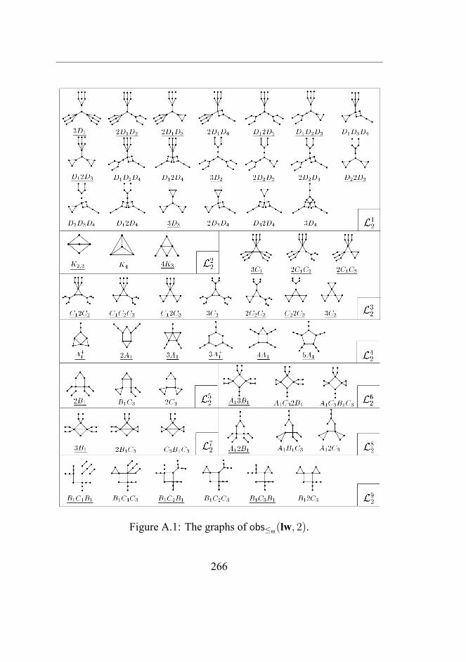
D.M. Thilikos /Discrete Applied Mathematics 105 (2000) 239–271 269
Fig. 13. The obstruction set L2 =L12 ∪L2
2 ∪L32 ∪L4
2 ∪L52 ∪L6
2 ∪L72 ∪L8
2 ∪L92.
Electronic Engineering of Tokyo Institute of Technology on February 1997, motivatedthe present research. Finally, I acknowledge the helpful and detailed comments of thereferees that substantially improved the presentation of this paper.
Figure A.1: The graphs of obs≤m(lw, 2).
266

APPENDIX A. SOME NICE FIGURES OF OBSTRUCTIONS!
Figure A.2: The set obs≤m(ms, 2).
267

200 N.G. Kinnersley, M.A. Langston / Discrete Applied Mathematics 54 (1994) 169-213
Appendix
The 3-GML Obstruction Set
A 4.3.1
A 6.4.1
8.3.1
8.2.3
e 8.2.1
8.2.4
9.4.2
N.G. Kinnersley. M.A. Langston / Discrete Applied Mathematics 54 (1994) 169-213 201
h 10.3.1 11.2.1
12.3.1 12.4.1 11.3.1
13.2.1 13.3.1 13.3.2 202 N.G. Kinnersley, M.A. Langston / Discrete Applied Mathematics 54 (1994) 169-213
13.3.3
13.3.6
13.3.4
4 13.3.7
13.3.9 14.2.1 14.2.2
/ I 13.3.5
N.G. Kinnersley, M.A. Langston / Discrete Applied Mathematics 54 (1994) 169-213
_; 14.2.3
203
14.2.6 14.2.7 14.2.8
9
0 OF%:; 14.3.1 14.3.2 14.3.3
Figure A.3: The first part of the set obs≤m(ns, 3).
268

APPENDIX A. SOME NICE FIGURES OF OBSTRUCTIONS!
204 N.G. Kinnersley, M.A. Langston / Discrete Applied Maihematics 54 (1994) 169-213
14.4.2
14.3.6
\
14.4.4 15.1.1 15.1.2
N.G. Kinnersley, M.A. Langston / Discrete Applied Maihematics 54 (1994) 169-213 205
\ p--J\ 1 /
15 1 A 151.5
l l
152.1 ) 15.2.2
t
\
Ifl 15.2.6 15.2.4 206 N.G. Kinnersley, M.A. Langston 1 Discrete Applied Mathematics 54 (1994) 169-213
15.2.7
b
15.3.1 15.3.2
16.2.1 16.2.2 16.2.3
N.G. Kinnersley, M.A. Langston / Discrete Applied Mathematics 54 (1994) 169-213 207 p-n * 16.2.6
b l / 16.2.4 16.2.5 1 \, d
16.3.1 16.3.3
i
17.1.2
Figure A.4: The second part of the set obs≤m(ns, 3).
269

208 N.G. Kinnersley, M.A. Langston / Discrete Applied Mathematics 54 (1994) 169-213
17.2.1
17.2.4 17.2.5 17.2.6
N.G. Kinnersley, M.A. Longston / Discrete Applied Mathematics 54 (1994) 169-213 209
210 N.G. Kinnersley, M.A. Langston J Discrete Applied Mathemarics 54 (1994) 169-213
18.2.2
A& ! !j l = :‘\I/ &
19.1.2 l *
N.G. Kinnersley. M.A. Langston / Discrete Applied Mathematics 54 (1994) 169-213 211
/ 4 R-4 \\ _
19.3.1 / 20.1.1 \
Figure A.5: The third part of the set obs≤m(ns, 3).
270

APPENDIX A. SOME NICE FIGURES OF OBSTRUCTIONS!
212 N.G. Kinnersley, M.A. Langston / Discrete Applied Mathematics 54 (1994) 169-213
22.0.6
. .
22.0.7
N.G. Kinnersley, M.A. Langston / Discrete Applied Mathematics 54 (1994) 169-213 213
22. 0 . 9
‘I: Figure A.6: The forth part of the set obs≤m(ns, 3).
271

272

BIBLIOGRAPHY
Thesis Papers[1] Micah J Best, Arvind Gupta, Dimitrios M. Thilikos, and
Dimitris Zoros, Contraction Obstructions for Connected GraphSearching, Discrete Applied Mathematics, Volume 209, pp. 27–47,2016.
[2] Micah J Best, Arvind Gupta, Dimitrios M. Thilikos, andDimitris Zoros, Contraction Obstructions for Connected GraphSearching, 9th International Colloquium on Graph Theory and Com-binatorics (ICGT 2014), 2014.
[3] Dimitris Chatzidimitriou, Dimitrios M. Thilikos, and Dim-itris Zoros, Parameter Invariant, Minor-monotone Kernels, Un-published Manuscript, Submitted to: 12th International Symposiumon Parameterized and Exact Computation (IPEC 2017), 2017.
[4] Archontia C. Giannopoulou, Iosif Salem, and Dimitris Zoros,Effective Computation of Immersion Obstructions for Unions ofGraph Classes, Journal of Computer and System Sciences, Volume80, Issue 1, pp. 207–216, 2014.
273

BIBLIOGRAPHY
[5] Archontia C. Giannopoulou, Iosif Salem, and Dimitris Zoros,Effective Computation of Immersion Obstructions for Unions ofGraph Classes, Scandinavian Workshop on Algorithm Theory(SWAT 2012), pp. 165-176, 2012.
[6] Menelaos I. Karavelas, Spyridon Maniatis, Dimitrios M. Thi-likos, and Dimitris Zoros, Geometric Extensions of Cutwidth inany Dimension, 9th International Colloquium on Graph Theory andCombinatorics (ICGT 2014), 2014.
Papers Not Included In This Thesis
[7] Dimitris Chatzidimitriou, Archontia C. Giannopoulou, Spyri-don Maniatis, Clément Requile, Dimitrios M. Thilikos, andDimitris Zoros, Fixed Parameter Algorithms for Completion Prob-lems on Planar Graphs, 41st International Symposium on Mathe-matical Foundations of Computer Science (MFCS 2016), 2016.
[8] Dimitris Chatzidimitriou, Archontia C. Giannopoulou, Spyri-don Maniatis, Clément Requile, Dimitrios M. Thilikos, andDimitris Zoros, Fixed Parameter Algorithms for Completion Prob-lems on Planar Graphs, Algorithmic Graph Theory on the AdriaticCoast (AGTAC 2015), 2015.
[9] Dimitris Chatzidimitriou, Archontia C. Giannopoulou, Clé-ment Requile, Dimitrios M. Thilikos and Dimitris Zoros, AFixed Parameter Algorithm for Plane Subgraph Completion, 13thCologne-Twente Workshop on Graphs & Combinatorial Optimiza-tion (CTW 2015), 2015.
274

BIBLIOGRAPHY
Graph Theory
Textbooks
[10] Bela Bollobas, Graph Theory, An Introductory Course, Springer,1979.
[11] Bela Bollobas, Modern Graph Theory, Springer, 1998.
[12] Adrian Bondy and U.S.R. Murty, Graph Theory, Springer, 2008.
[13] Reinhard Diestel, Graph Theory, GTM 173, 4th edition, Springer,2010.
[14] Jonathan L. Gross, Jay Yellen, and Ping Zhang, Handbook ofGraph Theory, CRC Press, 2013.
[15] Graph Theory, Frank Harary, Westview Press, 1994.
[16] T. Kloks, Treewidth. computations and approximations, LectureNotes in Computer Science, 842, 1994.
[17] Dénes Kőnig, Theorie der endlichen und unendlichen Graphen,Leipzig: Akademische Verlagsgesellschaft, 1936.
Surveys
[18] S. Arnborg, Efficient algorithms for combinatorial problems ongraphs with bounded decomposability (a survey), BIT 25, pp. 2–33,1985.
[19] Hans L. Bodlaender, A tourist guide through treewidth, Acta Cy-bernetica, 11, pp. l–23, 1993.
[20] Hans L. Bodlaender, A partial k-arboretum of graphs withbounded treewidth (Tutorial), Theoretical Computer Science, Vol-ume 209, Issues 1–2, pp. 1–45, 1998.
275

BIBLIOGRAPHY
[21] Hans L. Bodlaender, Treewidth: Structure and Algorithms, Inter-national Colloquium on Structural Information and CommunicationComplexity (SIROCCO 2007), Structural Information and Commu-nication Complexity, pp. 11-25, 2007.
[22] Josep Díaz, Jordi Petit, and Maria Serna, A survey of graph lay-out problems, ACM Computing Surveys (CSUR), Volume 34 Issue3, pp. 313–356, 2002.
[23] B. A. Reed Algorithmic Aspects of Tree Width Recent Advancesin Algorithms and Combinatorics Part of the series CMS Books inMathematics, pp. 85–107, 2003.
Papers
[24] Noga Alon, Daniel Lokshtanov, and Saket Saurabh, FastFast, In Susanne Albers, Alberto Marchetti-Spaccamela, Yossi Ma-tias, Sotiris E. Nikoletseas, and Wolfgang Thomas, editors, CALP(1), Volume 5555 of Lecture Notes in Computer Science, Springer,pp. 49–58, 2009.
[25] K. Appel and W. Haken, Every planar map is four colorable. PartI. Discharging, Illinois J. Math., 21, pp. 429–490, 1977.
[26] K. Appel and W. Haken, Every planar map is four colorable. PartII. Reducibility, Illinois J. Math., 21, pp. 491–567, 1977.
[27] K. Appel and W. Haken, The Solution of the Four-ColorMap Prob-lem Sci. Amer. 237,pp. 108–121, 1977.
[28] K. Appel and W. Haken, The Four Color Proof Suffices, Math. In-tell. 8, pp. 10–20 and 58, 1986
[29] K. Appel and W. Haken, Every Planar Map is Four-Colorable,Providence, RI: Amer. Math. Soc., 1989
276

BIBLIOGRAPHY
[30] Stefan Arnborg, Derek G. Corneil, and AndrzejProskurowski, Complexity of Finding Embeddings in a k-Tree,SIAM. J. on Algebraic and Discrete Methods, 8(2), pp. 277–284,1987.
[31] Stefan Arnborg, Jens Lagergren, and Detlef Seese, Easy prob-lems for tree-decomposable graphs, Journal of Algorithms, 12,pp. 308–340, 1991.
[32] Patrick Bellenbaum and Reinhard Diestel, Two Short ProofsConcerning Tree-Decompositions, Comb. Probab. Comput. 11, 6,pp. 541-547, 2002.
[33] Umberto Bertelé and Francesco Brioschi, Nonserial DynamicProgramming, Academic Press, 1972.
[34] Hans L. Bodlaender, A linear time algorithm for finding tree-decompositions of small treewidth, SIAM Journal on Computing, 25(6), pp. 1305–1317, 1996.
[35] Hans L. Bodlaender, Dynamic programming on graphs withbounded treewidth, Automata, Languages and Programming: 15thInternational Colloquium Tampere, Proceedings, Springer BerlinHeidelberg, pp. 105–118, 1988.
[36] Hans L. Bodlaender, Jitender S. Deogun, Klaus Jansen, TonKloks, Dieter Kratsch, Haiko Müller, and Zsolt Tuza, Rank-ings of graphs, SIAM J. Discrete Math., 11(1),pp. 168–181 (elec-tronic), 1998.
[37] Hans L. Bodlaender, Ton Kloks, Efficient and Constructive Al-gorithms for the Pathwidth and Treewidth of Graphs, Journal of Al-gorithms Volume 21, Issue 2, pp. 358–402, 1996.
[38] B. Bollobás, P. A. Catlin, and Paul Erdős, (1980), Hadwiger’sconjecture is true for almost every graph, European Journal of Com-binatorics, 1, pp. 195–199, 1980.
277

BIBLIOGRAPHY
[39] Fan R. K. Chung, On the cutwidth and the topological bandwidthof a tree, SIAM Journal on Algebraic and Discrete Methods, 6(2),pp. 268–277, 1985.
[40] Moon Jung Chung, Fillia Makedon, Ivan Hal Sudborough,and Jonathan Turner, Polynomial time algorithms for the MINCUT problem on degree restricted trees, SIAM Journal on Comput-ing, 14(1),pp. 158–177, 1985.
[41] Dariusz Dereniowski, From Pathwidth to Connected Pathwidth,SIAM J. vol 26, 2012.
[42] M. DeVos, Z. Dvořák, J. Fox, J. McDonald, B. Mohar, andD. Scheide, Minimum degree condition forcing complete graph im-mersion, Combinatorica, Volume 34, Issue 3, pp. 279–298, 2014.
[43] Leonhard Euler, Solutio problematis ad geometriam situs perti-nentis, Eneström 53, 1741.
[44] Fedor V. Fomin, Saket Saurabh, and Dimitrios M. ThilikosStrengthening Erdös-Pósa property for minor-closed graph classes,Journal of Graph Theory, Volume 66, Issue 3, pp. 235–240, 2011.
[45] Hugo Hadwiger, Über eine Klassifikation der Streckenkomplexe,Vierteljschr. Naturforsch. Ges. Zürich, 88, pp. 33–143, 1943.
[46] Marcin Kamiński,Daniël Paulusma, and Dimitrios M. Thi-likos, Contractions of Planar Graphs in Polynomial Time, 18th An-nual European Symposium on Algorithms ESA 2010, Lecture Notesin Computer Science, Springer, Vol. 6346, pp. 122–133, 2010.
[47] Marcin Kamiński and Dimitrios M. Thilikos, Contraction check-ing in graphs on surfaces, International Symposium on TheoreticalAspects of Computer Science, STACS 2012, 2012.
[48] T. Kashiwabara and T. Fujisawa, NP-completeness of the prob-lem of finding a minimum-clique-number interval graph containing
278
BIBLIOGRAPHY
a given graph as a subgraph, Proc. International Symposium on Cir-cuits and Systems, pp. 657–660, 1979.
[49] Nancy G. Kinnersley, The vertex separation number of a graphequals its path-width, Information Processing Letters Volume 42, Is-sue 6, pp. 345–350, 1992.
[50] Ephraim Korach and Nir Solel, Tree-width, path-width, andcutwidth, Discrete Applied Mathematics, 43(1), pp. 97–101, 1993.
[51] Kazimierz Kuratowski, Sur le problème des courbes gauches entopologie, Fund. Math., pp. 271–283, 1930.
[52] Jens Lagergren, The size of an interwine, In Serge Abiteboul andEli Shamir, editors, ICALP, Volume 820 of Lecture Notes in Com-puter Science, Springer, pp. 520–531, 1994.
[53] Thomas Lengauer, Black-white pebbles and graph separation,Acta Informatica, 16 (4), pp. 465–475, 1981.
[54] R. H. Möhring, Graph problems related to gate matrix layout andPLA folding, in Computational graph theory, vol. 7 of Comput.Suppl., Springer, Vienna, pp. 17–51, 1990.
[55] B. Monien and I. H. Sudborough, Min cut is NP-complete for edgeweighted trees, Theoretical Computer Science, 58(1-3), pp. 209–229, 1988.
[56] T. Ohtsuki, H. Mori, E. Kuh, T. Kashiwabara, and T. Fujisawa,One-dimensional logic gate assignment and interval graphs, IEEETransactions on Circuits and Systems, 26 (9), pp. 675–684, 1979.
[57] N. Robertson, D. P. Sanders, P. D. Seymour, and R. Thomas, ANew Proof of the Four Colour Theorem, Electron. Res. Announc.Amer. Math. Soc. 2,pp. 17–25, 1996.
279

BIBLIOGRAPHY
[58] Dimitrios M. Thilikos, Hans L. Bodlaender, and Michael R.Fellows, Derivation of algorithms for cutwidth and related graphlayout parameters, Journal of Computer and System Sciences, 75(4),pp. 231–244, 2009.
[59] Dimitrios M. Thilikos, Maria J. Serna, and Hans L. Bodlaen-der, Cutwidth I: A linear time fixed parameter algorithm, Journal ofAlgorithms, 56(1), pp. 1–24, 2005.
[60] Robin Thomas, A menger-like property of tree-width: The finitecase Journal of Combinatorial Theory, Series B, 48(1), pp. 67 –76,1990.
[61] R. Thomas, Tree-decompositions of graphs (lecture notes), Schoolof Mathematics. Georgia Institute of Technology, Atlanta, Georgia30332, USA, 1996.
[62] Mihalis Yannakakis, A polynomial algorithm for the min-cut lin-ear arrangement of trees Journal of the ACM, Volume 32, Issue 4,pp. 950–988, 1985.
Graph Minors
Surveys
[63] Daniel Bienstock, Algorithmic implications of the graph minortheorem, Book Chapter, Handbooks in Operations Research andManagement Science Volume 7, pp. 481–502, 1995.
[64] N. Robertson, P.D. Seymour, Graph minors—a survey, Surveysin combinatorics 1985, London Math. Soc. Lecture Note Ser., vol.103,pp. 153–171,1985.
280
BIBLIOGRAPHY
Graph Minors Series
[65] Neil Robertson, P.D. Seymour, Graph minors. I. Excluding a for-est, Journal of Combinatorial Theory, Series B, Volume 35, Issue 1,pp. 39–61, 1983.
[66] Neil Robertson, P.D. Seymour, Graph minors. II. Algorithmicaspects of tree-width, Journal of Algorithms, Volume 7, Issue 3,pp. 309–322, 1986.
[67] Neil Robertson, P.D. Seymour, Graph minors III: Planar tree-width, Journal of Combinatorial Theory, Series B, Volume 36, Issue1, pp. 49–64, 1984.
[68] Neil Robertson, P.D. Seymour, Graph minors IV:Tree-width andwell-quasi-ordering, Journal of Combinatorial Theory, Series B Vol-ume 48, Issue 2, pp. 227–254,1990.
[69] Neil Robertson, P.D. Seymour, Graph minors. V. Excluding a pla-nar graph, Journal of Combinatorial Theory, Series B, Volume 41,Issue 1, pp. 92-114, 1986.
[70] Neil Robertson, P.D. Seymour, Graph minors VI: Disjoint pathsacross a disc, Journal of Combinatorial Theory, Series B, Volume41, Issue 1, pp. 115–138,1986.
[71] Neil Robertson, P.D. Seymour, Graph minors VII: Disjoint pathson a surface, Journal of Combinatorial Theory, Series B, Volume 45,Issue 2, pp. 212–254, 1988.
[72] Neil Robertson, P.D. Seymour, Graph minors VIII: A kuratowskitheorem for general surfaces, Journal of Combinatorial Theory, Se-ries B, Volume 48, Issue 2, pp. 255–288, 1990.
[73] Neil Robertson, P.D. Seymour, Graphminors IX: Disjoint crossedpaths, Journal of Combinatorial Theory, Series B, Volume 49, Issue1, pp. 40–77, 1990.
281

BIBLIOGRAPHY
[74] Neil Robertson, P.D. Seymour, Graph minors X: Obstructions totree-decomposition, Journal of Combinatorial Theory, Series B, Vol-ume 52, Issue 2, pp. 153–190, 1991.
[75] Neil Robertson, P.D. Seymour, Graph minors XI: Circuits on aSurface tree-width, Journal of Combinatorial Theory, Series B, Vol-ume 60, Issue 1, pp. 72–106, 1994.
[76] Neil Robertson, P.D. Seymour, Graph minors XII: Distance ona Surface, Journal of Combinatorial Theory, Series B, Volume 64,Issue 2, pp. 240–272, 1995.
[77] Neil Robertson and P. D. Seymour Graph minors. XIII. The dis-joint paths problem, Journal of Combinatorial Theory. Series B, Vol-ume 63, Issue 1, pp. 65–110, 1995.
[78] Neil Robertson, P.D. Seymour, Graph minors XIV: Extending anEmbedding, Journal of Combinatorial Theory, Series B, Volume 65,Issue 1, pp. 23–50, 1995.
[79] Neil Robertson, P.D. Seymour, Graph minors XV: Giant Steps,Journal of Combinatorial Theory, Series B, Volume 68, Issue 1,pp. 112–148, 1996.
[80] Neil Robertson and Paul D. Seymour, Graph minors. XVI. Ex-cluding a non-planar graph, Journal of Combinatorial Theory. Se-ries B, Volume 89, Isuue 1, pp. 43–76, 2003.
[81] Neil Robertson, P.D. Seymour, Graph minors XVII: Taming aVortex, Journal of Combinatorial Theory, Series B, Volume 77, Issue1, pp. 162–210,1999.
[82] Neil Robertson, P.D. Seymour, Graph minors XVIII: Tree-decompositions and well-quasi-ordering, Journal of CombinatorialTheory, Series B, Volume 89, Issue 1, pp. 77–108, 2003.
282

BIBLIOGRAPHY
[83] Neil Robertson, P.D. Seymour, Graph minors XIX: Well-quasi-ordering on a surface, Journal of Combinatorial Theory, Series B,Volume 90, Issue 2, pp. 325–385, 2004.
[84] Neil Robertson and P. D. Seymour, Graph minors. XX. Wagner’sconjecture, Journal of Combinatorial Theory. Series B, Volume 92,Issue 2„ pp. 325–357, 2004.
[85] Neil Robertson and Paul D. Seymour, Graph minors. XXI.Graphs with unique linkages, Journal of Combinatorial Theory. Se-ries B, Volume 99, Issue 3, pp. 583–616, 2009.
[86] Neil Robertson and P. D. Seymour, Graph minors. XXII. Irrele-vant vertices in linkage problems, Journal of Combinatorial Theory.Series B, Volume 102, Issue 2, pp. 530–563, 2012.
[87] Neil Robertson and Paul D. Seymour, Graph minors XXIII.Nash-Williams’ immersion conjecture, Journal of CombinatorialTheory. Series B, Volume 100, Issue 2,pp. 181–205, 2010.
Papers
[88] Harvey Friedman, Neil Robertson and P. D. Seymour Themetamathematics of the graph minor theorem, in Simpson, S.,Logic and Combinatorics, Contemporary Mathematics, 65, Amer-ican Mathematical Society, pp. 229–261, 1987.
[89] Ken-ichi Kawarabayashi and Paul Wollan, A shorter proofof the graph minor algorithm: the unique linkage theorem, InLeonard J. Schulman, editor, STOC, pp. 687–694, 2010.
[90] C.St.J.A. Nash-Williams, On well-quasi-ordering infinite trees,Proc. Comb. Philos. Soc. 61, pp. 697–720, 1965.
[91] C.St.J.A. Nash-Williams, On well-quasi-ordering trees, Theory ofGraphs and Its Applications (Proc. Symp. Smolenice, 1963), Publ.House Czechoslovak Acad. Sci., pp. 83–84, 1964.
283

BIBLIOGRAPHY
[92] Neil Robertson, Paul Seymour, and Robin Thomas, Quickly ex-cluding a planar graph, Journal of Combinatorial Theory. Series B,Volume 62, Issue 2, pp. 323–348, 1994.
[93] K. Wagner, Graphentheorie, vol. 248/248a, B. J. Hochschul-taschenbucher, Mannheim, p. 61, 1970.
[94] K. Wagner, Über eine Eigenschaft der ebenen Komplexe, Math.Ann., 114, pp. 570–590, 1937.
Graph Searching
Surveys
[95] B. Alspach, Searching and sweeping graphs: a brief survey,Matematiche (Catania), 59, pp. 5–37, 2006.
[96] D. Bienstock, Graph searching, path-width, tree-width and relatedproblems (a survey), Reliability of computer and communicationnetworks, DIMACS Ser. Discrete Math. Theoret. Comput. Sci., vol.5, 1989.
[97] Fedor V. Fomin, Dimitrios M. Thilikos, An annotated bibliogra-phy on guaranteed graph searching, Theoretical Computer Science399, 2008.
[98] Stephan Kreutzer, Graph Searching Games, Book Chapter, Lec-tures in Game Theory for Computer Scientists, Edited by KrzysztofR. Apt and Erich Grädel, Cambridge University Press, 2011.
Papers
[99] Isolde Adler, Christophe Paul, and Dimitrios M. Thilikos,Connected search against a lazy robber , 8th workshop on GRAphSearching, Theory & Applications (GRASTA 2017), 2017.
284

BIBLIOGRAPHY
[100] Lali Barrière, Paola Flocchini, Fedor V. Fomin, PierreFraigniaud, Nicolas Nisse, Nicola Santoro, Dimitrios M. Thi-likos, Connected graph searching, Information and Computation219, 2012.
[101] L. Barrière, P. Fraigniaud, N. Santoro, and D. M. Thilikos,Searching is not jumping, in Proceedings of the 29th InternationalWorkshop on Graph-Theoretic Concepts in Computer Science (WG2003), vol. 2880 of Lecture Notes in Comput. Sci., Springer, pp. 34–45, 2003.
[102] D. Bienstock and P. Seymour, Monotonicity in graph searching,J. Algorithms, 12, pp. 239-245, 1991.
[103] H. L. Bodlaender and D. M. Thilikos, Computing small searchnumbers in linear time, in Proceedings of the First InternationalWorkshop on Parameterized and Exact Computation (IWPEC 2004),vol. 3162 of Lecture Notes in Comput. Sci., Springer, pp. 37–48,2004.
[104] R. Breisch, An intuitive approach to speleotopology, SouthwesternCavers (A publication of the Southwestern Region of the NationalSpeleological Society), VI, pp. 72–78, 1967.
[105] N. D. Dendris, L. M. Kirousis, and D. M. Thilikos, Fugitive-search games on graphs and related parameters, Theoret. Comput.Sci., 172, pp. 233–254, 1997.
[106] F. V. Fomin and D. M. Thilikos, On the monotonicity of gamesgenerated by symmetric submodular functions, Discrete Appl.Math., 131, pp. 323–335, 2003.
[107] P. Fraigniaud and N. Nisse, Monotony properties of connectedvisible graph searching, in Proceedings of the 32nd InternationalWorkshop on Graph-Theoretic Concepts in Computer Science (WG2006), vol. 4271 of Lecture Notes in Comput. Sci., Springer,pp. 229–240, 2006.
285
BIBLIOGRAPHY
[108] P. A. Golovach, A topological invariant in pursuit problems (Rus-sian), Differentsialʹnye Uravneniya, 25, 923–929. 1097, 1989. trans-lation in Differential Equations 25, no. 6, pp. 657–661, 1989.
[109] P. A. Golovach, Equivalence of two formalizations of a searchproblem on a graph (Russian), Vestnik Leningrad. Univ. Mat. Mekh.Astronom., pp. 10–14, 1989. translation in Vestnik Leningrad Univ.Math. 22, no. 1,pp. 13–19, 1989.
[110] R. Isaacs, Differential games, A mathematical theory with appli-cations to warfare and pursuit, control and optimization, John Wiley& Sons Inc., New York, 1965.
[111] L. M. Kirousis and C. H. Papadimitriou, Interval graphs andsearching, Discrete Math., 55, pp. 181–184, 1985.
[112] L. M. Kirousis and C. H. Papadimitriou, Searching and pebbling,Theoret. Comput. Sci., 47, pp. 205–218, 1986.
[113] A. S. LaPaugh, Recontamination does not help to search a graph,J. Assoc. Comput. Mach., 40, pp. 224–245, 1993.
[114] T. Lengauer, Black-white pebbles and graph separation, Acta In-formatica, Volume 16, Issue 4, pp. 465–475, 1981.
[115] N. Megiddo, S. L. Hakimi, M. R. Garey, D. S. Johnson, andC. H. Papadimitriou, The complexity of searching a graph, J. Assoc.Comput. Mach., 35, pp. 18–44, 1988.
[116] T. D. Parsons, Pursuit-evasion in a graph, in Theory and applica-tions of graphs, vol. 642 of Lecture Notes in Math., Springer, Berlin,pp. 426–441, 1978.
[117] N. N. Petrov, A problem of pursuit in the absence of informationon the pursued, Differentsialʹnye Uravneniya, 18, pp. 1345–1352,1982.
286

BIBLIOGRAPHY
[118] N. N. Petrov, The Cossack-robber differential game, Differ-entsialʹnye Uravneniya, 19, pp. 1366–1374, 1983.
[119] A. Takahashi, S. Ueno, and Y. Kajitani, Minimal forbidden mi-nors for the family of graphs with proper-path-width at most two,IEICE Trans. Fund. E78-A, pp. 1828–1839, 1995.
[120] D. M. Thilikos, Algorithms and obstructions for linear-width andrelated search parameters, Discrete Appl. Math., 105, pp. 239–271,2000.
[121] P. D. Seymour and R. Thomas, Graph searching and a min-maxtheorem for tree-width, J. Combin. Theory Ser. B, 58, pp. 22–33,1993.
[122] B. Yang, D. Dyer, and B. Alspach, Sweeping graphs with largeclique number, in Proceedings of the 15th International Symposiumon Algorithms and Computation (ISAAC 2004), vol. 3341 of Lec-ture Notes in Comput. Sci., Springer, pp. 908–920, 2004.
Obstruction Sets
Papers
[123] Isolde Adler, Martin Grohe, and Stephan Kreutzer, Comput-ing excluded minors, In Shang-Hua Teng, editor, SODA, pp. 641–650, 2008.
[124] S. Arnborg, A. Proskurowski, and D. G. Corneil, Forbiddenminors characterization of partial 3-trees, Discrete Math., Volume80, Issue 1, pp. 1–19, 1990.
[125] Kevin Cattell, Michael J. Dinneen, Rodney G. Downey,Michael R. Fellows, and Michael A. Langston, On comput-ing graph minor obstruction sets, Theor. Comput. Sci., 233(1-2),pp. 107–127, 2000.
287

BIBLIOGRAPHY
[126] F. R. K. Chung and Paul D. Seymour, Graphs with small band-width and cutwidth, Discrete Mathematics, 75(1-3):pp. 113–119,1989.
[127] Bruno Courcelle, Rodney G. Downey, and Michael R. Fel-lows,A note on the computability of graphminor obstruction sets formonadic second order ideals, J. UCS, 3(11), pp. 1194–1198, 1997.
[128] Erik D. Demaine, MohammadTaghi Hajiaghayi, and Ken-ichiKawarabayashi, Algorithmic GraphMinor Theory: ImprovedGridMinor Bounds and Wagner’s Contraction, International Symposiumon Algorithms and Computation (ISAAC 2006), pp. 3–15, 2006.
[129] Zdenek Dvorak, Archontia C. Giannopoulou and DimitriosM. Thilikos, Forbidden graphs for tree-depth, European J. Combin.33 (5), pp. 969–979, 2012.
[130] Archontia C. Giannopoulou, Michal Pilipczuk, Jean-Florent Raymond, Dimitrios M. Thilikos, and MarcinWrochna, Cutwidth: Obstructions and Algorithmic Aspects, 11thInternational Symposium on Parameterized and Exact Computation(IPEC 2016), pp. 1–13, 2017.
[131] Archontia C. Giannopoulou, Michal Pilipczuk, Jean-Florent Raymond, Dimitrios M. Thilikos, and MarcinWrochna, Cutwidth: Obstructions and Algorithmic Aspects, CoRRabs/1606.05975, 2016.
[132] Marcin Kaminski, Daniël Paulusma, and Dimitrios M. Thi-likos, Contracting planar graphs to contractions of triangulations,Journal of Discrete Algorithms, Volume 9, Issue 3, pp. 299–306,2011.
[133] Nancy G. Kinnersley, Michael A. Langston, Obstruction setisolation for the gate matrix layout problem, Discrete Applied Math-ematics, Volume 54, Issues 2-3, pp. 169–213, 1994.
288

BIBLIOGRAPHY
[134] A. Satyanarayana and L. Tung, A characterization of partial3-trees, Networks 20(3), pp. 299–322, 1990.
[135] A. Takahashi, S. Ueno, and Y. Kajitani, Minimal acyclic for-bidden minors for the family of graphs with bounded path-width,Discrete Mathematics, Volume 127, Issues 1-3, pp. 293–304, 1994.
[136] A. Takahashi, S. Ueno, and Y. Kajitani, Minimal forbidden mi-nors for the family of graphs with proper-path-width at most two,IEICE Trans. Fund. E78-A, pp. 1828–1839, 1995.
[137] Paul Wollan, The structure of graphs not admitting a fixed im-mersion, CoRR, abs/1302.3867, 2013.
Parameterized Complexity
Textbooks
[138] Hans L. Bodlaender, Rod Downey, Fedor V. Fomin, andDániel Marx, editors, The Multivariate Algorithmic Revolutionand Beyond, Essays Dedicated to Michael R. Fellows on the Occa-sion of His 60th Birthday, Volume 7370 of Lecture Notes in Com-puter Science, Springer, 2012.
[139] Marek Cygan, Fedor V. Fomin, Lukasz Kowalik, Daniel Lok-shtanov, Dániel Marx, Marcin Pilipczuk, Michal Pilipczuk,and Saket Saurabh, Parameterized Algorithms, Springer, 2015.
[140] Rodney G. Downey and Michael R. Fellows, Fundamentals ofParameterized Complexity, Texts in Computer Science, Springer,2013.
[141] Rodney G. Downey and Michael R. Fellows, ParameterizedComplexity, Springer, 1998.
289

BIBLIOGRAPHY
[142] Jörg Flum and Martin Grohe, Parameterized Complexity The-ory, Texts in Theoretical Computer Science. An EATCS Series.Springer-Verlag, Berlin, 2006.
[143] Rolf Niedermeier, Invitation to fixed-parameter algorithms, Vol-ume 31 of Oxford Lecture Series in Mathematics and its Applica-tions. Oxford University Press, Oxford, 2006.
Surveys
[144] H. L. Bodlaender, P. Heggernes, and D. Lokshtanov, Graphmodification problems, Dagstuhl seminar 14071, Dagstuhl Reports,Volume 4, Issue 2, pp. 38–59, 2014.
[145] Jiong Guo and Rolf Niedermeier, Invitation to data reductionand problem kernelization SIGACT News, Volume 38, Issue 1,pp. 31–45, 2007.
[146] Christian Komusiewicz, André Nichterlein, and Rolf Nie-dermeier, Parameterized Algorithmics for Graph ModificationProblems: On Interactions with Heuristics, International Workshopon Graph-Theoretic Concepts in Computer Science (WG 2015),pp. 3–15, 2015.
[147] Stefan Kratsch, Recent developments in kernelization: A survey,Bulletin of the EATCS, 113, 2014.
[148] Yunlong Liu, Jianxin Wang, and Jiong Guo An Overview ofKernelization Algorithms for Graph Modification Problems, Ts-inghua Science and Technology, Volume 19, Issue 4, 2014.
Papers
[149] Karl R. Abrahamson and Michael R. Fellows, Finite au-tomata, bounded treewidth and well-quasiordering AMS Summer
290

BIBLIOGRAPHY
Workshop on Graph Minors, Graph Structure Theory, Contempo-rary Mathematics vol. 147, pp. 539–564, 1993.
[150] Faisal N. Abu-Khzam and Henning Fernau, Kernels: Anno-tated, proper and induced, In Proc. 2nd IWPEC, Volume 4169 ofLNCS, pp. 264–275, 2006.
[151] Rémy Belmonte, Pim van 't Hof, Marcin Kaminski, DaniëlPaulusma, and Dimitrios M. Thilikos, Characterizing graphsof small carving-width, Discrete Applied Mathematics, 161(13-14),pp. 1888–1893, 2013.
[152] Hans L. Bodlaender and Babette van Antwerpen-de FluiterReduction algorithms for graphs of small treewidth, Inf. Comput.,167, pp. 86–119, 2001.
[153] Hans L. Bodlaender, Rodney G. Downey, Michael R. Fel-lows, and Danny Hermelin, On problems without polynomial ker-nels, J. Comput. Syst. Sci., 75(8), pp. 423–434, 2009.
[154] Hans L. Bodlaender, Fedor V. Fomin, Daniel Lokshtanov,Eelko Penninkx, Saket Saurabh, and Dimitrios M. Thilikos,(Meta) Kernelization, In Proceedings of the 50th Annual IEEE Sym-posium on Foundations of Computer Science (FOCS 2009), pp. 629–638, 2009.
[155] Hans L. Bodlaender, Fedor V. Fomin, Daniel Lokshtanov,Eelko Penninkx, Saket Saurabh, and Dimitrios M. Thilikos,(Meta) Kernelization, J. ACM 63(5), pp. 1–69, 2016.
[156] Richard B. Borie, R. Gary Parker, and Craig A. Tovey, Auto-matic generation of linear-time algorithms from predicate calculusdescriptions of problems on recursively constructed graph families,Algorithmica, 7, pp. 555–581, 1992.
[157] Jonathan F. Buss and Judy Goldsmith, Nondeterminism withinP, SIAM J. Comput., 22(3), pp. 560–572, 1993.
291

BIBLIOGRAPHY
[158] Liming Cai and Jianer Chen, On fixed-parameter tractability andapproximability of NP optimization problems, Journal of Computerand System Sciences, Volume 54, pp. 465–474, 1997.
[159] Marco Cesati and Luca Trevisa, On the efficiency of polyno-mial time approximation schemes, Information Processing LettersVolume 64, Issue 4, pp. 165–171, 1997.
[160] J. Chen, X. Huang, I.A. Kanj, and G. Xia Polynomial time ap-proximation schemes and parameterized complexity, Discrete Ap-plied Mathematics Volume 155, Issue 2, pp. 180-193. 2007.
[161] J. Chen, I.A. Kanj, and G. Xia, Improved upper bounds for vertexcover, Theoretical Computer Science, Volume 411, Issues 40–42,pp. 3736–3756, 2010.
[162] J. Chen, I.A. Kanj, and G. Xia, Simplicity is beauty: Improvedupper bounds for vertex cover, Technical Report TR05-008, Schoolof CTI, DePaul University, 2005.
[163] Rajesh Hemant Chitnis, Marek Cygan, MohammadTaghi Ha-jiaghayi, Marcin Pilipczuk, and Michal Pilipczuk, DesigningFPT algorithms for cut problems using randomized contractions, In53rd Annual IEEE Symposium on Foundations of Computer Science(FOCS 2012), pp. 460–469, 2012.
[164] Marek Cygan, Jesper Nederlof, Marcin Pilipczuk, MichalPilipczuk, Johan M. M, van Rooij, and Jakub OnufryWojtaszczyk, Solving connectivity problems parameterized bytreewidth in single exponential time, In Rafail Ostrovsky, editor,FOCS, pp. 150–159, 2011.
[165] Erik D. Demaine, Fedor V. Fomin, Mohammadtaghi Haji-aghayi, and Dimitrios M. Thilikos, Subexponential parameter-ized algorithms on bounded-genus graphs andH-minor-free graphs,Journal of the ACM, 52(6), pp. 866–893, 2005.
292
BIBLIOGRAPHY
[166] Erik D. Demaine and MohammadTaghi Hajiaghayi, Bidimen-sionality: new connections between FPT algorithms and PTASs,Proceedings of the sixteenth annual ACM-SIAM symposium on Dis-crete algorithms (SODA 05), pp. 590–601, 2005.
[167] Rodney G. Downey and Michael R. Fellows, Fixed-parametertractability and completeness I: Basic results, SIAM J. Comput.,Volume 24, series 4, pp. 873–921, 1995.
[168] Rodney G. Downey and Michael R. Fellows, Fixed-parametertractability and completeness II: On completeness for W[1], Theor.Comput. Sci., Volume 141, series1&2, pp. 109–131, 1995.
[169] Michael R. Fellows and Bart M. P. Jansen, FPT Is Character-ized by Useful Obstruction Sets, International Workshop on Graph-Theoretic Concepts in Computer Science (WG 2013), pp. 261–273,2013.
[170] Henning Fernau, Till Fluschnik, Danny Hermelin, AndreasKrebs, Hendrik Molter, and Rolf Niedermeier, Diminishableparameterized problems and strict polynomial kernelization CoRR,abs/1611.03739, 2016.
[171] Fedor V. Fomin, Daniel Lokshtanov, Neeldhara Misra, andSaket Saurabh, Planar F-Deletion: Approximation, Kernelizationand Optimal FPT Algorithms, In Proceedings of the 2012 IEEE 53rdAnnual Symposium on Foundations of Computer Science (FOCS’12), pp. 470-479, 2012.
[172] Fedor V. Fomin, Daniel Lokshtanov, Neeldhara Misra, andSaket Saurabh, Planar F-Deletion: Approximation, Kernelizationand Optimal FPT Algorithms, CoRR abs/1204.4230, 2012.
[173] Fedor V. Fomin, Daniel Lokshtanov, Venkatesh Raman, andSaket Saurabh, Bidimensionality and EPTAS, In 22st ACM–SIAMSymposium on Discrete Algorithms (SODA 2011), pp. 748–759,2011.
293

BIBLIOGRAPHY
[174] Fedor V. Fomin, Daniel Lokshtanov, Saket Saurabh, andDimitrios M. Thilikos, Bidimensionality and Kernels, SODA2010, pp. 503–510, 2010.
[175] Fedor V. Fomin, Daniel Lokshtanov, Saket Saurabh, andDimitrios M. Thilikos, Bidimensionality and Kernels, CoRRabs/1606.05689, 2016.
[176] Valentin Garnero, Christophe Paul, Ignasi Sau, and Dim-itrios M. Thilikos. Explicit linear kernels via dynamic program-ming, SIAM J. Discrete Math., 29(4), pp. 1864–1894, 2015.
[177] Archontia C. Giannopoulou, Bart M. P. Jansen, Daniel Lok-shtanov, and Saket Saurabh, Uniform kernelization complexityof hitting forbidden minors, CoRR, abs/1502.03965, 2015.
[178] Archontia C. Giannopoulou, Michal Pilipczuk, Dimitrios M.Thilikos, Jean-Florent Raymond, and Marcin Wrochna, Lin-ear kernels for edge deletion problems to immersion-closed graphclasses, (To appear in ICALP 2017), CoRR, abs/1609.07780, 2016.
[179] Martin Grohe, Ken-ichi Kawarabayashi, Dániel Marx, andPaul Wollan, Finding topological subgraphs is fixed-parametertractable, In STOC, pp. 479–488, 2011.
[180] Eun Jung Kim, Alexander Langer, Christophe Paul, FelixReidl, Peter Rossmanith, Ignasi Sau, and Somnath Sikdar, Lin-ear Kernels and Single-Exponential Algorithms Via Protrusion De-compositions, ACM Trans. Algorithms 12(2), pp. 1-41, 2016.
[181] Daniel Lokshtanov, Fahad Panolan, M. S. Ramanujan, andSaket Saurabh, Lossy kernelization, In Proceedings of the 49th An-nual ACM SIGACT Symposium on Theory of Computing, (STOC2017), pp. 224–237, 2017.
[182] Dimitrios M. Thilikos, Bidimensionality and parameterized al-gorithms (invited talk), In 10th International Symposium on Param-eterized and Exact Computation (IPEC 2015), pp. 1–16, 2015.
294

BIBLIOGRAPHY
[183] Siamak Tazari, Faster approximation schemes and parameterizedalgorithms on H-minor-free and odd-minor-free graphs, Mathemati-cal Foundations of Computer Science 2010: 35th International Sym-posium (MFCS 2010), pp. 641–652, 2010.
Logic and Complexity
Textbooks
[184] B. Courcell and Joost Engelfriet, Graph Structure andMonadic Second-Order Logic: A Language-Theoretic Approach(1st ed.), Cambridge University Press, 2012.
[185] Sanjoy Dasgupta, Christos Papadimitriou, and Umesh Vazi-rani, Algorithms, McGraw-Hill Education, 2006.
[186] Herbert B. Enderton, Amathematical introduction to logic, Aca-demic Press, 1972.
[187] Michael R. Garey and David S. Johnson, Computers and in-tractability. A guide to the theory of NP-completeness, W. H. Free-man and Co., San Francisco, Calif., 1979.
[188] Elliott Mendelson, Introduction to mathematical logic (3. ed.).Chapman and Hall, 1987.
Papers
[189] B. Courcelle, Graph rewriting: an algebraic and logic approach,Handbook of theoretical computer science (vol. B), pp. 193 - 242,1990.
[190] B. Courcelle, The expression of graph properties and graphtransformations in monadic second-order logic, Handbook of GraphGrammars, pp. 313–400, 1997.
295

BIBLIOGRAPHY
[191] B. Courcell, The monadic second-order logic of graphs I: Rec-ognizable sets of finite graphs, Information and Computation,85,pp. 12–75, 1990.
[192] Michael R. Fellows and Michael A. Langston, Nonconstruc-tive tools for proving polynomial-time decidability, J. Assoc. Com-put. Mach., Volume 35, Issue 3, pp. 727–739, 1988.
[193] Michael R. Fellows and Michael A. Langston, On search, de-cision, and the efficiency of polynomial-time algorithms, J. Comput.System Sci., Volume 49, Issue 3, pp. 769–779, 1994.
Other
[194] J. Hajek, K:)nigsberg bridges solved,http://www.matheory.info/konigsberg/
[195] ΝΙΚΟΣ ΚΑΖΑΝΤΖΑΚΗΣ, Ταξιδεύοντας: Ρουσία, Εκδόσεις Καζαντζάκη,1956.
[196] Nikos Kazantzakis, Russia: A Chronicle of Three Journeys in theAftermath of the Revolution, Creative Arts Book Company, 1956.
[197] Milan Kundera, The Festival of Insignificance, Harper, 2013.
[198] James Joseph Sylvester, Chemistry and Algebra, Nature, 17, 284,1878.
[199] Wolfram MathWorld, Seven Bridges of Königsberg Problem,http://mathworld.wolfram.com/KoenigsbergBridgeProblem.html
296

LIST OF SYMBOLS
Symbol Explanation Page
(p, r)-dist(G) The function measuring the number of verticeswe have to delete from G in order for p to havevalue at most r
11, 68
N The set of natural numbers 21
N+ The set of positive natural numbers 21
Z The set of integers 21
Z+ The set of positive integers 21
R The set of real numbers 21
R+ The set of positive real numbers 21
[n] The set 1, 2, . . . , n 21
2S The power-set of S 21(S2
)The set of all subsets of S with cardinality 2 21
f |S f |S = (x, f(x)) | x ∈ S ∩A 22
f \ S f \ S = (x, f(x)) | x ∈ A \ S 22
∅ The empty function 22
297

List of Symbols
Symbol Explanation Page
V (G) The vertex set of G 22
E(G) The edge set of G 22
n(G) The number of vertices of G 22
|G| The number of vertices of G 22
m(G) The number of edges of G 22
G[S] The subgraph of G induced by S ⊆ V (G) 22
G[F ] The subgraph of G induced by F ⊆ E(G) 22
G \ S The graph G[V (G) \ S] 22
NG(u) The neighbourhood of vertex u in G 22
degG(u) The degree of vertex u in G 22
NG(S) The neighbourhood of S ⊆ V (G) 22
NG[S] The closed neighbourhood of S ⊆ V (G) 22
∂G(S) The set of vertices of S that are incident to edgesnot in G[S]
22
Leaf(T ) The set of leaves of T 24
aTb The unique path in T with end points a and b 24
Kk Clique of k vertices 24
Kk,l The graph (A∪B,u, v | u ∈ A and v ∈ B
)
for disjoint A,B24
L(G) The line graph of G 24
G1 ∪G2 The union of G1 and G2 24
G1 +G2 The disjoint union of G1 and G2 24
G1 ×G2 The lexicographic product of G1 and G2 24
⊞k The (k × k)-grid 24
298

List of Symbols
Symbol Explanation Page
G \ u The graph obtained after the deletion of vertex uin G
26
G \ e The graph obtained after the deletion of edge e inG
26
G/e The graph obtained after the contraction of edgee in G
26
G/u The graph obtained after the dissolution of vertexu in G
26
≤ The subgraph relation 27
≤sp The spanning subgraph relation 27
≤in The induced subgraph relation 28
≤c The contraction relation 28, 219
≤tp The topological-minor relation 28
≤m The minor relation 28, 138
≤im The immersion relation 28
G The class of all graphs 29
obs⪯(C) The obstruction set of C for the relation ⪯ 30
G(Γ) The abstract graph defined from Γ 32
F (Γ) The set of faces of Γ 32
ar(Ri) The arity of the predicate Ri 38
LG The language of graphs 39
A |= ϕ A is a model of ϕ 39
cardq,r(S) The atomic formula testing whether the cardinal-ity of S is equal to q modulo r
41
Σ∗ The set of strings over Σ, the Kleene closure of Σ 44
|w| The size of the word w 45
299

List of Symbols
Symbol Explanation Page
P The class of polynomially solved problems 45
NP The class of polynomially verified problems 45
p-Π The parameterized version of Π 47
FPT The class of FPT-problems 49
p-Π ⋒ C The restriction of problem p-Π to graph class C 51
dom(p) The dominion of p 57
G[p, k] The class containing the graphs with p(G) ≤ k 57
obs⪯(p, k) The obstruction set of G[p, k] 57
LV(G) The set of all vertex layouts of G 60
Stσ(i) The tree-supporting set of σ in position i 60
costt(G, σ) The “tree” cost of a vertex layout of G 60
tvs(G) The tree vertex separation number of G 60
width(T,B) The width of a tree-decomposition 61
tw(G) The treewidth of G 61
Spσ(i) The path-supporting set of σ in position i 63
costp(G, σ) The “path” cost of a vertex layout of G 63
pvs(G) The vertex separation number of G 63
pw(G) The pathwidth of G 63
∂G(σ, i) The cut at position i 64
costc(G, σ) The “cut” cost of a vertex layout of G 64
cw(G) The cutwidth of G 64
LE(G) The set of all edge layouts of G 65
Slσ(i) The line-supporting set of σ in position i 66
costl(G, σ) The “line” cost of an edge layout of G 66
lw(G) The linearwidth of G 66
300

List of Symbols
Symbol Explanation Page
vc(G) The size of the minimum vertex cover of G 67
fv(G) The size of the minimum feedback vertex set ofG
67
pl(G) The minimum number of edges we have to deletefrom G in order to make it planar
67
GF ,k The class containing all graphsG for which thereexists a subset S ⊆ V (G), of size at most k, suchthat G \ S contains no graph from F as a minor
70
H(d) The set of hyperplanes of Rd 74
S(d) The set of hyperspheres of Rd 75
Ed(G) An embedding of G in the euclidean space Rd 75
Ed(G) Then set of essential Embedding of G in Rd 75
∂G(Ed(G),Π) The set of curves of Ed(G) that are intersected byΠ
76
∂G(Ed(G),Σ) The set of curves of Ed(G) that are intersected byΣ
76
cwd(G) The d-cutwidth of G 76
E1(G) An embedding of G in R 77
scwd(G) The spherical d-cutwidth of G 80
F1 ≤ F2 Ordering between two finite setsF1,F2 of graphs 95
Tk The class of graphs of treewidth at most k 97
CTk the class of tree-dec expansions of a graph G ∈Tk
97
width(C) The width of an immersion-closed graph class C 98
dec(p) The protrusion decomposability constant 112
B(t) The set of all t-boundaried graphs 113
301

List of Symbols
Symbol Explanation Page
B(≤t) The set∪t′∈0∪[t] B(t
′) 113
T (≤t) The set of all boundaried graphs in B(≤t) whoseunderlying graph has treewidth at most t− 1
113
ψG The label normalizing function of G 113
⊕ The “gluing” operation on boundaried graphs 114
≡p,t The equation relation on boundaried graphs 114
null(p) The equivalence class of all graphs G, such thatG /∈ dom(p)
114
repp(G) The (unique) boundaried graph in a representa-tive collectionR equivalent to G
114
cardp The function giving the number of equivalenceclasses of ≡p,t
115
pp-Π pp-Π(G) = •k | (G, k) ∈ p-Π where • is minor max depending on the type of p-Π
116
solp-Π(G) solp-Π(G) = S where |S| = pp-Π(G) and(G,S) ∈ p-Π, if such S exists
117
Leaf(T, r) The set of leaves of (T, r) other than r 132
a ≤T,r b b is a descendant of a in (T, r) 132
a =T,r b a and b are uncomperable in (T, r) 132
descT,r(q) The set of descendants of q in (T, r) 132
childT,r(q) The children of q in (T, r) 132
depthT,r(v) The depth of v in (T, r) 133
heightT,r(v) The height of v in (T, r) 133
innerT,r(a, b) The inner part of (a, b) 133
outerT,r(a, b) The outer part of (a, b) 133
capacityT,r(a, b) The capacity of (a, b) 133
302

List of Symbols
Symbol Explanation Page
(T, r) \ (a, b) The tree obtained after an (a, b)-compression 134
transpp The transposition function of p 136
G \ S The boundaried graph obtained from G after thedeletion of the vertices of S
138
tw(G) The treewidth of G 140
gohigherT,r(v, µ) The ancestor u of v such thatminµ, depthT,r(v) − depthT,r(u) is max-imized
164
A(G,Y ) The set containing the vertex set of the augmentedconnected components for (G,Y )
167
potential(G,D)(a, b) The potential of a transition pair (a, b) of (G, D) 172
potential(G,D)(P) The potential of the transition collection P of(G, D)
173
p(v) Placing a searcher on v 194
r(v) Removing a searcher from v 194
s(v, u) Sliding a searcher along v, u 194
E(S, i) The set of clean edges after i steps of S 194
costG(S) The cost of search strategy Σ 195
es(G) The edge search number of G 195
ns(G) The node search number of G 196
ms(G) The mixed search number of G 196
mes(G) The monotone edge search number of G 197
mns(G) The monotone node search number of G 198
mms(G) The monotone mixed search number of G 198
ces(G) The connected edge search number of G 199
cns(G) The connected node search number of G 199
303

List of Symbols
Symbol Explanation Page
cms(G) The connected mixed search number of G 199
cmes(G) The connected and monotone edge search num-ber of G
200
cmns(G) The connected and monotone node search num-ber of G
200
cmms(G) The connected and monotone mixed search num-ber of G
200
ilns(G) The node search number ofG, where the fugitiveis invisible but lazy
202
prefsec(A) The ordering of prefixes of A 206
The concatenation of orderings 206
rev(G) The reversed rooted graph (G,Sout, Sin) 207
enh(G,Sin, Sout) The enhancement of (G,Sin, Sout) 207
∂G(F ) The boundary of the edge set F 209
costG(E , i) The cost of an expansion E at position i on G 210
costG(E) The cost of an expansion E on G 210
p(G,Sin, Sout) Minimum cost over all expansions 210
mp(G,Sin, Sout) Minimum cost over all monotone expansions 210
cmp(G,Sin, Sout) Minimum cost over all connected and monotoneexpansions
210
cmp(G) cmp(G, ∅, ∅) 210
glue(G1, . . . ,Gr) The “gluing” operation on r rooted graphs 212
304

GLOSSARY OF TERMS
Symbols
C-Membership 35τ -structure 38FPT 49FPT-algorithm 49FPT-problem 49NP 45NP-complete 46NP-hard 46No-instance 44, 47P 45Yes-instance 44, 47F-Covering 11, 69F-Deletion 69F-Packing 120(p, r)-Distance 69k-p-Modification 68p-p-Modification 68p-Feedback Vertex Set 118p-Vertex Outerplanarization
118Immersion-Containment 49Minimum Cut Linear Arrange-
ment 64Minor-Containment 49(α, β)-tree-decomposition 146(β, f)-rich protrusion 167(E1, E2)-expansion 209(E1, E2)-expansion (connected)
209(Sin, Sout)-complete strategy 208(a, b)-aligned 134(a, b)-compression 134(a, b)-compression 1501-cutwidth 77H-Immersion-Containment 37H-Minor-Containment 35H-minor-free 28H-topological-minor-free 28c-normal parameter 124d-cutwidth 76
305
Glossary of Terms
k-Coloring 43k-Search 260k-Vertex Cover 43p-Immersion-Containment 50p-Independent Set 55p-Minor-Containment 50p-Vertex Cover 54, 68r-approximate k-edge-linkage 104r-approximate k-linkage 101r-approximate edge-linkage 104r-approximate linkage 101t-boundaried graph 113t-representative collection 1142-connected graph 23
A
Adler, Isolde 12, 92Agile fugitive 193Alon, Noga 2Alphabet 44Annotated graph 53Anti-chain 29Appel, Kenneth 33Approximation algorithms 128Atomic formula 39Axiom of Choice 36
B
Bag 60Bidimensionality Theory 119Bienstock, Daniel 198Binary tree 133Block 23, 221Block (Extended) 241Block (Spine) 239Block (Extremal, Right) 239
Block (Extremal, Left) 239Block (Extremal) 239Block (Central) 236Block (Essential) 224Block (Cycle) 224Block (Bridge) 224Block (Hair) 223Block (Trivial) 221Bollobás, Béla 2Boolean connectives 39Boundaried graphs (strongly com-
patible) 150Boundaried graphs (compatible)
113Boundaried graph 113Boundary of edge set 209Boundary size 113Boundary vertices 113Boundary of boundaried raph 113Bounded fugitive speed 193Bridge 221
C
Capacity (Maximum) 134Capacity (Minimum) 134Capacity of pair 133Capture 193Carving-width 5, 89Central cut-vertex 236Children 132Chord 222Clique 24CMSO-definable 42Component (edge-linkage) 104Component (linkage) 101Component (2-connected) 23
306

Glossary of Terms
Computable parameter 57Concatenation of orderings 206Connected component (aug-
mented) 167Connected (set of graphs) 127Connected component 23Connected (graph) 23Contraction (rooted) 219Contraction-closed 29Contraction (graph) 28, 94, 219Core 112Cost (expansion) 210Cost (search strategy) 195Courcelle’s Theorem 86Curve 75Curve end 75Cut-vertex of a block 222Cut-vertex 222Cut at layout position 64Cutwidth 5, 64Cycle 23
D
Degree 22Degree (maximum) 57Dendris, Nick Nick Dendris 202Depth of tree 133Descartes’ rule of signs 82Descendant 132Dirac, Gabriel Andrew 2Disjoint union 24Distance of vertices 23Dominion 57
E
Edge 22
Edge extensions 207Edge-coloring 89Edge layout 59Edge contraction 26Edge deletion 26Edge-disjoint paths 23Edges lift 27Edge set 22Endpoint 22EPTAS 129Erdős, Paul 2Essential-embedding 75Euler, Leonhard 2, 25Eulerian cycle 25Excluded Grid Theorem 89Expansion property 214Extended fan 241
F
Face 32, 222Fan 234Feedback vertex set 6, 67Finite Integer Index (optimization
problems) 117Finite Integer Index (parameter)
114Fixed Parameter Tractable 49Fomin, Fedor V. 199Forbidden graph characterization
8, 34Forest 24Four Color Theorem 2, 32, 33Frontier graph 113Fugitive search games 5, 17, 195Function (Transposition) 136Function (Label normalising) 113
307

Glossary of Terms
Function (Edge subset certifying)54
Function (Vertex subset certifying)54
G
Golovach, Petr 192Graph 3, 22Graph sweeping 195Graph embedding in R 77Graph embedding 75Graph Modification Problem 67Graph modification operation 66Graph property 66Graph structure 39Graph isomorphism 24Graph Searching 5, 191Graph parameter 4, 57Grid 24Grohe, Martin 12, 92Guaranteed Search 191Guthrie, Francis 2
H
Haken, Wolfgang 33Haploid chord 223Haploid vertex 223Haploid face 223Harary, Frank 2Hardwiger’s Conjecture 34Heavy cut-vertex 224Height of tree 133Hyperplane 74Hypersphere 75
I
Immersion model (minimal) 95Immersion model 95Immersion-closed 29Immersion (strong) 28, 95Immersion (weak) 28, 95Immersions Conjecture (strong)
37Immersions Conjecture (weak) 36Independent set 55Index of vertex 113Induced subgraph 28Induced subgraph (from vertex
set) 22Inert fugitive 193Inner vertex 223Inner part of pair 133Inner face 32, 222, 223Input 44Instance 44Interior of curve or arc 32, 75Internal chord 223Internal vertices of path 23Invisible fugitive 193Irrelevant vertex technique 89Isolated edge 23Isolated vertex 23Isomorphic graphs 24
K
Kalinin, Mikhail 25Kawarabayashi, Ken-ichi 93Kernel 52Kernel (α-approximate) 110Kernel (proper 110Kernel (induced subgraph-
monotone) 109
308

Glossary of Terms
Kernel (parameter-invariant) 53Kernel (minor-monotone) 53Kernel (⪯-monotone) 53Kernelization 52Kernelization (strict) 110Kirousis, Lefteris 198Kreutzer, Stephan 12, 92Kruskal’s Tree Theorem 36Kuratowski, Kazimierz 8, 34Kuratowski characterization 8, 34Kőnig, Dénes 2
L
Labeling 113Language 44LaPaugh, Andrea 198Lazy fugitive 193Leaf 24Length of path 23Lexicographic product 24Light cut-vertex 224linearwidth 66Line-supporting set 66Line graph 24Linkages equivalence 101Lovász, László 2
M
Machine description 92Minor (rooted) 219Minor (boundaried graph) 138Minor model (minimal) 94Minor model 94Minor-closed 29Minor (graph) 28, 94, 139, 219Model 40
Monadic Second-Order Logic(Counting) 41
Monadic Second-Order logic 12,39
Monotone (E1, E2)-expansion 209Monotonicity 198MSO-definable (Layer-wise) 98MSO-definable 39MSO-formula 39Möhring, Rolf H. 201
N
Nash-Williams, Crispin 37Neighbourhood (closed) 22Neighbourhood (open) 22Node 60Normal parameter 124
O
Obstruction-branches 252Obstruction set 8, 30Optimization problem (Protrusion
decomposable) 117Optimization problem (Linearly
separable) 117Optimization problem (Separable)
117Optimization problem (f -
separable) 117Optimization problem (Treewidth
modulable) 117Optimization problem (Minor-
bidimensional) 117Optimization problem (Minor-
closed) 117
309

Glossary of Terms
Optimization problem (CMSO-definable) 54
Optimization graph problem 54Order of an edge-linkage 104Order of a linkage 101Outer vertex 223Outer edge 222Outer part of pair 133Outer face 32, 222Outerplanar graph 222
P
Pair (null transition) 172Pair (transition) 155Pair (≡p,t-admissible) 151Pair (compressible) 150Pair (collection) 134Pair (edge) 133Pair (vertical) 133Pairs (non-interfering) 134Papadimitriou, Christos 198Parameter (distance to search
number) 203Parameter (sum) 127Parameter (max) 127Parameter (big in grids) 70Parameter (distance to p) 69Parameter (modification) 67Parameter (vertex-deletion) 6, 67Parameter (Width) 5, 58Parameterization 47Parameterized Complexity 16, 44Part of boundaried graph 150Path 23Path-decomposition 63Path-supporting set 63
Path end 23Pathwidth 5, 63Pendant edge 23Pendant vertex 23Perfect matching 24Petrov, Nikolai 192Planar graph 33Planarity 6, 67Plane embedding 222Plane graph 32Polynomial Time 45Pontryagin, Lev Semyonovich 34Position in layout 60, 65Potential (collection) 173Potential (pair) 172Problem (max-CMSO) 54Problem (min-CMSO) 54Problem (graph) 51Problem (classic) 44Problem (Parameterized) 16, 47Proper subgraph 141Proper contraction 94Protrusion 111Protrusion decomposition (tight)
131Protrusion replacers 119Protrusion decomposability con-
stant 112Protrusion decomposable 112Protrusion decomposition 111
Q
Quasi-ordering 28
R
Recontamination move 194
310

Glossary of Terms
Replacement 150Restriction of problem 51Robertson–Seymour Theorem 7,
15, 35Robertson, Neil 2, 7, 31Rooted graph enhancement 207Rooted graph triple 207Rooted tree 132Rényi, Alfréd 2
S
Search (Connected, monotone)200
Search (Mixed, connected) 199Search (Node, connected) 199Search (Edge, connected ) 199Search number (Mixed, monotone)
198Search number (Node, monotone)
198Search number (Edge, monotone)
197Search strategy (Monotone) 197Search number (Mixed) 196Search number (Edge) 195Search strategy (Mixed) 195Search strategy (Node) 195Search strategy (Edge) 195Search strategy (complete) 195Search strategy (Connected) 15,
199Search strategy 5, 193Search (Mixed) 5, 11, 14, 195Search (Node) 5, 11, 195Search (Edge) 5, 11, 195Seven Bridges of Königsberg 2, 24
Seymour, Paul 2, 7, 31, 198Signature 38Slide along an edge 193Spanning subgraph 27Spherical d-cutwidth 80Spine-degree 235sSearch number (Node) 196Straight-line embedding 76String 44Subdivision 66Subgraph 27Sylvester, James Joseph 2Szemerédi, Endre 2
T
Terminal 93Thilikos, Dimitrios M. 199Time complexity 45Topological-minor 28Transition collection 173Tree 24Tree-decomposition (boundaried
graph, linked) 156Tree-decomposition (boundaried
graph, weakly lean) 156Tree-decomposition (boundaried
graph, binary) 141Tree-decomposition (boundaried
graph, lean) 141Tree-decomposition (boundaried
graph) 140Tree-decomposition (small) 130Tree-decomposition (graph, lean)
130Tree-decomposition (graph) 60Tree vertex separation number 60
311

Glossary of Terms
Tree-supporting set 60Treewidth (boundaried graph) 140Treewidth modulable (parameter)
117Treewidth (graph) 5, 61Trunk 252Turing machine 45Tutte, William Thomas 2
U
Unbounded fugitive speed 193Uncomparable 132Underlying graph 113Union of graphs 24Unique linkage 101Unique Linkage Theorem 12, 102
V
Vertex 22Vertex extensions 207Vertex separation number 63Vertex layout 59Vertex subset maximization prob-
lem 54Vertex subset minimization prob-
lem 54
Vertex coloring 33Vertex dissolution 26Vertex deletion 26Vertex-disjoint paths 23Vertex set 22Vertex cover 6, 43Vertical projection 78Visible fugitive 193Vital linkage 101Vital Linkage Theorem 93, 101
W
Wagner’s Conjecture 31Wagner, Claus 31Well-quasi-ordering 29Width (tree-decomposition,
boundaried graph) 140Width (graph class) 98Width (path-decomposition 63Width (tree-decomposition, graph)
61Wollan, Paul 93Word 44Worst-case analysis 45
312