Observations of wave orbital scale ripples and a nonequilibrium

time-dependent model

Peter Traykovski1

Received 10 July 2006; revised 20 December 2006; accepted 19 March 2007; published 30 June 2007.

[1] Measurements of seafloor ripples under wave-dominated conditions from theLEO15 site and the Martha’s Vineyard coastal observatory were used to develop atime-dependent model for ripple geometry. The measurements consisted of backscatterimagery from rotary side-scan sonars, centimeter resolution bathymetric maps from atwo-axis rotary pencil-beam sonar, and forcing hydrodynamics. During moderate energyconditions the ripple wavelength typically scaled with wave orbital diameter. In moreenergetic conditions the ripples reached a maximum wavelength of 0.8 to 1.2 m and didnot continue to increase in wavelength or decrease in height. The observations showed thatthe relict ripples left after storms typically had wavelengths close to the maximumwavelength. The time-dependent model is based on an equilibrium model that allows theripples to maintain wavelength proportional to wave orbital diameter until a suspensionthreshold determined by wave velocity and grain size is reached. The time-dependentmodel allows the ripple spectra to follow the equilibrium solution with a temporal delaythat is based on the ratio of the ripple cross-sectional area to the sediment transport rate.The data was compared to the equilibrium model, a simplified version of thetime-dependent model (where the ripples were assumed to follow the equilibrium modelonly when the bed stress was sufficient to move sediment), and the completetime-dependent model. It was found that only the complete time-dependent model wasable to correctly predict the long wavelength relict ripples and that the other approachesunderpredicted relict ripple wavelengths.

Citation: Traykovski, P. (2007), Observations of wave orbital scale ripples and a nonequilibrium time-dependent model, J. Geophys.

Res., 112, C06026, doi:10.1029/2006JC003811.

1. Introduction

[2] Small scale ripples generated by waves or thecombination of waves and currents are ubiquitous featureson sandy seafloors in depths where wave energy is sufficientto move sediment. A variety of laboratory experiments,field investigations, and synthesis efforts have been under-taken in order to develop models to relate ripple morphol-ogy to sediment characteristics and forcing hydrodynamics.For recent reviews of field and laboratory studies see theworks of Soulsby and Whitehouse [2005] or Doucette andO’Donoghue [2003]. These efforts have largely focused onequilibrium approaches, in which the ripples are assumedto be in equilibrium with the hydrodynamic forcing. How-ever, some of the field studies [e.g., Traykovski et al., 1999]have shown that there are significant periods during activeconditions (sufficient energy to mobilize seafloor sedi-ment) when ripples are not in equilibrium with the forcinghydrodynamics. The recent laboratory experiments byDavis et al. [2004] and Testik et al. [2005] have also

focused on ripples that were not in equilibrium withhydrodynamic forcing conditions. All the field and labo-ratory studies have shown that ripples will not be equilib-rium with the hydrodynamic conditions when the energy atthe seafloor is insufficient to move sediment (subcriticalstress conditions). The morphology of the ripples at thetransition from active to subcritical conditions, which willdetermine the characteristics of the ripples preserved undersubcritical conditions (relict ripples), has received lessattention, especially in regards to analysis of field meas-urements, despite the importance of the state of preservedripples.[3] For sediment transport processes, ripple morphology

during active conditions is most important; however, thestate of relict ripples left after a storm is important forseveral reasons. The roughness of the seafloor, as deter-mined by the relict ripples, can be an important parameter inthe bottom boundary condition for modeling waves [Ardhuinet al., 2002; Ardhuin et al., 2003] and mean flow [Grantand Madsen, 1986] during subcritical conditions. Themorphology of relict ripples can also be important forbiological and chemical processes. Pore water flow throughripples has been shown to be an important mechanism forexchange of nutrients and chemicals in the upper fewcentimeters of the seabed [Precht and Huettel, 2004].The state of relict ripples immediately after the transition

JOURNAL OF GEOPHYSICAL RESEARCH, VOL. 112, C06026, doi:10.1029/2006JC003811, 2007ClickHere

for

FullArticle

1Applied Ocean Physics and Engineering Department, Woods HoleOceanographic Institution, Woods Hole, Massachusetts, USA.

Copyright 2007 by the American Geophysical Union.0148-0227/07/2006JC003811$09.00

C06026 1 of 19

to subcritical conditions is the initial condition for subse-quent ripple degradation processes, which are often bio-logically controlled by a variety of burrowing organisms[Wheatcroft, 1994]. Ripples have also recently been shownto enhance the amount of acoustic energy that penetratesinto the seafloor at subcritical acoustic grazing angles[Chotiros et al., 2002; Jackson et al., 2002]. Since theuse of acoustics to detect buried objects usually occurs insubcritical conditions, the morphology of relict ripples is offirst order importance to these issues. Finally, small-scalestratigraphy preserved in the geologic rock record can be aproduct of ripples buried during active or subcritical con-ditions. Thus understanding the relationship between hydro-dynamic forcing and ripple morphology throughout the timehistory of a ripple formation-preservation event is crucial tointerpreting the geological record [Clifton and Dingler,1984].[4] In order to increase our ability to quantify the rela-

tionship between ripple morphology and hydrodynamicforcing this paper examines the use of a time-dependentripple morphology model that does not assume the ripplesare in equilibrium with the forcing. This model builds onwork based on recent laboratory experiments, in which theinvestigators examined the response of ripples to rapidlychanging hydrodynamic forcing [Davis et al., 2004; Testiket al., 2005]. In a similar manner to the work of Davis et al.[2004], we use a spectral approach to characterize rippleparameters, as recently developed instrumentation allows usto measure the elevation spectra of the ripple as a functionof wave number. Parameters such as ripple height andwavelength can be calculated from the spectra. In this paperthe model results are compared to several field data setsfrom the LEO15 site offshore of southern New Jersey andthe Martha’s Vineyard Coastal Observatory (MVCO) site.The analysis in this paper is restricted primarily to a certaintype of ripples, often called wave orbital ripples, becausethey have wavelengths that scale with the wave orbitaldiameter [Clifton and Dingler, 1984; Wiberg and Harris,1994]. In continental shelf environments with energeticwaves, these ripples are generally found in coarser sandswith median grain diameters (D50) larger than 0.35 mm, andthey typically have wavelengths ranging from 0.30 to 1.5 m[Traykovski et al., 1999]. The larger forms of these ripplesare sometimes referred to as long-wave ripples (LWR)[Williams et al., 2005], but the wave orbital ripples consid-ered here are steeper [with height (h) over wavelength (l)ratios of 0.12 to 0.2] than other low amplitude longwavelength bed forms also called (LWR) [Hanes et al.,2001]. These coarse sand orbital ripple range in wavelengthfrom 0.3 m [which would be termed short wave ripples(SWR) in the SWR-LWR nomenclature] to LWR wave-lengths of 1.5 m, while maintaining a relatively constantratio of orbital diameter to ripple wavelength during equi-librium conditions. Thus in this paper, they are referred to aswave-orbital scale ripples. The motivations for consideringprimarily orbital scale ripples in the development of thetime-dependent model are: (1) the relationship betweenhydrodynamic forcing and ripple morphology is fairly welldefined when the ripples are in equilibrium with the forcingand (2) larger orbital scale ripples are most likely to be outof equilibrium with hydrodynamic forcing. Other types of

ripples are sometimes defined as anorbital and suborbitalripples [Wiberg and Harris, 1994]. Anorbital ripples occurprimarily in fine sands and maintain a constant wavelengthin low stress conditions during changing orbital diameters.While the relation between hydrodynamic forcing andripple morphology is fairly well defined for anorbital ripplesin low-stress conditions, in moderate- to high-stress con-ditions fine sand ripples go through a complicated sequenceof three-dimensional morphologies (for example, the irreg-ular ripples, cross ripples, linear transitional ripples, mega-ripples, and flat bed states as documented by Crawford andHay [2003], Hay and Mudge [2005], Hay and Wilson[1994], Smyth and Hay [2002]), which are more compli-cated than coarse sand ripples in the orbital scale regime.While these transitions may be complicated, based on thestudy of Hay and Mudge [2005] (see their Figure 14), thetransitions occur approximately in equilibrium with hydro-dynamic forcing.

2. Observations

2.1. Site Background, Observation Techniques, andHydrodynamic Forcing

2.1.1. LEO15[5] The first data set was taken during September 1995 at

the LEO15 site in 11 m water depth [Traykovski et al.,1999]. This site is located on the crest of an oblique shore-faced attached ridge; the sand grain diameters on the crestare medium to coarse with D50 of 0.3 to 0.5 mm and aremoderately to moderately well sorted [Craghan, 1995]. Thehydrodynamic forcing during the deployment was charac-terized by a series of tropical storms that passed welloffshore of the study site and generated low amplitude[significant wave heights (H1/3) of 0.6 to 1.2 m], relativelylong-period waves (10 to 16 s) (Figure 1). Hydrodynamicparameters were calculated from Benthic Acoustic StressSensor (BASS) current meters as described by Traykovski etal. [1999]. These waves generated near-bed wave velocitiesof 0.2 to 0.3 m/s and wave orbital diameters of 0.3 to 2 m atthe seafloor. Mean currents in the across-shore directionwere mainly due to semidiurnal tides and were relativelyweak with velocities of 0.05 to 0.08 m/s. In the alongshoredirection mean currents of 0.05 to 0.20 m/s were due tocombination of tides and longer timescale (2–3 day) pro-cesses such as the synoptic weather patterns. As is typicalfor shelf environments with weak to moderate strengthcurrents, the stress at the seafloor during wave eventsenergetic enough to mobilize sediment was dominated bythe waves. The mean currents typically contributed less than10% to the combined stress [Traykovski et al., 1999]. Herewave events are defined as the 1- to 3-day periods withwave energy sufficient to mobilize sediment at the seafloor.The 10-day period (days 240–259) of elevated wave energyin the LEO15 data set can be considered as one wave event,although these waves persist longer than the typical storm-generated waves. The wave stress (tw) is calculated usingthe Swart [1974] friction factor (fw) and a roughness definedby 2.5 D50

tw ¼ 1

2rw fw u

2br ð1Þ

C06026 TRAYKOVSKI: TIME-DEPENDENT RIPPLE MODEL

2 of 19

C06026

where the representative wave velocity (ubr) is calculatedfrom the r.m.s. of the measured wave velocities by ubr =ffiffiffi2

puw,rms. For this study, wave orbital diameter based on

significant wave properties was calculated by d0,1/3 =

4uw,rms/wr, where wr is the radian wave frequency calculatedfrom the first moment of the velocity spectral components(uw,i

2 )

wr ¼P

wiu2w;iP

u2w;ið2Þ

[Madsen et al., 1988]. This calculation was found to producesimilar estimates of d0,1/3 as the method by Traykovski et al.[1999]. A stress (tw,1/3) associated with the significant wavevelocity (ub,1/3 = 2uw,rms) was also calculated by using ub,1/3in place of ubr in equation (1). The Shields parameter due towaves was calculated from the ratio of the wave stress to theimmersed weight of the sediment.

qw ¼tw;1=3

r s� 1ð ÞgD50

ð3Þ

As described by Traykovski et al. [1999], when the Shieldsparameter calculated using the significant wave velocityexceeded a critical Shields parameter of 0.04, ripplesappeared to change in response to changing wave conditions.During the LEO15 deployment, this occurred during theextended period between yeardays 238 and 265. Duringconditions in which the Shields parameter was below thiscritical threshold no changes to ripple morphology wereobserved.[6] During the LEO15 experiment, a Mesotech-Simrad

rotary side-scan sonar [Traykovski et al., 1999] wasmounted on a tripod to image ripple morphology. Thissystem provides a plan view of ripple morphology basedprimarily on the angle of the insonified surface relative tothe sonar, and thus does not give an estimate of rippleelevation at all points in the image (Figure 2). Becauseof mounting height of 1.0 m above the seafloor and the2.5-MHz transmission frequency this sonar produced

Figure 1. Hydrodynamic forcing parameters from theLEO15 Deployment. (a) Wave height (gray line, right yaxis) and wave velocity (black line, left y axis). (b) Orbitaldiameter. (c) Wave period. (d) Near-bed mean currentvelocity (across-isobath velocity, U: gray line, along-isobathvelocity, V: black line). (e) Wave (black line) and current(gray line) Shields parameter. The dotted line represents thecritical shield parameters of 0.04.

Figure 2. Schematic of quadpod deployed at MVCO during fall 2005 showing the rotary side scan and2-axis pencil beam sonar systems that were used to measure ripple morphology. Altitude and Azimuthalangles of rotation are denoted by qAlt and qAz.

C06026 TRAYKOVSKI: TIME-DEPENDENT RIPPLE MODEL

3 of 19

C06026

images with 7-m diameter of useful data. The systemproduces images relatively quickly (20 to 50 s per unaver-aged image, depending on range settings), as all range cellsare insonified by a single ping at a given azimuthal angle. Inthe work of Traykovski et al. [1999] a manual imageprocessing technique was employed to measure ripplewavelength and direction, and an estimate of ripple heightwas calculated from the intersection of the rotary side-scanbeam pattern with the seafloor in an approximately 1-mradius circle under the sonar. In this paper, an automatedtechnique based on an edge detection scheme wasemployed to measure ripple wavelength and direction(Figure 3c, with 20-m image diameter data from MVCO05

as discussed in section 2.1.3). The use of the automatedtechnique ensures all data sets are processed in a consistentmanner and avoids tedious manual processing. Because ofthe unusable data region at the center of each image for theLEO15 data a 3- by 2-m area of the image was extracted foredge detection analysis. The long axis of the 3- by 2-m areawas aligned with the ripple crests. Since the rotary side-scansystem does not measure topography and the crest perpen-dicular dimension of the usable area for processing wasrelatively short (2 m) compared to maximum ripple wave-lengths of 1.3-m edge detection analysis was used ratherthan spectral techniques. For the 20-m diameter imagery inFigure 3c the extracted section was 10 � 5 m. For this data

Figure 3. Ripple images from (a and c) the rotary side-scan sonar and (b and d) the 2-axis pencil beamsonar, deployed during MVCO05. A time series of (e, dashed lines) wave heights shows time A when(a and b) unimodal spectra images were taken and time B when (c and d) the bimodal spectra imageswere taken. In Figures 3a and 3b the complete imaged area from each sensor is shown for the ripples attime A. In Figures 3b and 3d a subset of the imaged area from time B that was used for processing isshown. The detected crests of ripples are shown as white lines in Figure 3c.

C06026 TRAYKOVSKI: TIME-DEPENDENT RIPPLE MODEL

4 of 19

C06026

set either edge detection analysis or spectral techniquescould be used. However, edge detection was also used onthat data so that all the rotary side-scan data was processedin consistent manner. The edge detection scheme is similarto that employed by Smyth and Li [2005], and it was foundthat slight variations in the technique did not lead tosignificant differences in the ability to detect the crest ofthe image. The accuracy of the edge detection is on theorder of the pixel size (0.2 to 0.5% of the range of the sonar,or 1 to 5 cm for the LEO15 data set [Traykovski et al.,1999]). To estimate wavelengths from the detected edges,differences in the locations of adjacent crests were calcu-lated in the crest perpendicular direction. These distanceswere used to produce a histogram of ripple wavelength fromwhich a single ripple wavelength was estimated from the85th percentile of the histogram. The results from the edgedetection technique and the manual technique are generallyfairly similar, partly as a result of the choice of the ‘‘85thpercentile’’ definition of wavelength in the analysis of thehistograms. The most pronounced differences between thecomputational technique and the manual technique occurduring transitional periods from a long wavelength ripple toa short wavelength ripple or vice versa, since the manual

technique had a subjective determination of the exact timeof the transition (for example, day 240 in Figure 4a).2.1.2. MVCO 2001–2002[7] The second data set used in this study was taken as

part of the Office of Naval Research Mine Burial Predictionexperiments at MVCO. During the winter of 2001–2002the same rotary sonar used in the LEO15 work in wasdeployed in coarse sand at MVCO [Richardson andTraykovski, 2002]. The sonar, along with a Nortek Vectoracoustic Doppler velocimeter, was mounted on a 2.5-mpole jetted approximately 1 m into the seafloor, so that therotary side-scan transducer was 1.4 m above the seafloor,and the Vector sampling volume was 2.1 m above theseafloor (see Figure 3 of Richardson and Traykovski[2002], for a similar mounting of an Imagenex rotaryside-scan sonar). This deployment also produced imageswith 7-m diameter of useful data.[8] The MVCO site has both coarse and fine sand near

the 12-m node, which supplies power and real-time datacommunication from the shore [Austin et al., 2000]. Thevariability in grain size is due to a series of rippled scourdepressions (RSDs, Goff et al. [2005]) which are alternatingswaths of coarse and fine sand approximately 150 m wide in

Figure 4. Time series of ripple wavelength estimates (red and black lines) shown together withwavelength histograms based on edge detection of rotary side-scan data [gray scale shading in (a) LEO15,(b) MVCO02, and (c) MVCO05) and spectra from the 2-axis pencil beam data (gray scale shading in d)MVCO05] as function of time and wavelength. The 85th percentile estimate of wavelength is shown as asolid black line, and the spectral peak estimate of wavelength is shown as a red line for (c and d) theMVCO05 data set. The scaled orbital diameter (0.75 d0,1/3) is shown as a blue line. This quantity is similar tothe equilibrium ripple model, but without the transition to suborbital ripples. (a) The LEO15 data set alsoincludes the manual detection method from Traykovski et al. [1999] shown as a red line.

C06026 TRAYKOVSKI: TIME-DEPENDENT RIPPLE MODEL

5 of 19

C06026

the vicinity of the MVCO node. The deployment location in2001–2002 was 150 m to the east of the MVCO node incoarse sand at a depth of 13.8 m. The grain size in coarseareas of the RSD is coarsest (D50 of 0.65 to 0.90 mm) nearthe transitions to fine sand and slightly finer near the center(D50 of 0.5 to 0.6 mm). The median grain diameter (D50) offour grab samples taken within 20 m of the location of thesonar was 0.640 mm so this value was used for calculationsfrom this data set.[9] The hydrodynamic forcing during this experiment

was characterized by a series of smaller wave events inthe fall and early winter (before day 15, 2002 orbitaldiameters were typically less than 2 m), but with sufficientenergy to occasionally mobilize bottom sediment, followedby a series of higher energy events in the winter with waveorbital diameters in excess of 2 m (Figure 5). The two mostenergetic wave events have Shields parameters of 0.5 to 0.7,which is considerably higher than the maximum of 0.15 to0.2 at LEO15. Mean currents were characterized by slightlylarger alongshore tidal velocities than LE015 (±0.2 m/s atMVCO), combined with longer timescale alongshore flowsand relatively weak across-shore flows. Despite the slightlylarger currents, bed stress was still dominated by the wavevelocities. The hydrodynamic parameters were calculatedfrom the Nortek Vector velocimeter data in a similar mannerto the processing of the BASS data from the LEO experi-ment. The MVCO node malfunctioned for a period betweenyeardays 23 and 40, thus there is no data available for thistime.2.1.3. MVCO 2005–2006[10] In September through April of 2005–2006 an instru-

mented frame (quadpod) with two systems to measureripple morphology was deployed in coarse sand 120 m

west of the MVCO node at a depth of 12.7 m (Figure 2).The median grain diameter (D50) of two grab samples takenwithin 10 m of the location of the quadpod was 0.75 mm.An Imagenex 881 rotary side-scan sonar was mounted onthe corner of the frame 2.2 m above the seafloor. Thishigher elevation than the previous deployments combinedwith the adjustable range setting on the Imagenex sonarversus the fixed 5-m range of the Mesotech-Simrad sonar,allowed a larger field of view (10-m radius image asopposed to 3 to 4 m) at the expense of lower resolution(also approximately a factor of 2). The quadpod also had anImagenex 881a pencil beam (with ±1.4� beam width asdefined by half power points) sonar with two stepper motorsto control the sonar orientation. As opposed to the rotaryside-scan system, this sonar only insonifies one range bin onthe seafloor per ping (Figure 2). Thus the stepper motorswere activated sequentially so that the system imaged avertical slice by stepping the altitude angle (qalt) drive with1.2� steps. This generated intensity images as a function ofboth range from the transducer and altitude angle. Theresolution in range was determined by the 1-cm range binsselected for this deployment. After each slice was imaged,the azimuthal stepper motor was activated to rotate thesonar 3� in qAz. The transducer was mounted 0.90 m abovethe nominal seafloor, and was typically able to image out to60� in qalt, resulting in microtopographic maps with 3-mradius and 2-cm horizontal by 1-cm vertical resolution nearthe center, decreasing to 10-cm horizontal and 5-cm verticalresolution near the edges. Subsequent data processingcalculates the location of the ripple surface in each azimuthalslice, which was then gridded with 1-cm horizontalresolution (Figure 3d). A two-dimensional FFT was thenperformed on the gridded surfaces to calculate surfaceelevation spectra as a function of wave number, and the peakof the spectra were used to estimate wavelength and directionof the ripples. The integral of spectral energy under the peakwas used to estimate representative ripple height (hr) with ascaling factor of 4 similar to that used to calculate significantwave height:

hr ¼ 4

ffiffiffiffiffiffiffiffiffiffiffiffiffiffiffiffiffiffiffiffiffiffiffiffiffiffiffiffiffiffiffiffiffiffiZ Zh kð Þ2dkxdky

sð4Þ

The integral was computed on a surface bounded by acontour located at 1.5 � 10�5 m3/rad in order to eliminatehigh frequency noise from the height estimate. Thistechnique was found to agree reasonably well with a peakto trough estimate defined by the 2nd and 98th percentile ofthe elevation distribution. Since each azimuthal slice takes22 s, and the total map takes 22 min, it was not possibleto perform any averaging of images within the hourly-sampling schedule. The rest of the hour was dedicated tosampling other instrument systems with the same dataacquisition system as the 2-axis sonar. Since each rotation ofthe Imagenex 881 rotary side-scan sonar takes 25 s, the 881data logger averaged eight sequential full rotations of thesonar data with 30 min between averages. The lack ofaveraging in the 2-axis sonar data combined with thedecreased resolution at larger altitude angles results inspectra that decrease linearly (i.e., a red noise floor) at wavenumbers greater than 30 rad m�1, which makes ripples with

Figure 5. Hydrodynamic forcing parameters from theMVCO 2002 Deployment. The gap in the data betweendays 23 and 40 was due to an equipment malfunction. Thequantities and line types in each plot are the same as inFigure 1.

C06026 TRAYKOVSKI: TIME-DEPENDENT RIPPLE MODEL

6 of 19

C06026

wavelengths less than 0.20 m difficult to resolve. Formeasuring anorbital ripples this could be improved by abouta factor of two by only using data from the center (qalt < 40�)of the sampled area, which has higher resolution at theexpense of smaller sampling area. For the large orbitalripples at this site the lower resolution was acceptable;however, for smaller ripples, the higher resolution data in thecenter of the sampling area would be required. Useful datawas collected from both the rotary fan beam sonar and the 2-axis pencil beam system until yearday 285, when biofoulingsignificantly degraded the imagery. While the 2-axis pencilbeam spectral estimates of ripple wavelength and rotary side-scan edge detection estimates of ripple wavelength aregenerally quite similar, at times there are significantdifferences (Figure 3 and Figure 6). The times withsignificant differences occur usually when multiple ripplewavelengths are present, i.e., both the histograms are broador bimodal and the spectral bandwidth is large, or bimodalspectra are present. There does not appear to be a bias in onetechnique versus the other during unimodal conditions.During bimodal conditions the edge detection scheme isbiased toward short wavelengths due to the fact that thedistance between successive detected ripple crests isshortened by the presence of the short wavelength ripples(Figures 3c and 6b, and 6d), because the edge detected crestsof the short wavelength ripples are not treated differentlyfrom the edge detected crests of the long wavelength ripples.In the future, an algorithm for calculating the distancebetween detected crests that has an ability to distinguishsmall ripples that are oblique to larger ripples should bedeveloped to eliminate these biases during periods ofbimodal spectra; however, this is not a trivial development.In Figure 6 and subsequent figures, the two-dimensionalwave number spectra are converted to one-dimensionalspectra for ease of visualization by integrating the spectraover all angles.[11] The choice of the 85th percentile for the wavelength

estimate from the histograms was also a result of compar-

ison with the spectral peak estimate during periods withunimodal ripples. The 50th percentile results in wavelengthestimate of that is considerably shorter than the spectralpeak. Higher than 85th percentile estimates sometimes arein better agreement with the spectral peak, but becomesensitive to the long wavelength outliers.[12] The data presented in Figures 3 and 6 to demonstrate

the differences between instruments was also chosen sincethey represent two interesting examples of ripple morphol-ogy. The data during time period A was selected during a5-day period of relatively constant wave forcing in whichthe 68-cm wavelength, 14-cm height ripples were in equilib-rium with the forcing. The ripples are relatively long crestedand have unimodal spectra (Figures 6a and 6c).[13] The data during time period B shows a typical

example of a bimodal spectrum at the beginning of a waveevent. On days 246 through 250, ripples with a wavelengthof 0.93 m were present from a previous wave event on day245 with an additional spectral component at 0.47 m,(Figure 4d). The ripples associated with both of thesespectral peaks were oriented in a SSW direction consistentwith the forcing from the previous wave event. On day 250a new wave event with waves from the SSE begins to formnew shorter wavelength ripples superimposed on the previ-ous ripple field. These new ripple had a wavelength of0.55 m due to the orbital diameter of the new waves, but anorientation to the SSE as can be clearly seen in rotary side-scan imagery (Figure 3c) and in the resulting bimodal wavenumber spectra (Figure 6b) calculated from the 2-axis sonardata (Figure 3d).[14] The hydrodynamic forcing during the MVCO 2005

deployment was similar to the forcing in the beginning ofthe 2001–2002 deployment, with peak wave heights of 2 to3 m during events, resulting in orbital velocities of 0.3 to0.5 m/s, peak orbital diameters of 1 to 2 m, and Shieldsparameters of 0.1 to 0.3 (Figure 7). During this deploymentthe Vector velocimeter experienced problems with interfer-ence from other systems of the frame during some non-

Figure 6. (a and b) Spectra and (c and d) histograms from time A in Figure 3 with (a and c) unimodalspectra and from time B with (b and d) bimodal spectra.

C06026 TRAYKOVSKI: TIME-DEPENDENT RIPPLE MODEL

7 of 19

C06026

energetic conditions, thus the Acoustic Doppler CurrentMeter (ADCP) on the 12-m depth MVCO node was usedto calculate hydrodynamic parameters. Uw,rms at the seafloorwas calculated from spectra at lowest bin [3.2 mab (metersabove bed)] of the ADCP data which was translated to theseafloor using linear wave theory. Wave period at theseafloor was calculated in a similar manner to equation(2) using the spectra derived from the ADCP beam velocitydata [Terray et al., 1997], which was also translated to theseafloor using linear wave theory.

2.2. Results and Discussion of Observations

2.2.1. Temporal Evolution of Ripple Wavelength[15] Time series of ripple wavelength histograms

(Figures 4a, 4b, and 4c) and spectra (Figure 4d) showepisodic changes in ripple wavelength associated withenergetic wave events. Typically the ripple wavelengthadjusts fairly coherently with wave orbital diameter at thebeginning of wave events with moderate values of d0,1/3. InFigure 4 the orbital diameter is scaled by 0.75, consistentwith the 0.75d0,1/3 equilibrium orbital scale ripple model assuggested by Traykovski et al. [1999]. As the energyincreases in larger wave events (d0,1/3 > 1.2 m), the ripplesdo not continue to grow in wavelength. In conditions whered0,1/3 is small, the Shields parameter tends to be subcriticaland the ripples do not adjust. The time series data oftenshows that relict ripples are preserved with a fairly longwavelength after a wave event, and then rapidly adjust to anew wavelength at the beginning of the next wave event.This preservation of long wavelength relict ripples is morenoticeable in the MVCO data, which had slightly coarsergrain size and a larger number of wave events interspersedwith periods of subcritical conditions, than in the LEO15data.

2.2.2. Wavelength: Orbital Diameter Phase Spaceand Equilibrium Models[16] Since ripple wavelength appears to scale with wave

orbital diameter, particularly in periods of increasing waveenergy at the beginning of a wave event and in moderateenergy (0.04 < qw < 0.1) conditions, it is useful to examinethe ripple wavelength data as a function of orbital diameter(Figure 8). Previous studies [e.g., Wiberg and Harris [1994]have suggested that scaling both l and d0,1/3 by D50

�1 resultsin the collapse of the data onto a single curve spanningorbital, suborbital (a transitional state between orbital andanorbital ripples), and anorbital regimes. This plot showsthat the shortest ripple wavelength for a given orbitalexcursion under moderate values of d0,1/3 is approximatelybounded by the equilibrium relation of l = 0.75d0,1/3 ford0,1/3 / D50 of less than 1500 to 2000. However, in all threedata sets a large number of data points occur above and tothe left (larger wavelengths and/or smaller orbital diameters)of the equilibrium ripple relationship. There are also asignificant number of points to the right of the l = 0.75d0,1/3equilibrium ripple relationship during energetic conditionswith large wavelengths and large orbital diameters (d0,1/3 >1500 to 2000). The points above and to the left of the curveare relict ripples left at relatively long wavelengths after astorm. These relict ripples often appear as horizontalclusters of data with constant wavelength, as the ripplesremain at a long wavelength as orbital diameter decreasesduring the waning stages of a wave event. A typical trajectoryin l � d0 space is shown by Traykovski et al. [1999] (seeFigure 10 of that paper). These l � d0 space trajectoriesshow the ripples remaining at long wavelength, oroccasionally decreasing wavelength by a factor of 1=2,depending on the rate of decay of the wave conditions, untilthe next wave event begins. At the onset of the next waveevent, short wavelength ripples that are in equilibrium withthe new orbital diameter forcing appear. These shortwavelength ripples are often superimposed on longerwavelength ripples from the previous waves, thus creatingbimodal spectra (Figures 3c, 3d, 6b, and 6d). During moreenergetic conditions (d0,1/3 > 1500 to 2000 or q > 0.3), theripples do not continue to grow in wavelength with orbitalscaling, and reach a maximum wavelength of 0.7 to 1.2 m.These are the points to the right of the equilibrium ripplerelationship. So at large wave orbital diameters, these ripplesare anorbital in the sense that they do not change wavelengthin response to changes in orbital diameter. However, theyhave a much larger wavelength relative to grain size (l /D50 = 1000 to 1800, Figure 8) than the typical anorbitalripples found in fine sand (l / D50 = 535, as suggested byWiberg and Harris [1994]) and would thus be classified assuborbital ripples in the work of Wiberg and Harris [1994]classification scheme.[17] In order to describe some of the variance in maxi-

mum ripple wavelength (between l / D50 = 1000 to 1800 orl = 0.70 to 1.5 m), Smith and Wiberg [2006] suggested amaximum orbital ripple wavelength that is determined by asuspension threshold. Their threshold for suspension deter-mines the maximum wavelength of the suborbital ripples bycalculating the orbital diameter at the time that the ratio ofthe grain roughness wave shear velocity (u* =

ffiffiffiffiffiffitw

p/r) to the

particle settling velocity (ws) is approximately one. Forconditions with u* < ws, the ripples obey the Wiberg and

Figure 7. Hydrodynamic forcing parameters from theMVCO 2005 Deployment. The quantities and line types ineach plot are the same as in Figure 1.

C06026 TRAYKOVSKI: TIME-DEPENDENT RIPPLE MODEL

8 of 19

C06026

Harris [1994] equilibrium ripple relation of l = 0.62d0,1/3,whereas for conditions with u* > ws, the ripple wavelength isequal to 0.62 times the wave orbital diameter (calculated bythe forcing wave period and the velocity associated with u* =ws). This criterion makes the maximum ripple wavelength a

function of both wave orbital diameter and wave period. Forlonger wave periods, larger maximum wavelengths arepredicted, as the velocities associated with longer periodsare lower for the same orbital diameter. This threshold (basedon shear velocity calculated from grain roughness is oversimplified), as the turbulence calculation that determines thetransition to suspension is based on a friction coefficient.Friction coefficients poorly describe flow over orbital scalebed forms that typically have heights larger than the waveboundary layer thickness. However, examining the datashows that a suspension threshold of approximately oneworks fairly well. For the purposes of this paper, a velocitythreshold of (ub,1/3 / ws = 4.2) was used rather than a shearvelocity threshold. Here the settling velocity is calculatedusing theGibbs et al. [1971] formula. The constant of 4.2 wasdetermined by a fit to the observations, and it is roughlyconsistent with a typical ripple slope of 0.2 to 0.3 (i.e., 1/4.2 =0.23). This relationship to the ripple slope is based on theconcept that if settling velocity is greater than the ripple slopetimes the horizontal velocity, the particles will settle on thesame ripple, whereas if settling velocity is greater than ub,1/3the particles will be advected onto the next ripple and thetransition to more complex morphologies may occur. Thisapproach is also overly simplistic given the complexity ofturbulent flow over orbital scale ripples, but results in a fitover range of wave velocities and periods that is as good asthe shear velocity approach and the velocity thresholdapproach is slightly simpler to apply.[18] On the basis of the velocity threshold for maximum

wavelength and the equilibrium relation of l = 0.75d0,1/3defined by Traykovski et al. [1999], an equilibrium model of

leq ¼ 0:75d0;1=3 ¼ 1:5ub;1=3=wr ub;1=3 � 4:2ws

leq ¼ 1:5 4:2wsð Þ=wr ub;1=3 > 4:2wsð5Þ

is used here for the ripples in coarse sand. Some of the variancein ripple wavelength at the highest wave orbital diameters(d0,1/3 > 2 m) may also be due to measurement uncertainties,since ripples evolve into a more complex three-dimensionalripple morphology as discussed in the next section.2.2.3. Morphology of Ripples in Energetic Conditions(q > 0.3 or d0,1/3 > 1.5 m)[19] These data sets with orbital scale ripples show that

the ripples continue to become longer crested and moreregular (Figure 9) as wave energy increases up to a Shieldsparameter of approximately 0.2, if the waves are notchanging direction or changing orbital diameter too rapidly.In excess of a Shields number of 0.2 to 0.3 the bed formsbecome highly three-dimensional, occasionally showinglunate characteristics (Figure 9b) similar to lunate mega-ripples seen near the surf zone [Ngusaru and Hay, 2004], orshowing characteristics of large scale cross ripples [Hay andMudge, 2005]. Height estimates of the complex bed formsshow crest to trough heights of 0.2 to 0.3 m. On the basis ofthe Shields parameters, this complex three-dimensionalmorphology may be due to transition from bed loaddominated to suspended load-dominated conditions. Up tothe maximum observed wave averaged Shields number ofapproximately 0.5, the bed forms in coarse sand show noindication of approaching a flat bed or reducing steepness,as has been observed in finer sands and is included inmany equilibrium ripple models. As the Shields number

Figure 8. Ripple observations (blue dots) and equilibriummodel results (black + s) for (a) LEO15, (b) MVCO02, and(c) MVCO05. The black dashed line represents theequilibrium relation of l = 0.75d0,1/3 without the waveperiod dependent maximum ripple wavelength cut-off thatis seen as the black circles depart from the dashed line. Thelower x axis and left y axis are normalized by median graindiameter, while the upper x axis and right y axis are notnormalized, with units of meters.

C06026 TRAYKOVSKI: TIME-DEPENDENT RIPPLE MODEL

9 of 19

C06026

approaches 0.5, many of the bed forms are partially hiddenfrom view in sonar imagery due to clouds of suspendedsand attenuating the acoustic energy. However, the briefglimpses of the ripples in between clouds of suspendedsediment do not show flattening on the ripples.

3. Time-Dependent Modeling

3.1. Formulation of a Model for the TemporalEvolution of Ripples

[20] In order to quantify the relation between forcinghydrodynamics and ripple morphology when the ripplesare not necessarily in equilibrium with the hydrodynamicforcing, a time-dependent model is required. On the basis ofthe scour literature [Whitehouse, 1998] and the sedimentcontinuity equation, a time-dependent model can be derivedas follows. The flux convergence term (dQ / dx) in thesediment continuity equation is scaled by a heuristic‘‘departure from equilibrium’’ factor ((heq(k) � h(k)) /hs(k)), based on the concept that when ripples are far fromequilibrium, the transport convergence required to drive theripples toward an equilibrium state will be maximized,whereas when the ripples are close to equilibrium transportconvergence will be minimized.

1� fð Þ dh kð Þdt

¼ dQ

dx

heq kð Þ � h kð Þ� �

hs kð Þ ð6Þ

This equation models the temporal evolution of the ripplespectral components (h (k)) as a relaxation process, with the

assumption that each wave number component of ripplespectra evolves independently. Comparison with data in asubsequent section will examine the validity of this approach.The term (1 � f, where f is set to 0.35) accounts for theporosity of sand in the ripples. The flux convergence term istreated as a scaling term based on the approximation thatconvergence goes to zero at the ripple trough and ismaximized at the crest.

dQ

dx¼ Q

ls=2ð7Þ

Here the bed load flux rate is calculated using a bed loadformula of Meyer-Peter and Muller [1948]) whereby

Q ¼ q� qcð Þ1:5=r s� 1ð ÞgD50 q � qc0 q < qc

ð8Þ

On the basis of the observations discussed by Traykovski etal. [1999], it is assumed that the ripple evolution processesare dominated by bed load flux. The use of this steady flowbed load formula under oscillatory forcing is also discussedby Hsu and Hanes [2004] and Hsu and Raubenheimer[2006]. If suspended sediment transport also contributes toripple formation processes, this formulation involving bedload flux only may over estimate the adjustment timescale.However, during the energetic periods where suspended loadis likely to be important the adjustment timescale tends to bemuch shorter than the timescale of the variability of the waveforcing, so the omission of a suspended load contribution

Figure 9. MVCO 02 data showing the transition from (a) long crested ripples at the beginning of awave event, with Shields number around 0.2, to (b) complex three-dimensional irregular ripples withShields number around 0.4 to 0.6, and then back to (c) long crested ripples with Shields number around0.2. Time series of (d) wave orbital diameter (d0,1/3) and (e) wave Shields parameter are marked withdashed lines correspond to the time Figures 9a, 9b, and 9c were acquired.

C06026 TRAYKOVSKI: TIME-DEPENDENT RIPPLE MODEL

10 of 19

C06026

should not be significant. The wavelength in equation (7)is also a function of wave number (l = 2p / k). Here theShields parameter (q) is calculated from wave stress only[equation (3)]. Thus equation (6) becomes

dh kð Þdt

¼heq kð Þ � h kð Þ

T kð Þ : ð9Þ

The adjustment timescale for each wave number (T(k) =(1 � f)hsls / 2Q = (1 � f) 0.16(2p / k)2 / 2Q) is equal tothe cross-sectional area of each ripple spectral componentdivided by the bed load transport rate. Laboratory studiesfor the temporal adjustment of ripples have generallyconsidered the timescale to be a function of sedimenttransport rate and not the ripple cross-sectional area [Smithand Sleath, 2005; Testik et al., 2005]. The ripple shape isapproximated by a triangle for this calculation, and asteepness relation of hs = 0.16 ls has been assumed. Thevariables hs and ls are denoted with the subscript ‘‘s’’since they are scaling parameters applied to the equili-brium ripple spectra that are used to force the model. Thevariables hs and ls depend on only wave number and areconstant in time, unlike the spectral amplitudes (h), theequilibrium spectral amplitudes (heq), and the predictedsteepness, which vary in time in response to forcingconditions. This timescale allows large ripples under lowstresses to adjust slowly while allowing small ripplesunder high stresses to adjust quickly (Figure 10). Underthe most energetic conditions in the observations (qw 0.5) the adjustment timescale becomes a few minutes orless and thus on the order of the wave group timescale.[21] In response to a step change in forcing conditions,

the solution to equation (9) is an exponential adjustment:h(k) = heq(k)(1 � e�t / T(k)). This formulation has been used

extensively in the scour literature, and various approachesto time stepping the exponential solution have beendeveloped [Sumer and Fredsøe, 2002; Trembanis et al.,2007; Whitehouse, 1998]. The literature on ripples generat-ed in laboratory flumes also examines this type of exponen-tial decay [Smith and Sleath, 2005; Testik et al., 2005;Voropayev et al., 1999; Voropayev et al., 2003]. However,here we discretize and time-step the differential equation[equation (9)] directly, as this allows the most accuracy infollowing changing input conditions and avoids awkwardapproaches to using exponential decay solution with variableforcing and temporal adjustment scales. The input parame-ters into the model are q, qc, D50, and heq(k). The Shieldsparameter is calculated from the wave parameters as describedpreviously. The critical Shields parameter (qc) is assigned avalue of 0.04 for the sand sizes in these experiments. Tocalculate heq any two of the three following parameters arerequired: wave velocity (ubr,1/3), wave frequency (wr), andorbital diameter (d0,1/3). Thus an alternative set of completeinput parameters to the model is ubr,1/3, d0,1/3, qc, and D50.[22] The equilibrium ripple spectra are modeled by a

Gaussian distribution:

heq kð Þ ¼0:25heq;pffiffiffiffiffiffiffiffiffiffiffiffiffiffiffiffiffis 2pð Þ1=2

q e� k�kpð Þ2=4s2 ð10Þ

with the peak equilibrium wave number (kp = 2p / leq)calculated from the peak equilibrium wavelength asdetermined by equation (5) and amplitude (heq,p) calculatedfrom an equilibrium steepness relation (heq,p / leq = 0.16).The bandwidth (s) was set to 0.1 rad/m based onobservations of ripple spectra. Sensitivity tests show thatthe model output for wavelength (estimated as the peak ofthe spectra) was not very sensitive to the choice ofbandwidth. The factor of 0.25 arises since the ripple heightis calculated from the spectrum in a manner similar to thecalculation of significant wave height [equation (4)]. Theactual observed ripple profiles are not sinusoidal buttypically have broader troughs and sharper crests than asinusoid. Thus the observed spectra have low amplitudeharmonics which are not included in this spectral model forthe sake of simplicity.[23] In order to compare the model to data, the model was

run two ways: (1) as described above (henceforth called thevariable timescale model) and (2) in a ‘‘binary timescale’’mode. In the binary timescale mode, the timescale T(k) is setto a small value when q > qc and a large value when q < qc.The small and large values approximate 0 and 1, but finitevalues are used for numerical stability. This ensures thatwhen sediment is in motion, the modeled ripples are alwaysin equilibrium with the forcing, and are preserved at thestate consistent with q = qc when the stress becomessubcritical. For the binary timescale model, the wavelengthat preservation is then an exact function of orbital diameterat the time when the stress equals the critical stress, whilefor the full model it depends on both conditions at q = qcand on the time history prior to q = qc. The motivation forexamining the binary approach is that some sedimenttransport models use this in the implementation of the ripplecalculation subroutine (for example, ROMS sedimenttransport [Warner et al., 2007]). Other sediment transport

Figure 10. Contours of ripple adjustment timescale (withunits of hours) as a function of ripple wavelength andShields parameter.

C06026 TRAYKOVSKI: TIME-DEPENDENT RIPPLE MODEL

11 of 19

C06026

models allow ripples and the associated roughness to evolvein equilibrium with wave forcing during subcritical bedstress conditions (for example, Delft3d [Lesser et al., 2000]and [Styles and Glenn, 2002]) or set the roughness to somebackground level during periods of low stress [Harris andWiberg, 2001; Li and Amos, 2001]).

3.2. Simulated Input Model Runs

[24] To illustrate the difference between the equilibriummodel, the binary timescale model and the variable time-scale model, the models were run by simulating three waveevents. The first event had peak wave velocities of 0.3 m/s(period = 8 s) and the second two events had peak velocitiesof 0.5 m/s (period = 12 s, Figure 11a). The first and secondwave events were both 12 hours long while the third onewas 24 hours long. The model run was initialized with relictripples with wavelengths of 0.68 m for the variable time-scale model and 0.48 m for the binary timescale model,consistent with the final conditions. At 3.0 hours into thefirst wave event, the binary timescale model immediatelyadjusted to a new wavelength of 0.3 m as critical conditionswere exceeded. For the next 0.8 hours the variable timescalemodel predicted a bimodal spectrum, with a peak at 0.75 mand a shorter wavelength peak that followed the increasingequilibrium wavelength. The binary timescale model canonly predict unimodal spectra with a peak at the equilibriumwavelength, or in the case where the Shields numberdecreased below critical, at the last equilibrium value.During the portion of the wave events with q > qc, bothmodels follow the equilibrium solution, with a very slightdelay visible in the variable timescale model solution. Theseslight delays appear as offsets from the equilibrium relationin l � d0 parameter space (Figure 11b). The offsets seen inthe simulated data, due to temporal delays in rippleadjustment, may account for some of the spread ofthe observed data about the equilibrium relation duringmoderate conditions.

[25] The difference between the binary and the variabletimescale model is also seen by comparing the second andthird events. The binary timescale model predicts equalwavelengths after both events, while the variable timescalemodel predicts a shorter wavelength after the third eventdue to the longer time over which the wave orbital diameterchanges (24 hours for the third event versus 12 hours for thesecond event). Since the wave velocity and period was thesame in the second and third wave events the adjustmenttimescale (T ) was the same for both events, but the longerduration of the third storm allowed the ripples stay in phasewith the forcing. Thus the 24-hour wave event results inshorter wavelength relict ripples with the variable timescalemodel as compared to the binary timescale model orequilibrium model.[26] After all three wave events, the variable timescale

model predicts longer relict ripples preserved than doesthe binary timescale model due to the model dynamics,whereby only the shortest wavelength components adjustrapidly at low stresses. Consistent with the observed data,both the binary timescale and the variable timescale modelsimulated input results show horizontal lines to the left andabove the equilibrium relation in l � d0 parameter space, asrelict ripples are preserved after the wave events. The modelsalso show horizontal lines to the right of the equilibriumcurve at low wavelengths because the second wave event hasa longer period than the first wave event thus the bottomstress exceeds critical stress at a longer orbital diameter thanin the first wave event (around hour 15). Consistent with theobserved data, the model shows a pattern whereby the ripplewavelength rapidly adjusts at the beginning of a wave event(visible in the first and third wave events for the variabletimescale model) and then grows with orbital scaling.

3.3. Model-Data Comparison

[27] Both the binary timescale model and the variabletimescale model were run with hydrodynamic and sediment

Figure 11. Simulated data model runs. The simulated data consists a wave event with ub,1/3 = 0.30 m/s,period = 8 s, followed by two additional wave events with ub,1/3 = 0.50 m/s, period = 12 s. In the twolatter wave events, the first is 12 hours in duration and the second is 24 hours in duration. (a) Time seriesof predicted spectra (gray scale intensity) and wavelength estimates from the equilibrium model (blue),the binary timescale model (green), and the variable timescale model (red). (b) Results as a plotted as afunction of the parameters l and d0.

C06026 TRAYKOVSKI: TIME-DEPENDENT RIPPLE MODEL

12 of 19

C06026

input parameters from the three data sets. The model runswere initialized with ripple wavelengths from the observa-tions and equilibrium ripple heights consistent with theobserved wavelength at the first time step. In order tooptimize the models’ ability to fit the observed wavelengthdata, a single tuning parameter was introduced by scalingthe timescale (T ) by a constant (at). The same constant (at =3.7) was used for all model runs. This tuning accounts forboth uncertainties in the stress estimates and uncertainties inthe heuristic approach to scaling transport convergence inequation (7), and is surprisingly close to unity given thelevel of approximation in the approach. The stress estimateis based on flow over a flat bottom with a roughness definedby the grain diameter, and is not based on flow over arippled seafloor. Thus the transport convergence scaling andthe timescale are relative measures of ripple adjustment timeand require scaling to best fit the data. Alternate approaches,such as using a power law dependence for the timescale,have been employed in the scour literature [Whitehouse,1998], but a linear scaling is used here for simplicity.[28] A second modification to the model was performed

to account for the role of mean current induced stress in thedegradation of wave-formed orbital scale ripples. Theobservations show events where mean currents rapidly(within a single tidal phase) degrade a wave formed ripplefield that otherwise may have been preserved with relativelylong wavelength relict ripples. For instance during yearday257 in the LEO15 data set, the large ripples are completelyflattened by the combination of waves and mean currents

(this is described in more detail by Traykovski et al. [1999].In order to account for this phenomenon during periodswhen a particular ripple spectral component is decreasing,the Shields parameter in equation (8) is replaced by q = qw +qcur, where the current stress is calculated from a dragcoefficient as described by Traykovski et al. [1999]. Thesemodifications to the model were applied to both the variabletimescale model and the binary timescale model.[29] The predicted ripple wavelength is estimated from

ripple elevation spectra by finding the peak of the spectra ina manner similar to the technique applied to the measuredspectra. The predicted ripple height is found by integratingthe spectra in a similar manner to the ripple height techniqueused with the observations [equation (4)].3.3.1. Time Series Results[30] Time series of observed ripple wavelength and model

output for the three model options (equilibrium, binarytimescale, variable timescale) show increasing ability tomatch observations as model complexity is increased. TheLEO15 model runs show the spectral energy shifting fromthe long wavelength ripples that were present at deploymentand used as initial conditions for the model runs to theshorter wavelength ripples created from the first wave event(Figure 12a). The wavelength estimated from the peak ofthe variable timescale spectra (red lines in Figure 12)slightly lags the observations, but a wavelength estimatebased on the spectral mean of the model output (not shown)does not show this lag. This different performance of themean and peak wavelength parameter estimator is due to the

Figure 12. Time series of model predicted spectra (gray scale intensity), model predicted wavelength(colored lines), and observed wavelength (black lines) for (a) LEO, (b) MVCO02, (c) MVCO05 05variable timescale model, and (d) MVCO 05 binary timescale model.

C06026 TRAYKOVSKI: TIME-DEPENDENT RIPPLE MODEL

13 of 19

C06026

model predicting a bimodal spectrum during the transition,consistent with observations. After the peak of the firstwave event, the observations show a period of 1.5 dayswhere the ripples remain at their peak wavelength beforedecreasing. While the peak wavelength estimates fromeither the variable timescale or binary timescale model donot show this delay, the spectra from the variable timescalemodel does show a significant amount of long wavelengthenergy which persists for the same 1.5 days. As wave orbitaldiameter begins to increase during the vent from day 245 to253, the wavelength predicted by the variable timescalemodel increases more smoothly, as some of the highfrequency fluctuations in wave orbital diameter forcing(and binary timescale model output) are effectively filteredout by the finite temporal adjustment timescale. The binaryand equilibrium models do not have this filtering. For thisdata set, the binary model exactly matches the equilibriumforcing, since the Shields parameter is above the criticalvalue except for the initial four days. The observations showless high-frequency variability than the wave orbital diam-eter forcing, but are not exactly matched by the variabletimescale model. After the peak of this second wave event(day 253.5), the observed wavelength lags the decreasingwave orbital diameter by approximately 1 day. Whilesignificant amounts of predicted long wavelength spectralvariance remains for several days after the peak of the waveevent, inconsistent with data (Figure 12a), the peak wave-length parameter estimate from the model closely matchesthe observations. As the waves are decreasing in waveorbital diameter, there is a period of one day (254–255)during which the wave orbital diameter remains constant.This allows the formation of 0.6-m wavelength ripples,which remain for the next 3 days (255–258). This ripplebehavior is successfully predicted by the variable timescalemodel, while not captured by the binary timescale model.On day 257, strong mean currents combined with wavesallowed the ripple adjustment timescale to become shortenough so that the ripples are flattened. Correctly modelingthis behavior required incorporation of the combined waveand mean current stress as described in section 3.3.[31] With the MVCO02 data set, the variable timescale

model has an increased ability to predict long wavelengthripples preserved after wave events compared the binarytimescale model (Figure 12b). The observations typicallyshow relict ripple wavelengths of 0.6 to 0.8 m after waveevents. The binary timescale model incorrectly predictswavelengths of 0.3 to 0.5 m after most wave events dueto the lack of a temporal delay in weak forcing conditions.The relatively low variability (between 0.3 and 0.5 m) is dueto strong correlation of wave orbital diameter and Shieldsparameter, which is a result of the relatively small range ofwave periods (8–10 s) at the time that the Shields parameterdecreases below the critical level. The variable timescalemodel has a slow adjustment timescale for large ripples, andis able to correctly predict wavelengths of 0.6 to 0.8 m aftermost wave events.[32] The MVCO05 data set also shows long wavelength

relict ripples that are correctly modeled by the variabletimescale approach, and incorrectly modeled by the binarytimescale approach. For this data set, measurements of theripple elevation spectra are available, and these can becompared to the model spectral output. The ripple elevation

measurements show a bimodal spectrum after the first waveevent (Figure 12c, day 250, and Figures 4c and 4d). Thevariable timescale model is able to predict this occurrence ofbimodal ripple spectra, although it slightly underestimatesthe wavelength in both peaks. As described in section 3.2the binary timescale model is unable to predict bimodalspectra. An additional occurrence of bimodal spectra isvisible in the data and the model output after the waveevent on day 260–264. In the events where unimodalspectra are preserved (for example, after day 252) thevariable timescale model predicts broad bandwidth spectra,consistent with the observations, compared to the narrowbandwidth spectra of the binary timescale model. Thisspectral spreading is due to the long adjustment timescalefor large ripples. Longer wavelength ripples also appear tohave broader spectra in the figures since the calculations areperformed with spectral components with equally spacedwave numbers and the results are displayed versus wave-length, which broadens low wave number spectra andcompresses high wave number spectra.[33] One feature of the observations that is not well

captured by the any of the models is the significant decreasein wavelength at the beginning of wave events as the ripplesadjust to new short orbital diameter forcing conditions.Before the wave events on yeardays 250, 262, 277, and282, there is a rapid decrease in wavelength as small ripplesappear due to the arrival of the next waves. The model iscapable of predicting these decreases in wavelength (seesimulated data section) and does predict a slight decrease inwavelength before the wave event on day 282, but it doesnot predict as dramatic a decrease as the data shows. Thiswould suggest that there may be some asymmetry to theripple adjustment timescale from before a wave event toafter a wave event, or that the ripple timescale does not varylinearly with ripple size and should be parameterized by apower law dependence, as used by some of the scourmodels in the literature [Whitehouse, 1998].3.3.2. Wavelength: Orbital Diameter Phase SpaceTime-Dependent Modeling Results[34] Examining the model results in wavelength �

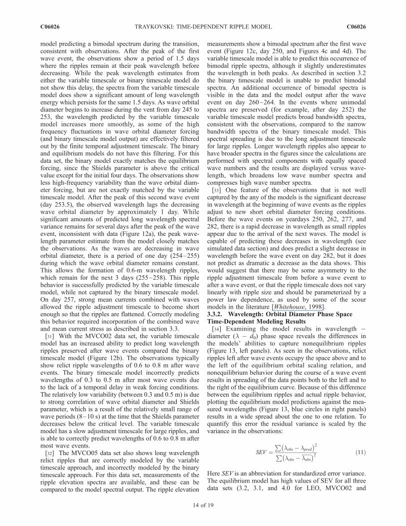
diameter (l � d0) phase space reveals the differences inthe models’ abilities to capture nonequilibrium ripples(Figure 13, left panels). As seen in the observations, relictripples left after wave events occupy the space above and tothe left of the equilibrium orbital scaling relation, andnonequilibrium behavior during the course of a wave eventresults in spreading of the data points both to the left and tothe right of the equilibrium curve. Because of this differencebetween the equilibrium ripples and actual ripple behavior,plotting the equilibrium model predictions against the mea-sured wavelengths (Figure 13, blue circles in right panels)results in a wide spread about the one to one relation. Toquantify this error the residual variance is scaled by thevariance in the observations:

SEV ¼P

lobs � lpred

� 2P

lobs � lobs

� 2 ð11Þ

Here SEV is an abbreviation for standardized error variance.The equilibrium model has high values of SEV for all threedata sets (3.2, 3.1, and 4.0 for LEO, MVCO02 and

C06026 TRAYKOVSKI: TIME-DEPENDENT RIPPLE MODEL

14 of 19

C06026

MVCO05, respectively, Table 1). These values of greaterthan one indicate that for both equilibrium and relictconditions, the mean of the observed wavelength (0.71,0.72, and 0.80 m) would be a better ripple wavelengthpredictor than using the equilibrium relation.[35] The binary timescale model predicts model output

points on the l = 0.75 d0,1/3 line except at low orbitaldiameters, when the Shields numbers are subcritical(Figure 13, green dots in left panels) and at high orbitaldiameter when the equilibrium relation predicts suborbitalripples. With the exception of the LEO15 data set, whererelict ripples existed as an initial condition, the relict ripplespredicted by the binary timescale model have wavelengthsof 0.3 to 0.6 m. While the data does show some relictripples at these wavelengths, there are a large number ofrelict ripple data points at longer wavelengths. Thus thebinary timescale model is only a significant improvement

over the equilibrium model for the LEO15 data (SEVreduced from 3.2 to 0.47), in which most of the data pointsare close to equilibrium since the measurements occurredmostly in active conditions. For the MVCO data sets thebinary timescale model still has SEV values over one,indicating that the mean of the observations is still a better

Figure 13. Model and data comparison. (a, c, and e) Left side panels show observed wavelength andmodel estimates of wavelength from the three modeling approaches as a function of the parameter d0,1/3and (b, d, and f) right side panels show observed wavelength versus model predicted wavelength for (aand b) LEO15, (c and d) MVCO02, and (e and f) MVCO05.

Table 1. Standardized Error Variances (SEV) for the Three

Different Modeling Approaches and Three Data Sets, Calculated

Using Equation 11a

LEO MVCO02 MVCO05

Equilibrium Model 3.2 3.1 4.0Binary Time Scale 0.45 (15%) 2.2 (72%) 3.3 (82%)Variable Time Scale 0.25 (8%) 0.78 (25%) 0.32 (8%)

aThe numbers in parentheses are the percentage of the equilibrium SEVfor the alternate modeling approaches.

C06026 TRAYKOVSKI: TIME-DEPENDENT RIPPLE MODEL

15 of 19

C06026

predictor for both equilibrium and relict conditions. If onlyequilibrium conditions were considered, the binary time-scale and the equilibrium model would perform better.[36] The variable timescale model predictions have con-

siderable spread about the equilibrium relation both duringactive and subcritical conditions. During active conditions,when the ripples are not in the suborbital regime (wave-lengths of approximately 0.8 m or greater), this spreadappears to be similar for both short and long orbitaldiameter conditions. This equal spread most likely resultsfrom the ripple adjustment timescale remaining relativelylong compared to the rapid fluctuations in orbital diametereven at high orbital diameters, due to the large cross-sectional areas of the large ripples (Figure 10). This is mostvisible in the MVCO02 data set (Figure 13c, red dots). Thesubcritical periods with relict ripples predicted by the modelare evident by long horizontal clusters of data points in l �d0 parameter space, which occur at all wavelengths from 0.3to 1.2 m, consistent with the data. While the variabletimescale model fills the same portions of parameter spaceas the data, it does not always do so coherently (i.e., it doesnot always exactly predict the correct wavelength at thecorrect time). The variable timescale model produces resultswith SEV values that are considerably better than the othermodeling approaches, but are still occasionally near one(MVCO02). Despite the inability to capture all the details ofripple wavelength fluctuations, the variable timescale mod-eling approach is clearly the preferred approach for predict-ing both equilibrium and relict ripple wavelengths in bothactive and subcritical conditions due to the significantlylower SEV values compared to the other approaches. Inparticular, the variable timescale is generally able to cor-

rectly predict the long wavelength relict ripples observed inthe data, and thus represents a significant improvement overthe other modeling approaches in this regard.3.3.3. Ripple Height and Steepness[37] While most of the analysis has focused on ripple

wavelength, since all three data sets have high qualitymeasurements of wavelength, the MVCO05 2-axis rotarypencil beam data set provided measurements of rippleheight and steepness (h / l). The spectral model alsoprovides predictions of ripple height and steepness. Theobservations show ripple steepness of around 0.15 to 0.17during active conditions, with lower steepness (0.05 to 0.1)during subcritical conditions. The ripple heights follow asimilar trend, with heights of 0.10 to 0.15 m duringenergetic conditions and 0.05 to 0.10 m during low-energyconditions (Figure 14). This decrease in ripple steepness indecreasing wave energy conditions (for example, after 245and 260) is qualitatively similar to the ripple splitting andflattening processes observed in laboratory studies [Testik etal., 2005]. Most of the periods of low steepness are alsoassociated with observed and predicted occurrences ofbimodal spectra.[38] Many of the equilibrium ripple models in the liter-

ature suggest that ripples will begin to flatten at Shieldsnumbers over 0.2 [Nielsen, 1981] or d0 / h over 20(consistent with suborbital and anorbital ripples, [Wibergand Harris, 1994]). The MVCO05 data, which is examinedin detail in this paper, has Shields numbers slightly over 0.3and d0 / h ratios of less than 25; thus it is not expected thatthe ripples should show a significant decrease in steepness.Other data from MVCO-05, which is not included in thetime series analysis presented here due to data gaps, show

Figure 14. Times series of (a) observed and modeled ripple height (h) and (b) ripple steepness (h / l)from the MVCO05 data set. Model predictions of (c) ripple height and (d) steepness are plotted againstobservations in the lower panels.

C06026 TRAYKOVSKI: TIME-DEPENDENT RIPPLE MODEL

16 of 19

C06026

ripples with a steepness of 0.15 to 0.20 during conditionswith Shields numbers of 0.5 to 0.6. The data with energeticconditions from MVCO02 (Figure 9) also does not show adecrease in steepness, although the height estimates fromthe rotary side-scan system are of lower quality than the 2-axis pencil beam system deployed at MVCO05 [Traykovskiet al., 1999]. Since the observations do not show a decreasein steepness during the most energetic conditions, the use ofa constant steepness (h / l = 0.16) in the equilibrium modelfor the model calculations is justified. The binary timescalemodel also predicts the same constant steepness because theheight of the predicted ripples is always directly related tothe wavelength. This results in poor model performance inpredicting steepness for both the equilibrium and binarytimescale model, which have SEVs for ripple steepness of2.0 (Table 2). The variable timescale model adjusts thespectral variance of each wave number component with adifferent timescale, which results in long wavelength relictripples with relatively low height during subcritical con-ditions. The performance of this model in predicting steep-ness (SEV = 0.62) is significantly better than the equilibriumor binary timescale models.[39] Despite the inability of the equilibrium and binary

timescale models to predict steepness well, all three modelspredict ripple height with approximately similar skill, withthe equilibrium model being slightly inferior to the othertwo approaches (Figures 14a and 14c). The equilibrium andbinary timescale models both under predict ripple wave-length during subcritical conditions. The combination of theprediction of short wavelength ripples and a constantsteepness assumption results in relatively low amplituderipples during subcritical conditions, while observations lowamplitude long wavelength ripples in combination with lowamplitude short wavelength ripples (bimodal spectra). Thevariable timescale model predicts correctly these bimodalspectra with long wavelength peak components duringsubcritical conditions, resulting in the correct prediction ofrelatively low integrated ripple heights.

4. Conclusions

[40] An extensive data set of ripple observations collectedat two locations with medium and coarse sand show thatripple parameters such as wavelength and ripple height areoften not in equilibrium with hydrodynamic forcing. Theobservations were conducted with two different measure-ment and analysis techniques. While the rotary side-scantechnique produces a large field of view ripple planformimage rather quickly (or with better averaging for reducednoise), a pencil beam sonar with two stepper motorsprovides a topographic map of ripple surface elevation fromwhich elevation spectra can be calculated. Both techniquesproduce estimates of ripple wavelength that scale with wave

orbital diameter during moderate energy conditions whenthe ripples are in equilibrium with hydrodynamic forcing.This orbital scaling, combined with the absence of areduction in ripple height, steepness, or wavelength at highstresses, suggests that examining the data in terms of thewavelength and orbital diameter parameters (l � d0 space)is the most useful approach for these ripples. An equilib-rium model for these ripples was developed by combiningorbital ripple scaling with a suspension threshold to deter-mine the maximum wavelength ripple as the orbital ripplestransition into the suborbital regime [Smith and Wiberg,2006]. This threshold is a function of wave orbital velocityand grain size, while maximum wavelength at the thresholddepends on wave orbital diameter. Consequently, thisapproach depends on orbital velocity, orbital diameter,and grain size, and represents an improvement on previousapproaches that depended only on orbital diameter and grainsize.[41] Examining the observations in l � d0 space shows

that the majority of the nonequilibrium points are longwavelength relict ripples that remain after the peak of thewave event as wave orbital diameters decrease. Threedifferent modeling approaches were compared to betterpredict ripple parameters in active and subcritical condi-tions. The first approach assumed that the ripples were inequilibrium at all times, with no ability to predict relictripples. The second approach forced relict ripples to bepreserved with geometry consistent with the equilibriumforcing at the time the stress became subcritical. Thisapproach predicted relict ripples that were considerablyshorter than observed. A third modeling approach wasdeveloped with a first order differential equation whichallows the ripples to lag the forcing by means of atemporally variable adjustment timescale, defined by theripple cross-sectional area divided by the sediment transportrate. To fit the data, the adjustment timescale was multipliedby a single constant for all three data sets. In both thesecond and third modeling approaches the ripple spectra aremodeled linearly, so that each spectral component is treatedindependently. The variable timescale model allowed longerwavelength relict ripples to be preserved after wave events,due to the long delay timescales associated with largeripples formed at the peak of a wave event.[42] The variable timescale model was also able to predict

bimodal ripple spectra due to the different timescalesassociated with small and large ripples. The other modelingapproaches can only predict unimodal spectra due to theirequilibrium relation with forcing. The ability to predictbimodal spectra is partially a function of the varyingtemporal adjustment for different wavelength ripple compo-nents in the model, and partially due to the temporalevolution of the hydrodynamic forcing. The model willonly predict bimodal ripple spectra under certain temporalpatterns of hydrodynamic forcing. The observations, otherlaboratory observations [e.g., Testik et al., 2005] and othertypes models [Andersen et al., 2001; Werner and Kocurek,1999] suggest that bimodal spectra may be a phenomenoninherent to ripple dynamics and not dependent on the detailsof the hydrodynamic forcing. For instance, if the onlymechanisms that decrease ripple wavelengths are the growthof new ripples in the troughs of the previous ripples or thealong-crest propagation of crest bifurcations, then bimodal

Table 2. Standardized Error Variances (SEV) for the Three

Different Modeling Approaches for Ripple Height and Steepness

With the MVCO05 Data Set

Ripple Height Ripple Steepness

Equilibrium Model 0.93 2.0Binary Time Scale 0.68 (73%) 2.0 (100%)Variable Time Scale 0.52 (56%) 0.48 (25%)

C06026 TRAYKOVSKI: TIME-DEPENDENT RIPPLE MODEL

17 of 19

C06026

spectra maybe an intrinsic feature of ripples that aredecreasing in wavelength. The equilibrium model that isinherent to this type of model does not account for thepossibility that there could be multiple stable ripple statesfor a given forcing condition. This model, with parameter-ized scaling relations, does not capture the complexity ofthese types of nonlinear ripple-ripple interactions. Futurework on ripple evolution using three-dimensional couplednumerical hydrodynamic and sediment transport models, aswell as additional analysis of the observations could be usedto tune the parameter dependence of simplified models suchas those presented here. Compared to a coupled numericalhydrodynamic sediment transport model, the parameterizedapproach employed here is more practical for use as apredictive tool when the input is a long-time series ofhydrodynamic conditions. Since this parameterized modelcan incorporate any equilibrium ripple model, future workcould also extend this modeling approach to other condi-tions and environments where there are significant delaysbetween hydrodynamic forcing and ripple morphologicchange.

[43] Acknowledgments. The author would like to thank the supportstaff of the Martha’s Vineyard Coastal Observatory and the LEO-15observatory for assistance in the deployments. I would also like to thankthe captain and crew of the RVAsterias, RV Tioga, and RV Connecticut fortheir able seamanship in the deployment of the instrumentation. James Irishprovided invaluable technical support in developing and maintaining theinstrumentation. This work was funded under ONR grants N00014-01-10564 and N00014-06-10329 under the direction of program managerThomas Drake.

ReferencesAndersen, K. H., M.-L. Chabanol, and M. V. Hecke (2001), Dynamicalmodels for sand ripples beneath surface waves, Phys. Rev. E, 63, 8.

Ardhuin, F., T. G. Drake, and T. H. C. Herbers (2002), Observations ofwave-generated vortex ripples on the North Carolina continental shelf,J. Geophys. Res., 107(C10), 3143, doi:10.1029/2001JC000986.

Ardhuin, F., W. C. O’Reilly, T. H. C. Herbers, and P. F. Jessen (2003), Swelltransformation across the continental shelf: Part I. Attenuation and direc-tional broadening, J. Phys. Oceanogr., 33, 1921–1939.

Austin, T. C., J. B. Edson, W. R. McGillis, M. J. P. C. von Alt, R. Petitt,M. K. McElroy, J. Ware, and R. Stokey (2000), The Martha’s vineyardcoastal observatory: A long term facility for monitoring air-sea pro-cesses, paper presented at Proceedings of the Oceans 2000, MTS/IEEEConferenc.

Chotiros, N. P., D. E. Smith, and J. N. Piper (2002), Refraction andscattering into a sandy ocean sediment in the 30–40-kHz band, IEEEJ. Oceanic Eng., 27, 362–375.

Clifton, H. E., and J. R. Dingler (1984), Wave-formed structures andpaleoenvironmental reconstruction, Mar. Geol., 60, 165–198.

Craghan, M. (1995), Topographic changes and sediment characteristics at ashoreface sand ridge—Beach Haven Ridge, New Jersey, M.S. thesis,123 pp., Rutgers University, Rutgers, N. J.

Crawford, A. M., and A. E. Hay (2003), Wave orbital velocity skewnessand linear transition ripple migration: Comparison with weakly nonlineartheory, J. Geophys. Res., 108(3), 3091, doi:10.1029/2001JC001254.

Davis, J. P., D. J. Walker, M. Townsend, and I. R. Young (2004), Wave-formed sediment ripples: Transient analysis of ripple spectral develop-ment, J. Geophys. Res., 109, C07020, doi:10.1029/2004JC002307.

Doucette, J. S., and T. O’Donoghue (2003), Sand ripples in irregular andchanging wave conditions: A review of laboratory and field studies,Report for EC MAST Project No. MAS3-CT97-0086 Sandpit project,http://sandpit.wldelft.nl/reportpage/right/SandpitLiteratureReviewVanDerWerf.pdf.

Gibbs, R. J., M. D. Mathews, and D. A. Link (1971), The relationshipbetween sphere size and settling velocity, J. Sediment. Petrol., 41, 7–18.

Goff, J. A., L. A. Mayer, P. Traykovski, I. Buynevich, R. Wilkens,R. Raymond, G. Glang, R. L. Evans, H. Olson, and C. Jenkins(2005), Detailed investigation of sorted bedforms, or ‘‘rippled scourdepressions,’’ within the Martha’s Vineyard Coastal Observatory,Massachusetts, Cont. Shelf Res., 25, 461–484.

Grant, W. D., and O. S. Madsen (1986), The continental-shelf bottomboundary layer, Annu. Rev. Fluid Mech., 18, 265–305.

Hanes, D. M., V. Alymov, and Y. S. Chang (2001), Wave-formed sandripples at Duck, North Carolina, J. Geophys. Res., 106, 22,575–522,592.

Harris, C. K., and P. L. Wiberg (2001), A two-dimensional, time-dependentmodel of suspended sediment transport and bed reworking for continentalshelves, Comput. Geosci., 27, 675–690.

Hay, A. E., and T. Mudge (2005), Principal bed states during Sandy-Duck97: Occurrence, spectral anisotropy, and the bed state storm cycle,J. Geophys. Res., 110, C03013, doi:10.1029/2004JC002451.

Hay, A. E., and D. J. Wilson (1994), Rotary sidescan images of nearshorebedform evolution during a storm, Mar. Geol., 119, 57–65.

Hsu, T. J., and D. M. Hanes (2004), Effects of wave shape on sheetflow sediment transport, J. Geophys. Res., 109, C05025, doi:10.1029/2003JC002075.

Hsu, T. J., and B. Raubenheimer (2006), A numerical and field study oninner-surf and swash sediment transport, Cont. Shelf Res., 26, 589–598.

Jackson, D. R., K. L. Williams, E. I. Thorsos, and S. G. Kargl (2002),High-frequency subcritical acoustic penetration into a sandy sediment,IEEE J. Oceanic Eng., 27, 346–361.

Lesser, G., J. Kester, and J. A. Roelvink (2000), Report Z3899, DelftHydraulics, Delft, Netherlands.

Li, M. Z., and C. L. Amos (2001), SEDTRANS96: The upgraded and bettercalibrated sediment-transport model for continental shelves, Comput.Geosci., 27, 619–645.

Madsen, O. S., Y.-K. Poon, and H. C. Graber (1988), Spectral WaveAttenuation by Bottom Friction: Theory, paper presented at Proceedingsof the 21st International Conference on Coastal Engineering, Am. Soc. ofCiv. Eng., New York.

Meyer-Peter, E., and R. Muller (1948), Formulas for bed-load transport,paper presented at Paper presented at 3rd Meeting. IAHR, Int. Assoc.Hydraul. Res., Stockholm.

Ngusaru, A. S., and A. E. Hay (2004), Cross-shore migration of lunate mega-ripples during Duck94, J. Geophys. Res., 109, C02006, doi:10.1029/2002JC001532.

Nielsen, P. (1981), Dynamics and geometry of wave-generated ripples,J. Geophys. Res., 86, 6467–6472.

Precht, E., and M. Huettel (2004), Rapid wave-driven advective porewater exchange in a permeable coastal sediment, J. Sea Res., 51,93–107.

Richardson, M. D., and P. Traykovski (2002), Real-time observations ofmine burial at the Martha’s Vineyard Coastal Observatory, paper pre-sented at Proceedings of the 5th International Symposium on Technologyand the Mine Problem, Naval Postgraduate School, Monterey California,22–25 May.

Smith, D., and J. F. A. Sleath (2005), Transient ripples in oscillatory flows,Cont. Shelf Res., 25, 485–501.

Smith, J. J., and P. L. Wiberg (2006), Ripple Geometry in Wave-DominatedEnvironments Revisited, paper presented at Eos Trans. AGU, 87(36),Ocean Sci. Meet. Suppl., Abstract OS35D-24.

Smyth, C., and A. E. Hay (2002), Wave friction factors in nearshore sands,J. Phys. Oceanogr., 32, 3490–3498.

Smyth, C. E., and M. Z. Li (2005), Wave-current bedform scales, orienta-tion, and migration on Stable Island Bank, J. Geophys. Res., 110,C02023, doi:10.1029/2004JC002569.

Soulsby, R. L., and R. J. S. Whitehouse (2005), Prediction of ripple proper-ties in shelf seas. Mark 1 predictor, Report TR150, Release 1.1, producedby HR Wallingford Ltd, UK for the ONR Ripples DRI Program, http://www.hrwallingford.co.uk/downloads/projects/ripples/TR150_ripples.pdf.

Styles, R., and S. M. Glenn (2002), Modeling bottom roughness in thepresence of wave-generated ripples, J. Geophys. Res., 107(C8), 3110,doi:10.1029/2001JC000864.

Sumer, B. M., and J. Fredsøe (2002), The Mechanics of Scour in the MarineEnvironment, World Scientific, Singapore.

Swart, D. H. (1974), Offshore sediment transport and equilibrium beachprofiles, p. 302, Delft Hydraulics Laboratory, Delft, Netherlands.

Terray, E. A., R. L. Gordon, and B. H. Brumley (1997), Measuring waveheight and direction using upward-looking ADCPs, paper presented atProc. of Oceans’97. Oceans’97 MTS/IEEE.

Testik, F. Y., S. I. Voropayev, and H. J. S. Fernando (2005), Adjustment ofsand ripples under changing water waves, Phys. Fluids, 17, 072,104–072,108.

Traykovski, P., A. E. Hay, J. D. Irish, and J. F. Lynch (1999), Geometry,migration, and evolution of wave orbital ripples at LEO-15, J. Geophys.Res., 104, 1505–1524.

Trembanis, A. C., C. T. Friedrichs, M. Richardson, P. A. Traykovski, andP. Howd (2007), Predicting seabed burial of cylinders by wave-inducedscour: Application to the sandy inner shelf off Florida and Massachusetts,IEEE J. Oceanic Eng., in press.

C06026 TRAYKOVSKI: TIME-DEPENDENT RIPPLE MODEL

18 of 19

C06026

Voropayev, S. I., G. B. McEachern, D. L. Boyer, and H. J. S. Fernando(1999), Dynamics of sand ripples and burial/scouring of cobbles inoscillatory flow, Appl. Ocean Res., 21, 249–261.

Voropayev, S. I., F. Y. Testik, H. J. S. Fernando, and D. L. Boyer (2003),Morphodynamics and cobbles behavior in and near the surf zone, OceanEng., 30, 1741–1764.

Warner, J. C., C. R. Sherwood, R. P. Signell, C. K. Harris, and H. Arango(2007), Development of a three-dimensional, regional, coupled wave-,current-, and sediment-transport model, Comput. Geosci., in review.

Werner, B. T., and G. Kocurek (1999), Bedform spacing from defectdynamics, Geology, 27, 727–730.

Wheatcroft, R. A. (1994), Temporal variation in bed configuration andone-dimensional bottom roughness at the mid-shelf STRESS site, Cont.Shelf Res., 14, 1167–1190.

Whitehouse, R. (1998), Scour at Marine Structures: A Manual for PracticalApplications, 198 pp., Thomas Telford Publications, London.

Wiberg, P. L., and C. K. Harris (1994), Ripple geometry in wave-dominatedenvironments, J. Geophys. Res., 99, 775–789.

Williams, J. J., P. S. Bell, and P. D. Thorne (2005), Unifying large and smallwave-generated ripples, J. Geophys. Res., 110, C02008, doi:10.1029/2004JC002513.

�����������������������P. Traykovski, Applied Ocean Physics and Engineering Department,

Woods Hole Oceanographic Institution, Woods Hole, MA 02543, USA.(ptraykovski@whoi.edu)

C06026 TRAYKOVSKI: TIME-DEPENDENT RIPPLE MODEL

19 of 19

C06026