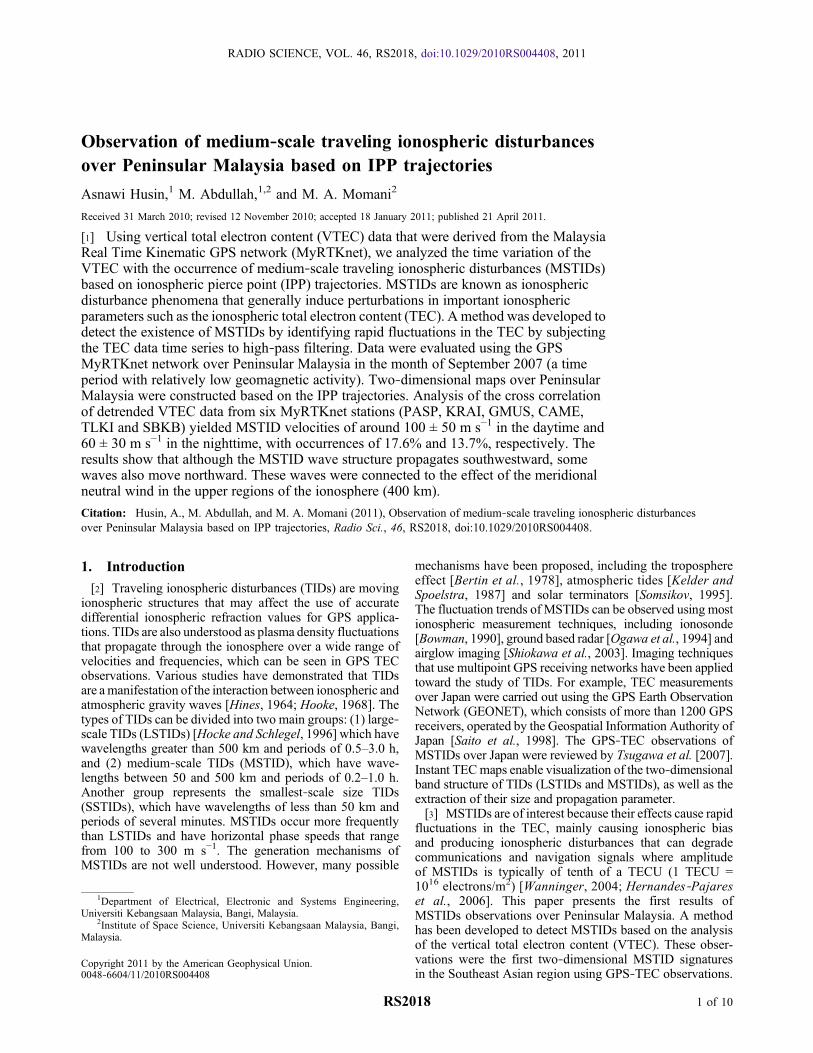
Observation of medium‐scale traveling ionospheric disturbancesover Peninsular Malaysia based on IPP trajectories

Asnawi Husin,1 M. Abdullah,1,2 and M. A. Momani2

Received 31 March 2010; revised 12 November 2010; accepted 18 January 2011; published 21 April 2011.

[1] Using vertical total electron content (VTEC) data that were derived from the MalaysiaReal Time Kinematic GPS network (MyRTKnet), we analyzed the time variation of theVTEC with the occurrence of medium‐scale traveling ionospheric disturbances (MSTIDs)based on ionospheric pierce point (IPP) trajectories. MSTIDs are known as ionosphericdisturbance phenomena that generally induce perturbations in important ionosphericparameters such as the ionospheric total electron content (TEC). Amethod was developed todetect the existence of MSTIDs by identifying rapid fluctuations in the TEC by subjectingthe TEC data time series to high‐pass filtering. Data were evaluated using the GPSMyRTKnet network over Peninsular Malaysia in the month of September 2007 (a timeperiod with relatively low geomagnetic activity). Two‐dimensional maps over PeninsularMalaysia were constructed based on the IPP trajectories. Analysis of the cross correlationof detrended VTEC data from six MyRTKnet stations (PASP, KRAI, GMUS, CAME,TLKI and SBKB) yielded MSTID velocities of around 100 ± 50 m s−1 in the daytime and60 ± 30 m s−1 in the nighttime, with occurrences of 17.6% and 13.7%, respectively. Theresults show that although the MSTID wave structure propagates southwestward, somewaves also move northward. These waves were connected to the effect of the meridionalneutral wind in the upper regions of the ionosphere (400 km).

Citation: Husin, A., M. Abdullah, and M. A. Momani (2011), Observation of medium‐scale traveling ionospheric disturbancesover Peninsular Malaysia based on IPP trajectories, Radio Sci., 46, RS2018, doi:10.1029/2010RS004408.

1. Introduction

[2] Traveling ionospheric disturbances (TIDs) are movingionospheric structures that may affect the use of accuratedifferential ionospheric refraction values for GPS applica-tions. TIDs are also understood as plasma density fluctuationsthat propagate through the ionosphere over a wide range ofvelocities and frequencies, which can be seen in GPS TECobservations. Various studies have demonstrated that TIDsare amanifestation of the interaction between ionospheric andatmospheric gravity waves [Hines, 1964; Hooke, 1968]. Thetypes of TIDs can be divided into two main groups: (1) large‐scale TIDs (LSTIDs) [Hocke and Schlegel, 1996] which havewavelengths greater than 500 km and periods of 0.5–3.0 h,and (2) medium‐scale TIDs (MSTID), which have wave-lengths between 50 and 500 km and periods of 0.2–1.0 h.Another group represents the smallest‐scale size TIDs(SSTIDs), which have wavelengths of less than 50 km andperiods of several minutes. MSTIDs occur more frequentlythan LSTIDs and have horizontal phase speeds that rangefrom 100 to 300 m s−1. The generation mechanisms ofMSTIDs are not well understood. However, many possible

mechanisms have been proposed, including the troposphereeffect [Bertin et al., 1978], atmospheric tides [Kelder andSpoelstra, 1987] and solar terminators [Somsikov, 1995].The fluctuation trends of MSTIDs can be observed using mostionospheric measurement techniques, including ionosonde[Bowman, 1990], ground based radar [Ogawa et al., 1994] andairglow imaging [Shiokawa et al., 2003]. Imaging techniquesthat use multipoint GPS receiving networks have been appliedtoward the study of TIDs. For example, TEC measurementsover Japan were carried out using the GPS Earth ObservationNetwork (GEONET), which consists of more than 1200 GPSreceivers, operated by the Geospatial Information Authority ofJapan [Saito et al., 1998]. The GPS‐TEC observations ofMSTIDs over Japan were reviewed by Tsugawa et al. [2007].Instant TECmaps enable visualization of the two‐dimensionalband structure of TIDs (LSTIDs and MSTIDs), as well as theextraction of their size and propagation parameter.[3] MSTIDs are of interest because their effects cause rapid

fluctuations in the TEC, mainly causing ionospheric biasand producing ionospheric disturbances that can degradecommunications and navigation signals where amplitudeof MSTIDs is typically of tenth of a TECU (1 TECU =1016 electrons/m2) [Wanninger, 2004; Hernandes‐Pajareset al., 2006]. This paper presents the first results ofMSTIDs observations over Peninsular Malaysia. A methodhas been developed to detect MSTIDs based on the analysisof the vertical total electron content (VTEC). These obser-vations were the first two‐dimensional MSTID signaturesin the Southeast Asian region using GPS‐TEC observations.

1Department of Electrical, Electronic and Systems Engineering,Universiti Kebangsaan Malaysia, Bangi, Malaysia.

2Institute of Space Science, Universiti Kebangsaan Malaysia, Bangi,Malaysia.

Copyright 2011 by the American Geophysical Union.0048‐6604/11/2010RS004408

RADIO SCIENCE, VOL. 46, RS2018, doi:10.1029/2010RS004408, 2011

RS2018 1 of 10

The GPS network system belonging to Malaysia (i.e., theMalaysia Real Time Kinematics GPS Network System;MyRTKnet) was used to analyze ionospheric TEC variationswith the occurrence of MSTIDs at low latitudes. Data wereanalyzed for days having relatively low geomagnetic activi-ties in September 2007.

2. Data and Methods

2.1. Data

[4] The MyRTKnet owned and operated by the Depart-ment of Survey and Mapping Malaysia (Jabatan Ukur dan

Pemetaan Malaysia, JUPEM) consists of 50 dual frequencyGPS reference stations in Peninsular Malaysia and 28 in EastMalaysia. MyRTKnet provides various levels of GPS data.The Receiver Independent Exchange (RINEX) data from50MyRTKnet GPS stations in Peninsular Malaysia (Figure 1)were used to derive the TEC values and study the variationsin TEC associated with the occurrence of MSTIDs at lowlatitudes. MyRTKnet data included carrier‐phase and groupdelays (P‐code pseudorange) of dual‐frequency (f1 = 1.57542and f2 = 1.22760 GHz) GPS signals in 15 s intervals; thesedata were processed using scientific software.

Figure 1. Distribution of the GPSMyRTKnet stations in Peninsular Malaysia that were used for the detec-tion of MSTIDs.

Figure 2. GPSTk TEC data processing with MyRTKnet stations. Adapted from Gaussiran et al. [2004].

HUSIN ET AL.: MSTID OVER PENINSULAR MALAYSIA RS2018RS2018

2 of 10

2.2. GPS Toolkit TEC Measurements

[5] Many researchers have developed ionospheric GPSTEC measurement methods. Simple measurements of theTEC can be derived from pseudorange calculations; however,the noise term and interfrequency biases cannot be ignored.The relative TEC variation can be obtained with a higherdegree of precision from the carrier phase since the carrierphase noise is less than the pseudorange noise. Since thecarrier phase is measured with far greater precision thanpseudoranges, which are derived from code correlation, theGPS carrier phase‐derived TEC provides a smooth and pre-cise, albeit relative, measurement of the ionospheric TEC.The relativity of this measurement is due to ambiguities inthe total number of wave cycles between the satellite andreceiver. Cycle slips produce isolated discrete discontinuities

in the carrier phase that must be detected and removed beforethe phase TEC can be computed. After this has been com-pleted, the overall phase ambiguity may be removed from thephase TEC, with the help of the pseudorange, to produce aTEC estimate that is both low in noise and without phase bias.To obtain the TEC values, a GPS Toolkit (GPSTk) scientificsoftware package was used which can accomplish both thecarrier phase discontinuity correction and the phase ambi-guity removal [Garner et al., 2008].[6] The GPSTk is an open source software from the

Applied Research Laboratories of the University of Texas atAustin (USA) which was developed for discontinuity cor-rections. This software provides a core library and a collec-tion of applications that support GPS research, analysis anddevelopment [Tolman and Harries, 2004]. The code is

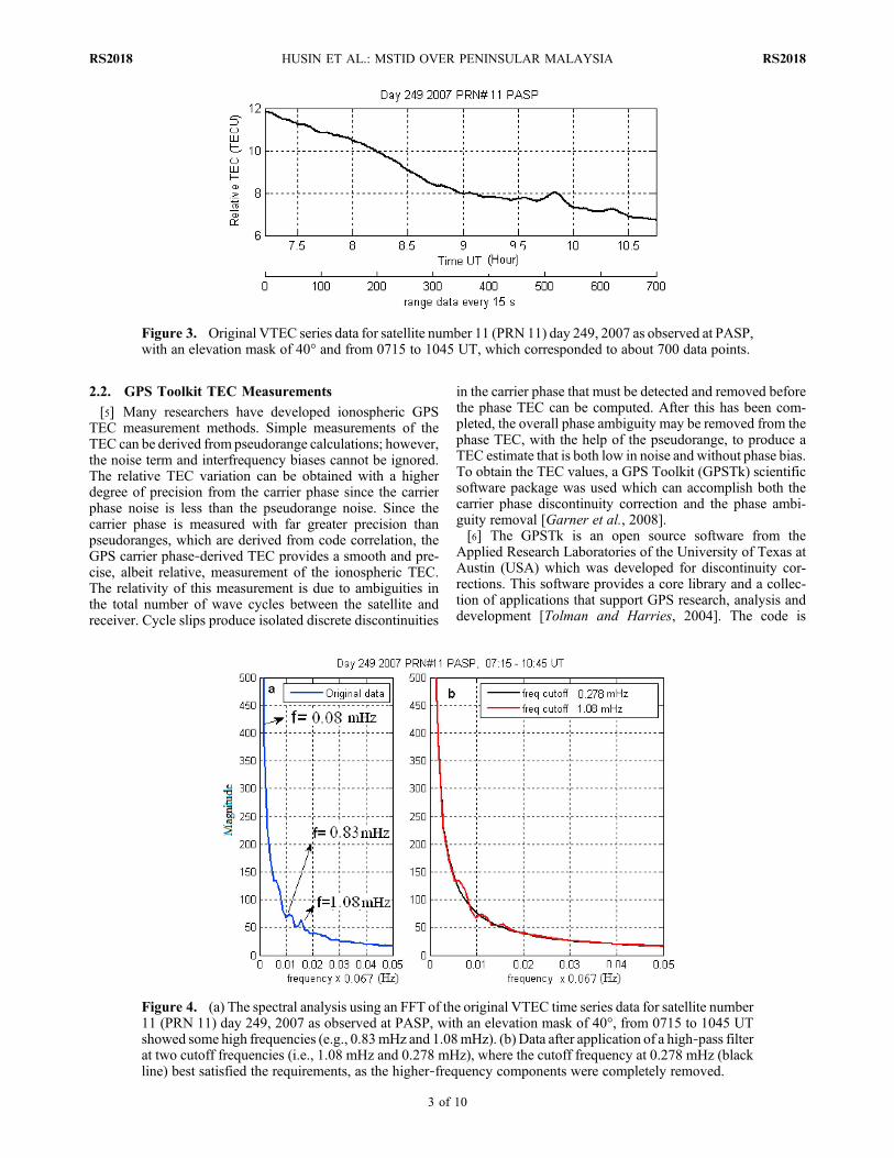
Figure 3. Original VTEC series data for satellite number 11 (PRN 11) day 249, 2007 as observed at PASP,with an elevation mask of 40° and from 0715 to 1045 UT, which corresponded to about 700 data points.

Figure 4. (a) The spectral analysis using an FFT of the original VTEC time series data for satellite number11 (PRN 11) day 249, 2007 as observed at PASP, with an elevation mask of 40°, from 0715 to 1045 UTshowed some high frequencies (e.g., 0.83mHz and 1.08mHz). (b) Data after application of a high‐pass filterat two cutoff frequencies (i.e., 1.08 mHz and 0.278 mHz), where the cutoff frequency at 0.278 mHz (blackline) best satisfied the requirements, as the higher‐frequency components were completely removed.

HUSIN ET AL.: MSTID OVER PENINSULAR MALAYSIA RS2018RS2018

3 of 10

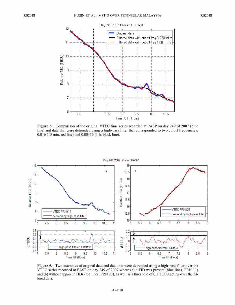
Figure 5. Comparison of the original VTEC time series recorded at PASP on day 249 of 2007 (blueline) and data that were detrended using a high‐pass filter that corresponded to two cutoff frequencies:0.016 (15 min, red line) and 0.00416 (1 h, black line).

Figure 6. Two examples of original data and data that were detrended using a high‐pass filter over theVTEC series recorded at PASP on day 249 of 2007 where (a) a TID was present (blue lines, PRN 11)and (b) without apparent TIDs (red lines, PRN 23), as well as a threshold of 0.1 TECU acting over the fil-tered data.

HUSIN ET AL.: MSTID OVER PENINSULAR MALAYSIA RS2018RS2018

4 of 10

released under the terms of the Lesser GNU Public License.Anyone who is interested in GPS software development candownload the source code and participate in discussions withother GPS software developers on the official GPSTk web-

site at http://www.gpstk.org. This algorithm is based on thewide‐lane (WL) bias and the geometry‐free (GF) phase,which are linear combinations of the pseudorange and phasesfrom both the L1 and L2 frequencies [Garner et al., 2008].The TECwas processed using the GPSTk assumption that theionosphere consists of a thin shell at a fixed height, usually350 or 400 km, that surrounds the Earth (single layer model;SLM) [Gaussiran et al., 2004]. The GPSTk was used toperform data editing and estimates of the TEC for RINEXformat data as shown in Figure 2. The analysis includedpreprocessing for cycle slip detection and removal usingDiscFix. The ResCor application was used to generate theslant TEC, the geographic latitude and longitude of the IPPand the elevation and azimuth of the satellite, as well as toremove satellite biases. The RinexDump application wasused to provide data in columnar format. This measurementstill contains the receiver interfrequency biases. The knowl-edge of relative TEC changes is sufficient for this work, as theaim of this study is to focus on the perturbation components ofthe TEC that are caused by MSTIDs.

2.3. TEC Detrending

[7] The TEC variations are strongly influenced by itsregular variations, long‐term trend as well as by differentshort‐term changes. The long‐term variations refer to diurnal,seasonal and solar cycle variations, while the short termvariations are mainly caused by geomagnetic storms andionospheric disturbances (from a few minutes to 2 days). TheMSTID effects cause a rapid fluctuation in the measured TECwith a time period between 0.2 and 1.0 h. Taking advantage ofthis feature, the method developed here detects the existence

Figure 7. The IPP trajectory of PRN 6 over station PASPand KRAI on day 249 of 2007. dripp is the distance vectorbetween IPP of PASP (green line) and IPP of KRAI (blueline) and vipp is the velocity vector of IPP of PRN 6.

Figure 8. The IPP trajectories of all GPS satellites on day 249 of 2007 (6 September 2007) with an ele-vation mask of 40°: (a) single station GPSMyRTKnet (PASP), 24 h observation and (b) all GPSMyRTKnetstations from 0000 to 0045 (45 min). The black lines are the IPP directions moving toward high latitudes(north), and the red lines are the IPP directions moving toward lower latitudes (south).

HUSIN ET AL.: MSTID OVER PENINSULAR MALAYSIA RS2018RS2018

5 of 10

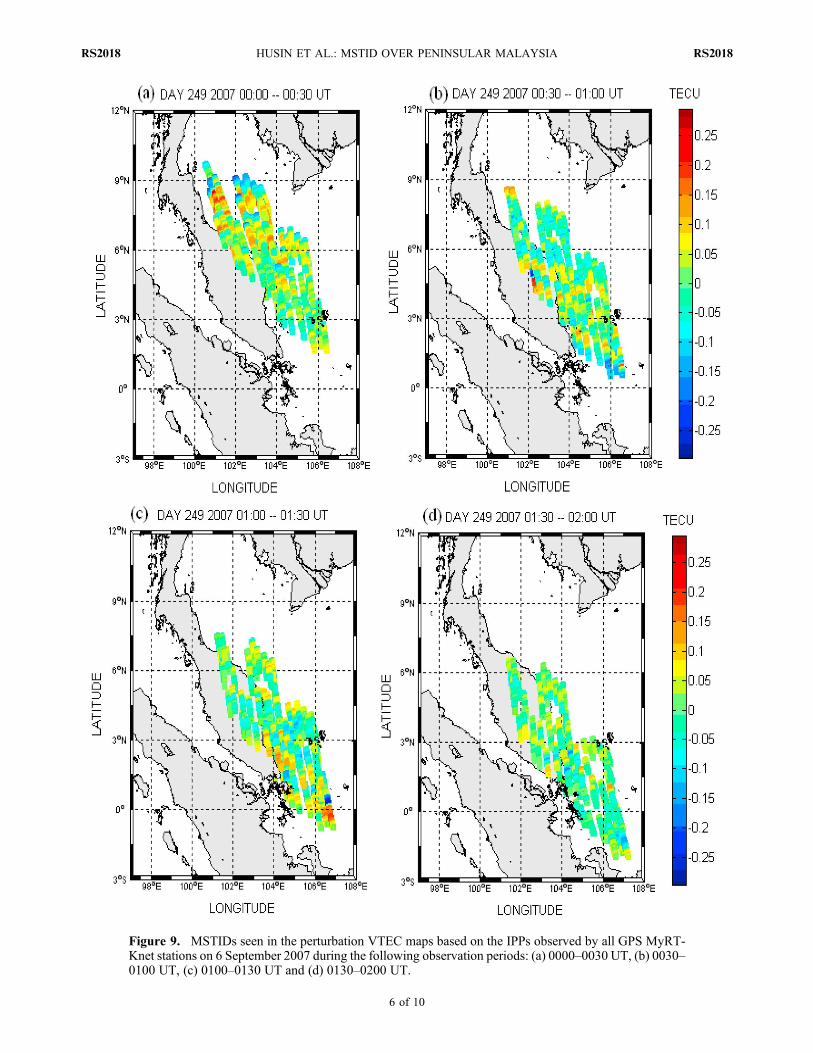
Figure 9. MSTIDs seen in the perturbation VTEC maps based on the IPPs observed by all GPS MyRT-Knet stations on 6 September 2007 during the following observation periods: (a) 0000–0030 UT, (b) 0030–0100 UT, (c) 0100–0130 UT and (d) 0130–0200 UT.

HUSIN ET AL.: MSTID OVER PENINSULAR MALAYSIA RS2018RS2018

6 of 10

of MSTIDs by identifying rapid fluctuations in the TECvalues. To do this, it is assumed that the TEC data corre-sponding to satellite‐to‐ground station paths are time series inthe universal time (UT) which is then detrended from diurnalvariations. Detrending can be done in several ways as it hasbeen done by previous researchers, for example by using therate of TEC (ROT) parameter [Warnant and Pottiaux, 2000].In this work, rapid fluctuations in the TEC series data wereidentified using a high‐pass filter. To avoid multipath effectsand elevation angle dependences, an elevation mask of 40°was applied (i.e., data below 40° were excluded). A high‐pass filter was applied to the data with cutoff frequency of0.278 mHz which corresponds to a period of 1 h.[8] The GPS MyRTKnet has a typical temporal resolution

of 15 s. Thus, for one satellite pass with an elevation mask at40°, we obtained 700–1000 data points, which correspondedto 3–4 h of data (Figure 3). The trend components andhardware noise were included in this data. A series transfor-mation from the time domain to the frequency domain wasperformed using a fast Fourier transform (FFT). For example,Figure 4a displays the frequency domain of the VTEC seriesof PRN 11 day 249 of 2007 PASP, which had a minimumfrequency of 0.08 mHz (period around 3.5 h) and containedsome high frequencies (i.e., 0.83 mHz and 1.08 mHz), cor-responding to 20 and 15 min periods, respectively. Theminimum frequencies were associated with regular varia-tions, while the higher frequencies were associated withirregular variations that might have been caused by MSTIDs.Fourth‐order Butterworth high‐pass filter design techniqueswere used and forwarded by zero‐phase digital filtering[Trauth, 2006]. To select the most appropriate cutoff fre-quency, the original VTEC time series for one satellite passwas processed with two cutoff frequency sizes of 1.08 mHz(15 min, red line in Figure 4b) and 0.278 mHz (1 h, black linein Figure 4b). As shown in Figure 4b, a frequency cutoff of

0.278 mHz (black line) best satisfies this requirement. This isbecause the higher‐frequency components were completelyremoved in this case. Data detrending was carried out bysubtracting the filtered data from the original series data. Inother words, the higher frequencies in the original data wereremoved using the high‐pass filtered data. Figure 5 provides acomparison of the original series VTEC data curve with thedetrended data using two cutoff frequencies of the high‐passfilter. As shown in Figure 5, the curve corresponding to a 1 hcutoff period was adequate.[9] Other phenomena can also occur, such as equatorial

ionospheric plasma bubbles that are capable of depleting theTEC; however, the present study is particularly concernedwith the VTEC variations associated with MSTIDs. There-fore, only increases in the amplitude of the TEC fluctuationsabove a certain threshold were taken into account. Thethreshold values were set to permit detrended TEC valueswith fluctuation amplitude greater than 0.1 TECUwith a timeinterval between 5 and 60 min (MSTID period). Figure 6provides two examples of the original data and the data thatwere detrended using a high‐pass filter over the VTEC serieswithout apparent TIDs (red lines, PRN 23) and where a TID ispresent (blue lines, PRN 11), as well as a threshold of 0.1TECU acting over the filtered data.[10] After a TEC increase was identified as a TID, it was

necessary to locate it geographically. As a first approxima-tion, it was supposed to be situated at the IPP. The IPP is thepoint at which the signal crosses the model ionospheric shell(400 km altitude). The IPP for a given satellite and receivercan be computed from the receiver position and the observedelevation and azimuth angles of the satellites, as seen at thereceiver, along with the height of the ionosphere. Thisparameter represents the assumed altitude of the centroid ofmass of the ionosphere [Birch et al., 2002], which is mostlyused in the calculation of irregularity drifts and in converting

Figure 10. Temporal variations of the detrendedVTEC (a) on day 246 of 2007 at the IPP trajectory of PRN6 and (b) on day 249 of 2007 at the IPP trajectory of PRN 8, as observed at GPS MyRTKnet sites: PASP,KRAI, GMUS, CAME, TLKI and SBKB.

HUSIN ET AL.: MSTID OVER PENINSULAR MALAYSIA RS2018RS2018

7 of 10

the measured slant TEC to the VTEC [Rao et al., 2006]. Asmentioned previously, the ResCor application was used togenerate the slant TEC, as well as the geographic latitude andlongitude of the IPP. The GPSTk was used to process theVTEC from the slant TEC at the IPP, as described byGaussiran et al. [2004].[11] The wave propagation parameters (i.e., velocity and

direction) can be obtained by performing a cross‐correlationanalysis of the relative change in TEC between receivers. Therelative movement of the GPS satellites and receivers in-troduces a Doppler effect that must be corrected in theobservational equations. The Doppler effect depends on thealtitude where the TID occurs; however, this impact is small,in general [Hernandes‐Pajares et al., 2006]. To estimate thepropagation parameter, we assumed that the TID propagatedas a planar wave [Hernandes‐Pajares et al., 2006], for aninstant time t and a pierce point ripp:

�VTEC t; ripp� � ¼ F !t � k � ripp

� � ð1Þ

where F is an arbitrary function, w is the frequency, and k isthe propagation vector. By defining the slowness of the vector[Jacobson et al., 1995], s = k/w:

�VTEC t; ripp� � ¼ ! � F t � s � ripp

� � ð2Þ

By looking for the correlation between this ionospheric per-turbation for different receivers, the temporal delay formaximum correlation (dtmax) between the two receivers canbe obtained as the solution of:

dtmax ¼ dripp þ dtmax � vipp � s� � ð3Þ

where dripp is a relative vector between its pierce points and ismoving with a relative velocity vipp as shown in Figure 7.Applying this equation in a network of receivers, one canobtain the component of s and, as consequence, the horizontaldirection.

3. Results and Discussion

[12] The approach proposed in this study for observingMSTIDs is the use of the IPP trajectory. Figure 8a providesthe IPP trajectories of all PRN GPS satellites observed by asingle GPS MyRTKnet station (PASP) over 24 h on day 249of 2007 (6 September 2007) with the elevation mask 40°.Figure 8b shows the IPP trajectory of all PRN GPS satellitesobserved by all GPS MyRTKnet stations from 0000 to 0045(45 min). In Figure 8b, the black lines are the IPP directionsmoving toward high latitudes (north), and the red lines are theIPP directions moving toward lower latitudes (south).[13] Based on these IPP trajectories, the VTEC that was

detrended using a high‐pass filter could be represented as atwo‐dimensional map over Peninsular Malaysia. Figure 9shows the VTEC perturbation obtained by using IPP trajec-tories during four intervals of 30 min, that is, 0000–0030 UT,0030–0100 UT, 0100–0130 UT and 0130–0200 UT. InFigure 9, there is evidence that the MSTIDs over PeninsularMalaysia were moving toward the equator and westward.[14] The MSTID propagation parameters were obtained

using equation (3) and were evaluated with data from six GPSMyRTKnet stations. Figure 10 provides two examples of thetemporal variations of the detrended VTEC on day 246 of2007 at the IPP trajectory of PRN 6 (Figure 10a) and on day249 of 2007 at the IPP trajectory of PRN 8 (Figure 10b), asobserved at the following GPS sites: PASP, KRAI, GMUS,CAME, TLKI and SBKB that are marked at the respectivecurves. Based on Table 1, PASP is on the north side, whileSBKB is in the south. The phase lags can be recognized fromthe increasing delay of the dip in the detrended VTECwaveforms associated with PRN 6 and PRN 8. The durationof the dip in the waveforms shown in Figure 10 was about30min and it had an amplitude of about 0.2 TECU.Accordingto equation (3), the average speed of the VTEC waveformof PRN 6 (Figure 10a) was around 106.5 m s−1 and that ofPRN 8 (Figure 10b) was around 130.1m s−1. According to thephase lag, the structure in Figure 10a moved from SBKB toPASP (northward), while the structure in Figure 10b movedfrom PASP to SBKB (southward).[15] Table 2 provides the probability of MSTID daytime

(0600–1800 LT) and nighttime occurrences and the propa-gation velocity evaluated for days 245–275 (2 September to

Table 1. Geographic and Geomagnetic Coordinates of the GPSMyRTKnet Stations Used in This Studya

StationName

Latitude(deg)

Longitude(deg)

GeomagneticLatitude(deg)

GeomagneticLongitude

(deg)

arau 6.45 100.28 −3.76 172.09ayer 5.75 101.86 −4.48 173.66babh 5.15 100.49 −5.05 172.27bant 2.83 101.54 −7.39 173.27behr 3.77 101.52 −6.45 173.27bent 3.53 101.91 −6.69 173.65ceme 4.42 101.39 −5.52 173.61gaja 2.12 103.42 −812 175.16geti 6.23 102.11 −4.02 173.9gmus 4.86 101.96 −5.37 173.74jhjy 1.54 103.80 −8.71 175.52jnrt 1.92 102.38 −8.67 174.10juml 2.21 102.26 −8.01 173.98krai 5.50 102.05 −4.74 174.0krom 2.76 103.50 −7.48 175.24kual 5.32 103.14 −4.94 174.92kukp 1.33 103.45 −8.90 175.18lasa 4.92 101.06 −5.29 172.84lipi 4.14 102.10 −6.09 175.59mers 2.45 103.82 −7.8 175.57muad 3.05 103.07 −7.16 174.82mukh 4.62 103.21 −5.64 174.98pasp 5.84 102.36 −4.41 174.15pdic 2.53 101.81 −7.69 173.54pekn 3.49 103.38 −6.76 175.14prts 1.98 102.87 −8.25 174.60pupk 4.21 100.56 −5.99 172.31sbkb 3.81 100.82 −6.39 172.56seg1 2.49 102.73 −7.75 174.47seti 5.53 102.73 −4.72 174.54sgpt 5.64 100.49 −4.55 172.28sik1 5.81 100.73 −4.40 172.52spgr 1.81 103.32 −8.43 175.05srij 3.66 102.91 −6.58 174.67teri 5.15 102.97 −5.10 174.74tgpg 1.37 104.11 −8.88 175.85tgrh 2.08 103.95 −8.17 175.68tlki 3.99 101.05 −6.22 172.81tloh 3.45 102.42 −6.78 174.17upms 2.99 101.72 −7.22 173.46usmp 5.36 100.30 −4.58 172.53uumk 6.46 100.51 −3.50 172.32

aAvailable at http://wdc.kugi.kyoto‐u.ac.jp/igrf/gggm, 2009.

HUSIN ET AL.: MSTID OVER PENINSULAR MALAYSIA RS2018RS2018

8 of 10

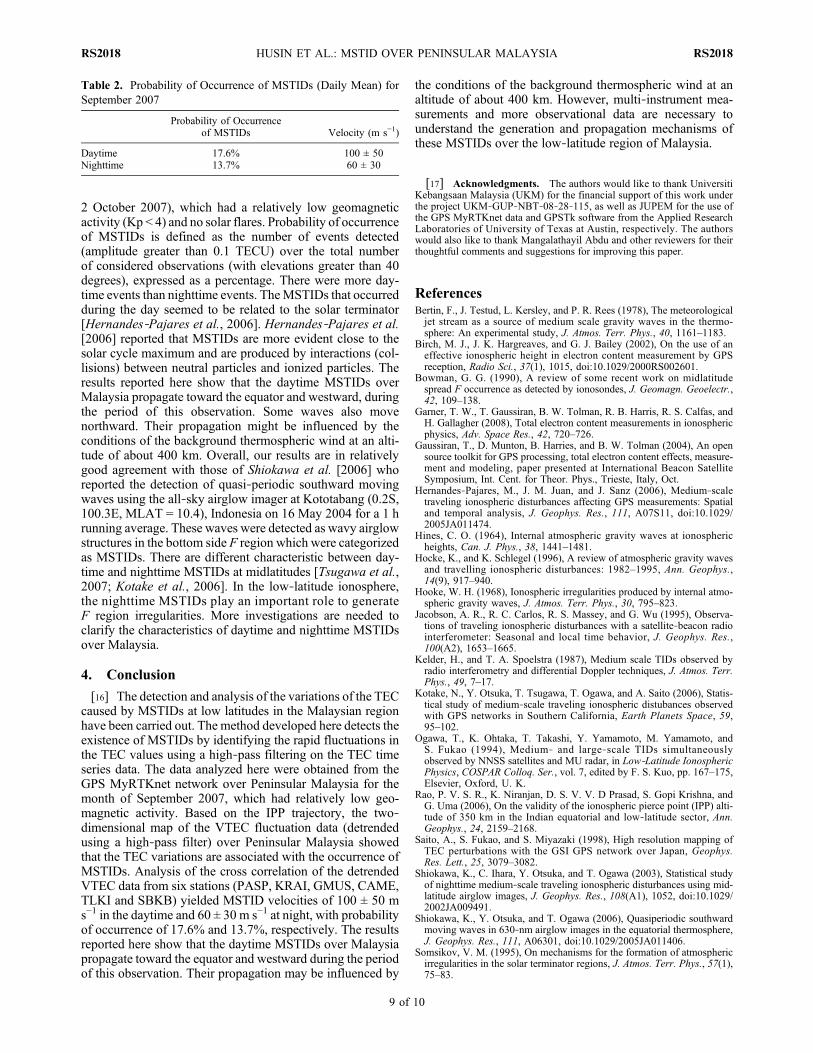
2 October 2007), which had a relatively low geomagneticactivity (Kp < 4) and no solar flares. Probability of occurrenceof MSTIDs is defined as the number of events detected(amplitude greater than 0.1 TECU) over the total numberof considered observations (with elevations greater than 40degrees), expressed as a percentage. There were more day-time events than nighttime events. TheMSTIDs that occurredduring the day seemed to be related to the solar terminator[Hernandes‐Pajares et al., 2006]. Hernandes‐Pajares et al.[2006] reported that MSTIDs are more evident close to thesolar cycle maximum and are produced by interactions (col-lisions) between neutral particles and ionized particles. Theresults reported here show that the daytime MSTIDs overMalaysia propagate toward the equator and westward, duringthe period of this observation. Some waves also movenorthward. Their propagation might be influenced by theconditions of the background thermospheric wind at an alti-tude of about 400 km. Overall, our results are in relativelygood agreement with those of Shiokawa et al. [2006] whoreported the detection of quasi‐periodic southward movingwaves using the all‐sky airglow imager at Kototabang (0.2S,100.3E, MLAT = 10.4), Indonesia on 16 May 2004 for a 1 hrunning average. These waves were detected as wavy airglowstructures in the bottom side F region which were categorizedas MSTIDs. There are different characteristic between day-time and nighttime MSTIDs at midlatitudes [Tsugawa et al.,2007; Kotake et al., 2006]. In the low‐latitude ionosphere,the nighttime MSTIDs play an important role to generateF region irregularities. More investigations are needed toclarify the characteristics of daytime and nighttime MSTIDsover Malaysia.

4. Conclusion

[16] The detection and analysis of the variations of the TECcaused by MSTIDs at low latitudes in the Malaysian regionhave been carried out. The method developed here detects theexistence of MSTIDs by identifying the rapid fluctuations inthe TEC values using a high‐pass filtering on the TEC timeseries data. The data analyzed here were obtained from theGPS MyRTKnet network over Peninsular Malaysia for themonth of September 2007, which had relatively low geo-magnetic activity. Based on the IPP trajectory, the two‐dimensional map of the VTEC fluctuation data (detrendedusing a high‐pass filter) over Peninsular Malaysia showedthat the TEC variations are associated with the occurrence ofMSTIDs. Analysis of the cross correlation of the detrendedVTEC data from six stations (PASP, KRAI, GMUS, CAME,TLKI and SBKB) yielded MSTID velocities of 100 ± 50 ms−1 in the daytime and 60 ± 30 m s−1 at night, with probabilityof occurrence of 17.6% and 13.7%, respectively. The resultsreported here show that the daytime MSTIDs over Malaysiapropagate toward the equator and westward during the periodof this observation. Their propagation may be influenced by

the conditions of the background thermospheric wind at analtitude of about 400 km. However, multi‐instrument mea-surements and more observational data are necessary tounderstand the generation and propagation mechanisms ofthese MSTIDs over the low‐latitude region of Malaysia.

[17] Acknowledgments. The authors would like to thank UniversitiKebangsaan Malaysia (UKM) for the financial support of this work underthe project UKM‐GUP‐NBT‐08‐28‐115, as well as JUPEM for the use ofthe GPS MyRTKnet data and GPSTk software from the Applied ResearchLaboratories of University of Texas at Austin, respectively. The authorswould also like to thank Mangalathayil Abdu and other reviewers for theirthoughtful comments and suggestions for improving this paper.

ReferencesBertin, F., J. Testud, L. Kersley, and P. R. Rees (1978), The meteorologicaljet stream as a source of medium scale gravity waves in the thermo-sphere: An experimental study, J. Atmos. Terr. Phys., 40, 1161–1183.

Birch, M. J., J. K. Hargreaves, and G. J. Bailey (2002), On the use of aneffective ionospheric height in electron content measurement by GPSreception, Radio Sci., 37(1), 1015, doi:10.1029/2000RS002601.

Bowman, G. G. (1990), A review of some recent work on midlatitudespread F occurrence as detected by ionosondes, J. Geomagn. Geoelectr.,42, 109–138.

Garner, T. W., T. Gaussiran, B. W. Tolman, R. B. Harris, R. S. Calfas, andH. Gallagher (2008), Total electron content measurements in ionosphericphysics, Adv. Space Res., 42, 720–726.

Gaussiran, T., D. Munton, B. Harries, and B. W. Tolman (2004), An opensource toolkit for GPS processing, total electron content effects, measure-ment and modeling, paper presented at International Beacon SatelliteSymposium, Int. Cent. for Theor. Phys., Trieste, Italy, Oct.

Hernandes‐Pajares, M., J. M. Juan, and J. Sanz (2006), Medium‐scaletraveling ionospheric disturbances affecting GPS measurements: Spatialand temporal analysis, J. Geophys. Res., 111, A07S11, doi:10.1029/2005JA011474.

Hines, C. O. (1964), Internal atmospheric gravity waves at ionosphericheights, Can. J. Phys., 38, 1441–1481.

Hocke, K., and K. Schlegel (1996), A review of atmospheric gravity wavesand travelling ionospheric disturbances: 1982–1995, Ann. Geophys.,14(9), 917–940.

Hooke, W. H. (1968), Ionospheric irregularities produced by internal atmo-spheric gravity waves, J. Atmos. Terr. Phys., 30, 795–823.

Jacobson, A. R., R. C. Carlos, R. S. Massey, and G. Wu (1995), Observa-tions of traveling ionospheric disturbances with a satellite‐beacon radiointerferometer: Seasonal and local time behavior, J. Geophys. Res.,100(A2), 1653–1665.

Kelder, H., and T. A. Spoelstra (1987), Medium scale TIDs observed byradio interferometry and differential Doppler techniques, J. Atmos. Terr.Phys., 49, 7–17.

Kotake, N., Y. Otsuka, T. Tsugawa, T. Ogawa, and A. Saito (2006), Statis-tical study of medium‐scale traveling ionospheric distubances observedwith GPS networks in Southern California, Earth Planets Space, 59,95–102.

Ogawa, T., K. Ohtaka, T. Takashi, Y. Yamamoto, M. Yamamoto, andS. Fukao (1994), Medium‐ and large‐scale TIDs simultaneouslyobserved by NNSS satellites and MU radar, in Low‐Latitude IonosphericPhysics, COSPAR Colloq. Ser., vol. 7, edited by F. S. Kuo, pp. 167–175,Elsevier, Oxford, U. K.

Rao, P. V. S. R., K. Niranjan, D. S. V. V. D Prasad, S. Gopi Krishna, andG. Uma (2006), On the validity of the ionospheric pierce point (IPP) alti-tude of 350 km in the Indian equatorial and low‐latitude sector, Ann.Geophys., 24, 2159–2168.

Saito, A., S. Fukao, and S. Miyazaki (1998), High resolution mapping ofTEC perturbations with the GSI GPS network over Japan, Geophys.Res. Lett., 25, 3079–3082.

Shiokawa, K., C. Ihara, Y. Otsuka, and T. Ogawa (2003), Statistical studyof nighttime medium‐scale traveling ionospheric disturbances using mid-latitude airglow images, J. Geophys. Res., 108(A1), 1052, doi:10.1029/2002JA009491.

Shiokawa, K., Y. Otsuka, and T. Ogawa (2006), Quasiperiodic southwardmoving waves in 630‐nm airglow images in the equatorial thermosphere,J. Geophys. Res., 111, A06301, doi:10.1029/2005JA011406.

Somsikov, V. M. (1995), On mechanisms for the formation of atmosphericirregularities in the solar terminator regions, J. Atmos. Terr. Phys., 57(1),75–83.

Table 2. Probability of Occurrence of MSTIDs (Daily Mean) forSeptember 2007

Probability of Occurrenceof MSTIDs Velocity (m s−1)

Daytime 17.6% 100 ± 50Nighttime 13.7% 60 ± 30

HUSIN ET AL.: MSTID OVER PENINSULAR MALAYSIA RS2018RS2018

9 of 10

Tolman, B. W., and R. B. Harries (2004), The GPS toolkit, Linux J., 125,27.

Trauth, M. H. (2006), MATLAB®Recipes for Earth Sciences, Springer,New York.

Tsugawa, T., N. Kotake, and Y. Otsuka (2007), Medium‐scale travelingionospheric disturbances observed by GPS receiver network in Japan: Ashort review, GPS Solut., 11, 39–144, doi:10.1007/s10291-006-0045-5.

Wanninger, L. (2004), Ionospheric disturbance indices for RTK and net-work RTK positioning, paper presented at ION GPS, Inst. of Navig.,Long Beach, Calif.

Warnant, R., and E. Pottiaux (2000), The increase of the ionosphericactivity as measured by GPS, Earth Planets Space, 52, 1055–1060.

M. Abdullah and A. Husin, Department of Electrical, Electronic andSystems Engineering, Universiti Kebangsaan Malaysia, 43600 UKMBangi, Malaysia. (mardina@eng.ukm.my; asnawihs@yahoo.com)M. A. Momani, Institute of Space Science, Universiti Kebangsaan

Malaysia, 43600 UKM Bangi, Malaysia. (momani@ukm.my)

HUSIN ET AL.: MSTID OVER PENINSULAR MALAYSIA RS2018RS2018

10 of 10