Traveling wave solutions for case II diffusion in polymers

Traveling Wave Solutions for Case II Diffusion in Polymers

THOMAS P. WITELSKI*

Department of Applied Mathematics, 21 7-50 California Institute of Technology, Pasadena, California 91 125

SYNOPSIS

Case I1 diffusion of penetrant liquids in polymer films is characterized by constant-velocity propagation of a phase interface. We review the development of viscoelastic models describing case I1 diffusion and then present a phase plane analysis for traveling wave solutions. For simplified, piecewise-constant coefficient models we give closed-form analytic solutions showing the dependence on various physical parameters in both viscous and viscoelastic diffusive systems. We will also compare the results of our analysis with results from numerical simulations of more general models. 0 1996 John Wiley & Sons, Inc. Keywords: case I1 diffusion anomalous polymer diffusion viscoelasticity traveling waves

INTRODUCTION

Polymer materials are being used in an increasing number of technological applications. To optimize performance and further extend applications of polymers, their physical properties must be well un- derstood. One area of active research is the study of diffusion of a penetrant liquid in a polymer substrate. This work has applications to many physical problems, including the effect of humidity on thin polymer films and the use of polymer materials as liquid seals and in controlled-release pharmaceuticals. We will present a mathematical analysis of case I1 polymer diffusion and produce closed-form solutions for a simplified model of this transport behavior.

The terms “case 11,” “non-Fickian,” and “anomalous” are commonly used to describe the occurrence of various nontraditional effects that cannot be pre- dicted from classical Fickian diffusion models. Case I1 diffusion is characterized by experimental studies of polymer sorption behavior that show constant- velocity spreading of the penetrant with a well-defined sharp front. Diffusion models for classical materials do not yield such characteristics. As a result, numerous studies have focused on tying anomalous

* Present address: Department of Mathematics, 2-336, Mas- sachusetts Institute of Technology, 77 Massachusetts Avenue, Cambridge, MA 02139-4307. Journal of Polymer Science: Part B: Polymer Physics, Vol. 34, 141-150 (1996) 0 1996 John Wiley & Sons, Inc. CCC 0887-6266/96/010141-10

behaviors to the special material properties of polymers. Because polymers are very long molecules, some effects can have considerable characteristic times.’.’ Consequently, it is important to couple the diffusion equation with viscoelastic stress models to account for relaxational effects. Additionally, polymer materials can undergo a phase transition from a relatively inflexible “glassy” state to a more re- sponsive “rubbery” state with corresponding changes in diffusion coefficients and relaxation times. These effects will be incorporated in our model for case I1 diffusive transport.

We study the diffusive spreading of a liquid into a one-dimensional semi-infinite layer of initially dry, unstressed polymer material on the interval 0 < x < 00. Following a derivation given in refs. 3 and 4, we obtain the model for the penetrant concentration in the polymer,

* = a [mu,(- au + E(u) ”) I , at ax ax ax (1)

where D ( u ) is a diffusion coefficient, E(u) is a stress coefficient, and (r is the stress induced in the polymer material. As in [4], we will take the diffusion coefficient to be

l f t 1 - E tanh(?), (2) D(u) = - + -

2t 2t

where 0 < t 6 1 is a small parameter corresponding

141

142 WITELSKI

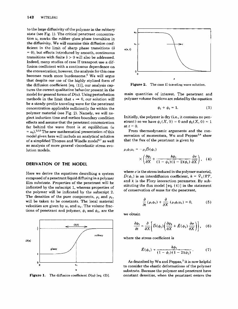
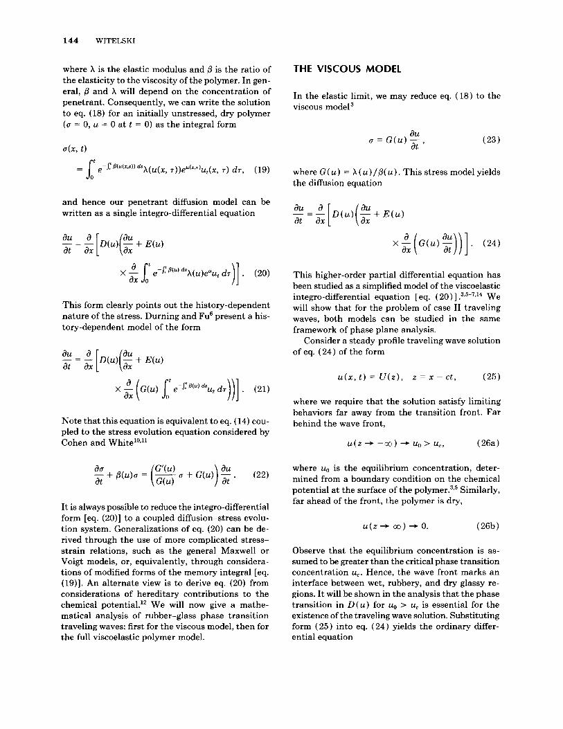
to the large diffusivity of the polymer in the rubbery state (see Fig. 1). The critical penetrant concentration u, marks the rubber-glass phase transition in the diffusivity. We will examine this diffusion coefficient in the limit of sharp phase transitions (6 = 0), but effects introduced by smooth, continuous transitions with finite 6 > 0 will also be addressed. Indeed, many studies of case I1 transport use a diffusion coefficient with a continuous dependence on the concentration; however, the analysis for this case becomes much more b~rdensome.~ We will argue that despite our use of the highly stylized form of the diffusion coefficient [eq. ( l ) ] , our analysis cap- tures the correct qualitative behavior present in the model for general forms of D(u). Using perturbation methods in the limit that t -+ 0, our solution will be a steady-profile traveling wave for the penetrant concentration applicable sufficiently far within the polymer material (see Fig. 2). Namely, we will ne- glect induction time and surface boundary condition effects and assume that the penetrant concentration far behind the wave front is at equilibrium (u = The new mathematical presentation of this model given here will include an analytical solution of a simplified Thomas and Windle m0de1~9~ as well as analysis of more general viscoelastic stress evolution models.

DERIVATION OF THE MODEL

Here we derive the equations describing a system composed of a penetrant liquid diffusing in a polymer film substrate. Properties of the penetrant will be indicated by the subscript 1, whereas properties of the polymer will be indicated by the subscript 2. The densities of the pure components, p1 and p 2 , will be taken to be constants. The local material velocities are given by u1 and u2. The volume fractions of penetrant and polymer, 41 and 42, are the

0 ’ I I 0 U I

U

Figure 1. The diffusion coefficient D(u) [eq. (2)]

uo I t 0 1

0 2

Figure 2. The case I1 traveling wave solution.

main quantities of interest. The penetrant and polymer volume fractions are related by the equation

41 + 4 2 = 1. ( 3 )

Initially, the polymer is dry (i.e., it contains no penetrant) so we have $l (X, 0) = 0 and 42(X, 0) = 1 at t = 0.

From thermodynamic arguments and the conservation of momentum, Wu and pep pa^^'^ show that the flux of the penetrant is given by

where u is the stress induced in the polymer material, D ( c # J ~ ) is an interdiffusion coefficient, k = V , / R T , and x is the Flory interaction parameter. By substituting the flux model [ eq. ( 4 ) ] in the statement of conservation of mass for the penetrant,

we obtain

where the stress Coefficient is

As described by Wu and pep pa^,^ it is now helpful to consider the elastic deformations of the polymer substrate. Because the polymer and penetrant have constant densities, when the penetrant enters the

TRAVELING WAVES FOR CASE I1 DIFFUSION 143

substrate, the polymer material must swell in size. If boundary conditions are being applied at the edges of the polymer material then we will have to solve a moving boundary problem. We can reduce this to a fixed-domain problem by changing to the material coordinates associated with the undeformed polymer substrate. The deformation tensor F is defined by

axi F.. = - lJ axj ’

where Xi are the present, deformed (or Eulerian) coordinates and x, are the material (or Lagrangian) coordinates. The instantaneous volume ratio for deformed to undeformed states is given by the deter- minant of F

deformed volume undeformed volume

J = IF1 =

Therefore, the change of variables to material coordinates in one dimension is

and eq. (6) becomes

where

The extension of eq. (11) to general multidimensional problems is still being studied because simple volume flux arguments like those in eq. (9) are in- sufficient to yield the form of the deformation tensor and hence the coordinate transformation [ eq. ( 10) ] .2,839 Indeed, experiments have shown that complicated behavior, such as buckling instabilities, can occur in multidimensional problems. To remain in the regime of validity of linearized elasticity, the relative deformations in eq. ( 11) must be small. Hence, we will allow the penetrant to take up only a small portion of the volume, 0 I 41 4 1. We will

now relate this model to derivations done by Durning‘ and Cohen,10-12 and conclude with a dis- cussion of stress evolution equations.

Equation (11) may be put into a more standard form by using a change of variables. If we change dependent variables by

u = - ln( l - &) - & J ~ = 1 - e-” , (13)

where 0 < 41 < 1 corresponds to 0 < u < co, then we get

ax ax

where D( u) and E ( u ) are given by

E ( u) = e-”E( 1 - e - ” ) . (15)

Observe that eq. (14) is a nonlinear diffusion equation for u with an extra term in the flux to account for the effects of induced stress.” In the limit that 41 + 0, to leading order we get

and eq. ( 14) is the leading-order approximation of the original diffusion equation [ eq. (6) 1. Therefore, u may be regarded as a modified concentration. Moreover, we conclude that in the low penetrant limit, 41 + 0, the swelling of the polymer is a higher- order effect and that the induced stress is primarily responsible for the observed phenomena. With this in mind, we now focus our attention on models for the stress.

To close the description of the model, it is nec- essary to relate the induced stress to the penetrant concentration. In linear elasticity, the strain is given by E = F - 1. For our problem in one dimension, this reduces to

Having the strain in terms of u allows us to use the framework of stress-strain models from viscoelasticity to describe the stress.13 One simple choice is the Maxwell model,

aff a& - + + p a = X - at at

144 WITELSKI

where X is the elastic modulus and p is the ratio of the elasticity to the viscosity of the polymer. In general, p and X will depend on the concentration of penetrant. Consequently, we can write the solution to eq. (18) for an initially unstressed, dry polymer ( a = 0, u = 0 at t = 0) as the integral form

and hence our penetrant diffusion model can be written as a single integro-differential equation

au au at ax - = 2 [ D ( 4 ( - ax + E(u)

This form clearly points out the history-dependent nature of the stress. Durning and Fu6 present a history-dependent model of the form

-=2[ au ( au at ax ax m u ) - + E(u)

Note that this equation is equivalent to eq. (14) coupled to the stress evolution equation considered by Cohen and

aa at - + ~ ( u ) u = ($ u + G(u)

It is always possible to reduce the integro-differential form [eq. (20)] to a coupled diffusion-stress evolution system. Generalizations of eq. (20) can be de- rived through the use of more complicated stress- strain relations, such as the general Maxwell or Voigt models, or, equivalently, through considerations of modified forms of the memory integral [eq. (19)]. An alternate view is to derive eq. (20) from considerations of hereditary contributions to the chemical potential.” We will now give a mathematical analysis of rubber-glass phase transition traveling waves: first for the viscous model, then for the full viscoelastic polymer model.

THE VISCOUS MODEL

In the elastic limit, we may reduce eq. (18) to the viscous model3

au at

a = G ( u ) -,

where G( u ) = A( u ) / p ( u ) . This stress model yields the diffusion equation

au au at ax - = 2 [ D O ( - ax + E ( u )

This higher-order partial differential equation has been studied as a simplified model of the viscoelastic integro-differential equation [ eq. ( 20) ] .3*5-7*14 We will show that for the problem of case I1 traveling waves, both models can be studied in the same framework of phase plane analysis.

Consider a steady-profile traveling wave solution of eq. (24) of the form

u ( x , t ) = U ( z ) , z = x - c t , ( 2 5 )

where we require that the solution satisfy limiting behaviors far away from the transition front. Far behind the wave front,

where uo is the equilibrium concentration, determined from a boundary condition on the chemical potential a t the surface of the p ~ l y m e r . ~ ? ~ Similarly, far ahead of the front, the polymer is dry,

Observe that the equilibrium concentration is as- sumed to be greater than the critical phase transition concentration u,. Hence, the wave front marks an interface between wet, rubbery, and dry glassy regions. I t will be shown in the analysis that the phase transition in D ( u ) for uo > u, is essential for the existence of the traveling wave solution. Substituting form (25) into eq. (24) yields the ordinary differential equation


which may be integrated once, subject to the boundary condition (26b), to yield

- C U = D ( U ) - - cE( U ) ( Z

Interestingly, we may relate eq. (28) to the classical model for traveling waves in reaction-diffusion systems. A well-known model in population dynamics and other applications is Fisher’s equation, l 5 3 l 6

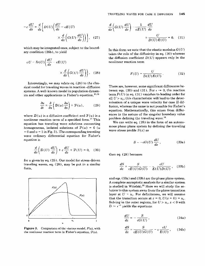
where 3 ( u) is a diffusion coefficient and 3 (u) is a nonlinear reaction term of a specified form.17 This equation has traveling wave solutions connecting homogeneous, isolated solutions of 3 ( u ) = 0 (u = 0 and u = 1 in Fig. 3 ) . The corresponding traveling wave ordinary differential equation for Fisher’s equation is

- ( . Z l ( U ) z ) + c x + 3 ( U ) d dU = 0 , (30) dz

for u given by eq. ( 25 ) . Our model for stress-driven traveling waves, eq. (28 ) , may be put in a similar form,

0 11. 1 U

Figure 3. the nonlinear reaction term in Fisher’s equation, 3 ( u ) .

Comparison of the viscous model, F(u), with

In this form we note that the elastic modulus G ( U ) takes the role of the diffusivity in eq. (30) whereas the diffusion coefficient D ( U ) appears only in the nonlinear reaction term

There are, however, some significant differences between eqs. (30) and (31 ). For t + 0, the reaction term F ( U ) in eq. (31 ) vanishes to leading order for all U > u,; this characteristic will lead to the deter- mination of a unique wave velocity for case I1 diffusion, whereas the same is not possible for Fisher’s equation. Mathematically, this arises from differences in the nature of the singular boundary value problem defining the traveling wave.18

We can write eq. (28) in the form of an autono- mous phase plane system by defining the traveling wave stress profile S (2) as

dU dz

S = - c G ( U ) - - ,

then eq. (28) becomes

and eqs. (33a) and (33b) are the phase plane system. A complete asymptotic analysis for a similar system is studied in Witelski.“ Here we will study the solution to this system away from the phase transition layer a t U = u,. For definiteness, we will assume that the transition occurs a t z = 0, U ( z = 0) = u,. Solving in the outer regions, for U > u,, z < 0 with D - t - ’ yields the equations

S - dU dz c G ( U ) ’

cu - 6 - (34b)

S - d S dz c E ( U ) G ( U ) E ( U ) ’ - _

146 WITELSKI

and for U < u,, z > 0 with D - 1

. (35b) cu -- S - dS

dz c E ( U ) G ( U ) E ( U ) - _

Our solution procedure will consist of solving the two-phase plane systems above to leading order in t and then matching the solutions together through the transition layer.

We will first solve the problem for the simplified, but illustrative, case of constant coefficients with

T o account for the significant effects of the rubber- glass transition on the viscoelastic properties of the polymer material, a much more realistic model for G ( U ) is

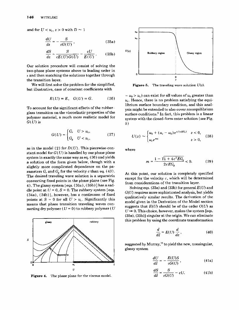
as in the model ( 2 ) for D ( U ) . This piecewise-constant model for G ( U ) is handled by our phase plane system in exactly the same way as eq. (36) and yields a solution of the form given below, though with a slightly more complicated dependence on the parameters Gr and Gg for the velocity c than eq. (43) . The desired traveling wave solution is a separatrix connecting fixed points in the phase plane (see Fig. 4 ) . The glassy system [ eqs. ( 35a), (35b) ] has a saddle point a t U = 0, S = 0. The rubbery system [ eqs. (34a), (34b) 1, however, has a continuum of fixed points a t S = 0 for all U > u,. Significantly this means that phase transition traveling waves connecting dry polymer ( U = 0) to rubbery polymer ( U

I rubbery

U

Figure 4. The phase plane for the viscous model.

0 I

0 z

Figure 5. The traveling wave solution U(z) .

= uo > u,) can exist for all values of uo greater than u,. Hence, there is no problem satisfying the equilibrium surface boundary condition, and this analysis might be extended to also cover nonequilibrium surface condition^.^ In fact, this problem is a linear system with the closed-form outer solution (see Fig. 5)

where

(39) 1 - V 1 + 4c2EG,

m = < 0. 2 c EG,

At this point, our solution is completely specified except for the velocity c , which will be determined from considerations of the transition layer.

Solving eqs. (33a) and (33b) for general E( U) and G( U) requires more sophisticated analysis, but yields qualitatively similar results. The derivation of the model given in the Derivation of the Model section suggests that E ( U ) should be of the order O(U) as U + 0. This choice, however, makes the system [eqs. (35a), (35b)l singular a t the origin. We can eliminate this problem by using the coordinate transformation

suggested by Murray,15 to yield the new, nonsingular, glassy system


Like eqs. (35a) and (35b), eqs. (41a) and (41b) have a saddle point at the origin with a separatrix corresponding to a unique traveling wave solution (see Fig. 6); however, in this case it is a nonlinear (non- hyperbolic) saddle point, which is more complicated to analyze mathematically.

TRANSITION LAYER BEHAVIOR

In the phase transition region, the form of the diffusion coefficient D ( U ) becomes important for determining the structure of the solution. We will study the limit of sharp transitions in D ( U ) as 6 +

0. This analysis will yield some observations about the stress, as well as determining the value of the traveling wave velocity c.

For studying the transition region, it becomes useful to represent the phase plane system [eqs. (33a) , (33b)I as

1 (42) -- dS c 2 G ( U ) U

dU E ( U ) D ( U ) S E ( U ) ' - =

This is a first-order ordinary differential equation for the stress as a function of the concentration. In the transition region, S > 0 and it can be shown that the terms in eq. (42) are nonsingular and bounded. Hence, we can conclude that the stress is continuous. If the transition is very sharp ( 6 - 0) , then the stress will be slowly varying (almost constant) across the interval. Continuity of the stress can then be enforced by matching together the solutions in the rubbery and glassy regions. For our linear constant-coefficient problem, eq. (36) , with 6 = 0 we simply make the first derivative of eq. (38) continuous at 2 = 0. This condition yields the velocity

U

Figure 6. Phase plane for the nonlinear saddle point.

! : rubbery -1

U C

U

Figure 7. phase transitions, 6 > 0.

The phase plane for models with smooth

where the concentration ratio is y = u , / h < 1. When the transition layer has finite thickness, 6 > 0, then eq. (42) must be integrated directly to obtain the stress, and the form of the diffusion coefficient will modify the velocity and the outer solutions. Signif- icantly, we note several trends that occur as the transition layer thickness increases: the maximum of the stress profile increases, it becomes broader and occurs ahead of the concentration front, in the glassy region (see Fig. 7 ) , and the traveling wave velocity c increases gradually (see Fig. 8). These properties of the stress profile agree with the observations of Durning et al.5 and Hui et al.7 Further- more, because neither the phase plane structure nor the velocity changes dramatically for smooth transitions with 6 > 0, we conclude that model ( 2 ) with 6 = 0 is a good first approximation for systems with general forms of D ( u ) .

C

CC

0 6

Figure 8. dependence on 6.

The dependence of the traveling wave velocity

148 WITELSKI

THE VlSCOELASTlC MODEL

We will now show how the phase plane method can be applied to more general stress evolution models. General viscoelastic models can be written as single integro-differential equations of the form of eq. (20) ; however, we will use the coupled form

We consider a Maxwell model [ eq. (44b) 1 , as was used in Wu and pep pa^,^ for our analysis; however, the approach is very similar for other equations, such as Durning's model [ eq. ( 22 ) 1.

Again, searching for steady-profile traveling wave solutions moving into dry, unstressed polymer material, let

u ( x , t ) = U ( z ) ,

a(x, t ) = S ( z ) , z = x - c t , (45)

then eqs. (44a) and (44b), subject to boundary condition (26b), become

dz

or in a more standard form

- - P ( U ) U - E ( U ) Q ( U dU dz _ - S , (47a)

dS - = - X ( U ) P ( U ) U + Q ( U ) S , (47b) dz

where

and

In this representation, the influences of diffusion

and stress relaxation are given by the functions P( U ) and Q( U ) , respectively. As in the viscous model, in the limit of a sharp transition, we can separate eqs. (47a) and (47b) into two simpler phase plane systems. In the rubbery region for z < 0, U > 4,

- -E( U ) Q ( U ) S - e l?( U ) U , (50a) dU dz

dS dz

- _

- Q ( U ) S - A ( U ) R ( U ) U , (50b) - -

and in the glassy region for z > 0, U < u,,

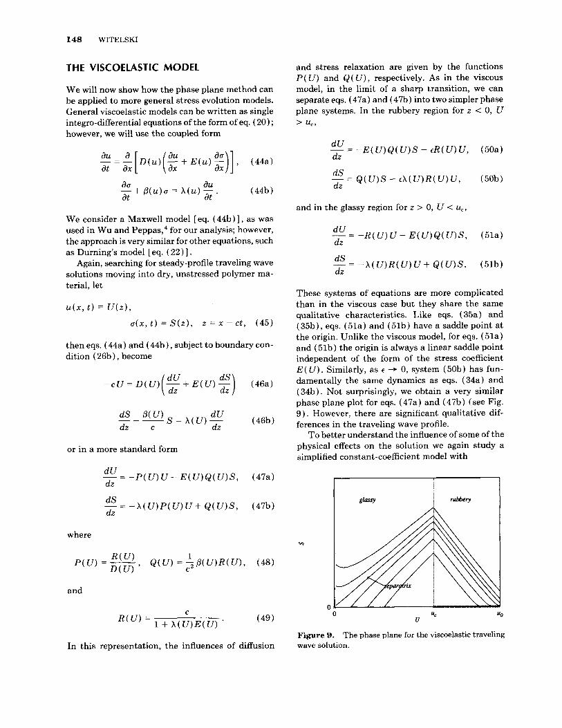
These systems of equations are more complicated than in the viscous case but they share the same qualitative characteristics. Like eqs. ( 35a) and (35b), eqs. (51a) and (51b) have a saddle point a t the origin. Unlike the viscous model, for eqs. (51a) and (51b) the origin is always a linear saddle point independent of the form of the stress coefficient E ( U ) . Similarly, as c 3 0, system (50b) has fun- damentally the same dynamics as eqs. (34a) and (34b). Not surprisingly, we obtain a very similar phase plane plot for eqs. (47a) and (47b) (see Fig. 9 ) . However, there are significant qualitative differences in the traveling wave profile.

To better understand the influence of some of the physical effects on the solution we again study a simplified constant-coefficient model with

0 % U

Figure 9. wave solution.

The phase plane for the viscoelastic traveling


E ( U ) = E , p( U ) = p, A ( U ) = A. (52)

As in the case of the viscous model studied in the previous section, to properly describe the influence of the rubber-glass transition on the viscoelastic properties of the polymer material, p( U ) and X ( U ) should be piecewise constant in the rubbery and glassy regions. Again, the solution of this extended problem has the same form as that of the solution with eq. ( 52), except for a more complicated parameter dependence in c [ eq. (58) 1. This model can be expected to capture most of the qualitative properties of the general model, and it also admits the closed-form analytic solution

uo + (u, - uo)eQZ z < o u, e mRz z > o

(53) U ( Z ) - where

p, - c 2 - v( 0, + c 2 ) ' + 4P,c2X,E 2c2 m = < o , (54)

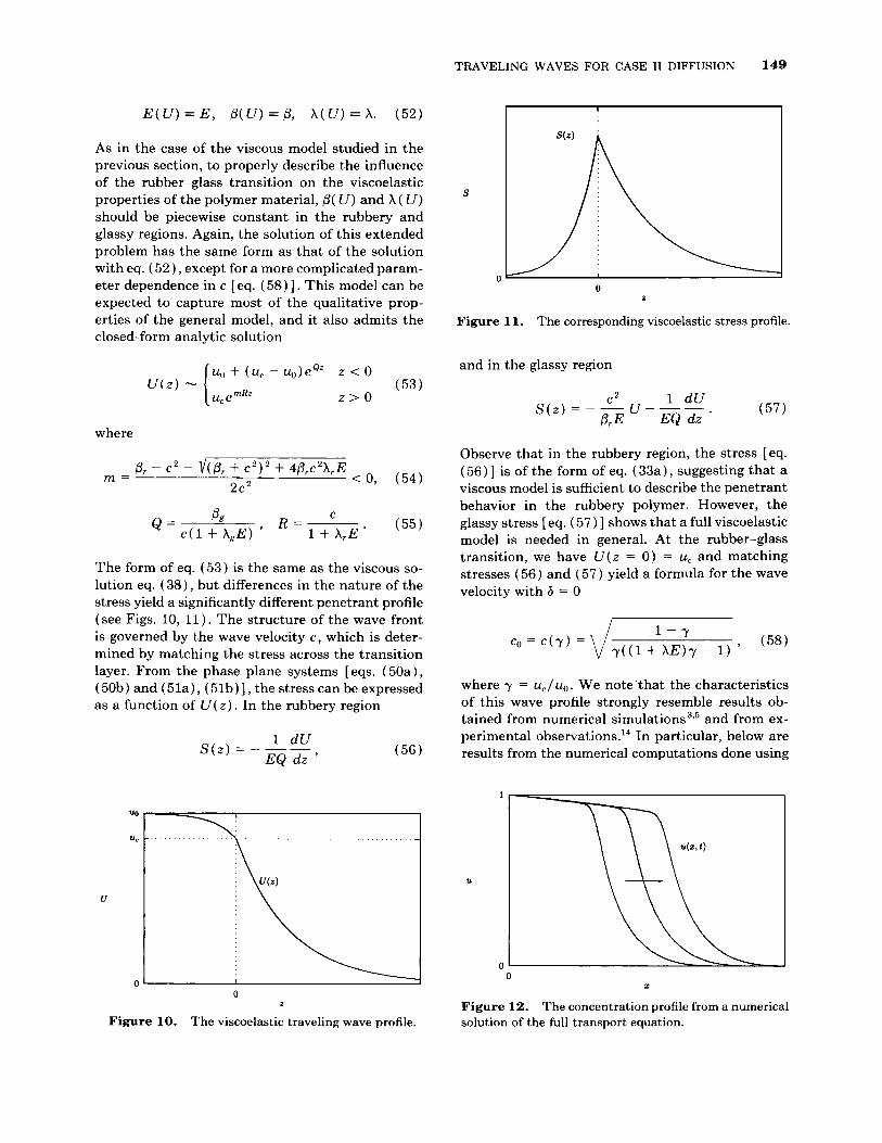
The form of eq. (53 ) is the same as the viscous solution eq. (38) , but differences in the nature of the stress yield a significantly different penetrant profile (see Figs. 10, 11 ) . The structure of the wave front is governed by the wave velocity c, which is determined by matching the stress across the transition layer. From the phase plane systems [eqs. (50a), (50b) and (51a), (51b)], the stress can be expressed as a function of U ( z ) . In the rubbery region

1 dU S ( z ) = - --

EQ d z '

n I

0 z

Figure 10. The viscoelastic traveling wave profile.

0 z

Figure 11. The corresponding viscoelastic stress profile.

and in the glassy region

Observe that in the rubbery region, the stress [eq. (56) ] is of the form of eq. (33a), suggesting that a viscous model is sufficient to describe the penetrant behavior in the rubbery polymer. However, the glassy stress [ eq. (57) ] shows that a full viscoelastic model is needed in general. At the rubber-glass transition, we have U ( z = 0) = u, and matching stresses (56) and (57) yield a formula for the wave velocity with 6 = 0

where y = u,/uo. We note'that the characteristics of this wave profile strongly resemble results ob- tained from numerical sir nu la ti on^^'^ and from experimental observation^.'^ In particular, below are results from the numerical computations done using

1

U

0 0

2

Figure 12. solution of the full transport equation.

The concentration profile from a numerical

160 WITELSKI

C 0

2

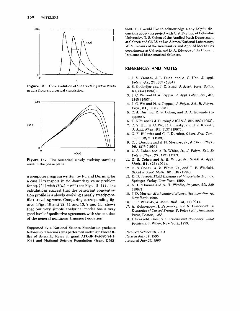
Figure 13. profile from a numerical simulation.

Slow evolution of the traveling wave stress

0 1 U(Z,t)

Figure 14. wave in the phase plane.

The numerical slowly evolving traveling

a computer program written by Fu and Durning for a case I1 transport initial-boundary value problem for eq. (24) with D (u) = eMu (see Figs. 12-14). The calculations suggest that the penetrant concentration profile is a slowly evolving (nearly steady-profile) traveling wave. Comparing corresponding fig- ures (Figs. 10 and 12, 11 and 13, 9 and 14) shows that our very simple analytical model has a very good level of qualitative agreement with the solution of the general nonlinear transport equation.

Supported by a National Science Foundation graduate fellowship. This work was performed under Air Force Of- fice of Scientific Research grant AFOSR-F49620-94-1- 0044 and National Science Foundation Grant DMS-

9501511. I would like to acknowledge many helpful dis- cussions about this project with c. J. Durning of Columbia University, D. S. Cohen of the Applied Math Department at Caltech and CNLS at Los Alamos National Laboratory, W. G. Knauss of the Aeronautics and Applied Mechanics departments at Caltech, and D. A. Edwards of the Courant Institute of Mathematical Sciences.

REFERENCES AND NOTES

1. J. S. Vrentas, J. L. Duda, and A. C. Hou, J . Appl.

2. S. Govindjee and J. C. Simo, J . Mech. Phys. Solids,

3. J. C. Wu and N. A. Peppas, J . Appl. Polym. Sci., 49,

4. J. C. Wu and N. A. Peppas, J . Polym. Sci., B: Polym.

5. C. J. Durning, D. S. Cohen, and D. A. Edwards (to

6. T. Z. Fu and C. J. Durning, AIChE J . , 39,1080 ( 1993). 7. C. Y. Hui, K. C. Wu, R. C. Lasky, and E. J. Kramer,

8. G. F. Billovits and C. J. Durning, Chem. Eng. Com-

9. C. J. DurningandK. N. Morman, Jr., J . Chem. Phys.,

10. D. S. Cohen and A. B. White, Jr., J . Polym. Sci., B:

11. D. S. Cohen and A. B. White, Jr., SIAM J . Appl.

12. D. S. Cohen, A. B. White, Jr., and T. P. Witelski,

13. D. D. Joseph, Fluid Dynamics of Viscoelastic Liquids,

14. N. L. Thomas and A. H. Windle, Polymer, 23, 529

15. J. D. Murray, Mathematical Biology, Springer-Verlag,

16. T. P. Witelski, J . Math. Biol., 33, 1 (1994). 17. A. Kolmogorov, I. Petrovsky, and N. Piscounoff, in

Dynamics of Curved Fronts, P. Pelce (ed.) , Academic Press, Boston, 1988.

18. I. Stakgold, Green’s Functions and Boundary Value Problems, J. Wiley, New York, 1979.

Polym. Sci., 29, 399 ( 1984).

41,863 (1993).

1845 (1993).

Phys., 31, 1503 (1993).

appear).

J . Appl. Phys., 61, 5137 (1987).

nun. , 8 2 , 2 1 (1989).

98, 4275 (1993).

Polym. Phys., 27,1731 (1989).

Math., 51,472 (1991).

SZAM J . Appl. Math., 55, 348 (1995).

Springer-Verlag, New York, 1990.

( 1982).

New York, 1990.

Received October 26, 1994 Revised July 19, 1995 Accepted July 23, 1995

Traveling wave solutions for case II diffusion in polymers

Documents

Transcript of Traveling wave solutions for case II diffusion in polymers