electronics

Article

OATCR: Outdoor Autonomous Trash-Collecting Robot DesignUsing YOLOv4-Tiny

Medhasvi Kulshreshtha 1,†, Sushma S. Chandra 1,†, Princy Randhawa 1, Georgios Tsaramirsis 2,* ,Adil Khadidos 3 and Alaa O. Khadidos 4

�����������������

Citation: Kulshreshtha, M.; Chandra,

S.S.; Randhawa, P.; Tsaramirsis, G.;

Khadidos, A.; Khadidos, A.O.

OATCR: Outdoor Autonomous

Trash-Collecting Robot Design Using

YOLOv4-Tiny. Electronics 2021, 10,

2292. https://doi.org/10.3390/

electronics10182292

Academic Editor: Amir Mosavi

Received: 18 August 2021

Accepted: 14 September 2021

Published: 18 September 2021

Publisher’s Note: MDPI stays neutral

with regard to jurisdictional claims in

published maps and institutional affil-

iations.

Copyright: © 2021 by the authors.

Licensee MDPI, Basel, Switzerland.

This article is an open access article

distributed under the terms and

conditions of the Creative Commons

Attribution (CC BY) license (https://

creativecommons.org/licenses/by/

4.0/).

1 Department of Mechatronics, Manipal University Jaipur, Jaipur 303007, India;medhasvi.179403034@muj.manipal.edu (M.K.); sushma.179403054@muj.manipal.edu (S.S.C.);princy.randhawa@jaipur.manipal.edu (P.R.)

2 Abu Dhabi Women’s College, Higher Colleges of Technology, Abu Dhabi 25026, United Arab Emirates3 Department of Information Technology, King Abdulaziz University, Jeddah 21589, Saudi Arabia;

akhadidos@kau.edu.sa4 Department of Information Systems, King Abdulaziz University, Jeddah 21589, Saudi Arabia;

aokhadidos@kau.edu.sa* Correspondence: gtsaramirsis@hct.ac.ae† These authors contributed to this work equally.

Abstract: This paper proposed an innovative mechanical design using the Rocker-bogie mechanismfor resilient Trash-Collecting Robots. Mask-RCNN, YOLOV4, and YOLOv4-tiny were experimentedon and analyzed for trash detection. The Trash-Collecting Robot was developed to be completelyautonomous as it was able to detect trash, move towards it, and pick it up while avoiding anyobstacles along the way. Sensors including a camera, ultrasonic sensor, and GPS module played animperative role in automation. The brain of the Robot, namely, Raspberry Pi and Arduino, processedthe data from the sensors and performed path-planning and consequent motion of the robot throughactuation of motors. Three models for object detection were tested for potential use in the robot:Mask-RCNN, YOLOv4, and YOLOv4-tiny. Mask-RCNN achieved an average precision (mAP) ofover 83% and detection time (DT) of 3973.29 ms, YOLOv4 achieved 97.1% (mAP) and 32.76 DT, andYOLOv4-tiny achieved 95.2% and 5.21 ms DT. The YOLOv4-tiny was selected as it offered a verysimilar mAP to YOLOv4, but with a much lower DT. The design was simulated on different terrainsand behaved as expected.

Keywords: Mask-RCNN; YOLOv4; YOLOv4-tiny; robot; trash; rocker bogie mechanism; machinelearning; object detection; path-planning

1. Introduction

Traditionally, robots have been aiding humans in many areas as they are more capableand often better equipped to deal with tasks that include high repeatability. The advance-ments in the areas of batteries, sensors, artificial intelligence (AI), and machine learning(ML) open new horizons and application domains as they allow robots and, more precisely,mobile robots to perform more complex tasks [1]. These can be anything from driving anddelivering packages to cleaning jobs [2]. There are many mobile robots designed for indoor-cleaning operation, however there are less low-cost robots designed for outdoor-cleaningoperations with the ability to remove medium-size objects [3]. This is very important whenthe cleaning must be done under difficult environmental conditions, such as heat or cold orwhen cleaning materials that are hazardous for humans or the environment [4]. In the cur-rent study, trash widespread at picnic spots, on or near pavements, washed by waves ontosandy or pebbly beaches and other such outdoor locations were focused upon. Keepinga pragmatic outlook in mind, this robot was designed to conquer the regular challengesof outdoor land terrains and obstacles. A completely autonomous robot was capable of

Electronics 2021, 10, 2292. https://doi.org/10.3390/electronics10182292 https://www.mdpi.com/journal/electronics

Electronics 2021, 10, 2292 2 of 22

performing activities like trash detection, obstacle avoidance, robotic path-planning, androbotic motion control automatically.

• A unique flap-bucket system was used in the mechanical design, which enabled trashcollection through a sweep where multiple trash objects of varying sizes were collectedsimultaneously, unlike when a robotic hand is used, which can only pick up a singleitem at a time. The novel approach of assimilating the six-wheeled Rocker-Bogiemechanism into the robot for its smooth movement on multiple outdoor terrains madeit perfect for outdoor trash collection.

• The use of modern technologies of artificial intelligence in this robot facilitated mak-ing it smart and autonomous. Image processing and deep learning constituted thecomputer vision model. A more advanced method, namely transfer learning, wasused in the object detection model building. Varied models and the latest versionsof these models at the time like MaskRCNN, YOLOv4, and YOLOv4-tiny were ex-perimented on and analyzed comprehensively. Experimental results demonstratedthat YOLOv4-tiny performed the fastest detection, thereby making it apt for usage fordetection in real-time.

• Path-planning algorithm made the robot truly autonomous, as once the coordinates ofthe area to be cleaned were fed to the robot, it did not require any further assistance.It autonomously searched for the trash, avoided obstacles, and generated its ownpath accordingly. The sensors provided all the necessary information required for thefeedback mechanisms of the robot and helped in its decision-making process.

The rest of the paper is organized as follows. Section 2 discusses the previous worksand compares them with our current robot. Section 3 contains a backdrop of the materialsand methods used to build this robot. Section 4 elaborates on the structure of the robot andthe functioning of each mechanical and electronic part. Section 5 provides insights and astep-by-step procedure for building the object-detection model to detect trash. In Section 6,the software implementation into the Raspberry Pi and the path planning followed by theautonomous robot are discussed in detail. Section 7 evaluates the proposed design in solidworks, using various generated terrains. Section 8 portrays the results obtained from theexperimental analysis and a comparative study. Finally, Section 9 summarizes this work.

2. Related Work

This section discusses the existing work in the field of trash-cleaning robots. In themechanical design of the robot built to operate on water bodies, a conveyor belt wasused to collect floating trash from the surface of rivers [5–7]. In [8], the robot employedbroom bristles to sweep trash controlled by a servo motor and the collector bin was openedperiodically to empty this trash. Some of the trash-collecting robots used a robotic arm tocarry out the process of trash-picking. The degree of freedom of the manipulator that wasused varied from two degrees of freedom to seven degrees of freedom. The end-effector ofthe manipulator played the role of grasping the concerned object, which was trash [9].

The remote-controlled robots were controlled through mobile applications via Blue-tooth like in [10–12], or via Wi-Fi like in [8,13,14]. LIDAR (Light Detection and Ranging)and GPS (Global Positioning System) were incorporated in some of the trash-collectingrobots and prototypes [15,16]. A modified YOLOv3 was proposed for garbage detectionwhere the original three-scale detection was changed to two-scale to cope with speedyprocessing in real-time [17]. A lightweight neural network for garbage detection based onAlexNet-SSD model was used in [18] where the traditional VGG network was replacedby AlexNet for the base. In [19], a lightweight SSD model was developed, where a focalloss function for smooth handling of class imbalance was used as well as a new featurepyramid for achieving strong semantics on all scales; here, the ResNet was used as the basenetwork in place of the original VGG network.

The processing for path planning was carried out in a ROS (Robotic Operating Sys-tem) where map segmentation was implemented. An exploration algorithm, namely A* algorithm, was used for navigation of the robot while avoiding any obstacles. In this

Electronics 2021, 10, 2292 3 of 22

algorithm, the path that had the minimum cost to the goal, while considering the Euclideandistance, was taken [20].

Comparative Study

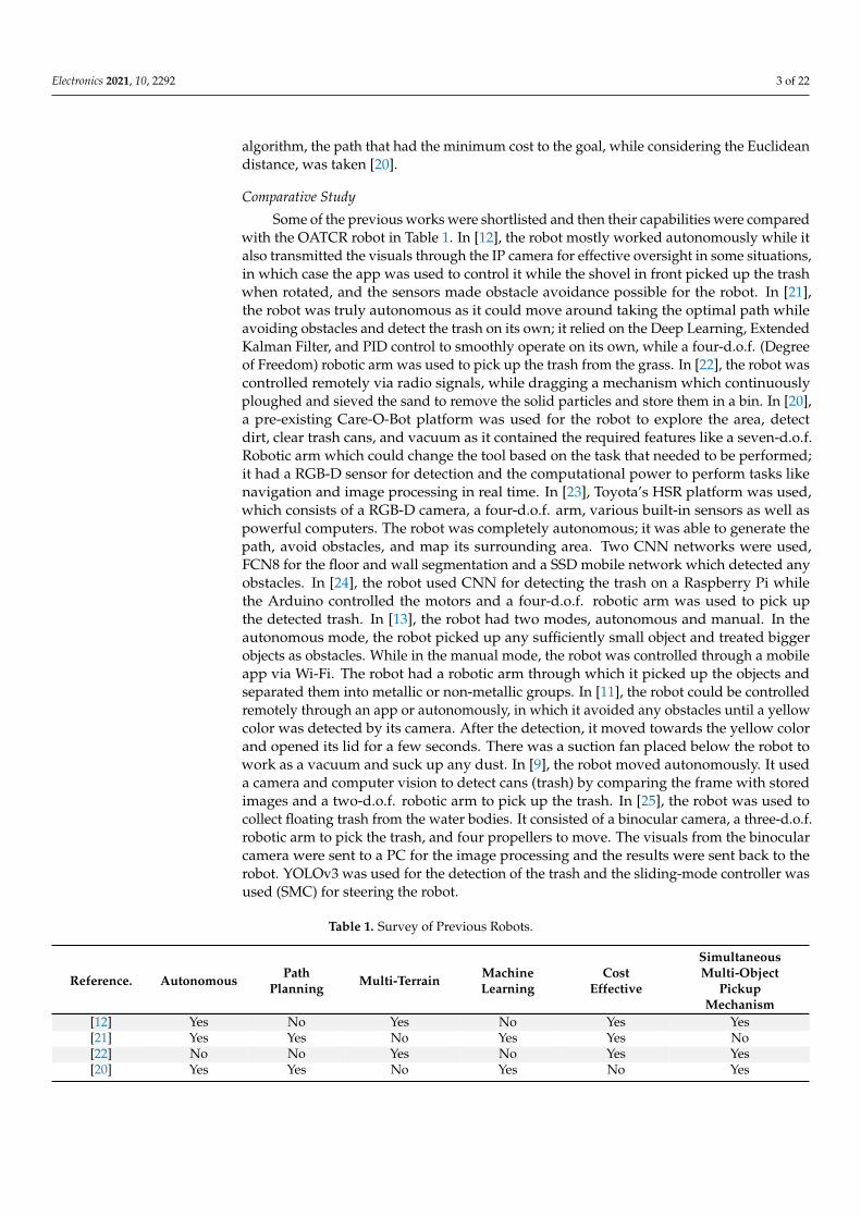
Some of the previous works were shortlisted and then their capabilities were comparedwith the OATCR robot in Table 1. In [12], the robot mostly worked autonomously while italso transmitted the visuals through the IP camera for effective oversight in some situations,in which case the app was used to control it while the shovel in front picked up the trashwhen rotated, and the sensors made obstacle avoidance possible for the robot. In [21],the robot was truly autonomous as it could move around taking the optimal path whileavoiding obstacles and detect the trash on its own; it relied on the Deep Learning, ExtendedKalman Filter, and PID control to smoothly operate on its own, while a four-d.o.f. (Degreeof Freedom) robotic arm was used to pick up the trash from the grass. In [22], the robot wascontrolled remotely via radio signals, while dragging a mechanism which continuouslyploughed and sieved the sand to remove the solid particles and store them in a bin. In [20],a pre-existing Care-O-Bot platform was used for the robot to explore the area, detectdirt, clear trash cans, and vacuum as it contained the required features like a seven-d.o.f.Robotic arm which could change the tool based on the task that needed to be performed;it had a RGB-D sensor for detection and the computational power to perform tasks likenavigation and image processing in real time. In [23], Toyota’s HSR platform was used,which consists of a RGB-D camera, a four-d.o.f. arm, various built-in sensors as well aspowerful computers. The robot was completely autonomous; it was able to generate thepath, avoid obstacles, and map its surrounding area. Two CNN networks were used,FCN8 for the floor and wall segmentation and a SSD mobile network which detected anyobstacles. In [24], the robot used CNN for detecting the trash on a Raspberry Pi whilethe Arduino controlled the motors and a four-d.o.f. robotic arm was used to pick upthe detected trash. In [13], the robot had two modes, autonomous and manual. In theautonomous mode, the robot picked up any sufficiently small object and treated biggerobjects as obstacles. While in the manual mode, the robot was controlled through a mobileapp via Wi-Fi. The robot had a robotic arm through which it picked up the objects andseparated them into metallic or non-metallic groups. In [11], the robot could be controlledremotely through an app or autonomously, in which it avoided any obstacles until a yellowcolor was detected by its camera. After the detection, it moved towards the yellow colorand opened its lid for a few seconds. There was a suction fan placed below the robot towork as a vacuum and suck up any dust. In [9], the robot moved autonomously. It useda camera and computer vision to detect cans (trash) by comparing the frame with storedimages and a two-d.o.f. robotic arm to pick up the trash. In [25], the robot was used tocollect floating trash from the water bodies. It consisted of a binocular camera, a three-d.o.f.robotic arm to pick the trash, and four propellers to move. The visuals from the binocularcamera were sent to a PC for the image processing and the results were sent back to therobot. YOLOv3 was used for the detection of the trash and the sliding-mode controller wasused (SMC) for steering the robot.

Table 1. Survey of Previous Robots.

Reference. Autonomous PathPlanning Multi-Terrain Machine

LearningCost

Effective

SimultaneousMulti-Object

PickupMechanism

[12] Yes No Yes No Yes Yes[21] Yes Yes No Yes Yes No[22] No No Yes No Yes Yes[20] Yes Yes No Yes No Yes

Electronics 2021, 10, 2292 4 of 22

Table 1. Cont.

Reference. Autonomous PathPlanning Multi-Terrain Machine

LearningCost

Effective

SimultaneousMulti-Object

PickupMechanism

[23] Yes Yes No Yes No No[24] Yes Yes No Yes No No[13] Yes No No No Yes No[11] Yes No No No Yes Yes[9] Yes No Yes No Yes No[25] Yes Yes No Yes Yes No

This Paper Yes Yes Yes Yes Yes YesThe OATCR Robot was built to function with complete autonomy and independently make decisions like identification of trash anddetermination of the optimum path to be taken while avoiding any collisions with obstacles. A human is only needed to input theworkspace coordinates of the robot and turn it on. Once an area was defined as its workspace, the robot independently roamed within itsboundaries, detecting and collecting the trash. An advanced mechanism, namely the Rocker-bogie mechanism inspired by NASA’s rovers,which can tread uncharted territories, was incorporated in the OATCR. This ensured its smooth motion on different types of terrain, makingit truly robust. Machine learning was used for computer vision, which processed the information received from the camera and made senseout of that image so as the robot could perceive its surroundings like humans. It was used specifically for trash detection and obtaining thetrash objects’ coordinates in 2D. A state-of-the-art machine learning algorithm of object-detection named YOLOv4-tiny was used for thispurpose. Easily available and low-price electronic equipment were used, like Arduino and Raspberry Pi microprocessors and sensors.Open-source services were used in software development for the robot, thus making it further cost-effective. A custom model was built tocarry out its computer vision tasks, which made it better suited and adept at the specific tasks. The flap and bucket system, where the flapswept the trash presented in front into the bucket, allowed multiple trash particles of different sizes to be easily collected simultaneously.

3. Materials and Methods

The graphical design and modelling of the mechanical structure was carried out inSolidWorks 2018. SolidWorks is a 3D modelling software that is used for generating 3Ddesigns. It has integrated tools to provide analytical and design automation to simulate thereal-world behavior such as kinematics, dynamics, stress, deflection, vibration, tempera-tures, or fluid flow. It was developed by Dassault Systèmes as a CAD (Computer AidedDesign) and a CAE (Computer Aided Engineering) software.

The Raspberry Pi 4 Model B and Arduino UNO were the two microcontrollers used tocarry out cognitive decisions for the robot. The Raspberry Pi 4 Model B was the latest atthe time and was substantially more capable than its previous models. With the increasein clock speed to 1.5 GHz and RAM from 1 GB to 2 GB and with 4 GB variants available,the benchmark score is 4 to 5 times better in performance than that of its predecessor.Similar to the function of brain and spine in humans, the Raspberry Pi had the functionof running the heavier computational tasks such as image processing and robot tracking,while the Arduino UNO performed intermediary tasks such as obstacle avoidance andpath planning, which lifted some load from the Raspberry Pi.

Geared DC motors, Stepper motors, and Servo motors served different purposes.Geared DC motors played a role where the precision of moments was not the primaryconcern/objective/motive or where the system was a closed loop with a sensor workingas a feedback loop, such as in the movement of the robot. The stepper motors were usedto provide accuracy in control with high torque in an open-loop system. Disparate to theearlier-mentioned motors, the servo motors provided excellent control over its accuracy inmovement while high torque was not a major requirement.

To control these motors, motor controllers were required. Motor controllers are veryuseful circuits which can be used to control the motor’s directions and speeds. The L298Nmotor driver consists of an H-bridge circuit which is able to switch the polarity of voltagein the output, changing the direction of the motor, whereas the PWM control allows for achange in speed according to the input value. It was used to control the Geared DC motors.Meanwhile, the TB6600 stepper motor driver is capable of controlling two-phase steppermotors. It has two enable pins, two direction pins, and two pulse pins to communicatewith the microcontroller and control the stepper motors.

Ultrasonic sensors were used to detect any obstacle in the path and avoid them, as theyare able to perform adequately even in an outdoor environment, as opposed to an IR sensor,

Electronics 2021, 10, 2292 5 of 22

which may not be able work properly due to the infrared radiation from the sun. Theinfrared sensor was used inside the trash-collector bin of the robot to detect when it wasfilled. As the IR sensor was positioned inside the robot, it was protected from the radiationof the sun and thereby was able to work efficiently/suitably. The Neo 6M GPS module wasused to track the location of the robot at all times. The sensor contained a backup batteryin case the power supply failed, which was an important feature to extract the robot fromany system or tackle power failure. A webcam inputted visuals of its surroundings to therobot and worked as eyes for the robot, and a Triple-Axis Compass Magnetometer SensorModule guided the robot in the right direction.

Raspbian was installed in the Raspberry Pi micro-processor, which was its operatingsystem. Since it was Debian-based, the commands were similar to bash shell in Linux,where it was addressed as sudo each time a command was given. The Picamera librarywas installed and then imported in order to control the camera module via Raspberry Pi.Programming in Arduino IDE was performed in the C language. Object classification, alongwith object localization, was a task required to be executed by the Outdoor AutonomousRobot. Object classification provided information about whether the object to be detectedwas present or not, whereas object localization apprized the robot of the location of thedetected object in the images captured by the camera in real-time. In this case, the concernedobject was trash.

There were some essential libraries which were utilized in the programming forimage-processing: Deep Learning and Computer Vision in Python. Keras was one suchneural network library and Tensorflow provided a wide range of tools and libraries formachine learning. Numpy was a powerful tool to perform mathematical computationsand Matplotlib was used for plotting bounding boxes and for predicting scores and labelson the input images. OpenCV was used for detection in real time.

In the model evaluation process, IoU and mAP contributed significantly. Intersectionover Union (IoU) is an evaluation metric used to compute the accuracy of an object-detection model on a specific dataset. It is also known as the Jaccard Index, which iscalculated as (1).

J(A, B) =|A∩ B||A U B| (1)

where J is the Jaccard distance, A is Set 1, and B is Set 2

IoU = (Area of overlap)/(Area of Union)

IoU gives the deviation of predicted truth annotation from the output of the computervision model and the actual ground truth annotation.

Furthermore,

Precision =TP

TP + FP(2)

where TP stands for true positive and FP stands for false positive, thereby the denominatorbeing the positive examples in the test set.

Recall =TP

TP + FN(3)

where FN stands for false negative, thereby the denominator being the actual numberof examples in the test set therefore helping in evaluating the ability of the model todetect correctly.

AP =

1∫0

P(R)dR (4)

mAP =∑N

i=1 APi

N(5)

Electronics 2021, 10, 2292 6 of 22

where AP stands for Average Precision, mAP for mean Average Precision, N for totalnumber of objects in all categories [26].

4. Robotic Structure

The robot had an overall cuboidal structure with a hollow interior which acted as atrash-collector bin. The rocker-bogie mechanism was adopted for suspension and affordedthe robot more flexibility to move through different surfaces so that it could move overuneven surfaces without toppling; hence, six wheels needed to be used. It used six motors,one for each wheel, therefore being a six-wheel drive. A flap was attached to the anteriorpart of the robot. Movement of this flap was controlled by two linear actuators and twostepper motors. The linear actuators were mounted on a rotatable platform which waspowered by the two stepper motors so as to enable the flap’s horizontal as well as verticalmotion as shown in Figure 1. A bucket resembling the one in excavators was attached tothe front part of the robot to collect trash. The flap with help of the linear actuators slidthe trash from the ground into the bucket and the bucket thereafter transferred it into atrash-collector bin inside the robot’s body.

Electronics 2021, 10, x FOR PEER REVIEW 6 of 22

where FN stands for false negative, thereby the denominator being the actual number of examples in the test set therefore helping in evaluating the ability of the model to detect correctly.

AP = 푃(푅)푑푅 (4)

mAP = ∑ AP

푁 (5)

where AP stands for Average Precision, mAP for mean Average Precision, N for total number of objects in all categories [26].

4. Robotic Structure The robot had an overall cuboidal structure with a hollow interior which acted as a

trash-collector bin. The rocker-bogie mechanism was adopted for suspension and af-forded the robot more flexibility to move through different surfaces so that it could move over uneven surfaces without toppling; hence, six wheels needed to be used. It used six motors, one for each wheel, therefore being a six-wheel drive. A flap was attached to the anterior part of the robot. Movement of this flap was controlled by two linear actuators and two stepper motors. The linear actuators were mounted on a rotatable platform which was powered by the two stepper motors so as to enable the flap’s horizontal as well as vertical motion as shown in Figure 1. A bucket resembling the one in excavators was at-tached to the front part of the robot to collect trash. The flap with help of the linear actua-tors slid the trash from the ground into the bucket and the bucket thereafter transferred it into a trash-collector bin inside the robot’s body.

Figure 1. Robot’s body (left) and flap motors (right).

4.1. Flap The main function of the flap was to sweep the trash from the ground to the bucket.

It was controlled by a combination of four motors. The motors in red rotated the housing on which the motors in green were mounted, which in turn moved the flap in vertical translation. The green motors rotated the lead screw, due to which the flap moved linearly in the direction of the axis of the motor.

To move the flap, two Geared DC motors were with a rpm (rotation per minute) of 30 and an operating voltage of 9–12 volts and two NEMA17 stepper motors were imple-mented with step angles of 1.8 degrees and holding torques of 4.2 kg-cm. The two Geared DC motors were attached to each side of the robot, and then each was connected to the DC Stepper motors such that the axes of the two motors were perpendicular to each other.

Figure 1. Robot’s body (left) and flap motors (right).

4.1. Flap

The main function of the flap was to sweep the trash from the ground to the bucket. Itwas controlled by a combination of four motors. The motors in red rotated the housingon which the motors in green were mounted, which in turn moved the flap in verticaltranslation. The green motors rotated the lead screw, due to which the flap moved linearlyin the direction of the axis of the motor.

To move the flap, two Geared DC motors were with a rpm (rotation per minute) of 30and an operating voltage of 9–12 volts and two NEMA17 stepper motors were implementedwith step angles of 1.8 degrees and holding torques of 4.2 kg-cm. The two Geared DCmotors were attached to each side of the robot, and then each was connected to the DCStepper motors such that the axes of the two motors were perpendicular to each other.The Geared DC motors were responsible for the vertical movement of the flap, while theStepper motors were responsible for the extending and retracting motion of the flap. Inthis setup, the two Geared DC motors were both connected to the second motor port ofthe second L298N motor driver, while the two DC Stepper motors were controlled withthe TB6600 stepper motor driver, which was powered by the second Li-Po battery. Furtherdetailed specifications of the components can be found in Table A1.

4.2. Bucket

Following the flap motion of sweeping trash into the bucket, the bucket was pro-grammed to empty the trash into the collector bin of the robot. This bucket was rotated

Electronics 2021, 10, 2292 7 of 22

with the help of gears, as the load from the weight of the bucket on the motor alone waslarge enough for it to be lifted. These gears provided an additional mechanical advantage,and the bucket was thus lifted. Once the bucket was lifted, owing to the force of gravity,the trash fell into the bin as desired.

For the gears, a 5:1 ratio was used due to their large mechanical advantage in theoutput and availability at the time. The load capacity can be calculated by Equation (6).

Since,

Gear Ratio =ω1

ω2=

n1

n2=

d2

d1=

T2

T1(6)

where, T1 = 4 kg-cm (2 kg-cm each) & d2:d1 = 5:1.Therefore, T2 = 20 kg-cm.Assuming the distance to the center of mass to be around 13 cm, the gear assembly is

capable of lifting up to 1.5 kgs of load. The distance to the center of mass can vary as thetrash of varying sizes can be picked up, which would affect the load-lifting capability ofthe robot.

To move the bucket, two DC Geared motors with an rpm of 60 and operating voltageof 9–12 volts were used. One motor was attached to each side of the bucket, and a smallgear was attached to the shaft of the motors, which drives the larger gear attached to theshaft of the bucket. Due to this gear setup, lifting heavy objects in the bucket was madepossible. These motors were connected to a different L298N motor driver module, butin the same port as they were both required to move at the same time. The motor driverwas powered by a separate 2200 mAh Li-Po battery with the same specifications. Furtherdetailed specifications of the components can be found in Table A1. The connections of theactuators of flap and bucket are shown in Figure 2.

4.3. Rocker-Bogie Mechanism

This mechanism was developed in 1988 by NASA for their rover missions to be ableto easily adapt to unknown and rugged terrains. This system principally worked like asuspension system, but without any springs. Using this mechanism, the robot motion onthe rough surfaces was made relatively smooth. When the rocker in red on the one siderotated, it either pushed or pulled the differential shaft, which in turn moved the rockers onthe other side in the opposite direction. As can be seen in Figure 3, the rockers were movedin opposite directions when one was moved. The differential shaft was to be restrainedwithin a certain range to maintain the integrity of the structure through the differentiallimiters [27].

To drive the robot, around six DC geared motors were implemented (one on each legof the rocker-bogie mechanism). These motors were connected to the L298N motor drivermodule. The motor driver was powered by a 2200 mAh Li-Po battery at 11.1 v. The controlsignals were provided to the motor driver by the Raspberry Pi. The wheel on each siderotated in the same direction in all cases, so they could be connected at the same port of themotor driver. There were four cases in which the motor ran:

• All forward—robot moves forward.• All backward—robot moves backward.• Left Forward and Right Backward—robot turns right.• Right Forward and Left Backward—robot turns left.

4.4. Camera Setup

A web camera was placed on top of the robot at a height of 15 cm above the robot’sbody to give the camera a better viewing angle (especially when the camera pans) andimprove trash-detection capability. Otherwise, the robot’s body would obstruct the view ofthe ground. The camera was attached to a servo motor to pan the camera in the left-rightdirection. The camera served as an important sensor for the robot as it was used to detecttrash, following the trash by panning the camera with the help of the servo motor. Whenthe trash was not detected, the camera looked actively for the trash, and when the trash

Electronics 2021, 10, 2292 8 of 22

was detected, it changed the mode from searching to following and kept the trash in thecenter of the camera.

Electronics 2021, 10, x FOR PEER REVIEW 7 of 22

The Geared DC motors were responsible for the vertical movement of the flap, while the Stepper motors were responsible for the extending and retracting motion of the flap. In this setup, the two Geared DC motors were both connected to the second motor port of the second L298N motor driver, while the two DC Stepper motors were controlled with the TB6600 stepper motor driver, which was powered by the second Li-Po battery. Further detailed specifications of the components can be found in Table A1.

4.2. Bucket Following the flap motion of sweeping trash into the bucket, the bucket was pro-

grammed to empty the trash into the collector bin of the robot. This bucket was rotated with the help of gears, as the load from the weight of the bucket on the motor alone was large enough for it to be lifted. These gears provided an additional mechanical advantage, and the bucket was thus lifted. Once the bucket was lifted, owing to the force of gravity, the trash fell into the bin as desired.

For the gears, a 5:1 ratio was used due to their large mechanical advantage in the output and availability at the time. The load capacity can be calculated by Equation (6).

Since,

Gear Ratio =ωω

=푛푛

=푑푑

=푇푇

(6)

where, T1 = 4 kg-cm (2 kg-cm each) & d2:d1 = 5:1. Therefore, T2 = 20 kg-cm. Assuming the distance to the center of mass to be around 13 cm, the gear assembly

is capable of lifting up to 1.5 kgs of load. The distance to the center of mass can vary as the trash of varying sizes can be picked up, which would affect the load-lifting capability of the robot.

To move the bucket, two DC Geared motors with an rpm of 60 and operating voltage of 9–12 volts were used. One motor was attached to each side of the bucket, and a small gear was attached to the shaft of the motors, which drives the larger gear attached to the shaft of the bucket. Due to this gear setup, lifting heavy objects in the bucket was made possible. These motors were connected to a different L298N motor driver module, but in the same port as they were both required to move at the same time. The motor driver was powered by a separate 2200 mAh Li-Po battery with the same specifications. Further de-tailed specifications of the components can be found in Table A1. The connections of the actuators of flap and bucket are shown in Figure 2.

Figure 2. Circuit Diagram: part A.

Electronics 2021, 10, x FOR PEER REVIEW 8 of 22

Figure 2. Circuit Diagram: part A.

4.3. Rocker-Bogie Mechanism This mechanism was developed in 1988 by NASA for their rover missions to be able

to easily adapt to unknown and rugged terrains. This system principally worked like a suspension system, but without any springs. Using this mechanism, the robot motion on the rough surfaces was made relatively smooth. When the rocker in red on the one side rotated, it either pushed or pulled the differential shaft, which in turn moved the rockers on the other side in the opposite direction. As can be seen in Figure 3, the rockers were moved in opposite directions when one was moved. The differential shaft was to be re-strained within a certain range to maintain the integrity of the structure through the dif-ferential limiters [27].

Figure 3. Rocker movements (left) and differential shaft (right).

To drive the robot, around six DC geared motors were implemented (one on each leg of the rocker-bogie mechanism). These motors were connected to the L298N motor driver module. The motor driver was powered by a 2200 mAh Li-Po battery at 11.1 v. The control signals were provided to the motor driver by the Raspberry Pi. The wheel on each side rotated in the same direction in all cases, so they could be connected at the same port of the motor driver. There were four cases in which the motor ran: All forward—robot moves forward. All backward—robot moves backward. Left Forward and Right Backward—robot turns right. Right Forward and Left Backward—robot turns left.

4.4. Camera Setup A web camera was placed on top of the robot at a height of 15 cm above the robot’s

body to give the camera a better viewing angle (especially when the camera pans) and improve trash-detection capability. Otherwise, the robot’s body would obstruct the view of the ground. The camera was attached to a servo motor to pan the camera in the left-right direction. The camera served as an important sensor for the robot as it was used to detect trash, following the trash by panning the camera with the help of the servo motor. When the trash was not detected, the camera looked actively for the trash, and when the trash was detected, it changed the mode from searching to following and kept the trash in the center of the camera.

To move the camera, a TowerPro SG90 Continuous Rotation 360 Degree Servo Motor with a rated speed of 60 rpm, stall torque of 1.2 kg-cm, and rotational degree of 360 de-grees was used. The camera was directly connected to the shaft of the servo motor such that when the motor rotated, a left-right motion was induced in the camera. This servo motor was directly connected to and controlled by the Raspberry Pi board. Further de-tailed specifications of the components can be found in Table A1.

Figure 3. Rocker movements (left) and differential shaft (right).

To move the camera, a TowerPro SG90 Continuous Rotation 360 Degree Servo Motorwith a rated speed of 60 rpm, stall torque of 1.2 kg-cm, and rotational degree of 360 degreeswas used. The camera was directly connected to the shaft of the servo motor such thatwhen the motor rotated, a left-right motion was induced in the camera. This servo motorwas directly connected to and controlled by the Raspberry Pi board. Further detailedspecifications of the components can be found in Table A1.

The connections between the actuators, camera and sensors with the microcontrollersare shown in Figure 4.

Electronics 2021, 10, 2292 9 of 22

Electronics 2021, 10, x FOR PEER REVIEW 9 of 22

The connections between the actuators, camera and sensors with the microcontrollers are shown in Figure 4.

Figure 4. Circuit Diagram: part B.

4.5. Sensors Four ultrasonic sensors (two in front and one on each side of the robot) were placed.

The two sensors in front were used to detect the trash and stop the robot at the right spot for the flap to sweep the trash, and for obstacle avoidance. The sensors on each side were used to avoid obstacles as well as to circum-navigate around the obstacles as the robot moved towards the trash. A GPS module tracked the robot’s location in real time, which in turn aided in the monitoring of the robot at any given time. This location was important for the path-planning purposes.

5. Object Detection Model Building an object detection model to detect ‘trash’ specifically can be an exacting

task. A polythene bag, a can, coffee cup, toffee wrapper, paper plate, liquor bottle, card-board piece, plastic bottle, and many other items of varying brands and built materials can be considered as trash. Often, these trash items are not brand new: they could be par-tially or completely crushed, their paint could be tinted, and their structures worn out, torn, partly broken, faded, rusted, covered with dust, smeared, tarnished, and etc. More-over, the trash object could be lying upside down on the ground or horizontally, and any angle of this object could be facing the camera fitted on the robot’s roof. The trash-collect-ing robot might have to carry out these detections at different times of the day and with varying lighting. The background has a key role in such detections and training the object-detection model with a suitable background is beneficial for building a model which can provide accurate detections.

5.1. Data Preparation and Pre-Processing In this paper, the dataset for the computer vision model was taken from the TACO

(Trash Annotations in Context) collection of images. TACO is an open dataset containing about 1500 images of all sorts of non-biodegradable litter in vast variations of back-grounds like on green foliage, beaches, near sidewalks, rocky regions, as well as indoors and at varying times of the day. The resolution of these images ranged from about 2000 to 6000 pixels in each dimension [28]. Out of these, 310 outdoor images were hand-picked to use in the given application of building the Outdoor Autonomous Trash-Collecting Ro-bot. These images were then cropped into square images. During training, the model

Figure 4. Circuit Diagram: part B.

4.5. Sensors

Four ultrasonic sensors (two in front and one on each side of the robot) were placed.The two sensors in front were used to detect the trash and stop the robot at the right spotfor the flap to sweep the trash, and for obstacle avoidance. The sensors on each side wereused to avoid obstacles as well as to circum-navigate around the obstacles as the robotmoved towards the trash. A GPS module tracked the robot’s location in real time, which inturn aided in the monitoring of the robot at any given time. This location was importantfor the path-planning purposes.

5. Object Detection Model

Building an object detection model to detect ‘trash’ specifically can be an exacting task.A polythene bag, a can, coffee cup, toffee wrapper, paper plate, liquor bottle, cardboardpiece, plastic bottle, and many other items of varying brands and built materials can beconsidered as trash. Often, these trash items are not brand new: they could be partiallyor completely crushed, their paint could be tinted, and their structures worn out, torn,partly broken, faded, rusted, covered with dust, smeared, tarnished, and etc. Moreover, thetrash object could be lying upside down on the ground or horizontally, and any angle ofthis object could be facing the camera fitted on the robot’s roof. The trash-collecting robotmight have to carry out these detections at different times of the day and with varyinglighting. The background has a key role in such detections and training the object-detectionmodel with a suitable background is beneficial for building a model which can provideaccurate detections.

5.1. Data Preparation and Pre-Processing

In this paper, the dataset for the computer vision model was taken from the TACO(Trash Annotations in Context) collection of images. TACO is an open dataset containingabout 1500 images of all sorts of non-biodegradable litter in vast variations of backgroundslike on green foliage, beaches, near sidewalks, rocky regions, as well as indoors andat varying times of the day. The resolution of these images ranged from about 2000 to6000 pixels in each dimension [28]. Out of these, 310 outdoor images were hand-pickedto use in the given application of building the Outdoor Autonomous Trash-Collecting

Electronics 2021, 10, 2292 10 of 22

Robot. These images were then cropped into square images. During training, the modelresized images to square format, and thereby the cropping of images beforehand facilitatedmaintaining the aspect ratio. Images reduced to 300 × 300 pixels before inputting into themodel fastened the process of training and enabled less load on the processor.

LabelImg, an image annotation tool, was incorporated for manually annotating theselected images. Bounding boxes were made on all the objects which were considered aslitter on each image for a single class, namely ‘Trash’, to be used in the custom model. Theimage annotations contained x-y coordinate information regarding the ‘trash’ locations ineach image. They were saved in both YOLO format, as .txt files, as well as in the PASCALVOC format, as .xml files. Annotating images was a necessary step, without which the useof a weakly supervised model was the only resort. The dataset was then split into a 10%test set and a 90% train set, out of which the training set contained 277 images and the testset contained 30 images.

5.2. Model Selection and Model Structure

There were multiple deep-learning object-detection models, for example, SSD-MobileNet,RCNN, and different versions of YOLO, to name a few. All these models principally wereconvolutional neural networks (CNNs) [29]. The models that were experimented on in thecurrent article for the purpose of trash detection for inculcation in the autonomous outdoorTrash-Collecting Robot were Mask-RCNN, YOLOv4, and YOLOv4-tiny, respectively. Mask-RCNN is an extension of faster-RCNN.

In Mask-RCNN, there was a backbone of deep convolutional neural networks, follow-ing which a region proposal network (RPN) and RoIAlign together provided region CNNfeatures. These features finally were computed in a Box offset regressor, Softmax classifier,and Mask FCN predictor to produce the end results of bounding box, object classification,and the image segmentation [30].

The loss function for Mask-RCNN is calculated as shown in (7), where Lcls stands forlosses in classification, Lbox stands for losses in bounding box regression, and Lmask standsfor losses in mask prediction. The overall loss function of Mask-RCNN is similar to that ofFaster-RCNN, the only difference being those losses due to mask (Lmask) were additional.

L = Lcls + Lbox + Lmask (7)

Lcls(Pi, P∗i ) = −1

Ncls[P∗i log(Pi) + (1− P∗i ) log(1− Pi)] (8)

Pi is the predicted probability and Ncls is the factor by which the loss functionis normalized.

Lbox =λ

NclsPiR(ti − t∗i )i ∈ {x, y, w, h} (9)

R is a robust L1 loss and ti for i belongs to {x, y, w, h} is the position and dimensionparameters of the bounding box

Lmask = −1

m2 ∑1≤i, j<m

[yij log ykij +

(1− yij

)log(1− yk

ij)] (10)

The dimension of mask for every RoI (Region of Interest) is m∗m and yij is the groundtruth table, i.e., 1 or 0 in cell (i, j) and yk

ij is the probability that is predicted for the kth

class [31].YOLO (You Only Look Once) belonged to the family of one-stage detectors, unlike the

RCNN, which belonged to two-stage detectors. YOLO performed bounding box regressionand classification at the same time as a single convolutional network was run on theimage. In the present paper, the base network that was used in the Mask-RCNN deep-learning model was Resnet-101 and the base network used in YOLOv4 and YOLOv4-tinywas CSPDarkNet53. In YOLO, the input image is divided into a S∗S grid. Each cell ofthis grid is responsible for contributing to the bounding box predictions and the scores

Electronics 2021, 10, 2292 11 of 22

for those boxes as well. The non-max suppression technique is used to fix the issue ofmultiple detections by discarding the boxes with lower probabilities [32]. In YOLOv3,DarkNet53 was used [33], whereas in YOLOv4 the superior learning ability of the CSPnet(Cross Stage Partial network) was implemented by using CSPDarkNet53. The activationfunction used in YOLOv4 was ‘mish’. YOLOv4 used a DropBlock regularization, mosaicdata augmentation method, Cross mini-Batch Normalization (CmBN), and self-adversarial-training (SAT), which were all new features compared with its previous versions. Moreover,Complete Intersection over Union loss (CIoU loss) was applied as well [34].

YOLOv4-tiny is a compact version of YOLOv4. YOLOv4-tiny is known for its muchfaster training and detection ability, making it beneficial for development on mobile andembedded devices. YOLOv4 has three YOLO heads, whereas YOLOv4-tiny has onlytwo. The activation functions used in YOLOv4-tiny are leaky and linear. YOLOv4 wastrained from the weights of 137 pre-trained convolutional layers, while YOLOv4-tiny from29 pre-trained convolutional layers.

The loss functions for YOLOv4 and YOLOv4-tiny are given below:

Total Loss = Localization Loss + Con f idence Loss + Classi f ication Loss (11)

The localization loss measures the errors between the predicted boundary box and theground truth of the locations and sizes. The localization loss is based on CIoU (CompleteIntersection over Union) loss. CIoU simultaneously considers the overlapping area, thedistance between center points, and the aspect ratio. To count the box responsible fordetecting the object, the function is given in (12).

Localization Loss = 1− IoU +ρ2(b, bgt)

c2 + αv (12)

where: ρ2(b, bgt) is the Euclidean distance (d), c is the diagonal distance of the closure.

CIoU =d2

c2 + αv (13)

α =v

1− IoU + v′(14)

v =4

π2

((arc tan

ωgt

hgt − arc tanω

h)

)2

(15)

where, w and h are the width and height of the box.Confidence loss is the measure of the objectness of the box. The function is given as

in (16):

Con f idence Loss = −S2

∑i=0

B∑

j=0Iobjij[Ci log(Ci) +

(1− Ci

)log(1− Ci)

]−λnoobj

S2

∑i=0

B∑

j=0Inoobjij

[Ci log(Ci) +

(1− Ci

)log(1− Ci)

] (16)

where: Ci is the box confidence score of the box j in cell i, Iobjij denotes that the jth bounding

box predictor in cell i is “responsible” for that prediction. It is also a complacent for Inoobjij .

Most boxes do not contain any detectable objects. This can cause class imbalanceproblems, which means that the model is trained to detect background more rather thandetecting the objects. To counter it, a factor λnoobj (default: 0.5) is added to weigh it down.

Electronics 2021, 10, 2292 12 of 22

Once an object is detected, the loss due to overlap between the classes can be calculatedmathematically as the classification loss at each cell is given by the squared error of theclass conditional probabilities for each class, as shown in (17).

Classi f ication Loss = −S2

∑i=0

Iobjij ∑

c∈classes[ pi(c) log(pi(c)) + (1− pi(c)) log(1− pi(c))] (17)

where, pi(c) is the conditional class probability for class c in cell i [35].

5.3. Training and Hyperparameter Tuning

The technique of transfer learning was implemented. In transfer learning, a modelpre-trained on a large image classification dataset, for example ImageNet or the MS COCO(Microsoft Common Objects in Context) dataset, could be customized to perform a giventask. The ImageNet dataset is a much larger dataset with a whopping 14 million plusimages, approximately, while the MS COCO has only 328 K images. Though ImageNet is abetter option for the computer vision model, the computational power at disposal must beconsidered. In this study, weights of models pre-trained on the MS COCO dataset wereused. The convolutional neural network base of the pretrained model was frozen so asto be used as a feature extractor while the top few layers, i.e., the head, were trained onthe ‘Trash’ dataset for the purpose of performing the specific classification. The learningrate of this new, desired object-recognition-training dataset was kept low, at 0.001 initially.This was done so that small updates to the weights were made during the training, whichavoided undesirable divergent behavior in the loss function. Transfer learning indefinitelyincreased the effectiveness of the model by producing much more accurate results, sincehere the model was not trained from scratch; instead, some pretrained weights were used.The impediment due to the small dataset was overcome through this technique as well.The intersection over union (IoU) threshold was used to determine Average Precision (AP)being 0.5% or 50% for all three of the models. The Mask-RCNN model was trained for25 epochs, where the number of training steps per epoch was set to 277, which was alsothe number of images in the training set. The YOLOv4 model was trained for one epochand was given a batch size of 64 and the max_batches parameter was set to 2000 since themodel was used to detect a single class.

5.4. Challenges in Implementation and Its Possible Solutions

A very large number of appropriate pertinent images were required to be trained to besuited for practical implementation in real-world scenarios. These images were additionallyrequired to be annotated images, and otherwise needed to be manually annotated by ahuman, which was laborious. By increasing the training-set size, the training time tooproportionally increased, and higher computational power was required. If one wishedto commercialize the product, then to increase the computing power for training of thedeep-learning model, some cloud services like AWS, IBM, etc., using multiple GPUs at onetime, could be used. Companies may wish to invest in them, as most of those services arepaid for depending on the number of use-hours and how much of their computing powerand other tools are used.

Moreover, the Coral USB Accelerator could be used in Raspberry Pi, as it increasesthe processing capacity of the Raspberry Pi and thereby also decreases the object detectiontime drastically.

6. Implementation and Operation of the Robot6.1. Object-Detection Model Preparation for Raspberry Pi

The trained deep-learning model weights were saved in Hierarchical Data Format(HDF), i.e., as an h5 file. The files in this format, or h5 files, occupy much less memorythan pickle files. The saved model was converted into a TensorflowLite model to make itfeasible for running in embedded systems like Raspberry Pi.

Electronics 2021, 10, 2292 13 of 22

6.2. Robot Locating and Workspace Definition

Before the robot was switched on, four coordinates were needed to be input in theRaspberry Pi to define the working area of the robot. The four coordinates representedthe four corners of a rectangular box. When the robot got out of this box, the robot turnedaround to return to the workspace. This was carried out by calculating the normal distancefrom the lines to the location robot with the help of the GPS module.

6.3. Robot Path-Planning

After entering the previously mentioned coordinates, when the robot was switchedon, it roamed around inside its workspace and searched for any trash through the camerawhile also avoiding any obstacle with the help of the ultrasonic sensors placed on its frontand sides. When the robot detected garbage, it made a box around the trash. The centroidof this box was calculated and then it compared the position of the centroid with respect tothe x and y axis of the frame. In any case, if the robot detected multiple trash boxes in asingle frame, it then chose the box whose centroid was closer to the left side of the frame.

When any obstacles were detected, the robot would stop for 2 s and check again ifthe path was still blocked. If the path was not blocked, the robot continued on its path.However, if the path was still blocked, the robot would generate a random angle and turnto match that angle with the help of the magnetometer sensor module. Since the generatedangle would be random each time, the robot followed a random path and covered theentirety of the defined workspace. As the robot did not need to cover each point, thismethod should suffice the needs of the robot in the coverage to detect any trash throughthe camera. The robot turned such that the angle of the servo motor controlling the camerabecame 90 degrees, i.e., the robot, camera, and servo were aligned in the direction of thetrash. The robot started moving towards the trash and maintained the trash in the centerof the frame of the camera by moving the wheels and changing its direction accordingly.If the robot encountered an obstacle during trash following, it could simply move over itthanks to the Rocker-Bogie mechanism, which allowed it to climb over obstacles twice thesize of its wheel’s diameter.

If any obstacle blocked the view of the trash for the robot that may have been placedafter the trash was detected by the robot, the robot did a couple of things. Firstly, the servomotor attached to the camera started to move to keep the trash in the frame and allowedthe robot to turn. Furthermore, the robot turned either left (default) or right according tothe input from the sensors. After turning (say, left), the robot started to circum-navigatewhile maintaining a certain distance from the obstacle with the help of the right ultrasonicsensor. The robot continued to circumnavigate till the angle of the servo and the robotcoincided again, after which the robot left the obstacle and continued moving towardsthe trash.

When the robot reached the trash, the two ultrasonic sensors on the front returnedTRUE and made the robot stop. The bucket rotated to touch the ground. Next, the flapunfolded and swept the trash into the bucket. The flap then folded and went back to itsdefault position, after which the bucket rose to roll the trash in the bin. This concluded inthe trash pick-up activity being completed, and thereafter the robot began searching formore trash again.

6.4. Monitoring of Collector Bin

When the bin of the robot filled up with trash, IR sensors inside the collector bin gavethe signals to the microcontroller. Then, the robot moved to the predesignated location andswitched itself off. The location was to be initially fed to the robot and must be inside ofthe box created by the four coordinates.

7. Simulation on Various Terrains

The SOLIDWORKS Motion tool was used to perform a motion analysis of the robotwhen it encountered any obstacle in its path. The motion was simulated over various

Electronics 2021, 10, 2292 14 of 22

terrains of different shapes and sizes to test its limits. Table 2 shows screenshots from thesimulation run. The simulation run video can be found in the supplementary files.

The robot easily overcame the rise in the terrain of the size of the wheel’s diameter.The flexibility granted through the Rocker-Bogie mechanism allowed the robot to remainstable with all wheels grounded even when the terrain on each side of the robot was atdifferent levels.

Table 2. Testing the robot on different terrain.

Electronics 2021, 10, x FOR PEER REVIEW 14 of 22

The SOLIDWORKS Motion tool was used to perform a motion analysis of the robot when it encountered any obstacle in its path. The motion was simulated over various ter-rains of different shapes and sizes to test its limits. Table 2 shows screenshots from the simulation run. The simulation run video can be found in the supplementary files.

Table 2. Testing the robot on different terrain.

Electronics 2021, 10, x FOR PEER REVIEW 14 of 22

The SOLIDWORKS Motion tool was used to perform a motion analysis of the robot when it encountered any obstacle in its path. The motion was simulated over various ter-rains of different shapes and sizes to test its limits. Table 2 shows screenshots from the simulation run. The simulation run video can be found in the supplementary files.

Table 2. Testing the robot on different terrain.

Electronics 2021, 10, x FOR PEER REVIEW 14 of 22

The SOLIDWORKS Motion tool was used to perform a motion analysis of the robot when it encountered any obstacle in its path. The motion was simulated over various ter-rains of different shapes and sizes to test its limits. Table 2 shows screenshots from the simulation run. The simulation run video can be found in the supplementary files.

Table 2. Testing the robot on different terrain.

Electronics 2021, 10, x FOR PEER REVIEW 14 of 22

The SOLIDWORKS Motion tool was used to perform a motion analysis of the robot when it encountered any obstacle in its path. The motion was simulated over various ter-rains of different shapes and sizes to test its limits. Table 2 shows screenshots from the simulation run. The simulation run video can be found in the supplementary files.

Table 2. Testing the robot on different terrain.

Electronics 2021, 10, x FOR PEER REVIEW 14 of 22

The SOLIDWORKS Motion tool was used to perform a motion analysis of the robot when it encountered any obstacle in its path. The motion was simulated over various ter-rains of different shapes and sizes to test its limits. Table 2 shows screenshots from the simulation run. The simulation run video can be found in the supplementary files.

Table 2. Testing the robot on different terrain.

Electronics 2021, 10, x FOR PEER REVIEW 14 of 22

The SOLIDWORKS Motion tool was used to perform a motion analysis of the robot when it encountered any obstacle in its path. The motion was simulated over various ter-rains of different shapes and sizes to test its limits. Table 2 shows screenshots from the simulation run. The simulation run video can be found in the supplementary files.

Table 2. Testing the robot on different terrain.

Electronics 2021, 10, 2292 15 of 22

Table 2. Cont.

Electronics 2021, 10, x FOR PEER REVIEW 15 of 22

The robot easily overcame the rise in the terrain of the size of the wheel’s diameter. The flexibility granted through the Rocker-Bogie mechanism allowed the robot to remain stable with all wheels grounded even when the terrain on each side of the robot was at different levels.

8. Results and Discussion The decrease in losses as shown in Figures 5 and 6 is an indication of increase in the

confidence level of the model predictions with increase in training. All the three models displayed a steep decline in the losses in the initial training period itself, after which it continued to decline gradually. In MaskRCNN, the final loss obtained at the end of train-ing for 25 epochs was 0.0282. In YOLOv4, the final average loss obtained after a total of 2000 iterations was 0.7609, whereas the final average loss in YOLOv4-tiny was 0.1696. While training in the three models, the mAP followed a trend of increasing with some small decreases along the way. Mask-RCNN demonstrated major upside in the mAP in the 4th epoch, YOLOv4 in the approximately 1500th iteration, and YOLOv4-tiny in the iteration around 1500. YOLOv4 showed an overall rise in mAP; YOLOv4-tiny showed a slight overall increase in mAP.

Figure 5. Loss and mAP in the Custom Mask-RCNN model.

Electronics 2021, 10, x FOR PEER REVIEW 15 of 22

The robot easily overcame the rise in the terrain of the size of the wheel’s diameter. The flexibility granted through the Rocker-Bogie mechanism allowed the robot to remain stable with all wheels grounded even when the terrain on each side of the robot was at different levels.

8. Results and Discussion The decrease in losses as shown in Figures 5 and 6 is an indication of increase in the

confidence level of the model predictions with increase in training. All the three models displayed a steep decline in the losses in the initial training period itself, after which it continued to decline gradually. In MaskRCNN, the final loss obtained at the end of train-ing for 25 epochs was 0.0282. In YOLOv4, the final average loss obtained after a total of 2000 iterations was 0.7609, whereas the final average loss in YOLOv4-tiny was 0.1696. While training in the three models, the mAP followed a trend of increasing with some small decreases along the way. Mask-RCNN demonstrated major upside in the mAP in the 4th epoch, YOLOv4 in the approximately 1500th iteration, and YOLOv4-tiny in the iteration around 1500. YOLOv4 showed an overall rise in mAP; YOLOv4-tiny showed a slight overall increase in mAP.

Figure 5. Loss and mAP in the Custom Mask-RCNN model.

8. Results and Discussion

The decrease in losses as shown in Figures 5 and 6 is an indication of increase in theconfidence level of the model predictions with increase in training. All the three modelsdisplayed a steep decline in the losses in the initial training period itself, after whichit continued to decline gradually. In MaskRCNN, the final loss obtained at the end oftraining for 25 epochs was 0.0282. In YOLOv4, the final average loss obtained after a totalof 2000 iterations was 0.7609, whereas the final average loss in YOLOv4-tiny was 0.1696.While training in the three models, the mAP followed a trend of increasing with somesmall decreases along the way. Mask-RCNN demonstrated major upside in the mAP inthe 4th epoch, YOLOv4 in the approximately 1500th iteration, and YOLOv4-tiny in theiteration around 1500. YOLOv4 showed an overall rise in mAP; YOLOv4-tiny showed aslight overall increase in mAP.

Electronics 2021, 10, x FOR PEER REVIEW 15 of 22

The robot easily overcame the rise in the terrain of the size of the wheel’s diameter. The flexibility granted through the Rocker-Bogie mechanism allowed the robot to remain stable with all wheels grounded even when the terrain on each side of the robot was at different levels.

8. Results and Discussion The decrease in losses as shown in Figures 5 and 6 is an indication of increase in the

confidence level of the model predictions with increase in training. All the three models displayed a steep decline in the losses in the initial training period itself, after which it continued to decline gradually. In MaskRCNN, the final loss obtained at the end of train-ing for 25 epochs was 0.0282. In YOLOv4, the final average loss obtained after a total of 2000 iterations was 0.7609, whereas the final average loss in YOLOv4-tiny was 0.1696. While training in the three models, the mAP followed a trend of increasing with some small decreases along the way. Mask-RCNN demonstrated major upside in the mAP in the 4th epoch, YOLOv4 in the approximately 1500th iteration, and YOLOv4-tiny in the iteration around 1500. YOLOv4 showed an overall rise in mAP; YOLOv4-tiny showed a slight overall increase in mAP.

Figure 5. Loss and mAP in the Custom Mask-RCNN model.

Figure 5. Loss and mAP in the Custom Mask-RCNN model.

Electronics 2021, 10, 2292 16 of 22Electronics 2021, 10, x FOR PEER REVIEW 16 of 22

Figure 6. Loss and mAP in the custom YOLOv4-tiny model and Loss and mAP in the custom YOLOv4 model.

Figure 7 shows the detection using MaskRCNN model and the YOLOv4 model. Whereas, in Figure 8 shows the detection using YOLOv4-tiny model.

Figure 7. Trash detection using the custom Mask-RCNN model and trash detection using the custom YOLOv4 model.

Figure 6. Loss and mAP in the custom YOLOv4-tiny model and Loss and mAP in the custom YOLOv4 model.

Figure 7 shows the detection using MaskRCNN model and the YOLOv4 model.Whereas, in Figure 8 shows the detection using YOLOv4-tiny model.

Electronics 2021, 10, x FOR PEER REVIEW 16 of 22

Figure 6. Loss and mAP in the custom YOLOv4-tiny model and Loss and mAP in the custom YOLOv4 model.

Figure 7 shows the detection using MaskRCNN model and the YOLOv4 model. Whereas, in Figure 8 shows the detection using YOLOv4-tiny model.

Figure 7. Trash detection using the custom Mask-RCNN model and trash detection using the custom YOLOv4 model.

Figure 7. Trash detection using the custom Mask-RCNN model and trash detection using the custom YOLOv4 model.

The YOLOv4 and YOLOv4-tiny had a much faster inference time in comparison withMask-RCNN. Table 3 provides a clear outline of the best mAP and the respective inferencetime that was achieved for each of those models. These detection speeds were obtainedwhen testing using a GPU NVIDIA GeForce GTX1650 on the computer.

Table 3. mAP and detection time results.

Mask-RCNN YOLOv4 YOLOv4-Tiny

Best mAP 89.10 99.32 95.25Final mAP 83.30 97.10 95.20

Detection time (ms) 3973.29 32.76 5.21

Electronics 2021, 10, 2292 17 of 22

Electronics 2021, 10, x FOR PEER REVIEW 16 of 22

Figure 6. Loss and mAP in the custom YOLOv4-tiny model and Loss and mAP in the custom YOLOv4 model.

Figure 7 shows the detection using MaskRCNN model and the YOLOv4 model. Whereas, in Figure 8 shows the detection using YOLOv4-tiny model.

Figure 7. Trash detection using the custom Mask-RCNN model and trash detection using the custom YOLOv4 model.

Figure 8. Trash detection using the custom YOLOv4-tiny model and trash detection using the YOLOv4-tiny model withminimum confidence for bounding boxes set to 0.7, i.e., 70%.

The inference times were noted after testing for various resolution images containingdifferent numbers of trash items, and not much variation was observed in terms of inferencetime when tested using the same model. The average of three inference time values foreach model was calculated and written in Table 3 for analysis and comparison with othermodels. Although YOLOv4 attained the highest mAP, YOLOv4-tiny attained the highestdetection speed. For autonomous trash-collecting robots which have to make on-the-spotdecisions, swiftness in detections is paramount and thereby YOLOv4-tiny was an aptmodel, since even accuracy was not compromised much.

Once the training of the model was completed on the laptop, it was ported to theRaspberry Pi. Based on the frame rate (frames per second), the Raspberry Pi was able touse the trained model at 12% (8.34 times slower) than the computer.

The YOLO models performed faster detections than Mask-RCNN, since these modelsare single-shot detectors, in contrast to the RCNN family, which performs two-shot detec-tion. Furthermore, between the two YOLO models used, YOLOv4-tiny produced fasterresults as compared with YOLOv4 since it has a much lighter architecture. YOLOv4-tinywas thus incorporated in this project where the software portion was required to give quickresults for the robot to work in a comprehensive manner. The model worked decentlyin the real-world tests. The fps was capped at 20 frames per second to ensure consistentperformance on the Raspberry Pi 4b.

The path-planning algorithm adopted made the robot work in an endless loop wherethe robot searched, detected, and picked up the trash [36]. This loop can be bounded bytime where a specific duration can be picked for the robot to work. An emergency stopbutton can be placed on the robot as well such that the program monitor could stop therobot due to unforeseen events.

9. Conclusions

A unique robot was built from scratch to autonomously collect trash from publicareas. The robust mechanism allowed the robot to pick up trash of varying sizes fromdifferent types of surfaces. The robot was capable of traveling, avoiding any obstacles, andsearching for trash with the help of the sensors and image-processing on the camera feed.A comparative analysis among MaskRCNN, YOLOv4, and YOLOv4-tiny computer visionmodels was carried out. The graph for loss and mAP while training was obtained, whichprovided in-depth insights regarding how the loss and mAP varied with more training ofthe model. The experimental results revealed that YOLOv4 was able to achieve the highestmAP (mean Average Precision), while YOLOv4-tiny, owing to its light nature, producedthe fastest inference time. The final model classified all the trash objects present in the

Electronics 2021, 10, 2292 18 of 22

given frame accurately as ‘Trash’, along with the object localization and confidence level ofthe detected object or objects. Once the trash was detected, the robot was adept at reachingthe trash and picking it up while avoiding any obstacle that may have been in the way byusing the circum-navigation technique. In the future, we will produce a prototype and testthe system with more datasets within a university campus.

For further improvements in this project, several features could be added. Once thenon-biodegradable garbage was collected, garbage segregation could be separated intocategories/classes like glass, metal, plastic, cardboard, paper, and etc. so that, accordingly,the decision between applying pressure at all and applying proportional pressure to thematerial strength to compress the item could be taken so as to enable easy recycling, andmore garbage could be collected by the robot at a time before every unload. In addition,all types of wastes could be programmed to be collected, i.e., both biodegradable andnon-biodegradable, and thereafter additional segregation could be performed if feasible.The incorporation of the advanced technology of self-charging into the autonomous robotwas an additional favorable attribute. The deep-learning model could be trained morewhile keeping overfitting in check and on a substantial dataset. It could be programmedto perform additional software computations for the detection of moving obstacles likepeople, animals, and vehicles, making it more prepared for unforeseen circumstances.Reinforcement learning is another method which could be considered for implementationin the future versions of this robot where the robot learns on its own from its surroundingenvironment, develops intelligence, and grows capable of making better intuitive decisionswith more exposure and experiences. The front and rear wheels of the robot can be turnedon their axes to steer the robot in any direction while staying in the same place. Thetrajectory of the robot can be tracked to increase the efficiency of the robot by avoidingmultiple visits to the same area and rather moving to other areas [37].

Supplementary Materials: The following are available online at https://www.mdpi.com/article/10.3390/electronics10182292/s1.

Author Contributions: Conceptualization, M.K., G.T. and S.S.C.; methodology, M.K. and S.S.C.;design and modelling, M.K.; software, G.T., S.S.C. and M.K.; investigation, S.S.C.; writing—originaldraft preparation, G.T., A.O.K., A.K., P.R., M.K. and S.S.C.; review and editing, A.K., A.O.K., G.T.,P.R., M.K. and S.S.C.; supervision, P.R. All authors have read and agreed to the published version ofthe manuscript.

Funding: This research received no external funding.

Data Availability Statement: The dataset used in this research can be accessed from https://github.com/pedropro/TACO/tree/master/data (Last accessed on 17 September 2021).

Conflicts of Interest: The authors declare no conflict of interest.

Abbreviations and AcronymsAI Artificial IntelligenceML Machine Learning

MaskRCNN Mask Regional Convolutional Neural NetworkYOLO You Only Look Once

D.O.F. Degree Of FreedomGPS Global Positioning System

SSD Single Shot multi-box DetectorVGG Visual Geometry Group

ROS Robot Operating SystemOATCR Outdoor Autonomous Trash-collecting robot

Electronics 2021, 10, 2292 19 of 22

PID Proportional Integral DerivativeFCN8 Fully Convolutional Network with 8 layersCNN Convolutional Neural NetworkSMC Sliding Mode ControllerCAD Computer Aided DesignPWM Pulse Width ModulationIoU Intersection over UnionAP Average PrecisionmAP Mean Average PrecisionTP True PositiveFP False PositiveFN False NegativeRPM Revolutions per MinuteTACO Trash Annotations in ContextRPN Region Proposal NetworkRoI Region of InterestMS COCO Microsoft Common Objects in ContextHDF Hierarchical Data FormatCIoU Complete Intersection over Union

Appendix A

Table A1. Component Specifications.

Component Quantity SpecificationsMotors

Geared DC Motor 100 rpm 6

Rated Speed: 100 rpmRated Torque: 2.9 kg-cmStall Torque: 11.4 kg-cmOperating Voltage: 12 v

Load Current Max: 300 mANo-Load Current: 60 mA

Geared DC Motor 60 rpm 2

Rated Speed: 60 rpmRated Torque: 3.6 kg-cm

Stall Torque:15 kg-cmOperating Voltage: 12 v

Load Current Max: 300 mANo-Load Current: 60 mA

Geared DC Motor 30 rpm 2

Rated Speed: 30 rpmRated Torque: 5 kg-cm

Stall Torque: 18.8 kg-cmOperating Voltage: 12 v

Load Current Max: 300 mANo-Load Current: 60 mA

NEMA17 Stepper Motor 2

Step Angle: 1.8◦

Current: 1.2 A/PhaseHolding Torque: 4.2 kg-cm

Detent torque: 2.2 N.cm (Maximum)

SG90 Servo Motor 1

Operating voltage: 3.0 V–7.2 V Rotational Degree:360◦

Operating Speed @4.8 V: 0.12 s/60◦

Stall torque @4.8 V: 1.2 kg-cm

Electronics 2021, 10, 2292 20 of 22

Table A1. Cont.

Component Quantity SpecificationsMotor Drivers

L298N motor driver 2

Logical voltage: 5 VDrive voltage: 5 V–35 V

Logical current: 0–36 mADrive current: 2 A (max. single bridge)

Max power: 25 W

TB6600 Stepper MotorController 1

Input Current: 0–5 AOutput Current: 0.5–4.0 AControl Signal: 3.3–24 V

Power (MAX): 160 WMicrocontrollers

Arduino UNO 1

Micro-controller: ATmega328P.Operating Voltage: 5 VInput Voltage: 7–12 V

Digital I/O Pins: 14 (6 provide PWM output).Analog Input Pins: 6Clock Speed: 16 MHzFlash Memory: 32 KB

SRAM: 2 KB

Raspberry Pi 4B 1

Processor: Broadcom BCM2711, quad-coreCortex-A72 (ARM v8) 64-bit SoC @ 1.5 GHz

RAM: 4 GB LPDDR4 SDRAMClock Speed: 1.5 GHz

Connectivity: 2 × USB 2.0 Ports, 2 × USB 3.0 Ports,2.4 GHz and 5.0 GHz IEEE, 802.11 b/g/n/ac

wireless LAN, BLE Gigabit Ethernet, Bluetooth 5.0Operating Power: 5 V 3A DC

GPIO: Standard 40-pin GPIO HeaderSensors

US-100 or HC-SR04 Ultrasonicsensor 4

Voltage: DC 2.4 V–5 VAverage Current Consumption: 2 mA

Detection distance: 2 cm–450 cmFrequency: 40,000 Hz

Sensing Angle: 15◦

Neo 6M GPS Module 1Input Supply Voltage: 2.7–6 volts

Navigation Update Rate: 5 HzPosition Accuracy: 2 m

MLX90393 Triple AxisMagnetometer 1

Operating Voltage: 2.2 V–3.6 VCurrent Consumption: 100 µA

Resolution: 0.161 µTMax Full Scale Resolution: 44,000 µT

Power Supply

Li-Po Battery 2Voltage: 11.1 V

Capacity: 2200 mAhMax Continuous Discharge: 40 C (88.0 A)

References1. Floreano, D.; Mondada, F. Evolutionary neurocontrollers for autonomous mobile robots. Neural Netw. 1998, 11, 1461–1478.

[CrossRef]2. Hofner, C.; Schmidt, G. Path planning and guidance techniques for an autonomous mobile cleaning robot. Rob. Auton. Syst. 1995,

14, 199–212. [CrossRef]3. Tuluc, C.; Verberne, F.; Lasota, S.; Almeida, T.; Malheiro, B.; Justo, J.; Ribeiro, C.; Silva, M.F.; Ferreira, P.; Guedes, P. The MopBot

Cleaning Robot–An EPS@ISEP 2020 Project. Adv. Intell. Syst. Comput. 2020, 1328, 79–90. [CrossRef]4. Heyer, C. Human-robot interaction and future industrial robotics applications. In Proceedings of the 2010 IEEE/RSJ International

Conference on Intelligent Robots and Systems, Taipei, Taiwan, 18–22 October 2010; pp. 4749–4754. [CrossRef]

Electronics 2021, 10, 2292 21 of 22

5. Akib, A.; Tasnim, F.; Biswas, D. Unmanned Floating Waste Collecting Robot. In Proceedings of the TENCON 2019 IEEE Region10 Conference (TENCON), Kochi, India, 17–20 October 2019; pp. 2645–2650. [CrossRef]

6. Jayawant, A.; Sakpal, A. Aqua Skimmer for Trash Collection. Int. J. Appl. Eng. Res. 2018, 13, 5–8.7. Shalini Priya, J.; Balaji, K.T.; Thangappan, S.; Yuva Sudhakaran, G. Beach Cleaning Bot Based on Region Monitoring. In

Proceedings of the 2019 International Conference on Computation of Power, Energy, Information and Communication (ICCPEIC),Melmaruvathur, India, 27–28 March 2019. [CrossRef]

8. Mehta, N.; Verma, S.; Bhattacharjee, S. Automatic garbage collector bot using arduino and GPS. In Lecture Notes on Data Engineeringand Communications Technologies; Springer: Berlin/Heidelberg, Germany, 2018; pp. 273–280.

9. Oliveira De Araújo, T.; César, V.; Roza, C. Autonomous Robot Groomer of Cans-Project Description Time. 2011. Available online:robosource.com (accessed on 21 February 2021).

10. Pawar, S.; Shinde, S.; Fatangare, J. Remote Operated Floating River Cleaning Machine. Int. Res. J. Eng. Technol. 2019, 6, 3344–3347.11. Meghna, A.; Immanuel, M.; Subhagan, P.; Raj, R. Trash Bot. Int. J. Res. Eng. Sci. Manag. 2019, 2, 7.12. ALeniziI, N.; Alajmi, O.; Alsharhan, S.; Khudada, S. Autonomous Beach Cleaner. URC Conference Dubai. 2019. Available online:

http://hdl.handle.net/11675/5187 (accessed on 10 September 2021).13. Mangayarkarsi, P.; Sarath, G.; Sudheer, G. Arduino based trashbot. Tierärztliche Praxis 2020, 40, 1429–1436.14. Jha, A.; Singh, A.; Kerketta, R.; Prasad, D.; Neelam, K.; Nath, V. Development of Autonomous Garbage Collector Robot.

In Third International Conference on Microelectronics, Computing and Communication Systems. Electrical Engineering; Springer:Berlin/Heidelberg, Germany, 2019; Volume 556. [CrossRef]

15. Francis, N.; ArunMa Sudheer, A.P. Design, modelling and fabrication of railway track cleaning bot. In Proceedings of theInternational Conference on Robotics and Smart Manufacturing (RoSMa2018), CHENNAI, India, 19–21 July 2018; Elsevier:Amsterdam, The Netherlands, 2018. [CrossRef]

16. Shaharear, R.; Islam, M.F.; Shakhawat, H.A. Designing and Optimization of an Autonomous Vacuum Floor Cleaning Robot. 2019.Available online: https://doi.org/10.1109/RAAICON48939.2019.11 (accessed on 23 February 2021).

17. Li, X.; Tian, M.; Kong, S. A modified YOLOv3 detection method for vision-based water surface garbage capture robot. Int. J. Adv.Robot Syst. 2020, 1–11. [CrossRef]

18. Lee, S.H.; Hou, T.W.; Yeh, C.H.; Yang, C.S. A lightweight neural network based on AlexNet-SSD model for garbage detection. InACM International Conference Proceeding Series; Association for Computing Machinery: Guangzhou, China, 2019; pp. 274–278.

19. Ma, W.; Wang, X.; Yu, J. A Lightweight Feature Fusion Single Shot Multibox Detector for Garbage Detection. IEEE Access 2020, 8,188577–188586. [CrossRef]

20. Bormann, R.; Hampp, J.; Hägele, M. New brooms sweep clean—An autonomous robotic cleaning assistant for professional officecleaning. In Proceedings of the 2015 IEEE International Conference on Robotics and Automation (ICRA), Washington StateConvention Center, Seattle, DC, USA, 26–30 May 2015; pp. 4470–4477. [CrossRef]

21. Bai, J.; Lian, S.; Liu, Z.; Wang, K.; Liu, D. Deep Learning Based Robot for Automatically Picking Up Garbage on the Grass. IEEETrans. Consum. Electron. 2018, 64, 382–389. [CrossRef]

22. Bano, N. Radio Controlled Beach Cleaning Bot. In Proceedings of the 2019 IEEE 6th International Conference on EngineeringTechnologies and Applied Sciences (ICETAS), Kuala Lumpur, Malaysia, 20–21 December 2019; pp. 1–6. [CrossRef]

23. Teng, T.W.; Veerajagadheswar, P.; Ramalingam, B.; Yin, J.; Mohan, R.E.; Gómez, F. Vision Based Wall Following Framework: ACase Study With HSR Robot for Cleaning Application. Sensors 2020, 20, 3298. [CrossRef] [PubMed]

24. Bansal, S.; Patel, S.; Shah, I.; Patel, P.; Makwana, P.; Thakker, R. AGDC: Automatic Garbage Detection and Collection. arXiv 2019,arXiv:1908.05849.

25. Kong, S.; Tian, M.; Qiu, C.; Wu, Z.; Yu, J. IWSCR: An Intelligent Water Surface Cleaner Robot for Collecting Floating Garbage. InProceedings of the IEEE Transactions on Systems, Man, and Cybernetics: Systems, 9 January 2020; Volume 51, pp. 6358–6368.Available online: https://ieeexplore.ieee.org/document/8954887 (accessed on 10 September 2021). [CrossRef]

26. Yu, J.; Zhang, W. Face Mask Wearing Detection Algorithm Based on Improved YOLO-v4. Sensors 2021, 21, 3263. [CrossRef][PubMed]

27. Jordan, E. Mars Science Laboratory Differential Restraint: The Devil is in the Details. In Proceedings of the 41st AerospaceMechanisms Symposium, Jet Propulsion Laboratory, California Institute of Technology, Pasadena, CA, USA, 16–18 May 2012.

28. Proença, P. TACO: Trash annotations in context for litter detection. arXiv 2020, arXiv:2003.06975.29. Song, Q.; Liu, H. Deep Gradient Prior Regularized Robust Video Super-Resolution. Electronics 2021, 10, 1641. [CrossRef]30. He, K.; Gkioxari, G.; Dollár, P.; Girshick, R. Mask R-CNN. In Proceedings of the 2017 IEEE International Conference on Computer

Vision (ICCV), Venice, Italy, 22–29 October 2017; pp. 2980–2988. [CrossRef]31. Chiang, C.Y.; Barnes, C.; Angelov, P.; Jiang, R. Deep Learning-Based Automated Forest Health Diagnosis from Aerial Images.

IEEE Access 2020, 8, 144064–144076. [CrossRef]32. Redmon, J.; Divvala, S.; Girshick, R.; Farhadi, A. You Only Look Once: Unified, Real-Time Object Detection. In Proceedings of the

2016 IEEE Conference on Computer Vision and Pattern Recognition (CVPR), Las Vegas, NV, USA, 27–30 June 2016; pp. 779–788.[CrossRef]

33. Redmon, J. Yolov3: An incremental improvement. arXiv 2018, arXiv:1804.02767.34. Bochkovskiy, A.; Wang, C.; Liao, H. YOLOv4: Optimal Speed and Accuracy of Object Detection. 2020. Available online:

https://arxiv.org/abs/2004.10934 (accessed on 2 July 2021).

Electronics 2021, 10, 2292 22 of 22

35. Parico, A.I.B.; Ahamed, T. Real Time Pear Fruit Detection and Counting Using YOLOv4 Models and Deep SORT. Sensors 2021,21, 4803. [CrossRef] [PubMed]

36. Tsaramirsis, G.; Al-jammoor, S.; Buhari, S. Proposing a New Hybrid Controlled Loop. Int. J. Softw. Eng. Its 2014, 8, 203–210.[CrossRef]

37. Al-Darraji, I.; Piromalis, D.; Kakei, A.A.; Khan, F.Q.; Stojmenovic, M.; Tsaramirsis, G.; Papageorgas, P.G. Adaptive RobustController Design-Based RBF Neural Network for Aerial Robot Arm Model. Electronics 2021, 10, 831. [CrossRef]