Improving Traveler Information and Collecting Behavior Data with Smartphones

By

Jerald Jariyasunant

A dissertation submitted in partial satisfaction ! of the requirements for the degree of

Doctor of Philosophy

in

Engineering - Civil Engineering

in the

Graduate Division

of the

University of California, Berkeley

Committee in charge:

Professor Raja Sengupta, Chair

Professor Joan Walker

Professor Shachar Kariv

Spring 2012

1

Abstract

Improving Traveler Information and Collecting Behavior Data with Smartphones by

Jerald Jariyasunant

Doctor of Philosophy

in Engineering – Civil Engineering

University of California, Berkeley

Professor Raja Sengupta, Chair

The recent growth of smartphones along with cheap, scalable cloud computing infrastructure has allowed for a plethora of new applications to be built. In transportation, two main efforts have been greatly impacted by this, delivering better traveler information to users, and collecting travel behavior information for researchers. This thesis describes 4 major efforts along these two themes; the development of a real-time transit trip planner, the evaluation of the value of real-time data, the development of a smartphone based automated travel diary system, and the design and evaluation of a behavior change experiment using the travel diary system. The first half of the thesis describes the technical development of the real-time transit trip planner along with experiments showing the positive impacts to travelers. Prior to this work, transit trip planners primarily used schedule data to route people through a transit network. This work is the first solution to the K-shortest paths problem to use real-time transit arrival data retrieved from a third party API. The algorithm then was implemented in an application called BayTripper, which serves over 1,000 users in the San Francisco Bay Area. The second half of the thesis describes the technical development of the automated travel diary system, which consists of battery efficient smartphone applications, server infrastructure to process data with trip determination algorithms, and web tools used to evaluate the accuracy of the system. The contribution to the literature is a catalogue of problems and related algorithmic solutions to building an end-to-end, battery efficient, automated travel diary. A behavior change experiment was designed and run using the automated travel diary system, which showed the potential for  changes  in  users’ awareness of their travel behavior, intentions to change, and short-term behavior change. This experiment represents a large scale test of the automated travel diary system, as well as a demonstration of using behavior change techniques, feedback and comparison, to promote sustainable travel behavior.

Contents1 Thesis Introduction 1

1.1 RECOGNIZING OPPORTUNITIES IN TECHNOLOGY . . . . . . . . . . . 11.1.1 Influencing Mode Choice . . . . . . . . . . . . . . . . . . . . . . . . . 2

2 Mobile Transit Trip Planning with Real–Time Data 42.1 INTRODUCTION . . . . . . . . . . . . . . . . . . . . . . . . . . . . . . . . 42.2 NEED FOR REAL-TIME INFORMATION IN TRANSIT . . . . . . . . . . 42.3 SYSTEM ARCHITECTURE . . . . . . . . . . . . . . . . . . . . . . . . . . 6

2.3.1 Client Side: Mobile device implementation . . . . . . . . . . . . . . . 62.3.2 Server Side: Routing Engine . . . . . . . . . . . . . . . . . . . . . . . 72.3.3 Third Party Information Providers . . . . . . . . . . . . . . . . . . . 82.3.4 Static Information . . . . . . . . . . . . . . . . . . . . . . . . . . . . 82.3.5 Dynamic Information . . . . . . . . . . . . . . . . . . . . . . . . . . . 8

2.4 ROUTING ALGORITHM . . . . . . . . . . . . . . . . . . . . . . . . . . . . 92.4.1 Static network flow framework . . . . . . . . . . . . . . . . . . . . . . 92.4.2 Dynamic network flow problem . . . . . . . . . . . . . . . . . . . . . 112.4.3 Online shortest paths implementation . . . . . . . . . . . . . . . . . . 112.4.4 Routing engine summary . . . . . . . . . . . . . . . . . . . . . . . . . 12

2.5 SYSTEM EVALUATION . . . . . . . . . . . . . . . . . . . . . . . . . . . . 122.5.1 Experimental setting . . . . . . . . . . . . . . . . . . . . . . . . . . . 132.5.2 Accuracy of the estimated transit vehicle arrival engine . . . . . . . . 132.5.3 Accuracy of the estimated trip travel time . . . . . . . . . . . . . . . 142.5.4 Route selection optimality . . . . . . . . . . . . . . . . . . . . . . . . 142.5.5 Implications for further research . . . . . . . . . . . . . . . . . . . . . 16

2.6 CONCLUSION . . . . . . . . . . . . . . . . . . . . . . . . . . . . . . . . . . 16

3 Algorithm for finding optimal paths in a public transit network with real-time data 183.1 INTRODUCTION . . . . . . . . . . . . . . . . . . . . . . . . . . . . . . . . 18

3.1.1 Recent Trends of Open Data . . . . . . . . . . . . . . . . . . . . . . . 193.1.2 Relation to Transit Node Routing in Road Networks . . . . . . . . . 20

3.2 ALGORITHM IMPLEMENTATION . . . . . . . . . . . . . . . . . . . . . . 203.2.1 Preparing Data . . . . . . . . . . . . . . . . . . . . . . . . . . . . . . 223.2.2 Convert Open Transit Data To Route Configurations . . . . . . . . . 223.2.3 Link Bus Stop To Real-Time Feed . . . . . . . . . . . . . . . . . . . . 223.2.4 Refine Route Configurations . . . . . . . . . . . . . . . . . . . . . . . 233.2.5 Pre-computation of Lookup Tables . . . . . . . . . . . . . . . . . . . 233.2.6 Find Transfer Points and Routes . . . . . . . . . . . . . . . . . . . . 233.2.7 Build Path Lookup Table . . . . . . . . . . . . . . . . . . . . . . . . 24

i

3.2.8 Build Service-Time Lookup Table . . . . . . . . . . . . . . . . . . . . 253.2.9 Build Geolocation Lookup Table . . . . . . . . . . . . . . . . . . . . . 253.2.10 Real-Time Queries . . . . . . . . . . . . . . . . . . . . . . . . . . . . 253.2.11 Find Nearest Stops . . . . . . . . . . . . . . . . . . . . . . . . . . . . 253.2.12 Retrieve precomputed paths . . . . . . . . . . . . . . . . . . . . . . . 253.2.13 Remove irrelevant paths . . . . . . . . . . . . . . . . . . . . . . . . . 253.2.14 Retrieve Real-Time Information From API . . . . . . . . . . . . . . . 26

3.3 PERFORMANCE AND RESULTS . . . . . . . . . . . . . . . . . . . . . . . 263.3.1 Implementation Details . . . . . . . . . . . . . . . . . . . . . . . . . . 273.3.2 Real-Time Algorithm Performance . . . . . . . . . . . . . . . . . . . 273.3.3 Pre-computation Performance . . . . . . . . . . . . . . . . . . . . . . 283.3.4 Memory Usage . . . . . . . . . . . . . . . . . . . . . . . . . . . . . . 293.3.5 Pre-computation Time . . . . . . . . . . . . . . . . . . . . . . . . . . 293.3.6 Sensitivity Analysis . . . . . . . . . . . . . . . . . . . . . . . . . . . . 29

3.4 CONCLUSION . . . . . . . . . . . . . . . . . . . . . . . . . . . . . . . . . . 30

4 Overcoming battery life problems of smartphones when creating auto-mated travel diaries 314.1 ADVANCEMENTS IN AUTOMATED TRIP DIARIES WITH SMARTPHONES

AND GPS . . . . . . . . . . . . . . . . . . . . . . . . . . . . . . . . . . . . . 314.1.1 Trip Determination with GPS devices . . . . . . . . . . . . . . . . . . 334.1.2 Trip Determination with Mobile phones . . . . . . . . . . . . . . . . . 344.1.3 Prior to smartphones . . . . . . . . . . . . . . . . . . . . . . . . . . . 344.1.4 The smartphone era . . . . . . . . . . . . . . . . . . . . . . . . . . . 34

4.2 CONCERNS ABOUT BATTERY CONSUMPTION OF SMARTPHONES . 354.2.1 Users care about battery life . . . . . . . . . . . . . . . . . . . . . . . 354.2.2 Prior research on everyday location monitoring . . . . . . . . . . . . 36

4.3 OVERALL ARCHITECTURE . . . . . . . . . . . . . . . . . . . . . . . . . 374.3.1 Mobile application . . . . . . . . . . . . . . . . . . . . . . . . . . . . 374.3.2 Server . . . . . . . . . . . . . . . . . . . . . . . . . . . . . . . . . . . 394.3.3 Website - Online Mapping Tools . . . . . . . . . . . . . . . . . . . . . 40

4.4 AN ALGORITHM FOR TRIP DETERMINATION WITH SPARSE DATA 414.4.1 Filtering noisy data . . . . . . . . . . . . . . . . . . . . . . . . . . . . 414.4.2 Hotspots . . . . . . . . . . . . . . . . . . . . . . . . . . . . . . . . . . 424.4.3 Determining Start/End Location of trips . . . . . . . . . . . . . . . . 434.4.4 Determining Route taken . . . . . . . . . . . . . . . . . . . . . . . . . 464.4.5 Loop problems . . . . . . . . . . . . . . . . . . . . . . . . . . . . . . 474.4.6 Determining Mode taken . . . . . . . . . . . . . . . . . . . . . . . . . 484.4.7 Classifier . . . . . . . . . . . . . . . . . . . . . . . . . . . . . . . . . . 484.4.8 Map Matcher . . . . . . . . . . . . . . . . . . . . . . . . . . . . . . . 494.4.9 Catching all trips made . . . . . . . . . . . . . . . . . . . . . . . . . . 50

4.5 EVALUATION . . . . . . . . . . . . . . . . . . . . . . . . . . . . . . . . . . 514.5.1 Phone Tests . . . . . . . . . . . . . . . . . . . . . . . . . . . . . . . . 514.5.2 Phone issues . . . . . . . . . . . . . . . . . . . . . . . . . . . . . . . . 524.5.3 User behavior issues . . . . . . . . . . . . . . . . . . . . . . . . . . . 53

ii

4.5.4 Trip evaluation . . . . . . . . . . . . . . . . . . . . . . . . . . . . . . 534.5.5 Hotspot evaluation . . . . . . . . . . . . . . . . . . . . . . . . . . . . 534.5.6 Method for verifying accuracy of the data . . . . . . . . . . . . . . . 544.5.7 Errors in Origin and Destination location . . . . . . . . . . . . . . . . 544.5.8 Routing Errors . . . . . . . . . . . . . . . . . . . . . . . . . . . . . . 554.5.9 Travel Mode Errors . . . . . . . . . . . . . . . . . . . . . . . . . . . . 564.5.10 Errors in Trip start time and end time . . . . . . . . . . . . . . . . . 574.5.11 Falsely detected trips and missed trips . . . . . . . . . . . . . . . . . 58

4.6 FUTURE WORK . . . . . . . . . . . . . . . . . . . . . . . . . . . . . . . . . 59

5 The Quantified Traveler: Changing transport behavior with personalizedtravel data feedback 605.1 BEHAVIOR CHANGE OPPORTUNITY IN TRANSPORTATION . . . . . 605.2 LESSONS FROM PRIOR BEHAVIOR CHANGE WORK . . . . . . . . . . 61

5.2.1 Behavior Change in Transportation . . . . . . . . . . . . . . . . . . . 615.2.2 The Quantified Self : Self tracking to change behavior . . . . . . . . . 615.2.3 Self-tracking potential in transportation . . . . . . . . . . . . . . . . 625.2.4 Recent Examples of Technology Designed for Behavior Change . . . . 625.2.5 Understanding Behavior Models to Measure Aspects of Change . . . 63

5.3 THE QUANTIFIED TRAVELER SYSTEM . . . . . . . . . . . . . . . . . . 635.3.1 Architecture and Data-flow . . . . . . . . . . . . . . . . . . . . . . . 645.3.2 Website Design . . . . . . . . . . . . . . . . . . . . . . . . . . . . . . 64

5.4 EVALUATION . . . . . . . . . . . . . . . . . . . . . . . . . . . . . . . . . . 655.4.1 Experimental Design . . . . . . . . . . . . . . . . . . . . . . . . . . . 675.4.2 Recorded Activity . . . . . . . . . . . . . . . . . . . . . . . . . . . . . 675.4.3 Measuring Attitudes . . . . . . . . . . . . . . . . . . . . . . . . . . . 685.4.4 Survey Questions and Baseline Results . . . . . . . . . . . . . . . . . 685.4.5 An increase in awareness, changes in intention, but not in pro-sustainability

attitudes . . . . . . . . . . . . . . . . . . . . . . . . . . . . . . . . . . 705.4.6 Classification of participants . . . . . . . . . . . . . . . . . . . . . . 725.4.7 Measured behavior change . . . . . . . . . . . . . . . . . . . . . . . . 735.4.8 Feedback about the website . . . . . . . . . . . . . . . . . . . . . . . 74

5.5 CONCLUSIONS AND FUTURE WORK . . . . . . . . . . . . . . . . . . . . 74

6 Thesis Conclusion 766.1 IDENTIFYING PROBLEMS AND USING TECHNOLOGY TO SOLVE THEM 76

6.1.1 SUGGESTIONS FOR FURTHER RESEARCH . . . . . . . . . . . . 77

iii

List of Figures1 Architecture and system implementation of BayTripper. . . . . . . . . . . . . 72 iPhone and web-browser implementation. Markers on screen indicate transfer

points, and clicking on the markers or swiping the bar at the bottom of thescreen reveals more information, such as the name/location of the stop andwaiting times. The arrows on the top right of the touch screen can be used totoggle between different routes, while an information panel displays the totaltravel time for a selected route. . . . . . . . . . . . . . . . . . . . . . . . . . 8

3 Estimated arrival time error. The error in minutes in the estimated arrivaltime for 23,349 estimates, as a function of the estimated arrival time. X-axis:estimated arrival time in minutes. Y-axis: error in minutes. Points of thenegative half of the Y-axis correspond to bus arriving earlier than predicted,while points on the positive half correspond to the bus arriving later thanpredicted. . . . . . . . . . . . . . . . . . . . . . . . . . . . . . . . . . . . . . 13

4 Effect of travel time accuracy when using real-time data. Positive values onthe Y-Axis refer to cases in which real-time TTP more accurately predictedtotal travel time. Trips with zero transfers: 40 (41.6%) more accurate, 38(39.6%) less accurate 18 (18.8%) same prediction. Trips with one transfer: 232(51.3%) more accurate, 190 (42.0%) less accurate, 30 (6.6%) same prediction.Trips with two transfers: 58 (48.8%) more accurate, 47 (39.5%) less accurate,14 (11.8%) same prediction. . . . . . . . . . . . . . . . . . . . . . . . . . . . 15

5 Flowchart of the algorithm described in Sections 3.2.1, 3.2.5, and 3.2.10. . . 216 Example transit network structure built from open transit data with no link

travel times defined. . . . . . . . . . . . . . . . . . . . . . . . . . . . . . . . 227 GTFS file structure. Optional Files in dashed boxes, Required files in solid

boxes (a) Files and linking columns (b) Properties of files needed to be extracted 238 Example of a bus route with two termini. This particular route is broken up

into three segments. . . . . . . . . . . . . . . . . . . . . . . . . . . . . . . . . 249 Histogram of number of paths searched Washington D.C.. 99% Percentile:

1900 paths. 80% Percentile: 304 paths. 50% Percentile: 224 paths. X-Axis:Number of precomputed paths which are computed in real-time. Y-Axis:Frequency of occurrences . . . . . . . . . . . . . . . . . . . . . . . . . . . . . 28

10 Histogram of number of bus stops sent to real-time API per O-D query inWashington D.C. 99% Percentile: 82 hits. 80% Percentile: 40 hits. 50% Per-centile: 26 hits. X-Axis: Number of hits to real-time API. Y-Axis: Frequencyof occurrences . . . . . . . . . . . . . . . . . . . . . . . . . . . . . . . . . . . 28

11 Scatterplot of lookup table size for all transit agencies. Y-Axis: Size of pathlookup-table generated for transit agency X-Axis: Number of routes run bytransit agency . . . . . . . . . . . . . . . . . . . . . . . . . . . . . . . . . . . 29

iv

12 Histogram of number of bus stops sent to real-time API per O-D query inWashington D.C. for three different walking distances X-Axis: Number ofhits to real-time API. Y-Axis: Frequency of occurrences . . . . . . . . . . . . 30

13 System Architecture Diagram. The components of the system consist of mo-bile phones, trip determination algorithms running on a server, and web toolsto view and correct trips. . . . . . . . . . . . . . . . . . . . . . . . . . . . . 38

14 1Hz data vs. Sparse data. The figure on the left shows the amount of locationdata from the phone with the GPS sensor gathering data at 1 Hz. Thisexemplifies the type of data a standalone GPS logger would receive. The figureon the right shows the amount of data generated by our mobile application.The red circles represent the horizontal accuracy values, which captures theuncertainty of the location. . . . . . . . . . . . . . . . . . . . . . . . . . . . . 39

15 An example of the tool used to correct a trip’s route and start time. Thefigure on top shows the trip data that is generated by the trip determinationalgorithm. The figure on the bottom shows the trip after the route and starttime have been corrected. . . . . . . . . . . . . . . . . . . . . . . . . . . . . 40

16 Overall algorithm flowchart. Each block and data source is described in Sec-tions 4.4.1 - 4.4.9 . . . . . . . . . . . . . . . . . . . . . . . . . . . . . . . . . 42

17 Hotspot algorithm flowchart . . . . . . . . . . . . . . . . . . . . . . . . . . . 4418 Example of location points at a hotspot center and at another location which

signifies movement away from the hotspot cluster. . . . . . . . . . . . . . . 4519 Routing Algorithm flowchart . . . . . . . . . . . . . . . . . . . . . . . . . . . 4720 Top: Example of an inaccurate location point causing a loop in the route

Bottom: Corrected route with loop removed . . . . . . . . . . . . . . . . . . 4821 The two types of routing errors are shown on a map. The green line represents

the ground truth, and the purple line represents the predicted route . . . . . 5622 System Architecture Diagram. The components of the system consist of mo-

bile phones, trip determination algorithms running on a server, and web toolsto view and correct trips. . . . . . . . . . . . . . . . . . . . . . . . . . . . . 64

23 The summary page, which shows a person’s travel stats and comparisons withpeer groups. . . . . . . . . . . . . . . . . . . . . . . . . . . . . . . . . . . . . 65

24 The breakdowns page, which shows mode split by trips made and distancetraveled. . . . . . . . . . . . . . . . . . . . . . . . . . . . . . . . . . . . . . . 66

25 The timelines page, which shows a person’s change in travel time/emissions/calories/costover time. . . . . . . . . . . . . . . . . . . . . . . . . . . . . . . . . . . . . . 67

26 The trips page, which shows all trips for a calendar day on a map. Theaddresses are blanked out in this figure. . . . . . . . . . . . . . . . . . . . . . 68

27 Mode Split of all trips recorded in 3-week period. Top: Mode Split measuredby number of trips made. Bottom: Mode Split measured by distance traveled. 70

v

List of Tables1 Optimality of fastest route returned by the schedule-based TTP and the real-

time TTP with respect to the observed fastest route. Values represent per-centage of cases. . . . . . . . . . . . . . . . . . . . . . . . . . . . . . . . . . . 15

2 Mode Split for trip determination accuracy evaluation. . . . . . . . . . . . . 543 Routing Errors. The table above represents the error metrics when no user

corrections are used for six different users. The table below represents theerror metrics when user corrections are used. . . . . . . . . . . . . . . . . . 57

4 Transportation Mode Errors. The table above represents the error metricswhen no user corrections are used for six different users. the table belowrepresents the error metrics when user corrections are used. . . . . . . . . . 58

5 Methodology for calculating trip footprint . . . . . . . . . . . . . . . . . . . 696 Sample questions given to participants at the beginning and end of the study 717 Answers to question on future mode use . . . . . . . . . . . . . . . . . . . . 728 Mobility styles among the study participants; “+” = above mean, “-” = below

mean. . . . . . . . . . . . . . . . . . . . . . . . . . . . . . . . . . . . . . . . 739 Mode split by distance traveled, showing the significant shift from driving to

walking . . . . . . . . . . . . . . . . . . . . . . . . . . . . . . . . . . . . . . 73

vi

AcknowledgementsThis thesis was made possible by a lot of people who have helped me over my lifetime. Iwould like to thank my mom and dad, my advisors, Raja Sengupta and Joan Walker, myfellow colleagues, Branko Kerkez, Dan Work, Eric Mai, Andre Carrel, Venky Ekambaram,DJ Gaker, Justin Martinez, all the undergraduates who helped me with my work, Adam Be-mowski, John Gunnison, Stasa Zivojnovic, Michael Nole, Thomas Wong and Tracy Stallard,my coworkers, David Palmer, Thejo Kote, Ram Jayaraman, Swaroop CH, Ljuba Mijlkovic,and Jerome Tave. I would also like to thank Nextbus for providing me with data and theUniversity of California Transportation Center and USDOT SafeTrip21 Networked Travelerproject for funding the research.

vii

1 Thesis Introduction

1.1 RECOGNIZING OPPORTUNITIES IN TECHNOLOGYDevelopment of technology is often the result of recognizing opportunities - when creativeideas become technically feasible to solve problems in the world. Examples include the birthof search engines used to index the world’s information on the internet, or in-car navigationunits which displaced maps once GPS technology became public. My work over the pastfew years, summarized in this thesis, is the result of four trends which started around 2007,which opened up opportunities at the intersection of mobile technology and transportation.The technology that I’ve developed stands on the foundation laid by others who worked inthese fields.

• Proliferation of Smartphones. Smartphone usage has been growing at a rapid ratesince 2007. Smartphones offer more advanced computing ability, with features suchas touch screens, cameras, GPS, and accelerometers, which have been used by humancomputer interaction designers to implement persuasive technology.

• Open Transportation Data. Since 2007, hundreds of transit agencies have released theirschedule and route configuration data in a popular format called GTFS. Many of thoseagencies have also made available real-time positions and of buses and released openApplication Programming Interfaces (APIs). Mapping data, thanks to Open StreetMap and the USGS has allowed for developers to enhance transportation datasets todeliver innovative routing applications for ordinary citizens.

• Persuasive Technology. Persuasive technology is broadly defined as technology that isdesigned to change attitudes or behaviors of the users through persuasion and socialinfluence. This technology focuses on the design, research, and analysis of interactivecomputing products created for the purpose of changing people’s behaviors. Althoughbehavior change methods have been used by psychologists for years, only in the pastfew years have these techniques been implemented on computing devices, deliveringinformation in an automated manner.

• The Quantified Self. The concept of the Quantified Self describes applications whichenable the process of recording behavior, processing the data collected, and feeding itback to the individual or group so that they can better understand the patterns of theiractivity and eventually adapt their behavior more intelligently than they would withoutthese augmentations. As smartphone usage has increased, the launch of applicationson smartphones has increased to track and study many features of people’s daily lives(i.e. fitness, mood, spending habits).

The first trend is the most significant - smartphones and mobile technology have lead tofar reaching advancements in many fields. Specifically in the field of transportation, mobilephones have lead to applications which help people get directions on the go, retrieve real-time

1

transit information, check traffic conditions, hail taxis, and tools that help planners learnabout travel patterns and route choices, amongst other things. Some of the aforementionedapplications have been enabled as a result of the second trend, the release of transportationdata to the public, and a number of mapping related tools developed by both private industryand open-source communities.

The first two chapters of my thesis take advantage of the first two trends. At the timeI developed a real-time transit trip planning application, NextBus, had just installed GPSdevices on public buses and released the position information and estimated arrivals on theweb. Google had just developed a format by which to encode transit routes and schedulescalled GTFS, and about 10 agencies had packaged their transit data into GTFS and releasedit to the public. The “app economy” had barely started, as Apple had just released their SDK(Software Development Kit), Android did not exist, and mobile Java development for phonesexisted for a few games. The work that was put together thanks to open transit data andsmartphone app development was a real-time transit trip planning application that used thepositions of buses to determine the quickest route between origin and destination. Chapter2 describes the algorithm and evaluation of the system, while Chapter 3 describes the valueof real-time data in trip planning. This work represents the design and implementation ofthe first transit trip planner to use real-time data instead of schedule data to route peoplein a transit network. Prior to this work, there did not exist an algorithm to fuse real-timeinformation from a third party API with transit trip planning, and more importantly, theredid not an actual application that users could run to route themselves with real-time data.The application that was developed, called BayTripper, was an implementation of the real-time routing algorithm and serves over 1,000 active users in the San Francisco Bay Areadaily.

1.1.1 Influencing Mode Choice

The second half of thesis is about using these trends and technology to influence mode choicebehavior. Mode choice behavior refers to understanding the way people use transport, wherethey go, what mode they take, and the reasons why they make these decisions. There is alarge body of work dealing the with the modeling of transportation behavior and also at-tempting to influence travel behavior. It was recognized that there now exists an opportunitynow to advance that body of research even further because of advances in technology overthe past few years. The latter two major technological trends have given rise to advances inpsychology and human computer interaction which has lead to a growth in academic researchinvolving new methods of behavior change.

The first step to changing behavior is understanding the person’s current travel behavior- which has been done in the past with manual pen and paper travel surveys. These travelsurveys have started to take advantage of new advances in technology, namely GPS, currentsolutions are not ideal due to the burden of carrying around additional devices or still havingto log information. With smartphones being equipped with multiple sensors, the manualwork of recording travel diaries has been enhanced with GPS traces. Chapter 4 describesmy work in automated travel diaries on smartphones, and the challenges of working withthe limited battery life of smartphones. The result of that work is a system that generatestravel diaries, which can be used for experiments to influence mode choice behavior. The

2

contribution to the literature is an end-to-end, battery efficient, automated travel diarysystem using smartphones, and a catalogue of the challenges of using smartphones as theprimary data collection tool with solutions to these problems.

Smartphones, persuasive technology and apps around the Quantified Self movement havealready been recognized by industry and the academic community, leading to new researchin the fields of health and fitness, as well as environmental conservation. Those trends haveadvanced the fields of behavioral psychology by using technology; the aim of my research isto advance the body of knowledge around influencing transportation mode choice behavior.Chapter 5 describes the first step to achieving this; the development of a website called“The Quantified Traveler” which uses the automated travel diary system to provide feedbackto users about their travel habits in a easy to understand graphic interface. Results onchanges to users’ awareness of their travel behavior, intentions to change behavior and actualmeasured behavior change show that there is more potential for behavior change experiments.

3

2 Mobile Transit Trip Planning with Real–Time Data

2.1 INTRODUCTIONMobile phones equipped with GPS and Internet access are promising platforms upon whichfuture transportation information will be shared and collected. With these devices, real-time monitoring of the transportation system will become not only feasible, but ubiquitous.Numerous emerging traffic monitoring applications use vehicle probe data collected fromon-board GPS devices to reconstruct the state of traffic (for example, velocity or densitymaps). This information is used to predict travel time of vehicles in the transportationnetwork. Some emerging examples include Mobile Millennium [1, 2], CarTel [3], JamBayes[4], TrafficSense [5], and systems for surface street estimation [6].

The Internet has expanded these capabilities significantly, with various mappingproviders (i.e. Google and Navteq) merging static and real-time traffic data to help driversmake the most of their commute. Yet, relatively little attention has been paid to publictransportation and real-time data applications. Services such as 511.org and Google Transitallow users to plan public transit trips by generating routes based on static scheduling data.A multi-modal trip planning system was developed by Rehrl et al. [7] to address the increasedcomplexity and lack of information required by travelers. Their platform includes directionsfor public transit based on published schedules, as well as transfer directions between differ-ent transportation modes. An open-source multi-modal trip planner, Graphserver, has alsobeen developed by the online transit developer community to address the same issues [8].However, buses and trains do not always run on time. Some transit agencies, TriMet in Port-land, Chicago Transit Authority, Bay Area Rapid Transit, and King County in Seattle haveresponded by releasing real-time bus arrival feeds online, allowing application developers touse this data in new, novel ways.

BayTripper is a real-time public transit trip planning system accessible on mobiledevices designed to use this information. It combines a user’s geographic location with real-time transit information provided by transit agencies to determine the fastest route to adesired destination. It fuses real-time data feeds with the existing technology of schedule-based transit trip planners (TTPs) currently available online. To the best of our knowledge,the research is the first instantiation and evaluation of a real-time TTP which uses thepredicted bus arrival feeds to route users on mobile devices.

This article is organized as follows. In Section 2.2 the challenges and previous workwith real-time information in transit. In Section 2.3, we describe the system architecture ofBayTripper, which has been deployed to serve transit networks in two metropolitan areas.We describe the dynamic K-shortest paths algorithm with predicted link travel times inSection 2.4. Using data from hundreds of trips planned in San Francisco, we evaluate theperformance of BayTripper in comparison with a schedule-based TTP in Section 2.5. Fromanalysis of the data, we describe areas of research to improve the accuracy and optimalityof the system.

2.2 NEED FOR REAL-TIME INFORMATION IN TRANSITAnnual system reliability reports are published by most transit agencies to address the issue

4

of schedule adherence. Measured at terminals and intermediate points, system reliability ofa public transit network is defined as the percentage of vehicles that run on time accordingto schedule (up to four minutes late and one minute early) [9]. Schedule adherence in theSan Francisco area is estimated to be 70% [9]. For the past two years, official MetropolitanTransportation Authority (MTA) numbers for New York, show a system reliability of 80%for subways and 66% for buses. In such cases, real-time information may be used to reducetime wasted waiting for delayed transit vehicles, and it can also enable users to take fasteralternative routes. Hickman and Wilson [10] analyzed the benefits of real-time information,limiting the assessment to look at travel time improvements, and concluding that real-timeinformation systems may only lead to marginal travel time benefits from improved pathdecisions. Their conclusion was supported by the development and subsequent evaluation ofa dynamic path choice problem, in which a mathematical optimization reflects the decisionof a transit rider to board a transit vehicle based on the availability of real-time information.Mishalani [11] et al. developed an evaluation method for the value of real-time informationand noted that the value of information to passengers is affected by the type of availableinformation as well as operations characteristics. The research lead to the development ofa piece-wise linear function to model passenger utility, taking into account waiting times atstops as well as projected waiting times given by an arrival time engine. Surveys conducted byCaulfield et al. [12] suggest that users are generally unhappy about the on-time performanceof public transit vehicles, and that the bulk of those surveyed would use real-time informationif it were available.

The need for real-time data stems from the unreliable nature of bus schedules, whicha number of researchers have explored. [13, 14]. One significant problem is the phenomenonof bus bunching, in which multiple buses on the same line arrive at a stop concurrently,followed by no subsequent buses for a significant amount of time [15, 16]. This can leadto travel delays, as some passengers experience longer wait times than predicted by thepublished schedules. Various control schemes have been proposed to combat this issue, themost popular of which allots slack time in the routes in a procedure known as holding [17].By building some wait time into the schedule, a bus can wait at a stop if it is on time orahead of schedule, or skip the waiting process if behind schedule.

The present chapter does not attempt solve the bus bunching issue, but rather aimsto enable commuters to make informed decisions based on the inherent variability in thesystem, and to quantify the discrepancy of travel time as predicted by published schedulesand real-time data. This work provides a tool which enables a commuter to use real-timeinformation to find an optimal route in the transit system. BayTripper leverages bus arrivalestimation engines developed by NextBus, TriMet, and other agencies which provide a real-time feed for bus arrival predictions.

Previous studies have focused on transit vehicle arrival prediction, which convert real-time bus locations to predictions for arrivals at downstream transit stops. However, none ofthe studies have consider applying the research into a transit trip planning tool. Previouswork by Jula et al. [18] used historical and real-time data to show that travel times canbe estimated confidently along arcs of dynamic stochastic networks. Ignoring correlationbetween adjacent arcs on a network, the authors employed a technique based on a predictor-corrector form of the Kalman filter, in which historical data were used to predict traveltime, and real-time measurements were used to correct the predictions at each time instant.

5

Shalaby and Farhan [19]used two Kalman filter algorithms for the prediction of runningtimes and dwell times alternately in an integrated framework. Separating the bus dwell timeprediction from bus running time prediction in this modeling framework captures the effectsof lateness or earliness of bus arrivals at stops on the bus dwell time at those stops, and hencethe bus departure from such stops. Other models were developed by Abdelfattah [20] andChien [21] which used a large number of parameters such as live traffic volumes, speeds, andpassenger counts. In the previous two papers, a very comprehensive models were developed,although many of those parameters featured in these models may be difficult to measure inreal-time and consolidate for a user-application for transit trip planning. The chapter doesnot propose new estimation algorithms; it uses the information as provided from the onlinereal-time data feeds.

2.3 SYSTEM ARCHITECTUREThis section presents the architecture for BayTripper, a real–time transit trip-planning sys-tem developed for mobile devices which incorporates data from a variety of sources. Unliketraditional schedule-based services, BayTripper integrates a user’s origin obtained by GPSdestination select on a map with real-time transit vehicle arrival time estimates, allowingtransit riders to plan trips from their current location. The prototype system relies on threecomponents, described in the following sections and illustrated in Figure 1:

1. Clients: Travelers using location aware mobile devices (such as GPS or cell tower basedlocation technology).

2. Server: A routing engine which determines the K-shortest paths between an origin anddestination

3. Third Party static and dynamic information providers:

• A transit vehicle arrival prediction system generating estimates from GPS equippedmass transit vehicles

• A set of static schedules from which to build the transit network graph.

2.3.1 Client Side: Mobile device implementation

BayTripper was developed on two client-side platforms: the iPhone (programmed in Ob-jective C), and JavaScript enabled web-browsers. The two implementations feature a user-interface overlaid on top of a map, which eases the use of mass transit without requiringsignificant knowledge about a particular geographic area. Users select their origin and des-tination, either by using the mobile device’s on-board GPS, tower based triangulation, or bymanual entry into the device. The origin and destination points are geo-coded into latitudeand longitude points and submitted as a query to the server.

6

Figure 1: Architecture and system implementation of BayTripper.

Upon receiving the above request, the server creates an XML response which containsinformation for the five fastest routes. XML provides a simple, open, and extensible formatto encode pertinent information about a user’s trip, including such as walking directions,location of stops and transfers, and the duration of the trip. Although the application hasbeen developed on two platforms, the same XML feed can be generated in response to arequest from any mobile device or phone, thus making the underlying technology portableto multiple platforms.

2.3.2 Server Side: Routing Engine

The web server contains a routing engine written in Java and deployed as a web applicationusing Java Server Pages. The routing engine determines the optimal routes by performing adatabase look-up on a set of feasible routes, which are generated from static schedules androute configuration information. The routing engine then communicates with external serversto obtain feeds for real-time bus arrival predictions. The construction of the optimal routesis described in detail in Section 2.4. The routing engine was implemented on a Linux version2.6 server, with a QuadCore 64-bit processor, 1024 MB RAM, 400GB of storage, a MySQLdatabase infrastructure, and a Jetty 6 web application server. Tests of the application serverwere conducted in New York City during the ITS World Congress on November 14-20th aspart of the Federal Safe Trip 21 program. Over five days, approximately 1000 transit ridersused the iPhone application to plan trips around Manhattan and the five Burroughs withrequests processed within five seconds. Additional load testing and benchmarking of serverperformance revealed that 72% of that process time is due to communication with the 3rdparty real-time data feed. An additional experiment of the first prototype of the system wasperformed and filmed in Berkeley, CA, which is available online at YouTube [22].

7

Figure 2: iPhone and web-browser implementation. Markers on screen indicate transferpoints, and clicking on the markers or swiping the bar at the bottom of the screen revealsmore information, such as the name/location of the stop and waiting times. The arrows onthe top right of the touch screen can be used to toggle between different routes, while aninformation panel displays the total travel time for a selected route.

2.3.3 Third Party Information Providers

2.3.4 Static Information

BayTripper’s routing engine requires a transit agency’s static schedules and route configura-tion. With the growth in popularity of Google Transit, many transit agencies offer this datain the format specified by Google called the Google Transit Feed Specification (GTFS) [23].The type of data needed to by the routing engine is a subset of the Google Transit Feed.Within the GTFS format, the data required for each bus stop in the network includes: namesof routes which serve the bus stop, latitude, longitude, the scheduled times each bus arrivesat the stop, and an identifier - typically the name of the closest intersection to give directionsto transit riders. Other transit agencies store the static information in a proprietary formatwhich is parsed into the GTFS format to create the routing engine.

The first implementation of BayTripper system was tested in three agencies in theSan Francisco Bay Area, the San Francisco Municipal Transportation Agency (SFMTA), ACTransit, and Bay Area Rapid Transit (BART). For SFMTA and BART, the data was pro-vided in the GTFS format. The Metropolitan Transportation Commission (MTC) providedthe data for the AC Transit network, which serves Oakland, Berkeley, and other cities east ofSan Francisco Bay. BayTripper was also implemented for TriMet, which serves the Portland,Oregon area and publishes its static data using GTFS.

2.3.5 Dynamic Information

While static information allows for the transit network graph to be constructed, real-timeinformation is required to update the wait and travel times between links. This real-timeinformation is provided in the form of bus arrival predictions from external servers, which

8

aggregate bus data from locations of GPS equipped transit vehicles and generate predictions.

For SFMTA, roughly 1,000 buses equipped with GPS units operate 87 different routes,broadcasting their position at approximately one minute intervals to NextBus, a privatecompany, which performs bus arrival predictions and provides the real-time estimates via anXML feed. NextBus also provides real-time data for a subset of routes run by AC Transit.Delays due to factors such as traffic are calculated by NextBus and incorporated into the busarrival predictions that are used by the BayTripper routing engine. Some transit agenciesinternally operate their own real-time data feeds which are made available to the public,such as TriMet.

BayTripper is able to serve any transit agency that provides both static scheduleinformation along with an interface to real-time bus arrival information.

2.4 ROUTING ALGORITHMThis section describes the construction of the routing engine running inside the web serverdescribed in Section 2.3.2. The routing is solved using K-shortest path techniques specific tothis problem, outlined below. The algorithm determines k-shortest paths instead of a singleshortest path in order for the user to decide between a set of optimal routes, possibly usingpersonal preferences not captured by the algorithm. The set of optimal routes is constructedin two steps. First, we construct a graph representing all possible ways to go from any pointin the network to any other point. The construction of the graph requires static schedulesand the resulting graph is stored in a database. Next, the dynamic updates of the graphsare constructed using real-time information in the form of updates to the static graph. Therouting operations on the graph utilize the user inputs (origin and destination), obtained fromgeo-positioning. This method was chosen to minimize computation time when responding toa real-time query while shifting the computation time to the process of pre-calculating thefeasible routes in the graph with static information. In this implementation, the dynamicupdates are received from a third party source - thus, the problems of finding K-shortestpaths and estimation of bus arrivals are decoupled. The bus arrival estimates which updatethe graph are received from online feeds. They do not take uncertainty into consideration;this is a limitation of the real-time data feeds available online, which only produce a singleestimate for an arrival time.

2.4.1 Static network flow framework

Using a technique similar to time-expanded graphs [24], we construct the transit network asa directed graph. In this graph, the shortest path represents the minimum time to reach atarget from a given starting location. For this, we introduce the set of time-indexed verticesV ⇥T . A vertex (v, t) 2 V ⇥T corresponds to a physical location v at a given time t. Edgescan thus be defined to model motion between the different vertices. Three types of edgescan be constructed:

9

• Waiting . The action of waiting at vertex v from time t to time t0 is encoded by anedge e(v,t),(v,t0). This mode occurs when someone is waiting for the bus at a bus stop.

• Walking . The action of walking from vertex v to vertex v0 starting at time t can beencoded by an edge e(v,t),(v0,t+d(v,v0)/w) where d(v, v0) is the distance between v and v0

and w is the walk speed . It is assumed that the model works in integer increments, i.e.that d(v, v0)/w 2 N for all v, v0.

• Riding . The action of taking a transit vehicle from vertex v to vertex v0 starting attime t can be encoded by an edge e(v,t),(v,t+d(v,v0)/rv,v0,t) where r

v,v

0,t

is the average ridespeed between v and v0 at time t (note that r

v,v

0,t

depends on t since transit buses’travel times are contingent on traffic conditions).

We introduce the cost of an edge e(v,t),(v0,t0) as c(v,t),(v0,t0) = t0 � t, which is the time to travelfrom v to v0 using the edge e(v,t),(v0,t0), if this edge is allowed. We first construct a staticnetwork problem encoding published schedules as follows. Let us introduce T the set oftimes considered for the scheduling problem.

• Waiting subgraph. It is always possible to wait everywhere: 8v 2 V , 8t < |T | � 1,assign c(v,t),(v0,t+1) = 1.

• Walking subgraph. For every pair (v, v0) connected by a physical road walkable in timed(v, v0)/w, assign c(v,t),(v0,t+d(v,v0)/w) = d(v, v0)/w for all t < |T | � d(v, v0)/w. Thisencodes that it takes d(v, v0)/w time units to walk from v to v0 and thus that thisoption is open any time until |T | � d(v, v0)/w (after that time, the walk exceeds theduration of the considered period).

• Riding subgraph. For every pair ((v, t), (v0, t+ d(v, v0)/ rv,v

0,t

)) of the graph connectedby a transit option at time t, assign c(v,t),(v0,t+d(v,v0)/rv,v0,t) = d(v, v0)/r

v,v

0,t

.

The published transit graph, which encodes all possible options of a pedestrian starting atany vertex v of the physical graph is the union of the waiting subgraph, the walking subgraphand the riding subgraph. A path from a given origin o 2 V at time t, (o, t) to a destinationd 2 V at time t0, (d, t0) on this graph corresponds to a feasible way to travel from o tod in t0 � t time units, and is given as a sequence of vertices {(o, t), · · · , (d, t0)}. Given anorigin node o 2 V at time t and a destination node d 2 V , the smallest t0 such that a path(o, t) ! (d, t0) exists defines the fastest route t0 � t to go from o to d at time t. Assumingall static schedules are known in advance, riding edges are constructed using d(v, v0)/r

v,v

0,t

as the cost for these edges. The construction of the shortest path for the static (published)schedule can be computed using standard dynamic programming tools to answer questionssuch as the shortest path problem [25], the all points shortest path problem [26, 27], andthe k shortest paths problem [28]. The set of edges constructed from the static (published)schedule is denoted E

s

.

10

2.4.2 Dynamic network flow problem

As time t is marched in T , transit schedules are updated based on knowledge of delays fromonline data feeds which run an estimation engine, predicting the arrival time of the transitvehicles.

When the knowledge of a delay appears at time t in the system, the correspondingedge of the transit vehicle in question must be updated. If the vehicle which left stop v 2 Vat ✓ t, scheduled to arrive at v0 2 V at time ✓0 = ✓ + d(v, v0)/r

v,v

0,✓

, incurs a delaytd

(known from a transit monitoring system), the edge e(v,✓),(v0,✓0) is removed and replacedby e(v,✓),(v0,✓0+td) (the length of the corresponding edge is thus extended by t

d

). Similarly,adjacent edges e(v0,✓0),(v00,✓00) which represent the same vehicle scheduled to leave v0 at ✓0 to athird vertex (v00, ✓00), are removed and replaced by e(v0,✓0+td),(v00,✓00+td) (the corresponding edgeis shifted later in time).

The full dynamic graph is represented similarly to the static graph, using a union ofa waiting, walking and the updated riding subgraphs. The walking and waiting subgraphsare identical to the static network; it is always possible to wait everywhere, and walking isalways allowed on roads which can be physically walked. The static schedule graph is thusupdated for all T , leading to an online (time varying) set of edges denoted by E

t

, where Et

is revealed at time t.

2.4.3 Online shortest paths implementation

A variety of methods have been proposed for computing the solution to shortest path prob-lems on a dynamic graph. A brute force implementation involves recomputing the shortestpaths after every update, using static algorithms such as the all pairs shortest path algo-rithms of [26, 27], for all t 2 T . Alternatively, one can dynamically maintain the all pointsshortest paths on the dynamic graph as the edges are added and removed [29, 30, 31]. Theefficiency gain is made by recomputing (or updating) the solution of the all pairs shortestpath problem using the previous solution.

Another implementation technique leverages an offline pre-computation of feasiblepaths on the graph [32]. Since the feasible paths, denoted by the set P are precomputed, theshortest path p(o,t),(d,t0) in the set of feasible paths P(o,t),(d,t0) ✓ P for an origin destinationpair (o, t), (d, t0) can be computed by updating the costs on the feasible paths at the timethe user query is generated. Thus, the update step is completed on all paths for a givenorigin destination pair, then the fastest path is returned. This implementation has twoadvantages for the system presented in this article. First, the main computation expense ispaid once upfront. Second, when the number of updates to the graph is large relative to thenumber of queries, the algorithm is likely to be more efficient than algorithms which placethe computational burden on the update step.

In the current system, a pre-computation method is selected. Using the static transitgraph, a list of feasible paths from all pairs of vertices is computed. When a transit vehicleis delayed, the specific feasible path on the static graph becomes infeasible (because thee(v,t)(v0,t0) edge is removed), but a new set of feasible paths can be constructed using the newedge e(v,t+td)(v0,t0+td). We wish to maintain a list of feasible paths on a dynamic graph bymodifying the feasible paths on the static graph when updated edge data becomes available.

11

The static feasible paths are updated with dynamic information as follows. When anedge from the static graph is updated, it is replaced by a new edge. If the new edge beginsat a later time t

d

, and td

< |T |, then it is feasible to wait for the later edge. Similarly, atthe destination end of the edge, if the destination vertex appears in the static feasible path,then the new dynamic path remains feasible, and the path is successfully updated. If thedestination vertex is not in the static feasible path, the new dynamic path is infeasible.

Since the look up cost of the shortest paths in the pre-compute algorithm is linearin the number of feasible paths in the dynamic network, we implement two techniques todecrease the number of feasible paths which are stored after the pre-computation step. First,we remove all paths which exceed a maximal number of transfers. Second, for a fixed origindestination pair, we remove all paths whose fastest historical time is longer than anotherpath’s slowest historical time, since no series of updates will likely ever lead to the dominatedpath becoming the shortest path. These steps reduce the size of the database while stillmaintaining a list of feasible paths.2.4.4 Routing engine summary

To implement the routing engine, we build the published graph from the transit schedules.Then, we compute all of the all pairs feasible paths on the static graph, and store themby origin destination pair. Then, for each origin destination pair, paths which have morethan three transfers, or paths which under no edge update scenarios could ever be fastestare removed. The remaining edges are stored permanently. At each time t 2 T , the newedge information is obtained. The first time a given origin destination is queried at t, theset of static feasible paths and their costs are updated to find dynamic feasible paths andtheir associated costs. The shortest k paths are cached for other queries at t for the sameorigin destination pair, then returned to the user.

2.5 SYSTEM EVALUATIONIn this section we present an evaluation of the BayTripper system. In order to quantifythe effects of real-time data in trip planning, a schedule-based transit trip planner (TTP)was developed using the same routing algorithm as the real-time trip TTP. The two TTPsdiffer in two aspects, the sources of data for the wait times at bus stops, and the travel timebetween bus stops. The schedule-based TTP uses a static database of bus schedules, whilethe real-time TTP obtains estimated wait times from a real-time bus prediction engine. Thereal-time TTP takes a snapshot of the actual state of the system at the time the user makes arequest, and uses historical data to predict the evolution of the network, and the user’s trip.By comparing two nearly identical TTPs, we can examine the scenarios in which real-timedata more accurately estimates travel times and more frequently predicts the optimal route.

This section is organized as follows. First, we present a description of an experimentalevaluation of the system using the transit system in the San Francisco Bay Area. Next, wecharacterize the accuracy of the transit vehicle arrival estimates provided by NextBus, onwhich the real-time TTP relies. For each TTP, the accuracy of the estimated trip traveltime along a fixed path is assessed by comparing the estimated travel time given by theTTP at the start of the trip to the observed travel time to complete the trip. Because of theerrors in the estimated trip travel times, the TTPs do not always select the optimal (shortest

12

0 5 10 15 20 25 30!10

!5

0

5

10

15

Estimated arrival time (min)

Err

or

(min

)

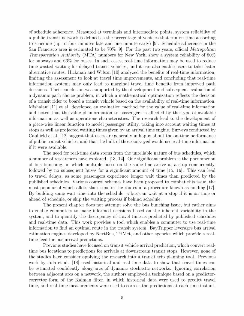
Figure 3: Estimated arrival time error. The error in minutes in the estimated arrival time for23,349 estimates, as a function of the estimated arrival time. X-axis: estimated arrival timein minutes. Y-axis: error in minutes. Points of the negative half of the Y-axis correspond tobus arriving earlier than predicted, while points on the positive half correspond to the busarriving later than predicted.

travel time) route. The frequency with which the optimal route is selected, and the degreeof sub-optimality of each TTP when the optimal route is not returned is also assessed.

2.5.1 Experimental setting

Over six-hundred trips were planned using the schedule-based TTP and the real-time TTPusing real–time data from San Francisco Municipal Transit Authority buses and light railtrains running 87 routes across the city. The trip origin and destination pairs were generatedusing a spatially uniform random distribution over the city. The trips were planned over theperiod of July 23 - 28, 2009 at various times throughout the day.

Because each transit vehicle is tracked using the on-board GPS receivers, the actualtravel times along each path between the origin-destination (O-D) pairs can be determinedafter the trip is completed. These travel times serve as a ground truth upon which thetransit vehicle arrival predictor (NextBus), the schedule-based TTP, and the real-time TTPare benchmarked. These GPS tracks also allow for the actual optimal (fastest) route to bedetermined between the O-D pairs.

2.5.2 Accuracy of the estimated transit vehicle arrival engine

The performance of the real-time TTP is dependent on the estimation of the transit vehi-cle arrival times at its upcoming stops, which is provided by NextBus. NextBus generatespredictions by using historical averages of travel times between segments, calculated at dif-ferent times of day. Fig. 3 shows the error of the arrival time estimate for 23,349 queries toNextBus. Each time NextBus is queried, an an arrival time is estimated, and the error is

13

calculated after the bus arrives at that stop.Estimated arrival times between 0 and 10 minutes have a median error of zero, and

the interquartile range (the middle 50% of estimates) tend to fall within a minute of the truetravel time. However, a small number of outliers, specifically for small arrival times, canpotentially cause significant challenges if the information is used to determine if a transferbetween buses can be made. As the estimated arrival time increases, variance in error alsoincreases. This variance effects the results of real-time TTP in two ways: determining thetravel time of the bus to the transfer point, and determining the wait time at the transferpoint for the next leg of the trip. In the set of six-hundred trips planned, there existed overfour-hundred trips which required transfers over 10 minutes past the time the trip requestwas made.

2.5.3 Accuracy of the estimated trip travel time

The accuracy of of the travel time estimate along the paths suggested by schedule-based andreal-time TTPs are compared to the ground truth travel time along the same paths. Fig 4characterizes the amount of uncertainty in the estimated travel times, divided by the numberof cases in which the planned trip required zero transfers, one transfer, or two transfers.Evaluated over all the cases, real-time data increases accuracy for travel time prediction,most noticeable in trips requiring transfers. The Wilcoxon signed-rank test was used to testfor statistically significant difference between the two trip planners . The Wilcoxon signed-rank test evaluates the null hypothesis that two related samples have the same distribution.The data compared were the percentage error of the travel times returned by the schedule-based and real-time TTP, each verified against the actual travel times. The median errorof the schedule-based TTP is 14.9% vs 11.7% for the real-time TTP. Statistical significancewas defined as z = 4.08, P < .00001 two-tailed, thus the null hypothesis is rejected. It isconcluded that the use of real-time data reduces travel time prediction error. However, thesmall difference between the errors show that the improvement in travel time accuracy ismarginal.

2.5.4 Route selection optimality

The main functions of the TTP are to provide an expected travel time from origin to desti-nation as well as suggest a set of routes based on the state of the transit network at the timeof the user’s request. The routing algorithm calculates the K-shortest paths and returns thefive fastest routes to the user. This allows the user to make a decision based on the totaltrip time, as well as personal preferences such as walking distances and number of transfersand other variables which the application does not factor in. In this analysis done in thissection, only one route predicted by each TTP - the expected optimal route determined bythe shortest travel time, is evaluated. The predicted route by both TTPs is compared to theground truth - the actual optimal route, obtained by tracking the position of multiple busesover the duration of the trips.

Table 1 summarizes the route selection optimality of the TTPs. The percentage ofcases in which the two TTPs accurately predicted the actual optimal route was determined.These cases are split into three rows, when both TTPs predicted the optimal route, and when

14

0 20 40 60 80 100!10

!5

0

5

10

15

Actual travel time (min)

Real t

ime p

lanner

decr

ease

in e

rror

(min

)Zero transfers

20 40 60 80 100 120 140!50

!40

!30

!20

!10

0

10

20

30

Actual travel time (min)

Real t

ime p

lanner

decr

ease

in e

rror

(min

)

One transfer

20 40 60 80 100 120!30

!20

!10

0

10

20

30

40

50

Actual travel time (min)

Real t

ime p

lanner

decr

ease

in e

rror

(min

)

Two transfers

Figure 4: Effect of travel time accuracy when using real-time data. Positive values on the Y-Axis refer to cases in which real-time TTP more accurately predicted total travel time. Tripswith zero transfers: 40 (41.6%) more accurate, 38 (39.6%) less accurate 18 (18.8%) sameprediction. Trips with one transfer: 232 (51.3%) more accurate, 190 (42.0%) less accurate,30 (6.6%) same prediction. Trips with two transfers: 58 (48.8%) more accurate, 47 (39.5%)less accurate, 14 (11.8%) same prediction.

only either one of the TTPs made the correct route prediction. If neither TTP predicted theactual optimal route, the actual travel times of the predicted routes were compared. Thenext three rows show the percentage of cases in which one of the sub-optimal routes resultedin a shorter actual travel time, or if the same sub-optimal route was predicted by both TTPs.The results are split into four scenarios: long trips (trips longer than 30 minutes), short trips(trips shorter or equal to 30 minutes), trips in which a transfer was involved, and trips whichrequired no transfers. In most cases, the real-time TTP outperformed the schedule-basedTTP by a small margin.

Long Short With transfers No transfersBoth predicted optimal 27.3 44.4 20.5 75.0Only real-time predicted optimal 20.3 16.7 23.8 0.0Only schedule-based predicted optimal 14.1 11.0 15.6 4.1Neither predicted optimal: real-time faster 12.5 11.2 13.9 4.2Neither predicted optimal: schedule-based faster 10.2 5.6 11.4 0.0Neither predicted optimal: same prediction 15.6 11.1 14.8 16.7

Table 1: Optimality of fastest route returned by the schedule-based TTP and the real-timeTTP with respect to the observed fastest route. Values represent percentage of cases.

15

2.5.5 Implications for further research

The study shows that the inclusion of real-time information in the BayTripper system pro-vides two benefits over schedule-based TTPs: more accurate predictions for total trip times,and a larger number of cases in which the optimal route was suggested. However, thesebenefits were found to be marginal, leaving room for improvement in three areas: removal ordetection of outliers as shown in Figure 3, improved long-term estimation of buses arrivingin over 15 minutes, and incorporation of uncertainty into bus arrival estimates.

Currently, BayTripper is dependent on third party data sources to perform bus ar-rival estimation, which is based on time-of-day historical averages of segment trip times. Asdescribed in Section 2.2, newer estimation algorithms exist which take into considerationfactors such as real-time traffic, but have not been tested in the context of a trip planningapplication. As shown in Figure 3, NextBus accurately predicts bus arrivals when the ex-pected arrival time is under 15 minutes, with the exception of outliers in 1-5% of cases.However, the incorporation of real-time data into a trip planner requires estimation of busarrivals at transfer points, which often occur greater than 30 minutes from the time thetrip is initially planned. In these problems, the current estimation engine is less accurate inpredicting bus arrivals, leading to missed transfers and large discrepancies in estimated triptimes and optimality of suggested routes. Further studies will be done to incorporate moreadvanced bus arrival estimation techniques into the BayTripper application, while charac-terizing uncertainty into the predictions to compensate for potential missed transfers.

In addition, the experiment examined the ability of the TTP to determine the optimalroute based on information only at a single time instant prior to the trip. Table 1showed thatthe real-time TTP performed better in shorter trips. Larger errors in estimation for the totaltime of longer trips, and trips which include transfers, lead to greater number inaccuraciesin the suggestion of optimal routes. The conclusion from these results is that accuracydrops with respect to the amount of time into the future the TTP must predict the stateof the system. A solution to this problem is to allow for the algorithm to re-calculate theexpected optimal route after the trip has been planned, allowing a user to receive updatedinformation about their route as the state of the transit system evolves. As more recentinformation becomes available, users will receive new estimates for their route travel time.It is also possible that the prediction for the optimal route may change after the user hasreached a transfer point, or even while riding the bus. Further evaluation of the systemincludes re-calculating the optimal route at different stages of a trip, and examining theaccuracy of the total travel time at these stages.

2.6 CONCLUSIONThis chapter described an implementation of a transit trip planning system, which includesan application developed for mobile phones, a routing engine running a K-shortest pathsalgorithm, and interfaces to bus arrival prediction engines provided by third parties. It wasdiscovered through over six-hundred experiments in San Francisco that the real-time dataprovided marginal improvements to current schedule-based trip planners. The study showedthat there is potential for much improvement in transit trip planning by using real-time datain conjunction with more advanced estimation techniques which focus on solving long term

16

estimates for bus arrivals, and characterizing uncertainty into the predictions. The growthof geo-positioning systems in transportation and the availability of real-time data feeds fromtransit agencies and other transportation modes is promising, as more opportunities forresearch are opened in the field of real-time transit, and multi-modal navigation.

17

3 Algorithm for finding optimal paths in a public transitnetwork with real-time data

3.1 INTRODUCTIONThe focus of the chapter is the introduction of a new algorithm which overcomes the problemof computing shortest paths in a transit network which pulls real-time data from a third-party Application Programming Interface (API). Over a web-based or smartphone interface,a user enters a geo-coded origin and destination (O-D), and the algorithm must respond byreturning K-shortest paths based on the real-time state of the transit network. Thus, ourprincipal performance measure is the time elapsing between input of the O-D and outputof the path, which we call the path computation time. Web usage studies show this timeshould be less than 7 seconds [33, 34].

Paths cannot be wholly pre-computed since the aim is to return results based on real-time state, which needs to be acquired at run-time. We call the time required to get thisinformation the real-time state acquisition time. Industry Service Level Agreements (SLAs)create constraints on how this real-time state can be acquired. The industry appears to beevolving towards an open model where the public agencies are making real-time bus dataavailable on the web, allowing third party developers to use this data to provide transitinformation via web-based services or native applications on smartphones or over the web.The real-time data needs to be consumed through web-based APIs that limit the amount ofdata per request to the transit agency web server and the number of requests per second.For example, NextBus, a provider of real-time data in 61 cities, limits real-time data to 300stops per request.

Data analyzed for this chapter showed that in most transit networks, running a commonK-shortest path algorithm after obtaining predictions for all transit stops in a network is notfeasible. For example, the Washington DC transit network has 28,627 stops, which takes anaverage of 75 seconds to acquire the real-time data for the entire network. Moreover, the 75seconds does not account for the request rate constraint, 1 request every 10 seconds, imposedby the data provider[35]. It takes 96 requests to get all the Washington DC data, which addsat least another 9600 seconds to the time required to acquire the data for the entire network.This time is long enough for at least some portion of the data to become obsolete by thetime the data for the entire network has been acquired. The transit routing algorithm inthis chapter needs to acquire its real-time data and compute with the K-shortest paths inless than 7 seconds. Thus, we need an algorithm able to route each trip by acquiring thereal-time data for only some small part of the total network.

Fortunately part of the literature is helpful. The obvious approach might be to modelthe transit network as a graph, albeit time expanded [36, 37, 38, 39] or time dependent[40, 41, 42, 43], and run one of the widely used shortest path algorithms on it [25, 44, 45].There has been research on speed up techniques [46, 47, 48] to Dijkstra’s algorithm as wellas heuristic algorithms developed [49, 50, 51, 52]. The literature also covers the K-shortestpath [53, 54, 55, 56] and reasonable (multi-objective) path computation [57] problem. Thisliterature helps with schedule based transit routing, i.e, when the edge costs of the graph aresingle numbers known a priori. The purpose of the discussion in this paragraph is to show

18

the real-time transit routing problem is not easily reduced to this case. These algorithmsrequire that all link costs (travel time) in the network are known at all times. However,this time required to acquire the edge costs for the network graph from the transit agencyweb servers is the major bottleneck due to the software architecture of implemented transitinformation systems today. Thus, the run-time of traditional K-shortest path algorithms inthis problem is extremely slow.

There is also literature on routing in transit networks formulated as shortest path prob-lems in stochastic and dynamic networks [58, 59, 60, 61, 62]. This literature helps considerthe reliability of travel time as well or other measures of robustness. These methods couldbe blended to improve the algorithm in this chapter to optimize higher moments of traveltime. In this chapter we do not leverage this literature.

Feder [63] addresses the routing problem when edge costs are approximately known butcan be made more precise at run-time at a cost, a parallel to the problem of determiningthe wait and travel times at bus stops by accessing a real-time API. Likewise, Pallottinodeveloped an algorithm for transit graphs where the edge costs are known, but subject tosmall changes (i.e. updates in real-time information) [64]. Though this chapter is abouta problem similar to the ones in these papers, we use a different solution technique, oneleveraging off-line pre-computation in a manner similar to Bast, Sanders, and Schultes[65, 66],for routing in road networks.

Through 770,000 simulations covering transit networks in 77 US cities, we find this ap-proach is able to keep the real-time data acquisition time under 1.5 seconds and the totalpath computation time less than 3 seconds for 99% of the O-D requests.

The structure of the chapter is as follows. Sections 3.1.1 and 3.1.2 provide further infor-mation on open transit data and the routing methods of Bast et al, respectively. Section3.2 describes our algorithm. Section 3.3 is the evaluation. We evaluate the algorithm bydoing 10,000 simulations of trip requests for each transit network in 77 cities. Worst-casebounds on path computation time, real-time data acquisition time, off-line pre-computationtime, and run-time memory requirements, are based on all 770,000 simulations. We measurethe time required to service it by actually executing the request that communicates overthe Internet in real-time to the transit agency data server for the city relevant to the O-D.Since execution times are machine dependent measures, we also provide histograms show-ing machine independent measures determining the complexity of our algorithm. The routecomputation time depends on the size of a database of paths produced by pre-computationplus the real-time data acquisition time. The real-time data acquisition time depends on thenumber of bus stops per transit trip request. We present histograms on these measures forWashington DC. The DC transit network turns out to be the most complex of the 77 cities,including Los Angeles, Chicago, and San Francisco. Section 3.4 concludes the chapter.

3.1.1 Recent Trends of Open Data

The development of a real-time transit routing algorithm has been spurred by two trends inpublic transportation technology: open data, and real-time tracking of buses.

Starting in 2007, a growing number of transit agencies have packaged their route con-figuration and schedule data into a format called the Google Transit Feed Specification(GTFS)[23] in order to have trips planned by Google Transit. The benefit of this was the in-

19

tegration of public transit into online trip-planners, but more importantly, the release of theGTFS data by transit agencies has allowed for a plethora of innovative apps being createdby third party and independent developers. For example, an open-source multi-modal tripplanner, Graphserver, was developed and has been embraced by the online transit developercommunity. Last year, our research group introduced a system for real-time transit tripplanning on mobile phones called BayTripper. The potential travel time benefits for incor-porating real-time data into travel time predictions were evaluated[67, 68]. As of July 2010,BayTripper is the only real-time transit trip planning application released and available tothe public.

The second trend is the use of GPS to track buses, not only for transit agencies tomonitor their fleet, but to open the data up for users to code with. Pioneered by TriMetin Portland Oregon, transit agencies have begun to not only release route configuration andschedule data, but also real-time feeds of the location and expected arrival time of theirtransit vehicles. Transit agencies throughout the United States have slowly been openingdata to the public. As of July 2010, there exist 787 transit agencies in the United States, 107of which provide open data and a small fraction those agencies provide open real-time data.This number has been growing, as has research involving the value of real time data[69].

3.1.2 Relation to Transit Node Routing in Road Networks

Although there has been an enormous body of work on routing in public transit networks,the algorithm we developed takes cues from the work of Bast, Sanders, and Schultes, whodeveloped an innovative algorithm for routing in road networks. Their algorithm, calledTransit Node routing is currently the fastest static routing technique available [65, 66]. Themain observation of theirs was something intuitively used by humans: When you drive tosomewhere far away, you will leave your current location via one of only a few access routesto a relatively small set of transit nodes interconnected by a sparse network relevant forlong-distance travel. Likewise, in public transit networks, when you travel to a destinationthat is not served by a bus/train route near your origin, you will look at a set of potentialtransfer stations to change buses. Transit Node Routing precomputes distance tables forimportant (transit) nodes and all relevant connections between the remaining nodes and thetransit nodes. As a result, the difficult problem of finding shortest paths on extremely largeroad networks is “almost” reduced to about 100 table lookups. This lookup table only storesdata for a certain subset of points to speed up the performance of the algorithm, which isa major innovation. The same strategy is used in the real-time transit routing algorithmpresented in Section 3.2. We calculate a set of feasible paths for only a subset of nodes inthe transit network and store the results in a lookup table.

3.2 ALGORITHM IMPLEMENTATIONAs described in Section 3.1.2, the algorithm takes cues from Transit Node Routing. TheTransit Node Routing algorithm has a pre-computation step to store distances betweenimportant nodes. The nontrivial concept is defining ‘important’ nodes such that optimalroutes are found. In our routing algorithm, the ‘important’ nodes to perform the pre-computation are defined by the following statements about routing in transit network:

20

Figure 5: Flowchart of the algorithm described in Sections 3.2.1, 3.2.5, and 3.2.10.

1. If the origin and destination are not served by the same bus route, humans intuitivelyplan trips by finding transfer points to connect between bus routes.

2. The set of feasible paths from any bus stop along Route X to any bus stop along RouteY is a subset of all feasible paths from the origin station of Route X to the terminusstation of Route Y.

Statement 2 defines the important nodes that are precomputed; it is only necessary fromthe origin node of each bus line to the terminus of every other bus line to create a lookuptable the size of the number of total bus routes squared. Statement 1 defines the process bywhich the pre-computation is done: storing transfer points to build a sequence of locationsof where to transfer to reach the terminus of the bus line. In this chapter, a feasible path isdefined as any path that can be traversed by taking a series of buses between an O-D witha maximum of four transfers. The constraint of four transfers puts a cap on the number ofpaths needed to be precomputed, and prior research has shown that the accuracy of real-timedata deteriorates significantly when predicting arrival times over 20 minutes into the future,well over the time a fourth transfer would be made [68]. Any O-D query that requires morethan four transfers cannot be computed by the algorithm.

The routing algorithm is broken up into three steps: preparing the schedule data receivedfrom third-party providers, building a lookup table of feasible paths from a subset of O-Dpairs, and dynamically performing the real-time calculation of the K-shortest paths usingthe lookup table. These steps are shown in a flowchart in Figure 5.

21

Figure 6: Example transit network structure built from open transit data with no link traveltimes defined.

3.2.1 Preparing Data

Software was built to convert schedule data to build a graph of the network with no linktravel time data as shown in Figure 6. Link travel time data is only known at real-timeby accessing an API over the internet. Although the amount of data that is needed to betransferred to deliver all real-time predictions for all bus stops in an entire network is notlarge, today’s API’s are not designed to do this. Until the groups that perform the real-time arrival predictions create a standard for this, this chapter presents a solution that isimplementable immediately to perform routing with real-time data.

3.2.2 Convert Open Transit Data To Route Configurations

Transit data is read into the system from two different sources, Google, and NextBus.com.Google has established a standard for encoding transit data, GTFS, which can be convertedinto route configuration files that store the following relevant information in the structurespecified in Figure 7, the route name, direction name, stop / intersection name, latitude,longitude, stop sequence, and agency name.

A route configuration is categorized by a route, direction, and agency name. Each config-uration specifies a set of stop names with corresponding latitude and longitude points in thesequence which the bus traverses the route. Configurations with the same route, direction,and agency name are grouped together.3.2.3 Link Bus Stop To Real-Time Feed

GTFS does not have a specification for a real-time data format, thus, each stop must be

22

Figure 7: GTFS file structure. Optional Files in dashed boxes, Required files in solid boxes(a) Files and linking columns (b) Properties of files needed to be extracted

linked to a real-time URL by an unique stopcode. This assignment is done by matching theroute configurations with the real-time feeds provided by Nextbus.com and Portland TriMet.Real time predictions are accessed through HTTP by specifying the agency name, bus route,direction, and stopcode.

Not all transit agencies that have released open data in the GTFS format are servedby NextBus.com, however any future real-time feeds provided by those agencies can beintegrated into the algorithm.3.2.4 Refine Route Configurations

Most train routes only run in two opposing directions, however there are numerous casesin which bus routes have different route configurations but run under the same route name.The transit routes are broken up into segments as described in Figure 8 such that eachunique segment defines a route configuration that all buses follow. If the set of stations ina configuration that a bus follows is a subset of another configuration of stops, the two areconsidered the same. Whether or not a bus stops at every station is determined at run-time.

3.2.5 Pre-computation of Lookup Tables

The pre-computation step generates three tables, a path lookup table, a bus service-timetable, and a geolocation table, which are defined in the following sections.

3.2.6 Find Transfer Points and Routes

The entire set of stops is sorted by either latitude or longitude, and stops within a reasonabledistance are stored as a potential transfer points between the two routes. In the implemen-tation, the reasonable transfer distance is arbitrarily chosen at half a mile. Previous researchhas shown that transit riders’ preference for walking between transfers varies quite a bit, and

23

Figure 8: Example of a bus route with two termini. This particular route is broken up intothree segments.

is dependent on many variables, including land use, open space, and topographical features[70]. In a future implementation, this transfer distance can be varied to account for thesevariables.

Bus routes are often designed to share common stations, such as in a trunk-line configu-ration. In these route configurations, there exist a large number of potential transfer pointsbetween lines, which increases the size of the lookup table linearly. To address this scenario,all transfer points between the two lines are removed except for the optimal point. Thisoptimal point is defined by the station with the lowest probability of missing a transfer asspecified by the GTFS schedule.

3.2.7 Build Path Lookup Table

A set of feasible paths is built from the origin stop of every bus route to the terminus ofevery bus route in each direction and stored in a path lookup table. The set of bus routes isiterated through to create a list of reachable routes in one to four transfers. For each O-Dpair, the transfer points corresponding to each of the list of reachable routes are stored inthe path lookup table. Paths that require more than four transfers will not be found, andthus not stored in the database.

The size of this database grows polynomially with the number of bus routes in the transitnetwork, as shown in Figure 11. The potentially infinite size of this database is limited intwo ways: by setting the number of possible transfers at four transfers, and excluding pathsthat take two transfers more than any existing feasible paths between an O-D. The secondlimitation measure is based on an analysis of GTFS schedule data, which shows that a directroute between two points is always faster than a route with two additional connections with

24

no waiting time at transfer points.3.2.8 Build Service-Time Lookup Table

The lookup table includes paths from all bus routes in the transit agency’s network.However, not all bus routes are in service at the same time: there are often nighttime orrush hour only routes being run. The final step in the pre-computation of routes builds a“service-time” table of hours in which each bus route is in service. In real-time, the busservice table used to remove any paths which include a bus route not in service.3.2.9 Build Geolocation Lookup Table

All bus stops from the route configuration files are aggregated and a geolocation table iscreated to store the set of all transit stops in the entire network, indexed by their latitudeand longitude.3.2.10 Real-Time Queries

The following section describes the algorithm when it responds to real-time queries fromusers. A query is a request for the shortest path between an O-D, specified by a latitudeand longitude point. The process is very simple: a set of paths is retrieved from the lookuptable, the travel times are accessed from the real-time API, and the total travel times foreach path are calculated and sorted. Thus, in real time, the computational complexity ofthis algorithm is linear in the number of paths retrieved from the lookup table.

3.2.11 Find Nearest Stops

Transit routes in a half-mile walking radius of both the user’s origin and desired destinationare looked up from the geolocation table. For each route, the stop nearest to the user issaved, and all other stops are not considered. If no stops are within this distance, the searchradius is increased until a bus route is found.

3.2.12 Retrieve precomputed paths

Precomputed paths are retrieved for each O-D pair of bus routes retrieved from the geoloca-tion table. When the query is made in real-time the set of transfer points is sent to the realtime API to retrieve bus arrival predictions at each node. Every time a query is made bya user, new real-time arrival predictions are sent to the real-time API, retrieving the latestdata for each user request. Thus, the algorithm instantly handles changes in bus arrival pre-dictions: even in major situations such as a bus breaking down, or multiple buses bunchingtogether, such that the wait time at any bus stop is greater than the specified headway.

3.2.13 Remove irrelevant paths

As described in Section 2.2, the precomputed lookup table contains the superset of all feasiblepaths from the origin station of every bus route to the terminus station of every bus route.Therefore, not all paths retrieved from the path lookup table are physically possible to be

25

made and are thus ignored. In addition, paths which include a bus route not in service areremoved.

3.2.14 Retrieve Real-Time Information From API

The set of feasible paths contains information for all bus stops to board, get off, and transfer.These stops are all bundled into a HTTP request to the real-time API. At this point, thealgorithm is dependent on the speed at which the third-party server can process the busarrival predictions and internet traffic between the third party server and the localhost.

The total time of each path is calculated, all paths are sorted and returned to the user.

3.3 PERFORMANCE AND RESULTSThe real-time routing algorithm was tested with transit data from 77 different cities. Thedata was obtained from GTFS Data Exchange [71], an online aggregator of GTFS files,NextBus [72], and Portland TriMet [73]. For each transit agency’s network 10,000 simulatedqueries for real-time paths were made. The 10,000 different O-D points were randomlydrawn from the set of bus stops served by each agency. As described in Section 3.2.11,the K-shortest-paths algorithm computes paths to all bus stops within a half-mile walkingdistance of the random O-D. In the implementation of the iPhone application, only the fiveshortest paths are displayed for each request in order to provide users with a variety ofoptions to reach their destination.

The route computation time depends on the size of a database of paths produced bypre-computation plus the real-time data acquisition time. The real-time data acquisitiontime depends on the number of bus stops per transit trip request. The tradeoff of using thereal-time routing algorithm is the time to precompute the lookup table and size of the table,versus the reduced time to respond to queries in real-time. To evaluate this trade off, wecollected data for four metrics:

1. Number of paths. We show that the algorithm searches through a set of paths that istractable at runtime, and even in the worse case scenario it responds to queries in atimely manner.

2. Number of requests sent to real-time API. We show that our algorithm makes a smallnumber of queries to the real-time API for all networks analyzed.

3. Number of total paths stored in precomputed lookup table. We show that the size ofthe lookup table is small enough to be loaded into memory to run on a server on evena home computer.

4. Time to generate precompute lookup table. We show that the time to compute thelookup table is small: under 1 minute for most networks, with a worst-case of 100minutes.

26

3.3.1 Implementation Details

The simulated queries were run on an Amazon EC2 server located in Northern California.Amazon EC2 is a cloud computing service that allows users to rent virtual machines called“instances”. The algorithm is running on the smallest instance available, which provides 1.7GB memory, 1 EC2 Compute Unit (1 virtual core with 1 EC2 Compute Unit), 160 GBinstance storage, on a 32-bit platform at a cost of 4 cents per hour. In addition to the testsrun for the purpose of this chapter, the server is used daily 350 times daily by 600 activeusers as of July 2010 via the BayTripper iPhone application. The EC2 server serves requestsfrom the iPhone application and the web for real-time routing on the BART and MUNIsystems in the San Francisco Bay Area.

3.3.2 Real-Time Algorithm Performance

In the following section we present histograms of metrics 1 and 2: the number of paths andrequests to the real-time arrival API. We also focus on discussing two worst-case scenariosfound in all 770,000 simulated queries, the O-D pair that requires computation of travel timesamongst the largest number of paths, and another scenario that requires the largest numberof hits to the real-time API. In both the worst-case scenarios the algorithm computes theK-shortest paths problem in less than 3 seconds, while taking 1 second to query the real-timeAPI in 99% of cases. The speed of the algorithm is affected by the number of precomputedpaths retrieved from the lookup table. The larger number of paths, the more estimates forwait and travel times are needed to be retrieved from the real-time API, the bottleneck inthe system.

Both of the worst-case scenarios were found in Washington D.C., the agency with thelargest number of bus stops and routes served that we tested. The worst-case scenariofor number of feasible paths retrieved from the precomputed lookup table is 10,127. Theworst-case scenario for number of total hits to the real-time API was 127. Figure 9 showsa histogram of the number paths computed in real-time, generated from 10,000 simulatedqueries. Washington D.C. is presented because to demonstrate that even in the worst-casethe algorithm computes in under 3 seconds.

The performance of the system is a function of the real-time API and constraints placedon accessing the API. In current real-time APIs the number of stations able to be queriedin a HTTP request is limited to 300 bus stops per request, and 10 stops per bus route.Additionally, consecutive requests cannot be made more often than every 10 seconds. Thus,as the number of hits required to the API increases, the response time grows approximatelyas a step function. The worst-case scenario for number of queries to the real-time API was127, in Washington D.C. Figure 10 shows a histogram of the number of hits to the real-timeAPI for the simulated queries in Washington D.C. The number of bus stops in the worstcase scenario, 127, can be made in a single request and fits well within the limitation of thereal-time API.

The real-time algorithm makes a new request for bus arrival estimates to the real-timeAPI every time a user request is made, ensure the most up to date estimates are used in thealgorithm. As a comparison, the total number of stops in the network is 28,627; the time

27

Figure 9: Histogram of number of paths searched Washington D.C.. 99% Percentile: 1900paths. 80% Percentile: 304 paths. 50% Percentile: 224 paths. X-Axis: Number of precom-puted paths which are computed in real-time. Y-Axis: Frequency of occurrences

Figure 10: Histogram of number of bus stops sent to real-time API per O-D query in Wash-ington D.C. 99% Percentile: 82 hits. 80% Percentile: 40 hits. 50% Percentile: 26 hits.X-Axis: Number of hits to real-time API. Y-Axis: Frequency of occurrences

to query this is 75 seconds. The alternative of querying every route in the system for thisnetwork and running Dijkstra’s algorithm on the transit graph is infeasible, as bus positionsupdate more frequently than every 75 seconds.

3.3.3 Pre-computation Performance

In the prior section we demonstrate that the real-time performance of the algorithm returnsresults in 3 seconds in the worst-case, with 1 second being spent with the real-time APIquery, versus 75 seconds to query the entire network. This performance comes at a cost ofhaving to precompute a lookup table.

28

Figure 11: Scatterplot of lookup table size for all transit agencies. Y-Axis: Size of pathlookup-table generated for transit agency X-Axis: Number of routes run by transit agency

3.3.4 Memory Usage

Each path takes on average 20 bytes to store. The size of the path lookup table that hasto be loaded to memory ranges from .664KB to 1.2GB for the largest transit network weanalyzed. The geolocation and bus service tables range from 8KB to 2MB.

As shown in Figure 11, the size of the lookup table increases polynomially as the numberof routes served by a transit agency grows.

3.3.5 Pre-computation Time

The largest region we analyzed, Washington D.C. took 99 minutes to precompute 63,308,845paths, while 70% of all other cities took under 1 minute to complete. Every time a transitagency makes a route configuration change, the lookup table must be re-computed.3.3.6 Sensitivity Analysis

The number of paths searched through at runtime is dependent on the distance a personis willing to walk to his origin, and from the last bus stop to his destination. Although theprevious simulations were made with a fixed half-mile distance, the distance can be variedper the user’s request. Figure 12 shows a histogram of the number of bus stops sent to thereal-time API for three different walking distances, .5 miles, .75 miles, and 1 mile. With a1 mile walking radius, the number of hits to the real-time API increases, but never exceeds140 requests. The response time from the server for 140 requests still is 1 second on average,thus there is a negligible increase in the time to compute the K-shortest-paths with thiswalking distance.

Additionally, the number of paths searched at runtime is dependent on an even greater

29

Figure 12: Histogram of number of bus stops sent to real-time API per O-D query in Wash-ington D.C. for three different walking distances X-Axis: Number of hits to real-time API.Y-Axis: Frequency of occurrences

variety of specific features of transit agencies and metropolitan regions, such as number ofbus stops served, number of transfer stations, as well as geographic locations and spatialdistribution of these stops. These factors affect the following performance metrics of thealgorithm in ways which have not been fully explored, but are important to consider forfuture implementations of the algorithm in larger-scale metropolitan transit networks thanWashington D.C.

3.4 CONCLUSIONThis chapter presented a new algorithm for calculating K-shortest paths in a transit networkwith real-time data. We describe that the modeling of this particular shortest path problem isa result of the state of technology used by transit agencies to disseminate information today.It was shown that pre-computation of a lookup table for paths between certain transit stopssignificantly reduces the run-time speed of responding to user requests. Transit data in77 cities was precomputed into lookup tables, and 10,000 simulated user requests for eachtransit agency were made, showing that in the worse case scenario, the algorithm computesK-shortest paths in 3 seconds. Based on these results, additional testing is proposed toinvestigate the performance of the algorithm in larger regional transportation areas whichinclude multiple transit agencies and intercity networks.

30

4 Overcoming battery life problems of smartphones whencreating automated travel diaries

4.1 ADVANCEMENTS IN AUTOMATED TRIP DIARIES WITHSMARTPHONES AND GPS

Collecting data on the way people travel has been a longstanding research problem; theinformation is incredibly valuable, can be applied in a variety of industries and researchfields, but obtaining a rich dataset is not simple. In the transportation community, workon travel survey innovation has been researched for years, and today behavior modificationprograms such as travel feedback programs is a growing research topic.

Travel surveys and data collection are essential for travel behavioral studies, which areused to understand individual travel behavior, collecting socio-economic and demographicdata, household and vehicle data, alongside travel diaries listing all trips the individual madein a day. The data is used to estimate transportation planning models, which forecast traffic,land use patterns, changes to the transportation infrastructure, and policies. The problemwith the current state of practice is that household travel surveys are expensive and do notcapture people’s lifestyles[74]. These traditional data collection methods with paper surveysare expensive and require survey subjects to constantly record data, disrupting their normalbehavior. Therefore, these surveys are typically only carried out with small sample sizes,at intervals of 10 – 15 years, covering 1 – 2 days of travel. With these sparse amounts ofdata, models are derived for 20 to 25 year forecasts of both transportation and land useconditions, making strong assumptions to cover for the lack of long-term data (e.g., thatwork location follows residential location choice). As an example, the San Francisco BayArea travel survey (BATS) was last conducted in 2000 and only covers two days per studyparticipant in 15,000 households and is used for long-range transportation planning in theentire Bay Area. Researchers have recognized that this style of data collection: running 48-hour surveys with a large sample population does not provide as much value as travel diariesover longer survey periods but with small sample sizes[75]. Because of these difficulties ofrunning surveys, there is a limited amount of data available for travel behavior modeling. Ithas been suggested for some time that addressing the data collection pain-point is the rolethat such technology can play [76, 77] .

For decades, researchers have been using GPS technology to supplement travel diaries,and have shown the benefits of using GPS location data to create travel surveys as a resultof the increased accuracy. Many early studies focused on using independent GPS devices[78, 79] and validating conventional diary surveys with these devices. These studies startedwith participants in the range of 100 persons and have expanded to as many as 1500 withthe French National Travel Survey and 2200 households in Halifax [80].

Starting in 2007, researchers began looking at smartphones as a potential tool to performtravel survey studies. There are many advantages of using a smartphone versus a separateGPS device. First, the smartphone is a ubiquitous device used by over 200 million Americans.Of the 450 million mobile phones used everyday, 46.8% are smartphones [81]. This numberis expected to grow to 70% by 2015. Thus, running a large-scale travel survey is muchmore feasible and affordable for researchers and local governments. Another advantage is

31

the distribution of travel surveys - instead of GPS devices that have to be sent to people,installing an application on a smartphone is quick and cheap, and more importantly it is aconcept that people are already accustomed with.

Unfortunately, smartphones cannot collect location data in the same way wearable GPSdevices collect data because they were not designed for that purpose. Smartphones cannotconstantly collect location data due to the power usage of location based services and thelimited battery capacity of phones; a battery will be drained in 5 hours if the phone’s GPSsensor continuously collects location points[82]. Between running apps, surfing the internet,writing emails, and talking on the phone, there is a limited power budget that a smartphonecan use for the purpose of collecting location data for travel studies. On top of that, peopleare very concerned about the battery life of their phones, are aware of the power consumptionof their apps, and actively manage applications running on their phone to minimize batterydrain [83]. People have regular charging patterns, and it is the opinion of the authors thatany system for creating automated travel diaries must do so in a battery efficient mannerthat does not change the user’s behavior and interaction with their smartphone.

There is a solution: the battery usage of phones can be managed by sampling varioussensors on the phone very infrequently. By doing this, it is possible to collect a small amountof location points without draining the user’s battery, and still recreate trips using as littledata as possible from various sensors: GPS, WiFi radio, and accelerometer. With sparsedata, determining trip attributes, even as simple as the start time and location of tripsbecome more complex.

Thus, the challenges of building a travel behavior data collection system is thus two-fold. First, developing an application which gathers location data in a battery efficientmanner, and second, developing algorithms to translate sparse location data into accuratetrips. Fortunately, there exists a large community of researchers focused on solving thelocation tracking problem in a battery efficient manner. In fact, many of these researchershad already nearly solved the problem of collecting location data that can be applied for thepurpose of generating trip diaries.

Using the ideas developed by this community, a smartphone app was developed to tracka user’s movements and locations. The smartphone app sends data to a server which runsa trip determination algorithm that outputs the following details of a person’s trips takendaily: trip start/end times, start/end locations, route taken, and travel mode used. The tripdata is displayed on a web site or can be downloaded to analyze and run travel models on.

In theory, solving this automated travel diary problem is not complex - if phones behaveas expected and provide sparse, yet accurate data, and if users never shut off their phonesor turn off location services, this research simply combines the work of the battery researchcommunity with the research done to determine travel mode on smartphones. However, inpractice this is not the case. The number of external variables: types of phones, geographiclocations, topographies, user behaviors, users’ phone settings, and many more, require arobust solution to the problem.

To learn about these externalities, a lengthy evaluation of the system was conducted,with 125 users providing data on 21 different phones in 20 different states featuring manytypes of topographies - amounting to a total of over 120,000 user-hours of data recorded.The data provided insight into the issues of various phones, the effect of different types ofgeographies on the accuracy of data, and smartphone habits of users which affected the

32

quality of the location data. In addition, the quality of the trip determination system wasevaluated: a set of metrics is proposed as the standard to evaluate any automated traveldiary system, and a detailed evaluation of 1850 trips made over 3 months was conducted,consisting of a thorough daily review of trips made.

The chapter is outlined as follows: Section 4.1.1 gives a history of travel studies usingGPS devices. Recent work in the field of travel mode determination on smartphones isdescribed in Section 4.1.2. The vast field of research of battery usage in smartphones isdiscussed in Section 4.2. Section 4.3 describes the architecture of the travel diary system,and the algorithms which process the location data into trips made are described in Section4.4. The evaluation of the system is described in Section 4.5 and Section 4.6 outlines theresearch areas needed to take the project further.

4.1.1 Trip Determination with GPS devices

Starting in the late 1990s, researchers began incorporating GPS devices into travel diarystudies[84]. Transportation researchers recognized that pen and paper travel surveys werenot providing accurate enough data in an efficient manner[85], and attempted to use newtechnologies to improve the state of tracking individual travel behavior.

The first GPS enhanced travel diary studies started with tracking driving movementsonly. A proof of concept in-vehicle GPS logger was first demonstrated by Wagner [86, 87]in 100 household vehicles in Lexington, KY. In this study, any many subsequent studies, apersonal digital assistant (PDA) was used as the data recorder. Respondents were asked toenter such information as the identity of the driver of the vehicle, the purpose of the trip,and the identity of other persons accompanying the driver. Further studies were conductedwith subjects in the range of 100-200 participants [88, 84]. The GPS devices showed manyflaws in the traditional methods of collecting travel data: the standard trip-based CATIsurvey conducted in the US under-reports travel by about 20–25% [89], short trips lasting10 minutes or less are likely to be unreported [90].

Portable GPS devices were developed to capture a person’s activity through out the day,not just while driving. Initial devices were bulky, heavy, had issues with battery life [91],but future iterations lead to smaller, lighter, and battery efficient devices. These devicescaptured all trips, even non-driving trips, and as a result significant research has been madeto develop algorithms that automate the identification of trip details, including trip purposeand travel mode [92, 76, 93, 94, 95, 96] . Studies with wearable devices ranged from smallstudies of 100-200 people to much larger studies of 2,000 people of varying time periods[91, 97].

Many studies required participants to enter information into PDAs or write down theirtrips in addition to carrying around GPS devices [98, 99, 100]. Participants experiencedfatigue in recording their travel activity, thus some studies were performed with passivedevices: users were required to simply carry the device with no data entry needed. The datafrom the passive device was collected, processed, and only in some studies the user was askedto respond to a prompted recall survey [101, 102, 103, 104, 79, 89] . In these GPS-basedprompted recall studies, the data was processed then presented back to the respondents forconfirmation and/or correction of derived trip details and the completion of other traditionalelements that cannot be derived from GPS data, such as number of travel companions and

33

destination activities. [105]

4.1.2 Trip Determination with Mobile phones

4.1.3 Prior to smartphones

Before the widespread popularity of smartphones, researchers explored using mobile phonesas a data collection tool, using GSM technology (Wermuth et al 2003). An electronic ques-tionnaire on mobile phone was also used to record the trip purpose, travel mode, and startand end time of the trip. Locations, which were derived from phone communication tow-ers rather than GPS, were successfully used for estimating travel patterns in a region [106].Building on these studies, more technology solutions were explored, include Bluetooth, WiFi,RFID, and smart-cards as a replacement, or enhancement to location gathered by GPS [107].

In Japan, PHS (personal handyphone systems), which work by gathering locations frombase stations, similar to how location via WiFi beacons work today, became popular fordoing geo-location in cities [108, 109]. More than 20 case studies using PHS technology withparticipants of up to 100-300 were conducted in Japan since 2003 [110, 111, 112, 113].

One problem with these studies is that there have been varying levels of validation per-formed to date on GPS processing software, with a general lack of ground truth datasetsavailable to perform this critical task[84]. Although mobile phone technologies seem to bean obvious method for collecting travel data, only a handful of studies have verified theaccuracy of automated processing algorithms on GPS data from mobile phones.

4.1.4 The smartphone era

An increasing number of researchers have worked on the problem of inferring modes oftransportation using smartphones, both in real-time[114, 115] as well as via post-processing[116,117]. This research attempts to differentiate a person walking, biking, driving, taking a bus,or some subset of these five modes. Common to all previous work is the extraction of sig-nificant attributes from the raw sensor data, using a training set of data, and building amodel with a classification algorithm. One of the earliest systems predicted not only modeof transportation, but destination, and route taken in real-time with a hierarchical Bayesiannetwork[115]. Greater classification accuracy was reached when post-processing GPS datawas enhanced with mapping data[116]. However, compared with the previous works, thehighest levels of accuracy were demonstrated by combining GPS and accelerometer data todetermine mode of transportation in real-time[114].

Determining the transportation mode cannot be done with the GPS sensor alone - dataabout the underlying transportation network is required to differentiate driving with transittrips. Stenneth proposed and validated a method which separated walking, cycling, driving,and public transit (Stenneth 2001). One problem that has plagued both standalone GPSdevices and smartphones is problems getting GPS signals in certain regions (near high rises).By augmenting GPS-based positioning with network-based localization to the impact ofmissing GPS signals is reduced and transportation modes can determined in a more robustmanner [118].

34

However, creating a solution for automated travel diaries using smartphones is not onlyabout determining the mode of transportation a person takes. It is also necessary to de-termine the time of the trip, route, and trip purpose among other things. A system calledCTrack was developed, which recreated trajectories from GSM data only, due to the batteryconstraints of keeping GPS running constantly - a major issue in the use of smartphones asdata collection tools which is discussed in great detail in Section 4.2. [119].

The reported accuracy of these algorithms is very high - over 90% in nearly every case -which shows that data collection for automated travel diaries can be done. However, thesealgorithms have not been used in long-term studies to analyze two things:

1. Battery consumption of the application on smartphones

2. Accuracy of determining characteristics trips made, which include more than justtravel mode: start/end times, start/end points, route, and trip purpose among a largedataset.

4.2 CONCERNS ABOUT BATTERY CONSUMPTION OF SMART-PHONES

When collecting data to generate a person’s travel history, location-based services on smart-phones are required to be turned on. The use of these location-based services is a majorlimitation: constant tracking with GPS drains smartphones batteries very rapidly, allowingonly for a few hours of usage, and making users very unhappy. The issue of battery life isof major concern: the smartphone is not solely a travel diary tool and for the system towork the travel diary application cannot be a burden to the user. Our philosophy whendesigning the system was: If one is to develop a system that uses smartphones as a tool forautomated travel diaries, the system cannot change the regular habits of the person usinghis smartphone.

4.2.1 Users care about battery life

Battery consumption on devices used for travel surveys is a major issue. Researchers inthe travel behavior community have also been concerned with the battery life of standaloneGPS devices. Stopher did a test for average battery life of various GPS devices, findingthat the average was 22:46 hours [120]. Battery consumption on smartphones is an evenmore serious issue. Previous research has shown that existing battery interfaces presentlimited information, and, as a consequence, users develop inaccurate mental models abouthow the battery discharges and how the remaining battery percentage shown in the interfacecorrelates to application usage [121].

Rahmati[122]coined the term Human-Battery Interaction (HBI) to describe mobile phoneusers’ interaction with their cell phones to manage the battery available. According to asurvey they conducted, 80% of users take measures to increase their battery lifetime, andmaximizing battery life will continue to be a key concern for users due to the major usabilityissues involved in this task. Further studies analyzed user charging characteristics and howusers consume battery in their devices [123, 122].

35

According to the study done by Ferriera, users avoided lower battery levels, with the dailyaverage of the lowest battery percentage values being 30%. In addition, the majority of thecharging instances occur for a very small period of time (up to thirty minutes) or betweenone to two hours, which is the average required time to recharge completely a battery. Thecharging habits were found to be erratic by time of day, but maintained the average batterypercentage greater than 30%.

The result of these studies show that it is important for the travel behavior applicationon the smartphone to not have a noticeable effect on the battery life of the phone and beable to last through out the day or longer.

4.2.2 Prior research on everyday location monitoring

Outside of the transportation community, many researchers and businesses are also interestedin monitoring users’ mobility during daily life. Understanding human mobility providesuseful information in a variety of fields [117, 124, 125], and as a result there has beensignificant research in identifying a person’s places of interest using smartphones, often called“everyday location monitoring”. This research in this field has direct applications to the travelsurvey community.

For the everyday location monitoring researchers, the major problem that must be solvedis minimizing energy consumption of the smartphone while providing accurate location read-ings. Continuous measurement of a user’s position is possible by keeping the GPS on, how-ever, smarter solutions exist to balance the need to obtain GPS data with extending the lifeof the smartphone battery. First, instead of simply using GPS, Wireless Positioning Systems(WPS) using cell towers and Wi-Fi access points (AP) are technologies used to provide auser’s raw coordinates [126, 127]. Also, rather than simply sampling the GPS, or the otherlocation sensors at a constant rate, new algorithms have a variety of strategies to minimizethe amount of time the GPS samples location. In nearly all studies, a movement detector isused, either by using the accelerometer[128, 129, 130, 131] or a combination of sensing WiFiand GSM networks[132]. An an adaptive scheduling policy is also used to adjust samplingrates for the various sensors, depending on the objective of the algorithm: to minimize lo-cation error[133, 128], minimize energy consumption[134, 130], or maximize place detection.In a few studies, a mobility predictor is also used to estimate times when a person is likely tomove, and adapt the sampling rate based on these predictions[133, 134, 132]. These studieshave been used to collect significant locations, or points of interest which a person travelsto, and similar innovations are used in our design the system to not only detect significantlocations, but also the mode of transportation used by individuals. This requires highersampling rates and levels of location accuracy while a person is in motion.

This prior research shows the problem of tracking and monitoring a person’s meaningfulplaces (points of interest) using the regularity of individual mobility pattern has been solved.Thorough evaluations of the energy consumption of mobile phones and the various sensorson the phone have been done, and innovative algorithms have optimized the performanceof the tracking users’ locations. For this research to be used in an automated travel diarysystem, this work has to be extended in two ways.

1. The algorithms focus on “where people go”. It is need to know “where people go and

36

how and when people got there”. Evaluations on the battery consumption of apps aswell as the accuracy of predicted trips is necessary.

2. The travel survey community does regular evaluations with hundreds of people andknows how to correctly sample from household populations. It is not likely that thesehouseholds will all carry the same types of phones, and use their phones in the sameway.

Thus, it is necessary to perform tests on a variety of phones, in a variety of locales, and withvarious types of users with different phone usage characteristics (turning on and off GPS,WiFi, charging habits, etc.)

4.3 OVERALL ARCHITECTUREBefore detailing the way the trip determination algorithm works, this section describes thebig picture: the overall architecture and data flow of the trip diary system. The design of thedata collection system is shown in Figure 13. It consists of three components: the trackingapplication on smartphones, the server architecture to handle incoming location data andhandle data requests, and the analytics software to transform the raw data into trips madeand meaningful statistics and information about those trips. The applications running onthe participants’ phones collect raw sensor data which is uploaded to cloud-based server andstored in a database. A periodic job reads the raw data, processes it to infer trip originand destination location and times and determines route and travel mode(biking, walking,driving or taking transit). This also makes use of information from third party sources suchas public transit data which are stored on the server. Trips are further augmented with datasuch as addresses/neighborhoods of trips made, distance traveled, time spent traveling, CO2emitted, calories expended, travel costs, and other data that can be layered once trip timesand locations are determined.

4.3.1 Mobile application

The mobile application runs in the background on all smartphones running the Androidoperating system. The goal of the application is to minimize the amount of energy used tocollect location and movement data while collecting enough data to allow the algorithms onthe server to recreate trips made. In this section, we describe the algorithm implemented onAndroid phones.

We implemented an algorithm with ideas already implemented by previous groups, asdescribed in Section 4.2.2. The application used similar techniques to reduce battery con-sumption: a movement detector using WiFi and accelerometer, an adaptive sensor selectionduring movement adjusting the duty cycles of GPS, WiFi, and accelerometer, and a mobilitypredictor based on a person’s familiar locations at various times of day. We refer the readerto Chon[82] as an example for more detail on the mobility learner, mobility predictor, andadaptive duty cycling strategies used by our application. The only difference between thisapplication and the ones described in Section 4.2.2, is the adjustment of the duty cycling ofthe GPS sensor while a user is in motion. When a person is detected as moving faster than a

37

Figure 13: System Architecture Diagram. The components of the system consist of mobilephones, trip determination algorithms running on a server, and web tools to view and correcttrips.

walking speed, GPS is triggered more frequently, until the person begins to move at walkingspeed or slower. Thus, the energy consumption of the application can be broken down intotwo numbers representing the energy consumption while one is in motion and while one isin stasis. Based on readings from 125 users with 21 different types of phones (describedin Section 4.5.1) on average, the amount of power consumed while a person is in motionis 8.7mA while the amount of power consumed while a person is in stasis is 0.7mA. Thesevalues are directly queried from the Android SDK. On average, the application accounts for3% of total battery consumption at any given time. With the average mobile phone batterycapacity being 1500mAH, the energy consumption of the application allows for 33 hours ofenergy consumption, assuming 2 hours of traveling each day and average smartphone us-age (internet use, texting, talking on phone, using apps). This is significantly longer thanmany applications used in practice, simply collecting GPS data every second, or even every5 seconds, which will drain a user’s battery in 5 hours[82].

Due to the requirement to minimize battery consumption, the number of location pointsgenerated by the application is very low. The map in Figure 14 shows the number of pointsreceived when all sensors are turned on compared to the number of points received usingour mobile application. The large rings around the points represent the horizontal accuracyof the location points - red represents GPS points, and green represents network points(retrieved from either WiFi or cell tower positioning). In addition, accelerometer points areonly requested once per minute while the user is in motion, and mac addresses of nearbyWiFi access points are recorded only when a person transitions from stasis to motion, asdetected by the accelerometer. These pieces of data from each sensor is sent to the serverwith a timestamp, which does the work of sorting through these independent readings andgenerating trips.

Upon launch of the application, the user is asked two survey questions: the number ofdays per month they bike, and take transit. The results of the survey are used in the modedetermination portion of determining trips made, described in Section 4.4.6. Afterwards,

38

Figure 14: 1Hz data vs. Sparse data. The figure on the left shows the amount of locationdata from the phone with the GPS sensor gathering data at 1 Hz. This exemplifies the typeof data a standalone GPS logger would receive. The figure on the right shows the amount ofdata generated by our mobile application. The red circles represent the horizontal accuracyvalues, which captures the uncertainty of the location.

the application runs in the background. If the application is killed or the phone restarts, theapplication is brought back up after a short delay. This allows for the phone to record dataat all times to determine trips.

4.3.2 Server

The server is the hub of data where all trip processing occurs. Sensor data from the phoneis uploaded once every three hours and split into various databases depending on the typeof data: accelerometer readings, wifi access points, battery levels, locations (latitude andlongitude) based on cell tower / wifi positioning, locations based on GPS, whether or notvarious location providers are on, and other data points. All the pieces of data play adifferent role in re-creating trips made by a user: the algorithm is described in greater detailin Section 4.4. The server contains databases of third party data used to process trips (i.e.transit, weather data). The server is run on a medium sized instance on Amazon ElasticCompute Cloud (EC2), with API access from the phone handled by NGINX storing data ina Postgres and Mongo database.

39

Figure 15: An example of the tool used to correct a trip’s route and start time. The figureon top shows the trip data that is generated by the trip determination algorithm. The figureon the bottom shows the trip after the route and start time have been corrected.

4.3.3 Website - Online Mapping Tools

A web interface was written to provide a suite of tools to handle research subjects’ data. Theinterface allows a researcher to process trips with one-click, and also allows the researcherto visually inspect the set of trips generated for any user with mapping tools. In additionto simply inspecting the trips for correctness, the researcher can correct the trip, by select-ing different start/end points, changing the start/end time, adjusting the route taken, ortransportation mode.

These tools are used in the evaluation of the algorithm, described in Section 4.5. Usingthe tools, testers validated the accuracy of their trips by viewing their data and having theresearcher correct the computer generated trips; the users’ inputs generated the ground truthwhich was used to evaluate the algorithms, as shown in Figure 15.

40

4.4 AN ALGORITHM FOR TRIP DETERMINATION WITH SPARSEDATA

The goal of the trip determination algorithm is to take the sparse data from the phone’ssensors and recreate trips made. For the purpose of this chapter, the definition of a tripis a period of motion surrounded by two periods of stasis greater than 3 minutes. Duringthis period of motion, a person must have traveled a minimum of 250m from an origin todestination able to be mapped to points along the street network. As described in Section4.3.1, and shown in Figure 14 data from the location sensors is not frequently generated,however, the much bigger issue is that there exists a wide variety of phones that have avariety of behaviors which can only be learned through real world testing. A list of someof the problems encountered during testing of the application are described in Section 4.5.1.These discoveries from field testing the application have contributed to the various processeswhich the data flows through. A flowchart of the trip determination algorithm is shown inFigure 16, and each block in the flowchart is described in the following sections.

4.4.1 Filtering noisy data

All location points generated by the phone are returned with a latitude, longitude, horizontalaccuracy (the error range of the latitude longitude pair), velocity, altitude, and the sourceof the location point (from GPS or Wifi/Cell towers).

In theory, the true location of the phone is contained within the centroid around thelatitude, longitude geopoint with value of the horizontal accuracy as the radius of the circle.However, this is not true; once in a while completely inaccurate GPS points are created,and inaccurate network points occur extremely frequently. In a test of 777,670 data pointsgathered from the data set of 125 users (described in Section 4.5.1), under 1% of GPS pointslied outside the circle defined by the latitude, longitude and horizontal accuracy, while 51%of Network points, with the location sourced from either cell towers, or WiFi beacons liedoutside the circle.

Despite the fact that network points are often inaccurate, they are used as part of themobility detection algorithm, to ensure that the GPS sensor is not used very frequently.Thus, faulty points are simply filtered out before attempting to build trips. Although muchmore rare, inaccurate GPS points are generated from time to time. Like the inaccuracieswith the network points, the reasons for this are unknown, but the points are filtered out aswell.

Location points are filtered under the following conditions:1) If two points are generated with the same timestamp, the more accurate point is taken.2) If the speed required to travel the distance between the edge of the location centroids

is greater than 105 miles an hour between consecutive points, but the first and last pointis less than 105 miles per hour, the in-between points are removed. The speed of 105 mphwas chosen from empirical evidence of the same observations used to calculate the locationaccuracy values descried in this section.

3) It has been observed that once in a while the GPS sensor can enter a “disrupted mode”in which it can temporarily return faulty points outside the horizontal accuracy centroid for

41

Figure 16: Overall algorithm flowchart. Each block and data source is described in Sections4.4.1 - 4.4.9

up to 2 minutes at a time (based on empirical evidence). Any points created during the“disrupted mode” are removed.

4) Faulty networks points often are returned repeatedly from the network listener - ifa WiFi/Cell based location point is tagged as faulty even once, all future instances of theexact same location point are removed.

The filtering algorithm with the preceding rules is run forwards and backwards in time.

4.4.2 Hotspots

Before any trips are calculated, the raw location points are used to identify locations where aperson spends a large amount of time (i.e. home, work, gym) which we refer to as “hotspots”.In Section 4.3.1, we referred to a number of papers which minimized battery life to identify

42

points of interest. We follow the same logic here, and further describe the methods foridentifying trips made in the following sections - the contribution of this chapter on top ofthe research from Section 4.2.2.

Figure 17 shows the algorithm flowchart for hotspot generation. The first step, thelocation filter, is used such that all non-GPS points and GPS points with accuracy greaterthan 66 meters are not used to determine the hotspot centers. In the process of markingthese points, each GPS point with a horizontal accuracy of under 66 meters is assigned aduration for which it can be proven that the person was at the latitude, longitude specifiedby that GPS point.

The duration of each point is set as follows. For each GPS point, each subsequent locationpoints are analyzed to see if it can be proven that the person has moved. First, if the areascovered by the centroids (specified by latitude, longitude, and horizontal accuracy) of thelocation points do not intersect, then the duration of the GPS point is set as the difference intime between the two points. In addition, WiFi beacon scans can prove a person has moved.If the intersection of access points seen by two subsequent WiFi beacon scans is null, then itthe duration is set as the difference in time from the second WiFi beacon scan and the timethe GPS point was captured. Figure 18 illustrates a situation in which location points areused to set the duration which the hotspot is valid. In the figure, the duration of the pointsin the hotspot cluster is calculated from the time of the earliest location point seen in thecluster until the time of the earliest location points seen in the other cluster. The points inthe other cluster may be as a result of movement, or faulty readings from the phone, butbecause neither of those can be proven from the raw data itself, it is assumed that the personhas moved.

The output of the location filter is a set of latitude-longitude-duration tuples, which isrun through a weighted clustering algorithm[135]. Any hotspots within 250m of each otherare merged, with the center of the hotspot set as the hotspot with points holding the longestduration values. Any hotspots with a total duration value of less than 2 hours is eliminated -this is an arbitrary value used to capture a person’s total points of interest. For example, if aperson spends two hours at a library, or goes to a fast food restaurant for 20 minutes at least6 times, both will be considered hotspots. However, a location where a person repeatedlydrops off or picks up another passenger probably would not be captured by this algorithm.

Finally, each hotspot is annotated with the set of all WiFi beacon seen within a 250mradius of the point.

4.4.3 Determining Start/End Location of trips

Determining trips requires input from a variety of databases, raw locations, phone sensorstates, prior trips made, and hotspots. The data from the various databases are fused, asthe algorithm makes a series of guesses to determine the features of each trip made.

The first guess for the start and end location of trips initiated by the state of all thesensors on the phone: this is defined as the sampling rate of the accelerometer, WiFi beaconsensor, GPS, and Network Listeners. When the phone detects a person is traveling at aspeed faster than a walking speed, the duty cycle of GPS is reduced - the time first instance

43

Figure 17: Hotspot algorithm flowchart

of the change in duty cycle is the initial guess of the trip start. The nearest location pointto that timestamp is defined as the first guess of the trip start location. Likewise, the timein which the duty cycle of the GPS sensor increases back to the stasis mode is the initialguess of the trip end. The nearest location point to that timestamp is defined as the firstguess of the trip end location. Based solely on the raw location points and the state of thephone sensors, a set of initial trip guesses are made.

For each initial trip guess, the trips are refined to a second estimate of the actual tripstart/end time and location. The second guess of the start location is determined by iteratingthrough the filtered location points backwards in time - after it can be proven that thesmartphone has not been moving, as described by Section 4.4.2and Figure 18, the set oflocation points during the timeframe in which the phone is in stasis is returned. Each pointin this set of points has a corresponding horizontal accuracy; these points are sorted byhorizontal accuracy. If the most accurate point in the set has a horizontal accuracy below66m and is generated by the GPS sensor, it is assigned as the starting point of the trip.Otherwise, if there exists hotspots that are contained within the shape created by the set of

44

Figure 18: Example of location points at a hotspot center and at another location whichsignifies movement away from the hotspot cluster.

potential starting points, those hotspots are set as the potential starting points of the trip.The hotspot which most closely matches the characteristics of the start time of the trip isassigned as the starting point of the trip - for example, if a trip starts at 7:00AM, the hotspotwhich corresponds with the location where the person usually spends the hours of 6PM -7AM daily (most likely one’s home) is favored over the location where the person spendsthe hours 3PM - 4PM on Saturdays. If no hotspots are contained within the shape createdby the set of potential starting points, the raw location point with the smallest horizontalaccuracy is used - trips which fall into this scenario are rare, and are described in greaterdetail in the evaluation of the accuracy of hotspots in Section 4.5.5.

The initial guess for the start time of the trip is determined a combination of the ac-celerometer, Wifi, and location sensors. The accelerometer runs on a duty cycle of approx-imately 1 minute; when the accelerometer detects movement, the phone scans for WiFibeacons. If the intersection of the set of beacons seen at subsequent WiFi beacon scans isnull, then it is assumed that movement occurred during the time between the two scans.

Determining the end location and time of scans is easier than determining the startlocation of trips. To determine the start time, many of the sensors have long duty cycles ina “low-power” mode. On the other hand, while the person is in motion and arrives at theirdestination, the sensors have shorter duty cycles. The end location of a trip is determined byiterating through the filtered locations forwards in time from a location prior to the initialguess of the end location. After it can be proven that the smartphone has not been moving,

45

same steps are taken as determining the start point of trips - sorting the potential endpointsand using the hotspots database when necessary.

Determining the end time of a trip is based on a combination of the location sensor andaccelerometer. If the accelerometer detects a prolonged period of no motion, the trip endtime is defined as the time of the first reading of the no motion period. However, while theaccelerometer can provide a clear signal when the phone is still, not all trips end with thephone being still - for example, after one has arrived at an office building, the person mustwalk up the stairs to his final destination. If a prolonged period of stasis is not detected, thelocation sensor is used as the method of determining the trip end. The same set of locationpoints used to determine the end location - proving that a person has stopped moving - isused by using the time of the first point in the set of points as the end time. In the eventthat accurate location points are not returned from the phone, WiFi scans are used, If asingle common access point is seen between two consecutive scans, the end time of the tripis set as the time of the first of the two WiFi scans.

4.4.4 Determining Route taken

Once the trip’s start and end locations are determined, the route taken between the pointsis generated. The route determination algorithm uses these start points, the raw locationpoints, and the Google Directions API[136]. The flowchart of the Route Determination blockis shown in Figure 19.

While it is possible to have built our own routing engine and mapping database, therouting algorithms were outsourced to the Google Directions to save time and take advantageof the expertise of the Google team. The input to the web request are, the starting and endingpoints, a set of waypoints, a choice of directions by mode (driving, bicycling, walking), andwhether or not alternate routes should be searched. The output of the API is a set of shortestpaths (by time) between the origin, destination, and that run through the waypoints. Itshould be noted that there are a couple of minor disadvantages of using Google Directions.First, the number of calls to the API is limited to 2,500 requests per day, with a limit of100,000 requests for paying customers. Second, the number of waypoints that can be sentto the API is limited to 8, and for paying customers the limit is 23. This means that anytrip which uses extremely suboptimal routes(by travel time) such as looping around blocksor taking a long series of residential streets instead of the highway, may not have its routescalculated accurately.

Before sending a request to the Google Directions API, a set of possible waypoints isgenerated. The purpose of generating a set of waypoints that does not include a raw pointstimestampped between the start time and end time of the trip is to minimize the chances ofgenerating an incorrect route. The Google Directions API assumes the origin, destinationpoints and waypoints are exact, while the phone returns points with horizontal accuracyreadings that are not centered at the exact latitude longitude point. Location points greaterthan 100m accuracy potentially encapsulate multiple streets, and even GPS points with a5m horizontal accuracy often are centered on the wrong side of the street, which affects theroute returned from Google. Getting the route correct is important not just for the sake ofbeing correct, but the route is also necessary for the map matching of transit routes whendetermining travel mode, as described in Section 4.4.6.

46

Figure 19: Routing Algorithm flowchart

To minimize these routing errors, the most accurate GPS point, measured by smallesthorizontal accuracy radius, for each minute is kept in the set of waypoints, all other pointsare filtered out. Before waypoints are considered, only the origin and destination points aresent to Google. One to three routes are returned, and if none of the routes pass throughall of the raw points, the path is sent to google again with a waypoint at the most accuratepoint along the section of the route missed by the returned routes from Google. This processis repeated until the route matches or the waypoint limit is exceeded.

4.4.5 Loop problems

Even with the measures taken to minimize routing errors, there exists cases in whichusing any combination raw location points as waypoints does not allow for the correct pathto be returned from the Google Directions API. In these situations, the incorrect sections ofthe route have to be removed.

The first step involves detecting all loops in the route - this includes loops that areactually valid sections in-between loops which should be eliminated.

47

Figure 20: Top: Example of an inaccurate location point causing a loop in the route Bottom:Corrected route with loop removed

Loops are then eliminated if the speed required to traverse the loop(based on the rawlocation points) exceeds the speed limit by 1.5x.

Figure 20 shows an example of a loop removed when meeting the preceding conditions,and a loop that is not removed. Because the number of GPS points are sparse, the velocitiesat any given time along the route are generated by a velocity profile generator, which snapsraw locations to the route returned from Google and generates a range of potential velocitiesfor the duration of the trip.

4.4.6 Determining Mode taken

The last piece of data needed to generate a trip is annotating the mode of transportationto the start/end time and location and route taken. Determining travel mode is done intwo steps: a classifier to differentiate between motorized modes, bicycling, and walking, anda map matching algorithm to differentiate between public transit and driving. The travelmode is defined as the main mode a person during a trip (defined in Section 4.4). While atrip may consist of many segments, such as walking to a car in a parking lot, then drivinghome, only the main mode, here, driving, is classified.

4.4.7 Classifier

The classifier is built with the same techniques used in prior research to determine modeof transportation as described in Section 4.1.4. In that research, techniques were developedto perform real-time mode determination, which identifies the transportation mode beingused at each unit time interval (e.g. every second). The purpose of this classifier is toidentify the main mode used during a trip, but the same steps are followed: collecting a setof training data, identifying a large set of features, performing feature selection, and pickinga classification algorithm. The only difference this research and prior work is the set of

48

features selected; instead of using features which can only be observed in real-time, featuresthat are defined over the course of a trip are used, such as the median speed between thetrip start and end times.

A set of training data was collected daily across various modes of transportation over thecourse of 1 month for 6 individuals. A set of features was identified, which included:

1. Speed

2. Trip duration

3. Trip length (distance covered)

4. Expected Driving duration (obtained via Google Directions API)

5. Expected Biking duration (obtained via Google Directions API)

6. Expected Walking duration (obtained via Google Directions API)

Although the accelerometer is a useful sensor to determine transportation mode, featuresfrom the accelerometer are not used for the following reasons. Velocity alone can differentiatewalking from biking/driving modes. Biking and driving cannot be successfully distinguishedbecause similar accelerometer signatures when the phone is placed in a backpack, or a lo-cation that does not allow the phone to capture the biking motion. Previous work hasshown that Decision Tree-based classification is simple and effective for classifying the sen-sory features into transportation modes [114, 116]. In this work we used the Random Forestclassifier, which is also tree-based, based on our preliminary experiments and comparisonswith Decision Trees. A Random Forest classifier consists of a number of decision trees, eachperforming classification and voting for the predicted class. Overall output is the class whichhas the highest number of votes. Each decision tree is built using samples randomly selectedfrom the training set. While growing the tree, a fixed-size subset of features is randomly se-lected at each node. Random Forests are known to be efficient on large datasets, estimatingmissing data and handling unbalanced datasets. In addition, they evaluate the importanceof variables for classification[137]. In this work, we built a Random Forest with 10 decisiontrees and 6 attributes.

The classifier predicts between walking, motorized, or biking. An additional classifierwas built to predict only between walking and motorized. Based on the results of the surveyquestions asked in the mobile application about the frequency of biking (Section 4.3.1), theappropriate classifier is used. For example, a user who responds that he never bikes will havehis trips processed through the classifier that distinguishes between walking and motorizedonly.

4.4.8 Map Matcher

Before the entire trip generation algorithm is run, a database of transit route config-urations is built using open transportation data. In 2006, Google established a standardfor encoding transit data called GTFS, which contains data that can construct route con-figurations. Files that store the following relevant information in the structure specified in

49

Figure 3, the route name, direction name, stop / intersection name, latitude, longitude, stopsequence, and agency name. A route configuration is categorized by a route, direction, andagency name. Each configuration specifies a set of stop names with corresponding latitudeand longitude points in the sequence which the bus or train traverses the route. Configu-rations with the same route, direction, and agency name are grouped together. The dataalso specifies whether or not the path taken by the route occurs on the road network oron dedicated lanes, Currently, GTFS-Data-Exchange[138] is the premier repository of allopen transit data stored in the Google Transit Feed Specification format. GTFS files arepulled from GTFS-Data-Exchange and converted into route configurations which are storedin a database. At the time of writing, the database stores data from 339 different transitagencies.

At the time of processing, trips with a route are sent to the Map Matching algorithmto determine the percentage of the route that matches with any bus or train lines whichcrosses the route taken. The algorithm for performing the map matching is a variation ofthe Bentley-Ottmann algorithm[139], which finds intersections in set of straight lines. Thebus route, and the actual route taken are defined as a series of latitude and longitude points,which when connected form the set of straight lines which the algorithm iterates through.The bus or train line with the highest percentage is returned, and any trip matching greaterthan 90% is defined as a trip taken as a transit trip.4.4.9 Catching all trips made

The preceding Sections 4.4.2 - 4.4.6 describe the flow of data through the algorithm whenthe phone properly adjusts its’ duty cycles to capture location data while a person is inmotion. However, many trips are made while the phone does not function properly. Thereare many reasons for this; as discovered in the evaluation in Section 4.5, users often turnoff their phones, turn off GPS or other location services, and most commonly, the phonedoes not respond properly to requests to return readings from the accelerometer, GPS, orNetwork listener. To account for these situations when trips are made, but zero, or very fewsensor readings are received, data flows through a separate module.

This module, called the Point Connector in Figure 16, evaluates all sensor data during the“non-trip” times when the person is expected to be in stasis. The same clustering algorithmas the one described in Section 4.4.2 is used to identify locations where a person potentiallycould have traveled to. Like the hotspot algorithm, the locations must have a horizontalaccuracy reading of 100m or less, due to the number of inaccurate network point readingsreturned by the phone. In the situation that no point in a cluster has an accuracy of under100m, sensor readings from WiFi access points are queried against the master WiFi accesspoint database to provide a more accurate position.

The result of the clustering algorithm is a set of centroids defined by latitude, longitude,and horizontal accuracy, and the corresponding time a person was assumed to be at thatcentroid. The centroids are sorted by time and routes are generated by sending the originand destination with no waypoints to the Google Directions API. The end time of the tripis set as the timestamp of the earliest reading at the centroid, and the start time of thetrip is set as the same timestamp minus the duration of the trip as returned by the GoogleDirections API. The mode of transportation is determined in two steps. If the same trip hasbeen made in the past, the transportation mode most commonly used for that trip is set as

50

the transportation mode. If not, the transportation mode most commonly used for a trip ofthat distance is set as the transportation mode. Trips which are generated by this methodmainly occur during short trips under 2km and are less accurate in terms of start/end time,route taken, and transportation mode.

4.5 EVALUATIONEvaluations were performed on the system to accomplish two goals. The first goal was to getthe application running on as many different types of phones, living in different locations,with different user behaviors as possible. The second goal of the evaluation is define a set ofmetrics and to test accuracy of trip determination system with these set of metrics. In thisevaluation, separate from the first evaluation, a set of users manually checked the accuracyof all trips generated by the system and made corrections to set the ground truth for tripsmade. This evaluation consisted of a three-month process in which six users discussed theirtrips daily with the researcher and used web-based tools to correct their logged trips. Thisallowed us to evaluate the errors in the start/end time, start/end location, route taken, andtravel mode taken for these trips made and determine error statistics, instances in which thesystem missed trips, or incorrectly created trips when no trip was actually made. These sixerror metrics are described in the following sections and are proposed as the measures forwhich all automated travel diary systems should be evaluated upon.

4.5.1 Phone Tests

This system is meant to be used by researchers to gather data from the field. In the field,there exists a large number of uncontrollable variables: smartphones are made differently,by different manufacturers, users live in different locations which don’t produce data ina uniform way across all topographies and locations, and user’s phone behaviors are verydifferent. To run a large scale trip diary study, the system must be robust enough to handleall different types of scenarios and corner cases which do not show up in a limited study.

The application was tested with 125 different users on a number of phones in a varietyof states and cities with different topologies and population densities. The phones testedinclude: HTC Desire, HTC Hero, HTC Droid Incredible, HTC Incredible S, HTC Evo 4G,HTC Inspire 4G, HTC myTouch, HTC Wildfire, HTC Thunderbolt, LG LS670 OptimusS, LG P970 Optimus, Google Nexus One, Motorola Atrix 2, Motorola Droid, MotorolaDroid 2, Motorola Droid X, Motorola Droid X2, Motorola Droid Pro, Samsung GalaxyS II, Samsung Galaxy Nexus, and Google Nexus S. The data was collected in a variety ofcities with different topologies and population densities, in the states of Washington, Oregon,California, Texas, Utah, Illinois, Missouri, Alabama, Georgia, Florida, South Carolina, NorthCarolina, Virginia, Ohio, Maryland, New Jersey, Massachusetts, New York, New Hampshire,and Ontario, Canada. This data was collected over the course of 9 months for a total of6,440 days of logged data across all testers. The 125 testers used the application for differentperiods of time, from as short as 3 days to as long as 9 months, starting in July 2011. 30 ofthe 125 testers ran the application for more than 3 months.

This evaluation allowed allowed us to learn about the problems encountered from thefield, which is divided into phone problems, and user issues. Because of these problems, the

51

phone does not always detect when a person is in motion, and trips are not always perfectlydetected.

4.5.2 Phone issues

Across all phones, it was very quickly learned that location readings from non-GPSsources return inaccurate readings very frequently: this means that the true position ofthe person lies outside the circle defined by the latitude, longitude, and radius being thehorizontal accuracy returned from the phone’s location readings. The number of inaccuratelocation readings was as high as 80% for some users while being as low as 5% for other users.The reason for the inaccuracies was not investigated, but the filtering algorithms describedin Section 4.4.1 were adapted as a result of the large number of inaccurate network readings.

While most phones were found to be able to access the accelerometer in the background,several models of phones are unable to do so, mostly from the Motorola line of phones (at thetime of testing running Android 2.3 or lower). As a result, WiFi beacons were necessary toact solely as the motion detector instead of both the accelerometer and WiFi beacon sensor.

The accuracy of location readings were also highly affected by geographic topology. Ithas been widely reported that GPS does not work well in areas with large skyscrapers,however this study showed location readings in areas with skyscrapers were very accurate,possibly due to both the density of WiFi access points used in positioning. The areas whichprovided the most inaccurate readings were suburban and rural areas when only locationwas attempted to be gathered from non-GPS sources. In these scenarios, network pointswere inaccurate up to 10 miles for one particular user, and were about 1 mile off the actuallocation in general. Most troubling is that multiple inaccurate points were often returnedin sequence, making it appear as if the phone could be moving. In these instances, theaccelerometer, and WiFi access point scans allowed for the algorithms to ignore the resultof the inaccurate network points.

While inaccurate network points are common, inaccurate GPS readings are very uncom-mon. However, errors in GPS readings may lead to faulty generation of trips made. It hasbeen observed that GPS readings of high accuracy often drifts anywhere from 20m to 50mwhile the phone is in stasis. In addition, readings have been observed to be as far as 1500kmaway from the true location of the phone. While faulty trips are generated, many of thesetrips do not follow the road network - leading the system to flag the trip as a potentiallyinaccurate trip.

Finally, it is expected that when the app makes a request for a reading from the GPS,accelerometer or any sensor, the appropriate process will execute to provide the data tothe app. However, this is not always the case: 82% of the time when a location point isrequested, a point is actually returned from the operating system to the app. The app triesagain if a location is not obtained, however, there have been instances when a person hastraveled for up to 32 kilometers with the app requesting GPS the entire time but with nolocation points generated. For the accelerometer: this problem occurs on average 95% of thetime. This behavior is often hard to predict and reduces the accuracy of the route taken ona trip.

52

4.5.3 User behavior issues

In the Android operating system, a user can choose whether or not to turn on GPS sen-sors, Network location sensors, and data connection. To perform optimally, the applicationrequires that these three settings are turned on - however during the tests, we did not forcethe user to do so. A small notice was shown to users that the settings should be, but didnot require users to follow the given instructions. This allowed us to observe users’ phonebehaviors and their affect on the trip diary application running properly.

Not all users turned on GPS services on their phone. It is widely known that turning offGPS increases the battery life of phones, and 4% of the testers followed this advice > 99%of the time. An additional 2% of users frequently switched GPS settings on and off, whilethe rest constantly kept GPS running. The system still works when GPS services are turnedoff, however, the start/end locations trips can only be determined to the nearest kilometerfor most trips.

Another problem encountered is users turn off their phones, allow the phone to run outof battery, or the phone reboots (for undetermined reasons), although these cases happeninfrequently. In these situations, which occurred .11% of the total recorded time, no datacould be collected. In cases when this occurred between trips, the algorithm in Section4.4.9could be implemented, but in cases when round-trips were made, the phone is unableto detect trips.4.5.4 Trip evaluation

After the 125 person test was conducted, a second evaluation was run to evaluate the accuracyof the algorithm for detecting trips made. This evaluation consisted of 6 people over 3months, which generated a total of 1850 trips. Due to the extensive work required to havepeople manually verify their trips made, a decision was made to run a long test with fewpeople, rather than a short test with a large amount of people. The reason for the smallernumber of people in this test compared to the prior test is the ability to gather a datasetwith large longitudinal depth to capture people’s lifestyles, hotspots, and travel behaviors.However, the 3 month period is the longest study of its kind for an evaluation of a traveldiary system using smartphones. To collect the ground truth for trips made, each of thesetrips were discussed verbally with the researcher to gather the most accurate readings andmanually verified using the tools described in Section 4.3.3 . This one-on-one discussion madepossible the detailed metrics by pinpointing locations of trip start/end locations, hotspots,and routes taken on a map to gather error rates measured to the meter accuracy.

4.5.5 Hotspot evaluation

The first evaluation of the system is the evaluation of the accuracy of the hotspots identifiedby the system. Validating the accuracy of determining hotspots is important because mosttrips made start and/or end at a hotspot. Across all users, of the trips made, 48% of tripsoccurred between two hotspots, 32% of trips occurred starting or ending with a hotspot,and 20% of trips did not include a hotspot at all. The use of hotspots is important becauseaccurate location data at the start/end point is not always present for all trips.

The most common hotspots, such as one’s home and work can be identified in the first

53

Mode Trips Logged and VerifiedBiking 154Driving 998Transit 349Walking 349

Table 2: Mode Split for trip determination accuracy evaluation.

day of using the system while other hotspots such as a friend’s house or the supermarketslowly enter the system as they are visited.

4.5.6 Method for verifying accuracy of the data

Here, we propose a definition of a trip, and the 6 metrics used to verify the accuracy ofthe trip determination algorithms and overall system:

1. Start Time

2. End Time

3. Start Location

4. End Location

5. Path Match Accuracy

6. Transportation Mode

Of the 1850 trips recorded, the start/end location, was verified for all trips, while the modeand route taken was verified for only 609 trips, which occurred during the last month of theevaluation. The mode split of the trips made is described in Table 2. The start/end timeof trips were verified in a different manner, described in Section 4.5.10. The reason why thestart/end time, path, and transportation mode were not validated for all trips was becauseof the fatigue of manually correcting trips daily by the testers.

4.5.7 Errors in Origin and Destination location

Errors in location are measured by the true start/end location of the trip as validated by theperson making the trip compared to the start/end location automatically generated by thesystem. The true start/end location was recorded using the online web tools described inSection 4.3.3 which used a draggable google maps marker to set the location. The averageerror for a hotspot location was 25m with a standard deviation of 101m. Across all users,a total of 182 hotspots were detected. This error understandably increases to 197m with astandard deviation of 599m for origin/destination locations which were not hotspots.

There results show that errors in hotspot trips is significantly lower than trips that donot contain any hotspots. Across the 3 month evaluation, 90% of hotspots were discovered

54

by the 3rd week for 4 out of 6 of the users. Two users moved their residences during thistime, thus their hotspots changed significantly before and after the move. These resultsare promising for long-term studies, but a wider evaluation with more users is required tovalidate this.

4.5.8 Routing Errors

To measure errors in the route generated by the system, the system was evaluated withthree measures: meters traveled in which predicted route matches true route, meters traveledin which predicted route does not match any part of the true route, meters of the true routewhich is not covered by the predicted route. These three measures were translated intometrics called :

1. Route Match : meters traveled in which predicted route matches true route / trueroute meters traveled, expressed as a percentage

2. Route Error 1: meters traveled in which predicted route does not match any part ofthe true route/ true route meters traveled, expressed as a percentage

3. Route Error 2: meters of the true route which is not covered by the predicted route /true route meters traveled, expressed as a percentage

Figure 21 shows an example of the three different types of errors. In the evaluation, onlydriving, transit and biking trips were evaluated. Many walks occur in parks, on campus, orareas where there is no mapping data for all paths.

Table 3 shows the breakdown of errors across these three metrics for the six individualusers. The errors are separated by user to show the larger errors in the system for users whouse underground transit systems. Users 1 and 2 primarily travel by underground subway,which does not run on a path able to be mapped by the Google Directions API, which onlyreturns results for driving, bicycling, and walking directions. On the other hand, users 3 and4 use the underground subway once in a while, and users 5 and 6 are primarily auto users.

The second half of Table 3 shows the routing errors after user input. Each day, after thetrips were generated, users corrected their trip details: start location and end location, andfor one month users corrected their start location, end location, route taken, and transporta-tion mode taken. To generate data for the second table, the trip determination algorithm wasre-run daily, taking these corrected routes, called “hot routes”, as generated by the hotspotalgorithm described in Section 4.4.2. These “hot routes” were used only for trips betweentwo hotspots, and significantly increased the route match percentage. The evaluation showsthat with a set of user input, there is potential for designing a feedback system to greatlyincrease the accuracy of the overall trip determination system.

55

Figure 21: The two types of routing errors are shown on a map. The green line representsthe ground truth, and the purple line represents the predicted route

4.5.9 Travel Mode Errors

The errors in the travel mode determined by the system are described by the confusionmatrix in Table 4.

The errors show that much work is needed to improve the system. Reasons for the errorsinclude the following:

1. One of the users is a very fast biker in the city, and the set of features used in theclassifier did not distinguish between motorized and biking very well.

2. Because some transit trips are made underground, location points had very large hor-izontal accuracy values, causing the route to be calculated incorrectly

3. Errors in the route predicted by the system propagated to the travel mode determina-tion due to the map matching of incorrect routes.

These errors show that the initial predictions for trips made needs room for improvement.However, immediate and significant improvement can be made with some user input. Asdescribed in 4.5.8, users checked and corrected their trips made, which were cached as“hotroutes”. Any future trip made between the same origin and destination used the cachedhotroute and corresponding transportation mode if the raw location points matched up withthe stored route. On average, a total of 49 hotroutes per user were stored, with an average of1.56 hotroutes per origin-destination pair. Considering these values, it is plausible to developinterfaces to prompt users of an automated travel diary system to check their trips made

56

user Route Match Route Error 1 Route Error 21 45.3 41.4 29.82 40.5 44.9 34.63 59.3 30.8 11.84 85.9 5.5 11.65 94.1 4.2 4.26 90.1 9.5 5.7

user Route Match Route Error 1 Route Error 21 79.3 9.2 13.32 83.5 6.2 13.33 87.8 8.9 7.04 90.6 9.1 5.75 95.4 3.0 3.66 93.4 5.0 4.0

Table 3: Routing Errors. The table above represents the error metrics when no user correc-tions are used for six different users. The table below represents the error metrics when usercorrections are used.

without creating a large burden for the user. Future work will investigate a system withmore methods for user input to increase the accuracy of the trip determination algorithm.

4.5.10 Errors in Trip start time and end time

During the manual correction phase, the testers did not correct the trip start or end time,due to the amount of work required to accurately log the start and end time for trips made.However, the error range in the start and end time of trips can be calculated based on theaccelerometer and Wifi readings during the trips made.

In the ideal scenario, movement is detected by the accelerometer, which leads to a scan-ning of WiFi beacons to determine if a significant location change has occurred. It is thenknown that a trip has started within the 2 minute window in which these sensor eventsoccurred. Of the 1850 trips evaluated, 48% of trips fell into this category.

In some cases it takes two to three cycles for the Wifi scan to identify a significantlocation change. The reason for this is if the intersection of the set of beacons seen atsubsequent WiFi access point scans is null, then it is assumed that movement occurredduring the time between the two scans. However, the range of WiFi access points vary indifferent environments, anywhere from 50m for 802.11b routers to 200m for 802.11g routers.A person can walk to start a trip and still be in range of an access point in 2 minutes. Ofthe 1850 trips evaluated, 36% of trips were detected within 4-6 minutes of their true starttime.

In the last 16% of cases, a variety of scenarios lead to the system being able to pinpointthe start time of the trip to under 6 minutes. This includes a variety of reasons described

57

Predicted\True Bike Drive Transit WalkBike 66.1 30.8 1.8 1.3Drive 19.2 53.1 19.2 8.5

Transit 5.0 9.4 85.0 0.6Walk 2.5 8.6 0.5 88.4

Predicted\True Bike Drive Transit WalkBike 81.9 15.2 0.6 2.3Drive 10.4 80.4 9.7 0.5

Transit 4.0 5.8 90.1 0.1Walk 2.5 8.0 0.5 89.0

Table 4: Transportation Mode Errors. The table above represents the error metrics when nouser corrections are used for six different users. the table below represents the error metricswhen user corrections are used.

in Section 4.5.1, such as user behaviors such as a phone turned off, phone behaviors such asthe sensors unable to obtain readings, or the nature of the trip, which are often short tripsof under 1 kilometer. In these scenarios, the algorithm described in Section 4.4.9 is used todetermine the start/end time of trips.

Calculating the end times of a trip is a much simpler process. While a person is movingduring a trip, the duty cycles for location acquisition are much smaller, and thus can be usedto determine a transition to the end of a trip. 40% of trip end times are accurate within 1min. 44% of trip end times are accurate within 2 minutes. The reason for the increase is thesampling period of the GPS sensor is increased in certain scenarios, such as when a personis traveling greater than a particular speed, or traveling along a hotroute. The last 16% oftrips the system is unable to detect the end time within 2 minutes as the problems describedabove in detecting the start time of a trip cascade into the end time prediction problem.4.5.11 Falsely detected trips and missed trips

Due to the issues described in Section 4.5.1, it is often the case that trips are falselydetected, or trips are completely missed. A total of 33 trips were not identified by the system(missed trips), and 39 were identified as trips when no movement occurred (false trips). The33 missed trips occurred were all 2 kilometers or less. Falsely detected trips occur as a resultof inaccurate location points which slip through the filter described in Section 4.4.1. Certainsequences of inaccurate location points make it appear that a trip is occurring, which foolsthe system into generating trips. Missed trips are a result of two problems. As describedin Sections 4.4.9 and 4.5.10, not all movements are captured, leading to a situation wherelocation points exist only at the origin and destination of trips. In situations where thepoints at the destination have a high horizontal accuracy, it is difficult to determine if thepoint is a faulty reading from WiFi/cell tower positioning, or if the person actually madethe trip. Thus, there are thresholds set, by horizontal accuracy and number of points seen,for which any location points under the threshold will set a valid destination. Increasing thisthreshold will increase the number of faulty trips made, therefore, there is a balance betweenmissing, and falsely identifying trips.

58

4.6 FUTURE WORKThe research presented in this chapter represents a first step in introducing a complete, end-to-end, and battery efficient automated travel diary system which operates on smartphones,and describing the number of difficulties of using smartphones rather than GPS loggers,as the main data collection tool. Smartphones are ubiquitous and are equipped with thetechnology needed to be used as a data collection device in travel diary systems, but thereare a number of problems that must be overcome before they can be used in a wide-scaleautomated travel diary system. In this chapter, large scale tests have allowed us to cataloguea large list of problems with smartphones and solutions found from real devices in the fieldfor over 9 months. These early results from the system are promising, and more work has tobe done evaluating the trip metrics defined in this chapter and analyzing how small amountsof human input can increase the accuracy of these metrics. Identifying the start and endlocations of trips have shown to be very accurate, while improvements are needed to moreaccurately identify the start/end time of trips, route, and mode taken. First, the researchshowed that the start/end time of 16% of trips could not be identified within a 6 minutewindow. The problem here lies with the mobile application, whose parameters for detectingmotion with the accelerometer need to be better tweaked. Accurately identifying the routetaken is a larger research problem. With sparse location data, the amount of improvementon the current algorithm is limited. However, fusing accelerometer, and magnetometer datawith location data can improve on accurately identifying routes by better identifying turnsand changes in direction. , The mode determination portion of the algorithm can alsobe improved by adding features which come from the accelerometer and magnetometer.However, all these improvements come at a cost of reducing the battery life of phones - andthe tradeoff between improving the metrics for trip determination and increasing batteryusage is a tricky balancing act.

Another area for improvement is expanding upon the 6 person test to obtain more datafor the accuracy of the trip determination algorithm. While validating the ground truth fortrips for an extended period of time is an arduous task, better web tools can be built to helpthe researcher and users to make this process easier to expand the number of users who canvalidate trips.

Aside from these goals for future research, there are a few research directions which werenot tackled in this automated travel diary system. Travel diaries always record contextualinformation about a trip, for example, the number of passengers in a car, or the purpose ofa trip. There is work to be done to derive these pieces of data from the smartphone, eitheractively by prompting users, passive detection, or a combination of both. For this system tobe of use to researchers building travel behavior models, trip attributes like these must beannotated. An area to explore is the use of third party APIs such as Yelp, Foursquare, orGoogle Places to obtain trip purpose information and design a system which prompts theuser for feedback on their trip purpose.

59

5 The Quantified Traveler: Changing transport behaviorwith personalized travel data feedback

5.1 BEHAVIOR CHANGE OPPORTUNITY IN TRANSPORTA-TION

There exists a large body of work dealing the with the modeling of transportation behaviorand also attempting to influence travel behavior, and we believe there is a new opportunityto advance the body of research even further because of recent advances in technology overthe past few years. In this chapter, we present a system and experiment which are designedto collect statistics on study participants’ travel footprint (emissions, calories burned, timeand costs) and to feed back that information in a personalized, informative way. The goalis to explore the possibility of influencing people’s awareness, attitudes and potentially be-havior, and to encourage them to engage in more sustainable transportation behavior. Thisstudy is informed by previous research in the area of behavior change that has shown somesuccess; in particular, personalized feedback programs that have been able to achieve certainchanges in behavior. However, given recent developments in mobile technology and behav-ioral economics, we believe it is time to revisit this issue. The four major technological trendsdescribed in Section 1 have given rise to advances in psychology and human computer inter-action which has lead to a growth in academic research involving new methods of behaviorchange: persuasive technology, the proliferation of smartphones, the rise of self-tracking andthe Quantified Self movement, and open, accessible transportation data.

The first three trends have already lead to new research in the fields of health and fitness,as well as environmental conservation. This chapter describes how we have taken advantageof these four trends to develop and evaluate a system which influences users’ awarenessabout their travel behavior, intentions to take sustainable modes of transportation, andactual behavior. We developed an automated travel diary system which used smartphonesto collect location and other sensor data and sent data to a server which processed theraw data into trips and attributes of each trip, including travel mode, travel time, cost,and CO2 emissions among other statistics. The technical details of the infrastructure andalgorithms are discussed in Section 4. Using this smartphone travel diary system, we rana three-week experiment with 135 participants, in which they were presented a webpagewhich gave users feedback on their personal travel statistics and comparisons to various peergroups. Section 5.2 describes related work in behavior change and persuasive technology innon-transportation fields, which influenced the design of our feedback system. Section 5.3describes the smartphone travel diary system in more detail, only recently made possibledue to advancements in smartphone technology and accessible transportation data. Ourexperiment, called the Quantified Traveler, along with the evaluation of the experiment andchanges in users’ awareness, attitudes, intentions, and behaviors are outlined in Section 5.4.We recognize that this work is just the first step in a long process to influence travel modechoice, and ideas for future work are presented in Section 5.5.

60

5.2 LESSONS FROM PRIOR BEHAVIOR CHANGE WORKIn this section, we review prior work which allowed us to develop and design the system,website, and surveys. The first step was to learn about the successes of prior behaviorchange studies in transportation, which have been ran for the past 20 years. These studieswere successful, but had many difficulties, with room for improvement thanks to modernsmartphone technology. The design of the system and implementation of the behavior changetechniques was also influenced by other studies non-transportation persuasive technologyexperiments, while the design of the surveys were influenced by models of behavior changefrom the psychology literature. Based on this prior work, our contribution to the literatureis the design and evaluation of an updated version of a Travel Feedback Program usingsmartphones and web technology.

5.2.1 Behavior Change in Transportation

There is a large body of work in Travel Feedback Programs, which aim to influence modechoice behavior with information and psychological factors. There are various styles of TravelFeedback Programs, but common to all programs are: users receive feedforward information(i.e. directions for using alternative modes) as well as feedback information (i.e. amount ofCO2 emitted) which is gathered from program participants filling out travel diaries. Therehave previously been several small-scale travel behavior feedback programs conducted byresearchers in Japan [140]; in those experiments, the feedback was based on paper-and-pensurveys, and participants were often given feedback during face-to-face contact with a “travelcoach”. It could be shown that through travel feedback programs, measurable and lastingshifts away from automobile use and toward more sustainable modes of transportation couldbe achieved. Individualized marketing has also succeeded in changing travel behavior towardsmore pro-environmental modes of transportation [141].

Although Travel Feedback Programs have been shown to be successful in inducing a modeshift away from auto usage, the implementation of these programs is not scalable. Manuallyentering information in travel diaries is a time consuming process. Using smartphones fordata collection provides an opportunity to partially or fully automate many of the tasksinvolved in the travel feedback programs, and do things that was previously not technicallyfeasible. There is an opportunity to leverage the lessons learned from HCI researchers in thedesign of automated tools on the web and smartphones to motivate behavior change, startingwith the integration of open transportation data into persuasive technology programs.

5.2.2 The Quantified Self : Self tracking to change behavior

The concept of the Quantified Self describes applications which enable the process of record-ing behavior, processing the data collected, and feeding it back to the individual or groupso that they can better understand the patterns of their activity and eventually adapt theirbehavior more intelligently than they would without these augmentations. Recently, theincreasing abundance of low-cost sensing devices(including smartphones), coupled with theuse of social networks, mobile devices and web-based applications for many different aspectsof daily life (e.g., banking) has led to an abundance of detailed data becoming availableto end-users. This has given rise to many companies which have incorporated self-tracking

61

and behavior change into their products: Zeo - tracks sleep patterns, Fitbit - fitness levels,RunKeeper - jogs and runs, CureTogether - reactions to various medication, Mint - personalfinance, RescueTime - time usage and productivity.

The Quantified Self website and regular meeting groups across the country have becomeactive forums where people exchange ideas, experiences and findings about themselves. Whilethere have been significant advances in self-tracking applications for health and fitness, therehas been a relative lack of work on quantifying one’s travel behavior.

5.2.3 Self-tracking potential in transportation

The maturity of GPS tracking technology and the surge in self-tracking interest presenta new and powerful opportunity to collect traveler data by combining these two areas. Inour system, smartphone technology is used to collect data through continuous, unobtrusivesensing with minimal effort required from the traveler. With large amounts of individualtravel behavior data, the research community can also model behavior and manage demandby getting a better understanding of how and why people travel.

There are also considerable benefits to introducing self-tracking in transportation: Manyof the costs are not paid when the trip is made, but are hidden in infrequently paid itemssuch as car insurance fees or the price of a season parking pass. Emissions are not routinelymeasured and quantified, and since travel is an induced activity that is conducted for thepurpose of another desired activity (e.g., shopping), many travelers may not be making aconscious, informed decision about how much time they want to spend traveling, or howmany calories they want to burn when traveling. However, transportation decisions havea large impact on people’s lives. For instance, the average Californian household spendsaround 15% of total income on transportation [142, 143], and the average Californian spends26.5 minutes per day commuting; this adds up to more than 110 hours per year - almostas much as a typical worker’s yearly vacation[144]. If people were to track their own travelpatterns and attempted to reduce travel time or costs, for example, this could also benefitsociety as a whole as it may catalyze a reduction in vehicle miles traveled or a shift to moresustainable modes of transportation. Raising awareness of negative impacts of transportationon the environment and public health can be considered a policy tool in its own right toreduce the overall footprint of the transportation sector. The introduction of automated self-tracking devices presents a new, powerful method to present every traveler with personalizedinformation on their specific contributions.5.2.4 Recent Examples of Technology Designed for Behavior Change

Many researchers recognized the potential of implementing many of the behavior changetechniques into computer technologies, including providing personalized feedback on actionsmeasured with smartphones. Two very active fields in which Human Computer Interac-tion researchers have built and evaluated applications are in Health/Fitness and EnergyConservation/Eco-Feedback Technology. Studies using these applications have shown thatfeedback is a powerful behavior change technique in health and fitness applications [145, ?],and eco-feedback technologies [146].

Health and fitness researchers have tried using goal-setting and feedback to design appli-

62

cations that help people maintain healthy lifestyles. One of the most notable applicationswas Ubifit[147], which automatically detected the physical activity levels of a user wearing acustom device, and also provided feedback to users. One of the notable features of Ubifit wasthe simplicity of the feedback: the person’s cell phone background changed depending on theamount of physical activity, such that a user could understand their data at a glance. Ubifitis one example of numerous applications which have evaluated the effects of Goal-Setting andFeedback in monitoring fitness[148, 149, 150]. There are also numerous examples of applica-tions of eco-feedback technology, which have been designed to change behavior[151, 152, 146]and successfully shown that feedback has an effect to conserve energy. While transportationplays a role in potentially reducing one’s environmental impact on the earth, only one behav-ioral HCI study has been conducted to influence transportation behaviors[153] and showeda high potential for behavior change to sustainable modes of transportation.

5.2.5 Understanding Behavior Models to Measure Aspects of Change

While the goal of a system may be to design behavior, it is just as important to measure thefactors which contribute to behavior change.

theory of Planned Behavior showed that behavior was influenced by attitudes, normativebeliefs[154], a person’s level of self-efficacy[155] and a person’s past experiences, social per-suasion and emotional states[156]. Later models based on the TPB expanded the influenceson one’s behavior to habits, environmental constraints, knowledge and skills to perform be-haviors, and moral obligations[157, 158, 159]. Thus, our system was designed to surveyswere designed to capture these influences.

Other behavior change models such as the TransTheoretical Model, which used people’sattitudes and levels of self-efficacy to classify people in to different stages of change[160]. Thismodel is notable because it recognizes that behavior change techniques have different effectson people in different stages of change. While education and information may be the mosteffective technique in influencing someone at the very early stages of change, goal-settingmay be a better technique for one attempting to maintain a changed behavior.

While acting “green” has been a popular movement for a while, in transportation mostpeople are not actively attempting to change their modes of transportation or distancetraveled. Therefore, the feedback website was designed as a educational and informationpage, and an attempt was made to measure a change in education by surveying if one’s“awareness” of their emissions, calories burned, and other factors changed.

5.3 THE QUANTIFIED TRAVELER SYSTEMWe built an automated travel feedback system based on the work of prior researchers andnew technology using smartphones. The system consists of many parts, from smartphonesto collect data efficiently without draining the battery, server infrastructure to receive dataand handle large loads of data requests, algorithms to process data into trips and attributes,and a carefully designed website which presented a large amount of data to users in a concisegraphical manner. The first three parts are briefly described in this section, with furtherdescribed in Section 4 while the website is described here.

63

Figure 22: System Architecture Diagram. The components of the system consist of mobilephones, trip determination algorithms running on a server, and web tools to view and correcttrips.

5.3.1 Architecture and Data-flow

The design of the data collection and feedback system is shown in Figure 22. It consists ofthree components: the tracking application on smartphones, the server architecture to handleincoming location data and handle data requests, and the analytics software to transformthe raw data into trips made and meaningful statistics and information about those trips.The applications running on the participants’ phones collect raw sensor data and uploadit to a cloud-based server which saves it to the database. A nightly job reads the rawdata, processes them to infer trip origin, destination, start time, end time, route and travelmode. Trips are further augmented with data such as addresses/neighborhoods of tripsmade, distance traveled, time spent traveling, CO2 emitted, calories expended and travelcosts. The methodology for computing the last three of these items is detailed in Table 5.

As described by Section 4, the trip determination system consists of a smartphone ap-plication that runs on Android phones and iPhones, in a battery efficient manner. A personwho travels 2 hours a day experiences on average 33 hours of typical usage (including tex-ting, talking o the phone, browsing the web, and using apps). The application runs in thephones’ background and periodically uploads location data to a server which runs a tripdetermination algorithms to generate trips and statistics to be shown on the website.

5.3.2 Website Design

Users of the data collection system are given access to a website on which they can viewtheir individual travel behavior data in different ways. Specifically, the website consists offour pages, as shown in Figures 23 - 26. After logging onto the website, participants are

64

Figure 23: The summary page, which shows a person’s travel stats and comparisons withpeer groups.

first presented with a “summary”page, which presents an overview of their aggregate traveldata and a brief explanation. The main metrics which are shown to the user are emissions,calories burned, cost, and travel time, for their own data and a set of groups they cancompare themselves to, the average America, the average resident of the San Francisco BayArea, and the average of other people in the study. In this page, our goal was to delivera summary of one’s travel history such that a person could quickly glance at the page andimmediately understand their data and trends. From there, users can access three pages:One that explains the scoring methodology, one with the detailed daily history of scoresand one with the trip history (termed “Tripography”). The “Breakdown” and “Timelines”page provide more detail from the summary page and present the information in a differentmanner. The “Breakdowns” page focuses on describing a person by his mode split, while the“Timelines” page shows how a person’s travel statistics change over various periods of time.

The “Trips” page shows a history of one’s trips on a map by calendar day, and also allowsusers to correct the travel mode of any incorrectly predicted trips. Changes entered intothe system also update the travel statistics shown on the various feedback pages to give themost accurate view of the user’s travel behavior data.

5.4 EVALUATIONTo evaluate the effectiveness of the system, we designed and conducted an experiment inthe San Francisco Bay area with 135 participants. The participants were recruited fromthe subject pool of the UC Berkeley XLab (the “Experimental Social Science Laboratory”),

65

Figure 24: The breakdowns page, which shows mode split by trips made and distance trav-eled.

which is run by the Haas School of Business. This is a computer laboratory for conductinghuman-subject experiments. The lab maintains a subject pool of over 2500 members, all ofwhom are UC Berkeley affiliates and most are undergraduate students. Xlab administrationhandles the recruiting and requires that researchers provide subjects with participation feesof around $15/hour.

For recruitment, we reached out to both students and staff at UC Berkeley. In total, 111students and 24 members of staff participated in the experiment, of which 37 were male and98 female. All participants owned smartphones; 82 were iPhones and 53 Android phones.Of the 135 participants, 121 completed the two surveys that were given (see below). Thesesurveys showed that 106 (94%) were between 17 and 29 years old. Of those 113 participants,44 had access to an automobile, 17 regularly biked, 101 regularly used transit and 103 hada transit pass.

This three-week experiment ran from March 18 to April 7, 2012. We utilized the infras-tructure described in Section 5.3 for collecting traveler data via smartphones, and the goalsof the experiment were twofold: first, it was intended to demonstrate how the QuantifiedSelf movement can be leveraged by the travel demand modeling community for data collec-tion, with a positive outcome for both sides. Second, as stated above, the experiment wasdesigned to investigate whether a data collection effort that includes elements of travelerfeedback and a direct engagement of subjects via a website can lead to a change in behaviortoward more sustainable modes of transportation. If that proved to be possible, it wouldprovide evidence of the viability of automated, web-based traveler feedback on a large scalefor use as a policy tool to promote more sustainable transportation.

We chose to focus on studying the effect of feedback and peer influences on (1) attitudestowards sustainable travel and (2) awareness of the impacts of one’s own travel behavior.The latter comprises both awareness of absolute values (e.g., amount of emissions) and anawareness of where the person stands compared to average Americans, San Francisco BayArea residents and to their peer group, which in this case was the group of survey participantsfrom the XLab. In addition, we were interested in using this experiment as a learning

66

Figure 25: The timelines page, which shows a person’s change in traveltime/emissions/calories/cost over time.

experience for the long-term research goal of using technology to persuade individuals to usemore sustainable transportation modes.

5.4.1 Experimental Design

At the beginning of the study, the participants were asked to fill out a survey about theirawareness of transportation impacts and their attitudes toward sustainable modes of trans-portation. This was followed by a three-week period in which the users were tracked. Duringthe first week, participants received no feedback information until the seventh day, when theywere sent a link to a website on which they could view their trip history and a set of per-sonalized statistics (explained in section 5.3.2) related to their travel patterns. Followingthis, the students went on a spring break, in which trips were recorded, but the data shownin users’ “summary” page did not reflect the trips during spring break. Users then receivedanother email reminder to log into the site and view their data. On average, the participantslogged in 4.1 times during the final week of the experiment. At the end of the three weeks,participants were asked to fill out a survey that contained the same questions as the first one,but with an added section asking them for feedback on the website. The following sectionsdescribe the components of the experiment in detail.

5.4.2 Recorded Activity

During the three-week study we recorded a total of 8607 trips and 115,169 miles of travelacross 6 different modes: walking, biking, taking the bus, taking the train, and driving.Plane trips are included in the amount of miles logged but ignored in the calculation oftrip statistics. The breakdown of the usage of modes is shown in Figure 27. As described inSection 5.3.2, study participants corrected their trips on the website if the system incorrectlypredicted their travel mode. Out of the 8607 trips, 13.5% of trips were corrected.

67

Figure 26: The trips page, which shows all trips for a calendar day on a map. The addressesare blanked out in this figure.

5.4.3 Measuring Attitudes

The field study provided valuable information with respect to both of its goals. The surveysshowed that there was a potential for increasing participants’ awareness of their transporta-tion carbon footprint via the personalized statistics, trends, and trips shown on the website.

5.4.4 Survey Questions and Baseline Results

The design of the survey was based on measuring factors contributing to behavior change asidentified by the Integrated Behavior Model: Experiential attitudes, Instrumental attitudes,Injunctive Norms, Descriptive Norms, Perceived Control, Self-Efficacy, and Moral Obligationfor public transit, biking, driving, and walking attitudes on a 7-point Likert scale. Thesequestions were based on common travel surveys used by the transportation community[164],and categorized into the various components of the behavior model.

The survey consisted of 55 statements which participants agreed or disagreed with on aseven-point Likert Scale. 11 of these questions were asked about the participant’s level ofawareness of their own travel behavior. This included questions about their knowledge of theamount of CO2 emitted by their daily transportation habits, the number of calories burned

68

Mode CO2 Calories CostsWalking 0 Used a calories

calculator whichadjusts calories

burned by walkingspeed [161], assuming a

150lb person.

0

Biking 0 Same as above. 0Driving Used a CO2

calculator for driving[162].

0 58.6 cents / mile [163].

Train Averaged to39g/mile [162].

0 Appropriate costs fortaking BART or

Caltrain as specifiedby the respectivetransit agencies.

Bus Averaged to25g/mile [162].

0 Same as above.

Table 5: Methodology for calculating trip footprint

by traveling, their amount of time spent traveling, and the amount of money they spenton transportation. Based on ideas from theory of planned behavior, 3 questions were askedabout participants’ willingness to set goals to change travel behavior. Sample questions forthese various categories of questions are listed in table 2. The baseline (pre-experiment)survey showed that participants responded positively to questions asking about their envi-ronmental sentiments (M = 4.73, SD = 1.73; on a scale from 1 to 7 where 7 corresponds tothe strongest pro-environmental attitudes), but on average, they slightly disagreed with thestatement that they engaged in more sustainable travel behavior than the average personat UC Berkeley (M = 3.22, SD = 1.40). Furthermore, participants responded positively tostatements about health, exercise and the possibility of burning calories while traveling (M= 5.09, SD = 1.45). The results of the survey also showed that the participants were notvery aware of how “green” they actually were (M = 4.41, SD = 1.69; 1 corresponding tocompletely unaware, 7 corresponding to very aware). In particular, the participants didn’tknow the amount of CO2 they emitted, the amount of CO2 emitted by the average person inSan Francisco, nor the magnitude of the impact of their emissions. This showed that therewas an opportunity for education on the environmental effects of using different transporta-tion modes, and that this was a group that was generally motivated to engage in sustainablebehavior.

Due to the heterogeneous nature of the participant pool (students and staff), we furtherdecomposed the group by their self-reported planned mode use during the months followingthe experiment. Specifically, we created the following three groups, based on their plannedauto use:

• People who were planning to use a car once a month or less (including never): Non-

69

Figure 27: Mode Split of all trips recorded in 3-week period. Top: Mode Split measured bynumber of trips made. Bottom: Mode Split measured by distance traveled.

drivers (55 observations)

• People planning to use a car between once a month and once a week: Multimodaltravelers (29 observations)

• People planning to use a car more than once a week: Drivers (29 observations)

We found that in terms of their attitudes toward environmental and health issues, there wasno significant difference between the three groups.

A last set of questions was related to people’s intention to change their transportationbehavior in the future. On average, the study participants slightly disagreed with statementssuggesting that they were going to change (M = 3.83, SD = 1.44), and there was no noticeabledifference between the three mode use groups.

5.4.5 An increase in awareness, changes in intention, but not in pro-sustainabilityattitudes

We were able to measure statistically significant changes in participants’ awareness of en-vironmental, health, financial and time impacts of travel as well as their attitudes towardssustainable travel behavior. The questions in the survey were divided into 6 categories:

70

Category Sample QuestionAwareness I know how much CO2 I emit from my daily

transportation.Self-Efficacy I can get exercise when traveling.Perceived Norms My friends actually engage in sustainable

transportation behavior(carpooling/biking/walking/taking public transit)

Setting Goals I would consider setting a goal to reduce my carbonfootprint.

Attitudes on Sustainable Behavior I value the benefits to society when I take sustainablemodes of transportation.

Table 6: Sample questions given to participants at the beginning and end of the study

awareness, perceived norms, goal-setting, attitudes towards sustainable behavior and towardshealth benefits of sustainable transportation modes. A paired t-test was run to compare thepre- and post-experiment results for each individual question. In addition, the questions weregrouped together to create composite scores for the five categories. A Hotelling’s T-Squaredtest for two multivariate independent samples with unequal covariance matrices was carriedout to compare composite scores for the five categories between the pre- and post-experimentsurvey. The different questions in each of the categories correspond to different variables thatare correlated and the T-squared test is used to see if there is a significant difference in thesecategories.

Example statements which showed a statistically significant (p < 0.001) increase in aware-ness of the amount of CO2 emitted were: “I know how much CO2 I emit from transportation”and “I know how much CO2 the average person in my city emits from transportation”. Whileall awareness questions (environmental, health, financial and time) showed an improvementof awareness over the study period, the change was the strongest with respect to the envi-ronmental footprint. On the other hand, even though we detected a positive shift in someof the attitude questions related to sustainable travel behavior, the overall shift in this cate-gory was statistically insignificant. An example statement (with a p-value of 0.19) was: “Weshould raise the price of gasoline to reduce congestion and air pollution.” There was also nosignificant difference between the three mode use groups.

Finally, a set of questions was asked regarding people’s intention to change their travelbehavior in the future towards using more sustainable transportation modes. A examplestatement was: “I am certain that I am going to change my transportation behavior for thebenefit of the environment”. Overall, the average answer for this group of questions was“neither agree nor disagree”, and it did not change significantly during the experiment (p= 0.46). However, in a related question, people were asked to indicate whether they wereplanning to increase or decrease their use of certain modes in the future. It was interestingto find that even though people did not state explicitly they had an intention to change, theplanned mode use of drivers revealed significant shifts. Specifically, after the experiment,drivers reported that they were planning to walk more and drive less compared to what theyhad answered before the experiment. The exact question was “Over the next few months,

71

Pre-survey Post-surveyParticipant type Mode M SD M SD t stat p-val

Drivers Driving 4.76 1.4 3.86 1.55 5.31 0.02Walking 3.86 0.87 4.79 1.56 7.8 0.01

Non-drivers Driving 3.8 1.35 3.96 1.36 0.4 0.53Walking 4.45 1.03 4.75 1.43 1.49 0.22

Multimodal Driving 4.31 0.96 4.34 1.07 0.02 0.89Walking 4.68 1.13 4.48 1.15 0.47 0.49

Table 7: Answers to question on future mode use

and compared to what you do now, how often do you intend to use the following modes oftransportation for commuting/traveling?”, and the possible answers, on a scale from 1 to 7,ranged from “much less than now” to “much more than now”. Answers are shown in table7. Planned use of other modes (carsharing, biking, transit) did not change. Multimodalparticipants and non-drivers on the other hand did not state mode use plans after theexperiment that were significantly different from those before the experiment.

While this does not mean that people were averse to change, it appears that they wereunsure about how they might change in the near future, and the feedback provided duringthe survey did not have a statistically significant influence on that.

5.4.6 Classification of participants

We suspected that participants viewing their stats on the website would be influenced bywhether they were above or below the average of their peer group on the four dimensionsplotted (emissions, calories, money and time), and by how far from the mean they were. Thisled us to conduct an analysis of how the participants in our study compared to the meanof their group. Given 16 possible combinations (above or below the mean on each of thefour dimensions), the study participants can technically be divided into 16 groups. However,we found that in our population, only 7 groups were represented, and of those, only 4 werelarger than 5 people. This is shown in table 8; a “+” means that the participant was abovethe mean in that category, whereas a “-” is below the mean.

Which group a person falls into is related to that person’s travel-related lifestyle, whichwe shall call mobility style. Groups 1 is worst on all four dimensions and likely representshabitual drivers. People in group 2 are quite similar to group 1, except that they burnmore calories. It is likely that these are high-mileage travelers. The opposite is group 3,which is consistently below the average on all four dimensions and presumably includes low-mileage travelers, which is plausible since many participants live near campus and only travelminimally. Groups 4 and 5 might be multimodal travelers who combine transit with walkingand biking, while group 6 is too small to meaningfully interpret. Finally, group 7, which isthe largest group, is best on all four dimensions. This group is likely characterized by verygreen travel behavior, predominantly walking and biking.

72

Group Observations Time Calories burned Emissions Costs1 15 + - + +2 7 + + + +3 26 - - - -4 5 + - - -5 5 + + - -6 2 - - + +7 30 - + - -

Table 8: Mobility styles among the study participants; “+” = above mean, “-” = below mean.

First week Last weekMode share M SD M SD p-val

Drive 0.63 0.35 0.55 0.36 0.08Walk 0.19 0.26 0.27 0.29 0.03Bike 0.03 0.10 0.03 0.08 0.99Bus 0.14 0.23 0.14 0.21 0.83

Train 0.01 0.01 0.01 0.04 0.15

Table 9: Mode split by distance traveled, showing the significant shift from driving to walking

5.4.7 Measured behavior change

Interestingly, our analyses of participants’ travel behavior showed a shift in mode usage.Table 9 shows the mode split by distance traveled for the first and last survey weeks. Mostimportantly, we observed a significant decrease in driving and a significant increase in walk-ing. In other words, a number of trips were shifted in the direction of lower emissions, highercalories, and lower costs. Regarding the shares of other modes, there was no significantchange in the use of bikes and buses, and there was a slight, though not significant, increasein train rides (not visible in the table due to rounding).

In order to gain a better understanding of the potential influences of the feedback providedon the website, we built several linear regression models. The individuals’ distance from themean, averaged over all four dimensions, were regressed on either the participants’ changesin time, emissions, costs and calories burned between the first and the last survey week or onthe log-odds ratio of walking as the dependent variables. Every group described in section5.4.6 was represented by an explanatory variable. Additional variables were binary variablesindicating whether somebody was female and a student, as well as the number of logins tothe website by that person. The goal of the regression model was to understand whether thedifferent groups reacted differently to the presentation of the feedback, and which ones weremost likely to shift their behavior. Unfortunately, the regression analysis was complicatedby the strong correlation between the four feedback dimensions, and even though we hadobserved a significant shift from driving to walking at the aggregate level, we were not ableto find statistically significant covariates explaining what types of people and travelers were

73

more likely to shift.

5.4.8 Feedback about the website

To evaluate the website, the post-experiment survey contained an additional set of questionsregarding the participants’ evaluation of the website. They were asked to login to the websiteand respond to the following four statements on a 7-point Likert scale about the website.

1. I enjoyed taking a look at my dashboard/statistics/trip history page and getting asummary of my travel (M = 5.37, SD = 1.2)

2. In the future, this web page is something I would consider using. (M = 5.87, SD =1.01)

3. If I were to set a goal to change my travel behavior (be greener, reduce cost, travelless), I consider this web page helpful. (M = 5.12, SD = 1.28)

4. This web page was easy to use. (M = 5.3, SD = 1.13)

Overall there was positive feedback on the website and the subjects liked the presentationof their trip data. In particular, they reported that they enjoyed seeing their transportationdata and enjoyed seeing how they compared with their peers. Users were also asked whichwebpage they liked the most, and there was a strong preference for the summary and tripspage: Summary: 38.46% Breakdown: 15.38% Timeline:6.84% Trips: 39.32%. On averagemany of them reported that they would consider using the webpage in the future and feltthat it would help setting a goal to change their travel behavior.

5.5 CONCLUSIONS AND FUTURE WORKThis chapter showed the reasoning behind the designs of an automated smartphone traveldiary system and the subsequent experiment showed how feedback on one’s travel historycan affect one’s awareness of their impact on the environment, and for some segments of thepopulation, intentions to change behavior, and actual behavior change. In addition, we wereable to show that an automated travel diary system using smartphones along with a webinterface to view trips could successfully collect data from 135 participants and process loca-tion data into trips, which was used to both influence behaviors, intentions, and awarenessand build a travel behavior model.

The next step is expanding the study from 3 weeks to a longer duration. A numberof other variables may have contributed to the measured changes in behavior, such as theparticipants’ mindfulness of being tracked and taking part in a study, or even a novelty effectof using a new application. The measured change in behavior is a step in the right direction,and the real test of a behavior change system is prolonged and maintained changes in travelmode usage over a much longer study period.

The experiment we ran used two behavior change strategies of feedback and comparison.This was an initial attempt into the concept of using technology to influence users’ trans-portation behavior, and there exists a large number of other behavior change techniqueswhich have been successfully applied in other fields that could have been experimentally

74

incorporated in our system. Behavior change techniques which have been recognized andtested include: Information, Goal-Setting, Comparison, Incentives, and Feedback [165]. Allof these techniques have been tested in a variety of fields and largely confirmed to havepositive effects for behavior change. The next step involves analyzing successful experimentswhich have used one of these techniques and molding it to our problem of nudging peopletowards sustainable modes of transportation.

75

6 Thesis Conclusion

6.1 IDENTIFYING PROBLEMS AND USING TECHNOLOGYTO SOLVE THEM

The work presented in this thesis covers two related but different areas, improving transitinformation delivered to users, and tracking and influencing people’s travel behaviors. Theyboth follow a similar formula:

1. Identify a pain point in the transportation world(of users of the transportation systemand researchers)

2. Propose a solution using smartphone technology and behavior change techniques

3. Build the system and describe the steps on how to do so

4. Evaluate the system to see if it achieved the goal of solving the problem identified inthe first place.

The first problem that I identified was that people were not using the public transportationsystem as effectively as they could. There was a new wave of GPS devices installed onbuses, and access to the information was made available to the public, but this informationwas being used to only inform users when the next bus was coming. There was potentialto solve the main goal: get users to their destination in the fastest way possible with thecurrent state(position of buses) of the transportation system, without them having to knowany information about the network.

The proposed solution was a new routing algorithm that routed users in a network ac-cording to the realtime positions of buses, not based on the schedule, like all other tripplanners discussed in the literature up until this point. The routing algorithm was madeinto part of an iPhone application called BayTripper, which served over 1,000 active users.The routing algorithm also proved not just an innovative algorithm, but it also saved time aswell. Studies showed that the value of real-time data in the trip routing application was im-mense: it gave users more accurate predictions of their expected travel times, and suggestedfaster alternative routes to use. Another contribution was made by solving this problem ina real-world network, and showing how the algorithm could scale to other larger networksas proved by a large scale test of 10,000 simulated trips in 77 different real world networks,including large systems as Washington D.C., New York City, and Los Angeles.

The second problem I identified focused solving a problem for both users and researchers.Getting people to “be green” has been a ongoing goal of both researchers and people witheco-friendly ideals. Changing behavior is a long and complex process, and before startingto influence behavior, researchers needed to understand how users currently behave. Thus,there was a sub-problem identified. Researchers needed a more efficient way to collect dataon how people travel, and the current state of the art (using either pen and paper surveys orGPS loggers to collect travel behavior data) was both expensive and not scalable to long-termstudies.

The proposed solution to this sub-problem was the creation of an automated travel diarysystem which used smartphones as the tool to collect data. While smartphones were an

76

obvious solution to the traveler data collection problem due to their widespread use and easeof distributing applications, there were a number of problems to overcome, which previouslyhad not been discussed in the travel diary literature: collecting location data with the con-straints of a limited battery life, processing data into trips with sparse, and often inaccuratedata, and high variations in data accuracy and collection with different models of phones,geographic locations, and user behaviors. These were all discovered and solved with a largescale evaluation across 20 states and 125+ users. A smaller scale evaluation proved that itwas possible to accurately generate trips from smartphone data. This contribution allowsfuture researchers to easily collect data from large sets of users, and over long periods oftime, using smartphones. The collected data can be used for a variety of purposes, such asbuilding models, or influencing behavior, the main problem I aimed to solve.

Once this data collection sub-problem was solved, I took a crack at the larger behaviorchange problem. Using the smartphone based travel diary system built, I proposed a feedbacksystem in which users received personalized feedback about how they traveled. The design ofthe website and survey questions were informed by prior research in psychology and relatedbehavior change studies in health and fitness, and eco-feedback. The designed webpageallowed users to view their data over time and along with various peer groups, averageAmericans, average residents of the San Francisco Bay Area, and their peers taking part inmy experiment.

The system was shown to be effective: users increased their awareness about the waytravel and their impact on the environment, a subset of the group, primary drivers, showedtheir intention to drive less and walk more, and the data showed that they actually changedtheir behavior for a short period, Although there is a lot more work that needs to go intoshowing a sustained, long-term behavior change. A short term success is a step in the rightdirection, but there are a number of proposed solutions to take my research further.

6.1.1 SUGGESTIONS FOR FURTHER RESEARCH

The baseline technology for conducting traveler behavior experiments has been built, butthere are some algorithmic improvements that need to be made before running large scalebehavior change experiments. The experiment in Section 5 was a successful experiment andtest of the automated travel diary system, but the participants were still asked to view andcorrect their trips daily. While only 13.5% of trips were corrected, having users check theirtrips instead of just their feedback pages is not ideal. The most promising research area iscombining small amounts of user input about their trips to boost the accuracy of the tripdetermination system. As shown in section 4, user inputs were able to boost the accuracyof the route and travel mode metrics significantly. The development of an interface as wellas algorithms that fuse user feedback with the trip determination algorithms is the mostpromising technique to improve upon the system.

While there are areas in algorithm development and technology that can be addressed,there are also many potential experiments that can be run. There exists a broad spectrumof techniques to influence traveler behavior: Information, Goal-Setting, Comparison, Incen-tives, Feedback, and Prompts. These techniques can be used in different ways and differentapplications. In the first half of my research I focused on improving Information to transitriders. For this group, information as well as feedback about their travel along different

77

routes is a potential research area. A technique that I am most excited about is prompts.Prompts are timely messages of either information or feedback which influences a person atthe time of decision. For example, a person walking out the door to work typically doesnot consider his mode of transportation, but if prompted about alternatives at the momenthe leaves the door, may be persuaded to changes depending on transportation conditions.This technology is already made possible by my prior work, and a system designed to deliverprompts would be an interesting step, However, it has been studied that prompts work beston those people who are motivated to change and have the ability to change. There areother groups of people who lack the motivation or ability to change. For these groups, I pro-pose attempting to use incentives along with different methods of feedback and informationto understand what it may take for a person to change travel mode, and change behavior.Understanding a person’s decision making process and utility of various modes is critical tochanging behavior.

With a strong technology infrastructure that I have built, it is possible to conduct thesefurther experiments for long-term studies. The work presented in this thesis has only laidthe groundwork to learning more about travel behavior - the innovative experiments are stillto come.

References[1] D. B. Work, O.-P. Tossavainen, S. Blandin, A. M. Bayen, T. Iwuchukwu, and K. Trac-

ton, “An ensemble kalman filtering approach to highway traffic estimation using gpsenabled mobile devices,” 47th IEEE Conference on Decision and Control, Cancun,Mexico, 2008.

[2] B. Hoh, M. Gruteser, R. Herring, J. Ban, D. B. Work, J. Herrera, A. M. Bayen,M. Annavaram, and Q. Jacobson, “Virtual trip lines for distributed privacy-preservingtraffic monitoring,” in MobiSys ’08: Proceeding of the 6th international conference onMobile systems, applications, and services, Breckenridge, CO, June 17-18 2008, pp.15–28.

[3] J. Eriksson, L. Girod, B. Hull, R. Newton, S. Madden, and H. Balakrishnan, “Thepothole patrol: using a mobile sensor network for road surface monitoring,” in MobiSys’08: Proceeding of the 6th international conference on Mobile systems, applications,and services, Breckenridge, CO, June 17-18 2008, pp. 29–39.

[4] E. Horvitz, J. Apacible, R. Sarin, and L. Liao, “Prediction, expectation, and surprise:Methods, designs, and study of a deployed traffic forecasting service,” In Twenty-FirstConference on Uncertainty in Artificial Intelligence, (UAI-05), Edinburgh, 2005.

[5] P. Mohan, V. N. Padmanabhan, and R. Ramjee, “Trafficsense: Rich monitoring of roadand traffic conditions using mobile smartphones,” Technical Report MSR-TR-2008-59,2008.

78

[6] J. Yoon, B. Noble, and M. Liu, “Surface street traffic estimation,” in 6th InternationalConference on Mobile Systems, Applications, and Services, San Juan, Puerto Rico,June 11-14 2007, pp. 220–232.

[7] K. Rehrl, S. Bruntsch, and H. Mentz, “Assisting multimodal travelers: Design andprototypical implementation of a personal travel companion,” IEEE Transactions onIntelligent Transportation Systems, vol. 8, no. 1, pp. 31–42, 2007.

[8] Graphserver, “The open-source multi-modal trip planner.”http://graphserver.sourceforge.net/.

[9] “Service standards report,” San Francisco Municipal Transportation Authority, Tech.Rep. Q3 FY08, July 2008.

[10] M. Hickman and N. Wilson, “Passenger travel time and path choice implications ofreal-time transit information,” Trans. Research C, vol. 3, no. 4, pp. 211–226, 1995.

[11] R. Mishalani, S. Lee, and M. McCord, “Evaluating real-time bus arrival evaluatingreal-time bus arrival information systems,” Transportation Research Record, vol. 1731,no. 00-0739, pp. 81–87, 2000.

[12] B. C. M. O’Mahony, “An examination of the public transport information requirementsof users,” IEEE Transactions on Intelligent Transportation Systems, vol. 8, no. 1, pp.21–30, 2007.

[13] M. D. Rossetti and T. Turitto, “Comparing static and dynamic threshhold based con-trol strategies,” Trans. Research A 32A, 607-620, 1998.

[14] G. F. Newell and R. B. Potts, “Maintaining a bus schedule,” Proc. Second ConferenceAustralian Road Research Board, pp. 388–39, 1964.

[15] M. Dessouky, R. Hall, L. Zhang, and A. Singh, “Real-time control of buses for schedulecoordination at a terminal,” Transportation Research Part A: Policy and Practice,vol. 37, no. 2, pp. 145–164, February 2003.

[16] C. Daganzo, “How to improve bus service,” Institute of Institute of TransportationStudies, Working Paper UCB-ITS-VWP-2008-6, University of California, Berkeley,CA, 2008.

[17] J. Xu, N. Wilson, and D. Bernstein, “The holding problem with real-time informationavailable,” Trans. Sci. 35, 1-18, 2001.

[18] I. P. H. Jula, M. Dessouky, “Real-time estimation of travel times along the arcs andarrival times at the nodes of dynamic stochastic networks,” IEEE Transactions onIntelligent Transportation Systems, vol. 9, no. 1, pp. 97–110, 2008.

[19] Shalaby and Farhan, “Prediction model of bus arrival and departure times using avland apc data,” Journal of Public Transportation, vol. Vol. 7, no. No. 1, pp. 41–61,2004.

79

[20] Abdelfattah and Khan, “Models for predicting bus delays,” Transportation ResearchRecord, vol. 1623, no. 0361-1981, pp. 8–15, 1998.

[21] D. Chien and Wei, “Dynamic bus arrival time prediction with artificial neural net-works,” Journal of Transportation Engineering, pp. 430–438, September/October 2002.

[22] YouTube, “Real-time transit application,” http://www.youtube.com/watch?v=fSeTuisLw6c.

[23] Google, “Google transit feed secification,” http://code.google.com/.

[24] R. Ahuja, T. Magnanti, and J. Orlin, Network flows: theory, algorithms, and applica-tions. Prentice-Hall, Inc. Upper Saddle River, NJ, USA, 1993.

[25] E. Dijkstra, “A note on two problems in connexion with graphs,” Numerische Mathe-matik, vol. 1, no. 1, pp. 269–271, 1959.

[26] D. B. Johnson, “Efficient algorithms for shortest paths in sparse networks,” Journal ofthe ACM, vol. 24, no. 1, pp. 1–13, 1977.

[27] R. W. Floyd, “Algorithm 97 (shortest path),” Communications of the ACM, vol. 5,no. 6, p. 345, June 1962.

[28] D. Eppstein, “Finding the k shortest paths,” in Proc. the Annual Symposium on Foun-dations of Computer Science (FOCS), 1994, pp. 154–165.

[29] C. Demetrescu and G. F. Italiano, “A new approach to dynamic all pairs shortestpaths,” Journal of the ACM, vol. 51, no. 6, pp. 968–992, 2004.

[30] V. King, “Fully dynamic algorithms for maintaining all-pairs shortest paths and tran-sitive closure in digraphs,” in In Proc. 40th IEEE Symposium on Foundations of Com-puter Science (FOCS), 1999, pp. 81–91.

[31] G. Ramalingam and T. Reps, “An incremental algorithm for a generalization of theshortest-path problem,” Journal of Algorithms, vol. 21, no. 2, pp. 267–305, 1996.

[32] J. Miller and E. Horowitz, “Algorithms for real-time gathering and analysis ofcontinuous-flow traffic data,” in Proc. IEEE Intelligent Transportation Systems Con-ference ITSC ’06, 2006, pp. 1454–1459.

[33] R. Jain, T. Raleigh, C. Graff, and M. Bereschinsky, “Mobile internet access and qosguarantees using mobile ip and rsvp with location registers,” IEEE Int. Conf. Com-mun., vol. 3, pp. 1690–1695, 1998.

[34] T. Erl, Ed., Service-oriented architecture (SOA): concepts, technology, and design.Prentice Hall, 2005.

[35] N. T. Conditions, http://www.sfmta.com/cms/asite/nextmunidata.htm.

[36] M. Muller-Hannemann and K. Weihe, “Pareto shortest paths is often feasible in prac-tice.” In Proc. 5th Workshop on Algorithm Engineering (WAE 2001), vol. 2141, pp.185–198, 2001.

80

[37] S. Pallottino and M. G. Scutella, Equilibrium and advanced transportation modelling,chapter 11. Kluwer Academic Publishers, 1998.

[38] F.Schulz, D.Wagner, and K.Weihe, “Dijkstra’s algorithm on-line: An empirical casestudy from public railroad transport,” ACM Journal of Experimental Algorithmics,vol. 5(12), 2000.

[39] F. Schulz, D. Wagner, and C. Zaroliagis, “Using multi- level graphs for timetable in-formation in railway systems,” In Proceedings 4th Workshop on Algorithm Engineeringand Experiments, pp. 43–59, 2001.

[40] G. Brodal and R. Jacob, “Time-dependent networks as models to achieve fast exacttimetable queries,” In Proc. 3rd Workshop on Algorithmic Methods and Models forOptimization of Railways (ATMOS 2003)Electronic Notes in Theoretical ComputerScience, vol. 92, issue 1, Elsevier, 2003.

[41] K. Nachtigal, “Time depending shortest-path problems with applications to railwaynetworks,” European Journal of Operations Research, vol. 83, pp. 154–166, 1995.

[42] A. Orda and R. Rom, “Shortest-path and minimum-delay algorithms in networks withtime-dependent edge-length,” Journal of the ACM, vol. 37(3), 1990.

[43] ——, “Minimum weight paths in time-dependent networks,” Networks, vol. 21, 1991.

[44] R. Bellman, “On a routing problems,” Quarterly of Applied Mathematics, vol. 16(1),pp. 87–90, 1958.

[45] P. E. Hart, N. J. Nilsson, and B. Raphael, “A formal basis for the heuristic determina-tion of minimum cost paths,” IEEE Transactions on Systems Science and Cybernetics,pp. 100–107, 1968.

[46] E. Pyrga, F. Schulz, D. Wagner, and C. Zaroliagis, “Efficient models for timetable infor-mation in public transportation systems,” ACM Journal of Experimental Algorithmics,vol. 2.4, 2007.

[47] R. Bauer, D. Delling, and D. Wagner, “Experimental study on speed-up techniques fortimetable information systems,” Networks, no. 0.1002/net.20382, 2009.

[48] D. Delling, T. Pajor, and D. Wagner, “Engineering time- expanded graphs for fastertimetable information.” Lecture Notes in Computer Science, vol. 5868, pp. 182–206,2009.

[49] G. Desaulniers and D. Villeaneuve, “The shortest path problem with time windowsand linear waiting costs,” Transportation Science, vol. 34, pp. 312–319, 2000.

[50] R. Dial, “Transit pathfinder algorithms,” Highway Research Record, vol. 205, pp. 67–85,1967.

81

[51] J. Granat and F. Guerriero, “The interactive analysis of the multicriteria shortest pathproblem by the reference point method,” European Journal of Operational Research,vol. 151 (1), pp. 103–118, 2003.

[52] T.-N. Chuang and J.-Y. Kung, “The fuzzy shortest path length and the correspondingshortest path in a network.” Computers and Operations Research, vol. 32(6), pp. 1409–1428, 2005.

[53] N. Van der Zijpp and C. Fiorenzo, “Path enumeration by finding the constrained k-shortest paths,” Transportation Research Part B, vol. 39 (6), pp. 545–563, 2005.

[54] W. Xu, S. He, R. Song, and S. S. Chaudhry, “Finding the k shortest paths in a schedule-based transit network,” Computers & Operations Research, 2010.

[55] Y.-L. Chen and H.-H. Yang, “Finding the first k shortest paths in a time-windownetwork.” Computers and Operations Research, vol. 31 (4), pp. 499–513, 2004.

[56] L. Zhao, Y. Xiong, and H. Sun, The K Shortest Transit Paths Choosing Algorithm inStochastic Transit Network, R. Sets and K. Technology, Eds. Springer, 2008.

[57] M. Tan, C. Tong, S. Wong, and J. min Xu, “An algorithm for finding reasonablepaths in transit networks,” Journal of Advanced Transportation, vol. 41, No. 3, pp. pp.285–305, 2010.

[58] R. W. Hall, “The fastest path through a network with random time-dependent traveltimes,” Transportation Science, vol. 20(3), pp. 182–188, 1986.

[59] D. E. Kaufman and R. L. Smith, “Fastest paths in timedependent networks for intel-ligent vehicle-highway systems applications,” IVHS Journal, vol. 1(1), pp. 1–11, 1993.

[60] M. P. Wellman, K. Larson, M. Ford, and P. R. Wurman, “Path planning under time-dependent uncertainty,” in Eleventh Conference on Uncertainty in Artificial Intelli-gence, 1995, pp. 532–539.

[61] O. E. Karasan, M. C. Pinar, and H. Yaman, “The robust shortest path problem withinterval data,” manuscript, August 2001.

[62] P. Zielinski, “The computational complexity of the relative robust shortest path prob-lem with interval data,” European Journal of Operational Research, vol. 158, pp. 570–576, 2004.

[63] T. Feder, R. Motwani, L. O’Callaghan, C. Olston, and R. Panigrahy, “Computingshortest paths with uncertainty,” Journal of Algorithms, vol. 62, pp. 1–18, 2007.

[64] S. Pallottino and M. Scutell, “A new algorithm for reoptimizing shortest paths whenthe arc costs change,” Operations Research Letters, vol. 31 (2), pp. 149–160, 2003.

[65] H. Bast, S. Funke, P. Sanders, and D. Schultes, “Fast routing in road networks withtransit nodes,” Science, vol. 316(5824):566, 2007.

82

[66] D. Schultes, “Route planning in road networks,” Ph.D. dissertation, Universitat Karl-sruhe (TH), 2008.

[67] J. Jariyasunant and E. Mai, “Baytripper,” www.baytripper.org. [Online]. Available:www.baytripper.org

[68] J. Jariyasunant, D. B. Work, B. Kerkez, R. Sengupta, S. Glaser, and A. Bayen, “Mobiletransit trip planning with real-time data,” in Proceedings of the 2010 TransportationResearch Board Annual Meeting, 2010.

[69] B. Ferris, K. Watkins, and A. Borning, “Onebusaway: Results from providing real-timearrival information for public transit.” in Proceedings of CHI, 2010.

[70] Z. Guo and N. H. M. Wilson, “Assessment of the transfer penalty for transit tripsgeographic information system-based disaggregate modeling approach,” TransportationResearch Record: Journal of the Transportation Research Board, vol. 1872, pp. 10–18,2004.

[71] GTFS-DataExchange, www.gtfs-data-exchange.com.

[72] NextBus, www.nextbus.com.

[73] TriMet, developer.trimet.org.

[74] E. D., H. Timmermans, and L. V. Veghel, “Effects of data collection methods in traveland activity research,” Prepared for European Institude of Retailing and Services Stud-ies, Tech. Rep., 1996.

[75] P. R. Stopher, K. Kockelman, S. P. Greaves, and E. Clifford, “Reducing burden andsample sizes in multiday household travel surveys,” Transportation Research Record,vol. 2064, pp. 12–18, 2008.

[76] J. Wolf, R. Guensler, and W. Bachman, “Elimination of the travel diary: An experi-ment to derive trip purpose from gps travel data.” in Transportation Research RecordNo. 1768, Transportation Research Board, Washington, DC, USA, 2001, pp. 125–134.

[77] P. R. Stopher, N. Swann, and C. FitzGerald, “Using an odometer and a gps panel toevaluate travel behaviour change programs,” in 11th TRB National Planning Applica-tions Conference, Daytona Beach, FL, USA, May 2007.

[78] L. M. T. M. . A. C. Wolf, J., Transport survey quality and innovation. Oxford:Pergamon Press, 2003, ch. Trip rate analysis in GPS-enhanced personal travel surveys.,pp. 483–498.

[79] J. Wolf, Travel survey methods: Quality and future directions. Oxford: Elsevier, 2006,ch. Applications of new technologies in travel surveys, pp. 531–544.

[80] S. Bricka, “Non-response challenges in gps-based surveys,” in 8th International Con-ference on Travel Survey Methods, Annecy, France, May 2008.

83

[81] D. N. P. P. i. t. U. Nielsen, Smartphones Account for Half of all Mobile Phones,“http://www.nielsen.com/us/en.html,” Tech. Rep., 2012.

[82] Y. Chon, E. Talipov, H. Shin, and H. Cha, “Mobility prediction-basedsmartphone energy optimization for everyday location monitoring,” in Proceedingsof the 9th ACM Conference on Embedded Networked Sensor Systems, ser.SenSys ’11. New York, NY, USA: ACM, 2011, pp. 82–95. [Online]. Available:http://doi.acm.org/10.1145/2070942.2070952

[83] D. Ferreira, A. Dey, and V. Kostakos, “Understanding human-smartphone concerns: Astudy of battery life,” in Pervasive Computing, ser. Lecture Notes in Computer Science,K. Lyons, J. Hightower, and E. Huang, Eds. Springer Berlin / Heidelberg, 2011, vol.6696, pp. 19–33.

[84] J. Wolf, “Applications of new technologies in travel surveys,” in 7th International Con-ference on Travel Survey Methods, Costa Rica, 2004.

[85] P. R. Stopher and S. P. Greaves, “Household travel surveys: Where are we going?”Transportation Research Part A: Policy and Practice, vol. 41, no. 5, pp. 367–381, 2007,bridging Research and Practice: A Synthesis of Best Practices in Travel DemandModeling. [Online]. Available: http://www.sciencedirect.com/science/article/B6VG7-4M6SBB1-2/2/65f88300cd48e4189ca4bd661243ba5d

[86] D. P. Wagner, E. Murakami, and M. Guindon, “Using gps for measuring householdtravel in private vehicles,” in 6th TRB Conference on the Application of TransportationPlanning Methods, Dearborn, Michigan, USA, 1997.

[87] L. a. t. d. c. t. g. p. s. f. p. t. s. F. R. t. F. F. H. A. Battelle Transportation Division,“http://fhwa.dot.gov/ohim/trb/reports.htm,” Tech. Rep., 1997.

[88] E. Murakami and D. P. Wagner, “Can using global positioning system (gps) inprovetrip reporting?” Transportation Research C, pp. 7, 149–165, 1999.

[89] P. Stopher, C. FitzGerald, and M. Xu, “Assessing the accuracy of the sydneyhousehold travel survey with gps,” Transportation, vol. 34, pp. 723–741, 2007,10.1007/s11116-007-9126-8. [Online]. Available: http://dx.doi.org/10.1007/s11116-007-9126-8

[90] J. Zmud and J. Wolf, “Identifying the correlates of trip misreporting–results from thecalifornia statewide household travel survey gps study,” in 10th IATBR, Lucerne, 2003.

[91] G. Draijer, N. Kalfs, and J. Perdok, “Global positioning system as data collectionmethod for travel research,” Transportation Research Record, vol. 1719, pp. 147–153,2000.

[92] J. Wolf, “Using gps data loggers to replace travel diaries in the collection of travel data,”Ph.D. dissertation, Georgia Institute of Technology, School of Civil and EnvironmentalEngineering, Atlanta, Georgia, USA, 2000.

84

[93] R. de Jong and W. Mensonides, “Wearable gps device as a data collection method fortravel research, its working paper 03-02,” Institute of Transport Studies, Sydney, Tech.Rep., 2003.

[94] J. Wolf, S. Schönfelder, U. Samaga, and K. Axhausen, “80 weeks of gps-traces: Ap-proaches to enriching trip information,” in 83rd Annual Meeting of the TransportationResearch Board, Washington, D.C., USA, 2004.

[95] E. Chung and A. Shalaby, “Development of a trip reconstruction tool to identify trav-eled links and used modes for gps-based personal travel surveys,” in 83rd Annual Meet-ing of the Transportation Research Board, Washington, D.C., USA, January 2004.

[96] E. Chung, T. Ye, and A. Shalaby, “An integrated gps-gis system for personal travelsurveys,” in GEOIDE Annual Conference, Quebec, May 2004.

[97] S. Greaves, “A panel approach to evaluating voluntary travel behavior changeprograms–south australia pilot survey,” in Transportation Research Board 85th An-nual Meeting, 2006.

[98] S. T. Doherty, N. Noel, M.-L. Gosselin, C. Sirois, and M. Ueno, “Moving beyondobserved outcomes: integrating global positioning systems and interactive computer-based travel behavior surveys.” Transportation Research Circular, pp. 449–466, 2001.

[99] E. Hato, T. Mitani, and S. Itsubo, “Development of moals (mobile activity loggerssupported by gps-phones) for travel behavior analysis,” in Transportation ResearchBoard 85th Annual Meeting, 2006.

[100] C. Williams, J. Auld, A. K. Mohammadian, and P. C. Nelson, “An automated gps-based prompted recall survey with learning algorithms,” Transportation Letters: TheInternational Journal of Transportation Research, vol. 1, pp. 59–79, 2009.

[101] P. R. Stopher, P. Bullock, and F. Horst, “Exploring the use of passive gps devices tomeasure travel,” in Proceedings of the 7th International Conference on Applicationsof Advanced Technologies to Transportation, S. N. K. C. P. Wang, S. Medanat andG. Spring, Eds. Reston, VA: ASCE, 2002, pp. 959–967.

[102] C. A. Stopher, P. and P. Bullock, “Gps surveys and the internet,” in 27th AustralasianTransport Research Forum, Adelaide, September 2004.

[103] M. E. H. Lee-Gosselin, S. T. Doherty, and D. Papinski, “Internet-based promptedrecall diary with automated gps activity-trip detection: System design,” in TRB 85thAnnual Meeting Compendium of Papers CD-ROM, Transportation Research Board,Washington, D.C., USA, 2006.

[104] S. Y. A. Tsui and A. S. Shalaby, “Enhanced system for link and mode identification forpersonal travel surveys based on global positioning systems. transportation researchrecord, 1972,” in Transportation Research Board, Washington, D. C., USA, 2006, pp.38–45.

85

[105] P. Bachu, R. Dudala, and S. Kothuri, “Prompted recall in global positioning survey:Proof of concept study,” Transportation Research Record, vol. 1768, pp. 106–113, 2001.

[106] S. Krygsman, J. Nel, and T. de Jong, “The use of cellphone technology in activityand travel data collection in developing countries.” in 18th International Conferenceon Transport Survey Methods, Annecy, France, 2008.

[107] P. R. Stopher, Transport survey methods: Keeping up with a changing world. Bingley,UK: Emerald, 2009, ch. Collecting and processing data from mobile technologies.

[108] Y. Asakura, E. Hato, Y. Nishibe, T. Daito, J. Tanabe, and H. Koshima, “Monitoringtravel behaviour using phs based location positioning service system,” in 6th ITS WorldCongress, Toronto, Canada, 1999.

[109] Y. Asakura and E. Hato, “Tracking survey for individual travel behaviour using mobilecommunication instruments,” Transportation Research C, vol. 12(3/4), pp. 273–291,2004.

[110] K. Sugino, S. Yano, E. Hato, and Y. Asakura, “Empirical analysis of sightseeingbehaviour using probe person survey data,” Proceedings of Infrastructure Planning,vol. 32, 2005.

[111] S. Itsubo and E. Hato, “Effectiveness of household travel survey using gps-equippedcell phones and web diary: comparative study with paper-based travel survey,” inTransportation Research Board 85th Annual Meeting, 2006.

[112] H. Yatsumoto, T. Kitazawa, S. Nakagawa, A. Okamoto, and Y. Asakura, “Analysis ofroute choice behavior under flexible toll system of urban expressway based on probeperson trip survey,” in 33rd Meeting of Infrastructure Planning, 2006.

[113] T. Mitani, “Study on the applicability of travel information provision system supportedby probe person survey,” Ph.D. dissertation, Ehime University, 2005.

[114] S. Reddy, M. Mun, J. A. Burke, D. Estrin, M. Hansen, and M. B. Srinivastava, “Usingmobile phones to determine transportation modes,” 2008.

[115] L. Liao, D. J. Patterson, D. Fox, and H. Kautz, “Learning and inferringtransportation routines,” Artificial Intelligence, vol. 171, no. 5-6, pp. 311 – 331, 2007.[Online]. Available: http://www.sciencedirect.com/science/article/B6TYF-4N49VP9-1/2/8f05b8caf7327ceb8762ab5e1b95efc9

[116] Y. Zheng, Y. Chen, Q. Li, X. Xie, and W.-Y. Ma, “Understanding transportationmodes based on gps data for web applications,” ACM Trans. Web, vol. 4, pp. 1:1–1:36,January 2010. [Online]. Available: http://doi.acm.org/10.1145/1658373.1658374

[117] P. Gonzalez., J. Weinstein, S. Barbeau, M. Labrador, P. Winters, N. Georggi, andR. Perez, “Automating mode detection for travel behaviour analysis by using global po-sitioning systems-enabled mobile phones and neural networks,” IET Intelligent Trans-port Systems, vol. Vol. 4, Iss. 1, pp. 37–49, 2010.

86

[118] X. Y., D. Low, T. Bandara, P. Pathak, H. B. Lim, D. Goyal, J. Santos, C. Cot-trill, F. Pereira, C. Zegras, and M. Ben-Akiva, “Transportation activity analysis usingsmartphones,” Massachusetts Institute of Technology, Cambridge, MA, USA, Tech.Rep., 2011.

[119] A. Thiagarajan, L. Ravindranath, H. Balakrishnan, S. Madden, and L. Girod,“Accurate, low-energy trajectory mapping for mobile devices,” in Proceedings ofthe 8th USENIX conference on Networked systems design and implementation, ser.NSDI’11. Berkeley, CA, USA: USENIX Association, 2011, pp. 20–20. [Online].Available: http://dl.acm.org/citation.cfm?id=1972457.1972485

[120] P. Stopher and N. Speisser, “Evaluation of gps device properties for a possible use infuture household travel surveys,” The University of Sydney, Sydney, Australia, Tech.Rep. Working Paper ITLS-WP-11-08, April 2011.

[121] K. N. Truong, J. A. Kientz, T. Sohn, A. Rosenzweig, A. Fonville, andT. Smith, “The design and evaluation of a task-centered battery interface,” inProceedings of the 12th ACM international conference on Ubiquitous computing, ser.Ubicomp ’10. New York, NY, USA: ACM, 2010, pp. 341–350. [Online]. Available:http://doi.acm.org/10.1145/1864349.1864400

[122] A. Rahmati, A. Qian, and L. Zhong, “Understanding human-battery interactionon mobile phones,” in Proceedings of the 9th international conference onHuman computer interaction with mobile devices and services, ser. MobileHCI’07. New York, NY, USA: ACM, 2007, pp. 265–272. [Online]. Available:http://doi.acm.org/10.1145/1377999.1378017

[123] E. Oliver, “The challenges in large-scale smartphone user studies,” in Proceedings ofthe 2nd ACM International Workshop on Hot Topics in Planet-scale Measurement, ser.HotPlanet ’10. New York, NY, USA: ACM, 2010, pp. 5:1–5:5. [Online]. Available:http://doi.acm.org/10.1145/1834616.1834623

[124] C. Song, Z. Qu, N. Blumm, and A.-L. Barabsi, “Limits of predictability in humanmobility,” Science, vol. 327, no. 5968, pp. 1018–1021, 2010. [Online]. Available:http://www.sciencemag.org/content/327/5968/1018.abstract

[125] L. Song, D. Kotz, R. Jain, and X. He, “Evaluating next-cell predictors with exten-sive wi-fi mobility data,” IEEE Trans. Mobile Comput., vol. 5(12), pp. 1633–1649,December 2006.

[126] F. Alizadeh-Shabdiz and E. J. Morgan, “System and method for estimating positioningerror within a wlan-based positioning system,” USA Patent 2008/0 108 371 A1, 2008.

[127] A. LaMarca, Y. Chawathe, S. Consolvo, J. Hightower, I. Smith, J. Scott, T. Sohn,J. Howard, J. Hughes, F. Potter, J. Tabert, P. Powledge, G. Borriello, and B. Schilit,“Place lab: Device positioning using radio beacons in the wild,” in Pervasive Comput-ing, ser. Lecture Notes in Computer Science, H. Gellersen, R. Want, and A. Schmidt,Eds. Springer Berlin / Heidelberg, 2005, vol. 3468, pp. 301–306.

87

[128] H. Lu, J. Yang, Z. Liu, N. D. Lane, T. Choudhury, and A. T. Campbell, “Thejigsaw continuous sensing engine for mobile phone applications,” in Proceedingsof the 8th ACM Conference on Embedded Networked Sensor Systems, ser.SenSys ’10. New York, NY, USA: ACM, 2010, pp. 71–84. [Online]. Available:http://doi.acm.org/10.1145/1869983.1869992

[129] Z. Zhuang, K.-H. Kim, and J. P. Singh, “Improving energy efficiency of locationsensing on smartphones,” in Proceedings of the 8th international conference on Mobilesystems, applications, and services, ser. MobiSys ’10. New York, NY, USA: ACM,2010, pp. 315–330. [Online]. Available: http://doi.acm.org/10.1145/1814433.1814464

[130] J. Paek, J. Kim, and R. Govindan, “Energy-efficient rate-adaptive gps-based position-ing for smartphones,” in Proceedings of the 8th international conference on Mobilesystems, applications, and services, ser. MobiSys ’10. New York, NY, USA: ACM,2010, pp. 299–314. [Online]. Available: http://doi.acm.org/10.1145/1814433.1814463

[131] D. H. Kim, Y. Kim, D. Estrin, and M. B. Srivastava, “Sensloc: sensing everydayplaces and paths using less energy,” in Proceedings of the 8th ACM Conference onEmbedded Networked Sensor Systems, ser. SenSys ’10. New York, NY, USA: ACM,2010, pp. 43–56. [Online]. Available: http://doi.acm.org/10.1145/1869983.1869989

[132] Y. Ma, R. Hankins, and D. Racz, “iloc: a framework for incremental location-state acquisition and prediction based on mobile sensors,” in Proceeding of the18th ACM conference on Information and knowledge management, ser. CIKM’09. New York, NY, USA: ACM, 2009, pp. 1367–1376. [Online]. Available:http://doi.acm.org/10.1145/1645953.1646126

[133] I. Constandache, S. Gaonkar, M. Sayler, R. Choudhury, and L. Cox, “Enloc: Energy-efficient localization for mobile phones,” in INFOCOM 2009, IEEE, 2009, pp. 2716–2720.

[134] K. Lin, A. Kansal, D. Lymberopoulos, and F. Zhao, “Energy-accuracy trade-offfor continuous mobile device location,” in Proceedings of the 8th interna-tional conference on Mobile systems, applications, and services, ser. MobiSys’10. New York, NY, USA: ACM, 2010, pp. 285–298. [Online]. Available:http://doi.acm.org/10.1145/1814433.1814462

[135] A. K. Jain, M. N. Murty, and P. J. Flynn, “Data clustering: a review,”ACM Comput. Surv., vol. 31, no. 3, pp. 264–323, Sep. 1999. [Online]. Available:http://doi.acm.org/10.1145/331499.331504

[136] “Google directions api, http://code.google.com/apis/maps/documentation/directions/,”Tech. Rep., 2012.

[137] L. Breiman, “Random forests,” Machine Learning, vol. 45,pp. 5–32, 2001, 10.1023/A:1010933404324. [Online]. Available:http://dx.doi.org/10.1023/A:1010933404324

88

[138] GTFS-Data-Exchange, “http://www.gtfs-data-exchange.com/,” Tech. Rep.

[139] J. Bentley and T. Ottmann, “Algorithms for reporting and counting geometric inter-sections,” IEEE Transactions on Computers, vol. 28, pp. 643–647, 1979.

[140] S. Fujii and A. Taniguchi, “Reducing family car-use by providing travel advice orrequesting behavioral plans: An experimental analysis of travel feedback programs,”Transportation Research Part D: Transport and Environment, vol. 10, no. 5, pp. 385 –393, 2005.

[141] “How much do californias low-income households spend on transportation?” PublicPolicy Institute of California, no. 91, July 2004.

[142] P. Haas, C. Makarewicz, A. Benedict, and S. Bernstein, “Estimating transportationcosts by characteristics of neighborhood and household,” in Transportation ResearchRecord 2077, 2009, pp. 62–70.

[143] How much do California’s Low-Income Households spend on Transportation?, 2004.

[144] "Americans Spend Over 100 Hours Commuting every Year", Census and Statistics,2005.

[145] S. Consolvo, D. W. McDonald, T. T., M. Y. Chen, J. Froehlich, B. Harrison, P. Klasnja,A. LaMarca, L. LeGrand, R. Libby, I. Smith, and J. A. Landay, “Activity sensing in thewild: a field trial of ubifit garden,” in Proceeding of the twenty-sixth annual SIGCHIconference on Human factors in computing systems, ser. CHI 08. New York, NY:ACM, 2008, pp. 1797 – 1806.

[146] K. Kappel and T. Grechenig, “show-me: Water consumption at a glance to promotewater conservation in the shower,” in Proceedings of the 4th International Conferenceon Persuasive Technology, ser. Persuasive 09. New York, NY, USA: ACM, 2009, pp.26 1 – 26 6.

[147] S. Consolvo, P. Klasnja, D. W. McDonald, and J. A. Landay, “Goal-setting consider-ations for persuasive technologies that encourage physical activity,” Persuasive Tech-nology Conference, 2009.

[148] C. Obermair, W. Reitberger, A. Meschtscherjakov, M. Lankes, and M. Tscheligi, “per-frames: Persuasive picture frames for proper posture,” Persuasive, 2008.

[149] J. Lin, L. Mamykina, S. Lindtner, G. Delajoux, and H. Strub, “Fish n steps: Encour-aging physical activity with an interactive computing game,” Proceedings of UbiComp,pp. 261–78, 2006.

[150] P. Klasnja, S. Consolvo, D. W. McDonald, and J. A. Landay, “Using mobile per-sonal sensing technologies to support health behavior change in everyday life: Lessonslearned,” American Medical Informatics Association (AMIA) Symposium Proceedings,2009.

89

[151] D. Holstius, J. Kembel, A. Hurst, P. Wan, and J. Forlizzi, “Infotropism: living androbotic plants as interactive displays,” Proc. DIS 04, pp. 215–221, 2004.

[152] J. Mankoff, D. Matthews, S. R. Fussell, and M. Johnson, “Leveraging social networksto motivate individuals to reduce their ecological footprints,” Proc. HICSS 07, 2007,pp. 87–96.

[153] J. Froehlich, D. T., P. Klasnja, J. Mankoff, S. Consolvo, B. Harrison, and J. A. Landay,“Ubigreen: investigating a mobile tool for tracking and supporting green transporta-tion habits,” in Proceedings of the 27th international conference on Human factors incomputing systems, ser. CHI 09. New York, NY: ACM, 2009, pp. 1043 – 1052.

[154] M. Fishbein and I. Ajzen, “Belief, attitude, intention, and behavior: An introductionto theory and research,” Reading, MA: Addison-Wesley, 1975.

[155] A. Bandura, “Self-efficacy: Toward a unifying theory of behavioral change,” Psycho-logical Review, vol. 84(2), 1977.

[156] I. Ajzen, “The theory of planned behavior,” Organizational Behavior and Human. De-cision Processes, vol. 50, pp. 179–211, 1991.

[157] P. Stern, “Toward a coherent theory of environmentally significant behavior,” Journalof Social Issues, vol. 56, pp. 407–424, 2000.

[158] C. Carver and M. Scheier, On the Self-Regulation of Behavior, Cambridge, Ed. Cam-bridge University Press, 1998.

[159] P. Gollwitzer, “Goal achievement: the role of intentions,” European Review of SocialPsychology, vol. 4, pp. 141–185, 1993.

[160] J. Prochaska and C. DiClemente, “Toward a comprehensive model of change,” 1986.

[161] Table of calories burned per hours. Wisconsin Department ofHealth Services. Last retrieved 08/01/2011. [Online]. Available:http://www.dhs.wisconsin.gov/health/physicalactivity/ToolCalcs.htm

[162] M. Chester, “Life-cycle environmental inventory of passenger transportation in theunited states,” PhD Thesis, University of California, Berkeley, 2008.

[163] Your drivig costs. American Automobile Association. Last retrieved 08/01/2011.[Online]. Available: http://www.aaaexchange.com/

[164] T. Schwanen and P. L. Mokhtarian, “Attitudes toward travel and land use and choiceof residential neighborhood type: Evidence from the san francisco bay area,” HousingPolicy Debate, 2007.

[165] e. a. Geller, E.S., “A conceptual framework for developing and evaluating behaviorchange interventions for injury control,” Health Education Research, vol. 5, pp. 125–137, 1990.

90