NUREG/CR-7291 - Assessments on Eddy Current Detection of ...

NUREG/CR-7291 ANL-18/41

Assessments on Eddy Current Detection of Cracking Near Volumetric Indications in Steam Generator Tubes

Office of Nuclear Regulatory Research

AVAILABILITY OF REFERENCE MATERIALSIN NRC PUBLICATIONS

NRC Reference Material

As of November 1999, you may electronically access NUREG-series publications and other NRC records at the NRC’s Library at www.nrc.gov/reading-rm.html. Publicly released records include, to name a few, NUREG-series publications; Federal Register notices; applicant, licensee, and vendor documents and correspondence; NRC correspondence and internal memoranda; bulletins and information notices; inspection and investigative reports; licensee event reports; and Commission papers and their attachments.

NRC publications in the NUREG series, NRC regulations, and Title 10, “Energy,” in the Code of Federal Regulations may also be purchased from one of these two sources:

1. The Superintendent of DocumentsU.S. Government Publishing OfficeWashington, DC 20402-0001Internet: www.bookstore.gpo.govTelephone: (202) 512-1800Fax: (202) 512-2104

2. The National Technical Information Service5301 Shawnee RoadAlexandria, VA 22312-0002Internet: www.ntis.gov1-800-553-6847 or, locally, (703) 605-6000

A single copy of each NRC draft report for comment is available free, to the extent of supply, upon written request as follows:

Address: U.S. Nuclear Regulatory Commission Office of Administration Digital Communications and Administrative Services Branch

Washington, DC 20555-0001 E-mail: [email protected]: (301) 415-2289

Some publications in the NUREG series that are posted at the NRC’s Web site address www.nrc.gov/reading-rm/doc-collections/nuregs are updated periodically and may differ from the last printed version. Although references to material found on a Web site bear the date the material was accessed, the material available on the date cited may subsequently be removed from the site.

Non-NRC Reference Material

Documents available from public and special technical libraries include all open literature items, such as books, journal articles, transactions, Federal Register notices, Federal and State legislation, and congressional reports. Such documents as theses, dissertations, foreign reports and translations, and non-NRC conference proceedings may be purchased from their sponsoring organization.

Copies of industry codes and standards used in asubstantive manner in the NRC regulatory process are maintained at—

The NRC Technical Library Two White Flint North 11545 Rockville Pike Rockville, MD 20852-2738

These standards are available in the library for reference use by the public. Codes and standards are usually copyrighted and may be purchased from the originating organization or, if they are American National Standards, from—

American National Standards Institute 11 West 42nd StreetNew York, NY 10036-8002Internet: www.ansi.org(212) 642-4900

Legally binding regulatory requirements are stated only in laws; NRC regulations; licenses, including technical specifications; or orders, not in NUREG-series publications. The views expressed in contractor prepared publications in this series are not necessarily those of the NRC.

The NUREG series comprises (1) technical and administrative reports and books prepared by the staff (NUREG–XXXX) or agency contractors (NUREG/CR–XXXX), (2) proceedings of conferences (NUREG/CP–XXXX),(3) reports resulting from international agreements(NUREG/IA–XXXX),(4) brochures (NUREG/BR–XXXX), and(5) compilations of legal decisions and orders of theCommission and the Atomic and Safety Licensing Boardsand of Directors’ decisions under Section 2.206 of theNRC’s regulations (NUREG–0750).

DISCLAIMER: This report was prepared as an account of work sponsored by an agency of the U.S. Government. Neither the U.S. Government nor any agency thereof, nor any employee, makes any warranty, expressed or implied, or assumes any legal liability or responsibility for any third party’s use, or the results of such use, of any information, apparatus, product, or process disclosed in this publication, or represents that its use by such third party would not infringe privately owned rights.

http://www.nrc.gov/reading-rm.html

http://www.bookstore.gpo.govTelephone:

http://www.bookstore.gpo.govTelephone:

http://www.ntis.gov1-800-553-6847



mailto:[email protected]

http://www.nrc.gov/reading-rm/doc-collections/nuregs

http://www.nrc.gov/reading-rm/doc-collections/nuregs

http://www.ansi.org

http://www.ansi.org


Assessments on Eddy Current Detection of Cracking Near Volumetric Indications In Steam Generator Tubes

Manuscript Completed: July 2021 Date Published: March 2022

Prepared by: S. BakhtiariT. ElmerC. B. BahnZ. ZengS. Majumdar

Argonne National Laboratory 9700 South Cass Avenue Lemont, IL 60439

P. Purtscher, NRC Project Manager

Office of Nuclear Regulatory Research

iii

ABSTRACT

Stress corrosion cracking (SCC) in steam generator (SG) tubes can occur in conjunction with volumetric degradation. When a flaw-like indication is detected by eddy current (EC) bobbin probe examination, the tube is usually re-inspected with a rotating probe to help better characterize the signal. In subsequent inspections, the location affected by volumetric degradation (e.g., a manufacturing burnishing mark [MBM] or a wear scar) may not be re-inspected with a rotating probe, unless the bobbin probe signal exhibits a measurable change from the previous inspection. If the source of an EC signal is not properly determined (i.e., SCC vs. volumetric flaw), analysts may not be able to accurately characterize and size the indication using the most appropriate EC nondestructive examination (NDE) technique. Missing this determination is of particular concern if SCC were to develop in, or near, volumetric degradation and as a result, not be detected.

Research was conducted at Argonne National Laboratory (Argonne) to assess the ability of conventional EC inspection techniques to detect and characterize cracks located at the same axial elevation as a volumetric flaw in an SG tube. Investigations were also carried out on alternative signal processing methods that could help improve the detection of a crack-like signal affected by interaction with a more dominant volumetric signal. To augment the limited EC data available for this particular mode of degradation, a set of specimens were assembled in-house for this study. Specimens containing a wear scar and SCC located at the same axial position along the tube were manufactured. Cracks were produced at different circumferential positions, relative to the mechanically induced wear mark in each tube. EC inspections were performed, using bobbin and rotating probes, in accordance with generically qualified examination techniques. The specimens were examined at different stages of the flaw manufacturing process. The EC data were subsequently analyzed using both conventional and alternative data analysis methods. For the latter approach, background suppression algorithms for the processing of spatially one- and two-dimensional data were implemented and evaluated, using both actual and simulated data generated through signal superposition. The viability of the conventional and alternative methods were further evaluated using a database of laboratory-produced specimens for a pertinent degradation mechanism, which was provided by Atomic Energy of Canada Limited (AECL), through the International Steam Generator Tube Integrity Program (ISG-TIP). Additional analyses were also performed using a limited set of data from tubes with field-induced damage and degradation. Assessment of EC inspection technique capability with regard to detection of cracking near volumetric degradation was ultimately evaluated through comparison with destructive examination (DE) data for the laboratory-produced specimens at Argonne.

The results of this investigation indicate that detection of an outer-diameter stress corrosion crack (ODSCC) that is axially collocated with a volumetric degradation can pose a challenge to conventional EC examination techniques used for inspection of SG tubing. This finding holds true particularly for cracks with small signal amplitudes relative to the interfering volumetric signal. Utilization of complementary inspection techniques, such as those based on rotating and array probe examinations, can help improve the detection probability of cracks for this rather complex form of degradation. Furthermore, in the presence of volumetric degradation, crack-like indications detected through bobbin probe examination may not be conservatively dismissed based on the absence of a confirmatory signal in the data obtained through rotating probe examination. The results also indicate that background suppression algorithms can improve the detection of crack signals affected by nearby volumetric degradation.

v

FOREWORD

The requirement to inspect nuclear power plant systems, structures, and components is part of the U.S. Nuclear Regulatory Commission’s (NRC’s) defense-in-depth philosophy. In-service inspection (ISI) of tubes found in the SGs of pressurized water reactors (PWRs) is required to ensure that service-induced degradation does not compromise their structural integrity or their leak-tightness.

EC techniques are the primary means of detecting and characterizing flaws in SG tubes. These techniques are based on the physical principles governing the flow of induced eddy currents in the presence of discontinuities in a conducting medium. Consequently, it is important to assess the ability of EC examination techniques to detect and properly characterize separate indications of degradation located in close proximity, so SG tubes with cracks are not unknowingly left in service.

Bobbin probe examination is the most common technique for ISI of SG tubing; however, the bobbin cannot readily discriminate between multiple flaws at the same axial position along the tube. Rotating probes allow discrimination of multiple discontinuities around the tube’s circumference but are generally used only for examining special interest sections and for resolving questionable signals encountered during bobbin probe inspections. Regardless of the EC inspection technique that is used, small-amplitude signals from degradation such as SCC could be obscured by a larger signal from nearby volumetric degradation.

To better understand the issue of close proximity signal masking, this report presents the results of assessments made on the ability of different EC inspection techniques to detect cracks that may occur in conjunction with wear scars in SG tubes. The work was performed at Argonne National Laboratory (Argonne) as part of the activities under the ISG-TIP sponsored by the U.S. NRC. The experimental work involved producing tubes that contained SCC flaws near wear scars in the laboratory, and then assessing the ability of the different techniques to detect the cracking and the viability of alternative data analysis methods to distinguish the component of the EC signal associated with the crack. The EC results were then compared with destructive evaluation of the flaws to document the uncertainty associated with the detection capabilities of the inspections. Additional assessments of the alternative data analysis methods are made with a dataset from a prior study conducted at AECL and with EC inspection data from field-degraded tubes.

The research described in this report provides relevant test data and technical support for the NRC to analyze the ISI results of SG tubes. The results may also be used to determine the appropriate inspection and analysis procedures that can be used to support operational assessments, which help determine the length of inspection intervals. Finally, many of the observations made regarding the ability to detect cracks near volumetric flaws are also applicable to other EC inspection techniques where an improved probability of detection (POD) would be valuable.

vii

TABLE OF CONTENTS

ABSTRACT ............................................................................................................................... iii FOREWORD ............................................................................................................................... v LIST OF FIGURES ......................................................................................................... ix LIST OF TABLES ......................................................................................................... xv EXECUTIVE SUMMARY ............................................................................................ xvii ACKNOWLEDGMENTS .............................................................................................. xix ABBREVIATIONS AND ACRONYMS ......................................................................... xxi 1 INTRODUCTION ...................................................................................................... 1-1 2 PRODUCTION OF LABORATORY SPECIMENS ................................................... 2-1

2.1 Procedure for Manufacturing SCC ................................................................................ 2-1 2.2 Post-Exposure Examination of Specimens ................................................................... 2-5

3 ASSESSMENTS ON EDDY CURRENT NDE CAPABILITY .................................... 3-1 3.1 Eddy Current Data Acquisition and Calibration Methods ............................................... 3-1 3.2 Analyses of Eddy Current NDE Data from Laboratory Specimens ................................ 3-4

3.2.1 Axial ODSCC and Wear on Diametrically Opposed Sides of a Tube ................ 3-4 3.2.2 Axial ODSCC Adjacent to or Collocated with Wear Scar ................................ 3-16

3.3 Influence of Wear and Support Structure on SCC Signal ........................................... 3-31 3.3.1 Background Interference without Use of a TSP Suppression Mix ................... 3-31 3.3.2 Background Interference with Use of a TSP Suppression Mix ......................... 3-32

3.4 Historical Data Subtraction Methods for Suppression of Background Signals ............. 3-38 3.5 Suppression of Combined Wear and TSP Signals ...................................................... 3-42 3.6 Historical Subtraction of Background in Data from Argonne’s Laboratory Specimens .. 3-61 3.7 Analysis of Eddy Current Data from AECL .................................................................. 3-72 3.8 Assessing Historical Background Subtraction in Application to Field Data .................. 3-85

4 ASSESSMENTS ON EDDY CURRENT SIZING CAPABILITY ............................... 4-1 4.1 Estimation of Flaw Sizes in Argonne Tube Specimens ................................................. 4-1 4.2 Evaluation of Sizing Accuracy Using the Signal Injection Approach .............................. 4-6

5 DESTRUCTIVE EXAMINATION OF LABORATORY SPECIMENS ........................ 5-1 5.1 Destructive Examination Method ................................................................................... 5-1 5.2 Destructive Examination Results for Argonne Specimens ............................................ 5-1

6 SUMMARY AND CONCLUSIONS ............................................................................ 6-1 7 REFERENCES .......................................................................................................... 7-1

viii

APPENDIX A – APPLICATION OF BACKGROUND SUPPRESSION TO DATA FROM ARGONNE’S TUBE SPECIMENS ........................................ A-1

APPENDIX B – DEPTH SIZING OF OUTER-DIAMETER STRESS CORROSION CRACKING IN ARGONNE’S TUBE SPECIMENS ...... B-1

ix

LIST OF FIGURES

Figure 2-1 Alloy 600MA Tubes with Mechanically Induced (A) 20% TW or (B) 30% TW Axial Flat Wear Scar. .......................................................................................... 2-4

Figure 2-2 (a) Schematic of a Tube Specimen with a Solution Dam Filled with Test Solution and (b) Photograph of the Tube Specimen in a Test Chamber (Equipped with Two Acoustic Emission Sensors: Above and Below the Chemical Exposure Area). .................................................................................. 2-4

Figure 2-3 Photograph of Specimen (a) SG4-150, (b) SG4-151, (c) SG4-152, and (D) SG4-156 Following Termination of the Crack Growth Process............................ 2-5

Figure 2-4 Photograph of Specimen (a) SG4-153, (b) SG4-157, (c) SG4-154, (D) SG4-158, and (E) SG4-159 Following Termination of the Crack-Induction Process. ... 2-6

Figure 3-1 Drawing of ASME Standard Tube Used for Calibration of Bobbin Probe Data. .... 3-3

Figure 3-2 Drawing of EDM Notch Standard Tube Used for Calibration of Rotating Probe Data. ................................................................................................................... 3-4

Figure 3-3 Bobbin Probe EC Inspection Data for SG4-150, a Tube Specimen with a 20% TW Wear Scar and with Axial ODSCC at 180° Away. ......................................... 3-8

Figure 3-4 Rotating Probe EC Inspection Data for SG4-150, a Tube Specimen with a 20% TW Wear Scar and with Axial ODSCC at 180° Away ................................. 3-9

Figure 3-5 Bobbin Probe EC Inspection Data for SG4-151, a Tube Specimen with a 20% TW Wear Scar and with Axial ODSCC at 180° Away. ....................................... 3-10

Figure 3-6 Rotating Probe EC Inspection Data for SG4-151, a Tube Specimen with a 20% TW Wear Scar and with Axial ODSCC At 180° Away ............................... 3-11

Figure 3-7 Bobbin Probe EC Inspection Data for SG4-152, a Tube Specimen with a 30% TW Wear Scar and with Axial ODSCC at 180° Away. ....................................... 3-12

Figure 3-8 Rotating Probe EC Inspection Data for SG4-152, A Tube Specimen with a 30% TW Wear Scar and with Axial ODSCC at 180° Away................................ 3-13

Figure 3-9 Bobbin Probe EC Inspection Data for SG4-156, a Tube Specimen with a 20% TW Wear Scar and with Axial ODSCC at 180° Away. ........................................ 3-14

Figure 3-10 Rotating Probe EC Inspection Data for SG4-156, a Tube Specimen with a 20% TW Wear Scar and with Axial ODSCC at 180° Away. ............................... 3-15

Figure 3-11 Bobbin Probe EC Inspection Data for SG4-159, a Tube Specimen with a 20% TW Wear Scar and with Axial ODSCC at ~0.25 In. (6 mm) Away from Wear...................................................................................................................3-21

Figure 3-12 Rotating Probe EC Inspection Data for SG4-159, A Tube Specimen with a 20% TW Wear Scar and with Axial ODSCC at 0.25 In. (6 mm) Away From Wear. ................................................................................................................ 3-22

x

Figure 3-13 Bobbin Probe EC Inspection Data for SG4-153, a Tube Specimen with a 30% TW Wear Scar and with Axial ODSCC near the Edge of Wear Scar. ................. 3-23

Figure 3-14 Rotating Probe EC Inspection Data for SG4-153, a Tube Specimen with a 30% TW Wear Scar and with Axial ODSCC near the Edge of Wear Scar........ 3-24

Figure 3-15 Bobbin Probe EC Inspection Data for SG4-157, a Tube Specimen with a 20% TW Wear Scar and with a Relatively Short Axial ODSCC near Its Edge..... 3-25

Figure 3-16 Rotating Probe EC Inspection Data for SG4-157, a Tube Specimen with a 20% TW Wear Scar and with a Relatively Short Axial ODSCC near Its Edge ..... 3-26

Figure 3-17 Bobbin Probe EC Inspection Data for SG4-154, a Tube Specimen with a 30% TW Wear Scar and with Axial ODSCC inside the Wear Scar. .............................3-27

Figure 3-18 Rotating Probe EC Inspection Data for SG4-154, a Tube Specimen with a 30%TW Wear Scar and with Axial ODSCC inside the Wear Scar ..................... 3-28

Figure 3-19 Bobbin Probe EC Inspection Data for SG4-158, a Tube Specimen with a 20% TW Wear Scar and with Axial ODSCC at the Same Location . ........................... 3-29

Figure 3-20 Rotating Probe EC Inspection Data for SG4-158, a Tube Specimen with a 20% TW Wear Scar and with Axial ODSCC at the Same Location ................... 3-30

Figure 3-21 Simulated Differential Bobbin Probe Response At 400 Khz Composed Of Signals from a TSP, a 30% TW Wear Mark, and a Lab-Grown ODSCC outside the TSP................................................................................................. 3-34

Figure 3-22 Simulated Differential Bobbin Probe Response at 400 Khz Composed of Signals from a TSP, a 30% TW Wear Mark, and a Lab-Grown ODSCC at the TSP Edge. ......................................................................................................... 3-35

Figure 3-23 Simulated Differential Bobbin Probe Response at 400 Khz Composed of Signals from a TSP, a 30% TW Wear Mark, and a Lab-Grown ODSCC below the TSP. ............................................................................................................ 3-35

Figure 3-24 A Snapshot of Measured SCC Signal from the Composite Signal Shown in Figure 3-21 with the Position of Features Depicted in Figure 3-21(a). ............... 3-36



Figure 3-27 Snapshots of the Measured ODSCC Signal from the Mix Channel Composite Signal Shown in (a) Figure 3-22 and (b) Figure 3-23, with the Position of Features Depicted in Figure 3-22(a) and Figure 3-23(a), Respectively ..............3-47

Figure 3-28 Snapshots of the Measured ODSCC Signal from the Primary Channel Composite Signal Shown in (a) Figure 3-22 and (b) Figure 3-23, with the Position of Features Depicted in Figure 3-22(a) and Figure 3-23(a), Respectively. ......................................................................................................3-48

xi

Figure 3-29 Comparison of Background Subtraction Results (a) with and (b) without Frequency-Based Resampling of Data. ............................................................ 3-49

Figure 3-30 Evaluation of the Influence of TSP on Measurement of an SCC Signal both with and without Subtraction of the Background................................................ 3-50

Figure 3-31 Evaluation of the Influence of Wear on Measurement of an SCC Signal both with and without Subtraction of the Background. .............................................. 3-51

Figure 3-32 Evaluation of the Combined Influence of Wear And TSP on the Measurement Of An SCC Signal both with and without Subtraction of the Background. ......... 3-52

Figure 3-33 Evaluation of the Phase Distortion of an SCC Signal for Bobbin Probe Data as a Function of the TSP and Wear Scar Position............................................. 3-53

Figure 3-34 Rotating Probe Data Collected from Tube Specimen SG4-153 with Axial ODSCC at the Same Axial Position and near the Edge of a Wear Scar with a Nominal Depth of 30% TW.............................................................................. 3-54

Figure 3-35 Bobbin Data Collected from Tube Specimen SG4-153 (a) before and (b) after Growing Axial ODSCC near the Edge of a 30% TW Wear Scar . ....................... 3-55

Figure 3-36 Different Stages of the Background Subtraction Process using the Primary Channel Data for Tube SG4-153 with SCC Grown near the Edge of a 30% TW Wear Mark................................................................................................... 3-56

Figure 3-37 Different Stages of the Background Subtraction Process using the Mix Channel Data for Tube SG4-153 with SCC Grown near the Edge of a 30% TW Wear Mark.......................................................................................................... 3-57

Figure 3-38 Rotating Probe Data Collected from Tube Specimen SG4-156 after Growing Axial ODSCC at the Same Axial Position but on the Opposite Side (180°) of a 20% TW Wear Scar............................................................................................ 3-58

Figure 3-39 Bobbin Data Collected from Tube Specimen SG4-156 (a) before and (b) after Growing Axial ODSCC at the Same Axial Position but on the Opposite Side (180°) of a 20% TW Wear Scar........................................................................... 3-59

Figure 3-40 Different Stages of the Background Subtraction Process for Tube SG4-156 with SCC at the Same Axial Position but on the Opposite Side (180°) of a 20% TW Wear Scar............................................................................................ 3-60

Figure 3-41 1D Subtraction on 200-kHz Bobbin Probe Data for SG4-150, a Specimen with SCC 180° Opposite of a 20% TW Wear Scar..................................................... 3-63

Figure 3-42 1D Subtraction on 400- kHz Bobbin Probe Data for SG4-150, a Specimen with SCC 180° Opposite of a 20% TW Wear Scar...................................................... 3-64

Figure 3-43 1 D Subtraction on 200- kHz Bobbin Probe Data For SG4-152, a Specimen with SCC 180° Opposite of a 30% TW Wear Scar............................................... 3-65

xii

Figure 3-44 1D Subtraction on 200- kHz Bobbin Probe Data for SG4-159, a Specimen with SCC ~0.25-in. (6 mm) away from a 20% TW Wear Scar........................... 3-68

Figure 3-45 2D Subtraction on 300- kHz +Pointtm Data For SG4-159, a Specimen with SCC ~0.25-in. (6 mm) away from a 20% TW Wear Scar................................... 3-69

Figure 3-46 1D Subtraction on 200- kHz Bobbin Probe Data for SG4-154, A Specimen with SCC inside of a 30% TW Wear Scar.......................................................... 3-70

Figure 3-47 2D Subtraction on 300- kHz +Pointtm Data for SG4-154, a Specimen with SCC inside of a 30% TW Wear Scar.................................................................. 3-71

Figure 3-48 Cross-Sectional Drawings for Two Types of Specimens Produced at AECL. .... 3-72

Figure 3-49 Different Stages of Processing for 2D Background Subtraction using +Pointtm Data at kHz from Tube Specimens with Four Coplanar Volumetric and 30% TW Crack-Like Circumferential Machined Flaws................................................ 3-75

Figure 3-50 Different Stages of 2D Background Subtraction for the Same Specimen Addressed in Figure 3-49. ................................................................................. 3-76

Figure 3-51 Different Stages of Processing for 2D Background Subtraction using +Pointtm Data At 300 kHz From Tube Specimens With Four Coplanar Volumetric and 40% TW Crack-Like Circumferential Machined Flaws. ...................................... 3-77

Figure 3-52 Different Stages of 2D Background Subtraction for the Same Specimen Addressed in Figure 3-51. ................................................................................. 3-78

Figure 3-53 Stages of Processing for 2D Direct and 1D Axial Line-By-Line Background Subtraction using +Pointtm Data At kHz from a Tube Specimen withCollocated 0.75-mm-Wide Volumetric and 0.1-mm-Wide Circumferential Machined Flaws.................................................................................................3-81

Figure 3-54 Representative Case for 1D Circumferential Line-By-Line Subtraction using Rotating Probe Data with a Trigger Anomaly. ................................................... 3-82

Figure 3-55 Example of SCC in Conjunction With Volumetric Flaw from the AECL Data Set and Displayed using Eddynettm Data Analysis Software ........................... 3-83

Figure 3-56 Analysis of Representative Data from the AECL Dataset for a Tube with Electrochemically Produced Flaws. .................................................................. 3-84

Figure 3-57 EC Bobbin Probe Data Analysis Results for an OTSG Tube from Oconee with Cracking near a Composite Volumetric Flaw. ................................................... 3-89

Figure 3-58 EC Rotating Probe Data Analysis Results for an OTSG Tube from Oconee with Cracking near a Composite Volumetric Flaw.............................................. 3-90

Figure 3-59 EC Data Analysis Results for an RSG Tube from Braidwood with an OD Indication ~2.0 in. (50.8 mm) below the Fifth Support Plate on the Hot Leg Side..............................................................................................................3-91

Figure 3-60 Bobbin Probe Data Analysis Results for the Same Tube from Braidwood as in Figure 3-59 .........................................................................................................3-92

xiii

Figure 3-61 Bobbin Probe Data Analysis Results for an RSG Tube from Waterford-3 with Crack-Like Indications near a Wear Scar under the 03H Eggcrate Support Structure. .......................................................................................................... 3-93

Figure 3-62 Bobbin Probe Data Analysis Results for an RSG Tube from Waterford-3 with Crack-Like Indications near Wear Scar under the 04H Eggcrate Support Structure. .......................................................................................................... 3-94

Figure 3-63 Rotating Probe Data Analysis Results for an RSG Tube from Waterford-3 with Crack-Like Indications near a Wear Scar under the 03H Eggcrate Support Structure. .......................................................................................................... 3-95

Figure 4-1 Estimated Depth Profile for the ODSCC In Specimen SG4-150, a Tube with Cracking Produced Diametrically Opposite of a 30% TW Wear Scar. ................. 4-4

Figure 4-2 Flaw Profiles on 300-Khz +Pointtm Data for SG4-153, a Specimen with SCC near the Edge of a 30% TW Wear Scar. ............................................................. 4-5

Figure 4-3 Analysis of Rotating Probe Data for an Eggcrate Support Elevation from Waterford-3 RSG Using Signal Injection Simulation. .......................................... 4-8

Figure 4-4 Analysis of Rotating Probe Data from an Oconee OTSG Tube Using Flaw Injection Simulation. ............................................................................................ 4-9

Figure 5-1 Pressure Testing and DE Results for Specimen SG4-150. .................................. 5-5





Figure 5-6 Pressure Testing and DE Results for Specimen SG4-156. ................................ 5-10 Figure 5-7 Pressure Testing and DE Results for the Primary Crack in Specimen

SG4-157.............................................................................................................5-11

Figure 5-8 DE Results for the Secondary Crack in Specimen SG4-157. ............................. 5-12

Figure 5-9 Pressure Testing and DE Results for Specimen SG4-158. ................................ 5-13

Figure 5-10 Pressure Testing and DE Results for Specimen SG4-159. ................................ 5-14

Figure A-1 1D Subtraction on 200-Khz Bobbin Probe Data for SG4-150, A Specimen with SCC Opposite of a 20% TW Wear Scar. ............................................................. A-2

Figure A-2 2D Subtraction on 300-Khz +Pointtm Data for SG4-150, A Specimen with SCC Opposite of a 20% TW Wear Scar. . . ....................................................... A-3

Figure A-3 1D Subtraction On 200- kHz Bobbin Probe Data For SG4-151, A Specimen With SCC Opposite of a 20% TW Wear Scar. ..................................................... A-4

xiv

Figure A-4 2D Subtraction On 300- kHz +Pointtm Data For SG4-151, A Specimen with SCC Opposite of a 20% TW Wear Scar.............................................................. A-5


Figure A-6 2D Subtraction On 300- kHz +Pointtm Data For SG4-152, A Specimen with SCC Opposite of a 30% TW Wear Scar.............................................................. A-7


Figure A-8 2D Subtraction On 300- kHz +Pointtm Data For SG4-156, A Specimen with SCC Opposite of a 20% TW Wear Scar. ............................................................. A-9

Figure A-9 1D Subtraction On 200- kHz Bobbin Probe Data For SG4-159, A Specimen with SCC ~0.25-In. (6 Mm) Away from a 20% TW Wear Scar......................... A-10

Figure A-10 2D Subtraction On 300- kHz +Pointtm Data For SG4-159, A Specimen with SCC ~0.25-In. (6 Mm) Away from a 20% TW Wear Scar. ................................. A-11

Figure A-11 1D Subtraction On 200- kHz Bobbin Probe Data For SG4-153, A Specimen with SCC Near The Edge of a 30% TW Wear Scar ........................................... A-12

Figure A-12 2D Subtraction On 300- kHz +Pointtm Data For SG4-153, A Specimen with SCC Near The Edge of a 30% TW Wear Scar. ................................................. A-13

Figure A-13 1D Subtraction On 200- kHz Bobbin Probe Data For SG4-157, A Specimen with SCC Near The Edge of a 20% TW Wear Scar........................................ A-14

Figure A-14 2D Subtraction On 300- kHz +Pointtm Data For SG4-157, A Specimen with SCC Near The Edge of a 20% TW Wear Scar................................................... A-15

Figure A-15 1D Subtraction On 200- kHz Bobbin Probe Data For SG4-154, A Specimen with SCC Inside of a 30% TW Wear Scar......................................................... A-16

Figure A-16 2D Subtraction On 300- kHz +Pointtm Data For SG4-154, A Specimen with SCC Inside of a 30% TW Wear Scar................................................................. A-17

Figure A-17 1D Subtraction On 200- kHz z Bobbin Probe Data For SG4-158, A Specimen with SCC Inside of a 20% TW Wear Scar. ....................................................... A-18

Figure A-18 2D Subtraction On 300- kHz +Pointtm Data For SG4-158, A Specimen with SCC Inside of a 20% TW Wear Scar ................................................................. A-19

Figure B-1 Estimated Depth Profile For The ODSCC In Specimen SG4-150, A Tube with Cracking Produced Diametrically Opposite of a 30% TW Wear Scar. ................ B-2

Figure B-2 Estimated Depth Profile For The ODSCC In Specimen SG4-151, A Tube with Cracking Produced Diametrically Opposite of a 20% TW Wear Scar. ................. B-2

xv

Figure B-3 Estimated Depth Profile For The ODSCC In Specimen SG4-152, A Tube with Cracking Produced Diametrically Opposite of a 30% TW Wear Scar. ................. B-3

Figure B-4 Flaw Profiles on 300- kHz +Pointtm Data for SG4-153, a Specimen with SCC near the Edge of a 30% TW Wear Scar. ............................................................. B-4

Figure B-5 Estimated Depth Profile for the ODSCC in Specimen SG4-156, a Tube with Cracking Produced Diametrically Opposite of a 20% TW Wear Scar. ................. B-5

Figure B-6 Estimated Depth Profile for the ODSCC in Specimen SG4-159, a Tube with Cracking Produced 0.25-In. (~6 mm) away from the Edge of a 20% TW Wear..............................................................................................................B-6

xv

LIST OF TABLES

Table 2-1 Mill-Annealing Conditions and MechanicalPproperties of Alloy 600MA Tubing used as SCC Specimens .................................................................................... 2-3

Table 2-2 Chemical Compositions (wt%) of Alloy 600MA Tubes used as SCC Specimens ................................................................................................. 2-3

Table 2-3 List of Specimens with Laboratory-Grown Axial ODSCC and Wear Scar (Listed by SCC Location) .................................................................. 2-3

Table 4-1 Summary of EC Data Analysis results for Argonne Specimens with Laboratory-Grown Axial ODSCC and a Wear Scar ..................................... 4-2

xvii

EXECUTIVE SUMMARY

The occurrence of cracking in SG tubes at locations previously affected by volumetric degradation, such as wear scars and MBMs, is of potential concern from a structural integrity standpoint. The initiation of cracking in Alloy 600 tubes in connection with regions of higher residual stress, such as volumetric damage and deformation (e.g., dents, dings, and expanded zones), has been documented extensively; however, the evidence of cracking in conjunction with volumetric flaws, such as wear scars and MBMs, is less well documented. The few cases reported in recent years were found during the analysis of ISI data. EC NDE techniques are the primary means of detecting and characterizing flaws in SG tubes. Based on the physical principles governing the flow of induced ECs in the presence of discontinuities in a conducting medium, the probe response from a crack on the outside surface of a tube could be obscured by a nearby shallow volumetric flaw. Consequently, it is important to assess the ability of EC examination techniques to detect indications of cracking located at the same axial elevation as volumetric flaws.

Eddy current examination with bobbin probes is the most prominent technique for ISI of SG tubing. Bobbin probes are effective for detecting axially oriented discontinuities and volumetric flaws but they provide only spatially one-dimensional (1D) data along the tube axis, which intrinsically limits their ability to resolve multiple flaws present at the same axial position. Rotating probes, which incorporate small sensing elements, are used to compensate for the lack of circumferential resolution of bobbin probes. However, because of their slow inspection speed, such rotating probes, which provide spatially two-dimensional (2D) data, are used only for examining special interest sections and for resolving questionable signals encountered during bobbin probe inspections. As such, site-specific ISI guidelines may not always require supplementary inspections with rotating probes, unless there is a measurable change in bobbin probe signal from an existing volumetric indication. Regardless of the EC inspection technique used, small-amplitude signals from degradation such as SCC could be obscured by a larger signal from a nearby volumetric degradation. Implementation of complementary EC examination techniques is expected to enhance detection and characterization of complex forms of degradation that may pose a challenge to any single inspection technique.

This report presents the results of assessments made to ascertain the ability of EC inspection techniques to detect cracks that may occur in conjunction with wear scars in SG tubes. The work was performed at Argonne National Laboratory (Argonne) as part of the activities under the ISG-TIP sponsored by the U.S. NRC. The main objectives of this work were to assess the ability of conventional EC inspection techniques to detect cracks that occur in conjunction with volumetric flaws and to assess the viability of alternative data analysis methods to distinguish the component of the signal associated with the SCC. The EC inspection techniques considered in this study include conventional bobbin and rotating probe examinations, which are routinely utilized for ISI of SG tubing.

A summary of observations made based on the results of research conducted in this work pertaining to conventional data analysis methods follows:

Detection of EC signals associated with outside-diameter (OD)-initiated cracks located in close proximity to a relatively shallow volumetric degradation, such as a wear scar, can pose a challenge to all conventional EC examination techniques. Other potential sources of signal

xviii

interference that could complicate the analysis of EC data include extraneous discontinuities such as tube support structures, deposits, and geometry variations.

The interaction distance between the signals from a crack and a volumetric flaw is dependent on both the physical separation between the two indications and on the coil design, which determines the sensing area of the coil. For conventional EC rotating probes with pancake-type coils used for inspection of SG tubing, the interaction distance is empirically estimated to be ~6 mm (~0.25 inches), below which the signals begin to overlap. Within the interaction zone, the probe response does not exhibit a null value between the peak responses of the signals from two nearby discontinuities. The interaction zone, however, is also dependent on additional factors, including EC probe type and the operating frequency.

Rotating probe examinations allow analysts to distinguish among multiple coplanar flaws around the tube circumference; nevertheless, the ability of such probes to discriminate between individual signals is limited by the interaction distance between flaws. This means additional rotating probe examinations may not detect a low-amplitude signal from a crack located near a wear scar when the interaction between the two flaw signals is significant.

Detection of outer-diameter SCC (ODSCC) at the same location as a volumetric flaw poses an even greater challenge to bobbin probe examination techniques because of the probe’s lack of circumferential resolution. By its very nature, bobbin probe response from coplanar discontinuities is always in the form of a composite signal, irrespective of the circumferential separation of the discontinuities. As such, detection of ODSCC that is coplanar with a wear scar may be unreliable when conventional data analysis procedures are used. Therefore, if the potential for such a damage mechanism exists, conducting supplementary examinations subject solely to detecting a discernible change in bobbin probe signal from the previous ISI may not constitute a conservative approach.

Conversely, indications of cracking near a volumetric flaw, identified through analysis of bobbin probe data, cannot be positively dismissed based on the lack of a confirmatory signal in rotating probe data. This approach to the detection of cracking has arisen because of the intrinsic limitation of EC probes in discriminating among signals located within the interaction distance of flaws governed by the coil sensing area.

In view of the observed limitations of conventional data analysis methods in dealing with complex modes of degradation such as cracking near volumetric flaws, systematic studies were conducted in this work to assess alternative data analysis methods that could help improve detection of weak signals in the presence of large background interference. A number of approaches were evaluated for enhancing the discrimination of signals through increasing the signal-to-noise ratio (S/N). The approaches included independent suppression of unwanted signals using spatial and frequency domain filters and background suppression using EC data from prior inspections. For the latter approach, both spatially 1D and 2D background subtraction schemes were evaluated for processing of bobbin and rotating probe data. Based on the results of this study, subtraction of background using historical data provides the most effective method for suppressing the interference from volumetric signals while maintaining the signals associated with cracking. The consistency of the EC examination technique’s essential variables between the current and historical data is an important factor in suppressing background interference.

xix

ACKNOWLEDGMENTS

The authors wish to acknowledge C. W. Vulyak, Jr., J.Y. Park, E. R. Koehl, and E. J. Listwan for their assistance with experimental activities. The authors thank K. Karwoski, E. Murphy, C. Harris, M. Baquera, P. Klein, A. Johnson, and P. Purtscher for their useful guidance in the performance of this work. Finally, the authors thank L. Obrutsky, Atomic Energy of Canada Limited (AECL), and J. Riznic, Canadian Nuclear Safety Commission (CNSC), for facilitating access to the supplementary data used in this study. Use of the Center for Nanoscale Materials, an Office of Science user facility, was supported by the U.S. Department of Energy, Office of Science, Office of Basic Energy Sciences, under Contract No. DE-AC02-06CH11357.

xxi

ABBREVIATIONS AND ACRONYMS

1D one-dimensional

2D two-dimensional

AECL Atomic Energy of Canada Limited

Argonne Argonne National Laboratory

ASME American Society of Mechanical Engineers

DE destructive examination

EC eddy current

ECT eddy current testing

EDM electro-discharge machine

ERC equivalent rectangular crack

ETSS examination technique specification sheet

FBH flat-bottom hole

FFT Fast Fourier Transform

ID inner-diameter

ISG-TIP International Steam Generator Tube Integrity Program

ISI in-service inspection

MA mill-annealed

MBM manufacturing burnishing mark

NDE nondestructive examination/evaluation

NRC U.S. Nuclear Regulatory Commission

OD outer-diameter

ODSCC outer-diameter stress corrosion crack/cracking

OTSG once-through steam generator

RA running average

POD probability of detection

ROI region of interest

RSG recirculating steam generator

SAI single axial indication

SCC stress corrosion crack/cracking

SEM scanning electron microscope

SG steam generator S/N signal-to-noise ratio

xxii

TSP tube-support plate

TT thermally-treated

TW throughwall

1-1

1 INTRODUCTION

The occurrence of cracking in SG tubes at locations previously affected by volumetric degradation such as wear scars and MBMs is of potential concern from a structural integrity standpoint. While initiation of cracking in Alloy 600 tubes in connection with regions of higher residual stress such as volumetric damage and deformation (e.g., dents, dings, and expanded zones) has been documented extensively, the evidence of cracking in conjunction with volumetric flaws, such as MBMs and wear scars, is less well documented. The few cases reported in recent years have been based merely on the analysis of ISI data. EC NDEs techniques are the primary means of detecting and characterizing flaws in SG tubes. Based on the physical principles governing the flow of induced ECs in the presence of discontinuities in a conducting medium, the probe response from a crack on the outside surface of a tube could be obscured by a nearby shallow volumetric flaw. Consequently, it is important to assess the ability of EC examination techniques to detect indications of cracking located at the same axial elevation as volumetric flaws.

When a flaw-like indication is detected by EC bobbin probe examination, the tube is usually re- inspected with a rotating probe to better characterize the signal. In subsequent inspections, a location affected by volumetric degradation may not be re-inspected with a rotating probe unless the bobbin probe signal exhibits a measurable change from the previous inspection. If the source of an EC signal is not determined properly, an indication may not be accurately characterized or sized using the most appropriate EC examination technique. This is of particular concern if cracking were to develop in or near volumetric degradations such as MBMs and wear scars.

Eddy current inspection is the primary NDE method used for ISI of SG tubing. Among various techniques, bobbin probe examination is the most common method used for ISI applications. High-speed bobbin probe inspections are effective in general for detecting axially oriented discontinuities and volumetric flaws. Bobbin probes, however, cannot readily discriminate between multiple flaws at the same axial position along the tube.

Rotating probes, which incorporate small sensing elements, are used to compensate for the lack of circumferential resolution of bobbin probes, which provide a single integrated transverse response at each axial position along the tube. Rotating probes allow analysts to distinguish among multiple discontinuities around the tube’s circumference. With their high spatial resolution, rotating probes are often used for examining special interest sections and for resolving questionable signals encountered during bobbin probe inspections. However, given their relatively slow inspection speed, site-specific ISI guidelines may not always recommend implementation of supplementary inspections with rotating probes unless there is a measurable change in bobbin probe signal from an existing volumetric indication. Regardless of the EC inspection technique that is used, small-amplitude signals from a potentially aggressive mode of degradation such as SCC could be obscured by a larger signal from a nearby volumetric degradation. Implementation of complementary EC examination techniques is expected to enhance detection and characterization of complex forms of degradation that may pose a challenge to any single inspection technique.

This report presents the results of assessments made on the ability of EC inspection techniques to detect cracks that may occur in conjunction with wear scars in SG tubes. The work was performed at Argonne National Laboratory (Argonne) as part of the activities under the International Steam Generator Tube Integrity Program (ISG-TIP) sponsored by the U.S. NRC. The main objectives of this work were to assess the ability of conventional EC inspection techniques to detect cracks that may occur in conjunction with volumetric flaws and to assess the viability of alternative data analysis methods in discriminating the component of the signal

1-2

associated with the crack. The EC inspection techniques considered in this study include conventional bobbin and rotating probe examinations, which are routinely utilized for ISI of SG tubing. Many of the observations made regarding the ability to detect cracks near volumetric flaws, however, are also applicable to other EC inspection techniques.

The experimental activities consisted of three principal tasks: • To assemble a set of tube specimens with representative flaws of interest.• To acquire and analyze NDE data on all of the specimens using pertinent EC inspection

techniques and analysis methods.• To destructively examine the specimens, which were used as the basis for assessing the

NDE results.

Each of the three principal tasks is discussed in a separate section of this report. Section 2 describes the specimens used in this study, including the manufacturing process. A table is provided that lists all the specimens and the location of the laboratory-produced flaws in each tube. Acquisition and analysis of NDE data are discussed in Section 3. This includes the generic EC examination techniques used, the assessments on detection of ODSCC coplanar with a wear scar, and the analysis of data obtained from other sources. The destructive examination (DE) results of the laboratory-produced specimens are presented in Section 4. The NDE and DE data are then compared to assess the capability of EC inspection techniques and data analysis methods. Section 5 highlights the research results and provides concluding remarks.

2-1

2 PRODUCTION OF LABORATORY SPECIMENS

To assess the ability of EC examination techniques to discriminate coplanar flaws, a set of tube specimens containing cracks and volumetric flaws was assembled. The flaws in each tube consisted of a mechanically induced wear scar and a laboratory-produced SCC, both at the same axial location along the tube. In order to assess the degree of interaction between the EC signals from the two flaw types, the cracks were produced at different circumferential positions with respect to the volumetric flaws. First, a wear scar was produced in each tube by mechanically removing the tube wall material with a hand file. A hand-held ultrasonic thickness gage was utilized during the process to monitor the depth of the wear. Subsequently, SCC was produced in each tube at different circumferential proximities to the wear scar. Crack initiation sites included (a) inside the wear, (b) near the edge of the wear, and (c) at the diametrically opposite side of the tube (i.e., 180 degrees away). The experimental methods used for manufacturing of SCC in the test specimens are described in Section 2.1, and visual examination of the specimens is discussed in Section 2.2.

2.1 Procedure for Manufacturing SCC

In this work, Alloy 600 mill annealed (Alloy 600MA) – heat # NX8520 from Valinox – with 22.2-mm (7/8-in.) OD and 1.27-mm (0.050-in.) wall thickness was used. The mill-annealing parameters and mechanical properties are provided in Table 2-1. Chemical compositions of the Alloy 600MA tubing are provided in Table 2-2.

The proposed method for manufacturing SCC specimens at ambient conditions was developed by Argonne in the late 1990s. To accelerate the SCC initiation and growth at ambient conditions, a sensitized microstructure, corrosive chemicals, and tensile stress are needed. Tube specimens were heat treated in a vacuum furnace at 650°C for 6 hours to sensitize the grain boundary. For the corrosive chemical, 0.1 to 1 mol/L sodium tetrathionate (Na2S4O6) aqueous solution was applied to the OD of the tube. To apply an OD tensile stress in the cracking region, the specimens were internally pressurized using nitrogen gas. The procedure for producing axial ODSCC near a wear scar in a straight tube specimen is briefly described below.

• Alloy 600MA tubes are cut into sections of desired length, typically into (12-in. (300-mm)sections.

• The initial wall thickness of the tube is measured at the region where the wear scar will belocated.

• A wear scar is made manually using a file. The axial length of the wear scar is around0.75 in. (19 mm). Two different nominal wear scar depths of 20% and 30% throughwall(TW) are produced (see Figure 2-1). The depth is measured by an ultrasonic thicknessgage during the process of filing the tube surface.

• Filing is followed by polishing with diamond paste to make the wear scar surface smooth.

• The tubes are then cleaned, first with alcohol and then with high-purity water in anultrasonic bath for 10 minutes.

• The Alloy 600MA tubes are then heat treated in a vacuum furnace at 650°C for 6 hours toenhance SCC growth along the grain boundaries and relieve any compressive stress inthe wear scar region.

2-2

• Chemically inert lacquer is painted on the tubes’ OD surface except for a narrow region 0.5 to 0.8 in. (12- to 20-mm) long and 0.08 to 0.12 in. (2- to 3-mm) wide), as shown in Figure 2-2(a). Once the lacquer becomes dry, a half-cut plastic dam is placed around the narrow region, and the interface between the plastic dam and the lacquer is sealed with a silicone-based sealant (see Figure 2-2(b)).

• Multiple tube specimens can be installed in a test chamber and processed in a batch.

• Once tube specimens are installed in the test chamber, 0.1–1 mol/L sodium tetrathionate

solution (1–2 mL volume) is added to the solution dam so that only a narrow region is exposed to the corrosive chemical (sodium tetrathionate).

• The internal tube pressure is then raised to 19 MPa using nitrogen gas. Once cracks start

to grow, the gas pressure can be reduced to slow the crack growth for better crack depth control.

• The gas inlet valve is closed and the gas supply line is depressurized so that only the tube

specimens are under pressure.

• Because the tube interior is a closed system, TW cracking can be detected by monitoring the pressure gage connected to each tube specimen and by observing gas bubbles from the exposure area.

• Specimens with TW cracking are taken out of the test chamber for EC inspection and DE.

• When part-TW crack specimens are necessary, the tube specimen is taken intermittently

out of the chamber after a certain exposure time and inspected by EC testing. If indications of cracking are observed, the specimen is transferred for DE. Otherwise, this process is repeated until a measurable crack signal is detected.

Three different cracking locations were selected: 180° away from wear scar (i.e., on the opposite side of the tube), near the wear scar edge, and inside the wear scar. Crack initiation and growth was monitored using acoustic emission sensors, as shown in Figure 2-2(b). The tube specimen was inspected using bobbin and rotating probe examination techniques after a certain exposure time. The EC inspection and chemical exposure steps were repeated for each tube specimen until the crack production process was completed. The method for manufacturing SCC tube specimens at ambient conditions is also described in reference [1].

Table 2-3 shows a listing of the specimens with laboratory-grown ODSCC and a wear scar. Three 30% TW wear scar specimens and six 20% TW wear scar specimens were prepared in this work. In reference to Table 2-3, there is one specimen, SG4-159, in which the crack location is different from the three crack locations in other specimens. The SCC in that tube is located around 0.25 in. (6 mm) away from the edge of the wear scar. This specimen was used to confirm that a rotating probe can clearly discriminate between the crack signal and the wear signal if the crack is more than 6 mm away from the wear scar. While this report discusses DEs of the tube specimens used in this work in Section 4, the burst effective length and depth of SCCs are also provided in Table 2-3 for the sake of completeness. The values listed in the last column of that table represent the equivalent rectangular crack (ERC) length and depth (also referred to as burst effective length and depth) obtained from the DE results. Description of the ERC method is provided in other reports in connection with structural integrity assessments under this program [2–3].

2-3

Table 2-1 Mill-Annealing Conditions and Mechanical Properties of Alloy 600MA Tubing used as SCC Specimens.

Tube OD

(mm) Heat # Carbon

Content (wt%) Final Mill-Annealing

Condition Mechanical Properties @ Room

Temperature 0.2% YS (MPa) UTS (MPa)

22.2 NX8520 0.002 @980°C for three min 286 696

Table 2-2 Chemical Compositions (Wt%) of Alloy 600MA Tubes used as SCC Specimens.

Heat # C Mn Fe S Si Cu Ni Cr Al Ti Co P B N

MA

0.022 0.19 7.96– 8.03

<0.001 0.18– 0.21

0.02 Bal. 15.28 –

15.40

0.21 0.26– 0.34

0.02 0.004 0.002– 0.004

<0.01

Table 2-3 List of Specimens with Laboratory-Grown Axial ODSCC and Wear Scar (Listed by SCC Location).

Specimen No. Wear Depth SCC Location ERC Size from DE

SG4-150 20% TW 180° opposite 0.49” (12.6 mm) × 89% TW




SG4-153 30% TW Near the edge 0.30” (7.7 mm) × 77% TW

SG4-157 20% TW Near the edge 0.20” (5.1 mm) × 52% TW

SG4-154 30% TW Inside wear 0.51” (13.1 mm) × 54% TW

SG4-158 20% TW Inside wear 0.55” (14.1 mm) × 59% TW

SG4-159 20% TW 6 mm (1/4 in.) from edge

0.12” (3 mm) × 74% TW

2-4

Figure 2-1 Alloy 600MA Tubes with Mechanically Induced (a) 20% TW or (b) 30% TW Axial Flat Wear Scar.

(a) (b)

Figure 2-2 (a) Schematic of a Tube Specimen with a Solution Dam Filled with Test

Solution and (b) Photograph of the Tube Specimen in a Test Chamber (Equipped with Two Acoustic Emission Sensors: Above and Below the Chemical Exposure Area).

2-5

2.2 Post-Exposure Examination of Specimens

A qualitative approach based on monitoring the change in EC probe response was adopted to guide the SCC manufacturing process. The tube specimens were intermittently inspected with a rotating probe after each period of exposure. The process was terminated once a measurable change in the signal from the wear scar was detected. A measurable change refers to an increase in signal amplitude, which is judged (based on conventional analysis of EC data) to be above the expected range of measurement variability. The measurement ambiguity varied significantly depending on the proximity of the wear scar to the crack (i.e., the crack being located inside, adjacent to, or diametrically opposite to the wear scar). As a confirmatory measure, visual examination of the specimens was also performed at each stage of the process.

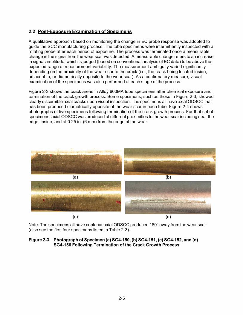
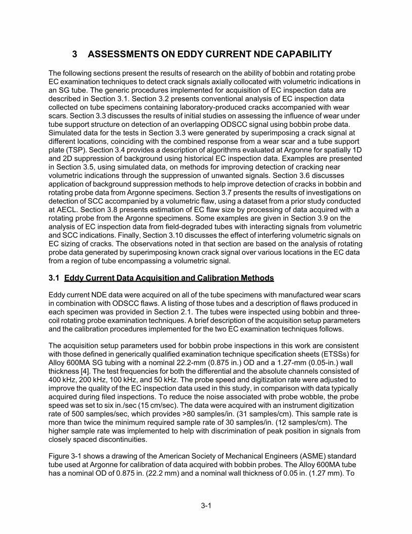
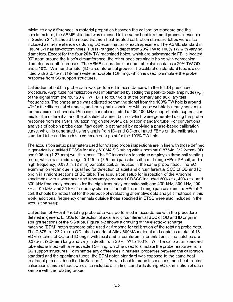
Figure 2-3 shows the crack areas in Alloy 600MA tube specimens after chemical exposure and termination of the crack growth process. Some specimens, such as those in Figure 2-3, showed clearly discernible axial cracks upon visual inspection. The specimens all have axial ODSCC that has been produced diametrically opposite of the wear scar in each tube. Figure 2-4 shows photographs of five specimens following termination of the crack growth process. For that set of specimens, axial ODSCC was produced at different proximities to the wear scar including near the edge, inside, and at 0.25 in. (6 mm) from the edge of the wear.

(a) (b)

(c)

(d)

Note: The specimens all have coplanar axial ODSCC produced 180° away from the wear scar (also see the first four specimens listed in Table 2-3). Figure 2-3 Photograph of Specimen (a) SG4-150, (b) SG4-151, (c) SG4-152, and (d)

SG4- 156 Following Termination of the Crack Growth Process.

2-6

(a) (b)

(c)

(d)

(e)

Note: Axial ODSCC was produced near the edge of the wear (a, b), inside the wear (c, d), and at 0.25 in. (6 mm) away from the wear (e) (also see the last five specimens listed in Table 2-3).

Figure 2-4 Photograph of Specimen (a) SG4-153, (b) SG4-157, (c) SG4-154, (d) SG4-

158, and (e) SG4-159 Following Termination of the Crack-Induction Process.

3-1

3 ASSESSMENTS ON EDDY CURRENT NDE CAPABILITY

The following sections present the results of research on the ability of bobbin and rotating probe EC examination techniques to detect crack signals axially collocated with volumetric indications in an SG tube. The generic procedures implemented for acquisition of EC inspection data are described in Section 3.1. Section 3.2 presents conventional analysis of EC inspection data collected on tube specimens containing laboratory-produced cracks accompanied with wear scars. Section 3.3 discusses the results of initial studies on assessing the influence of wear under tube support structure on detection of an overlapping ODSCC signal using bobbin probe data. Simulated data for the tests in Section 3.3 were generated by superimposing a crack signal at different locations, coinciding with the combined response from a wear scar and a tube support plate (TSP). Section 3.4 provides a description of algorithms evaluated at Argonne for spatially 1D and 2D suppression of background using historical EC inspection data. Examples are presented in Section 3.5, using simulated data, on methods for improving detection of cracking near volumetric indications through the suppression of unwanted signals. Section 3.6 discusses application of background suppression methods to help improve detection of cracks in bobbin and rotating probe data from Argonne specimens. Section 3.7 presents the results of investigations on detection of SCC accompanied by a volumetric flaw, using a dataset from a prior study conducted at AECL. Section 3.8 presents estimation of EC flaw size by processing of data acquired with a rotating probe from the Argonne specimens. Some examples are given in Section 3.9 on the analysis of EC inspection data from field-degraded tubes with interacting signals from volumetric and SCC indications. Finally, Section 3.10 discusses the effect of interfering volumetric signals on EC sizing of cracks. The observations noted in that section are based on the analysis of rotating probe data generated by superimposing known crack signal over various locations in the EC data from a region of tube encompassing a volumetric signal.

3.1 Eddy Current Data Acquisition and Calibration Methods

Eddy current NDE data were acquired on all of the tube specimens with manufactured wear scars in combination with ODSCC flaws. A listing of those tubes and a description of flaws produced in each specimen was provided in Section 2.1. The tubes were inspected using bobbin and three- coil rotating probe examination techniques. A brief description of the acquisition setup parameters and the calibration procedures implemented for the two EC examination techniques follows.

The acquisition setup parameters used for bobbin probe inspections in this work are consistent with those defined in generically qualified examination technique specification sheets (ETSSs) for Alloy 600MA SG tubing with a nominal 22.2-mm (0.875 in.) OD and a 1.27-mm (0.05-in.) wall thickness [4]. The test frequencies for both the differential and the absolute channels consisted of 400 kHz, 200 kHz, 100 kHz, and 50 kHz. The probe speed and digitization rate were adjusted to improve the quality of the EC inspection data used in this study, in comparison with data typically acquired during filed inspections. To reduce the noise associated with probe wobble, the probe speed was set to six in./sec (15 cm/sec). The data were acquired with an instrument digitization rate of 500 samples/sec, which provides >80 samples/in. (31 samples/cm). This sample rate is more than twice the minimum required sample rate of 30 samples/in. (12 samples/cm). The higher sample rate was implemented to help with discrimination of peak position in signals from closely spaced discontinuities.

Figure 3-1 shows a drawing of the American Society of Mechanical Engineers (ASME) standard tube used at Argonne for calibration of data acquired with bobbin probes. The Alloy 600MA tube has a nominal OD of 0.875 in. (22.2 mm) and a nominal wall thickness of 0.05 in. (1.27 mm). To

3-2

minimize any differences in material properties between the calibration standard and the specimen tube, the ASME standard was exposed to the same heat treatment process described in Section 2.1. It should be noted that non-heat-treated calibration standard tubes were also included as in-line standards during EC examination of each specimen. The ASME standard in Figure 3-1 has flat-bottom holes (FBHs) ranging in depth from 20% TW to 100% TW with varying diameters. Except for the four 20% TW machined holes, which are axisymmetric FBHs located 90° apart around the tube’s circumference, the other ones are single holes with decreasing diameter as depth increases. The ASME calibration standard tube also contains a 20% TW OD and a 10% TW inner diameter (ID) circumferential groove. The calibration standard tube is also fitted with a 0.75-in. (19-mm) wide removable TSP ring, which is used to simulate the probe response from SG support structures.

Calibration of bobbin probe data was performed in accordance with the ETSS prescribed procedure. Amplitude normalization was implemented by setting the peak-to-peak amplitude (Vpp) of the signal from the four 20% TW FBHs to four volts at the primary and auxiliary test frequencies. The phase angle was adjusted so that the signal from the 100% TW hole is around 40o for the differential channels, and the signal associated with probe wobble is nearly horizontal for the absolute channels. Process channels included a 400|100-kHz support plate suppression mix for the differential and the absolute channel, both of which were generated using the probe response from the TSP simulation ring on the ASME calibration standard tube. For conventional analysis of bobbin probe data, flaw depth is estimated by applying a phase-based calibration curve, which is generated using signals from ID- and OD-originated FBHs on the calibration standard tube and includes a common data point for the 100% TW hole.

The acquisition setup parameters used for rotating probe inspections are in line with those defined in generically qualified ETSSs for Alloy 600MA SG tubing with a nominal 0.875-in. (22.2-mm) OD and 0.05-in. (1.27-mm) wall thickness. The EC inspection technique employs a three-coil rotating probe, which has a mid-range, 0.115-in. (2.9-mm) pancake coil; a mid-range +PointTM coil; and a high-frequency, 0.080-in. (2-mm) pancake coil, all housed in the same probe head. The EC examination technique is qualified for detection of axial and circumferential SCC of OD and ID origin in straight sections of SG tube. The acquisition setup for inspection of the Argonne specimens with a wear scar and laboratory-produced ODSCC included 600-kHz, 400-kHz, and 300-kHz frequency channels for the high-frequency pancake coil; and 400-kHz, 300-kHz, 200- kHz, 100-kHz, and 35-kHz frequency channels for both the mid-range pancake and the +PointTM

coil. It should be noted that for the purpose of evaluating alternative data analysis methods in this work, additional frequency channels outside those specified in ETSS were also included in the acquisition setup.

Calibration of +PointTM rotating probe data was performed in accordance with the procedure defined in generic ETSSs for detection of axial and circumferential SCC of OD and ID origin in straight sections of the SG tube. Figure 3-2 shows a drawing of the electro-discharge machine (EDM) notch standard tube used at Argonne for calibration of the rotating probe data. The 0.875-in. (22.2-mm ) OD tube is made of Alloy 600MA material and contains a total of 18 EDM notches of OD and ID origin with axial and circumferential orientations. The notches are 0.375-in. (9.6-mm) long and vary in depth from 20% TW to 100% TW. The calibration standard tube also is fitted with a removable TSP ring, which is used to simulate the probe response from SG support structures. To minimize any differences in material properties between the calibration standard and the specimen tubes, the EDM notch standard was exposed to the same heat treatment process described in Section 2.1. As with bobbin probe inspections, non-heat-treated calibration standard tubes were also included as in-line standards during EC examination of each sample with the rotating probe.

3-3

Calibration of the data for all the rotating probe channels is performed by normalizing the signal amplitude and adjusting the phase angle of each channel in reference to the signals from the 100% TW notch and the 40% TW ID notch, respectively. The amplitude is normalized so that the peak-to-peak voltage (Vpp) associated with the 100% TW notch is approximately 20 volts. The phase angle is adjusted so that the 40% TW ID notch forms an angle of approximately 15° in the impedance plane, using the EC convention for measurement of phase.

Separate process channels are created for analysis of +PointTM data associated with circumferential indications. The probe response for those channels is adjusted such that circumferentially oriented flaws produce a signal with a positive vertical component. To allow measurement of the axial extent of signals, the data is axially scaled based on the position of known indications on the calibration standard tube. Circumferential positional information, displayed in degrees, is based on the trigger channel data, which is supplied by the rotating probe motor unit.

Estimation of crack depth is performed by applying a phase-based calibration curve to the rotating probe data, which is generated using signals from ID- and OD-originated EDM notches on the calibration standard tube. Separate calibration curves are generated for the axial and circumferentially oriented flaws for the analysis of +PointTM data. The phase-based calibration curve for the axial channel is generated from the main analysis window. The calibration curve for estimating the depth of circumferential cracks is generated using the circumferential lissajous pane from the C-scan analysis window. While all the analysis channels are independently calibrated, the flaw-sizing results reported here are all based on measurements made using +PointTM data from the 300-kHz channel. For the analysis results here, the estimates of flaw depth are based on the depth at or near the maximum amplitude of the measured signal.

Figure 3-1 Drawing of ASME Standard Tube Used for Calibration of Bobbin Probe Data.

3-4

Figure 3-2 Drawing of EDM Notch Standard Tube Used for Calibration of Rotating Probe Data.

3.2 Analyses of Eddy Current NDE Data from Laboratory Specimens

The EC inspection data collected with bobbin and rotating probes on the specimens produced for this study were initially examined using conventional data analysis procedures. A description of the intentionally produced flaws in those tube specimens was presented in Section 2. The purpose of this study was to assess the capability of EC examination techniques to detect cracks in the presence of axially collocated wear scars based on conventional manual analysis of the data. However, for these initial evaluations, EC inspections were performed without placing a TSP collar over the tube, thus ignoring the influence of support structures on the detection capability. Data collected on the tube sections with a manufactured wear scar, before and after introduction of axial ODSCC, were analyzed. The following paragraphs first discuss the results pertaining to the four specimens with laboratory-produced cracking located diametrically opposite of the wear scar in each tube, followed by discussion of the results from analysis of data for five other specimens with cracking located at different circumferential positions relative to the wear scar.

Next is a discussion of the results of analyses performed on EC inspection data collected from the tube specimens with volumetric and cracking indications. The EC examination data were acquired and analyzed using the EddynetTM (Zetec, Inc.) software. Analysis of bobbin probe data is based on the 400|100-kHz differential mix channel. This support plate suppression channel was used both to allow comparison of the data analysis results with and without the influence of support structures and for consistency with common data analysis procedures. Analysis of +PointTM

rotating probe data is based on the primary channel at a test frequency of 300 kHz. Measurement of signals in all cases is based on the peak-to-peak value of the probe response (i.e., Vpp measurement).

3.2.1 Axial ODSCC and Wear on Diametrically Opposed Sides of a Tube

Figure 3-3 through Figure 3-10 show screen shots of the data analysis window for four specimens with a wear scar, both before and after ODSCC was produced in a location diametrically opposite

3-5

of the volumetric flaw in each tube. For each specimen, the bobbin and corresponding rotating probe data are displayed in separate figures. Bobbin probe data are shown in the main analysis window, which displays the data in a strip chart and a lissajous format. The rotating probe data are also shown in the main analysis window, as well as in the C-scan display format (i.e., isometric plot). For the first specimen discussed below, the measured values of signals are delineated on the main analysis window associated with the bobbin and the rotating probe data.

Specimen SG4-150

Bobbin probe data for specimen SG4-150, a tube with a 20% TW wear scar, are shown in Figure 3-3. The measured signals associated with the flaws in that tube are displayed for the pre- and post-SCC data in Figure 3-3(a) and Figure 3-3(b), respectively. The measurement window in both cases encompasses the entire signal. Comparison of the bobbin probe response in Figure 3-3(a) with that in Figure 3-3(b) indicates a noticeable change in the peak amplitude of the signal, from 0.86 v to 1.8 v, after introduction of the ODSCC in that tube. While the bobbin probe response from the volumetric flaw and the SCC are not individually discernible, the more dominant signal associated with the SCC is clearly detectable in the presence of the 20% TW wear scar located on the opposite side of the tube.

The graphics associated with the analysis of +PointTM rotating probe data for the same specimen, before and after introduction of ODSCC, are shown in Figure 3-4(a) and (b), respectively. As expected, the probe response from the two diametrically opposite flaws are individually distinguishable, and their respective signal characteristics are indicative of a volumetric and a crack-like discontinuity. The measured signals for the two flaws in this case exhibit comparable peak amplitudes at 300 kHz. Based on a phase angle calibration curve established using the +PointTM data at 300 kHz, the depth estimates for the wear and the ODSCC are 16% TW and 55% TW, respectively. It should be noted that the estimated depth of the wear scar is based on a single measurement along its length, which may not represent its maximum depth.

Specimen SG4-151

Bobbin probe data for specimen SG4-151, a tube with a 20% TW wear scar, are shown in Figure 3-5. As in the previous case, the measured signals associated with the flaws in that tube are displayed for the pre- and post-SCC data. Comparison of the probe response in Figure 3-5(a) with that in Figure 3-5(b) indicates a significant change in the peak amplitude of the signal, from 0.83 v to 2.12 v, after introduction of the ODSCC in that tube. While the bobbin probe response from the volumetric flaw and from the SCC are not individually discernible, the more dominant signal associated with the SCC is clearly detectable in the presence of the 20% TW wear scar located on the opposite side of the tube.

The graphics associated with the analysis of +PointTM rotating probe data for the same specimen, before and after introduction of ODSCC, are shown in Figure 3-6(a) and (b), respectively. Once again, the probe response from the two diametrically opposite flaws are individually distinguishable, and their respective signal characteristics are indicative of a volumetric and a crack-like discontinuity. The phase-based depth estimate is 15% TW for the wear scar and 46% TW for the ODSCC. The analysis results based on rotating probe data shown in Figures 3-4 and 3-6 indicate that the estimated maximum depth and the signal amplitude of the ODSCCs in specimens SG4-150 and SG4-151 are comparable. On the other hand, the change in bobbin probe signal amplitude after introduction of SCC is much larger in specimen SG4-151 than in SG4-150. Based on the estimates of flaw extent from the rotating probe data, this difference can be attributed to the longer extent of the crack in specimen SG4-151.

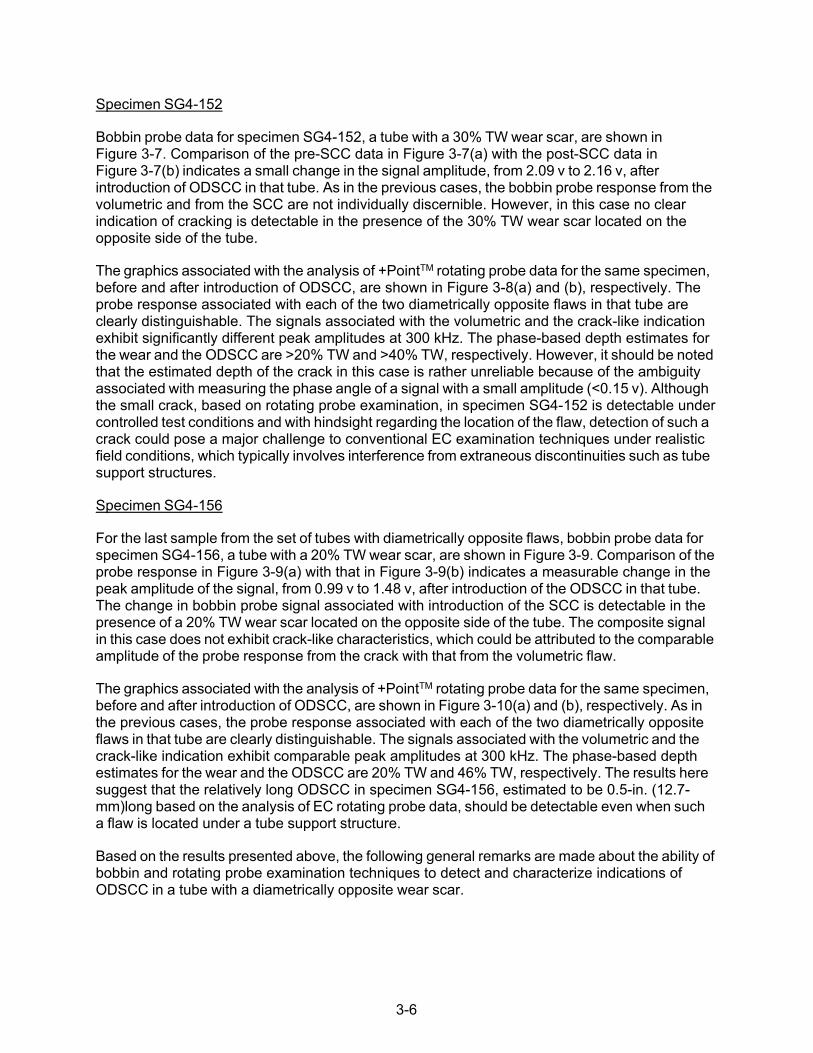
3-6

Specimen SG4-152

Bobbin probe data for specimen SG4-152, a tube with a 30% TW wear scar, are shown in Figure 3-7. Comparison of the pre-SCC data in Figure 3-7(a) with the post-SCC data in Figure 3-7(b) indicates a small change in the signal amplitude, from 2.09 v to 2.16 v, after introduction of ODSCC in that tube. As in the previous cases, the bobbin probe response from the volumetric and from the SCC are not individually discernible. However, in this case no clear indication of cracking is detectable in the presence of the 30% TW wear scar located on the opposite side of the tube.

The graphics associated with the analysis of +PointTM rotating probe data for the same specimen, before and after introduction of ODSCC, are shown in Figure 3-8(a) and (b), respectively. The probe response associated with each of the two diametrically opposite flaws in that tube are clearly distinguishable. The signals associated with the volumetric and the crack-like indication exhibit significantly different peak amplitudes at 300 kHz. The phase-based depth estimates for the wear and the ODSCC are >20% TW and >40% TW, respectively. However, it should be noted that the estimated depth of the crack in this case is rather unreliable because of the ambiguity associated with measuring the phase angle of a signal with a small amplitude (<0.15 v). Although the small crack, based on rotating probe examination, in specimen SG4-152 is detectable under controlled test conditions and with hindsight regarding the location of the flaw, detection of such a crack could pose a major challenge to conventional EC examination techniques under realistic field conditions, which typically involves interference from extraneous discontinuities such as tube support structures.

Specimen SG4-156

For the last sample from the set of tubes with diametrically opposite flaws, bobbin probe data for specimen SG4-156, a tube with a 20% TW wear scar, are shown in Figure 3-9. Comparison of the probe response in Figure 3-9(a) with that in Figure 3-9(b) indicates a measurable change in the peak amplitude of the signal, from 0.99 v to 1.48 v, after introduction of the ODSCC in that tube. The change in bobbin probe signal associated with introduction of the SCC is detectable in the presence of a 20% TW wear scar located on the opposite side of the tube. The composite signal in this case does not exhibit crack-like characteristics, which could be attributed to the comparable amplitude of the probe response from the crack with that from the volumetric flaw.

The graphics associated with the analysis of +PointTM rotating probe data for the same specimen, before and after introduction of ODSCC, are shown in Figure 3-10(a) and (b), respectively. As in the previous cases, the probe response associated with each of the two diametrically opposite flaws in that tube are clearly distinguishable. The signals associated with the volumetric and the crack-like indication exhibit comparable peak amplitudes at 300 kHz. The phase-based depth estimates for the wear and the ODSCC are 20% TW and 46% TW, respectively. The results here suggest that the relatively long ODSCC in specimen SG4-156, estimated to be 0.5-in. (12.7- mm)long based on the analysis of EC rotating probe data, should be detectable even when such a flaw is located under a tube support structure.

Based on the results presented above, the following general remarks are made about the ability of bobbin and rotating probe examination techniques to detect and characterize indications of ODSCC in a tube with a diametrically opposite wear scar.

3-7

• For the subset of specimens examined here, consequential axial cracks are detectable with the bobbin probe in the presence of a 0.75-in. (19-mm)-long, 20% TW wear scar at the same axial location in a tube.

• The crack-like characteristics of the composite bobbin probe signal diminish when the

response from ODSCC and the wear scar exhibit comparable signal strengths. In one case presented above, detection of a small crack in the presence of a 30% TW wear scar was determined to be highly unreliable.

• On the other hand, rotating probe examination results indicate that the ODSCC signals in

all of the specimens were detectable, independent of the relative strengths of signals associated with the crack and the wear scar in each tube.

In general, the analysis results indicate that the signal associated with a consequential crack diametrically opposite of a volumetric flaw, a condition in which the two signals do not interact, has a high probability of being detected and accurately characterized with a rotating +PointTM probe.

3-8

(a)

(b)

Note: Shown here are data collected with bobbin probe (a) before and (b) after introduction of SCC. The measured values for each signal are delineated on the data analysis screen. Figure 3-3 Bobbin Probe EC Inspection Data for SG4-150, a Tube Specimen with a

20% TW Wear Scar and with Axial ODSCC at 180° Away.

3-9

(a)

(b)

Note: Shown here are data collected with +PointTM rotating probe (a) before and (b) after introduction of SCC. The measured values for each signal are delineated on the data analysis screen. Figure 3-4 Rotating Probe EC Inspection Data for SG4-150, a Tube Specimen with a


3-10

(a)

(b)

Note: Shown here are data collected with bobbin probe (a) before and (b) after introduction of SCC.

Figure 3-5 Bobbin Probe EC Inspection Data for SG4-151, a Tube Specimen with a


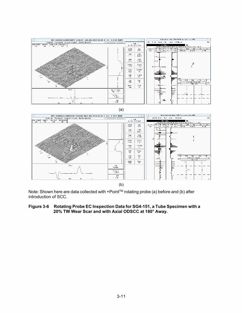
3-11

(a)

(b)

Note: Shown here are data collected with +PointTM rotating probe (a) before and (b) after introduction of SCC.

Figure 3-6 Rotating Probe EC Inspection Data for SG4-151, a Tube Specimen with a


3-12

(a)

(b)




3-13

(a)

(b)




3-14

(a)

(b)




3-15

(a)

(b)




3-16

3.2.2 Axial ODSCC Adjacent to or Collocated with Wear Scar

EC data analysis results are presented next for five specimens with axial ODSCC produced either adjacent to or inside the wear scar in those tubes. As with the previous set of specimens, the cracks are at the same axial location along the tube as the volumetric flaw. In reference to Table 2-3, the intended location of laboratory-produced cracking is either outside the wear scar but in close proximity to its edge or is inside the wear scar (i.e., SCC was produced at the bottom of wear scar). The methods used for analysis of EC inspection data are in line with those used for the first set of tubes discussed in Section 3.2.1.

Specimen SG4-159

Bobbin probe data for specimen SG4-159, a tube with a 20% TW wear scar, are shown in Figure 3-11. An OD-initiated axial crack was produced at approximately 0.25 in. (~6 mm) away from the edge of the wear scar in that specimen. The measured signals associated with the flaws in the pre- and post-SCC data are displayed in Figure 3-11(a) and Figure 3-11(b), respectively. The measurement window in both cases encompasses the entire flaw signal. Comparison of the bobbin probe response in Figure 3-11(a) with that in Figure 3-11(b) indicates that while there is a measurable change in the phase angle of the signal, there is no discernible change in the peak amplitude of the signal, 1.59 v to 1.56 v, after introduction of the ODSCC in that tube. The negligible difference between the two Vpp values is well within the measurement variability of the EC inspection technique. Based on the results from conventional analysis of bobbin probe data, we may then conclude that the detection probability for the crack in specimen SG4-159 is low.

The graphics associated with the analysis of +PointTM rotating probe data for the same specimen before and after introduction of the ODSCC are shown in Figure 3-12(a) and (b), respectively. The presence of the small cracking indication near the much larger signal from a 20% TW wear scar is detectable in the rotating probe data. Furthermore, the signals associated with the two flaw types are individually distinguishable, and their respective characteristic responses are consistent with those from a volumetric and a crack-like discontinuity. Based on a phase angle calibration curve established using the +PointTM data at 300 kHz, the depth estimates for the wear scar and the ODSCC are 19% TW and 73% TW, respectively. It should, however, be noted that the estimated depth of the crack in this case may not be reliable because of the uncertainties associated with measuring the phase angle of signals with small amplitude. The analysis results here indicate that, in the absence of interference from extraneous sources, the spatial resolution of the +PointTM

probe at a test frequency of 300 kHz allows discrimination of crack-like indications that are separated 0.25 in. (6 mm) or more from a wear scar. While the crack in this case may be detectable, the measurement reliability would decrease at a closer proximity to the 20% TW wear as a result of stronger signal interaction with the nearby volumetric flaw.

Specimen SG4-153

Bobbin probe data for specimen SG4-153, a tube with a 30% TW wear scar, are shown in Figure 3-13. An OD-initiated axial crack with a nominal length of ~0.5 in. (12.7 mm)was produced near the edge of the wear scar in that specimen. The measured signals associated with the flaws in the pre- and post-SCC data are displayed in Figure 3-13(a) and Figure 3-13(b), respectively. The measurement window in both cases encompasses the entire flaw signal. Comparison of the bobbin probe response in Figure 3-13(a) with that in Figure 3-13(b) clearly indicates a large change in both the peak amplitude and phase angle of the signal after introduction of the ODSCC in that tube. The presence of a crack-like, OD-initiated indication is detectable from the composite signal displayed in Figure 3-13(b). Also evident from the composite probe response is the

3-17

distortion of signal from both the crack and the volumetric indication caused by the interaction of signals from two closely spaced flaws. In reference to Figures 3-13(a) and (b), the measured signal amplitude for the wear and for the SCC are 2.77 v and 3.59 v, respectively. In this case, the measured bobbin probe signal amplitude is based on the component associated with the crack rather than the entire signal. The measurement was performed in this manner because the more dominant component of the signal associated with cracking can be readily identified within the composite probe response. Based on conventional analysis of bobbin probe data, the crack in specimen SG4-153 can be detected with high probability. This conclusion can be attributed to the relatively large signal from the crack in comparison to that from the adjacent volumetric flaw.

The graphics associated with the analysis of +PointTM rotating probe data for the same specimen, before and after introduction of ODSCC, are shown in Figure 3-14 (a) and (b), respectively. Although the change in signal is clearly evident after introduction of the SCC near the wear scar, the probe response from the crack exhibits the characteristics of a volumetric flaw. Furthermore, in reference to Figure 3-8(d), the signals associated with the two flaw types are not individually distinguishable. Based on a phase angle calibration curve established using the +PointTM data at 300 kHz, the estimated maximum depth along the wear scar before and after introduction of the ODSCC is 31% TW and 64% TW, respectively. It should be noted that the estimated depth of the crack in this case may not be reliable because of the strong influence from the nearby wear scar. The rotating probe data analysis results for specimen SG4-153 suggest that while the ODSCC in that tube can be detected with a high degree of probability, the spatial resolution of the probe does not allow clear discrimination of the two closely spaced flaws in that tube.

Specimen SG4-157

Bobbin probe data for specimen SG4-157, a tube with a 20% TW wear scar, are shown in Figure 3-15. A relatively short OD-initiated axial crack was produced immediately next to the wear scar in that specimen. The measured signals associated with the flaws in the pre- and post-SCC data are displayed in Figure 3-15(a) and Figure 3-15(b), respectively. The measurement window in both cases encompasses the entire flaw signal. Comparison of the bobbin probe response in Figure 3-15(a) with that in Figure 3-15(b) indicates a small but measurable change in the peak amplitude, from ~0.9 v to 1.15 v, and the phase angle of the signal. The signals from the wear scar and from the SCC are not individually discernible, which is indicative of the smaller amplitude of the crack compared to that of the wear. Based on the results from conventional analysis of data, the detection probability for the cracking indication near the 20% TW wear scar in specimen SG4-157 is relatively low under field conditions with just bobbin probe examination. However, with regard to inspection of SG tubing, the small change in bobbin probe signal between the pre- and post-SCC data is likely to result in implementation of supplementary examinations with EC rotating probes.

The graphics associated with the analysis of +PointTM rotating probe data for the same specimen, before and after introduction of ODSCC, are shown in Figure 3-16(a) and (b), respectively. Although the change in phase angle of the signal in Figure 3-16(b) is discernible after introduction of the SCC, the probe response from the crack exhibits characteristics indicative of a volumetric flaw. In addition, the signals associated with the two flaw types are not individually distinguishable. Based on a phase-angle calibration curve established using the +PointTM data at 300 kHz, the estimated maximum depth along the wear before and after introduction of the ODSCC is 20% TW and 41% TW, respectively. The rotating probe data analysis results for specimen SG4-157 suggest that the ODSCC signal in that tube cannot be reliably detected and characterized as such because of the strong influence of the probe response from the adjacent volumetric flaw.

3-18

Specimen SG4-154

Bobbin probe data for specimen SG4-154, a tube with a 30% TW wear scar, are shown in Figure 3-17. An OD-initiated axial crack was produced inside the wear scar in that tube. The measured signals associated with the flaws in the pre- and post-SCC data are displayed in Figure 3-17(a) and Figure 3-17(b), respectively. The measurement window in those figures encompasses the entire flaw signal. Comparison of the bobbin probe response in Figure 3-17(a) with that in Figure 3-17(b) indicates a change in the peak amplitude, from 2.37 v to 2.41 v, that is within normal measurement variability of the inspection technique. However, the presence of a flaw-like indication is discernible in the composite probe response displayed in Figure 3-17(b). Based on the results from conventional analysis of bobbin probe data, we can state that the cracking indication inside the 30% TW wear scar in specimen SG4-154 is detectable. The SCC signal, however, is distorted as a result of interference from the collocated volumetric signal.

The graphics associated with the analysis of +PointTM rotating probe data for the same specimen, before and after introduction of ODSCC, are shown in Figure 3-18(a) and (b), respectively. Although there is a noticeable change in the phase angle of the signal after introduction of SCC inside the wear scar in that tube, the probe response from the crack exhibits similar characteristics to a volumetric flaw. Based on a phase-angle calibration curve established using the +PointTM

data at 300 kHz, the estimated maximum depth along the wear scar before and after introduction of the ODSCC is 29% TW and 43% TW, respectively. As in the previous case with specimen SG4-157, the rotating probe data analysis results for specimen SG4-154 suggest that the ODSCC signal in that tube cannot be reliably characterized as such because of the strong influence of the probe response from the adjacent volumetric flaw.

Specimen SG4-158

Bobbin probe data for specimen SG4-158, a tube with a 20% TW wear scar, are shown in Figure 3-19. A relatively short OD-initiated axial crack was produced inside the wear scar in that specimen. The measured signals associated with the flaws in the pre- and post-SCC data are displayed in Figure 3-19(a) and Figure 3-19(b), respectively. As in the previous cases, the measurement window encompasses the entire flaw signal. Comparison of the probe response in Figure 3-19(a) with that in Figure 3-19(b) indicates a measurable change in the peak amplitude of the signal, from 0.72 v to 1.2 v, after introduction of the ODSCC in that tube. The change in bobbin probe signal associated with SCC is detectable in the presence of a 20% TW wear scar at the same location in that tube. The composite signal in this case does not exhibit crack-like characteristics, which could be attributed to the comparable amplitude of the probe response from the crack with that from the volumetric flaw.

The graphics associated with the analysis of +PointTM rotating probe data for the same specimen, before and after introduction of ODSCC, are shown in Figure 3-20(a) and (b), respectively. Although there is a noticeable change in the phase angle of the signal after introduction of SCC inside the wear scar in that tube, the probe response from the crack exhibits similar characteristics to a volumetric flaw. Based on a phase-angle calibration curve established using the +PointTM

data at 300 kHz, the estimated maximum depth along the wear scar before and after introduction of the ODSCC is 10% TW and 37% TW, respectively. The rotating probe data analysis results for specimen SG4-158 suggest that the ODSCC signal in that tube cannot be reliably detected and characterized as such because of the strong influence of the probe response from the adjacent volumetric flaw.

3-19

Based on the results of the analyses presented above, the following general remarks can be made about the ability of bobbin and rotating probe inspection techniques to detect and characterize ODSCC that may occur inside or adjacent to a wear scar in a tube.

• The signals associated with larger cracks are detectable with the bobbin probe, regardless

of the circumferential position of the crack relative to the wear scar. However, detection of smaller cracks, based on the observed change in the wear scar signal after the introduction of cracking, is rather unreliable.

• In all cases, the crack-like characteristics of the composite signal diminish significantly

when the bobbin probe response is dominated by the signal component associated with the wear scar, similar to the conclusion based on analysis of data presented in Section 3.2.1.

• Analyses of EC inspection data collected with the +PointTM rotating probe show that, while

the changes in the wear scar signal caused by introduction of cracking are generally detectable, characterizing those signals as indications of cracking with a reasonable degree of confidence is not always possible. This result occurs because the +PointTM

probe response from a crack in close proximity to a wear scar exhibits a volumetric-like signal.

• The detection probability using a rotating probe examination technique could diminish

notably when the crack is located at the edge of a wear scar.

• The capability of the EC examination technique using the +PointTM rotating probe to detect and characterize an ODSCC indication in the presence of an axially collocated wear scar is highly dependent on the relative position of the two flaw types.

• An important observation based on comparison of the EC data analysis results between

the two sets of specimens used in this study is that, unlike the rotating probe, the bobbin probe response is less dependent on the relative position of the crack and the volumetric flaw around the tube circumference. Therefore, questionable indications of cracking detected by bobbin probe examination cannot be readily dismissed based on the lack of a confirmatory crack-like signal in rotating probe data.

As previously noted, the analysis results presented in this section are based on EC data collected on tube specimens with no extraneous discontinuities. The majority of wear scars in SG tubes, however, occur under tube support structures. While software-based tools such as multi- parameter mixes are available to help suppress the effect of support structures, the presence of external discontinuities nevertheless can further influence the ability of EC inspection techniques to detect and characterize flaws at those SG elevations. Imperfect suppression of probe response from support structures is one such factor that can degrade the signal-to-noise ratio (S/N) and in turn degrade the detection probability. Such factors as high level of mix residuals have a larger influence on detection of crack signals with small amplitude. The effect of tube support structures on detection of cracks that occur in conjunction with wear scars using bobbin probe inspection is discussed in Section 3.3 of this report.

The initial studies on the ability of conventional EC inspection techniques and data analysis methods to detect and characterize indications of cracking near volumetric flaws pointed out the potential challenges involved in dealing with this complex mode of degradation, even under ideal test conditions. Improving the detection probability for cracks in such cases may be achieved only

3-20

by suppressing the probe response from the more dominant volumetric flaw. To this end, a series of studies were carried out to assess the viability of various signal processing schemes for this particular application. The results of those studies using different EC examination datasets are presented in the following sections.

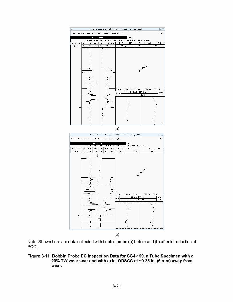
3-21

(a)

(b)



20% TW wear scar and with axial ODSCC at ~0.25 in. (6 mm) away from wear.

3-22

(a)

(b)

Note: Shown here are data collected with the +PointTM rotating probe (a) before and (b) after introduction of SCC.

Figure 3-12 Rotating Probe EC Inspection Data for SG4-159, a Tube Specimen with

a 20% TW Wear Scar and with Axial ODSCC at 0.25 in. (6 mm) Away from Wear.

3-23

(a)

(b)



30% TW Wear Scar and with Axial ODSCC Near the Edge of Wear Scar.

3-24

(a)

(b)



30% TW Wear Scar and with Axial ODSCC Near the Edge of Wear Scar.

3-25

(a)

(b)



20% TW Wear Scar and with a Relatively Short Axial ODSCC Near Its Edge.

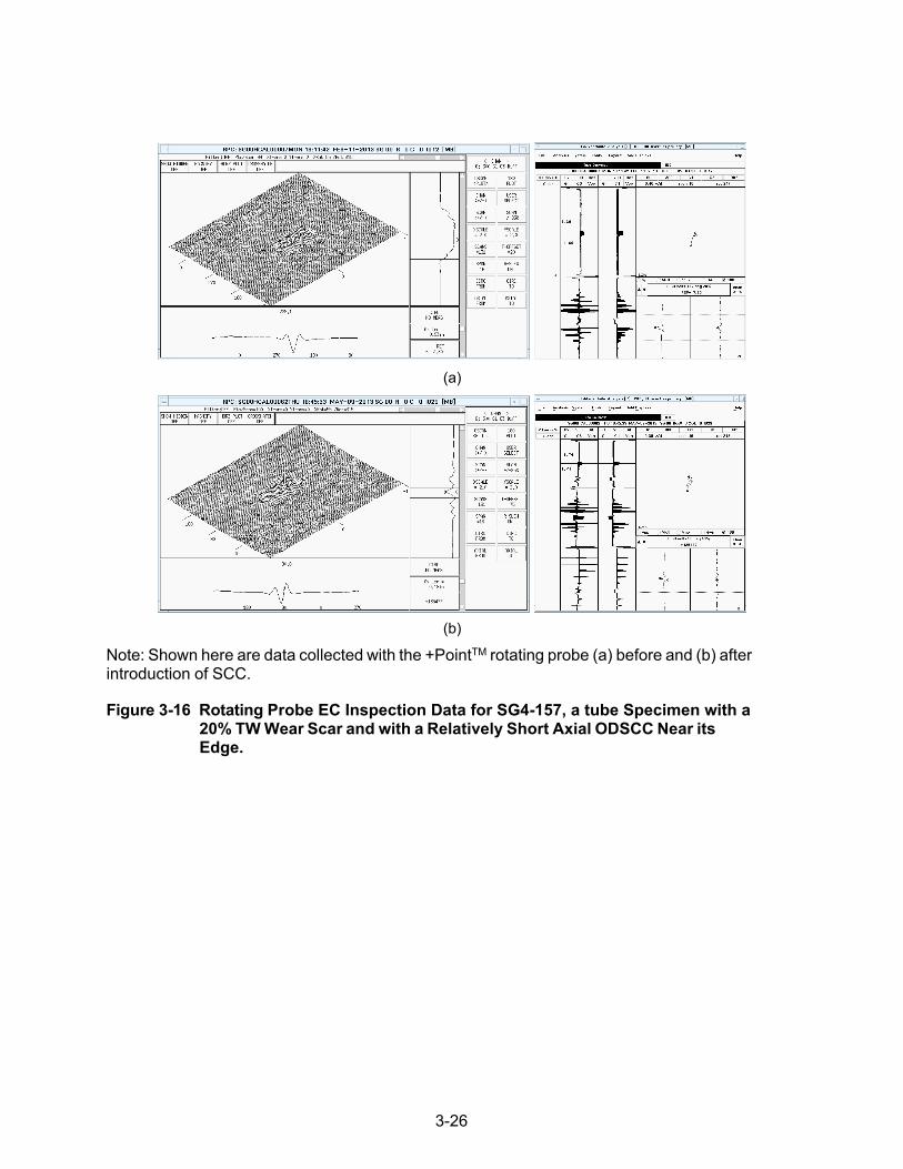
3-26

(a)

(b)


Figure 3-16 Rotating Probe EC Inspection Data for SG4-157, a tube Specimen with a

20% TW Wear Scar and with a Relatively Short Axial ODSCC Near its Edge.

3-27

(a)

(b)



30% TW Wear Scar and with Axial ODSCC Inside the Wear Scar.

3-28

(a)

(b)



30% TW Wear Scar and with Axial ODSCC Inside the Wear Scar.

3-29

(a)

(b)

Note: Shown here are data collected with bobbin probe (a) before and (a) after introduction of SCC.

Figure 3-19 Bobbin Probe EC Inspection Data for SG4-158, a Tube Specimen with a 20% TW Wear Scar and with Axial ODSCC at the Same Location.

3-30

(a)

(b)


Figure 3-20 Rotating Probe EC Inspection Data for SG4-158, a Tube Specimen with a 20% TW Wear Scar and with Axial ODSCC at the Same Location.

3-31

3.3 Influence of Wear and Support Structure on SCC Signal

A series of simulations were performed to help in better assessing the effect of interference from volumetric flaws and tube supports on detection of cracks located at the same axial position along the tube. The EC bobbin probe data used in these studies were generated by combining signals from flaws (crack and wear) and tube support plates using the data analysis tool implemented at Argonne. Systematic simulations were generated by moving the crack signal over the region of interest (ROI) along the tube. The test cases discussed here, however, pertain only to three specific positions of the crack with respect to the background signal consisting of bobbin probe response from a wear scar plus a TSP. It should be noted that a composite signal generated by superimposing individual signals from a wear scar and an OD-initiated crack may not truly represent the actual probe response from a volumetric wall loss collocated with cracking. Nevertheless, any differences between the simulated and the actual data are not expected to have a major impact on the general observations made based on the results of this study.

To minimize the effect of measurement variability, data from a laboratory-produced ODSCC with a relatively large signal amplitude was selected for this study. The peak-to-peak (Vpp) value of the SCC signal in the presence of wear and a TSP was measured using two different approaches. One was based on a fixed window encompassing the crack signal, and the other was based on a known position of the crack signal, which is expected to more closely emulate the measurement of a crack-like indication through manual analysis of the data. For the latter approach, measurement of the differential signals was made using only the part of the signal that was less corrupted by background interference. The amplitude and phase of the crack signal, as a function of position relative to the interfering signal (i.e., TSP, wear, or both) were calculated along the tube axis with the SCC placed in the center of the data segment. For the cases presented here, the relative positions of EC signals along the tube axis are displayed as data points.

3.3.1 Background Interference without Use of a TSP Suppression Mix

Figure 3-21 to Figure 3-23 show a series of simulations that illustrate the effect of background interference for the test cases examined in this study. The bobbin probe data are shown for three cases composed of a lab-grown ODSCC located at different positions relative to a 19-mm (0.75-in.)-long, 30% TW flat wear scar under a 19-mm (0.75-in.)-wide TSP collar. For this initial study, a TSP suppression mix, which is commonly used for analysis of field data, was not applied to the data.

Figure 3-21 shows a case where the background signal, generated by combining signals from a wear scar and a TSP, does not interfere with the SCC signal. Figure 3-21(a) depicts the approximate position of the three features (i.e., TSP, wear, and SCC) on the tube. Figure 3-21(b) displays snapshots of the data segment at a test frequency of 400 kHz for each individual feature on the tube, as well as the composite signal. As there is no overlap between the SCC and the background, the crack signal is clearly detectable in this case. In reference to the bottom trace in Figure 3-21(b), the lack of a gap between the SCC signal and the composite signal from the wear scar and the TSP is attributed to the field spread of the EC probe.

The composite signal for a case where the SCC is located at the edge of the overlapping background is shown in Figure 3-22. The approximate position of features along the tube axis is depicted in Figure 3-22(a). The snapshot of the composite data segment is shown in Figure 3-22(b). As a consequence of interference from the dominant background, the SCC signal in this case is significantly corrupted and thus cannot be reliably detected.

3-32

Another case in which the SCC is located in the center of the background signal is shown in Figure 3-23. Once again, Figure 3-23(a) depicts the approximate position of the features along the tube section. The snapshot of the composite trace is shown in Figure 3-23(b). While the SCC signal in this case is also affected by the background interference, the signal can nevertheless be detected. With the crack in this case being located in the center of the TSP, there is less interaction between the crack signal and the large probe response from the edges of the combined signal from the wear scar and the TSP.

3.3.2 Background Interference with Use of a TSP Suppression Mix

Measurements of an SCC signal in the presence of background interference for the same test cases discussed above are shown in Figure 3-24 to Figure 3-26. The bobbin probe data analysis channel in this case is the 400|100-kHz differential mix, which is used to suppress the TSP influence. The measurement points were selected based on the known position of the crack signal, which was placed, in all cases, in the middle of the data segment. This measurement method was implemented to somewhat emulate the approach employed by a human analyst in selecting the signal of interest at TSP elevations.

Figure 3-24 displays the vertical and the horizontal component of the data segment and the lissajous plot of the same data. Also shown are the measured amplitude and phase of the SCC signal and a snapshot of the calculated standard deviation as a function of position covering roughly half the length of data. It should be noted that the best measurement method here is the one with the smallest variation of amplitude, phase, and standard deviation over the selected data segment. These criteria were used in this study to assess the influence of background on detection capability. The SCC signal in this case, which was depicted in Figure 3-21(a), is essentially unaffected by the background interference, as the signals do not overlap.

Figure 3-25 and Figure 3-26 show the results for the cases depicted in Figure 3-22(a) and Figure 3-23(a), respectively. The measured SCC signal in Figure 3-25 shows perturbation of the phase angle as a result of interference from the wear scar signal. The measurement results shown in Figure 3-26 indicate that, while the phase angle of the signal in this case is less affected by the presence of wear, the amplitude of the signal is more strongly affected with a much lower S/N than those shown in Figure 3-24 and Figure 3-25.

In summary, the results of this limited study confirm that, without the use of processed data from the TSP suppression mix channel, detection of an SCC signal in conjunction with a wear scar under a support structure poses a major challenge to bobbin probe examination techniques. Without proper suppression of the background signal, detection of a shallow wear scar alone that spans the entire length of TSP can be unreliable. The results also indicate that the ability to detect and characterize the SCC signal, with or without use of a TSP suppression mix, is highly dependent on its position relative to the background signal. For the cases discussed above, the largest distortion of the crack signal phase angle occurs near the edge of the wear scar, where the probe response from the abrupt wall thickness transition is at a maximum. The largest overall distortion of the crack signal, both in amplitude and phase, occurs when the crack is collocated with the wear scar under the support plate. Although not investigated here, the level of residual signals in the mix channel data is another factor that can influence the ability to detect flaws at support structures.

It is important to note that in this study, which was focused on assessing the degree of signal distortion due to background interference, the measurements were performed with prior

3-33

knowledge about the location of the cracking. As such, the results are not truly indicative of the ability of the bobbin probe inspection techniques to detect cracks under realistic test conditions.

Finally, the results point to the importance of effective methods for suppressing the influence of background interference to increase the detection probability of cracks. To this end, various background suppression techniques are discussed in the following sections.

3-34

(a)

Note: Shown here are (a) depiction of the approximate position of the three features on the tube; and (b) individual signals from SCC, wear, and TSP, as well as the composite probe response (Sum). The SCC signal in this case is not affected by the presence of wear and TSP.

Figure 3-21 Simulated Differential Bobbin Probe Response at 400 kHz Composed of

Signals from a TSP, a 30% TW Wear Mark, and a Lab-Grown ODSCC Outside the TSP.

Wear

SCC

TSP

50 100 150 200

-2-1012

Position

V-c

omp.

50 100 150 200

-2-1012

PositionH

-com

p.-2 0 2

-2-1012

H-comp.

V-c

omp.

50 100 150 200

-2-1012

Position

V-c

omp.

50 100 150 200

-2-1012

Position

H-c

omp.

-2 0 2

-2-1012

H-comp.

V-c

omp.

50 100 150 200

-2-1012

Position

V-c

omp.

50 100 150 200

-2-1012

Position

H-c

omp.

-2 0 2

-2-1012

H-comp.V

-com

p.

50 100 150 200

-2-1012

Position

V-c

omp.

50 100 150 200

-2-1012

Position

H-c

omp.

-2 0 2

-2-1012

H-comp.

V-c

omp.

SCC

Wear

TSP

Sum

3-35

(a)

(b)

Note: Shown here are (a) depiction of the approximate position of the three features on the tube, and (b) the composite probe response over the measurement segment. The SCC signal in this case is distorted by the presence of overlapping wear and TSP.

Figure 3-22 Simulated Differential Bobbin Probe Response at 400 kHz composed of Signals from a TSP, a 30% TW wear mark, and a lab-grown ODSCC at the TSP Edge.

(a)

(b)

Note: Shown here are (a) depiction of the approximate position of the three features on the tube, and (b) the composite probe response over the data segment. The SCC signal in this case is partially distorted by the presence of collocated wear and TSP.

Figure 3-23 Simulated Differential Bobbin Probe Response at 400 kHz Composed of Signals from a TSP, a 30% TW Wear Mark, and a Lab-Grown ODSCC Below the TSP.

50 100 150 200

-2

0

2

Position

V-c

omp.

50 100 150 200

-2

0

2

PositionH

-com

p.-2 0 2

-2

0

2

H-comp.

V-c

omp.

50 100 150 200

-2

0

2

Position

V-c

omp.

50 100 150 200

-2

0

2

Position

H-c

omp.

-2 0 2

-2

0

2

H-comp.

V-c

omp.

3-36

Note: The bobbin probe data are from the 400|100-kHz differential mix channel with the measurement points selected based on known position of the SCC signal in the middle of the data segment. Shown here are (left) the vertical and horizontal components of the data segment and (right) the lissajous plot of the same data.

Figure 3-24 A Snapshot of Measured SCC Signal from the Composite Signal Shown in

Figure 3-21 with the Position of Features Depicted in Figure 3-21(a).

Note: The bobbin probe data are from the 400|100-kHz differential mix channel with the measurement points selected based on known position of the SCC signal in the middle of the data segment. Shown here are (left) vertical and horizontal components of the data segment and (right) the lissajous plot of the same data.



50 100 150 200-1

-0.5

0

0.5

1V

-Com

p.

50 100 150 200

-0.4

-0.2

0

0.2

0.4

0.6

0.8

H-C

omp.

50 100 150 200-1

-0.5

0

0.5

1

1.5

V-C

omp.

50 100 150 200

-0.5

0

0.5

1

H-C

omp.

3-37

Note: The bobbin probe data are from the 400|100-kHz differential mix channel with the measurement points selected based on known position of the SCC signal in the middle of the data segment. Shown here are (left) vertical and horizontal components of the data segment and (right) the lissajous plot of the same data.



3-38

3.4 Historical Data Subtraction Methods for Suppression of Background Signals

Detection of ODSCC that may occur in conjunction with volumetric damage or degradation poses a challenge to all EC examination techniques used for ISI of SG tubing. Indications of cracking with relatively low signal amplitude located at the same elevation as a volumetric flaw can remain undetected by bobbin as well as rotating probe examination. Consequently, questionable flaw-like signals in close proximity to existing volumetric indications flagged by bobbin probe inspection may not always be resolved using supplementary inspection with a rotating probe.

One difference between the growth of cracks and volumetric flaws such as wear scars in SG tubes is that crack growth has a more variable rate and thus can change more rapidly over time than wear. In light of this difference, the viability of monitoring the change in EC signals over time was evaluated as a method for detecting SCC. Comparison of current EC inspection data with the available historical data is routinely performed as part of the ISI process. The aim is to detect any atypical change in signals near existing volumetric indications that have occurred since the previous inspection. Performing such comparisons through manual analysis of data, however, can be challenging if cracking initiates in close proximity to a volumetric flaw. As shown in Section 3.2, the signal from an OD-initiated crack can be obscured or significantly distorted by the more dominant signal from an interfering wear scar or MBM.

Removal of stationary background signals is used in many applications to help with detection of more subtle signals of potential interest. The viability of background suppression algorithms was investigated in application to EC inspection of SG tubes for detecting cracks collocated with volumetric indications, as well as other stationary sources of interference. In essence, such algorithms subtract the historical NDE data from the current data to identify changes in signals that may not otherwise be readily discernible. In its simplest form, the difference signal can be expressed as

∆Si = ci − hi (1)

where hi is the historical data with a preexisting volumetric indication; ci is the current data, which contains volumetric and SCC signals; and ∆S is the change in signal, conceivably attributable to initiation of SCC. Representative data were provided in Section 3.2 that exhibit such changes in EC probe response from a volumetric flaw after introduction of cracking at the same axial location along the tube.

Various implementations of background suppression schemes were evaluated in this work. Those implementations included 1D and 2D subtractions in the spatial and the frequency domains. Alignment and resampling methods in both the Fourier domain, based on spectral matching, and in the spatial domain, based on signal extrema, were evaluated. What follows is an overview of the background suppression schemes examined in this work.

In order to perform background subtraction, the historical data and the current data must be accurately aligned and have the same sample rate. The first technique evaluated in this study for 1D subtraction of data was to independently resample each data segment so as to have the same spatial scaling. The scaling variables for each dataset were calculated based on known spacing between machined flaws in a calibration standard tube. While under ideal test conditions this approach can provide the desired results, it became immediately apparent that it would not be a robust approach in practical applications where possible variations in translational and/or rotational speed of the EC probe in the ROI could render alignment of data imprecise.

3-39

The second technique evaluated for 1D subtraction of data was an extrema-based detection and resampling method. In this approach, the locations of maxima (and/or minima when dealing with differential signals) are obtained in both data segments, and the historical data is resampled to match the current data. The technique is based on the assumption that the dominant features in the data do not change appreciably over time. The assumption, however, can be invalidated when the features used for aligning different data segments vary over time. This outcome could occur as a result of interaction between the historical features and new features such as initiation of an SCC on the edge of a wear scar.

It is worth noting that resampling of 1D data based on prominent stationary features could serve as a viable approach to historical subtraction of field data. For this approach, SG landmarks can be used as markers for aligning data collected during different outages. A landmark table that provides the location of tube support structures and geometry transitions for a particular SG design can be used for that purpose. This approach, however, was not fully pursued here as it was deemed to be outside the scope of this study. It should also be noted that this technique is susceptible to the problems mentioned above, namely, varying probe speed in the ROI and potential distortion of landmark features due to such factors as displacement of or interference from extraneous sources that could lead to inaccurate alignment of data in the ROI.

The third technique investigated for 1D background suppression used a frequency-based resampling method. The concept behind this approach is that in the frequency domain, the bulk frequency components of a background feature should still be present even if that feature has interaction with another signal, such as a crack. The crack-like signal is, in effect, a secondary waveform superimposed on the primary background waveform, creating its own spectral components in the frequency domain. In addition, because the frequency domain has a fixed origin (0 Hz), only a single parameter, the frequency scaling, is used to optimize the alignment of signals, rather than two parameters as in the spatial domain (i.e., spatial alignment and spatial scaling). The first step is to convert the data, x, from the spatial domain to the frequency domain, X, using fast Fourier transformation (FFT), which can be expressed as

( ) ( ) ( ) ( )( )1 1 2 /

1

; N

j k i NN N

j

yieldsFFT x X k x j e πω ω− − −

=

→ = =∑ (2)

By using C = abs(FFT(c)) and H = abs(FFT(h)) to represent the current and the historical frequency power spectra, respectively, we can then optimize the frequency scaling of the two data segments to match. In this study, we used the Levenberg–Marquardt optimization, which is an iterative algorithm that minimizes the error function, S, as

( )( ) 2

1,

n

i iiC f H

Sn

ββ =

− = ∑ (3)

in which f (H , β ) = γ ⋅ NNI (H , β )

(4)

3-40

where NNI is the nearest-neighbor interpolation of H given a frequency scaling factor, β, determined by the algorithm, and with γ being an amplitude scaling factor that is adjusted to match the two frequency spectra. The final output of the function is a scaling factor, which is used to resample the data in the spatial domain by using an appropriate data resampling algorithm.

For spatially 1D data, suppression of unwanted signals (i.e., background) can be implemented either in the spatial domain or in the frequency domain. In the spatial domain, the process requires an additional step to align the current and historical data before subtraction. Precise alignment of signals is unnecessary if subtraction is performed in the frequency domain. To subtract 1D data in the frequency domain, both the phase and the amplitude of the Fourier- transformed signal are used for processing of the complex impedance associated with EC inspection data. To suppress the background, the amplitude spectrum of the historical data is subtracted from that of the current data, keeping only the positive values. In effect, this operation suppresses the amplitude of all waveforms in the current data that are also present in the historical data, with the goal of leaving only the non-stationary signals once data are transformed back to the spatial domain. The results of investigations here indicate that this technique is particularly useful in situations where alignment of signals is problematic in the spatial domain. The drawbacks of this technique, on the other hand, include its sensitivity to the level of noise present in the data and the potential for loss of phase information.

For example, frequency-based background suppression did not perform well when the background noise was on the same scale as the flaw signals to be detected. This result can occur in cases where the flaw signal and the background noise have shared frequency components of comparable amplitude. In addition, the resulting phase information, particularly for low-amplitude EC signals, were in some cases unreliable, which was attributed to loss of information as a result of transformation between different domains. Based on these observations, the conclusion was that the frequency domain subtraction is better suited for detection of signals when aligning of the historical and current data in the spatial domain cannot be attained with sufficient accuracy.

As noted above, to suppress background interference in the spatial domain, the signals must be aligned so the measurement points correspond between the current and the historical EC data. One simple method is to align the data based on the position of common prominent peaks in both traces. However, as with the extrema-based resampling, this approach assumes that the dominant signals are solely from stationary sources (e.g., the wear scar). The interaction of other signals, such as those associated with cracking, with the edge of the stationary signal used for alignment could shift the location of maximum value to coincide with the combined peak position (e.g., wear plus SCC), resulting in misalignment and in turn imperfect subtraction of signals. In consideration of such issues, another option investigated in this work was to use correlation-based alignment of signals. The correlation coefficients are given by

( ) ( )( ) ( )

( ) [ ]( ) [ ]( )1 2 1 1 2 2

,, ; ,

, ,

V i jR i j V x x E x E x x E x

V i i V j j = = − − (5)

in which V is the covariance vector and E[x] is the expected value of the data x. If all values of x have equal probability, then E[x] is simply the mean of x. By maximizing the correlation coefficient, we can best align the two signals, regardless of where the actual peak of the stationary signal lies. For the correlation-based alignment algorithms evaluated in this study, optimal results were obtained when nulling of the baseline and smoothing of the data were applied prior to calculation of correlation coefficients.

3-41

In the case of spatially 2D data, such as that acquired with rotating or array probes, the EC data are initially resampled based on the number of data points around the tube circumference (360o), and an axial scaling coefficient is calculated based on either the axial scaling obtained from the calibration standard tubes or, when available, prominent features in the data. The EC data are then aligned by using a 2D correlation-based algorithm. Following this coarse spatial scaling and alignment, the data may then be subtracted either directly or following additional fine-scale alignment and resampling. Application of the latter stage depends primarily on the quality and the consistency of the data sets being processed.

In the case of 2D direct suppression of background data, each rescaled historical data point is subtracted from the corresponding point in the current data. As an extension of Eq. (1), the difference signal ∆S can be denoted as , , ,

ˆi j i j i jS c h∆ = − (6)

in which hi,j and ci,j are elements of the historical and the current data array, respectively.

This direct subtraction method is optimal for avoiding possible artifacts caused by spatial scaling of each individual line of data. Furthermore, this approach is more computationally efficient as it does not require implementation of additional steps, such as smoothing, that are necessary for more elaborate methods. Direct 2D suppression introduces inherently the least amount of signal distortion compared to other data manipulation methods evaluated in this work. However, it should be noted that this method is more susceptible to variations in rotating probe speed, whether axial or circumferential, and potentially to coil misalignment or offset for data collected with array probes.

For fine-scale subtraction of spatially 2D data, the approaches considered in this study included 1D line-by-line subtraction in either the axial or the circumferential direction. Line-by-line subtraction of EC data in the circumferential direction is more reliable if the probe rotational speed is inconsistent over the area of interest. Accordingly, line-by-line subtraction in the axial direction is a better choice when the axial speed of the probe has changed in the ROI. One drawback for both of these methods, when applied to 2D data, is that they can produce artifacts caused by independent re-scaling of each line. Examples are provided in the follow-on sections that illustrate the advantages and limitations of the background suppression methods discussed above.

While all three methods discussed here have their advantages and drawbacks, compensating steps could be taken to help minimize the drawbacks in each case. In the case of 1D suppression, an upper limit can be placed on the amount of scaling and alignment that is performed, as the data has already been coarsely scaled in the preceding stage of the process. In the case of 2D suppression of background, one could first calculate the coefficients on an axial line-by-line basis and assemble the conglomerate coefficients for scaling and alignment, which in effect addresses the issue of variation in axial probe speed in the ROI. Although not evaluated as part of this limited study, more elaborate trigger-handling techniques can largely address the circumferential alignment issues associated with rotating probes.

3-42

3.5 Suppression of Combined Wear and TSP Signals

Various background suppression algorithms described in Section 3.4 were evaluated in application to EC detection of cracks present at the same elevation as volumetric degradation in SG tubes. As a follow-up to simulation-based studies discussed in Section 3.3, EC inspection data were generated by systematically superimposing the background signal, composed of a 30% TW wear scar under a TSP collar, over a section of data from a tube with a laboratory-produced ODSCC. Creating simulated data in this manner rendered an efficient approach to systematic analysis of data for a large number of scenarios of interest. Further evaluation of background suppression algorithms using different sets of experimentally acquired EC data are discussed in the following sections of this report.

Snapshots of the measured SCC signal in the presence of a background signal, generated by combining the probe response from a TSP and a wear scar, are shown in Figure 3-27 and Figure 3-28 both with and without applying a TSP suppression mix, respectively. In both cases, the bobbin probe data are displayed after application of the background subtraction. As in previous cases, the Vpp measurement of the signal was made using a pair of fixed points associated with a known position of the signal in the middle of the data segment.

Snapshots of measured SCC signals from the composite data, corresponding to the configurations of Figure 3-22(a) and Figure 3-23(a), are displayed in Figure 3-27(a) and Figure 3-27(b), respectively. The measurements were made from the 400|100-kHz differential mix channel. Observations of the lissajous plots of the data indicate that, following subtraction, the SCC signal in both cases is recovered with minimal influence from the much larger background signal. Corresponding to the cases shown in Figure 3-27, the results of SCC signal recovery using background subtraction, but without application of the TSP suppression mix, are shown in Figure 3-28. While the SCC signal is also clearly recovered in this case, in comparison to Figure 3-27, the results in Figure 3-28 exhibit lower values of S/N, as well as a larger distortion of signal phase angle. In this case, the larger distortion of the signal is associated with imperfect subtraction of the TSP signal, when multi-frequency mix suppression is not applied.

Simulations were carried out to further evaluate the viability of a frequency-based resampling algorithm when used as part of the background subtraction process. Comparisons were made between the background subtraction results, with and without frequency-based resampling, of the data. Figure 3-29 shows the measured SCC signal as a function of the background position (TSP plus wear) along the length of the data from a tube section containing a crack. The laboratory- produced ODSCC is once again located in the middle of the data segment, centered approximately at data point number 180. The measurement of the SCC signal in all test cases was made using a fixed window. The background-subtracted data, with and without frequency- based resampling, are shown in Figure 3-29(a) and (b), respectively. In each case the measurements were made using both the differential 400-kHz and the 400|100-kHz mix channels. Each row displays the measured phase and amplitude of the SCC signal, as well as the standard deviation of the background-subtracted data as a function of position. Comparison of the results in Figure 3-29(a) and (b) indicate that smaller overall variation, based on standard deviation of the SCC signal amplitude and phase, is obtained in both cases using the mix channel data.

The results of these test cases also demonstrate the validity of the resampling algorithm. It is worth noting that because the sample rates of the signal and the background data are similar, resampling is not expected to provide any notable improvement for the simulated data used in this study. EC data collected at different outages during field inspections, however, could exhibit variability in their sample rates, which in turn requires data to be resampled prior to historical

3-43

subtraction of signals. As noted previously, frequency-based resampling can provide a viable alternative to spatial alignment of EC inspection data when the latter approach is ineffective.

Next, a series of test cases are presented to assess the influence of different background signals on the measurement of an SCC signal. The simulated background data consist of the bobbin probe response from a TSP, a wear scar, and the combined signal from a wear scar and a TSP. The measurements are provided with and without subtraction of the background. In addition, the background subtraction results are displayed using both the original and the mix suppression channel. Once again, the Vpp measurement of the SCC signal was performed using a pair of fixed points associated with a known position of the crack signal in the middle of the data segment.

Figure 3-30 displays the results when the interfering background consists only of the TSP signal. As in the previous cases, each row displays the measured phase and amplitude of the SCC signal as well as the standard deviation of the data as a function of position as the background signal slides over the data segment containing the SCC signal. Figure 3-30(a) shows the calculated values as a function of position using the data from the 400|100-kHz mix channel without background subtraction. The calculated values for the background-subtracted data using the 400-kHz channel and the 400|100-kHz channel are shown in Figure 3-30(b) and (c), respectively. In all three cases, small levels of measurement variability are observed over the entire length of data. Based on the standard deviation values in Figure 3-30, a slightly more effective suppression of the TSP signal is obtained using the background subtraction method. The results here generally indicate that the TSP influence is suppressed effectively by both the mix suppression and the background subtraction algorithm.

Results shown in Figure 3-31 are for the case in which the background consists only of the wear signal. In comparison to Figure 3-30(a), significantly larger variability is observed in the data shown in Figure 3-31(a), for which the background is not subtracted. In addition, in comparison to Figure 3-31(a), a smaller level of variability is observed in Figure 3-31(b) and (c) for which background is subtracted using the 400-kHz channel and the 400|100-kHz mix channel, respectively. Based on the standard deviation plots, a similar level of measurement variability is obtained with and without applying a mix suppression. This result is expected as the there is no TSP signal present in the composite data in this case.

Finally, the case in which the background signal is composed of the bobbin probe response from wear and TSP is shown in Figure 3-32. Similar to the previous test case, the data in Figure 3-32(a) display significant measurement variability when the background is not subtracted. In reference to Figure 3-32(b) and (c), the level of variability is relatively small when the composite background signal is subtracted. As expected, the lowest overall coefficient of variation (i.e., the ratio of standard deviation to the mean) of the measured signal amplitude in this case is obtained using the 400|100-kHz analysis channel for background subtraction.

Simulated data displayed in Figure 3-33 show the level of phase distortion experienced by the SCC signal as a result of interference from a TSP and a wear scar when treated individually as background signals. Presented in that figure are surface plots of the measured phase angle (z-axis) as a function of the position of the TSP (x-axis) and the position of the wear (y-axis) along the tube. In the plots shown in Figure 3-33, the flat areas in each quadrant represent minimal interaction of the background with the crack signal and are thus the “true” phase of the SCC signal. The measurement of the phase angle of the SCC signal was made systematically using an approach emulating selection of signal by an analyst. It should, however, be noted that the measurement approach is not indicative of the ability to detect the flaw signal as the location of flaw is known a priori.

3-44

Figure 3-33(a) through Figure 3-33(d) are plots of the measured phase based on (a) the original data (i.e., 400-kHz channel), (b) the TSP suppression mix (i.e., the 400|100-kHz mix channel), (b) the historical suppression using the original data, and (d) the historical suppression using mix channel data. An ideal background suppression technique should perfectly eliminate the TSP and wear signals, resulting in the same phase angle for the SCC signal at every point, and thus produce a flat terrain plot. As expected, large variations of the SCC signal phase angle are introduced using the original data, which are visible in the central region of the surface plot in Figure 3-33(a).

In reference to Figure 3-33(b), the mix suppression effectively eliminates the TSP influence (movement along the x-axis); however, the phase distortion due to interaction with the wear scar (movement along the y-axis) is unchanged. The historical subtraction using the original channel, shown in Figure 3-33(c), is able to suppress, to a high degree, the influence of the wear and the TSP signal. The noticeable phase variations coinciding with the initial and the end points along the TSP axis on Figure 3-33(c) are artifacts of the background subtraction associated with the trailing and leading edges of the TSP signal. Both processing methods shown in Figure 3-33(b) and Figure 3-33(c) result in rotation of the baseline phase angle of the SCC signal by approximately 5° based on its median value toward a larger depth.

As shown in Figure 3-33(d), the technique with the least phase distortion (based on variance) due to interaction with the TSP and the wear scar signal is the background suppression using the mix channel data. As a result of that process, however, the baseline phase angle of the SCC signal has been rotated by approximately 10° toward a larger depth.

It should be noted that regardless of the channel used for historical suppression of background, in all of the test cases herein, the alignment and resampling are based on the data from the reference channel (i.e., unprocessed data). This approach was found to be more robust in avoiding data alignment issues associated with inconsistent mix residuals from TSP suppression.

Next, data analysis results are presented on the subtraction of background signals in bobbin probe data from representative specimens with laboratory-produced ODSCC at the same axial position as a wear scar in the tube. A description of flaws in those specimens was provided in Section 2.1. The EC data used in this study were collected with a TSP collar placed over the tube as depicted in Figure 3-23. This configuration more closely resembles the test condition that is encountered during ISI of SG tubes.

Specimen SG4-153

As the first example, rotating probe data collected from specimen SG4-153, a tube with an axial ODSCC at the same axial position and near the edge of a nominal 30% TW wear scar, are shown in Figure 3-34. A TSP collar was placed over the flawed region of the tube. Shown in that figure are the +PointTM data at 300 kHz in the main analysis window and as a terrain plot (C-scan display). The probe response associated with the 360° TSP collar is visible in those plots. Measurements of the volumetric signal associated with the wear and the signal associated with the SCC in conjunction with wear are shown in Figure 3-34(a) and (b), respectively.

Bobbin probe data from the 400|100-kHz differential channel for the same specimen both before and after introduction of the crack are shown in Figure 3-35(a) and (b), respectively. The data in that figure indicate that, while the change in the wear scar signal due to introduction of a large SCC is clearly detectable, the signals from both flaws are distorted as a result of their interaction.

3-45

Next, in Figure 3-36, the bobbin probe data was processed in order to suppress the influence of the composite background on the crack signal. In the first attempt, background subtraction was performed using the original data from the 400-kHz differential channel, in which the probe response from the TSP is present. In this case, direct subtraction of the pre- from post-SCC data was performed following correlation-based alignment and Fourier domain resampling of signals. The vertical and horizontal components of the calibrated data, before and after alignment of the data segments, are shown in Figure 3-36(a) and (b), respectively. Figure 3-36(c) shows the vertical and horizontal components of the difference signal. Also displayed in that figure are the lissajous plots of the original, pre- and post-SCC signals and the difference signal. While the contributions from the TSP and the wear are for the most part removed, the residual signal in Figure 3-36(c), nevertheless, exhibits distortion of the lobes, which is attributed to imperfect subtraction of the probe response from the edges of the TSP.

In the second attempt, background subtraction was performed using the processed channel data from the differential 400|100-kHz TSP suppression mix. The processes used in this case are in line with those of the previous case using the 400-kHz channel, which also served as the reference channel for resampling and alignment of the data. Shown in Figure 3-37(a) and (b), respectively, are the vertical and horizontal components of the calibrated data, both before and after alignment of the data segments. Figure 3-37(c) shows the components of the difference signal and its lissajous plot. Also displayed in Figure 3-37(c) are the lissajous plots of the original pre- and post-SCC signals. Comparison of the resultant signals shown in Figure 3-36(c) and Figure 3-37(c) indicate better overall suppression of the background in the latter case. While the SCC signal in Figure 3-37(c) exhibits a higher S/N, and thus a higher detection probability compared to that in Figure 3-36(c), the phase angle of the signal in the lissajous plot of Figure 3-37(c) displays a larger rotation as a result of the background subtraction process.

Specimen SG4-156

As the second example, rotating probe data collected from specimen SG4-156, a tube with an axial ODSCC at the same axial position but diametrically opposite to a nominal 20% TW wear scar, are shown in Figure 3-38. A TSP collar was placed over the flawed region of the tube. The figure shows the +PointTM data at 300 kHz in the main analysis window and as a terrain plot. Measurements of the volumetric signal associated with the wear and the signal associated with the SCC were made using the same data shown in Figure 3-38(a) and Figure 3-38(b), respectively. Bobbin probe data from the 400|100-kHz differential channel for specimen SG4-156 both before and after introduction of the SCC are shown in Figure 3-39(a) and Figure 3-39(b), respectively. The data indicate that, while the change in wear scar signal due to introduction of SCC is detectable, the signals from both flaws are distorted as a result of the bobbin probe’s lack of circumferential resolution.

Next, the bobbin probe data were processed to suppress the influence of the composite background on the crack signal. Background subtraction was performed using the processed channel data from the differential 400|100-kHz TSP suppression mix. The processes used in this case are in line with those of the previous case, that is, using the 400-kHz channel as the reference channel for resampling and alignment of the data. Shown in Figure 3-40(a) and Figure 3-40(b), respectively, are the vertical and horizontal components of the calibrated data both before and after alignment of the data segments. Figure 3-40(c) shows the components of the difference signal and its lissajous plot. The lissajous plots of the original pre- and post-SCC signals are also displayed in Figure 3-37(c). The resultant signal shown in Figure 3-40(c) shows a high degree of suppression of the background signal. Once again, the phase angle of the signal is also affected as a result of the background subtraction process.

3-46

General Observations

Volumetric degradation such as wear scars play the primary role in limiting the ability of conventional EC inspection techniques to detect cracks under support structures that may occur at the same axial location. Interference from support structures can be considered as a secondary effect, because it can be suppressed rather effectively by using either conventional multi- parameter techniques (i.e., a two-frequency TSP mix) or by alternative background suppression techniques, such as those described in this work.

Background suppression algorithms provide a viable tool for improving the detection of cracking that may occur in conjunction with volumetric degradation. However, as a result of the process, the phase angle of the resultant difference signal may not be reliable for depth sizing of cracks. Although it was not explored in this study, phase compensation methods could potentially be used to address this issue.

As demonstrated here, background suppression algorithms can operate both on the original and the processed channel data. For bobbin probe data, the use of the TSP suppression mix, rather than the original channel, was found to be more effective in dealing with composite background signals that include a contribution from a tube support structure. However, the resampling and alignment of data should be based on data from the original channels. That approach was proven more effective since mix residuals can affect alignment of data and in turn result in imperfect subtraction of the background signal. High levels of mix residuals could further complicate the detection of crack signals with small amplitude.

Finally, the results of this study further validated the utility of the frequency-based resampling method in dealing with composite background signals that render spatial domain methods rather ineffective. Choosing the more suitable resampling method, however, depends on various factors including uniformity of the test conditions, quality of the EC inspection data, and consistency of the essential variables between the current and the historical examination technique.

3-47

(a)

(b)

Note: The bobbin probe data shown here are from the 400|100-kHz differential mix channel, following subtraction of the background signal, which was composed of a wear scar under a TSP collar. Shown in each case are the vertical and horizontal components of the data segment (left) and the lissajous plot of the same data (right).

Figure 3-27 Snapshots of the Measured ODSCC Signal from the Mix Channel

Composite Signal Shown in (a) Figure 3-22 and (b) Figure 3-23, with the Position of Features Depicted in Figure 3-22(a) and Figure 3-23(a), Respectively.

50 100 150 200

-0.5

0

0.5

1∆

V-C

omp.

50 100 150 200

-0.6

-0.4

-0.2

0

0.2

0.4

0.6

0.8

∆H

-Com

p.

50 100 150 200

-0.5

0

0.5

1

∆V

-Com

p.

50 100 150 200

-0.5

0

0.5

1

∆H

-Com

p.

3-48

(a)

(b)

Note: The bobbin probe data shown here are from the 400-kHz differential channel following subtraction of the background signal, which was composed of a wear scar under a TSP collar. Shown in each case are the vertical and horizontal components of the data segment (left) and the lissajous plot of the same data (right).

Figure 3-28 Snapshots of the Measured ODSCC Signal from the Primary Channel

Composite Signal Shown in (a) Figure 3-22 and (b) Figure 3-23, with the Position of Features Depicted in Figure 3-22(a) and Figure 3-23(a), Respectively.

50 100 150 200

-0.5

0

0.5

1∆

V-C

omp.

50 100 150 200

-0.4

-0.2

0

0.2

0.4

0.6

0.8

∆H

-Com

p.

50 100 150 200-0.8

-0.6

-0.4

-0.2

0

0.2

0.4

0.6

∆V

-Com

p.

50 100 150 200

-0.4

-0.2

0

0.2

0.4

0.6

∆H

-Com

p.

3-49

(a)

(b)

Note: The Vpp measurement of the SCC signal was made systematically using a fixed window. Shown in each case are the background-subtracted data using the differential (top) 400-kHz channel and (bottom) 400|100-kHz mix channel. Each row displays the measured phase and amplitude of the SCC signal and the standard deviation of the background-subtracted data as a function of position as the combined signal from the wear and the TSP slides over the region containing the SCC signal in the middle.

Figure 3-29 Comparison of Background Subtraction Results (a) with and (b) without

Frequency-Based Resampling of Data.

120 140 160 180 200 220 240

30

40

50

60

70

80

Pha

se ( °

)

Position120 140 160 180 200 220 240

1.5

2

2.5

3

3.5

Am

plitu

de (V

)

Position120 140 160 180 200 220 240

0.3

0.4

0.5

0.6

0.7

Std

Dev

iatio

n (V

)

Position

120 140 160 180 200 220 240

30

40

50

60

70

80

Pha

se ( °

)

Position120 140 160 180 200 220 240

1.5

2

2.5

3

3.5

Am

plitu

de (V

)

Position120 140 160 180 200 220 240

0.3

0.4

0.5

0.6

0.7

Std

Dev

iatio

n (V

)

Position

120 140 160 180 200 220 240

30

40

50

60

70

80

Pha

se ( °

)

Position120 140 160 180 200 220 240

1.5

2

2.5

3

3.5

Am

plitu

de (V

)

Position120 140 160 180 200 220 240

0.3

0.4

0.5

0.6

0.7

Std

Dev

iatio

n (V

)

Position

120 140 160 180 200 220 240

30

40

50

60

70

80

Pha

se ( °

)

Position120 140 160 180 200 220 240

1.5

2

2.5

3

3.5

Am

plitu

de (V

)

Position120 140 160 180 200 220 240

0.3

0.4

0.5

0.6

0.7

Std

Dev

iatio

n (V

)

Position

400|

100

kHz

400

kHz

400|

100

kHz

400

kHz

Phase Amplitude Std. Dev. of Ampl.

3-50

Note: Each row displays the measured phase and amplitude of the SCC signal and the standard deviation of the data as a function of position as the TSP signal slides over the region containing the SCC signal in the middle. Shown here are the results using (a) the 400|100-kHz mix channel without background subtraction, (b) the 400-kHz channel with background subtraction, and (c) the 400|100-kHz mix channel with background subtraction. The Vpp measurement of the SCC signal was made systematically using an approach emulating selection of signal location by an analyst.

Figure 3-30 Evaluation of the Influence of TSP on Measurement of an SCC Signal Both with and without Subtraction of the Background.

120 140 160 180 200 220 240

1.5

2

2.5

3

3.5

Am

plitu

de (V

)

Position120 140 160 180 200 220 240

0.3

0.4

0.5

0.6

0.7

Std

Dev

iatio

n (V

)

Position

120 140 160 180 200 220 240

30

40

50

60

70

80

Pha

se ( °

)

Position120 140 160 180 200 220 240

1.5

2

2.5

3

3.5

Am

plitu

de (V

)

Position120 140 160 180 200 220 240

0.3

0.4

0.5

0.6

0.7

Std

Dev

iatio

n (V

)

Position

120 140 160 180 200 220 240

30

40

50

60

70

80

Pha

se ( °

)

Position120 140 160 180 200 220 240

1.5

2

2.5

3

3.5

Am

plitu

de (V

)

Position120 140 160 180 200 220 240

0.3

0.4

0.5

0.6

0.7

Std

Dev

iatio

n (V

)

Position

120 140 160 180 200 220 240

30

40

50

60

70

80

Pha

se ( °

)

Position


400|

100

kHz

w/o

sub

tract

ion

400

kHz

w/ s

ubtra

ctio

n 40

0|10

0 kH

z w

/ sub

tract

ion

(a)

(b)

(c)

3-51

Note: Each row displays the measured phase and amplitude of the SCC signal and the standard deviation of the data as a function of position as the wear signal slides over the region containing the SCC signal in the middle. Shown here are the results using (a) the 400|100-kHz mix channel without background subtraction, (b) the 400-kHz channel with background subtraction, and (c) the 400|100-kHz mix channel with background subtraction. The Vpp measurement of the SCC signal was made systematically using an approach emulating selection of signal location by an analyst.

Figure 3-31 Evaluation of the Influence of Wear on Measurement of an SCC Signal Both with and without Subtraction of the Background.

120 140 160 180 200 220 240

1.5

2

2.5

3

3.5

Am

plitu

de (V

)

Position120 140 160 180 200 220 240

0.3

0.4

0.5

0.6

0.7

Std

Dev

iatio

n (V

)

Position

120 140 160 180 200 220 240

30

40

50

60

70

80

Pha

se ( °

)

Position120 140 160 180 200 220 240

1.5

2

2.5

3

3.5

Am

plitu

de (V

)

Position120 140 160 180 200 220 240

0.3

0.4

0.5

0.6

0.7

Std

Dev

iatio

n (V

)

Position

120 140 160 180 200 220 240

30

40

50

60

70

80

Pha

se ( °

)

Position120 140 160 180 200 220 240

1.5

2

2.5

3

3.5

Am

plitu

de (V

)

Position120 140 160 180 200 220 240

0.3

0.4

0.5

0.6

0.7

Std

Dev

iatio

n (V

)

Position

120 140 160 180 200 220 240

30

40

50

60

70

80

Pha

se ( °

)

Position


400|

100

kHz

w/o

sub

tract

ion

400

kHz

w/ s

ubtra

ctio

n 40

0|10

0 kH

z w

/ sub

tract

ion

(a)

(b)

(c)

3-52

Note: Each row displays the measured phase and amplitude of the SCC signal and the standard deviation of the data as a function of position as the wear signal slides over the segment containing the SCC signal in the middle. Shown here are the results using (a) the 400|100-kHz mix channel without background subtraction, (b) the 400-kHz channel with background subtraction, and (c) the 400|100-kHz mix channel with background subtraction. The Vpp measurement of the SCC signal was made systematically using an approach emulating selection of signal location by an analyst.

Figure 3-32 Evaluation of the Combined Influence of Wear and TSP on the

Measurement of an SCC Signal Both with and without Subtraction of the Background.

120 140 160 180 200 220 240

1.5

2

2.5

3

3.5

Am

plitu

de (V

)

Position120 140 160 180 200 220 240

0.3

0.4

0.5

0.6

0.7

Std

Dev

iatio

n (V

)

Position

120 140 160 180 200 220 240

30

40

50

60

70

80

Pha

se ( °

)

Position120 140 160 180 200 220 240

1.5

2

2.5

3

3.5

Am

plitu

de (V

)Position

120 140 160 180 200 220 240

0.3

0.4

0.5

0.6

0.7

Std

Dev

iatio

n (V

)

Position

120 140 160 180 200 220 240

30

40

50

60

70

80

Pha

se ( °

)

Position120 140 160 180 200 220 240

1.5

2

2.5

3

3.5

Am

plitu

de (V

)

Position120 140 160 180 200 220 240

0.3

0.4

0.5

0.6

0.7

Std

Dev

iatio

n (V

)

Position

120 140 160 180 200 220 240

30

40

50

60

70

80P

hase

( °)

Position

(a)

(b)

(c)

Phase Amplitude Std. Dev. of Ampl. 40

0|10

0 kH

z w

/o s

ubtra

ctio

n 40

0 kH

z w

/ sub

tract

ion

400|

100

kHz

w/ s

ubtra

ctio

n

3-53

(a) (b)

(c) (d)

Note: Presented here are surface plots of the measured phase angle of an SCC signal (z-axis) as a function of the position of a TSP (x-axis) and a wear scar (y-axis). Plots show the measured phase based on (a) the original data from the 400-kHz channel, (b) the 400|100-kHz TSP suppression mix, (c) the historical suppression using the original data, and (d) the historical suppression using the mix channel data. The technique with the least phase distortion is the dual suppression technique in (d).

Figure 3-33 Evaluation of the Phase Distortion of an SCC Signal for Bobbin Probe

Data as a Function of the TSP and Wear Scar Position.

3-54

(a)

(b) Note: A TSP collar was placed over the flawed region of the tube. Shown here are the +PointTM

data at 300 kHz in the main analysis window and in the C-scan display. Measurement of the signal was made (a) near one end of the wear in the pre-SCC data, and (b) at the location of the crack in the post-SCC data.

Figure 3-34 Rotating Probe Data Collected from Tube Specimen SG4-153 with Axial

ODSCC at the Same Axial Position and near the Edge of a Wear Scar with a Nominal Depth of 30% TW.

3-55

(a)

(b) Note: In both (a) and (b), a TSP collar was placed over the flawed region of the tube. Shown here are the 400|100-kHz differential mix channel data in the main analysis window.

Figure 3-35 Bobbin Data Collected from Tube Specimen SG4-153 (a) Before and (b)

After Growing Axial ODSCC Near the Edge of a 30% TW Wear Scar.

3-56

(b)

(c) Note: Bobbin probe data were collected with a TSP collar placed over the flawed region of the tube. Direct subtraction was used following correlation-based alignment and Fourier domain resampling of signals. Shown here are the vertical and horizontal components of the calibrated data at 400-kHz (a) before and (b) after alignment. The components of the difference signal are shown in (c). Also displayed in (c) are the lissajous plots of pre- and post-SCC data and the difference signal.

Figure 3-36 Different Stages of the Background Subtraction Process Using the Primary Channel Data for Tube SG4-153 with SCC Grown Near the Edge of a 30% TW Wear Mark.

(a)

3-57

(b)

(c)

Note: Bobbin probe data were collected with a TSP collar placed over the flawed region of the tube. Direct subtraction was used following correlation-based alignment and Fourier domain resampling of signals. Shown here are the vertical and horizontal components of the calibrated data for the 400|100-kHz TSP mix channel (a) before and (b) after alignment. The components of the difference signal are shown in (c). Also displayed in (c) are the lissajous plots of pre- and post- SCC data and the difference signal.

Figure 3-37 Different Stages of the Background Subtraction Process Using the Mix

Channel Data for tube SG4-153 with SCC Grown Near the Edge of a 30% TW Wear Mark.

(a)

3-58

(a)

(b)

Note: A TSP collar was placed over the flawed region of the tube. Shown here are the +PointTM

data at 300 kHz in the main analysis window and in the C-scan display. Measurement was made on (a) the wear and (b) the SCC signal.

Figure 3-38 Rotating Probe Data Collected from tube specimen SG4-156 After

Growing Axial ODSCC at the Same Axial Position but on the Opposite Side (180°) of a 20% TW Wear Scar.

3-59

(a)

(b)

Note: In both cases, a TSP collar was placed over the flawed region of the tube. Shown here are the 400|100-kHz differential mix channel data in the main analysis window. The analysis results suggest that while the change in signal due to the presence of SCC is detectable, the distortion of the signal due to the presence of wear and a TSP could lead to an inaccurate estimate of the SCC size.

Figure 3-39 Bobbin Data Collected from Tube Specimen SG4-156 (a) Before and (b)

After Growing Axial ODSCC at the Same Axial Position but on the Opposite Side (180°) of a 20% TW Wear Scar.

3-60

(c) Note: Bobbin probe data were collected with a TSP collar placed over the flawed region of the tube. Direct subtraction was used following correlation-based alignment and Fourier domain resampling of signals. Shown here are the vertical and horizontal components of the calibrated data at 400 kHz (a) before and (b) after alignment. The components of the difference signal and its lissajous plot are shown in (c). Also displayed in (c) are the lissajous plots of pre- and post- SCC data and the difference signal.

Figure 3-40 Different stages of the background subtraction process for tube SG4-156 with SCC at the same axial position but on the opposite side (180°) of a 20% TW wear scar.

(a)

(b)

3-61

3.6 Historical Subtraction of Background in Data from Argonne’s Laboratory Specimens

Data analysis results are presented next on the application of background suppression methods to improve detection of cracks present at the same axial position as a volumetric flaw in a tube. The dataset used in this study consisted of EC bobbin and +PointTM rotating probe data collected from tube specimens with a wear scar in conjunction with laboratory-produced ODSCC. A description of the flaws in those specimens was provided in Section 2.1. The initial results based on manual analysis of the data were presented in Section 3.2. For the specimens containing cracks diametrically opposite of the wear scar in the tube, only bobbin probe data are presented here as the cracks in those tubes, for the most part, do not pose a challenge to inspection techniques using rotating probes. The analysis results based both on bobbin and +PointTM probe data are presented for those specimens with cracking inside or in close proximity to the wear scar, as that condition poses a challenge to both of those EC examination techniques. While only the data from a subset of the specimen tubes are presented in this section, analyses were performed using bobbin and +PointTM data on all the specimens in that dataset, and the results are presented in Appendix A.

Analyses of bobbin probe data used in this study are all based on the 200-kHz differential channel. This channel was selected because, in the absence of a TSP, the flaws in that dataset can be treated as free-span indications, and the 200-kHz test frequency provides better sensitivity to shallow OD-initiated flaws. To corroborate this point, a representative test case follows comparing the analysis results based on the probe response at 400-kHz and 200-kHz channels. A 1D subtraction algorithm was used for processing of bobbin probe data. The processing stages for suppression of background signals (i.e., probe response from wear scars) consisted of direct subtraction of the pre-SCC data from the post-SCC data following correlation-based alignment and Fourier domain resampling of signals.

In line with previous evaluations, analyses of +PointTM rotating probe data here are all based on the primary test frequency of 300 kHz. A 2D subtraction algorithm was used for processing of +PointTM data. As described in Section 3.4, the background suppression method is based on direct subtraction of pre-SCC and post-SCC data using correlation-based alignment of the spatially 2D data over the ROI. To improve the S/N, the processing steps included application of a signal-smoothing filter prior to subtraction of the data.

Specimen SG4-150 – 1D Subtraction

As the first example, different stages of 1D background subtraction using bobbin probe data for specimen SG4-150, a tube with ODSCC located 180° opposite of a 20% TW wear scar, are shown in Figure 3-41. EC data for that specimen were displayed in Figure 3-3. The vertical component of both the pre-SCC (i.e., wear) and post-SCC (i.e., wear plus SCC) data before and after alignment are shown in Figure 3-41(a) and (b), respectively. It should be noted that the alignment procedure includes the nulling of the baseline data prior to subtraction of signals. Plots of the same difference signal following subtraction of the background are shown in Figure 3-41(c) and (e). Marked on those plots are the parts of the signal associated with the leading and trailing edges of the probe response from SCC. The lissajous plots of the data in Figure 3-41(c) and (e), with the corresponding lobes of the probe response being highlighted, are shown in Figure 3-41(d) and (f), respectively. In addition to the residual signal, the lissajous plots also display the historical data and the current data in light colors. The results in this case indicate good suppression of interference from the volumetric background signal, with the resultant signal exhibiting crack-like characteristics.

3-62

As noted previously, the 200-kHz differential channel was selected for the analyses of bobbin probe data used in this study. In the absence of a support structure, this channel provides better sensitivity, in comparison with the primary test frequency of 400 kHz, to shallow OD-initiated flaws. To corroborate this choice of test frequency, data analysis results using the 400-kHz channel are presented in Figure 3-42 for specimen SG4-150. The processing stages of the EC data from a section of the tube encompassing the wear scar and ODSCC are in line with those shown in Figure 3-41. Comparison of the data segments displayed in Figure 3-42(a) and (b) with their counterparts in Figure 3-41(a) and (b) indicates that a higher S/N is obtained at the lower test frequency. It is evident from comparison of the processed data shown in Figure 3-42(c)–(f) with those in Figure 3-41(c)–(f) that, following subtraction of the probe response from the wear scar, the residual signal associated with ODSCC has a higher POD due to its larger S/N in the data at 200 kHz. For ease of comparison of signals, the axes of the lissajous plots in Figure 3-41 and Figure 3-42 are drawn using the same limits and scaling. It is worth noting that, for a subset of specimens, crack signals were detectable only in bobbin probe data from the lower-frequency channel following subtraction of the background signal.

Specimen SG4-152 – 1D Subtraction

As the second example, different stages of 1D background subtraction using bobbin probe data for specimen SG4-152, a tube with ODSCC located 180° opposite of a 30% TW wear scar, are shown in Figure 3-43. EC data for that specimen were displayed in Figure 3-7. The vertical component of both the pre- and post-SCC data before and after alignment are shown in Figure 3-43(a) and (b), respectively. Plots of the same difference signal following subtraction of the background are shown in Figure 3-43(c) and (e). Marked on those plots are the data segments exhibiting flaw-like characteristics. The lissajous plots of the data in Figure 3-43(c) and (e), with the corresponding probe response from flaw-like signals being highlighted, are shown in Figure 3-43(d) and (f), respectively. In addition to the residual signal, the lissajous plot on the left side in Figure 3-43(d) also displays the historical data and the current data. The results indicate good suppression of interference from the volumetric background signal, with the resultant signal suggesting the presence of small crack-like signals. It is worth noting that, in reference to Figure 3-7, no clear indications of cracking were detectable in that tube based on manual analysis of the bobbin probe data.

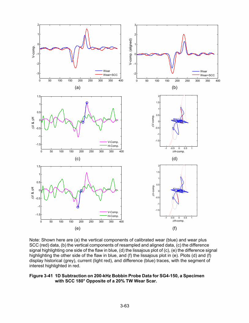
3-63

(a) (b)

(c) (d)

(e) (f)

Note: Shown here are (a) the vertical components of calibrated wear (blue) and wear plus SCC (red) data, (b) the vertical components of resampled and aligned data, (c) the difference signal highlighting one side of the flaw in blue, (d) the lissajous plot of (c), (e) the difference signal highlighting the other side of the flaw in blue, and (f) the lissajous plot in (e). Plots (d) and (f) display historical (grey), current (light red), and difference (blue) traces, with the segment of interest highlighted in red.

Figure 3-41 1D Subtraction on 200-kHz Bobbin Probe Data for SG4-150, a Specimen with SCC 180° Opposite of a 20% TW Wear Scar.

0 50 100 150 200 250 300 350 400

-3

-2

-1

0

1

2

V-co

mp.

WearWear+SCC

0 50 100 150 200 250 300 350 400

-2

-1

0

1

2

3

V-co

mp.

(alig

ned)

WearWear+SCC

0 50 100 150 200 250 300 350 400

-1.5

-1

-0.5

0

0.5

1

1.5

∆V &

∆H

V-Comp.H-Comp.

-1 -0.5 0 0.5 1

-1.5

-1

-0.5

0

0.5

1

1.5

2

∆V-c

omp.

∆H-comp.

0 50 100 150 200 250 300 350 400

-1.5

-1

-0.5

0

0.5

1

1.5

∆V &

∆H

V-Comp.H-Comp.

-1 -0.5 0 0.5 1

-1.5

-1

-0.5

0

0.5

1

1.5

2

∆V-c

omp.

∆H-comp.

3-64

(a)

(b)

(c) (d)

(e) (f)

Note: Shown here are (a) the vertical components of calibrated wear (blue) and wear plus SCC (red) data, (b) the vertical components of resampled and aligned data, (c) the difference signal highlighting one side of the flaw in blue, (d) the lissajous plot of (c), (e) the difference signal highlighting the other side of the flaw in blue, and (f) the lissajous plot in (e). Plots (d) and (f) display historical (grey), current (light red), and difference (blue) traces, with the segment of interest highlighted in red. Figure 3-42 1D Subtraction on 400-kHz Bobbin Probe Data for SG4-150, a Specimen

with SCC 180° Opposite of a 20% TW Wear Scar.

0 50 100 150 200 250 300 350 400-1

-0.8

-0.6

-0.4

-0.2

0

0.2

0.4V-

com

p.

WearWear+SCC

0 50 100 150 200 250 300 350 400-0.6

-0.4

-0.2

0

0.2

0.4

0.6

0.8

V-co

mp.

(alig

ned)

WearWear+SCC

0 50 100 150 200 250 300 350 400-1

-0.5

0

0.5

1

∆V

& ∆

H

V-Comp.H-Comp.

-1 -0.5 0 0.5 1

-1.5

-1

-0.5

0

0.5

1

1.5

2

∆H-comp.

∆V-c

omp.

0 50 100 150 200 250 300 350 400-1

-0.5

0

0.5

1

∆V

& ∆

H

V-Comp.H-Comp.

-1 -0.5 0 0.5 1

-1.5

-1

-0.5

0

0.5

1

1.5

2

∆H-comp.

∆V-c

omp.

3-65

(e) (e) (b)

(c) (d)

(e) (f)

Note: Shown here are (a) the vertical components of calibrated wear (blue) and wear plus SCC (red) data, (b) the vertical components of resampled and aligned data, (c) the difference signal highlighting one side of the flaw in blue, (d) the lissajous plots of (c) shown with and without raw data traces, (e) the difference signal highlighting the other side of the flaw in blue, and (g) the lissajous plot of (f). Plots (d) and (f) show difference (blue) traces, with the segment of interest highlighted in red. Plot (d) also displays historical (grey) and current (light red) traces.

Figure 3-43 1D Subtraction on 200-kHz Bobbin Probe Data for SG4-152, a Specimen with SCC 180° Opposite of a 30% TW Wear Scar.

0 50 100 150 200 250 300 350 400

-4

-3

-2

-1

0

1

2

3

4V-

com

p.

WearWear+SCC

0 50 100 150 200 250 300 350 400

-4

-3

-2

-1

0

1

2

3

4

V-co

mp.

(alig

ned)

WearWear+SCC

0 50 100 150 200 250 300 350 400

-0.6

-0.4

-0.2

0

0.2

0.4

0.6

∆V &

∆H

V-Comp.H-Comp.

-2 -1 0 1 2-3

-2

-1

0

1

2

3

∆V-c

omp.

∆H-comp.-0.5 0 0.5

-0.8

-0.6

-0.4

-0.2

0

0.2

0.4

0.6

∆V-c

omp.

∆H-comp.

0 50 100 150 200 250 300 350 400

-0.6

-0.4

-0.2

0

0.2

0.4

0.6

∆V &

∆H

V-Comp.H-Comp.

-0.6 -0.4 -0.2 0 0.2 0.4-0.8

-0.6

-0.4

-0.2

0

0.2

0.4

0.6

∆V-c

omp.

∆H-comp.

3-66

Data analysis results on the suppression of background interference are presented next for bobbin and rotating probe data from two other specimens, one with cracking present adjacent to the wear scar and the other with cracking inside the wear scar. As noted previously, detection of cracks in those situations can pose a major challenge to all conventional EC examination techniques.

Specimen SG4-159 – 1D and 2D Subtraction

Different stages of 1D background subtraction using bobbin probe data for specimen SG4-159, a tube with ODSCC located ~0.25-in. (6 mm) away from a 20% TW wear scar, are shown in Figure 3-44. The EC inspection data for that specimen were displayed in Figure 3-11. The vertical components of both the pre- and post-SCC data, before and after alignment, are shown in Figure 3-44(a) and (b), respectively. Plots of the difference signal following subtraction of the background are shown in Figure 3-44(c) and (d). Marked on those plots are the data segments exhibiting flaw- like characteristics. The lissajous plots of the data in Figure 3-44(c), with the corresponding probe response from flaw-like signals being highlighted, are shown in Figure 3-44(d). In addition to the residual signal from subtraction, the lissajous plot on the left side in Figure 3-44(d) also displays the original historical and the current data. Once again, the results indicate good suppression of interference from the volumetric background signal, with the resultant signal suggesting the presence of small crack-like signals. It is worth noting that, in reference to Figure 3-11, no indications of cracking were detectable in that tube based on manual analysis of the bobbin probe data.

Different stages of 2D background subtraction using +PointTM rotating probe data for specimen SG4-159 are shown in Figure 3-45. The EC data for that specimen was displayed in Figure 3-12. The vertical components of the pre- and post-SCC data in image format are displayed in Figure 3-45(a) and (b), respectively. The lissajous plot of the data encompassing the ROI is shown in Figure 3-45(c), with the data outside that region plotted in light colors. The background-subtracted data in image format is displayed in Figure 3-45(d), where the difference plot indicates reasonable suppression of the wear signal. Figure 3-45(e) and (f) show lissajous plots of cross-sectional traces across the wear signal, one this is intersecting (e) and the one that is not intersecting (f) with the SCC signal. The residual signal in Figure 3-45(e) exhibits a crack-like response with negligible contribution from the nearby volumetric flaw. In reference to Figure 3-12, which also displays the data for specimen SG4-159, although the small signal from SCC in Figure 3-12 was detectable, the crack signal in Figure 3-45(e) shows a higher S/N and thus has a higher POD.

Specimen SG4-154 – 1D and 2D Subtraction

Different stages of 1D background subtraction using bobbin probe data for specimen SG4-154, which is a tube with ODSCC inside of a 30% TW wear scar, are shown in Figure 3-46. The EC data for that specimen was displayed in Figure 3-17. The vertical components of both the pre- and post-SCC data before and after alignment are shown in Figure 3-46(a) and (b), respectively. Plots of the difference signal following subtraction of the background are shown in Figure 3-46(c) and (d). Marked on those plots are data segments exhibiting flaw-like characteristics. The lissajous plots of the data segment are shown in Figure 3-46(c), with the corresponding probe response from a flaw-like signal highlighted in Figure 3-46(d). In addition to the residual signal from subtraction, the lissajous plot on the left side in Figure 3-46(d) also displays the original historical and current data. Once again, the results in this case indicate good suppression of interference from the volumetric background signal, with the resultant signal exhibiting crack-like characteristics. In reference to Figure 3-17, while the change in wear scar signal due to

3-67

introduction of cracking is discernible, identifying that change as being of crack origin was not feasible based on manual analysis of the bobbin probe data.

Different stages of 2D background subtraction using +PointTM rotating probe data for specimen SG4-154 are shown in Figure 3-47. The EC data for that specimen was presented in Figure 3-18. The vertical components of the pre- and post-SCC data in image format are displayed in Figure 3-47(a) and (b), respectively. The lissajous plot of the data encompassing the ROI is shown in Figure 3-47(c), with the data outside that region plotted in light colors. The background-subtracted data in image format is displayed in Figure 3-47(d), where the difference plot indicates reasonable suppression of the wear signal. Figure 3-47(e) and (f) show lissajous plots of cross-sectional traces across the wear signal, one that is intersecting (e) and the one that is not intersecting (f) with the SCC signal. The residual signal in Figure 3-47(e) exhibits a crack-like response with minimal contribution from the collocated volumetric flaw. As with the previous test case, the crack signal in the background-subtracted data also shows a higher S/N and thus has a higher POD. In reference to Figure 3-18, which also displays the data for specimen SG4-154, while the change in wear scar signal due to introduction of cracking is discernible, identifying that change as being of crack origin was not feasible because the composite signal exhibits characteristics of a volumetric flaw.

3-68

(a)

(b)

(c)

(d)

Note: Shown here are (a) the vertical components of calibrated wear (blue) and wear plus SCC (red) data, (b) the vertical components of resampled and aligned data, (c) the difference signal highlighting the flaw in blue, and (d) the lissajous plots of (c) shown with and without raw data traces. Plots in (d) show difference (blue) traces, with the segment of interest highlighted in red. Plots in (d) also display historical (grey) and current (light red) traces.

Figure 3-44 1D Subtraction on 200-kHz Bobbin Probe Data for SG4-159, a Specimen

with SCC ~0.25-in. (6 mm) Away from a 20% TW Wear Scar.

0 50 100 150 200 250 300 350 400

-2

-1.5

-1

-0.5

0

0.5

1

1.5

2

V-co

mp.

WearWear+SCC

0 50 100 150 200 250 300 350 400

-2

-1.5

-1

-0.5

0

0.5

1

1.5

2

V-co

mp.

(alig

ned)

WearWear+SCC

0 50 100 150 200 250 300 350 400

-0.5

0

0.5

∆V &

∆H

V-Comp.H-Comp. -1 -0.5 0 0.5 1

-1.5

-1

-0.5

0

0.5

1

∆V-c

omp.

∆H-comp.-0.2 0 0.2 0.4

-0.5

-0.4

-0.3

-0.2

-0.1

0

0.1

0.2

0.3

0.4

∆V-c

omp.

∆H-comp.

3-69

(a)

(b)

(c)

(d)

(e)

(f)

Note: Shown here are (a) historical data (wear without SCC); (b) current data (wear plus SCC); (c) the lissajous plot for the entire ROI; (d) the difference plot; (e) cross-section across wear, including SCC; and (f) cross-section across wear, not including SCC. Plots (c), (e), and (f) all display historical (grey), current (red), and difference (blue) traces.

Figure 3-45 2D Subtraction on 300-kHz +PointTM Data for SG4-159, a specimen with

SCC ~0.25-in. (6 mm) Away from a 20% TW Wear Scar.

Ax. scale (pts.)

Cr.

scal

e (p

ts.)

10 20 30 40 50 60 70 80

10

20

30

40

50

60

70-0.4

-0.3

-0.2

-0.1

0

0.1

0.2

0.3

0.4

Ax. scale (pts.)

Cr.

scal

e (p

ts.)

10 20 30 40 50 60 70 80

10

20

30

40

50

60

70-0.4

-0.3

-0.2

-0.1

0

0.1

0.2

0.3

0.4

-0.6 -0.4 -0.2 0 0.2 0.4 0.6

-0.4

-0.3

-0.2

-0.1

0

0.1

0.2

0.3

∆H-comp.

∆V-c

omp.

Ax. scale (pts.)

Cr.

scal

e (p

ts.)

10 20 30 40 50 60 70 80

10

20

30

40

50

60

70 -0.2

-0.15

-0.1

-0.05

0

0.05

0.1

0.15

0.2

0.25

-0.6 -0.4 -0.2 0 0.2 0.4

-0.4

-0.3

-0.2

-0.1

0

0.1

0.2

0.3

∆H-comp.

∆V-c

omp.

-0.6 -0.4 -0.2 0 0.2 0.4 0.6

-0.4

-0.3

-0.2

-0.1

0

0.1

0.2

0.3

∆H-comp.

∆V-c

omp.

3-70

(a)

(b)

(c)

(d)

Note: Shown here are (a) the vertical components of calibrated wear (blue) and wear plus SCC (red) data, (b) the vertical components of resampled and aligned data, (c) the difference signal highlighting the flaw in blue, and (d) lissajous plots of (c) shown both with (left) and without (right) raw data traces. Plots (d) show difference (blue) traces, with the segment of interest highlighted in red. Plots in (d) also display historical (grey) and current (light red) traces.

Figure 3-46 1D Subtraction on 200-kHz Bobbin Probe Data for SG4-154, a Specimen

with SCC Inside of a 30% TW Wear Scar.

0 50 100 150 200 250 300 350 400

-4

-3

-2

-1

0

1

2

3

4

V-co

mp.

WearWear+SCC

0 50 100 150 200 250 300 350 400

-4

-3

-2

-1

0

1

2

3

4

V-co

mp.

(alig

ned)

WearWear+SCC

0 50 100 150 200 250 300 350 400

-1

-0.5

0

0.5

1

∆V &

∆H

V-Comp.H-Comp.

-2 -1 0 1 2

-2

-1

0

1

2

3

∆V-c

omp.

∆H-comp.-0.8 -0.6 -0.4 -0.2 0 0.2

-1

-0.8

-0.6

-0.4

-0.2

0

0.2

0.4

0.6

0.8

∆V-c

omp.

∆H-comp.

3-71

(a)

(b)

(c)

(d)

(e)

(f)

Note: Shown here are (a) historical data (wear without SCC); (b) current data (wear plus SCC); (c) the lissajous plot for the entire ROI; (d) the difference plot; (e) cross-section across wear, including SCC; and (f) cross-section across wear, not including SCC. Plots (c), (e), and (f) all display historical (grey), current (red), and difference (blue) traces.

Figure 3-47 2D Subtraction on 300-kHz +PointTM Data for SG4-154, a Specimen with

SCC Inside of a 30% TW Wear Scar.

Ax. scale (pts.)

Cr.

scal

e (p

ts.)

10 20 30 40 50 60 70 80 90

10

20

30

40

50

60-0.8

-0.6

-0.4

-0.2

0

0.2

0.4

0.6

0.8

Ax. scale (pts.)

Cr.

scal

e (p

ts.)

10 20 30 40 50 60 70 80 90

10

20

30

40

50

60-0.8

-0.6

-0.4

-0.2

0

0.2

0.4

0.6

0.8

-1 -0.5 0 0.5 1

-0.8

-0.6

-0.4

-0.2

0

0.2

0.4

∆H-comp.

∆V-c

omp.

Ax. scale (pts.)

Cr.

scal

e (p

ts.)

10 20 30 40 50 60 70 80 90

10

20

30

40

50

60-0.2

-0.1

0

0.1

0.2

0.3

0.4

-1 -0.5 0 0.5 1

-0.8

-0.6

-0.4

-0.2

0

0.2

0.4

∆H-comp.

∆V-c

omp.

-1 -0.5 0 0.5 1

-0.8

-0.6

-0.4

-0.2

0

0.2

0.4

∆H-comp.

∆V-c

omp.

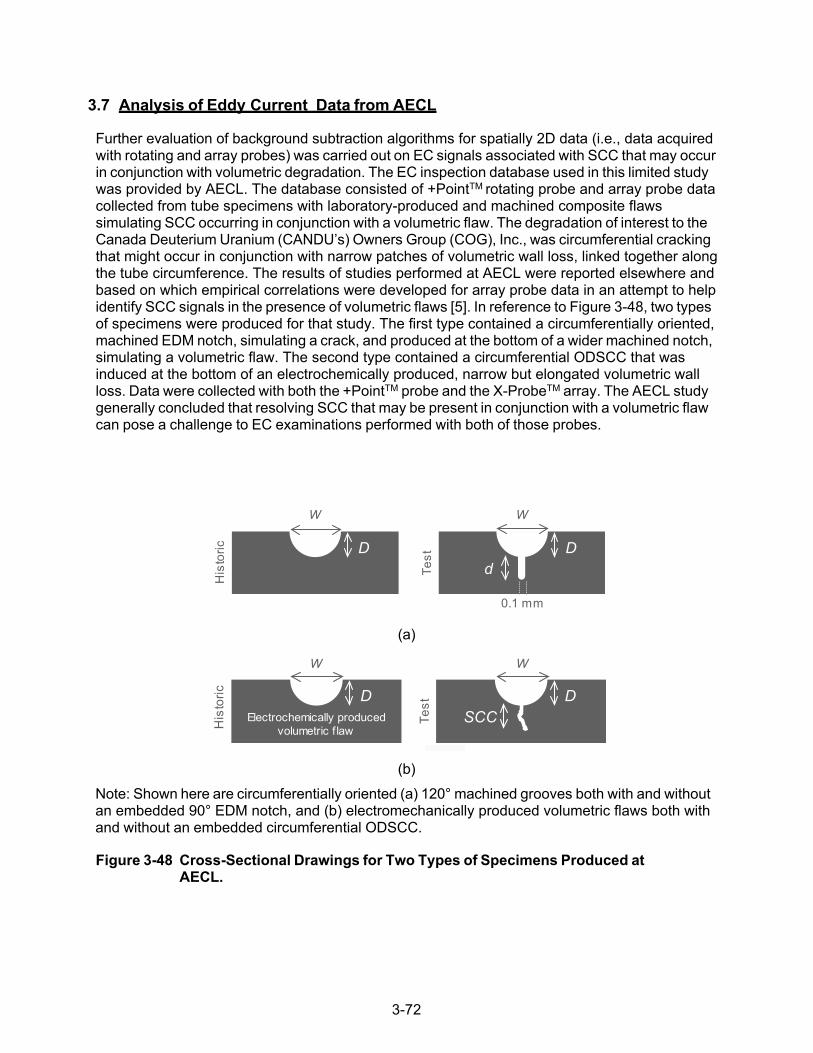
3-72

3.7 Analysis of Eddy Current Data from AECL

Further evaluation of background subtraction algorithms for spatially 2D data (i.e., data acquired with rotating and array probes) was carried out on EC signals associated with SCC that may occur in conjunction with volumetric degradation. The EC inspection database used in this limited study was provided by AECL. The database consisted of +PointTM rotating probe and array probe data collected from tube specimens with laboratory-produced and machined composite flaws simulating SCC occurring in conjunction with a volumetric flaw. The degradation of interest to the Canada Deuterium Uranium (CANDU’s) Owners Group (COG), Inc., was circumferential cracking that might occur in conjunction with narrow patches of volumetric wall loss, linked together along the tube circumference. The results of studies performed at AECL were reported elsewhere and based on which empirical correlations were developed for array probe data in an attempt to help identify SCC signals in the presence of volumetric flaws [5]. In reference to Figure 3-48, two types of specimens were produced for that study. The first type contained a circumferentially oriented, machined EDM notch, simulating a crack, and produced at the bottom of a wider machined notch, simulating a volumetric flaw. The second type contained a circumferential ODSCC that was induced at the bottom of an electrochemically produced, narrow but elongated volumetric wall loss. Data were collected with both the +PointTM probe and the X-ProbeTM array. The AECL study generally concluded that resolving SCC that may be present in conjunction with a volumetric flaw can pose a challenge to EC examinations performed with both of those probes.

(a)

(b)

Note: Shown here are circumferentially oriented (a) 120° machined grooves both with and without an embedded 90° EDM notch, and (b) electromechanically produced volumetric flaws both with and without an embedded circumferential ODSCC.

Figure 3-48 Cross-Sectional Drawings for Two Types of Specimens Produced at

AECL.

d

W

0.1 mm

TestD

W

His

toric D

D

His

toric

Electrochemically produced volumetric f law

W

DSCCTe

st

W

3-73

Although the flaw types in the AECL database are specific to CANDU SGs, the EC data were nevertheless used in this study to better assess the applicability of the historical background subtraction schemes implemented in this work to other complex modes of SG tube degradation. As noted previously, the inherent limitation associated with the spatial resolution of EC probes renders conventional spatial and frequency domain signal processing methods ineffective in discriminating crack signals interacting with a more dominant signal from a volumetric flaw. For the initial evaluations, +PointTM probe data from a subset of tubes containing machined flaws were analyzed. The composite flaws consisted of coplanar OD circumferential EDM notches and machined grooves. The cross-sectional drawings of the flaws in those tubes are shown in Figure 3-48. In reference to Figure 3-48(a), the machined flaws were trench-like grooves of different depth, D, and width, W, extending 120° circumferentially both with and without an embedded 90° EDM notch. Rotating probe data from 0.5-mm, 0.75–mm, and 1.0-mm wide grooves, both with and without EDM notches having a nominal width of ~0.1 mm, were initially examined. Representative test cases are presented next on assessing the effectiveness of 2D background subtraction using different data alignment methods. The first method is based on 2D direct subtraction of data while the second method is based on 1D (line-by-line) subtraction of spatially 2D data, with both methods using frequency-based resampling. A description of the background subtraction techniques was provided in Section 3.4.

Direct Subtraction of 2D Data

Different stages of 2D background subtraction are presented next for a tube specimen with four collocated volumetric and crack-like circumferential machined flaws. The volumetric flaws are four 1-mm-wide, 30% TW OD circumferential machined grooves with a 120° extent. The coplanar crack-like flaws are 0.1-mm-wide, 90° circumferential EDM notches with depths, d, of 0%, 20%, 30%, and 40% TW (i.e., combined depth, D+d, of 30%, 50%, 60%, and 70% TW). Displayed in Figure 3-49(a) and (c) are the pre- and post-processed data, respectively, over a small region of the tube encompassing a volumetric groove with an embedded 30% TW EDM notch. Also shown in Figure 3-49(b) and (d) are the expanded lissajous plots of a single axial trace through the middle of the composite flaw. The results indicate near-complete suppression of the +PointTM

probe response from volumetric flaws, thus allowing unambiguous characterization of the signals from circumferential notches.

Figure 3-50(a) and (c) show the pre- and post-processed data, respectively, over the section of tube containing all four machined flaws. Also shown in Figure 3-50(b) and (d) are the expanded lissajous plots of single axial traces through the middle of all four composite flaws. The results indicate near-complete suppression of the probe response from volumetric flaws and unambiguous identification of circumferential notches. Comparison of the lissajous plots in Figure 3-50(b) and (d) indicate that following background subtraction, the signals all exhibit crack- like characteristics. In addition, as a result of the background subtraction process, the signal associated with the volumetric groove without an embedded EDM notch in Figure 3-50(a) has been eliminated in the data displayed in Figure 3-50(c). Although it is not shown here, for this test case, the 1D subtraction method provided results that were comparable to the 2D method.

Presented next are different stages of 2D background subtraction for another tube specimen with four collocated volumetric and crack-like circumferential machined flaws. The volumetric flaws in this tube are four 1-mm-wide (W=1.0 mm), 40% TW OD circumferential machined grooves with a 120° extent. The coplanar crack-like flaws are 0.1-mm-wide, 90° circumferential EDM notches with depths, d, of 0%, 20%, 30%, and 40% TW (i.e., combined depth, D+d, of 40%, 60%, 70%, and 80%TW). Displayed in Figure 3-51(a) and (c) in various formats are the pre- and post- processed data, respectively, over a small region of tube encompassing a volumetric groove with

3-74

an embedded 30% TW EDM notch. Also shown in Figure 3-51(b) and (d) are the expanded lissajous plots of a single axial trace through the middle of the composite flaw. The results, once again, indicate near-complete suppression of the +PointTM probe response from volumetric flaws, thus allowing unambiguous characterization of circumferential notches.

Figure 3-52(a) and (c) show the pre- and post-processed data, respectively, over the section of tube containing all four machined flaws. Also shown in Figure 3-52 are the expanded lissajous plots of single axial traces through the middle of all four composite flaws. The results indicate near-complete suppression of the probe response from volumetric flaws and in turn unambiguous identification of circumferential notches. Comparison of the lissajous plots in Figure 3-52(a) and (c) indicate that following background subtraction, the signals all exhibit crack-like characteristics. In addition, as a result of the background subtraction process, the signal associated with the volumetric groove without an embedded EDM notch in Figure 3-52(a) has been eliminated in the data displayed in Figure 3-52(c). Although it is not shown here, also for this test case, the 1D subtraction method provided results that were comparable to the 2D method.

3-75

(a) (b)

(c) (d)

Note: The volumetric flaws are four 1-mm-wide, 30% TW, 120o circumferential machined grooves. Shown here are (a) pre- and (c) post-processed data over a small region containing a volumetric groove with an embedded 30% TW (i.e., combined depth of 60% TW), 90o circumferential EDM notch. Also shown in (b) and (d) are the expanded lissajous plots of single axial traces crossing the middle of the composite flaw.

Figure 3-49 Different Stages of Processing for 2D Background Subtraction Using

+Pointtm Data at 300 kHz from tube Specimens with Four Coplanar Volumetric and 30% TW Crack-Like Circumferential Machined Flaws.

-0.5 0 0.5

-0.1

0

0.1

0.2

0.3

0.4

0.5

0.6

0.7

0.8

0.9

H-comp.

V-c

omp.

-0.4 -0.2 0 0.2 0.4

0

0.1

0.2

0.3

0.4

0.5

0.6

0.7

0.8

0.9

∆H-comp.

∆V-c

omp.

3-76

(a) (b)

(c) (d)

Note: The embedded crack-like flaws are 90o circumferential EDM notches with 0%, 20%, 30%, and 40% TW depths at the bottom of 30% TW volumetric grooves. Shown here are (a) pre- and (c) post-processed data over the section of tube containing all four machined flaws. Also shown in (b) and (d) are the expanded lissajous plots of single axial traces crossing the middle of all four composite flaws.

Figure 3-50 Different Stages of 2D Background Subtraction for the Same Specimen

Addressed in Figure 3-49.

-0.4 -0.2 0 0.2 0.4 0.6

-0.1

0

0.1

0.2

0.3

0.4

0.5

0.6

0.7

0.8

0.9

H-comp.

V-c

omp.

-0.6 -0.4 -0.2 0 0.2

0

0.1

0.2

0.3

0.4

0.5

0.6

0.7

0.8

0.9

∆H-comp.

∆V-c

omp.

3-77

(a) (b)

(c) (d)

Note: The volumetric flaws are four 40% TW, 120o circumferential machined grooves. Shown here are (a) pre- and (c) post-processed data over a small region containing a volumetric groove with an embedded 30% TW (i.e., combined depth of 70% TW), 90o circumferential EDM notch. Also shown in (b) and (d) are the expanded lissajous plots of single axial traces crossing the middle of the composite flaw.

Figure 3-51 Different Stages of Processing for 2D Background Subtraction Using

+Pointtm Data at 300 kHz from Tube Specimens with Four Coplanar Volumetric and 40% TW Crack-Like Circumferential Machined Flaws.

-0.4 -0.2 0 0.2 0.4

0

0.1

0.2

0.3

0.4

0.5

0.6

0.7

0.8

0.9

H-comp.

V-c

omp.

-0.6 -0.5 -0.4 -0.3 -0.2 -0.1 0 0.1 0.2

0

0.1

0.2

0.3

0.4

0.5

0.6

0.7

0.8

0.9

∆H-comp.

∆V-c

omp.

3-78

(a) (b)

(c) (d)

Note: The embedded crack-like flaws are 90o circumferential EDM notches with 0%, 20%, 30%, and 40% TW depths at the bottom of 40% TW volumetric grooves (i.e., combined depth of 40%, 60%, 70%, and 80% TW). Shown here are (a) pre- and (c) post-processed data over the section of tube containing all four machined flaws. Also shown in (b) and (d) are the expanded lissajous plots of single axial traces crossing the middle of all four composite flaws.

Figure 3-52 Different Stages of 2D background subtraction for the Same Specimen Addressed in Figure 3-51.

Line-by-Line Subtraction of 2D Data

A representative test case is provided in Figure 3-53 that shows comparison of 1D axial line-by- line and 2D direct background subtraction methods using +PointTM rotating data at 300 kHz. The volumetric flaws in this tube are four 0.75-mm-wide (W=0.75 mm), 30% TW, OD circumferential machined grooves with a 120° extent. The coplanar crack-like flaws are 0.1 mm -ide, 90° circumferential EDM notches with depths, d, varying between 0% TW and 40% TW. Figure 3-53 shows different stages of processing using 2D direct and 1D background subtraction over a small region of the tube encompassing a volumetric groove with an embedded 20% TW EDM notch (i.e., combined depth of 50% TW). Figure 3-53 (a) and (b) show the pre-and post-processed data using 2D subtraction and 1D subtraction without smoothing, respectively. Displayed in Figure

-0.6 -0.4 -0.2 0 0.2

0

0.1

0.2

0.3

0.4

0.5

0.6

0.7

0.8

H-comp.

V-c

omp.

-0.6 -0.5 -0.4 -0.3 -0.2 -0.1 0 0.1 0.2

0

0.1

0.2

0.3

0.4

0.5

0.6

0.7

0.8

∆H-comp.

∆V-c

omp.

3-79

3-53(a) are the vertical components of the data (in image format) for the volumetric groove, the composite signal (i.e., groove plus EDM notch), and the difference signal (∆V). Also shown in Figure 3-53(a) is the lissajous plot of the difference signal for the same data segment. The original signals, associated with the volumetric and the composite flaw, are also displayed on the lissajous plot in light color. While the background has been suppressed to a certain degree using the 2D subtraction method, the results in Figure 3-53(a) illustrate that without proper compensation for variations of data in the axial direction (i.e., along the flaw width), the background feature is only partially removed, resulting in anomalies in the resultant difference signal. Figure 3-53(b) shows the same data, but in this case, a 1D subtraction is applied using line-by-line axial alignment to compensate for the varying axial widths between the current (i.e., composite flaw) and the historical (i.e., volumetric groove) data. In the lissajous plot in Figure 3-53(b), after axial compensation is implemented, a near-complete suppression of the probe response from the volumetric flaw is achieved, resulting in a difference signal with crack-like characteristics.

Another representative test case is provided in Figure 3-54 on comparison of 1D circumferential line-by-line and 2D historical background suppression methods using +PointTM rotating data at 300 kHz. In addition to factors such as variability in probe speed noted earlier, other factors such as anomalous trigger channel data can render alignment of data acquired with rotating probes imprecise. Shown in Figure 3-54 is the data segment associated with a flaw that has an anomalous trigger channel. The volumetric flaw in this case is a 0.5-mm-wide (W=0.5 mm), 50% TW OD circumferential machined groove with a 120° extent. The coplanar crack-like flaw is a 0.1-mm-wide, 90° circumferential EDM notch with a depth, d, of 40%TW. Figure 3-54(a) shows the original trigger data and the same data after compensation for trigger discontinuity. While the trigger data is significantly improved after this process, the small remaining anomalies in the trigger data will, nevertheless, result in imperfect alignment of the flaw signal. Using the 2D and the 1D circumferential line-by-line subtraction method, Figure 3-54(b) displays the vertical components of the data (in image format) for the volumetric and the composite flaw along with the difference data, ∆V.

Because one goal is to obtain as little distortion in the data as possible, the results in Figure 3-54 indicate that 1D subtraction provides improved compensation with regard to fine-scale alignment issues by adjusting the current data to match better with the background data. It is worth noting that while alignment problems in a corrupted signal could be compensated for to a certain degree, care should be taken in such cases not to artificially alter the features in the original signal. Figure 3-54(c) displays circumferential lissajous plots of the 2D and the 1D background-subtracted data, along with the original data in light colors. Comparison of the difference signals in the lissajous plots illustrates the potential for introduction of artifacts caused by imperfect alignment of data. In this case, the artifact present in the 2D subtracted data is not present in the line-by-line subtracted data (see the arrow in Figure 3-54(c)). The results of this study suggest that in selecting the proper technique for suppression of background in EC inspection data, a number of factors should be taken into consideration including the quality of the data and the type of features present in the data. Although not investigated in this work, optimization-based methods could be used to automatically determine the most appropriate algorithm for a given test condition.

Data analysis results are presented next for representative cases from the second type of laboratory-produced flaws in the AECL dataset. Figure 3-55 displays the +PointTM rotating probe and the array probe data acquired from a specimen with electrochemically produced circumferential ODSCC in conjunction with a volumetric flaw. Displayed in Figure 3-55(a) and (b) are screen captures of the rotating probe data analysis results performed under the EddynetTM

environment for the pre- and post-SCC data, respectively. The signals associated with the volumetric flaw and the crack signal are marked on the terrain plots in those figures. As noted in

3-80

[5], the +PointTM response from these circumferentially oriented composite signals has characteristics of a volumetric flaw, which could render the discrimination of collocated cracks based on conventional analysis of data ineffective. These features include a camel-hump cross- section and a hook-like shape in the lissajous plot that could complicate detection of nearby crack- like signals. Another observation made about this dataset was that the change in signal from the volumetric flaw, both before and after introduction of cracking, was notable for a large number of cases. This result is illustrated by the example shown in Figure 3-55(a) and (b), in which comparison of signals in the pre- and post-SCC data shows a clear change in the amplitude and phase angle of the signal associated with the volumetric flaw. With the effectiveness of background subtraction schemes being strongly dependent on the stationary nature of the background signal, only a small subset of data from AECL specimens with laboratory-produced flaws were included in this study.

Next, an example is provided on the application of historical background subtraction to the detection of a crack signal in the presence of a collocated volumetric flaw from a tube specimen in the AECL dataset. As in previous cases, the 300-kHz channel of the +PointTM rotating probe was used for the analysis of data. In reference to Figure 3-48(b), the electrochemically produced, OD- initiated volumetric flaw in that tube specimen has a width, W, of ~1.06 mm and a depth of 44% TW. A circumferentially oriented ODSCC was produced at the bottom of the volumetric flaw. Figure 3-56(a)–(c) displays, respectively, the calibrated data after production of the volumetric flaw, after production of the SCC, and the resulting difference signal. Data in each case is displayed in image, terrain, strip chart, and lissajous format using the Argonne data analysis tool [6]. Also shown in each case is a separate terrain plot of the data segment encompassing the flaw signals. Comparison of the lissajous plots in Figure 3-56(a) and (b), for the pre- and post-SCC data, shows that the probe response in both figures exhibit volumetric-like signal characteristics. The difference signal in Figure 3-56(c), on the other hand, has crack-like characteristics and thus can be detected without ambiguity.

It should be noted that, while the background suppression algorithms implemented in this work proved effective when applied to data collected from machined specimens, the results were not generally as effective in application to laboratory-produced flaws from the AECL dataset. A general observation made based on the analysis of rotating probe data from chemically produced flaws, is that in the majority of cases examined in this study, the pre- and post-SCC signals from volumetric flaws were notably different. This finding suggests that the size of volumetric flaws changed following production of collocated cracks. As discussed earlier, applicability of historical subtraction of data is based on the assumption that the background signal is stationary. As such, suppression of background signals, and in turn detection of potential nearby crack signals, cannot be performed effectively if the change in the background signal is comparable to the change associated with initiation or growth of the nearby cracking. In general, the results of this study further indicate that for proper suppression of background signals, the test conditions for the current and historical data should be consistent.

3-81

(a)

(b)

Note: The volumetric flaw is a 30% TW OD, 120o circumferential machined groove. The crack-like flaw is a 90o circumferential EDM notch with a 20% TW depth. Shown here are data from the section of tube using (a) 2D subtraction, (b) 1D subtraction without smoothing. Displayed in image format are the vertical components of data for volumetric flaw, composite flaw (groove plus EDM), and the difference signal (∆V). Also shown are the lissajous plots of data with original signals shown in light color. Shown in (b) are the same data but using 1D-axial, line-by-line subtraction to compensate for the varying axial widths of signals between current and historical data.

Figure 3-53 Stages of Processing for 2D direct and 1D Axial Line-by-Line

Background Subtraction Using +Pointtm Data from a Specimen with Collocated 0.75-Mm-Wide Volumetric and 0.1-mm-Wide Circumferential Machined Flaws.

-0.4 -0.2 0 0.2 0.4 0.6

0

0.1

0.2

0.3

0.4

0.5

0.6

∆H-comp.∆

V-c

omp.

Ax. scale (pts.)

Cr.

scal

e (p

ts.)

Volumetric trench

10 20 30 40 50 60 70 80 90 100

10

20

30

40

50

60

70

80

90

100

Ax. scale (pts.)

Cr.

scal

e (p

ts.)

Trench + 20% notch

10 20 30 40 50 60 70 80 90 100

10

20

30

40

50

60

70

80

90

100

Ax. scale (pts.)

Cr.

scal

e (p

ts.)

∆V

10 20 30 40 50 60 70 80 90 100

10

20

30

40

50

60

70

80

90

100-0.15

-0.1

-0.05

0

0.05

0.1

0.15

0.2

0.25

0.3

-0.1

0

0.1

0.2

0.3

0.4

0.5

0.6

0.7

-0.

0

0.1

0.2

0.3

0.4

0.5

0.6

-0.5 -0.4 -0.3 -0.2 -0.1 0 0.1 0.2 0.3 0.4 0.5

-0.1

0

0.1

0.2

0.3

0.4

0.5

∆H-comp.

∆V

-com

p.

Ax. scale (pts.)

Cr.

scal

e (p

ts.)

Ax-aligned volumetric trench

10 20 30 40 50 60 70 80 90 100

10

20

30

40

50

60

70

80

90

100

Ax. scale (pts.)

Cr.

scal

e (p

ts.)

Trench + 20% notch

10 20 30 40 50 60 70 80 90 100

10

20

30

40

50

60

70

80

90

100

Ax. scale (pts.)

Cr.

scal

e (p

ts.)

∆V

10 20 30 40 50 60 70 80 90 100

10

20

30

40

50

60

70

80

90

100-0.1

-0.05

0

0.05

0.1

0.15

0.2

0.25

0.3

-0.1

0

0.1

0.2

0.3

0.4

0.5

0.6

0.7

0

0.

0.

0.

0.

0.

3-82

(a)

(b)

(c)

Note: The tube has collocated 0.5-mm-wide volumetric and 0.1-mm-wide circumferential machined flaws. The volumetric flaw is a 50% TW OD, 120o machined groove. The crack-like flaw is a 90o circumferential EDM notch with 40% TW depth. Shown in (a) are the original trigger signal (left) and the signal after compensation (right). Shown in (b) are different stages of the process using 2D (top row) and 1D (bottom row) methods. Displayed in image format are the vertical components of data for volumetric (groove, left), composite flaw (groove plus EDM, center), and the difference signal (∆V, right). Displayed in (c) are circumferential lissajous plots for 2D (left) and 1D (right) subtractions with the original signals plotted in light colors.

Figure 3-54 Representative Case for 1D Circumferential Line-by-Line Subtraction

Using Rotating Probe Data with a Trigger Anomaly.

Ax. scale (pts.)

Cr.

scal

e (p

ts.)

Volumetric trench

10 20 30 40 50 60 70 80

10

20

30

40

50

60

70

80

90

-0.1

0

0.1

0.2

0.3

0.4

0.5

0.6

0.7

0.8

Ax. scale (pts.)

Cr.

scal

e (p

ts.)

Trench + 40% notch

10 20 30 40 50 60 70 80

10

20

30

40

50

60

70

80

90

0

0.5

1

1.5

2

2.5

3

Ax. scale (pts.)

Cr.

scal

e (p

ts.)

∆V

10 20 30 40 50 60 70 80

10

20

30

40

50

60

70

80

900

0.5

1

1.5

2

2.5

Ax. scale (pts.)

Cr.

scal

e (p

ts.)

Circ-aligned volumetric trench

10 20 30 40 50 60 70 80

10

20

30

40

50

60

70

80

90

-0.1

0

0.1

0.2

0.3

0.4

0.5

0.6

0.7

0.8

Ax. scale (pts.)

Cr.

scal

e (p

ts.)

Trench + 40% notch

10 20 30 40 50 60 70 80

10

20

30

40

50

60

70

80

90

0

0.5

1

1.5

2

2.5

Ax. scale (pts.)

Cr.

scal

e (p

ts.)

∆V

10 20 30 40 50 60 70 80

10

20

30

40

50

60

70

80

90 0

0.5

1

1.5

2

-3 -2.5 -2 -1.5 -1 -0.5 0 0.5 1 1.5

0

0.5

1

1.5

2

2.5

3

∆H-comp.

∆V

-com

p.

-3 -2.5 -2 -1.5 -1 -0.5 0 0.5 1 1.5

0

0.5

1

1.5

2

2.5

3

∆H-comp.

∆V

-com

p.

50% TW Groove 50% TW Groove + 40% TW EDM ∆V

50% TW Groove (aligned data) 50% TW Groove + 40% TW EDM ∆V

3-83

(a)

(b)

(c)

Note: Shown here are (a) pre-SCC volumetric, (b) post-SCC data collected with the +PointTM rotating probe, and (c) post-SCC data collected with the X-ProbeTM array with separate measurements of crack signal made from axial and circumferential channels.

Figure 3-55 Example of SCC in Conjunction with Volumetric Flaw from the AECL Data Set and Displayed Using Eddynettm Data Analysis Software.

Vol. signal

Vol. signalCSCC

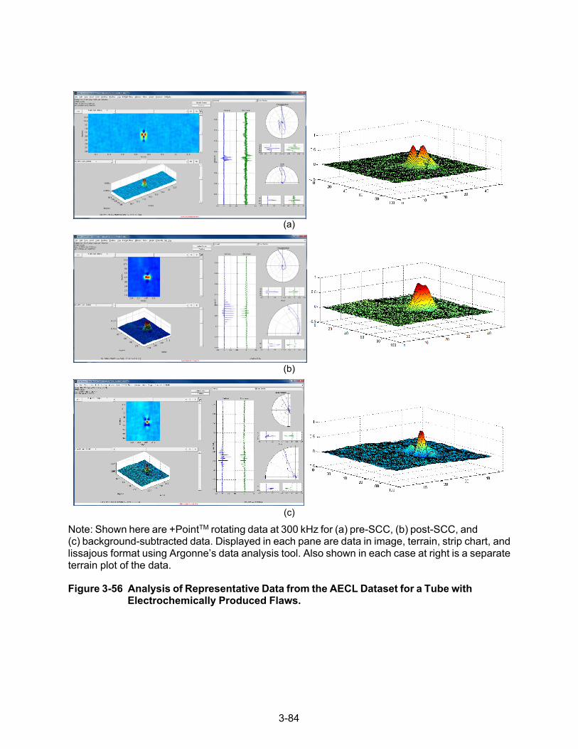
3-84

(a)

(b)

(c)

Note: Shown here are +PointTM rotating data at 300 kHz for (a) pre-SCC, (b) post-SCC, and (c) background-subtracted data. Displayed in each pane are data in image, terrain, strip chart, and lissajous format using Argonne’s data analysis tool. Also shown in each case at right is a separate terrain plot of the data.

Figure 3-56 Analysis of Representative Data from the AECL Dataset for a Tube with

Electrochemically Produced Flaws.

3-85

3.8 Assessing Historical Background Subtraction in Application to Field Data

Data analysis results are presented next on the application of historical background subtraction to EC examination data acquired from ISI of SG tubes. The limited set of field data used in this study is associated with past incidences of complex flaws including cracking that occurred in conjunction with volumetric degradation. These examples are provided both to point out the challenge associated with detecting and characterizing crack signals for such complex flaw types and to further demonstrate the viability of historical subtraction schemes in detection of consequential flaws at an earlier stage. It should be noted that for the examples presented here, the evidence of cracking is anecdotal as it is based solely on the analysis of EC inspection data (i.e., not based on DE data from pulled tubes).

Oconee

As the first example, EC data analysis results are presented on detection of cracking near a volumetric flaw in an SG tube from the Oconee plant. The SG unit is a model BW177-FA once- through steam generator (OTSG) with the tube bundle manufactured using 0.625-in. (16 mm) OD tubing with 0.037-in (0.95 mm). nominal wall thickness made of Inconel 600MA material. The tube supports are 1.5-in. (38.5 mm)-thick, drilled and broached, and made of carbon steel material. The available ISI data for the tube with a composite flaw included bobbin probe examination data from five successive outages and rotating probe examination data from the last four of those outages. The ROI in that tube had a complex EC signal composed of elements including tube deformation (denting damage associated with the manufacturing process), MBM (volumetric flaw), and ODSCC degradation. Over the timespan of the available ISI data, both bobbin and rotating probe examinations were shown to exhibit a gradual increase in the SCC signal. The indications of cracking, however, were not detected or characterized as such prior to the last ISI, the year in which the largest increase was observed. Evaluations made at the time suggested that the large volumetric signal from an existing tube deformation (>14 v ding) complicated timely detection and characterization of nearby cracking based on the analysis of bobbin probe inspection data.

Calibrated bobbin probe data for that particular tube is displayed in Figure 3-57(a), using the EddynetTM data analysis software. Shown in that figure are data from the 400-kHz differential channel, acquired during two different outages four years apart, denoted as ISI #N-4 (left pane) and ISI #N (right pane), representing the historical and the current ISI data. The main analysis window in each case displays the strip chart plot of the data over the entire length of tube, as well as the data over the ROI in both strip chart and lissajous plot formats. While indications of cracking are present in the historical data (left), the signals are difficult to discern in the presence of the large signal from volumetric indication. Figure 3-57(b) shows separate plots of the vertical and horizontal components of the calibrated data (top) over the ROI for the same ISIs as in Figure 3-57(a) using the Argonne data analysis software. Also shown in Figure 3-57(b) are plots of the background-subtracted data (bottom) in different formats. The position of the signal with largest depth is marked on both traces in that figure with the corresponding signal extrema also indicated on the lissajous plot. While some residual signal from the volumetric indication is still present, the historical subtraction results show clear improvement in the S/N of the crack-like indications of OD origin in the resultant difference signal.

Presented next are analyses performed on EC data acquired with a rotating probe over the ROI in the same OTSG tube discussed above. The data analyzed in this case are associated with the mid-range pancake (0.115-in.-diameter coil) and the +PointTM probe of a 3-coil rotating probe. Figure 3-58(a) and (c) display the data from the 300-kHz channel of the pancake coil and the +PointTM probe, respectively. Shown in each case are the original calibrated data under the

3-86

EddynetTM environment from two outages, denoted as ISI #N-2 and ISI #N. Also provided in Figure 3-58(b) and (d) are the background-subtracted data based on the pancake and the +PointTM data, respectively, using the Argonne data analysis tool. The difference signals, between the current and historical data, are presented in image, terrain plot, and strip chart formats. A lissajous plot of a single transverse line through the resultant signal is also provided in each case. The processing was based on 1D subtraction of spatially 2D data from the two outages. Unlike the original data, the processed data associated with both the pancake coil and the +PointTM probe primarily exhibit crack-like characteristics. Although it is not shown here, a larger difference was also observed when historical data that went further back in time was used. In those cases, however, the alignment of the spatially 2D data posed a bigger challenge because of non-uniform test conditions.

Braidwood

As the second example, results are presented on the detection of small changes in bobbin probe signals using ISI data that are closely spaced in time. The EC inspection data used here are associated with an SG tube from the Braidwood plant. The SG unit is a Westinghouse Model D5 recirculating steam generator (RSG) with the tube bundle manufactured using 0.75-in. (19 mm) OD tubing with 0.043-in. (1.1 mm) nominal wall thickness made of thermally treated Inconel 600 material (600TT). The tube bundle has a vertical U-bend design with 1.125- in. ( 28.9 mm)- thick, broached quatrefoil tube supports made of 405SS material. The available ISI data included bobbin probe examination data from three successive outages, denoted here as outage #N, #N-1, and #N-2, and rotating probe examination data from the last outage only. Therefore, the background subtraction results presented here pertain only to the processing of bobbin probe data. For manual analysis of the EC data performed at Argonne, locations were measured with respect to the center of each landmark. The flaw signal of interest is located at ~34 in. (87.2 cm) above the third tube support on the hot leg side or alternatively ~2.0 in. (50 mm) below the fifth tube support. The EC signal located in the free-span region of the tubing was detected by bobbin probe in all of the last three outages during the field inspections and was characterized as a shallow OD indication. However, the signal was reported as having no detectable change between the last two outages based on manual analysis of data.

Figure 3-59 displays the results from manual analysis of EC data, performed at Argonne, for the SG tube at Braidwood. Figure 3-59(a) and (b) show the bobbin probe data at the 300-kHz and at the 550|130-kHz differential channels from outages #N and #N-1, respectively. In both cases, the measured signal from the 300-kHz channel is displayed in the main EddynetTM analysis window, while the signal from the 550|130-kHz channel is displayed in a lissajous window. The signals from both channels indicate the presence of a shallow indication of OD origin with an asymmetric lissajous pattern. Comparison of the data shown Figure 3-59(a) and (b) indicates that the change in signal amplitude and phase between the two consecutive ISIs is within the measurement variability for both data analysis channels. For comparison, the +PointTM rotating probe data from outage #N over the same region of the tube is displayed in Figure 3-59(c). The location of the flaw indication in the rotating probe data is at ~1.8 in. (46.1 mm) below the fifth support structure measured from the center of the TSP, which is consistent with the location of the signal in bobbin probe data. The +PointTM probe signal at 300 kHz has an amplitude of 0.4 v and a phase angle that is indicative of a deep OD-initiated flaw. The axial extent of the indication was estimated to be 0.17 in. (4.4 mm) based on the measurement made from the same channel. Further analyses of the EC data performed at Argonne also suggested the presence of a localized volumetric tube deformation (i.e., ding). This plausible explanation for the source of distortion of the free-span OD flaw signal was made at the time based on analyses of the three-coil rotating probe data at multiple channels.

3-87

Figure 3-60 displays the results from historical subtraction of bobbin probe data for the same tube as Figure 3-59. In comparison with the previous example, the available ISI data from the Braidwood plant are more closely spaced in time, which renders the detection of small changes in signals more challenging. Shown in Figure 3-60 (a) and (b) are the bobbin probe data from the 550|130-kHz differential channel associated with outages #N-2 and #N-1, and with outages #N-2 and #N, respectively. Displayed in each case, as separate plots, are the vertical and the horizontal components of the calibrated data, as well as the background-subtracted data as linear and lissajous traces. The lissajous traces also display the original data in light colors. Also displayed in each case is the magnified lissajous plot of the difference signal. The results for both cases show the presence of a crack-like signal in the background-subtracted data. In comparison with the results shown in Figure 3-57, the smaller relative change in signal in Figure 3-60 can be attributed in part to the shorter time interval between the ISIs, resulting in suppression of flaw signals that were likely present during both outages. The results of this test case clearly point to the importance of using historical data that extend sufficiently far back in time so that the data consist primarily of the stationary background data.

Waterford-3

Next, EC bobbin probe data analysis results are presented for field data from the Waterford-3 plant, with potential indications of cracking in conjunction with a wear scar under a support structure (03H). The available ISI data acquired with bobbin and rotating probes are from two consecutive outages, denoted here as ISI #N-2 and ISI #N. The RSG tube bundle is manufactured using 0.75-in.–diameter Inconel 600 MA tubes with 0.048-in. (12.3 mm) nominal wall thickness. Tube supports are the eggcrate type with interlocking carbon steel strips. The signal from the ODSCC in the tube was difficult to identify and verify in both outages based on manual analysis of bobbin probe data, as there was a negligible change in signal between the two outages. Indications of SCC were detectable in the +PointTM data, to a lesser degree from the 300-kHz channel and more clearly from the 300|100-kHz TSP suppression mix channel. Figure 3-61(a) and (b) display the bobbin probe data from the 400|100-kHz differential mix channel in the EddynetTM analysis window acquired during the #N-2 and #N outages, respectively. Figure 3-61(c) and (d) display the historically subtracted data, as linear and lissajous traces, using the Argonne data analysis software. While the background is for the most part suppressed as a result of the subtraction process, the residual signal in this case indicates a very small change between the two consecutive outages.

EC bobbin probe data analysis results for flaws at another support structure in the same tube from Waterford-3 discussed above are presented in Figure 3-62. As in the previous case, crack-like indications at that elevation are present near wear scars under the eggcrate support (04H). Shown in that figure are bobbin probe data from the 400|100-kHz differential channel associated with two outages (ISI #N-1 and #N). The vertical components of the data over the ROI from both outages are plotted in Figure 3-62(a). The lissajous plot of the data from ISI #N is displayed in Figure 3-62(b). The vertical and horizontal components of the difference signal, as a function of position and as a lissajous plot, are displayed in Figure 3-62(c) and (d), respectively. While the cracking indication is discernible in the unprocessed data, no measurable signals can be observed in the difference signal. As in the previous case, the residual signal from historical subtraction of the data shows that the probe response did not exhibit a measurable change between the two consecutive outages. The results of bobbin probe data analysis from both support structures in Waterford-3 essentially indicate that, while the historical subtraction process effectively eliminates the background interference, the available historical data used in this study do not go sufficiently far enough back in time, thus resulting in negligible change in transient signals of interest. The results, once again, point to the importance of historical data for proper

3-88

subtraction of background interference. The use of EC examination data from earlier ISIs including the baseline data from pre-service inspection, can help improve detectability of flaw signals at an earlier stage.

Finally, analysis of data acquired with a rotating probe for an RSG tube from Waterford-3, with crack-like indications near a wear scar under the 03H eggcrate support structure, is presented in Figure 3-63. Analysis of bobbin probe data from the same tube indicated that the current data do exhibit a measurable change from the available historical data. Therefore, in an attempt to improve the S/N for crack signals, the current data (ISI #N) were processed by employing spatial and statistical filtering schemes, implemented previously in this work, to help suppress background interference. Rotating probe data from the ROI encompassing the support structure are displayed in Figure 3-63. The +PointTM rotating probe data from the 300-kHz channel and from the 300|100-kHz mix channel displayed in the EddynetTM C-scan window are presented in Figure 3-63(a). The data from the 300|100-kHz TSP suppression mix channel in the main analysis window are displayed in Figure 3-63(b), with the measurement window positioned over a crack- like signal. The +PointTM and the mid-range pancake coil data at 300 kHz are displayed in various formats in Figure 3-63(c) using the Argonne data analysis tool. Terrain plots of processed data from the 300|100-kHz channels for the same two coils are displayed in Figure 3-63(d), following application of a statistical filter. Finally, displayed in Figure 3-63(e) are the processed pancake coil data from the 300|100-kHz channel, following application of a cross-correlation filter. The processed data in all cases show clear improvement in the S/N, with the remaining signals being primarily associated with crack-like indications. The analysis results here demonstrate the utility of signal processing algorithms for improving the detection probability through suppression of background interference. Such software-based tools are particularly useful when appropriate historical EC data are not available for subtraction of stationary background signals. However, as noted previously, such tools should be used with caution, as improper application of filters could result in elimination or distortion of potentially consequential signals.

3-89

ISI #N-4 (a) ISI #N

(b)

Note: Shown here are bobbin probe inspection data from the 400-kHz differential channel for two different outages (ISI #N-4 and ISI #N) (a) displayed in the EddynetTM analysis window, and (b) the vertical and horizontal components of the calibrated data (top) and the background- subtracted data (bottom) displayed using the Argonne data analysis software. The position of the signal with largest depth is marked on both traces in (b) and with the corresponding signal also indicated on the lissajous plot.

Figure 3-57 EC Bobbin Probe Data Analysis Results for an OTSG Tube from Oconee

with Cracking Near a Composite Volumetric Flaw.

3-90

ISI #N-2 (a) ISI #N

(b)

0.9

0.8

0.7

0.6

0.5

0.4

0.3

0.2

0.1

0

-0.4 -0.2 0 0.2 0.4 H-comp.

ISI #N-2 (c) ISI #N

(d)

0.8

0.7

0.6

0.5

0.4

0.3

0.2

0.1

0

-0.6 -0.5 -0.4 -0.3 -0.2 -0.1 0 0.1 H-comp.

Note: Analyses are based on the rotating probe data at 300 kHz from two different outages (ISI #N-2 and ISI #N). Displayed are pancake coil data (a) from original channels, and (b) after background subtraction and +PointTM probe data (c) from original channels, and (d) after background subtraction. Data in (a) and (c) are displayed in the EddynetTM analysis window, and in (b) and (d) using the Argonne data analysis software.

Figure 3-58 EC Rotating Probe Data Analysis Results for an OTSG Tube from Oconee

with Cracking Near a Composite Volumetric Flaw.

V-c

omp.

V-co

mp.

3-91

Note: Shown here are bobbin probe data at 300 kHz (left) and 550|130 kHz (right) from two subsequent outages (a) #N and (b) #N-1. Also shown are the (c) +PointTM rotating probe data for the same tube from outage #N in the EddynetTM analysis window (left) and C-scan window (right).

Figure 3-59 EC Data Analysis Results for an RSG Tube from Braidwood with an OD

Indication ~2.0 in. (50.8 mm) Below the Fifth Support Plate on the Hot Leg Side.

(a)

(b)

(c)

3-92

(a)

(b)

Note: Shown here are bobbin probe data from the 550|130-kHz differential channel (a) for outages #N-2 and #N-1, and (b) for outages #N-2 and #N. Displayed in each case are the vertical and horizontal components of the calibrated data (top) and the background-subtracted data (bottom) as linear and lissajous traces. Also displayed in each case is the magnified lissajous plot of the difference signal.

Figure 3-60 Bobbin Probe Data Analysis Results for the Same Tube from Braidwood as in Figure 3-59.

3-93

(a) (b)

(c) (d)

Note: Shown here in (a) and (b) are bobbin probe data from the 400|100-kHz differential channel from ISI #N-2 and ISI #N, respectively. Displayed are bobbin probe data from (a) original channels in the EddynetTM analysis window, and (b) background-subtracted data using the Argonne data analysis software.

Figure 3-61 Bobbin Probe Data Analysis Results for an RSG Tube from Waterford-3

With Crack-Like Indications Near a Wear Scar Under the 03H Eggcrate Support Structure.

600 650 700 750 800 850 900 950 1000-1

-0.8

-0.6

-0.4

-0.2

0

0.2

0.4

0.6

0.8

Position (data point)

∆V &

∆H

V-Comp.H-Comp.

-0.5 0 0.5

-0.6

-0.4

-0.2

0

0.2

0.4

0.6

0.8

∆V-c

omp.

∆H-comp.

3-94

(a)

(b)

(c)

(d)

Note: Analyses are based on the bobbin probe data from the 400|100-kHz differential channel from two different outages (ISI #N-2 and ISI #N). Displayed in (a) are the vertical components of the data over the ROI from both outages, and (b) lissajous plot of the data from ISI #N. Shown in (c) and (d) are, respectively, the difference signal as a function of position and the lissajous plot of the same data.

Figure 3-62 Bobbin Probe Data Analysis Results for an RSG Tube From Waterford-3

with Crack-Like Indications Near Wear Scar Under the 04H Eggcrate Support Structure.

0 200 400 600 800 1000

-0.4

-0.3

-0.2

-0.1

0

0.1

0.2

0.3

0.4V-

com

p. (a

ligne

d)


ISI #N-1ISI #N

-0.8-0.6-0.4-0.2 0 0.2 0.4 0.6

-0.8-0.6-0.4-0.2

00.20.40.60.8

H-comp.

V-c

omp.

0 200 400 600 800 1000

-1

-0.5

0

0.5

1


∆V &

∆H

V-Comp.H-Comp.

-0.5 0 0.5

-0.8

-0.6

-0.4

-0.2

0

0.2

0.4

0.6

0.8

1

∆V-c

omp.

∆H-comp.

3-95

(a) (b)

(c)

(d)

(e)

Note: Displayed here are data from ISI #N showing (a) +PointTM data from the 300-kHz (top) and the 300|100-kHz (bottom) channels in the EddynetTM C-scan window, and (b) the 300|100-kHz data in the main analysis window. Also shown using the Argonne data analysis tool are (c) unprocessed data at 300 kHz for +PointTM (top) and pancake coil (bottom) channels, (d) terrain plots of +PointTM (top) and pancake (bottom) data at 300|100 kHz after application of a statistical filter, and (e) 300|100-kHz pancake data following application of a cross-correlation filter.

Figure 3-63 Rotating Probe Data Analysis Results for an RSG tube From Waterford-3

with Crack-Like Indications Near a Wear Scar Under the 03H Eggcrate Support Structure.

4-1

4 ASSESSMENTS ON EDDY CURRENT SIZING CAPABILITY

Although the assessments in this work focused on the ability of EC inspection techniques to detect cracks that may occur in conjunction with volumetric flaws, efforts were made to estimate the size of flaws in Argonne laboratory-produced specimens with a wear scar and ODSCC at the same axial position along the tube. In addition, limited studies, using simulated EC data, were carried out to assess the effect of background interference on the sizing results. The EC data were generated by superimposing known signals at different locations near a volumetric flaw in a tube. Data analysis results on estimating the size of cracks in Argonne tube specimens with a wear scar and ODSCC are presented in Section 4.1. The effect of interference from a volumetric indication on sizing of a nearby crack is discussed in Section 4.2.

4.1 Estimation of Flaw Sizes in Argonne Tube Specimens

The EC estimates of the crack size in Argonne specimens were made using conventional analysis of EC data and by profiling the crack depth after suppression of background signals using data acquired with a +PointTM rotating probe. As noted previously, while background subtraction is expected to improve detection of SCC signals in the presence of background interference, estimation of crack size using the processed data may not be reliable. This result can be attributed to the non-uniform distortion, in amplitude and phase, of the crack signal that could be introduced by the background subtraction process. The degree of distortion, and in turn the reliability of flaw-sizing results, will depend on a number of factors including the spatial separation (degree of interaction) between the SCC and the volumetric signal; the relative strength of the crack signal to the background (i.e., the S/N); the degree of correlation between current and historical data; and the consistency of the test conditions between different data sets, including uniformity of the essential variables between the historical and the current data.

The EC signal amplitudes for all of the laboratory-produced flaws in Argonne specimens, with wear and ODSCC at the same axial location along the tube, were provided in Section 3.2. The data and the results of assessments on the ability of EC inspection techniques to detect and characterize the crack signals are summarized in Table 4-1. The data in Table 4-1 were obtained using conventional analysis of bobbin and rotating probe data. Analysis of bobbin probe data is based on the 400I100-kHz differential channel. Analysis of +PointTM rotating probe data is based on the 300-kHz channel. Table 4-1 includes the change in pre- and post-SCC measurements of the bobbin signal amplitude in the two types of specimens used in this work. In the first specimen type, SCC is produced diametrically opposite of the wear scar; in the second specimen type, SCC is adjacent to or inside the wear scar in the tube. For the bobbin probe data, in nearly all of the cases, the measured signal amplitudes before (wear scar only) and after crack production (wear plus SCC) include the contribution from the wear scar given that the crack signal could not be distinguished in the composite signal. As such, for the bobbin probe data, the contribution from the SCC is exhibited as the change in the wear signal. It should be noted that in a few cases, the measured signal amplitude in post-SCC data collected with the bobbin probe is slightly lower than that in the pre-SCC data. The differences in those cases, however, are well within the expected measurement variability and indicate an indiscernible change in the wear signal amplitude that could be attributed to cracking. For rotating probe data, the measured signal amplitudes for the first type of specimens with cracking produced 180° away from the wear, the measurements represent the contribution from individual flaws, as the two signals do not interact. For flaws in the second type of specimens, with a closely spaced or collocated wear scar and SCC, the measured crack signals include the contribution from the volumetric flaw. As noted previously, the degree of

4-2

interaction between the two signals in those cases depends on the relative position of the crack and the volumetric flaw in the tubes.

The information summarized in Table 4-1 includes the estimated depth of the wear scar based on the rotating probe data, the ERC depth based on the DE results, the change in bobbin probe signal amplitude (∆V) between pre- and post-SCC data, and the decision as to whether the flaw signal in rotating probe data has crack-like characteristics. Also listed in Table 4-1 are the expert judgments on whether further evaluation with rotating probe would be called for based on the change in bobbin probe signal. This assessment is analogous to the decision-making process under field scenarios to conduct supplementary EC examinations based on the results of bobbin probe examinations. The decision to conduct additional inspections can be influenced by such factors as expert judgment and site-specific guidelines at a particular plant. Therefore, the results of assessments summarized in Table 4-1 should be viewed with those considerations in mind.

Table 4-1 Summary of EC Data Analysis Results for Argonne Specimens with Laboratory- Grown Axial ODSCC and a Wear Scar.

Specimen #

ODSCC Location

w.r.t. Wear Center

Wear Depth (% TW)

Goal/ECT*

SCC DE ERC Total

Depth (% TW)

∆Vd

Bobbin Signal

Further Evaluation (based on

BP* Signal)

Crack-like from RP*

Signal

SG4-150 180° 20 / 16 89 +0.94 Yes Yes

SG4-151 180° 20 / 15 74 +1.29 Yes Yes

SG4-152 180° 30 / >20 58 +0.07 Noe Yesf

SG4-156 180° 20 / 20 82 +0.49 Yes Yes

SG4-153 a 15° 30 / 30 77 +0.82 Yes Nog

SG4-157 a A (B) 12° 20 (0) /20 52 +0.26 Yes Nog

SG4-154b 0° 30 / 30 54 +0.04 Yes Nog

SG4-158b 0° 20 / 10 59 +0.48 Yes Nog

SG4-159c 32° 20 / 19 74 -0.03 Noe Yes

* BP=bobbin probe; ECT=eddy current testing; RP=rotating probe. a Adjacent to wear mark edge. b Inside wear mark. c 6-mm away from wear mark edge. d Change in signal amplitude (voltage) between pre-SCC (i.e., wear only) and post-SCC (i.e., wear plus

SCC) data. e ∆V would not result in supplementary examination with rotating probe. f Detection and characterization would be challenging under field conditions. g Signal cannot be reliably characterized as SCC.

4-3

Next, test cases are presented on estimation of the depth profiles for cracks in the set of Argonne specimens with SCC present at the same axial position along the tube as a wear scar. The depth- sizing results for the subset of cracks used in this study are presented in Appendix B. Analyses are all based on +PointTM probe data at a frequency of 300 kHz and performed using the software- based tool implemented at Argonne. A description of algorithms used for generating the crack depth profile based on EC inspection data is provided elsewhere [6]. In summary, the profiles are based on point-by-point calculation of the depth along the crack axis, using a pre-calculated calibration curve following the pre-processing stage to suppress the baseline. For the cases shown here, the depths were calculated using a phase-based calibration curve. Also displayed on each plot is the ERC profile, also referred to as the burst effective depth and length, which is calculated automatically by the software using the EC sizing data. Description of the ERC algorithm that is currently integrated into the Argonne data analysis software is provided in other reports in connection with the tube integrity–related activities under this program [2-3].

Specimen SG4-150

Figure 4-1 shows a plot of the estimated depth profile for the ODSCC in specimen SG4-150, a tube with cracking produced diametrically opposite of a 30% TW wear scar. Also plotted on that figure is the ERC depth profile that is automatically calculated by the embedded software using the EC depth values. In this case, the sizing results for the crack are not affected by the presence of the wear scar as the rotating probe responses from the two flaws do not interact.

Specimen SG4-153

Depth-sizing results are presented in Figure 4-2 for specimen SG4-153, a tube with cracking produced near the edge of a 30% TW wear scar. Unlike with the previous example, there is a strong interaction between the signals associated with the SCC and that associated with the volumetric flaw. To assess the wear scar’s degree of influence on the crack signal, depth profiles were generated using post-SCC data with and without historical subtraction of the background. Figure 4-2(a) shows the depth-sizing results using the composite data, which includes the contribution from both the wear scar and the SCC. The maximum depth, plausibly associated with the ODSCC, located approximately in the middle part of the depth profile is ~70% TW. The ERC depth plotted on the same graph based on EC sizing data, which includes the contribution from the wear scar, is less than 50% TW. The depth profile over the flawed region of the tube, after suppression of the background signal, is displayed in Figure 4-2(b). While the contribution from the volumetric flaw is more pronounced near the two ends of the depth profile, the estimated maximum depth of greater than 90% TW for the crack is substantially larger than that in Figure 4-2(a). The crack signal is clearly enhanced as a result of suppressing the contribution from the volumetric signal. However, the EC sizing results, based on the signal phase angle, are affected by the background subtraction process. Assessment of the EC sizing results are discussed later in this report in connection with DE of the specimens.

Note: The analysis results are based on +PointTM probe data at 300 kHz using the data analysis tool implemented at Argonne. Also plotted is the ERC depth profile that is automatically calculated from the EC data by the software.

Figure 4-1 Estimated Depth Profile for the ODSCC in Specimen SG4-150, a tube with Cracking Produced Diametrically Opposite of a 30% TW Wear Scar.

4-4

4-5

(a)

(b)

Note: The analysis results are based on +PointTM probe data at 300 kHz using the data analysis tool implemented at Argonne. Also plotted are the ERC depth profiles that are automatically calculated from the EC data by the software. Shown here are (a) a profile generated based on raw data, largely dominated by the wear scar signal; and (b) a profile generated based on background-suppressed data.

Figure 4-2 Flaw Profiles on 300-kHz +PointTM Data for SG4-153, a Specimen with SCC near the Edge of a 30% TW Wear Scar.

0 0.2 0.4 0.6 0.8 1 1.2 1.4 1.6 1.8 20

10

20

30

40

50

60

70

80

90

100

Dep

th

Axial (in)

Axial OD==============Depth: 46.0417%Length: 0.62069 inCenter: 0.96983 inPCR: 3.4282 ksiPSC: 5.8512 ksi==============

0 0.2 0.4 0.6 0.8 1 1.2 1.4 1.6 1.8 20

10

20

30

40

50

60

70

80

90

100

Dep

th

Axial (in)


4.2 Evaluation of Sizing Accuracy Using the Signal Injection Approach

Studies were performed to assess the influence of volumetric indications on estimation of flaw size by superimposing known signals at different locations in field data acquired with a rotating probe. The ISI data used in this study were discussed in Section 3.8, which included data from an once-through steam generator (OTSG) tube from Oconee with cracking near a multi-component volumetric flaw. The ISI data also included data from an eggcrate support elevation in an RSG from Waterford-3. Suppression of the background interference in all cases was performed using signal processing algorithms implemented previously at Argonne, which includes statistical filters and conventional spatial domain filtering routines. The analyses are based on +PointTM rotating probe data from the 300-kHz channel and the 300|100-kHz TSP suppression mix channel for the flaws in the free-span and under support structures, respectively. The estimates of flaw depth are based on a phase angle calibration curve generated using an EDM notch standard. A description of the notch standard and the calibration procedure was provided in Section 3.1. Processing of the data in all cases was performed using the data analysis software implemented at Argonne.

Figure 4-3 displays various stages associated with processing of data collected with a rotating probe from an eggcrate support elevation in a Waterford-3 SG tube. Signal injection was used to generate the simulated data. A description of the composite flaw in that tube was provided in Section 3.8. To assess the influence of background interference on sizing of nearby cracks, data from a laboratory-produced ODSCC (obtained from another tube) was superimposed on the field data at four locations within the ROI. The crack signal was previously characterized as an OD- initiated 80% TW single axial indication (SAI), which was scaled to 50% of its original amplitude before injection. It is worth noting that, in principle, the scaling of signal amplitude should not affect the result of EC sizing based on the signal phase angle. However, in practice, a decrease in signal amplitude translates to a lower value of S/N, which can in turn lead to a larger measurement variability.

Figure 4-3(a) displays the calibrated +PointTM data at 300 kHz after superposition of the crack signal. The location of signals are delineated on the image display of the data. Also shown in the inset of the same figure is the zoomed-out view of the ROI with the crack locations marked on the image. The injected signal farthest from the support structure is denoted as the reference signal. Figure 4-3(b) displays the data from the 300|100-kHz TSP suppression channel after application of a statistical filter to suppress the influence of wear scars in that region. Comparison of the data in Figure 4-3(a) and (b) indicates that the combined effect of the frequency mixing and the statistical filter effectively suppresses the interference from the TSP and the volumetric degradation.

The estimated depth profiles of the flaws based on the processed data shown in Figure 4-3(b) are displayed in Figure 4-3(c) for the reference flaw (#1) with no interaction, in Figure 4-3 (d) for the injected flaw (#2) interacting with the volumetric indication, in Figure 4-3(e) for the injected flaw (#3) interacting with the support structure on the side without reduced wear extent, and in Figure 4-3(f) for the injected flaw (#4) interacting with the opposite side of the support structure. As expected, the estimated depth of the reference flaw located farthest from the support structure is least affected by the background. The flaw (#2) injected near the edge of support structure and interacting with the volumetric wall loss from the wear scar shows the largest underestimation of flaw length compared to the sizing results for the other three flaws. While the maximum depth of all four injected flaws are comparable, the ERC depth and length calculated based on the EC data exhibit differences among those flaws. This result can be attributed to both the constructive and destructive addition of the crack and the background signals at different locations within the ROI.

4-6

4-7

As the second example, Figure 4-4 displays various stages associated with processing of data collected with a rotating probe from an OTSG tube from Oconee using signal injection to generate simulated data. A description of the complex free-span flaw in that tube, composed of ODSCC in conjunction with volumetric damage and degradation, was provided in Section 3.8. To assess the influence of background interference on sizing of nearby cracks, data from an EDM notch standard was superimposed on the field data at four locations within the ROI. A description of the notch standard and the calibration procedure was provided in Section 3.1. The signal from a 40% TW OD axial notch, with a measured amplitude of ~0.3 v, was scaled to 50% of its original amplitude before injection.

Figure 4-4(a) displays the calibrated +PointTM data at 300 kHz before and after superposition of the crack-like signal. Figure 4-4(b) displays the processed data after application of a statistical filter to suppress the influence of the background. The location of injected signals are marked on the image display of the data. The injected signal farthest from the volumetric indication is denoted as the reference signal. The signals injected adjacent to the volumetric indication are numbered from 1 to 3. The estimated depth profiles of the injected flaws based on the processed data are displayed in Figure 4-4(c) with the flaw number noted on each plot. Also displayed on those plots are the ERC profiles of each flaw calculated automatically by the software using the EC depth profile. Figure 4-4(d) displays the 2D and 3D plots of the sizing data both in terms of amplitude and depth. As expected, the estimated overall size of the reference flaw located farthest from the volumetric indication shows the closest agreement with the actual size of the EDM notch. Also evident in this case, the EC sizing results and consequently the ERC depth and length show differences among the estimated sizes of the injected flaws. As in the previous case, this result can be attributed to both the constructive and destructive addition of the crack and the background signals at different locations within the ROI.

The results of this limited study indicate that, when appropriate historical data are not available, application of signal processing algorithms could help improve detection and characterization of flaw signals of interest in the presence of background interference. Current industry guidelines in general allow the use of filtering routines for detection purposes during the data-screening stage. Proper application of background suppression algorithms to current data could help improve detection and characterization of complex signals during engineering assessments. Care, however, should be taken when filters are applied to the data. Improper application of filtering algorithms can potentially eliminate consequential signals of interest.

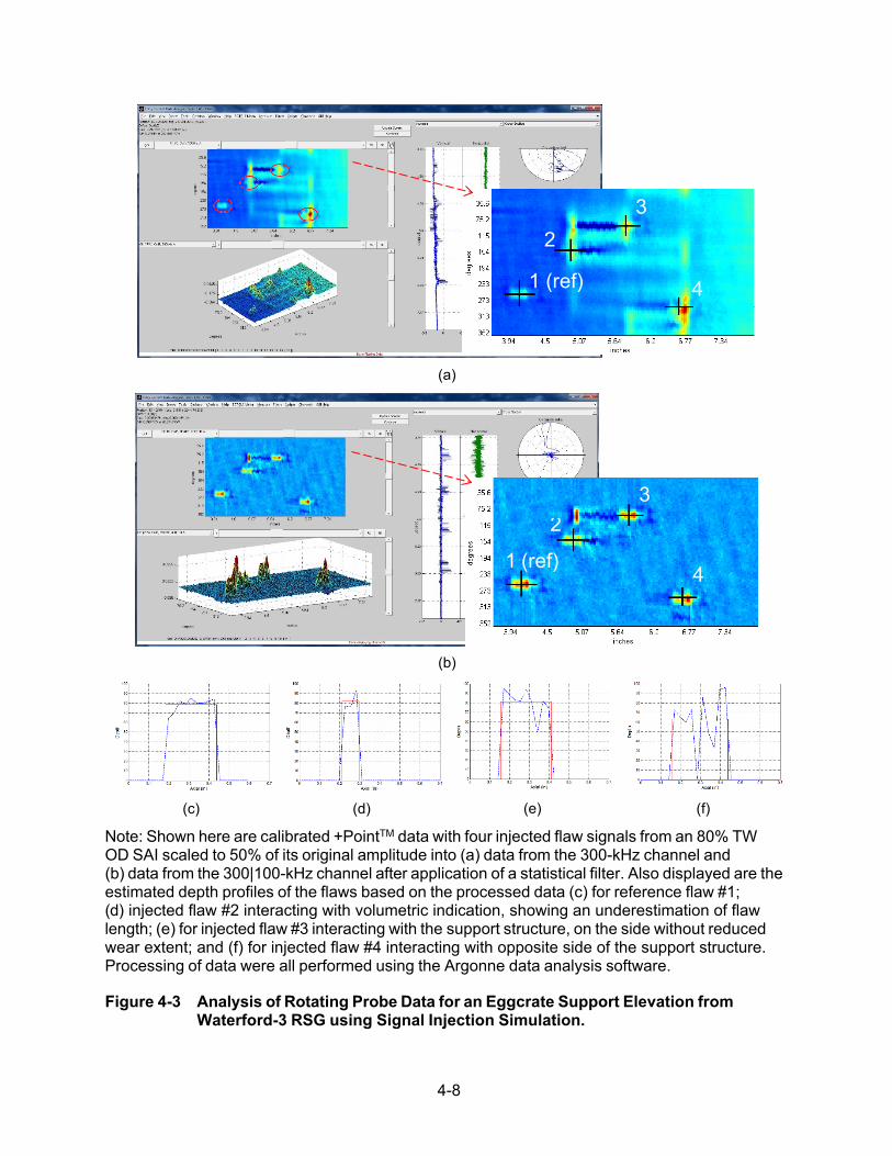
(a)

3 3

2

1 (ref) 4

(b)

(c) (d) (e) (f)

Note: Shown here are calibrated +PointTM data with four injected flaw signals from an 80% TW OD SAI scaled to 50% of its original amplitude into (a) data from the 300-kHz channel and (b) data from the 300|100-kHz channel after application of a statistical filter. Also displayed are theestimated depth profiles of the flaws based on the processed data (c) for reference flaw #1;(d) injected flaw #2 interacting with volumetric indication, showing an underestimation of flawlength; (e) for injected flaw #3 interacting with the support structure, on the side without reducedwear extent; and (f) for injected flaw #4 interacting with opposite side of the support structure.Processing of data were all performed using the Argonne data analysis software.

Figure 4-3 Analysis of Rotating Probe Data for an Eggcrate Support Elevation from Waterford-3 RSG using Signal Injection Simulation.

1 (ref)

4-8

4-9

(a) (b)

(c) (d)

Note: The data were presented in Figure 3-51. Shown here are (a) calibrated +PointTM data from the 300-kHz channel before (top) and after (bottom) injection of an 40% TW OD axial EDM notch at 50% of its original amplitude; (b) processed data after application of a statistical filter followed by smoothing with markers pointing out the injected flaw locations; (c) estimated depth profiles using processed data and (d) 2D and 3D plots of the sizing data, showing amplitude (left) and depth (right).

Figure 4-4 Analysis of Rotating Probe Data from an Oconee OTSG Tube using Flaw Injection Simulation.

1 2

3Ref.

1 2 3

Ref

2 3

Ref

1

5-1

5 DESTRUCTIVE EXAMINATION OF LABORATORY SPECIMENS

In the following sections, a brief description is provided of the methods used to destructively examine the flaws produced in a set of specimens for NDE-related studies. As described in detail in Section 2, the set of specimens assembled at Argonne included nine tube sections made of Alloy 600MA material with 22.2-mm (7/8-in.) OD and 1.27-mm (0.050-in.) nominal wall thickness. The flaws in those tubes consisted of mechanically induced wear scar in conjunction with laboratory-produced ODSCC at the same axial location along the tube. The intended locations of cracks in those tubes are also provided in Section 2. To facilitate DE of flaws by fractography, the tubes were pressure tested up to the limit of the test facility (~7,500 psi). Fractography was then performed to measure the crack size. A description of the DE procedure is provided below, followed by a brief description of the results.

5.1 Destructive Examination Method

The following procedure was implemented for DE of laboratory-produced SCCs in the specimens with the wear scar at the same axial position along the tube. The tubes were first engraved with identification numbers and subsequently photographed. The SCC areas of interest were removed from the tube specimen using a high-speed cutting saw, leaving a ligament of approximately 2.5 mm from the visible crack ends, to keep the fracture surface uncut. When multiple cracks were present in close proximity on a tube, the area was carefully cut and all cracks with separation distances of more than 2.5 mm were separated. Documentation also included information on all of the specimens for which fracture surfaces were cut because the distance between adjacent cracks was too short. The remaining ligaments, if present, were broken manually into two pieces. Shallow cracks that did not open when tubes were burst at high pressure were opened manually by bending the piece back and forth. When the 2.5 mm ligament was too long to open the crack, a file was used to carefully reduce the ligament length until the crack could be opened manually. The two broken pieces were flattened without damaging the fracture surface. The pieces were cleaned individually with methanol in an ultrasonic bath for 10 minutes.

Scanning electron microscope (SEM) images were taken along the fracture surface at 40X or higher magnification. These images were assembled into a montage. Crack length was measured by using SEM with a low magnification calibration standard, or measured directly using a caliper. A crack depth profile was obtained along the length of the montage. The intergranular crack front is distinguishable from the ductile fracture surface induced by the burst testing and manually bending separation and is not affected by the bursting pressure. The ductile fracture surface shows typical dimples and voids and does not show grains and grain boundaries. The distance between the surface and the crack front was measured every 0.25 mm or less. The percentage of the SCC crack depth to the local thickness of the tube was provided. Nominal crack depth can be obtained from the percentage of the SCC crack depth and the nominal tube thickness.

5.2 Destructive Examination Results for Argonne Specimens

The results from DE of nine specimens with a wear scar accompanied by ODSCC are presented in Figures 5-1 to 5-10. Provided in each case are the pressure test data, photographs of the SCC following pressure testing, measured pressure and flow data, the SEM image montage used for fractography measurement, and the depth profile of SCC both with and without a running average filter.

5-2

Figure 5-1 displays the DE results for specimen SG4-150, a tube with a 20% TW wear scar and with axial ODSCC located 180° away. Shown in Figure 5-1(a)–(f), respectively, are pressure and flow data from the rupture test, a photograph of SCC following the rupture test, the pressure and flow data for the burst test, a photograph of SCC following the burst test, the SEM image montage used for fractography, and the measured depth profile of SCC both with and without application of a running average filter. In reference to Figure 5-1(e), the montage made from SEM images shows a rock candy–like appearance of grains observed in the SCC area. Each grain is separated from its neighbors along the grain boundaries that it once shared prior to the flaw manufacturing process. The intergranular crack front is at the boundary of the rock candy–like and non-rock candy–like areas. The crack depths decrease near a small ligament inside the crack.

Figure 5-2 displays the DE results for specimen SG4-151, a tube with a 20% TW wear scar and with axial ODSCC 180° away. Shown in Figure 5-2(a)–(d), respectively, are pressure and flow data from the rupture test, a photograph of SCC following the rupture test, the SEM image montage used for fractography, and the measured depth profile of SCC both with and without application of a running average filter. In reference to Figure 5-2(c), the montage made from SEM images shows a rock candy–like appearance of grains observed in the SCC area. Each grain is separated from its neighbors along the grain boundaries that it once shared prior to the flaw manufacturing process. The intergranular crack front is at the boundary of the rock candy–like and non-rock candy–like areas. The boundaries of the rock candy–like and non-rock candy–like appearances are shown by the images with high magnification.

Figure 5-3 displays the DE results for specimen SG4-152, a tube with a 30% TW wear scar and with axial ODSCC 180° away. Shown in Figure 5-3(a)–(d), respectively, are pressure and flow data from the rupture test, a photograph of SCC following the rupture test, the SEM image montage used for fractography, and the measured depth profile of SCC both with and without application of a running average filter. In reference to Figure 5-3(c), the montage made from SEM images shows a rock candy–like appearance of grains observed in the SCC area. Each grain is separated from its neighbors along the grain boundaries that it once shared prior to the flaw manufacturing process. The intergranular crack front is at the boundary of the rock candy–like and non-rock candy–like areas. The boundaries of the rock candy–like and non-rock candy–like appearances are shown by the images with high magnification. The crack depths decrease to zero near a full ligament at the center of the crack.

Figure 5-4 displays the DE results for specimen SG4-153, a tube with a 30% TW wear scar and with axial ODSCC near the edge of wear scar. Shown in Figure 5-4(a)–(d), respectively, are pressure and flow data from the rupture test, a photograph of SCC following the rupture test, the SEM image montage used for fractography, and the measured depth profile of SCC both with and without application of a running average filter. The crack depth profile is plotted both relative to the remaining wall thickness (SCC plus wear) and relative to the nominal wall thickness of the tube. In reference to Figure 5-4(c), the montage made from SEM images shows a rock candy–like appearance of grains observed in the SCC area. Each grain is separated from its neighbors along the grain boundaries that it once shared prior to the flaw manufacturing process. The intergranular crack front is at the boundary of the rock candy–like and non-rock candy–like areas.

Figure 5-5 displays the DE results for specimen SG4-154, a tube with a 30% TW wear scar and with axial ODSCC inside the wear scar. Shown in Figure 5-5(a)–(d), respectively, are pressure and flow data from the rupture test, a photograph of SCC following the rupture test, the SEM image montage used for fractography, and the measured depth profile of SCC both with and without application of a running average filter. The crack depth profile is plotted both relative to the remaining wall thickness (SCC plus wear) and relative to the nominal wall thickness of the tube. In

5-3

reference to Figure 5-5(c), the montage made from SEM images shows a rock candy–like appearance of grains observed in the SCC area. Each grain is separated from its neighbors along the grain boundaries that it once shared prior to the flaw manufacturing process. The intergranular crack front is at the boundary of the rock candy– and non-rock candy–like areas. The boundaries of the rock candy–like and non-rock candy–like appearances are shown by the images with high magnification.

Figure 5-6 displays the DE results for specimen SG4-156, a tube with a 20%TW wear and with axial ODSCC at 180° away. Shown in Figure 5-6(a)–(f), respectively, are pressure and flow data from the rupture test, a photograph of SCC following the rupture test, pressure and flow data for the burst test, a photograph of SCC following the burst test, the SEM image montage used for fractography, and the measured depth profile of SCC both with and without application of a running average filter. In reference to Figure 5-6(e), the montage made from SEM images shows a rock candy–like appearance of grains observed in the SCC area. Each grain is separated from its neighbors along the grain boundaries that it once shared prior to the flaw manufacturing process. The intergranular crack front is at the boundary of the rock candy–like area and exhibits non-rock candy–like areas.

Figure 5-7 displays the DE results for specimen SG4-157, a tube with a 20% TW wear scar and with a relatively short axial ODSCC near its edge. Shown in Figure 5-7(a)–(d), respectively, are pressure and flow data from the rupture test, a photograph of SCC following the rupture test, the SEM image montage used for fractography, and the measured depth profile of SCC both with and without application of a running average filter. The crack depth profile is plotted both relative to the remaining wall thickness (SCC plus wear) and relative to the nominal wall thickness of the tube. In reference to Figure 5-7(c), the montage made from SEM images shows a rock candy–like appearance of grains observed in the SCC area. Each grain is separated from its neighbors along the grain boundaries that it once shared prior to the flaw manufacturing process. The intergranular crack front is at the boundary of the rock candy–like area and exhibits non-rock candy–like areas.

Figure 5-8 displays the DE results for the secondary crack in specimen SG4-157, displayed in Figure 5-7. Shown in Figure 5-8(a)–(c), respectively, are a photograph of the secondary SCC following the rupture test, the SEM image montage used for fractography, and the measured depth profile of SCC both with and without application of a running average filter. In reference to Figure 5-8(b), the montage made from SEM images shows a rock candy–like appearance of grains observed in the SCC area. Each grain is separated from its neighbors along the grain boundaries that it once shared prior to the flaw manufacturing process. The intergranular crack front is at the boundary of the rock candy–like and non-rock candy–like areas.

Figure 5-9 displays the DE results for specimen SG4-158, a tube with a 20% TW wear scar and with axial ODSCC at the same location. Shown in Figure 5-9(a)–(d), respectively, are pressure and flow data from the rupture test, a photograph of SCC following the rupture test, the SEM image montage used for fractography, and the measured depth profile of SCC both with and without application of a running average filter. The crack depth profile is plotted both relative to the remaining wall thickness (SCC plus wear) and relative to the nominal wall thickness of the tube. In reference to Figure 5-9(c), the montage made from SEM images shows a rock candy–like appearance of grains observed in the SCC area. Each grain is separated from its neighbors along the grain boundaries that it once shared prior to the flaw manufacturing process. The intergranular crack front is at the boundary of the rock candy–like area and exhibits non-rock candy–like areas.

Figure 5-10 displays the DE results for specimen SG4-158, a tube with a 20% TW wear and with axial ODSCC at 0.25 in. (6 mm) away from the wear scar. Shown in Figure 5-10(a)–(d),

5-4

respectively, are pressure and flow data from the rupture test, a photograph of SCC following the rupture test, the SEM image montage used for fractography, and the measured depth profile of SCC both with and without application of a running average filter. In reference to Figure 5-10(c), the montage made from SEM images shows a rock candy–like appearance of grains observed in the SCC area. Each grain is separated from its neighbors along the grain boundaries that it once shared prior to the flaw manufacturing process. The intergranular crack front is at the boundary of the rock candy–like area and exhibits non-rock candy–like areas. Although the DE profile in Figure 5-10(d) shows a maximum flaw depth of 100% TW, the tube did not leak until reaching a very high pressure because of the short extent of the crack.

5-5

(a)

(b)

(c)

(d)

(e)

(f)

Note: Shown here are (a) pressure and flow data for the rupture test, (b) a photograph of SCC following the rupture test, (c) pressure and flow data for the burst test, (d) a photograph of SCC following the burst test, (e) the SEM image montage used for fractography, and (f) the fractography depth profile of SCC both with and without a running average (RA) filter.

Figure 5-1 Pressure Testing and DE Results for Specimen SG4-150.

0 20 40 60 80 100 120 140 160 180 200-500

0

500

1000

1500

2000

2500

3000

3500Pr

essu

re (P

SI)

Time (s)0 20 40 60 80 100 120 140 160 180 200

0

5

10

15

Flow

(GPM

)

0 20 40 60 80 100 120-500

0

500

1000

1500

2000

2500

3000

3500

Pres

sure

(PSI

)

Time (s)0 20 40 60 80 100 120

0

2

4

6

8

10

12

14

Flow

(GPM

)

-0.1 0 0.1 0.2 0.3 0.4 0.5 0.6 0.70

10

20

30

40

50

60

70

80

90

100

Relative Axial Location (in)

Cra

ck D

epth

(%TW

)

Depth (%)RA

5-6

(a)

(b)

(c)

(d)

Note: Shown here are (a) pressure and flow data for the rupture test, (b) a photograph of SCC following the rupture test, (c) the SEM image montage used for fractography, and (d) the fractography depth profile of SCC both with and without a RA filter.


0 50 100 150 200 250 300

0

1000

2000

3000

4000

5000

Pres

sure

(PSI

)

Time (s)0 50 100 150 200 250 300

0

5

10

15

Flow

(GPM

)

-0.2 0 0.2 0.4 0.6 0.8 10

10

20

30

40

50

60

70

80

90

100


Cra

ck D

epth

(%TW

)

Depth (%)RA

5-7

(a)

(b)

(c)

(d)



0 20 40 60 80 100 120 140 160 180

0

1000

2000

3000

4000

5000

6000

7000Pr

essu

re (P

SI)

Time (s)0 20 40 60 80 100 120 140 160 180

0

5

10

15

Flow

(GPM

)

-0.1 0 0.1 0.2 0.3 0.4 0.5 0.60

10

20

30

40

50

60

70

80

90

100


Cra

ck D

epth

(%TW

)

Depth (%)RA

5-8

(a)

(b)

(c)

(d)

Note: Shown here are (a) pressure and flow data for the rupture test, (b) a photograph of SCC following the rupture test, (c) the SEM image montage used for fractography, and (d) the fractography depth profile of SCC both with and without a RA filter. Depth profiles are plotted relative to both the remaining wall thickness (red) and to the nominal wall thickness (green).


0 20 40 60 80 100 120 140-500

0

500

1000

1500

2000

2500

3000

3500

4000

Pres

sure

(PSI

)

Time (s)0 20 40 60 80 100 120 140

0

5

10

15

Flow

(GPM

)

0 0.1 0.2 0.3 0.40

10

20

30

40

50

60

70

80

90

100


Cra

ck D

epth

(%TW

)

Depth vs Wear wallRA for Depth vs WearDepth vs Tube wall

5-9

(a)

(b)

(c)

(d)

Note: Shown here are (a) pressure and flow data for the rupture test, (b) a photograph of SCC following the rupture test, (c) the SEM image montage used for fractography, and (d) fractography depth profile of SCC both with and without a RA filter. Depth profiles are plotted relative to both the remaining wall thickness (red) and to the nominal wall thickness (green).


0 20 40 60 80 100 120

0

1000

2000

3000

4000

5000

6000

7000

Pres

sure

(PSI

)

Time(s)0 20 40 60 80 100 120

0

5

10

15

Flow

(GPM

)

-0.1 0 0.1 0.2 0.3 0.4 0.5 0.6 0.70

10

20

30

40

50

60

70

80

90

100


Cra

ck D

epth

(%TW

)


5-10

(a)

(b)

(c)

(d)

(e)

(f)

Note: Shown here are (a) pressure and flow data for the rupture test, (b) a photograph of SCC following the rupture test, (c) pressure and flow data for the burst test, (d) a photograph of SCC following the burst test, (e) SEM image montage used for fractography, and (f) the fractography depth profile of SCC both with and without a RA filter.


0 20 40 60 80 100 120-500

0

500

1000

1500

2000

2500

3000

3500

4000

4500Pr

essu

re (P

SI)

Time (s)0 20 40 60 80 100 120

0

5

10

15

Flow

(GPM

)

0 20 40 60 80 100 120 140 160-500

0

500

1000

1500

2000

2500

3000

3500

4000

Pres

sure

(PSI

)

Time (s)0 20 40 60 80 100 120 140 160

0

5

10

15

Flow

(GPM

)

-0.1 0 0.1 0.2 0.3 0.4 0.5 0.6 0.70

10

20

30

40

50

60

70

80

90

100


Cra

ck D

epth

(%TW

)

Depth (%)RA

5-11

(a) (b)

(c)

(d)

Note: Shown here are (a) pressure and flow data for the rupture test, (b) a photograph of the primary SCC (SG4-157 a) following the rupture test, (c) the SEM image montage used for fractography, and (d) the fractography depth profile of SCC both with and without a RA filter. Depth profiles are plotted relative to both the remaining wall thickness (red) and to the nominal wall thickness (green).

Figure 5-7 Pressure Testing and DE Results for the Primary Crack in Specimen SG4-

157.

0 0.5 1 1.5 20

10

20

30

40

50

60

70

80

90

100


Cra

ck D

epth

(%TW

)


5-12

(a)

(b)

(c)

Note: Shown here are (a) a photograph of the secondary SCC (SG4-157b) following the rupture test, (b) the SEM image montage used for fractography, and (c) the fractography depth profile of SCC both with and without a RA filter.

Figure 5-8 DE Results for the Secondary Crack in Specimen SG4-157.

0 0.5 1 1.5 20

10

20

30

40

50

60

70

80

90

100


Cra

ck D

epth

(%TW

)

Depth (%)RA

5-13

(a)

(b)

(c)

(d)

Note: Shown here are (a) pressure and flow data for the rupture test, (b) a photograph of SCC following the rupture test, (c) the SEM image montage used for fractography, and (d) the fractography depth profile of SCC both with and without a RA filter. Depth profiles are plotted relative to both the remaining wall thickness (red) and to the nominal wall thickness (green).


0 10 20 30 40 50 60 70 80 90

0

1000

2000

3000

4000

5000

6000Pr

essu

re (P

SI)

Time (s)0 10 20 30 40 50 60 70 80 90

0

5

10

15

Flow

(GPM

)

0 0.2 0.4 0.6 0.8 1 1.2 1.4 1.6 1.8 20

10

20

30

40

50

60

70

80

90

100


Cra

ck D

epth

(%TW

)


5-14

(a)

(b)

(c)

(d)



0 10 20 30 40 50 60 70 80 90

0

1000

2000

3000

4000

5000

6000

7000Pr

essu

re (P

SI)

Time (s)0 10 20 30 40 50 60 70 80 90

0

5

10

15

Flow

(GPM

)

-0.05 0 0.05 0.1 0.15 0.20

10

20

30

40

50

60

70

80

90

100


Cra

ck D

epth

(%TW

)

Depth (%)RA

6-1

6 SUMMARY AND CONCLUSIONS

Research was conducted at Argonne to assess the ability of conventional EC inspection techniques to detect and characterize cracks located at the same axial elevation as a volumetric flaw in a SG tube. Investigations were also carried out on alternative signal processing methods that could help improve the detection of a crack-like signal affected by interaction with a more dominant volumetric signal. A set of specimens containing a wear scar and SCC located at the same axial position along the tube were manufactured in-house for this study. Cracks were produced at different circumferential positions relative to the mechanically induced wear mark in each tube. Production of laboratory specimens was described in Section 2. The procedures for the manufacturing of flaws and post-manufacturing examination of the specimens were discussed in that section.

EC inspection of the specimens with laboratory-produced flaws was described in Section 3.1. Bobbin and rotating probe examinations were performed in accordance with generic EC examination techniques. The specimens were inspected at different stages of the flaw manufacturing process. The EC data were subsequently analyzed using conventional data analysis methods. Analyses of bobbin and rotating probe data for all of the specimens were presented in Section 3.2. A systematic study was also conducted to assess the effect of background interference from volumetric flaws and support structures on detection of nearby cracks using a bobbin probe. Data used in this study were generated by superimposing signals from wear, TSP, and SCC at different proximities to each other. The results of that investigation were presented in Section 3.3.

Some observations made based on the results of research conducted initially in this work to assess the conventional EC inspection techniques are summarized below.

• Detection of EC signals associated with OD-initiated cracks located in close proximity to

relatively shallow volumetric degradation, such as a wear scar, can pose a challenge to all conventional EC examination techniques employed for ISI of SG tubes. Other potential sources of signal interference that could complicate the analysis of EC data include extraneous discontinuities such as tube support structures and deposits.

• The interaction distance between the signals from a crack with those from a volumetric

flaw is dependent on both the physical separation between the two and on the probe’s sensing area (coverage), which is dictated by the probe design and the operating frequency. While rotating probe examinations allow discrimination of multiple flaws around the tube circumference (i.e., coplanar flaws), the ability of such probes to discriminate between individual signals is nevertheless limited by the interaction distance between flaws. Hence, supplementary rotating probe examinations may not always allow detection or proper characterization of low-amplitude signals of interest in the presence of a large background interference.

• Because of their lack of circumferential resolution, the existence of ODSCC at the same

tube location as a volumetric flaw could pose an even greater challenge to conventional bobbin probe examination techniques. Intrinsically, bobbin probe response from coplanar discontinuities is always in the form of a composite signal, irrespective of the circumferential separation. As such, detection of coplanar ODSCC with a wear scar may be unreliable when conventional data analysis procedures are used. Therefore, if the potential for such a damage mechanism exists at a particular site, the decision to conduct supplementary examinations based on a measurable change in bobbin probe signal from

6-2

the previous inspection may not be considered as a conservative approach. Conversely, indications of cracking near a volumetric flaw identified through analysis of bobbin probe data cannot not be positively dismissed due to the lack of a confirmatory signal in rotating probe data.

In view of the limitations associated with conventional data analysis methods, when dealing with complex modes of degradation such as cracking near volumetric flaws, we conducted systematic studies to assess alternative data analysis methods that could improve detection of weak signals in the presence of large background signals. A number of approaches were evaluated for enhancing discrimination of signals of interest through increasing the signal-to-noise ratio. These included independent suppression of unwanted signals using spatial and frequency domain filters, as well as background suppression algorithms using data from prior inspections.

A description of the algorithms implemented in this work for suppression of background signals was provided in Section 3.4. Both spatially 1D and 2D background subtraction methods were evaluated for processing of EC examination data. Only 1D subtraction schemes were evaluated in application to processing of bobbin probe data. Both 1D and 2D subtraction schemes were evaluated in application to processing of rotating probe data. Evaluation of historical background subtraction routines was performed using both actual and simulated data generated through signal superposition. The data sets included bobbin and rotating probe data on laboratory specimens from Argonne and AECL. Evaluations were also carried out using a limited set of data from tubes with field-induced damage and degradation. The results of those studies were presented in Sections 3.6 to 3.8. In addition to historical data subtraction methods, the use of conventional spatial domain and statistical filters for suppression of unwanted signals were also evaluated.

From observations made based on the results of background subtraction methods, a viable conclusion is that subtraction of background using historical data provides the most effective approach to suppressing the interference from volumetric signals while maintaining the signals associated with cracking. When appropriate historical data are not available, application of signal processing methods including spatial domain and statistical filters can improve detection and characterization of flaw signals in the presence of background interference.

Current industry guidelines, in general, allow the use of filtering routines for detection purposes during the data-screening stage. Proper application of background suppression algorithms to the current data could help improve detection and characterization of complex signals. Care, however, should be taken when filters are applied to the data. Improper application of filtering algorithms can potentially eliminate signals of interest.

Consistency of the EC examination technique’s essential variables as well as consistency of test conditions between the current and the historical data are key factors affecting suppression of unwanted background signals. The applicability of historical subtraction is based on the assumption that the background signal is rather stationary. As such, suppression of background signals, and in turn detection of potential nearby crack signals, cannot be performed effectively if the change in the background signal between inspections is comparable to the change in signal associated with initiation or growth of nearby cracking. Flaw detection is less reliable when the current and historical inspection data are more closely spaced in time.

The use of EC examination data from earlier inspections, including the baseline data from pre- service inspection, can help improve detectability of flaw signals at an earlier stage. When

6-3

appropriate historical data are not available, application of signal processing routines could help improve detection of flaw signals in the presence of background interference.

Although the assessments in this work focused on the ability of EC inspection techniques to detect cracks that may occur in conjunction with volumetric flaws, efforts were made to estimate the size of flaws in Argonne laboratory-produced specimens with a wear scar and ODSCC. The results of that study were presented in Section 4.1. Limited studies, using simulated EC data, were also carried out to assess the effect of background interference on the sizing results. The EC data were generated by superimposing known crack signals at different locations near a volumetric flaw in a tube. The results of that study were presented in Section 4.2. In general, while background suppression algorithms evaluated in this work are effective in suppressing volumetric signals, the reliability of EC sizing results is dependent on a number of factors including the spatial separation (degree of interaction) between the SCC and the volumetric signal and relative strength of the crack signal to volumetric signal (S/N).

Assessment of EC examination technique capability with regard to detection of cracking near volumetric degradation was ultimately evaluated through comparison of NDE with DE data for the laboratory-produced specimens at Argonne. The procedure for DE of laboratory-produced SCCs in the Argonne specimens were presented in Section 5.1. The results of that work were presented in Section 5.2.

It is relevant to note that the background suppression schemes evaluated in this work could be adapted to processing of data for a wider range of EC inspection applications, such as detection of subtle signals influenced by interference from slowly varying indications, and in the presence of extraneous SG tubing discontinuities. Finally, it is worth noting that future research activities on implementation of improved signal processing and data analysis techniques for detection and characterization of signals interacting with large background signals could leverage the existing EC and DE database assembled at Argonne under this program.

7-1

7 REFERENCES

[1] Bahn, C.B., S. Bakhtiari, J. Park, and S. Majumdar, “Manufacturing of Representative Axial Stress Corrosion Cracks in Tube Specimens,” Nucl. Eng. Des. 256 (2013), 38-– 44.

[2] Majumdar, S., C. Bahn, K. Kasza, and S. Bakhtiari, “Technical Letter Report on Validation of the Equivalent Rectangular Crack Method,” ANL-08/26, U.S. Nuclear Regulatory Commission, ADAMS Accession No. ML090830126, 2009.

[3] Majumdar, S., S. Bakhtiari, K. Kasza, and J. Y. Park, “Validation of Failure and Leak Rate Correlations for Stress Corrosion Cracks in Steam Generator Tubes,” U.S. Nuclear Regulatory Commission, NUREG/CR–6774ANL–01/34, Dec. 2001.

[4] Pressurized Water Reactor Steam Generator Examination Guidelines: Revision 7, Requirements, Electric Power Research Institute, Palo Alto, CA (2006).

[5] Obrutsky, L., J. Lu, and B. Cassidy, “Correlation of ET Probe Responses to Small Circumferential Cracking in the Presence of Volumetric Flaws,” COG report TN-03- 4029, March 2004.

[6] Bakhtiari, S., and T. W. Elmer, ”Technical Letter Report on Development of Flaw Sizing Algorithms for Eddy Current Rotating Probe Examinations,” U.S. Nuclear Regulatory Commission, ADAMS Accession No. ML090690837, Sept. 2008.

A-1

APPENDIX A – APPLICATION OF BACKGROUND SUPPRESSION TO DATA FROM ARGONNE’S TUBE SPECIMENS

In reference to what was presented in Section 3.6, data analysis results are presented here on the application of historical background subtraction to help improve detection of cracks present at the same axial position as a volumetric flaw. The dataset used in this study consisted of EC bobbin and rotating probe inspection data collected from tube specimens with wear scars in conjunction with laboratory-produced outer-diameter SCC (ODSCC). A description of the flaws in those specimens was provided in Section 2.1. The initial results based on manual analysis of the data were presented in Section 3.2. A description of the methods used for processing of the data was provided in Section 3.6.

A-2

(a)

(b)

(c)

(d)

(e)

(f)

Note: Shown here are (a) the vertical component of calibrated wear (blue) and wear plus SCC (red) data, (b) the vertical component of resampled and aligned data, (c) difference signal highlighting one side of the flaw in blue, (d) lissajous plot of (c), (e) difference signal highlighting the other side of the flaw in blue, and (f) lissajous plot of (e). Plots (d) and (f) display historical (grey), current (light red) and difference (blue) traces, with the segment of interest highlighted in red.

Figure A-1 1D Subtraction on 200-kHz Bobbin Probe Data for SG4-150, a Specimen

with SCC Opposite of a 20% TW Wear Scar.

0 50 100 150 200 250 300 350 400

-3

-2

-1

0

1

2

V-co

mp.

WearWear+SCC

0 50 100 150 200 250 300 350 400

-2

-1

0

1

2

3

V-co

mp.

(alig

ned)

WearWear+SCC

0 50 100 150 200 250 300 350 400

-1.5

-1

-0.5

0

0.5

1

1.5

∆V &

∆H

V-Comp.H-Comp.

-1 -0.5 0 0.5 1

-1.5

-1

-0.5

0

0.5

1

1.5

2

∆V-c

omp.

∆H-comp.

0 50 100 150 200 250 300 350 400

-1.5

-1

-0.5

0

0.5

1

1.5

∆V &

∆H

V-Comp.H-Comp.

-1 -0.5 0 0.5 1

-1.5

-1

-0.5

0

0.5

1

1.5

2

∆V-c

omp.

∆H-comp.

A-3

(a)

(b)

(c)

(d)

(e)

(f)

Note: Shown here are (a) historical data (wear without SCC); (b) current data (wear plus SCC); (c) a lissajous plot for the entire ROI (d) difference plot; (e) a cross-section across wear, including SCC; and (f) a cross-section across wear, not including SCC. Plots (c), (e), and (f) all display historical (grey), current (red), and difference (blue) traces.

Figure A-2 2D Subtraction on 300-kHz +PointTM Data for SG4-150, a Specimen with

SCC Opposite of a 20% TW Wear Scar.

Ax. scale (pts.)

Cr.

scal

e (p

ts.)

20 40 60 80 100

10

20

30

40

50

60

70

80

90 -0.4

-0.3

-0.2

-0.1

0

0.1

0.2

0.3

0.4

Ax. scale (pts.)

Cr.

scal

e (p

ts.)

20 40 60 80 100

10

20

30

40

50

60

70

80

90 -0.4

-0.3

-0.2

-0.1

0

0.1

0.2

0.3

0.4

-0.6 -0.4 -0.2 0 0.2 0.4 0.6

-0.3

-0.2

-0.1

0

0.1

0.2

0.3

0.4

∆H-comp.

∆V-c

omp.

Ax. scale (pts.)

Cr.

scal

e (p

ts.)

20 40 60 80 100

10

20

30

40

50

60

70

80

90-0.1

0

0.1

0.2

0.3

0.4

-0.6 -0.4 -0.2 0 0.2 0.4 0.6

-0.3

-0.2

-0.1

0

0.1

0.2

0.3

0.4

∆H-comp.

∆V-c

omp.

-0.6 -0.4 -0.2 0 0.2 0.4 0.6

-0.3

-0.2

-0.1

0

0.1

0.2

0.3

0.4

∆H-comp.

∆V-c

omp.

A-4

(a)

(b)

(c)

(d)

(e)

(f)

Note: (a) the vertical components of calibrated wear (blue) and wear plus SCC (red) data, (b) the vertical components of resampled and aligned data, (c) the difference signal highlighting one side of the flaw in blue, (d) the lissajous plot of (c), (e) the difference signal highlighting the other side of the flaw in blue, and (f) the lissajous plot of (e). (d) and (f) display historical (grey), current (light red), and difference (blue) traces, with the segment of interest in red. Figure A-3 1D Subtraction on 200-kHz Bobbin Probe Data for SG4-151, a Specimen


0 50 100 150 200 250 300 350 400

-3

-2

-1

0

1

2

3

V-co

mp.

WearWear+SCC

0 50 100 150 200 250 300 350 400

-3

-2

-1

0

1

2

3

V-co

mp.

(alig

ned)

WearWear+SCC

0 50 100 150 200 250 300 350 400

-2

-1.5

-1

-0.5

0

0.5

1

1.5

2

∆V &

∆H

V-Comp.H-Comp.

-1 0 1

-2

-1.5

-1

-0.5

0

0.5

1

1.5

2

2.5

∆V-c

omp.

∆H-comp.

0 50 100 150 200 250 300 350 400

-2

-1.5

-1

-0.5

0

0.5

1

1.5

2

∆V &

∆H

V-Comp.H-Comp.

-1 0 1

-2

-1.5

-1

-0.5

0

0.5

1

1.5

2

2.5

∆V-c

omp.

∆H-comp.

A-5

(

(a)

(b)

(c)

(d)

(e)

(f)

Note: Shown here are (a) historical data (wear without SCC); (b) current data (wear plus SCC); (c) a lissajous plot for the entire ROI; (d) the difference plot; (e) a cross-section across wear, including SCC; and (f) cross-section across wear, not including SCC. Plots (c), (e), and (f) all display historical (grey), current (red), and difference (blue) traces. Figure A-4 2D Subtraction on 300-kHz +PointTM Data for SG4-151, a Specimen with


Ax. scale (pts.)

Cr.

scal

e (p

ts.)

10 20 30 40 50 60 70 80 90

10

20

30

40

50

60

70

80

90-0.6

-0.4

-0.2

0

0.2

0.4

0.6

Ax. scale (pts.)

Cr.

scal

e (p

ts.)

10 20 30 40 50 60 70 80 90

10

20

30

40

50

60

70

80

90-0.6

-0.4

-0.2

0

0.2

0.4

0.6

-0.8 -0.6 -0.4 -0.2 0 0.2 0.4 0.6 0.8-0.4

-0.2

0

0.2

0.4

0.6

∆H-comp.

∆V-c

omp.

Ax. scale (pts.)

Cr.

scal

e (p

ts.)

10 20 30 40 50 60 70 80 90

10

20

30

40

50

60

70

80

90-0.2

-0.1

0

0.1

0.2

0.3

0.4

0.5

0.6

-0.8 -0.6 -0.4 -0.2 0 0.2 0.4 0.6 0.8-0.4

-0.2

0

0.2

0.4

0.6

∆H-comp.

∆V-c

omp.

-0.8 -0.6 -0.4 -0.2 0 0.2 0.4 0.6 0.8-0.4

-0.2

0

0.2

0.4

0.6

∆H-comp.

∆V-c

omp.

A-6

(a)

(b)

(c)

(d) (e)

(f)

(g)

Note: Shown here are (a) the vertical component of calibrated wear (blue) and wear+SCC (red) data, (b) the vertical component of resampled and aligned data, (c) difference signal highlighting one side of the flaw in blue, (d,e) lissajous plots of (c) shown with and without raw data traces, (f) difference signal highlighting the other side of the flaw in blue, and (g) lissajous plot of (f). Plots (d), (e), and (g) show difference (blue) traces, with the segment of interest highlighted in red. Plot (d) also displays historical (grey) and current (light red) traces.



0 50 100 150 200 250 300 350 400

-4

-3

-2

-1

0

1

2

3

4

V-co

mp.

WearWear+SCC

0 50 100 150 200 250 300 350 400

-4

-3

-2

-1

0

1

2

3

4

V-co

mp.

(alig

ned)

WearWear+SCC

0 50 100 150 200 250 300 350 400

-0.6

-0.4

-0.2

0

0.2

0.4

0.6

∆V &

∆H

V-Comp.H-Comp.

-2 -1 0 1 2-3

-2

-1

0

1

2

3

∆V-c

omp.

∆H-comp.-0.5 0 0.5

-0.8

-0.6

-0.4

-0.2

0

0.2

0.4

0.6

∆V-c

omp.

∆H-comp.

0 50 100 150 200 250 300 350 400

-0.6

-0.4

-0.2

0

0.2

0.4

0.6

∆V &

∆H

V-Comp.H-Comp.

-0.6 -0.4 -0.2 0 0.2 0.4-0.8

-0.6

-0.4

-0.2

0

0.2

0.4

0.6

∆V-c

omp.

∆H-comp.

A-7

(a)

(b)

(c)

(d)

(e)

(f)

Note: Shown here are (a) historical data (wear without SCC); (b) current data (wear plus SCC); (c) a lissajous plot for the entire ROI; (d) the difference plot; (e) a cross-section across wear, including SCC; and (f) cross-section across wear, not including SCC. Plots (c), (e), and (f) all display historical (grey), current (red), and difference (blue) traces.



Ax. scale (pts.)

Cr.

scal

e (p

ts.)

50 100 150 200

10

20

30

40

50

60

70

80

90 -0.6

-0.4

-0.2

0

0.2

0.4

0.6

Ax. scale (pts.)

Cr.

scal

e (p

ts.)

50 100 150 200

10

20

30

40

50

60

70

80

90 -0.6

-0.4

-0.2

0

0.2

0.4

0.6

-0.8 -0.6 -0.4 -0.2 0 0.2 0.4 0.6 0.8

-0.6

-0.4

-0.2

0

0.2

0.4

∆H-comp.

∆V-c

omp.

Ax. scale (pts.)

Cr.

scal

e (p

ts.)

50 100 150 200

10

20

30

40

50

60

70

80

90-0.2

-0.1

0

0.1

0.2

0.3

0.4

-0.8 -0.6 -0.4 -0.2 0 0.2 0.4 0.6 0.8

-0.6

-0.4

-0.2

0

0.2

0.4

∆H-comp.

∆V-c

omp.

-0.8 -0.6 -0.4 -0.2 0 0.2 0.4 0.6 0.8

-0.6

-0.4

-0.2

0

0.2

0.4

∆H-comp.

∆V-c

omp.

A-8

(a)

(b)

(c)

(d)

Note: Shown here are (a) the vertical components of calibrated wear (blue) and wear plus SCC (red) data, (b) the vertical components of resampled and aligned data, (c) the difference signal highlighting the flaw in blue, and (d) the lissajous plot of (c). Plot (d) displays historical (grey), current (light red), and difference (blue) traces, with the segment of interest highlighted in red.



0 50 100 150 200 250 300 350 400-4

-3

-2

-1

0

1

2

V-co

mp.

WearWear+SCC

0 50 100 150 200 250 300 350 400-3

-2

-1

0

1

2

3

V-co

mp.

(alig

ned)

WearWear+SCC

0 50 100 150 200 250 300 350 400

-1.5

-1

-0.5

0

0.5

1

∆V &

∆H

V-Comp.H-Comp.

-1 -0.5 0 0.5 1

-1.5

-1

-0.5

0

0.5

1

1.5

2

∆V-c

omp.

∆H-comp.

A-9

(a)

(b)

(c)

(d)

(e)

(f)

Note: Shown here are (a) historical data (wear without SCC); (b) current data (wear plus SCC); (c) a lissajous plot for the entire ROI; (d) the difference plot; (e) a cross-section across wear, including SCC; and (f) a cross-section across wear, not including SCC. Plots (c), (e), and (f) all display historical (grey), current (red), and difference (blue) traces.



Ax. scale (pts.)

Cr.

scal

e (p

ts.)

20 40 60 80 100 120

10

20

30

40

50

60

70

80

90-0.5

0

0.5

Ax. scale (pts.)

Cr.

scal

e (p

ts.)

20 40 60 80 100 120

10

20

30

40

50

60

70

80

90-0.5

0

0.5

-0.8 -0.6 -0.4 -0.2 0 0.2 0.4 0.6 0.8

-0.4

-0.3

-0.2

-0.1

0

0.1

0.2

0.3

0.4

0.5

∆H-comp.

∆V-c

omp.

Ax. scale (pts.)

Cr.

scal

e (p

ts.)

20 40 60 80 100 120

10

20

30

40

50

60

70

80

90 -0.1

0

0.1

0.2

0.3

0.4

0.5

-0.8 -0.6 -0.4 -0.2 0 0.2 0.4 0.6 0.8

-0.4

-0.3-0.2

-0.1

00.1

0.2

0.30.4

0.5

∆H-comp.

∆V-c

omp.

-0.8 -0.6 -0.4 -0.2 0 0.2 0.4 0.6 0.8

-0.4

-0.3-0.2

-0.1

00.1

0.2

0.30.4

0.5

∆H-comp.

∆V-c

omp.

A-10

(a) (b)

(c) (d)

Note: Shown here are (a) the vertical components of calibrated wear (blue) and wear plus SCC (red) data, (b) the vertical components of resampled and aligned data, (c) the difference signal highlighting the flaw in blue, and (d) the lissajous plots of (c) shown both with and without raw data traces. Plots in (d) show difference (blue) traces, with the segment of interest highlighted in red. Plot (d) also displays historical (grey) and current (light red) traces.

Figure A-9 1D Subtraction on 200-kHz Bobbin Probe Data for SG4-159, a Specimen with SCC ~0.25-in. (6 mm) Away from a 20% TW Wear Scar

0 50 100 150 200 250 300 350 400

-2

-1.5

-1

-0.5

0

0.5

1

1.5

2V-

com

p.

WearWear+SCC

0 50 100 150 200 250 300 350 400

-2

-1.5

-1

-0.5

0

0.5

1

1.5

2

V-co

mp.

(alig

ned)

WearWear+SCC

0 50 100 150 200 250 300 350 400

-0.5

0

0.5

∆V &

∆H

V-Comp.H-Comp. -1 -0.5 0 0.5 1

-1.5

-1

-0.5

0

0.5

1

∆V-c

omp.

∆H-comp.-0.2 0 0.2 0.4

-0.5

-0.4

-0.3

-0.2

-0.1

0

0.1

0.2

0.3

0.4

∆V-c

omp.

∆H-comp.

A-11

(a)

(b)

(c)

(d)

(e)

(f)



SCC ~0.25-in. (6 mm) Away from a 20% TW Wear Scar.

Ax. scale (pts.)

Cr.

scal

e (p

ts.)

10 20 30 40 50 60 70 80

10

20

30

40

50

60

70-0.4

-0.3

-0.2

-0.1

0

0.1

0.2

0.3

0.4

Ax. scale (pts.)

Cr.

scal

e (p

ts.)

10 20 30 40 50 60 70 80

10

20

30

40

50

60

70-0.4

-0.3

-0.2

-0.1

0

0.1

0.2

0.3

0.4

-0.6 -0.4 -0.2 0 0.2 0.4 0.6

-0.4

-0.3

-0.2

-0.1

0

0.1

0.2

0.3

∆H-comp.

∆V-c

omp.

Ax. scale (pts.)

Cr.

scal

e (p

ts.)

10 20 30 40 50 60 70 80

10

20

30

40

50

60

70 -0.2

-0.15

-0.1

-0.05

0

0.05

0.1

0.15

0.2

0.25

-0.6 -0.4 -0.2 0 0.2 0.4

-0.4

-0.3

-0.2

-0.1

0

0.1

0.2

0.3

∆H-comp.

∆V-c

omp.

-0.6 -0.4 -0.2 0 0.2 0.4 0.6

-0.4

-0.3

-0.2

-0.1

0

0.1

0.2

0.3

∆H-comp.

∆V-c

omp.

A-12

(a) (b)

(c) (d)

Note: Shown here are (a) the vertical components of calibrated wear (blue) and wear plus SCC (red) data, (b) the vertical components of resampled and aligned data, (c) the difference signal highlighting the flaw in blue, and (d) a lissajous plot of (c). Plot (d) displays historical (grey), current (light red), and difference (blue) traces, with the segment of interest highlighted in red.

Figure A-11 1D Subtraction on 200-kHz Bobbin Probe Data for SG4-153, a Specimen with SCC near the Edge of a 30% TW Wear Scar.

0 50 100 150 200 250 300 350 400

-4

-3

-2

-1

0

1

2

3

4

V-co

mp.

WearWear+SCC

0 50 100 150 200 250 300 350 400

-4

-3

-2

-1

0

1

2

3

4

V-co

mp.

(alig

ned)

WearWear+SCC

0 50 100 150 200 250 300 350 400

-2

-1.5

-1

-0.5

0

0.5

1

1.5

2

∆V &

∆H

V-Comp.H-Comp.

-2 -1 0 1 2

-3

-2

-1

0

1

2

3

∆V-c

omp.

∆H-comp.

A-13

(a)

(b)

(c)

(d)

(e)

(f)



SCC near the Edge of a 30% TW Wear Scar.

Ax. scale (pts.)

Cr.

scal

e (p

ts.)

10 20 30 40 50 60 70 80

10

20

30

40

50

60

70 -0.8

-0.6

-0.4

-0.2

0

0.2

0.4

0.6

0.8

Ax. scale (pts.)

Cr.

scal

e (p

ts.)

10 20 30 40 50 60 70 80

10

20

30

40

50

60

70 -0.8

-0.6

-0.4

-0.2

0

0.2

0.4

0.6

0.8

-1 -0.5 0 0.5 1

-0.8

-0.6

-0.4

-0.2

0

0.2

0.4

0.6

∆H-comp.

∆V-c

omp.

Ax. scale (pts.)

Cr.

scal

e (p

ts.)

10 20 30 40 50 60 70 80

10

20

30

40

50

60

70-0.4

-0.2

0

0.2

0.4

0.6

-1 -0.5 0 0.5 1

-0.8

-0.6

-0.4

-0.2

0

0.2

0.4

0.6

∆H-comp.

∆V-c

omp.

-1 -0.5 0 0.5 1

-0.8

-0.6

-0.4

-0.2

0

0.2

0.4

0.6

∆H-comp.

∆V-c

omp.

A-14

(a) (b)

(c) (d)

Note: Shown here are (a) the vertical components of calibrated wear (blue) and wear plus SCC (red) data, (b) the vertical components of resampled and aligned data, (c) the difference signal highlighting the flaw in blue, and (d) lissajous plots of (c) shown with and without original data traces. Plots in (d) show difference (blue) traces, with the segment of interest highlighted in red. Plot (d) also displays historical (grey) and current (light red) traces.

Figure A-13 1D Subtraction on 200-kHz Bobbin Probe Data for SG4-157, a Specimen with SCC near the Edge of a 20% TW Wear Scar.

0 50 100 150 200 250 300 350 400

-2

-1.5

-1

-0.5

0

0.5

1

V-co

mp.

WearWear+SCC

0 50 100 150 200 250 300 350 400

-2

-1.5

-1

-0.5

0

0.5

1

1.5

2

V-co

mp.

(alig

ned)

WearWear+SCC

0 50 100 150 200 250 300 350 400

-0.4

-0.2

0

0.2

0.4

0.6

∆V &

∆H

V-Comp.H-Comp.

-1 -0.5 0 0.5-1.5

-1

-0.5

0

0.5

1

∆V-c

omp.

∆H-comp.-0.4 -0.2 0

-0.5

-0.4

-0.3

-0.2

-0.1

0

0.1

0.2

0.3

0.4

∆V-c

omp.

∆H-comp.

A-15

(a)

(b)

(c)

(d)

(e)

(f)

Note: Shown here are (a) historical data (wear without SCC); (b) current data (wear plus SCC); (c) a lissajous plot for the entire ROI; (d) the difference plot, (e) a cross-section across wear, including SCC; and (f) a cross-section across wear, not including SCC. Plots (c), (e), and (f) all display historical (grey), current (red), and difference (blue) traces.


SCC near the Edge of a 20% TW Wear Scar.

Ax. scale (pts.)

Cr.

scal

e (p

ts.)

10 20 30 40 50 60 70 80 90

10

20

30

40

50

60 -0.4

-0.3

-0.2

-0.1

0

0.1

0.2

0.3

0.4

Ax. scale (pts.)

Cr.

scal

e (p

ts.)

10 20 30 40 50 60 70 80 90

10

20

30

40

50

60 -0.4

-0.3

-0.2

-0.1

0

0.1

0.2

0.3

0.4

-0.6 -0.4 -0.2 0 0.2 0.4

-0.4

-0.3

-0.2

-0.1

0

0.1

0.2

∆H-comp.

∆V-c

omp.

Ax. scale (pts.)

Cr.

scal

e (p

ts.)

10 20 30 40 50 60 70 80 90

10

20

30

40

50

60-0.1

-0.05

0

0.05

0.1

0.15

0.2

0.25

-0.6 -0.4 -0.2 0 0.2 0.4

-0.4

-0.3

-0.2

-0.1

0

0.1

0.2

∆H-comp.

∆V-c

omp.

-0.6 -0.4 -0.2 0 0.2 0.4

-0.4

-0.3

-0.2

-0.1

0

0.1

0.2

∆H-comp.

∆V-c

omp.

A-16

(a)

(b)

(c)

(d)

Note: Shown here are (a) the vertical components of calibrated wear (blue) and wear plus SCC (red) data, (b) the vertical components of resampled and aligned data, (c) the difference signal highlighting the flaw in blue, and (d,e) lissajous plots of (c) shown with and without raw data traces. Plots (d) and (e) show difference (blue) traces, with the segment of interest highlighted in red. Plot (d) also displays historical (grey) and current (light red) traces.



0 50 100 150 200 250 300 350 400

-4

-3

-2

-1

0

1

2

3

4

V-co

mp.

WearWear+SCC

0 50 100 150 200 250 300 350 400

-4

-3

-2

-1

0

1

2

3

4

V-co

mp.

(alig

ned)

WearWear+SCC

0 50 100 150 200 250 300 350 400

-1

-0.5

0

0.5

1

∆V &

∆H

V-Comp.H-Comp.

-2 -1 0 1 2

-2

-1

0

1

2

3

∆V-c

omp.

∆H-comp.-0.8 -0.6 -0.4 -0.2 0 0.2

-1

-0.8

-0.6

-0.4

-0.2

0

0.2

0.4

0.6

0.8

∆V-c

omp.

∆H-comp.

A-17

(a)

(b)

(c)

(d)

(e)

(f)

Note: Shown here are (a) historical data (wear without SCC); (b) current data (wear plus SCC); (c) a lissajous plot for the entire ROI; (d) the difference plot; (e) a cross-section across wear, including SCC; and (f) a cross-section across wear, not including SCC. Plots (c), (e), and (f) all display historical (grey), current (red), and difference (blue) traces.

Figure A-16 2D subtraction on 300-kHz +PointTM Data for SG4-154, a Specimen with


Ax. scale (pts.)

Cr.

scal

e (p

ts.)

10 20 30 40 50 60 70 80 90

10

20

30

40

50

60-0.8

-0.6

-0.4

-0.2

0

0.2

0.4

0.6

0.8

Ax. scale (pts.)

Cr.

scal

e (p

ts.)

10 20 30 40 50 60 70 80 90

10

20

30

40

50

60-0.8

-0.6

-0.4

-0.2

0

0.2

0.4

0.6

0.8

-1 -0.5 0 0.5 1

-0.8

-0.6

-0.4

-0.2

0

0.2

0.4

∆H-comp.

∆V-c

omp.

Ax. scale (pts.)

Cr.

scal

e (p

ts.)

10 20 30 40 50 60 70 80 90

10

20

30

40

50

60-0.2

-0.1

0

0.1

0.2

0.3

0.4

-1 -0.5 0 0.5 1

-0.8

-0.6

-0.4

-0.2

0

0.2

0.4

∆H-comp.

∆V-c

omp.

-1 -0.5 0 0.5 1

-0.8

-0.6

-0.4

-0.2

0

0.2

0.4

∆H-comp.

∆V-c

omp.

A-18

(a)

(b)

(c)

(d)

(e)

(f)

Note: Shown here are (a) the vertical components of calibrated wear (blue) and wear plus SCC (red) data, (b) the vertical components of resampled and aligned data, (c) the difference signal highlighting one side of the flaw in blue, (d) lissajous plots of (c) shown with and without raw data traces, (e) the difference signal highlighting the other side of the flaw in blue, and (f) the lissajous plot of (e). Plots in (d), and (f) show difference (blue) traces, with the segment of interest highlighted in red. Plot (d) also displays historical (grey) and current (light red) traces.



0 50 100 150 200 250 300 350 400

-2

-1.5

-1

-0.5

0

0.5

1

1.5

2V-

com

p.

WearWear+SCC

0 50 100 150 200 250 300 350 400

-2

-1.5

-1

-0.5

0

0.5

1

1.5

2

V-co

mp.

(alig

ned)

WearWear+SCC

0 50 100 150 200 250 300 350 40-0.6

-0.4

-0.2

0

0.2

0.4

0.6

0.8

1

∆V &

∆H

V-Comp.H-Comp.

-0.5 0 0.5 1

-1.5

-1

-0.5

0

0.5

1

∆V-c

omp.

∆H-comp.-0.4 -0.2 0 0.2 0.4

-0.6

-0.4

-0.2

0

0.2

0.4

0.6

∆V-c

omp.

∆H-comp.

0 50 100 150 200 250 300 350 400-0.6

-0.4

-0.2

0

0.2

0.4

0.6

0.8

1

∆V &

∆H

V-Comp.H-Comp.

-0.4 -0.2 0 0.2

-0.6

-0.4

-0.2

0

0.2

0.4

0.6

∆V-c

omp.

∆H-comp.

A-19

(a)

(b)

(c)

(d)

(e)

(f)

Note: Shown here are (a) historical data (wear without SCC); (b) current data (wear plus SCC); (c) a lissajous plot for the entire ROI; (d) the difference plot, (e) a cross-section across wear, including SCC; and (f) a cross-section across wear, not including SCC. Plots (c), (e), and (f) all display historical (grey), current (red), and difference (blue) traces.



Ax. scale (pts.)

Cr.

scal

e (p

ts.)

10 20 30 40 50 60 70 80 90

10

20

30

40

50

60 -0.4

-0.3

-0.2

-0.1

0

0.1

0.2

0.3

0.4

Ax. scale (pts.)

Cr.

scal

e (p

ts.)

10 20 30 40 50 60 70 80 90

10

20

30

40

50

60 -0.4

-0.3

-0.2

-0.1

0

0.1

0.2

0.3

0.4

-0.6 -0.4 -0.2 0 0.2 0.4

-0.4

-0.3

-0.2

-0.1

0

0.1

0.2

∆H-comp.

∆V-c

omp.

Ax. scale (pts.)

Cr.

scal

e (p

ts.)

10 20 30 40 50 60 70 80 90

10

20

30

40

50

60-0.15

-0.1

-0.05

0

0.05

0.1

0.15

0.2

0.25

-0.6 -0.4 -0.2 0 0.2 0.4 0.6

-0.4

-0.3

-0.2

-0.1

0

0.1

0.2

∆H-comp.

∆V-c

omp.

-0.6 -0.4 -0.2 0 0.2 0.4

-0.4

-0.3

-0.2

-0.1

0

0.1

0.2

∆H-comp.

∆V-c

omp.

B-1

APPENDIX B – DEPTH SIZING OF OUTER-DIAMETER STRESS CORROSION CRACKING IN ARGONNE’S TUBE SPECIMENS

In reference to what was presented in Section 4.1, depth-sizing results are provided here for a subset of tubes from the Argonne National Laboratory (Argonne) set of specimens with laboratory- produced ODSCC in conjunction with the wear scar in those tubes. The estimated depth profiles are provided for cracks located diametrically opposite of the wear scar. The estimated depth profiles are presented only for the subset of cracks collocated with a wear scar for which background subtraction results allowed reasonable discrimination of crack signal from the composite flaw signal.

B-2

Note: The analysis results are based on +PointTM probe data at 300 kHz using the data analysis tool implemented at Argonne. Also plotted on the figure is the ERC depth profile that is automatically calculated from the EC data by the software.

Figure B-1 Estimated Depth Profile for the ODSCC in Specimen SG4-150, a Tube with

Cracking Produced Diametrically Opposite of a 30% TW Wear Scar.


Figure B-2 Estimated Depth Profile for the ODSCC in Specimen SG4-151, a Tube with


B-3

Note: The analysis results are based on +PointTM probe data at 300 kHz using the data analysis tool implemented at Argonne. Also plotted on that figure is the ERC depth profile that is automatically calculated from the EC data by the software.

Figure B-3 Estimated Depth Profile for the ODSCC in Specimen SG4-152, a Tube with Cracking Produced Diametrically Opposite of a 30% TW Wear Scar.

0.2 0.3 0.4 0.5 0.6 0.7 0.8 0.9 1 1.10

10

20

30

40

50

60

70

80

90

100

Dep

th

Axial (in)


B-4

(a)

(b)

Note: The analysis results are based on +PointTM probe data at 300 kHz using the data analysis tool implemented at Argonne. Also plotted on the figure is the ERC depth profile that is automatically calculated from the EC data by the software. Shown here are (a) the profile generated based on raw data, largely dominated by wear scar signal; and (b) the profile generated on background-suppressed data. Figure B-4 Flaw Profiles on 300-kHz +PointTM Data for SG4-153, a Specimen with SCC

near the Edge of a 30% TW Wear Scar.

0 0.2 0.4 0.6 0.8 1 1.2 1.4 1.6 1.8 20

10

20

30

40

50

60

70

80

90

100

Dep

th

Axial (in)


0 0.2 0.4 0.6 0.8 1 1.2 1.4 1.6 1.8 20

10

20

30

40

50

60

70

80

90

100

Dep

th

Axial (in)


B-5

Note: The analysis results are based on +PointTM probe data at 300 kHz using the data analysis tool implemented at Argonne. Also plotted on the figure is the ERC depth profile that is automatically calculated from the EC data by the software. Figure B-5 Estimated Depth Profile for the ODSCC in Specimen SG4-156, a Tube with


0 0.5 1 1.5 2 2.50

10

20

30

40

50

60

70

80

90

100

Dep

th

Axial (in)


B-6


Figure B-6 Estimated Depth Profile for the ODSCC in specimen SG4-159, a Tube with Cracking Produced 0.25-in. (~6 mm) Away from the Edge of a 20% TW Wear Scar.

0.4 0.45 0.5 0.55 0.6 0.65 0.7 0.75 0.8 0.85 0.90

10

20

30

40

50

60

70

80

90

100

Dep

th

Axial (in)



S. Bakhtiari, T. Elmer, C. B. Bahn, Z. Zeng, S. Majumdar

Argonne National Laboratory 9700 South Cass Avenue Lemont, IL 60439

Office of Nuclear Regulatory Research United States Nuclear Regulatory Commission Washington, DC 20555-0001

Cracking in steam generator tubes can occur in conjunctin with volumetric degradation. When a flaw-like indication is detected by eddy current (EC) bobbin probe, the tube is usually re-inspected with a rotating probe to help better characterize the signal. The affected location may not be re-inspected with a rotating probe unless the bobbin signal exhibits a measureable change from the previous inspection. This research was conducted to assess the ability of conventional EC techniques to detect and characterize cracks located at the same axial elevation as a volumetric flaw. Investigations were also carried out on alternative signal processing methods that could help improve the detection of a crack-like signal affected by a more dominant volunetric signal. The results indicate that crack detection near a volumetric degradation can pose a challenge to conventional EC examination techniques. Complementary inspection methods can help improve the probability of detection (POD). However, in the presence of volumetric degradation, crack-like indications detected by bobbin probe may not be conservatively dismissed based on the absence of a confirmatiory signal in rotating probe data. The results also indicate that background suppression algorithms can improve the POD near volumetric flaws.

Eddy current inspections, steam generator tube, cracking, volumetric defects, Signal processing, filtering, background suppression algorithms, bobbin probe, Rotating probe

March 2022

Technical

A ssessments on Eddy Current Detection of Cracking Near Volumetric Indications in Steam Generator Tubes

P. Purtscher, NRC Project Manager

Federal Recycling Program

NU

REG

/CR

-7291 A

ssessments on Eddy C

urrent Detection of C

racking Near Volum

etric Indicationsin Steam

Generator Tubes

March 2022

NUREG/CR-7291 - Assessments on Eddy Current Detection of ...

Documents

Transcript of NUREG/CR-7291 - Assessments on Eddy Current Detection of ...