,,j qOAAISNUREG/CR-2239SAND81-1549

Technical Guidance forSiting Criteria Development

Prepared by D. C. Aldrich, J. L. Sprung, D. J. Alpert, K. Diegert, R. M. Ostmeyer, L. T. Ritchie, D. R. Strip/ SNLJ. D. Johnson/Dikewood CorporationK. Hansen, J. Robinson/Dames and Moore

Sandia National Laboratories

Prepared forU.S. Nuclear RegulatoryCommission

NOTICE

This report was p repared as an account of work sponsored by an agency of the United StatesGovernment. Neither the United States Government nor any agency thereof, or any of theiremployees, makes any warranty, expressed or implied, or assumes any legal liability of re-.sponsibility for any third party's use, or the results of such use, of any information, apparatus,product or process disclosed in this report, or represents that its use by such third party wouldnot infringe privately owned rights.

Availability of Reference Materials Cited in NRC Publications

Most documents cited in NRC publications will be available from one of the following sources:

1. The NRC Public Document Room, 1717H Street, N.W.Washington, DC 20555

2. The NRC/GPO Sales Program, U.S. Nuclear Regulatory Commission,Washington, DC 20555

3. The National Technical Information Service, Springfield, VA 22161

Although the listing that follows represents the majority of documents cited in NRC publications,it is not intended to be exhaustive.

.Referenced documents available for inspection, and copying for a fee from the NRC Public Docu-ment Room include NRC correspondence and irternal NRC memoranda; NRC Office of Inspectionand Enforcement bulletins, circulars, information notices, inspection and investigation notices;Licensee Event.. Reports; vendor reports andicorrespondence; Commission papers; and applicant andlicensee documents and correspondence.

The following documents in the NUREG series are available for purchase from theN RC/GPO SalesProgram: formal. NRC staff and contractor reports, NRC-sponsored conference proceedings, .and

•NRC booklets and brochures. Also available are Regulatory Guides, NRC regulations in the Code ofFederal Regulations, and Nuclear Regulatory Commission Issuances.

Documents available from ýthe National Technical Information Service include.NUREG seriesreports and technical reports prepared by other federal agencies and reports prepared.by the AtomicEnergy Commission, forerunner agency to the Nuclear Regulatory Commission.

Documents available from public and special. technical libraries include all open literature items,-such as books, journaland periodical articles, and transactions. Federal Register notices, federal andstate legislation, and congressional reports can usually be obtained from these libraries.

Documents such as theses, dissertations, foreign reports and translations, and non-N RC conferenceproceedings areavailable for purchase trom the organization sponsoring the publication cited.

Single copies of NRC draft reports are available free upon written request to the Division of Tech-nical Information and Document Control, U.S. Nuclear Regulatory Commission, Washington, DC20555.

Copies of industry codes and standards used in a substantive manner in the NRC regulatory processare maintained at the NRC Library, 7920 Norfolk Avenue, Bethesda, Maryland, and are availablethere for reference use by the public. Codes and standards are usually copyrighted and may bepurchased from the originating organization or, if they are American National Standards, from theAmerican National Standards Institute. 1430 Broadway, New York, NY 10018.

GPO Pr•,nted copy price: $1 1.00

.NUREG/CR-2239SAND81-1549

Technical Guidance forSiting Criteria Development

Prepared by D. C. Aldrich, J. L. Sprung, D. J. Alpert, K. Diegert, R. M. Ostmeyer, L. T. Ritchie, D. R. Strip/ SNLJ. D. Johnson/Dikewood CorporationK. Hansen, J. Robinson/Dames and Moore

Sandia National Laboratories

Prepared forU.S. Nuclear RegulatoryCommission

S

NUREG/CR-2239SAND81-1549

TECHNICAL GUIDANCE FOR SITING CRITERIA DEVELOPMENT

D. C. AldrichJ. L. Sprung

(Project Coordinators)

D. J. AlpertK. DiegertR. M. OstmneyerL. T. RitchieD. P. Strip

Sandia National LaboratoriesAlbuquerque, New Mexico 87185

J. D. JohnsonDikewood Corporation

Albuquerque, New Mexico

K. Hansen, J. RobinsonDames and Moore

Los Angeles, California

Manuscript Submitted: July 1982Date Published: December 1982

Sandia National LaboratoriesAlbuquerque, New Mexico 87185

operated bySandia Corporation

for theU.S. Department of Energy

Prepared forU.S. Nuclear Regulatory Commission

Washington, D.C. 20555NRC FIN A1123

S

C'

FOREWORD

On July 29, 1980 an advance notice of rulemakingwas published for the siting of nuclear power reactors.One of the principle elements contained in the advancenotice was the development of a comprehensive analysis ofall technical issues relevant to siting. Sandia NationalLaboratories-.was contracted by the Nuclear RegulatoryCommission to perform:the analysis and-document the tech-nical guidance:to support the formulation of: new regula-ýtions. This report completes the effort to provide thetechnical guidance. -

The workhas been.primarily:-:focused toward thedevelopment of generic'siting criteria, uncoupled fromspecific plant design..: To, achieve this end, the NRCstaff developed a representative set of severe..accident-release source: terms which-covers the full-spectrum/ofpostulated severe accident releases for typical:' lightwater reactors. NUREG-0773, "The Development of SevereReactor Accident Source Terms: 1975-1981," provides the

.detailed description of the-,considerations that wentinto the development of the spectrum--of source-terms(SSTs) in general-terms;f a more specific idiscussionof the concept of a representative, or generic spectrum ofsource terms is given in pages 6 through:21 of;NUREG-0771,"Regulatory Impact of Nuclear Reactor Accident SourceTerm Assumptions." From the- results of-ProbabilisticRisk Assessments available at the time,:of the prepara-tion of this report, the NRC staff would assign typicalprobability values to the source terms for a range oflight water reactor designs as follows: -

Probability of SSTl release 1 x 10 5 /reactor year

Probability of SST2.release 2 x 10 5 /reactor year

Probability of SST3, release 1 x 10 4 /reactor year

Table 2.3.1-3 presents the comparative impact of these,-releases in terms of public health effects. These ratiosindicate the relative importance of the source termsgiven equal probability-ofoccurrence. Their absoluteand relative probabilities of occurrence affect theirsignificance for the selection of siting criteria.

There are very large uncertainties associated with thesenumbers. The absolute values and the ratios of theseprobabilities for a given facility are design specific.To accurately portray the risk, very specific accidentsequence probabilities and source terms are needed.Thus, the results presented in this report do not repre-sent nuclear power risk.

iii

The siting source terms were used to calculate accidentconsequences at 91 U. S. reactor sites using site specificmeteorology and population data and assuming an 1120 MWereactor. These calculations treat siting factors such asweather conditions and emergency response probabilisticallybut postulate the s-iting source term-release. The resultsare thus conditional consequence values.

Currently there is significant controversy about therealism:.of -accident source terms, that is, the accuracywith which they, describe potential releasesýof radioactivityfor a gien sequence of events in a core melt accident.The work done to date on siting uses the source termsdeveloped for the Reactor Safety Study, held unchangedby newer projections as explained in NUREG-0772, "TechnicalBases for Estimating Fission Product Behavior During LWRAccidents.." The staff expects newer information to beavailable by mid 1983 to modify these source terms.: Inthe meanwhile, sensitivity-analyses are given to explore.how the calculated consequence values would change withvarious source term reductions..

Contained in this report are sensitivity studies forthe major parameters important to siting decision making.Only through consideration of material such as this canreasoned decisions be made concerning recommendations forimproved siting regulations..

This report represents some of the work being doneto support the expanding use of probabilistic risk assess-

Sment in the regulatory process. The NRC must be carefulwith the results of such analyses, considering the verylarge uncertainties in the results. -The studies shownin this report must be used in a manner that is consis-tent with the stated objectives. The results are toprovide technical perspective on siting-related issues.Results presented in this report are not significantlydifferent than results of consequence studies that havebeen available in the open literature for decades. Giventhe source term assumptions, large consequences arecalculated. However, the risks (probabilities timesconsequences) posed by such accidents are very small.Therefore, the absolute numbers should only be quotedwith the associated probabilities and with the stated.assumptions recognizing the uncertainties in theanalyses.

Robert M. Bernero, DirectorDivision of Risk AnalysisU.S. Nuclear Regulatory Commission

iv

Abstract

Technical guidance to support the formulation andcomparison of possible siting criteria for nuclear powerplants has been developed for the Nuclear RegulatoryCommission by Sandia National Laboratories. Informationhas been developed in four areas: (1) consequencesof hypothetical severe nuclear power plant accidents,(2) characteristics of population distributions aboutcurrent reactor sites, (3) site availability within thecontinental United States, and (4) socioeconomic impactsof reactor siting.

The impact on consequences of source term magni-tude,rmeteorology, population distribution and emer-gency response have been analyzed. Population distri-butions about current sites were analyzed to identifystatistical characteristics, time trends, and regionaldifferences. A site availability data bank was con-structed for the continental United States. The databank contains information about population densities,seismicity, topography, water availability, and land userestrictions. Finally, the socioeconomic impacts ofrural industrialization projects, energy boomtowns, andnuclear power plants were examined to determine theirnature, magnitude, and dependence on site demographyand remoteness.

V

t

a

4

TABLE OF CONTENTS

Page

1. iIntroduction and Summary......................... 1-1

1.1 Introduction ................................ 1-1

1.2 Summary.... ................................... 1-3

References for Chapter 1 .................... 1-7

2. Consequences of Potential Reactor Accidents .. 2-1

2.1 Introduction .............................. 2-1

2.2 Background ................................ 2-2

2.2.1 Overview of Consequence Model..... 2-2

2.2.2 Input Data for Consequence Model.. 2-5

2.2.3 Uncertainties ........................ 2-7

2.2.4 Base Case Calculation............. 2-10

2.3 Reactor Accident Source Terms ............. 2-10

2.3.1 Accident Release Characteristicsand Source Terms .................... 2-10

2.3.2 Uncertainty in Source TermMagnitudes ........................ 2-18

2.4 Site Meteorology and Population ........... 2-23

2.4.1 Sensitivity to MeteorologicalRecord................................. 2-24

2.4.2 Sensitivityto Site PopulationDistribution ...................... 2-32

2.5 Sensitivity to Emergency Response ........ 2-38

2.6 Distance Dependencies of ReactorAccident Consequences .................... 2-53

2.7 Other Sensitivity Calculations ............ 2-66

2.7.1 Reactor Size ...................... 2-66

vii

TABLE OF CONTENTS (cont)

2.7.2 Energy Release Rate ...............

2.7.3 Dry Deposition Velocity ...........

2.7.4 Population Distribution ...........

2.7.5 Interdiction Dose Criterion .......

2.8 Summary ..................................

References for Chapter 2 .................

3. Population Statistics for Current ReactorSites ....................................... ......

3.1 Introduction ..............................

3.2 Exclusion Zones and Site PopulationFactors ..................................

3.3 Site Population Statistics ...............

3.4 Time Dependent Trends ....................

References for Chapter 3 .................

4. Site Availability Impacts .....................

4.1 Introduction...............................

4.2 Methodology ..............................

4.2.1 Issues of Concern .................

4.2.2 Data Structure Diagram ............

4.2.3 Display of Results ................

4.2.4 Geographic Information ManagementSystem .............................

4.2.5 Mapping Approach ..................

4.3 Data Base ................................

4.3.1 Demographic Data ...................

Page

2-72

2-76

2-80

2-96

2-102

2-106

3-1

3-1

3-3

3-6

3-17

3-24

4-1

4-1

4-1

4-1

4-3

4-3

4-5

4-5

4-6

4-6

a

a

viii

TABLE OF CONTENTS (cont)

Page

4.3.2 State Boundaries .................... 4-8

4.3.3 Restricted Lands .................... 4-8

* 4.3.4 Seismic Hardening ................... 4-10

4.3.5 Site Preparation .................... 4-15

4.3.6 Water Availability ................. 4-16

4.4 Environmental Suitability Analysis........ 4-20

4.4.1 Individual Site Availability IssueAssements (Utility Functions)..... 4-20

4.4.2 Site Availability Issue Overlay... 4-22

4.4.3 Environmental Statistics .......... 4-23

4.5 Demographic Analysis ..................... 4-24

4.5.1 Stand-Off Zones ..................... 4-24

4.5.2 Population Density ................. 4-25

4.5.3 Composite Population Densities .... 4-30

4.5.4 Sector Population Density ......... 4-32

4.6 Impact Analysis ................. ........... 4-36

4.6.1 Environmental Statistics ........... 4-37

4.6.2 Impact Comparisons................... 4-37

4.7 Summary 4-394.7.Su marye............. ,............ ... ... . 4 3

References for Chapter 4 ................... 4-41

5. Socioeconomic Impacts .......................... 5-1

5.1 Introduction ............................. 5-1

5.2 Site Remoteness ........................... 5-1

5.3 Growth Rates ............................. 5-4

ix

TABLE OF CONTENTS (cont)

Page

5.4 Transmission Line Costs .................... 5-9

5.5 Discussion ............................... 5-10

5.6 Conclusions .............................. 5-18

References for Chapter 5 ................... 5-19

Appendices

A.ýý Site Data...... ........ ......................... A-i

A.l General Site and Reactor Data.'............. A-I

A.2 Population Data .......................... A-8

A.3 Weather Data ............................. A-9

A.4 Site Wind Rose Data ...................... A-18

A.5 Economic Data ............................ A-27

References for Appendix A ................. A-31

B. Reactor Core Radionuclide Inventories .......... B-I

B.I Core Radionuclide Inventory ............... B-i

B.2 Radionuclide Inventory Impacts.onReactor Accident Consequences ............ .. B-3

References for Appendix B ................. B-8

C. Site Specific Consequence Estimates ............ C-I

D. Additional Population Statistics for-Current Reactor Sites ......................... D-1

D.1 Site Population Statistics ................. D-1

D.2 Exclusion Distances ...................... D-51

D.3 Site Population Factors .................... D-54

X

TABLE OF CONTENTS (cont)

Page

E. CRAC2: A Brief Description .................... E-1

E.I Atmospheric Dispersion Parameters ......... E-1

E.2 Plume Rise .................................. E-2

E.3 Precipitation Scavenging (WetDeposition) ................................. .E-2

E.4 Mixing Heights ............................ E-2

E.5 Improved Weather Sequence Sampling

Technique ................................. E-3

E.6 Emergency Response (Evacuation) Model ..... E-4

E.7 Updated Cancer Risk Factors ................ E-9

References for Appendix E................... E-11

F. 'Site Availability Maps and Tables ............... F-1

xi

S

LIST OF TABLES

Table Page

2.2.2-1 Emergency Response Scenarios ............... 2-7

2.3.1-1 Brief Descriptions Characterizing theAccident Groups Within the NRC"Accident Spectrum" ........................ 2-12

2.3.1-2 NRC Source Terms for Siting Analysis..... 2-13

2.3.1-3 Comparison of Conditional MeanConsequences Predicted for Five SourceTerms ........................................... 2-14

2.3.2-1 Sensitivity of Mean' Consequences toReductions in SST1 Release Fractionsof Iodine, Cesium, and Tellurium .......... 2-21

2.3.2-2 Sensitivity of Mean Consequences toReductions in SSTI Release Fractionsýof All Elements Except Noble Gases ....... 2-22

2.5-1 Effect of Delay Time on Early Fatalitiesand Early Injuries for Evacuation to 10Miles .................................... 2-43

2.5-2 Effect of Evacuation Distance on EarlyFatalities and Early Injuries forSummary Evacuation....... .................. 2-43

2.5-3 Effect of Sheltering Distance on EarlyFatalities and Early Injuries forPreferential Sheltering Followed byRelocation......... ........................ 2-45

2.5-4 Effect of Early Fatalities and EarlyInjuries for Sheltering to 10 MilesFollowed by Relocation ...................... 2-45

2.5-5 Effect of Relocation Time on EarlyFatalities and Early Injuries forSheltering to 10 Miles ..................... 2-46

2.5-6 Dependence of Early Fatalities and EarlyInjuries on Response Distance for EightEmergency Response Scenarios .............. 2-47

xiii

LIST OF TABLES (cont)

Table

2.5-7 Impact of Emergency Response Beyond10 Miles on Early Fatalities and EarlyInjuries .................................

2.6-i Summary of Consequence Distances .........J

2.6-2 Sensitivity of Fatal, Injury, andInterdiction Distances to ReleaseMagnitude .................................

2.7.1-1 Dependence of Consequences Upon ReactorSize .........................................

Page

2-50

2-62

2-65

2-69

M

2.7.1-2

2.7.2-1

2.7.3-1

2.7.4-1

2..7.4-2

2.7.4-3

2.7.4-4

Dependence of Mean Early FatalitiesUpon Reactor Size and EvacuationScenario ..................................

Sensitivity of Estimated Consequencesto-Energy Release Rate.....................

Sensitivity of the Distances to whichConsequences Occur for VariousDeposition Velocities .....................

Early Fatalities and Early Injuries forPopulation Distributions 1 Through 9 .....

Effects of Size and Distance ofPopulation Centers on Early Fatalities...

Mean Early Fatalities by DistanceIntervals for Four Emergency ResponseScenarios, All Evacuations................

Dependence of Mean Early Fatalities onEmergency Response Effectiveness andExclusion Zone Size .......................

2-70

2-73

2-79

2-88

2-90

2-93

2-94 a

2.7.4-5 Probability of Having at Least 1 EarlyFatality or Injury by Exclusion Zone:Distance ................................. 2-95

2.7.5-1: Mean and 90th Percentile Values ofSeveral Consequences by InterdictionDose Level................................. 2-99

xiv

LIST OF TABLES (cont)

Table Page

3-1 SPF and WRSPF Values for the FiveNRC Administrative Regions............... 3-6

3-2 Maximum, 90th Percentile, Median, andMinimum Population Densities for SevenRadial Annuli by Geographic Region andfor All Regions Combined ............. • .... 3-14

3-3 Maximum, 90th Percentile, Median, andMinimum Population Densities for SevenRadial Distances by Geographic Regionand for All Regions Combined.............. 3-15

3-4 Maximum, 90th Percentile, Median, andMinimum Population Densities for the MostPopulated 22.50 Sector within Four RadialDistances by Geographic-Region and forAll Regions Combined ....................... 3-16

3-5 Analysis of Variance...,. ................... 3-21

4-1 Seismic Hardening Utility-Function ....... 4-21

4-2 Site Preparation Utility Function ........ 4-21

4-3 Water Availability Utility Function ....... 4-22

4-4 Stand-Off Zones .......................... ... 4-25

4-5 Complex Composite Population Densities... 4-32

5-1 Site Remoteness Matrix ..................... 5-3

5-2 Distribution of Remoteness ................ 5-4

5-3 Cross-Classification Remoteness Matrixfor 7 Remote and 14 Non-Remote Sites ..... 5-5

5-4 Average Yearly Government Revenue andExpenditures for Remote and Non-RemoteGroups .................................... 5-6

5-5 Average Growth Rates for Population,Employment, and Payroll at Remote andNon-Remote Sites ........ ..... .. ......... 5-8

xv

LIST OF TABLES (cont)

Table Page

5-6 Power Transmission Line Data for 29Operating Nuclear Sites .................... 5-11

5-7 Socioeconomic Impacts at SelectedRemote Sites ................................ 5-14

5-8 Variation of Migrant Proportion by

Location .................................. 5-16

A.I-I General Site and Reactor Data....... .... A-2

A.I-2 General Site Data........................ A-5

A.1-3 Sheltering Regions ........................... A-7

A.3-1 NWS Station Locations and MixingHeights... .......... ..................... A-13

A.3-2 Meteorological Data for 29 NWSStations Summarized Using WeatherBin Categories ........................... A-14

A.3-3 Summary of Rainfall Data for 29 NWS

Station TMYs ...... ........................ A-17

A.4-1 Site Wind Rose Data. •........................ A-20

A.5-1 National Economics Data... ................ A-29

A.5-2 Aqricultural Land Use Characteristics .... A-30

B.1-1 Inventory of Radionuclides in the3412 MWt PWR Core ........................... B-2

B.2-1 Reactor Operating Characteristics ........ B-4

B.2-2 Inventory of Selected Radionuclides forthe Reactors Studied ..................... B-5

B.2-3 Summary.of CRAC2 ConsequencePredictions ................................ B-6

C-1 Mean Number of Early Fatalities, EarlyInjuries and Latent Cancer Fatalitiesfor Each of 91 Sites for SSTI, SST2,or SST3 Accident Source Terms ............ C-2

xvi

LIST OF TABLES (cont)

Table Page

D.1-1 Population Densities for 91 Reactorto Sites .................................... D-43D.1-4

D.2-1 Exclusion Distance for 91 ReactorSites .................................... D-52

D.3-1 Site Population Factors and Wind RoseWeighted Site Population Factorsfor 91 Reactor Sites ..................... D-55

E.5-1 One Year of New York City MeteorologicalData Summarized Using Weather BinCategories., ........ ....................... E-6

E.7-1 Expected Total Latent Fancer (excludingthyroid) Deaths per 10 Man-Rem fromInternal Radionuclides Delivered DuringSpecified Periods ........................ E-10

F.1-I Fractions of Land, by State, thatto Fall within each of the EnvironmentalF.1-5 Suitability Categories Shown in Figures

F-3 to F-7 ................................ F-58

F.2-1 Fractions of Land Available for Reactorto Siting in each State if Sector PopulationF.2-24 Restrictions are Added to a Composite

Population Density Criterion .............. F-63

F.3-1 Environmental Suitability of Land Notto Restricted by each of 5 PopulationF.3-5 Siting Criteria ............................ F-87

F.3-6 Effects of Applying Different Populationto Criteria on Land Available within each ofF.3-10 the Suitability Categories ................ F-92

xvii

LIST OF FIGURES

Figure

2.2.1-1 Schematic Outline of Consequence ModelCRAC2 ....................................

2.3.1-1 Comparison of Predicted Mean Bone MarrowDose to Exposed Individuals vs Distancefor the Five Source Terms ................

2.3.1-2 Comparison of Predicted Mean ThyroidDose to Exposed Individuals vs Distancefor the Five Source Terms ................

2.3.1-3 Risk to an Individual of a) EarlyFatality, b) Early Injury, and c) LatentCancer Fatality (from early exposureonly) vs Distance Conditional on Eachof the Five Siting Source Terms ..........

2.4.1-1 Indian Point Early FatalityComplementary Cumulative DistributionFunctions Generated With MeteorologicalData From 29 National Weather ServiceStations .................................

Page

2-3

2-16

2-16

2-17

2-26

2.4.1-2

2.4.1-3

2.4.1-4

2.4.1-5

Diablo Canyon Early FatalityComplementary Cumulative DistributionFunctions Generated with MeteorologicalData from 29 National Weather ServiceStations .................................

Indian Point Early Injury ComplementaryCumulative Distribution FunctionsGenerated with Meteorological Data from29 National Weather Service Stations .....

Diablo Canyon Early Injury ComplementaryCumulative Distribution FunctionsGenerated with Meteorological.Data from29 National Weather Service Stations .....

Indian Point Latent Cancer FatalityComplementary Cumulative DistributionFunctions Generated with MeteorologicalData from 29 National Weather ServiceStations ....................... ..........

2-26

2-28

2-28

2-30

xviii

LIST OF FIGURES (cont)

Figure Page

2.4.1-6 Diablo Canyon Latent Cancer FatalityComplementary Cumulative DistributionFunctions Generated with MeteorologicalData from 29 National Weather ServiceStations .................................. 2-30

2.4.1-7 Interdicted Land Area ComplementaryCumulative Distribution FunctionsGenerated with Meteorological Datafrom 29 National Weather ServiceStations ................................. 2-31

2.4.2-1 (a) Early Fatality, (b) Early Injury,and (c) Latent Cancer Fatality CCDFsConditional on an SST1 Release at all91 Current U. S. Reactor Sites ............ 2-33

2.4.2-2 Histogram of Mean Early Fatalities for91 Sites ................................. 2-35

2.4.2-3 Histogram of the 99th Percentile of theDistribution of Early Fatalities for 91Sites .................................... 2-36

2.5-1 Relationships between Evacuation ModelParameters ............................... 2-41

2.5-2 Early Fatality Complementary CummulativeDistribution Functions for 10 mphEvacuations within 10 Miles afterDelays of 1, 3, and 5 Hours andSummary Evacuation ....................... 2-41

2.5-3 Conditional Risk of Early Fatality ....... 2-49

2.5-4 Conditional Risk of Early Injury ......... 2-49

2.5-5 Impact of Range of Emergency ResponseScenarios upon Early Fatalities ........... 2-52

2.6-1 Conditional CCDFs of Early FatalityDistance for 29 Meteorological Records... 2-55

2.6-2 Conditional CCDFs of Early InjuryDistance for 29 Meteorological Records... 2-56

xix

LIST OF FIGURES (cont)

Figure

2.6-3

2.6-4

2.6-5

2.6-6

Conditional CCDFs of InterdictionDistance for 29 Meteorological Records...

Sensitivity of SSTl Early FatalityDistances to Emergency Response ..........

Conditional Probability of ExceedingPAGs Versus Distance for SSTI, SST2,and SST3 Source Terms ....................

Cumulative Fraction of Latent CancerFatalities as a Function of Distancefrom the Reactor a) for a UniformPopulation Distribution and b) for theIndian Point Population Distribution .....

Page

2-57

2-59

2-61

2-63

2-67

2-68

2.7.1-1 Effect of Reactor Size upon a) EarlyFatalities, b) Early Injuries, andc) Latent Cancer Fatalities ...............

2.7.1-2 Effect of Reactor size upona) Interdiction Distance andb) Interdicted Land Area ..... ............

2.7.1-3 Plots of Mean Values of a) EarlyFatalities, b) Early Injuries, c) LatentCancer Fatalities, d) InterdictionDistance, and e) Interdicted Land Areavs Reactor Size ..........................

2.7.2-1 Individual Risk of Early Fatality vsDistance for 4 Energy Release Rates..,....

2.7.3-1 Early Fatality CCDFs for Five DifferentDeposition Velocities......... .............

2.7.3-2 Individual Risk of Early Fatality vsDistance for 5 Deposition Velocities .....

2-71

2-75

2-78

2-78

2.7.4-1 Schematic Representations of the NineHypothetical Population DistributionsUsed to Examine the Impact onConsequences of Radial and AngularVariations in Population Density ......... 2-83

XX

LIST OF FIGURES (cont)

Figure Page

2.7.4-2 Comparison of the Early FatalityCCDFs for Population Distribution 2(4 high density rings) to that of theReference Distribution ..................... 2-85

2.7.4-3 Comparison of the Early Fatality CCDFfor Population Distribution 3 (allpopulation in 1 sector) to that ofthe Reference Distribution ................ 2-85

2.7.4-4 Comparison of the Early FatalityCCDFs for Distributions 4 thru 8(distributions that contain cities)that of the Reference Distribution..

to..... 2-87

2.7.4-5 Comparison of the Early FatalityCCDF of Distribution 9 (scaled realpopulation distribution) to thatof the Reference Distribution .......

2.7.5-1 Impact of 30-Year Interdiction Doseupon a) Latent Cancer Fatalities,b) Interdiction Distance, andc) Interdicted Land Area ............

..... 2-87

..... 2-98

2.7.5-2 Plots of a) Mean Latent CancerFatalities, b) Mean InterdictionDistance, and c) Mean InterdictedLand Area vs Interdiction Dose Level .....

3-1 The Five NRC Administrative Regionsand the Location of the 91 ReactorSites ....................................

3-2 Exclusion Distances for 91 ReactorSites by Geographic Area .................

3-3 CCDFs of Population Density at 91Sites for Six Radial Annuli ..............

3-4 CCDFs of Population Density at 91Sites for Six Radial Distances ...........

3-5 CCDFs of Population Density in theMost Populated 22.5 Degree Sector at91 Sites for Six Radial Annuli ...........

2-100

3-2

3-4

3-8

3-9

3-10

xxi

LIST OF FIGURES (cont)

Figure Page

3-6 CCDFs of Population Density in theMost Populated 22.5 Degree Sector at91 Sites for Six Radial Distances ........ 3-11

3-7 CCDFs of Population Density in theMost Populated 45 Degree Sector at 91Sites for Six Radial Annuli ............... 3-12

3-8 CCDFs of Population Density in the MostPopulated 45 Degree Sector at 91 Sitesfor Six Radial Distances ................... 3-13

3-9 Population Density at 91 Reactor Sitesby Geographic Region for 7 RadialAnnuli: 0-5, 5-10, 10-20, 20-30,30-50, 50-100, and 100-200 Miles .......... 3-18

3-10 Population Density at 91 Reactor Sitesby Geographic Region for 7 RadialDistances: 0-5, 0-10, 0-20, 0-30,0-50, 0-100, and 0-200 Miles .............. 3-19

3-11 Population Density in the Most Populated22.5 Degree Sector at 91 Sites byGeographic Region for 4 Radial Intervals:0-5, 0-10, 0-20, and 0-30 Miles ........... 3-20

3-12 Scatter Plot by Region of Year of SiteApproval ................................. 3-22

3-13 Plots of 30-Mile Population Density vsYear of Site Approval .................... 3-23

4-1 Data Structure Diagram for the Damesand Moore Study .......................... 4-4

4-2 Cost Increase as a Function of SeismicLoad for Nominal 1100 MWe NuclearPower Plant .............................. 4-14

4-3 Example of Standoff Zone Maps ............. 4-26

4-4 Annular Population Density Data Files .... 4-27

4-5 Example of Annular Population DensityData Maps ................................ 4-28

xxii

LIST OF FIGURES (cont)

Figure Page

A.3-1 Isopleths of Mean Annual AfternoonMixing Heights ........................... A-lI

A.3-2 Geographic Location of the 29 NWSStations and the 91 Reactor Sites ........ A-12

A.4-1 Summary Histograms of Peak to MeanWind Rose Probability Ratios forthe 91 Sites .............................. A-19

C-1 Early Fatality, Early Injury, andto Latent Cancer Fatality CCDFs at 91C-18 Sites Conditional on an SSTI Release ..... C-7

D.1-1 CCDFs of Population Density at 91 Reactorto Sites for the NRC Five AdministrativeD.1-40 Regions and for All Regions Combined ..... D-3

E.5-1 Comparison of Uncertainty Due to Samplingby a) WASH-1400 and b) Weather BinTechniques .............. ! ................ E-5

F.I Legally Protected and Wetland Areas inthe U. S. Where Reactor Siting Wouldbe Restricted............................ F-6

F.2 Seismic Acceleration Contours ............. F-7

F.3 Seismic Hardening Costs .................... F-8

F.4 Topographic Character Site Preparation ... F-9

F.5 Surface Water Availability Cost ........... F-10

F.6 Ground Water Availability Cost ............ F-Il

F.7 Combined Water Availability Cost ......... F-12

F.8-1 Land that would be Restricted fromto Reactor Siting by Standoff DistancesF.8-13 to Cities ................................ F-13

F.9-1 Areas that would be Restricted fromto Reactor Siting by Population DensityF.9-26 Criteria.... ............................. F-26

xxiii

LIST OF FIGURES (cont)

Figure Page

F.10-1 Areas in the NE U. S. that wouldto be Restricted from Siting byF.10-4 Composite Density Criteria between

2 and 30 Miles of a Prospective Site ..... F-52

F.11 Areas Restricted from Reactor Sitingand by the Combination of a PopulationF.12 Density, Restriction within 2 Miles

and a Composite Population DensityRestriction between 2 and 30 Miles ofthe Site................................... F-56

xxiv

ACKNOWLEDGEMENTS

Funding for this study was provided principally bythe Siting Analysis Branch in NRC's Office of NuclearReactor Regulation (NRR). Jan Norris, NRC Project Mon-itor, Len Soffer, Bill Regan and Dan Muller from thatoffice provided helpful discussions and suggestionsduring the course of the project. Supplemental fundingfor the accident consequence analyses was provided bythe Division of Risk Analysis, Office of Nuclear Regu-latory Research. Roger M. Blond, from that division,provided significant technical assistance and usefulcriticism for those evaluations. The accident sourceterms utilized in Chapter 2 were defined by R. M. Blondand M. A. Taylor, NRC. C. Cluett, S. Malhotra andD. Manninen, Battelle Human Affairs Research Centers,performed the assessment of socioeconomic impacts undercontract to Sandia. David E. Bennett, Sandia NationalLaboratories, calculated the core radionuclide inven-tories used in the assessment of potential accidentconsequences. Nancy C. Finley, Sandia National Labor-atories, performed the examination of offsite hazards(documented in a separate report) and providedassistance in the evaluation of socioeconomic impacts.

xxv

1. Introduction and Summary

1.1 Introduction

At the request of the Nuclear Regulatory Commission,Sandia National Laboratories has performed a study todevelop technical guidance to support the formulationof new regulations for siting nuclear power reactors [1].Guidance was requested regarding (1) criteria for popula-tion density and distribution surrounding future sites,and (2) standoff distances of plants from offsite hazards.Studies were performed in each of these two areas ofconcern.

The study of offsite hazards had two areas of con-cern: (1) determination of which classes of offsitehazards are amenable to regulation by fixed standoffdistances, and (2) review of available methods for thedetermination of appropriate standoff distances. Thehazards considered included aircraft, hazardous chem-icals, dams, faults, adjacent nuclear power plants,tsunamis, meteorite impact, etc. The study concludedthat none of the hazards are suitable to treatment byfixed standoff distances and that sufficient methodsexist for evaluating the risk for most types of hazards.Because they have been published elsewhere [2], theresults of the study of offsite hazards are not in-cluded in this report.

The studies of site characteristics, which are.presented in this report, involved analyses in fourareas, each of which could play a role in evaluatingthe impact of a siting policy. The four areas were:(1) consequences of possible plant accidents, (2) pop-ulation distribution characteristics for existing sites,(3) availability of sites, and (4) socioeconomic impacts.

Accident consequence analyses were performed tohelp define the risks associated with existing sitesand with alternative siting criteria. Consequenceanalyses also help to evaluate the dependence of riskon factors such as meteorology, population distribution,and emergency response which can be mandated or con-strained by regulations. Population distributions atexisting sites were examined to provide perspectiveon demographic characteristics as well as to determinewhether there have been trends with time or regionaldifferences in site selection. The site availability

1-1

analysis examined the impact of various populationdistribution criteria on the amount of land restrictedfrom siting. Impacts of environmental and legal con-straints were also examined. In addition, studies wereperformed to evaluate the extent of socioeconomic impactsand the degree to which they are dependent on site demo-graphic characteristics. These four areas of analysisprovide information that could be used to assess andcompare alternative siting criteria.

The information developed by this study is pre-sented in four chapters and six appendices. Chapter 2presents the results of the consequence analyses thatwere performed to identify factors that have a signi-ficant impact upon risk. The factors examined includesource term magnitude (Section 2.3), meteorology(Section 2.4.1), population (Section 2.4.2), emergencyresponse (Section 2.5), consequence distances (Section2.6), reactor size (Section 2.7.1), plume heat content(Section 2.7.2), dry deposition velocity (Section 2.7.3),characteristics of population distributions (Section2.7.4), and criteria for the interdiction of contami-nated land (Section 2.7.5).- CRAC2 [3,4], the computermodel used to perform these consequence analyses, isdescribed briefly in Section 2.2.1 and more fullyin Appendix E. Model input data are described inSection 2.2.2. Site specific input data are presentedin Appendix A and core radionuclide inventory datain Appendix B. Data and model uncertainties are dis-cussed in Section 2.2.4. Finally, a series of sitespecific calculations were made using a standard setof source terms uncorrected for the characteristicsof the reactor at the site. The results of these cal-culations are presented in Appendix C.

Chapter 3 and Appendix D present an examinationof the population distributions surrounding existingsites to provide perspective on demographic characteris-tics and to determine (1) whether there is evidence ofa trend over time to less-dense siting and (2) whethersite characteristics differ significantly in differentregions of the country. The site availability analysesdeveloped a capability for measuring the impact ofpopulation criteria on the availability of reactorsites. Also considered in these analyses were the seis-micity, topogaphic character, availability of surfaceand ground water at potential sites, and the restric-tion of power plant siting because of the presence of

1-2

national parks or wilderness areas. This study, whichwas performed by Dames and Moore [5] under contractto Sandia, is presented in full in Chapter 4 andAppendix F. Finally, a study was performed to examinethe socioeconomic impacts of reactor siting and thedependence of the magnitude of these impacts on sitedemography. The study examined impacts caused bylarge construction projects, energy boomtowns, and theconstruction of nuclear power plants. Also examinedwas the impact of site remoteness on transmission costs.The study, performed by Battelle-HARC under contractto Sandia, is summarized in Chapter 5 and presentedin full in a separate report [6].

1.2 Summary

This report contains the results of numerouscalculations and analyses performed at Sandia NationalLaboratories, Dames and Moore, and Batelle-HARC. Theprincipal results or conclusions reached are-

o Estimates of the number of early fatalitiesare very sensitive to source term magnitude.Mean early fatalities (average result for manyweather sequences) are decreased dramatically(about two orders-of-magnitude) by a one order-of-magnitude decrease in source term SSTI (largecore melt, loss of most safety systems).Because the core melt accident source termsSSTI-3 used in this study neglect or under-estimate several depletion mechanisms, whichmay operate efficiently within the primaryloop or the containment, consequence magnitudescalculated using these source terms may besignificantly overestimated.

o The weather conditions at the time of a largerelease will have a substantial impact on thehealth effects caused by that release. Inmarked contrast to this, mean health effects(average result for many weather sequences) arerelatively insensitive to meteorology. Over therange of meteorological conditions found withinthe continental United States (1 year meteoro-logical records from 29 National Weather Servicestations), mean early fatality values for adensely populated site show a range (highestvalue/lowest value) of only a factor of 2, andmean latent cancer fatalities a factor of 1.2.

1-3

o Peak early fatalities (maximum value calculatedfor any weather sequence) are generally causedby rainout of the radioactive plume onto apopulation center. For an SSTI release, thepeak result is about 10-times less probablein a dry locale than in a wet one.

o The distances to which consequences might occurdepend principally upon source term-magnitudeand meteorology. Frequency distributions ofthese distances, calculated using large numbersof weather sequences, yielded expected (mean),99 percentile, and maximum calculated distances(expressed in miles) for early fatalities, earlyinjuries, and land interdiction as follows:

Source MaximumTerm Consequence Mean 99% Calculated

SSTl Early Fatalities <5 <15 <25Early Injuries -10 -30 :50Land Interdiction -20 >50 >50

SST2 Early Fatalities -0.5 <2 <2Early Injuries <2 <5 -5Land Interdiction <2 -7 -10

The maximum calculated distances are associatedwith improbable events, (e.g., rain-out of theplume onto a population center). For the SSTIrelease reduced by a factor of 10, early fatal-ities are confined to -5 miles, early injuriesto -20 miles, and interdiction of land to -25miles.

o Calculated consequences are very sensitive tosite population distribution. For each of the91 population distributions examined, early fa-tality, early injury, and latent cancer fatalityCCDFs were calculated assuming an SST1 releasefrom an 1120 MWe reactor. The resulting setsof CCDFs had the following ranges:

Early Fatalities. -3 orders-of-magnitudein the peak and mean numbers of early fatal-ities and in the probability of having atleast one early fatality.

1-4

Early Injuries.: 3 orders-of-magnitude inthe means, -2 in the peaks, and -i in theprobability of having at least one earlyinjury.

Latent Cancer Fatalities. -1 order-ofmagnitude in the peaks and the means andin the probability of having at leastone latent cancer fatality.

Generally, mean results are determined by theaverage density of the entire exposed popula-tion, while peak results (especially for earlyfatalities) are determined by the distanceto and size of exposed population centers.

o Early fatalities and early injuries can be sig-nificantly reduced by emergency response actions.Both sheltering (followed by relocation) andevacuation can be effective provided the responseis expeditious. Access to basements or masonrybuildings significantly enhances the effective-ness of sheltering. Expeditious response requirestimely notification of the public. If the evacua-tion is expeditious (timely initiation), evacua-tion speeds of 10 mph are effective. Evacuationbefore containment breach within 2 miles, afterrelease within 10 miles, and sheltering from 10to 25 miles appears to be a particularly effectiveresponse strategy.

o Population densities (people/sq mi) about the91 sites have the following maximum, 90thpercentile and median values within the indi-cated distance intervals:

Distance (mi) 0-5 0-10 0-20

Full CircleMaximum 790 660 71090th percentile 190 230 380Median 40 70 90

Most Populated22.5* Sector

Maximum 4200 3800 450090th percentile 950 1000 1800Median 330 270 480

1-5

o At the 91 sites examined, the distance to thenearest exclusion zone boundary ranges from0.1 to 1.3 miles and averages about 0.5 miles.

o There appears to be a slight trend with timetowards selection of reactor sites in lessdensely populated locations.

o A site availability data base has been con-structed on a 5 x 5 km grid cell for the con-tinental United States. For each grid cellthe data base contains information on popula-tion density, seismicity, topographic character,surface and ground water availability, and landuse restrictions (wetlands, national parks, etc.)

o Analysis of boomtown literature, studies of largenon-nuclear energy projects, and economic datafrom existing nuclear power plant sites suggeststhat only siting in very remote regions has thepotential for significant socioeconomic impacts,that these impacts may be both beneficial ordetrimental and that the detrimental impacts canbe mitigated by advance planning.

o Outside of the Rocky Mountains, few potentialreactor sites are located at a large distancefrom the national power grid. Consequently,site remoteness and transmission line costsare not strongly correlated.

This study examined a number of factors which couldimpact the development of siting criteria. The analyses,which are reported in the following chapters, can be usedto determine many of the impacts of alternative criteria,and provide guidance in evaluating tradeoffs amongcriteria. In addition, the data and analyses containedin the study should be useful to the wider community ofusers interested in evaluating the consequences of reac-tor accidents.

1-6

References for Chapter 1

1. Advance notice of this rulemaking appeared in theFederal Register, July 29, 1980, FR DOC 80-22643.

2. N. C. Finley, Nuclear Power Plant Siting:Consideration of Offsite Hazards, NUREG/CR-2380,Sandia National Laboratories (to be published).

3. L. T. Ritchie, J. D. Johnson, and R. M. Blond, Calcu-lations of Reactor Accident Consequences, Version 2:Useros Guide, NUREG/CR-2326, SAND81-1994, SandiaNational Laboratories, Albuquerque, NM, (to be published).

4. L. T. Ritchie, et al., CRAC2, Calculation of ReactorAccident Consequences, Version 2, Model Description,SAND82-0342, NUREG/CR-2552, Sandia National Labora-tories, Albuquerque, NM (to be published).

5. J. H. Robinson and K. L. Hansen, Impact of Demo-graphic Sitin2 Criteria and Environmental Suitabili•yon Land Availability, Dames and Moore, Los Angeles,California, 1981.

6. C. Cluett, S. Malhotra, and D. Manninen, Socio-economic Impacts of Remote Nuclear Power PlantSiting, NUREG/CR-2537, SAND81-7230, Battelle HumanAffairs Research Centers, Seattle, Washington, (tobe published).

1-7

v

0

I3

2. Consequences of Potential Reactor Accidents

2.1 Introduction

During this: study, a large number of caiculationswere performed to provide a basis for understanding:::the dependence of reactor accident consequences on sitecharacteristics. Some characteristics were examinedbecause of the possibility of their, inclusion in reactorsiting criteria (e.g.,"'population 'distribution, reactorpower .level). A number of additional parameters wereinvestigated to' determine the sens'itivity of predicted

consequences to* variation or uncertainty iný data used-.as input.

•'All , consequence caiculations. for'' this study: wereperformed 'us i ng % CRAC 2, an: imprved version of CRC,a"the Reactbr Safety Study. [1] consequdeInce model".Section 2.2.•I'provides a ;brief overview of the CRAC2model, while Section 2.2'.2" describes the- data udsed a sinput to` the :cohsequence calculations. : Section 2.2.'3is a qualitative discussi on of the :sources -and impactsof uncertainties associated with the consequence model".Section 2.2.4 defines the "base case" calculation whichwas used• as a' re.fere'nce case for examination of:'theimpact• Of variations 'in p-arametersý an~d assumptionPs.

Section 2.3 briefly describes' the five accidentsource 'terms used: in the. calculations":. These source''terms, denoted SST1-5, were'developed by NRC and: rangefrom a full core-melt .with uncontr0oled release to agap release with minimal leakage. Section 2.3.1:pre-sents results of consequence'cal'c6ulations for each ofthe five Isource terms, and Section 2.3 .2 examines -thepotential impact on consequences of'reductions in themagnitude of the most severe accident (SSTI)'.

S section 2.4 examines the impact of meteorology andpopulation on consequence estimates. VMeteoriolog.icaldata from 29 National Weather Service stations and windrose and population data from each of the 91 currentlyapproved reactor sites in the United States are examined.Section 2.5 presents the impact on consequences of var-ious emergency response assumptions; both evacuationand sheltering_ scenarios are evaluated. Section 2.6discusses'the distances to which various consequencesoccur and the sensitivity of these distances to input

a. CRAC stands for Calculation of Reactor AccidentConsequences.

2-1

data and assumptions.. Section 2.7 examines the sensi-tivity of consequences to variations in reactor size,energy-release rate, dry deposition velocity, populationdistribution, and land-interdiction criteria. Finally,Section. 2.8 presents a summary of the insights gainedfrom'these calculations.

2.2 Background

2.2.1 Overview of Consequence. Model

The accident consequencecaliculations describedin this chapter were performed using CRAC2 [2,31, animproved version of the Reactor Safety Study (WASH-1400)consequence model, CRAC [1,4]. Modifications made in

the upgrade from CRAC to CRAC2 are briefly described inAppendix E.a The model describes the progression *ofthe cloud of radioactive material released from, thecontainment structure during and following a reactoraccident, and predicts its interaction with and influ-ence on the environment and man. A Schematic:outlineof the computational steps taken in the. model is pre-.sented in Figure 2.2.1-1.

.Analyses of potential plant system failures andaccident phenomenology provide an estimate of accidentprobabilities and release characteristics (magnitudes,timings etc.): that are-used as input to the consequencemodel.' Given these estimates,la standard Gaussian dis-persion model is used to calculate ground-level concen-trations of airborne radioactive material downwind ofthe! reactor site., Weather data for a 1-year period are

input to0 the dispersion, model in. the form of hourlyrecordings of wind speed, thermal stability,'and accumu-lated precipitation. The wind direction is.assumed tobe invariant duringand following the release. Radionu-clide concentrations within the cloud are depleted bydeposition (both, wet and dry) and radioactive decay,and integrated air and ground contamination are calcu-lated for downwind distances.

a. Results calculated using the two models are similar,as shown in the recent International ComparisonStudy of Reactor Accident Consequence Models [5,6].

b. Specific release characteristics assumed in thisstudy are described in Section 2.3.

2-2

46 0

t.J

Figure 2.2.1-1. Scheiratic Outline of Consequence Model, CPAC2.

Hourly weather recordings are used to account forweather variations during the progression of the acci-dent. Beginning at a selected hour within the year'sdata, the dispersion model uses the subsequent meteoro-logical conditions to predict the dispersion, downwindtransport, and deposition of the released cloud of ra-dioactive material. Hourly recordings are sequentiallyincorporated until all of the-released radioactive mate-rial (excluding the noble gases) has been deposited. Byusing an appropriate sample of weather sequences fromthe year's data, a frequency distribution of estimatedconsequences can be produced.

The conseouence model uses the calculated airborneand ground radionuclide concentrations to estimate thepublic's exposure toaexternal radiation from (1) air-borne radionuclides in the' cloud and (2) radionuclidesdeposited from the cloud onto the ground, and internalradiation from (1) radionuclides inhaled directly fromthe passing cloud, (2) inhaled resuspended radionuclides,and (3) the ingestion of contaminated food and milk.Radiation exposure from sources external to the bodyis calculated for time periods over which individualsare exposed to those sources, while the exposure fromsources internal to the body is calculated over the re-maining life of the exposed individual.

The consequence model allows the input of eithersite-specific or hypothetical population data as a func-tion of distance and'. direction• from the reactor site.A simple evacuation model is incorporated, which is basedon a statistical analysis of evacuation data assembledby the U.S. Environmental Protection Agency [7-91 (seeAppendix E). The model incorporates a delay time beforepublic movement, followed by evacuation radially awayfrom the reactor. A range of evacuation delay times,speeds, and distances have been assumed in this study,as is described in later sections.

Based on the calculated radiation exposure to down-wind individuals, the consequence model estimates thenumber of public health effects that would result fromthe accidental release. Early injuries and fatalities,latent cancer fatalities, and thyroid and genetic effectsmay be computed. Early fatalities are defined to bethose fatalities that occur within 1 year of the exposureperiod. They are estimated on the basis of exposure tothe bone marrow, lung and gastrointestinal tract. Bonemarrow damage is the dominant contributor to early

2-4

fatalities. In both the Reactor Safety Study and thisstudy, early fatalities are calculated assuming anLD 56a of 510 rads to the bone marrow. supportivemedh a• treatment' of the exposed 'individual is alsoassumed. Early injuries are definedlas non-fatal, non-carcinogenic illnesses, that appear within 1 year ofthe exposure and:require medicaf attention or hospitaltreatment. The late: somatic leffects considered includelatent cancer fatalities plus benign and malighantthyroid nodules.

The consequence 0model also includes ýan •ec onomicmodel to estimate the potential extent oflpropertydamage associated with the release of radioactivematerlal. '"The total'- ffs!ite-,doollar: cost of" the acci-dent is es timated a s he sum o f- -(1•), the evaac'uatioh cost,(2) the. val.uLe of-condemned; crops and,, milkr, (3) the costof decontaminating land and structures,(4) the cost ofh

inteerdicting : land and :structures., and (5) relocationcosts (moving costs and•temporary loss of income).

2.2.2 Input Data for Consequence Model

CRAC2 requires a large set of input data, includ-ing accident release characteristics and source terms,various site-r elated data (e.g. , meteorology,, popula-tion), reactor core radionuclide inventOries, ahd emer-gency response scenarios. The accident release charac-teristics and source terms assumed in this study aredescribed in Section 2.3.

The site-related data, gathered for use in thisstudy, are presented in Appendix A. The data gatheredincludes:

1. General site and reactor data (e.g.., reactorsize, vend0or, st:art -up date, site location):for each of the 91 U.S. sites at which areactor is operating or a construction permithas been obtained.

2. Regional shielding factors for shelteredpopulations.

3. Site population data derived from the 1970census.

a. The dose that would be lethal to 50 percent of thepopulation:within 60 days..

2-5

4.. Meteorological data consisting of hourly re-.co.rdings of weather conditions from 299 NationalWeather .service stations plus mixing heights, from Holzworth [10]

..5.. A.,innuall ,.sitte. wind. :roses obtained. fromý eiit her,Environmentail Im pact Reports. or: Safety Analysis

;,Reports....

6. Site economic data, updated from those used in.WASH-140 0 to, reflect inflation-and •changingeconomic conditions. and changing

Scote. rad ionu~c llide ;inventory, for a. 3412,.:.MWt (11:2 0MWe) reactor was cal'ciula6-ti•ed• ,for.r. ,thlisl Sbtud y using 'theSANDIA-ORItGEN 'J[I]i ;computerpcode. T:_hisl cculation-.assumed an end-orf-ýcyc.le _.f.ute.l '.burnlup, .".of: 3,3,'•0i0,0 'MWd/MTU"(about 25 percent greater than was. assum~ed',in WASH.-1400).which is r epresentativ-e'ý of the c.6uirrent ,generat.ion-olflarger reactors. Differences in reactor size wereaccommodated by linearly ,sca1ing. the inventory withrated thermal power level. A description of the inven-tory -calculations and -,a discussion ýof the -impact -of.inventories, onn predicted"-consequences. .are, pres ented inAppendix,, B . The ;sensiltivity of conssequencebs tp, reac or, ,size. ims examined in Section 2.7.1.

The emergency r e-spon. se submodel incorporated in-CRAC2 'is described in Sect~ion :2.5 :and AAppendix E.. ' Themodel allows specification of up to six emergency re-sponse scenarios plus a weighted sum of these scenariostermed "Summary Evacuation." Unless otherwise specified,calculations were performed using the scenarios presentedin Table 2.2.2-1. The scenarios range from a promptevacuation to sheltering. to no emergency response. Theresponse ..distance -of 1.0. miles' was- selected to.coincidewith the Eergency Pianning •Zqne (IEPZ), recommended bythe NRC [12]. The delay times and .speeds assumed werebased' on a statistical analysis , of 'evacuation datagathered by the EPA. (see Appendix E). The "SummaryEvacuation" was defined as -a 30 percent, 40 percent,30 percent weightinga of scenarios 1 2, and 3, and

a. Thirty percent of the time, all people within 10miles evacuate with a* 1hour delay and* 10 mph speed;40 percent of the time, all people within 10 milesevacuate -with a 3-hour de~lay and..10. mph speed; and30 percent of the time all people within.10 milesevacuate with a 5-hour delay and. 10omph speed.

2-6

represents a "best estimate" for consequence predictions.Most of the results presented in the following sectionsassumed this "Summary Evacuation." The sensitivity ofpredicted consequences to emergency response assumptionsis examined in Section 2.5. Differences in emergencyresponse due to site-specific characteristics were notaddressed.

Table 2.2.2-1. Emergency Response Scenarios

Scenario Type of Response Delay Time ResponseNumber Response Distance Before Speed

Response

1 Evacuation 10 miles 1-hour 10 mph

2 Evacuation 10 miles 3-hours 10 mph

3 Evacuation 10 miles 5-hours 10 mph

4 Evacuation 10 miles 5-hours 1 mph

5 Sheltering, 10 miles none,Relo cation 6-hours

6 No Emergency -- --

Response

2.2.3 Uncertainties

Uncertainties in offsite consequence predictionsstem principally from uncertainties in two areas: model-ing and input data. Modeling uncertainty arises from(1) an incomplete understanding of the phenomena involvedin the transport of released radionuclides to man and theconsequent health impacts, and (2) simplifications ofphenomena made in the modeling process to reduce costsor model complexity. Input data uncertainty arises fromproblems associated with the quality and availability of

2-7

data, selection or determination of appropriate valuesfor model input (including radioactive source terms),and statistical variations in data. To date, a compre-hensive assessment of these uncertainties in conseouencepredictions has not been performed. However, a numberof partial uncertainty estimates have been derived usingsensitivity analysis techniques [J1,3,14].

Improvements in a number of model areas could sub-stantially reduce current uncertainties. The most im-portant of these include source terms (see Section 2.3),plume depletion processes (see Section 2.7.3), the effectof wind trajectories on population exposures, and theeffectiveness of emergency response (.see Section 2.5).Each of these areas is briefly described below.

Radioactive source terms for atmospheric releasesare subject to a number of important uncertainties,including uncertainties about release magnitude andtiming, and about aerosol size distributions. It hasbeen suggested [15,16] that removal processes withinthe primary coolant system and containment could reducethe amount of material released to the atmosphere tolevels significantly below those currently estimated.Possible removal processes include plate-out of hotvapors on cooler surfaces, agglomeration and depositionof aerosols, and dissolution in water. Better specifi-cation of the timing of a release is important for tworeasons: (1) a longer warning period increases the chanceof an effective emergency response and (2) a long, slowrelease spreads the radioactive material over a largerarea, thereby decreasing individual doses and (usually)health effects. The particle-size distribution of thereleased material, and thus the efficiency of dry depo-sition processes during downwind transport, is determinedprincipally by aerosol agglomeration rates. Resolutionof these source-term uncertainties by ongoing or futureresearch activities may require a reevaluation of someof the conclusions reached by this study. For example,some of the conclusions about emergency planning andresponse presented in Section 2.5 could be significantlyaltered.

A plume of radioactive material may be depletedduring transport by dry deposition and/or washout pro-cesses. The dry-deposition removal rate is stronglydependent on the Size distribution of particulate matterin the plume. Therefore, the current lack of informationabout this size distribution prevents reliable modeling

2-8

of dry deposition. Since washout of material by rain-fall is a very efficient removal mechani'sm, it is im-portant to account for the freauency, intensity, andspatial variability of rainfall. Moreover, becausehigh-consequence events are usually associated withrainfall over population centers, failure to adequate-*ly model rainfall can lead to large inaccuracies inpredicted peak consequences.

Wind trajectories determine the specific popula-tion exposed by downwind itransport of: the plume of

radioactive material. .Wit'h the exception of the com-puter code CRACIT [17,18], current consequence models.neglect wind trajectories.-.Although results obtai~nedwith CRACIT indicate that treatment of wind trajectoriesmay affect risk less than intuition suggests [6],ýa "thorough examination of this subject (perhaps using aGaussian puff model), particularly for' sites with complexterrain, seems essential [191

The sensitivity of predicted consequences to dif-ferent emergency response scenarios is examined inSection 2.5. If consequence models are to be appliedto evaluate the risk at specific sites, considerationshould be given to those characteristics of the site ''andof local organizations that could influence the effe .c-tiveness of offsite emergency rIesponse. .For example,local and utility'emergency response plans, availablemechanisms for warning the public, and characteristicsof the surrounding road network should be examined.Road networks could be particularly important if popu-lation densities are sufficient to result in "trafficjams" or "bottleneck" conditions, or if terrain featuresare likely to cause evacuation routes and the plumetrajectory to overlap.

Another area of uncertainty is the estimation ofthe late somatic effects, of which the incidence ofcancer is the most important. The recent BEIR IIIreport [20] discusses these uncertainties, which arelargest for low doses (and dose rates) of low-LETradiation. In addition, Loewe and Mendelsohn [21] haverecently conducted a reassessment of the dosimetry datafor the populations exposed by the detonations atHiroshima and Nagasaki. These new findings have ledto major changes in the estimates of the neutron andgamma-ray doses received by survivors. Efforts arecurrently underway at the Los Alamos National Laboratoryto redefine the source terms from the two detonations

2-9

and at Oak Ridge National Laboratory to recalculatedose estimates.: When completed, these reassessmentsmay result in some changes in estimates for latesomatic effects.

2.2.4 Base Case Calculation

The results of a large number of calculations arepresented in Sections 2.3 through 2.7 of this report.These calculations examine the impact on predicted con-sequences of. a wide variety of parameters and assump-tions. To simplify the examination of the impact ofvariations in input parameters and assumptions, a"base case"' calculation was defined. Assumed in thebase case were:

a standard 1120 MWe PWR• an SST1 release (defined in Section 2.3)• New York City meteorology" the Indian Point wind rose and population" Summary Evacuat-ion

The:values of all other input parameters were thosetypically used in CRAC2. The sensitivity of predictedconsequences to the base case assumptions and to otherinput parameter values is discussed' in later sections.

2.3 Reactor Accident Source Terms

This section describes the reactor accident sourceterms used to perform the consequence calculations.Consequences that might result from these source termsare compared and the most important source terms areidentified. In addition, source term uncertainties areaddressed. Results that show the impacts of these uncer-tainties on reactor accident consequences are presentedand discussed...

2.3.1 Accident Release Characteristics and Source Terms

The Nuclear Regulatory Commission recently spon-sored an evaluation of the technical bases for reactoraccident source term assumptions and the potential im-pact of possible source term changes on the regulatoryprocess [16,22]. These studies found that the DesignBasis Accidents (DBAs), which have been the basis forregulatory policies governing nuclear power plant sitingand design, do not constitute a realistic representation

2-10

of the full spectrum of possible accident source termsfor any reactor design. Therefore, they do not providean adequate estimate of reactor risk at specific sites.Consequently, after review of current source term in-formation, the NRC defined a spectrum of accidents [22],which more adequately spans the range of possible accidentsource terms and better reflects current understandingof fission product behavior during reactor accidents.

The spectrum of accidents that was defined rangesfrom accidents within the design basis envelope to coremelt accidents which may release large quantities ofradioactive material :to the environment. IFive accidentgroups were designated as being representative of thespectrum of potential accident conditions. Each grouprepresents a different degree of core degradation and offailure of containment safety: features. Brief descrip-tions of. the characteristics of the accident types in-cluded in each group are_presented in, Table 2.3.1-1.

For the purpose of decision-making in such areas assiting and emergency response, NRC defined a set of fiveSitingSource Terms (denoted SSTl-5) to represent thefive accident groups... By adj]usting the probabilitiesassociated with each of the five source terms, the setcan be made to approximately represent'any current LWRdesign.a Table 2.3.1-2- summarizes the five NRC-definedsource terms used in this study.

The, Consequences that could potentially resultfrom each of the five source terms were determined byperforming a series of CRAC2 calculations. Table 2.3.1-3compares the relative magnitudes (normalized to 100 forsource term SSTl) of the mean valuesb of selected con-sequences, given the occurrence .of each of the five

source terms and assuming an 1120 MWe PWR, Indian Pointpopulation distribution and wind rose, New York Citymeteorology, and Summary Evacuation (see Sections 2.2.2and 2.5.,and Appendix E). These results indicate thatsource terms SST2 through SST5 would not be expected toproduce substantial numbers of offsite consequences

a. Detailed Probabilistic Risk Assessments (PRAs) havenot been performed for all reactors. Based on currentlyavailable PRAs, NRC has suggested that representativeprobabilities for the SSTs are: P1 for SST1 = 1 x 10-5P for SST2 = 2 x 10-5, and P3 for SST3 = 1 x 10-4.There are very large variations (factors of 10 to 100)in the accident probabilities associated with a specificdesign.

b. Using approximately 100 sampled weather sequences,the CRAC2 code calculates frequency distributionsfor consequences that might result from a radioactiverelease. The means of these distributions are themean values referred to in the text.

2-11

compared to the SSTI source term.. The 'mean consequencescalculated for the 'SSTl release exceed those frOm theSST2re'lease by 1 to 4 orders of magnitude and exceedthose from releases SST3, SST4, and SST5 by 4 to 7 ordersof maghitude. Early fatalities, early injuries, and landinterdiction do not result from releases SST3,:SST4, andSST5 because these accidents 8 do not! release'enough radio-activity to''produce doses that' exceed the dose thresholdsfor these consequ'ences.

Table 2.3'. 1 -1 . Br ie f Descripti ons Char'acterizing,the'Accident Groups Within theNRC"Accident Spdctrum"' [2221

Group 1 Severe core dama;ge. !Essentially involveslossof all installed safety features. Severedirect breach of containment.

Group 2 Severe core damage'. Containment fails t0oisolate. Fission product release mitigatingsystems (e.'g., sprays, suppression'pool, fancoolers) oper'ate to reduce release.

Group 3 Severe core damage.. Containment fails by base-mat melt-through. All other release mitigationsystems function as' designed.

Group 4 Modest Core damage.: Containment systemsoperate in a degraded mode. :

Group 5 Limited core damage.. No failures of engineeredsafety features/beyond those postulated'by thevarious design basis accidents. The most'severe accident in this group assumes that thecontainment functions as designed following asubstantial core melt.

2-12

: . j,

Table 2.3.1-2. NRC Source Terms for Siting Analysis.

Eli!

Release Cbaracteristicsa

Accident Type

Containment Failure Mode

Containment Leakage

Time of Release (hr)

Release Duration (hr)

Warning Time (hr)

Release Height (meters)

Release Energy

Inventory Release Fractions

Xe-Kr Group

I Group

Cs-Rb Group

Te-Sb Group

Ba-Sr Group

Ru Group

La Group

Source Term

SSTI

Core Melt

Overpressure

Large

1.5

2

0.5

10

0

1.0

0.45

0.67

0.64

0.07

0.05

9 x 10-3

SST2

Core Melt

H2 Explosionor Loss ofIsolation

Large

3

SST3

Core Melt

1%/day

1

SST4

Gap Release

1%/day

0.5

2

1

10

0

4 '

0.5

10

0

1 1

SST5

Gap Release

0.1%/day

0.5

10

0

10

0

0.9

3 x 10-3

9 x 10-3

3 x10-2

1ix 10,3

2 xO-3

3 x 10-4

6 x 10-3

2 x 10-4

1 , 10-5

2 , 10-5

1 1 076

2 x 10-6

1 , 10-6

3

1

6

1

1•

x 10-6

x 10-7

x 10-7.

x 10-9

0

0

3 x 10-7

1 x 10-8

6 x 10-8

1 x 10-10

1 x 10-12

0

0

a. As defined in the Reactor Safety Study El).

Table 2.3.1-3. Comparison of Conditional Mean Consequences Predicted for FiveSource Termsa'.

SourceTerm

SSTI

Mean EarlyFatalities

100b

Mean EarlyInjuries

100

Mean LatentCancer Fatalities

100

Mean ThyroidNodules

100

Mean InterdictedLand Area

100

HSST2

SST3

SST4

SST5

1 io2 0.5

0

0

0

0

0

0

7

2 x 10-2

4 x 10 -`4'

4 x 10-5

3

5 x 10-2

8 x 10-5

8 x 10-6

1

0

0

0

a. Assumptions: 1120 MWe PWR, population distribution and wind roseNew York City meteorology, "Summary Evacuation" of persons within

b. All consequences are normalized to 100 for source term SSTI.

for Indian Point,10 miles.

eA

Figures 2.3.1-1 and 2.3.1-2 present mean bone mar-row dose and mean thyroid dose to exposed individualsas a function of distance for each of the five s;ourceterms. a The doses were calculated assuming no emergencyresponse, an 1120 MWe'PWR, and New York City meteorology.The mean doses at any distance vary by nearly 8 orders ofmagnitude over the spectrum of five releases,. For anypair of releases, relative doses are roughly proportionalto the ratios of curies of released radioactivity exclud-ing noble gases (Xe-Kr group). These figures also showthat: individual bone marrow and thyroid doses would gener-ally not be expected to exceed a few tens 'of millirem forthe SST4 release and a few millirem for the SST5 release.

Figure 2.3.1-3 displays the variation with distancgof the mean individual risks (averaged over .360 degreesof early fatality and early injury for source terms SSTIand SST2, and of latent cancer fatality (from early ex-posure onlyc) for all' five source terms. .These' curveswere calculated assuming an 1120 MWe PWR, New York Citymeteorology, a uniform wind rose,:and no emergency re-sponse. Because early fatalities and injuries have dosethresholds, their risks of occurance decrease rapidlywith distance for large source terms (e.g., SSTI and SST2)and are zero offsite ( Z0.25 mi) for small source terms(e.g., SST3, SST4, and SST5). Since no offsite risk ofearly fatality or injury was predicted for source termsSST3, SST4,' or SST5, in- Figures 2.3.1-3a and 2.3.1-3b nocurves were'plotted for these source terms. In contrastto this, because no dose threshold is assumed for latentcancer fatalities, the risk of latent cancer fatalitydecrea'ses more slowly with distance and is non-zero. forall five source terms:. Therefore, in Figure 2.3.1-3c a

a.! The doses are the means of the frequency distribu-tions of estimated individual dose calculated usingan appropriate sample of weather sequences from asingle year of meteorological data.

b. Individual risks shown are the product of two proba-bilities: (1) the probability of exposure to theplume given that the release occurs, and (2)' theprobability that the individual dies following theexposure.

c. Early exposure includes exposure to the radioactiveplume, all exposures resulting from inhalation ofradioactive materials from the plume, and short-termexposure to radioactivity deposited on the groundfrom the plume.

2-15

3w

0

Wiz0

U6z

w

a5xI-

2N)

I.-,0~'

DISTANCE (MILES)DISTANCE (MILES)

Figure 2.3.1-1. Comparison of Predicted.Mean Bone Marrow Dose to Exposed. Individualsvs Distance for the Five Source;Terms.-

Figure 2.3.1-2. Comparison of PredictedMean Thyroid: Dose to Exposed Individualsvs Distance for -7the Five Source Terms.

Assumptions: 1120 MWe reactor, New York City meteorology, no emergency response, one dayexposure to radionuclides deposited on the ground.:

.;!/,

100

I-14U.

-C

z

0t

SSTI

-S

66

Sb

0

2

5--J

4

P-a.z

1.

-4 10-4

.1-5 .i .2oI,.0.202 1 10 1 :10

DISTAKCE (MILES)) R-• SOF EARLY INJURY

05 1 10

DISTANCE IMILES)C) RtSK OF LATENT CANCER FATALITY

DISTANCE (MILES)A) RISK OF EARLY FATALITY

Figure 2.3.1-3. Risk to an Individual. of a) Early Fatality, b).Early injury,and c) Latent Cance.r Fatalityi(from early exposure only)vs Distance Conditional on Each of the Five Siting SourceTerms. Assumptions: 1120 MWe PWR, New York Cit'y meteorology,no emergency response, and a uniform wind rose..

risk curve is plotted for each source term. The latentcancer risk curve for the SSTI release crosses the riskcurve for the SST2 release at short distances. Thefalloff in the latent cancer fatality risk at shortdistances (i 2 mi). for SSTI is caused by the very highrisk of early fatality at these distances. Because ofthe highrearly fatality risk, the latent cancer fatal-ity risk is essentially conditional on surviving thehigh early radiation doses produced close, to t he reactorby SST1. Finally, comparison of Figure 2.3.1-3c withFigures 2.3.1-1 and 2.3.1-2 shows that the r elativedifferences between the five latent cancer fatality riskcurves are similar to those between the five dose vsdistance curves for bone marrow or thyroid doses.

Together, the results presented in Table. 2.3.1-3and Figures 2.3.1-1 through 2.3.1-3 show that. the SST1accident would likely dominate overall reactor risk tothe public.a Furthermore, consequences resulting fromthe SST4-and SST5 accidents were shown to be much smallerthan those resulting from the core melt accidents (sourceterms SSTI, SST2, and SST3). Therefore, because thesenon-melt releases probably have little influence on off-site reactor risk, the SST4 and SST5 releases will notbe considered further.. In addition, because offsite riskis dominated by the most severe core-melt accidents, theremainder of this chapter will concentrate priincipallyon the SST1 release, although results for the SST2 andSST3 releases will be presented when appropriate.

2.3.2 Uncertainty in Source Term Magnitudes

At present there is a-great deal of controversyover the magnitude and nature of source terms for severereactor accidents. A. recent study, [15] suggested thatsource terms for atmospheric releases could be substan-tially smaller than those assumed in WASH-1400 (or alsoin this report). The study cited evidence that removalprocesses, which have generally been neglected but whichshould operate within the primary coolant system and con-tainment, would decrease the amount of material releasedfollowing an accident to amounts substantially belowthose usually assumed. Such removal processes includeplate-out of hot vapors, agglomeration and deposition ofaerosols, and dissolution of soluble materials in water.

a. This conclusion depends on the relative probabilitiesof releases.

2-18

The effectiveness of these removal processes

would be strongly dependent on the conditions inside

the co oa•nt sstainmentem and d on the chemical

and physical fOrm of. thefission products.. .For exam-

ple, Camp4bell et aI. [231 sugg-est that under accident

conditions in LWRs, fission prd .uld be in

the form of _a soluble, metallic, iodide; (pobbably CsI)

rather than -volatile, M'olecular iodine, as is currently

assumed. Also, Morewitz [24], after review of past

reactor accidents anda destructive tests, concluded that

in all cases where water was Present- no fission product

tellurium had been. relea sed. Mor~ewitZ proPOspoed two

explanations for this observation Either telilurium

remains in solution iinthIe form -of 'soluble CsoTe 2 or

telluriu.• ýparticles are ,f fiýienpty sdavenged_,by rapid'.

droplet growth caused by condensation of water vapOr.

Morewitz further noted*th.ait leven in the absence of water

droplet formationn, the generation of slargequantities

of aerosol from structural materls concrete,

etc.) would produce rates of aerosol agglomeration

rapideenough to ensur that "a large. fractiion .of the

radioactive part icles would quickly, settleout inside

the containmen .

Th .ese. su gge.stion s, have 'rece ive~d substantial, sup-,

port in a recent NRC repOrt [160] The significance

of these .proposals is that the sol ubillt of Y volatile

fission products and poentiall aerosol. removal mecha.-

nisms could limitthe .uantity of .released •radionuclides

to levels I ne to two orders f magnituow those

currenitly aissumed.

To evaluate the impact on predicted consequences

of significant reductions in the amount of released

material, a series of calculations wasperfeoraed with

arbitrary .reductions in the quantities of released

fission products. The impact of potential reductions

due to t e solubilitY of fission products in 'water

was evaluated by arbitrarily reducing the release

fractions of iodine, cesium, and telluri a to 50,

10 and o 'percent of the standard SSTl level,, singly,

a The tellurium release fraction includes both.tellurium and anti0oly .and the. cesium release '

fraction includes both cesium and rubidium (see

Table 2.3.1-2). Cesium and tellurium, however

dominate the predicted consequences for each

release group.,

2-19

in pairs (Cs and I only), and all simultaneously(50 percent reduction only). To evaluate the impacton predicted consequences of potential reductions insource terms due to efficient aeroso1 removal processes,calculations were performed-with- the release fractionof all isotopes except noble gases"arbitrarily'reducedto 50, 10, 5, andi percent of the SST'I release.-

The results of the calculations a r e summarized in;Tables 2.3.,2-1 and 2.3.2-2'. Assumed in these calcula-tions were the Indian Point site, New York City meteor-ology, an 1120 MTKe reactor, and Summary Evacuati~on. :The results in Table 2.3.2-1 indicate.that a factor of10 reduction in the rielease frction of either iodine ortellurium results only in about a factor 'of 2 reductionin early effects. Because of"the' dose-thr'esh6ld forearly effe'cts, this does. nt imply that iodine ortellurium "account": for -half of the early effects.

Table 2.3.2-1 does, however, present a measure ofthe relative doses resulting from exposure to individualelements. Iodine isotopes account, for about 35 percentof the expected acute bone marrow dose and for about 80percent of the thyroid dose. Bone-marrow dose has beenshown to be the dominantl cause of early fatalities.Telluriun isotope's -acc unt f Or.about -35•percentofthe acute bone marrow d'se: an.d about 20 percen't of .thyroid dose. PB use of the long half-lives of Cs• "(2 years) ýand Cs•• "(30years), cesium . is the.dominant I

element' for long-termr exposure. However,,a factor of10 reduction in the release fraction of cesium reducesthe mean number of latent cancer fatalities .by only 25percent.

The small reduct io0n in the number of latent cancerfatalities is a result'of the assurmption in CPAC2...thatland will be interdicted to reduce!long-tert exposure.Thus, reducing the release fraction of cesium reducesthe amount of :interdicted' land but Ides not significantlyalter the total population. exposure' .The amount ofinterdicted land is very sensitive to the release frac-tion of cesium. A factor of ten reduction in the cesiumrelease fraction results in an 85% reduction in theinterdicted land area. The sensitivity oflatent cancer-fatalities to the criterion used.for the interdictionof land is discussed in.Section 2.7.5.

Table 2.3.2-2 presents the impact on consecuencesof reductions in the SST1 release fractions of all

2-20

V

Table 2.3.2-1. Sensitivity of Mean Consequences to Reductio ps in SSTI ReleaseFractions of"Iodine, Cesium, and Telluriuma,.

bi

Latent Acute DosecAccident Early Early Cancer Area of LandRelease .Fatalities Injuries Fatalities Bone Marrow. Thyroid Interdiction

SSTI.(Standard) i00b 100 100 100 100 100

50% I 75 75 98 . 85 60 .10010% I 60 55 95 70 30 100

0% I 50 55 95 65 20 100

50% Cs 95 95 90 95 100 55l0% Cs 90 95 75 90 100 15

0% Cs 85 90 60 90 100 1

50% Te 75 65 95 85 90 10010% Te 50 45 90 70 80 1000%Te 45 40 90 65 80 100

50% I,Cs 70 70 90 80 60 5510% ICs 45 55 70 60 30 15

0% I,Cs 40 50 55 .55 20 . 1 .

50% .I,Cs,Te. 40 45 85 . 60 50 55

a. Assumptions: 1120 MWe reactor,Summary Evacuation.

Indian Point site, New York City meteorology,

b. All consequences normalized to 100 for source'term SSTl.

c. Relative doses are approximately independent of distance.

t%)

Table 2.3.2-2.... Sensitivity of Mean Consequences to Reductions in SSTIRelease Fractions of All Elements Except Noble Gasesa,b

Accident Early Early Latent Cancer - Acute Dosesc Interdicted..Release- Fatalities Injuries Fatalities .._ Bone Marrow. Thyroid Land Area

SST1

(Standard) 1 0 0 b 100 100 100 100 100

50% SSTld 30 35 74 53 50 55

10% SSTld 1 4 32 16 10 10

5% SSTld 0.2 2 19 11 5 5

1% SSTld. 0.03 1 5 8 11

a. Assumptions-:: 1120 MWe reactor, Indian Point Site, New York City meteorology,

Summary Evacuation.

b. All consequences normalized to 100 for source term SSTl..

c. Relative doses are approximately independent of distance.

d. Release fractions reduced for all isotopes except noble gases.

t'

elements except the noble gases. The results indicatethat an order-of-magnitude decrease in the release.fractions causes the mean number of early fatalitiesto decrease by about 2 orderso6f-magnitude and otherconsequences to decrease by about 1 order-of-magnitude.The 99th percentilea of the calculated distribution ofearly fatalities for the standard SST1 release was8,300. When the SST1 release fractions for elementsother than noble gases were reduced to 10 and 1 percentof the standard values, the 99th percentile values forearly fatalities fell to 100 and ', respectively.

Only the impact on consequences of potentialreductions in the magnitude *ofr source terms has beenexamined in this section. Two other areas of' largeuncertainty, the energy releaseI rate accompanying aradioactive release and the physical characteri.sticsof the reIleased material (as refiect.ed in the- ..drydeposition velocity) are discussed in Sections 2.7.2and 2.7.3, respectively. Other areas of uncertainty,such as release timing k(including variable And longduration releases) and release height, have not beenaddressed in this study.

In summary, if resolution of present uncertaintiesconcerning Source term magnitudes'determines that theamount of material releasedl to the atmosphere is signifi-cantly less than that currently assumed, there could belarge decreases in the predicted 6consequences of largecore melt accidents (e.g.., SST1 and SST2). Therefore,the reader should bear in mind that the consequences pre-sented in this report may be significantly overestimatedand, thus, some conclusions drawn may not remain valid.

2.4 Site Meteorology and Population

In very general terms, the predicted consequencesof an accidental release of radioactive material aredependent on four factors: 1) the assumed source term,2) the meteorological conditions during and followingthe release, 3) the number of people exposed to the re-leased material, and 4) the effectiveness of populationprotective measures. In the previous section, the sensi-tivity of co•;cuences to the source term was discussed.In this section, the impact cii :onsequences of the mete-

a. Those consequences that would be equalled or exceededby 1 out of every 100 releases.

2-23

investigated. The impact of emergency protectivemeasures on consequences is, discussed in Section 2.5.

2.4.1. Sensitiv ity to Meteorological RecordPredictions Of the potential consequences of reac-

tor accidents normally assume that an accident may occurat any time, day ornight, under any possible weatherconditions. So that all possible weather conditions areadequately represented in the calculations, CRAC2 samplesweather sequences from an actual record of meteorologicalconditions. The meteoro0logical record required by CRAC2consists of the site wind rose and 8760 hourly observa-tions (I year) of wind speed, atmospheric stability, andaccumulated precipitation. As described in Section 2.2.1and Appendix E, approximately 100 weather sequences are

sampled 'from the meteorological record and used in thecalculations to generate frequency:'distributions for var-i ous consequehces. Current regulatory policy requiresa licensee to monitor meteorological conditions for atleast 1 year as part of the site approva: process [25].Data from reactor sites, however, are often of poorquality. Some site meteorological files do not includeobservations 'of precipitation and there are often "gaps"in the recordings.ý For this study, meteorologicalrecords from 29 National Weather Service (NWS) stationswere used ;with the site wind rose. The 29 records: representthe broad range ofo climatic conditions found in the UnitedSt.ates., ranging from arid climates, such as Phoenix, AZ,to wet climates, such as'Apalachicolaý, FL. NWS data haveseveral Potential advantages over reactor site data inthat they are generally of higher quality, are readilyavailable, contain more detailed observations, and areof durations of up to 30 ýyears. A description of the 29meteorological records may be found in Section A.3 ofApp~endix A.'.

A sensitivity analysis was performed to'examine

the impact that the meteorological record used in thecalculations has on predicted consequences. Each of.the 29 records-was used as input for calculations atthe Indian Point and Diablo Canyon sites (i.e., thepopulation distributions and wind rose for each sitewere used with each of the 29 NWS records). IndianPoint was selected because it has one of the highestpopulation densities surrounding the site, while DiabloCanyon has one of the lowest.

The calculations assumed Summary Evacuation (seeSection 2.5), an 1120 MWe plant, and an SSTI release.

2-24

Any observed variation in the predicted consequences ateither of the two sites must be due either to differencesin the 29 meteorological records or to inadequacies inthe procedure used to sample weather sequences.

The weather sequence sampling procedure currentlyused with CRAC2 has several deficiencies. Because onlyone year of data is sampled,, verylow probabilitysequences (e.g., intense rain alt a' specific distance)may not be adequately represented. Sequences thatcontain rain events are currently properly weighted

..as to frequency of occurrence only.when the rain event-occurs within 30 miles of the Site.;, This is probablyadequate for early fatalities, which:.typically do notoccur beyond 25 miles. However, consequences such asearly injuries and interdiction'of land, that have dose.thresholds and'which occur to distahce:s substantiallygreater than 30 miles, are probably not properly repre-

.. sented by a sampling procedure that does not character-ize weather sequences beyond 30 mileS.. Finally, becauserainfall sequences are not weighted for rainfall inten-sity, ground contamination also may not be adequately:characterized by the current sampling procedure.

Figure 2.4.1-1 presents the 29 early fatalityCCDFsa for the Indian Point site obtained using the 29meteorological records. Probabilities are conditional

..on the occurrence of an SST1 accident. The means of the.29 conditional distributions vary by less than a factorof 2. At the 90th percentile of the distributions, theconsequences range from about 2000 to 4000 early fatal-ities. At the 99th percentile, the range is about 7000to 14,000. The higher-consequence events with condi-tional probabilities less than 10- typically resultfrom sequences with an onset of precipitation over apopulated area. The frequency of precipitation (frac-tion of hours with recorded precipitation) in the 29....

. records varies by about a factor of 10, ranging from...1 percent for the Phoenix record to 10 percent at Caribou,

ME (see Table A.3-3). Therefore, the probabilities of. the high-consequence events also vary by about a factor

of 10. The peaks (maximum calculated number of earlyfatalities) of the 29 early iatalitý CCDFs also vary

.,by about a factor of ten (10 to 10 fatalities). This

a. -Complementary Cumulative Distribution Functions arelog-log plots of the probability that a consequenceof a given magnitude will be equalled or exceeded.

2-25

Figure 2.4.1-1 Finure 2.4.1-20o 10e-

" -' .. ." , i 0 "A ADiab~lo Canyon

.o" 0

>1 >

*r4 J -4

S102U 1

0 ' b- 10 .0 .0 11 1

X, 1 -

XErl atitis

o c. - . ..- .. ,n o c r i. h a o

have tIndian Point 7. ab C 0.-.

10 S mTTmTfry Ev cuT-t onTT 1120T MTTrT -'T UT iU1"'" " 111 r TIT, " T 10....TY i - T ITTT Y T-T- III "'T-1'11 IraTrnct oTr T100 1: 5Li L 0• 1-0l 19' 10s-. " , .0• -l] :.:.

X, Early Fatalities-

Early Fatality Complementary cumulative Distribtio Fucin "CDs eeaeWith Meteorological Data From. 29 National Weather Service Stations. Probabilitiesare conditional on an SSTl accident occurring. The means of the distributionshave the following ranges: Indian Point 710-1300, Diablo Canyon 0.1-18.Assumptions: Summary Evacuation, 1120 M4We reactor.

range probably is caused by inadequacies in the weathersequence sampling procedure used in the calculations.

In marked contrast to the Indian Point result,the 29 earlyk fatality. CCDFs. for the Diablo Canyon site(Figure 2.4.1-2) are not• 6osely clustered. Because ofthe very low population density surrOunding the Diablo.:Canyon site, early fatalities occur above vthe 99th per-.centile of the distributionsa for only one *of. the 29meteorological records. Examination of the •sequenceswhich. produced any early fatalities showed that almostall were sequences containing precipitation. The spreadof the distributions (as much as 2 orders of magnitudein both probabilities and consequences) is caused byvariations in the frequency of precipitation amongthe29 records and inadequacies in the weather sequencesampling procedure.

Results similar to those presented in Figure 2.4.1-2were found by Sprung [26] for calculations with buoyantplumes where, again, the occurrence of precipitation isrequired to produce significant numbers of early fatal-'ities (Note that all releases in the present study are-assumed to be non-buoyant. The effect of plume buoyancyon predicted consequences is discussed in Section 2.7.2.)

Figures 2.4.1-1 and.2.4.1-2 indicate that out to the99th percentile of the conditional distributions, themeteorological record used in theeý calculations does not

'have a significant impact on the predicted distributionsof early fatalities (CCDF mean values differ by less thana factor of 2). Figures 2.4.1-3 and 2.4.1-4 :show the 29early-injury CCDFs for the two sites. Except for threeof the meteorological records, there is again very littlevariation among conse uences with conditional probabili-7.ties greater than 10-. The outlying curves are for the:Apalachicola, Seattle, and El Paso meteorological recordsat the Indian Point site and the Apalachicola and Seattlerecords at Diablo Canyon. Apalachicola and Seattle aretwo of the "wetter" meteorological records; inexplicably,-El Paso is one of the driest. The source of these anom-alies is not certain, but is probably due to inadequaciesof the weather sequence sampling procedure (i.e.,.rainevents beyond 30 miles are not appropriately weighted).

a. Those consequences that would be equalled or exceededby 1 out of every 100 releases.

2-27

Figure 2.4.1-3 Figure 2.4.1-4i d

10',

A• A4-4 440

>14J 4J.I

-4"

-'--4

ot0

p4J4

0~ 10-10 - "T_ _T - I. I -I ...I r m 1 -1 11"1 t 11

• (f 10. 1> u, 10 1 .1 1 1 '

f-Ii I -.njH _ sE ry i~ re

Earl InuyCmlmntr uuaie itiuinF.)cin CD~)-eeae

o iW 0...

a n- on an .a...en .

hnga Puint "-Diablo Canyon. E .cain

1 12 0 10e 102t r a0 4 .a

hae the following ranges " nia oit240.400.240..500.ihotth.hihotyn CCD .:s)", Dibl Cnyn 4"40 Asup ions..: Su'.mary Evacuation,..

1120 M,, ..eac.t ..

Figures 2.4.1-5 and 2.4.1-6 present the 29 latentcancer fatality CCDFs for the two sites. Both figuresshow Variations only in the probabilities of the high-consequence events, most likely a reflection of thedifferent probability of precipitation ineach meteor-ological record. These two figures clearly indicatethat the meteorological record does not have a signifi-cant impact on predicted distributions of latent cancer':,fatalities.

Figure 2.4.1-7 shows the interdicted-land areaCCDFs for the 29 records. Interdicted land is a mea-sure of the potential offsite economic consequences ofan accident and is.calculated independent of populationdistribution and wind rose. At the 90th percentile,the predicted areas vary by about a factor of 3. Thereis a 2-order of magnitude spread in the probabilitiesof the CCDF maxima (high-consequence sequences). Thedifferent probabilities of precipitation among the 29meteorological records can account for about 1 orderof magnitude. The remaining factor of 10 most likelyis caused by inadequacies in the weather-sequencecategorization procedure (see Appendix E).

This section has examined the sensitivity ofconsequence magnitudes to meteorological record. Thesensitivity-to meteorological record of the distances towhich consequences occur is discussed in Section 2.6.

The following conclusions can be drawn from thissensitivity analysis:

o Given a specific. release, the one-year meteor-ological record used in the calculations doesnot have a significant impact on predictedconsequences out to the 99th percentile of thedistributions. Therefore, when suitable meteor-ological data is not available from the site,the use of substitute meteorological data, suchas that available from a nearby National WeatherService station, is probably adequate for per-forming consequence calculations with CRAC2.

o Major differences in predicted consequencesamong the 29 meteorological records occur atprobabilities less than 10-2 and probably arisefrom variations in the frequency of precipita-tion and inadequacies in the procedure used tosample weather sequences.

2-29

Figure 2.4.1-5 Figure 2.4.1-6100 IOU

0

>1

"-P

0

0_4

0U

N)

(A)

0

10-

10"

"0

C14

0

0]

Indian Point% Diablo Canyon

1 .-T TT1." 1 -" I ,T - r-I I- TT TT rq- "- r-I' T- i t' i r11

101 "1 "lifi - I flln -- ill r, .t rir-- . r r'rr.10"s. '1-0 10. 1 1O' 1 0'lli 10 0.' '' t '1 2-0 O l •

X, Latent Cancer Fatalities %X, Latent Cancer. Fatalities

Latent Cancer Fatality Complementary Cumu]ative Distribution Functions (CCDFs)Generated With Meteorological Data From 29 National Weather Service Stations.Probabilities are conditional on an SST1 accident occurring. The means of thedistributions have the following ranges: Indian Point 7600-9300, Diablo Canyon750-1600. Assumptiors: Summary Evacuation, 1120 MWe reactor. ,

o Further refinement is needed in the CRAC2treatment of meteorological data. Possibleimprovements include the use in the weathersequence sampling procedure of more than 1year of weather data and the considerationof precipitation intensity. In addition-,sequences with an onset of precipitation .mayneed to be categorized to- distances beyondthe present 30 miles, perhaps to 100 iriles.

fr 10Tt. .

A\

0

>14U)

10

0

4J

0 t

r, 10-5

10s . . .. ... 10

X, Interdicted Land Area (sq mi)

Figure 2.4.1-7. Interdicted Land Area ComplementaryCumulative Distribution Functions (CCDFs) Generatedwith Meteorological Data from 29 National WeatherService Stations. Probabilities are conditionalon an SST1 accident occurring. The means of thedistributions range from 72 to 140 square miles.Assumption: 1120 MWe reactor.

2-31

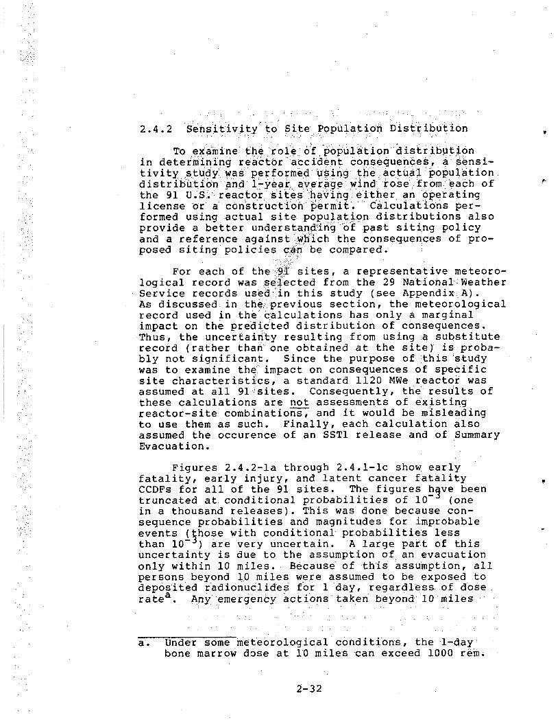
2.4.2 Sensitivity to Site Population Dist~r ibution

To examine.. the role of population distributionin determining reactor accident consequences, a"sensi-tivity study was' performed: usli ng the actual :population.distribution and I-year average, wind rose. fr om .each ofthe 91 es avingeither an operating

license or a constructiohnpermit. Calculations per-formed using actual site.population distributions alsoprovide a better understanddhing "'of 'past siting policyand a reference against which the conseq.uences of pro-posed siting policies, can be compared.

For each of the 91.,,, sites, a representative meteoro-logical record was .selected from the 29 National:-1WeatherService records used in this study (see Appendix.A).As discussed in the,. previous section, the meteorologicalrecord used in the.calculations has only a marginalimpact on the predicted distribution of consequences.Thus, the uncertainty resulting from using :a substituterecord (rather than one obtained at the site) is-proba-bly not significant. Since the purpose of :this studywas to examine the impact on consequences of specificsite characteristics, a standard 1120 MWe reactor wasassumed at all 91 'sites. Consequently, the results ofthese calculations are not assessments of existingreactor-site combinations, and it would be misleadingto use them as such. Finally, each calculation alsoassumed the occurence of an SSTI release and of SummaryEvacuation.

Figures 2.4.2-la through 2.4.1-1c show earlyfatality, early injury, and latent cancer fatalityCCDFs for all of the 91 sites. The figures hive beentruncated at conditional probabilities of 10- (onein a thousand releases). This was done because con-sequence probabilities and magnitudes for improbableevents (ýhose with conditional probabilities lessthan 10- ) are very uncertain. A large part of thisuncertainty is due to the assumption of an evacuationonly within 10 miles. Because of this assumption, allpersons beyond 10 miles were assumed to be exposed todeposited radionuclides for 1 day, regardless of doseratea. Any.-emergency actions taken beyond 10 miles,

a. Under some meteorological conditions, the 1-daybone marrow dose at 10 miles can exceed 1000 rem.

2-32

• " I¸,

id' 100. 100.

xA4-40>14-)*-4

.0

0

-4

0

U

xA\'44

0

~4J

.0"I04

:0s-1

4i

0

U

x

A.

44-

0>1

4J

-4

0

r-

c..0-14J

14.

0U

4..(A

X, Early Fatali

Figure 2.4.2-l.

ties. X, Early Injuries, X, Latent Cancer Fatalities

(a) Early Fatality, (b) Early Injury, and-(c) Latent Cancer FatalityCCDFs Conditional on an SSTI Release at all 91 Current U.S. ReactorSites. Assumptions: 1120 MWe reactor, Summary Evacuation, repre-sentative meteorology. Range of means:-early fatalities'0.4 to 970,early injuries 4 to 3600, and latent..cancer fatalities 230-1to 8100.

(e.g., sheltering or prompt relocation) wouidA signifi-cantly mitigate the consequences of low-probability,high consequence events [27]. The effect on conse-quences of different emergency response scenarios isdiscussed in Section 2.5.

The 91 early fatality CCDFs range (on the proba-bility axis) over almost 3 orders of magnitude in theconditional probability of any early fatalities [i.e.,P( 21)] and over nearly 4 orders of magnituqe in conse-quences at a conditional probability of 10- (consequenceaxis;). The conditional means of the -91 CCDFs range from0.4 to 970 fatalities. Figure 2.4.2-2 presents a histo-gram of-the conditional nieans of the early fatalityCCDFs versus number of sites. Only four sites havemeans above 250 fatalities; over half are less than 50.Tabl~e C-l in Appendix: C lists the conditional meannumber of early fatalitiesl," early injuries, and latentcancer fatalities for e~aoch of the 91. sites. The 99thpercentilea of the conditional distributions of earlyfatalities range from zero-to:8000. :Figure 2.4.2-3presents a histogram of the 99th percentile of thedistributions versus number of sites.

The 91 early injury CCDFs (Figure 2.4.2-1b) :..rangeover approximately 1 order of magnitude in the'.condi-tional probability of having any injuries [P( 21)],andover 2 orders in consequence magnitude at a conditionalprobability of 10-3. The conditional mean numbers'ofearly injuries range from 4 to 3600. The latent cancer

fatality CCDFs (Figure 2.4.2-1c) show less than 1 orderof magnitude spread on both axes. ;The conditional meansof the latent cancer fatality CCDFs range from 230to 8100.

In Section 2.4.1, it was shown that the meteor-ological record does not significantly affect the cal-culated distributions of consequences. Therefore, thewide variability in calculated distributions displayedin Figures 2.4.2-la through c (early fatalities, earlyinjuries, latent cancer fatalities) can be due only todifferences in the 91 population distributions sinceall other factors were either held'constant or haveno significant effect on predicted consequences.

a. Those consequences that would be equalled or exceededby 1 out of every 100 releases.

2-34

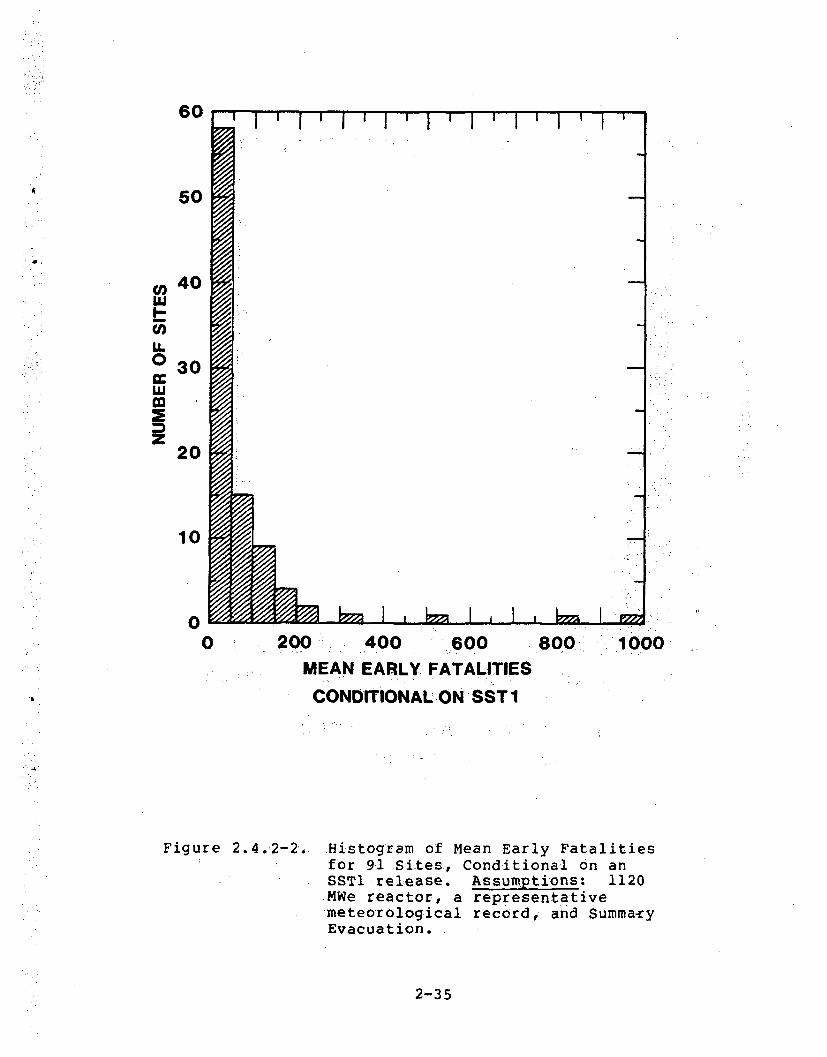
60

50

4.,

040

U.030

z20

10

00 200 400 600 800

MEAN EARLY FATALITIES

CONDITIONAL ON SST1

1000

Figure 2.4.2-2. Histogram of Mean Early Fatalitiesfor 91 Sites, Conditional on anSST1 release. Assumptions: 1120MWe reactor, a representativemeteorological record, and SummaryEvacuation.

2-35

60

s0

40

LU

LL0 30

LU

z 20

10

0

0 2000 4000 6000 '8000 10,0001000 3000 .5000;: 7000 9000

99 PERCENTILE EARLY FATALITIES

CONDITIONAL ON SSTI

Figure 2.4.2-3. Histogram of the 99th Percentile of theDistribution of Early Fatalities for 91Sites, Conditional on an SSTI Release.Assumptions: 1120 MWe reactor, a repre-sentative meteorological record, andSummary Evacuation.

2-.36.

The different degrees of variability of thethree consequences are primarily 'due to the differentdistances to which each consequence occurs. Within20 miles of the %reactor there is tremendous variabil-ity 'in the 91 population distributions. Within thisdistance, the population densities range fromi1 to710 people per square mile (see Sec tion 3). There-fore, the distributions of early fatalities, which areconfined to areas within a few tens of 'miies of the'site ý(most occur within a few miles, see 'Section 12ý.`6),show the greatest variability. Early injuries canoccur to 'many tens o:f miles,' but mosto occur withinabout30 miles.ý' Within 50 miles of the 91 site's,average population densities range from 10 to 2100people per square mile. Since this range (factor~of210) is less-,than that observed to 20 miles (factor of710) ,-the variability in the 91 ea rly injury -qCCDFS isless than othat o aIined .for early 'fatalities. Finally,ýwhen averaged over very large areas, the variability-in the 91 population distributions is greatly reduced.

The population densities within .200 miles of the:9. 91sites vary between 14 and 335 people per square mile

(factor of 24),.- Thus, the distributions of latentcancer fatalities, which can occur overyery lyegeareas, show the least variability. ry l g

some specific.,characteristics'of populationdistributions which might impact the variabilityof consequences are discussed in Section 2.7.4.Finally, for each of the 91 sites examined in thisreport, early fatality, early injury, and latent'cancer fatality CCDFs conditional on an SSTI releaseare presented in Appendix C. When examining theseCCDFs, it is important to remember that they arenot truly site specific. Although each CCDF wascalculated using the site's wind rose, the populationdistribution about the site, and an appropriatesubstitute meteorological record, the SSTI releaseassumed in each calculation was not modified toreflect the specific design of the site's reactor.Instead, a standard 1120 MWe PWR was assumed ineach calculation.

2-37

2.5 Sensitivity to Emergency Response

Should an-accident at a nuclear power plantlead .to a significant release of radioactivity, public

radiation exposures Iculd'be mitigated by evacuation,sheltering, relocation, or medical p rophylaxisa.Summary Evacuation within 10 miles was assumed in most,.:of the calculations presented in other sections of-this report. In this section the sensitivity of earlyfatalities and early injuries to emergency response isexamined by a series of parametric calculations. Allof these calculations assume an SSTI releasefrom :an1120 Mte reactor, Indian Point population and wind rose,and New York City meteorology.169 y

The emergency response submodel in CRAC2.. was brie-f-ly described in Section 2.2.2 and is more fUlly describedin this section and inAppendix E. The model allows for

the mitigation of radiation exposures by evacuation or bysheltering followed by relocation. Evacuation is charac-terized by the delay time between accident warning and.the initiation of evacuation, by the-distance withinwhich people evacuate, and by the evacuation speed [8].Sheltering is characterized by the distance within whichall people take shelter, the shielding factors afforded'by the structures in which they take shelter [29-31], andthe delay time between cloud passage and the relocationof sheltered population. The parameters that describethese emergency response scenarios are first definedand then the results of the parametric calculations arepresented.

a. Evacuation is the/expeditious movement of peopleto avoid exposure to the passing cloud of radio-active material. Sheltering is the expeditiousmovement of people indoors, if possible, intobasements or masonry buildings which afford en-hanced shielding from radiation. Relocation isthe movement of exposed persons out of contaminatedareas after the passage of the radioactive cloud.Medical Prophylaxis is the administration of agentswhich decrease or block internal exposures (e.g.,KI prophylaxis decreases thyroid exposures [28]).

2-38

The following eight parameters essentially deter-mine the impact of the CRAC2 emergency response modelon consequence predictions:

Warning Time: Time from accident notification byplant personnel to release of radioactivity due to,containment failure (e.g., 0.5 hr for SST1).

Delay Time: Time from accident notification to theinitiation of emergency response (0 hr for sheltering;

1-5 hr for evacuation).

Evacuation Radius:., The radius within which alloccupants of a 900 sector (centered.on the plumecenterline) evacuate (10 mi in the base casecalculation).

Evacuation Speed: The effective speed at which eva-cuees move radially away from the reactor (10 mph inthe base case calculation').

Evacuation Distance: The radial distance to whichthe evacuees move (Smi beyond the evacuation radius;therefore, 15 mi for the base case calculation) beforethey are removed from the calculation because they areassumed to have enough information to avoid additionalexposure.

Sheltering Radius: The radius within which all non-evacuating occupants of a 90' sector (centered on theplume) take shelter. If the sheltering radius is lessthan or equal to the evacuation radius, only evacuationtakes place. If the sheltering radius, is larger thanthe evacuation radius, then all persons between theevacuation radius and the sheltering radius take shel-ter. Beyond the sheltering radius, normal activity isassumed to continue (i.e., some people are outdoors).

Shielding Factor [29]: The fraction of the dose to'an unsheltered individual received by an individualsheltered in a building or in a vehicle (i.e., duringevacuation). Shielding factors for buildings dependon the housing stock (percent brick, availability ofbasements) and, therefore, vary by geographic region.Different shielding factors are used to decreaseunshielded exposures to the radioactive plume and tocontaminated ground (see Appendix A).

2-39

Relocation Time: The period which elapses after pas-sage of the' radioactive pium6 before non-evacuatingindividuals are moved from contaminated areas (24 hr-in the base case calculation)':

Relations hips between several of these *eight emergencyresponse model parameters are schematically depictedin Figure 2.5-1.

The CRAC2 emergency response'submodel allows fo r'ý'.the specification of' up' to six d"iffrent emergency re-sponse scenarios and will calculate a weighted averageof the results for any designated set of scenarios.CRAC2 calculations presented inoother sections; of thisreport generally assume "Summary Evacuation,"'' which is:the weighted summation of three different evacuatioon"scenarios as follows:

DelayScenario Type 'of Response Re*sponse Before

Number Weighta Response Distance Speed Response

1 30% evacuation' 10 miles 1 10 mph 1 hour2 40% evacuation 10 miles 10 mph 3 hours3 30% evacuation 10 miles 10 mph 5 hours

a. The 30%/40%/30% weighting provides a best fit to EPAevacuation data [7] (See Appendix E).

The sensitivity of the CRAC2 evacuation model toevacuation speed has been previously investigated byAldrich, et al. [9], who found that, for evacuationwithin 10 miles after a 3 hour delay, early fatalitieswere minimally affected by effective evacuation speedprovided that the evacuation speed was at least 10 mph.The impact of delay time on early health effects 'isillustrated in Figure 2.5-2, which presents earlyfatality CCDFs for 10 mph evacuations within 10 milesafter delays of 1, 3, and 5 hours, respectively(scenarios 1, 2, and 3). Also plotted is the CCDF forSummary Evacuation, which is the 30:40:30 weightedsummation of the CCDFs for scenarios 1, 2, and 3.Figure 2.5-2 shows (1) that early fatalities aresubstantially decreased by short delay times ( 'i hr);and (2) that Summary Evacuation yields results nearlyidentical to those obtained for scenario 2 (3 hr delay).

2-40

A

I-

--

ALL PERSONS IN ZONE 10 ARE EVACUATED TO THEDISTANCE MARKED EVACUATIONDISTANCE

ALL PERSONS IN ZONE ETAKE SHELTER.

I..a DELAY TIME EVACUATION

WARNINGTIME

® ® ® A)®ACCIDENT.INITIATION IREACTOR SCRAM).A WARNIG BY PLANT OPERATING P ERSONNELA) BEGINNING OF RELEASE TO ATMOSPHERE

SEGINNING OF. EVACUATION MOVEMENTX, EARLY FATALITIES

Figure 2.5-1. Figure 2.5-2.

Relationships BetweenEvpcuation Model Parameters.

Early Fatality Complementary Cummulative• DistributionFunctions for 10 mph Evacua-tions within 10 Miles after Delays ofl0 '.3, and 5 Hours :(Scenarios- 1,: 2, and 3,.respectively). and for Summary Evacuation._AssumJtions:-; 1120 MWe reactor, IndianPoint population and wind rose, New YorkCity meteorology.

Table 2.5-1 presents mean and 99th percentilea valuesof early fatalities and early injuries for emergency

.response scenarios 1, 2, and 3 and for Summary Evacuation.The table shows (1) that, for evacuations of populationwithin 1O miles of the reactor, mean and 99th percentilevalues of early fatalities are more sensitive to delaytime than are the-corresponding values for early injuries;and.(2) that for both early fatalities and early injuries,

..99th percentile values are about 10 times mean values.

The different sensitivities displayed result large-ly from the fact that each consequence has a differentcharacteristic distance within which the consequence iscalculated to occur(distance dependencies are discussedin detail in Section 2.6). For most weather sequences,fatal doses of radiation are generally confined to dis-tances of less than 10.miles. Therefore, for almost allof fthe weather sequences sampled, the entire populationpotentially subject to fatal radiation doses is evacuat-ing. ,Consequently, mean and 99 percentile values forearly fatalities are highly sensitive (factors of 8;:1400/180 and.7 •i0,000/ 1400) to delay time. In contrastto this, doses of radiation sufficient to cause earlyinjuries frequently occur to distances significantlygreater than 10 miles. Therefore, because a significantfraction of the population potentially subject to dosessufficient to cause injuries (i.e., the population beyond10 miles) is not evacuating, mean and 99th percentilevalues of early injuries are less sensitive (factors of1.7 and 1.1) to delay time than are the correspondingvalues for early fatalities. Finally, for evacuationsof population within i0 miles, peak values (worst casecalculated for anymweather sequence, conditional probabi-lities of i0-3) of early fatalities and early injuriesare essentially insensitive to evacuation delay timee.g., in Figure 2.5-2 the four early fatality CCDFs haveidentical tails). This is because early fatality andinjury worst case results (CCDF tails) are caused byrainout of radioactivity from the plume onto populationcenters (cities) located more than 10 miles from-thereactor. Since these. cities were not evacuated in thisset of calculations, these calculations yield peak valuesof early fatalities and early injuries that are notaffected by evacuation delay time.

Table 2.5-2 presents the effect of the distance with-in which population is evacuated upon early fatalities

a. Consequence magnitude that would be equalled orexceeded following 1 out of every 100 releases.

2-42

Table,2.5-1. Effect of Delay Time on Early Fatalitiesand Early Injuries for Evacuation ,to.10.Miles. Results are Conditional on an SSTlRelease..

.Delay. Early Fatalities Early Injuries

Time (.hr), Mean 99th Percentile Mean 99th.Percentile

1 180 1,400 2500. .30,000

3 920 8,000 4000 32,000

5 1400 10,000 4300 34,000

Summary 83.0 8,300 3600 33,000

Assumptions: 1120 MWe reactor, SSTI release, Indian Pointpopulation and wind rose., New York City meteorology.

Table 2.5-2. Effect of EvacuationFatalities and EarlyEvacuation. Resultsan SST1 Release.

Distance on EarlyInjuries for Summaryare Conditional on

EvacuationDistance (mi)

.Early.Fatalities Early InjuriesMean.99th Percentile Mean 99th.Percentile

5

10

25

3600

1100

830

700

18,000

11,000

8,300

7,200

6300•

5500

3600

180o

41,000

40,000

33,000

9,400

a. No evacuation

Assumptions: 1120 MWe reactor, SST1 release, New YorkCity meteorology, Indian Point population and wind rose.

2-43

and early injuries for Summary Evacuation. The tableshows that mean and 99th percentile-values of early

ýfatalities and injurieS are all quite sensitive to thedistance within which population is !evacuated. Becausqworst case results (conditional probabilities of -lO--)for early fatalities are generally caused by rainout ofthe radioactive plume onto a city located further than10-but less than .25 miles from:the reactor, evacuationwithin 25 miles l.,iowers .the worst case number of earlyfatalities from 57,000 (for evacuation within 10 mi) to15,000 o(for evacuation within 25 mi).

-'The next three tables examine the sensitivityof early health effects to sheltering parameters.Table 2.5-3 displays the effect of the distance withinwhich population takes shelter in preferred locations(building interiors, basements if available) on earlyfatalities and early injuries. Examination of the tableshows that the effect of response distance for shelteringis similar to-'that • for evacuation. Mean and 99th!p•e-rcen-tile valu es ofI ear ly fatalIties -andinjur:ies are all,quite sensitive to sheltering distance. As before, 99thpercentile values are about 10 times the mean result anda 25 mile response distance significantly decreases (byabout a facto r oIf 5) the' worst case kresult (conditionalprobability-of Ol 03) 'below the result obtained with a10 mile response distance.

Table 2.5-4 illustrates the impact of the avail-ability of basements upon the degree of shielding (andthereby the reductions in consequences) afforded bysheltering" Thý table shows that mean and 99th per-m.centile values of early fatalities are substantiallydecreaied, if Northeast regional shielding factors(building characteristics: 87% basements, 47% brick)are used rather than Pacific Coast regional shieldingfactors (building characteristics: 23% basements, 27%brick) [29]. Because sheltering was assumed to takeplace only to 10 miles, mean and 99th percentile valuesof early injuries show a lessened sensitivity. Theseresults are consistent with results previously obtainedby Aldrich et al. [27].

2-44

Table 2.5-3. Effect of Sheltering Distance on EarlyFatalities .'and Early Injiries'forPreferential'Sheltering Followed byRelocation. Results are Conditionalon an SST1 Release.,

Sheltering Eariy Fatalities Early Injuries

Distance (mi) Mean 99th Percentile Mean 99th Percentile

5 830 9,300 560. 0 40"000

10 560 5,500 37... ,00 32,000

15 490 4,900 2700 25,000

25 420 4,500 1800 11,000

Assumptions: 1120-MWe reactor, SSTI release, Indian Pointpopulation and wind rose, New York City meteorology, noevacuation, Northeast regional .shielding factors, reloca-tion after 6 hr.

Table 2.5-4. Effect of Early Fatalities and EarlyInjuries for Sheltering to 10 MilesFollowed by Relocation. Results areCon ditional on an SSTI Release.

Number of Early Fatalities Early Injuries

Basements Mean 99th Percentile Mean 99th Percentile

Fewa 1200 9,300 4100 34,000

Manyb 56 0 5,500 3700 32,000

a. 23% basements '(Pacific Coast regional shieldingý`factors used, see Appendix A).

b. 87% basements (Northeast regional shielding factorsused, see Appendix A).

Assumptions: 1120 MWe reactor, SSTI release, IndianPoint population and wind rose, New York City meteor-ology, no evacuation, relocation after 6 hr.

2-45

After plume passage, .relocation of •sheltered pop-ulations decreases exposure.to contaminated ground.The effect upon early fatalities'and early injuriesof decreasing relocation time from i24 to 6 hours ispresented in Table 2.5-5. As before, because shelter-ing was assumed to take place only to 10 miles, meanand 99th percentile early injury values show littlesensitivity, while mean and 99th percentile values forearly fatalities decrease by a factor of two.

Table 2.5-5. Effect of Relocation Time on EarlyFatalities and Early Injuries for.Sheltering to 10 Miles. Results areConditional on an SST1 Release.

Relocation Early Fatalities Early Injuries

Time (hr) Mean 99th Percentile Mean 99th Percentile

6 560 5,500 3700 32,000

12 750 7,500 3800 33,000

24 1200 9,300 4100 34,000

Assumptions: 1120 MWe reactor, SSTl release, IndianPoint population and wind rose, New York City meteor-ology, no evacuation, Northeast regional shieldingfactors.

Table 2.5-6 gathers together in a single tablethe results of all-the calculations which examined:evacuation or sheltering separately. The table pre-sents the variation with response distance of earlyhealth consequences for five evacuation scenarios andthree sheltering scenarios. Examination of Table 2.5-6shows that for any response distance, expeditiousevacuation (1 hr delay, 10 mph) and sheltering withexpeditious relocation (after 6 hr) yield the smallestpredictions of early health consequences. The tablealso confirms the strong dependence of mean earlyhealth consequences on response time and the lessstrong dependence on response distance.

2-46

W

Table 2.5-6. Dependence of Earily Fatalities and Early Injuries on Respofle"Distance for EightEmergency Response scenarios. Results are conditic)naloh an SSTI Releas.e

b•I

•J

.Emergency Response Response Distance (mi)

Type Characteristics 0 a 15 10 -15 25 a 5. 10 15 25

- Mean Early Fatalities -mean Early-Injuries

Evacuation 5 hr delay, I mph 3,600 2100 -1,900 1,800 1,800" 63000 .6,200 5,300 5,100 4,7005 hr delay, 10 mph - 3,600 1i,600 , 1,400. -15,300- 1,250 6300 6,000 4,300 3,300 2,5003 hr..delay, 10 mph 3,600 1, 200 920 9601' 790.. 6,300 .5,800. 4,000 3,000 2,200Summary*Evacuation 3,600 1,100 830 7801 700 -6,300 5,500 3,600. 2,700 1,8001 hr. delay, 10mph 3, 00 440 180 1 10 40 6300 . 4,6006 2,500 1,500 700

Shelte.ringb 24 hr relocation. 3,600 c 1,200. c x c., 6,300 c 4,100 c c12 hr relocation. 3,600 c 750 c c 6,300 .c 3,800 c c6 hr relocation 3,600 830 560., 490 "420-1. .6,300 5,600 3,700., 2,700 1,800

99th Percentile Early Fatalitiesd. . 99th Percentile Early Injuriesd

Evacuation 5 hr delay, . I mph .18,-000 16,000 14,000 12,000 11, 000 41;000 41,000 40,000 "41,000 28,0005 hr delay, 10 mph 18,000 14,:000 10,0000 9,4007 86,800".. 41,000 40,-000 34,000 26,000 . 10,0003 hr delay, 10 mph 18,000 i1,000 8,000 7,300 7,000- 41,000 40,000 " 32,000" 26,000 10,000Summary Evacuation 18,'000 11 ,000 8,300. 7,600 7,200.. -41,.000 40,.000 - 33,000, 26,000 9,400

.1 hr delay, 10 mph 18.000 7;000 1,400 1,200' 1,000-' 41;000 " 39,000 30,000 24,000 5,200

Shelteringb 24 hr relocation 18,00 "c 9,300 c c 41,000 c 34,000 c. c12 hr relocation 18,000 c 7,500 c c 41,000 c 3,0 "

*6 hr relocation 18,000 9,300 5,,500 4,900 4,5006 41,000 40,000 - 32,000 25,000 11,000

Assumptions: 1120 MWe reactor, SSTI release, .Indian Point populationwand wind rose, New York City Meteorology. - •

a. No emergency response. b. Northeast Regional Shielding Factors.' c. Not calculated". d. Consequence. magnitude equalled. , or exceeded, following 1 out of

every 100. releases.

lFigures 2.5-3 and 2.5-4 present the variationwith distance of the-risk to an individual of earlyhealth effects (death or injury) for seven emergencyresponse scenarios. The figures show that, as distancedecreases, the different scenariosýpredict increasinglysimilar individual risks (the seven ;risk curves con-

verge)., The curves converge at short distances becausemany weather sequences result in radiation doses largeenough to have fatalities or injuries for each of theseven emergency response scenarios. For example, expe-ditious evacuation (1 hr delay) is not always adequatebecause for manyweather sequences the radioactive plumereaches .people before they begin to evacuate. Andsheltering with exipeditious relocation is inadequatebecause for many weather sequences fatal or injurycausing doses are still received by sheltered personseven with expeditious relocation. Accordingly, because

at short distances each of the seven scenarios fails toprovide isufficient protection for a substantial number ofweather sequences, at these distances little sensitivityto differences in emergency response is observed:. Inagreement with Table 2.:5-6, both figures show thatindividual risk of early health consequences decreasesmost rapidly with distance for expeditious evacuation(1 hr delay, 10 mph') or sheltering with expeditiousrelocation (after 6 hr).

The emergency response submodelJ in CRAC2 is ableto apply one emergency response scenario to an innerregion and a second scenario to an outer region. Usingthis option, the impact of emergency response scenarios,which call for both evacuation and sheltering, and theeffect of response beyond 10 miles were briefly exam-ined. Table 2.5-7 presents some evacuation data fromTable 2.5-2 and contrasts that data with results ob-tained for emergency response scenarios which call forevacuation of population within 10 miles and shelteringof population from 10 to 25 miles. The table shows thatfor Summary Evacuation, increasing the response distancefrom 10 to 25 miles-decreases mean and 99th percentileearly injury values by factors of 2 and 3.5, respec-tively, while mean and 99th percentile early fatalityvalues are somewhat lowered (mean, 19%; 99th, 15%). Thetable also shows (1) that Summary Evacuation to 10 milesin combination with sheltering (relocation after 24 hr)from 10 to 25 miles is as effective as Summary Evacuationto 25 miles; and (2) that in comparison to SummaryEvacuation, expeditious evacuation (1 hr delay, 10 mph)

2-48

+ -

-J

U-

~.1

U..0

C,,

-J

0

I-

0L)

10.

10-1

10-

10-'102•

j-4

10.•

10"

0I0

SSTI. NYC WEATHER

10°

-J

'.0

..... "k m 1 101 10

DtSTANCE (MO) D)ISTANCE. (Ml)

Figure 2.5-3. Conditional Ri~sk of EarlyFatality

Figure 2.5-4. Conditional': Risk of EarlyInjury

Legend Assumptions: 1120 MWe reactor, uniformwind rose, New York City meteorology,results-conditional on an-SST1 release.+

0x0

V0

No evacuation5 hr delay, 1 mph, within 10 mi5 hr delay, 10 mph, within 10 mi3 hr delay, 10 mph, within 10 miSummary Evacuation, within 10 miSheltering within 10 mi, 6 hr relocation1 hr delay, 10 mph, within 10 mi

Table 2.5-7. Impact of Emergency Response Beyond 10 Miles on EarlyFatalities and Early Injuries. Results are.Conditional.on an SSTI Release.

Evacuation Evacuation Sheltering Early Fatalities- Early InjuriesDistance (mi) Delay Distance (mi) Mean 99th Percentile Mean 99th Percentile

Eli

C)

0 - 10

O - 25

0 - 10

0.- 10

Summary

Summary

Summary

1 hr

None

None

10 - 25

10 - 25

830

700

690

40

8,300

7,200

5,400

750

3600

1800

1900

750

33, 000

9,400

8,400

5,800

Assumptions: 1120 MWe reactor, SST1 release, Indian Point population and windrose, New York City Meteorology, Northeast regional shielding factors, relocationof sheltered individuals after 24 hr.

a

to 10 miles combined with the sheltering (relocationafter 24 hr) from 10 to 25 miles substantially reducesmean and 99th percentile values for early fatalities(factors of 17 and 7, respectively) and significantlyreduces mean and 99th percentile values for early injuries(factors of 2.5 and 1.5, respectively). Further, 3 peakearly fatalities (conditional probabilities :i 10- ) arereduced by a factor of almost 10 (peak 15,000 to 1,600).Because of the substantial impact of emergency responsebeyond 10 miles upon peak early fatalities, 'it should benoted that most- results presented in other sections ofthis report assume no immediate emergency response beyond10 miles and consequently may significantly overestimateearly fatality peaks.

Finally, Figure 2.5-5 indicates the sensitivityof early fatalities to the range of emergency responsescenarios examined. ,In Figure 2.5-5 the CCDF for Sum-mary Evacuation is the "base case" (see Section 2.2.4)result. The two bounding early fatality CCDFs for noemergency response iand for expeditious evacuation to25 miles show that the emergency response scenarioselected has a substantial impact on consequencemagnitude.

2-51

10b'

x

'CD

L->

10s

X, EARLY FATALITIES

Figure 2.5-5. Impact of Range of Emergency ResponseScenarios upon Early Fatalities. ResultsConditional upon an SSTI Release

0 - No emegency responseo - Summary Evacuation,

within 10 mi* - 1 hr delay, 10 mph,

within 25 mi

Assumptions: 1120 MWereactor, SSTI release,Indian Point populationand wind rose, New YorkCity meteorology.

2-52

2.6 Distance Dependencies of Reactor AccidentConsequences

This section considers distances within whichselected consequences might occur, as well as dis-tances within which'Protective Action Guides (PAGs)for radiation exposure [32] might:be. exceeded follow-ing a severe reactor accident. The sensitivities ofthese distances to meteorological conditions at thetime of the accident, to differences between meteor-ological records,to accident severity, and to emer-gemcy response are examined.- Because of the currentcontroversy concerning the magnitudes of source termsfor, severe accidents: (see Section 2.3:.2),the impact

of source term reductions on distance estimates isalso considered.,

The consequences that could result from a severereactor accident include short-term effects such asearly fatalities and injuries a.nd long-term effectssuch as delayed' cancer deaths and interdiction ofland. Because early consequences would occur onlyafter large, acute doses of radiation,ithese effectswould be limited to areas close to the'reactor (a fewtens of miles). Population restrictions within theseareas could therefore- significantly impact the numberof'early c nsequences. As a result," estimates of.:distances to which fatal or injury-causing doses ofradiation could be received are of interest for thedevelopment of. reactor siting criteria." Foliowing asevere reactor accident,, contamination could be suf-ficiently high to require interdiction of-property(buildings and land) to substantial distances (severaltens *of miles). Because interdict'ion of large areascould be a significant, and possibly dominant, con-

tributor to the offsite costs of a reactor accident,distances to which land might be interdicted could alsobe an important consideration for the development ofsiting criteria. Since latent cancers can be inducedby small doses of radiation, they can occur at largedistances 'from the rea.ctor. 'As a result, latent can-cers would generally be less affected by populationrestrictions close to a reactor than would earlyfatalities or early injuries.ý

For each sampled meteorological sequence, theCRAC2 code calculates the maximum distances at whichselected consequences might occur. These distanceswill depend on the magnitude and characteristics of

2-53

the source term as well as plume dispersion and deple-tion processes. By using the weather sequence samplingtechnique discussed in Section 2.2.1, the CRAC2 codecan generate CCDFs of "maximum" consequence distancesfor any given source term._ These curves illustrate theimpact that radionuclide dispersion, which is determinedby, the weather conditions at the time of the accident,has on distances to which consequences occur.

Figures 2.6-1, 2.6-2, and 2.6-3 show SSTI and SST2early fatality distance, early injury distance, andinterdiction distancea CCDFs for the 29,meteorologicalrecords discussed in Section, 2.4-. The figures show thatfor an SSTl release early fatality distances range from1 ito 20 miles, early injury distances from 1 to 80miles,

and interdiction distances from 1 to 100 miles.,. Thus,for a single event, consequence distances are stronglyinfluenced by the weather at the time of the release.However, the figures also show that for a specificrelease (e.g ., SST1), CCDFs calculated using differentmeteorological records are quite similar. .For example,the. 90th percentile values of. the 29 early fatality'CCDFs calculated assuming an SST1 release range onlyfrom 6 to 9 miles.

These results also show that for the SST1 release,early fatalities would be limited to about 20 miles,injuries to about 50 miles, and land interdiction toabout 100 miles. For the SST2 release, early fatalitieswould generally be lim ted to about 2 miles, in.Juriesto about 8 miles, and landl interdiction to about; 10miles. For each set of CCDFs, the variation in the.peaks, and probabil ities of the peaks, .is principallydue to a combination of (1) the order of magnitude .variation in rain frequencies for the 29 meteorologicalrecords and (2).errors .inherent in the weather sequencesampling procedure (see Section 2.4) . .

a. Fatality and injury distances are defined to bedistances within which individuals are at risk ofbeing an early fatality or injury: given the assumedrelease (SSTi or SST2). The interdiction distanceis defined to be the distance within which landwould be interdicted following the assumed release.The SST3 release is not large enough to causeearly fatalities, early injuries, or interdictionof land offsite..

2-54

:xA]

0a:-.J

z0E:0z.00.

io 2

X.EARLY FATALITY DISTANCE (MI)

Figure 2.6-1. Conditional CCDFs of Early Fatality Distancefor 29 Meteorological Records CalculatedAssuming SST1 and SST2 Releases from an1120 MWe PWR and No Emergency Response.

2-55

XAl

0

.Q

-J

102

X,EARLY INJURY DISTANCE (MI)

Figure2.26-2. Conditional CCDFs. of.Early Injury Distancefor 29 Meteorological Records Calculated

..As..Asuming SSTl and SST2 Releases from an1120 MWe PWR and No Emergency Response.

2-56

Al

'0

103

104

1600 101 :102

XINTERDICTION DISTANCE (MI)

Figure 2.6-3. Conditional CCDFs of Interdiction Distancefor 29 Meteorological Records CalculatedAssuming SSTl and SST2 Releases from -an1120 MWe PWR.

2-57

The results presented thus far show the distancesto which fatal or injury-causing doses of radiationcould be receivedlas-suming no emergencyri: i-6response.However, given_.a, ýsevere reactor accid!t, some typeof emergency response would be expet'ed and therefore,

acute doses clo se to the reactor could be reduced. Asshown in. Sectioin 2.5, emergency protective actions canhave a substntial impact on reactor accident conse-quences.. Figre 2.6-4 comparesSSTl fatality distance

CCDFs calcu.lated using New York ,tCity meteorology andfour different emergency response.: scenarios: no emergen-cy respons•e, sheltering, and twb. ,evacuation scenarios(1 hr delay,ý,, 10 mph, within 25. mi; 5 hr delay, 10 mph,with in 25 mi). In general, these•, CCDFs show that earlyfatality distances are quite -senisitive to emergencyresponse.•, Thus, effective implementation of emergencyprotect.ive actions in areas near the reactor could re-suit in substantial reductions in distances to whichfatal or injury-causing, doses of radiation coudld. bereceived. For example, with no' emergency i9esponse the90th precentile value of the fatality radius for .anSST1 !release is > 8 miles, while with sheltering'l the90th percentile distance is 4 miles and with expeditiousevacuation (1 hr delay,'10O mph) the distance is furtherdecreased to about 2 miles. ýC•!•CDFs of fatality distancethat' were calculated using ý::other meteorological recordsshow the same sensitivity 'to emergency response.

Other distances that might be of interest for thedevelopment of siting criteria are those within whichthe EPA Protective Action Guides (PAGs) L32J for wholebody and thyroid dose might be exceeded. A PAG is de-fined as the projected dosea to an individual in thegeneral public which warrants the initation of emergency

a. The "projected dose" is defined by the-EPA as thedose that would be received within a few days follow-ing the release if.no prote~ctive actions are taken.PAGs range:from 1 to 5 rem for whole body exposureand from 5 to 25 rem for projected dose to the thy-roid. The lower value of these ranges should beused if there are no major local constraints limit-ing the ability to provide protection at that level.However, when determining the need for protectiveaction, in no case should the higher value be,exceeded.

2-58

10O

o 1 HR DELAY... 10MPH

:0.

SHELTERI NG.: .0

5HRDELAY10 MPH

foo 103i OI ] '1.. I I

XEARLY FATALITY DISTANCE (MI)

Figure 2.6-4. Sensitivity of SSTI Early FatalityDistances to Emergency Response.Assumptions: New York City meteor-ology, 1120 MWe PWR, and 25 MileResponse Radius.

2-59

protective actions and,, as such, is a trigger valueto aid in decisions to implement these actions.Figure 2.6-5 shows the probabilities of exceeding thePAGs as a function of distance for the SST1, SST2,and SST3 releases?,.. The probabilities were, calculatedassuming an 1120 MWe PWR, New York City meteorology,and no emergency response. In general, these resultsshow that PAGs could be exceeded to very large dis-tances (in excess of 50 miles) given an SSTI accidentwhile they would probably not be exceeded beyond about30 miles for an SST2 release. In addition, doses wouldnearly always exceed PAGs tc distances of approximately30 miles for the SST1 release and 2 miles for the SST2release. Doses from an SST3 release are shown not toexceed PAGs beyond about 3 miles of the reactor.

The-results discussed thus - far in this section aresummarized in Table 2.6-1. In the table consequencedistances are presented for three releases (SSTl, SST2,and SST3) and for three conditional probability 'levels:mean, 99th percentile, and peak (maximum calculated).The distances presented in the table summarize the largenumber of distance CCDFs calculated using the 29 meteor-ological records. The fatality and injury distancespresented could be reduced by any effective emergencyresponse action. In general, Table 2.6-1 suggests that:(1) for severe-core melt accidents, early fatalitieswould generally not occur beyond about 15 miles, and inthe worst case, would be confined to about 25 miles,while early injuries would probably be confined to down-wind distances of about 50 miles; (2) for smaller coremelt accidents (on the order of SST2 in severity),early fatalities would be confined to about 2, miles,and ;injuries and land interdiction to about 7 miles;and (3) for accidents on the order of SST3 in severity,PAGs, would probably not be exceeded beyond a, few miles.

As discussed earlier, latent somatic effects couldresult from relatively small doses of radiation. There-fore, given a reactor accident, these consequences couldoccur at large downwind distances from the reactor.Figure 2.6-6 shows the cumulative fraction of latentcancer fatalities versus distance for the SST1, SST2,and SST3 releases. These curves were calculated assum-ing an 1120 MWe PWR, New York City meteorology, and aone mile per hour evacuation to ten miles after a fivehour delay. In general, theresultsshow that signifi-cant fractions of latent health effects could occur atlarge distances from the reactor. For the uniform

2-60

'V.

100

za

C.)0

0

az00.

LL

0

CQ

0

z_

w

0

U

InLI

0I--J

z0

0

0ccIn2n

bI

1 10 100

DISTANCE (MILES)

a) SSTI

DISTANCE (MILES)

b) SST2

DISTANCE (MILES)

C) SST3

Figure 2.6-5. Conditional Probability of Exceeding PAGs Versus Distance forSSTI, SST2,and SST3 Source Terms. Assumptions: 1120 MWe PWR, New York City meteorology,and'no emergency response.

Table 2.6-1. Summary of Consequence Distancesa (miles)

SourceTerm

Consequence Conditional Probability Levelb

Mean

SSTI Early Fatalities

Early Injuries

Land interdictio'n

PAC sc.

Early Fatalities

Early Injuries

Land Interdiction

PAGSc

<5

99%

•15

-30

>50

,>50

Calc Max

<25

-10

250

-0.5

>50

>50

>50

SST2 <2

<2

<2

<20

<5

-7

-20

<2

--5

-10

<50

<3SST3 PAdsc

a. These distances are for a 1120 MWe PWR which iscomparable in size to many of the most recentlysited nuclear reactors.

b. Mean distances are the average of the probabilitydistributions of distance; 99% distances refer tothose beyond whi-ch a consequence or dose is cal-culated to occur" in 1 in 100 accidents; and thecalculated maxima represent the largest distancescalculated.

c. A PAG is defined as the "projected" dose to an indi-vidual in the general public which warrants the ini-tiation of emergency protective actions. PAGs rangefrom 1 to 5 rem for whole body exposure and from 5 to25 rem for projected dose to the thyroid.

2-62

(1)IL.

-ILLA-0z0

L6WL

Q

.4

D80• . ( 120ME•DISTANCE (MILES)

a) Uniform Population Distribution

(nU.

0z0

U.

200

DISTANCE (MILES)

b) Indian. Point Population Distribution

Figure 2.6-6. Cumulative Fraction of Latent Cancer Fatal-ities as a Function of Distance from the Reactor a) for aUniform Population Distribution and b) for the Indian PointPopulation Distribution.

-Assumptions: 1120 MWe PWR, New York City meteorology, and aslow evacuation (5 hr delay, 1 mph, 10 mi response distance).

2-63

population distribution, t-he calculated cancer,-fatal-ities are shown to be somewhat uniformly dist-ributedwith distance .. This uniform" distribution results.because the decrease in cancer risk with distance isapproximately offset by the increase in the exposedpopulation. The results shown for the-.Indian Pointsite illustrate the impact of a highly nor-'uniformr,population distribution. The high population. densitieswithin approximately 50 miles of the-Indian ,Point site(relative to lower densities further away) ca~use a

* significantly larger fraction of the predicted cancerfatalities to occur within 50 miles of the reactor.Thus, the high n.6n-unifornity of thet. exposed ,populationdistribution also causes the distribution of cancerfatalities to be :•nnun-iudfn"-iform with distance.

S-'cti'on 2.13.,2 di~scuss ed. rIcent::revi~ews of accidentphenomenology which indicate that the magnitudes of cur-

s"rent -ssevere reactor accidents-may be

significantly too large. To investigate the impactof source term reduc'tifons on distances to which conse-quences might occur, a series of. caIculaticns was per-formed for the SSTl release reduced ýby arbitrary factorsof 2, 10, 20, and 100. Important assumptions for thecalculations included New York City meteorology, an: 1120M~e PWF, and no emergency response. Table 2.6-2 summar-izes the results and in general shows that reductionsin severe accident source terms substantially reduceconsequence distances. An order of mag'nitude re~duc:tionin the SSTI release reduced the peak fatal distance ,fromabout 20 miles to 5Smiles while a two-orxder of magnitudereduction reduced the peak distance to 1imile. Similarreductions are shown for early injury and` land i:nter-diction distances.

This section has examined the impact of meteor-Sological conditions, accident severity, and emergency,response on consequence distances. Four factors, thatalso could influence conseauence distances, are dis-cussed in other sections of this report. They arereactor size (i.e., size of radionuclide inventory,see Section 2.7.1), liUmreheat content (determinesplume rise, see Section 2.7.2), dry deposition velocity(see Section 2.7.3) and interdiction criteria (seeSection 2.7.5).

2-64

b 9

Table 2.6-2. Sensitivity of Fatal, Injury, and Interdiction Distances to ReleaseMagnitudea

SourceTerm

Fatal

Mean

Distance

9 9 %b

(mei)Peakb

Injury

Mean

Distance (mi)

9 9 %b Peakb

Interdiction Distance (mi)

:Mean 9 9 %b Peakb

N)

0*'.LYI

SSTI

1/2 SSTlc

1/10 SSTlc:

1/20 SSTlc

1/100 SSTlc

3.9

2.5

0.9

0.5

12 18

10 18

2.2

2.0

1.0

5.0

2.0

1.0

11

7.0

.2.8

1.9

0.9

35

20

10

50 19

14,25

7.0 10

5.5,

3.6

55::

45

18

12

10

85

50

25

18

100 4.0 5.0

a. Assumptions: New York City meteorology, 1120. MWe PWR, and no 'emergency- response.

b. The 99 percent distances refer are the distances.- beyond which .a:. consequence iscalculated to occur in only 1 in 100 accidents. The peak result is that obtainedfor the most unfavorable weather sequence sampled.

c. Release fractions reduced for all isotopes except noble gases.

2.7 Other Sensitivity Calculations

2.7.1 Reactor Size

All of the calculations presented in previoussections of this report assume an.1120 MWe reactor.This reactor size was selected because many reactorscurrently operating and most under construction areabout this size. Because consequences depend stronglyon the amount of radioactivity released (see Section 2.3,Accident Source Terms), which in turn .is dependent onreactor size, the sensitivity of consequences to reactorsize was examined. Calculations were performed for ninereactor sizes ranging from 11.2 to 1500 MWe. All calcu-lations assumed a 1120 MWe core radionuclide inventory'scaled according to reactor size, an SSTI release, NewYork City meteorology, and the Indian Point populationdistribution and wind rose. The linear scaling proce-.dure used is described in Appendix B, Core RadionuclideInventories, which also discusses inventory changes dueto annual operating cycle and differences between PWRand BWR inventories.

Figures 2.7.1-1 and 2.7.1-2 present conditionalCCDFs of early fatalities, early injuries, latent can-cer fatalities, interdiction distance, and interdictedland area for five of the nine reactor sizes examined,assuming Summary Evacuation. Table 2.7.1-1 presents themean and 99th percentile values of these distributions.The effects of emergency response and reactor size onmean early fatalities are presented in.Table 2.7.1-2.Finally, Figure 2.7.1-3 presents plots of the meanvalues presented in each table versus reactor size.

Several conclusions can be drawn from these results.First, Figure 2.7.1-3 shows that mean values of all fiveconsequences increase roughly linearly with reactor size.The rates of increase are largest for early fatalitiesand smallest for interdiction distance. Table 2.7.1-1shows that mean values increase more rapidly than 99thpercentile values. The mean early fatality resultspresented in Table 2.7.1-2 clearly display the signifi-cant impact of emergency response, seen previously (seeSection 2.5). For an 1120 MWe reactor, No Evacuationyields a mean result of almost 3600 early fatalities,while Best Evacuation (1 hr delay, 10 mph, 10 mi re-sponse region) decreases this number to less than 300.Figure 2.7.1-3a shows that for an emergency response ofa given effectiveness, there is a reactor size (x-axis

2-66

A

A

I.0%

A, LRKLT rIRLUIIU, X, EARLY INJURIES

Figure 2.7.1-1. Effect of Reactor Size upon a) Early Fatalities, b) Early Injuries,Fatalities, Conditional on an SSTl Release.

X, LATENT CANCER FATALITIES

and c) Latent Cancer

Assumptions: 1120 MWe core radionuclide inventory scaled to reactor size,SSTI release, New York City Meteorology, Indian Point wind rose and population,Summary Evacuation.0-

4--

O0-

15001120

750500250

MWeMWeMWeMWeMwe

reactorreactorreactorreactorreactor

I 0f

AU-

0x

CL

>C

AU-

WJ

I--

!0%O0

J - r-r-rfT ~--i3 1 T - =Tri T-TTT ---r-T rTT1 I11 3

X, INTERDICTION DISTANCE (MI) X, INTERDICTED LAND AREA (SO MI)

Figure 2.7.1-2. Effect of Reactor size upon a) Interdiction Distance (mi) andb) Interdicted Land Area (sq mi), Conditional on an SST1 Release.

Legend

X -

0-

0-

15001120

750500250

MWe reactorMwe reactorMWe reactorMWe reactorMwe reactor

Assumptions: 1120 MWe core radionuclide inventoryscaled to reactor size, SST1 release, New YorkCity meteorology, Indian Point wind rose andpopulation, Summary Evacuation.

,.I

'.0

Table 2.7.1-1.. Dependence of Consequences Upon Reactor Size,, Conditional-on an SST1 Releasea

Reactor InterdictedSize Latent Cancer Interdiction Land Area(MWe) Early Fatalities Early Injuries Fatalities Distance (mi) (sq mi)

Mean 99th Mean. 99th Mean 99th Mean 99th Mean 99th

250 34 1,200 323 3,800 3970 10,000 9.,.7 38 •20.8 97

500 172 3,200 1020 9,700. 5560 20,000 13:,1 ' ý45 ;'37.2 120

750 455 5,900 1880 16,000 6710 20,000 :16.0 49 53.7 190

1120 831 8,200 3640 33,000 8110 24,000 193 54 75.'8 250

1500 1250 12,000 6340 57,000 9600 30,000 22.8 .56 106 340

a. Assumptions: 1120 MWe core radionuclide inventory scaled:according to reactor size,SST1 release, New York City meteorology, Indian Point population and wind rose,Summary Evacuation..

Table 2.7.1-2 Dependence of•Mean Early FatalitiesUpon Reactor -Size :and .EvacuationScenario, Conditional on an SSTIReleasea

Evacuation Scenario

Reactor. Best ... Summary NoSize i(MWe),', Evacuat.ionb, Evacuation Evacuation

C0 0.3 1

60 2 34

1 1 2 c 0 9 147

250 0.01 .34. 551

500 6 172 1490

5 6 0 c 17 224-1 1700.

750 102 455 2380

1120: 176 831 3580ý

1500 287 1250. 4880

a. 1120 MWe core raduinuclide inventory scaled accord-ing to reactor size,, SSTl: .. release, New York Citymeteorology, Indian.Point population 'and wind rose.

b. 1 hour delay, 10 mph, 10 mi response region (seeSection 2.5).

c. Noble gas release fractions not scaled; this hasno. significant impact on early fatalities ('seeSection 2.3, Accident Source Terms).

2-70

2Vr

dcWZ

7

4

3

2

1

-SUMMARY EVACUATION

7

8000.J

3. 2400

ZlOO

S

nl | |i i

-1

lO

B00 1000REACTOR SIZE (MW.)

1500

.1-:34

4Z

7

0

•S

4

3

2

I I Ilb __1 -_

EU

ZW45

a

,-I

120

100

so

40

500 1000REACTOR SIZE (MWo)

1500

[4

00

20

I I IG00 1000 1500.

REACTOR SIZE (MWe)

I I ~ I

-0 a00 1000 1500REACTOR SIZE .(MWe)

Figure 2.7.1-3. Plots of Mean Values of a) EarlyFatalities, b) Early injuries, c) Latent CancerFatalities, d) Interdiction Distance (mi), ande) Interdicted Land Area (sq mi.) vs Reactor Size,Conditional on an SSTl Release.

Assumptions: 1120 Mwe core radionuclide inventoryscaled to reactor size,,-.SSTl release, New York:Citymeteorology, Indian Point. population and wind rose.

2-71

intercept) for which on the average (mean result) fewearly fatalities would be expected. For Best Evacua-tion that size is -500 MWe; for Summary Evacuation,-100 MWe; and for no evacuation, -10 MWe.

2.7.2 Energy Release Rate

The calculations considered so far have been forground-level releases containing no .sensible heat,i.e., nonbuoyant plumes. In an accident where thereis a large uncontrolled release directly to the atmo-sphere, it is possible for the plume to contain asizable amount of sensiblie heat. For example, therelease categories described in WASH-1400 [11 hadenergy release rates• of up to several hundred millionBTUs per hour.a Thýerate of energy release determinesthe final plume height and, therefore, the downwinddistance at which the plume first contacts the ground(touchdown). Since uhder the same weather conditionsa buoyant plume would be more dilute at touchdown thana nonbuoyant plume, a significant reduction in the i•number of early health effects is possible. However,since plume depletion by dry deposition occurs onlyafter touchdown, buoyant plumes might therefore produceground concentrations high enough to produce earlyeffects at greater distances than nonbuoyant plumes.Furthermore, for highly buoyant plumes, precipitation-washout is the primary mechanism by which r~adioactivematerial reaches the ground in sufficient concentra-tions to cause early health effects. Thus,-,for abuoyant release the probability of having any earlyfatalities and injuries is strongly dependent on theoccurrence of precipitation. The final plume height•is calculated in CRAC2 using the formulae developed .byBriggs [33] for emissions from smokestacks. Consider-able differences could exist between smokestack plumesand plumes released in a reactor accident [341. Thesedifferences have been investigated by Russo, Wayland,and Ritchie [35] who found that predicted consequenceswere only marginally sensitive to the moisture contentof the plume and atmosphere but, under certain condi-tions, consequences could be quite sensitive to radio-active heating and initial plume momentum.

For the present study, the sensitivity of predictedconsequences to energy release rate was investigated

a. In WASH-1400, an energy release rate of 170 x 106BTU/hr was assumed for a PWR-2 accident.

2-72

by performing calculations for an SSTl release withthree arbitrary energy release rates: 17, 170, and430 million BTU/hour. New York City meteorology anda uniform population density of 50 pecple per squaremile beyond 1 mile were assumed. Table 2.7.2-1 com-,pares selected results for these energy release rateswith a cold (no sensible-beat) SST1 release (the basecase, see Section 2.2.4).

Table 2.7.2-1. Sensitivity of Estimated Conseauencesto Energy Pelease patea

Release. SSTI ZSS7T SST1 SSTI

Energy .Relea'seRate (BTU/hr) 0. 17x10 170..•IO 430x10

Mean Early Fatalities

Summary Evacuation .22. .12 9 10No Evacuation 140 140 47 47

Mean Early Injuries

Summary Evacuation 140 180 110 85No Evacuation 350 390 270 150

Mean Latent CancerFatalities 730 790 830 860

Maximum CalculatedFatal Distance (mi) 17.5 17.5 25 25

Maximum CalculatedInjury Distance (,im) 50 50 50 60

Maximum Calculated LandInterdiction Distance (mi) 85 85 85 85

a. Assumptions: New York City meteorology, uniformpopulation of 50 people per square mile beyond 1 mile.

2-73

The results for the low-energy release (17 x i06BTU/hr) differ only slightly from those for the coldrelease, because this release rate is not large enoughto cause substantial differences in the plume touchdownpoint. The two high-energyrelease rates result inconsequences markedly different from the cold release.Because the occurrence of precipitation is necessary,to cause significant numbers of early health effectsfor hot releases, the mean number of early effects islower for the high-energy releases.

At.:ver.y large distances, the amount of initialplume-rise does not significantly affect the transportand deposition of radioactive material. Consequently,'latent cancer fatalities, which occur to great distances(see Section 2.6),, are not significantly affected byplume'buoyancy. The maximum observed- fatal distance 'is:8 miles farther for the high-energy releases, althoughthe maximum calculated injury distance is only slightlyincreased and interdicted land distance is unaffected.Neither land interdiction nor injury distances are verysensitive to energy release rate because these cohse-quences also occur to-distances where initial plumerise is generally not important.

Figure 2.7.2-1 plots the conditional-individualrisk of early fatality versus distance for the fourenergy release rates,.assuming a uniform wind rose.Within 10 miles, the hot releases have lower risks thanthe cold releases. However, for low probability events(i.e., precipitation), the hot releases could result infatalities out to 25 miles. The non-monotonicity in the6risk at about 8 miles for the two hot releases (170 x 106and 430 x.10. BTU/hr) is believed to be an artifact ofthe weather-sequence sampling procedure used (seeSection 2.4.1).

.In summary, for an SSTI release the estimatednumbers of early fatalities and injuries and thedistance to which early fatalities occur are bothquite sensitive to the energy release rate. However,consequences which can occur to great distances, suchas latent cancer fatalities, are not sensitive toenergy release rate. The maximum distances, to whichearly injuries may occur or land may:be interdicted,are also not sensitive..to-energy release rate. Acautionary note: these.conclusions may not hold forsource terms significantly smaller than SST1.

2-74

0-

DISTANCE (MILES)

Figure 2.7.2-1. Individual Fisk of Early FatalityVersus Distance for 4 Energy ReleaseRates, Conditional on an SSTI Release.Assumptions: SSTI release, New YorkCity meteorology, uniform wind rose,no emergency response.

2-75

2.7.3 Dry Deposition Velocity

The deposition of radioactive material on theground is the first step in many of the pathways bywhich radioactive material can reach people. Drydeposition of airborne material onto a surface is acomplex process which includes a number of differentphenomena such as gravitational settling, turbulentand molecular diffusion, and inertial impaction [36].

Hosker [37]:and Kaul [38] have reviewed currentmodels of dry removal processes.. All current dr,,y-deposition models incorporate a "dry-depositionvelocity" which is defined as the ratio of the time-ýintegrated air concentration of a material to theconcentration of the material on the ground.ý Alargenumber of parameters can affect the value of thedeposition velocity. About 80 have been lisited bySehmel [39J. Among these are surface roughness,relative humidity, chemical composition, and particle:diameter. Dry deposition velocity is highly sensitiveto particle diameter [39].

Radioactive material released to the atmosphere'is likely to have a range of particle diameters, eachwith a different deposition velocity. Despite this,:-•Iin CRAC2 only a single deposition velocity may be inputfor each element considered, and generally the samevalue (1 cm/sec) is used for all elements except noblegases (the deposition velocity of noble gases is zero).All CRAC2 calculations presented in other sections ofthis report treat deposition velocity in this manner.

As discussed in Section 2.2.3, there are largeuncertainties about the characteristics of the radio-active aerosol released from containment. Becausepredicted ground concentrations can be very sensitiveto deposition velocity, a sensitivity analysis was per-formed to assess the impact of dry deposition velocityon predicted consequences. The analysis was somewhatsimplistic in that only a single deposition velocitywas used. Thus, no attempt was made to account for arange of particle sizes by use of a distribution ofdeposition'velocities. Also neglected were effects ofchemical composition and the possibility that differentelements may be associated with particles of differentsizes. Gravitationallsettling of particles, which canbe treated by "tilted plume" models [40] was alsoignored (gravitational settling would be the dominant

2-76

contributor to dry removal for particle diametersgreater than about 5 microns).

Calculations were performed for an SST1 releasewith five deposition velocities: 0.1, 0.3, 1.0, 3.0,and 10.0 cm/sec-a These values are believed to spanthe range of possible deposition velocities. Only non-buoyant releases were considered. For buoyant releases,early consequences are dominated by the occurrence ofprecipitation; therefore, the variation of consequenceswith dry deposition velocity could be substantiallysmaller for buoyant releases (see Section 2.7.2). Otherassumptions included Summary Evacuation, an 1120 MWereactor, the Indian Point population distribution andwind rose, and New York City meteorology. Differentpopulation distributions and emergency response assump-tions could impact the observed variation'of early con-sequences with deposition velocity (see Sections 2.4and 2.5).

Figure 2.7.3-1 presents the early fatality CCDFsfor the set of deposition velocities examined. Exceptfor the low-probabililty, high-consequence events,there are only very minor differences. Mean numbersof early fatalities vary by less than a factor of 1.5.Deposition velocities of 0.1, 0.3, and 1.0 cm/sec yieldthe highest consequence events (over 50,000 fatalities)from weather sequences with precipitation beginningbetween 10 and 20 miles from the reactor. With eithera 3 or 10 cm/sec deposition velocity, the particulatematter in the plume is sufficiently depleted beforethis distance range is-reached and, thus, rain does notproduce a ground concentration in this interval highenough to cause significant numbers of early fatalities.

Figure 2.7.3-2 shows the conditional individualrisk of early fatality versus distance within 10 milesof the reactor. Larger values of deposition velocityresult in slightly greater individual risk within 2miles of the reactor but a much reduced risk fartherout. Table 2.7.3-1 lists the means, 90th and 99thpercentiles, and maxima of the CCDFs of early fatalitydistance, early injury distance, and interdicted land

a. In all calculations a single deposition velocitywas used for all elements except noble gases.The deposition velocity of the noble gases wasassumed to be zero.

2-77

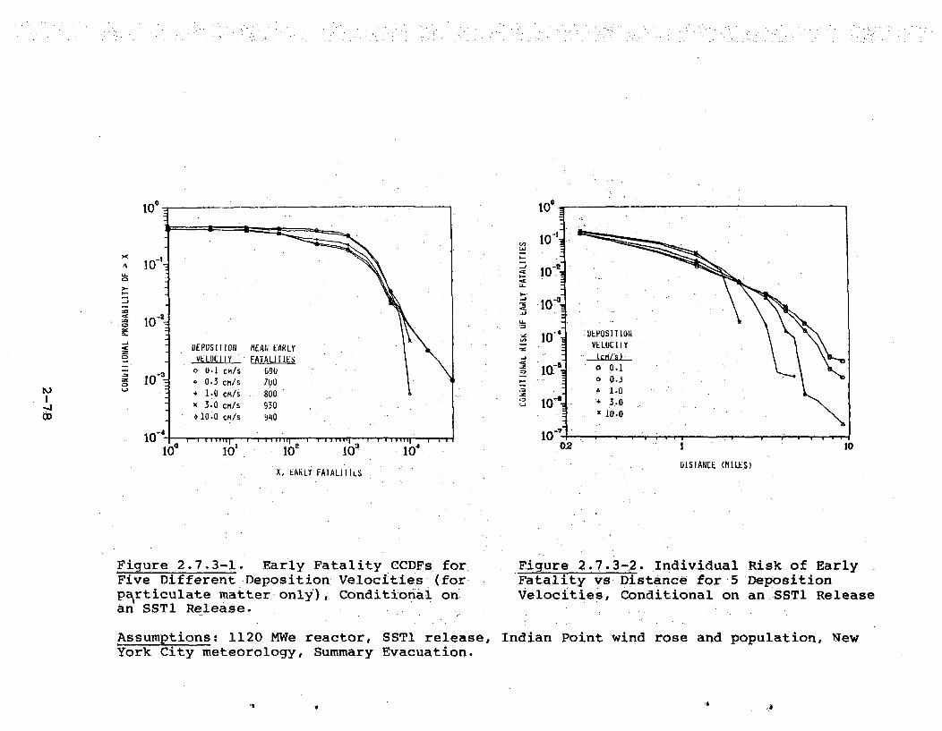
to0

A -J

I-

-J

U-0

-J

.2

0.2

tOo

10-1

.lOT

102

10 .

io-0, -02

.ftpos MI0IVk LUC II(CM /S)

o 0.1o0..31.

+3-0

x 10.000I,

i I0

X, EARLY FAlALIIILS 0ISIANCE (MILES)

Figure 2.7.3-1. Early Fatality CCDFs forFive Different Deposition Velocities (forpa~rticulate matter only), Conditional onan SSTI Release.

Assumptions: 1120 MWe reactor, SSTI release,York City meteorology, Summary Evacuation.

Figure 2.7.3-2. Individual Risk of EarlyFatality vs Distance for 5 DepositionVelocities, Conditional on an SSTl Release

Indian Point wind rose and population, New

Table 2.7.3-1 Sensitivity of the Distances (miles) to which ConsequencesOccur for Various Deposition Velocities.

Land' InterdictionEarly Fatality Distance Early Injury Distance Distance

Dry-.Deposition Maximum Maximum MaximumVelocity Calcu- " Calcu- Calcu(cm/sec). Mean 90% 99%* lated Mean 90% 991% lated Mean 90% ;99% lated

0.1 2.1 4 15, 25, 7,2 15. 55, . ,65 11 30 60 100

0.3 1.9 4 15 25- 7.1 201 4:0. 50 16 40ý. 65* 85

1.0 1.7 4 12 18 8.3 25: 35 50 19 40 60 85

3.0 1.6 3 4 18 6.6 12 231 25 20 25.. 40 45

10. 1.4 3 3 3 3.5- 6 15 18 13 22 23 25

-J-'0

Assumptions: 1120 MWe reactor, SSTIEvacuation within 10 miles.

release, New York CI ity meteorology, Summary

distance (see Section 2.6). The mean distances foreach consequence are only marginally sensitive to.deposition velocity. However, the tail of the dis-tributions (99th percentile and maximum calculated.)are very sensitive to deposition velocity. As thedeposition velocity increases, there is .a large re.-duction in the 99th percentile and maximum calculateddistances. Again, the tails of each distributionresult from sequences with precipitation beginningsome distance from the reactor. Deposition velocitiesabove about 3 cm/sec deplete the plume closer to thereactor, and thus the distance to which precipitationcan produce significant ground concentrations is muchreduced.

Despite the narrow scope of this sensitivity anal-ysis (only the deposition velocity has been studiedrather than trying to account for the more realisticcondition of a distribution cf deposition velocities),the following conclusions can be drawn:.

o For a single deposition velocity applicable toall particulate matter, the maximum distanceto which land is interdicted and early fatal-ities and injuries occur is very sensitive todeposition velocity. These maximum distancesoccur for low-probability, worst-case weatherconditions.

o For the population distribution and emergencyresponse scenario assumed"(Summary Evacuation),the mean number of early fatalities is onlymoderately sensitive to deposition velocity-andthus may be largely insensitive to the particle-:size distribution of the released material.,

2.7.4 Population Distribution

Results presented in Section 2.4, Site Meteor-ology and Population, showed that early fatalitiesand early injuries are strongly sensitive to thecharacteristics of the surrounding population distri-bution. Three sets of calculations were performedto better define the sensitivity of early-fatalitiesand injuries to the following features of populationdistributions: (1) radial and angular variations inpopulation density, (2) the size and distance ofpopulation centers, and (3) exclusion zone size.

2-80

... ,Radial and Angular Variations. Radialiand an-gular variations in population density were.examinedby constructing a hypothetical reference populationdistribution and then calculating consequences forthat distribution and eight transformations of thatdistribution. Beyond 20 miles all of the distribu-tions were identic'al. • Each had uniform populationsof ,750 people per ýsquare mile from 20 to 30 miles,2500:from 30 to 50 miles, 500 from 50 to 100 miles,and- 300 from 100DPI. to 500 miles. None of the distribu-tions had any people within 0.5 miles of the reactor(0.51mile Exclusion Zone). All nine distributionsmet the following criterion: within 5, 10, i5, 20,and 30 miles of the reactor, the average populationdensity was either zero (the distribution is empty tothat radial distance) or 750 people per square mile(if there are any people within a given radial dis-tance,, then on average within that distance thereare 750 people per sq mi). In addition, all ninedistributions had 939,000 people within20 miles ofthe reactor, but each had a different distribution.,of those people, as is schematically depiC.ted inFigure 2.7.4- ..

Figure 2 1 indicates that the referencedistribution (Dis:tribution 1.) was uniform from 0.5.to 20 miles. It had.530 people per square mile from

0..5 to 2 miles and 750 people per square milie•ie from2 to 20 miless.! Distribution 2 was constructed fromthe refer~ence distribution by moving the populationwithin-20 miles forward into 5 high density rings.Distribution 3 moved the population within 20 milesentirely into a single 22.50 sector. Distributions4 through 8 moved all of the population within 2, 5,10, 15, or 20 miles, respectively, into a single22.50 sector toward the back of the vacated region.Distribution 9 was constructed by scaling the actualpopulation distribution around a New England reactorsite, so that the resulting distribution had 530 peopleper square mile from 0.5 toý2 miles and 750 people persquare mile in each of four distance intervals: 2-5,5-10, 10-15, and 15-20 miles.

..Tbhe transformations used to generate Distribu-

tions 4 through 8 in effect created population centersby vacating 15 of the 16 sectors of the referencedistribution-out to 2, 5, 10, 15, or 20 milesprespec-tively., The Population centers thereby-created: hadthe following sizes and distances from the':reactor:

2-81

Distribution 1 Distribution s2 Dlst:ýiblltion.'3

Distribution 4 Distribution 5 Distribution 6

.4

Distribution 7 Distribution 8 Distribution 9

Figure 2.7.4-1. Schematic Representations of the ?Nine Hypothetical Population DistributionsUsed to Examine the Impact on Consequences-of Radial and Angular Variations in PopulationDensity.

1) Distribution 1 (Reference Distribution): uniform to 20 mi.2) Distribution 2: 4 high density population rings.,-,3) Distribution 3: all population in I sector.4) Distribution 4: city at 1.0 mi, uniform beyond 2 mi..5) Distribution 5: city at 3.0 mi, uniform beyond• 5 mi.6) Distribution 6: city at 6.8 mi, uniform beyond 10 mi.7) Distribution 7: city at 12.5 mi, uniform beyond 15 mi-.8) Distribution 8: city at 16.3 mi, uniform beyond 20 mi.9) Distribution 9: real distribution scaled to match the densities of Distribution 1.

Distribution City Size City Distance (mi)

4 6,300 15 55,800 36 232,000 6.757 527,000 12.58 940,000 16.25

For each of the nine population distributions,early fatality and early injury CCDFs were calculatedassuming an SST1 release from an 1120 MWe reactor,Summary Evacuation, New York City.meteorology, and auniform wind. rose. The early fatality CCDFs are pre-sented in Figures 2.7.4-2 through 2.7.4-5. For eachearly fatality and early injury CCDF, mean (expected)and 99th percentile (consequence magnitude equalled orexceeded following 1 out of every 100 releases) valuesand the probability of having at least one earlyfatality or injury are presented in Table 2.7.4-1.

Figure 2.7.4-2 compares the second populationdistribution to the Reference Distribution. Movingpopulation forward into five high-density rings (den-sities of 2700, 7000, 5100, 1700, 1600, respectively)increases the number of early fatalities calculated ateach probability level (the reference CCDF is shiftedtoward higher consequences).

Figure 2.7.4-3 compares the third populationdistribution to the Reference Distribution.. :Movingall of the population into I sector (vacating 15 .sec-tors out to 20 miles) reduces the likelihood of havingany early fatalities (,the CCDF shifts downward) butincreases the number observed, whenever fatalities dooccur (the CCDF shifts to the right)..

..The CCDF shifts downward because, with 15 sec-tors vacant to 20 miles, many plumes do not intersectany population before plume concentrations fall belowfatality dose thresholds. Therefore, the probabilityof having at least 1 early. fatality is substantiallydecreased. If plumes were always exactly 1 sector.wide,then the probability of having at leastj 1early fatal-ity would decrease by a factor of exactly 16.. Becauseplume meander frequently causes plumes to be much wider

2-84

10a

"-" DISTRIBUTION 2

1 0-2

-3

,: • ... • .DIST•IBUTION 1

10

10

100 10 10jB 10 10 10

X, EARLY :FATALITIES

-ire 2.'7. 4-2. Comparison of the EarlyFatalityr PopUlatibn L'istribution 2 (4 high den0ity

rings). to that of the Refe'rence :Distrib'ution, a

DISTRIBUTION 1

A\ 10-X, DiSTRIBUTION 3

-D

1-

0 • 2 i 4 5 .

10 10 1 10 2 10 10 10 6 10X, EARLY FATALITIES

Figure 2.7.4-3. Comparison of the Early.FatalityCCDF for ,Populationn Distribution 3 (all populationin 1 sector) to thaet ofthe Reference Distribution*a

a. Assumptions: ' 1120 MWe reactor, SSTI release,-New York City meteorology, uniform wind rose,Summary Evacuation.

2-85

than 1 sector, the probability of observing at least1 early fatality actually decreases by only a factorof- 6. Conversely, because all of the people out to20 miles are now in 1 sector, when the plume goes outthat sector, consequence magnitudes increase by aboutthe same factor. Therefore, the mean (expected) result(400 early fatalities) is unchanged (see Table 2.7.4-1).

Figure 2.7.4-4 compares the early fatality-oCCDFscalculated using population distributions 4 through 8to the Reference Distribution CCDF. The presence ofpopulation centers and vacant land in Distributions4 through 8 produces two effects which are related.First, because increasingly larger areas of land sur-rounding the reactor are being vacated, the probabilityof observing any early fatalities decreases from 0.8for the Reference Distribution to 0.001 forý Distribu-tion 8. Second;- because the population centers areincreasing in size (from 6000 people in Distribution 4to 1,000,000 in Distribution 8), the maximum number ofearly fatalities (conditional probabilities of < 10-3caused by adverse weather) alsoincreases from 2.5 x 104

early fatalities for the Reference Distribution (whichcontains no population center) to 4.0 x 10 for Distri-bution 8 (which contains a population center of almost1 million people),,. Finally, the mean number of earlyfatalities for these distributions ranges from a low of110 for Distributions 6 and 8 to a high of 560 forDistribution 4, while 99th percentile values range from0 for Distributions 7 and 8 to 8500 for Distribution 5.

Figure 2.7.4-5 compares the CCDF calculated usingthe Reference Distribution to that calculated using Dis-tribution 9. Figure 2.7.4-5 shows that incorporationinto the Reference Distribution of radial and'angularirregularities characteristic of a "real" populationdistribution alters the early fatality CCDF of theReference Distribution in a predictable way.' BecauseDistribution 9 is not uniform, the probability of hav-ing any early fatalities falls to 0.2 from the ReferenceDistribution value of 0.8, mean early fatalities decreaseto 260 from 400,: but the 99th percentile result increasesfrom 1200 to 2800. Because Distribution 9 containspopulation centers (17,700 at`2.75 miles; 62,800 at 5.5miles; 150,000 at 19 miles), the largest calculatednumber of early fatalities increased to 6.5 x i04 fromthe Reference Distribution value of 2.5 x. i04•.

Examination of Table 2.7.4-1 and Figures 2.7.4-2through 2.7.4-4 shows that the chance of having anyearly fatalities or early injuries, and the numbers that

2-86

t0oDISTRIBUToIO

A10'

~10,

a-

~10-

164

X. [ARLY FAIALIIILS

Figure 2.7.4-ý4. [Comparison1 of the Early FatalityCCDFs for Distributions 4 thru 8 (distributionsthat'contain cities)to that of the ReferenceDistr ibution.a

DISTRIBUTION 1~_ -

DISTRIBUTION q

C3

1 10--

le10o 10 10 t t 10

X. EARLY IATALITIFS

Figure 2.7.4-5. Compariscn of the Early FatalityCCDF of Distribution 9 (scaled re:al populationdistribution) to that of the Reference Distribution.a

a. Assumptions: 1120 MWe reactor, SST1 release,.New York City meteorology, uniform wi'nd rose,$Summary Evacuation.

2-87

Table 2.7.4-1. Early Fatalities and Early Injuries forPopulation Distributions 1 Through 9,Conditional on an SSTl Release

Early Fatalities Early Injuri-es

Distri- 99th 99thbution P( Ž1) Mean , Percentile P( ?1) Mean Percentile

1 0.79 400 1200 0 0.99 2.2x,0 3 19,000

2 0.79 1000 2700.- 0.99 3.9x10 3 30,000

3 0.14 400 5600 0.17 2.2x10 3 67,000

4 0.32 560 5800 0.82 2.3x10 3 17,000

5 0.04 250 8500 0.48 2.2x10 3 26,000

6 0.01 110 90 0.38 1.5x,0 3 27,000

7 0.006 160 0 0.20 1.9xI0 3 59,000

8 0.001 110 .0 0.05 1.2x,0 3 34,000

9 0.17 260 2800 0.62 1.8xl0 3 24,000

P(>1) probability of having at least 1 earlyfatality or early injury (CCDF probability-axis intercept).

Mean = expected number of early fatalities orearly injuries.

99th Percentile = consequence magnitude equalled or exceededfollowing 1 out of every 100 releases.

Assumptions: 1120 MWe reactor, SST1 release, New YorkCity meteorology,, uniform wind rose, Summary Evacuation.

2-88

might occur, are both highly variable. Therefore,because each of the nine distributions met the sameradial population density criterion (populated radialintervals have population densities of 750 people persq mi), it appears that any siting population criterionthat restricts only the number of people within variousradial distances may allow population distributionswith significantly different risk characteristics. Forthis reason, consideration should perhaps be given toadditional criteria which limit the number of people inany single sector or annular region.

'Size and Distance of Population Centers. Theeffect of the size and distance of population centersupon consequences was further examined by imposing popu-lation centers of three sizes (l04, i105, and 1 people)upon a 50 people per square mile background populationdensity at the distances given in Table 2.7.4-2, therebygenerating i3 population distributions, the backgrounddistribution and 12 distributions with population cen-ters. Early fatality CCDFs were calculated for each otthe 13 distributions assuming an SST1 release from a1120 MWe reactor, New York City meteorology, a uniformwind rose, a 1-mile population exclusion zone, andevacuation to 10 miles at 10 mph with a distributionof delay times (Summary Evacuation, see Section 2.5).Mean, 90th, 99th, and maximum early fatality valuesfor each CCDF are presented in Table 2.7.4-2.

Four conclusions may be drawn from the resultspresented in Table 2.7.4-2. First, irrespective ofsize, population centers beyond 25 miles do not con-tribute to early fatalities, i.e., these populationcenters have early fatality CCDFs identical to thebackground CCDF. Early fatalities are confined to25 miles because, even for unfavorable meteorologicalconditions, plume concentrations fall below all earlyfatality thresholds before that distance.a

Second, population centers between 10 and 20 milescause peak early fatality valuesb to increase substan-tially and mean values to increase by up to factors

a. The maximum distance to which early fatalitiesoccur for an SSTI release was shown in Section 2.6to range from 13 to 25 miles, depending on meteor-ology, and is 18 miles for New York City meteorology.

b. Improbable events with conditional probabilitiesof '<i03 caused by adverse weather, e,g., rainoutof the radioactive plume onto a population center.

2-89

Table 2.7.4-2. Effects of Size and Distance of PopulationCenters onEarly Fatalities, Conditionalon an SSTlRelease .

iJ

Center CenterPopulation Distance

(mi)

Early Fatalities

Mean. 90 Per-centile

99 Per-centile

i -. ..

::.Maximum.Calculateda

Backgroundb 2.3 67 150 1,700

175.0 23 67 150 1,700

92.5 23. 67 150 1,700106

52.5 23 67 150 1,700

32.5 23 67 150 1,700

52.5 , 23 67 "150 1,7.00

27.5 23. 67 1"50 1,700105

16.25 37 67 150 51,000

11.25: 44 67 160 49,000

16.25 26 67 150 "11,000.

11,5 . 27 67 150- io00oo.104

5.5 24 68 160 1,700

S 2•.25 '120 190 2,300 5,100

a. Maximum value calculated for any weather sequence. Animprobable event (conditional probability ._ I0Q.-)typically. caused by adverse weather (rainout of theradioactive plume onto a city).

b. Background population density = 50 people per sq mi.

Assumptions: 1120 Mwe reactor, SSTI release, New YorkCity meteorology, uniform wind rose, Summary Evacuation.

a I

2-90

of 2, but do not affect 90th or 99th percentile values(only mean and peak values differ from those of the back-ground CCDF)'. Examination of individual calculationsshows that population centers between 10 and 20 milesexperience early fatalities principally when rain fallson .the radioactive plume after it arrives over the popu-lation center. Because this is an .improbable event, itaffects only the CCDF peak and not" its 90th, or 99thpercentile values.a

Third, if effectively evacuated, population cen-ters between 5` and 10 miles probably can avoid ýearlyfatalities, (the CCDF for the population center at 5.:5miles is almost ident'ical •to ..the background CCDF). Thepopulation center at 5.5 miles experiences few earlyfatalities because the charatcteristics of Summary Evac-uation (delay times, evacuation .speed, see Section 2.5)assure that most persons in the population center avoidlarge exposures to radioactivity by evacuation forlmostweather sequences sampled.

Fourth, population centers very close to a reactor(•5 miies) are more likely to experience early fatal-ities even with evacuation (the CCDF of the populationcenter at 2.25 miles differs from the background CCDFat all levels of probability). Early fatalities arelikely to occur because only a timely warning followedby.a very prompt evacuationý cOUld assure'that allpeople in population centers within 5 miles of areactor will escape plume exposures (see Section 2.5).

Exclusion Zone Size. All existing reactors are

surrounded by an exclusion zone, which has no permanentinhabitants and is controlled exclusively by the utilityoperating the reactor. At current reactor sites exclu-sion zones are irregularly shaped with minimum exclusiondistances which range from 0.1 to 1.3 miles (average 0.6miles, see Appendix D). Larger exclusion zones would beexpected to reduce the incidence'of early health effects(those health effects induced by relatively large dosesto individuals). The influence of exclusion zone sizeon early fatalities and injuries was examined for each-

a. The effects of rain are discussed more fully inSections 2.4 and 2.6; the effects of assumingemergency response beyond 10 miles are consideredin Section 2.5.

2-91

of four emergency response scenarios (Scenarios 1, 5, 6,and 7 as defined in Section 2.2.2). Scenario 1 is an.expeditious evacuation (1 hr delay, 10 mph), Scenario 5.is No Emergency Response, Scenario:6 is Poor Evacuation

(5 hr delay, lmph), and Scenario 7 is Summary Evacua-tion. All calculations assumed no immediate emergencyresponse beyond-10 miles,, a uniform-population distri-bution (100 persons-per square mile), an .SSTl releasefrom an 1120 MWe reactor, and NewYork City meteorology.

Table .2.7.4-3 presents for each emergency responsescenario t.he mean number of early fatalities calculatedto occur within each of 20 distance intervals to 17.5miles (for :New.York City meteorology, early fatalitiesare confined to 17.5 miles). Without any emergencyresponse, the expected total number of early fatali-ties is 338, given an, SSTI release at 'a reactor havinga surrounding population density of 100 persons persquare mile. and no exclusion zone. However,,, itheereactor had a 1-mile exclusion-zone, 58 fatalities..would be avoided. Alternatively, an effective emer-gency response within 10 miles (e.g., Best Evacuation)would reduce the mean number of fatalities observedfrom 338 to 23 without .any exclusion zone, and to 14fatalities (those occurring beyond 10 miles) with a1-mile exclusion zone..

The combined..effecý-ts of-exclusgion zone size .andemergency responseýeffectiveness are further illus-,;trated by the data in Table' 2.7.4-4, which-is drawnfrom Table 2.7.4-3. Table 2.7.4-4 presents for variouscombinations of emergency response effectiveness andexclusion zone size the number of early fatalitiesoccurring within and beyond 10,miles and their sum.

:Table, 2.7.4-4 shows that for large core-melt accidentsmean early fatalities are reduced 16-fold (from 320 to<20) by an 0.5-mile exclusion zone and a very effectiveevacuation (Best Evacuation), by a 3-mile exclusionzone and a reasonably effective evacuation (SummaryEvacuation), or by a 5-mile exclusion zone and anineffective evacuation (Poor Evacuation). Alterna-tively, an 0.5-mile excliusion zone and aY very effectiveevacuation within 2 miles (achieved possibly by earlywarning [41]) and a reasonably effective evacuationfrom 2 to 10 miles reduced mean early fatalities12-fold (320 to 26).

Table 2.3--;4-5 shows how the probability of havingat least 1 early fatality or early injury varies with

2-92

Table 2.7.4-3. Mean Early Fatalities by DistanceIntervals for Four Emergency ResponseScenarios, All Evacuationsa

Distance .Emergency Responseb

Interval-None Poor Summary Best

0.00.25 6.3 6.3 5.6 3.90.5 11.5 11.4 8.6 2.4

0.75 17.6 16.6 9.9 1.61.0 22.2 16.3 8.2 0.61.5 51.4 26.1 12.6 0.22.0 42.3 25.7 7.7 0.12.5 38.9 21.0. 4.5 - 0.0

'3.0 29.5 10.0 2.3 03.5 26.6 6.5 1.5 04.0 19.;6 5.1 0.7 04.5 14.7 3.9 0.2 05.0. 11.3 02.1 0.1 06.0 15.2 0.6 0.0 07.0 7.8 0.2 0.0 08.5 3.1 0 0 0

10.0 6.4 0.6 0.0 0

12.5 6.9 6.9 6.9 6.915.0 .0 0 0 017.5 7.1 7.1 7.1 7.1

Total 338 166 76 23

a. Assumptions: SST1 release, 1120 MWe reactor,York City meteorology, uniform wind rose, 100per square mile.

Newpeople

b. No emergency response beyond 10 miles; relocationafter 1 day (i.e., 1-day exposure to radioactivitydeposited on t-he ground).

2-93

rTable 2.7.4-4. Dependence of Mean Early Fatalities

on Emergency Response Effectivenessand Exclusion Zone Sizea

Emergency Exclusion . :Mean Early Fatalities:*Response Zone (mi)m • i-- " • >10 MI _<10 ýMi Total

Best Evacuationb 0.5 14 2.5 16.5

3.0 14 2.5 16.5Summary 2.0 -14 9.3 23.3Evacuationb 1.0 4 29.6 43.6

0.5 14 .47.7 61.7

5.0 14 1.4 15.4Poor b 3.0 14 19.0 33.0Evacuationb 2.0 14 :50.0 64.0

1.0 !:-14 101.8 115.80.5 14 134.7 148.7

5.0. 14 32.5 46.53.0 14 104.7 118.7

No Evacuation 2.0 14 173.1 187.11.0 14 266.8 280.80.5 14 306.6 320'.6

Best <2 mi 0Sumr > i 0.5 14 11.8 25.8Summary > 2 mi . .. "

a. Assumptions: SST1 release, 1120 MWe reactor, NewYork City meteorology, 100 people per square mile.

b. No emergency response beyond 10 miles; relocationafter 1 day (i.e., 1-day exposure to radioactivitydeposited on the ground).

2-94

Table 2.7.4-5. Probability of Having at Least1 Early Fatality or Inj-rya byExclusion Zone Distance

'0ul

Emergency None Poor Summary Best None Poor Summary BestResponse

Distance Early Fatalities Early Injuries(mi) " 0

0 1.00 1.00 0.96 0.88 1.00 1.00 1.00 1.000.25 1.00 1.00 0.81 0.38 1.00 1.00 1.00 1.00

0.5 1.00 0.97 0.76 o0.26 1.00 1.00 0.92 0.720.75 0.97 0.85 0.55 0.21 1.00 1.00 0.85 0.501.0 0.97 0.60 0.37 0.10 1.00.: 1.00 0.82 o.412.0 0.59 0.40 0.19 .0.01 0.98 0.97 0.76 0.365.0 0.20 0.10 0.02 0.01 0.78 0.57 0.39 0.36

a. CCDF intercept on probability axiz (y-axis).

b. Assumptions: SST1 release, 1120 MWe reactor, New100 people per square mile.

York City meteorology,

exclusion zone size. The table shows that the probabi-lity of having at least 1 early fatality following alarge core-melt accident (SSTl release) can be reducedto 0.2 by the following combinations of an EmergencyResponse and an Exclusion Zone distance:

Emergency Response None Poor Summary Best

Exclusion Zone (mi) 5. 4 2 0.75

Taken together Tables 2.7.4-3 through 2.7.4-5 suggestthat a large Exclusion Zone without an emergencyresponse is not nearly as effective as a substantiallysmaller Exclusion Zone and a. timely emergency response.

Finally, because atmospheric releases of radio-activity of the size of SST1 are improbable (possiblyextremely improbable, see Section 2.3.2, Source TermUncertainties), it is important to note that for smallerreleases (e.g., SSTl reduced an order of magnitude orSST2) the mean and peak distances to which early fatal-ities and injuries are likely to occur is much reduced,even with no emergency response (see Section 2.6, Dis-tance Dependencies). Thus, for SSTl reduced 10-fold, onthe average (mean result) fatalities would be confinedto 1 mile and injuries to 3 miles, while for SST2 thesedistances are 0.5 miles and 2 miles, respectively.Thus, for releases substantially smaller than SST1,because early health effects are usually confined toonly a few miles, typical Exclusion Zones ( -lImi) canhave a substantial impact even without an emergencyresponse.

2.7.5 Interdiction Dose Criterion

Following a nuclear power plant accident, contin-ued usage of land contaminated by radioactive materialdeposited from the plume would result in increasedpopulation exposures, and thus would increase latenthealth effects. Chronic exposure to contaminated landcan be avoided by interdicting the usage of the landuntil removal processes (decontamination, radioactivedecay, weathering, runoff) have decreased exposures toacceptable levels. The dose criterion (allowed ground-shine dose to an individual accumulated in 30 years)for interdiction of land is called the "interdictiondose." As interdiction dose increases, latent healtheffects increase (because more people are continuingto use contaminated land) and interdicted land area

2-96

and interdiction costs decrease (because less land isinterdicted).

All of the calculations presented in other sec-tions of this report used an interdiction dose of 25rem due to a 30-year exposure to contaminated land.This section examines the sensitivity of latent cancerfatalities and of interdiction distance (distance towhich land is interdicted), area, and costs to inter-diction dose. Calculations were performed for fourdifferent 30-year interdiction doses (5, 10, 25, and50 rem) and also for no interdiction. All of thesecalculations used an 1120 MWe reactor, the SSTI sourceterm, the Indian Point population distribution and windrose, and New York City meteorology.

.. Figures 2.7.5-la through 2.7.5-1c present CCDFs forlatent cancer fatalities and the interdiction distanceand area. Table 2.7.5-1 presenrs mean and 90 percentile(conditional probability of 10- ) values of latent cancerfatalities and of interdiction distance, .area, and costsas a function of interdiction dose. In Figures 2.7.5-2athrough 2.7.5-2c the mean values in Table 2.7.5-1(except the cost data) are plotted versus interdictiondose. Examination of the CRAC2 code showed that thenear linear dependence of mean latent cancer fatalitiesupon interdiction dose displayed in Figure 2.7.5-2a wasto be expected.a Figure 2.7.5-2a shows that, if allcontaminated ground were interdicted (interdiction doseof zero), then 3200 latent cancer fatalities would stillresult due to the pre-interdiction dose (cloudshine dose;inhalation dose, which includes the chronic dose from

500

a. Latent cancer fatalities - population dose- PJD(x)xdx,

where p = population density (approximately constantover large areas), D(x) = dose at distance x, x =interdiction distance, and 500 mi = maximum disvancefor latent cancers (variable but large). From thetransport 2 and deposition algorithms used in CRAC2,D(x) - x-. So latent cancer fatalities

-p In xj which is approximately linear in xO for

xO < 50 mi.

2-97

A .A

22

A

%O

10*" 1(f 10, 10, 10'X, INfTERDICTED LANID AREA (SO MI)

1WX, LATENT CANCER FATALITIES X, INTERDICTION DISTANCE (MI)

a) b) c)

Figure 2.7.5-1: Impact of 30-Year Interdiction Dose upon a) Latent Cancer Fatalities,b) Interdiction Distance (mi), and c) Interdicted Land Area (sq mi)

Legend

+- no interdictionA- 50 rem interdiction doseX- 25 rem interdiction dose0- 10 rem interdiction doseo- 5 rem interdiction dose

Assumptions: 1120 MWe reactor, SST1 release, IndianPoint population and wind rose, New York Citymeteorology.

A

Table 2.7.5-1. Mean and 90th Percentile.Values of SeveralConsequences by Interdiction Dose Levela

•o!•D

InterdictedInterdiction Latent Cancer Interdiction Land Area Interdiction

Dose (rem) Fatalities Distance (mi) (sq. mi) Costs (billions)

90 Per- 90 Per- 90 Per-Mean centile Mean centile Mean centile Mean

5 4,300 9,100 56 90 580 640. 36

10 5,400 11,000 32 52 200 380 17

25 8,100 20,000 19 35. 76 140 5

50 12,000 31,000 14 25 41 86 2

None 68,000 130,000 0 0 0 0 0

a. SST1 release, 1120 MWe reactor, Indian Point population and wind rose, New YorkCity meteorology.

NjI-

00

12

A10-

IL

S06

W 4 0I-.49

2 2-

00 10 20 30 40 50

INTERDICTION DOSE LEVEL (rem)

o0r-

Eau0z

4

z2

sok

40o- Xo-D;l/2

30

20

E6

z0

1-:zz

5001-

400 -

600,-

A0 - D 0

300ok

2001-

101- 1ook-

I I i i ,

01 1 L I I I I0 10 20 30 40 50

INTERDICTION DOSE LEVEL (rem)

0 lI f I L I I II I I N

0 10 20 30 40 50

INTERDICTION DOSE LEVEL (rem)

C),.a) b)

Figure 2.7.5-2: Plots of a) Mean Latent Cancer Fatalities, b) Mean InterdictionDistance (mi) , and c) Mean Interdicted Land Area vs Interdiction Dose Level (rem).

Assumptions: 1120 MWe reactor, SSTl release, Indian Point population and wind rose,New York City meteorology.

4

radioactivity deposited in the respiratory system;and pre-interdiction groundshine dose, which is assumedto be 1 day in duration). Figure 2.7.5-2b shows thatinterdiction distance is inversely proportionalto the square root •of the interdiction dose (xo^Do-I/2and Figure 2.73.5-2c shows that interdiction area is1inversely proportional to interdiction dose -(A_ Do-.),which is not surprising since interdiction .area shouldbe roughly proportional to the square of interdictiondistance (Ao0 o-x ).

Table 2.7.5-1 and Figures 2.7.5-la through 2.7-.5-lcshow that latent cancer fatalities, and interdictiondistance,, area, and costs are all quite sensitive tointerdiction dose.- If all contaminated land wereý.interd icted,ý the mean number of latenti :cancert fatal-ities would 'be .reduced by about a factor .of '20 fromthe number that would zoccur, -if :no-land Were inter-dicted-(at the 90 ýpercentile level "the reduction factoris 15). .Similrarlyi a 10-fold increase (5 to: 50 rem) ininterdiction dose produces about a 10-fold decrease inmean interdiction area and nearly a 20-fold decreasein mean interdiction costs.

Data :in :Table -2.7.5-1 canýbe- used to illustratethe inverse relationship.between .latent -fatalities andinterdiction costs... For' example, changing-the inter-diction dose criterion from no interdiction (all dosesare tolerated) to an interdiction:dose of 50 rem de-creaýes mean latent fatalities by 57,000 and producesinterdiction costs of $1..9 x 109 or: -1$3 x 104 per lifesaved.-. Further decrease from 50 rem to 25 rem savesan additional 4000 lives at a cost of '-$7 x' 10 perlife, while the decrease from 25 rem to 10 rem saves3000 lives .at a cost of.-$5 x 106 per life. Therefore,because of the inverse relationship between latentcancer fatalities and interdiction area, the high cost

..of interdicting land may make the interdiction oflarge areas .(selection of a low interdiction dose)unacceptable.

2-101

2.8 Summary

This chapter has presented-results from a largenumber of CRAC2 calculations, which characterize thesensitivity of accident consequences to input data andmodel parameters. Sensitivities were determined bycomparison to a Base Case Calculation which assumedan SST1 release from a standard 1120 MWe reactor,meteorology typical of New York City, the Indian Pointwind rose and population distribution, and SummaryEvacuation. The principal conclusions derived fromthe results of these calculations are as follows:

o Estimates of the number of early fatalitiesare very sensitive to source term magnitude.Mean early fatalities (average result for manyweather sequences):are decreased dramatically(about two orders-of-magnitude) by a one order-of-magnitude decrease in source term SSTI (largecore melt, loss of most safety systems).Because the core melt accident source termsSSTI-3 used in this study neglect or under-estimate several depletion mechanisms, :whichmay operate efficiently within the primary loopor the containment, consequence magnitudescalculated using these source terms may besignificantly overestimated.

o The weather conditions at the time of a largerelease will :have a substantial impact on thehealth effects caused by that release. .Inmarked contrast to this, mean health effectsý(average result for many weather sequences) arerelatively insensitive to meteorology. Overthe range of meteorological 'conditions foundwithin the continental United States (1 yearmeteorological records from 29'National WeatherService stations),. mean early fatality values fora densely populated site show a range (highestvalue/lowest value) of only a factor of 2,and mean latent cancer fatality values a factorof 1.2.

o Peak early fatalities (maximum value calculatedfor any weather sequence) are generally causedby rainout of the radioactive plume onto apopulation center. For an SST1 release, thepeak result is about 10-times less probablein a dry locale than in a wet one.

2-102

U

o The d-istances to which consequences might occurdepend principally upon source term magnitudeand meteorology. Frequency distributions ofthese distances, calculated using large numbersof weather sequences, yielded expected (mean),99 percentile, and maximum calculated distances(expressed in miles) for early fatalities andearly injuries as follows:

Source- MaximumTerm Consequence Mean 99% Calculated

SSTI Early Fatalities <5 :SI5 <25Early. Injuries -10 -30 <50Land Interdiction -20 >50. >50

SST2 Early Fatalities '0.5 <2 <2Early- injuries <2 <5 -5Land Interdiction <2 -7 -10

The maximum calculated distances are associatedwith very improbable events, (e.g., rain-out ofthe plume onto a population center). ''For theSSTI release'reduced by a factor of 10, earlyfatalities are confined to-' 5 miles, earlyinjuries to -20 miles, and interdiction ofland to -25 miles.

o Calculated consequences are very sensitive tosite population distribution.: For each of the91-population distributionsexamined, earlyfatality,.early injury, and latent cancer fatal-ity CCDFs were calculated assuming an SST1release from an 1120 MWe reactor. The resultingsets of CCDFslhad the following ranges:

Early Fatalities. -3 orders-of-magnitudein the peak and mean numbers of early fatal-ities and in the probability of having atleast one early fatality.

Early Injuries. -3 orders-of-magnitude inthe means, -2 in the peaks, and -1 in theprobability of having at least one earlyinjury.

Latent Cancer Fatalities. -1 order-of-magnitude in the peaks and the means andin the probability of having at leastone latent cancer fatality.

2-103

Generally, mean results are determined by theaverage density of the entire exposed popu-lation, while peak results (especially forearly fatalities) are determined by the dis-tance to and size of exposed population centers.

o Early fatalities and early injuries can besignificantly reduced by emergency responseactions. Both sheltering (followed by reloca-tion) and evacuation can be effective, providedthe response is expeditious. Access to base-ments or masonry buildings significantlyenhances the effectiveness of sheltering.Expeditious response:requires timely notifi-cation of the public. If the evacuation isexpeditious (timely initiation), evacuationspeeds of 10 mph are:effective. Evacuationbefore containment breach within 2 miles, afterrelease within 10 miles, and sheltering from10 to 25 miles appears to be a particularlyeffective response strategy.

o Because accident source terms increase withreactor size, smaller reactors pose lesserrisks.to the public than are posed by largerreactors.

o Buoyant plumes (high heat content) can belofted over close-in populations, therebydecreasing the7:risk of early healthleffectsat short distances ( <10 mi) but increasingthat, risk at longer distances (-20ý.mi).Because only rainout of lofted plumes is ableto produce fatal exposures, mean early fatalityvalues for buoyant plumes are substantiallydecreased by comparison to non-buoyant plumes(early fatalities result from fewer weathersequences).-

o Dry deposition velocity has a substantialimpact on the distance to which land is inter-dicted and early health effects occur. How-ever, the number of early health effects cal-culated are only moderately sensitive todry deposition velocity.

2-104

o Exclusion zones (unless very large) areunlikely to significantly reduce early healtheffects for very large core melt accidentssuch as SSTI. However, for smaller accidents(e.g. 1/10 SST1, SST2) 'early ýhealth effectscould be significantly mitigated by-exclu-sion zones of 1 to 2 miles.

o Decreasing the level of contamination at whichland is interdicted decreases latent cancerfatalities and increases the amount oflandinterdicted. As interdiction* dose is,-Iin-•creased, interdiction costs (value of inter-dicted land and buildings) increase morerapidly than doesthe number of latent cancerfatalities avoided.

2-105

References for Chapter 2

1. ReactorSafety Study,'Appendix VI: Calculationof Reactor Accident Consequences, U.S. NuclearRegulatory Commission, WASH-1400 (NUREG-75/014),1975.

2. L. T. Ritchie, J. D. Johnson, and R. M. Blond,Calculations of Reactor Accident Consequences,Version 2 (CRAC2): Computer Code User's Guide,NUREG/CRM-2326, SAND81-1994, Sandia NationalLaboratories, Albuquerque, NM (to be published).

3.' L. T. Ritchie, et al., CRAC2, Calculation ofReactor Accident Consequences, Version 2, ModelDescription, SAND82-0342, NUREG/CR'2552, SandiaNational Laboratories, Albuquerque, NM (to bepublished).

4. I. B. Wall et al., Overview of the Reactor SafetyStudy Consequence Model, U.S. Nuclear RegulatoryCommission, NUREG-0340, 1977.

5. R. M. Blond, D. C. Aldrich and E. H. Johnson,"International Standard Problem for ConsequenceModeling," International ANS/ENS Topical Meetingon Probabilistic Risk Assessment, Port Chester,New York, September 20-24, 1981.

6. D. C. Aldrich et al., "International StandardProblem for Consequence Modeling: Results," Inter-national ANS/ENS Topical Meeting on ProbabilisticRisk Assessment, Port Chester, New York, September1981.

7. J. M. Hans, Jr., and T. C. Sell, EvacuationRisks - An Evaluation, U.S. Environmental Protec-tion Agency, EPA-52076-74-002, 1974.

8. D. C. Aldrich, R. M. Blond, and R. B. Jones, AModel of Public Evacuation for Atmospheric Radio-logical Releases, SAND78-0092, Sandia Laboratories,Albuquerque, NM, 1978.

9. D. C. Aldrich, L. T. Ritchie, and J. L. Sprung,Effect of Revised Evacuation Model on ReactorSafety Study Accident Consequences, SAND79-0095,Sandia National Laboratories, 1979.

2-106

10. G. C. Holzworth, Mixing Heights, Wind Speeds, andPotential for Urban Air Pollution Throughout theContiguous United States, Publ. No. AP-101, U.S.Environmental Protection Agency, Office of AirPrograms, Research Triangle Park, NC, 1972.

11. D. E. Bennett, Radionuclide Core Inventories forStandard PWR and BWR Fuel Management Plans, SandiaNational Laboratories, SAND82-1111. NUREG/CR-2724(to be published).

12. Planning Basis for the Development of State andLocal Government Radiological Emergency ResponsePlans in lSupport of'Light Water Nuclear PowerPlants, NUREG-0396, U. S. Nuclear RegulatoryCommission, 1978.

13. Deutsche Risikostudie Kernkraftwerke, Fachband 8:Unfallfolgenrechnung und Risikoergebnisse, TUVRheinland, Koln, Federal Republic of Germany, 1981.

14. PRA Procedures Guide, Review Draft, U.S. NuclearRegulatory Commission, NUREG/CR-2300, September1981.

15. M. Levenson and..F. Rahn, "Realistic Estimates ofthe Consequences of Nuclear Accidents," Nucl.Technol. 38, 99 (1981).

16. Technical Basis for Estimating Fission ProductBehavior During LWR Accidents, NUREG-0772, U.S.Nuclear Regulatory Commission, June 1981.

17. K. Woodard and T. E. Potter, "Modification of theReactor Safety Study Consequence Computer Program(CRAC) to Incorporate Plume Trajectories," Trans.Amer. Nucl. Soc., 33, 193 (1979).

18. Zion Probabilistic Safety Study, CommonwealthEdison Co., Chicago, IL, September 1981.

19. D. J. Alpert, P. H. Gudiksen, and K. Woodard,"Modeling Atmospheric Dispersion for ReactorAccident Consequence Evaluation," InternationalANS/ENS Topical Meeting on Probabilistic RiskAssessment, Port Chester, NY, September 20-24,1981.

2-107

20. BEIR (Committee on the Biological Effects ofIonizing Radiation), The Effects on Populationsof Exposure to Low Levels of Ionizing Radiation,National Academy of Sciences, Washington, DC, 1980.

21. W. E. Loewe and E. Mendelsohn, "Revised DoseEstimates at Hiroshima and Nagaski", UCRL-85446,Lawrence Livermore National Laboratory, 1980.

22. Regulatory Impact of Nuclear Reactor AccidentSource Term Assumptions, NUREG-0771, U.S. NuclearRegulatory Commission, June 1981.

23. R. 0. Campbell, A. P. Malinauskas, and W. R.Stratton, "The Chemical BehaVior of Fission Product

Iodine in Light Water Reactor Accidents,"! Nucl.Technol., 38, 111, (1981).

24. H. A. Morewitz, "Fission Product and Aerosol BehaviorFollowing Degraded Core Accidents," Nucl. Technol.38, 120, (1981).

25. U.S. Nuclear Regulatory Commission, "Onsite Meteor-ological Programs," Regulatory Guide 1.23, 1972.

26. J. L. Sprung, iAn Investigation of the Adequacy ofthe Composite Population Distributions Used in theReactor Safety Study, SAND78-0556, Sandia NationalLaboratories, Albuquerque, NM, 1978.

27. D. C. Aldrich, P.; E. McGrath'and N. C. Rasmussen,Examination of Offsite Radiological EmergencyProtective Measures for Nuclear Reactor AccidentsInvolving Core Melti SAND78-0454, NUREG/CR-1131,Sandia National Laboratories, Albuquerque, NewMexico, October (1979).

28. D. C. Aldrich, and R. M. Blond, Examination ofthe Use of Potassium Iodide (KI) as an EmergencyProtective Measure. for Nuclear Reactor Accidents,SAND80-0981, NUREG/CR-1433, Sandia National Labor-atories, Albuquerque, NM, March 1980.

29. D. C. Aldrich, D. M. Ericson, Jr., and J. D.Johnson, Public Protection Strategies for PotentialNuclear Reactor Accidents: Sheltering ConceptsWith Existing Public and Private Structures,SAND77-1725, Sandia Laboratories, Albuquerque, NM,February 1978.

2-108

30. D. C. Aldrich, and D..M. Ericson, Jr., PublicProtection in the Event of a Nuclear ReactorAccident: Multicompartment Ventilation Model forShelters, SAND77-1555, Sandia Laboratories,Albuquerque, NM, -February 1978.

31. A. F. Cohen, and B. L. :Cohen, Infiltration ofParticulate Matter Into :Buildings, NUREG[CR-1151,SAND79-2079, Sandia Laboratories, March 1980.

32. Manual of Protective Action Guides and ProtectiveActions for Nuclear Incidents, EPA-520/1-75-001,U. S. Environmental Protection Agency, September1975.

33. G. A. Briggs, "Plume Rise Predictions" in Lectureson Air Pollution and Environmental Impact Analysis,D. A. Haugen, ed., American Meteorological Society,Boston, MA, 1975, pp. 59-105.

34. A. J. Russo, Reactor Accident Plume Rise Calcula-tions, SAND76-0340, Sandia National Laboratories,Albuquerque, NM, 1976.

35. A. J. Russo, J. R. Wayland, L. T. Ritchie,Influence of Plume Rise on the Consequences ofRadioactive Material Releases, SAND76-0534, SandiaNational Laboratories, Albuquerque, NM, 1977.

36. T. W. Horst, "A Surface Depletion Model forDeposition From a Gaussian Plume," Atmos. Environ.11, 41 (1977).

37. R. P. Hosker, Jr., "Practical Application of AirPollutant Deposition Models -- Current Status, DataRequirements, and Research Needs," in Proc. Intern.Conf. on Air Pollutants and Their Effects on theTerrestrial Ecosystem, Banff, Alberta, Canada, May10-17, 1980, S. V. Krupa and A. H. Legge, ed., JohnWiley and Sons, NY, 1980.

38. D. C. Kaul, "The Effect of Plume Depletion ModelVariations on Risk Assessment Uncertainties," Inter-national ANS/ENS Topical Meeting on ProbabilisticRisk Assessment, Port Chester, NY, September 1981.

39. G. A. Sehmel, "Particle and Gas Dry Deposition -A Review," Atmos. Environ. 14, 983 (1980).

2-109

40. T. J. Overcamp, "A General Gaussian Diffusion-Deposition Model for Elevated Point Sources,"J. Appl. Meteor. 15, 1167 (1976).

41. R. P. Burke, In-Plant-Considerations for OptimalOffsite Response to Reactor Accidents, Master'sThesis,- MIT Department of Nuclear Engineering,Cambridge, MA, November 1981.

2-110

3. Population Statistics for Current Reactor Sites

3.1 Introduction

This chapter examines a variety of characteristicsof the population distributions about the 91 reactorsites first discussed in Section 2.4 and described indetail in Appendices A and C. Each of these sites haseither an operating license or a construction permit.The site characteristics examined include distance tothe boundary of the reactor site exclusion zone, sitepopulation factors, the distribution of populationdensities within different radial annulioand distances,maximum population densities within 22.5 and 45 sec-tors, and time-dependent trends in site populationdensities. As a group these analyses delineate thedemographic characteristics of current reactor sitesand provide a perspective of past siting decisions.'

The population distributions examined in this chapterwere derived from 1970 census data. A computer programwas used (see Appendix A) to construct from U. S. CensusEnumeration District (CED) data, the population distri-bution (16 sectors, 34 radial intervals) surrounding eachof the 91 reactor sites. The procedure used may producea distribution with significant errors close to the site.Errors may result because the computer program assumesthat the entire population of each CED is located entire-ly at the "centroid" of the CED, when it may actuallybe dispersed over areas which are substantially largerthan the area of the spatial interval in which the cen-troid is located. Because a CED typically contains about1000 persons, the magnitude of this error decreases aspopulation density increases. Given the spacing of thecircular polar grid, the error is most likely negligiblebeyond 20 miles even for sparsely populated regions(• 40 people per sq mi). Beyond 7 miles, errors are un-likely to be substantial for population densities greaterthan 500 people per square mile.

Throughout this chapter results are frequently pre-sented for each of the five NRC administrative regions.Figure 3-1 displays the boundaries of these regions andthe locations of the 91 reactor sites examined. InSection 3.2 scatter plots of site exclusion zone dis-tances and site population factors are presented byregion. Section 3.3 presents population density CCDFsand displays percentile values drawn from the CCDFs foreach region. Scatter plots of these data are also

3-1

rn-I- -9

i- - - -. - -

* "-'

w

V

v •

S

* '~-

O

Vi

Sw S,

Figure 3-1.- The Fi-ve NRC Administrative Regions and the Locationof the 91 Reactor Sites.

presented. Time trends of site population charac-teristics are analyzed by region in Section 3.4.Finally, population characteristics for individualsites and additional regional results are presentedin Appendix D, and additional population data areavailable in NUREG-0348 [1].

3.2 Exclusion Zones and Site Population Factors

Distance to the exclusion zone boundary, distanceto nearby cities, and site population factors have allbeen used by the NRC to describe population distribu-tions about reactor sites. Consequence sensitivity toexclusion zone size and to distance to nearby citiesýwas examined in Section 2.7.4. This section examinesregional variation (1) of the minimum distance to theexclusion zone boundary and (2) of site populationfactors, with and without wind rose weighting.

All reactors are surrounded by an exclusion zone,which has no permanent inhabitants and is controlledexclusively by the Utility operating the reactor. Ex-clusion zones are usually irregularly shaped. For the91 sites examined in this study, minimum distances tothe exclusion zone boundary range from 0.1 to 1.3 mileswith 0.5 miles being about average. The value for eachof the 91 sites is presented in Appendix D. Figure 3-2displays these values as scatter plots, one for eachNRC administrative region. Median values for eachscatter plot are indicated on the figure. The medianvalues increase in the order NE, MW, W, S, SW.

Site population factors were developed by theNRC [2] to provide a way to compare populationsaround different sites. The factors are intended tobe dimensionless measures of the total risk to thepopulation within a specified radial distance. Sincecorrelations between population distribution and winddirection may significantly influence risk at somesites, a wind rose weighted formulation of the sitepopulation factor was also developed.

The Site Population Factor (SPF) and Wind Roseweighted Site Population Factor (WRSPF) are defined asfollows:

3-3

D DENOTES HEDIAN

0

01.21

(A)

ib *-Pw2

0

-0

0

00

00

0

00

0

0.8 1

80

0

Is0,

0

0

9

0

80

0

00

0

*1

0.410

NE

Figure 3-2.

H14W S 1

NRC Administrative Region

Exclusion Distances for 91 Reactor Sitesby Geographic Area.

w

S14

(4

m m 161.5 /1.5

_ P ii.. . .16W ,

SPF i=l WRSPF =n m .. . n .m:i, •-_ ::

i= 1 / :. . ., i=l

where ri is the outer radius of annulus .i of.rM..concentric annuli (rO = 0, rm =n).

n is the outer radius of the outermost annulus,,annulus m.

Pi is the population of annulus i assuming auniform population density ofl000Qpeopleper. sq. mi, i.'e,.=ii.=j00 ?T (r - ri-,)

Pi., 'is the actual. population of annulus i.

is the.actual population of the ith radial,interval of wind rose sector j.

wj is the fraction of time that the windblows into sector j.

Finally, the power 1.5 to which the radius ri is raised-was.a selected because it approximates the functional relationship

between risk and distance; and WRSPFn = SPFn wheneverw = 1/.16 for all j, i.e., whenever.the wind rose is uniform.

Site population factors (both SPF and WRSPF for n -5, 10, 20, and 30 miles) are presented in Appendix D for eachof the 91 sites. Table 3-1 presents average.values for thesefactors for each of the five NRC administrative regions.Examination of Table 3-1 shows that, for. each distance andfor both factors, the regional average values are highestfor the Northeast region and lowest for the Southwest region,and decrease in the order NE, MW, S, W,. SW.

3-5

Table 3-1

SPF and WRSPF Values for the FiveNRC Administrative Regionsa

NE MW S W SW

SPF 5 0.16±0.22 0.09±0.15 0.03±0.04 0.01±0.02 0.01±0.01SPFIo 0.17±0.19 0.10±0.14 0.05±0.03 0.0±0.03 0.01±0.01SPF2 0 0.20±0.18 0.12±0.12 0.08±0.06 0.040.03 0.03±0.02SPF3 0 0.25±0.24 0.14±0.13 0.09±0.06 0.05±0.04 0.04±-0.04

WRSPF 5 0.17±0.29 0.10±0.18 0.04±0.04 0.020.02 0.01±0.01WRSPF 1 0 0.18±0.22 0.11±0.16 0.05±0.03 0.04±0.06 0.02iO.01WRSPF20 0.22±0.20 0.13±0'.14 0.08±0.07 0.050.04 0.03-0.02WRSPF 0 0.26±0.26 0.15±0.14 0.00.07 0.06t0.06 0.04±0.03

aStandard Deviations are indicated as bounds

3.3 Site Population Statistics

The 91 population distributions examined in thischapter are all constructed on a *16 sector, circularpolar grid. For any specified portion (a circle, anannulus, a sector) of that grid, 9.1 values of popula-tion density are available, one for each of the 91population distributions. By cumulation of the 91values for a given portion of the grid, a populationdensity CCDF may be constructed.* Six different setsof population density CCDFs have been constructed forthe following areas of the population distributiongrid:

Set 1:: eight annuli (0-2, 2-5, 5-10, 10-20,:20-30', 30-50, 50'100, and l00-200 mi).

Set 2: eight radial distances' (0-2, 0-5, 0-10,0-20, 0-30. 0750, 0-100, and 0-200 mi).

*Population density CCDFs are'Log-Log plots of thefraction of sites vs population density.+ Any pointon the distribution gives the fraction of sites(y-axis value), which have a population density withinthe specified portion of the grid (annulus, circle,sector), that is greater than or equal to the speci-fied population density (x-axis value).

3-6

Set 3: the most populated 22.50 sector in eachof six annuli (0-2, 2-5, 5-10, 10-20,20-30, and 30-50 mi) on the 16 sectorgrid.

Set 4: the most populated 22.50 sector in eachof six radial distances (0-2, 0-5, 0-10,0-20, 0-30 mi, and 0-50 mi) on the 16sector grid.

Set 5: the most populated 450 sector (twoadjacent 22.50 sectors) in each of sixannuli (0-2, 2-5, 5-10, 10-20, 20-30,and 30-50 mi) on the 16 sector grid.

Set 6: the most populated 45' sector (twoadjacent 22.50 sectors) in each of sixradial distances (0-2, 0-5, 0-10, 0-20,0-30, and 0-50 mi) on the 16 sectorgrid.

Each set of CCDFs contains CCDFs for each of the fiveNRC administrative regions (NE, MW, Si W, SW) and forall regions combined (All). CCDFs were also calcu-lated for 450 sectors because atmospheric dispersioncan produce plumes with an angular dispersion greaterthan 22.50.

Because of the large number of CCDFs calculated(total of 240) most of the CCDFs are presented inAppendix D. Also presented in Appendix D are the sitespecific data from which the CCDFs were constructed.In this section, Figure 3-3 presents CCDFs of popula-tion density at the 91 sites for six radial annuli(0-2, 2-5, 5-10, 10-20, 20-30, and 30-50 mi) andFigure 3-4 presents CCDFs for six radial distances(0-2, 0-5, 0-10, 0-20, 0-30, and 0-50 mi). CCDFs ofpopulation density, in the most populated 22.50 and450 sectors at each of the 91 sites, are presentedfor the same two sets of six annuli and six radialdistances in Figures 3-5 through 3-8. Tables 3-2 and3-3 list maximum, 90th percentile, median, and minimumpopulation densities for each of the five NRC admin-istrative regions and for all regions combined foreight annuli and eight radial distances. Table 3-4presents population densities for 4 radial distancesof the most populated 22.50 sector for each of the fiveadministrative regions and for all regions combined.Finally, Figures 3-9 through 3-11 present scatter plots

3-7

I IOkL 0-2 mi

0.8

0.6

0.4

0.2

0.8

0.6

0.4

0.2

I to too 1001 IE4 I 10 10.0 lOO

00I,,1c

41J

U)

0

0.rA

4-)

o.0

1.6

1.4

6.2

6

i.1

6.8

o.4

6.2

I

I I

16 16I

1.8

11.6

6.4

6.2

S.6

1.2

6.4

0.2

6 . 1 1 I S1 1O 6 1 1 6 1 6 O 1 6 0 0 1O

People per square mile

Figure 3-3. CCDFs of Population Density (People/Mile ) at91 Sites for Six Radial Annuli,

16o 16o6

I

I I IPLL 0-2 mi

0.6

0.4

0 .Z

O.0

0.6

0.4

6.2

6.5

6.6

1'.4

6.2

0 a

wIAD

.4..1-4

4-40

0.H.

r4.

1 II 100 100 IE4 I Is IIs I I1 I M6

I

0..

IS.'

9.4

6.2

6.6

6.6

0.4

6.2

6.6

6.6

0.4

6.2ALL

a6 F.. g r 3-4

Figure 3-4.

6....................................."

.People per square mile

CCDFs of Population Density (People/Mile 2) at91 Sites for Six Radial Distances

III IMa

I I I

ALL 0-2 mi

0.a

0.6

0.4

0.2

0

0.6

0.4

0.2

0.0

0.6

0.4

0.2

0I 10 100 1000 JE4 I Q0 100 1000 lc4 10 100 1000 IE4

I-

0

.H~

l44

0

U(d

0 .6

I 1

0.4

0.2

0

1

0.0

0.6

0.4

0.2

010 100 loco

ALL 30-.50 mi

0.4

0.2

01o 100 1000 1E4 1 10 100 1000 1E4 IES

People per square mile1E4 IES

Figure 3-5. CCDFs of Population Density (People/Mile 2 ) in theMost Populated 22.5 Degree Sector at 91 Sites forSix Radial Annuli.

1?p

." "V

I ALL 0-2 mi I I

0.5

0.6

0.4

0.2

0.8

0.6

0.4

0.2

0.8

0.6

0.4

0.2

0 0 0

IA

H-

.)g4J

44I0

0-4 0.8.4-)

S0.6

1 10 100 1000 IE4 1 10 1oo 1o0o 1E4 to 100 loco IE4

IALL 0-50 mi

0.8 0.5

0.6

0.4

0.2

0.4 0.4

0.2

0 010 too 1000 IE4 o1 I0 10 1000

People per square mileIE4 10 100 1000 IE4 IES

Figure 3-6.2

CCDFs of Population Density (People/Mile ) inMost Populated 22.5-Degree Sector at 91.SitesSix Radial Distances.

thefor

LL 0-2 mi

0.9

0.6

0.4

0.2

01 10 100 1000 I4

1

I.e•

0.6

0.4

0.2

0.6

6.4

0.2

I

to lot 1800 1E4

ALL 5-10 mi

H

4J

.1-qU)

440

0.--44J14

4.4l

0.2

0.8

0.6

0.4

0.2

1

0.8

0.6

'.4

9.2

10 190 1000 1E4

ALL 30-50 mi

0.a

0.6

0.4

6.2

0 I01o 1#0 1004 is4 1 to 100 to1o 114 Its to 1#0

People per square mile

Figure 3-7. CCDFs of Population Density (People/Mile 2) in theMost Populated.45 Degree Sector at 91 Sites forSix Radial Annuli.

i800 114 I55

1,

I ALL 0-2 mt I

c.a,

0.8

0.4

0.2

0.8

1.60.6

6.2

0IQ - lO 16610 114 t 16 10 IS 106S ILE4

0.2

aI0 t00 1000 1F4

wI-1

4.)

'440

00-4.)4J

0.8

6.6

0

0.8

0.6

IALL 0-50 mi

6.8

6.6

1.4

6.2

0,;4

0.20.2

0 5 0I IC 160 100t 1E4 o10 100 106 IE4 10 to# lose

People per square mile

IE4 IE1

Figure 3-8. CCDFs of Population Density (People/Mile 2) in theMost-Populated 45 Degree Sector at 91 Sites forSix Radial Distances.

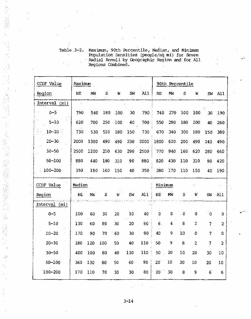
Table.3-2. Maximum, 90th Percentile, Median, and MinimumPopulation Densities (people/sq mi) for SevenRadial Annuli by Geographic Region and for AllRegions Combined.

CCDF Value Maximum 90th Percentile

Region NE MW S W SW All NE MW S W SW All

Interval (mi)

0-5 790 540 180 100 30 790 740 270 100 100 30 190

5•-10 620 700 250 100 40 700 550 280 180 200 40 260

10-20 i 730 530 510 180 150 730 670 340 300 180 150 380

20-30 2000 1300 490 490 230 2000 1800 620 200 490 240 490

30-50 2500 1200 210 630 290 2500 :770 940 160 620 280 660

50-100 880 440 180 310 90 880 820 430 110 310 90 420

100-200 350 190 160 150 40 350 280 170 110 150 40 190

CCDF Value Median Minimum

IRegion I NE MW S W SW All NE MW S W SW All

Interval (mi) .

0-5 100 60 30 20 10 40 0 8 -0 0 0 0

5-10 130 60 80 30 20 80 6. 4 8 2 7 2

10-20 f170 90 70 60 30 90 40 9 10 0 7 0

20-30 1180 120100 50 40 110 50 9 8 2 7 2

30-50 400 100 80 40 130 110 50 20 10 20 30 10

50-100 360 130 80 50 40 90 20 10 30 10 20 10

100-200 !170 110 70 30. 30 80 20 30 8 9 6" 6

3-14

Table 3-3. Maximum, 90th Percentile, Median, and MinimumPopulation Densities (people/sq mi) for Seven RadialDistances by Geographic Region and for All RegionsOombined.

CCDF Value

Region

Interval (mi)

0-5

.0-10

0-20

0-30

0-50

0-100

0-200

Maxijmn

NE MW S W SW All

790 540 180 100 30 790

650 660 200 170 30 660

710 470 410 160 110 710

1500 850 380 320 180 1500

2100 890 210 460 200 2100

760 370 170 350 100 760

350 210 160 120 50 350

90th Percentile'

NE MW S W SWAlIl

740 270 100 100 30 1901

470 270 150 170 280 230

630 340 250 160 110 380

1300 460 290 330 180 420

880 830 200 460 200 530

750 350 130 360 100 440

340 200 100 120 50 290'

4 .----- - I -- -

CCDF Value

Region

Interval (mi)

0-5

0-10

0-20

0-30

0-50

0-100

0-200

Median

NE MW S W Sw

100 60 30 20 10'

120 60 70 30 20

210 90 60 50 30

230 120 100 50 30

320 120 .90 50 90

330 120 80 70 70

290 130 80 40 40

Minihu~i

NE MW S W SwAllAll

40 0

70 4

90 30

110 50

120 50

90 80

90 50

8 0

10 6

10 20

20 10

20 20

10 40

30 20

0

3

1

2

10

10

20

0

7

8

7

20

30

10

0

3

2

10

10

10

3-15

Table 3-4. Maximm, 90th -Percentile,. Median, and Minimum PopulationDensities (people/sq ni) for the Most Populated 22.50 Sectorwithin Fbur Radial Distances by Geographic Region and forAll Regions O(mbined.-

(A0

CCDF Value Maximum 90th Percentile

Region NE MW S W SW All ,E MW S W SW All

Interval (mi)

0-5 4200 2000 950 450 320. 4200 3500 2000 510 460 310 950

0-10 2000 3800 1300 1600 140 3800 1300 1400 1000 1500 140 1000

0-20 4500 3400 2600 800 860 4500 2000 2100 2100 780 860 1800

0-30 8700 5200 4000 1800 1600 8700 3700 3200 1300 1800 1600 2500

CCDF Value Median Miniram

Region NE MW S W SW All ME MW S W. SW All

Interval (mi)

0-5 630 350 240 280 170 330 0 .50 0 0 0 0

0-10 '750 220 280 150 70 270, 40 40 60 20 50 201

0-20 •880 620 360 430 150 480 170 40 50 6 40 6

0-30 940 .800 430 290 120 550 1 110 60 40 5 70 5__ _ I _ _ _ _ _ _ ._ _ _ _ _ _

1.

by administrative region of the site specific popula-tion data for population density seven annuli and sevenradial distances, and for four radial distances of themost populated 22.50 sector.

In Section 2.7.4 the:sensitivity of consequencesto population distribution was' examined using a numberof hypothetical population distributions, all of whichhad average densities within 30 miles of the reactorof 750 people per square mile. Figure 3-4 shows that,within 30 miles of the reactor, only 4 of the 91 sites(4%) have population densities within that distancewhich exceed 750 people per square, :,mile.' Figure 3-8shows that for the most populated 450 sector 30 of the91 sites (33%) have'population densities that exceed750 people per square mile. Fihally, 'Fiqure 3-6.andTable D1.4 show that for the most populated 22.5 sec-tor 38 of the 91 sites (42%) have densities greaterthan 750 people per square mile'.

iExamination of the reactor site population densityscatter plots for the five NRC administrative regionspresented in Figures 3-9 through 3-11 shows that thedensities within any region range across approximatelytwo orders of magnitude and that between regions thereis substantial overlap of ranges.. Densities are largestin the Northeast and lowest in the. Southwest; qualita-tively the densities are ordered from largest to, small-est: NE, MW, S, W, SW. Tables 3-2 through 3-4 confirmthis qualitative ordering, although there are a numberof exceptions (S and W are often inverted) .

3.4 Time Dependent Trends

Figure 3-12 presents scatter plots by region ofthe year of site selection (the year in which a con-struction permit was granted was used as a surrogatefor the actual year of site selection) for theg91reactor sites examined in this study. Only four siteswere selected prior to 1960, two each in the Northeastand the Midwest. Not until 1973 was a reactor siteselected in the Southwest.

Because the years during which sites were selectedare distributed over time quite differently by region,trends by selection year in the density of the popula-tion distributions surrounding reactor sites were alsoexamined both by region and for all regions combined.Figure 3-13 presents plots of population density within

3-17

ANNULZ RADZI AREn~w~r €_n~r_ qn-onmT. on-AnHT. '-O-s5nMZ !o-10oHfZ# 100-200HZ1E4 UIA

0

8,0

1.000 000090 00 1 8 0

0 0 0 o1 88 0"0 -o , 00 0 0

00 0 0 0 0 0

8 0_ 0000

000 00000 o .06 oo I o Io0 o I:10 0 000 Io 0 0 000

•) O .0-... - V• 0 . .0. .

0 , 00 ' '8

8 00011 000ý4

0 0

00

0.1"

NE M£ . I" I

NRC Administrative Region

F'igure 3-9. Population Density (People/Mile2) at 91 ReactorSites by Geographic Region for 7 Radial Annuli:0-5, 5-10, 10-20, 20-30, 30-50, 50-100, and 100-200 Miles (the Lines Connect Median Values).

0000

00

00600

0 00

1E4

1000

CIRCLE'RADII AREo-51Z, 0-10n1, 0-20o1Z, .0-3011Z.* 0-5O0.oz 0-11Z,1 0-200HZ

0

o80, ...00is 0 goo 0O! 000

0 0008

00 0 0 0

6 0 8

00 0 8 0 00

00 00 0

0 00 0 •O~o 0';' 0 .

00

00 0

0 .. " 00

.,> 0

100

t.-II•o

a)

P-4.P4

r-4

0U)

10

IF

0.1HE rill S U SU

NRC Administrative Region

2Figure 3-10. Population Density (People/Mile ) at 91 Reactor

Sites by Geographic Region for 7 Radial Distances.0-5, 0-10, 0-20, 0-30, 0-50, 0-100, and 0-200 Miles.

IE4

1000

CZRCLE8

800o

8 8

oo0°0000

RADZZ ARE O-5HZ, O-IOHZ* O-20CHlO0-30HZ

.8000

00000o

0

o 00

00

08800

0

§0

80

80g

°•0

00 0

0

0 0

00

:0

,--r-1

04

0-40

9L4

100 00

0

00

00

o 0

V00 00

0:.0

101

0 0

1NE 'ho4 S U SU

NRC Administrative Region

Figure 3-11. Population Density (People/Mile 2 ) in the MostPopulated 22.5 Degree Sector at 91 Sites byGeographic Region for 4 Radial Intervals:0-5, 0-10, 0-20, and 0-30 Miles. (The linesconnect median Values).

30 miles of the site versus year of site selection, foreach region and for all regions combined. The line oneach plot is the least squares linear fit of the data.The slope of the line is the change in the logarithm of30-mile population density with time. The lines for theNortheast, Midwest, and South have slopes which, -giventhe scatter in the data points, are little differentfrom zero (NE = -0.04, MW = -0.01, S = 0.03). Giventhe narrow time span and considerable scatter of thefive 'Southwest site selection years, the slope of thatplot (SW = 0.7), though substantial, is of no importance.Only ýfor the West (W = -0.23) and to a lesser degreefor all regions combined (All = -0.08) do the slopesof the plots seem important.

To better define the significance of the time trendsdisplayed in Figure 3-13, an analysis of variance [3]0f the logarithm-transformed population density data wasperformed. The analysis partitioned the variabilityin the data among four terms: one for the common timetrend of all regions combined, one for-unique t:imetrends within each region, one for".riegional•di-fferencescorrected for regional time trends, and a residual termfor variability not attributable to either regionaldIfferences or time trends. The results of this analy-sis are presented in Table 3-5. In the table, the meansquare value is obtained by dividing the sum of squaresvalue by its number of degrees of freedom (number ofindependent terms in the sum of squares). Comparisonof the magnitude of the mean square values indicatesthe relative importance of the three terms (mean squarevalues large by comparison to the residual mean squarevalue are useful in explaining the observed variability).

Table 3-5 Analysis of Variance

Source of Sum of Degrees of MeanVariation Squares Freedom Square

Common time trend 11.2 1 11.2

Regional time trend 18.4 4 4.6

Regional differences 7.1 4 1.8corrected for regionaltime trends

Residual 82.0 81 1.0

TOTAL 118.7 90

3-21

8B [ YEAR OF SZTE APPROVAL FOR REGZONS

0

$4

4-)4.,q

0

C)

70

60

ID

CmI'D

am

cm13

cmCm.MI

Cm033am

ma

Cm,0

arnID

NJ

to%0

0

0

a0

0.0

50A

+NE S W SW

NRC. Administrative Region

Figure 3-12. Scatter Plot by Region of Year of Site Approval.

..: Wý

F" DEISITY Of APOOI YEARFOR %1 RECTOR WIES Sy ffECION

0

0 00

mia

CDtoo$

to*

to

op--00-o000 0

00

telsS

itg

~0

*0.0

0

0

ties

S

0@O00 :0"

08

•0

a

0 0 0

0

0V.

Is

Li

a)'-I

0)

F-I

040a,P4

I M • i • • . . . . . . .

56 so 64 Ga "2 76 S6 6 64 66 N 72 76 S6 : 6 64 66 72 76

U

lice

too

ls'e toll

0

0

0 60

lee0

0/o/0

tog

ALL

0 00 00

090 00 * 000S-00 0

0

8 00000

00

0

. . .° . . . ++. o. °.I.

I

to

• " " I I t l • * "0I . " . . - I . . . I

56 Go 64 66 ?2 76 56 61 64 7 2 76 56 60 64 68 72 76

Year of Approval

Figure 3-13. Plots of 30-Mile Population Density vs. Year ofSite Approval. The lines are the least squareslinear fit to the data. The slope of the linesare: NE = -0.04, MW = -0.01, S = 0.03, W = -0.23,SW = 0.7 and All = -0.08.

Table 3-5 suggests that the variability in logarithm-transformed site population data results principallyfrom a common trend with time. Since this common trendis not strong (the slope of the linear correlation forall regions combined is only -0.i08), its importance isunclear. It is possible that the trend toward lessdense siting with time is (1) real, or (2) an artifact ofthe data. If the trend is real, .it may result from somefactor not addressed by this analysis (e.g., with thepassage of time, suitable sites near cities become un-available, so more remote sites are selected, whichare necessarily-less densely populated!).

References for Chapter 3

1. Demographic Statistics Pertaining to Nuclear PowerReactor Sites, U. S. Nuclear Regulatory Commission,

.NUREG-0348, October 1979.

2. .J. E. Kohler, A. P. Kenneke, and B. K. Grimes,ýThe Site Population Factor: A Technique ForConsideration of Population In Site Comparison,U. S. Atomic Energy Commission, WASH-1235, October1974.

3. P. W. M. John, Statistical:Design and Analysis ofExperiments, Macmillan, New York, NY, 1971.

3-24

4. Site Availability Impacts

4.1 Introduction

The previous chapters of this report have examinedthe potential consequences of-accidents-at nuclearpower reactors ,and the. relationship of site populationdistribution to consequences. In addition, the popula-tion characteristics of current sites were examined.In order to reduce societal risk.from siting, it is.desirable to locate:,reactors in..areas o;f: low populationdensity... This., of course,, forces a trade-off betweenreduced risk and site availability. To evaluate moreprecisely the implications: of this trade-off,_ thischapter reports on work performed by Dames and Moore,under contract to Sandia, to study the impacts ofsiting criteria alternativeson land availability.

.The study included.consideration:,of ý'the: impacts onsite avaiiability of environmental factors (seismicity,topographic character, surfaceý and groundwater availa-bility, and restrictions due to regulations (wetlands,National parks,. etc.)) as well as population.

4.2. Methodology

The. study was performed in three steps: identi-fication of issues affecting site availability, datacollection, and analysis and display of data. Thefinal step was performed iteratively, using Dames andMoore's Geographic Information Management System

(GIMS), which manipulates geographical data in a gridcell format.

4.2.1 Issues of Concern

A set of general siting-issues was defined andused to identify and discriminate more suitable sitingareas from less suitable ones., These issues cover avariety of demographic considerations and a diverseset of environmental siting criteria relating normallyto costs.

4-1

Three issues were defined for population criteria.These are:

1. Stand-off Zones -- restrictions imposed bydistance from urban centers of a particularsize;

2. Population Density -- a measure of populationdensity within-a specified: (circular) area;and

3. Angular:Population:Distributio6n-- a measureof the'uniformity of •population distributionwithin a specified (circular)area.

Four issues were defined for environmental cri-teria. These are:

.1. Restricted Lands -- those areas in which thedevelopment of a nuclear power plant'is dif-ficult due to legal constraints or-the pre-

...dominance of wetlands;,.

2. Seismic Hardening -- the additional cost ordifficulty of compliance with seismic designcriteria; assumed to be measured by the maxi-mum expected (50 year) horizontal groundacceleration ekpressed in fractions of gra-vity (g);

:3. Site Preparation- A relative measure of theruggedness ortopographic character expressedas an index which indicates the percentageof land with access and construction diffi-culty; and

4. Water Availability -- an index reflecting therelative cost of obtaining water for cooling.

The latter three issues were further combined to definean overall environmental suitability measure.

It is necessary to keep in mind that the goal ofthis study was to provide information regarding landavailability and not to select sites on which to con-struct nuclear power plants. The defined issues were

4-2

analyzed on a nationwide basis to yield trends andindicate areas on a regional basis that could beconsidered for selection of power'plant sites•.Site selection analyses are generally conducted ata more specific scale and level of resolution.This is especially true for environmental criteria.Many site selection issues are related to physicalfeatures that are not geographically extensive, orconsider factors that are important in the site plan-:ning process (which includes the precise locationof the reactor and other plant facilities within thesite). While these factors are important for specificsite identification, they are not considered here.

4.2.2% Data Structure Diagram

A data structure diagram describing the flow of.data and information through the Dames and Moore studyis presented in Figure 4-1. The diagram shows thesources and flow of information on the demographic andenvironmental issues as well as how these issues arecombined to provide assessments of land 7availabilityfor various siting ;criteria.

The data structure diagram is principally an aidto help conceptualize the entire impact analysis.. Forthe most part, each box on the diagram represents amap that was created or a data .file, that could be dis-played as a map.

4.2.3 Display of Results

Results are presented as maps which display theimpact of a criterion, which when printed on a trans-parent medium, can be overlaid on other maps to seethe effect of composite criteria. Many of the resultsare displayed for the whole U.S. as well as for thenortheastern section of the U.S. (the most populousregion of the country).

In addition'to maps, results are presented astabulations of statistics for each state for various -

categories of information. Most of this statisticalwork was performed for comparisons of impacts ofenvironmental suitability and population criteriaand is described in, Section 4.6.

4-3

SlAT! STAl1ST!CAL. CATA£mmoAIES I!SlATEAALCIM)

lbb

ol.I

II , oSWU CATA I O(11150 DATA IANALTTI!AI. DATA J

I J

Figure 4-1 Data Structure Diagram for the Dames and Moore Study

4.2.4 Geographic Information Management System

The Dames and Moore Geographic Information Manage-ment System (GIMS) was employed for this study. GIMSis a computerized system that provides planners witha comprehensive approach to recording, storing, mani-pulating and displaying the mappable information usedin studies of this nature. The system provides a database which can be readily updated, and allows evalua-tion of many alternative criteria that would otherwisebe explored by time-consuming manual procedures.,

4.2.5 Mapping Approach

The mapping approach is a function of four re-lated factors: (1) characteristics of the study area;(2) nature of the input data; (3) analysis methodology;and (4) desired output or display ;Products. All ofthese factors are important in determining the basemap and grid cell size and shape. Based on these con-siderations, the Albers Equal Area projection waschosen at a scale of 1:3,168,000 (1 inch = 50 miles)for digitizing input data and displaying output results.In addition, it was decided that data would be analyzedusing a grid system consisting of square cells 5 km ona side (each cell represents 25 km or 9.65 squaremiles). An artificial equal-area grid was placed onthe base map by converting longitude and latitudecoordinates into X and Y coordinates given in meterson the ground from an origin in the southwest cornerof the map. Using grid cells of this size and shapeand the Albers projection ensures that any maps pro-duced from the analysis have several important charac-teristics:

1. Format is consistent with map projection andlevel of detail of input data;

2. A reliable sampling of population data(especially for the smaller area annuli) ismaintained;

3. Computer time and cost are at an efficientlevel;

4. Maps are o~f-manageable size while retainingimportant visible regional patterns;

4-5

6

5. Directional bias of analysis is minimal; and

6. Line printer graphics show area relationshipstruly,'and thus, do not distort the impliedimpacts of crit.eria.

4.3 Data Base

The data base consists of those data necessaryfor analyzing both demographic criteria and net envi-ronmental suitability. It includes:

1. Demographic Data

o Location and-population of urban centers

o 19801population estimated for enumerationdistrict ts

2. State and national boundaries

3. Restricted lands

o Legally protected

o Major wetlands

4. Seismic hardening

o Seismic acceleration

5. Site preparation

o Topographic character

6. Water availability

o Surface water availability

o Groundwater availability

4.3.1 Demographic Data

Site availability impacts based on demographiccharacteristics considered both standoff distancesfrom urban centers and surrounding population densityand angular distribution. These analyses requiredtwo types of data.

4-6

4.3.1.1 Urban Centers

Data concerning urban centers were extracted fromNUREG-0348 [1] . This publication categorizes urbancenters into three groups: those centers with popula-tion in excess of 25,000 people, greater than 100,000people, and greater than 200,000 people. The data:were updated with information provided by the NRC toinclude population figures for urban centers greaterthan 250,000 people, greater than 500',000 people andgreater than 1,00.0,000 people.

Populations for these urban centers were identi-fied geographically by latitude and longitude coordi-nates. The degrees of longitude and latitude wereconverted into X and Y coordinates which correspondedto the same geographic grid that was applied to theAlbers base map as discussed in Section 4.2.5. Thisconversion prepared the data for eventual use in theproduction of maps showing how much land would beavailable after imposing population center standoffzone criteria. The analysis of standoff zones isdiscussed in Section 4.5.1.

4.3.1.2 Population Density

To calculate population density, analyze variouscriteria, and ensure that the results are reliable inthe face of changing national population trends, itwas necessary to obtain the most up-to-date and de-tailed population figures. Figures from the 1980decennial census were not available in time for usein this study. In their place, estimates for 1980population were used. Data were supplied by theNational Planning Data Corporation (Ithaca, New York).While it is difficult to give an estimate for thepercent error, it is believed that the data are quitereliable, especially when individual data points(which correspond to centroids of enumeration dis-tricts or block groups) are taken in groups of 4 or 5.This is typically the case in this study. It isespecially true for all areas except the most remoteand rural. Thus, the data are considered reliablefor its intended function, the analysis of populationdata around the more urbanized areas of the country.

4-7

The 1980 population estimates were obtained for-matted on magnetic tapes with population figures geo-graphically referenced by latitude and longitude. Aswith urban center data, the degrees of longitude andlatitude were converted into X and Y coordinates on theAlbers grid system. This process prepared the demo-graphic data base for analysis of population density.

The analysis is discussed in Section 4.5.2.

4.3.2 State Boundaries

Using the Albers base map at 1:3,168,000 scale,all coastlines, international boundaries, and stateboundaries were digitized. The area within each statewas assigned a unique code to identify it for furtheruse. The state boundaries map file allows analysisor display of results on an individual state basisor by any group of states.

4.3.3 Restricted Lands

The nature of certain areas of the country causesthem to be protected or restricted from development.Two types of lands were considered as restricted:legally protected lands and existing wetlands.

4.3.3.1, Protected Lands

The Energy Reorganization Act of 1974 (Section207) states that national forests, national parks,national historic monuments and national wildernessareas should be excluded from consideration as poten-tial nuclear energy center sites. While this studydid not deal with nuclear energy centers, it is rea-sonable to consider such lands as protected from thesiting of a single nuclear power plant, regardlessof a national policy on-this matter. Utility indus-tries tend to avoid such areas because of the possi-bility of time consuming and costly legal battles.The following areas were considered to be protected:

o National Parks

o National Forests

o National Monuments

o National Wilderness Areas

U

4-8

o National Grasslands

o National Wildlife (Game) Refuges

o National Recreation Areas

o National Seashores

o State Parks

o State Forests

o State Reserves/Refuges

o State •Recreation Areas

o Military Reservations

o Indian Reservations

Three different map sources were used to obtainthe locations of these protected lands. The UnitedStates base map utilized in this study •(compiled bythe U.S. Geological Survey, 1965) was used to extractthe location of national parks, forests, monuments,wildlife refuges, and Indian reservations. Sectionalsheets at a scale of 1:2,000,000 from the NationalAtlas [2] were used to update the boundary informationfor the above protected lands as well as to obtainthe location of national recreational areas. Becauseof the relatively small size of protected state areasand some protected national areas, a screening processwas used for certain types of land, rather than iden-tifying and digitizing every one. Because this studydealt not with site selection but with the generalpatterns of land availability, a minimum size screenof 100 square miles was used for the following typesof areas: military reservations, national grasslands,state parks, state forests, state monuments, statereserves and refuges, and state recreational areas.Information for these types of lands was obtained fromthe 1980 Rand McNally. Atlas, as this was the mostdetailed, up-to-date and uniform source of information.

4.3.3.2 Wetlands

Besides the above legally protected lands whichwould be restricted from development either on thebasis of national policy or avoidance on the part

4-9

of the utility industry, certain types of environ-mental restrictions might be imposed as well. Forthis study, one such environmental constraint wasapplied -- namely, the location of major wetlands. Itis the policy of the Water Resources Council to ensurethe protection of wetlands from adverse impacts anddegradation [3J.

No uniform nationwide data base exists regardingthe location of major wetlands. After considerationof several approaches to defining the extent'of wet-lands in an efficient manner, a source was found tosatisfy the needs of this study. The 1:12,000,000scale sectional sheets of the National Atlas [2J wereused to outline the extent of major wetlands.- At thisscale, only major wetlands can be shown. A comparisonof these source data with more detailed map-data showsthat some of the wetland boundaries have been general-ized and most wetlands less than 60 square miles wereprobably not shown on the sectional sheets.

The locations of both protected lands and wet-lands were digitized into separate map files. Eachof the 15 different types of protected lands-was givena unique identifying code to allow individual consi-deration of each type of protected land. The two mapfiles were added together to produce a mapifile calledrestricted lands (Figure Fl in Appendix F). The re-stricted lands file was later added to the individualenvironmental issue map files as well as the environ-mental suitability map file to produce maps showingthe location of restricted lands, and conversely, thenet availability of land.

4.3.4 Seismic Hardening

There are generally three major factors to beconsidered in the seismic evaluation of a nuclear powerplant site:

1. Fault Rupture Hazard'-- primarily a sitingproblem;

2. Dynamic Soil Stability (liquefaction) -- botha siting and a design problem; and

3. Strong Ground Motion (vibratory) -- both asiting and design issue.

4-10

Siting requirements are specified by the NRC [4Jand the evaluation of a site (for design purposes) isbased on the additional cost imposed by the site-relatedconditions.` Although a detailed site qualificationsstudy would require the careful consideration of allthree' factors, their evaluation generally requireseffort far beyond the scope of this study. However,after careful consideration of their overall impact,a methodology was developed for a coarse screeningprocess which reflects the overall impact of thesefactors. The data necessary to evaluate the potential

problem from the standpoints of rupture hazard anddynamic soil stability 'were not uniformly availablethroughout the United States. For this reason, seismichardening was evaluated solely on the basis of Vibra-tory ground motion.-.

Strong ground motion criteria are determined bythe postulated Safe Shutdown Earthquake (SSE) which isthe largest possible event on the controlling seismo-genic feature, which could be a capable fault (notnecessarily the closest one) or a tectonic province.The :SSE is determined on 'the basis of historicalearthquake data '(seismicity) and detailed investiga-tion of the length and capability of nearby faults,according to procedures specified by the NRC [5]. Theplant must be able to survive such an earthquake in amanner which will not result in'the release of radio-activity in excess of stated limits. An additionaldesign requirement is imposed by the Operating BasisEarthquake (OBE) which is commonly defined as havinga peak acceleration equal to 1/2 that of'the SSE.The plant must be designed so that it can continueto operate during and after an OBE: alternatively,none of the structural or mechanical components maybe stressed beyond'their elastic limit by the OBE.

While the detailed investigations required forthe determination of the: SSE for each 5 km by 5 kmgrid cell were clearly beyond the scope of this study,it was possible using available data to probabilisti-cally evaluate the relative severity of the strongground motion hazard in the study area and considercosts of seismic hardening. This was accomplishedusing probabilistic studies of seismic risk preparedby Algermissen and Perkins [6] and the Applied

4-11

Technology Council (ATC) [7] and supplemented withinformation from a U.S. Geological Survey professionalpaper [81. The ATC map represents an adaptation of acomprehensive analysis by Algermissen and Perkins.The map shows accelerations in bedrock expressedas a fraction of gravity.: The combination of thesethree sources -resulted in the seismic accelerationsource data map illustrated in Figure F2, Appendix F.

The map shows the horizontal acceleration (ex-pressed as a fraction of gravity) in rock with a90 percent probability of not being exceeded in 50years. According to Algermissen and Perkins:

"Certain facilities such as nuclear powerplants may require design adequate for accel-erations with exceedance probability no largerthan 0.5 percent in 50 years. For structuresfor which very low exceedance probabilitiesare appropriate, it is clear that this sourcemap indicates only a relative idea of thehazards -- the design motions will be highfor much smaller exceedance probabilities. Inthose regions where seismicity is lower thanin California,. the accelerations shown on thismap vary with return period according to thevery approximate rule: the level of motiondoubles as the return period increases by 5(exceedance probability decreases by 5)."

This rule was used to modify the values on thesource data map. The exceedance probability was de-creased by a factor of 5 -- from 10 percent to2 percent -- and the acceleration values were doubled.Another iteration of this process decreased the ex-ceedance probability from 2 to 0.4 percent and againdoubled the acceleration values. The new valueswere then considered to be four times the valuesexpressed in Figure F2. Thus, the data in the modi-fied map file became consistent with the notion ofusing a 0.5 percent exceedance probability for nuclearpower plants (as suggested by Algermissen and Perkins).

The seismic risk source data file was furtheradapted by interpolating between the contour levelsto develop a more continuous distribution of seismicrisk (horizontal acceleration). The continuous dis-tribution was desirable from a siting standpoint,

4-12

so that sites falling on either side of a dividingcontour would not appear to have greatly differingseismic requirements. (The contours of the source mapdo not generally have any geological significance whichwould warrant such sharp distinctions.) It is stillrecognized that the absolute resolution of the sourcedata map is probably no more precise than the contourintervals given. However, the relative ranking ofareas for reactor sites is probably representable tothe finer resolution implied by the interpolation.

The general impact of seismic design requirementsis assumed to be proportional to the specific costof the additional design and construction featuresrequired to satisfy the seismic design requirements.In NUREG/CR-1508 C9], seismic hardening costs werecalculated and shown on a graph relating the SafeShutdown Earthquake expressed as a fraction of gravityto the estimated cost differential in millions ofdollars. The cost curve used in this study is shownin Figure 4-2.

The map shown in Figure F2, Appendix F, indicatesthat the lowest acceleration contour is equal to 0.05g.Remembering that the exceedance probability was twicedecreased by a factor of 5 (thereby twice doublingthe ground motion), the lowest acceleration contourmay now be considered equivalent to 0.2g. By applyingStevenson's cost information to the modified probabi-listic seismic acceleration information, a cost surfacethat shows the additional cost of seismic hardeningwas generated.

Using the curve shown in Figure 4-2, accelerationvalues between 0.2g and 0.6g (0.05 and 0.15 on thesource map) were assigned costs ranging from $23.7million to $55.5 million. Acceleration values of lessthan 0.2g were assigned a cost of $23.7 million (the.same as for 0.2g). This was because nuclear powerplants in the U.S. are designed for an SSE of 0.2g,although it may be possible to build them more cheaply.For acceleration values greater than 0.6g, it was feltthat there is no reasonable way to accurately estimatethe increased costs of seismic hardening. Rather thanassign a cost, they were labeled "inestimably high".

4-13

80 16

~70 ;14

60- 12 CI Z

cz<

5: 0 - . .. 1 "

S40 " BEST ESTIMATE WITH SELECTED BACKFILL _g

9zz

30,- 6,.

Lw 20

A- W

9x

~I'-"

10 4"- L0 -

0 0o.1- 0.2D 0.30 0.40 0.50 0.60

SAFE SHUTDOWN EARTHQUAKE ZERO ,PERIOD GROUND ACCELERATION, g

Figure 4-2. Cost Increase As A Function Of Seismic

Load for Nominal ll00-1•e Nuclear PowerPlant (1977 Dollars)

4-14

The costs derived from Figure 4-2 (1977 dollars)were next converted to 1980 dollars yielding a low of$31.5 million and a high of $73.9 million. To calculatethe cost of seismic hardening that was considered as"additional", the design-basis value of $31.5 millionwas subtracted from all the costs. This resulted in arange of costs of 0.0 to $42.4 million. The graphicdisplay of seismic hardening cost is shown in Figure F3,Appendix F.

4.3.5 Site Preparation

An increase in slope or ruggedness of terraintranslates directly into increased cost for construc-tion. This includes the difficulty that may be encoun-tered in excavation for foundations, construction of*access roads where low grades are required (due tothe transport of large components such as the turbineor pressure vessel), and finally, measures that mustbe taken to mitigate environmental disturbances suchas control of run-off and erosion from cut slopes.

To evaluate the impact of topographic-character.on site preparation cost over a large regional area,a general index that indicates both the steepness ofslopes and the areal extent of such slopes was sought.Such data was found in a paper by E. H. Hammond [10]and his map which was adapted and found in the NationalAtlas [2). Regions on the map are characterized by thepercentage of their area which is classified with atopographical gradient of less than 8 percent slope(gently sloping). The 8 percent slope is not a criticalthreshold value for land utilization. It does, however,indicate a value beyond which movement of vehiclesbecomes impeded, and in general, construction and oper-ation becomes more difficult.

The smallest region delimited and given a classi-fication has an .area of about 800 square miles. Smal*lerareas are omitted or absorbed into the adjacent regionthat they most resemble. With this level of resolution,it is possible that sites suitable for building a nuclearpower plant' exist within the area characterized byeven the highest proportion of rugged terrain. However,at this regional level of analysis, these special con-ditions are not practically observed. Because not onlysite ruggedness but the ruggedness of the access route

4-15

for implacement of heavy components affects the con-struction costs, the analysis of site preparation costsis based solely on the general indication of topogra-phic character, as defined by the data. Figure F4,Appendix F, is a map showing. the source data with greytones implying preparation costs. Four terrain clas-sifications are shown: regions with less than 20%, 20to 50%, 50 to 80%, and. greater than 80% gently sloping(less than 8% slope).

4.3.6 Water Availability

Cooling system cost has become a major componentof total power plant cost. Several factors are in-volved in determining cooling system cost:. the typeof cooling-system -- mechanical draft wet towers,natural draft wet towers, cooling ponds, or oncethrough cooling; climatic temperature distributions,existing priorities for use of available water,; andrestrictions such as wild and scenic rivers. Whilea detailed analysis of these factors is beyond thescope of this study, a methodology was developed topresent a general picture of water availability andthe cost involved in its use. Sources of both surfacewater and groundwater were mapped and costs. were deter-mined for each. The two. map files were then overlaid,and a map was produced showing the least cost of avail-able water.

4.3.6.1 Surface Water

Hydrological implications of water consumption bynuclear power plants have been discussed by Giustiand Meyer, [11]. Many existing power plants are locatedon sites next to streams and draw their water directlyfrom those streams without provisions for significantstorage. In siting 'plants along rivers one-must con-sider the periods of low flow when the impact on thewater resources of total water consumed in the coolingprocess is at a maximum. This consideration is espe-cially significant for plants that do not use coolingponds with a large amount of storage capacity. Inlight of. this, it is important to have reliable esti-mates of the low flow of streams from which plantscan draw cooling water. According to Giusti and Meyerthere are several reasons -for estimating these flows:

4-16

1. Safety -- the regulatory staff of the U.S.Atomic Energy Commission (1972) in referenceto a safety analysis report for nuclear powerplants states:"Estimate the probable, minimum flow~rate,resulting from the most severe drought con-sidered reasonably possible in.the region.as such conditions may affect the abilityof the ultimate heat: sink to perform ade-quately-.";

2. ýStandards-- most .states have issued stan-dards regarding the maximum permissiblemineral concentration in surface water tobe used for coolingý. As is well known, this-concentration is at a maximum at a low flow

.period because the flow consists of ground-water discharge which is normally more con-centrated:mineralogically than surface water.Additional concentration of the-stream flowmineral content is brought about ýby tran-spiration which is also at a maximum duringlow flow periods;

3. Ecology -r maximum-ecological impact on freshwater biota can occur on some streams duringlow flow periods if the mineral concentrationexceeds certain limits or if the flow is ab-ruptly reduced by withdrawal at power plants.Furthermore,-the withdrawal entails loss ofbiota by physical entrainment on the intakescreens: or by physical injury on passagethrough the water pumps;,and

4. Plant Operation -- the conditions describedabove may be such as to force the shutdownof the plant, with contingent costs and lossof revenue to plant operators and loss ofservice to consumers. While this may be con-sidered an acceptable operationalrule underexceptional circumstances, say once in 10years, it becomes a serious problem of, mis-design when recurring more often, say onceevery year.

Stankowski, Limerinos, and Buell [12] have exam-ined the low water flow in the United States to provideinformation regarding potential sources of cooling

4-17

water. They have prepared a map which identifies thosestreams for which the average 7-day low flow with arecurrence interval of 10iyears is at least 300 cubicfeet per second (cfs). (The 7-day, 10-year low flowor 7Q10, is the average' low flow that occurs over 7consecutive days'with a probable recurrence of 10 years.)Their map shows those stream reaches that: (1) havea 7QiO of at least 300 cfs, or (2) could furnisha sustained flow of at least 300 cfs if storage wereprovided. For their study, 300 cfs was Jselected asthe needed flow in the stream on the assumption thatmany states will not permit more than 10 percent ofthe dependable flow to be withdrawn for a consumptionuse. Ten percent of 300 cfs equals 30 cfs which isthe amount oflwater that might be considered necessaryto cool a 1,000 MWe nuclear power plant if coolingtowers, sprays, or ponds are used. -The requirementof 30 cfs for coolingýis in agreement with the informa-tion produced by Giusti and Meyer [11]. The Stankowski,et al., map~was digitized -and used as a source mapto show surface water availability...

To extend the utility of surface water informa-tion, the map file showing surface water availabilitywas converted into a map showing surface water cost.First, an estimate was made of the dollar per milepumping cost to move surface water. These costs wereestimated for each of the four terrain types charac-terized for site preparation (Section 4.3.5).; Bothan initial capital cost and a 30-year operating andmaintenance cost were estimated. In addition to thepumping cost, a penalty cost was added for those streamsthat required the use of reservoirs in order to sustaina 7Q10 of 300 cfs. Based on this information, a com-puter imodel was used to calculate, for each cell, thecost of obtaining surface water as a function of pumpingcosts over a variety of terrain and the potential useof a reservoir. The model determined the least of thecost alternatives for supplying surface water to acell. The cost information was mapped and is shownin Figure F5, Appendix F. There are eight equal inter-val levels between zero and $300 million. Costs above$300 million were grouped together -- amounting to about10 percent of the study area. This grouping at thehigh cost end allows regional differences in the morereasonable range of costs to'be displayed.

4-18

4.3.6.2 Groundwater Availability

Groundwater is an important source of cooling. waterin many parts of the country. Characteristics of ground-.water can vary quite,dramatically within a small region.Despite this, an attempt: was made to locate a sourceof information'that would satisfy the broad scalerequirements of this study. Using the USGS WaterSupply Paper 1800 [131, and supplementing this withsuch maps as the Hydrologic Investigations Atlas [14],Tectonic Map of North America [15], and Shaded Reliefof U..S. [16], major regions and subregions of thecountry were mapped as source data. Although variabil-ity exists within any one of the regions or'sub-regions,regions do show differ.ences regarding their... characteris-tics of quality, quantity, depth to water,, and requiredwell field size.

Based on these characteristics, cost informationwas applied to the map data. Both capital costs and30-year operating and maintenance costs Were calculatedfor each of the delimited areas on the basis of dollarsper well. To obtain the equivalent of 30 cfs fromany of the generalized aquifers,, it would be necessaryto sink several wells., The required number of wellswas calculated by dividing 30 cfs by the expected yieldper well of the given aquifer. Multiplying this numberof wells by the cost per well resulted in the cost asso-ciated with bringing 30 cfs to the surface from any ofthe generalized aquifers,. Itwas observed that severalof the generalized aquifer areas require well fieldswhich are too large for practical use. For these areas,groundwater was considered to be unavailable in a prac-tical sense. For reasonably sized well field areas,the cost of collecting the water from numerous wellsand bringing it to .a single point was estimated. Foreach of the groundwater regions, the two costs -- thatof bringing the water to the surface, and that ofcollecting the water from a well field, were addedtogether. The cost data were then mapped as is shownin Figure F6, Appendix F.

4.3.6.3 Combined Water Costs

Using the cost information for both surface waterand groundwater, a map file was created which indicated

4-19

the cost of obtaining cooling water using the leastexpensive alternative. To do this, the two map files-- surface water costs and groundwater costs, werecompared on a cell-by-cell basis. For every cell, thelowest cost value was saved and placed into anothermap file. This was called "Combined: water cost" andthe map is shown in Figure F7, Appendix F.

4.4 Environmental Suitability Analysis

In order to evaluate the impact of demographic'criteria on land availability it was necessary to'first

establish a base of available land. This base was con-Pstructed from the protected area and environmental'consideration data bases. The environmental factors,were combined 'by dividing' utility functions for eachfactor, and then summing the utility values Within eachcell. The protected areas were then overlaid on thisdata.

4.4.1 Individual Site Availability Issue Assessments(Utility Functions)

To evaluate the suitability of each potential sitearea, each of 'the siting issues was first evaluatedindependently. This evaluation was accomplished bydefining a utility function for each issue such thatthe characteristics of a specific site area could betranslated into a value on a defined suitability scale.Thiss was a numeric scale ranging from 1 to '9, where 1was the lowest level of suitability and 9 was thehighest.

4.4.1.1 Seismic Hardening Cost Utility Function

The issue of seismic hardening was assigned autility function on the basis of additional hardeningcosts as discussed in Section 4.3.4. Table 4-1 showsthe data categories of seismic hardening costs andtheir corresponding utility value.

A map of the seismic hardening utility functionwas produced and is shown in Figure F3, Appendix F.(This is the same map used to show the cost of seismichardening.)

4-20

TABLE 4-1

SEISMIC HARDENING UTILITY FUNCTION

Cost inMillions of.1980 Dollars Utility Value

0.0 to 6.16.1 to 12.1

12.1 to 18.218.2 to 124.124.1 to 30.330.3 to 36.436.4 to 42.4

No reasonable estimate

8 (high suitability)7654_321 (low suitability)

4.4.1.2 Site Preparation Utility Function'

Actual dollar costs associated with site prepara-tion could not be located as source data. However,discussions with authorities in the construction ofnuclear power plants as to how the topographic charac-ter of the landscape might affect the site preparationcosts have allowed for the assignment of the utilityvalues to terrain classifications which were discussedin Section 4.3.5. These are shown in Table 4-2.

A map of the site preparation utility functionwas created and is shown in Figure F4, Appendix F.(This is the same map used to show the site preparationsource data.)

TABLE 4-2

SITE PREPARATION UTILITY FUNCTION

Topographic Character.(percent of area that

is gently sloping*) Utility Value

>80 percent50 to 80 percent20 to 50 percent

<20 percent

*Gently sloping means

8 (high suitability)52'1 (low suitability)

8 percent slope.

4-21

4.4.1.3 Water Availability Utility Function

Utility values have also been assigned to datarepresenting the cost of obtaining cooling water. Basedon this cost information (described in Section 4.3.6),costs in excess of $300 million were grouped togetherand assigned the lowest utility value. For costs lessthan $300 million utility values were assigned on thebasis of 8 equal intervals as shown in Table 4-3.

TABLE 4-3

WATER AVAILABILITY UTILITY FUNCTION

Combined Water Cost

(in millions of 1980 dollars) Utility Value

0 to 37.5 9 (high suitability)37.5 to 75.0 875.0 to 112.5 7

112.5 to 150.0 6150.0 to 187.:5 5187.5 to 225.0 4225.0 to 262.5 3262.5 to 300.0 2

>300.0 1 (low suitability)

A map was prepared showing the water availabilityutility function and is shown in Figure F7, Appendix F.(This is the same map used to show the combined watercost.)

4.4.2 Site Availability Issue Overlay

Using the utility functions, each issue map wastranslated into a partial suitability map where eachpotential site area was represented by a utility value.These individual suitability maps are represented inFigures F3, F4 and F7. They are considered partialsuitability maps because each includes only one sitingissue. They were combined into a composite suitabilitymap by adding the individual map files together. Itwas felt that the reconnaissance nature of this study,as well as the broad scale representation of environ-mental data, did not justify a more sophisticatedmanipulation of the files. For this reason, the threemaps were overlaid -- each with an equal importanceweighting.

4-22

The addition of the three utility value map filesresulted in a map file with values ranging from 4through 25 -- each value having a different frequencyof occurrence. Maintaining the relationship that highvalues represented the most suitable land, the distrib-ution of the composited utility values was dividedinto five intervals. The intervals were selected to..include equal land areas. This resulted in five cate-gories or levels of environmental suitability -- eachlevel representing 20 percent of the data base. .Therestricted lands file was then added to the compositeutility value file. A color-coded version of a mapproduced from this combined file was supplied to NRC.

4.4.3 Environmental Statistics

Analysis of the impact of various siting criteriaon land availability was accomplished in'two ways:creation of maps to visually show these impacts andproduction of statistics to quantify the impacts. Themaps concerning environmental factors have been pre-sented elsewhere in this section. To quantify theimpacts of various siting criteria, tables were pre-pared which used the data files created during thevisual or map analysis. Statistics regarding theamount of area in each data category were computedfor each of the 48 states.

For each of the three environmental issues--seismic hardening costs, site preparation costs, andwater availability costs -- a table was prepared thatshows the amount of land in each of the categoriesthat was represented by a utility value. Two addi-tional tables were produced: One for surface watercost and one showing the five different levels ofcomposite environmental suitability. These statisticsare shown inlTables F1.1 through FI.5, Appendix F.The numbers in each column indicate the amount ofland in the specified category. The area is shownin square miles as well as percent of the total statearea.

4-23

4.5 Demographic AnalysisU

As discussed in Section 4.2, three issues weredefined as relevant to population criteria - stand-offzones, population density, and angular distribution.Stand-off zones are restrictions on distances fromurban centers to nuclear plant sites. Populationdensity is a measure of the persons per square milewithin a specified (circular) area surrounding a site.The population density, calculations were mapped assingle data files or in combination with other annulardensities to produce composite population criteria maps.Angular distribution restrictions are limitations onthe permissable population within one or more 22 1/20sectors surrounding a sit e. .

4.5.1 Stand-off Zones

To study 'the impact of restrictions :imposed bydistance from urban centers, stand-off zone maps wereprepared. As discussed in Section 4.3.1, populationsand locations were provided for urban centers of avariety, olfsizes., The location of these urban centerswas indicated by a single latitude/longitude coordinatewhich was converted to a Y and X coordinate correspond-ing to grid cells on the Albers base map. Urban centerswere grouped according to their size: greater than25,000, 100,000, 200,000, 250,000, 500,000 and 1,000,000people. For each grid cell in the study area, its dis-tance from the nearest urban center of a particular sizewas computed. This resulted in six separate data files.These files were converted into maps by specifying athreshold distance at which a cell would be consideredeither suitable or unsuitable for siting a nuclearplant. , Based on the above data, thirteen such stand-offmaps were produced. The maps produced are indicatedin Table 4-4 and presented in Figures F8.1 through F8.13,Appendix F. The maps illustrating stand-off zones fromthe three largest cities were created only for thenortheastern U.S.

Maps of stand-off zones are quite self-explanatory.There is a direct relationship between the stand-offdistance and the amount of area that is constrained bythe specified criteria.

4-24

TABLE 4-4

STAND-OFF ZONES

Size of MappedUrban Stand-Off

Center Distance (in miles)

25,000 5, 10100,000 10, 15, 25200,000 25, 30, 40, 50, 100250,000 12.5500,000 18

1,000,000 25

An example of these maps is shown in Figure 4-3.

4.5.2 Population Density

A wide variety of population distribution criteriabased on density surrounding a prospective site werestudied for their impact on land availability. Densi-ties were calculated for both circular areas and annularareas. As described in'Section 6.3.1, population sourcedata was identified by a latitude and longitude coordi-nate system. These coordinates were converted into theY and X coordinates compatible with the Albers grid basemap. This raw data were then converted into a set ofmap files giving the population density of an area agiven radius centered on each cell. Maps of varyingthresholds were produced from these files. The matrixshown in Figure 4-4 indicates all of the map filesthat were produced regarding population density. An"X" in a box means that the map files were producedfor both the total US and the northeastern window.An "NE" in a box means that the map file was producedonly for the northeast. An example of these mapsis shown in Figure 4-5. Maps representative of thevariety of population densities are shown in FiguresF9.1 through F9.26, Appendix F.

An understanding of the spatial relationshipsproduced by various criteria can be gained by compar-ing some of the maps. Figure F9.5 shows the areasconstrained by a density threshold of 100 peopleper square mile in the 0-5 mile circle. Figure F9.8,concerning the same circle employs a density thresholdof 500 persons per square mile. It is obvious that

4-25

t'Jt

. , .

IEISITED ARTA$EEISMIC

WETLANDSSURFACE WATERARSEJA WATERWATER cost

Figure 4-3. Example of Standoff Zone Maps.

Id-

ANNULUSRADII IN MILES

DENSITY PEOPLE/SQUARE MILE

ý100 1 150 1 200 1t5 ý350.1 ý4O000 1 ý 7SO1?50 1 800 1?ý1ooo

!

0-2 X x NE NE

0-5 X X X X

0-10 X X X x

0-20 X

0-30 x

5-10 x x

5-20 x

10-20 X x x

20-30. X X

30-50 X X

Figure 4-4. Annular Population Density Data Files

4::-

i'0o

N-

y

\ ~

S

-K

RAMT~~

Figure 4-5. Example of Annular Population Density Data Maps.

(4

every area constrained in Figure F9.8 is also con-strained in Figure F9.5. If the size of the annulusremains constant, the area constrained using a higherdensity threshold is always completely containedwithin the area constrained by a lower threshold.In addition, the use of a lower density thresholdas in Figure F9.5, constrains a much greater portionof the suburban and rural land areas.

Spatial differences are also noted through acomparison of circle size while maintaining a constantdensity threshold. For example, compare Figure F9.8,which shows the areas constrained by a 500 peopleper square mile density threshold within the 0-5mile circle, with Figure F9.14 which applies thesame threshold to the 0-30 mile circle. Use of thelarger radius tends to ýconstrain only the urbanand some suburban areas of major cities. None ofthe rural or• smaller urban areas are constrainedand the impacts look similar' to thosewhich resultfrom stand-off zone criteria.

Another interesting spatial effect of. the demo-graphic criteria can be seen on any of the maps in::which the annulus is defined using an inner radiusgreater than zero. 'In these cases, the annulussurrounding a prospective site is shaped like aring rather than a circle and the effect is thatthe shape: of some of the constrained areas is alsothat of a ring.: The occurrence of this type of pat-,tern depends upon the specified density thresholdin conjunction with the limits of the annulus andthe population data itself. For example, Figure F9.23indicates the amount of land constrained if a criterionof 500 people per square mile in the 20-30 mile annuluswere applied. Note that in the St. Louis area theland surrounding the city would be constrained --

but not the land comprising the city. St. Louis'land area is small enough so that a relatively smallpopulation is located *between 20 and 30 miles ofthe city center, and yet the city population-islarge enough to cause the density threshold to beexceeded in the surrounding areas. Chicago, on theother hand, occupies an area large enough so thatgrid cells at the city center are within 20 to 30miles of significant population and the pattern ofconstrained land is solid.

4-29

A comparison of the St. Louis area between FigureF9.23 and Figure F9.21, which employs the same densitythreshold within the 10 to 20 mile annulus indicatesnot only the absence -of a ring structure but also ashrinking of the extent to which land is constrainedusing the smaller 'annulus. The pattern of the areaconstrained near Chicago remains solid in both figures;however, both the extent and amount of land increasewith increasing annular radii. Thus, if the densitythreshold remains constant, the extent from the centralcity of the criterion's effect increases with increas-ing annular radius... However, the total amount of landconstrained may not increaseý accordingly dlue to thepossible elimination from constraint of the centralcity. -

4.5.3 Composite Population Densities

When using a criterion of the form of less than500 people per square. mile from 2 to 30 miles,, it ispossible for a cell to satisfy that criterion, whileit doesn't satisfy a 500 people per square mile cri-terion out to only 15 miles. This occurs when thereis a dense population pocket surrounded by low densityareas.. In order to pinpoint areas for which thisoccurs, a new set of criteria were developed whichrestricted population to a given density for allradii from an inner radius to an outer radius.Thus, for the example -of 500 people per square milefrom 2 to 30 miles, the •new criterion is satisfiedonly if the population density is less than 500 .people per square mile from 2 to R miles, where Rtakes every value from 2 to 30.

Evaluating population density for every radiusfrom the inner radius to the outer radius is imprac-tical in practice, so an approximation is used..

Using the example of mapping any cells that ex-ceed the 500 persons per square mile threshold for the2-30 mile annulus,, density calculations were made for6 portions of the 2-30 mile annulus and were thencomposited. First, any cell that exceeded the 500persons per square mile threshold within the 2-3 mileannulus was recorded. Next, unsuitable cells in the2-4 mile annulus were recorded and unsuitable cells

4-30

in the 2-5 mile annulus were recorded. This processwas repeated for the 2-10 mile annulus, 2-20 mileannulus, and the large' 2-30 mile annulus. These6 individual files were then added together, creatinga file in which a-cell: that. was shown to be unsuitablein any of the 6 was also considered unsuitable for the2-30 mile composite,,annulus. In this manner, datafiles were created'for the 2-30 mile composite annulusfor the following densities.

250.persons/square mile500 persons/square mile750 persons/square mile

1,000 pe~rsons/square mile1,500 persons/square mile

Example maps 'for rthe' no'rtheast are* shown in FiguresF10.1 thru FAA.4, Appendix' 'F.

Besides creating a composite map file for aParticular annulus (such asý 2-30 miles)and a parti-cular density (such as 500 persons per square mile), ,another type of composite was created. 'This consistedof two separate annui.i -_ each with its o0wn given popu-lation density threshold. ForS example, as discussedabove, 6 individual data files were added together tocreate the 2-30 mile composite annulus. Now, a dif-ferent annulus with a different population densitythreshold was added to the 2-30 *mile composite annulus.Two maps were created in this manner and are: shownin Figures Fll and F12, Appendix F. Each map showscells that are considered unsuitable for the: 2-30 milecomposite annulus (with density of 500 persons persquare mile) as well as: for the 0-2 mile annulus forpopulation densities of'either 100'persons per squaremile or 250 persons per square mile. In addition tothese two mapped data files, other complex compositefiles were created. Some of these were used for sta-tistical analyses in combination with the environmentalcriteria. (These statistics are'discussed in-Section4.6). The six complex composite data files which werecreated are indicated in Table 4-5. The numbers inthe columns underneath the two annu'i represent popu-lation density figures (persons/mile).

4-31

TABLE 4-5

CCMPLEX CCMPOSITE POPULATION DENSITIES

0-2 Miles 2-30 Miles (Composite)

(1) 100 250(2) 100 500(3) 250 500(4) 250 750(5) 500 750(6) 500 1500

4.5.4 Sector Population Density

To this point in the chapter, any potential demo-graphic criteria addressing population density wereanalyzed using what might be termed a uniform densitydistribution. -Criteria were stated in terms of thenumber of persons that would be allowed in an areaof a given size -- that is, population density --

and the shape of the area was always circular. Usinga circular area allowed relatively dense concentra-tions of population to exist provided that the totalnumber of people within the circle did not exceed astated limit.

Results of reactor accident consequence calcula-tions indicate that certain risk characteristics dependstrongly on the maximum number of persons within anygiven direction sector, (see Section 2.7.4). Therefore,criteria regarding the maximum allowable populationwithin sectors in addition to total population sur-rounding a site were considered. The impact on landavailability was examined for alternative sector cri-teria and compared to the impact of uniform density,criteria.

Sector criteria were stated. in terms of allowingup to a fraction of the allowed number of peopleto be located in any sector of a particular width..'For example, a sector criteria might be stated: nomore than 1/6 of the people allowed by a uniformdensity of 500 persons per square mile canbe locatedin any 45 degree sector at distances within 3 milesof a site.

4-32

The impact of sector criteria was investigatedwith regard to several variables. The parameterswere:

o Distance: Radii of 2, 5, 10, 20, and 30 miles

o Sector width: 22.5, 45.0, 90.0 degrees, and360 degrees (for uniform density)

o Fraction: 1/16, 1/8, 1/4, 1/3, and 1/2 thepopulation allowed by uniform density

o Density: 250, 500, 750, and 1500 persons persquare mile

Population counts were determined within 2,-5, 10,20, and 30 miles of potential sites (grid cells) andwithin sector widths-of 22.5, 45.0, and 90.0 degrees..The maximum number of persons found in a sector ofa stated width and for a particular radius was recorded.For example, investigating a circle of radius 10 milesand using a sector width of:22.5 degrees, the circlewas divided into 16 sectors. The number of people wasdetermined within each sectorland the maximum of the16 counts was recorded. This procedure of determiningthe maximum countzwas undertaken 15 times .. once forevery combination of sector width (3) and radius (5).

Alternative criteria were then applied to thecount data on the basis of allowing a certain fractionof the total number of:people allowed within the circleto be located in any sector. The total number of peo-ple allowed in a circle is dependent upon the radius(for area) and the density that is allowed. For thissector analysis, the previously established densitieswere analyzed -- 250, 500, 750, and 1500 persons persquare mile and five radii were used -- 2, 5, 10, 20,and 30 miles. For 0-2 miles, only one density wasused as a part of every criteria -- namely, 250 per-sons per square mile. To calculate the allowablepopulation theshold out to 5, 10, 20, and 30 milesfor each of the densities, the area from 2 miles to rmiles (radius) was multiplied by the density and theproduct added to the threshold for 0-2 miles withits 250 persons per square mile density. For example,at 20 miles using density 750 persons per square mile,the threshold equals:

4-33

.. (Area of 0-2) x 250 + (Area of 2-20) x 750

= (12.57 x 250) + (Area of 2-20) x 750

- (3142 :+ 933075)

- 936,217:people

Using only one density (250 persons per square mile)for 0-2 miles and four densities for thet other fourdistances resulted in 17. separate:thresholds.. Thesethresholds Were used not only for uniform densitycriteria analyses but also for calculating the frac-tional thresholds applied to sector population dis-tributions. Thus, if a criterion was stated that nomore than 1/4 of the people allowed by, a uniform den-sity- of ý750 persons per square mile within 20 mileswould. be -allowed in a sector, :the threshold would be936,217. x 1/4 = 234,054 people.

Being consistent with previously computed impacts,the -impacts for sector criteria for- any particulardensity or fraction were composited to 130 miles.. Thatis, sites exceeding a threshold at.2 miles were re-,corded and saved .into a map file. .ý-,Sites exceeding athreshold at 5 miles were also recorded and storedintoi, a :map. file,, as were all sites for: 10, 20,.and 30 miles. Finally, all five map files were mergedresulting in a:file that showed sites constrainedby any one or more of the thresholds. Spatially, itwas ýfound ,that any criteria at smaller radii tendedto eliminatesites in rural areas as well as in. citiesbut-only out to their-edge. Criteria applied at largerradiitended to eliminate cities and :large areas aroundtheir edges (similar to a "standoff" criteria) butallow local population concentrations in rural areas.Bycompositing :criteria for all five radii, both urban.and rural population concentrations were evaluated fortheir. impact on availability of potential nuclearsites. Additionally, it was found that.the effectsof sector criteria occurred in the same areas asaffected by annular density criteria.

Sector criteria were of interest in regard totheir impact on land availability above and beyondthat already affected-by uniform density criteria.To depict and quantify this information, tables-werecreated to show the amount of land available for siting

4-34

in each state if a particular sector criterion wasestablished. The information is shown in Tables F2.1through F2.24, Appendix F. Each table shows the impactof alternative fractional Criteria along with the uni-form density criteria on land availability. All of-the fractional and uniform density Criteria have beencomposited to 30 miles by adding the individual impactsof a criterion at 2, 5, 10, 20, and 30"miles.

Each table considers a unique, combination ofallowable annulus population density and sector width.'The four population densities and three sector:widths,resulted in 12 combinations. Twenty-four :tables-werecreated as each of the 12 combinations was tabulatedusing. two different formats.."•i Tables F2.1 through` F2.12are formatted such that the numbers 'in the columns re-present the 'amount of land that-is uniquely constrainedcriteriai ...... ..by the specified criteria.

The columns are arranged so that total magnitudeof constrained land decreases from left to right.' 'Asan example, Table F2.1 indicates the"impacts'of alter-native fractional criteria applied to 22.5 degree sec-tors using a density threshold of 250 people per squaremile for both the 0-2 mile- ýand 2-30 mile annulus. 'The"

leftmost column'"Available'Land," shows the'ramount ofland available for 'siting if the criterion stated inthe adjacent column is applied; that is, no more than'1/16 of the population allowed in the annulus at adensity of 250 people per square.mile .can be locatedin any 22.5 degree sector of the annulus. The:cri-terion stated in the second column of these 12 tablesalways represents the most constraining fractionalcriterion.

The rightmost column, "Restricted Lands," showsthe amount of land that is constrained because itis either legally protected or a major wetland. Nodemographic criteria affect these numbers.

The numbers in each of the middle columns showthe amount of land that is uniquely constrained bythe specified criterion which is above the total amountpreviously constrained by the criteria in all of thecolumns to the right. In Table F2.1, for example,the column labeled "Uniform Density'" shows-for Alabamavalues of 5,703 square miles or 11.0 percent of thestate area. This is the area that would be constrained

4-35

by applying a uniform (annular) density criterion andit is additional to the area already constrained byrestricted lands (2,075. square miles or 4.0 •percent).Thus, the application ,of this particular uniform densitycriterion in Alabama would constrain a total of 7,778square miles or 15.0 percent of the state area if nosector criteria were applied. The next column to theleft, "1/2 Allowable Pop.," would add another 2,355square miles or 4.5 percent of constraint if a sectorcriterion were stated that no more than 1/2 of thetotal population allowed..by a density threshold of-250people per square mile. in both the 0-2 mile and 2-30mile annuli could be •located in any 22.5 degree sector.Similarly, using a criterion, of allowing up to I/3 ofthe allowable uniform• density population to be locatedin a single sector, would constrain an additional.6,388 square miles or 12.3 percent of the land area.The total constrained land in this case would be 16,521square miles or 31..8 percent of the state area. Con-versely, 68.2 percent (100 minus 31.8) of the landwould be available for siting.

To more clearly summarize the information thatshows the availability of land when specific• sectorcriteria are applied Tables F2.13 through F2.24 werecreated in a different format than the previous 12tables. On these tables,• the numbers in the columnsshow the amount of land available. for siting if thespecified criterion is applied, For example, TableF2.13 indicates that 68.,2 percent of the land inAlabama would be available for siting if a criterionof allowing up to 1/3 of the population .(allowed bya uniform density criteria using a density threshold,of 250 people per square mile in both the 0-2'mileand 2-30 mile annuli) to be located in any 22.5 degreesector. This number agrees with the one produced inthe above example regarding Table F2l.. The columnlabeled "Uniform Density" indicates land availabilitywhen no sector criteria are applied. The column "NoPop. Criteria" shows the amount of land availablewhen only restricted lands are considered a constraint.

4.6 Impact Analysis

Analysis of the impact of various siting criteriaon land availability was accomplished in two ways:creation of maps to visually show these impacts, andproduction of statistics to quantity the impacts. Many

4-36

of the maps produced have already been reviewed inother sections of this chapter. All maps were producedon a transparent base enabling them to be overlaid.This capability allows creation of complex composite

* population criteria maps. In addition, these popula-tion criteria maps can be overlaid on the color-codedenvironmental suitability map.

To quantify the impacts of various siting cri-teria, tables were prepared which used the data filescreated during the visual or map analysis. For a par-ticular subject, whether environmental or demographic,statistics regarding the amount of area impacted werecomputed for each of the 48 states. Fifteen tableswere produced which were grouped into three differenttypes: environmental criteria, environmental suitabil-ity levels versus selected population cases, and popu-lation criteria versus individual environmental suita-bility levels.

4.6.1 Environmental Statistics"

For each of'the three environmental issues--seismic hardening costs, site preparation costs, andwater availability costs -- a table was prepared thatshowed the amount of land 'in each of the categoriesthat was represented by a utility value (see Section4.4). Two additional tables were produced: one forthe surface water cost, and one showing the five dif-ferent levels of composite environmental suitability.As discussed earlier, these statistics are shown inTables F1.1 through F1.5, Appendix F.

4.6.2 Impact Comparisons

The overlay of transparent maps provided a quicklook at potential land availability. A map containingfive levels of environmental suitability along with asixth level showing restricted lands, when overlaid witha variety of population criteria, produces numerousgroupings of data. To present these data in statisticalform, a method was devised to keep each table simpleenough to be understood, while retaining a largeamount of information.

First, five population cases were defined on thebasis of complex composite criteria. These populationcases are shown in Table 4-6. The numbers in thecolumns underneath the 0-2 and 2-30 mile annuli repre-sent population density figures.

4-37

TABLE .4-6

,Population 2-30 MilesCase 0-2 Miles (Composite).

- 1 00 2502 .250 5003 250 750

-4 500 -750.5. 500 .1500

:Five tables were .produced --. ;one foreach popula-tion ,c.ase -- which compared the environmental suitabil-ity levels toan individual population case. These

,statistics .indicate the-amount of land in each of theenvironmental suitability levels that is available forsiting nuclear power plants ifa given set of populationcriteria (a population case) is.applied. These statis-tics are shown in Tables F3.1 to F3.5..

To illustrate the effect ofapplying differentpopulation criteria (the five population cases) on landavailability in a particular environmental suitabilityclass, five more tables were produced. ,In these tables,-the statistics represent the amount ,of land availablefor siting nuclear power plants in a given environmentalsuitability-class as well.as the amount of land: uniquelyconstrained by each of .the five population cases. Thesestatistics are shown in Tables F3.6 through F3.10. Thecolumns representing population cases have been arrangedsuch that in moving from left to right, the stringencydecreases. The leftmost column of the.table -- availableland -- shows land that is available for the given envi-ronmental suitability class even.if the most stringentpopulation criterion (population case 1) is applied.The second column -- population-case 1 -- represents anadditional amount of land considered available if popu-lation case 1 were relaxed. The next column -- popu-lation case 2 -- represents the additional incrementof available land if the criteria for population case2 were also relaxed. It follows that if no populationcriteria were established, the,.amount of land availablein a particular environmental suitability class wouldbe equal to the total of the first six. columns in thetable; the only land considered constrained would bethat by a restricted land designation.

4-38

4.7 Summary

ýThe analytical methods'used in this.'study weredesigned to explore the impact of various demographicsiting criteria on the availability of land consideredsuitable for the siting of nuclear power plants. Mapswere created so that impacts could be easily visual-ized and tabbular statistics were prepared'to allow amore rigorous analysis.

The determination of land considered suitable forsiting was' accomplished through a"muti-objective envi-

ronmentalýsuitability analysis. The analysis ,.Iwas per-formed using"factors generally related to engineeringcosts as well as 'conservation of specific resources.Because. this ihvestiigation. concerned the entire 48cont iguous United St :ates and•was' not a site selectionproject,' environmental factors' were analyzed at a rela-tively general level 'of detail and were each consideredtobe of equal importance. The' most suitable areas werecharacterized by an adequate water supply, low seismi-city'and'gentle topography as'well as an absence of..protected resources.' Although'. the map of. environmentalsuitability (Figur"eF8) shows the eastern one-half ofthe country to'be more suitable than the western, itis felt that there are numerous suit~able sites availablein the western portion.

Three types of population criteria were investi-gated: stand-off zones, annular density and sectordensity. The effects of stand-off zone criteria arestraightforward. There is a direct relationship betweenthe stand-off distance and the amount of land area con-strained.

The analysis of annular density thresholds showedthat the use of smaller radii to define the annulusresulted in constraints on sites near both large andsmall urban populations as well as sites near somelocally dense rural areas. Larger radii tended toconstrain a greater amount of area near suburbanpopulation but only around major cities; small urbanand rural areas were not constrained.

Because results of reactor accident consequencecalculations indicated (Section 2.7.4, Chapter 2) thatcertain risk characteristics depended strongly on themaximum number of persons within any given direction

4-39

sector, sector population criteria were designed.Their impacts were investigated to determine the amountof land area that would be constrained additional tothat affected by annular density criteria. It wasfound that sector criteria affected the same areas andthose adjacent to theareas affected by annular densi-ties. Also, .the area of impact responded to changesin annular radius in the same manner as for annulardensity criteria.

Transparent overlay maps and tabular statisticswere provided to NRC for use in establishing siting,criteria which would be numerically based upon populationdensity,.distribution and exclusion distance. Tabularstatistics were used to quantify the impacts on a state-by-state basis. The use of transparent overlays providesa means not, only to see the. impacts of the generatedcriteria but also to create and view the effects ofcomplex criteria by overlaying any combination of maps.

Maps showing demographic criteria were also overlainonto the map of environmental suitability to visualizethe potentially available suitable land. .Through 'boththe overlay procedure and a, comparison of statistics,it was found that the greatest impacts of demographiccriteria occur in the areas of high environmental•suitability. (i.e., Northeast)..

4-40

References for Chapter 4.0

I. Demographic Statistics Pertaining to Nuclear PowerReactor Sites, U. S. Nuclear Regulatory Commission,WNUREG-0348, October 1979.

2. National Atlas:of the United States of America,U.S. Geological Survey, compiled. 1967,:revised1972-73.

3. Federal.Register, Volume 45, #226, November 20,.. 1980,,: pages ý76682-76684-. • •• •

4. 10 CFR, Part :100: Reactor Site .Criteria.

5. 10: CFR,; Part 100::! Appendix:A --. Seismic andGeologic Criteria for' Nuclear Power Plants.

6. S. T. Algermissen 'and-D. M. Perkins,'"A Proba-bilistic: Estimate of Maximum Acceleration in Rockin the Contiguous United States," U. S. GeologicalSurvey Open File Report, 76-416, 1976.

7. R. V. Whitman, N. C. Donovan, B. Boalt, andS. T. Algermissen, Effective Peak Velocity RelatedAcceleration Map, Applied Technology Council ofStructural Engineers Association of California,1977.

8. G. A. Bolliner, "Reinterpretation of the IntensityEffect of the 1886 Charleston, South CarolinaEarthquake," U. S. Geological Survey ProfessionalPaper 1028, 1977.

9. J. D. Stevenson, "Evaluation of the Cost Effectson Nuclear Power Plant Construction Resulting Fromthe Increase in Seismic Design Level," Office ofNuclear Reactor Regulation, NUREG/CR-1508, 1981.

10. E. H. Hammond, "Analysis of Properties in LandForm Geography: An Application to Broad-ScaleLand Form Mapping," Annals of the Association ofAmerican Geographers, Volume 54, Number 1, 1964.

11. E. V. Giusti and E. L. Meyer, "Water Consumptionby Nuclear Power Plants and Some HydrologicalImplications," U. S. Geological Survey Circular745, 1977.

4-41

12. S. J. Stankowski, J. T. Limerinos, S. E. Buell,Stream Reaches In The Conterminous United StatesWhere Dependable Flows of 300 Cubic Feet perSecond Are Available Or Could Be Provided, U. S.Geological Survey Open File Report 77-646, 1977.

13. The Role of Groundwater in the National WaterSituation, U.. S. Geological Survey Water SupplyPaper 1800, 1963.

14. C. L. McGuinness, Generalized Map Showing AnnualRunoff and Productive Aquifers in the ConterminousU. S., U. S. Geological Survey Hydrologic Inves-tigations Atlas HA-194, 1964.

15. P. E. King, Tectonic Map of North America, U. S.Geological Survey 1:500,000:7 1969.

16. R. E. Harrison, Shaded Relief of U. S., U. S.Geological Survey 1:7,500,000; 1969.

4-42

5. Socioeconomic Impacts

5.1 Introduction

Because the construction and operation of a nu-clear power plant can have social and economic impactson nearby communities, the dependence of socioeconomicimpacts on site location was examined by the BattelleHuman Affairs Research Centers (Battelle-HARC) undercontract to Sandia National Laboratories. The Battelle-HARC study (1) developed a classification scheme for theremoteness of light water reactor (LWR) site locations;(2) calculated average growth rates for several demo-graphic and economic variables during the period of plantconstruction for two groups of LWR sites of differingremoteness, (3) examined the dependence of transmissionline costs on site remoteness; and (4) discussed thesignificance of these results in the light of previousstudies of the socioeconomic impacts of rural indus-trialization projects, boom towns, and nuclear powerplants. This chapter presents a summary of the Battelle-HARC study. Full details are reported in the finalreport of that study [1).

5.2 Site Remoteness

Conceptually, the degree of remoteness of anuclear power plant site depends upon both populationdensity (the more sparse the population the more remotethe site) and proximity to major population centers(nearby cities of significant size decrease remoteness).To capture this dual dependence, two measures weredeveloped to define the degree of site remoteness, oneof population sparseness and the other of proximity tourban centers.

Sparseness was defined in terms of total populationand number of communities of population 25,000 or morewithin 20 miles of the site. Four sparseness categorieswere defined as follows:

5-1

Sparseness Measure

Category

Most Sparse

Least Sparse

Definition

1. Less than 50,000 persons and nocommunity with more than 25,000persons within 20 miles.

2. From 50,000 to 74,999 personsand no community with more than25,000 persons.within 20 miles.

3. From 75,000 to 149,999 personsor less than 75,000 persons butwith at least one community

Swith more than 25,000 personswithin 20 miles.

4.- 150,000 or more persons within20 miles.

Proximity was defined in terms of total populationand the presence of cities with population ý100,000within 50 miles of the site. Four proximity categorieswere.defined as follows:

Proximity Measure

Category

Not in Close Proximity

Definition

1. No city with more than100,000 persons and lessthan 400,000 personswithin 50 miles.

2. No city with more than100,000 persons and between400,000 and 1,499,999persons within 50 miles.

3. One or more large citieswith more than 100,000persons and less than1,500,000 persons within50 miles.

4. 1,500,000 or more personswithin 50 miles.

11.

VIn Close Proximity

5-2

The distance of 20 miles and a community size of25,000 (sparseness measure) were chosen because the NRCSiting Policy Task Force [2] recommended that populationdensities around sites be limited out to a distance of20 miles and because current siting practice requiresthat the nearest town of 25,000 persons be at least moredistant than one and one-third times the distance to theouter boundary of the low population zone surrounding theplant site. The distance of 50 miles (proximity measure)was chosen because workforce commuting distances, whichstrongly affect the degree of population increase duringconstruction periods and thus the magnitude of socioeco-nomic impacts, are usually limited to about a one-hourcommute [3], or about 50 miles at current speed limits.

Table 5-1 presents the cross-classification by sparse-ness and proximity of 84 LWR sites in the U.S., wherereactors are currently operating or under construction.

Table 5-1. Site Remoteness Matrix

Proximity

Category 1 2 3 4 Total

Sparseness

1 11 1 3 0 15

2 3 1 4 2 10

.3 4 7 10 " 4 25

4.1 0 .0 1 23 3410 4 i ._ __ _

Total 18 9 28 29 84

Within this matrix remoteness decreases as one moves fromcell (1,i) to cell (4,4) and sites in cells with indicesthat sum to the same total [e.g., cells (3,1), (2,2), and(1,3)] should be similar in degree of remoteness. By

5-3

summing the numbers of sites having similar degrees ofremoteness, the distribution of remoteness over the 84sites is obtained. Table 5-2 displays this distribution.

Table 5-2. Distribution of Remoteness

Number ofGroup Cell Sites

1. Most Remote Sites (1,1). YI2. A (2,1), (1,2) 43. (3,1), (.2,2), (1,3) 84. (4,1), (3,2), (2,3), (1,4) 115. (4,2), (3,3), (2,4) 126. (4,3), (3,4) 157. Least Remote Sites (4,4) 23.. .. 8 4

Tables 5-1 and 5-2 show that, of the 84 sites,only 15 are not located within 20 miles of a town of25,000 or within 50 miles of a city of 100,000. Bycontrast, 23 of the 84 sites have populations of150,000 within 20 miles of the site and 1,500,000within 50 miles. Thus, Tables 1 and 2 show that mostcurrent U.S. LWRs are not remotely sited.

5.3 Growth Rates

The socioeconomic impacts of large industrialprojects usually depend on the size of the project work-force. Since the peak construction workforce ( >2000)for a nuclear power plant is substantially larger thanthe plant's operational staff (-200), the socioeconomicimpacts of nuclear power plants should be largest dur-ing the plant's construction phase. A measure of themagnitude of these impacts can be obtained by calcu-lating average growth rates for population and economicactivity in the areas surrounding nuclear power plantsduring their preconstruction (baseline) and constructionperiods. Variation of impacts with remoteness can beexamined by performing these calculations for twogroups of sites, a non-remote group and a remote group,and comparing the results.

Time series data for population, employment (total,retailtrade, and construction), payroll (total, retail

5-4

trade, and construction), and government revenues(property tax per capita) and expenditures (total,education, highway, health, and welfare) were obtainedfor the preconstruction and construction periods at21 nuclear power plant sites. Cross-classification ofthe 21 sites, according to the sparseness and proximitymeasures previously defined, yields Table 5-3. Table5-3 shows that 7 of the sites are relatively remoteand the other 14 are nonremote.

Table 5-3. Cross-classification Remoteness Matrix for7 Remote and 14 Non-Remote Sites.

proximity

Categoryl 1 2 I3 I 4 Total

Sparseness

1 4 1 i4

21 1- l 1

42 - 5 '2 1

-____ -*. 5 1 6 ;' 11

Total 7 1 7 7 . 21

Population data were available in census publica-tions .[4) for the years 1960, 1966, and 1970 through1978. :Employment and payroll data were obtained for theyears 1959, 1962, and 1964 through 1978 from CountyBusiness Patterns [5]. Government; revenue and expen-diture-data were collected from the County and CityData Book [6] for 1962, 1967,,, and 1972, and from theCensus of Governments [7] for 1977.

Average yearly values of government revenues andexpenditures for the preconstruction (baseline) andconstruction periods for the non-remote group of 14sites and the remote group of 7 sites are presentedin Table 5-4. Table 5-4 also presents the percentage

5-5

Table 5-4. Average Yearly Government Revenue and Expendituresfor Remote and Non-Remote Groups*

Remote

Variable

Property Tax Per Capita

Total Government Expenditures

Education Expenditures

Highway Expenditures

Health Expenditures

Public Welfare Expenditures

BaselinePeriod

71

7,658

3,852

684

792

174

ConstructionPeriod

88

12,567

6,566

909

1,687

200

Percentage.Increaset

24

64

70

33

113.

15.

Non-Remote

Baseline Construction PercentagePeriod Period Increaset

112 139 24

78,582 115,478 47

30,274 57,159 89

5,677 6,383 12

3,626 5,657 56

5,275 9,787 85

U,

.*Property tax per capita in dollars, expenditures in thousands of dollars.t[(Construction Period Value/Baseline Period Value)-ll00.

A

increase of each variable for the construction periodrelative to the baseline period. Table 5-4 shows thatthe percentage increases in totaligovernment, highway,and health expenditures were greater at remote than non-remote sites, that-the converse is true for educationand welfare expenditures-, and that the increase in percapita property tax was the same for both site groups.Therefore, because these data showed no consistentvariation and because the amount of data was scant(data were available for only 4-years), average yearlygrowth rates were not calculated for these governmentvariables.

The exponential growth of the variable X at a ratek per year over the time period t is given by

= Xtekt (1)t t

Average growth rates for a group of sites can:,be obtainedby linear regression analysis after recasting equation1 as follows, where k is the yearly average growth rateof the variable X for the site group, i is a site index,and wewwi is a site specific difference term.

tn i = nXi t + kt ei (2)

Average growth rates were calculated for both site groupsfor the preconstruction,,(baseline) and construction per-iods for 7 variables (population, and total, retail, andconstruction employment and payroll). Table 5-5 presentsthe results of these linear regression analyses.

Examination of Table 5-5 reveals a consistent pattern.For each of the 7 variables and for both periods (baselineand construction), growth rates are higher for the remotesite group than for the non-remote group. On the average,during the baseline period growth rates at remote sitesexceed those at non-remote sites by about 50 percent. Dur-ing the construction period growth rates at remote sitesare 2 to 3 times, larger than are growth rates at non-remotesit es. As would be expected, growth rates are largest forconstruction payroll and employment. In addition, becauseof the increased demand for labor, the average number ofhours worked also increases and therefore payroll growthexceeds employment growth.

5-7

Table 5-5. Average Growth Rates for Population, Employment,and Payroll at Remote and Non-Remote Sites.

Average Yearly Growth Rates (%)a

OD

Population.

Total Employment

Total Payroll

Retail Employment

Retail Payroll

Construction Employment

Construction Payroll

Preconstruction

Remote Non-Remote

1.7+0.2 1.4+0.2

5.7+0.4 3.9+0.2

8.4+0.3 5.7+0.3

5.5+0.3 3.8+0.3

8.1+0.2 5.0+0.3

8.3+0.8 3.9+0.5

io.8+1.0 7.2+0.6

Construction

Remote Non-Remote

6.1+0.8 1.6+0.6

12.8+1.5 4.4+0.9

18.9+2.4 7.3+1.5

8.8+1.0 4.3+0.6

9.9+1.0 4.5+0.6

33.3+3.5 11.8+2.2

45.9+5.0 17.2+3.1

Remote

4.3+1_.0d

7. 1+1 9d

I0. + 2 -.7d

3.4+1:. 3 d

1.7+1.2

24.9+4.3d

35.1+6.0d

Construction Impacts(%)b

Non-Remote

0.2+1.4

0.5+1.1

1.6+1.8

0.5+0.9

-0.5+0.9

7.9+2..7dlO.0O.7Ld

ImpactDifferences

(%)c

4.i1+2.4'd

6.5+3.00

8.9+4.5d

2.8+2. 2 d

.2.2+2.7e

17..1Z7.0d

25.i+9.7d

a. All values are significant at the 0.01 level by f-testb. (Construction Growth Rate) - (Preconstruction Growth Rate)c. (Remote Impact) - (Non-Remote Impact)d. Significant at the 0.01 level by t-teste. Significant at the 0.05 level by t-test

14

By subtracting baseline period growth rates fromconstruction period growth rates, estimates of thegrowth rates due only to nuclear power plant construction(construction impact) are obtained. Table 5-5 shows thatfor the non-remote group of sites, construction impactswere significant only: fo'r construction. payroll and employ-ment. '.However', for the remote-group of sites, impactswere signifificant for all variables, being largest forconstruction:payroll (35%) and~employment (25%) ,and sub-stantial for total payroll (10%). Finally, the lastcolumn of Table 5-5 shows that, for all variables exceptretail payroll, :impact differences :(remote site construc-tion impact minus non-remote, site construction impact)are all statistically .signifian't at 'the-0.0 level.

5.4 Transmission :Line Costs

Transmission line costs are comprised of installationand operating costs. Installation costs depend on (1) thel.ength, of the" right-of'wayý along which the lines will bestrungý ihý order to connect the power plant to the-existingna~tional power grid; :(2)1 right-of-way-acquisition costs;(31) the number and tsize :(conductor rating) of the linesinstalled; and (4) installation labor costs (right-of-waypreparation, constructio;n of line towers and substations,stringing of lines).',: Operat-ing costs consist principallyof thelcost of line losses during transmission and main-tenance costs.,

Transmission losses are less for shorter line lengthsand larger conductors. Larger conductors cost more thansmaller conductors,! requirel a wider right-of-way (125 ftwide for 230 kV cable; 200 ft for 500 kV [8]), and aremore costly to install. Despite these higher costs, EPRIprojections [9] predict an increasing use of higher rated(larger) conductors through the year 2000. This agreeswith the findings by Power Transmission, Inc. [10] thatutilities currently preferý to minimize future transmissionlosses by installation of larger conductors.

Unit costs for labor (hourly wages) in suburban areaswere found by an EPRI study [11] to exceed those in ruralareas by about 25%. Unit costs for the ;acquisition ofland for right-of-way are also likely to be lower in ruralareas than in suburban areas. In contrast to this, totalcosts due to acquisition of right-of-way, purchase ofmaterials and equipment, payment of labor, and transmis-sion line losses all increase with increasing line length.Therefore, since remote siting would seem to requirelonger transmission lines, remote siting would appear to

5-9

entail higher transmission line installation and oper-ating costs. This is not always the case,. however.

.. Maps of the existing national transmission grid.show that, except for the more remote regions of theRocky Mountains., grid transmission lines pass throughall regions (both remote and non-remote) of the U.S.[12]. Although consideration of environmental, social,and asthetic issues as required by NEPA has tended tosomewhat lengthen line..right-of-ways, the factor thatdominates the length of new transmission lines is thegross distance of the power plant site from the nearestleg of the national transmission gr~id. Because thisgrid runs through both remote and non-remote areas,remote siting does not necessarily mean a lengthy trans-mission line. Table 5-6 presents data in support of thisconclusion..

Table 5-6.presents data on the conductor rating,length, ardacreage of.the transmission lines.whichconnect 29 power .plant sites (tho.se with all facilitiesoperating as of 1978) of varying remoteness to thenational power grid. Examination of the right-of-waylengths, *which were drawn from DOE maps:[12] , .shows thatfor existing sites right-of-way lengths do not correlatewith remoteness. Some• remotessites are closer to thenational grid than are some less remote sites. Thus,it is distance from the national transmission grid andnot-distance from major population centers (remoteness)that principally determines the costs of transmissionline installation and operation.

5.5 Discussion

Major constructioh projects have large workforcerequirements. In rural settings, when workforce re-quirements can not be met locally, or by commuting fromnearby cities, in-migration of workers occurs. If thisin-migration is substantial, "boomtown" conditions mayresult and the host area may experience significantsocioeconomic impacts. This scenario has been:.the sub-ject of considerable study. Rural industrial development'studies [13,14] have examined the impacts of industrialprojects upon small, rural communities. Boomtown studies[15-18] have examined the local. impacts of rapid, large-scale energy development. projects, located primarily inremote farming and ranching areas of the Rocky Mountains.The impacts of nuclear power plant construction have alsobeen examined by several previous studies [19-211..

5-10

Table 5-6. PowerTransmission Line Data for 29 OperatingNuclear Sites

RemotenessIndex

Total Miles ofRight-of-Way

Estimated Acres Average Kilovoltsof Right-of-Way Per Mile of Line

1-1 230 4,182 3452-1 *266 4,030 230

2-1 38' 800 399532 52 661 '156

3-2 230 4,061 3013-2 102 1,855 3453-2 179 2,670 206

2-4 30 545 345"2-4 151 2,655 3093-3 118 2,675 4183-3 85 1,370 2673-3 .5 91 "3453-3 95 1,803 "3163-3 84 1,273 2303-3 123 2,236 337

3-4 17 309 345.3-4 124 2,255 3453-4 24 291 1154-3 170 3,576 4234-3 85 1,455 3044-3 25 358 1984-3 67 1,218 345

4-4 409 8,291 1474-4 60 758 1344-4 4 61 2304-4 104 2,545 4854-4 90 1,636 3454-4 217 4,561 3784-4 29 527 345

5-11

Significant in-migration to a construction pro-ject's host area occurs only if workforce requirementscan not be met locally or by commuting from nearby popu-lation centers (generally, those located within about 'aone-hour commute of the site [3]). Even when substantialin-migration does occur, a boomtown can be avoided, ifthe resulting population growth is spread over severalnearby communities [22]. In general, •adverse socio-economic impacts are not observed until the rate ofpopulation growth of a single community exceeds 10 to15 percent per year [23,24]. Under these conditionsinstitutional breakdowns may occur- in the labor andhousing markets and in the provision of governmentservices (education, health care, recreational facil-,ities, police and fire protection) [23].

The small sizes, undiversified economies, smalltax bases, homogeneous populations, and traditionallife styles of rural communities tend to increase theirsusceptibility to socioeconomic impacts resulting fromrapid population growth. Mortgage investors tend to findsmall, economically undiversified, rural communitiesunattractive investment locales. Lack of mortgage moneycombined with shortages of building materials and hous-ing construction workers can produce a serious housingshortage. Because of their limited tax bases and becausethe project under construction generally yields littletax revenue until nearly completed, rural communities areoften unable to finance the increased load of governmentservices needed to accommodate rapid population growth.Finally, rural communities having a homogeneous popu-lation and life style may be less willing or able towelcome newcomers having different ideas, ways of doingbusiness, and life styles and to accept the changes inpersonal, social, business, and institutional inter-actions that incorporation of the newcomers into theircommunities would entail [16-18,251.

The willingness of rural communities to acceptchange depends upon community perception of the benefits(and risks) that will accompany the changes, and uponthe degree of community involvement in the decisionswhich determine the nature and rate of the changes.Because the construction of a large industrial or energyfacility promises increased tax revenues, new jobs, moreretail trade, and therefore improved government services,an end to out-migration of children and friends [14,15],and a higher standard of living [211, many rural commun-ities welcome these projects (at least initially).

5-12

However, community resistance may develop, if theeconomic benefits are unevenly distributed (e.g.,business men and land owners profit while the poor,the elder ly, and minorities suffer), if the projectis perceived to benefit principally distant cites(e.g.., electriic generating.stations [19,25]), ifproject decisions affecting the community are madewithout community involvement, and if there are con-cerns about the safety of the facility (e.g., nuclearpower plants [21]).

The degree to which the socioeconomic impacts,characteristic of krural industrialization and boom-towns, have occurred as the result of nuclear powerplant siting was examined by gathering data about peakconstruction employment,,: n umber oof in-migrants, andsocioeconomic impacts at: 12 remote nuclear power plantsites. The data, which were extracted from Environmen-tal Impact Statements and post-licensing case studies(where available), are presented in Table 5-7. For the12 sites listed in Table 5-7, peak construction employ-ment was approximately 2200 (+700), or 5 percent of thesurrounding population to 20 miles. For the 9 siteswhere in-migration data were available, peak constructionin-migration (workers plus families) on an average repre-sented only 3 percent of the surrounding population to20 miles. Examination of the last column in Table 5-7shows that with scattered exceptions (crowded classrooms,Yellow Creek; stressed government services, Hatch; wageinflation, St. Lucie; safety controversy, Diablo Canyon)the socioeconomic impacts at the 12 sites were largelybeneficial (significantly increased tax revenues, in-creased retail trade). Given the modest increases intotal population in the regions surrounding the sites,it is not surprising that detrimental impacts wereminimal, while economic impacts were favorable.

Since socioeconomic impacts depend principallyon the rate of population growth, which scales withconstruction workforce growth, additional data onconstruction workforce growth were developed for 19non-remote construction projects including 15 nuclearpower plants and for 28 remote construction projectsincluding one nuclear power plant. The data are pre-sented in Table 5-8, which shows that an averageremote site experiences twice as much in-migrationas a non-remote site.

5-13

Table 5-1. Socioeconomic Impacts at Selected Remote Sites

Site(Projected

Year ofCompletion forEach Reactorat a Site)

1

YELLOW CREEK3

1985. 1988(Luke, MS)

GRAND GULF4

1982, 1986(Port Gibson.MS)

SOUTH TEXAS5

PROJECT1984, 1986(Palacios, TX)

Utility(Total

Meqawattsat Site)

1

TVA2570 MWC

MississippiPower & Light2,500 K•e

HoustonLighting andPower Company2,500 1*e

RemotenessIndea

2

(1,1)Most SparseLeastProximate

Estimated PeakConstructionEmployment(Workers)

2,60n

Totsti;

It

PrDame

al Popula-on Within20 Miles Estimated

(19R8 Number ofrojected, Inmiqrantsovided by at Peak ofes& Moore) Construction

55,430 780 Workers(470 withfamilies, 310without fami-lies)

* Overall kmss smaentSocial and Economic Impacts

Increase in students will require seventeen classrooms andteachers, classroom space is currently scarce..

(1,1) Up to 2,600

(1,1) 2.100

]1ATCHf6

.7

Georgia Power1975. 1979 Company(Baxley, GA) 1,572 hWe

unI

VOGTLE8

1985, 1988

(Waynesboro,Gh)

CLIMTGN9

1982(Clinton, IL)

ARFMSASI0

1973.1976(Rueselvilis,AK)

STý LUCIEI11976, 1983(HutchisonIsland, FL)

CRYSTAL12RIVER1977(CrystalRiver, FL)

DIABLOI3

CANYON1981, 1981(Avle _ Beach,CA)

FARLEy14

1977, 1980(Dothan, AL)

SURREYI 51972, 1973(Gravel Neck,VA)

Georgia PowerCompany2,200 MWe

Illinois PowerCompany1,900 NWe

Arkaosas Powerand LightCompanyL1748 MWe

Florida Powerand LightCompany1,554 MWe

Florida PowerCorporation825 Hue

Pacific Gas*and Electric2,190, MWe "

Alabama PowerCompany1,720 MWe

VirginiaElectric andPower Company1,550 MWe

(1,1)

(1,2)

(2.2)

(1,1)

(3,1)

11,11"

(2,1)

(3.1)

(4,4)20

2,300

3,800

1,200

973

1,847

1,790

.2,470

2,25018

1,934

27,592 Not provided 1. More electrical power available.2. Dramatically increases the tax base.3. Significant irect and indirect increases in employment

and income.4(P. B-16)

32,307 2.000 persons Similar to Grand Gulf.

49,808 920 to 1,150 Some growth impacts on schools, housing, and public servicesworkers but not serious. Nounmanageableistrains on community

intrastructure.: Plant's economic benefits (reduced tax rate,growth and employment) were viewed very positively.by host:area.,

26,170 815 workers Construction of the proposed nuclear plant will slow, butnot halt, the current trend in population migration from thisrural area. For the effects of construction to be mostbeneficial, efforts to-attract new and-related commercialactivity should continue.(p. 27)

47,792 41A persons Minimal impacts anticipated due to close'proximity (approximately(191 workers, 60 miles) of-large urban areas. .

121 adults, .

106 children)

I. Stablilize areai.s construction workers.59,322 200 persons 2..•Increases in direct -and indirect employment and income.

-3. Expansionof electric power provisions to the servicearea. • .... .

4. Increase in property. tax payments which-aided in reversal.of- school overcrowding and financial difficulties. .

11 Increased tax base by approxiately 355. " - "

Not provided 2. Publicconstruction projects in the county had to he -"

delayed or cancelled due to inflated wage rates resultinq.from construction of the plant. ., . - , .

1., Increased tax, base. "39,705 Not provided ~arlctdt rsaN2. 50 (85) of operating Workforce relocated to CrystalRiver,. -.. , : -

3. Retail-sales in area increased due to relocation of - .non-local construction workforce. : ,

101.151 3,30A 1. Divisiveness of-ýentire Diablo Canyon issue a'mongpersonsl

7 community residents (not necessarily due to workforce "in-migtation). Operation of facilities held up due to

:environmentalists' concerns regarding-geologlc-faultat site.

93,185 1,657 1. Increase in direct and indirect employment and*

workersI9

income.

284.669 102persons16

1. Increase in tax base.2. Increased employment, business income, tourism, traffic

and land cost during construction in Surrey and Isle ofWight Counties.

d.V

c4ý

Table 5-7. Footnotes

l"Commercial Nuclear Power Stations in the United States--Operable, Under Construction or Ordered--August 1, 1980,Wallchart, published by Nuclear News, La Grange Park, Illinois.

2 The remoteness index as defined by sparseness and proximity measures (see text).3 Tennessee Valley Authority, Final Environmental Statement, Yellow Creek Nuclear Plant Units I and 2, Vol. 1,

Vol. 2., January 1978.4Mississippi Power & Light Company, Final Environmental Statement Related to Construction of Grand Gulf Nuclear

Stations Units I and 2, Sec. 8.2, August 1973.5 Houston Lighting & Power Company, "Benefits and Costs" Chapter R and "Summary Benefit-Cost Analysis" Chapter 11

of South Texas Project-Environmental Report, Vol. 1, amended June 1975.

6 Altameda Area Planning and Development Commission, Impact of the Georgia Power Company Nuclear Plant on CommunityFacilities in the Toomb--Appling BiCounty Area, Georgia Institute Of Technology,. Winter 1969.

7Shiels, H. A., et al., Socioeconomic Impacts of Nuclear Power Plants: A Paired Comparison of Operating Facil-ities, NUREG/CR-0916, Oak Ridge, TN: Oak Ridge National Laboratory, July 1979.

8Central Savannah Area Planning and Development Commission, Impact Of the Georgia Power Company VoLtle NuclearPower Plant on the Central Savannah River Area, Appendix A, Georgia Institute of Technology, Spring 1972.

9 1llinois Power Company, "Economic and Social Effects of Plant Construction and Operation," Chapter 8 ofEnvironment Report--Construction Permit Stage for the Clinton Power Station, September 1974...

lOPijawka, D., Arkansas Nuclear One, Preliminary Site Report, Washington: U.S. Nuclear Regulatory Commission,U, February 1979.

llPijawka, D., St. Lucie, Units 1 and 2, Preliminary Site Visit Report, Washington: U.S. Nuclear Regulatory(. Commission, February 1979.

12Pijawka, D., Crystal River, Unit 3, Preliminary Site Visit Report, Washington: U.S. Nuclear RegulatoryCommission, February 1979.

1 3 York, M. N., Diablo Canyon, Units 1 and 2, Preliminary Site Visit Report, Washington: U.S. Nuclear RegulatoryCommission, February 1979.

1 4 Alabama Power Company, Final Environmental Statement Related to Operation of Joseph M. Farley Nuclear Plant,Units 1 and 2, December 1974.

1 5 Flynn, J., Surrey Nuclear Plant, Units 1 and 2, Preliminary Site Visit Report, Washington: U.S. NuclearRegulatory Commission, February 1979.

1 6 Flynn J., Socioeconomic Impacts of Nuclear Generating Stations, Surry Case Study, Washington: U.S. NuclearRegulatory Commission. November 1980.

1 7 pijawka, D., and Yoquinto, G., Socioeconomic Impacts of Nuclear Generating Stations, Diablo Canyon Case Study,Washington: U.S. Nuclear Regulatory Commission, December 1980.

1 8 Alabama Power Company, Estimate, February 1979.1 9 Based on percentages from a survey at Joseph M. Farley #2. Malhotra, S., Manninen, D., Migration and Residen-

tial Location of Workers at Nuclear Power Plant Construction Sites, Vol. 11, Profile Analysis of Worker Survey, FinalReport. BHARC-100/80/030, Seattle, WA: Battelle Human Affairs Research Centers, September 1980.

2 0 Based on population size within 20 and 50 miles of the site, Surrey is classified as non-remote. However whennatural barriers are taken into consideration the population of the area within 20 miles of the site which has easyaccess to the site is considerably less. The figure for 50 miles is still appropriate as a representation of thepopulation within commuting distance of the site.

ý4,

Table 5-8. Variation in Migrant Proportion by Location

MigrantProportion (%)

Construction Workers

Number ofLocation* Sites. Average Range

Remote

Bureau of Reclamation 10 59 40-89Water Development Projects 1 ,2

Old West Regional Commission Study, 14 60 .. 21-97Coal-fired Power Plants 3

North Dakota:State University 2 50 **'-Leland Olds and Square Butte 4 1, 39Coal.Creek

5

NRC Labor Migration Study6 , 7 1 47

N =,28 WeightedAverage =

58Non-remote

NRC Labor Migration Study 6 ,7(excluding TVA) 8 29 15-49

TVA Sites 8

Nuclear 9 7 26 11-40Non-nuclear 9 2 34 29-47

Bureau of ReclamationWater Development Projects 2 2 17 12-22

N 19 WeightedAverage =

27

*Remoteness assignments were made using the sparseness and proximitymeasures described in the text.

"*Migrant proportions were not provided separately for these sites inthe reference document.

5-16

Table 5-8. Footnotes

iJ. A. Chalmers, Bureau of Reclamation construc-tion Worker Survey, Bureau of Reclamation, Engineeringand Research Center, October 1977.

2 1n general the Bureau of Reclamation WaterDevelopment Projects were constructed in sparselysettled regions of the western United States. Twosites, however, were located in the Phoenix area andare included in the nonremote group.

3 Mountain West Research, Inc., Construction WorkerProfile, Final Reporti, prepared for the Old West RegionalCommission, 1975.

4 A. G. Leholm, F. L. Leistritz and J. S. Wieland,Profile of Electric Power Plant Construction WorkForce, Agricultural Economics Statistical Series, IssueNo. 22, Department of Agricultural Economics, NorthDakota State University, July 1976.

5 J. S. Wieland and F. L'. Leistritz, Profile of theCoal Creek-Project Construction Work Force. AgriculturalEconomics Miscellaneous Report No. 33, Department ofAgricultural Economics, North Dakota State University,February 1978.

6S. Malhotra and D. Manninen, Migration and Resi-dential Location of Workers at Nuclear Power PlantConstruction Sites, Vol. II Profile Analysis of WorkerSurveys, Battelle Human Affairs Research Centers,September 1980.

7 The NRC labor migration study included only one

remote site.8 TVA has published numerous reports containing the

results of construction worker surveys conducted at TVAsites. For example see Tennessee Valley Authority,Hartsville Nuclear Plants Socioeconomic Monitoring andMitigation Report, March 31, 1978, Knoxville, Tennessee,Tennessee Valley Authority, 1978.

9Multiple surveys were conducted at the TVA sites.The average and range of migrant proportions shown arefor 35 surveys conducted at the nine TVA sites.

5-17

5.6 Conclusions

Classification of current nuclear power plantsites according ,to remoteness shows that most sitesare nonremote, while few are truly remotely sited. Infact, although half of the current sites are .locatedin nonmetropolitan counties, a majority are within 60miles of [191 and few are more than 100 miles from amajor metropolitan area.

The d a a on. an •c n

The data on growth rates (Table 5-5) and con-struction workforce in-migration proportions (Table5-8) show that population and economic growth ratesare higher at more remote as, opposed to less, remotesites. Impac ts do increase with site remoteness.However, although the differences in growth ratesbetween more and less remote sites presented inTable 5-5 are all statistically significant, the6 percent growth rate in total population observedfor the more remote sites is significantly below therate of 10 to 15,percent needed to produce boomtownconditions and thus adverse socioeconomic impacts.This conclusion is supported by the data presentedin Table.5-7,.which showed that 12 somewhat remotelysited nuclear power plants produced principallyfavorable socioeconomic impacts (much increased taxrevenues, increased retail trade, some strains ongovernment services, stabilization of population) onnearby communities.

Finally, it ,seems clear (1) that should futurenuclear power plants be sited no more remotely thanare current plants, then they will have few if anyadverse socioeconomic impacts and (2) should they besited in truly remote locations, then the potentialfor adverse impacts on nearby small rural communitiescan be substantially reduced by advance planning.

5-18

References for Chapter 5

1. C. Cluett, S. Malhotra, and D. Manninen, Socioeconomic Impacts of Remote Nuclear Power PlantSiting, BHARC-400/81/002, Battelle Human AffairsResearch Centers, Seattle, Washington, May 1981.

2. U.S. Nuclear Regulatory Commission, Report of theSiting Policy Task Force, NUREG-0625, August 1979.

3. W. ýP. Freudenburg, "The Social Impact of EnergyBoom Development on Rural' Communities: A Reviewof Literatures and Some Predictions," Departmentof Sociology, Yale University, August 1976.

4. 'U.S. Bureau of the Census, Current ,PopulationReports, Series P-25 and P-26, Washington:Government Printing Office, 1966 and 1971-1978.

5. U.S. Bureau of the 'Cens.us, County Business Patterns(for individual states), Washington: GovernmentPrinting Office, 1.959 and 1962 and 1964-1978.

6. U.S. Bureau of the Cen sus, County andl City DataBook, Washington: Government: Printing Office, 1967and 1972 and 1977.

7. U.S. Bureau of the Census, Census of Governments,Washington: Government Printing Office, 1977.

8. EPRI Planning and Evaluation Staff, "TechnicalAssessment Guide," EPRI Rept.: No. PS 1201-SR,July 1979, Exhibit 9-1, p. 9-2.

9. Ibid, p. 2-3.

10. I. S. iGrant and V. J. Longo, "Economic Incentivesfor Larger Transmission Conductors," Power Trans-mission, Inc., Schenectady, NY, p. 1.

11. Commonwealth Associates, Inc., "Cost Componentsof High Capacity Transmission Options," EPRI Rept.No. EL-1065, Vol. 1, May.1979, p. 2-35.,

12. Principal Electric Facilities (Map Series), Depart-ment of Energy, Energy Information Administration,1979.

5-19

13. Frankena, F., Community Impacts of Rapid Growthin Nonmetropolitan Areas, East Lansing, MI:Michigan State University, Department of Sociology,June 1980.

14. Summers, G. F., et al., Industrial Invasion ofNonmetropolitan America: A Quarter Century ofExperience, New York, NY, Praeger Publishers, 1976.

15. Freudenburg, W. R., "The Social' Impact of EnergyBoom Development on Rural Communities: A Reviewof Literatures and Some Predictions," Departmentof Sociology, Yale University, August 1976.

16. C. F. Cortese and B-. Jones, "The SociologicalAnalysis of Boom Towns," Western Sociological Review,8:76-90, 1977.

17. C. F. Cortese, "The Social Impacts of Energy Devel-opment in the West: An Introduction," The SocialScience Journal, 16:1-7, April 1979.

18. C. F. Cortese-, "Rapid Growth and Social Change inWestern Communities," Social Impact Assessment,No. 40/41, 5April-May 1979 .. ,

19. U.S. Nuclear Regulatory Commission, Office of NuclearRegulatory Research, Socioeconomic Impacts: NuclearPower Station Siting, NUREG-0150, June 1977.

20. E. Peelle, "Social Effects of Nuclear Power Plants,"in C. P. Wolf, ed.i', 2: Social Impact Assessment,Milwaukee, WI: Environmental Design Research Asso-ciation, Inc., 1974, p. 114.

21. M. A. Shields et al., Socioeconomic Impacts ofNuclear Power Plants: A Paired Comparison ofOperating Facilities, NUREG/CR-0916, Oak Ridge,TN: Oak Ridge National Laboratory, July 1979.

22. Conversation with John Gilmore and Dean Coddington,Denver Research Institute, November 26, 1980. Casestudies reviewed by DRI suggest that communitieswith a population of less than 1,000 are likely tobe by-passed by in-migrants looking for housing,shopping facilities, and schools.

5-20

23. J. S. Gilmore, "Boom Towns May Hinder EnergyResource Development," Science, 191:535-540,February 13, 1976.

24. U.S. Department of Housing and Urban Development,Office of Community Planning and Development,Rapid Growth From Energy Projects: Ideas forState and Local Action, a Program Guide, 1976,p. 2.

25. U.S. Congress, Senate, Statement of S. H. Murdockin Hearing Before the Subcommittee on RuralDevelopment, Committee on Agriculture, Nutrition,and Forestry, The Socioeconomic Effects of aNuclear Waste Storage Site on Rural Areas andSmall Communities, 96th Cong., 2d Sess., 1980,p. 67.

5-21

Appendix A: Site Data

A large body of site-related data was collected foruse in performing the consequence calculations discussedin Chapter 2 of this report. These data are summarizedin the following sections of this appendix as listedbelow.

Section Data Description

A.1 General Site and Reactor Data

A.2 Site Population Data

A.3 Weather Data

A.4 Site Wind Pose Data

A.5 Economic Data

A.1 General Site and Reactor Data

Calculations were performed for 91 sites where.reactors are currently operating, are under construction,or have been assigned a construction permit. Table A.1-llists the site locations (county/state) and the powerlevel (MWe), type, supplier, and date of startup (actualor expected) for the reactors located at these sites.Table A.1-2 gives the latitude and longitude of eachsite,* as well as the meteorological station and shelter-ing region assigned for performing site consequence cal-culations. The meteorological data used in this studyare further described in Section A.3.• The shelteringregion is based on housing types and is used to determineexternal.exposure shielding factors when population shel-tering is. assumed to be an emergency protective measure.The important housing characteristics and assumed shield-ing factors for the seven regions used in this study aredescribed in Table A.1-3. For further information onsheltering regions and shielding factors, see reference[2].

*Latitudes and longitudes were taken from reference [1].

A-I

Table A.1-1 General Site and Reactor Data

Plant

Allens CreekArkansas 1,2

BaillyBeaver Valley 1,2

Bellefonte 1,2.......

Big Rock Pt.Black Fox 1,2

Braidwood 1,2

Browns Ferry 1,2,3

Brunswick 1,2

Byron 1,2

Callaway 1,2

Calvert Cliffs 1,2

Catawba 1,2

Cherokee 1,2,3

Clinton 1,2

Comanche Peak.1,2

Cooper -Crystal River 3Davis-Besse-Diablo Canyon 1,2

Donald C. Cook 1,2

Dresden 1,2,3

Duane ArnoldFermi 2Fitzpatrick*Forked River **Ft. Calhoun,Ft. St. VrainGinna (Brookwood)Grand Gulf 1,2

Haddem..NeckHartsville,-Al,A2,

BlIB2

-. Location P(County/State)

Austin, TXPope, AR

Porter, IN

Beaver, PA

Jack son, AnL

Charlevoix, MIRogers, OK

Will, IL. .

Limestone, AL

Brunswick, NC

Oglej IL

Callaway, MO

Calvert, MD

York, SC

Cherokee, SC

Dewitt, IL

Somerve.ll, TX

Nemaha, NBCitris, FLOttawa,; Ol:San Luis Obispo, CA

Berrien, MI.

Grundy; , " IL

Linn, IAMonroe, MIOswego, NYOcean, NJWashington, NBWeld, COWayne, NYClairborne, MS

Middlesey, CT"Troysdale & Smith, TN

'ower Level(MWe)

1200836912645833833

12131213

•63 .11501150

,11201120"10671067.1067

790790

1120.112011501150850850

11451145;128012801280"950

95011501150

778825906

10841106105410 .94

200800800545

11I00

821::1120

457330

... 49012501250575

1233123312331233

BWRPWRPWRBWRPWRPWRPWRPWRBWRBWRBWRPWRPWRBWRBWRBWRBWRBWRPWRPWR.PWRPWRPWRPWRPWRPWRPWRPWRPWRBWRBWRPWRPWRBWRPWRPWRPWRPWR

- PWRPWRBWRBWRBWRBWRBWRBWRPWRPWRHTGRPWRBWRBWRPWRBWRBWRBWR.BWR

ReactorSupplier

GEB&WC-EGEWWB&WB&WGEGEGEWWGEGEGEGEGEWWWWC-EC-EWW .

C-EC-E..GEGEWWGEB&WB&WWWW:WGEGEGEGEGEGEC-EC-ECAW

GE

WGEGEGEGE

Actual orExpected Date

of Startup

/8712/74

3/806/874/775/869/836/84

12/627/857/88

10/8510/868/748/753/773/77

11/7510/8310/8410/824/875/755/777/831/851/901/92

Indef.12/82Indef.

/811/83

7/743/77

11/77/81/81

8/75ý6/788/60:8/70

10/715/743/827/755/869/731/793/704/829/86:1/687/867/87

Indef.Indef.

A

*Same site as Nine Mile Point**Same site as Oyster Creek

A-2

Table A.1-l General Site and Reactor Data (cont)

Plant

Hatch 1,2

Hope .Creek 1,2*

Indian Point 2,3

Joseph M. Farley 1,2

KewauneeLaCrossLaSalle 1,2

Limerick 1,2

Maine YankeeMarble' Hill 1,2

McGuire 1,2

Midland 1,2

Millstone 1,2,3

MonticelloNine..Yile Pt. 1,2**

North.Anna 1,2,3,4

Oconee 1,2,3

Oyster Creek ***

PalisadesPalo -Verde 1,2,3

Peach Bottom 2,3

Pebble Springs 1,2,

Perkins 1,2,3

Perry 1,2

Phipps Bend 1,2

Pilgrim 1,2

Pt. Beach 1,2

*Same site as Salem**Same site as Fitzpatrick

***Same site as Forked River

Location(County/State)

Appling, GA

Salem, NJ

Westchester, NY

Houston, AL

Kewaunee, WIMonroe, WILaSalle, IL

Montgomery, PA

Lincoln, ME.Jefferson, IN

Mecklenberg, NC

Midland, MI-::

New London, CT

Wright, MNOswego, NY

Louisa, VA

Oconee, SC

Ocean, NJVanBuren, MIManicopa, AZ

York, PA

Gilliam, OR

Davie, NC

Lake, OH

Hawkins, TN

Plymouth, MA

Manitowoc, WI

Power Level(MWe)

786786

10701070*873965860860535

501078107810551055

790113011301180,1180

530 .805660.-.-870

1150536610

1080850850934934860860860620..740

12701270127010651065126012601280128012801205.120512331233

6701150

497

BZWR.

BWR.BWRBWRBWRPWR'PWRPWRPWRPWRBWRBWRBWRBWRBWRPWRPWRPWR

PWRPWRPWRBWRPWRPWRBWRBWRBWRPWRPWR .PWRPWRPWR

.PWRPWRBWRPWRPWRPWRPWRBWR.BWRPWRPWRPWRPWRPWRBWRBWRBWRBWRBWRPWRPWR

ReactorSupplier

GEGEGEGEWWWWWAllisGEGEGEGEC-EWWWWB&WB&WGE.C-EWGEGEGEWWB&WB&WB&WB&WB&W

.GEC-EC-EC-EC-EGEGEB&WB&WC-EC-EC-EGEGEGEGEGEC-EW

Actual orExpected Dateof Startup

12/75.8/79

12/86 -

12/89,7/74..

8/76S.12/77:

11/80.6/74

1n/6.9/.6/816/824/854/87ý

- 12/72/86/87

8/80-4/827/84

12/8312/7012/755/867/71

.12/6910/866/788/804/874/887/739/74

12/7412/6912/715/835/84.5/867/74.

12/749/889/90

Indef.Indef.Indef.

5/845/88

Indef.Indef.12/72

* Indef..,12/70.

A-3

Table A.1-1 General Site and Reactor Data (cont)

Actual orReactor Expected DateSupplier of StartupPlant

Prairie Island 1,2

Quad Cities 1,2

Rancho SecoRiver Bend 1,2

Robinson 2St.Lucie 1,2

Salem 1,2*

San Onofre 1,2,3

Seabrook 1,2

Sequoyah 1,2

Shearon Harris 1,2,3,4

ShorehamSkagit 1,2

South Texas 1,2

Surry-l,2

Susquehanna 1,2

Three Mile Island 1,2

TrojanTurkey Pt. 3,4

Vermont YankeeVirgil SummerVogtle 1,2

WPPSS 1,2,4

WPPSS 3,5

Waterford 3Watts Bar 1,2

Wolf CreekYankee RoweYellow Creek 1,2

ZimmerZion 1,2

*Same site as Hope Creek

Location(County/State)

Goodhue, MN

Rock Island, IL

Sacramento, CAWest Feliciani,

Darllngton, SCSt. Lucie, FL

Salem, NJ

San Diego, CA

Rockingham, NH

Hamilton, TN

Wake & Chath'am,

Suffolk, NYSkagit, WA "

Matagorda, TX

Surry, VA

Luzerne, PA

Dauphin, PA'

Columbia, ORDade, FL

Windham, VTFairfield, SCBurke, GA

Benton, WA

Grays Harbor, W;

St.' Charles:, LARhea, TN

Coffey, KSFranklin, MATishomingo, MS

Clermont, OHLake, IL

Power Level(MWe) Type

520 PWR520 PWR800 BWRý800 BWR913 PWR

LA 940 BWR940 BWR665 - PWR777 .PWR777 PWR

1090 PWR1115 PWR

436 PWR1100 PWR1100 PWR1150 PWR'1150 PWR1148 PWR1148 PWR

NC 900 PWR900 PWR900 PWR900 PWR820 BWR

1288 BWR1288 BWR1250 PWR1250 PWR

775 PWR775 PWR.

1050 BWR1050 BWR

792 PWRý880 'PWR

1130 PWRI666 PWR666 PWR514 BWR900 PWR

1100 PWR1100 PWR1250 PWR1100 BWR1250 PWR1240 PWR1240 PWR1165 PWR1177 PWR1177 PWR1150 PWR

175 PWR1285 PWR1285 PWR

810 BWR1100 PWR1100 PWR

WWGEGEB&WGEGEWC-EC-EWWWC-EC-EWWWWWWWWGEGEGEWWWWGEGEGEWWWWGEwwwB&WGEB&WC-EC-EC-EWWWWC-EC-EGEWGW

12/7312/748/72

10/724/754/84

Indef.3/71

12/765/836/771/811/68

12/812/83

12/8"3/85/80,

6/813/853/883/9,43/923/83

IndefIndef4/844/86

12/72.5/73

1/821/839/74ý

12/785/76

12/729/73

11/726/81

/85/88

6/851/836/866/866/87

/829/816/824/836/61

11/854/88

/816/73

12/73

A-4

Table A.1-2 General Site Data

0

Plant

Allens CreekArkansasBaillyBeaver ValleyBellefonteBig Rock PointBlack FoxBraidwoodBrowns FerryBrunswickByronCallawayCalvert CliffsCatawbaCherokeeClintonComanche PeakCooperCrystal RiverDavis-BesseDiablo CanyonDonald C. CookDresdenDuane ArnoldFermiFitzpatrick*Forked River**Ft. CalhounFt. St. VrainGinnaGrand GulfHaddem NeckHartsvilleHatchHope Creek***Indian PointJoseph M. FarleyKewauneeLaCrosseLaSalleLimerickMaine YankeeMarble HillMcGuireMidland

123456789

1!0

1213141516.17192021221823.24262728293031323334359236253739384042414344

29-40-4335-18-4241-38-30

40-37-1834-42-3245-21-3236-07-0141-14-3734-42-1333-57-3242o-04-3038-45-42

,38 -25-39

.35-603-0535-0.2-1240-10-19

.32-17-49A40-21-4128-57-2641-35-42

.35-12-4141-58-44

ý41-23-2342-05-5441-58-4143-31-1939-48-3641-31-12.40-14-40•43-16-3932-00-2741-28-5636-,2.1-1531-56-0539-27-464.1-15-5731-.13-2144-19-3443-33-3641-14-2440-13-1243-57-0238-26-0035-25-5943-35-10

96-06-15.93-13-1587-07-30

80-26-0685-55-3685-11-45

95-32-54,88-13-4487-07-1678-01-1589-16-5591-46-5276-25-35 .81-04-1081-30-4388-50-0397-4 7-0 795-38-1782-41-5683-05-11

120-51-0886-33-4388-16-1791-46-2183-15-3476-23-5474-12-36

.96-04-50

104-52-2777-18-3091-02-5372-29-57.86-05-1082-20-4075-32-0873-56-06

.85-06-4287-31-2791-13-4288-40-1275-35-2469-41-4885-26-5380-56-5584-13-08

Fort Worth (14)Columbia (10).Chicago (9)Washington, DC (29)Nashville (23)Milwaukee (21)Columbia (10.)Moline (22)Nashville (23)Cape Hatteras (6)Moline (22)Columbia (10)Washington, DC (29).Nashville (23)Nashville (23)Moline (22).Ft. Worth (14)Omaha (25)Apalochicola (2)Chicago (9):Santa Maria (27)Chicago (9)Moline (22)Omaha (25)Chicago (9)Milwaukee (21)New York (24)Omaha (25)Dodge City (11)Milwaukee (21)Lake Charles (17)New York (24)Nashville (23)Charleston (8)Washington, DC (29)New York (24)Lake Charles (17)Milwaukee (21)Madison (18)Moline (22)..Washington, DC (29)Caribou (7)Moline (22)Nashville (23)Milwaukee (21)

Number Site Latitude Longitude .Meteorological StationSheltering.

Region

3721

7234764466

• :6

4347

•.2

524421

144

1717611

722411

262

State

TXARINPAALMIOKILALNCILMOMDSCSCILTXNBFLOHCAMIILIAMINYNJNBCONYMSCTTNCANJNYALWIWIILPAMEINNCMI

*Same site as Nine Mile Point**Same site as Oyster Creek

***Same site as Salem

A-5

Table A.1-2 General Site Data (cont)

Plant

MillstoneMonticelloNine Mile Point*North AnnaOconeeOyster Creek*PalisadesPalo VerdePeach BottomPebble SpringsPerkins'PerryPhipps BendPilgrimPoint BeachPrairie IslandQuad CitiesRancho SecoRiver BendRobinsonSt. LucieSalem tSan OnofreSeabrookSequoyahShearon HarrisShorehamSkagitSouth TexasSurrySusquehannaThree Mile IslandTrojanTurkey PointVermont YankeeVirgil SummerVog tleWPPSS 1,2,4ttWPPSS 3,5WaterfordWatts BarWolf CreekYankee RoweYellow CreekZimmerZion

Number Site Latitude Longitude Meteorological StationSheltering

Region

4546

.4748495051'52,:53.54555657585960.61

6263

646566ý67

:6869707271737576777879807481

848582838788899091

41-18-3245-20-0343-31-1938-03-48

...34-47-40•.39-48-50

42-19-2433-23-2539-45-3345-4 2-05

-35-50-53

41-48-0336-27-4741-56-4044-16-35

44-37-2541-43-3838-21-0030-45-2634-24-1227-20-5539-127-46*33-2-5342-53-5335-13-3135-38-0040-5.7-3048-32-0028-47-4237-10-0041-06-0040-09-1246-02-2425-26-0242-46-4934-17-5433-08-3146-28-0346-57-1130-00-00

"35-36-1038-14-2042-43-41

• 34-57-2438-51-5542-27-34

72-10-04 Boston (4)93-50-55 .Maison (18) •76-23-54 Milwaukee (21)77-47-13 Washington, DC (29)82-53-55 Nashville (23)74-12-41 "New.York (24)86-18-52 Chicago (9)

112-51-45 Phoenix (26)76-16-08 Washington, DC (29)

120-08-17 Medford (19)80-27-10 ,Nashville (23)ý81-08-36 'Chicago (9),82.-48-32 Nashville (23)70-34-41 -:Boston (4)87-31-08 zMilwaukee (21)92-38-04 'Madison (18)090-20-30 :Moline (22)

121-07-12 Fresno (15)91-i'9-54 Lake Chalres (17)80-09-30 Nashville (23)80-14-47 Miami (20)75-32-08 Washington, DC (29)

117-31-17 Santa Maria (27)70-51-05 Boston (4)85-05-13 Nashville (23)

*78-:57-22 Nashville (23)-72-52-00 New York (24)122-07-26 'Seattle (28)

96-02-53 Brownsville (5)76-41-50 Washington, DC (29)76-09-00 Washington, DC (29)76"43-37 Washington, DC (29)

122-52-06 .Medford (19)80-19-54- Miami (20)72-30-57 Caribou (7)81-18-55: Nashville (23)81-45-53. Charleston (8)

119-18-51 Medford (19)123-28-11 Medford (19):90-28-12 Lake Charles (17)84-47-25 Nashville (23)95-41-20 -Omaha (25)72-55-29 New York (24)88-12-57 Nashville (23)84-13-45 Nashville (23)87-48-23 Chicago (9)

State

CTMNNYVASCNJMIAZPAORNCOHTNMA-WIMNILCALASCFLNJCANHTNNCNYWATXVAPAPA.ORFLVTSCCAWAWALATNKNMAMSOHIL

0

*Same site as Fitzpatrick**Same site as Forked river

tSame site as Hope CreekttSame site as Skagit

A-6

Table A.1-3 Sheltering Regions

Reg ionNumber

1

2

3

4

5

6

7

Location

Northeast

Great Lakes

Southwest

Midwest

Pacific Coast

Atlantic Coast

% BrickHousing Units

% Homes WithBasements

ShieldingFactor*

Cloud Ground

47

36

40

-3

35

27

45

59

87

77

13

71

23

51

16

0.5

0.6

0.7

0.5

0.7

0.6

0.7

0.08

0.1

0.3

0.09

0.3

0.2

Southeast 0. 2

*The ratio of dose received when sheltered to the dose that would

be received if outdoors. Cloud.,refers to gamma exposure fromradionuclides dispersed in the atmosphere. Ground refers to gammaexposure from ground-deposited radionuclides.

A.2 Population Data

CRAC2 requires a description of the populationdistribution surrounding the reactor site being eval-uated. Distributions are input as population countsfor individual spatial elements. These elements arethe cells in a polar grid consisting of up to 34 annuliand 16 sectors (each 22 1/20 in width). This studyused 34 annuli, with radii of 0.5, 1, 1.5, 2, 2.5, 3,3.5, 4, 4.5, 5, 6, 7, 8.5, 10, 12.5, 15, 17.5, 20, 25,30, 35, 40, 45, 50, 55, 60, 65, 70, 85, 100, 150, 200,350, and 500 miles. The population distribution foreach site was derived from 1970 census data using aprogram called SECPOP which was developed by the Officeof Radiation Programs, Environmental Protection Agency.*SECPOP constructs a polar grid from user-specified annu-lar radii and number of sectors. This grid is centeredon a location specified by latitude and longitude. Adata file containing census data is then scanned todetermine which enumeration district centroids fallinto each spatial element. The population of eachenumeration district is considered to be wholly withinthe spatial element in which its centroid falls. Whilethis is an approximation, especially in sparsely popu-lated areas for which the centroids are widely dispersed,it has an accuracy comparable to much of the other dataused as input to CRAC2. In addition, the nature of theinaccuracy is such that it should have a very limitedimpact on conclusions drawn from exercising the model.The latitudes and longitudes for the 91 sites are pro-vided in Table A.1-2. Summary population statisticsfor each site are provided in Chapter 3 and Appendix E.

*Technical Memorandum 73-146, U.S. Department ofCommerce, Office of Telecommunications.

A-8

A.3 Weather Data

CRAC2 requires an input file containing 8760hourly weather'observations (one year). The ho urly-.;observations consist of wind speed, wind direction,stability class,. and precipitation. These data areused in the dispersion/ deposition submodel to deter-mine the rate at which the radioactive plume travels,di'spe'rses, and; is -depleted.

Past studies have typically'employed data gatheredby a licensee over •a one-year' period at aa prop6sedsite, usually as part of the license application. Forthis study we have selected 29 National Weather Service(NWS) stations -as the sources of meteorologial. data.NWS-data, i are"' zavai1 al-e fr 'a large' numberý of sites,cover long periods of time, :are generally ,of higherquality, and sare more Adetail-ed 'than* actual reactor sitedata. Each o'f the NWS stations selected hasapproxi-mately 25 years of available daitai.-, Therefore, 'ratherthan' select a single year at random,m a Typical Meteor-ologica~l, Year (TMY)ý [31] was used to represent the long-term average behavior of the weather at a station. Thetechnique u:sed to determine a, TMY ýinvolves comparingthe distribution of certain 'weather characteristics:fora given month over the entire period of record. Usingst-atistical' techniquesdescribed i3nreference [3], theone month "most typical"i of the period is selected aspart of týhe TMY.:This procedure was performed for eachof the twelve calendar months to obtain the TMY. Inaddition, a small amount of smoothing is performed atthe boundaries between months to avoid abrupt changesin weather conditions.

The criteria used to generate the TMYs wereselected based on their relevance to solar heatingsimulations and include temperature, wind speed, andinsolation. Since these parameters are correlated tothe data required for the CRAC2 input, the TMYs areconsidered to be reasonably representative years touse as input to the consequence model. These data areprobably better than the single year weather data usedin the past which are of uncertain quality and aresubject to the anomalies of a single year's weather.

The TMYs are available from the National ClimaticCenter (NCC), Asheville, NC. The data tapes suppliedby the NCC are not compatible with CRAC2 requirements.In addition, these tapes do not contain a classificationof stability class. A conversion program, METDAT, was

A-9

developed by Science Applications, Inc. (SAI)+ undercontract to Sandia. This program uses CRSTER [4],developed by the National Oceanic and AtmosphericAdministration (NOAA), to generate the stability classusing the insolation and wind speed ýdata available inthe TMY tapes..

CRAC2 requires rainfall intensity data for eachhourly observation. Like atmospheric stability, rain-fall data are not available on the TMY tapes. Therefore,rainfall statistics were gathered from other NWS dataand were merged with the TMY information using the METDATprogram.

The diffusion model used in CRAC2 also takes intoaccount mixing height during dispersion calculations.The mixing height can affect the vertical diffusion ofthe radionuclide plume because mixing is essentiallyterminated at these levels. The mixing heights used forthe 29 NWS stations were determined from :the Holzworthisopleths of mean annual afternoon mixing height [51(see Figure A.3-1). Table A.3-l lists the 29 NWS sta-tions with the assigned mixing heights. Figure A.3-2shows the location of these stations in addition to thelocations of the 91 reactor sites.,

The meteorological data used for each of these 29stations are summarized in Table A.3-2 in terms of theweather bin categories described in Appendix F. Addi-tional rainfall data for the 29 stations are includedin Table A.3-3.

A-10

a

Piue .- Iso ,s(m. .-2) o .- Men _nua, Atrno

M g h F er

..6 ,0 . 12 :...

24 - '

20

1! 14 I

Figure A.3-1 Isopleths (M •X 10-2) of Mean Annual AfternoonMixing Heights. •From reference []

t.a•a

* NWS STATION* REACTOR SITE

Figure A.3.2 Geographic location of the 29 NWS Stations and the 91 Reactor -ates.

Table A.3-1 NWS Station Locations and Mixing Heights

No. Station

2

,3

4

5

6

7

8

9

*0

11

12

.13

14

15

Albuquerque, NM-

Apalachicola, FL

Bismarck, ND

Boston, MA

Brownsville, TX

Cape Hatteras, NC

'Caribou, ME

Charleston, Sc

Chicago, IL

Columbia, MO

Dodge City, KS

El Paso, TX

Ely, NV

Fort Worth, TX

Fresno, CA

MixingHeight

(in)

2600

1200

1500

1100

1300

1000

1300

1300

1200

1200

1600

2600

2400

1500

1600

No. Station

16

17

18

19

2.0

21

22

23

24

25

26

27

28

29

Great Falls, MT

Lake-Charles, LA

Madison, WI

Medford, OR

Miami, FL

Milwaukee, WI

Moline, IL

Nashville, TN

New York, NY

Omaha, NB

Phoenix, AZ

Santa Maria, CA

Seattle, WA

Washington, DC

MixingHeight

(m)

2000

1100

1200

1600

1200

1200

1200

1600

1200

13,00

2400

800

1200

1500

A-13

Table A.3-2 Meteorological Data for 29 NWS Stations Summarized

Using Weather Din Categories

Weather Bin Definitions

R - Rain starting within indicated interval (miles).

- S - Slowdown occurring within indicated interval (miles).

A-C D E F - Stability categories

1(0-1), 2(1-2), 3(2-3), 4(3-5), 5(GT 5) - Wind speed intervals (m/s).

Percent of Weather Sequences

-41S

0*

0~

C 0.0 c e

0 14to

0 -

O -4

W 0 0 .14 U

o.

0

Weather Bin

1

2

3

4

5

67

8

910

11

12

13

14

15

16

17

18

19

20

21

22

23

24

25

26

27

28

29

R (0)

R (0-5)

R (5-10)

R (10-15)

P (15-20)

R (20-25)

R (25-30)

s (0-10)

S (10-15)

S (15-20)

S (20-25)

S (25-30)

A-C 1,2,3

A-C 4,5

D I

D 2

D 3

D 4

D 5

E I

E 2

E 3

E 4

E 5

F I

F 2

F 3

P 4

F 5

1.46

0.09

0.31

0..55

0.33

0.33

0.40ý

2.00

2.01

1.78

1.55

1.62

12.97

11.08

0.00

1.51

3.07

4.81

19.29

0.00

1.26

3.15

7.87

2.35

0.00

6.94

7.50

5.78

0.00

4.50

0.70

1.14

1.34

1.11

0.99

0.96

1.36

1.02

1.04

1.02

1.19

6.44

15.70

0.00

2.19

2.81

7.72

12.31

0.00

1.85

2.48

5.34

1.85

0.00

14.51

6.46

4.01

0.00

-3.94

0.15

0.40

0.67

0.76

0.55

0.66

1.02

0.90

0.63

0.73

0.88

4.22

7.11

0.00

1.713.18

8.56

35.99

0.00

1.11

1.91

6.21

1.67

0.00

7.71

5.48

3.85

0.00

8.89

0.17

0.79

1.24

0.82

0.90

0.94

0.55

0.43

0.50

0.37.0.45

1.51

7.52

0.00

0.74

1.77

9.63

45.75

0.00

0.23

0.79

6.36

3.13

0.00

1.13

1.80

3.58

0.00

*2.25

0.06

0.390'..49

0.54

0.53

0.42

0.34

0.27

0.27

0.21

0.31

1.18

1i.46

0.00

0.59

1.95

7.33

43.07

0.00

0.54

2.44

7.28

2.69

0.00

3.69

6.40

5.30

0.00

6.69

0.11

0.75

-1.12

1.02

ý0.83

0.83

0.14

0.08

0.09

6.o7

0.14

1.66

12.48

0.00

0.21

1.67

8.50

38.66

0.00

0.26

1.23

9.68

3.01

0.00

1.56

4.20

5.00

0.00

10.14

0.38

1.26.1.60

1.28

1.29

0.53

•0.42

0.40

0.29"0.33

4.29

5.48

0.00

1.82

4.49

10.92

31.i0

0.00

0.53

2.43

6.71

2.09

0.00

3.11

4.75

3.28

0.00

5.87

0.29

• 0.88

1.32

0.81

0.87

0.99

0.51

0.43

0.33

0.39

0.39

3.05

13.11

0.00

1.06

3.41

12.45

19.92

0.00

0.83

4.01

7.57

1 .80

0.00

8.17

6.92

4.61

0.00

6.19

0.15

0.68

1.21

0.87

0.68

0.86

0.51

0.41

0.35

0.38

0.28

2.66

10.98

0.00

1.02

3.62

11.90

32.15

0.00

0.48

2.20

7.25

2.84

0.00

2.75

4.93

4.60

0.00

6.26

0.11

0.75

0.91

0.91

0.76

0.76

0.53

0.42

0.39

0.32

0.45

3.32

13.53

0.00

0.92

-3.05

11.18

27.92

,0.00

0.50

2.00

9.06

2.23

0.00

2.32

4.73

6.74

0.00

3.69

0.11

0.27

0.58

0.37

0. 55

0.50

0.24

0.25

0.14

0.15

.0.18

2.48

13.03.0.00

0.43

*1.61

7.39

49.13

0.00

0.09

0.67

7.68

3.74

0.00

0.72

2.24

3.74

0.00

1.30

0.06

0.26

0.51

0.34

0.32

0.34

0.98

0.96

0.91

0.71

0.89

11.08

14.74

0.00

1.31

2.91

5.89

20.500.00

1.53

3.15

6.45

2.51

0.00

9.59

8.32

4.42

0.00

(

A-14

Table A.3-2 Meteorological Data for 29 NWS Stations Summarized

Using Weather Bin Categories (cont)

Weather Bin Definitions

R - Rain starting within indicated interval (miles).

S - Slowdown occurring within indicated interval (miles).

A-C D E F - Stability categories

1(0-1), 2(1-2), 3(2-3), 4(3-5), 5(GT 5) - Wind speed intervals (We/).

Percent of Weather Sequences

0 0 0a4 0

5. 4

- N

Weather Bin

I R (0)

2 R (0-5)

3 R (5-10)

4 R (10-15)

5 R (15-20)

6 R (20-25)

7 R (25-30)

8 S (0-10)

9 S (10-15)

10 S (15-20)

11 S (20-25)

12 S (25-30)

13 A-C 1,2,3

14 A-C 4,5

15 D 1

16 D 2

17 D 3

18 D 4

19 D 5

20 E 1

21 E 2

22 E 3

23 E 4

24 E 5

25 F 1

26 F 2

27 F 3

28 F 4

29 F 5

3.06.,

0.36

0.65

0.65

0.66

0.57

0.51

0.86

0.32

0.73

0.28

0.64

9.60

13.70

0.00

1.54

3.12

8.57

25.41

0.00

0.59

1.78

10.75

3.78

0.00

2.82

4.29

4.81

0.00

3.97

0.10

0.47

0.66

0.45

0.45

0.48

0.49

0.33

0.25

0.33

0.33

4.12

14.92

0.00

0.67

2.35

9.57

31.63

0.00

0.43

2.10

8.802.88

0.00

2.90

5.14

6.18

0.00

2'.09 5.56

0.11 0.40

0.56 0.94

0.49 1.11

0.32 0.82

0.40 0.59

0.39 0.76

0.90 0.59

0.81 0.39

0.70 0.40

0.62 0.34

0.78 0.33

16.69 4.49

7.45 8.12

0.00 0.00

4.65 1.36

5.91 2.92

4.94 8.64

7.21 42.24

0.00 0.00

2.40 0.55

3.85 2.34

6.37 6.28

2.39 2.79

0.00 0.00

13.63 2.32

11.28 3.09

5.07 2.64

0.00 0.00

3.73

0.32

1.00

0.98

0.68

0.76

0.66

0.5i

0.43

0.35

0.38

0.42

.3.97

11.58

0.001.35

4.87

13.79

19.93

0.00

0.75

3.89

6.29

0.99

0.00

6.95

9.62

5.75

0.00

6.08

0.24

0.98

1.28

1.03

0.84

0.98

0.94

0.73

0.75

0.58

0.68

3.38

8.64

0.00

2.40ý

3.90

11.86

29.43

0.00

1.26

1.97

5.40

1.24

0.00

4.61

1.37

1.56

1.59

1.13

1.13

1.19

1.47

1.37

1.30

1.27

1.29

15.49

6.06

0.00

10.54

7.31

4.50

5.27

0.00

2.93

3.26

2.11

0.45

0.00

4.37

0.32

1.14

1.34

1.15

1.02

1.31

0.62

0.50

0.49

0.41

0.53

3.46

15.70

0.00

0.95

2.39

8.89

17.64

0.00

1.16

3.73

8.20

1.97

0.00

8.06

8.54

6.12

0.00

6.12

0.18

0.66

1.20

0.84

o. 71

0.88

0.59

0.40

0.34

0.32

0.43

2.25

9.68

0.00

1.26

2.53

10.61

36.80

0.00

0.78

0.70

6.90

2.11

* 0.00

5.22

3.78

* 3.71

0.00

5.84

0.11

0.79

1.03

0.83

0.66

0.80

0.47

0.32

0.35

0.41

0.35

3.50

10.73

0.00

1.71

4.68

10.82

29.33

0.00

1.63

2.56

5.74

1.47

0.00

8.24

5.32

3.49

0.00

6.60

0.18

0.79

1.04

0.90

0.01

0.73

0.73

0.66

0.65

0.68

0.70

4.40

11.18

0.00

2.23

3.86

9.66

19.65

0.00

1.36

3.36

6.06

1.07

0.00

7.25

8.26

4.41

0.00

7.96

0.14

0.71

1.16

0.86

0.76

0.70

0.27

0.18

0.21

0.16

0.21

1.92

10.18

0.00

0.70

2.58

10.82

37.96

0.00

0.31

1.91

7.79

3.08

0.00

1.32

3.54

4.59

0.00

8.12 13.89

4.32 7.65

2.96 1.26

0.00 0.00

A-15

Table A.3-2 Meteorological Data for 29 NWS Stations Summarized

Using Weather Bin Categories (cont)

Weather Bin Definitions

R - Rain starting within indicated interval (miles).

S - Slowdown occurring within indicated interval (miles).

A-C D E F - Stability categories

1(0-1), 2(1-2), 3(2-3), 4(3-5), 5(GT 5) - Wind speed intervals (mi/).

Percent of Weather Sequences

U,(.4

aa 0

0.

I-

(.4

a

.,

Go

(.4-44,

"6)

0%

4J,0'

A4U

Weather Bin

R (0)

R (0-5)

R (5-10).

R (10-15)

R (15-20)

R (20-25)

R (25-30)

S (0-10)

S (10-15)

S (15-20)

S (20-25)

S (25-30)

A-C 1C2,3

A-C 4,5

D I

D 2

D 3

D 4D5

E 1

E 2

E 3

E 4

E 5Fl

F 2

F 3

F4

P5

5.43

0.13

0.62

0.89

0.70

0.51

0.591.16

0.90

0.750.67

0.86

3.79

12.36

o.o0

1.26

3.23

8.87

3o.39

0.00

0.99

2.24

6.53

1.77

0.00

7.63

4.17

3.56

0.00

1.00

0.08

0.31

0.25

0.23

0.24

0.22

1.27

1.211.20

0.91

1.13

16.02

15.92

0.00

1.52

3.18

6.69

6.30

0.0.0

1.96

3.57

6.35

0.92

0..00

11.20

12.0 9

6.22

0.00

2.24

0.19

0.40

0.62

0.41

0.32

0.43

2.4 1

1.84

1.63

1.45

1.77

7.96

12.53

0.00

11.16

8.'66.

6.97

13.40

0.00

2.44

2.41

2 .42

0.81

0.00

11.16

4.81

1.54

0.00

8.72

0.42

1.87

2.12

1.90

1.53

1.77

1.36

1.44

1•.02

0.98

1.21

5.15

6.87

0.00

2.95

6.55

16.12

19.46

0.00

0.72

2.07

4.82

1.02

0.00

3.46

3.80

2.68

0.00

5.79

0.39

1.28

1.14

0.88

0.87

0.86

0.71

0.67

0.48

0.63

0.6•3

7.33'

11.30

0.00

2.9198

6.018

10.64

16.20

0.00

1.85

3.52

5.27

1.23

0.60

9.81

6.3 8

3.09

0.00

A-16

Table A.3-3 Summary of Rainfall29 NWS Station TMYs

Data for

Station

Albuquerque (1)Apalachicola (2)Bismarck (3)Boston (4)Brownsville (5)Cape Hatteras (6)Caribou (7)Charleston (8)Chicago (9)Columbia (10)Dodge City (11)El Paso (12)Ely (13)Fort Worth (14)Fresno (15)Great Falls (16)Lake Charles (17)Madison (18)Medford (19)Miami (20)Milwaukee (21)Moline (22)Nashville (23)New York (24)Omaha (25)Phoenix (26)Santa Maria (27)Seattle (28)Washington (29)

Hours ofObservedRainfall

1281394345779

197586888514542548-323

114:268348183!487"327533404383536512578697476

88196764507

AnnualRain

(inches)

7651641164931523737"

.266

.:10

337

16412917532737494930

4104032

A-17

A.4 Site Wind Rose Data

CRAC2 uses a straight-line trajectory model forplume movement, employing the wind speeds in the weathersequence to determine the rate of travel. To calculatethe effects of the accident in different directions,CRAC2 uses the wind rose as an empirical distributionfor the probability that the plume trajectory will bein a given direction. All consequences are calculatedassuming that the plume follows each of the 16 direc-tions, and the results are weighted by the frequency of,wind travel in that direction.

The wind rose data for the 91 sites were taken fromeither the Environmental.,Reports or the Preliminary orFinal Safety Analysis Reports submitted to the ,NuclearRegulatory Commission. The site wind roses used in thisstudy are presented in Table A.4-1. A summary histogramof peak to mean wind rose probability ratios for the 91sites is presented in Figure A.4-1. This histogramillustrates the importance of wind rose probabilities toreactor accident consequence calculations. (The meanwind rose probability is 1/16.)

-"

A-18

i

20 I I

15F

c

Cr

LL

10k

Im

I

I

5F

01.01.0

-I M

2.0 3.0 4.0 5.0 6.0

Ratio (Maximum wind rose probability

E)Mean wind rose probability

Figure A.4-1 Summary Histogram of Peak to Mean Wind Rose Probability Ratiosfor the 91 Sites

Table A.4-1

Site Wind Rose Data

Explanation of Titles:

Arkansas

site nan

I ator2""re actors

190 f t'

anemometer.height

6/69-5/70

period ofdata

collection

Note: All wind roses in Table A.4-1 are presented asithe probability of wind blowing toward the sectorindicated., .This is the opposite of the conventionaldefinition used by meteorologists.

A-20

'able A.4-1 Site Wind Rose Data

Probability of Wind Blowing Tovards Sector

N MRSE WE INEStation S SSW SW WSW

E • SE *BE SSEw WNW NW NNW

Allens Creek

Arkansas 1. 2

Bailly

Beaver Valley 1, 2

Bellefonte 1

Big Rock Point

Black Fox

Braidwood 1

Browns Ferry 1, 2, 3

Brunswick 1-2

Byron I

Callaway

Calvert Cliff 1. 2

Catawba 1

Cherokee

Clinton

Commenche Peak

10 _•

.121 .073 .043.107 .075 .062

190 ft

.103 .074 .052

.025 .015 .037

230 ft

.064 .105 .095

.064 .068 .069

150 ft

.087 .078 .051

.055 .023 .021

54 ft

.064 .075 .092

.069 .066 .031

250 ft.

-. 112 .075 .071.056 .039 .034

33 ft

.180 .055 .026

.067 .064 .056

30 ft..

.105 .113 .077

.052 .048 .048

300 ft

.072 .066 .058

.052 .067 .056

350 ft

.055 .077 .145

.059 .065 .084

30 ft

.097 .089 .081

.053 .037 .048

10 m

.126 .096 .074

.051 .040 .026

33 ft

.116 .089 .070.084 -. 058 .038

30 ft

.023 .056 .207

.075 .079 .179

30 ft

.036 .048 .124.. 064 .059 .075

10 m

.104 .093 .086

.070 .068 .071

10 a

.151 .084 .041

.060 .040 .029

8/1/1972 - 7/31/1973

3 .024 .022 .021 .027.050 .046 .055 .101

6/69 - 5/70

.074 .126 .087 .053

.056 .098 .077 .057

12/4/51 - 12/3/57

.086 .069 .056 .040

.063 .038 .028 .053.

9/15/69 - 9/5/70

.041 .083 .137 .123

.023 .040 .059 .. 067.

1971

.082 .071 .067 .060

.040 .037 .053 .064

2/61 - 2/63

.081 .099 .058 .057

.046 .088 .037 .037

12/73 - 11/74

.026 .022 .030 .051

.045 .034 .046 .079

11/1/73 - 10/31/74

.065 .061 .070 .065

.045 .043 .044 .056

2/11/67 - 12/31/68

.058 .052 .067 .055-. 036 .032 .072 .101

9/25/70 - 1/5/73

.088 .053 .037 .036

.078 .053 .044 .047,

6/11/73 - 5/31/74

.065 .075 .063 .076

.058 .049 .044 .039

5/4/73 - 5/4/74

.043 .058 .070 .058

.028 .036 .046 .083

.069

.104

.021

.042

.038

.066

.050

.064

.076

.053

.065

.045

.059

.160

.045

.063

.054

.099

.041

.038

.057

.069

.050

.116

.078

.082

.026

.017

.059

.019

.052

.067

.076

.149

.045

.024

.087

.060

.104

.055

.054

.056

.025

.025

.064 .061 .103

.035 .028 .028

6/30/71 - 6/30/72

.043 .024 .026

.033 .025 .040

9/11/73 - 9/11/74

.094 .081 .114

.029 .022 .036

5/72 - 6/73

.042 .041 .042

.054 .038 .049

5/12/72 - 5/14/76

.024 .029 .067

.032 .060 .105

A-21

Table A.4-1 Site Wind Rose Data (cont)

Probability of Wind glowing Towards Sector

Station

Cook DC 1. 2

Cooper

Crystal River

Davis-BE 1

Diablo Canyon 1. 2

Dresden 2, 3

Duane Arnold

Parley 1. 2

Fer~ni 2

Fitzpatrick

Forked River

Port Calhoun

Port St. Vrain

Ginna R.E.

Grand GulfI

Haddem Neck

N NNE NE ENE E ESE SE SSES SSW SW WSW W WNW NW NNW

200 ft

.091 .105 .055

.078 .042 .042

318 ft

.116 .117 .079

.094 .061 .025

33 ft

.043 .048 .051

.062 .047 .098

35 ft

.064 .116 .130

.030 .039 .058

250 ft

.031 .012 .014

.059 .029 .055

300 ft

.088 .090 .096

.049 .031 .039

165 ft

1967

.045 .056 .069 .057

.050 .040 .063 .072

3/70 - 2/71

.037 .030 .041 .060

.031 .027 .034 .058

l/l/75 - 12/31/75

.048 .082 .057 .043

.121 .111 .064 .061

8/4/74 - 8/3/75

".102 .081 .039 .053.057 .077 .041 .038

10/69 - 9/70

.015 .026 .045 .363

.017 .014 .015 .103

:.067 .101 .085 .:080

.033 .036 .033 .060

1971

.036 .051 .062 .083

.034 .039 .060 .061

.062.073

.100.090

:030-.034

.037

.039

;128.075

.056

.055

.095

.076.129 .073 .053.075 .040 .032

33 ft

.073 .070 .064

.097 .083 .086

.041 .088 .089

.026 .025 .059

200 ft

.087 .059 .102.040 .047 .033

400 ft

.075 .096 .087

.044 .037 .052

40 ft

.093 .059 .034

.071 .018 .017

205 ft

.063 .069 .076

.164 .085 .076

50 ft

.090 .081 .102

.030 .032 .031

.101 .074 .062

.065 .060 .061

129 ft

.048 .046 .043-. 013 .006 .009

33 ft

.045 .058 .048.045 .113 .175

.044.062

.102.063

.132.014

.068

.055

.. 021.022

.057

.064

.097

.038

.043

.040

.038

.013

.044 .045 .067 .090

.044 .035 .040 .056

9/l/73 - 8/31/74

.083 .086 .063 .047

.069 .050 .058 .058

1963 - 1964

.115 .056 .053 ;035

.018 .037 .101 .068

2/66 - 2/67

.087 .093 .075 .063

.039 .040 ' .047 .040

10/68 - 9/70

.042 .079 .113 .098.028 .064 .115 .126

1967 - 1968

.040 .029 .035 .039.058 .043 .051 .049

1966 - 1967

.112 .101 .079 .044

.045 .036 .030 .052

1951 - 1960

.036 .043 .070 .064

.040 .044 .080 .117

1963

.070 .160 .265 .052

.035 .092 .055 .055

I

Hartsville 2/1/73 - 1/31L74

.056 .051 .034 ý044

.063 .050 .074 .069.025.051

A-22

Station

Hatch, E.I. 1. 2

Indian Point 2. 3

Kewaunee

LaSalle 1, 2

La Crosse

Limerick 1

Marble Hill "

Me Yankee

McGuire 1, 2

Midland 2

Millstone 1, 2

Monticello

Nine M. Pt. 1, 2

North Anna 1, 2, 3

Oconee 1. 2. 3

Oyster Creek

Palisade

Table A.4-1 Site Wind Rose Data (cont)

Probability of Wind Blowing Towards Sector

1 NNE MWE ENE E ESE SE SSE

8 SSW SW WSW w WNW NW -NW

150 ft 6/1/70 - 0/31/74

.055 .069 .082 .073 .075 .077 .072 .049

.040 .038 .051 .067 .081 .068 .057 .044

100 ft 1/1/71 - 12/31/71

.076 .055 .038 .039 .053 .079 .077 .070.124 .135 .066 .027 .019 .019 .041 .063

180 ft 6/31/68 - 3/25/70

.082 .090 .064 .075 .094 .117 .082 .080

.066 .055 .042 .030 .022 .023 .028 .050

300 ft

.088 .090 .096 .067 .101 .085 .080 .056

.049 .031 .039 .033 .036 .033 .060 .055

350 ft 1968 - 1970

.194 .139 .084 .018 .051 .026 .076 .062

.125 .101 .048 .011 .022 .010 .026 .033

270 ft 1/72 - 12/74

.071 .068 .052 .051 .090 .150 .109 .059

.054 .039 .035 .046 .0670 .040 .037 .040

33 ft 1/74 - 12/74

.058 .141 .124 .074 .062 .060 .044 .037

.045 .044 .063 .060 .047 .030 .030 .041

149 ft 7/67 - 6/68

.118 .124 .082 .041 .041 .055 .088 .089

.075 .068 .064 .030 .024 .027 .031 .044

130 ft 10/17/70 - 10/16/71

.070 .090 .122 .062 .054 .042 .042 .040

.057 .068 .113 .078 .056 .037 .038 .030

1962 - 1966

.060 .082 .123 .106 .124 .066 .064 .051

.045 .046 .061 .043 .045 .024 .028 .032

152 ft 8/65 - 9/67

.038 .060 .076 .170 .078 .070 .078 .073

.066 .060 .036 .035 .058 .035 .025 .041

140 ft 2/9/67 - 2/10/68

.089 .091 .063 .055 .030 .089 .104 .119

.036 .041 .029 .051 .031 .055 .052 .065

204 ft 1963 - 1964

.082 .060 .104 .131 .118 .059 .054 .037

.041 .048 .034 .013 .018 .037 .097 .069

150 ft 9/16/71 - 9/15/72

.141 .095 .058 .047 .055 .047 .074 .084.100 .048 .044 .035 .041 .035 .042 .054

6/19/68 - 6/19/69

.021 .036 .075 .051 .062 .043 .061 .081

.174 .084 .100 .058 .060 .038 .036 .019

400 ft 2/66 - 2/67

.075 .096 .087 .068 .087 .093 .075 .063

.044 .037 .052 .055 .039 .040 .047 .040

55 ft . 9/67 - 8/68

.204 .113 .027 .030 .058 .046 .072 .081.080 .033 .013 .012 .052 .038 .049 .093

-A-23

Table A.4-1 Site Wind Rose Data (eont)

Probability of Wind Blowing Towards Sector

Station

Palo Verde I

Peach Bottom 2, 3

Pebble Springs

Perkins

Perry 1

Phipps Bend

Pilgrim 1

Point Beach 1, 2

Prairie 1.2

Ouad Cities 1, 2

Rancho Seco

Riverbend I

H. B. Robinson 2

Saint Lucie I

Salem 1. 2

San Onofre

Seabrook I

N NNE NES SSW SW

• 200 ft

.055 .073 .144

.048 .059 .068

: 320 ft

.085 .064 .046.060 .043 .031

S 30 ft

.017 .039 .075

.012 .019 .050

30 ft

.036 .067 .125

.068 .066 .104

200 ft

.105 .095 .092

.045 .030 .057

33 ft.

.037 .054 .107

.054 .110 .112

72 ft

.051 .185 .118

.051 .038 .042

150 ft

.088 .122 .097

.096 .070 .055

140 ft

.065 .031 .02S

.046 .023 .019

400 ft

.072 .128 .090

.068 .051 .042

50 ft.

.066 .073 .069

.049 .034 .029

135 ft

.057 .058 .048

.069 .066 .066

120 ft

.045 .074 .072

.141 .114 .095

50 ft

.062 .056 .063

.045 .038 .070

300 ft

.067 .062 .060

.062 .046 .049

10 M

.066 .061 .054..034 .111 .134

30 ft

.030 .040 .069

.039 .024 .033

ENE E ESE SEWSW W WNW NW

8/13/73 - 8/13/74

.082 .068 .047 .052

.048 .073 .059 .056

8/67 - 7/69

.052 .069 .095 .115

.032 .034 .046 .054

1/74 - 12/74

.201 .313 .094 .021.055 .035 .028 .020

10/12/73 - 10/11/74

.066 .058 .047 .064

.067 .063 .037 .044

5/1/72 - 4/30/73

.084 .081 .054 '.057

.045 .048 .037 .054

2/l/74 - 1/31/75

.106 .053 .071 .053

.045 .020 .018 .021

.085 .094 .060 .053

.035: .048 .031 .033

4/67 - 4/68

.048 .081 D097 .075

.022 .020 .018 .031

6/1/71 - 5/31/72

.031 .073 .102 .125

.019 .055 .108 .134

4/68 - 9/69

.049 .045 .069 .083

.028 .037 .033 .075

1967 - 1969

.107 .114 .078 .100

.021 .029 .039 .057

10/1/72 - 9/30/73

.048 .054 .048 .061

.060 .076 .082 .072

4/14/67 - 4/19/68

.081 .071 .037 .036

.050 .040 .035 .038

11/1/72 - 12/31/72

.046 .030 .041 .053.088 .121 .093 .098

6/69 - 5/71

.056 .073 .095 .132

.037 .028 .023 .042

1/25/73 - 1/24/76

.065 .088 .109 .060

.028 .016 .022 .049

11/71 - 10/72

.089 .110 .167 .145.046 .038 .041 .043

SSE aNNW

.035

.041

.109

.064

.009

.014

.053.034

.042.073

.120.019

.046

.030

.056.036

.005M0O0

067.063

.074

.062

.066

.067

.043

.029

.029

.0.67

.094

.074

.031

.070

.049

.037

_e

A-24

Table A.4-1 Site Wind Rose Data (cont)

Probability of Wind Slowing Towards Sector

Station

Sequoyah 1. 2

Shearon Harris

Skagit

Shoreham

South Texas

Virgin C. Summer

Surry St 1. 2

N NNE NES SSW SW

33 ft

.066 .151 .161

.058 .169 .116

ENEWSW

E ESE SE SSEW WNW NW 8NNW

4/21/71 - 3131/72

.48 .024 .024 .035

.026 .011 .008 .013

1/76 - 12/76

.079 .053 .054 .057

.047 .033 .031 .035

.070

.019

.062

.053

Susquehanna 1

Three Mile Island

Trojan

Turkey Point 1, 2

Vermont Yankee I

Vogtle

Waterford 3

Watts Bar 1, 2

WPPS 1, 4

WPPS 2

10 m

.079 .107 . .098

.083 ..067 .063

10 m

.014 .011 .021

.037 .021 .041

150 ft

.060 .129 '.095

.050 .045 .049

33 ft

.148 .046 .029

.075 .078 .080

202 ft

.068 .090 .118

.029 .042 .080

150 ft

.064 .082 .002

.072 .051 - .046

.037 .070 .125

.046 .039 .049

100 ft

.054 .045 .054

.040 .027 .036

30 ft

.203 .070 .026

.172 .054 .016

30 ft

.038 .041 .047

.035 .028 .048

140 ft

.072 .027 .018

.070 .025 .017

30 ft

.064 .062 .074

.043 .043 .072

30 ft

.042 .053 .045

.046 .092 .088

300 ft

.033 .109 .183

.053 .106 .132

33 ft

.100 .082 .063

.164 .045 .036

33 ft

.100 .082 .063

.164 .045 .036

.037

.028

.050,

.043

.010.047

.087

.070

.062

.045

.126

.054

.059

.057

.013

.006

.027

.100

.023

.019

.079

.065

.047

.059

.089

.059

.052.031

.052

.031

.128 .109 .085 .062.. 109 .058 .039 .020

10/1/73 - 9/30/74

.079 .103 .094 .066

.032 .028 .036, .041

7/20/73 - 7/20/74

.015 .014 .020 .037

.o53 .059 .137 .153

1975

.064 .046 .055 .043

.059 .041 .052 .056

11/67 - 12/69

.059 .061 .087 .081

.057 .052 .055 .043

1956 - 1960

.044 .059 .100 .090

.040 .062 .031 .029

4/71 - 3/72

.091 .092 .091 .070

.085 .082 .062 .057

9/1/.71 - 8/31/72

.022 .037 .070 .132

.007 .009 .046 .120

1969

.027 .047 .051 .077

.136 .135 .100 .062

8/67 - 7/68

.069 .086 .117 .196

.024 .066 .085 .086

12/73 - 12/74

.084 .075 .056 .031.069 .060 .063 .060

5/72 - 4/73

.049 .056 .064 .072

.029 .100 .083 .077

7/1/73 - 6/30/75

.040 .U31 .035 .037.041 .019 .014 .019

4/74 - 3/75

.061 .099 .107 .085

.022 .026 .040 .075

4/74 - 3/75

.061 .099 .107 .085

.022 .026 .040 .075

A-25

Table A.4-1 Site'Wind Rose Date (cont)

Probabilityof'Wind Blowing Towards Sector

N 'NNE NE ENE E ESE SE SSE

Station S SSW SW ýWSW W WNW. NW NNW

WPPS 3, 5 60 m 5/73 -4/74

.071 .098 .124 170 -. 125 .031 .015 .010

.014 .019 .062 .074 047 .052 .050 .027

Wolf Creek 10 m 6/1/73 - 5/31/75 "

.080 .100 .040 .024 .030 .041 .064 .069

.164 .058 .039 .035 .039 .046 .061 .111

Yankee Rowe 30 ft 10/71 - 9/72

.101 .080 .052 .037 .039 .041 .072 .086

.086 .064 .065 .063 .047 .036 .052 .081

Yellow Creek 33 ft 7/1/74 - 6/30/75

.142 .097 .049 .039 .040 .050 .057 .087

.037 .070 .049 .019 .021 .046 .060 .330

Zimoer I 30 ft 3/1/72 - 2/28/74

.108 .066 .068 .056 .051 .059 .047 .062

.062 .031 .027 .023 .030 .054 .127 .129

Zion 35 ft 1970

.071 .078 .079 .113 .069 .076 .046 .071

.046 .059 .037 .039 .035 .035 .060 .096

A-26

A. 5-- Economic Data

The input data to the economic model in CRAC2 canbe divided into two groups: those which are national incharacter and I those which are applicable to individualstates., Appendix VI of WASH-1400 [6] contains a detaileddiscussion of these parameters.

The national data can be: further divided into datawhich lmeasure costs on a per capita basis, and datawhich measure costs on a per acre basis. Decontamina-tion costs for business, residential, and public areas,relocation costs, consumed dairy products, and consumednondairy products, are all measured in dollars per per-son. The decontamination cost for farm land is measuredin dollars per acre. Table A.5-1 lists current figuresfor these cost parameters and in addition compares thesecosts with those contained. in Appendix VI of WASH-1400.

WASH-1400 Appendix VI describes some of the decon-tamination techniques considered when the original costsestimates were made. It does not, however, give adetailed breakdown of costs. As an approximation, thedecontamination costs were broken down into labor,energy, and durable goods (equipment) components. Thebreakdown of costs was assumed to be 40% labor, 50%energy, and 10% durable goods for farmland decontamina-tion and 60%, 30%, and 10% for decontamination of publicareas. Using data contained in the Statistical Abstractof the US [71, the change in the Consumer Price Index(CPI) from 1972 to 1979 was calculated for each of theseareas. These factors are 1.69 for labor, 2.66 forenergy, and 1.55 for durable goods. The updated decon-tamination costs were obtained by multiplying the origi-nal WASH-1400 cost figures by the appropriately weightedcombinations of these CPI factors.

Relocation costs were calculated in Appendix VI asa combination of lost income, both individual and cor-porate, and moving costs. These costs, which were cal-culated on a per capita basis, are $1,100 for lostindividual income, $940 for lost corporate income, and$1,300 for transportation expenses. Based on data fromthe Statistical Abstract, the employee compensation ratehas increased by a factor of 1.44 between 1973 and 1978.The nonfarm business gross national product (GNP) hasincreased by a factor of 1.54 and transportation servicesby a factor of 1.53 in the same period. The updatedrelocation cost was obtained by summing the products ofeach of the three costs and the appropriate factor.

A-27

The revised per capita value of residential, busi-ness, and public areas, and annual per capita dairyand nondairy consumption costs were derived from datacontained in the Statistical Abstract of the U.S. Thenet value of residential, business, and public assets,less farm assets, was divided by the US population toobtain the updated per capita value of nonfarm assets.

The updated agricultural consumption figures wereobtained by dividing the total annual market value ofthese commodities by the US population. Per capitaagricultural consumption figures are used by CRAC2 todetermine radiation exposure through dairy and nondairyproduct ingestion.

The data, which are supplied on a state-by-statebasis, all relate to farm costs and values. The inputparameters are fraction of state area devoted to farm-ing, average annual sale of farm products in dollarsper acre, the fraction of farm sales resulting fromdairy products, the average value of farmland in dollarsper acre, and the major farming season. Table A.5-2lists the values for all of these fields. The Statisti-cal Abstract of the United States is the. source forfarmland value and farmland fractiOn. Farm sales anddairy share are found in reference [8]. The farmingseasons are the same as the WASH-1400 figures.

A-28

Table A.5-1 National Economics Data

Description WASH-1400 Data Current Data

Decontamination cost 230 500*for farmland ($/acre)

Decontamination cost for 1,700 4,400*residential, business,and public property(S/person)

Value of residential, 17,000 32,000*business, and publicproperty ($/person)

Depreciation rate for 0.2 0.2improvements (yr-1)

Relocation cost 2,900 4,300**(S/person)

Annual cost of dairy -- 135**product consumption($/person)

Annual cost of -- 690**non-dairy productconsumption ($/person)

*Represents 1979 statistics**Represents 1978 statistics

A-29

Table A.5-2 Agricultural Land Use Characteristics

Fraction ofState Used

as Farm Land*,**

Average AnnualSale of Farm

Productst($/acre-year)

Average Shareof Dairy Productst(S dairy/$ products)

AverageValue ofFarmlahdt(S/acre)

MajorFarmingSeasonState

MaineNew HampshireVermontMassachusettsRhode IslandConnecticutNew YorkNew JerseyPennsylvaniaOhioIndianaIllinoisMichiganWisconsinMinnesotaIowaMissouriNorth DakotaSouth DakotaNebraskaKansasDelawareMarylandVirginiaWest VirginiaNorth CarolinaSouth CarolinaGeorgiaFloridaKentuckyTennesseeAlabamaMississippiArkansasLouisianaOklahomaTexasMontanaIdahoWyomingColoradoNew MexicoArizonaUtahNevadaWashingtonOregonCalifornia

0.0770.0970.2830.1230.0810.1400.3150.1970.3070.6180.7280.7950.2850.5200.5630.9440.7240.9220.9220.9670.9150.4710.4140.3710.2700.3680.3270.4170.3680.5570.5070.4000.4750.4940.3320.7820.8110.6580.8940.5600.5700.6000.5560.2360.1270.3690.3000.318

250150177372476500188376239183206213197194160242ill

45469992

508273126

44261148164233141118144135158137

68542093156921363619

13268

316

0.1820.4440.7910.2830.2200.3130.5790.1620.4130.1530.0670.0410.2380.5980.18,50.0500.0790.0470.0740.027.0.0340.0460.2270.1710.2030.0560.0630.0580.0770.117.0d1400.0410.0470.0300.0870.0510.053.0.026.0.114.0.0240.0390.0560.0690.2150.1170.1380.0930.119

485802657

136621332158

6422222669.

151614981786

955807854

ýý1458:674•306257470437

17251799

864472819635609930792669515520691763442354186485119332100134265104586330936

May-SeptMay-SeptMay-SeptMay-SeptMay-SeptMay-SeptMay-SeptMay-Sept

,.May-SeptMay-Sept

-:May-Sept

May-SeptMay-SeptMay-SeptMay-SeptMay-Sept-May-SeptMay-SeptMay-Sept

* May-SeptMay-SeptApril-OctApril-Oct.April-OctApril-OctApril-OctApril-OctApril-OctApril-OctApril-OctApril-OctApril-OctApril-OctApril-OctApril-OctApril-OctApril-Oct•May-SeptMay-SeptMay-SeptApril-OctApril-OctApril-OctApril-OctApril-OctMay-SeptMay-SeptApril-Oct

*Fraction of total state area**Reflect 1979 statistics

tReflect 1978 statistics

(including water areas) devoted to agricultural use

A-30

References for Appendix A

1. Demographic Statistics Pertaining to Nuclear PowerReactor Sites, NUREG-0348, U.S. Nuclear RegulatoryCommission, October 1979.

2. D. C. Aldrich, D. M. Ericson, and J. D. Johnson,Public Protection Strategies for Potential NuclearAccidents: Sheltering Concepts with Existing Publicand Private Structures, SAND77-1725, Sandia Labora-tories, Albuquerque, NM, February 1978.

3. I. Hall, R. Prairie, and E. Boes, Generation ofTypical Meteorological Years for 26 SOLMET Stations,SAND78-1601, Sandia Laboratories, August 1978.

4. User's Manual for Single Source (CRSTER) Model, USEnvironmental Protection Agency, Office of Air andWaste Management, Research Triangle Park, NC, July1977.

5. G. C. Holzworth, Mixing Heights, Wind Speeds, andPotential for Urbain Air Pollution Throughout theContiguous United States, Publ. No. AP-101, USEnvironmental Protection Agency, Office of AirPrograms, Research Triangle Park, NC, 1972.

6. Reactor Safety Study, Appendix VI: Calculationof Reactor Accident Consequences, WASH-1400(NUREG 75/014), US Nuclear Regulatory Commission,October 1975.

7. US Department of Commerce, 1979, Statistical Abstractof the United States.

8. US Department of Agriculture, Agricultural Statistics,1979.

A-31

SIf

Appendix B: Reactor Core Radionuclide Inventories

B.1 Core Radionuclide Inventory

Reactor accident consequence calculations are oftenperformed using the Reactor Safety Study El 'radionuclideinventory for a 3200 MWt Westinghouse pressurized waterreactor (PWR). This inventory, calculated for an end-of-cycle .equilibrium core, has been used to represent bothboiling water reactor (BWR)'and PWR cores. Recently,however, an end-of-cycle equilibrium inventory for a3412 MWt Westinghouse PWR was calculated using the SANDIA-ORIGEN computer code [2]. This inventory, whichkwas cal-culated using a 25% greater fuel burnup than used for-theWASH-1400 inventory, was used to perform the reactor con-sequence calculations discussed in Chapter 2. (A spentfuel burnup of 26,400 MWd/MTU was assumed to calculatethe WASH-1400 inventories.)

The 3412 MWt PWR inventory was calculated by assumingthat the three regions of the reactor core-(each initiallyloaded with uranium enriched to 3.3% U-235) were operatedat a constant specific power density of 38.3 MW/MTUcharged. A three year refueling cycle and an 80% capacityfactor were also assumed.: This inventory is representativeof an equilibrium core at a time when the three regionshave average burnups of 11,000, 22,000, and 33,000 MWd/MTUcharged (end-of-cycle).

..The SANDIA-ORIGE code calculates the time dependentactivities of approximately 500 radionuclides; includingactivation products, fission products, and actinides. Ofthis number, only 54 radionuclides are expected to signi-ficantly impact reactor accident consequence calculationsand as a result, are input to the CRAC2 code. The elimi-nation of radionuclides from consideration was based ona number of parameters, such as quantity (curies), releasefraction, radioactive half-life, dosimetry, and chemicalcharacteristics Ell. Table B.1-1 lists the 54 radionuclidesused to perform the consequence calculations. Also givenis the activity of each radionuclide at the time the acci-dent is assumed to occur. The reactor core inventoriesused to perform the power level sensitivity calculationsdiscussed in Chapter 2 were obtained by linearly scaling(by thermal power level) the inventories presented in TableB.1-1.

B-1

Table B.1-1 Inventory of Radionuclides in the 3412.MWt PWR Core

No. RadionulcideRadioactive. Inventor•Source (curies. x 10") Half-Life (davs)

12:34567.89

101112131415161718192021222324252627282930313233343536.373839404142434445464748495051525354

Cobalt-58-Cobalt-60Krypton-85Krypton-85mKrypton-87

Krypton-88Rubidium-86Strontium-89Strontium-90Strontium-91Yttrium-90Yttrium-91Zirconium-95Zirconium-97Niobium-95Molybdenum-99Technetium-99mRuthenium-103Ruthenium-105Rutheniuin-106Rhodium-105Tellurium-127Te6lurium-127m.Tellurium-129Tellurium-12.9mTeliudium-131mTellurium-132Antimony-127Antimony-129Iodine-131Iod ,ie-132Iodirie-133.Iodine-134Iodine-135Xenon-133Xenon-135Cesium-134

,Cesium-136Cesium-i137Barium-140Lanthanum-140Cerium-141Cerium-143Cerium-144Praseodymium-143Neodynium-147Neptunium-239Plutonium-238Plutonium-239Plutonium-240Plutonium-241Americium-241Curium-242Curium-244

0.0075:0,0000450.00660.310.570.770.000480.960.0521.20.0551.2

1.61.41.71.41'.20.820.290.560.0750.00980.250.0670.131 .30.0770.270.871.31.82.01.71.80.380.130.0390.0651.7

1.51.5

0.921.50.65

19.00.0012 "0.-000260.00029.0.0540.0000360.0140.00084

B-2

71 .01,9203,950

0.1830.05280.117

18.752.1

10,3000.4032.67

59.065.2"0.71

35.02.80.25

39.50.185

3661.500.391

1090.•048

34.01.253.253.880.1798.05"0-.0958

0.8750.03660.280'5.28

0.38475013.0

11,00012.81.67

32.31.38

28413.711.12.35

32,5008.9 x:10

6

2.5 x.1o 6

5,3501.6 x 105.

1636,630

B.2 Radionuclide Inventory Impacts on ReactorAccident Consequences

The potential impacts of different radionuclideinventories on predicted accident consequences, and-theappropriateness of inventory scaling, were examined usingthe CRAC2 code [3]. Consequence ocalculations were per-formed using end-of-cycle equilibrium inventories for theWASH-1400 3200 MWt Westinghouse PWR, the 3412 MWt Westing-house PWR, a 3578 MWt General Electric (GE) BWRi and a1518 MWt Westinghouse PWR. Calculations were also per-formed for the 3412 MWt PWR at 1/3 and 2/3 of the wayway through the annual operating cycle. (The 3578 MWt,BWR and 1518 MWt PWR inventories,. like those for the3412 MWt PWR, were generated with: the SANDIA-ORIGEN com-puter code.) The operating characteristics for the fourreactors are summarized in Table B.2-1. 'The.3412 MWtand 1518 MWt PWRs and the 3578 MWt BWR are considered tobe representative of current reactor designs and composi-tions.

Table B.2-2 summarizes the four reactor inventoriesfor selected radionuclides. In general, inventories ofshort-lived radionuclides are proportional to reactorthermal power level, while inventories of long-livedradionuclides are proportional to burnup; both areinfluenced by in-core fuel management plans.

Consequences were calculated assuming (1) an SST1release (large-scale core melt with uncontrolled releasedirectly to the atmosphere), (2).Indian Point populationand wind-rose data, (3) New York City weather data, and(4) a distribution of evacuations within 10 miles ofthe reactor.* Table B.2-3 summarizes the consequencecalculation results from which the following observationscan be made.

1) The 3412 MWt PWR land interdiction anddecontamination results are approximately30% larger than those for the WASH-1400PWR. 'Differences for other consequencesare somewhat less (10-17%).

*Consists of a 30%, 40%, 30% weighting of a 10 mile perhour evacuation after 1, 3, and 5 hour delays,respectively.

B- 3

Table B.2-1 Reactor Operating Characteristics

w

3412 MWt 3578 MWea 1518 MWtCharacteristic WASH-1400 PWR_ BWRl PWR

Total Uranium in-. --- 89.1 136t.7 47.5Fresh Core (MT)

Initial U-235 3.3 3.3 ý2.66, 2.83 3.2Enrichment(percent)

Refueling Cycle annually annually, annually -annually

Number of Years 3 3 3,4 3an Element Spendsin Core (years)

Capacity Factor 80 80 80.(Percent of timeat Full Power)

Average Fuel 26,400 33,600". 28,000Burnup at dis-charge (MWd/MTU):

Average Power 40 38.3 26.1 32.0Density (MW/MTU)

aThe SANDIA-ORIGEN BWR calculations were :Performed on a 'per fuel :assembly basis.

The code generated radionuclide inventorie-s by blending- individual assemblyresults.

0-

Table B.2-2 Inventory of Selected Radionuclides for the Reactors Studied.

(Designated Inventory) + (3412 MWt PWR Inventory)WASH-1400

Radionuclide Half-Life End-of-Cycle End-of-Cycle End-of-Cycle End-of-Cycle 1/3 Cycle 2/3 Cycle(days) 3412 MWt PWR 3200 MWt PWR 3578 MWt BWR 1518 MWt PWR 3412 MWt PWR 3412 MWt PWR

(Ci)

Kr-85 0.117 6.64 x 105 1.03 1.36 0.44 0.68 0.84Mo-99 2.8 1.66 x 108 0.94 1.05 0.45. 1.02 1.01Tc-99m 0.25 1.43 x 108 1.00 1.05 0.45 1.03 1.01Ru-103 39.5 1.25 x 108 0.85 1.06 0.44 0.87 0.96Ru-105 0.185 8.22 x 107 0.88 1.07 0.43 0.86 0.94Ru-106 366 2.90 x 107 0.86 1.24 0.42 0.66 0.83Te-129m 0.34 6.70 x 106 0.79 1.06 0.44 0.88 0.96Te-131m 1.25 1.28 x 107 1.00 1.07 0.44 0.97. 0.98Te-132 3.25 1.27 x 108 0.92 1.06 0.45 1.00 1.00Sb-129 0.179 2.72 x 10 7 1.22 1.06. 0.44 0.93 0.971-131 8.05 8.74 x 107 0.98 1.06 0.45 0.99 1.001-132 0.096 1.29 x 108 0.92 1.05 0.44 0.99 1.001-133 0.875 1.84 x 10 8 0.94 1.05. 0.45 1.02. 1.011-134 0.037 2.02 x 10 8 0.95 1.05 0.45 1.02 1.011-135 0.28 1.73 x 10 8 0.88 1.06 0.45 1.02 1.01Cs-134 750 1.26 x 10 7 0.60 1.20 0.38 0.55 0.76Cs-136 13.0 3.91 x 10 6 0.77 1.04 0.41 0.67 0.84Cs-137 11,000 6.54 x 106 0.72 1.39 0.44 0.67 0.83Ba-140 12.8 1.68 x 108 0.94 1.05 0.45 1.02 1.01Ce-144 284 9.15 x 107 0.92 1.14 0.45 0.77 . 0.90

wU'

Table B.2-3 Summary of CRAC2 Consequence Predictions.

ConsequenceWASH-1400 . . I . . Scaled!

End-of-Cycle End-of-Cycle End-of-Cycle 1/3 Cycle 2/3 Cycle End-of-Cycle End-of-Cycle3412 MWt PWR 3200 MWt PWR 3578 MWt BWR 3412 MWt PWR 3412 MWt PWR 1518 MWt PWR 1518 MWt PW

3'

.Mean EarlyFatalities

Mean EarlyInjuries

Mean LatentCancerFatalities

Mean LandInterdic~ionArea (km

Mean iandDecontaminationAres(km9)

800

3600

7800

200

3800

690

.3000

7000

140

2800

890

4100

8400

280

5900

750

3400

6800

130

2800

*780

:3500

7300

160

3100

150

..960

5300

150

970

5400

92 97

2000 2100

iInventory = (1518 MWt/3412 MWt) x (3412 MWt PWR inventory).

ýW

2) The 3578 MWt BWR land decontamination andinterdiction consequences are approximately50% larger than those for the 3412 MWt PWR.Again, differences for other consequencesare on the order of 10%.

-3) Comparison of the 3412 and 1518 MWt PWRresults indicate reductions in reactor sizeresult in proportionately larger reductionsin early consequences... .

4) Comparison of the 1/3, 2/3, and end-of-cycleý,3412 MWt PWR results indicate that differencesin radionuclide inventory during the annualoperating :cycle have little influence on earlyconsequences. However, time of the accidentduring the cycle does significantly influencepredicted latent cancer fatalities and areasof land interdiction and decontamination.

5) There is essentially no difference inconsequences for the 1518 MWt PWRpredicted by using either the calculatedor scaled inventories.

Differences in latent cancer fatality, land interdic-tion, and land decontamination consequences largely resultfrom long-lived radionuclide inventory differences (e.g.,Cs-137). Differences in early consequences are primarilydue to differences in short-lived radionuclide inventories.

In summary, the results presented above indicate thatreactor accident consequences are sensitive to differencesin radionuclide inventories due to reactor size and design.Because of in-core fuel management plans, boiling waterreactors will likely have larger inventories of long-livedradionuclides than a pressurized water reactor of the samesize. Therefore, using PWR inventories for BWR consequencecalculations could underestimate latent consequences. Thetime of a reactor accident during the annual operatingcycle has little influence on early consequences; however,it can significantly influence latent effects. Reductionsin reactor size will lead to substantial reductions in.early consequences, more so than would be expected basedon differences in reactor power levels. In addition,linear scaling of radionuclide inventories by thermal powerlevel is adequate for consequence calculations, providedthat the reactor of interest has operating and designcharacteristics similar to those of the reactor from whichthe inventories are scaled.

B-7

References for Appendix B

1. "Reactor Safety Study Appendix VI: Calculation ofReactor Accident Consequences," WASH-1400 (NUREG 75/014), U.S. Nuclear Regulatory Commission, October 1975.

2. D. E. Bennett, Radionuclide Core Inventories forStandard PWR and BWR Fuel Management Plans, SAND82-1111,NUREG/CR-2724, Sandia National Laboratories, Albuquerque,NM, to be published.:

3. R. M. Ostmeyer, "Radionuclide InventorylImpacts onReactor Accident Consequences," Transactions of theAmerican Nuclear Society (November 1981).

B-8

Appendix C: Site Specific Consequence Estimates

This appendix presents the consequence estimates,* for each of the 91 sites analyzed in Chapter 2. It

is important to note that in each case lthe calculationsassumed (1) that the site contained an 1120 MWe PWR,(2) meteorology based on the most appropriate regionalNational Weather Service Station (from among the 29detailed in Appendix A), (3) actual site wind rose andpopulation, (4) a summary evacuation (all persons within10 miles evacuate at 10 mph after delays of 1, 3, or 5hours, with probability .3,- .4, .3, 'respectively) and:(5), hypothetical releases of radioactive materials (see

Section 2.3, Chapter 2). Thus the estimates presentedin this appendix are only a' guide to the impact of sitecharacteristics (principally population distribution)''on predicted consequences.' In no'way are these to betaken as estimates of existing/reactor combinations.

Table C.1 provides a summary of the mean earlyfatalities, early injuries, and latent cancer fatalitiesfor SSTl, SST2, and SST3. Figures C-1 through C-18 con-tain early fatality, early injury, and latent cancerfatality CCDFs for each of the 91 sites, conditional onan SSTI release and assuming the 1120 MWe PWR, summaryevacuation, regional meteorology, and actual site popu-lation and wind rose.* Since some of these characteris-tics do not exactly duplicate the characteristics ofthe actual reactor/site combinations, the' CCDFs are notto be used in place of actual risk estimates for existingreactor/site combinations.

C-1

Table C-1. Mean Number (Per Reactor-Year) of Early Fatalities, EarlyInjuries and Latent Cancer Fatalities for each of 91 Sites,for SSTI, SST2, or SST3 Accident Source Terms.

&

Assumptions:

(1) Standard 1120 MWe PWR

(2) Summary Evacuation

(3) Actual Site Population and Wind rose

(4) Best Estimate Meteorology

I

Mean Early Fatalities*SST1 SST2 SST3 -

Mean Early Injuries*. .:CanSSTI SST2 SST3 SST1

Mean Latentcer Fatalities*

Allens Creek

Arkansas

Bailly

Beaver Valley

Bellefonte

Big Rock Pt.

Black Fox

Braidwood

Browns Ferry

Brunswick

31xP1

17xP1

58xP1

15QxP1

63xP1

15xP1

13xP1

16OxP1

25xP1

12xP1

OXF2

0XP2

0xP2

0. 08xP2

0XP2

0. 05xP2

0xP2

0xP2

OxP3

Wx3

OXP3

OxP3

OxP3

OxP3:

OxP3

Q'cP3

OXP3

OXP3

93xP1

115oxP1

1200xP1

11 OxP1

90xP1

220xPl

42ex1

220xP1

120xP1

0.9xP2

0.2xP2

0.4xP2

5.6xP2

.0,5xP2

0. OlxP 2

10XP2

0 03xP2

0. 0lXP2

OxP 3

0x23 .

OXP 3

OXP 3

OxP3

OXP 3

OxP 3

OXP 3

OxP3

620xP1

95 0,P 1

3300xPi

3400xP1

18 OxP 1

.6 8Ox2 1

780XP1

3200xP1

970xP 1

890xP1

SSr2

49XP2

82xP2

260XP2

2 OxP2

53xP2

•69xP2

240xP2

69xP 2

98xP2

SST3

0.2xP3

0.3xP3

0.9xP3

0.6xP3

0. 3xP3

0.2xP 3

0.3xP3

0. 9xP 3

0. 3xP 3

0.4xP3

*Detailed Probabilistic Risk Assessments (PRAs) have not been performed for all reactors.Therefore, consequence calculations were performed in this study using Siting SourceTerms (SSTs) defined by NRC (see Section 2.3.1, Chapter 2). By adjusting the probabil-ities associated with each of the source terms, the set can be made to approximatelyrepresent any current LWR design. Based on currently available PRAs, NRC ýas suggestedthat epresentative probabilities for the SSTs are: P1 for SSTl 1 x 10-, P2 forSST2 = 2 x 10', and P3 for SST3 = 1 x W0 . There are very large variations(factors of 10 to 100) in the accident probabilities associated with a specific design.

Caution should be used when applying these numbers. Probability times consequence isnot an adequate representation of risk; it provides only a comon, measure for corpara-tive purposes (i.e., rank ordering). The Ccuplementary Cumulative DistributionFunctions (shown in Figure C-I through C-18) are a better representation of risk.

C-2

Table C-i. (continued)

Mean latentMean Early Fatalities* Mean Early Injuries* Cancer Fatalities*

SSTl SST2-ý SST3 SSTI SST2 SST3 SSTI SST2 SST3

Byron 54xPI 0.09xP2 OxP 3 330xPI 4.3xP2 OxP3 2500xP1 190xP 2 0.7xP3

Callaway lOxP1 0xP2 0xP3 100xP1 0.04xP2 OxP 3 1200xP1 97xP2 0.3xP3

Calvert Cliffs l8xP1 OxP 2 . OxP 3 l.7OxP O.08xP2 xP3 2400xPI l20xP2 Q.4xP3

Catawba lOxP1 OxP2 OxP 3 7l0xP1 0.2xP2 OxP 3 1500xP 1 llOxP2 3.4x3

Cherokee 27xPI OxP2 OxP 3 250xP1 O.IxP2 0xP3 1200xP1 76xP2 0.3xP3

Clinton 16xP1 OxP2 OxP 3 .30xP 1 O.7xP2 0xP3 2300xP1 17OxP2 0.7xP3

Comanche Peak l.3xP1 OxP 2 OxP 3 37xPI OxP2 0xP3 640xPI 49xP2 0.2xP3

Cooper •4,7x/P1 OxP2 ,,OxP3 47xP1 0.09x!)2 xP 900xP1 81xp• 0.3xP3

Crystal River 21xP1 OxP2 OxP 3 88xP1 0.9xP2 0xP 3 590xPI 66xP2 .,0.3xP3

Davis-Besse 21xPI OxP2 OxP3 420xPI 0.6xP2 OxP3 2600xPl l60xP2 0.5xP3

Diablo Canyon 4. 7xP1 OxP 2 OxP3 50xP1 0xP2 OxP 3 1200xP1 98xP2 04xP3

Donald C. Cook 55xP1 0.04xP2 OxP3 590xP1 2.2xP2 0xP3 2500xP1 120xP2 0.4xP3

Dresden 42xP1 0xP2 OxP 3 540xP1 0.3xP2 OxP3 3300xP1 260xP2 0.9xP3

Duane Arnold 21xP1 OxP2 OxP3 380xP1 0.4xP2 OxP 3 1700xP1 190xP2 0.8xP3

Fermi l60xP1 0.08xP2 OxP3 970xP1 7.lxP2 OxP3 3000xP1 200xP2 0.6xP3

Fitzpatrick 5.OxP1 0xP2 OxP 3 llOxPI 0.06xP2 0xP3 1200xP1 57xP2 0.2xP3

Forked River 84xP1 OxP2 OxP3 530xP1 0.8xP2 0xP3 4400xP1 200xP2 0.6xP3

Fort Calhoun 50xP1 0.ixP2 OxP 3 440xP1 3.0xP2 OxP 3 ll00xP1 llOxP2 0.4xP3

L't. St. Vrain 15xPl OxP 2 OxP 3 220xPl OxP2 0xP3 81OxP1 82xP2 0.3xP3

Ginna llxP1 OXP2 OxP3 37oxP1 O.lxp2 OxP3 l900xpl 89xP2 0.3xp3

Grand Gulf 14xP1 OxP 2 OxP 3 73xP1 0.7xP2 OxP 3 700xP1 60xP2 0.3xP3

Haddem Neck llOxP1 OxP2 OxP3 890xP1 1.2xP2 0xP3 2100xP1 160xP2 0.5xP3

• e •footnote, page C-2.

C-3

Table C-I. (continued)

Mean Early Fatalities* Mean Early Injuries*SSTI SST2 SsT3 SSTl SST2 SST3

Mean LatentCancer Fatalities*

SST1 SST2 SST3S*

Hartsville

Hatch

Hope Creek

Indian Pt.

Joseph M. Farley

Kewaunee

LaCrosse

La Salle

Limerick

Maine Yankee

Marble Hill

McGuire

Midland

Millstone

MDnticello

Nine Mile Pt.

North Anna

Oconee

Oyster Creek

Palisades

Palo Verde

l9xP1

4xP]

120xP1

830xP1

12xP1

1. 2xPl

32xP1

26xPl

970xP1

4. lxP1

28xP1

l3OxP1l

320xP1

240xPl1

12xP1

5. 2xP1

14xP1

2. oxp]

84xP1

37xP1

5.8xP1

oxP2

oxp2

0 OBxP2

OxP2

0xP2

0xP2

0xP2

2 .2xP2

OXP2

OxP2

OxP2

0. 2xP2

0. 02xP2

OxP2

OxP2

OxP2

OxP2

2xP2

0. 02xP2

Oxp 2

0xP3

0xP3

oxP3

0XP3

0xP3

0xP3

0xP3

0xP3

0xP3

oxp30xP3

0xP3

0xP3

0xP3

0xP3

0xP3OxP3

Oxp 3

0xP3

0xP3

0xP3

140x]? 1

6 2x1'1

44Ox1'1

3600xP1

85xP1

78x1'1

200x]?1

180x]?1

2800x]? 1

34x1'1

420x]?1

680x]?1

llO0x]?1

499OxP 1

2box Pi

1 l~x]?

92xP1

240x]?1

530xP1

25OxP1

59x1'1

0. 04xP2

0 0xP2

18xP2

0.03xP2

0xP2

1. 8xP2

0. 6xP2

6.6xP.2

OxP2

0xP2

...oxP2

1. 3xP2

4.5xP2

O.x08XP2

0. 06xP2

0. 08xP2

0.03xP2

0. 8x]P2

1. 3xP2

0. 2xP2

0xP3

0xP3

Oxp?3

OXP30xP3

0xP3

0xP3

0xP3

0xP3

oxp3

0xP3

0xP3

0xP3

Oxp 3

0xP3

0xP3

0xP3

0xP3

0xP3

0xP3

0xP3

97OxP1

770x]?1

3000xI' 1

BlO0x]?l

670x1'1

1200xP1

850x1'1

2800xF'1

5400x]?1

77x]?1

240OxP1

1600x]?1

220Ox]?1

3200x]?1

llO0x]?1

1200x]?1

1800x]?1

llooxP1

4400x]?1

l70Ox]?1

450x]?1

64x]?2

64xP2

160x]?2

590x]?2

56x]?2

70x]? 2

58x]?2

200X]?2

370x]?2

29x1'2

180x]?2

l3OxP2

l3Ox]?2

160x]?2

98x]?2

58x]?2

7 5x]?2

7Ox]?2

200x]?2

90X]?2

26X]?2

0. 2xP3

0. 22iV

0. 5xP3

0. 3xP3

0. 2xP3

0. 7xP3

1. 3xP3

0. lxP3

0. 7xP3

0. 5xP3

0. 5xP3

0. 6xP3

0. 4xP3

0.2xP3

0. 3xP3

0.3AP3

0. 6xP3

0. 3xP3

0. 09xP3

Peach Bottorn 97xP1 OxP 2 OxP 3 400xP1 0.02xP 2 OxP 3 2800xP1 140xP2 0.4xP3

*See footnote, page C-2.

C-4

Table C-I. (continued)

Mean LatentKMean Early Fatalities* Mean Early Injuries* Cancer Fatalities*

SSTI SST2 SeT3 SSTI SST2 SeT3 SeT1 SST2 SST3

Pebble Springs 0.41xP1 OxP 2 OxP 3 3.7xP1 OxP 2 OxP 3 230xP1 18xP2 0.07xP3

Perkins 98xP1 OxP 2 OxP 3 520xP1 2. lxP2 OxP3 l500xPl l20xP2 0. 5xP3

Perry 95xP1 0.07xP2 OxP 3 520xPl 4.2xP2 OxP3 2500xPl 160xP2 0.6xP3

Phipps Bed 170xPI 0.3xP2 OxP 3 300xPl 16xP2 OxP 3 1300xPI 82xP2 0.3xP3

Pilgrim 7lxPI 0.02xP2 OxP 3 300xPI 2.4xP2 OxP 3 1500xPI 85xP2 0.3xP3

Pt. Beach 7.7xP1 OxP2 OxP3 1 lOxPI 0.3xP2 0xP3 1400xPI 77xP2 0. 3xP3

Prairie Is. 56xP1 OxP 2 OxP3 260xPl 2.4xP2 OxP3 1400xP1 ll xP2 0.4xP3

Quad Cities 17xP1 OxP2 OxP3 290xP1 0.04xP2 OxP 3 1900xP1 l70xP2 0.7xP3

Rancho Seco 15xP1 OxP2 OxP3 llOxP1 0.02xP2 OxP 3 870xP1 87xP2 0.3xP3

River Bend 31xP1 OxP2 0xP3 200xP1 0.2xP2 OxP 3 750xP1 60xP2 0.2xP3

Robinson 16xP1 0xP2 0xP3 170xP1 0. 0ixP2 0xP3 880xP1 59xP2 0.2xP3

St. Lucie 77xP1 0xP2 0xP3 310xP1 0.6xP2 0xP3 700xP1 69xP2 0.4xP3

Salem 120xP1 OxP 2 OxP3 44°XP1 0xP2 OxP3 30°°xPl l6°xP2 °.5xP3

San Onofre IlxPI 0xP2 OxP 3 l50xPI 0xP2 OxP 3 1800xPI 150xP2 0. 5xP3

Seabrook l3xP1 OxP 2 OxP 3 210xPl 0. 04xP2 OxP 3 1000xPI 54xP2 0.2xP3

Sequoyah II0xP1 OxP2 OxP 3 690xP1 0.6xP2 0xP3 1300xPl 95xP2 0.3xP3

Shearon Harris 40xP1 OxP 2 OxP 3 260xP1 0.4xP2 OxP 3 1300xP1 llOxP2 0.4xP3

Shoreham 140xP1 OxP 2 OxP 3 870xP1 1. 9xP2 OxP 3 3400xP1 170xP2 0.5xP3

Skagit 50xP1 0xP2 OxP 3 370xP1 0.4xP2 0xP3 500xP1 49xP2 0.2xP3

South Texas 5.2xP1 OxP2 OxP 3 32xP1 OxP2 0xP3 6lOxP1 43xP2 0. 2xP3

Surry 65xP1 OxP2 0xP3 330xP1 0xP2 OxP 3 1700xP1 95xP2 0.3xP3

Susquehanna 18OxP1 OxP 2 OxP3 700xP1 0. 2xP2 OxP3 3300xP1 150xP2 0. 5xP3

*See footnote, page C-2.

C-5

Table C-I. (continued)

Mean LatentMean Farly Fatalities* Mean Farly Injuries* Cancer Fatalities*SSTI SST2 SST3 SST1 SST2 SST3 SSTI SST2 SST3 '

Three Mile Island 24OxP 1 OxP 2 OxP 3 1200XP 1 4.5xP2 OxP 3 3500xP1 170xP2 0.6xP3

Trojan 46xP1 0. lxP2 OxP 3 350xP1 3.8xP2 OxP 3 ll0OxP1 73xP2 0. 3xPl3

Turkey Pt. 31xP1 OxP2 OxP3 460xP1 OxP2 OxP 3 690xPI 83xP2 0.4xP3

Vermont Yankee 130xP1 OxP 2 OxP 3 320xPl 4.4xP2 OxP 3 1800xPI 72xP2 0.3xP3

Virgil Summer 12xP1 OxP 2 OxP 3 120xPl OxP 2 OxP 3 1000xPI' 63xP2 0.2xP3

Vogtle 0.07xP1 OxP 2 OxP 3 85xPI OxP 2 OxP 3 900xP1 70xP2 0.3xP3

WPPSS 1,4 0. lxP1 OxP 2 OxP 3 ll0xP1 OxP 2 OxP 3 3l0xP1 37xP2 0.2xP3

WPPSS 2 1.OxP1 OxP 2 OxP3 120xP1 OxP 2 OxP3 720xP1 53xP2 0.2xP3

WPPSS 3,5 0. lxP1 OxP2 OxP 3 llOxP1 OxP2 OxP3 310xP1 37xP2 0. 2xP3

Waterford 170xP1 0.2xP2 OxP 3 580xP1 8.3xP2 0xP3 990xP1 93xP2 0.4xP3

Watts Bar 13xP1 OxP2 OxP 3 llOxP1 0.02xP2 OxP 3 1000xP1 66xP2 0.3xP3

Wolf Creek 2.4xP1 OxP2 OxP 3 34xP1 0.04xP2 OxP 3 760xPI 70xP2 0.3xP3

Yankee Rowe 18xPI OxP2 0xP3 180xPI 0.05xP2 OxP3 2300xP1 l10xP2 0.2xP3

Yellcw Creek 5.6xPI OxP2 OxP 3 68xP1 OxP2 OxP 3 850xP1 63xP2 0.3xP3

Zimmer 46xP1 OxP 2 OxP 3 670xP1 0.4xP2 OxP3 2400xP1 l70xP2 0.6xP3

Zion 520xP1 4.1xP2 OxP 3 1600xP1 32xP 2 OxP 3 4000xP1 330xP2 1.2xP3

*See footnote, page C-2.

C-6

Note: These CCDFs do not represent effects from existing reactor/site combinations,all assume an 1120 MWe reactor. In addition, these results are conditionalon the occurrence of a hypothetical SST1 release. Recent evidence suggeststhat the source term magnitude assumed for SST1 may be overestimated by a..factor of 10 or more (see section 2.3.2).

|J-J

EARLY FATALITIES, X,CONDITIONAL ON SSTI*

EARLY INJURIES, X,CONDITIONAL ON SSTI*

LATENT CANCER FATALITIES, X,CONDITIONAL ON SST1*

KEYa ALLENS CREEK

o ARKANSASA BAILLY

BEAVER VALLEYBELLEFONT

Figure C-l: Early fatality, early injury, and latent cancer fatality CCDFs at named sites,conditional on an SST1 release.Assumptions: 1120 MWe reactor, summary evacuation, representative meteorology(see Appendix A), -and actual site population and-windrose.-

*See footnote, page C-2.

Note: These CCDFs do not represent effects from existing reactor/site combinations,all assume an 1120 MWe reactor. In addition, these results are conditionalon the occurrence of a hypothetical SSTl release. Recent evidence suggeststhat the source term magnitude assumed for SST1 may be overestimated by afactor of 10 or more (see section 2.3.2).

AD

LL0

>--j

DO

0

ýz0

0U-

0

EARLY'FATALITIES, X,CONDITIONAL ON SST1*

EARLY INJURIES, X,CONDITIONAL ON SSTI*

LATENT CANCER FATALITIES, X,CONDITIONALWON SSTI*

KEYe BIG ROCK PTB ULICK FOXBRRIDWOOD..

• BROWNS FrERRYx BRUNSWICK

Figure C-2: Early fatality, early injury, and latent cancer fatality CCDFs at named sites,conditional on an SST1 release.Assumptions: 1120 MWe reactor,."sumniary evacuation, representativeýmeteorology(see Appendix A), and actual site population and windrose.

*See footnote, page C-2. .. 6-

Note: These CCDFs do not represent effects from existing reactor/site combinations,all assume an 1120 Mwe reactor. In addition, these results are conditionalon the occurrence of a hypothetical SST1Irelease'. Recent evidence suggeststhat the source term magnitude assumed for SSTlniay be overestimated by afactor-of 10 or more (see section 2.3.2).

AP

LL

>- .0 *, o.. ,,

0Cr

-J JO ,

z0

Cl

(-,%0

EARLY FATALITIES, X,CONDITIONAL ON SSTI*

EARLY INJURIES, X,CONDITIONAL ON SST1*

LATENT CANCER FATALITIES, X,CONDITIONAL ON.SST1* .

. KEY.YRo YRNo CRLLRWAY.. CALVERT CLIFFsCATRWBACHEROKEE

Figure C-3: Early,.fatality, .earlyinjury, and latent cancer fatality CCDFs at named sites,conditional on an SSTl release..Assumptions: 1120 MWe reactor, summary evacUationi, representative meteorology.(see Appendix A), and actual-site population and-w-vindrose'.:

* See footnote, page C-2.'

Note: These CCDFs do not represent effects from existing reactor/site combinations,all assume an 1120 MWe reactor. In addition, these results are conditionalon the occurrence of a hypothetical SST1 release. Recent evidence suggeststhat the source term magnitude assumed for SST1 maybe overestimated by afactor of 10 or more (see section-2.3.2).

ADt

0>. Io' O*.I0O"

F-

'II

0

S10", I0' 0-

<z0

z0U LiI

I)

EARLY FATALITIES, X,CONDITIONAL ON SSTI*

EARLY INJURIES, X,CONDITIONAL ON SST1.*

LATENT CANCER FATALITIES, X,CONDITIONAL ON SSTI*

KEY' CLINTONo COFtIRNCHC PEAKSD.C. COOK* COOPKR

CRYSTRL RIVER

Figure C-4: Early fatality, early injury, and latent cancer fatality CCDFs at named sites,conditional on an .SSTl release.Assumptions: 1120 -Me reactor1 'summary evacuation, representative me teorology(see Appendix A) , and actual site population and windrose.

*See footnote, page C-2.

%

Note: These CCDFs do not represent effects from existing reactor/site combinations,all assume an 1120 MWe reactor. In addition, these results are conditionalon the occurrence of a hypothetical SST1 release. Recent evidence suggeststhat the source term magnitude assumed for SST1 may be overestimated by afactor of 10 or more (see section 2.3.2).

AllU-0

107 100-'-I

0.

0- 0

<

z

0

,z

0I-

EARLY FATALITIES, X,CONDITIONAL ON SST1*

EARLY INJURIES, X,CONDITIONAL ON SSTI*

LATENT CANCER FATALITIES, X,CONDITIONAL ON SSTI*

KEYo DRVI5 1ESEo DIABLO CANYONA. DRESDEN. DUANE ARNOLD

FARLEY

Figure C-5: Early fatality, early injury, and latent cancer fatality CCDFs at named sites,conditional on an SSTI releasee.:Assumptions: 1120 MWe reactor, summary evacuation, representative meteorology(see Appendix A)J, and actual site population.and windrose.

*See footnote, page C-2.

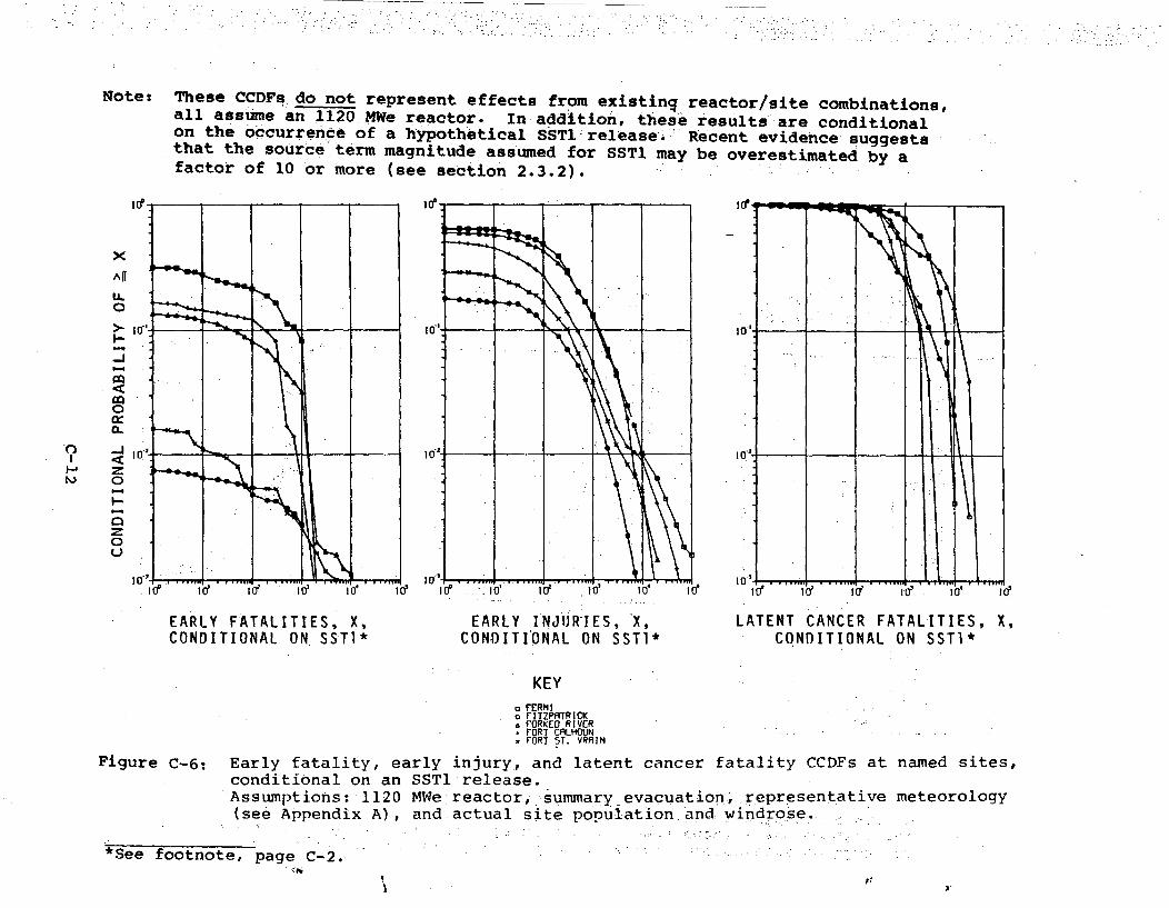
Note: These CCDFs do not represent effects from existinq reactor/site combinations,all assume an 1120 MWe reactor. In addition, these results are conditionalon the occurrence of a hypothetical SST1 release. Recent evidence suggeststhat the source term magnitude assumed for SSTI may be overestimated by afactor of 10 or more (see section 2.3.2).

id .ID !. .

,

All

U-0

I-

-J 1 O0' 1.

z0L)

I-.

EARLY FATALITIES, X,CONDITIONAL ON SST1*

EARLY INJIJR-IES, X,CONDITIONAL ON SST1*

LATENT CANCER FATALITIES, X,CONDITIONAL ON SSTI*

KEYo FERM I

FITZPATRICKFORKED RIVER

+ FORT CALHOUNa FORT ST. VRRIN

Figure C-6: Early fatality, early injury, and latent cancer fatality CCDFs at named sites,conditional on an SST1 release.Assumptions: 1120 MWe reactor, summary evacuation, representative meteorology(see Appendix A), and actual site population and: windrose..

*See footnote, page C-2.

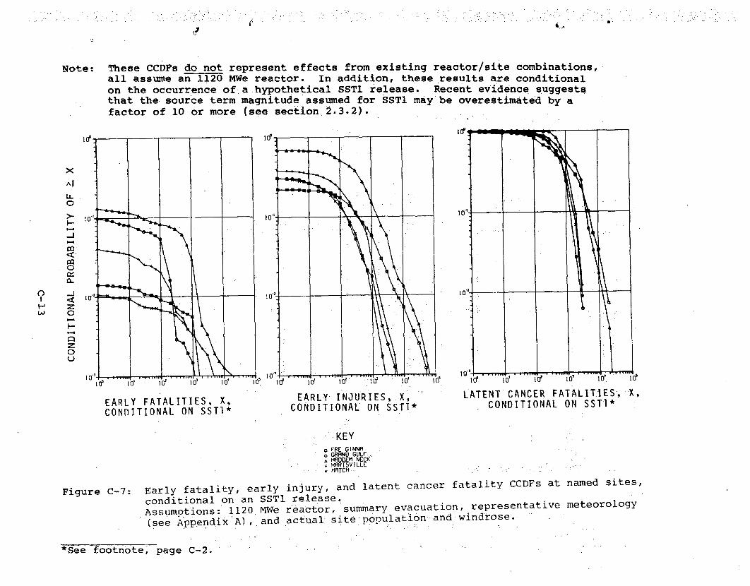
Note: These CCDFs do not represent effects from existing reactor/site combinations,all assume an 1120 MWe reactor. In addition, these results are conditionalon the occurrence of a hypothetical SSTI release. Recent evidence suggeststhat the source term magnitude assumed for SSTl may be overestimated by afactor of 10 or more (see section.2.3.2).

XAll

LL

0

-J

0

z0Li

0C)to

.I .1

LATENT CANCER FATALITIES, X,CONDITIONAL ON SSTI*EARLY FATALITIES, X,

CONDITIONAL ON SSTI*EARLY INJURIES,.X,

CONDITIONAL ON SST1*

KEYo FRE GINNAo GRAND GULF..

HADDEM NECK. HRRT5VILLE

HATCH

Figure C-7: Early fatality, early injury, and latent cancer fatality CCDFs at named sites,conditional on an SSTI release.Assumptions: 1120 MWe reactor, summary evacuation, representative meteorology(see Appendix A), and actual site population::and windrose.

*See footnote, page C-2.

Note: These CCDFs do not represent effects from existing reactor/site combinations,all assume an 1120 MWe reactor. In addition, these results are conditionalon the occurrence of a hypothetical SSTI release. Recent evidence suggeststhat the.source term magnitude assumed for SSTl may be overestimated by afactor of 10 or more (see section 2.3.2).

X

All

4c-ý

0

< IC I -' 10'-z0

0

° ,-..

0(H

EARLY FATALITIES, X,CONDITIONAL ON SSTI*

EARLY INJURIES, X,CONDITIONAL ON SSTI*

LATENT CANCER FATALITIES, X,CONDITIONAL ON SSTI*

KEYo INDIAN POINTo KEWIAJUNECA LASALLE* LA CROSSEx LIMERICK

Figure C-8: Early fatality, earlyjinjury, and latent cancer fatality CCDFs at named sites,conditional on an SSTl release.Assumptions: 1120 MWe reactor, summary evacuation, representative meteorology(see Appendix A)-, and actual sitelpopulation and windrose.

*See footnote, page C-2.

Note: These CCDFs do not represent effects from existing reactor/site combinations,all assumne:aWn 20 MWe reactor. In addition, these results are conditionalon the occurrence of a hypothetical SST1 release. Recent evidence suggeststhat the source term magnitude assumed for SST. may be overestimated by afactor of 10 or more.(see section 2.3.2).

I U -FI04

All

0

CL

0

I-

0

C) I O~'

IC,10, 1*ID ..............................4

IDI..................................................1.10

EARLY FATALTrIES, X,CONDITIONAL ON SSTI*

EARLY INJURIES, X.CONDITIONAL ON SST1*

LATENT CANCER FATALITIES, X,CONDITIONAL ON SSTI*

KEYa MARBLE HILLS HoE TRNKEE

M MCGUIRE*MIDLAND

* MILLSTONE.

Figure C-9: Early fatality, early injury, and latent cancer fatality CCDFs at named sites,conditional on an SSTl release.Assur.ptiOns:: 1120 MWe:reactor, summary evacuation, representative meteorology(see Ai-nendix A) , and actual site population and windrose;.

*See footnote, page C-2.

Note: These CCDFs do not represent effects from existing reactor/site combinations,all assume an 1120 MWe reactor. In addition, these results are conditionalon the occurrence of a hypothetical SSTl release. Recent evidence suggeststhat the source term magnituderassumed for :SST1 may-be overestimated by afactor of 10 or more (see section 2.3.12). .

'-

.1 .10

EARLY FATALITIES, X,CONDITIONAL ON SSTI*

EARLY INJURIES, X,CONDITIONAL ON SST1*

LATENT CANCER FATALITIES, X,.CONDITIONAL ON SSTI*

KEYM MONTICELLO

o NINE MILE PT.- NORTH RNNR

OCONEEx OYSTER CREEK

Figure c-10: Early fatality, early injury.., and latent cancer fatality CCDFs at named sites,conditional on an SSTI release. .. - .Assumptions: 1120 MWe.reactori summary evacuation, representative meteorology(see Appendix A):, and. actual site .population and windrose.

*See footnote, paqe C-A.V'

4

Note: These CCDFs do not represent effects from existing reactor/site combinations,all assume an 1120 MWe reactor. In addition, these results are conditionalon the occurrence of a hypothetical SSTl release. Recent evidence suggeststhat the :source term magnitude assumed for SSTI may be overestimated by afactor of 10 or more (see section 2.3.2).

ADl

LL0

I--

-J

0

0-

z0

0U..)

!-

EARLY FATALITIES, X,CONDITIONAL ON SST1*

EARLY INJURIES, X,CONDITIONAL ON SST1*

LATENT-CANCER FATALITIES, X,CONDITIONAL ON..SST1*

KEYo PAL I SADEo PALO VE•RE, PEACH BOTTOM* PEBBLE SPRINGSx PERKINS

Figure C-ll: Early fatality, early injury, and latent cancer fatality CCDFs at named sites,conditional on an SSTl release.Assumptions: 1120 MWe reactor, summary evacuation, representative meteorology(see Appendix A), and actual site population and windrose.

*See footnote, page C-2.

Note: These CCDFs do not represent effects from existing reactor/site combinations,all assume an 1120 MWe reactor. In addition, these results are conditionalon the occurrence of a hypothetical SST1 release. Recent evidence suggeststhat the source term magnitude assumed for SST1 may be overestimated by afactor of 10 or more (see section 2.3.2).

0

'-a

EARLY FATALITIES, X,CONDITIONAL ON SSTI*

EARLY INJURIES, X,CONDITIONAL ON SSTI*

LATENT CANCER FATALITIES, X,CONDITIONAL ON SSTI*

KEYa PERRYo PHI PPS, PILGRIM

POINT BEACHPRAIRIE

Figure C-12: Early fatality, early injury, and latent cancer fatality CCDFs at named sites,conditional on an SST1 release.Assumptions: 1120 MWe reactor, summary':evacuation, representative meteorology(see Appendix A), and actual site population and Windrose.

*See footnote, paqe Q,2.A

&A

Note: These CCDFs do not represent effects from existing reactor/site combinations,all assume an 1120 MWe reactor. In addition, these results are conditionalon the occurrence of a hypothetical SSTl release. Recent evidence suggeststhat the source term magnitude assumed for SST1 may be overestimated by afactor of 10 or more (see section 2.3.2).

X

LL0

--

_j

O .

0

0

0

EARLY FATALITIES, X,CONDITIONAL ON SSTI*

EARLY INJURIES, X,CONDITIONAL ON SSTI*

LATENT CANCER FATALITIES, X,CONDITIONAL ON SSTI*

KEY0 OURD CITIESo RRNCHO SECO

RIvERBENOROB INSONSAINT LUCIE

Figure C-13: Early fatality, early injury, and latent cancer fatality CCDFs at named sites,conditional on an SST1 release.Assumptions: 1120 MWe reactor,..summary evacuation, representative meteorology(see Appendix A), and actual site population and windrose.

*See footnote, page C-2.

Note: These CCDFs dofnot represent effects from existing reactor/site combinations,all assume an 1120 MWe reactor. In addition, these results are conditionalon the occurrence of a hypothetical SST1 release. Recent evidence suggeststhat the source term magnitude assumed for SST1 may be overestimated by afactor of 10 or more (see section '2.3.2).

It? id'

x

All

U.0

>-

0

Q:

z0

z

0U

0

toC1

I

EARLY FATALITIES, X,CONDITIONAL ON SST1*

EARLY INJURIES, XiCONDITIONAL ON .SST1*

LATENT CANCER FATALITIES, X,_CONDITIONAL ON. SSTI*

KEYaSALEM

o SAN ONOrRE4 SEABRODK* SEOU•YRH

SHERRON HARRIS

Figure C-14: Early fatality, early injury., and latent cancer fatality CCDFs at named sites,conditional on an SST1 release.

.. Assumptions: 1120 M%,.e reactor, summary evacuation, representative meteorology(see Appendix A), and actual sit n population and windrose.

*See footnote, page C-2.

Of

' , I&

Note: These CCDFs do not represent effects from existing reactor/site combinations,all assume an 1120 MWe reactor. In addition,,these results are conditionalon the occurrence of a hypothetical SSTl-release. Recent ev idence suggeststhat the source term magnitude assumed for SSTI may be overestimated by afactor of 10 or more (see section 2.3.2).

X

All

U-0

(L

o

z

0

EARLY FATALITIES, X,CONDITIONAL ON SSTI*

EARLY INJURIES, X,CONDITIONAL ON SSTI*

LATENT CANCER FATALITIES, X,CONDITIONAL ON SSTI*

KEYa SKAGIT .o SHOREHAM

SOUTH TEXAS÷ SUME--CRx SURRY

Figure C-15: Early fatality, early injury, and latent cancer fatality CCDFs at named sites,conditional on an SST1 release.Assumptions: 1120 MWe reactor,-summary evacuation, representative meteorology(see-Appendix A), and actual site population and windrose.

*See footnote, page C-2

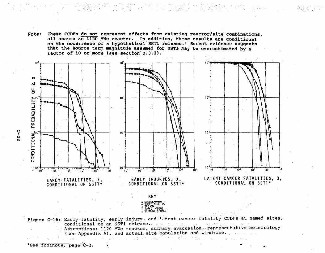
Note: These CCDFs do not represent effects from existing reactor/site combinations,all assume an 1120 MWe reactor. In addition, these results are conditionalon the occurrence of a hypothetical SSTl release.- Recent evidence suggeststhat the source term magnitude assumed for SSTI may be overestimated by afactor of 10 or more (see section 2.3.2).

0

NJ

EARLY.FATALITIES, X,CONDITIONAL ON SSTI*

EARLY INJURIES, X,CONDITIONAL ON SST1*

LATENT CANCER FATALITIES., X,CONDITIONAL ON SST1*

KEYSSUSOUEHRNNR"

oTHREE MILE 15a TRO.J1N

* TURKEY POINTx VERMONT YRNKEE

Figure C-16: Early. fatality, early injury, and latent cancer fatality CCDFs at named sites,conditional on an SSTI release..Assumptions: 1120 MWe reactor, summary: evacuation,- representative meteorology(see Appendix A), and actual site population and-windrose. .

*See footnote, page t-2.

a"

Note: These CCDFs do not represent effects from existing reactor/site combinations,all assume an 1120 MWe reactor. In addition, these results are conditionalon the occurrence of a hypothetical SST1 release. Recent evidence suggeststhat the source term magnitude assumed for SST1 may be overestimated by afactor of 10 or more (see section 2.3.2).

All

0

,> .I0I __ _:__ ___s 0

I--

00

o0 iLiJ

EARLY FATALITIES, X,CONDITIONAL ON SSTI*

EARLY INJURIES, X,CONDITIONAL ON SSTI*

LATENT CANCER FATALITIES, X,CONDITIONAL ON SSTI*

KEYo VOGTLEo WATERrORD

WRTT5 BAR* iss 1.4WP5 3*5

Early fatality, early injury, and -latent cancer fatality CCDFs at named sites,-conditional on an SST1 release:....Assumptions: 1120 MWe reactor, summary evacuation, representative meteorology-(see Appendix A), and.. actual-site.population and windrose.

Figure C-17:

*See footnote, page C-2

Note: These CCDFs do not represent effects from existing reactor/site combinations,all assume an 1120 MWe reactor. In addition, these results are conditionalon the occurrence of a hypothetical SST1 release. Recent evidence suggeststhat the source term magnitude assumed for SST1 may be overestimated by afactor of 10 or more (see section 2.3.2),.

If I(f -

x

All

U-

>- 1O7

0-

-j10-'

z•0

UO

1 ___________________

0

Ab -N

I O' lo, I01 -iý 0'R

EARLY FATALITIES, X,CONDITIONAL ON SSTI*

EARLY INJURIES, X0CONDITIONAL ON SSTI*

LATENT CANCER FATALITIES, X,CONDITIONAL ON SSTI*

* KEYoWOlf CPI•tK

T*INKEE VdWE* YELLOW CREEK

ZIMM ..ERo ZION

Figure C-18: Early fatality, early..injury, and-latent cancer fatality CCDFs at named sites,conditional on an: SSTI release.:,Assumptions: 1120 MWe reactor, summary evacuation, representative'meteorology(see' Appendix A), and actual site population and windrose.

*See footnote, page¶,C-2

Appendix D: Additional Population Statistics for CurrentReactor Sites

The demographic characteristics of the 91 reactorsites described in Chapter 2 and Appendix A were analyzedfor this study.: These data, which' were summarized inChapter 3, provide a perspective of previous sitingdecisions and delineate the population characteristicsof currentreactor sites. This appendix contains addi-tional demographic data which complement the datapresented in Chapter 3. These data are presented in thefollowing sections.'

Section Data Description

D.1 Site Population StatisticsD.2 Exclusion DistancesD.3 Site Population Factors

D.1 Site Population Statistics

The 91 population distributions examined in thisreport were all constructed on a 16 sector, circularpolar grid. For any specified portion (a circle, anannulus, a sector) of that grid, 91 values of populationdensity are available, one for each of the 91 populationdistributions. By cumulation of the 91 values for agiven portion of the grid, a population density CCDFmay be constructed.* Six different sets of populationdensity CCDFs have been constructed for-the followingareas of the population distribution grid:

Set 1 (Figures D.I-I thru D.I-8): Eight annuli(0-2, 2-5, 5-10, 10-20, 20-30, 30-50,50-100, and 100-200 mi).

Set 2 (Figures D.1-9 thru D.1-16): eight radialdistances (0-2, 0-5, 0-10, 0-20, 0-30,0-50, 0-100, and 0-200 mi).

*Population density CCDFs are Log-Log plots of thefraction of sites vs population density. Any pointon the distribution gives the fraction of sites(y-axis value), which have a population density withinthe specified portion of the grid (annulus, circle,sector), that is greater than or equal to the speci-fied population density (x-axis value).

D-1

Set 3 (Figures D.1-17 thru D.I-22): the mostpopulated 22.50 sector in each of six annuli(0-2, 2-5, 5-10, 10-20, 20-30, and 30-50 mi)on the 16 sector grid.

Set 4 (Figures D.1-23 thru D.1-28): the most popu-lated 22.50 sector in each of six radialdistances (0-2, 0-5, 0-10, 0-20, 0-30 and0-50 mi) on the 16 sector grid.

Set 5 (Figures D.1-29 thru D.1-34): the most popu-lated 450 sector (two adjacent 22.50 sectors)in each of six annuli (0-2, 2-5, 5-10, 10-20,20-30, and 30-50 mi) on the 16 sector grid.

Set 6 (Figures D.1-35 thru D.1-40): the most popu-lated 45* sector (two adjacent 22.50 sectors)in each of six radial distances (0-2, 0-5,0-10, 0-20, 0-30, and 0-50 mi) on the 16sector grid.

Each figure contains six CCDFs, one for each of the fiveNRC administrative regions (NE, MW, S, W, SW, see Figure3-1) and one for all regions combined (All)_.

Tables D.1-1 thru D.1-4 present the data used toconstruct the CCDFs in Figures D.1-1 thru D.1-28.Table D.1 presents, for each of the 91 sites, populationdensities within eight annuli; Table D.2 presents similardata for eight radial distances; Table D.3 for the mostpopulated 22.50 sector of six annuli; and Table D.4 forthe most populated 22.50 sector of six radial distances.

D-2

I

I I IME $

0.0

0.4

0 .&

0.8

0.6

0.8

0.6

0.4

0.2

0)

4J)

0

.r4.4

0.4

0.2

0'S.

I10 100

18 too

I(.•

I

0.6

0.6

0.4

O.2

0

1000 1E4 I

0.0

0.S

0.6

3.4

0.2

10 100 LoO 1E4

0.0

0.6

0.4

I 0.2

I I I - p

to

ALL

10e 100O

0I 10 I 10 10 IS0 1 is I#0 10 1E4

Mean Population Density (people/sq mi)

Figure D.1-1. CCDFs of Population Density (people/sq mi) at 91 Reactor Sites for theFive NRC Administrative Regions (NE, MW, S, W, SW) and for All RegionsCombined (All): Population Density Within the Annulus Interval 0-2 Miles.

I I

:3.4

.4J

.9.4

0r.5

.r4.

$4J

4.2.

0

0.0

0.6

0.4

0.

10 100 10s#$ I

1.6

II Ito 1000 1 10 106 1000

I

a

0.4

0.2

I 0I It too 1003 1 10 lOg I 10 too logo

Mean Population Density (people/sq mi)

Figure D.1-2. CCDFs of Population Density (people/sq mi) at 91 Reactor Sites for theFive NRC Administrative Regions (NE, MW, S, W, SW) and for All RegionsCombined (All): Population Density Within the Annulus Interval 2-5 Miles.

• 9 <P

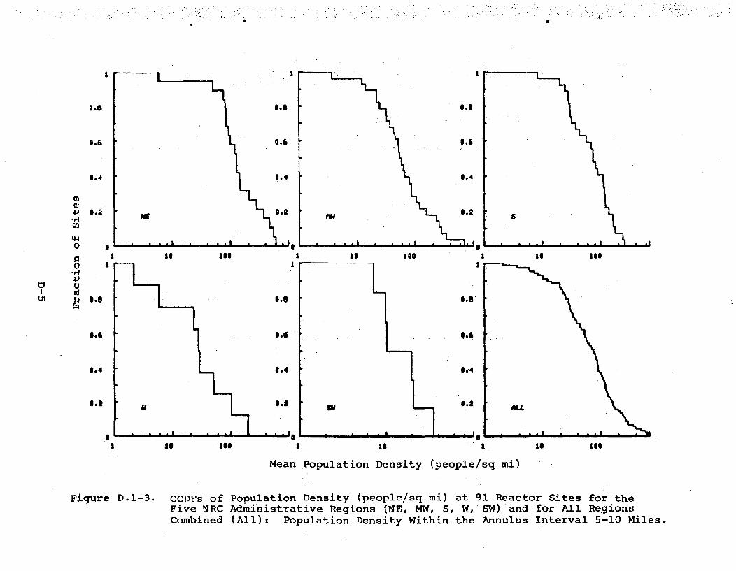
a

P $. t.a 1 .2 0.2

'4.

0

0 111is1tell is too 1 10 10of

on 1 1-844,

oia caU

M to toi i too

Mean Population Density (people/sq mi)

Figure D-1-3. CCDFs of Population Density (people/sq mi) at 91 Reactor Sites for theFive NRC Administrative Regions (TIE, MW, S, W, SW) and for All RegionsCombined (All): Population Density Within the Annulus Interval 5-10 Miles.

I .1 I

6.4 6.4 1.4

4-' 6.2 1.2 6.2r.,4'S

.4

'4'

I .I . I.$4-

...

•

6. 4 6.4 6 ..4

U. 6.1 ALL

l.o I is let I1 is 10l I.1 1i its

Mean Population Density (people/sq mi)

Figure D.1-4. CCDFs of Populationý Density (people/sq mi) at 91 Reactor Sites for theFive NRC Administrative Regions (NE, MW, S, W, SW) and for All RegionsCombined (All): Population Density Within the Annulus Interval 10-20 Miles.

1'

.6

At

6.6 6.6 6.6

0.4 6.4 6.4

U)041 .2 O.2 6.2

0 0 O0 . . .|. .n0 is II to lo t is•

0.46 1.4 1.43, 1

o so AL

to too Is • Ilit III lose

Mean.Population Density (people/sq mi)

Figure D.1-5. CCDFs of Population Density (people/sq mi) at 91 Reactor Sites for theFive NRC Administrative Regions (NE, MW, S, W, .SW) and for All RegionsCombined (All): Population Density Within the Annulus Interval •20-30 Miles.

I I

A1.S 6.5 U..,

6.6 0.6 8.6

0.4 0.4 1.4

4 J 1.4 0.2

EO Il MEO tOI tlSl"1 04.4

0to is$ 1006 to si iee los 0ie

r4.

0,.r.4 6.6 1.6

6.6 6.6 1.6

004 604 1.4

to to is &Islos

. . . .S 1 ... III 10 ltg16

Mean Population Density (people/sq mi)

Figure D.1-6. CCDFs of Population Density (people/sq mi) at 91 Reactor Sites for theFive NRC Administrative Regions (NE, MW, S, W, SW) and for All RegionsCombined (All): Population Density Within the Annulus Interval 30-50 Miles.

a

I

6.0 6 .8 6. .5

.6 61.6, 1.6

0.4 6.4 0.4

4-)." 0.1 M .2 6.2

414 -

0 10 106 10 166 10 100

u.o al .a a..6.6 0.6- 1.6

* . .. 6 " I .. . J ..

Mean Population Density (people/sq mi)

Figure D.I-7. CCDFs of Population Density (people/sq mi) at 91 Reactor Sites for theFive NRC Administrative Regions (NE, MW, S, W, SW) and for All RegionsCombined (All): Population Density Within the Annulus Interval 50-100 Miles.

IV

e.g

S.6

6.4

41J.5-4U)

0W

0

4.)0to

0.~

a

IIS 106 to lei 1 to to0

I-

0 6.6

6.6

6.4

0.8

I 1I ISO 1 16 1 to 1I6

Mean Population Density (people/sq mi)

Figure D.1-8. CCDFs of Population Density (people/sq mi) at 91, Reactor Sites for theFive NRC Administrative Regions (NE, MW, S, W, SW) and for All RegionsCombined (All): Population Density Within the Annulus Interval 100-200 Miles.

A,

o .. 0.8

0.6 0.6

0.4 0.4 0.4

U)

00.0.2 0.2

S 10 to0 100 1E4 1 10 100 1000 1E4 I t0 100 100p0 t 1.q U SU 4LL.4J

04

0.6 0.6 6.6

0.4 0.4 0.4

0.2 0.2 0.2

0 ' ' 0 ... . I . . . 5 ..

1 1 i 10 1So 1 to 1o 1006 IF

Mean Population Density (people/sq mi)

Figure D.1-9. CCDFs of Population Density (people/sq mi) at 91 Reactor Sites for theFive NRC Administrative Regions (NE, MW, S, W, SW) and for All RegionsCombined (All): Population Density Within the Radial Distance 0-2 Miles.

4

t. I

6.g

6.6

0.4

4IJ

e44

0

0*.r4

4aJUito'

0.2

0 aI to M6 I to l66 I too16

I I

I-'6.0

O.6

6.4

0.,

6.8

3.6

9.4

3.2w

Ia is 166 1 Is 1

Mean Population Density (people/sq mi)

to M66

Figure D.1-10. CCDFs of Population Density (people/sq mi) at 91 Reactor Sites for theFive NRC Administrative Regions (NE, MW, S, W, SW) and for All RegionsCombined (All): Population Density Within the Radial Distance 0-5 Miles.

I I

0.8

0.6

0.4

I,)4,

1440

04.3-

U

Iý4

9. 1i f Iif Is@ Its 1 is l90

I

0

I48

.6.

0.4

Is*

II isas Ma to I t its

Mean Population Density (people/sq mi)

Figure D.l-ll. CCDFs of Population Density (people/sq mi) at 91 Reactor Sites for theFive NRC Administrative Regions (NE, MW, S, W, SW)and for All RegionsCombined (All): Population Density Within the Radial Distance 0-10 Miles.

I I 1

0.6

6.6

6.4

42

.r4En

04

0

.r'441U

o .a

S

£

I.e

$

0to too I 10 Is$ tO t0o

0,

.6.

'.4

to see

1 10 D n i •.1 tO16 136Mean Population Density (people/sq mi)

Figure D.I-12. CCDFs of Population Density (people/sq mi) at 91 Reactor Sites for theFive NRC Administrative Regions (NE, MW', S, W, SW) and for All RegionsCombined (All): Population Density Within the Radial Distance 0-20 Miles.

I I

S..

8.6

0.4

6.6

0.6

1.4

0.2Ea).4..9-4

44I0

0.9-4

U

44

O.2'

S

HEE

to log lots to too *to Is#I

0I-aCit 1.o

O.2

I aI to log I Is ago a ilieO ile

Mean Population Density (people/sq mi)

Figure D.1-13. CCDFs ofFive NRCCombined

Population Density (people/sq mi) at 91 Reactor Sites for theAdministrative Regions (NE, MW, S, W, SW) and for All Regions(All): Population Density Within the Radial Distance 0-30 Miles.

I II

U)

'440

00'.H

D14

4..

0S.

0.4

0.2

S

.I

S..

5.4

S.,

0

r t010

s o 100

0

4.0 $.0

S.6

0.4 6.4

S.2 8.aN SN ALL

Is atso II 1to Is I is less

Mean Population Density (people/sq mi)

Figure D.1-14. CCDFs ofFive NRCCombined

Population Density (people/sq mi) at 91 Reactor Sites for theAdministrative Regions (NE, MW, S, W, SW)-and for All Regions(All): Population Density Within the Radial Distance 0-50 Miles.

/

I I

g.8e,-.!S. *...1 6.6

0.6 6.6 6.6.

6.40.4 0.4

.4.S

0 1 6

1.6 06. 6 161 0.66

t.11i

Cobie (Al) Poplaio Denit WihnteRdilDsac 010Mls

1.4 6.4

Mean Population •Density (people/sq mi)

FigreD.I-15. CCDFs of Population Density (people/sq mi) at 91 Reactor Sites for the".F'ive ?'RC Administrative Regions (NE, MW, S, W, SW) and for All Regions~Combined (All): Population Density Within the Radial Distance 0-100 Miles.

I I

0.6 .6 0.6

6.4 6.4 0.4

0)

4 •.6.... .. ,. #

0 106 16 1M6 10 lto

0

6.4 r. 6os .4

Is see is to see

Mean Population Density (people/sq mi)

Figure D.l-16. CCDFs of PopulationrDensity (people/sq mi) at 91 Reactor Sites for theFive NRC Administrative Regions (NE, MW, S, W, SW) and for All RegionsCombined (All): Population Density Within the Radial Distance 0-200 Miles.

Mýý

I 1 1

1I

I S

0.6

0.4

to4)4IJ.9-IW,

4.40

0.9-I

D.4

0I

II

% GA:

0.6

0.4

1.2

10 100 1000 IE4I

0.0

0.6

0.4

0.2

1 10 100 t1o0 1E4

r SUI1

10 100 1000 IE4

ALL.

0.6

0.4

0.2

a - I

0 0 . . ... . . ... i . . . ... . . ... 01 I1 100 1000 1E4 1 10 100 1000 1f4 I is 100 1600 1E4

Mean Population Density (people/sq mi)

Figure D.1-17. CCDFs of Population Density (people/sq mi) at 91 Reactor Sites for theFive NRC Administrative Regions (NE, MW, S, W, SW) and for All RegionsCombined (All): Population Density Within the Most Populated 22.50 Sectorof the Annular Interval 0-2 Miles.

1 .1 I

0.8

0.6

0.4

0.24J).- 4i

4.d0

0.1-4.41

$4

0

I

0 0t 1 t 0oo 1000 1E4 1 10 100 1000 1E4 1 10 100 1000 1E4

IU

0

0 0.1

0.6

'.4

0.2

0.8

0.6

0.4

0.2

I 0 0I 10 too 1040 E14 1 10 t00 1000 1o 4 1 10 t0o 1000 114

Mean Population Density (people/sq mi)

Figure D.1-18. CCDFs of Population Density (people/sq mi) at 91 Reactor Sites for theFive NRC Administrative Regions (NE, MW, S, W, SW) and for All RegionsCombined (All): Population Density Within the Most Populated 22.50 Sectorof the Annular Interval 2-5 Miles.

I I I

U.6

u1.4

00

0

.4-U

144

0

1

0 0

01.3H U.a

0.6

0.4

1.2

10 100 1000 114 10I

0.0

0.6

0.4

1001

1000 1E4 10

Sly

100 1000 1E4

0.8

0.6

0.4

0.20.2

0 010 100 1000 114 10 100 1800 114 10 100 1000 1E4

Mean Population Density (people/sq mi)

Figure D.1-19. CCDFs of Population Density (people/sq mi) at 91 Reactor Sites for theFive NRC Administrative Regions (NE, MW, S, W, SW). and for All RegionsCombined (All): Population Density Within the Most Populated 22.5* Sectorof the Annular Interval 5-10 Miles.

I I 1

0.8 o.8 0.8

0.6 0.6 0.6

0.4 0.4 0.4

02

.a- 0.. 0 .2 0.2 •

o 0 0 0 1 ••i

r Io 100 1000 IE4 1. 1o 100 1000 1E4 1 10 100 1000 1140 1 1 -u 1.rq U SU ALL

bi 4 0.8 . 0.0rz.r

0.6 0.6 0.6

0.4 0.4 0.4

0.2 0.2 0.2

S~ 001 10 100 1900 1E4 1 10 100 1000 1E4 I to 100 1000 IE4

Mean Population Density (people/sq mi)

Figure D.1-20. CCDFs of Population Density (people/sq mi) at 91 Reactor Sites for theFive NRC Administrative Regions (NE, MW, S, W, SW) and for All RegionsCombined (All): Population Density Within the Most Populated 22.5* Sectorof the Annular Interval 10-20 Miles.

*1 lp

1C'i

I

4).r-4

.440

0.r4.

1.4r44

0.8

0.6

0.4

0.

0.8

a1 10 r o0 1000 1E4 IES I 10 100 1000

I - I sU1E4 IES 1 10 100 1000

I rx 4LL

IE4 IES

hi

0.6

0.4

0.2

0 0 0I is 100 1000 1E4 IES 1. 10 100 1000 1E4 IES 1 10 100 deao 1E4 1E5

Mean Population Density (people/sq mi)

Figure D.I-21. CCDFs of Population Density (people/sq mi) at 91 Reactor Sites for theFive NRC Administrative Regions (NE, MW, S, W, SW) and for All RegionsCombined (All): Population Density Within the-Most Populated 22.50 Sectorof the Annular Interval 20-30 Miles.

I I I

1

IH" S

4 J

49-4

0

00

1.4rX4

0.8

0.6

0.4

0.2

0

0

0.8

0.4

0.2

0.8

0.6

0 010 t00 1000 1E4 IE5

F-I UIto 100 1000 1E4 IE5 10 .100 1000 1E4 1E5

51j

I'

ALL

0.8 0.8

0.6

0.4

0.2

0

0.6 0.6

0.4

0.2

0.4

0.2

0 0I0 106 1000 1E4 1ES 10 100 1000 1E4 1ES 10 100 1000 1E4 IE5

Mean Population Density (people/sq mi)

Figure D.1-22. CCDFs of Population Density (people/sq mi) at 91 Reactor Sites for theFive NRC Administrative Regions (NE, MW, S, W, SW) and for All RegionsCombined (All): Population Density Within the Most Populated 22.5* Sectorof the Annular Interval 30-50 Miles.

fE.AM

0.4

0.6

0.4

r IME 5

0.8

0.6

4J

0

0

0.,q44)

r±..

0.4

0 0.2

0.;

. I . . 1I0

1

0*

I

Ln 0.8

0.6

0.4

6.2

0

to 100 1000 1E4

0.A

0.6

0.4

0.2

• . ., . .. , . . . t . " I

t0 100 1000 IE4 1 10 100 1000 1E4

Si.

0.8

0.6

0.4

0.2

0

ALL

1 1t 10o 1000 1E4 I 10o to0 1000 1E4 1 10 10, 1000 1E4

Mean Population Density (people/sq mi)

Figure D.1-23. CCDFs of Population Density (people/sq mi) at 91 Reactor Sites for theFive NRC Administrative Regions'(NE, MW, S, W, SW) and for All RegionsCombined (All): Population Density Within the Most Populated 22.5° Sectorof the Radial Distance 0-2 Miles.

I .1 I

0.8

C.6

0.4

4.).,4to,

4.40

0.A.)

'4j

0

0.6

0 010 100 1000 1E4 1 10 100 1000 IE4 I 10 100 1000 IE4

W(n

U I I

0.9

0.6

0.4

0.2

It.

U.6

0.4

0.2

0 01 1t too 1000 1E4 I 10 100 1000 1E4 I 10 100 1000 1E4

Mean Population Density (people/sq mi)

Figure D.1-24. CCDFs of Population Density (people/sq mi) at 91 Reactor Sites for theFive NRC Administrative Regions (NE, MW, S, W, SW) and for All RegionsCombined (All): Population Density Within the Most Populated 22.50 Sectorog the Radial Distance 0-5 Miles.

iV

I I £ I I

1.6 .'0.6 0.6

0.4 0.4 0.4

o:•0.2 0.20)'

0 0 0t o0 100 1000 1E4 10 too 1000 1E4 10 100 1000 1E40!t

• Sm ALL

S.O 0.8 0.8

0.6 0.6 0.6

0.4 0.4 0.4

0.2 0.2 0.2

S0 0is Is0 1000 IE4 10 100 1000 1E4 10 100 1400 1E4

Mean Population Density (people/sq mi)

Figure D.1-25. CCDFs of Population Density (people/sq mi) at 91 Reactor Sites for theFive NRC Administrative Regions (NE, MW, S, W, SW) and for All RegionsCombined (All): Population Density Within the Most Populated 22.50 Sectorof the Radial Distance 0-10 Miles.

I1 I I

4IJ

44I0

0.1.4

41,

14Ir44

0.8

0.6

0.4

0.:•

0

0.e

1 10 100 1000 IE4 I tO to0 1000 1E40

to 100 1000 IE4

OD

I I

0.6

0. 4

0 0 0I 10 1t0 1000 1E4 I to 100 1000 1E4 10 100 1000 IE4

Mean Population Density (people/sq mi)

Figure D.I-26. CCDFs of Population Density (people/sq mi) at 91 Reactor Sites for theFive NRC Administrative Regions (NE, MW, S, W, SW) and for All RegionsCombined (All): Population Density Within the Most Populated 22.50 Sectorof the Radial Distance 0-20 Miles.

AI

I I 1

0.6

tO

4-4

4-40

0*r4

14JUz.

0.4

0 .',

0

1

0 0I 10 too 1000 1E4 1 10 100 1000 1E4 1. 10. .100 1000 1E4

I

I~

0.6

0.6

0.4

0.2

a 0 a1 is 180 1000 1E4 10 100 1000 1E4 1 1 10 100 1000 IE4

Mean Population Density (people/sq mi)

Figure D.l-27. CCDFs of Population Density (people/sq mi) at 91 Reactor Sites for theFive NRC Administrative Regions (NE, MW, S, W, SW) and for All RegionsCombined (All): Population Density Within the Most Populated 22.5* Sectorof the Radial Distance 0-30 Miles.

I I ~II IIs' S

0.6

0.6

0.4

0.a

6.6

0.6

4).4J

0

0

4 J

44

0.2

0

I

0 0to 100 1000 IE4 1ES 10 to0 1000 IE4 IE5 10 100 100O

1I-'~

1E4 IES

d I

ALL0

o.e 0.6

0.6

0.4

1.2

0.4

0.2

0 .010 100 tO00 1E4 IE - 10 100 1000 1E4 IES 10 100 1000 1IE4 IFS

Mean Population Density (people/sq mi)

Figure D.1-28. CCDFs of Population Density (people/sq mi) at 91 Reactor Sites for theFiveNRC Administrative Regions (NE, MW, S, W, SW) and for. All RegionsCombined (All): Population Density Within the Mbst Populated 22.5° Sectorof the Radial Distance 0-50 Miles.

A1

A

1

0.4

0.4

1 IHE 'WI S

0.8

0.6

0.0

0.6

0,0)

0

4IJ

D)

S.,

0.:

4

2

0.4

0.. 0.2

6 a

C,

1

I 1 160 1000 1140

1

1f

WP

0.5

8.6

0.6

0.6

0.4

0.2

1.

to 100 1000 1E4

0.8

~0.'

0.4

0.2

A~LL

10 100 1090

0.2

02

a. . . . . . i In I l I

10 t00 I 10 leg lase - 10 too 100 114

Mean Population Density (people/sq mi)

Figure D.1-29. CCDFs of Population Density (people/sq mi) at 91 Reactor Sites for theFive NRC Administrative Regions (NE, MW, S, W, SW) -and for All RegionsCombined (All): Population Density Within the Most Populated 450 Sector(two adjacent 22.50 sectors) of the Annular Interval 0-2 Miles.

I I Itug

6.0

9.6

1.4

0.6

0.4

0.245 9J.2.rqU)

0

0

,4

0Sý4PU

o 0

I1 10 to0 lost 114 It

r U r

to$ 1000 114 I t0 100 1000I r

I'

0.e

S.60.6

0.4

0.2

0.4

I.0

0.6

6.4

0.2

19000

,1 0r0

to00 1

~1. I

I & i iI I i II ia

i0 lee Is le0 I10 t0o 0oso: 1E4

Mean Population Density (people/sq mi)

Figure D.1-30. CCDFs of Population Density (people/sq mi) at 91 Reactor Sites for theFive NRC Administrative Regions (NE, MW, S, W, SW) and for All RegionsCombined (All): Population Density Within the Most Populated 450 Sector(two adjacent 22.50 sectors) of the Annular Interval 2-5 Miles.

YJ

6

0.4

I Iw, S

e.6

0.6

6.4

02

02

*e4

'44

C.; 1.2

I

I

0

e.g

0.6

0.4

8.2

1t O00 1000 IE4 1t0

~0.6

0.6

8l.2

100 18600 E4 10

.SU

6.8

1 6.6

100 LO00 114

0.4

0.2

0 0 0Is M66 1sel 1E4 10 see 1o0o to too LOss L4

Mean Population Density (people/sq mi)

Figure D.1-31. CCDFs of Population Density (people/sq mi) at 91 Reactor Sites for theFive NRC Administrative Regions (NE, MW, S, W, SW) and for All RegionsCombined (All): Population Density Within theýMost Populated 450 Sector(two adjacent 22.50 sectors) of the Annular Interval 5-10 Miles.

I II 6ME

CA30.4 0.4

4) 0.2 0.24J4-0

0 1800 1E4 10 too Igo0 e14 10 100 1000 .E4

0 ..

r14 I1.6 0.6 0.6

1.4 3.4 0.4

0.2 1-.2 a0.2

t 1o 100 1os0 t1 l3o 100g 1 1, 100 too1 5.4

Mean Population Density (people/sq mi)

Figure D.1-32. CCDFs of Population Density (people/sq mi) at 91 Reactor Sites for theFive 1RC Administrative Regions (NE, MW, S, W, SW) and for All RegionsCombined (All): Population Density Within the Most Populated 450 Sector(two adjacent 22.5* sectors) of the Annular Interval 10-20 Miles.-I

A*1

AIU

VV

0.8 0.6 0.6

0 . 0.6 0.6

0.4 0.4 0.4

o.0 0.2 •.2

:U

44

,,,oo . 0 0

100 loc0 1 04 IES As too logo 1E4 to t10 l0o0 1E 4

o a 1 w6 AOLL

Cii

4J1 ~ g6060.6

0.6 0.6 0.6

0.4 6.4 0.4

0 ~001 1 106 lses 114 10 lee logo 114 1 is zoo t000 1141 115

Mean Population Density (people/sq mi)

Figure D.1-33. CCDFs of Population Density (people/sq mi) at 91 Reactor Sites for theFive NRC Administrative Regions (NE, MW, S, W, SW) and for All RegionsCombined (All): Population Density Within thed Most Populated 450 Sector(two adjacent 22.50 sectors) of the Annular Interval 20-30 Miles.

I I I I IkEE 9

6 :. E0.4 6.4 0.4

6.) 6.2 0.2

o 1e0 le66 114 IES to 110 100# 1E4 is to0 1600 1E4•: 1. 1 1:•

o Uk ALL

6I• 6, .8 0.8r4J I..Ia

8.6 6.6 6.6

1.4 6.4 1.4

6.2 0.2 .2

S S 0I@ 186 to10 1E4 to 100 too0 114 10 its 1000 2E4 1E5

Mean Population Density (people/sq mi)

Figure .D.1-34. CCDFs of Population Density (people/sq mi) at 91 Reactor Sites for theFive NRC Administrative Regions (NE, MW, S, W, SW) and for All RegionsCombined (All): Population Density Within the Most Populated 450 Sector(two adjacent 22.50 sectors) of the Annular Interval 30-50 Miles.

. 4t

.

0.8

O.t.

I IMEE MI S

0.8

0.6

0.8

0.6

0.4

4-).1-4

to-

0

.H-.4-U

'44

0.-' 0.2

G

II. IC... 16

I

0.8

S.6

0).4

0.2

0

~~00 1000 1E4

0.8

0.6

0.4

0.2

7777.'

1.

r10 100 1000 IE4

ISU

0.8

0.4

!0.2

10 too 1000

AL L

I e . . . . . i BE l l 0 .I010 1001 I 10 1o0 lOVtC 1 10 100 1080 1E4

Mean Population Density (people/sq mi)

Figure D.1-35. CCDFs of Population Density (people/sq mi) at 91 Reactor Sites for theFive NRC Administrative Regions (NE, MW, S, W, SW) and for All RegionsCombined (All): Population Density Within the Most Populated 450 Sector(two adjacent 22.56 sectors) of the Radial Distance 0-2 Miles.

I 1 I I D I

HU

A A

.0. . 0.6 U0.4U .

S0.6 1.6

0.0 .4 6.4

4-) 0.2 0.2

.1__

o 0 6 0., • .. .

1 10 to 1000 1E4 16 too 1500 IE4 1 to t00 1COO

M I 0uI L

.4-U"

0.04 0.8 6.8

0.1 6.6 6.6

0.4 6.4 1.4

6.2 6.2 ,.2

, . .,.,* .. " - ... 'g .| * "-'*

1 to o6 1006 1 to 100 10oo I is 160 1810 14

Mean Population Density (people/sq mi)

Figure D.1-36. CCDFs of Population Density (people/sq mi) at 91 Reactor Sites for theFive NRC Administrative Regions (NE, MW, S, W, SW) and for All RegionsCombined (All): Population Density Within the Most Populated 450 Sector(two adjacent 22.50 sectors) of the 'aIdial Distance 0-5 Miles.

t I I'SI

0.6

1.40.4

.1-iEn

00*rq4iJ

O.i

0

3.2

I10 100 1066 1E4 is M66 1000 1E4 10 100 1000

I I

I%0 0.8

0.6

0.4

1.2

I 0I to 100 1660 1E4 ,. 12 too I it Ile lee& 314

Mean Population Density (people/sq mi)

Figure D.1-37. CCDFs of Population Density (people/sq mi) at 91 Reactor Sites for theFive NRC Administrative Regions (NE, MW, S, W, SW) and for All RegionsCombined (All): Population Density Within the Most Populated 450 Sector(two adjacent 22.59 sectors) of the Radial Distance 0-10 Miles.

I 1X, $

..6

0.0

1.2

'.4

6.24 J

.r4EO

040

4.JU

$.4

0 01S0 1800 1IE4 10 t0o .1000 tE4

I

.08.8

1.6

0.4

0.2

0 I 0I is 100 1046 1i IGO 1000 1 lC 100 1068 1E4

Mean Population Density (people/sq mi)

Figure D.1-38. CCDFs of Population Density (people/sq mi) at 91 ReactoroSites for theFive NRC Administrative Regions (NE, MW, S, W, SW) and for All RegionsCombined (All): Population Density Within the Most Populated 45* Sector(two adjacent 22.50 sectors) of the Radial Distance 0-20 Miles.

.11

I

0 .~

p 4

I I

4J"14

4.40

0

'1.ý

iIS 10 OS E4 t00

I

9.8

*.6

1.4

0.2

to0 lo00o E4 10

0.8

11 0.6

lot too$ 1(4

0.4

0.2

Iz is tonl IA had a&.

, w tuo tool 1E4 I to too 100l 114

Mean Population Density (people/sq mi)

Figure D.1-39. CCDFs of Population Density (people/sq mi) at 91 Reactor Sites for the

Five TTRC Administrative Regions (NE, MW, S, W, SW) and for All Regions

Combined (All): Population Density Within the Most Populated 450 Sector

(two adjacent 22.50 sectors) of the Radial Distance 0-30 Miles.

I I IME1

6.6

C.6

0.4

e.8

6.6

6.4

U)

4-i000.H.4IJU0.448

6.2

,2

1

to

Is$ 106o IE4 1E5 10

0.8

6.6

6.4

0.2

100 1000 I14 10 100 1400 1E4

ALL

0

6.6

0.4

0.2

*tO

010S 1000 IE4 16 10L 1100 114 to 10t

Mean Population Density (people/sq mi)

1000 1E4 US

Figure D.1-40. CCDFs of Population Density (people/sq mi) at 91 Reactor Sites for theFive NRC Administrative Regions (NE, MW, S, W, SW) and for All RegionsCombined (All): Population Density Within the Most Populated 450 Sector(two adjacent 22.50 sectors) of the Radial Distance 0-50 Miles.

TABLE D.1-1

POPULATION DENSITIES (PEOPLE PER SQ. MI.) FOR 91 REACTOR SITESINNER AND OUTER ANNULAR RADII ARE GIVEN IN MILES

SITE 0-5 '5-10 10-20 20-30 30-.50 50-100 100,200

1 ALLENS CREEK 312 ARKANSAS 1 + 2 583 BAILLY S 2714 BEAVER VALLEY 1 + 2 1605 BELLEFONTE .1 216 BIG ROCK POINT 547 BLACK FOX 298 BRAIDWOOD 1 1279 BROWNS FERRY 1, 2, + 1210 BRUNSWICK 1 + 2 3111 BYRON 1 8312 CALLAWAY 813 CALVERT CLIFF 1 + 2 3414 CATAWBA 1 4915 CHEROKEE 4816 CLINTON 1817 COMMANCHE PEAK 2018 COOK DC 1 + 2 9319:COOPER S .1420 CRYSTAL RIVER 1521 DAVIS-BE 1 3122 DIABLO CANYON 1 + 2 023 DRESDEN 2 + 3 6824 DUANE ARNOLD 5025 FARLEY 1 + 2 2226 FERMI 2 12627 FITZPATRICK 2928 FORKED RIVER 1 7629 FORT CALHOUN 10130 FORT ST VRAIN 9

,*, 31 R. E. GINNA 7732 GRAND GULF 1 1633 HADDEM NECK 113

* 34 HARTSVILLE 4435 HATCH, E.I. 1 + 2 1336 INDIAN PT 2 + 3 75237 KEWAUNEE 2138 LASALLE 1 + 2 1239 LA CROSSE 1340 LIMERICK 1 79241 MARBLE HILL 8842 ME YANKEE 043 MCGUIRE 1 + 2. 6444 MIDLAND 2 53545 MILLSTONE 1 + 2 58246 MONTICELLO 67

2183

283565

89141053

12125591252

237113

4620

15722305530

118346

29259150131

2535

12428

2113720

.617335322

38144

6137

87284

38

D-43

3026

5343423027

147798862

2503255

431.113

367

11519118969

1994271

38650

146312143611

19473

6138

732809089

668301

36505289167

45

3916

1024787

419

234168

9826

1278751

154220168

33226

228

38032

2593727

125472

17618218814340

8034628

2046997534

1877379

63193

85102155

28615

.906403147

1636

7007113-8524.

456107162

79142117

2231

21217

11575441

562129565

23192

6740

305148

332462

66140

35619

6745

113109410340

4842

145210

8 71 138

258.76.40

43912320111 16

956894

4187089

35013

1565848

19479

8753415

11449

8224641

30484

39155

705

14118

il1185624

35

3547

134139

7639

ý35

80487456

16773

Si91.

18830

1694025

158151108

9455

12567

14842: 65257

1588364

196139

•18106169104

827397

20426

TABLE D.I-I (cont'd)

SITE 0-5 5-10 10-20 20-30 30-50 50-100 100-200

47 NINE M. PT. 1 + 2 29 150 50 72 129 79 6748 NORTH ANNA 1, 2, + 3 12 28 29 58 146 183 16149 OCONEE 1, 2 + 3 42 176 68 163 72 77 9450 OYSTER CREEK 76 131 146 176 565 875 14851 PALISADE 70 106 92 58 158 423 14852 PALO VERDE 1 6 7 8 7 122 18 853 PEACH BOTTOM 2 + 3 44 96 .246 362 659 428 26354 PEBBLE SPRINGS 5 2 0 2 15- 15 4855 PERKINS 79 109 203 251 172 96 7856 PERRY 1 224 230 178 296 374 135 17057 PHIPPS BEND 82 57 128 98 78 78 9258 PILGRIM 1 119 85 132 407 699 110 19459 POINT BEACH 1 + 2 30 80 63 88 70 90 13960 PRAIRIE 1 + 2 60 67 51 114 358 46 3461 QUAD CITIES 1 + 2 18 64 313 77 47 85 15062 RANCHO SECO 22 29 133 492 93 210 1663 RIVERBEND 1 49 74 86 176 43 92 3464 H. B. ROBINSON 2 97 75 50 75 77 98 6865 SAINT LUCIE 1 71 160 34 29 41 58 3866 SALEM 1 + 2 45 102 334 348 778 410 24967 SAN ONOFRE 18 103 183 134 632 314 1i68 SEABROOK 1 120 .88 89 64 272 129 1669 SEQUOYAH 1 + 2 108 115 303 71 51 82 8970 SHEARON HARRIS 23 69 168 205 109 97 7471 SHOREHAM 135 146 347 847 699 714 17372 SKAGIT 49 52 34 66 43 74 973 SOUTH TEXAS 0 10 25 11 26 94 3174 VIRGIL C. SUMMER 1 43 47 194 67 110 8475 SURRY ST 1 + 2 26 253 185 194 212 40 i1176 SUSQUEHANNA 1 188 130. 330 178 172 378 35477 THREE MILE ISLAND 320 470 499 248 168 506 28178 TROJAN 104 197 50 52 190 48 2679 TURKEY POINT 1 + 2 0 164 179 437 152 26 880 VERMONT YANKEE 1 102 79 99 68 217 363 23681 VOGTLE 0 8 26 162 35 58 7982 WATERFORD 3 181 119 282 490 91 40 2783 WATTSBAR 1 + 2 22 31 61 68 101 61 10384 WPPSS1+4 0 6 69 22 16 14 4385 WPPSS 3 + 5 28 24 46 53 49 86 2086 WPPSS 2 0 6 61 27 16 14 4387 WOLF CREEK 34 4 9 32 21 97 3588 YANKEE ROWE 12 88 84 129 255 311 26189 YELLOW CREEK 15 32 42 35 49 66 6590 ZIMMER 1 53 87 203 622 126 156 10591 ZION 538 697 347 484 1130 196 83

D-44

TABLE D.1-2

CUMMULATIVE POPULATION DENSITIES (PEOPLE PER SQ. MI.) FOR 91REACTOR SITES, CIRCLE RADII ARE GIVEN IN MILES

SITE .... 0-5 0-10 0-20 0-30 0-50 0-100 0-200

.2

34567.89

10.11121314151617181920212223242526272829

- 30313233343536373839.40414243444546

ALLENS CREEKARKANSAS 1 + 2BAILLY SBEAVER VALLEY 1 +BELLEFONTE 1.BIG ROCK POINTBLACK FOXBRAIDWOOD 1BROWNS FERRY 1, 2,BRUNSWICK 1 + 2BYRON 1CALLAWAYCALVERT CLIFF 1 + 2CATAWBA 1CHEROKEECLINTONCOMMANCHE PEAKCOOK DC 1 + 2COOPER. SCRYSTAL RIVERDAVIS-BE 1DIABLO CANYON 1 +DRESDEN 2 + 3DUANE ARNOLDFARLEY 1 + 2.FERMI 2FITZPATRICKFORKED RIVER 1FORT CALHOUNFORT ST VRAINR. E. GINNAGRAND GULP 1HADDEM NECKHARTSVI LLEHATCH, E.I. 1 + 2INDIAN PT 2 + 3KEWAUNEELASALLE 1 + 2LA CROSSELIMERICK 1i••

MARBLE HILLME YANKEEMCGUIRE 1 + 2MIDLAND 2MILLSTONE 1 + 2MONTICELLO

2

31•58

271160

215429

127+ 12

31.83

8* 34

49481820931415

310

685022

1262976

1019

7716

1134413

752211213

79288

064

535582

67

2377

280464

7224.15

.72942665.1148

190973920

14120264922

105272

27226119

1174429

11225

1873918

651304220

48355

4119199359

45

D-45

2839

4713734126

114778953

2042753

371109

3710

12219157957

176100

60346

67139245114486

20401

5533

711687871

622.240

28408266215

45

3526

778603

41

16181128

9438

1616152

250171109

23180

2111

24643

2226542

85170

160210155295

31624

5031

1453857651

1319317

47289166152106

19619

860475109

1688

4948022

11237

310159165

9099

13922

ý24225

27821

5841

666107419

91179149

37

420113

322099

73117

41871157

46176129317256

8537

324277

92i251

3177736

357102.229126113

7495

3495873

31817

3225846

3128.6

7614856

12346

7226239

75281

32251

746145

25

128171547

90

4844

182174803239

1638045

14567

1828796

15946

21444337

198117162

8553

17272

3014319

7054

2997858

335124169

92313115

6887

116290

42

TABLE D.1-2 (cont'd)

SITE 0-5 0-10 0-20 0-30 0-50 0-100 0-200

47 NINE M. PT. 1 + 2 29 119 67 70 107 86 7248 NORTH ANNA i, 2, + 3 12 24 28 44 109' 165 16249 OCONEE 1, 2 + 3 42 142 87 129 93 81 9150 OYSTER CREEK 76 117 .139 160 419 761 30151 PALISADE 70 97 93 74 128 349 19852 PALO VERDE 1 6 7 8 7 81 34 1453 PEACH BOTTOM 2 + 3 44 83 205 292 527 452, '31154 PEBBLE SPRINGS 5 3 1 2 10 14.. '4055 PERKINS 79 102 178 219 189 119 .8856 PERRY 1. 224 228 190 249 329 183 173,57 PHIPPS BEND 82 63 112 104 87 80 89;58 PILGRIM 1 119 94 122 280 548 220 20159 POINT BEACH 1 + 2 30 67 64 77 73 85 1.26,60 PRAIRIE 1 + 2 60 . 65 55 88 261 100 5161 QUAD CITIES 1 + 2 18 53 248 153, 85 85.- 13462 RANCHO SECO 22 27 107 321 175 201 6363 RIVERBEND 1 49 68 81 134 76 88 4764 H. B. ROBINSON 2 97 80 58 67 73 92 7465 SAINT LUCIE 1 71 138 60 43 42 54 4266 SALEM 1 + 2 45 88 272 314 611 460 .30267 SAN ONOFRE 18 82 158 144 456 350 9668 SEABROOK 1 120 96 91 76 202 147 4969 SEQUOYAH 1 + 2 108 113 255 153 88 83 8770 SHEARON HARRIS 23 58 141 176 133 . 106 .8271 SHOREHAM 135 144 296 602 664 702 305-72 SKAGIT 49 51 38 54 47 67 . 2373 SOUTH TEXAS 0 7 21 15 22 76 4274 VIRGIL C. SUMMER 1 33 43 127 89 105 8975 SURRY ST 1 + 2 26 196 188 191 204 81 10476 SUSQUEHANNA 1 188 144 284 225 191 331 348.,77 THREE MILE ISLAND 320 433 483 352 234 438 32178 TROJAN 104 174 81 65 145 72 37,79 TURKEY POIN4T 1 + 2 0 123 165 316 211 72 2480 VERMONT YANKEE 1 102 84 95 80 168 314 25581 VOGTLE .0 6 21 99 58 58 7382 WATERFORD 3 181 135 245 381 195 7.9 4083 WATTS BAR1+2 22 29 53 61 87 68 9484 WPPSS1+4 0 4 53 36 23 16 3685 WPPSS 3 + 5 28 25 41 48 48 77 .3486 WPPSS 2 0 4 47 36 23 16 3687 WOLF CREEK -34 11 10 22 21 78 4688 YANKEE ROWE 12 69 81 107 202 283. 26789 YELLOW CREEK 15 28 39 37 44 60 6490 ZIMMER 1 53 78 172 422 232 175 12291 ZION 538 657 424 457 888 369 154

D-46

TABLE D.1-3

POPULATION DENSITIES (PEOPLE PER SQ. MI.) IN

MOST POPULATED 22.5* SECTOR OF EACH ANNULUS

SITE 0-5MI 5-10MI 10-20MI 20-30MI

1 ALLENS CREEK2 ARKANSAS 1+ 23 BAILLY S4 BEAVER VALLEY 1 + 25 BELLEFONTE 16 BIG ROCK POINT7 BLACK FOX8 BRAIDWOOD 19 BROWNS FERRY 1, 2, + 3

10 BRUNSWICK 1 + 211 BYRON 112 CALLAWAY13 CALVERT CLIFF 1 + 214 CATAWBA 115 CHEROKEE16 CLINTON17ý COMMANCHE PEAK18 COOK DC 1 + 219 COOPER S20 CRYSTAL RIVER21 DAVIS-BE 122 DIABLO CANYON 1 + 223 DRESDEN 2 + 324 DUANE ARNOLD25 FARLEY 1 + 226 FERMI 227. FITZPATRICK28 FORKED RIVER 129 FORT CALHOUN30 FORT ST VRAIN31 R. E. GINNA32 GRAND GULF 133 HADDEM NECK34 HARTSVILLE35 HATCH, E.I. 1 + 236 INDIAN PT 2 + 337 KEWAUNEE38 LASALLE 1 + 239 LA CROSSE40 LIMERICK 141 MARBLE HILL42 ME YANKEE43 MCGUIRE 1 + 244 MIDLAND 245 MILLSTONE 1 + 246 MONTICELLO

209.4364.2

1123.1S107 3.8

199.6716.9267.3619.3189.1452.3356.3129.8293.4263.0276.9107.8316.6335.3

54.2235.3337.6

0.0332.7269.1160.7586.9468.3458.6976.8139.1692.2207.8789.6456.9210.4

2513.7225.1122.2148.3

4232.5649.0

0.0388.5

2006.63739.0

456.3

182.3676.5

1650.52108.9420.6

48.981.0

283.1814.7112.9173.8

57.3240.3

1613.2981.9287.3

88.51053.0

108.6164.5318.3175.2359.6"

2488.4134.5

1364.61758.1

858.5239.0120.7.515.3168.7881.2

79.6112.9

1916.9197.0192.5

68.01340.1

166.250.9

425.8276.6

1369.8190.9

130.8112.0

4113.31003.9

89.1160.5

1148.5409.35021.6809.6

2191.8161.8220.0

2719.9.. 448.0

83.129.2

474.363.151.7

417.2566.8

2023.6102.4619.9

2637.4310.2847.5

3212.8574.2

5883.260.7

1725.3274.1136.1

2363.0814.8383.3891.6

2167.52318.0

218.83096.12221.0

865.498.2

153.169..4

9294.16199.0

79.728.7

2232.1.1462.9

730.4254.8355.3557.6

171.7607.2807.3

1001.1183.6

1930.483.752.6

2358.0295.71093.6

86.246.1

6556.7599.6

1029.915931.9

965.4700.6301.1

2730..1160.261.5

14617.91292.6

337.7160.7

12296.53443.4

683.2433.5304.1251.1621.0

D-47

TABLE D.1-3 (cont'd)

SITE 0-5MI 5-10MI 1O-20MI 20-30MI

47 NINE M. PT. 1 + 2 468.3 1758.1 310.2 599.648.NORTH ANNA 1, 2, + 3 187.2 98.5 57.2 294.649 OCONEE 1, 2 + 3 215.1 821.7. 277.7 920.650 OYSTER CREEK 458.6 858.5 847.5 1029.951 PALISADE 415.8 460.0 944.2 220.552 PALO VERDE 1 69..7 53.2 75.4 88.153 PEACH BOTTOM 2 + 3 290..1 255.2 1292.9 1092.954 PEBBLE SPRINGS :76.4 21.2 5. 3 8..655 PERKINS 458.8 314.9 675.8 810.256 PERRY 1 811.4 1561.6 899.0 3837.357 PHIPPS BEND 265.9 287.9 915.8 ...557.458 PILGRIM 1 886.6 611.8 413.4 1773.159 POINT BEACH 1 + 2 355.1 876.7 617.3 i 625.460 PRAIRIE 1 + 2 280.3 596.8 219.0 :-866.561 QUAD CITIES 1 + 2 109.8 .240.1 1937.6 383.862 RANCHO SECO 348.6 101.5 573.9 3087.363 RIVERBEND 1 .295.8 298.9 440.0 1673.564 H. B. ROBINSON 2 525.0 523.0 198.9 262.965 SAINT LUCIE 1 947.7 1350.3 221.0 303.366 SALEM 1 + 2 626.6 601.1 2014.0 1568.167 SAN ONOFRE 280.9 887.1 1061.9 1252.768 SEABROOK 1 ...540.7 469.8 548.7 453 .3

S69 SEQUOYAH 1 + 2 294.2 372.0 1900.2 274.770 SHEARON HARRIS 190.5 242.8 721.1 1106.371 SHOREHAM 805.7 816.3 1589.7 32,19.472 SKAGIT 288.3 525.8 207.1 502.373 SOUTH TEXAS 0.0 61.4 26.5.7. 53.374 VIRGIL C. SUMMER 17.7 99.8 206.9 1956.775 SURRY ST 1 + 2 244.5 1751.9 1320.4 1521.076 SUSQUEHANNA 1 1309.7 561.9 2560.7 8.69.877 THREE MILE ISLAND 2157.0 2319.5 1622.8 1158.478 TROJAN 365.9 2151.1 176.8 582.679 TURKEY POINT 1 + 2 0.0 1289.1 2107.5 4119.780 VERMONT YANKEE 1 507.7 532.1 361.2 350.681 VOGTLE 0.0 74.4 76.9 991.782 WATERFORD 3 880.3 452.7 3399..3 -5068.183 WATTS BAR 1 + 2 203.1 98.3 248.0 163.384 WPPSS1+4 0.0 95.1 581.8 158.185 WPPSS 3 + 5 453.7 193.3 540.7 225.586 WPPSS 2 0.0 95.1 538.3 197.787 WOLF CREEK 427.6 21.5 16.8 225.388 YANKEE ROWE 95.5 705.1 286.1 670.689 YELLOW CREEK 132.2 101.6 262.6 102.390 ZIMMER 1 325.9 180.0 949.5 5331.291 ZION 2040.9 4367.4 1665.5 3344.7

D-48

TABLE D.1-4

POPULATION DENSITIES (PEOPLE PER SQ. MI.) INMOST POPULATED 22.50 SECTOR OF EACH CIRCLE

SITE 0-5MI 0-10MI O-20MI 0-30MI

12345678910111213141516171819202122232425262728293031323334353637383940414243444546

ALLENS CREEKARKANSAS 1 + 2BAILLY SBEAVER VALLEY 1 + 2BELLEFONTE 1BIG ROCK POINTBLACK FOXBRAIDWOOD 1BROWNS FERRY 1, 2, + 3BRUNSWICK 1. + 2BYRON 1CALLAWAYCALVERT CLIFF 1 + 2,CATAWBA 1CHEROKEECLINTONCOMMANCHE PEAKCOOK DC 1 + 2COOPER SCRYSTAL RIVERDAVIS-BE 1DIABLO CANYON 1 + 2DRESDEN 2 + 3DUANE ARNOLDFARLEY 1 + 2FERMI 2FITZPATRICKFORKED RIVER 1FORT CALHOUNFORT ST VRAINR. E. GINNAGRAND GULF 1HADDEM NECKHARTSVI LLEHATCH, E.I. 1 + 2INDIAN PT 2 + 3KEWAUN EELASALLE 1 + 2LA CROSSELIMERICK 1MARBLE HILLME YANKEEMCGUIRE 1 + 2MIDLAND 2MILLSTONE I + 2MONTI CELLO

209.4364.2

1123.11073.8

199.6-716.9

267.3619.3.189.1452.3356.3129.8293.4263.0276.9107.8316.6335.3S54.2235.3337.6

0.0332.7269.1160.7586.9468.3458.6976.8139.1692.2207.87,89.6456.9210.4

2513.7225.1122.2148.3

4232.5649.0

0.0388.5

2006.63739.0

456.3

136.7598.4

1355.61594.2

335.6215.9

66.8218.8611.1113.1162.6

43.0229.0

1209.9736.4215.579.1

867.990.3

123.4238.7131.4269.7

1922..2100.8

1073.21318.6

758.5244.2

90.6386.5178.5660.9114.2

84.71627.5

147.7144.4

53.71343.5

184.638.1

319.4549.1

1962.1143.2

98.1194.6

3423.91903.2

107.7132.2861.4316.7529.7607-.2

1656.5129.7:210.1

2075.7361.2

72.2

38.5572.7

63.353.5

327.8441.6..

1538.2505.8475.8

2069.3362.0.825.3

2417.8430.7

450.7.851.8

1439.7205.6102.1

2161.0618.5301.9682.1

1758.11753.1

173.62386.11718.5

877.786.2

128-.6125.1

5163.43845.3

80.5ý66.2

.. 1622.9878.7427-.3

)411.4889.0

341.3...109.31259.9

501.1572.2102.0

1.141.4-56.541.4

1367.2201.4876.8S241.. 8231.4

4507.6

365.6939 0

1960.0553.9

2392.7183.1

2009.7155.2

61.28684.2

735.8228.0392.5

7511.82692.1

404.31301.3

911.8485.5368.5

D-49

TABLE D.1-4 (cont'd)

SITE O-5MI 0-10MI 0-20MI 0-30MI

47 NINE M. PT. 1 + 2S48 NORTH ANNA 1, 2, + 349 OCONEE 1, 2 + 350 OYSTER CREEK51 PALISADE52 PALO VERDE 153 PEACH BOTTOM 2 + 354 PEBBLE SPRINGS55 PERKINS'56 PERRY 157 PHIPPS BEND58 PILGRIM 159 POINT BEACH 1 + 260 PRAIRIE 1:+ 261 QUAD CITIES 1 + 262 RANCHO SECO63 RIVERBEND 164 H. B. ROBINSON 265: SAINT LUCIE 166 SALEM 1 + 267 SAN ONOFRE68 SEABROOK 169 SEQUOYAH 1. + 270 SHEARON HARRIS71-SHOREHAM,72 SKAGIT73 SOUTH TEXAS74 VIRGIL C. SUMMER75 SURRY ST 1 +1 276 SUSQUEHANNA 177 THREE MILE ISLAND78 TROJAN79 TURKEY POINT 1 + 280 VERMONT YANKEE 181 VOGTLE82 WATERFORD 3:83 WATTS BAR 1 + 284 WPPSS1+485 WPPSS 3:+ 586 WPPSS 287 WOLF CREEK88 YANKEE ROWE89 YELLOW CREEK90 ZIMMER 191 ZION

468.3187.2215.1458.6415.8

69.7290.1

76.4458.8811.4265.9886.6355. 1280.3109.8348.6295.85,25.0947.7626.6280.9540.7294.2ý190. 5805.7288.3

0.017.7

244.51309.72157.0

365.9.0.0

507.70.0

880.3203.1

0.0453.7

0.0427.6

95.5132.2325.9

2040.9

1318.673.9

629.3758.5448.9

57.3191.4

19.1291.7

1276.5215.9584.3657.6496.1180.1146.1231.9523.5

1012.7450.8735.6352.3283.0182.1813.7451.5

46.074.9

1313.9748.9

1758.21618.7

966.8526.0

55.8426.9124.571.4

145.071.4

123.0528.8

76.2162.0

3779.5

362.047.0

235.0825.3741.4

56.5969.7

S6.4'529.3993.4688.3456.1627.4171.2

1456.3430.4335.1280.0419.0

1511.5796.4475 .5

1456.0580.4,

1289.1201.2199.3173.9

1318.81979.11656.6

480.51628.8

270.957.7

2618.1186.0436.3405.5403.7

39.7223.7

213.0747.0

1724.0

365.6178.5611.8939.0452.0

74.11,841.6

5.2651.1

2573.3374. 3

1155.4362.0557.5860.5.5

1814.3.1078. 7

270.5230.7

1543.0951.5344.2799.7647.5

2361.5301,.2

.. :98.3

1091:. 11164.11362.8

824.4382.6

2316.4261.4559.2

3979.2127.9281.7196.8289.3129.5464.0107.0

3264.52349.3

D-50

t1

D.2 Exclusion Distances

Table D.2-1 presents the distance to the closestboundary of the exclusion zone surrounding each of the91 reactor sites, discussed in Chapter 2 and Appendix A.The variability of these distances is displayed inFigure 3-2 in Chapter 3.

D-51

TABLE D.2-1

EXCLUSION DISTANCES (MILES) FOR 91 REACTOR SITES

SITE. EX. DIST.

I ALLENS CREEK 0.822 ARKANSAS 1 + 2 0.653 BAILLY S 0.124 BEAVER VALLEY 1 + 2 0.385 BELLEFONTE 1 0.576 BIG ROCK POINT 0.517 BLACK FOX 0.538 BRAIDWOOD 1 0.289 BROWNS FERRY 1, 2, + 3 0.76

10 BRUNSWICK 1 + 2 0..5711 BYRON 1 0.2912 CALLAWAY 0.6813 CALVERT CLIFF 1 + 2 0.7114 CATAWBA 1 0.4715 CHEROKEE 0.3716 CLINTON 0.6117 COMMANCHE PEAK 0.8718 COOK DC 1 + 2 0.3819 COOPER S 0.4620 CRYSTAL RIVER 0.8321 DAVIS-BE 1 0.3922 DIABLO CANYON 1 + 2 0.5023 DRESDEN 2 + 3 0.4224 DUANE ARN~OLD 0.2725 FARLEY 1 + 2 0.7826 FERMI 2 0.5727 FITZPATRICK 0.6128 FORKED RIVER 1 0.3829 FORT CALHOUN 0.2330 FORT ST VRAIN 0.3731 R. E. GINNA 0.2832 GRAND GULF 1 0.4733 HADDEM NECK 0.3334 HARTSVILLE 0.7635 HATCH, E.I. 1 + 2 0.7836 INDIAN PT 2 + 3 0.2137 KEWAUNEE 0.7538 LASALLE 1 + 2 0.3239 LA CROSSE 0.2140 LIMERICK 1 0.4741 MARBLE HILL 0.4242 ME YANKEE 0.3843 MCGUIRE 1 + 2 0.4744 MIDLAND 2 0.3145 MILLSTONE 1 + 2 0.31

D-52

TABLE D.2-1 (cont'd)

SITE EX. DIST.

46 MONTICELLO 0.3047 NINE M.* PT. 1 + 2 0.9748 NORTH ANNA 1, 2, + 3 0.8449 OCONEE 1, 2 + 3 1.0050 OYSTER CREEK 0.2551 PALISADE 0.42.52 PALO VERDE 1 0.5653 PEACH BOTTOM 2 + 3 0.5154 PEBBLE SPRINGS 0.4955 PERKINS 0.3756 PERRY 1 0.5757 PHIPPS BEND 0.4758 PILGRIM 1 0.2759 POINT BEACH 1 + 2 0.7560 PRAIRIE 1 + 2 0.4461 QUAD CITIES 1 + 2 0.2462 RANCHO SECO 0.4063 RIVERBEND 1 0.5764 H. B. ROBINSON 2 0.2665 SAINT LUCIE 1 0.9766 SALEM 1 + 2 0.7267 SAN ONOFRE 0.5068 SEABROOK 1 0.5769 SEQUOYAH 1 + 2 0.3670 SHEARON HARRIS 1.3371 SHOREHAM 0.1972 SKAGIT 0.3873 SOUTH TEXAS 0.8974 VIRGIL C. SUMMER 1.0175 SURRY ST 1 + 2 0.3576 SUSQUEHANNA 1 0.3577 THREE MILE ISLAND 0.3878 TROJAN 0.4179 TURKEY POINT 1 + 2 0.7980 VERMONT YANKEE 1 0.1781 VOGTLE 0.6882 WATERFORD 3 0.5783 WATTS BAR 1 + 2 0.7584 WPPSS1+4 1.2185 WPPSS 3 + 5 0.8186 WPPSS 2 1.2187 WOLF CREEK 0.7588 YANKEE ROWE 0.5989 YELLOW CREEK 0.4390 ZIMMER 1 0.2491 ZION 0.57

D-53

D.3 Site Population Factors

Table D.3-1 presents the Site Population Factor(SPFn) and the Wind Rose Weighted Site PopulationFactor (WRSPFn) for each of the 91 reactor sites dis-cussed in Chapter 2 and Appendix A..For every site,the factors have been calculated for each-of thefollowing four distances: 5, 10, 20, and 30 miles.The equations used in these calculations are presentedin Section 3.2 of Chapter 3.

• 4

D-54

.t

Table D.3-1. SITE POPULATION FACTORS (SPF) AND WIND ROSEWEIGHTED SITE POPULATION FACTORS (WRWSPF)FOR 91 REACTOR SITES

(I

SITE NAME REGIONALLENS CREEK SnARKANSAS I + 2 SBAI LLY 5 mtBEAVER VALLEY I + 2 NEBELLEFONTL 1 5BIG ROCK POINT MAABLACK FOX SmBRAII)qOOD I A ABROWNS FERRY 1. 2, + SBRUNSWICK I + 2 5BYRON 1 IAnCALLAWAY MACALVERT CLIFF I + 2 NECATAWBA.. SCHEROKEE SCL INTON jAMCO(MAi.CHE PEAK 5iC(X)K DC I + 2 AwC(XOPER S MNCRYSTAL RIVER 5DAVIS-BE I MwDIABLO CANYON I + 2 4DRESDEN 2 + 3 MWiDUANE ARNOLD A"FARLEY I + 2 SFERMI 2 :01FITZPAFRICK NEFORKED RIVER I 14EFORT CALHOUN AnFORT ST VRAIN wGINNA R.E. 4i:GRAND GULF I SHADiDEM NECK 1EHAR'SV I LLE SliA'T'CHt, E.I. I + 2 5I NDI Aj PT 2 + 3 iqEKbE ,AUaE3: ,,JALASALLE I + 2 .4wLA CROSSE- ,ArLIMERICK I 1EMARBLE. HILLME YANKEEMCGUIRE I + 2MIDLAND 2M II..LS. o1E I + 2 ,4FMONTI L;ELLO 0NINE M,. PT. I + 2 a•NOIk'Tf ANNA I. 2. + 3 'SOCONEE I. 2 + 3 5

SPF5.31084E-01.34737E-01.11129E+00.90963E-IJ1.60386E-01I.32287E-01. 17274E-01;13580E+00.79286E-02.2018HE-OI.7)963E-01.90153E-02.19608E-01.28386E-0l.32364E2-)I.19499E-01.84912E-U2.W4697E-01.1uu/8E-UI.16346E-01.32672E-03.0.44120E-01.39515E-01. 114992-01.15821E+00.19642E-UI.*805HE-0I.73958H2h-0.73b44E-U02.4/1184E-UI.12290E-011.12231E+00.21 5572-01.11122E-01.8I326E+00.93780E-U2.13544E-01.F/126E-4)1,.69D802,+UO.b259OE-UJ.0.68!:2.7E-0 I, b15hoE ÷!)o

* 44b3?/E+OU.304552-0.1

.*9642E-Ul

.7,415l /-02.2U 9 46E-0I

SPFIO.26170E-0i.60184E-01.2 1 447E+L0.25042E+0O.72908E-03.25840E-01.14603E701.10993E+00.44405E-01.22260E-01.67722E-01.10237E-01.30431E-01.97801E-01.60843E-01.31270E-01.127OOE-01.I IJ03E+00.148IIE-Ol.22168E-01.40451E-01.9859HE-02.67169E-01.12939E+00.17446E-01.19137E+00.68462E-0.1.94443E-01.55546E-01.20285E-01.72451E-01.19601E-01* 14928E+W.26881E-UI.14720E-01.74045E+00.173902-01.29233E-01. 19149E-0I.581252+0u.488 201:-0

1764UE-02.89197E-:U.362l2t-+LU.39 792E+,O.364H8E8O:0.68462E-01.16242E-01./*10832-U)

SPF20.27085E-01.48306E-01.33316E+00.29870E+005131 33E-0lI

.21861E2-01

.55139E-01

.96933E-01

.64588-E01'

.32303E-01,

.11826E+00

.19330E-01.

.40544E-01.20199E+÷00.7499HE-0O.332 18E-0I.10855E-0I. 11942E200.16822E-l01

18219E-01. 55738E-0I.35215E-01.1113E*00.12819E÷+0.33556E-01.245331E00.62453&-01.11249E+00.12552E+00.63296E-01.23521E+00. 19342E-01.2 4484E+400.37927/,0l.22/31E-01.7355/2+00.36593E-01.*5!404--O I* 3948%7&-101 .1.59208E+00.. 12305E+(..1415/E-Ul.222942+00.32814E+00.31930E+00.401082-01.624t32-0I.2049 IE-01.710122-01

SPF30.29669E-01.41624E-01.46225E+00.38618E+00.54642E-01.23975E-01.93730E-0l.11376E+00.70623E-01.31477E-01,2009E+00

.32205E-01

.42677E-0I

.19320E+60

.I0486E+00:

.62132E-01

.15435E-01

.14056E20017901E-OI.161872ý-01.121406+00.34517E-01.143782+00

10952E+00.32332E-01.44021E+00.63600E-01

I125482E0014071 +00'

.86448'E-0.213713E+00.23405E-01.36523E+00%.39203E-03

.23.889EoI

.98620E2+Ob

.41946E-0I

.59426E-0l

.386HQE2-o

.13 IIOE10+

.18013E+00

.230322-03

.2 hi53+E00

.2 18552E+00

.21479E+00

.63248E-013

.63500a-01

.2328!E-0I

.8 7412-0I

WRSPF5.29167E-01..26405E-01.15890E+00.76206E-0f.68453E-01..33586E-01.14052&-01.12694E200.83789E-02.1 7567E-01.78011E-03.51928E-02.25289E-03.15367E'-0.38806E-01.15294E-01.20515E-0I.88946E-O01. 10219E-;0:.29057E-Or.56239E`01

.42523E-01

.313492'01

.88854E-02.12502E+00

.59291E-01

.10434E+00

.51651E-02

.46365E-01I

.13523E-03.95413E--O I.20832E201.12330E-01.11163E÷+0.1635E,-01.90269E202.182/0E-01, 82582 E+UO.4241 I1E-01.0

.47273.+00

.38361E+00,3t726E-or I.18938E-01.1/126E-01.203162-01

WRSPFIO.28190E-01.60023E-0.1.24294E+00.22261E+00

*.84200E-01.27221&-01.13323E-01ý.iOl A9E+OO.52503E-0!.22345E-01.73461E-01.83736E-02.41027E-01.58678E-01.82775E-01.23542E-0 I.201'85E-0I.10599E+00.14122E-01.30043E-01.59827E-u1.57107E-U2.704892-03

I335902E00.15052E-0I.17859E+00.9831742-03O.72795E-01.73083 E-0 1.21 997E-0 I.81548E-01.22849E-01.19216E+00.26524E-01.135662-01

.953466+00

.23622E201

.24474E-01

.20467E 01

.65562E200

.45750E-0l11468F-U2

.863"IE-01. .33162E+00.334b9E+00.34902E-03.985866-01.22356E-03.54069E-O0

WRSPF20.29801E-01.48555E-01.40154E+00.2420sE+00.65040E-0I.27626E-01.41818E-0I.88696E-01.78023E-0.1.32963E-01

10 102s2E+00.17585E-0 1*5536.22-0.3

.24996E+00-. 90473E-01•.29828E-0I.15354E-01.10839E+00

35045E-03.24442E303.70913E-01.14153E-01.94596E- 03

.1351'9E+00S.28956E-O0

.I8463E+00• 833592-031

.88249E-01

.20,j58E+M0

.60302&-01I

.33809t- +00

.21192E-:03

.3910)5E+00

.36980E-01

.21401t-03

.8/47/3: *00,4913/3:-03

.602146-01

.bO259E-03

.64060E+0014/129i+00

S.1222E-03.2uH39E+0u.2761 12+0(Xi.21492E+00.3883•7-01.83033E-01.24040E-01.5633qt-01

MRSPF30.33529E-01.42915E-01.5150E÷00.344742+00.591392-01

.23175E-01

./3356E-01.99681E-01.77910E-0I.31882E-0..330302+00

.28591E-0f

.53537E-03

.24078E+00

.. 1931E+00

.65338E-03

.1 7198E-01

.13656E+00

.17308E-01.21577E-01.12767E+0X).18607E-01.11579E+00,13 n62+00.284652-01.313192E2+O.82(342-03.102 13+010.23105E+00.97050E-01.333772E+÷.24940E-01.23225E+00.3/85OE-0I.22 88E-01.111,6 7E+01

.126622-03

.64080E-03

.481358E-0.'I/140E+00).216292+00

19443&-0l... 20379E+UO.239813E+00..240U E÷+00.60259E-Ut.82225E-03.29313i3-01, l Jm1 -01

Table D.3-1. (continued)

S;ITE iiAMEOYSTER CREEKPAL ISADEPALO VERVE: IPEACH BOTHOA 2 + 3PEBBLE SPR.INGS

.PERKINSPERRY IPHIPPS BENDPILGRIM IPOINT BEACH I + 2PRAIRIE I + 2OUAD CITIES I + 2RANCHO. SECORIVERIE-,:D IH. 1. ROBINSON 2SAINT LUCIE ISALEM I + 2SAN ONOFRESEABR(X)K ISE,)1J(OYAH I + 2SHEIARON HARRISSKAul i

0. SHOREHAMI SOUTH TEXASUI VIRGIL L,. SUMMIERCh SURRY SIC I + 2

SSUOU6A;t•rA I

THREE A ILE ISI.AAI"R: JANlTURKEY POINT I + 2VEI•M)O;T YANKEE IVoT(;'LENATI:RFOR)J 3WA'[S BAR I + 2ýNPPS I1+4rlPPSS 2

WPPiS J + 5AOI.t: ý.;Rc2 EKYAIvKE' ROAEYh LLO'I CREEKZI. vm.R IZIO 4

REG I ON=4

NEi

NE

S

,'WE0S

S

,iESPil

NE

S

An

jS

.,1

. SPFS

.54980E-01

.59341E-02

.21262E-01

.32039E-02

.56885E-0 I

. I1834E+00

.10524E+00

.11534E+00.21 f77E-OI.52533E-01.92684E-02.11965E-O1.30502E-01.44152E-01.54634E-01.204.14E-0I.69UU2E-02.671564E-0 I.74640E-01.10925E-oI.34859E-Ol* 16493E+UU. 0.b0986E-OJ. I1499E-0i

H *H449E0) I. 22949E+4).6U039E-0 I.0.95964E-Ul.0

16326E+00

:15094E-0I.0.ja.- 1904 E-01

.1,699EIt-91

.124U3tJ0

.650•bE-02.2/940E-0I. 1136Jt+(A

* SPFI0

.7418IE-0I

.57060E-02

.46280E-uI

.2660 E-WU2*.73595E-UI. 1963JE+00.84886E-01.*10936E+00.42796E-01.60849E-0I.28898E-01.16493E-U1.43167E-01.60(49E-UI.839UIE-0I.44902E-OI.48712E-OI0.70954E-01.92644E-01.32954E-01o43992E-Ol. 15862E+UU.32669E-02.169OIE-0I.10123E+00. I0759E+00

.312(iIt+00.10 194E+W..53684E-01.94227E-01.36769i-U2.14)43E+ W.22252E-'01.33914E-.2.269 2 0M-02.18N311t-0I.12359E-01.352266-01

14111E-0I.4639/E-UI.10 6 1E+ (A

. SPF20

. II 74ME+00.78747E-01

.64846E-02

..103922+00

.19549E-02

.11950E+00* 1s7 IE+O0.97704E-01.11597E+00.50634E-0I.58239E-0l1.I1516E+00.49437E-01.55364E-01.56364E--Ul.69659E-01l12554E+00

.75767E-01

.16439E+00

.7i277E-01.

.42008d-01

.22164E+0O

.11964E-01

.254 17E-0112692E+00

.I 1999E+4W;3(996,-+00.8,390JE-UI

.9085HE-0-l:ý9t0oJE-01.19H71E-01

,11643E+00.34829E-OI.2541HE-UI.22569E-01.21064b-Ol

.il4,I0E-01

.22904E-01

.936gE-0O

..* . I :/ 1 00

SPF301.2 74=8E+00

.714770E-01.63884E-02.. 1547 1.E+00.19379E-02.14722E+00.20736E+00..91858E-01

11212E+00.56137E-01.68463E-01

10.374E+J01!4276E+00

.81505E-01.l59736E-01.61,06E-01.1 1034E+00.96513E-01.74094E-0I.1 4585E400I 10028E+00

.47567E-0 Ii3:.388E+00.11540E-01.59106E-01,.14067E+00.1 1990E+00.371 54E+UO.805671E-0I16790E+00

.88NHOE-O I

.39824E-0I

.25577t+00

.41281E-01

.24944t-01

.237717-01

.3197;c-v 1

.i5201E-01

.6I44UE-0I2tJ71E-Ul

.2U056I+U0bý56,E+00

WRSPF5.5929'7E -o0.64503E-UI.7218IIE-02.16166E-01. 0765E-02.69392E-01.19364E+00..14545E+0O.10559E+00.30607E-01.68018E-0I.74518E-02.21t786E-UI.26O84E-01.316t8E-01.26940E-01.10118E-01.66242E-02.51712E-01.1IU85E÷00

18313E-0I.55447E-01

.. 14089E÷00

.0

..5440E-0314434E-01

.13817E400

.191 79E+300

.68927E-01

.0'.10817E+00.0.14376E+00.lOI58E-0I

.0

.1 ,4004E.701

.RS718E-02

.1t425E-01

.662U0E-02

.2UI 34E-uI

.6 /I42E+oW.

. RSPFIO.72-9ý5E-OI.90103E-0I.65626E-02.43229E-01.18643E-02.77.501E-01.22503E*00

11 126EU00.:10456E÷00l.61374F-01.89779E-01.26202E-0I.24511E-0i.38615E-01.40944E-01.571388-01.37371E-Ul.33136E-01.53509E-01.99429E-01.27659E-01.72359E-01

I!4828E+00.31599E-02.

.16344E-01

.981l2E-01I14840UE+UO.30 91+000•618!3E400

.44722E-01

.1 41159E+00

.34954E-02.1 4389E+U0.17328E-01.14139E-u2.11239E-02.15221E-01.66541E-02.30271t-0I.16426t-01

.313 550-010

.84U40E+UU

ORSPF20.8249E- I.10466E+00.6822SE-02.10408E-00.12494E-02.12921E+00.21854E+00..911.14E-01.12056EO00.781I8E-VI..81B43E-01.1:572E+00.62466E-01.5391 I1-01.40993E-0U.50326E-01.13494EW00.6935UE-Ul.61434E-01.24659E+00.6200UE-01.61 4312-01

.23 SbE00

.11627E-01

.27235F-01.117102+00

.1867UE 00

.42313E+00.154b6E+00.72604E-UI.I11 33E+00.10971E-011 D4246+00

.21514E-0U.33159E-01.290-95-01. I9 01It-U I.8041E-U2.44181I-UI.25,S4 -Ul.191UJE-OI.6d87DE+00

ARSPF30.10273E+OU.1IU41E+00.67663E--02.162866+00.16 177E-02.16516E+00.2ti100+00.90997E-01.I8-316E+00.84159E-01.98066E-01.14606E+00.I dOIE+00.83519E-01.46:573t-U.43984E-01.1/3746+00./3646E-0160J80E-Ul

.22043E+00

.894012-01

.61842t-0I

.39069E+00

.109927E-01

.54J35E-01,121812+00.18442E+00.39465E+00.14013E+00

102956+L0I 0599E+00

.29954E-0I.20/17Z+00.37328E'U-.3 11g16-01.30828E-01.25655E-0I.133112-01,t6389t-UI.26n47E-0I

I .i 20t+U0

.6:)141 E+0(U

iI

Appendix E: CRAC 2: A Brief Description

The accidenticonsequence calculations presentedin Chapter 2 were performed using CRAC2 [1,2], an im-proved version of the WASH-1400 consequence model CRAC.A number of modifications were made in the upgrade fromCRAC to CRAC2. These include changes in the treatmentsof atmospheric dispersion parameters,. plume rise, pre-cipitation scavenging (wet deposition), mixing heights,weather sequence sampling, emergency response (evacua-tion and sheltering), and latent cancer risk factors.These changes are briefly described below. In addition,several errors found in CRACzwere corrected in the CRAC2version.

E.Il Atmospheric Dispersion Parameters

The values of the horizontal dispersion coeffi-cients, a. , obtained from the :Pasquill-Gifford curves(and paraxeterized by Tadmore and Gur [3]) correspondto a release duration of three minutes.- To correctthe standard dispersion coefficients for releases-oflonger duration, the summary report of the NationalCommission on Air Quality's Atmospheric dispersionModeling Panel [4] endorses the method suggested byGifford [5]. An adjustment for releases of durationt 2 (minutes) is made by means of the formula

cr( 3tmin)

YPG

where 0 is within the range 0.25-0.3 for 1 hr < t2< 100 hr and: equals ,0.2: for .3 min < t 2 < 1 hr.In CRAC2, Q is equal to 0.2 for release durationsbetween 3 minutes and one hour and 0.25 for releasedurations greater than one hour. The lower valueof 0.25, rather than 0.3, was selected for long-duration releases because it results in higher con-centrations.

The vertical dispersion coefficients, az, obtainedfrom the Pasquil-Gifford curves (parameterized by Martinand Tikvart [6]) are based on data from releases over

E-1

terrain with very low surface roughness (grasslandswith roughness length of approximately 3 cm). InCRAC2 a more typical roughness length of 10 cm (crops,bushes) is assumed.. The vertical dispersion coeffi-cients are adjusted using the following recommended,.equation [7,8]:

z z= r2/r) 0.2z2. z 2 1.

where (zY is the unadjusted parameter, Uz2 is the ad-

justed parameter, r1 =:3 cm, and r 2 10 cm. Impactsof these changes in the treatment of dispersion para-meters were examined in [9].

E.2 Plume Rise

The WASH-1400 consequence model used plume riseequations. recommended •in Briggs (1969) [10]. The plumerise model used in CRAC2 is based on a more recent .paper by Briggs: (1975) [11]T.

E.3 Precipitation Scavenging (Wet Deposition)

The WASH-1400 consequence model (CRAC) used weatherdata which reported rainfall in terms of the incidenceor nonincidence of rain within any clock hour. Tocalculate precipitation scavenging, the model assumedthat rain reported for a clock hour fell at a rate of1 mm/hr for half the hour. The CRAC2 code contains amore sophisticated wet deposition model which requiresas input the amount of rain falling in an hour. Rainis assumed to occur during the entire hour with a con-stant rate. The hourly rainfall rate is multiplied bya rainout coefficient to determine precipitation scav-enging. A coefficient of 1.0 x 107 (sec)V1 (mm/hr)- 1

is used for stable conditions-and 1.0 x i0- (sec)-(mm/hr)-l for neutral and unstable conditions.

E.4 Mixing Heights

The WASH-1400 consequence model used Holzworth. [12]morning and afternoon mixing heights for all stabilityconditions. In CRAC2, the treatment is somewhat sim-plified. For stable conditions (E and F stability),the inversion layer is ground based and no mixing depth

E-2

is assumed. For neutral and unstable conditions, theHolzworth afternoon mixing height is assumed. Thischange has minimal impact on resulting predicted conse-quences.

E.5 Improved Weather Sequence Sampling Technique

WASH-1400,'s consequence model (CRAC) used a strat-ified sampling technique by which sequences are selectedevery four days ± thirteen hours to provide coverage ofdiurnal, seasonal and four-day weather cycles [13].In this manner, a total- of 91 weather sequences werechosen to represent one year of data (8760 hours).Sensitivity studies have shown that considerable var-iation in predicted consequences result from samplingby this method. Consequences can vary significantlyfor calculations performed using different sets ofweather. sequences (see Figure E5-lA). Differences inpeak predicted consequences of an order of magnitudeor more are not uncommon.

There are several reasons for the large variationin consequences due to the WASH-1400 sampling technique.Given an accident, large consequences are normallyassociated with relatively low probability weatherconditions such as rainfall within a few 10's of kilo-meters of the site [14], wind-speed slowdowns, orstable weather conditions with moderate wind speeds.ýNot only is the occurrence of rainfall or a slowdownimportant, but where it occurs as well. Rain beginningover a densely populated area could result in extremelyhigh consequences. Because of their low probability,such weather conditions will be selected infrequently,if at all, by the WASH-1400 sampling technique. Further-more, estimated probabilities for adverse weather condi-tions can be significantly in error. For example, aparticularly adverse weather sequence with actual pro-bability of 1/8760 would, if sampled, be assigned aprobability of 1/91.

CRAC2 uses a new weather sequence sampling method[15] which produces improved estimates of accident-consequence frequency distributions. Prior to sequenceselection, the entire year of weather data is sortedinto 29 weather categories (termed "bins"), as definedin Table E.5-1. Each of the 8760 potential sequencesis first examined to determine if rain occurs anywherewithin 50 kilometers (30 miles) of the accident site.

E-3

If not, a similar examination is made for wind-speedslowdowns. If neither of these conditions occurs,. thesequence is categorized by the stability and wind speedat the start of the• accident. -A probability for eachweather bin is estimated from the number of sequencesplaced in the bin. Sequences are then sampled fromeach of the bins :(with appropriate probabilities) foruse in risk calculations. In the current analysis,four sequences were selected from each bin. Samplingwith this method assures that low probability adverseweather conditions are -adequately included.

A comparison of the variation in consequences dueto sampling bythe two methods is provided in Figure,E.5-,1. For both methods, early-fatality frequency dis-tributions (CCDF's) for a PWR2 -release [15] were cal-culated with CRAC,. using 32 different sets of weathersequences sampled from the New York City weather datasummarized in Table E.5-1.- •Also assuied were a uniformpopulation density of 100 people/mile and a relativelyineffective evacuation. The results clearly indicatethat the weather bin method results in substantiallyless variation due to sampling than the previousWASH-1400 -technique.

E.6 Emergency Response (Evacuation) Model

The CRAC2 evacuation modeI [16,17) is signifi-cantly:different from the RSS evacuation model. Inlieu of the small "effective" evacuation speeds assumedin the RSS model, the revised treatment incorporatesa delay time before public movement, followed by evac-uation radially away from the reactor. Both an assumeddelay time and evacuation speed are required as inputto the model. Different shielding factors and breathingrates are used while stationary or in transit. Inaddition, all persons within the designated evacuationarea move as a group with the same delay time and evac-uation speed. Therefore, the possibility that somepeople may not leave the evacuated area is ignored.This latter assumption results in upper bound estimatesof-evacuation effectiveness, given a specific delay timeand speed.* Unlike the RSS model in which persons continue

*The evacuation effectiveness would decrease linearlywith an increasing nonparticipating fraction of thepopulation. In actual evacuations, Civil Defensepersonnel have observed a nonparticipating minorityof approximately 5%. i

E-4

ef

1.0 .... 1 .0Al

Al -1 -10 4• ---

--3 .10 10

4

30 -- l 11 102 101110101

a (b

andi (B Weahe Bi-ehius3 o ec ehiu,3

- -0l

A- "bs esiae sn l 70 vial euneishw by th akne ie

C . 9-. ,.

o 4..... : 1- 4

1 - 1 10....O .. .....1 2 10 - - 1 41 10l 102 !v

X, Early Fatalities X,.Early Fatalities(a) "(b)

Figure E.5-1. Comparison of Uncertainty Due to Sampling by (A) WASH-1400and (B) Weather Bin Techniques. For each technique, 32different sets of weather sequences are used to generateearly-fatality frequency distributions for a PWR2 release.A "best estimate" using all 8760 available sequences, isshown by the darkened line.

9s

Table E.5-1 One Year of New York City MeteorologicalData Summarized Using Weather BinCategories

Weather Bin Definitions

R - Rain starting within indicated interval(miles).

S - Slowdown occurring within indicatedinterval (miles).

A-C D E F - Stability categories.

1(0-1), 2(1-2), 3(2-3), 4(3-5), 5(GT 5) -Wind Speedintervals (m/s).

Number ofWeather Bin Sequences Percent

1 R (0) 697 7.962 R (0-5) 12 .143 R (5-10) 62 .714 R (10-15) 102 1.165 R (15-20) 75 .866 R (20-25) 67 .767 R (25-30 61 .708 S (0-10) 24 .279 S (10-15) 16 .18

10 S (15-20) 18 .2111 S (20-25) 14 .1612 S (25-30) 18 2113 A-C 1,•2,3 168 1.9214 A-C 4,5 892 10.1815 D 1 0 0.0016 D 2 61, .7017 D 3 .226 2.5818 D 4 948 10.8219 D 5 3325 37.9620 E1 0 0.0021 E 2 27 .3122 E 3 167 1.9123 E 4 682 7.7924 E 5 270 3.0825 F1 0 0.0026 F 2 116 1.3227 F 3 310 3.5428 F 4 402 4.5929 F 5 0 0.00

8760 100.00

E-6

evacuating until they are either overtaken by thecloud or leave the model grid, all evacuating personsin the new model travel a-designated distance fromthe evacuated area and are then removed from theproblem. This treatment allows for the likelihood thatafter traveling outward for some distance, people maylearn their position relative to the cloud :and-beable to avoid it.

.The new model also calculates more: realistic ex-posure durations to airborne and-ground-depositedradionuclides than the RSS evacuation model.. The RSSconsequence model employs an exposure model for an in-stantaneous point source and thus all released plumeshave zero effective lengths., Because of this, evacu-ating persons overtaken by the cloud in the RSS evacu-ation model are exposed to the entire cloud at thepoint overtaken. However, a released cloud of radio-active material would have a finite release durationand a length that depends on the wind speed duringand following the release. A person overtaken by thefront of the cloud might still -escape before beingpassed by the entire cloud and thus receive only afraction, of the full cloud exposure.* -The revisedevacuation model assigns the cloud a finite lengthwhich is calculated using the assumed release durationand wind speed during the release. To simplify thetreatment,Athe length of the cloud is assumed to remainconstant following the release (i.e.,:, the front andback of the cloud travel .at the same speed), and theconcentration of radioactive material is assumed tobe uniform over the length of the cloud. The radialposition of evacuating persons, while stationary andin transit, is compared to both the front and theback of the cloud as a function of time to determinea more realistic period of exposure to airborne radio-nuclides.

The revised treatment calculates the time periodsduring which people are exposed to radionuclides onthe ground while they are stationary and while they

*pIt is also possible that an evacuating person maytravel under the cloud for a long time and thusreceive more exposure than if he had remained sta-tionary during the passage of the cloud.

E-7

are evacuating. Because radionuclides would be depos-ited continually from the cloud as it passed a givenlocation, a person while under the cloudý would beexposed to ground contamination less concentrated thanthan if the cloud had. completely passed. To accountfor this, the new model assumes that persons complete-ly passed by the cloud are exposed to-the total groundcontamination concentration, calculated to exist aftercomplete passage of the cloud, to one-half the calcu-lated concentration when anywhere under the cloud, andto no concentration when in front of the cloud. Amore detailed discussion of the models is providedin [161 and [17]..

The CRAC2 model of public evacuation requires asinput estimates of the delay time before evacuationcommences and the evacuation speed.: Reexamination ofthe EPA evacuation data used to develop the WASH-1400

:model :[181 show that, if a constant evacuation speedwas assumed, a distribution of delay times could beestimated. For assumed evacuation speeds of 10 mphor greater,Adelay times were found to be satisfac-torily represented by a normal distribution with 15,50, and 85 percentile delay times of approximately 1,3, and 5 hours respectively.

The CRAC2 evacuation model can incorporate thisdistribution of evacuation delay times by calculatinga 30:40:30% weighted sum of consequences for 10 mphevacuations after delays of 1, 3, and 5 hours. Theweighted distribution of evacuations is denoted"Summary Evacuation", and was discussed in Sections2.2 and 2.5.1

The CRAC2 model is also capable of consideringpopulation sheltering as an emergency protectiveaction. Sheltering would involve the expedient move-ment of people into basements or masonry buildings,.if possible, followed by relocation.- Table A.1-3 ofAppendix A lists sheltering factors for differentregions in the U.S. A discussion of sheltering isprovided in [19].

E-8

E.7 Updated Cancer Risk Factors

The latent cancer fatality risk factors used inCRAC2 are updated versions of those reported inWASH-1400. The RSS factors assumed a latency periodduring which the risk of cancer was assumed to bezero, followed by a risk period where the individualis assumed to be at a constant risk (risk plateau).Depending on the type of cancer and the age of theexposed individual, the latency periods ranged from0 to 15 years and the risk periods ranged from 10to 30 years. Basedion recommendations in BEIR III [201,the factors used in CRAC2 were updated to reflect ex-tension of the risk period to the end of an indivi-dual's life for all cancers except leukemia and forall age groups (of exposed individuals) other thanthose exposed in utero. Table E.7-1 compares theupdated factors to those from WASH-1400. The 0-1year factors are used for external exposures.

E-9

Table E.7-1 Expected Total Latent Cancer (Excluding Thyroid) Deaths per109 Man-Rem From Internal Radionuclides Delivered DuringSpecified Periods

I-.0

WASH-1400

Time Period (years) After Accident

0-1 1-10 11-20 21-30 31-40 41-50 51-60 61-70 71-80

Leukemia 28.4 27.2 18.7 13.8 9.7 6.8 4.0 1.7 0.5

Lung 22.2 22.2 22.2 14.5 8.1 4.0 1.5 0.2 0

GI Tract(a) 13.6 13.6 13.6 8.9 5.0 2.5 0.9 0.1 0

Pancreas 3.4 3.4 3.4 2.2 1.3 0.6 0.2 .0 0

Breast 25.6 25.6 25.6 16.8 9.4 4.6 1.7 0.3 0

Bone 6.9 6.7 5.0 2.6 1.6 0.9 0.4 0.1 0

All Other 21.6 19.8 17.1 11.2 6.3 3.1 1.2 0.2 .0

UPDATED WASH-1400 (CRAC2)

Leukemia 28.4 27.2 18.7 13.8 9.7 6.8 4.0 1.7 0.5

Lung 27.5 27.5 27.5 15.8 8.1 4.0 1.5 0.2 0.0

GI Tract(a) 16.9 16.9 16.9 9.7 5.0 2.5 0.9 0.1 0.0

.Pancreas 4.2 4.2 4.2 2.4 1.3 0.6 0.2 0.0 0.0

Breast 31.7 31.7 31.7 18.3 9.4 4.6 1.7 0.3 0.0

Bone 11.1 10.6 7.0 3.0 1.7 0.9 0.4 0.1 0.0

All Other 28.0 26.3 21.1 12.2 .6.3 3.0 1.2 0.2 0.0

.4 ýA

References for Appendix E

1. Ritchie, L. T., J..D. Johnson, and R. M. Blond,Calculations of Reactor Accident Consequences,Version 2: User's Guide, NULREG/CR-2326, SAND81-1994,Sandia.National Laboratories (to be published).

2. Ritchie, et al., Calculations of Reactor AccidentConsequences Version 2: CRAC2 Model Description,NUREG/CR-2552, SAND82-0342, Sandia NationalLaboratories (to be published).

3. Tadmor, J. and Y. Gur, "Analytical Expressionsfor the Vertical and Lateral Dispersion Coeffi-cients in Atmospheric Diffusion," Atmos.:Environ. 3:688-689 (19696)

4. Summary Report of the NCAQ Atmospheric DispersionModeling Panel, Vol. 1, Recommendations.(FinalReport), M. W. Chandler, et al., Dames and Moore,Bethesda, MD, PB80-174964, pg. 37 (1980)

5. Gifford, F., Atmospheric Dispersion Models;forEnvironmental Pollution. Applications, Lectureson Air Pollution and Environmental Impact:Analyses,American Meteorological Society, Boston, pg. 42(1975).

6. Martin, D. 0., and J. A. Tikvart, "A GeneralAtmospheric Diffusion Model: for Estimating theEffects on Air Quality of One or More Sources,"paper presented at 61st annual meeting of theAir Pollution Control Association (1968)

7. "AMS Workshop on Stability Classification Schemesand Sigma Curves - Summary of Recommendations,"Bulletin American Meteorological Society, Vol. 58,#12 (December 1977).

8. Hoffman, F. Owen (General Chairman), Proceedingsof a Workshop on the Evaluation of Models Usedfor the Environmental Assessment of RadionuclideReleases (Gatlinburg, TN, September 6-9, 1977),CONF-770901, Oak Ridge National Laboratory(April 1978).

E-11

9. Aldrich, D. C., Impact of Dispersion Parameterson-Calculated Reactor Accident Consequences,SAND 79-2081, NUREG/CR-1150, Sandia Laboratories,Albuquerque, NM March (1980).

10. ýBriggs, G. A., Plume Rise, USAEC'Critical ReviewSeries, TID-25075 (1969.

11. Briggs, G. A., "Plume Rise Predictionss" inLectures on Air Pollution and EnvironmentalImpact Analysis, D A. Haugen, ed.', AmericanMeteorological Society, Boston, MA, pp 59-105(1975). .

12. Holzworth, G. C., Mixing Heights, Wind Speeds,and Potential for Urban Air Pollution.Through-out the Contiguous United States, Publ. No.AP-IOI, ,U.S. Environmental Protection Agency,Office of Air Programs, Research Triangle Park,N. C. (1972).

13. Reactor Safety Study Appendix VI: Calculationsof Reactor Accident Consequences, WASH-1400,(NUREG;75/014), U. S. Nuclear Regulatory Commis-Sion (October 1975). .

14. Ritchie, L. T., W. D. Brown and J. R. Wayland,Effects of Rainstorms and Runoff on Consequencesof Nuclear Reactor Accidents, SAND79-0379, SandiaLaboratories, Albuquerque,'NM (February 1980).

15. Ritchie, L. T., D. C. Aldrich,:and R.. M. Blond,"Weather Sequence Sampling for Risk Calculations",Transactions of the American Nuclear Society(June 1981)..

16. Aldrich, D. C., R. M. Blond and R. B. Jones,A Model of Public' Evacuation for AtmosphericRadiological Releases, SAND78-0092, SandiaLaboratories, Albuquerque, NM (1978).

17. Aldrich, D. C., L. T. Ritchie and J. L. Sprung,Effect-of Revised Evacuation Model on ReactorSafety Study Accident Consequences, SAND79-0095,Sandia Laboratories, Albuquerque, NM (1979).

E-12

18. Hans, J. M., Jr. and T. C. Sell, EvacuationRisks - An Evaluation, U. S. EnvironmentalProtection Agency, EPA-520/6-74-002 (1974).

19. Aldrich, D. C., D. M. Ericson, and J. D. Johnson,Public Protection Strategies for PotentialNuclear Reactor Accidents: Sheltering Conceptswith Existing Public and Private Structures,SAND77-1725, Sandia Laboratories, Albuquerque,NM (1978).

20. BEIR (Committee on the Biological Effects ofIonizing Radiation), The Effects on Populationsof Exposures to Low Levels of Ionizing Radiation,National Academy of Sciences, Washington, D.C.(1980).

E-13

4'I

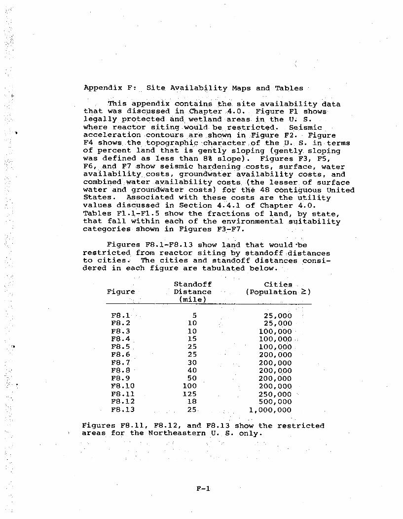
Appendix F: Site Availability Maps and Tables

This appendix contains the site availability datathat was discussed in Chapter 4.0. Figure Fl showslegally protected and wetland areas in the U. S.where reactor siting would be restricted. Seismicacceleration contours are-shown in Figure F2. FigureF4 shows the topographic character of the U. S. in termsof percent land that is gently sloping (gently slopingwas defined as less than 8% slope). Figures F3, F5,F6, and F7 show seismic hardening costs, surface, wateravailability costs, groundwater availability costs, andcombined water availability costs (the lesser of surfacewater and groundwater costs)*for the 48 contiguous UnitedStates. Associated with these costs are the utilityvalues discussed in Section 4.4.1 of Chapter 4.0.Tables Fl.l-Fl.5 show the fractions of land, by state,that fall within each of the environmental suitabilitycategories shown in Figures F3-F7.

Figures F8.1-F8.13 show land that would-berestricted from reactor siting by standoff distancesto cities., The cities and standoff distances consi-dered in each figure are tabulated below.

Standoff CitiesFigure Distance (Population )

(mile)

F8.1 5 25,000F8.2 10 25,000F8.3 10 100,000F8.4 15 100,000F8.5 25 100,000F8.6 25 200,000F8.7 30 200,000F8.8 40 200,000F8.9 50 200,000F8.10 100 200,000F8.11 125 250,000F8.12 18 500,000F8.13 25 1,000,000

Figures F8.11, F8.12, and F8.13 show the restrictedareas for the Northeastern U. S. only.

F-1

Figures F9.l-F9.26 show areas that would berestricted from reactor siting by population densitycriteria. These criteria restrict the number of peoplethat can reside in an annulus surrounding a reactorsite. The population density restrictions and theannuli considered in each figure are tabulated below.The population restrictions are shown in terms ofaverage population density (people within the annulus/annulus area).p.

4

Radii of theAnnulus(mile):Figure

F9.l1F9.2F9. 3F9.4F9.5F9.6F9.7F9.8F9.9F9.10F9.11F9.12F9.13F9.14F9.15F9.16F9.17F9.18F9.19F9.20F9.21F9.22F9.23F9.24F9.25F9.26

0-20-20-20-20-50-50-50-50-100-100-100-100-200-300-305-105-105-105-20

10-2010-2010-2020-3020-3030-5030-50

Average PopulationDensity ...

(people/mile 2 )

100250500750100

200350500100200350500200500

1000.150350500800400500

1000500

1000500

1000

Figures 9.3 and 9.4 show restrictedNortheastern U. S. only.

areas for the

Figures FI0.I-FlI.4 show areas in the NE U. S."that would be restricted from siting by composite densitycriteria between 2 and 30 miles of a prospective site.Each criterion would simultaneously restrict the mean

F,2

population densities within six annuli: 2-3 miles,2-4 miles, 2-5 miles, 2-10 miles, 2-20 miles, and 2-30miles. The mean population densities in each of thesix annuli can not exceed the prescribed density limitsfor the site to be acceptable. .Figures FIO.I, F10.2,F10.3 and F1O.4 consider density restrictions of 500,750, 1000, and 1500 people/mile., respectively for theNortheastern U. S.

Figures FIl and F12 show areas in the 48 conti-guous United States that would be restricted from reac-tor siting by the combination of a population densityrestriction within ' two miles and a composite popula-tion density restriction between 2 and 30 miles ofthe site. Figure Fll considerl a populationdensity-restriction of 100 people/mile within 2 miles ind acomposite population density of 500 people/mile.Figure F12 is based on a 250 people/mile densityrestriction within 2 miles and a composite populationdensity restriction (2-30 miles) of 500 people/mile 2 .The 2-30 mile composite restriction is as defined forFigures FI0.1-FIO.4.

Tables F2.l-F2.24 show the fractions of landavailable for reactor siting in each state if sectorpopulation restrictions are added to a compositepopulation density criterion. These restrictions wouldlimit the number of people that could reside withinany sector in each of the composite annuli (see Section4.5.4 of Chapter 4.0). For these tables, five annuliwere considered: 0-2 miles, 0-5 miles, 0-10 miles,0-20 miles, and 0-30 miles. The allowable populationsin each annuli were calculated assuming 250 people/mile 2 between zero and two miles! and from 250 to 1500people/mileý in the two to thirty mile region. Anacceptable site must satisfy the sector population-restriction for each of the composite annulfi. Thesector population restrictions (fraction of annuluspopulation allowed within the sector), sector widths,and the 2-30 mile average population densities(people within an annulus/annulus area) consideredin each table are given below. Tables F2.l-F2.12show the land areasfthat are uniquely restricted bythe specified criterion. Tables F2.13-F2.24 showthe fraction of land available for reactor sitingbased on the specified criterion.

F-3

Sector PopulationRestrictions

PopulationDensity (2-30 miles) •

.(People/mile 2 )Table Width

F2.1 & F2.13 22.50 1- 11 1

F2. 2 & F2. 14 :22:.50 1111

F2. 3 & F2.15 22.50 1 1 1 1 1 1 116' 8' 6' 4' 3' 2' T

F2,.4 & F2.16 2 2.50 3 ~

F2. 5 & F2.17 450 1 1 1 1 I 1

S2 6,6 &,72.18 45, 5, ,

P2.7 & F2.19 450 1 115 1 1

.. .. • • 26 , 6 7 •3 •,' T

F2.8 &,F2.20. 450 1 1 1 1

F2. 9 & F2.1 45° 1 o1 1F2 9& F.21 0° ' 3' 2''T

F2.10 & F2.22 9g0 1 1 i 1

F2.11 & 72.23 90 ° 1 1 1 1F4' 3' .2' 1&

P2.12 & F2.24, 900 1 1 1 1

250

500

750

1500

250

5.00

750

1500

250.

500

750

1500

Tables F3.1-F3.5 show the environmental suitabilityof land not .restricted by each of 5 population siting

criteria. (The environmental suitability classifica-tions were discussed in Section 4.4 of Chapter 4.0).These tables show the fraction of land,. by state,that 1) lies within each. of the five suitability cate-gories and .2) satisfies the population criteria. Thepopulation criteria consist of a population restrictionwithin two miles and a composite, population restrictionwithin the 2 to 30 mile region. (The annuli consideredby the 2 to 30 mile composite population restriction.include 2-3 miles, 2-4 miles, 2-5 miles, 2-10 miles,2-20 miles, and 2-30 miles.) The population. criterionconsidered by each table are tabulated below.

1ý

F-4

PopulationCase

0-2 miles(people/mile

2 )2-30 miles (compcsite)

(people/mile )Table

F3. 1F3.2F3. 3F3.4F3.5

12345

100250500500500

250500750750

1500

Tables F3.6-F3.10 show the effect of applying differentpopulation criteria (the five cases considered in TablesF3.I-F3.5) on land available within each of the suita-bility categories. The suitability category consideredin each table is tabulated below.

Table Environmental Suitability Cateqory

F3.6F3.7F3.8F3.9F3.10

lowmedium-low

mediummedium-high

high

F-5

3

FIGURE Fl

RESUITED LNDS

an uwmmE],UUATU!S A

(a;

HORIZONTAL ACCELERATION: EXPRESSED AS A FRACTION OF GRAVITY (g) IN ROCKWITH 90% PROBABILITY OF NOT BEING EXCEEDED IN50 YEARS.

FIGURE F2

03 4M

FIGUR F3DE CS

1rj

FIGURE F4

F~ -& URE F

FIGURE F5

;P

I-F-a

GROUNDWATER AVAMILAlITY COSTps .m a im inijn

DA-11Ain'

FIGURE F6

F U F

FIGURE F7

(A

I-

FIGURE F8.1

f>4 um- i

lost MMstdm

WAMM r-3 ,•

FIGURE F8,2

fo

LLE

_ • d.. Ud

FIUE--PW INNOW-'

FIGUR F8.

H

FIGURE F8.4

-iý

t-tam

FIGURE F8.5

00

FIGURE F8.6

U,

MWINclo/

/itef LMI

SamHWA WT

com wi

PW¶U? ow S

4' I .. -N

FIGURE F8.7

puLAtim CtMtISMMtO AWASStancLRMW orvrnm..E~3Iwo u WITCKg WArn E

WATO MI

U.. - --

4N

FIGURE F8.8

JoN

N) I-

HLE=

L~J

FIGURE F8.9

ILIM

mr

_____ ____ ____4'

ED

-wx will I3will Wm~ C3

FIGURE F8.10

C6

t

(,j

FIGURE.F8.11

F F

FIGURE F8.12

.0

UL

FIGURE F8.13

Izj

,AAi- om

thin -774T7

FIGURE F9.1

i-11

I

-..

FIGURE F9.2

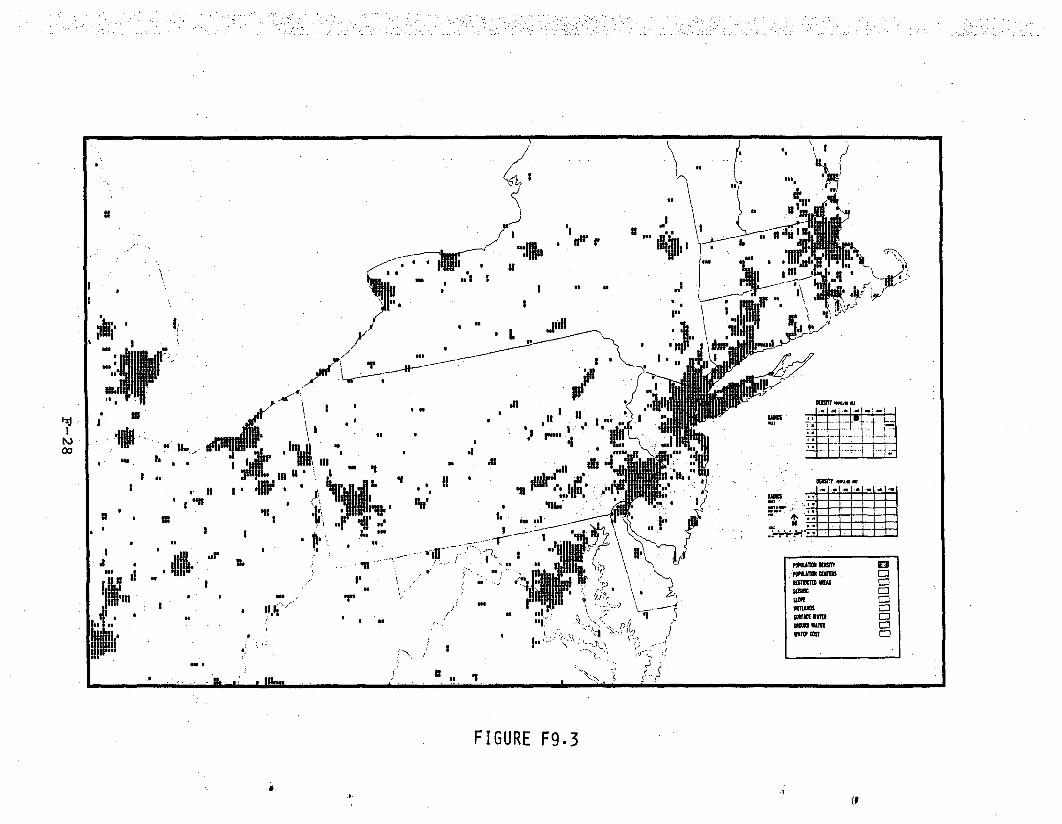
, .,.I~ h , , , I *I • *~ *.

,'U 0 1llr

an .Ia '' I j• - ', a' "I,,"'In 3. q ." .. 111 I '. I ,,

, ,III , I; ' • _, m• .3 ..r i '...... ".. - "1

ml a uIIL- ~ _.-* , -

in ,... I,,,

a:,,•l *. a -. -.- "i,

a m cm ilta,.

hIIh o It •-a • -a - ::,

'" I IU I ,,a

FIGURE F9.3

(f

3rI. 9.

I um

Is Igo

~ij I

S -h

* r

FIUR F9.

mmmIf -.

man= mm

WMIN

FIGURE F9.5

1,

)i~

I-

77. I

N

FIGURE F9.6

t1T

.1

RnmU EDf

gm um mWA1A 0

N 7

FIGURE F9.7Iri

iO

I

FIGURE F9.8

LA)

ta 7

FIGURE F9.9ý "A

I's

ul

'77.

Mum cum C

Tm [Mm=AM in Ci

YOU M

FIGURE F9.10

~~iv-P lciý

-~ flU 7VAIN IF

V~iN IT 4

SN

FIGURE F9.11

I-I

imm am l

sm osm -SAEVAIMLi

_vwmlimi

*Am cm

FIGURE F9.12

-I.

LA)00O

FIGURE F9-.13

I ,'

um ymD-uam m3

FIGURE F9.14

-- Ia I - 4'-

mum mm

FIGURE F9.15

1Tj1

.um

~*41- Ella -

mull C.NILE CUM

agm4.mam

lowWAM 1:

FIGURE F9.16

mm own lam

Rom AMnurSa

nwN

FIGURE F9.17

i

Iwa ID- - -

to=uAMU t

owN

FIGURE F9.18

am wn

won I o

FIGURE F9.19

-n 9.n

T7 T4... -'a .- .L

FIGURE F9.20

~TJ

a'

Um

FIGURE F9.21i

4

pOW*TOn Ow"'IPOILTmRIN u -i

KM Amr E-D

FIURIF,2

00

I - .

T-TNTT

FIGURE F9.23

I 314

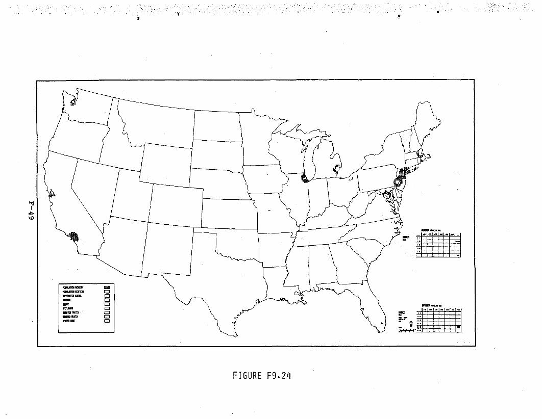
mmxo iii. EEDUllAU Egal la E

smd

FIGURE F9.24

0

Dow

Do-

V. 4,~

FIGURE F9.25

-4 44

ITj

ulH

FIGURE-F9.26

Ly

FIGURE F10.1

I*!j - Will

~iiiJLfit

Ill. F 't~ira" llt.nmFIGURE: F1-

4~. AIII

U,. A 0"uI .I1 I. I il II.Iii .. .... .

fib.,5Si

*~ " * ~. * N

iFIGURE F10-3

qlD

.. .up dli 'I !!i'

"It~

ii~ . Ul

EIIn,, /'inn.....i "

-um. ... ._

FIGURE F1O.4

I.

m'

Ilium

.AI Lr -L

K~IM mimn

WMANN

FIGURE Fll

4i

1.

Ln-J4

smw Em Dam g-l DOKm CD

=AM WAM E

FIGURE F12

TABLE F1.1

A,- ",-A :

AV, A4SAS

C4..Ir04N16

CO..08ADO

,ONNECT I CUT

DE.4..ARE

FLO-4.DA

CE3O.;IA

ID0•D

ILLINOIS

INDIANA

LOUISIANA

PIAINE

PIARYLAND

MASSAC•• SETTS

FMIcHIGA

MINNESOTA

MISSISIPP:I

MoNTA44A

NIERASKA

NEVADA

NE, HAMIPHI RE

!EN SEXICO

"Lw Mexico

NORTH CAROLINA

NORTH DAKOTA

PENNSYLVANIA

RH40DE IsSLAND

SOUTH CAROLINA

SOUTH DAKOTA

TENNOESSEE

TEXAS

UTAH

'IAGINIA

NAS5 INGTON

SET VIRGINIA

240MING

SEISMIC 24ARE4.14Ž J-.r::T4 rF2CTIO,.COES I'. Y..L"O'7 0" ,, 98..STATE AREA. IN £GJA-4E MILES AND % 01 S7AVE

INESTIMA;l V1 HIGH3 • TO 42 2

24 2 70 30 2i6 2 TO 24

'I2 :1

"-.

b

UTILITY VALUE 1 3 4 -

oc 0 C !"C CZ1!C- 0. 0 C% 0 C0% 0 0.. 0 * a. iC.V.2. IC 49 29 3 25t.,.: 4

0 2% 0 . c:. 0 2 %,. 40. . Z'.6;343 473 '2z I 4o 724 20.Z ZT.- 32.t: -Z--'

0:: 091, 1 13 12% - 7 .6.2F. Z200 2;42 2Sc1 3416 83a 1412" l2t-" ;.4; 1.::sc.

399 1 247 1 -. 158% 27 ".%

0 0 0 0 0 ' 5. 72!F . 2. 10432!

0 0% 00% 00 0 0%. 0 0% 0.C. 0 0 C, 0 5~

0 . 0 0 0 0 0. 0 0,. 0 I: 2 C.0 -C0 l C . 0 0 £r

0 007 0 0x 007 07. 0 0 0 0 00. go3,0 0 0 0 0 0 o 46272.- :7xzo 593ý-

0 0*7 00% 0 07 0 07 007 0 0 0 07. 77 z. V*2q 434 702 1409 3377 140-1 n.'- 259-E 58o 54.'-

0 07 077% -23% 2 4% *5 0 239%. 114. 43

.73. 819 94. 120. 965 '23L4. 6'T 2.C 36. 63-'*1 27 1 074 2 27 471 .2% 2 87 e 1% 32 4*4 •4 -!.

23Z.4 97 1342 2764 20.260 00 54" 323. 3. - ::54:

4 27 1 77 2 45 3 1% 4 67 2$570 20 3.0 53 5 .. 7 1%0 0 0 0 0 0 . 23. '3205" 13Z 3N'4.

0%0 0 0o 007 007. 0.0. 1277 6 B 1.8 , 3 t'-

0 0 0 : 0 0.. 2g9 146" 5430! C. 540-0 07 0 0 c 00 07 007 0 1 2 68. 9 % 9 0 0.

0 0 0 0 0 0 2220 .< 9795 91 004! 20 3 .22,.0 0 11 0 007 00. 00 1 "487 1297 73. 01283" 232 174 212 415. 2603 420' 28793 2473 402b"

3.2% 0.67 0 41 0 207. 6 7% 10 4. 721 0;3 . .0 0 0 0 0 0 0 3373. 1241" 481!.-.

007. 0 0 7. x 0.000 0 0 0 007 007 70 12 21 97.0 0 0 0 0 10722 7962 9 2I015 35 340"'

0 07 007 0 0% 0 0 0.07 31 57. 23.4 44 17 1 0-* 0 0 0 0 0 11311 14! 1115,

0 07 0 0• 0 0 07 0 0% 0 07 0 07• 0 07 98 77 1 3*,0. 0: 0: 8002' 0 o. 0 0

0 07 0.07 0 04 0 0% 0 0%.Zo000. 0 0% 0 07 l0 0 0 0 0 0 0 52154 91:76. .163

0 0x 0 0 0 07 07 0 07 0 07 84a 3 2% 7.0 0 0 , 6094 24924. 65914

007 .00 0 004 0.071 007% 007. 0 07 71 07 2q 0:.29 1o25 193 262 233 1245 2972 28883 3841 476.s,

0 17 0 37 0. 4% 0 AS 0 77 2 4.7 6 27 81 2% 6 0%79821 59 628 685 1 9. 4642 7324 42354 , 45•4 49934

11 47. 08 0 7 1-.0 1 -3" 7 17_ 0 20 604.17 4b S713521 252 " 74 : 522 50 10895 6272 "7593 472%. 140447097 0.27 0.37 0347 2. 47 7 37 4.27 53 . 31 8%

0 0 0 0 0 5694 34.2B 6664.! 153, 72

0.0:00 7O 007: 00 007. 7 3% 4 77 060% 2 01

31565 " 2220 2953 4767 143212 17978 10692 587 202!7 1104.2

2 0a %77: 4237. 22 97. 2 6376 9 7% 5 3. is 23..0 0 0 0 0: 759 674. 0 11-7 :4.E

0 07 0 07 0.07 007 0 80 21 72 17 0 06 12. 6%3049 9. 4024 oo

0 0 : 0.07 007 007 0.07 31 7 I1 71. 50 27 0 050 : 0 . 0 : 0 220 2292 6020o 3253e 121744

007 0%.07 0.07 00 0.07" : •5 0: 9 77 49 7% 25 070 0 0 o. 0 21037.. 71221 22202 6o93 5022o

0, 07" 0 07 0 07o 0 07 0,07 41 97 . 14 27 24 .7 . 29 .?

0 0 0 0 154 : 10905 4970 26...13 862- 076-0 07 007 0.07,1 00: 0 37 22 57: 9 81. 51 47. 17 0.

0 0 0. 0. 0. 0: 0 64433 657". 71007D0.07: 0 : 007: o 0 0% 0.07 0 00 90 7. 9 3.

0 0a 0 0. 0. 0: 0 s507 2=3. 483:

0 07 0 007 00 007: 0.0. 007. 0 07 94 474 56&0 0 0 . 0 0 .124617 15932 25.01 3464 bi94-t

0 07. 00x 0 0 00 7 07 "35 4: 22 97 366 5 "

0 00: 1So 454 694 3034-. 9792"07 0 07 0.0 007 0.070 0.27 057 e 4.873207

0 0 0. 0 0 "74, 444r 30533 3551 4527000% 0.07 00 7 o00 007 149Z 987 6747 76;

0. 0 0 0 0.2204 0 0 120L.

0 0-3 007 007 0 .007 .100 07 007 0.0 007 11843 2 2564 5037 390G 2663 31180

40 47% 59 • 2%7 37 26.27 12 57 0.07. 8 77'0 .00 0 • 0 0 00 0 54214 22793 77007

007: 0.07 0.07. 007: 0.07. 0.07 0 0% 70 47 294.73532 540 5)69 4.26 : 37 .12342 . 1508 5787 2594. 4212-7

84 17 27 1.7 15 287 .9 237 .0 0 0 0 0: 0 2248 262124 9491 26804,

0 0, 0 0% : 007. 007 007 0 07 .04 97 5% . 0%

17573 1274 1204 1766 2210 4873 $17 2573 2-!-!•2,. 80220 67 1 5% 1 47 2 17 2 67 5 7 . 1- 30 07. 33'07

0 0 830 0 00 223 985S

0 0OI 0 07 " 0 07 00 00789 68 0. 0% 007 • %0-

00 0 1 0 . 8 504 2563 26-7; 7.!t 4'.14be0 07 0 07 0.07 0.4.7 V to. i5 . 36 3 57 '. :. ': -t7044 39. 454 52%1 647 2520 5037 527037 .4742 :.932.

20 2. 0 67 0 77 0 77 0 97 3 67 7 3% 40 3% 7.0 0 0 0 0 2248 l2- 1905- M7.2: 24:0.7

007 00 7 0 0074 0 007 4 4ex .1 79 2% 1*: - .C 0 0 0 0 0 L, 51°- ! 72 --- z.

0 07 0 7. 007 0W0 00% 0 0% 0 0:. 92'. f%2O 2. 9 270 24: 299 123.4 3252 64.72 27Z7 ".'q

1 14*. 0 37 0 37. 0 27 0 37 I 3Z 3 3 a, % 66 Z 27.

TOTWA 1622!8 12720 05141 20207 38349 257403 1836412 17915.' 57.7547 04 05% 0 77 1 37 so.0 if 2Z-

... UTILITY VA2UES ARE DERIVED FRO MAP 0F EFFECTIVE PEA

ACCELERATT•O EPPAESSEL AS •g ¢GAAV2TYI )AND ASSOCIATED COSTSor oEIS.4 -CiARD0ENIk" COSTS ARE RELEVANT TO 1100 MRe PLANTFOR S'Aý 8-40UTDO' EARTYO2.4E THE %g HAS A PROA6ILITY 0FLESS THA4 0 57 0 o5:14; E4CEEDED IN 50 YEARS VNESSTII111.

.41N" REFERS TO AREAS 24TT7 OREATEP THAN 60%t COSTS F0.AREAS WIT1 20% T1' .01.9 WEKE 2HVIDEC INTO EMG4,. INTERVA..AND AOIBSEC U,1.ITv 1 .6.5 4-• .- a

F-58

TABLE F1.2

SITE PREPARATION UTILITY FUNCTION *.PER CENT OF AREA LESS THN" 0% SLOPE (GENTLY SLOPING ISTATE AREAS IN SQUARE MILES AND I OF STATE

7ABULATION U 20% OF AREA20% TO 50% OF AREA

TO R T0" or ARE"0 OP THAN O 30 AREAI RESTRICTED LANDS

UTIITY VALUE I 2 2 a

ALABAMA 0 27360 30069 2403 2007? 519070?* 33?% 59% 5% 4%

ARIZONA 125 2972 5134% - 492 59405 114342Ox 3% 45" 0G: 22

ARkNANSAS 6269 7131 "14381 18914 6263 5 23258122% 13% 27,: 36% 12X

26075 2112S9 32223: 235515 21492 .1603641 72 13% 22% 16% 32

COA07296 A3626 46922 7932 20660 :1043.267% 13% 45 02 -27%.

CONNECTICUT 0 2673 2538 0 0 5211DELA&ME 0% 3. 4%: .% 0*.

O 0:: 6- 2220 .- 39 2327. 0% 0ox 3% 92%. "2:

FLORIDA 0 0 4941 41392 13105 2 9322

.0%: 0%. 9%: 70X: 22%:GEORGIA 520 2742 30725 15691 5867 29602

IS1 10%. 22=: 27: 101*1044 4362 13009 2:7860 0 37519 93550

5% 17% 33% 0 47.:ILLINDIS 0 1013 2946t 24704 1361 56539

0IN N 2I . 22 44 2"INDIANA 0 2557 13217 19146 1322 36342

01 7% 1371? "32Z 4%IOWA 0 23096 37249 4922 0 6067

0% 2252 6% 9%. 0%•4(64 .0 9202 49540 223 193 6=6t7

Z tax : 9 " 30%v 0oPENTUCKY 9795 14670 13026 290 2470 40269

245. 36%: 22% 6%LOIJISIANA 0 0 9573 24164 14417 4,124

S0%: 20% .50% 30%.M1I1N 618 1i22 .197? 0 327 34075

a% 33% 64% .02 1 -.VYL"IND 0 1321 9809 3950 145 11155

al : 12% .71 "3% I%"ASS8CHuslrs 0 2741 . 297 0 0 9628

0% 3=% 69% X. 0%0RICHIMAN 0 0 30166 22"2 9679 61837

o0x 0%: -497 36%. 16"MINIDSOTA 0 &1M7. 34817 24~4: 234926 92914

" 0 '%: 1 42 % 29% 29%MISSISSIPPI 0 4507 29770 9766 3841 47964

OX 19%, -6-% 20% "9%92999.32 7662 96904 19M46 12002 4226 69933

12 39% 27% " 172 -6%

RWTANA 3242 41427 26327 0 47160 :2494262Z- 28% 39% .0% . =2% .

01MASIIA 0 7097 .: 31546 17244 a1234 - 777210% 32% 41% 2% 2%.--

MIEVADA 0 2490 97944 29 20222 :130610S % 2. *,79? 0o 189%

NEW 6WSUIRE 772 2269 2229 0 12297 9467AM 26% 54 • 0% 13%

NEW lERY . 0 1023 1254 2443 0 S0P00% 23Z 19% 69% 0% .

;am mNICO " 0 0649 62638 13471 31236 :121744MEN ,14% 1- 51%: 21% 26X

-. 63 " 2136 232 24926 975 : 930 9 0219" . 22%: 20% 2%. 20%

NORTH CAROLINA 2461 296 t9424 27640 2627 90769: s SK* I1, 1 25 a38A 3? 171

NORtTH DmrDT 0 2432 3=70 2063 6272 71006* 0% "3 47A 40%. 9%

OIO4 q947 : 24 24649 12527 : 2326 419833an3 01 32%. .36% 6%.

O•L•LHMA 1090 4690 49V447 10932 3464 6961421 . 7%. 71% 16%. 2%

OREGON •26695 : 29799 32096 -0 30349 97929172 29% 323 0l 321

PENNSYLVANIA 7054 2*4743 9891 9 22551 4227916%: 3$% 22% 0% *5

IHDE ISLAND .0 0 1206 0 0 12060% 0% 100% 01 0: .

SOUTH CAROLINA 339 376 11995 13826 2663 311891% 2% .39% 21% 9%.

SOUTH DAKOTA 2274 4169 31874 16997 8 22793 770072z 2% 41% .22% 30%

TENNESBEE 2312 2922 : 17727 965 2 3296 421223% 46% 42% 2% 6%

T4S 534 6106 :174906 74942 2491 !208392% 3% &2% 29% 22

UTAH 1709 w36e 43483 6021 25523 951213% 10% 21, . 7 30%

VERIONT 1640 2616 1273 0 "1023 99217% 57% : A6 0 I "02

VIRGINIA 2999 5201 22927 4063 9665 412687 23% 262 101% 141%

IA3:1%:;T3. llJ• 12352 21722 a 0 24762 69316152 109 31% : "0% 36%

lEST VIRGINIA : 16936 4072 376 : 0 2 27122 2410270% 2?1{ 2% 0%X 13%

UISERS2 . 0. 0267 3229 9242$ 2029 27301, 19, IL 14. •

laYbINO 6253 23202 .23403 0 252222 979061 13%. 52%: 0% 26%

TOTAL 362293 412897 2393039, 522176 2576739% 24% 42% 17% 19%

;; -SITE PREPARATION UTILITY 15 DERIVED FROM A CONSIDERATION,OF AR AEA'S TOPOGRAPHIC CHARACTER SOURCE DATA IS A rAPINDICATING S OF AREA THAT IS GENTLY SLOPING (LESS THAN 8%SLOPE) MW CONTAINS 4 CATEGORIES UTILITY VALUES HEREAREW4ED ON TiE RASIG OF RELATIVE DEGREE OF DIFFICULTY"aR ACCESS MND CONSTRUCTION

F-59

TABLE 1.304104091f4 WATER IGmNV.C1 6 ONAS') 0221.770 V%82612 -.COSTS IN MIL.LIONS 0R DOL.LARS t2490UTATE AREAS IN "VANE "ILA$5 244 It or STAVE

1TABU.ATION ME THA4 $300 "21".2

262 5 TO 300 0225 0 TO 262 5

287 5 TO 225 0120 0 70.20' 5

3 t TO 10 C

USIrT' VALUE 2 2 3 4 5 6 7 a 9

ALABAMIA 0 0 0 0 37 1370 103b4 29... " 203. 2o7n .7' "

43201m. 0 0 0 0X '0 06 32 20. 38,. 352, % .1

ZONA 59 37 47 39 2)63 135 3b603 3638 2297 5"2O. .34.,.;

2 R 0 R 26 16 7, '32. 3%A*K3PASA 0 0 0 0 s524 . 95. 6567 1779t 1603' 6263 53z29

0In 0 06 OR 36 "R -122 33%. 3-!:

CALIFRMNIA 0 0 77 473 926 1419 6339 20702 220" 5249. 1603.-

02 06 02 0% 2 22 402- "3! 24"

COLORADO 29074 2441 2490 3069 4449 5462 22640& 2295. 4 26 2t5'. .04 32t

292 26 26 3x 46 56 22 .26 4

CONNECTIcUT 0 0 0 0 0 .656 2104 24.51 0 52. 1

0 060% 0 6 OR 06 23*4 402 a 47 0%

312.LA25*E 0 0. 0 0 0. 0 637 2650 3; 23Z,

AD .06 OR 06 06 06 0% 27% "'2 2

FLRID A 0 0 0 0 0 0 10 20632 2261 2322' 59.2

06 06 02 06 02 . 06 0x 35% 43 2

015201 0: 0 0 0 .39 2769"05 241Z5 20.92 58::; 2r6640A 2% 06 0 06 06 . 2% 16X 426 32 1020

104i0 77 309 405 74 •62 2136 127438 21900 32241 3751 833.'

0O 0. 06 12 26 26. 226 242 .- 6% 46,

ILLINOIS 0 0 0 0 0 0 20480 R4 25239 123.: 25.5.-

06 O 02 .0 06 0. 192 4"% 322= Z

INDIA 0 0 0 0 0 0 4690 10721 1262q 2Me2 3634;.

02 0 0 06 06 6 0- 26 52 36 4OR OR O" DROF 0%. OX: OR • 13%€ 29• 32% 4 C 5. 1

I26A 0 0 0 0 77 &27 26470 39039 9023 0 ."52,e

R0 0 R0 06. 0 2 47% 34 so" 02 0 1

I26441 2493 062 325 0 69 96 12025 26"47 "062 293 W022

-326 4, 46 46 26 96 216 201 7, 02

10 0 0 0 56 227 9326 21953 1093 2470 6

O 06 OR 06 6 56 236 302 26, 602

2LOUISIAlN6 A 0 a 0 0 29 347 4564. 12767 16029 244217 40823

06 6 6 6 0 2. 92, 27 33 302

MI66h 0 0 0 0 0 0 %3346 2140 20962 357 34073

.%0 0a 0 0 0 77. 12226 2250 7459 I'5 2225.502O 6.R 6 06 26 226 206 76 26

5IAO1(1TTS 0 0 a 0 0 0: . 4 201 4 140 0 0621

06 06. 0 06 06 06 20%,.. 32% 492 06

MICHIGAN * 0 0. 0 20917 V92" w. ' 3 %.2 94f 403'

106 0 06 06 0 06 176 322.. 36% 262

ININNE6TA 00 0 39 233 462 376 332792 S 7447 6447 .2492. 05923

02t 06 06 .0 It 06 4 2061 6 29

0 0 0 0 37 676 9902 13245 2'53 3041 47054

at 06 02 06 06. 06 1 26 126 30 326 a%

23. 0] 0 0 90 3625 5365 29474 20034 25205 4226 6"33

OR 06 11 26 26 . .202 30: 222 66

,,+MANA, 202 926 o3 60.94 2347 2W5I3 233802 , 2422 ,a260 190456

06 61. 32 6 66 9 6 276 66: 22121 32 3.

I0+ASKA . 222 2233 2537 442 050 920 1260 lo25 9652 253. 77722

72 36 46 66 92• 2•1 236 2 46• . 2 26NEVADA 0 a 0 0 10 20: "36 256. 469 20256.110619

-06 06 06[ 06 06• 7660 369 3 6 20

ONS42EIR 0 0 0 0 0. 0 2123 2702 34453 2329 9467

02 0OR 0 06 . 06 06 222 296 6 3

NEW .ERSEY 00 0. 0 0 0 0 442 2355.5 5272 0 .009

%0 0 06 06 06 06 86 296 622 06

2• MEX IICO 556 9150 20w0 a2 026, 11 2660 1960 &523 2 554 31536 222743

426 26 26. 26 26 2. 266 56: 26 262

la o 0 10 3S6 '30 191$0 604 lM 9 21 6,

0 0 0. 0. 0 0 . 252 9 I""S1. . 93

106 0226 06 06 . 0 06 22 302 252 206

WORTH CAROLINA 0 0 21024 4449 2300 27. a",2' 5076.

m0 O 06.o. 06 2 1 4"26 9 300 1346 276MONTH DWTA 111754 6562 . 22 *99 59 4236 22022 6620 14420 4272 72005

276 f6 206 202 62t a 2 16% 96 .6't 9Ct420 0 0 0 0 567 1679 22440 16492 5321 2226% 41233

6O 06 06 06 26 46. 306 3V% 206 66

MANC421H5A 7692 2264 2" 325 2996 5020 5336 22767 34306 2164 346 6960.1

26. &1 26 5X : 46 62 236 35. 22% 26

OREGON 0 0 0 0 . 10 425 .• 392 122643 12625 3034. 97925

OR 0 06 06 6 .06 362 266 2• 326

05355LVA36.. 0 0 0 293 2432 22307l 122" 22053 3202 45270

a%06 06 0 06 02 6 2R02R 3 356 27. 6

0LN 0t 0 0 0 0 29 425 772 0L 2206

06 0€ 6OR O•6 0 06 2 346 646 02

55U196435.36 .¢ l 0 0 0 0 203 276"0 2 25702 263 322

02. 06. 06 06 06 26 96 322w 506 9*2SOL""2 mDATA 9239 455) 5066 5279 439 4256 9396 7202 4709 52793 770DO

1226 2 76 76 66 62 1222 9 62 3060ams 0 0 20. 530m 2940 9425 26296%4 2264 2296 42122-

02 02. 06 06, 6 26 22%. 306 28! 6

33%4 It) I47 346 263 292 90721 70474 .425225 20933 249 .24403q326 26 2 2"26 262 2A W .' 76 2

UTAH2 405 37 430 2364 M94 402- 35444 7275 4973 225553 050.2

26 06 26 36 2 56 426 q% '% 302

VERMOT 00 0 0 0 -0 .0 4623 2037 128 202. 5

06 06 06 06 02 02- .72 Z.6 s-7 20.2

V2RG2NI6 0I 0 0 396 2229 2242 6456 12245 12091 266! 4--6

02 6 .0 21 26 56 262 30! 322 142

WASHINGTO 0 0 0 20 253 330 90225 2307. 22,43? 2-7 Z .937

06 6 6 06 OR OR 0*4 &A- .26 2 362

4WE1T V2602926A 0 0 2300- 33 23 23 7170 525b 2721 2-30!

06 0O0R:2 .46. 206 222. 302. 23 227.

WIS6ONSIN 0 0 0 0 226 2235 23394. 9902; 27447 502 2,40z;

06 06 06- 06 0 2% 22 322 3!!. 322% 9

APPOM226 2943 3927 2327 626. 27439 9206 2060W 20626 601; 25227% 9796.32, 46 26 41 66 23 10% 22 22 62 262

MAL41 a22702 3=376 39770 49727 to203392210.66 740)69 6536612 522404 257.7.

31 12 12 26 36 46 242 222 1 272 e2

AGGREGATE WATE3 COST DE3I96T2ON 2.EA5 COST ALTERNATIE6

995A 511192246 FOR 6005216 or 0ROU3DWATER COST AND SURFACEE619C ST IAE 12261 S5DRO 2DWTER COSTS F52 MAJOR 3EG02N5 OF

THE COWMIU WER9E CALCULATED F3OM INFORMATION NEGARDINGOVA.3TV. 422591212. 3DEPTH A00 3221f OF 462.6-522.0 4561631 SIX

aw62 i 40956611T COSTS Law 7225 4200 MILLION NE31 D2V2310510110%~. 29213925.5

P-60

TABLE Fl. 4lUWOC 60T73 UTILITY N4N2CTI6k -.

COSTSl IN "IILLJ.i SOMS OF DOLLARS41"01

STATEARA ain mum 66224 mmLE IL or fv47

TAIULATION Mt 71"D 03100 "ILL.342 5 TO 300 0

31" TO 24 23 5267.5 T`0327 0

s50 0 To 237 Ia32 5 70 IS0 0

'~~~ .

T 12 5750t T 37 1

913Y VALUE I a 4 5 .4, 7 0 9"

dd0 0 0 0 0 83S 2731 . 6945 296 2.032 3075 .51"07

4 St 0 01 . 1% 2 35 4%ARIZO4N 02201 47 45 4 .4233 4140 42 43&2 34&W 2-27 99405 .134343

19' 4 41 4t A 4% 14 4 35, 2% ST.ARKAN A0 0 77 SA473 334 " 74 4617 17793 21037 642 3 3259

01. 0IL 05 It. 21 .41 '25% 335 35% 13a'CALIUVNIA 12732 40 421 7 7109 1463 10567 2" 12 50701 8 7iB, 5249. 1603"4

95 ý3 4 51 31" 7% 10% 135 141 321A

.064LM•0 39903 2490 DA1 33" 46473.: 4 20007 . 1100 I. 4514 26' 0 :0432395 35 35 35 51 45 O05 "25 4 27%

CONNECTICUT 0 0 0 0 I0 0 .56 2104 . a452 0 1305 0 as OR Ol: 1. 135 0. 7. 5

s.4445 0 0 0 0 0 0 a "37 3460 39 2W3,0t 0M OR 0. at O. 275. 725 25

PLARID.6 0 0 0 0 0. "79 43721 1.91 2.611. 13205 1935705 05 0R5 0, DO5 it 71 .265 43% 22^

0e0"1^a 0 0 : 0 0 206 293 1 0--, 165 32=4 8649. "- M.0405t St . O5 05. 05 3: I25 40% 32% 10%

WAND 77 3209 405 1314 %..14064 :436 903 12900l. 12943 2,520 3355D05 05 0 5 11 45 SI 125 2 2; I 45.

IuLINOIS 0 0 0 0 725 9 A9•2 .• 239 .1361 3654001 0 .. 05 05 05: 21 27: 47,I Wt 25

IN t 0A 0 0 0 0 1"0 .474 . 1373 16219 . 3222 3&34205 SO 05 ft 0al 0x 235 5O5 325 4%

to" 0 0U 0 994 :4574 :603 134D1 19039 0953 0 36040lt 3L OIL 25 ,05 155 a4t 34% 235 01

4.M4 18444 2 2 293 62 3M5 4642 7736 21214 *4473 4642 39 62"225 4% 415 .45 55 ft 2145 Oft 75 05

6TU33lUi0 0 0 0 640 "1271 92 9:133 O20392 5470 40"49.05 01 ft M5 91. 222; M5 35 26 %6&MI23Ism 0 0 0 0 ;145 .05110 113747 02402 24427 412T4

ft 05 05 05 2 35: 71L 375w 33= 30562136 a 0 40 542 907 707 7*2 2404 1094 207 24073

0n * 5 91 2t M5 91 2% *rl 33t "ITLA0 0 0 It 0 D9 .0 2004 10 459 245s21

05 0 . 05 0 55: .5 95 ,150" 471[ 25

,MIAaHmEM 0 0 "0 0 0 06 9592 3779 4250 0 . 6427

fOah2l 0 00 SO" 0 0 0 9054 291 3 01 3

So 0IR 085 ft 45 25 25nl 221 3b% I&%:TA 9 31193 50 O1145 9-19 7UI 20633 4'4 17447 4607 14A2 6913

as Ox IS o 45 GO An5 271t 105 AM 29MISSISSIPPI 0 0 0 0 ... 2o 5 03233 f14 26440 52131 1421 47M3

c1 1 "01 05: 05 41 Wk :an I3

IMOUiT 0 0 244 2 J s246 610 SOW 23424. 50104 1506 4526• &99340 S 05 "" 3" 14 2 an5 305 mm 6"SOf11 15 264 415 9 6235 52245 644"M Wg 90297 21422 . 4750 2341455

05 I 25 S ft e1 05 205 24% 245 235 33mass 2533 36N .7 4 449 7490 113not 2490 :117 9450 534 : 77722

7: =5 45 41 - :0 IS% in a4t 12, 2.6017 44672 4?67 4644 9020 9013 3790 325 336 609 2025 :230260

40 4 4 3 35 OR ft I& JIM20

235416t 0 0 0 46t ST90 153 50 3445 22197 9467'at 01 95 a" 05f 25 35 25 345 323

Im JER 0 0 0 • 0 0 0 AM " 1MS 17273 0 6009

at 05 05 a5 at 4•t , Si an .6455 01NEW- 0935775V 4=64 W676 2640 :MM!0 2: a4 4104 65 : 2514 2•54 :1211744

47. 35 t 3L 35 35 45 I all' : *"23' 9622 0 0 0 0 123 a29 6437 25179 29647 99130% 9302

--- Cg 7,~i 'M 0AI I=084.4 43 90 27254 6427 10764OR .: ft •, OR St .

MORTN I1DAKTA 31194 443I 736 V1014 :0919 : l5 660J 0: 441420 0372 •7003I'M ft JIM .501 "01": 50* 9. ,.I' m 91

0420 0 : 0 0 0 ROD7 6433.22 24,96 *492 65231 4*654St 0 S St as AX an36 395 505 4

SMA4OM 7691 2944 2on5 5094 6454 35 121367 034266 624 2444 49615IM5 4 11 ,3. 41 0 i 0 M a" 321 I1

7M SP69 2207 221: 4 2•2634 11027 0 196443 2455 9 20249 907971 ý35 25X 35 85 II 22 341 27 321

vo". IA 0 0 " 0 .04 " 3M 20036 S42 :2053 5052l 3 45M7

0 Id 0 0 0 0 0 ft0 19 *4* 2 0 *30605 011 O 05 : 03 05 .. 1T 3• . 2"41[ 441 01

1m C,,L0.211 : 0 0 0 0 0 553 1012 9362 25701 6443 31269

SOUTH4 330l1:1 9146 4999 306 A1404, 3455 M0954 660S. 72001 4704 M9 77501)

255 41 ft Ma 75 SO~ -5 9t ft 20%TNES 0 0 0 &0 5262. .&1M " 2434 144 224 39496 43224

TEAM 2I57 5644 GOS6 94•0 : 220114 29474 31449 420 ;26432 "49t 546140421 35 INK 4 41 75 M 225 265 =5

UTAH 22I 1442 312 43304" 4140 5129 405 75175 4673 3O5153 '5•379541 21 45 SO at 41 271 '9 ." 45 L 301

0 a t0 .210 697 23a, 37 3637 226 02003 9952

In 0% 9 '3 9 235 9225 292; 124 20%VINOINIA 0 0 0 9 1Z2"29 6490 6140 23437 23692 . 6465 411617

05 J•1 0 "5 5 41-• an1 205 ,15 14.•

amm42D3M 0 . 0 0 1374 : *51106 13040 2626 22076 224I33 24762 493127: 0 at ex OR as 4" 4 I2'9 32. 341

MIST VIRGINIA1 0 0 :0 SW0 X4 1044 .234 7270 . 242 072 24205

.0 01 0 1 21 41 10 2 5 a• 2311 01 1 M2324.3521 0 0 0 0 225 6423 223P03 2960 17447 6026 5702..

ft 051 j 5 05 05 DO 3O l 2135 -31 9552I235754 335 449 37430 9043 90 $0605 20610 6012 . .202-5 . 97935

71 9 7ft 'am 95 205 555 J11 45: '26%

L 1190600 66912 6919* 3t437 29629 1929064 244340 447940 228404 '357673231 Al l 8S 311 41 1 235 285r M1 36,

S3IERACE HAT"13 'W6r • TIoN- GUIT 3 .IE dIl2l, AlUSCRA, SWAT LAKESI AN NON-INIT""ITIONA DOAJY 81111 ,, M ,

NOT"4 7-9AT. 20..9E4 LOW4 FUN61113 GRATR246N2 f. N00 242 OR3331P --D 3V,0-•4d 1,0441 3201111 73T2 5*0•I" .11 •42 23

005 MW PEE IVIE MWE 1 10 " I0E•i1 SEC311TV. :,#AT7

2325.I.I1 52D24A5 251r0 6664 2I63. ..

F-61

TABLE F1.5-*i MA.L BUIT63l2bt" VV•?3IT Pq13KTIONI

62*3 ".a to @own OIL me2 V StAYS

WTak"Tvaam um 4 .

F3LM F"LUR a2.111% an 3" M 4

mos•: A 4301 3&04" 2075 2314 09401l 11434322 4% tn sn 52

SallA 0"4: 24 M So" 25. A9 9 2 :

CM $ ..I : • : GM IA f t , 0 4" 1 ,03 1229 OU5. 5249.1 :&0363M ,322 52. 32%:

: . .44 :34 13 433, .I 2"" :*04326

Ci3CVT, 393 9607S 762 3754 0 " 0 a "$I1 402 12 ,1242 02" • 2,

i . 0 " 21217 29 2202 % C932Oe 22

su S .0 0 0 3122 44120 30509398

e32 392 222 - 302

it : 4% 3 ' *74 - 7 : -2% : 242

m " 0 30: 94 : l3w V.94" 3:53* :.140 36042

tllldook 13 AS.: "76 ;, o 811 ,"40 I1 • 0:" "

' : :1Z 9 ,; Sax 22: 0t,

$ D I 1 0 :7,002 2961 ISM '731 1 839 :392 332rIz 8 92 ft

474 10576 15101 3569 397 240402662: • 32 202: 23: .,' 52: *2..

33I 3 57* : 7633: : 8:4 0 "77 '2437 : 4335 .

3*126 324 8" 4979 3774 : 3754 3 57 . 4074

.MM ,,47 ZL :S I •4 : . , 45I% :. 52•1:: Ilr02 8M 31•42 . : 12 lli

. . 5 377* :6 46 1"62 : 1011 :, " 0 3627

AX4 312 u12s ,422: 02: J .'ouI ag4 0 M" 273 ,5049 : ft"7 :" 1337

+ l02 "l • 53 57 3*2• :

unee! % 0. : Us 9740':: ,41092 : 29*4 24922 :35946ass 02 3M: '42 252: • 32:'

- " "11 0 263 : 490 20767 13572 :., 341 4733f 02 ýJf ',421 Of2. 32:

• ' :3 32709 14437 35749 33 30557 : 4536 : *1 9 ...

" 1811 171 822 372.il 332il: *2 :+

12M 323 56044 JO575 , : 49 : 4•7*6 : ,344

I •.O •'I m 302 "i •* 42 5 :"$2• .S A 3 : O 3*77 2445 35"- 3 : 352 .i772

: @ "M 416 3n 2

- 3.31 4 926 27*72 .i"8 3 I 20 555 2 "0"SIM - R -n 12 02Ol 3l;

MWIA241111 AMR"4 274 ,'71 3 - .0114 a s;ilo1

20 9711 vSX -• a& I'11 :' .

ow 2 47 4461 3son 311" 0 : 3397 : 94I *

MUMM I& 472 SI3 -3 02: 25:

- 34426, .• •o: 0: 3030

32 32 4"2: 02:01

a 147 0 I@= 1ID.": 2352, .- 52742

an askJ : 16i1 II ::"0%::'-: RR% "

-M M 7773 11 211064 3OM939=3 310M742 332 IX a 62 302

NO m OASO SSW.3 46 *33 4473 In"6 S 3077

so" &1 318430 37172 847 ti AS?& _:,7&005

Od: IL.35 3 0 : 330*t IM 4:6A39411 12103 106 Islas 115 93an $7 2 1= -111% 3a3t2 •

simm• a" !.- 298114TI $40, l8l4" 'R'R7l *Wplil ITI,,II..- 1 l

40w~s 3*21113 332 2553 45273MO2 340 62"32

01141111 SLAN0 3: 44 I72m 0: 0: 3206

inivw GROnLfth ' 79 7M9 : *344 IS 332=:25 36*2 2ý3305on a3s 2: 2 42 92

mo 1A92 38267 2 "2 :737 :IS 223 $ 2301 1130711 U359 770062:1 102: 33i: 3*2:.34%: 202:

RAGmS 14$3452 VM 993 W60* 454 21096 423232:X '"%2 $4Z' 3&f' I 62

Van" :3 "4 2 :~ 272o 3492 Sf 22O

an 262: IN .332: 2. 2025wof 0 001 : 457 a 12* 0 30623 .41531

V23338* 4555 3env 2430 3=3 35463 5665 412*2133%: 7 . AS; 23n 202: 342'

23732 : 9535 n: 6394 Y OW25 :- 2 :4932 : 47*2 *23l724£, gaý ta 34.. 24 72. 262

3437 VIRGINIA *12 433 0364 *563I 1 45 :222 57212 541"6.%72: 422. 37n 32: 32: 332.

u3C"IN IM 311 260 &M *0,24*37 .~i 3*5 : 524510220: 72: 3la: 431% .332 a" .92

I33 734 .372M Sa077 23730 :4767 am$2 07901

vwft3 415244 45505 4*6310 *491932MI 312576"2

4 SW03PAPOWIAL. 001tA33LIV 5g3AT3IO: 7362 FACTORS,W12MC MiODINIMS. 9327 P4576341304 AND A00209"71 347.1

4-13.4533.377 WO C@WM3113 665230 TA633 4-%PUS UL37YtttV62.33 MA.CH ROOK 1-9l 1253L13N0 22A MY 3/TLIIy:# WITH33WALMS FROM 4-s$' OC VftIMS NMX. DOOSES 12WM OrIV CATE-; '

AsO141 OF O"3021321RAMV aft. AN".4 BUT 202tO OR041 3V2L ..

Mi WA #Ate "Us", owgn4S36Jtai o11T633LTv 3623.1

EN SIM W13337 VFLVW MaaSM %Ifl GUSIMzIL.

F-62-

TAL•UATIONI

TABLE F2.1POPULATION SECTOR ANALYSIS - TOTAL U. 6.DENSITY - 230 /90. Mt. -, SINGLE BECTON (22 5 )EGRES)•STATE ARE" IN S 1UARE PIILES AM 1 OF STATE

AVAILAILE LAND> 1/14 ALLOWABLE POP

> 2/6 ALLOWABLE Pop.> 2/6 A±OHADLS POP.

> 1/4 ALLOWA4BL.E POP.> 2/3 ALLOWABLE POP.

1/12 ALLO•ALE POPUNIFORM DENSITY

IR.ESTA 1¢TF. LAMM9

ALABAMA

ARIZONA

ARKANSAS

CAL.IFORNIA

COLORADO

C€NWECTICUT

FLO RIDA

GEORGIA

IDAHO

ILLINOIS

KENTUCKY

L.OUI8IANAU

MAINE

MASSACHUSIETTS

MICHIGAN

MINNESOTA

NISSIBEIPPI

MISSOURI

MONTAN

NEBRASKA

NEVA"A

NOW MEX ICO

NORTH CAROLINA

NOTH 4AROTA

OHIO

OKLAHOMA

OREGON

PENNSYLVANIA

RHODE ISLAND

60JTH CAROLINA

SOUTH DAK•OTA

TENNESSEE

TEXAS

UTAH

VERMIONT

VIRGINIA

WASHINGTON

•EST VtRQINIA

WIISCONSIN

WYOMING

1.0 -%6,9011 31.91

2.0 4402=

2.0 235944 41):64.31.

4.0 2970:33.0%:

5. 0 : '557.56. 0 1

6.01:. 10)

0 217.0 309:

13.32.0 : 10769

:2II 11:

9.0 1634727.92:

10.0 : 3566:42.72:

11.0 11it9:20.52:

IS.0 20420

12.41 0 59579 :

72 42

16.0 11455

17.0 2X3I4&a'. 82

a. 92r19. w

.0..o20. 0 50004

'L :32.42,

21. 0 3530:41. II

22. 0 ISM2

23. 0 323244I .4 .6

24.0 : .92206

62.11:25.0: '&15$

62.4) ItIl :26.0 : •9•5277.22

27.0 s1le :1

• 2:1. 3 :IM

20-0 00 1. 01

59.0 1 60346b. 01:

30. 0 0 702I L.41

21.0 :691913.6!X

= 5 400676.22

33.0: IM74.31

34.0 :396233

35 0 497945061:

360 35907.91:

7.0: 0:0.01:

36.0 5742:.10.4 :

39.0 :46910:60.91:

40.O : 1143527.11:

41 0 .164136t61. 6

42.0 : 5266461,42

43.0 365939, 3

440. 677416.52

450. 2209033.02

46 40 507421, IX

47.0: 1959034,41

48.Q .6533066,711

3802.7.3%

6300.7134646.3171004.15%•,4 51,.25942. 11

S0:0.01

772. 3147570.0.40927.0:

2.2a .03 :

2561.6.35

4.5:

4.5:3001

.7. 121=6

14364.21

5.42193

2 21

0782

1.31:2. 4e224504 92710

5.31.291

0.14

1034

173702.91

2967190 41

31004:

5.IX2229

35

2.34

209

4:0:

0.012123

6 61:

.2. 3126256.2"

13356S.01(463

0ý 51579

5& 9230017.3127504,012219

10.4137546.6 '1t331.9 :

4072 1674 28 63127.61 10.91 :1021 122.311303 19V7 1071 17271.1 1-7`X 0.91 1524940 4979 367 :245

.. 92: 9.3: 6.91: 4.46417 9645 5365 : 53014.01: 41. 23.32: 3. '2972 2529 2200 :17562.621 2.41: 2.11 1.7I10 97: .. 190.21 1.91 .1 : 0.4%

2612: 599: 36: 212,11.2 : 1292 9 16,64 :9.1

4101 : 5510 .297 40346.9: ,9.31: 5.71: 6.f506. :7 752 : $70 SO,7': 13. A 1: .71: 6.f2210: 1716: 1= :I.•62: M 2: 1.&1: 1 :8194 : 6502 4137 : 49

14.4% 1:.01:10.91: 7.41t3754 : 3607 : 500 3676...

10. 31 .4,22 613:• :10.:40..26140 L' 6310 47V6 :3 :

'14.52 :11.1 : = .61 : .&5=1 ., 4207 MI S11 :2 7306.31: 5.12: -. 4: 32WI1G : 252 427W : 5437.0!: 6.71: 10.6: .,1633157: 4392: 4545:3=6.51: 9.11 :, 9.41: 6.&.1976 : . 1642 : 1621 :&5.: 1%5,4: 4.6%: •4. ,656 904 .907 762

'S91 6f. ft 611 461. 94 : 421 2 :,2 0 .396

1. S. 49%: 2- .91:i%4.43631 :4726 : 3544 =-6.21: 7.71: 7. 9% .7%72 : "44 :'2107 : 3 '147

.41: 50: 2.6&X: 2.942w1 : 5269 B OB6 :+ 4101

.91. 11.01 :.2.n1 : 6Z720n. 46W:. 4410 :3.L

10.41 : 10.01 : 4.3: :'-4. 491631 : 32274 "S. 731.11 1 .4: 0.61: 0.82577: 127: : 1s"2.31: 4.01: .2.: 2.0

70,52 : , .0 ., 6 ' 0.79 : =0711 061Wr 0.714 5067 697 714 650

1 951 .752 .561 "

0.61: 4. 91: 5.41: 23.01966 : 1700 19• :3 10141.61: 1.42 1.1 : 1.32164 : 4410 : 4719 36.31 61:. 9,41: 9. 7 ,34&4 6041 4902 : 6747.6.06 11.92 : . 7: 13.4:3937 1949 : 1004 5795.5 2..71: 1.41: 60%320 4700 442:.7.71 11.3: 11.02: 9.95163 4246 : 4176 4130S7.43: 6.1% 6.02 0.91

: 35=: 1756 : 20072 : 3.612 : 1.01 :,. 2.330•4693: 40192: 42%7.1 1061: 9.02 9.

0 .0. 29: 30.041 0.0: 2,41: 2.312393 3339 : 43=3 : 44037.7 101 i 13.91 4 ,0216"6 1727 647 3092.21: 2.31: 0.61: 0.61:2818 3"99 S 4683 : 54236. 71 . 59. 2 :114" 12.91

17003 19397 12477 : 103546.3: 7.2:. 461: 3.911390 10"1 1: 1119:1.62% 1 : 1 1.02 1 .3975 "4 : 994 550

9. 9.10.1 10.12 5.6.3213 4236 4642 : 4527.68 10.31 1131 13.273117 3339 2676 21424.5% 4.86 4.11 3. 112287 2976 2741 "27419.3 5 11.9 2 4 11 11.415520 632: 5047 36699.71 12.0. 0.91: 66%1737 1563 ' 7.2 .6$1.% 61.6 061Z 0.6.

2.5 5 702: 2075 5190711.02 A, 0403329 59405 ;1143422.9 1 : 5 :.01

620 3165 6263 : 532579. 5. : 1: .6"

2142 22603 : 52492 :1603631. 31 14.31 : 32.1 :1139 3947 : 29360 :104325

.1 X 3.1 : 27.311 4969 0 3512

0.4 : .. 1 : 0.00135 :, 6 : 39 :2324

2.8?M :,.26.11: 1,75227: 11397 : 13108 :i59873; %: 19.3 : 22.121004 :,7014 :5647 :566043:.22 21.01 I 10.02,444. 1206 :75019 i2550

,0.5J: -1.42 : :4491:5 .1293 :11792 1361 5653632.31 20:91 5,411466 10547 22 36341

927 3613 0 560~• 1.6 " :...3 e: .0.02,712 27 71 193 N2242,.01 "',4.51 . 0.2, '"094 24314 : 470 40270

,S.521 1.0.71L :_2.1:'1071 2725 : 14417 441542. a& 7.7% :29. 91599 130 357 24074

I ft12. 3.1 1. 01 :57 $742 : .145 : 11155

3.2 51 . : 1.3 :7674: ,0 666

1204 13423 94": 979.. 1637.20 2:-1.71.: 1.71L

44 &= 24926W 65913i£ 6O.4 : W 29.0%1042 2905 :.2421. 4766

94 5356 4514 :69931.4 :7.71 : .&.n367 :' 206 :047160 :146457

0A 3 0.61 : 21.6 1I ,510 :+17 :21514. 77721

0.71 2.01: 2.02:141 1177 : 50255 :11062701; ".12 :I 1631

241 1901 1197 94640,25 20.12 12.61

194 :699 0 6t01I. 6 :5.8. : 020S 2 1476 : 31&6U :121744

.0.12, .4. 2 :,.25912:2467 : 14707 '. . 52192.91 29.33 19.15245 9110 , 6627 : 50769

.4.6% 17.91 17.01'4731 473 63272: 710050. n 0.71 9.3:1399 17775 : 52226 418232.31: 42.n1 : 5.6:1177 . 4043 : 3444 -94*41.71{ 5.61 :" .502:

1206 4159 . 30349 : 979271.21 .4.21 :.3L,021216 17467 : ,3551 : 4520a. 71: 262.6 : 7.1 .

0 1129 : . 0 : 1207O.0O: 94.41 001 :1177 4825 2463 : 22162.61: *5.52: 6.51:

212 : 610: 22"793 : 770000.31•: 40. 5.462:2 612 476 : .26 : 421225.21 :4.7: 4.t3 :3647 20941 : •491 :260A291.42 7.61 : 2.01425 2064 :,25553 90180

0.513 2.41 30'032290 560 1023 9954

2 9. :5.7% 10 411563 6402 . 654 411673.18 16.02 13.681139 6301 24762 69"161.6 :". 11 35.7:s64 2277 : 2721 24106

3.61. 9.41 11.31:1245 &12s 5026 570242 22 10to. n a.t"326 550 22225 97985

0.31 0.41" 25.7

C.

TOTAL1405512 123194 163116 182502 148233 137771 49349 2622611 57673

46•. . 2.71 5 41% .o 4,91 4.31 .1.62 9.32 18.31

NOTE: "AVAILA1LE LAND I T1HAT AVAILABLE 004DER TIE MOST CON-STRAINING CRITERIA (I. IF > 1/16 OF THE POPULATION ALLOWEDY A UNIFORM DENSITY CRITERION 1S FOUNG IN A SINGLE SECTORO 22. 5 DEGRES. ) NUIMBERS IN THE COLUMNS REPRESENT THAT LAUNIQUELY CONSTRAINED 9Y THE IVIEN FRACTIONAL CRITERION. THISLAND IS CONSIDERED AVAILABLE IF THE CRITERION IERE RELAXED.IF SECTOR CRITERION IS APPLIED. ASUMER THAT •NIFORM DENEITYCRITERION IS ALSO IN EFFECT. .. COMPOSITE OF 5 RADII6 1

P-63

7AsIu.ATIOP

TABLE F2.2POPULATION SECTOR ANALYSIS - TOTAL U. S.OENSITY - S00 /IQ. NI. --- SINGLE SECTOR (22. 5 DEGREESI

STATE AREAS IN SOWAM MILES AND % OF STATE

AVAILABLE LANf1$1 ALLOWAILE POP

> 1.8 ALLNAJLILE POP,• 1/ 4 AL LOIABLE POP.

• > 1/4 ALLOWABLE POP.- I 2 1/3 ALLOWABLE POP.

> 1/2 LLOAL POP'UNIFORM DENSITYI fI[RSTR ICTE.D LANDl0S

ALABAMA

CALIFORNIA

COLORADO

CONNECTICUT

DELAWIIRE

FLORIDA

ILLgOIA

ILLUEDIS

INDIANA

IOWA

RJENTUCAV

L&JISIAMA

MAINE

MARYLAN

NICHIGAN

MINNESOTA

NISSOUGPPI

MqONTdAN94IASM

NEVADA

fe HAMPSHIRE

NEW! JERSEY

MEN MEIqFCO

HORTN CAROL.IM

140111 DAKOTA

OHIO

OREGON

PENNSYLVANIA

OHME ISLA

SOUTH1 CAROLINA

SOUTH DAOTA

TENNESSE

TEXAS

UTAH

VERMONT

VIRGINIA

WASHINGTON

WEST VIRGINIA

WISCONSIN

WIYOM ING

1.0 24036:46.31z

2.0 4&600:40.8%,

m.0 304

570 442

S0' 4342960.1I:

&.0 :" 10:

7.0 : 06924 9 :

00 2014

9.0 2504J

10.0 3975::47. 61[

II 0 19370.: •': :34'6 1:6

120 a 700314 .7911.0 22213

17. U14.0 16961

281.919, •0 16119:

:' 41. 11 1

1 .•: ý-ý $ :29

17.0 :2522977.02

1. 0 : 2122:39.0:

19.0: 434:-. 0%:

SO. 0 22996*6 242

51.0 :41171

22 0 3412.: 0.411

2.0 0 41963

: 9.4% :

: 4. II32.0 :6632: 3. &Z

16 0 .3029. 77.38

270. • 23619.M. 222

N.0 121I ý 1.71 :

.29.0 : .11300:9 : 60•r :

20.0 94v19 32

3210 owls5

e. 0 716017 1:

34.0 47131

210 1226696.4z :

24.0 909

27.0: 0::0.01:

3 .0 9764: 2t3. =1

9. 0 :,50759: ".lr :Z

40,0 1"36239 .5

41.0 :194524: 72.4:

42.0 53480:42.91:

43.0 .9306023.9"

44.0 12120

.29.4143.0 . 29757

:,41.524-.0 ,,93

39.0247.0 : 26566

4..: "494

71.9 1

2 0 . 3088:4.92 : 4.01l

926 : 11970. ej &. "a%1"0 .92 : 0.01444 4661

4410 40322502 3.0:1633 : 24901.64 : 2.42•145 : £32:2.52 : -".41

39: 241,.1.71 : 10.42375 230696. 2212704 36196.432 4.31•742 :in2

0.91 :, 51.4332 . 7247.73 : .4z2490020404.f2 :iO "1.23" 544:4.21 - 13.011447 : 271541.AM : 4."6,1487 "104683. 6%; 1. 122499 273

23"{2.41 4. :

1341 4374

.1042 5597£52 5

1 197 .2162. ,01",12502 :292I0•2.21 : ".62302 1117

0. l 0,521197 249018 2 3221907: 791:

W004m: 0.17434: 674

4.4: :7.11:.299 3%44.11.:" 4.92:

423 : 11260.22 : 1.012270 2: 2 .1

071 :. 111 i" :..230&0.7%I :. 3 . 2216P11 :311364.1% :.7.53

1940 327321.1 M "5.4X

2063 1392.11 1.6 "241 :33492.42 7.4:

0 : 10 :.

0.02. 0.0:2133 : 25194.32: 3.11

39 : 11970.11 1.64£370 252773.32: 6.1

10605 t115453,9Z . £24.72

1129 1004122I 1 22

0 772

2133 22772.21 S.22:1024 2302.42: 3.41994 1150

4. Ix 452.2229 213

0:4 932:0.2 151:

4072 43237. :t 8.3114"9 1 0621.1 0.913912 24667. 21. 5.426i37 45163t. ft 2 i.1698 : 15441.42: 1.52357: •2706.92 : 1.22347 339

12, 9 : 142 54140 : 27417.02 : 4.424439 9 49127.42 " 0. 42

•£1164 £ 0041£s4e1 1 :"

-350 417:11.1 2& 7.42-491 :3 29

3.•1• :'14. 225336 20429.12 1.92:3049: 22W 6*S1. :7 2.524 " 3M:21490 : 2 93'7

4.21: 9+ 0

7.2: 7 61

9.127 :•:P £12.71 411023: a

.9.21 0. 0

1100: 41;1. : 7. "

.:134 :462S5.32:. 7A

3172 s -"2.71: 2.4072 :.236.52: 10.9474 4It"

.1146 73*0 : 0.5%2 :.143021.77. i. 91

0.SM":"O 43 4:0.4? US 6.4

•. 7 + 7.0%2.70 : 41

". 3. 4% 3.0%!1Q .9171.1 5 i0. •4111 4839.21 . 9. 41

4140

1476 9172 •. As 1. 3Z.:

94. 41 3:1 2%3903 30015.72L 4.31949 1427201 2.112

9.4% : 9.6%:39: 97

3.21 7.21.2441 2339:7.91 '0 72940: 121:

1. 1: 0.713406 : 43048. i% 10.2% i 112140 . 92544.31: 3.42:1=46 . 7331.41 0..9%

49.o 3787.02 . 9Z2:3931 45649.3% 11.1%2422 : 24313.52: 2.22.1920 : 2673

. 02 : 11. 1.4970 : 43919.71: 7. 71:

3: 492:0.72: 0.52:

45159.34

-0.91•

17373. 2zX40332. 217661.7•309

5.92164

7.122&25"4. 4%44107.-51•.942

3172

13.6.4092:

11.31.1812

2286:4.72

4.42.924

2492

"3. 7z

8.922111

.2 1

13201.02

4.0185490.4?.

30821.49

0.4%

g11

23.3011

"IIV

0.644*64

4149

6494

4300.4%

491011.0 :m

2438

2.42129191.71

,4574:

3106

2.42

4169

20-

.831'3.11%

5).01%450710. "•

2'01811.7%3194

0.3%,

2567 : 3329 2075 : 51907492: 6.44 4.02:. 444 2026 29405 : 114342

0.4 8 " 1. :•2'0820 1736 62 3 53251

1. 22 2.32 11.912191 16115 5 21492 1t03631 42 10 0. 32. 12619 2490 29660 :104326

:0.41 2 41 27.:3231: 3732: 0 3212

4.92", 71.72 0.0O145 42: 39 2327

4.26 2: 19.3 : 1.722663 7131 : 1310S :935294.31 12.0 2:22.: 121•, 11 4429 : 5867 9605

3.71 7.41 10.02:434 . 743 37519 : 93550

•0.51 :0.9,44 9:1013 : 7936 1361 . 565401.92: 13.92: 2.42199 59 : 1322 : 3M3431. ft 4.42.. 3.42211: 2075 0: 56064

0.92 : 3.7Z£ 0.0%540 + 2 3046 : 193 a52267

0.72: 2.52: 0.21,M248 : 2•82 :2 470 : 40269

1'.4: '64. : 41.994" 2200 : 14417 : 49153

2.1: .4.2 :29.9:427: 349: 3257: 34074

1.•I 2.92 : 1.01,99 4507 : 145 11135

6.21 : 40.42 : 1.31649: 511: 0: 16427

4 29.31 : 0.022393: 7472: 9679 :18372.91: 1242: £s..2 :"907 : 2 '24926 : 329131.12: 3.92f 29 0:£12 :'2 . 1792 3841 . 479838.42 3.72 8.02

VMS 3444 4514 .99341. 2: 5.0z: 6•.2:339 454 : 47160 :149437

.0.21 : " 0.31 :31. :47 "1052 .1334 : 77721

0.42: 14. 2 :02,22: 909 : 2022 :110619

"0.2: 0.21: 19.32347 : t090 :'.1197 :9447

3.71 : £1.12 : 12.42454 : 96 " 0 6010

"8.1 : 73.46 : 0.01209 "94 :" 31232 121741

0.32 - 0.85 : 25.92.252 : 1 : 9930 :20219

.01 17.31 19. 2:-36 .0037.27 : 20760

".42:"9.9: 17.01:154 237 6572 71004

021. .0.5 9.322209 : 10490 2326 418324.01Z : 2.11 3.611147 .2222 3 444 494141.71: 3.4 5.'012 ." 2413 30349 . 979291.&1 23.2 31:02:2.32 $11117 3531 432781."1 24. " *7.ft

5: 907 0: 12074.9 75.721: 0.01505j 2644 23 : 311994.9 2 9.51: 9.1 :

164 415 22793 : 77008

0.32. 0.52:29422721 3644 : 2596 421226/.8 SZ .7?+ &' 2Zl

3030 12902 5491 :249831.12 4.52 2-.01330 1071 2225533 65181

0.4 . 1.32 30.0%-347 347 1023 .9932

3.2. 3.5 :10.421998 4072 45665 41147A 492 9.92 13.821216 3744 24762 693161. " 5.242 35.3 7413 1447 3721 24105

4.02 64.1 132.

1392 .3908 .5029 . 702£2.M 4. 91. 9.9

222 4 : 25222 97985

0.2% 0.42: 25.72:

46749 .177165 5574731.9 2 1.8. t19.3

IV3

TOTAL.1446=5• 79720 131711 139287 .128934 114370

24. 22 2:4% .4.21 4.42 .. 4.+21 2.92

NOTE- AVAILA"LE LANO" 11 THAT AVAILABLE L44DER THE MST CON-

STRAINING CRITERIA I3. .. IF > 1114 OF THE POPULATION ALLOWED.

.9 A UNIFORM DENSITY CRITERION 13 FOUND IN A SINGLE SECTOR_

OF 22. 2 DEGREES. 1 NUIMERS IN TOW COLUIMN REPRESENT THAT LAD

UNIOIGELY CONSTRAINED BY THE OIVEN FRACTIONAL CRITERION. THIS

LAND IS CONSIDERED AVAILABLE IF THE CRITERION WERE RELAXED.

IF SECTOR CRITERION 19 APPLIED. ASSJUME THAT UNIFORM IEQUITYICRITERION IS ALSO IN EFFECT. - COMOSITE OF 5 RADII•

TA:SLATION

TABLE F2.3POPIPLATION SCTOR ANALYSIS - TOTAL U. 3.DEN6SITY .750 */SO.1 MS. - SINGLE SCTOR (22. 2 DEGREES)STATE AREAS IN 550402. MILES AND It OF STATIE

AVAILABLE LANDU 114 ALLOWABLE POP

> 2/6 ALLOWdABLE Pop.711% ALLOWABLE POP

> 1 6 d.LSAULE POP.S13 ALLOABLE POP.

> /2 ALLOWABLE POP.UNSIFORIM DEINITY

I T

ALABAMIA

ARIZONA

ARKANSAS

.ALIFORNIA

C0cOrAO0

CONNECTICUT

DELAWARE

FLORIDA

GEORGIA

ILLINOIS

INDIANA

IOWA

KANSAS

HETItCAY

LOIBIANA

MAINE

IMARYLAND

MABBACISTTe

MICHIGAN

HMINESOTA

flIssisIPPI

MISSOURI

NEVADA

NEW MEXICO

NORTH CAROLINA

MNT DAKOTA

OHIO

OREGON

PENNYLVANIA

RHODE ISLAND

SOUTH CAR•L I•

SOUH DAKOTA

TENNSSEE

TEXAS

VIRGINIA

22ASSIINGTON,

WEST VIRGINIA

WISCONSIN

WYONING

TOTAL

1 0 2743552r91

2. 0.: 47429I;42.52

3. 0 31645

4:0 :1729935 44, 6-7

5.0 65038

A0 0 403

I. 7

7.0 934227. 42

1.0 25013

:4 49527[

15.0 264611. 0 : i6e43

49.3I:10.0 :4 972

78,921

t.*0 24167

190: 454.9 .

12.+ 0, 9842,:

27.42:

12.'0 30647

14.0: 69157

15.0 42ow:"+"49.9%,

16.0 16943' .. is9.31

MO 26T224,'0 97494•

472Z

I1.0 24900

10.0 4960

S.0 240673W291

11.0 4363790, eix

401s390 64544

.2.19224.0 : 17494 -

85.72

2 :0 9B2597. 0 5-'113

' :24.17+9:

21.0 :50&9u72. 2

r :- 564169• :44.01:

21.01 4113 :M.0 022

0. 0189 0 14544

:69. iz

39. 0 511I9

4k.5t

40. 0.7612

: 4.1241.0 :9124

22 41

42. : 5449

44. I :

* 2;39 42

36. 0 11368

3531%

37.0 0.74

460 .0721

34.0 2179437 72

51.01

40.0 :102442.:43.11[

71..729"

177.4 ,

420 '461:" 4. 11[

43. 0 5"941

`441 a 14552I . 31.3ZT7

44.41[46. 0 4++0721

: 4.5%[

480,0 70262:71. 71Z

1743M957-42[

29725.7114192 21

2.01433.:2.71

a. 7%:1573.

10:4.415224

4.5 :2425

02W4415:

24904.4216145.01X

'1554 :is"l

2-911994I. q5[11973 01486:

I0"

0.02,

4054.71

1912

0.

3.2110421. :.

01 52-0

0.01

1646:It"301

0.72

I . ?z[4.61772:

0.42

4.50

142931.41 :IsZ2.64

Il

10611.677232

100.01

19144.315468

2.11.:

1.02

10

14S&3.41Z2949

3.61[2I. 8Z245

0.42x15542.72

0:0.01

27609.321255

4217:7.9147393. 0.14791.4

5.21

20. 01:31755. 21:29954.9•t0621.3%1:.7746:.t

13.71

10.726019 :14. 31232:4.0 a1727:4,321,

4IIm

12463.424,16

610452

7,2245557,415472:6.412415

a. 941:

917O. &1':

is. 1It

0. 71:

0433. 0%

5.22

.214

7.IS532719441. SZ.

7.11

29:2.42

2450

.3.2:

7142

20945.01Z9939:

11061.32

714

7.22,

7220

577750 3219512.61924

3.6In4777

0.61

5.4212541.41243 .&.524m932s. 4v174,

309

13. 324254, 42706

7530.91

4900

713.2

4314:

7. 7Z*

24613.01is. n1

27.

7. 51

86046. 31:"414241

7.1 2Z

3. .:

7.7%•:474:

7. 91[+

2.21

8043052

"96&.9OX

2645:17 72

457

4. 5%;:

O.72

27471

7. VZ[

2.22

4767

11.45%

051939.6

0372

A. 11

&. 4%

102 :.

1474

2902:

.154

10943

1.6111

2402:5.21

7321

509144. &1

42071:

7406

492"3.31

3667 :7.11

02524. WX•

44m62.02

1421.I.61

7.41290:

122.42.+14992.91.:446:7.4

9"51.224156 :

7. 414497:

12. 4 L::

S. 0% :5.012.1127229.22.:2145.33469,:

1221

10049:01:

41 :4. a:4304:7.01

2.32:490m:SO. 2z .4121a. q'[&.9S

0. 5223121.7:

7.2:

754

46139.21:

9. 0a'

I. OL"752:

0.41 :

9 21

5101 :

24512.522061

0. It

,~S1 :1

0.01

0342

9.41[02914352

4593S8,15[:

9.61

1467:

513:0.21

1071

1.02

10' 21:i54

4.62[

7.41

1.0"2

23590S5.9

1554

5924.41,

295214. nZ

S4.:

4.6 " :

2224.10.'~ v591-6.93

4 9Q34:

6. A''3.72

4342

6760. 2

0910.21

052

45075.106

"417

2122

073613.1 :

5.01

4400

4So It

13. 49 :

1.1•

11.613254

41782

5. 4252120.32

11. l%

01. 6z[

O,92

2624 2056 : 2075 : 519075.52. 2.52 : 4.01

44 15479 59405 :1143450.42 51. 52.01 :380 1554 42.43 23359

1619: A 1 29 11. I :5304 233287 5292 :140363S.41 3. 3. 32.51% :704 19&2 20660 :104324

0.71 261.1': 27.52415 2943.: 0 301t0. 5 456.91 0.02114 396: 9 227

7.11 17.01 1, 2722770 &44425 13505 59224.71 2.0 91 S25 1t2342 =12.: 517 546024.01 6.25 0 : iO0O1444 465,': 3799 I3550

0.011 0. 82 44.911214.: 6417 : 1361 :54292.22 1:.41: 2.41a345.: 41'': 1322 : 26341&.0t :Stl. 4z :3i. 6%

940 1795': 0 6047501.0 . :22 001[

I9M 1747 593 :22670.71 2.12 0.22392 2152 i2470 :40269691. f 2•: 2 416.15042': 1253 14417 462152. 2Z 3: . 29•: 1647 179 : 357 24074

591 2.32 .:1 -1. z964 229 243 11154

8661 2222 5 .3Z.743 446M . 0 342

64." 52.72 '0.O:2725•4..: 9479: 611m4.42 10.64 13.72.11426: 8557 249M G3:I51I.2 2.01 2W1.0156 , p 3 3M641 . 47M3

9 .431 222 a01.265 : 4514 : .649M3

I.• 2z 4.2: 111, :212 412: 47140 :214045

0.21 0. :2 31.61':3 49.-• 1534 : 77722

0.4" A1. 1.: 2.01S 46 3 : 03225 :110617

0.1%[ 0.41: 16.2 1:. 946 : "1197 94%7

4. OR :0. -' 12. 4240 9433: 0: 0000

4, 72 67.61 0.01:526 049 2146 :52174402. 1 0.72 2692

:7 7453 9920 50I02Z.54 25521 :2$96103942 i 433 6•4 307697.2 0 " 01.5%[ 17.0%

145: 299: 372 : 720050.21: 0.42: 9.2:.3164 : 620. : 4 : 4121r7.41: 19.-4: B".:"

5.4 : 206B4: 34264 z .415.1: 301 : 59.01 :

1&02• 90 23 30349 ! 979.2 : 2.01 :201. 02

31[4 9023. : 325 1t 652701. 19. 9z .7. t

425 62:.. 0: 2205

5440 2297 :24463 21109

134 :7.41 .471 1i. 7 : 4 22793 . 77005

0 21. 0 . 5 n 29.41 1

16 523 14 •2294 : 7222

o 27 0.4 9 42.21

3275 105712 491 z726640

21 1 .. X1: 2,1:

92 2 :38 25551 : 626

0. 5.21t.: 20.01236: 326 202: 96533.41: 2.42: 50.42:2104 3 445: 14965 :411445.12 8 .42 2 53.61

2341 30M 24762 : T3172.91: 4.51: 35.72:

964 1 312 2722 241044.51: 5.42 12.32:s&79 3546 $ 028 57022

22 3&7 :252252 979670.21: 0.41: 22.71:

42233 248019 5574732.01 4,9219 53.

68192 152542 257471 214690 1074732.01 , 4.01 3. 2 .61 3..5

DTE:. AVAILADIE LAND7 29 THA AVAILABLE UNDER THE NOS CC*-ITRAININO aCR1TS RIA t . IF > 1/16 OF THE POPULATION A ALLOWEDmy A UNIFORI DENSITY CiRiMIION IS FOUND IN A SINGLE SECTOROr 22. 2 DEGREE I NIUMBERS IN THE CGOLUWS REPRESENT THAT LAND.UNIGE&LY CONSTRAINED MY THE GIVEN FRACTIONAL. CRITERION THIS:LAND IS COSIDERED AVAILABLE IF THE CRITERION WERE RELAXED.IF SECTOR CRITERION 13 APPLIED, ASSUME TH4T UNIFORM DESEITYCRITERION IS ALS 1N EFFECT-. - £O0I87E OF 5 W40ll

F-65

TAIBLATI1O

TABLE F2.4P13P£LATI?4P ICCYOP ANIALYSIS - TOTAL U- 3.06)4311 S" 150 3$01. 4.4 SINGLE 41CTOR Q525 DEGREES)STATE A04AS IN WOIANE MILES5 AND Z OF STATE

AVAILABLE LAND> fbALLOWALE POP

1/6/ ALLOWABLE POP.> 114 A3LL& L POP.

3/3/ ALLOWABLE pop-

£ /2 A! _3A3LE POP.

0314" DENSTYV

ALABAMA4

CAL IFAIIIA

CONNECTICUJT

IN.434041

PLOP £04

ONOeGA

£0430

luIINOI

IND01N0A

OWYLAN

"10641007A

MISISIPPI

smas

NEW 041014D

#MJTN CARM.INA

1040430CIL14D

Sa51 CAIROINIA

SOL""C DOPW

TOALMkOC

1.0 32462': 704h62: 1.41:

2L 0 4944 1621:4.2 L. 417

3 . 0- . ":.

". 41 5.9

14. 0 : 6 30"93 "atl

: 611VA 40.

6.0 .299 219:

L ::• 74 r" 51 .:' 3. 6%

9.0 22-1 241

. II, £S:"I41!

10.0 41004 o0:0.0:. 00X

I1. 0 29712': 714I .:. . W :: t. 1.12. 30: 13290. 5134

3 46.6"

£ V2 00.S.. ' .01 : 0.•1"14.0 ra sm•O :• 0.:

ftN. Is:. 0. 61 z19.0,; 20429.: 647

&&.0 21£9 ' l45 71 0£!

17.0 '7194.: 0.:3. 0.: am 006

£9.0 1•0 473':U .1 . UI .8.0 1n

20-0 27387m .. L0:3 %I11.0 ."44&= 473.:-

ft. 792 0. It"102.0 2i?•.:0 71•.- 0I. 0%.: O. PI

4 0 7 7433

60 @1 . 001I14. 0 49405 50

". 071 .as.0 130~ : 9074". 61 0.7%

".9% : 0.= 3+,47.0 1 90':

7. •1 0. 11"410 4 ý : M

130 1 3.513 0 1 06134 : 704

: 70.0% 0.46430.0 • *dl161':: +1440

41 :.3.9151.0 19512: 106

3.91 0.21:m.0 39 10I 0. L: 043., 0.01

110 .1131 4.03

34.0 a $ : 111950:' 6. 4%{ : 1.3

35-0 ~PN9 .N

32.n4%t 06", "37.0 10 : 196

3.0.:' 19002 IS. " 0.15

39. 0 195: 0:6 01: 001f

40.0 309£ 5469

41.0 319402 .3• 79. : i . 6%,: 1.4 :

42.0 5016: £119:6451.: 1-31

43.0 9607 0:06.91 0.1:

44 0 : 16704 1164. : 4001 32.r;

45.0 . 3320 124•do : 1: 1 @1

46.0 8312.6 £0

. 243 .0 0X47.0 31932. 367

56.0•: .0.6144.0: 70412: 0:

73.21: 001:

£1,3531 .2152161.0% t. I%

3 433 17506 344432.0 : 3.41 64.71743. 44 32£.

001: 01 .4: 0• 1:2714 . 3914 : Z3747.01 5.51 4.03591 3: 242": 21362.3 ;2 2.01 2'.011314 10a= I"3 .1.7 101 041

i16 183 4012. 21 3.51. 7.• f19r: 251 270.

3.1 . 10. • s :1.:411r37 1064 : 132613.0 1.: S 2..,3104 : 33953.62 4. 91': 7. 5Z830: 519: SW:,

.1.01 0.71 : ..72 : 4449 33

13.9:, ; 7.91.: 6.2:2.45 3903

3.7*1 9. 01;' £1 017411,.. 442 : 2403

12.41%. It.:. 4.3789: 1511 4 :

£201• 1+3: ; 143£: ,-

- 5.41 1:. 4 .0 1.4 f1399., 1. 31,: 3 -3.941 4.0% ..2 .9% 4.8: 11 *- •,:.

1030:- 1140: 1•51301.:., 5.41: 4.01 :

950 : 1224,: 1071 £:4.9%: 11.0%:: 9•...-

2491 3860,: 4

6 4£ :. 'L:.: 6 :307 : 31,: 44.51:2725 ,: , 6 f 25 214.21{:' 63.1:- +. •:0 424 : 3400t' : 34363:4.3 2: 01: Z .ft3094 : 313&4: 4730'

5742,: 2379 2700a312 5. 1%' 5.31:

"0.7{: 1.M'-: W.L•.04 00..: 0.41:

3130 i£37 £0332.2 £.511.3

0.• 0. 7,: 0.21:ft*,": , 431 :•676;

S.5" $.64, 7.11:361' ,, 04 : 33 .L..

5. = 4.0t 3. 31':4695 45 • 50

0.64b1 0.41 0.1I:3557 : 3347. 43225111: 5.71: 3.1:1776 : 3454 : : 3953513{: 5I.31 .: 7,61::

2055 12116 : 6"42.91: 1.71: 091 :314 3117. : 4=17.13: 7.•: £0.513094" . 153 : 33743. 0.71: 3.4Z1:

907 06: 340.0+9: 0.9: 0. ":

4322 2731 44645.21 0O1 9.91

37 21 467.31 2 41 4.011033 1274 20710213: 431: 9.91

917: 579 374.1.31: 0.31t 0.1$1322 . 2210 . 3012

3.31 : 1.0: . 0359

3.21. 2+71• 2.41%473 . 247 : t£"

0416 0,41 021%054- 549. S304713: 531: 31

6.7"% 3 +.1X. a 4%{

1534 2441 . 39953.7 S1 .5 : 9.7 .1

.1197 : 1204 : 14"01.. £1. : 311:. 1

321 . 1703 2"4153,4 7.1. 10 I£ 0 14240 2792 40437.41 .071. 7.1%

502: 3•02 3: 213051 05.3. 0 3.

99456 37023 104450 A3 31 2,91 3.4%

0I. 4x94" :

2. 74;

1327

3000:

1. 01.

Ia. a%

A335

3. 4

1100 :

£4. SI.:

£4294

213"4.'

3•4.5,00

. 3s

14.33{:

673{

340•

0. 3Z :

36400. 5 :

£043

a%42.

21.31:

112

9. 4 .

0.22

S47191•:

1311

1041•

4243

4 91

04159

23.312

2330

0.3 As

3 01-

14711.

3040

5 .31143

0 32

0702 2692 2075 51900S.3.; 51.2 4.01402 1443 59405 :£14343

0.41 1.21 52: 01830 £476 62633 52233.&- 3.8% 101

2548 1100 4 1492 1403421.61 : 4.9 32.11 !

704 . 1416 . 246600:1043250.71 £41 271. :911 3473 . 0 5210

9. e1 1.1t. 0.01144: 2 367 39: 2336

7.11. 1*5.01. 1.71:23" : 02 12105 9293994.1 : 10 1 ": M-11234 219 :,. 906:7 516044. 43 : RE 10.01

444 67& 37519 :3213

0.5 001 44.911303 5645 :, 1361 : 36592.31 :. 10.01 : 3.41.:24132 3612 : 122• : 343426.4.41.10.51: 23.4:

" 99 . 660 : 0 : 500071.0,: 3.0 :, 0.01539 1431 1932 127

0. 7i 2.01 0312Z3441 3005 3470 402704:11 8 &11 6. 411:,1062 1766 14417 48154

2.31. 2.71 2 9.91.:465 : 7 : 357 : 34071

1£91 321 1.01L£214. 27•0 148 1:155

10.9: 4.471: 1.21:975. 4063 0. 3O:

£1.31 47. 1 : 0 020.:3020 5742 :9479 & 18"4.91: *.31 2 5.721355 R191.: 34924 : 039101.51 :a .3.1 23.0Z1£107 :$ £515 : 3141 : 47MR. 51.,: 2.3t.: 8"011013 255• 7 451& 699M11.4: 371, : 456. 2.:3219:. 405 . 47160 :340450

0.31: 0.W1 3 1% :2 0010£ 1534 77721

ý0. 4%1 101 20•01164 370 20255 :110&17

0.412.; 0.2% 291.3r%405 : £1197 9469

4.31 9.412: £3.1.6.1012 4181: 0: 101012.71 :52.321 : 0.01

310 712 . 31524 :1217"40.23: 0.61: 35.9:"2963 :: 49•9 : 9930 : 502195.91 : 13.9: £9.013512: 4217 : 3027: 507694.91: . 1= 17.0%:

145 D 390" . 272 : 7100S0.2% 0.41. 9.21:

3245 £132 :. 3464 . 44151: 371-: 501

1411. £333 50349 979271.71 : 1. 9 1 .3.01-3241"' : 3037 : . 2551 1 4327

7.01 : 17.91 7.01164 5S9 0 1204

13.61 49.61 O. 01440 2220 23A3 311£95.21 7.1: 3515

1644 367 22793 77007O0 2% 0 532 29. 6%3584 30910 2" 421230.%3 .741% 4313455 3435 .$491 2&02391 231.:" 201

3764 10£ 25353 051004% 0.91 :,20 01333 M33 1 023 98353341 341.. 10 41

2312 310 : 5045 4115 31 7.61 f131443 3692 : 24762 09317

904 1303 2721 241054.1 541 £11.311747 22M 5022 .70233.11- 4.9% 30 1.

332 267 25225 979370.21 0 41 2 7Z

a

14523 4959 12193 2576723 41 2.3% 4 =1 1£.31

N011: *AVAILABLE LAD TW•T 1)44 AVAILABLE UNDER TI MST CON-3TR2AINING CRITER4IA 41.0. IF > 1/10 OF THE POPULATIN' ALLOWED

3V A lNIFOPrN 363421tY CRITERION IS FOUN0D IN A SINGLE SECTOR

OF 22 5 OCONE0$. ) 3AS IN THE CGLWNS REPRESENT 1)41 TAT4L.

(531NI2I5. CONSTRAIIN. IV TIE G3IVEN FRACTIONAL CRITERION .TWIG

LAND1 S C0N32 t"RED AVAILABLI IF THI CR+13I £01N ABE ILA61.r0IF SCTOR CRIT11I30N IS APPLIED. 435116E TH4AT UNIFiW" DEN0ITMCITERION S1 ALOND 10 3l1CT. - COe011W 1 OF 5 RADII .9

F-66

.TABLE F2,5POP.LA'TION SECTOR ANALYSIS - TOTAL U 9DENSITY - 230 .1931/M.I *.. DOUBLE SECTOR (45 0 DEGREES5STATE AREAS IN SOUARE MILES AND X OF STATE

TABULAT ION AVAILABLE LAND

S118 AL.LOW(ABLE Pop> 1/6 ALLOWABLE POP.

> (/4 ALLOWABLE POP./2 ALLOWABLE POP.

> 1/2 ALLOt44BLE POP.>1 UN FORM DENSITY

R ESTRICTED LANDS

ALAANMA 1.0 19647 (534 5616 5944 6813 4555 5702 -207, 51907*3. 29 3 01 * 09t 81 I 1 31, IX 6 (tX 4I0%, :

ARIZONA 2 0 44969 236 1949 1110 1361 1882 3329 59405 . 11434331. 3Z 0.31. 172. 1.01 1.21: "1 2.91 52 0% ;

ARKANSAS 3.0 2 89767 762 . 3616 3426 3307 1872 3165 6263 5325854 02 1.41 10.5% 6.4Z 6.41{ 3.51 %93 11.91

CALIFORNIA 4.0 59693 1449 7604 5713 4495 5124 2290 3' 1492 (60364Alb 37. 22 0 92 4 72 3 6% 4. 01 21 14 2X 32. 114

COLORADO 3. 0 61702 . 1004 2625 1380 2953 2055 3947 29660 10432659.11 1 01X 2.351 121: 2.91 2.01: 3 82 27.51%

C0NNECTICUT 6.00 30 0 29 68 :97 19 4989 0 521202 001 0.6 1.31 1.91A 0.40% 9S:9 7 0.01%

0DL0AAARZ 7.0: 444 0 376 290 376 20: 600 39 232619. I 1. 0.0 16.22 12.01 16. 2 9.717 26. 1% 1.7%

FLORI DA *.' o 12790 2413 3221 4053 4738 4642 11397 13105 593*9: 23,22 4,11 6918 6.82 8.01 7,81, 19.21 22.11

0EORGIA 9 0 203 •35 1 8• S .70023 3944 3 42 701, 3967 396043302 2.41 132 1241 10.32 6.01 12.0 1 (002

IDAHO 10. 0 : 391893 94 3 972 975 1679 .959 1206 373(9 83549.437: 022 262 3 2 6 :• 2 2.01: 1.02: 1. 44.9

ILLINOIE S1.0 : 17138 1795 8009 : 6176 6745 3322 11792 1361 5633830.31 3.22 14.22 1092,9 11.9: 6.2 2 00:9 2.4%

INDIANA 12. 0 : 4709 1303 4999 : 5240 4960 3271 10547 1322 36341132.0 3.62 13.7%: 14:4%: 13:61 9.02 29.01% 3.6%

10W 13.0 3247 1361 6620 : 3260 - 3414 2634 3812 0 5606857.72: 242 I(1.2 6.9 2 9.71 4.71: 6.01 0.01

KANIAS 14.0: 63166 4"1(5 4393 2364 3300 2499: 371( 193 82265:79.2% O.31 3.462 2:.92. 4.02 3.0% 4.351 - ,2

KENTUCKY 18.0 14172 "050 4140 : 4936 6"68SO 3329 . 4314 2470 4026923.41: 1.4% 10. 3: 11:31 165 : .31. 10.72 6.1%

LOJISIANA 1&.0 12931 : (4481 4593 : 2870 4757 24123 3725 14417 4813426.92: 3.02 9.32: 3.02: 9.92 5.01 7.7• 29:91

MAINE 17.0 253" '68: 2461: 1736. 1901 930 1203 357 3407574 5. 0.2 : 7.22 5321 5.6 2.41: 3.81 1.0%

MARYLAND 3 10.0 1573. 48 (233 : 772 1001 . 40 5742 145 111614(2 0.42 :11 2 6.9 T: . 72 4.81 31 1.3113

MASSACHUETT 19.0 174: 67 309 328 473 482 6774 0 96272. 0: 1. 02 3.61 3.92 15. 1 61 76.53 002,

MICHIGA0 0 : 2362 : 2 4(86 4362 25472 3M 2337 13423 9679 619383.& 52 0.53 6.81 : 7.12 7.62 4r 1% 21. 71 15.71

NNESOTA 21. 0 42235 3 10232: 913 : 2001 290S I 93I 44 24926 9591549. 31 1.22: 6.02: 3.35 3.421 2.2 5.41% 29.0:

NIful9B19PPI 22 0 21954 444 5462 : 6080 4613 2536 2905 3841 478•543. 0.92.: 11.41 12.7 9.61 : 5.42 6.12 9.02:

M41IS0SOR 23.0 41061 : 704 7344 4314 4169 2470 3356 4516 : 69934: .'731: 1ý02 :10 92 6,22 6-02 3.3:. 71. 6.3 :

MON.rANA 24.0 94744. : • r 1940.: 1448 897 637 630 47160 :14843763.91 0.951. 1(.32 1.02: 0.61 0.42 0.6% 31.8:

1MASKA 5 2 .0 65473 415 2377 2441 1515 IM(2 2171 1334:: 77720642 2 0.351 3.3 3. .111 1.92 2.0: 2.81 2.0%:

NEVADA 2a. o 8063 133 (004 405 975 792 . 1177 20233 :11061877.6: 0,1.0 0.92 0.42. 091 0.7% 1.1% 16.3%.

NEW 4NA•HII E 27.0 o 3194 116 1090 936 693 338, 1901 1197 9467:3. 7% 1.22. 1(.9 9.9: 7.3% 3.61: 20.1 12.6&

NO0: JERSEY M 0 19 97 290 434 241 6929 0 80100.02. 0.22 1.2. 3.% 3.42: 3.01 96 " 0.01:

SlmMEXICO 29.0 82363 123 1m83 1013 1700 1640. 1476 31536 :121743677. 0.1% 1.92: 0.81. 1.41 1.3 22 235.91

- O 32.0 . 7449 762 4246 4458 4909 3637 14707 9930 3021(149.9 1. 92: 8.31: .92. 9.92 7.31 29.32 19.02

NORTH CAROLINA 31.0 6463 1 302 5 105 4861 7469 3831 : 9110 6627 5076916&71 2.61" 10.1 13.5% 143 1 ( 7.53 17.92 (7.02

NORTH DAKOTA 22.0 36209 61. 2536 965 . 647 936 . 473 6572 7100632 012 0. 0V2 3.61: 1,41 0.92 31{. 0 7.1 9.31

0HI0 .0 : 2351 1(01 4553 49 : 4487 3059 17773 2326 410333.52 326. 10.91. 11.92 1(. 71 7.3"& 42 5%2 5 6.6.:

OKLIAOA 24.0 44011 1727 4526 3677 4497 3609 4043 3444 696t4

6O3EG 232 53 62 3 251 6 4% 5.2% 5 92: 3 01.

iREG.N 2•.0 3249 907 3168 2596 2229 2374 4159 30349 97929533.31:0.92: 3.22 271: 2.31:2.4%: 42221 102

PIDNSYLVARIIA 36. 0 5790 10532 4894 4709 3268 2567 17467 3551 45279( 2.81 2.3. 10.7 10.4 1 (1.7% ? 3.71 38.62 7.

RHODE IBLAND 37.0 : 0: 0 0 10 46 10 1139 0 L207: , 002 00 0 .0.0 091 4 01: 0 92 94 42 0 0%

SOUTH CAROLINA 3. 0 737 454 3426 3735 6031 2519 4825 2663 3119024.24 El.l1 11.0% 12.02 19.31 9 I % 15,5Z a 53

SJTH DA0TA 39.0 49655 724 2036 907 627 647 O61 22793 7700763.2% 0.92: 2.62: 1. 2: 0 1: 0 891 0.2 29.62

TE•NESSEE 40. 0 .14030 676 41(99 4314 6379 3773 6176 2596 421M333.41% 1.62 9.92 1 0.22 1 . (1 9.02 1 4. 7% & 2

TEAXA 41. 0 :191256 5221 20091 13346 12777 9718 20941 5491 269841

: 67.4% 1.9. : 7.352 5.02: 4 8.2 3. 64 7 89 2.0%UTAH 42.0 53220 203 1071 714 12(26 1110 2084 25553 95181

: 42.5 0.2: I.1: 0 8X 1.42: 1.3 2 4% 30010VEONT 43. 0 4420 311 1090 (177 : 66 405 560 1023 9932

44.92. 5.22 11 1: 11.92 6.92: 4.11: 53.7 10 42

VIRGINIA 44 0 95325 1110 4170 : 499 3: 722 : 3368 6601 5665 4116923. 1% 2.72% 10 22 : 12. 1: 13.9% : 9.22 16 02 13 9x

WASHINGTON 45 0 24974 1592 3175 : 31$6 2883 : 2470 6301 24762 6931536.02 2.21 3 462 : 4.461: 4.22 : 3.62% 9 1. 35.72

a581 VIRGINIA 46.0 : 7141 695 3831 : 2905 3300 : 1233 2277 2721 24105296&1 2..91 .92 : 12.02 13 7(27: 5.12 9 42 11.32

W16C01a1N 47. 0 24949 975 7527 : 4603 3037 : 2976 6128 5028 5702343,61% 1 .7 13. 2% 0. 11: 9.2: 35,0 10 7% 89 .

WrYOMING 480 67627 0 :2530 : 676 61( : 743 530 25225 97997

469.0 0.01: 2.42: 0 71 062: % 0.1 0 62 25 7:

1544002 39908 199(0• 132051 166674 107973 282611 5576/jTOTAL 300 1,7(.1 6.22 3.02 3.32 3.61 9ý 31 18.32

NOTE: 'AVAILABLE LAND' IB THAT AVAILABLE UNDER THE MOST CON-

STRAINING CRITERIA (i.e. IF :7 1/0 OF THE POPULATION ALLOWEDBy A UNIFORM DENSITY CRITERION 1B FOUND IN A DOUBLE SECTOR.OF 4.. 0 DECREES ) NUMBERS IN THE COLUMNS REPRESENT THAT LANDUNIQUELY CONSTRAINED BY THE GIVEN FRACTIONAL CRITERION. THISLAND IS CONSIDERED AVAILABLE IF THE CRITERION WERE RELAXED.IF SECTOR CRITERION I• APPLIED. ASUME TH*T UNIFORM D6ENITV

CRITERION IA LS.O IN EFFECT. ** COMPOSITE OF 5 RADII **

F-67

TABLE F2.6POP•.LATION SECTOR ANALYSIS - TOTAL U S.DENSITY * 500 0/SO MI *-- DOUBLE SECTOR (45.0 DEOREES)..

STATE AREAS IN SOUARE MILES AND 2 OF STATE

TARtJLATION AVAILABLE LAND) 3/8 ALLOWABLE POP

> 1/6 ALLOWABLE POP.> .1/4 ALLOWABLE POP.

> I/2 ALLOWADB E POP

UNIFORM DENSITYR ESTR IC•TED LANDS

ALABAMA 1 0 26653 1710 3937 5192 5058 3146 3329 2075 51900

I 3 3.3x 7 6, 10.05 11.3 6 " 15< 6 4% . 4 0

ARIZONA 2.0 47353 454 1312 1255 1351 11 87 20026 59405 114343

41 0 45 1.15: 1,a 1% 1 . 7% 1.0 1 ,0185 52 0 %

ARKANSAS 2.0 33910 328 4304 2799 2499 1399 1756 6263 53258

63 7% 065 1.3 5,32; 4.7 2 65 3 35 .

CALIFORNIA 4 9 69422 2634 5549 5877 5269 4005 16115 51492 .10363

43.3 1.6% 3$1 3.7% 3.35 2.5% 10.05 32. 13

COLORAD 5.0 65224 328 2712 1390 1624 1696 2490 20660 104326 0-25% 0 3 2.65 1.31, 1. 7% I 6% 2.4% 27.5X

CONNECTICUT 6.0 29 48 232 376 4182 309 3735 0: 5211

0,62% 0.9 , 45: 7.2%: 9,3 .95 71.71% 0.01

DELAWARE 7 656 .. 29 366 347 200 164. .425 39 2326

28,2 1 2% 16.65 14.9% 12 0% 7. 5 I1 6 : 1.75

FLORIDA -0.0 23170 640 3773 3725 321 3792 : 7131 13105 29357

'9 0% 1.41 645 X 6_41 6,4: 12.0% 2;f. 1:

GEORGIA 9.0 342 14 4025 572 5240 2914.: 4429 1667 58603

0 41: 3,.W: 622: e8x: 6.9% 5.0%: 7.65: 0.0O

10AHO 100 :41099.9: .46 1457 : 1033 640 a11 : "743': 3751!9. 83550.

9".2%: 0.1% 1 .7• 32 , C•,• .01: 0.9 9 44.,95

ILLINOIS 11.0 27396 : 332 7498 4391 : 4053 2673 : 7036 1361. 56$40

4.51 : 2.4% 1 3,33 7.61 7.21 4.71 : 13.95.: 2.45

INDIANA 12. 10731 : '6.: 4642 44251: 5520 3406 : 5298 : 1322 36342

" 29.5% 2:4 1218%.: 12..5% 15212 9.4%134.6% 6 3 6%

IOWA 13.0 39652 415 6427 865 129. 2075 0 56067

70.7: 0.72 115. . I5t11 5.3 2.92 371 0.0%

KANSAS 14.0 70397 290 3349 2133 2277 15093 2046 193 8 62266

1. 656 0 4% 4.14 2.61 28%1 1.95 2.1% 0.2:

KENTUCKY 15.0 1 ,830, .917 2586 3937 6369 2924, 2683 2470 40269

4.'.7 25.3 6&4% 9.6 1582 7.3% 6.'7: 6.2

LU•UISIANA 16.0 i 18653 33 4343 3350 3368 1476 2200 14417 48153

36.'75 0.71 9.05 7.0. 7.0% 3:,3. 4.6% 29.9X

MIANE 17.0 27474 0: 152, : 14241 1679 . 791 6049 357 34074

00 65 0.0% 4.62 3.95 4.'9 2.3% 2.21 1.0%

MARYLAND 18. 2419 106 946 : 926 1 061 926 4507 145 : 11156

22T61 (0% 65.% 6.31 9 77: 8.31 40.45 1:3%:

MASSACIHSjETTS 19.0 569 1 06 454 868 753 743 5115 0 66286.01 1.2% 2.32 10.1 9. 71 a 66 59,35 0.02

MICHIGAN 20_0 25650 907 4909 491: 4664 3146 7672 9679 61839

41.21 1.2% 8..11 '0. 7:9%1 5.11 12.41 1 S .

MINNEST0A 81.0 47430 . 345 3242 4 663 9144"1 1720 329 2426 05934

55.21%: 0,22 360 3..,A1 2.6S1 2.01. 3.9% 290%,

MISSISSIPPI 22. 0 26052 : 579 4815 5443 3366 1679 . 1785 3841 478083

54,41% 1.22 203 1,41. 7.71. 3.51 3.75 6.01

MISSOURI 23 0 47169 i376 510$ 3703 3339 . 2181 3464 4516 69933

67 41 0.'1 7.31 5.4% 465B : 3212 5.02 6.52

MONTANA 24. 0 97603 '.0 1081 .656 772 531 434 47160 :348457

65,91 0. 02: 071 04x 0.51. 041 : 0.31 31.0%

NBRASKA 5" 0 86J43 .462 1766 1719 1 1117: 1239 1052 3534 7772196:4% 0.62 2.35 2.,.2 1.51 1.51 1,41: 200

NEVADA 26.0 67072 : 77 907 685 415 b6i 59 20255 110610.

' 7071 O11 06.,5 0.,6% 04%1: 0.61 0.1:% 16 31

New HAMIPSHIRE 27.0 4256 : 154 2 724 762 463 1090 1197..: 946645.01: 2,6. 6W Tx 7.61 6.1: 419: 11.1:% 12 6%:

NEW JERSEY 58.0 270 116i 462 309 434 502: 5996 0 6009

3.4: 1.41 6.01 391. 5.41 6.3: 73.61: 0.01:

NEW MEXICO 390. : 4360 203 2505 1583 926 665 : 946: 31536 :121744

: 69.31 0.22 1322 1 -'3" 06.: 0.6% : 0.65 2595:

NEW YORK 30 0 t 11976 t216 392"! 2066 2105 4369 : 6803 9930 50220

2391 2"3 890: 20-. .10:5, 6.31 17.25 19,801

NORTH CAROLINA 31.0 . 14986 1872 4053 5336.: 7022 3931 5 2037 827 50767

29"55 3.71 8'O% 10.'52 .1 13.9% 75.5 9 95 17,0"

NORTH DAKOTA 32.0 . 60698 0 1 503 .878 616 376 i357 6572 72004

68525 0..0% 2.12 12%'1 0.9% 0:21: 0.32 9 3%

ONTO 33 0 9747 492 356t 5132 5626 4420 10490 2326 41634

23 31 - 3 2 6.5% 1241: 13.41 10 61 25.1 265:

OKLAHOMA 34 0 . 50393 415 3763 3570 : 37•35 1930 23•5 3464 69615

:72.41 0.6% 5.4 .21: 5, 41 2.86 3.41 05:

OREGON 35.0 56586 1110 1940 1640 1650 2239" 2413 30349 97929

57 8% 1 I5 2.0 1. 75 1: 7% 2.31 2 1% 31 05 "

PENNSYLVANIA 36.0 11397 1206 4458 5143. 5250 :3156 1 127 3551 : 45278

25 2% 2.71 9.86[ 11.4% 11.:62 7.01 24.6% 7" 6

RHODE ISLAND 37.0 0 0 10 49 345 97 907 0: 1507

0.0% 0.0% 0.865 4.0: 12.0Z 601"72.22: 0.0 :

SOUTH CAROLINA 3. 0 11030 1052 3291 3976. 4622 : 191 2644 .663 : 31189

3154% 304% 10.65 132.7%: 14.68.1: 6.11: 8.5% 8.25:

SOUTH DAKOTA 39.0 51606 0 811 521 : 569 : 290 415 22793. 77007

67 0% 0.0 1. 1% 075: 0.71: : 45 0.52% 29 6%:

TENNESSEE 40 0 18017 550 3792 4706 : .5607 . 3127 3648 2596 42123

42 65 1.3% 9.05 It 4% : 2335% 7 45% 0"7 6 2%

TEXAS 41 0 207629 2856 1312. 9563 9322 7894 12902 $491 260939

77.2%: 1.1% 49: 3. 65: 3.25% 2.9% 4.95: 2.01 :

UTAH 42 0 54387 : 434 1090 4627 : 1293 724 . 1072 25553 : 6517963.8% 0.25 2.35 0.75 1.51 05 I 31 30 05.

VERMONT 430 5954: 0 695 097: 511 425. 347 1023 9052

60.45: 0.0%. 7.11 9 1%: 5 2% 43:3 5 10 45%::

VIRGINIA 44 0 14195 782 3551 5008 5201 2692 : 4072 5.65 41166

34 5% 1 9% 80.65 12 2% 12.6% 6.5% 99. 13 6%

WASHINGTON 45 0 30572 : 540 2663 2374 : 2557 2104 3744 24762 . 69315

44:2X : 0 8% 3 95 3 4% : 3.71 305 : 5 4% 35 7%

WEST VIRGINIA 46. 0 0673.: 174 2374 2606 : 2963 1129 1467 2721 24107

443%, 0.75 9.8% 10 01 1231 4 75 : 6.11 : It.3."

W(ISCONSIN 47 0 31334 665 5423 4593. 3648 2403 3906% 5026 57022

55 0% 1 21 9. 57. W 11 6 45 4 25 6 95 0 05

WYOMING 46. 0 70233 : 0 743 :0540 •52 336 405 23225 9798671 75: 0.01:0 65: 0 8: 05 3% 0 4% 25 7%:

1761966 28-69 145927 136449 140321 91495 177165 557673

TOTAL 56.01 1 30 a 4% 4 51 4 6% 303 50% 28 35

NOTE -AVAILABL.E LAND" Ir THAT AVAILABLE UNDER THE MOST CON-

8TRAININ2 CRITERIA (1 ., IF > 1/8 OF THE POPULATION ALLOWED

aY A UNIFORM DENSITY CRITERION IS FOUND IN A DOUBLE SECTOROF 45 0 DEGREES ) NUMBERS IN TH4E COLUMNS REPRESENT THAT LAND

UNIQUELY CONSTRAINED BY THE GIVEN FRACTIONAL CRITERION THIS

LAND IS CONSIDERED AVAILABLE IF THE CRITERIONNWERE AELAXED.IF SECTOR CRITERION IS APPLIED. ASSUME THAT UNIFORM DENSITY

CRITERION IS AL:O IN EFFECT .. COMPOSITE OF 5 RA6I2 I.

F-68

TABLE F2.7POP LATION SECTOR ANALYSIS - TOTAL U_ S.DENSITY - 750 */SQ MI *.. DOUBLE SECTOR (45 0 DEOREESISTATE AREAS IN SQUARE MILES AND I OF STATE

TABULATION AVAILABLE LAND> 1/: ALLOWABLE POP

) 1/6 ALLO'WABLE POP.3 2/4 ALLOWABLE POP.

> 1/3 ALLOWABLE POP.>112 ALLOWABLE POP

I I UNIFORM DENSITY: I RESTRICTED LANDS

ALABAMA 10 2994 . 630 4024 41250' 43 2895 256 2075 : 51907:57.71 161 781 8.07%9.9": 2.61: 2.5: 41 02

ARIZONA 2 0 48308 596 1505 997 12913: 656 1679 : 59405 "11434142 22 G 51 1.3 0 8 1 . 12 0. 6% 1.5% 52.01

ARKANSAS 3.0 35531 . 492 3628:; 2712. 1959 1119 1554 6263 553258B66%7 : 019 682 2.1 " 3.71 2.11: 2.91: 11.8:

CALIFORNIA 4.0 752270: 1197 5732 452t :. 5134 3686 : 13327 . 51492 :16036446.9: 0. 71 3 61 2.98: 3.21: 2.31: a 31 4 35.1.%

COLORADO 5.0 : 67174 311 1690 1361 : 1843 1216 : 862: 28660 :10432564.41 : 0. 1 1 61 1.31 1.81 1. I 1: I 82% 27.52

CONNECTICUT 6.0 : 154 10'6: 376 0 : 685 444 2 2943 ; 0 52103.01: 2.0i: 7.2* 9.6": 13.11 8.51 26.51: 0.01

DELAWARE 7.0: 765: 77: 376: 29& : 212: 174: 396: 39 :2326:32 81: 3 31: 16.2% 2412 : 9. 11 7251 17.01 1.71

FLORIDA 8.0 : :26422 : 73'.: 3763 2538 : 3136 3175 6465 13105 59357:44.52: 3 : 6 31 4.31 25.23: 5.3% 10.92 22.11.

GEORGIA 9.0 : 20> 357 4246 4738 4844 2731 3812 2867': 286044.6 0.61: 7.22 8.12 . "33' 4.71 6.2SIX 10.02:

IDAH.O 10.0 41920 125: 830 917 8o8 066 685 375t9 '.3550202.2 0.32 1.0X 11 1.1% 0.811 0810 449 1X

ILLINOIS 1. 0 . 32.134 .. 907 . 2674" 380 " 3841 2355 6417 : 1361 2653956. : 1.61 :10.01 6.8%: 6.:8 4.21 11.4% 2.4%

INDIANA 12.0 13066 240 : 4767':; 4706': 4504: 3117 : 4159 1322 : 3634136.02: 1.5%131S: 132 126 2. 8 0.62 11.42: 3.62

IOA 13.0 42547 10"62: 4574 5827W : 2065.: 1197 1795 0 5606775292 191 ,852% 2.02 3.7: 2.1%: 3.21 0.02

KANSAS 14.0 :757200 965 2548 1911 1747 1148:: 1747 193 82267: 87.5: 1_2; 3.1% 2.3: 2.12: 1.4% 2.12 0.52

KENTUCKY 1is 0-: 20313 193 2384 . 3724 : 6186 2838 2152 2470 4027050.42 0.1 5. 91 91: 15 41 7.0: It .3% 6AlL

LOUISIANA 16.0 20564 el 3098 3570. 2413 1428 1853 14417 4815442.71 17 1Z 6.42 7.4% 5.01 5.02 581 29.91:

MAINE 1710 :-27952. 0: 1303. I322 1:235 791 791 357 34074.812 0.01 3.81 3.91: 4.22 2,31 2.32 1.01

MARYLAND 180: 28958 106 897: 997': 1148 1476 3599 145 1115321 91 1.0% 0. B 01 : I 032 : 13.2% 32.31 1.35

MASSACHUJSETTS 19.0 : 859 174 : 830 : 579 724 : 30": 4632 0 SAN2 100% 2.0O 9.62 .6 7 . 42 9.61 93.7 D. 002

MICHIGAN 20.0 27950 . 926 4622 4854 : 4101 :271 6533 9679 61836,45101 1.2: 7.21: 7. 8% 662 5.3 10.6% 15.71

MINNESOTA 1.0 ' 40414 116 3088 2506" 0441 17359 5 27 S 24926 089135 642 0.1: 3.6. 32.02 2: a8: 2.2 31 X 0229.02 :

MISSISSIPPI 22 0 28207 : 20 402.: 5008': 3320 . 1263 1303 3841 4788428 91 0.62 0.1 :022o. : 6.91 3.31. 31 8.02 "

MISSOURI 22.0 : 48983 3 270 42652 4034 =252 1726 . 2856 4516 69932:70.0% 042 6.1 5281: 4.72: 2.1: 4.12 6.51

MONTANA 24.0 : 90179 0 917: 733: 618hi 434 415 47160 :1484566 •12 0.0A 0,62 0.51. 04Z 0.35 0.31 31.011

NEBRASRKA 25. 0 70040'; 125 2220 1042 2454 666 849 5134 7772190 12 0t . 2,9 : I. 3; 1 _ 1 0,A : 1. 2 0 1

NEVADA 26. 0 077719 193 733 367 : 550 338 . 463 20255 :11061079.31: 052. O.72. 0.31. 0. 51 0.31 0.41 1.31:

NEW HAMPSHIRE 27 0 4661 : 97 618 : 704 801 : 444 : 946 1197 : 946849.2. 1.0%: 6.93: 7. 42: 3.52 4.7: 0. 0 " 12.6:

NEWJERSEY 280:0 59: 193 396. 318. 463 6060: 5433. 0: 80097.52. 2.42 4.91. 4.02: 5. . 7.6% 67.81% 0.0

NEW MEXICO 29 0 85354 : 357 1244": 849 940 : 421 849 31236 :12174470.1: 0.31 2 31 0.71 0.71. 0.31 0.7% 25.91

NEW YORK 30. 0 14670 " 482 4178 : 4613 5201 : 3513 . 7623 : 9930 2 502829.5• 1202 8.31 9. 52 10.4% 7.01 1552. 291. :

NORTH CAROLINA 31.0 18402 " 347 4053 . 4294": 6890: 3621 4333 8•27 507683652 0 .71. .OX 62%: 13.62 7. 9.5 • 170. 2

NORTH DAKOTA 32. 0 61133 0 : 1573 733, 338 327 299 6572 7100586.1 001.: 2 21 1.0 0 02 02 0"42 9.31

ONIO 33.0 11329 647 4150: 537 : 2 4517 9106 2326 41834.27. 152,: 9 5 91121 236. 10.1% 19 4% 562

OKLAHOMA 34. 0 52274 714 3179 2731 : 279 1669 064 3464 69614752.1: 1. .x 5862 3.91 46.0 2.42 350. 5.0:

OREGON 35. 50913 135 1756 1293:: 1699 1795 1998 30349 : 9792760.21 0 .1 1. 8 1.31 1.7% 1.8% 20% 31a 02"

PENNSYLVANIA 36. 0 34378 666 4170 4130 5452 3909 9013 3551 42276311. 12.52 9.2% 9.12 12.01 8.62 19 91 7 81:

RHMOE ISLAND 37.0 0 10 29 122 193 164 6885 0 12060.0 0,82 244 S10.41% 16.02 13 62 2681 00.21

SOUTH CAROLINA 38 0 13549 743 242%2 3387 : 4207 1920 2597 263 31188434: 5.1: 781 1O.9: 13.25 622 74% . 85%.

SOUTH DAKOTA 90 22965 0: 840 482: 270 280 376 22793 7700667.5 : 0.0 2. .": 0.6% 0 42 0 41 0. 52 29 62

TENNESSEE 40.0 19937 656 3300 :. 4275 4970 3175 3213 2596 4212247.3X 1 612 71 j tIo, 12 I1 0 7.524 7,62 6.52

TEXAS 41.0 :217173 1361 11020 9396 99640 5587 10171 5491 .268039.80.8: 0.21 4. 1: 3.1. 3.62 2.1% 3 82 2.0 :

UTAH 42.0 "55381 251 2168 656 . 782 463 926 25553 05920625.0 O " 0.31 : 142 0 09 92 13 1 302031

VERMONT 43 0 6128 0 .6761 791: : 52 396 338 1023 9054: 25 0.01 692 8 01%: 5. 1 40 1 342 20.41

VIRGINIA 44 0 .... 24 473 13299 4362. 2092 2364 3442 2665 4116739 32 1. 11% 0.7% 10 6% 12 42 5. 71% 0 1 3.8

WASHINGTON 45 0 32292 030 2268 2374 . 2104 1698 3088 24762 6931646. 42 2.21: 3. 3 3 .4: 3.02: 2.5% 4_5 35.71%

WEST .IRGINIA 46.0 11561 0 1872 2654 : 2800 1177 1312 2721 2410548 0% 0.01 7 8% I1 02 . 1.61 4 91 5 4% 11.3%

WISCONSIN 47 0 34016 0125 4719. 4130 : . 3590 2268 3146 2028 : 57022:971 0.22. 8 31: 7.2;.: 6 31 4.0 5 521 88 2

WYOMING 48.0 70677 0. 733 356: 328 270 367 25225 9799672.1: 0.02: 0.71 0.42: 0.3 0.31 0.4%: 257

1849701 "19801 132151 121809 129552 92244 148018 557673TOTAL 60 8 .0 7% 4 31 4 .02 4.31 2. 7 4A .9X 18 31 "

NOTE -AVAILABLE LAND- IS THAT AVAILABLE UNDER THE MOST CON-STRAINING CRITERIA ] I.. IF > 1/8 OF THE POPULATION ALLOWEDBY A UNIFORM DENSITY CRITERION IS FOUND IN A DOUBLE SECTOROF 45 0 DEGREES I NUMBERS IN THE COLUMNS REPRESENT THAT LANDUNIQUELY CONSTRAINED BY THE GIVEN FRACTIONAL CRITERION. THISLAND IS CONSIDERED AVAILABLE IF THE CRITERION WERE RELAXEDIF SECTOR CRITERION IS APPLIED, ASSUME THAT UNIFORM DENSITY

CRITERION IS ALSO IN EFFECT. .4 COMPOSITE OF 5 RADII

F-69

TABLE F2.8FOPULATION SECTOR ANALYSIS - TOTAL U. S

DENSITY - 1500 */SO MI *_. DOUBLE SECTP.I(43.0 DEGREES)STATE AREAS IN SOVARE MILES AND % OF STATE

TABULATION AVAILABLE LAND1 1/8 ALLOWABLE POP

1 116 AL.OWABLE POP.> 1 14 ALLOWABLE POP

-- 1/3 ALLOWABLE Pop1/2 ALLOWABLE POP1/ IF2 -0 DENSITY

RESTRICTED LANDS

ALABANA I 0 33956 0 2277 3493,: 4555 2856 2692 2075.." 500664 ", 2 o 002 4 4 6 7 : BB:. 55 : 5.2% 4 01:

ARIZONA 2 0 50499 328 3119 $50 492 511 :1438 59405 :11434144 2, 0 32 1.0% 052 0. 4%:. 0. 4ll' I 3. 520,:*

ARKANSAS 3 0 37201 270 3136 2297 1344 1071 ": 1476 6263 : 5325S69 8% 0 5% 5 9% 4 3i 2.92 2 .0% 26% IB1

CALIFORNIA 4 0 61842 946 4092 4227 3870< 2876 11020 51492.<160365i5 .0 , 0 6 2 264k':: 1.91 69] 32 I:

COLORADO 5 0 69229 212 1669 1129 1062 875. 1496 21660" 10432566.84 0.2% 1.6% 1.1% 1.05> 0.82: 1.42 27.52:

CONNECTICUT . o 50 203 203 396 647 540 2673. 0 521210.6% 3. 9 3 .92 7.68 12,4: 10.42 51.2 := 0.01

DELAWARE 7. 0 1013 10 270 232 212 1 83 367 39 232643.62 0.4%2 1162 10.01 9.11 7.92 15 % 1. 71

FLORIDA 80 31527 SIR 1805 1525" 2229 . 3107., 6002 13105 S9358153.1 . 0. I 3 01 2 62 3.81 5.2% 10.12 ', 22.1

GEOR1IA 9 0 34258 347,: 32262. 4236.:, 42•52' 2731 3619 S87 5860554. 52 0.62 2.6% 7.21 7.3:. 4.72: 6.22% 10.02:

IDAH0 D 0. 42460 0 704 820 791.: 579 676.: 37519 8354958439 O 01[ .02 I O. ox 0.92 0 7 0 9: 44 92:

ILLINOIS 11. 0 35666 357. 501 3599 2929 1901 . 5645. 1361 5653963"1. 02 :L .6 8.9% 6 41 S.3% 3 4: 10.0% 2.4

INDIANA 12. 0.': 16112 I 772 3831 3976 3754': 2760.: 3812 . 1322 <'36342: 44,3% 2. .10. 5 0 "92 10,.3: 7.62': -10 51 316%1: ..

IOWA 13 0 4: 145741 39 3715 2393 1496 : 1023 1660 0 :. 56"07.62 0.11 6.6% 4.3 2.7. 1 '.• 30. 0.02.:

KANSAS 14 0 74913 124 1824. 1370 1177 1004 . 1631,: 193 8226691.12 0.22 222• 1.7 1,4' 122, 2o0 0.21:

KENTUCKY 15 0 212580 57 2007: 3445 566% 2702 2065 2470 40269:53.51 0 92 5.0: 8.6: 14. 11. 6.71 5. 1T2 6,1 ::

LOUISIANA 16.0 : 23112 10 2422 : 2934 : 2210 1283 . 1766 14417 : 4815448.0o 002 5.02 6.11: 4.62' 2.7% 3.72 29,9:.

MAINE 17.0 :2 18207 0 1129,: 1332W: 1496 , 772 7•2 357.:' 34075:82 8 0.02 33% 3 91: 4.4%' 2 32 273 1.02:

MARYLAND 1. 0.: 3271 164 881.: 1235: 1332: 1370 2720: 140.: 1115 229.32 13 5 .901 11 12 x 1 11I 931 12.31: 24.7; 1.3%

MASSACHUSETTS 19. 0 : 1824 87 454 444 743 1013': 4063': 0 0628:21.12 t102 S 3: 5.11: S.6 :. 1.7: 47.1.: 0.02:

MICHIGAN 20ý 0 . 31305 97 3773.: 4101 ': 3921.:' 3320 :5 2742 ' 9679 . 6193=50 6% 0. 2% 6.1% & 6 61 6 2% :" 5.42 % 9.31 . 75.•7

MINNESOTA 10 453 822 2056 t5499 ROW59: 1631 :2191 :24986 :,9591357.7 0.3 : 2.92:2,41, 14.9 2.: .2529. :2 .

MISSIsSIPPI 22.0 29674 222 3320.: 4757. 305 1498 1515. 3041 478416202 0.52 6.9 992: 64.4 3.lZ 3,2%2 9.01

MISSOURI 23.0 50489 30" 4236 3821 2557': 1448.: 2557. 4526 _69933

7222% 0.4% 6.12: 2. 1 3.7: 2.1%: 3.72.:. 6.52NONTANA 24.0 98575: 0. 917. 599' 444: 357': 405 47160 :148456

6 ,41' 0.01 0.6 . 0.41 0.32 0.22: 0.3% .31,8% : 2NEBRASKA 25.0 71535 60 1525 : 1129 600 52' 801 1534.: 77721

92. 01 0.11 2.01 : 1.5%. 0e82 0.72 1.02 2 0 *.NEVADA 26 0 88712 ;0. 521,: 309 i 232 212 . 376' 20255 110617

0.203 00 2 02.2 03 0 .22 . 02 . 0 .3 16.32..NEW HAMPSHIRE 27.0 ' 4912 : 10 5l69: 685..: 743 463 : 9e 1197: 9467

'5192. O 1. 6.0 : 7.32%: 7.81: 4.92: 942. 12.61,NEW JERSEY 28.0 : 1187 : 145 327 : 270.: 666.: 1197.: 4108 0 9010

:14. 9 . 1.82% 4.21. 3 42 8.31 .14 9: 5232 0.01NEW MEXICO 29.0 :87217:. 0: 666.: 627 : 579.: 338 702 31536 :121745

71.6: 0.02: 0.2 : 0.31: 0. 52 0.32 0.61 25 92.;NEW YORK 30.0. :: .178115 :' 425: 3349 : 4246 : 4371, 3397 6996 9930. : 50219

34.92'.091 .: : 8.72' 92 ' 8.72: 6.71: 13.92: 19.91NORTH CAROLINA 31.0 . 20963 19 :. 2760 3947 6591..: 3744.: 40217 0627 -5.0769

:41.1%: 0.01: 5.42 7.91 13.01: 7. 1 a 63: 17.0%

NORTH DAKOTA 32.0..: 61741 0'" 1169 647 309. 280 . r290 6572 71007:7 0: 0.02' 1.62 0.92 0.42 0.41: 0.4% 9.32

OHIO 33.0 , 14252.' 895 : 4111 4719 4256 : '4053 : 7122 2326 4103434:02:' 1.72 9 .9 11.3 10.2 2: 9.7% 17 0: 5.62

OKLAHOMA 34.0 55922:: 39 " 2036 2249 2413.: 1612 1882 3464 6961680 3X: 0. 1: 292 3 2% 3 52. 2. 3: 2 71 5.01

OREGON 35. 0 60399 : . 261 : 1459 975 965 ; 1710 . 1853 30349. 4792961. : 0.32: 1 42 1.02 1.02: 1.8 2: 1 9; 31.0%2

PENNSYLVANIA 36 0 172i74 : 97 : 3909 4304 5230 .: 392 : 8097. 3551 4527936 22 022 6.21 9.59 11.61: 9.72: 17.91. 7.92

RHODE ISLAND 37.0 40 97 87 87 ilt 174: 598: 0: 1207402 . &0. 7.2z 7 2%. 9 6X .14 4 49.62' 0.01

SOUTH CAROLINA 39 15 961. 0 1341 : 3070 . 4043 . 1992 2220. 2663 31189:51.22: 0%02 4. 3: 9.92 13 01 6 01 7 1% 9 52.

SOUTH DAKOTA 39 0 5 2439 0 .569 357 : 232: 2•1. 367 22793 77007be. I o. 02 0.72 0 5: 0 32: 0.32 0. 5 29 6:

TENNESSEE 40.0 22398 193 2220': 3841 :. 4719 : 3059 3098 . 2596 4212453.22 0 52 . 5 32 9 1 11.2% 7.32 7 4% 6 22

TEXAS 41 0 226061 :. 109t 9892 7141 5993 . 4507 6685 . 5491 268841 9S4 "' 0 42 . 3.71 : 2.72 :' 2.22 : 1 72 3 22 2o0

UTAH 42 0 ' 56894.. .37 ' 647. 203 . 463 : 473 o0l . 25553 05181:66 5: 0 42 0. S9 2 0 52': 0. 61' '0.9 30o0

VERMONT 43.0 : 6213" 0 : 569 , 001 462 366 338 1023 98526352.0.02 5.82.. 81t1 4.92.. 3.92. 3 4. 10 42:

VIRCINIA 44. 0 " 19470 . 99. 2910. 399.1 4451.. 335 3136. 5665 ; 41166'44, 9 0 71' 6 92 9 72. 10 % :5 7% 7 6% 13 89:

WASA.NGTON 45 0 35078 415 1718 1669 1322 1660 2692 S 24762 693165061% 082 2.22. 242' 1691 24 4 392 35 72

WEST '4IRGINIA 46 0 116998 10 1718 25491 2770 1139 1303 2721 2410749 42 % 0 02 7 22 10 62 11 52' 4 72 5 42 II 32

WISCONSIN 47 0. 35753 164 4014 3920 3194 2133 2808 . SO26 57022

62 72 . 032 7 0. 6 91 5 S% 3 7.: 4 92 6 92WYO•M.IN 48 0 : 71227.: 0 . 381. :79 232 251 367 25225 97987

72 7 : 0 0O 0 4X 0 12 0 22ý 0 32 0 42 25.72

1946617 9539 102175 107452 107475 77115 131926 557673TOTAL 64.02 O. 32 3 42 3 52 3 5' 2 52 4 3% a10.32

NOTE "AVAILABLE LAND' IS THAT AVAILABLE UNDER TiE moIIT. CON-STRAINING CRITERIA It I IF > I/ OF THE POPULATION ALLOWEDB Y A UNIFORM DENSITY CRITERION IS FOUND IN A DOUBLE SECTOROF 45 0 DEGREES ) NUMBERS IN THE COLUMNS REPRESENT THAT LANDUNIQUELY CONSTRAINED BY THE GIVEN FRACTIONAL CRITERION THISLAND IS CONSIDERED AVAILABLE IF THE CRITERION WERE RELAXEDIF SECTOR CRITERION IS APPLIED, ASSUG' THAT UNIFORM DENSITYCRITERION IS ALSO IN EFFECT -* COMPOSITE OF 5 RADII * ,

F-70

TABLE F2.9POP LATIN ZSECTOR ANALYSIS -OTOTAL U. SDENSITY 204/SQ I. 0 "OUA" SECTOR (90. 0 DEGREES)STATE AREAS IN SQUARE MILES AND . OF STATE

TABULATION AVAILASLE LAND

> 1/4 ALLOWASLE POP

1/ LOW AS.LEOP.LSPI ) 1/2 AL.LO ABLE POP

)I FORPM DENSITY'RESTRICTED LANDS

ALABAMA I 0 28834 2364 6977 3924 5?33 2075 11907

5 52 A 6:4 13. 4 1i 52 11 0% 4.02,ARIZONA 2 0 47575 473 . 1476 2094 3329 5.9405 114342

41 62 a 4% • 3% .1. 8% 2.9 , 12 0%

ARKANSAS 3.0 37162 318 3-95 " 2364 3165 . 6263 5325769 5% 0 62 7 5X 4. 4% 5 9/. 11 :2

CALIFORNIA 4.0 69268 2803 696 0000 22903 51492 . 16036443 21 I 12 . 4 4% 5 0% . 14 2% .32 12

COLORADO 2. 0 56928 202 2856 2403 3947 20660 . 10432663. 2. 0 92 27 % . 2•.32 3.92:27. 5%

CONNECTICUT 6.0 . 39 o0 a" 1 97 4-9- 0 52120..72 0 2% 1.. 1 1, .'% 95 7% 0.0%

DELAWARE 7.0 936 29 376 339 608 . 39 232640 2% 1.2% •16 2 .145 :5-26.12 1.72

FLORIDA S 0 .722247 1033 5703 5973 11397 13105 3935837 32 1.7%.9 6%..10,1% 19.22 22:12

GEORGIA 9.0 32124 2394 5983 3201 7016 .5$67 2860554 9: 4. 1 : 10.22 8 9% 9 12..02 10 0X

IDAHO 10 0 41553 492 : • 1602 t 1t77 1206 37519 "0354949 7 . 0.62 1 "9% . . 41 1 4 44. 92

ILLINOIS 11.0 29249 1216 : 7922 4970 11792 1362 5624051 7% 2 2 4. 1. 2 e 209 2 4%

INDIANA 12 0 : 12323 1476 5790 4883 10547 1322 3634333 9% 4 1 ..% 1 92 13,42 29. 0 3;6%

10WA 13 0.: 42074 9820 6147 3213 3912 0 :6066:75.02: 1.22 11L,02 .72 6921 0.02:

KANSAS 14 0 . 71410 : 369 : 3090 .3281 3715 .93 . 9226696.9: 0.72 3.9%2 402 4"5% 0 22

KENTUCKY is 0 22224 830 .. 7073 . 44591 4314 2470 402692 52 :% 2. 12 17 6% *It 2 10. 7" 6.2 %

LOUISIANA 16.0 : 20738 : 994 4979 3300 3725 .14417 48153:43. tI 2, 22 .10.3: 6 92 7.'72 29,9%

MAINE 17.0 , 28603 423 2200 ,1197 1303 397 34075:98392 .1.2% 622 : ý3.% 3. 3 % 3 I2

mARYLARO 39.0 : 3059 9 251 1004 953 2742 2142 122627.4% 2.2% 2 OX 9 62 13223S A 3"

MASSACHUSETTS 19.0 482 ' 97 492 7921 67,74 0 962d62.6: 6 1.02 1 7: 9. 79A52 : 0 0DS

MICHIGAN 20.0 29641 704 2201 41:9 13423 :,9679 61836A463 3 112 94% a 2 21.72 12S72

MINNESOTA 21.0 . 5022 21 2943 2615 4632 24926 8591359 99 02h 342 : 3.02 2,42 29902

MISSISSIPPI 22,0 32038 724 .5029 3249 2905 3041 4799566 92 1.3% 1 M051 % 7.0A ý6 22 8902

MISSOURI 23.0 513319 1255 3870 .3619 5356 4516 699351 73%42 . ."2 212 7 72 .46.522

MONTANA 24.0 : 99874 B%0 '926 676 920 47160 :14456:66. 62 002 0 62 052 06 312 8:

NESRASKA 25 0 : 69267 970 1699 1272 2171 1534 7772099.52 . 2 22 2. 2 2.42 2 .2 2 0%

NEVADA 26,0 . 97159 232 714 1081 2 177 20222 .22062978 99 0.2% 06 1 2021 I2 932 '

NEW HA•PSHIRE 27.0 . 4487 347 975 560 .901 .21197 . 9467:47.4. 3.72 10"32 292 01 12 62:

NEW JERSEY 28.0: 29 97 444 521 .6929 0: 80100 4: 1.12 23 2 . 6.5% 66. 5% 002:

NEW ME•ICO 29 0 94949 2 241 1592 1949 1476 32236 12174369 89 0 2% 13 1.6% 26 12 25.9%

NEW YORK 30 0 . 12912 " 2104 2299 5362 14707 9930 2022925257 4 22 10 5% 10 7% 29 32 19 9%

NORTH CAROLINA 31.0 , 16530 1428 : 8859 621 .9110 8627 5076932 6% . 2 2 "17 42 12.2% . 17.9% 27 0%

NORTH DAKOTA 320:62146 0: 820 994: 473 1 672 71005?7. 2 0.0% 1 22 1.42 0 71 : 9. 3

OHI0 33 0 1 20721 1013 5529 4460 17775 . 2326 41932.25 6 2* 4 : % 2% t0o 7 42 2. 2.66%

OKLAHOMA 34 0 52650 376 4749 433"3 4043 3464 .6961475 6% 0 22 6 92 6.2 : 82 : % . 0.

OREGON 35 0 56356 1699 2249 3117 4159 30349 97927522 I 7% 2.3. 3.22 4 22 31.0%

PENNSYLVANIA 36 0 21629 2940 6427 4275 17467 3222 45278.2.72 43 2422 9 42 39 62 7 9

RHODE ISLAND 37.0 0 0 . . 39 29 1139: 0 12070 0% 0 0. 3.22 2 4% 94 42 0 0%

SOUTH CAROLINA 38 0 12535 1013 6311 3941 4925 2663 3118040 22 3 22 20 22 12 32 15 22 93.25%

SOJTY DAKOTA 39 0 53226 0 627 743 62b 22793 77007679 002. 0x 84 0% 0 92 29 62

TENNESSEE 40 0 20979 899 6463 3029 6176 2596 4212249 92 2 12 25 32 21 92 14 7% 6 2%

TE.A3 41 0 21.2698 3667 13529 12497 20941 5491 26894079 1% 1 4% .5 0%. 62 7.82 2 02

UTAH 42 0 54252 •618 936 1737 2084 25553 9519063 72 0 72 1 2% 2 0% 2 4% 30 02

VERMONT 43 0 6959 0 : 782 531 2$60 1023 985470 62 0 05 7 92 5 42 5 72 10 4X

VIRGINIA 44 0 16772 1399 6070 "466 6601 . 5665 4116840 7% 3 42 . .4 7% 11.3 I' 6 02 13 02

.'S.I.OTON 45 0 30967 202 3521 3233 6301 24762 6931644 72 0 72 5 12 4 72 9 12 35 72

W1EST VIRGINIA 46 0 12651 907 3377 2271 2277 2721 2410412 IX 3 a% 14 40 902 9 42 11 32

WISCONSIN 47 0 34'21 1032 5636 4179 6128 5028 5702360 9% 2 3% 9 92 7 32 10 72 a 89

1 : N0, 49 0 70792 0 't9 801 230 25-223 9798672 2 0 0 0% 9 2_ 0 " .06% 25 72

1830731 38643 1H0056 149246 282611 557673TOTAL 60 22• 3% 5 92 4 9% 9 32 29 32

NOTE "AVAILABLE LAND IS THAT A ý;.AIA. •:NDER TýE 3•OS CON-STRAININO C8ITERIA Ji . Ir : I.4 OP THE Ir=JLA-ICN ALLOWED

UY A UNIFORM DENSITY CRITERION 16 FiJND IN A '0..AD- SECTOROF 90 0 DEGREES I NUJMERS :N THE C0LL'-2S REPRESENT THAT LANDUNIQUELV CONSTRAINEr I/ T4"E 0IEN VqACT11NAL CRITERION THIS

LAND IS CONSIDERED AVAILABLE IF THE CRITERION WERE RELAXED.IF SECTOR CRITE:RION 1I APPLIED. ASSUME THAT UNIFORM DENSITYCRITERION IS ALS0 IN EFFECT .. COMPOSITE OF 2 RADII ..

F-71

TABLE F2.10POPULATION SECTOR ANALYSIS - TOTAL U S.

DENSITY - 500 */SO MI *0* 'QUAD" SECTOR ý90 0 DEGREES)

STATE AREAS IN SQUARE MILES AND % OF STATE

TABULATION AVAILABLE LAND

I ) 1/4 ALLOIJBLE Pop.) 1/3 ALLOWABLE POP

> 1/2 ALLOWASLE POP.S1F411M DENSITY

I "RE8STRICTED LANDS

ALAAB"A 1. 0 358B8 376 6233 3995 3329 2075 . 51906

69 1% 0. 7. 12 0 7.7 . 6 4% 403:

ARPIZOMA 2.0 : 49244. 936 116 1563 2026. 59405 .114342

43. 1'. 0V3 1. 0% 4% 1 80 52 03:

ARKANSAS 3 0 40501 07 2779 1872 : 1756 :, 6263 53258

76.0. 0 2: 5 2. 3 52: 3 3: 1 0%:

CALIFORNIA 4.0 79062 1612 6202 5600 1611% 51492 160363

49. 3 1.0 0 3 9% 3 6% 10.0% 32 I%

COLORADO 5.0 69210 * 193 177o 1998 2490 285160 104327"."670 %66 2: 4%. 27. 5%66.3": 0.53: 1,.73 193: " 5.43 "27.•3

CONNECTICUT 6.0 : 164 3164 482 . 66 3732 0 52113.1,' 31: 93" 12.93:71 0 0:

DELAWARE 7. 0 1206 so 347 : 251 . 425 : 39 23Z6

51.93 2.53 14 943 10 l 193S 1.7x

FLORIDA 9 0 29301 s1i 14642 5288 7131 13100 : 59358

1 4709 1. 4 7.6% 3 8 92 12 0 22 1:

GEORGIA 90 396a7 309 5259 4033 4429 5067 8b604

,66Q0% 0 9.03 ,69 7:6% 0,03

IDAWO 10 0 43435 0 926 926 743 37519 63549

520 0 00. 11& 1.31% 09 3A 44.9%

ILLINOIS I1.0 36166 463 4730 "3976 7836 1361 56540

:67. 5: 0.8 6.4% 7.0% 13.9: 2.4%

INDIANA 12. : 10991 : 704 5102 4844 5298 1322 36341

52.33 1.9 14.3% 13.3% 14 6% 3.63

IONA 13.0 49356 193 3291 .2152 2075 0 56067

96.2 033a 29% 33 N 3,7% O 3O

KANSAS 14 0 75309 : 434 1949 2335 2046 . 193 62266

91.5% 053: 2.4% :.:2, : 2,53: 021

KENTUCKy 15. 0 25090 193 628•2.. _3561 :' 2683 : 2470 40269

62.33 : 0.523 1563: 9.93: 6,73: 6.1

LOUISIANA 16.0 25765 : 492 3156 : 2123 : 2200 : '14417 46153

3. 53: 1 .03 6,63: 4.43: 4.6% 29.9%

MSAINE 17.0 30224' 0 16.69 '975: 849 : 357 .34074

:s 073' 0.0% 4.93 2 03, : 1.03I "

MARYLARND IS.0 4014 : 222 1091 1197 '4507 : 145 11156

36.03 20%. 9.73 10.6: 40.4: 1.3:

MArBACHUSXSTTS 19.0 1091 : 261 1139 1033 : 5115 : 0 8629

1a 5: 3 0 13.2 "12, 2.0 :93 0. 0MICHIG~N 20.0 33052 : 1409 4902 4323 7672 9679 61837

547.7 2.3: 7.93 7.0% 132,42 3127

MINNESOTA 21.0 52766 164 2506 2142 3329 24926 65913

6143 0 *23 3,03 .2.5% 3*9% 29.0%3

M8sS•S pP1 22.0 3 56042 106 : 5 24 1703" 3041 47003

75.3' 0.2 • 603' 4.7: 3,73 .8.0%

MISSOURI 23.0 5%61 .290 3059 2943 3464" 4516 :69933

2 7.6% 0.43 4.4: 4.23 5303 6. 2:

MONTANA 94.0 "491 0 647 704 434 47160 :148456

67. 0 0.03 0. 4% ..5 5 . 0.3X 31.8% :

NEBRASKA 25,0 723 5 193 ' 1177 1390 -. 1052 '1534 : 7772t

9f.1 0..2' 1.53 1.93 1.41 2.03

NEVADA 286. 0 804959 434 347 .733 : 99 20255 :110617

7903' 01 43 03 3 07.7 0 5 to 19•3

NEW HAMPSHIRE 27.0 9520 135 0b6 656 1090 1197 9466

59.32 1.4: 9.23 6.93 11.5% 12.6%:

NEW jnseY 29.0 627 26)1 473 .7323 2996 0 : 9010

7. 91t 3.33 5.9. 9 43 73.6% 0.0%:

NEW X SEICO 9 20 60I 2 724 .702 936 946 31536 :12174571.313 0 & 6 0.63 :0 0. 6 25.93 :

NEW YORK 30.0 19474 1197 2395 5443 6001 9930 5,0220

31.0' 063 2.43 10.73 1093% 17.5% 19.80

NORTH CAROLINA 31. 0 2262 946 7691 4006 2037 0627 50769

46.61: 1.9% 15. 1 9.5% 9.9' %7 0%

NORTH DAtOTA 32. 0 62947 t 0 . 65. 444 357 6572 "71005

8.97 . 0.0 1.0% 063 0.5% 9.3%3

OH10 "3 0 16434 1033 5423 61)2a 10490 2326 41834

39.2% 29%3 13.03 14 6% 25.13 : 5.63

OKLAHOMA 34,0 56192 1100 3754 2750 :2355 3464 69615

'0.73: 13.6% 2:43 4.03: 3 4% 5.0%

OREGON 35.0 60699. 154 1689 .2634: 2413 30349 97928

62 02 0. 23% 1.7.• 27% . 2.53 31 03

PENNSYLVANIA 36 0 19721 1390 6002 4307 : 11117l 3251 .45279 .

41. 3X 3,03 13..33 10.0% : 24 68 7.0%

RHODE ISLAND 37.0 19 10 50 212 : 907 0 1206

1.6% 0863 4.9% 17.6% 75.23 0 0:

SOUTH CAROLINA 39.0 16132 145 01)9 2386 2644 '2663 31188

9)s. 1% 0.23 16.)13 , 3 9"53: 923

SOUTH DA•OTA 39 0 52795 0 608 405 415 22793 77006

6805% 0.0 0931 0 5% 0,53 29.63

TENNESSEE 40 0 25244 940 5800 395 : 3646 2596 42123

59.93 2,03 13 89 9 513: .7% 6 23

TEXAS 41.0 :229207 1891 .9003 10345 12902 5491 268039

2 . 5.3. 0 73. 3 3% 3.63 4 :% 2 0%

UTAH 42. 55916 492 1293 96S 1071 25553 .85160

.65 5% 0.6% 1.5% 1". ". 13 30 0:

VERMONT 43.0: 7421 29 250 482 347 1023 9852

752.33 0.33 2 63 , . 4 93% 3 5% 10 4%

VIRGINIA 44.0 : 21635 637 5452 3706 4072 .5665 41)67

52 65 1.3 % 13 23 9 0% 9 9% 13 9%

WASHINGTON 45 0 . 34692 386 27t2 3020 3744 24762 69316

.50.03X 0 6% 3 9 4 43 5 43 3 7%.

WEST VIRGINIA 4".0 : 15459 0 2750 1708 1467 2721 24105

64 13 0.0%: 11.4% 7.13: 6& % 11 3%

WISCONSIN 47.0 40935 193 3937 3020 3908 5026 .57021. 71 0% 0.3: 6 9% 5 3 6 93 06

WYOMING 46 0 71400: 0 579 376 405 25.05 . 979•5

72.93 003 0.63 0 4%: 0 4% 25 7%

2015062 21627 142462 122968 177165 557673

TOTAL. 66.3% 0:7Z 483 403 5,9 1. 33

NOT7E. AVAILAVLE LAND" IS THAT AVAILASLEL UNDER THIE HOST CON-

STRAININO CRITERIA (1 I. IF > 1,4 OF THE POPULATION ALL.OWED

39 A UNIFORM DENSITY CRITERION IS FOUND SN A 'QUAD" SECTOR

OF 90. 0 DECREES.I NUMBERS IN THE COLUMNS REPRESENT THAT LAND

URNIQUELY CONSTRAINED BY THE GIVEN FRACTIONAL CRITERION. THIS

LAND IS CONSIDERED AVAILABLE IF THE CRITERION WERE RELAXED

IF SECTOR CRITERION IS APPLIED, ASSUME THAT UNIFORM DENSITY

CRITERION 15 ALSO IN EFFECT -- COMPOSITE OF 5 RADII• K

F-72

TABLE 'F2.11POPULATION SECTOR ANALYSIS - TOTAL U S

DENSITY s 750 ISO MI. Q*. 0UAD SECTOR (90.0 DEISEESI

STATE AREAS IN SGUARE MILES AND . OF STATE

TABULATION AVAILABLE LAND

> 1/4 ALLOWABLE POP1/3 ALLOWABLE POP

> 1/2 ALLOWABLE POP.

UNIFORM DENSITYRESTRICTED LANIDS

ALABAMA 1. 0 37838 482 4950 3706 2856 20725 51907

72.9%: 0 9% 9. 5% 7. 12 55: 4 0 :

ARIZONA 2 0 50614 328 1226 1090 1679 59405 1.24342

44 3% 0,3% 1. 1 1 0% 1 22 52 0IARAANSAS 3 0 41630 0203 20725. 1534 1554 6263 23259

72 0 4 . 3 97. 2 92 2 9% 11 85

CALIFORNIA 4.0 83520 1033 5098 . 5684 13327 $1492 16036452.32 0.6% 3. 1: 3.52 932:321%

COLORADO 5 0 70300 174 1427 1072 1962 28660 :104325

67 4% 0 2 1 4%: 1.92 1.98 27 5.

CONNECTICUT 6 0 415 193 1023 637 2943 0 5211

a. 0% 3 7% 19.6%. 12 21 26.52: 0 0%

DELAWARE 7.0 1390 19 280 212 396 39 2326593 3% 0.9 12 02 9 1I 17. 0 1.72

FLORIDA 8.0 31112 1042 3802 3S31 6465 13105 59357

52 4 1.2 6 4% 6.5% 10 92 22.1 X

GEORGIA 9. 0 40096 290 : 4912 3648 3812 5867 658602

* 68A4 052 8. 4: % 6.22 6.52: 10,0:

IDAHO 10.0 43705 0:. 949: 791 695 37519 93549

32 0.02: 1. 0X: 0.9. 0 .. .4492

ILLINOIS 11. 0 40791 444 3909 : 3619 6417 1361 56540

72.1 0.8% 6.92: 6.4% :114 % 42%..

1NDIANA 12 0 21346 733 4719 .. 4063 4159 1322 3 6342

50.72 2 .02 .13 0, IL 1.22 11.4%" 3.6%

10I4A 13.0 50093 261 2094 :. .1824 1795 : .06067

993.3% 0). 5 2, 3,72. 332. 3.22 0.0%:

KANSAS 14.0 76650 135 1911 1631 .1747 193: 9226793.2. 0.22 2.32 2.02 2.12 0.22:

KENTUCKY 15.0 .26036 6 241 6031 . 3339 2152 =2470 : 40269

64A72 0.612 15.0 0.32 5.32 6.15:

LOUISIANA 16.0 27464 0O 2702 1708 1953 14417 : 48154

57 02 002 5.62: 3. 5x 3.8% 2%9.2:MAINE 17.0 30494 0 3534 .97 791 357 :34073

:19 52 0.02 4.5. 2.62: 2532 2. 02

MARYLAND 1 .0 4439 125 1052 1795 3599 145 11155

:39.2 1.12: 9.44 16 .1 22 3: 1.3 :

MASSACHUSETTS 19.0 1795 376 5•20 1013 4632 0: 96

20.7% 4.42% 9.52% 11.7% 53..72 0.0%

MICHIG•II 20.0 36992 222 4429 4092 6533 9679 : 61837

5319. 65 0.42: 7.22: 6. 62: .06: 15. 72 :

MINNESOTA 21.0 53529 193 6 316 2393 25657 24926 : 92914

62.32 0-2% 2.7%: 2.92: 3.02 29.02:

NIRSSISBIPPI 22.0 . 27087 145 : 2310 M 197 13 1 3942 : 47594

77,22 0.32 692 4.1%2 33 a: ý .02:

MISSORI 23. 0 i "6674 w9 3030 2512 8 2;863 . 4 16 . 6V932.

a91.0G 052 432 3826 4.12: 6.52:

MOJNTANA 24. 0 9917213 1 647 511 416 47160 :148456

67.22 0 02 0 .42 0.32 : 0.32 31.98:

NEBRASA 25. 0 72771 357 1245 965 8 949 1534 . 77721

:938.6 0.52: 1.6% 1432:. 2.22 2.02:NEVADA 26.0 9902 0: 550: 444: 463 20255 :110617

204% 0.02 052 t42 04: 19. 32:

NEW H4AMPSHIRE 27.0 8919 125 520 560 946 1'197 : 9467

61.5, 1.3%3 8 72 5 .9% 10 .0 12 61,

NEW ,JRSEY 29.0 1110 97 260 911 5433 0 : 9011

13.9 121 7.02 10 21 67 92 0 0:

NEW NEXICO 29. 0 8792 0 936 5321 949 31536 121744

72722 0.0 09 2t 0 42. 0.72 25.92 P

NEW YORK 30.0 21954 926 5326 4429 7623 9930 : 50218

432 7 1 92 10.71 : B.92 : 25.22 19.89

NIRTH CAROLINA 31. 0 26393 9 6765 : 4632 4333 0627 50769

52.01 0.1% 13,3% 9212 8.952 17.02

NORTH DAMOT6 32. 0 63362 0 347 . 425 299 6572 71005

9922 0.0! 0.52: 0 6: 0 42 9.32

01410 23 0 19750 1249 5867 5636 9206 2326 . 41833

44.9 272: 14.02: 13.52 19.4% ,.62:

OILAHOMA 34,0 59132 .637 3223 2075 20.4 3464 : 69615

.3 52 0.92. 4A62 3 02: 3 0% 5.02:

OREGON 35 0 61519 174 1650 : 249 1988 30349 : 97929

62 89 2 2. 15 7 2.3% 2 0. 31 02.

PENNSYLVANIA 36 0 22041 290 5 9192 5201 9013 3551 .45278

49 72 O62. .115% .1 52: 19 9: 7 92

RHODE ISLAND 37.0 48 10 193 270 685 0 12064.02 0 :. 8 6 2X 2 4% 56 : 0.02.

SOUTH CAROLIN4A 38. 0 19629 0 4275 2326 2297 2663 31159

62 91, 00: 13. 72 7 5. 7.4: 8 59.

SOUTH DAKOTA 39 0 53162 0 347 3298: 376 22793 77006

69 0. 002. 0 52 0 4% 0.22. 29 6%

TENNESSEE 40.0 :27309 116 5269 3619 3213 2596 42122

6492: 0132 1 52, 2 9. 62 7 6x 6 22

TEXAS 41.0 .234659 1042 9406 7990 10171 5491 26883987.3%: 0 4. 3.52 3 02 3 9% 2 02

UTAH 42.0 3565989 666 ., 724 1 724 . 926 : 2,553 95191

66.42. 0 8. 0.9% 0 89 1.21 30 0%

VERMONT 43 0 7556 0 482: 454 338 1023 9853

76 2 . 002 4 92 . 4 6 A 3 42 t0 4%

VIRGINIA 44.0 23121 647 . 5213 30798 3445 . 5665 41167

56.22 1.62 152 72 7 5% 8 42% 13 82

WASHINGTON 45. 0 36332 454 : 2306 2374 3089 24762 69316

52 4% 0. 72 331' 3 42 42 35 7L

NEST VIRGINIA 46 0 15729 0 : 2876 1467 : 2312 2721 24105

6 32: 002 22. 92: 6.12: 5 42 5237

WISCONSIN 47 0 423215 . 74 . 3213 346: 3246 5029 -57022

74.22 6% 0 52 252. 91,921.

WYOMING 49 0 71796 • 0 290 328 • 367 25225 97996

73 3t 000% 0 32 0 3. 0 4% 25 7

2080704 13949 • 131259 108457 148019a 557673

TOTAL 69.42 0 52 4.32 362 4X 9 10 3

NOTE "AVAILABLE LAND" 18 THAT AVAILABLE UNDER THE MOST CON-

STRAINING CRITERIA (1, . F > 1/4 OF THE POPULATION ALLOWED

,Y A UNIFORM DENSITY CRITERION IS FOUND IN A 'QUAD" BECTOR

OF 90 0 DEGREES ) NUBIRERS IN THE COLUMNS REPRESENT THAT LAND

uNmDUEL.Y CONSTRAINED BY THE GIVEN FRACTIONAL CAITERION THIS

LAND IS CONSIDERESD AVAILABLE IF THE CRITERION WERE RELAXED

IF SECTOR CRITERION IS APPLIED. ASSUME THAT UNIFORM DENSITY

CRITERION 1S ALSO IN EFFECT -- COMPOSITE OF 5 RADII .4

F-73

TABLE F2.12POPUL.AT10N SECTOR ANALYSIS - TOTAL U SDENS•ITY *SO 10 S2 M I ."_.An" SECTOR (90 0 DEOREESI

STATE AREAS IN SQJARE MILES AND S OF STATE

TABULATION AVAILABLE LAND

I1/,4 ALLO.ýABLE POP>1 /3 ALLO..DLE POP.

1/2 ALLOWABLE POP

I j UNIFORM DENSITYRESTRICTED -ANDS

ALISAMA I.0 39391 0 4!!36 3213 2692 2075 5%0-0

7S5 9 !00 , 97 62 22 2 40 0

ARIZONA 2 0 "1820 31e 772 289 ".438 .59403 114342

A.RS3. 03% 0 7% 0 5% 1.32. 4 202 :

AR-I•SAS 3 0 2. 0 . 1747 1 1274 t .I63 5325979 8% 0 0% 3% 4%? • It 2.• 2S .10

CALIFORNIA 4 0 88259 926 1603 4063 . 11020 514 92 160363

520 0 06. : 29 2. 2 5% 6. 9% 32 1

COLORADO 5.0 71272 .589 1187 1129 1406 28660 104326

68 3% " 0 62 1 1% : I ID 1 4% 27 5%

CONNECTICUT 6 0 122 . 10 * 676 29 589 2673 0 5212

24 12 0 2X 13 0x II "2 51 3% 0 02

DELAWARE 7. 0 1467 0 241 212 367 39 2326

63. 3 0 02 10 4% 9 IX 15 8% 1 72

FLORIDA 0 0 34479 29 2345 3397 6002 13105 59357

582 1 002 4 02 Z72 10 12 22 1%

GEORGIA 9 0 41309 241 43=3 3165 '3619 5 5867 2-8604

,70 62 0 42 7.4% 5 42X 6 2% 10 02

IDAOA 10.0 43946 0 772 637 676 37519 83220

226% 0'02 092 0 82 0 82 4492%ILLINOIS 11 0 42981 454 3464 2634 5645 1361 56539

76 0% 0. S 6 12 4 75 ' 10. 0 2 4%

INDIANA 12.0 23980 135 3899 3204 3812 1322 36342

66. 0 0 4% 10.7% 8 02 10i 22 3 6%

lowJA 1310 51299 0 1785 1322 1660 0 56066

91. 5% 00 2 3".2% 2 4% 3:02 0*0 .

KANSAS 14.0 77866 39 1293 1245 1631 193 02267

94.7% 0 02 1: 6% 1.3% 2 02 0 2%

KENTUCKY 15. 0 27097 " 40 5616 2972 2065 2470 40268

67.23 0. 1% 13 9% 7 4% 5 1% h 2 "

LOUISIANA 16.0 20217 0 2306 1449 1 766 14417 48124

.59.62: 0.0 4 82 3 0q 3 7 29.9%

MAINE 17 0 : 30501 : 0 1476 870 782 357 34074

-9 72 o 00 .4.32 2 62 2 32 1 O0

MIARYLAND 19 0 4804 . 319 1341 1747 2750 142 11155

43 2: 2.9% 1202 125 7 24.7% 1.3%

MASSACHUSETTS 19 0 2663 : 39 685 1177 4063 0 8627

:30 9 0 42 7/92 13 62 47 12 0,02

MICHIGAN 20.0 39571 116 3802 3928 5742 9679 61830

6242% 0.22% 6.12 642: 9.32: 12.72MINNESOTA 21 0 24214 367 : 2345 " 1872 : 2191 24926 00915

63.12 0 42 .2.7% 2 2 2:2X 29 0O

MIsSISsIPPi 22.0 .37703 0 "3099 1727 ISIS 3841 47084

78 72 0. 02 6 5: 3 6: 3.22 : 0":

MISSOURI 23.0 57087 222 2721 :1930 : 2557 :'4216 69933

82.9% O.32 3 9: 2.02: 3 7% 5

MONTANA 24. 0 :100051 0 z 463 : 276 : 402 ; 47160 :140455

67. 4 0 00 0.3% : 032 : 0.3% 33 892NEBRASKA 22 0 73909 0 859 : 618 901 1534 77721

95.12: 0.02 1. I : 0. 0: 1.02 20

NEVADA 26 0 99446 0 290 251 376 20252 110610

S00 9 002 0 3: 0 22 0 32 10 32

NEW HAMPSHIRE 27.0 6110 0 692 569 1388 1197 9467

:646: 0.02: 7.32 60% 9:4% 12.61

NEW JERSEY 20 0 1602 142 211 1263 "4180 0 : 8009

20 0, 182 642 19.5 2 2, 32 :0.02:

NEW MEXICO 29.0 88404 42 49 4: 702 31536 121745

72.62 0 02 0 2 4 0.62 : 422 92

NEW YORK 30 0 24907 590 4314 4014 6996 & . 9930 20219:4962 0. 062 8.02 13.92 19 823:

NORTH CAROLINA 32.0 27232 0 6480 4189 4217 8627 : 50769

:23.72 0 02 12 89 8 22 9.32 17 0:

NORTH DAKOTA 32. 0 63420,o 0 357 329 290 6272 7100589 42 0.02 02X 0 40 9 3:

OHIO 33 0 22861 290 4226 4709 7122 2326 : 41334

24 62 07 10,0 11.3. 17 02 5.6 :

0KLAN'MA 34.0 29878 : 0 2267 1024 10112 3464 .69612

:6 0: 0.02 3 72 2 62:2.72 2.02:

OREGON 35 0 62744 0 1206 1776 : 1523 30349 : 97928

64.1% 0 02 I 22% I 92 : 1,92 31:0%

PENNSYLVANIA 36 0 23440 310 2172 4709 0087 3551 452775 0 72 It 42. 10 4% 17 92 7 02

RHODE ISLAND 37 0 : 270 : 0 145 193 2598 0 " 1206

22 4% 0 0% 12 Olt 16. 0% . 49 62 0. 05

SOUTH CAROLINA 30.0 20159 0 0 3992 2152 2220 2663 31109

64 6% 02 1 2 : 6.9 : 7.1 . 022

SOUTH DAKOTA 39 0 53297 0 .241 309 367 22793 .77007

69. 2"4 0 0% 0.3% 0 42 02. 295 6:.

TENNESSEE 40 0 29342 0 4757 3329 3098 . 2296 42122

67 32 0 0% 11 32 7.92 742 622:

TEXAS 41 0 241327 975 6890 . 5481 8682 5491 268939

99 82 O 42 2 62 2 02 3.22X 202:5

UTAH 42 0 57823* 0 425 579 *901 52223 25101

67 9 002 02 2 0 72 0392 30 02

VERMONT 43 0 7528 0 473 434 338 1023 9853

77 02 0 02 4 89 4 42 3 42 10 42

VIRGINIA 44 0 25090 58 4613 2606 3136 5662 41169

60 92 0 12 I1 2" 6 32 7 62 13 82

;ASH•NGTON 45 0 38108 280 11292 1882 2692 247.2 69316

00 0 4% 2 3 2 72 3 9 35 72

WEST VIRGINIA 46 0 16039 0 2625 1419 1303 2721 24106

66 11 0 02. 10 9% 2 92 5 4% 11 .32

WISCONSIN 47 0 43319 203 3099 2267 . 2808 2028 . 5'023

7602 0 42 5 4 42 52 4 9% 98 9

WYOMING 49 0 71 '912 0 193 290 367 25222 97997

73 42 . 00 0 22 0 32 0 42 22 72

2341133 6170 112074 90981 131929 557673

T0YAL 70 4% 0 22 3 7 3 07. 4 32 18 32

NOTE "AAI.AB.LE LAND" IS THAT AVAILABLE UNDER 1-1. HOST CON-

STRAININg CRITERIA i iF ' IA OF THE PO .6TI.N ALLOWED

B' A UNIFORM DENSITY CRi'ERION IS FOUND IN A "OUAD' SECTOR

O 90 0 DEGREES I NU•.ERS IN THE COLUMNS REPRESENV, THAT LAND

UNIQUELY CONSTRAINED BY THE GlVEN FRACTIONAL CRI1ER40N THIS

LAND IS CONSIDERED AVAILABLE IF THE.CRITERION *GRE RELAXED

IF SECTOR CRITERION IS APPLIED, ASSUME THAT UNIFORM DENSITY

CRITERION IS ALSO IN EFFECT *. COMPOSITE OF 5 RADII 44

F-74

TA9J4ATION

TABLE F2.13POPULATION SECTOR ANALYSIS - TOTAL U. S.DENSITY - 250 O/SG MI . SINGLE SECTOR 422.5 DSEREES)STATE AREAS IN SQUARE MILES AND % OF STATE

>1/16 POP IN SECTOR> 1/8 POP IN SECTOR~ / O.IN SECTOR

> 1/4 POP, IN SECTORS1/3 POP IN SECTOR

I /2 P0P IN SECTOR

, N RNO POP CRITERIA

I | NO RESTRICTIONS•ý "P~l I

ALABAMA

A• IZONA

ARAANSAS

CA .IFORNIA

COLORADO

CONNECTICUT

DELAWARE

FLORIDA

GEORG IA

IDAHO

ILLINOIS

INDIANA

IOWA

KANSAS

ENTUCAY

LOUISIANA

FAIRNE

MARYLAND

MIASSACHURSEIT9T

MICHIGAN

MINNESOTA

MissIssIPPi

MISSORI

MONTANA

NEBRASKA

•EVADA

NEW H4AMPSHIRE

NEW JERSEY

NEW MEXICO

NEW YORK

NORTH CAROLINA

NORTH DAKOTA

OHIO

OKLAHOMIA

OREGON

PENNSYLVANIA

RHODE ISLAND

SOUTH CAROLINA

SJTM DAKOTA

TENNESSEE

TEXAS

UTAH

VERMONT

VIRGINIA

WASHINGTON

WEST VIRGINIA

: Sc.NS IN

wvOMING

TOTAL

1.00 16550. 20352.. 2442431.90. 39 22 47 : 2

2 0 44033 44863 4616638 5% 39 22 40 4%

3 0 23594 27059 3201944. 3 50 82 60. 12

4.0 52978 6035R "8575" 33 0. 37 52 42 52

5.0 58527 681123 64095

56.1 S 58 62 :1.4%60 : 10 20": 19

0 2% 0.221 0"47 0 309 386: 847

13. 3Z 1682 . 27 898.0 10769 1527: 19628

2918 12 26 22-:' 33. 1.9.0 16347 .20439 2 55434

" 27 9- 34 9% 43 6210 0 356 : 37809 : 40019

42.72 45.32: 47.92IL10 11"99 1 5101 :23305

2052 : 26.8 : 41 2%.212.0 3020 ".442: 8396

8.32: 12.9* 2.3.1%.123 0 26238 : 28767 .'36911

46 9 - 51.32 ' 65.2

14.0 59579 :. 8580 : 6780172.42: 76 1 :82:4%

15.0 "1368 : 14234 : 1705226.2% -352 X 42:32

16. 0 11455 . 23078 ' 1670423.8% : 2832 : 34.7%

17. 0 23334 : 24772 :2675068 5% 72.7 %: 79.52

1.0 994 1602 : 2250a.92 34 4% 20 202

19 0 5S: 251: 4150. 7 2.92: 4.08

20.0 20024 :20805. 24638• 3 24 % 33.6 . - 39.82

21. 0 315290 30359 45567:.4122 44862 53.02

22. 0 18259 20603': 24808

= % 43.02 :51.9223. 0 : 33254 36969 : 44274

47.62 52.92 : 63.3224.0 92206 :94396: 96027

62.12 : 63.62 : 84.7225.0 63815 64356 8"932

.82.2 8298 86.1228&0 8593 "28692 . 8445

7722 77.5 781.27. 0 282 : 308 3988

9.92. 32.62 41.922 90 0 29: 96

002 0: 42 1-2229. 0 80346 91350 93337

I6 Ox 66.0a% 69 5%

30.0 w 5703 7440 31062522.42 14 9 : 21 22

31.0 69129 9486.. 1295013.62 18:7 % 25 .52

32.0 34099 58019 . 5995576:ý22 78.92: 94.42

3.0 1872 :4101 : 7305452> 9.92 : 27,52X

34 0 39633 43213 : 4837556 92 62.12: 69.5

35.0 49794 52139 54918

S50.9 53.22 $6.1236.0 3590 6405 9804

" 7.92 24 32 21 7237.0. 0: 0: 0

0 002 0.02: 0 0239 0. 5742: 78665 102S8

.104% 25.22 32 9239.0 84892 . 49723 504;2

:6099 8 33 5 5240 0 11435 14060": 1687?

27 12 : 33 42 40 22

41.0 216613 179519 19652261.2• 8 92 73 22

42.0 52264 : 52729 $411716242 : 81.92 63 52

43 0 3989 -4488 544339,5 : 45 31 55.22

44 0 : 6774 : 9775 2298916 52 23.72 31 62

45 0 22890 : 25640 2875733 0% : 37.02 41 5X

46.0 5076 : 7595 9882

21.-1 31:5% 41 0247 0 19090 23343 28863

34 4- " 40 9% 50 6249 0 65330 t A9 I01

8872 68 5% 70 32

1405512 1518712 168182046 2% 50.01A 55 3

- 30098 : 35397 4L775 44129 1 49833 1 519075 Ox 6138 20 s0 5% 85 02 : 96 O :100 0X48144 - 49215 50942 51609 .. 54937 :11434342 12 43 O 44 &2 45. 12 48 0% :100 03.998 40665 43010 43830 - 46995 : 5325869 5% . 76 42 809 82.32 : 98. 22 :100. 01

73060 78426 83926 806068 108871 :160364

458: 48 .92 52 32 53.7 67.92 :100 02- 66624 : 68824 70580 71719 75666 :104326

63.92.: 88.02 67 72 72.5 :2100.0:116 : 183 203 22 5211 : 5211

2 2: 3.05 3.92 4 3:200.02 :100 02946 : 1332 1544 1679 : 2287 : 2328

40 72: 57. 32 " 684 72 22 99. 32 :100 0:

2 5138 28535 32569 34856 : 46252 : 5935742 4% 48 ,, 54 9%,:' 56 7%.: 77.9% : 100.0O%

33186 30889 :43898 : 45722 : 52737 . 5860456 6 66 42. 74.9 79 0 :90. 0 :100. 0

1:4173d. 43058 44380 :44824 : 46031: 83550

: '500: 51.'2:%3.3 : 53.682% 55 1 :12000231806 37944 : 42103 : 43386 : 5179 : 5653956 3: 67.1: 74.52-: 7. 72: 97.6 :1 00.OX

.14002- -19011 ,:- 22986 :. 24472 : 35020 : 3634238.521: S2.32 :63.3: 67.3%: 96 42 :100,0%

.43242 : 48038 : 51338 22255 : 56067 : 56067

77.1% .72 : 91. 6: 93.22- :-00. 0% :200. 072008 : 74828 ". 77578 78358 : 82073 : 822"97. 5% 912.0 :- 94. : 95.22 99 82 :200 O%

:.20574 : 24049 : 31391 33485 : 37799 : 40269

51, 1 1: 7% 7 0 83.2 :93:92 :100 0%

21092 25640 28940 30012 : 33736 : 4912443 8 53.22 - 60.22 62 22 : 70 1% :100 0228593 :30214 339816 32414 .- 33707 : 34074

3 92 8871:7 93.4: 95.2: 99t02 :1 00. OXw 3242 4120 : 4912 : 5269 :11011 : 11155

29.122: 37.'2 : 44:02 . 47.22 9:.72: 100.02940 1277 : 1573 1853 8627 : 8627

9.72 13862 : 18.2•:222 :10002 :100.0229375 34007 37529 -39735 02158 8 6183747.52 50.02 80. : 7 6 &2: 94.3% :100.0:

49882 5299 35459 :'56356 :60988: 8591458, 02r 61.72 64.8 6 65:68 : 71.0 :130, 0

>30137 359705 40076 41138 . 44043- 1-813

., : 75: ", 93. 7% :5.92 : 92:02 100.02"51261 05671 :977 60062: 65417: 6993473 32 9.86 84" 5% 85.92 : 93.52 :200 .099401 99356 :100109 :100476 :101296 :2144568.832 88'92 6742 67.72: 6.,21: 200. 0270059 712941 73465 : 74016 : 76107 : 7772190 22 926% 94.55 : 95.22 - 98.02 :200.0297275 a9088 99 9 : 9185: 90383 :11061878 92 792 90.42 6082 8 721000 24964 -55727 6129 6369 8270 9467

5242 58969 64:724 87.32 97.4%. :100 0"

492 885 926 0601 0010 : 001082 6 82 6 11 68 123.• 100.0 :100.02

85045 68339 88 153 98732 9020 :121744

69. 92 70 91 72 41:72.92 :74. 1% :100.0:10035 1 9754 24125 25582 40299 : 502192992: 3932- 48.0% 5092: 90,2% :100.0228992- 23893 30697 3 33032 42142 : 5076937 42 47.1: 60 4%: 6. % 03 0 :00. 082900 62900 63487 : 83960 84433 : 71005

-87.22: 9882:% 99.42: 90.22 90 7%2.100 0212005 16608 20333 : 21732 39507 41833

2972 39 72 48. : 51:9: 94 42• .00.0%52621 56900 80930 : 42107 : "151 6961575 6% 92.82 .97.5: 89.22: 95. 02 :00.0253450 60206- 62214 - 3420 67579p 9792859 72 : 61 52 : 63 52 - 864921 69.02 :00 0214697 18789 23044 : 24260 -41727 4527832 52 41.02 : 50.92 - 53 2 -92.:2 :O 000

0: 29 > 69: 88 ' 208 . 2o00 2.. 4% .8% 562. 2002 20•02 0

13597 . 17920 .:ý2523 .:237 2020 221899- 43 6' 7.52 -72 2 76 02 :91, 5:00 Ox

52149 52795 : 53394 -53596 - 54i24 :177007

87 72 6982: -6932 - 698 62 70"42 -20. 0220873 25756 : 31179 33350 : 39152 - 4212249 68: 1.1%. 74 02 79 2 93,82 200.02

215919 .22393 239751 242409 263349 26983980 32% 85 0 - 9892 90 22 go 02 :100 0,55199 56009 57129 57543 59627 8518164 92 65.9 % 67. 22 87. % 70 02 :2 00. O

-- 6437 7431 : 7991 9270 .930 : 9853

65 32 75 42 : 01. O 93 9 68 :100. O017225 21867 27319 29902 35502 ; 41167412.8 53-12 66 42 702 2 622 10%0032098 34972 : 37114 1353 44054 : 69316

4832 50 "253. 525522 :43 2.00 0.12757 25498 : 19239 19107 21394 : 24106

•52 92 64 3% , 75 72 79.32 o8 72 :100 023568X 40733 44622 45866 51994 - 5702262 - 72 42 • 7. 3 s 42 .1 2. :100 027,464 71248 . 721823' 72211 72761 : 97988

7 72.92 72.72 : 73 42 73 72 74.32 :100 02

1864324 2012560 2150329 2199678 2482299 3539964" .1.32 6,•.21 70.72& 72.42 81.72 100.02

NOTE NUMBERS IN THE COLUMNS REPRESENT THE AMOUNT OF LANDTHAT IS CONSIDERED TO BE AVAILABLE II THE GIVEN CRITERIONIS APPLIED WHENEVER A SECTOR CRITERION IS APPLIED. 17 IsASSUMED THAT A UNIFORM DENSITY CRITERION IS ALSO IN EFFECT.CRITERIA WERE APPIED TO 5 RADII 12. 5. 10. 20. 30) 1NDI-VI|DALLY AND THE RESULTS COlPOSITED.

F-75

TABLE F2.14POPULATION SECTOR ANALYSIS - TOTAL U. S.

DENSITY . 500 */So MI. *.. SINgLE SECTOR (22.5 DEGREES)STATE AREAS IN SQUARE MILES AND % OF STATE

TA3U-ATION >1/16 POP IN SECTOR

3 /9 POP., IN SECTOR> 3P. POP. IN SECTOR

> /4 POP. IN SECTOR> 1/3 POP. N1 SECTOR

2 OP IN SECTOR

NO POP CRITERIA

U I NO RESTRICTIONSP;

ALABAMA 1.0 . 24039 27629 30726 - 34799. 3912! 43936 - .46503 49933" 51907

46 32,: 53 2•2- 9 2 . 67 0D % 75 42- 04 68 % 6l 96" 0% .00 02

ARIZONA 20 46600 47526& 49723: 50421.: 51493> 52467 . 52911 54937 :114343. 40 92 463 42. 6.44 I1 45 02 45,91. 46. 3% 40 0x:100 02

ARAANSAS 3 0 30677 31343 36004 - 39816 42602 44419 .: 45239 46996 : 53259S 7 7.62: 58 99%: 67.6: 74.81: 00.t1: 93 42: 949 .4 9 9.2 100 0:

CA.IFORNIA . 4.0 6566.: 70976 : 75859 W 9)996 96512)2 90565 92756 10.971 160364

:45 : 44 3: 47.3: 51.2 % 53.92.: 56 57 16% 67 9% :1000:

CO..ORADO 5 2.0 : 63429 .. 65060 67550.. 69248 70792': 72559 73176 *75666 10432660.2.: &62 4 :64.7%:A. 41[ 67.9: 69.5% 70,1% 72 5% :100.0%:

CONNECTICUT 6.0: 0 10: 154 : 290 : 647 917 1226.: 1476 5211 : 5211*0,22% 3.02: S.6% 1242: 1762 2,352.: 29.32% 00.02 :1000

DELAWARE 7. 0 69 608 0 49.. 1216 1554 1710 : 1062 2207 : 2326:-24 52 26 36. 36 52[ :' 2232 66 98 73 92 90 13 90832 :300.02

FLORIDA 8 0 20149 23884 .26952 : 31092 33033 36458 39121 46252 : 59357

33,92: 40,22 454% 52 42 57 01[ 61 4%.:,, 652912 77.9 :100.0%:

GEORGIA 9 0 25061 28767 3.2385 36824 . 41736 46146 49309 52737 : 642 0: 49 .1 2532.: 62 0 71.22. 79.72 '2 42 9002 :100 02

IDAHO 00.0 397298.: 40501 :41727 :42805 : 43808 44053 45297 : 46031 91835500 47,62 49.5. 49 92 51 32 5252 53. 72 5 22" 51 i -10030-

ILLINOIS I1.0 19570:: 23903 . 32627 .38976 43155 : 46330. 47343 . 55)79 :156 39S34.62 42,32: 57.72 68. 9121 76. 32:: 81.9A 93.7Z 97 62 00 02

INDIANA 1 12 0 t 7083 • 9573 .1,L3433 19374; 22633 27724 : 29722 - 35030 2 36342:192 % 26.3 27.0% 50.62 2025.0 . 76:31 801.8% 96.4 100.02

IOWA 13,0 =3241 34605 430,9.a49375 $. 516 13480. 5392 56066 16066

57.5% :61. ,76.09 86 -3 9)I 992 41[ 96.31 :1O0.00 100.01[

KANSAS- 14. 0 67396 60062 .272616 75646 ;.77933 :7947 00027 82073 . 8226681.9 , 83. 72 89.3% 92.02 94.72 96.62 97.32: 99. 30 : 0020.

KENTUCKY ISt 0 • 16839 1 89296 20362 2 32951 26788 32860 35116 :.37799 : 40269

41,982 45,4% 5.06 56 72 66.5 11'1"6% 67.2Z :.9, :1900,02

LOUISIANA .16 0 15955 19354 21095 24550 .20204 30542 31236 33736 7 4915432 9 8.13 % 439 2 .St 01 02.5 7, 63412 65.22 70.1% :100 0%

MAINE 17. 0 26229 26557 ' 27956 29230: .30659 32241 32960 23717 : 34074:77. 0 0 77-92 92 02 95.2: 90.02 94,62 96. 1: 99.02 :100, 02

MARYLAND t9 0 2123 2393 963 6 390 5 : .. 49 2 1809 6204 11031 : 1115519 02 21.2 2. 26•6:35.7- 439.2: 52.1) 29 32 99.72 :100,02

MASSACH)USETTS 19 0 . 434 656: 1004 . 1834": 2451 2943 3223 9627 9627

, 02 7 6% 1I.6&%: 21132 29 42 341 I 40 72 •'00. 02 100. 02MICHIGAN 210. 0 -259)1 23922 29496 33630 39455 42092 44497 52158 61037

36 52 39 72 46.1 :54 4% 62.32 68,12% 71:)9% 94.31 5 00 .02MINNESOTA 21.0.: 41971 42914 49511 51685 54639 56752 57659 .60998 . 95914

472.:-9 4992 16225 60,22 6262%: 66.12: 67.12. 7$102.100.02:MISSISSIPPI 32 0 24125 22322. 28458 2.2530 : 37760: 41120 42257 44043 : 47993

50.42 52.92 594%. 67. .92: 78.992:05.92 : 3% 92.012 100.02

MISSOURI . 23.0 4)163 43069 .49090 53937 10035 61065 61953 &6417 : 6993429 42 &1 62 70.22 ", 02% 90•. 9 67.32. 9962 93.52 :300,01

MONTANA 24 0 96654 :96857 99054 .1922 99155100505 :100943 :101296 149456

:6".62 &.22% 6:026692 4l 7.22:6772.:6&7 92 4922 00002NEBRASKA 25 0 66527 67724 70213 722 73736 74799 " 75135 . 76)97 77721

:9 6.1:•7)12 90.32 . 9302 94.9 96.22 96.72 9.02 :300.012

PE•A0•4 56.0 :986059 96966 :.7757 98935 39069 89252 99774 90360.1)0619779 2 762 793 80 9t 80.52 9 0102 931.22 91. 71 :100.02

NEW HAIMPSHIRE 27.0 3619 : 4053 4729 . 5362 : 6031 6832 7150 9270 . 94673922 : 42.9 : 49 92 56 7Z 63.72 72-22 73,0% 9• 7.4. 100.02

NEW JERSEY 29 0 .135 , 463 289 )1129 1370 : 266 2)13 - 9010 80101.2 7 5.19 13072 14. 137.12 207 • 2 ;64 :100.02, 100.02

NEN MEXICO 29 0 93901 04225 05383 67;46 - ge162 699954 99262 90209 121744

:68.6.07 692.2 70.1% 71:7 "72.4% 73:12 73.32 74.12 00,0:

NEW YORK 30 0 9669 11927 15150 19261 24096 29960 31490 40209 : 50219

59. = 3.8% 302% 20 42 40.0% 57.72 - 7% 00.2 3000

NORTH CAROLINA 31.0 12902 1562 10769 22909 27252 33746 37)04 42142 :076925 4% 309 1% 37.02 45.1: $3.7 .66 2: 73.1 830 100.02

NORTm, DAKOTA 32.0 59315 98797 61104 &6250 63497 : 63922 64076 64433 7100582.1) 02 82 B6. 1 ) 2 .99 42: 9002 :90.22: 90.7: 100.02:

OHIO 33.0 7160 0859 112995 16029 21552 26509 29010.9 39507 : 41833171 2' 2 298.7% 3 3% 211 63 5 342 69.4% 94.40 :300 0I

O..AP)4A 34 0 47353 ", 49292 53075 B7060 60062 62600 &3796 661• 1 : 69615

002 70,6276 2% 82,02 :,.163 9.9%929 .6 92.02:.100.0.:OREDN 31 0 55266" 57331 9 923 60992 .62349 63642 6166 67579 : 97929

1 42 : "64 52 :-60 22 62 22 7 672.602 6622 5 69 02 :1000 2

PENNSYLVANIA . 360 9090 11551 14900 19155 2 3507 2095 : 306)0 41727 : 452703.1 "25 5, 2, 9 43.,[ S a O 7 : 92J 2% :1J0020.1 22 215 32 92 42.32 51,92 620%0 67 62 922 x00

RHODE ISLAND 37. 0 0 0 30 49 135 241 299 . 1206 12060 02 02 092 40x .11.22 202 0 2492.4:100 02 :300,02

SOUTH CAROLINA .3. 0 9756 .14999 4407 16968 20207 .74376 .2521 . 29525 ý 31109313•2 3912 46 2.54 12 649 8 .70.72 :,83 0% 91.)5 :100 02

SOUTH DAKOTA +39 0 50759 50799 51994 52834 53315 536325 53799 5424 ; 77007- .65 9 " 0%0 67 51 2 6861 69.31 69:62 69 92 7042 :100 01

TEN•E.SSEE 40 0 16656 t1026 20603 24009 29313 33157 35079 39126 42122-. 39 51 42 89 4 992 57 02 67'2: 79 72% 05 22 932.9 :100 02

TEXAS 4100 294554 205159 217704 229044 239099 .247416 250446 263349 .26182972 4%[ 76 3 " 01 0%. 05. X1 a8s[:9.1 ::3 " 8 9 0

-74562 32 91 999 92 0%.93 22 9902 :100 02UTAH 42. 0 •53480 " 54609 :55613 56039 37572 9219 58556 59607- :9519•

629 2 64:113 6532 6672 67,6% 60 32 68 7% 70.0 :100.00%

VERMONT 43 0 . 5309 5309 6090 6765 7643 4 9131 0492 9830 9953

53 92 53 92 6172 69 72 77.61 82 "69 6)1 09,9 6 :10002:

VIRGINIA 44 0 12120 14253 16530 20360 24926 : 29433 .31430 31502 , 41167

29 42 3462 40 22 :49. .:- 60 .2 71: 5 , 7632. 96 22 :100 02

WASHINGTON - 45.0 20757 30501 33090 - 35512 . 37963 39594. 40910 44554 69316

41)5 44.32 47 : 3 1 2 :54 922 57). 99 64 32 100102

WEST VIRGINIA 46 0 .9399 10393 11511 13473 : 16144 .. 19962 I93 21394 24)06

39 0. 43. 1% 47 9 2 5B 91 67 0" 79,7% 82 62 99.72 100 02

WISCONSIN 47 0 26566 28796 33949 .3919 . 43309 . 46494 48096 51994 27022

46 6% S 5% 19 5% "8 3 76 02% 81. s2 94 32 91 22 100 02

WYOIN" 40 0 " 69663 69663 706219 71352 71944 72134 72256 72761 97986

71 51 71. 22 72 3% 72 OX 73 32 73"62. 73 92 74. 2 100 02

1845335 172895- 18.3766 2003049 2131962.2349355 2305123 2493229 3039963

TOTAL 54 2ý "56 8% 61 3% 65 9 70 )1 74 02 75 0 973 100 02

NOTE NUBrERS IN THE COLUMNS REPRESENY THE ANOUNT OF LAN4DTHAT IS CONSIDERED TO BE A&AILA9LE IF THE GIIVEN CRITERION

IS APPLIED -YENE-/ER A SECTOR CR!TERION IS APPLIED. IT IS

ASSUMED THAT A UNIFORM DENSITY CRITERION IS ALSO IN EFFECT.

CRITERIA WERE APPLIED TO 5 RADII 12, 5. 10. 20. 301 INI-

DISUALLY AND THE RESULTS C9015PITED,

F-76

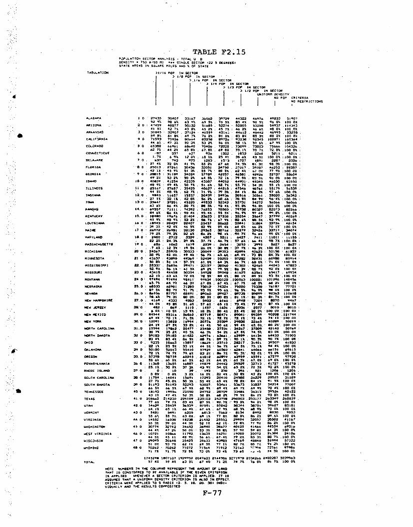
TABULATION

A

AR IZ ONA

AR•A NSAS

CALIFORNIA

CO..ORAO0

CONNECTICUT

DEL .•ARE

FLORIDA

GEORGIA

IDANO

ILLINOIS

IDItANA

IOWA

KANSAS

KENTUCKY

LOUISIANA

MAINE

MAqYLAND

MASSACH4USE TTS

MICHIGAN

MINNESOTA

M•SSISSiPPi

MISSOURI

MONTANA

NIERASKA

NEVADA

NEW HAMPSHIRE

NEW JERSEY

NEW "ExICo

NEW YORK

NORTH CAROLINA

NORTH DAKOTA

OHIO

OKLAHOI•A

OREGON

PENNSYLVANIA

RHODE ISLAND

SO.,TH CAROLINA

SOUTH DA•OTA

TENNESSEE

TEXAS

UTAH

VERMONT

VIRGINIA

WASHINCTON

NEST VIRGINIA

WISC3NSIN

WYOMING

TABLE F2.15POPYLATION SECTOP AN4LVSIS - TOTAL U S.

DENSITY Y 750 e/S0 MI *.. SIN2LE SECTOP 922 5 DEGREES)STATE AREAS IN SQ3,ARE "ILES AND % OF STATE

)1116 POP IN SECTOR1/8 POP IN SECTOR

3/6 POP IN SECTOR> 1 34 POP IN SECT T

> / /2 POP IN SECTO R

:>

1" Po

INSC OPR

NSCO

U IIFFORM DENSITY

POP'° CR I*TERAI'" No RE.TRITIONS

1 0 27435 30407 33167 3i062 39729 44322 46976 49833 51907

529 9 8 96 63 9% 69 53: 76 5% 85 4% 90 5% 96 0* 100 02

2 0 4T459 48877 50132 51685 52274 52805 53259 34937 .114343

41 5% 42 7Z 43 82 45 2% 45 72 46 22 46 68 46 0% 100 02

3 0 31845 32907 37124 "40559 431.' 44612 45442 46995 1 5325959 B% 61 87. 69 72 7622 BIOS 83 8% 82 32 se 22 100 02

04 0 71593 75926 80664 85258 69726 93238 95545 108071 160364

44 6% 47.3% 50 37 53 22 56 0%" 58 1% 59 68 67 9% 100 02

3 0 653R8 66961 86640 70406 72028 73099 73803 75666 104328

62. 64 22 65 "8 67-5.1 69 0% 70.11 70 72 72.5% 10002:

6 0 ". 357 627 936 1322 1853 2288 5211 5211

1. 72 6 9 2 127 .1 0% 25 4 358 % 43 52 100 02 :100.02

7 60 37 743 975 1283 1373 1727 1891 2287 , 2326

27 42 32 02 41 9% 55 22 67 62 74.32 61. 3% 9.32 :100 02

a 0 25013 27261 30436 33031 34730 37017 39797 46252 593579 42. I 45 92 .1.32 35.72 58 53 .2 43 30702 77 9% :100 0I

9 0 28815 & 31189 34084 37789 42257 481 S 48928 52737 58604

49 22 33 22 58 22 64.52 7 X 2 79.5 : 3 53 900 .1 00 02

I0 40839 41254 42335 43087 44052 44901": 45345 46030 93550

:49 92 49 4% S0 7% 51 6 2.7% 53.7%: 54 3. 55 71 100.0%

110 25167 27657 35425 40627 44815 47546 48761 55179 56539

44 5% 48.92 62 72 71.92 79 32 04 1% 98.22 97 6 :100. 0:

12.0 9843 51637 S1537 20439 24936 28516 : 308b1 3502. 3634227.1 % 321 I 42. 8: 56.22 68.68 78.52- 84" 9% 96-42 :00.02:

13 0 35647 37201 45220 49533 32342 53731 5 54272 56066 5 6086

63 68 66 4% 00 7% 88 32 934: 953.8 96 8 100 0% .100 0%

14.0 : 69557 71111 74392 '76853 78580 79738 : 80327 . 82073 82266084. 62 86 42 " 0. 93,4x 95 '% 9.9% :97 86 99.68 .100 02

15.0 . 18480 19676 21404 23623 27338 33254 : 35,47 : 37799"; 40269

45 92. 48 92 53.22 58.7. 6792 826% so5 3 93.92:100.0%

16.0 .18943 :20D429 :22407 25457 28822 30041 31884 337341 4515439.32 42.42' 4865 32.92 59.42 AR 0% 8822; 70 II 100.02

17 0 26972 26981 28130 29364 30716 32279 32926 33717 :134074

79.22 79.22 8282 88.621 90 1 .94: 72 96 6 : 99'0 '0002

19.0 2480 2712 3329 4207 : 5211 .6427 7411 :18011 " 111552.2•2• : 4.3% 29 82 37.72.48.72 57.62 " 44: 9872: 100:0%

19 656 1062 1679 22329 2654 3252 3995 8627 •8627

72.6 12 32 19.53 2602 30. 82 37.72 46832 .1000. "10002

20.0 24067 2,970 30533 35049 39353 42894 45625: 52158 : 61837

38 92 42.02 49 42 Sb. 73L 63.362 69.42 73, ,8 84[39" :I100.802

21 0 43637 43898 49369 52409 5 33215 57292 5.431 . 60988 : 05914

5 082 51,11: 57.22 61.0 0 64.34 2 672 6&802: 71.02 :100 0222. 0 25331" 2•856 29471 33157 38060 41302 42460. 44043 47883

32.9• 2 56.1: 61.52 69.22 7 2.5 86,32 G872 9202 100 O2

•23.0 43415 44458 50354 .54928 59G048 61625 62361 65417 . 6993462 .2It 63 82 72.0% 78. 2*: 84 42 s8 12" 9 53 93 5 .100.02

24 0Q .97494 97494. 98411 99434 100128 100563 109881 101296" 1484516

65.72 65.72 88 3 687.02 87 42 : 687 72 02 68 2% :100 02

25.0 88033 8901 71285 73012 74324 73000 '75339 - 76187 . 77721

87" 3 08s72 91 7: 93 92 95 68 96 53 96 92 98 .0 100 02

26. 0 8896 87757 :8491 l9900 99427 0 89735 99899 : 90363 110618

78, %2 93%. 80 02:, 80 53 80 82 :1.1% : 1 32: 81.72 :100 02

27.0 4169 . 4333 4883 5452 . 8166 6 8948 7324 8870 9487

44,02 45 a 31.62 37.62 65.12 73.42 77 4X 87.42 .00 0%

29.0 482 889 1110 I 1457 . 1831 . 2036 2577 8010 .0010

6, 02 10 8% 13 9% 181 2 2042 4 25.4% W.2% 2 000 100%02

09. 84544 85316 6880 07719 98471 ' 89041 G9359 9020 .0121744

69.42 70, It 7.ý32 72.1. 72,72 73.12 73 42 74:1 2:100.02

30.0 12091 13828 16994 20776 25389 29838 32885 40289 : 50219

24 12 27325, 33811.41 4% 50 62 59 42 6501 80.22' 1000231 0 IS594 17062 20477 23489 27531 - 34267 37809 42142 50769

30 721 35 22 40 32 46 3 5422 :67.52 74.32 83 0 t100 02

32.0 59183 59183 61422 62976 63641 4163909 44134 64433 . 71005

8342 83.4. 86 52. so72.8972 90,1% 90.32 90. 7 2.100.02

33 0 9233 10683 13857 18625 23710 28217 31401 39507 41833

22 111 25 51 33 12 44 52 5•8" 72 67 52 75.1% 94 42 .1002 :

34 0 50180 32013 3S410 57929 80380 62841 64066 88151 69615

72 1% 74 72 79,6.8 83•.• 88 7 90132 92 0% 95.02 10002

35.0 57398 58759 60245 61818 62899 63989 45591 67579 97928

S8 6" 60 02 61 52 N 61 &42 632.8702: 69.02 1002 :

36 0 11368 13655 16687 . 19879 24443 29329 3713 41727 45278

25.%12 30 2. 37 32 43 92 54.02 65 22 72 3% 92 2% 100 02

370 0 10. 39: 193 270 1398 521 120, 12060o0 08 322 16 022 224%.32 43 2.1000.100 0%

39 0 11734 14041 135691 177293 20410 24588 2b229 , 28525 . 31189

.3772 43.02 So 32 . 53 42 65 42 78 82 84 1% 91 " :100 0%

39 0 51193 51193 52293 53027. 53461 53673 S3;37 54214 77007

652 66 83 67 92 68 9• 8942 69 72 69 92 70 42 10 00

40 0 19142 19956 22050 2472 8709 33496 36313 39526 42t22

43 17. 47 42 52 32 58 82 68 22 79 53 86 22 93 87 1t00 0241 0 2086"2 214230 224189 .235103 243798 250003 .253177 263349 268839

77862 772 3 42 07 52: 90.7 :9302 94 22 902.100 02

42 0 5462 53439 56539 . 57591 . 57842 38344 38701 59627 85181

64. 2 5 12 I 8 42 67,.68 . 67. 92 68 52 be 9% 70 02 100 0%

43 0 3481 5491 6205 "813 7662 8154 0492 0830 9853

6 355 7X 63 08 69 91 77 13 828% 86 2% 89.68 100 00

44 0 14552 16038 18238 21452 25553 . 29954 32057 35502 41187

35 32 39 0% 44 32 1 52. 12 62 12- 72.8• 77 92 86 22 100 02

45 0 30774 32742 34653 36940 . 38677 40125 41466 44554 69316

44 47 47 2Z 50 02 13 5332 15 3% 57 92 59 98 64 32 100 0%

46 0 . 10721 10866 11792. 13635 16251 19088 20072 . 21384 24106

44 53 43 12 4897 56 6%2. 47.4. 79 22 03 37. 89 74 .100 02

47 0 29095 30648 35425 39633 43905 47169 48840 51994 5732251 0 1 3 72 62 12 69 5% 77 I 6 82 72 91 22 100 07

48 0 70262 70262 71072 71564 71912 72163 '7-4 72761 97986

71 72 71.72% 72 32 : 73 02 73 x2 73 6% -. TC 74 32 1.0 02

TOTAL

1745298 1007107 1929952 2047623 2164506 2271978 2334266 2482287 303996357 42 59 4% 63 52 67 42 71 22 74.72 76 02 81 72 100 O0

NOTE NUMBERS IN THE COLUMNS REPRESENT TIE AMOUNT OP LAND

THAT IS CONSIDERED TO BE AVAILABLE IF TIE GIVEN CRITERION

IS APPLIED IWENEVER A SECTOR CRITERION IS APPLIED, IT'ISASSUMED THAT A UNIFORM DENSITY CRITERION IS ALSO IN EFFECT.

CRITERIA WERE APPLIED TO 5 RADI1 (2, 5. 10. 20. 30W 101-VIDUALLY AND THE RESULTS COMPOSITED

F-77

TABLE F2.16POPIJIATION SECTOR ANALYSIS - TOTAL U S.DENSITy 5 100 */SGoMI. --- SINGLE SECTOR (22 5 DEGREES)STATE AREAS IN SQUARE MILES AND X OF STATE

TAIULATION >t/16 POP. IN SECTOR1. /o IN STO- SECTORI 16 POP I ESNTO

I POP. IN SECTOR> 1/3 POP I PN SECTOR

1,2PP IN SECTORUNIFORM DEN1SITYI 0 POP CRITýRIAr NO 6ESTS ICT tONS

ALABAMIA 1 0 32492 33186 34624 36301 39043 44430 47140 49933 51907

62 62 63 9. 66.7% 70 IX 76.89 a5 62 90 8 9 96. 0. too 00ARIZONA 2. 0 49466 51007 51930 52204 52544 53017 53500 : 54937 114343

43:3% 44.72* 45.32 45.72 4602 46.42 46.92 . 49020% .100 0lARKANSAS 3.0 33765 34200 37953 40968 * 43242 44689 45519 46995 53259

634 64.22 713 76.72 01,2% 93.92 85 5, a 922 200 02CALIFORNIA 4.0 79535 . 92206 01937 89079 922 15 9303 97951 :108871 260364

49 62 51.32 53.52 55.52: 57.52:. 9.42 61 0: 67.9% : 100 07COLORADO 5.0 68226 60833 70648 71671 : 72539 73475 74190 75666 :104326

6.0 542 660267.7.:67%:69 5%:70.4%:71 12: 72.52 :00.02:CONNECTICUT 6.0 36 .695 a1 994 : 1399 5027 2538 5 5211 5211

7.42 13.32: 15.62: 19.12 26.92: 39 92 46 71 00 OX 10002o

DELAIAE 7.a0 312 959 052 1 303 1573 1756 1920 2287 23263492. w 36,91 45. 22: 5601 67. 6 755 2 82. 62 99 3% • 300.02

FLORIDA S. 0 29394 31546 32733 33794 35155 37413 40250 46252 . 59317.49 52.3.1%:51 5:1 6 92 59 .22:63.0%:67.92: 77,9%:200357

GEORGIA 9.0 32279 : 33071 35174 30069 42442 46733 49319 52737 5604:55.31[ 56. 4 60 02 65 02 72. 4 79 72 83 92 90 0. o0002:

IDAHO 10.0 41304 41313 42643 43232 44081 44922 45355 46030 9355050 02 50 0SX 31.02 51 72 $2.98 $3. e x 4 32 5 12 :10002

ILLINOIS 11.0. 29712 30426 37693 42142 45644 48231 49533 55379 : 565395 26• 2 53, 66.7". 74.5 090.7% 95.3%9 7.62 97,62 :100.02

INDIANA 12. 0 13298 14632 17997 21259 25244 28796 31308 35020 . 363421 : 36.62 40. t 49.52 :% 3.52 69.5$ 79.29 09.92 96,42 :100.02

ISMA 1 3: 366 39140 46629 :04 507 2 477 5337 :4407 56067 : 56067:69,0 69.9 S 93 22 69. = 93. 6 96.0% 97 0% 100.02 :100.02

PANS 14.0 72500 7302 75791 77306 79754 79854 010442 : 92073 92266

962 6.7 "2. 9 .94 0 95.72 97.2: 97.9z :99e 100 0KENTUCKY 13 0 50429 21076 225436 24067 27464 3323•93 35734 : 37799 . 40269

50.7x 52.32 SS. 39.92Z 60.22: 82.72: 69.72: 939 :1300-0LOUISIANA 16.0 : 21923 220331 23430 35727 2699 20909 31970 : 33736 : 48154

:45 7 45.9ft 48972 53.42 59.62 64.22: 6642: 70, 1 :100.0-MAINE 27.0 : 27194 27194 20226 29375 30726 32279 2293: W3 33717 34074

79.2 : 7.82 92. 92 622 90.22 94.72 96ý 72 99.02 100.07.PMARYLAND 1.0 : 779 3156 3706 4931 6002 7045 9260 11021 . 11135

2:4.91 2:5 32 33.22 44.22 53,9% 46.31 74.02 986722100.02

MASSACH4USETTS 19. 0 : 1390 1•33 2094 2480 2943 3590 4564 3627 96276I.OX 2 31.52 24.3 20 .7: 34.22 42.6% 52.92 :100 02 100.02

MICHIGA 20. 0 2763N 26419.: 302 35763 39955 43396: 46417 : 52158 6133744.72: 7 46.02 :2.11 32 .65 4.52 70.22 : 75.1 : 84,32 2100 02

MINNESOTA 21. 0 446212 45094 5050 53114 $9536 57543 : 39797 : 609•9 9592452.92 : 52.52 30.6, 61. 9 64.62 67.02 : 68 42 : 71L02 D00 02

MISSISSIPPI 2.0.: 2772r: 59110 30204 33341 : 38127 41341 42129 44043 478835 : 5.0 : 72-63. 12 69.6 79.61 86.32 960.8 92.02 :100.0%

M18501A1 22.0 . 45345 : 46008 . 52130 55709 : 59415 61947 . 62860 . 65417 69934: 64.8" :'65.9% 7412%' "9.72•:0.50 08.42 99-9: 935% 100.02

MONTANA 24.0- : 97929= 97926 99768 "9646 :100206 :100572: 100891 : 101296 34845666.0: 66.02 : 66.5• 67 67.5% :67.7: 68 OX 668 2 9000 2%

EBRAS K. 0 : 69605 70295 7228 73475 74498 75048 75386 :7627 7775399.62 90.32 93.02 94.52 9592 96.62 97.O2, 99.02 200.02

NEVADA 26.0 0 365 09732 9190 99417. 89629 09822 09986 90363 .1106187 ].92 0 22 90.62 90. 92 .0 02 .21 22 .3% 3 1.72 :.00 02

PEW HAMPSHIRE 2 7. 0 :4420 :4429 4989 5520 6195 6977 7392 6270 946746.72: 46.92t 92.72 6.32 65421 73.72 7602 3742 300.02

NEW JERSEY 20.0 : 042 1 322 1 563 1%299 :2240 2906 3821 9009 . 00911.02: 16.5 2 19.2:64.6 22.312 2.522 47,72 :t10o00 :2 0.0OX

NEW MEXICO 29. 0 6163 : 6669 7564 0907, 36597 09093 89427 90206 12174470.6 IM 71.41 73.9% 72.3 722 73 2% 72.5 74.32 :300402

New8 YOR 30.0 34661 3630O 109666: 217133 26036 30330 33293 40299. 502192V62 32.52 37.62: 43.2 2: 52.9 60.42 66.32 90,22 :100 02

WORTH CAROLINA 1. 0 29232 19353 21134 23707 27"44 34412 37925 . 42343 5076937"2 39.3 41.62 . .9 3-562 678 74.7 93.02 1000 2o

NORTH DAKOTA 32. 0 59903 5960 61856 : 63075 63729 6399 64144 64433 7100542! 64i4. 3 ' 7.2 6980 999 2. 90.1%290.32 90.72 :100 02

0HI0 3. 0 11912 13938 169G4 20111 24492 2•982 32385 39507 : 418338.22 533.2% 40.62 48.32 5.%95 69.02 77.42 94.42 ;100.0% -

OKLAHOMA 34.0 : 53200 54320 56414 56267 60641 63024 64269 66131 : 6962576.42: 78.0% 81,02: 93.72 97.1 90 52 92.32 95.02 :100.02

OREGON 35. 0 : 59649 6044 615 : 63223 63063 64105 65726 67579 : 97929631 I 61.72 62. : 63.52 64.41 65 5% 67 32 69 02 :300 02

PESNNSYLVANIA 36.-0 215102 15363 17705 20516 24994 30308 33640 41727 4527033.42 33. 92 39.32 453.3 55 27 :66%52 74 32 92.22 10002

RHODE ISLAND 37.0 10 164 2531 200 323 ' 444 609 1206 12G00.X 13.6%2 5092 23 22 37 221 36.92t 50 42 &00:0 :0300 02

SOUTH CAROLINA 30.0 15093 2 5122 16254 17429 20506 24661 26306 20525 31189: 46.4% 435112 51. 5 5$.92 657:1 79".1 64.32. 91252 00 010

SOUTH DAKOTA . 0 : 12599 51359 525315 53094 53471 :53683 53947 . 54214 77007:47.01 67012 60.2. 68 9 69 4X 69 7 64 91 70 4Z 31000 2

ESSE 40. 0 20931 21500 22922 25032 220844 33563 36429 . 39526 : 4212249 7 .2 021 54. 22 59 42 60 52 79. 72 06. 52 93 912 :100 02

TEXA2 41 0 ;229402 :223282 232082 .239262 :245621 .252509 : 254663 263348 26883921. 62 03. 12 06.32 99 02 91 421 92.42 94 72 . 99 02 100 02

tUTAN 4o 0 %5016 56935 57409 .7755 57949 98450 50926 59627 8191865•5. 66" 67 42. 67 89 68 0- 60 6% 69 13 70 0% 100 t0

VERMIONT 43 0 5607 5616 2673 6842 7672 0154 0. 492 9930 . 995336 92 7.02 632.72 69:42 77.92 92 6% 06 2% 89 6% 100 02

VIRGINIA 44.0 16704 17272 19406 21848 25933 30204 32366 35502 4116740 6% 43.4% 47.1% 53 1. 62 9% 73 42 7 662 9622% 1002 .

WASHINGTON 45.0 33920 35145 36342 37540 "9034 40414 41062 44554 6931649.92: 50.,72 52.4% 54.22 56.3: 56.32 60 4% 64. 32 100.02

WEST VIRGINIA 46.0 11126 111236 1947 13655 16270 19097 20082 21394 2410646 21 46.22 49.62 566%•, 67 2 S: 79" 2% 3.,32 8 72 200.0

iWISCONSIN 47.0 31932 32299 36545 40337 44400 47439 49186 51994 5702256 024 56 62 64. 312 70 77, 77 92 03 22 96 32 93 22 -2I00 0

IWYOMING 490 0 70612 70812 71313 71642 71970 72163 72394 . 72761 97996:72.32 72.3: 72.90 73:12 73 42 73.612 73 9. 74 3% 100.02.

1935531 2996350 1997603 2075429 2179979 2204405 2350362 2492296 3039963

TOTAL 621.0 62. 21 65. 4Z 60 32 71 7% 75 12 77 32 81 7% 100 O2

NOTE: NUiU5ERS IN THE COLUMINS REPRESENT TIE AIIOUPNT OF LANDTHAT 19 CONSIDERED TO iE AVAILABLE IF T4E GIVMN CRITERIONIS APPLIED a EINEVER A SECTOR CRITERION IS APPLIED. 1 IASAIPED THAT A UNIFORM DENSITY CRITERION IS ALSO IN EFFECT.CmRITERIA WERE APPLIED TO 9 RADII 42. 5. 10, 20. 302 I2OI-VIDUALLY ANDO THE RESJLTS COM6POSITED.

F-78

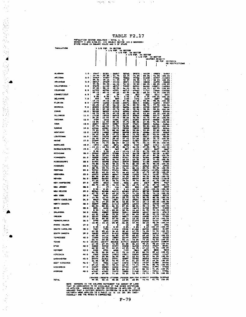
TABLE F2.17POPULATION BECTOR ANALYSIS - TOTAL U. S.DENSITY - 250 6/9G. Ml. -. DOUBLE SECTOR (41. 0 DECREES)

.STATE AREAS IN SQUARE MILES AND Z OF STATE

TABULATION ) 1/9 POP. IN SECTOR1 3/8 POP .IN ECTOR

> 1 13 POP, IN SECTOR> 1,3 POP. IN SECTOR

u.I/ POP. IN SECTORUNFORM DENSITY

NO POP. CRITERIAI I r N RESTRICTI:ONS

ALABAMA 1.0 o %47 23101 2:617 32782 39571 44129 49833 : 51907.37. %.40*87 51.A7Z 63.1% -76.22 9..OZ 98.02 :300. 0O

ARIZONA 2.0 :4499 45207 47256 48266 :4978 316048 14937 :11434339. 22 39.62 43x•3 42•31 4m 1 4'.' 12 44 Oz 100.0.

ARKANSAS 3.0 28767 29129 39145 28171 41938 43830 46991 15221314. 0[ :1.42 88.0Z 72.1 4 73.62 02. 33 886 2 100.0.o

CALIFORNIA 4.0 19891 81342 88? :- 74419 : 60944 86068 I06971 16036437.22 36.1% 42.92 46.42 :90.12 53 72. 11'. 79 100:0z

COLORADO 3.0 &1702 62706 8 65331 8710 893 6 71719 78568 1043659.12 8 I 0.:12 :2.82 83.92 ".6:8 68.72 72.12 3100'0%

CONNECTIChT 6.0 : 10 10 39 10 2 103 .222 :1211; $21101.212 0.22 0.72 ý2.02%6 3.92 4.32 :300' .0 100.02

DELAWJARE 7.0 , 444 444 820 1100 1478 1479 2287 232619.1l: 19.12 35322 47.322 83. 12 72.22 962 : 100.021

FLORIDA U. 0 :.1279 :. 18202 23423 :2,15478 30214 34186 46252 1.993172322 n 27.32 36 81 42.9 150. 51672 77:.9 100:02

GEORGIA 9. 0 20135 21924 312 : 362M22 42190 49722 M2737 ;56804030 37.42 49, T 8 61.82 72.012 70. :900. 300 OZ

IDAHO 10.0 381i9 36339 41212 42286 42985 44824 48030 8315045.17 41. 92 : 49.41 :20.62: 52.82 1382 :5. 113.: 100.0Z

ILLINOIS 1.0 17139 16933 262943- 33119 : 39• 43386 9179 : 1681930.22 : 33.12 47.7 • 5682 70.1X 76.72 :'97.68 :100.02

INDIANA 12.0 .'4709 :...6012 11001 :.16241 21201 : 24472 :23020 : 3634213.02 : 16.512 302 : 44.72 56. : 87.2 : 96.42 :100.02

ilam 13.0 32347 :3:3707 40317 !.44137 49801 : =59 : 1808 : .56088177 87 ::60.32% 7192 716. 612 9.: 2 92•2Z :300.02 :100.02

KNSAS 14.0 - 85138 &5561 70175 72318 73959 78350 82073 :322"79" ' 29 7 015.1 M:22 92 221 9.22 9962 3 100.02

KENTUCKY 1S. 0 :%..14272 148M2 3~982 22,V4 2031 3348• 37799 4028953142 2862. 47. 1Z :.6.4% :74 .9: 6322 93.29% :100. 02

LOUISIANA 18.0 12931 14379 16972M 213842, "719 30011 23386 : 4815421891 29.9% :9,42 47-.4 :-37:23 68222 70.132 100.01

MAINE 17.0 21399 25488 17927 29683 .3114 .32414 2:3717 3407474.12 74172 :.130.2: 87.12: 92.7: 9•.% :.99.02:100.'02

MARYLAND L .0: 1373 31621 "76 364 .:4729 59: 31011 : 11115114. 2 14.1 2. •M 32.%7% : 42.41 47.2 .972 100. 02

MASSACI4USETTS 19.0 : 174 281 169 : G97 : .!1370 1153 68627 96271.02 3.02 66 30.42 :1.9 : .21.332 :100.01 :10.010

MICHIGAN 20.0 :-22182 22699 37066 123449 :236176 .39735 1215 : ,41W76832% 27.021 43 112 50.92 9 916 6 .8 2 9422% :100.02

MINNE9OTA 1.0 a-423 43257 463i0 9193 94426 982" 60104 : 93934:49.32 30.2 51. 6 8 .60.02 63 2 :68.612 71.02. :100.01

MissIssIPPi =.a0 2193 22396 27060 3M929 30515 41132 44043 : 47866:.43:82 46. .622 .9 709•29012 :3.9 92.02. :100.02

MISSOURI I0 41061 41781 49109 ;53422 :17191 60062 46417 : 89934511-711 19. 72 70.2 76.42 62342 0.92 92-12 :100•0•

MONTANA 24.0 94744 91154 97494 98941 9969 :100476 :101296 146416263;2 .64. 42 85.71 8 87-3 67. 71 68.2 100. 02

NEBRASKA 21.0 :5475 65690 8"?48 70900 72423 74015 74167 77721104-2 3492S 6632191 :91.22 9.222 9222n 96020 10002O

NEVADA 3.0 91691 :986020 67024 : ,67429 66404 69195 90363 :1106167782 77.82 70.72 :.790.2 7992 810.82 61.72 :100.01

NEW HAH41M E 27. 0 2194 : o10 : 4400 _ 5263 1 8053 8289 : 6 9487272: * 7 31 48Z 412 3&.r4% 63.72 67.1382 87342 :100. 02

NEW JtEY 2.L : • 0 , 19 116 t,403 040 1061 9009 : 0009002 0: : 1.4211.1t 10.-31 1.5% :32100.021 0 :002:

NEI wEiICO 190 :.62363 6242 370: 9123 0 67091 66732 90206 :1217447.72 87.82: 9.22 : 9 70.12 .71.61 72.91 74.1% :100.02

M101 :P).30 0 7469 ma 1 12477 : 169U86 21925 23562 40269 : 50219149 2% 18.42 .2482I .33-72 43.7 2 0. MD. 209 :92 100.0:

NORTH CAROLINA 31.0 3463 9788 14671 21732 29201 31032 :42142 : 10769&167X 19.n 29.32 42. 92 57.31 65.12 83. OZ 3100.02:

NORTH DAOTA 32. 0 16109 2696 61413 62=79 63024 63960 64433 : 7300562021 932ý0. M.22 67.981 68.2 .90.32 90 72 :100.02

OHIO =.0 3331 4632 9137 1418, 19873 21732 3907 : 4AID012. 111% 22021 3 4482.9 5119 94.42 ;100.0%

0KLAHOM5 A 34. 0 44081 42609 10334 S4013 26496 2107 8811 : 6961:6322 8% 182 7222.31 77.82 9402 69221 9.02 :100.02

OREGON 3. 0 12149 153018 38631 0617 61048 83420 87379 : 99253.22 54.22 37.42 60.112 62.32 64.62 69.2 0 :300.02

PE14NSYLVANIA 3.0 57090 6042 311698 .16403 21692 24280 41727 45127312,10 11.12 : 31 6 36 82 47.92 13 82 922 2 1002 OX

RHODE ISLeND 37. 0 0 0 0 50 se 656 1206 :3 20600.2 0.02 0.02 0.82: 4.82 9 3400 3o00 T02

SOUTH CAROLINA 39.0 7137 7990 ,11416 1510 21142 23700 28525 3118924.22 23.82 3868. 43.82 : 67.92 76.0 91.5% 100. 02

SOUTH DAKOTA 39. 0 4861 49379 51415 52322 : 1295 5396 4214 7700783.2 n 34.211 8862& 87.92 6a. 898 4 2.6 70.42 100.0

TENNESSEE 40. : 4050 14726 1969185 2399 29177 23350 39126 4211233.42 32.012 48 54.211: 70.22. 79.22 953 OZ 100 002

TEXAS 41.0 191254 106477 :20660 :219914 :232690 :242404 :28349 268839

&.74%:89.42 7.82 3382M 9882" 90.22 96.02 10002OUTA04 42. 0 13220 93422 14494 2108 16423 17143 19627 95101

2.3 2 62.-71 2 .0 "0 882 "6.3 67862 70,02 3100.02E."MONT 43. 0 .4420 : 4931 .6802 7199 7868 9370 9930 9653

44. 9X 50.01 61.3 273.12: 9. 9812 63.92 69 " :10002VIRGINIA 44.0 9152 10634 14813 1t6il 25534 28902 31102 41167

23.52 : 25.62 36802 4312 :62.02 70.22 86.22 100.02WAS*HINGTON 41. 0 24974 .26566 29741 32697 35793 332253 44114 86931

38.02: 39.32 42.92. 4712: 5118. 1 12 84 32.:00 02WE:ST VIRGINIA 46.0 7141 7636 11667 14572 17672 19107 213•4 24106

298. 2.12 48.42 60.42 74.-2 793 32 M. 72 100.02WISCONSIN 47 O 24849 23633 32350 37912 42•91 456•8 13994 17032

43.82 45.22 3 56. " 88.61 : 75.42 9042 91, 2 360 0WYOMING 48 0 67837 67437 70175 70610 71468 72211 72761 97968

8 69.02..: 69.0Z 71.4 " 72.32 72. 92 73.72 74.32 100.02

1544C002 IS877 377299 193023 2091704 2199677 2482288 30399"2TOTAL so10 32.12 12 = 22 = 22 8862 72:42 01.72 3000 2

NOTE- NUIBERS IN THE COLUMNS REPRESENT THE AMOUNT OF LAMTHAT IS CONSIDERED TO BE AVAILAILE IF THE GIVEN CRITERIONIS APPLIED. WHIEEVER A SECTOR CRITERION IS APPLIED. IT i2ASSUMED TWAT A UNIFORM DENSITY CaITERIIO 1S ALSO IN EFFECT.CRITERIA WERE APPLIED TO 5 RADII 2. 1. ,O,r 10. 30) INDI-VIDlALLY AM THE RESULTS COMPOSITEO.

F-79

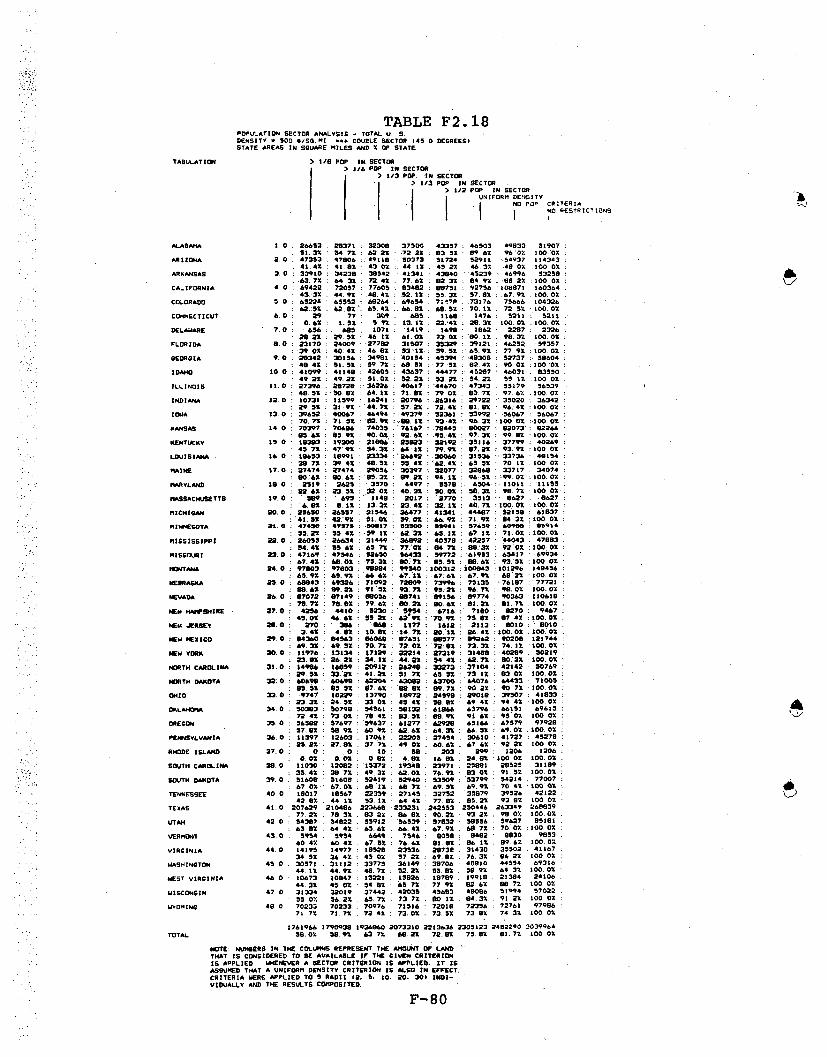
TABLE F2.18POPULATION SECTOR, ANALYSIS - TOTAL U S.

DENSITY - 500 */,S. MI -. DOUBLE SECTOR (45 0 DEGREES)

STATE AREAS IN SQUARE MILES AND % OF STATE

TABULATION > 2/8 POP IN SECTOR

3 1/6 POP. IN SECTORS .3 POP. -IN SECTOR

I 1/ O N SECTORI 1/2 POP IN SECTOR

I UNIFORM DEUISITYNO POP CP.TERIA

I NO RESTRIC!IDNSPOP It

ALABAMA 1. 0 26653 29371 2 32308 37500 43357 46503 49S33 51907

t51.32[ ;4 7 62 2[ .72 2% 83 5Z 696Z 960%. 100.0%

ARIZOIOA 2.0 - 47353 47906 ,49119 50373 51724 529.1 3.54937 114343

41.42 41,8% - 43 02 44 12 45 46.3. 48 07. .100 02

ARKANSAS 3.0 33910 34238 3•542 41341 43840 45239 . 46996 53258

63 72' 64 31 72 4% 77.62 02 32 94 9X 60 22 :100 02

CALIFORNIA 4 0 .69422 . 72057 77605 93482 88751 : 92756 .108971 160364

43.32. 44 92[ .4.4% .52: 12 15 32. 57.92 .67. 92 .100 0%

C0LORADO 50 6524 65552 68264 69654 72'7 73176 75666 104326

62.:S. 6292: 6584.66.9` 68.5%: 70.12: 72 5% "100.02:

CONNECTICUT 6.0 :29 777 3309 695 1168: 2476 5221 : 5211

0.62 1.52 ft 32 13. 122;.4% 29.3% :100 02 :100 0%

DLA•kARE 7.0 636 685 . 1071 1419 . 1698 1962 2207 :"20326

2.22 :9529 46 T 61.02 73.0: 0.12 98.32 100.02;

FLORIDA 8.0 23170 24009 27792 31507 25329 39121 46252 59357

39.02 4042 46 02 532 I 59•52 65.92 77,92[ 02[

OSOROA 9 0 28342 30156 34981 40154 45394 .48300 ; 52737 : 58604

494 51. 52 1 972: 68521 77 512 8.42 90.02 :100 0%

IDAHO 10.0 4109$ 41149 . 426015 43637 : 44477 : 45287 46031 8 93550

49 22 491 2: 51.02 0 52.2% 53.2• 54.2% 55 12 .100 02

ILLINOIS 11. 0 27396 58728 26226 40617 :44670 47343 . 35179 56539

4835 50.892 64.1I 71. 79.0. 83.72. 97.62.100 02;

INDIANA 12-0 1 20731 11599 16241 ,20796 2 26316 9722 ; 35020 :36342

59 32 31 92 44.72 57.2% ; 72.42. 91.92 ; 9642% :100.0%

ZIOA 12.0 39652 40067 46494 49279 32361 53992 56067 : 56067

70.71 71ý 52• 8.29 88. 912 9342. w 96.3 :100 00 :.100.02

KANSAS 14. 0 70397 70"68 74035 76167 279445 O W27 6 92073 62266

95.62 05.95 90.02 92 %2 95.42 :97.3 :99.90:100.02;

KENTUCKY 1S 0 10383 19300 2186 .25923 32192 :35116 37799 40269

45 72 47: 92 4 32 . 64;12 799 ;/ 87.22 ;. 93.9% :100 02

LOUISIANA • 16 0 18653 18991 23334 :'6692 ",30060 31536 33736 ! 48154

38,7129 94z 4.5%2:5542.62.42; 6,552:701%2.10002PAINE 17.0 27474 ;57474 29056 30397 25077 32868 33717 34074

90:62 00. 6% 95.32 992.2X 94.1? 96:2 5 •99. 9902100.02;

MARYLAND 1S 0 2519 . 2625 3570 : 4497 9579 6504,: 11011 11155

22,62 5 3.52 3202: 40 .3 so02.8 32 9872% 100 02

MASSACHUSETTS 19.0 5: 9 695 1148 2017 2770 3 811 9627 6-27

682 9.12 13.32 23.42 32.12 &40.7.. 10 100.002

MiICHIOAN 20.0 25650 26557 31546 36477 41341 44497 52159 61837

.41.3% 429• 1 .102 59.0 66O.X 71.92 84.32 :1000 2

MIHNESO•TA 21.0 4740 47878 90.17 95500 59;"91 117699 6898 83914

55.2 2 . 5.42 99 1% 62.22 63.21 67. 12 71.0? :100.02

MISSISSIPPI . 2. 0 26055 26634 31449 36892 40579 42257 44043 47883

54. 42 55 61. 63,7 77:021 84.972 89932 92.02 :100 02

MISSOURI 23.0 47169 47546 :5260 56432 59772 61953 65417 ý 69934

67.42 6902 75.32 60. 71 9.52 8a. 62 932 52 100.02

MONTANA 24. 0 97803 97803 96884 99540 :100312 : 100843 101296 149456

65.9% 69. 9% 6 6% "7 1" 6:62 67.92 6822 10002;

NESRASKA 25. 0 680943 69326 71092 72809 73996 75135 76187 :77721

: $86" 89. .1 I. $152 93" 71 9522. 96.7 99.0% 100.00%

NEVADA 26. 0 97072 67149 680056 9741 09156 09774 90363 110618

78.72 .79.82 79.62 8022 90,.62 812 81.72% 10002.0

NEW HAMPSHIRE• 27.0 ; 4256 44,80 5220 5'754 6716 : 71o80 8270 946745.0 46.6 9 522 629 70.92 73.5 82 7 94 100. 02

NEW JERSEN 29.0 : 270 396 868 : 1277 '1612 2 2113 8010 8010

3.42 4.89 0O.92X 1 4.712 20.1I 36.42I 100,02% :100.02;

NEN MEXICO 29 0 94360 04563 96068 97651 99577 99262 90209 121704

&69.3 69.32 70.7 2. 72.02 75918 73 3. 74.1% .100.0%

NEN YORK 30 0 . 11976 13134 17129 22214 27319 31480 40289 . 50219

.232•0% 62.2 34.12 44.2 .544%2 62.72 80.22 100.02

NORTH CAROLINA 31-0 1496 1•6899 .20912 ;26240 3r'5273 37104 42142 50769

29:.5 33.2' 4V22 31 7X 65.5I :,73. 9 8302 0 100,02

NORTH DAKOTA 32: 0 6069 60699 2204 3082 3700 64076 64433 "7105

9552% 85 52 97.62 8 9%82-9.71.90ý22 90.72 100.02;

0410 3.30 9:747 10229 13790 18972 24598 29019 39507 41933

A. 3 24.32 33 02 45 425 99 2 69 42 94 42 100.02

0KLAH40MA 34 0 50393 50798 54561 50132 61866 63796 66151 6961572 42 702 78 4? $3.5 89: 9162 95 0% 100 0;

OREGON 35 0 56589 57697 "9637 61277 62929 65166 67579 9792857.2 58 92 6092 6262 64. 32 66.5%2 69.02% .20. 02

PENNSYLVANIA 26 0 21397 12603 17062 22205 2 7454 : 30610 4172?• 45278

2522• 27.82 37.72 49 02 60.62 67 6% 9222 100 02

RHODE ISLAND 37.0 0 0. 210 S8 203 299 1206 1206;

0.02 0.02 09.2 4.1 1692. 24.8% 2-1000 t 100.02.

SOUTH CARO1.INA 38.0 11030 12082 15372 19349 23971 ; 25091 29125 31189

35.42;' 3872. 49 32 62002 76,9% 03 02 91.5% 10002%

SOUTH DAKOTA 39.0 .51609 31609 52419 52940 53509 : 53799 ;14214 77007

67.02 67.02 68 1% 68 721 69.52 : 69.92 ; 70"2 10'002

TENNESSEE 40 0 18017 18567 22335 27145 32752 35879 39526 42122

42 n2 , 44 1% 53. 12 64 42 77 91 . 15, 22 93 82 100 02

TEXAS 41.0 207629 210486 223669 233231 2423553 250446 263349 268939

.77.22 78 32% 83 2Z 86 82 90.2 293 22. 99.0 100.0.

UTAH 42 0 5439 a 5:422 .55912 56539 l7933 59556 .59627 851018;

6382. 64 4 65.62: 66.42. 67.92 68.72 7002 :100 02.;

VERN•O4T 43.0 5 954 35954 6649 a 7546 ;98 8492 9930 9913

60 42 60 4% 67.52. 76 62 82.92 A12. 6It 200 02ý

VIRGINIA 44.0 14195 14977 18528 23 536 287398 31430 35502 . 41167

34 52 . 36 42% 45 02 37 22 69.-12 76.31 8622 100 02

WJASHINGTON 45 0 305721 31112 33775 36249 39706 840920 44514 69316

44.12 44.9% 48.7% 2; 52%. 55.92 9892 6432 100.02

WEST VIRGINIA 46 0 10673 10847 132221 15926 18799 19916 21384 24106

44.32 45 0 2; 4 1% 65 72. 7792• 92 9X 9e 72 100 0%

WISCONSIN 47 0 31334 32019 37442 42035 45683 49086 5199 57022

55 02 56.2%. 61. .7 73 7% .0 1. 84.3. 91 2 10002

WYVOMIN 46 0 70233 70233 70976 71516 72018 , 72356 72762 97996

7, 72 71 72. 72 42 73.0%. 73 5% ; 73 89 74 32 100 02

1761966 1790938 1936860 2073320 2213636 2305123 2492290 3039964

TOTAL 58.02 58.92 63 72 68.2X 72.81 75.92 91. 72% 100 02

NOTE: NUMBERS IN THE COLUMNS REPRESENT THE AMOUNAT CE LAND -

THAT IS CONSIDERED TO BE AVAILABLE IF THE GIVEN CRITERION

IS APPLIED WAENEVER A SECTOR CRITERION IS APPLIED. IT IS

ASSUMED THAT A UNIFORM DENSITY CRITERION IS ALSO IN EFFECT.

CRITERIA HERE APPLIED TO I RADII (2. 5. 10. 20. 30) 2INI-

VIDUALLY AND THE RESULTS CONROSITED.

F-80

A. I . 1.

TABLE F2.19POPULATION SECTOR ANALYSIS - TOTAL U. 8.DENSITY - 750 0/30. "1|. --. DOUBLE SECTOR 445. 0 DEGREES)*STATE AREAS IN SQUARE "ILES AND Z OF' STAlE'

TAIALATION > 1/0 POP. IN SECTOR1/ 3 POP. IN SECTOR

a 3 OP. IN SECTOR71/3 POP. IN SECTOR

, 2 POP. IN SECTORWIIORM DENSITY

NO POP, CRIT"R">UN I NO RESTRICTI"ON

DLAISIA 1.0 29934 30764 : 34769 3:9W2 44091 46976 .49033 . 51907977' 5•93 :"67.01' 7503C 04-•9: 90.3- 96022 "100.0%

ARIZONA 2.0 441306 40906 50412 11309 52602 53250 54937 11434342521 42.92 .44. 11t: 44. 919 46.01: 46.61. 490% :100.0%1

AKANSAS 3. 0 251 560223 596452 42362 64432 = 45442,.: :46995 : 532566.71 67.61{: 74.51% 79.851.:' 93 '21 95,32 :9 922. 1 :100.01

CALIFORNIA 4. 0 75270 76467 9,199 86725 V9199 95545 . 109871 . 16036444.9% 47.7L r 95132 4. 5412 7ý31 9.62 67. 92- 1.00.02

COLORADO 5.0 67174,: 67685 69304 . 70744, 72507 73903 75666 10432664.414 :*64.9 1 6621 67.92X 69 61. 70.71A 72-52X 100.0:

CONNECTICUT 6.0 114 .261 637 11".9 1924' 2269ý 5213 :52113.01 1.02 122.1. 21.92:: 35.02 43.512 .GO0.0% :100.01

?.MAWW 7.0 762 940 '1216 1509 : 1710 19193 227 : 232632.91 3611 52-31 641. 72.92 :,61.32 90.31 :.100. OO .

FLOW IDA 0.0 26422: :27174. 50939.346 263 399 65 954411 492 5.11 6.4 61.7 ;.67.0% 77ý912 :100.01

41=0IA 9.0 22009 32526 5612 450 46195 :.48926 527'37 1 060454.6% 15.2%' 62. 92 70.6 'a. Z :,51 83. .90.0o :100.002

iOANO 20.0 41920 42G045,: 42075: 43792 ;44&679.; 45345.: 46030 135500.022": 30.3%.: .1.3%.;5..4%.: 3.051 :.1234. 3 %: 55. 11 i100.02

ILLINOiS I1.0 32134 33042 39716 4256• 46407 49761 55179 :1653956.92 19 .42 .56 5 75.3'75 2X 96. 2i 97.62 300.02

INDIANA 12.0 13066 13607-: ,974 23160 i44 20961:35020. 3634226.01 37.4% 50,61 63.71 74.21 84.9 : 9641. :100.0%

Ita 13.0 423547 43600 402 :.10100: 31075.: 472:60675.:606773.91:7•.• 9 519 jý O9101.- 94.7 :96.1000 .*00011

5*N466 14.0 7•009 .72V97 7215 : 7743:: 79173 90327 .2073 8226687.951': 9972 91.2 O : 9C12,96.21 976..b. 999 1% :100.01

NITUCI Y 12.0 1=013 : 505:06 22090W 6644 399 5647 37799, 4026910.4%.: 50. 91 1692 .. % l 663 i.5 9981 3 93.9M1:W. 0102

LOUISIANA 16.0 20164 21275. 24472 21043 30455 31384 . 33736 :,4815442.71. 44.41 9 . .21 639: 6621 2 3 70.11 :100.02{

MAINE 27. 0 27983 27995 292 ý30610 3213' :4 3"3 : 2 33717 2:4607462.1% 02 9601 O 99 2S8 94"396X619.i 9 0. 10010

HARTLAND 190 BD 29913. W9 4716,. 595: 7411 1101: 11155a5.91..: 46Soz 34.9 499 5321 66.41K 9-9:7100.01,:

"AMMACH4MrTTS 39.0 0 : 9 I9 20o3 29.2 844 5 326 995 9627, 96271. 0,.01: 12.01 12 61:, 39.3: 6. 71 46.3: 102.00': 100.01

MICHIGAN 10. 0 8790.) 297 3399 33212, 4254 45625 52250,: 6103745.02 46"8.1 5.401 621 9 65.2 W .73.9 2 . 21 : 100.02

mmaOTA 31.0 4414 493 96. M1 04204 .. 9664"9: 99432. 60q999: 91456.41 •6'51: 60 11 621 65.91 : 6902. 71.01 :3002OX

NI99IlppI 2. 0 127 3949 ii 25169: :727577-:. 40997 :-42460 44042 47093

5.691 39. 9 " 61.02 7.11. 29:.419;:97.1 9:32.301 100. OI:MISSOURI 23.0 449M 49254.: 2519 5 7553: 60905 2562 :65417 :.&9934

700 1 70.41,: 76.11.: 9.31 : 66.1 9 519 : 35.:100.016NOT6N 24.0 9917" 99179 : 99096 99:89:: 100447 30093 :01296 :148426

66.12 : 66.11: 66. 92.: .67. 2 6 7.71 69 02 6•92• 1 t100 01

NEBA10A 250:70040 ' 0165 :. 723395. 73427: 74472 75539 76297 :777239.21 : 90.31 •: 93.A1.A .5 96.11 96.91 99: 01 :200.02.

NEVADA : 7719: 3732 : 66495`:9 -90124 : 2 9562 99999 90363 :110618

9. 31 791• : 40.11 0.5z *1.1 91.33 81.71 2:100.01Now HAPS4PIRS 27. 0 4662 : 4787 : . 579 606 & 6 7224 9270 : 9467

49•22:: 50.03 1692 641. 2 72.7K :,77.4 94. : :3.010 0%Bo,5b539 =0.a 59.. 791 1197. 1505: 1969 2577 6009 909

731 9.1 .492[ 18.99 214. 61" 3•.2 100.02 :100.001ý:No MEXICO 29.0 .01314 51711 017285 99305 58994 393T 90208 :121744

70.12, 70.41 ?71. %, .72.4 732 1 7:.4: 74.1% :200.02S50 .0 34673 18:1160 I9339 33912' 29153, 26S" 40299 50219

99.23; 203.21 : 1 n 477.97 ft 1. : 650. 2 0. 2:: 1000 12NORT CAR.OINA 31.0 11403 33750 22903 27097 33917.: 37• 9 42142 50769

a61 6.92: 44.91 5.41 66.911 74. n 3.01 100.02NOR9TH 06 20 65153 62133 42706 63439 63777 64134 64433 71005

9611i 91632 9931 99.31 99.8 90.31 90.7 1 30002Oto 25.0 21139 22976" 2632 23100. 271394 31401 39507 41033

27.21 391.4% 19.52 51.412 64501 75•1 94.41 :100.02

OKLAHOMA 4. 0 52274 52999 16967 395 22J97 64066 66151 696157".1, 76.1 4 1.71 : 5,6 &: 09.6": 92..0 :98.02:300, 01:

OREGON :35.0 , 9913 9048 60905 62099 63796 :'65591 : 67879 .960.2% 60.31 : 42.1 : 63.4"1 :65.11 : 67.01 69.02 :100.01

PENLVANIA 36. 0 14279 12044 9223 253 28905 :5713 : 41727 : 4527331 .92 3321 : 31.51 : "1.61 6261 : 72.3 : 92.21 :100.01

RHODEIS.LA 37.0 0 20: 39 164: 357: 523: 1206 12060.01 ' •O1 : 3.21 13.62 " 29.6 " 321 . 100.02 200

SOUTH CAROINA .0 13549 242 6724 303021 43 26229 : 25525 32•9043.42 45.09: 53.62: 64.41: 77.92, 94.11: 91.23 :100.0

SOT DA0U7A 39. 0 51965 51965 : "I05 :53597 :53557 .: :93 4214 : 7700767. 511 67.51: 68 6": 69.31 69.52 6991{ 7O. 74 :100.01

TEESSEE. 0 19937 20593 : 2393 :2 2269 : 33133 36313 39526 ; 4212247.31; 4.92: 56.71 66.91 : 73.71 86.21 92 9 200 02

TEXAS 41.0 :217123 :210834 :229554 :237950 :24750" :253177 :263349 :26992

0.92 9231t.1: 5ý41 99 52 92.12 94.21 990.2 :100•0•WnAN 42.0 05391 55235 56800 5716 89239 1970 59627 : 85123

65.01 65.31 6671 67.52 6.41 6% . 92 70,01 :100.01:VERVIONT 42 0 6129 6129 6903 7595 8096 8492 930 : 9853

6212- 621.2 :69.01 77.11 221.2 96.21 09.62 :100.02VIROINIA 44.0 16164" 1667 30226 2459i 29692 2=57 21502 41167

"931 40.41 49.21 59.2 722.1% 77.9 561.2 0002 OidA4INCTOW 45. 0 251i92 302 35290 37664 39762 43466 45154 69336

.464 47.1 : 509.Z 54.11{ 57.42 59.8K 64.31 :1300.0WEST VIROINIA 46.0 11561 11161 1•534 16097 91095 20072 21394 24106

48901: .49,02 5 66571".7 730.4 83 31 Be 971 10.00WISCONSIN 47. 0 • 4016 : 34142 3:063 42991 46501 4849 521994 57022

59.71 :5 9.92 : 0.2 75.42 :01.71 95.71 91. 2X .100.0%WYOMING 49. 0 : 0677 : 70677 : 73410 72796 : 72124 72394 72761 : 97906

72.1Z 72,92. 73.91 753.3 73.61 73.92 74.3 :100.01%

1849701 1069505 2000166 2122471 2252019 2334266 2493296 303"293TOTAL 60. 11 61. 5% 65. 69. 8 74 11 76. 91. 71 100. 0

NOTE.: NMBERS IN THE COLUMNIS REPRESENT THE AMOUNT Or LANDT14AT 1I CONSIDERED TO SE AVAILABLE If, THE GIVEN CR3TEntONgi APPLIED, NMENE A SECTOR CRITERION IS APPLIED. IT 18.ASSIUED THAT A UNIFORM 11DEITY CRITER1IN 1 1ALSO IN 9ElECT.CRITERIA WRE APPLIED TO 5 RADII 42. 5. 2o. 80, 302 "161-VIDUALLY Ae THE REACLTS C€MPOSITED.

F-81

TABLE F2.20POPUA.ATION SECTOR ANALYSIS - TOTAL U. 4.DENSITY - 1500 9/SS. Ml. *.. DOUBLE SECTOR (43.0 DGREES)STATE AEAS IN GQUARE MILES AND 1 OF STATE

TABULATION > S/i POP. IN SECTORI f&6 POP. IN SECTOR

> 1/3 POP .IN SECTOR> 1/a POP. IN SECTOR

UN, FORMq DENS ITY

A AP I NO POP. CRITERIAI I No RESTRI|CTIONS

ALABMA 10 2399 39o• o 36234 39729 4204. 47140 490M . 5190745. 4% 65,41 6991 74. 52 9.32' 909O 196 0, 100 0%

ARIZONA 2.0 50498 :50827 51944 52496 :.29 530 0 54937 114343L:"

ARAIA .0.4c 2% .44. 51 4 45 4591 4431 .46.9 4001 to.10%0ARKAN0SAS 7.0 37201 .3471 40607 "'43904" 44449 . 45519 •995 53258

69.89 70.4% 76,21: 9041 13. 5%, 5•. :.00, A'100. 01CALIXFOR1NIA 4.0 081842 92767L 8697.9 91106 94975 :.1,978351 : 106871 ;'16034 :34

51. 0: 51.61 543 21 5: . 81 59.21 :.61.0% :..67. 9 :.00 0ECOLORADO 5.0 69229 :69441 7:111 3 72240 : 73301,'. : 74190.,' 75666," 104326.:

4441: 4441: 68.21 69. 2: 70,31': 7 1..: "72 St :100.01:CONNECTICUT 4.0 s o 5 753 955 1351 : 1998 . 2539: 5 611 f 5211

10.64 : 14.42: 1.2.31 . 25. 92.; 30. 31 48.72 1:00.01 to00.0DELAWARE 7.0 1013: 1023: 1293 : 1525 :, 1737: 19210 2297.: 2 2 :2

43. A : 44.0':'546 A-5 62 : 74. 7 82. 6. : 9831% 100.0FLORIDA 8.0 31527 '31584 23399: : 34914' :7143 :40250 464252 S957

532:53,.5 •":2 582 462.6%;: 64.7 81 .79 100, 01:GEORGIA 9.0 425) 1 3445 37&7 : 42103 "39 49119 i $277 51 S&04":

56.;:"59•.0'4. 4 : 71. 4:M_ t .; 93e1 9001. 1a00o02x:.

IDAHO 10.0 42460 : "4240 : 43144.43995 : 44776 3435 44031 83550,:OZ. 8:50.0 51.57:.52 .6 :53.2 5 4. 3 S5.51 :100. : "02

ILLINOIS I. 0 356 ": 363 :_ 41041': 44641 : 47432 49533 55179 5653964.11 : 4S. 71': 75.461-:. 79.01: 84:.2 :?97.461: 97.61 100.01

INDIANA 12.0 :14115 :14898 520729 9 4694' 28440 ;,31508 35020 34"2: 44.3:4&.5 '.57. O 0A 2 731 92.9• 9A.4%110002. 0%

IOWA 13. 0 45741 : 45790 4949"" 5199 53394" 54407..•: 546047.: 547: '812:..11'2 9832 173: TV 92.5.9 "5 21 970 1 .:101 100.012

KANSAS 14.0 : 7 110973 : '757. 9: 7 2 9 9 00442 620731 02244

91.21 : 91.24 :-3. * 9: 91 9461. 97401 99 A91200 02KENTUCKY 15. 0 2 1558 2 11 3952.74 203 35734 3799 40953.•2. 54.42 51 4. 61 :,62. 9% W.7 : 9319 :100.0%

LOUISIANA 16.0 :231t;2 : '23212-: 55544ý i`2477: 30697 : 31970 33734 48254'48. ON All8O0Z1: •3•01 : 5912: L63.27:8' 4%-; :7018. :100.02:

MAINE 17.0 28207 20207ý 29334 i 30468 33243 5::2935i 2 3727 3 407462.2 2.628.1 M4A1. 1% 90. 01 942.:96.72: 199.01 :O 100. o0:

MARYL.AND 19.0 272 3435L • 433= 5556. 4,890 =50 11011 1115:293: 30. 6 90 490. 811" - 7 4: 1 2: 0 . 7• 100. 02:

MASSACHUSETTS 19 0 124 2911 34 2908 2' 3551 454'4 427 9637'22 :1% 2212' 3742 *14'421 52*91 00 02

MICHIGAN 20.0 .32305 3'21401-. 35274 39274 4397 464427-52258618237* &.42 • 3081• : 54. 42" 52 69.7::: 79.17 : 84.3,11200.01W:

MINESOTA 31.0 : 4953-0: 49798 . 9 998122 874 1 97 :98797 v069W 89142457.71: •57.9E,' Al.01.. 446.4%: 464.515:: 46 42 : '71. 01: o0. 02:

MIS1S1ISPPI 22. 0 : 29674 299: 9::33215" : 37973 42013= :42529 44043 47r03: 42.02 :0 24 1'.: 4941': ".9a.% : 35.1: 98.81 O 92. 02 100. O2

MIOSAD 2. 0 : 50489 : 307L&:1 41334 : &0055 '7421 42960 45417 4992472.52{ 72. 6% : 71.71. 84. 21 :,:879.61'.: :99.92 935. 2 10002. E

MOTANA 24.G0 9957•'995:: 75 : 99492 ! 200090 : 100534 200M91 301294: 3484568.42 : 686.% 4 47.02 67. 42': 47. 7• AB 01 610.2 :100.01

EVRABIIA 25.0 7 21535 : 72103 : 123:2 : :74257'ý: 74865 -475396 76207 777219202 92.12.:94'P2.:%• 2X.-: L9.31': 97.02 99 01 2:.0001 "

NEVADA 54.0 98715"7 9872 14 : 9517422 34 : 89774 9994 90343 1504109021 805:2•9T: 60.:0.7. 031 :117 : S2002 :

NEW HA4I1.E 27.0 4912 4921 :.5491 : 6. 69 1 730 2 81. 32 27 94

NORTH ~ ~ ~ ~ ~ ~ ~ ~ ~ ~~7 D~•T 1, 14 14 •0,.695: 64919: 73824 :" 0 9"•3. 710:

S19 52.02 5002 45.28 '732 %2 0•. 90742 .100.02:NE0 "MY 29.0 1161 2332 2469 195 2623 362• 090•20 41.000

14.82 : 4.42 2L IZ 54 SE 22 47.71• 100. 41:100.0101DA MEXICO 29.0 : 97217 : 7217 9799. 8 1510 :99009 89427 :"'90206 :221:744

71 .42: 71.4 6 7221 7272n 7.22, 73.52 74.1% :100.01:NEW VoYR 30.0 60755 .1793 • 22209 2553" 29905 33 2 : 49 90219,:

6491 -.:5. 71 : 4. 42 6300.1 59.6 62 .3% :44 40.21 :;100.01 :NORTH CAROLINA 51.0 20043 20093-.723643 57 . 51271 E 34190: 0 37925 42142 50749L:

1.12.: 41.12 44.61 544 1{ 7 : .:1 74. 7 02 X1.100. 02NRHTH DAKOTA 32.0 46171 :. 6741 6290 43 35 63944 464 144 64433.: 71006

37.02: 07.02 :989.4 : 395 : 5 9.0. : 90.1: 90.72 :100,01OHIO 33.0 145526: 153247.: 19358 24077.: 420332o: 22309 39307 :1 41l8

34 01 ' 34 41 4 3. 57.42 '7. 67.7: 77.4% : 94.41 :100.02OKLAHOMA 34.0 55922 : 53940 : 5799: 640245 : 425 6 : 44249: 52 .49415 : .1

90.13 90.4X : 9831 60 5.: 90.: . 92.3 = 95.02 :200. 10OREGON 350.0 40399 4066 42049 6 43043. '44000 : 152 : 47579 : 97929,:

41.72.: 46191 :4 24% 64.44:% 5•4 47.2: 69.02 :100.0:

PENNSYLVNIA 34.0 z 17274 273470 : 20170 244"62 : 297 :2 2 3340 :41717..:' 45273:39.1• 391.4. 44. 41' 54. : 4m5.62 74.3 92.0"1 :100.01.

RHODE SLAM 37. 0 40 i'. 145 -232 : 318 : 454 40 120 12044.02. 12.02: 19.22 26.42 54.02 30.14 :200,01.2:I00.0

SOUTH CAROLINA 30 0 1 25941 2592 12732: 20392 24434 36304 28525 : 5 31189:512% 6.51 2. 55. St 4653.7310. 6 04.1X 9251 2 100.092

SOUTH DAKTA 39. 0 2438 52439 53007 : 533,5 5359. 353847 354214 :77007&4'1:4 % All41. 6491: &942 49 9. 70.4 100.01{

TENINESSEE 40 0 22309 22359 240 20865t 445 6433 3: 4 3952 42122 :

53 21 534,2 589 601.01' ". 9219 6.52X: 93910% 20O0.0:TEIAS 42.0 224 2 227142 :237023 :2441644 :325O :54643 .263349: 24603

:942.0 4.52 98.21 90.81 92.1294.72,:98.0%1200.02:UTAH 42. 0 54684 3 57042 57680 45799 5835 : 56924 56948 7 : 05211

68.5 A.4.0 7 0.7 68.02 68.92 69.21 700% :100.02

VERMONT 43.0 6 4252 6253 7 823 7624, 814 8492 6930 9963635.7:. 9 1 7742.% 69 : 34 9841 n 7.6% :8 00.01

VIRGINIA 44.0 19470 .1879 :22587 25573 30032 32366 35502,L: 42674O4.491 45.4' 5842' 4%. 1.3% 72.91 78.64. 261.100.01

WASHINGTON 45. 0 35079 a 35492 37210 .3880 40202 41842 44554 924

:50.4%. 51.21:53.72 54.12. 5o.(1 40.41 6443% 100-02WEST VIRGINIA 4.0 128" 21909E 13&26 11.73 19943 20062 21304 : 24104

49 .42: 49 4% 56.% 47.1' 73.61 93.31 8.7%1200.02:WISCONSIN 4.0 35753 35917 •3932 N43959 47053 49184 521"4 57022

R42,7R 43.01:7 76.9% 82.1 5 86.31 92.2 2100.0%WYOMING 48.0 727 71227 : 711423 :72912 7 2143 .72394 72761. 97906

:72.7% .722:3.21: 7.,41 '1.42' 73.91:74.3 2A 0002:Z

1946617 2954252 2059327 5145779 2273250 2330343 2462299 30399644TOTAL A44.02 44.31 ' .7% 7 712%2 74.112 77. 31 81.72 100.01

NOTE NUMBERS IN TIE COLUMN4S REPRESENT THE AMOUNIT OF LANDTHAT IS9 CONSIDERED TO BE AVAILABLE IF THE GIVEN CRITERIONIs APPLIED WHENEVER A SECTOR CRITERtOION. APPLIED, IT 10ASSUMED THAT A UNIFORM DENSITY CRITERION IS ALSO IN EFFECT.CRITERIA WERE, APPLIED TO 5 RADII (22. 5. 10, 20. 302 INDI-VISUALLY AND THE RESULTS COMPOSITED.

F- 82

TABLE F2.21POPULATION SECTOR ANALYSIS - TOTAL U. S.DENSITY - 250 4,00.MI. *. -QUAD' SECTOR (90 0 DEGREES)$STATE AREAS ZN SQUARE MILES AND I OF STATE

TABULSATION 1 1/4 POP. IN SECTOR> 1/3 POP. 'IN SECTOR

1/2 POP. IN SECTORUNI.FORM DENSITV" I O PCP. CRITERIA

70 RESTRICTIONS

ALAAI•A 1.0 29834 311W.::38175.: 44129. 49832 51CRIT-:

52.52: b0o.11 :'73.5. : 81.0X.2: 96.01 :100.%0%ARIZONA 2.0 47575 48047-: 49524'! 5180m: 54937, 114343

41.681 42:0: 43,31l, 45:11 482, 0 100.01.'ARKANSAS 3. 0 37162 37481 4146'] 43030 46995 . 53252

8991 070.4' 779. 92 2. 3% 69:22.:,00. 0CALIFORNIA .0 6926 7072.77908• 980• 8 9 ý09•971 .1603•8:

43.21 44. 31. :- 49. 71T: 53.7, 67..912:10 00•0:COLORADO 5.0 65959 84608.: 69316,.: 71719 786688: 104326.;

23211. 63. .72, :6&: 8"9.-:72 723Z 100.011 :CONNECTICUT . 0 29 49 135. 222,: 5211 3211..:

0.72 0..9 : 2.64.:- 4.31 'I0.0 0 t o00. 0::DELAUARE 7.0 9346 962: 1341 : 1679: 2297.: 2326:,

40.'2"% 41.53%: 57.72X£: 72 •5,.: 99. 3? oo100. 01 *:FLORIDA 9,0 22147 23179.: 28W9.9'•4O2: 46252 $9357.i

37.32 39.52.: 490;7.: 507.: 7". 9%,: 100 01.,:GEORGIA 9.0 32154 345237 : 40520,: 42722 ;52737 :' ,98b04.

54.91 20.9, 69:81.,:' X: 90 OZ,: 0 to:100.0':IDAHO 10.0 41553 42045;: 43647 : 44824 : 46030 : 835•0:

.49.77. B0A3% ,: 52.231t: 53•,% i 55. 11- 100. 0:ILLINOIS 11.0 29249 30465 -: 39417 : 43329:: 251791 ' 56539

51.72 3, 239,: 67.!92.: 76:'71 97, 6W': 100',01INDIANA 12.0 12323 13800,:, 19590,:: 24472 35020.: 36342.:

33.92: 38;,01 .: S3..91: 67.:,= 96.41:100W0:Io"A 13.0 42074 42994,: 49041, ii 522S52: 56067, 667

75.0 76.52': 97.52%,; 93:2 1:I00.0Z:100.02':KANSAS 14.0 71410 71979": 72077./: 79220: 92073.: 9•2664:

96.r: BM 7.532.: 91ýý32.• 9T.217%2: 99,I•9:00. 0 :ENTUCKY 12.0 : 21124 21954;:. 9057,: 334 ; 37799 . 40269.

52.5% 54.51 72.,1:: 93.... 93.97":.100"0'LOUISIANA 54. 0: 207340 21732: r 26711j.:: 3 2 3372, 4815

443.1 .4,, : 55.31 5 63, 70.1 *i 100 0MAINE 17.0 ;2803 2902:: 31237.: 32454,,: 5717e. 34074

13.9 9 91.41: 92.12: .'02 W00.0.MARYLAND 19.0 3059 3310-: 4324" 35*94.: 11011": 11525

27.41 29.72[ ! 39..7 : 47;2 ,: 99.,72'100.01-MASSACHUSETTS 19. 0 : 4102 :,.569.: I042, 1:923 8&9627': 9627

S.4 6,62 . 1.: 21, 21 too W0.1: Soo .2:MICHIGAN 20.0 29641 .2926: 34S47.,: 30735 52158 : O1937

46.32 47.52: $5.9.: 2.5"12 : 94.31.: 100.0OMINNESOTA 21.0 50595 507991 53741 : 563U6 .; 6409: 95914

20 •9 5• II.:" 621. 85 65::2' ; 71,01 .100.0. :MIssissIPpI 02 0 :20412324i27'• : 57709 ,: 4115 3: 44043 .: 470".:

64"92 94, 79:92:95.92': 92.:02 :100. 02.MBSOUPI 23.0 51319 .52573 : 5644".' 40642': 65417 69434

73.42 5:'72 ', 907 8 5ý.vx2.: 93.52' 50002ox.ONT4A 24.0 90974 90074..': 99000: 500474 :5101296 :140456

646 ' 4,61 47.2.':: 67. 72 921 8.1 0.:01':IEBRASKA 25.0 69567 7046,: 72143.: 740155: 76197, 77721'

9.51 .90.6' 92.82,: 9;.2A. , 91.0%:.:,100. 0%;1:NEVADA 26.0 87159 :97390 : 39OS; 09195,: 90383,:S106191,:

78.9% . 79.02 : 79.62": 90.81 : 05.72,-100.07.:,EW -- ,,HAMS 27.R0 47444. 49 4427 :: 009 , 4369, 02760: 9467.,:

47.4% 51-12 61.4% 67. 31 017-74% :100.OZ,EW JERSEY M.0: 29: : 5 0I. : W 1091: '9010 : 9010:

0.4: I..41: 7.025 3; $%,. I50.OX 0 -100.0ZNEW MEXICO 29.0 : 64949 92190 :8795 : 0712 : 90200.: 121744

69.91: ,70.0: 7131 72.911 : 74..17,:1000. :NEW YORK 30.0. 1215 .14919. :-20217 j: 25502 4029 : 50219,

53L.5. 972.: 40.'32: 50.9 90..21 1O0.002,ORTH CAROLINA 35,,,0 .0 ,.o 17959 221,7,3 42142 , 50749

32.6%: 5.'42l: 52.592' : 6552 83.,02 200o0NORTH DAKOTA 32.0 : 64246 425148 42944 : 6398 6444313: 71005..;

97.22: 07.5p:: 39.72.: 90.51: 90.,71 .:100.02OHIO 33,0 . 10721 51734 17264 21732 39507 r 41933

23:.6 20.91: 432. 5 1. 9ft 94,42.! 100.02.OKLAHOMA 34.0 : 5260 53027 : 57771 6207,: 4151 69615.':

:75.61 76,2. 8_013 : 09.2Z.9 : 95.0% 100.01.:OREGON, 35.0: 56356 20054 0303 4340: ,7579 : 97929

57.22 59 .. 61.41 : 64.2 49.0 : 100,0t .PENNSYLVANIA 36 0 11628 13568, 19905 . 24260 41727 45278

25.72 30,01. 44.4I2 : 53.62 ' 92.2% :100.01RHODE ISLAND 37.0: 0 0: ,.39' ,6: 12064: 1206:

0.01 0.0: 3.2. : i.61 106.0D1,.:500. 02:SOUTH CAROLINA 38 0 12535 13549 59080: 23700 29525.. 3119:

40.21 43.4% :63,71 7602,: .91•5. 100.O'SUTH DAKOTA 39 0 2226 52226 : 32853 53596,: 54214 77007

67.9 47 614 62 69.61. 70.4? :100.02:;TENNESSEE 40.G0 20979" 21067, 29332 3330: 34526'- 42122

.4992.5 51+9 7 .,' 79.,32.: 9•1. :11000TEXAS 41.0 :212696 :216363 :229921 :24240 .. 263349 :269839

791% so21 5% 95513 g 90 go 9002 10002 0UTAH 42. 0 2452 854970.:: 2206' 57543 59627 85191'

63.7% 644i 855'1X': 67.6' 70.02 :100.02VERMONT 43. 0 6950 6950 7739 8 9270 : 8830 9953

70.6: 708 62. 70.62 0:3 92, 9.681 :10001:VIRGINIA 44.0 16772 18171 24241 29902 ' 35202 : 41167

40.7: 44.12.: 29:W 70:2 962. ;10009':'WASHINGTON 45.0: 30967 31469.: 35020 389223ý 44354: 4931&

44 72 454% : 0. St S5.2% 64.3* 100 0?.WEST VIRGINIA 46 0 1651 135583, 15693 19107: 21394 2 24106

52 51 586.'22 70.,3" 79.3% :.'71 :100,02WISCONSIN 47.0 34721 360522 41683 4361" 21994 57023

40. 9 6•:'32 . 73 I73. 0 4t1 91.21• :100. 01WYOMING 48.0 : 70792 :70792 71410 . 72211 72761 : 97996

:72.2Z 72.2% 7292' : 737, 74"3':100.02

1930731 590372 2020431.2599679 5492•298 3039964TOTAL 60 242 61: 511 67.41 72.42 91.:72 1000:

MOTE: NUMBERS IN THE COL•MNS REPRESENT THE AMOINT: OF LANDTHAT IS CONSIDERED TO BE AVAILABLE IF THE GIVEN CRITERIONIS APPLIED. HIENEVER A SECTOR CRITERION IS APPLIED. IT IIASSUIED THAT A UNIFORM DENSITY CRITERION IS ALSO IN EFFECT:CRITERIA WERE APPLIED TO 5 RADII (2, 5, 10. 20. 30) 1ND|I" 'VIDUALLY AND THE RESULTS CIPOSITED.

F-83

TABLE F2.22POPUILATION SECTOR ANALYSIS - TOTAL U. a, .: • .. .DENSITY - S00 0/50. MI. *.. :QUAD" SECTOR (90. 0 DEGREE3)

STATS AREAS IN SOLIARE MILES AIM % OF STATE

TAIULATION 31 1/4 POP. IN SECTOR> 1/3 pop. IN SECTOR

POP. IN SECTORS 1:0IFmN DENSITYIN NO POP.' CRIlTERIA'" 3 6NO RESTRICTIONS

L.ABAMA 1.0 . 3: 9 36265 42516 46502 4923 : 5190769.22 69.'91[ 1 99 69.6: 96.0x :100.00

ARIZONA 2. 0: 49244 501i0 51348 52911 54927 :11434343.12 43.92 44. 9 46". 2 40.0 :0100. 0

ARKANSAS 3. 0 40501 4063: 423W6 45239 46996 5225076.02 76.21 6 041 04., : 1 .2 9W 1000%

CALIFORNIA 4. 0 79062 80674 9695• 92756 :106971 16036449.32 50.3•3.•14 : 5792 67a92 :100.01

COLORADO 0. 69210 69403': 7117" 73176 7566 :10432666-31 66.52 6032 70.11 722.5 :1000 ox

CONECTICUT &. 0 64 39 Bt1 1476 5211 : .52113.22 6.32 15.624 2.32 :100.02 :100.0:

DELAWARE 7.0 12306 12&4 ,2622 1962 2287 :232351.92 94.41 69.32 90' 1. 99232 :100.01

FLORA 0. 0 291 29191 3393 392121 46252 : 593• 747.112 49.2" 9701. 0" 65: 91 779 0 :200100.0

GEOROIA 9. 0 39607 3096 "44255 493008: 52737. 50604

66. O 66.51 75. 91 :2842: 90.02 :.100:01

I•AHO 10.0 43435 : 43435, 44362:: 457 4600 : 955052.01 0 52.01% : 53211• 542 : 5'52 20002

ILLINOIS 1t. 0 4S166 3862-69 43367 47343 91r79: 565967.5 60.32m: 76.1: 03. 71: 97.61 :100.01

INDIANA 23 0 1W091 19696 : 3476: 39721 : 33020 363425332 5452%:: 615: 916.rim : 96:41 :100.1 :

ISN 13.0 46356 49549 i2940: 539921 " 36066 56066916.21 S6.62': 9•3.51: 96.3• 2 100.01 100.0 O

KANSAS 14. 0 753093M 75743 77692 0 0027.: •2073 8226691.52. 92. 11 94.42 97'32ý 99. f2 :100. 01

RIMTUY 15.0: 35090 235273 2:.21956 351126 3779 : 40269

62.51 . 62.62: 7W142 72 939.1 ':100.02

LOIUIS 6. : 35765 6 99413 2336" =736 49154:52.519z 4.52: 61. 12: &5.52:. 70.12 100.0f

"A1)6 27.0 2 0224 :30224: 216193 : 23068 33727 34074ft. 71 $ 9:7 :X 93.6 41 96: 5%': 99. 01 :100'02

NARYLAND 12.0: 4024 .4236 5217 6504,' 11011 : 1115536. 01 3. 01 47.72 0 5613 98.71.:2000:,

K*AMACN4 3 19. 0 1062 13241 2480 2213 6627 : 662712.52 15.51 3671 40.72 :.200,0% :100,01

MICHIGAN 30.0 : 3652 2 5262 40162 644466 522561 6163754.71 57.01 65 OZ 71 9 I6.43 :100.01

MINNESOTA 21.0 =2766 : 1529W0 9556 5769 6090l & i091461.41 41.61 64'6•2ý 67. 1W 72. 01: 100: 02

N2661"2391 4111.0 3 609M 36299 1: 39990': 48297,: 44042 47403:75.3S 75.52 : 0S3.2: RR.3: 93.01' I00.02,

NIEIoWI 22 0 55661 55952 59010': 61953,: 65417 69934796 t. 60 0 1 04;4: 63,6% 93523%• • 100. 00

I9TARIA 24.,0 : "4•r-: 99491 :iO0130': 100042 t:010296 14845667.02 67.01: 67 52i 67 9 : 6.2 At.":100. 0Z

omAIRAl 25. 0 72395 72568 : 73745.; 75135 : 76167 7772192. 1X 93.4 : 94. 921 : 96.7: 99t. 100.02

NEVADA .6 .0 99 M 669: 69041 69774": 90363 :120616

79.9 022 60.5 1W.: 21.2'.: 11.71% :100.01:l MM9RNI•• 37. 0 52 9655 45623 7190 9270 : 9467

562 59.7 609 2 756 IM 74 11; 1:100.'01

um 36.0 : :0 7 : 1361 3225 6010 1: 6010

7. 11.2 I12 17.012& 641 :tO0.OX :2 00.01ME51CO 99. 0 866121 r97545 : 626:' 662 90200 :121744

72.32 71. 92. 7.62: 73.3Z: 74'12 :1000S:

Rw vwO 20. 0 : 19474 3066 26045:21486 : 5021361.62: 41.12 522 67 02202

4.62: 4 6.52 62.6 &- 73.22@.. 93.t0: :20. 00

NORTH DAKOTA 35.0 62947 62947 36 64076 : "3 : 71005':U-71 U 67:416:90.2IC: 90.'712.00.02:

0410 23.0 16434 17467 22090 2908,: 29307: 41933

393. 41 54.71.69.41: 94:.42 01:

KLAHOA 34. 0 5•612 57392 62046 6276 64191 69619

60. 71 22 9771 91:6: 95.0*t 100: 01 1

OREGON 35.0 6069 042 6552 691566 :6759 97929

62.02 6212 6392 662 690 2t:100.02PEI35YLVANIA 36.0 167221 3012 26202 30620 41727 45276

.41.2 ,41,4 : 57.72 67.62, 922*2 1:000RHODE lL.A• 27.0 19 29 - 7 9 9: 1236 1206:.

1. &1 2.41 7,21 2 34. : 1000.20 :0A. 01

SOUTH CAMI.INA MG. 182132 16'77: 33295 25001 =6525 :3119956.122 50.62 74.71.: OX 02 91. 1 :100.01

SOUTH DAKOTA 29.0 S2769 52785 : 5393 : 53799 : 54214 : 770076235 608.35 49.31 . 69.9 : 70.42 :100.01

?INNER= 40.0 2524" 06 4 .: 31904 : 3079 9526.: 42122,59.92 61.2•: 75.71.: 6952.: 93.62; :200.01

TEXAS 41.0 :229207 :231098 240202 :25446 :26349 :269839: 6. 6 4601 0932 932. 1:: 90.:02% 2100:012

UTAH4 43. 0 : 57591 : 37392 .556 : 59627 : 3•262:65.5 266.1 :67.6% 69.;72 70'0% :2OO.01

II•CR43. 0 : 7421 7450 6000 iý8: i : 926 93:375.32 75.62 al. 22 86.12 99 " :100.02

VIRGINIA 44.0 21 4= 22272 27724 31430 35502 411672.6 54.12 67-32 76,"32.: 6.62 2O001

1ASH1NOCTId 45.0 : 34692 32070 ?7769 400610 4554 69316

50.02 So.61. & 4 4.5: 9 2.9% 64.3%. :20 00

WEST VIRGINIA 46. 0 15499 I2459 19210 : 19918.: 1284 24106

64 .1 64.15. 75.5 .62 9. 72 100.0

WISCOiNSN 47. 0 40935 41130 45065 48006 521994 57022

: 71682 7311% 79" 01.43.: 91:1 :200.0

IWYOMINO 4.0 71400 71400 : 71979 72356 7 2761 97986:72.9. 72.V 73.51. 736.20 74.32.:10001

2025062 303669031922SS. 2303121 240i226i 3039963

TOTAL 66" 3 67.010 71. 12, 75 I .1L 1 200 01

NOTE: W1INDERS IN TIE COLUMIS REPRESENT THE AMOUNT OF LADTHAT 18 CONSIDERED TO ME AVAILAIBLE IF THE GIVN CRITERION1i APPLIED. iOENEVER A SECTOR CRITERION 19 APPLIED, IT 1I

ASSIMED THAT A UNIFORMt DENSITY CRITERION 1I ALSQ IN EFICT.

CRITERIA WERE APPLIED TO RADII (2, 5.-10. 20, 30) IM01-

VISUALLv AmD THE RICITS C¢WBOSTED.

F-84

TABLE F2.23POPULATION SECTOR ANALYSIZS - TOTAL U. . .DENSITY . 710 ./50 .1l *... -QAD- SECTOR (90. 0 D0E0RES)STATE M 4 1AE ISU4URSE "ILES AM % OF. STATE

TABULATION 1/4 POP. IN SECTORi n/2 PoP. IN SECTOR

1 82 PDR. IN SECTORUN • IFIPORM "ENS¢ty .

I I 65POPCRITER$ANO MESTRICTIONS

ALA 10 379= 38320 43271 4697 6 49832 : 5190772. qx 73T. 8" 02; 4%, 90.3 9 6 07. :190. 0%*

MNilo" 2. 0 90614 : 9042 52144 0=9 93M 49"27, I IJ6,33

44.3 " : 9 &46 1 46. : 41 4 0• :10C. Ox

AWLtSr S5 3,0 41630 41633 43907 45442 449S : 532567.2: 7.52X 62,42 05-.Z 610.2 :.100_02

CALIFORNIA 4,0 63820 :4852 69861 95545 1086718:16036492.3% :52. 9 56.01,: 59.61 67. 92 :100+0%

COLORADO & 0 70300 70474 71931 : 73603 7:664 1043267.41 67.62 66.92.: 70.:71 72.52 11800O

CONNECTICUT 6.0 415 606 1631 226• : 211 12110.0 11.71 31.2 43,32 :100.0 :100.0

DLmAWARE 7.0 360 1599 3679 1691 2207 :23269.% 60.22 72j22 61ý 31 "6 31 8100-02

P1.ORID•. .0 23112 32154 30916 39707 46212 1931713241 542•1 60: 62, 67.02 77 q% 100.01

OGIA 9.0 40066 40366 45376. 4626 56737. 98604"6.42 6 9: 77 2311: 63 12 90OZ 0 100.01

0@ 10. 0 .4705 43705 44554q 45345 46030 O3510MR.3 an 52.22 1231 % 54; 22 55.1 oo 8000

LLINOs 11.0 : 40791 41224 45143": 40761 5179" 5653972..1: 72.92 ". O 8623 97:62:100.02 .

INDIAA 12. 0 : 2134 209 2679 3061: 35020 : 36342.:16.72 60.62 73.71: 04:V2 % 9.42 :100.,02

Iaw 1s. 0 60093 :50354 52440,: S4O7= 56067 : 1606769.2% at. 0 93:. ; 5 .-: 9 .- :100;02 :100.02

348666 14. 0 76650 767•65 76696 : D0W :: Q073 : 6226692.22 95.31 9.71: 97.62:.61 :.6% 00.

KENTUCKY 80.0 26056 26277 3JO:: 267. : 377 4026964.72 65.2Z 60:2% : 6.82 9. 9 '. : 100- 02

LOUISIANA 6. 0 7464 : 57474 176": 166 : 53736 : 4615407.02 : 17.11- 62.72 :66.21,: 01 100 01:

61MA.. 17.0 30494 30494 532026 . :32926 22717 . 0 :5469.61 : 6.52 6 94.02 :9.2 : 99.02 :100.02. :

MARYLAND36.0 4439 110.0 4i 4564 : 4 .: 01 : 8", stall 11355.3961s 4092& 50.1 66 . 42 .9 :1:0002:

W7' 2532. 46Z 2 &.a :46320042 :300.01

1 CHIAN 80.0 26862 27104 4 .34: 43625 :2156 : 61837*99. 60.02 67221ý 7260% 84.n :300.02

MNNESOT0A 10o 9 35W2936272 56036' 56421: 60966 65984: 62.2 62.5 6 2 6.:02 7.02 "1000 f

MISSISSPPI ES,0 57907 27872 40466 40460. 44043 6769577.2 77.6 4.11 66772 9526 * 8:100.02

M!1260231 63.0 66674 . 7002 600=3 62541 65487, 69934.:. 1.02: : 61.62 il64.6,: 69.. 2 • W.0002

MONTANA 24.0 :9972M 9972 :O ,10027.:0066 :101296,:14841667.2i : 74 : 67.6 WE0: 8:• "67 :W21100.0 0

N5BA0K: .7277: 7.12§ 74273': 753=6 76867 .7772195.62 " 94.11 : 95.71 : 96.92 : 96.02 :100.0oz

NEM 66.0 : 660 : 00905 69455,: 6999 : 9063 1.061660.42 :00.42 : 09% : 3132 : 71L :00.02

NEW HAMPSHIR 37.0 919 5944 : ,765-.: 74 .6270 : 946768.5 .: 62.62 : 71-45 . : 1.412 0. 800

MEN .oh69 6M.0 : 21 & : 67 : 2577: 6130 : 610

:412.9 4710.% 22-1.6 30.41 04:100. 01 : :.O. '821.9 851.32£ I: 53072 : 53:22. :0.02K :800102

ME N 06.0: 6M692:67692 66626: 69359 :.W 0 903 .21744:72.25 72. 2 7:01 2 73..4X 7442: 100.0 :

OVA v3.0 : 394 6 2236 53665 40 : 2 :0219:43.7 4562 56.2x 653.02 6022 n to00,'OZ

MOTH CAROLIN 218 0 6633 26412 533177 27609, 42142, 90769:522. O 22. ft 6521 74.2.' 6.01 :100.0 :

NOTH SAMOA 360 . 62362 62362 65709 64824 6433: 78005.69.2 69.22 69.72 9032 90.74 :8O0.0:

.410 =0 16710 31969 2576: 3341 39507 : 410W.44. 2 47. 6 36. &Z 7582 7. 4 :4100.02

OKLAHOMA 24.0 56132 56766 61992 64066 66151 :6968583655 2 442 69.02 950 2IL 9502; 3000 %

ORE0ON 25.0 68519 63692 63343 65591 67579 9792662.6f2 63.02 64 7C 67. IM 6%.01 100 01

PSYLNINI A 26. 0 3204t 12320 2752 37823 48727 412724.7 4 6.3 6A061 72,3 922.2% 1001OZ

MOM 1SLAN 37.0 46 68 251 $18 .106 320640 I .4n 20:M 4 2 . 100.02 00.0

SOUTH CAROLINA 3, 0 1962 19626 2390 26339 253 5: 3186962.92 62.92: 76.62 8 6.182 91.52 :100.02.

6SOUT4 DAKOTA 59.0 5316, $5162 : 13637 : 7 4214 : 77007169.0OI 6902: 69:51: 69.92: 70.42 :10002:

T236656 40.0 27309 27425 3Z694 :36313 :3M&6 42123A4.f1 & 6 2 1 77.6": at. 22 92. :100.0

TEXAS 41.0 2534A9 :1235701 :24567 :233177 :263349 :26883983672 67.72• •1. 912 942.2 9602. 100. 02

UTAH8 42.0 56566 57253 57977 56701 59627 6 5311". 42 7 7. 2 66.12 669.2 70.02 3•000"• "

S42.0 7936 7996 0036 8492 60 905376.72 76.71 61.62 4 622 6962" 100:0O

VIRGINIA 44.0 53121 23768 26 979 3M07 31503 4336736.2 57.71 ".041 77.92 6.22 :100.01

M6.34160TOM 45.0 :3633= 36736 39093 41466 44554 :6931652.42: 53.31Z.56,42' 5962M 64;31 8100 01

WET VIRGINIA 46. 0 :~. 152 5729 33605 30073 21834 :24806&5. 31 65.21 77 22 6531 R' 672 8100 02

WISCOMS5N 47. 0 :42385 :43469 45702 46646 531994 5 70322:74. 22:74.5% 6082 6%5.7% 9.22L :100.02

woIWOIs 46.0 71766 71766 72066 72394 :727681 ; 9790673.32 73.31:73.52:73. T2:74.21 :100.01

2060704 2094548 2232562 2334266 24626 3039964TOTAL 66. 42 66 92 73:22 76.61 61.71 100.02

NOTE: NUMER IN THE CO.W6N REPRESENT T14E AMO0UNT OF LANDTHAT IS CONSIDERED TO It AVAILABLE IF THE 0GIVEN CRITERION36 APPLIED. WHENEVER A SECTOR CRITERINIS 13APPLI.ED- IT ISASSUMED THAT? A UNIFORME 0436171CR1126154: ALSO4. IN EpFFETCRITERIA MIE APPLIED TO 9 RADII132. 5. 0 SO, SO, 130);N.IYIDIALLY AND 186 RESULTS C56541125.

F- 85

TABLE F2...2,4POPUL ATION SECTOR ANALYSIS - TOTAL T BU.DENSITY * i500 /IS Mn i ** .OUAD" SECTOR (90.0 DEGREES)'STATE AREAS IN SQUARE MILES AND 2 OF STATE

TABULATION > 1/4 POP. IN SECTOR> 1/3 POP IN SECTOR

> 1/2 POP. IN SECTORS UNIFORM DENSITYI j.i NO POP CRITERIA

N9-o 0o RESTRICTIONS

ALABAMA I 0 39391 39399 43927 47140 49033": 51907

."S,91{ 75.9X E4.6%X 90."B 96 0% :100 02ARIZONA 2. 0 5820 52139 -5"291' 53500 J37 114343

.3% 45 62A 46 46"8. 4•08% 00 024A5NASAS 3. 0 42499 42499 44245 45519 464995 53259

79 92 799, 93.1: 93.5.:-' $9.2S2 :100 .CALIFORNIA 4,0 8259 89195 93789 : 97 51t :108971 160344

3 O .5,2 56:5%2. 641.O02 67. 4•2 000{COLORADO 2 0 71275 71864 73051 74190 7566 :50432&6

68.32 69.9% 7002 71A : 72;52 :100"02

CONNECTICUT 6. 2 1255 1264 "1940 2538 31': 5211 l24 :% 24.32 37:21 40:71 1 G0001{ :100- 02

DELAWARE " 447 14&7 1708 :; 1920 22!07: 2326.ý*63. 1I 6. 42 4. I 73.42 9612. 31" 90 .O 100.0%:

FLORIDA 9 0 34479 34509 36853 6 40230 46252 5957:0. 17% 59.1 2 62."1 6790 "77 9" .100 0 ,

GEORGIA 9 0 :41309 41630 45953: 4911' , 5273?. 560470.62 71.02 ?7L942 93.9-2 90.0 :, 00.01

IDAHO 10 0 43946 43946 4471 :: 42355 : 46030 : 83550322. 6 '2 6% :2 : 54.5 32t: 15ý 1:Itoo0002

-"ILLINOIS 11. : 42901 :43432 4699'; 49233 . 25179.: %4%3976.0% 76, 2 92, 92 91'6 : 97: 6% 100:O2

INDIANA 2.0 23990 24112 :29004 3120' 35020': "63426602 66.44 77 12-905y/92: 96.41{10002:

IOWA 1320 : 51299 51299 S8095 :' 4407 : 56067 : 6067' ,912 21 91. 5 9472: 97.OX": :100.0.: 100: 0%:

KANSAS 5140 77846 77904 79199 90442 :'02073 9:: =66: 94.7% 94.72 96. 32, 97.921:: 999• 2 .100. 02

KENTUCKY 15. 0 . 27097 27145 32762: ,: 35734 37799". 40269467.3% 67.42 St. 91 42:0972939 100: 02

LOUISIANA 16.0 .29217 2119217 30223 : 31970 : 33736 48154..06 30 5 2. 63 42 6642 7012 1 000

MAINE 17.0 30291 30591 32507'; 32932 33717 ý:34074;:99. 9 997% 9C41 967.2 ".a:100% 02

MARYLAND 18 0 4924 a 172 6214t 960 110 IO £1122 .43.22 46.42 50.42 740 01 990fOl :1000:%

MASSACI4SI[TT8 19. 0 . 23 2702 3387 :4244 8627 :. 962730. ft 31.22 39. 32 522 92 :100. 02:O 100 0

HICHIGAN 20. 0 : 3971 39667 42499,; 46417 •31•3': 61937,:62.4% 62.62 487.2 75:12, 94:31 ;100.02.t

MINNESOTA SI. 0 : 24214 24290 54925 29797 60909 : 95914:6321% :3.52 663• 1 68.42 71. :70 100,01

MISSI81PPI 23.0 37703 37703 40900 48353 44042 4799279.72. 79.72 95282 89.9% 92.02, 1W000

MISSOURI 23. 0 : 27997 : 02209 60930;: 62960 65417 69934:: 82.9% :983.82, 97: 12:;: II .'9x9.: 9232,$' 1;00,02

MONTANA 34.0 :100021 10001 :100514 100091 101296 149456:.67.42 674 7 77 f 4901 68: 22:' 100. 0

NEBRASKA 25. 0 73909 73909 74749 72396 76107 " 7772195.1 % 92.11 96.3 97.01 9.:1? 00. 0002:

NEVADA 26. 0 99446 99446 99735 9996: 90363 : 11061890.92 90.92 9.112 91.-32 91-71 :100;02

NEW HAIPS•IRE 27 0 6119 6118 :6813 7382 9.270 : 946744.6 64.62 72.02 79;102 .7.4% :100.02

NEW JERKY 211. 0 £602 1747 :2259 391 9009 30: 9•20,011 2.1-9 9.:21 47. 7 100. 02 ; 00. OX.:

NEW IEXICO 29.0 99404 89404 90973 99427 90208 :121744'72. 62 73.46 721, 73:32 74AX £2 O0002

NEW YORK 30. 0 -24907 -24942 2927W! 3329 40299 5021949.42 49.72 SW 3% :. 6632 9022, 100. 02

NORTH CAROLINA 31.0 - 272• 2 - 2722 3326:: 27922 42242 •0769372: 33. 72 t ". 51663 74-72 093.01 :100;02

NORTH DAKOTA 3. .0 63459 63459 63915 64144 44433 : 71003S99.42 - 9.42 9:992 90.32 90.72 £0001X

OHIO 33 0 22961 :23120 27676.: 32389 2907 ; 41933 -

24 62 33, 32 66 82 : 77.,42 : 94.,42. : I.02:OKLAHOMA 34 0 39997 59879 7 6244S .: 644269 66131 : 96913':

86.9 0 96.02 9.71: 92.3% - :01:20002-OREGON 35. 0 62744 62744 63951 : 62726 67579 979289

64. 12 64.12 6•- :67.12: 69.01 100, 02":PENNSYLVANIA 36.0 23440 23753 20931 - 33640 41727 41279

31.9% 522.5 6.-9: 74.32 92.22 100.01%RHODtE ISL4AN 37 0 270 270 41 - 0" - 1206 120b.:

22,41% 22.4% 3•14% 5042:100,0, 3100.01SOUTH CAROLINA 39 0 2 20129 20159 24154 2 26306 : 28225 : 31189

64.62 44.6% 77 4% 94.2% 91.352 100..00SOUTH DAKOTA 39. 253297 53297 53539 53947 : 24214 77007 .

692 % 6982 4932 69 9% 70.4%: 100ý02TENNESSEE 40.0 29342 20242 33100 36429 39324 42122

67.32 67 32 79.4 962 25 93.9 100.02,TEXAS 41 0 :241327 .242302 :249182 2:25464 :263349 .268839

09 992 90.12 92.72 94.72 99O0 .100 01UTAH 42.0 27823 35723 39247 29934 29627 ; 85191

6792 6792 404 69.1% 70.0 :100.02VERMONT 43. 0 75 7 5 58 9 9492 : 930 : 983

770.2% 77.02 91-92 0622:99.62 :.1000.VIRGINIA 440 235090 285149 29761? - 3234 35302 : 4116

60 61 & , 12, 72,31 78.6% 962.2 :100.02:WASHINGTON 45 0 38109 38389 39980 41*62 44554 : 69316

55.0: 55.4% 57+72 60-42 64:31 :100.0%WEST VIRGINIA 46 0 16039 1603 19663 : 002" 21384 - 24106

61.5" 664.5 7742 93-32 90-721 :100.01WISCONSIN 47 0 : 43319 43521 46619 . 49106 51994. : 57022 -

76.0 -7.37 t 91 7 9632 91.'2:100.02WYOMING 49.0 71912 : 71912 72105 723294 72761 : 97996

7342 7342 73.% 3 :% 73.92 74. 32 :100. O2

2141133 t ý730' 25'3.P' 2320363 2482297 3039963TOTAL 70 , ....o 77.32 . 72 100. 02

NOTE NUMBERS IN THE COLUMOS REPRESENT THE AMOUNT OF LAN .

THAT IS CONSIDERED TO BE AVAILABLE IF THE GIVEN CRITERIONIS APPLIED -HENEVER A SECTOR CRITERION IS APPLIED, IT ISASSUMED TNAT A UNIFORM DENSITY CRITERION I ALSO.IN EFFECT.CRITERIA WERE APPLIED TO 5 RADII (2. 5. 10. 20. 301 IN1I-VIDUALLY AND THE RESULTS COPOSITED.

F-86

Y410

TABLE F3.1L9.3,4O16'A•M 5'J31A91..177 3.069L .0

STATE ^REAr IN SQ0JAAE "ILES ANO % Or STATE

TABULATO 0LW SUITArILITY

E D 0U5-L034

mE~l•• .'T 309. 3.'

ALAS.e Z5o 03o 15758 0954 307ý; l.- 19:1 51-i-

4,1ZONA 21133 57 3"3.11 172 " 'z- 4z. " " '04 1 11-41

27..- %4 • 4". 2% ' * 0s.Ale* SAS 469: 6950: 6=21 e97. - 4195 56b 3 61!

CA,-IP01NIA 40520 16772 9052- 10596 4944 27099:, 3' 49Z;-" 3 '1603.-

CO.OADO 29079'6 13616 10654 12487 3763. 5 ?f9 971 2??0 - 1043Zý29% 13'. 10% :21. 4%. 1

CONNCTICUT o0 30, 2Z 21 0 530 c 0 52300 2 1 3 . 0%.5 0'

DEL.A4WARE 0. 0 0 0 126%. 1073 0 3 3

00 0% . 00 0 321 46. O. 2,

FLORID0 0 ". 0 0 1699 29009 I5!56 2063 3104.0 9356

02 0. 0 32 497 26 3%39GEORGIA 2220 Z625'. 6990, 12973 15739. 1236 3B99 1260 3991•

4%, .% 120, 22.0 270 1 1IDAHO 10451 7356 11361 9920 4220 2393 21- 37307 93550

I3"'' 92 1401 120- 5 : 3: 07 AS%"

ILLINOIS. 2799 34.7 3792, 1331 19619 .1568 97 1264 3653'

32- 3X 7 2.' 2 350 2 0INDIANA 0 434 336 .1 6321 12206 .5443 49; 1274 3.34.

00, 30 32 170 34%0 400 0%0 %31346 30 . 9023 4603.. 25,16 10094 6- 0 0 5606,

00. 360 95, 460 319 1a*. 0... C0%

KASA54 33346.. 263'4 13208 IS 3337 2674 1913 0 93. 9826

39a'. . 2251 390 365 . ?2 :16 7. 71A 0. , 0 -

KENTUCKY 3377. 9376 9439 337 917 10113. 5321 1949 402.E

92 2-3 23, .2 34l5 l 2% 25; 1% 5"ALOUISIANA4 0 0 347 675,5 20226 669'. 3609 . 3oeO 4.935z

0A 02 3 313" . 427. 14% . 7% 2..

MAIE1 3197 . 630.. 4574. 1474 1602 . 3252 o., 357, 3471"42 245 133 . 430 3% 10% :.. 0?. 30

MARYLAND "0. 212. 62& o. 1433. 6697 Z9 336 13355

02 20 6% ox 31. 60% 0. 1.

MASSACHUSETTS 203 647 0 347 0 7430 0 0 9627210 72? 02 40. . 05".96 0 03. 00.

M3ICHIGAN 0 0 0 13390. 22533 - 39046', 251 9428'. 61839

0x .0 00 190., 36 %' 29 % 0 % N1.

MIlNESOTA 0 232 133 23650 26130 7537 704. 24222 .. 959•50 . , Ir- 320. ' 306 1%. . 5 . 157.

Mis$sissiPPi 0 2355 4294 '39036 33249 6IO 145" 3696 47893

0 2X" 90 390 28% 13% 0% 00 '

MI SSOURI 11406 1 32400 133539 10171 9235 9666 ad' 4449 69934

316% . Al2 9 330 . 133': .120 00.

MON4TANA 13329' 57307.. 29663.: 23276 .6311" 1633 241 46939-349455

9x 30 502 360 " 42 . . 36 , 0 - 32%6•IE9A99.A 36437 32236 3 6039/ 13365 37396 . 3233 ~. " 0. . "33.5 7?7.3

"90 .. .6 9 232 . 3 17 3723 40: 702 1

36640 37363 41046 27570.." 4719 463 13q 425 90931 3110613

340 372 230 . 40. 0'. 3 ox0 93.634 349199P3.49 13322 3 •474 696d "' 39.. 0 . 260.." 0. 397 94'?

32 372 7' 3.'. .02 29% 05.. 330',few 6R9SEV 00 0' 0' 627.. 7315 0 0 s 190

0% 32 OX 0x 9' 912. 0 " 02

NEW MEXICO 46831 37939 19230 4449 222 2509. 032.. 30494 :121744

390 313 130 42 05 - 2 . 31 23X

NEW YORK263 49Z9 7139 S443 23. 3926,1 : 415. 9335 30219

NORT CAROLINA 2374 6915 1913 6!36 130 36364 3329 V4-11 3076-32 1% 40 13 2 . 325 20 15%

N91190 DAKOTA .1241 32207 37476 14347 ti334 3It" 29 6343 . 71005

33O 2% 372 222 M M0 6 22, 02 9503410 t13o 2735 t737' 3204 7779 21934- 600) 11719 "41933

32 95 42 92 192' 32% . 3 40

OKLAO4MA 7923 11329 19370 1 31209 7016 7604 290 3175 69616

31132 3612 262 3 102 11% 0% 5•

N233 369 32226 24926 44103 . 6176 Z32 30313 119

S 02 205 1330.: 232 420. 62. 0 " 330

fI49YL.Vd43. 0•:1226 9396 7035 "154 376. 22340 374 3377 0 43279

32. 20 , 362 " 5' 21- 490 0x n ?2

93490139 46MAN 0 0 0' 6 0 1139 0 0 3207

0x 07 02. 62 a.' 940 05 02

9011134 CAROLINA4 3090 3363 33349 -063 .11972 212 445433 1 3337

32 q 37% "3621 .%' 35 290 30SOUTH 94KOTA I3369 7334 3334 . 33947 30605 IT24 164 22629 77007

153 300 150' 160 1-4. 25 0. 292TE7M4ES9E 4275 , 9363 ' 7065 3S69 125 12130 357 2239 42122

10% 23% 192 132 OX 29Z0 I3 3 5I

TIE.MS 53065 413333 26730. 93936 29442 .23963 347 '1343 26983'

202 15 3 100% 315X 33% I I Ox 20,

VT1444 16521 129431 32420 30094 41 1 ' 2047 917 2463. 911.9

39 150% 151. 12% 62 30 30 29%

VERM01NT 3921 2538 1013 68 0 1390 125 997 0 89 5

390 263 30 132 02 4% 1 3 . 90

VIRGI33NIA 3532 1359 3776 9392 7595 11049 &30 49i35 '43169

91 5.% ' 40 2304 190 270 210 32.WASHI6'NGTON 2132 7499 10403 0926 309 "9 646 • 337 2.4405 69315

7. 332 35% 130 62 1!Z5 30 320WE0ST VI90GNIA 3203 9342 4409 49 69 2392" 49 26711 2430.

3 •. 340 9. 0 00 00 220 0 1 1%

WI0SCONSIN sb6 3629 5674 20091 12246 30239 241 4796 57cz.

00. 60 30% 35" 230 1 39 0% 60%

34501N0 37613 233520 20364 1946 "44.9 1149 .154 250731 9796.

39" a4a% 213 16;. 32 3% 00 260

TOTAL 38199 3920053 400812 $31013 373547 412309 23024 .534.50

33 1313 133 137% 12% . 34, 1% 110%

... POPULATION CASE I COMPOSITE

91ADIUS 0 - 3 3I.LEStD03.S315 100 PERISONS P0 903VARfi PMILE9ID3US 2 - 30 3ILES0IENSITY 210 PERSONS 909 99UARE 393LE

POULTION. 0 CAM I IS I3 t IN INC AMON0T OF L.AN 17 ¢9NST963US

F-87

TABLE F3.2IMPOA.4TION CASE I o.f

2UW2I4E'd1S.• 7A.SI1J2 .IT- LEVELS ...S1TAT i-5 got 1e 6um0 t ILAS A I. or VIr

TAM.+LATION LOW SUITABILITY1601292-L024

tiED122P 2.1!la0•:...17.

HE: U, r U'NC

^L-9mA Se2051;A. %ft.. 283 z!

2172 4011 1598!5 2997 1275.. " : S -P&M '

&M-00S+S 4979 7392 7373 9043 154.1 6" .:-

9. 14. 247. t87. ;. 4 1 W.CAL..F06920 44s93 IW924 9969 219148 6562 j49'z I64 t-ý-1

307.' 22."'. 67... 72? 47. 127. 1'.

COLORADO 3099. 13925 12 040 132 43 395. 2.L,. 15 2e :.;

202 237 21A !37 2U I-7.

47 132, 9* 42 0a. 73% 0% 7..

DELAWAR 0 0 0 0 286. 4.-! CZ07. 07 00 . 07. 9 1*. ..

FLO5M2 0a 0 0 2930, 3634 775? 20i 120%• aX. •0, O • 62!* 1• •• •'

02 02 02' 3%. 422 237|00a0 259b 3426 9196 25247 27429 4954 I26 5464 5se.

4. 67. 16. 2•6 !7310 • 61 C. 10%

IDAHO 10702 7768 11929 .20239 4510. 68e 6b 3147.Z E-1-:

237. 9 . 14 21L 57. 27. 0% 4514

ILLINOIS 29281 295 4420 23452 23756 6309 1?0 1351 s54.

42 32 SZ • .242. 427 1.. 157 0' 2-:

3210DI1 0 102 2776 0714 183A5 5694 1it 1 32 3343

0.2 22 5, ~241, 50. 267. 4~10 9409 4941- 279211 2484 413 ' C :o02 172 W.' 9 50% 20% 47. )" a-

AI 15751 57194 1 25770'. 14359 6610 3374 l i.;I:t192 33: ' 297. 17"-'' 0o.i .

902, 2631 4301 20297 11 2455 7556 1 2341 2779 77 23-.3 4:,22c2 " 67.- 292 192 32 77. C.

IflBD2 41M 0 0 376 4671 53961 2526 1' 2293 13&Z.4 4e:t:

07. 2 I2, I42 502 51. 3"-.. R

il45 12;35 8144 4 33 1 24023 7 3.2, 34*,.

4% 1152 242 407. 57. 37. 0% 2' -0PTANS 289 097 329 4912 4555 221! 21!"

* 0 , 02 37. 44%. 427 . Im.U r124•7TS - 7921 2457 235 P27 0 5327 942"

,9 172 22 121 oi 0 2.; ot 0o

I2C241 0 00 0 3501S. 59921' O22 s! 959Z 61A3-OX 02 07 424 472. 13M, 0, 1*:,

fE5O9TA - 0 251 1"40 2 27753 27931 3513 116 24810 5s14.

02 02' 22 2 32. .4. 0M 29%= is |;ISllvt0 0. 2548 4719 20072 I 4600 5204. 39 390Z 4790.

0 52 202. 422 3071 47. 07. 61.

1 22RM " 23500 *SO4O832 129 2004065 3744"0 . 451. .93

7.7. 292 212 14' 2 4x 52 0t. 67.

12423 2739 2 ant 2992 - 55440' 6454 408 3 47121 124945€

9 %9 2024 142 07. 07.6259A l ',4205 1122275 21644 124022 28045 129 0 2534 777..-Z

M82 16'4 217. 26 231' 2 0K M 21

INEW406 x77 1011146 276210 49" 492 6476 2' 20=. I2IF% 1272 .1. 25 35 02 2 0 " 26l..

e4w 41 IE : 2457 4126 946 454 0 1226. 0. 1229" 941-

125 +442 202. 52. 0. o 123. 07. " 32'

a" .i5i58 0 31. 29 S4 .679 5925 a 0 907-ON0. 42 02 2. 212 747. 0N 0!.

lead IKuC0 .47296 10261 12702, 44p9o - 30 2229 203 31334. . 12174..292 IS52 252f 42. 02. 22, 0at 267

mw 96m *242 4621 10210 9203 1420 925 77 9053 s332262 232 202 292 52 m9 07. 207.

4I2TH C~A10.114 2•43 1255 3590 .. 10676 17043 563.) 2421 3le. S0770

42 22X 72 . 212 35% 11227. 0 177.

OWTH 542T0 A R32M 12342 27554 14321 21474 434 0 5,2 7100!

22 172 252 202 242 12 02 9

6810 44 47Tq 3770 4147 1325 21165 t4242 2064 4193232 227. 72 252 321 272 27. 5%.

3215 1122021 5L292 2426 7575 2535 48 3397 696!! 4%

M2 272 21% 202 222 47. 02 5%.

W22290 20990 12423 25244 5074 2557 29. .30320 -979;!

0 2211L 14%42 262 5 32 0. 321.

2L Sl •35 S2854 10250 32542 10012 11734 46 3503 4207451 292 . 232 0% 27. 267. 07. . 9

4040K :. 0 0 125 212 .0., 066 0 0 120T

Op : . 1 0 •2 180, 02' 727 011 - 0.

331;I46m.2M. 544 .671 14552 2361 1255 - 2943 29' 2434 311202' V222 47X 4A 4% 9" O. ft.

f8 1OTA I292 SB . 45O 12494 13023 -' 20095 540 4c 22745 770-"

157, 10% 257 162. 214% 1% 07. 307

5av772 " 2047 9264 7003 Ro0 402 49 - '254. 21.-242 322 22 272 2 - 207. 03. 62

TlEN" 53934 L42465 2 27946 19627 33239 2392 7 2424 2682Ž•

202 24" '202 ' 1 .42 SI 12 5. 07 2.2111" '21033 113292 t 22516 20223 • 48225 1148 36. Z*518. Me:1221% 1252 25. 222' " .6 17. 07. 207.

41350 2047 1322. .7. 0 425. Se 9*5 .61.z

427. 292 232 22' 07. 42 27. 201.

- VI1IllIA 4352 2546 23.1 12043 "40 4304 221 2412 4. 't;122 62 6% 42 29% 247 107 27. 231.

12590I97O6 -7044 002' .. 11590 A 9142 ", 4294 " 4256 71 " -46e!" 6q31.207. 122 217% 1 23' 64 6%. 07. 3t7.

2597T VIRG0INIA 3947 9902 S626 -1334 233 15,92 77 'C ! 2t. 2-..1624 427 232 1% 27. 71'/ 0. 1 ,.

M1;0cmNsi 1i6 202 3 1 179 2275 124697 424.. 8- 49-: 0702

- 07 77. 227. 40". ' 267 7. 0. 7

~vtwNO 17727 236., 20709 25.. 4642 . S11 25114. 9'6lSt

SIM. 247. 21%. &W. 52. 22 07. 2.%:

TOTAL 402791 424229 439406 519390 44=12 29065!' 7374 550W7:

132 24% 142 20% 152 07. % 0. IWI.

P9P44TIOP2 CASE 2 COMPOSITE

RADIUS 0 It IILES/lIENSITY 230 9868965 PEN 002440 "2LE

042I26 2 - 30 uILES/t026TV 500 VE3RINS P E UNSAPE MILE

OWMTIU cam I toSA IN429 1"t & fl Or LAND IT CO A1F 8

F- 88

TABLE F3.3

S1T7T ^&LAS IN s5.v8r .LE s JAr I, (P _-7.7

TA3J..T ION LOW 5'3I TAF I1l

-I :z, A't:

.-. SN 54 6839 I10: 6. ' Se. 2- 10!-! 2!!

AP04 I..4 4A .. I4S; 2Se 2 •. - 4Z' 5-e:3" 4 41. 2 .. '. .C.*. 5%'.

49.ANSA4 504' 74Z! 7538 - 1: 1; ! 46 &':.. -

9t4 114; 1 4%. 1 22-

CA-3V09NI. 4830.ý 19Z., .05 2Z:: 704' S_~ 7 : 50!0 1 L.-

2 ,5. 52. 4 "- 7'.c0.0980 .3325 39q 112 .33 397 " 99 32 2 :19

30" , 3 33 ... 23.CONNECTICUTV3 1 5 33E 0 -4 !:

7% 91% W49 8 0%. 5C:.08:8.4893 0 0 C. .. 1 37. c 7

FLORIDA3 07 0 0 3930 3 69743 93 54: 3122" 502:

%3 9,C 0.. 37' * 85.. 1,- 0% !..

ILLINOIS 3349 2342 454 13393 " 24:7! 64! " 0 t 33!-1 5-.52ZA3 4-. 93 24., 44 3 .. 0 %

INDIAN1 0 533- s 3405 0907. 19319 4479 t0 131? 3834Z01' ' 3 Z 5- 5. 533.. 32 03- 4".

.0" 0 9409 49&0 29024 11677 1989 0 0 580890NA 170! 91 " 5301 21% 4-. 0.. 0%.

5.64969 1577; 27300 Is77, 14'.4 .67!4 1930 0 193 9-;:.'

1I•EfrIKIY 4393 103286 115&1 774 1498 .2162 28 2433 412713 1 283 59. 201 42. % 0c• 8'

LOUISIANA 0 0 278 -040 2"437822 9 2 95. .13348. 4e9.

01 01 00 X1 741. 554 4!V

83I'432 1235 8444" 4903 "6511 1727 @'IS 357 360-,A4% 253 141 491. 53 3:.. C

9493.Y4 0 339 948; 618 545.2 3.7- 14315ox 31 91 83 4926 331 *. 1

96ASSACU49ETTS 030 5"54 376 IQ330 0 475' 0 0 982'101 391" 43 131 0" 55. 03.

3NIC3430N 0 0 0 |5343 399167 - 6949 77 9602 6083"0 03* 03 25% 491 &1? 01 36%

I'14MS0T1 0 211 1737 21130 201791 2692 308 214920 95914

01 0" 23 331 331 33 0 m29ississippi 2548 4768 20140 14032 9998 39 3902 47893

03 521L 33%1 4*P 0, 93"NIsOLI 12294 13799 34957 x3204 0152 3033 0 453b 68933

33 ;201 31% 36%8. 35% 4! 0" 83

3893..487 13 2739 39992 23440 6552 50; 39 47121 3494-!t9 a 1 23 20% 1381 41 03 03 323

NEDR54A . 14205 . 12275 16550 314069 1852 917 0 " 3534 772;.101 1638 213 393 234:. .1 ; 03 22%

WVADA 37709 5848 278• 0 0086 492 531 02 024. 110632343" 17% 253 53 01 0x 0- 189.

NEW4 H4AMPHIRE3 3457 4217 1033 540 0 3033 0 3347 9481315 451 31 81 01x 11% 0a 133

NEW,4 JERSEY 0 405 97 . 27. 2046 5375 *0 " 0 30303. 5%. 1% it 261 67Z W3 0X

MEN 39I3C0: 47227 35249 36780 4738 339 917 154 3132 '31374439% Is% 35% 41 9 01 1% 03 268

NEW3 Y K. 3291 6697 30 309 30007 1534 9253 77 491 533 381- 07 053 5.7% 3t 21X 210%. 3% 161{ DIX 20%

N0RTH C93 48LINA .. 2983 3293 3896. 11377 39049. 4767 221" 0405 5076.6% 33 71 • 21 361C 9k 01. 17

RTH DAKOTA " 32 2352 17534 31431 "11512 30. 0 657 730•5321 17. 253 .. 210" 16% 1% o" 9

OHI0 3449 4906 2995 7739 14157 0473 212 2113 438333z 11% ?7 19%[ 34%{ 201A¢ 1% 5%

03L.840M8 0335. 11060 23033 34301 7604 2220 " 6 3397 . 68916

312% 371 32% 23% IS% 33 0% 230RGON 29 2102' 13500 25273 5423 2D55 19 30330 979.

01 213 341. 2863 61 23 0%.. 313PENNSYLVANIA4 2374. 13693 10768 3966 3323 496 39 3513 452-*

53 30% 2,42 91 33. 2133 01 93RHO0DE ISLAND41 0 0. 261': 32" 0 83 0' 0 32-'

03 0. 223 273 1 53 0 019OUT0rH CAROL.INA 1573 7073 . 14903. 3370 1325 2451 29 2634 33310

53 231 473 43 4" 93 03 0a.SOUTH D6R0T0 11823 7450 11303 132063 10924 44 4f 2.745 7700i:

353 301. 1334 . 63 341 3 03 333TE NNE9SSEE 593I 13338 9399 7286 290 3300 49 2549 A2.2;'

14". 32% 22% 173 13 81 0" 83TE-AS 54069. 4311638 20053 931"03 34004 30926• 23c 54!; 26806-

20. 31. . 303 353 I3N 43 01.U8TAH4 19046 13192 32528 10113 4925 9.8 23-; 532. 67:-;

2 1%. 4 1 1? 5t• 12%'• 6%. 1:1 01. 301•

VERMONT " 17 5+•' 134.1 07 0 " .7 G •• ••415e 33 38ý 63! 3o

VI'642333 4382 2596 2355 12217 " 9 t97 36608 193 347 41kt.s333. AS1 83 303 253 934 C- ~

8S94N33TON 7527 6059 31725 9399 443 0 43 247364 -931.31 2 12, 373 341 8- 5!. 0 c3

NEST VIRGINIA 3047. 10007' 522 1 33 393 1330 30 33 2 4:L71 :163 42% 243 133 1 . 0% 1.

WISCON9SIN 3ib 3802 . 689 37 • 3304 3348 477. 5723:03 71 313 .11 .14 ." 028 8.

WY0OMING 37737 133.• 2019 139575 4681 434 2- 253', 87r3-193 14% 21:% 383 5% 0:.

10T83. 408733 439399 4439433 808437 4522310 358827 549. 552'" o

.4 POPULATION CASE(9 3 COMIPOSITE

*8ADJUS 0 - 2 ISILESr/OdEiSTY 250 PERSONS PER S0QUARE MI3LE"RADIUS 2 - 30 333L3•53O•I3V 70 PERSONS4 PEP 00UAR8 "ILE

PI3P4AAlIOg CAM I Is 2 IN84 l3 w AMO4UNT or 3.8D" IT 3099198A1

F- 89

TAGBJLATI 0N

P TABLE F3.4P0-U,-Tto. CASE . -0e

ONVIE0P A NTAI S4ýT8.TtLtE L 5E ..STATE ^11 A5 58 50A41 0• 1 or 5 0 A6f

LO. SUV APILI7T

.... SSSIAO..

I I I P! *1r

ASABASA 50 8514 se 11930 175 •530 I'580:: 3:5. 7

R II2OA Z2'1 409o2 15985 24.e1 5805 13"0

2. 45 14% 268 t 1%AR8KA•SAS 5105 7548 7604 100o8 1573- -. 1

05X "4I 14. 159 305 2%

CALIFR03NIA 47285 19846 .0200 1206-"7363 11831

29. Z2?" 6 0 8 .5% 7%

COLORADO 35498 54002 11252 13230 4024 5b88

30% 53 35 4% 2CONNECTICUT 405 1322 54C 434 0 250S

8% 25% 10% 0% 0o. 4e 'DELAWARE 0 0 0 0 200' 286

OX 0% 0 o0x5' 8&%' 12%

FLOR•IDA6 0 0 0 5046 39025, 5•82

0% 05 0% 3%. 66%' 50EORGIA 2644 3b67. 9930 -15990 57930 2577

IDAHO 10779 7797 12014 10354 4642 . 444133% 95 14% 525. 85. 12

ILLINOIS 3484 2200 . 4690 14070 -25488 5230.

X5 45 2% 5' 455 95'INDIANA 0 521 1930 9283 20272 . 30115

05 %5 5% 2& : 56. a,,IOWA 10%' 9457 5010 58477-. 11918• .18

05 175 95 55%, 5 2%8KANSA8 13807 27493 15874 14716'- 8958.. 5226

19% 33% 197 58'. 85% 1 x

KPENTUCKY 4555 10490 11773 3545 5544. 1293

115 265 295 20" 4. 3%

LOUIBSANa 0 0 376 7025 24993 15341

0: 0% IA % 55. 52% 31

MAIN5 E 1 245 8453 4941 1654708 1756 4A4

4% 25% - 554 505* Z 55 X,MARYLAND 0 338 1004 743 57815 3585

oz 35' 9. 75: 525 20%SSASSACMUWTTS 917 . 1640 540 1430 " 0 4092

5I5 I95: 85 6 75 0' 475MICHIOAN 0 0 0 15951. 31237 - 4970

0t 05 0X 2685 .55. 85

MIN4ESOTA 0 261 51-7 -. 0516 58477. 1959

'a" 0X 2%5 335 337. .1MiSsissiPPi 0 2 2615 " 4873 20429 15073.1: 1052

05. 55 1507 435 315. 2.

MISSOURI 12516 39"3 15552 11348 1 50335, 2123I8s 20% 225 165 155 3%

MONTANA 13529 27348 30069 23469 6 881 299

-9 565" 20% 165 4., 0o

NEBRASKA 14254 12-284 16627 54137-. 18316 "0a

EVADA 37847 18846 27638 5'185 51 - 40%34% 577.: 25X 57. 05 05

NEW KI•S4IRE a 476 4375 1 1071 : 714.: 0 837165 48X 55 " 5: 0I 7."

NEW R3EY &Mc 51 t 145.. 154M" 235114 4883

WE X 5IC(l2O 47324 82986 : 58888 4777 318 627

391% 5 555: 4. o0 I it

NEW YORK 3416 6967 2 5)020 . 11001. 1689 6195

72 14X. 2•2 225 " 3 a 525.

"MTN CARO.LIN 3070 5440 4092 1284 1 65086 5654

6%8 35 35. 245 327 'ItNORTH 00T4 8338 . 12385 .. 17544 14321 51541 309

125 177 25% 285 58 . 070410 5467 8000 3117 3347 5 1505 . 63505

- 5 25 7f( 20%. 385 1&85OKL6H554 8545 5)978 . 22330 14494 7720 148%

- 5 75: 3 257. 55 25

OREGON 299 25085 13700 2532 . 74 1405 22% 14. 286: 4 NO

PENNSYLVASNIA 548 14504 11050 45386 515 1 774

65. 255 286 105' 35. t5

RHODE 5l4(AW8 0 0 290 405 0 sit05 05 545 345 0"5 425

SOUTH CMROLIN546 1650 7344 15570 5486 15293 5503

25 245: 497. 05: 4 at5

SOUTH DAKOTA 81570 7480 : 11132 52072 ,%00) 251

TENNESE 6137 13096 9$45 7691. 357 5189

- 155 33% =3 - 55 5 .1 45.

TEXAS 54204 43567 2•274 94445 2458& 0203

20% 16% 557 355 535 35

UTAM4 . 13200 13201 12564 10113 4835 71421% I5% 15% 12X 6% 1 1

VERMOT 2 4.27 2934 1370 87 0 2)2

435 30, 145 51% 0 25L

VIORINIA 4407 2892 2432 12574 10685 26891) 75% 6% .1" 286 75

66ASHIN070N 7828 - 8583 51870 1534 4655 25886

11% 12% 157 14% 7% 4%

WEST VIRGINIA 4072 10219 6012 135 203 743

17% 42% - O5 1 IS 35

WSICONSIN 15)6 3831 6523 23759 -5392 23'4

- 01. 75 I11. 427. 27% 45WYOM8ING 17775 13655 20738 - 5563 4690 2 580

545 255 - 165 X% 05

TOTAL 410763 423915 650935 686084 465237 114556

145 14 355 205 155% 4%

44* P08U.ATI85 CASE 4 COMPOSITE

IAISIUS 0 - 2 "ILESI7 .SIYTY SO0 PE790N7S PEG SBOUARE MILE

RADIUS 2 - 30 MILESIDEhSITV 750 P[SONS PER SGUARE M5ILE

PVWILATISO CEAE 1 IS 4t& IN 555 MOUNT OF L.Oal It CUMTR1A1

F-90

0, Z052 !!.

01. 2z:.

1062 .55431 5853t45? 3 :!;

se 02803 5O432•

0% C%.

a 39 a3&607. 2?.

425 52600 59358

9' 5715 580.0.

50:, 37550 8355505, 45%

10 1355 56541

0. 122- 3634205 4:'.

05. 00 05

0 193 8226'01. 0%l29 2441 402700% 85

743 13674 4815225 29%

0 357 34074

05 2.5 isOx. I >-0 545 15558l05X 15

0 0 862"0. 0

0 987" 618370% 16%"39 24807 55915oz. 2-%

0 3341 47083

0 4516 89933

0 47160 14845505. 325

0 1534 777200o 2%s0 .20246 5510818a% Is%

0o' 1197 . 9466

0. 0' 00907. 05"40 - 31488 121744O. 268..0, 920 5025805 22567 6540 50•69

0 - 8572 71006&06 22 . 4112

o0. 5%19 3445 69615

.: 30349 9 792805 355-15 " 3532 4527805 . 35

0 0 5208Ox. 0"

0 - 2883 : 35589

0 22793 - 7700705I. 305

O% 2019 2577 .425522

39 5 452 :5885405 25

174 22379 9531500 30550 1013 - 9053

68 '597 41165

29 24733 69318o0 38%?

S0 5725 2410!

50 4970 57022

59 252"08 81900

0% 26%

3333 3534860% 10.

TAB -,~AT ION

TABLE F3.5;Op, T.Alp4 cAse 5 .-.3-'3803.W',A. SillhAAZ.3" L.>~. .

*At^- I4444 8 i MILES • • ATE V 11

MED3UMI-LO,

i~ ~ ~MCU , 4ýe " *1 112"'2I 7,J3433.10.I f 030 8(0C:

.LAvAAi4

CA; .3IIV083AR I IOA0

CCýORADO

CONNECTSI

DE..WA34A

7L083 104

GEOGIA

IL.LINOIS

INDI41N

JDW^

I•I•SAS

MENTUCPly

MASS^CNU

NNliESOTA

. SSOUR I

NEVAD

39E4 V640k

PORTH DAP

WI88AS8

014I1 T0

4i1T'.' lRla

OSSC•NO

SOUTH C*A

S~vM AM"

TENNSS0

8001 V100

"MOWS"I&VOKIl

so 655P t3117 IV232 11345 14.i30% 1::. 3% % 3'Z 2e7.

2e10 409e 1!o-90 2438 I5M? 1.c*,2% 4 34% 26% 2.

5326 15&, 7¢6.' 3001t 35•87 -1

30%. M.. 14% 34% 303. 33.IA 49572 19% 0306 1.11U1 7452 sebb

31%7 1 2,4 6%: 8% 5,4 !%.31758 14050 11426 327e 4072 3063

307 i 133 " | 1% 3% 4". : " 1CUT 473 153A3 644' 0 3 0 37

9,. 29'. 127% 333 0% .34'.0 0. 0 •0 20)65 2-Z

0% 0% 0% 0% 09% 10'1.0 0 0 5057 409 402730% 07 0% 3T7 480 7

2644 370k 10200 1Z22 1804. M3cA7 4% M77 287, 33% 3%.

1071" 7W07 3 03. 30374 4614 357133' 917 147 127: 64 0."

3493 8248 483 1 34315 24383 . 403447 4% 7 7 47% 77

O 550' 1949 V" 20M83 2229

to0 94 7 5057 2 "9 :)3 3 .034 93

07 77 9- 577: 237 27I 36007 276201 35M4 .4873 7074 830* IV?9 347% " %. 3 3 97*. 37

4'55, 04919 11" 20 3660 926'3It 24% 297 2IT. 42 2%

0 0- 374 7025 25=2 3013

1*145 8453 49041 138994 1774. 32843V- 257 327% 50.. U7. 3

0' 338 3033 3751 6446 3842,GI' 37 97 27 Se% Q7

S "1 ' 6 4 3 148 04" 0 2 2750'..7 207 133 247 M 0 323

0 0 0 34403 32202 30307 0% 07 2V7 52 • 4,

A 0 J163 3024 0.6ip9 00757 . 44301 " 7. 307 4 7". "27 27

V- 0"..•) " 12• . 05 4 SM. M2. •

,IS74 314313 35227 33 13 30344 3573'I3 207 22" 137 1 527. 27.

I3708 27367 30049 211474 6191 532V% 9 in3 207 347 4% 0%

14214 3224 314627 14214 10345 002lit87 167 21T sx3 247 37

37006 13846 276=8 N2o$1 033 - 28034% 3711 257 11' 07: 02

33-438 1476 4371 3083 M79 0 442.16% 4&7 I1% 97 07 07L0V 7 280 394 307 3361 3059

CO473•3 36004 . 3933 4794 3 482S 97 " 16 37 .6 47 07 07

34"4 7"13 1134" Il430 3774 4804* 77 347 22= 2=7 41 307

INA .078 1447 4207 12593 18808 1396%A 37' 87 257' 377 47

A074 130 122831 1753 39149 11390 . 212 "I 3127 177 257 207 • 07. 071:.

- 463: 8013': 2744 - 9 57031 4432* 47: 127 M7 237 27 33n

345 33p,974 2494 -3439 7740 112912% 3177 327 237 % 3 .I 22

- 07 227 84 34 43 39 7 o4243 8075 3241 s"6 30 .412

MM2I 3107. 47 2137AND 0 0 274. 473 0 357

07 07 1I7 397 1. 30703.39 3449 7421 30403 14 3293. 3245

as87 247 49% 7 7 4044 338" 7438 114334 .3072 3 1643:307 107 327 34T : 47 0

436 14050. 940l 7777 374 1496,S35%7 3=7 237 IVA 31 4704223 43482 21190 "9 6 36490 194I,

207 17 113 347 337 271389 1332013 32074 130313 4335 523

227 307' 307 127 17374227 -2443 3399 97 : 0 364

- 437 207 14 137.1 07 274487 2702 2841 . 380 304 39981 33 77. -4t 3137 27% 27

8 39 22*. 32005 954 4403 3872

384 4072 20M48 435M 3145 23 231177 431 . 26" 17 37 27114 1"3 62333 24000 15749 374as 07 7% 3 427 287 3

* 7785 3 384 20743 37433 4709 20330 n 4% 23% 34%: 57 07

434403 424228 4157442 424334 474353 6333934% 347 3M 237 347L 37

•0 ItDIAylIw CAWl 5 COMPOSITE

RA3DIUS 0 TV See0 PENGGNG PM9 BOUA RILEAD21418 2u - 30 93755iD6337 1600, PERSON p" 1 61 - 943

PWAvt@38 canI 3s 94% so. "a 935 w W Law If "11in73433

F- 91

1'. ;=.11, -

C . ;.3z."

Oi. -?.11 "$I. 5.3s,21

0"1' 2023 ..

40 •tlO3. 32432

01.33e 8!.* 5*3:0% 1%15 383 :rl , "t0% 4ý

10 13531 5653-01." 2%.

0 I3.. 3434.

0%06

0D 0%41

29 2443: 6026.

33 13390e 4918317" 2-x

0 35' *3407.0% 1 14

0 147 1115.0 I3 x

0 0. 8626

0 9479 6 38370% 16%

14 24907 65931

0 M.. 284.. 47044

0 4516 49933

0 4?760 14045.0o 32%

0 1534 7772007 27.s0 . 02W46 .3110610•- 18%

0 337. 19 94601'" 13

0. 0 8010014 07'92310O? 7321744

so 920 S0239a% 20%&8 854X0 50749

0 4572, 71005

lob 252n 4384

39 2447 694150 30349 97928

0% 31739 3332. 4577

0 0 3204

0 . 2443 1 33380a% 97

0 22793 770050I, 30%to. 25" 4212207{ 47.1

29 9462 .24603307 2%

48 230t 70

30 1013 V13530% 30t40 514 41W470% 14"

0 .4742. 4931307 736%

1 27231 2410.2

0% 36L.

0'. 97Z39 252.-G 9'8707. 247

3903 5007750% 187

4£

TOTAL

TABLE F3.6IW341'14. 3 O~601 ,41v awdl. P0ýý^.IA3 CASES I - 0

- .3C~ su163.3.ISTATE 401rAt IN *LOlAAI MILE.S awt %[ or STVET

TlAL&ATION AVA6 I LA•LE4 LANE

^SE PE60PSA

4L.AIAa 99S 36.6 1493 42T 37 421t 3 3 3 a; .2 ".. t.O .

I39.- 3' 0). . 07 it - 3.. 4%.3727 29 4F C c IC 53.- 2.9-c- 1323"

S ¢ 0.. 0- 'r, C. 44'. 2l.

AM S 14:95- 1321 3.06 2;22 125 324 303Z9.- 623 93225x

279 "40. 0% :D . s8". I2*.

CMI trA 4944 3739 492 339 733 1004-P 5249 z2 C3.z

3". 3! 0 0. 0% ". 0 3!. 3!;.

COLORADO 3763 133 29 3. a a 1: 213..' 3a03•.

4a , .% Ox 0%. ! Z7:. .

CWONECT ICUT 0 0 0 0.0. 0. 0 50* 0t. 05 0. 09- w . 300; C0,

DELAWR 1234 647 46 97 56 2za 0 7. -3Z.929 29Z3. 4 0%. ;%

FLORIDA !400- 755O. 359 160;1 3369 39 1 2333 13133s 5•'3..

A9x 133 19- 31. 2%4. 229

GEORGIA 35739 1674 243 270 116 3 * 34315 5G. .? 6o•.•279 39 0. 09 0 " . 94. , 10-

IDAHO 43&0, 367 50 A9 IQ 3t6 41254 37519 03t!;

-- 9 0% 094 09 0.4 06 496 4as

ILLINOIS 39610.9 4140 937 313 3 097. 3293 2s539 13 36 56W4

359 79 2% 39., 24 1 459 2I NDI A N A 22 306 9 0338 9 7 5 9 " S 609 19 3 32D4D .392 36 3 .:

349x. 36% 39 39. 341 4a

TEA4 10094 1330 1393 241 3 136 4i 2 43350 .0 56,0b

339 910•9- 09 ... 7 3,9 717 0@%

I.NESA9 5 674 936 274 374 97. 39 74120, 397 9220'

z2 3 09 09' 91% 05

KENUC8Y 617 4129 354 46 16 319 . 391 92 470 4028-

22 It 09. a% 0. I9 699.- 6%LOWS~4 20226 3735 435 63. 324- 959 749 343 43:iSS~kA 4'5 5'04119

42r 3M '% 39 35. 301.VI3 602, 325 0 39 0- .0 31963 357 3432

59 Ox 09 09 09- .0 149. 3 1

O"4L4N0 - 3435 3476 40 304 465". 300 3484t . 345 331114

=f31 339 52 3, 6"9 309 339. 1

81*54041"9TS 0 0 0 0 0 0 3647 0 O627

- 090- 09 09. 0 09. 0%: 1009 0.

MIlCHI4GA 3133 3 633 046 1370 965 3937 1 1709 9679 6r33336 109 29 29 - 29 59 28% 369

93140907T 3660.- 350 347 29 . 290 397 33334 .9446 9991330% 29 09% ax 91, 02 3 39 29"

MISoISSIPPI 13249 351 232. 941 135 463 29371 3941 47393

32f 3L 0% 3%. 09 % 3 t 99. ex

"I j3OUR 9235 330 37 163 go 393 34960 4936 69933

133 39 0 09 0" 09 7 6

MONTAN• 6333 03 34 39 30 99 944,47 47160 14345'

09 09 0• 0% 05. OX 4al'. 32.

"8342iKA 17396 "a 37 1364 2 10 5773t-. 13534 7772C

-229 32 0X: 09 c2 09' " 749. 2X

*V60DA 463 29 0 s9 0 0 99951 30255 1330137S 0% 0% a02 0 09 07X 331.- 139%

-NEW 4•4•94J93 0 0 0 0 0 ' 0 3370 3It-" 46709 09 09ft.0. 0 9 in7% IW

63 amv&7 3093 367 370 12345 3082 25.' 0 3010

ft 33 9- 31. 36% 239 329 01

GREWMEXICO 322 07 30 0a 19 0 90970 31336 121744

09: 0IL 0 02 Ox"- 0- 749 269-

9E4 9'0.8 73 676 306 35•4 - 37 1216 37V97 9930 50239

1% 32 %2 0 9 0 29 749ý 209'343l7r34 CAROINA laws 24 203 540 232 S33 32003 0627 50769

33 72• T ' 02% 3 It 459 37 n.

MONTH VD 7A 33194R4 39D 39 29r. Go 34. 33,9 6572 73006

362 0 9m 0ox 0I 09 91 TAX 9"

0HI0 7779 3481 W?7 39 3364 • : 33)2442 36 41032

I.• 133 2.9; 3 29 62 539 9

I7016 530 9 336 43 " 336 146 4 It63

1 30 3L 09 02 0', 0 949 590. 44303 975 347 293 263 753 09 30349 972

4% 32, 09 Ox Ox 12 62 329

Pf333YL.3&4 376 704 241 393 345 454 29613 3551 42727

" " 1. 2 . 32. • " 0 13% 379 3% .

336ISL0ND 0 0 a0 0 0 0 ., 06 0 33206

09 09 09 09 9 0" 3 .009 0

RODLT""4 C0LINA G`4 270 0 . "9 27203 2663 31138

3 3, 09, 09 02 09' 37*- 99' ,

S.OT O06T 30609 390 39 77 59 49 43136 3273. 77007

14. 0 09 0% 0. O9 014 56% 309.

?3id3SSEE 335 1i54 s0 63 I 77 o39073 2596 421;

09 09 0a 09 0- 405 93" ' 64 '

1T3XA 59442 3696 946 772 " 94 2413 22.82096 5492 ,2934C

332 32 09 0ft 0. 139 W4t 2

41UTAH 435 0 0 a 0.t 0 0 54793 2553 4519369 O9- 0, 0 0 0 09x 649 309

IMEhfOWT 0 0 0 0' 0 0-0 830 3023 9953

It"9 02 0 0MO 0- 90. I30.

.18 3 7395 23455357 3"29 444 1399 23035 5665 41368

I33 " 69 39 39 3a 3" 56% 34.NA6, NT01N 3"0 316 1345 336 40 309 39642 2347161 69336

6% 39 09 09 09 09 57L 385

WEST VI001NlA AIR - i34 0 0 39 23353 2721 2410809 09 09 0" 01. ga09 O. I33%

WISCO9NSIN 134&6 3459 367 - 329 35 03033 35233 3026-, 57023

2 13 4% 32 39 1% 39 6z9. 99

WOMING 4449 39" to 29 19 So 6794 3225 " 979*t

52 0". 0 0 0 09 6O0. 39% 6 -

T03TAL 273547 677 3132333 13729 10914 31971 19749316 357673

1.-% 29 09 09 09 39 659 is%

303 -1UAILAD3E LAND" i3 THAT1 9A"It."L3 O1 1HE MOST

CONSTRAINING, POPULATION CG.3372926 H 130 3901SER 333 73POULATION" CAW CIB0u.a OIMES4ENrr THAT LAN UNlGM.

136368•D 39 9361 042l93-09 F-92

TABLE F3.7£It'3INOIWWWL Wu3

9dl8ILIT3 &Z POPULAA30. CAE5S I - 5

.c <;'923 S'.323632..32Is TA AREAS I942WAAE "ILES AN90D % OF STATE

T72A.u0TION AVAILABLE LAND

PB I I I I P~w• A[ • . S

AL4fAm 15759 283' 232 3 7 3C:5E W 7• 5 DF30!7 5* 0o I ! . 5s C

ARIZONIA 27502 .3399 36' 231; 1- - 2427' 524!" IA474

-24, 7 ."0*7 370% 14 zl L99'!S q? 969 do 17. 77 39

*37 0 ox 0 o 0 o 0 C%. 69c623093NA M.S9 3377, 357 232 319 '04 .53:, 547 6~

77 % o% 0c. 0. 0 0. . W003.09600 1248 7 At 6 do 3 49 3q 4f 6:31 39 2 38.4 1

%Z% 0. 0V, o . 0, o% a* :

C9IEC•UT 29 371 A 3435 9 1 47 34.27 3 3% 97 6

IDLAWARE 0 o 0 C o . 2.1c9 39

0 ox .7 0Q% o0 " O- O 99% 2,

91.SI0910? 36 . S168' 14) 0 336 10 7'144177 327 59;39

137 .0 - 07 07 07 07 "7'; 0

9CORCIA 12973 237. 297 _4.54 232 96 4 355 5B.' 350v2274 9 07 . 7. o0x. 2I 62. 20'

9H9o2 1 4 328 8 49 2 6 3be49 375 1 37j2% 07 o0x 07 .07 0

LL341DI 13932 16213 '243 376 136 290 40104 1362 565C231% 3 07 1% 07 3 2. V.

4W44 323 23903 393 376 306 "29 2534; 30 3634;

:IfD, 21117 ,3075 231%2 451%4 336 34 27124 5 6D

467. 47 07 37 07 3"'1 649 b

RANIIA 1 3375 9"4 335 222 354 26' .647 33 0p9

si&% 3% 07 07 ox. 07 0 % o%

03T397 959 319 270o - 133 290 29230 2470 o4;,.

La@•ithA3 6473 39 . 33 3 0 o 98 26673 34 417" losI33 17 Ol07 07 0x 07 337 307..

MINE 147914 163•4 7 367 16 2010 36444 - 357 3.o7,

'47 o7 07 14 140 37 487 3 x,A9YLM 39 290 290 :22 o60 be0 9977 1343 3a% 37. 37 37 27 67 4104 37

SmrAc.4 340 56 19 39 • 357 I4q9 . 0 86.'27 •7% 2% 4 9 39 8 . 0

3306 335.0 343C 320 608 202 656 3k049 .9679 6391 3397 67 3t 0 37 37 57 167

333K B44A 23650 2304 376 396 .346 23189 2690. 97'21

14118739933 39036 3036 2:9 I7 611 2u*B. 2384 41833.397 .4 0 37 0t 17 49% 8%~

033593A. 130373 9137 13& 34" 1423 434 5343; 456 6 &194•327 3 0 " 07 07 x. O% .x.1 67%

vl9871N. 23476 36 244 0 29 1 97 7,771"2 47360 &3497

36% a%7 0% .0 07 07 I37 377.

011:111^11 133365 6417 77 4S 77 241 6373: 1334 777.7C377.1 : 47 07 . 0 07 %0 79- 2%

79. 26 0, 7 39 97 374 .4 255 32947. 0% ox -a% o0 07 77. 1 el3.

96A .usW91E6 %396 7 3462 1 44 5 376 7035 3397 46E3

emu24 Am38 0 60 b 9 6•0 2013 3319 7334 00 90•0

0 37" a" 0 % % 37 4% 92. .07

saw 36930O 4449 243 4 39 v v7 95316 3153%6 1217454% 07 07 0% -07 0 707. .26,

'IE ORI 30S 704 4'm 979 2306 2632! 930 5W021

"141 %3 1% 21% 0 U• 4S"% 20

NORT c6EN. 394 6630 4246 502 907 30 q75 2574 62' 70770

IdOIG1246 a"+ 1% . 4I 1% .? •?• 2%22 t,6. . I

$OPT" 9076 1341347 374 0 0 30 39 500335 657 71006

g07 ox 07 0x 0% 0% 70D 9t

OHIO0 3204 2943 1 352 Ro00 Is377 1795 29398 2326 43033

6a am ' 47 it 37 47 6'7 67UI41.140M 12709 3477 1337 193 145 218 5339 3464 6963

397 97 07k .0x 07. 07 747 57

09"24926 339 .29 4s 39 661 423723 3034.. 97928

257 07 .0. 0IA 07 07 437.. 3317*

98999L7963 3554 39Me 45 S69 473 3390 35329 355 4 377

37 471 s7. 17 37 37 79% .97

1014ME ISLAND do 345 34 77 66 299 43 0 3207

67 227 307 6% 67 257 36% 09V03793 09903.59 965 396 to 336 30 97 26943 .2663 311-C

37 37 Ox. .07 07 0% 067 9x

sv)T3 DAATA : 14947 .04 t0 30 0 29 42113 22793 77006

151669 . 5533 203 603 97 39 33430 2796, 4.73.7

1334 47 07 3" 07 37 777. 67

VI1834 03936 7703 1 466 3343 3 07: 26.4 363399 543 2691133e

V9934 I0094 2o D 0. 0 a 49t,14 23773 9329327 07: x 07 0 07 07 S07 377

37 07 07 0 o%0 07 097 307..

343903.43 v 592 2473 174 231~ 232 607 229:z .1W 636

237 67 07 37 31 31 3 4

~40WHNCTO ..26 435 Do 337 30 58 3497 2476 Z 33

33 17 0% 07 07 07 03. 367: "'WEST 90903936 49 a? 0 00 30 0 73747" 2'7-: z40

07 7 0 0 7 . .07 07 Ow7. 3

IP39003009 20093 2643 522 492 243 1 3 37 503 '357 57 37 37 07 v 3 77 3o;? sloz

35nlc46- 07 q9 48a 3 7? v'7 37 79uo37 07 0M 0 7 0. 393. 7:

TOTAL. M3013 62975 10433 32468 9V422 296299 139320 55767':377 27 07 07 07 1- 37 67 9

NOW8 6AV63L68L LAND 19 ¶946 AVAILABLE ~98 THE "D0STWU946593INWC POPUL&.6120 CRITERIA WE6 .610CP9 294 bI

F- 93

TABLEF3.8ENV4IRONMENTAL SUITABIL!TY AND0 POPULATION CASES I- .

IAlT AREAS IN SOUAQE MILES AND % OF STATE

TA9BULATION AVAILABLE LAND

PDPC.SE I

POPCASE 3

POPCAS3

P O C A S E

ALABAMA 0930 1766 135 •29q a- 27L 3fr4A 2:-! !aý:T

A •I IOWt4A |17)? 339 19 106 10 50 38B- 5--) 1 48

1% .D 0 0%0% C 4ARKAMNSAS 63RI 3052 135 7 58 3 Z512 3920• !3.-+12% • 2 O .0% Ox Ok .74 I 2..

CALIFORNIA 405. 917 97 145 .306 232 -e33- 514 352. 6% 3. 0 X .% 0% C, -1.

CLORADO0 10654 506 134 39 274 2 6401k 284' 1,A3;"

10% 0% 03 . 0% .. 0%

CONNECTICUT 29 299 325 07 106 135 44.0 0 73Cý

1X 6% .2% 2% 2% 311. N'. 0%

DE.•AARE 0 0 0 0 0 a 22e3 32 ;Z,

.07 .0% •0% 0% .0 + 0% -9B9 2%

FrumIIDA 0 ., 0' 0 0 . 0 0 4625Z 1330! 5935"

'0% €)% 01 OR D%. 0',0 7eO ý* z

M0OROI 6990 2306 270 .443 2 70 521 4.016 59.7 5B6.3

12% 4% o ' 1% 0% I : 72". 0t.

IDAHO 31161 357 10 07 19 5o 33930 31! 3 0355-

14% .0x 0%: 0% 0x .0% .413 2 45%

ILLIN301 37T2 627 1354 11 . 125 .270 50093 1361 56536

INDIANA 1216 560 . 29 125 - 9 . 9 3032 13227 3634.3% . 2 OX ,. Ox 0% OX 0x 915 4%

OWA 4603 338 19 "0 39 6 5092z 0 5606

0% 1. O ox a 0% .0% 93% 0%

08440S2S 1309 569 u 10 07 " 30 • 77 6611. 193 622..

1 %9 IX o x. 0x 0% S0o 0 %

RK|TUCKY 9419 2036 306 212 106 22; 25698 2470 " 402:0

23X 5% 0%.. I% 0%. 3% ... 64% %

LOU•SIMNM 347 29 0 0 0 0 33360 14417 46153

% 0x OX .0 . 0x OR 0o 69% 305

MAINE 4574 309 0 S o0 0 39 20738 357 34015

.13% :1% ... 0% 0% 0% .'0% 04% 1%

IMNYLAN 627 270 48 50 1 0 '6 9930 145 11156

6% 2%% D 1sx x-4 69% 3 %

)MAC6¢9ETTS 0 335 243 364 600 3310 6369 0 9627

.0% . 2% 3% 21 7% 1 3% 74x 0%

MICHIGAN 0 0 0 2 0 5 0 22358 9679 61837

S0% 0% O 0*% 0*% 0% 04% 2&6%

MINESOTA 1390 S53 97 39 49 154 59010 2492a 5919

.2. OR 0% a% 10% 0% 69X 29%

MISS1ISSPPI W494 425 60 97 39 U .. 08 39073 3043 4700%

..9%: 3% 0% 0% Olt 0% A92% 1 93%

mI0ass"1 13539 3123 125 154 125 153 49669 4516 6993;

191, 2% 05 0% 0% 3% 71 % 6% 1

1DWANA 29683 - 09 0 77 0 29 71198 47160 348456

20% 0% 0% 0% Ox ox 40% .01,x

NKIR6ASMA 16019 425 306 77 0 . 345 59435 1534 777:1

23% 3%x 0% 0x 0% 0% 76 2%

NEVADA 21570 40 0 19 0 30 62715 20255 .110617

21% 0. 0%y: 0% 0% 0% 27% . 39%

84034 WMI'.4RE 656 290 77 o4 30 30 7130 3)97 946s

75 3 32: 1 It 0% 0%. 76% 13%

N4EW JERSE5Y 0 29 . 60 48 251 432 7031 0 90o0

0% 0% 13% 1 . 3% 6% .09% 0O

"Itm M |9CO 18250 444 + 50 : 308 . 6 232 73043 31536 321745

05% O0 "0% 05 0% 0% 50% 26%

wtu6 YORK 1399 3 020 : 299 51 64 560 2925 93 03

341 6% .- 1 " I t I % 56% 20.%

NORTH CAROINA 3911 1679 .106 396 116 270 37664 9627 50'69

4% 3% 0% "1 01: 1 .74% 17%

NORTH DRWTA 17476 .50 0 30 30 .9 46960 6572 71005

252% OR 01 O 0% 0% 66% 9%

OHI0 2737 1033 336 232 29 : 39 3S975 :2326 .41a34

S6%. 2% 0a', I 0 x O. 961 6%

OKLMK40A 19570 2355 106 29 164 569 43007 3464 69634

2 3% '0 0% OO 1%. 62% 5%

ORE|ON I 1153 0 07 200 306 354 530 30349 97920

3 TA 0% 0% 0% 051 55% 33%

IOYNLVANiA 7035 32223 6&1 975 600 - 1913 27377 3551 45270

361 7% 1% 2% 1% 4% 80% 0%

SNOW0ISLAND 0 125 135 29 07 39 772 0 1206

0% 10% It3% 2% 7%; 3'. 64% 0%

SOTH CAROLINA 1 1 34a 32104 251. 367 232 743 12301 2663 31199

SOT AOA136% M0 3% -3% 3% 2% a40% ~9%IWYr 06*0TM 13360 116 39 29 0 39 42634 22793 71009

15% 0% 0% 0% 0% O 55, 30%

TENNE E 7965 TG 399 135 154 306 310 29548 2596 42121

19% 3% 0% 05 0%. 1% 70%. 6%

7II69 * 26730 '235 97 22 3316 270 2346:0 5493 268a3-

30% 0% O% "0% •'0% 0% 07% 2%

U1TAH4. 12420 97 10 39 0 19 47044 25553 85109

% . OR 0% 0% 0% 0% 35% 30x

ERONT03 309 1 59 29 50 7373 1023 9073

10% 3% ' 0% 0 % 0. 3 75% -10%

VIOGINIA 1776 540 39 77 10 39 3302. 5665 411.e

4% 1% 0% 0a 0x 00 000% a4%

11%43HINGIO4 30403 .)97 33 '45 335 2 32327 2476Z 69316

15% 2% 0% a. 0 0% 47% 36%

WEST VIRGINIA 4429 1197 97 290 383 320 1496: 2723 2430.

3% -5% 0% 3% 13% 1% 62. 11%

WISCO3N S 5674 704 30 135 so 30 45324 5026 57"Z

30x . % 0 0% 0% 60:.%

6W"I3iNG 2:0564 145 30 019 30 30 52004 25225 0-5"'

23% 01 0% 0% 0% O 53'. 26%

TOTAL 600012 50592 4440 7094 471 11163 5 2035479 t57673

133 3% 0% 0% 0% 0% 69'; 10%

NOTE: *AVAILABLE LAND" IS THAT AVAILABLE UNDER THE POST

CNSTAINING POPULATION CAITERIA THIE NUME5RS IN THE

POPUILAT•O CAWE CoU REPRESENT T04T LAND UINIaiLY"

CUTO"AIIED SI THAT CRITERION

F-94

TABLE F3.9II3l1mWlNTAL. 8VITrOaLITV * P0w.ATIOf CAS4ES 1 - 0

I33.0r[ 06580 3 ISM8OI N[IqLE 6ilt.113. 09rI~T

TAi6LAS300 AVAILABLE LAND

* JOPC ,AS! 3 ,"S 0' CADE 4.SE Z

I 0'C-1A*! .

nALABAM 5.120 1052 97 116 3q 31E 4296;103. 2,4 03. 0%. 01 J!. .0:t.

Aft I IONA 393 232 0 2 0 0 IC 50,3 -1$4",1!-<32. 0.'* 0O ' 3. 0. 4

4*A.,N910 6958 .434 29 132 It 46i 393.7 ' 6251]"; !-5

--33 3. 0a% 03. 03 01; W 4 1CAL3IFORNI 24272 215z 299 443 v04 se 8044. 534' .36 -3

.1014 "1 - OX 0. 0, 0x. -". 31 .CIlO6A80 116 209• 00• 10 40 . 3 60130. 20-:- 1043.-b

3 3% 0% 0% 03. C% !.23.19:. 0 5.CONCTCT0 569 3 4? 3919 212 ;C3 313. 5-

23. six. '73 . % 43. ,20. 260%DELA4WARE C a 0 0 a 0 - ° ;.4

O% OX OX 00. 07T 03. 8. ".

FrLO-M0 0 0 .b 0, -0 0 0 402S. 13305 , 1'3501. 0 OX OX 0. x.. 03 :. :%

GORGOIA 2625 601 so 303 R9 16 49903 510.-7 1.

42 at OX OXA 0%. 0!3 9%. 1IDAND 7120 &212 0 t1 o0 60 36215- 3751.9 93-3

L OC OX -OX 0X 03. 02a. 46" *4IL4INOIS7 ,502 33 00 68 77 53234 ::3361 $6540

2 .. IX OX 05.- 0 03 93 •".93 .IND I0014 434 6: . 130 0 29 20 34441 23=; 36343

*2 0. OXL 02 OX 03. 913. 41IOWA 903 369.- 0 . 4 0 19 46190 0 580..

I IX 03 03. 03. x 03. 3 0,K4ANSAS 00354 040 100 1 93 235 "174 14272 13 IV 226'

22. 03. 02- 04 OX 03. 66.1 -03%-KE34TUCIKV 837' 3911 . 164 10 77 272.3 2470 4O?'0;

SIX{ I% 0 X OX- OX- 03. -680 . "-6"LOUISIAN3 A 0 0 0 0 0 0 3736 1441? 46313

-0. OX OX Ox 05. OX 703 303.mAINE 3309 1 0 10 s o 0 s 25214 317 34075

842 O OX OX 0X 0X 74', 1 "MARYLAND 212 10f 0 3 19 0 10 10063 345 11135

.X 1X .X 0X OX .' 96X IX1MASSC¢HU.SETTS 047 .1 97 67 10 77 01 5 0 62160

72 92 IX 3 IX IX • %?1 79% OX6I1cio04m 0 0 0 0 0 0 23219 9679 61837

fX OX . X OX 0x . OX" - 043. 163.MINNESOTA1. 1 3 0 30 0 0 60727 34926 01934

02• OX OX* OX OX- 03. 713. 29

M3681332Pp" 2350 293 2 29 30 0 41416 . 641 473185

OX O OX OX OX , 03 0663 03MI0SOURI 312400 1300 .0 39 3 33 235 399, 0000 451 609322

1* 22 O . X OX a% 0 OX 733. 60318UI4T 3 271307 212 19 1 0 19 39 73909 4a7100 140415

1 al 0t Ox OX OX OX% 0% . 31 .IIESA51A 3223 .29 0 •10 0 30 03093 1534 77722

36 I" O OX0 OX OX, OX 335 -2rNVADA 61946 0 0 0 0 0 7151 A 20255 110601

3.17 .0" 0 0X at OX 0135. 103NEW (4I6IIi 3474 714 39 154 a .97 2602 I397 0467

275.. 9 0X 22 0X aI 40 132-NEW iEOY 20 213 67 300 39 30 7244 0 6033 l

3 z 23. ," 1 2 " X IX : 95 OXNi1w30 37939 343 0-I41 9 30 77 7111 33120 .121704

313 02 CO OX- 0 02 9 23302 25. 0:M ., Os• 0015

,E 199X 3992 1&& 27 " 3 SXOL 1" 22$1 ;RO-M "0

O1M 641 0~9.6 6 309 39 314 It 145 410030 86*27 10768

HRII" DM10700d 30107 •25 30 39 0 29 12023 6572 71003272 01 Go. OX 0 2lt OX 72. 9

01430 2725 q94 67 "03 30 7'7 % 1442 3122 , 41364- 9&- 33. 02 02 021 02 "33 1 .2

OKLAHOMA 3i9 492 r39 336 0 325 01400 2464 - 1•09316X 11 02 OX 02 OX 73." 5.

O9EGON -916 1329 39 9 0 46 46441 20249 97927I0X ."It 02 OX% 'M 0 • 472 31 13

Pf386WL0IA 9390 1657 "40 all 509 1033 21521 31551 43278a0" 0 " 2 22 I 2 7t 3. 57 03.

sIom2 IsLAII 0 0 0. 0.-, 0 0 :1200 0 12060ft 02. • 2: 0. 0 .O X 100%. 0X

SOJ114 CAROLI4N 5s 301 203 "D270 77 376 30720 2603 31187375. .I 35. 3. IX 1 a5 1 .66 9

SOU1H DM1TA0 7224 016 0 39 0 39 40696 32793 . 77007305. 02 0A 0. OX OX 613 303.

TE-S 9563 2464 290 " "0 34 403 2,103 2391• 9 421223

TEXAS 41233 3134 21 ss 28•3 13 4.02 :2193103 5492 26839313 35.' 0 OX 0X a23 ,-22

OTA14 18343 053 0 30 0 391 46407 23S153 Osl3o313 0. 02 02 0 at 0ft . 543 30%.32RMON2 30 0 - 77 20 so 1029 1023 -9654263 25. 05. 1 0 0. 35 •59% 104

VIRINIAI 1399 l69 39 ",06 10 67 i713 0665 413665% IX% 05 0 03. 02 9. 14%,

16AS3411TU ?400 140 9 121 5 9 77 262515 4741. 69313

335. 33. OX 02 05. OX 02 63WEST V3R03NIA I245 3716 100 812 at 1 16 11020 272. 24105

.33 75.a ? 03. 33. 05. 05. + 465. 31I3ItSIC | II• 76 ox 1141 ex o % Ill.l 4

WIS3CONSIN 3020 17£ 0 39p 0 2- 9 46334 00on 070":5. :02 0x : 0. 03. 04%. 93.

4V16l"33 13132% 97 3t 39 21 9 09019 2522! 9?790342 03. a& 02 ft OX 605. 26.3

T0OTAL 2600 5322 31 211 733 2323 0012 3049232211707-3333. It ox 02 a5. .% OX 75. 3

"011 *0 ,A3L4.f 4.446" II 134? MMILI.Ag, 434 13 96T6WaTE336 PW~ILO?39 LAND*13930 AV3LAW WINDER3 16

UM9300733 6MM 6.1041 614330 141 MMinOiI?60IMM 31 1146? 6631r 950 6 F-95

TABIE F3.10awv2PWV.".2L 091UIV2IL4T0 44 POPULATIO'N AS -GS I .

*,.T, E O, *!T~ LZY."• .I747T TUIAIOS 26 I03S.4[ I:LES C X OF SdTAT

2439114206 OAVAILABLE LAND

1O SI2 A, I 7°+ :O•RCAI 2 %P.PCAS% 3

P082621

R L..69-S

A..l0424A 4 30 20 0 0 0 0 4*,9!7 20S9 51

W*4 02 0% 0. 0. 01. lb'. . A.

,pmrNAs 4:60, 2- IS' s0 e ai :,' lq' 626? SUS.-" 9• " 119 07 41Z "37 • O. "2,

CA%.IrOIINA 40•20 4072 1708 0104 2287 4417 520 8 a*P149 Wt03.25% 3% 21 21 il 4% 3. 32.

COLOR6ADO 29.P76 2219 299 2 3 22 386 43522 ".&07 10,132% 17 0% , 0 % 0 0% 42' 27 7.

CONNECTICUT 0 2193 * 14b4 48 0 127 4613 l 0 2210x 41 3. IX 1% 2% . S" 01

DE..AAE 0 S 0 0 0 0 5 29."7 " 3- 23SX. 0SI St t 0 0% 9W". 2'

FLORIDA 0 0 0 0 0 0 4625• r31205 "•5"0 . 0. 01 0t " t 0% o0. x22

GEORGIA 2220 376 29 29 0 0 30003 5867 10.044% 1t at 0s 0t 0% , 051 to ,

IDAHO 2041 251 0 t 8 R 19 48 235l28 37519 S355ý21 .0% 0 C0% 0% 0*' 421. 45.

ILLINOIS 2799 4482 40 225 20 226 2270 262 5ý41* ?. . 041% 0 1€ 01 '92 " 25.

INDIANA 0 0 0 0 0 0 202?0 2222 364-4ox at a. St It 0% 962. 4%

2014 a0• 0 0 0 a a 115'i 0 14.060% t 0" SI 0X 0 'O 1001 0%

PASAS 15246 212 to 29 0 29 4"247 23 1212659 1 015 0% 01 0, 01f 01 t1% .. 0%

£ENTU07V =277 2004 a 174 0 9 23225 2470 4026961 21 01 OX1 01. ox 813t. 41

L.OUIIAINA 0 0 0 0 0 0 2?37 2447 40153St 0 1 01X 01 02 .70% 20%

MAIN4E 2297 39 0 20 0 0 2•267 357 24075* 6 0% 01 0IX 0% 0% 95% 1%

MARYLAND 0 0 0 0 0 a 11011 2 45 3*2260 OK 0t 0SIX 0% 0x 9% It

290AC24J81778 203 369M 29 37 to 3%9 7442 0 - 629* % 71 01o it 0% 0 W 4 01-

lI C2480le 0 0 0 0 0 0 822 : 9679 61037* 0 0. 0. 01 0 - 01 104% .216%

IINNE1WTA 0 0 0 0 0 0 609N 24926 6S21401 SIX1OK 0 0% ..7Ix 391

N28510S2PP1 0 0 0 0 to 0 440332 3841 4738*8%. 01 01 0% 0IL 10 9% m 31.0

221160U2 211406 732 ,06 0 222 g 3 32,5 1 01% 01S 0I 0 7"t 4

MONTANlA4 t3 s22 48 96 89 29 17709 47.60 41414695 0o 01 01% S OK 0% of 22n

ilRASKA4 14157 40 0 .0 0 0 62977 : 314 77721

2JENV07. 01 0. 0K 0l0 8 1 30- '21 os11KADA 274 4 9 3 39 97 O 8280 00235 120419

2 4 1% . 01 01K 0 01 47% 123.ME2W H9243423 1222 135 0 to 0 0 416794 97 946741 It[ 01. 0 01% a% 7Z% 212%

NE2W .UKT 4 0 0 a 0 67 0 42 744 0 30201 "I1 01P 01 0, 21 91% 0

m MEXIC0 46102 247 29 97 9 77 42770 3222 .2274,31 01X 0.a 01 01 0• 225 241

NEW 9E Us24 111100 4: 320 40 X 6 267173 99210 0229t 2K 0. 0 02 01[ m 721 20

MOTH CAROLINA 04 ,1 549 291 24 I 0 3496 29. 07 907&9I: 0 2 01 0% ft 01" I 171A~T*4 OH2OTA 3601 37 0 200s3o9 27 20

, 07. 01 01 01 S I 01 9 91

:I •is 1. .1O1 0 19 29 20 21002 , 6• 4.2- 2HIO O 12K 22 Ol 01 01 01 91 41

OKLA9OMA m22 03 to 4 0 0 a 96006 244 496461

0"12 0 . 0?. 0 01 t ?. sK.OREGO a12 29 20 0 0 20 47270 03049 972

ox 01 02 OK 0 01, 41" 2218U97L4248*A 2024 2022 2*6 274 40 42 311m7 212 41.go

411. 42 = 0 1 01 0L AN. -• 001 *6%AU 0 0 0• 02 0 204.00 . 0- 0OK0% 001 0 Vol 20 .0

0I0N172 CAROLINA 209 0 64 29 77 29 20 3I046 S43" 211*.. 2 2. 0 0% SIX 01 at .6% -9%

MIS.T" 04074MA 31260 206 29 .48 29 29 42277 52723 77007215 0x 01 .0 01 01 21 so X 30%

TENNESSEE 4272 21496 142 222 29 223 2204T 396 42122

201 4% 0D 21 0 01% M3. .41

TEXAS 3"1065 048 225 22•2 2 9 .197 209029 249264 1169201 01 ¢0 St" 0%.• 78r '. 2.

UTAH2 24222 2222 222 224 *93 482 4071z 2125 0527921191 2K 0% 0r 0% 2K

40% 30lVERMONT% 2812 1 2 29 40 0 29 6276 *022 9022

29% 21 01 O 01 01 46% 2 0%vI3NA 2532 0 20 1o25 0 461 200411 265. 42240

91t 21 0x 01 01 01% 12 4

W*24824207 112112 2S6.1 4w2 89 402 . 206 220 29 4762 49324

71 al, 3 01 3% 22 114% 36K.

WEST VIRGI2N2A 253 444 0 1225 0 40 27264 27221 24205* 2 1 07. 12, 0! 1 72 . I2

WISCONSI1N a 2, 0 0 0 0 -0 1120761 302 57w;0x 01, 01 v1 1 07. 92 91

229021NO *7422 12. 20 29 to 29 3,937 3-2222 9290'20% 0x 01 01 0x 0% 24% 26%

TOTAL. 282"9 21192 2929 6024 26142 l022; 202?727 217673

13K It ot 0t 01 01 aft 141%

OM? 422PA2LAILE LAM It THAT AW2L464.E WUN§ *9 10111WOSU734N240 POPULATIO*N C" 2I82 TERI THE 30 20a 740T

VKL47 2am GAMIC COLUMNS 06991368 TWAT La UnikLl

Th741263 ev 72967 CR2738204

F-96

DISTRIBUTION:

US NRC Distribution Center (CDSI)7300 Pearl St.Bethesda, MD 20014

1200 copies for NL, RB(6B), RR, XC, AN, CF, CG, CO, C3, C425 copies for NTIS25 copies for R. M. Blond RRBR, DRA

Herschel SpecterPower Authority, State of New York10 Columbus Circle, 19th floorNew York, NY 10019

Don PaddlefordWestinghouseP. 0. Box 355Pittsburgh, PA 15230

Robert BudnitzFuture Resources Associates734 The AlemedaBerkeley, CA 94707

Anthony R. BuhlTechnology for Energy Corp.10770 Dutch Town Rd.Knoxville, TN 37922

Keith WoodardPickard, Lowe & Garrick, Inc.1200 18th St., NWSuite 612Washington, DC 20036

Norman C. RasmussenDept. of Nuclear EngineeringMassachusetts Institute of Technology77 Mass AvenueCambridge, MA 02139

Jon YoungEnergy Incorporated515 West HarrisonSuite 220Kent, WA 98031

Ching Wang305 Memorial Drive, Room 410ACambridge, MA 02139

Mr. Toshinori IijimaDivision of Reactor Safety EvaluationReactor Safety Research CenterJapan Atomic Energy Research InstituteTokai Research EstablishmentTokai-muraNaka-gunIbaraki-ken 319-11JAPAN

Mr. Bert Th. EendebakKEMA LaboratoriesUtrechtseweg, 310Postbus 9035NL-6800 ET ArnhemNETHERLANDS

Mr. John R. D. StouteHealth Physics DivisionEnergieonderzoek Centrum Nederland (ECN)Westerduinweg, 3Postbus 1NL-1755 Petten ZGNETHERLANDS

Mr. Ulf TvetenInstitute for Energy TechnologyPostboks 40N-2007 KjellerNORWAY

Mr. Juan Bagues SomonteJunta de Energia NuclearCiudad UniversitariaAvenida Complutense, 22Madrid-3SPAIN

Mr. Ove EdlundStudsvik Energiteknik ABStudsvikFackS-611 82 Nykoping 1SWEDEN

Mr. Auguste ZurkindenAbteilung fur die Sicherheit

der KernanlagenBundesamt fur EnergiewirtschaftCH-5303 WurenlingenSWITZERLAND

Dr. Klaus BurkartInstitut fur Neutronenphysik und

Reaktortechnik (INR)Kernforschungszentrum Karlsruhe G.m.b.H.Postfach 3640D-7500 Karlsruhe 1WEST GERMANY

Dr. Frank W. HorschProjekt Nukleare Sicherheit (PNS)Kernforschungszentrum Karlsruhe G.m.b.H.Postfach 3640D-7500 Karlsruhe 1WEST GERMANY

Mr. Siegfried VogtHauptabteilung Sicherheit-UmweltmeteorologieKernforschungszentrum Karlsruhe G.m.b.H.Postfach 3640D-7500 Karlsruhe 1WEST GERMANY

Mr. Ioannis G. BartzisGreek Atomic Energy CommissionNuclear Research Center DemokritosAghia ParaskeviAttikisGREECE

Mrs. Carla BrofferioComitato Nazionale per 1'Energia NucleareViale Regina Margherita, 125Casella Postale N. 23581-00100 Roma A.D.ITALY

Mr. Pietro CagnettiPASComitato Nazionale per l'Energia NucleareCentro di Studi Nucleari della CasacciaVia Anguillarese km 1+3001-00060 RomaITALY

Mr. Sebastiano SerraENEL-DCOEnte Nazionale per 1'Energia ElettricaVia G.B. Martini, 3Casella Postale N. 3861-00186 RomaITALY

Mr. Jan G. KretzschmarStudiecentrum voor Kernenergie (SCK/CEN)Boeretang, 200B-2400 MolBELGIUM

Mr. Alistair D. ChristieDeputy Director, Air Quality and

Inter-Environmental Research BranchEnvironment CanadaAtmospheric Environment Service4905 Dufferin StreetCity of North York, DownsviewOntario, M3H 5T4CANADA

Mr. Soren Thykier-NielsenHealth Physics DepartmentRiso National LaboratoryPostbox 49DK-4000 RoskildeDENMARK

Mr. Daniel ManesseInstitut de Protection et de

Surete' Nucleaire (IPSN)Commissariat & l'Energie AtomiqueCentre d'Etudes Nucleaires de

Fontenay-aux-RosesBoite Postale 6F-92260 Fontenay-aux-RosesFRANCE

Mr. G. Neale Kelly (2)National Radiological Protection BoardChiltonDidcotOxon. OXll ORQUNITED KINGDOM

Mr. Shan NairResearch DivisionCentral Electricity Generating BoardBerkeley Nuclear LaboratoriesBerkeleyGloucestershire GLI3 9PBUNITED KINGDOM

Mr. William NixonUnited Kingdom Atomic Energy AuthoritySafety & Reliability DirectorateWigshaw LaneCulchethWarrington WA3 4NEUNITED KINGDOM

Mr. Michael HaynesUnited Kingdom Atomic Energy AuthoritySafety & Reliability DirectorateWigshaw LaneCulchethWarrington WA3 4NEUNITED KINGDOM

S. ChakrabortyAbtielung fur die Sicherheit der KernanlagenEidgenossisches Amt fur EnergiewirtschaftWurenlingenSWITZERLAND

Mr. Geoffrey D. KaiserConsulting DivisionNUS Corporation910 Clopper RoadGaithersburg, MD 20878

Mr. Dean C. KaulScience Applications, Inc.Suite 8191701 East Woodfield RoadSchaumburg, IL 60195

Mr. Ilkka SavolainenTechnical Research Centre of FinlandNuclear Engineering LaboratoryP.O. Box 169SF-00181 Helsinki 18FINLAND

A. BayerINR-Kernforschungszentrum KarlsruheD-7500 Karlsruhe 1Postfach 3640WEST GERMANY

Douglas CooperDepartment of Environmental Health PhysicsHarvard School of Public Health665 Huntington AvenueBoston, MA 02115

I. B. Wall (2)Electric Power Research Institute3412 Hillview AvenueP.O. Box 10412Palo Alto, CA 94303

John RobinsonDames & MooreSuite 10001100 Glendon AvenueLos Angeles, CA 90024

Ken HansenDames & MooreSuite 10001100 Glendon AvenueLos Angeles, CA 90024

Chris CluettBattelle Memorial InstitutePacific Northwest DivisionHuman Affairs Research Centers4000 NE 41st StreetSeattle, WA 98105,

7223 K. V. Diegert9000 G. A. Fowler9400 A. W. Snyder9410 D. J. McCloskey9411 A. S. Benjamin9412 J. W. Hickman9413 N. R. Ortiz9413 N. C. Finley9414 G. B. Varnado9414 D. M. Ericson9415 D. C. Aldrich (50)9415 D. J. Alpert (2)9415 Rick Burke9415 D. E. Bennett9415 C. D. Leigh9415 R. M. Ostmeyer (2)9415 L. T. Ritchie (2)9415 J. L. Sprung (5)9415 D. R. Strip (2)9415 J. D. Johnson (2)9415 A. R. Taig9416 L. D. Chapman9420 J. V. Walker9440 D. A. Dahlgren9551 J. M. Taylor8214 M. A. Pound3141 L. J. Erickson (5)

3151 W. L. Garner (3)For DOE/TIC (Unlimited Release)

NRC FORM 335 1. REPORT NUMBER (Assignedby DDC)8U.S. NUCLEAR REGULATORY COMMISSION NUREG/CR-2239

BIBLIOGRAPHIC DATA SHEET SAND81-15494. TITLE AND SUBTITLE (Add Volume No., if appropriate) 2. (Leave blank)

Technical Guidance for Siting Criteria Development 3. RECIPIENT'S ACCESSION NO.

7. AUTHOR(S) D. C. Aldrich, J. L. Sprung, D. 3 . Alpert, 5. DATE REPORT COMPLETED

K. Diegert, et al. MONTH YEAR

July 19829. PERFORMING ORGANIZATION NAME AND MAILING ADDRESS (Include Zip Code) DATE REPORT ISSUED

Sandia National Laboratories MONTH !YEARAlbuquerque, New Mexico 87185 December icR2

6. (Leave blank)

8. (Leave blank)

12. SPONSORING ORGANIZATION NAME AND MAILING ADDRESS (Include Zip Code) 10. PROJECT/TASK/WORK UNIT NO.

U. S. Nuclear Regulatory Commission 11. FIN NO.

Washington, D. C. 20555A-1123

13. TYPE OF REPORT PERIOD COVERED (Inclusive dates)

15. SUPPLEMENTARY NOTES 14. (Leave blank)

16. ABSTRACT (200 words or less)

Technical guidance to support the formulation and comparison of possible siting criteriafor nuclear power plants has been developed for the Nuclear Regulatory Commission bySandia National Laboratories. Information has been developed in four areas: (1) con-sequences of hypothetical severe nuclear power plant accidents, (2) characteristics ofpopulation distributions about current reactor sites, (3) site availability within thecontinental United States, and (4) socioeconomic impacts of reactor siting.

The impact on consequences of source term magnitude, meteorology, population distributioland emergency response have been analyzed. Population distributions about current siteswere analyzed to identify statistical characteristics, time trends, and regional differ-ences. A site availability data bank was constructed for the continental United States.The data bank contains information about population densities, seismicity, topography,water availability, and land use restrictions. Finally, the socioeconomic impacts ofrural industrialization projects, energy boomtowns, and nuclear power plants wereexamined to determine their nature, magnitude, and dependence on site demography andremoteness.

17. KEY WORDS AND DOCUMENT ANALYSIS 17a. DESCRIPTORS

17b. IDENTIFIERS/OPEN-ENDED TERMS

18. AVAILABILITY STATEMENT 19. SECURITY CLASS (This report) 21. NO. OF PAGES

Uncl assifiedUnlimited 20. SECURITY CLASS (Thispage) 22. PRICE

llnrlaggifipd SNRC FORM 335 lU-81)

t

C