NUREG/CR-6511, Vol. 8, Steam Generator Tube Integrity Program ...

NUREG/CR-6511, Vol. 8 ANL-00/17

Steam Generator TubeIntegrity Program

Annual Report October 1998 - September 1999

Argonne National Laboratory

U.S. Nuclear Regulatory Commission Office of Nuclear Regulatory Research Washington, DC 20555-0001

AVAILABILITY OF REFERENCE MATERIALS IN NRC PUBLICATIONS

NRC Reference Material

As of November 1999, you may electronically access NUREG-series publications and other NRC records at NRC's Public Electronic Reading Room at http://www.nrc.gov/reading-rm.html. Publicly released records include, to name a few, NUREG-series publications; Federal Register notices; applicant, licensee, and vendor documents and correspondence; NRC correspondence and intemal memoranda; bulletins and information notices; inspection and investigative reports; licensee event reports; and Commission papers and their attachments.

NRC publications in the NUREG series, NRC regulations, and Title 10, Energy, in the Code of Federal Regulations may also be purchased from one of these two sources. 1. The Superintendent of Documents

U.S. Government Printing Office Mail Stop SSOP Washington, DC 20402-0001 Intemet: bookstore.gpo.gov Telephone: 202-512-1800 Fax: 202-512-2250

2. The National Technical Information Service Springfield, VA 22161-0002 www.ntis.gov 1-800-553-6847 or, locally, 703-605-6000

A single copy of each NRC draft report for comment is available free, to the extent of supply, upon written request as follows: Address: Office of the Chief Information Officer,

Reproduction and Distribution Services Section

U.S. Nuclear Regulatory Commission Washington, DC 20555-0001

E-mail: [email protected] Facsimile: 301-415-2289

Some publications in the NUREG series that are posted at NRC's Web site address http://www.nrc.gov/reading-rm/doc-collections/nuregs are updated periodically and may differ from the last printed version. Although references to material found on a Web site bear the date the material was accessed, the material available on the date cited may subsequently be removed from the site.

Non-NRC Reference Material

Documents available from public and special technical libraries include all open literature items, such as books, journal articles, and transactions, Federal Register notices, Federal and State legislation, and congressional reports. Such documents as theses, dissertations, foreign reports and translations, and non-NRC conference proceedings may be purchased from their sponsoring organization.

Copies of industry codes and standards used in a substantive manner in the NRC regulatory process are maintained at

The NRC Technical Library Two White Flint North 11545 Rockville Pike Rockville, MD 20852-2738

These standards are available in the library for reference use by the public. Codes and standards are usually copyrighted and may be purchased from the originating organization or, if they are American National Standards, from

American National Standards Institute 11 West 42rd Street New York, NY 10036-8002 www.ansi.org 212-642-4900

Legally binding regulatory requirements are stated only in laws; NRC regulations; licenses, including technical specifications; or orders, not in NUREG-series publications. The views expressed in contractor-prepared publications in this series are not necessarily those of the NRC.

The NUREG series comprises (1) technical and administrative reports and books prepared by the staff (NUREG-XXXX) or agency contractors (NUREG/CR-XXXX), (2) proceedings of conferences (NUREG/CP-XXXX), (3) reports resulting from international agreements (NUREG/IA-XXXX), (4) brochures (NUREG/BR-XXXX), and (5) compilations of legal decisions and orders of the Commission and Atomic and Safety Licensing Boards and of Directors' decisions under Section 2.206 of NRC's regulations (NUREG-0750).

DISCLAIMER: This report was prepared as an account of work sponsored by an agency of the U.S. Government. Neither the U.S. Government nor any agency thereof, nor any employee, makes any warranty, expressed or implied, or assumes any legal liability or responsibility for any third party's use, or the results of such use, of any information, apparatus, product, or process disclosed in this publication, or represents that its use by such third party would not infringe privately owned rights.

I

NUREG/CR-6511, Vol. 8 ANL-00/17

Steam Generator Tube Integrity Program

Annual Report October 1998 - September 1999

Manuscript Completed: October 2001 Date Published: July 2002

Prepared by D. R. Diercks, S. Bakhtiari, K. E. Kasza, D. S. Kupperman, S. Majumdar, J. Y. Park, W. J. Shack

Argonne National Laboratory 9700 South Cass Avenue Argonne, IL 60439

J. Muscara, NRC Project Manager

Prepared for Division of Engineering Technology Office of Nuclear Regulatory Research U.S. Nuclear Regulatory Commission Washington, DC 20555-0001 NRC Job Code W6487

L�J

NUREG/CR-6511, Volume 8, has been reproduced from the best available copy.

Steam Generator Tube Integrity Program: Annual Report October 1998-September 1999

by

D. R. Diercks, S. Bakhtiarl, K. E. Kasza, D. S. Kupperman, S. Majumdar, J. Y. Park, and W. J. Shack

Abstract

This report summarizes work performed by Argonne National Laboratory on the Steam Generator Tube Integrity Program during the period October 1998 through September 1999. The program is divided into five tasks: (1) Assessment of Inspection Reliability; (2) Research on In-Service-Inspection (ISI) Technology; (3) Research on Degradation Modes and Integrity; (4) Integration of Results, Methodology, and Technical Assessments for Current and Emerging Regulatory Issues; and (5) Program Management. Under Task 1, progress is reported on the assembly of the steam generator tube mock-up, the collection of data for the round robin exercise, and the review of these data. In addition, the effect of a corrosion product on the eddy current signal from a stress corrosion crack is being evaluated, and a technique for profiling cracks based on phase analysis is being developed. Under Task 2, research efforts were associated primarily with multiparameter analysis of eddy current NDE results. Two separate multifrequency mixing procedures are being evaluated, and the application of a signal restoration technique to enhance the spatial resolution of rotating probes is being studied. Under Task 3, laboratory-induced cracking has been produced in a total of =450 Alloy 600 tubes. Additional tests have been conducted using the Pressure and Leak-Rate Test Facility on EDM axial notch OD flaws of several different lengths and flaw depth, and the High-Pressure Test Facility has been completed and utilized in initial tests on tubes with OD axial EDM throughwall and part-throughwall notches. Models for predicting the onset of crack growth and for calculating crack opening area and leak rate from a throughwall circumferential crack in a steam generator tube have been developed. In addition, models for predicting the failure of Electrosleeved tubes have been developed. Under Task 4, eddy current and ultrasonic examinations were conducted on test sections with cracks grown at Argonne.

iii

Contents

Abstract ........................................................................................................................

Executive Summary ....................................................................................................... xix

Acknowledgments .......................................................................................................... xxix

Acronyms and Abbreviations .......................................................................................... xxxi

1 Introduction ........................................................................................................... 1

2 Assessment of Inspection Reliability ........................................................................ 2

2.1 Steam Generator Tube Mock-up Facility ......................................................... 2

2.2 Round-Robin Protocol and Procedures ............................................................ 5

2.3 Data Acquisition from the Mock-up ............................................................... 6

2.4 Effect of Surface Oxide Films on Eddy Current Signals from SCC .................... 13

2.5 Comparison of BC Voltages from Notches and ODSCC ................................... 13

2.6 Comparison of Voltages from McGuire and ANL SCC ....................... 13

3 Research on ISI Technology ..................................................................................... 16

3.1 Multifrequency Mix for Improving Bobbin Coil Detection .................... : ........... 16

3.1.1 Direct and Indirect Mix Processes ....................................................... 17

3.2 Multiparameter Analysis of Rotating Probe Data ............................................. 21

3.2.1 Computer-Aided Data Analysis ........................................................... 22

3.2.2 Analysis of 20 Lab-Produced Tube Specimens ...................................... 23

3.2.3 Reanalysis of Lab-Produced Specimen SGL-432 ................................... 25

3.2.4 Analysis of Laser-Cut Specimens ....................................................... 31

3.3 Improving Spatial Resolution of RPC data ....................................................... 44

3.3.1 Application of Pseudo-Deconvolution to Eddy Current Signal Restoration ...................................................................................... 44

3.3.2 2-D Discrete Model ............................................................................. 45

3.3.3 Test Case Results on RPC Signal Restoration ...................................... 46

4 Research on Degradation Modes and Integrity .......................................................... 57

4.1 Production of Laboratory-Degraded Tubes ..................................................... 57

4.1.1 Production of Cracked Tubes ............................................................. 57

4.2 Testing in the Pressure and Leak-Rate Test Facility ......................................... 73

4.2.1 Characterization of the Flaws .............................................................. 73

4.2.2 Testing of Specimens with EDM Axial Notches ..................................... 74

4.2.3 Testing of Specimens with Laboratory-Produced SCC Flaws ................. 77

4.3 High-Pressure Test Facility ........................................................................... 81

V

4.3.1 Facility Description ........................................................................... 81

4.3.2 Results frorn High-Pressure Test Facility ............................................. 86

4.4 Pre-Test Analysis of Crack Behavior .............................................................. 95

4.4.1 Model for Predicting Failure of Partially Supported Tube with a Circumferential Crack ........................................................................ 95

4.4.2 Finite-Element Analysis ...................................................................... 105

4.5 Posttest Analysis of Tests .............................................................................. 118

4.5.1 Leak-Rate Tests on Notched Specimens ............................................... 118

4.5.2 Calibration Curves to Correct for Flow Stress ....................................... 120

4.5.3 Leak-Rate Tests on Specimens with Laboratory-Grown SCC Cracks ....... 123

4.5.4 Conclusions on Failure Mechanisms .................................................... 137

4.6 Behavior of Electrosleeved Tubes at High Temperatures .................................. 139

4.6.1 Problem Description and Assumptions ................................................. 140

4.6.2 Determination of mp for Axial Cracks ................................................... 141

4.6.3 Material properties data for Electrosleeve ............................................. 143

4.6.4 Analytical Models ................................................................................ 145

4.6.5 Initial Analytical Results ..................................................................... 149

4.6.6 ANL Test Results ................................................................................ 154

4.6.7 Predicted Failure Temperatures for Postulated SBO Severe Accidents .... 165

4.6.8 Sensitivity Analyses ............................................................................. 166

4.6.9 Discussion of Results on Behavior of Electrosleeved Tubes at High Temperatures ..................................................................................... 176

5 Integration of Results, Methodology, and Technical Assessments for Current and Emerging Regulatory Issues ..................................................................................... 179

5.1 NDE of Electrosleeved Tubes .......................................................................... 179

References ..................................................................................................................... 184

vi

I I I

Figures

2.1. Schematic representAtioh of steam generator mock-up tube bundle ......................... 3 2.2. Isometric plot showing eddy current response from 400-plm-wide x 250-/pm-thick x

25-mm-long, axially oriented magnetite-filled epoxy marker located on' ID at end of 22.2-mm -diam eter Alloy 600 tube ...................... " ................................................... 4

2.3. Isometric plot showing eddy current response from 100-pum-wide by 100-gm-thick by 20-mm-long, axially oriented epoxy-coated piece of magnetic tape located on ID at the end of 22.2-mm-diameter Alloy 600 tube .......................................... 5

2.4. Photograph of activity during acquisition of eddy current data by Zetec team ............. 7 2.5. Photograph of underside of tube bundle ..................................... 8 2.6. Lissajous figure from mock-up flaw obtained with mag-biased +Point coil at

300 kHz ........................................... ................................... 1 2.7. Lissajous figure from same mock-up flaw as in Fig. 2.6 obtained ;With a non-mag

biased +Point coil at 300 kHz ................ : ................................................................ 11 2.8. Lissajous figure from mock-up flaw obtained wtih a mag-biased +Point coil at

300 rpm, 2.54 mm/s axial speed, and 300 kHz. ............................... 12 2.9. Lissajous figure from mock-up flaw obtained with a mag-biased +Point coil at

900 rpm, 12.7 mm/s axial speed, and 300 kHz . ..................................................... 12 2.10. Mag-bias BC Lissajous figure after corrosion products were formed in a tube with

axial ODSCC by exposing the tube to PWR conditions for =2 months ....................... 14 2.11. Comparison of McGuire steam generator D BC voltages and phase from axial

ODSCCs at tube support plates to voltages and phase from ANL-produced axial ODSCC. .............................. ............................... 15

3.1. Differential BC horizontal and vertical signal components of calibrated original and renorm alized traces at f = 400 'kHz ............................ .................................... 19

3.2. Intermediate mix outputs using high- and low-frequency signals to suppress TSP indication from bottom trace shown in Fig. 3.1 ..................................................... 19

3.3. Residual differential and absolute mix channel signals for shallow OD'indication subsequent to combining intermediate mix outputs .............................................. 20

3.4. DifferentiUd BC horizontal and verti cal signal components of calibrated o0riginal and renormalized traces at f = 400 kHzl ........................................... 20

3.5. Independent mix output signal for differential and absolute channels of data shown in Fig. 3 .4 ............................................................................................................. 2 1

3.6. A series of MATLAB-based Graphical User Interface tools are currently under implementation to allow automated analysis of EC inspection results acquired with standard commercial instruments ......................................... 23

3.7. Outputs of data analysis tool for estimation of defect depth profile for circumrferential notch standard containing five OD machined flaws ranging from 20 to 100% throughwall and an ASME standard containing OD flat-bottom holes of same range, followed by TSP ring, 10% OD, and 20% ID grooves .................. 24

3.8. Output of data analysis tool for roll-expanded specimen #1-11 that was destructively identified as having 100% LIDSCC degradation ................................. 27

vii

3.9. Output of data analysis tool for roll-expanded specimen #2-06 that was destructively identified as having 100% LODSCC degradation ................................. 27

3.10. Output of data analysis tool for specimen #2-11 that was destructively identified as having 95% LODSCC degradation ........................................................................ 28



3.13. Output of data analysis tool for roll-expanded specimen #3-14 LIDSCC degradation ........................................................................................................ 29

3.14. Output of data analysis tool for roll-expanded specimen #4-04 that was destructively identified as having 64% CODSCC degradation .................................. 30

3.15. Output of data analysis tool for roll-expanded specimen #4-10 that was destructively identified as having 100% CODSCC degradation ................................ 30

3.16. Output of data analysis tool for roll-expanded specimen #B10-07 that was destructively identified as having 28% LODSCC degradation ................................. 31

3.17. Stripchart and lissajous display of calibrated differential readings at 400 kHz and 100 kHz frequencies made with 18.3-mm-diameter magnetically biased bobbin probe on 22.2-mm-diameter Alloy 600 tube.................................. 32

3.18. Calibrated readings with 2.92 mm pancake and midrange +Point coils of three-coil rotating probe at 400 kHz and 100 kHz frequencies on 22.2-mm-diameter Alloy 600 tube ............................................................................................................. 33

3.19. Outputs of multifrequency depth profile algorithm at 40013001200 kHz and 30012001 100 kHz for specimen SGL-432 ............................................................... 34

3.20. Image display of RPC inspection results at 400 kHz showing data segments from in-line standard followed by Type-1 laser-cut specimen .......................................... 37

3.21. Image display of RPC inspection results at 400 kHz showing data segments from in-line standard followed by Type-5 laser-cut specimen. ........................................ 37

3.22. Image display of RPC inspection results at 400 kHz showing data segments from in-line standard followed by Type-9 laser-cut specimen .......................................... 38

3.23. Image display of RPC inspection results at 400 kHz showing data segments from in-line standard followed by Type-'l laser-cut specimen ........................................ 38

3.24. Representative stripchart, lissajous, and isometric plots of inspection results with mag-biased bobbin and mid-range +Point probe for laser-cut type-1 specimen #5528-2-2 analyzed with Eddynet98 software ....................................................... 39

3.25. Representative stripchart, lissajous, and isometric plots of inspection results with mag-biased bobbin and mid-range +Point probe for laser-cut type-2 specimen #5516-4-3 analyzed with Eddynet98 software ....................................................... 40

3.26. Representative display of multiparameter analysis results showing calibrated voltage amplitude profile and estimated relative depth ............................................ 41

3.27. Representative display of multiparameter analysis results showing calibrated voltage amplitude profile and estimated relative depth ............................................ 41

viii

I I I

3.28. Representative display of multiparameter analysis results showing calibrated voltage amplitude profile and estimated relative depth ............................................. 42

3.29. Representative display of multiparameter analysis results showing calibrated voltage amplitude profile and estimated relative depth ......................... 42

3.30. Representative display of multiparameter analysis results showing calibrated voltage amplitude profile and estimated relative depth ........................................... 43

3.31. Representative display of multiparameter analysis results showing calibrated voltage amplitude profile and estimated relative depth ........................................... 43

3.32. Typical amplitude response of RPC to a 100% 'W, 6.35-mm-long axial EDM notch at 300 kHz and normalized Gaussian and Lorenzian impulse responses having approximately the same parameters ...................................................................... 47

3.33. Spatial domain 2-D kernels for Gaussian and Lorenzian impulse responses constructed by two orthogonal 1-D functions and rotation of I-D function about vertical axis ........................................................................................................ 47

3.34. Original and restored signals with 2-D Lorenzian kernels of Fig. 3.34 for Type-1 laser-cut specimen #5528-1-1 with nominal OD flaw depth of 80% TW ................... 49

3.35. Original and restored signal for Type-2 Laser-cut specimen #5516-4-3 with nominal OD flaw depth of 80% TW ........................................................................ 50

3.36. Original and restored signal for lype-3 Laser-cut specimen #552873-3 with nominal OD flaw depth of 40% 1W ........................................................................ 51

3.37. Original and restored signals with 2-D Lorenzian kernels for 'Type-4 laser-cut specimen #5469-2-1 with nominal OD flaw depth of 80%TW .................................. 52

3.38. Original and restored signal for Type-4 Laser-cut specimen #5469-2-2 with nominal OD flaw depth of 40% TW ..................'1W............................................... 53

3.39. Original and restored signal for Type-5 Laser-cut specimen #5469-2-4 with nominal OD flaw depth of 80% 'W .............. ........................... 54

3.40. Original and restored signal for Type-8 Laser-cut specimen #5469-4-1 with nominal OD flaw depth of 40% TW ...................'.W..................................... ............ 55

3.41. Original and restored signals with 2-D Lorenzian kernels for Type-9 laser-cut specimen #5469-4-3 with nominal OD flaw depth of 80% TW ................................. 56

4.1. Eddy current NDE test results for Alloy 600 Tube'SGL4 13 with a 90% 'W axial ODSCC indication ................................................................................................. 58

4.2. Dye-penetrant results for Alloy 600 tube SGL413 with a 5-mm-long axial ODSCC indication ............................................................................................................ 58

4.3. Optical microscopy of axial ODSCC in Specimen SGL288 at 10OX. ................ 59

4.4. Dye-penetrant examination of Specimen SGL288 showing two axial cracks............ 59

4.5. Eddy current NDE test results from Specimen SGL288 showing an axial ODSCC indication ........................................ ......... ....................................................... 60

4.6. Dye-penetrant examination of Tube SGL-415 showing segmented axial ODSCC ........ 61

4.7. Eddy current NDE test results for Tube SGL-415 showing two =40% 'W axial ODSCC indications ............................................................................................. 61

4.8. Dye penetrant examination of tube SGL-418 showing circumferential-axial ODSCC.. 62

ix

4.9. Eddy current NDE test results for tube SGL-418 showing TW circumferential-axial ODSCC indication .................................................. ........................................... 62

4.10. Dye-penetrant examination results for Alloy 600 tube SGL-495 showing segmented ODSCC indications ............................................................................................ 63

4.11. Eddy current NDE test results for Alloy 600 tube SGL-495 showing segmentation of axial ODSCC ....................................................... 63

4.12. Dye-penetrant examination of roll-expanded Alloy 600 tube SGL-591 with 5-mmlong circumferential ODSCC indications ................................................................ 64

4.13. Eddy current NDE test results of roll-expanded Alloy 600 Tube SGL-591 with circumferential ODSCC indications of 80% TW depth ............................................. 64

4.14. Dye-penetrant examination of roll-expanded Alloy 600 tube SGL-571 with segmented circumferential ODSCC indications .................................................... 65

4.15. Eddy current NDE'test results of roll-expanded Alloy 600 Tube SGL-571 with circumferential ODSCC Indications of 90% TW depth ............................................. 65

4.16. Dye-penetrant examination of roll-expanded Alloy 600 tube SGL-564 with 16-mmlong axial and 6-mm-long circumferential ODSCC indications. ............................... 66

4.17. Eddy current NDE test results of roll-expanded Alloy 600 tube SGL-564 with axialcircumferential ODSCC indications of 95 and 90% 'W depth .................................. 66

4.18. Eddy current NDE test results for Alloy 600 tube SGL-366 showing ODSCC indications in roll-expanded area ............................ .................................... 67

4.19. Photomacrograph' of specimen SGL-397 showing axial dent oh OD surface .............. 68

4.20. Eddy current NDE test results from SGL-397 before degradation ............................ 68

4.21. Eddy current NDE test 'results from specimen SGL-397 after degradation ............... 69

4.22. Dye penetrant examination of dented Alloy 600 tube SGL-527 showing segmented axial ODSCC indication ........................................................................................ 70

4.23. Photomicrograph of dented Alloy 600 tube specimen SGL-527 showing an axial ODSCC ...... ...................... I.............................................................................. 70

4.24. Dye penetrant examination of dented Alloy 600 tube SGL-447 showing two parallel axial ODSCC indications ....... ................................. ........................................... 71

4.25. Opening of 25.4-mm-long axial 100% TW EDM notch after test was interrupted at 13.8 MPa to m easure flaw area .............................................................................. 75

4.26. Opening of 25.4-mm-long axial 100% TW EDM notch in tube shown in Fig. 4.25 after continuing test to 15.9'MPa ......................................................................... 75

4.27. Side view of tube specimen shown in Fig. 4.26, showing three-dimensional bulging at failure site .................... ............................................................................. 76

'4.28. Posttest photograph of tubeT24EATWX5 LIG tested at room temperature at up to 17.2 MPa, showing little flaw distortion and Intact ligament .................................... 78

4.29. Posttest photograph of tube T25EATWX.5 LIG tested at 2820C at up to 17.9 MPa, showing appreciable flaw notch widening and torn ligament ........ ............ 78

4.30. Pretest dye-penetrant digital image of Westinghouse ODSCC cracked tube produced using doped steam ................................................................................. 79

x

I I I

4.31. Schematic diagram of High-Pressure Test Facility pressurizer and associated com ponents ......................................................................................................... 82

4.32. Overall view of major components of High-Pressure Test Facility: water pump pressurizer, test module, tube support, video system, and 3000-L tank for conducting tests on field-pulled tubes ...................................... 82

4.33. W ater pum p pressurizer ........................................................................................ 83

4.34. Test module and high-speed video camera and high-intensity light source mounted on test m odule support table ................................................................................. 84

4.35. Tube support system ............................................................................................ 84

4.36. Posttest appearance of specimen 0M107, tested without bladder at a quasi- steadystate pressurization rate ........................................................................................ 88

4.37. Posttest appearance of specimen 0M122, tested without bladder at a pressurization'rate of 13.8 MPa/s ................. ........................ 88

4.38. Posttest appearance of specimen OM109, tested without bladder at a pressurization rate of 48:3 MPa/s ......................................................................... 89

4.39. Posttest appearance of specimen 0M120, tested without bladder at a quiasi-steadystate pressurization ............................................................................................. 89

4.40. Side view of tube with bladder and bored plug seal being installed ................ 90

4.41. End view of tube with bladder and plug installed .................................................. 90

4.42. Posttest appearance of specimen 0M121, tested with bladder at a pressurization rate of 13.8 M Pa/s .............................................................................................. 91

4.43. Posttest appearance of specimen 0M123, tested with bladder at a pressurization rate of 13.8 M Pa/s .............................................................................................. 91

4.44. Tube OMI 13 with a 12.7-mm-long 60% TW EDM axial OD notch, tested without a bladder .............................................................................................................. 93

4.45. Tube OMI 12 with a 12.7-mm-long 60% 7W EDM axial OD notch, tested with a bladder .............................................................................................................. 93

4.46. Side and top views of Tube OM102 with a 12.7-mm-long 100% TW EDM axial notch, tested with a 2.4-mm-thick hard bladder at a pressurization rate of 13.8 M Pa/s ........................................................................................................ 94

4.47. Top and side views of tube OM101 with a 12.7-mm-long 100% 'W EDM axial OD notch, tested with a 2-4-mm-thick bladder at a pressurization rate of 13.8 MPa/s.... 94

4.48. Geometry, loading, and idealized deformation of tube with single TW circum ferential crack ................................................................................. : ..... 96

4.49. Calculated displaced and original shape of laterally supported tube with single 2400 'W circumferential crack at clamped edge ................................................... 96

4.50. Stress distribution through section at collapse of a tube with single 'W circumferential 'crack ............. ............................................ 98

4.51. Variation of fracture toughness with critical crack tip opening displacement ............. 100 4.52. Variation of failure pressure, normalized by'tinflawed burst pressure, of tube Iwith

crack angle of single 7W circumferential crack ........................................................ 102

xi

4.53. Variation of failure pressure, normalized by unflawed burst pressure, of tube with 1800 TW crack with span for several edge conditions, crack locations and 8c values of 0.25 m m and 0.76 m m ...................................................................................... 102

4.54. Variation of failure pressure, normalized by unflawed burst pressure, of tube with 2400 TW crack with span for several edge conditions, crack locations, and Sc values of 0.25 mm and 0.76 mm ............................................................................ 103

4.55. Variation of failure pressure, normalized by unflawed burst pressure, of tube with 2700 TW crack with span for several edge conditions, crack locations and 8c values of 0.25 m m and 0.76 m m ...................................................................................... 103

4.56. Variation of applied tearing modulus and J-term in Eq. 4.13 with pressure of clamped edge tube with midspan cracks of angular length 1200 and 2400 ................ 104

4.57. Determination of axial yield strength Sy for bending analysis using Tresca criterion and predicted variation of pressure to first yield the tube away from crack plane with crack angle as a function of ratio between yield and flow stress ........................ 105

4.58. Normalized uniaxial stress-strain curve and power-law fit ....................................... .106

4.59. Comparison of model prediction and elastic-plastic FEA results for crack section rotation and support reaction force of tube simply supported at one end and clamped at the other at various normalized pressures ............................................ 106

4.60. Calculated variation of plastic strains, with normalized pressure, at top and bottom of section located at axial distance 4R from crack in laterally supported tube with single 240 T'W circumferential crack at clamped edge .......... : .................................. 107

4.61. Radial loading path used in FEA is replaced in model by nonradial path consisting of loading to final pressure, followed by applying axial bending stress at constant hoop ................................................................................................................... 107

4.62. Stress distribution through section away from crack sectioni after yield: bilinear for bilinear stress-strain curve and nonlinear for power-law hardening curve ................. 109

4.63. Rotation vs. applied bending moment for configuration' of Fig. 4.48 for various values of ET and polynomial fit to curve for ET/E = 1/50 ...................... 112

4.64. Model-calculated normalized rotation versus applied bending moment for configuration of Fig. 4.48 and polynomial fit to results for power-law hardening stress-strain curve with exponent m = 0.1846 ........................................................ 112

4.65. Variation of crack section rotation with normalized pressure as calculated by FEA and those calculated by a model that allows for plastic yieldiing away from crack plane using bilinear stress-strain curve and power-law hardening stress-strain curve .................................................................................................................. 115

4.66. Model predictions for stresses, allowing for plastic deformation away from crack plane, using bilinear stress-strain curve and power-law hardening stress-strain curve and elastic-plastic FEA results for stresses at section located at distance 4R from crack plane in tube simply supported at one end and clamped at the other at various pressures ...................................................... .. .......................... 115

4.67. Calculated variation of pressure, normalized by unflawed burst pressure, with crack angle for onset of crack growth in tube with singl6 'W circumferential crack, using elastic-plastic model with bilinear stress-strain curve and power-law hardening stress-strain curve ................................................................................ 116

Xii

I I I

4.68. Normalized crack opening area vs. pressure plots calculated by Paris/Tada model and by current model for L/R = 0, 60, 120, and infinitely long simply supported clamped tube with 2400 crack at clamped edge ....................................................... 116

4.69. Calculated variation of applied tearing modulus with pressure, normalized by unflawed burst pressure, for single 'W circumferential crack in a tube, using elastic-plastic model with bilinear stress-strain curve for 2400 crack and power-law hardening stress-strain curve for 1800, 2400, and 3000 cracks ................................. 117

4.70. Predicted crack opening area of 12.7-mm-long TW crack in heat-treated tube as functions of pressure ............................................................................................ 121

4.71. Calculated vs. experimentally measured leak rates at 200C for as-received and heat-treated 22.2-mm-diameter tubes with 12.7-mm and 25.4-mm-long 'IW axial E D M notches ........................................................................................................ 12 1

4.72. Comparison of calculated versus experimentally measured leak rates in as-received 22-mm-diameter tubes with 6.35-mm-long flaw at 20'C and 12.7-mm-long flaw at 2820C ................................................................................................................. 122

4.73. Correction factors for obtaining leak rates in as-received Alloy 600 tubes from sensitized tube data at 200C and 2880C for tubes containing singled TW axial cracks without axial segments and initially 0.19-mm-wide rectangular TW axial notches..... 124

4.74. Estimated crack depth profile from EC +Point data, calculated ligament failure pressures for two equivalent rectangular crack sizes, and effective TW crack length estimated from leak-rate data for test SGL-104 conducted at 2880 C .............. 126

4.75. Posttest view of OD crack of specimen SGL- 104 ............................................ : ......... 127

4.76. Estimated crack depth profile from'EC +Point data, calculated ligament failure pressure for equivalent rectangular crack,' and effective 'IW crack length estimated from leak-rate data for test SGL-195 conducted at 200C .......................................... 128

4.77. Post-test view of OD crack of specimen SGL-195 ..................................................... 129

4.78. Estimated crack depth profile from EC +Point data, calculated ligament failure pressure for two equivalent rectangular cracks and effective 'TW crack length estimated from leak-rate data for test SGL-177 conducted at 20'C........................... 130

4.79. Post- and pretest dye-penetrant-enhanced views of crack in test specimen SGL-177 ............................................................ 131

4.80. Estimated crack depth profile from EC +Point data, calculated ligament rupture pressure for two equivalent rectangular cracks, and effective TW crack length estimated from leak-rate data for test SGL-219 conducted at 2880C ......................... 132

4.81. Posttest view of OD crack of specimen SGL-219 ...................................................... 133

4.82. Estimated crack depth profile from EC +Point data for Westinghouse tube 2-10 ........ 134

4.83. Calculated ligament rupture pressure for two equivalent rectangular cracks in Westinghouse tube 2-10 at room temperature and 2880C ........................................ 134

4.84. Calculated leak rate in Westinghouse tube 2-10 vs. crack length for two pressures at room temperature and for 2.7 ksi at 2820C ......................................................... 135

4.85. Posttest view of OD crack of Westinghouse specimen 2-10 ............. " ......................... 135

4.86. Reference geometry for Electrosleeved steam generator tube with axial crack ............ 141

Xiii

4.87. Variation of mp factor with pressure for 76-mm-long and 13-mm-long cracks for various values of flow stress ratios between tube and Electrosleeve ........................ 142

4.88. Comparison of mp values calculated by ANL correlation with those by FEA for ratios of flow stress of Alloy 600 to Electrosleeve material of 1, 2. and 3 ................. 143

4.89. Variation of mp reduction factor with flow stress ratio as calculated from FEA results for various crack lengths .......................................................................... 143

4.90. Variations of normalized Vickers Hardness Number of Electrosleeve material with time under isothermal aging at various temperatures ........................................... 145

4.91. Variation of activation energy for reciprocal of time to onset of rapid reduction of flow stress with tem perature ............................................................................... 145

4.92. Flow stress vs.' temperature plot for Electrosleeve material and Alloy 600 ............... 146 4.93. Flow stress data on Electrosleeve material preaged for various times at high

temperatures ....................................................... 146 4.94. Flow stress parameter vs. temperature plot for Electrosleeve material .................... 149 4.95. Flow stress vs. temperature plot for Electrosleeve material and Alloy 600 ............... 149

4.96. Variation of calculated "nucleation" times to onset of rapid loss of flow stress under isothermal aging with aging temperature for Hall-Petch exponents of n = 0.33 and n = 0.40, using a temperature-dependent activation energy given by step function in Fig. 4.81 .................................................................................... 150

4.97. Calculated variations of normalized Vickers hardness number of Electrosleeve, using Hall-Petch model with n = 0.33 and n = 0.4, with the experimentally measured variations under isothermal aging at various temperatures .................... 150

4.98. Actual variation in time-temperature history for tests reported in NUREG-1570 and simplified scoping ramp ANL simulation of temperature during an SBO severe accident transient ..................................................................................... 151

4.99. Calculated reductions of flow stress of Electrosleeve material with temperature, using Hall-Petch exponent n = 0.33 and n = 0.40, for scoping ramp and constant ram p rate of l°C/m in ......................................................................................... 153

4.100. Predicted ligament failure temperatures by Hall-Petch model for Electrosleeved tubes with throughwall axial cracks under scoping ramp and constant temperature ramp rates of 1 and 5°C/min and constant internal pressure of 16.2 MPa, using n = 0.33 and n = 0.4 .................................................................. 153

4.101. Predicted ligament failure temperatures by Hall-Petch model for Electrosleeved tubes with a 7W 3600 circumferential crack under various temperature ramps with constant internal pressure of 16.2 MPa. ............................... 154

4.102. Temperature ramps used in FTI tests on Electrosleeved specimens BTF-23, BTF25, and R .5.2 ..................................................................................................... 155

4.103. Calculated variation and ANL test simulation of temperature and pressure differential during SBO severe accident transient .................................................. 157

4.104. Original unaged flow stress curve of Electrosleeve estimated from FTI tensile data before ANL tests were conducted, and revised unaged flow stress curve of Electrosleeve calculated using ANL tests .............................................................. 158

xiv

I I

4.105. Variation of ANL test failure temperatures and predicted upper and lower bounds to failure temperatures with notch length ......... ; ................................................... 158

4.106. Predicted vs. observed failure temperatures of tests .............................................. 159

4.107. Stress-strain curves used for Electrosleeve and Alloy 600 ...................................... 159

4.108. Calculated variations of average ligament stress, average ligament plastic' strain, yield stress and flow stress of Electrosleeve with temperature under Case 6 loading on tube with 13-mm, 25-mm, and 51-mm-long, 100% TW crack ................ 160

4.109. Predicted vs. observed failure temperatures of FTI tests ........................................ 161

4.110. Comparison of experimental ligament failure temperatures with predicted values for unsleeved Alloy 600 tube with part-TW axial notches under EPRI ramp ............ 161

4.111. Comparison of FTI test failure temperatures for Electrosleeved tubes with adjusted values obtained by using flow stress model so that all specimens have identical geometry except notch length and are subjected to the same tem perature ram p as BTF-25 .............................................................................. 163

4.112: Calculated variations of ligament-averaged stress, plastic strain, yield stress and flow stress with temperature under Case 6 loading of tube with 13-mm, 25-mm, and 51-mm-long, 80% part-TW crack .................................................................. 164

4.113. Calculated variations of ligament-averaged plastic strain with temperature under Case 6 loading of tube with 13-mm, 25-mm, and 51-mm-long, 80, 90, and 100% deep part-TW crack .................................................. 165

4.114. Predicted ligament'failure temperatures for 80%, 90%, and 100% TW cracks due to Case 6 loading ................................................................................................ 166

4.115. Calculated variations of average plastic strain in Alloy 600 tube ligament with temperature under Case 6 loading of tube with 13-mm, 25-mm, and 51-mm-long, 80 and 90% TW cracks ....................................................................................... 167

4.116. Calculated variation of mp for Alloy 600 tube ligament with temperature under Case 6 loading of tube with a 13-mm, 25-mm, and 51-mm-long, 80 and 90% 'W cracks ................................................................................................................ 168

4.117. Predicted ligament failure temperatures by simplified model for 80, 90, and 100% TW cracks due to Case 6 loading ......................................................................... 169

4.118. Part-TW crack depth profiles reported by FF1 for specimen BTF-7 and BTF-3 ......... 169

4.119. Temperature ramps used in FT1 tests on Electrosleeved specimens with part-TW notches BTF-3 and BTF-7 ................................................................................... 170

4.120. Variation of temperature and pressure during SBO with pump seal leak severe accident transient ............................................................................................... 171

4.121. Time variations of temperature, flow stress of Electrosleeve, and average ligament stresses predicted for 100% TW cracks of length 13 mm, 25 mm, and 51 mm in parent tube during severe accident Case 20C ....................................................... 171

4.122. Effect of Electrosleeve thickness on predicted ligament failure temperature of tube with 'W axial cracks ........................................................................................... 172

4.123. Effect of crack length on predicted ligament failure temperature of reference Electrosleeved tube with TW axial cracks in parent tube during Case 6 SBO severe accident ram p .......................................................................................... 173

XV

4.124. Effect of shape of variation of activation energy with temperature on calculated loss of flow stress for 1°C min ramp ...................................................................... 174

4.125. Variations of average hoop stress, average effective stress, and average hoop plastic strain in ligament with pressure as calculated from FEA results for homogeneous tube of wall thickness 2.24 mm that contains a 76-mm-long, 1.27mm -deep part-IW axial crack ............................................................................. 175

4.126. Variations of average hoop stress, average effective stress, and average hoop plastic strain in ligament with pressure as calculated from FEA results for bilayer tube with 0.97-mm-thick inner layer and 1.27-mm-thick outer layer containing a 76-mm-long, 100% 'W axial crack. .................. ............................ 175

4.127. Comparison of calculated' flow stresses of Electrosleeve with flow stress data of Ni 200 and Ni-201.......................................................177

5.1. Eddy current isometric plot of 90% TW CODSCC in 22.2-mm-diameter Alloy 600 tube before Electrosleeving ............................................ 180

5.2. Eddy current isometric plot of 90% 'W CODSCC in 22.2-mm-diameter Alloy 600 Electrosleeved parent tube. ............................................. 180

5.3. Eddy current isometric plot of = 40% TW CIDSCC in a 22.2-mm-diameter Alloy 600 tube before Electrosleeving ........................................................................... 181

5.4. Eddy current isometric plot of -40% 'W CIDSCC in a 22.2-mm-diameter Alloy 600 Electrosleeved parent tube ............................................................................ 181

5.5. Ultrasonic echo from 90% 'W CODSCC in 1.25-mm-wall-thickness Electrosleeved 22.2-mm-diameter Alloy 600 parent tube ....................................... 182

5.6. LT echo expanded from center of trace in Fig 5.5 .................................................. 182

5.7. Ultrasonic echo from 40%TW CIDSCC In a 1.25-mm-wall-thickness Electrosleeved 22.2-mm-diameter Alloy 600 parent tube ....................................... 183

5.8. Ultrasonic reference echo from 1.0-mm-deep COD EDM notch in the 2.5-mmthick wall of 22.2-mm-diameter tube ................................................................... 183

xvi

I I I

Tables

2.1. Comparison of BC voltages and phase for two tubes before and after treatment to produce a surface oxide film .................................................................................. 14

3.1. Tabulated destructive examination and estimated EC NDE results by depth profile algorithm for PNNL 20-tube set of laboratory-grown specimens ............................... 26

3.2. List of laser-cut samples and their nominal dimensions .......................................... 35

4.1. Hardness vs. heat treatm ent .................................................................................. 71

4.2. Chemical compositions of three heats of Alloy 600 ................................................. 72

4.3. Hardness vs. heat treatment for heats NX8527 and NX8520 ................................... 72

4.4. Effective lengths of tubes for several circumferential crack locations and edge conditions ............................................................................................................ 99

4.5. Summary of estimated throughwall crack lengths for pressure and leak rate tests on Alloy 600 steam generator tubes with laboratory-grown SCC cracks .................... 127

4.6. Observed and initial predictions of failure temperatures for the FTI severe-accident tests on unsleeved and Electrosleeved tubes ........................................................... 156

4.7. Summary of simulated severe accident tests conducted at ANL and FTI on notched Electrosleeved tubes ............................................................................................. 156

4.8. Summary of simulated severe accident tests conducted at ANL and FTI on part-TW notched Electrosleeved tube .................................................................................. 157

4.9. Predicted failure temperatures by flow stress model and creep rupture model for unsleeved tube with 3APNO crack subjected to various temperature transients and constant internal pressure of 16.2 MPa .................................................................. 172

"xvii

Executive Summary

Assessment of Inspection Reliability

Assembly of the nine mock-up levels, each consisting of 400, 0.3-m (1-ft.)-long Alloy 600 test sections, has been completed. In addition to test sections with stress corrosion craclking (SCC), test sections with dents have been installed. Flawed test sections in the tube bundle have been examined with both bobbin coil and three-coil (including +Point) rotating probes before assembly. For each scan, the probe passes through the degraded test section, a standard with 18 notches, and an ASME standard. After assembly, the tube bundle was examined with a borescope. In addition to an eddy current examination, cracked test sections

.were examined with dye-penetrant before being incorporated into the mock-up tube bundle.

Simulation of magnetite in the tube support plate (TSP) crevice was accomplished by filling the crevice with magnetic tape or a ferromagnetic fluid. Sludge was simulated by a mixture of magnetite and copper. Sludge was placed above the tube sheet roll transition and above the TSP in some cases.

An indication that the cracks grown at Argonne are representative of field cracks comes from a comparison of bobbin coil voltages and phases for the field-degraded McGuire steam generator tubes with the bobbin coil voltages and phases for the Argonne laboratory-cracked tubes. A comparison for axial outer diameter (OD) SCC at tube support plates shows the two plots to be similar.

During June 1999, a three-person team from Zetec collected data from the mock-up as part of the data-acquisition exercise. The data acquisition team included persons qualified at QDA Level Ila and QDA Level Ilia. A 10-D pusher-puller, MIZ30 with 36-pin cables, and Eddynet software were used for data acquisition. Bobbin coil data from a mag-biased probe was collected from 3600 test sections of the mock-up. Calibration for the bobbin coil data was carried out before and after the four-hour interval required to collect the data., No change in voltage from the standard was detectable during this time period.

In addition, MRPC data was taken from all degraded test sections as well as many test sections with artifacts and many clean test sections. The three-coil mag-bias probe used consisted of a 2.92-mm (0.115-in.)-diameter pancake coil, a +Point coil, and a 2.03-mm (0.080-in.)-diameter high-frequency shielded coil. An ASME standard, and as well as a standard with 18 ID and OD axial and circumferential EDM notches (20, 40, 60, 80 and 100% TW1 were used for calibration.

Data have been collected to show equivalency of mag and non-mag-biased probes. Data have been analyzed from several mock-up flaws using all frequencies employed in the mockup data acquisition exercise. In general, data from a mag-biased +Point coil and non-magbiased coil are virtually the same. Nevertheless, problems do occur for a small number of test sections that have a heat different from the rest of the mock-up. For those cases, a phase rotation is observed when using the pancake coil. This problem does not appear for the +Point coil (i.e., the phase from a flaw Is the same for,both mag-biased and non-mag-biased +Point coils regardless of the heat of material). Data have also been analyzed to show equivalency

xix

between an MRPC at 900 rpm (12.7 mm/s [0.5 in./s]) and an MRPC at 300 rpm (2.54 mm/s [0.1 in./sI). The signals are almost indistinguishable.

The mock-up data collected for the round robin exercise was reviewed by a recognized industry expert. The overall quality of the data was judged to be good and generally representative of field data. In addition, bobbin coil data from the mock-up were analyzed to show the distribution of voltages and distribution of crack depths based on pre-mock-up assembly data. The histograms show a good dynamic range of bobbin coil voltages and crack depths.

In preparation for the round robin exercise, several meetings were held with the NDE Task Group. Documents prepared by the NDE Task Group members provided technical direction for the eddy current (EC) examination, These documents include the Site-Specific Performance Demonstration, Analyst's Guideline, Examination Technique Specifications Sheets, and Training Manual. The documents were reviewed by the Task Group and by ANL leading to several revised versions.

The effect of a corrosion product (thin oxide film) on the eddy current signal from an SCC is under evaluation. Alloy 600 tubes with OD axial SCC were placed under pressurized water reactor (PWR) water chemistry conditions (3000C [572°F] and oxygen at the ppb level) for about two months. The cracks have been examined with both mag-bias bobbin and +Point coils before and after corrosion products developed. The voltages for the bobbin coil increased significantly with the creation of the thin oxide film. However, the general shape of the Lissajous figures remained unchanged. In contrast, the results for the +Point coil are inconclusive at this time. The creation of corrosion products in the crack could lead to a reduction in the number of electrically conducting paths from contacting crack faces. 'In that case, the EC signal would be expected to increase, as observed, while the depth remains essentially the same.

A technique for profiling cracks hasbeen attempted. The phase angle from the Lissajous pattern generated by a +Point coil at 300 kHz was compared, at various deep points along the crack, to the phase angle of EDM notches of depths 40, 60, 80 and 100 percent throughwall (%TW). The estimate of % TW was made at intervals of 1 mm (0.040 in.) as long as reasonable signal-to-noise ratios were evident. For smaller signals and where phase analysis is not effective (depth less than 60-70% TW), a depth was established from the phase analysis at relatively deep points and then depth was correlated with signal amplitude using straight linear extrapolation to 0% TW. As a result, the entire eddy current profile of the crack could be made.

Numerous test sections with 80% 'W laser-cut slots in various geometrical configurations were examined with a +Point coil. The purpose was to help establish the reliability of +Point phase analysis to estimate the maximum depth of cracks, especially segmented cracks. The results for 12 test sections is presented in this report. In all cases, the predicted depth of the 80% TW axially oriented laser-cut slots was less than the design depth, despite very high signal-to-noise ratios. The greatest deviation occurs when there is a ligament between the axial slots. The ligaments provide a current path between slots resulting in a phase shift of the Lissajous figure. For circumferentially oriented laser-cut slots, the estimate with the +Point coil is greater than the design depth. This discrepancy may be the result of lack of

xx

I I

contouring of the circumferentially oriented part of the +Point coil to the tube inner surface. The axially oriented part of the coil has'a better fit to the inner surface of the tube.

Research on ISI Technology

Research efforts were associated primarily with multiparameter analysis of eddy current NDE results. Preliminary results are presented on two separate multifrequency mixing proceduresithat could help improve bobbin'coil detection of flaw indications in presence of interfering artifacts at the same axial location along the tube axis. Both direct anld indirect mixing techniques were evaluated. This investigation was initiated In part to assess alteriiate mixing methods that could help compensate ftor lack of similarity between simulated artifacts in tube standards and those In the field. To assess the validity'of independentdmix'algorithmns, bobbin coil readings on two tubes with laboratory-grown circumferential and axial stresscorrosion cracking (SCC) at tube sheet (TS) roll transition iegion were examined. The outcome of this on-going study suggests that improved detection with bobbin coil could be achieved through selective application of direct mixing methods.

A description of recent activities is provided on multiparameter data analysis of eddy current Inspection results. Implementation of a rule-based computer-aided 'data analysis routine Is initially discussed. The algorithm' uses multiple frequency eddy current readings from rotating probes to bstimate depth profile of Indications in a tube.' Preliminary results are also presented on the application of this multifrequency phase-based'algorithm to vrarious sets of experimental data acquired with conventional rotating probes. Results of the analysis are presented on a set of twenty tubes furnished by PNNL that contained laboratory-produced cracking morphologies that represent thbse that are incorporated into'the ANL's SG mockup. Data analysis results are also presented for a single specimen with' laboratory-produced cracking which exhibited reportable bobbin 'coil indications with no clear flaw signal from rotating probe inspections (pancake and +PointT' coils).

Estimated depth profiles are also provided for a set of 24 laser-cut 'specimens with single and multiple axial/circumferential notches (with and without ligament) that simulate complex' cracking geometries. The NDE and nominal flaw size on this set of 24 tubes, originally constructed for high-pressure studies under Task 3 of this program, provide'a useful mean for assessment of data analysis algorithms that'are currently under investigation at ANL. Using inspection data from bobbin and rotating probes, preliminary analysis of data on the laser-cut specimens was performed. NDE data was' initially analyzed using the-Eddynet98TM analysis s6ftware.- Subsequent multiparameter analysis of laser-cut specimens was 'carried out using the data from a 2.92-mm (0.1 15-in.)-diameter primary pancake coil of a three-coil rotating probe. Although all flaws were detected with ýall three techniques, the sizing estimates vary significantly between bobbin and RPC probes and to a lesser extent betweeni the two RPC methods. Initial analysis of bobbin coil data indicates-an overall underestimation of de'pth for all the available flaw types. Results from +PointTM coil inspections show Improved sizing accuracy over bobbin for the majority of ihdications and in particular the ligamented flaws. The +PointTM results indicate some urider-estimatiorn of axial flaw depths, particuliily for, the ligamented notches and overestimation of depth, for most circumferential flaws. The multiparameter sizing estimates, although closer to the single-frequency +Point' estimates, show smaller overall scatter of the sizing results and better agreement with the nominal values for the notch depths.

xxd

Finally, results are presented from a recent study on the application of a signal restoration technique to enhance the spatial resolution of rotating probes. In particular, the application of pseudoinverse filters to the restoration of RPC indications is described. The primary purpose of this on-going investigation is to evaluate the effectiveness of real-time approximate deconvolution algorithms for improving spatial resolution and, in turn, sizing accuracy of rotating probes for crack-like indications. The collection of laser-cut notch specimens mentioned above was utilized for the initial benchmarking studies. So far, results of this investigation suggest that, in general, pseudoinverse filters, when applied discerningly, can help reduce EC signal background variations, improve spatial resolution, and, in turn, improve multiparameter sizing of crack-like indications. The pseudo-deconvolution scheme described here has been integrated as part of the multiparameter data analysis algorithm to further help improve characterization of complex SG tubing flaws. Further verification of the proposed signal processing, scheme will be carried out by including laboratory-produced samples from the ANL steam generator mock-up facility.

Research on Degradation Modes and Integrity

Laboratory-induced cracking has been produced in a total of =450 22.2-mm (7/8-in.)diameter Alloy 600 tubes under accelerated (chemically aggressive) conditions. These cracked tubes are being used for the evaluation of NDE equipment and techniques in the steam generator mockup and for pressure and leak-rate testing. The stress corrosion cracks produced in these tubes have six different basic configurations, namely circumferential cracks at the inner and outer (ID and OD) surfaces, axial cracks at the ID and OD, skewed cracks at the ID and OD. Cracking has also been produced in roll-expanded and dented tubes. In some cases, multiple and segmented cracks have been produced. The cracks are detected by visual inspection, dye penetrant techniques, and nondestructive eddy current inspection. Additional facilities for the production of cracked tubes are being constructed.

Additional tests have been conducted using the Pressure and Leak-Rate Test Facility on EDM axial notch OD flaws of several different lengths and flaw depth, including initial tests on multiple interacting flaws. An OD cracked tube produced by Westinghouse using doped steam has also been tested for comparison with results obtained earlier from four Argonne laboratory-degraded tubes. These tests addressed flaw leak stability behavior at constant temperature and pressure under normal operating and main-steam-line-break conditions. The tubes were tested at both room and elevated temperature, to assess flaw behavior dependence on temperature. Testing of EDM and laser-cut axial and circumferential flaws with multiple interacting notches separated by various sized ligaments has also been initiated.

-, The tests conducted to date have yielded information on the influence of crack geometry, temperature, and pressure on, flaw behavior, and pre- and posttest flaw characterization procedures. The results from these current tests may be summarized as follows:

1. Single axial throughwall and part-throughwall EDM notches of lengths 8.9, 12.7, and 25.4 mm were tested at room and elevated temperatures. The observed leak rates were well predicted by a circular hole orifice model after the flaw area was corrected for three dimensional curvature effects. For the two longest flaws as well as for the 38. 1-mm-long flaws reported previously, the ligament rupture pressures and crack opening areas for the

I I

part-throughwall flaws were well predicted by analytical methods. However, the 8.9-mmlong flaw exhibited a considerably larger ligament rupture pressure than predicted.

2. Tubes with two aligned axial EDM throughwall notches was tested to evaluate the influence of small ligaments on the link-up behavior of aligned axial flaws and on the resulting leak and flaw-opening pressures. The two aligned axial notches are each 6.35 mm long and 0.19 mm wide and were separated by a 0.25-mm-long ligament. Tests were conducted at both room temperature and 2820C. The flaw did not fall at pressures up to 17.2 MPa at room-temperature, and very little flaw distortion was observed, even though ,the ligament was calculated to tear at a pressure considerably less than 13.8 MPa. The observed leak rate through the flaw during the test was essentially identical to that calculated for the two individual notches using an orifice model. The companion tube tested at 282°C exhibited ligament tearing at 15.5 MPa, and the leak rate corresponded to that expected for a widened 12.7-mm-long notch. This ligament tearing appears to be the result of the somewhat reduced flow stress of Alloy 600 at 5400F.

3. A tube containing a nominally 12.7-mm-long axial OD crack produced by Westinghouse using doped steam was tested at both room temperature and 2820C. The flaw had a maximum depth of =90% throughwall, though local throughwall penetration of the crack was Indicated by bubble testing. The tube was first tested at room temperature under extended hold times at 8.3 and 17.2 MPa. No leak was observed at the lower pressure. Likewise, no leak was initially observed at 17.2 MPa,, but a leak rate of =0.04 L/min was measured after a 3.25-h hold time and =0.068 L/min after an overnight hold time. Increasing the pressure to 18.6 MPa and holding for 5.5 h resulted in a leak rate of 0.12 L/min. The tube was thenjtested at 2820C and -18.6 MPa, and the leak rate increased from =0.30 L/min to 0.72 L/min during a 2-h hold. A posttest examination revealed that the flaw had opened slightly along its length. Thus, like three of four similar ANL laboratory-cracked tubes tested and reported previously, the Westinghouse tube exhibited a time-dependent increase in leak rate at constant pressure.

The design and construction of a room-temperature, high-pressure (0-51.7 MPa), lowflow-rate (0-48.4 L/min) High-Pressure Test Facility was completed, and shakedown and performance quantification testing were carried out. This facility complements the elevatedtemperature Pressure and Leak-Rate Test Facility in that it permits the failure testing of tubes that cannot be failed at the 20.7 MPa maximum pressure of that facility. The continuous pressurized water supply in this facility also permits long-term ýcrack stability and jetimpingement testing, since it is not limited by the 760-L blowdown vessel water inventory of the high-temperature Pressure and Leak-Rate Test Facility. In addition,, the finite flow capacity of-the High-Pressure Test Facility will-permit testing of many leaking throughwall flaws without the use of internal bladders and foils.

Initial tests were conducted in the High-Pressure Test Facility using a tube with 0.79-mm (1/32-in.)-diameter sharp-edge circular orifice. Two test runs were made with the tube, the first with pressures plateaus up to 51.7 MPa (7500 psi) and the second with plateaus to 34.5 MPa (5000 psi). The pressurizer control operated yery smoothly over the full range, and the pressure pulsations generated by the triplex pump, were small. The accuracy of the turbine flow meter readings was verified, and pump heating of the water was found to be controllable. The flawed tube was examined visually after each test, and interesting structural

'cla

changes were observed. Post-test examinations of the aluminum plate impacted by the jet from the specimen at a distance of =12.7 mm (5 in.) revealed two erosion craters, one for each test. The craters were nominally 1.6 to 3.2 mm (1/16 to 1/8-in.) deep and =3,2 to 6.4 mm (1/8 to 1/4-in.) wide. Additionally, some erosion of the" circular orifice hole was detected after the first test, and the, second test of this same tube yielded a higher flow rate than predicted by the circular hole orifice-fl6w model. This suggests that the hole geometry/area was increased by jet erosion during the first test.

Following this, pressure tests, on tubes with OD axial EDM throughwall and partthroughwall notches predicted to be unstable at <7500 psi were initiated. A total of 42 flawed specimens of several different designs have been fabricated, with some flaw geometries in triplicate for the assessment of test reproducibility. These notches are all 0.19 mm (0.0075-in.) wide and 6.35, 12.7, 19.1, or 25.4 mm (0.25, 0.5, 0.75, or 1.0-in.) long. The flaws are 60, 80, 90, or 100% TW.' Upon completion of these tests, the facility will be used for testing tubes with SCC flaws or with complex segmented tight laser-cut notches.

Models for predicting the onset of crack growth and for calculating crack opening area and leak rate from a'throughwall circumferential crack in a steam generator tube have been developed. It is shown that under normal operating and design-based accident conditions of PWRs, plasticity is confined to the plane of the'crack. However, in failure tests conducted in the laboratory, plasticity spreads to sections away from the crack section. For typical'steam generator tubes containing a circumferential throughwall crack at the top of tube sheet, any crack 1800 or less in circumferential extent does not reduce the failure pressure from the burst pressure of an unflawed tube. Also, tubes with throughwall cracks >_2400 will behave as if they were fully constiained against bending and will have significantly greater failure pressures than the same tubes under free bending condition. For typical PWR steam generator properties,' thb longest throughwall circumferential cracks at the top of tube sheet that are predicted to experience onset of crack initiation during normal operation and design basis accident conditions are 3101 and 3400, respectively. Crack' opening areas during normal operation and design-basis accidents are small when compared with the tube cross-sectional area for a steam generator tube w•ith <2400-throughwall crack at the top of the tube sheet. The driving force for crack instability, which is negligible as long as plasticity is confined to the crack plane, increases'rapidly with plastic yielding away from the crack plane. However, failure by unstable tearing is more likely with short cracks (<1800) than with long cracks.

Failure pressures, leak rates, etc. depend on the mechanical properties (primarily the flow stress) of the tubing. The minimum ASME code requirements for yield and ultimate tensile strengths of Alloy 600W steam generator tube are 240 MPa (35 ksi) and 550 MPa (80 ksi), respectively, which correspond to a minimum flow stress of 400 MPa (58 ksi). Some of the older steam generators may have tubes with properties'close to the code minima. The actual flow stress of steam generator tubes in most current plants can vary widely, depending on the age and heat of material used. In order to compare results' on one material with results on a different material, the effect of variations in the mechanical properties must be accounted for, i.e., the results must be normalized in terms of the flow stress. The analyses of the pressure and leak rate tests have been used to develop procedures for accounting for flow stress effects.

Models for leak rate at room temperature and high temperature have been validated with leak rate tests on specimens with notched EDM slots. Simplified equations for calculating

xxiv

I I

crack opening area have been verified with finite-element calculations. The models for crack opening area and leak rate have been used to develop calibration curves for converting leak rate data from one material to a different material.

Detailed analyses of the tests on specimens with laboratory-grown SCC cracks show that if the pretest crack depth profile is reasonably uniform and deep (80-90%) as measured by eddy current +Point, a significant portion of the through-thickness crack tip ligament can rupture abruptly at a pressure that can be calculated by the ANL correlation. Post-test pictures of the OD surface did not reveal the presence of any surface ligaments in these specimens. Effective throughwall crack lengths 'estimated by the ligament rupture model using the eddy current plus point data are reasonably close to those estimated from the leak rate data and correspond closely to a segment of the crack that is >70% through wall thickness. In these specimens, the leak rate generally increased abruptly from 0 or <0.04 L/min to >19 L/min under increasing pressure loading, indicating-sudden rupture of the ligament, and the leak rate did not increase under constant pressure hold subsequent to ligament rupture.

For specimens having highly non-uniform crack tip ligament thickness (as measured by eddy current +Point) with predicted ligament failure pressures that are greater than our system capability (i.e., 19.3 MPa), the ligaments can fail locally during constant pressure hold at a lower pressure than the predicted failure pressure. The effective throughwall crack lengths for these specimens can subsequently increase due to time-dependent ligament rupture both at room temperature as well as at 2821C. Based on very scant data, It appears that the time-dependent ligament rupture process occurs at a much slower rate (hours rather than minutes) in the higher strength Westinghouse tube than in the lower strength heattreated ANL tubes. Also, the time-dependent rupture process occurs more rapidly at 2820C than at room temperature. A procedure for coriverting the constant pressure hold data on time-dependent leak rate from heat-treated tube to as-received tube has to be developed in the future.

In all the ANL specimens to date, the lengths of the throughwall segments of the cracks calculated from leak rate data are close to the lengths of the most open part of the cracks as evident visually from post-test pictures of the specimens. None of these pictures showed the presence of axial segments separated by ligaments. In one test, the post-test measured length of the throughwall segment of the crack (by a submerged bubble technique) is reasonably close to that calculated from the measured leak rate. In contrast to the ANL specimens, the calculated throughwall crack length for the Westirnghouse specimen is much shorter than that observed visually. However, a post-test photograph of the OD surface of this specimen revealed at least three axial segments separated by ligaments showing that the effective throughwall crack length can be seriously underestimated from the measured leak rate if the effects of the ligaments on the'crack opening area are not taken into account.

Under severe accident conditions, steam generator tubing can be subjected to very high temperatures. In some accident sequences, the temperatures of the tubing will be high enough (=840'C) that even virgin, undegraded tubing can fail. If other primary system components fail prior to the time the steam generator tubing would reach the temperature at which it will fail, the system will vent inside 'the containment, the 'primary system will

xxv

depressurize, and the steam generator tubes will not fail. If the tubes reach failure conditions before another primary system component fails, a bypass event can occur.

Prediction of failure of a complex composite structure like Electrosleeved steam generator tube under severe accident transients is a difficult problem. The Electrosleeve material derives its strength from its nanocrystalline grain structure. At the high temperatures that are anticipated during severe accidents, rapid grain growth occurs, resulting in a loss of strength. When the review of the behavior of Electrosleeve repairs at high temperatures was initiated, only very limited data on the strength of the Electrosleeve material at high temperatures were available. Analytical models were developed to predict failure. The available data were used to determine the parameters of the models, but no confirmatory test results were available.

Two approaches for predicting failure of Electrosleeved tubes were developed. The first is an approximate analytical procedure based on a linear damage rule hypothesis analogous to that often used to analyze creep failures. The second is a more mechanistically based approach that accounts for the loss of flow stress due to grain growth. Initial studies showed the failure temperatures predicted by the two approaches were comparable, but the mechanistic model was used for most of the analyses.

After the initial development of the analytical model, FTI provided failure data from six tests on internally pressurized tubes that were subjected to a variety of temperature ramps simulating those expected during the most challenging severe accidents, namely "high-dry" sequences that can occur when the core melts, the primary side remains at high pressure, and the secondary side is depressurized. The initial comparison of the model with the actual tests on tubes showed that the predicted failure temperatures were within 35-701C of those observed in the experiments. FTI also provided additional Electrosleeve specimens, and eleven tests were subsequently conducted at ANL. The results from these tests were used to refine the input parameters used in the analytical model. Using the refined model and more accurate data on the test geometries, the predicted temperatures in the FTI and ANL tests are within ±15*C of the observed temperatures.

The model predicts that Electrosleeved tubes with throughwall axial cracks •1 in. and throughwall 3600 circumferential cracks in the parent tubes will survive "high-dry" transients based on the temperature histories for such sequences presented in NUREG-1570. Tubes with throughwall axial cracks, of any length but crack depths <80% are also predicted to survive these transients. Electrosleeved tubes with throughwall axial cracks of any length or 3600 circumferential cracks are predicted to survive severe accidents in which the primary system is depressurized significantly, such as SBO sequence with pump seal leakage.

Development of Methodology and Technical Requirements for Current and Emerging Regulatory Issues

Several test sections with cracks grown at Argonne were electrosleeved by FTI. Results of EC and ultrasonic (UT) examinations of two test sections are presented in this report. Although significant deterioration of the EC signal was observed after Electrosleeving, detection of relatively deep cracks (>40% TW) was found to be possible for both circumferential inner-diameter stress corrosion cracks (CIDSCC) and circumferential outer-diameter stress

I I I

corrosion cracks (CODSCC). For the CODSCC, CIDSCC and an EDM notch, the ultrasonic echoes have a very good signal-to-noise ratio. By using a frequency around 3-4 MHz, the distortion of the ultrasonic signal from the rough ID surface of the electrosleeve is minimized. By propagating waves nearly parallel to the tube axis, echoes can be generated from cracks that do not intersect either the ID or OD, a situation where the comer reflector, that can provide a strong echo for crack detection, has been eliminated.

xxvoi

Acknowledgments

The authors acknowledge the contributions of J. E. Franklin, L. Knoblich, D. R. Perkins, and C. W. Vulyak to the experimental work described in this report. This work is sponsored by the Office of Nuclear Regulatory Research, U.S. Nuclear Regulatory Commission, under FIN W6487, and the Project Manager, Dr. J. Muscara, has provided useful guidance in the performance of this work.

xxix

Acronyms and Abbreviations

ABBCE ANL ASME BC CIDSCC CODSCC DE EC EDM EM EPRI ETSS FEA FS FSR FrI ID IDSCC IGA IGSCC ISG-TIP-2 ISI LIDSCC LODSCC MP MRPC NDE NRC OD ODSCC PNNL POD PWR PWSCC QDA RR RT SBO SCC SG S/N SS SSPD TGSCC TS

xxxi

ASEA Brown-Boveri Combustion Engineering Argonne National Laboratory American Society of Mechanical Engineers bobbin coil circumferential inner-diameter stress corrosion crack/cracking circumferential outer-diameter stress corrosion crack/cracking destructive examination eddy current electrodischarge machining electromagnetic Electric Power Research Institute examination technique specification sheet finite-element analysis free span flow stress ratio Framatome Technologies, Inc. inner diameter inner diameter stress corrosion cracking intergranular attack intergranular stress corrosion cracking Intemational Steam Generator Tube Integrity Program-2 in-service inspection longitudinal inner-diameter stress corrosion crack/cracking longitudinal outer-diameter stress corrosion crack/cracking multiparameter motorized rotating pancake coil nondestructive evaluation U.S. Nuclear Regulatory Commission outer diameter outer-diameter stress corrosion crack/cracking Pacific Northwest National Laboratory probability of detection pressurized water reactor primary-water stress corrosion cracking qualified data analyst round-robin room temperature station blackout stress corrosion cracking steam generator signal-to-noise ratio stainless steel site-specific performance documentation transgranular stress corrosion cracking tube sheet

TSP tube support plate TTS top of tube sheet TW throughwall UT ultrasonic testing VHN Vickers hardness number

xxxii

I I I

1 Introduction 4 1

The objective of this program is to provide-the experimental data and predictive correlations and models needed to permit the U.S. Nuclear Regulatory Commission (NRC) to independently evaluate the integrity of steam generator (SG) tubes as plants age and degradation proceeds, new forms of degradation appear, and new defect-specific management schemes are implemented. The areas addressed by the program include assessment of procedures and equipment used for in-service inspection (ISI) of SG tubes, and recommendations for criteria and requirements to improve the reliability and accuracy of ISI; validation and improvement of correlations and models that are used to evaluate integrity and leakage of degraded SG tubes; and validation and improvement-of correlations and models that predict the generation and progression of degradation in SG tubes.

The studies in this program focus primarily on Alloy 600 SG tubing in the mill-annealed condition, because this tubing material is (and will be) present in plants where SGs have not been replaced and because It is more susceptible to cracking than replacement materials such as thermally, treated Alloy 600 or 690. Although most SGs that use mill-annealed Alloy 600 will probably require eventual replacement, the behavior of this material will be of concern for many more years.

The bulk of the materials used in the program will be exposed to simulated operating conditions and more aggressive environments representing accelerated conditions during laboratory testing. Because of the necessity to use accelerated conditions and because service degradation, tubing conditions, and In-service operating and inspection conditions cannot always be faithfully represented in laboratory conditions and specimens, this program has obtained and will use service-degraded tubing for correlation with and validation of experimental data,, integrity and degradation predictive models, and inspection capability. Comparisons are being made with the morphology and character of service-degraded flaws to help ensure that the flaws produced in the laboratory and used for studies on inspection reliability, pressurization, and leak-rate testing will be as realistic as possible. The reliability of flaw detection and accuracy of flaw sizing data will be assessed by typical ISI personnel, procedures, and equipment.

This program is divided Into four technical tasks and one management task:

1. Assessment of Inspection Reliability,

2. Research on ISI Technology,

3. Research on Degradation Modes and Integrity,

4. Integration of Results, Methodology, and Technical Assessments for Current and Emerging Regulatory Issues,

5. Program Management.

This annual report describes program activities and results from October 1998 through September 1999.

1

2 Assessment of Inspection Reliability (D. S. Kupperman and S. Bakhtiari)

The objective of the inspection task is to evaluate and quantify the reliability of current and emerging Inspection technology for current-day flaws, i.e., establish the probability of detection (POD) and the capability to accurately size cracks. Both eddy current (EC) and ultrasonic testing (UT0 techniques will be evaluated. The results of the NDE will be validated by inspection and destructive evaluation of service-degraded tubing.

A steam generator mock-up has been assembled for round-robin (RR) studies that will use currently practiced techniques and commercial teams. The mock-up will also be used as a test bed for evaluating emerging technologies for the ISI'of SG tubes. The RR test will include both EC and UT methods. Teams will report the flaw types, sizes, and locations, as well as other commonly used parameters such as voltage responses, from the EC tests.

2.1 Steam Generator Tube Mock-up Facility

Assembly of the nine mock-up levels, each consisting of 400 0.3-m (1-ft.)-long Alloy 600 test sections, has been' completed. Above the ninth levelis a 0.91-m (3-ft.)-long run-out section (see Fig. 2.1 for tube bundle diagram). In addition to stress corrosion cracks (SCCs), test sections with dents (cracked and uncracked) have been installed in levels with tube support plate simulations. Flawed test sections in the tube bundle have been examined with both bobbin coil (BC)-and three-coil* (including +Point] rotating probes before assembly. After assembly, the tube bundle was examined with a borescope. This examination indicated some misalignment of test sections between level I and the three-foot runout sections. This misalignment was corrected by placing wooden spacers between the runout tubes and using a very long tapered rod'that correctly aligns the test sections as the rod passes from level to level. In addition to a full EC examination, cracked test sections were examined with dyepenetrant before being incorporated into the mock-up tube bundle.

Simulation of magnetite in the tube support plate'(TSP) crevice was accomplished by filling the crevice with magnetic tape or a ferromagnetic fluid. Sludge was simulated by a mixture of magnetite and copper. Sludge was placed above the tube sheet roll transition and above the TSP in some cases.

Magnetite-filled epoxy markers were placed on the ends of all test sections. These markers provide a reference for the angular locations of flaws when collecting data with a rotating pancake coil (RPC) or array probe. Figure 2.2 shows an isometric plot (c-scan) indicating the EC response from a 400-Jum (0.016-in.)-wide x 250-tim (0.010-in.)-thick x 25-mm (1-in.)-long. axially oriented magnetite-filled epoxy marker located on the ID, at the end of a 22.2-mm (7/8-in.)-diameter Alloy 600 test section located in tube support plate simulation Level I. This test section also has an outer-diameter stress corrosion crack (ODSCC) at the TSP. These data were acquired at 400' kHz by using a 2.0-mm (0.080-in.)diameter high-frequency shielded pancake coil rotating at 300 rpm with an axial speed of 5 mm/s. The epoxy marker can also be seen clearly with a 2.9-mm (0.1 15-in.)-diameter pancake coil at 300 kHz.

2

I I I

Back plate: Carbon steel (Drwng SGT17)

Mechanical slip fit for Alloy 600 tubes

Alloy 600, 22.2-mm (7/8-in.)-diameter tube sections (3600) are 305-mm(1 2-in.) -long

F ----------Tube support plates: Carbon steel

E 22.2-mm (3/4-in.)thick (Drwng SGT1 1)

D

C

B Polyethylene 22.2-mm (3/4-in.)- i thick (Drwng SGT1 3) A

Spacer plate: Aluminum 6.3-mm (1/4-in.)-thick (Drwng SGT18) Simulated tube\

sheet 152-m (6-in.)- - mm Tube bundle base plate: Carbon steel

"12.7-mm(1/2-in.)-thick(Drwng SGT15) carbon-steel- \- .

collar, over Alloy 600 tube] Eddy current \ Tube bundle support plate: Carbon steel

S25.4-mm (1 -in.)-thick

Fig. 2.1. Schematic representation of steam generator mock-up tube bundle.

A second type of circumferential reference marker has also been evaluated. Figure 2.3 shows the results using an epoxy-coated strip of 25-pm (0.001-in.)-thick magnetic-tape. An isometric-plot (c-scan) shows the EC responsefrom a 100-pm (0.004-in.)-wide x'100-pm (0.001-in.)-thick x 20-mm (0.79-in.)-long, axially oriented epoxy-coated strip of magnetic tape located on the inner diameter (ID) at the end of a 22.2-mm (7/8-in.)-diameter Alloy 600 test section. These data were acquired at 300 kHz with a 2.9-mm (0.1 15-in.)-diameter standard pancake coil rotating at 300 rpm with an axial speed of 5 mm/s. This type of marker could

3

SFt1tar:OFF Pts/ScarPUV XTra_-2 YTra ii i iot-4S 2ot_ r,i|

240-0.

00S1

Fig. 2.2. Isometric plot (c-scan) showing eddy current response from 400-jim (0.016-in,)-wide x 250-Am (0.010-in.)-thick x 25-mm (1-in.)-long, axially oriented magnetite-Jfdled epoxy marker located on ID at end of 22.2-mm (7/8-in.)-diameter Alloy 600 tube. This type of marker is being used as a circumferential reference for location offlaws in mock-up test sections. Data were acquired at 400 kHz with a 2.0-mm (0.080-Ln,)diameter high-frequency shielded pancake coil'rotating at 300 rpm with axial speed of 5 mm/s. ODSCC in simulated tube support region can also be seen.

also provide a circumferential reference for location of flaws in mock-up test sections but was not selected for the final assembly.

To ensure the uniformity of epoxy markers, a special tool was fabricated for quick removal of excessive epoxy without scratching the tube wall. All test sections of assembled levels were cleaned and checked for obstruction and alignment with both a bobbin coil (BC) and a motorized RPC (MRPC) probe.

A magnetically biased three-coil probe that includes a +Point, 2.9-mm (0.115-in.)diameter pancake and high-frequency shielded coil has been used on sensitized tubes with flaws. A comparison of magnetically biased and unbiased coils shows that the biasing eliminates the voltage shift and noise in the EC signal resulting from the tube sensitization.

All of the EC files accumulated for Task 1 were entered into a spreadsheet (Excel 4.0). About 5000 scans of tubes with various combinations of flaws and artifacts from both rotating and bobbin coil probes have been accumulated and stored. The spreadsheet permits quick reference for locating the optical disk and file number for any scan of a test section. Each line in the spreadsheet has the tube identification number, type of probe used, flaw type, source of flaw, and nature of artifact if one was used in collecting the data. The spreadsheet allows an

4

I I I

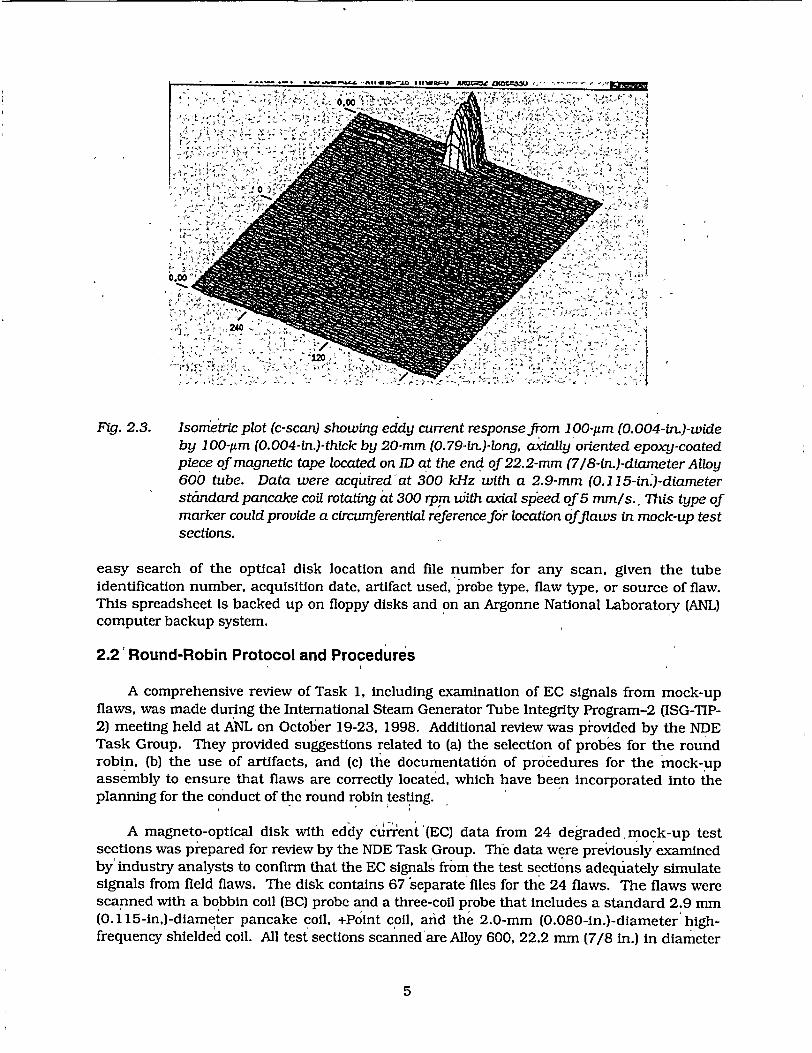
240

Fig. 2.3. Isometric plot (c-scan) showing eddy current response from 1 O0-0m (0. 004-in.)-wide by 100-j1m (0.004-in.)-thick by 20-mm (0.79-in.)-long, axially oriented epoxy-coated piece of magnetic tape located on ID at the end of 22.2-mm (7/8-in.)-diameter Alloy 600 tube. Data were acquired at 300 kHz with a 2.9-mm (0.1 15-in.)-diameter stindard pancake coil rotating at 300 rpm with axial speed of 5 mm/s., This type of marker could provide a circumferential reference for location offlaws in mock-up test sections.

easy search of the optical disk location and file number for any scan, given the tube identification number, acquisition date, artifact used, probe type, flaw type, or source of flaw. This spreadsheet is backed up on floppy disks and on an Argonne National Laboratory (ANL) computer backup system.

2.2 Round-Robin Protocol and Procedures

A comprehensive review of Task 1, including examination of EC signals from mock-up flaws, was made during the International Steam Generator Tube Integrity Program-2 (ISG-TIP2) meeting held at ANL on October 19-23, 1998. Additional review was provided by the NDE Task Group. They provided suggestions related to (a) the selection of probes for the round robin, (b) the use of artifacts, and (c) the documentati6n of procedures for the mock-up assembly to ensure that flaws are correctly located, which have been incorporated into the planning for the conduct of the round robin testing.

A magneto-optical disk with eddy curent (EC) data from 24 degraded mock-up test sections was prepared for review by the NDE Task Group. Thee data were previously examined by industry analysts to confirm that the EC signals from the test sections adequately simulate signals from field flaws. The disk contains 67 'separate files for the 24 flaws. The flaws were scanned with a bobbin coil (BC) probe and a three-coil probe that includes a standard 2.9 mm (0.115-in,)-diameter pancake coil, +PPoint coil, arid the 2.0-mm (0.080-in.)-diameter highfrequency shielded coil. All test sections scanned'are Alloy 600, 22.2 mm (7/8 in.) in diameter

5

and 0.30 m (12 in.) long. For each scan, the probe passes through the degraded test section, a standard with 18 notches, and an ASME standard. To locate data files associated with a given test section, a table was prepared that shows (a) the type of flaw scanned; (b) location of the data file on the disk provided, and (c) whether the flaw is in a free span (FS), has a ring over it to simulate the tube support plate (TSP), or whether the tube has a steel collar over the lower half of the test section to simulate the tube sheet (TS). The table also indicates whether a simulated artifact (either a ring of sludge or a ring, of magnetite) covers the area of the flaw. Other information indicates the test section identification number, location of the original data file at ANL, and which probe was used to generate the EC data.

A second review of EC data from mock-up flaws by members of the Task Group was held at the EPRI NDE Center in Charlotte, NC on May 12 and -13, 1999. More than 2000 scans were available for examination. EC signals from flaws with and without artifacts were compared. Suggestions made at the meeting with regard to improving the quality of the data that would be used for the RR have been implemented. The main improvements in the EC system were the replacement of cables and a slip ring in order to minimize electronic noise in the EC signals. Mag-biased MRPC will be used to eliminate noise problems resulting from sensitization of test sections in the crack-growing procedure in all but a few of the sensitized pieces. The problem associated with a few of the sensitized test sections when using a pancake coil (but not +Point), was addressed by modifying the test procedure.

Documents that provided technical direction for the EC examination, Site Specific Performance Demonstration, and Examination Technique Specifications Sheets were prepared based on input from NDE Task Group members on current industry practices. The documents were reviewed by the Task Group and by ANL personnel, leading to several suggested changes that have been incorporated into revised versions.

2.3 Data Acquisition from the Mock-up

Nine color-coded maps of each level of the mockup have been completed. In addition, 17 color-coded maps have been prepared to show each row. This format allows the status (flaw, artifact, etc.) of each test section in a tube to be easily verified by ANL staff during EC examination of the tube. Graphs and tables showing the distribution of flaws as a function of type have also been prepared.

During June 1999, a three-man team from Zetec collected data from the mock-up (Figs. 2.4 and 2.5). An observer" from Westinghouse was also present. The data acquisition team included a QDA Level Ila and a QDA Level IlIa. Data were acquired with a 10-D pusherpuller, MIZ30 with 36-pin cables, and Eddynet software. Before data acquisition, misalignment of three test sections had to be corrected by using the same procedure developed for the mock-up before it was placed on its stand (moving the tube bundle from floor to stand probably was the cause of the additional tube misalignment). BC data from a mag-biased probe was collected from 3600 test sections of the mock-up. The BC data were calibrated before and after the 4-h interval required to collect the data. No change in voltage from the standard was detectable during this' time period.

The BC data were taken at 0.53 m/s (21 in./s), maintaining a digitization rate of 37 samples per inch. Bobbin coil data were taken at 400, 200, 100, and 20 kHz (differential and

6

I I I

Fig. 2.4. Photograph of activity during acquisition of eddy current data by Zetec team.

absolute). MRPC data was taken from all degraded test sections in addition to' many test 'sections with artifacts and many, clean test sections. The three-coil mag-bias probe used consisted of a 2.92-mm (0.115-in.) pancake, ,a +Point, and a 2.0-mm (0.080-in.), highfrequency shielded coil. An ASME standard and a standard with 18 ID and OD axial and circumferential EDM notches (20, 40, 60, 80, and 100% throughwall) were used for calibration. MRPC data were taken at 900 rpm and an axial speed of 12.7 mm/s (0.5 in./s) to maintain a digitization rate of 30 samples per Inch in the circumferential direction and 30 in

7

Fig. 2.5. Photograph of underside of tube bundle. Conduit carrying the EC probe is shown being positioned under a tube.

the axial direction. Data were taken at 600, 400, 300, 200, and 100 kHz. A total of nine MRPC- probes containing the +Point, pancake, and high-frequency coils were used during tlhis exercise because of probe wear. The probes were replaced when one of the channels could not be nulled. The MRPC probe wear rate exceeded expectations.

All data were collected on a 2.6-GB magneto-optical disk: Two copies of the master disk were made, and all'the data were copied to an ANL archive computer back-up system. The quality of the data collected was Judged to be good. The set-up for the bobbin coil and +Point

8

probe matches or exceeds the specifications of the examination technique specification sheets (ETSSs) qualified for the flaws in the tube bundle.

The mock-up data collected by Zetec was analyzed at ANL by ANL personnel with Eddynet98 software. The purpose was to review the BC signals and MRPC signals to confirm that they are similar to field data. In addition, the locations of the flaw signals were checked against the location data of the flaw map. Locations of possible dings due to assembly that could lead to significant EC signals were noted. These dings could be created if a test section were Inadvertently pressed against the simulated TSP during assembly. A preliminary review shows about ten possible dings near the test-section ends.

1 During the week of August 9th, Cheryl Gortemiller of Moretech analyzed the ANL steam generator mock-up bobbin coil data and some of the MRPC data acquired by Zetec. Her review was much more comprehensive than of-the NDE Task Group. The purpose was to an additional independent expert opinion on the representativeness of the mock-up EC indications. The overall quality of the data was judged to be good and to be generally representative of field data. Gortemiller commented that, in her opinion, the data from intergranular attack (IGA) did not look like data from field IGA (a similar 'opinion was expressed by many of the NDE Task Group). This comment ultimately resulted in a call to Westinghouse to discuss the differences between IGA specimens they fabricated for the mock-up and IGA of current field Interest. The mock-up IGA is "pure" in that it is not mixed with other cracks. Westinghouse argued that the IGA they prepared for the mock-up simulates IGA found in the tube sheet crevice and is representative of the IGA at Cook, Point Beach, and San Onofre,.

EC signals from dings not previously known to exist in the mock-up were also observed by Gortemiller. Presumably, these dings were introduced inadvertently during the assembly of the mock-up tube bundle. As a result of this data review, 'important knowledge on how to prepare the site training document was acquired. An example of the IGA in the mockup was included in the "site" training sample set.

, Gortemiller's review of the data was presented at an NDE Task Group meeting held ,August 24-26, 1999, at Argonne. The meeting was attended by S. Bakhtiari (ANL), C. Gortemiller (Moretech), G. Henry (EPRI), D. Kupperman (ANL), R. Maurer (ABBCE), D. Mayes (Duke), R. Miranda (FTI), S. Redner (Northern States Power), T. Richards (FTI), and B. Vollmer (Zetec). As a result of this meeting, the Degradation Assessment and Site Applicability documentation, ETSSs, Analysis Guidelines, rand Data Acquisition documents were subsequently revised. In addition, opinions were expressed on how to handle "spin calls" (MRPC examination of test sections in which nonquantifiable or distorted indications were found by BC examination), how to handle the logistics of distributing EC data to the various teams, what should be in the training documentation, and what equivalency demonstrations need to be carried out. Following the meeting, for the purpose of demonstrating equivalencies, -data were taken from notches, cracks, and dents at 900 rpm and 12.7 mm/s (0.5 in./s) and 300 rpm at 2.54 mm/s (0.1 in./s). In addition, data from mock-up flaws were taken with mag- and non-mag-biased rotating coils.

Other input from the NDE Task Group meeting included a suggestion to have a separate ETSS for sizing depth and length of axial and circumferential primary water stress corrosion cracking (PWSCC) based on the two qualified techniques. In addition, an opinion was

9

expressed that the round robin team should consist of five members. A five-member team would include a primary, a secondary, and two resolution analysts, and an independent qualified data analyst (QDA) from a utility. Names of possible independent QDAs were provided by the Task Group.

Following the Task Group meeting, BC data from the mock-up were analyzed to show the distribution of voltages and distribution of crack depths, based on pre-mock-up assembly data. The histograms show a good distribution of BC voltages and crack depths. In addition, prints of MRPC Lissajous figures and isometric plots were generated for each of the flaws in the tube bundle.

Following the August 24-26 NDE Task Group Meeting, an extensive effort was made to revise the RR documentation as a result of opinions and suggestions from Task Group members. The Analysis Guideline (ANLOO) text was revised. The inspection teams were planned to include primary and secondary analysts, along with two resolution analysts and an independent QDA. The ETSSs 1 and 2 for bobbin and rotating coil probes, which are part of ANLOO1, were corrected and modified. Preparation of the ETSSs for sizing was started. They will be based on EPRI ETSSs 96702 and 96703, which have been developed for sizing PWSCC. Although qualified only for PWSCC, these ETSSs will form the basis for profiling both ODSCC and PWSCC. The document ANL002, ("Multi-Frequency Eddy Current Examination of Tubing within the ANL SG Mock-up"), was revised based on input from Todd Richards of FTI. The Steam Generator Mock-up Tubing Degradation Assessment and Technique Qualification (ANLO03) was revised extensively by using new EC signal graphics that better represent the various types of flaws in the mock-up. The revised documentation was distributed to the Task Group. Further modifications are anticipated as additional comments are received following review of the revised documents.

Preparation of the Training Manual was begun. Flaws have been selected for the manual to provide an example of each type of degradation and potential artifact. The training manual will include an IGA example.

Tests have been performed to show equivalency of mag- and non-mag-biased probes. Data using both types of probes have been obtained for several mock-up flaws using all the frequencies employed in the mock-up data acquisition. Figure 2.6 shows data from a magbiased +Point coil. Figure 2.7 shows data from the same flaw obtained with a non-mag-biased coil. The signals' are virtually the same. Problems do occur for a small number of test sections that were fabricated from a heat of material different from those used for the rest of the mockup specimens. For these test sections, using a mag-bias pancake coil could result in a phase shift, relative to a non-mag-biased coil of up to 900. This problem does not occur with the +Point coil (i.e., the phase from a flaw is the same for both mag- and non-mag-biased +Point coils regardless of the heat of material). Tests have also been performed to show equivalency between an MRPC operating at 900 rpm [12.7 mm/s (0.5 in./s)] and an MRPC operating at 300 rpm [2.54 mm/s (0.1 in./s)]. Figure 2.8 shows a Lissajous figure from a mock-up flaw at 300 rpm (2.54 mm/s) using a +Point coil. Figure 2.9 shows a Lissajous figure from a mock-up flaw at 900 rpm (12.7 mm/s) using the same +Point coil as for data in Fig 2.8. The signals are almost indistinguishable. Similar results have also been seen for other frequencies and coils.

10

I I I

" 5" S.ISV/d sona 119 - -: - `- -c' nt 231 !' I'- -'

Fig. 2.6. Lissajous figure' from mock-up flaw (in sensitized test section) obtained with magbiased +Point coil at 300 kHz

$.85v/d span 11 - I "- 231 .

VNon-Mag-Biased +Point at 300 kJh

43.,57 1 Volt-. 204 De9rees

.i.27..saos...efo .am. . fg.....2. 6 -- -- - -- -- - --- . . . .

Fig. 2.7. Lissajous Jijure from same mock-up flaw as in Fig. 2.6 obtained with a non-magbiased +Point coil at 300 kHz

11

"Mlag-Bias +Point Coil at300 kHz

,.F 50 V.lts 200 De9.rees

S.. .. .

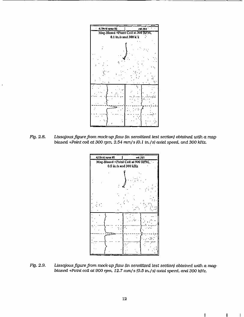
Fig. 2.8. Lissajous Jwure from mock-up flaw (in sensitized test section) obtained wtith a magbiased +Point coil at 300 rpm, 2.54 mm/s (0.1 in. Is) axiat speed, and 300 kHz.

Fig. .9. issajusfiurefrm mok-upflaw in snsitied tst sction.obt..ed.ith..mag

Mig. 2.9. Ltssajous Jigure from mock-up Jlaw (in sensitized test section) obtained with a magbiased +Point coil at 900 rpm, 12.7 mm/s (0.5 mn./s) axial speed, and 300 kHz.

12

I I

4tS9v/d san 5 I rot 261 Mag-Biased +Point Coil at 900 RPM,,°

0.5 in./s and 300 klz

-----------

I

2.4 Effect of Surface Oxide Films on Eddy Curient Signhals from SCC

The effect of corrosion products (thin oxide films) formed on crack faces on the EC signal from an SCC is under evaluation. Alloy 600 tubes with axial ODSCC were exposed under PWR water chemistry conditions (3000C and 3-8 ppb oxygen) for about two months. The cracks have been examined with both mag-bias bobbin coils (BCs) and a +Point coil before and after corrosion products were formed. The voltages for the BCs increased significantly with the creation of the thin oxide film. However, the general shape of the Lissajous figures remained unchanged. In contrast, the results for the +Point coil were inconclusive. In two cases, no change in +Point voltage was observed, while in a third, the voltage dropped significantly after the oxide film was formed. Figure 2.10 shows the BC Lissajous figure, along with voltage and phase Information for one of the tubes. Table 2.1 summarizes the BC results for two tubes. While voltages increased significantly, the phase angle did not. The creation of corrosion products in the crack could lead to a' reduction in the number of electrically conducting paths from contacting crack faces. In that case,'the EC signal would be expected to increase, as observed, while the depth remains essentially the same.

2.5 Comparison of BC Voltages from Notches and ODSCC

The similarity of BC voltages for ,notches and cracks of comparable depth and length is illustrated in Table 2.2, which presents BC voltages for notches, four axial ODSCCs generated at ANL, and one ODSCC generated at Westinghouse.

For notches and cracks In the 80-90% TW range, the BC voltages appear comparable, with variations in voltages being attributed to profile variations. Variations in BC voltage for cracks, over the voltage range shown in Table 2.2, lead to relatively small changes in predicted failure pressure if the estimated failure pressure is from the alternate plugging criteria voltageburst-pressure model for axial ODSCC at the TSP.

2.6 Comparison of Voltages from McGuire and ANL SCC

An indication that the cracks grown at ANL are representative of field cracks comes from a comparison of McGuire steam generator BC voltages and phases with-ANL SCC BC voltages and phase. Figure 2.11 shows McGuire voltages and phases from axial ODSCCs at TSPs, together with voltages and phases from the ANL-grown axial ODSCCs. The plots of voltage vs. phase are comparable.

13

P1.1-711 400, Hi GO, fi. CO if Diff0.77 v d soon 40 rot 79

3.24 volts 76 deg 81 % OD f.ij t.•_ LLI+ 85 - <

Fig. 2.10. Mag-bias BC Lissajous frgure after corrosion products (thin oxide film) were formed in a tube with axial ODSCC by exposing the tube to PWR conditions for =2 months. Voltage increased from 2.43 to 3.24 volts, suggesting less contact at crack faces. Estimated depth changed from 87 to 81% 7W.

Table 2.1. Comparison of BC voltages and phase for two tubes before and after treatment to produce a surface oxide film. Each tube has an axial ODSCC =15 mm (0.60 in.) long.

BC BC Phase BC Tube # Voltage Angle % TW

SGL-197 (before) 2.43 660 87

SGL-197 (after) 3.24 760 81

SGL-149 (before) 3.27 870 73

SGL-149 (after) 4.51 890 72

14

I I I

Axial ODSCC . I I

160 A McGuire i Argonne

120 A

80

A 4

S40 N A A

0 , ,t ,,, I , , , I .,,,I , , ,I , , , I i

0 2 4 6 8' 10 12 14 BC Voltage (V)

Fig. 2. 11. Comparison of McGuire steam generator D BC voltages and phase from axial ODSCCs at tube support plates to voltages and phase from ANL-produced axial

ODSCC. Ranges of plots are comparable.

15

3 Research on ISI Technology (S. Bakhtiari and D. S. Kupperman)

The objective of this task is to evaluate advanced NDE and signal analysis techniques for the reliable in-service inspection (ISI) of original and repaired SG tubes. Improved correlations between EC probe response and flaw morphology,'leak rate, and failure pressure will be developed and validated. In addition, the reliability of the voltage parameter and other EC parameters and techniques will be evaluated with respect to their ranges of applicability.

The present research on improved ISI of SG tubes focuses on four primary areas: (a) implementation of analytical methods for prediction of EC response as a function of probe design, flaw characteristics, and material properties; (b) development of effective signal analysis procedures; (c) development of flaw imaging and display methods for simple and accurate flaw characterization; and (d) evaluation of improved probe designs that may use directional arrays so that defects of arbitrary orientation can be examined simultaneously. The reliability and effectiveness of improved inspection techniques and the robustness of potential correlations will ultimately be 'substantiated through laboratory testing of the SG tube bundle mock-up and of SG tubes that contain various flaw morphologies. Final validation will also utilize in-service-degraded SG tubes.

Task 2 activities during the present reporting period are described here. Research efforts that are associated primarily with multiparameter analysis of EC NDE results are discussed. Representative test cases are presented in Sec. 3.1 for a study initiated to evaluate potential advantages of alternate multifrequency mixing techniques involving more than two frequencies over standard two-frequency mixes. These alternate techniques could help improve BC detection of flaw indications in the presence of interfering signals. Multiparameter data analysis is discussed in Sec. 3.2. Initial analysis of the results is provided on a set of 20 laboratory-grown specimens with various forms of cracking degradation. Flaw morphologies in these tubes are representative of those incorporated into ANL's tube bundle mock-up. Eddy current rotating probe readings on this set were analyzed by using an automated multifrequency data analysis algorithm that is currently under evaluation. Subsequently, analysis results are presented for a single laboratory-produced mockup specimen that exhibited a reportable BC signal without a clear rotating probe indication. Data analysis results are presented on a set of 24 laser-cut specimens with single and multiple axial/circumferential notches (with and without ligaments) that simulate complex cracking geometries. The NDE and nominal flaw size for this set of tubes, originally constructed for high-pressure studies under Task 3 of this program, provide a useful means for assessing data analysis algorithms currently under investigation at ANL. Finally, in Sec. 3.3, results are presented from a recent study on the application of a signal restoration technique to enhance the spatial resolution of rotating probes. The pseudo-deconvolution scheme described here has been integrated as part of the multiparameter data analysis algorithm to further help improve characterization of complex SG tubing flaws.

3.1 Multifrequency Mix for Improving Bobbin Coil Detection

Preliminary results are presented on two separate multifrequency mixing procedures that could possibly improve BC detection of flaw indications in the presence of interfering artifacts at the same axial location along the tube axis. This investigation was initiated in part to

16

I I I

evaluate alternate mixing methods ,that might help compensate for lack of similarity between simulated artifacts in tube standards and those in the field. All the data conversions and -calibrations In this study were carried out automatically by using MATLAB-based graphical user interface (GUI) tools that have been developed at ANL and described previously.'

3.1.1 Direct and Indirect Mix Processes

Recovery of defect-induced signals in the presence of strong background interference is an important and often challenging NDE problem when analyzing NDE results for ISI of SG tubing. Data analysis is further complicated when degradations are accompanied by tube ID variations such as design-related tube diameter changes or the presence of significant denting. These difficulties are associated with such factors as low S/N ratio and small phase separation between ID and deep OD indications. Multifrequency mixing Is routinely applied to improve detection of flaw signals that are obscured by tubing artifacts. However, the mix channel information should be analyzed discerningly, particularly when more than two frequencies are used in the process. Conventional two-frequency least-squares (LS)-based mix algorithms that are optimized primarily to suppress a single OD artifact generally provide- consistent outcomes. On the other hand, processed channel, Information from mixing algorithms that incorporate more than two frequencies could be unreliable for the interpretation of signals outside the segment where the mix coefficients were calculated. This is due in part to uneven perturbation of the signal amplitude and phase information that is introduced by higher-order (nonlinear) mix models.

Two separate approaches, direct (independent) and indirect (dependent) mixing algorithms, to suppress multiple unwanted indications from a composite signal were considered in this study. In an indirect mix, regression coefficients are determined by using a data segment from a simulated artifact such as a TSP ring on a reference standard tube, which is expected to :closely resemble those present in the actual SGs. Theaim of the regression model is to best reproduce the primary/base frequency signal by combining signal components from auxiliary frequency channel(s). This is the conventional approach used for the analysis of EC ISI results. Alternatively, independent mix procedures have the potential to suppress unwanted signals by using multiple-frequency readings on the same tube. This approach, primarily suggested for suppression of dominant signal features, is of particular interest when tube standardsmwith simulated artifacts that resemble field-induced signals are not readily available. Representative test case results are presented next on recent studies associated with direct and indirect mixing techniques.

To Initially evaluate the direct mixing approach, a simulated composite BC signal was constructed by using normalized EC readings from an ASME tube standard. Individual signal components consisted of a simulated TSP ring and 10 and 20% ID circumferential grooves. The main objective was to develop a mixing procedure that would allow recovery of the shallow OD indication from the composite signal with minimal perturbation of the signal outside this region. A standard linear LS regression algorithm was initially utilized in this study. Various two- and three-frequency regression fits were implemented. Preliminary results indicated that two-frequency mixes are generally more consistent, so the approach was to sequentially apply two-frequency mixes for suppression of two unwanted indications at the same axial location. To improve the mix outcome, several modifications were made to our previously developed I standard mix algorithm. These consisted of energy-scaling each trace, resampling in

17

frequency domain, and phase-angle referencing. Frequency resampling was done to increase the number of available independent variables. Phase-angle tracking was done to help reduce phase ambiguity from multiple application of linear regression coefficients. Based on the small number of cases tested so far, the amplitude renormalization consistently exhibited improved quality of mix outputs. This Is believed to be a result of the weighting introduced by the energy-scaling process. It is worth noting that this transformation does not significantly perturb the original phase information of original channels (i.e., the lissajous patterns remain nearly unchanged).

Figure 3.1 shows the horizontal and vertical differential signal components of the calibrated original (top) -and renormalized (bottom) traces' at f = 400 kHz. The drilled-hole signal was added to each trace to serve as the phase reference indication. Figure 3.2 shows intermediate results of, the mix obtained by using a high- and low-frequency signal to suppress the TSP Indication from each trace. Figure 3.3 displays the recovered differential and absolute channel signals for the shallow OD indication subsequent to combining the two intermediate mix outputs. In both cases, the 10% OD groove was recovered from the original composite trace. It should be noted that the three-frequency mix outputs shown in Fig. 3.3 do not contain the Identical phase angle information as the original traces. Nevertheless, the results show significant improvement over standard three-frequency LS mixing procedures that were examined as part of this study.

To assess the validity of independent mix algorithms, BC readings on two tubes with laboratory-grown circumferential and axial SCC at tube sheet ([1S) roll transition regions were utilized for analyses. Available metallography results indicate depths of 30% ID for the circumferential and 100% TW cracking for the axial flaw. The'specimens used here were part of a 20-tube set of representative mock-up specimens furnished by Pacific Northwest National Laboratory (PNNL). With reference to Fig. 3.4, the indications from left to right consist of 100% TW hole and two roll transitions with ID circumferential and OD axial SCC flaws, respectively. Once again, a throughwall indication from the ASME standard was attached to the beginning of each trace to serve as the phase reference. Figure 3.4 displays both the calibrated original and the renormalized traces at f= 400 kHz. As in the case of direct mixing, regression coefficients were initially calculated for suppression of roll transition signals. The two intermediate mix outputs were once again produced by using the signal components from a high- and a low-frequency channel to suppress the strong signal from the tube diameter change. However, unlike the Indirect mix, data from the first roll transition were used to suppress the artifacts. Subsequently, a final mix process was applied to recover the residual signal that is expected to contain Information predominantly about the flaw.

Figure 3.5 displays the results of the independent mix for the differential and absolute channels, respectively. In both traces, the residuals at the roll transition regions (located approximately around data points 350 and 750) exhibit the presence of SCC flaws. A notable feature of the processed signal is the phase separation between the two indications and their relationship to the throughwall reference signal. This phase information cannot be recovered consistently with conventional multifrequency mixing techniques. Further evaluation of multifrequency mixing algorithms is currently being pursued under this program, and a more detailed discussion of the findings will be presented In future reports.

18

I I I

50 100 150 200 Data Point

50 100 150 200 250 Data Point,

250 300 350

Fig. 3. 1. Differential BC horizontal and vertical signal components of calibrated original (top) and renormalized (bottom) traces atf = 400 kHZ. Simulated indications from left to right consist of throughwall drilled hole, TSP ring, 10% OD and 20% ID circumferential grooves, and composite (of last three indications) signal.

-0.5 F

L I It

0 o50 100 150 200 Data Point

250 300

Fig. 3.2. Intermediate mix outputs using -high-,- and low-frequency] suppress TSP indication from bottom trace shown in Fig. 3.1.

19

20

0E

-20

-40' 0

11

I II

1

0.5 F

E

0 z-0.5 -

01 0*1

300 350

i ,

051

E

z

350

signals to

I I I f I I

t

A6,.L

I

0 50 100 150 200 Data Point

50 100 150 200 Data Point

250 300 350

350250 300

Fig. 3.3. Residual differential (top) and absolute (bottom) mix channel signals for shallow OD indication subsequent to combining intermediate mix outputs.

100 200 300 400 500 600 Data Point

700 800 900 1000

0.5 F

E

0 Z

0

-0.5

.10 100 200 300 400 500 600 700 800 900 1000

Data Point

Fig. 3.4. Differential BC horizontal and vertical signal components of calibrated original (top) and renormalized (bottom) traces at f = 400 kHz. Indications from left to right consist of TW reference hole and two roll transition zones with 30% ID circumferential and TW OD axial SCC, respectively.

20

I I I

10

05

0

-0.5

0 Z

-I

0.5 F

E

0 Z

0

-05-

-1 0

-Ir

I %t

till

40

20F

0 z 0

Ii !I

fl II

II II

fi Ii

II II

-20 0

ii

- �---.----- I

= I I I I I I I I I

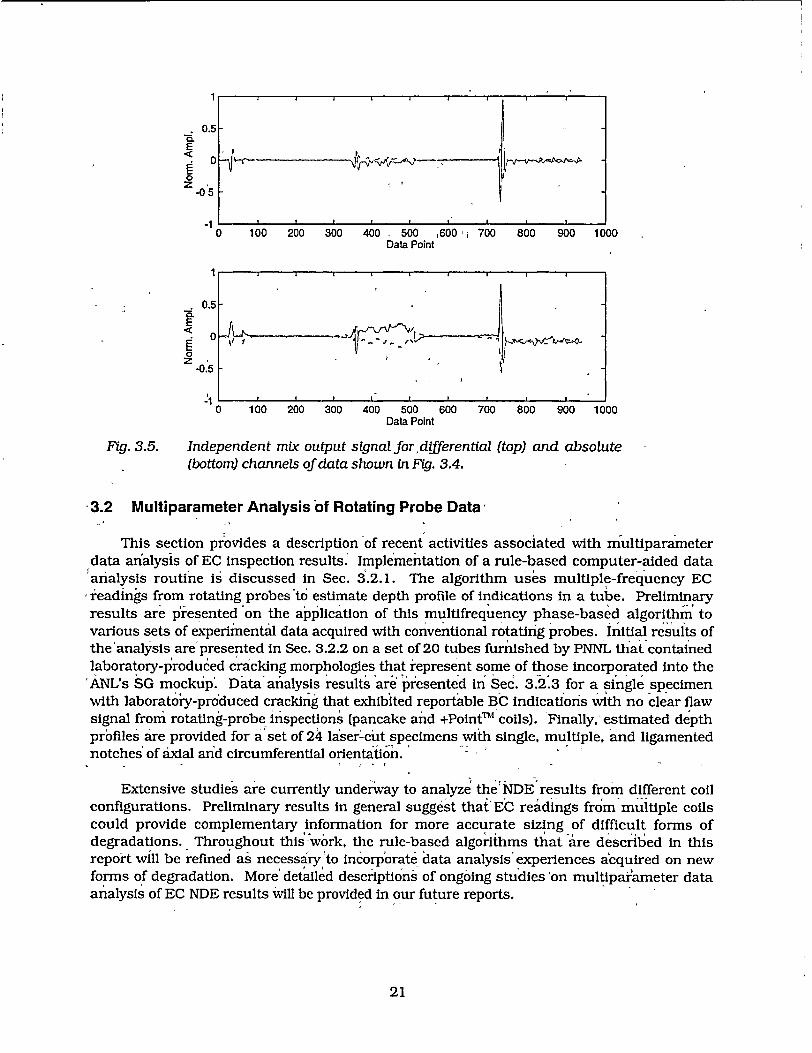
1

0.5E

z-0 5

0 100 200 300 400 500 600• 700 800 900 1000 Data Point

1 I ii I p

0.5

Z -0.'5

-1 1 I II I I

0 100 200 300 400 500 600 700 800 900 1000 Data Point

Fig. 3.5. Independent mix output signal for, differential (top) and absolute (bottom) channels of data shown in Fig. 3.4.

-3.2 Multiparameter Analysisof Rotating Probe Data,

This section provides a description of recent activities associated with multiparameter data analysis of EC inspection results. Implementation of a rule-based computer-aided data analysis routine is discussed in Sec. 3.2.1. The algorithm uses multiple-frequency EC readings from rotating probes to estimate depth profile of indications in a tube. Preliminary results are lpresented on the application of this multifrequency phase-based algorithmI to various sets of experimental data acquired with conventional rotating probes. Initial results of the'analysis are' presented in Sec. 3.2.2 on a set of 20 tubes furnished by PNNL th at ,contaiIned laboratory-jFroduced cracking morphologies that represent some of those incorporated into the

"ANL's SG mockup. Data analysis results ,are presented in Sec. 3.2.3 for a single specimen with laboratoiy-produced cracking that exhibited reportable BC indication's with no clear flaw signal from rotating-probe inspections (pancake and +PointTM coils). Finally, estimated depth profiles are provided for a"set of 24 laser -cut specimens with single, multiple, and ligamented notches' of axial and circumferential orientation.

Extensive studies are currently underway to analyze the' NDE results from different coil configurations. Preliminary results in general suggest thai' EC readings from muitiple coils could provide complementary information for more accurate sizing of difficult forms of degradations. Throughout this work, the rule-based algorithms that are described in this report will be refined as necessary'to incorp'orate data analysis- experiences a~cquired on new forms of degradation. More' detailed description's of ongoing stu'dies 'on multipai-ameter data analysis of EC NDE results will be provided in our future reports.

21

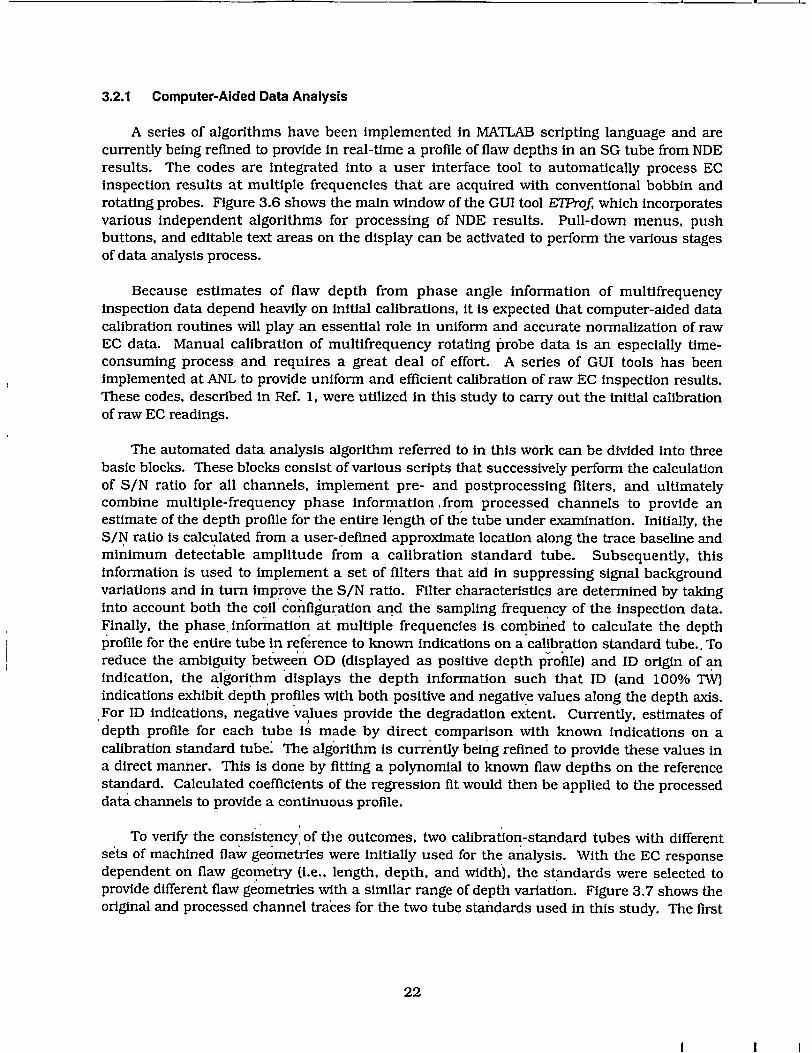
3.2.1 Computer-Aided Data Analysis

A series of algorithms have been implemented in MATLAB scripting language and are currently being refined to provide in real-time a profile of flaw depths in an SG tube from NDE results. The codes are integrated into a user interface tool to automatically process EC inspection results at multiple frequencies that are acquired with conventional bobbin and rotating probes. Figure 3.6 shows the main window of the GUI tool ETProf, which incorporates various independent algorithms for processing of NDE results. Pull-down menus, push buttons, and editable text areas on the display can be activated to perform the various stages of data analysis process.

Because estimates of flaw depth from phase angle information of multifrequency inspection data depend heavily on initial calibrations, it is expected that computer-aided data calibration routines will play an essential role in uniform and accurate normalization of raw EC data. Manual calibration of multifrequency rotating probe data is an especially timeconsuming process and requires a great deal of effort. A series of GUI tools has been implemented at ANL to provide uniform and efficient calibration of raw EC inspection results. These codes, described in Ref. 1, were utilized in this study to carry out the initial calibration of raw EC readings.

The automated data analysis algorithm referred to in this work can be divided into three basic blocks. These blocks consist of various scripts that successively perform the calculation of S/N ratio for all channels, implement pre- and postprocessing filters, and ultimately combine multiple-frequency phase information from processed channels to provide an estimate of the depth profile for the entire length of thee tube under examination. Initially, the S/N ratio is calculated from a user-defined approximate location along the trace baseline and minimum detectable amplitude from a calibration standard tube. Subsequently, this information is used to implement a set of filters that aid in suppressing signal background variations and in turn improve the S/N ratio. Filter characteristics are determined by taking into account both the coil configuration and the sampling frequency of the inspection data. Finally, the phase, information at multiple frequencies is combined to calculate the depth profile for the entire tube in reference to known indications on a calibration standard tube.. To reduce the ambiguity between OD (displayed as positive depth profile) and ID origin of an indication, the algorithm displays the depth information such that ID (and 100% MW) indications exhibit depth profiles with both positive and negative values along the depth axis. For ID indications, negative values provide the degradation extent. Currently, estimates of depth profile for each tube is made by direct comparison with known indications on a calibration standard tube: The algorithm is currently being refined to provide these values in a direct manner. This is done by fitting a polynomial to known flaw depths on the reference standard. Calculated coefficients of the regression fit would then be applied to the processed data channels to provide a continuous profile.

To verify the consistency, of the outcomes, two calibration-standard tubes with different sets of machined flaw geometries were initially used for the analysis. With the EC response dependent on flaw geometry (i.e., length, depth, and width), the standards were selected to provide different flaw geometries with a similar range of depth variation. Figure 3.7 shows the original and processed channel traces for the two tube standards used in this study. The first

22

I I I

DA. ET Det oieTo

Fig. 3.6. A series of MATLAB-based Graphical User Interface (GUI) tools are currently under implementation to allow automated analysis of EC inspection results acquired with standard commercial instruments.

tube contained five circumferential OD notches of nominal length and width of 8 mm (0.315 in.) and 0.3 mm (0.012 in.), respectively, with depths ranging from 20 to 100% throughwall. The second tubeselected is an ASME standard with drilled holes of similar depth. This standard also contains a TSP simulation ring, as well as 20% TW ID and 10% TW OD circumferential grooves. Figure 3.7(a) shows the calibrated amplitude traces at two frequencies. Examination of these data clearly indicates the presence of a nonlinear amplitude relationship that is dependent on both flaw geometry and operating frequency. Fig. 3.7(b) displays the estimated depth profiles for these tubes by combining the information from two and three channels, respectively. In all cases, the traces show similar depths for the entire range of OD indications. As mentioned earlier, the throughwall and ID Indications have depth profiles that also extend in the negative direction. Although the results of analysis for the standards indicate similar results for two- and three-frequency depth profiles, studies so far have shown that for realistic flaws, more consistent estimates are generally achieved when three frequencies are used.

3.2.2 Analysis of 20 Lab-Produced Tube Specimens

The automated data analysis algorithm rdescribed In the previous section was utilized to estimate flaw sizes in a set of laboratory-grown specimens. Preliminary results on estimation of flaw depth profiles in this set of 20 tubes are presented next. The samples were furnished by PNNL and were originally manufactured by the Westinghouse Science and Technology Center (WSTC). Flaws in this set of 22.2-mm (0.875-in.)-diameter Alloy 600 tubing consisted mostly of longitudinal and circumferential ID/ODSCC, with a few samples containing shallow intergranular attack (IGA). The data set, which also contains metallography results, is currently being used to evaluate multiparameter sizing algorithms under study in this program.

The preliminary outcome of the assessments presented here pertains to the EC readings made with the primary 2.92 mm (0. 115 In.) pancake coil of a three-coil rotating probe and at frequencies of 400, 300, and 200 kHz. The NDE results also contain information from several other probes that are also being evaluated as part of this study. Eddycurrent inspections were carried out by Zetec, with the frequency selection being limited to the range that is commonly used for ISI of 22.2-mm (0.875-ln.)-diameter, tubing. Attempts, will be made throughout this study to evaluate potential ,improvement of the sizing ,capability by incorporating the inspection results from a wider range of frequencies. I ,

23

IIJUANLEJA..1,m U91EY

[LE x~lueNM DpyR-E

(a)

(b)

Fig. 3.7. Outputs of data analysts tool for estimation of defect depth profile for circumferential notch standard (left) containing five OD machined flaws ranging from 20 to 100% throughwall and an ASME standard (right) containing ODflat-bottom holes of same range, followed by TSP ring, 1096 OD, and 20% ID grooves. Traces show (a) calibrated 400 kHz (top) and 200 kHz (bottom) amplitude (volts) and normalized depth profiles based on combining (b) two (upper), and three (lower) frequtency channels. OD indications have positive trace and ID indications have both positive and negative traces. 'Eddy current readings are from 2.92 mm (0.115 in.) pancake of three-coil rotating probe.

24

I I I

315 [

10 .. ..- ,I. 5- I

20 2000 4000 6000 8000 10000 12000 14000 16000 18000

30

0 20

2000 4000 6000 8000 10000 12000 14000 16000 18000

CL

z". 20;004'0006000 8o000 10000 12;00014;0001600018000 ID 05

-10.

2000 4000 6000 8000 10000 12000 14000 16000 18000

Table 3.1 lists all the available information on the PNNL 20-tube subset of mock-up specimens, as well as the NDE depth estimates. For this initial investigation, NDE depth estimates are given at 20% intervals that cover the entire range of 0-100% of tube wall thickness. Figures 3.8-3.16 show selected test cases from the analysis of specimens in the data set. For all samples, both the calibrated amplitude trace at 400 kHz and the estimated three-frequency normalized depth profile are displayed. Each trace from left to right consists of the OD circumferential notch standard followed by the degraded-test specimen, with a vertical line separating the two tubes. To reduce the size of the data, only the section of the tube that contains the NDE suggested flaw Indication(s) is displayed. Because the EC reading at each measurement location is, in effect, an integration of the current distribution over the entire field of view of the coil, it is not expected that point-type defects, if detected, will produce EC responses proportional to the actual flaw depth. Also, because the NDE results are dependent on the S/N ratio, estimation of depth (particularly for shallow OD indications) should take into consideration the level of noise present in each trace.

3.2.3 Reanalysis of Lab-Produced Specimen SGL-432

NDE results from laboratory-produced specimen SGL-432, 22.2-mm (0.875-in.)-diameter Alloy 600 tubing, was also reanalyzed by using the multifrequency depth profile algorithm described earlier. This tube was reanalyzed because of the atypical nature of the original EC NDE results. Inspection results exhibited a BC indication with a relatively large flaw amplitude response, but without a discernible signal from midrange pancake and +Point coils. Figure 3.17(a) displays calibrated differential readings at 400 kHz primary and 100 kHz auxiliary frequencies that were acquired with an 18.3-mm (0.72-in.)-diameter magnetically biased bobbin probe. In the figure, the trace from an'in-line ASME standard is shown on the left, and the response of the test specimen on the right. The lissajous patterns of the defected segment at the two frequencies are shown in Fig. 3.17(b). The bobbin results clearly suggest the presence of a shallow OD indication. The peak-to-peak signal amplitude and relative phase-angle for the flaw at 400 kHz were estimated to be 3.4 v and 1600, respectively. This rather large bobbin signal amplitude and phase are indicative of a shallow volumetric degradation. Figure 3.18 shows calibrated readings from 2.92-mm (0.115-In.) pancake and midrange +Point'T coils at the same two frequencies. For both coils, any signals are buried within the noise level. The noise level In this tube is relatively high for both bobbin and pancake coils and is presumably associated with permeability variations introduced by sensitization of the specimen.

The raw EC readings from specimen SGL-432 were analyzed off-line -by ,using the multifrequency algorithm that was described earlier. Information from three frequencies is used to estimate the flaw depth. Figure 3.19 displays the processed data showing the calculated depth profiles at 40013001200 and 30012001100 kHz frequencies. Responses from an in-line EDM notch standard with 10 axial and circumferential (D indications are displayed on the left side of the trace; a comparison of the response from the indication with these responses provides an estimate of relative depth. In both cases, a shallow OD indication is visible just past data point No. 20,000, which is consistent with the location of the flaw based on the bobbin profile. The position of the flaw relative to the tube end was calculated by converting the number of measurement points to axial position along the tube using the locations of known markings on the standard. The phase-based flaw depth is estimated to be

25

1��I�

Table 3.1. Tabulated destructive examination and estimated EC NDE results by depth profile algorithmfor PNNL 20-tube set of laboratory-grown specimens. Degradations were fabricated on 22.2-mm (0.875-in.)-diameter Alloy 600 tubes manufactured by Westinghouse Science and Technology Center. NDE results are given in 20% depth intervals from 0 to 100% TW.

Tube Flaw Roll Max Depth (% 7W) Depth Range (% 'W) ID # Typea Expansion (Destructive Exam) (NDE Estimate)

1-03 CIDSCC X 44 40-60

1-11 LIDSCC X 100 >80

1-19 LIDSCC X 100 >80

2-06 LODSCC 100 >80

2-11 LODSCC 95b 60-80

2-19 LODSCC 46 20-40

2-20 LODSCC 16 <20

2-21 LODSCC 30 20-40

3-05 CIDSCC X 69 60-80

3-14 LIDSCC X NAC 20-40

4-01 CODSCC X 83 60-80

4-04 -CODSCC X 64 20-40

4-06 CODSCC X 100 >80

4-10 CODSCC X 100 >80

5-02 IGA 4 NDDd

5-03 IGA 5 <20

5-04 IGA 24 20-40

5-09 IGA 43 20-40

5-25 IGA 66, 20-40

B-10-07 LODSCC 28 20-40

a LIDSCC: longitudinal IDSCC; CIDCSS: circumferential IDSCC; LODSCC: longitudinal ODSCC; CODCSS: circumferential ODSCC.

b A single point Is Identified as having 95% degradation extent with flaws on both sides <20% 'W. All other crack networks (105 marked locations) are <38% TW.

c Destructive results not available (NA). Target depth is 30%-60% TW. d No detectable degradation (NDD).

26

I II

L1EI .pfr,.. xip RriF

Fig. 3.8. Output of data analysis tool for roll-expanded specimen #1-11 that was destructively identified as having 100% '(max. depth) LIDSCC degradation. ýTraces show calibrated amplitude in volts (top), and normalized multifrequency depth profile (bottom) of notch standard (left) followed by sample tube, suggesting >80% degradation depth around scan location 1.3 x 104. Eddy current readings are from 2.92 mm (0.115 in.) pancake of three-coil rotating probe.

UIp Pold. DaIlay

Fig. 3.9. Output'of data analysis tool for roll-excpanded specimen #2-06 that was destructively identified as having 100% (max. depth) LODSCC degradation. Traces show calibrated amplitude in volts (top), and normalized multifrequency depth profile (bottom) of notch standard (left) followed by sample tube, suggesting >80% degradation depth around scan location 1.4 x 104. Eddy current readings are from 2.92 mm (0.115 in.) pancake of three-coil rotating probe.

27

!

10 j

E

Ii '- ________________________________

2000 4000 6000 8000 10000 12000 14000 16000U

~15 > 10

05

2000 4000 6000 8000 10000 12000 14000 16000 18000

E 1! 9-05Z

2000 4000 6000800 10000 12000 14000 16000 180C00

Fig. 3.10. Output of data analysis tool for specimen #2-11 that was destructively identified as having 95% (max depth at a single point with all other indications marked <38%) LODSCC degradation. Traces show calibrated amplitude in volts (top), and normalized multifrequency depth profile (bottom) of notch standard (left)followed by sample tube, suggesting 60-80% degradation depth around scan location 1.5 x 104 . Eddy current readings are from 2.92 mm (0.115 in.) pancake of three-coil rotating probe.

Fig. 3.11. Output of data analysis tool for specimen #2-19 that was destructively identified as having 46% (max. depth) LODSCC degradation. Traces show calibrated amplitude in volts (top), and normalized multifrequency depth profile (bottom) of notch standard (left) followed by sample tube, suggesting 20-40% degradation depth around scan location 1.6 x 10W. Eddy current readings are from 2.92 mm (0.115 in.) pancake of three-coil rotating probe.

28

I I I

10-j

0 02 04 06 08 1 12 14 16 182

x~o

02 04 06 08 1 12 14 16 1'8 2

x10

O x, " . . . . . . . . *. . .. . in . . . .I

02 04 06 08 1 12 14 16 18 2 10

E

05

0 02 04 06 08 1 12 14 16 18 2

xl10,

l-E T epth w~ndn, Jipe R nolE l

tag,, - - - - - - -1

Fig. 3.12. Output of data analysis tool for specimen #2-20 that was destructively identified as having 16% (max. depth) LODSCC degradation. Traces show calibrated amplitude in volts (top), and normalized multifrequency depth profile (bottom) of notch standard (left)followed by sample tube, suggesting <20% degradation depth around scan location 1.2 x 10i. Eddy current readings are from 2.92 mm (0.115 in.) pancake of three-coil rotating probe.

Fig. 3.13. Output of data analysis tool for roll-expanded specimen #3-14 LIDSCC degradation (no DE'results available; target value 30%-60%). Traces show calibrated 'amplitude in volts (top), 'and normalized multifrequency depth profile (bottom) of notch standard'(left)foll6wed by sample tube, suggesting 40%-60% degradation depth around scan location 1.4 x 104. Eddy current readings are from 2.92 mm (0.115 in.) pancake of three-coil rotating probe.

29

0

02 04 06 08 1 12 14 16 18 2

0-

0

02 04 06 08 1 12 14 16 18 2

xlO

- y -r-------i--------, 1

E I

0.2 04 06 08- 1 -12 14 16 18 2 xlO

0_05

02 04 06 08 - 1 12 14 16 18 2

xlO4

[LIE Det rflxipay.I- i F JF

Output of data analysis tool for roll-expanded specimen #4-04 that was destructively identified as having 64% (max. depth) CODSCC degradation. Traces 'show calibrated amplitude in volts' (top), and normalized multifrequency depth profile (bottom) of notch standard, (left) followed by sample tube, suggesting >40% degradation depth around scan location 1.5 x 104. Eddy current readings are from 2.92 mm (0.115 in.) pancake of threecoil rotating probe.

1LIETDepthIsiods 0 --v_

Output of data analysts tool for roll-expanded specimen #4-10 that was destructively identified as having 100% (max. depth) ,CODSCC degradation. Traces show calibrated amplitude in volts (top), and normalized multifrequency depth profile (bottom) of notch standard (left) followed by sample tube, suggesting >80% degradation deptlh around scan location 1.4 x I0W. Eddy current readings are from 2.92 mm (0.115 in.) pancake of threecoil rotating probe.

30

I I I

10 I

02 04 06 08 1 12 14 16 18 2

x 104

02 04 06 08 1 12 14 16 18 2

x 10'

Fig. 3.14.

FMg. 3.15.

02 04 06 08 1 12 14 16 18 2

1

15

101

E - 5

02 04 06 08 1 12 14 16 18 2

x iO4

I

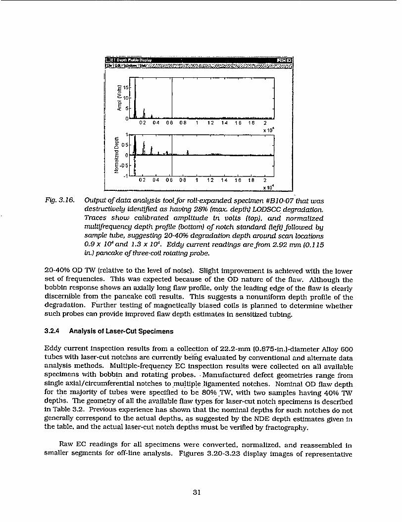
Fig. 3.16. Output of data analysis tool for roll-expanded specimen #B10-07 that was destructively identified as having 28% (max. depth) LODSCC degradation. Traces show calibrated amplitude in volts (top), and normalized multifrequency depth profile (bottom) of notch standard (left) followed by sample tube, suggesting 20-40% degradation depth around scan locations 0.9 x 104and 1.3 x 104. Eddy current readings are from 2.92 mm (0.115 in.) pancake of three-coil rotating probe.

20-40% OD TW (relative to the level of noise). Slight improvement is achieved with the lower set of frequencies. This was expected because of the OD nature of the flaw. Although the bobbin response shows an axially long flaw profile, only the leading edge of the flaw is clearly discernible from the pancake coil results. This suggests a nonuniform depth profile of the degradation. Further testing of magnetically biased coils is planned to determine whether such probes can provide improved flaw depth estimates in sensitized tubing.

3.2.4 Analysis of Laser-Cut Specimens

Eddy current inspection results from a collection of 22.2-mm (0.875-in.)-diameter Alloy 600 tubes with laser-cut notches are currently being evaluated by conventional and alternate data analysis methods. Multiple-frequency EC inspection results were collected on all available specimens with bobbin and rotating probes. Manufactured defect geometries range from single axial/circumferential notches to multiple ligamented notches. Nominal OD flaw depth for the majority of tubes were specified to be 80% TW, with two samples having 40% TW depths. The geometry of all the available flaw types for laser-cut notch specimens is described in Table 3.2. Previous experience has shown that the nominal depths for such notches do not generally correspond to the actual depths, as suggested by the NDE depth estimates given in the table, and the actual laser-cut notch depths must be verified by fractography.

Raw EC readings for all specimens were converted, normalized, and reassembled in smaller segments for off-line analysis. Figures 3.20-3.23 display images of representative

31

01

02 04 06 08 1 12 14 16 18 2 x 10

2 X 4

LIE T Depth P,91J.Diplay R R-1 173

200 400 600 800 Data point

1000 1200 1400 1600

200, 400 600 800 1000 1200 1400 1600 Data point

(a)

I-4W kHz I .100 iz

-3 -2 -1 0 1 2 h-cor (voit)

-4 -3 2 .- 0 1 h--oP, (vo*)

(b)

(a) Stripchart and (b) lissajous display of calibrated dffferential readings at 400 kHz (top) and 100 kHz (bottom) frequencies made with 18.3-mm (0.72in.)-diameter magnetically biased bobbin probe on 22.2-mm (0.875-in.)diarmeter Alloy 600 tube. Response from in-line ASME standard is shown on left; response of test specimen SGL-432 is on right. Calibrated signal amplitude and phase at 400 kHz were estimated to be 3.4 v and 1600, respectively, suggesting <20% OD degradation.

32

I I I

20

10 E 0

0 0

-20

I.

'I II ?5-v-�-4-��

II

.1

-2

3

2

1

-2

-3

.31

Fig. 3.17.

2 3

3. 4

-4-

0 0>

E

E

8

05

50

o

E 0 0 >U

1.5 Data point

2 2.5

x 104

15 2 25 Data point x 104

(b)

Calibrated readings with (a), 2.92 mm (2.92-mm 10.11 5-in.) pancake and (b) midrange' +Point coils of three-coil rotating probe at 400 kHz (top) and 100 kHz (bottom) frequencies on 22.2-mm (0.875-in.)-diameter Alloy 600 tube. Response from 20-100% OD, 6.35-mm (0.25-in.)-long axial/circumferential EDM notches from in-line standard is shown on left: signal from test specimen SGL-432 is on right. No discernible indications are present in these traces, although a BC indication is present, as shown in Fig. 3.17.

33

10

fit

-5 ; -10

-505 1 is 2 25

Data point x 104

10

5

-5

-10 05 1 15• 2 25

Data point x 104

(a)

20

10

10

120

d E 0 U

Fig. 3.18.

1

Data point (xl 000)

(a)-1IT xlh1Wl iplyI Ipn

(b)

Outputs of multifrequency depth profde algorithm at (a) 40013001200 kHz and (b) 30012001100 kHz for specimen SGL-432. Selected data segments show calibrated amplitude in volts (top), and normalized multifrequency depth profile (bottom) for 20-100% OD, 6.35-mm (0.25-in.)-long axial/circumferential EDM notches from in-line standard followed by test specimen. Degradation extent around scan location 20 x 10i suggests =20-40% OD flaw with maximum depth being slightly to right. Eddy current readings are from 2.92 mm (2.92-mm [0.1 15-in.j) pancake of threecoil rotating probe.

34

I I I

0

0

-0!

Fig. 3.19.

15 Data point (xl000)

I .lIIRFý - ET Deplh Fidile Display , I

Table 3.2. List of laser-cut samples and their nominal dimensions. Also listed are single-frequency NDE results from mag-biased bobbin and +Point probes, along with multiparameter depth estimates with 2.92-mm (0.1 15-in.) pancake probe.

Speci- Notch Ligament Notch Depth (% TW) Notch men No. of Length Width Nominal Bobbin -Multi

Geometry Tube I.D. Type Notches (mm) (mm) Value Coll +Point param.

Single- 5528-1-1 1 1 6.35 N/A 80 58 75 75 (Type 1) 5528-1-2 1 1 6.35 N/A 80 51 68 74

5528-1-3 1 1 8.89 N/A 80 56 -75 76 5528-1-4 1 1 8.89 N/A 80 58 75 73 5528-2-1 1 1 12.7 N/A 80 44 67 69 5528-2-2 1 1 12.7 N/A 80 27 56 61

Ligament 5516-4-3 2 2 12.7 0.25 80 35 53 72 (Type 2) 5516-4-2 -2 2 12.7 0.13 80 50 62 70 Dotted Line 5528-3-1 -3 6 12.7 0.13 80 53 69 70 (Type 3) 2 5528-3-2 3 6 12.7 0.25 80 45 74 73

5528-3-3 3 6 12.7 0.25 40 42, 66 61 Side Step 5528-3-4 '4 6 12.7 0.13 80 61 75 76 (Type 4) 5469-2-1 4 6 12.7 0.25 80 45 71 74

5469-2-2 4 6 12.7 0.25 40 43 56 60 2x3 Side 5469-2-3 5 6 12.7 0.25 80 52 77 79 (Type 5) 5469-2-4 5 6 12.7 0.50 80 45 64 78 6 Claw 5469-3-1 6 6 12.7 0.25 80 56 78 80 (Type 6) 5531-3-1 6 6 12.7 0.50 80 58 76 79 Parallel- 5469-3-3 '7 2 3600 0.13 80 44 95 75 (Type 7), 5469-3-4 71 2 3600 0.25 80 37- 92 74 p-Side Step 5469-4-1 8 6 3600 0.25 80 39 88 70 (Type 8) 5469-4-2 8 6 3600 0.13 80 54 98 70 T (Type9) 5469-4-3 9- 2 1800 x 0.5 N/A 80 48 62 69 L (Type 10) 5469-4-4 10 2 1800 x 0.5 N/A .80 53 68 72

CO CJ,

samples from the available data set at a frequency of 400 kHz. Each image is composed of reconstructed data segments from an EDM notch standard, followed by the tube containing the laser-cut flaw. - In all cases, the EC profile conforms to the actual flaw geometry. However, the lack of spatial resolution in most cases limits the ability of the image to provide the detail necessary to view small ligaments (nominal widths of =0. 13-0.50 mm [0.005-0.02 in.]) between segmented flaws. The resolution of the EC probe that is dependent on the coil dimensions and frequency of operation dictates the coil's field of view. The image resolution is also limited by the sampling rate and probe travel speed, which is typically adjusted to provide a reasonable trade-off between resolution and data size.

Spatial resolution could be improved through signal enhancement and restoration schemes. Resolution enhancement-techniques such as frequency and spatial domain deconvolution algorithms are currently being evaluated. A detailed description of the findings on the analysis of laser-cut specimens through utilization of multiparameter depth estimation and Fourier domain deconvolution will be provided in future reports. Comparative studies are being carried out to- evaluate the accuracy of these techniques against conventional data analysis procedures. This collection of specimens that will be used for the pressure and leakrate studies provide an ideal data set for assessing conventional EC NDE methods and will be used in our ongoing studies for implementation and verification of improved data analysis algorithms.

Conventional and Multiparameter Analysis of Laser-Cut Specimens

Preliminary analysis of EC inspection results on the laser-cut specimens was performed using inspection data from bobbin and RPC probes. All data were analyzed with the Eddynet98TM analysis software. Bobbin results were calibrated with reference to an in-line ASME machined hole standard in accordance withl the conventional bobbin calibration of voltage amplitude and phase. The primary frequency was taken as f = 400 kHz, and the signal amplitude for all other channels was normalized in reference to the primary channel. The +PointTM results were calibrated in reference to an 18-notch EDM standard containing 6.35-mm (0.25-in.)-long axial/circumferential flaws of vaLrious OD/ID depths" taking f = 300 kHz as the primary channel. A single OD calibration curve for the bobbin and two separate (OD/ID axial and circumferential) +Point phase-angle calibration curves were used to estimate flaw depths.

Representative stripchart, lissajous, and isometric plots of inspection results with magnetically biased (mag-biased) bobbin and mid-range +Point probe for two laser-cut specimens are shown in Figs. 3.24 and 3.25. Although all flaws were detected by both types of probes, the sizing estimates for the two probe types vary significantly.

Subsequent multiparameter analysis on the laser-cut specimens used the data from 2.92 mm (0.1 15-in.) primary pancake coil of a three-coil rotating probe at 400, 300, and 200 kHz frequencies. 'Figuies 3.26-3.31 display selected results'of the analysis using the multiparameter approach. Each figure contains the voltage amplitude and relative depth of the selected sample.

Although all flaws were detected with all three techniques described in this section, the sizing estimates vary significantly between bobbin and RPC probes and, to a lesser extent,

36

I I I

I [sIay MOM I

Fig. 3.20. Image display of RPC inspection results at 400 kHz showing data segments from in-line standard followed by Type-1 laser-cut specimen. Response from in-line standard with 6.35-mm (0.25-in.)-long axial/circumferiential EDM notches of various depths is at' left; response from laser-cut specimen containing 6.35-mm (0.25-in.)-long 80% OD (nominal depth) axial notch is at right.

I5, OE mg islyFR

6 20

0 40 60 50 '100 150 200 250 30C

Ax.

0 20 40 60 80 100 120

Fig. 3.21. Image display of RPC inspection results at 400 kHz showing data segments from in-line standard followed by Type-5 laser-cut specimen. Response from in-line standard with 6.35-mm (0.25-in.)-long axial/circumferential EDM notches of various depths is at left; response from laser-cut specimen containing two sets of 12.7-mm (0.25-in.)-long, 80% OD TW ci'rcumferentially offset parallel flaws (three axial' notches) with 0.51-mm (0.02-in)-wide ligaments is at right.

37

20

040

lO 10U 150 200 250 300 Ax.

0 20 40 80 100 120

___ - - T-777177 7777 7: 30 "20 '40 E I 80 100 12030

)

,3 20f 05 4 0

604

50 100 150 200 250 300 AX.

0- '20 40 60 80 100 120

Fig. 3.22. Image display of RPC inspection results at 400 kHz showing data segments frori in-line standard followed by Type-9 laser-cut specimen. Response from in-line standard with 6.35-mm (0.25-inr4-long axial/circumferential EDM notches of various depths is at left, responseý from laser-cut specimen containing T-shapedflaw composed of 12.7-mm (0.5-in.)-long axial and 1800 long circumferential notch of 80% OD (nominal depth) TW is at right.

S20

(.40

6O 50 100 150 200 250 300

Ax.

0 20 40 60 80 100 120

Fig. 3.23. Imrage display of R5PC inspection results at 400 kHz showing data segments from in-line staidard followed by Type-lO laser-cut specimen. Response from in-line standard -with 6.35-mm (0.25-in.)-long axial/circumferential EDM notches of various depths is at left, response from laser-cut specimen containiing L-shaped flaw composed of a 12.7-mm (0.5-in.)-long axial and 1800 long circumferential notch of 80% OD (nominal depth) 7W is at right.

38

I I I

(a)

(b).

Representative stripchart, lissajous, and isometric plots of inspection results with (a) mag-biased bobbin and (b) niid-range +Point probe for laser-cut typeI specimen #5528-2-2 analyzed with Eddynet98 software. Also shown at right of each figure is phase-angle calibration curve used for estimating flaw depths. Bobbin results were calibrated in reference to an in-line ASME machined hole standard,- taking f = -400 kHz as primary channel. +Point results were calibrated in reference to 18-notch EDM standard with 6.35-mm (0.25-in.)-long axial/circumferential flaws of various OD/ID depths, takingf= 300 kHz as primary channel.

39

.LASI OOW49C ..... 906.a-25--9 3100 8 COO. C 1121

It I I CI '1-' 0."O 1 - ' " 0. 1 x

Ga CI M2 11 a9I -0 Je ¥e+'l

+ g ++ ' O+-- ...

t34 -!2. 140 d"g 770D n, ~ ~ ~ l

M :I. I"0.s~'-, WO

00 . . ,D.V.. 100 lP-.,.4

00 62 ,ii-o 110 P-,o .. 4

00 MA D OV* 400 POCO*

001. iSI D9.ý 20 P-m

Fg. 3.24.

I I

(a)

.12. 1. -1 ~ :

CIO

Im SO D.,- 1(14_-1____

021. 840,2.0% 100 P-o..4

r0 7 DOOO...; D0o011

054 014240 11I.C4

(b)

Representative stripchart, lissajous, and isometric plots of inspection results with (a) mag-biased bobbin and (b) mid-range +Point probe for laser-cut type2 specimen #5516-4-3 analyzed with Eddynet98 software. Also shown at right of each figure is phase-angle calibration curve used for estimating flaw depths. Bobbin results were calibrated in reference to in-line ASME machined hole standard, taking f = 400 kHz as primary channel. +Point results were calibrated in reference to 18-notch EDM standard with 6.35-mm (0.25-in.)long axial/circumferential flaws of various OD/ID depths, takingf = 300 kHz as primary channel.

40

I I I

LASC•fgAO4MIC I'd O1.M; M- 9-1011-0 020 ROE 8 COL 0 234 S. . . ." "I 4 0 0 0D O4"1 V I . . . F 1 °i 0I

S C) C . OV24 d 0 24W9 4O as

*'2pp •-0,,. 0 lS 0M 04 Li ISO

2oo07- M d.. 350

Fig. 3.25.

Fig. 3.26. Representative display of multiparameter analysis results showing calibrated voltage amplitude profile (top) and estimated relative depth. ''Profiles are composed of 18-notch standard (left) with axiallcircumferential OD/ID EDM flaws followed by' Type-i specimen #5528-1-1 (right).

Fig. 3.27. Representative display of multiparameter analysis results showing calibrated voltage amplitude profile (top) and estimated relative depth. Profiles are composed of 18-notch starnidard (left) with axial/circumferential OD/ID EDM flaws followed by Type-1 specimen #5528-1-2 (right).

41

LO

II1 2 14 1i 1

2 4 8 8 10 12 14 18 16 20 Oolap•v1it1O0)

2 4 6 OnaP0,1 12 14 16 1

84 6 10 12 14 16 18

DO" ODat OlIl) •

!a

Fig. 3.28. Representative display of multiparameter analysis results showing calibrated voltage amplitude profile (top) and estimated relative depth. Profiles, are composed of 18-notch standard (left) with axial/circumferential OD/ID EDM flaws foUowed by-Type-2 specimen #5516-4-3 (right).

Fig. 3.29. Representative display of multiparameter analysis results showing calibrated voltage amplitude profile (top) and estimated relative depth. Profiles are composed of 18-notch standard (left) with axial/circumferential OD/ID EDM flaws followed by Type-2 specimen #5516-4-2 (right).

42

I I I

2 4 6 8 10 12 14 16 18 20 Dm p.,8x1000)

105

2 h, 8, 1 0 12. 14 16 1, 2

i" P I 20)

2 4 0 a 10 12 14 is, 18 20

Fig. 3.30. Representative display of multiparameter analysis results showing calibrated voltage amplitude profile (top) and estimated relative depth. Profiles are composed of 18-notch standard (left) with axial/circumferential OD/ID EDM flaws followed by Type-9 specimen #5469-4-3 (right).

Fig. 3.31. Representative display of multiparameter 'analysts results showing calibrated voltage amplitude profile (top) and estirhated relative depth. Profiles are "composed of 18-notch standard (left) with axial/circumferential OD/ID 'EDM flaws followed by Type-l0 specimen #5469-4 4 (right).

43

15

is

0 10 12 D0a p.r r.0001

05

2 4 0 8 10 10 10 2D~a pare IO0O)

I0

.0'

2 4 6 I 10 12 14 16 is

(Da cart(x1000)

n•I

14 15 Is 20

14 16 is 20

between the two RPC methods. The multiparameter sizing estimates, although closer to the single-frequency +Point estimates, show smaller overall scatter of the sizing results.

Preliminary metallographic studies show that the actual depths of the laser cut notches are significantly different than the nominal depths provided by the vendor. Quantitative comparison of the depths predicted by the various NDE methods with the actual depths cannot be made until metallographic results are available.

3.3 Improving Spatial Resolution of RPC data

Preliminary results of recent studies on signal processing, methods pertaining to the multiparameter analysis of EC inspection data are presented next. In particular, the application of pseudoinverse filters to the restoration of RPC indications is described. The primary purpose of this ongoing investigation is to evaluate the effectiveness of real-time approximate deconvolution algorithms for improving.spatial resolution and, in turn, sizing accuracy of rotating probes for crack-like indications. A collection of laser-cut notch specimens described in the previous section was utilized for, the ihitial benchmark evaluation of the proposed, signal processing scheme. As described earlier, manufactured defect geometries in these tubes range from single axial to multip!e axial/circumferential ligamented notches. Nominal OD flaw depths for the majority of tubes were specified to be 80% TW, with two samples having 40% TW depth. EC readings on this collection of 22.2-mm (0.875-in.) Alloy 600 tubing was recently analyzed using conventional and alternative methods. Multiplefrequency NDE results on all the available specimens were collected with a standard bobbin and a 3-coil rotating probe.

So far, results of this investigation suggest that, in general, pseudoinverse filters, when applied discerningly, can help reduce EC signal background variations, improve spatial resolution, and, in turn, improve multiparameter sizing of crack-like indications. The proposed signal processing scheme will be further verified by including laboratory-produced samples from the ANL SG mock-up facility.

3.3.1 Application of Pseudo-Deconvolution to Eddy Current Signal Restoration

The application of approximate deconvolution/inverse-filtering schemes to real-time processing of multifrequency inspection results is currently being investigated. This study was prompted by the need for more accurate characterization of complex cracking morphologies In SG tubing. Deconvolution techniques are used In a wide range of signal processing applications, primarily to recover signals distorted by the sensing environment. In EC inspection applications, pseudoinverse filters could be effective for enhancement of spatial resolution that is degraded by the finite spread of the coil-induced fields. Better separation of flaw indications from extraneous signals could, in turn, Improve the estimation of flaw depth determined from the phase-angle information of multifrequency data. Frequency-dependent signal restoration could also help reduce differences in probe response at different frequencies. This could be particularly beneficial for multifrequency mixing techniques in which the differences in the coil impulse response at the base and auxiliary frequencies could significantly contribute to the level of mix residuals.

44

The fundamental limitation of deconvolution in application to EC signal restoration could be attributed to the flow of current in a conducting medium that is governed by the diffusion phenomenon. This suggests that distortion is not simply a modulation of signal amplitude. Instead, the waveform could experience complete alteration of structure that is not linearly dependent on its original form. Another factor that could significantly influence the degree to which a signal can be recovered is the lack of separation between the spectral content of flaw indications and extraneous signals. Internal/external artifacts and design discontinuities (e.g., conducting and magnetic deposits, tube dimensional variations, external support structures, etc.) could produce signal trajectories with spectral components that are close to those from flaw indications. Furthermore, practical sampling rates that are typically used for acquisition of ISI data with rotating probes do not render continuous smooth signals that are essential for optimal restoration by inverse-filtering schemes. Finally, it is important to note that physically realizable optimal inverse filters are often unstable. For this reason, approximate deconvolution algorithms may provide the best alternative for real-time restoration of EC flaw signals for practical ISI applications.

3.3.2 2-D Discrete Model

Degradation of probe's spatial resolution in two dimensions (2-D) could, 'in general, be described by the following discrete convolution model:

M-I N-I g(x, y) I I,• f(m, n)h(x - mn, y - n) + 71(x, y) m=0 n=O (3.1)

--h(x, y) * f(x, y)

wherefis the nondistorted signal (probe input), g is the measured signal (probe O/P), h is the probe impulse response. 17 Is the additive noise, and * denotes the convolution operation. With prior knowledge of the distortion model, the original signal may theft be recovered through deconvolution, either directly by polynomial division in the spatial domain, or more efficiently by transformation into frequency domain. The inverse-filtering operation in the Fourier domain could be expressed as

f(X'-Y)'= FJ G(u, v) (3.2) 1.H(u,v)J,

where f is the new estimate of the original signal. The distorted frequency-domain signal

G(u,v) and Probe transfer function H(u,v) are defined as

G(u, v) = F{g(x, y)} (3.3)

H(u, v) = F{h(x, y)), (3.4)

in which the transformed variables (u,v) are inversely proportional to'the sample spacing in the original spatial domain. Equation 3.2 suggests that the level to wvhich a 'signal can be'restored is dependent on knowledge of the degradation function.

45

Representative amplitude response (1 -D circumferential trace) of a rotating probe to a narrow axial flaw is shown in Fig. 3.32(a). The coil is a stýndard 2.92-mm (0.115-in.)diameter pancake that was excited at a frequency of 300 kHz. The machined flaw is an axial notch of length 6.35 mm (0.25 in.) and depth of 100% T1W: The' trace in this figure was resampled at approximately twice the minimum prescribed ISI sampling rate of rotating probes. As an approximation to the coil response in Fig. 3.32(a), two different functions were considered in this study. Figure 3.32(b) displays Gaussian and Lorenzian functions of the form

G(x) = Ae-a(x-#)1 (3.5) A

L(x) = A 2 (3.6)

in which P3 determines the peak position, and the parameter a is inversely proportional to the variance for the Gaussian function and to the width at half-height for the Lorenzian function. Values of the parameter 83 in Fig. 3.32(b) were selected such that the two functions have approximately the same widths at the half-height.

Although both Gaussian and Lorenzian functions could be considered as close approximations to the coil impulse response, the former can be adjusted to better match the measured response. This is expected, since the coil impedance is a complex exponential function (i.e., sinusoidal response). However, the Gaussian function, which often is the principal choice for simulating the coil impulse response, may not be the optimal choice for inverse-filtering applications. The sharp taper of this function could result in amplification of high-frequency signal components and false indications. The smoothly decreasing Lorenzian function, on the other hand, could resolve this problem associated with the use of Gaussian function as the impulse response of the coil.

Figure 3.33 displays a series of 2-D kernels that was constructed from 1-D Gaussian and Lorenzian functions of Fig. 3.32(b). The two types of kernels considered in this study consisted of (0 two superimposed orthogonal 1-D functions and (it "true" 2-D impulse response made by rotating a 1-D function about its vertical axis. Although both the Gaussian and Lorenzian functions have been implemented as part of a 2-D deconvolution algorithm, for all test cases considered so far the results have pointed to the consistency and improved stability of the Lorenzian over the Gaussian impulse response for restoration of RPC indications.

3.3.3 Test Case Results on RPC Signal Restoration

Preliminary evaluation of the 2-D deconvolution scheme that is integrated into a multiparameter data analysis algorithm was carried out using a subset of laser-cut notch specimens. A description of the sample/flaw geometries, along with the analysis of EC inspection results" using bobbin and +Point' probes, as well as multiparameter data analysis, was reported earlier. Inspection results that were acquired with a standard mid-range pancake coil were preprocessed by using both types of 2-D kernels described in the previous

46

(a) I (b)

Fig. 3.32. (a) Typical amplitude response of RPC (2.92-mm 10.1 15-in.] pancake) to a 100% TW, 6.35-mm (0.25-in.)-long axial EDM notch at 300 kHz and (b) normalized Gaussian [solid line] and Lorenzian (dashed line) impulse responses having approximately the same parameters.

I I

0B.

04ý

0.2,

20

10--

5y-dwr

10

t - 20 15

15

10

5y-dr 0 0x-dir

10 ,

x-.r

(a)

08.

L6.

~04

02.

2ý 20

1-0 15

y-dir

15

x-dr

20 15

y-dw 0 0

(b) Fig. 3.33. Spatial domain 2-D kernels for Gaussian (left) and Lorenzian (right) impulse

responses constructed by (a) two orthogonal 1-D functions and (b) rotation of 1-D function about vertical axis.

47

08.

IM08

~04. 2 0.2,

20

08

106.

04

02.

20

15

:o ,

10

section. To display the outcome of the inverse-filtering scheme, intermediate results with a Lorenzian impulse response are presented at a single frequency. However, It should be noted that for multiparameter data analysis, the code automatically calculates the impulse response parameters for all the available excitation frequencies. A user-defined segment of the EC trace, typically from the available tube standard, is initially used to calculate these parameters.

Figure 3.34(a) shows a terrain plot of the original C-scan data from a Type-1 laser-cut specimen (#5528-1-1) containing a single axial notch of length 6.35 mm and nominal OD depth of 80%TW. Figures 3.34(b) and (c) display the restored signals subsequent to application of the 2-D kernels that were shown in Figs. 3.32(a) and (b), respectively. In both cases, the deconvolved signals display better spatial resolution and lower baseline variation. The improvement in spatial resolution could most clearly be observed from comparison of the original and restored response at opposite ends of the axial flaw in which the flaw ends in the deconvolved signal are better defined. This is also.reflected in the lissajous trace displayed alongside the terrain plot. Similar improvement in spatial resolution is also expected in the circumferential direction. NDE maximum depth estimates for this sample were 58% by BC (phase-angle) and 75% by multiparameter analysis of RPC (2.92-mm 10.1 15-in.] pancake) data.

Figures 3.35-3.41 show the results of inverse filtering on a selected subset of laser-cut specimens with one or both types of 2-D lorenzian kernels. In all cases, the restored data show improved spatial resolution and reduction of the baseline noise level. It is important to note that the primary objective of the proposed deconvolution scheme as a preprocessing tool for multiparameter analysis of EC inspection results is to maximize the separation between crack-like indications and extraneous signals with minimum loss of information from the original data. For all test cases shown here, the results also indicate less ambiguity in the measurement of the phase-angle of restored indications in comparison to those from the original readings. Studies are currently underway to further evaluate the applicability of inverse filters as efficient signal processing schemes for the analysis of EC inspection results. Effectiveness of the algorithms will also be tested by including various lab-produced specimens from the SG mock-up.

48

I I I

35

3

25

2

1I

05

0

~30 (1

(a)

--cow

-2 -1 0 H-comp

205

30

Ax -dr

(b)

I I~ , It _

Z A.

40

40 20 20 35

a~vc -w 0 0 10 ~ 2 Ax-dr

-1-5 .1 -05 0 05 H-comp

(C) (a) Original and (b)-(c) restored signals with 2-D Lorenzian kernels of Fig. 3.34 for Type-1 laser-cut specimen #5528-1-1 with nominal OD flaw depth of 80% 7W. In both cases, the deconvolved signal displays higher spatial resolution and lower baseline variation. NDE maximum depth estimates were 58% by bobbin coil (phaseangle) and 75% by multiparameter analysis of RPC (2.92-mm [0.1 15-in.] pancake) data.

49

40 20

Cmr 4dw10

A. -dr1 2

I

2

15 .A> A'

� I - I

A1�

0

Cýr -dir

-05F

-1

-15 -1 -05 0 05 1 H-comp

2

15

140,

120,

1001

40.

20.

80

Fig. 3.34.

g F

A

1

1 15

25.

Si i i i I I I

I

1

C

• '-1

2

'15t1

05

0

-05 V

10

Ax-3r

(a)

20

0 Ax -dr

15F

Ak

S II

0

3040

-1 -05 0 H-cornp

05-

-05 L

(b)

Fig. 3.35. (a) Original and (b) restored signal for Type-2 Laser-cut specimen #5516-43 with nominal ODflaw depth of 80% TW. NDE maximum depth estimates were 35% by bobbin coil (phase-angle) and 72% by multiparameter analysts of RPC (2.92-mm [0.1 15-in.] pancake) data.

5o

I I I

F, - ~ l Ea

50

20

-2 -15 -1 -5 0 05 1 15 2 H-corup.

2.

I

80

60

40

Circ -dir 05 1

-1

1

so

60 20

Or-r0 0 10 "0.j5 5-I 0 0 0 -A-0.-0 0r

Care-di Ax dlrH-ccnip

(a) so

140

120 2

'iI 140,

200,

80 ,•

60, 05

40,j

400130140

2020

0) 0 so

60 50

10 -05 CIr -dr 0 0 -1 -05 0 0.5

Ax -dir H-cowp.

(b)

Fig. 3.36. (a) Original and (b) restored signal for Type-3 Laser-cut specimen #5528-33 with nominal ODflaw depth of 40% TW. NDE maximum depth estimates were 42% by bobbin coil (phase-angle) and 61% by multiparameter analysis of RPC (2.92-mm 10.115-in.] pancake) data.

51

5

25.

2

05

60

20

Omc -d

-0.5F

10

(a)

40

20

Cnrc.-di

40

10Ax-dr

(b)

140.

120.

100.

60,

40.

20.

6 0 2

20 f-lO2040 50 60

Om 0 0 10 20 -0 4 Ax~ -dr

"-2 -15 -. -05 0 05 1 15 2 H-corrp.

2

15

0-i

5 L ii

25

05 -05 0 0

H-comp

2

15 -I

35

0

-1

-0

"•-15S -I -0 LS 0 0'5 1 15 2

-0

H-comp

(c) (a) Original and (b)-(c) restored signals with 2-D Lorenzian kernels for Type-4 lasercut specimen #5469-2-1 with nominal ODflaw depth of 80% TW. NDE maximum depth estimates were 45% by bobbin coil (phase-angle) and 74% by multiparameter analysis of RPC (2.92-mm 10. 115-in.] pancake) data.

52

I I

0

1,

so

Fig. 3.37.

d

¢

-0

I

0i

f�05!-

140.

120t

100.

80

60,

40

20,

80

40

-1 -05 0 H-corr

05 1 15

(a)

140

120

100.

8.0,

• 60,

40

20,

05F

0

.• •,• :" ,0.5,

60 50 40 4 0

30 4 20 20I______________________

10 .1 Crc- 0 0 x-15 .1 H-C p 0 05

(b)

Fig. 3.38. (a) Original and (b) restored signal for Type-4 Laser-cut specimen #5469-22 with nominal ODflaw depth of,40% TW. NDE maximum depth estimates were 43% by bobbin coil (phase-angle) and 60% by multiparameter analysis of RPC (2.92-mm [(0'1 15-in.] pdncake) data

53

y

ý40 N~r 30

20 20 10

0 0 Ax-dir

2

1

C

I

4

120, 3

100, 80. ' •f

25

40 .J

15

20

80

60 o5,

40 ~40 10 20 •20 30 400 i .

010 -05 7"2i Circ -dr 01 0 1 2

Ax.-dw H-comp

(a)

25

140, 2-,

120,,

100 so II

9 60,

S it

-0 so 0

400 0

C -5 -2 -1 5 A' -05 0 05 1 15 2 Ax -dir H-cornp

(b)

Fig. 3.39. (a) Original and (b) restored signal for Type-5 Laser-cut specimen #5469-24 with nominal ODflaw depth of 80% 7W. NDE maximum depth estimates were 64% by bobbin coil (phase-angle) and 78% by multiparameter analysis of RPC (2.92-mm [0.1 15-inr pancake) data

54

5

-t

Ax-d~r

-2 -1 0 H-comp

-15 -1 -05 0 H-comp

Fig. 3.40. (a) OriginaI and (b) restored sgnal for Type-8 Laser-cut specimen #5469-41 with nominal ODflaw depth of 40% TW. NDE maximum depth estimates were 39% by bobbin coil (phase-angle) and 70% by multiparameter analysis of RPC (2.92-mm [0.1 15-in.] pancake) data

55

4

"140 120

100.

80

60,

40ý

20ý

0. 80

35

3

25

2

I,

60

,1

c'*/

'r� ,'

�kI � It,. S - -S

St

* - .�- �L

-V

'I

�5 4-

COrc -di

15

05

40 5

-05

(a)

1 2

2

2

0 c 1

/ L�A' / f.f( f '-,�> -•,.

7-

COrc .dr

-0 5

40 -1

-2

(b)

05 1 15I

I

4

35

3

15

05

so 0

Ax -di

(a)

I

A

-- 50

30

0 0 AJL-d,r

.2 51 0 1 2 H-coMp

2

15

05

0

-05 -O5

.15 -1 -05 0 05 1 15 H-comp

3

25 -. ,

2

154

"12 -i - -o- ' '

05 4

0.

-05

-2 -LS -1' -0L5 0 O'S 1 15 2H-cor,

(c) Fig. 3.41. (a) Original and (b)-(c) restored signals with 2-D Lorenzian kernels for

Type-9 laser-cut specimen #5469-4-3 with nominal ODflaw depth of 80% 7W. NDE maximum depth estimates were 48% by bobbin coil (phaseangle) and 69% by multiparameter analysis of RPC (2.92-mm [0.11 5-in.] pancake) data.

56

1 I

n.A-d.

140.

120

100,

80,

60,

40

20

60

Cio'dw

'1

I

140.

120.

100,

40

20

01 80

40

Circ-dir

(b)

140.

120,

20

Ax -dr

I

4 Research on Degradation Modes and Integrity (K. E. Kasza, S. Majumdar, J. Y. Park, W. J. Shack, and D. R. Diercks)

4.1 Production of Laboratory-Degraded Tubes

Because degraded tubing from operating or retired SGs is difficult and expensive to obtain and the availability of such tubing is limited, it is necessary to produce prototypical degradation in tubes as a part of this program. These tubes are to be used to evaluate NDE equipment and techniques in the SG mock-up and for ,pressure and leak-rate testing. Techniques for Alloy 600 tubes have been developed to produce SCC degradation of various sizes, depths, and orientations that are prototypical of field-degraded SG tubes.

4.1.1 Production of Cracked Tubes

The production of laboratory-degraded tube specimens continued throughout the reporting period. Alloy 600 tubes of 22.2-mm (7/8-in.) diameter (Heats NX8527 from Valinco and NX7968 from PNNL) were subjected to the cracking process. These tubes were cracked by exposing them to a 1 M aqueous solution of sodium tetrathionate (Na 2 0 6 S4 .2H2 0) at room temperature and atmospheric pressure. Before exposure to the tetrathionate solution, the specimens were solution-heat-treated at 11001C (=20120 f° for 10 min and aged at 6000C (I 1 12'F) for 48 h to produce a microstructure that is susceptible to cracking. I During this reporting period, approximately 250 of these tubes have been processed in the tetrathionate solution for axial or circumferential ODSCC and IDSCC at straight, roll-expanded, and dented tube sections. Some of the heat-treated tubes have been installed as uncracked blanks in the NDE SG tube mock-up (see Section 2.1).

Several techniques have been explored in an effort to produce segmented SCC, including surface defects, shot-peening, localized environmental exposure, low load, and applied electrochemical potential. A localized electrochemical potential technique with low applied load and area masking appears to be most effective to date.

Degraded tubes have nondestructively been examined by optical microscopy, dyepenetrant techniques, and EC NDE. The lengths and orientations of cracks in the tubes varied widely. Crack depths also ranged from 5 to 100% TW, as determined by EC NDE. Figures 4.1-4.24 show examples of optical microscopy, dye-penetrant examination, and EC NDE results for various SCCs in the tube specimens.

Figures 4.1 and 4.2 show the EC NDE measurements and the dye penetrant examination results for specimen SGL-413 with an axial ODSCC indication. The depth of the ODSCC is estimated to be =90% TW. Figure 4.3 is an optical photomicrograph of an axial ODSCC at the surface in Specimen SGL-288 at a magnification of 10Ox. Figure 4.4 shows the dye-penetrant examination of axial ODSCC cracks in Specimen SGL-288. Two axial cracks of lengths 6 and 3 mm (0.24 and 0.12 in.) are seen. Figure 4.5 shows EC NDE results for the two axial ODSCC cracks. The maximum depth of these cracks was estimated to be -40% TW. Figure 4.6 is the dye-penetrant examination of axial ODSCC in Specimen SGL-415, showing that the crack is

57

Fig. 4. 1. Eddy current NDE test results

axial ODSCC indication.

I.

for Alloy 600 Tube SGL-413 with a 90% TW

,rf

Fig. 4.2. Dye-penetrant results for Alloy 600 tube SGL-413 with a 5-mm- (0.20-in.)long axial ODSCC indication.

58

I

## ji

Fig. 4.3. Optical microscopy of axial ODSCC in Specimen SGL-288 at 1 OOX.

g3 aOD tmn

FMg. 4.4. Dye-penetrant examination of Specimen SGL-288 s hlowi"g two axial cracks.

59

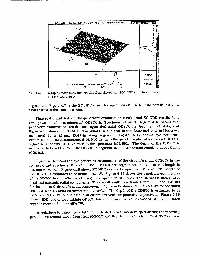
Fig. 4.5. Eddy current NDE test results from Specimen SGL-288 showing an axial

ODSCC indication.

segmented. Figure 4.7 is the EC NDE result for specimen SGL-415. Two parallel 40% 'W

axial ODSCC indications are seen.

Figures 4.8 and 4.9 are dye-penetrant examination results and EC NDE results for a

throughwall axial-circumferential ODSCC in Specimen SGL-418. Figure 4.10 shows dye

penetrant examination results for segmented axial ODSCC in Specimen SGL-495, and

Figure 4.11 shows the EC NDE. Two axial SCCs (5 and 12 mm [0.20 and 0.47 in.] long) are

separated by a 12-mm (0.47-in.)-long segment. Figure. 4-12 shows dye penetrant

examination of the circumferential ODSCC in the roll-expanded region of specimen SGL-591.

Figure 4.13 shows EC NDE results for specimen SGL-591. The depth of the ODSCC is

estimated to be =80% *TW. The ODSCC is segmented, and the overall length is about 5 mm

(0.20 in.).

Figure 4.14 shows the dye-penetrant examination of the circumferential ODSCCs in the

roll-expanded specimen SGL-571. The ODSCCs are segmented, and the overall length is

=15 mm (0.59 in.). Figure 4.15 shows EC NDE results for specimen SGL-571. The depth of

the ODSCC is estimated to be about 90% TW. Figure 4-16 shows dye-penetrant examination

of the ODSCC in the roll-expanded region of specimen SGL-564. The ODSCC is mixed, with

axial and circumferential components. The overall length is =16 and 6 mm (0.63 and 0.24 in.)

for the axial and circumferential component. Figure 4-17 shows EC NDE results for specimen

SGL-564 with an axial-circumferential ODSCC. The depth of the ODSCC is estimated to be

=95% and 90% 'W for the axial and circumferential components, respectively. Figure 4.18

shows NDE results for multiple ODSCC introduced into the roll-expanded SGL-366. Crack

depth is estimated to be =45% TW.

A technique to introduce axial SCC in dented tubes was developed during the reporting

period. Ten dented tubes from Heat NX8527 and five dented tubes from Heat NX7968 were

60

-IW

-On

.20

Fig. 4.6. Dye-penetrant examination of Tube SGL-415 showing segmented axial ODSCC.

Fig. 4.7. Eddy current NDE test results for Tube SGL-415 showing two =40% 7W axial ODSCC indications.

61

Fig. 4.8. Dye penetrant examination of tube SGL-418 showing circumferential-axial ODSCC.

Fig. 4.9. Eddy current NDE test results for tube SGL-418 showing TW circumferential-axial

ODSCC indication.

62

4-.

Fig. 4.10. Dye-penetrant examination results for Alloy 600 tube SGL-495 showing segmented ODSCC indications.

,~cn,..-,.qc :C~,Cf ýr,nr n, A f, At viq £.fun

i -,----------, ----.---,--------_______________ -

=.A 4'A

Fig. 4.11. Eddy current NDE test results for Alloy 600 tube SGL-495 showing segmentation of axial ODSCC.

63

DA-

Fig. 4.12. Dye-penetrant examination of roll-expanded Alloy 600 tube SGL-591 with 5-mm (0.20-in.)-long circumferential ODSCC indications.

/

IF

Fig. 4.13. Eddy current NDE test results of roll-expanded Alloy 600 Tube SGL-591 with circumferential ODSCC indications of 80% 7W depthk

64

Fig. 4.14. Dye penetrant examination of roll-expanded Alloy 600 tube SGL-571 with segmented circumferential ODSCC indications.

pot

Fig. 4.15. Eddy current NDE test results of roll-expanded Alloy 600 tube SGL-571 with circumferential ODSCC indications of 90% TW depth.

65

l

330 -1

K 4

Fig. 4.16. Dye-penetrant examination of roll-expanded Alloy 600 tube SGL-564 with

16-mm (0.63-in.)-long axial and 6-mm (0.24-in)-long circumferential ODSCC

indications.

Fig. 4.17. Eddy current NDE test results of roll-expanded Alloy 600 tube SGL-564 with

axial-circumferential ODSCC indications of 95 and 90% TW depth.

66

Fig. 4.18. Eddy current NDE test results for Alloy 600 tube SGL-366 showing ODSCC indications in roll-expanded area

processed for axial SCC. Figure 4.19 is a photomacrograph of specimen SGL-397 showing a 12.7-mm (0.5-in.)-long mechanical dent introduced on the OD surface. Figures 4.20 and 4.21 are EC NDE results for the specimen SGL-397 before and after the introduction of axial IDSCC, respectively. The depth of the IDSCC is estimated to be =60% 'W. Figure 4.22 shows dye penetrant examination results for dented specimen SGL-527, indicating segmented axial ODSCC. Figure 4.23 is a photomicrograph of the OD of the specimen SGL-527. Figure 4.24 is an example of a dye-penetrant examination of OD axial cracks in dented specimen SGL-447. Two parallel axial ODSCCs with lengths of 20 and 30 mm are seen.

The solution and sensitization heat treatments cause grain growth and a reduction in hardness and flow stress. Tensile tests were performed for eight tube specimens (SGMCO0 1 through 008) at room temperature to measure the reduction of flow stress for Alloy 600 tubes (Heat NX8527). The results show that ultimate tensile and yield strengths of the as-received mill-annealed tubes are 696±t14 MPa (101±2 ksi) and 317±14 MPa (46±2 ksi), while the corresponding values for the heat-treated tubes are 600±_14 MPa (87±2 ksi) and 179±t14 MPa (26±2 ksi), respectively. Thus, the flow stress of the material is reduced by -20% due to the heat treatments. A correction for this effect on mechanical properties will be required when these tubes are used for subsequent pressure and leak-rate testing. To minimize this effect on mechanical properties, different heat treating conditions are being investigated. In particular, specimens were heat treated at lower temperatures and tested for stress corrosion cracking. Twenty Alloy 600 tube specimens were solution-heat-treated at 990-10200 C (1814-1868OF) rather than 1 1000 C (2012'F) and are ready for SCC testing. Hardness measurements were performed for the Alloy 600 specimens from Heat No. NX8527 that were heat treated at different temperatures, and the results are summarized in Table 4.1. It appears that the hardness begins to drop substantially at solution-heat-treating temperatures of =9901C (1814 0 F) and greater.

67

8-1624-32 40--48',,

Fig. 4.19. Photomacrograph of specimen SGL-397 showing axial dent on OD surface.

bTIe: I•.R R MAR--I- S 00 ROE 0 COL 0 1013

K~jrk.I 8 3001 Diff 1 8 180 : Df 300 -GýI -C4 W2 iff I7

�,

47 -I-

0.00

0.00

IVD,, IxRI FVm IGAnj 11801

Mi +22581I

Fig. 4.20. Eddy current NDE test results from SGL-397 before degradation.

68

I- -,-.", ............ .... ....... .. ..... q . ý ]T•,hA •,-imm•nf•

0.00 vtd sp~an 36 rot 40uG1IC4 W~ertl G1 I C4 Morz

S..................... -........................ S.................... Ii........................

t.,Ja...,, a. LLJ

SGOO 8 1CAL000D THU 16:25:53 MDAR-2-99 SG 00 ROE 0 COL 0 1130

I C4 V 0.00 v/d span 44 rot 290

•___ IV~~~nn IMAUl W~nlu !Vi•Al181

rM IT + 31690 b.-iA

40.00

0.00T

Fig. 4.21. Eddy current NDE test results from specimen SGL-397 after degradation.

A new heat (Heat NX8620) of 22.2-mm (7/8-in.)-diameter Alloy 600 tubes was obtained for the program in addition to heats NX8527 and NX7968. This new heat was mill-annealed for 2 to 3 min at two different temperatures: 980'C (1796°F), Heat NX8520L, and 10601C (1940'F), Heat NX8520H). The chemical composition of the new heat is presented in Table 4.2 along with that of heats NX8527 and NX7968. The hardnesses of this material as-millannealed and after sensitization were measured, and the results are summarized in Table 4.3. Further materials properties characterization will be conducted for this new heat.

To examine the influence of the oxide film on EC response, 10 cracked tubes were oxidized in high-temperature-water environments. Of these, five tubes (SGL-1 14, 159, 170, 182, and 187) were oxidized in deionized high-purity water with 8 ppm dissolved oxygen at 290'C (5541F) and 8.8 MPa (1280 psi) for 1680 h. Five additional tubes (SGL-127, 149, 169, 189, and 197) were oxidized in deionized high-purity water with 3 ppm dissolved oxygen at 290°C (554°F) for 120 h and then in a simulated primary water environment (1200 ppm B and 2 ppm Li) at 320'C (6081F) and 12.4 MPa (1800 psi) for 1400 h. Eddy current NDE was performed before and after the oxidation treatment. Results from the EC examinations of these specimens are described under Task I in Section 2.4 of this report. The BC voltages were found to increase significantly for the oxidized tubes, though the shape of the Lissajous figures remained unchanged. In contrast, the results for the +Point coil were inconclusive.

Three additional cracking facilities were constructed to increase the production rate of cracked tubes. Each facility will be able to handle four individual tube specimens to produce axial ODSCC. The existing cracking facilities were also refurbished to improve the stability of the applied loads. Efforts are continuing to produce additional degraded tubes with more complex geometries prototypical of field SCC, e.g., axial ODSCC with ligaments between small multiple cracks. Future efforts will focus on degrading tubes with denting or on producing cracking at the roll expansion.

69

....... ..... ......... I. .................... .......... ........

Fig. 4.22. Dye penetrant examination of dented Alloy 600 tube SGL-527 showing segmented axial ODSCC indication.

Fig. 4.23. Photomicrograph of dented Alloy 600 tube specimen SGL-527 showing an

axial ODSCC (433X).

70

Fig. 4.24. Dye penetrant examination of dented Alloy 600 tube SGL-447 showing two parallel axial ODSCC indications.

Table 4.1. Hardness vs. heat treatment (Alloy 600, Heat NX8527)

Specimen ID Heat Treatment Vickers Hardness

5455-4 As Received 181

5457-3 As Received 176 SGL-684 9600C 20 min, 6000 C 48 hr 165 SGL-694 9700C 20 min, 6000C 48 hr 169

SGL-673 9800 C 20 min, 6000C 48 hr 173 SGL-710 9900C 20 min, 6000C 48 hr 161

SGL-703 10000C 20 min, 6000C 48 hr 153 SGL-130 11000C 10 min, 6000C 48 hr 136

71

Table 4.2. Chemical compositions of three heats of Alloy 600 (wt.%)

Element Heat NX8520 Heat NX8527 Heat NX7968

Carbon 0.022 0.025 0.040

Manganese 0.19 0.21 0.24

Iron 8.03 8.49 8.38

Sulfur <0.001 <0.001 0.001

Silicon 0.21 0.13 0.14

Copper 0.02 <0.01 0.18

Nickel 75.63 75.20 75.44

Chromium 15.40 15.35 15.58

Aluminum 0.21 0.23 a

Titanium 0.26 0.36 a

Cobalt 0.02 0.02 a

Phosphorus 0.004 0.005 a

Boron 0.004 0.001 a

Nitrogen <0.01 <0.01 a

aNot reported.

Table 4.3. Hardness vs. heat treatment for heats NX8527 and NX8520

Heat No. Heat Treatment Vickers Hardness

NX8527 Mill annealed (940'C 3 min) 179

NX8527 Mill annealed + 1100°C 10 min. and 148 6000 C 48 h

NX8520 L Mill annealed (980'C 3 rmin) 162

NX8520 H Mill annealed (1060'C 2 min) 146

72

4.2 Testing in the Pressure and Leak-Rate Test Facility

Testing continued in the high-temperature Pressure and Leak-Rate Test Facility through the first three months of the present reporting period, after which effort was diverted to the production of cracked tubes for the Steam Generator Tube Mockup (see Section 2.1) and the assembly of the High-Pressure Test Facility (see Section 4.3). The tests conducted in the Pressure and Leak-Rate Test Facility during this three-month period are described here.

These additional tests (beyond those described in the previous annual report 2 ) were conducted on 22.2-mm (7/8-in.)-diameter Alloy 600 (Valinco heat NX8524) tubes containing axial OD electrodischarge machined (EDM) notches of various lengths and depths. Tests were also conducted on tubes containing multiple interacting flaws. The flawed tubes were all 0.56 m (22 in.) long, with the flaw centered at 0.15 m (6 in.) from the end of the tube that was fitted with a welded plug. The unplugged end of the tube is held in place in the test module vessel by a Swagelock fitting mounted on a blind flange with a hole that allows the flow from the blowdown vessel to enter the flawed tube. Tests have also been conducted on a specimen containing an axial ODSCC crack produced by Westinghouse with doped steam for comparison with ANL-produced SCC flaws. All SCC flaws were analyzed structurally, and the results are described in Section 4.5.3 and Ref. 3. These tests of SCC flaws were directed at addressing questions concerning flaw leak stability under constant temperature and pressure associated with normal operating and MSLB conditions. Tests were conducted at both room temperature and 2820C (5490F) to assess flaw behavior dependence on temperature.

4.2.1 Characterization of the Flaws

All flaws tested in the Pressure and Leak-Rate Test Facility are characterized before and after testing. In general, the EDM flaws tested are relatively easy to characterize with respect to flaw dimensions, but characterization of the SCC flaws is much more difficult. Because of the need to evaluate leak-rate and flaw-opening-pressure prediction capabilities and improve the models if necessary, accurate information on flaw pre- and posttest dimensions and leak area is essential. Procedures have been developed and implemented to obtain these data by using the following flaw characterization steps:

1. Eddy current NDE is used to obtain crack depth profiles and voltage information.

2. Ligament failure and burst pressures are estimated by analyses using the crack depth profiles determined by NDE.

3. Flaw regions are characterized by dye-penetrant techniques and digital photography.

4. Tubes are bubble-tested with low-pressure air (276 kPa, or 40 psi) in a water bath to identify regions of throughwall penetration.

5. Posttest destructive examination of specimens with part-throughwall flaws is carried out to help validate the estimated of depth obtained by NDE and to better understand the process of failure, i. e. how crack segments grew and linked to produce the failure.

73

For SCC flaws (as opposed to EDM notches), the use of dye-penetrant inspection and

digital photography is an essential part of pre- and posttest flaw characterization to relate flaw

characteristics to leak behavior. These procedures, along with image processing techniques

involving NIH Image software, are used to obtain flaw information such as crack area, total

linear length, location, and number of branch points. Computerized digital image analysis of

flaw images yields a more systematic and less subjective characterization of flaw features than

does use of an optical microscope or measuring manually from photographs.

Throughwall portions of the crack are identified by a low-pressure leak test. With the

dye-penetrant still in the crack, the capped tube is mounted in a low-pressure (276 kPa, or

40 psi) pressurization apparatus and submerged in a water bath. The flaw region is observed

with a low-magnification optical microscope underwater for gas bubbles indicating leaks.

4.2.2 Testing of Specimens with EDM Axial Notches

Tests on axial notches of length 25.4 and 9.0 mm (1.0 and 0.35 in.) at room and elevated

temperature were performed. Testing of multiple axial flaws also began during this reporting

period.

Single Axial Notches

Results from a test on a TW EDM 25-mm (l-in.)-long axial notch of initial width 0.19 mm

(0.0075-in.) [tube T14EAIWXI] at room temperature are presented. The pressurization of the

tube was done in two stages. In the first stage, the internal pressure was increased in four

steps (0.69, 6.9, 10.3, and 13.8 MPa [100, 1000, 1500, and 2000 psi]), at which point the test

was stopped and the tube removed to measure flow area prior to higher-pressure testing in

which unstable tearing was anticipated. This permitted a check on our ability to predict the

flaw opening and the flow rate at this intermediate stage of pressurization. The flaw at this

stage of the test is shown in Fig. 4.25. Based on a two-dimensional projection, the flaw

opening area is 52 mm2 (0.081 in. 2 ),. The measured flaw length was 24.9 mm (0.98 in.), and

the maximum flaw width was 2.8 mm (0.11 in.). Based on the measured opening area, a

pressure differential of 13.8 MPa (2000 psi), an orifice coefficient of 0.6, and the fluid density

at 751F, the orifice flow through the flaw would be 312 L/min (82.5 gpm). This is in good

agreement with the experimentally observed flow rate of 302 L/min (79.8 gpm).

In the second stage of the test, the tube (T14EATWX1) was reinstalled in the facility and

pressurized to higher levels. The test was restarted by quickly raising the pressure to

13.8 MPa (2000 psi) and holding for a short time to reestablish a flow rate of 302 L/min

(79.8 gpm), in agreement with that observed when the test was interrupted. The pressure was

then raised in a series of 0.69 MPa (100 psi) increments. The leak rate increased significantly

with each increment of pressure. At =15.9 MPa (2300 psi), the flow rate increased abruptly

and the pressure dropped momentarily before stabilizing at 12.8 MPa (1859 psi), at which

point a flow rate of 1,098 L/min (290.0 gpm) was observed. Figure 4.26 shows the posttest

flaw opening area; the unstable tearing that occurred at 15.9 MPa (2300 psi) is seen at each

end of the notch. Figure 4.27 is a side view of the flaw bulge. The projected flow area is

170 mm 2 (0.264 in. 2 ), the projected length 21.8 mm (0.86-in.), and the maximum flaw width

11.7 mm (0.46 in.).

74

4 8 12 16 20 24 28 4 8 12 15 20 MADE IN U2S2A4 5

8 16 24 32 4,0 48 56 8 16 24 32 40

Fig. 4.25. Opening of 25.4-mm (1-in.)-long axial 100% TWEDM notch (tube TI4EATWX1) after test was interrupted at 13.8 MPa (2000 psi) to measure flaw area.

Fig. 4.26. Opening of 25.4-mm (1-in.)-long axial 100% TW EDM notch in tube shown in Fig. 4.25 (tube T1 4EATWXI) after continuing test to 15.9 MPa (2300 psi).

75

Fig. 4.27. Side view of tube specimen shown in Fig. 4.26, showing three-dimensional bulging

at failure site.

Based on the measured opening area, the pressure differential of 12.8 MPa (1859 psi), an

orifice coefficient of 0.6, and the fluid density at 75°F, the orifice flow rate is 984 L/min

(260 gpm), which is 114 L/min (30 gpm) lower than that observed. This underprediction (in

contrast to the accurate prediction for the first stage of the test) is probably the result of the

large amount of bulging associated with the flaw (Fig. 4.27).

A simple geometric correction factor was obtained by comparing the curved arc length of

the flaw, 24.3 mm (0.958 in.) with the projected length, 21.8 mm (0.86 in.). The ratio is 1.114.

Applying this correction factor to the flaw opening area gives an orifice flow rate of

1,096 L/min (289.5 gpm), in good agreement with experiment.

A pressurization test was also performed on tube T13EA90X.35, which has a partial TW

axial ODSCC EDM flaw of length 8.9 mm (0.35 in.), width of 0.19 mm (0.0075-in.), and a

uniform 90% throughwall depth. This flaw length is shorter than any previously tested. The

tube was first tested at room temperature, with the pressure increasing in 0.69 MPa (100 psi)

increments up to 19.3 MPa (2800 psi). No flaw opening or tube leakage occurred, and the test

was terminated at this pressure when the pressure relief valve began to leak. Upon removal

and inspection, the tube showed virtually no crack widening or bulging of the tube wall. The

tube was reinstalled and tested at 282°C (5400 F) at increasing pressure up to 19.3 MPa

(2800 psi). Again the tube did not leak, and post-test inspection revealed no change in the

flaw width or tube bulging. The observed >19.3 MPa (2800 psi) ligament failure pressure

exceeds the prediction of both the ANL and Battelle models. The ANL model predicts a failure

pressure of 18.6 MPa (2700 psi) at room temperature and 16.9 MPa (2450 psi) at 282°C

(540'F), and the Battelle model predictions are 12.4 and 11.0 MPa (1800 and 1600 psi),

respectively. Failure pressures observed in previous tests on tubes with notches of 12.7 mm

(0.5 in.) or longer were very close to the predicted values.

76

Multiple Notches

Tests were also performed on two identical tubes each with two aligned axial EDM TW notches separated by a short axial ligament. The notches were each 6.35 mm (0.25 in.) long and 0.19 mm (0.0075 in.) wide and were separated by a 0.25-mm (0.01-in.)-long full-wallthickness ligament.

The first of these two tubes (T24EATWX.5 LIG) was tested at room temperature at pressures up to 17.2 MPa (2500 psi). Figure 4.28 is a posttest photograph of the flaw; little structural distortion is evident, and the flaw exhibited only a 50-75 jtm (0.002-0.003 in.) increase in width at the end next to the ligament. Calculations indicated that the ligament would tear at a pressure considerably lower than 13.8 MPa (2000 psi). However, posttest inspection after pressurization to 17.2 MPa (2500 psi) with no failure revealed no tearing of the ligament, although stretch marks were evident on the ligament outer surface. The observed leak rate through the flaw during the test was essentially identical to that calculated for the two individual notches. At pressures of 14.5 and 17.7 MPa (2100 and 2500 psi), the flaw flow rate was 14.8 and 18.5 L/min (3.9 and 4.9 gpm), respectively. However, as described earlier, single axial notches shorter than =12.7 mm (0.5 in.) appear to exhibit higher strengths (i.e., higher opening pressures and smaller flow areas) than predicted by the models that have been found to accurately predict the behavior of longer axial notches.

The second tube (T25EAT'WX.5 LIG) was tested at 2820 C (5400 F). Ligament tearing occurred at 15.5 MPa (2250 psi). The tearing coincided with an abrupt increase in flow rate as the two notches merged. The resulting leak rate corresponded to that expected for the resulting 12.7-mm (0.5-in.) notch. The posttest appearance of tube T25EATWX.5 LIG after testing at pressures up to 17.9 MPa (2600 psi) is shown in Fig. 4.29. Ligament tearing and appreciable flaw widening are apparent.

At 14.5 MPa (2100 psi) (ligament intact) and 17.2 MPa (2500 psi) (ligament torn), the flow rates for tube T25EATWX.5 LIG were 17.0 and 32.2 L/min (4.5 and 8.5 gpm), respectively. At the maximum test pressure of 17.9 MPa (2600 psi), the flow rate was 35.6 L/min (9.4 gpm). This tube had a higher flow rate at all pressures, even before ligament tearing, than did tube T24EATWX.5 LIG at room temperature as would be expected because of the somewhat reduced flow stress at the higher temperature. After tearing, the notch behaved like a longer, and hence weaker, flaw.

4.2.3 Testing of Specimens with Laboratory-Produced SCC Flaws

Results from tests on four Alloy 600 tubes with laboratory-produced axial ODSCC of nominal length 12.7 mm (0.5 in.) were presented in the previous report.2 The tubes were cracked in an aqueous sodium tetrathionate solution after a sensitization heat treatment. A 22.2-mm (7/8-in.)-diameter Alloy 600 tube (T505CATW2-10) with an axial ODSCC flaw produced by Westinghouse with doped steam was tested during the present reporting period (Test W 2-10). ANL tubes 177 and 195 were tested at room temperature, and ANL tubes 104 and 219 were tested at 2820C (5400 F). The Westinghouse tube W 2-10 was tested at both temperatures.

77

Fig. 4.28. Posttest photograph of tube T24EATWX.5 LIG tested at room temperature at up to

17.2 MPa (2500 psi), showing little flaw distortion and intact ligament.

24 32 40_48!

Fig. 4.29. Posttest photograph of tube T25EATWX.5 LIG tested at 2820 C (5400 F) at up to

17.9 MPa (2600 psi), showing appreciable flaw notch widening and torn ligament.

The four ANL-produced tubes were selected as having the same nominal axial ODSCC

crack length of 12.7 mm (0.5 in.), as determined by dye-penetrant examination, as well as

other similarities. The Westinghouse tube had an axial ODSCC flaw of similar length.

Figure 4.30 shows the pretest image of the flaw in the Westinghouse tube accentuated by dye

penetrant. The flaw is axial and has an overall length of 12.4 mm (0.49 in.). Bubble-testing at

276 kPa (40 psi) revealed that the flaw had two locations of throughwall penetration,

coinciding with the two largest dye stains in Fig. 4.30. Each penetration exhibited very small

78

16- 243 2 .40 -48 56 Aht!;ffi~iith IdtIII~lI~i;dItdlUIIID J

Fig. 4.30. Pretest dye-penetrant digital image of Westinghouse ODSCC cracked tube produced using doped steam (Test T505CA7W2-1 0).

intermittent bubble generation. The largest dye stain on the right exhibited a larger bubble size and higher generation frequency than that on the left.

For comparison with the Westinghouse test, the following observations summarize the results from the tests of the four ANL-produced SCC tubes (Tests SGL-177, SGL-195, SGL104, and SGL-219):

1. All SCC flaws were very tight and had regions of throughwall penetration, as determined by bubble testing. However, none of the four flaws exhibited detectable water leakage at pressures below 8.3 MPa (1200 psi), nor was leakage detected during a 2-h (or greater) hold time at this pressure. Detectable leakage did not occur until much higher pressures were attained.

2. Posttest inspection showed that three flaws opened significantly in width along their entire length, even into the extremities of the Y branches on each end of the main flaw. The exception was Test SGL- 177, for which the nominal EC voltage of 4 V was considerably lower than the values of 6-10 V observed for the other three tubes. Additionally, the latter three tubes had several obvious posttest secondary cracks emanating from the main crack, even though these cracks were barely perceptible in pretest characterizations. Furthermore, the region around the flaws was raised noticeably upward, or puckered. However, Test SGL- 177 exhibited very little puckering. Tests previously conducted on 12.7-mm (0.5-in.)-long axial EDM notches over the same pressure range produced significantly less puckering.

3. Specimens in three of the four tests (SGL-195, SGL-177, and SGL-219) exhibited crack tearing under constant temperature and pressure conditions, which caused the leak rate to increase under constant pressure.

79

4. Specimen flaws in three of the four tests (SGL-195, SGL-104, and SGL-219) suddenly

opened to their full extent at pressures less than that associated with MSLB, yielding flow

rates of 23 to 38+ L/min (6 to 10+ gpm). These three tubes had the highest EC voltages

(6-10 V). This behavior suggests that once a small ligament tears, there is a strong

tendency for other ligaments to tear in a domino fashion (sometimes after a delay under

constant pressure) until the crack is completely open over its full extent. Test SGL- 177,

which had the lowest voltage (4 V), had a leak rate of only 1.7 L/min (0.44 gpm) and did

not exhibit this behavior.

The detailed structural analysis predictions and a proposed flaw behavior model for these

flaws and the Westinghouse flaw (T505CATW2-10) is presented in Section 4.5.3.

Eddy current examinations suggest that all four ANL-produced SCC flaws had variable

crack depths along their lengths (see Section 4.5), with maximum depths of 75 to 95%. The

Westinghouse tube exhibited a similar crack depth profile. The throughwall regions identified

by bubble testing in both the Westinghouse and the four ANL flaws were not seen by EC

techniques because of their tightness and very small axial extents. The EC BC voltage for the

Westinghouse tube was 4.5 V, very close to the 4.0 V exhibited by the ANL tube in Test SGL

177. The other three ANL tubes had higher EC voltages in the range of 6-10 V. The crack

depth profile for the Westinghouse tube was used not only to qualitatively prescreen the flaw

for similarity with the ANL flaws but also in calculations to estimate the initial flaw-opening

pressure. Analysis indicates that the Westinghouse tube was most similar to the ANL tube in

Test SGL-177, although somewhat stronger. Hence, the Westinghouse tube was expected to

exhibit leak behavior similar to that of the ANL tube. Because of the similarity to the ANL

tube, which was tested at room temperature, the initial testing phase for the Westinghouse

tube was also conducted at room temperature, with follow-on testing at 282°C (540'F).

In the room-temperature test of the Westinghouse tube, the pressure was increased from

0 in 1.4-2.1 MPa (200-300 psi) increments, with hold times of 15-30 min at each level until

8.3 MPa (1200 psi) was reached. The pressure was held at this level for 2 h. Like the four

ANL specimens, the Westinghouse tube exhibited no observable leakage during this portion of

the test, even though all of these tubes were shown to have localized throughwall penetration

during bubble testing at very low pressure. Following the 2-h hold at 8.3 MPa (1200 psi), the

pressure was increased in a series of steps to 17.2 MPa (2500 psi) over 45 min. Again, no leak

was observed. After a subsequent hold time of 3.25 h at this pressure, a leak rate of

=0.04 L/min (0.01 gpm) was detected. The 17.2 MPa (2500 psi) pressure was held overnight,

and the tube continued to leak, with the leak rate increasing to =0.068 L/min (0.018 gpm) by

the following morning. The pressure on the Westinghouse tube was then raised to 18.6 MPa

(2700 psi) and held at this level for 5.5 h, at which time a leak rate of 0.12 L/min (0.032 gpm)

was measured. The room-temperature phase of the test was terminated at this point. Thus,

the Westinghouse tube, like SGL-177, developed a leak under constant pressure and exhibited

an increasing, although somewhat lower, leak rate over an extended hold period.

The blowdown tank was refilled with water, and the tube was then tested at 2820 C

(540'F) and 18.6 MPa (2700 psi) to determine the leak rate at this temperature and to see if

the crack would open further. The flow rate was observed to increase from =0.30 L/min

(0.08 gpm) to 0.72 L/min (0.19 gpm) during a 2-h hold at this -pressure. The test was then

terminated and the tube was removed. A posttest photograph of the flaw is shown in

80

Section 4.5.3 (Fig. 4.85). The flaw has opened slightly over its entire axial extent (see pretest photograph of Fig. 4.30). Like Test SGL- 177, no flaw-zone puckering was evident.

The above behavior suggests that ligament failure in an SCC flaw may occur progressively, sometimes with delays under constant loading conditions. In flawed specimens in which the width of the remaining ligament is highly variable, initial leakage occurred abruptly at pressures significantly lower than those predicted by the equivalent rectangular crack approach (See Section 4.5.3). The experimental evidence of time-dependent increase of leak rate possibly due to progressive ligament rupture at 2821C (540°F), as well as at room temperature, highlights the fact that no criterion for predicting time-dependent ligament rupture is currently available. More laboratory-cracked tubes with SCC flaws and, eventually, service-degraded tubes with SCC flaws, will be tested to develop a better understanding 9f tube flaw behavior.

4.3 High-Pressure Test Facility

Design and construction of a new room-temperature tube testing facility with a maximum operating pressure of 51.7 MPa (7,500 psi) and a maximum flow rate of 48.4 L/mln (12.8 gpm) has been completed and has successfully undergone shakedown and performance quantification testing. This facility is being readied for the testing of tubes with SCC flaws produced at ANL and of tubes with more complex tight segmented laser-cut notches.

The room-temperature High-Pressure Test Facility permits pressure testing of tubes that cannot be failed in the high-temperature Pressure and Leak-Rate Test Facility, which has a 20.7 MPa (3000 psi) pressure limit. Most high-pressure tube test facilities have very low flow capabilities so that almost all very deep or throughwall flaws must be tested using a bladder and frequently a backup foil to prevent leakage through the flaw resulting in system depressurization. Very short pressurization times of =2-3 s are used to minimize the tendency for bladder extrusion and leakage through the flaw. The Argonne facility, because of its 48.4 L/min (12.8 gpm) flow capability at 51.7 MPa (7500 psi), allows tubes with small TW flaws to be tested without the use of a bladder. When bladders and foils are required, the small leaks that can occur during tube pressurization may not result in an aborted test.

This facility can also be used for very-long-duration crack stability tests and for longduration crack jet impingement erosion tests on adjacent tubes, since water can be continuously supplied from an outside source during a test. The apparatus is also capable of measuring very low flow rates (considerably less than the 0.04 L/min [0.01 gpm] lower limit for the Pressure and Leak-Rate Test Facility) through the use of flaw leak collection and timed measurement of water mass. Additionally, the optical access to the crack location permits real-time ultra-high-speed video recording (2000-12,000 frames per second) of crack and jet dynamic behavior during testing.

4.3.1 Facility Description

Figure 4.31 is a schematic diagram of the High-Pressure Test Facility, and Fig. 4.32 is a photograph of the overall facility. The facility is pressurized by a constant-rpm single-acting triplex constant-displacement pump driven by a 60-hp electric motor (see Figure 4.33) that

81

Pressure Transducers (2)

Fig. 4.31. Schematic diagram of High-Pressure Test Facility pressurizer and associated

components.

Fig. 4.32. Overall view of major components of High-Pressure Test Facility: water pump

pressurizer, test module, tube support, video system, and 3000-L (800-gal) tank for

conducting tests on field-pulled tubes. Also shown is LexanTM personnel-protection

barrier.

82

Fig. 4.33. Water pump pressurizer

provides a constant 48.4 L/min (12.8 gpm) flow of water at up to 51.7 MPa (7500 psi). The pump-generated pressure pulsations were found to be small, <0.34 MPa (<50 psi). The pump has two overpressurization protection safety relief valves, one located on the pump and the other on the 139-L (40-gal) water accumulator suction tank. The lever-operated hydrodiverter control valve furnished with the pressurizer was modified to work in series with a screw unloader valve, that allows more positive, finer remote control of tube pressurization. The pressurizer water pump system was also modified to operate with a continuous supply of water from the building water system by installing a pressure regulating valve on the water line supplying the pump accumulator suction tank. The facility operation is no longer limited by the 40 gal reservoir supplied with the pump, and thus extended-duration leak tests can now be conducted. Pump-generated water heating can be avoided by bleeding water to the drain during long-duration tests and adding cold makeup water.

The test module protective enclosure shown in Fig. 4.34 consists of an 0.46-m (18-in.)diameter, 1.02-m (40-in.)-long stainless steel pipe. A transparent LexanTM plate at each end of the test module confines the water jets and spray produced by a leaking tube. The ultra-highspeed video camera and light source for illuminating the test tube are also shown in Fig. 4.34.

The tube support system, shown in Fig. 4.35, consists of two collars that fit around the tube and can be located anywhere along its length. It can provide either single or two-point lateral support. The ability to vary tube lateral support conditions is important in testing tubes with circumferential flaws, where flaw behavior is sensitive to tube constraint. The twopoint support also prevents axially flawed tubes from undergoing significant bending from jet thrust upon failure.

The basic operation of the facility can be described with reference to Figs. 4.31-4.35 according to the following steps:

83

Fig. 4.34. Test module and high-speed video camera and high-intensity light source mounted

on test module support table.

Fig. 4.35. Tube support system.

84

1. The tube to be tested is mounted in the test module and fastened to the supply hose that feeds water from the high-pressure pump. All air is bled from the supply line and test specimen through a high-pressure valve fastened to the downstream end of the tube. This valve is then closed during the test.

2. The accumulator suction tank is filled with water. If the test is expected to produce some leakage before failure or to be of extended duration, the water supply line to the accumulator tank can be opened to provide a continuous water supply for long-duration testing. Both tap water and deionized water are available.

3. The high-pressure bleedoff valve and the diverter control valve are both set fully open and the pump is then turned on, causing flow recirculation through the bypass lines to the accumulator suction tank. The tube specimen will be pressurized at <275 kPa (<40 psi) at this point. For long-duration tests, water temperature rise caused by pump heating is minimized by dumping water to the building drain and adding cool makeup water to the accumulator tank.

4. The high-pressure bleedoff valve is then fully closed, and the diverter control valve is slowly closed to direct the flow to the test specimen, causing its internal pressure to rise. The diverter control valve allows the pressure to be established at any value in the range from 0 to 51.7 MPa (0 to 7500 psi). Downstream and in series with the diverter valve is a spring-loaded screw unloader valve, which furnishes a more precise linear control of pressure than can be obtained using the diverter control valve. When this valve is used, the diverter control valve is set to the fully closed position, allowing flow and pressure to be controlled by the screw unloader valve, which also has a bypass line.

5. When the desired maximum test pressure has been reached or the tube has failed, the test is terminated by opening the diverter control valve, turning the pump off, and opening the high-pressure bleedoff valve.

Tube pressure is read on an analog pressure gauge and is also measured and recorded by two redundant pressure transducers. A sustained flow of up to 48.4 L/min (12.8 gpm) can be maintained through a leaking specimen at any pressure up to 51.7 MPa (7500 psi), depending on flaw geometry and flow resistance. The flow is measured by both timed direct collection and weighing of water from the test module and by a flowmeter immediately upstream of the tube. All data are recorded redundantly on both a multi-channel strip chart recorder and a dedicated computer digital data acquisition system that uses LabView software.

The tube pressurization rate can be varied from quasi-steady-state (<0.7 MPa/s or <100 psi/s) to 7-21 MPa/s (1000-3000 psi/s), which encompasses the EPRI guideline range for burst testing, to 70 MPa/s (10,000 psi/s). Pressurization over the full range of the system, 0-52 MPa (0-7500 psi), is possible at all of these pressurization rates. The screw unloader valve provides very precise and reproducible linear pressure control at all pressurization rates. The potential also exists for programmed control of pressurization for more complex pressure transient histories.

85

4.3.2 Results from High-Pressure Test Facility

Facility checkout, the establishment of test protocols and initial flaw testing were

conducted through a series of tests on 22.2-mm (7/8-in.)-diameter Alloy 600 SG tubes with small circular orifice holes and EDM axial notches. The circular orifice hole flaws allowed facility checkout with continuous flow, and the part-throughwall flaws permitted operation

with no flow until ligament tearing or tube burst occurred during pressurization. These tests

are described below.

Circular-Hole Tests

A 0.80-mm (1/32-in.)-diameter sharp-edge circular-orifice-flawed test tube was held in

the test module by the two-point constraint lateral support. Two test runs were made with the

tube, the first with pressure plateaus up to 51.7 MPa (7500 psi) and the second with plateaus to 34.5 MPa (5000 psi). For both runs, six to eight pressure plateaus were held for nominally

5 min each, with total test time of <35 min. For each pressure plateau, the flaw flow rate and pressure were measured. The pressurizer control operated very smoothly over the full range, and the pressure pulsations generated by the triplex pump were <0.34 MPa (<50 psi). The

turbine flowmeter readings were checked against the timed collection of water from the flaw, and the two results were in agreement. The system installed for controlled dump of water

from the pressurizer water accumulator tank was successful in preventing excessive pump

heating of the water during these 35-min tests.

The tube was examined visually after each test, and interesting structural changes were

observed. It should be noted that this same flaw geometry had been used in previous shakedown tests of the Pressure and Leak-Rate Test Facility, and no tube changes were noted during several short-duration tests. Posttest examination of the aluminum plate holding the

test specimen mounting brackets, which is parallel to the tube and upon which the orifice jet impacts from an =125-mm (=5-in.) standoff distance, revealed two large jet-impact erosion craters, one for each test. The craters were nominally 1.6-3.2 mm (1/16-1/8 in.) deep and =3.2-6.3 mm (1/8-1/4-in.) wide. The crater for the highest pressure test was the largest. The

tube wall had also undergone some plastic distortion at the location of the two support brackets. Additionally, some erosion in the Alloy 600 tube orifice hole was detected after the

first test, and the second test of this same tube yielded a higher flow rate than predicted by

the circular-orifice flow model, even at the initial low pressures. This suggests that the hole geometry/area was increased by jet erosion during the first test.

EDM Axial Notch Tests

Prior to testing the SCC flaws, tubes with OD axial EDM TW and part-TW notches predicted to be unstable at <51.7 MPa (7500 psi) are being tested. These tests were used to

develop and validate techniques for testing with and without bladders and various bladder/shim combinations. These tests also can be used to assess the influence of bladders and pressurization rate on ligament tearing and unstable flaw failure pressures. A total of 42 flawed specimens of several different designs have been fabricated, with some flaw geometries in triplicate for the assessment of test reproducibility and other test parameter effects on the

data. These notches are all 0.19 mm (0.0075 in.) wide and of four axial lengths, namely 6.35,

86

12.7, 19.1, and 25.4 mm (0.25, 0.5, 0.75, and 1.0 in.). Flaws depths are 60, 80, 90, and 100% '1W.

The flaw geometries ensure that the tests will encompass a range of failure behaviors. For example, the 12.7-mm (0.5-in.)-long 60% TW flaw is expected to exhibit unstable tearing, or bursting, at a pressure of 38.6 MPa (5,600 psi) simultaneous with ligament failure. This is in contrast to an 80% TW flaw of this length, which will first undergo ligament tearing at 25.5 MPa (3700 psi) and subsequent unstable bursting at 30.3 MPa (4,400 psi). For this flaw geometry, when ligament failure occurs, the flow rate will be well above the maximum 48.4 L/min (12.8 gpm) system capability, and pressurization to a higher level is not possible. Hence, this flaw would require a bladder to achieve the flaw burst pressure. In contrast, the 60% TW flaw of the same length can be burst without a bladder; this flaw geometry can then also be tested with a bladder to allow assessment of the influence of bladders on burst data. These flaw geometries are also being tested at different pressurization rates.

Three identical 80% 'W 19.1-mm (0.75-in.)-long axial notches (OM107, OM122, and OM109) were tested in three different pressurization scenarios. A slow quasi-steady-state pressurization rate resulted in ligament tearing at 21.4 MPa (3100 psi), pressurization at 13.8 MPa/s (2000 psi/s) produced ligament tear at 24.2 MPa (3510 psi), and pressurization at 48.3 MPa/s (7000 psi/s) produced ligament tear at 26.4 MPa (3830 psi). The predicted ligament tearing pressure for this flaw geometry is 20.7 MPa (3000 psi), which is in good agreement with the quasi-steady pressurization rate test OM107.

Figures 4.36-4.38 show the posttest flaw openings. All three flaws exhibited ligament failure but no discernible unstable tearing at the notch ends. In addition to the increase in ligament failure pressure with pressurization rate, there is a slight increase in maximum notch opening width with increasing pressurization rate.

The behavior of the 12.7-mm (0.5-in)-long 80% 'W flaw (OM120) under a quasi-steadystate pressurization rate without a bladder was similar to that of the 19.1-mm (0.75-in)-long 80% TW flaw tested under similar conditions. A posttest photograph of the flaw OM120 is shown in Fig. 4.39. It experienced ligament tearing at a pressure of 26.9 MPa (3900 psi), which is in reasonable agreement with the predicted value of 25.5 MPa (3700 psi). No discernible unstable tearing occurred at the notch ends. Testing of this flaw at faster rates of pressurization is underway to see if the ligament tear pressure will exhibit a dependence on pressurization rate, as did the 19.1-mm (0.75-in.)-long flaws.

The 80% 'W flaws of 12.7 and 19.1-mm (0.5- and 0.75-in.) length have also been tested with bladders to see if unstable tearing would occur. The tests were performed with a 2.4-mm (3/32-in.)-thick wall hard Tygon bladder and no backup metal foil. Figures 4.40 and 4.41 show photographs of how a bladder with an OD slightly smaller than the tube ID is sealed in the tube with a bored tapered Teflon plug to prevent water penetration between the bladder and the tube ID. For an initially 'W flaw, such leakage would result in possible premature flaw leakage and possibly prevent further pressurization if the leakage is excessive.

Figures 4.42 and 4.43 are posttest photographs of flaw opening for the bladder testing of the 80% TW flaws of 12.7 mm (0.5 in.) (OM121) and 19.1 mm (0.75-in.) (OM123) lengths,

87

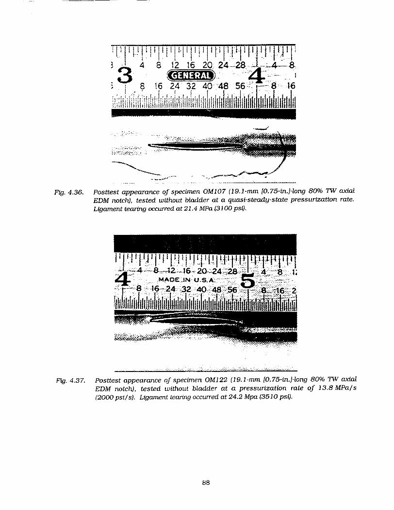
~~~~ III I II- !,•I I ' I I • ' I [I I: lj I ! I' I!' iT 3 J 4 8 12 16 20 24 -28, J, ;-_ -8,

3 4l. .....8 6 24 32 40-48 5616

Fig. 4.36. Posttest appearance of specimen OM107 (19.1-mm [0.75-in.]-long 80% 7W axial

EDM notch), tested without bladder at a quasi-steady-state pressurization rate.

Ligament tearing occurred at 21.4 MPa (3100 psi).

Fig. 4.37. Posttest appearance of specimen OM122 (19.1-mm [0.75-in.]-long 80% TW axial

EDM notch), tested without bladder at a pressurization rate of 13.8 MPa/s

(2000 psils). Ligament tearing occurred at 24.2 Mpa (3510 psi).

88

Fig. 4.38. Posttest appearance of specimen 0M109 (19.1-mm [0.75-in.J-long 80% TW axial EDM notch), tested without bladder at a pressurization rate of 48.3 MPa/s (7000 psils). Ligament tearing occurred at 26.4 MPa (3830 psi).

)24_-28 8L-- 67-02 4. MADE-,.N USA .~~56 8 A& 16-24 -32- 4 f

Fig. 4.39. Posttest appearance of specimen OM120 (12.7-mm 10.5-in.r-long 80% TW axial EDM notch), tested without bladder at a quasi-steady-state pressurization. Ligament tearing occurred at 26.9 MPa (3900 psi), as compared to the predicted failure pressure of 25.5 MPa (3700 psi).

89

C. 4

Fig. 4.40. Side view of tube with bladder and bored plug seal being installed.

f ~ ~ f - V- r I T I . I . f ^" , 1 1 , 'I ,

Fg. 4.41. End view of tube with bladder and plug installed.

90

4

F!

128. 24J2 4 LI MADEJN U.SA---,5- '16-24 84O56--1

Fig. 4.42. Posttest appearance of specimen 0M121 (12.7-mm [0.5-irn]-long 80% TW axial EDM notch), tested with bladder at a pressurization rate of 13.8 MPa/s (2000 psils). Flaw burst occurred at 29.0 MPa (4200 ps)i, as compared to the predicted failure pressure of 30.3 MPa (4400 psi).

Fig. 4.43. Posttest appearance of specimen 0M123 (19.1-mm [0.75-in.]-long 80% TW axial EDM notch), tested with bladder at a pressurization rate of 13.8 MPa/s (2000 psils). Flaw burst occurred at 21.9 MPa (3180 psi), as compared to the predicted failure pressure of 22.8 MPa (3300 psi).

91

respectively. These tests were conducted at a nominal pressurization rate of 13.8 MPa/s

(2000 psi/s). Clearly, both flaws experienced significant unstable bursting, with a large

amount of tearing at both ends of each original notch. As noted above (Figs. 4.37 and 4.39),

these flaws experienced ligament tearing but could not be burst without a bladder. The

experimental/predicted unstable burst pressures for the 12.7 and 19.1-mm (0.5 and 0.75-in.)

long 80% TW flaws were 29.0/30.3 MPa (4200/4400 psi) and 21.9/22.8 MPa (3180/3300 psi),

respectively. These flaws will also be tested with bladders at different pressurization rates.

A 12.7-mm (0.5-in.)-long 60% TW flaw, unlike an 80% TW flaw of the same length, is

predicted to exhibit unstable tearing or bursting simultaneous with ligament tearing at a

pressure of 38.6 MPa (5,600 psi). Hence, this flaw can be tested with and without a bladder to

assess the influence of bladders on burst data. Figure 4.44 shows a post-test photograph of

tube OM 113 with such a flaw that was tested without a bladder at a pressurization rate of

13.8 MPa/s (2000 psi/s). The flaw burst unstably without a bladder at 40.7 MPa (5900 psi),

as compared to the predicted burst pressure of 38.6 MPa (5600 psi).

Figure 4.45 is a posttest photograph of Tube OM1 12 with the same flow geometry tested

with a 2.4-mm (3/32-in.)-thick hard bladder at a pressurization rate of 13.8 MPa/s

(2000 psi/s). The flaw burst at 41.4 MPa (6000 psi), versus the predicted value of 38.6 MPa

(5600 psi). Use of the bladder caused significantly more unstable tearing of the notch ends

than in Tube OM1 13. However, most important, the burst pressure was almost the same as

for Tube OMI 13, which failed at 40.7 MPa (5900 psi).

Presented next are results from tests on tubes with a 12.7-mm (0.5-in.)-long 100% TW

EDM axial OD notch. This flaw cannot be unstably burst in the High-Pressure Test Facility

without the use of a bladder because the flow rate at the burst pressure exceeds the

48.4 L/min (12.8 gpm) limit of the facility. This flaw geometry was tested with two different

bladder types using the same pressurization rate of 13.8 MPa/s (2000 psi/s). Tube OM102

was tested with a hard TygonTM bladder having a 2.4-mm (3/32-in.)-thick wall, and Tube

OM101 was tested with a 3.2-mm (1/8-in.)-thick hard bladder. The post-test results for the

thinner bladder test (OM102) are shown in Fig. 4.46. As shown in the side view, the bladder

has extruded through the flaw opening created by ligament tearing, and, as seen in the top

view, the flaw has undergone a very slight amount of unstable tearing at both ends. The flaw

unstably burst at 29.6 MPa (4300 psi), which is close to the predicted value of 30.3 MPa

(4400 psi).

Figure 4.47 shows the posttest appearance of tube OM101, which was tested with the

thicker bladder. The thicker bladder did not extrude through the flaw, in contrast to tube

OM102, and significantly more flaw bulging and unstable tearing took place at the notch ends.

Tube OM101 burst at 29.6 MPa (4296 psi), which is good agreement with the predicted value

of 30.3 MPa (4400 psi), despite the more extensive tearing with the thicker bladder. Thus, the

proper use of bladders produces a unique value for the unstable burst pressure for a given

flaw geometry, irrespective of the extent of tearing. However, it is readily apparent that the

resulting leak areas can be drastically different. The question therefore arises concerning the

correct area to be used at unstable burst for the purposes of predicting the leak flow rate. It is

believed that this can only be determined through a detailed simulation of flaw structure and

fluid dynamic interactions during burst.

92

MAOE..IJNU 6 r~ 24 -32 40.48

Fig. 4.44. Tube GMl 13 with a 12.7-mm (0.5-in.)-long 60% TW EDM axial OD notch, tested without a bladder.

I t I I I ' I I ' I lI - I 1' - 11 I'1 / 24 28 4 12.6 20 -241-.28

MADE #NU.S.A. 58 8:1--2 32 40 48,5

Fig. 4.45. Tube OM112 with a 12.7-mm (0.5-in.)-long 60% TW EDM axial OD notch, tested with a bladder.

93

Fig. 4.46. Side (left) and top (right) views of Tube OM102 with a 12.7-mm (0.5-in.)-long 100%

TW EDM axial notch, tested with a 2.4-mm (3/32-in.)-thick hard bladder at a

pressurization rate of 13.8 MPa/s (2000 psils).

121 6 20 24 28 4. -8..8•42-16 20 , 4- MADE -IN U.S.A 24 32 40 48 56 8 '16--24 32. ,'4•o,,

24 32 40 48 56MADE IN U.S

16 24 32 40 I.1 F

Fig. 4.47. Top (left) and side (right) views of tube OM101 with a 12.7-mm (0.5-in.)-long 100%

TW EDM axial OD notch, tested with a 2-4-mm (18-in.)-thick bladder at a

pressurization rate of 13.8 MPa/s (2000 psils).

94

Tl 'I

4.4 Pre-Test Analysis of Crack Behavior

4.4.1 Model for Predicting Failure of Partially Supported Tube with a Circumferential Crack

Circumferential cracks in SG tubes are often detected at the top of the tube sheet in PWR nuclear generating plants. Analytical models 4 for the failure of tubes with circumferential cracks predict that the pressure required to cause onset of crack extension may fall within the design-basis accident condition (17 MPa, or 2500 psi) if the tube section that contains the crack is free to bend and the crack is sufficiently long (>180'). It is also known that if the crack section is fully constrained against rotation, the failure pressures are significantly increased and cracks must be much longer (>3000) to be of concern. In an actual SG, the tubes are neither free to bend nor fully constrained. The degree of constraint on a circumferential crack at the top of the tube sheet depends on the span between the top of the tube sheet and the first TSP or baffle plate (15-125 cm or 6-50 in.). Recent tests on SG tubes have shown that tubes that are laterally supported fail at significantly higher pressures than tubes that are free to bend. 5

An extensive series of tests on failure and leak rates in circumferentially flawed reactor coolant piping subjected to externally applied forces and moments has been conducted at Battelle under the USNRC-sponsored Degraded-Piping6 and Short Cracks in Piping and Piping Welds Programs. 7

A simplified stability analysis of circumferentially cracked reactor piping was presented by Tada et al.,8 who analyzed the pipe as a beam whose cracked section was subjected to plastic limit moment. A similar approach was followed by Smith to analyze failure9 and leakage' 0 of a TW circumferential crack in piping. Smith 1 1 also emphasized the importance of the cracksystem compliance on the onset and stability of crack extension and leakage through a crack. In all of these analyses, plasticity was confined to the crack section, while the rest of the pipe responded elastically. In this report, we use the similar approaches to analyze the problem of failure of SG tubes with circumferential cracks under internal pressure loading in the absence of externally applied forces and moments, and we consider the case where plastic deformation may spread to sections other than that of the crack.

Description of Model

Consider a tube of mean radius R, wall thickness h, and length L, containing a TW circumferential flaw of angular length 20 at any axial location. The tube can be subjected to various edge conditions. For example, the tube may be clamped at one end (simulating the tubesheet) and simply supported at the other end (simulating the first TSP). Figure 4.48 shows such a tube with the crack at the top of the tube sheet. Under internal pressure loading, FEA shows that a tube in the configuration of Fig. 4.48 deforms as shown in Fig. 4.49 with a definite crack flank rotation and crack tip opening displacement. In the present report, limit load analysis will be used to estimate failure pressure of tubes made of ductile materials such as Alloy 600.

We assume that the tube is thin and is under internal pressure loading only (no constraint on axial deformation of the tube), and that the onset of crack extension occurs after the

95

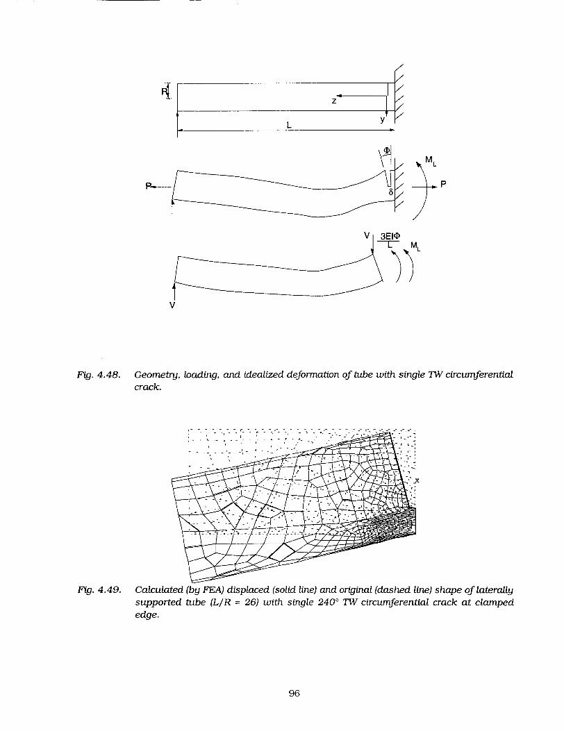
M L

Fig. 4.48. Geometry, loading, and idealized deformation of tube with single 7W circumferential crack.

Fig. 4.49. Calculated (by FEA) displaced (solid line) and original (dashed line) shape of laterally supported tube (L/R = 26) with single 2400 TW circumferential crack at clamped edge.

96

attainment of the limit state. The last assumption is valid if the Battelle Screening Criterion 12

is satisfied, i.e.,

R (I 1 (4.1)

where E is the Young's modulus, 5c is the critical crack tip opening displacement, and Uis the flow stress. Thus, for Alloy 600 SG tubing with E = 207,000 MPa (30,000 ksi), U = 483 MPa (70 ksi), R = 10 mm (0.4 in.), and 20 = 2700, we find that 5c > 0.1 mm (0.004 in.), which is generally satisfied by all ductile alloys.

The stress distribution through the section containing the crack at the limit-state is shown in Fig. 4.50. We further assume that plastic deformation is limited to only the section containing the crack, while the rest of the tube responds elastically.

The bending moment (about the tube centerline) and axial force equilibria of the stress distribution of the limit-state (Fig. 4.50) give the following:

ML = 4UR24(1sin 0- sinlJ (4.2)

and

=n-6 P n-0 npR 03=--T (4.3a) 2 4Rh- 2 4b-h'

or

pb -h=ý 40 (4.3b) Pb Oh nit 7C

where P defines the location of the plastic neutral axis, p is the internal pressure, and Pb is the burst pressure of an unflawed tube.

Plasticity Confined to Crack Section

Denoting the calculated bending moment (positive counterclockwise in Fig. 4.50) in an undefected tube at the crack location (z = 0) by M (for internal pressure loading, M = 0) and by considering the equilibrium of the bending moment in the elastic part of the tube just to the left of the crack section with the plastic limit moment ML acting just to the right of it (see Fig. 4.48).

M = -ML + 3EI = 0, (4.4)

where I is the bending moment of inertia (niRh), and (D is the rotation at the cracked section due to crack opening (Fig. 4.48). Equation 4.4 is applicable for the configuration shown in

97

Fig. 4.50. Stress distribution through section at collapse of a tube with single TW

circumferential crack

Fig. 4.48. It can be generalized for any set of edge conditions and crack locations by using an

effective length Le. The generalized version of Eq. 4.4 is as follows:

M = -ML + O = 0. (4.4a) Le

The relationships between L and Le for several crack locations and edge conditions are given in

Table 4.4. The plastic rotation (Dc about the neutral axis at the onset of crack extension is

related to the critical crack tip opening displacement 5c by

_c = _ 8____(4.5) - R(cos 3 + cos 0)'

Combining Eqs. 4.2, 4.4a, and 4.5 at the point of crack initiation,

(½sinO- sinl3)(cosp + cosO)- c = 0, (4.6a)

where

_Ec (4.6b)

4 Le•"

Equation 4.6a can be solved for the critical value P3= 13c, which when substituted in

Eq. 4.3b, gives the crack initiation pressure Pc. Note that the equation for the free-bending

case can be obtained by setting Le = oo, i.e., c = 0 in Eq. 4.6a.

The onset of crack extension can also be expressed in terms of the critical value of the

plastic component of the deformation J integral Jp, which, for the bending case, is defined in

terms of the plastic rotation 0 as follows:

98

Table 4.4. Effective lengths of tubes for several circumferential crack locations and edge conditions.

Edge conditions and crack location Effective length

Le =,L/ Clamped Clamped Le L/4

Clamped Clamped Le = L

S.S. Clamped Le L/3

dp -= - do, (4.7)

where A = 2RhO. In the context of limit analysis J =Jp and M = ML, as given in Eq. 4.2. Differentiating Eq. 4.2 with respect to 6 and noting from Eq. 4.2 that at constant rotation, i.e., at constant pressure,

013 _1

a - 2'

J = R7Gf0(cosj3+cosO)d0 = RUO(cosi3+cosO). (4.8)

Thus, the critical plastic rotation is given in terms of the critical J integral Jc as follows: Jc

'c RU(cos 0 + cosO) (4.9a)

Comparing Eq. 4.5 and 4.9, we recover the familiar equation

Jc = .8c. (4.9b)

A plot of the fracture toughness Kjc = EJC versus the critical crack tip opening displacement is shown in Fig. 4.5 1. For ductile alloys, the critical crack tip displacement is somewhere in the range of 0.76-2.54 mm (0.03-0.1 in.).

Crack Opening Area (COA). If the critical crack opening displacement is not exceeded and there is no crack extension, the crack opening area can be expressed in terms of the rotation ( and crack size by

99

600 . , . .. . ..

500

L~400Cz 550 MPa

aZ 300 13_•.300 •450 MPa

0

200 Flow Stress = 350 MPa

100 . .

0 0.5 1 1.5 2 2.5 3 8C (mm)

Fig. 4.51. Variation of fracture toughness with

critical crack tip opening displacement.

A = 2R240" (cos P + cos a)dca = 2R24(Ocos • + sine). (4. 10a)

Using Eqs. 4.4a and 4.2, Eq. 10a reduces to (for 0 -< )j

A= 8 (0cosp + sine 1sin0- sin. (4. 1Ob)

At the point of crack initiation, 0 = oc and 0 = PC, which when substituted in Eq. 4. 10b, gives

(using Eq. 4.5)

A = Ac = 2R8c (0cos c + sine) (4. 10c) (Cos PC + Cos e)

Instability.

Unstable failure need not necessarily be associated with onset of crack extension. If the

crack is to be unstable at onset of crack extension under constant loading, the following

condition must be satisfied (using Eq. 4.4a) for

dM dML + <0, (4.11)

d do Lee

with dML measured at the onset of crack extension. Equation 4.11 can be expressed in terms do)

of the familiar tearing modulus by first differentiating Eq. 4.8 with respect to e,

&J oU JMdo) r 1 1d dJ -+--=R~~ X -sin0--sin + d-(cosP+cos6) (4.12a)

dO M4 a d 4 2 c) dO)

100

and then solving

1 dJ sin 0 - I sino3

U~j -2 d_ do cosl3+cos0 dO Ra(cosp3+coso) (4.12b)

Differentiating Eq. 4.2 with respect to 0, using Eq. 4.12b, and rearranging, we obtain the condition of instability as

1

2 Le (COS p + COS 0)2 J sin s E dJ(4 nR Rcs )2 C OS dJ-C' (4. 13a)

where a is the crack length (RdO = da). We can identify the left-hand-side of Eq. 4.13a as the applied tearing modulus, TApp, and the condition of instability can be written as

2 Le2 EJ sinO- I sin Tp- (cos• +COS 0)c2 _l-3co_ > TMAT. (4.13b) TAPP = 7cRRa2 COS p + COS 0

Note that Eq. 4.13b is the same as that given by Smith. 10 For ductile materials with high crack growth resistance, the J-term is usually negligible. In such cases, we can simplify Eq. 4.13b as

TApp = -• (COS p + COS 0)2 > TMAT. (4.13c)

For many ductile alloys, TmAT = 200.

Results. A plot of the failure (onset of crack extension) pressure versus crack angle is shown in Fig. 4.52 for various values of the elastic stiffness parameter c. Note that even for a low value of c (i.e., large Le), tubes with long cracks behave as if they were fully constrained. For c > 0.5, tubes with any crack behave as if they were fully constrained. Figure 4.52 also shows the maximum angular lengths of TW circumferential cracks corresponding to typical pressures during normal operation and design basis accident conditions. If we use the nominal values E = 207,000 MPa (30,000 ksi) and ? = 483 MPa (70 ksi) for the mechanical properties in Eq. 4.6b, we then calculate

c = 300Qse (4.6b) Le'

The value of the critical crack tip opening displacement Sc must be obtained from failure tests on tubes with circumferential cracks. Plots of the calculated normalized failure (onset of crack extension) pressure as a function of the span are shown in

Figs. 4.53a-b for a 1800 crack at several locations, edge conditions, and for critical crack tip opening displacements of 0.25 and 0.75 mm (0.01 and 0.03 in,), respectively. Similar plots for a 2400 crack and a 2700 crack are shown in Figs. 4.54a-b and 4.55a-b, respectively. Depending on the span, the model predicts that the failure pressure is increased significantly

101

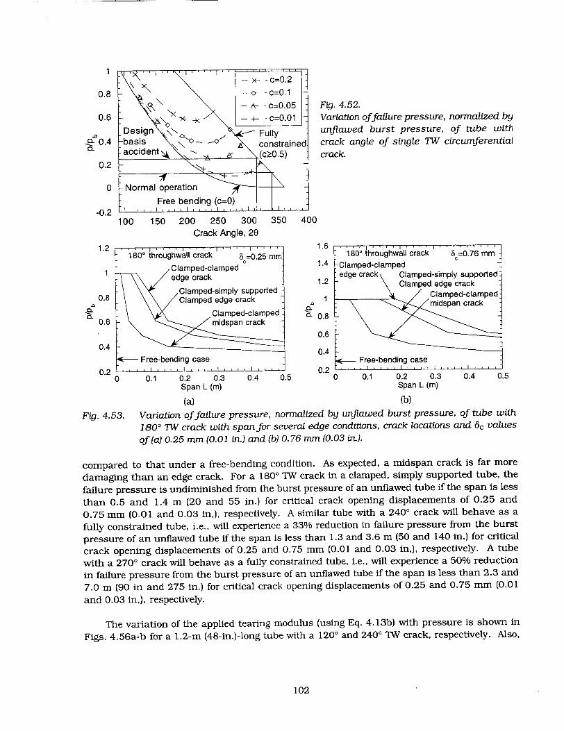
I

0.8 -3- o-c=O. 1 \- c=0.05 Fig. 4.52.

0.6 'x 4> -- - c=0.01 Variation offailure pressure, normalized by

De .4bsisn Ful unflawed burst pressure, of tube with constranedscrak angle of single TW circumferential

accident (cŽ!0.5) cak

0.2+

0 -Normal operation

100 150 200 250 300 350 400

Crack Angle, 20

1800 whoghall crackl 8 =0.'25' m'm' 1800 houghwall'crack 8' =0O.7'6mm'

Clamped-clamned C1.4 -Clamped-clamped edge crack edge crack Clamped-simply supported: e rc1.2 Clamped edge crack

Clamped-simply supportedClmecapd Clamped edge crack 1lamiedspncracke

Clamped ed-ecrampdk. 0.6 midspan crack

0.6 0.4

0.4 < Free-bending case F~ree-bending case

0 0.1 0.2 0.3 0.4 0.5 0 0.1 0.2 0.3 0.4 0.5 Span L (in) Span L (in)

(a) (b)

FMg. 4.53. Variation of failure pressure, normalized by unflawed burst pressure, of tube with

180' 7W crack with span for several edge conditions, crack locations and 5c values

of (a) 0.25 mm (0.01 in.) and (b) 0.76 nmm (0.03 in.).

compared to that under a free-bending condition. As expected, a middspan crack is far more

damaging than an edge crack. For a 1800 TW crack in a clamped, simply supported tube, the

failure pressure is undiminished from the burst pressure of an unflawed tube if the span is less

than 0.5 and 1.4 m (20 and 55 in.) for critical crack opening displacements of 0.25 and

0.75 mm (0.01 and 0.03 in,), respectively. A similar tube with a 240' crack will behave as a

fully constrained tube, i.e., will experience a 33% reduction in failure pressure from the burst

pressure of an unflawed tube if the span is less than 1.3 and 3.6 m (50 and 140 in.) for critical

crack opening displacements of 0.25 and 0.75 mm (0.01 and 0.03 in,), respectively. A tube

with a 2700 crack will behave as a fully constrained tube, i.e., will experience a 50% reduction

in failure pressure from the burst pressure of an unflawed tube if the span is less than 2.3 and

7.0 m (90 in and 275 in.) for critical crack opening displacements of 0.25 and 0.75 mm. (0.01

and 0.03 in,), respectively.

The variation of the applied tearing modulus (using Eq. 4. 13b) with pressure is shown in

Figs. 4.56a-b for a 1.2-rn (48-in.)-long tube with a 1200 and 2400 TW crack, respectively. Also,

102

0.8

0.6edge crack 0.6 edge crack

0.2 0 CaeClamped-simply supportert S0.4 Clamped edge crack .0.4

0.2 0.2 ~-Clamped-simplysupre

Clamped edge crack Clamped-clamped

0 Free-bending case Clamped-clamped 0 Free-bending case midspan crack midspan crack

0 0.1 0.2 0.3 0.4 0.5 0.6 0.7 0.8 0 0.2 0.4 0.6 0.8 1 Span L (m) Span L (m) (a) (b)

Fig. 4.54. Variation of failure pressure, normalized by unflawed burst pressure, of tube with 2400 TW crack with span for several edge conditions, crack locations, and 5c values of(a) 0.25 mm (0.01 in.) and (b) 0.76 mm (0.03 in.).

0.6 ....... 0.6 2700 throughwall crack 8=0.25 mm 2700 throughwall crack 5 =0.76 mm

G C 0.5 Clamped-simply supported 0.5 \ • Clamped edge crack

0.4 Ca0.4 lamped-lampedClamp~ed-clampededg crc edge crack 0o.3 0.3

0.2 ped 0.2 Clamped-simply supported Clampeddedgeamped midspan crack Clamped edge crack Clamped-clamped

0.1 0.1 - midspan crack SFree-bending case 4(--r Free-bending case

0 0.2 0.4 0.6 0.8 1 1.2 0 0.2 0.4 0.6 0.8 1 1.2 Span L (m) Span L (m) (a) (b)

Fig. 4.55. Variation of failure pressure, normalized by unflawed burst pressure, of tube with 2700 TW crack with span for several edge conditions, crack locations and 8c values of(a) 0.25 mm (0.01 in.) and (b) 0.76 mm (0.03 in.).

shown in the figures are the pressures at which a crack tip opening displacement of 1.3 mm (0.05 in.) is reached as indicative of the pressures for the onset of crack extension. In the case of the 1200 crack, the J-term of Eq. 4.13a is small compared to the applied tearing modulus. Because the applied tearing modulus is less than TMAT = 200, the crack should propagate stably after the onset of crack extension. For the 2400 crack, the J-term is not negligible unless the pressure at the onset of crack extension is small (P/Pb <<0.3). However, since the J-term (positive) in Eq. 4.13a has a stabilizing influence, the initial crack growth will be stable in both cases.

Limitations of the model. The onset of yielding away from the crack plane can be calculated by using the current model and assuming a loading path consisting of first applying the

103

0.8

200 ' '•8i. . . . . . . . .60 .. .................. 20 in.'' '! ~ 6 L=48 in. 1200 Midspan crack 50 .2400 Midspan crack ....... ........ J-term....-150 --------- --- .......................

., 40 --..... ------------- ................... ------- .............- ........ ......... I ............

-0 0 ---------------..................... ................ --------- ........ ................. g a 0

S~J-term::

a) a 0 .... .0............

............ --------- .... ............

0- .................. ........ ......... ...................................... . 005 in.

-50 . i.-10 -•, .

0.75 0.8 0.85 , 0.9 0.95 1 0 0.1 0.2 0.3 0.4 0.5 0.6 0.7 P/Pb P/Pb

(a) Mb)

Fig. 4.56. Variation of applied tearing modulus and J-term in Eq. 4.13 with pressure

(normalized by the unflawed burst pressure) of clamped edge tube with midspan

cracks of angular length (a) 1200 and (b) 240'.

membrane stresses due to pressure, keeping the bending stresses at zero, and then applying

the bending stresses holding the membrane stresses constant. Although the axial bending

analysis in the current model is uniaxial, the axial yield stress Sy is adjusted to account for the

biaxial stress effect by assuming it to vary with the hoop stress ah as follows (Fig. 4.57a):

]•y2-h for Gh-<OyY S= Oy f (4.14)

!-2- foroh>oY

where ay is the virgin uniaxial yield stress. If we denote the bending moment to cause first

yielding in an uncracked section just adjacent to the cracked section by My,

= Sy (4.15a) My- R'

and Eq. 4.2 can be written in a nondimensional form as follows:

ML 4 f My -• •sin O0- sin 13•(4.15b)

MY n iSyl (2 P).

Thus, the condition for first yielding in an undefected section just adjacent to the cracked

section by bending is

ML 4 (Isinm0-sin I 1. (4.16a)

Noting that yielding of the undefected tube section can occur either by axial bending or by

yielding in the hoop direction by membrane hoop stress, we find that the pressure to cause first

yielding (denoted by py) is the lesser of the following two values:

104

0.55

yield surface./ 0.5

0.45

0.6

V cr A x a L0 .3 5 0 .5 - Initial yield

L surface 0.3 CFy 0.4

0.25 =0. 150 200 250 300 350

26 (a) (b)

Fig. 4.57. (a) Determination of axial yield strength Sy for bending analysis using Tresca criterion and (b) predicted variation of pressure to first yield the tube away from crack plane with crack angle as a function of ratio between yield and flow stress.

Py {2,y s(Isin 0 -sinf)(.6b

Pb U _2y (4.16b)

Since 3 is a function of pressure (Eq. 4.3a), Eq. 4.16b must be solved numerically. A plot of the pressure to first yield versus crack length is shown in Fig. 4.57b for various values of yield to flow stress ratios.

4.4.2 Finite-Element Analysis

To provide a basis for comparison with the analytical models, an incremental elasticplastic FEA that uses a multilinear kinematic hardening rule was conducted for a tube (L/R = 60, simply supported at one end and clamped at the other) with a 2400 'TW circumferential crack at the clamped end under internal pressure loading. The assumed stress-strain curve is shown in Fig. 4.58. The difference between kinematic and isotropic hardening rules should be small for the nearly radial loading path used for the problem at hand. Comparisons of the variation of the crack section rotation and support reaction with pressure are shown in Figs. 4.59a-b, respectively. The slight discrepancies between the FEA results and the model predictions at low pressures are due to neglecting the elastic deformation in the model. However, the FEA results diverge from the model calculations significantly as the pressure exceeds =50% of the unflawed tube burst pressure. This is because at these higher pressures, tube sections away from the crack plane experience significant plastic deformation (Fig. 4.60), which is assumed to be negligible in the model. Note that with ay/d = 0.5, the analytical model predicts (Fig. 4.61 b) onset of yielding in a tube containing a 2400 crack at P/Pb = 0.43, which agrees very well with the FEA result. Thus, the limit of applicability of the current model depends on the crack angle as well as the strain hardening behavior (Oy/U) of the material (Fig. 4.57b).

105

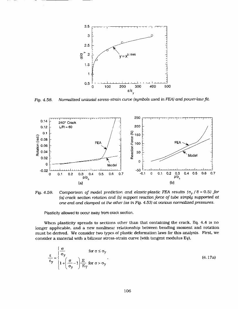
100 200 300 400 500

Fig. 4.58. Normalized uniaxial stress-strain curve (symbols used in FEA) and power-law fit.

0 0.1 0.2 0.3 ( P/P(

(a)

250

200

;-150

0 LL 100

50

c 5

0.4 0.5 0.6 0.7-50 L

-0.1 0 0.1 0.2 0.3 P/Pb

(b)

0.4 0.5 0.6 0.7

Fig. 4.59. Comparison of model prediction and elastic-plastic FEA results (ay / i = 0.5) for

(a) crack section rotation and (b) support reaction force of tube simply supported at

one end and clamped at the other (as in Fig. 4.53) at various normalized pressures.

Plasticity allowed to occur away from crack section.

When plasticity spreads to sections other than that containing the crack, Eq. 4.4 is no longer applicable, and a new nonlinear relationship between bending moment and rotation

must be derived. We consider two types of plastic deformation laws for this analysis. First, we

consider a material with a bilinear stress-strain curve (with tangent modulus ETr),

[ for a _c y

EY 1+G -.I for a > a ( y )E

(4.17a)

106

3.5

3

2.5

1.5

1

0.5

0.14

0.12

0.1

S0.08

0 0.06

"5 0.04 cc

0.02

0

-0.02

1EA

Model

I. . I . . .. I I . i

240' throughwall

axial ---- -hoop

crack Top of tube ,

Bottom of tube , ,1.5

1

• 0.5 CU 0

._2 -0.5

-.. -1

-1.5

0 0.1 0.2 0.3 0.4 0.5 0.6 P/Pb

Fig. 4.60. Calculated (by FEA with yield stress/flow stress = 0.5) variation of plastic strains, with normalized pressure, at top and bottom of section located at axial distance 4R from crack in laterally supported tube (L/R = 60) with single 2400 TW circumferential crack at clamped edge.

Hoop

Axial

Fig. 4.61. Radial loading path used in FEA is replaced in model by nonradial path consisting of loading to fimal pressure (at 2 to I stress ratio), followed by applying axial bending stress at constant hoop.

and second, a material with a power-law hardening stress-strain curve is considered,

cr for (Y 5 c

Y -a - for cr>a y

2

Top of tube

0.7

(4.17b)

107

. I . .IIIq

In both cases, we continue to assume that the section containing the crack is at the plastic

limit state with flow stress i, the assumption being that the crack section experiences

extensive plastic deformation long before any plastic yielding occurs away from the crack

section.

To keep the analysis tractable for the current analytical model, we make a simplifying

assumption that the stresses and total deformation at any pressure can be obtained by

considering a nonradial loading path, consisting of first loading radially to the final pressure

(hoop to axial membrane stress ratio of 2:1) at zero axial bending stress and then applying the

axial bending stresses, holding the pressure-induced membrane stresses constant (Fig. 4.61).

This assumption allows us to use the same yield surface (Eq. 4.14 and Fig. 4.57a) for all axial

locations and makes it possible to obtain an analytical solution for the bending problem. The

relatively good agreement between the model prediction and the FEA results, to be discussed

later, shows that this assumption is probably reasonable as long as no unloading or reversed

yielding occurs.

With the above assumptions, we determine a relationship between the bending moment

and rotation in the elastic-plastic regime by a detailed analysis of axial bending of the tube

subjected to an end moment Mo at a constant internal pressure p. For p > py, a length of the

tube extending from z = 0 to z = Zy will deform plastically, while the rest of the beam L > z > Zy

will remain elastic. The stress distributions in a plastically deforming section are shown in

Figs. 4.62a and 4.62b for the bilinear and power law hardening stress-strain curve,

respectively. At every section, there will be an elastic core extending from 0 = -ýy to 0 = Py, with

Py varying from 3y = 13 at z = 0 to Py = 7E/2 at z = zy.

By stress integration and using the definition of Zy, the bending moment at any section is

given by

.M _2 i- Py + 1sin2Jy +-2E-J L-z (4.18a)

MY nsinpyL( El 2E-yL-zy

for the bilinear stress-strain curve and

M 2 ( 1 + 4(1__mr~yim+l L-z

'My-tsn y- sinlsn2PY+y -t2si-n--in)m OdOL=- (4.18b)

for the power-law hardening curve, where My corresponds to the bending moment at first yield

away from the crack section.

Differentiating Eqs. 4.18a-b and solving,

dNy 1 1 (4.19)

dz (L- zy) f( y)'

where

108

(a) (b) Fig. 4.62. Stress distribution through section away from crack section after yield: (a) bilinear for bilinear stress-strain curve and (b) nonlinearfor power-law hardening curve.

2 (y)=21- -•sin2fy + 2E Ssin Iy tan 3 y (4.20a)


_ = _2 _ - V2 sin 2y 2mI20b)

f( - siny ýtany + sinm% tanjy4

for the power-law hardening stress-strain curve with

Im= f sinm+l dO. (4.20c)

The equation for bending is given by

d2 w Ky dz2 sin y (4.21 a)

where w is the transverse deflection and

Y El ER (4.2 lb)

Making a transformation of independent coordinate from z to fOy with the help of Eq. 4.19,

dw 1 1 dw (4.22a) dz - z f(py) d~y

and

109

d2w r 1 ______ I_ I dz2 L(L)- i)

Ksy sin Py"

1 d F 1 dw1

f(y) dpy Lf(y) dpy I(4.22b)

Integrating Eq. 4.22b from 03 = Po (i.e., z = 0) to 3 = ir/2 (i.e., z = Zy), and denoting the slope at z

= 0 by 0o,

dwy dz ZZ

=•)oKy(LZy)fo f(P3y) df3 Psin yY (4.23a)

In a similar fashion,

" f ''(w d f -y)) d(LydI-y. WL=Zy = o( -y) o f Y) sin -y (L - )2 E f(PY)J 0(,- yf_ýo ~ d y sinP y PO O iy

The slope and displacement at z = Zy from the elastic part of the beam are

(4.23b)

My (L- zy)

2EI

w = =-M (L _- )2 -c,(L- -),

where C 1 is an arbitrary constant. Combining Eqs. 4.24a and 4.24b,

(4.24c)dw

Satisfying continuity of slope and displacement at z = Zy, using Eq. 4.24c, and solving gives

4oMo _ 311 + 312 + 1 (4.25)

OYMY 1+13

where

_ 2 P + 1sin2P) + IEET (4.26a)

MY t l s t sin cuErv 2E


110

dw dz Z

and

(4.24a)

(4.24b)

+ W =z y -- - (L - Z y ) ._

M° ( sn 20+ I 7f--tin) •• sinm+lodo (4.26b) My 7E sin P0 sin 1] o

for the power-law hardening stress-strain curve,

*y = MYL (4.26c) .L f

I, = 2 --- d o(4.27a) Po sin y

and

13 =Jf ýf(p3y)doy~ (4.27c)

We can represent the rotation in terms of a function G of the bending moment as follows, with the tangent modulus ETp as a parameter for the bilinear stress-strain curve:

* = •yc(;-ij- (4.28a)

In a similar fashion, for the power-law hardening case, we can represent the rotation in terms of a different function G of the bending moment with the exponent m as a parameter,

=yG(y;mJ. (4.28b)

A plot of the end rotation versus the applied moment for various values of tangent modulus is shown in Figs. 4.63a-b for the case of bilinear stress-strain curve. For perfect plasticity (Dr = 0), the limit moment is reached in = 1.7 times the rotation for initial yield. The bending moment capability of the section increases with increasing value of tangent modulus. However, the plastic rotation is considerably greater than the elastic rotation even for a tangent modulus of ET/E = 1/50. In a similar fashion, a plot of the calculated end rotation versus the applied moment for the power-law hardening case is shown in Fig. 4.64. In both cases, the function G can be represented by a cubic polynomial of the bending moment (see Figs. 4.63b and 4.64):

x for x_< I G(x) = A + Bx + CX2 + Dx 3 for x > 1. (4.28c)

Equation 4.4 can be generalized for the elastic-plastic case as follows:

111

8

7

6

S5 -0

4

3

2

8

7

6

5

4

3

2

1

01 1.1 1.2 1.3 1.4 1.5 1.6 1.7 0 0.5 1 1.5 2

M/M M/M Y y

(a) (b)

Fig. 4.63. Rotation vs. applied bending moment for configuration of Fig. 4.48 (a) for various

values of ET and (b) polynomial fit to curve for ET/E = 1/50.

14

12

10

8

4

2

00 0.5 1 1.5 2 2.5

M/M Y

Fig. 4.64. Model-calculated normalized rotation versus applied bending moment for

configuration of Fig. 4.48 and polynomial fit to results for power-law hardening stress-strain curve with exponent m = 0. 1846 (Fig. 4.58).

-ML+G (4.29a)

or, alternatively

ML) (4.29b)

Onset of Crack Initiation

Combining Eqs. 4.29b and 4.5, at the point of crack initiation,

112

1

(Cos 0c + Cose)c{L - 3E8 31tEc 4 d S4My) - LSy 4L- cSy

4c e - 'R (4.30a)

where ML/My is given by Eq. 4.15b, c is defined in Eq. 4.6b, and Eq. 4.14 can be rewritten as follows:

9~y !--p for p~p _<z (y

_ =! d 2 Pb Pb U (4.30b)

Sr p for P- > -( [2 Pb Pb ;6

Equation 4.30a can be solved for the critical value 0 = f3c which, when substituted in Eq. 4.3b, gives the crack initiation pressure Pc.

The onset of crack extension can also be expressed in terms of the critical value Jc of the

plastic component of the deformation J integral Jp, and Eqs. 4.7, 4.8, and 4.9a-b still hold.

Instability

Proceeding as before, if the crack is to be unstable at onset of crack extension under constant loading, the following condition must be satisfied (using Eq. 4.29a):

dM dML 3E+ M dML 3EM 1 (4.31) de de I L j do d L d M

where dML/d¢ is measured at the onset of crack extension. Using Eqs 4.12a and 4.12b and following the procedure that was used to derive Eq. 4.13b, we find the condition for unstable failure to be

2L )2 E- EJ sin O - 1 sin 3 E dJ TAP (CRo 2 eos2+cos >2 da - TMAT (4.32)

dM)I M=ML

Results

Figure 4.65a shows a comparison of the variation of crack section rotation with pressure as predicted by the model using a bilinear stress-strain curve with that calculated by FEA. A

113

reasonable correlation between the clamped-edge rotation by FEA and the model prediction can

be obtained by assuming ET/E = 1/100 and oy/- = 0.5. Figure 4.65b shows a similar

comparison for the model using a power-law hardening stress-strain curve (Fig. 4.58). As

expected, the model using power-law hardening stress-strain curve fits the FEA data better

than that using the bilinear stress-strain curve. The stresses calculated by FEA are in good

agreement with the elastic-plastic model (Fig. 4.66a-b) using either stress-strain curve.

Figures 4.67a-b show the calculated pressures for crack initiation versus crack angle plots

for various values of the toughness parameter c, calculated using the elastic-plastic model with

a bilinear stress-strain curve and a power-law hardening curve, respectively. Note that for high

values of c, crack initiation pressures (Figs. 4.67a-b) predicted by the models that allow for

plastic deformation away from the crack section can be significantly lower than those

(Fig. 4.52) predicted by the model in which plastic deformation is confined to the crack section.

In particular, the minimums in the curves predicted by the latter model (Fig. 4.52) disappear in

the former models (Figs. 4.67a-b). The plasticity effects are, of course, absent at lower values of

c corresponding to lower crack initiation pressures.

Because the value of c for PWRs is expected to be in the range of 0.5-1, the occurrence of

plasticity away from the crack plane is not a concern in PWRs. However, laboratory leak-rate

and failure tests on circumferentially cracked tubes, such as those reported by the Belgians 2

generally involve significant plastic deformation away from the crack plane. Failure curves that

are based on tests that were performed on circumferentially cracked SG tubes by the Belgians

are similar to those in Fig. 4.67b.

Crack opening areas for a 2400 crack, calculated by the current model (Eq. 4. 1Oc, with P3c

calculated from Eq. 4.30a) and by the small-scale yielding Paris/Tada model,1 3 are shown in

Fig. 4.68. It is assumed that onset of crack extension does not occur before maximum

pressure is reached. In Fig. 4.68, the curve labeled L = -c corresponds to the free-bending case,

whereas the curve labeled L = 0 corresponds to the fully constrained case. Results from the

Paris/Tada model, which is restricted to small-scale yielding in the crack plane and is

independent of the span L, are plotted up to pressure levels significantly above the range of

applicability. It is evident that lateral restraint to bending significantly reduces the COA when

compared with the tube cross-sectional area, even under a design-basis accident condition

(P/Pb = 0.25).

The calculated tearing-modulus-vs.-pressure plots (Figs. 4.69a-b) show a marked increase

in tearing modulus with plastic yielding using either stress-strain curve. The bilinear stress

strain curve (Fig. 4.69a) results in higher values of TAPP for the 2400 crack than those

(Fig. 4.69b) calculated with power-law 'hardening, because the stress increases linearly with

pressure in the bilinear case, whereas it remains relatively bounded in the power-law

hardening case (Fig. 4.58). Figure 4.69b shows that TAPP increases to high values for the

power-law hardening case in a tube with shorter cracks (•1800), indicating that the driving

force for crack instability, which is negligible as long as plasticity is confined to the crack plane,

increases rapidly with plastic yielding away from the crack plane. This is to be expected

because the loss of bending stiffness of the tube with plastic yielding produces a higher elastic

follow-up, which causes the tube to behave like one with a much longer effective span.

However, even with the enhanced values of TApp, tubes with longer cracks (>2400) may not fail

114

C 0

Cr

•0.15

0

6 0

0 CO

0 05

0.05 0.

0

-0.05 -0.1

0 0.1 0.2 0.3 0.4 0.5 0.6 0.7 P/Pb(a) (b)

Fig. 4.65. Variation of crack section rotation with normalized pressure as calculated by FEA (ay / Z = 0.5) and those calculated by a model that allows for plastic yielding away from crack plane using (a) bilinear stress-strain curve and (b) power-law hardening stress-strain curve.

2

0 0.1 0.2 0.3 0.4 0.5 0.6 0.7 P/Pb

(a)

1.5Ca

0.5

•0.

'.,

-0.5 -0

.1 0 0.1 0.2 0.3 0.4

p/pb (b)

0.5 0.6 0.7

Fig. 4.66. Model predictions for stresses, allowing for plastic deformation (ay / U = 0.5) away from crack plane, using (a) bilinear stress-strain curve and (b) power-law hardening stress-strain curve and elastic-plastic FEA results for stresses at section located at distance 4R from crack plane in tube (L/R = 60) simply supported at one end and clamped at the other (as in Fig. 4.49) at various pressures. Symbols, and lines without symbols, represent model calculations and FEA results, respectively.

by unstable tearing at the onset of crack extension (TMAT for ductile alloys like Alloy 600 is typically =200) and will very likely fail by plastic collapse after some stable crack growth. Because, for values of c that are typical for SG tubes (0.5-1), the pressure for onset of crack extension (Fig. 4.67a-b) is already close to the pressure that corresponds to the fully constrained case, the extent of stable crack growth should be small.

115

0.2

0 0.1 0.2 0.3 0.4 0.5 0.6 0.7 P/Pb

2

1.5

CO

-0.5

C 0

-0.5 -0.1

2400 crack Max. axial stress

Hoop stress

MIi . axial stress

Flee bending (c=0)

100 150 200 250 300 Crack Angle, 20 (a)

350

1

0.8

0.6

S0.4 C.

0.2

0

400 100 150 200 250 300 Crack Angle, 20 (b)

Fig. 4.67. Calculated variation of pressure, normalized by unflawed burst pressure, with crack

angle for onset of crack growth in tube with single TW circumferential crack, using

elastic-plastic model with (a) bilinear stress-strain curve and (b) power-law

hardening stress-strain curve.

0.20

0.15

0.10

o0 0.05

O0

0 0.1 0.2 0.3 P/Pb

0.4 0.5 0.6 0.7

Fig. 4.68. Normalized crack opening area vs. pressure plots calculated by Paris/Tada

model (dashed line) and by current model (solid lines) for L/R = 0 (fully

constrained), 60, 120, and infinitely (free-bending) long simply supported

clamped tube with 2400 crack at clamped edge.

Conclusions

An approximate model is presented for calculating crack opening area and failure pressure

of laterally supported SG tubes with a TW circumferential crack at a clamped edge. The results

show that the critical crack tip opening displacement, as well as the span and the boundary

conditions, are important determining factors for the pressure at onset of crack extension. For

typical mechanical properties and spans that are expected in PWR SGs, tubes with TW cracks

behave as if fully constrained against rotation, and plastic deformation is confined to the

section containing the crack. Crack opening areas during normal operation and design-basis

116

0.8

0.6

0.4

0.2

0

350 400

1

100

200 80IO Co

60 "0150 T 05 AP 2400

. 100 400

0 - J-term 020 300 50

50 0

0 0 0.1 0.2 0.3 0.4 0.5 0.6 0., 0 0.2 0.4 0.6 0.8 1 1 P/Pb P/Pb

(a) (b) Fig. 4.69. Calculated variation of applied tearing modulus with pressure, normalized by

unflawed burst pressure, for single TW circumferential crack in a tube, using elasticplastic model with (a) bilinear stress-strain curve for 240' crack and (b) power-law hardening stress-strain curve for 1800, 2400, and 300' cracks.

accidents are small when compared with the tube cross-sectional area for a SG tube with <24 0 0 TW crack at the top of the tube sheet.

A model that allows for plastic deformation away from the crack plane is also proposed. The plasticity constitutive law is assumed to be either a bilinear stress-strain curve or a powerlaw hardening stress-strain curve. Comparison with finite element analysis shows that the FEA results are closer to those predicted by the power-law hardening model than those by the bilinear model, as would be expected. The predicted shapes of the crack initiation pressure versus crack angle plots by the power-law hardening model are smoother than those predicted by the bilinear model. The minima in the curves predicted by the earlier model, which assumes that plasticity is confined to the crack section, disappear in both elastic-plastic models that allow for plasticity away from the crack section, and the curves are similar to the experimental curves obtained by the Belgians.

Although plasticity is confined to the crack section for normal operating and design-basis accident conditions of PWRs, significant plastic deformation usually occurs away from the crack section in leak-rate and failure tests of SG tubes in the laboratory. The simplified model, which can account for plastic deformation away from the crack plane, predicts failure pressure curves that are similar to curves derived from test data. The model also predicts a significant increase in the applied tearing modulus with the onset of plastic deformation away from the crack plane; however, failure by unstable tearing is more likely with short cracks (<1800) than with long cracks.

For typical SG tubes (span = 0.6-1.2 in [24-48 in.]) with 5c >0.76 mm (0.03 in.) (Kjc >220 MPa-m 1 / 2 [200 ksi-in. 1/2]) and containing a circumferential TW crack at the top of tube sheet, any crack of _ 1800 does not reduce the failure pressure from the burst pressure of an unflawed tube. Also, tubes with TW cracks of >240' will behave as if they were fully constrained against bending and will have significantly greater failure pressures than the same

117

250

tubes under free bending condition. Thus, for typical mechanical properties of SG tubes, the

longest TW circumferential cracks at the top of tube sheet that are predicted to experience

onset of crack initiation during normal operation and design basis accident conditions are 3100

and 340', respectively. A further conservative factor in the current model is the assumption

that the tubes are free to expand or contract in the axial direction at the tube support plates.

If, as experience with real SGs suggests, the tubes are locked in at the tube support plates and

require several thousands of pounds of axial loads to pull them free during removal from

service, the axial tensile force due to internal pressure must first overcome this lock-in force

before the circumferential cracks see any driving force for crack initiation and growth.

4.5 Posttest Analysis of Tests

All pressure and leak-rate tests conducted to date on specimens with laboratory-grown

SCC cracks have been analyzed with available models for ligament rupture and leak rate.

Failure pressures, leak rates, etc., depend on the mechanical properties (primarily flow stress)

of the tubing. The minimum ASME code requirements for yield and ultimate tensile strengths

of Alloy 600 SG tube are 240 and 550 MPa (35 and 80 ksi), respectively, which corresponds to a

minimum flow stress of 400 MPa (58 ksi). Some older SGs may have tubes with properties

close to the code minimum. The actual flow stress of SG tubes in most current plants can vary

widely depending on the age and heat of material used. Yield strength can range from 280 to

410 MPa (40 ksi to 60 ksi), while the ultimate tensile strength can range from 620 to 760 MPa

(90 to 110 ksi), which potentially cover a range of flow stress of 450 to 590 MPa (65 to 85 ksi).

The yield and ultimate tensile strengths of our as-received tubing are 296 and 676 MPa (43 and

98 ksi), respectively, right in the middle of the ranges reported above. However, because of the

annealing and sensitizing heat treatments given to our tubes with laboratory-grown SCC

cracks, their yield and ultimate tensile strengths are estimated to be reduced to 179 and

607 MPa (26 and 88 ksi), respectively. Thus, although the yield strength of our heat-treated

tubing falls below the code minimum, the ultimate tensile strength is sufficiently above the

code minimum to give a flow stress that is close to the code minimum. In order to compare

results from one material with results from a different material, the effect of variations in the

mechanical properties must be accounted for, i.e., the results must be normalized in terms of

the flow stress. Analyses of the pressure and leak-rate tests have been used to develop

procedures for accounting for flow stress effects. In addition, these analyses shed some light

on the mechanisms of failure during the pressure tests.

In the case of the heat-treated tubing used in our tests, the heat treatment reduces the

room-temperature flow stress of the as-received tubing by =20%. Using the procedures that

have been developed, data generated on annealed and sensitized material can be interpreted in

terms of the behavior of the as-received material. The same procedures would be used to

convert the present data to predict the behavior of tubing with a different yield strength.

4.5.1 Leak-Rate Tests on Notched Specimens

Leak-rate tests on 22.2-mm (7/8-in.)-diameter Alloy 600 tubes containing 12.7- and

25.4-mm (0.5- and 1 .0-in.)-long TW axial EDM notches have been conducted on both as

received and heat-treated materials. The heat treatment, which is used to accelerate

production of stress corrosion cracks in the laboratory, involves a solution treatment at 1 100°C

followed by a sensitizing treatment at 7000 C, which reduces the yield strength of the tube from

118

296 to 179 MPa (43 to 26 ksi). Such a reduction in yield strength will have a significant influence on the crack opening area and, hence, on the leak rate. Therefore, we first investigate the predictive capability of the standard leak-rate equation for the leak-rate tests conducted on as-received and heat-treated specimens with EDM notches.

The formula used to calculate the volumetric leak-rate Q is as follows: Q = 0.6A (4.33a)

Qp

or, using English units,

Q = 180.2A , (4.33b)

where A is the flaw opening area in in. 2 , Ap is the pressure differential across the tube wall in psi, and p is the density (62.27 lb/ft3 at RT and 45.9 lb/ft3 at 2880 C). In contrast to that of a circular hole, whose area remains relatively constant under increasing pressure, the area of a crack or notch increases with pressure and must be taken into account for calculating the leak rate. Crack opening areas were calculated by the Zahoor model, 1 4 which is described below.

Zahoor Model for Crack Opening Area

The crack opening area by the Zahoor model 14 for an axial '1W crack in a thin-walled tube is given by

A = 2rc,2Vo / E, (4.34)

where

S= hoop stress = pR/h,

p is the differential pressure across the tube wall,

E is the Young's modulus, R and h are the mean radius and thickness of tube,

Vo = + 0.64935X2e - 8.9683xl0-3)4 + 1.33873x0"4 X6,

S= c7 /Rh ce,

c e = F l+ F( , 2

F = 1 + 1.2987X2 - 2.6905x1O-2X4 + 5.3549x10-4X6,

X2 c2 / Rh, and

119

Sy is the yield strength and c is the crack half-length.

The flaw opening area for an EDM notch was obtained by adding the initial flaw area

(equal to flaw length multiplied by flaw width) to the crack opening area given by Eq. 4.34.

Crack opening areas calculated by Eq. 4.34 were found to agree well with FEA results

(Fig. 4.70).

Calculated and observed leak rates at room temperature for a 12.7-mm (0.5-in.)-long EDM

notch in as-received and heat-treated tubes are shown in Fig. 4.71a. Note that the curves for

as-received and heat-treated tubes diverge as the pressure is increased beyond 6.9 MPa (1000

psi). At 17.2 MPa (2500 psi), the leak rate in a heat-treated material is greater by a factor of 3

than that in the as-received tube. The predicted leak rates are reasonably close to the observed

leak rates for both tubes.

A similar plot for an as-received tube with a 25.4-mm (1-in.)-long EDM notch is shown in

Fig. 4.71b. This test specimen was depressurized after a pressure of 13.8 MPa (2000 psi) was

attained. Subsequently, it was repressurized and tested to failure. The measured crack

opening areas were used to calculate the leak rates, which agree remarkably well with the

observed leak rates (Fig. 4.71b). A similar plot for a 0.25 in. flaw in an as received tube is

shown in Fig. 4.72a. The predicted leak rates are reasonably close to the observed leak rates

for all tubes. Thus, Eq. 4.33b appears to predict the leak rates through EDM notches at room

temperature very well.

A leak-rate test at 288°C on an as-received tube with a 12.7-mm (0.5-in.)-long EDM notch

has also been conducted. Because high-temperature tensile data are not available for the

22.2-mm (7/8-in.)-diameter tubing, the yield strength at 288°C needed for calculations was

obtained from tensile data on 12.7-mm (0.5-in.)-diameter bar stock as reported by INEEL.15

The calculated leak rate is reasonably close to the measured value, as shown in Fig. 4.72b.

Thus, the standard smooth-edge-orifice leak rate equation (Eqs. 4.33a-b) appears to

predict the leak rates through EDM notches at room temperature and 282°C very well. The

difference in leak rate between room temperature and 2821C can be accounted for by the

difference in the density of water. Also, reasonable correlation between the Zahoor model

predictions and the measured leak rates indicate that the crack opening areas are reasonably

estimated by Eq. 4.34. Whether the same set of equations can predict leak rates through tight

and nonplanar stress corrosion cracks remains to be seen.

4.5.2 Calibration Curves to Correct for Flow Stress

All pressure and leak-rate tests on laboratory-grown stress corrosion cracks at ANL have

been and will continue to be conducted on Alloy 600 tubes subjected to prior annealing and

sensitizing heat treatments. The yield and flow stresses of these heat-treated tubes are

considerably lower than those of the as-received tubes. To convert the failure pressure and

leak-rate data from the heat-treated tubes to the as-received tubes, we must multiply the

measured failure pressure and divide the leak-rate data on heat-treated tubes by appropriate

correction factors (> 1).

120

0 5 10 15 Ap (MPa)

Fig. 4.70. Predicted crack opening area (by FEA and Zahoor model) of 12.7-mm (0.5-in.)-long 7W crack laboratory-grown) in heat-treated tube as functions of pressure.

-5 0 5 10 Ap (MPa)

(a)

15 20

1400

1200

-1000

E800

$ 600

r 400

_, 200

0

-200 -5

As-riAs-r 25.4

x

Xi l

received mm ED

Test Calul meas

tube IM notch (200C)

ated with 7

ured COA

Predicted

I, .. . ... I ....

0 5 10 Ap (MPa)

(b)

15 20

Fig. 4.71. Calculated (solid line) vs. experimentally measured (symbols) leak rates at 20°C for as-received and heat-treated 22.2-mm (7/8-in.)-diameter tubes with (a) 12.7-mm (0.5-in.) and (b) 25.4-mm (1-in.)-long TW axial EDM notches. Cross symbols in Fig. 4.71b denote calculated leak rates using posttest measured crack opening areas.

121

15

E

CU

CD

0

as Mi

10

5

0L -5 20

120

100

Sa 80

~60

"• 40 a:

0 20

0

-20

L

70 L Asrcie T '''II II I 60. .......... L As-received tube' As-received tube

60 6.35 mm EDM notch (20'C) 50 12.7 mm EDM notch (2820C)

50 -- 40

C :ol TestI E 40 t- E

:1 ~~~30LPrdce "e 30 - Predicted CC Predicted c 20

n"-20! (D 10 ..j 10. , x Test

0 0 LZ~ -10 , , -10

-2 0 2 4 6 8 -5 0 5 10 15 20 Ap (MPa) Ap (MPa)

(a) Mb}

Fig. 4.72. Comparison of calculated (solid Line) versus experimentally measured (symbol) leak rates in as-received 22-mm (7/8-in.)-diameter tubes with (a) 6.35-mm (0.25-in.)-long

flaw at 20'C and (b)12.7-mm (0.5-in.)-long flaw at 282°C.

Correction factor for ligament rupture and tube burst pressures

The room-temperature flow stress of our as-received Alloy 600 tube is estimated to be

about 20% greater than that of the sensitized tube. Thus, a correction factor of 1.2 should be applied to either the ligament failure pressure or unstable burst pressure of the heat-treated tube to obtain that of the as-received 22.2-mm (7/8-in.)-diameter tube. Until flow stress data

at high temperature are available, the same correction factor should also be applied at 2821C.

Correction factor for leak rate

The correction factor for accounting for the effect of changes in mechanical properties on

leak rate is more complex, because it depends on pressure, temperature, and crack area or length. It also depends on whether the flaw is initially a tight SCC crack or a 0.19-mm (0.0075

in.)-wide EDM notch.

To derive the leak-rate correction factors, we used the Zahoor model (Eq. 4.34) to calculate the flaw opening area and Eq. 4.33b to calculate the volumetric leak rate through EDM flaws. The effect of the material flow properties on leak rate enters through their effect on the flaw opening area A.

Variations of the leak-rate correction factor with pressure, flaw length, and temperature

are given in Fig. 4.73a for tight SCC cracks and in Fig. 4.73b for 0.19-mm (0.0075-in.)-wide EDM notches. These curves are based on room-temperature yield strengths of 296 and 179 MPa (43 and 26 ksi) for the as-received and heat-treated tubes, respectively. The yield

strengths are assumed to be reduced by 10% at 2820C. Note that the leak-rate correction factors for notches are generally lower than those for cracks. Also, the longer the crack (or

notch), the higher the correction factor.

122

4.5.3 Leak-Rate Tests on Specimens with Laboratory-Grown SCC Cracks

The leak-rate tests on laboratory-grown SCC cracks were described in the 1998 Annual Report. 15 In this annual report, we present analyses conducted for these tests.

Estimation of TW crack length from leak-rate data

To apply the leak-rate correction factors (Fig. 4.73a) to a laboratory grown SCC crack, we must first establish an effective length for the TW segment of the crack after ligament rupture and verify that ligaments separating the axial segments are ruptured so that in effect we have a single TW crack. This creates an uncertainty for an initially part-TW laboratory grown SCC crack, because the geometry of the crack, such as the lengths of the '1W segments of the crack after ligament rupture and whether the ligaments between the axial segments survive the test, cannot be reliably estimated from the pre-test EC +Point data.

There are several ways to obtain the effective TW crack length. Together with visual observation of the crack morphology at the OD surface, these lengths should be compared with each other to check for consistency.

1. The most rigorous but laborious and time-consuming way to obtain the length of the TW segment of the crack is by posttest sectioning of the specimen.

2. A far less laborious but nonetheless useful approach is to pressurize the ruptured tube with gas while the tube is submerged in water and estimate the crack length from the length of the emerging bubble zone.

3. We can calculate analytically an effective TW crack length from the measured leak rate by using Eq. 4.33b and the Zahoor model for calculating the crack opening area (Eq. 4.34), assuming that even if the crack was initially segmented axially, all the ligaments between the segments are ruptured before the leak-rate data are taken.

4. Finally, we can use the pretest crack morphology as measured by EC +Point method, together with the ANL correlation for ligament rupture pressure, to calculate the crack length, assuming that even if the crack was axially segmented initially, all ligaments between the segments are ruptured before rupture of the through-thickness crack tip ligament.

Estimation of TW crack length by ligament rupture model

Ideally, we can use the ANL correlation for ligament rupture pressure of part-TW rectangular cracks to estimate the length of the TW segments of the cracks after crack-tip ligament rupture. However, laboratory-grown SCC cracks are irregular in shape and have variable depth along their length. Instead of being a single planar crack, they are composed of a family of crack segments in different planes. Local variations in crack depth and geometry are smoothed out in the EC measurements because the EC signals are necessarily averaged over a finite volume, and hence the EC data tend to show a relatively smooth variation of crack depth along the crack length. This is evidenced by the fact that although all the SCC

123

6

_j 4

C. 2

a

0

. )

0 0

-0.5 0 0.5 1 1.5 2 2.5 3 p (ksi)

0 ''-0.5 0 0.5 1 1.5

p (ksi)

(a)

5

4

0

3

0

0 (2

0 0.5 1 1.5 p (ksi)

6 CO

(3

(U

0)

C 2 0

0

2 2.5 30 F,

-0.5 0 0.5 1 1.5 2 2.5 3 p (ksi)

(b)

Fig. 4.73. Correction factors for obtaining leak rates in as-received Alloy 600 tubes from

sensitized tube data at 201C and 2880 C for tubes containing (a) single TW axial

cracks without axial segments and (b) initially 0. 1 9-mm (0.0075-in.)-wide rectangular

TTW axial notches.

specimens tested to date (including a "doped-steam" cracked specimen supplied by

Westinghouse) have shown leakage under low gas pressure before test, the EC +Point method

has failed to detect or identify the locations of these TW segments. However, no leakage of

water was detected through these cracks until much higher pressures were applied.

Currently, no widely accepted models are available for predicting the ligament failure

pressure of cracks with such complex geometries. From a limit analysis viewpoint, it can be

argued that the collapse behavior of a crack tip ligament with an irregular point-by-point

variation of crack depth should be similar to that of a crack with a smoothed-out "average"

crack depth profile. For the present, we assume that the average profile measured by the EC

+Point method is the one that is relevant for limit analysis. With this assumption, although the

real crack may have short TW segments at a number of locations, from the viewpoint of plastic

collapse of the ligament, the tube behaves as if it has a smoothly varying average ligament

thickness (or crack depth) profile.

124

5

M

CU .-J

U_ .o_ 0

0 o)

2 2.5 3

Because the measured crack depth profile by EC +Point is generally not rectangular (e.g., see Fig. 4.74a), the following procedure was used to establish the length and depth of an equivalent rectangular crack:*

1. Choose a crack depth do and assume that any crack segment with depth d < do does not adversely affect the crack tip ligament rupture pressure of the tube. In other words, replace the original crack depth profile with a new crack depth profile in which any crack segment with depth d < do is replaced by d = 0. The choice of do determines the length of an equivalent rectangular crack.

2. The depth of the equivalent rectangular crack is determined by equating its area to the area under the newly defined crack depth profile in step 1. For example, in Fig. 4.74a, the choice of do = 70% fixes the length and depth of the equivalent rectangular crack at 10 mm (0.4 in.) and 85%, respectively.

3. Generate a series of candidate equivalent rectangular cracks by parametrically varying do, use the ANL correlation for calculating the ligament rupture pressures for all the candidates, and select the one that gives the lowest ligament rupture pressure as the applicable equivalent rectangular crack. Generally, a couple of trials for do were sufficient for cracks with relatively uniform ligament thickness as in specimen SGL- 104 (Fig. 4.74a). The length of the equivalent crack was used as an estimate for the length of the TW segment of the crack after ligament rupture. Determination of the equivalent crack size can be automated by a computer code.

Estimation of TW crack lengths for laboratory-grown SCC cracks

The procedure for estimating TW crack length is illustrated here by using the tests conducted at ANL to date. A summary of all TW crack lengths estimated by the different methods is included in Table 4.5. Figures 4.74a-c show the crack depth profile (by EC +Point) for specimen SGL-104, the calculated ligament rupture pressures corresponding to three equivalent rectangular cracks, and calculated leak rates for various crack lengths at pressures for which experimental leak rates (at 282°C) were measured, respectively. The ligament rupture model (Fig. 4.74b) predicts a failure pressure of 18.0 MPa (2610 psi), compared with experimentally measured 16.2 MPa (2350 psi), for an equivalent crack length of 10 mm (0.40 in.). The leak-rate model (Fig. 4.74c) predicts the effective TW crack length to be between 0.38 in. (9.6 mm) and 0.39 in. (9.9 mm) from the measured leak rates of 6.2 and 5.6 gpm at 2500 (17.2 MPa) and 2350 psi (16.2 MPa), respectively. The leak rate in this test did not increase during a 15 min constant-pressure hold at 17.2 MPa (2500 psi). It should be noted that a >24-h hold at constant pressure and room temperature did not increase the leak rate through a rectangular EDM slot. A posttest view of the crack at the OD surface is shown in Fig. 4.75, which also includes a marker identifying the estimated TW crack length. A comparison with Fig. 4.74a indicates that the estimated crack length corresponds to the crack length over which the depth equals or exceeds about 70% of the wall thickness. Note that the estimated TW crack length is significantly shorter than the OD surface crack length of 16 mm (0.63 in.).

*Similar equivalent rectangular crack approaches have been used by others, e.g., see Report by Aptech Engineering Services, Inc. in Docket No. 50-361, Steam Generator Run Time Analysis for Cycle 9, San Onofre Nuclear Generating Station, Unit 2, September 25, 1997.

125

100 SGL-1304 e 9 0 9.2 volts -2 Phase=77° 30B 10 MM

t60 25 Failure Pressure

CC -40_Ma

CL. 20

20 SGL-104 . 15 Axial OD

0 1 oZ 10 -2 0 . . . . . . . ' ' - 5 , , , , , , , , , , , I

-10 -5 0 5 10 0.6 0.7 0.8 0.9 Relative Axial Position (mm) Crack Depth (a/h)

(a) (b) 35 -- 'r •

SGL-104

30 --e-- 16.2 MPa

-a-- 17.2 MPa 125

r 20 CU a)

-j 15

8.8 9 9.2 9.4 9.6 9.8 10 10.2 Effective Crack Length (mm)

(c)

Fig. 4.74. (a) Estimated crack depth profile from EC +Point data, (b) calculated ligament failure pressures for two equivalent rectangular crack sizes, and (c) effective TW crack length estimated from leak-rate data for test SGL-104 conducted at 2880 C.

Figures 4.76a-c show similar plots for test SGL-195, which was conducted at room temperature. The ligament rupture model predicts a failure pressure of 16.5 MPa (2390 psi) for an equivalent crack length of 12.3 mm (0.48 in.). In this test, the leak rate was <0.04 L/min (<0.01 gpm) at 14.7 MPa (2129 psi), suggesting a TW crack length of <2 mm (<0.08 in.). The leak rate abruptly increased to 29.9 L/min (7.9 gpm) at 15.1 MPa (2188 psi) and then to 32.6 L/min (8.6 gpm) at 15.5 MPa (2250 psi). Estimated TW crack length corresponding to the largest leak rate is 12 mm (0.47 in.). The leak rate did not increase during a 15-min hold at 15.5 MPa (2250 psi). A posttest view of the crack at the OD surface is shown in Fig. 4.77, which also includes a marker identifying the estimated TW crack length. A comparison with Fig. 4.76a shows that the estimated crack length corresponds to the crack length over which the depth equals or exceeds about 70% of the wall thickness.

Figures 4.78a-c show similar plots for test SGL-177, which was also conducted at room temperature. Note that in contrast to the previous cases, the ligament thickness in this specimen was highly nonuniform (Fig. 4.78a). The ligament rupture model (Fig. 4.78b) predicts

126

100 35

Table 4.5. Summary of estimated throughwall crack lengths for pressure and leak rate tests on Alloy 600 steam generator tubes with laboratory-grown SCC cracks

Max. Estimated Final Throughwall Calc. Pressure (MPa) Leak Crack Length (mm) by Lig. Liga- Max. Rate Sub- Leak Lig. Rupture

Test ment Test (L/ Section- merged Rate Rupture Pressure No. rupture min) ing Bubble model Model (MPa)

SGL-104a 16.2 17.2 23.6 - - 9.9 9.9 18.0 SGL- 195b 15 15.5 32.7 - - 11.9 12.2 16.5

SGL-177bc 16.9 19.3 1.7 - 4.8 5.3 8.9 30.0 SGL-219a'c 13.3 16.2 39.0 - - 10.9 10.4 20.0 W 2 - 1 0 c,d 16.9 18.6 0.7 - 4.8 10.9 20.0

a Conducted at 282°C (540'F). b Conducted at 20*C (680F). c Test showed evidence of time-dependent ligament rupture d Test was initially conducted at 20'C (68TF) and later repressurized at 2820C (5400 F).

Fig. 4.75. Posttest view of OD crack of specimen SGL-104. Marker indicates effective TW crack length (10 mm or 0.39 in.) calculated from measured leak rate.

127

25 30 35 Relative Axial Position (mm)

(a)30

Cal FE CCi 2• CI

T 25

Q20

LL

E15 E SGL-195 C 0

0.65 0.7 0.75

100

10 E0

CL

Cz a) -j 0.1

0.01

Fig. 4.76. (a) Estimated crack depth profile from EC +Point data, (b) calculated ligament failure pressure for equivalent rectangular crack, and (c) effective TW crack length estimated from leak-rate data for test SGL-195 conducted at 20'C.

0.8 0.85 0.9 0.95 a/h

(b)

2 4 6 8 10 12 14 Effective Crack Length (mm)

(c)

128

100

80

.0 60

. 40

CD 020

0 S0

-20 2.0 40

•F'•5,.- V_

-x

N ¶

Fig. 4.77. Post-test view of OD crack of specimen SGL-1 95. Marker indicates effective TW crack length (12 mm or 0.47 in.) calculated from measured leak rate.

a failure pressure of 30 MPa (4350 psi) for an equivalent crack length of 9 mm (0.35 in.). The predicted failure pressure is significantly greater than the experimentally observed 16.9 MPa (2450 psi).

However, the leak rate in this test was essentially zero for the first 100-min hold at 16.9 MPa (2450 psi), after which a leak rate of 0.04 L/min (0.01 gpm) was detected. The leak rate abruptly increased from 0.04 to 0.26 L/min (0.01 to 0.07 gpm) after a further 60-min hold at the same pressure. The leak-rate model (Fig. 4.78c) implies that the TW crack length increased abruptly from 1.5 mm (0.06 in.) to 3.7 mm (0.15 in.). The leak rate increased to 1.7 L/min (0.44 gpm) when the pressure was increased to 19.3 MPa (2800 psi), suggesting that the TW crack length increased to 5,5 mm (0.22 in.), which again corresponds (Fig. 4.78a) approximately to the length over which the crack depth exceeds 70% wall thickress. A posttest picture of the crack (Fig. 4.79a) that also includes a marker of length 5.5 mm (0.22 in.). A comparison of the posttest crack (Fig. 4.79a) with its pretest dye-penetrant-enhanced view (Fig. 4.79b) shows that although some secondary cracks opened up, the surface length of the main crack did not increase during the test. This specimen was internally pressurized under water with 280 kPa (40 psi) air after the test. From the emerging air bubble, it was estimated

129

-5 0 5 Relative Axial Position (mm)

(a)

0.6 0.7 0.8 Crack Depth (a/h)

(b)

Fig. 4.78. (a) Estimated crack depth profile from EC +Point data, (b) calculated ligament failure pressure for two equivalent rectangular cracks and (c) effective TW crack length estimated from leak-rate data for test SGL-1 77 conducted at 200 C.

0.9 1

1 2 3 4 5 6 7 Effective Crack Length (mm)

(c)

130

100

80

S60

_ 40 a)

20 "~ 20 tC

0

-20 -1(

0o 4V . (I0o

()

10

45 -r

0.

M 40 2? 0 35 C,)

30

S25

E 20

• 15 -• 0.5

0.5

0.4

S0.3 •a

-0.2

a) -J

0.1

0 -'

0

(a) (b) Fig. 4.79. (a) Post- and (b) pretest dye-penetrant-enhanced views of crack in test specimen SGL

177. Marker in (a) indicates effective TW crack length (5.5 mm or 0.22 in.) calculated from measured leak rate.

that the length of the TIW segment of the crack was =4 to 4.8 mm (0.16 to 0.19 in.). In view of the additional crack opening due to pressurization, the measured length of the TW segment of the crack is reasonably close to that calculated from the measured leak rate. Two questions that remain unresolved from this test are (a) how long the leak rate would have continued to increase in a time-dependent fashion if the pressure were held constant at 19.3 MPa (2800 psi) indefinitely, and (b) whether the full ligament would have ruptured if the pressure, instead of being held constant, were rapidly increased to the calculated ligament rupture pressure.

Figures 4.80a-c show similar plots for test SGL-219, which was conducted at 2820C. Like test SGL-177, this specimen also had a highly nonuniform ligament thickness and may even have been segmented (Fig. 4.80a). The ligament rupture model (Fig. 4.80b) predicts a failure pressure of 20 MPa (2900 psi) for an equivalent crack length of 10.5 mm (0.41 in.). Predicted failure pressure is significantly greater than the experimentally measured 13.3 MPa (1925 psi). The leak rate for this specimen increased from 3.7 L/min (0.97 gpm) (but did not increase during a 90-min hold) at 13.3 MPa (1925 psi) to 14.0 L/min (3.7 gpm) at 16.2 MPa (2346 psi). Figure 4.80c suggests that the effective crack length is between 8.4 and 9.3 mm (0.33 and 0.37 in.). During an 1 1-min constant-pressure hold at 16.2 MPa (2346 psi), the leak rate increased steadily frorri 14.0 to 39.0 L/min (3.7 to 10.3 gpm,) which would suggest that the effective TW crack length increased to 11 mm (0.43 in.) during the hold period. The flow remained constant at 39.0 L/min (10.3 gpm) for the next 9 min at the same pressure. Note that although the final estimated TW crack length is reasonably close to that predicted by the ligament rupture model, the predicted rupture pressure is significantly greater than the experimental maximum pressure. A posttest view of the crack at the OD surface is shown in Fig. 4.81, which also includes a marker identifying the estimated TW crack length.

131

-5 0 5 Relative Axial Position (mm)

(a)

10

Fig. 4.80. (a) Estimated crack depth profile from EC +Point data, (b) calculated ligament rupture pressure for two equivalent rectangular cracks, and (c) effective 7W

crack length estimated from leak-rate data

for test SGL-219 conducted at 288°C.

0.6 0.65 0.7 0.75 0.8 0.85 0.9 0.95 a/h

(b)

7.5 8 8.5 9 9.5 10 10.5 11 11.5 Effective Crack Length (mm)

(c)

132

100

S80

-860

-C (OD40

20 o• 20 6

-10

0 000 6.3V 0 0

0

0 0

00

00

o o

-e- 0.5 mm -9-16 mm

Max Pressure =16.2 MPa

.55

c 35 a

"- 30

n 25 20

"c 15 LL

a(, 10 E

.Lm 5 S0

14

12

-. l0 E S8

Cr 6

S4 2

0

Fig. 4.81. Posttest view of OD crack of specimen SGL-219. Marker indicates effective TW crack length (11 mm or 0.43 in.) calculated from measured leak rate.

A comparison with Fig. 4.80a suggests that the estimated final crack length corresponds to the length over which the crack depth exceeds 70% of the wall thickness. None of the ANL specimens showed the presence of OD axial segments separated by ligaments at the end of the tests, implying that all such ligaments most likely ruptured during the tests.

An additional pressure and leak-rate test was conducted on a Westinghouse-supplied tube with a SCC crack generated in doped steam. Figure 4.82 shows the pretest crack depth profile by EC +Point. Ligament thickness for this specimen was highly nonuniform, as in test specimen SGL-177. Two equivalent rectangular crack profiles (Figs 4.83a-b) were used for calculating the ligament rupture pressure. The yield strength and flow stress of the Westinghouse tube were estimated from a few hardness tests at room temperature to be 240 and 485 MPa (35 and 70 ksi), respectively. The ligament rupture pressure was calculated to be 22.0 and 20.0 MPa (3190 and 2900 psi) at room temperature (Fig. 4.83a) and 2821C (Fig. 4.83b), respectively, for an equivalent crack length of 11 mm (0.43 in.). However, as in test SGL-177, this specimen developed a leak rate of 0.04 L/min (0.01 gpm) after a >3-h hold at 17.2 MPa (2500 psi) at room temperature, and the leak rate increased to 0.068 L/min (0.018 gpm) after an overnight hold at the same pressure. Figure 4.84 implies that the effective 'TW crack length increased from 1.8 to 2.3 mm (0.07 to 0.09 in.) during this hold period. The leak rate then increased to 0.12 L/min (0.032 gpm) after a >5-h hold at 18.6 MPa (2700 psi), which would imply a final effective TW crack length of 2.8 mm (0.11 in.). The same specimen was later pressurized to 18.6 MPa (2700 psi) at 282°C and held at constant pressure. The leak rate was observed to increase from 0.30 to 0.72 L/min (0.08 to 0.19 gpm) during a 2-h hold. Figure 4.84 implies that the effective TW crack length increased from 3.6 to 4.8 mm (0.14 to

133

4-0

0. 0 4)

100

80

60

40

20

0"-15 1U -5 U I U

Relative Axial Position (mm)13

Fig. 4.82. Estimated crack depth profile from EC +Point data for Westinghouse

tube 2-10.

30 CL

T 25

Cl) (D 20 0.

E15 a) E ._) ": 10

0.7 0.75 0.8 0.85 0.9 0.95 a/h

(a)

0.7 0.75 0.8 0.85 0.9 0.95 a/h

(b)

Fig. 4.83. Calculated ligament rupture pressure for two equivalent rectangular cracks in Westinghouse tube 2-10 at (a) room temperature and (b) 288°C.

0.19 in. during the hold period. The ligament rupture model overestimates the TW crack

length, even though the final test pressure is close to the predicted ligament rupture pressure (cf. SGL-219). A posttest view of the crack at the OD surface is shown in Fig. 4.85, which also includes a marker identifying the estimated TW crack length at 4.8 mm (0.19 in.).

In contrast to the ANL specimens, the estimated posttest TW crack length for the Westinghouse specimen is significantly shorter than that observed visually. A closer

examination of Fig. 4.85 shows that in contrast to the ANL specimens in which none of the ligaments between axial segments survived the test, the crack in the Westinghouse specimen had at least three axial segments (undetected by the EC +Point method) separated by 0.4-mm (0.0 15-in.)-thick surface ligaments that survived the pressure loading. It is not clear whether

134

Tube 2-10 A LODSCC BC volts = 4.5 A Phase= 100' A

A A

A A

A

A A

A A

35 Ca

S30

O. 25

r 20 C) E CU 0)

:Zi 15

0.2

0.15 - - -2.5 ksi S2.7ks

S0.1

15 "4d cu

.9 0.05

2.5 ksi 0 ,,,I, 1 ,,1 1 ,n ,I .... I I II I ,I ,... ".

1.5 2 2.5 3 3.5 4 4.5 5 5.5 Crack Length (mm)

Fig. 4.84. Calculated leak rate in Westinghouse tube 2-10 vs. crack length for two pressures at room temperature and for 2.7 ksi at 282°C.

6 24 32 40 48 56

Fig. 4.85. Posttest view of OD crack of Westinghouse specimen 2-10. Marker indicates effective TW crack length (4.8 mm or 0.19 in.) calculated from measured leak rate.

the ligaments between the segments persist through the full thickness of the tube wall. It is likely that the effective crack length calculated from the leak rate would be much closer to that observed visually if the stiffening effects of the ligaments on the crack opening area were taken into account. Also, the ligament rupture model using the equivalent rectangular crack approximation most likely underestimates the pressure to rupture the through-thickness crack tip ligament significantly (and overestimates the TW crack length) in this case for the same reason.

135

Discussions of results

If the pretest crack depth profile is reasonably uniform and deep (80-90%) as measured by EC +Point, a significant portion of the through-thickness crack tip ligament can rupture

abruptly at a pressure that can be calculated by the ANL correlation. Posttest pictures of the

OD surface did not reveal the presence of surface ligaments in these specimens. Effective IW crack lengths estimated by the ligament rupture model using the EC +Point data are

reasonably close to those estimated from the leak-rate data and correspond closely to a

segment of the crack that is >70% TW thickness. In these specimens, the leak rate generally increased abruptly from 0 or •0.04 L/min (•0.01 gpm) to >19 L/min (>5 gpm) under increasing pressure loading, indicating sudden rupture of the ligament, but did not increase under a

constant-pressure hold subsequent to ligament rupture. It is not clear (although it appears

likely) that leakage would have initiated eventually in similar specimens in a time-dependent fashion had they been subjected to a constant-pressure hold at a lower pressure before full ligament rupture.

For specimens with highly nonuniform crack tip ligament thickness (as measured by EC +Point) with predicted ligament failure pressures that are greater than our system capability

(i.e., 19.3 MPa [2800 psi]), the ligaments can fail locally during a constant-pressure hold at a lower pressure than the predicted failure pressure. The effective TW crack lengths for these specimens can subsequently increase due to time-dependent ligament rupture at both room

temperature and 282"C. In some cases, leakage began only after many minutes of constantpressure hold, following which the leak rate often increased gradually or intermittently during constant-pressure holds (minutes), indicating that the ligament was undergoing timedependent rupture. It is not clear how long the time-dependent ligament rupture process would have continued had the constant pressure been applied indefinitely. Based on very scant data, it appears that the time-dependent ligament rupture process occurs at a much

slower rate (hours rather than minutes) in the higher-strength Westinghouse tube than in the lower-strength heat-treated ANL tubes. Also, the time-dependent rupture process occurs more rapidly at 282°C than at room temperature. A procedure for converting the constant-pressurehold data on time-dependent leak rate from heat-treated tube to as-received tube must be developed in the future.

In all ANL specimens tested to date, the lengths of the TW segments of the cracks

calculated from leak-rate data are close to the lengths of the most open part of the cracks, as evident visually from posttest pictures of the specimens. None of these pictures showed the presence of axial segments separated by ligaments. For test SGL- 177, the posttest measured length of the TW segment of the crack (by the bubble technique) is reasonably close to that

calculated from the measured leak rate. Also, the effective TW crack lengths calculated from the leak-rate data correspond to a length of the crack that is >70% TW thickness (as measured by EC +Point method). In contrast to the ANL specimens, the calculated TW crack length for

the Westinghouse specimen is much shorter than that observed visually. However, a posttest picture of the OD surface of this specimen revealed at least three axial segments separated by ligaments, showing that the effective TW crack length can be seriously underestimated from the

measured leak rate if the effects of the ligaments on the crack opening area are not taken into account.

136

Procedure for calculating leak-rate correction factor

Based on the above discussion, we tentatively propose the following procedure for calculating the leak-rate correction factors for tests conducted between 10.3 and 19.3 MPa (1500 and 2800 psi) on laboratory-grown deep and approximately planar SCC cracks 9-16 mm (0.35-0.63 in.) long (with possibly a few initial nonleaking TW segments):

From the measured leak rate at a given temperature and pressure, estimate the effective TW crack length by using Eq. 4.33a, the Zahoor model for flaw opening area (Eq. 4.34) and the flow properties of the annealed and sensitized material, assuming that even if the crack was initially segmented axially, all the ligaments between the segments are ruptured before the leak-rate data are taken. If the crack remains segmented at the time the leak rate is measured, a different set of correction factors must be developed to take into account the geometry of the remaining ligaments.

It is recommended that the calculated effective TW crack length should be confirmed by posttest immersion bubble test. If possible, TW crack lengths in a few of the SCC specimens should also be measured by posttest sectioning. In particular, it should be established whether any of the ligaments separating the axial segments survived the test.

The leak-rate correction factor can be obtained from Fig. 4.73 a for a given temperature, pressure, and effective TW crack length. These curves are inapplicable if the crack remains axially segmented at the time the leak rate is measured. The correction factor gives the leak rate in the as-received tube having the same effective TW crack length as in the heat-treated tube subjected to the same temperature and pressure. This does not imply that the as-received tube with the same pretest crack morphology as the heat-treated tube would experience the calculated leak rate if subjected to the same pressure history as the heat-treated tube..

Currently, we do not have a method for converting the time-dependent leak-rate data for the heat-treated tube to those for the as-received tube.

4.5.4 Conclusions on Failure Mechanisms

The conclusions here are drawn from limited number of tests on approximately planar (macroscopically) SCC cracks, 9-16 mm (0.35-0.63 in.) long, as measured by pretest EC +Point, during pressure and leak-rate tests at 10.3-19.3 MPa (1500 to 2800 psi). They require verification by further testing on specimens with different crack sizes and morphology, including posttest sectioning of some of the specimens.

In all specimens tested to date, including that supplied by Westinghouse, very short TW segments already existed before testing, as evidenced by leakage of gas at 275 kPa (40 psi). However, the same specimens did not show measurable water leakage even up to 10.3 MPa (1500 psi), implying that these `1W segments were so short and tortuous that they did not open significantly under pressure to allow leakage of water. The time-dependent history and magnitude of leakage from a laboratory-grown SCC crack during pressure testing depends critically on the sequence of rupture events of the ligaments between axial segments and the through-thickness crack tip ligaments (some of which are initially breached). Two extreme scenarios are helpful in discussing these effects during pressurization of the tube, although in

137

reality there will be a mixture. At one extreme (Scenario 1), if all or even a significant fraction of the ligaments between the axial segments rupture before through-thickness rupture of a significant fraction of crack tip ligaments (including those already breached before the test), we would expect to see an abrupt initiation of large leakage when the crack tip ligaments finally fail by plastic collapse. It would be expected that in these cases, the ligament rupture model based on a long equivalent rectangular part-through crack would predict the rupture pressure reasonably well. ANL specimens SGL-104 and SGL-195 tended to follow this pattern.

At the other extreme (Scenario 2), if the through-thickness crack tip ligament of one or more axial segments rupture before any of the ligaments separating the axial segments, the total leakage remains low because the crack-opening areas of the individual TW segments are small. In these cases, the initial pressure to cause measurable leakage can be much lower than the ligament rupture pressure calculated for a full rectangular part-through crack because the leakage will be due to gradual opening of short TW segments (including the preexisting TW segments), as well as successive rupture of ligaments at the through-thickness tips of shallower segments with increasing pressure. The continuous or intermittent timedependent increase of the leak rate during a constant-pressure hold may be due to anelastic effects and/or sequential rupture of the through-thickness ligaments of the crack segments. Although more data are needed to confirm this, the time-dependent rupture process appears to be faster at higher temperatures and lower flow stresses. Occasional failure of ligaments between axial segments can also contribute towards the intermittent increases of leak rate. However, as long as some of the ligaments separating the axial segments survive, the total leak rate under Scenario 2 will be much lower than that under Scenario 1. The Westinghouse specimen appeared to follow this pattern. Ultimately, with increasing pressure, all the ligaments separating the axial segments will eventually rupture even under Scenario 2, and the leak rates under both scenarios would converge. The actual failure path followed by any particular specimen is controlled by the relative thicknesses and widths of the various crack-tip ligaments and the ligaments between the various axial segments. Therefore, it is recommended that a series of specimens with multiple laser-cut notches (to keep the notch width small compared to ligament widths) with several ligament widths be tested to establish failure criteria for the various ligaments.

A shortcoming of the EC +Point method as it is practiced today is that although it can detect narrow through-thickness crack tip ligaments quite accurately, it fails to detect narrow ligaments between axial crack segments. Thus, if the +Point data are used ignoring the presence of axial segments, the leak rate may be significantly overestimated. Conversely, the crack length can be seriously underestimated from the measured leak rate if the segmented nature of the axial crack is not taken into account. Although the ligaments between axial segments were ruptured in most of the ANL specimens, at least three survived in the Westinghouse specimen up to 18.6 MPa (2700 psi) at 2820 C. It would be extremely useful for future development of leak-rate and failure models for SG tubes if a procedure can be developed to estimate the number, size, and shape of the ligaments between axial crack segments from the EC +Point data.

138

4.6 Behavior of Electrosleeved Tubes at High Temperatures

The behavior of Electrosleeved* tubes during a severe accident is of interest, because Electrosleeves have potential use for the repair of steam generator tubes. Although the nanocrystalline Electrosleeve material has better mechanical properties than those of Alloy 600 at reactor operating temperatures, it loses strength at high temperatures because of grain growth, which raises concern regarding its integrity during severe accidents. No relevant data were initially available, and so the high-temperature behavior of Electrosleeved tubes with notches was investigated analytically.

Prediction of failure of a complex composite material like the Electrosleeved steam generator tubing under severe accident transients is a difficult problem. The Electrosleeve material is almost pure Ni and derives its strength and other useful properties from its nanocrystalline grain structure, which is stable at reactor operating temperatures. However, as mentioned above, it undergoes rapid grain growth at the high temperatures expected during severe accidents, resulting in a loss of strength and a corresponding decrease in the flow stress. The magnitude of this decrease depends on the time-temperature history during the accident. Low-temperature tensile data on Electrosleeve material (without the tube) are available, but available tensile data at high temperatures in either the aged or unaged condition are very limited. Initially, the assumption was made that there were no experimental failure data available on Electrosleeved tubes with cracks. Therefore, analytical models were exclusively relied upon to predict failure of the composite structure with flaws, using the available tensile data to determine the parameters of the models.

Following initial modeling and analysis, Framatome Technologies, Inc. (FTI) provided failure data from six tests on unsleeved and Electrosleeved tubes with and without notches under simulated severe accident loading. In contrast to the prediction by the model that the damaging effect of notch length should level off with increasing notch length, the FTI test data indicated that the failure temperature of the Electrosleeved tube decreased almost linearly with notch length. On the other hand, the failure temperatures of the unsleeved and degraded tubes were predicted quite accurately by the flow stress model for Alloy 600 presented in Ref. 17. One of the tests was on an undegraded Alloy 600 tube and involved a long hold time at constant temperature, which the flow stress model cannot handle. However, the creep rupture model for Alloy 600 tubing presented in Ref. 17 predicts the failure time of this specimen within a factor of 2.

Subsequent to its initial tests, FTI supplied twelve Electrosleeved tube specimens, three of which have 51-mm (2-in.)-long TW notches for testing at ANL. Eight other specimens were notched by EDM at ANL with notch lengths of 13, 25 and 76 mm (0.5, 1, and 3 in.), all nominally 100% TW of the parent tube. All specimens were tested to failure using a temperature and pressure history that closely simulated those for a station blackout (SBO) with a depressurized secondary side (Case 6). This report describes the basis for the analytical models and shows how they were revised on the basis of the test results. Although the initial model overestimated the failure temperatures of the FTI tests, the failure temperatures were predicted accurately by the revised model. Finally, the models are used to predict failure of Electrosleeved steam generator tubing during postulated severe accidents.

* Electrosleeve is a trademark of Ontario Power Generation, Inc.

139

Two approaches were developed for predicting failure of the Electrosleeved tube, both

based on the flow stress failure model, as discussed in Ref. 17. The first is an approximate

analytical procedure based on a linear damage rule hypothesis. The second is a more

mechanistically based approach that accounts for the loss of flow stress due to grain growth.

The predicted failure temperatures by both approaches led to comparable results. Although

the work in Ref. 17 showed that a creep model gave a more accurate prediction of failure at

high temperatures than a flow stress model, insufficient data are available to conduct a creep

analysis of the Electrosleeved tube at present. However, based on comparison with limited

experimental failure data, it is believed that in the absence of hold times at constant

temperature, flow stress models give reasonable estimates of failure temperatures for

Electrosleeved tubes with notches. Predictions of the relative strength of tubes with and

without repairs are probably more accurate than predictions of failure temperatures. The

reference geometry of Electrosleeved tubes considered in this report is a 22-mm

(7/8-in.)-diameter, 1.27-mm (0.050-in.)-wall-thickness Alloy 600 tubing, with a nominal

0.97-mm (0.038-in.)-thick Electrosleeve at the ID surface.

4.6.1 Problem Description and Assumptions

The Electrosleeved tube is a composite with a fine-grained Ni layer bonded to the ID

surface of the 7/8-in.-diameter, 0.050-in.-wall-thickness Alloy 600 tube (Fig. 4.86). An axial

crack of various lengths is assumed to exist through the full thickness of the tube wall.

The Electrosleeve material is stronger than the tube material at normal reactor operating

temperature. However, at high temperatures, it begins to lose its strength because of grain

growth. The thermal aging effect is a complicated phenomenon consisting of at least two steps.

In the first step, the grain boundary phosphide precipitates, which prevent grain growth from

occurring, are dissolved. In the second step, grain growth occurs predominantly by grain

boundary diffusion at lower temperatures when the grain size is small and gradually switches

to lattice diffusion with increasing temperature and grain size. Both steps involve thermally

activated processes. A model was developed for predicting grain growth under variable

temperature condition.

A schematic diagram of an Electrosleeved tube is shown in Fig. 4.86. For evaluating the

structural integrity of the tube, either an axial crack of various lengths or a 3600

circumferential crack is assumed to exist through the full thickness of the parent tube wall.

During a severe accident, the tube is subjected to a time-varying temperature and pressure (Ap)

history. To predict failure of the crack tip ligament, a flow stress model was used. The flow

stress failure criteria for both the axial and circumferential cracks can be stated as follows:

U11g = H(Tt), (4.35a)

where H is the hardness or flow stress (dependent on the temperature history) of the

Electrosleeve and cylig is the ligament stress, which for the two types of crack is given by

Glig = mpah for axial cracks (4.35b) l= A for circumferential cracks'

140

Alloy 600 tube2c

0.97 mm (0.038 in.)

Electrosleeve

Fig. 4.86. Reference geometry for Electrosleeved steam generator tube with axial crack.

where mp, which depends on the axial crack length and depth, is the ligament stress magnification factor, oh is the hoop stress (calculated using the mean radius and total thickness of the tube and the sleeve), and GA is the axial stress based on net section of the tube and the sleeve. During severe accidents, the Ap across the tube wall and the tube wall temperature are ramped up at various rates. In the flow stress model, failure is predicted to occur when the magnified stress in the crack tip ligament equals or exceeds the flow stress. Initially, we assumed that the stress magnification factor mp for the crack tip ligament In the Electrosleeve is given by the same equation as used for a single-layer shell in Ref. 17. However, finite element analyses showed that the effective value of mp is reduced when the flow stress of the Electrosleeve is significantly lower than that of the parent tube.

The model for predicting grain growth of the electrosleeve material was combined with a flow stress model (where the flow stress is determined from grain size via the Hall-Petch relationship) for predicting failure under temperature histories that are expected to occur during severe accidents.

4.6.2 Determination of mp for Axial Cracks

Initially, the hoop stress magnification factor mp for the crack tip ligament in the Electrosleeve was estimated from the equation for a single-layer shell used in Ref. 17. However, the mp factor could be reduced if the flow stress of the Electrosleeve ligament is significantly lower than that of the parent tube. In fact, detailed analyses of available tensile data of the Electrosleeve (to be discussed later) showed that at the temperatures of interest, the flow stress ratio between the parent tube and the Electrosleeve ranges from 2 to 3. To determine the effect of the flow stresses of the Electrosleeve and Alloy 600 on mp, a series of finite element analyses (FEA) was conducted for a bilayer tube with a 100% 'W crack in the outer layer (simulating Alloy 600) under a constant temperature and increasing pressure loading. The ratio between the flow stress of the outer layer and the inner layer (simulating the Electrosleeve) was varied from 1 to 3. The results, plotted in Figs. 4.87a-b, confirm that the values of mp are indeed reduced significantly when the flow stress ratio is increased. The mp factor as computed from FEA results generally varies with pressure. However, the behavior for long cracks is different from that for short cracks, as shown in Figs. 4.87a-b. For long cracks, mp increases with

141

76 mm 1 00%TW crack 13 mm 100%'- crack 1.8 0.97 mm Electrosleeve 0.97 mm Electrosleeve

1.7 1.5 < Flow stres ro

w w LL 1.6 Flow stress ratio=1

E'•1.5lo stress ratio=2E' 1

Flow stress ratio=2 1 1.4

Flow stress ratio=3 1.3 ,,L,• •. . . . . .i. . 0.5 .... 1 , i 1 , 1 . . .. I . ..

10 20 30 40 50 60 10 20 30 40 50 60 70 Ap (MPa) Ap (MPa)

(a) Mb) Fig. 4.87. Variation of mpfactor with pressure for (a) 76-amm (3-in.)-long and (b) 13-mm (0.5-in.)

long cracks for various values offlow stress ratios between tube and Electrosleeve.

pressure and tends to level off at higher pressure. Behavior for the shorter 12.7 mm (0.5 in.) crack is just the opposite; it decreases with pressure and tends to level off at higher pressure. However, in both cases, the mp factor increases rapidly (suggesting onset of failure) with further increase in pressure in a regime where the Electrosleeve experiences significant plastic yielding away from the crack tip ligament. The values of mp at the point where it levels off (i.e., just prior to failure) were used in the failure models. As shown in Fig. 4.88, the mp obtained from FEA (for flow stress ratio = 1) agrees well with that calculated with the ANL correlation for cracks < 25 mm (1 in.), but levels off with increasing crack length beyond 51 mm (2 in.). On the other hand, the mp calculated by the ANL correlation continues to increase with increasing crack length, although the actual increases are small beyond a crack length of 51 mm (2 in.).

Note that the mp factor for the 12.7 mm (0.5 in.) crack can drop below 1 for an Electrosleeve if the decrease in flow stress is large. Although mp is decreasing with increasing pressure for short crack, the average ligament stress (or plastic strain) is still increasing with increasing pressure because mp is obtained by dividing the average ligament stress by the nominal hoop stress in the uncracked section. Nor does a value of mp < 1 imply that the Electrosleeve/Alloy 600 composite tube wall away from the crack will fail before the crack tip ligament. The average stress in the Electrosleeve ligament relative to its flow stress always remains higher than the average stress in the Electrosleeve/Alloy 600 composite tube wall (away from the crack section) relative to its thickness-weighted flow stress.

Because the FEA grid may not have been sufficiently fine to obtain highly accurate solutions, the FEA results were used to calculate the ratio between the mp for the Electrosleeved tube and that for the homogeneous tube as a function of the ratio between the flow stress of the parent tube and the Electrosleeve, as shown in Fig. 4.89. This mp ratio was then used to scale the mp calculated by the ANL correlation 1 7 for a homogeneous tube to obtain the effective mp of the Electrosleeved tubes with notches, as indicated in Eq. 4.36 (FSR denotes flow stress ratio):

rmp(eff.) = mp(FEA) x = m(ANL). (4.36) mp(WEA.FSR = 1)

142

2 .2 . . . . . . . ., , , , i I ' , , L , , i

2 0.97 mm Electrs _v 2

a (tube)/,, (sleeve)=1

ECL 1.4 a ow(tube)/a fow(sleeve)=2

1.2

1 fow(tube)/a ow(sleeve)=3

0.8

10 20 30 40 50 60 70 80 Crack Length (mm)

Fig. 4.88. Comparison of mp values calculated by ANL correlation with those by FEA for ratios of flow stress of Alloy 600 to Electrosleeve material of 1, 2, and 3. Tube wall and Electrosleeve thicknesses were assumed equal to 1.27 mm (0.050 in.) and 0.97 mm (0.038 in.), respectively.

0.9* 13m

CC0.8LL

0.7

EL 0.6

0.5

0.5 1 1.5 2 2.5 3 3.5 4

Flow Stress Ratio

Fig. 4.89. Variation of mp reduction factor with flow stress ratio (FSR) as calculated from FEA results for various crack lengths.

4.6.3 Material properties data for Electrosleeve

The initial development of the model was based on three sets of material properties data contained in a report by FTI titled "Electrosleeving Qualification for PWR Recirculating Steam Generator Tube Repair," Report No. BAW-10219P, Rev. 03, October 1998. Subsequently, FTI provided two additional sets of data, one describing the time-dependent decrease in flow stress of the Electrosleeve material upon isothermal aging and the other dscribing failure tests on Electrosleeved tubes with notches under simulated severe accident transients.

143

As stated previously, The FTI data show that the Electrosleeve material is stronger than the tube material at normal reactor operating temperature, but it begins to lose its hardness because of grain growth at temperatures >4000 C (Fig. 4,90). The thermal aging effect is a complicated phenomenon consisting of at least two steps. In the first step, the phosphide precipitates in the grain boundary, which prevent grain growth, are dissolved, and in the second step grain growth occurs. The starting or initial hardness of the FT1 isothermal aging specimens show a very large specimen-to-specimen scatter. Therefore, the loss of hardness data for each specimen was normalized with respect to its initial hardness, as shown in Fig. 4.90. The data in Fig. 4.90 suggest that the hardness of the material begins to decrease, albeit at a relatively slow rate, starting very early. The nucleation times for this process for specimens aged at >425°C are relatively short and are ignored in the nucleation model to be discussed later. The data in Fig. 4.90 also suggest the existence of a second process with longer nucleation times that involves very rapid decrease in hardness with time and is very likely linked to the process of rapid grain growth. The reciprocal of the incubation time for the onset of rapid loss of hardness (rapid grain growth) has a temperature-dependent activation energy as shown in Fig. 4.91. For analyses of loss of hardness, the continuously varying activation energy curve Q was replaced by the step function indicated in Fig. 4.91. Sensitivity studies, which are presented later in the report, showed that the results are not sensitive to the form chosen for Q.

Data for the yield and ultimate tensile strengths of the Electrosleeve material are given in the FTI report from room temperature to 343°C (650'F). The flow stress, which is the average of the yield and ultimate tensile strengths, as a function of temperature is shown in Fig. 4.92. The single high-temperature flow stress data of the Electrosleeve in Fig. 4.92 was estimated from a tensile test conducted on aged material and will be discussed later. Initially, in the absence of any other flow stress data at high temperature, the solid line in Fig. 4.92 was used as an estimate for the unaged flow stress curve of the Electrosleeve. It should be remembered that during a severe accident, the actual flow stress of the Electrosleeve is reduced from the unaged curve (H) shown in Fig. 4.92 because of grain growth. The high-temperature tests conducted by ANL (to be discussed later) and FTI suggested that the unaged flow stress of the Electrosleeve material is lower than that shown in Fig. 4.92.

FTI also submitted to the NRC data from a series of tensile tests at 343°C on specimens exposed to isothermal preaging treatment at high temperatures for various times (Fig. 4.93). The data at 7600 C are for a tensile test conducted at 760'C. This particular specimen was heated at a slow linear ramp of =5.8°C/min from 327°C. The effective aging time at 7600 C was estimated from an activation energy of 35 kcal/mole to be 39 min.

FTI also provided failure data from six tests on internally pressurized tubes that were subjected to a variety of temperature ramps simulating those expected during SBO accidents. The initial temperature ramp rate up to =5000 C varied between 3-5 0C/min, which was generally followed by a ramp rate of 7-91C/min until failure. However, in some cases the ramp rate was gradually decreased to 1.2 0 C/min above 705°C. Three tests were conducted on unsleeved Alloy 600 tubes with and without any degradation and three on Electrosleeved tubes (22.2-mm [7/8in.]-diameter) with 12.7, 25.4, and 50.8-mm (0.5-, 1-, and 2-in.)-long TW axial notches in the parent tube.

144

1.1

0.9

00.8

"0.7

0.6

0.5

0.4 -

101 1 0° 101 102 103 1 105 Time (min.)

Fig. 4.90. Variations of normalized Vickers Hardness Number (VHN) of Electrosleeve material with time under isothermal aging at various temperatures.

80

"o 70

60

2 50 CD

40 0

30

20 35

Use

0

O\ 0

0

0

0~d in calculations I f fiI ,, I ,,,I, ,

400 450 500 Temperature (°C)

550 600

Fig. 4.91. Variation of activation energy for reciprocal of time to onset of rapid reduction offlow stress (or grain growth) with temperature.

4.6.4. Analytical Models

Two analytical models were originally developed for estimating the failure temperature under severe accident transients-a model based on linear damage rule and a model based on the Hall-Petch relationship. In both models, a basic assumption is the existence of a temperature-dependent unaged (i.e., without grain growth) flow stress curve of the Electrosleeve. This unaged flow stress curve is largely a theoretical construct of the models because to establish it directly from tensile tests at high temperatures would be difficult due to the grain growth that would occur in the specimens unless the specimens could be heated,

145

i0

S1000 v •LDR and

Electrosleeve 0600

2 6 00

S400 Alloy 600

i 200

0) 0 •0 0 , , • I , , , I , , I , ,, I ,

F. 0 200 400 600 800 T (0C)

Fig. 4.92. Flow stress (without aging) vs. temperature plot for Electrosleeve material and Alloy

600. Electrosleeve data (square symbol) at 760'C were estimated from tensile data

on a single specimen preaged and tested at 7600 C, using n = 0.33. The Electrosleeve

flow stress curve of was subsequently modified on the basis of ANL tests.

6 0 0 . . . . F - 1 . . . . I . . . . I . . . . I . . . . I . . . . Unaged Flow Stress

"" 500 o 60 mn at 3430C=690 MPa

. 110 min oO 400 o 30 min It 0 100 min _ 300 0 60 min

Ca CO 30 min

a 200 o

100 Flow Stress at 7600C IJ_

450 500 550 600 650 700 750 800

Aging Temperature (°C)

Fig. 4.93. Flow stress data on Electrosleeve material preaged for various times at high

temperatures. All tensile tests were conducted at 343'C, except for that on specimen

preaged at 760'C, which was conducted at 7601C.

stabilized, and tested very rapidly. Therefore, it was calculated from high-temperature failure

data by using the models. Ideally, high-temperature failure tests on specimens subjected to

severe accident temperature and pressure ramps should be used to derive the flow stress curve

of the Electrosleeve. Because such test data were not available when the models were first

developed, the unaged flow stress curve of the Electrosleeve was derived initially from analyses

of the FTI tensile test data on specimens preaged at 760'C. Subsequently, the flow stress curve

of the Electrosleeve was recalculated on the basis of high-temperature failure tests conducted

at ANL.

146

Both models gave comparable results for failure temperatures. Because the Hall-Petch model was more mechanistically based, it was selected for use in failure prediction.

Model based on Hall-Petch equation

In this model, the "nucleation" phase is explicitly separated from the "growth" phase of the grain-growth phenomenon. As mentioned earlier, it was assumed that the Electrosleeve has an initial "unaged" flow stress curve Hi(T), e.g., Fig. 4.92. The hardness or flow stress (at a sufficiently high strain rate) of the Electrosleeve material was assumed to depend on the grain size by the Hall-Petch relationship, i.e.,

HMI) = Ad-nfM, (4.37)

where H(T) is the flow stress at any temperature T, d is the grain diameter, n is the Hall-Petch exponent, and fT is a correction factor for temperature. During high-temperature exposure, the growth rate of grain diameter was assumed as

0 for t < tn ={ e B (-g) 'for t > tn, (4.38)

where tn is the nucleation time to loss of flow stress (i.e., onset of grain growth), B is a constant, Qg is the activation energy for grain growth, R = 1.987 cal/mole/0 C. Recrystallization due to plastic straining was ignored. The form of the grain growth rate equation was chosen such that under isothermal aging, the grain growth follows a parabolic law. Under isothermal aging, the reciprocal of the nucleation time (1/tn), which has an activation energy Qn, is given by

ltn Cex4(,_) (4.39)

where C is a constant. The variation of Qn with T is given in Fig. 4.91.

The tensile data reported by FTI on preaged specimens of Electrosleeve material were used to calculate the values of various parameters in Eqs 4.37-4.39. Integrating Eq. 4.38, using Eq. 4.39, and assuming Qn = Qg =Q,

F --2 + 2Bte x Q , (4.40)

where di is the grain diameter of the as-received material and T is the aging temperature. Substituting Eq. 4.40 into Eq. 4.37, denoting the tensile testing temperature as To, the initial "unaged" flow stress at To as Ho, and solving,

t _)=L2F /exp _) ~[~i HJ -1 + 1 (4.4 1 a)

147

where

HO = Ad,-nf(To). (4.4 1b)

Results from the FTI tensile data (To = 343'C) on preaged specimens are plotted in

Figs 4.94a-b for assumed values of n = 0.33 and n = 0.4, respectively. Both fits are quite good

and reasonably close to the conventional value of 0.5. Values of di 2 /2B and 1/C were obtained

from the slope and intercept of the linear fits. As mentioned earlier, the specimen that was

aged for 30 min at 760'C was also tensile-tested at 760'C. Because this specimen was ramped

from 3271C to 760'C at the slow rate of 5.80C/min before constant-temperature aging, an

analysis that used an activation energy of 35 kcal/mole gave an effective aging time at 760'C of

39 min. A reduction factor for the flow stress at 760'C compared to that at 343'C was obtained

by fitting the data, excluding the 7600C data, and extrapolating the best-fit line to the value of

the time-temperature parameter of the test, as shown by dotted lines in Figs 4.94a-b. The two

flow stress curves, shown in Figs. 4.94 and 4.95, correspond to the two estimated values of flow

stresses at 760'C by the two fits. The difference between the two flow stress curves is negligible.

Nucleation times to onset of loss of flow stress (i.e., grain growth) under isothermal aging were calculated with Eq. 4.39 and the step-wise varying approximation to the activation energy

data shown in Fig. 4.92. The results, plotted in Fig. 4.96 for two Hall-Petch exponents, show

that the two exponents give widely varying estimates for nucleation times. Nucleation times for

the rapid loss of hardness as derived from the FTI data (Fig. 4.90), also plotted in Fig. 4.96,

show that n = 0.33 fits the data better. The calculated curves of loss of hardness (for n = 0.33

and 0.4) with time under various isothermal aging are compared with the FTI data in Fig. 4.97.

Although the model does not simulate the initial low rate of loss of hardness, it does represent

the subsequent rapid loss of hardness reasonably well for both values of n.

Under a variable temperature history, Eq. 4.39 can be generalized to give the time to nucleation as follows:

C On ex• -- t = 1. (4.42)

Similarly, Eq. 4.38 can be integrated to give the grain diameter at any time t

tdi/2 fort <(4.43) d~t)=di 2B e for t > tn

[L di + ex1t R(tF)1)dj

Substituting Eqs 4.42-4.43 into Eq. 4.37 and solving for the flow stress H at any time,

Hi(t) for t< tn H F)= [2B tt ( -Q _ -2.(4.44)

=II+-f expi ),t H(t) fort ! tn

[[ d? tn RT(t) )dj

148

10u 10' 10z 3 104 10 106 (HJH)6 -1

(a)

10-510"5

10 7

10-6

,10-7

109

10-91 2 3 10 10 10

(Hd/H) 5-1

(b)

104 10s 06

Fig. 4.94. Flow stress (unaged) parameter vs. temperature plot for Electrosleeve material. Data (open square symbol) at 7600 C were estimated from tensile data (flled square symbol) on specimen aged and tested at 760'C, using a Hall-Petch exponent (a) n = 0.33 and (b) n = 0.40.

0 200 400 600 800 T (-C)

Fig. 4.95. Flow stress (unaged) vs. temperature plot for Electrosleeve material and Alloy 600. Electrosleeve data (square symbol) at 760'C were estimated from tensile data on single specimen preaged and tested at 760'C, using n = 0.4.

where Hi(t) is the initial "unaged" flow stress at T(t). Ligament failure is predicted to occur when Eq. 4.35a is satisfied.

4.6.5 Initial Analytical Results

The model using the Hall-Petch equations to represent the changes in the flow stress was used to calculate failure temperatures. The studies in Ref. 18 showed that the most severe challenge to the integrity of SG tube arises from station blackout (SBO) sequences in which the secondary system dries out and the primary system fails to depressurize (a "high-dry"

149

Ho=690 MPa Tested at 7600C 0=35 kcal/mole

n=1/3 ,

/0

Y=5.129xl 0-9+6.4189xl 0"'°X

10 .6

$1 0-7

CL X

61)

--10-

Tested at 7600CHo0=690 MPa

Q=35 kcal/mole n=0.4

0

O)As

Y=2.2098x1&0"1+1.5676xl ff0X

C1000

- 800

( 600

o 400 10

S200 ,)

o 0 LL

10"9 , i OP

108

010.

a, 104 Si-~

C ._ 102

n 00

Z 100

102

250 300 350 400 450 500 550 600 650 T(°C)

Fig. 4.96. Variation of calculated "nucleation" times to onset of rapid loss of flow stress (or

grain growth) under isothermal aging with aging temperature for Hall-Petch

exponents of n = 0.33 and n = 0.40, using a temperature-dependent activation

energy given by step function in Fig. 4.81. Also shown are nucleation times for rapid

loss offlow stress derived from F71 data shown in Fig. 4.92.

1.1

0.9,.

0.8 ',

"-0.7 0.6 5500 0

0.5 6000C 0

0.4 : -. 1 1 00 101 102 103

Time (min.)104 105 106

Fig. 4.97. Calculated variations of normalized Vickers hardness number (VHN) of Electrosleeve,

using Hall-Petch model with n = 0.33 and n = 0.4, with the experimentally measured

variations under isothermal aging at various temperatures.

sequence). In this case, the Ap across the tube wall is a constant 16.2 MPa (2.35 ksi). The

time-temperature history was taken as bilinear with an initial 50C/min segment to 6700 C

(12380 F), followed by 20C/min segment until failure (Fig. 4.98). This temperature ramp is a

simplified version of those used in Ref. 18 for the severe accident tests on flawed tubes without

repairs. It is even more conservative than the Ref. 18 versions because the slower segment

starts at a lower temperature. If another primary system component fails before the SG tube

150

1000

900 - -

0-800 0 2 700 Surge line failure M <0 2°C/min"

S600 E 4. 500 I

Ap=2.35 ksi 400 50C/min. 3 0 0 . . . , , , . . , , , ,

150 200 250 300 350 Time (min.)

Fig. 4.98. Actual variation in time-temperature history for tests reported in NUREG-1570 (Ref. 18) (dashed line) and simplified scoping ramp ANL simulation (solid line) of temperature during an SBO (old case 6) severe accident transient. Internal pressure = 16.2 MPa (2.35 ksi).

fails, the system depressurizes and subsequent failure of the tubes is unlikely. The surge line is probably the limiting primary system component. Based on earlier calculations, it was assumed that the surge line would fail when the tube temperature is 674°C (1245°F) for this bilinear ramp. Subsequent discussions with NRC staff and additional thermohydraulic calculations led to the conclusion that this particular bilinear ramp, which will be referred to in the remainder of the report as the "scoping ramp." is an overly conservative representation of the "high-dry" SBO sequence, and thus a more realistic time-temperature history was used for most of the calculations. However, because calculations with the different histories are useful for understanding the sensitivity of the failure temperature to ramp rate, the results are still useful. Additional sensitivity studies were done with simple l°C/min and 5°C/min ramps. Results are reported for both Electrosleeved and unsleeved tubes so that the relative strengths can be compared.

Results for Unsleeved Tubes

The data and the flow stress model presented in Ref. 17 showed that the failure temperature of an unflawed Alloy 600 tube is 8400C (15440 F), which is greater than the temperature corresponding to surge line failure. Thus, an unflawed tube is predicted to survive the scoping ramp.

An unsleeved Alloy 600 tube with the deepest cracks that can survive a Ap equal to three times the Ap during normal operation (3APNO) was also considered; for these calculations 3APNO was taken as 26.5 MPa (3.84 ksi). The maximum depths of 6.4, 12.7 and 25 mm (0.5, 1, and 2 in.) long cracks that satisfy this criterion are 76.6%, 67.1%, and 62%, respectively. The corresponding maximum depth for a 3600 circumferential crack is 80%. Note that mp = 2.32 for all these cracks, which will be collectively referred to as the 3ApNO crack. For this value of mp the ligament stress alig = 310 MPa (45 ksi). The corresponding failure temperature for both

151

• I . . . . I ' ' I

J

the axial and circumferential cracks by the flow stress criterion is 681°C (see, e.g., Fig. 4.92),

which is greater than the assumed surge line failure temperature (6740C). The creep rupture

model, which is more accurate than the flow stress model, predicts a failure temperature of

7280 C (1342'F). Thus the Alloy 600 tube with a 3ApNO crack is predicted to survive the

scoping ramp.

Predicted Results for Electrosleeved Tubes

Figures 4.99a-b show the calculated reduction of flow stress of the Electrosleeve during the

scoping ramp, as well as at 10C/min for Hall-Petch exponents n = 0.33 and 0.4, respectively.

Note that, for each transient, the variations of flow stress with temperature are almost identical

for the two exponents. Further, for each exponent, there is a difference in the flow stress

curves initially for the two transients. Although the two curves ultimately converge, the

convergence occurs at a much higher temperature than all the predicted failure temperatures.

Figures 4. 100a-b show the variation of the predicted failure temperatures (for n = 0.33 and

0.4) with axial crack length for an Electrosleeved tube with a TW crack in the parent tube

subjected to the scoping ramp and to two other constant-temperature ramp rates. Note that

the predicted failure temperatures corresponding to n = 0.33 and n = 0.4 differ by =50. The

predicted failure temperatures under the scoping ramp for all the cracks considered are above

681'C, which is the failure temperature of unsleeved tubes with a 3APNO crack. The same is

also true for the slower constant temperature ramp rate of l°C/min for cracks < 12.7 mm

(0.5 in.).

The variation of failure temperature with the constant temperature ramp rate is shown in

Fig. 4.101 for an Electrosleeved tube with a TW 3600 circumferential crack in the parent tube.

It is evident that the failure temperatures for such a tube under ramp rates >1 0C/min (which

includes the scoping ramp) exceed 681'C (1258°F), which is the failure temperature of

unsleeved tubes with a 3 APNO crack. As before, the differences in the predicted failure

temperatures using n = 0.33 and n = 0.4 are small.

Predicted vs. Observed Failure Temperatures for FTI Tests

As mentioned earlier, FTI performed tests on 22-mm (7/8-in.)-diameter unsleeved tubes,

both degraded and undegraded, and Electrosleeved tubes with 100% deep axial notches in the

parent tube. All the tests were conducted under a constant internal pressure = 16.2 MPa

(2.35 ksi) and a variety of temperature ramps with the initial rate (at <500'C) ranging from 3 to

5°C/min. Above a temperature of 500'C (932°F), the notched Electrosleeved specimens were

ramped at 7-9°C/min to failure, except for the test with a 12.7 mm (0.5 in.) notch. For this

test, the ramp rate was gradually reduced to 1.2°C/min above 705'C (1301'F). Failure

temperatures were calculated using the temperature ramps for each specimen supplied by FTI

(Figs. 4.102a-c). The predicted failure temperatures for the notched unsleeved Alloy 600 tubes

were independent of the temperature history. The comparison between the predicted and

observed failure temperatures is shown in Table 4.6. The details of the notch and tube

geometry of the specimens are included in Table 4.7. The predictions in Table 4.7 were made

wityh a high-temperature flow stress curve for the Electrosleeve material that was based on

152

800 RU 700

600 S500

400

LL -. 300 0

2 500 loo "• 400

"U

0 "300

U

"0

CO

MU

700 800 900

800-.

700 Unaged electrosleeve

600

500 Alloy 600 400

300

5oc-20C/min. 100 -n=0.40 1°C/rin

0 300 400 500 600 700 800 900

T (°C)

(b)Fig. 4.99. Calculated reductions of flow stress of Electrosleeve material with temperature,

using HaUl-Petch exponent (a) n = 0.33 and (b) n = 0.40, for scoping ramp (Fig. 4.98) and constant ramp rate of I °C/min.

30 40 Axial Crack Length (mm)

(a)

50 60

-730 0 o 720

710

CL 700 E 1- 690

2• 680 US670 1 E 660

"D 65010 20 30 40

Axial Crack Length (mm) (b)

50

MPa

60

Predicted ligament failure temperatures by Hall-Petch model for Electrosleeved tubes with throughwall axial cracks under scoping ramp (Fig. 4.98) and constant temperature ramp rates of I and 5C/rmin and constant internal pressure of 16.2 MPa (2.35 ksi), using (a) n = 0.33 and (b) n = 0.4.

limited high-temperature tensile test data provided by FTI. The predictions are in much better agreement with the observed values, if a modified flow stress curve that includes the results of additional ANL tests is used, as will be discussed later.

In all cases, the predicted failure temperatures overestimate the experimentally observed failure temperatures of the Electrosleeved tubes. The failure temperatures of the two degraded Alloy 600 tubes were predicted quite well by the flow stress model of Ref. 17. Note that these two tests are consistent with each other because the mp value for a 50% deep 51 mm (2 in.) notch is =2, which is also the hoop stress magnification factor for a 50% uniformly thinned tube. The test on undegraded Alloy 600 involved a hold at constant temperature, which the

153

400 500 600 T (°C)

(a)

-720

°710

S700

E 690

• 680

u- 670

E 660 ca

:D 650

Ap=l 6.2 "".. n=O.z

5°C/min.

"50C/min. to 670°C ""- then 20C/min.

1 °C/min.

10 20

Fig. 4.100.

; . . . . . . l lI l . l . . . .

".---P.0,I . . . . = . . I

.-. 7 3 0 . . . . I . . . . I . . ' '

0)

-..° 3600 crack n=0.4

S720 Ap=2.35 ksi

ca

710 n=0.33 I-

S700

U_

c 690 E

"n 680 . ... .... _L 0 1 2 3 4 5 6

Temperature Ramp Rate (°C/min.)

Mig. 4.10 1. Predicted ligament failure temperatures by Hall-Petch model for Electrosleeved

tubes with a TW 3600 circumferential crack under various temperature ramps

with constant internal pressure of 16.2 MPa (2.35 ksi).

flow stress model cannot handle. However, the creep rupture model presented in Ref. 17 can

predict the failure time within a factor of 2.

4.6.6 ANL Test Results

As mentioned earlier, FTI provided twelve Electrosleeved specimens, three of which were

notched. Eight additional specimens were notched [=0.2 mm (0.0075 in.) wide] at ANL by

electrodischarge machining. Eleven tests were conducted at ANL. The time temperature

history for these tests consisted of holding the pressure constant at 16.2 MPa (2.35 ksi) while

ramping the temperature from 300'C to 545°C (572 to 1013'F) at 4.2 0C/min, followed by

12.5°C/min ramp until failure (Figs. 4.103a-b). This closely simulates the SBO sequence

identified as Case 6RU in Ref. 18 and is felt to be a more realistic representation of the

sequences of interest than the scoping sequence used for the initial analytical studies. For this

case, the tube temperature is 6840 C when the surge line failure occurs. A summary of all the

tests conducted by ANL and FTI is given in Table 4.8. Note that the FTI tests were conducted

with different temperature ramps, as discussed in Section 4.6.3.

In all of the ANL specimens with 51- and 76-mm (2- and 3-in.)-long flaws the unsleeved

tubes with and without Electrosleeves failed with large flaw openings (fish-mouth). Although the specimens without repairs also failed with large flaw openings, the Electrosleeve tubes with

13 and 25 mm (0.5 and 1 in.) flaws failed with no visible openings. Similar failure modes were

also observed by FTI.

Revised Unaged Flow Stress Curve of the Electrosleeve

The failure temperatures for the ANL tests were used to recalculate the unaged flow stress

curve of the Electrosleeve material using the Hall-Petch model (with n = 0.33) and the effective

mp factors from Fig. 4.89 and Eq. 4.36. The revised flow stress curve is compared with the

154

I"

(a)

IO MFig. 4.102. _ _ __ _ Temperature ramps used in FTI

tests on Electrosleeved specimens (a) BTF-23, (b) BTF-25,

and (c) R.5.2

(b) -j

ia"

(c)

155

Table 4.6. Observed and initial predictions of failure temperatures for the FTI severe-accident

tests on unsleeved and Electrosleeved tubes.

Electrosleeved Alloy 600 tube Unsleeved Alloy 600 tube

Failure Temperature 13 mm 25 mmn 51 mm 51 mm 50% Uniform Un

(°C) 100%TW 100%TIW 100%TW 50% 'W Thinning degraded

Observed 731 69i 611 727 724 82 mina

Predicted 766 728 682 738 726 164 minb

aTest was held at 7641C until it failed after 82 min. bpredicted by creep rupture model of Ref. 18.

Table 4.7. Summary of simulated severe accident tests conducted at ANL and FTI on notched Electrosleeved tubes.

Notch Tube wall Electrosleeve Failure Test length, Notch depth, thickness, thickness, temperature, No. mm (in.) mm (in.) mm (in.) mm (in.) (OC)

BTF-21 13 (0.5) 1.24 (0.0490) 1.24 (0.0490) 1.04 (0.0410) 807 BTF-13 13 (0.5) 1.25 (0.0492) 1.30 (0.051) 1.02 (0.0400) 806

BTF-4 25 (1.0) 1.22 (0.0482) 1.30 (0.051) 0.99 (0.0390) 722

BTF-10 25 (1.0) 1.27 (0.0500) 1.32 (0.0520) 0.97 (0.0380) 724

BTF-14 25 (1.0) 1.24 (0.0490) 1.27 (0.0500) 0.99 (0.0390) 714

BTF-19 51(2.0) 1.24 (0.0490) 1.30 (0.051) 1.02 (0.0400) 680

BTF-22 51(2.0) 1.26 (0.0495) 1.27 (0.0500) 0.97 (0.0380) 653

BTF-20 51(2.0) 1.24 (0.0490) 1.30 (0.051) 0.94 (0.0370) 653

BTF-18 76 (3.0) 1.28 (0.0503) 1.28 (0.0505) 1.00 (0.0395) 643

BTF-17 76 (3.0) 1.25 (0.0493) 1.30 (0.051) 0.89 (0.0350) 630

BTF-5a 76 (3.0) 1.24 (0.0490) 1.24 (0.0490) 1.12 (0.0440) 673

BTF-23b 13 (0.5) 1.24 (0.0490) 1.27 (0.0500) 0.89 (0.0350) 731

BTF-25b 25 (1.0) 1.30 (0.051) 1.30 (0.051) 0.91 (0.036) 691

R.5.2b 51(2.0) 1.30 (0.051) 1.27 (0.0500) 0.91 (0.036) 611

aOne tip of notch in this specimen was =2,5 mm (0.1 in.) from end of Electrosleeve.

bConducted by FTI.

previously estimated flow stress curve (Fig. 4.92) in Fig. 4.104. Note that the revised curve has

a different shape and falls below the earlier estimated curve. This revised flow stress curve is

used for all failure predictions in the remainder of this paper.

Predicted Failure Temperatures

ANL Tests. An examination of Table 4.7 shows that the geometries of the Electrosleeved

tubes have some variations. An upper bound to the predicted failure temperatures was

obtained by using the following:

Tube thickness = 1.3 mm, sleeve thickness = 1.0 mm and notch depth = 1.2 mm,

and a lower bound was obtained by using the following:

156

20

19

ca

0

a.

800

2700 _

CaL600 E 4.

I500

400 -2 180

Fig. 4.103.

18 17

16

15

14

13

12 180 190 200 210 220 230 240 250

Time (min)

Mb)Calculated variation and ANL test simulation of (a) temperature and (b) pressure differential during SBO (case 6) severe accident transient.

Table 4.8. Summary of simulated severe accident tests conducted at ANL and FFl on part-TW notched Electrosleeved tube

Predicted Tube Wall Electrosleeve Crack Crack Test Failure failure

Test Thickness Thickness Length Depth Temp temp. No. mm (in.) mm (in.) mm (in.) mm (in.) (°C) (°C)

BTF-3a 1.27 0.99 (0.039) 44.7 1.04 689 692 (0.050) (1. 7 6 )b (0.041)b

BTF-7a 1.32 0.97 (0.038) 51 (2)b 1.09 699 678 (0.052) (0.043)b

BTF-16 1.32 0.97 (0.038) 51(2) 1.14 675 678 (0.052) (0.045)

aTests were conducted by FTI. bEquivalent crack length and depth of trapezoidal flaws.

Tube thickness =1.2 mm, sleeve thickness = 0.89 mm and notch depth = 1.2 mm.

In cases where the notch depth was less than the full thickness of the parent tube wanl, an effective flow stress for the ligament (average flow stress weighted by thickness) was used. The two bounds together with the test data are plotted in Fig. 4.105. Both the test data and the model indicate that the decrease in failure temperature with flaw length saturates at a notch length of = 76 mm (3 in.) and no significant additional decrease of failure temperature should occur at longer flaw lengths. The tube-to tube variations in geometry give rise to a significant difference between the two bounds, and a much better correlation between the predicted and the observed failure temperatures is obtained if the actual geometry for each specimen is used in calculating the predicted failure temperatures (Fig. 4.106).

157

900

190 200 210 220 230 240 250 Time (min.) (a)

200 400 600 T (-C)

800 1000

Original unaged flow stress curve (dashed line) of Electrosleeve estimated from FTI

tensile data before ANL tests were conducted, and revised unaged flow stress

curve (solid line) of Electrosleeve calculated using ANL tests.

-I

4.2/rmin. then 12.5

I Predicted us h(tube)=1.24

550 - k Snotch depth:

to 5450C 2 °C/min.

Predicted using h(tube)=1.30 mm h(Sleeve)=1.02 mm notch depth=1.22 mm

ing mm

.89 mm E ANL Tests =1.24 mm

O, Uu I'll - 1. . .. . 10 20 30 40 50 60 70 80

Notch Length (mm)

Fig. 4.105. Variation of ANL test failure temperatures and predicted upper and lower bounds to

failure temperatures with notch length.

Confirmation of predictions by FEA. Finite-element analyses were conducted for an

Electrosleeved tube (Reference geometry, Fig. 4.86) with 13, 25, and 51 mm (0.5, 1, and 2 in.)

cracks that were 100% TW and subjected to the Case 6 temperature ramp at a constant

pressure Ap = 16.2 MPa (2.35 ksi). The grain-growth model discussed in Section 4.8.4 was

used to estimate the flow stress curve of the Electrosleeve as a function of temperature during

the Case 6 ramp. The INEL flow stress curve was used for the Alloy 600 tube. Stress-strain

curves for both materials were approximated by bilinear curves (Figs. 4.107a-b) with low

tangent modulus (strain hardening). The tangent moduli were determined by a linear fit

between the yield and ultimate tensile strengths.

158

150

02

-100 0-lO 0,q

0

M 50

C.

0 L 0

Fig. 4.104.

900

850

800

750

700

650

600

0

0.. E i

,) L=

- lI...l.l.lS. . . . . . . 1 1 1 1 1 1 1 1 1 1 • I

.850 0

1800

-E 750 (D

I

2700

w 650

.600 600

Fig. 4.106. Predicted vs. observed failure temperatures of tests.

400

,a

U)

0.003 3.005 0.007 0.009

Fig. 4.107.

Otrair 0.4 1.2 2.0 2.8 3.6 4.4 5.2

Strain x 103 (a) (bM

Stress-strain curves used for (a) Electrosleeve (Case 6 ramp) and (b) Alloy 600.

Figures 4.108a-c show the calculated variations of the average ligament hoop stress and average ligament plastic strain with temperature during the ramp for a specimen with a 13 mm (0.5 in.), 25 mm (1 in.), and 51 mm (2 in.) 100% TW cracks. Also shown are variations of yield stress and flow stress of the Electrosleeve during the transient. In each case, the FEA predicts a rapid rise in the Electrosleeve ligament plastic strain after the average ligament stress exceeds the yield stress of the Electrosleeve. The temperatures needed to accumulate 2% average creep strain in the ligament of the 13, 25, and 51 mm cracks are 780, 720, and 6751C (1436, 1328, and 12470F), respectively. These temperature agree fairly well with the test failure temperatures, which ranged from 806 to 8070 C (1483 to 1485°F), 714 to 722°C (1317 to 13320F), and 650 to 6800C (1202 to 12560F) for the 13, 25, and 51 mm notches, respectively.

159

650 700 750 800 Test Failure Temperature (°C)

850

0.02

250

-ia200 -FI

;ý150'-Y

100

5050 0 ,

50 400 500 600 700

T (0C)

(a)

0.015

0.01

0.005 0

-0.005

800 900 450 500 550

0.015

0.01 (0

0.005

0

. . . 1.. .1. . ` .. 1 .. 1 -0.005 600 650 700 750 800 850

T (°C)

(b)

300

250

15200 Q0

-150 a0

rn 100,

50'

0.02

0.015

0.01

0.005

o r ....- 0.005 450 500 550 600 650 700 750 800

T (0C)

(c)

Fig. 4.108. Calculated variations of average ligament stress, average ligament plastic strain,

yield stress and flow stress of Electrosleeve with temperature under Case 6 loading

on tube with (a) 13-mm (0.5-in.), (b) 25-mm (1-in.), and (c) 51-mm (2-in.) long, 100%

TW crack.

Calculated Failure Temperatures, FTI tests.

Figure 4.109 compares the failure temperatures as reported by FTI and the two bounds

based on the same geometrical assumptions as in Fig. 4.105. All of the test results tend to fall

near the lower-bound curve, which is not surprising because the thicknesses of the

Electrosleeve were close to the lower-bound thickness assumed for the curve. The predicted

failure temperatures (using actual geometry and actual temperature ramp) are within 150 C of

the observed values. Failure temperatures of the Electrosleeved tubes with TW notches appear

to vary almost linearly with notch length (the curve is actually slightly concave downward), as

shown in Fig. 4.109, which is quite different from the predicted concave-upward shape of the

bounds.

Figure 4.110 shows typical failure temperature data for Alloy 600 tubes with part-TW

notches reported in Ref. 17, together with predicted values using a flow stress model. For the

160

0.02300

80(

o- 75( 0 0

S70(

~65( E a) 1-60(

L 55C LL0

500

0 ' ' I II' ' -l1 'l ' , 1I ' -rr'r'' , , , , ,

Petdicted using

httbe)=e1.30

mm notch ddepthh=1.222 mm

OPredicted using h(tube)=1.24 mm

h(Sleeve)=0.89 mm . FTI Tests notch depth=1.24 mm o Predicted

10 20 30 40 50 60 70 80 Notch Length (mm)

Predicted vs. observed failure temperatures of FTI tests. Predicted points are based on actual geometry and actual temperature ramp for each specimen.

a 900 0

S850

C< 800 E 0)

F- 750

700 LL

E - 650

"- 6000 10 20 30 40

Axial Crack Length (mm)50 60

Comparison of experimental ligament failure temperatures (open symbols from Ref. 18) with predicted values (solid lines using flow stress model) for unsleeved Alloy 600 tube with part-TW axial notches under EPRI ramp. Also shown are FTI data (filled circle) for unsleeved tube with 51 mm (2 in.)/50% TW notch and Electrosleeved tubes (filled squares) with TW notches in the parent tubes.

notch depths chosen, the predicted failure temperatures by the flow stress model are close to those predicted by the creep rupture model, which was shown to be the more accurate of the two in Ref. 17. In all cases, the predicted curves, which have been validated with many hightemperature tests at ANL, are concave upward, which is the shape predicted by all other available correlations also. However, as mentioned earlier, the FTI test failure temperatures of the Electrosleeved tubes appear to vary almost linearly with notch length. The difference can be traced to the fact that specimen BTF-23 (13 mm [0.5 in.] notch) had a slower temperature ramp at high temperature (>705'C [1301'F]) while the other two specimens did not. Also, the notch in specimen R.5.2 (51 mm [2 in.] notch) penetrated into the Electrosleeve. The test

161

Fig. 4.109.

Fig. 4.110.

failure temperatures were adjusted by using the flow stress model so that all specimens had

identical (as those of BTF-25) tube wall thickness, Electrosleeve thickness, and notch depth

and were subjected to the same temperature ramp used for specimen BTF-25. The adjusted

failure temperature curve is concave upwards, as shown in Fig. 4.111. Note that the upward

shift of the adjusted failure temperature for the specimen with the 13-mm (0.5-in.)-long notch

(primarily due to adjusting the ramp rate) is much greater than that for the specimen with the

51-mm (2.0-in.)-long notch.

Part-TW Cracks

Initially, the failure temperatures of part-TW cracks were calculated by using the same

approach as that for 100% TW cracks by replacing the ligament stress and flow stress by their

thickness-averaged values. Since then, FTI has reported results from tests conducted on

specimens with nominally 80% deep, 51-mm (2-in.)-long notches. The above approach

overestimated the failure temperatures of these tests significantly. Therefore, a series of FEA

was conducted on part-TW cracks (with the same reference tube wall and Electrosleeve

thicknesses shown in Fig. 4.86 subjected to the Case 6 ramp).

Figures 4.112a-c show the calculated variations of the ligament-averaged hoop stress and

plastic strain with temperature during the ramp for specimens with 13 mm (0.5 in.), 25 mm

(1 in.), and 51 mn (2 in.) 80% TW cracks. Also shown are the variations of the ligament

averaged yield stress and flow stress during the transient. In contrast to the 100% deep

cracks, the FEA-predicted rapid rise in the ligament-averaged plastic strain for the 80% deep

cracks does not correlate with the ligament-averaged stress exceeding the ligament-averaged

yield stress or flow stress. Figures 4.113a-c shows the variations of the ligament-averaged

plastic strains with temperature for 80, 90 and 100% deep, and 13, 25, and 51 mm cracks

under Case 6 loading. The increases in failure temperature compared to those of a tube with

100% deep, 13, 25, and 51 mm cracks are 10, 25 and 300 C for 90% deep cracks and 40, 60,

and 80 0 C for 80% deep cracks, respectively. These incremental temperatures were added to the

predicted failure temperatures for the 100% deep cracks to obtain the failure temperatures of

the Electrosleeved tubes with part-throughwall cracks (Fig. 4.114).

Simplified Prediction Model for Shallow Flaws.

Figure 11 5a compares the accumulation of plastic strain with temperature in the ligament

of a 100% TW crack with that in the Alloy 600 portion of the ligaments of 80% and 90% part

TW, 13-mm (0.5-in.)-long cracks. Similar plots for 25 and 51 mm (1 and 2 in.) cracks are

shown in Figs. 4.115b-c. It is possible that because of the relatively high ductility of the

Electrosleeve at high temperatures relative to that of Alloy 600, the Alloy 600 portions of the

ligaments of the part-TW cracks may run out of ductility and fail first. Under this scenario,

since the failure temperatures of the ligament of 100% TW cracks are less than or equal to

those of the Alloy 600 ligaments of the part-TW cracks, the Electrosleeve ligaments will fail

immediately after the collapse of the Alloy 600 portion of the ligaments. Such a two-step failure

process would imply that the increases in failure temperature compared to those of a tube with

100% deep, 13-, 25-, and 51-mm-long cracks are 0, 10, and 250 C for 90% deep cracks and 30,

45, and 750C for 80% deep cracks, respectively. These increases are somewhat smaller than

those estimated earlier on the basis of sudden collapse of the full ligament.

162

800

0750 -- e--FTI Tests * -- djusted

700 0D.

E D 650

Adjusted using Ramp of BTF-25 • 600 h(tube)=1.3 mm (0.051 in.) u. h(Sleeve)=0.91 mm (0.036 in.)

notch depth=1.3 mm (0.051 in.) 5 5 0 . . . . . . . . . . .

0 10 20 30 40 50 60 Notch Length (mm)

Fig. 4.111. Comparison of FF1 test failure temperatures for Electrosleeved tubes with adjusted values obtained by using flow stress model so that all specimens have identical geometry (that of BTF-25) except notch length and are subjected to the same temperature ramp as BTF-25 (Fig. 4.102b).

As the Alloy 600 portion of the ligament becomes larger compared to the Electrosleeve thickness (i.e., as the crack depth decreases), the hoop load carried by the Alloy 600 ligament begins to dominate that carried by the Electrosleeve ligament, particularly at high temperatures. Figure 4.116a shows the calculated variation of the mp for the Alloy 600 ligament at the tip of a 13-mmn (0.5-in.)-long, 80 and 90% deep crack. Similar plots for 25- and 51-mm (1- and 2-in.)-long cracks are shown in Figs. 4.116b-c. Note that the values of mp at the failure temperatures are much closer to those of the same cracks in an unsleeved tube [i.e., mp (ANL)] for the 80% deep cracks than the 90% deep cracks. This is consistent with the fact that the hoop stress generated by the pressure loading in the ligament is carried mostly by the Alloy 600 tube ligament at high temperatures.

For the simplified model, the following two-step procedure is used to calculate the failure temperature of the ligament of the Electrosleeved tube with a part-TW crack. First, the failure temperature of the Alloy 600 ligament is calculated, ignoring the contribution of the Electrosleeve ligament and using the mp for the same crack in an unsleeved tube. After the failure of the Alloy 600 ligament, the crack becomes 100% TW. If the failure temperature of an initially 100% 'W crack is less than the failure temperature of the Alloy 600 ligament, the full ligament of the initially 80% 'TW crack will fail immediately upon failure of the Alloy 600 ligament. On the other hand, if the failure temperature of an initially 100% TW crack is greater than the failure temperature of the Alloy 600 ligament, the full ligament of the initially 80% TW crack will fail at the same temperature as the initially 100% TW crack. The predicted failure temperatures for Case 6 loading are shown in Fig. 4.117. Note that the simplified model predicts no increases in failure temperatures for 90% deep cracks from those of 100% TW cracks. The predicted failure temperatures for 80% deep, 25-51 mm (1-2 in.) long cracks are about 10-20 0 C lower than those predicted by FEA (Fig. 4.114).

163

0.06 300

500 600 700 T (T)

(a)

0.05 250

0.04 -@ .- 200

0.03 St c"n~

0.02 '2 6. 100

0.01 50

0

800 900450 500 550 600 650 700 750 800 850

T (°C)

(b)

450 500 550 600

T (°C)

(c)

6 " C1 a' -. . .I. 0.01 0%TW Crac =16.2 MPa 0.008

0.006 -a

0.004 0"

0.002 '

Avg. Ligament , PiOtig ,trin .. -0.002

650 700 750 800

Fig. 4.112. Calculated variations of ligament-averaged stress, plastic strain, yield stress and

flow stress with temperature under Case 6 loading of tube with (a) 13-mm (0.5-in.), (b) 25-mm (1 -in.), and (c) 51 -mm (2-in.)-long, 80% part-TW crack.

Tests on Part-throughwall Notched Specimens. A summary of the ANL and FTI tests on

Electrosleeved specimens with part-TW notches are given in Table 4.8. The notches in the FTI

test were trapezoidal (Figs. 4.118a-b). As before, the FTI tests were conducted with different

temperature ramps than ANL tests (Figs. 4.119a-b). The predicted failure temperatures for all

the tests are given in the last column of Table 4.8. The predicted failure temperature for the

test conducted at ANL was based on the FEA analysis of part-TW cracks and is also shown in

Fig. 4.114. Because FEA results for the FTI specimens subjected to the FTI ramps were not

available, the simplified model was used to estimate the failure temperatures, which, as

mentioned earlier, tend to be =10--2 0 0C lower than the FEA results. The predicted failure

temperatures are within 10-15 0 C of the experimentally observed values.

164

250

-a2 0 0

v150

(7100

50

0 F-,

400

-u

ci)

a"

300

250

c.200

-150

100

50

0

50

400I ,I.. I., 1 1 I , I I qt I

300 0.06

0.04 ct_

rn 0.03 .0

0.02

() E 0.01

00

<)00

<•-0.01

600 650 700 T (°C)

(a)

750 800 850 550 600 650 700 750 800 T (0C)

(bM

550 600 650 T (0C)

(c)

700 750 800

Fig. 4.113. Calculated variations of ligament-averaged plastic strain with temperature under Case 6 loading of tube with (a) 13-mm (0.5-in.), (b) 25-mm (1-in.), and (c) 51-mm (2-in.)-long, 80, 90, and 100% deep part-TW crack.

4.6.7 Predicted Failure Temperatures for Postulated SBO Severe Accidents

Case 6 (SBO severe accident)

As mentioned earlier, calculations were done for the temperature and pressure histories shown in Figs. 4.103a-b that closely simulate Case 6RU of Ref. 18. Failure calculations were performed for the reference 22.2-mm (7/8-in.)-diameter tube (wall thickness = 1.27 mm [0.050 in.] and Electrosleeve thickness = 0.97 mm [0.038 in.]) with 90% and 100% 'W cracks of various lengths in the parent tube. The results, plotted in Fig. 4.114, show that failure temperatures for 100% TW 76-, 51-, 25- and 13-mm (3-, 2-, 1-, and 0,5-in.)-long cracks are 640, 650, 700 and 795°C (1180, 1200, and 14600 F), respectively. Because the surge line failure occurs when the tube temperature = 6840 C, cracks < 25 mm long are predicted to survive the Case 6 transient. If the cracks were 90% rather than 100% 7W, cracks < 40 mm long are predicted to survive the Case 6 SBO severe accident. All cracks < 80% deep are predicted to survive the Case 6 transient.

165

0.01

.90.0085 0

0.006

0.004 E CU

2.00.002

0.002 0)0

.- 850 .... Ap=16.2 MPa ]A Test (90%TW)

m Case 6 S800

"<D Based on FEA

E 750 I.

S700 90% TW ,, Surge lines

S650 failure E Reference case S100%TW

10 20 30 40 50 60 70 80

Axial Crack Length (mm)

Fig. 4.114. Predicted ligament failure temperatures for 80%, 90%, and 100% TW cracks due to

Case 6 loading. Symbol represents failure temperature of test (BTF- 16) conducted

at ANL on specimen with 90% part-TW, 51 -umn (2-in.)-long EDM notch.

Case 20C (SBO with pump seal leakage)

The variation of temperature and pressure during an SBO severe accident with pump seal

leakage (Case 20C) is shown in Fig. 4.120. The variations of temperature, ligament flow stress

and ligament stresses for various crack lengths with time are plotted in Fig. 4.121 for the

reference 22-mm (7/8-in.)-diameter tube (wall thickness = 1.3 mm [0.50 in.] and Electrosleeve

thickness = 0.97 mm [0.38 in.]) with 100% TW cracks. Because none of the ligament stresses

exceed the flow stress before surge line failure, tubes with 13-, 25-, and 51-mm (0.5-, 1.0-, and

2.0-in.)-long cracks are predicted to survive this transient.

4.6.8 Sensitivity Analyses

Creep Effect

In this report, a flow stress model was exclusively used to predict failure under severe

accident transients. However, as was concluded in Ref. 17, a creep rupture model can predict

the failure temperatures under severe accident transients more accurately than a flow stress

model. A comparison between the predicted failure temperatures by the two models is shown

in Table 4.9 for the case of an unsleeved tube with a 3APNO crack, i.e., a 13 mm by 76.6% or a

25 mm by 67.1% or a 51 mm by 62% crack or a 80% deep 3600 circumferential crack.

Note that the failure temperature predicted by the flow stress model agrees well with that

by the creep rupture model for the l°C/min ramp, but is conservative for the other three

ramps. In particular, the faster the ramp rate the more conservative the prediction is. Since

the unaged flow stress of the Electrosleeve was calculated from tests conducted with a

temperature ramp of 12.5°C/min, it is expected that the flow stress model will overestimate the

failure temperatures for tests at slower ramp rates unless grain growth effects predominate

166

0.02

.0.015

0.01

E 0o.005

�0O

-5- r

550 600 650 700 T (°C)

(a)

750 800 850 550 600 650 700 750 800 T (°C)

(b)0.02

Case 6 0.015- Ap=1 6.2 MPa

S51 mm Crack 250

0.005 0.0 -e- 1 00%TW

<- .005 .. .'. . W . . . .,

E E3- 80%TW

.00

F

500 550 600 650 700 T (°C)

(c)

750 800

Calculated variations of average plastic strain in Alloy 600 tube ligament with temperature under Case 6 loading of tube with (a) 13-mm (0.5-in.), (b) 25-mm (1-in.), and (c) 51-mm (2-in.)-long, 80 and 90% TW cracks. Also shown are average ligament plastic strains for 100% TW cracks.

over creep effects. Also, it should be noted that the failure times under constant temperature holds cannot be calculated with the flow stress models presented in this report unless grain growth effects predominate over creep effects. To accurately predict failure of Electrosleeved tubes under an arbitrarily varying temperature history including constant temperature holds, a creep rupture model analogous to that presented in Ref. 17, coupled with a grain growth model, must be developed.

Thickness of Electrosleeve

The effect of an increase of Electrosleeve thickness from 0.97 to 1.09 mm on the ligament failure temperature under the reference Case 6 SBO ramp is shown in Fig. 4.122. There is a =20 0C increase in the failure temperature for all crack lengths.

167

Case 6 30°C Sp=16.2 MPa 13 lmm Crack

- -e--100% TW --- 90% TW ---80% TW

Fig. 4.115.

V VV• .....................

10

9 -® 8

E

36 (0

v-4 E

2

8

-. 7

"E

05 o,

0•4

E 3

6

5.5

D 5 E .W) 4.5

0 4 0 (0 >, 3.5 0

-- 3

E 2.5

2 41

25 mm Crack

Case 6 90%TW 7 -....... .------ JKUnsleeved:

13 mm Crack Case 6

90%TW Unsleeved->

UnOeve Unsleeved / ,...,

- II II I]' ''I 80%TW iI

90%TW

80%TW

450 500 550 600 650 700 750 800 850 T (-C)

(b)

450 500 550 600 650 700 750 800 T ('C)

(c)

Fig. 4.116. Calculated variation of mpfor Alloy 600 tube ligament with temperature under Case

6 loading of tube with a (a) 13-mm (0.5-in.), (b) 25-mm (1-in.), and (c) 51-mrm (2-in.)

long, 80 and 90% TW cracks. Also shown are mp (ANL) values for unsleeved tubes

with 80 and 90% 7W cracks.

Crack Depth

In most of the analyses to date, the crack depths were assumed to be 100% of the parent

tube wall. This is a major conservatism in the analysis, since the crack depth will typically be less than this. Limited analyses were carried out for Electrosleeved tubes with part

throughwall cracks, as discussed in Section 4.6.4. The predicted failure temperatures, plotted

in Fig. 4.105 (which also includes a test data point), show that the increase in ligament failure

temperature from that for a 100% deep crack ranges between 10-300 C for a 90% deep crack and 40-80'C for a 80% deep crack, with the larger increases occurring for longer cracks. The stress intensity factor for the preexisting crack would also be greatly reduced by the addition of

the overlay which should substantially reduce, if not arrest, subsequent crack growth by

fatigue or by stress corrosion. Additional tests with part-TW cracks are needed to verify the predicted failure temperatures.

168

Z00 800 900

80%TW Unsleeve

-, , I , ,

500 600 T (°C)

(a)

51 mm Crack 90%TW Case 6 Unsleeved

80%TW 90%TW Unsleeved

80%TW

O00

I . . . . I ' ' ' ' 1 . . . . I . . . .

9

,-850 0 o Ap=1 6.2 MPa S.• ~~Case 6 - --- 1 0

S800 8 10 M 8O 6 90%

E 750 (D 1.

S700 U

650 Reference case E • J 6 0 0 . . . . i . . . . • . . . . f , , r

10 20 30 40 50 60 70 80 Axial Crack Length (mm)

Fig. 4.117. Predicted ligament failure temperatures by simplified model for 80, 90, and 100% TW cracks due to Case 6 loading.

1.2 . . . . 1.2 .. . . . .

1 -0 1 e- e

E 0.8 51 mm(2 in.) E 0.8 44.7mm(1.76in.)

S0.6 " 0.6 0.4 0.4 D 0.4 D 0.4

o 0

0 0.2 Z 0.2 zz 0 BTF-7 0 BTF-3

-0.2 1 .... . . . I-0.2 ,I 210 220 230 240 250 260 270 280 200 220 240 260 280 300 Axial Location (mm) Axial Location (mm)

(a) (b) Fig. 4.118. Part-TW crack depth profiles reported by FMl for specimen (a) BTF-7 and (b) BTF-3.

Also shown are equivalent crack lengths and depths.

Crack Length

In all the calculations and tests to date, the maximum crack length considered was 76 mm (3 in.) The test data shown in Fig. 4.115 clearly suggest a leveling-off of the failure temperature with increasing crack length beyond 76 mm (3 in.). However, a question arises as to whether there could be a significant reduction in failure temperature if the crack length were much longer. This is of particular concern because although the mp values calculated by the ANL correlation and by FEA agree remarkably well for crack lengths < 25 mm, there is some discrepancy between the two for crack lengths > 25 mm (Fig. 4.88). In Fig. 4.88, it is evident that for a flow stress ratio of 1, although the ANL correlation shows a slight increase of mp from 2.0 to 2.1 as the crack length is increased from 51 to 76 mm, the FEA shows virtually no change in mp from 1.85. In a similar fashion, for a flow stress ratio of 2, the FEA shows no

169

I

(a)

"go

Co0 fu. 20.5 3". 40,0 7'Nat

Fig. 4.119. Temperature ramps used in F7 notches (a) BTF-3 and (b) BTF-7

aOs lOO MA. A". no.

(b)

rl tests on Electrosleeved specimens with part-TW

170

a-

20

18

16

14

12

10

8

6Y

150 200 250 300 t (min.)

Fig. 4.120. Variation of temperature and pressure during SBO severe accident transient.

400

0. 350 B- 51 mm , --- -25mm T I

Co 300 o-- 3mm 250

2 Lig. stress V

150 0 Flow stress

100 -Surge line failure

t 50 -0-0 [-L

150 200 250 300 t (min.)

600

550

500

450

--

" 400 ' 350 350

with pump seal leak (case 20C)

S- 600

550

500 -0

450

400

- 350 350

Fig. 4.121. Time variations of temperature, flow stress of Electrosleeve, and average ligament stresses predicted for 10096 TW cracks of length 13 mm (0.5 in.), 25 mm (1 in.), and 51 mm (2 in4) in parent tube during severe accident Case 20C (SBO with pump seal leak). Flow stresses for times less than =228 min are >400 MPa. Ligament stresses are well below flow stress up to time of surge line failure

increase in mp from 1.6 when the crack length is increased from 51 to 76 mm. The FEA results suggest that there should be no change in failure temperature beyond a crack length of 51 mm, and the test data in Fig. 4.105 may be interpreted to support this. On the other hand, ANL correlation implies a further decrease in failure temperature with crack length. To be conservative, the ANL correlation for mp modified by flow stress correction factors derived from FEA was used. To estimate the magnitude of reduction in failure temperature with crack

171

Table 4.9. Predicted failure temperatures by flow stress model and creep rupture model for unsleeved tube with 3ApNO crack subjected to various temperature transients and constant internal pressure of 16.2 MPa (2.35 ksi).

Ramp Flow Stress Model Creep Rupture Model Rate (°C) (0C)

l°C/min 681 683

50C/min 681 728

5°C/min to 670°C, 681 707 then 2 0C/min

4.20c/min to 5450C, 681 756

then 12.5°C/min

- 0.97 mm (0.038 - (Reference cas

- , , , , I. . . . . .

Case 6

Ap=16.2MPa "

1.09 mm (0.043 in.)

in.) e)

I . .. . 1 . . . . I . .

10 20 30 40 50 60 Axial Crack Length (mm)

70 80

Fig. 4.122. Effect of Electrosleeve thickness on predicted ligament failure temperature of tube with TW axial cracks.

length, a plot of the ligament failure temperature with crack length up to 152 mm (6 in.) is shown in Fig. 4.123. Note that the reduction is 50C in failure temperature when going from a crack length of 51 to 76 mm and an additional 50C from 76 to 152 mm. Thus although the ANL correlation suggests that the failure temperature continuously decreases with increasing crack length, from a practical standpoint the additional decrease beyond a crack length of 76 mm is negligible.

172

-850

W - 800

E 750 a)

S.700

IL

z 650 E "06 :D 600

800 0 0)

R 750 (D CL E I- 700 CD Surge Line Failure

U_ - 650

E

"- 600 0 20 40 60 80 100 120 140 160

Crack Length (mm)

Fig. 4.123. Effect of crack length on predicted ligament failure temperature of reference Electrosleeved tube with TW axial cracks in parent tube during Case 6 SBO severe accident ramp.

Variation of Activation Energy with Temperature

For all analyses in this report, the variation of the activation energy with temperature has been idealized by a step function, as shown in Fig. 4.91. To check the sensitivity of the calculated flow stress on the shape of the activation energy curve, the step function was replaced by the following: i.e, plateaus at high and low temperature connected by a ramp. Figure 4.124 shows that while the choice of Q does affect the shape of the transition of the flow stress, it seems to have little real effect on the predicted behavior in severe accidents at high temperatures.

Failure Criterion

The failure criterion Eq. 4.35a was originally developed for cracks in homogeneous single layer shells and has been shown to be valid for a wide variety of ductile materials at low temperatures. FEA calculations for various ligament averaged stresses and plastic strain with pressure in a homogeneous tube with a 2.24 mm wall thickness containing a 76-mm-long, 1.27-mm (0.050-in.)-deep crack are shown in Fig. 4.125. This geometry corresponds to a crack in an Electrosleeved tube with a flow stress ratio = 1. Because the flow stress for the tube was assumed to be 414 MPa (60 ksi), Eq. 4.35a-b would predict a failure pressure of -55 MPa (8 ksi), which is close to the failure pressure (48 MPa [7 ksiJ) predicted by the ANL correlation for mp. Note that the failure pressure correlates better with the average hoop stress rather than with either the average von-Mises effective stress or the average plastic strain in the ligament. In fact, the failure pressure corresponds to a calculated average ligament plastic strain of only =3%, much less than the uniaxial ductility of Alloy 600. However, Fig. 4.125 shows that the average ligament plastic strain is rising steeply with pressure. This rapid rise of plastic strain with pressure, together with the high average hydrostatic stress (which generally reduces ductility) in the ligament. Is probably the reason for the success of the criterion. Although different materials may have different uniaxial strains to failure, they would cause only modest changes in the failure pressure.

173

800 - .,.

700 7mod t=222 min

S600 S500

400 2?o Q mood t =0 Qmod

t- 0 U) 300 l/

0 200 Q step function

1007 0 . . .

200 300 400 500 600 700 800 900 Temperature (°C)

Fig. 4.124. Effect of shape of variation of activation energy with temperature on calculated loss

of flow stress for 1 PC min ramp. Nucleation time tn has little effect on flow stress at

temperatures of interest.

The corresponding case of a bi-layer tube (simulating an Electrosleeved tube at high

temperature) with a flow stress ratio = 2 is shown in Fig. 4.126. Since the flow stress of the

softer inner layer (simulating the Electrosleeve) is 207 MPa (30 ksi), the current procedure with

Fig. 4.126 would predict a failure pressure of 33 MPa (4.8 ksi), which again corresponds to an

average ligament plastic strain of =3%. As before, the average plastic strain in the ligament is

rising rapidly with pressure at this load level. Figure 4.126 shows results (using infinitesimal

strain and displacement theory) up to a ligament plastic strain of 25%. A more appropriate

finite deformation analysis would have indicated an even more rapidly rising plastic strain with

pressure. Thus, even if the ductility of the inner layer (Electrosleeve) is greater than that of the

outer layer (Alloy 600), the additional pressure capability of the tube beyond that corresponding

to an average ligament plastic strain of 3% would be small. At room temperature where failure

is controlled by time-independent plastic deformation, the FEA results suggest that Eq. 4.35a

would be a reasonable failure criterion for Electrosleeved tubes. At high temperatures, tests on

notched Alloy 600 tubes have shown that the flow stress criterion is less successful and that

failure is better described by a creep damage criterion, particularly for deep notches (>80%).

But the flow stress model was still reasonably successful for shallower notches (•66%), and it

might be expected that the relative estimates of strength provided by the model are accurate

even if the absolute failure temperatures are somewhat less so. Failure temperatures for tests

on notched unsleeved and notched Electrosleeved tubes conducted by ANL and FTI have been

predicted with reasonable success with the flow stress model except for a single test on an

unnotched Alloy 600 tube which was subjected to a constant-temperature hold. It is expected

that the current flow stress model will overestimate the failure temperatures if the temperature

ramp rates are significantly slower than those used in the tests at ANL and if creep effects were

to predominate over grain growth effects.

174

0.03

400

a. 300

C',,

S200

100

0 -10 40 50 60

Variations of average hoop stress, average effective stress, and average hoop plastic strain in ligament with pressure as calculated from FEA results for homogeneous tube of wall thickness 2.24 mm (0.088 in.) that contains a 76-mm (3-in.)-long, 1.27-mm (0.050-in.)-deep part-TW axial crack. Also shown is variation of nominal hoop stress in unflawed tube with pressure.

10 20 30 40 Ap (MPa)

Variations of average hoop stress, average effective stress, and average hoop plastic strain in ligament with pressure as calculated from FEA results for bilayer tube (simulating an Electrosleeved tube at high temperature) with 0.97-mm (0.038-in.) thick inner layer and 1.27-mm (0.050-in.)-thick outer layer containing a 76-mm (3-in.)-long, 100% TW axial crack. Flow stress ratio between outer and inner layer = 2. Also shown is variation of nominal hoop stress in unflawed tube with pressure.

175

0 10 20 30 Ap (MPa)

0.025 r

0.02 C

-3 0.015

0.01 CD

0.005 "

0

Fig. 4.125.

500

400

300

S200

100

0

r-" ao

3

"(D

Fig. 4.126.

50 60

500

Reduction of flow stress with aging

In this report, aging has been simulated by using a grain growth model together with hardness data supplied by FTI on Electrosleeve specimens aged at high temperatures. Thus, there is reason to expect some uncertainty in the calculated loss of flow stress with aging. FTI has suggested that the flow stress of Ni-200 at high temperature should provide a reasonable estimate for the flow stress of Electrosleeve after grain growth. A comparison of flow stress data of Ni-200 and Ni-201 with the calculated flow stress of the Electrosleeve for the Case 6 ramp rate (including the effect of aging) is shown in Fig. 4.127. The data for Ni-201 extend only to 6490C. The two FTI data points at 5930C and 7600C on aged Electrosleeves fall quite close to the Ni-200 curve. In the temperature range of interest for severe accidents, i.e., >6500C, the calculated aged flow stress curve is close to but a little below the Ni-200 flow stress curve. Note that the FTI data at 7600C on aged Electrosleeves fall below the Ni-200 curve and are closer to the calculated flow stress curve. Thus, the present estimates for loss of flow stress with aging are consistent with the FTI assumption for the severe accident transient.

4.6.9 Discussion of Results on Behavior of Electrosleeved Tubes at High Temperatures

Two flow-stress-based models have been developed for predicting failure of Electrosleeved tubes under expected severe accident transients. Both models account for the loss of flow stress of the Electrosleeve with aging and predict comparable failure temperatures for both axial and circumferential cracks during a postulated SBO transient. The predicted flow stresses after accounting for aging agree reasonably well with those of Ni-200 at high temperatures. The Hall-Petch model, which is the more mechanistic of the two approaches, was adopted for calculating the failure temperatures of Electrosleeved Alloy 600 tubes with axial and circumferential TW cracks subjected to two severe accident transients: (a) SBO (Case 6) and (b) SBO with pump seal leakage (Case 20C).

Finite-element analyses were conducted to validate the mp factor used in the model for calculating average ligament stress in single layer shells with part-'TW axial cracks. The same model showed that the mp factor for the Electrosleeve ligament in a 100% TW axial crack is reduced when the flow stress of the Electrosleeve is reduced compared to that of the parent tube. The reduction is greater for shorter cracks. Therefore, a flow-stress and crack-lengthdependent correction factor was applied to the mp factor calculated with the ANL correlation that was developed originally for single layer shells.

Eleven high-temperature tests simulating an SBO (Case 6) pressure and temperature ramp have been conducted on notched Electrosleeved tubes supplied by FTI. The test results indicate a leveling-off of failure temperature with notch length beyond 51-76 mm, which is consistent with the FEA results. The flow stress data supplied by FT1, together with the ANL test results, were used to derive an unaged flow stress curve of the Electrosleeve from room temperature to high temperatures. The unaged flow stress curve was used in the model for predicting failure. All the test data fall within the upper and lower bounds calculated on the basis of limiting geometrical parameters observed in the specimens. Also, high temperature test data on notched unsleeved, as well as on notched Electrosleeved tubes reported by FTI, can be predicted reasonably well by the flow stress model.

176

400

cL 300 Unaged electrosleeve

CO, SCase Ni-200 (Huntington) 2 200

uL 100 -Ni-201 (ASTM)

FTI pre-aged data >

450 500 550 600 650 700 750 800 850 T (°C)

Fig. 4.127. Comparison of calculated flow stresses (including aging) of Electrosleeve (solid line)

with flow stress data (open symbols) of Ni 200 (Huntington) and Ni-201 (ASTM).

Also shown are flow stress of unaged Electrosleeve (short dashed line) and two FTI

flow stress data (filled circle) on 30-min-aged specimens.

Based on model prediction and on four tests on two different heats of Alloy 600 tubes,

undegraded virgin tubes are predicted to survive both severe accident transients. Tubes with

the deepest axial and 3600 circumferential cracks that meet the 3APNO criterion are predicted

to fail during the postulated SBO (case 6) transient at 6810 C, which is close to the 684°C that

corresponds to surge line failure. The same cracked tubes are predicted to easily survive the

severe accident transient Case 20C until surge line failure.

Electrosleeved tubes with TW axial cracks •25 mm and TW 3600 circumferential crack in

the parent tube are predicted to survive the postulated SBO (Case 6) transient until surge line

failure. Tubes with any < 90% TW axial cracks in the parent tubes are predicted to survive the

same transient until surge line failure. Electrosleeved tubes with TW axial and circumferential

cracks are predicted to survive the severe accident transient Case 20C until surge line failure.

A sensitivity analysis showed that the predicted failure temperatures are increased

significantly if the depth of the crack in the parent tube is <90% TW. They will also increase if

the thickness of the Electrosleeve is increased. FEA calculations and ANL tests suggest that

the adverse crack length effect should level off at 51-76 mm (2-3 in.). The model predicts a

continuing reduction of failure temperature with increasing crack length. However, the

additional reduction in predicted failure temperature from a crack length of 76 to 152 mm (3 to

6 in.) is only 50 C (90 F).

The proposed model with the unaged flow stress curve of the Electrosleeve reported here

are valid for temperature ramps that are not significantly different from the ramp rate

(12.5°C/min) used in the ANL tests because creep effects are neglected in the model. The rate

effect that is predicted by the model is due to grain growth only. Predicted failure temperatures

at ramp rates significantly different from 12.5 0C/min will be accurate if grain growth effects

predominate over creep effects.

177

The ligament rupture criterion based on flow stress of the ligament used in the present report was developed from analyses and tests on part-TW cracks in single-layer shells. Application of the flow stress criterion to a composite structure using the flow stress of the weaker Electrosleeve without any credit given to the stronger parent tube may be conservative, particularly for a highly ductile material like the Electrosleeve. However, all of the ANL and FTI tests, which did not include constant temperature holds, are consistent with the flow stress failure criterion. If prediction of failure under an arbitrarily varying temperature history is of interest, a creep-rupture-based model coupled with a grain growth model may be needed.

178

5 Integration of Results, Methodology, and Technical Assessments for

Current and Emerging Regulatory Issues

5.1 NDE of Electrosleeved Tubes

Several tube sections with cracks grown at ANL have been Electrosleeved by FTI. Results

of EC (+Point probe at 300 kHz) and ultrasonic (UT) examinations of two test sections are

presented in this report. Figure 5.1 shows the EC isometric plot of a 90% TW CODSCC in a

22.2-mm (7/8-in.)-diameter Alloy 600 test section before Electrosleeving. The wall thickness is

1.25 mm (0.050 in.). Figure 5.2 shows a degraded EC isometric plot of the 90% 'W CODSCC

after Electrosleeving. The total wall thickness of the Electrosleeved test section is =2.1 mm

(0.085 in.). Figure 5.3 is an EC isometric plot of a 3600 CIDSCC, -=40% TW, in a 22.2-mm

(7/8-in.)-diameter Alloy 600 test section before Electrosleeving. The wall thickness is 1.25 mm

(0.050 in.). Figure 5.4 is an EC isometric plot of the CIDSCC after the test section was

Electrosleeved. The total wall thickness is =2.1 mm (0.085 in.). Although significant

deterioration of the EC signal is evident after Electrosleeving, detection through the

Electrosleeve of relatively deep cracks (>40% TW) is still possible, at least under laboratory

conditions.

The two test sections examined by EC were also examined with UT 650 shear waves

launched in the Electrosleeve by means of a 3.5 MHz, 6-mm (0.25-in.)-diameter PZT crystal on

a wedge curved to fit the ID surface of the Electrosleeved test section. This configuration

results in the propagation of essentially guided waves in the test section wall. Figure 5.5 shows

the ultrasonic echo (center of trace) from a 90% TW CODSCC present in an Electrosleeved

22.2-mm (7/8-in.)-diameter Alloy 600 parent tube. The echo from the crack can be

distinguished from spurious signals by its movement to shorter transit times as the probe

approaches the crack. Crack echoes are recorded in a 12-15 /s window. Figure 5.6 shows the

ultrasonic echo expanded from the center of the trace in Fig. 5.5.

Figure 5.7 shows a UT echo from the 40% TW (0.5-mm-deep) CIDSCC in the parent tube of

the second Electrosleeved test section. The total tube wall thickness with sleeve is again

=2.1 mm (0.085 in.). The echo from the crack can be distinguished from spurious signals by its

movement to shorter transit times as the probe approaches the crack. Again, the crack echo is

recorded in a 12-15 ps window. This crack does not intersect either the ID or the OD of the

Electrosleeved tube, and thus no comer reflector is present to provide a strong ultrasonic echo.

The echo is the result of backscattered UT waves from the crack surface.

Figure 5.8 shows an UT reference echo from a 1.0-mm (0.040-in.)-deep COD-EDM notch in

a 2.5-mm (0.10-in.)-thick wall of a 22.2-mm (7/8-in.)-diameter test section. The echoes are

also recorded in a 12-15 !Ls window. This reference test section has been very useful for setting

up the UT system and setting system parameters.

For the CODSCC, CIDSCC, and EDM notches, the UT echoes have a very good S/N ratio.

By using a frequency of =3-4 MHz, distortion of the UT signal from the rough ID surface of the

Electrosleeve is minimized. Propagation of waves nearly parallel to the tube axis allows echoes

to be generated from cracks that do not intersect either the ID or OD without the need for a

comer reflector to provide a strong echo for crack detection.

179

0,00Uh9lecvcd CODSOC t9OTwp&"rt tube) Point at 800kHz

Fig. 5.1. Eddy current isometric plot of 90% 7W CODSCC in 2 2.2-mm (7 / 8 -in.)-diameter Alloy 600 tube before Electrosleeving. Scan was generated with +Point probe at 300 kFlz. Wall thickness is 1.25 mm (0.050 in.).

0.00

Fig. 5.2. Eddy current isometric plot of 90% 7W CODSCC in 2 2.2-mm (7 /8-in.)-diameter Alloy 600 Electrosleeved parent tube (courtesy of FTI). Scan was generated with +Point probe at 300 kHz. Total wall thickness is =-2.1 mm (0.085 in.).

180

0

V.

flasleeved CIDSCC (40%TWp.art tobe) .Point at 300k3,1

O.0Q

240

120

Fig. 5.3. Eddy current isometric plot of = 40% TW CIDSCC in a 22.2-mm (7/8-in.)-diameter

Alloy 600 tube before Electrosleeving. Scan was generated with +Point probe at 300

kHz. Wall thickness is 1.25 mm (0.050 in.).

Fig. 5.4. Eddy current isometric plot of =40% TW CIDSCC in a 22.2-mm (7/8-in.)-diameter

Alloy 600 Electrosleeved parent tube (courtesy of FTI). Scan was generated with

+Point probe at 300 kHz. Total wall thickness is =2.1 mm (0.085 in.).

181

Fig. 5.5. Ultrasonic echo (center of trace)from 90% TW CODSCC in 1.25-mm (O.050-in.)-wallthickness Electrosleeved 22.2-mm (7 /8-in.)-diameter Alloy 600 parent tube. Total tube wall thickness is =2.1 mm (0.085 in.). A 3.5 MHz, 6-mm (0.2 5 -in.)-diameter PZT crystal on wedge launches 650 shear waves from ID into Electrosleeve, effectively generating guided waves in tube walL Echo from crack can be distinguished from spurious signals by its movement to shorter transit times as the probe approaches the crack. Crack echoes are recorded in 12-15 As window.

Fig. 5.6 UT echo expanded from center of trace in Fig 5.5. Echo is from CODSCC, 90% 7W in 1.25-mm (0.050-in.)-wall-thickness Electrosleeved 22.2-mm (7/8-in.)-diameter Alloy 600 parent tube. Total tube wall thickness Is =2.1 mm (0.085 in.).

182

DigItal OSCjjjfj.4'(:ODiý

Fig. 5.7. Ultrasonic echo from 40% TW (0.5-mm-deep) CIDSCC in a 1.25-mm [0.050-in.]-wall

thickness Electrosleeved 22.2-mm (7/8-in.)-diameter Alloy 600 parent tube. Total

tube wall thickness with sleeve is =2.1 mm (0.085 in.). Crack does not intersect

either ID or OD of Electrosleeved tube and thus no comer reflector is present to

provide a strong ultrasonic echo. Echo is result of backscattered waves from crack

surface.

Fig. 5.8. Ultrasonic reference echo from 1.0-mm (0.040-in.)-deep COD EDM notch in the

2.5-mm (0.010-in.)-thick wall of 22.2-mm (7/8-in.)-diameter tube. Notch echoes are

recorded in 12-14 jis window.

183

I) I? ItaI Osc I!lIoscopi-,,

References

1. D. R. Diercks, S. Bakhtiari, K. E. Kasza, D. S. Kupperman, J. Y. Park, and W. J. Shack, Steam Generator Tube Integrity Program, Annual Report, October 1996-September 1997, NUREG/CR-65 11, Vol. 4, ANL-98/15, U.S. Nuclear Regulatory Commission, Washington, DC (Jan. 1999).

2. D. R. Diercks, S. Bakhtiari, K. E. Kasza, D. S. Kupperman, J. Y. Park, and W. J. Shack, Steam Generator Tube Integrity Program, Semiannual Report, October 1999 - March 1999, NUREG/CR-651 1, Vol. 7, ANL-98/15, U.S. Nuclear Regulatory Commission, Washington, DC (September 2000).

3. K. E. Kasza, S. Majumdar, and J. Muscara, "Steam Generator Tube Integrity/Analysis," Paper #D4-A5-US, SmiRT- 15 International Conference on Structural Mechanics in Reactor Technology, Seoul, Korea, Aug. 15-20, 1999.

4. S. Ranganath and H. S. Mehta, "Engineering methods for the assessment of ductile fracture margin in nuclear power plant piping," Fracture Resistance Curves and Engineering Applications, ASTM STP 803, Philadelphia, 1983.

5. P. Hernalsteen, "Structural and leakage integrity of tubes affected by circumferential cracking," presented at NEA/CNRA/CSNI Workshop on Steam Generator Integrity in Nuclear Power Plants, Oak Brook, IL, Oct. 30- Nov. 2, 1995.

6. G. M. Wilkowski et al., "Degraded-Piping Program - Phase II," Semiannual Report, NUREG/CR-4082, Vols. 1-8, USNRC, Washington, DC, 1984-1989.

7. G. M. Wilkowski et al., "Short Cracks in Piping and Piping Welds," Semiannual Report, NUREG/CR-4599, Vols. 1-3, USNRC, Washington, DC, 1991-1994.

8. H. Tada, P. C. Paris and R. M. Gamble, "A stability analysis of circumferential cracks for reactor piping systems," Fracture Mechanics, ASTM STP 700, Philadelphia, 1980.

9. E. Smith, "The effect of axial forces on the conservatism of the net-section stress criterion for the failure of cracked stainless steel piping," SmiRT-12, Vol. G, pp. 57-62, 1993.

10. E. Smith, "Leakage via a through-wall circumferential crack in a piping or tubing system under accidental loading conditions," Int. J. Pressure Vessels and Piping, Vol. 75, pp. 121124, 1998.

11. E. Smith, "Factors influencing the crack-system compliance of a piping system," Int. J. Pressure Vessels and Piping, Vol. 75, pp. 125 -129, 1998.

12. G. M. Wilkowski et al., "Degraded Piping Program-Phase II Progress," Proc. 13th Water Reactor Safety Information Meeting, Oct. 22-25, 1985, Gaithersburg, MD, U.S. Nuclear Regulatory Commission, Washington, DC 1986.

184

13. P. C. Paris and H. Tada, "The application of fracture proof design methods using tearing

instability theory to nuclear piping postulating circumferential throughwall cracks,"

NUREG/CR-3464 , USNRC, Washington, DC, 1983.

14. A. Zahoor, Ductile Fracture Handbook, Electric Power Research Institute, Palo Alto, 1989.

15. J. L. Rempe, S. A. Chavez, G. L. Thinnes, C. M. Allison, G. E. Korth, R. J. Witt,

J. J. Sienicki, S. K. Wang, L. A. Stickler, C. H. Heath, and S. D. Snow, "Light Water Reactor

Lower Head Failure Analysis," NUREG/CR-5642 , EGG-2618, Idaho National Engineering

Laboratory, Oct. 1993.

16. D. R. Diercks, S. Bakhtiari, K. E. Kasza, D. S. Kupperman, J. Y. Park, and W. J. Shack,

Steam Generator Tube Integrity Program, Annual Report, October 1997-September 1998,

NUREG/CR-651 1, Vol. 6, ANL-99/8, U.S. Nuclear Regulatory Commission, Washington,

DC, Jan. 1999.

17. S. Majumdar, W. J. Shack, D.R. Diercks, K. Mruk, J. Franklin, and L. Knoblich, "Failure

Behavior of Internally Pressurized Flawed and Unflawed Steam Generator Tubing at High

Temperatures - Experiments and Comparison with Model Predictions," NUREG/CR-6575,

ANL-97/17, 1998.

18. SGTR Severe Accident Working Group, "Risk Assessment of Severe Accident-Induced

Steam Generator Tube Rupture," NUREG-1570, U.S. Nuclear Regulatory Commission,

Washington, DC, 1998.

185

___________________________ p I1. REPORT NUMBER (Assigned by NRC, Add Vol., Supp., Rev.,

FORM 335

A1102. 3202

U.S. NUCLEAR REGULATORY COMMISSION

BIBLIOGRAPHIC DATA SHEET (See instructions on the reverse)

NRCt 3201,

2. TI

Steam Generator Tube Integrity Program, Annual Report: October 1998-September 1 999

5. AUTHOR(S)

D. R. Diercks, S. Bakhtiad, K. E. Kasza, D. S. Kupperman, S. Majumdar, J. Y. Park, and W. J.

Shack

1 10/98 to 9/99

8. PERFORMING ORGANIZATION - NAME AND ADDRESS (if NRC, provide Division, Office or Region, U.S. Nuclear Regulatory Commission, and mailing address; if contractor,

provide name and mailing address.)

Argonne National Labortory

9700 S. Cass Ave.

Argonne, IL 60439

9. SPONSORING ORGANIZATION - NAME AND ADDRESS (If NRC, type 'Same as above'; if contractor, provide NRC Division, Office or Region, U.S. Nuclear Regulatory Commission,

and mailing address.)

Division of Engineering Technology

Office of Nuclear Regulatory Research

U.S. Nuclear Regulatory Commission

Washington, D.C. 20555-0001

10. SUPPLEMENTARY NOTES J,- Mu.scara, NRCProject Managp.r

11. ABSTRACT (200 words or less)

This report summarizes work performed by Argonne National Laboratory on the Ste am Generator Tube Integrity Program

during the period of October 1998 through September 1999. The program is divid ed into five tasks: (1) Assessment of

Inspection Reliability; (2) Research on Inservice Inspection Technology; (3) Research on Degradation Modes and Integrity; (4)

Integration of Results, Methodology, and Technical Assessments for Current and Emerging Regulatory Issues; and (5)

Program Management. Under Task 1, progress is reported on the assembly of the steam generator tube mock-up, the

collection of data for the round robin exercise, and the review of these data. In addition, the effect of a corrosion product on

the eddy current signal from a stress corrosion crack is being evaluated, and a technique for profiling cracks based on phase

analysis is being developed. Under task 2, research efforts were associated pr imarily with multiparameter analysis of eddy

current NDE results. Two separate multifrequency mixing procedures are being evaluated, and the application of a signal

restoration technique to enhance the spatial resolution of rotating probes is b eing studied. Under Task 3, laboratory-induced

cracking has been produced in a total of -450 Alloy 600 tubes. Additional test s have been conducted using the Pressure and

Leak-Rate Test Facility on EDM axial notch OD flaws of several different length s and flaw depth, and the High-Pressure Test

Facility has been completed and utilized in initial tests on tubes with OD axia I EDM throughwall and part-throughwall notches.

Models for predicting the onset of crack growth and for calculating crack openi ng area and leak rate from a throughwall

circumferential crack in a steam generator tube have been developed. In additi on, models for predicting the failure of

Electrosleeved tubes have been developed. Under Task 4, eddy current and ultra sonic examinations were conducted on test

sections with cracks grown at Argonne.

I

13. AVAILABIUTY STATEMENT

unlimited 14. SECURITY CLASSIFICATION

(This Page)

unclassified

(This Report)

unclassified 15. NUMBER OF PAGES

16. PRICE

NRC FORM 335 (2-89)

ThE AND SUBTITLE

|I

I

12. KEY WORDS/DESCRIPTORS (List words or phrases that will assist researchers in locating the report.)

Steam generator tubes, inservice inspection, stress corrosion cracking, eddy cu rrent, ultrasonics,

crack growth

1REPORT NUMBER (Assigned by NRC, Add Vol, Supp., Rev, and Addendum Numbers, If any.)

NUREG/CR-6511 ,VoI. 8

3. DATE REPORT PUBLISHED

MONTH YEAR

July 2002

4. FIN OR GRANT NUMBER

W6487

6. TYPE OF REPORT

Technical

7. PERIOD COVERED (inclusive Dates)

II

Federal Recycling Program

UNITED STATES NUCLEAR REGULATORY COMMISSION

WASHINGTON, DC 20555-0001

OFFICIAL BUSINESS PENALTY FOR PRIVATE USE, $300

NUREG/CR-6511, Vol. 8, Steam Generator Tube Integrity Program ...

Documents

Transcript of NUREG/CR-6511, Vol. 8, Steam Generator Tube Integrity Program ...