NUREG/CR-1759Vol. 3

Data Base forRadioactive Waste Management

Impacts Analyses Methodology Report

Prepared by 0. I. Oztunali, G. C. Re, P. M. Moskowitz, E. D. Picazo, C. J. Pitt

Dames and Moore, Inc.

Prepared forU.S. Nuclear RegulatoryCommission

NOTICE

This report was prepared as an account of work sponsored byan agency of the United States Government. Neither theUnited States Government nor any agency thereof, or any oftheir employees, makes any- warranty, expressed or implied, orassumes any legal liability or responsibility for any third party'suse, or the results of such use, of any information, apparatusproduct or process disclosed in this report, or represents thatits use by such third party would not infringe privately ownedrights.

Available from

GPO Sales ProgramDivision of Technical Information and Document Control

U. S. Nuclear Regulatory CommissionWashington, D. C. 20555

Printed copy price: $I0.00

and

NI.tional Technical Information ServiceSpringfield, Virginia 22161

NUREG/CR-1759Vol. 3

Data Base forRadioactive Waste Management

Impacts Analyses Methodology Report

Manuscript Completed: August 1981Date Published: November 1981

Prepared by0. I. Oztunali, G. C. R6, P. M. Moskowitz, E. D. Picazo, C. J. Pitt

Dames and Moore, Inc.20 Haarlem AvenueWhite Plains, NY 10603

Prepared forDivision of Waste ManagementOffice of Nuclear Material Safety and SafeguardsU.S. Nuclear Regulatory CommissionWashington, D.C. 20555NRC FIN B6420

Availability of Reference Materials Cited in NRC Publications

Most documents cited in NRC publications will be available from one of the following sources:

1. The NRC Public Document Room, 1717 H Street., N.W.Washington, DC 20555

2. The NRC/GPO Sales Program, U.S. Nuclear Regulatory Commission,Washington, DC 20555

3. The National Technical Information Service, Springfield, VA 22161

Although the listing that follows represents the majority of documents cited in NRC publications, it is notintended to be exhaustive.

Referenced documents available for inspection and copying for a fee from the NRC Public DocumentRoom include NRC correspondence and internal NRC memoranda; NRC Office of Inspection and Enforce-ment bulletins, circulars, information notices, inspection and investigation notices; Licensee EventReports; vendor reports and correspondence; Commission papers; and applicant and licensee documentsand correspondence.

The following documents in the NUREG series are available for purchase from the NRC/GPO Sales Pro-gram: formal NRC staff and contractor reports, NRC-sponsored conference proceedings, and NRCbooklets and brochures. Also available are Regulatory Guides, NRC regulations in the Code of FederalRegulations, and Nuclear Regulatory Commission Issuances.

Documents available from the National Technical Information Service include NUREG series reports andtechnical reports prepared by other federal agencies and reports prepared by the Atomic Energy Commis-sion, forerunner agency to the Nuclear Regulatory Commission.

Documents available from public and special technical libraries include all open literature items, such asbooks, journal and periodical articles, transactions, and codes and standards. Federal Register notices,federal and state legislation, and congressional reports can usually be obtained from these libraries.

Documents such as theses, dissertations, foreign reports and translations, and non-NRC conference pro-ceedings are available for purchase from the organization sponsoring the publication cited.

Single copies of NRC draft reports are available free upon written request to the Division of Technical Infor-mation and Document Control, U.S. Nuclear Regulatory Commission, Washington, DC 20555.

TABLE OF CONTENTSSection Page

1.0 INTRODUCTION1.1 Purpose of the Study . . . ........ . . . . . . . . 1-31.2 Background . .................. . . . . . 1-31.3 General Approach ... ................ ..... 1-61.4 Impact Measures ....... ................ . . . . . . 1-9

2.0 PATHWAY ANALYSES2.1 Introduction .......... .................... . . . . 2-12.2 Release/Transport/Pathway Scenarios . . . . . .. . 2-4

2.2.1 Approach . .............. . . . . . . 2-42.2.2 Release Scenarios ................... . . . .2-102.2.3 Control Mechanisms .... ............ . . . . . 2-142.2.4 Other Potential Exposure Pathways . . . . 2-21

2.3 Pathway Dose Conversion Factors .. ........... . 2-252.3.1 Background . . . .............. .. . .. 2-252.3.2 Pathways. ................ ..... 2-282.3.3 Pathway Dose Conversion Factor Tables .... ... 2-33

2.4 Release/Transport Scenarios . .o... ...... 2-452.4.1 Concentration Scenarios . ............. .. 2-452.4.2 Total Activity Scenarios . .............. 2-50

3.0 DISPOSAL IMPACTS3.1 Introduction .. ................. .... 3-1

3.1.1 Information Base ................ .. .. 3-23.1.2 General Approach .................. . . . . 3-3

3.2 Disposal Technology Indices .... ........... . ... 3-53.2.1 Region Index... . . ............... . . . . 3-53.2.2 Design and Operation Indices .... .............. o 3-83.2.3 Site Operational Options ................ . . .. 3-113.2.4 Post Operational Indices ....... . . . . 3-13

3.3 Waste Form Behavior Indices o........... . . . . 3-153.3.1 Flammability Index ...................... . . . 3-203.3.2 Dispersibility Index ............... . . . . 3-223.3.3 Leachability Index ................ . . . 3-243.3.4 Chemical Content Index ............ . . . . 3-273.3.5 Stability Index . . . . ............... 3-293.3.6 Accessibility Index ................. . . 3-30

3.4 Waste Classification ...... ................. . . 3-333.4.1 Introduction . ................ .. . 3-343.4.2 Intruder-Construction Scenario . ... .. .. .. . 3-38

3.4.3 Intruder-Agriculture Scenario .. ............ 3-433.4.4 Waste Classification Test Procedure . .. .. .. . 3-50

3.5 Groundwater Scenarios .. . .............. ... 3-573.5.1 Source Term .................. . . . 3-593.5.2 Migration Reduction Factor ........... . . 3-673.5.3 Special Cases ..... . . . . . . . . . . ... . 3-79

i

TABLE OF CONTENTSSection Page

3.6 Exposed Waste Scenarios . . . . . . . . ......... 3-823.6.1 Wind Transport Scenarios . . . ............ 3-853.6.2 Surface Water Scenario .. .. .. .. . . . . . . 3-87

3.7 Operational Accident Scenarios ... . . . . . ... . 3-893.7.1 Accident-Container Scenario ... . . . . ... . 3-893.7.2 Accident-Fire Scenario . . ... . . . . . . . 3-92

3.8 Other Impact Measures ... . . . . . .. . . 3-953.8.1 Land Use . . .......... ... .. .. . 3-953.8.2 Occupational Exposures . . . . 3-963.8.3 Disposal Costs . . . ................. 3-96

4.0 TRANSPORTATION IMPACTS4.1 Packaging and Shipping Assumptions ........... 4-1

4.1.1 Surface Radiation Levels . . . . ........... 4-24.1.2 Packaging Parameters . . . . . ....... 4-54.1.3 Mode of Shipment . . o.. . ... .... 4-7

4.2 Costs . . .. . ......o ..... . .... 4-8

4.3 Other Impacts . . o....... . . .. .. . . o . . : : : : o 4-104.4 Occupational Exposures to Waste Handlers . . . . . . . . . 4-13

5.0 WASTE PROCESSING IMPACTS5.1 Waste Processing Index .... .............. 5-15.2 Population Exposures . . . . . . . . . . . 1. 5-45.3 Other Impacts . . ........ o o . . . . . .. . . . 5-5

6.0 IMPACT ANALYSES CODES

6.1.1 - Purpose . . . ........ . ........... . 6-26.1.2 Summary of Data Bases 6. . . . . . . . . ..... 6-26.1.3 General Approach .......... .... ..... 6-56.1.4 Overview of Codes .................. 6-66.1.5 Discussion . . . . . ................. 6-8

6.2 Description of the Codes o . , , .. . .. . 6-96.2.1 INTRUDE Code . . . .. . . . . 6-96.2.2 GRWATER Code . . . . . . . . . . . . 6-116.2.3 OPTIONS Code . . . . . . . . . .......... . 6-156.2.4 INVERSI and INVERSW Codes ...... ... 6-176.3 Basic Parameters of the Codes ....... .. 6-20

APPENDIX A Transfer FactorsAPPENDIX B Pathway Dose Conversion FactorsAPPENDIX C Reference Disposal LocationsAPPENDIX D Computer Listings

ii

LIST OF TABLESTable Page

2-1 Major Pathways for LLW Disposal Facility.. .......... . 2-152-2 Access Location-to-Human Pathway Descriptions........ 2-312-3 Radionuclides Considered in Analyses ........... 2-342-4 Pathway Dose Conversion Factor - 1 ........... 2-372-5 Pathway Dose Conversion Factor - 2 ... . . . . . . . 2-382-6 Pathway Dose Conversion Factor - 3 ... . . . . . . . 2-392-7 Pathway Dose Conversion Factor - 4 ........ . .... 2-402-8 Pathway Dose Conversion Factor - 5 ... . . . . . . . 2-412-9 Pathway Dose Conversion Factor - 6 . . .......... 2-422-10 Pathway Dose Conversion Factor - 7 . . . . .... . . . 2-432-11 Pathway Dose Conversion Factor - 8 ... . . . . . . . 2-44

3-1 Disposal Technology Indices . . . . . . . . ...... .3-63-2 Region Index Dependent Properties.............. 3-73-3 Waste Form Behavior Indices .............. . 3-163-4 Waste Groups and Streams ........ 3-183-5 Waste Form Behavior Index Values . . . . ....... 3-193-6 Leachability Relative to Unsolidified Waste o o ... .. 3-263-7 Radionuclide Partition Ratios Between Waste and Leachate . 3-653-8 Sets of Retardation Coefficients Used in Impacts Analyses . 3-763-9 Unit Rates For Impact Measures .............. . 3-973-10 Illustrative Calculation ............... . 3-101

4-1 Distribution Between Care Level Required withType and Specific Activity . o o . .. . ..o. .. . ..o. 4-4

4-2 Packaging of LLW for Waste Spectrum 1 ... . ........ 4-64-3 Packaging and Shipment Mode Parameters . . . . . . . . . . 4-94-4 Unit Occupational Exposures During Loading . . . . . ... 4-14

5-1 Waste Processing Index - 110 . o . . . . . o. .. . 5-25-2 Processing Index Breakdown . ... . . . . . . . . . . 5-35-3 Summary of Processing Unit Impact Rates o . . . . . . . 5-65-4 Compaction Unit Rates . . . . . . . . . . . . . . . 5-95-5 Evaporator Unit Rates .......... .. ........ . 5-105-6 Pathological Incinerator Unit Rates . ..... .... . 5-125-7 Large Processing Volume Calciner/Incinerator Unit Rates . . 5-135-8 Small Processing Volume Calciner/Incinerator Unit Rates . . 5-145-9 Solidification Unit Rates .... ...... . . . . . . . . 5-15

6-1 Summary Description of Waste Spectra ........... 6-46-2 Example INTRUDE Output ... . . . .. . . . .. 6-126-3 Example GRWATER Output .......... ........ 6-166-4 Example OPTIONS Output-I ....... . . . . . 6-186-5 Example OPTIONS Output-Il . ...... .o. .o. 6-196-6 General Data Definitions .............. . 6-21

iii

LIST OF FIGURESFigure Page

1.1 Schematic of Radioactive Waste Classification System .... 1-5

2.1 Classical Pathway Diagram. . ... ........... 2-52.2 Modified Pathway Diagram Illustrating

Biota Access Locations . o . . . . . . . . . . . . . . . . 2-72.3 Simplified Pathway Diagram . . . . . . . . . . . . o . . . 2-162.4 Regulatable Barriers in the Release/Transport Scenarios . . 2-182.5 Details of the Uptake Pathways . . . . .o . ... 2-29

3.1 Direct Radiation Exposure Geometry . o . .o. o . . . . . . . 3-493.2 Waste Classification Test Procedure . . . . . . . . . . 3-523.3 Geometric Relationships of Disposal Area

and Groundwater Discharge Locations ............ 3-583.4 Geometry of Groundwater Scenario , ............. 3-693.5 Well Case . . . .. . . .. . . . . . . . . . . . . . . 3-71

iv

AC NO GM !f,

L Ue nut un vi soU Q . ack owl dgetA. h1~. 1. ýI it a n[--:

G.Rlsa eU.S Nucea R egultry O' ComanrFsiod in the j~l j-

of mnya it~ ,_ýxusr scenWarios and ~- ~r' ~d~

brngn thi reor At a fia fa TL& assi stac of P. F oa

an T Smt Lf USMc&Va Regulatowry- &Malissla 6MP th' Me

iopmahGT th wast ClassifctionflY testi tg -procedure Cocetsi

grtful n, anobegedr~

1.0 INTRODUCTION-

This report presents the methodologies utilized to calculate poten-

tial impacts resulting from the management of low level radioactive

waste (LLW). The report considers three phases of waste management

that may result in various types of impacts: (1) processing of the

waste at the generation source or at a centralized location prior to

disposal, (2) transportation of the waste from the generationsource

to the disposal location, and (3) disposal of the waste.

Potential impacts resulting from the management and disposal of LLW

are expressed through "impact measures." Five quantifiable impact

measures have been selected for treatment in this report: dose to the

members of the public, occupational exposures, costs, energy use, and

land use. Other impact measures may be quantified; however, the above

five measures have been selected since they implicitly reflect many of

the other impact measures.

The methodologies considered in the report include calculational

procedures to determine:

o the occupational exposures and the exposures to the members of

the public (individuals and population) resulting from the

disposal of LLW;

o the occupational and the population exposures resulting from the

processing of the waste at the generator location or at a cen-

tralized location (assumed to be at the disposal site), and the

transportation of the waste from the waste generators to the

disposal site;

o the costs and the energy use associated with processing, trans-

portation, and disposal of LLW; and

o the land area committed to disposal of LLW.

1-1

These methodologies may be applied to a number of alternatives for

waste form and packaging, disposal facility location, facility design

and operation, and institutional controls to determine performance

objectives and technical requirements for acceptable disposal of the

wastes and to determine the environmental impacts of the selected

alternatives.

This chapter provides an overview of the purpose and application ofthe impact analysis methodologies, presents the background rationale

for the fundamental assumptions utilized in the development of themethodology and the data bases, and presents the approaches adopted to

define the interfaces of the three phases associated with the manage-

ment and disposal of LLW.

Chapter 2.0 discusses the waste-to-human pathways involved in the

calculation of exposures to the members of the public. It includes adiscussion of the basic rationale and background of the pathway

analysis methodology, presents and analyzes the generic pathways

considered in this report, and develops the equations applied in

subsequent chapters.

Chapters 3.0, 4.0, and 5.0 address the three phases associated withthe management and disposal of LLW, and discuss the disposal impact

measures, transportation impact measures, and waste processing impactmeasures, respectively. Additional backup data and discussion re-

garding the pathway analyses are provided in three appendices address-ing the pathway transfer factors, dose conversion factors, and refe-

rence disposal locations, respectively.

Finally, Chapter 6.0 contains a discussion of the computer codes

written to perform the impacts analyses. Included in the discussion

are the basic assumptions, general approach to the development of thecodes, and a discussion of the analyses performed by each code. The

listings of the codes and data bases utilized in the analyses are

provided as Appendix D.

1-2

I.i Prps oftestd

The primOary purpose of the impact Anys m ,ethodooy i:s to provide atool to enable e*ermgnat. - Specii values ,,of paramet-ers that can

be contro • I ed and/or specfe t h tecr h no l o.r. admi n istrat ive.... rn 5 aV-I - .. .... 0-- : t o l

AAN- ns a-.t dposal K LLNin,% I a nccordanCe with oals

for manageme.r a.nd dcipo.sa• f LLWI. Tese goals are the long-ter and

sho d •t--term protec•t1e C- v•• of the human e2ione uent.

The ,,ong-erm potect..n WY5 the human environment may be achieved by

reducing to acceptabie levels: (1I) radioloqical impacts to the members

of the public, and (2) long-term- social commitment, The level of

radiological impacts may be qua-ntfied through -calculating individual

and population exposures resulting from handling and disposal of LLMo

The level of iong=term social commitment may be quantified through

calculating the long-term costs for site control and surveiilance, as

well as the amount of land'committed to LLW disposal0 Other impact

measures address the short-term protection of the human environment 0

The secondary purpose of the impact analysis methodology is to enable

the calcul ation of the selected impact measures associated with a

i1e1 0' con.ainin' several .ste ..eams with dif=

the AI de'nA'F''n W~~ UAPgl~n h eesr upring

denue~scontnue tobe a imortat isuE Guidnce is needed nov

In -tor)~ adrs spcii daytoda disha ,rbm at the existng

apevoklg sites, but also to F U...es.. and final

.losur-ef- ,he sitesttat are g'u loe operational, ' and to provi e. raii •qu oan- •I L, .t apican seeki ng to establ is new .Ut disposal

facilities. One of the tools needed to provide this guidance is a

workable methodology for determining what disposal requirements are

applicable for a given type of waste -- i.e., a waste classification

methodology.

The primary reason for the development of a waste classification

methodology is the need to assure that uniform and environmentally

acceptable practices are adopted throughout an extremely diverse

industry that generates LLW with varying physical, chemical and

radiological characteristics. Definition of specific waste cate-

gories, to allow for a commonly understood basis for managing LLW,

would resolve many of the issues facing the industries that produce

and dispose of LLW.

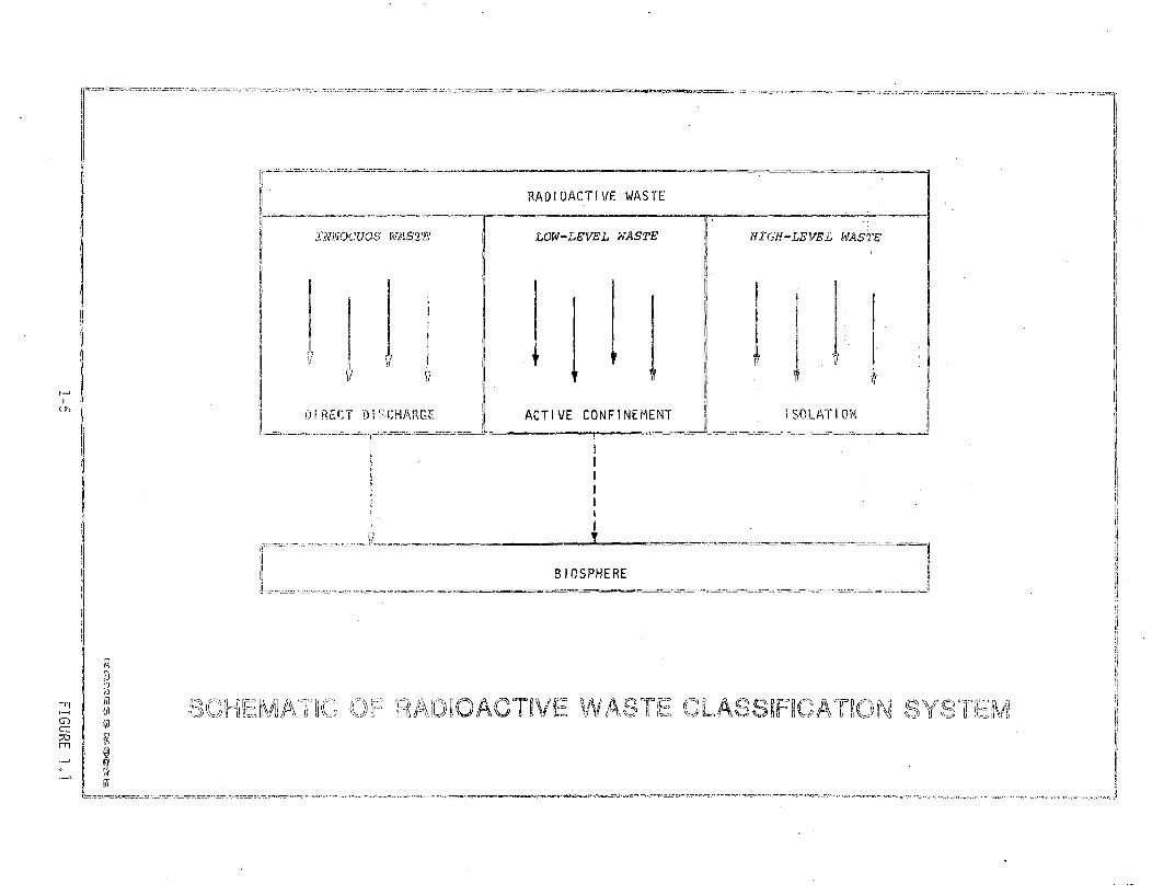
Several waste classification systems have been proposed and are

summarized in reference 7. Based on a review of these proposed

systems, reference 7 concludes that a viable waste classification

system should be based on the ultimate disposition of the waste

material. It further outlines three potential methods for disposition

of the wastes, namely, (1) discharge directly to the biosphere for

innocuously low-level wastes, (2) active confinement for low-level

waste, and (3) isolation for high-level waste. This classification

system is illustrated in Figure 1.1.

Reference 7 also concludes that the method governing the disposition

of the waste should be based primarily on its hazard potential and

expressed in terms of radioactivity per unit volume or mass at the

time of disposal. The reference goes on to note that the interfaces

of the three disposal categories are yet to be established, that the

issue of whether or not specific activity limitations should be

established for individual isotopes or groups of isotopes has not been

resolved, and that a total activity inventory limit may have to be

established for each disposal facility in order that the radiological

impacts remain below the established guidelines.

1-4

tcl-

II.-.

RADIOACTIVE WASTE

.Jfi~voclUO,1 VAISTE LOW-LEVEL WASTE HIG'H-LEVEL WA&E

VV

I III0 RGT 01 CHARGE ACTIVE CONFINEMENT ISOLATION

BIOSPHERE

--r1

o:

iii

5X__'_ EA']§J(G ir 19,ýANACTh,`E WVASTE CLA~SSHATORG~~

A subsequent attempt to quantify the interfaces of the above three

disposal categories is presented in reference 8. This report details

a three-category waste classification system determined by two refe-

rence disposal methods and the corresponding acceptance tests. The

reference disposal methods which determine the interfaces of the three

classes are based on the shallow land burial and sanitary landfill

disposal concepts. A following report(9) expands on the "work in

progress" presented in reference 8, and outlines a classification

system composed of five classes which are delineated by radioactive.

concentration guides.

The impact analysis methodology presented in this report is one of the

tools which may be used to aevelop a waste classification system and

determine the interfaces of the eventual disposal categories. This

report devotes considerable attention to the variable conditions of

LLW and potentially viable different disposal technologies.

1.3 General Approach

The most important rationale governing the selection of the metho-

dologies and the calculational procedures used in this report is

the generic nature of the analysis. The methodologies are focused

toward helping to establish generic criteria for LLW management and

disposal rather than calculating impacts' at a particular disposal

facility.

This is especially significant in view of the level of information

available for a generic analysis as opposed to the level of data

which will be available for a specific disposal facility site.

Increased complexity and sophistication of a calculational procedure

cannot compensate for a lack of data. Moreover, increased complexity

and sophistication cannot compensate for the fact that all calcu-

lational procedures are based on an idealized picture of the system;

this is an integral aspect of all predictive tools which are an

1-6

***-:.'',£ 1 •::r6 :@ njWl r-'SS f "' r •c o,.-',, 4 .-' .. . ". ,. , ->

1ona MW- geeaia for e generi . *40'flfl,•,. to.MW.:,,he potentialimpa.-,,ht.. 4Lct.As of W' 'psal'

1' 7~'b.(jj K ~ .> ¾ f¢p c-E ;rj:4l'.- 5 .;:,-,r I -. .--'

;from••i Yomr••. .simple= to•} very comple'x ÷•-techiqus Exrmnl ,omp.,-

W-C)S?02I ORO:J b1veie cale ;;Ov-Iz~ a-~ specifi Alofy%ý

.................................... .............................

favelmsed:•i~-, 0! ;the r'elative costs.. and impacts uf altrnaiv ae ..oý

:-•{:,;,{:,'o a~•,at ,••._ . schemes appear to be more appropri'•r.,".C.,... . -::ý,•,s

..... .. ficreasing the complexity of calculational s•h•me• with To.

0inTo -..- s, amnount and specificity of the available lae is,

WA the concept of tiering as set out by regulations promulga'ted ,.

the W901 on Environmental Quality (CEQ). (13)

.- .- : 1 .- .- -., ia, a Tfor the selecti on of The.ý, 4v q ',t , ., )CUI e

.... ., ... 51.. .. .. . ... .. C '•.0 ": " .• " " I

. ... ... :.. .,;.. : . '- - .- 1 : pq- ;z " 4"2.5•p ,'j5 .?¾ , ;: C . .t ...'¼" " -r - "

. .. .... "/• • -.-.-• ' W £:I. -,"-a,.. ............ ............................ 'a @: ""-6£%

I,, , : 0 4r , .... . .. . .--..' I @ : . i!i • ;..../ :"%f :t . •:

... . . .. .. '. .. . ." ' •-.¾ • ' r 4 iH:;" • , k > ,!ipt ! , • 4'0 > . -ti ,:' j , ? , " . . . .. I- " - , :

7- Vyo-y.T.h. •i .Q. ...., .. P O n T th : [lO. ,.."S0 TIM Mu 1 0..t,. . , IPT- ,

I~ 1 4 ,,- . ~4 41'R'dO~~oo~ Ot4Ir

W•o

Another example of a factor complicating an accurate definition of

the interfaces is the possibility that the waste processing may occur

at the waste generator's site or at a centralized regional location.

This aspect has to be included in the calculation of the impact

measures, specifically the transportation impacts.

A third rationale for the selection of the methodologies is the need

to have a flexible methodology that can be updated in a straight-

forward manner as adaitional information is obtained. Any methodology

that cannot accommodate timely changes is bound to become obsolete in

a short time. The methodologies selected provide for continuous

updating of the calculational techniques and the data base used for

the analyses.

The general criteria used in the development of the impact analyses

methodology (IAM) are as follows:

o The IAM should be constructed in terms of measurable properties

of the waste and the disposal environment;

o The IAM should be able to treat extreme values of these measure-

able properties;

o The IAM should be able to consider diverse impact measures

associated with the disposal of LLW;

o The IAM should be capable of rapid calculation of these impact

measures;

o The IAM should be able to assess the comparative importance of

the measurable parameters in affecting the impact measures; and

finally,

o The IAM should allow the incorporation of more complex and

sophisticated calculational procedures, if necessary.

1-8

L0 Ampact Measures

Five basic impact measures !are quantifiec in this reporto deteryilier

a preferred alternative or option associateo with•h e managemenr. >y

disposal of LLWo Two of, these measures - irb.0I dual anr poin•uJa. "u,.

exposures associated with the handl ing ana aisposal of the taste - ara

representatie of the level of long-term protection D- 'de hiumaI-

environment from raaiologicai impactso The other measures - costs".

energy use, and committedi lanti area associatec,• with tl,,e cisposa o-i,:

waste - are representative of the levele of..long-term protection of the

human environment from socioeconomic impacts. Other potential impact

measures, such as man-hours and-material requirements oo r•,a

gravel . concreted are implicitly included in the above five mpt

measures. 1P view of past disposal history and practices,'• impa&

measures related to long-term protection of the human environment are

stressed in this report.

The methodologies selected for determination of individual and popu-

lation exposures resulting from the disposal of waste, which are

iscussea in Chapter 3oU. are primarily geared towards the generic

nature of the analysiso Accordingly, determination of the rela-W.ie effects af various barriers ,netwoeen thze ýýjste ari;, the huma

-,"iso*nmen - wa t f.orUm and p ac., , ir s e i .

in the formul aion Q the Cal Cu , onaI pr, rel F.

SINS. D,'ý,i. occupational eposrs o tcal cu.lated boased upon a•ssumpt,'i ons reag iam ,_h ieern-ebe'q•e

07o-,th.e~r SmpacTmeasures . c.-ost, energy., u-se,. s-ad lan.•d u.se - is r.,el.a:ý

i sroased on the iormaio and *isumpt.epcPrevnseo•-e,; in, the other, volumes of this data base. M J'

The impact measvres associated with wJaste .processing aý iradsportI--

atlon • - oeo, occupational and population exposures, costs, anc

1_9

energy use -- are all representative of the level of short-term

protection of the human environment afforded by the alternatives

considered; it is assumed that no land is permanently committed during

waste processing and transportation activities. Again, impact

measures other than these four are implicitly included in the selected

set of measures.

The transportation impact measures are straightforward functions of

the packaging and shipping mode assumptions detailed in Chapter 4.0,

and the population exposure calculational procedures given in docu-

ments such as references 15 and 16. Impact measures associated with

waste processing, presented in Chapter 5.0, are calculated based on

the assumptions presented in reference 14 and the transfer factors

developed in Appendix A.

1-1U

REFERENCE F CHPT .,

1. Clancy X __ , A.a. = ov,-Yo

Wastec ManbcJJ lint. Wv A-. Rewla 0. Toy r~~x p~~

USNRC Report HMUR. -,..F j59 NovemIe- 19K

2. Johnson, L.o et.al ... " fJ .. .... .. .Practivvc ," Pesironmeak Pi ciye , P,,•1 p-1 2-. .197K

3. Dugu .i . 0. , "Assesmen of - -- ofs L- -e h . "• ~ ~ ~ ~~ . 4 . . ...... " ...... - -, = L e, '.

Col umbus -a " -tor s "iubus Oh o B T....--198,<- Novemb,•f]!er-, 157K:T

4. Papadopouios, S-S.. andRadioactive Wastes ink theFactors - with an Appendixtire Waste Storage .i5te:Quantitative Hydrageolqgic74t344, 174.

3kroud and Lri~m Hyd o hemimnal-- he Ma- -y Flatsu entukj Raio

Cuýre, AS- .- and- -Da 0 (' H-eds torEvlato,"' U. PA Ope File- RZLDC-

5. Webster, [DA., "A Review off Hvdrooic ,nd Geoo~i,"P Conditicir.Related to the Radioactive Solid-Waste Burial GroundsFi at OekRidge National Laboratory, Tennessee," U.S. Geologicai .urvev, eOpen File Report 76-727, 1976.

6. DPuguid, Jo0., "Status Report on Radioactivitt:rlbgmmi: FromBurial Grounds in Melton and Bethel Valleys," Envui r iomentalSciences Division Publication 653, ORNL-5017, ul.y 1975°King W.Co and 1 Jo' mohen, m -- t.R

.inn... im Report to the i'•• • ... Regu=-

latory Comm1ssio0•n ' P.R.diactive Waste Cassif-ic-ation Lawrence

8 Km ,.A b and -'S "A C-u vrRadio-

--.. .

bern. 197S7-107 atemb- ' 0 3r' F.',-:

Marc 1981

12. U.S. Department of Energy, Final Environmental Impact Statement"Management of Commercially Generated Radioactive Waste," DOE/EIS-0046F, October 1980.

13. Council on Environmental Quality, Executive Office of the Presi-dent, "Reguliations For Implementing the Procedural Provisionsof the National Environmental Policy Act," 45 FR 55978-56007,November 29, 1978, 40 CFR Parts 1500-1508.

14. Wild, R., et.al. Dames & Moore, "Data Base for Radioactive WasteManagement. Volume 2. Waste Source Options," USNRC ReportNUREG/CR-1759, November 1981.

15. U.S. Atomic Energy Commission, Directorate of Regulatory Stan-dards, "Environmental Survey of Transportation of RadioactiveMaterials To and From Nuclear Power Plants," USAEC Report WASH-1238, December 1972.

16. U.S. Nuclear Regulatory Commission, "Final Environmental State-ment on the Transportation of Radioactive Material by Air andOther Modes", USNRC Report NUREG-0170, January 1977.

1-12

2.0 PATHWAY AMUSE.;

Afer 'e,,jase h,- , ý,ean dfgsad of T-ug p Pý

control mrechaisms such as tý' sj

site design andc opertin st ýj ~r e --I (jf 4 p S L!

begin to funrction it ~ is t-e

"~barriers"~ whic confin and co~n ý,asr~

acio of 1 the ' wast wit the'r

This. chap,• details the mech-anis through which :-0n ..- : ma,intieract with ithe ený,;/!ronment afrtxr di sposal, and -n~fe Vs- "

interaction mechanisms in term ,of applicable corol-- men . ,,

the charterist"cs of I.he d- pa• system. , ...

the disposal system incu.de those a ... •-

packaging' 1') facility desigr -nd.. operations, 2)ad er' i -

requirements.

A brief introduction to the basic rationale and the deqe.oret Kr

the pathway analysis methodology is presented in Seci2io : .

the alternative release/transport/pathway routes through Bicm th!.-

waste may, interact with the environment (scenarios) a,- ... ozs- O-

.ct ion2.•-. The.i. ac.tional procedures for ,:etrmin-r, =,' Mon

- - . . .. . .. ,U ... ,..--, * ,. -.

.n. .o . . .. p.. .p Sect o 2... M.... ...m e c~h a n..r i s:m s. a r;e qiu a n t i f i e d i -, S e V I:• ,n 2 -. .. . & : M ýi-. C< ..• •" :f . .V- j: •:rega-rdn tahe 3 ' 1•,i

is~~~ prode N Apev.A

So thog 14.0 Pas

ON A 1 A Riao be

-aS 6eIom- to x Orypr - *1i3'

a

location to another through the atmosphere or soil by a transport

agent), and thereby become accessible to humans through various

pathways. Human access to the radioactivity may result either through

direct human contact with contaminated material (e.g., inhalation

of air, ingestion of water, or direct exposure to radiation) or

indirectly through contaminated biota (through a multitude of pathways

involving vegetation and animals) which have come into contact with

contaminated material.

Each of these radionuclide release/transport/pathway combinations

(scenarios) represents a complex series of interactions which are

affected by a wide range of parameters such as waste properties,

disposal site properties, and operational procedures. These diverse

release/transport/pathway scenarios must be unified so as to achieve

a simple, accurate, and readily usable methodology for pathway ana-

lysis. The development of the methodology employed in this report for

pathway analysis is based on the following procedure:

o Define and analyze, as completely as is practically possible, all

the potential release/transport/pathway scenarios that may lead

to radiation exposures to either individuals or populations, and

select the significant scenarios for further analysis.

o Simplify the structure of the selected release/transport/pathway

scenarios by separating the radiation release and transport

mechanisms from the pathway mechanisms. In other words, separate

the calculational procedures used to model release of radionuc-

lides from the waste and movement of radionuclides through the

environment from those calculational procedures used to model the

resulting dose to humans.

0 Determine applicable radionuclide-specific dose conversion

factors for various human organs from human exposure to conta-

minated material for all release/transport/pathway scenarios.

2-2

SThese dose corversicn factors, henceforth called the pathway dose

conversior fa.ctors (PDCF-s) to distinguish them from the conven-

tiona u:se cf the term "dose conversion factor" (which are

referr,:ed to as fundamental dose conversion factors in this

report), are determined for an entire pathway to permit rapid

dete.Fr-.iimti o, dose equivalent rates to human organs.

o Model the radioactivity release and transport mechanisms between

the disposed wastes and the locations where the radionuclides

may be contacted by humans (the "biota access locations"). Then

identify the control mechanisms and barriers that may be techno-

logically or administratively implemented that affect these

release and transport mechanisms.

SUtilizing the iinfor-mation presented in references 1, 2 and

Appendix C, determine the various options available for these

control mechanisms in terms of waste form and packaging, facility

site selection, facility design and operation, and institutional

requiremients..

o Finally, determine the potential radiological impacts from the

disposed LLW for various alternative options.

The methodology considers only one radionuclide at a time. Total

impacts resulting from the movement of radionculides from the waste

and through the environment are obtained by summing over all of

the radionuclides assumed to be present in the LLW. Several radio-

nuclides considered.") however, result in decay chains. These

decay chains are imp kicity included by incorporating the effects

of the daughters. through the dose conversion factors for the parent

radionuclide or by decaying the appropriate fraction of the parent

radionu:lide arid adding it to the daughter radionuclide inventory as

in the case of the decay of Pu.=241 to Am-241. However, more detailed

consideration of radionuclide chains would be appropriate during an

analysis for a specific disposal facility location.

2-3

2.2 Release/Transport/Pathway Scenarios

In accordance with the first two steps outlined above, the defini-

tion and simplification of the potential release/transport/pathway

(RTP) scenarios that are quantifiable and can lead to significant

radiation exposures to humans are discussed in this section. The

approach to the definition of the RTP scenarios is presented in

Section 2.2.1, applicable release/transport scenarios are discussed

in Section 2.2.2, control mechanisms that may be applied to these

scenarios are discussed in Section 2.2.3, and the RTP scenarios not

included in detail in this report are considered in Section 2.2.4.

2.2.1 Approach

The conventional approach to quantifying the routes and pathways

between radioactive materials and humans, and thereby determining the

resulting radiological impacts, is widely known and can be found in

the literature. ( A representative diagram is given in simplified

form in Figure 2.1.

As shown in this figure and beginning with the disposed waste, the

transfer of radionuclides (and/or direct ionizing radiation) is traced

along numerous transport paths as the contamination is transferred

between adjoining compartments and is eventually taken up by humans.

The boxes represent the contaminated media and the arrows indicate

that contaminant transfer can occur between adjacent compartments via

the stated radionuclide-mobilizing mechanism.

This classical pathway methodology is very useful in determining

specific impacts associated with a particular disposal facility,

but is unfortunately a bit awkward for use in determining generic

regulatory requirements. This results from the fact that most of the

arrows between the boxes represent environmental parameters that are

site specific, and depend on the location of the disposal facility.

2-4

" -I -1

00RUNOF SURFACE WATERA

WATERIN ANIMALS

x In

LEA I-N

S CLASSICALGROUND PAATAR

,,, 8CLASSICAL PATHWAY DIAGRAM

Moreover, the diagram does not permit rapid identification and ana-

lysis of alternative control mechanisms, which may be used to reduce

or eliminate the potential radiological impacts.

To aid in analyzing alternative overall performance objectives and

technical criteria, a more practical calculational procedure is needed

which separates those parameters that can be controlled (through

technological and/or administrative requirements) with a high degree

of confidence from those that cannot be controlled with the same

degree of confidence. For example, waste form and packaging are

parameters that may be potentially controlled with a higher degree

of confidence than such parameters as the irrigation rate of crops,

which must be assumed to be uncontrollable. A pathway diagram that

has been rearranged in order to satisfy these conditions is presented

in Figure 2.2.

As can be seen in this figure, most of the site specific pathway

compartments and parameters have been separated from the rest of the

diagram at what are-termed the biota access locations. Most of the

parameters which can be controlled (which are the solid waste/soil

mixture box and the connections of this box with the other biota

access locations) have been separated from the rest of the diagram.

The significance of this separation is that performance objectives,

technical requirements, and administrative regulations which would be

formulated to reduce the radiological impact of LLW disposal would be

aimed at the controllable parameters.

After the contamination reaches a biota access location, it becomes

available for immediate or eventual uptake by humans. Comparatively

little control (mostly through site selection) can be implemented over

the segments of the pathways beyond these biota access locations

(e.g., selection of a desert location may minimize ingestion path-

ways). Because of this comparative lack of control, movement of

radionuclides through the pathways beyond the biota access locations

2-6

BiOTA ACCESS LOCATION BIOT ACESS OCAIONEXPOSURE PATHWAY

EXPOSURE

PATHWAY

m

m

MODIFIED PATHWAY DIAGRAM

and the resulting human exposures may be expressed through radionuc-

lide specific pathway dose conversion factors (PDCF's) that are

independent of the original means of contamination. Based on an

appropriate reference concentration at the biota access location

(e.g., 1 Curie/m3 of contaminated media), the dose to humans may becalculated for each pathway from the biota access location to the

point of eventual human exposure. In other words, once the radio-

nuclide concentrations at the biota access locations are known,

potential human exposures may be determined by multiplying the actualaccess location concentration Ca (in units of Ci/m 3 ) by the PDCF

(in units of millirem per Ci/m

H = PDCF x Ca (2-1)

where H is the human dose in millirem (see Section 2.3). As anexample of the development and use of a particular PDCF, consider the

impacts that could result to a human from the presence of a concen-

tration of radioactivity in off-site air. Potential exposures could

result from the following uptake pathways:

o Inhalation of the contaminated air,

o Direct ionizing radiation exposure from standing in the conta-

minated air;

o Consumption of leafy vegetables dusted with radionuclides settled

out of the air;

o Direct ionizing radiation exposure from contaminated dust

deposited on the ground;

Direct ionizing radiation referred to in this report includesalpha, beta, and gamma radiations. Alpha and beta radiations havevery short ranges and usually only gamma radiations are consideredin the impact calculations. However, beta radiation has beenincluded in this work in the fundamental dose conversion factorsfor the above exposure scenarios (see Appendix B).

2-8

o Inhaiatio-, of contaI iiated dust which has been resuspended from

the ground surface;.

o C~onsumpt.or of v.,eQe.als containing radion.uclides transferred

into t.he plant -hrough root pathways; and

o Coonsumptio,, of food. containing radionuclides transferred to the

-ood tvh'-ouin vaiv'ous pathways such as plant-animal-meat or

At a specific csite, the dose resulting from these uptake pathways

wouiJ be detear-ined through the use of (1) transfer factors such as

air-tooleaf and soil-to-air transfer factors, and (2) fundamental

dose conversion factors (DCF) such as the inhalation DCF (50-year

committed dose per pCi inhaled), ingestion DCF (50-year committed

dose per pCi ingested), and direct radiation DCF (annual dose per

unit concen`!ration in the contaminated medium). The transfer factors

anid the act.ual potential impacts would be specific to particular

envirorneni.tai conditions (e.g., humidity, types of food grown, etc.)

anid specific human actions at the location where the airborne conta-

mi nation 0•U. . .. .

~v~e;'.... - . " ses reasonable yet conservative assumptions

•.i Oe -- , -, ,ronmleCCa characteristics and human actions.

....: univ concentration of a radionuclide

d, he undamentaL dose conversion factors

.e.! C -i-- n e'ernal exposure) , the potential

i. a. .a result of each uptake

c .. -'ed.F -ihen the doses from each uptake pathway

b. e a . ,F- e hivno1 dual organ, a single pathway

ooe . -. aon ve -S.tia; " Cr-ent . the total potential dose

C p ,A -e • i ,. The end result is the ability to

GI U C et e-Pmi n e o, a eeneri c •asi s (eo. o by consulting a table and

mu-ItipIi ngI• the tota potential organ doses received by a human

Frrou any concentration of radionuclides in air.

This approach introduces a conservatism in the calculation of doses

since not all of the uptake pathways may be applicable for every

release pathway and environmental setting. The generic nature of the

analysis, however, precludes a detailed consideration of site specific

pathway factors.

2.2.2 Release Scenarios

There are three fundamental transport agents which can mobilize

radioactivity from disposed waste:

o Direct Contact - The waste may be directly accessed by humans

through ionizing radiation exposures or through human activities

which contact the waste/soil mixture.

o Air - Air can mobilize radioactivity from the waste when the

waste is directly exposed to the atmosphere.

o Water - Ground water and surface water can act as transport

agents to mobilize radioactivity from the waste.

Moreover, there are two comparatively distinct time periods of the

site lifespan during which releases from LLW can reach a biota access

location: the operational period and the post-operational period. The

post-operational period may be further divided into the closure and

observation period, the active institutional control period, and the

passive institutional control period.

Operational Period - The operational period includes the time during

which the waste disposal operations takes place. During this period,

the principal mechanism at a disposal facility that can result in

significant transport of radioactivity to a biota access location is

an operational accident. In this case, wind is the primary transport

agent, the biota access location becomes off-site air, and the expo-

sure period is acute - i.e., a discrete event occurring over a short

time span.

2-10

1i "gl-i s Per~iO0) i C4 he control.and main`Mena-ce ,• Tfom operational

acciderts are impor-c.i-ui'v •, i-- to the I ong-term

performance of a near.-s, c_ .i: OpeI-ational acci-

dents are important insora,- aS poteiia y, u.aona-I releases may be

precluded or minimized by. imp.W"-ovemei: ,aste form and packaging or

site operational . .. roCe . dr cpati onal exposures and potential

off-site exposures due • CAO sur-a.- = ..- uP f 0o, concaminated on-site

Soi may oc,;ur 'however, he a.e : •,, ta.ie ` :I ihis report. Suchpotential short-tterm exposures _ vh.j , add"essed as part of licensing

specific -di sposal i:acii ities,. Rou0LIt U " ccupationa• exposures during

.he operational period are consi.'.-Jeredl n hC-1apider L ,.0o Groundwater

migration is not ca-,c-atec! •1. th-s i- . -or calculational

convenience, andbecause of the short time span and operational

measures that could be taken to minimize the potential for migration.

During the. operational period, other short-term exposures would also

resuit at locations other than the disposal facility site. Exposures

To populations could result from airborne releases of radioactivity

during waste processing activities especially if such processing

activities .involvE ineat f combsti-e waste streams. Such

processing act-vities vwouli. Fr m by tIhe waste generator or at

p 5 P2 1,J. Z, U IN. J I -ld a c sc occur

_ ,,., -Occupational

expos I- es. s ' o result w, .o u 2"- • S u .t;- :-(ng and pro-

CaS. g w_ t .e. t-rean , a -SPrlstng the waste

_D _, ' n- J W::_ 3 1 t.e end of

J. i pOIE--C'.- i .' hU 3 ,t L . . . ti t e for the

- ii . i t ,. e..re :. begins during. - .i i Lp,.. Wit- , -,:g: . : ,h any period

,i [sevatio e-ed .:ii " .i assure that the

Ci Sposar facitiiy is ci a I:f : i 'ansfer to the

site owner. During this period, the facility operator is responsible

for the control and maintenance of the site. The groundwater scenarios

are initiated during this period. Groundwater may transport radioac-

tivity to locations where the radioactivity may be accessed by humans.

Possible access locations would include either a well drilled into the

contaminated aquifer or open water (e.g., a stream) into which the

contaminated aquifer has discharged. For both of these cases the

exposure periods are chronic (i.e., continuous events).

Active Institutional Control Period - This period lasts from the

transfer of the title of the site by the site operator to the site

owner until a point in time at which a breakdown in active institu-

tional controls is assumed to occur. During this period, the waste is

not exposed to the atmosphere. The waste may, however, interact with

humans through direct radiation attenuated through the disposal cell

cover. Thus, the waste itself is an access location. The other

principal agent that can transport radioactivity from the waste during

this period is groundwater, which continues during this period.

Prior to the transfer of the title to the site owner, the site will be

closed by the site operator. A desirable goal during the closure

activities is that the site will have been stabilized so that there is

essentially no need for active ongoing maintenance by the site owner.

During the active institutional control period, the site owner is

responsible for the care and maintenance of the site. Access to the

site is restricted (e.g., fenced) and/or controlled by means of some

manner of licensed surface use. The direct radiation exposure sce-

nario, in comparison with other scenarios, is likely not to be signi-

ficant since the radiation must pass through the intact trench cover.

The groundwater scenarios are assumed to continue during this period.

Passive Institutional Control Period - During the passive institution-

al control period (after active institutional controls are assumed to

have broken down), the waste may be exposed to the atmosphere through

2-12

erosion or human activities. During this period, the waste/soil

mixture may, potentially, be directly accessed by humans. For example,

a house could be inadvertently constructed on the waste disposal

facilty and after the house is constructed a person or small group of

persons could live in the house and possibly consume garden vegetables

inadvertantly grown in the waste/soil mixture. These two potential

inadvertent intruder scenarios are referenced several times in this

report and are referred to as the intruder-construction scenario and

the intruder-agriculture scenario. In addition, wind and water may

act as transport agents that may lead to dispersion of radionuclides

and off-site contamination of air and open water, respectively. In

the case of direct human contact with the waste/soil mixture, the

exposure period is acute for the inadvertant intruder-construction

scenario, and chronic for the inadvertant intruder-agriculture sce-

nario. For scenarios involving the wind and surface water transport

agents, the exposure periods are chronic. The groundwater scenario

continues during the passive institutional control period.

During the active institutional control period, it may be assumed that

active controls exercised by the site owner on the closed disposal

facility will gradually lessen. The period of time between the site

inspection and routine monitoring of the site will lengthen. Even-

tually a passive institutional control period may be assumed during

which the control of the site is principally expressed through site

ownership and control of land use. During this period, there may be

occasions in which inappropriate use of the facility by people occurs.

As extreme examples of inapropriate use, a house may be constructed on

the disposal facility and persons may live in the house'. It is

likely, however, that the passive institutional controls would pre-

clude continuation of inappropriate site use for long time periods.

The seven pathways that have been discussed above (one for the ope-

rational period, two for the closure and observation period, one for

the active institutional control period, and three for the passive

2-13

institutional control period) are summarized in Table 2-1. A brief

discussion of the release/transport/pathway scenarios not considered

quantitatively in this report is given in Section 2.2.4.

For calculational purposes, it is convenient to reorganize these seven

pathways. This modification involves breaking up the passive institu-

tional control period on-site soil exposure pathway into two exposure

scenarios (inadvertant intruder-construction and inadvertant intruder-

agriculture), and eliminating the active institutional control period

on-site soil exposure scenario since it involves potential radiation

exposure attenuated through an intact disposal cell cover. These

exposures are not expected to be significant as long as the disposal

cell cover is intact. Direct radiation exposures to a potential

intruder are considered as part of the above inadvertant intruder

scenarios. The resultant seven pathways are illustrated in Figure 2.3.

All of these pathways involve PDCF's which are composed of more than

one uptake mechanism, i.e., there are secondary biota access locations

such as off-site air containing wind suspended radionuclides that were

deposited after wind transport from the waste. Additional information

on secondary biota access locations is provided in Section 2.3.2.

2.2.3 Control Mechanisms

The release and transport of radioactivity from the disposed LLW

are significantly affected by the-properties and characteristics of

the waste form and packaging, site design-and location, disposal

practices, etc.. Most, if not all, of these items are controllable to

some degree. Specific controls of these items can be made mandatory

through administrative regulation; hence these may be termed regu-

latable items or control mechanisms.

In order to permit the specification of controls and the quantitative

assessment of their effects, these control mechanisms should be

2-14

TABLE 2-1

Major Pathways for LLW Disposal

uI

Period

Pathway Initiated

Operational Period

Closure and

Observation Period

Active Institutional

Control Period

Passive Institutional

Control Period

Transport Agent

Wind

Groundwater

Groundwater

Direct Radiation

Direct Access

Wind

Surface Water

Facility

Biota Access

Location

Off-site Air

Well Water

Open Water

On-site Soil

On-site Soil

Off-site Air

Open Water

Exposure

Period

Acute

Chronic

Chronic

Chronic

Chronic

or Acute

Chronic

Chronic

FIGURE 2.3 : Simplified Pathway Diagram

Release/Transport Biota Access Pathway DoseScenario Location Conversion Factor

Accident Offsite Air I Multiple (see text)r

Intruaer-Construction I Onsite Soil I Multiple

"' Intruder-

Agriculture Onsite Soil Multiple

C:))

K 0ILiJ

Groundwater l Well Water I, Multiple

Groundwater apOpen Water I Multiple

Surface Water I Open Water--] Multiple

L- -Wind Transport I Offsite Air Multipl-e

2-16

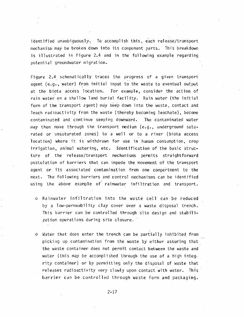
identified unambiguously. To accomplish this, each release/transport

mechanism may be broken down into its component parts. This breakdown

is illustrated in Figure 2.4 and in the following example regarding

potential groundwater migration.

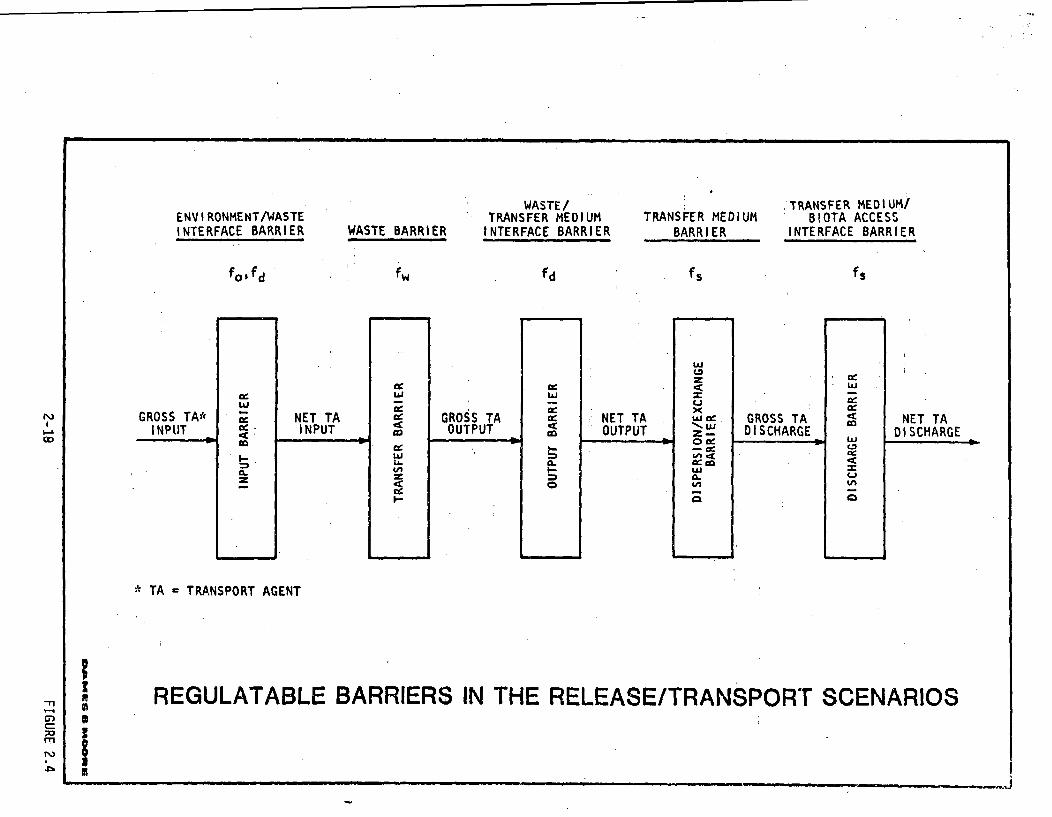
Figure 2.4 schematically traces the progress of a given transport

agent (e.g., water) from initial input to the waste to eventual output

at the biota access location. For example, consider the action of

rain water on a shallow land burial facility. Rain water (the initial

form of the transport agent) may seep down into the waste, contact and

leach radioactivity from the waste (thereby becoming leachate), become

contaminated and continue seeping downward. The contaminated water

may then move through the transport medium (e.g., underground satu-

rated or unsaturated zones) to a well or to a river (biota access

location) where it is withdrawn for use in human consumption, crop

irrigation, animal watering, etc. Identification of the basic struc-

ture of the release/transport mechanisms permits straightforward

postulation of barriers that can impede the movement of the transport

agent or its associated contamination from one compartment to the

next. The following barriers and control mechanisms can be identified

using the above example of rainwater infiltration and transport.

o Rainwater infiltration into the waste cell can be reduced

by a low-permeability clay cover over a waste disposal trench.

This barrier can be controlled through site design and stabili-

zation operations during site closure.

o Water that does enter the trench can be partially inhibited from

picking up contamination from the waste by either assuring that

the waste container does not permit contact between the waste and

water (this may be accomplished through the use of a high integ-

rity container) or by permitting only the disposal of waste that

releases radioactivity very slowly upon contact with water. This

barrier can be controlled through waste form and packaging.

2-17

ENVI RONMENT/WASTEINTERFACE BARRIER

WASTE/TRANSFER MEDIUM

INTERFACE BARRIERWASTE BARRIERTRANSFER MEDIUM

BARR I ER

TRANSFER MEDIUM/BIOTA ACCESS

INTERFACE BARRIER

N)

ICGROSS TA*I NPUT

w

I.-J

z

cc

NET TAINPUT

w

wj

cc

lu.1

GROSS TAOUTPUT

w

a-

o

NET TAOUTPUT

z

U.'

La-a-

GROSS TADISCHARGE

w.

72' NET TADISCHARGE

* TA - TRANSPORT AGENT

REGULATABLE BARRIERS IN THE RELEASE/TRANSPORT SCENARIOS-I,

III,,

SI003U

-. 1

o Release of contaminated water from the trench may then be

reduced by another low-permeability clay layer at the bottom of

the trench. However, this barrier should be implemented with

caution. Otherwise, accumulation of leachate could occur which

could eventually, fill up the trench and posssibly overflow the

trench. This barrier can be controlled through site design.

o After the water enters the transfer medium (i.e., the soil), the

natural geologic barriers that can impede and/or reduce the

magnitude of the radionuclide transfer include adsorbtion onto

soil particles as the water moves through an underlying strata,

dispersion of the radionuclides during migration, and radioactive

decay during the contaminant travel through the geologic medium.

These barriers can be controlled through site selection.

o Once the transport agent reaches the biota access location,

another mechanism that would reduce the magnitude of the conta-

minant concentration is dilution with uncontaminated water at the

discharge location. For example, the flow rate of a river or the

pumping rate of a well affects the degree of dilution achieved.

This barrier can also be controlled through site selection.

o Finally, the point in time at which the groundwater scenario is

initiated depends on the waste form and package,-site operational

procedures, and administrative requirements. For example, the

waste may be packaged in a high integrity container. This

results in a time-delay factor, due to radioactive decay, that

can reduce the magnitude of the source term significantly.

The barrier concepts that have been discussed above can be generalized

and applied quantitatively to each release/transport scenario. This

may be accomplished by using an interaction factor (denoted by the

symbol I) that relates the radionuclide concentration at the biota

access location to the radionuclide concentration in the waste:

2-19

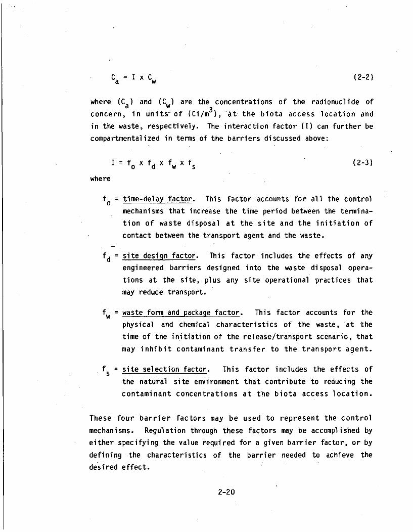
Ca = I x Cw (2-2)

where (C a) and (C w) are the concentrations of the radionuclide of

concern, in units of (Ci/m 3 ), at the biota access location and

in the waste, respectively. The interaction factor (I) can further be

compartmentalized in terms of the barriers discussed above:

I =f 0 x fd x fw x fs (2-3)

where

fo= time-delay factor. This factor accounts for all the control

mechanisms that increase the time period between the termina-

tion of waste disposal at the site and the initiation of

contact between the transport agent and the waste.

f = site design factor. This factor includes the effects of any

engineered barriers designed into the waste disposal opera-

tions at the site, plus any site operational practices that

may reduce transport.

fw= waste form and package factor. This factor accounts for the

physical and chemical characteristics of the waste, at the

time of the initiation of the release/transport scenario, that

may inhibit contaminant transfer to the transport agent.

f= site selection factor. This factor includes the effects of

the natural site environment that contribute to reducing the

contaminant concentrations at the biota access location.

These -four barrier factors may be used to represent the control

mechanisms. Regulation through these factors may be accomplished by

either specifying the value required for a given barrier factor, or by

defining the characteristics of the barrier needed to achieve the

desired effect.

2-20

2.2.4 Other Potential Exposure Pathways

The above seven release/transport mechanisms are comparatively the

most significant potential pathways to human exposure, and calcula-

tional procedures are developed in this report to determine potential

human exposure levels resulting from these pathways. The calcula-

tional procedures are used to help determine overall performance

objectives and technical criteria for -near--surface radioactive waste

disposal. There are other potential pathways to humans which may be

considered during development of the performance objectives and

technical criteria, but calculational procedures to estimate specific

exposure levels are not developed in this report. These potential(7)

exposure pathways include the following:

o Groundwater migration during the operational period of the

facility lifespan;

o The bathtub effect -- i.e., filling up of the disposal cells with

accumulated leachate and subsequent overflowing;

o Diffusion of radioisotope-tagged decomposition gases through

disposal cell covers;

o Dispersion of radioactive material by means of surface runoff or

wind dispersion from accidentally contaminated site surfaces and

equipment.

All of these potential pathways have been observed at commercial

and/or DOE operated disposal facilities.(8-13) The first three

pathways are fundamentally caused by site instability problems--that

is, by degredation of compressible material within a disposal cell and

subsequent subsidence of the disposal cell contents, leading to

cracking and slumping of disposal cell covers and increased infiltra-

tion of rainwater into the disposal cell. At sites with moderate to

high permeability soils, an infiltration problem (resulting from a

subsidence problem) can lead to migration of some radionuclides being

2-21

observed during the operational period of the facility life. This

would principally involve very mobile radionuclides such as tritium.

However, during site operations the potential for groundwater mig-

ration would be monitored and if it occurs, the licensee would take

steps to correct the situation. Of more concern is the potential

long-term migration of all the radionuclides in the waste after site

operations have terminated. At sites with very low permeability

soils, an infiltration problem can lead to collection of trench

leachate in disposal cells. This leachate would have to be removed

and treated during disposal operations.

It has been demonstrated that potential problems of increased in-

filtration -- migration during the operational period or the bathtub

effect -- can be minimized or avoided during the operational period

through siting or operational procedures. For example, increased

attention paid to compaction of disposal trench covers can greatly

reduce the maintenance required during site operations. Of more

interest is the long-term stability of a disposal facility, and

methods which may be used to ensure this stability. Impacts from the

bathtub effect could ultimately include overland flow of a few to some

hundreds of gallons of leachate. The principal impact, however, is

likely to be the very high costs of remedial action, which could

include pumping, treating and solidifying leachate, and restabiliza-

tion of trench covers. This remedial action could result in an

expense to a site owner of better than a million dollars per year, for

a number of years. (14) Treatment of leachate could involve airborne

or waterborne release of radionuclides.

Past disposal experience indicates that potential diffusion of radio-

isotopetagged decomposition products such as methane or carbon dioxide

can be significantly retarded by facility design and operating prac-

tices such as thicker trench covers.( 1 2 - 3 ) In any case, generation

of decomposition gasses would be reduced through efforts to minimize

the degredation of trench contents. In other words, actions undertaken

2-22

promote site stability and to minimize or eliminate trench subsidence

will also serve to significantly reduce generation of radioisotope-

tagged decomposition gases.

Potential operational impacts due to run-off or wi.nd dispersion of

contaminated site surfaces are site specific and would be addressed as

part of the licensing of individual disposal facilities, and calcu-

lational procedures to estimate the levels of these potential impacts

are not developed in this report. In any case, these impacts can be

reduced to negligible levels through strict on-site contamination

control at a disposal facility, and through better attention paid to

packaging of wastes for transportation. In the past, one of the most

significant contributor to on-site contamination has been accidental

spillage of trench leachate during pumping for treatment. In addition,

another significant contributor to on-site contamination has been

accidental spillage of low-level liquids which were at one time

delivered to some disposal facilities for solidification and disposal.

More recently, however, this practice has been discontinued and all

disposal facilities accept only solid wastes for disposal. Probably

another cause for on-site contamination is through excessive free-

standing liquids in (and leaking out of) disposal containers.

Potential intrusion by deep rooted plants or burrowing animals through

disposal cell covers is another potential pathway. This intrusion

could poten~tially result in increased human exposures by three general

mechanisms:

! surfacing of radioactive material which could then be dispersed

y ,,ind or water,

(2 human consumption of contaminated plants or animals, or

(3) increasing rainwater percolation into the disposed waste through

root channels and animal burrows, thereby potentially increasing

radionuclide migration through groundwater.

2-23

0

These potential exposures, particularly the first two mechanisms,are difficult to quantify. Past occurrences of plant and animal

intrusion at existing disposal facilities, potential exposure pathways

to humans, and methods to reduce or preclude such intrusion are site

specific and are not quantified in the generic analysis developed in

this report. In any case, the major impact of deep-rooted plant and

burrowing animal intrusion at a disposal facilty is likely to be an

increase in the potential for groundwater migration. This potential

effect on groundwater migration is quantitatively considered in this

report (see Section 3.5). However, for perspective, a brief discus-sion based on reference 13 of potential deep-rooted plant and animal

intrusion is presented below.

For uptake by vegetation, a biomass model, using the parameters of

the ecosystem that follow the generation and transfer of biomass,

assumes that 0.2 percent of the root mass of a mature tree is below

1.5 m from the soil surface with the uptake linearly proportional to

this fraction.( 1 3 ) An evaluation of uptake for wastes containing

plutonium at a concentration of 10 nCi/g was performed and yielded

a concentration 8x10-6 nCi/g at the soil surface after 5000 years.L13"

From these results, reference 13 concludes that this mechanism is

unlikely to produce surface concentrations exceeding the original

waste concentrations. Therefore, the intruder scenarios will be the

limiting scenarios.

The other mechanism is potential animal or insect intrusion. The

depths of burrows or tunnels for some typical animals and insects are

given below: (13)Maximum Typical Burrow

Species and Tunnel Depth

Harvester Ant 3 mMoles 1.2 mPocket Gopher 0.6 mPocket Mouse 1.6 mDeer Mouse 0.6 mField Mouse 0.6 mEarthworms 0.5 m

2-24

As can be seen, the probability of animals other than harvester ants

reaching the wastes with a two meter cover is low. Even after

significant erosion of the waste cover, the surface concentrations

will be lower than the wastes and the doses will be controlled by the

pathway of people living on the area after the wastes are exposed by

erosion. (13) This implies that the intruder scenarios will again be

the limiting scenarios. In any case, burrowing animals that may be

found in various regions of the continental U.S. are discussed in

Appendix C for four hypothetical disposal facility sites.

2.3 Pathway Dose Conversion Factors

This section considers the pathway dose conversion factors (PDCF's)

introduced in equation 2-1. It presents a background on dose calcu-

lational procedures, presents detailed pathway diagrams for the seven

pathways considered in Section 2.2, discusses the biota access loca-

tions, and gives PDCF values for the seven pathways of concern for

the seven human organs and 23 radionuclides selected for consideration

in this report.

2.3.1 Background

The use of the pathway dose conversion factors (PDCF's) in the calcu-

lat.ional methodology is straightforward. It is multiplied by the

radionuclide concentration at the biota access location(s) (C a) to

obtain the human exposures:

H = PDCF x Ca (2-1)

where PDCF stands for the pathway dose conversion factor in units of

millirem (mrem) per Ci/m 3 for the acute exposure scenarios and in

units of mrem/year per Ci/m3 for the chronic exposure scenarios.The radionuclide concentration at the biota access location (C ) is

3ain units of Gu/m

2-25

In this report, for acute exposures, H will be taken as the dose in

mrem, received during 50 years following a one-year exposure to the

radioactive material; and for chronic exposures, H will be taken as

the dose rate in mrem/year, received during the 5 0 th year of an

exposure period lasting 50 years. These two definitions result in

use of the same fundamental dose conversion factors for the chronic

and acute scenarios. Hereinafter, the qualifier equivalent is assumed

to be implicit in the term dose; similarly, the dose equivalent rate

will be referred to as the dose rate.

Some of the acute exposure scenarios last for much shorter periods

than one year. However, for calculational convenience all acute

exposures will be assumed to last one year. A correction factor, used

to normalize acute exposure periods to the one-year reference value,

will be incorporated into the release/transport portion of the sce-

nario, usually into the site selection factor fs9 as appropriate to

the scenario.

Use of the PDCF requires a clear quantitative pathway model, which is

arrived at through the following steps:(3)

(1) defining the objective of the modelling effort,

(2) forming, the block diagram of the system ioentifying the ecolo-

gical and environmental compartments,

(3) identifying and quantitatively aetermining the "translocation"

parameters of the system,

(4) predicting the response of the system to the input parameters by

using either the concentration factor (CF) methoa or the systems

analysis (SA) method, and

(5) analyzing this response for the critical radionuclides and

pathways and the effects of parameter uncertainties.

2-26

These steps are straightforward, except for the definition of the

"translocation" parameters (which are-referred to as transfer factors

in this work) and the use of either the CF or the SA methods to

predict the response of the system. These are briefly summarized

bel ow.

The transfer factors are simply the transfer functions or coefficients

that express contaminant exchange between the various environmental

compartments of the pathway diagram -- e.g., animal bioaccumulation

factors, plant uptake factors, etc. A survey of the literature yields

a considerable range of values for these parameters dependent on the

human environment. One may obtain preliminary values from laboratory

and field experiments, but these should be refined by observations in

the actual system. Values for the transfer factors utilized in this

work are detailed in Appendices A and B.

In order to mathematically model the movement of a radionuclide

from its source to its uptake by a human population, two modeling

systems may be used. They are referred to as the CF and SA methods.

Both require the conceptualization of the actual system as a series

of compartments through which the radionuclides pass (e.g., as in

Figures 2.1 and 2.2). The movement of radionuclides from one compart-

ment to the next (e.g., soil to crops) is characterized by a transfer

.pathway that may be quantified by a mathematical representation of the

transfer mechanism. The two systems differ primarily in the degree of

complexity to which the transfer mechanisms are treated.

In the CF method, time-dependent behavior is neglected. In other

words, chronic releases of a contaminant are treated as time-averaged

concentrations (usually on an annual basis), and acute releases are

treated as time integrated quantities. The transfer pathway is thus

reduced to a single factor that, when multiplied by the concentration

in a given compartment, yields the concentration in the next compart-

ment. The result is that a very simple series of computations can

2-27

trace the radionuclide concentration through the- various compartments

postulated for the model.

The SA method is utilized-in systems where the compartment transfer

mechanisms are time dependent, An example of this would be the

release of radionuclides into a soil where chemical reactions may

take place that result in irreversible fixation (reversible sorption

is assumed in this work). This represents a time-dependent concen-

tration reduction mechanism other than simple dilution and can be

modeled with the SA method using reaction rate data. The end result

of using the SA method is a series of differential equations that must

be solved in order to follow the dynamics of radionuclide movement

through the model system.

The choice between the two methodologies is generally based on the

state of knowledge of radionuclide movement through a transfer path-

way. If little is known about the dynamics of the system, the CF

method must be used to obtain first order estimations of concentra-

tions at biota access locations. If transfer mechanisms are known

in sufficient detail and time-dependent factors are important, then

the SA method should be used. Because of the generic nature of the

impact analysis methodology, the CF method has been utilized through-

out this report.

2.3.2 Pathways

The PDCF's for the pathways indicated in Figure 2.3 are the total

dose conversion factors for the individual pathways of importance in

contributing to human exposures from concentrations of radionuclides

at biota access locations. The individual pathways that comprise the

total pathways are shown in Figure 2.5. Also shown are the PDCF

symbols for groups. of uptake pathways that will be utilized in this

report. These individual uptake pathways that comprise the total

pathways are discussed below.

2-28

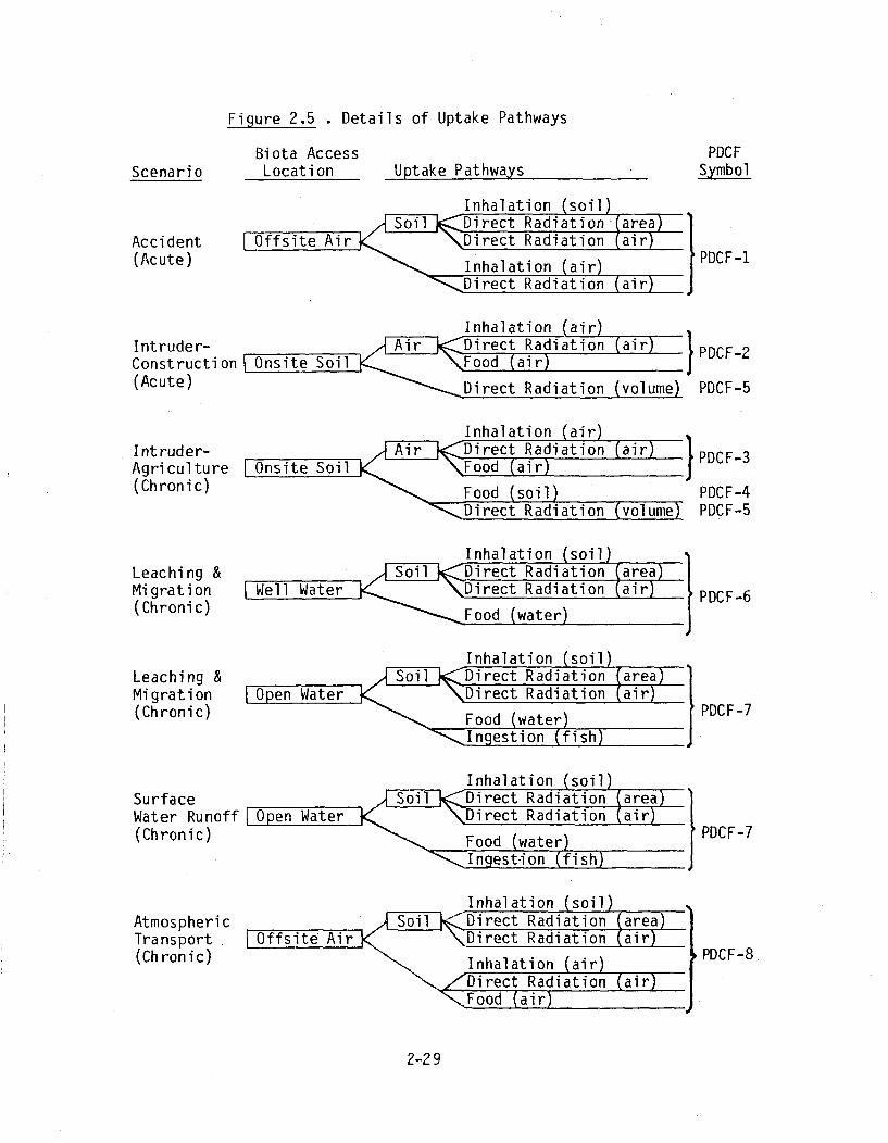
Figure 2.5 . Details of Uptake Pathways

Scenario

Accident(Acute)

Biota AccessLocation Uptake Pathways

PDC FSymbol

PDCF-I

Inhalation (air)Intruder- Air Direct Radiation (air)Construction Onsite Soil Food air)(Acute) MDirect Radiation (volume)

PDCF-2PDCF-5

Intruder-Agriculture(Chronic)

Inhalation (air)Air Direct Radiation (air)

Onsite Soil Food (air)

Food (soil)PDCF-3PDCF-4

KDirect Radiation (volume) PDCF-5

Leaching &Migration(Chronic)

Inhalation (soil)Soil Direct Radiation area

F Well Water ] •Direct Radiation air

Food (water) I PDCF-6

Leaching &Migration(Chronic) PDCF-7

Inhalation (soil)Surface Soil Direct Radiation area)Water Runoff Open Water Direct Radiation (air)(Chronic) Food (water) ' PDCF-7

".. Inqest-ion (fish) -J

AtmosphericTransport(Chronic) PDCF-8

2-29

As presented in Figure 2.5, all of the scenarios involve a secondary

biota access location resulting from the primary access location. Two

of the scenarios have four uptake pathways, four have five, and one

has six, yielding a total of 34 uptake pathways. However, of these

34 uptake pathways only 9 are unique types of uptake pathways, if only

the uptake mode and transport agents are considered. These nine

distinct types of uptake pathways are described in Table 2.2.

Only primary and secondary biota access locations are considered in

the determination of these uptake pathways. The effects of possible

tertiary access locations, such as air contaminated due to natural

suspension of radioactivity from soil which is originally contaminated

from deposition of radioactivity from air, are not considered. These

effects are considered, however, in the selection of transfer factors

between the uptake pathways.

The accident scenario includes offsite air as the primary access

location leading to two uptake pathways: inhalation (air), and direct

radiation (air); it also includes soil contaminated by radionuclide

deposition as the secondary access location leading to three more

uptake pathways: inhalation (soil), direct radiation (area), and

direct radiation (air). Since the exposure period is acute, the food

(air) uptake pathway has been excluded from this scenario. However,

the direct radiation (air) uptake pathway is included in the secondary

access location in addition to the direct radiation (air) from the

primary access location.

The construction scenario includes onsite soil as the primary access

location leading only to the direct radiation (volume) uptake pathway.

The scenario also includes onsite air as the secondary access location

leading to three uptake pathways: inhalation (air), direct radiation

(air), and food (air). Although the exposure period is acute, the

food (air) uptake pathway is included with a modification to account

for non-equilibrium deposition and root-uptake conditions.

2-30

TABLE 2-2 . Access Location-to-Human Pathway Descriptions

Pathway Designation

Food (soil)

Food (air)

Food (water)

Ingestion (fish)

Inhalation (air)

Inhalation (soil)

Direct Radiation(volume)

Direct Radiation(area)

Direct Radiation(air)

Description

This uptake pathway includes a total of threesubpathways and denotes uptake of radionuclidesoriginating in plants via soil-to-root transferfrom contaminated soil:

plant-to-humanplant-to-animal-to-humanplant-to-animal-to-product-to-human

This uptake pathway includes a total of sixsubpathways and includes the above three food(soil) subpathways resulting from uptake ofradionuclides originating on plant surfaces viadeposition from contaminated air and the samethree food (soil) subpathways resulting fromfallout contamination of the ground.

This uptake pathway includes a total of ninesubpathways and includes all the food (soil)pathways resulting from radionuclides originatingon plant surfaces via irrigation deposition fromcontaminated water and from irrigation contamina-tion of the ground. The following three subpath-ways in addition to the plant pathways are added:

water-to-humanwater-to-animal-to-humanwater-to-animal-to-proauct-to-human

Uptake of radionuclides from eating fish caughtin contaminated open water.

Uptake of radionuclides from breathing aircontaminated due to suspension of contaminatecsoil particulates by human activities.

Uptake of radionuclides from breathing aircontaminated due to natural suspension andvolatilization of surface soil.

Direct exposure to ionizing radiation fromstanding on ground homogeneously contaminated.

Direct exposure to ionizing radiation fromstanding on ground whose surface is contaminated.

Direct exposure to ionizing radiation fromstanding in air homogeneously contaminated.

2-31

The agriculture scenario also includes onsite soil as the primary

access location; however, the food (soil) uptake pathway is included

in this case in addition to the direct radiation (volume) uptake

pathway. The scenario al~so includes ,onsite air as the secondary

access location leading to the same three uptake pathways as the

construction scenario secondary access location: inhalation (air),

direct radiation (air), and food (air). However, in this case,

chronic conditions are assumed to prevail, and equilibrium conditions

are assumed for the food (air) uptake pathway.

The next three scenarios involving water are very similar. As a

matter of fact, the two open water scenarios are identical. The only

additional uptake pathway in the open water scenario as opposed to the

well water scenario is the ingestion (fish) pathway. This pathway

is included since the bioaccumulation factors for several fish species

are significantly greater than unity. However, direct radiation

exposure to contaminated water was omitted; it turned out to result in

negligible additional exposures (less than 0.1%) when compared with

the other uptake pathways.

The last scenario, the atmospheric transport scenario, is identical

with the accident scenario with the addition of the food (air) uptake

pathway to the primary access location. In this case, however, the

exposure is assumed to be chronic as opposed to acute for the accident

scenario.

As can be seen from Figure 2.5, five of the release/transport/pathway

scenarios are represented by a single PDCF. However, the other two

scenarios involving intrusion are more complex since different trans-

fer factors are applicable to the individual uptake components of the

intruder-construction and intruder-agriculture scenarios. The diffe-

rences in the transfer factors result from either differences in the

mechanism mobilizing the radioactivity or differences in the access

1 ocations.

2-32

2.3.3 Pathway Dose Conversion Factor Tables

This section presents the calculated values for the eight pathway dose

conversion factors (PDCF's) identified in Figure 2.5 which will be

utilized in the radiological impact calculations. Seven human organs

are considered in this report for each radionuclide and each pathway:

total body, bone, kidney, thyroid, liver, lung, and gastrointestinal

(GO) tract. These pathway dose conversion factors have been derived

from the 9 independent pathways presented in Table 2-2. The informa--

tion utilized in the calculation of the PDCF's includes human physio-

logical parameters (e.g., breathing rates, nuclide metabolism), die-

tary intakes, and nuclide-specific food chain transfer rates.( 15 - 2 6 )

A brief discussion of the calculational methodology is presented

oelow. Details of the calculation (including the computer code used

in the calculation) can be found in Appendix B.

The PDCF's have been calculated for 23 radionuclides. These radio-

nuclides have been selected based on the discussion and considerations

presented in reference 3. Uptake pathway data on other radionuclides

is presented in Appendix B, and calculation of the PDCF's for other

radionuclides is straightforward. The radionuclides considered in

this report are summarized in Table 2-3.

All the PDCF's are calculated based on five sets of fundamental dose

conversion factors. Two of the sets include DCF's for determing

the inhalation 50-year committed dose in units of mrem per pCi inhaled

and the ingestion 50-year committed dose in units of mrem per pCi

ingested. Three different direct radiation exposure DCF's are used

depending on the particular biota access location considered. These

include DCF's for volume contamination of soil (mrem/year per pCi/m3 ),

surface contamination of soil (mrem/year per pCi/m2 ), and air conta-

mination (mrem/year per pCi/m 3 ). These fundamental DCF's are a

function of the radionuclide of concern and the organ receiving the

dose. A brief description of the fundamental DCF's is provided below.

2-33

TABLE 2-3 . Radionuclides Considered in Analyses

Half LifeIsotope (years)

H-3 12.3

C-14 5730

Fe-55 2.60

Co-60 5.26

Ni-59 80,000

Ni-63 92

Sr-90 28.1

Nb-94 20,000

Tc-99 2.12x10 5

1-129 1.17x10 7

Cs-135 3.0xlU6

Cs-137 30.U

U-235 7.1x1U8

U-238 4.51xi0 9

Np-237 2.14x406

Pu-238 86.4

Pu-239 24,400

Pu-240(a) 6,580

Pu-Z41 13.2

Pu-242 2.79x10 5

Am-241 458

Am-243 7950

Cm-243 32

Cm-244 17.6

Radi ati onEmi tted

X-rays

8 ,y

X-rays8

8

8 ~y

8

S,y8

S,yci ,y

Ot ,y

ci,BY

c , ya ,ydi8,

a 2

a ,Y

ai,

ai, y

Principal Means of-Production

Fission; Li-6 (n,c)

N-14 (n, p)

Fe-54 (ny

Co-59 (n, Y )

Ni-58 (ny

Ni-62 (nfy

Fission

Nb"93 (n,y

Fission; Mo-9b

Fission

(n,y) Mo-99 ( 8)

Fission; daughter Xe-135

Fission

Natural

Natural

U-238 (n, 2n) U-237 ( 8)

Np-237 (n,y ) Np-238 ( 8);

daughter Cm-242

U-238 (n,y ) U-239 ( 8•) Np-239 ( 81

Multiple n-capture

Multiple n-capture

Multiple n-capture; daughter Am-242

Daughter Pu-241

Multiple n-capture

Multiple n-capture

Multiple n-capture

(a) Pu-239 and Pu-240 are considered as a single radionuclide in theimpact analyses since they generally cannot be radiochemicallyaistinguishea. The activity of Pu-240 is added-to that of Pu-239.

2-34

The most comprehensive compilation of information on the initial

deposition of inhaled particles in the respiratory tract was published

by the ICRP Task Group on Lung Dynamics in 1966.(15) This report

includes an anatomical description of the respiratory tract, charac-

teristics of particle size distribution, and physiological parameters

describing the inhalation process. Based on these parameters, a

quantitative model for initial respiratory tract deposition was

developed. The report also describes a lung clearance model that is

more comprehensive than those used previously; it is based on exten-

sive studies with laboratory animals and results of human contami-

nation cases and it also incorporates the major clearance processes.

With this model, various retention characteristics are described for

compounds of all the elements in the periodic table.

The complete lung model, as proposed by the Task Group(15'16) has

been utilized in this report to calculate the fundamental inhalation

dose conversion factors. This model permits a more realistic calcu-

lation of raaiation cose to the human respiratory tract from inhaled

radioactivity than does the initial ICRP lung model. (17) The inha-

lation DCF's utilizea in this report have been obtained by utilizing a

computer code called DACRIN.(18) A description of this code is

summarized in Appendix B.

For the fundamental ingestion DCF's, existing models that are pre-

sented in several documents are considered to be reasonable represen-

tations of the human organism,(17,19,20) and ingestion DCF's given

in reference 2u have been utilized in this report.

The need to use three different fundamental direct radiation exposure

DCF's arises from the geometry of exposure, and the attenuation and

buildup afforded by the different contaminated media. These con-

siderations are detailed in many references.( 1 7 ' 2 0 ' 2 1 ) In this

work, fundamental direct radiation (volume) DCF's have been calculated

based on the equations presented in reference 21 and the emitted gamma

2-35

energy characteristics of the radionuclides considered. ( 2 2 ) The

details of the calculations can be found in Appendix B. For the

fundamental direct radiation (area) and the direct radiation (air)

DCF's, the tables given in reference 23, which include effects of beta

radiation in addition to gamma radition, are utilized.

The PDCF's calculated based on these fundamental dose conversion

factors and pathway uptake factors (i.e., the translocation para-

meters) obtained from several references( 4 ' 6 ' 19 ' 24 - 2 6 ) are presented

in Tables 2-4 through 2-11. The most recent information available on

the transuranic translocation parameters has been utilized in these

computations (see Appendix B).

The 1-129 PDCF for thyroid requires further discussion. The calcu-

lated 1-129 PDCF's in Tables 2-4 through 2-11 do not take into account

the dilution of 1-129 with natural iodine. Environmental concentra-

tions of 1-129 with respect to natural iodine (1-127) has been the

subject of several studies.( 2 7- 2 9 ) One study indicates that around

existing nuclear facilities, the atom ratio of 1-129 to that of 1-127

measured in biota ranges up to 3.9x10-5 in thyroid tissues of animals

other than bovine (deer around the Hanford Reservation), and up to

1.7x10-6 in bovine thyroid tissues (around Northeastern Oregon).( 2 7 )

In another study, bovine thyroid tissues have been observed to have an

1-129/1-127 atom ratio of 4.5x10-7 around the Savannah River Plant. (28)

It has also been estimated that the 1-129/1-127 ratio may possibly be

as high as 0.0035 in the waste/soil mixture in a disposal site.( 2 9 )

This calculation assumes the disposal of waste from 25 reactors and a

conservatively low average 1-127 concentration in soil of 1 ppm' (parts

per million). Reference 29 further calculates that if this atom ratio

is below 0.02 it would not be possible to exceed the existing dose

guidelines for thyroid exposures.

Experimental environmental data and calculations such as the above

have led some investigators in the past to utilize the total body dose

2-36

TABLE 2-A. , Pathway Dose Conversion Factor - 1

C I'L'

P U 23 ,P

A~ 1. 23

C'm -2 35"

c!'l-24&!

iC .4 -2)4

C:4 I ,,

I OT A-"L '-.,i._ o fi.

S, - q 5 .- ,0 7'-. 17 F 0(

! 1 1

3 o,"0 4: E

9 i '- 4

3 .8 4 0 I

3 o 44 1L o)6 80E ), 1

I• o ,. - 'I

'0 L22,13

9 oS 0 0•.H o 52__E'- 1.

~ 5 ? F I

60.3 4E 4 113o 0 6F. 132o'40F•13

4 08E 15

12044 1 In044E b10 62 F 15

40 .'3. 0 + 154 4,0 F-* 1 5

L T V ý-

1 21)F +0

3, 1 F I'1020 36E + 12

se). +' I n 17:, 6E + I06.5 4F+ 1c,

1 67+ 111,1 1E + I

?7o7rFL+1 1

?.2?1F+.1 l

1 .45E+l I! .1?F~ls

3.? 2E+ IS4.56.F-+ 13

3 04E. + 156. 64E + 1L6.48EI+ 15 6 Sn F + I 5,4. 1 bF +15

T'HY HOOIL

:31 7LOE 1 1. 10

1 )34E+ 1 ,,? o %,E",l!0

1 OA7E+ 11

Li. I 3 ,F 3.1 35.0 Ei-08d.42EL1 1.

2.21E34I I1 .Q9E' 101 * 34E÷ 1 11 *Q2F*I0

7.40E,094.'78-E+*7

1 .44E+107 . k 7E + 109 1 0 F O .1 o2.44E 111 . 71 E 10

0 I)\Jt , I.. UNu 61 I-LI[o?..,•*0' Uio fU'094 bo!-•F1.07'

3o1/L*09 ?olF-'O. 2o53E*09o¢,1E ) 10 0o08D11 .193 T. F-t0

2o34E*1 F ? .63Fr-13 2 Li0 E>-22o3HL> 1~0 o70*10 2od5E1÷I01. o55E+-0I d0o86?10 7o44.EU09Io67E-II o9 !+ I Io 9E.-lI

oI IE,>I I 1o33E-ý12- 6 , ,lE4IE

6o00E.10 7 0 ,40E109 7,S9FiF09Ro)fEE I H.I7E: I!1 P.52E 113 3o3E3 i10 1.49E 10 1 .oOOE 094,o?6E+ l 1 '3o.3 0F- 1 2o.4 4 E I70 26E+-1 3oE.3 15 10 47E-E,11

6 0 57E+12 3o12_.I 15 2 0 55E' "I !3.84E +,15 3.60F 14 3o.74E+I!•o80FE414 4,.,0 SE*15 3o3i , 1I)9.60E,14 3,84F-ý15 3o03E !Il1,44E+13 6o80E>*12 5o57E+099bOF1I 4. 3o68F A15 b294E .l13 .B4Ei5 I 424F 14 3.59E, 113 176E.15 4o00FE*14 3o63E<1i1,76E-15 4o40 1 b- 5o48EI.1o23E+15 4o40E+14 Jo05'E1,

TABLE 2-5 . Pathway Dose Conversion Factor - 2

!~

CON T P ICT

H-3

(F- 14C()-bll

".J I -59:i 1 -6 3

iqH-9flTC-9L

CS-135CS-i137ti-23511-2 3 3i + )PI.J-237 +!)

PU-239PUj-241Pl)-24?2AM-241AM-243CM-243Cr-244

TOTAL 3OUY BONE LIVEP THYROID KID DNEY LUNG GI-LLI1.1l7E+O 5.19E+O7 1.17E+1) 1.17E+1O 1.17E+1O 1.17L1i0 1.OSE+1O6.btiE÷14 3.32E÷II F-,.6ý3E÷I0 (..68E*10 6.6tiE÷I0 6.68F+10 6061E÷I0

9.2HE+O9 4.42E+10 3.94E+÷I i5.08'E07 5,OHE+07 2.10F.1 2.12E+101.24EL*I 2.28E÷10 7.60E110 2.2E*10 2.28E+10 2.40F13 8.59E#113.81E10io 2.33E.II 8.13E+10 S.%t•÷7 5.98E+07 3.21K+10 1.44E+101.04F+11 3.15E*12 ?.IE I.L3SE÷•8 1.56E*08 8.82F+10 3.91E+10

5.52E13 2.23E+14 1.76E+÷9 1.76E*oc) 1.76E÷.09 3.30F*+10 3.69E+121.39E+10 1.51E+IO0 1.45E*I0 1..3?E÷I0 1.45E+10 7.33E÷II 4.43E*II

2.2iEou9 3.b4E*09 6.26E÷09 7.60E+08 7.nOE+1O 7.74F09 1.38E.112.OOE+12 6.88E.1I ;.91F+Il 1.57E.15 1.2'E+12 6.37E+09 9.45E+101.57E÷II 4.21E~ll 3.8iiE÷1l 5.nRE÷18 l.47E~ll 4,89E+10 8.01E+09

l.4OE*1? 1.72E+1? ?.35E÷12 1.53E÷JQ 8.OIE+ll 2.94E÷II 3.92E+102.b4E.*I 4..36E+13 1.59E+09 1.L9E÷09 i..01 ÷13 3.36F+15 1.59E"122.43EF12 4.15E+13 8.57E'.07 8.57E+07 9.45E12 3.12E÷15 1.1SE÷125.21E+14 1.20E+16 1.12E+15 8.40E÷08 3.85E÷15 3.60EF14 1.5SE*122.OOE+14 4.09E÷15 ?.80E+15 8.P7E+07 8.81E*14 4.08F1. 11.51E+122.24E÷14 4.81E+15 3.12E+15 5.17E+07 9.61E+14 3.84P+15 1.39E+123.05F.12 7.47E+13 4.56E÷13 4.78E÷07 1.44E÷13 6.80E*12 2.86E+1O2.16F+14 4.49'.+15 3.04E÷15 6.Q3E÷07 9.61E÷14 3.68E*15 1.35E+125.05E+14 7.13E+15 6.64E+15 3.80E+08 3.85E+15 4.24E+14 1.51E+124.97E'+14 7.USEI15 6.48E+15 6.09E÷08 3.77E÷15 4.0OEL14 1.71E÷123.85E÷14 b.17E÷15 5,60E+15 2,?6E÷09 1.76E÷15 4.40E*14 1,59E+122.8()E+14 4.41E+15 4.16F*15 7.P3E÷i07 1.2,3E*15 4.40E+14 1.53E÷12

TABLE 2-6 . Pathway Dose Conversion Factor - 3

AG 6 R CULT IWq

C-14

C -60F, F -,S Cý

I - 6.3

k

T C -991-129CS- I:35

CS-1 37•-235

'j-238÷l)NP-237 +f)

PJ-2 3 6pi.J- 2.39P 1 -241

SU -24 -?AMW-24 1AM -243

C 11- 2 4 3CM -244

TOT'•L HODY4o45E+10

3.70E+lI

3 34F.+ I 1I L53E+141I 1)E.~~ + 10r561 E + 9

5 . 7 3E , +I I5o73E. II

5.12E+125o 15E+12'+ 77 E*+125S44E* 142o01E÷142825E÷ 143j06E+ 122o 17E+145 Or + 14:3O<)FE+ 14

?3 .H7E + 14

H ONE5.19E+071 33- -121 9 E +(.f ÷112o28t->1P

I oO~ti13

6.21E+14I .55E+i01 . 2OP6.+102. ,84F + 1I o44t + 1?t3 .,- H7 F. 1 I8o5OE+ 138 l it- + 1 31 .216Z164. 1 3F + 154.85E*157o.55+134 . 53f + 15

7. lU F÷+156 . 20E÷+ 1 54.43F+15

LIVER THYROID4.45E.+I0 4.45E+10?.66E÷I] ?.6bE+]i

?.38E+11 '5. E*071.87E÷II ;?.?8E÷I02 . E8 ii + 1,S. 98E +0 76.93E÷II 1.56E+08

1.76E09 1.76E+091.47E÷10 1.32E÷I0)

1.87E÷10 7.60E+082.446+12 6.33E÷151.33E+12 '-.08E+08R.03E÷I? .-53E+091.59E+09 I159E+09H.57E÷07 8..57E÷071.13E÷15 A.40E÷082.81E+15 8.97F-173.13E+15 5.1S7E÷74.7F'+13 4.7T E+073.05E+15 6.43E+1)76.t6E+15 3.POE+OH6050E+15 6.09E+()84.61E715 7.?6E+094.17E-+15 7.?3E÷07

KIDNEY LUN6 GI-LLI4.45E+I0 4.45E+10 4,313E÷+02.66E+I1 2.66E'11 2,65E÷I15.08E÷07 2.64E÷11 7,75E÷102.28E÷10 2.40F+13 2.95E+12L 98F:+07 3.21Ž+10 5.08E+101.56E608 8.82F÷I0 1.38E'ii1.76E+04 3.30EF10 1.52E.131.46E+10 7.33E÷II 1.56E+12?.27E+II J.F80F419 5.45E+Ii

5.24E÷12 6.37E+09 3.87E+115.02E+11 1i55E÷I1 3o00E*102.13E+12 9.35E÷Il 1.496E+l1.9HE÷13 3.36F+15 5.62E÷121.85E÷13 3.12E÷15 3.99E+123.8'7E+1 3.60EF14 5.65E+128.d5E÷14 4.08E+15 5.28E÷129.66E+14 3.84E+15 4.83E+121.45L+I1 6.80E+12 I.OIE+II9.65E+14 3.68F÷15 4.72E+123.87E+15 4.24E+14 5.36E+123.79E+15 4.00F+14 6.22E+121.77F+15 4.40F+14 5.63E+12].29ý+ln 4.40E+14 5.43E-12

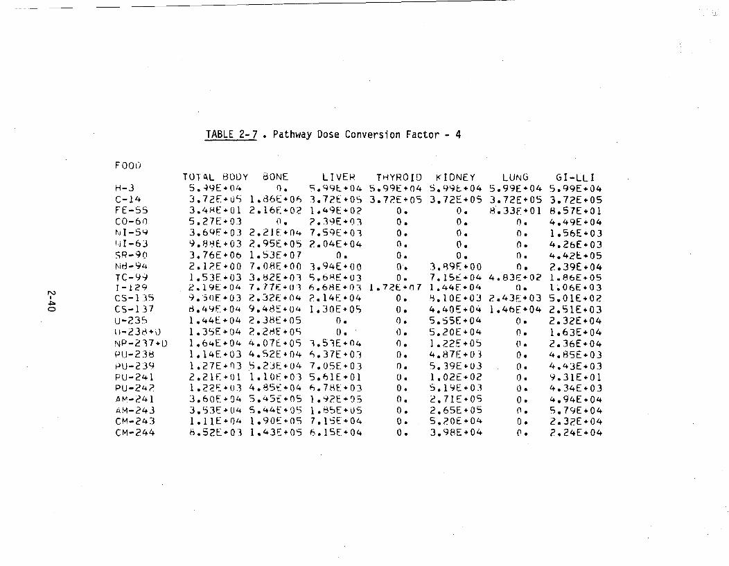
TABLE 2-7 . Pathway Dose Conversion Factor - 4

CD

FO00

H-3C-14FE-S5CO-60I , -54

tjI-..63

SR-90N8-94TC-99T-129CS- 1.35CS- 1.37U-235

NP-237÷lP U -238PU-239PU-241PU-24?,AM-24 1AM-243CM-243CM-244

TO•AL BOO)5. 49E+043.72E+093.4ME+015.27E+033.69F+.039.88E+033.76E+062. 1?E.001 .53E+032. 19E÷049*. 50[F+038,49F+041 .44E+04I .35E + .f41 .64E+041 *•14E+03

1.27E+032.21F-01I .22;.+J033.60E+043.53E÷041 . I IE÷048.52E+03

BONE0.

1.86E+062.16E+02

2.21 E + 042.95E+051.53F+077.08E+003.82E+037. 77E+032.32E+049.48E÷042.38E+052.2HE,0Lý4.07E÷054.52E+045.23E÷04I . 10E+034. 85E+ 045.45E÷055.44E÷051.90E+051.43E+05

LIVER5.49E÷043.72E+051 .49E+02?.39E.037.59E+032.04E+04

0.3.94E+009.68E+036.68E +(02.14E+041.30E+05

0.0.

3.53E÷046. 37E+037,05E÷035.61E.01

6.78E+03

1 .9?E-951 0.SE+057. 1SE+046. 15E.+04

THYROID5.99E÷043.72E+05

0.0.0.0.0.

0.1.72E.07

0.0.0.

000.0.0.0.0.0.0.0.0.

KIDNEY5.99E+043. 72E7 05

0.0.0.0.0.

3.99E+007. 15E÷041.44E+04li. IOE+034.40EP045.55F+ 045.20E÷041.22E÷054.87E + 0 35. 39E+031 .02t-025. 19E+032. 71E+052.65E÷055.20E+043.98E+04

LUNG5.99E+043.72E÷058.33E+01

0.0.0.0.00 0

4. 83E+ 02()

2.43E+031,.46E+04

0.0.

00.

() a

Oa

0.

0.0.00.

0.

GI-LLI5.99E+043.72E+058.57E+014.49E+041.56E*034.26E+034.42E+052.39E+041.86E+05I 06E+035.01E+022.51E+032.32E÷041.63E+042.36E+044.85E+034.43E+039.31E+014.34E+034.94E+045.79E+042.32E+042.24E+04

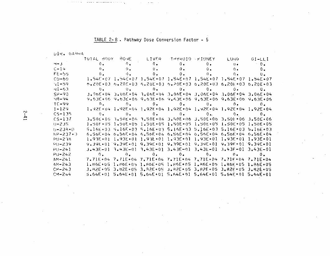
TABLE 2-8 . Pathway Dose Conversion Factor - 5

N,

4-

b Ilq. (7;A m m

H-JC-14FE-55CF -60

"N 1-59

NI-63SP-90

TC-991-129CS -137CS-I 13 7U -235

2 -23 8 + )N P -237 + 1)Pt J-238

P U-239Pt.1-241PU-242AM-241AM-243CM -243CM-244

TUIAL HODY RONE LIVER0. flo 0.

0. 0. 0.

1.54•+01 1.54E+07 1.54E+07&,.20E+03 6.20E+03 6.20E÷03

O. O. 0.3.ObR+)04 3o06F1+04 1.06E()049.63Ei+06 q.63t>+06 q.63E.+06

no . ,0.

1,.)2E+04 1.92F+04 1.92E+040. 0. 0.

3.50L÷0o 3 . 50E+O I [.E+0t].l0oe+05 1.SUE.Os 1.50E+055.16E+93 5.16.+03 ;.16E+036.56E+04 6.56E+04 6.56F:+041.93F*01 1.93E+01 1.93E+019.39E+01 9.39E.+01 9.39E+0I3.43E-01 3.43E-0] 3.43E-01

0. 0. 0.7.71E-+04 7.7tIE+04 7.71E+041.H6[+05 1.86E+05 1.H6E+053.82E÷95 3.'2E+05 3.i?+__+OL5.64E+01 5.64E+01 5.64E÷01

THYkOIO -IDNEY0. 0.

LUN C70°

0. 0. o. 0.0. o. 0. 0.

1.54E+07 1.54E+07 1.54E+07 1.54E+075.?OE+03 6.20E÷03 6.20k03 b.20E+03

()o 0. 1 0. 0.3.06E+04 3.06E+04 .3.06E+04 3.06E+049o.63E+06 9.63E*06 9.63E+06 9.63E*06

0. 0. 0. 0.

1.92E+04 1.92E*04 1.92F+04 1.92E*040. 0., 0. 0.

3.,0E+06 3.50E.Ob 3.50F+06 3.50E÷061.50E÷05 1.50E÷05 1.50E05 1.50E+05

5.16E+03 5.46E+03 5.16E÷03 5,1bE.036.56E+04 6.56E+04 6.56E+04 6.56E*04I.,;3E*nl 1.93E+01 1.93E+01 1.93E+01

9.39E+01 9.39E401 9.39F+01 9.39E+013.43E-01 3.43E-01 3.43E-01 3,43E-01

0. 0. 0. 0.

7.71E+04 7.71E+04 7°71F+04 7.71E+041.86E+05 1.H6E+0s 1.86E÷05 1.86E+053.2E+05 3.8?E+05 3.82E÷05 3.82E055.64E+01 5.64E+01 5.64E÷01 5.64E+01

GI-LLI.0

TABLE 2-9 . Pathway Dose Conversion Factor - 6

N)I.

NJ

wELL W'ATFH

H-3C-14FE-55CU-60

IN 1-5qI -63

SR -90)'Nb-94

TC-991-129CS- 1 3LCS-137u-235i'-238 +0NP-237+)PU-238PU-239PU-241P U.-24?AM-2414,-1-24 3CM-243CM-244

TOTAL. HODY2.37E+061.44E.0 72.73E÷06I . 4.3E +'18-8.54+E+ 06I .92E+077.61E+093.19E÷073.60E÷ 054.1BE073.32E+073 . 09 E + 082 . 07 E'+ 081 .?.3E+082.31E,÷087.0?2F0'11. 77E+071 .34,E.061. 532E + 072.25E+0 F2.21E÷08

1. 17E+08

bONE1.42E-01

.21. E(071.24FE÷071.24E.0•4.42E+0750.I1E+0•

3 a10 E +I1

3.20E+078.96E÷051. 72 E+078.09E÷073.44E÷O03.24EP'093.09E÷095.55E÷092.74E+093. 17E+096.64E*072.94F .093.34E+043.34F+092.60E+091.95E+09

* LIVER2.37E*061•44E+078.86E+06I .33E+Oi1.61E+073.96E.078.83E÷063.19E071. .33E+061.53E+077.471E-074.65E+081.18E+077.74E÷054.8hE÷083.93E.084.34E.083.51E+064.18E+081. 19F+0q1.15E+09Q.T97E +088,44E+OA

THYROID2.37E+061.44E+078.61E+051 .?4E+18

1.38E+064.?8E-018H.3E+063i 19E+072.0BE00?.99E. 101.39E+001.29E+07I .IRE+077.74E+057.13E+061.03E.063.93E÷n5] .31E-01

7.67E+054. 19E÷064.94Eb06I .30E÷079.09F-+05

KIDNEY2.37E+061.44E:078.61.E051.24E+081.38E+064.28BE-018.,33E÷063. 19E*07I .68E.072.87E+072.83E+071.66E+087.64E÷087.05E081.67E.092.97E+083.28E+086. 18E.063. 17E+081.66E+091.63E÷097.21E+085.43E+0'.

LUNG2.37Fe+061 .44E+,075.33F .061 .24E÷081.38E+062.42F+028.83F+063.19F+071.13F+053.64E+06B.4bF.066.39EO '72.10E÷079.32E+068.1 1E÷061.22F+07I .09E÷071.86F+041.09E+075. 35F+065.93F+001.42F+072. 12F+06

GI-LLI2.37E+061,44E+075.45E.062.89E+084.41E.068.26E+069. 04E+081.47E+084.36E+075.48E+061.75EE062. 16E+073.26E+08?.22E+OR3.26E+082*94E÷082.68E*085.62E÷062.63E+083. 05E+083.57E+083.27E+083904E+08

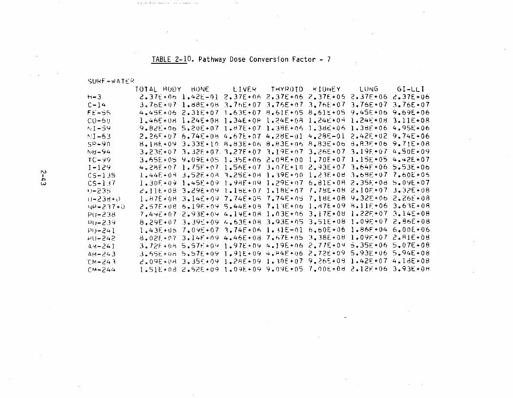
TABLE 2-10. Pathway Dose Conversion Factor - 7

SURF -W ATt'RTOTAL RODY HONE LIVEP THYOID KIDr1NEY LUNG GI-LLI

PA)

H-3C-14FE--S5

CO-6 QNI-59ý!1I-63

SP-90NIB-94TC -991-129CS-135C S - 1371-235I 1-23 + L)Nf-p-2 3 7+0Pt -238L)u -.-239PlJ-241PUJ-242.4 -1 - 24 1AM -243

CM-24 3CM-244

9 .82E+Ob 5.20E0'7 1.87E÷07 1.38E4n6 1.38E+06,2.26_6-*07 6.74E÷0. 4.67EF 07 4.28E-01 4.28E-O18.18E*09 3.33E+10 8.83E+06 8.83E+06 R.83E+Oo3.23E÷07 3.32E+07.3.27E÷07 3.19E+07 3.26E+073.65E+O5 9.09E+05 1.3bE*06 2.011EO0 1.70E÷074.28E+O( 1.15E+!7 1.56E+07 3.07E+.10 2.93E+071.44F+03 3.52F+O 3.2¶5E+08 1.39E÷00 1.23E081.3(F4,09 1.45EO09 o.9SE÷+)9 1.29E+i)7 6.81E+082.1IE.+0B 3.29E+01 1.18E+07 1.18E+07 7.78E+OB1.87E+08. 3.14E'+0) 7.74E÷05 7.74E+06 7.18E+082.57F+08 6.19F+09 5.44E+0. 7.13E+O)b 1.87E+097.44E+07 2.93E+04 4.19E+0 1.03E+06 3.17E+088.29E+07 3.39>+09 4-.63E+0$ 3.93E+05 3.51E+081,43E+06 7.09E+07 3.74E+0#A 1.3lE-01 6.60E+068.02E+07 3.14E+09 4.46E÷08 7.67E÷o5 3.38E+083.72F,+08 5.57F+Q0(, 1.97E+09 4.]9E+)6 2.77E*093.65LE+o, 5.57E+09 1.91E+09 +.R4E+06 ?.72E+092.09E+08 3,35"+01 1.2PE÷09 I. 3OE07 9.26E+081.51E+08 2.52E+09 1..09E09 9.09E+05 7.00E+08

1.38EF06 4.95E÷062.426+02 9.74E+068.83F+06 9.71E+083.19F'U7 4.50E+091.15F+05 4.,+2E+073.646.06 5.53E+Ob3.,48E07 7.60E+062.35F÷08 5.09E+072.10F÷07 3.32E÷089.32E40b 2.26E+088. 11F+06 3.6*E'081.22F+07 3.14E+081.096+07 2.86Ei081.86F+04 6.00+E061.09F+07 2.81E÷085.35V'÷06 5.07E+085.936'U6 5.94E+081.42F+07 4.18E+082.12F+06 3.93E+OH

2.37E+Ob 1.42E-01 2.37E40'. 2.37E+06 2.37E*06 ?.37F+06 2.37E+063.o7hE07 1.l78E+0 3.70E+07 3.76E+07 3,76E'+07 3.76E+07 3.76E+074.45F+06 2.31E+07 1.63F.07 8.61E+05 8.61E+05 9.45f+0b 9.69E+06

1.46U+8H 1.24E+08 1.34E*O0 1.24E÷08 1.24E÷+O 1.24E÷08 3.11E+08

TABLE 2-11 . Pathway Dose Conversion Factor - 8

r•I4•4•

A TMOSPHERE

H-3C-14FE-55)

Co-60N.\ 1 -59NI-63S-R-90N18-94TC-991-129CS-135CS-137Ij-235÷u-238.L0N P-237 ÷DPU-238PU-239PU-241PU-242AM-241AM-243CM-243CM-244

TOTAL HO0)Y4.45F + 02.66E+I I4..,3E + 102.68E,12

3.34E÷[Ii .53E+146.IoE+l15.61E÷09b.91E+125, 73E÷ 115.36E+ 125.37E+124.79E +125. ?4E+ 142.01E+l42.2SE+143.06E÷122.17E+145.08E÷145.00E+143.87E+142.82E÷14

HONE5.19E÷071.33E+122.06E+lI2.34E÷127.73E+lI1,0OE÷136.21E÷146.12E.111.20E+103.69E.121.44E+126. 12E+128.52E÷138.11 E+131.21E÷164.13E÷154.85E+157.55E+134.53E 157.18E÷157. 1 0E+ 156.20E÷154*.43E*15

LIVFP4.45E+102.66E÷ I11.54E+lI

.5,)E +12.?.84E+1]6.93E* III .67E÷ I+6. 1E1 E11.87E÷103.29E÷121.33F÷124.27E+12

2.21 E + 11I .45E+Io16 13E÷1IL?.61E+153.13E+154,57E+133.05E+.156.66E÷156,50E+155.62E÷154. 17E÷15

THYROID4.49E+10

2.66E÷II1.61E+102.34E])22,•8E÷101:96E÷081.67E÷I16.10E+117.60E÷086.33E+155.08E+082.4?E.ll2.21E÷II1.45E+101.34E÷II1.92E+10

.'740E+094.78E+071,44E+107,8'7E÷109.10E+102.44E+ll1.71E+10

KIDNEY4.45E+10

2.66E. 11I.61E102. 34E÷ 122.58E101.56E÷081.67E÷116.1 1E+ 112.27E.16.10E+125.02E+1I12.97E+122.00 E.+1311 .85E+133.87E+158.85E+149.66E+ 14I.45E+139.65E+ 143.87E÷153. 79E+151.77E+151.29E+15

LUN64.45E+102.66F+I I2.80E+I I

2.63E+ 135.78E.108.82E+ 101.98E 111.33E+128,80E+098.57E+I 11.55E 111. 18E+123°36E÷153.12E+153*60E+144,08E÷ 153,84E÷156.bOE+123.68E*154&24E+144.00E+144*40E÷144.40E÷ 14

GI-LLI4.33E÷102.65E+j 19.36E+ 105.27E+127.65E 101. 38E+ 111.53E+132. 1SE+125.45E+ 111.24E+123900E+103.90E÷1I5084E+124.OOE.125.79E÷125. 30E+ 124.83E÷121.O1E÷114.74E+125.43E+126.31E+125.87E. 125.45E.12

to humans as a better indicator of the limiting exposure due to 1-129

than the thyroid dose.( 3 0 ) This selection results in a significant

difference in limiting exposures since the fundamental dose conversion

factors for thyroid are about 1000 times that of total body (see

Tables 2-4 through 2-11). A correction to the calculated 1-129

thyroid PDCF's to account for dilution with natural iodine has not

been made in this report, however, in view of the evidence, judicious

use of the 1-129 thyroid PDCF's is indicated.

2.4 Release/Transport Scenarios

The connection between the radioactive concentrations at the various

biota access locations and the potential radiological dose to man was

examined in the previous section. This section introduces and sum-

marizes the remaining part of the waste-to-man connection, namely the

release/transport scenarios that relate the radioactive concentra-

tions in the waste to the radionuclide concentrations at the biota

access locations. Considerable additional information regarding the

release/transport scenarios is provided in Chapter 3.0.

As detailed in Section 2.3, there are seven release/transport sce-

narios to be considered. Three of these scenarios - the accident,

construction, and agriculture scenarios - depend on the concentration

of the individual waste streams, and hence are termed the "concen-

tration scenarios". The other four - leaching and migration with well

and open water access, surface water transport of exposed waste, and

atmospheric transport of exposed waste - depend on the total inventory

of radioactivity and the total volume of the disposed waste, and are

termed the "total activity scenarios." These are examined below.

2.4.1 Concentration Scenarios

The first scenario considered concerns accidents that may happen

during the operational period of the disposal facility lifespan, and

2-45

which may result in off-site atmospheric transport of radionuclides.

The other two scenarios are concerned with exposures to a potential

inadvertant intruder. An intruder may unintentionally come across a

closed waste disposal site due to a temporary breakdown in institu-

tional controls, and subsequently modify it for a specific purpose,

such as housing construction or agriculture. As a result, short- and

long-term radiation exposures to the individual can ensue.

Two of the concentration scenarios (accident and inadvertant intru-

der-construction) are acute exposure events. That is, the release

and subsequent exposure occurs for a limited period of time (less than

a year). The other scenario (inadvertant intruder-agriculture),

however, is assumed to be chronic, since it is possible (but unlikely)

that the intruder would live for several years at the site before it

is discovered that there is a hazard.

Very few individuals are involved in the concentration scenarios, and

they may also be distinguished from the total activity scenarios by

the dose limitation criteria which may be applied. In other words,

different limits on allowable human doses may be used, depending upon

whether a few individuals or populations are exposed. (2,3,13,17)

The equation generally applicable to the above concentration scenarios

is:

C = I x Cw (2-2)

where (Ca) denotes the radionuclide concentration at the biota accessa

location and (C ) denotes the radionuclide concentration of the waste,w

both in units of (Ci/m 3 ), and (1) is the dimensionless interaction

factor, which depends on the specific scenario considered.

For these scenarios, the as-generated waste radioactive concentrations(1)are utilized. For the intruder-construction and intruder-agricul-

ture scenarios, this is conservative since it is equivalent to the

2-46

assumption that the inadvertant intruder initiates the scenario

at a location containing waste from the last year of disposal facility

operation.

The interaction factor (1) can generally be expressed through the

following equation:

I.= f0 x fd x fw x fS' (2-3)

where all the parameters are dimensionless, and where

fo = time-delay factor;

fd = site design and operation factor;

fw = waste form and package factor; and

f = site selection factor.s

The time-delay factor (f ) is expressed as an exponential radio-0

nuclide decay factor and incorporates the effects of the closure

period and the active institutional control period. The activities

are decayed to the time that the specific scenario is initiated.

This factor is a property of the scenario and the disposal technology

Deing considered. For the accident scenario, no credit for radioactive

decay can be assumed and (f ) will be taken equal to one. However,

for the construction and agriculture scenarios, it is given by the

formula:

f= exp[ X T] (2-4)

-1

where X is the radionuclide decay constant in units of year ,

and T is the period between the cessation of disposal operations and

the end of active institutional control period.

The site design and operation factor (f ) expresses the waste frac-

tion that is available to the transfer agent. It usually depends on

2-47

the efficiency of the disposal design. Furthermore, its definition

and value depends on whether the scenario is an inadvertant intruder

scenario or an accident scenario (see Sections 3.3 and 3.7).

The waste form and package factor (f w) expresses the resistance of

the waste to mobilization by the specific transfer agent initiating

the scenario. For example, this factor would be considerably less

than unity for waste streams solidified in a matrix and/or packaged in

containers that are likely to retain their integrity at the time of

inadvertant intrusion. This factor is a property of the waste stream

as it is being disposed.

The site selection factor (f s) depends on many parameters. In some

cases, it is proportional to the fraction of a year that the human

exposure episode takes place. Since the dose conversion factors

presented in Section 2.3 have been calculated for a full year exposure

period, the factor (fs) must compensate for this calculational con-

venience. In other cases, however, (f s) is also proportional to

the release/transport/transfer factor between the biota access loca-

tions. For example, for the inadvertant intruder-construction sce-

nario, it is proportional to the transfer factor between contaminated

soil and contaminated air. This factor is examined in greater detail

in Appendix A.

A brief description of the concentration scenarios is presented below.

Specific values of the transfer factors used to calculate impacts are

discussed in Chapter 3.0 and Appendix A.

Accident Scenario

Non-occupational acute radiation exposures may result from planned and

unplanned releases of material to offsite environs during the opera-

tional life of the facility. Planned releases would be addressed on a

site-specific basis during the licensing phase of site startup. This

2-48

report-considers only the-unplanned (accidental) releases. Two

accidental release scenarios can be postulated. One of them involves

a postulated breaking open of a waste container and subsequent release

of airborne radioactivity, and the second scenario considers the

consequences of a fire igniting in an open disposal trench, with

subsequent burning of a portion of the waste and airborne release of

combustion products. The comparative severity of these two scenarios

depends on various parameters including those associated with the

waste form and with site operations.

Construction Scenario

An inadvertant intruder may choose to excavate or construct a building

on a disposal site. Under these circumstances, dust will be generated

from the application of mechanical forces to the surface materials

(soil, rock) through tools and implements (wheels, blades) that

pulverize and abrade these materials. The dust particles generated

are entrained by localized turbulent air currents. These suspended

particles can thus become available for inhalation by the intruder.

-The intruder may also be exposed to direct gamma radiation resulting

from airborne particulates and by working directly in the waste-soil

mixture, etc. (See Section 2.3 for the uptake pathways considered.)

For convenience, this scenario is called the intruder-construction

scenario, and appropriate values applicable to typical construction

activities are used.

Agriculture Scenario

In this scenario, an inadvertant intruder is assumed to occupy a

dwelling located on the disposal facility and ingest food grown in

contaminated soil. Garden crops may be subject to radionuclide

contamination as a result of direct foliar deposition of fallout

particulates. Garden crops may also uptake radionuclides via soil-

root transfer from contaminated soil. The soil may be initially

2-49

contaminated, or it may become contaminated as a result of deposi-

tion. The inadvertant intruder may also be exposed to direct ionizing

radiation such as'beta and gamma radiation from the naturally sus-

pended radioactivity and from the waste-soil mixture. He may also

inhale contaminated air particulates, etc. (See Section 2.3 for the

uptake pathways considered.) This scenario is called the intruder-

agriculture scenario.

2.4.2 Total Activity Scenarios

This section considers those release/transport scenarios that are

dependent upon the entire activity disposed of at the site. There-

fore, all the waste streams disposed at the site contribute to the

radionuclide concentrations at the biota access locations. The degree

of contribution from a given waste stream is a function of its volume

and characteristics (e.g., its form and packaging) and facility design

and operating practices (e.g., waste segregation).

All of the total activity scenarios are chronic exposure scenarios

(i.e., continuous release and exposure). Theoretically, all four

different types of biota access locations are possible as a result of

the total activity scenarios. Some of the release/transport scenarios

that lead to them are considered below.

The equation applicable to the total activity scenarios for each

radionuclide is:

Ca D i x Cwi (2-5)

where (Ca) and (Cwi) denote the radionuclide concentrations at the

biota access location and in the (i)th waste stream, respectively,

in units of (Ci/m 3), and (Ii) is the interaction factor between

the (i)th waste stream and the biota access location. The capital

sigma indicates that the total radionuclide concentration at the

2-50

biota access location is a summation of the radioactivity contributed

by each waste stream. This summation may also include any potential

integration that must be performed due to the areal extent of the

disposal site and the areal distribution of thewaste streams.

For these scenarios, generation time-averaged radioactive concentra-

tions averaged over the time of waste generation and disposal are

utilized as a source term.( 1 ) In other words, the radionuclides in

waste streams that are disposed of at the beginning of the disposal

site operational period are decayed to the end of the operational

period. The need for this averaging is obvious since the entire waste

volume interacts with the environment.

The interaction factor (Ii) can generally be expressed through the

following equation:

Ii = f x fdi x fwi x fsi (2-6)

where the subscript i denotes the waste stream, and where:

f = time-delay factor (dimensionless);

f di site design and operation factor (dimensionless);

fwi= waste form and package factor (m /yr); and

fsi= site selection factor (yr/m3);

and where the values of fdi' fwi and fsi may be functions of the

properties of the individual waste streams.

Groundwater Scenarios

There are several groundwater scenarios depending on the assumed

access location. One of the access locations is an on-site well which

may be drilled and used by a potential inadvertant intruder (intruder-

well scenario); another is a well at the boundary of the site which

2-51

may be utilized by individuals (boundary-well scenario), a third

location is a well pumped for common use by a small population some

distance away from the disposal facility (population-well scenario);

and the fourth location is a stream that receives the discharge from

the unconfined groundwater table and which may be used by a larger

population (population-surface water scenario).

In this report, it is assumed that the water table gradient underneath

the site is unidirectional, and that the individual-well located at

the boundary of the disposal area (rather than the boundary of the

site) contributes to the intruder scenarios. This location is more

conservative than a well located in the middle of the site since only

about half of the potential effluent from the site would contribute to

the contamination at a well in the middle of the site whereas all of

the potential effluent from the site would contribute to the location

assumed for the intruder-well.

The factors fdi and fwi are assumed to be independent of the areal

extent of the disposal facility, however, the factor fsi represents

these areal relationships. The factors fdi and fwi and their

computations are straightforward and representative values for

these factors are given in Section 3.0. However, a brief discussion

of fsi is presented below.

The following general equation is applicable to determine the site

selection factor fsi :(31,32)

fsi = rg rti IQ (2-7)

where

rg = dimensionless time independent reduction factor due to

the transverse (perpendicular to the groundwater velocity

direction) spatial relationship of the disposal facility with

the discharge location,

2-52

r ti= dimensionless reduction factor due to migration and radio-

active decay; this factor is dependent on both space and time

including the longitudinal (in the direction of the ground-

water velocity) spatial relationship of the disposal facility

withthe discharge location; and

Q = dilution factor in units of volume/time.

The factor Q is independent of the characteristics of the disposed

wastes and is also independent of the geometrical relationship of the

disposal facility with the discharge location. The factor Q may be

the pumping rate of a well or the flow rate of a river. The factors

rg and rti are discussed in Section 3.5.

Exposed Waste Scenarios

In these scenarios, part or all of the surface area of the disposed

waste is assumed to be exposed through some means, and this exposed

waste is assumed to be accessed by transfer agents such as wind or

water. The mechanism that initiates uncovering of the waste may be

erosion of the waste cover by surface water or wind action, or it may

be anthropogenic activities such as construction or farming. Initi-

ating mechanisms related to human activities are examined in the

intruder-agriculture and intruder-construction scenarios, and initi-

ating mechanisms related to erosion of the waste cover are examined in

Appendix A.

There are two basic exposed waste scenarios depending on whether the

transfer agent is wind or surface water. For the wind transport

scenario, only population exposures are considered; individual expo-

sures are bounded by the above intruder-construction and intruder-

agriculture scenarios. The entire exposed waste area is assumed to be

a point source for the impact calculations since the population is

assumed to be comparatively distant.

2-53

For the surface water ,transport scenarios, exposures to individuals

.consuming water from an open water access location is considered.

Again the disposal facility is considered a point source for this

scenario since it is not possible to consider the areal extent of the

facility for surface water transport. The equations and values for

the various barrier factors used in the calculations are examined in

-Chapter 3.0 and Appendix A.

2-54

REFERENCES FOR CHAPTER 2.0

1. Wild, R., et.al., Dames & Moore, "Data Base for Radioactive WasteManagement. Volume 2. Waste Source Options," USNRC ReportNUREG/CR-1759, November 1981.

2. U.S. Nuclear Regulatory Commission, Office of Nuclear MaterialsSafety and Safeguards, "Draft Environmental Impact Statement on10 CFR Part 61 : Licensing Requirements for Land Disposal ofRadioactive Waste," NUREG-0782, September 1981.

3. International Commission on Radiological Protection (ICRP),"Radionuclide Release into the Environment: Assessment of Dosesto Man," ICRP Publication 29, 1978.

4. Denham, D. H. et.al., "Radiological Evaluation for AdvancedWaste Management Studies," Battelle Pacific Northwest Labora-tories Report No. BNWL-1764, 1973.

5. Cember, H., Introduction to Health Physics, Pergamon Press Inc.,New York, 1969.

6. Healy, J.W., and J.C. Rodgers, "Limits for the Department ofEnergy Transuranic Wastes," Los Alamos Scientific Laboratory,LA-UR-79-100, January 1979.

7. Clancy, J., et.al., Dames & Moore, "Data Base for RadioactiveWaste Management. Volume 1. Review of Past Disposal Practices,"USNRC Report NUREG/CR-1759, November 1981.

8. Duguid, J. 0., "Assessment of Department of Energy Low LevelRadioactive Solid Waste Disposal Storage Activities," Battelle-Columbus Laboratories, Columbus, Ohio, BMI-1984, November 1977.

9. Dames & Moore, "Development of Monitoring Programs for ERDAOwned Radioactive Low-Level Waste Burial Sites," U.S.ERDA Con-tract No. E(49-1)-3759, July, 1976.

10. Lu, A.H., and Matuzsek, J.M., "Transport Through a Trench Coverof Gaseous Tritiated Compounds from Buried Radioactive Wastes,"Symposium on the Behavior of Tritium in the Environment, SanFransisco, CA, IAEA-SM-232/60, October 1978.

11. Dames & Moore, "Assessment of Levels, Potential Origins andTransport Routes of Radioactivity Measured in the Vicinity ofMaxey Flats Low-Level Radioactive Waste Disposal Site," Preparedfor the Commonwealth of Kentucky, Department of Human Resources,March 1977.

2-55

12. Webster, D.A., "A Review of Hydrologic and Geologic ConditionsRelated to the Radioactive Solid Waste Burial Grounds at OakRidge- National Laboratory, Tennessee," U.S. Geological SurveyOpen File Report, 76-727, 1976.

13. Clancy, J., Dames & Moore, "Trench Gas Study at the BeattyLow-Level Radioactive Waste Disposal Site," Prepared for NuclearEngineering Company, Inc., Louisville, Kentucky, October 1978.

14. "Four Million Dollars Sought for Maxey Flats," The Morehead News,Morehead, Kentucky, Vol.97, No.14, pp.1-2, February 15, 1980.

15. "Task Group on Lung Dynamics for Committee II of the Interna-tional Commission on Radiological Protection," Health Physics12, 173 , 1966.

16. International Commission on Radiological Protection (ICRP),"The Metabolism of Compounds of Plutonium and Other Actinides,"ICRP Publication 19, Pergamon Press, Oxford, 1972.

17. International Commission on Radiological Protection (ICRP),"Report of Committee II on Permissible Dose From Internal Radia-tion," ICRP Publication 2, 1959.

18. Houston, J.R., D.L. Strenge, and E.C. Watson, "DACRIN - A Com-puter Program for Calculating Organ Dose From Acute or ChronicRadionuclide Inhalation," Battelle Memorial Institute PacificNorthwest Laboratories Report, BNWL-B-389, December 1974.

19. U.S.Nuclear Regulatory Commission, Regulatory Guide 1.109."Calculation of Annual Doses to Man from Routine Releasesof Reactor Effluents for the Purpose of Evaluating Compliancewith 10 CFR Part 50, Appendix I." Revision 1, October, 1977.

20. U.S. Nuclear Regulatory Commission, "Age specific Radiation DoseCommittment Factors for a One Year Chronic Intake," USNRC ReportNUREG-0172, November 1977.

21. Beck, H. and G. de Planque, "The Radiation Field In air Due toDistributed Gamma Ray Sources in the Ground," U.S. Atomic EnergyCommission, Health and Safety Laboratory Report No. HASL-195,1968.

22. Lederer, C.M., J.M. Hollander, and I. Perlman, Table of Isotopes,Sixth Edition, John Wiley & Sons, Inc., New York, 1967.

23. Kocher, D.C., "Dose-Rate Conversion Factors for External Exposureto Photon and Electron Radiation from Radionuclides Occurring inRoutine Releases from Nuclear Fuel Cycle Facilities," Preparedfor U.S. Nuclear Regulatory Commission by Oak Ridge NationalLaboratory, USNRC Report NUREG/CR-0494, 1979.

2-56

24. Ng, Y.C., et.al., "Prediction of the Maximum Dosage to Man fromthe Fallout of Nuclear Devices," Part IV., Handbook for Esti-mating the Maximum Internal Dose from Radionuclides Releasedto the Biosphere, Lawrence Livermore Laboratory Report No.UCRL-50163, 1968.

25. Greenhouse, N.A. and E.T. Lessard, "A Dosimetric Analysis ofPathways to Man From the Environmental Release of Low LevelRadioactive Wastes," Prepared for Dames & Moore by Occupationaland Environmental Health Analysts, Inc., 1980.

26. Napier, B.A., W.E. Kennedy, Jr., and J.K. Soldat, "PABLM - AComputer Program to Calculate Accumulated Radiation Doses fromRadionuclides in the Environment," Battelle Pacific NorthwestLaboratory Report PNL-3209.

27. Brauer, J.K., et.al. "Natural Iodine and Iodine-129 in MammalianThyroids and Environmental Samples Taken From Sites in the USA,"Environmental Surveillance Around Nuclear Installations, Vol.11,Proceedings of a Symposium Warsaw 5-9 November 1973, IAEA Pub-lication, IAEA-TM-180/34, 1974.

28. Palms, J.M., and V.R. Veluri, "A Summary cfjqthe Analysis Asso-ciated with the Environmental Impact of I Released by theBarnwell Nuclear Fuel Plant," Emory University Report EMP-122,July 1974.

29. Leddicotte, G.W., et.al. "Suggested Quantity and ConcentrationLimits to be Applied to Key Isotopes in. Shallow Land Burial,"Management of Low-Level Radioactive Waste, Volume 2, PergamonPress, New York, 1979.

30. Adam, J.A. and V.L.Rogers, "A Classification System for Radio-active Waste Disposal - What Waste Goes Where?," NUREG-0456,FBDU-224-10, Prepared by Ford Bacon & Davis Utah for USNRC,June 1978.

31. Aikens, A.E., et.al., Dames & Moore, "Generic Methodology forAssessment of Radiation Doses from Groundwater Migration ofRadionuclides in LWR Wastes in Shallow Land Burial Trenches,"Prepared for Atomic Industial Forum, Inc., AIF/NESP-013, Decem-ber, 1977.

32. Lester, D., et.al., Science Applications, Inc., "Systems Analysisof Shallow Land Burial Project 5 " USNRC Report NUREG/CR-1963,March 1981.

2-57

3.0 DISPOSAL IMPACTS

This chapter further develops the calculational procedures utilized

to determine the impact measures associated with the disposal of LLW.

These impact-measures include individual and population exposures,

occupational exposures, costs, energy use, and land use.

Section 3.1 is an introduction to the chapter and presents a discus-

sion on the information base and the approach utilized in the radio-

logical disposal impacts calculations. Following this introduction,

Section 3.2 presents the background assumptions regarding the disposal

technology alternatives considered, discusses how these assumptions

are incorporated into the impact calculations, and presents background

information on the specific values utilized to quantify the effects of

these alternatives. Section 3.3 presents procedures through which

the effects of waste form and packaging are incorporated into the

calculations, and presents background information on the specific

values selected to quantify the effects of waste form and packaging on

the impact calculations.

Following these three background sections, Sections 3.4 through 3.7

present the equations and specific parameter values used to calculate

individual and population exposures for the scenarios considered in

Chapter 2.0. Finally, Section 3.8 details the calculation of many of

the other impact measures considered in this report, including occu-

pational exposures, land-use, disposal costs, and energy use.

3.1 Introduction

The impact measures associated with the disposal of L.LW are strongly

dependent on waste form and package properties,1) and disposal

facility environment, design, and operating practices.( 2' 3 ) This

section presents a discussion on the information base utilized in this

report and the general approach adopted.

3-1

3.1.1 Information Base

The information base for disposal impact calculations includes three

main components: waste characteristics, disposal facility environment,

and disposal facility design. In this report, the continental U.S. is

assumed to be divided into four regions, based on the 5 U.S. NRC

regions (see Appendix C): the northeast (Region I), the southeast

(Region II), the midwest (Region III), and the west (Regions IV and

V).(1) Waste characteristics and disposal facility environment are

correlated with these four regions as discussed below.

The first component of the information base is on waste characteris-

tics. The calculational methodology allows consideration of a wide

range in waste forms and processing options. In many previous studies

on LLW management and disposal, the disposed waste was usually assumed

to be a mostly uncharacterized mass with little attempt to distin-

guish, in a quantitative manner, the different waste forms. In this

work, however, LLW is separated into 36 waste streams and each waste

stream is characterized in terms of its physical , chemical, and

radiological properties. The volumes of each waste stream are con-

sidered on a regional basis. That is, the volume of a given waste

stream is projected for each of the above four regions over the next

20 years, which allows consideration of regional impacts of management

and disposal of LLW. Furthermore, four generic alternative waste form

and processing options are considered. These generic processing

options, called "waste spectra," represent four relative levels of

waste processing activities applied to the 36 waste streams charac-

terized. The waste spectra have been developed to limit the number of

waste form and packaging alternatives that would have to be analyzed,

since an infinite number of possible combinations of various waste

streams and processing options are available. The waste spectra

considered (see Chapter 6.0) range from Waste Spectrum No.1, which

characterizes a continuation of existing or past waste management

practices, to Waste Spectrum No.4, which characterizes the maximum

3-2

volume reduction and improved waste forms that currently can be

practically achieved. The waste streams corresponding to a given

spectrum may be transported to and disposed into facilities located at

the regional sites and the resulting potential impacts calculated.

The second component of the information base is the disposal facility

environment. In each region, a hypothetical regional disposal faci-

lity site has been characterized (see Appendix C). These sites, while

not representing any particular location within the region, represent

typical' environmental conditions within the regions. This allows

consideration in the calculational methodology of a wide range of

environmental parameters such as the amount of rainfall or the average

distance from the waste generator to the disposal facility site. (One

of these four sites, the southeastern site, is frequently referred to

in this work as the reference disposal facility site.)

The third component of the information base is the disposal facility

design. --To develop the calculational procedures, a reference near-

surface disposal facility is assumed. A description of this disposal

facility design, which is condensed from Appendix E of the U.S. NRC

environmental impact statement on management and disposal of LLW,(3)'

is provided in Appendix C of this report. A number of alternative

disposal facility designs and operating practices (e.g., thicker

disposal cell covers, use of cement grout) may be considered to

estimate the effect of these alternatives on the impact measures.

3.1.2 General Approach

From the above information base, it can be seen that, when considering

the effect of alternative regional, waste form, and facility design

characteristics on the magnitude of the impact measures calculated, an

extremely large number (thousands) of possible permutations can be

generated. To enable development of performance objectives and

technical criteria for LLW disposal, the number of these permutations

3-3

must be controlled and analyzed in a systematic manner. To do this,

two features in the disposal impacts analysis have been adopted:

(1) use of a reference disposal facility and a reference waste volume

distribution, and (2) extensive use of computer technology including

the use of waste form and disposal technology indices.

For the first.feature, a reference disposal facility is assumed which

is located in the humid eastern U.S. For this work, the reference

disposal facility site is assumed to have environmental characteris-

tics corresponding to the southeast regional site, although either the

northeast regional site or the midwest regional site could have been

used for this purpose. ( The reference waste volume distribution

is generated through summing all the waste volumes projected to be

generated in each of the four regions for each of the 36 waste streams,

and normalizing these volumes to one-million m3 of waste for Waste

Spectrum 1.(1) This allows the effects of alternative waste spectrum

and disposal facility designs to be compared on a common basis.

For the second feature, five computer codes have been written to

manipulate the alternatives and determine impact measures. These

include the codes INTRUDE, GRWATER, OPTIONS, INVERSI, and INVERSW, and

a description of these codes is provided in Chapter 6.0. In these

codes, extensive use of "indices" have been made to characterize waste

stream properties or disposal facility environmental and design

alternatives (see Sections 3.2 and 3.3). In other words, the value of

the indices are used to initiate specific calculational procedures or

use specific values of appropriate parameters. Use of integer indices

enables rapid and convenient consideration of alternatives for rule-

making. In addition, use of indices enables updates of the data base

and calculational procedures to be readily accomplished without

changing the values of the indices or the structure of the calcula-

tions. In the remainder of this report, the calculational procedures

are developed and discussed in the context of these indices.

3-4

3.2 Disposal Technology Indices

In order to analyze the impacts from disposal of LLW, alternative

disposal technology properties and their effect on the impact measure

calculations must be quantified. For example, depending on specific

operational procedures such as random or stacked disposal, the values

of the barrier factors presented in Section 2.2 vary. In this report,

the disposal technology properties have been expressed in the form of

integer indices that refer to a specific procedure used in the barrier

factor computations or determine a specific value of the environmental

parameters. These indices, which will be referred to as the disposal

technology indices, basically denote the selection options available

for a specific property. These selection options may be in the form

of a specific calculational procedure or a specific value for an

environmental property.

The disposal technology properties that have been considered in the

calculation of impacts in this report are summarized in Table 3-1, and

are discussed below.

3.2.1 Region Index - IR

This index, whose value is 1 or higher, is set depending upon the

region considered and determines use of a specific set of environmen-

tal properties in the impact calculations. The main effect of the

region index is on the site selection factor. Environmental proper-

ties that depend on the region index are presented in Table 3-2.

The value of this index corresponding to each of the regions consi-

dered (see Appendix C) are as follows:

IR = : Northeastern RegionIR = 2 : Southeastern RegionIR = 3 : Midwestern RegionIR = 4 : Western Region

3-5

TABLE 3-1

Property and Index

Disposal Technology Indices

Description

Region

Design

Cover

Emplacement

- IR- ID

- IC

- IE

Stabilization - IX

Layering - IL

Segregation - IS

Grouting - IG

Hot Waste - IHFacility

Geographic location of the disposal facility.

Two options are considered: regular trenches,and the so-called "concrete walled" trenches.

Three options on the cover between the wasteand the atmosphere are considered: regular,thick, and intruder barrier.

Three options on the emplacement of the wasteare considered: random, stacked, and randomcombined with decontainerized disposal forunstable wastes.

Three options on the stabilization programapplied to disposal cells, which may containstructurally unstable wastes, are considered:regular, moderate, and extensive.

Option on separating and putting selected wastestreams (usually with higher external radiationlevels) at the bottom of the disposal cell.

Option to segregate and separately dispose ofwastes that are combustible/compressible andthose that could contain complexing agents.

Option on filling of the interstitial spacesbetween the wastes with grouting material.

Option on having a special area within thedisposal facility with special procedures tohandle high activity wastes.

Closure Index - IQ This index indicates the activities during theclosure period (regular or extensive).

Care Level - ICL This index indicates the care level anticipatedIndex during the active institutional control period

(low, moderate, and high).

Post Opera- - IPO Duration of the period between the cessation oftional Period active disposal and the transfer of the title(Years) from the site operator to the site owner.

Institutional - IIC Duration between transfer of the title to theControl Period site owner and the assumed time for loss of(Years) institutional controls over the site.

3-6

TABLE 3-2 . Region Index Dependent Properties

Symbol Scenario Environmental Property

TPO

FSC

FSA

QFC

TTM

DTTM

TPC

DTPC

RGF

RET

PRC

Accident

Construction

Agriculture

GroundwaterII

a,

Im

{I

Exposed Waste

Air-to-air transfer factor

Soil-to-air transfer factor

Soil-to-air transfer Factor

Dilution Factor

Water Travel Time

Incremental Water Travel Time

Peclet Number

Incremental Peclet Number

Factor rg

Retardation Coefficients

Infiltrating Percolation

Air-to-air and surface water

transfer factors.

One-way travel distance

Number of stops per trip

Cask days per round-trip

POP

DIST

STPS

CASK

TransportationII

3-7

In this report, the southeastern region environmental characteristics

are used to represent the environmental characteristics of the refe-

rence disposal facility site. Variations of the values assumed for

the regions (e.g., to perform sensitivity analyses) can also be

triggered through the use of the region index.

3.2.2 Design and Operation Indices

There are four design and operation indices: design index - ID, cover

index - IC, emplacement index - IE, and stabilization index - IX. The

values of these indices are I or higher denoting the options available

in the design of the disposal facility; details of the options can be

found in Appendices E and F of reference 3. These indices are consi-

dered below.

The Design Index - ID characterizes the disposal cell design used for

radioactive waste disposal. Two options have been used in this study:

regular trench disposal and concrete-walled trench disposal. This

index primarily affects the site design factor.

In this report, three different "efficiencies" are utilized to des-

cribe the specific procedures employed in the disposal of wastes:

(1) the volumetric disposal efficiency which is defined as the volume

of disposal space available in the disposal cell (in m 3) per

unit surface area (in m 2) of the disposal cell,

(2) the emplacement efficiency which is the volume of waste emplaced

in the disposal cell (in m 3) per unit volume (in m 3) of available

disposal space, and

(3) the surface efficiency which is defined as the ratio of the

surface area occupied by the disposal cells to the surface area

occupied by the disposal cells plus the surface area between

these cells that have not been utilized for disposal.

3-8

The design index determines the volumetric disposal efficiency and

the surface efficiency of the design. The emplacement efficiency is

discussed below. Use of a hot waste facility (see Section 3.2.3).

which is defined as a special group of disposal cells. used for dispo-

sal of relatively high activity waste, is not included in the above

definitions; its efficiencies are assumed to be independent of the

design index.-

The Cover index - IC can be either 1, or 2, or 3, and it denotes

whether a "regular" cover (denoted by 1), a "thick" cover (denoted by

2), or an "intruder barrier" cover (denoted by 3) is placed over the

disposed waste. These three options are described in reference 3, and

are summarized below.

A regular cover refers to a 1 meter thick cover below the existing

grade plus a minimum of I meter cover above grade. A thick cover

refers to the same 1 m thick cover below the existing grade plus a

minimum of 2 meters thick engineered cover (e.g., containing low

permeability layers) to minimize infiltration of precipitation. An

intruder barrier cover refers to the same I meter thick cover below

the existing grade plus a minimum of 5 meter thick engineered cover

(e.g., low permeability layers, interbedded sand/gravel/boulder

layers) to minimize infiltration and prevent intrusion for at least

500 years.

Successful coverage of a waste disposal cell with an "impervious"

system of layers is an important engineering barrier against perco"

lation of precipitation into the waste mass. It also increases the

stability of the waste by minimizing the effects of external agents.

This option affects both the site design factor and the waste form

factor.

The Emplacement Index " IE denotes the specific method used to emplace

the waste in the disposal cells and primarily affects the site design

3-9

factor. The three options considered and the associated emplacement

efficiencies are discussed below.

Random emplacement (index value 1) involves simply dumping the

waste directly into the disposal cell. It is the fastest method

which can be used, and therefore leads to the lowest occupational

exposures. However, random emplacement of waste containers may

be accomplished with only about 50% emplacement efficiency

(one-half the available space is empty or filled with earth or

other material), and there is a higher probability of the

occurrence of accidents as well as container damage during

haphazard dumpi ng.

Stacked emplacement (index value 2) involves stacking waste

containers in neat piles, using cranes, fork lifts, etc. This

technique may be difficult to employ on a routine basis but

represents the maximum practical volume utilization. In this

case, the potential for accidents and waste' container damage is

much lower, and approximately 75% of the available disposal'space

is used - i.e., the emplacement efficiency is 0.75. However,

additional fuel must be used to operate the heavy equipment used

for emplacement, and occupational exposures increase as more men

must spend more time near the disposed waste.

Decontainerized emplacement (index value 3) involves randomly

disposing of all structurally stable wastes, and decontainerizing

and disposing those low-activity wastes that are, over the

long-term, structurally unstable. In this case, the disposal

facility would be operated somewhat like a sanitary landfill.

This option can substantially reduce disposal cell instability

problems by accelerating the compression of unstable wastes.

However, it requires a significantly increased effort by the site

operator and leads to higher occupational exposures.(3) The

emplacement efficiency of this option is estimated to be about

3-10

0.5 since part of the waste containers are randomly emplaced, and

additional material such as soil or sand between wastes is likely

to be required during emplacement of decontainerized wastes.

The Stabilization Index - IX, whose value can be either 1, 2, or 3,

denotes the extent to which the disposal cells are stabilized. Such

stabilization measures may be implemented during disposal operations

and/or during closure aft:er the cessation of disposal operations.(4)Past disposal experience indicates that the difficulties currently

experienced at several existing disposal sites may have resulted from

the natural compaction and decomposition of the wastes leading to

subsidence of the disposal cell cover and increased rainwater perco-

lation.

A stabilization program with no special compaction procedures other

than the use of the weight of heavy equipment is denoted by 1. A more

extensive stabilization program involving sheeps-foot rollers and/or

vibratory compaction during operations is denoted by 2. A program

involving very extensive techniques such as dynamic compaction or

similar measures is denoted by 3. This option affects the site design

factor and the waste form and package factor.

3.2.3 Site Operational Options

Four operational options which may be exercized in the design of the

disposal facility are considered: layering - IL, segregation - IS,

grouting - IG, and use of a hot waste facility - IH. The values of

all these indices are either 0, signifying that the option has not

been exercized, or 1, signifying that the option has been implemented

in the design. These options are briefly discussed below.

Layering Option - IL denotes whether selected waste streams (usually

those with higher external radiation levels) are separated and dis-

posed of'at the bottom of the disposal cells. This practice is

3-11

frequently implemented at the existing sites to minimize occupational

exposures. This option, however, affects the site design factor

significantly by limiting access of potential inadvertant intruders

to the layered waste streams.

Segregation Option - IS indicates whether, during the disposal opera-

tions, the wastes are segregated and disposed of in separate disposal

cells based on their compressibility/combustibility and whether they

contain radionuclide-complexing chemical agents. Implementing the

segregation option increases the performance capability of the dis-

posal cell covers by limiting expected long-term waste volume reduc-

tion after disposal to those cells containing unstable wastes. It

also limits the effects of chemicals that may increase radionuclide

mobility to those cells containing these chemicals. This index

primarily affects the groundwater scenario through the site design

factor and the waste form factor.

Grouting Option - IG indicates whether the interstitial spaces bet-

ween the waste packages are filled with a material that will improve

disposal cell stability. During the grouting operation, as each

layer of waste is emplaced in the disposal cell, pumpable concrete

(grout) is pumped in to fill all interstitial spaces between the waste

containers. Some grout is also placed under the lowest layer of waste

and on top of the total waste mass. Grouting is expensive, but its

use is advantageous in that the waste is totally encapsulated and

immobilized. There is little opportunity for infiltrating precipita-

tion to contact the waste, the grout provides stability, and potential

long-term migrational and intruder impacts are minimized. This

option affects the site design factor and the waste form factor.

Hot Waste Facility Option - IH indicates use of specially designed

disposal cells utilizing special operational procedures to dispose

of certain high activity waste streams. In this report, if a hot

waste facility is used, it is located at the center of the disposal

3-12

facility. Confinement of the wastes and limiting their interaction

with transport agents such as wind and water are the primary consi-

derations in hot waste facility design; other factors such as costs

and surface efficiency are secondary desi'gn objectives. Consequently,

the hot waste facility represents an "idealized" confinement concept

which is nonetheless achievable utilizing existing disposal techno-

logy. If the hot waste facility option has been included in the site

design, each waste stream is tested for acceptability at the hot waste

facility if it fails an acceptability test for other and more conven-

tional near-surface disposal cells (see Section 3.4). Various example

"hot waste facility designs" such as use of caissons and concrete

walled trenches are considered in Appendix F of reference 3. In this

report, the hot waste facility is assumed to be composed of concrete

walled trenches.

3.2.4 Post Operational Indices

There are four post operational indices: closure index - IQ, care

level index - ICL, post operational period - IPO, and active insti-

tutional control period - IIC. These are considered below.

The Closure Index - IQ, whose value can be 1 or 2, refers to actions

implemented during the closure period after the cessation of disposal

operations and prior to the transfer of the site title to the site

owner.

An index value of 1 indicates that closure operations are assumed to

last two years and involve a relatively modest level of effort by the

facility operator. Closure operations are assumed to consist of

dismantlement and decontamination of site buildings (except those

necessary for the site owners during the active institutional control

period), disposal of wastes generated during the dismantlement and

decontamination operations, final contouring (including implementation

of final surface drainage systems) and vegetation of the site, final

radiation surveys, etc.

3-13

An index value of 2 indicates that a complete site restabilization

program is carried out at site closure in addition to the other

closure operations discussed above. This closure program, which is

assumed to increase the closure period to four years, is intended to

enhance the integrity of the disposal cell covers and therefore reduce

the amount of water potentially infiltrating into the disposal cells.

The restabilization program involves: (1) stripping off the existing

disposal cell covers, (2) use of vibratory compaction or similar

measures to accelerate disposal cell compression, (3) backfilling

the resultant compressed areas, (4) reconstruction of the cell covers,

and (5) revegetation of the covers. Implementation of these closure

measures is assumed to be equivalent to the implementation of a

stabilization program during disposal operations corresponding to

an IX value of 2.

The Care Level Index - ICL, whose value can be either 1, 2, or 3,

refers to activities during the active institutional control period

that are implemented by the site owner. Different measures may have

to be implemented depending on operational parameters such as the use

of a particular stabilization program, whether the segregation option

has been implemented, the type of disposal cell covers utilized, etc.

The level of care may range from routine surveillance and maintenance

of the disposal facility (e.g., cutting the grass) which would not

include any active maintenance such as cover engineering (low care

level denoted by 1) to extensive stabilization and remedial programs

similar to those being implemented at the Maxey Flats disposal faci-

lity (high care level denoted by 3). These care levels primarily

affect the costs of the disposal facility. They are discussed briefly

in Section 3.8 and more extensively in Appendix Q of reference 3.

The Post Operational Period - IPO is a property of the disposal

technology utilized, and denotes the number of years between the

cessation of active disposal of waste and transfer of the site title

3-14

to the site owner. It includes the closure period and any. observation

period implemented by the site operator, and it affects the time-delay

factor.

At a minimum, it would be equal to the two years required for the

actions by the site operator to close the site prior to the transfer

of the site title to the site owner. At a maximum, it may include

four to possibly thirty years which may be required for site closure

plus verification that the site condition is suitable for the transfer

of the site title to the site owner.

The Active Institutional Control Period - IIC is also a property of

the disposal technology, and it indicates the number of years between

the transfer of the site title to the site owner and the assumed loss

of active institutional controls. This period also affects the

time-delay factor.

3.3 Waste Form Behavior Indices

This section presents the manner in which waste form and packaging

properties are handled in the impact calculational procedures. The

waste form properties are considered in the impact calculations in a

manner similar to the disposal technology properties. They have been

expressed through discrete indices, which are called the waste form

behavior indices, that indicate a certain property of the waste form

or a specific calculational procedure to be utilized in the impact

calculations. The indices utilized in this report are summarized in

Table 3-3.

It has been common practice in the past to give partial or no credit

to the waste form properties in the calculation of impacts.( 5' 6,)

Some credit was sometimes given to the comparative leachability of

the solidification agent utilized and this effect was considered in

groundwater impact calculations. However, a quantitative analysis of

3-15

TABLE 3-3 . Waste Form Behavior Indices

Parameter and Symbol Indices

Flammability

Dispersibility

(14) 0 = non-flammable1 = low flammability (mixture

of material with indicesof 0 and 2)

2 = burns if heat supplied(does not support burning)

3 = flammable (supports burning)

(M5)

Leachability(a) (16)

Chemical Content(17)

StabiTity (18)

Accessibility (19)

0 = near zero1 = slight to moderate2 = moderate3 = severe

1 = unsolidified waste form2 = solidification scenario A3 = solidification scenario B4 = solidification scenario C

0 = no chelating chemicals1 = chelating chemicals are likely

to be present 'in the waste form

0 = structurally unstable waste form1 = structurally stable waste form

123

readily accessiblemoderately accessibleaccessible with difficulty

(a) Solidification scenario A is assumed to be 50% cement and50% urea-formaldehyde; solidification scenario B is assumedto be 50% cement and 50% synthetic polymer; and solidificationscenario C is assumed to be 100% synthetic polymer.

3-16

the mechanical strength, thermal properties, resistance to chemical

and biological attack, resistance to leaching, and other properties of

the waste form and their effects on all the pathways considered has

not been performed.

The primary reason for this past conservatism has. been the lack of

detailed data on the different types of wastes included in the impact

analyses. All the LWR wastes or all the non-fuel cycle wastes, or

both, were considered as one stream. A contributing reason for this

conservatism has been the lack of data on the performance of the waste

form over long periods of time. However, in this report, the waste

has been separated into 36 individual waste streams and each stream is

considered separately in the impact calculations. Consequently, wide

variations in waste stream properties may be quantified based on the

available qualitative and comparative data on the properties of each

of these waste streams. Therefore, an attempt has been made in this

report to quantify the waste form properties and their effects on the

impact calculations.

As shown in Table 3-3, six indices have been assigned to each waste

stream for each waste spectrum considered: a flammability index,

denoted by 14, a dispersibility index, denoted by 15; a leachability

index, denoted by 16; a chemical content index, denoted by 17. a

stability index, denoted by 18, and an accessibility index, denoted

by 19. The waste streams considered in this work are summarized in

Table 3-4, and the integer values for these six indices that have been

assigned to each waste stream for the four waste spectra considered

are given in Table 3-5.

In addition to these six indices, two more indices for each waste

stream are utilized in the impact calculations: the waste processing

index - denoted by 110 - is explained in Chapter 5.0, and the "dis-

posal status index" - denoted by III - is calculated during the

impacts analyses and is explained in Section 3.4.

3-17

TABLE 3-4 . Waste Groups and Streams

Waste Stream Symbol

Group I : LWR Process WastesPWR Ion Exchange ResinsPWR Concentrated LiquidsPWR Filter SludgesPWR Filter CartridgesBWR Ion Exchange ResinsBWR Concentrated LiquidsBWR Filter Sludges

Group II : TrashPWR Compactible TrashPWR Noncompactible TrashBWR Compactible TrashBWR Noncompactible TrashFuel Fabrication Compactible TrashFuel Fabrication Noncompactible TrashInstitutional Trash (large facilities)Institutional Trash (small facilities)Industrial SS Trash (large facilities)*Industrial SS Trash (small facilities)*Industrial Low Trash (large facilities)Industrial Low Trash (small facilities)

Group III : Low Specific Activity WastesFuel Fabrication Process WastesUF Process WastesIngtitutional LSV Waste (large facilities)-*Institutional LSV Waste (small facilities)*Institutional Liquid Waste (large facilities)Institutional Liquid Waste (small facilities)Institutional Biowaste (large facilities)Institutional Biowaste (small facilities)Industrial SS Waste*Industrial Low Activity Waste

Group IV : Special WastesLWR Nonfuel Reactor ComponentsLWR Decontamination ResinsWaste from Isotope Production FacilitiesTritium Production WasteAccelerator TargetsSeeled SourcesHigh Activity Waste

P-IXRESINP-CONCLIQP-FSLUDGEP-FCARTRGB-IXRESINB-CONCLIQB-FSLUDGE

P-COTRASHP-NCTRASHB-COTRASHB-NCTRASHF-COTRASHF-NCTRASHI-COTRASHI+COTRASHN-SSTRASHN+SSTRASHN-LOTRASHN+LOTRASH

F-PROCESSU-PROCESSI-LIQSCVLI+LIQSCVLI-ABSLIQDI+ABSLIQDI-BIOWASTI+BIOWASTN-SSWASTEN-LOWASTE

L-NFRCOMPL-DECONRSN-ISOPRODN-TRITIUMN-TARGETSN-SOURCESN-HIGHACT

* SS : Source and Special Nuclear Material; LSV : LiquidScintillation Vials.

3-18

TABLE 3-5 . Waste Form Behavior Index Values

Waste Spectrum 114 15 16 17 18 19

Waste Spectrum 214 15 16 17 18 19

Waste Spectrum 314 15 16 17 18 19

Waste Spectrum 414 15 16 17 18 19

LXRESINB-CONCLIQP'-FSLUDGEi' -FCARTRGiý IXRESINi,.CONCLIQi:-FSLUDGE

*,-COTRASH' NCTRASH

ir-COTRASHhA-NCTRASHi-COTRASHI-NCTRASH

I-COTRASHI COTRASHN-SSTRASHNiSSTRASHN-LOTRASHN LOTRASH

i-PROCESSii-PROCESS

.-LIQSCVLILIQSCVL,-ABSLIQD

AIABSLIQDI-BIOWASTtiBIOWAST

N-SSWASTEN-LOWASTE

I-NFRCOMPI-DECONRSN-ISOPRODN-HIGHACTN-TRITIUMN--SOURCESN-TARGETS

3-19

This section discusses the procedures through which these indices are

incorporated into the analysis. Specific values assigned to the waste

form properties which are denoted by the waste form behavior indices

are discussed in Appendix D of reference 1. Below is a summary of the

information presented in that reference.

3.3.1 Flammability Index (M4)

This index ranks waste forms according to their flammability. Waste

forms which will not burn even on prolonged exposure to open flame and

moderately intense heat are assigned an index of (0). These consist

of waste forms that experience no evidence of combustion or decompo-

sition upon exposure to 1000°F for 10 minutes. Those waste forms that

will sustain combustion are assigned an index of (3). These include

waste forms such as liquids with flame points around 600°F. Between

these extremes are two additional flammability categories. Waste

forms which show evidence of combustion and/or decomposition upon

exposure to 1000lF for 10 minutes but will not sustain burning when

the heat source is removed are assigned an index of (2). Waste

forms consisting of a mixture of materials with flammability indices

(0) and (2) are assigned an index of (1).(1)

The only scenario in which this index is utilized is the accidentýfire

scenario. Each waste- stream is subjected to the accident scenarios

separately. The accident-fire scenario is assumed to be possible only

if (1) the waste stream being tested can support combustion (i.e.,

14=3), or -(2) the waste stream being tested is mixed during disposal

with other waste streams containing combustible material. This latter

case is possible only if there is no waste segregation (i.e., IS=O).

In the accident-fire scenario, the total volume of waste subjected

to the fire is assumed to be 100 m3 (about 250 55-gallon drums or

equivalent volume). This volume is estimated from an assumed vo-

lume of 200 m3 of waste received daily at the disposal site (which

3-20

corresponds to about 1,000,000 m 3 of waste over 20 years). Two

disposal cells are assumed to be simultaneously in operation, and

the waste in one of the disposal cells is subjected to the accidental

fire scenario.

In another study, the fraction of waste released into the atmosphere

as the result of an accidental fire involving LLW has been estimated-2 -5to be about 10 for combustible material , and about 10 for un-

solidified resins;,7) it was estimated in this study that most of

the radioactivity will remain in the ashes which remain localized. In

a more recent report, it has been estimated that the fraction of

combustible material released from an accidental fire involving LLW

is about 10- (8)

In this report, all unprocessed fuel cycle compactible trash, most

of the institutional streams, industrial low specific activity waste,

and industrial tritium waste have been assumed to be combustible

(see Table 3-4), and have been assigned a flammability index of 3.

Similarly, unprocessed LWR resins and cartridge filters, some of the

industrial trash, and wastes solidified in a synthetic polymer (soli-

dification scenario C) have been assigned a flammability index of 2.

LWR concentrated liquids and filter sludge have been assigned an index

of 1. Non-combustible trash, process waste from fuel fabrication and

UFL6 conversion plants, and high specific activity industrial waste

streams (see Table 3-4) have been assigned an index of 0.

In this report, waste streams with indices of 3 and 0 have been as-

sumed to release a fraction of 0.1 and 1.25 x 10-5 of their activity

into the air, respectively, upon being subjected to the accident-fire

scenario. The waste streams with flammability indices between these

two extremes have been assigned a release fraction calculated from the

geometric mid-points of these two values (each index value is 20 times

the adjacent lower index value). The following table gives the

assumed fraction of waste released for the respective indices.

3-21

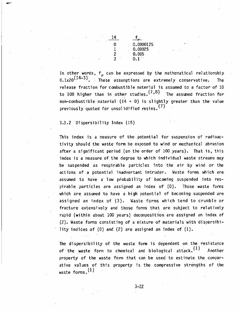
14 f

0 0.00001251 0.000252 0.0053 0.1

In other words, fr can be expressed by the mathematical relationship

.lx2 14-3 )-. These assumptions are extremely conservative. The

release fraction for combustible material is assumed to a factor of 10

to 100 higher than in other studies.( 7 ' 8 ) The assumed fraction for

non-combustible material (14 = 0) is slightly greater than the value

previously quoted for unsolidified resins.( 7

3.3.2 Dispersibility Index (15)

This index is a measure of the potential for suspension of radioac-

tivity should the waste form be exposed to wind or mechanical abrasion

after a significant period (on the order of 100 years). That is, this

index is a measure of the degree to which individual waste streams may

be suspended as respirable particles into the air by wind or the

actions of a potential inadvertant intruder. Waste forms wh ich are

assumed to have a low probability of becoming suspended into res-

pirable particles are assigned an index of (0). Those waste forms

which are assumed to have a high potential of becoming suspended are

assigned an index of (3). Waste forms which tend to crumble or

fracture extensively and those forms that are subject to relatively

rapid (within about 100 years) decomposition are assigned an index of

(2). Waste forms consisting of a mixture of materials with dispersibi-

lity indices of (0) and (2) are assigned an index of (1).

The dispersibility of the waste form is dependent on the resistance

of the waste form to chemical and biological attack.(') Another

property of the waste form that can be used to estimate the compar-

ative values of this property is the compressive strengths of the

waste forms.(I)

3-22

As a upper bound for this property, the- most dispersible waste form

(15 = 3) has been assumed to be equivalent to soil and no credit has

been considered due to waste form. This value is believed to be

conservative considering that the fraction dispersible into respirable

particles of powder PuO2 packages in transportation accidents have

been assumed in the past to be 0.001.(9) In the radiological impact

analyses, unsolidified LWR filter sludges, all fuel-cycle process

waste other than LWR process waste, all non-trash low activity wastes

from industrial sources, and all non-trash institutional wastes have

been assumed to be readily dispersible into respirable particles after

a long time and have been assigned a dispersibility index of 3.

In comparison, waste forms such as trash are taken to be not as

readily dispersible into respirable particles as waste streams such as

filter sludges. These wastes easily decompose. However, the decom-

posed residues are likely to contain water and other liquid decomposi-

tion products which will cause the residues to aggregate into a less

dispersible state. Similarly, unsolidified LWR resins would appear to

be less dispersible into respirable particles than LWR filter sludge.

These waste forms have been assigned a dispersibility index of 2 and

the dispersible fraction is assumed to be 0.1.

Waste streams solidified in accordance with solidification scenario A

and B procedures may be represented by cement properties. Cement is

an inert material, and wastes solidified in cement are likely to

retain their form over very long periods of time as long as no mecha-

nical forces are applied Similarly, wastes subjected to solidifi-

cation scenario C, which may be represented by the properties of

vinyl-ester styrene (VES) solidifed waste, are also likely to resist

biological and chemical attack.(1) Compressive strengths of most

cement waste forms are of the order of 100 psi and compressive

strengths of VES solidified waste forms range from 1700 to 7000 psi.

The compressive strengths of unsolidified wastes forms are of course

negligible. (1)

3-23

Based on this information, wastes solidified using solidification

scenario A or B procedures have been assigned an index of 1 and are

assumed to have a fraction of 10- 2 of the waste volume dispersible

into respirable particles. Waste streams solidified using solidifi-

cation scenario C procedures have been assumed to result in a near

zero dispersible state, have been assigned an index of 0, and are

assumed to have a fraction of 10-3 of the waste in a dispersible

form.

To summarize, the fraction of the respirable dust loading in air that

is contributed by each waste stream as a result of intruder activities

or wind action are assumed to be the following:

15 f

3 12 .11 .010 .001

In other words, the factor f is given by the relationship 10(15-3).rThe dispersibility index is applied to the intruder-construction,

intruder-agriculture, and exposed waste wind transport scenarios.

3.3.3 Leachability Index (16)

This index is a measure of a waste form's resistance to leaching

and is primarily determined by the solidification procedures used.

Unsolidified waste forms, which are assumed to be readily leached,

are assigned an index of 1. Waste streams solidified according to

solidification scenarios A, B, and C are assigned indices of 2, 3,

and 4, respectively.

The solidification scenarios represent varying levels of performance

that can be achieved through available solidification techniques. In

this report, a level of performance designated by solidification

3-24

scenario A has been simulated by assuming that half of the waste is

solidified using urea-formaldehyde and the other half using cement; a

level of performance designated by solidification scenario B has been

simulated by assuming that half of the waste is solidified using

cement and the other half using synthetic organic polymers (assumed

to be equivalent to vinyl ester styrene); and a level of performance

designated by solidification scenario C has been simulated by assuming

that all of the waste is solidified using synthetic organic polymers.

The primary purpose of this index is to assign values to the estimated

leachability potential of solidified waste streams in comparison with

unsolidified waste streams. Radionuclide-specific leaching fractions

for unsolidified waste streams have been estimated based upon actual

leaching data from two existing disposal facilities and are presented

and discussed in Section 3.5.1. The leachability index assigns values

to a multiplier of these unsolidified waste stream leaching fractions.

The product of the multiplier and the unsolidified waste leaching

fractions gives, for each waste stream, the actual leaching fraction

used in the radiological impact calculations. The multiplier is

assigned a value of unity for unsolidified waste streams such-as

dewatered resins or trash and a value less than unity for solidified

waste streams. The multiplier value assigned to solidified waste

streams is dependent upon the particular solidification scenario and

agent considered.

Although a large amount of experimental data is available on the

leaching characteristics of various solidified waste forms, lack of

widely used standardized testing procedures make quantitative compa-

risons difficult. Some comparisons can be made using the data pre-

sented in Reference 1. Table 3-6 is obtained from reference 1 and

gives the leachabilities for various waste-binder combinations rela-

tive to that of unsolidified wastes. Experimental data was used

for leaching of unsolidified resins; in all other cases complete

leaching of the unsolidified wastes is assumed.

3-25

TABLE 3-6

Leachability Relative to Unsolidified Wastea

Waste Type

Resins

Cement

5

Urea-

Formal dehyde

0.70

Vinyl

Ester Styrene

2.5x10-4

Concentrated Liquids

BWR's

PWR's

Diatomaceous Earth

0.5

0.02

0.70

0.83

0.9

0.4

0.07

0.04

0.06

(a) Averaged over all radionuclides reported.

Source : Reference 1.

3-26

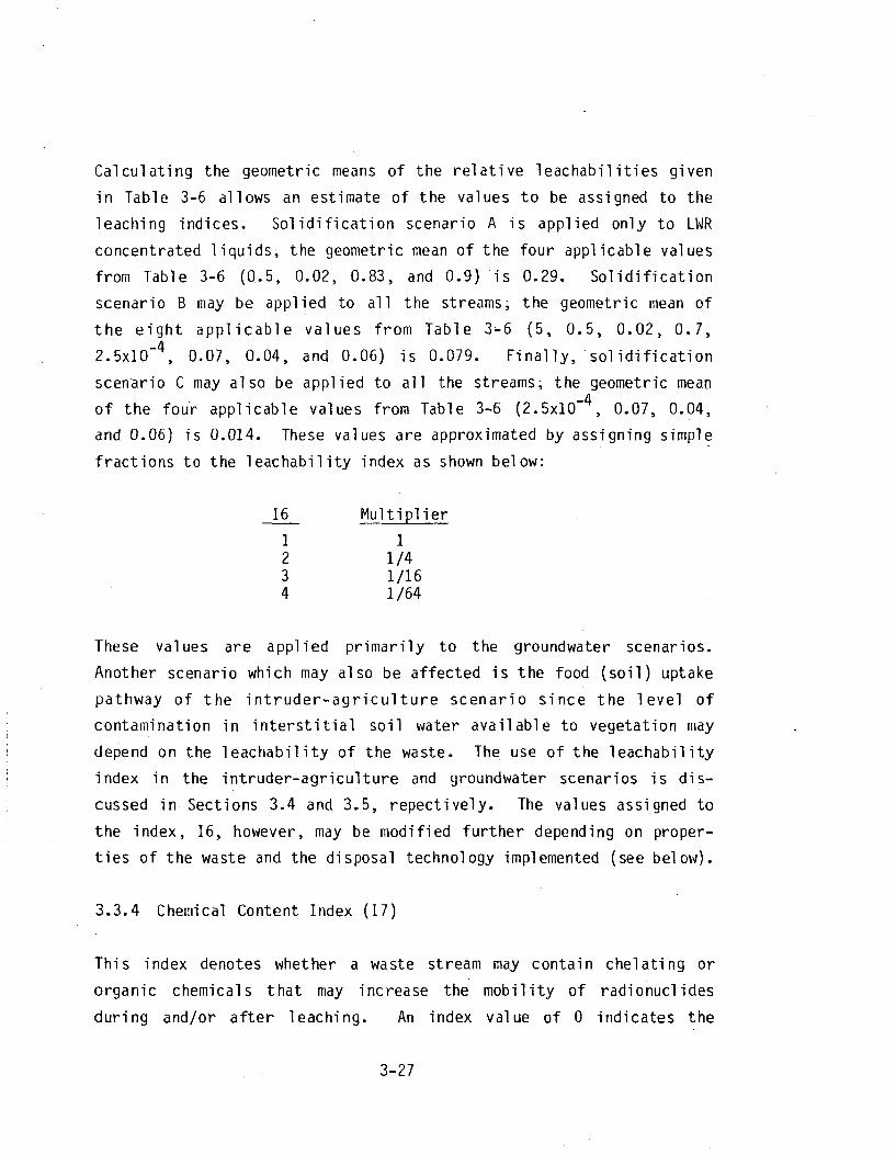
Calculating the geometric means of the relative leachabilities given

in Table 3-6 allows an estimate of the values to be assigned to tile

leaching indices. Solidification scenario A is applied only to LWR

concentrated liquids, the geometric mean of the four applicable values

from Table 3-6 (0.5, 0.02, 0.83, and 0.9) is 0.29. Solidification

scenario B may be applied to all the streams; the geometric mean of

the eight applicable values from Table 3-6 (5, 0.5, 0.02, 0.7,

2.5x10-4, 0.07, 0.04, and 0.06) is 0.079. Finally, solidification

scenario C may also be applied to all the streams; the geometric mean-4of the four applicable values from Table 3-6 (2.5xi0- , 0.07, 0.04,

and 0.06) is 0.014. These values are approximated by assigning simple

fractions to the leachability index as shown below:

16 Multiplier

1 12 1/43 1/164 1/64

These values are applied primarily to the groundwater scenarios.

Another scenario which may also be affected is the food (soil) uptake

pathway of the intruder-agriculture scenario since the level of

contamination in interstitial soil water available to vegetation may

depend on the leachability of the waste. The use of the leachability

index in the intruder-agriculture and groundwater scenarios is dis-

cussed in Sections 3.4 and 3.5, repectively. The values assigned to

the index, 16, however, may be modified further depending on proper-

ties of the waste and the disposal technology implemented (see below).

3.3.4 Chemical Content Index (17)

This index denotes whether a waste stream may contain chelating or

organic chemicals that may increase the mobility of radionuclides

during and/or after leaching. An index value of 0 indicates the

3-27

likelihood that these agents are absent in the stream, whereas an

index value of 1 indicates that the stream is likely to contain

chelating or organic chemicals.

This index, in conjunction with the segregation option index IS (see

Section 3.2.3) is used to modify the multiplier values assigned to

the leachability indices for the groundwater and intruder-agriculture

scenarios. The following table is used in determining the fraction

leached from a particular waste form:

Mult(16,17,1S)

16 IS=1 and 17=0 IS=O or 17=1

1 1 12 1/4 13 1/16 1/44 1/64 1/16

This table should be interpreted as follows. For a waste stream

with a given leachability index (16), if the waste stream either

contains chelating agents (17=1) or is disposed mixed with other waste

streams containing chelating agents (IS=O), then the higher leach

fraction multiplier is used. If the waste stream does not contain

chelating agents (17=(J) and it is not mixed with other wastes con-

taining chelating agents (IS=1), then the lower leach fraction mul-

tiplier is used.

A similar procedure is applied to the soil retardation coefficients

assigned to individual radionuclides. Retardation coefficients denote

the potential of the disposal facility site soils to retard the

radionuclides during groundwater migration. If there is no waste

segregation at the disposal facility, then the retardation potential

of the disposal site soils is assumed to be reduced as discussed in

Section 3.5.

3-28

3.3.5 Stability Index (18)

This index denotes whether the waste form is likely to reduce in

volume after disposal due to compressibility, large internal void

volume, and/or chemical and biological attack (no credit is taken

for the waste containers). An index value of 0 indicates a likeli-

hood of structural instability, whereas a value of 1 indicates a

structurally stable waste form.

The stability indices presented in Table 3-5 have been assigned based

on the physical descriptions of the waste provided in reference 1. In

general, this index has been assigned based on the void volume and/or

compressibility of the waste and its biodegradability. For example,

all trash waste streams are assumed to be unstable unless they are

incinerated and/or solidified. All waste forms expected to be pack-

aged in trash or similar degradable void fillers, such as LWR non-

compactible trash streams, are also assumed to be unstable.

The use of this index in the impact calculations depends on the

stabilization index IX. If IX is 3 (extensive stabilization measures

are implemented), then the index 18 is ignored in the calculations.

If IX is 1 or 2 (regular or moderate stabilization measures), then

the segregation index IS also affects the calculational procedure. If

IS = 1 (segregation), then the higher percolation estimate is adopted

for wastes that are unstable (18 = 0), and the lower percolation

estimate is adopted for wastes that are stable (18 = 1); if IS = 0

(no segregation), then the higher percolation figure is adopted for

all the streams (see Section 3.5).

Similarly, in the disposal cost calculations, if there is segrega-

tion, then any moderate or extensive stabilization measures (IX=2 or

IX=3) are applied to only the disposal cells that contain unstable

wastes; otherwise, the entire site undergoes these stabilization

measures.

3-29

3.3.6 Accessibility Index (19)

This index triggers the use of a correction factor for those unsoli-

dified waste streams that have a comparatively high metal content.

The radionuclides contained in these waste streams are not as easily

accessible to transfer agents such as wind and water as are the

radionuclides contained in other waste streams.

Most of the waste streams contain surface contaminated wastes and

waste containing radioactivity in readily soluble forms; these streams

are assigned an accessibility index of 1. The waste streams that

are almost exclusively activated metals with imbedded radioactivity

not readily accessible to the elements are assigned an index of 3.

Only the inaustrial high activity waste stream (N-HIGHACT) has been

assigned an index of 3. Several other streams containing a signifi-

cant portion of metallic waste which have both activated and surface

crud contamination have been assigned an accessibility index of 2.

The waste streams assigned an accessibility index of 2 include non-

compactible trash from LWR's (P-NCTRASH, B-NCTRASH) and fuel fabri-

cation facilities (F-NCTRASH), LWR non-fuel reactor core components

(L-NFRCOMP), and industrial sources (N-SOURCES). All other waste

streams have been assigned an accessibility index value of 1. The

value of this index does not change depending on the waste spectrum

considered.

This index is applied to all the release/transport scenarios that

involve wind or water transfer agents, and to all the direct radia-

tion scenarios. In the calculations, the degree to which a waste

form resists mobilization by external transfer agents is expressed

through the waste form and package factor (f w). One of the mathe-

matical terms in the waste form and package factor is a fractional

multiplier that expresses the effect of the accessibility index. This

fractional multiplier is assumed to be given by the relationship

10(1I9)" ;that is:

3-30

19 Multiplier1 1

.2 .3 .01

A brief comparative discussion of the materials for which the access-

ibility index is different than unity is given below.

The mainpurpose of the accessibility index is to evaluate the compa-

rative isolation from transport agents of the radioactivity contained

in certain unsolidified wastes. The function of this index is similar

to that of the leachability index applied to solidified wastes. The

reduction of the accessibility of some radioactive materials is the

result of the combined physical and chemical characteristics of these

materials. No reduction is considered for wastes which contain

radioactivity in forms which are readily soluble and/or displaced.

Combustible trash and absorbed liquids are examples of these types of

wastes.

At the other extreme are unsolidified waste streams such as activated

metals where in the absence' of surface contamination, much less

radioactivity is initially accessible to transport agents. Industrial

high activity metals are assumed to be the only waste stream of this

type which is virtually free of surface contamination. Many of these

activated metals are high-alloy materials (alloys with a high non-

ferrous metallic component), which are inert and corrode very slowly

in the disposal environment. For example, a corrosion rate of 0.002

mg/100 cm2/day (7.3x10-6 g/cm 2/yr) has been quoted for high-alloy

stainless steel.(10) Such corrosion produces finely-divided but

highly insoluble oxides.

Although insoluble, these oxides may be more accessible by virtue of

being finely divided. The percentage of the total activity of such

waste forms converted to the oxide form in a given time is highly

dependent on the geometry of the waste (i.e., surface area to mass

3-31

ratio). For example, consider a' high-alloy rod 100 cm long and 1 cm

in diameter and having a density of 7.8 g/cm 3, and a pipe having

the same external dimensions and density but with a wall thickness of

0.1 cm. The surface area to mass ratios are 0.259 cm2/g for the rod

and 2.56 cm2 /g for the pipe. Assuming that the activation products

are distributed uniformly through both pieces, the fraction of the

activity lost from the pipe is nearly ten times that of the rod

(1.87x10- 5 per year versus 1.89x10-6 per year). The small magnitude

of both numbers clearly show the inaccessibility of the radioactivity

in both cases -- especially in view of the insolubility of the corro-

sion products. In 1000 years, only about 0.2 percent of the activity

from the rod becomes available. Based on this estimate, a conserva-

tive correction factor (multiplier) of 0.01 has been applied to these

wastes in scenarios that involve dispersibility of the wastes.

The remaining unsolidified wastes fall between these two extremes.

Wastes in this group include the non-compactible trash streams and

non-fuel reactor core components. The trash streams include large

amounts of surface contaminated failed equi pment. Many pieces of

equipment are internally rather than externaly contaminated and are

sealed to prevent release of any free liquids they may contain (e.g.,

pumps). A pump sealed with 1 cm thick carbon steel caps (corrosion

rate of 0.03 cm/yr)(7) would isolate the radioactivity for about 30

years. After this period the release of radioactivity is controlled

by the activity and amount of liquid inside the piece, the nature of

the internal contamination, and the ease with which the transport

agents can get in and out of the equipment.

Non-fuel core components are a special case. These components are

generally highly activated stainless steel pieces coated with crud

deposits. The accessibility of the radioactivity of these wastes

depends on the thickness of the crud layer and the relative activity

of the crud and underlying metal. Crud mainly consists of oxides of

iron and has been found to range in thickness from 0.0003 to 6 mil

3-32

on fuel rods.(11) The strong decontamination agents necessary to

remove such crud deposits from LWR primary cooling systems attests

to the inaccessibility of the radioactivity they contain. Further-

more, the transporting medium must penetrate the crud layer to begin

corroding the activated metal beneath. Because the fractions of

activity contained in the crud and the metal components of these

wastes are not well-characterized, these wastes are considered to

more closely resemble non-compactible trash rather than clean-surfaced

high activity metals.

A reduction factor for the direct radiation exposure components of the

scenarios is also applicable due to the high -metal content of the

streams with an accessibility index greater than 1. This reduction is

due to the self-shielding afforded by the higher density metals and

packaging practices. For example, the uncollided gamma flux from a

half-space source at the surface is inversely proportional to the

density of the material; this effect alone would result in a gamma

flux attenuation by a factor of about 7 (see Appendix A). Further-

more, when these non-compactible metallic wastes, which usually have

irregular shapes, are packaged, other materials such as trash or soil

that usually have much lower activities are placed around them to fill

the voids. For the high energy gamma rays found in LLW (Co-60,

Cs-137, and Nb-94), it takes only about 2 inches of metal shielding to

result in an attenuation of 10. In this report, in view of the above

two effects, a reduction factor of 10 has been applied to direct

radiation exposure pathways for streams having an accessibility index

greater than 1.

3.4 Waste Classification

As discussed in Chapter 1.0, a waste classification methodology is

one of the essential tools to assure that uniform and environmentally

acceptable practices are adopted throughout an extremely diverse

industry that generates LLW. This section presents a waste classifi-

cation procedure and associated tests.

3-33

An introduction to the section outlining the considerations in the

approach adopted is presented in Section 3.4.1.. This is followed by

two sections on the intruder-construction and the intruder-agriculture

scenarios that constitute the basis of the waste classification

testing procedure. Finally, the waste classification testing proce-

dure is summarized in Section 3.4.4.

3.4.1 Introduction

As discussed in Section 2.4, potential long-term exposure scenarios

from LLW disposal can be seperated into two types: concentration

scenarios and total activity scenarios. The concentration scenarios

include those involving direct human contact with the disposed waste,

such as those involving exposures to a potential inadvertent intruder.

In these scenarios, potential exposures are calculated considering

only the radionuclide concentrations in the waste' streams assumed to

be actually contacted by the intruder. The radionuclide concentra-

tions in parts of the disposal facility not contacted by the potential

inadvertent intruder do not enter into the calculations. On the other

hand, exposures from the total activity scenarios are determined by

considering the total radionuclide activity disposed at the facility.

Examples of total activity scenarios include groundwater migration

scenarios.

The fact that impacts from scenarios involving direct human intrusion

into disposed waste are governed by the concentrations in the parti-

cular waste streams assumed to be contacted makes the intruder scen-

arios very useful for waste classification purposes. Assuming that a

limit is placed on the exposures allowed to a potential human in-

truder, then the maximum allowable concentrations of radionuclides in

waste streams to meet this exposure limit may be calculated.

Once concentration limits are determined, waste generators can rela-

tively easily determine what class their waste belongs to by comparing

3-34

the radionuclide concentrations in their wastes with the limiting

concentrations determined through the intruder scenarios. Use of

potential human intrusion as a means of classifying wastes for dis-

posal has also been used by others.( 1 0 ' 13 )

By contrast, it is much more difficult to classify wastes through

the use of total activity scenarios such as groundwater migration.

Comparatively speaking, impacts from groundwater migration are much

more dependent on site specific environmental conditions than the

intruder scenarios. In addition, since the potential impacts are a

function of the total activity of waste disposed, it is difficult to

set conc-entration limitations for individual radionuclides to meet a

specific dose limitation criteria. It would be difficult, based upon

groundwater migration considerations, to set concentration limits that

can be used by a waste generator to determine the classification of

his waste.

It is important to emphasize, however, that this does not mean that

groundwater migration from a disposal facility is not an important

consideration in LLW disposal. It does suggest that rather than

establishing concentration limitations to be met by a waste generator

to meet a particular groundwater exposure limitation criteria, it

would probably be more useful to set an inventory limitation for a

particular disposal facility (based upon site-specific information)

for particular radionuclides of concern. Then, if the waste genera-

tors were required to report the quantity of the radionuclides of

concern which are contained in each shipment of waste, the disposal

facility operators could maintain a running inventory of the radio-

nuclides of concern at their particular sites. When the site inven-

tory reaches the established limit for the facility, the disposal

facility operator would no longer accept waste streams containing the

particular radionuclides of concern. It is expected that such radio-

nuclides of concern would include long lived mobile isotopes such as1 4 C, 9 9Tc and 1291.

3-35

Potential inadvertent intruder exposures (and maximum radionuclide

concentrations corresponding to a given dose conversion criteria) are

a function of three general parameters: (1) the time after disposal

that the intrusion occurs (the length of the active instititional

control period), (2) waste form and packaging properties, and (3)

disposal facility design and operating practices. Regulatory require-

ments can be placed upon these parameters and depending upon the

particular requirements placed upon these parameters, a classification

system may be aeveloped.

From an analysis of the effect of waste form and packaging properties

and disposal facility design and operating practices on impacts from

human intrusion, it may be concluded that:

o Barriers may be used to reduce the possibility of human intru-

sion. These barriers may include disposal at greater depths or

emplacement of the waste into a highly engineered facility

designed to resist human intrusion (e.g., a hot waste facility).

o If the waste is in a stable waste form that resists dispersion

and if the stable waste is placed in a disposal cell which is

segregated from unstable waste forms, than potential intruder

exposures would be reduced over those exposures expected if the

stable wastes were disposed mixed with the unstable wastes.

Based upon establishment of a maximum time for active institutional

controls and incorporating the above two conclusions, a waste classi-

fication system may be developed based on a maximum exposure limit to

a potential inadvertent intruder.

In this work, three generic levels of intruder barriers are considered

in detail, which correspond to three general levels of effectiveness

against intrusion at three levels of overall costs: (1) no barrier;

(2) layering; and (3) hot waste facility.

3-36

In the first case, the waste stream is assumed to be disposed in a"regular" manner without consideration of protecting a potential

intruder. In the second case, the waste stream is assumed to be

disposed at the bottom of the disposal cell, so that at least 5 meters

of earth or other (lower activity) waste streams cover the layered

waste. In the third case, the waste stream is assumed to be disposed

in a hot waste facility, which for this report is taken to be a

concrete walled disposal trench. The waste is stacked into the

trench, grouting is poured around the waste packages, a concrete

cover is then poured over the grouted waste mass, and finally 2 meters

of soil is emplaced over the concrete cover. The effectiveness of the

hot waste facility is somewhat speculative, but is included to indi-

cate an upper level of protection against an inadvertent intruder that

can be achieved through near surface disposal.

In addition, it may be assumed that the operational practice of

segregated disposal of stable waste streams from unstable waste

streams results in reduced exposures to a potential intruder con-

tacting the stable waste streams -- at least for the first several

hundred years following waste disposal. Segregated disposal of the

stable waste streams greatly improves the stability of the disposal

cells containing the stable wastes, resulting in significantly less

water infiltration and subsidence problems for these disposal cells,

and less decomposition of the disposal cell contents. Exposures to

a potential inadvertent intruder contacting these disposal cells at

the end of the active institutional control period would be limited to

those acquired during discovery of the waste. It is not credible, for

example, to postulate that an intruder would construct a house in, or

attempt to grow vegetables in, a disposal cell composed of such wastes

as 55-gallon drums filled with concrete.

Finally, consideration needs to be given to the length of time that

intruder barriers and segregation of stable wastes serves to reduce

or eliminate potential inadvertent intruder impacts. Based on the

3-37

analysis in reference 3, a time period of 500 years after site closure

is used as a limit of the effectiveness of layering and waste segre-

gation. Following this time period, wastes disposed through layering

and/or segregation are assumed to be as-accessible to an intruder as

waste disposed by regular means (i.e., non-segregated shallow land

burial). A time period of 1000 years is assumed as a maximum length

of time for a hot waste facility to be effective against intrusion.

These concepts are further expanded in the following two sections

which present the calculational procedures for determining, intruder

exposures from the two basic intruder scenarios considered in this

appendix. These include the intruder-construction scenario presented

in Section 3.4.2 and the intruder-agriculture scenario presented in

Section 3.4.3. Following this section is Section 3.4.4 which presents

the te sting procedure through which the intruder concepts developed in

this section are used in the computer codes developed in this work to

classify the waste streams for further analysis.

3.4.2 Intruder-Construction Scenario

This is one of the scenarios utilized to determine the classification

status of the waste streams -- the other scenario being the intruder-

agriculture scenario. This section considers the values of the

pathway barrier factors under alternative values of the waste form

behavior indices and the disposal technology indices.

This scenario assumes that at some time after the end of operations at

the disposal facility, institutional controls breakdown temporarily

and an intruder chooses to inadvertantly construct a house on the

disposal facility. In so doing, the intruder is assumed to contact

the disposed wastes while performing typical excavation work such as

installing utilities, putting in basements, and so forth. These

typical activities should not be expected to involve significant

depths - e.g., in most cases no more than approximately 3 m (about

3-38

10 ft). There is, however, a much less likely chance that some

excavations could proceed at a lower depth. This could occur, for

example, through construction of a sub-basement for a high rise

building.

To implement this scenario, the inadvertant intruder is assumed to

dig a 3 meter deep foundation hole for the house. The surface area

of the house is assumed to be 20 m by 10 m (200 mi2 ), which is a

typical surface area for a reasonably large ranch-style house. The

foundation hole is assumed to be 20 m by 10 m (200 m2 ) at the bottom

and 26 m by 16 m at the top (giving a 1:1 slope for the sides of the

hole). The top 2 meters of the foundation is assumed to be cover

material and the bottom I meter is assumed to be waste. This excava-

tion would result in about 232 mi3 of waste being intruded into.

The equation describing human exposure for the intruder-construction

scenario is as follows:

H = (fofdf wfsair Cw PDCF-2 +n

(fofdf s)DG Cw PDCF-5 (3-1)n

where H is the 50-year dose committment in torem, PDCF-2 and PDCF-5

are the radionuclide-specific pathway dose conversion factors which

were discussed and presented in Section 2.3, Cw is the radionuclide

concentration in the waste, and n denotes summation over all the

radionuclides.

The first term of the equation calculates the impacts from the air

pathways consisting of exposures due to suspension of contaminated

dust into the air: inhalation of the contaminated dust, direct radia-

tion exposure from the contaminated dust cloud, and the consumption

of food grown nearby upon which the airborne contamination settles.

The second term of the equation calculates the impacts from direct

3-39

radiation exposure to the wastes during excavation. The values of the

barrier factors are examined below in two sections: regular waste

disposal, and disposal with barriers against intrusion.

Regular Waste Disposal

The time delay factor fo is radionuclide-specific and is given by the

following equation:

f = exp [ -AT] (3-2)

where T is the time period between the end of active disposal opera-

tions and the initiation of the scenario (i.e., IPO plus IIC years),

and A is the decay constant of the radionuclide. This factor is the

same for both the air uptake pathways and the direct gamma pathway.

The assumed time period is equivalent to the assumption that the

intrusion scenario involves the last disposal cell constructed at the

site and conservatively neglects the possibility that the intrusion

scenario may involve one of the earlier disposal cells.

The site design and operation factor fd denotes the dilution of the

waste due to particular disposal practices regarding waste emplace-

ment. Its value is assumed to be 0.5, 0.75, or 0.5 depending upon

whether the waste disposal is random, stacked, or decontainerized,

respectively. The effects of other classification tests on fd are

described below.

For the air uptake pathways, the waste form and package factor fw is

given by the following formula:

fw - I0(15-3) x I0(1-19) (3-3)

where 15 is the dispersibility index (see Section 3.2.2) and 19 is the

accessibility index (see Section 3.2.6). Based on this formula, fw

ranges from a high of 1 to a low of 10- .(1)

3-40

For the direct radiation exposure pathway, only the self-shielding

inherent to the particular waste form affects the factor f In

this case, fw is set equal to the following:

f = Accessibility Multiplier x Solidification Multiplier (3-4)

The modification due to accessibility results from the substantial

metal component of some waste streams (see Section 3.3.6). The

accessibility multiplier is taken equal to 1 if the index 19 is equal

to 1, and it is 0.1 if the index 19 is equal to 2 or 3. The solidi-

fication multiplier is assumed to be 0.80 for those streams that are

solidified using solidification scenario A or B procedures which

contain a significant amount of cement; otherwise, this multiplier is

assumed to be unity. Since the streams with an accessibility index

different than 1 are never solidified, the minimum value of the factor

fw for the direct radiation exposure pathway is 0.1.

The site selection factor f is different for the air and directs

gamma uptake pathways of the intruder-construction scenario. For the

air uptake pathways, it is the product of the soil-to-air transfer

factor Tsa (which depends on the environmental characteristics of

the region in which the disposal facility is located) with the expo-

sure duration factor (the fraction of a year that the construction

takes place). For the direct gamma exposure pathway it is equal to

just the exposure duration factor. These factors are detailed below.

In this work, exposure duration is assumed to be 500 working hours for

the regular waste disposal. This is equivalent to a construction

period of 3 months, which is believed to be reasonably conservative

for typical construction. It is believed to be very conservative for

activities involving use of heavy construction equipment. This gives

a value of 0.057 for f for the direct gamma scenario. For the air

pathways, this number is multiplied with a soil-to-air transfer factor

given by the formula:

3-41

Tsa = [TIsao x (10/v) x (s/30) x (50/PE) 2 (3-5)

where [Tsa o is equal to 2.53 x" 10-, *v is the average wind speed

at the site in m/sec, s is the silt content of the site soils in

percent, and PE is the precipitation-evaporation index of the site

vicinity indicative of the antecedent moisture conditions (see Appen-

dix A). For the reference disposal facility, these values were

determined to be v = 3.61 m/sec, s = 50, and PE = 91, yielding a value

of 3.53 x 10 1for Tsa (see Appendix A). For an exposure duration

factor of 0.057, this yields a site selection factor of 2.01 x 10-11

for the air uptake component of the construction scenario.

Disposal With Barriers Against Intrusion

The barrier factors fd and fs are affected if the waste is disposed

using intruder barriers and/or if waste segregation is implemented at

the disposal facility. The factor fd is not affected by regular or

layered waste disposal; layered disposal only affects the factor f.

For the air uptake pathways, (a) for layered disposal, the factor fd

is multiplied by a factor of 0.1 to indicate the likelihood of contact

of the layered wastes by the intruder; and (b) for hot waste facility

disposal fd is multiplied by a factor of 0.01.

For the direct radiation exposure pathway, (a) for layered disposal,

fd is multiplied by a factor of 1/1200 which denotes attenuation of

the radiation through a 1 meter. thick soil equivalent layer; and (b)

for hot waste facility disposal, fd is multiplied by a factor of

1/12002 which indicates attenuation of the radiation through a layer

equivalent to 2 meters of soil (see Appendix A).

The site selection factor f is modified only if the waste form is

stable and has been disposed of in a segregated manner. The exposure

duration factor is reduced from 500 hours to 6 hours for all the

uptake pathways.

3-42

3.4.3 Intruder-Agriculture Scenario

The intruder-agriculture scenario is the second scenario (the first

being the intruder-construction scenario) utilized to determine the

classification status of the waste. It is used in three classifi-

cation tests: (1) for regular waste disposal at the end of IIC years

following facility closure, (2) at the end of 500 years for waste

streams that have been layered or are stable and segregated, and

(3) at the end of 1000 years for wastes that have been disposed into

a hot waste facility. Only intruder impacts from regular waste

disposal following IIC years is considered below. Intruder impact

*scenarios at 500 years and at 1000 years are somewhat speculative,

and have been conservatively assumed to be similar to those at the

end of IIC years.

The intruder-agriculture scenario assumes that at some time after the

end of disposal operations, an intruder inadvertently lives on the

facility, and consumes food grown on the disposal facility. Farming

is a surface activity and generally does not involve disturbing the

soil for more than a few feet. As long as a cap of one or two meters

is maintained over the waste, then it is very unlikely that agricul-

tural activities would ever contact the waste.

To implement the scenario at the end of active institutional control

period, however, a portion of the soil excavated during the intruder-

construction activity (232 m3 of waste and 680 m3 of cover material)

is assumed to be distributed around the completed house. After build-

ing the foundations of the house, about 312 m3 of this soil would be

put back in outside and around the cellar walls leaving a volume of

about 600 m3 of soil (of which about 150 m3 is the original waste/soil

mixture) involved in the agriculture scenario. The precise areal

extent to which this soil is distributed is somewhat speculative.

It is likely, however, that the soil will remain localized; moving

even a few cubic yards of soil more than 10 meters usually requires a

3-43

significant effort. It is assumed in this report that this areal2 2

extent is likely to be somewhere between 1000 m and 2000 m

That is, the waste/soil mixture is assumed to lie within a radius of

25 meters from the center of the house. The intruder is then assumed

to live in this distributed waste/soil mixture and is also assumed to

consume vegetables from a small garden located in the waste/soil

mixture.

A possible alternative to this scenario is that the waste cover is

stripped away by the intruder, and that the intruder lives on and

grows and consumes food grown directly in the waste. This does not

appear to be as reasonable as the above scenario. At current commer-

cial rates, it costs about $1.07 to move one cubic yard of dirt from

one place to an adjacent place with heavy equipment.(12) This

implies that to clear 2 meter of cover from 2 acres, the intruder has

either invested a sum of about $22,500 or spent a labor equivalent to

this sum. This is not a reasonable assumption since no reasonable

person is likely to strip and clear away surface soil with the hope of

finding a better soil underneath for growing food.

A non-commercial enterprise is therefore assumed for the intruder-

agriculture scenario. It appears to be unreasonable to expect that a

commercial operator, who would require a substantial investment for a

commercial agricultural operation and therefore a clear title to the

land, can be an inadvertant intruder.

The inaavertant intruder is assumed to live in a house built on the

site, work at a regular job during the day, and spend some of his

extra time working in a garden growing vegetables for his own use.

His time during a year is assumed to be allocated between various

activities as follows:

3-44

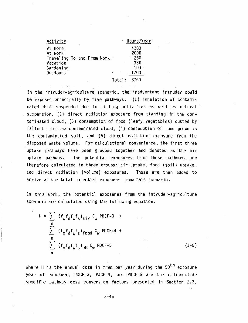
Activity Hours/Year

At Home 4380At Work 2000Traveling To and From Work 250Vacation 330Gardening 100Outdoors 1700

Total: 8760

In the intruder-agriculture scenario, the inadvertent intruder could

be exposed principally by five pathways: (1) inhalation of contami-

nated dust suspended due to tilling activities as well as natural

suspension, (2) direct radiation exposure from standing in the con-

taminated cloud, (3) consumption of food (leafy vegetables) dusted by

fallout from the contaminated cloud, (4) consumption of food grown in

the contaminated soil, and (5) direct radiation exposure from the

disposed waste volume. For calculational convenience, the first three

uptake pathways have been grouped together and denoted as the air

uptake pathway. The potential exposures from these pathways are

therefore calculated in three groups: air uptake, food (soil) uptake,

and direct radiation (volume) exposures. These are then added to

arrive at the total potential exposures from this scenario.

In this work, the potential exposures from the intruder-agriculture

scenario are calculated using the following equation:

H= 7 (fofdfwfs)air Cw PDCF-3 +n

Z (fo f df wfs)food Cw PDCF-4 +

n

Z (fofdfwfs)DG Cw PDCF-5 (3-6)

n

where H is the annual dose in mrem per year during the 50 th exposure

year of exposure, PDCF-3, PDCF-4, and PDCF-5 are the radionuclide

specific pathway dose conversion factors presented in Section 2.3,

3-45

Cw is the radionuclide concentration in the waste, and n denotes

summation over all the radionuclides. The values of the barrier

factors-are presented below.

The time delay factor f0 for this scenario is identical with the

construction scenario, and is *given by equation (3-2). The site

design and operation factor fd is also determined in the same manner

as the construction scenario. In addition, the dilution resulting

from mixing of the excavated waste (232 m 3) with the excavated cover

soil (680 m 3), which is a factor of about 0.25, is also included in

the design and operation factor fd"

Waste Form and Package Factor

The waste form and package factors for the air uptake and direct

radiation exposure pathways composing this scenario are identical with

those for the air uptake and direct radiation exposure pathways

composing the intruder-construction scenario. However, for the food

(soil) uptake pathway, other considerations are applicable. The

following formula is utilized to calculate fw fQr the food (soil)

uptake pathway (also see equation 3-12):

fw = M0x tc x Mult(16,17,IS) x 10(1I9) (3-7)

where, Mo is the radionuclide-specific leach fractions of unsoli-

dified waste forms (see Section 3.3.3 and 3.5). The contact time

fraction tc is the fraction of time in one year that the waste is

in contact with irrigation water, while 19 is the accessibility index

(see Section 3.3.6). Mult(16,17,IS), which is the reduction due to

solidification and the presence or absence of chelating chemicals

(see Section 3.3.4), is a function of the leachability index (16),

the chemical content index (17), and whether the waste streams con-

taining organic chemicals or-chelating agents have been segregated

from other waste streams (IS).

3-46

It appears to be reasonable to assume that only the fraction of

radionuclides transferred from the waste to the interstitial water

will be accessible to the roots. Inclusion of contact time in the

above equation is consistent with this approach. The contact time

fraction is conservatively assumed to equal unity in this work.

However, this fraction may actually be a very low value in view of the

soils likely to be found at most disposal locations. These locations

are likely to be at topographic highs whereas the most attractive

agricultural soils are found in or adjacent to flood plains.

Site Selection Factor

The site selection factor fs for the air uptake pathway is similar

to the intruder-construction air uptake pathway. However, the soil-

to-air transfer factor must be averaged to account for natural resus-

pension of the soils part of a year. This estimate is calculated by

assuming that (1) the construction scenario Tsa value of 3.53 x 10-I0

(see Section 3.4.2) is applicable during gardening (100 hours),

(2) during the time spent outdoors (1700 hours), typical natural

outdoor ambient air particulate concentrations of 100 ipg/m3 are

assumed to prevail;,(13 and (3) during the time spent indoors (4380tiours), typical ambient indoor concentrations of 50 Pjg/m3 have been

assumed.(1 3 ) Utilizing a mass loading of 565 Vg/m 3 for the time

spent while gardening (see Appendix A) and averaging these values

results in a site selection factor value of 3.18 x 10-11. This may

be compared with the site selection factor value of 2.01 x 10-

calculated for the intruder-construction scenario.

For the food (soil) uptake pathway, f is taken to be the fraction

of food consumed by the individual that is grown on site. This value

is assumed to be 0.5.

For the direct radiation exposure pathway, fs is equal to the expo-

sure duration fraction multiplied by a correction factor to account

3-47

for the limited areal extent of the direct radiation source that the

intruder is exposed to. Moreover, the fraction of the time the

intruder spends in relation to the source must be considered.

During a year, the intruder is assumed to spend 1800 hours outdoors

exposed to unattenuated radiation (100 hours tilling and 1700 hours

around the house). During the 4380 hours he spends indoors, he is

exposed to attenuated radiation. The correction factor due to the

limited areal extent of the radiation source may be estimated uti-

lizing Figure 3.1.

This figure shows that intruder may be assumed to be exposed to a full

disk source while outside, and an annular source while inside the

house. While he is inside the house, the center of the disk repre-

sents the shielding provided by the foundation slab. The contribution

to the direct radiation exposure from this center portion may be neg-

lected in comparison with the exposure from the outside of the house.

If the foundation slab is a one-foot thick concrete layer, the radia-

tion Would be attenuated to about 0.03 of its unshielded value for

Cs-137 gamma rays.(14) The correction factor for the areal extent

of the annular source may be represented by the following equation:

c = [El(pr l ) - El(pr2)] / El(pro) (3-8)

where c is the dimensionless correction factor, E[(x) is the first

order exponential integral, p is the linear attenuation coefficient of

air in units of mr- (it is taken to be 0.0097 m-1 in this report) (14),

and the r's are the distances from the exposure point indicated in

Figure 3.1 in meters. Details of the derivation of this equation can

be found in Appendix A.

For a full disk source (for the time spent outdoors), the radius

r in equation (3-8) is replaced by ro. In order to evaluate the

correction factor, these radial distances must be assumed. The

3-48

INDOORS OUTDOORS

EXPOSURE POINT

0

r Iro':r I

9 ............../ ,/ // /. //////

SIDE VIEW

WASTE

HOUSE TOP VIEW

DIRECT RADIATION EXPOSURE GEOMETRY

DA~mE B UMOO•I

3-49 FIGURE 3.1i

following table gives the value of the exponential integral for some

representative distances:

Distance pr E (pr)

1 m 0.0097 4.0688 m 0.0776 2.055

20 m 0.1940 1.33525 m 0.2425 1.068

For r and r1 it is reasonable to assume 1 m and 8 m, respectively;

1 m represents the height of 'the exposed person, and 8 m represents

the approximate radius of a 200 m2 house floor. The value assigned

to r 2 , however, depends on the areal extent to which waste/soil

mixture (600 m 3) has been spread. This mixture will likely be

spread unevenly within about a half acre around the house excavation,

and the areal extent is likely- to be between 1000 m2 and 2000 m2 .

A radius of the above 20 m represents an area of about 1050 m2 over

which the waste is spread, while a radius of 25 m represents an area

of about 1750 mI2 . A radius of 25 m is utilized in this work.

These assumptions yield a correction factor for the time spent out-

doors of about 0.74, and a correction factor for the time spent

indoors of about 0.24. Utilizing values of 1800 hours outdoors

and 4380 hours indoors yields an site selection barrier factor of

about 0.27, which is the value utilized in this report.

3.4.4 Waste Classification Test Procedure

The following section describes the waste classification tes,. proce-

dure developed from the previous sections regarding impacts from

potential human intrusion into disposed waste. The test procedure

is used in the OPTIONS and GRWATER (see Section 6.0) computer codes

which determine radiological, economic, and other impacts from

LLW disposal.

3-50

In the calculations, the disposal status of each waste stream, denoted

by the status index Ill, is determined and is used internally in the

computer codes. It denotes if any special procedures are required to

dispose of the waste stream in a near-surface disposal facility or if

the waste is unacceptable for near-surface disposal.

The index, III, is 1 if the waste is disposable through "regular

means," it is 2 if layering of the waste is required, and 3 if the

waste is disposed of in a hot waste facility. For disposal by regular

means, no special consideration is given to providing barriers against

potential inadvertent intruder exposures. Layering of waste streams

provides a barrier against an intruder contacting the layered waste

streams. Disposal into a hot waste facility provides additional

barriers against intrusion. An index value of 0 indicates that the

waste is unacceptable for near-surface disposal. The testing proce-

dure utilized in the determination of the disposal status index

is presented in Figure 3.2.

Each test consists of successively subjecting a given waste stream

to the intruder-construction and the intruder-agriculture scenarios

after a given period of time, and determining if the calculated

radiological impacts in each scenario for each human organ due to all

the radionuclides in the waste stream meet given organ specific "dose

limitation criteria." Therefore, there are four basic variables in

these tests: (1) the waste status (regular or layered or hot waste

test), (2) the type of test (standard or modified), (3) the time after

the transfer of the site title to site owner at which the test is

applied (after the active institutional control period - denoted by

IIC years, or after 500 years, or after 1000 years), and (4) the dose

limitation criteria which is applied to all the tests. The first

three variables are discussed below.

For a given waste stream, first the regular disposal test is applied

at IIC years. This regular disposal test may be either a standard or

3-51

FAI L

WASTE CLASSIFICATION TEST PROCEDURE

3' 52 FIGURE 3.2

a moaified test depending on whether the waste form is stable (I8=1)

and the waste streams are being segregated (IS=l) at the disposal site

(see Figure 3.2). If the waste is found acceptable during the stan-

dard test, then it is classified as regular waste. If the waste

passes a modified test, it must also pass a regular stanaard waste

test at 500 years before being classified as regular.

If the waste stream fails any of the above three tests, then it is not

regular waste. In this case, the layered disposal tests are applied

to the waste stream at IIC years if the layering option is available

to the disposal technology case being considered " i.e., if IL is

equal to unity. The layered test can also be a standard or modified

test depending on the values assigned to the waste stability index

(18) and the segregation index (IS). In both of these cases, a waste

stream that passes either of the layered tests is tested again in a

regular standard waste test at 500 years before being classified as

layered waste.

If the layering option is not available or if the waste stream is

found not to be acceptable for layered disposal (i.e., it fails one of

the above three tests), then hot waste facility disposal is attempted

if that option is available to the disposal case technology being

considerea - i.e., if IH is equal to 1. There are two tests for the

hot waste facility option: one is a special hot waste test at IIC

years, and the other is a regular standard test at 1000 years.

If the waste is found to be unacceptable in any of these options -

there may be no option but regular disposal, i.e., IL = U and IH = 0 -

then the waste is considered unacceptable for near-surface disposal

for the disposal technology under consideration and for the dose

limitation criteria being applied. In this manner the status index

Ill is determined and utilized in the total activity scenarios as

briefly summarized below and described in detail in Sections 3.5

and 3.b.

3-53

If the disposal status of the waste- stream is 1 or 2 (regular or

layered waste), then no special reduction factors are applied to

the groundwater scenarios. However, if the disposal status is 3,

then the percolation component of the groundwater scenario is reduced

to 25 percent of its minimum value (Section 3.5). This reduction is

due to the special measures adopted in the design of-a hot waste

facility.

If the disposal status of the waste is 1, then no special reduction

factors are applied to the exposed waste scenarios. However, if the

disposal status is 2, then the wastes are exempted from the erosion

initiated exposed waste scenarios (they are beneath a minimum of 6 to

7 meters of other material) and only 1 percent of the waste is

assumed to contribute to the intruder initiated exposed waste scena-

rios (see Section 3.6). For a disposal status of 3, the wastes are

exempteo from the erosion initiated exposed waste scenarios and only

0.1 percent of the wastes are assumed to contribute to the intruder

initiated exposeo waste scenarios (see Section 3.6).

As described above, there are five distinct classification tests:

regular standard, regular modified, layered standard, layered modi-

fied, and hot waste facility. These tests are briefly described

below.

Regular Standard Test

In this test, no additional reduction factors are applied to either

the intruder-construction or intruder-agriculture scenario. This test

may be exercised for regular wastes at the end of IIC years, or to

wastes that have passed layered waste tests at the end of 500 years,

or to wastes that have passed the hot waste facility test at the endof 1000 years.

3-54

Regular Modified Test

The modified test is applied only at the end of IIC years, and it

assumes that the waste stream is stable and segregated from unstable

waste streams. Therefore, an inadvertant intruder initiating the

intruder-construction scenario will clearly realize that wastes are

being intruded into, and will not continue any further. This results

in a substantially reduced contact time for the intruder-construction

scenario.

The regular standard test for the intruder-construction scenario uses

a contact time of 500 hours. However, in a regular modified test this

contact time is reduced to 6 hours (the actual contact time is likely

to be no more than half a working day plus 2 hours to account for

direct radiation exposure of the intruder through a reduced thickness

of cover material). As a consequence of the discovery that wastes are

being intruded into, the intruder-agriculture scenario is eliminated

in this test.

Layered Standard and Modified Tests

In the layered standard and the layered modified tests, the intruder-

agriculture scenario is not applied since the wastes are likely to be

disposed of beneath a minimum of 2 meters of cover and 4 to 5 meters

of other regular wastes. No reasonable mechanism after only IIC years

can be envisioned that would permit the interaction of these wastes

with the environment through an intruder-agriculture scenario. For

the intruder-construction scenario, different reduction factors are

applied to the two different uptake pathways: air uptake and the

direct radiation exposure pathways.

For the air uptake pathway, only 10 percent of the layered wastes are

assumed to be accessible to the intruder. This is a very conservative

assumption, it is unlikely that even 1 percent of the area exposed

3-55

during construction will be the layer of waste underneath a minimum

6 to 7 meters of other material. For the direct radiation exposure

uptake pathway, the intruder is assumed to be shielded from the

layered wastes by at least one meter of soil or equivalent material

resulting in a reduction of about 120 in the radiation intensity (see

Appendix A).

For the layered standard test a contact time of 500 hours is assumed.

However, for the layered modified test, a contact time of 6 hours is

assumed based on the same rationale given above for the regular

modified test.

It should be pointed out that all the waste streams that pass these

layered tests undergo a regular standard test at the end of 500 years

at which time no credit is assumed for layering.

Hot Waste Facility Test

This test is also applied only at the end of IIC years. The rationale

presented above for the layered tests is applicable for the hot waste

facility which is designed to confine the wastes regardless of cost

or land use considerations. Moreover, it in effect takes unstable

wastes, and through disposal design makes them into stable wastes for

intrusion purposes.

The intruder-agriculture scenario is not considered in the hot waste

facility test. For the intruder-construction scenario a reduction

factor of 0.01 is applied to the site design factor for the air uptake

component, and a reduction factor of 1/12002 is applied for the

direct radiation exposure pathway.

Again, it should be pointed out that the waste streams that pass the

hot waste facility test are subjected to a regular standard test at

the end of 1000 years.

3-56

3.5 Groundwater Scenarios

These scenarios calculate the potential impacts resulting from

groundwater migration of radionuclides from the disposed wastes to

three access locations downstream in the direction of the groundwater

flow: a well located either at the boundary of the disposal area or

the site boundary, a well located between the disposal facility and

the surface hydrologic boundary, and a stream located at the surface

hydrologic boundary. Different pathway dose conversion factors are

used depending on whether the access location is a well or a stream

(see Chapter 2.0). An idealized map showing the geometric relation-

ships between the disposal facility and the access locations are shown

in Figure 3.3.

As shown in this figure, the main streamline passing underneath the

disposal facility has been straightened out (the longitudinal coordi-

nates are measured along this streamline), and the disposal area

(excluding the 30 m wide buffer zone - see Appendix C), which is

assumed to cover an area of 450 m x 800 m, has been divided into

10 sectors.

The following equation is used to calculate human exposures which

may result from the well access groundwater scenarios:

H f Z Z difwifsi C w PDCF-6 (3-9)i n

where H is the annual dose rate in mrem per year during the 5 0 th

year of exposure, PDCF-6 is the radionuclide-specific pathway dose

conversion factor discussed and presented in Section 2.3, Cw is

the radionuclide concentration of the waste stream considered, i

denotes summation over all the waste streams, and n denotes summation

over all the radionuclides. For a surface water access location the

dose conversion factor PDCF-7 is substituted instead.of PDCF-6. The

values of the barrier factors are presented below.

3-57

860m - I

INDIVIDUAL-WELLPOPULATION-WELL

BOUNDARY-WELLE

0

It,il(co

POPULATION-SURFACEWATER

KEY:

X SOURCES) ACCESS LOCATIONS

BUFFER ZONE (30m) SITE

GROUNDWATER FLOWDIRECTION

GEOMETRIC RELATIONSHIPSOF DISPOSAL AREA AND DISCHARGE LOCATIONS

rri

U

KN

I

II

I

The time delay factor f is assumed to be one. This merely means0

that the groundwater scenario is assumed to be initated at the close

of the operational period.

The site design and operation factor is utilized to incorporate

modifications resulting from two of the site design options: use of

a hot waste facility, and grouting (the effect of the cover is incor-

porated into the factor fw for calculational convenience - see below).

If the waste is grouted, then fd is taken to be 0.1. If the waste

is placed in a hot waste facility, fd is further reduced by a factor

of 0.1.

Grouting of the waste minimizes the interstitial void volume, and

increases the stability of the waste form and the disposal cell cover.

A reduction value of 0.1 is estimated for these effects; however, this

value is likely to be conservative since the grouting will probably

prevent deterioration of the waste packages, thereby delaying waste/

leachate contact. A hot waste facility is a specially designed

disposal cell, (e.g., concrete walled trench) for problematic wastes.

It has several barriers against percolating precipitation. The

reduction factor assumed for this facility is also likely to be

conservative.

3.5.1 Source Term

The source term is represented by the waste form and package factor3

fwi' which has units of m /year, and denotes the annual volume of

contaminated liquid that leaves the disposal cell. This factor is

given by the formula:

fwi = fi x Vw x fc' (3-10)

where fi is the fraction of the disposed waste that is in the (i)th

waste stream, V w is the annual volume of water that percolates through

3-59

the trench cap and contacts the disposed waste/soil mixture, and f

is the fraction of the waste radionuclide concentration transferred to

the leachate.

However, two different source terms may be applicable in calculating

fwi: one for regular plus layered wastes (i.e., regular disposal

cells), and the other for the hot waste facility (if any). The

discussion below primarily considers the calculational procedures for

regular disposal cells, calculation of the source term for the hot

waste facility cells is mentioned where appropriate.

The first factor fi is self-evident, it is the ratio of the volume

of the waste stream being considered to the entire volume of waste

disposed at the either the regular disposal cells or the hot waste

facility.

Clearly, the variable (Vw) is simply the percolating infiltration

(p) multiplied by the appropriate surface area (Sf). However,

again, two different surface areas and percolation rates may be

applicable in calculating Vw: one for regular plus layered wastes

(i.e., regular disposal cells), and the other for the hot waste

facility (if any).

The surface area of the regular disposal cells is equal to the total

volume of regular plus layered wastes disposed at the facility divided

by the product of the emplacement efficiency with the volumetric

disposal efficiency (see Section 3.2.1). The surface area of the hot

waste facility is calculated similarly -- the volume of waste disposed

at the hot waste facility is divided by the product of the hot waste

facility emplacement efficiency (0.75) with its volumetric disposal

efficiency (7 m3 /m2 ).

For the regular disposal cells, there are several different tech-

niques for calculating the parameter (p) (also called PERC in several

3-60

references). One of these methods, usually called the water-balance

technique, is presented in references 17 and 18 (also see Appendices A

and C). The water-balance technique yields a percolation component of

about 180- mm of water per year for the reference disposal facility.

This value is applicable to those cases where no special effort has

been made to emplace a moisture barrier over the waste and to those

cases where the barrier integrity cannot be assumed due to instability

of the disposal waste. The volume of water percolating in this case

will be denoted by V1.

For the cases where there exist special trench covers and where the

trench cover integrity can be assumed, the percolation component may

be determined by the Darcy velocity of the least permeable stratum

between the waste and the atmosphere.t19" The Darcy velocity of a

material, with hydraulic conductivity (K) in units of m/yr and unit

hydraulic gradient (the most conservative assumption), is equal to K

m3 /m2 -yr. This number, however, should be modified by the fraction

of each year during which there is at least 0.01 inch of precipita-

tion. Therefore, in this latter case, (p) will be calculated from the

following equation:

p = K (w/365) (3-11)

where (K) is the hydraulic conductivity of the least permeable layer

covering the waste, and (w) is the mean annual number of days with

0.01 inch or more of rainfall (see Appendix A). Assuming that a

permeability of 3xlO- 7 cm/sec (about 0.3 ft/yr) is applicable for

the least permeable stratum of the designed trench cover, and assuming

(for the reference disposal facility) that w is equal to 115, this

yields an estimated percolation component of 30 mm. The volume of

water percolating in this case will be denoted by V2.

This permeability can be readily achieved through emplacement of

a clay layer (materials with permeabilities in the range 10-7 to

3-61

10-9 cm/sec are commonly available), and less readily by using

standard soils compaction methods on the existing soils.( 2 0 ) However,

after the active institutional control period, it is likely that as a

result of intrusion by humans and/or by plant roots and/or burrowing

animals, this low percolation rate may increase. Therefore, a time

dependent source term option has been incorporated into the calcula-

tions as discussed below and in Section 3.5.3.

In the basic case (no time dependent sources), the above two values

for the parameter Vw are used: VI for the case where no special

effort has been made to emplace a moisture barrier over the waste, and

V2 for the case where there exists special trench covers and where

trench cover integrity can be assumed. However, the specific value

utilized for this parameter is also determined by other factors.

These include the cover index (IC), the stabilization index (IX), the

waste form stability index (18), and the segregation index (IS). The

following table is utilized to arrive at the value of Vw for regular

disposal cells:

Cover

Regular

Cell Sta-bilization

RegularIt

Moderate11

ExtensiveI,

Regular

ModerateI'

Extensiveof

WasteStabi l ity

StableUnstable

StableUnstable

StableUnstable

StableUnstable

StableUnstable

Stabl eUnstable

Infiltrating Volume

NoSegregation Segregation

2xVl V12xV1 2xVl

1.5xV1 V11.5xV1 1.5xV0

Vl V1V1 Vl

2xV1 V22xVl 2xVl2xV2 V22xV2 2xV2

V2 V2V2 V2

Thick

For the

status"

trating

hot waste facility (i.e., for those

index III of 3), the above table is

water volume is taken to be V2/4.

wastes with a "disposal

ignored, and the infil-

3-62

For the time dependent source analysis option, an increase in the

infiltration rate is assumed after the active institutional control

period as follows. Only the infiltrating volumes that are less than

V1 are affected. For 10 percent of the regular disposal cell area

which is assumed to be disturbed by intruder activities (about 8

acres),- an infiltrating volume of V1 is assumed, and for the rest of

the area twice the previous value (i.e., either 4xV2 or 2xV2) is

assumed. For-the hot waste facility, the infiltrating volume is

assumed to become V2 over 10 percent of the area.

The factor fc represents the fraction of the radionuclides that are

transferred from the waste to the leachate. It may be calculated

using the following formula:

fc = M x tc x Mult(16,17,IS) x 10(119) (3-12)

where-M0 is the fraction of a specific radionuclide transferred

from unsolidified waste to trench leachate due to contact of water

at continuous full saturation, tc is the fraction of a year that

the infiltrating volume of water is in contact with the waste;

Mult(16,17,IS) is the reduction in leachate concentration considering

solidification methods and disposal facility operational practices

(see Section 3.3.4); and I0(119) is the accessibility factor (see

Section 3.2.6). These factors are discussed below.

The factor M can be estimated by many theoretical methods; however,

these theoretical calculations are not consistent with experimental

data.(1) In this report, the average upper bounds of the leach

fraction for unsolidified waste are estimated assuming that the

leachate/waste conditions at Maxey Flats disposal facility and the

West Valley disposal facility trenches (both of which can be assumed

to be at continuous full saturation) may be used to approximate this

bounding fraction. The primary rationale for this approach is that

under specified chemical conditions there is an upper limit to the

3-63

solubility of all elements. -The above two disposal sites,. because of

the presence of organic, chemicals and chelating agents -and because

they can be assumed to be at continuous full saturation, may be

assumed to represent extreme leachability conditions. Some re-

searchers in the field believe that use of Maxey Flats estimates

represent the best that can be achieved with the available experi-

mental data. ( 1 3 )

To estimate these ratios,- the measured leachate concentrations and

the estimated trench inventories from several trenches for each

radionuclide are utilized. This estimate takes into consideration

the fraction of the leached radioactivity that may be reversibly

adsorbed by the interstitial trench soils. These ratios are presented

in Table 3-7. Detailed calculations can be found in Appendix A.

The use of the factor M0 , however, necessitates a correction factor

to take into account the transient and partially saturated conditions

expected in the reference disposal facility. This correction factor

is expressed through tc. This fraction depends on the contact time

between the waste and infiltrating water. Assuming that leaching at

partial saturation is proportional to the moisture content, the

fraction (t c) may be expressed as the fraction of a year that the

percolation component calculated above takes to pass through a given

horizontal plane, i.e.,

tc = p/(nv) (3-13)

where p is the precipitation (in m/yr) that infiltrates and comes into

contact with the waste, n is the waste cell effective porosity, and v

is the .speed of the percolating water (in m/yr). The waste cell

effective porosity can conservatively be assumed to be about 25%

(partially compacted soils are likely to have higher porosities

resulting in lower contact times). The value of v depends on the

interstitial soils; a very conservatively low value of 1 ft/day

3-64

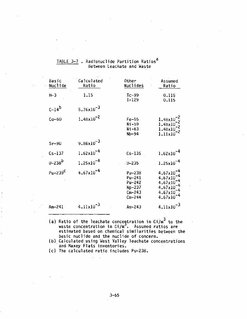
TABLE 3-7 . Radionuclide Partition RatiosaBetween Leachate and Waste

Basic-Nuclide

H-3

CalculatedRatio

1.15

5.76x10-3

1.48x10"2

OtherNuclides

Tc -991-129

Co'-60

Sr- 90

Cs-137

U-238 b

Pu-239c

Am"24 1

Fe-55Ni-59Ni-"63Nb'-94

9.86x1(f 3

1 .62x10ý4

1 .25x10- 4

4.67x10"

4.11xI10 3

AssumedRatio

0.1150.115

1.48x10 21.48x10•

2

1.11x102

-41 .62xl' 10

1.25x10 4

4.67x10 4

4.67x10"44.67x10- 44.67x10 44.67x104

4.11x10-3

Cs-135

U-235

Pu-238Pu-241Pu-242Np--237Cm-243Cm-244

Am-243

(a) Ratio of the leachate concentration in Ci/m 3 to thewaste concentration in Ci/m . Assumed ratios areestimated based on chemical similarities between thebasic nuclide and the nuclide of concern.

(b) Calculated using West Valley leachate concentrationsand Maxey Flats inventories.

(c) The calculated ratio includes Pu-238.

3-65

(corresponding to a permeability -of about 1x10- 4 cm/sec, an effec-

tive porosity of 0.25, and a hydraulic gradient of unity) will be

assumed in this report for the reference disposal facility. These

calculations yield the values 0.00647 and 0.00108 as the contact time

factor for the above percolation cases of 0.18 m/year and 0.03 m/year,

respectively.

These values may be modified for soils with different permeabilities

by multiplying by the ratios of the respective permeabilities; the

contact time factor would increase for soils with low permeabilities,

and would decrease for soils with high permeabilities by as much as a

factor of 10. For example, an increase in the speed of the perco-

lating water to 10 ft/day (i.e., the percolation goes through an 8

meter deep disposal cell in about 2.5 days) may be expected for sandy

soils, similarly, a decrease in the velocity to 0.1 ft/day can be

expected-for clayey soils. 2 1 )

It should be noted that an increase or decrease in the volume of

percolating water affects the contact time linearly, and this has to

be incorporated into the formulation. Therefore, the source term is a

quadratic function of percolation. For example, for the worst case

scenario (i.e., 2xV1 percolation), the above contact time of 0.00647

is multiplied by a factor of 2 yielding a total increase in the source

term by a factor of 4.

The last two factors in equation (3-18) are the multipliers due to

waste solidification and facility operating practices, and due to the

relative inaccessibility of activated radioactivity in metals waste

streams. The multiplier due to waste solidification and facility

operating practices has been discussed in Section 3.2.3, and the table

detailing the Mult(16,17,IS) factor in Section 3.4 is applied iden-

tically to this scenario. The multiplier for activated metal waste

forms has been discussed in Section 3.3.6.

3-66

3.5.2 Migration Reduction Factor

The waste form and package factor, as expressed above, yields the

total (in m 3/yr) source term that can be expected from a given

waste stream, and the product of the radioactive concentration with

the source term gives the annual release (in Ci/yr). This source term

must be related to the radionuclide concentrations at the groundwater

discharge locations. This relation is expressed through the site3

selection factor.(fs) in units of yr/im. This factor, which has also

been referenced as the "confinement factor" or reduction factor,( 1 8 )

is the ground water migration analog of the (X/Q) dispersion factor in

meteorological diffusion calculations (see Appendix A).

Dozens of models, both analytical and numerical, have been developed

to forecast the. probable extent of radionuclide migration (sometimes

called mass transport) and the associated environmental impact.

Reviews of some of the available simulation techniques are presented

in references 22, 23, and 24.

Analytical models simulate the mass transport processes using a

series of algebraically solvable mathematical equations having para-

meters that are homogeneous or can be homogenized. They are best used

under conditions where little hydrogeologic data exists, where the

existing site parameters can be represented by space- and time-

averaged quantities, where the stratigraphy of the site is so complex

as to preclude cost-effective detailed data accumulation or an accu-

rate consideration of the spatial variation of parameters (e.g.,

laterally discontinuous lenses of material interbedded with irregular

stratigraphy) or, as is the case in this report, where the study is

concerned with generic sites and designs. Numerical models are

preferable if the geologic setting of the site is relatively complex

(an exception is the complexity level discussed above) and site-

specific data defining significant space- and/or time-variation of the

site parameters is available.

3-67

The analytical simulation assumes that the porous medium consists of

an unsaturated and a saturated zone, each of which is stationary,

homogeneous and isotropic, and the fluid moving through these zones is

incompressible and of constant viscosity.

The source term is assumed to be given by J0 (which is equal to

fwi multiplied by the waste concentrations in this report), whose

units are in curies/year. The source term is assumed to exist during

the source duration time (T). A geometry of the migration problem is

shown in Figure 3.4.

The measurable hydrogeological parameters that must be included in an

accurate simulation of mass transport are: the geometry of the problem

(e.g., the travel distance, x, to a biota access location), the decay

constant of the radionuclides, the hydraulic velocities of the fluid

(e.g., v), the dispersion characteristics of the medium, and the

retardation coefficients of the radionuclide-medium interaction. The

space- and time-averaging of the above parameters, if necessary, may

be accomplished in a straightforward manner (see Appendix A).(18)

As discussed in Section 2.4, it can be shown that the time dependent

site selection factor is given by:(18)

= [r 9/Q] Z rtij (3-14)

where (Q) is the dilution factor in units of volume/time; the factor

r is the time independent reduction factor due to the geometry ofgthe problem (i.e.,. the spatial relationship of the burial trench and

the discharge location); j denotes the longitudinal sectors of the

disposal facility shown in Figure 3.3; and rtij is the reduction

factor due to migration and radioactive decay which depends on both

space and time, including the sectors of the disposal facility and

the duration of the source term (Ti).

3-68

INTERFACE OF THESATURATED AND

UNSATURATED ZONES

C=h

'.0

_1 t)

SATURATED ZONE PARAMETERS:V, X, Rs,

Ds,D,,DsDISCHARGE SURFACE

U

I

I00Nfl

GEOMETRY OF GROUNDWATER MIGRATION

Geometric Reduction Factor - r g

This reduction factor is assumed to be independent of the character-

istics of the waste streams. It is also independent of the longitu-

dinal relationship of the disposal facility with the access location.

This results in a second order approximation since the transverse

dispersion of the radionuclides depend on the travel time between the

disposal facility and the discharge location, and the factor rg is a

measure of the transverse dispersion of contaminants.(18) However,

this effect is negligible when compared with the primary effect of the

transverse extent of the disposal area (assumed to be 450 meters) in

relation to the access location. This primary effect is quantified

through rg

In this report, it is conservatively assumed that the biota access

location is always on the main streamline from the disposal facility

(see Figure 3.1). That is, it is located on the streamline that

passes through the center of the disposal facility. In off-center

location cases, this effect would be expressed through the factor

rg as well.

ggThe maximum value of rg is unity; it is different from unity only

in the well access cases. In the well access cases, it depends on

the radius of influence resulting from the pumping rate. In other

words, depending on the pumping rate of the well, some or all of

the radioactivity released across the entire disposal facility width

of 450 meters may be pumped up with the well water. An idealized

pumped well geometry illustrating these concepts is presented in

Figure 3.5.

The generalized formulae for the reduction factor r g are presented

in reference 18 and are summarized in Appendix A. However, they are

unnecessarily complicated for the generic cases being considered. The

following simplified equation is used in this work:

3~-7o

11 1I DISCHARGE SURFACE

WI

/

AINTERFACE OF SATURATEDAND UNSATURATED ZONES

I.

I~

zw

f

:3:

Zu.J0:3:

Ln

-J

GROUND WATERDIVIDE P IS A STA

EQUIPOTENTIALL I N E S . _

•GNATION POINT

FLOW LINES3.J

LB

WELL CASE A) SIDE VIEW

B) PLANVIEW WITH STREAMLINES

im^"iwe a m. MOR m

3-71 FIGURE 3.5

r = l surface water access

rg = 2 Yw/L well water access

where yw is the pumping radius of the well (see Figure 3.5), and L

is the transverse width of the disposal area. The pumping radius of

the well is dependent on the groundwater velocity, and may be repre-

sented by the following equation: ( 1 8 )

Yw = Q /-(2 zw n v)

where Q is the pumping rate of the well, z is the pumping depthw(minimum depth of the well below the interface of the saturated and

the unsaturated zones), n is the porosity of the stratum being pumped,

and v is the groundwater velocity.(1 8 )

For most locations where a disposal site may be located, the ground-

water velocity is likely to be low (partially intentionally, partially

because the site is likely to be located at a topographic high which

implies a low hydraulic gradient). In order to get water yields from

such a well sufficient to meet the needs of an individual, the pumping

radius would be expected to.be very high. For example, for a pumping

rate of 7700 m3 /year (representing the basic annual needs of a single

farmer - see below and Appendix A), in a medium with an effective

porosity of 0.25, a groundwater speed of 1.5 m/year, anda pumping

depth of 10 meters, the pumping radius turns out to be about 1000

meters (implying an rg value of unity). If equal values for the

pumping depth and the pumping. radius are assumed, these values turn

out to be about 100 meters (implying an rg value of 0.45).

In this report, the dilution factors that have been assumed imply that

in most cases the pumping radius is likely to be high. Therefore, the

geometric reduction factor rg is conservatively assumed to be unity

in all cases for the reference disposal facility.

3-72

I I-

Dilution Factor - Q

The dilution factor is independent of the characteristics of the waste

stream and the geometrical relationship of the disposal facility with

respect to access location. The factor Q may be the pumping rate of a

well or the flow rate of a stream.

In this work, the dilution rates assumed are 200,000 m3 /year (about

100 gpm - gallons per minute) for the population well scenario and

4.5 x 106 m3 /year (about 5 cfs - cubic feet per second) for the

surface stream scenario. Small farming communities that utilize

groundwater for their needs usually have wells that range from 100 gpm

to 1000 gpm depending on the population. 18) A stream flow rate of

about 5 cfs is selected since a stream with flow rate below this value

is very unlikely to be used for human consumption. For example, Rock

Lick Creek nearby the Maxey Flats disposal facility has an annual

average flow rate of about 7 cfs, but it is not used for human con-

sumption, it is used only for livestock.( 2 5 )

For the individual well and boundary well scenarios, Q is given by the

assumed total volume of percolating infiltration through the disposal

facility area. In other words, the source term J calculated in the

previous section is diluted by a minimum volume of water infiltrating

through the disposal area and recharging the groundwater.

The primary rationale for this procedure is that the source term

will be mixed with an appropriate volume of water in the groundwater

regime. In past studies, 1 0 ) this volume has been assumed to be the

annual aquifer flow rate underneath the site which necessitates

assumptions on the aquifer thickness (or radionuclide mixing depth)

and velocity. Furthermore, this approach necessitates the assumption

that the radionuclide source term is mixed homogeneously throughout

the aquifer thickness (or the assumed mixing depth). In this report,

this dilution volume is estimated to be the natural percolation of the

3-73

disposal site vicinity multiplied by 352,000 m2 , which is the disposal

area required for the reference facility. This value is conservative

since it is likely that there may be substantial contribution to

groundwater from areas upstream/downstream of the disposal facility.

There is a lower bound, however, for the value of the dilution volume

for the intruder well and boundary well scenarios. Otherwise the

above technique would give invalid results for disposal facilities

located in regional environments in which the natural percolation is

very low, e.g., an arid western environment. The lower bound dilution

rate in this report is taken to be 7700 m3 /year (3.84 gpm) , which

represents the needs of a single person living in a rural area.( 2 6 )

Migration Reduction Factor - rtij

This factor depends on the time that the exposure is assumed to occur,

the duration of groundwater travel between the jth longitudinal

section of the disposal facility and the access location, the retarda-

tion capability of the soils (radionuclide dependent), the duration of

the assumed source term, and the waste stream characteristics. The

longitudinal extent of the disposal facility is considered by dividing

the facility into 10 sectors and summing the contributions from each

sector (assumed to be equal) to obtain the concentrations at the

discharge location. Detailed formulae for this factor can be found in

Appendix A. In this work, the following formula is used for the

migration reduction factor r

rtij = [exp(- Xt)/(JxTi)] x [ F.(t) - Fj(t-Ti) ] (3-15)

where X is the decay constant of the radionuclide; t is the time at

which the migration reduction factor is applicable, J is the total

number of longitudinal sectors the disposal site has been divided

into, which is 10 in this work (see Figure 3.3); Ti is the source

duration factor for the ith waste stream, and j denotes the sector

3-74

of the disposal site. The function Fj(t) is given by the following

formula (see Appendix A):( 18 ' 2 7 )

Fj(t) 0.5 x U(t) x [erfc(X_) + exp(P.) erfc(X+)] (3-16)

X+- / t/Rtw (3-17)VT2 /t/(Rt

()

wj

where U(t) is the unit impulse function that is zero for a negative

argument and is equal to unity otherwise; twj is the water travel time

between the disposal sector being considered and the access location,

P. is the Peclet number for the distance between the disposal sector3and the access location, R is the retardation coefficient of the

radionuclide, and erfc(x) is the complement of the error function

and is given by the formula:( 2 8 )

x

erfc(x) = 1 - f (2/VT-) exp(-t 2 ) dt (3-18)

0

The retardation coefficients R that are utilized in the above equa-

tions depend on the radionuclide as well as the geochemistry of the

soils and the transporting groundwater. They are indicative of the

reversible ion exchange capability of the soils and represent the

ratio of the radionuclide velocities in the soil to the groundwater

velocities. The cation exchange capacity of the soils is a parameter

which can be used to estimate the retardation coefficients of the

soils, since retardation coefficients are usually linearly depend on

the cation exchange capacity. Five sets of retardation coefficients

are utilized in this work.( 2 9' 3 0 ) These coefficients are presented

in Table 3-8.

The clay and mineral content of the soils, in addition to the ground-

water chemistry, significantly affects the retardation capability of

the soils. The retardation coefficients given in Table 3-8 span the

general range of values that are encountered in groundwater migration

3-75

TABLE 3-8 . Sets of Retardation Coefficientsa

Used in Impacts Analysis

Assumed Retaroation

Nucl i de

H-3

C-14

Fe-55

Ni-59c

Co-60

Sr-90

Nb-94

Tc-99

1-129

Cs-137c

U-235c

Np-237

Pu- 2 38 c

Cm-243c

Am-241c

Set 1

1

10

630

42U

420

9

1000

2

2

85

840

300

840

300

300

Set 2

1

10

1290

860

860

18

2150

3

3

173

1720

600

1720

600

600

Set 3

1

10

2640

1750

1750

36

4640

4

4

350

3520

1200

3520

1200

1200

Coefficients

Set 4 Set 5

1 1

1U 10

5400 11050

3600 7350

3600 7350

73 146

10000 21500

5 6

5 6

720 1460

7200 14730

2500 5000

7200 14730

2500 5000

2500 5000

BNWLb

1

3333

333

333

100

10000

1

1

1000

14286

100

10000

3333

10000

(a) Sets 1 and 4 are values obtained from reference 29, except forthe radionuclides Nb-94 and U-235. These values are based oncomparative retardations given by the BNWL column (reference 30).Sets 2 and 3 are obtained as geometric midpoints of Sets 1 and 4,and Set 5 is similarly calculated, i.e,:

Set 2 = Set 1 x Cube Root of (Set 4/Set 1),Set 3 = Set 2 x Cube Root of (Set 4/Set 1),Set 5 = Set 4 x Cube Root of (Set 4/Set 1).

(b) These values are given in reference 30 for desert soils with amoderate cation exchage capacity of about 5 meq/100 g. They havebeen used as a guide to fill in missing values.

(c) Coefficients for other isotopes of these elements are assumed tobe the same.

3,-76

calculations. The first set is representative of coefficients for

sandy soils with low to moderate cation exchange capacities, and is

assumed to represent the lower bound of retardation coefficients used

in this.generic analysis. The fourth set is representative of coef-

ficients for clayey soils with moderate to high cation exchange

capacities, and is assumed to represent the best conditions that can

be routinely achieved. In between these two sets, two other sets have

been postulated and have been calculated utilizing the geometric

mid-points of sets 1 and 4. The third set of coefficients have been

assumed to be applicable to the reference disposal facility. A fifth

set of coefficients has been also calculated for use in special cases.

The source duration factor Ti for the i th waste stream is determined

by dividing the total activity in the stream with the annual release

fraction which is given by the factor fwi multiplied by the radio-

nuclide concentration. This calculation conservatively neglects the

depletion of the radionuclide inventory at the disposal facility by

previous releases.

The groundwater travel times tw depend on the distance between the

disposal facility sector being considered and the discharge location.

The travel time between the first sector and the access location is

denoted by twl* It is assumed for the reference disposal facility

that groundwater takes 10 years to traverse the unsaturated zone. The

assumed values of t w for the reference disposal facility are pre-

sented below:

Location Travel Time - t

Intruder-Well 42 yearsBoundary-Well 66 yearsPopulation-Well 400 yearsSurface Stream 800 years

The groundwater travel time between two adjacent sectors (a distance

of 80 meters for the reference disposal facility) is assumed to be

64 years (corresponding to a speed between two adjacent sectors of

3-77

1.25 m/year) and, to determine the groundwater, travel times for the

other sectors, an appropriate multiple of the travel time is added to

the twl. It should be pointed out that using groundwater travel times(and the Peclet numbers discussed below) as the primary variables on

which the migration analysis is based, implicitly allows for a sensi-

tivity analysis. Sites with differing environmental parameters may

lead to similar radionuclide concentrations at the access locations.

For example, similar results would be obtained if the groundwater

velocity is twice as high and the distance to the access location is

twice as large. Similarly, a larger unsaturated zone travel time

(water speeds of the order of 10-2 feet/year are frequently encoun-

tered) 23) would compensate for a shorter saturated zone travel time.

The Peclet number, P., is the distance to the access location divided

by the longitudinal dispersivity of the medium. Peclet numbers for

the distances between the sectors are determined in a manner similar

to the travel times. For the reference disposal facility, a value of

1600 is added for two adjacent sectors to the Peclet number for thefirst sector P1 which is assumed to be the following:

Location Peclet Number PI

Individual-Well 1300Boundary-Well 1900Population-Well 10000Surface Stream 20000

The discussion presented above for the variation of travel times is

applicable to the selected Peclet numbers as well. In this manner,

the unsaturated and saturated zones are considered as a single unit.

The primary justification for this approach is the generic nature of

the analysis. Moreover, as long as the groundwater travel time in the

unsaturated zone is added to the saturated zone travel time, and the

Peclet numbers for the two zones are added, the above is a valid

approximation to the alternative of considering saturated and unsatu-

rated zones as two units with the ensuing complications. Such a

treatment can be found in a previous work by the authors.( 1 8 )

3-78

3.5.3 Special Cases

This section considers three special cases utilized in the groundwater

migration calculational procedure: the maximum concentration case, the

time dependent source analysis, and high integrity containers. These

cases are considered below.

Maximum Concentration Case

The equations given above can be used to determine radionuclide

concentrations at a particular access location as a function of time.

It may also be of interest to determine the maximum concentration of

a particular radionuclide at a particular access location over all

time.

The maximum radionuclide concentration at the particular access

location considered may occur long after the initiation of the scen-

ario, and becomes significant for those radionuclides that have high

retardation coefficients and very long half lives -- e.g., U-235,

U-238, Pu-239. For this special case, only the reduction factor

r is affected in the above formulation and a modification of

equation (3-14) is necessary to calculate the maximum concentrations.

The equation utilized in this work is: (18)

f si: [rg ri]/Q (3-19)

where rg and Q are as defined previously, and r. is the time inde-

pendent maximum value of the migration reduction factor rtij. The

parameter ri is given by the following equation.

r = Maximum of [rillr i2, .,ril 0 ] (3-20)

where

rik =k x [exp[ - XRtwk]/(JxTi)] (3-21)

3-79

where the above variables J, Ti, X , R, and twk denote the same

parameters defined previously.

Time Dependent Sources

Although a disposal facility will be designed and operated so that

infiltration of rainwater will be minimized, it is possible that

sometime after the disposal facility is closed, active institutional

controls may breakdown and potential inadvertant intrusion into part

of the disposed wastes may occur and, as a result, rainwater infilt-

ration may increase. Similarly, a breakdown in institutional controls

may lead to intrusion into the waste mass by deep-rooted plants and

burrowing animals which also may lead to an increase in rainwater

infiltration. This potential increase in infiltration would result

in a corresponding increase in the groundwater migration source term.

A calculational procedure to account for this time de~pendent source

term is presented below.

For the case of the time dependent source term analysis, two different

source magnitudes are considered. The source term is assumed to

increase after the end of the active institutional control period as

represented by the following histogram:

Source

Term

fwi2

fwi I

Til Ti2 Time

Two source terms, denoted by fwil and fwi2' are calculated using

equation (3-15). These source terms are used in conjunction with two

source duration times denoted by (Til) and (Ti2-Til). The first

source term is applicable during the duration time of Til years

3-80

(equal to or less than IPO+IIC - see Section 3.1), and the-second

source term is applicable during a duration time T i2-Ti. The

second source duration time is calculated by substracting the radio-

activity that has migrated -from the -site during the first source

duration time from the activity inventory of the site (the area under

the above histogram), and dividing the remaining site activity inven-

tory by the second source term. In other words, it is calculated by

the formula:

T2 i = Til + f wil x (TDUR - Til) / fwi2 (3-22)

where TDUR represents the source duration time if f wil were the

source term during the entire period. In other words, TDUR is the

duration time for the time independent source term analysis and TDUR.times f times Cw is the entire site inventory of the radionuclide

being considered.

For calculational convenience, the source term for this analysis

is taken to be equal to fwil for all times, and the effect of the

increased source term after time Til is incorporated into the factor

rtij. The following equation is used to calculate the modified

factor r tij:

= [exp(- Xt)/(JxT1JUR)] x [ F.(t) - Fj(t-Ti +rtij

(f wi2/f wil) x [ Fj(t-Ti) - F (t-T.i2)]] (3-23)

where FW(t) is the function defined previously by equation (3-19),

and where the variables X , J, TUUR, Till Tiz, f wil and fwi2 are

as defined previously. For cases where the source is depleted within

the active institutional control period (TDUR is less than IPO+IIC),

or for cases where the percolation volume at the disposal facility is

greater than or equal to V1 (see Section 3.5.1), this analysis is

ignored.

3-81

High Integrity Containers

High integrity containers are packages which are designed to preclude

waste/trench water contact for long periods of time."() This time

period may vary-from a few years to several hundred years. The effect

of this delay due to use of high integrity containers is incorporated

into the analysis by adding the delay time to all the groundwater

travel times for the selected waste streams. This procedure results

in accurate consideration of the effects of this special case -- i.e.,

the time delay factor fo is waste stream independent, whereas high

integrity containers may be applied to only certain waste streams.

3.6 Exposed Waste Scenarios

In these scenarios, some or all of the surface area of the disposed

waste is assumed to be exposed through some means. The mechanism that

initiates uncovering of the waste can be either the erosion of the

waste cover by surface water or wind action, or intruder activities

such asconstruction or agriculture. Similarly, there are two exposed

waste surface scenarios depending on whether the transfer agent is

wind or surface water, the corresponding biota access location can be

either an off-site surface water body (through surface water runoff)

or off-site air (through wind suspension and transport). Therefore,

there are four exposed waste scenarios: intruder-air, intruder-water,

erosion-air, and erosion-water.

Only those wastes that have been disposed through regular disposal

designs are considered in the erosion initiated scenarios. Waste that

is layered (disposed of at the bottom of the disposal cells), and

waste that is disposed of in a hot waste facility are assumed not to

be exposed to the atmosphere for the erosion-initiated scenarios.

However, all the wastes are considered in the intruder-initiated

scenarios. The following equations are utilized to calculate human

exposures resulting from these scenarios. For the water transport and

access case:

3-82

H = (fofdifwifsi)wat Cwi PDCF-7 (3-24)i n

and, for the air transport and access case:

H : . L fodifwifsi)air Cwi PDCF-8 (3-25)

i n

where H is the 5 0 th year annual dose in mrem/year after 50 years

of exposure, PDCF-7 and PDCF-8 are the radionuclide specific pathway

dose conversion factors discussed and presented in Section 2.3,

C is the radionuclide concentration in the ith waste stream, n

denotes summation over all the radionuclides, and i denotes summation

over all the waste streams. The values of the barrier factors are

presented below.

The time delay factor (f ) is defined by:

f = exp[.- X T] (3-2)

where T is the delay time, and X is the decay constant. For the

intruder-initiated exposed waste scenarios, the delay time (T) is

taken to be the period between the cessation of active disposal

operations and the end of the active institutional control period..For the erosion-initiated exposed waste scenarios, it is taken to be

dependent on the cover thickness utilized -- i.e., it is a function of

the disposal technology index IC. The following table presents the

values asumed for the initiation of the erosion *scenario:

IC Delay Time

1 2000 years2 3000 years3 10000 years

These values are extremely conservative. Previous estimates on the

erosion potential of adequately emplaced cover materials have ranged

from 1000 years to 10,000 years to erode 1 meter of soil cover. ( 3 )

3-83

After consideration of the variability of this time period-, reference

13 assumes a time of 2000 years to erode through 2 meters of cover

material. This is the value utilized in this work.

The site design factor (fdi) is defined as the fraction of the

exposed area that is waste, and will be assumed to be independent

of the waste stream considered. Therefore, it will be taken to be

proportional to the emplacement efficiency of the waste; however,

in this case the percentage of the land area in between the disposal

cells that have not been utilized for waste disposal must be consi-

derea -- i.e., the land-surface utilization rate (see Section 3.2.2).

Therefore, the site design factor is taken equal to the product of the

emplacement efficiency (0.75 for stacked disposal and 0.5 for other

emplacement cases) with the land-surface utilization rate of the

design option (for reference disposal facility design it is conser-

vatively estimated to be 0.90).

The waste form and package factor (f wi) denotes the total volume of

the soil-waste mixture mobilized by the transfer agent per year. In

this report, it may be empirically broken down into the following

components.

fwi = E x (A/d)i (3-26)

where:

E = soil-waste mixture mobilization rate (in g/m -yr) which will

be taken to be independent of the waste stream.

Ai = total area of the soil-waste mixture (in m2 ) that can be

identified with the (M)th waste stream.

3di = density of-the soil-waste mixture (in g/m3) that can be

identified with the (i)th waste stream.

3-84

This equation is applicable for both the wind transport scenario and

the surface water scenario. Specific values of the parameters and the

site selection factor fsi are discussed below.

3.b.1 Wind Transport Scenario

For the intruder-initiated scenarios, the factor E can be calculated

based on use of the soil-to-air transfer factor (see Appendix A). It

may be taken as the time weighted average of the dust mobilization

rate (0.218 mg/mr2-sec) resulting from construction or gardening

activities such as tilling and the natural wind mobilization rate

of 4.1 x 10-4 mg/m2-sec (see Appendix A).

Both the intruder-construction and the intruder-agriculture scenarios

are used in the intruder-initiated exposed waste scenario depending on

the disposal status of the waste: regular unstable and layered

unstable wastes are subjected to the agriculture scenario, and regular

stable, layered stable, and hot waste facility wastes are subjected to

the construction scenario. However, only 1 percent of the layered

unstable wastes are assumed to contribute to the agriculture scenario,

while only 1 percent of the layered stable wastes and 0.1 percent of

the hot waste facility wastes are assumed to contribute to the cons-

truction scenario. Moreover, the duration of the exposed waste

scenario is modified by the duration factor of 6 hours (instead of 5JU

hours) for the stable wastes. Furthermore, about 1800 m2 of waste

area is exposed continuously in the agriculture scenario with only a

fraction used for gardening, and 200 m2 of area is exposed for 500

hours for the standard construction scenario.

In order to simplify the complicated procedure required to estimate

the factor E for the above conditional cases, a basic mobilization

rate is assumed to be applicable to all the cases with correction

factors applied to each waste stream as appropriate for the special

conditions outlined above. The basic dust mobilization rate for the

3-85

intruder-initiated scenario is assumed to be 2.9 x 10-3 mg/m2-sec.

This is calculated by multiplying 100 hours by 0.218 mg/m2 -sec,

adding this to the product of 8660 hours and 4.1 x 10-4 mg/mr2-sec,

and dividing the total by 8760 hours. For the erosion-initiated

scenario, the factor E is taken as the natural wind mobilization rate

of 4.1 x 10-4 mg/m2 sec.

For the erosion-initiated scenario the entire-disposal site area is

assumed to be exposed and Ai is calculated by dividing the volume of

the waste stream being considered by the product of three factors: the

volumetric disposal efficiency (assumed to 6.40 mr3 /Mr2 for the refe-

rence disposal facility case), the surface utilization rate (0.90),

and the emplacement efficiency. The density of the soil/waste mixture

is assumed to be 1.6 g/cm3 except for those streams that are soli-

dified using solidification scenarios A or B involving partial cement

solidification. These streams are assumed to be 34% heavier.

For the wind transfer scenarios, the site selection factor (f s) is

the air-to-air transfer -factor (meteorological dispersion factor

X/Q - see Appendix A). For these scenarios, the-number of people

exposed to atmospheric releases are incorporated into the definition

of the site selection factor. This results in an fs ýith units of3)peopl e-year/mr

To calculate the site selection factors, the population for the refe-

rence disposal facility (see Appendix C) is assumed to be doubled for

the intruder-initiated scenario, and tripled for the erosion-initiated

scenario. The number of people in each radial sector is multiplied by

the corresponding atmospheric dilution factor and the results summed.

The site selection factors are calculated to be 3.50 x 10"10 and

5.25 x 10- 1 0 people-year/m3 for the intruder- and erosion-initiated

wind transfer scenarios, respectively.

3-86

3.6.2 Surface Water Scenario

Based on surface water erosion calculations (see Appendix A), the

mobilization rate for the surface water scenario (i.e., the factor E

in equation 3-31) is calculated to be 1.84 x 102 g/m 2 -year. This

factor corresponds to an annual erosion rate of about 0.82 tons/acre.

Annual erosion rates vary with the soil properties, vegetation, prior

erosion, topography, etc. The annual erosion rate for the Appalacian

region for the past 125 million years has been calculated to be 0.75

tons/acre.(I0) The other factors in the equation (i.e., A and d)

remain as defined in Section 3.6.1.

The surface water site selection factor can be estimated by consider-

ing the flow rate of a nearby stream assumed to be utilized by a

member of the population. In this report, the inverse of twice the

value of the dilution factor Q previously utilized to determine

groundwater impacts at the surface water access location (1.12 x 10-7

3year/mr for the reference facility) will be utilized for the site

selection factor. Twice the value is utilized to account for the

increased flow conditions during heavy precipitation and subsequent

heavy strpam flow rates. The assumption of this value corresponds to

dilution 9 f the released radioactivity in a stream with a flow rate of

about 10 cubic feet per second, and it is conservative since a stream

with a flow rate this low is unlikely to be utilized for human con-

sumption.

Evaluation of the surface water contamination scenarios involves

consideration of certain second order effects. These effects are

primarily concerned with the deposition and/or sorption of the radio-

nuclides on soils and sediments during the surface water transport

episode. Deposited and sorbed radionuclides are available for resus-

pension or desorption and hence represent a long-term source of

radioactivity that may be further distributed. Concentration of

radioactivity onto fine particles may occur, resulting in localized

3-87

areas where radionuclide concentrations are higher than the initially

transported material. The two separate mechanisms of deposition/

resuspension and sorption/desorption are discussed below.

Deposition and/or ion-exchange by soils of mobilized radioactivity

during its travel to a nearby stream has been treated i~n reference 13.

These mechanisms are not likely to lead to significant uptake pathways

to humans in addition to those pathways already considered. Most of

these mechanisms take place during overland sheet-flow where condi-

tions are more quiescent than in gullies -- i.e., the radioactivity

becomes dispersed over a relatively large land area. The deposited

radioactivity is probably in oxide form and unlikely to contribute to

the food (soil) uptake pathway. Furthermore, any deposited or attached

radioactivity undergoes a natural elimination from the land surface

with a half life estimated to be about 2.5 years.( 3 1 ) Moreover, the

assumption of no deposition during surface water transport leads to

higher concentrations in the stream receiving the discharge. This

scenario is also likely to be bounded by the intruder-agriculture

scenario. In any case, estimation of this component is extremely

site-specific and requires a large amount of data,( 2 3 ) and cannot be

treated accurately in a generic study. Therefore, these mechanisms

are not considered as part of the surface water scenarios.

Sediment transport in streams and possible reconcentration of the

radioactivity in stream sediments are also considered in reference 13.

Several mechanisms may be considered to be applicable: reversible

sorption of the dissolved radioactivity by stream sediments through

ion exchange, deposition of the sediments suspended in water once they

reach the stream, resuspension and transport of stream sediments

containing radioactivity through stream flow, and deposition of these

sediments in man-made control features such as reservoirs.

A thorough evaluation of these mechanisms also requires a large amount

of site specific data, 13) and does not appear to be justified in a

3-88

generic analysis. Furthermore, the portion of radioactivity trans-

ported as suspended particulates is probably in the form of oxides,

is unlikely to become dissolved subsequently, and, therefore, unlikely

to contribute to many of the uptake pathways. The water is also

likely to be filtered or stilled in ponds, eliminating most of the

sediments prior to direct human consumption. Moreover, the ratio of

the Cs-137 concentrations in storage pool sediments to the concen-

trations in upstream sediments have been observed to range from 0.92

to 4.0. These reconcentration factors are not very large when com-

pared to bioaccumulation factors that range up to 1000 or more for

several nuclides. Therefore, in this report, all the radioactivity

conservatively has been assumed to be dissolved in the water access-

ible to the uptake pathways, and the contribution to the uptake

pathways resulting from the above mechanisms have been assumed to be

bounded by the scenarios considered.

3.7 Operational Accident Scenarios

There are two operational accident scenarios considered for applicabi-

lity to a given stream in the impact calculations: accident-container,

and accident-fire. These scenarios are described below.

3.7.1 Accident-Container Scenario

This scenario assumes that a waste container is dropped from a signi-

ficant height so that the waste container breaks open and a portion of

the radioactive contents of the package is released into the air where

it is transported off-site and leads to subsequent human exposure.

Potential releases can be modelled as a "puff", and the resulting

human exposures would be over a very short time period. The potential

exposures from this scenario are a strong function of the waste form -

i.e., improved, less dispersible waste forms lead to lower potential

releases and reduced potential human exposures. The equation des-

cribing the human exposures is as follows:

3-89

H = f f fodfwfs C w PDCF-1 (3-27)

n

where H is the 50-year dose commrittment in mrem, PDCF-1 is the radio-

nuclide specific pathway dose conversion factor discussed and pre-

sented in Section 2.3, C is the radionuclide concentration in the

waste, and n denotes summation over all the radionuclides. The values

of the barrier factors are presented below.

No reduction due to decay of the radionuclides is considered, and the

time delay factor f0 is assumed to be one. Similarly, no reduction

due to site design and operation has been assumed and the factor

fd has also been set equal to one.

The waste form and package factor f is affected by the dispersibi-w

lity of the material at the time of disposal. An index that can be

conveniently-used to represent this property is the leachability index

of the waste stream (see Section 3.3.3), which also represents the

solidification scenario utilized for the waste stream. The waste form

and package factor is given by the following equation:

fw = I0(1-19) x I0(1 - 16 ) (3-28)

The relationship 10(1-19) is the accessibility multiplier discussed

previously. The factor 10(1-16) indicates the relative dispersibility

of the solidified material after a container accident. The property

values for this comparative dispersibility are based on consideration

of comparative mechanical strengths (compressive, unnotched Izod

impact, and fragmentation tests) measured for waste forms.(I) If

the waste is not solidified, then 16 is assumed to be unity.

The site selection factor fs, which is dimensionless, may be calcu-

lated by assuming that the material released is a "puff", and it

stays in a puff form until it reaches the exposed individual. The

following equation is utilized in this report to calculate fs"

3-90

f = 1.56 x 10-7 X f r x V x (X/Q) (3-29)

where 1.56xi0'7 is the exposure duration factor, fr *is the fraction

released per second, V is the volume *of the container, and (X/Q)

is the atmospheric dispersion factor. These parameters are considered

below.

The exposure duration factor is given by the fraction of air inhaled

in one intake by a man performing light activity (1.25 liters) to the

annual inhalation volume (8000 mi3 ). (15) A man doing light activity

inhales about 17 times per minute, a man resting about 12 times per

minute, and a man doing heavy work about 21 times per minute.(15)

If one were to assume that the puff release is longer, say one minute,

then the longitudinal spread of the puff (i.e., a x) would be increased

by a factor of 60 (resulting in a corresponding reduction in the

atmospheric dispersion) while the amount of air inhaled would increase

only by about 17. The assumed condition - one inhalation during the

one second passage of the puff - is the most conservative case.

The *source term portion of the above equation is represented by the

product of fr' the fraction released per second, and V, the volume

of the container. For fr' for' the worst case, 0.1 percent of the

waste is assumed to be released into air. (the case of the PuO 2

powder accident).(9) This release fraction, however, is modified by

the solidification status of the waste stream (see above). The volume

of the container involved in the accident, V, is assumed to be 170 ft 3

- the size of a typical resin liner.

For puff releases, the atmospheric dispersion factor (X/Q) for a

ground level release and from a person standing in the-centerline of

the puff is given in reference 16 by the following formula:

(X/Q) = [Tr2'2•-ox Gy oz]- (3-30)Xy

3-91

where ax, ay, and cz are the standard deviation factors of the puffin three directions. These sigmas, in units *of distance (meters),

indicate the spread and dilution of the plume as a function of dis-

tance from the source. In this report, based on the average wind

speed at the reference disposal facility, utilizing a value of

a a y = 3.61 m, and a value-of a = 2.2 m,(16) yields a (X/Q)x y 30-yilsa3XQ

value of 4.42xl- sec/m-3 . The above assumed values yield a site

selection factor of 3.323x10- 1 2 for the reference disposal facility.

3.7.2 Accident-Fire Scenario

This scenario assumes that a fire starts in a disposal cell and lasts

for approximately two hours. A portion of the radioactive material is

released into the air where it is transported off site and leads to

subsequent exposure to humans. Potential exposures from this scenario

are a strong function of the waste form and facility design and

operation. For example, a waste disposal trench in which all of

the wastes are composed of compressible material (e.g., segregated

disposal of compressible waste) would involve larger releases (more

material to burn) than a case in which the compressible material is

mixed with non-combustible waste. However, most compressible waste

forms have very low levels of contamination. On the other hand,

improvements in the form of the compressible material would involve

lower potential releases. For example,. compressible material which

has been processed by incineration and solidified would involve lower

potential releases than compressible waste which has been processed by

compaction.

In this report, the accident-fire scenario is used to help assess the

effect of improved waste forms and site operational practices on

reducing the potential exposures from an accident involving an ope-

rational fire. Each waste stream or groups of waste streams may be

tested separately using this scenario. The equation describing the

human exposures is as follows:

3-92

H = f fofdfwfs Cw PDCF-1 (3-31)

n

where H is the 50-year dose committment in mrem, PDCF-1 is the radio-

nuclide specific pathway dose conversion factor discussed and pre-

sented in Section 2.3, Cw is the radionuclide concentration in the

waste, and n denotes summation over all the radionuclides. The values

of the barrier factors are presented below.

In a manner similar to the accident-container scenario, the time delay

factor f and the site design and operation factor fd are assumed

to be one. The waste form and package factor f is assumed to be

equal to 0,.1 x 20(14-3) where 14 is the waste form flammability index

(see Section 3.2.1).

The *site selection factor fs is determined by the atmospheric dis-

persion of the plume resulting from the accident. In this report,

the plume resulting from the fire is assumed to travel in one direc-

tion and that the exposed individual is assumed to stand in the

centerline of the plume for a period of time. This barrier factor is

calculated by the following formula:

fs = fe x fr x V x (X/Q) (3-32)

where fe is the exposure duration factor (dimensionless), fr is the

release fraction per second- V is the volume of the waste involved in

the fire in units of m3 , and (X/Q) is the atmospheric dispersion3factor in units of sec/mr

In this work, fe is assumed to be equal to 3.63 x 10-5 based on the

ratio of the air inhaled during the time period the individual is

assumed to stand in the plume of the fire (10 minutes during which

a man doing light activity inhales about 0.29 mi3 of air).( 1 5 ) It

is not reasonable to assume that an individual would stand in the

centerline of the plume from the fire for more than 10 minutes. The

3-93

fraction released per second, fr' is assumed to be 1/7200 based on

the assumed duration of the fire. This is equivalent to a fire

duration time of 2 hours. The volume of waste involved in the acci-

dental fire is assumed to be 100 m3 based on an estimated annual

disposal volume of 50,000 m3 , two disposal cells operating simul-

taneously, and one disposal cell involved in the fire. The atmos-

pheric dispersion factor (X/Q) for an accident lasting from 0 to 8

hours is given by the equation(17)

(X/Q). = exp[-h 2/(2a z)]/[Wu ay UZ] (3-33)

where h is the release height (or the effective height of tlhe plume at

the fire source), u is the wind speed which is specified to be 1 m/secassuming Pasquill Stability Class F atmospheric conditions, (17) and

a and a are as defined previously. Utilizing values for ayy ~zand a z given in reference 17 at 100 m from the fire, and conserva-

tively assuming ground level releases (i.e., h=O), yields a (X/Q)

value of 3.62 x 10- and a value for the site selection factor of

1.83 x 10-9.

3-94

3.8 Other Impact Measures

The impact measures other than individual and population exposures

associated with the operation of a disposal facility include occupa-

tional exposures, land-use, disposal costs, and energy use. This

section considers procedures for calculating these other measures.

3.8.1 Land-Use

Calculating the land area committed for waste disposal is a straight-

forward function of the total volume of the waste disposed, the waste

emplacement technique (i.e., whether random, stacked, or decontainer-

ized disposal is utilized), and the volumetric efficiency of the

disposal technology considered. The volumetric efficiency is a

function of site design as discussed in Section 3.2.2.

For the reference disposal facility and for disposal into a regular

shallow land burial trenches (design case ID=1), the disposal volume

(not the waste volume) per unit disposal cell area is 6.40 m3 /m2 .

Therefore, for each 3.20 m3 of waste that is disposed randomly, 1 m2

of area is committed. However, this land-use rate must be divided by

the surface utilization rate, calculated to be 0.90 for the reference

disposal facility, since for all practical purposes, the land area

between the disposal cells should be considered as committed land.2

Incorporating this correction results in 1 m2 of land area committed

for each 2.88 m3 of waste disposed with random emplacement. Stacked

emplacement would result in 1 m2 of land area committed for each

4.32 m3 of waste disposed.

Similarly, for the concrete-walled trench option (design case ID=2),

the volumetric disposal efficiency is calculated to be 7.00 m 3 of

disposal volume per unit disposal cell area (excluding walls of the

trenches). Therefore for each 5.25 m 3 of waste disposed through

stacked emplacement, 1 m2 of disposal cell area is committed. The

3-95

land-surface utilization rate in this case is calculated to be 0.35 m 2

2of disposal cell area per m2 of available land (including walls and

spaces between the trenches). Therefore, the land area committed is

1 m2 of land for each 1.84 m3 of waste disposed.

3.8.2 Occupational Exposures

In this report, calculation of occupational exposures at the disposal

facility is performed in two phases: exposures to the waste handlers

during unloading and emplacement of wastes, and occupational exposures

to other site personnel performing routine operational and administra-

tive functions not directly connected with waste handling.Z

Occupational exposures to waste handlers are strongly dependent on

the packaging of the delivered waste, the shipment mode, and the

disposal procedures. Therefore, procedures for determining the

occupational exposures resulting from unloading and disposal of waste

are considered in the transportation impacts section of this report

(see Chapter.4.0). Routine occupational exposures for personnel other

than waste handlders are calculated in the next section.

3.8.3 Disposal Costs

Other impact measures - disposal costs, routine occupational exposures

to people other than waste handlers, and energy use - are closely

interrelated and are dependent on the waste volume disposed, the

land-use rate, operational practices, etc. These three measures are

considered in this section.

All the basic rates (rates per unit volume or area) associated with

costs (prior to multipliers to account for the cost of money, profit,inflation, etc. - see below), energy use, and routine occupational

exposures at a disposal facility have been calculated in Appendices

E and F of reference 3. These basic unit rates are summarized in

Table 3-9.

3-96

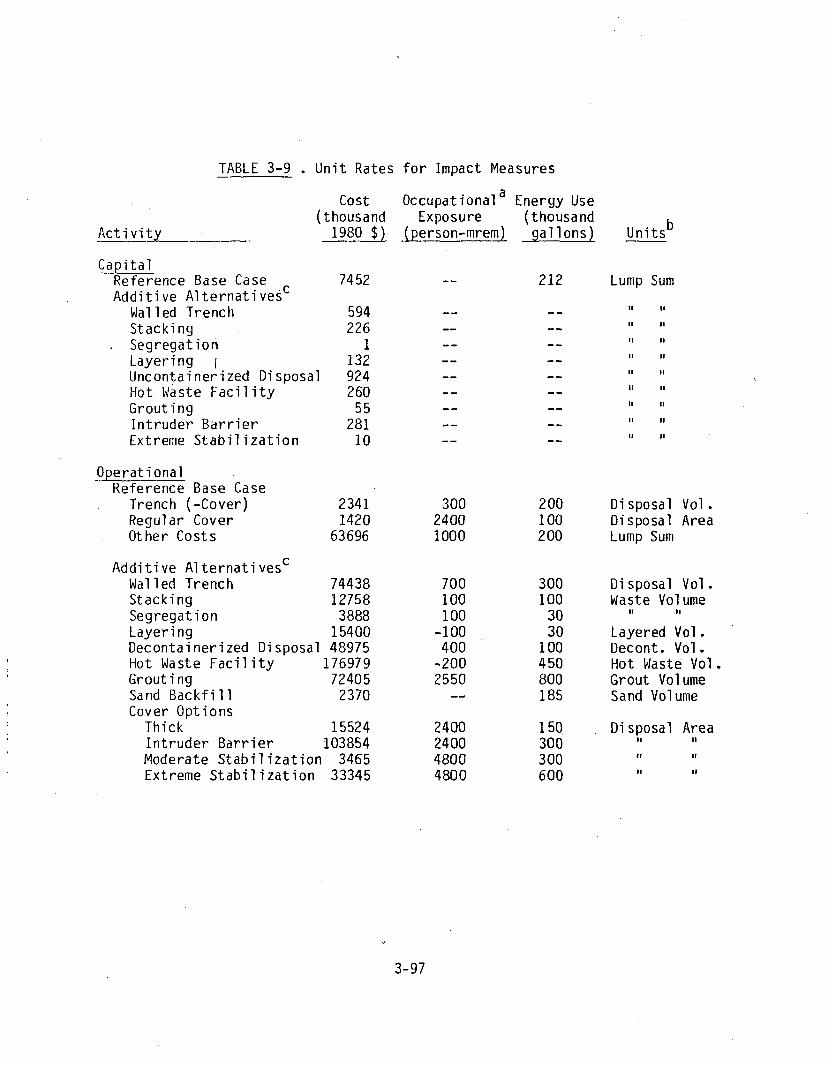
TABLE 3-9 . Unit Rates for Impact Measures

Cost(thousand

1980 $)

Occupational a

ExposureC person-mrem)

Energy Use(thousandgallons)Activ _ity

CapitalReference Base CaseAdditive Alternativesc

Walled TrenchStackingSegregationLayering iUncontainerized DisposalHot Waste FacilityGroutingIntruder BarrierExtreme Stabilization

7452 212 Lump Sum

594226

1132924260

55281

10

II

II

II

ii

II

II

II

II

'I

II

I,

II

I,

II

II

a'

I'

'I

OperationalReference Base Case

Trench (-Cover)Regular CoverOther Costs

Additive AlternativescWalled Trench

23411420

63696

74438127583888

1540048975

176979

StackingSegregationLayeringDecontainerized DisposalHot Waste Facility

30024001000

700100100

-100400

-2002550

2400240048004800

200100200

300100

3030

100450800185

150300300600

Disposal Vol.Disposal AreaLump Sum

Disposal Vol.Waste Volume

I1 1I

Layered Vol.Decont. Vol.Hot Waste Vol.Grout VolumeSand Volume

Disposal AreaII {I

II If

'I I

Grouting 72405Sand Backfill 2370Cover Options

Thick 15524Intruder Barrier 103854Moderate Stabilization 3465Extreme Stabilization 33345

3-97

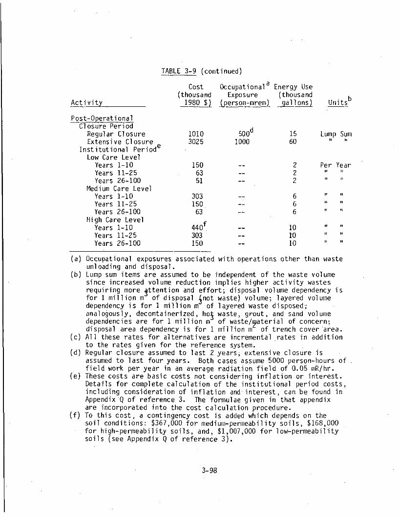
TABLE 3-9 (continued)

Cost Occupationala Energy Use(thousand Exposure (thousand

Activity 1980 $) (person-mrem) gallons) Unitsb

Post-OperationalClosure Period

Regular Closure 1010 50 0d 15 Lump SumExtensive Closure 3025 1000 60 " "

Institutional PeriodeLow Care Level

Years 1-10 150 -- 2 Per YearYears 11-25 63 -- 2 I

Years 26-100 51 -- 2 "

Medium Care LevelYears 1-10 303 -- 6Years 11-25 150 -- 6Years 26-100 63 -- 6

High Care LevelYears 1-10 4 4 0 f -- 10Years 11-25 303 -- 10Years 26-100 150 -- 10

(a) Occupational exposures associated with operations other than wasteunloading and disposal.

(b) Lump sum items are assumed to be independent of the waste volumesince increased volume reduction implies higher activity wastesrequiring more ittention and effort; disposal volume dependency isfor I million m of disposal Snot waste) volume; layered volumedependency is for I million m of layered waste disposed;analogously, decontainerized, ho waste, grout, and sand volumedependencies are for 1 million m of waste/paterial of concern;disposa.l area dependency is for I million m of trench cover area.

(c) All these rates for alternatives are incremental rates in additionto the rates given for the reference system.

(d) Regular closure assumed to last 2 years, extensive closure isassumed to last four years. Both cases assume 5000 person-hours offield work per year in an average radiation field of 0.05 mR/hr.

(e) These costs are basic costs not considering inflation or interest.Details for complete calculation of the institutional period costs,including consideration of inflation and interest, can be found inAppendix Q of reference 3. The formulae given in that appendixare incorporated into the cost calculation procedure.

(f) To this cost, a contingency cost is added which depends on thesoil conditions: $367,000 for medium-permeability soils, $168,000for high-permeability soils, and, $1,007,000 for low-permeabilitysoils (see Appendix Q of reference 3).

3-98

The unit rates presented in Table 3-9 are utilized in a computer

program (OPTIONS) that calculates the impact measures. Depending on

the disposal facility design option selected, the status of each

waste stream, Ill, is determined utilizing procedures outlined in

Section 3.4. Then, the volumes of waste that are unacceptable for

near-surface disposal, waste disposed of through regular means, waste

disposed through layered option (if any), and waste emplaced in a hot

waste facility (if any) are determined. These waste volumes together

with the selected emplacement procedure give the respective disposal

volume required, and the disposal volumes together with the volume

utilization rates give the respective areas involved. Then, these

areas are utilized to calculate costs for design options such as the

thickness of disposal cell covers. These unit rates are briefly

discussed below.

Costs associated with the operational life of the disposal facility

are divided into capital costs and operating costs as discussed in

Appendix Q of reference 3. base case capital costs are calculated

from the information given in Appendix Q (for the reference disposal

facility costs) and includes consideration of environmental inves-

tigations, licensing costs, land purchase cost, road construction,

building construction, and peripheral system installation. Additional

capital costs associated with implementation of a specific design

option are quantified in Appendix F of reference 3 and are added

appropriately during the calculation.

The options considered during the operational life are divided into

two groups: the reference system, and the design options which are

subdivided into volume dependent options and area dependent options.

For calculational convenience, these unit rates are -converted to

disposal volume rates since different emplacement procedures are

applicable. The items considered under "other" rates include payroll,

administration, equipment, etc. It is assumed that changing disposal

waste volumes due to processing will not alter the rates given as

3-99

"lump sum" significantly, increased volume reduction implies higher

activity wastes resulting in increased effort.

The second group of options (termed additive alternatives in Table

3-9) result from the application of the available design options

(ID, IS, IE, IL, IH, IG) discussed in Section 3.2 in a straight-

forward manner. These rates are also estimated from a wider range of

design and technology options considered in reference 3. The rates

given are normalized, however, to one-million m 3 of waste volume

for calculational convenience. Similarly, grouting option rates are

for one-million m3 of grout injected since the option may be exer-

cised with either random or stacked disposal, etc. One consequence of

the application of the hot waste facility option is that the total

routine occupational exposures are estimated to go down as a result of

increased shielding afforded by the special facility, this effect is

expressed by giving a negative occupational exposure to the hot waste

facility. The third group of operational options result from the

application of cover related options (IC, IX) discussed in Section

3.1. These options are area dependent. For calculational convenience

they also have been normalized to one-million m2 .

All these options are additive. For example, the preoperational and

operational costs resulting from disposal of 900,000 mi3 of waste

(all found acceptable for near-surface disposal) in the reference3 2facility with an assumed volume efficiency of 5 mi/m , with stacked

emplacement (0.75), with grouting, with thick cover, and with extreme

stabilization are tabulated in Table 3-10. Occupational exposures and

energy use are calculated in a similar manner.

These costs, however, must be multiplied with two conversion factors

to account for the cost of money, inflation and other financial

considerations. The formulae for these multipliers are presented

below. A more detailed explanation of the derivation of these mul-

tipliers can be found in Appendix Q of reference 3.

3-100

TABLE 3-10 . Illustrative Calculation

Assumptions: 900,000 m3 of wastestacked, grouted, thick cover,extreme stabilization, 3 2disposal efficiency of 5 m /m

Disposal Volume = 900,000/0.75Empty Disposal Space = 1,200,000x(1-0.75)Disposal Area = 1,200,000/5

Capital Costs

Reference System

Stacking

Grouting

Total Capital

Operational Costs

Reference System

Trench Construction

Regular Cover

Other Costs

Additive Alternatives

Stacking Option

Grouting Option

Thick Cover

Extreme Stabilization

Total Operations

= 1,200,000 m 3

- 300,000 m 2: 240,000 mi

$ 7,452,000

226,000

55,000

$ 7,733,000

$ 2,810,000

341,000

63,696,000

11,482,200

21,721,500

3,725,800

8,002,800

$111,779,300

3-101

For capital costs, the following items are applicable:

Item Factor'

Indirect Costs 1.73Fixed Charge 5.00Profit 1.20

Indirect costs result from interest during construction, contingency,

and other costs such as miscellaneous overhead expenses, insurance,

sales tax, etc. The fixed charge results from an assumed 25% charge

on capital over the 20 year operating life of the facility. These

three items result in a multiplier of 10.38 for the pre-operational

capital costs. For the operational costs, the following items are

applicable:

Item Factor

Contingency 1. 30Profit 1.20

This results in a multiplier of 1.56 for the operational costs. Using

these multipliers with the pre-operational capital cost of $7,733,000,

and the operational cost of $111,779,300 yields a total preoperational

and operational cost of about $254,644,000 in 1980 dollars.

Post-operational costs (composed of closure costs and long-term care

costs) are calculated using the following two equations. For the

closure costs, the following equation is applied:

Closure Costs = C8 0 x L x (1+j) L x f + i (3-34)

where C8 0 is the, closure costs presented in Table 3-9, L is the

facility life in years, f is an annual fee for a surety bond which

assures availability of closure funds (1.5% is used. in this report),

and j is the inflation rate (9% is used in this work). For long-term

care costs, the following equation is applicable:

3-102

L x (1+j)M x iLTC Cost = PV [ 8 L . 1 x (1 )C (3-3x)

where LTC stands for longrterm cares L is the site operational life in

years, C is the closure period in years, M is L+C, i is the interest

rate (assumed to. be 10% in this report), .j is the inflation rate, and

PV80 is given by the following equation:

10 25 100

PVs8 o Ca Z Rn + CbZ Rn + Cc.Z Rn (3-36)

n=1 n=11 n=26

where R is the ratio (1+j)/(l+i). The parameters Cas Cb2 and Cc

are the annual costs given in Table 3-9 for the long-term care costs

during the years 0-10, 11-25, and 26-100, respectively. The cost rate

Ca may include a contingency cost for a high level of long-term care

as explained in Table 3-9.

3 103

REFERENCES FOR CHAPTER 3.0

1. Wild, R., et al., Dames & Moore, "Data Base for Radioactive WasteManagement. Volume 2. Waste Source Options," USNRC ReportNUREG/CR-1759, November 1981.

2. Kelly, K., et al., Dames & Moore, "Draft Site Operations Report,"Prepared for U.S. Nuclear Regulatory Commission, May 1981.

3. U.S. Nuclear Regulatory Commission, Office of Nuclear MaterialsSafety and Safeguards, "Draft Environmental Impact Statement on10 CFR Part 61 Licensing- Requirements for Land Disposal ofRadioactive Waste," NUREG-0782, September 1981.

4. Clancy, J., et.al., Dames & Moore, "Data Base for RadioactiveWaste Management. Volume 1. Review of Past Disposal Practices,"USNRC Report NUREG/CR-1759, November 1981.

5. Rogers, V.C., Ford, Bacon and Davis Utah Inc., "A RadioactiveWaste Disposal Classification System," USNRC Report NUREG/CR-1005, September 1979.

6. U.S. Nuclear Regulatory Commission, Office of Nuclear MaterialSafety and Safeguards, "Environmental Survey of the Reprocessingand Waste Management Portions of the LWR Fuel Cycle," A TaskForce Report, NUREG-0116 (Supp.1 to WASH-1248), October 1976.

7. U.S. Atomic Energy Commission, Directorate of Regulatory Stan-dards, "Environmental Survey of Transportation of RadioactiveMaterials To and From Nuclear Power Plants," USAEC Report WASH-1238, December 1972.

8. U.S. Nuclear Regulatory Commission, Office of Nuclear ReactorRegulation, "Final Programmatic Environmental Impact StatementRelated to Decommissioning and Disposal of Radioactive WastesResulting from March 28, 1979, Accident, Three Mile IslandNuclear Station, Unit 2," USNRC Report NUREG-0683, March 1981.

9. U.S. Nuclear Regulatory Commission, "Final Environmental State-ment on the Transportation of Radioactive Material by Air andOther Modes", USNRC Report NUREG-0170, January 1977.

10. Adam, J.A. and V.L.Rogers, "A Classification System for Radio-active Waste Disposal - What Waste Goes Where?," NUREG-0456,FBDU-224-10, Prepared by Ford Bacon & Davis Utah for USNRC,June 1978.

11. Zima, G.E. Battelle Pacific Northwest Laboratories, "Comments onFuel Crud as a Safety and Operational Factor of Independent SpentFuel Storage Installations (ISFSI)," USNRC Report NUREG/CR-0163,November 1978.

3-104

12. McMahon, L.A. and P.E.Pereira, "McGraw-Hill's 1981 Dodge Guide toPublic Works and Heavy Construction Costs," McGraw-Hill Informa-tion Systems Company, New York, 1981.

13. Healy, J.W., and J.C. Rodgers, "Limits for the Department ofEnergy Transuranic Wastes," Los Alamos Scientific Laboratory,LA-UR-79-100, January 1979.

14. U.S. Department of Health, Education and Welfare, "RadiologicalHealth Handbook" Revised Edition, January 1970.

15. International Commission on Radiological Protection (ICRP)."Report of the Task Group on Reference Man," ICRP Publication 23,1975.

16. U.S. Nuclear Regulatory Commission, Office of Standards Develop-ment, Regulatory Guide 1.111, "Methods for Estimating AtmosphericTransport and Dispersion of Gaseous Effluents in Routine Releasesfrom Light-Water Covered Reactors," March, 1976.

17. Fenn, D.G., K.J. Hanley, and Truett V. DeGeare, "Use of the WaterBalance Method for Predicting Leachate Generation from SolidWaste Disposal Sites," U.S. Environmental Protection AgencyReport SW-168, 1975.

18. Aikens, A.E., et.al., Dames & Moore, "Generic Methodology forAssessment of Radiation Doses from Groundwater Migration ofRadionuclides in LWR Wastes in Shallow Land Burial Trenches,"Prepared for Atomic Industial Forum, Inc., AIF/NESP-013, Decem-ber, 1977.

19. Freeze, R.A. and Cherry J.A., Groundwater, Prentice Hall, Inc.,New Jersey, 1979.

20. Mitchell, J.K., Fundamentals of Soil Behavior, John Wiley andSons, Inc., New York, 1976.

21. Todd, D.K. Ground Water Hydrology, John Wiley & Sons, New York,1967.

22. Appel, C.A, and J.D. Bredehoeft, "Status of Ground-Water Modelingin the U.S. Geological Survey," Geological Survey Circular 737,Department of the Interior, 1976.

23. Hamilton, J.L. and O.I.Oztunali, "Comparative Evaluation ofRadionuclide Transport Models from Shallow Land Burial Grounds,"Prepared for Union Carbide Corporation, Nuclear Division byDames & Moore, Subcontract No.7273, October 1979.

3-105

24. Dames & Moore, "Development of Monitoring Programs for ERDAOwned Radioactive Low-Level Waste -Burial Sites," U.S.ERDA Con-tract No. E(49-1)-3759, July, 1976.

25. Dames & Moore, "Assessment of Levels, Potential Origins andTransport Routes of Radioactivity Measured in the Vicinity ofMaxey Flats Low-Level Radioactive Waste Disposal Site," Preparedfor-the Commonwealth of Kentucky, Department of Human Resources,March 1977.

26. U.S. Department of Commerce, Bureau of the Census, "StatisticalAbstract of the United States," 99th Annual Edition, 1978.

27. Lester, D., et.al., Science Applications, Inc., "Systems Analysisof Shallow Land Burial Project," USNRC Report NUREG/CR-1963,March 1981.

28. Abramowitz, M. and I.A. Stegun, Handbook of Mathematical Func-tions with Formulas, Graphs, and Mathematical Tables, NationalBureau of Standards, Applied Mathematics Series-55, December1965.

29. Staley, G.B., Turi, G.P., Schreiber, D.L., U.S. Nuclear Regula-tory Commission, "Radionuclide Migration From Low-Level Waste: AGeneric Overview," in Management of Low-Level Radioactive Waste,Volume 2, Pergamon Press, New York, 1979.

30. Schneider, K.J., and Platt, A.M., "High-Level Radioactive WasteManagement Alternatives," Battelle Pacific Northwest LaboratoriesReport No. BNWL-1900, May 1974.

31. Greenhouse, N.A. and E.T. Lessard, "A Dosimetric Analysis ofPathways to Man From the Environmental Release of Low LevelRadioactive Wastes," Prepared for Dames & Moore by Occupationaland Environmental Health Analysts, Inc., 1980.

3-106

4.0 TRANSPORTATION IMPACTS

This chapter discusses the calculational procedures used to deter-

mine impacts associated with transportation of waste to the disposal

facility. The impact measures developed in this report include: cost;

occupational exposures associated with loading, transportation, and

unloading of the waste; population exposures associated with trans-

portation; and energy use. Section 4.1 presents the packaging and

shipping assumptions utilized in the calculations. Transportation

costs and other impact measures are presented in Sections 4.2 and 4.3,

respectively.

4.1 Packaging and Shipping Assumptions

Potential impacts (e.g., occupational exposures, population exposures,

and costs) incurred during transportation of wastes to disposal

facilities and during subsequent unloading and emplacement operations

are influenced by a number of interrelated factors. These interre-

lated factors increase the complexity of the impacts analyses and

arise from the greatly variable nature of LLW and LLW transportation.

For example, LLW can be generated in a great variety of forms and can

range from wastes having very low to moderately high radioactivity

concentration levels. In addition, a range of waste container types

and sizes are presently available and in use.

For the purposes of this report, some simplifying assumptions regard-

ing waste packaging and transportation are made based upon past

experience. These assumptions include those in the following areas:

(1) The degree of care required for waste handling and transport-

ation (package surface radiation levels);

(2) Container sizes and types; and

(3) The shipment mode (vehicles and overpacks used).

4-1

Additional information on surface radiation levels, packaging para-

meters, and mode of shipment regarding these simplifying assumptions

is provided below.

4.1.1 Surface Radiation Levels

Radiation levels at the waste package surfaces affect the care re-

quired in handling of wastes and the shielding that may be required

during transportation. Depending on the package size involved and the

total activity content of each package, different waste packages have

different surface radiation readings. For the purposes of this

report, the waste streams are generically classified into three

categories according to the level of care required to handle each

waste stream:

(1) Regular care(2) Special care(3) Extreme care

Package sizes and packaging procedures are instrumental in determining

the self-shielding afforded by some of the waste packages. However,

there can be significant variations in the level of care required for

each package due to variations in the specific activities of the

wastes within a given stream. For this analysis, the level, of care is

assumed to be independent of waste package shape and volume. The

level of care is assumed to depend only on the total specific activity

contained in the waste package and the presence or absence of radio-

nuclides emitting high-energy gamma rays.

Each waste stream is denoted by an index representing the type of

activity with regard to high-energy gamma emitting radionuclides.

Waste streams containing significant quantities of fission products

(most notable being Co-60, Nb-94, and Cs-137) are denoted as the first

category. Waste streams containing very little high-energy gamma

emitters (and consequently all requiring a "regular" level of care)

4-2

are denoted as the third category. Other streams in between these two

are denoted as the second category:

Category 1 : Fission product type wastesCategory 2 • Other type wastesCategory 3 : All regular care wastes

In addition to these categories, the specific activity, and therefore

the required level of care, for a given waste stream varies signifi-

cantly. For example, surface radiation readings of similarly-sized

LWR resin packages varying over two or three orders of magnitude have

been observed.(I) To account for this normal variation, Table 4-1

is used to estimate the fraction of each waste stream that requires a

specific level of care based on the total specific activity of the

waste stream.

The values in this table are estimated based on standard health-

physics "rules of thumb" calculations for determining the surface

radiation level of a waste package, e.g., the 6CEn formula.(2) For

example, for waste in Category I with about 2 Ci/m 3 of activity, 20%

of the waste volume is assumed to require regular care, 60% of the

waste volume is assumed to require special care, and the remaining 20%

is assumed to require extreme care. According to the 6CEn formula,

assuming that all the radioacivity is Co-60 and the waste package is a

55-gallon drum, this waste may have a radiation reading of about 63

R/hour. For waste in Category 2 with about 0.2 Ci/m of activity,

80% of the volume is assumed to require regular care, and the remain-

ing 20% is assumed to require special care. All wastes in Category 3

are assumed to require regular care.

After determining the fraction of volume in each stream that requires

a specific level of care, this waste is assumed to be packaged and

shipped. The packaging and shipping assumptions for these fractions

are detailed below.

4-3

TABLE 4-1 . Distribution Between Care Level Required

with Type and Specific Activity of Waste

Total Specific

Activity (Ci/m3

Type 1 Type 2 Type 3

<0.01 <0.1 All

.01-.1 .1-1

.1-1 1-10

1-10 >10

10-100

>100

Percent Waste Stream Volume

in Each Handling Category

Regular Special Extreme

100 --..

80 20 --.40 50 10

20 60 20

10 50 40-- 20 80

4-4

4.1.2 Packaging Parameters

There are many different types of packaging currently utilized for

shipment and disposal of LLW.(3,4) These packages include wooden

boxes of various sizes ranging from 10 ft 3 to 248 ft 3 , 55 gallon

drums, and liners (usually carbon steel) of various sizes ranging from

16 ft 3 to 200 ft 3 which fit into transport casks. In this report,

for the generic type of analyses required for the transportation and

disposal impacts, these packages were generalized into five different

categories:

(1) Large wooden boxes - 128 ft 3

(2) Small wooden boxes - 16 ft3

(3) 55-gallon drums - 7.5 ft 3

(4) Small liners - 50 ft3(5) Large liners - 170 ft3

The primary rationale for selecting these sizes is that they appear to

the most widely used sizes, and may be used to represent an average of

other packages. For example, the 128 ft 3 box is the most commonly

used (4'x4'x8') size to ship low specific activity (LSA) waste, the

170 ft 3 liner is the commonly available 6'x6' right-circular cylin-

drical resin tank, etc.

During the transportation analysis, for regular- and special-care

wastes, all five methods of packaging are assumed to be acceptable.

The high-activity of extreme-care wastes renders the use of boxes for

packaging unacceptably inconvenient, therefore, all waste that is

classified "extreme care" has been assumed to be packaged in either

drums or liners which are remotely manipulated for loading and off-

loading.

The distribution of these package types for each waste stream have

been assumed using available shipping and survey data, (3-6) and are

presented in Table 4-2.

4-5

TABLE 4-2 . Packaging of LLW for Waste Spectrum I

(percent of volume packed in containers)

LargeBoxes

SmallBoxesWaste Stream

55-g

Drums

SmallLiners

Large

Liners

LWR Process Waste Group --

Trash Group 23

(except P-&B-NCTRASH)

P- & B-NCTRASH --

Low Specific Activity

Waste Group (except

F- & U-PROCESS)

F- & U-PROCESS --

Special Waste Group

* Other distributions depending on

on the individual waste streams.

-- 69

8 69

15 16

-- 1100

2.5 97.5

-- 100

10i

the spectrum may be imposed

4-6

4.1.3 Mode of Shipment

Similar to the numerous different types of available waste packages,

there may exist many different shipment modes ranging from rail and

barge transport to truck transport. Many different types of overpacks

may be used depending on the handling and shielding requirements for

individual waste packages.( 3 ' 4 )

In this report, only truck transport is considered because trucks are

the most commonly used mode of transportation and truck transport is

radiologically the most conservative case. Vehicles and overpacks

utilized in truck shipments depend on package sizes as well as package

shielding requirements. In this report, six different types of

transport vehicles and overpacks are assumed:

(1) Vans(2) Flatbed trailers(3) Shielded trailers(4) Large shielded casks(5) Small shielded casks(6) i-drum shielded casks

Large casks are used for transporting either large liners or fourteen

55-gallon drums, while small casks are used for transporting either

small liners or six 55-gallon drums. These casks are transported to

the disposal facility via flatbed trailers.

The use of particular types of vehicles and overpacks is strongly

influenced by the level of care required for safe waste handling and

transport of the waste packages. Vans are assumed to be suitable for

all types of containers in the regular care category, with the excep-

tion of large liners which require casks. In addition, flatbed

trailers are assumed to be used only for large boxes of regular-care

wastes. Shielded trailers are assumed to be required for large and

small boxes and drums of special-care wastes. Some of these small

boxes and drums, as well as large and small liners are assumed to

4-7

wP1

require casks. Casks are assumed to be the only accel, I

transport for extreme-care wastes.

The percentage use of different vehicles and overpa(.

container have been estimated considering records of was(.(-

delivered to the Maxey Flats Disposal Facility.("" A tabil.,,

of the basic assumptions made for the transportation of P,

presented in Table 4-3. Extreme-care liner shipments

assumed to be "overweight" shipments since these require siji'.

shielding for transportation purposes. These are also desi qi.

Table 4-3.(1,5)

4.2 Costs

Transportation costs include a mileage charge (including

surcharge), a cask use charge (rental), and an overweight shil-i

transportation charge.

The mileage charge is calculated by estimating the total Shi,:i.

miles required (including return trip mileage for casks), usiiol

assumed average distance per one-way shipment. The basic tv,,

portation charge depends on the one-way distance, and is assi:',

according to the following table:i 8

One-Way Round Trip

One-Way Distance ($/mile) ($/mile)

< 400 miles 1.69 1.25400-1000 miles 1.47 1L14

> 1000 miles io17 ]L08

Added charges., which become significant for extreme-care shipments.

include a fuel surcharge (15% of the basic cost) and an overweight.

charge.. The amount of the overweight charge depends on the maximum

gross ve-hicle weight (GVW) allowed in states through which the ship-

ment passes. Any overweight condition up to 85.000 lbs. is charged at

4-8

TABLE 4-3 : Packaging and Shipment Mode Parameters

'ire Level,ind Container

Regular Care

Irge Box

'inal I BoxDrumSmall Linerlarge Liner

Special Care

Large BoxSmall Box

Drum

Small Liner

Large Liner

Extreme Care

Drum

Small LinerLarge Liner

OverpackaPer Shipment

Pieces Percent Volume

Man-Minutes for DisposalPer Container

Random Stacked

VanFBVanVanVanLC

34

367011

1

2476

100100100100

2007416

6136

1200

240120

2424

1651440

STSTLCSTLCSCSCLC

3366

7014621

10096

44851

1100100

30026

2501086

200600

1200

36039

30024

175312720

1440

SCLDbSC b

6121

5149

100100

200600600

1500

312720720

1800

(a) FB = flatbed trailer ; ST = shielded trailer; LC = Large shieldedCask; SC = Small Shielded Cask; ID = 1-drum shielded cask.

(b) These shipments are estimated to be overweight.

4-9

$0.21/mile plus the permit charges for each state (about $100 per 600

miles). A GVW of over 85,000 lbs. is additionally charged $0.005

per mile per hundred pounds (cwt) over this limit. For example, for ashipment of 96,000 lbs., which is a minimum for an extreme-care cask,

the charges for a one-way trip of 600 miles would be as follows:

Basic cost @ $1.14/mile $1,368.00Fuel surcharge @ 15% of charge 205.00Overweight charge @ $0.21/mile 126.00Overweight surcharge @ $0.005/cwt/mile 330.00Five overweight permits @ $20.00/state 100.00

Total : $2,129.00

Per Mile : $ 3.55

The cask use charge calculation assumes an average turnaround time of

4 days. Cask rental rates vary depending on the size and weight of

the cask required. They average $250/day for shielded casks enclosing

high activity LLW, and range down to $110/day for an unshielded 120

cubic feet capacity cask.(9) The rental rates also vary with thespecific type of nuclear material the cask is licensed to carry and

the accompanying performance standards the cask must satisfy toaccommodate the various types of nuclear materials. The calculated

results for the additional factors can then be summed to determine the

total transportation cost for the waste.

4.3 Other Impacts

In addition to costs, three other impact measures resulting from

LLW transportation are calculated in this report: energy use, occu-pational exposures, and population exposures. These impacts are

reviewed in this section.

The energy use is calculated based on the total shipment miles,

including empty cask return trips, and an average fuel consumption

rate of 6 miles/gallon.

4-10

The occupational and population exposures incurred during transport-

ation are calculated based on total loaded miles and the number of

loaded shipments. The concept of loaded miles and shipments allows to

be eliminated from consideration those miles in which the vehicle is

empty because it is on a return trip.

Occupational and population exposures are calculated separately for

those resulting during transit, and those resulting from stopovers

during the trip. The occupational exposure during stopovers is

estimated by assuming two drivers. Each inspect the overpack for 3

minutes (1U mR/hr radiation field at the surface of the overpack), and

walk around the overpack for 30 minutes (1 mR/hr radiation field at

about 3 ft). This yields 2 person-mrem per stop for each shipment.

For population exposure during stopovers, the following equation can

be utilized:( 1 1 )

D = 2wK d T El(ir) (4-1)

where

D = Population dose in person-mrem

K = Source Density = 1000 mR-ft 2/hr

d = Population Density = 10000 people/mile 2

T = Duration of Exposure = 2 hours

E= Exponential Integral,

= Linear Absorption Coefficient of Air = 0.003 ftC1 .

r = Lower Distance for Population = 100 ft.

The source density K is based on an assumed maximum allowable exposure

rate of 10 mR/hr at contact with the overpack( 1 0 ' 1 2 ) (assumed to be

10 ft from the center of the waste package) extrapolated to the center

22of the package using the (1r ) radiation attenuation principle:

Exposure at 10 ft from the center = 10J mR/hr = K/(IO ft)2

4-11

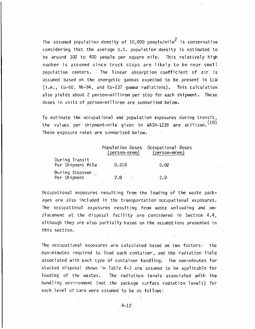
2The assumed population density of 10,000 people/mile is conservative

considering that the average U.S. population density is estimated to

be around 300 to 400 people per square mile. This relatively high

number is assumed since truck stops are likely to be near small

population centers. The linear absorption coefficient of air is

assumed based on the energetic gammas expected to be present in LLW

(i.e., Co-60, Nb-94, and Cs-137 gamma- radiations). This calculation

also yields about 2 person-millirem per stop for each shipment. These

doses in units of person-millirem are summarized below.

To estimate-the occupational and population exposures during transit,

the values per shipment-mile given in WASH-1238 are utilized.( 1 0)

These exposure ratesare summarized below.

Population Doses Occupational Doses(person-mrem) (person-mrem)

During TransitPer Shipment. Mile 0.018 0.02

During StopoverPer Shipment 2.0 2.0

Occupational exposures resulting from the loading of the waste pack-

ages are also included in the transportationoccupational exposures.

The occupational exposures resulting from waste unloading and em-

placement at the disposal facility are considered in Section 4.4,

although they are also partially based on the assumptions presented in

this section.

The occupational exposures are calculated based on two factors: the

man-minutes required to load each container, and the radiation field

associated with each type of container handling. The man-minutes for

stacked disposal shown in Table 4-3 are assumed to be applicable for

loading of the wastes. The radiation levels associated with the

handling environment (not the package surface radiation levels) for

each level of care were assumed to be as follows:

4-12

RadiationLevel of Care Level (ipR/hr)

Regular 750Special 1800Extreme 2200

The product of these two factors for each combination of care level,

package, and shipment mode have. been calculated and are presented in

Table 4-4. This table is utilized to compute transportation occupa-

tional exposures received during waste loading operations.

4.4 Occupational Exposures to Waste Handlers

The calculation of these exposures is straightforward based on esti-

mates of personnel time required for unloading and disposal of the

wastes. These estimates are presented in Table 4-3. Other parame-

ters necessary for the computations are the radiation fields associ-

ated with the working environment. These fields are assumed to be a

function of the care level of the package and whether the disposal is

random or stacked. The following table presents these assumptions:

Radiation Level (pR/hr)Level of Care Random Stacked

Regular 500 750Special 1200 1800Extreme 2200 2200

Impacts calculated from these relationships are added to the disposal

facility occupational exposures calculated in Section 3.8.3 for

disposal facility personnel other than waste handlers.

Decontainerized disposal of waste is assumed to require twice the

time needed for stacked handling for those packages that are to be

disposed in this manner (i.e., unstable wastes denoted by 18 = 0 --

see Chapter 3.0).

4-13

TABLE 4-4 . Unit Occupational Exposures During Loading

(person-millirem per container)a

Regular Care

Overpack Exposure

Special Care

Overpack Exposure

Extreme Care

Overpack ExposureContainer

Ia

Large Boxes

Small Boxes

Drums

Small Liners

Large Liners

Van

FB

Van

3.0

1.5

0.3

Van 0.3

ST

ST

LC

ST

LC

SC

SC

LC

10.8

1.17

9.0

0.72

5.25

9.36

21.6

SC1D

SC

LC

11.4426.40

26.40

80.67

Van 2.06

LC 18.0 43.2

(a) FB = flatbed trailer ; ST = shielded trailer; LC Large Shielded Cask;

SC = Small Shielded Cask; ID 1 I-drum Shielded Cask.

REFERENCES FOR CHAPTER 4.0

1. Radioactive Waste Shipment Records from the Maxey Flats, Ken-tucky, low-level waste disposal site, Dames & Moore Files.

2. U.S. Department of Health, Education and Welfare, "RadiologicalHealth Handbook" Revised Edition, January 1970.

3. Phillips, J., et al. "A Waste Inventory Report for Reactor andFuel Fabrication Facility Wastes," ONWI-20, Prepared by NUSCorporation for Battelle Office of Waste Isolation, March 1979.

4. Mullarkey, T.B., "A Survey and Evaluation of Handling and Dispos-,ing of Solid Low-Level Nuclear Fuel Cycle Wastes," AIF/NESP-008,Prepared by NUS Corporation for Atomic Industrial Forum, Inc.,October 1976.

5. Anderson, R.L., et.al. University of Maryland, "InstitutionalRadioactive Waste", USNRC Report NUREG/CR-0028, March 1978.

6. Beck, T.J., L.R. Cooley, and M.R. McCampbell, University ofMaryland, "Institutional Radioactive Wastes, 1977," USNRC ReportNUREG/CR-1137, October 1979.

8. Rutenkroger, TriState Motors, Inc., Personal Communication toP. Hopkins, Dames & Moore, 1980.

9. Spann, U.S. Ecology Co. Inc. (formerly Nuclear Engineering Co.,Inc.), Personal Communication to P. Hopkins, Dames & Moore, 1980.

10. U.S. Atomic Energy Commission, Directorate of Regulatory Stan-dards, "Environmental Survey of Transportation of RadioactiveMaterials To and From Nuclear Power Plants," USAEC Report WASH-1238, December 1972.

11. Dames & Moore, "Study of the Shipment of Spent Fuel from theShoreham Nuclear Power Station to the Reprocessing Plant,"Prepared for Long Island Lighting Co., Inc., June 1975.

12. U.S. Nuclear Regulatory Commission, "Final. Environmental State-ment on the Transportation of Radioactive Material by Air andOther Modes", USNRC Report NUREG-0170, January 1977.

4-15

5.0 WASTE PROCESSING IMPACTS

This chapter discusses the calculational procedures utilized to

determine the impact measures associated with the processing of the waste

streams considered in this report (see Chapter 3.0). These impact

measures include population exposures, occupational exposures, costs,

and energy use. The processing options being considered in this

report, and the derivation of the unit rates for costs, person-hours,

and energy use for these processing options are presented in reference

1. Based on this information and using an additional waste stream

index, denoted by I10, the processing impacts are calculated for

respective cases utilizing the assumptions and procedures presented in

this section.

5.1 Waste Processing Index

The variations in the processing technologies applied to a given

stream, which affect the calculation of the impact measures, include

the volume reduction process type, the volume increase process type,

the location of the processing, and the environment in which the

processing takes place. For calculational convenience, the waste pro-

cessing option applicable to each waste stream for each waste spectrum

has been digitized and is called the waste processing index, denoted

by 110 (see Chapter 3.0 for other waste form behavior indices).

The index 110 is a four digit number with each digit denoting a

specific procedure for calculation of the impact measures. These

digits cumulatively correspond to a specific case. The meaning of

the digits that make up the processing index is presented in Table

5-1. The processing indices applied to each waste stream for each

spectrum are presented in Table 5-2.

The impact measures calculated represent impacts in addition to those

associated with Spectrum 1 with the exception of a few streams for

5-1

TABLE 5-1 . Waste Processing Index - I10

First Digit - IPR

Second Digit- ISL

Third Digit - ILC

Fourth Digit - IEN

Value

0

1

2

3

4

5

6

7

Meaning

No Volume Reduction

Regul ar Compaction

Improved Compaction

Hydraulic Press

Evaporati on.

Pathological Incineration

Small Calciner

Large Calciner

No Solidification

Solidification Scenario A

Solidification Scenario B

Solidification Scenario C

0

1

2

3

0

1

2

0

1

2

No Processing

Processing at the Generator

Processing at the Disposal Site

No. Incineration

Urban Environment

Rural Environment

5-2

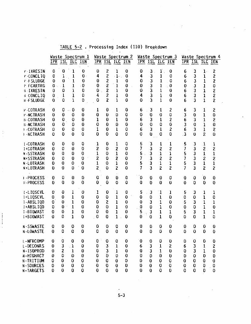
TABLE 5-2 . Processing Index (110) Breakdown

Waste Spectrum 1 Waste Spectrum 2 Waste Spectrum 3 Waste Spectrum 4IPR ISL ILC IEN IPR ISL ILC IEN IPR ISL ILC IEN IPR ISL ILC IEN

v-IXRESIN 0 0 1 0 0 2 1 0 0 3 1 0 6 3 1 2v -CONCLIQ 0 1 1 0- 4 2 1-_ 0 4 3 1 0 6 3 1 21'-FSLUDGE 0 0 1 0 0 2 1 0 0 3 1 0 6 3 1 21, FCARTRG 0 1 1 0 0 2 1 0 0 3 1 0 0 3 1 0it.IXRESIN 0 0 1 0 0 2 1 0 0 3 1 0 6 3 1 2it.CONCLIQ 0 1 1 0 4 2 1 0 4 3 1 0 6 3 1 2ii-FSLUDGE 0 0 1 0 0 2 1 0 0 3 1 0 6 3 1 2

v'-COTRASH 0 0 0 0 1 0 1 0 6 3 1 2 6 3 1 2i,'-NCTRASH 0 0 0 0 0 0 0 0 0 0 0 0 3 0 1 0ii-COTRASH 0 0 0 0 1 0 1 0 6 3 1 2 6 3 1 2i-NCTRASH 0 0 0 0 0 0 0 0 0 0 0 0 3 0 1 0I-COTRASH 0 0 0 0 1 0 1 0 6 3 1 2 6 3 1 2l-NCTRASH 0 0 0 0 0 0 0 0 0 0 0 0 3 0 2 0

I-COTRASH 0 0 0 0 1 0 1 0 5 3 1 1 5 3 .1 1IfCOTRASH 0 0 0 0 2 0 2 0 7 3 2 2 7 3 2 2N-SSTRASH 0 0 0 0 1 0 1 0 5 3 1 1 5 3 1 1N6SSTRASH 0 0 0 0 2 0 2 0 7 3 2 2 7 3 2 2N-LOTRASH 0 0 0 0 1 0 1 0 5 3 1 1 5 3 1 1NfLOTRASH 0 0 0 0 2 0 2 0 7 3 2 2 7 3 2 2

I-PROCESS 0 0 0 0 0 0 0 0 0 0 0 0 0 0 0 0il-PROCESS 0 0 0 0 0 0 0 0 0 0 0 0 0 0 0 0

I-LIQSCVL 0 0 1 0 1 0 1 0 5 3 1 1 5 3 1 1I+LIQSCVL 0 0 1 0 0 0 1 0 0 0 1 0 0 0 1 0I-ABSLIQD 0 0 1 0 0 2 1 0 0 3 1 0 5 3 1 1l+ABSLIQD 0 0 1 0 0 0 1 0 0 0 1 0 0 0 1 0I-BIOWAST 0 0 1 0 0 0 1 0 5 3 1 1 5 3 1 1I+BIOWAST 0 0 1 0 0 0 1 0 0 0 1 0 0 0 1 0

N-SSWASTE 0 0 0 0 0 0 0 0 0 0 0 0 0 0 0 0N-LOWASTE 0 0 0 0 0 0 0 0 0 0 0 0 0 0 0 0

i.-NFRCOMP 0 0 0 0 0 0 0 0 0 0 0 0 0 0 0 0L-DECONRS 0 3 1 0 0 3 1 0 6 3 1 2 6 3 1 2N-ISOPROD 0 2 1 0 0 3 1 0 0 3 1 0 0 3 1 0N-HIGHACT 0 0 0 0 0 0 0 0 0 0 0 0 0 0 0 0N-TRITIUM 0 0 0 0 0 0 0 0 0 0 0 0 0 0 0 0N-SOURCES 0 0 0 0 0 0 0 0 0 0 0 0 0 0 0 0N-TARGETS 0 0 0 0 0 0 0 0 0 0 0 0 0 0 0 0

5-3

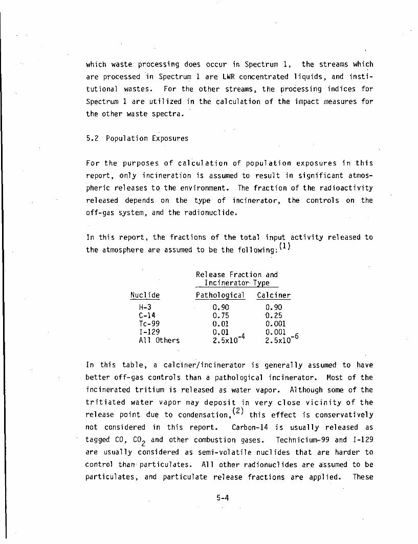
which waste processing does occur in Spectrum 1, the streams which

are processed in Spectrum 1 are LWR concentrated liquids, and insti-

tutional wastes. For the other streams, the processing indices for

Spectrum 1 are utilized in the calculation of the impact measures for

the other waste spectra.

5.2 Population Exposures

For the purposes of calculation of population exposures in this

report, only incineration is assumed to result in significant atmos-

pheric releases to the environment. The fraction of the radioactivity

released depends on the type of incinerator, the controls on the

off-gas system, and the radionuclide.

In this report, the fractions of the total input activity released to

the atmosphere are assumed to be the following:I•"

Release Fraction and

Incinerator Type

Nuclide Pathological Calciner

H-3 0.90 0.90C-14 0.75 0.25Tc-99 0.01 0.0011-129 0.01 4 0.001All Others 2.5x10 4 2.5x10-6

In this table, a calciner/incinerator is generally assumed to have

better off-gas controls than a pathological incinerator. Most of the

incinerated tritium is released as water vapor. Although some of the

tritiated water vapor may deposit in very close vicinity of the

release point due to condensation,( 2 ) this effect is conservatively

not considered in this report. Carbon-14 is usually released as

tagged CO, CO2 and other combustion gases. Technicium-99 and 1-129

are usually considered as semi-volatile nuclides that are harder to

control than particulates. All other radionuclides are assumed to be

particulates, and particulate release fractions are applied. These

5-4

fractions are also used in modifying the waste concentrations for

tritium and carbon-14. Release fractions for other radionuclides are

conservatively assumed not to affect the concentrations of the final

product.

The final assumptions on population exposure calculations involve

(1) the environment that is affected by the processing, and (2) the

pathway dose conversion factors used.

It is assumed that institutional facilities are in an urban environ-

ment and all other facilities (including the disposal site) are in a"rural" environment. Correspondingly, a site selection factor (sum of

the products of the atmospheric diffusion factor -- see Appendix A --

and-the number of people affected in each corresponding radial dis-

tance -- see Appendix C) of 1.75 x 10-10 person-year/m3 is applied

to a rural environment, and ten times this value, i.e., 1.75 x 10-9

person-year/m3 , is applied to an urban environment.*

The pathway dose conversion factor used in calculating the population

doses are those applicable to the erosion-air transport scenario,

-- i.e., PDCF-8 presented in Table 2-11.

5.3 Other Impacts

Other impacts are calculated based on the unit rates (cost, labor-

hours, and energy use) that have been assumed based upon information

presented in references 3 through 6 for selected waste processing

options. These unit rates are summarized in Table 5-3 and are dis-

cussed below.

In Section 3.6.1 a value of 3.50 x 10-10 person-year/m3 is esti-mated to be applicable to a disposal site 100 years after closure,this value is twice the value obtained from application of thepopulation distribution for the reference disposal facility pre-sented in Appendix C.

5-5

TABLE 5-3 . Summary of Processing Unit Impact Rates

Process

Compaction

Regular

Improved

Hydraulic Press

Evaporation

Incineration

Pathological

Calciner (small)

Calciner (large)

Solidification

Scenario A

Scenario B

Scenario C

Cost(1980 $)

335

503

1006

690

2060

1938

1039

1282

1873

2445

Labor

(hours)

15

15

15

4.42

8

6.12

5.35

24

24

24

Energy

(g of fuel)

4.6

4.6

4.6

56.3

116

129

72

40

40

40

Units

Per m

of Input

Per m

of Input

Per m3

of Input

Per m3 of

Output

5-6

In this report, the energy use impact measure is expressed in units of

gallons of fuel, and the factors utilized in the calculations to

correct from electrical energy and thermal energy to gallons of fuel

are 40.6 kW-hr per gallon of fuel and 138,690 BTU per gallon of fuel,

respectively.( 5 )" Another assumption involving energy use is that 10

percent of the first year capital cost (in 1980 dollars) has been

assumed to be attributable to fuel use at $1/gallon.

Occupational exposures resulting from waste processing occur primarily

as a result of repair and maintenance activities on the waste process-

ing equipment, however, there is no reliable way to estimate the

exposures resulting from equipment repair and maintenance in a generic

manner. This is due to the wide variations in the design of process-

ing equipment, as well as variations in the effectiveness of adminis-

trative controls at waste generator facilities.

In this report, the occupational exposures have been assumed to be

independent of the waste concentrations, and they are calculated

as the product of the person-hours required to process a unit volume

of waste and the radiation field associated with the general work

environment. The person-hours required to process a unit volume of

waste is substantially more than the repair work requirements, how-

ever, the volume of waste processed may be assumed to be proportional

to the repair work required. The radiation field associated with the

general work environment is likely to be less than the radiation

fields associated with repair work. However, the radiation field

values assumed in this report may be taken to represent an average of

those for repairing and maintaining the equipment, and those for

routine processing.

In this work, all LWR waste processing is assumed to take place in a

radiation field of 0.5 mR/hour, and all other waste processing is

assumed to take place in a radiation field of 0.1 mR/hour. Based on

these assumed radiation fields and the labor hours required to process

5-7

unit volumes of waste (presented below), it is straightforward to

calculate the occupational exposures.

Another factor which affects the impact measures and which has been

considered in the impact calculations is the "savings" resulting from

the change in waste volume. This is represented by differential costs

in packaging and storage, differential savings in occupational expo-

sures resulting from handling less waste in storage, and differential

savings in energy. These unit rates are assumed based on information

presented in reference 3. The unit "savings" applied to -each waste

stream are assumed to be $210, 4 person hours, and 0.4 gallons of fuel

per unit volume (m3). These unit rates are applied to the difference

between the pre-processing waste stream volume and the volume of the

waste stream after processing. If the waste processing results in

additional volumes of waste (e.g., solidification), then these savings

become additional impacts.

The unit rates for costs, energy use, and labor-hours assumed for the

processes considered in this report - compaction, evaporation, inci-

neration, and solidification - are presented below.

The unit rates for a compactor/shredder processing 7360 ft3 of trash

per year are presented in Table 5-4.(3,4) Based on the unit rates

given in Table 5-4, and the description of the equipment provided in

reference 3, an improved compactor is estimated to cost 50 percent

more while requiring the same labor hours and energy use. The hyd-

raulic press unit rates have been estimated to cost approximately

twice as much as the improved compactor while requiring the same

labor-hours and energy use.

The estimates presented in reference 3 for an evaporator/crystal-

lizer annually processing 15,963 ft 3 of waste have been used to

estimate the unit rates for evaporation. These rates are summarized

in Table 5-5.

5-8

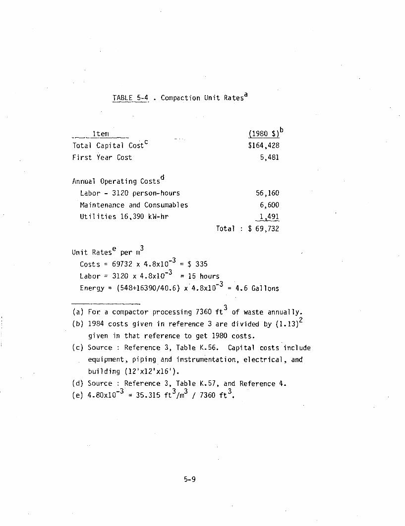
TABLE 5-4 . Compaction Unit Ratesa

Item (1980 $)b

Total Capital Cost $164,428

First Year Cost 5,481

Annual Operating Costsd

Labor - 3120 person-hours 56,160

Maintenance and Consumables 6,600

Utilities 16,390 kW-hr 1,491

Total $ 69,732

Unit Ratese per m3

Costs = 69732 x 4.8xi0 3 = $ 335

Labor = 3120 x 4.8xi0 3 = 15 hours

Energy = (548+16390/40.6) x 4.8x10-3 = 4.6 Gallons

(a) For a compactor processing 7360 ft 3 of waste annually.

(b) 1984 costs given in reference 3 are divided by (1.13)2

given in that reference to get 1980 costs.

(c) Source : Reference 3, Table K.56. Capital costs include

equipment, piping and instrumentation, electrical, and

building (12'x12'x16').

(d) Source : Reference 3, Table K.57, and Reference 4.

(e) 4.80xi0- 3 = 35.315 ft 3 /m3 / 7360 ft 3 .

5-9

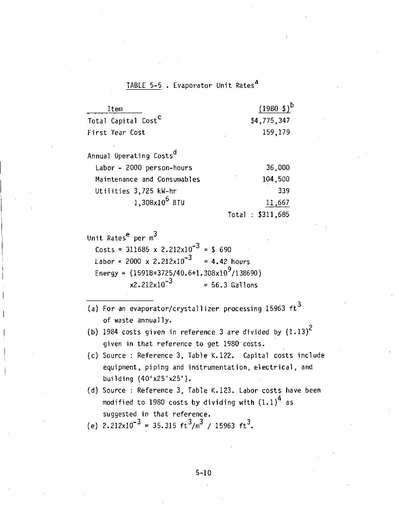
TABLE 5-5 . Evaporator Unit Ratesa

Item

Total Capital Costc

First Year Cost

Annual Operating Costsd

Labor - 2000 person-hours

Maintenance and Consumables

Utilities 3,725 kW-hr

1,308x10 6 BTU

(1980 $)b

$4,775,347

159,179

36,000

104,500

339

11,667

Total : $311,685

Unit Ratese per m3

Costs = 311685 x 2.212x10-3 = $ 690

Labor = 2000 x 2.212x10- = 4.42 hours

Energy : (15918+3725/40.6+1.308x10 9 /138690)

x2.212xlO0 3 = 56.3 Gallons

(a) For an evaporator/crystallizer processing 15963 ft 3

of waste annually.

(b) 1984 costs given in reference 3 are divided by (1.13)2

given in that reference to get 1980 costs.

(c) Source : Reference 3, Table K.122. Capital costs include

equipment, piping and instrumentation, electrical, and

building (40'x25'x25').

(d) Source : Reference 3, Table K.123. Labor costs have been

modified to 1980 costs by dividing with (1.1)4 as

suggested in that reference.3 3 3(e) 2.212x10_3 = 35.315 ft /m / 15963 ft3

5-10

The unit rates for a pathological incinerator processing 7360 ft 3 of

trash per year are also based on reference 3 data, however, labor hour

requirements, which are used in occupational exposure calculations,

have been reduced to 40% of the labor hours due to the comparatively

low activity levels of waste that will be handled by pathological

incinerators. These rates are summarized in Table 5-6.

In this report it is assumed that calciner/incinerators can process

trash in addition to other wastes such as LWR evaporator bottoms and

spent ion-exchange resins. Two types of calciners are considered in

this report. One is located at a centralized processing facility

(which may be located at the disposal site) with a large annual

processing volume - assumed to be 46,200 ft 3 , and the second one is

located at an individual waste generating facility with a smaller

annual processing volume - assumed to be 23,100 ft 3 .(3) The capital

costs, annual maintenance and consumables for these two units have

been assumed to be the same, however, the labor costs and utilities

have been modified for the reduced volume of wasteprocessed per year.

The unit rates for these two incinerators have also been obtained from

reference 3 and are summarized in Tables 5-7 and 5-8.

Solidification. costs are strongly dependent on the solidification

agent used. For example, cement is the cheapest material, however,

it requires the most elaborate equipment for solidification. The

properties of the solidification scenarios have been simulated by

50% urea-formaldehyde and 50% cement in solidification scenario A,

50% cement and 50% synthetic polymer (e.g., vinyl ester styrene - VES)

in solidification scenario B, and 100% synthetic polymer in solidifi-

cation scenario C. The solidification costs utilized in this report

have been obtained from reference 6 assuming an annual processing

volume -of 12,000 ft 3 for the purpose of estimating the capital cost

portion of the costs. These costs and other unit rates are presented

in Table 5-9.

5-11

TABLE 5-6 . Pathological Incinerator Unit Ratesa

Item (1980 b

Total Capital Costc $6,544,068

First Year Cost 218,136

Annual Operating Costsd

Labor - 4160 person-hours 74,880

Maintenance and Consumables 132,000

Utilities 24,000 kW-hr 2,184

240x10 6 BTU 1,990

Total $429,190

Unit Ratese per m3 of input:

Costs = 429190 x 4.8x10-3 = $ 2060

Labor = 4160 x 4.8xi0-3 = 20 hoursf

Energy = (21814+24000/40.6+240x0 6/138690)

x4.8x10- 3 = 116 Gallons

(a) For a controlled air incinerator processing 7360 ft3

of waste annually.

(b) 1984 costs given in reference 3 are divided by (1.13)2

given in that reference to get 1980 costs.

(c) Source : Reference 3, Table K.64. Capital costs include

equipment, piping and instrumentation, electrical, and

building (30'x40'x40').

(d) Source : Reference 3, Table K.65. Labor costs have been

modified to 1980 costs by dividing with (1.1)4 as

suggested in that reference.

(e) 4.8x10 3 = 35.315 ft 3 /m3 / 7360 ft 3 .

(f) Only 40% of the labor hours are considered in occupational

exposure calculations. (8 .hours) due to very low activity

waste being processed.

5-12

TABLE 5-7 '. Large Processing Volume

Calciner/Incinerator Unit Ratesa

Itemr (1980 $)b

Total Capital Costc $21,193,589

First Year Cost 706,453

Annual Operating Costsd

Labor - 7000 person-hours 126,000

Maintenance and Consumables 440,000

Utilities 945,000 kW-hr 85,995'

Total $1,358,448

Unit Ratese per m3 of input:

Costs = 1358448 x 7.65xi0 4 = $ 1039

Labor = 7000 x 7.65xi0-4 = 5.35 hours

Energy = (70645+945000/40.6) x 7.65xi0-4 = 72 Gallons

(a) For a calciner/incinerator processing 46200 ft3

of waste annually.

(b) 1984 costs given in reference 3 are divided by (1.13)2

given in that reference to get 1980 costs.

(c) Source : Reference 3, Table K.91. Capital costs include

equipment, piping and instrumentation, electrical, and

building (52'x50'x60').

(d) Source : Reference 3, Table K.92. Labor costs have been

modified to 1980 costs by dividing with (1.1)4 as

suggested in that reference.

(e) 7.65x10 4 = 35.315-ft./m / 46200 ft 3 .

5-13

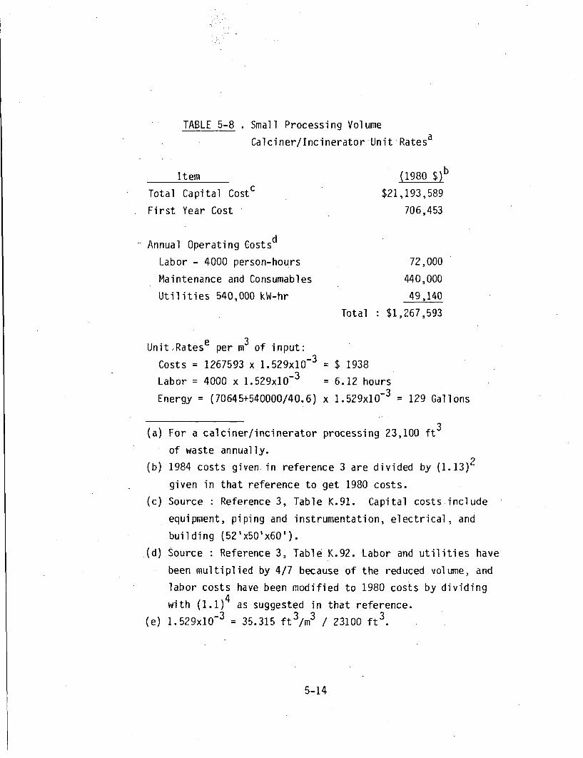
TABLE 5-8 . Small Processing Volume

Calciner/Incinerator Unit Ratesa

Item

Total Capital Costc

First Year Cost

Annual Operating Co s t s d

Labor - 4000 person-hours

Maintenance and Consumables

Utilities 540,000 kW-hr

Unit,Ratese per m3 of input:

Costs = 1267593 x 1.529xi0-3

Labor = 4000 x 1.529x0-3

Energy : (70645+540000/40.6)

(1980 $)b

$21,193,589

706,453

72,000

440,000

49,140

Total : $1,267,593

= $ 1938

= 6.12 hours

x 1.529x10-3 129 Gallons

(a) For a calciner/incinerator processing 23,100 ft 3

of waste annually.

(b) 1984 costs given in reference 3 are divided by (1.13)2

given in that reference to get 1980 costs.

(c) Source : Reference 3, Table K.91. Capital costs include

equipment, piping and instrumentation, electrical, and

building (52'x50'x60').

(d) Source : Reference 3, Table K.92. Labor and utilities have

been multiplied by 4/7 because of the reduced volume, and

labor costs have been modified to 1980 costs by dividing

with (1.1)4 as suggested in that reference.

(e) 1.529xi0- 3 = 35.315 ft 3 /m3 / 23100 ft 3 .

5-14

TABLE 5-9 . Solidification Unit Rates

Item (1980 $)

Scenario A : Total CapitalaFirst Year CostaOperating Costs

$3,520,000117 333 3$26.50/ft3

Unit RatesbCosts : 35.31-5x(26.5+117,333/12000) = $ 1282/m 3

Labor : 24 person-hours/mr3Energy Use : 40 gallons/mr

Scenario B : Total CapitalaFirst Year CostaOperating Costs

$3,520,000117,333 3$43.25/ft3

Unit RatesbCosts : 35.315x(43.25+117 3 333/12000) : $ 1873/m3

Labor : 24 person-hours/mr3Energy Use : 40 gallons/mr

Scenario C : Total CapitalaFirst Year CostaOperating Cos t s

Unit RatesbCosts : 35.315x(60.0+117,133/12000) =Labor : 24 person-hours/mr3Energy Use : 40 gallons/m

$3,320,000110,666 3$60. 00/ft

$ 2445/mr3

(a) Source : Reference 6. Capital costs are from Table K.10,operating costs are from Table K.7. Scenario A cost istaken equal to the cement case, scenario B is takenequal to the average of cement and VES cases, andscenario C is the VES case.

(b) Labor requirements for all scenarios are assuled to bethe same and taken equal to 24 person-hours/m (5 manhours per drum) as given in Reference 3, Table K.16.

5-15

In estimating these unit rates, it has been assumed that the primary

difference in the unit costs-results from the solidification material

costs. For solidification scenario A, it has been further assumed

that the lower costs for the simpler equipment required for the

urea-formaldehyde solidification is balanced by higher material costs

and that it may be represented by the cement case. The manpower

requirements used for estimating the occupational exposures have been

assumed to be the same for all scenarios.

The energy use has been estimated to be approximately the same for all

scenarios, since the difference in unit costs for solidification

scenarios are attributable to material costs. The energy use for all

scenarios has been assumed to be 3 percent of the solidification

scenario A unit cost.

5-16

REFERENCES FOR CHAPTER 5.0

1. Clancy, J., et al., Dames & Moore, "Data Base for RadioactiveWaste Management. Volume 1. Review of Past Disposal Practices,"USNRC Report NUREG/CR-1759,

2. Ziskin, M., E. Picazo, and J. Clancy, "Mist Eliminator Study forSubmerged Combustion Evaporator at the Maxey Flats Low-LevelWaste Disposal Site," Task 3.0 Draft Report, Prepared for theCommonwealth of Kentucky, Department of Natural Resorces andEnvironmental Protection by Dames & Moore, 1981.

3. Trigilio, G., Teknekron, Inc., "Volume Reduction Techniquesin Low-Level Radioactive Waste Management," USNRC ReportNUREG/CR-2206,

4. Johnson, T., Low-Level Waste Branch, U.S. Nuclear RegulatoryCommission, Personal Communication, 1981.

5. Department of Energy, Office of Energy Information Services,Washington D.C., Telephone Conversation, January 1981.

6. U.S. Nuclear Regulatory Commission, Office of Nuclear ReactorRegulation, "Final Programmatic Environmental Impact StatementRelated to Decommissioning and Disposal of Radioactive WastesResulting from March 28, 1979, Accident, Three Mile IslandNuclear Station, Unit 2," USNRC Report NUREG-0683, March 1981.

5-17

6.0 IMPACTS ANALYSES CODES

This chapter presents and discusses the computer programs written

to calculate impact measures associated with the management of

low-level radioactive waste (LLW). Three phases of waste management

which may result in impacts are considered: waste processing, trans-

portation, and disposal. The impact measures are calculated utilizing:

(1) information on waste characteristics(1) (2) data and assumptions

on disposal technologies and disposal site environment presented in

Appendix. C and reference 2, and (3) the impact calculational metho-

dologies presented in Chapters 3.0 through 5.0 of this report.

Section 6.1 is an introduction to the chapter and provides a discus-

sion of the applicability of the analyses to generic versus specific

disposal technologies, and presents the background rationale for

separating the analyses into the components presented in the subse-

quent sections. Following this section, discussions of five codes

utilized to perform impact calculations are presented in Section 6.2.

Included in the discussions are the assumptions utilized, the general

structure of the computer code employed, and an example of the results

of the codes. General parameters common to all the codes are pre-

sented in Section 6.3, and the listing of the computer programs and

the data bases employed are presented in Appendix D.

6.1 Introduction

This section presents the basic assumptions utilized in this chapter.

The discussion presented includes the purpose of the analyses, the

data base and the general approach adopted to compartmentalize the

analyses into five separate codes, and an overview of the five

codes including the approaches utilized in selection of the cases

considered.

6-1

6.1.1 Purpose

The purpose of the alternatives analyses is the need for a systema-

tic examination of the impacts resulting from the management and

disposal of LLW taking into consideration the extremely wide range of

variability in theavailable alternatives. This systematic examina-

tion permits identification of specific values of parameters that can

be controlled and/or specified through technological or administrative

action so as to assure the disposal of LLW in accordance with the

goals of LLW management and disposal.

The impacts considered in this systematic examination include longer

term safety considerations, short-term safety during operations,

long-term socioeconomic committment, and long- and short-term radio-

logical exposures -- occupational as well as to the members of the

public. In view of past disposal history,( 3 ) long-term performance

of the disposal system is stressed in the impacts analyses performed.

The long-term performance may be quantified through potential radio-

logical impacts and long-term socioeconomic impacts.

The secondary purpose of the alternatives analyses is to generically

quantify and assess the impact measures for selected alternatives.

These generic results may be utilized as a first estimate of the

actual impacts associated with a proposed disposal alternative,

however, site specific information obtained during the licensing

phase would permit a more accurate assessment of these impacts.

6.1.2 Summary of Data Bases

The alternatives to be considered result from the variation of para-

meter values associated with three major aspects of LLW management

and disposal. These aspects are disposal technology properties,

waste form and packaging properties, and dose limitation criteria

applicable for specific human organs. The first two of these aspects

6-2

of LLW management and disposal have been summarized in Chapter 3.0 in

the form of indices.

The disposal technology properties have been quantified through

thirteen indices called the disposal technology indices (see Section

3.2). These indices are read into all the computer programs through

an array called IRDC. The-effects of all the indices and:associated

information, except for the region index IR, have been incorporated

into the internal structure of the computer codes. The data associ-

ated with the region index is read-into the program from an informa-

tion file called TAPE1. The waste form and packaging properties have

similarly been quantified through waste form behavior indices (see

Section 3.3). Waste form behavior indices have been specified for 36

different waste streams (resulting from different waste generating

sources), and for four different waste spectra resulting from alter-

native waste processing methodologies which may be adopted by the

waste generators or at a central processing facility. These waste

spectra are summarized in Table 6-1.

There are two comparatively distinct information bases associated with

the waste streams: one information base details the basic radiological

characteristics of the waste streams; the other details the behavior

of the waste form under different waste spectra. The first informa-

tion base is stored in an array called BAS, and is also read into the

computer programs from TAPEI. The second information base is stored

in an array called ISPC, and is read into the computer programs

through an information file called TAPE2.

The third aspect of the LLW management and disposal to be considered

in the alternatives analyses -- the dose limitation criteria -- has

been discussed in reference 2. Finally, the last set of basic infor-

mation utilized in all the computer programs is on the radionuclides

and the pathway dose conversion factors. This data is stored in

several arrays (see Section 6.3), and is also read into the computer

programs from TAPEI.

6-3

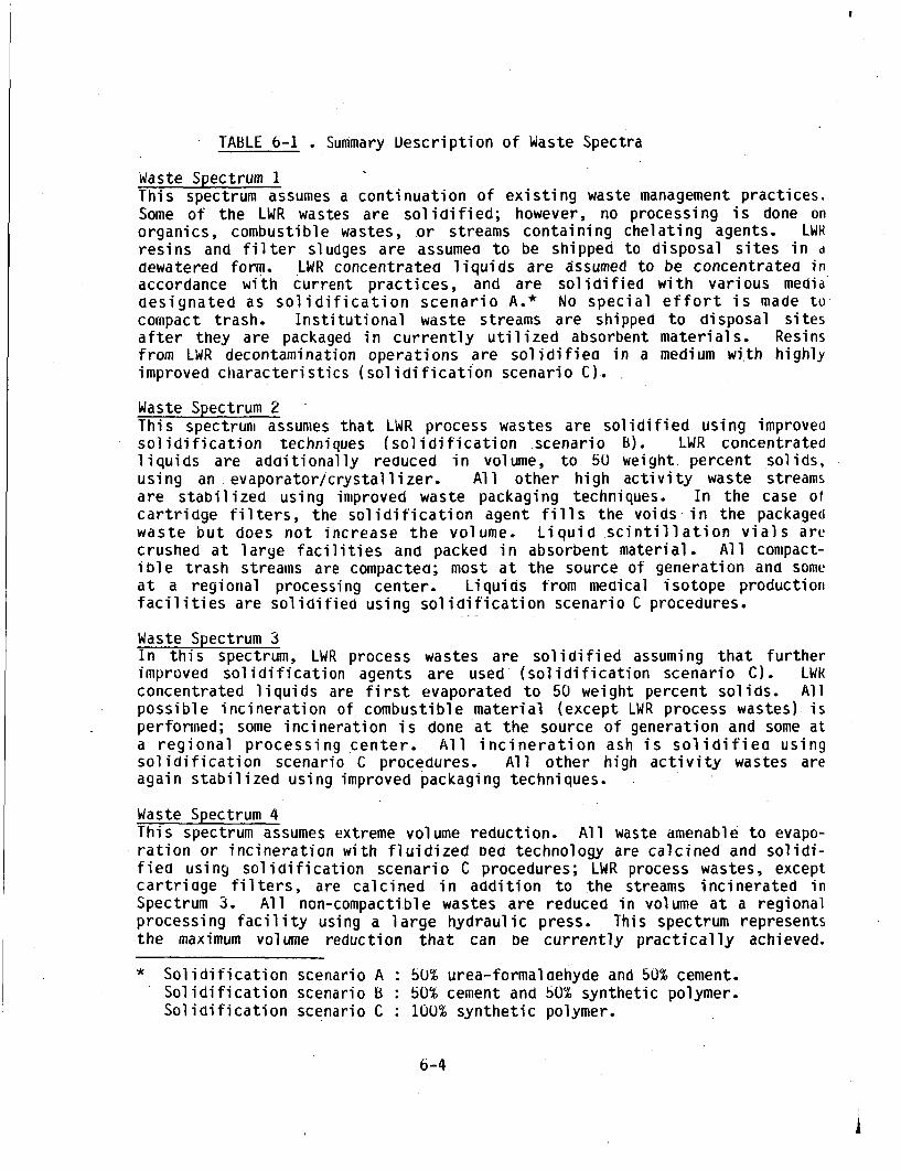
TABLE 6-1 . Summary Description of Waste Spectra

Waste Spectrum 1This spectrum assumes a continuation of existing waste management practices.Some of the LWR wastes are solidified; however, no processing is done onorganics, combustible wastes, or streams containing chelating agents. LWRresins and filter sludges are assumed to be shipped to disposal sites in d

aewatered form. LWR concentrated liquids are assumed to be concentratea inaccordance with current practices, and are solidified with various mediddesignated as solidification scenario A.* No special effort is made tocompact trash. Institutional waste streams are shipped to disposal sitesafter they are packaged in currently utilized absorbent materials. Resinsfrom LWR decontamination operations are solidifiea in a medium with highlyimproved characteristics (solidification scenario C).

Waste Spectrum 2This spectrum assumes that LWR process wastes are solidified using improvedsolidification techniques (solidification scenario B). LWR concentratedliquids are additionally reduced in volume, to 50 weight percent solids,using an evaporator/crystallizer. All other high activity waste streamsare stabilized using improved waste packaging techniques. In the case otcartridge filters, the solidification agent fills the voids in the packagedwaste but does not increase the volume. Liquid scintillation vials arecrushed at large facilities and packed in absorbent material. All compact-ible trash streams are compacted; most at the source of generation and someat a regional processing center. Liquids from medical isotope productionfacilities are solidified using solidification scenario C procedures.

Waste Spectrum 3In this spectrum, LWR process wastes are solidified assuming that furtherimproved solidification agents are used (solidification scenario C). LWkconcentrated liquids are first evaporated to 50 weight percent solids. Allpossible incineration of combustible material (except LWR process wastes) isperformed; some incineration is done at the source of generation and some ata regional processing center. All incineration ash is solidifiea usingsolidification scenario C procedures. All other high activity wastes areagain stabilized using improved packaging techniques.

Waste Spectrum 4This spectrum assumes extreme volume reduction. All waste amenable to evapo-ration or incineration with fluidized bed technology are calcined and solidi-fied using solidification scenario C procedures; LWR process wastes, exceptcartridge filters, are calcined in addition to the streams incinerated inSpectrum 3. All non-compactible wastes are reduced in volume at a regionalprocessing facility using a large hydraulic press. This spectrum representsthe maximum volume reduction that can be currently practically achieved.

* Solidification scenario A : 50% urea-formaldehyde and 50% cement.Solidification scenario b : 50% cement and 50% synthetic polymer.Solidification scenario C : 100% synthetic polymer.

6-4

A very large number of alternatives result from the variability of

values associated with these three aspects of LLW management and

disposal. For example, for each region (IR), post operational period

(IPO), and active institutional control period (IIC), there are 5184

possible permutations of the remaining disposal technology indices.

Therefore, the analyses of alternatives must utilize computer programs

to rapidly calculate and assess the impacts. Furthermore, several

computer programs are needed to examine and assess an isolated portion

of the decision base that is produced by the analyses. Only in this

systematic manner may one fully utilize the flexibility and detail

provided by the information base.

6.1.3 General Approach

As stated previously, long-term performance of the disposal system is

stressed in this report. In the analyses of the radiological impacts,

there are three major potential modes of exposure (see Chapter 2.0)

two of which relate to longer term safety consideration: humans

inadvertantly contacting the waste after disposal (which involves the

concentration of radionuclides in the waste), and the waste entering

one of several natural pathways leading back to biota which involves

the total activity disposed at the site.

The fact that impacts from scenarios involving direct human intrusion

into disposed waste are governed by the radionuclide concentrations in

the particular waste streams assumed to be contacted makes the intru-

der scenarios very useful for waste classification purposes. Assuming

that a limit is placed on the exposures allowed to a potential human

intruder, then the maximum allowable concentrations of radionuclide in

waste streams to meet this exposure limit may be calculated. Once

concentration limits are determined, waste generators can relatively

easily determine what class their waste belongs to by comparing the

radionuclide concentrations in their wastes with the limiting con-

centrations determined through the intruder scenarios.

6-5

By contrast, it is much more difficult to classify wastes through use

of total activity scenarios such as groundwater migration since

impacts from groundwater, migration are much more dependent on site

specific conditions than the intruder scenarios. In addition, since

the potential impacts are a function of the total activity of waste

disposed, it is difficult to set concentration limitations for indi-

vidual radionuclides to meet a specific dose limitation criteria. It

would be difficult, based upon groundwater migration considerations,

to set concentration limits that can be used by a waste generator to

determine the classification of his waste.

It is important to emphasize, however, that this does not mean that

groundwater migration from a disposal facility is not an important

consideration in LLW disposal. It does suggest that rather than

establishing concentration limitations to be met by a waste generator

to meet a particular groundwater exposure limitation criteria, it

would probably be more useful to set an inventory limitation for a

particular disposal facility (based upon site-specific information)

for particular radionuclides of concern.

6.1.4 Overview of Computer Codes

In view of the above discussion, therefore, the first step in the

alternatives analyses involves examination of the acceptable disposal

requirements of the waste streams. This is performed through a code

called INTRUDE (see Section 6.2.1) which determines the radiological

impacts resulting from potential inadvertant human intrusion into a

selected disposal facility containing waste processed through one of

the above waste spectra as a function of time after disposal.

The second step in the alternatives analyses involves determination of

long-term radiological and non-radiological impacts including those

which may result from potential groundwater migration. These analyses

are performed through two codes called GRWATER and OPTIONS.

6-6

Attention is principally focused upon long-term radiological, impacts

of potential inadvertant intrusion into disposed wastes and potential

groundwater migration of radionuclides, as well as potential long-term

costs to a site owner for surveillance and control of a closed dispo-

sal facility. A number of alternatives for waste form and packaging,

and disposal facility design and practices are examined for means to

mitigate or reduce these potential long-term radiological and cost

impacts. As a byproduct of implementing these alternatives, however,

there are short-term costs such as waste processing, transportation,

and disposal costs as well as short-term radiological impacts such as

occupational exposures during waste handling and population exposures

due to waste processing and transportation.

The code GRWATER calculates the individual exposures resulting from

use of contaminated water drawn from various human access locations

such as a well that may become contaminated as a result of potential

groundwater migration of radionuclides. These radiological impacts

are examined for several sets of disposal technology indices and a

selected waste spectrum. Exposures are calculated as a function of

time and may be presented as (1) total exposures from the contribution

of all waste streams, (2) total exposures from a particular waste

stream or group of waste streams, and (3) exposures from each of the

radionuclides considered.

The OPTIONS code calculates the waste volume-averaged inadvertant

intruder impacts, impacts resulting from exposed waste scenarios, as

well as impacts resulting from operational accidents and impacts

associated with short term considerations such as waste processing and

transportation impacts, disposal costs, energy use, land use, etc.

In addition to these three codes which consider projected low-level

waste characteristics, two codes have been programmed to calculate

limiting concentrations in waste streams and total inventories in

disposal facilities for specific cases. One of these codes is called

6-7

INVERSI and calculates the limiting concentrations in waste to meet a

specific dose criterion for a specific disposal facility design; it is

used for waste classification purposes. The other code is called

INVERSW and calculates disposal facility radionuclide concentrations

and inventories to meet specific allowable dose criteria for ground-water migration for a specific disposal facility design and regionally

representative environmental characteristics; it may also be used for

waste classification purposes.

Computer listings of the codes utilized to perform the analyses are

presented in Appendix 0. The codes have been designed to optimize

execution (running) time rather than memory. They have been executed

in a CDC-6600 computer in a time sharing mode. They use just two

lines of input: an IRDC(12) array which contains the disposal tech-

nology indices presented in above, and a NOTE(6) array which is a 60

character descriptive title that can be arbitrarily set. The rest of

the data is input to the codes through two tapes: TAPE1, which con-

tains most of the generic data (see Section 6.3), and TAPE2 which

contains waste spectrum specific information. A listing of these

tapes is also presented in Appendix D.

Alteration of the codes for other systems should be relatively easy

since they use only standard FORTRAN functions that are commonly used.

Output formats and statements, however, should be closely checked,

since they vary significantly from one computer system to the next.

6.1.5 Discussion

The alternatives analyses enable safety decisions (in addition to

those decisions resulting from the inadvertant intruder and ground-

water impacts analyses) to be made on performance objectives and

technical requirements for acceptable disposal of LLW. These per-

formance objectives and technical requirements may then be summarized

in a waste classification system that is addressed to waste generators

and whose primary objective is flexibility and practicality.

6"8

The most important limitation for the applicability of the analyses

and its results is the generic nature of the analysis, i.e. utiliza-

tion of generic waste spectra, generic disposal facility environments,

generic radiological impact analyses methodologies, etc. Similar, and

possibly much more detailed, analyses are likely to be necessary to

establish the potential impacts resulting from the disposal of LLW at

a particular disposal facility.

6.2 Description of the Codes

6.2.1 INTRUDE Code

In determining performance objectives and technical requirements for

LLW disposal , an important consideration is the potential for human

intrusion into the disposed waste. Such intrusion may act to increase

the potential for groundwater migration by increasing the infiltration

of precipitation into the waste and it may also bring wastes to the

surface where they may potentially be dispersed by wind or water.

These actions may result in radiation exposures to the surrounding

population. However, the largest radiation exposures by far would be

to the intruders themselves.

There are three basic scenarios for intruder exposure: potential

construction of a house on the disposal site, persons potentially

living in a house located in contaminated soil and consuming vege-

tables grown in an onsite garden, and the use of contaminated water

from an'on-site well. This section and accompanying code considers

the first two of these scenarios: intruder-construction and intruder-

agriculture scenarios. The third scenario, intruder-well scenario, is

considered in the next section on groundwater impacts analyses. The

potential exposures to the surrounding population as a result of the

actions qf the intruder, the exposed waste scenarios, are considered

in the following section on alternatives analyses.

6-9

There are three principal means of controlling potential exposures to

an intruder: use of institutional controls, use of natural and/or

engineered barriers which would make it more difficult for an intruder

to contact the waste, and use of less dispersible waste forms. None

of these controls can be assumed to be functional forever. However,

an important decision to be made at the time of disposal for a given

waste stream is whether it requires special considerations with

regards to institutional controls, waste form, and natural and/or

engineered barriers. INTRUDE performs a screening analyses to deter-

mine which waste stream (or streams when mixed and disposed together)

requires special consideration.

The code calculates seven human organ doses resulting from the "stan-

dard" or modified intruder-construction scenario and the "standard" or

modified intruder-agriculture scenario (see Section 3.4) as a function

of time. Also calculated are the ICRP weighted exposures summed over

all the organ doses. This yields an initial definition of what is

acceptable for near surface disposal under the reference disposal

conditions. The disposal technology indices selected for the screen-

ing analysis are presented below:

IR = 2 IS = 0ID = 1 IL = 0IC = 1 IG = 0IX = 1 IH = 0IE = 1 IQ = 1

In addition, the closure period (i.e., IPO) is assumed to be 2 years,

and the active institutional control period (i.e., IIC) is varied from

50 years to 2000 years.

In the analyses, all four waste spectra (see Table 6-1) are considered

one by one. A number of different analyses may be performed for

different groups of waste streams for a given waste spectrum. Four

such potential groupings are the following:

6-10

o Each waste stream separately (36 separate analyses);

o Waste streams in four macroscopic groups;

o Waste streams in five major waste generation sources;

o All the waste streams together.

During the screening analyses performed by INTRUDE, dose limitation

criteria are not needed as input since the purpose of the analysis is

to determine the acceptable disposal requirements of the wastes and

not to classify them. It should be noted that the intruder-pathway

analyses may also be changed easily to perform sensitivity analyses to

determine the effect on results of different assumptions for indices

such as the waste form behavior indices.

An example output of the code is presented in Table 6-2 for the above

set of disposal technology indices. Waste spectrum 2 is assumed, and

impacts -are presented for the first group of 7 waste streams (LWR

process waste streams) shown on Table 3-4. It should be pointed

out, however, that the code can be executed for an arbitrary set of

disposal technology indices.

6.2.2 GRWATER Code

This section discusses GRWATER, which is a code written to perform an

assessment of the impacts from groundwater migration of radionuclides

with emphasis on waste form and packaging performance parameters, and

site selection and design parameters. After classification of the

waste streams into categories in accordance with the test procedure

outlined in Section 3.4 and the dose limitation criteria specified

in the code as acceptable, the code computes seven human organ doses

as a function of time after closure of the disposal facility for

several biota access locations.

There are9 three basic scenarios for direct or indirect exposure of

humans to• radioactivity from potential groundwater migration: an

individual-well scenario which envisions drilling of a well either

6-11

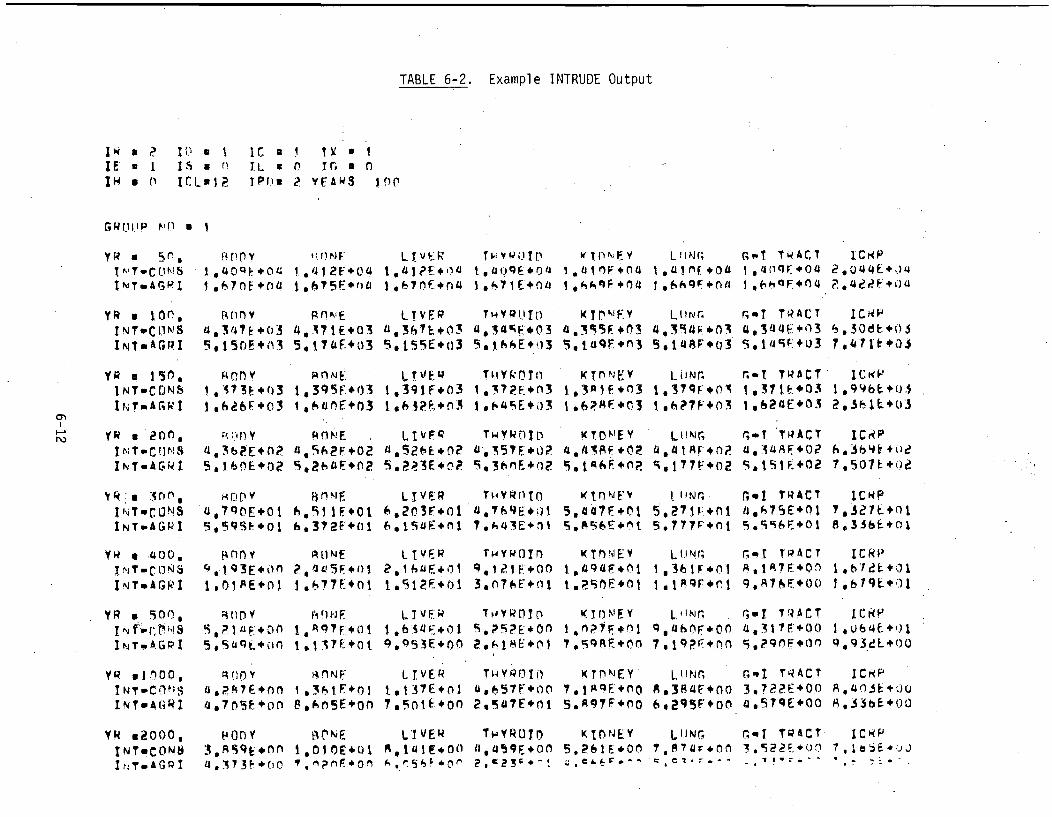
TABLE 6-2. Example INTRUDE Output

jw a 2 ID a IuE I I.• . f

IN w 0 ICLwIP

GR rH ,P ,ri ¶

IcaTL U1 P I.! i. YEAWS I f) ("0

I N-Tw* cr. KSj NTAG j I

YR • on

I NT,.CON SI NT, AGr I

YR a 1504INT-CONS1fTsArWj

cI r

jjT-C()NSI ~ T,,,A (GW I

INT-AGRII., YR S i50O,

7NT CO)N S

INT.AGPI

Yk a 400,

TNT-,CONS

INT.AGRI

YR 9008I N f.~0MI NT- AGP I

YR u10o.l

I NTw GkIS

YR 0200,INT.CONtSI rý Tm&G PI

raflrYI ,, 40'9 . ÷Ot:

9.3 4 7 E * 0 3

i "4713F.o3I ,9c626F+03

_ C, r_)E Y•[ Op V

Q, 03E÷0111, 01 ,AE÷+

P I aP Y

"0 D Y3o•sqE+oM40 4*0 0

1.4 ,1TF*÷02 F7 F* 0~ Li

5. 1 E sa~e~I,.73 3 F + 03

5, aoE+03

4,562F+02

B t,,i

6,91 IE016,372F.+01 I

IfINE

F

!,3*1. E*01.

tjPNF-1,010F+01TMPM 0 M

LTV ER P T 1-v Q 111 w T. 1) ; FEY L I IH ; r,,? TwAC,?

1.67MEr4 I61 40 1/+AI i,(,qF +o4 I 669Fe1 +o4I ,hF+04

LTVEEP THYWVQiE) KTn1'1FY L(I•!r G"T TqACTLi.3'7L*03 4.3a5,E*03 tJ* 55F+M3 4*3594~.*03 4,31441C03S.155E+}3 5 !.L6%.E+!)3 5,*iaFlt3 5,,I 8,F 03 5,1149ý+03

LTVýQ T fYOTO K I f NE" Y i. IINr. r,-T TRACT1,391F+04 ¶.3T2F,*3 I OR I F 03 1 ,379Fo' +0 1,371 tP*03

I..~fC31. 4E+c3 t.6PMECC3 1. '7F~o3 1,620E+(.5

LIVF T TTV.joT D,!Y L1!Nr, r-T TRACT

9.2a3E.0P SOWE+0.? r" Cr jaF0 9 , 7I F 0

LIVER T,. YR T0 w'nNt. I )N". rI TRACT6(,.03F*01'.769E*I 5,467F*.01 5,.271V:oi 4.675EC016ot.ISME~5 T.AuE. o, AEs6E+M1 5.7TTFoi 59,556E+01

L T VE.R T Yw IW T I"0NE y LtNf .,lt TRACTI,4E .+01. Q,,l 1¶E.00 I,494F,(,01 ¶,361F*01 A.1MIT7F.+ ,

I.5iFEeO1 3,,nTEnAFeot P.P)-+.0t I ,IAQFn1l 9,AEe00

LIVER ToywcIlO KIONElY L.hIri r;o. TRACT1•.0.1O 5,,?.ePE.0fl I.MPIF+n_0 Q6,4h0F.O0 4,,3175+009,C53E÷o0. 2.•1•F*+01 ?,9RE0+on 7,19?F +(nn ,?•qF0tn

LIVEP TWYQfl1, 1 TDNEY LUINr sGI TTRACTtT37E+01 (6•,.57F+00 7,1q.E+0o 9,.384F+oo 3,72??EC0.

7,50iE+O0 2,547EC01 5,A97.F+00 6, 2 qS9F+o &.S'TqE+00

LIVER TNYR{.)f KIDNEY LU.NrG nI TPACTRA.i4iE00 ,4*r"9vF_+O0 5,.P1E#0 , 7.A 7 41i,00 3.9224EO,

ý', OS . F 4O, C r 2 • ,- c, 2 3:. r -r€: €'. -0 c'? " - .

ICRP2 U/44L4.') 4

2,,36.•eu3

ICcip

I , 99b5 0 0.52.3 2 7 IL+03

8,336L+0,1

ICRP1.33be+01

IC14P1.033b+01

7, 9ebEw,:o

adjacent to a disposal cell or at the site boundary, a population-well

scenario which envisions pumping water from a well to satisfy the

needs of a small community located between the disposal facility and

an open water location receiving groundwater passing underneath the

site, and a population-surface water scenario which assumes that

population exposures result from consumption and utilization of open

water that has received discharge from contaminated groundwater

passing underneath the site.

All three of these scenarios are relatively unlikely to occur, espe-

cially considering the conservative assumptions that have been made

for the migration analysis-(see Section 3.5 and Appendix A). In

addition, for example, an intruder in need of water is likely to drill

a well where the groundwater is closer to the surface and where water

yields are more substantial. The potentially low water yields in

these wells are due to the comparatively low saturated zone hyd-

raulic velocity resulting from location of the disposal site at a

topographic high, which usually indicates that the location is near or

at a groundwater divide. Similar arguments are applicable for the

population-well scenario. Even a small community's water needs are

substantial, especially considering the fact that this community is

likely to be a farming community,.

The results of the groundwater impacts analysis may be used to deter-

mine if a limitation on the total activity of the waste disposed at

the site need be considered. In addition it may be used to recommend

minimum groundwater release standards for some of the wastes.

An idealized map of the disposal facility showing the areal relation-

ships of the disposal site and the groundwater access locations was

shown in Figure 3.3. As indicated in the figure, the transverse

(i.e., peirpendicular to the groundwater flow direction) dispersion of

the contaminants before and after they reach the saturated zone is

measured through the geometric reduction factor (r ). However, the

6-13

dispersion of the contaminants in the direction of groundwater flow is

dependent on the longitudinal (parallel to the groundater flow direc-

tion) extent of the disposal facility. Currently, there does not

exist a closed-form analytical solution of the areally distributed

source groundwater migration problem, only approximations of the

equations or numerical integrations of the point-source equations are

available.

The longitudinal extent of the disposal site is taken into account

in the analysis by the application of the point-source equations given

in Chapter 3.0 to each of 10 sectors. In this manner, the transverse

distribution is taken into account through the factor (r ), and the

longitudinal distribution of the source is numerially integrated.

In this calculation, water starting from each of the sectors has

different travel times to the three access locations. This travel

time is calculated in the computer code through the use of an incre-

mental travel time and Peclet number between the sectors (the DTTM and

DTPC arrays), through dividing the source term into 10 equal parts

(this is conservative since the higher specific activity waste is

likely to have higher surface radiation levels and is likely to be

placed at the center of the disposal site due to occupational health

considerations), and placing this source at the center of each sector.

This division of the source term into 10 sectors is significantly more

realistic and conservative than a single point source at the center of

the disposal facility. This is due to the additional decay afforded

to the comparatively fast travelling radionuclides such as tritium and

carbon-14. The rest of the groundwater migration assumptions have

been presented in Section 3.5. The code has several options built

into it:

(1) it can consider different dose limitation criteria in the

initial classification of the wastes into regular, layered,

or hot waste facility wastes.

6-14

(2) it can exclude a waste stream or group of waste streams from the

analysis through the use of the NDX(36) array.

(3). it can package a waste stream or group of waste streams in high

integrity containers thereby postponing the initiation of the

groundwater migration scenario for those streams for a specified

period of time, and/or stabilizing the waste streams,

(4) it has the option to perform a time dependent source term

calculation, and increase the released source term after an

intruder and/or time causes percolation values to increase,

(5) it can provide the total exposures from the contribution of all

the radionuclides in all the streams, total exposures from all

the radionuclides from a particular waste stream or group of

streams, or exposures from each of the radionuclides considered

in all or some of the waste streams.

A portion of an example output of GRWATER is presented in Table 6-3

for the case of waste spectrum 2, and the following disposal facility

indices:

IR = 2 ID = 1 IC = 2 IX = 2IE = 1 IS = 1 IL = 1 IG = 0IH = 1 IQ = 1 ICL = 2IPO = 2 years IIC = 100 years

6.2.3 OPTIONS Code

The previous two codes, INTRUDE and GRWATER, concentrate on the

long-term radiological impacts resulting from the disposal of LLW.

However, in a generic analysis to determine performance objectives and

technical requirements for management and disposal of LLW, other

impact measures must be included in the information base for decision

making. Moreover, a comparative analysis of the intruder impacts

averaged over all the streams within their respective disposal status

is useful in the decision making process. This section presents a

code for calculating this decision base.

6-15

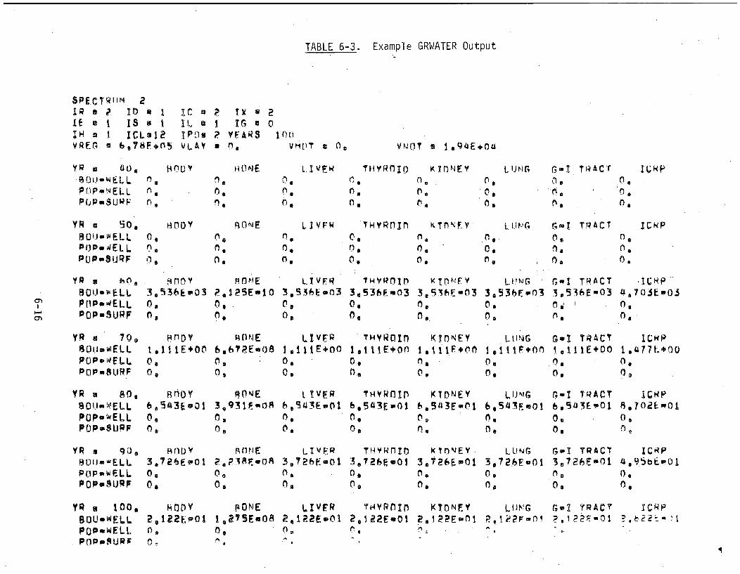
TABLE 6-3. Example GRWATER Output

SPECT5•uH 2

IF a I IS i

IH a I ICL L 2VREG u 6978F+0,5

IC.

I pei aVkAY

P T A

P YFARSa Oil

20

VH4VT S 0,VNOT a l9'4Ee04

I.-

yR a 0.. OUPWELLPrlP-=WELL

YR a 90,13- U a W E EL L

tP'OP"ELLPUP.SUIJRF

YR a (!BOU-lJ LL.8011-,,ELLPOP. wELL.POP-NSURF

YR U TOosoumwELL

P L sPELLPOP S U RF

YR * O80OU - •"EL LPUP.,,wE LLPOPinSURF

YR A qo )9 ( UtJ E L L

Pop.J-.ELLPOPLSURF

YR w 100,

SOU-WELLOapawELL.

POP.OUR;

0

0!

0 S

00

•0

-*60,

L. IVER

LIVFN

00,

r,0,

n

i DY

. DD

3,526Em0l

0,

0,

0,

BOD

0,0,

0,

On

F;~ E

0,

0,

P 2 5 E 010n,

?, IPSE-lOof

0,M

PONE

N- E

0,

RONE

THYRnIn kTnNFY

0,

0,0,0,

0,0,0,

THYROnID KTONEY

Lii iGo TRACT0, AC

0.

L IVER3,536E-030,0,

LIVFPI ,ItE+000,0,

3 9,3E-o1

LIVFR3,72NE-01

0,

LIVER2,122E-01

00

0.

0.0,•)

3,536..03

0,

THYROIn

THYROIn604a3E-01

0,

T.4YR I r)

0,

2,12E.01

K T 1) N F: Y

3,9 E 030,

0.

KTflNEY6,54J3E.010,0,

K TrEY

KYONEY

LUNG,3.536E-03

L t. G

3,943hF01n.0,

0,

LUM

0,N

LO J J

6.Lt3E.G

0,

n-I TRACT3.536E-03

Ge TPACT

G"I TRACT

6.543E+OO

0-0

r-I fl•ACT

0,

4,703t-0SO,0,'

0,00

() 0

ICkP

GPI TRACT IClP3.726E-01 4,95b£-01

0,0,

f;7 TRACT 1CNPP.,1 I 2 F' j - 2 ý--1

I

The decision base includes five major components: (1) the volumes of

waste requiring different disposal practices -- i.e., the volumes in

each disposal status which varies depending on the disposal technology

indices and waste form behavior parameters determined by the waste

spectrum assumed, (2) disposed waste volume-averaged inadvertant

intruder impacts; (3) radiological impacts resulting from potential

exposed waste scenarios; (4) exposures which may result from abnormal

operating conditions (accident scenarios); and finally (5) the impact

measures associated with the different phases of LLW management and

disposal (i.e., waste processing, transportation, disposal) consisting

of costs, occupational exposures, population exposures, energy use,

and land use. The OPTIONS code calculates these five items. All

radiological impacts calculated (except occupational exposures which

are total body exposures) calculated include seven human organs.

The volumes of waste in each disposal status, however, have further

been divided within each major category -- i.e., regular, layered,

and hot waste facility wastes -- into four subcategories: stable with

no chemical agents, stable with chemical agents, unstable with no

chemical agents and unstable with chemical agents.

The code has most of the options considered in the GRWATER code. For

example, it can consider different dose limitation criteria in the

initial classification of the wastes, it can exclude streams from the

analysis, etc. A portion of an example output of OPTIONS is presented

in Tables 6-4 and 6-5 for the GRWATER code example case.

6.2.4 INVERSI and INVERSW Codes

The inverse codes calculate the maximum allowable concentrations that

may be disposed within the radiological guidelines considered (maximum

exposure limits) and various disposal technology properties. There

are two inverse codes: intruder (INVERSI), and groundwater (INVERSW).

In each case, the maximum allowable concentrations for a given set of

6-17

TABLE 6-4 Example OPTIONS Output - I

OPTIONS PROGRAM IAM REPORT SPECTRUM 2

DISPOSAL TECHN'OLOGY INDICES-IR =: 2 Ai: = I IC =-- 2 IX = 2IE = I IS = 1 IL = :1 16 : !::0IH = 1 ICL=12 IPO-. 2 IIC= 100

REGULAR WASTECH--STAB

CH-UNSTAB

NCH-STAB

NCH-UNSTAB

6.784E+05 Mi4*3I-LQSCNVL 3,182E-,-04I+ABSLI (At' 4 .628E+03N-.ISOPROD 2., 8 IE-+-03

N-TRITIUM 9., 616EL.02TOTAL VOLUME FI+LUSCNVL 4 . 072E+04I-BIOWAST 8 332E03I+BIOWAST 8.•332E.÷..03

N-LOWASTE 1.665E+04TOTAL VOLUME : .P-IXRESIN 1.578E+04P-CONCLIQ 2. 4,',0E+04P-FSLUD:GE 1,9'50E+03

P-FCARTRG 6.0I4E+03B-IXRESIN 3 475E-04B.-CONCLIQ 3. 774E+04B-.FSLUDGE,7.703E4.04

P-NCTRASH 6 .017EV'-04B-NCTRASH 2.734E'-04F-PROCESS 2.•159E+0:4U-...PROCESS 7.765E+03

I-ABSLIQ. 2 iN 54oE*4,.1 03N-SSWASTE 1 751E+04L-.NFRCOMP 7.975E+02N-HIGHACT 7. 204E+02N-TARGETS &,702E+02TOTAL VOLUME .1P-COTRASH 5.862E+04B-COTRASH 2. 881E+Q4F-COTRASH 4.344E+04F-NCTRASH 1.152E+04

IICOTRASH 10/43E-+.04

I +COARASH 9.717E+03N-SSTRASH 3.308E-04N--).SSTRASH 1. 654E+04N...LOTRASH 6.•1.0:,-• .03

N+LOTRASH 3 *'49 7IE+0TOTAL VOLE 0 M (I S E ','.4.

L[-ECONRS 1.933E, +04N.--SOURCES 5<.152E+01.

/ . 028 0 i*,

7.404E+•.04 M**3

:.1: :125E+05 i*

2 ,.3Q:.E+-05 M**3

! .938E.+0:'4. M**3HOT WASTE

6-08

TABLE 6-5 . Example OPTIONS Output - II

INTRUDER IMPACTSBODY

REC-CONS 3 , 333E+0:1REC-AGRI 2,081E.i.01REC-CONS 1.646E+00REC-AGRI 2.066E+00REC-CONS 1. 447E-+00REC-AGRI 1.764EF+00

EXPOSE/ACC IMPACTSREC-AIR 1.624E-02

ERO-AIR 6o099E+00REC-WAT 1.972E-03

ERO..-WAT 8.847E-02ACC-SNGC 7, ,573E-f02ACC-FIRE :1* '27E+01ACC-AVG 5. 935 EF00

BONE3 , 342E+012 . , 091E +0 :1,1. 70SE+002,705E+002.799E+.002. 759E.:+00

7.2.31E I:E-:02I . 196E+025 .986E-037.014E-012.279E-014.059E+011.893E+01

LIVER3:336E'F011. 952.IE+0:11 * 688E+002.089E+002, 364E.+002, 137E+00

9.556E:-037 * 924E'+01:11 . 441LE-03:I.,* 4 :I. :I. i:...0O:i

I 249E-01'2 * :I. 08E'i: O 19, 836E+00

THYROID.3332E.+011.954E+011 . 645,:E+002.624E+001:378E.i.002.292E':'00

5 Q893E-046 , 426E: 011 .043E-049.899E-01

4 •581IE-026.872E+003.210E-400

KIDNEY3.333E+011,9".95 1E +011 .666E+002.* 070E+00I .742E+00:I. 896E.::00

4. 9OE.-032.744E+015.570E-04:1. 073E-0:1.B *075E"'02

:1. 357EF 4016.3301+ -00

LUNG3.335E:4.011.951E't-012.094E+002.236E+002 :74:E+002.275E+00

6*941::E-031. 085E:+022 . 357E.'.045. 389E.. 028 0 6:1. E-0:1.64 :1. 30E.:t012.887E.:.0:1

G-1 TRACT3.332E+01•1.966E+01

I .642E+002,064E':+001. 375E.+00I . 740E+00

:1.* 839E-03:3 * 5..: i::*..O :1.

20465E704:1. 9 806k E-0 14,848E-02

5.375E.FO02 5:1.7Eto00

ICRF'4.834E+013.027E+0:1.2.451E..03, 11. 1. F:+ 00

2 . 483Ei::002.783Ei:.00

2,674E-024 :. 8 +0:1.2. 857E-.0:32.o345E-0:1.2.224E-0:1.2.755E..I0:1.1. 289E 0:1.

0"1I-

'.0

i:OT"H.ER::r: IMPACTS

COST ($)

UNIT COST.T ($/M3)POP DOSE (MREM)OCC DOSE (MREM)LAND USE (M**2)ENERGY USE (GAL..)

WASTE PROCESSINGGENERAT DISPOSAL

5*80E:+08 3.63E.:.078 4:31E:+02 5 +20E1+01

06 0.3*91. 91 406 1 .25E " .- 0•5

0. 0.1.73E+07 4 .42E+05

TRANSP DISPOSAL LT CARE .100 +090

2.29E+083 29EF+027,03E.+O05

6 . 49E ."+060.

: . 65E+07

2 * 00EF:.408 1.61E. .072086E+02 2.31E+01.

0.2.93E+062.o46E.+052 ..34E.:.06

disposal technology parameters are calculated for 1 million m3 of

waste disposed in the facility.. For these two codes the basic data

matrices BAS and ISPC are not utilized. The waste form parameters,

however, are input into the calculation through the array ISPC, and

the disposal technology indices are input through the IRDC array.

The major option available in the running of these codes is to set

dose limitation criteria to different sets of values. In addition,

INVERSI code calculates and prints the results of all seven distinct

waste classification tests -- i.e., regular standard test at IIC

years, regular modified test at IIC years, layered standard test

at II years, layered modified test at IIC years, hot waste facility

test at GIIC years, regular standard test at 500 years, and regular

standard test at 1000 years (see Section 3.4.4). INVERSW code also

performs two sensitivity analyses: (1) it varies the percolation value

associated with the given region index IR by assuming 50 percent of

the value given, the value given, and twice the value given, and (2)

it varies the retardation characteristics of the soils by calculating

the limiting concentrations for all five sets of retardation coeffi-

cients considered in this work. These codes use a modified version of

TAPE1 containing the pathway dose conversion factors and the environ-

mental parameters associated with the given region index IR.

6.3 Basic Parameters of the Codes

Table 6.6 presents symbolic definitions of the data utilized in the

analyses which have been presented in the previous chapters. Also

given are the computer code definitions of most of the parameters, and

some of the assumed values for the analyses.

Almost all the codes use two data tapes (some do not need to use

all the information contained in these tapes) for input information:

TAPE1 contains waste spectrum-independent information such as radio-

nuclide concentrations of unprocessed waste, radionuclide specific

6-20

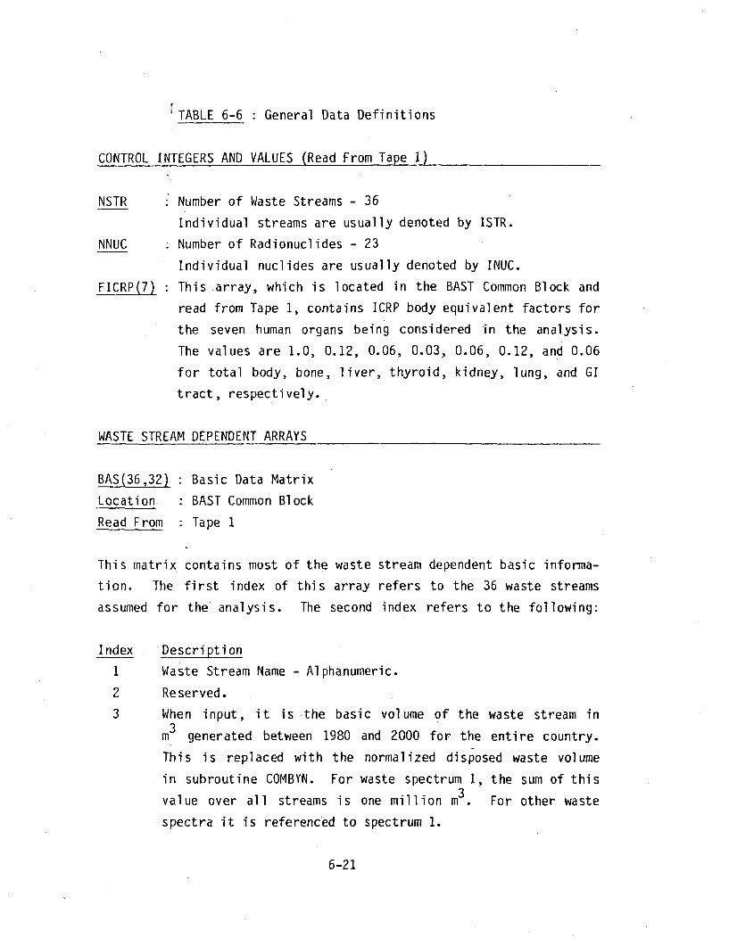
F

'TABLE 6-6 : General Data Definitions

CONTROL INTEGERS AND VALUES (Read From Tape 1)1

NSTR Number of Waste Streams - 36

Individual streams are usually denoted by ISTR.

NNUC Number of Radionuclides - 23

Individual nuclides are usually denoted by INUC.

FICRP(7) : This array, which is located in the BAST Common Block and

read from Tape 1, contains ICRP body equivalent factors for

the seven human organs being considered in the analysis.

The values are 1.0, 0.12, 0.06, 0.03, 0.06, 0.12, and 0.06

for total body, bone, liver, thyroid, kidney, lung, and GI

tract, respectively.

WASTE STREAM DEPENDENT ARRAYS

BAS(36,32) Basic Data Matrix

Location " BAST Common Block

Read From " Tape 1

This matrix contains most of the waste stream dependent basic informa-

tion. The first index of this array refers to the 36 waste streams

assumed for the analysis. The second index refers to the following:

Index Description

1 Waste Stream Name - Alphanumeric.

2 Reserved.

3 When input, it is the basic volume of the waste stream in

m3 generated between 1980 and 2000 for the entire country.

This is replaced with the normalized disposed waste volume

in subroutine COMBYN. For waste spectrum 1, the sum of this

value over all streams is one million m3 . For other waste

spectra it is referenced to spectrum 1.

6-21

TABLE 6-6 : (continued)

4 Gross undecayed activity of the untreated waste (Ci/m 3).

This value is used only in transportation calculations, it is

not modified in the program.

5-27 Radionuclide concentrations of the waste stream (in DATAD

file, decayed to year 2000) for the 23 radionuclides in the

stream (Ci/mr3 ). These concentrations are modified by

volume reduction and increase factors (if applicable) and

stored on top of the old concentrations in subroutine COMBYN.328 Transported waste volume in m which is calculated in

subroutine COMBYN. Depending on where the waste processing

takes place, this value may be different from the disposed

waste volume, i.e., BAS(ISTR,3).

29-32 Waste processing impacts: costs ($), occupational dose

(mrem), energy use (gallons of fuel), and population dose

(mrem), respectively, for the waste stream volume given in

BAS(ISTR,3). These impacts are calculated in subroutine

COMBYN.

ISPC(36,11) Waste Spectrum Matrix

Location - BAST Common Block

Read From : Tape 2

This matrix is read for each waste spectrum and contains all the

information that distinguishes waste spectra from each other. The

first index of the matrix refers to the 36 waste streams. The second

index refers to the following:

Index Description

1 Waste Packaging Index, which is used in the transportation

calculations, and is composed of two digits representing

packaging characteristics and the gamma emission character-

istics of waste.

6-22

TABLE 6-6 : (continued)

2 Volume Reduction Factor multiplied by 100 (to make it an

integer).

3 Volume Increase Factor similarly multiplied by 100.

4 Flammability Index - 14

5 Dispersibility Index - 15

6 Leachability Index - 16

7 Chemical Content Index - 17

8 Stability Index - 18

9 Accessibility Index - 19

10 Overall Waste Processing Index (110) (see Section G.5) which

is composed of four processing indices (digits) that are

unscrambled and utilized in subroutine COMBYN to calculate

BAS(ISTR,29) through BAS(ISTR,32).

11 Waste Disposal Status Index (Ill) (see Section G.3) which is

computed in subroutine RCLAIM.

RADIONUCLIDE DEPENDENT ARRAYS

DCF(23,7,8) : Pathway Dose Conversion Factor Matrix

Location : BAST Common Block

Read From : Tape 1

This matrix contains the multiple pathway dose conversion factors

calculated through the CODE DOSE (see reference 2). DCF(I,J,K) is the

pathway dose conversion factor for the radionuclide (I), human organ

(J), and multiple pathway (K). Human organs considered (as given for

the FICRP array) are total body, bone, liver, thyroid, kidney, lung,

and GI tract, respectively. Multiple pathways considered are those

resulting from the following release scenarios: accident, construction

(air uptake pathway), agriculture (air uptake pathway), agriculture

(food (soil) uptake pathway), direct-gamma (volume) exposure), well

water, open water, and air. (2 This matrix is not modified by the

code.

6-23

TABLE 6-6 : (continued)

NUC(23)

Location

Read From

Radionuclide Names

NUCS Common Block

Tape I

This array contains the alphanumeric names of the radionuclides: H-3,

C-14, FE-55, NI-59, CO-60, NI-63, SR-90, NB-94, TC-99, 1-129, CS-135,

CS-137, U-235, U-238, NP-237, PU-238, PU-239/240, PU-241, PU-242,

AM-241, AM-243, CM-243, CM-244.

AL (23)

Location

Read From

This array

nuclides in

FMF(23)

Location

Read From

This array

between the

: Decay Constants

: NUCS Common Block

: Tape 1

contains the decay constants of the 23 selected radio--1

units of year-

Leachate Partition Ratios

NUCS Common Block

:Tape 1

contains the radionuclide-dependent partition ratios

radionuclide concentrations in the trench leachate and in

the unsolidified waste obtained from Maxey Flats and West Valley

experimental trench concentration data (see Appendix A).

RET(23,,5)

Location

Read From

Retardation Coefficients

NUCS Common Block

Tape 1

This array contains the retardation coefficients of the radionuclides

for five different soil conditions (see Appendix A). Only RET(I,1) and

RET(I,4) are read in from Tape 1, the rest of the coefficients are

calculated from RET(I,1) and RET(I,4) and stored in subroutine COMBYN.

6-24

TABLE 6-6 (continued)

ENVIRONMENT DEPENDENT ARRAYS

Most of the codes utilized provide for six different disposal envi-

ronments, each of which is denoted by a specific value of IR in the

discussion below. The first four cases correspond to the regional

characteristics outlined in Appendix C: northeast, southeast, midwest,

and southwest. For most of the analysis only the second set of

environmental parameters (IR=2), which represent the reference dispo-

sal facility environment, is utilized. The fifth and sixth sets of

environmental parameters (IR=5 and IR=6) are variations of the refe-

rence facility environment and are utilized for the groundwater

migration analyses.

FSC(6) : Construction Dust Mobilization Factor

Location DTIS Common Block

Read From " Tape 1

This array (denoting f s-construction) contains the dust mobilization

factor, which depends on environmental parameters such as antecedent

moisture conditions, soil particle size distribution, and annual

average wind speed, for the air uptake pathway of the intruder-cons-

truction scenario.

FSA(6) : Agriculture Dust Mobilization Factor

Location DTIS Common Block

Read From : Tape 1

This array (denoting fs-agriculture) contains the dust mobilization

factor, which depends on environmental parameters such as antecedent

moisture conditions, soil particle size distribution, and annual

average wind speed, for the air uptake pathway of the intruder-agri-

culture scenahio.

6-25

TABLE 6-6 : (continued)

PRC(6,2)

Location

Read From

: Percolation Matrix

DTIS Common Block

* Tape 1

This matrix contains the potential infiltration into the disposal

cells modified by the anticipated waste-water contact time given in

units of-meters for two different conditions: PRC(IR,I) is the no

special cover condition, and PRC(IR,2) is the thick cover condition.

These percolation values are given in Appendix C.

QFC(6,3)

Location

Read From

: Dilution Factors

: DTIS Common Block

* Tape 1

This array contains the dilution factors (Q) in units of (m 3/year)

for three groundwater discharge locations: boundary-well, population-

well, and population-surface water discharge locations.

TTM(6,3)

Location

Read From

: Groundwater Travel Time Matrix

: DTIS Common Block

* Tape 1

This matrix contains the groundwater travel times in years (t W)between the sector of the disposal site (see Section 3.6) closest to

the discharge locations and the-three groundwater discharge locations

mentioned above in QFC(6,3).

TPC(6,3)

Location

Read From

* Peclet Number Matrix

- DTIS Common Block

*Tape I

This array contains the dimensionless Peclet Numbers (P) for the

groundwater travel times given by the above matrix TTM(6,3).

6-26

TABLE 6-6 : (continued)

RGF(6,3)

Location

Read From

Geometric Migration Reduction Factor

DTIS Common Block

Tape 1

This matrix conta.ins the geometric reduction factor (r ) resulting

from the transverse relationship of the discharge location and the

disposal facility for the three groundwater discharge locations

considered in the analysis. These values are assumed to be unity for

all three locations in the reference disposal facility case.

POP (6,3)

Location

Read From

Exposed Waste Site Selection Factors

DTIS Common Block

Tape 1

This matrix contains the exposed waste site selection factors (f s):

POP(IR,I) and POP(IR,2), in units of person-m3 /year, corresponding

to the factors for the exposed waste-intruder-air and exposed waste-

erosion-air scenarios, respectively, and POP(IR,3) corresponds to the

exposed waste-surface water (intruder and erosion) scenarios.

DTTM(6)

Location

Read From

Incremental Travel Times

DTIS Common Block

Tape 1

This matrix contains the incremental travel times between the sectors

of the disposal facility in units of years (see Section 3.6).

DTPC(6)

Location

Read From

: Incremental Peclet Numbers

DTIS Common Block

: Tape I

This matrix contains the incremental Peclet numbers between the sectors

of the disposal facility (see Section 3.5 and Appendix A).

6-27

TABLE 6-6 : (continued)

TPO(6,2) : Atmospheric Dispersion Factor Array

Location : DTIS Common Block

Read From : Tape 1

This array contains the atmospheric dispersion factors utilized inthe accident scenarios for the regional disposal facility site consi-dered. These factors have units of person-year/m3 and are the

atmospheric (X/Q) factors for a given radial distance multiplied bythe population at that distance summed over all distances. TPO(IR,1)is for the accident-fire scenario, and TPO(IR,2) is for the single-container accident scenario.

NRET(6) : Retardation Status Array

Location : DTIS Common Block

Read From : Tape 1

The values in this array indicates the condition of the soils in thevicinity of the disposal site with regards to the retardation ofradionuclides. It determines which RET(23,5) will be used in thegroundwater migration analysis, i.e., RET(23,NRET(IR)).

6-28

parameters, and environmental parameters; and TAPE2 contains infor-

mation on the waste spectrum being considered (e.g., volume reduction

and increase factors, and waste form behavior indices). In addition,

INPUT (query by the code at the terminal the code is being run from)

is utilized for reading in the disposal technology indices and

descriptive "header" information.

Computer printouts for the following programs and data files can be

found in Appendix D:

Computer Programs:

INTRUDEGRWATEROPTIONSINVERSIINVERSW

Data Files:

DATADATADNUCSSPC1SPC2SPC3SPC4

6-29

REFERENCES FOR CHAPTER 6.0

1. Wild, R., et.al., Dames & Moore, "Data Base for RadioactiveWaste Management. Volume 2. Waste Source Options," USNRC ReportNUREG/CR-1759, November 1981.

2. U.S. Nuclear Regulatory Commission, Office of Nuclear MaterialsSafety and Safeguards, "Draft Environmental Impact Statement on10 CFR Part 61 : Licensing Requirements for Land Disposal ofRadioactive Waste," NUREG-0782, November 1981.

3. Clancy, J.,. et.al., Dames & Moore, "Data Base for RadioactiveWaste Management. Volume 1. Review of Past Disposal Practices,"USNRC Report NUREG/CR-1759, November 1981.

6-30

APPENDIX A

TRANSFER FACTORS

TABLE OF CONTENTS

Section Page

A.1 Soil-to-Air Transfer

A.1.1 Background . . .

A.1.2 Construction . .

A.1.3 Other Activities

A.1.4 Wind Suspension

Factor * . A-i* . A-3

* . A-I* . A-14* . A-14O

A.2 Soil-to-Water Transfer Factors

A.2.1 Waste to Leachate Transfer

A.2.2 Groundwater Migration

A.2.3 Percolation .. .. .. .

A.2.4 Surface Water Erosion . .

A.3 Other Transfer Factors . ...

A.3.1 Air-to-Air Transfer Factor

Factor

* A-17

* A-17

* A-27

* A-31

* A-36

* A-41

* A-41

* A-42

* A-44

* C C C C

* *C C ~* C

Q

A.3.2 Air-to-Soil Transfer Factor .... .

A.3.3 Water-to-Soil Transfer Factor . . .

A.4 Direct Radiation Exposures .. . . . .. C . . . . . . . . . A-46

i

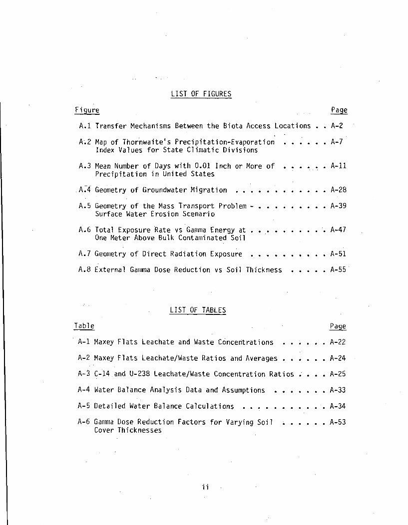
LIST OF FIGURES

Figure

A.1 Transfer Mechanisms Between the Biota Access Locations .

A.2 Map of Thornwaite's Precipitation-Evaporation . . ....Index Values for State Climatic Divisions

A.3 Mean Number of Days with 0.01 Inch or More of . . . . . .Precipitation in United States

A-4 Geometry of Groundwater Migration ............

A.5 Geometry of the Mass Transport Problem - . ........Surface Water Erosion Scenario

A.6 Total Exposure Rate vs Gamma Energy at... ........One Meter Above Bulk Contaminated Soil

A.7 Geometry of Direct Radiation Exposure . . . . . . . . ..

A.8 External Gamma Dose Reduction vs Soil Thickness . . ...

Page

A-2

A-7

A-11

A-28

A-39

A-47

A-51

A-55

LIST OF TABLES

Table

A-1 Maxey Flats Leachate and Waste Concentrations . .

A-2 Maxey Flats Leachate/Waste Ratios and Averages . .

A-3 C-14 and U-238 Leachate/Waste Concentration Ratios

A-4 Water Balance Analysis Data and Assumptions . . .

A-5 Detailed Water Balance Calculations . . . . ...

A-6 Gamma Dose Reduction Factors for Varying Soil .Cover Thicknesses

Page

. . . . A-22

. . . . A-24

* . A-25

. . . . A-33

A-34

. . . . A-53

ii

APPENDIX A: TRANSFER FACTORS

This appendix considers the numerous radionuclide release/transport

transfer factors between the various biota access locations defined

and utilized in the pathway analyses. It also presents formulae and

data with which they can be computed, and gives the transfer factor

values that are utilized in the impact analyses.

A diagram showing the interactions of the biota access locations and

the primary mechanisms through which they are connected is provided

in Figure A.I. Also given in the figure are the sections of this

appendix in which the transfer factors are considered. The term"multiple factor" implies that the transfer factor can be obtained

by the multiplication of other transfer factors alreaay being consi-

dered. For example, air (onsite) to soil (offsite) requires the

multiplication of the air-to-air (Section A.3.1) and air-to-soil

(Section A.3.2) transfer factors.

Various soil-to-air transfer factors, which will be utilized in the

intruder (construction and agriculture) ano the accident scenarios,

are considered in Section A.1. Also given in Section A.1 is the

wind initiated soil-to-air transfer factor, which is utilized in the

exposed-waste scenarios. The waste-to-leachate, leachate-to-water,

and soil-to-water transfer factors, which are applicable to ground-

water and surface water scenarios, are considered in Section A.2.

Other transfer factors are presented in Section A.3.

A.1 Soil-to-Air Transfer Factor

The soil to air transfer factor (T sa) depends on many factors such

as the moisture content and grain size distribution of the soil, the

degree of atmospheric turbulence, the exposure period fraction, and

the type of human activity, if any, affecting the soil. The magnitude

A-I

AIR AIR SOIL WELL OPENFROM (ON-SITE) .((OFF-SITE) OFF-SITE) WATER WATER

SOIL- SUSPENSION MULTIPLE MULTIPLE GROUNDWATER WATERWASTE (A.1) (A.1.4) MIGRATION TRANSPORT

(ON-SITE) " (A.2) (A.2)

AIR METEOROLOGICALAI IPRINMULTIPLE X MULTIPLE

(ON-SITE) DISPERSION(A.3.1)

AIR DEPOSITION DEPOSITION

(ON-SITE) (A.3.2) (A.3.2)

SOIL SUSPENSION GROUNDWATER WATER

(OFF-SITE) X (A.1) X MIGRATION TRANSPORT(A.2) (A.2)

WATER xIRRIGATIONWATER (A .3.3) -

r

I'1

I-.

II,U0I8n

TRANSFER. MECHANISMSBETWEEN THE BIOTA ACCESS LOCATIONS

of the exposure period fraction, which is the fraction of a year that

the transfer factor is applicable, depends primarily on the activity

or the transfer agent initiating the specific scenario such as wind,

human intrusion, etc.

After a background section on the assumptions and major parameters

influencing soil-to-air radionuclide transfer, the factor (T sa) is

examined in several sections that address the following different

transfer activities or agents: construction, vehicular traffic,

agriculture, and finally wind.

A.1.1 Background

In this appendix, the designations "transportable particulates" and"respirable particulates" are used as part of the procedures to

calculate the soil-to-air transfer factor. Transportable particulates

are usually defined as those with a mean aerodynamic diameter (MAD)

less than 30 Pm and they include respirable particulates. Transport-

able particulates must be considered if offsite wind transport of

airborne radioactivity is considered -- i.e., non-respirable parti-

culates may contribute to uptake pathways other than inhalation

through transfer mechanisms such as deposition, dissolution, and plant

uptake. The definition of respirable particulates may differ.(1'2)

However, the particulates that are entrapped in the nasopharyngeal

region (the upper part of the respiratory track) are usually particles

with a MAD above 5 pm. Below this MAD the particles may reach the

trachea bronchial and bronchiolar regions (i.e., the lung).(2) In

this appendix, the upper bound for transportable and respirable

particulates are assumed to be 30 pm and 10 pm, respectively.

There are several different types of techniques which may be used to

calculate soil-to-air transfer of radionuclides. These calculational

techniques are sometimes referred to as resuspension modelling. An

extensive treatment of the resuspension of soils by various types of

A-3

driving mechanisms such as wind-driven resuspension, mechanical

resuspension, and local resuspension can be found in reference 3.

This reference identifies three major types of resuspension modelling:

(1) the resuspension factor with units usually stated as m-1 , which

is defined as the ratio of the airborne concentration at a reference

height to the quantity of contaminant on the surface of the ground;

(2) the resuspension rate with units usually stated as sec- 1 , which

may be defined as the fraction of a contaminant present on the ground

that is resuspended per unit time by either winds or mechanical

disturbance; and (3) the mass loading concept, which gives the mass of3

soil particulates in air in units of g/m

The specific technique utilized depends on the system being simulated.

For average conditions, where very large areas for long periods of

time may be involved, either the resuspension factor or the mass

loading concept (both of which attempt to by-pass the details of the

soil characteristics) may be used. For example, to calculate pathway

dose conversion factors (see Appendix B) involving secondary biota

access locations for chronic exposure conditions, the resuspension

factor has been utilized. However, soil-to-air transfer factors

calculated in this section strongly depend on the exposed waste area,

duration of exposure, and the human activity initiating the exposure

scenario. In these cases, resuspension rates turn out to be more

convenient to use. For example, they can be used to describe con-

centrations at any point around a non-uniform contaminated area by the

use of point source dispersion and deposition equations and integra-

tion over the area.(3) In any case, the resuspension factor and

mass loading data are compared with the results from resuspension rate

calculations where applicable.

In this appendix, the resuspension rate of transportable particulatesS 2

will be denoted by E and will be expressed in units of (g/m -sec).

This form of the resuspension rate is also referred to as the resus-

pension flux and can be converted to other forms of resuspension rate

A-4

in a straightforward manner.(3) Mass loading and resuspension

factors are also very easy to calculate from the resuspension flux as

discussed in the sections below.

A.1.2 Construction

An inadvertant intruder may choose to excavate or construct on a

disposal site. Under these circumstances, dust will be generated from

the application of mechanical forces to the surface materials (soil,.

rock) through implements (wheels, blades) that pulverize and abrade

these materials. The dust particulates generated are entrained by

localized turbulent air currents. These suspended particles are thus

available for inhalation by the intruder and for transport offsite by

the wind.

The soil-to-air transfer factor (T sa) may be expressed in terms of

the geometry of the problem, the resuspension flux (E), and the

following empirical equation:

T = E x f r x G /(u x d), in m 3 of soil per m3 of air (A-i)

where:

E = suspension rate of transportable (<30 pm) particulates

in units of (g/m 2-sec)

f = fraction of suspended transportable particulates that are

respirable (<10 um).

Area subject to dusting__G = Geometry Factor Ara=btýt~yýijWidth of Area x Mixing height

u = wind speed (m/sec)

d = density of the soil (g/m )

A-5

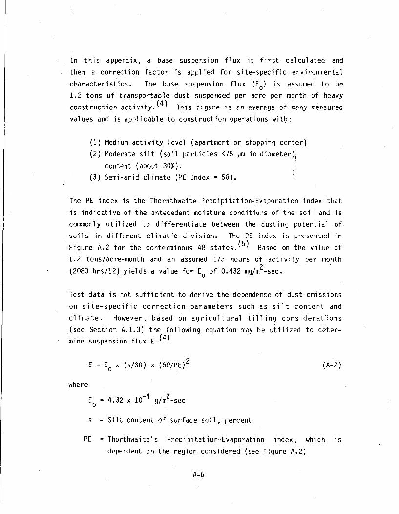
In this appendix, a base suspension flux is first calculated and

then a correction factor is applied for site-specific environmental

characteristics. The base suspension flux (Eo) is assumed to be

1.2 tons of transportable dust suspended per acre per month of heavy

construction activity.(4) This figure is an average of many measured

values and is applicable to construction operations with:

(1) Medium activity level (apartment or shopping center)

(2) Moderate silt (soil particles <75 pm in diameter),

content (about 30%).

(3) Semi-arid climate (PE Index = 50).

The PE index is the Thornthwaite Precipitation-Evaporation index that

is indicative of the antecedent moisture conditions of the soil and is

commonly utilized to differentiate between the dusting potential of

soils in different climatic division. The PE index is presented in

Figure A.2 for the conterminous 48 states. (5 Based on the value of

1.2 tons/acre-month and an assumed 173 hours of activity per month2(2080 hrs/12) yields a value for E0 of 0.432 mg/m -sec.

Test data is not sufficient to derive the dependence of dust emissions

on site-specific correction parameters such as silt content and

climate. However, based on agricultural tilling considerations

(see Section A.1.3) the following equation may be utilized to deter-

mine suspension flux E:(4)

E : E0 x (s/30) x (50/PE) 2 (A-2)

where

E 4.32 x 10- 4 g/m2-sec

s = Silt content of surface soil, percent

PE = Thorthwaite's Precipitation-Evaporation index, which is

dependent on the region considered (see Figure A.2)

A-6

.1

a

IMAP OF THORNTHWAITE'S PRECIPITATION-EVAPORATIONINDEX VALUES FOR STATE CLIMATIC DIVISIONS

SEE REPORT PB 275525, pg. 415

The geometry factor (G) can be calculated by assuming that the area

of construction is 1000 m2 (about a one-quarter acre lot) and -that

the mixing height is 3 meters. The area selected represents the size

of a lot for a typical family dwelling or a small farm bui.lding

complex with peripheral systems such as a barn, septic system, etc.

The mixing height of 3 meters is a reasonably conservative value based

on consideration of the height to which the construction dust may rise

during a short time interval. The width of the area is best repre-2

sented by the diameter of a circle whose area is about 1000 m

These assumptions yield G = 9.36.

The geometry factor is proportional to the square root of the area of

construction. For example, for the intruder-construction scenario, an

area of about 200 m 2 has been used. This area would yield a geo-

metry factor of about 4.18. The above conservative value of 9.36 is

used in this work for the intruder-construction scenario.

Wind speed varies with time and geographic location. However, a mean

value of 4.5 m/sec (long-term annual average for the 48 conterminous

states) may be utilized as an estimate of the average wind speed

during the construction activity (assumed to require 3 months, or

approximately 500 hours of dust-generating activity). Using these

values yields:

(E G/u) = 0.90x10-3 g/m 3

or 0.9 mg/mr3 , which represents the transportable "dust loading" in

the air -- i.e., the mass loading value.

Experimental determinations of respirable mass loading in the air in

and around heavy construction equipment have been performed for

surface coal mining operations. These experimental determinations

indicate a variation in the respirable dust- loading ranging from

fL.'(O Iuq/m3 (for a bulldozer) to 6.7 mg/m3 (for a front end loader)

A-8

within a few feet of the equipment. (6) Respirable dust loading

inside the cab of the equipment was a maximum of 1.8 mg/m3 for the

measurements taken. Ambient mass loading data for 1966 from the

National Air Surveillance Network- showed the average for urban sta-3 3

tions ranged from 0.033 mg/mr to 0.254 mg/mr, and a mean for nonurban

locations, of 0.038 rg/m3 .( 3 )

In this work, a combination of the above equations is utilized. The

regional.)•dependence of the soil-to-air transfer factor may be quan-

tified through: (1) the wind speed (u), (2) the soil silt content (s),3and (3) the PE index. Utilizing a soils density of 1.6 g/cm , and

an arbitrary reference wind speed of 10 m/sec, the following equation

may be derived from equations (A-i) and (A-2):!

(T) = (Tsa)O x fr x (10/u) x (s/30) x (50/PE) 2 (A-3)

where (Tsa)o is the value of the base transfer factor, 2.53x10 1 0 ,

u is the mean wind speed in m/sec, fr is the fraction of trans-

portable particulates that are respirable (usually assumed to be

unity), s is the soils silt content in percent, and PE is the preci-

pitation-evaporation index defined before. The value of (T sa)o is

obtained from equation A-1 assuming E = 0 = 0.432 mg/mr, f r 1,

G = 9.36, u = 10 m/sec, and d = 1.6 g/m 3.

Application of the reference disposal facility conditions (see Appen-

dix C) of s = 50, PE = 91, and u = 3.61 m/sec and fr = 1 yields a

value of 0.218 mg/m2_-sec for E (which is used in the exposed waste

scenarios), and a value of:

Tsa = 3.53 -x 1010

When this value is multiplied by the above assumed soils density of331.6 g/cm , it yields a value of 0.565 mg/m 3 as the construction

mass loading under the environmental conditions at the reference

disposal facility.

A-9

A.1.3 Other Activities

This section examines two activities other than construction that also

generate dust ana could be used to calculate the transportable dust

suspension rate (E): dust generated by a vehicle travelling on an

unpaved road, and agricultural tilling.

Unpaved Roads

Vehicular traffic on unpaved roads results in fugitive du~t emissions.

For four wheeled vehicles, this dust generation rate may be estimated

from the following empirical equation (within + 2U%):(4)

D = 0.49 x V x (s/30) x [(365-w)/365] (A-4)

where:

D = suspension rate of transportable dust, in pounasý

per vehicle mile

V = Average vehicle speed, miles per hour

s = silt content of the road surface material, percent

w = mean annual number of days with 0.01 inch or more

of rainfall (see Figure A.3).

This equation is estimated to be valid for vehicle speeds in the range

of 30-50 miles/hour.(4) Based on the values of 30% silt content, a

vehicle speed of 30 mi/hr, w = 100 days, and assuming a vehicle width

of 3 meters and a mixing height of 3 meters, a mass loading factor of

U.334 g/m 3 is calculated.

This value is considerably more than the value of 0.565 mg/m3 calcu-

lated for the construction case. A meaningful average may be obtained

from this value, however, by assuming that exposure of the individual

to this peak concentration lasts about 30 seconds. It is unreasonable

to assume that the individual would remain in the vehicle dust cloud

A-10

120 0 50100 200 300 400 500MILES

I

MEAN NUMBER OF DAYS WITH 0.01 INCHES.OR MOREI OF PRECIPITATION IN UNITED STATESU

!for more than a few seconds. Further assuming that during a period of

500 hours (comparable to the construction duration) he is exposed to

the maximum concentration of dust from 70 vehicles (about one vehicleper working day), yields an average exposure mass loading of about

30.390 mg/mr

Agricultural Tilling

Many operations are performed to cultivate crops. Among these ope-

rations, the largest producer of suspended dust is tilling. Tilling

produces a soil structure suitable as a crop seedbed and also elimi-

nates weeds. The primary tilling method is plowing, which cuts,

granulates and inverts the soil. Dust is generated as the loosened

soil drops to the surface.

In addition to the equipment utilized, dust emissions from tilling

depend on the surface soil texture (0-10 cm depth) and moisture

content. Soil texture is characterized by the silt content, which

is defined by the U.S. Department of Agriculture as particles between

2 um and 50 um in diameter. This is a slightly different definition

from the one used to characterize construction site soil. The dif-

ference merely indicates that different field measurement schemes were

used and is of little importance. Soil moisture is again character-

ized by the PE index (see Figure A.2).

Airborne radionuclide concentrations resulting from tillage can

be calculated using equation (A-1). The only difference is that the

suspension rate for transportable dust must be modified to reflect

dust generation by tillage. The following empirical equation can be

used to estimate the resuspension rate (E):(4)

K = 1.4 x s x ftrx (5/PE) 2 (A-5)

where:

A-12

K = suspension rate for transportable dust (less than

30 pm), in pounds per acre tilled

s = silt content of the surface soil (2 pm to 50 pm),

in percent

PE = Thornthwaite's PE index (see Figure A.2)

ftr= fraction of suspended particulates (less than 60 pm)

that is transportable (less than 30 pm).

The above resuspension flux (K) is not equal to (E) (different units

and base conditions), but it can be used to estimate (E). For condi-

tions similar to those specified for the construction scenario --

i.e., s = 30, PE = 50 -- and a typical value for ftr of 80%, equation

(A-5) yields a value of K = 34 pounds/acre per tilling event. This

value is equivalent to a dust mobilization of 3.81 g/m 2 per tilling

event. The time during which this suspension rate is applicable

(necessary in order to determine the resuspension flux) is not spe-

cified since the measured dust mobilization rates are based on a

single plowing event. It is assumed, however, that the tillage rate

for a tractor is approximately 8-10 km/h. Using 10 km/h, and an

effective plowing width for the tractor of three meters, the land is

tilled at the rate of 8.33 mn2 /s. Thus, in one second 31 grams of

transportable dust is suspended. This value results in a mass loading

of 1.3 g/m 3, if mixed uniformly with air to a height of three meters.

The respirable fraction is unknown, but is conservatively assumed to

be equal to one.

This calculated mass loading value would be applicable to the tractor

operator. However, it is not consistent with the measured values

for a bulldozer (0.565 mg/m3 ) or a front end loader (6.7 mg/m 3

(see above). It is likely that most of the mobilized dust deposits

within a few seconds of mobilization in close proximity of the trac-

tor. Moreover, other parameters in above calculation (speed of the

tractor, effective plowing width, and mixing height) are likely to be

conservative.

A-13

The concentration of dust at a biota access point is more difficult

to estimate. However, the mass loading for an observer standing on

the downwind side of a 100 acre site, who will be exposed to a dust-

laden air parcel only a small percentage of the time, is considered

below using the above calculated dust mobilization rate.

A three meter wide air parcel (width of the tractor) passes the

observer in 0.67 seconds in a 4.5 m/s wind. A square 100 acre site

requires 212 3-meter-wiae swaths to plow the field completely, thus

exposing the observer to maximum dust concentration for a total of

140 seconds. Averaging this over the total time required to plow the

field (13.5 hours) results in an average concentration at the access

point of 3.75 mg/m 3 . This does not account for dilution resulting

from dispersion.

The respirable particulate concentration calculated for tillage is

about 6.7 times -that for construction. Assuming that a construction

event takes three months (about 500 working hours) and an agricultural

season involves 3 soil tilling events (13.5 hours per tilling of the

100 acre site), exposure to construction"generated dust would be 12.35

times the duration of exposure to tillage dust. Averaging the agri-

culture-generated dust loading over 500 hours yields an airborne

concentration of 0.304 mg/m3 , which corresponds closely6to the 500

hour construction scenario average of 0.565 mg/im3, and' is smaller

than that associated with the unpaved road scenario.

A.1.4 Wind Suspension

The mechanism of mobilization of particulates from soil by wind

depends on factors such as wind speed, soil properties such as silt

and moisture content, and the nature of the surface. Wind action

results in three basic modes of particle motion: surface creep

(particles above 500 pm in size), saltation (particles between 100 pm

and 500 pm in size), and airborne suspension (particles less than 100

pm in size).

A-14

This section considers the last mode of particle motion -- i.e., air-

borne suspension, which in general is a consequence of the saltation

process. Many investigators have performed experimental and theo-

retical studies on airborne suspension. (7-12) A recent equation

based on these studies will be utilized here. The suspension rate (E)

for particulates less than 20 um in aerodynamic diameter is given

by (7)

E 2 x 10-6 (M) 2(! U 1 p/3-6

where:

E = Suspension rate, in g/m 2-s,

U = shear velocity (m/s),

U0 = threshold velocity for saltation (m/s), and

p = mass percent of particles less than 20 um

in aerodynamic diameter.

The sheer velocity, U, is given by the equation: (7)

U = wind speed at height (z) / [2.5 x ln(z/z 0 )]

where z0 . is the height at which t~he windspeed is equal to zero.

Assuming a particle density of 2.4 g/cm3 , and an average particle

diameter of 300 pm, typical of fine grained soils, the threshold

velocity for saltation U0 can be calculated to yield( 7 )

U0 = 0.29 m/s

An average wind speed of 4.5 m/sec (long-term annual average of 48

conterminous states) measured 1 meter above the ground surface yields

U = 0.39 m/s

and the equation (A-6) reduces to

A-15

E = 1.22 x 10- 6 [( 1 . 3 4))p/3 - 1] g/m2-s (A-7)

In general, (p) is a coefficient around a few percent. Assuming a

value of 3 percent yields:

E = 4.1 x 10-4 mg/m 2 -s

which is considerably less than the construction event value. This

value of E will be utilized in the calculation of the wind transport

waste form factor (f wi) for the erosion-initiated exposed waste

scenarios (see Section 3.7).

This value is conservative since it has been calculated using condi-

tions applicable to an uranium mining environment.(7) It is likely

to depend on site-specific conditions. However, due to the generic

nature of this report, this conservative value is assumed to be

applicable to all the sites considered.

This value is also likely to be very conservative for estimation of

the erosion rate of the waste cover. The value is calculated based

on granular soil and does not consider design measures such as a layer

of gravel or rip rap which act to stabilize the ground surface, and

prevent erosion from occurring.

Notwithstanding this, the above value for E can be used to estimate a

conservative upper bound value for the wind erosion rate. Assuming a3soil density of 1.6 g/cm , this suspension rate corresponds to an

erosion rate of the waste cover of about 0.001 cm/yr.

A-16

A.2 Soil-to-Water Transfer Factors

This section considers the soil-to-water transfer factor T for twoswspecific scenarios: (1) the groundwater scenario for which the trans-

fer factor is composed of two separate factors - waste-to-leachate and

leachate-to-water at access point; and (2) the surface water transport

scenario for-which it quantifies the water mobilization of the surface

sediments.

Of these two mechanisms only the groundwater scenario will be consi-

dered -in detail. Surface water mobilization and transport of parti-

culates from contaminated soil is briefly discussed in Section A.2.3.

Erosion of soil by surface water is also treated in the same section.

A.2.1 Waste-to-Leachate Transfer Factor

The groundwater scenario postulates the following sequential events:

(1) subsurface water (infiltrating rain water) contacts the waste;

(2) radioactivity is dissolved by the water (leached from the disposed

wastes); (3) water that is laden with dissolved radioactivity conti-

nues its downward movement through the subsurface strata (unsaturated

zone) and reaches the saturated zone; (4) the water and dissolved

radionuclides migrate horizontally through the saturated zone, in

accordance with the dynamics of fluids in porous media; and (5)

ultimately reach an access location, which can be a pumped well or a

surface water body.

The first step above, infiltration, is considered in Section 3.6 and

in reference 12. This section considers the second of the above

steps. The last three steps are treated in Section A.2.2.

The most commonly utilized concept in the quantification of the

waste-to-leachate transfer factor has been the "leach rate." This

concept is a somewhat crude representation (necessitated by the

A-17

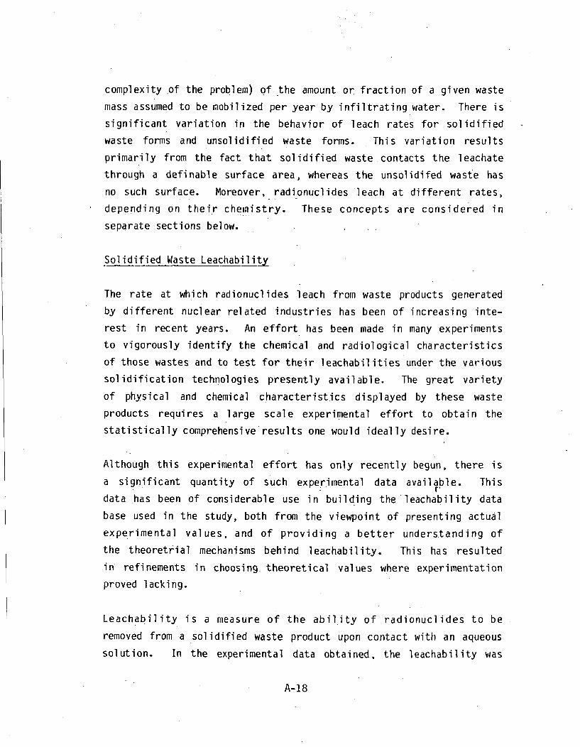
complexity of the problem) of the amount or fraction of a given waste

mass assumed to be mobilized per year by infiltrating water. There is

significant variation in the behavior of leach rates for solidified

waste forms and unsolidified waste forms. This variation results

primarily from the fact that solidified waste contacts the leachate

through a definable surface area, whereas the unsolidifed waste has

no such surface. Moreover, radionuclides leach at different rates,

depending on their chemistry. These concepts are considered in

separate sections below.

Solidified Waste Leachability

The rate at which radionuclides leach from- waste products generated

by different nuclear related industries has been of increasing inte-

rest in recent years. An effort has been made in many experiments

to vigorously identify the chemical and radiological characteristics

of those wastes and to test for their leachabilities under the various

solidification technologies presently available. The great variety

of physical and chemical characteristics displayed by these waste

products requires a large scale experimental effort to obtain the

statistically comprehensive results one would ideally desire.

Although this experimental effort has only recently begun, there is

a significant quantity of such experimental data available. This

data has been of considerable use in building the leachability data

base used in the study, both from the viewpoint of presenting actual

experimental values, and of providing a better understanding of

the theoretrial mechanisms behind leachability. This has resulted

in refinements in choosing theoretical values where experimentation

proved lacking.

Leachability is a measure of the ability of radionuclides to be

removed from a solidified waste product upon contact with an aqueous

solution. In the experimental data obtained, the leachability was

A-18

most commonly sought for univalent, divalent, and trivalent radio-

nuclides, most commonly represented by cesium, strontium, and cobalt,

respectively. Investigations included waste forms solidified by

agents such as vinyl ester styrene, cement, urea formaldehyde, bitu-

men, polyester, and polyethylene.-

There is a large body of "leach rate" data from several nations using

a variety of experimental methods.(131 5 ) Attempts at standardization

of experimental methodology and reporting of information have only

recently been initiated.( 1 3 )- In this report, L(t), which is defined

as the leached fraction of activity per year corrected for waste

shape, is presented here as given in reference 13:

L(t) = [Z.an/Ao] x [V/S] (A-8)

where:

a = leached activity after (n) time periodsn

A = total activity in the waste0.

V = volume of the waste (m3 )

S = surface volume of the waste (i )

The experimental results are, for the most part, presented in the

form of a graph with the absissa plotting time (t) ana the ordinate

recording L(t). The value (V/S) was employed in an effort to provide

leach rate measurements which are independent of specimen size

and geometry.

Data presented in this manner, following the recommended IAEA pro-

cedures, implies the use of the semi-infinite model from diffusion

mass transport theory. When expressed in this manner, the fractional

activity released for specimens of different sizes and geometries is

determined by using the relation:

A-1 9

[Ean/Ao]I x [V/S 1 = [Zan/Ao]1 x [V/S] 2 (A-9)

It has been shown that the cumulative fraction leached from a sample,

when plotted against time (t), is approximately linear for large t,

but not very linear, in a number of cases, for small t. It was found

that going beyond the linear to the fifth degree polynomial gave a

better fit for the time period considered, in this case one hundred

days. The resultant equationhas the form:

L(t) = Ao+ Alt0.5+ A2t+ A3t15+ A4t2+ A5t 2.5 (A-10)

Although this equation gives a good fit to experimental data at times

up to 100 days, the usual limit of experiments, it is not able to

predict values of leach rate L(t) consistent with in-situ measurements

of leachate concentrations. The values obtained after correcting for

actual waste geometries using equation (A.2-2) are frequently above

the upper bounds for unsolidified wastes derived from leaching data

obtained from Maxey Flats disposal facility (see Section A.4.2).( 1 5 )

Such discrepancies are probably due to the very large number of

independent- parameters that affect leachability and that cannot all

be controlled under simulated conditions. For example, the IAEA

procedure specifies that distilled or deionized water be used as the

leachant, that the ratio of the sample volume to surface ratio be

about 10 cm, and that the entire leachate volume be replaced peri-

odically. Moreover, there is no procedure to quantify the effects of

partially saturated conditions, which are more likely to be mechanisms

foF leaching.

In this report, experimental leachate/waste concentration ratios

derived in the following section for unsolidified wastes are utilized

to estimate the leachability of solidified wastes. A correction

factor derived from laboratory experiments, however, is applied to

account for the lower leachability of solidified wastes.

A-20

Unsolidified Waste Leachability

In view of the variable physical and chemical characteristics of

the waste, (13-14) the variable chemistry of the in-situ waste/soil

mixture,(15) and the variability of long-term conditions (e.g.,

bacterial action), theoretical or experimental tools available to

predict the leachability of unsolidified waste after it has been

disposed of cannot be considered reliable. For the solidified case,

at least the properties of the waste form (e.g., porosity, chemistry,

etc.) can be predicted with some reasonable degree of confidence.

However, for the unsolidified case, even this partial knowledge does

not exist. Therefore, in this report, the leach rates from unsoli-

dified waste streams are not calculated directly. Instead, a radio-

nuclide specific average leach fraction is calculated which is the

ratio, assuming totally saturated conditions, of the concentration

of a radionuclide in the leachate to the concentration of the radio-

nuclide in the waste. This leach fraction may then be multiplied by

the fraction of a year that infiltrating water contacts the waste.

In this report, the average upper bounds of the unsolidified waste

leach fraction, henceforth denoted by Mo, are estimated assuming

that the leachate/waste conditions at the existing Maxey Flats and

West Valley disposal facilities, can be used to approximate this

fraction. The reason these facilities have been selected is because

a considerable amount of data exists on these disposal sites and the

trenches are known to have been inundated for a considerable number

of years. Furthermore, a recent work( 3 6 ) on Maxey Flats leachates

has indicated that plutonium exists as a dissolved species (primarily

as complexes of the tetravalent ion with strong organic ligands such

as EDTA) and that the complexes are not sorbed well by sediment and

are only partially precipitated by ferric hydroxide. Average radio-

nuclide concentrations in the trench leachate( 1 8 ) and in the disposed

waste(1 9 ) for the Maxey Flats disposal facility for H-3, Co-60, Sr-90,

Cs-137, Pu-238, Pu-239, and Am-241 are presented in Table A-i.

A-21

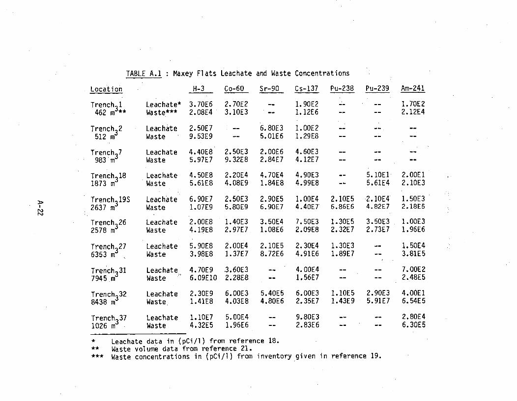
TABLE A.1 : Maxey Flats Leachate and Waste Concentrations

!

Location

Trench3 1462 m **

Trench3 2512 m

Trench 3 7983 m

Trench 3 181873 m

Trench019S2637 m

Trench 262578 m3

Trench 3 276353 m

Trench3 317945,m

Trench3 328438 m

Trench3 371026 m -

Leachate*Waste***

LeachateWaste

3.70E6 2.70E22.08E4 3.10E3

-- 1. 90E2-- 1. 12E6

-- 1. 70E 2-- 2. 12E4

2.50E79.53E9

-- 6.80E3 1.00E2-- 5.01E6 1.29E8

Leachate 4.40E8 2.50E3 2.00E6 4.60E3Waste 5.97E7 9.32E8 2.84E7 4.12E7

Leachate 4.50E8 2.20E4 4.70E4 4.90E3Waste 5.61E8 4.08E9 1.84E8 4.99E8

-- 5.1OE10 2.OOE1-- 5.61E4 2.10E3

LeachateWaste

6.90E7 2.50E3 2.90E5 1.00E4 2.10E5 2.10E4 1.50E31.07E9 5.8OE9 6.90E7 4.40E7 6.86E6 4.82E7 2.18E5

H-3 Co-60 Sr-90 Cs-137 Pu-238 Pu-239 Am-241

Leachate 2.00E8 1.40E3 3.50E4 7.50E3 1.30E5 3.50E3 1.00E3Waste 4.19E8 2.97E7 1.08E6 2.09E8 2.32E7 2.73E7 1.96E6

Leachate 5.90E8 2.00E4 2.10E5 2.30E4 1.30E3Waste 3.98E8 1.37E7 8.72E6 4.91E6 1.89E7

-- 1.50E4-- 3.81E5

-- 7. OOE2-- 2.48E5

Leachate 4.70E9 .3.60E3Waste 6.09E10 2.28E8

-- 4.00OE4-- 1. 56E7

Leachate 2.30E9 6.00E3 5.40E5 6.00E3 1.10E5 2.90E3 4.OOE1Waste. 1.41E8 4.03E8 4.80E6 2.35E7 1.43E9 5.91E7 6.54E5

Leachate 1.10E7 5.00E4Waste 4.32E5 1.96E6

-- 9.80E3-- 2.83E6

-- 2.80E4-- 6. 30E5

* Leachate data in (pCi/l) from reference 18.

** Waste volume data from reference 21.*** Waste concentrations in (pCi/l) from inventory given in reference 19.

To calculate the average waste concentrations, the fraction of the

waste labeled "mixed fission products" or "unidentified radionuclides"

have been conservatively ignored. For cobalt, several of the ratios

are unrepresentatively low, and have been conservatively discarded

assuming that they represent disposal trenches containing a signifi-

cant amount of sealed sources. The remaining ratios have been geo-

metrically-averaged to obtain the leachate-to-waste concentration

ratios presented in Table A-2.

For tritium, the ratio turned out to be higher than unity; this value

is reasonable considering the relative mobility of tritium. For

example, if 250 cm3 of water contacted 1000 cm3 of waste with an

effective porosity of 0.25 and leached all the tritium, this ratio

would have been 4.0. Furthermore, if the same leachate contacted

other unleached waste and leached some more H-3, the ratio would be

even higher.

For carbon-14 and uranium-238, Maxey Flats trench leachate data is not

sufficient for a similar calculation. For these nuclides, leachate

data obtained from the West Valley disposal facility is used.( 20 )

However, U-238 concentrations in West Valley waste could not be

determined from the existing information. For U-238, waste concen-

tration data from the Maxey Flats disposal facility is conservatively

used to obtain the ratios. These data and calculations are presented

in Table A-3.

These calculated ratios have also been used to estimate M for other

radionuclides for which the data is insufficient to calculate similar

ratios. It is assumed that the iodine and the technetium values are

10 percent of the tritium value, that nickel and iron are chemically

similar to cobalt, that the niobium value is 75% of the cobalt value,

and that neptunium and curium are chemically similar to plutonium.

The resulting ratios utilized in the impact calculations are presented

in Table 3-8.

A-23

TABLE A.2 : Maxey Flats Leachate/Waste Ratios and Averages

Location

Trench 1

Trench 1S

Trench 7

Trench 18

Trench 19S

Trench 26

Trench 27

Trench 31

Trench 32

Trench 37

H-3

1. 77E+2

2. 62E-3

7.37E+O

8.02E-1

6.45E-2

4. 77E-1

1.48E+O7. 72E-2

1.63E+1

2. 55E+1

C

8.

2.

5.

4.

4.

1.

o-60 S

70E-2-- 1.

68E-6* 7.

39E-6* 2.

31E-7* 4.

71E-5* 3.

46E-3 2.

r-90 Cs-137

-- 1.69E-4

36E-3 7.75E-7

04E-2 1.12E-4

55E-4 9.82E-6

20E-3 2.27E-4

24E-2 3.59E-5

41E-2 4.68E-3

-- 2.56E-3

13E-1 2.55E-4

-- 3.46E-3

Pu-238

3. 06E-2

5. 60E-3

6.88E-5

7. 69E-5

Pu-239 Am-241

8.02E-3

9.

4.

1.

4.

09E-4 9.52E-3

36E-4 6.88E-3

28E-4 5.10E-4

-- 3.94E-2

-- 2.82E-3

91E-5 6.12E-5

-- 4.44E-2

1. 58E-5*

1.48E-5*

2. 55E-2

1.

Average : 1.15 1.48E-2 9.86E-3 1.62E-4 ** 4.67E-4 4. 11E-3

* These low ratios were neglected, probably due to sealed sources.

** Pu-238 ratios were counted in the Pu-239 average.

TABLE A-3 . C-14 and U-238 Leachate/Wastea

Concentration Ratios

Leachate

Nuclide

C-14

Averages

Trench

WV 1-2

WV 3

WV 4

WV 5

WV 1-2

WV 3

WV 4

WV 5

(PCi/ml)b

1.27E-6

1.16E-6

1.38E-6

3.91E-5

2.48E-9

1.47E-9

5.77E-9

1.63E-7

Volume_ m_3 L

4800

5626

7771

7890

Trench

MF 7

MF 18

MF 19S

MF 26

MF 27

MF 31

MF 32

Waste

Inventory

(Ci)

1

5

8

3

(Oci/ml)

1.63E-4

1.06E-4

8.36E-5

7.94E-6

1.54E-5

9.32E-5

2.07E-4

6.11E-5

Ratio

6. 1OE-3

1.31E-3

1.34E-3

1.03E-1

5. 76E-3

1.25E-4

U-238

Averages 7.65E-9

(a) WV = West Valley Disposal Site, MF =

(b) Leachate concentrations are averages

(c) Source : References 18, 19, and 20.

Maxey Flats Disposal Site.

of several sumps.

A-25

The primary' rationale for this approach is that under specified

chemical conditions there is an upper limit to the solubility of all

elements. Moreover, several investigators feel that the use of Maxey

Flats leachate data is -the best that can be done with the available

experimental data. (3)

However, in order to use these calculated ratios, transient and

partially saturated conditions likely to exist in properly designed

trenches must be considered. It is unlikely that conditions existing

in Maxey Flats or West Valley trenches will be permitted to develop in

the future. Therefore, these ratios have been modified by the "contact

time fraction", denoted by tc, before application to groundwater

migration calculations in this work.

Several time dependent leaching experiments on solidified waste

samples have been performed.( 1 4 1 6 ) The results of these experiments,

however, appear not to be applicable to partially saturated conditions

since all the experiments were performed with complete inundation of

the samples. There is no data to indicate the behavior of leaching

under partially saturated conditions. Assumption of linear depend-

ence is one of the viable ways to approximate this behavior (first

order approximation). The linear dependence assumption means that tile

above ratio should be multiplied by the fraction of time the wastes

may be assumed to be in contact with water under fully saturated

conditions. In other words, the factor t is estimated from theC.

following formula (see Section 3.5.1):

t = p/(nv)

where p is the percolating water in meters/year that infiltrates and

comes into contact with the waste, n is the effective porosity of the

disposal cell, and v is the speed of the percolating water in meters

per year. This equation means that the contact time fraction is the

fraction of a year the percolating front (in a continuous mass) takes

to pass through a horizontal plane in the disposal cell.

A-26

A.2.2 Groundwater Migration

A detailed groundwater migration model is described in reference

22. This reference considers both saturated and unsaturated zones and

time dependent migration in three dimensions. One of the dimensions

(longitudinal - in the direction of the hydraulic velocity) is

treated exactly and the other two dimensions (transverse - perpendi-

cular to the direction of the hydraulic velocity) are treated through

an approximation called the "time-independent transverse dispersion"

approximation. The models and equations presented in this reference,

however, are too complicated for utilization in a generic study.

Therefore, a simplified one-dimensional migration model is formulated

and developed based on the formulae presented in reference 22.

A general geometry of the migration problem is presented in Figure

A.4. The most significant concept presented in this figure is that

the migration problem has been formulated in terms of the relationship

of the fluxes at the source and at the access location, rather than

concentrations. This formulation is easier to handle and more mean-

ingful in terms of calculating impacts. Based on this figure the

following relationship is applicable:

J(x,t) = rg rt Jo (A-Il)

where J(x,t) and Jo are the radionuclide fluxes in units of Ci/year

at the discharge surface and the source, respectively, and rg and

rt are dimensionless reduction factors. The reduction factor rg

expresses the reduction due to the geometrical relationship of the

source and the access location, while rt expresses the reduction due

to migration and decay.

* The above definition of flux is sometimes referred to as the 2 total

flux, in addition, "flux" is sometimes given in units of Ci/m -yearwhich is sometimes referred to as the differential flux. Thisreport will refer to the above defined variable as the flux inunits of Ci/year.

A-27

"oGO

SATURATED ZONE PARAMETERS:V, X, Rs,

S vD5DX y z

'-n-

irl

I

nlI GEOMETRY OF GROUNDWATER MIGRATION30a

The factor r is time-independent ana depends only on the geometricalgrelationship of the access location and the source. The factor rt,

however, depends both on space and time, including the duration of the

source term, henceforth called T. The combined factor (rgrt) quan-

tifies the effects of the intervening medium between the source and

the access location.

The time dependent concentration C(x,t) at the access location in

terms of the flux is:

C(x,t) = J(x,t) / Q (A-12)

where (Q) is the dilution factor in units of volume/time. It may be

the pumping rate of a well, or the flow rate of a river.

One-dimensional geometry is consiaered in this report to calculate the

factors rg and rt. This geometry is presented below:

o Properties : R,D J

x=U x

The general solution to this problem is obtained in reference 22 using

a Green's Function approach.( 23 ) Using this approach, first the

solution of the problem for a unit delta function source term is

obtained. (23) This solution (Green's Function of the problem) is

given by the following expression:

erc x +v(t-t')/R (A-13)

F(x,t~t')=-exp[-?d~t-t.)+_- VL~ xp [)______(A_13)g 2 ax I 2D ID__ t _______

A-29

Using this function, the flux J(x,t) at any point and time can be

calculated by evaluating the following expression:( 2 2 )

t

J(x,t) = (v - D fFg(x,t,t')do(t')dt' (A-14)

0

In this report the source term, J (t'), is assumed to be given by

the following:

J = U(T-t') S0 exp(- At') (A-15)

where U(t) is the unit impulse function that is unity for a positive

argument and zero otherwise., and A is the decay constant of the

radionuclide. The expression given in the above equation (A-14) can

be evaluated to yield:( 2 2 )

J(x,t) = S0 exp(- At) [F(t) - F(t-T)] (A-16)

where:

F(t) =0.5 U(t) [erfc(X+) + exp(P) erfc(X_)] , (A-17)

X+ 2-t and (A-18)-2 V/t/(Rt wj)

x

erfc(x) = I - f (2/VIT) exp(-t 2) dt (A-19)

0

This solution may be generalized for multiple dimensions or for

heterogeneous media. Heterogeneous media implies time dependence of

the variable x and time and space dependence of the variables v, D,

and R. The following expressions may be used to obtain space and time

independent parameters. (22)

A-30

1 TT x(t)dt (A-20)

T

v(x) v(x,t)dt (A-21)T

1 1 X dx (A-22)

[v] X f V(x)

[RI = [v] X R(z) dx (A-23)X f V(x)x 0j

where x, [v], and [R] represent time and space averaged parameters

(the parameter D, the dispersion coefficient, is handled in a manner

identical to v), and (x) and (t) are the space and time variables,

respectively. The averaging is performed over a sufficiently long

time (T) and sufficiently large space (X) to take into account all the

significant variations of these parameters.

A.2.3 Percolation

The amount of water infiltrating through the trench covers and con-

tacting the waste is a basic parameter required for the groundwater

migration calculations. This section presents the assumptions uti-

lized in this work.

There are several techniques for calculating the infiltrating compo-

nent of precipitation (also called PERC in several references). One

of these methods is the "water balance method" introduced by Thorn-

thwaite( 2 4 ) and developed by Fenn, et.al.( 2 5 )" This method has been

applied successfully to many site-specific problems. (22) However,

one of the most crucial parameters in this calculation is the maximum

soil moisture capacity (SM). This parameter is primarily a function

A-31

IL

o0 the. ve4etat on root zone thickness, and .the Vmount0 f•percolation"d ncreasnq maxtmum,' soil soisture capacfty. Moreoverdecreases w ith, inc i .,"'i " -J M-thtis. method dots not explictly consider, tOhydrau.1c propertesfthe substrata 'Use of the water tbalance method aT'so dos not diret1 ,y

allow consideration of the effect of potential, use of low-permeabiltybarrier.s against (;.'io termed bpercolation •barr, ers.: or• moisture barriers").

Another,- possible technique tO"cilCulate, PERCs-the .adoption of an,

unsaturated zone-.water. transport 'model that ,;considehrs, rthe ,,PgraVita-tional, ,capillary.1, osmotic and chemical'potentials. In this report-'.primarily due to the generic nature of the work, it was decided toadopt a more practical approach in the determination of the percola-tion component. .a, , .

For the cases where waste cover integrity cannot be assumed, which may, ..be either due to waste form instability or simpler design measuressuch as a minimum cover over the waste or no trench stabil.izationprogram, water balance calculations will be utilized to determine the.percolation component., Water-balance calculations typical ,of siteslocate in our. differ~ent regions• of t e country (northeast south-aeast, midwst, and southwest) are given in Tables A4 and A-5. Forthe four regions -of concern, these calculations lead to a percolatio-ncomponent of' 74 inm for the northeast,. 180 mm for the southeast. 50 mmu

a dwest',and, yaiaa fo afor the.midwest,,. andO 0m for the southwestern .locations (see Appendixay 'we' ita a rc'a I DuIa t ia o aa ai a a aed', C)." However• for.acalculational purposes, a value of 1 .u ismassumed, -

for the southwestern location. These values are used in the impact,.-analyses. .,

For the cases where there exists engineered trench covers including.percolation barriers such as low permeability cl-ay layers-and wherethe integrity of these covers may be assumed (e~g., the .wastes under"-neath are -stable) it will be assumed that the percolation componentis determined by the Darcy velocity of the least permeable stratum

.-'7 7- 77:"0 V:,

. .N-/

t "•. ; • •

_a", r: a,. a " ,r'a :

.. a .a f * ~ a a • . - . . . • .- -4 .

* ";

-"4ABLEA-4:1 W4 ter Balance AalyiData and Assumptions

Legend: All units in (m of water) except 'for

. , whichis dimens10.lesst. . ,.

* .:.. k * ma ,:mv SqiI Aoi~stureStorage

P- -Precipitation

SC, -,4;' 0Sur~fac 'Runoff Cofjficent

R ý.:" ,,Surface, Runoff " . ."

I InfiltrationPET a Potential Evapotranspiration

1..ET D~fferencei btI een CI) and (PET)

SoilS =C l ative suam of negati~ve, (-PET) ,,, ..

.. .S, Sojl+Moisture Storage.

45 -+-Change. In Soil MoIs.ture Storage

AET - Actual Evapotranspi ration....,

-PER. Jo '- Percolation Into Groundwater System

,Assumptions:

* ru rpresefitative lcto(4P: ET+. *• Datfromu representative location o 4 1 .

C -Estimated for eah, Mrgon based on •,

soil description ;and reference 11. *.

1 For humia ,sites. assumed WO m ani , V,

for. arid site assumed 50 Ml..

Calculations: Follows in Table A-b.

A-33;"' M( .

TABLE-A-5 : Detailed Water Balance Calculations

NORTHEAST REGION : SM 100 N m

J F M A M J J A S 0 N D

P 71 -65 73 72 92 110 114 110 92 86 78 71C .20 .20 .20 .20 .15 .15 .15 .15 .15 .18 .20 .20

R 14 13 15 14 14 16 17 16 14 15 16 14

I 57 52 58 58 78 94 97 94 78 71 62 57

PET 0 0 0 28 77 111 129 110 75 38 6 0

I-PET 57 52 58 30 1 -17 -32 -16 3 33 56 57

CNS 417 -49 -65

S 214 266 324 100 100 84 60 51 54 87 100 157

dS 57 52 58 0 0 -14 -24 -9 3 33 13 57

AET 0 0 0 28 78 108 121 103 75 38 6 0

PERC 0 0 0 30 1 0 0 0 0 0 43 0

SOUTHEAST REGION : M : 100 mn

J F M A M J J A S 0 N D

P 80 100 96 84 82 102 149 -147 103 64 77 81

C .14 .14 .14 .14 .14 .12 .12 .12 .12 .12 .14 .14

R 11 14 13 12 11 12 18 18 12 8 11 11

I 69 86 83 72 71 90 131 129 91 56 66 70

PET 13 15 37 65 115 158 172 157 114 64 29 13

I-PET 56 71 46 7 -44 -68 -41 -28 -23 -8 37 57

CNS -44 "112 -153 -181 -204 -212

S 100 100 100 100 64 32 21 16 12 11 48 100

dS 0 0 0 U -36 "32 -11 -5 -4 -1 37 52

AET 13 15 37 65 113 147 162 151 107 63 29 13

PERC 56 71 46 7 0 0 0 0 0 0 0 0

A-34

TABLE A-5 : (continued)

MIDWEST REGION M : I00 mm

J F M A M J J A S 0 N D

P 21 23 36 73 108 108 94 91 101 64 33 25

C .15 .15 .15 .15 .13 .10 .10 .10 .10 .13 .15 .15

R 3 3 5 11 14 11 9 9 10 8 5 4

I 18 20 31 62 94 97 85 82 91 56 28 21

PET 0 0 6 43 88 127 147 131 86 44 7 0

I-PET 18 20 25 19 6 -30 -62 -49 5 12 21 21

CNS -30 -92 -141

S 101 121 100 100 100 74 39 24 29 41 62 83

dS 18 20 0 0 0 "26 -35 -15 5 12 21 21

AET 0 0 6 43 88 123 120 97 86 44 7 0

PERC 0 0 25 19 6 0 0 0 0 0 0 0

SOUTHWEST REGION SM : 50 mm

J F M A M J J A S 0 N D

P 6 10 20 48 71 79 64 72 37 45 19 14

C .10 .10 .10 .10 .10 .10 .10 .10 .10 .10 .10 .10

R 1 1 2 5 7 8 6 7 4 4 2 1

I 5 9 18 43 64 71 59 65 33 41 17 13

PET 1 4 21 47 86 129 154 136 95 49 15 0

I-PET 4 5 -3 -4 -22 -58 -95 -71 -62 -8 2 13

CNS "3 -7 -29 -87 -182 -253 -315 -323

S 20 25 23 20 14 8 3 1 1 1 3 16

dS 23 9 -2 -3 -6 -6 -5 -2 0 0 1 18

AET 1 4 20 46 70 76 64 67 95 41 15 13

PERC 0 0 0 0 0 0 0 0 0 0 0 0

A"35

between the waste and the atmosphere. The Darcy velocity of a mate-

rial, with hydraulic conductivity (K) in units of m/yr and unit

hydraulic gradient (the most conservative assumption), is equal to K

m3/m 2-yr. This number, however, should be modified by the fraction

of each year during which there is at least 0.01 inch of precipita-

tion. Therefore, (p) may be calculated from the following equation:

p = K (w/365) (A-24)

where (K) is the hydraulic conductivity of the least permeable layer

between the atmosphere and the waste, and (w) is the mean annual

number of days with 0.01 inch or more of rainfall (see Figure A.3).

For the four regions of concern the above discussion was used as a

guide to determine the percolation component through an engineered

disposal cell cover containing moisture barriers. The following

percolation values were assumed: 38 mm for the northeast, 30 mm for

the southeast, 25 mm for the midwest, and I mm for the southwestern

locations. These values are used in the impacts analyses.

A.2.4 Surface Water Erosion

This section describes a model which may be used to predict the

rate of loss of trench cover via sheet erosion for various regions

and design parameters (material, length, slope, etc.). This model

is based on the Universal Soils Loss Equation (USLE) developed by

W. H. Wishmeier and his colleagues(26) and has been used extensively

in the past 20 years to estimate sheet erosion for agricultural lands.

Recent work has been performed to apply a modified form of this

equation to the control of erosion during highway and other construc-

tion sites.(27) The equation is semi-empirical and may be used to

estimate erosion of the trench covers or general erosion of the area

surrounding the trenches. The equation, its parameters, and an example

of its use follows. The USLE is usually stated as:

A-36

A = R x K x LS x VM (A-25)

where:

A = The computed soil loss in tons/acre per year. This quantity may

be converted to cubic meters using selected conversion factors.

R = The rainfall intensity factor, which is a measure of the erosion

force of rainfall.

K = The soil erodibility factor, which is highly regional and varies

from a low of 0.10-0.20 to a high of 0.37"0.49.

The next two parameters are of importance as they may be varied to

control and minimize erosion:

LS = The topographic factor, which is a measure of the effect of

lengths and steepness of slopes on the soil loss per unit area.

VM = The erosion control factor, which is a function of all erosion

control measures such as vegetation, mechanical manipulation of

the surface, chemical treatments, etc. For bare slopes VM=1.

For multiple slopes (as is the case here), the factor LS can be

calculated using the following formula:

n m+J m+l1

LS =1 - rk1 (1-6 ) CoS 2 k (A-2X e )-(72"6)mk r= r 1rl

k=1 r=

where: n

.6)

Xe = • 1 r

r=1

r= length of the (r)th segment

n = number of segments

(A-27)

A-37

1r ý= Kronecker delta for segment (1).

0 k = Angle between the (k)th segment and the horizon

Sk = (0.43+30 sinek + 430 sin 2 Ok)/6.574 (A-28)

Mk = 0.3 for Ek < 0.290

= 0.5 for 0.29' < Ek < 5.70

= 0.6 for 5.70 < Ek

An illustrative example of the calculation and the use of the LS fac-

tor equation (A-26) is given below. This calculation is not related

to the reference case (see below), but is provided to illustrate the

concepts introduced. The example is based on Figure A.5.

This figure represents an idealized trench cover cross section. The

maximum height is 10 m (32.8 ft). Two segments comprise the slope

with lengths of 10 m (196.9 ft) and 20.6 m (65.6 ft) and horizontal

angles of 1.72' and 140 respectively. Substituting these parameters

in the equation leads to an LS factor of 4.19. Assuming an average

erodability index of 0.28 and a rainfall intensity factor of 20 leads

to a erosion potential of 82 tons/acre-yr.

It should be noted that this calculation is for bare slopes with the

configuration as depicted in Figure A.5. This calculalion would have

to be repeated each time the configuration changed.

For long-term stability the last remaining factor VM in the USLE

equation (A-25) must be considered. By a judicious choice of ground

cover such as grass or rip rap, a reduction in the estimated soil loss

per acre to less than one-percent of the value calculated can easily

be attained. For example, assuming the VM is 1 percent, the erosion

potential of the example case becomes 0.82 tons/acre-yr. Assuming a

topsoil density of 100 lbs/ft 3 leads to a loss of 3.76 x 10-4 ft/yr

A-38

81 =1 .720

02=14.0°

1=60m (196.9FT.)

L2 =20.6m (65.6FT.)

GEOMETRYOF, THE MASS TRANSPORT PROBLEM -

SURFACE WATER EROSION SCENARIO

A- 39 FIGURE A.5

A- 39 FIGURE A.5

or 1.15 x 10- 2 cm/yr. Thus the type of final cover is quite critical

in preventing sheet erosion.

Prediction-of long-term erosion based on empirical and/or theoretical

equations cannot help but be speculative. For example, the above case

leads to a--calculated complete erosion of-one meter of disposal cell

cover in about 8700 years.' It is not sensible to rely on predictions

that depend on numerous uncontrollable factors that far into the

future. As stated previously in Section 3.6, for the erosion sce-

narios in this work, it will be assumed that the soil will be eroded

at a rate of about one meter per 1000 years. The above equations and

estimates, however, will be used to estimate the transfer factors.

Based on the above estimated soil loss of 0.82 tons/acre per year,

the soil/waste mixture mobilization rate E (see Section 3.6) can be

calculated to be 1.84x102 g/m -yr.

A-40

A.3..-Other Transfer Factors

This section considers several other transfer factors outlined in

Figure A.1, namely the air-to-air transfer factor, air-to-soil trans-

fer factor, and water-to-soil transfer factor.

A.3.1 Air-to-Air Transfer Factor

This section considers the atmospheric dispersion equations which can

be used to calculate the air-to-air transfer factor applicable to

chronic release scenarios. This is utilized to calculate population

exposures resulting from waste incineration and the exposed waste

scenarios. To determine population exposures from waste incineration,

generic population distributions for four U.S. regions have been

assumed and are given in Appendix C. To account for potential future

population growth, the population is assumed to be multiplied by 2 for

the intruder-initiated exposed waste scenario, and by 3 for the

erosion-initiated exposed waste scenario.

The assumption of a generic population distribution (population does

not depend on the direction from the source point) is calculationally

equivalent to the assumption that all wind directions are equally

likely. For site specific data, this assumption would have to be

modified. The transfer factor applicable to this source term, as-

suming ground-level release and sector-spread (22.50 sectors) dis-

persion, is: (28-29)

f = 2.032/(16az-ur) (A-29)s z

where:

O = vertical standard deviation of the plume (m).

u= wind speed, in (m/sec).

r = distance from the release point, in (m).

A-41

The vertical standard deviation of the plume ( a ) is given as azfunction of distance (r) and stability class in many references.

One form for this factor is:(7)

o = (ar)(l+br)c (A-30)

where r is the distance from the release point, and where a, b, and c

are constants that depend on the stability class. Assuming that (see

references 30 and 31) the wind is equally divided between Pasquill

Stability classes C (wind speed 3 m/s), D (wind speed 3 m/s), and F

(wind speed 2 m/s), the calculation yields.

fs= 4.156E-8 x (r- ) x q(r) (A-31)

where:

q(r) = [0.133 V/l+.0002r + 0.178 v'1+.0015r + I +.0003r ] (A-32)

where (fs) is in units of (yr/m3 ) and (r) is in units of meters.

A.3.2 Air-to-Soil Transfer Factor

Radionuclide-bearing airborne particulates can deposit on the ground

as a result of gravitational settling of the particles. Ti'Hs "fallout

deposition" results in soil contamination and must be accounted for in

human exposure pathways that involve contacting or use of soil (e.g.,

to grow food)o The transfer factor to be used in obtaining soil

radioactivity based on airborne particulate concentrations is derived

in this section.

The air-to-soil fallout deposition transfer factor can b.2 given as:

Ta = Cs/Ca (A-33)

A-42

rIII, I'P( .

T as= the air-to-soil transfer factor (dimensionless)

Cs = the soil-concentration, in (Ci/mr3 )Ca = the total air concentration, in (Ci/m3)

1he soil concentration will be dependent upon the deposition

r.ite and can- be given as:

Ds = CapVp (A-34)

where:-2 -1Ds = deposition rate, in (Ci.m .sec-3

.C ap= air concentration of particle size (p), in (Ci/mr)

Vp = deposition velocity r(m/sec) of particle size (p).

where Ca is defined as the sum of Cap over all (p). The deposition

velocity can be given for two-ranges of particle sizes, such that 1 um

to 10 um particles (5 um mean diameter) have a deposition rate of

0.010 m/sec, and 10 um to 80 um particles (35 um mean diameter) have a

deposition rate of 0.0882 m/sec. Using a normalized direct air

concentration of I Ci/m3 , (D s) is therefore calculated to be 0.098

Ci/(m2-sec).

The soil concentration over a period of time can be calculated from

the formula:. 3 2 )

Cs (D s/d) (1 - exp[-(.Xe+ X)t])/( Ae+ + ) (A-35)

where.

Cs the soil concentrations, in (Ci/m3)Ds the deposition rate, in (Ci/m2 -sec)d = depth of mixing, in (m). This parameter is usually

taken as the depth of the soil-root zone.

X J the radioactive decay constant, in (1/sec)

=e = effective removal constant, in (1/sec)

t = the time interval of deposition, in (sec)

A-43

The effective environmental removal constant accounts for removal by

downward migration in soil, removal by surface water runoff, and loss

due to chemical binding. It is calculated from an assumed half-life

in soil of 50 years.( 3 2 ),

A.3.3 Water-to-Soil Transfer Factor

Irrigation of crops with contaminated water will result in increased

radionuclide concentrations in the recipient soil. The radionuclides

will then be available for plant uptake via soil-to-root transfer.

The soil contamination resulting from irrigation must therefore be

accounted for by a transfer factor for this mechanism. The applicable

equation is:

Tws cs/Cw (A-36)

where (Cs) and (Cw) are the soil and water concentrations, in (Ci/m ).s wThe soil concentration will be directly dependent upon the irrigation

rate concentration (D) which is given by:

D = Cw I (A-37)

where:

D = the surface area contamination rate, in (Ci/mr2 -day)

I = the irrigation rate, in (m3 .m' 2 .day-)

Cw = the water concentration, in (Ci/m 3)

The subsequent soil concentration (C ) dependent upon (D) over time

(t)M, will be obtained by-t 3 2 )

Cs(t) = (D/d) (1 - exp[-(Xe+ X )t])/( X e+ A) (A-38)

where:

A-44

Cs (t) = the soil concentration, in (Ci/m 3 ) .

d = depth of mixing (see Section A.3.2)

X= the physical decay constant, in (1/day)

X = the-effective removal constant, in (1/day)et = thetime over which irrigation occurs, in (day)

The effective removal constant may be calculated from an assumed

half-life of 25 years (see Appendix B). This constant accounts for

removal of contamination due to such processes as wind erosion,

chemical binding and leaching, and other variables.

Variables such as irrigation rate, climatic conditions, and soil

characteristics are only a few of the variables which need considera-

tion. The irrigation rate may be dependentupon the crop, (e.g.,

wheat needs less irrigation than rice), the climatic conditions and

the geographic location. For example, the Midwest wheat fields will

need more irrigation during a hot, dry period than will western citrus

groves during periods of optimal temperatures and rainfall. Also,

variations in soil characteristics can influence the irrigation rate.

A porous soil, for example, will retain more water than a nonporous

one, thus reducing the frequency of irrigation. These individual

characteristics are accounted for in the effective removal constant

(xe). The irrigation rate will, however, be the deciding factor in

the calculation of soil concentration.

A-45

A.4 Direct Radiation Exposures

Intruders inhabiting a site may receive chronic radiation doses as

a result of direct exposures to alpha, beta, and gamma rays emitted

by the waste (the term "gamma rays" as used here means gamma rays,

x-rays, and bremsstrahlung). The most important of these radiations

is gamma rays since alpha and beta rays have extremely short ranges.

External exposure to alpha rays is not considered in this appendix.

Beta rays are considered, however, in determining exposures resulting

from human immersion in air containing suspended radioactivity, and

exposures resulting from standing on surface contaminated ground (see

Appendix B). Only gamma rays are considered in this section and for

determining exposures resulting from standing on soil that is homo-

geneously contaminated. The exposures experienced depend on factors

such as source strength, gamma ray energies, self-shielding effects of

the waste form and packaging, thickness of covering over the waste,

and geometry of the exposure.

The intruder scenarios postulated in Sections 2.0 and 3.0 of the

report involves a person living on top of the waste disposal site.

The actual geometry of the situation may be complicated but as a

first-order approximation is considered to be represented by a homo-

geneous mixture of waste and soil extending horizontally and downward

to infinity (i.e., an infinite slab source). The exposure can then be

calculated based on this geometry, or estimated empirically by mea-

surements taken over a simulated source.

The method used here to estimate exposure rates is empirical. The

exposure rate measurements were made above soil uniformly contaminated

with a variety of radionuclides.(33) The exposure rate per unit of

source activity was plotted versus gamma energy (see Figure A.6) and

the graph was used to directly obtain the exposure rate for a given

radionuclide based on the average energy of its gamma emissions.

Build-up of the exposure rate within the source is intrinsically

A-46

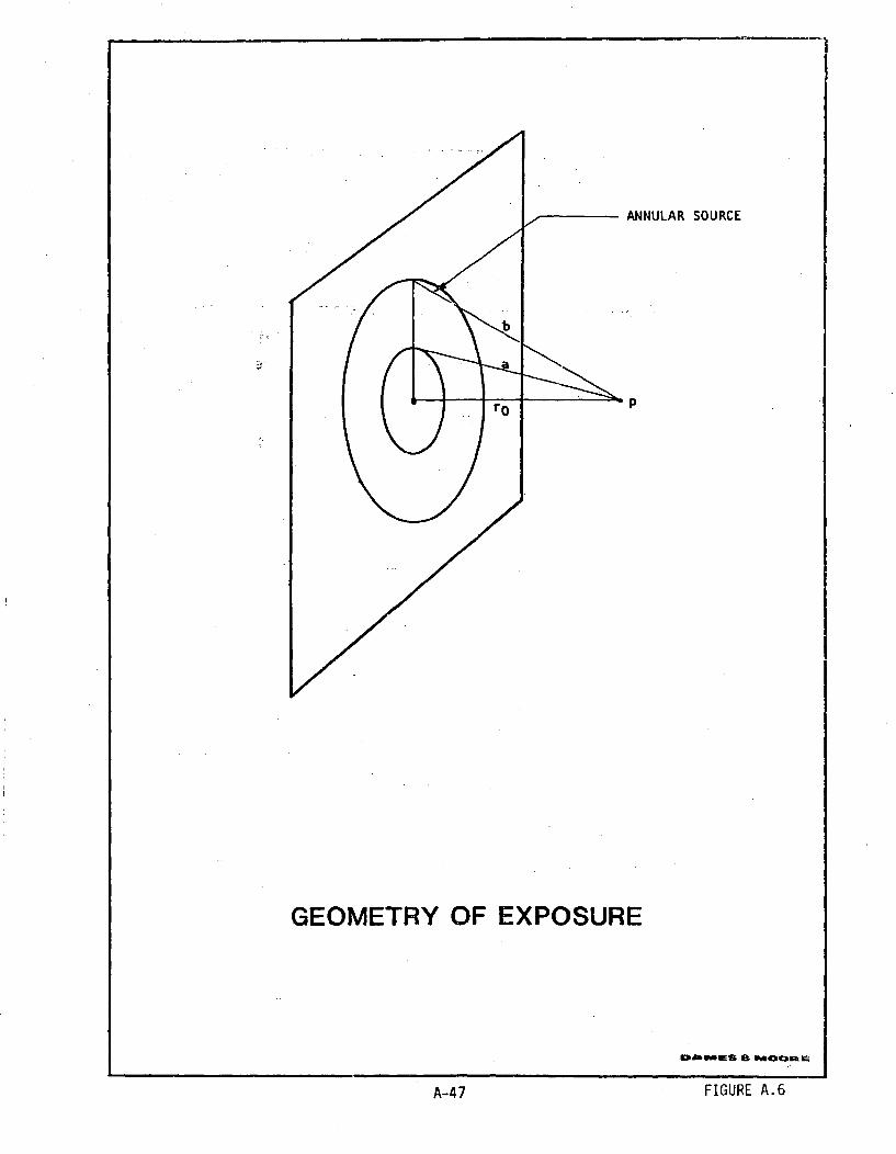
ANNULAR SOURCE

GEOMETRY OF EXPOSURE

Dm m 8 NOIE

A-47 FIGURE A.6

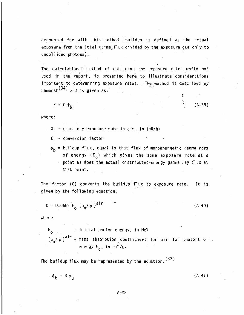
accounted for with this method (buildup is defined as the actual

exposure from the total gamma flux divided by the exposure Yue only to

uncol 1 ided photons).

The calculational method of obtaining the exposure rate, while not

used in the report, is presented here to illustrate considerations

important to determining exposure rates. The method is described by

Lamarsh( 3 4 ) and is given as:C

X C b , (A-39)

where:

X= gamma ray exposure rate in air, in (mR/h)

C = conversion factor

b= buildup flux, equal to that flux of monoenergetic gamma rays

of energy (E ) which gives the same exposure rate at a

point as does the actual distributed-energy gamma ray flux at

that point.

The factor (C) converts the buildup flux to exposure rate. It is

given by the following equation.

C 0.0659 E0 (PO/p )air (A-40)

where:

E° 0 = initial photon energy, in MeV

(jo/p )air = mass absorption coefficient for air for photons of

energy E0, in cm /g.

The buildup flux may be represented by the equation:( 3 3 )

•b=B ý u (A-41)

A-48

where:

B = e6posure buildup factor

Pu = photon flux at the point of interest due only to source

photons that have not interacted in the medium -- i.e.,2

the uncollided flux, in photons per cm /sec.

Determination of the uncollided flux and buildup factor are strongly

dependent on the geometry of the source. Postulation of a homogeneous

infinite slab source yields the following equations for these para-

meters: (33,34)

ýu = Sv/2p (A-42)

B = A/(+ n (A-43)

nwhere:

S = source strength, in Ci/m 3

P= linear attenuation coefficient of the source, in (cm-).

A W n= energy dependent coefficients used in evaluating the

Taylor form of the build-up factor.

After evaluating the build-up factor, it is multiplied by (C) to

obtain the exposure rate.

Experimentally determined exposure rates assume that an inadvertant

intruder is standing on the bare soil/waste mixture. A worst case

scenario would be an intruder occupying a below-ground-level struc-

ture. The intruder would thus be exposed from all sides except the

roof. A completely enclosed reclaimer would be exposed to an infinite

source, thus:

1u = Sv/P (A-44)

A-49

This is twice the flux calculated for the infinite slab geometry

(equation A-42). The factor of two difference is not considered

significant relative to the potential variations in surface flux

expected at an actual site. In any case, any below-ground-level

structure would require a floor and supporting walls, which would

most likely be made of a material such as concrete. The concrete

would provide considerable shielding. For example, a one foot thick

concrete slab results in a reduction factor of 0.03 for the predo-

minant gamma-ray of Cs-137 having an energy of 0.66 MeV.(35)

The actual exposure that an intruder would experience would be much

less than the worst case values since waste form and packaging and

other factors would act to reduce the exposure. Moreover, the geo-

metry of the exposure is not a fully infinite slab, and the reduction

in the radiation is considerable. This case may be approximated by

utilizing equations presented in reference 33 for the derivation of

the uncollided flux from a disk source. The geometry of exposure is

shown in Figure A.7.

In this case the uncollided flux is calculated to be:( 3 3 )

_ SI [ El(pa)- El(pb)] (A-45)

where a and b are the distances from the exposure point to the radii

shown above, and El(X) is the first order exponential integral.

Assuming that the ratios of the collided fluxes for two different

geometries may be approximated by the ratio of the uncollided fluxes

for the two geometries, this equation may be manipulated to yield

correction factors for finite disk sources or for finite annular

sources.

One subcase of the direct exposure case would involve calculating the

exposures resulting from utilization of the closed disposal facilit,.

as a public recreation area -- e.g., a golf course. For this case,

A-50

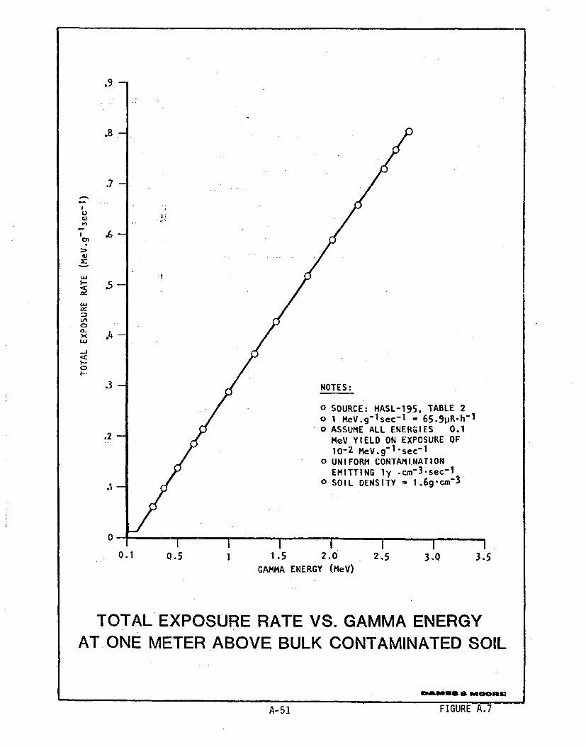
.9

.8

.7-

u

In

C)

Lu.

.6-

.4-

NOTES:

o SOURCE: HASL-195, TABLE 2

o 1 MeV.g-lsec-I = 65.9pR.h- 1

o ASSUME ALL ENERGIES 0.1MeV YIELD ON EXPOSURE OF1O-2 MeV.g-1"sec-I

o UNIFORM CONTAMINATION

EMITTING ly .cm-3.sec-10 SOIL DENSITY 1.6g-cm-3

.3-

.2

05

0.50.11 I I

1.5 2.0

GAMMA ENERGY (MeV)2.5

I3.0 3.5I I i

TOTAL EXPOSURE RATE VS. GAMMA ENERGYAT- ONE METER ABOVE BULK CONTAMINATED SOIL

•Ivmm s* a moome

A-51 FIGURE A.7

the potential exposures would be considerably reduced (e.g., orders

of magnitude) due to the shielding afforded by the thickness of the

cover. The correction factor that will be applied in this case is:

fc= B exp[ -(• /) x p x t ] (A-46)

where:

B = buildup factor

p/= mass attenuation coefficient, in cm 2/g

p = density of the cover, in g/cm3

t = cover thickness, in cm

The cover material may be assumed to be soil , hence the mass attenua-

tion coefficient used in the above calculation can be approximated by

that for Si0 2. (35 The assumed density is 1.6 g/cm 3. The product

of (V/ p ) and (p) is the linear attenuation coefficient (p), which

is an energy-dependent parameter, and hence is different for each

radionucl ide.

Table A-6 presents an "effective" gamma energy for each nuclide, which

is the highest energy gamma emitted by the nuclide in reasonable

abundance. The relative abundances of the "effective" gammas (percent

of gammas emitted that are of the "effective" energy) and the average

gamma energies are presented in Table A-6 for comparison. It should

be noted that the "effective" energy is not necessarily the maximum

energy gamma emitted by the nuclide. Maximum-energy gammas for some

nuclides are emitted in such small abundances that it would be in-

appropriate to determine cover thicknesses based on those energies.

The values for (p) based on the "effective" energies for SiO2 at 1.6

g/cm 3, are presented in Table A-6.

The buildup factors used in equation A-43 are for a plane, monodirec-

tional source, which is assumed to be representative of the "infinite-

A-52

TABLE A-6 : Gamma Dose Reduction Factors For Varying Soil Cover Thicknesses

('3

a AverageNuclide Energy

(MeV)

Co-60 1.25

Ni-59 0.35

Sr-90 0.76

Nb-94 0.787

1-129 0.040

Cs-137 0.662

U-235 0.180

U-238 0.51

Np-237 0.211

Pu-238 0.108

Pu-239 0.221

Pu-241 0.145

Am-241 0.060

Am-243 0.073

Cm-243 0.249

Cm-244 0.062

Effectiveb cEnergy Abundance c

(MeV)

1.33

0.35

0.76

0.871

0.040

0.662

0.204

0.90

0.31

0.150

0.414

0.145

0.060

0.075

0.278

0.150

50

100

100

50

100

100

7

60

60

11

16

100

100

93

47

6

(1/cm)0.086

0.16

0.12

0.11

0.11

0.12

0.21

0.11

0.18

0.22

0.15

0.22

0.42

0.32

0.18

0.22

f 0.368

0.12

0.06

0.09

0.09

0.01

0.08

0.05

0.09

0.06

0.04

0.07

0.04

0.02

0.03

0.06

0.04

E-1

0.50

0.27

0.37

0.39

0.03

0. 34

0.21

0.40

0.25

0.19

0.28

0.19

0.10

0.13

0.25

0.19

Soil Thickness

1 4.3

(meters)

7.3E-2

0.85

0.45

0.64

0.67

0.05

0. 58

0.35

0.68

0.42

0.33

0. 48

0.33

0.18

0.23

0.42

0.33

10.1E-3

1.17

0.63

0.88

0.93

0. 07

0.81

0.48

0. 94

0.58

0.45

0.67

0.45

0.24

0.31

0.58

0.48

12.8E-4

1.48

0.79

1.11

1.18

0.09

1.02

0.61

1.19

0.73

0.58

0. 84

0.58

0.31

0.40

0.73

0.58

15.4E-5

1.79

0.95

1.34

1.42

0.11

1.23

0.74

1.43

0.88

0.69

1.02

0. 69

0.37

0.48

0. 88

0.69

2.66E-1

0.30

0.16

0.23

0.24

0.02

0.21

0.12

0.24

0.15

0.12

0.17

0.12

0.06

0.08

0.15

0.12

vs. Dose Reduction Factor (f)d

(a) The following nuclides have been excluded from this table due to low effective gamma energies:H-3, C-14, Fe-55, Ni-63, Tc-99, Cs-135, and Pu-242..

(b) Effective gamma abundance is the percent of gammas emitted that are qf the effective energy.(c) Linear Attenuation coefficient (p) for SiO2 at a density of 1.6 g/cm .(d) R.L. = Relaxation lengths, f = ratio of the attenuated to unattenuated dose.

slab" waste geometry. Values for (B) are dependent upon the gamma

ray energy, type of cover material, and cover thickness. Since (B)

values for SiO2 were not readily available, the values used here are

an average of those for water and iron.(35) In addition, a gamma

energy of 0.5 MeV is assumed for all gammas, since all but one of the

gammas of concern are less than 1 MeV and (B) values were available

only for energies of 0.5, 1.0, 2.0 and higher MeV gammas. This is a

somewhat conservative assumption since (B) values increase at lower

energies. However, the values at 0.5 and 1.0 MeV do not differ

greatly, especially for ,relatively thin cover thicknesses. At a

thickness equal to 15 relaxation lengths (i.e., flux attenuates to

or approximately 3x10 7 , of the original flux) the value for

(B) is only a factor of 2 higher at 0.5 MeV than at 1.0 MeV. There-

fore, multiple-energy buildup factors are not used -in these calcu-

lations since they would complicate the calculations for relatively

little increase-in accuracy.

The thickness of soil (SiO2 ) required to reduce the dose from un-

covered waste by successive orders of magnitude are also presented in

Table A-6 for each nuclide. The corresponding number of relaxation

lengths (ut) is also indicated since the reduction factors were

obtained from a plot of (f c) vs. (ut), as presented in Figure A.8.

Table A-6 may be used to calculate the thickness of soil required to

reduce the intensity of a given radionuclide radiation by a given

order of magnitude. For example, for Cs-137, an average thickness of

0.81 m of soil is required to result in reduction in gamma radiation

intensity of 10-3, and a thickness of 1.02 m of soil results in a

reduction of 10-4. Using this table, and averaging over the radio-

nuclides expected to be present in LLW, a-generic reduction factor of

1200 may be calculated for I meter thick soil shielding.

A-54

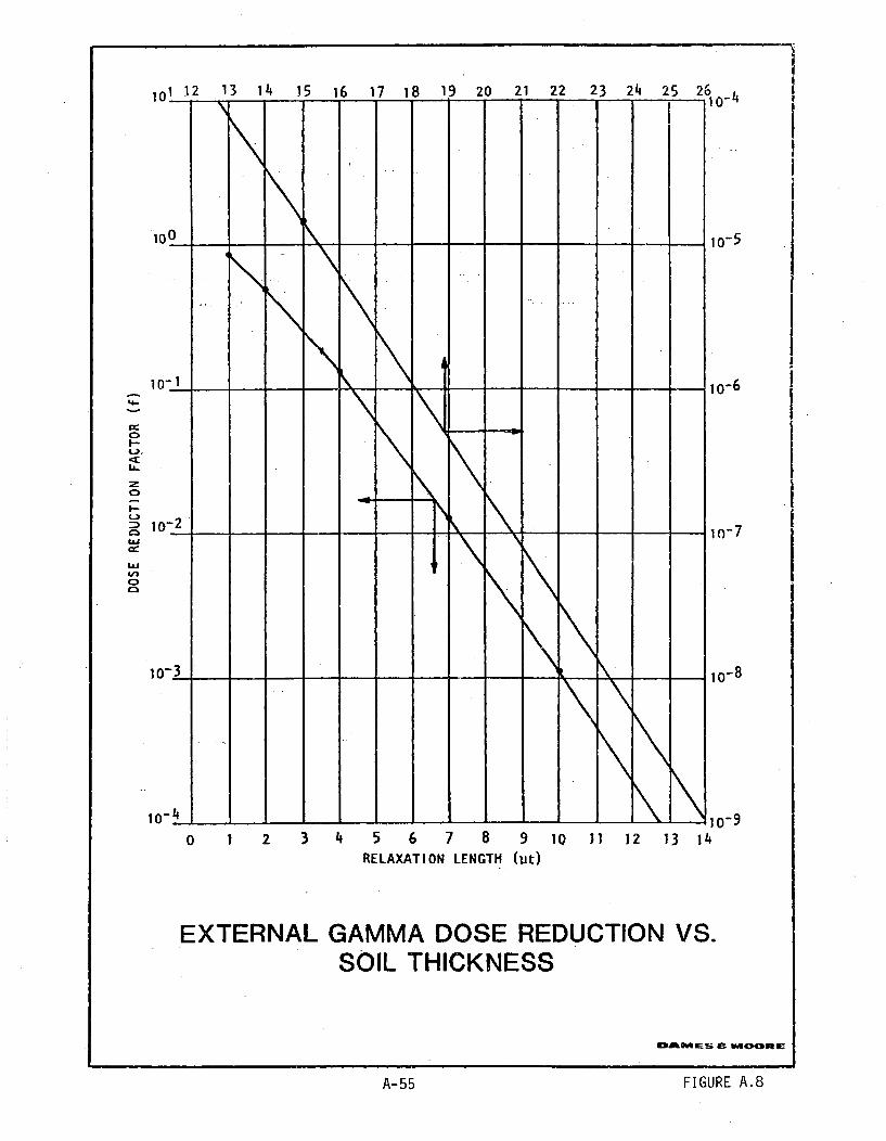
I'4I-

0I-

U-lLL.

I--

4L30D

0

0 1 2 3 4 5 6 7 8 9RELAXATION LENGTH (Ut)

10 11 12 13 14

EXTERNAL GAMMA DOSE REDUCTION VS.SOIL THICKNESS

9"1Al-S & VAOHMRI'

A-55 FIGURE A.8

REFERENCES FOR APPENDIX A

1. Casarett L.J. and J. Doull, "Toxicology," MacMillan PublishingCo., Inc., New York, 1975.

2. International Commission on Radiological Protection (ICRP).Report of the Task Group on Reference Man, ICRP Publication 23,1975.

3. Healy, J.W., and J.C. Rodgers, "Limits for the Department ofEnergy Transuranic Wastes," Los Alamos Scientific Laboratory,LA-UR-79-100, January 1979.

4. U.S. Environmental Protection Agency, "Compilation of Air Pollu-tant Emission Factors." Section 11.2, Fugitive Dust Sources,EPA, Research Triangle Park, N.C. August 1977, PB-275 525.

5. Thornthwaite, C.W., "Climates of North America According to a NewClassification." Geographic Rev. 21:633-655, 1931.

6. Volkwein, J. C., Bureau of Mines, Pittsburg Research Center,Personal Communication to G. Re of Dames & Moore, March 31, 1980.

7. U.S. Nuclear Regulatory Commission, Office of Nuclear MaterialsSafety and Safeguards, "Final Generic Environmental Statement onUranium Milling," USNRC Report NUREG-0706, September 1980.

8. Bagnold, R.A., The Physics of Blown Sand and Desert Dunes,Methuen and Co., Ltd., London, 1954.

9. Healy, J.W., "An Overview of Resuspension Models: Application toLow Level Waste Management," Los Alamos Scientific LaboratoryReport LA-UR-80-3366, 1980.

10. Start, G. E., and L. L. Wendell , "Regional Effluent DispersionCalculations Considering Spatial and Temporal Variations," NOAATech Memo ERL-ARL-44, 1974.

11. Slade, D.H., Editor, Meteorology and Atomic Energy, U.S. AECTID-24190, 1968.

12. U.S. Nuclear Regulatory Commission, Office of Nuclear MaterialsSafety and Safeguards, "Draft Environmental Impact Statement on10 CFR Part 61 : Licensing Requirements for Land Disposal ofRadioactive Waste," USNRC Report NUREG-0782,

13. Colombo, P., R.M. Neilson, Jr., "Properties of Radioactive Wastesand Waste Containers," First Topical Report, USNRC Report NUREG/CR-0619, August 1979.

A-56

14. Colombo, P., R.M. Neilson, Jr.,"Critical Review of the Propertiesof Solidified Radioactive Waste Packages Generated at NuclearPower Reactors," BNL-NUREG-50591, December 1976.

15. Colombo, P., R.M. Neilson, Jr., and B. Vyas, "Properties ofRadioactive Wastes and Waste Containers," Quarterly Reports:BNL-NUREG-50571, October 1976, BNL-NUREG-50617, January 1977,BNL-NUREG-50664, June 1977, BNL-NUREG-50692, August 1977,BNL-NUREG-50763, December 1977, BNL-NUREG-50774, January 1978,BNL-NUREG-50837, May 1978, BNL-NUREG-50921, September 1978,BNL-NUREG-50966, November 1978, BNL-NUREG-51026, May 1979,BNL-NUREG-51042, June 1979, BNL-NUREG-51101, October 1979,BNL-NUREG-51114, November 1979, BNL-NUREG-51132, January 1980.

16. Wild, R., et.al., Dames & Moore, "Data Base for Radioactive WasteManagement. Volume 2. Waste Source Options," USNRC ReportNUREG/CR-1759,

17. Columbo, P., A. J. Weiss, et.al., "Evaluation of Isotope Migra-tion - Land Burial, Water Chemistry at Commercially OperatedLow-Level Radioactive Waste Disposal Sites," Quarterly ProgressReports: BNL-NUREG-50623, March 1977, BNL-NUREG-50666, May 1977,BNL-NUREG-50670, June 1977, BNL-NUREG-50695, September 1977,BNL-NUREG-50739, December 1977., BNL-NUREG-50855, May 1978,BNL-NUREG-50861, May 1978,, BNL-NUREG-50937, November 1978.BNL-NUREG-50965, February 1979, BNL-NUREG-51083, September 1979,BNL-NUREG-51113, December 1979, BNL-NUREG-51147, February 1980.

18. Weiss, A. J. and P. Columbo, "Evaluation of Isotope Migration -Land Burial, Water Chemistry at Commercially Operated Low-LevelRadioactive Waste Disposal Sites, Status Report Through Septem-ber 30, 1979," NUREG/CR-1289, March 1980.

19. Prairie, R. and U. Gat, "Statistical Package for RadioactiveWaste Disposal Sites," University of Kentucky, Department ofMechanical Engineering, 1976.

20. Davis, J. F. and R. H. Fakundiny, New York State GeologicalSurvey, "Determination of the Retention of Radioactive and StableNuclides by Fractured Rock and Soil at West Valley, N.Y., PartI," Final Report of Research Presented to U.S. EnvironmentalProtection Agency, Research Grant WA 75 R421, March 1978.

21. Dames & Moore, "Assessment of Levels, Potential Origins andTransport Routes of Radioactivity Measured in the Vicinity ofMaxey Flats Low-Level Radioactive Waste Disposal Site," Preparedfor the Commonwealth of Kentucky, Department of Human Resources,March 1977.

A-5 7

22. Aikens, A.E., et.al., Dames & Moore, "Generic Methodology forAssessment of Radiation Doses from Groundwater Migration ofRadionuclides in LWR Wastes in Shallow Land Burial Trenches,"Prepared for Atomic Industial Forum, Inc., AIF/NESP-013, Decem-ber, 1977.

23. Morse, P. M. and H. Feshbach, Methods of Theoretical Physics,McGraw-Hill Book Company, Inc. New York, 1953.

24. Thornthwaite, C. W. and J. R. Mather, "Instructions and Tablesfor Computing Potential Evapotranspiration and the Water Balance,"Climatology, Vol.10, No.3, 1964.

25. Fenn, D. G., K. J. Henley, and T. V. DeGeare, "Use of the WaterBalance Method for Predicting Leachate Generation from SolidWaste Disposal Sites," EPA/530/SW-168, 1975.

26. Wischmeier, W. H., "Estimating the Soil Loss Equation's Coverand Management Factor for Undisturbed Areas," Proceedings of theSediment Yield Workshop, ARS-S-40, Sedimentation Laboratory,Oxford, June, 1975.

27. U.S. Department of Agriculture, Soil Conservation Service,Syracuse, New York, "Guidelines for Erosion & Sediment Control inUrban Areas of New York State,".

28. U.S. Nuclear Regulatory Commission, Office of Standards Develop-ment, Regulatory Guide 1.111, "Methods for Estimating AtmosphericTransport and Dispersion of Gaseous Effluents in Routine Releasesfrom Light-Water-Cooled Reactors," March 1976.

29. U.S. Nuclear Regulatory Commission, Office of Standards Develop-ment, Regulatory Guide 1.145, "Atmospheric Dispersion Models forPotential Accident Consequence Assessments at Nuclear PowerPlants," August 1979.

30. U.S. Atomic Energy Commission, Directorate of Regulatory Stan-dards, Regulatory Guide 1.3, "Assumptions Used for Evaluating thePotential Radiological Consequences of a Loss of Coolant Accidentfor Boiling Water Reactors," June 1974.

31. U.S. Atomic Energy Commission, Directorate of Regulatory Stan-dards, Regulatory Guide 1.4, "Assumptions Used for Evaluating thePotential Radiological Consequences of a Loss of Coolant Accidentfor Pressurized Water Reactors," June 1974.

32. U.S.Nuclear Regulatory Commission, Office of Standards Develop-ment, Regulatory Guide 1.109, Revision 1, "Calculation of AnnualDoses to Man from Routine Releases of Reactor Effluents for thePurpose of Evaluating Compliance with 10 CFR Part 50, AppendixI." October, 1977.

A-58

33. Lainarsh, J. R., Introduction to Nuclear Engineering, AddisonWesley Publishing Company, Reading Mass., 1975.

34. Goldstein, H., Fundamental Aspects of Reactor Shielding, AddisonWesley Publishing Company, Reading Mass., 1959.

35. U.S. Department of Health, Education and Welfare, "RadiologicalHealth Handbook" Revised Edition, January 1970.

36. Cleveland, J.M. and T.F. Rees, U.S. Geological Survey, Denver,Co., "Characterization of Plutonium in Maxey Flats RadioactiveTrench Leachates," Science, Vol.212, p.1506, June 1981.

A-59

APPENDIX B

PATHWAY DOSE CONVERSION FACTORS

TABLE OF CONTENTS

Section Page

B.1 Introduction and Background .. .... ........... B-1

B.2 Fundamental Dose Conversion FactorsB.2.1 Ingestion DCF's ........B.2.2 Inhalation DCF's .

B.2.3 Direct Radiation (Volume)'DCF'sB.2.4 Other Direct Exposure DCF's

B.3 Pathway EquationsB.3.1 Uptake Factors .... .........

-B.3.2 Calculational Procedure ....

" B-2. B-4" B-9" B-11

. . . . . . . . . . . . B-13

. . . . . . . . . . . . B-22

B.4 Computer Code DOSE . ......... . B-24o o

LIST OF FIGURES

Figure Page

B.1 Schematic Diagram of the Task Group Lung Model ........... B-6B.2 Schematic Diagram of DACRIN Metabolic Model ........... .. B-8

Tabli

B-1B-2B-3B-4B-5B-6B-7B-8B-9B-10B-11B-12

LIST OF TABLES

Ingestion Fundamental Dose Conversion Factors . . .

Inhalation Fundamental Dose Conversion Factors . . ...

External Exposure Fundamental Dose Conversion Factors .Radionuclide Independent Parameters Used in CalculationsOther Parameters Used in Calculations .........Soil-to-Plant Transfer Factors . . ...........Feed and Water-to-Meat Transfer Factors . . ....

Feed and Water-to-Milk Transfer Factors . . ....

Water-to-Fresh Fish Transfer Factors .... . . . .

Water-to-Freshwater Seafood Transfer Factors .........Intermediate Parameters Used in Calculations . ....

Equations Used in Calculations . .... . . . . . .

Page

B-3B-1O.B-12B-14B-15B-16B-17B-18B-19B-20B-21B-23

1

APPENDIX B : Pathway Dose Conversion Factors

The purpose of this appendix is to present the data and calculational

procedures utilized to determine the total pathway dose conversion

factors (PDCF's) presented and discussed in Section 2.3 of the main

report. An introduction and background to the appendix is presented

in Section B.1, and the fundamental dose conversion factors utilized

in the calculation of the PDCF's are discussed in Section B.2. After

these two background sections, the calculational procedures and uptake

parameters utilized are presented in Section B.3. The computer code

utilized in the calculations is given in Section B.4.

B.1 Introduction and Background

The human exposure pathways considered in this report, resulting from

the disposal of low level radioactive waste (LLW), are presented in

Figure 2.5 for each of the seven postulated exposure scenarios.

Although each pathway component (e.g., foliar deposition-cow-milk-

human ingestion) is calculated by a unique equation (or set of equa-

tions), many of the combined pathways presented in Figure 2.5 repre-

sent combinations of pathway components. For example) the food (soil)

pathway is a combination of all pathway components initiated by root

uptake of radionuclide contamination. These components include the

direct plant-human ingestion component, and the plant-cattle-beef-

human ingestion and plant-cow-milk-human ingestion components. A

description of the components of the nine combined pathways is given

in Table 2-2.

The grouping of pathway components into the combined pathways given

in Figure 2.5 facilitates the development and use of the computer code

employed to calculate the total PDCF's, as given in Section B.4. Each

major branch of the diagram has been assigned a PDCF for which the

formulae are discussed later in this appendix.

B-I

All the PDCF's are calculated from fundamental dose conversion factors

(DCF's) obtained from the existing literature. Conventionally, DCF s

are the more common factors utilized in the computation of human

exposures. For a generic stuay, however, in the absense of site

specific information, generic information on the translocation para-

meters (uptake factors) have been assumed and utilized in the calcu-

lation of the PDCF's. For evaluation of a specific site, the funda-

mental DCF's could be utilized in conjunction with site specific

uptake factors.

B.2 Fundamental Dose Conversion Factors

All the PDCF's are calculated based on five fundamental dose conver-

sion factors: inhalation 50-year committed dose in units of mrem

per pCi inhaled; ingestion 50-year committed dose in units of mrem per

pCi ingested; and three different direct radiation exposure factors.

The use of these last three factors depends on the particular biota

access location considered, and include factors for volume contami-

nation of soil (mrem/year per pCi/m3 ), surface contamination of soil

(mrem/year per pCi/m2 ), and air contamination (mrem/year per pCi/m3)o

The values of these fundamental DCF's are a function of the radio-

nuclide of concern and the organ receiving the dose. A brief des-

cription of the fundamental DCF's is provided below.

B.2.1 Ingestion DCF

For the fundamental ingestion dose conversion factors (which are

denoted by DCF1), existing models that are presented in several

documents are considered to be reasonable representations of the

human organism.0 1-3) In this report, the fundamental ingestion

DCF's given in reference 2, which are reproduced in Table B-1, have

been utilized. A brief discussion of the internal factors obtained.

from reference 2 is presented below.

B-2

TABLE B-1 . Ingestion Fundamental Dose Conversion Factors(mrem per pCi ingested)

TotalBody Bone Liver Thyroid Kidney Lung GI-LLI

H-3 1.05E-7 0. 1.05E-7 1.05E-7 1.05E-7 1.05E-7 1.05E-7Be-lO 7.94E-8 3.18E-6 4.91E-7 0. 3.71E-7 0. 2.68E-5

C-14 5.68E-7 2.84E-6 5.68E-7 5.68E-7 5.68E-7 5.68E-7 5.68E-7CI-36 0. 0. 0. 0. 0. 0. 0.Ca-41 2.OOE-5 1.83E-5 0. 0. 0. 0. 1.84E-7Fe-55 4.43E-7 2.75E-6 1.90E-6 0. 0. 1.06E-6 1.09E-6Co-60 4.72E-6 0. 2.14E-6 0. 0. 0. 4.02E-5Ni-59 1.63E-6 9.76E-6 3.35E-6 0. 0. 0. 6.90E-7Ni-63 4.36E-6 1.30E-4 9.01E-6 0. 0. 0. 1.88E-6Sr-90 1.86E-3 7.58E-3 0. 0. 0. 0. 2.19E-4Nb-94 1.86E-9 6.22E-9 3.46E-9 0. 3.42E-9 0. 2.10E-5Mo-93 2.03E-7 0. 7.51E-6 0. 2.13E-6 0. 1.22E-6Tc-99 5.02E-8 1.25E-7 1.86E-7 0. 2.34E-6 1.58E-8 6.08E-6

1-129 9.21E-6 3.27E-6 2.81E-6 7.23E-3 6.04E-6 0. 4.44E-7Cs-135. 7.99E-6 1.95E-5 1.80E-5 0. 6.81E-6 2.04E-6 4.21E-7Cs-137 7.14E-5 7.97E-5 1.09E-4 0. 3.70E-5 1.23E-5 2.11E-6Eu-152 3.90E-8 1.95E-7 4.44E-8 0. 2.75E-7 0. 2.56E-5Eu-154 5.38E-8 6.15E-7 7.56E-8 0. 3.62E-7 0. 5.48E-5Re-187 0. 0. 0. 0. 0. 0. 0.Pb-210 5.44E-4 1.53E-2 4.37E-3 0. 1.23E-2 0. 5.42E-5Bi-207 0. 0. 0. 0. 0. 0. 0.Ra-226 4.60E-3 4.60E-2 5.74E-6 0. 1.63E-4 0. 3.32E-4Th-230 5.70E-5 2.06E-3 1.17E-4 0. 5.65E-4 0. 6.02E-5Th-232 1.50E-4 2.30E-3 1.OOE-4 0. 4.82E-4 0. 5.12E-5

U-233 5.28E-5 8.71E-4 0. 0. 2.03E-4 0. 6.27E-5U-234 5.17E-5 8.36E-4 0. 0. 1.99E-4 0. 6.14E-5U-235 4.86E-5 8.01E-4 0. 0. 1.87E-4 0. 7.81E-5U-236 4.96E-5 8.01E-4 0. 0. 1.91E-4 0. 5.76E-5U-238 4.54E-5 7.67E-4 0. 0. 1.75E-4 0. 5.50E-5

Np-237 5.54E-5 1.37E-3 1.19E-4 0. 4.12E-4 0. 7.94E-5Pu-238 1.71E-5 6.80E-4 9.58E-5 0. 7.32E-5 0. 7.30E-5Pu-239 1.91E-5 7.87E-4 1.06E-4 0. 8.11E-5 0. 6.66E-5Pu-241 3.32E-7 1.65E-5 8.44E-7 0. 1.53E-6 0. 1.40E-6Pu-242 1.84E-5 7.29E-4 1.02E-4 0. 7.81E-5 0. 6.53E-5Am-241 5.41E-5 8.19E-4 2.88E-4 0. 4.07E-4 0. 7.42E-5Am-243 5.30E-5 8.18E-4 2.78E-4 0. 3.99E-4 0. 8.70E-5Cm-243 3.75E-5 6.39E-4 2.41E-4 0. 1.75E-4 0. 7.81E-5Cm-244 2.87E-5 4.83E-4 2.07E-4 0. 1.34E-4 0. 7.55E-5

B-3

"Equations for calculating internal dose committment factors were

derived from those given by the ICRP(1) for body burden and

maximum permissible concentration (MPC). Effective absorbed

energies for the radionuclides were calculated from the ICRP

model. When necessary, these energies were corrected for the

ingrowth of daughter radionuclides following ingestion or

inhalation of the parent. . . Quality factors, as listed in

ICRP Publication 2,(i) were applied to the effective energies,

including the value of 1.7 for beta particles and electrons with

energies equal to or less than 30 keV. Age dependent parameters

were applied when available, but, where data were lacking,

metabolic parameters for the Standard Man( 1 ) were used for

other age groups."

B.2.2 Inhalation DCF's

The most comprehensive compilation of information on the initial

deposition of inhaled particles in the respiratory tract was published

by the ICRP Task Group on Lung Dynamics in 1966.(4) This report

includes an anatomical description of the respiratory tract, charac-

teristics of particle size distribution, and physiological parameters

describing the inhalation process. Based on these parameters, a

quantitative model for initial respiratory tract deposition is deve-

loped. The report also describes a lung clearance model that is more

comprehensive than those used previously; it is based on extensive

studies with laboratory animals and results of human contamination

cases and it also incorporates the major clearance processes. With

the lungs compartmentalized (nasopharyngeal region, tracheobroncial

region, and pulmonary region), and considering lymph nodes, blood and

the gastrointestinal tract, the Task Group calculates rate constants

for transfer of particles between compartments. With this model,

various retention characteristics may be described for compounds of

all the elements in the periodic table.

B-4

The compl'ete lung model, as proposed by the Task Group( 4 ' 5 ) has

been utilized in this report for the calculation of the fundamental

inhalation dose conversion factors. This model permits a more rea-

listic calculation of radiation dose to the human respiratory tract

from inhaled radioactivity than does the initial ICRP lung model. (2)

In this model, the respiratory tract is divided into three regions:

the nasopharyngeal (NP), the tracheobronchial (TB), and the pulmonary

(P). The schematic representation of the respiratory tract used in

the development of the mathematical model for the deposition and

clearance of inhalated radionuclides is shown in Figure B.1.

Deposition is assumed to-vary with the aerodynamic properties of the

aerosol distribution and is described by the three parameters D3,

D4D,_ and D5. These parameters represent the fraction of the inhaled

material, QI' initially deposited in the NP, TB, and P regions,

respectively. Each of the three regions of deposition are further

subdivided into two or more subcompartments. Each subcompartment

represents the fraction of material initially in a compartment that

is subject to a particular clearance process. This fraction is

represented by fk' where k indicates the clearance pathway. The

quantity of material in the TB region, for example, cleared by process

(c) is then represented by the product fcD4 Qi. Values of (fk) and of

the clearance half-times (T k) for each clearance process for the three

solubility classes of aerosols used in the model are those suggested

by the ICRP (Appendix A, Table A-5 of reference 4). Values of the

deposition fractions (D3 , D4, and D5 ) as functions of the median

aerodynamic diameters (MAD) of the inhaled particles have been pub-

lished in the form of a graph.(1 Routines to generate these values

directly from the AMAD have been included in the model and yield

essentially the same values as those presented by the Task Group for

the range of particle size distributions considered by the group.

The respiratory tract model has been incorporated by Voilleque into a

simple metabolic model for acute inhalation exposures and the model

B-5

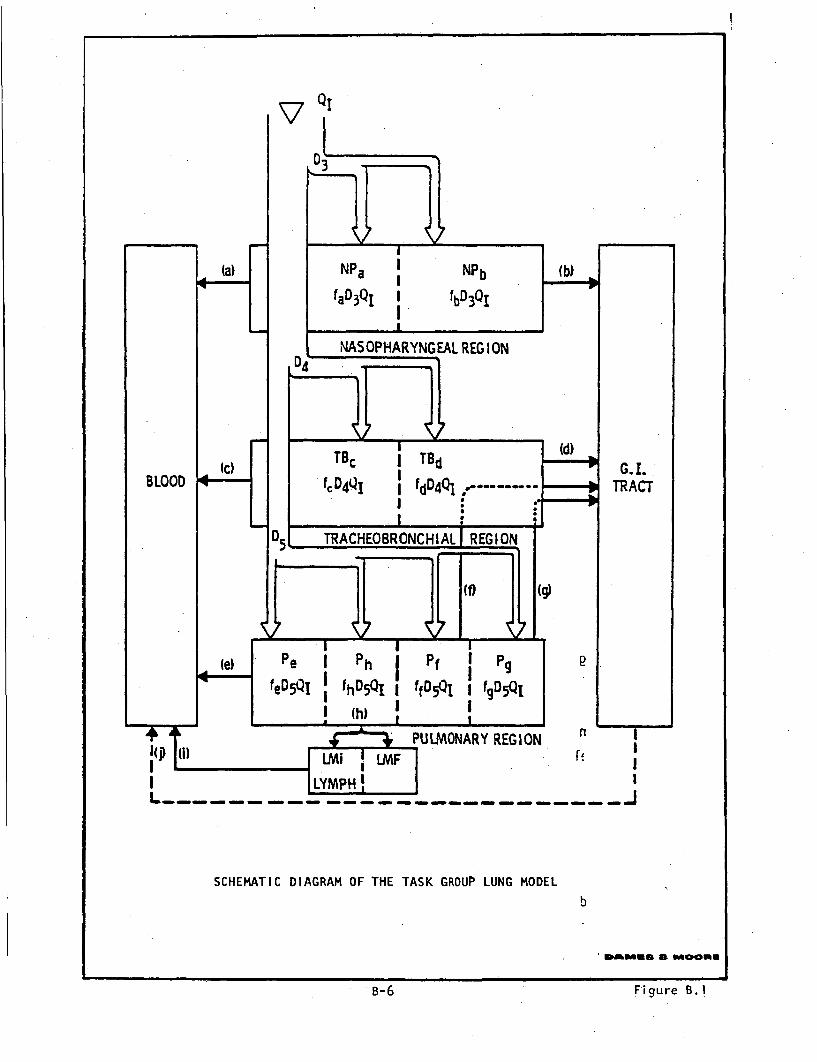
i

77 QI

03

'*1 I- j

I-- - - - - --- - -- - Si

SCHEMATIC DIAGRAM OF THE TASK GROUP LUNG MODEL

b

. EWM*mAS 0 VA0008

8-6 Fi9ure 8.1

B-6 Figure B.I.

was programmed into a computer code called AERIN.(8) In this model,

transport of a radionuclide from the respiratory tract lymphatic

system and GI tract to other organs and tissues where significant

accumulations of the inhaled radionuclides occur, is assumed to take

place via the blood. This translocation from the respiratory tract

and lymphatic system to the blood has been described in some detail by

the Task Group. Of the material clearing from-the respiratory tract

through the GI tract, a constant fraction, fl' is assumed to be taken

up by the blood. That moving to the nth organ or tissue is assumed

to be a constant fraction, f2n, of the amount entering the blood

stream at any time t. Once in the nth organ, the activity is assumed

to clear the organ (and the body) at a constant rate. Voilleque's

program, AERIN( 8 , calculates the quantity of radionuclides present

in and the dose received by organs of interest as a function of time

following acute exposures.

The inhalation dose conversion factors utilized in this report have

been obtained by utilizing a computer code called DACRIN(6) which

incorporates the Task Group lung model as described by the program

AERIN. A brief description of this code is presented below.

The DACRIN program calculates the effective radiation dose to any

of 18 organs and tissues from inhalation of any one or combination of

radionuclides considered by the ICRP. A maximum of 10 organs may be

selected for any one case (run). In addition, up to five multiple

intake intervals and 10 time intervals measured from the last intake

may be selected for each case.

Input to the code, in its simplest form, consists of a few program

control variables, the duration of inhalation exposure, ventilation

rate, the time interval within which the dose is delivered, the organs

of interest, the quantity of the radionuclide inhaled, its solubility

class and its particle size. Input to the code in its most complex

form, results from invoking an atmospheric dispersion model. It is

B-7

(a)

f2'

( J)

9,

SCHEMATIC DIAGRAM OF DACRIN METABOLIC MODEL

~m.s ~ ~qa@inu

B-8 Fiqure B.2

then necessary to input additional parameters which are determined by

the particular atmospheric dispersion model selected for analysis.

Output of the code consists of the effective radiation dose to the

selected organs at selected time intervals, for each radionuclide

inhaled as indicated by the input.

The present DACRIN code extends previous codes based on the Task

Group Lung Model to include calculating organ doses resulting from

chronic inhalation exposure. A schematic presentation of the DACRIN

metabolic model is shown in Figure B.2. A model for the dose to the

GI tract from radionuclides moving through it is not included in the

present version of the code, although some provisions have been made

in the code for the eventual addition of a GI tract dose model.

The contribution to the pulmonary lung dose from the ingrowth of

daughter radionuclides is computed indirectly by utilizing weighted

values of the effective energy emitted by the daughter nuclides in the

chain. Weighted values are calculated for each of the decay chains

tabulated by the ICRP (1,7) for residence half times of I day, 50 days

and 500 days (corresponding to solubility class D, W, and Y, res-

pectively). These values are included in the organ data library.

The radionuclides considered, the solubility classes assumed in this

report, and the calculated inhalation dose conversion factors, denoted

by DCF2,-are presented in Table B-2. The solubility classes assumed

were based upon information presented in references 9 through 14.

B.2.3 Direct Radiation (Volume) DCF's

Exposure rate data for K-40, natural uranium, and thorium plus daugh-

ters uniformly distributed in soil as an infinitely thick slab source

is presented in HASL-195.( 1 5 ) Table 2 in reference 9, which presents

exposure data as a function of gamma energy and height above soil

B-9

TABLE B-2 . Inhalation Fundamental Dose Conversion Factors(mrem per pCi inhaled)

Solubility TotalClass Body Bone Liver Thyroid Kidney Lung GI-LLI

H-3 1. .5E-7 0. 1.5E-7 1.5E-7 1.5E-7 1.5E-7 0.Be-lO W 4.6E-8 1.9E-4 2.9E-5 0. 2.2E-5 1.1E-4 1.3E-5

C-14 D 3.4E-7 1.7E-6 3.4E-7 3.4E-7 3.4E-7 3.4E-7 2.6E-7CI-36 W 4.8E-6 0. 0. 0. 0. 1.4E-4 8.1E-7Ca-41 W 1.4E-5 1.3E-4 0. 0. 0. 1.9E-6 9.OE-8Fe-55 Y 2.4E-7 3.4E-7 I.OE-6 0. 0. 2.4E-5 3.9E-7Co-60 Y 2.8E-'6 0. 2.2E-6 0. 0. 3.OE-3 2.1E-5Ni-59 W 1.4E-6 8.5E-6 3.1E-6 0. 0. 4.OE-6, 3.4E-7Ni-63 W 3.8E-6 1.2E-4 8.2E-6 0. 0. I.IE-5 9.1E-7Sr-90 9 3.OE-3 1.2E-2 0. 0. 0. 3.9E-6 2.8E-6Nb-94 Y 8.2E-8 2.3E-7 1.6E-7 0. 1.5E-7 9.0E-5 9.3E-6Mo-93 Y 1.2E-7 0. 4.6E-6 0. 1.4E-6 2.5E-4 0.Tc-99 D 5.2E-8 2.6E-8 1.9E-7 0. 2.4E-6 8.3E-7 8.9E-7

1-129 D 7.8E-6 6.OE-16 1.OE-14 6.3E-3 8.7E-15 7.1E-7 6.9E-8Cs-135 D 2.9E-6 1.2E-5 I.IE-5 0. 4.1E-6 1.8E-6 6.2E-8Cs-137 D 2.6E-5 4.9E-5 6.7E-5 0. 2.3E-5 1.1E-5 3.2E-7Eu-152 Y 1.5E-5 7.2E-5 1.7E-5 0. 7.7E-5 1.5E-3 4.5E-5Eu-154 Y 9.5E-7 8.5E-6 1.9E-6 0. 4.9E-6 2.8E-4 4.9E-6Re-187 D 4.7E-8 1.2E-8 3.9E-8 4.9E-7 0. 1.OE-7 1.1E-7Pb-210 W 1.OE-5 3.2E-2 8.2E-3 0. 2.6E-2 1.3E-2 IolE-6Bi-207 W 6.3E-7 1.2E-7 5.2E-6 0. 1.7E-5 2.3E-4 1.5E-5Ra-226 W 1.9E-1 2.7E-1 -0. 0. 0. I.OE-1 2.1E-5Th-230 W 6.7E-2 2.2E-0 1.4E-1 0. 6.6E-1 4.4E-2 2.9E-5Th-232 Y 3.2E-2 9.3E-1 4.4E-2 0. 2.1E-1 5.9E-1 2.8E-5

U-233 Y 2.5E-4 4.1E-3 0. 0. 9.6E-4 4.6E-1 3.5E-5U-234 Y 2.4E-4 3.9E-3 0. 0. 9.4E-4 4.5E-1 3.4E-5U-235 Y 2.3E-4 3.8E-3 0. 0. 8.8E-4 4.2E-1 3.7E-5U-236 Y 2.3E-4 3.8E-3 0. 0. 9.1E-4 4.3E-1 3.2E-5U-238 Y 2.1E-4 3.6E-3 0. ,0. 8.2E-4 3.,9E-1 3.OE-5

Np-237 W 6.5E-2 1.5E-O 1.4E-1 0. 4.8E-1 4.ME-2 3.OE-5Pu-238 Y 2.5E-2 5.1E-1 3.5E-1 0. 1.1E-1 5.1E-1 3.9E-5Pu-239 Y 2.8E-2 6.OE-1 3.9E-1 0. 1.2E-1 4.8E-1 3.7E-5Pu-241 Y 3.8E-4 9.3E-3 5.7E-3 0. 1.8E-3 8.5E-4 6.9E-7Pu-242 Y 2.7E-2 5.6E-1 3.8E-1 *). 1.2E-1 4.6E-1 3.5E-5Am-241 W 6.3E-2 8.9E-1 8.3E-1 0. 4.8E-1 5.3E-2 3.5E-5Am-243 W 6.2E-2 8.8E-1 8.1E-1 0. 4o7E-1 5.OE-2 3.4E-5Cm-243 W 4.8E-2 7.7E-1 7.OE-1 0. 2.2E-1 5.5E-2 3.8E-5Cm-244 W 3.5E-2 5.5E-1 5.2E-1 0. 1.6E-1 5.5E-2 3.6E-5

B-10

surface, has been used to construct a graph of exposure rate (at one

meter height above the soil surface.) as a function of gamma energy for

such a source. This graph has been presented in Figure A.6.

Exposure rates, E, for the radionuclides of interest in this, study

have been calculated from the expression:

E = K. Z fi ET

where f is the fraction of gamma photons of energy T per disintegra-

tion, ET is the exposure rate factor obtained from Figure A.6 for

energy T, and K is a proportionality constant which converts the

exposure rate factor in HASL-195( 1 5 ) to units of dose equivalent

(mrem/year per Ci/m 3). As indicated in Figure A.6, K = 65.9 uR/hr

per MeV/g-sec. In this report, it is assumed that one Roentgen equals

one rem. The resultant annual external gamma dose conversion factors

resulting from volume contaminated soil, denoted by DCF3, are pre-

sented in Table B-3.

B.2.4 Other Direct Exposure DCF's

The two remaining DCF's are the external exposure factors resulting

from direct photon and electron radiation emanating from radionuclides

on surface contaminated soil, and from immersion in uniformly contami-

nated air, these DCF's are denoted by DCF4 and DCF5, respectively.

In the past, the electron component (beta radiation) of the exposure

was frequently neglected in comparison to the photon component (gamma

radiation) of the exposure'due to the comparative penetration capabi-

lity of these radiations. For the direct radiation (volume) DCF's,

this is the case since a few millimeters of soil is sufficient to stop

most of the electron radiation from the radionuclides considered in

this work. However, it is more accurate to include the electron

component when the exposure is due to surface contaminated soil or to

immersion in contaminated air.

B-11

TABLE B-3 . External Exposure FundamentalDose Conversion Factors

H-3Be-lO

C-14CI-36Ca-41Fe-55Co-60Ni-59Ni-63Sr-90Nb-94Mo-93Tc-99'

1-129Cs-135Cs-137Eu-152Eu-154Re-187Pb-210Bi-207Ra-226Th-230Th-232

U-233*U-234U-235U-236U-238

Np-237Pu-238Pu-239Pu-241Pu-242.Am-241Am-243Cm-243Cm-244

DCF-3(mrem/yea§per Ci/m )

0.0.0.

8.80E-110.0.

1.54E-056.20E-09

0.3.06E-089.63E-06

0.0.

1 .92E-080.

3.50E-066.22E-068.07E-06

0.8.56E-099.37E-067.21E-061 .50E-092.66E-05

0.4.28E-101.50E-07

0.5.16E-096.56E-081.93E-119.39E-113.43E-13

0.7.71E-081.86E-073.82E-075.64E-11

DCF-4(mrem/yeaper Ci/m

0.2.36E-05

0.9.18E-104.49E-072.67E-063.84E-044.27E-06

0.2.74E-059.90E-051 .33E-05

0.1.13E-05

0.3.99E-052.71E-043.78E-04

0.2.27E-069.24E-059.47E-076.12E-072.28E-061.78E-062.88E-063.65E-052.72E-062.40E-062 .21E-053.18E-061 .22E-06

0.,

2 .38E-061 30E-051.50E-054.02E-052.82E-06

DCF-5(mrem/yeasper Ci/m )

5.19E-051.82E-034.46E-041.29E-072.45E-055.08E-052.28E-025.98E-051.56E-041.76E-031.32E-021.34E-047.60E-046.86E-045.08E-041.53E-03I.IIE-021.32E-02

0.1.43E-051.29E-024.90E-053.59 E-061.08E-045.16E-051.14E-041.59E-039.67E-058.57E-058.40E-048.87E-055.17E-054.78E-056.93E-053.80E-046.09E-042.26E-037.23E-05

B-12

These DCF's have been calculated for various radionuclides for unit2

concentration in the biota access media -- i.e., pCi/mr of soil and

pCi/rm3 of air. (16) For each exposure mode, DCF's for photons and

electrons have been calculated for tissue-equivalent material at the

body surface of an exposed individual. For internal body organs, only

photons have been considered.(16) The DCF's obtained from reference

10, presented in Table B-3, have been utilized in this work when the

exposure is due to surface contaminated soil (DCF-4), or to immersion

in contaminated air (DCF-5).

B.3 Pathway Equations

This section presents the equations, the parameters, and the data

utilized in the computation of the PDCF's. The components corres-

ponding to each pathway are defined in Figure 2.5.

B.3.1 Uptake Factors

In order -to calculate the PDCF's, several translocation parameters

(also referred to as uptake factors or pathway parameters) are re-

quired. These parameters fall into two groups: those that depend only

on the pathway being considered, and those that are radionuclide-

specific. The parameters that depend only on the pathway are pre-

sented in Table B-4 together with the values assumed in this work and

-the references from which they were obtained.

The other group of parameters and pathway factors, which are radio-

nuclide specific, are presented in Table B-5. The values utilized

for the five radionuclide-specific transfer factors were obtained from

the literature; a comparative compilation of these five factors is

presented in Tables B-6 through B-10. Based on the pathway uptake

parameters presented in Tables B-4 and B-5,- several intermediate

transfer parameters have been defined for the PDCF calculation. These

intermediate parameters are defined and presented in Table B-11.

B-13

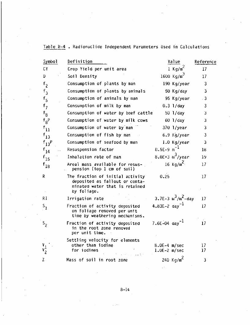
Table B"4 . Radionuclide Independent Parameters Used in Calculations

Symbol Definition Value

1 Kg/mr2

CY

0

f2

f3

f5f7

f8

f8Pf 11

f13f 13 P

f 14f15

f 18

R

RI

SI

S2

V 1V2

Z

Crop Yield per unit area

Soil Density

Consumption

Consumption

Consumption

Consumption

Consumption

Consumption

Consumption

Consumption

Consumption

of plants by man

of plants by animals

of animals by man

of milk by man

of water by beef cat

of water by milk cow!

of water by-man

of fish by man

of seafood by man

tles

1600

190

50

95

0.3

50

60

370

6.9

1.0

8.5E-9

8. 0E+3

16

Kg/m'A

Kg/year

Kg/day

Kg/year

1/day

1/day

1/day

1/year

Kg/year

Kg/year1-1

m 3/year

Kg/m 2

Resuspension factor

Inhalation rate of man

Areal mass available for resus-pension (top 1 cm of soil)

The fraction of initial activitydeposited as fallout or conta-minated water that is retainedby foliage.

Irrigation rate

Fraction of activity depositedon foliage removed per unittime by weathering mechanisms.

Fraction of activity depositedin the root zone removedper unit time.

Settling velocity for elementsother than iodinefor iodines

Reference

17

17

3

3

3

3

3

3

3

33

18

19

17.

17

17

17

17

1717

0.25

3.7E-3

4.83E-2

m /m2 -day

day-

-17.6E-04 day

8.OE-4 m/sec

1.0E-2 m/sec

240 Kg/m 2Mass of soil in root zone 3

B-14

Table B-5 . Other Parameters Used in Calculations

Symbol

CaC

5CSA

CSV

Cw

DCFI

DCF2

DCF3

DCF4

DCF5

fl

f 4

f 6

Definition

Initial Air Concentration

,Initial Soil Concentration

Initial Areal Soil Concentration

Initial Volume Soil Concentration

Initial Water Concentration

Fundamental DCF forIngestion

Fundamental DCF for Ingestion

Fundamental DCF for ExternalExposure (Volume Source)

Fundamental DCF for ExternalExposure (Area Source)

Fundamental DCF for ExternalExposure (Air Immersion)

Soil-to-Plant Transfer Factor(pCi/kg in fresh vegetationper pCi/kg in soil)

Feed or Water-to-Meat Transfer Factor(pCi/kg in meat per pCi/dayingested by beef cattle)

Feed or Water-to-Animal Product(Milk) Transfer Factor. (pCi/lin milk per pCi/day ingested by cow)

Water-to-Fish Transfer Factor(pCi/kg of fresh fish perpCi/l of water concentration)

Water-to-Freshwater Seafood TransferFactor (pCi/kg of fresh seafoodper pCi/l of water concentration)

Units

1 pCi/mi3

1 pCi/kg

1 pCi/m2

1 pCi/mi3

1 pCi/m/3

See Table

See Table

See Table

B-1

B-2

B-3

See Table B-3

See Table B-3

See Table B-6Dimensionless

See Table B-7day/kg

See Table B-8day/l

See Table B-91/kg

See Table B-IO1/kg

f 12 P

B-15

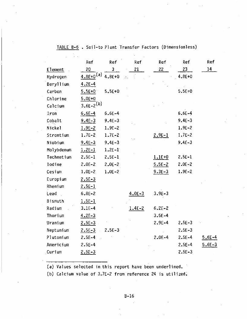
TABLE B-6 . Soil-to Plant Transfer Factors (Dimensionless)

Element

Hydrogen_-

Beryllium

Carbon

Chlorine

Calcium

Iron

Cobalt

Nickel

Strontium

Niobium

Molybdenum

Technetium

Iodine

Cesium

Europium

Rhenium

Lead

Bismuth

Radium

Thorium

Uranium

Neptunium

Pl utoni um

Americi um

Curium

Ref

20

4.8E+0(a)

4.2E-4

5.5E+0-

5.OE+O

3 . 6 E-2(b)

6.6E-4

9.4E-3

1.9E-2

1.7E-2

9.4E-3

1.2E-1

2.5E-1

2.OE-2

1.OE-2

2.5E-3

2.5E-1

6.8E-2

1.5E-1

3.1E-4

4.2E-3

2.5E-3

2.5E-3

2.5E-4

2.5E-4

2.5E-3

Ref

3

4.8E+0

5.5E+0

Ref

21

Ref

22

Ref

23

4.8E+0

5.5E+0

Ref

14

6.6E-4

9.4E-3

1.9E-2

1.7E-2

9.4E-3

1.2E-1

2.5E-1

2.OE-2

1.OE-2

6.6E-4

9.4E-3

1.9E-2

2.9E-1 1.7E-2

9.4E-3

1.1E+O

5.5E-2

9.3E-3

2.5E-1

2.OE-2

1.9E-2

4.OE-3 3.9E-3

1.4E-2 6.2E-2

3.5E-4

2.9E-4 2.5E-3

2.5E-3

2.OE-4 2.5E-4

2.5E-4

2.5E-3

2.5E-3

5.6E-4

5.6E-3

(a) Values selected in this report have been underlined.

(b) Calcium value of 3.7E-2 from reference 24 is utilized.

B-16

TABLE B-7 . Feed and Water-to-Meat-Transfer Factors (day/kg)

Element

Hydrogen

Beryllium

Carbon Y.-

Chlorine

Calcium

Iron

Cobalt

Nickel

Strontium

Niobium

Molybdenum

Technetium

Iodine

Cesium

Europium

Rhenium

Lead

Bismuth

Radium

Thorium

Uranium

Neptunium

Plutonium

Americium

Curium

Ref

20

1.2E-2(a)

1.OE-3

3.1E-2

8.OE-2

4 .OE- 3 (b)

4.OE-2

1.3E-2

5.3E-2

6.OE-4

2.8E-1

8.OE-3

4.OE-1

2.9E-3

4.OE-3

4.8E-3

8.OE-3

2.9E-4

1.3E-2

3.4E-2

2.OE-4

3.4E-4

2.OE-4

1.4E-5

2.OE-4

2.OE-4

Ref

3

1.2E-2

3.1E-2

Ref

21

Ref

22

Ref

23

Ref

14

4.OE-2

1.3E-2

5.3E-2

6.OE-4

2.8E-1

8.OE-3

4.0E-1

2.9E-3

4.OE-3

3.OE-4

8.7E-3

7.OE-3

1.4E-2

7.1E-4 9.1E-4

5.1E-4

2.OE-4

5.OE-4

1.6E-6

1.6E-6

4.1E-7

2.OE-4

3.9E-4

3.9E-3

(a) Values selected in this report have been underlined.

(b) Calcium value of 4.OE-2 from reference 24 is utilized.

B-17

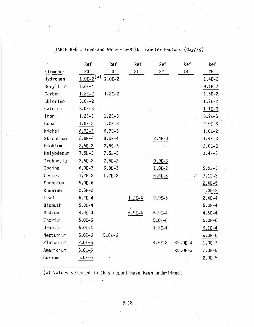
TABLE--B-8 . Feed and Water-to-Milk Transfer Factors (day/kg)

Element

Hydrogen

Beryllium

Carbon

Chlorine

Calcium

Iron

Cobalt

Nickel

Strontium

Niobium

Molybdenum

Technetium

Iodine

Cesium

Europium

Rhenium

Lead

Bismuth

Radium

Thorium

Uranium

Neptunium

Plutonium

Americium

Curium

Ref

20

l.OE_2(a)

1..OE-4

1.2E-2

5.OE-2

8.OE-3

1.2E-3

1.OE-3

6.7E-3

8.OE-4

2.5E-3

7.5E-3

2.5E-2

6.OE-3

1.2E-2

5.OE-6

2.5E-2

6.2E-4

5.OE-4

8.OE-3

5.OE-6

5.OE-4

5.0E-6

2.OE-6

5.OE-6

5.OE-6

Ref

3

1.OE-2

1.2E-2

Ref

21.-

Ref

22

Ref

14

1.2E-3

1.OE-3

6.7E-3

8.OE-4

2.5E-3

7.5E-3

2.5E-2

6.OE-3

1.2E-2

2.4E-3

9.9E-3

1.OE-2

5.6E-3

Ref

25

1.4E-2

9.1E-7

1.5E-2

1.7E-2

1.1E-2

5.9E-5

2.OE-3

1.OE-2

1.4E-3

2.OE-2

1.4E-3

9.9E-3

7.1E-3

2.OE-5

1.3E-3

2.6E-4

5.OE-4

4.5E-4

5.OE-6

6.1E-4

5.OE-6

1 OE-7

2.OE-5

2.OE-5

1.2E-4 9.9E-5

5.9E-4 5.9E-4

5.OE-6

1.2E-4

5.OE-6

4.5E-8 <5.OE-4

<5.OE-3

(a) Values selected-in this report have been underlined.

B-18

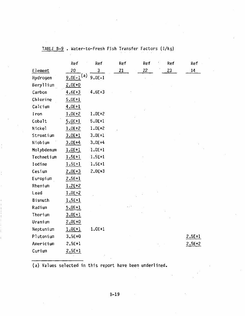
TABLE B-9 . Water-to-Fresh Fish Transfer Factors (1/kg)

Element

Hydrogen

Beryllium

Carbon

Chlorine

Calcium

Iron

Cobalt

Nickel

Strontium

Niobium

Molybdenum

Techneti um

Iodine

Cesium

Europium

Rhenium

Lead

Bi smuth

Radium

Thorium

Uranium

Neptuni um

Pl utoni um

Americi um

Curium

Ref

20

9.OE-1 (a)

2.OE+O

4.6E+3

5.OE+1

.4.OE+1

1.OE+2

5.OE+1

1.OE+2

3.OE+1

3.OE+4

1.OE+1

1.5E+1

1.5E+1

2.OE+3

2.5E+1

1.2E+2

1.OE+2

1.5E+1

5.OE+1

3.OE+1

2.OE+O

1.OE+1

3.5E+0

2.5E+1

2.5E+1

Ref

3

9.0E-I

4.6E+3

1.OE+2

5.OE+1

1.OE+2

3.OE+1

3.OE+4

1.OE+1

1.5E+1

1.5E+1

2.OE+3

1.OE+1

Ref

21

Ref

22

Ref

23

Ref

14

2.5E+1

2.5E+2

(a) Values selected in this report have been underlined.

B-19

TABLE B-10 . Water-to-Freshwater Seafood Transfer Factors (1/kg)

Element

Hydrogen

Beryllium

Carbon

Chlorine

Calcium

Iron

Cobalt

Nickel

Strontium

Niobium

Molybdenum

Technetium

Iodine

Cesium

Europium

Rhenium

Lead

Bismuth

Radium

Thorium

Uranium

Neptunium

Plutonium

Americium

Curium

Ref

20

9.0E-I(a)

1.OE+1

9.1E+3

1.OE+2

3.3E+2

3.2E+3

2.OE+2

1.OE+2

1.OE+2

1.OE+2

1.OE+1

5.OE+O

5.OE+O

1.OE+2

1.OE+3

6.OE+1

1.OE+2

2.4E+1

2.5E+2

5.OE+2

6.OE+1

4.OE+2

1.OE+2

1.OE+3

1.OE+3

Ref

3

9.OE-1

9.1E+3

3.2E+3

2.OE+2

1.0E+2

1.OE+2

1.OE+2

1.OE+1

5.OE+O

5.OE+O

1.OE+2

4.OE+2

Ref

21

Ref

22

Ref

23

Ref

14

(a) Values selected in this report have been underlined.

B-20

Table B-11 . Intermediate Parameters Used in Calculations

Symbol

P1

P2

P3

PT

PIPP2PP3 PPT P

F1

F,Fz

F3

FT

Transfer Factor

f1*f2

f1*f3*f4*f5/365

fl*f3*f 6*f7

P1 +P2+P3

f 2

f3*f4*f5/365

f3*f6*f 7

PIP+P 2 P+P3 P

f *f 4*f5

f8P*f6*f 7*365flf11

F1 +F2 +F3

f 1 2 *f 1 3f 12 P*f 13 P

F12 +F121 2

86400*V/( S2 *Z)

86400*RV/S1

RI/(S 2 *Z)

R*RI/S 1

86400

365

Description

Soil-Plant-Man

Soil-Plant-Animal -Man

Soil-Plant-Animal -Product-Man

Total Soil -to-Pl ant-to-Man

Plant-Man

Plant-Animal-Man

Plant-Animal-Product-Man

Total Plant-to-Man

Water-Animal -Man

Water-Animal -Product-Man

Water-Man

Total Water-to-Man

Water-Fi sh-Man

Water-Seafood-Man

Total Seafood-to-Man

Soil Deposition by Fallout

Foliar Deposition by Fallout

Soil Deposition by Irrigation

Foliar Deposition by Irrigation

seconds/day

days/year

F1 2 1

F122

F1 2

Wi1

W2

B-21

B.3.2 Calculational Procedure

The equations utilized to calculate the PDCF's are summarized in

Table B-12. Some of the PDCF's are calculated using a single equation

since common factors are present in the individual uptake pathway

components, however, some PDCF's require multiple equations.

All of these equations are basic pathway equations that bring together

the calculationa-] components contributing to the human dose. A

detailed treatment of these pathway equations may be found in Regu-

latory Guide 1.109.(3,20)

The fundamental equation for the calculation of total pathway dose

conversion factors for man from radionuclides in the environment via

specific exposure scenarios can be given as:

N

D.irps i= fips DCFirp (B.1)

where:

= the total pathway dose conversion factor (50-year doseDirps

committment in mrem), specific to organ r from nuclide i

from pathway p via scenario s;

N = the total number of pathways in the scenario,

Cips = the concentration of nuclide i in the medium of pathway p

via scenario s (in pCi/mi3 , pCi/kg, or pCi/In2 )

fips the pathway usage factor of nuclide i of pathway p viE

scenario s which is considered in the calculation of the

accumulated radiation dose conversion factor to man; and

DCFirp the fundamental dose conversion factor, a value specific

to a given nuclide i, pathway p, and organ r which is used

to calculate radiation dose commitments.

B-22

Table B-12 . Equations Used in Calculations

PDCF-1 = (6) + (9)

PDCF-2 = (7)

PDCF-3 = (8)

PDCF-4 = (1)

PDCF-5 = (2)

PDCF-6 = (3) + (10)

PDCF-7 = (3) + (4) + (10)

PDCF-8 = (5) + (8)

(1) Cs*(PT/D)*DCFI

(2) C *DCF3

(3) Cw*(W1*PT+(W 2 /CY)*PTP+FT/1000)*DCF1

(4) Cw*(f 1 2 /10O)*DCF1

(5) C *D1*f *(f *(f1*DCF2+DCF5)+DCF4)a 118 14 1

(6) Ca*D 1 *f 1 8 *(f 14 *(f 1 5*DCF2+DCF5)+DCF4)*U.242

(7) Ca*(f 1 5*DCF2+DCF5+(DI*PT+(D 2 /CY)*F*PTP)*DCFI)*0.242

(8) Ca*(f 1 5*DCF2+DCF5+(D 1*PT+(D 2 /CY)*F*PTP)*DCF1)

(9) Ca*(DCF5+f 1 5 *DCF2)

(10) Cw*W1 *f 1 8 **(f14 *(f15*DCF2+DCF4)+DCF5)

B-23

B.4 Computer Code DOSE

A listing of the code utilized to calculate the PDCF's presented and

used in the main body of the report is attached. The program is

written in Fortran IV _for a CDC 6600 computer. The program is

interactive -- i.e., it is executed in a time-sharing mode, and it

asks questions and requests answers by the person running the program.

All the uptake factors and translocation parameters have been incor-

porated into the data statements at the beginning of the program. It

requires a data tape, called TAPE1 containing the fundamental dose

conversion factors presented in this appendix. Using this program,

PDCF's for up to 39 radionuclides may be calculated. Inaddition, it

contains the option to change the fundamental dose conversion factors

for any of these radionuclides.

B-24

'COS I i'ETRY PROGRAAG PAGE. -1

05/18/81. 14.32,45.

'1'O PROGRAM DOSE (INU j"4 '. OUTPUTl TAPEI )01' DIMENSION NP(S)' ,ISCN ' (3,) vDCEF(39,7,7) , NNUi(39) ,I:OSE(8: 7)•0120 DIMENSION ORGAN(7) S3 (8) , F. ) (39) ,F4 (39) ,F6 (39)

11. N -IMENSIOCN Fl2 (39) ,FI2 F39)10i40 DATA ISCN/5,9,0,e7'0,08,0,0,1OOyl,,2,0,O,3y,0,0,3,4,10,6,8,0/'0150 DATA NP'/2,l11,II,,2,3,2/00160 DATA ORGAN!1OHTOTAL BODY',ICH BONE , i0H LIVER ,)0170+ 10H "THYROID ,LOH .KIDNEY ,10H LUNG , 10H GI-LLI /00180 DATA NNUC!1 OHH-3 , IOHBE-0 0 , 10HC-14 , IOHCL-36 v00190÷ 1OHCA-41 , IOHFE-55 ,10HCO-60 , 1OHNI-59 ,v0200+ IOHNI-63 ,IOHSR-90 ,YOHY-90 ,1OHNB-94 ,00210+ ÷ 1OHM0-93 , 1OHTC-99 ,10HI--129 ,l0HCS-135 Y00220+ 10HCS-137 ,1OHEU-152 , IOHEU-154 ,IOHRE-187 Y00230+ 1OHPB-210 Y10HBI-207 ,10HRA-226 ,1OHTH-230 Y.00240+ 10HTH--232 , 10HU-233 ,1OHU-234 ,10HU-235 Yu)0250+ 1OHU-236 ,IOHU-238 ,1OHNP-237 ,1OHPU-23890260K, IOHPU-239 ,1OHPU-241 ,10HPU-242 ,10HAM-241002704- IOHAM-243 ,1OHCM-243 , 10HCM-244 /:0280 DATA SCN/10HACCIDENT ,10HCONSTRUCT 10OHAGRF:ICULTURF, 1OHFOODj)024- 10HDIR. GAMMAY1OHWELL WATERY 10HSLURF-WATER, 10HATMOSPHERE/00300 DATA V1 r V2 $Sl, 32 Z ,RI, R/! 01 .0008, .04833, 000765p240. ,.0037, .25/,0310 DATA CYD'FF2,F3,F5,F7,FBF8PiI.,,1600.,.Il.,190.,50 .*,95°,.3,5S0.,6O./

3'32.) DATA Fi Fr3l,FI4,Fl5,FIB/30o,,6.9,8,SE.-9.8000,1l6./'0330 DATA FI/48, .00042,5.5,5.0, 037 ;:00066y ,0094"

'00340 .019, *019, .29, .0025, .009s, •.12, p1, .055, .0093, .0093, *0025,.0025,los5o' *25. .004, .15Y .014P .0042y ,0042y5*,0025Y 0025q4*.00056Y2*.0056,03*io• .0025, 0025/, F3P!. /

10376 DATA F4/.0i2, .00y ,.031 P .08, .04P .04, .03y .053Y .O53,3.OE-4,

'0380" .0046,.;28Y 008,8.7E-3,7.0E-3,2*1.4E-2, .20048Y .0048,.008, .00071,;0390 *.013, ... 00051 2,2 E-a*• 4E-4,2 .E-4,4*'3,. 9s-4,2*3.9E-3,2,22 E-4/)0400 DATA F6/401. , ÷0000':009' , .012? .017 .011 , .000059-",410 OO. I001, .0067, .00672.4E-3 .0000159 °.0025!.' 4.00i4,9.9E-3, .001,2*5.6E-3,'0420f '00002, 00002F.0013).00012,+0005,.00059,2*.0000055*"*00061,

.0430 000005 4*2. OE-6v4*5.0E-6/:0440 DATA F12/' ',2.. '4600. ,50. ,40•, 100. ,50 LW'000 t,10. v"0450 30.,25..'.30000.10."2*l54.2000o.20004, 25.,25.b,120°,100,.,15.,50.,•0460f 30.p3.0 -5*210.9•4.25.,9250 . , 250. '.Y5.,25./

00470 DATA FI12P/.9,L.'9100•. 00o,330, 3200'',2001,00.,I 00.,50480+ 100 L ,i0." I 00. '10. ,2*5 , 100., 100 •l,' 100. oO,,1000 ,60 . ,100, ,24.,10490+ 250.,5'0,500.,5*60*,400.,p4*100).,2*i000.,2"1000./00500 DO 90 K=I,2A0510 READ(07I 701)AF00520 ' 90 READ(,,700)((DCFtI(J 91K),J=I,7),I=1,39)

,05f5 REr:A fi ( ..1 , 7 01 A(.-*

*.0550 -95 READ(I, 7 0 0)(DCF(IlIK),I=1,39).i05.'j,'0 *70 F'0 i~iAiT 7 7E9 •. 2)v"57j70 70 F i"1;f A 1.0)

' O',"J ' Li'PR IT," P 1 Ii 'RIN'l,*THIS PROGRAM REQUIRES AN ,NITIAL INPUT OF THE NUCL.iE*

1"-.RIN'v* N.AME. AFTER THIS YOU INDtICATE W!"THFlUHER Y 1YOU WISH THE DOSE*60 P FRINT,*CONVERSIO[iN FACTORS TO BE READ 0ij "iR TAPE 1 OR*

B-25

A:;LOSIMETRY PROGRAM PAGE 2

0~5/18/81 * 14 34.35•

00620 PRI NT ,:::TO ENTER.-T'HESE VALUE:S INTERACTIVC:VLY THRU THE*k00636 -PR INWfiC0MrFi.JTER ERPINAL . (0 = TAPE 1 1 = INTERACTFIVE.*00640 PRINT, :!

06-0 & PRINT ,*I'F INTERACTIVE;*00660 PRINT,*NEXT 2 LINES ARE DOSE CONVERSION FACTORS FOR 7 ORGAJNS,*00.670 PRINT,:&:THESE ORGANS ARE:TOTAL BODY PBONE ,LIVER, THYROID r, tIDNEY!, *,00680 PRINT *LUNG, AND GI-LLI. *00690 PF:RINT T .: LINE 2: DCFI'S- INGESTION MREM/5OYR PER .-CI,i,00700 PRINTY.:V ItNGESTED IN FIRST YEAR*00710 PRINTN LINE 3:DCF2'S- INHALATION MREM/50YR PER PCI*00720 P PRINTT INHALED IN FIRST YEAR*0073C PRINT,>;THESE DCF'S ARE INPUT 7 PER LINE (ONE FOR EACH ORGAN) *,00740 PRINT-3SEPERATED BY COMMAS#*)0750 PRINTryNEXT 3 LINES ARE DIRECT GAMMA DOSE CONVERSION FACTORS*00-760 PRINT,X-ONLY ONE NUMBER FOR WHOLE BODY REGUIRED IN EACH CASE.*)077.0 PRINT7,*(SAME DCF IS USED FOR ALL OTHER ORGANS.)*

•00780 PRINT,* LINE 4:DCF3'S- DIRECT GAMMA(VOLUME) MREM/YR PER ,CI!i'r.00790 PRINT,* LINE 5:DCF4'S- DIRECT GAMMA(AREA) MREM/YR PER PCI/M"".00800 PFRINT-* LINE 6:DCF5'S- DIRECT GAMMA(AIR) MREM/YR PER FCI/W'"'.00810 PRINT N * $ PRINT,* * $ PRINT,*00820 PRINTh*TYPE. 'STOP' FOR NUCLIDE TO TERMINATE PROGRAM*00830 PRINT.* * $ PRINT,* * $ PRINT,* &00840 110 PRINT,-:4NUCLIDE *Q00"850 REALD 500 NUKE00860 DO 50 l:=I,39.00870 IF(NUKE *.EQ.NNUC(I)) GO TO 55008G0 50 CONTILNUE00.9.1) PRINT:NGO NUCLIDE OF THAT NAME FOUND*(;.0900 GO TO 11.000?10 55 N U C=:I

00920 PRIN'I",*INTERA(TIVE INPUT*, $ READIQ00930 IF(10.EOO) GO TO 6000940 PR*INT :DC F "S ,00950 - READ, ( C (NUC, J, 1) , J=1,7)00960 PP INT '.iCF2 / S : *,00970 READr, (.CF(NUCJ,2) ,J=l,7)00980 PR IN',` :-NlDCF3 I'sp00990 READ: DCI:- < NUC, 1,3)01000 PRINT :4,4CF4 : *,0101.0 READ (,2F NUC Y 1 , 4)01020 PRINT<,1DCF5: *,01030 READDCF(NUC, , 15)01040 60 DO 65 1=3,501050 1DO 65 J:=2,701060 65 DCF (NUC, J. I )=DCF (NUC, I, I )01070 S;= 4. $ A=I.. $ W=I.01080 CS:Si,/ $ CSV=S0:1.090 CA=A0:1. 1 00) C W- W $ CWP=CW*) *001

0111. P1=FI(NUC)*F2 $ P2=F1(NUC)*F3*F4(NUC)/365.*F501120 P3=Fl (NUC)*F3*F6 (NUC)*F701130 PF=I- 'P. ... I:2+P3 $ FTP='PT/F (NUC)

B-26

ISINETRY PROGRAM-

'5/8/ 1.1-4.35,40.

PAGE

.150

i.L60:1701 1 5.-0190

120012101220

A 23:•:01240250

1260. 12701280

i290* 3001-

13::20+.30

+r.-.01350

1.370[ 'i cr,0I. 390.+-L400

1420'1.430

1. 450'1 .,460 QL 4 7"0

.1460

'1500

2 00.I. 510

'FT=F8*F4 (HUC) ' ' 5.. FrP*F (WHUC;) *F7*365.+F-I 1F I2.-1 (kNUC) *F 13F I ( OUC) *F:1 3PV=V2 $ IFri',iiUCr . j 5) V=VI[138:42;54.*Vi. ,S *. $ Li2=86400 * *R*V/S1

1I=R i(S2Z) p =W :=R *IiSV

DO0 200 1F 1,DO 200 •10 1 .-I "N=NP(:) $ AI=O0.ETO 100 J=I.1NIP=ISCN(JI)GO TO (1,23y,4,5!,6y78,Y9;'i0),IP

1 A 1:=,:'14-G(S*PT:*IDGF ( NUCv 1 0 ~' 1 )

2 AI=AI+CSV*DCF(HUCICY3)3 AI=A'f (CW* (WI*PT+ (W2/CY)*PTP)+CWP*FT)*DCF (NUCU IOI 1)4 AI=AI +CWP*FI2N2DCF (NUC 10,?1 )5 AI=AI+CA*DI*FIS* '(FI4*(FI5*DCF (NUC, IO:2)+DGCF(NLiCIO 5) )+

DGCF (NUC Y I04) -6 AI=AI+CA*D1*FIB*(F14*C(F15*DCFFC(NUC,IO,2)+DCF(NUC:II05))+

DCF (NUC Y I0,4) ):0.2427 Al =At +•A•:(DCF (NU •( , 10y75) *FIF5*DCF (NUC, I:) F2)) +

CA* (D:' *PT- ( D2iCY) *F*PTP) *NDCFr (NUC, Iv 1) 1) V 2428 AI=AI'+CA* ( DCF (NUC, IO,5) +F15.*DCF (NUGC C1 2y +

CA* (BI *PT + ( D2./CY ) *F*PTP)*DCF UC. IUC) 1 )9 A 1=AI +CA* (DCF ( iUCv, I) y5) +FI 5*DGF (NU IC),I: 2)

10 AI=A1'+CW*W.I.*.F1S*(F14*.(F15*DCF( <NUC PIO2) +T.CF(NUC 10O5)q)+

DOCF (C i9U C TY : 0 )100 C01NT I N U E:

DOSE (II )=Al-I. E+-12200 CONT IN UE

PRINT 600 i'-NNUC ( NUC)PRINTI.610y (RGAN(J) ,0=1,7)PRINT 620, (SCN (I) , (DOSE(I,J v .J::1,7) ,I 1, 8)PRINT 63C0GO TO 110

500 FOR MAT (A 10600 FORMAT(!//*NUCLIDE: *AIO)610 FORMAT(I)X,7AIO)620 FORMAT (Al 0 1 .- )630 FORMAT (//A)99 STOP

EMN D

$$$$

GOGOGOGO

TOTOTOTO

100100100100

$ GO TO 100

$ GO TO 100

$ GO TO 100

$ GO TO 100$ GO TO 100

-. ii EIN D .l -.. -

.RND Y

B-27

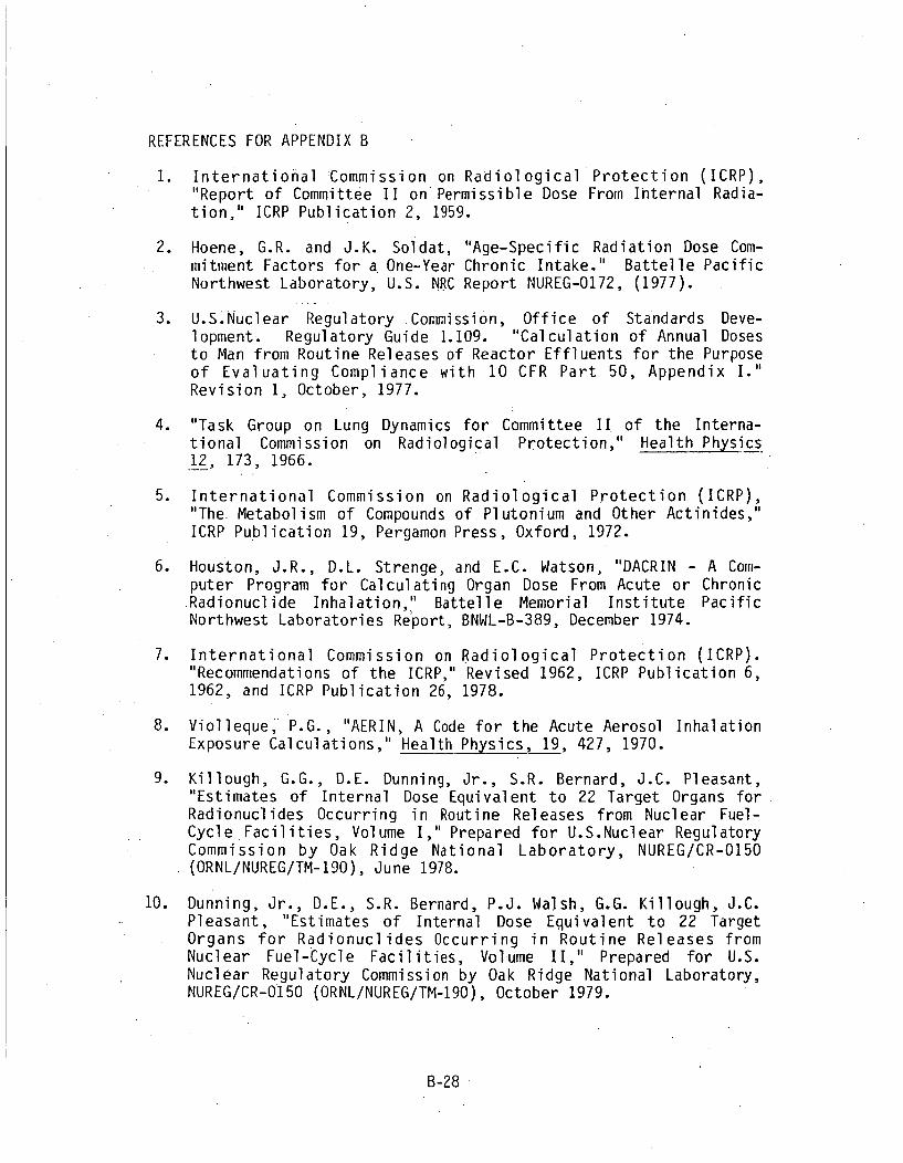
REFERENCES FOR APPENDIX B

1. International Commission on Radiological Protection (ICRP),"Report of Committee II on Permissible Dose From Internal Radia-tion," ICRP Publication 2, 1959.

2. Hoene, G.R. and J.K. Soldat, "Age-Specific Radiation Dose Com-mitment Factors for a One-Year Chronic Intake." Battelle PacificNorthwest Laboratory, U.S. NRC Report NUREG-0172, (1977).

3. U.S.Nuclear Regulatory Commission, Office of Standards Deve-lopment. Regulatory Guide 1.109. "Calculation of Annual Dosesto Man from Routine Releases of Reactor Effluents for the Purposeof Evaluating Compliance with 10 CFR Part 50, Appendix I."Revision 1, October, 1977.

4. "Task Group on Lung Dynamics for Committee II of the Interna-tional Commission on Radiological Protection," Health Physics.12, 173, 1966.

5. International Commission on Radiological Protection (ICRP),"The- Metabolism of Compounds of-Plutonium and Other Actinides,"ICRP Publication 19, Pergamon Press, Oxford, 1972.

6. Houston, J.R., D.L. Strenge, and E.C. Watson, "DACRIN - A Com-puter Program for Calculating Organ Dose From Acute or Chronic

.Radionuclide Inhalation," Battelle Memorial Institute PacificNorthwest Laboratories Report, BNWL-B-389, December 1974.

7. International Commission on Radiological Protection (ICRP)."Recommendations of the ICRP," Revised 1962, ICRP Publication 6,1962, and ICRP Publication 26, 1978.

8. Violleque, P.G., "AERIN, A Code for the Acute Aerosol InhalationExposure Calculations," Health Physics, 19, 427, 1970.

9. Killough, G.G., D.E. Dunning, Jr., S.R. Bernard, J.C. Pleasant,"Estimates of Internal Dose Equivalent to 22 Target Organs forRadionuclides Occurring in Routine Releases from Nuclear Fuel-Cycle Facilities, Volume I," Prepared for U.S.Nuclear RegulatoryCommission by Oak Ridge National Laboratory, NUREG/CR-0150

.. (ORNL/NUREG/TM-190), June 1978.

10. Dunning, Jr., D.E., S.R. Bernard, P.J. Walsh, G.G. Killough, J.C.Pleasant, "Estimates of Internal Dose Equivalent to 22 TargetOrgans for Radionuclides Occurring in Routine Releases fromNuclear Fuel-Cycle Facilities, Volume II," Prepared for U.S.Nuclear Regulatory Commission by Oak Ridge National Laboratory,NUREG/CR-0150 (ORNL/NUREG/TM-190), October 1979.

B-28

11. Adams, N., B.W. Hunt, and J.A. Reissland, "Annual Limits ofIntake of Radionuclides for Workers," National Radiation Protec-tion Board Report, NRPB-R82, October 1978.

12. International Commission on Radiological Protection (ICRP),"Limits for Intakes of Radionuclides by Workers, Part I," ICRPPublication 30, July 1978.

13. U.S. Nuclear Regulatory Commission, "Reactor Safety Study: AnAssessment of Accident Risks in U.S. Commercial Nuclear PowerPlants," WASH-1400 (NUREG-75/014), October 1975.

14. Healy, J.W., and J.C. Rodgers, "Limits for the Department ofEnergy Transuranic Wastes," Los Alamos Scientific Laboratory,LA-UR-79-100, January 1979.

15. Beck, H. and G. de Planque, "The Radiation Field In Air Due toDistributed Gamma Ray Sources in the Ground," U.S. Atomic EnergyCommission, Health and Safety Laboratory Report No. HASL-195,1968.

16. Kocher, D.C., "Dose-Rate Conversion Factors for External Exposureto Photon and Electron Radiation from Radionuclides Occurring inRoutine Releases from Nuclear Fuel Cycle Facilities," Preparedfor U.S. Nuclear Regulatory Commission by Oak Ridge NationalLaboratory, NUREG/CR-0494, 1979.

17. Denham, D. H. et.al., "Radiological Evaluation for AdvancedWaste Management Studies," Battelle Pacific Northwest Labora-tories Report No. BNWL-1764, 1973.

18. U.S. Nuclear Regulatory Commission, Office of Standards Deve-lopment, "A Methodology for Calculating Residual RadioactivityLevels Following Decommissioning," NUREG-0707, October 1980.

19. International Commission on Radiological Protection (ICRP),"Report of the Task Group on Reference Man," ICRP Publication 23,1974.

20. U.S. Nuclear Regulatory Commission, Office of Standards Deve-lopment. Draft Regulatory Guide 1.109. "Calculation of AnnualDoses to Man from Routine Releases of Reactor Effluents for thePurpose of Evaluating Compliance with 10 CFR Part 50, AppendixI." March 1976.

21. U.S. Nuclear Regulatory Commission, Office of Standards Deve-lopment, "Calculational Models for Estimating Radiation Doses toMan from Airborne Radioactive Materials Resulting from UraniumMilling Operations," Task RH 802-4, For Comment, May 1979.

B-29

22. Moore, R.E., et.al. "AIRDOS-EPA: A Computerized Methodology forEstimating Environmental Concentrations and Dose to Man fromAirborne Releases of Radionuclides," EPA 520/1-79-009, December1979.

23. Greenhouse, N.A. and E.T. Lessard, "A Dosimetric Analysis ofPathways to Man From the Environmental Release of Low LevelRadioactive Wastes," Prepared for Dames & Moore by Occupationaland Environmental Health Analysts, Inc., 1980.

24. Ng, Y.C., et.al., "Prediction of the Maximum Dosage to Man Fromthe Fallout of Nuclear Devices, Part IV., Handbook for Estimatingthe Maximum Internal Dose From Radionuclides Released to theBiosphere." University of California, Lawrence Livermore Labora-tory Report No. UCRL-50163 Part IV, (1968).

25. Ng, Y.C., et.al., "Transfer Coefficients for the Prediction of.the Dose to Man via the Forage-Cow-Milk Pathway from Radionuc-lides Released to the Biosphere." University of California,Lawrence Livermore Laboratory Report No. UCRL-51939.

26. Napier, B.A., et.al., "PABLM-A Computer Program to CalculateAccumulated Radiation Doses From Radionuclides in the Envi-ronment." Battelle Pacific Northwest Laboratory Report No.PNL-3209/UC-70, (1980).

B-30

APPENDIX C

REFERENCE DISPOSAL LOCATIONS

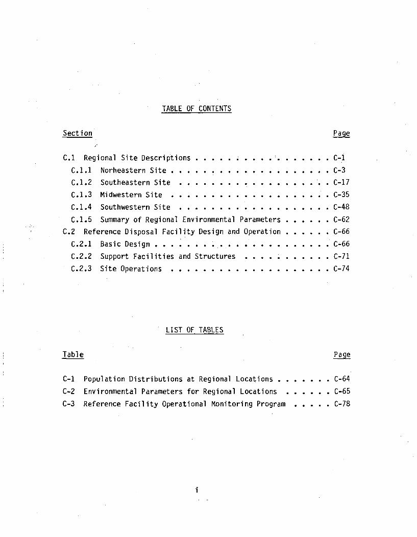
TABLE OF CONTENTS

Section

C.1 Regional Site Descriptions . . . . . . . . . ..

C.1.1 Norheastern Site . . . . . . . . . . . ....

C.1.2 Southeastern Site . . . . . . . . . . .

-C.1.3 Midwestern Site . ..............

C.1.4 Southwestern Site ......... . . .

C.1.5 Summary of Regional Environmental Parameters .

C.2 Reference Disposal Facility Design and Operation .

C.2.1 Basic Design . . . . . . . . . . . . . .

C.2.2 Support Facilities and Structures ....

C.2.3 Site Operations . ..............

Page

C-i

C-3

C-17

C-35

C-48

C-62

C-66

C-66

C-71

C-74

LIST OF TABLES

Table Page

C-1 Population Distributions at Regional Locations . . . . . . . C-64

C-2 Environmental Parameters for Regional Locations . . . . . . C-65

C-3 Reference Facility Operational Monitoring Program . . . . . C-78

i

LIST OF FIGURES

Figure

C.1 U.S.. NRC Inspection and Enforcement Regions ....C.2 Northeastern Site Topographic MapC.3 Geologic Profile of-the Northeastern Site . ....C.4 Flow Recurrance Intervals for the Northeastern SiteC.5 Precipitation Event Recurrance Intervals

for the Northeastern Site . .. ..........C.6 Temperature Characteristics of the Northeastern SiteC.7 Wind Rose Diagram for the Northeastern Site .

C.8 Southeastern Site Topographic Map . . . . .....C.9 Geologic Profile of the Southeastern Site .....C.1O Flow Recurrance Intervals for the East Basin

of the Southeastern Site. . . . . . . . . .....C.11 Flow Recurrance Intervals for the West Basin.

of the Southeastern Site .....................C.12 Precipitation Event Recurrance Intervals

for the Southeastern Site .............C.13 Temperature Characteristics of the Southeastern SiteC.14 Wind Rose Diagram for the Southeastern Site ....

C.15 Miawestern Site Topographic Map . . . . . . ....C.16 Geologic Profile of the Midwestern Site ......C.17 Flow Recurrance Intervals for the Midwestern SiteC.18 Precipitation Event Recurrance Intervals

for the Midwestern Site............ . . . . .C.19 Wind Rose Diagram for the Midwestern Site .....

C.2U Southwestern Site Topographic Map .........C.21 Geologic. Profile of the Southwestern Site . . ...C.22 Flow Recurrance Intervals for the Southwestern SiteC.23 Precipitation Event Recurrance Intervals

for the Southwestern Site .............C.24 Temperature Characteristics of the Southwestern SiteC.25 Wind Rose Diagram for the Southwestern Site . ...

C.26 Reference Disposal Site Layout . . . ........C.27 Support Facilities.... . .. . . . .C.28 Typical Trench Details ...............

Page

C-2C"4C-5C-10

C-11C-12C-14

. . . . C'-18

. . . . C~-19

* . . . C-23

*...C-24

* . . . C"26* . . . C-27* . . . C"28

* . . . C'-36* . . . C~-39* . . . C-41

* . . . C-43* . . . C-44

" C"49

"C-54

" C-56" C-57

"C-59

" C-68" Cý-71

ii

APPENDIX C Reference Disposal Locations

This appendix presents the environmental characteristics of four

hypothetical regional disposal facility sites as well as the general

disposal facility design for these sites. As shown in Figure C.1, the

conterminous U.S. has been divided into four regions with boundaries

based on those for U.S. NRC Regions. These waste generating regions

will be referred to in this appendix as the northeast (Region 1),

southeast (Region II), midwest (Region III), and western regions

(Regions IV plus V). Each of these regions are projected to generate

upto one million m3 of LLW between the years 1980 and 2000.(1)

Within each region a hypothetical disposal facility is assumed to be

located at a site having characteristics which are consistent with:

(a) the basic disposal facility siting considerations presented in

reference 2 and (b) the generic environmental characteristics within

that geographic region. These regional sites are described in Section

C.1. A description of the disposal facilities assumed to be situated

at each of these sites are presented in Section C.2. Finally, the

various environmental parameters associated with the regional sites

are summarized in Section C.3.

C.1 Regional Site Descriptions

This section provides a brief description of four hypothetical re-

gional sites: a northeastern site, a southeastern site (which is taken

to be the reference disposal facility site discussed in the main body

of the report), a midwestern site, and a southwestern site. The

regional site descriptions are meant to be typical of environmental

characteristics of the regions (not necessarily the "best" site that

could be located within a region) and have been developed from a

number of sources. Thus the regional site descriptions should not be

interpreted as representing any existing or possibly planned disposal

facility, or any specific location within the regions.

C-I

AAA

NUCLEAR GENERATING UNIT CAPACITYN Ucensed To Operate

72 licensed by NRC to operate*. 2 others authorized to operate (DOE-owned)

A Being Built87 construction permits

2 site work authorized

megawatts54,474.0

910.0 0

95,373.42,300.0

AA0 Plannod

M1U

0

17 reactors ordered 19,874.0180 172,931A

'Includes Scquoyah I and No. Anna 2, as of October 1, 1900 were startina upwith full power operating licenses from NRC, and Salem 2, which was authorizeadto load fuel and conduct low power testing. Does not Include Indian Point 1.rated at 2155 MWe; the operrating authority of thit unit was revoked on 6.1"-80by the Nuclear Regulatory Commission (the owner Is required to submit adecommissioning plan for Unit I within 120 days from said date). USNRC INSPECTION ANDBECAUSE OF SPACE LIMITATIONS, SYMBOLS

• "i- ::• '- =:E • :.. . ..!-r T ... 7 ENFORCEMENT REGIONS

C.1.1 Northeastern Site

The Northeastern facility site is' assumed to be located- within the

Appalachian Upland portion of the Appalachian Plateau physiographic

province. A general topographic map of the site is presented in

Figure C.2.

The area has been reworked by erosional and depositional forces

associated with glacial and post-glacial activities. The disposal

facility site is on an upland area, having an average elevation of

about 555 m (1820 ft) above mean sea level (msl), and slopes to the

south at a rate of about 3%. The drainage from the site flows into

the headwaters of Point Creek.

Geology

Throughout most of the Appalachian upland, the bedrock is underlain by

unconsolidated deposits of glacial origin. The thickness of these

units is generally greater in the lowlands and valleys, gradually

thinning out over the upland regions. The material properties of the

deposits are highly variable.

The. site is underlain by approximately 9 to 23 m (30 to 75 ft) of

compact glacial till frequently referred to as hardpan. Thin and

discontinuous interbedded layers of sand and gravel are observed

locally in the area. Coarser-grained sediments are principally found

in valleys and lowlands, and are associated with stream channels.

Underlying the glacial mantle are flat lying rocks of upper Devonian

Age belonging to the Schaffer Group. These rocks consist of marine,

black, and gray shales and siltstones, with some thin sandstone

layers. The regional dip of the strata is to the south-southwest at a

rate of about 2%. A westnorthwest-eastsoutheast geologic profile of

the site area is shown on Figure C.3.

C-3

Crol ia Center

CemI

0 0,,< ,'.;: ... -- :--.'I( ,

pIFACILITjt CFROLIA PUFRCHASE

/ ?

.G.

/180

7w..

NORTHEASTjEPN SITE

TOPOGRIAPHIC MAP0 500 1000L I 1/I

SCALE IN MfETERS

0 1000 2000 3000.I I -

SCALE IN FEETKEY :

500 YEAR FLOTDWAY:CONTOURS IN FEET - 20 FOOT INTERVALS

C-A FIGURE C.2FIGURE C.2C-4

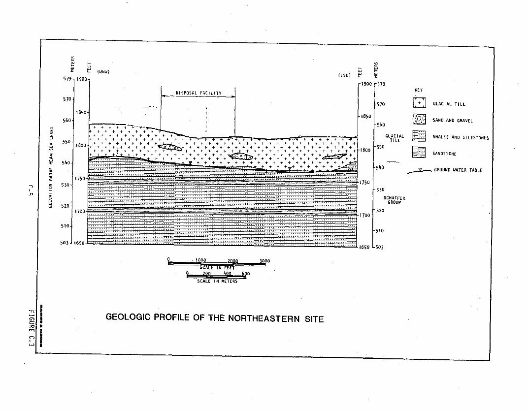
w i.L-

wa LX: (WNW)

579i 19001

(ESE) L

F19 0 0 -5 79

5701

1850-

560--J

* La

-J4

7-4La

a47

0

I-4

La

•+ ++ 7 --. +

r+I + + + + + + +

- + + + + + + + + + + + + + + + + + + + + + + + +

+ + + + + + ++++ + + ++ + ++++ + + + + + + + + + + + + + + + + + + + + +

4.,. +++ + + -f +... + + + + + . . + + + +....+

.................. . . . . .+ + + + .+ + + ++÷ + + + +. . . -. + ++

..... ..... ............... .. .... . . + + + + + + + + + +

- 185o

-570

-56o

KEY

D GLACIAL TILL

SAND AND GRAVEL

GLACIAL SHALES AND SILTSTONES

TILL

SANDSTONE5501 18oo- -18oo [550

.-I,

540.

530-

520-

510ý

503]

..............................................

1750

................................................................

..........................................................................

... ........... 777- ................................ I...............................

.. ....................................................... I......... ...... ......

. .. . . .. . . . . . . . .. ......... I........................... T....................... I....................... . . . . . . . . . . . . . . . . . .................................................................................

1650 ..... ............

.540 GROUND WATER TABLE

-530SCHAFFER

GROUP

-520

-510

L 5 0 3JU•

o 0 1000 2000 3000L §1I

SCALE IN FEET2?00 400 600

SCALE IN METERS

GEOLOGIC PROFILE OF THE NORTHEASTERN SITEC=

;a

I3I0

SI

The northeast site falls within one of the more tectonically stable

regions of the northeast. The site location has been estimated to

have a peak horizontal ground acceleration of 0.04 g, with a recur-

rance interval of more than 500 years. Based on available data, no

capable faults are known to underlie the site or lie within 5 miles

of the site.

Soils

The site area is covered by silty loams with an underlying brittle,

dense fragipan. The predominant soil types belong to the Brickton,

Warren, Chitta and Highland series. The parent material consists of

acidic, low-lime-content, dense glacial till.

The site has slopes ranging from nearly level to moderately rolling

grades, and the runoff potentials are correspondingly variable. The

soils are deep and generally poorly drained. Permeabilities for the

uppermost foot of soils are moderate, ranging from 15 to 50 mm per

hour (0.6 to 2 inches per hour). However, the dense silty fragipan

subsoil is of considerable thickness and is highly impervious, afford-

ing low permeabilities ranging between less than 1.5 to 5 mm (0.06

and 0.2 inches) per hour...

The soil is strongly acidic, especially in the topsoil layer. The

plentiful root material in the upper layers contribute to the rela-

tively high organic matter composition. In general, available nit-

rogen is high, with a moderate phosphorus and potassium content. The

low lime content of the glacial till might indicate a correspondingly

low calcium content.

Ground Water

The ground water generally occurs where the bedrock and glacial till

meet. The depth to ground water at the site averages about 12 meters

C-6

(39 ft). The amount of groundwater available in the local upland area

in which the site is located is largely limited to that which reaches

the zone of saturation from precipitation falling upgradient of the

site. This recharge quantity is small because of the low permeability

of the till, and the heavily vegetated nature of the land surface

which acts to hold water in the surficial organic matter affording

greater loss via evapotranspiration. Recharge in these areas is

limited, ranging from 5 to 50 mm (0.2 to 2 inches) per year.

Groundwater occurrence in the bedrock is limited to secondary openings

along fracture zones and bedding planes. Generally, the fine-grained

character associated with the shales and siltstones inhibits water

movement. Rocks of this type typically have an upper permeability

of about 4.72x10-7 to 4.72xi0-5 cm/sec (0.01 to 1.0 gallons/day/ft -

gpd/ft 2). Movement in the intergranular pore spaces of the sandstone

layers will be somewhat greater.

Groundwater flow is to the south, following the local topography, and

enters the unconsolidated deposits at erosional interfaces. As

stated previously, till is not a good water-bearing unit. The permea-

bility of this material is on the order of 4.72xi0-8 to 4.72xi0- 9

cm/sec (0.001 to 0.0001 gpd/ft 2 ). Where coarse-grained deposits are

encountered, the permeability increases considerably, with values

ranging from 4.72x10 2 to 4.72 cm/sec (1,000 to 10,000 gpd/ft 2 ). Most

of the recharge entering at the site follows the hydraulic gradient to

the south and is discharged as base flow into the headwaters of Point

Creek whbch is about 1000 m (3280 ft) away.

Groundwater usage in this rural setting is very low. Pumpage is

limited to widely scattered wells serving as domestic supplies to

local homes and farmsteads. Most of these rural supplies are obtained

from bedrock wells, 30 to 61 m (100 to 200 ft) in depth, although some

of the water comes from seepage from the overlying deposits around the

well casings. The average yields range between 23 to 30 liters per

minute (6 to 10 gpm).

C-7

The quality of ground water in the unconsolidated deposits and upper

shale units is generally good. Occasional samples collected in

the upper shales were found to be high in total dissolved solids

and hardness; however, average values are relatively low. Water in

the unconsolidated deposits tends to reflect the influence of the

underlying bedrock. In general, water from the deep gravel deposits

is high in iron, and water from shallow gravel deposits is very

hard.

Surface Water

The site is located in the once glaciated region of the Brokill

Mountains. The rolling terrain is typical of the region, the result

of glacial scour and fill. The drainage basin in which the site is

located covers 7.36 km 2, with a coarse drainage density of 0.5 (dimen-

sionless). Total stream length above the site is 2286 m (7500 ft).

The site vicinity is generally sloping to the south with total vege-

tative cover. The surface soils and vegetation allow for considerable

retention of precipitation; only 20 to 30 percent of precipitation

becomes surface runoff. A strong correlation exists between stream

discharge and precipitation in the basin. Mean annual discharge at

the outlet of the basin is 0.99 m3 /s (35 cfs), but a wide variation

in flow occurs throughout the year. Analysis of the unit hydrograph

indicates that while peak discharge in the stream occurs within 30

minutes of rainfall commencement, recession of the flow takes up to 30

hours. This variation is likely due to the base flow sustiained by and

fair weather runoff derived from groundwater.

Saturation of the lower basin area occurs during high in'tensity pre-

cipitation events, causing return flow. The maximum discharge of a

500 year flow is estimated to be on the order of 368 m 3/s. The

floodway of such a flow is delineated on Figure C-2. As can be seen,

the site is located well above the floodway.

C-8

Development of the site will tend to reduce the infiltration area of

the basin, reduce the time to peak discharge and increase the flood

stage of the stream. Facility operations such as placement of imper-

vious cover materials and clearing of vegetation are expected to

increase the runoff by approximately 60% by the time the facility is

closed. This increased runoff, however, will not result in increased

potential for site flooding. Flow recurrance intervals for the

location are shown in Figure C.4.

Meteorology

The climate in the area of the northeastern site is classified as

humid continental, characterized by wide variations in seasonal

precipitation and temperature. Moisture sources for precipitation

are obtained from the southerly flow of Gulf air during the summer,

cyclones that originate in the Great Lakes, and Atlantic coast sys-

tems. Precipitation is uniformly distributed over the year with the

greatest average monthly amounts occuring during April through Sep-

tember in the form of thunder showers. The average annual precipi-

tation is approximately 1034 mm (41 in). Precipitation event recur,

rance intervals for the location are shown in Figure C.5.

The area is characterized by distinct seasonal temperature varia-

tions. Winters are predominantly cold with maximum temperatures

ranging from 0 to 20 0 C (32 to 68°F), and nightime minimums of from

-9 to -7 0C (15 to 20°F). The temperatures are generally mild during

June through August and maximum temperatures average from 24 to 26°C

(75 to 790 F). The mean annual temperature for the area is 8°C (46°F).

Mean monthly temperatures, and the average of the monthly maximum and

minimum temperatures in the vicinity are shown in Figure C.6.

The prevailing wind direction is southerly from May through November

and westerly during the winter and early spring. The average wind

speedsý during these periods are 15.6 and 17.8 km/hr (8.4 and 9.6

C-9

U,ILL)

ILl

=U,

1.25 2 10 25 50RECURRENCE INTERVAL, YEARS

FLOW RECURRENCE INTERVALS FOR.THE. NORTHEASTERN SITE

-- DME 0 M1EORE

C-10 FIGURE C.4

1-

LhLJ

z(A

U,

w

%A Wu.1jL)~

4IA.

#t|I ý•I %F

24

22

20

18

16

14

12

10

9 9

71 7c-i

I-.I-.

20

I.-

D.

UIsA

5ýI

6k

4 -

8.

7

6

5

4

3

2

0 .

24

22

-20

18

1614

1210

1Lu~w

46

8

6

4

2

0.

3

2

24 HOUR STORM1 HOUR STORM6 HOUR STORM

I HOUR ST0R1AI

I'

I unhiD cTV.'? 2

0Oti1.001 1.25 2

RECURRENCE INTERVAL, YEARS5 10 20 50 100200 .5001000

C-)

I

IgII..

PRECIPITATION EVENT RECURRENCE INTERVALSFOR THE NORTHEASTERN SITE

- -I

4-,

0, 0I o-

30

100

80

140

30

20 .-

CL

10

u.'c-

20

10

60

40

0 * 0

-1020

0J F M A M J J A S 0 N D

MONTHAVERAGE MONTHLY MAXIMUM TEMPERATURE

MEAN MONTHLY TEMPERATURE

AVERAGE MONTHLY MINIMUM TEMPERATURE

MEAN MONTHLY TEMPERATURE AND AVERAGEOF THE MONTHLY MAXIMUM AND MINIMUM

TEMPERATURES IN THE VICINITY OFTHE NORTHEASTERN SITE

C- 12 FIGURE C.6

knots)., respectively. The average annual. windspeed near the site is

16.6 km/hr (10.3 mph), and occurs from-the west-southwest direction.

The wind rose diagram for the site is shown in Figure C.7.

Thunderstorms occur on an average of about 30 days per year and are

more vigorous during the warm season. Tornados are not common but may

occur between late May and late August. Freezing rain storms gene-

rally occur on one or more occasions during the winter but are of

short duration. Since the area is characterized by frequent storm

passages, particularly from late fall to early..spring, relatively low

frequencies of nocturnal solar radiation occur. Northwest winds

blowing over the western slopes of the nearby mountains during winter

also enhance the instability of the area climate. Inversions based

below 152 m (500 ft) above the surface may be expected to occur 20 to

30 percent-of the time in any season. As a result, mixing heights and

wind speeds have less variations.

Terrestrial Ecology

The site is located within the Appalachian Highland Division of the

Hemlock-White Pine-Northern Hardwoods Region. The region is charac-

terized by pronounced alternating presence of decidious, coniferous,

and mixed forest communities. Approximately half of the county in

which the site is located is currently used for agriculture, with much

of the remaining area covered by secondary forest growth. Public use

areas within a 40 km radius of the site include the Crolia Wildlife

Management Area located 2.7 km north, the Crown Lake State Park

located 9.7 km south, the Frog Pond State Park located 29 km east, and

the Severn Fish Hatchery located 6.4 km northwest.

The disposal facility site itself is forested. The dominant species

are sugar maple, American beech, yellow birch, hemlock and white pine.

The immediate vicinity of facility is also forested to a great extent,

continuous with the woodlands found onsite.

C-13

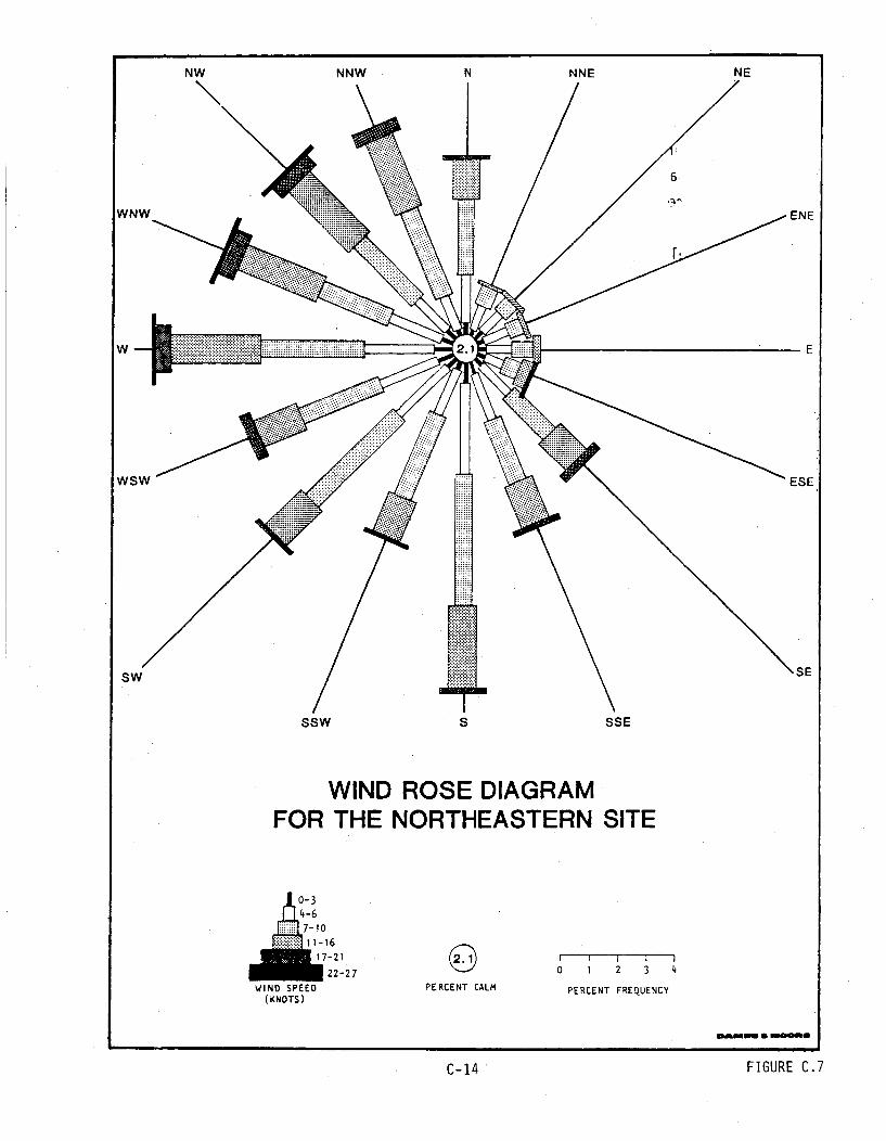
NW NNW N NNE NE

ENE

E

SW

SSW S SSE

WIND ROSE DIAGRAMFOR THE NORTHEASTERN SITE

A10-3Jj4-6

1-16

17-2 1

I 22-270 I 2 3

0 1 2 3 4

PERCENT CALM PERCENT FREQUENCYkKNUl!)

mwmmu a aO

C-14" FIGURE C.7

No state or federally declared rare or endangered species are known

to occur ohsite. A variety of mammal species are found onsite. The

most abundant are small mammals such as the white footed mouse, short-

tailed shrew, woodland jumping mice, and meadow mole. Common medium

sized mammals are woodchuck, opossum, and gray squirrel. White-tailed

deer are also abundant in this area.

Most mammals utilizing the site, with the exception of woodchucks,

are not burrowing species. These mammals dig tunnels which average

1.2 to 1.5 meters (4 to 5 ft) deep, and 7.6 to 9.2 meters (25 to 30

ft) long. Home ranges of the common mammals vary depending upon the

availability of food.

A moderate number of reptiles have been observed or are expected to

occur within the deciduous woodlands. Reptiles found include the

eastern garter snake and the snapping turtle, the latter being essen-

tially restricted to areas immediately adjacent to water. Other

reptiles observed include the spotted salamander, the wood frog, and

the American toad.

Aquatic Ecologjy

The aquatic environment near the site is limited to Point Creek (2 mi

from the site to the east) and its tributary, Boyle Creek (1 mi from

the site to the south). Point Creek leads into the Sprite River at a

point 37 km (23 mi) downstream, which then drains into the Wilder

River, 27 km (17 mi) further south. Both Point Creek and Boyle Creek

are considered Class C waters, best suited for recreational fishing.

Point Creek and its tributaries are shallow, rocky bottom streams.

The major primary producers of these waters consist of several genera

of diatoms, green and blue-green algae. The most common phytoplankton

are Tubellaria, Fragillaria, Asterionella, and Cyclotella. The flow

of these streams somewhat limits the abundance of macroflora. Forty-

seven fish species are known to occur within the county in the Wilder

C-15

River watershed. Most of these species are expected in Point and

Boyle Creeks. Point and Boyle Creeks are also stocked with rainbow

trout, and tiger muskellunge.

Land Use

The site, which is forested, is located in a rural land area. The

general region in which the site is located is comprised mostly of

forested land and active or inactive farmland. There are no farm

dwellings or other residences located onsite. The site is not suited

for any unique uses, but the soils are considered to be suitable for

farming. There is no significant mineral resource development within

10 km of the facility. County plans for the site, which is not in a

visually sensitive area, and surrounding land (2 to 7 km) include

reforestation and compatible uses.

There are no known mineral resources of economical consequences within

the vicinity of the site. Recovery operations in the area are limited

to a small bedrock quarry located one mile to the north, and a sand

and gravel quarry, located one mile to the east. No oil and gas

reserves of economically recoverable quantities are known to exist in

the area.

Other Parameters

Several other parameters are utilized in the impact analysis. These

are estimated to be the following. The precipitation-evaporation (PE)

index of the vicinity is equal to 136.. The average cation exchange

capacity of the subsurface media is about 20 milliequivalents per

100 grams (meq/100 g)o The average silt content of the site soils is

65 percent. The vertical water travel time from the bottom of the

trenches to the saturated zone is 50 years. The horizontal saturated

zone travel times from the edge of the vertical projection onto tile

saturated zone of the disposal cell closest to the discharge locations

C-16

are as follows: to the restricted area fence, 150 years (30 m), to the

closest drinking water well, 2,450 years (500 m), and to the nearest

surface water discharge location, 5,000 years (1000 m).

C.1.2 Southeastern Site .

The southeastern site is assumed to be located within the Liptone

Upland segment of the Atlantic Coastal Plain physiographic Province

at elevations ranging from 120 and 122 m (394 and 400 ft) above mean

sea level (msl). A general topographic map of the site is shown in

Figure C.8.

The site vicinity is characterized by gently rolling hills with broad

summits, and by relatively flat-lying fields bordered by somewhat

broad drainage depressions. Bordering the site area to the north is

the wide, flat lying topography of the Longville Plateau. In general,

natural surface drainage at the site is good. As a result of the low

topographic relief at the site, the probability of mass wasting and

other significant erosional events is low. The local drainage system

is dendritic with a typical perennial stream spacing of 1000 to 2000 m

or more.

Geology

The geologic profile of the site is provided in Figure C.9. The site

is underlain by 22 to 24 m of colluvium. Underlying the colluvium is

a cherty limestone (Winston Road) member of the lower Stablehead

Formation. The limestone has an average permeability of approximately

10-2 cm/sec and forms the basal portion of the unconfined aquifer.

Solution features in the limestone are minor and are not of the type

which would result in sinkhole development. Underlying the Stablehead

are Seymour and Wrigley Clayt members of the Brittle Limb Formation.

The Seymour member is a typically well-bedded, fine to coarse grained,

calcareous sand with clay lithofacies occurring as beds or lenses.

C-17

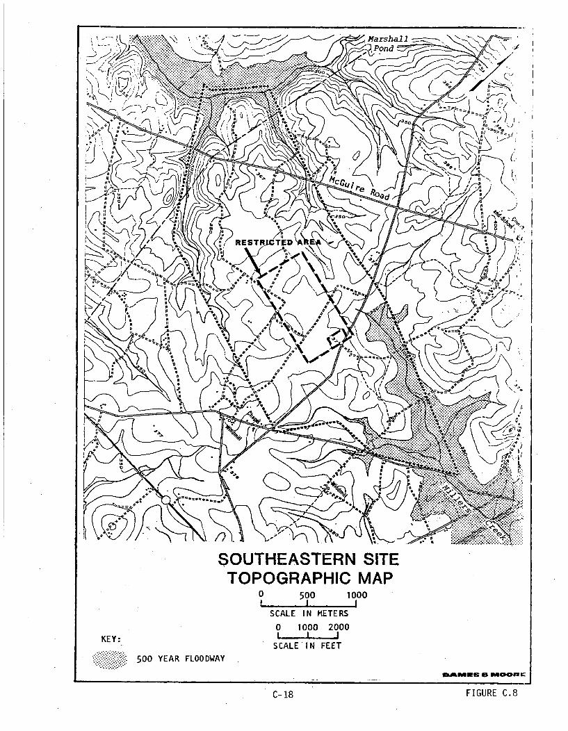
SOUTHEASTERN SITETOPOGRAPHIC MAP

0 500 1000L I I

SCALE IN METERS

0 1000 2000KEY: 1 1 I

SCALE IN FEET

500 YEAR FLOODWAY

C-18 FIGURE C.8

KEY

tnu

:I-

122-

110-

>-100-

,go-

z

0, 80-

70

-jw I

z Ll SURFICIAL SOIL LAYER

F122

SCHWI NNFORMATION

-110STABLEHEADFORMATION

-100WINSTON ROAD

MEMBER

FfIl

COMPACT SANDY CLAY

SAND- FINE TO COARSE

CHERT

LIMESTONE- CHERTY

LIMESTONE

LIMESTONE- ARENACEOUS

LIMESTONE- ARGILLACEOUS

CLAY

-90

SEYMOURMEMBER

-80

-70

WRIGLEYCLAY

-60 MEMBER

I-0u

cc

1I60-

50-

46-

,--, -- GROUND WATER TABLE

50 PORTER

46 FORMATION

0 1000 2000 3000

SCALE IN FEET

200 400 600

SCALE IN METERS

GEOLOGIC PROFILE OF THE SOUTHEASTERN SITE'1

m

C)

t-D

ItIII

The uppermost portion of the Seymour in the site area consists of

several thin limestone layers underlain by a clay layer. The Wrigley

member consists chiefly of a calcareous, marine clay. The total

thickness of the Brittle Limb Formation in the site area is about 45

meters. The clayey basal member of the Brittle Limb Formation serves

as an aquiclude to deeper aquifers.

The disposal facility site is located Within a general area having

a peak horizontal ground acceleration of approximately 0.11 g, with

a recurrence interval of more than 500 years. Structural features

associated within the area 'are geologically old and no capable faults

have been identified in the general vicinity of the site, The pro-

bability of significant ground displacement at the site is quite low.

Soils

The soils covering the reference disposal facility site are predomi-

nantly sandy loam and loamy sand. In engineering terms, these soils

may be described as medium-dense silty sands and clayey sands. The

surficial soils generally consist of 0 to 8 cm (0 to 3.2 in) of

topsoil mixed with silty sand.

This surficial soil layer is underlain by 10 to 12 m of sandy clay

from the Schwinn Formation. This sandy clayý layer has an average

permeability of about 5 x 10-6 cm/sec. Underlying this layer of

sandy clay are unconsolidated and semiconsolidated sediments of the

Eocene age Stablehead Formation. This sedimentary layer generally

consists of fine to coarse sands which are locally partially cemented

with occasional thin lenses of silt present. This sandy layer from

the Stablehead Formation is approximately 12 to 14 m (39 to 46 ft)

thick. The average permeability of this horizon is 1 x 10- cm/sec.

In general, under natural conditions, the nutrient levels and organic

matter content of all of the soil types occurring onsite are low.

C-20

Fertilization practices may raise these levels to a more moderate

level. The pH is strongly acidic with values generally ranging from

4.8 to 5.2. The cation exchange capacity of the soils will also be

low due to the small clay content over most of the site, and the

kaolinitic character of the minerals.

Groundwater

The depth to ground water fom the original ground surface at the si.te

ranges from 12 to 17 m (40 to 55 ft). The aquifer is unconfined and

is generally a subdued replica of the local topography. Well yields

in the unconfined aquifer are typically in the range of 1-10 gallons

per minute. Larger capacity uses are satisfied by deeper wells into

the confined aquifer.

The groundwater quality is fair (it meets the National Primary Drink-

ing Water Standards), however, the local consumptive use of water for

potable purposes is low and consists of 6 domestic wells within 5 km

(3.2 mi) and 60 wells used for farming and livestock. The closest

downgradient well is located 1.4 miles from the-site.

Recharge to the local groundwater system primarily results from

infiltration of precipitation. The closest major withdrawal location

is 36 km (22.5 mi) to the northeast where water is pumped from the

lower confined aquifer for a municipal drinking water supply.

Surface Water

The nearest perennial stream to the site is Millers Creek which is

located approximately 1000 m (3300 ft) to the southeast of the site

(Figure C.8). This is the nearest point of groundwater discharge, at

an approximate elevation of 295 ft above mean sea level. The other

major stream in close proximity to the site is the Signal Branch of

Basie Creek which is located approximately 2000 m (6600 ft) north of

the site.

C-21

Millers Creek Discharges into the Parker River which ultimately

empties into the Atlantic Ocean by Way of Feather Bay. The Signal

Branch has an average discharge of 0.028 m3 /sec (1 cfs - cubic feet

per second); this stream drains into the Basie Creek and the Turner

River,. which eventually drains into the Pepper River and ultimately

into the Atlantic Ocean.

Storm recurrence analysis for storms of variable durations indicate

that a 24 hour storm event with a 88.9 mm (3.5 in) total precipitation

will occur once a year. The 500 year storm will yield between 96.5

and 45.7 mm (3.8 and 1.8 in) of precipitation depending on the dura-

tion of the storm. The site is located on a topographic high, and

rainwater falling in the vcicinity of the site flows into one of two

drainage basins: an eastern basin and a western basin. Flow recur-

rance intervals for the east and west drainage basins of the site are

shown in Figures C.1O and C.11, respectively.

The soil, vegetation, and slope conditions on the site allow for

60 to 85 percent of precipitation to be lost by evaporation, rain-

splash, surface runoff, or return flow in saturated areas. Dis-

charge measurements from both basin- outlets indicate mean average

discharges of 73 cubic meters per second (26 cfs) for the eastern

basin and 2.1 cubic meters per second (74 cfs) for the western drain-

age area. Due to the limited extent of the basins, a direct corrol-

lary between precipitation intensity and peak stream flow exists.

Peak runoff for the eastern basin is expected to occur between 55 and

68 minutes after precipitation begins; and for the western basin,

between 150 and 172 minutes. The extent of the projected 500 year

flood is shown in Figure C-8.

Meteorol ocqy

The area of the site is classified as a humid subtropical climatic

regime. The annual precipitation at the site over the past twenty

C-22

L -

uJ

2

LI

2 5 1 0 0 200

RECURRENCE INTERVAL, YEARS

FLOW RECURRENCE INTERVALS FOR

EAST BASIN OF THESOUTHEASTERN SITE

0500

DAMIE€: I8 e-iOORE

I8

-2 2

n 102 .,02

25 I00 200500

WETBAIAOAH

6 6 S H T 6

25 100 200500

RECURRENCE INTERVAL, YEARS

-FLOW RECURRENCE INTERVALS FORWEST BASIN OF THESOUTHEASTERN SITE

C-24 FIGURE C.11

years has been 1168 mm (46 in), with-an annual range of 838 to 1473 mm

_(33 to 58 in).

High intensity storms can result from the remnants of inland travel

of hurricanes and tropical storms. The maximum 24-hour rainfall

recorded at the site-over the last twenty years is 152 mm (6 in).

Snowfall is generally observed during the months of January and

February. Precipitation event recurrance intervals for the site are

shown in Figure C.12.

The site area experiences four distinct seasons. Winters are short

and relatively mild with average temperatures of 9°C (49°F). Summers

are characteristically warm, averaging 24%C (76°F) and 27%C (80'F),

while the spring and fall periods are relatively mild. The average

annual temperature for the site area vicinity is 18% (65°F), with the

maximum occuring in July and August. The relatively mild temperature

variation observed at the site suggests that large-scale desiccation

and frost heaving of trench caps are not likely to occur. The tempe-

rature characteristics of the site are shown in Figure C.13.

The prevailing wind direction is south-southeasterly at an average

windspeed of 13 km/hr (7.0 knots). The wind rose diagram for the site

is presented in Figure C.14. The average humidity at the site is 78%

with an average low of 68% usually occurring in January and an average

high of 88% usually occurring in August.

Tornado activity within the immediate area of the site proper is

moderate with an estimated occurrance of one tornado every 500 years.

Within 50 km (31 mi) of the site, the occurrance frequency of torna-

does is on the order of once every fifty years.

The air quality at the site is quite good with concentrations of all

major pollutants below USEPA standards. The good air quality is

largely due to a lack of point sources of pollution near the site.

C- 25

wL Li-9

Li W

30 12 12 30

28 11 11 2826 -2624 10 10

24 24

22 9 22

z 20 8 8 20o zo< 78 ,,t: 186180.ed16-1

1.6- oo6 16L1i REUREC INERAL .14

9L 12E 5.ITE12120

oo0 -4 1

2- 22HU12ý 00 .0

4 H4 T M.

2 1 1 .2

1001 1.25 2 5 102'0 50 100 200 500 16000

RECURRENCE INTERVAL, YEARS

PRECIPITATION EVENT RECURRENCE INTERVALSFOR THE SOUTHEASTERN SITE

40

30-

ILL0

oLC-0J

I 100

LujI--

201-

40

30

20a

Il-

0

-10

10o

0.-

-10-

J. F M A M J J A S 0 N D

MONTHAVERAGE MONTHLY MAXIMUM TEMPERATURE

-MEAN MONTHLY TEMPERATU1REAVERAGE MONTHLY MINIMUM TEMPERATURE

MEAN MONTHLY TEMPERATURE AND AVERAGEOF THE MONTHLY MAXIMUM AND MINIMUM

TEMPERATURES IN THE VICINITY OFTHE SOUTHEASTERN SITE

DV41L S 6 A~qcO•I•e

C-27 FIGURE C.13

w -5.2

.ENE

-E

'ESE

"SE/w

WIND ROSE DIAGRAMFOR THE SOUTHEASTERN SITE

nl o,:

4-67-10

17-21

WIND SPEED(KNOTS)

0PERCENT CALM

0 I 2 3 4

PERCENT FREQUENCY.

S 01U

C-28 FIGURE C.II

C-28 .'FIGURE C.1.1

The only major point source of airborne pollutants is a coal fired

electrical generating station located 43 km (27 mi) to the northeast

of the site. Farming activity on land adjacent to the site is also a

source of air pollutants. Air quality at the reference disposal

facility is summarized below.

Concentration USEPA-3

Pollutant (mg/mi) Standard

Suspended particul ates24-hour average 90 150annual average 45 60

SO (annual average) 20 60

NOX (annual average) 28 100

Hydrocarbons3-hour average 70 160annual average 68 --

Terrestrial Ecology

Much of the general area of the site is composed of undeveloped

woodland which is dominated by longleaf pine and turkey oak. The

herbaceous layer is mostly turkey oak saplings, but bluejack, post

oak, and longleaf pine are also important. In addition to the

pine-upland hardwoods found near the site, there are two other forest

communities: bottomland hardwoods bording the eastern portion of the

site along Signal Branch and bluff hardwoods along the steeper slopes

of Millers Creek. Water oak, black (or sour) gum, and tupelo gum are

the dominant overstory species in the bottomlands. The bluff hard-

woods are characterized by hickory and northern red oak. Water oak,

northern red oak, ash and mulberry are the understory species.

Nestronia, a deciduous shrub that is considered to be threatened in

the state, is expected to occur in the pine-upland hardwoods. It also

may be found in the transition zone between these woods and the

C-29

may be found in the transition zone between these woods and the

bottomlands found closer to Signal Branch. While the bald eagle and

red-cockaded woodpecker may also be found in the county in which the

site is located, they are not expected onsite or within 5 km of the

site due to lack of suitable habitat. No other federally or state

protected species are anticipated to inhabit the area.

The most common mammals found "in the pine communities are pine mouse,

fox squirrel, and raccoon. Burrowing species that were observed are

southeastern pocket gopher and eastern mole. Gopher tunnels are

generally over 30 meters (100 ft) in length and dug at a depth of 15

to 2U cm (b to 8 in). While tunnels leading to the resting chambers

of the eastern mole may be 14 cm deep, most are only 2.5 to 5 cm (1 to

2 in) deep, and may extend for over O.b km.

Other mammals associated with the hardwood communities of the area

include the raccoon, opossum, woodrat, flying squirrel, gray squirrel

and swamp rabbit. Bobcat and gray fox have also been observed.

Common mammals found in the old field communities, and also in the

cultivated fields are several species of mice and, cottontail rabbit,

least shrew striped skunk, raccoon and opossum. Most mammals found in

this area are not underground burrowers.

Home ranges of most of the mammals found in the general area of the

site are relatively small: striped skunk - 4 ha (10 a); fox squirrel -

4 to 16 ha (10 to 40 a); gray squirrel - .8 and 2.8 ha (2 to 7 a);

eastern cottontail - 3 to 20 acres. Bobcat have the largest range,

the size of which is influenced by the abundance of prey. Their

general range is 8 km (5 mi), however they may wander up to 40 km (25

mi). The gray •fox may also wander over a large area particularly

during the winter.

As with the mammals, the different vegetative communities provide

habitat for several varieties of birds. Common species of the pine

C-30

communities include the state-colored junco, brown-headed nuthatch,

pine warbler, bluejay and common crow. The golden crowned-knight,

common flicker, and pileated woodpecker are common in the hardwood

forests. Predatory birds such as red-shouldered hawk, red-tailed

hawk, coopers hawk and barred owl are also found in moderate numbers

in these latter woodlands. These birds feed on the rodents and other

terrestrial vertebrates found in the area. The open fields and edge

communities provide habitat for the eastern meadowlark, field sparrow,

mockingbird, robin and common grackle. Dominant raptors in these

areas are the marsh hawk and sparrow hawk. The fields also prov-ide

hunting areas for the other hawks mentioned.

The pine upland forests provide habitat for many snakes, including

the corn snake, northern pine snake, black racer and diamondback

rattlesnake. The burrow of a gopher tortoise was also observed 4.5 m

(15 ft) from the northwestern boundary of the site. The gopher

tortoise is an accomplished burrower, its tunnels may be as wide as

33 cm, and generally as long as 10 meters. Many other animals tempo-

rarily or permanently use these burrows, including numerous insects,

opossum, and diamondback rattlesnakes. The more common reptiles of

the moister hardwood communities are the dusky salamander, cricket

frog, brown snake and eastern box turtle.

Active farming in the vicinity of the site limits the diversity and

abundance of the resident reptiles in these areas. Species that were

commonly found in the old field communities that may wander into the

cultivated fields include the southern toad, six lined racerunner and

eastern hognose snake. This latter species is known to burrow in

search of food.

In general (with the exception of the upland pine areas), the biomass

of southeastern forests and fields is high, compared to many other

regions in the United States. Mild climate and sufficient rainfall

promotes rich, stratified vegetative growth, which provides suitable

C-31

habitat and abundant food source for many herbivores and omnivores.

Primary and upper level carnivores, in turn, rely on the abundance of

these species.

Aquatic Ecology

Primary producers of the two nearby creeks include both algae and

macrophytes (aquatic vascular plants). Periphyton (attached algae)

are more common in the flowing waters of these streams. however,

increased turbidity or organic loading can quickly reduce the abun-

dance and types of algae found. Eight genera of aquatic plants were

identifiued within the nearby creek waters. These plants are most

abundant in areas of reduced current flow. The plants found, in

descending order of abundance, are:

Common Name Scientific Name Relative Abundance

Water milfoil Myriophyllum sp. Most abundant

Hornwort Ceratophyllum sp. Most abundant

Alligator weed Alternanters sp. Very abundant

Water weed Anacharis sp. Abundant

Duck potato Sagittaria sp. Not Abundant

Pickerel weed Pontederia sp. Scarce

Cattail Typha sp. Scarce

No endangered of threatened plant species are expected to occur. A

significant diversity of invertebrate species are also found in these

waters. The three most abundant groups, comprising just over 75

percent of the total number of insects sampled, are mayflies, beetles,

and waterfleas.

Approximately 38 species of fish are known to occur in the surface

water system. The most abundant fish are shinners, minnows, sunfish

and darter. Common recreational species include largemouth bass,

C-32

pickerel , channel catfish, black crappie, and sunfish. Two nearby

ponds are more popular fishing areas, however, than Millers Creek and

Signal Branch. Although several andromous species do spawn in the

rivers, no major spawning activity is noted in the above creeks. No

protected fish species have been recorded for these waters.

Land Use

Within an 8-.O km (50 mi) radius of the site, there are three prin-

cipal categories of land use: (1) woodland (about 25% of the area)

with both private and government preserves, (2) farmland (about 55% of

the area) with an approximate 50:50 mixture of rowcrops and pasture,

and (3) developed land (about 20% of the area) occupied by light

industry and residential dwellings. The area ocupied by the site

had been used for farming in the past, however, for the last several

years the land has been uncultivated and a thick secondary growth has

grown up.

The site vicinity and surrounding region is primarily agricultural,

with little high intensity development located outside of the towns

and cities. A school is located 6.4 km (4 mi) northwest of the site.

There are no historic sites, community facilities (other than the

school), or sensitive land uses located within 8-10 km of the site,

and the site is not particularly suited for unique uses. In the

absence of any indications of any incentives to develop the areas

near the site for non-agricultural uses, it is assumed that agricul-

ture will remain the dominant land use.

Mineral resources of a recoverable nature underlying the site are

limited to sand and gravel deposits. While these sands are not

believed to be pure enough for glass making, they are suitable for use

as fill or construction purposes. These deposits are widespread over

much of the southeastern portion of the state, and as such, do not

constitute a unique resource.

C-33

Other Parameters

Several other parameters are utilized in the impact analysis. These

are estimated to be the following. The precipitation-evaporation (PE)

index of the vicinity is equal to 91. The average cation exchange

capacity of the subsurface media is about 10 milliequivalents per

100 grams (meq/100 g). The average silt content of the site soils

is 50 percent. The vertical water travel time from the bottom of

the trenches to the saturated zone is 10 years. The horizontal

saturated zone travel times from the edge of the vertical projection

onto saturated zone of the disposal cell closest to the discharge

locations are as follows: to the restricted area fence, 32 years

(30 m), to the closest drinking water well, 400 years (500 m), and to

the nearest surface water discharge location, 800 years (1000 m).

C-34

C.1.3 Midwestern-Site

Falling within the Central physiographic province, the midwestern

site rests at an average elevation of about 247 m (810 ft) above

mean sea level (msl). The general topography of the site, which

is shown in Figure C.15, is that of a well dissected plain which is

virtually encircled-by various branches of the West Fork of Finley

Creek. The regional topographic surface undergoes only small changes

in relief.

Geology

A considerable thickness (about 35 m or 115 ft) of unconsolidated

deposits underlies the site. Most of this is composed of a rather

impermeable glacial till consisting predominantly of pebbly and sandy

clay and silt, and gumbotil. Gumbotil is a clay-rich till produced as

a result of thorough chemical decomposition. Portions of the glacial

drift may contain sand and gravel pockets of limited areal extent.

Southeast of the site is an area underlain by buried channel deposits

reflective of an ancient stream channel. This channel consists of

stream alluvium that filled the valley prior to or between glacial

periods. The buried channel represents the upper reaches of a tri-

butary to what is presently called the Washoe Channel. Evidence of

this system is the increased depth to bedrock by about 23 m (75 ft).

The bedrock consists of approximately 30.5 m (100 ft) of Mississippian

age rocks belonging to the Dette and Adams Series. The uppermost

formation of the Dette series, the Pile shale, which generally acts as

an aquiclude to the underlying Karesh and Becker formations, is absent

from the site area. The Karesh limestone is thin and discontinuous

over the Becker. Both formations are chiefly dense, crystalline,

lithographic or tightly cemented fragmental limestones and dolomites

with very low porosities. The basal 3 m (10 ft) of the Becker con-

sists of cherty sandstone.

C-35

.823

~.,

MIDWESTERN SITETOPOGRAPHIC MAP

0 500 1000I I I

SCALE IN METERS

KEY:

500 YEAR FLOODWAY

C-36FIGUE6 C.15R

C-36 - FIGURE C.15

Underlying the Dette series are the dense, cherty dolomites and lime-

stones of the Adams series. These rocks are exposed at the buried

channel/bedrock contact point. These two series make up what is

known as the Mississippian Aquifer. They are underlain by approxi-

mately 400 feet of siltstones and shales of Devonian age that serve as

a good aquiclude to the underlying Devonian Aquifer. Stratigraphic

sequences and the location of the groundwater table are illustrated in

the geologic profile on Figure C.16.

The midwestern site is located within the tectonically stable interior.

of the North American continent. The closest area of major seismic

risk covers the eastern section of the adjoining state to the north.

The site area has a probable peak horizontal ground acceleration of

less than 0.04 g, with a recurrence interval of more than 500 years.

Within historical record, no evidence was found to indicate the

occurrence of a capable fault within the site area.

Soils

The entire area in which the site is located is covered by about 3 to

3.7 m (10 to 12 ft) of Wisconsin loess, which is the parent material

of the site soils. The predominant soil types are silty clay loams

belonging to the Wancho, Houlik and Lyle series. These soils are

generally moderately-slow to moderately-well drained and have perme-

abilities ranging between 5 and 50 mm/hr (0.2 to 2.0 in/hr). The soil

is generally highly acidic in the topsoil layer and slightly acidic to

neutral in the substratum. Organic matter content is consistently

high throughout the series. Available nitrogen and phosphorus are low

to medium, and the soil content of potassium and calcium is very

low.

Ground Water

Ground water of appreciable amounts occur chiefly in the sand and

gravel deposits associated with the glacial drift and buried channel

C-37

systems. These "drift aquifers" are notably limited in areal extent,

although they sometimes serve as sources for farmsteads and livestock

drinking water. Water quality from the drift aquifers is generally

good, being low in dissolved solids and mineral constituents, however,

nitrates in excessive amounts are common, especially in those deposits

close to heavily fertilized ground surfaces.

Thicknesses of about 15 m (50 ft) or more of sand and gravel have been

associated with some of the larger buried valley systems. As the

channel in the site proximity is more representative of the upper

limits of a tributary to such a valley, it is likely to have lesser

quantities of permeable sediments. Water from these deposits is more

highly mineralized than in the drift aquifers. Permeabilities on the

order of 0.048 to 0.48 cm/sec (1,000 to 10,000 gpd/ft 2) can be

expected depending upon how well sorted the sand and gravel deposits

are within these aquifers.

Water in these Mississippian rocks is generally confined to secondary

openings, and movement is considered to be very slow. Specific

capacities are estimated to be less than 1.0 gallon per minute per

foot of drawdown. Based upon the dense, impervious nature of the

rock, a permeability of 2.4x10-5 cm/sec (0.5 gal/day/ft 2 ) can be

assumed. With little exception, water from the Mississippian aquifer

in the site area offers good to fair quality water.

The depth to the seasonally high ground water table under the site is

expected to be about 12 m (38 ft) from the ground surface. Local

ground water movement in the drift aquifer will be governed by the

topography, draining toward and being discharged into the various

branches of the West Fork of Finley Creek. Ground water from the

surficial aquifer, and also from the shallow bedrock aquifer, can be

expected to discharge to the buried alluvial deposits. The regional

ground water flow in the Mississippian aquifer is to the south-

southeast as controlled by the nearest major stream, the Deer River.

C-38

16(WEST) DISPOSAL FACILITY (EAST)

2 4 4 - 8 0 0 . r.. .. .. ...... ... . 0

.4 .+ . . . . . . . . . . . . . . . + +" + + + + + + 00

.+ .+• .. . . . . . .. . . .+q . . .. . . . . . + + + +zo7o ++ + +V+++ + ++ + f++ + + + . . . . . . . . . . . .

I +++ r+4+++++.+++F +++T+4++÷+++++750_

2075-+ ++++++++++++++++ ++++++++++ + + + + + + + + + + + + + + + + + + + + + + + + + + 70

+ + ++ + + + + + + + + + . . . . . . . . . . . . .220- + + + 4 .. . . . . . . . . . . . . . . . . . . . +

700°1.+ + +++++ + + + + + + + ++ + ++++ + + + +++ + ++ + + + + + + + + +++ 70

21 . . . . . . . . .+ . . ..210-~ ~~~ + . . . . . . . A .+' + +

20 650 -650

241,

24o0

KEY

[ 230

In

0

z2

C-)

;.0

-220

-210

BFO

-200

-190 JlFORI

-180 CFOR

CAFOR

168

GLACIAL LOESS

TILL

D I GLACIAL TILL- CLAY

I SAND AND GRAVEL

I• LIMESTONE- CHERTY

a..E T I N

ECKER CALCERITE

RMAT ION '

no DOLOMITE

I DOLOMITE- CHERTY

USTONRMATION . _

cc DOLOMITE- SILTY

LOVERRMATION SANDSTONE- CONGLOMPETOWN AND CHERMATION

F LIMESTONE- DOLOMIT

SSILTSTONE

E SHALE

. GROUND WATER LEVEL

RICH

-~ -~ - - .- -~ - ..- ?- ~ ~190-

180-

168:.

600- as V_ s x %v I ~ I I~ i

*,600

............................................................................

.. ... ... .. ... .. .......... ... .. .. ... .... ... ... ....... ... .. ..... ..... ..... ..... .. .. ..... ........ .. ... .. ......... .... ........ ..... ...

.......................... . ...... - .,***''''* ......................... .... . ...... .........

ERATEERTY

Errnl __________Q ,, I

0 1000 2000 3000

SCALE IN FEET

C 20L IN 0 E oE

SCALE IN METERS

I3UI

SIGEOLOGIC PROFILE OF THE MIDWESTERN SITE

Ground water usage in the area is limited to consumption as needed by

local homes and farmsteads for domestic, irrigation and livestock

supplies. It is estimated that the majority of wells tap Mississipian

aquifers and to a lesser degree, the drift aquifers. Yields of less

than 76 1pm (20 gpm) are the rule for this area. The only municipal

supply in proximity to the site belongs to the town of Mica, located

about 5.6 km (3.5 mi) to the southeast. Four of the nine municipal

wells tap the Lower Mississippian Aquifer. The remaining wells

utilize the Lower Ordovician Aquifer.

Surface Water

The site is located on a section of the Great Plains that is under-

going dissection as a result of recent climatic change. Approxi-

mately 90% of the streams in the drainage area are intermittent,

flowing only 6 to 8 months of the year. The drainage density of the

basin is 0.64, indicating a coarse drainage texture which is typical

of this region. Flow rates from the site average between 0.74 to 0.99

m 3/s (26 and 35 cfs) for the year.

Since the site is of limited areal extent, the correlation between

precipitation and stream discharge is very close. Peak discharge

rates are related to precipitation events of high intensity. Between

60 and 80 percent of precipitation in the drainage basin is discharged

as surface runoff. Analysis of the unit hydrograph of the site area

indicates that peak flow usually develops between 6 and 7 hours after

precipitation begins. Base flow and return flow play important roles

in the basin drainage; the extent is determined by the intensity and

duration of the precipitation event. Flow recurrance intervals for

the midwestern site area are shown in Figure C.17.-

As expected, the highest stream discharge rates are associated with

rain storms of limited duration but with high intensity (ranging

between 102 and 152 mm/hr). The 500 year flow floodway is delineated

in Figure C.15.

C-40

14

2

-9

ILOLL.

w

C,

c..

10k'8

6

4 6 HOUR FLOW

12 HOUR FLOW

.4HOUR-FL0O •

2

104

6

4

2

, r3

2

10 - . - . - . - . S ~I

25 100 200 500

RECURRENCE INTERVAL, YEARS

FLOW RECURRENCE INTERVALS FORTHE MIDWESTERN SITE

! s~~m

C-41 FIGURE C.17

During the development of the- site the discharge rate is expected

to increase as the area is-cleared of vegetation, and due to imper-

vious covers which may be placed over the disposal cells. While

the site development will decrease the time to peak discharge and

increase the peak flood stage, there will be no significant risk of

flooding at the site due to the elevation differences between the area

and -the site outflow. While overland flow of considerable velocity

may be expected during site development, prudent drainage engineering

will be able to divert flow, reduce velocities and limit erosion of

the, site.

Meteorology

The area has a humid continental climate, with a total annual local

precipitation of 777 mm (30.5 in). Approximately two-thirds of

the annual precipitation occurs during the months of April through

September. The source of this precipitation is the warm moist south-

erly air from the Gulf of Mexico.. The normal mean snowfall for the

site area is approximately 686 mm (27 in). Precipitation recurrance

intervals for the si-te area are shown in Figure C.18.

The average annual temperature in the site vicinity is approximately

11% (51°F). July is the hottest month, having an average daily

maximum of 31%C (87°F) and an average daily minimum of 18% (64°F).

During January, the coldest month, the daily temperature range is

approximately -0.6% (31'F) to -11% (12'F).

The prevailing wind direction at the site is southerly at an average

speed of 17 km/hr (9.0 knots). During the months of November through

March, a -northwesterly wind component develops in response to the

Canadian cold air outbreaks. Wind speeds during these months average

22 km/hr (1'2.- knots). Severe weather events such as thunderstorms

and tornadoes occur during midspring to late summer. The wind rose

diagram for the site vicinity is shown in Figure C.19.

C-42

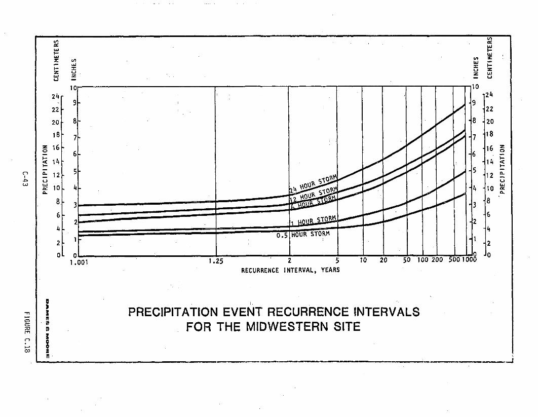
U,3

x w-- ww

I'm~- w. = I--I .J Z

LI -

10 1024 .24

9- 922 -22

20 8 8 - 20

18 7 18

g 16 16 z66- --< 14 14<

" 1 2 - 1 2LI - 10 4- .10w

. cl

6 6

2 I O210 - 4-4

-O0 c

1.001 1.25 2 0000' 001000

RECURRENCE INTERVAL, YEARS

ag

-• • PRECIPITATION EVENT RECURRENCE INTERVALS,FOR THE MIDWESTERN SITE2 -

m L

NW NNW

7.4

N NNE NE

-ENEWNW

7.9

W -4.7 E

.6~E

S EWSW

SW SE

SSW 12.1S

SSE

WIND ROSE DIAGRAMFOR THE MIDWESTERN SITE

0•-37 10

-1617-2122-27

PERCENT CALM

r - I I I0 1 2 3 4

PERCENT FREQUENCY

(KNOTS) mns m

C-q4 FIGURE C.19

C;-44 FIGURE C.19

Statewide occurrences of tornadoes average about 10 for any given 8

year period. From the period 1920 to 1960, there have been approxi-

mately 75 occurrences within 20 latitude/longitude square inclusive of

the site.

Since the site has a pronounced continental type of climate, it has

inversion frequencies closely related to the diurnal cycle. In

general, inversions occur 20 to 30% of the time during spring and

summer, while during the fall and winter months, inversions may be

expected about 30 to 45% of the time. The higher frequency during the

fall and winter is probably a result of the relatively low number of

storms in the fall and maximum length of stable nocturnal period in

winter. The opposite is true for the summer months. As a result,

annual morning and afternoon mixing heights vary by small amounts.

Terrestrial Ecology

The natural vegetation within the vicinity of the site is a mixture of

oak-hickory forest and bluestem prairie. The forest community occurs

primarily along valley slopes and upland ridges. Big bluestem is the

dominant grassland plant where the prairie remains. However, most of

this area is cropland. Two terrestrially environmentally sensitive

areas, Deer River Access and Chatham Timbers, are located 18 km

(11 mi) to the southwest and 38 km (24 mi) to the south, respectively.

Green Lake, which is a prime recreational fishing area, is located

21 km (13 mi) southeast.

The two major land uses of the county in which the site is located

are pastureland (24 percent) and row crops (65 percent), with corn

and soybeans representing the dominant crops. Approximately 35 and

12 percent of the county, respectively, are planted in these crops.

Most of the naturally occurring prairie has been lost in the county.

Existing grasslands, dominated by introduced species, are interspersed

in 60 to 80 ha (150 to 200 acre) blocks throughout the county.

C-45

Almost 60 percent of the land area adjacent to the site is planted

in corn. Four small woodlots, about 4 ha (10 a) total, are found in

the near vicinity of the site -- either adjacent to residences or

farm buildings, or along creek boundaries. White oak, red oak, and

shagbark hickory dominate these woodlands. Small blocks of grassy

areas occur along stream banks, roadsides and other areas. Common

introduced grasses include bluegrass and smooth brome. Similar

ground cover is found within an 8 km radius of the site, with slightly

more oak-hickory forests occurring along the Deer River system.

No Federally declared endangered or threatened species have been

observed on or near the site. The most common mammals found onsite

and within a five mile radius are those for which corn is a predo-

minant food source, and can live in proximity to. man. The most

abundant species include the raccoon, striped skunk, eastern cotton-

tail, opossum and fox squirrel. Several burrowing mammals are also

found in the area, primarily in fields not actively cultivated.

These burrowing mammals include the badger, plains pocket gopher and

thirteen-lined ground squirrel. The badger and pocket gopher dig

tunnels in search of food which can be 1.2 to 1.5 m (4 to 5 ft) in

depth and up to one hundred meters long.

Most of the mammals that utilize the site have small home ranges,

e.g., thirteen-lined ground squirrel - 0.8 to 1.21 ha (2 to 3 a),

eastern cottontail - 3 to 8 ha (20 acres), and opossum - 6 to 16 ha

(15 to 40 acres). The raccoon, with a maximum range of 3.2 km (2 mi),

and an average of 1.6 km (1 mi), has the largest home range of those

species expected in this area.

Corn very often is a major winter food source for many upland game-

birds, including birds found in the area. The ring-necked pheasant

and bobwhite quail are the species most commonly hunted. Black ducks,

mallards and pintails are also numerous in the area, and feed heavily

on corn.

C-46

Numerous resident bird species are also found onsite and in the

surrounding cornfields. The most common species found, and which

feed extensively on corn, include the redwing, cardinal, meadowlark,

purple grackle, and common crow. Resident birds of prey include the

red-tailed hawk and great horned owl. Transient species include the

coopers hawk, broad winged hawk, and red-shouldered hawk.

As a result of ongoing agricultural activities, the reptile and

amphibian population of the area is limited. An occassional eastern

plains garter snake, bullsnake, or black rat snake may be found.

Aquatic Ecology

With the exception of the northwestern border, the site is surrounded

on all sides by the West Fork of Finley Creek, and other unnamed

intermittant tributaries. Finley Creek feeds into the Deer River

approximately 51 km (32 mi) downstream. There are no Federally

declared wild or scenic rivers within five miles of the site.

The West Fork of Finley Creek and its tributaries are Class B warm

waters. Primary uses of the creek are for wildlife, fish, aquatic andsemiaquatic life, and secondary contact water uses. Although the

soils along the stream banks are moderately to highly erodable, the

vegetated banks limit the amount of sediments that enter the streams.

No Federally declared endangered or threatened fish or snails are

expected in these streams.

Land Use

The site is located on agricultural land used extensively (85 percent)

for cultivation of crops, mostly corn. Five houses are located within5 km of the site. The site vicinity contains 4 towns - Mica, Grendle,

Reed and Lyme - but most of the land is not developed intensively.

Hayer Park (10 acres) is located 4.8 km from the site. There are

C-47

no other community facilities, historic places, or other visually

sensitive land uses within a 8 km radius. Two state-owned lands,

Lake Darling and Deer River Access, are located within 24 km of the

site.

The chief source of economically important resources in the state lies

in the substantial coal resources associated with Pennsylvanian age

rocks. No such deposits occur under the site as the initial bedrock

encountered is of Mississipian age. There is a potential for some

natural gas deposits. However, the Ordivician source rocks are thin,

making recovery unconsequential and uneconomical.

Other Parameters

Several other parameters are utilized in the impact analysis. These

are estimated to be the following. The precipitation-evaporation (PE)

index of the vicinity is equal to 93. The average cation exchange

capacity of the subsurface media is about 12 milliequivalents per

100 grams (meq/100 g). The average silt content of the site soils is

85 percent. The vertical water travel time from the bottom of the

trenches to the saturated zone is 30 years. The horizontal saturated

zone travel times from the edge of the vertical projection onto

saturated zone of the disposal cell closest to the discharge locations

are as follows: to the restricted area fence, 90 years (30 m), to the

closest drinking water well, 2,070 years (1250 m), and to the nearest

surface water discharge location, 3,770 years (2500 m).

C.1.4 Southwestern Site

The southwestern site is assumed to be located within the Northern

High Plains subdivision of the Great Plains physiographic province.

The regional topography shows sharply contrasting flat plains and

rolling to rugged erosional breaks. The general topography of the

site is shown in Figure C.20.

C-48

..EACILITY -.

+/-" .--

N I

I .3999 /

K- *? .-i d ;

•-'- -- -- -- -

5 .-..÷ ..- : , • " -

7..-'" ',-\::- - /..:: : • ÷ •: '::: : • . ::•;::.•.:

N ' -_ _ - . ...... •:.: :.>',

'e-:

SOUTHWESTERN SITETOPOGRAPHIC MAP

0 500 OOO0I I I

SCALE IN METERS

KE:0 1000 2000C-Y:9 FIUR ,.•ii!500 EARFLOOWAY SCALE IN METERS

C-42 FIGURE C.20

The plains are about 17,872 km 2 (6,900 mi 2) in areal extent and

show a gradual eastward, slope on the order of 0.2%. The site has an

estimated average elevation of 1219 m- (4,000 ft) above mean sea level.

Drainage is to the southeast and southwest to various intermittant

branches of Hotsprings Creek.

Geology

Below the surface cover of loam and clay-loam soil are Pliocene age

deposits of the Bixler formation. These sediments were eroded from

the ancient Rocky mountains and transported by streams to this area.

Because of their origin of deposition- their character varies both

vertically and horizontally. As a general rule, however, the sand and

gravels are in the basal portion of the formation.

The Bixler Formation is about 91 m (300 ft) thick in the site area.

The upper 12 to 15 m (40 to 50 ft) is composed of caliche, a calcium-

rich, carbonate-impermeable sandy clay which acts in a similar manner

as a hardpan. Effects of the semi-arid climate have cracked the upper

0.9 to 1.5 m (3 to 5 ft) of the caliche. Underlying the caliche is

approximately 15 m (50 ft) of dense, brown clay. Thin, discontinuous

streaks of sand are also associated with the clays. The balance of

the Bixler is principally composed of sand and gravel, extending down

to the eroded surface of the Triassic rocks.

The Triassic shales and sandstone belonging to the Maxwell group are

estimated to be about 152 m (500 ft) thick in the site area. The

first material encountered under the permeable Bixler strata is a red

clay, indicative of the weathered shale surface. A schematic repre-

sentation of the site geology is shown in Figure C.21. The site falls

within an area designated as having a peak horizontal ground accele-

ration of less than 0.04 g with a recurrance interval of more than 500

years. No evidence was found to indicate the occurrance of capable

faults under or near the site.

C-50

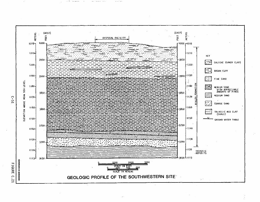
(WEST)

wj w

1219-1 400 L

(EAST) -I- eJ

Ui

p1

ui

w

1210-

1200-

1150-

1 18o.

1170-

1160,

1150

2

i-

U.

tU.

aJ

rKEY

L CAL ICHE (SAt

W BROWN CLAY

FINE SAND

L MEDIUM SAND7 WITH APPRI

AMOUNTS 01

MEDIUM SAND

COARSE 'SAND

TRIASSIC RE

(SHALE)

ECIABLEF FINES

NOY CLAY)

D CLAY

GROUND WATER TABLE

1 14o-

1130

112Q-

1113-

I3l

TRIASSIC-DEPOSITS

0 nanIN 2 0R 3000

6000

SCALE IN METERS

GEOLOGIC PROFILE OF THE SOUTHWESTERN SITE

Soils

The predominant soil types underlying the site are loams and clay

boams belonging to the Starble, Nester, Wixman and Jeeper series.

They were formed from moderately fine-textured, calcareous, wind-

blown sediments derived mostly from alluvial outwash from the Rocky

Mountains. Because rainfall is low, and there are long, dry periods,

soil development has been slow. The soils are seldom wet below the

root zone, and, as a result, many of the soils have a horizon of

powdery lime accumulation. Leaching has not yet removed free lime

from the upper layers of the calcareous Starble and Wixman soils.

Soils of the Nester and Jeeper series tend to be more neutral.

Calcium contents are high in all the soils. Generally, the prairie

type of vegetation contributes large amounts of organic matter to the

soil. The soils are rather deep (up to 2.5 m) and well-drained,

having nearly level to gentle slopes. Runoff is generally slow and

permeability values range between less than 1.5 to 50 mm/hr (0.06 to

2.0 in/hr).

Ground Water

The Bixler formation is an unconfined aquifer with very limited

consumptive use. The water occurs under water-table conditions,

and the differences in the thickness of the water saturated material

are closely related to the thickness of the Bixler formation. The

saturated thickness under the site is only about 7.6 m (25 ft) as the

water table lies some 84 m (275 ft) below ground surface. Available

data indicates that the Bixler is the local source for recharge to

the Triassic rocks where they are in contact.

The source of water (recharge) to the Bixler, and thence to the

Triassic rocks, is precipitation on its more permeable surfaces. The

amount of precipitation that enters the ground water is a very small

C-52

percentage of the total precipitation falling at the surface. It has

been estimated that -the quantity of precipitation annually reaching

the groundwater is negligible. For the purposes of this report,

however, it is assumed that the annual percolation is 1 amm. Due to

the rather impervious nature of the onsite surficial materials, most

of the precipitation will be -lost by evaporation or drain to Hot-

springs Creek as runoff. Part of this runoff will percolate downward

through the coarser stream deposits and enter the ground water regime.

Some infiltration may work its way through the fractured portions of

the caliche and slowly downward to the water table, but this is of

limited quantity.

Under natural hydraulic gradient conditions, the water table slopes to

the east, generally parallel to the surface slope which is about 0.2%.

The average permeability of the Bixler-Triassic aquifer in this area

is estimated to be 4.7x10-3 to 9.4xi0-3 cm/sec (100 to 200 gpd/ft 2 ).

Ground water within the site vicinity is used almost exclusively as

a supply for livestock with a few domestic wells serving ranches.

The wells are generally powered by windmills and generate yields not

likely to be greater than 7.6 to 11.4 liters/min (2 - 3 gpm). The

nearest irrigation well is located about 13 km (8 mi) from the site.

Surface Water

Elevations in the site vicinity range between 1169 and 1223 m (3835

and 4013 ft) above mean sea level. Total stream length above the site

is over 90 km (295,680 ft). With the limited precipitation in the

region, streams flow intermittantly throughout the year. A wide

variation in discharge occurs at the site. Since no base flow is

known to occur in the area, precipitation accounts for all of the

stream discharge. Short duration, high intensity thunderstorms

account for the peak discharges from the site. Flow recurrance

intervals for the site vicinity are shown in Figure C.22.

C-53

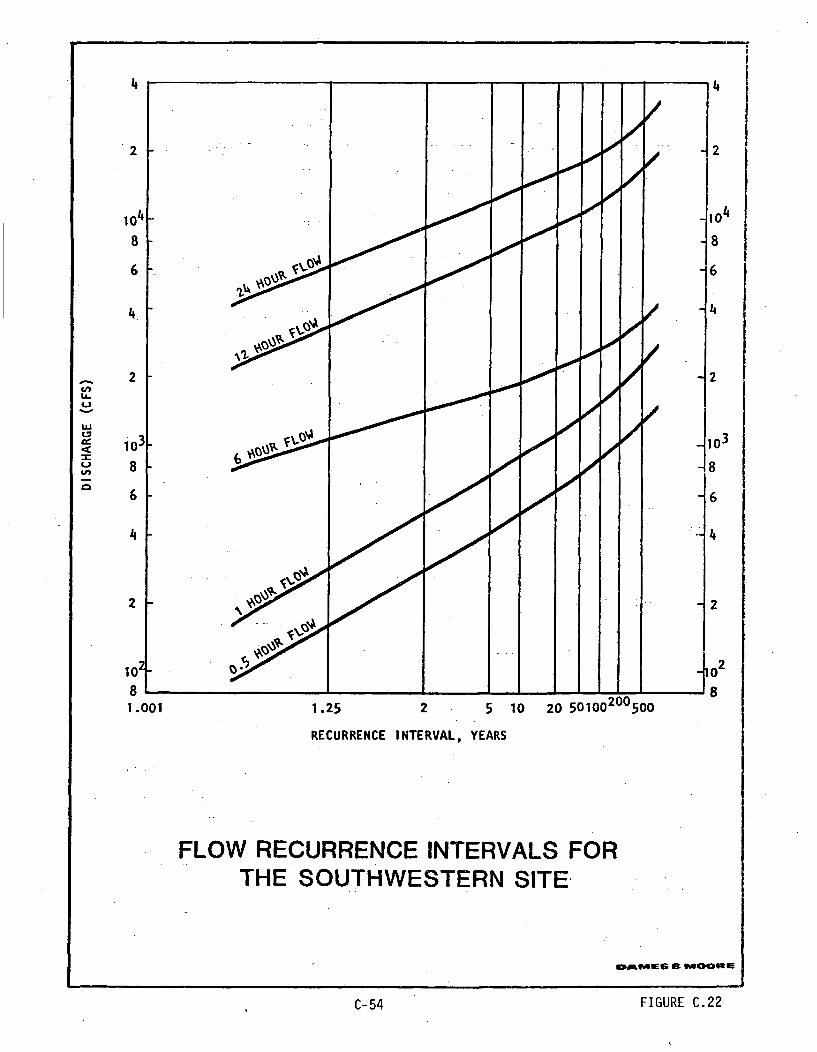
EnILLi

wC,

Li

En

a

RECURRENCE INTERVAL, YEARS

FLOW RECURRENCE INTERVALS FORTHE SOUTHWESTERN SITE,

AM ES 49WAORE

C-54 FIGURE C.22

The area of the basin receives considerable intense rain (greater

than 50 mm/hr), however, most peak flow is dissipated before discharge

at the outlet. Peak discharge occurs when the rain event is within

32 km (20 mi) of the outlet. Analysis of the unit hydrograph of the

site area and flow data indicate that discharge rates of up to 28.2

m 3/sec (1,100 cfs) may be expected to occur at least once a year.

The 500 year flood has-been determined to be approximately 736 m 3/sec

(26,000 cfs) and the floodway is delineated on Figure C.20. As shown,

the site is well above the floodway.

Meteorol ogy

The climate of this site is considered semi-arid, which is character-

ized by low humidity, wide temperature and precipitation variations,

and frequent windstorms. The average annual precipitation for the

site area is approximately 485 mm (19 inches). Departures from thenorm can be great with extreme yearly totals ranging from 243 to

1010 mm (9.56 to 39.75 in). Nearly three-quarters of the total

annual precipitation occurs during the growing season from April

through September, primarily--in the form of thundershowers. Pre-

cipitation event recurrance intervals for the site are shown in

Figure C.23.,

The average annual temperature for the area is about 14%C (57°F).

Maximum temperatures occur in the mid-summer months of June, July

and August. The temperature' characteristics of the site are shown in

Figure C.24.

Rapid and wide temperature variations are common, especially during

the winter months when cold fronts from the Rocky Mountain and Plains

States sweep across the plains. Temperature drops up to 16%C (60'F)

occurring within a 12-hour period may be associated with these fronts.

The highest recorded temperature in the region was 42%C (108°F) and

the lowest was -27*C (-16'F).

C-55

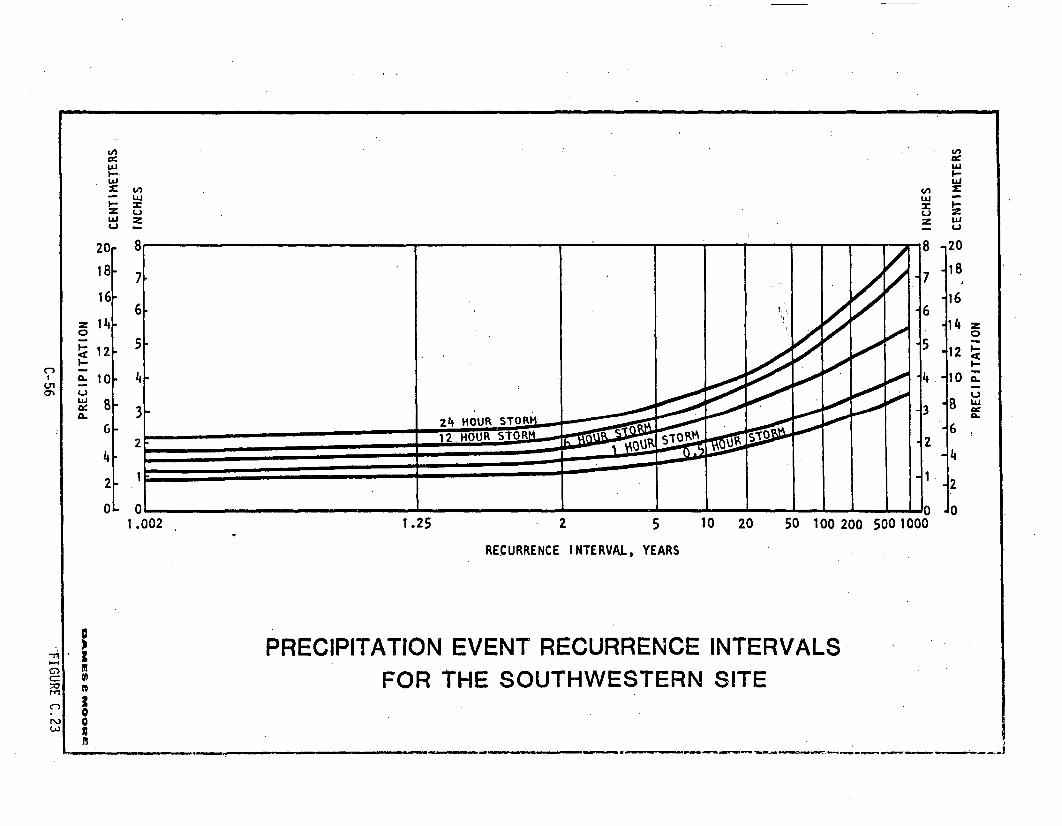
LLI

LiJ

tnLiJ

z

,'In

~iJ-z

t,

I--w

I-

iLi

20

18

16

141

I I ,,~9,YrrI 4

7// 7

6

5

6•;00

-20-118

lB-16

-14

12

"10c-

20

I-

I-

Li

w

0.

121- 5,-

10

81

6

41-

324 HOUR STORMt....

1 7 1 -1 M R ST tL Ou 1,

00000 000000010

.

18,. .......iivv .......,d

w

0I-

Li

z _ _ _ _ _ _ _ _ _ _ _ _ _ _ _ _ _ _ r - -r

3

2

41

a6

1441 I

I {2

0I2.J0A'

LI I I - I - I - d - I - i - - I . S LI1.002 1.25 2 5 10 20 50 100 200 500 1000

RECURRENCE INTERVAL, YEARS

PRECIPITATION EVENT RECURRENCE INTERVALSFOR THE SOUTHWESTERN SITEm

p-

a

II0

I00II

0

40.

30[

0 0 0

100

80

wcc

201

lot-

60

40

140

30

Liu20~

1-

10k

-10

0.

20-IOL

0J F M A M J J A S 0 N D

MONTH

AVERAGE MONTHLY MAXIMUM TEMPERATUREMEAN MONTHLY TEMPERATUREAVERAGE MONTHLY MINIMUM TEMPERATURE

MEAN MONTHLY TEMPERATURE AND AVERAGEOF THE MONTHLY MAXIMUM AND MINIMUM

TEMPERATURES IN THE VICINITY OFTHE SOUTHWESTERN SITE

C-57 FIGURE C.24

C-57 FIGURE C.24

The prevailing winds from March through October are southerly at 25

km/hr (13.6 knots), and southwesterly at 21 km (11.4 knots) during the

winter months. The annual mean speed for all directional components

is 24 km (13 knots) and southerly. These winds contribute to the

evaporation rate associated with the region. The strongest winds

generally occur in March and April and are associated with thunder-

storm activity. The strongest winds recorded (134 km/hr in 1949) were

associated with a tornado, however these climatic events are rare.

The wind rose diagram for the site is shown in Figure C.25.

Terrestrial Ecology

The site is located in the High Plains area, also known as the Tinson

Province. This area is a relatively level high plateau, and is better

drained than most of the other regions in the state. The shorter

growing season (179 - 225 days) and lower annual average temperature

(120 to 13'C) found in this region, compared to other parts of the

state, play an important role in the types of plants and animals

found here.

The area has been characterized (within a 40 km radius of the site) as

Grama Buffalo Grasslands. The most abundant native plant species in

this short grass/mixed grass prairie are buffalograss and blue grama.

Total ground cover is relatively dense, and tends to increase under

grazing. The preponderance of grass species results in large quan-

tities of organic materials in the form of living and dead grass roots

within the first ten to twelve centimeters of soil (some roots of

blue grama and buffalo grass extend to 0.9 m, however). The vegeta-

tive cover of the site is typical of the region. Although various

species of trees, including oaks, elms and hackberries, are often

found along stream floodplains and steep-walled canyons, these are not

found along Hotsprings Creek, an intermittant stream, or its feeder

streams, which surround the all but northern portions of the site.

Federally declared endangered species have not been observed within

the site.

C-58

NW N NNE7~6

W 5 N

ENE

-E

'ESE

SE

wS SSE

WIND ROSE DIAGRAMFOR THE SOUTHWESTERN SITE

k-10

7-10

-27

28-33 aPERCENT CALM

I I I I

0 1 2 3 4

PERCENT FREQUENCY(KNOTS)

S ineema

C-59 FIGURE C.25

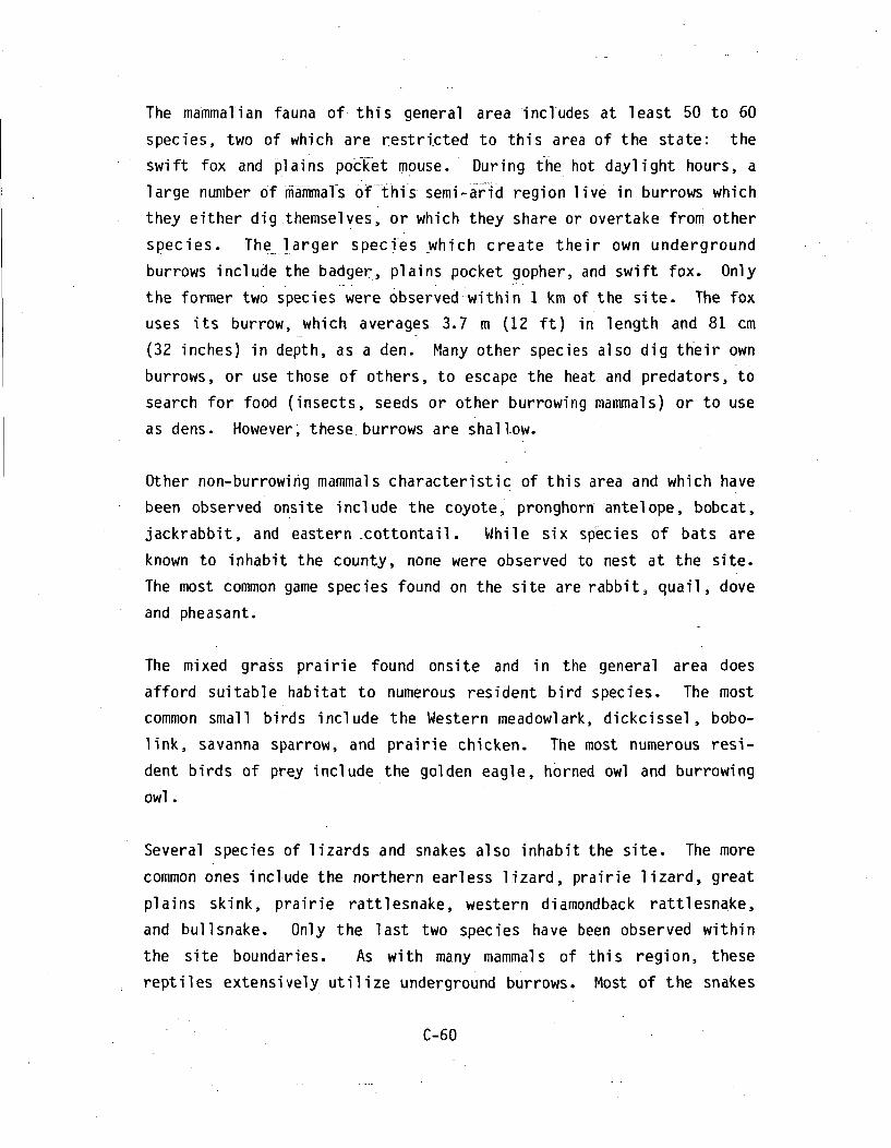
The mammalian fauna of this general area includes at least 50 to 60

species, two of which are restricted to this area of the state: the

swift fox and plains pocket mouse. During the hot daylight hours, a

large number of ma-nimal-s of-this semi-atrid region live in burrows which

they either dig themselves, or which they share or overtake from other

species. The larger speci-es which create their own underground

burrows include the badger, plains pocket gopher, and swift fox. Only

the former .two species were observed within I km of the site. The fox

uses its burrow, which averages 3.7 m (12 ft) in length and 81 cm

(32 inches) in depth, as a den. Many other species also dig their own

burrows, or use those of others, to escape the heat and predators, to

search for food (insects, seeds or other burrowing mammals) or to use

as dens. However; these burrows are shallow.

Other non-burrowing mammals characteristic of this area and which have

been observed onsite include the coyote, pronghorn antelope, bobcat,

jackrabbit, and eastern -cottontail. While six species of bats are

known to inhabit the county, none were observed to nest at the site.

The most common game species found on the site are rabbit, quail, dove

and pheasant.

The mixed grass prairie found onsite and in the general area does

afford suitable habitat to numerous resident bird species. The most

common small birds include the Western meadowlark, dickcissel, bobo-

link, savanna sparrow, and prairie chicken. The most numerous resi-

dent birds of prey include the golden eagle, horned owl and burrowing

owl.

Several species of lizards and snakes also inhabit the site. The more

common ones include the northern earless lizard, prairie lizard, great

plains skink, prairie rattlesnake, western diamondback rattlesnake,

and bullsnake. Only the last two species have been observed within

the site boundaries. As with many mammals of this region, these

reptiles extensively utilize underground burrows. Most of the snakes

C-60

use rodent burrows both for cover and in search of food. The great

plains toad and plains and western spadefoot toads dig their own

underground tunnels, which can range from several centimeters to a

meter in depth.

Aquatic Ecology

The aquatic environment of the site is limited to Hotsprings Creek and

its two feeder streams, all intermittent, which surround the site to

the east, west, and south. This creek remains intermittent until

approximately nine miles prior to its confluence with the Montreel

River approximately 136 km (85 mi) downstream. The only other tribu-

tories to Hotsprings Creek occur within an 8 km (5 mi) radius of the

site. After rainstorms when water does flow in this stream, aquatic

biota is limited to algae, insects (which use the water to breed),

and potential fish species such as minnows and sunfish. These fish

survive the dry seasons by gathering in small pools of water that may

remain throughout the year, and are then dispersed throughout the

stream with the flowing waters.

Land Use

The site is located near the administrative borders of a national

grassland administered by the U.S. Department of Agriculture, on open

grassland. The site itself was privately owned before purchase by the

state. There are no residences onsite or within the close vicinity (1

mi) of the site.

The site region is a plain containing numerous parcels of federal

grassland, distributed throughout this portion of the state and into

neighboring states. Portions of the site are used at times for

grazing cattle. The national grassland is the overriding factor

influencing land use in the area, and this is not expected to change

significantly in the foreseeable future.

C-61

The only known mineral resource occurring in the site area is caliche.

This calcium carbonate cement is associated with sand and gravel

deposits of the Bixler formation, and may be suitable for use as

aggregate. However, these deposits are widespread throughout the

entire region and- do not represent unique resources.

Whereas numerous producing oil and gas wells have been drilled in the

adjoining county to the east of the site, no historical production has

occurred within the site county. Prospect wells drilled within

proximity to the site have not indicated the presence of oil or gas

reserves of recoverable quantity.

Other Parameters

Several other parameters are utilized in the impact analysis. These

are estimated to be the following. The precipitation-evaporation (PE)

index of the vicinity is equal to 21. The average cation exchange

capacity of the subsurface media is about 5 milliequivalents per

100 grams (meq/lO0 g). The average silt content of the site soils is65 percent. The vertical water travel time from the bottom of the

trenches to the saturated zone is 275 years. The horizontal saturated

zone travel times from the edge of the vertical projection onto

saturated zone of the disposal cell closest to the discharge locations

are as follows: to the restricted area fence, 5 years (30 m); to the

closest drinking water well, 300 years (3000 mi); and to the nearest

surface water discharge location, 600 years (6000 m).

C.1.5 Summary of Regional Environmental Parameters

This section presents a summary of the regional environmental para-

meters and characteristics presented in this appendix and used in this

report to calculate radiological and economic impacts from LLW manage-

ment and disposal.

C-62

The assumed population distribution in the vicinity of each of the 4

regional sites at the year 2000 (postulated year of end Of facility

operations) is presented in Table C-1.

Water balance calculations for determining the amount of precipitation

reaching the saturated zones of the regional sites (i.e., the amount

of percolation) were presented in Tables A-4 and A-5. As shown

in Table A-5, the water balance calculations for the southwestern

regional site indicate that there is no calculable percolation reach-

ing the saturated zone. However, for purposes of determining bounding

impacts from waste disposed at this site, it is assumed that the

percolation coefficient equals 1 mm at the southwestern site.

Based upon this information and information presented in sections

C.1.1 through C.1.4, environmental parameters specific to the four

regional disposal sites may be calculated. A list of the region-

dependent parameters was included in Table 3-2, together with the

parameter symbols used in the computer codes developed as part of this

work. Values determined for each of these parameters for each of the

four regional sites are provided in Table C-2.

Use of a specific set of property values to calculate impacts is

determined by the value of the region index, IR. The transfer factors

for the accident, intruder-construction, intruder-agriculture, and

exposed waste scenarios are used to calculate the site selection

factors (f s) for these scenarios as described in Chapter 3.0 and

Appendix A of this report. The parameters for the ground water

scenarios are used to calculate the waste form and package factors

(f w) and the site selection factors (f s) for these scenarios as

described in Section 3.5 and Appendix A. The transportation parame-

ters are used to calculate radiological and economic impacts of waste

transport to the regional disposal sites as described in Chapter 4.0.

Additional information regarding the use of the parameters in the

computer codes is provided in Chapter 6.0.

C-63

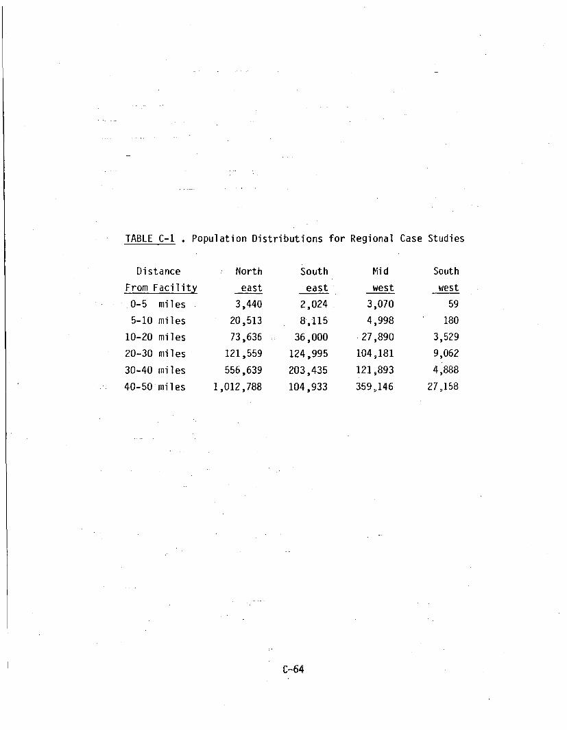
TABLE C-1 . Population Distributions for Regional Case Studies

Distance

From Facility

0-5 miles

5-10 miles

10-20 miles

20-30 miles

30-40 miles

40-50 miles

North

east

3,440

20,513

73,636

121,559

556,639

1,012,788

South

east

2,024

8,115

36,000

124,995

203,435

104,933

Mid

west

3,070

4,998

27,890

104,181

12159893

3594146

South

west

59

180

3,529

9,062

4,888

27,158

C-64

TABLE C-2 . Environmental Parameters for Regional Locations

ParameterAccident ScenarioFireSingle-Container

Intruder ScenariosConstructionAgriculture

Exposed Waste ScenarioIntruder-AirErosion-AirSurface Water

Groundwater ScenarioTravel Times - years

Between SectorsIndividual WellBoundary WellPopulation WellPopulation Surface

Peclet NumbersBetween SectorsIndividual WellBoundary WellPopulation WellPopulation Surface 3

Dilution Factors - mIndividual WellPopulation WellPopulation Surface

Geometric ReductionIndividual WellPopulation WellPopulation Surface

Percolation - mmRegular CoverThick Cover

Retardation Coef-ficient Set Used

TransportationOneway Distance (mi)Stops Along the WayCask Turnaround(days)

Symbol

TPO(1)TPO(2)

FSCFSA

POP (1)POP(2)POP(3)

DTTMTTM(1)

TTM(2)TTM(3)

DTPCTPC(1)

TPC(2)TPC(3)

QFC(1)QFC(2)QFC(3)

RGF(1)RGF(2)RGF(3)

NRET

DISTSTPSCASK

Northeast

1.83E-102.61E-12

Southeast

1.83E-10 1.83E-10 1.83E-103.32E-12 2.55E-12 1.79E-12

9.18E-12 2.01E-11 2.51E-11 2.64E-102.96E-11 3.18E-11 3.28E-11 8.06E-11

1.01E-091.51E-091. 12E-07

400200350

25005000

800400700

1000020000

77002.OE+54.5E+6

111

7438

4

30012

3.50E-105.25E-101. 12E-07

644266

400800

160013001900

1000020000

77002.OE+54.5E+6

111

18030

3

40013

3.86E-105.79E-101.12E-07

120130175

21003800

800400700

1250025000

77002. OE+54.5E+6

111

5025

3

60025

2.66E-113.99E-111. 12E-07

8280283580880

80013001600

3000060000

77002. OE+54.5E+6

111

11

2

100038

Midwest

Southwest

C-65

C.2 Reference Disposal Facility Design and Operation

In this section, a reference near-surface disposal facility design

is described, including the support facilities and structures, and

facility operations. The reference disposal facility design is meant

to be representative of existing disposal facilities and operating

practices and has been condensed from reference 2. The reference

near-surface disposal facility design is then assumed to be located at

each of the four hypothetical regional disposal facility sites des-

cribed in the previous section C.1. From this basic design, the

impact measures associated with LLW management and disposal may be

assessed on a regional basis as a function of alternative waste forms

and alternative disposal facility design and operating practices.

C.2.1 Basic Design

To provide a base case against which alternatives can be analyzed,

the, assumed disposal facility design is sufficient for a total waste

capacity of up to one million m 3 delivered to the disposal facility

at an annual average rate of up to 50,000 m3 . The actual volume of

waste disposed at one of the four regional disposal facilities is a

function of the volume of waste generated in the region and the waste

processing alternative (waste spectrum) considered.

To develop the disposal facility, the licensee is assumed in all

regions to purchase a plot of land covering 81 ha (200 acres), of

which 60 ha (148 acres) is turned over to state ownership. This 60 ha

of land is then leased back to the licensee and is used by the licen-

see for the disposal facility. The remaining 21 ha (52 acres) is

retained by the licensee for possible future use.

A conceptual layout of the reference disposal facility design is

illustrated in Figures C-26 and C-27. As shown in the figures, the

disposal facility may be divided into two basic areas: a "restricted

C-66

//

/

FENW

REFERENCE DISPOSAL SITE LAYOUT0 50 100

SCALE IN METERS

KEY:

S MONITORING WELLS m a OW040=0

C- 67 FIGURE C.26

C-67 FIGURE C.26

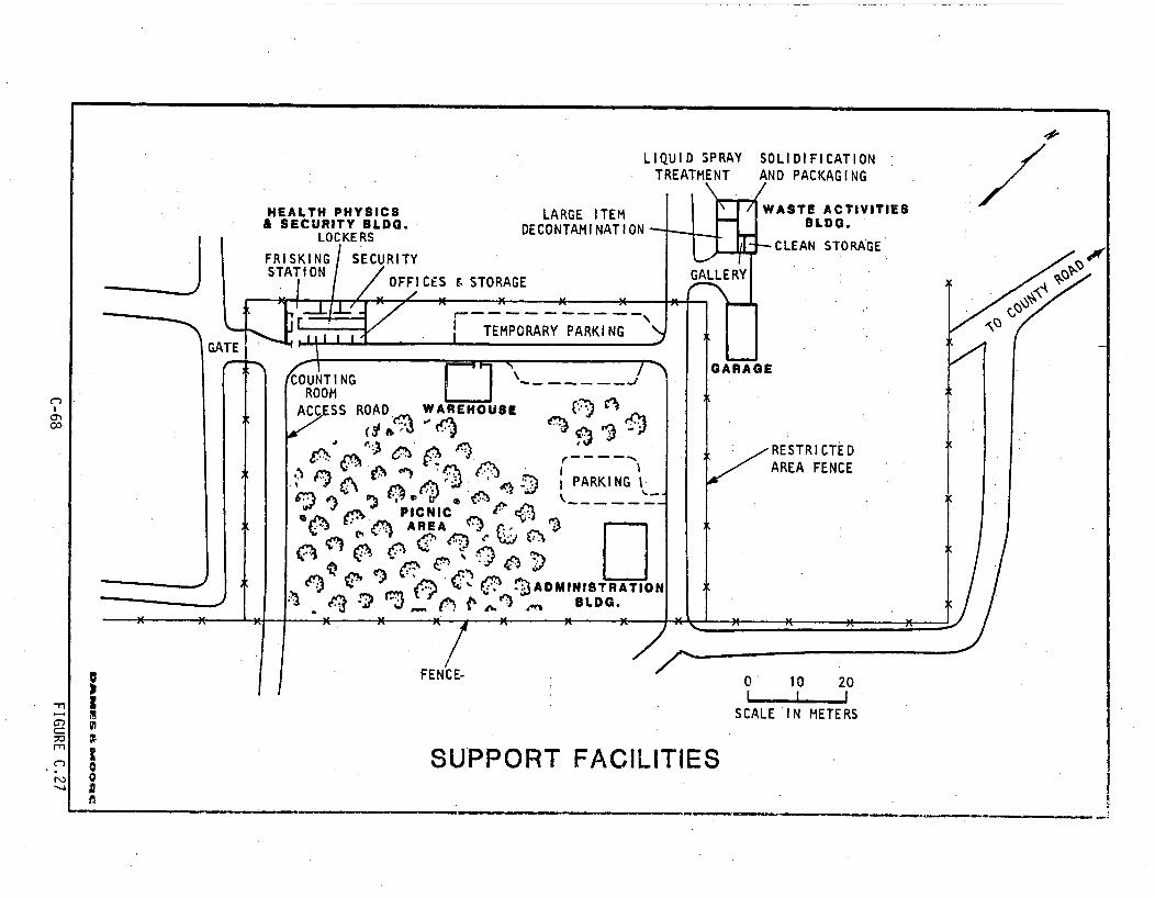
GATE I

HEALTH PHYSICS LARGE ITEM& SECURITY BLDG. LECONTAMINATION-

LOCKERS DN

FRISKING SECURITYSTATION OFFICES &STORAGE

TEMPORARY PARKING

BLDG.

CLEAN STORAGE

CC)

PARK ING I-

'RESTRICTEDAREA FENCE

UIS

0 10 20

SCALE IN METERS

K00Am•

SUPPORT FACILITIES

area" and an "administration area". The restricted area includes a

"disposal area", in which disposal of radioactive waste takes place,

as well as an "operational area".

The restricted area includes a buffer zone between the disposal

trenches and the restricted area fence of 30 m (100 ft). As shown in

Figure C-26, the operational area is located along the eastern side of

the disposal facility and isused as a borrow area,' for cask storage,

and for other miscellaneous functions. The operational area includes

two facilities, a decontamination facility and a garage, which are

used to support waste disposal operations. The administration area is

located near the eastern corner of the disposal facility and is

considered uncontrolled by the licensee for purposes of radiation

protection. The administration area includes support facilities plus

parking space for employees as well as for incoming waste delivery

vehicles.

The reference facility design occupies a total of 60 ha (148 acres),

including the disposal area, operational area, and administration

area. As is the case at existing disposal facilities, however,

considerably less than the total site acreage is used for waste

disposal. For example, specific areas of a particular disposal site

may not be suitable for waste disposal due to geohydrological or

topographical reasons.

The administration area occupies 3.7 ha (9.1 acres), and is assumed to

be a constant for all waste form and facility design and operation

alternatives considered. The area of the land committed for waste

disposal (in other words, the land actually containing disposed

radioactive waste) varies according to the alternatives considered.

For example, about 35 ha (86 acres) would be required for random

disposal of one million m3 of waste into trenches having average

dimensions of 180 m long by 30 m wide by 8 m deep, and having an

average spacing of 3 m between each trench. The remaining 21.6 ha (53

C-69

acres) includes the operational area and the 30 m buffer zone as well

as any excess land within the disposal area used for roads, working

areas, and so forth..

The entire disposal facility is surrounded by a 2.4 m (8 ft) high

chain-link-fence topped with three strands of barbed wire. A 2.4 m

high fence also separates the administration area from the restricted

area. Access to the disposal facility is via two short gravel roads.

There are no rail facilities. Incoming waste delivery and employee

vehicles enter the facility through one of two gates located in the

administration area. These gates are locked at night and at other

times when the site is not being operated. Access to the restricted

area is controlled by security check points near the gates in the

fence separating the administration area and the restricted area.

For security purposes, a narrow gravel road runs alongside the inside

of the fence surrounding the restricted area. Other on-site gravel

roads wide enough to accommodate two small vehicles lead to the active

disposal areas and are-constructed by the licensee as needed. A

lighting system is provided around the site perimeter and also in

the operational and administration area. There are no other lights

installed inthe interior of the restricted area.

The average disposal trench size assumed in this report is 180 m

(591 ft) long by 30 m (100 ft) wide by 8 m (26 ft) deep. The length

and width of the disposal trenches may vary somewhat (about + 10 m),

however, depending on the availability of disposal space. The

rather large trench sizes assumed in this report are representative of

recent trends at -existing disposal sites. Fifty-eight such trenches

would be required for random disposal of one million m3 of waste.

As a trench is constructed, the locations of the four corners of the

trench are surveyed and referenced to a bench mark. An approximate

one degree slope is provided in the bottom of a trench from end to end

C-70

and from one side toward a 0.6 m x 0.6 m (2 ft x 2 ft) gravel-filled

French drain. The French drain runs the entire length on the lower

elevation side to provide for collection of any liquid drainage that

might might occur. A gravel-filled sump is located at the low corner

of the trench.

Each trench is equipped with a minimum of three 0.15 m (6 in) diameter

polyvinyl chloride (PVC) standpipes located within the French drain

and standing along the sidewalls of the trench. Two of the three

standpipes are located at each end of the excavation. The third

standpipe is usually located at the trench midpoint (also standing in

the French drain). These PVC standpipes function as observation wells

or sumps. A typical trench cross section is shown in Figure C.28.

C.2.2 Support Facilities and Structures

The support facilities include (1) an administration building, (2) a

health physics/security building, (3) a warehouse, (4) a garage, and

(5) a waste activities building. All structures at the site are

one-story metallic structures on concrete pad foundations. The

building areas for these five major structures are listed below:

Area

Building or Facility m 2 ft 2

Administration 625 6,725Health Physics/Security 800 8,610Warehouse 470 5,060Garage Mechanics 420 4,520Waste Activities 560 6,025Storage Shed 80 860

The administration building contains office space for site management

and other administrative personnel working at the site. The activi-

ties performed within this building include coordination of waste

shipments to the site, billing customers, and other routing of file

work. Site records are also stored within this building.

C-71

I 30m•ll .... ""

CAP

COVER WASTE WASTE

0 5 10 15 201 I 1 I I

SCALE IN METERS

TYPICAL TRENCH CROSS-SECTION

co

0 10 20 30I I I ISCALE IN METERS

5

II'

£

I

PLAN VIEW OF TYPICAL TRENCH

TYPICAL TRENCH DETAILS

The health physics/security building serves as the focal point for the

majority of disposal activities at the site. This building houses a

security section, a counting room, health physics offices, a change

room/locker room, a lunch area, and a supply room. A safety decon-

tamination shower is located adjacent to the frisker location.

Emergency equipment such as safety ladders, respiration equipment, and

anti-contamination suits are stored in the vicinity of the frisker

station. The employee change/locker room includes both a street

clothes ("clean") and work clothes area. Showers are also located in

this section of the building.

The warehouse is used to store supplies used on site. This facility

is located within the administration area so that delivery trucks need

not enter the disposal area. Among the stored items in this warehouse

are cables, hooks, drums, bags, and other miscellaneous hardware.

Casks and site vehicles are stored in the operational area.

The garage is located in the restricted area and only vehicles and

equipment that have been surveyed and decontaminated to within speci-

fied limits use this facility. The garage is large enough to hold two

vehicles at a time for maintenance. Mechanic's tools, spare parts,

oil, and fuel (adjacent to the building in underground tanks) are also

stored in this garage.

The waste activities building houses several functional areas includ-

ing (1) a large item decontamination bay, (2) a control room for the

decontamination bay, (3) a liquid treatment system, (4) a waste

solidification, packaging, and overpacking area, (5) a supply room,

and (6) a small waste storage area.

The decontamination bay is used for washing down (decontaminating)

large pieces of equipment (including trucks if necessary) through the

use of a high-pressure recirculating water supply system. Contami-

nated liquids resulting from decontamination operations are collected,

C-73

treated in the liquid treatment facility, and then recirculated.

Contamination levels in these solutions are generally quite low,

however, water treatment is applied to recirculating fluids. Small-

scale decontamination of tools and other small items may be accomp-

lished within the solidification staging area. The solidification

area includes batch concrete mixing equipment for solidification of

small quantities of low-activity liquids. A small storage area is

provided for occasional temporary storage of shipments received from

common carriers. A loading dock is located along the southern corner

of this building.

A storage shed is used for supplies and miscellaneous tools used

at the disposal trenches. This shed is portable and is usually

located close to the active disposal trenches.

C.2.3 Site Operations

The regional near-surface disposal facilities are all assumed to be

operated for profit by small corporations which are also involved

in other nuclear-related business activities. The size of the faci-

lity staff required during the operational phase is a minimum of 70

people. The staff of 70 includes 7 upper-level management, 14 cle-

rical personnel, 8 radiation technicians, 34 operational personnel for

trench construction and waste emplacement, 3 quality assurance per-

sonnel , and 4 security guards. However, additional personnel may be

required depending upon the facility design and operations alterna-

tives considered.

The site operations discussed in this section include the following:

waste receipt and inspection, waste storage, waste disposal, radiation

and contamination control, site groundskeeping and maintenance,

environmental monitoring, security, recordkeeping and reporting, and

quality assurance.

C-74

Waste Receipt and Inspection

Shipments of radioactive waste arrive by truck and are processed onto

the site on a first come, first served basis. Accompanying the ship-

ments are manifest documents -- termed radioactive shipment records

(RSR's) -- which describe the -content of the shipment. Arriving

shipments are inspected for compliance with applicable Feaeral regu-

lations and waste acceptance criteria established as conditions in the

disposal-site license. The results of these inspections are recorded

on radiation survey forms and summarized on the RSR's accompanying the

waste shipments. Shipments found to be in compliance with Federal

regulations and license conditions proceed into the disposal area for

unloading. Violations of transportation regulations are reported to

Federal and state authorities in compliance with Federal and state

regulations and license conditions. Waste shipments which are not

acceptable for disposal at the facility are returned to the shipper.

Damaged or leaking waste packages are identified and appropriate

protective or remedial action is taken. Depending upon license

conditions, damagea or leaking waste containers may be overpacked or

repackaged, and either accepted for disposal or returned to the

sender. Free-standing -liquids detected are removed and solidified.

Activities such as overpacking and solidification are performed at the

waste activities facility.

Waste Storage

Generally, waste received at the site is disposed within a few days.

Waste that must be temporarily stored is generally left in transport

vehicles. However, there may be a need to store waste packages in a

designated storage area, especially if layering of high activity waste

is practiced at the disposal facility. In such cases, packages may

have to be stored until the proportion of high activity to low acti-

vity packages is acceptable for burial.

C-75

Waste Disposal

Waste is emplaced in the disposal trenches and the trench is then

backfilled. Depending upon the alternatives considered, the backfill

may be an earthen fill or a cement grout. License conditions require

that backfill operations commence immediately if radiation readings

greater than 100 mR/hr are recorded at the trench boundary, and

continue until radiation levels are reduced below 100 mR/hr. License

conditions also prohibit waste packages from being placed in standing

water, so waste disposal commences at the high end of the trench and

works down towards the lower end. Rainwater falling within the open

trench and contacting the uncovered waste packages drains away to

the lower end of the trench, where it is removed as necessary and

treated by such methods as solar evaporation or solidification.

Waste is emplaced to within one meter of the top of the trench. The

backfill material is spread over the trench and compacted using

conventional means until the trench cover approximately corresponds to

the original site surface. A one meter thick earthen cap is placed

upon the backfill. The cap may be additionally covered with natural

overburden material as necessary to provide good drainage characteris-

tics and according to the final contours planned for the site surface.

During waste handling and diposal, operations are monitored to ensure

radiation safety. After the transport vehicle is unloaded it is again

surveyed for contaminaton and decontaminated, as necessary, prior to

leaving the restricted area. The results of the survey are recorded

on the accompanying RSR.

Site Groundskeeping and Maintenance

Groundskeeping includes both the upkeep of grounds and the maintenance

of external building surfaces. Groundskeeping activities include

contouring of the ground surface, emplacement of a soil cover material

C-76

such as grass, fertilizing, mowing, etc. A site maintenance program

entails routine inspection of site surfaces and fences for trench

settlement, gullying, damage, debris, etc. Repairs are made as

necessary.

Other Site Programs

A number of other programs are also carried out by the disposal

facility by the site operator. These are discussed in detail in

Reference 2, but briefly, include the following:

o site safety,o enviromental monitoring;o recordkeeping and reporting, ando quality assurance.

The site safety program includes operations and procedures to ensure

site safety, to control radioactive materials at the disposal faci-

lity, and to minimize potential off-site releases of contaminants.

These include operations and procedures for personnel radiation

monitoring, site radiation and contamination control, industrialsafety, abnormal or emergency situations, and personnel monitoring.

The environmental monitoring program is carried out to detect move-

ment of radionuclides from the disposal cels and to help assess

Iong-term safety. A summary of the facility operational monitoring

program is included as Table C-3. This program includes collection of

well water samples, soil and vegetation samples, and air samples, as

well as monitoring for direct gamma radiation levels.

The security program is carried out both for radiation health and

safety considerations as well as to protect the many thousands of

dollars worth of equipment, buildings, and facilities located on

site. The security program includes security personnel, controlled

access to facility areas, communication equipment, identification

badges, and emergency procedures.

C-77

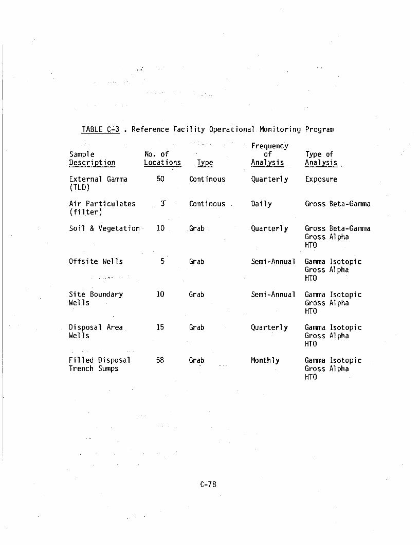
TABLE C-3 • Re

SampleDescription

External Gamma(TLD)

Air Particulates(filter)

Soil & Vegetation

Offsite Wells

Site BoundaryWells

Disposal Area.Wells

Filled DisposalTrench Sumps

ference Facility Operational Monitoring

FrequencyNo. of ofLocations Type Analysis

50 Continous Quarterly

3" Continous Daily

10 Grab ..Quarterly

Program

Type ofAnalysis

Exposure

Gross Beta-Gamma

Gross Beta-GammaGross AlphaHTO

Gamma IsotopicGross AlphaHTO

Gamma IsotopicGross AlphaHTO

Gamma IsotopicGross AlphaHTO

Gamma IsotopicGross AlphaHTO

5 Grab

10 Grab

15 Grab

58 Grab

Semi-Annual

Semi-Annual

Quarterly

Monthly

C-78

Records are maintained by the site operators to cover the areas

required by law, for operational control, and for future use. These

include those for:

o personnel exposures;o waste receipt and disposal;o personnel training;o quality assurance;o environmental monitoring;o operating procedures; ando site surveillance and monitoring.

The quality assurance program functions as a parallel department which

provides quality control and training support to facility operations.

As part of this, a management audit program is carried out to maintain

standards of radiological control and safety and to ensure compliance

with federal, state, local, and site license requirements. The

program includes a review of operating procedures and past exposure

records, facility inspections, and surveillance of work being per-

formed.

C-79

REFERENCES FOR APPENDIX C

1. Wild, R., et.al., Dames & Moore, "Data Base for Radioactive WasteManagement. Volume 2. Waste Source Options," USNRC ReportNUREG/CR-1759, to be published.

2. U.S. Nuclear Regulatory Commission, Office of Nuclear MaterialsSafety and Safeguards, "Draft Environmental Impact Statement on10 CFR Part 61 : Licensing Requirements for Land Disposal ofRadioactive Waste," NUREG-0782, to be published.

C-80

APPENDIX D

COMPUTER LISTINGS

APPENDIX D : COMPUTER LISTINGS

This appendix contains the listings for the computer programs and data

files discussed in Chapter 6 of this report. The five programs are

listed first and include, in order: INTRUDE, GRWATER, OPTIONS,

INVERSI, AND INVERSW. The seven data files are listed secondly, and

include three basic files (DATA, DATAD, and NUCS) as well as four

spectral files.

The DATA and DATAD files contain the volumes and radionuclide concen-

trations of the 36 indiviaual waste streams considered in the analy-

ses, as well as the pathway dose conversion factors and other infor-

mation specific to each of the 23 radionuclides considered. In the

DATA file,_the radionuclide concentrations are given as-generated. In

the DATAD file, the radionuclide concentrations are given as"decayed

to the end of the operating life of the reference disposal facility,

assuming that the operating life is 20 years. Also included in these

files are values for parameters used in the analyses which depend upon

the environmental characteristics of the particular regional site

considered. The NUCS file is similar to the DATA and DATAD files

except that the waste stream volumes and radionuclide concentrations

are omitted.

The four spectral files (SPC1, SPC2, SPC3, and SPC4) contain the

values of the waste spectral incides which vary depending upon the

waste spectrum considered. Values for waste spectrum 1 are given in

SPC1, values for waste spectrum 2 are given in SPC2, and so forth.

D-1

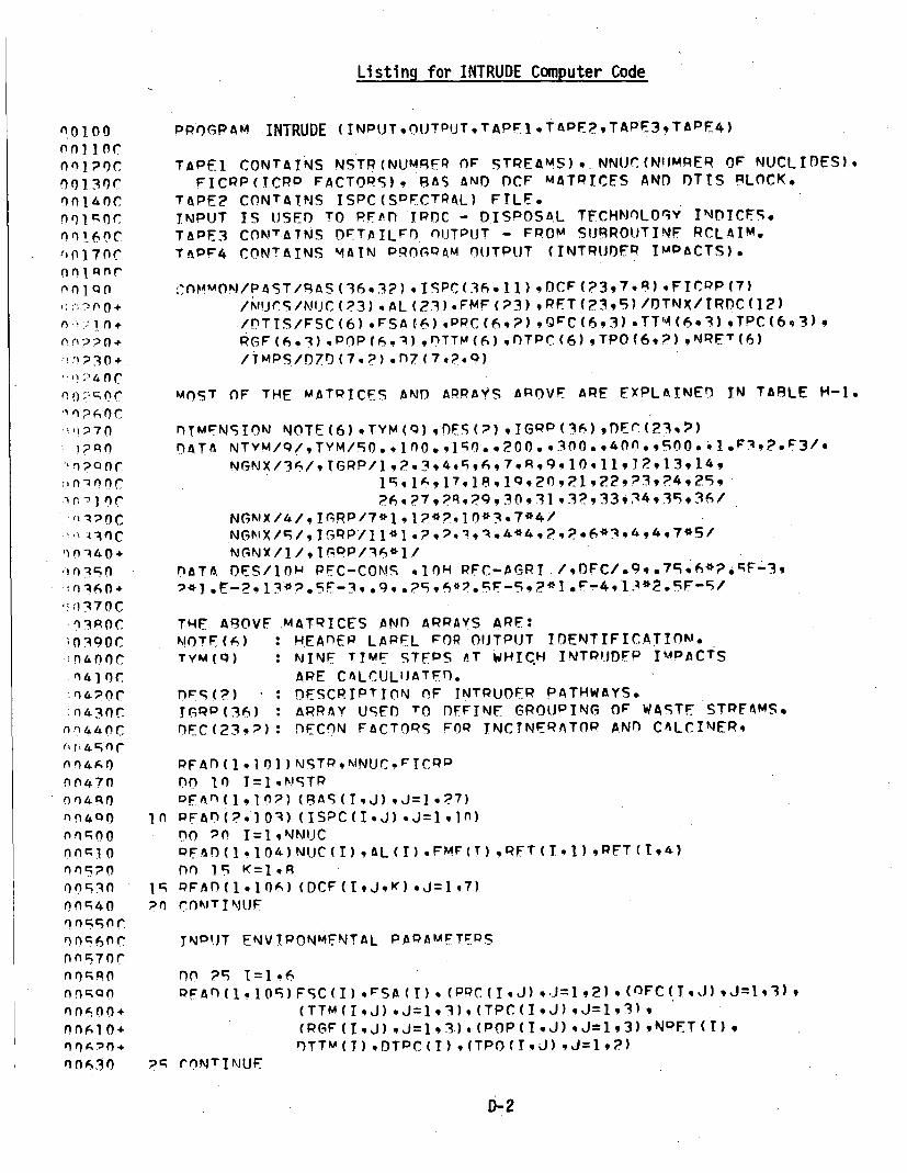
Listing for INTRUDE Computer Code

nlo Ino001100lnni lor

0 0 11 ornnlP0r

001 40C

nn) I 6nC"0 170Cnon!rn

I.,-nn +Q

Of'ri? 0+"2;!30*.

.. :, P ? 0 + .

(-) - f) r

n~l'14 +C

!o370C,I3POC,n3goc

A n 44 A n

nnA47

nnA04Q

o ol c; 6 n

on94O

00] 0.

0nfncAn

nnA 30

PROGPAM INTRUDE (INPUT,OUTPUT,TAPFITAPF?,TAPE3,TAPE4)

TAPEl CONTAINS NSTR(NUMRFR OF STREAMS),. NNUUC(NI)MRER OF NUCLIDES),FICPP(TCRP FACTORS)v 8AS AND DCF MATRICES AND OTIS RLOCK.

TAPE? CONTAINS ISPC(SDFCTPtAL) FILF.INPUT IS USED TO PFif IPDC - DISPOSAL TECHNOLOGY INDICEs.TAPE3 CONITATNS DFTAILFD. nOJTPUT - FPOM SURROUTINF RCLAIM.TAPF4 CONTAINS MAIN PROGQAM OUTPUT (INTRUDER IMPACTS).

.OnV4MONJ/PAST/Q.AS (36,3?) SPC( 36.11) .DCF (?3,7.R) FICPP (7)/Kljrl/N.!JC (?3) ,AL (21) ,FMF (P3) ,PFT (?19/DTNX/TRnC (12)

/DTIS/FSC(6),FSA(6),pPC(6,?) ,VC(693).TT' (6,3)gTPC(6,3).RGF(6.3),POP(6.),}nTTM(6) ,TPC(6),TPO(6,?),NRE'(6)

IT• SI070 (7,P).-n7 (7g,?,eo)

MOST OF THE MATPICFS AND ARRAYS AROVF ARE EXPLAINED IN TA9LE H-1.

nfIMNSION NOTE(6),TYM(Q),DFS(2),IGRP(36),fEC(?3,P)DATA NTYM/Q/,TYM/90 10. .no,15l. .200. ,3nlo. 40A. ,5f)* 1.F3,?.F3/,

NGNIX/4/,IGRP/7*1.•1?*7,1n*37*4/

DATA DES/Iow PFC-CONS ,JOH PFC-AGRI /,DFC/.9q.7S,6*?iF-3g

THE A9OVF .MATRICES AND ARRAYS ARE:NOTF(6) : HEADEP LAPEL FOP OUTPUT IOENTIFICATIOK.TYM()) : NINF TIMr STEPS AT WHICH INTPl.IDFP IMPACTS

APE CALCLJLIJATFD.DFS(7) : DESCRIPTION OF INTRUDER PATHWAYS.IRP(36) : ARRAY USED TO DFFINF GROUPING OF WASTE STPFAMS.DFC(23,?): DECON FACTORS FOP INCINERATOR AND CALCINER,

PFAn(.i,01)NSTPqINUC.FICRPDO 10 I=lNISTP0FAn(Iqjn?) (9AS(T,J),J:jI,?7)

1,n PF.An(?.]O01) ( IS,:C (IJ ),j=Il g n)

nO P0 I=1,NNIJCPFAD ( I,%10 ) NUC(I) ,AL(1T).FM-F (T) ,RFT(II),PFT(T,4)

no I c =19 PFAn(lolO6) (DCF(1,J,K),J=I,?)20 CONITINUJF

INPUJT ENVIPONMENTAL PAPAMFTErPS

no ?9 I=1.6PFAD(lI,]q)FSC(I),FSA(T),(PPC(IJ)q,J192),(OFC(IJ)9J=I93)9

(TTM(IJ),J=1,3),(TPC(IJ),J=1,3),(PGF (I ,J) ,J=1 , 3) * (POP ( I.J) ,J=1 ,3) ,NPET (1)9DTTM(T),DTPC(I),(TPO(IJ),J=1,?)

?q CONTINUF

D-2

.Listing for INTRUDE Computer Code (continued)

O064n In1 FORMAT(?Ig,7F5.2)0n061O 10? FORMAT(AlnfPE1O.3/IX,6FlO.3/lOX,6EIO.3/lOX,6EI0.3/lOX,6E10.3)n0660 In3 FnPMAT(!0Xq1015)00670 I04. FnRMAT(Alf,)4E1ne3)

.n6nn 1ng FORMATI(IXI7E10*3/1OX,6FIO.3/IOX,6EIO.3,15/lOX,4FIOo3)006QN 10r FORMAT-(IOXq7E103)0 070AC.0071.0 nf 314 ISTR=1,NSTRnoTpn AI=ISPC(IST-R,9) $ AI=AI/ISPC(ISTP,3)00730 AP=PAS(ISTP,3) $ A3=A2/(AI*3.62) $ RAS(ISTR.3)=A300740 no 30 1=59?7on7 iO RA3(ISTRI) =RAS(--ISTR, I)*AI00760 J=ISRC( .STP,1O) 1nn77n 1'P=JOnoO0 $ IS=(J/Io0)-IP*I0.1 IL=(,J/10)-IP*100-IS*10n07RO TH=J-IP*I00O0IS*100-IL*I0 $ IF(ILEO.O)GO TO 35007C0 IF(IP.LT.g)GO TO 35nnoon J=l S IF(IP.GT.5)J=?AORlO RAS(ISTP,5)=(1,-DEC(1,J) )*RAS(ISTR,•)

On2?f RAS(ISTP,6)=(l.-DEC(P,J))*RAS(ISTP,6)noR30 •s CONTINUE

0nnp;OC NIFXT LINE READS IN - THPU INPUT - THF 1? DISPOSALO0960C TECHNOLOGY INDICES AND HEADEP INFORMATION.0nP70CooRqO PrADgIRDC S READ 1002,NOTE % WRITE(4,1003) ',IOTE,.IRfC00R90 0n 70 IGNX=1,NGNXAnocO Ny=0 $ %/DIS=O. $ CALL 7EPO(0,l26)

OnqpOC nO 70 INTERPRETS IGRP(GROUPING) ARRAYnAq30C Dn 50 IS THF MAIN LOOP IN CALCULATING INTRUPER IMPACTSO094AC 00 45 LOOP nISTINGUISHFS RETWFEN THE TIME STEPS

Ongqo nO .00 I'qTP=1,NSTROOq7T IF(IGNX.NE.TGRP(ISTR)).GO TO 5(1O098O DO 45 ITYM=1,NTYMOIPO TIPDC(12)=TYM(ITYM)+O.l $ CALL RCLAIM(ISTRtNNUC)Oloon On 40 I=1.701.0].0 n0 40 J=l,?010?0 40 DZ(TJITYM)=DZ(IJ,I T YM)+ AS(ISTR,3)•DZD(TgJ),01030 4R CONTINUE01040 NY=1 $ VDIS='VDIS+RAS(ISTP,3)o 1 og so CONTINUIF01060 IFeIX.FO.t)GO TO 7001070 DO 55 I=],NTYMo1o0o no 99 J=1,701090 nO S K=1,2011O0 ;c;n f7(JKI)=1Z(J,K,I)/VDIS01110 IF(NIGNX.EO.36)WRITE(4,1004) RAS(IGNXP1)Oil?0 IF(NGNX.NE.36)WRITF(4v00n5) IGNX01130 On 65 I=1,NTYM01140 wPoTE(4,1006) TYM(I)01115O nO 65 K=19201160 Al=O.01170 DO 60 J=1,7nAIRO A0 A1.=A+1.07(JK,I)*FICPP(J)Ol]f 695 WPITE(4q,007) DES(K),(D7(JKq,I),J=I7),AIOl200 70 CONTINUE

D-3

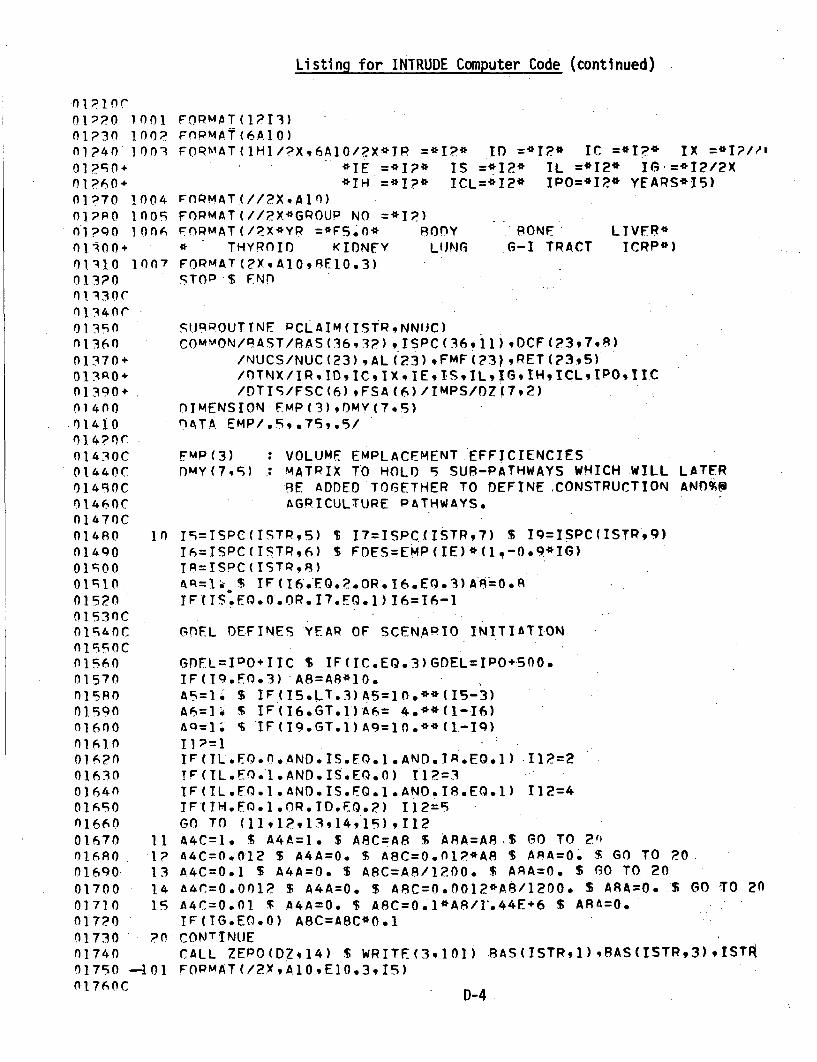
Listing for INTRUDE Computer Code (continued)

oIpIor01?PO 1001n l?,-n i. o n

n1?40 10o3

01 ?60.

01?70 1.004OiP0 1005

01?q0 10on

01310 101)7

013?001 330Cnl'A4nr0 l34flo01390n136001370+013,0+01390+0140.0n01410014?OC

01430C01440C01490C()14A0C01470C014R0 11001490015000 1 l.I015?f0153oc0140 Cnic;goc015600157001 0oniscin01600n)161.00167?016300164n01650

0166001670 11016so I ?01690 1301700 1401710 150172011730 n00174001750 -401n1 760C

FORMAT(IPI3)FOPMAT(6AIO)FORKiAT(IHI/?X,6A0/?X*TP =*I?* In =*Ip* IC =*I?• IX =IPi

*IE =*I?* IS =*I2* IL, =*12* IG'=*I2/2X*IH =*I?* ICL=*I?* IPO=*IP* YEARS*I5)

FORMAT.(//?X,AlO)FOPMAT(//PX*GROUP NO =*I?)FORMAT(/?X*YR =*F5.0* BODY

THYROID KIDNEY LUNG

FORMAT(2XAIOEl0.3)STOP $ ENO

RONEG-I TRACT

LIVER*ICRP*)

SUJROUTTNE PCLAIM(ISTRNNIJC)COMMON/PAST/RAS (36,3?) , ISPC (36, 11) ,DCF (73,7,8)

/NUCS/NUC (23) , AL (-23) ,FMF (?3) ,RET'(23,5)/rnTNX/IR, IDIC, IX, IE, IS, LI6, IH, CL, POI-C

/DTIS/FSC(6) ,FSA(6)/IMPS/DZ 7,2)DIMENSION EMP (3) ,OMy (7.5)9ATA EMP/.5,.75,.5/

FMP(3) : VOLUME EMPLACEMENT EFFICIENCIESDMY(7,S) : MATRIX TO HOLD 5 SUP-PATHWAYS WHICH WILL LATER

BE ADDED TOGETHER TO DEFINE CONSTRUCTION ANnO%AGRICULTURE PATHWAYS,

I5=ISPC(ISTP,5) $ 17=ISPC(ISTP,7) $ 19ISPC(ISTR,9)T6=ISPC(TITR,6) $ FDES=EMP(IE)*(1_00.9*IG)IR=ISPC ( ISTP9,)Aq-l'•$ IF ( 6.-EQ.?.OR. 16.EQ.3)AA-O .RIF(IS.FO.0.OR.17.EO.1) I6=I6-1

GDEL DEFINES YEAR OF SCEN.APIO INITIATION

GnFL=IO+OIIC $ IF(IC.EQ.3)GDEL=IPO+500.IF(I9.EO,3) A8=A8*10.A5.=1 IF(I5.LT.3)A5=]O.**(I5-3)A6=16 $ IF(16.GT.I)A6= 4.**(l-I6)AI=l S IF(19.GT.lA9=lO=1**(l-lc))II) l

IFCIL.E.O.f.AND.IS.FO.I.AND.IR.EQ.1) -I12=2TF (TL.ED.I •AND. IS.E0.0) T12=3IF(IL.EO. I.AND.IS.EQ.1.AND.I8.EO.1) I12=4IFC IH.EO. 1 .OR. ID.EQ.?) 112=9GO TO (11I1?q,13,14,I5),I12A4C=1I $ A4A=l. $ A8C=AS 5 A8A=A8.$ GO TO 20A4C=0.012 $ A4A=O. $ A8C=O.nI?*AS S APAAO $ GO TO P0.A4C=0.1 $ A4A=0. $ A8C=AS/1200. $ AAA=O. $ GO TO 20A4C0.=O01? $ A4A=0- $ A8C=O,0012*A8/1200, $ ARA=O. .$ GO TO 20A4C=0.01 $ A4A=O. $ ABC=0.1*Ag/1'.44E,6 $ A8A=O.IF(CG.EO.O) A8C=ABC*O.1CONTINUECALL ZEPO(DZ414) $ WRITE(3,101) .AS(ISTR,1),RAS(ISTR,3),ISTkFOPMAT (/?XA1OEl0.3, IS)

D-4

Listing for.INTRUDE Computer Code (continued)

nl.770C MAiTN LOOP IN CALCULATING DOSFS FROM ALL NUCLIDFS FOPnl7ROC SFVFN ORGANS.nj7QOCOIROn DO 40 INUC=lNNUC1iq0o AI=:9*FDES*FXM(AL(TNUC)*CDFL)*RAS(ISTP,INUC+4)

OlF?O nn 0 1=17,flR30 AP=0CF(INUC,iI,)OIA40 DMY(Iq,)=:A*O.057*A2*A8C D fMY(I,3):A]*0.27*A2*n.?c;*AFA.nIpso pMy(T,2)=Al*A4C*A9*FSC(TP)*DCF(TNUCT,?,)Ol60 OMY (Ie4)=AI*A4A*A5*FSA (IP) *OCF(!NUCI,-) *n.?PnIR70 OMY(.I,5)=n.2?*0.9*A1*A4A*A6*FMF(TNUC)*nCF(INUC.I,4)

nippoc OnY(I,?)=AI*A4C*FSC(IP)*nCr(TNUC,I,?)01 R90C OuY(I,4)=AI*A4A*FSA(IP)*OCF(INUCI.,3)*).2501,900C DMY(I,5)=O.?5*0.5*AI*A4A*fiCF(INUC,1,4)*FMF(INUr)01910 n7(Ifl.)=DZ(1,1)÷DMY(1,1)÷+fMY(I,?)019?0 f7(I,?)=O.Z(I,2).DMY(I,3)+nMV(I,4)÷fMY(1,5)01930 30 CONTINUF0.1940 IF(TSTR.LT.30)G0 TO 40oi]950r WPTTE (3,1nP) NUC (INUC) ,( (DM (,IJ) , I=1,7) ,J=],95)

01O60 i1? FoPMAT(?X.AlO,7E9.,/(IX,7Eq.?))01970 4n CONT I 'IEnlqpO PETURN 1 FND01 qqOc

0?000 SUIROUTINE ZERO(AN)o010. OIMFNSION A(N)

0070 fr.) l0 I=I.N07030 10 A(I)=O.0?040 PFTUPN $ END

OýOSO)ro FUNCTION FXM(-AI)-0 A71=0' T, IF(AI.LT.N30.)AS=E '(-A])

0ýnpo" PFTUIPN S FND

D-5

Listing for GRWATER Computer Code

n010o

nn0]OC00o130(7

00140C

00160c00170C00h1•000200+

00?10+00pPO÷00?30+

00no40c

00270(700?P0(7

00300C00310(7

On o ?6 C

n00320C0330

00340

0035O0036000370.003p0003QOC00400C7

00410C() n4?nr00430rnn440C00450(700fl0C

00470004'0

00510.7

00 53OCnnto 3or

00540

00550

nn•70OOSRO00590OnO0O00•1 0

0063000640on650C

PROGRAM GPWATER(INPIJT.OUTPUTTAPFI,TAPF?,TAPF3,TAPF4)

T APE1 CONTAINS NSTR(NUMRFR OF STREAMS), NNUC(NIJMREP.OF NUCLIDES).FICPP(ICRP FACTOPS). RAS AND DCF MATRICES AND OTiS RLOCK.

TAPE2 CONTAINS THE SPECTRAL (ISPC) FILE.INPUT IS USED TO PEAD IROC - nISPOSAL TECHNOLOGY INDTCFS.TAPE3 CONTAINS DETAILED OUTPUT - FROM SUBROUTINE GWATFR.TAPE4 CONTAINS THE MAIN PROGRAM OUTPUT (GROUNDWATER IMPACTS).

COfMON/RAST/BAS(36,32),ISPC(36,11),DCF(?3,7.8).FICPP(7)/NUCS/NUC(?3),AL(?3),FMF(?3),PET(23,9)/DTNX/TPnC(12)/DTIS/FSC(6)qFSA(6),PPC(6,?),OF(7(6,3) .TTM(6,3),TPr(6,3),RGF(6,3),POP(6.3) ,DTTM(6),DTPC(6).TPO(6,?),NRFT(6)/IMPS/DZD(23.lIP?1)/nHIC/IHIC(36),THIC

MOST OF THE MATRICFS AND ARPAYS ABOVE APE EXPLAINEn IN TABLE H-i.DTNX BLOCK CONTAINS DISPOSAL TECHNOLGY INDICES.IMPS PLOCK - DZD(23,lB,?I) - WILL CONTAIN PESULTS OF GWATER- DOSES FOR 23 NUCLIDES. I1 TIME STF 0 S9 7 ORGAN FOP 3 LOCATIONS.OHIC PLOCK CONCERNS THE USE OF HIGH INTEGRITY CONTATNFPS0THIC INDICATES WHICH STREAMS USE HIGH INTEGPITY CONTATNFRSANIP THIC IS TIME ATTRIBUTE ASSOCIATED WITH CONTAINPR.

DIMENSION TIMP(6) TYM(18),rES(3),7I(7,3,1R),NDX(36)DATA NDX/36*1/DATA IHIC/36*0/,THIC/100./DATA TYM/40..50..60.,i0.q?02,.300.o.4O0.,r00.*600.,700.,8n.,9gOO..O0OO.,0pon.4000.,96nO..R000.lOO0o./,NITYM/.1/DATA DES/1OH REC-WELL q10H oOP-WFLL 00OH POP-SURF /

NnX (36)

TYM (18)

DES (3)DZ (7,3, 1P)

IN!DEX TO INCLUDE OR EXCLUnF PARTICuILARSTREAMS IN ANAYSIS (1=INCLUnE, 0=EXCLUDF).18 TIMF STEPS TO RE CONSInE.pFD IN GROt.IIWATERANALYSIS.

DESCPIDTION OF 3 PATHWAYS OF CONCEPN.DOSES SUMMFD OVFP ALL NIJCLIDFS.

PEAn.IRDC 1 READ 10o?,TIMP 4 WRITE(4,1003) TTMPoTRnCCALL COmRyN(NSTR.NNUC)VNOT=0. a VPEG=O.' T VLAY=O. 1 VHOT=O.

LO0O 30 CLASSIFIES WASTE STPFAMS AND ACCUMULATrS TWFIPVOLUMF AS NOT ACCFDTA9LF, RFGULAP. LAYERED% OP HOT.

n0 30 ISTP=:]NSTPIF(IPDC(l).EQ.t) ISPC(ISTR.S)=ISPC(ISTR,5)-lTMOn=l % CALL RCLAIM(ISTRqNN(C.IMOnn)IF(NDX(ISTP).NE.1)ISPC( TSTR, I)=OII=ISPC(IST9,11)+I % GO TO(1oq5,?O,?5.)IIV/NOT=VNOT+RdS(ISTR,3) % GO TO 3nVPFG=VPEG÷RAS(ISTP,3) T SO TO 30VLAY=VLAY+RAS(IS TPq3) T GO TO 30VHOT=VHOT+AAS(ISTP.3)CONITINUFWOITE (4.100) VPEG.VLAY,%/HOTVNOT

in

20

10

D-6

Listing for GRWATER Computer Code (continued)

l0660D0670C.l06ROCPo6Qnc0070000710DQ7?fln073n0 0740

nn0750 400076oC00770C

nn83oOfo 8 P)

00840

00960 6000.k70 70nopR~ncOORQOC

OOQOlC

009..30009400 950 •

'09560 •0

01Q00C

00980 1001009QO 100?

01000 1I00.3010 10'

01030 1004010•40 100

n09150

01060 100601070 1007

01080'01090 100l01100

OlIIOC

011300114001150÷011ý0÷01170'011800190O01 1 00' -

CALL GWATEP(NSTRNNUCNTYMgTYM) % CALL ZERO(DZ,37S)

LOOP 40 SUMS DOSES OVER ALL NUCLIDES

DO. 40 ITYM=INTYMD0 40 K=1,3KK=(K-I)*7nO 40 J=1.7nO 40 INUJC=1NNUC07(JKITYM)=DZ(J,K, ITYM) DZD(INUC,TTYMKK÷J)

LOOP 70 OUTPUTS GROUNDWATER DOSES FOR 7 ORGANS, 3 PATHWAYS,AND 1P TIMES.

DO 70 TTYM=1,NTYMTYMn=TYM(ITYM) $ WRITE(491005) TYMnnO 60 K=1,3AI=06nor0o J=19741=Al+fZ(JKITYM)*FICRP(J)WPItE(4,1006) DES(K),(DZ(J,KITYM),J=1,7),,AlCONTINUE

LOOP 80 OUTPUTS DOSES FOR EACH TIME CONSIDERED FOR EACH NUCLIDE

nn Ro INUC=1,12WPITE(491007) NUC(INUC)nO 00 ITYM=1,NTYMno 00 K=1,3KK=(K-i)*7WPTTF(4,1008) TYM(ITYM)',OES(K),(DZD(INUC,ITYMgKK+J),J=1,7)

FORMAT(1213)FORMAT(6AIO)FORMAT(X,6AIO/2X*TIR =*I?* ID =*I?* 'IC'=.*I2* x I *?/?X

*IE =*I2* IS =*I2* IL =*12* .16 =*IP/2X*9H =*I?* ICL=*I2* IPO=*T?* YFARS*I5)

FnRMAT(?X*VRFG =*E9.2* VLAY =*Eq.?* VHOT =*F9.P* VNOT'=*EQ.2)FORMAT(/2X*YR =*F5.0* RODY RONE LIVFR*

THYROID KIDNEY LUNG G-I TRACT ICRP*)FORMAT(?XAl0,BE1O.3)FORMAT(/2XqAlOlOX*RODY RONE LIVEP** THYROID KIDNEY LUNG G-I TRACT*)FORMAT(2XF6.0,2X,A10,7FI0.3)STOP $ END

SURROUTINE COMRYN(NSTRNNUC)COMMON/RAST!/AS( 36,'?),ISPC( 6,11) DCF(23,7,8),FICPP(7)

/NIUCS/NUC(23),AL(?3),FMF(23),RET(?3,S)/DTIS/FSC(6),FSA(6),.PPC(6,2),QFC(6,3),TTM(6,3),TPC(6,3)tRGF(6,3),POP(693),DTTM(6),DTPC(6),TPO(6,2),NRET(6)

DIMENSION DEC(23,2)DATA DEC/.O9,7596*?.SE-3,2*1.E-2,13*?.SE-B3.9,,2596*?.SE-592*11,E-4,13"?o5E-5/

D-7

Listing for GRWATER Computer Code (continued)

n0 10 PFAn(I,.01)NSTPNNlJCFICPP0 p?? 00 70 T=1,NSTR0 Or760 FA (IoIn?) (AS (1 9J),J= 1 7)

091?40 PFA;)(2,103)(ISPC(IJ),J=1,lI)n 12O 7n CONTINNUEn I;0 F, nn O I:I,NINUCn 1 70 PPAD( 1 9104 )NUC ( I) PAL(fI ),9FMF(1),-RET(I!jl9 }RET(19 4)

01?RO DO 79 K:=1,i?290 PFA.(Q,I06)(nCF(IJK)qJ=],7)

01300 79 CONTI t.UE01310 A0 CONTINUE013120 00 I0 1=1,n0130n PFef(i,109)FSC(I),FSA(I),(PRC(I,J),J=19?),((FC(I,J),J=1 9 3)},n]934n+ (TTM(TJ),J=1,•),(TPC(TJ),J=],3),(RGF(IJ),J=1,3),)(POP(IJ},J=19,30l'50+ NIRFT(I) qfTTM(I),fDTPC(I),(TPO(I.J),J=l,2)nIoln q0 CONTINUE01370 I0] FOPMAT(?9,T7F5.2)01.pO 1n? FOPMAT(A1O,2EIO.3/lOX,6FlO.3/lOX,6E1O,3/10X,6EI0.3/lOX,6El0.3)01390 10 FnPMAT(1OX,10IS)01400 104 FORMAT(AIO,4E10.3)01410 109. FOPMAT(IOX,7E1O.3/10X,6F10.3/lOX,6FIO.3,15/]OX,4FIO.3)0142n 106 FORMAT(IOX,7E1O.3)

.01430 nn c0 ISTR=1,NSTP-1440 AI=TSPC(ISTP,2) $ A1=AI/ISPC(ISTR,3)nl4c•0 A?=RAS(TSTR,3) $ A3=A2/(Al*3.6?) S RAS(TSTR,3)=A3n1460 Dn 70 1=5,2711470 ?n RAS(ISTPI) =BAS(ISTRI)*+AOI&O J=ISPC(TSTRq1O)n1490 TP=J/lOOOS IS=(J/iOO)-IP*l % IL=(J/I.0)-IP*100-IS*1001P00 IH=J'IP*1000-IS*100-IL*10 $ IF(IL.EQ.O)GO TQ 5001910 IF(IP.LT.S)GO TO 5001n?0 J=1 $ IF(IP.GT.5)J=?0n930 RA.S(ISTP,;)=(0.-DEC(IJ) )*RAS(ISTR,5)nI940 RAS(.ISTP,6)=(I.-DEC(2,J))*RAS(ISTR,6)01950 c0 CONTINUE01960 00 An ItNUC=1,NNUC01970 A?=PT(INUC,i4) $ AI=(A?/RET(TNUC,1))**0.334015R0 RFT(INUC,5)=A2*A1 $ RET(INUC,3)=A2/Al01590 60 RFT(INUC,?)=PET(INUC,1)*A101600 PFTIJPN S ENn01610C

01630 SUPPOUTINE RCLAIM(ISTRNNUC,TMOO)01 64001690C THIS SURROUTINE IS USEO TO CLASSIFY EACH WASTE STREAM A':0160C (1) NOT ACCEPTARLE. (P) PFGULAR,0167nC (3) LAYERED, OR..(4) HOT

01690 COMMON/RAST/RAS(36,3?) ISPC(36,11) ,CF(?3,7,8.)01700+ /NUCS/NUC(23),AL(23),FMF(?3),PET(?3,5)01710+ /OTNX/IR,IDO,IC,IX,IE,ISIL,IG, IHICL,IPO,ITCn]7÷0+ /nT;S/FSC(6),FSA(6)/IMPSs/f7(7,2)/DHIC/IHIC(36),THTC017730C01740C 07(7*?) : INTRUDER nOSES USF) IN CLASSIFICATION TESTS01750C

D-8

Listing for GRWATER Computer Code (continued)•

0176-n nIMENSION EMP(9),9LC.(7)01770 DATA EMP/.95,.75,.5,.9,.7c/DLC/ O0.,*R0. 1500.,•O00i.,*1500./nl7AnC

nl7QOC EmD(q) VOLUME EMPLACFMFNT FFFICTENCIESn10oC fLC..(7) .: OSE LIMITINGCPITFPTA FOR 7 ORGANS

OIR01 Tt=ISPC(ISTP9,) $ 16=!SPC(ISTP,6) $ 17=ISPC(TSTP,7)nlp30 I=ISPC(TSTP,9) $ TQ=TSPC(jSTPq9)11P40 TF(THIC,(IcTP).GT.0) Tt=1 .

A1R•O A7=1. qS IF(T6.EQ.?.OP.T,'.F).3) A7=0.ROnl16o TF(!7.FQ.I.OP.ISEo.O) IT=T6-1n1970 FrflE--M(1E)*(I.-.9*IG)niO TF'(TO.,EO.3) A7=A7*l.OlraO Ab:=14 S IF(IS.LT.3) A51=0.**('T9-3)n1Qo0 A'=,S IF(16.GT.1) A6=4.**(1I-16)ol10n AQ=1,. T, IF(T9.GT.1) A9=1o.**(1-TQ)lIQ?0 13=1 $ TF(TS.EQ.I.ANO.IR.FO.1)I3=2

01930 !F(IT.EQ.P)I3=?r,! Q40Cýi:Q;n(- TESTING POUTINF FOR CLAtSSTFINr, WASTE. PASED ON TNTPJDFP

'1IQ•C ~CONSTRUCTTON AND AGPICULTUFO PATHWAYS.

01 Q7nCAlqo 10 Gr)FL=!IPO+TIC '% IF(IC.EO.1) GnFL=IPO÷-00.l.990 CALL 7EQO(97,14) $ Go TO (11,1?,13,14,1,16.17,1R).I3

fonO00 11 A4C=1. ; A4A=1. S ARC=A7 It AAA=A7 % (30 TO 2n0?0.10- 1? A4C=0.01? S A4A=O. $ AAC=0.fOlP*A7 q; ASA=O. $ GO TO 200?020 .1- GDFL=IPO+900. S A4C=1. S A4A=]. $ AFtC=A7 % ARA=A7 $ GO TO ponn030 14 A4C=O.l $ A4A=O. $ APC=A7/1?O0. % AAA=n. $ G'O TO 2n0n04 0 1r A4C=0.001? T, A4A=O. A ARC=O.Ol1?*A7/1200. $ ABA=. $ r0 TO 20,0>00 C; 1 3OEL=IPO.0n. $ A-4C=I.. $ A4A=1. T, ARC=A7 $ AAA=A7 'S rO TO POnpO0n 17 AqC=n.l*A7/1.44E> I. IF(T3.FOn)APC=ApC*n.10•070 A4C=0.01 T A4A=O. $ ApA=n. S SO T.O ?0 -

n0 p( GfEL=IPO÷l000. % AqC=A7 $ .TF(IG.FoQ.)APC=n.I*A7go9 b4C=l. S A46~=1. $S APA=ARC

,!:Il1C MAIN LOOP FOP CALCULATING DOFFS

p 130 o '0 nfO 40 1'I1.C=IN NYJCnln A1=A9*FfES*FXM(AL(TNUC)*GnFL)*RAS(TSTP.TNUC+4)fl?1.0 o 30 1=1 .70;,IA AP=OCF(INUIJC,15)0] 70 PI=AI*A4C*Ac*FSC (IP) *DCF( I NJC9 I,%)An1lfl P>=ft1*APC,*Ap*n0.57n?1Q0 Q3=0.?,*Al.*A4A*A5*FSA(TR)*fCF(INUCgT,3)

Oppon QmL=O,95*0.P9*A1*A4A*A6*FMF_(TNUC)*PCF(INUCI,4)n071OC Pl=AI*A4C*FSC(IR) *DCF(TINU.JCTI?)nl--?RO =0.?rý*AI*A4A*FSA(IR)*flCF(IMUC,1,3)np?ý30C P4=O,5*n. ?9*AI*A4A*nCF(TNUCT-p4)*FMF(INUC)t)?24n 9r~=0 * ?*A1*APtA*A2* 0.?7n0>?qn 77(,1)=07(T ,)+RI+P?n?;?A in n7(Iq?)=n7(T.?)+Q3+R4+R•n0P7 n 40 COTTINiIFOnPfOC

D-9

Listing for GRWATER Computer Code (continued)

n2pcqr TFST DOSES 4GAINST DLCo2300C

l?310 no 90 IOpr=1,7n,;, O ,; p0 IPTH=12np330 TF(n7(IORG,IPTH).GT.DLC(TOPA)) rn TO 600?340 qn CONTINLIEn,;,0 -icOo A TO (5l.9 ?,Sl,93 9 93 q9 4 9 95q9~6).I30P360 qI !SPr(ISTP*,I)=I S RETURJN0?370 cP Tl=' q GO TO 10n n i 3 13:6 $ GO TO inop3QO c4 TSPC(ISTP.11)=? $ RFTURN!n'P 400 kl qc; T1q=8 S GO TOlOnn?410 96 TPC(ISTPII)=3 $ PETUPN074?0 An GO TO (61,6. ,63,63,63,63,70,70)-130?430 61 IF(TL.EO.O)GO TO 63nP44n T1=4 $ nO TO 10n?490 A? TF(TL.EQ.O)GO TO 610l?460 13=c $ GO TO 100n4770 Al IF(IH.F0,n)GO TO 70O?4PO 13=7 $ GO TO 11

0n?4o0 70 TSPC(ISTP,]])=0

nc0or TSpr(ISTR.11) CONTAINS WASTF CLAISSIFICATION TNnFX0PC;P PETUIPN S FNO

02•40 FIJNWCTION FPFS(AlA2)& A3= GD•SOPT(A?/Al)

n ?;s n A4=t3*(1.-Al) S A5=A3*(1.*+A)0Pc70 TF.(A4.GT.O)GO TO 10

n,>c~pn FPF!ý.+FXM(A4*A4)*(POLY(A3)-PnLY(A 4 )) $ PFTURM~OqO 10 FPFS=EXM(A4*A4)*(POLY(A4)+POLY(AE))n.s;n n PFTURN %. FNn

0P230 FUKNrTION POLY(X1)02r40 nATA AiA?,A3,A4.A5,P/.2484?9 2?,-.?84496736'l.4?1413741,O;•A1+ -1.4931'?PO?7.O10614054?g, .327g911/02660 T1=l./(]-.+P*Xl)01E670 1,OLY=Tl*(Al+Tl*(A2+Tl*(83+Tl*(A4+Tl*5))))02Aoo PFTUPN S FN)n,)oc FUNCTIONI FX'(AI)N27o0 A?=n. € IF(Ai.LT.?3f.)aP=FxD(-A1)0?710 FXM=A20n7?0 PFTIJPN $ FNn

n->74nr

n;'7O SWPpnUTIT'F GWATEP(KISTPNNI.JC.NTYk.TYmf)n'>70;0 UMOnN/RAST/PAcU36,3?).ISPC(36.11)qflCF(?3,7*R),FTCPP(7)

n?770+ /KIUCS/NUC(23),AL(?3),FMF(23),RET(?395)nP7PfO* /0TNX/IPIDICTX,TE, IS*ILIGIHICLIPOOTICo027qf+ /nTTS/FSC(6),FSA(6),PPC(#,?).OFC(A,3)}TTM(6.,),)pqno0÷ TPC(6,'3) RGF(6*3) qPOp(6%.3) oTTM(6) .01TPC(6) )TPO(6*P) )NRET(6)nppIO. /IMPS/DT(23,IB,21)/nHIC/THIC(36),THIC

n'op2 nT4FNSION EMP(5),EFF(?),SFFF(?),nMY(3,?O),TYMD(18),PFS(189 3 )npp0A nTA FMP/.o,,7CToC,*, o7C/,FFF/Ao4,7,n/,SEFF/O.Qn.39/.NOPT/l/0-P04 TVOL=(. $ GTNS=IPO+IIC S NSFC=1O $ CALL ZFPO(DT7,P6q4)

D- 10

Listing for GRWATER Computer Code (continued)

n?Rn C

OPP70r

OP R7 ornpRqo

0?Q] 0

n;193 0nPQ4n

OqSO

0;q70

n0,Qqn0?Q90

0n3 40C

03060C

O3070C'0 OR OC

n3apoO

n31ooC0311 10C

nl13nCil14003 150nn31io.n0170

0319003pon03?0O-

0 3?1 003?3o

03?60

03?70

03300

ni3pn.n331o

03340

03370n-3Anr

NFXT SECTION DETERMINES PERCOLATION VALUE A•f!LOWER LIMIT FOR THF DILUTION FACTOR

PPCI=PRC(TR,1) $ PRC?=PRC(IRq2)IF(IG.EO...OR.ID.EQ.?) GO TO ;IF(IE.GT.3) PRC1=PRCfIR,1)/in.IF(IE.GT.1) PRC2=PRC(TR,9?)/10.

'~CONTIN.UE

IF.(IC.EQ.I)PRCD=PRCITF(IC.GT.])PRCO=PRC?IF( TX .EQ-. 1) PRCD=4.*PRCIIF(IC.FO.1.AND.IX.FO.?) PRCD=?.?5*PPCIIF(IC.EQ.?.AND.IX.EO.°) PRCD=4.0*PPC?TVOL=35200n.*SQRT(PRC(IR, 1)*27.A)IF(TVOL.LT.7700.) TVOL=7700.

MAIN LOOP OF GROUNDWATER PATHWAY EQUATION

SOME OF THE MAIN VARIARLE NAMES ARE:

PERC : SOURCE TEPMSPER2FMF : PADIONUCLIDE PARTITION RATIOSQFC : DILUTION FACTORTOUR : DURATION TIME OF RADIONUCLIDEPES : MIGRATION REDUCTION FACTORRGF : GEOMETRICAL REDUCTION FACTOR

DO qO ISTR=19NSTRI]=ISPC(ISTR,11).T IF(I11.EQ.0)GO TO g9WPITE(39101) BAS(ISTP,1) ,RAS(ISTP,3) ISTRI11I6=ISPC(ISTPq6) $ VUR=O.Q/(EMP(IE)*.FFF(ID))I7=ISPC(ISTR,7) $ IF(I11.EQ.3)VUR=0.19I9=ISPC(ISTRR) $-TIF(IS.EQ.0.OR.IT.EQ.1)16=T6-1IQ=ISPC(ISTR,9) $ GDEL=n° $ IF(IHIC(ISTR)..EO.I)GDEL.=THICTF(IHIC(ITlR;T).GT.O) IP=1

PERC=PRCD $ IF(I8.NEo.I0R.IS.NE.1)GO TO 10IF(IC.EQ.I)PERC=PRCIIF(IC.GT.°)PERC=PRC?

In IF(III.EQ..3.OR.ID.EQ.2)PERC=PPC2/16.EPRC=PERC*(1.0-0.9*IG) $ PER?=3.6*PERC+.1o*PRCI

IF(ID.EO.°)PER?:0.9*PERC+0.1*PRC?NX0n $ IF(PFRC.LT.PRCI)NX:lA6=1 $ IF(16.GT.1)A6= 4.**(1-.16)A9=16 $ IF(I9.GT.1)A9=10.**(l(I-)I1=NRET(IP) ,$ IF(IS.EQ..OOR.I7.EQ.1)I1=I1-ITDUM=1.0/(PERC*VUR*A6*A9) T IF(I1.LE.0)111=DO R0 INUC=1,91IF(9AS(ISTRINIJC+4),LT.1.F-14)GO TO 80TDURPTDUM/FMF(INUC) $ CALL 7ERO(mMY,60)CI=TDUR $ IF(NX.EQ.O.OR.NOPT.EQ.O)GO TO 15IF(Cl.LT.GINS)C1=GINS

D-11

Listing for GRWATER Computer Code (continued)

nO33QoC SIIRPOUTINF PTIJ CALCULATES THF MIGRATION REnUCTION FACTORnl400C PrS1!LTS APE RE'TURNED IN RES MATPIX.0341nC.0n44?0 I CA LtL -PT IJ (TYMDNTYM, INUC, IP, I , C11 9..0 PFS,GOEL)n'44330 RI=9AS(ISTP,3)R*8AS(ISTPINUC+4) /TnURfl3440 nO 30 IPTH=1,3034n0( RP7EI*PGF (IP, IDTH) / (OFC (IP, TDTH) *NSFC)n03&6n TF(TVOL.GT.QFC(IP,IPTH) )R?=t3?*QFC(TR,IPTH)/TVOLn03470 13=(IPTH-1)*7 $ I:=6 f% IF(IPTH.EQ.3)I•:=7n 14 nn.p? ITYM=1,NTYM014o0 A-=FXM(AL(INUC)*TYMDr(TTYM))03 c0 (n ?n 1=1,7fn]i 0 A4=A3*RES(ITYMIPTH)*P *frCF(TNUC,T1T?)035?0 rMY (IPTH, ITYM)=DMY ( IPTH, ITYM) +A4*FICOP (T)03530 ?0 ? 7 ( !NIJC. ITY, 13 .I) =DZ ( IUC, ITYM, 1T3+) +A4n';540 ? CONTI NIJE

n'0 30n, CONTINUE

03970C THE NEXT SECTION CONSInERS (OPTIONAL RY NOPT) THF SECONDniRnr rOUIJPCE TrPM OF A ?-STrD ANALYSIS WITH AN INCREASED SOuRCE03n;on TFPM (PEP7) AFTER THE INISTITTUTIONAL CONTROL PEPTOn.

03Aln Ir(NX.FQ°.0.P.NOPT.F-.0)GO TO 60lo'•p0 T(TOUP..LF.GINS)GO TO 6n

034630 T=GlTNIS'S S T?=TI+PEPC*(TPIJR-Tl)/PFR?

034640 CALL PTIJ(TYMP,NTYM,INUCIPI1 ]T?,TlPESGPFL)n -I$ C n Pl~tl*PFPP/PFRC

03660n no q0 IPTH=193

n0'f70 RP=1*PGF(IPIOTH) /(QrC,(TITIPTH)*NSFC)036P0 .TF(TVOL.GT.OFC(IRIPTH) )R?=P?*QFC(IR,IDTH)/TVOLvifSqo T1=(TPTH-1)*7 % I?=6 % IF(IDTH.FO.3)I?=7

037Tn nn 4c ITYM=I,NTYM

n1710 A1=EXM(AL(INIUC)*TYMfr(ITYM))037?0. nn 40 1=1,70n3730 .=•A="*PES (ITYM, IPTH) *P*nCF ('INUC, I,1?)0374n0 My (IPTH, ITYM) =DMY ( IPTH, ITYM) +A4*FICRP (I)0347C0 40 n7(TNUC, ITYM, 13+I)0=r7(IMI(JC.ITYM,1T3+T) ÷A40n3760 4= CONITINUFn0770 c; CONTINUE0n37A0 60 WPITF(3,10?) NIJC(INIJC)n-3700 WPTTE(3,103) ((nMY(IJ) ,J=lNTYM)-,1I=,3)

n3o 00 n An CONTIMUE03aIn QO CONTINUFn3 ?OC

n 0rC ENrn OF MATN LOOP

0"n 0 1; I FnOPAT (?XAIO,FlO.3,?I9)3pAn0 1n? FOPMAT(?XA7)

0n470 103 FODMAT(QXWFQ,2)n1Q n PFTIIPI T, PNr)%

3o]10 nuIRPOUTIN- PTIJ(TYMONTyM INLJC, I TRI1 ,TDUR,TMIN,PFSGfnFL)o03920 CrOMmON/NJUC,/NUC(?3),AL(,3),FMF(?3),PET(?3,S)

vlO30+ /DTTS/FSCA(4?),TTM(6,3),TPC(6,3),PGFP(36),DTTM(6) ,fTPC(6)nio4n rnTMENSION TYMr(NTYM),RFS(1R,3),.PTTM(A) ,RTPC(6)

D- 12

Listing for GRWATER Computer Code (continued)

03960n)3970C03Q•0C

n-499(.)04r)OOC04nno1

04n0n040300404004050fl4060O

04070040R0

0409004100

04110041PO

04130.. 04140

-94150

0416n004170041Rn04110n4?00fl4?1 004?PO04?30

fATA RTTM/350.966.,175o ,•8 3 .,q6,lIi6./,* BPTC/700.,1900 .,70.,1600.,1g9O.,l q00./,NnPTW!O/

NOPTW=0 SI(NIFIES INTRljrFRP WFLLNOPTW=l SIGNIFIES ROUNDARY WFLL (RTTMRTPC)

CALL ZEPO(RFS954)-nn 30 IPTH=1]3AI=PET(INJC, Ii)*TTM(IPIPTH)+GDFLIF(TPTH.EQI.AND.NOPTW.FQ.1) AI=PET.(INUC,I1)*BTTM(IP)÷GDELnn 20 ITYM=1,NTYMTyM=TYmn(TTVM)-TMiN $ AP=TYMO(ITYM)-TnURno 10 ISEC=Iv10R3=1'0/(Al+RET(INUC,I.l)*(TSEC-1)*DTTM(IR))IF(TYM*j.1*R3.LT.1.0) GO TO 20R4=TPC(TRTPTH)+(ISFC-I)*DTPC(IR)TF(IPTH.EO.1.AND.NOPTW.FO°.) P4=RTPC(IR)+(ISEC-l)*DTPC(IR)A3=0Oc6*EPFS (R3*TYMR4)

IF(A?.GT.O.)A3=A3-0.5*EPFS(R3*A?,84)TF(A3.LT.0.)A3=O.

10. PFS(ITYMqiPTH)=RES(ITYM,'ITPTH)÷A3;0 CONTINUE

30. CONTINUE

SURROUTINE ZEPOr( AN))TMFNSION AMN)nn 10 T=19N

10 A(.I)=n.PETURN i END

D- 13

Listing for OPTIONS Computer Code

001lO0

00140C

001 60C

00170C001TO0

00220.

OO?30.

00N24OC0o25nC

00?70CAOflPConponoC

OOaOOCnnln+OC

nnp?o+

o0330C

0ooPnr

nn003nC

00 370Cnn?00C

on nc

nol4nC

I., fl4 OCOn n.0

On n'10o

n n l4A o

o) 0 41 OC0() i?0

A n 447 nC.Oo4ROC

nn4ooC

0 n c; n0 Cnncaj. nr

00E30C0 1540C

00 =70ConcqOCnon *oC00• OC006 OC006 n.Cn n c:740C

on E. n C.

nn6, nc

PROGRAM OPTIONS(INPUTgOUTPUTTAPE],TAPE?,TAPE3,TAPF4)

TAPEl CONTAINS NSTR(NUMRER OF STREAMS), NNUC(NI.IMER OF NUCLIDES),FICPP(ICRP FACTORS), RAS AND DCF MATRICES AND OTIS RLOCKS.TAPF? CONTA-INS ISPC(SPFCTRAL)-FILE,TAPE3 READS IN THE DISPOSAL TECHNOLOGY CASESTAPE4 CONTAINS PROGRAM OUTPUT.

COMMON/RAST/RAS(36,3?) ispc(,361S• ) ,DCF(?397,A),FICRP(7)/NUCS/NUC(23),AL(?3),FMF(?3),RET(?3,S)/DTNX/TPDC(12)/DTIS/FSC(6)gFSA(6),PRC(6,?2) ,FC(6,3),TTM (6,3) TPC (6,3),

DGF(6,3),POP(6,3),DTTM(6),OTPC(6) ,TPO(6,2),NRET(6)/VOL/VREGVLAYVHOT/IMPS/DZ(R,7,?) •,O(4,7,?) DZA(7,7),D7S( 36,7,2)

MOST OF THE MATRICES AND ARRAYS ABOVE ARE EXPLAINEO IN TABLE H-I.DTNX RLOCK CONTAINS THE DISPOSAL TECHNOLOGY INDICES.VOL BLOCK CONTAINS TOTAL REGULAR, LAYERED, AND HOT WASTE VOLUMFS.IMPS IS EXPLAINED BELOW:n7(R97q?) = OUTPUT FROM SURROUTINE RCLAIM TO MAIN PROGRAM

CONTAINING INTRUDER IMPACTS FOR SEVFN OPGANS..AND TWO PATHWAYS UNDER EIGHT TFSTING CONDITION!S.

n70(4,7%?) = THIS. MATRIX IS USED TO VOLUME AVEPAGE THF OUTPUTDOSES FPOM RCLAIM. FINAL VALIJES ARE FOR SEVEN ORGANSAND TWO PATHWAYS AT THPFE TIMF STFPS (IIr, 600,1000 YEARS) AND SURSFQUENTLY PRINTFn OUT TO TAPE4.

07A(7,7) = OUTPUT FROM SiJRPOUTINE ACCFXP TO MAIN PROGRAMCONTAINING THE ACCtOENT AND EXPOSIIRF DOSES FORSEVEN ORGAN AND SEVEN PATHWAYS.

D7S(3697,?) = OUTPUT FROM SURROUTINF aCCFXP FOP TH• TWOACCIDENT PATHWAYS CONSIDERED *PY ALL STREAMS (36)AND 7 ORGANS.

DIMFNSION IOR(36),IOL(36),IOH(36),TQN(36),G(4),D(4)DIMFNSION NOTE(6),OES(9),TIMP(6),COST(6).IJN(5),NlDX(36)

THESE ARRAYS APEJOR(3A), IOL(36)TOH(1,). ION(36)

NIOTE (0)

DES (9)

COST(q)

G(4) ,D(4)

ININ (C;)

KNDx

FXPLAINFD PFLOW:- INDICES OF STREAMS BELONGING TO FACH

OF THE FOUR WA.STF'TYPPS (PEGIILAR, LAYERFD,HOT, AND NOT-ACCEPTABLE)

= HFAFAR INFORMATION READ IN THPIRI INPUT AND

PRINTED OUiT ON TOP OF OUTPUT FOR IDENTIFICATIONJ.

= DESCRIPTION OF 9 PATHWAYS COnSInERFE.= TRANSPORTATION IMPACTS CALCUlllATFD IN SURROUTINF

TRANSP AND PASSED TO MAIN PROGRA,4.

= DISPOSAL IMPACTS CALCULATED IN .SURPOIJTINE FCON.= LOCAL ARRAYS WHICH ACCUMIILATES PROCFSSING IMPACT

G FOP PROCFSSING AT GENERATOR AND Tn FOR PROCFSlTAT THE DISPOSAL SITE

= UNIT COSTS ($/M3) FOR-PROCFSSING, TRANSPORTATIONt.DISPOSAL DURING OPERATIONAL PFPIOD, AND DISPOSAl

DURING POST CLOSURE PERIOD.= STREAM CONTROL ARRAY

0 = DELETE STREAM FROM CONSIDrRATIONI = PROCEED AS NORMAL2= HIGH INTEGRITY CONTAINFR

3= STARLI7FD

D- 14

Listing for OPTIONS Computer Code (continued)

,n660C,0670 DATA DES/10H PFC-CONS ,9OH REC-AGRI ,,06O*+ 1OH REC-AIR ,1OH FPO-AIR ,10H REC-WAT,n6qO+ InH EPO-WAT .lnH ACC-SNGC q1OH ACC-FTQF 910H ACC-AVG.0700 DATA PIPJ/.I,.O0/n710 rATA NnX/16*1/07pnr

073nC S'J9POUTINF COMRYN READS IN MOST OF THE INPUT DATA0740C AND CALCULATES THE PROCESSING IMPACTS. PPOCFSSTNG IMPACTS

0750C ARE PETURNED IN 9AS(ISTP,2q) THRU 8AS(ISTRP?).0760C0770 CALL COM.RYN(NSTRgNNUCNfX)

0790 PFAO(3,)NCASEORO0 n 300 NC=I.NCASEORbO QEAD(3,1O02)NOTE % REAO(39)IDCn820 WPITr(4,10n3)NOTEIRDC0130 CALL 7EPO(D7,721)nn40 V0EG0O. $ VLAY=O, $ VHOT=n. % VNOT=n.n5As0 NREGO S NLAY=O $ NHOT=n % NNOT=nOR60C0870COPROC NEXT SECTTON CALCULATES THE INTRUDER IMPACTS AND DnTFPMTNESOP9OC TNE WASTE STREAM STATUS - ISPC(ISTP.11).0900CnglOr,

09?O nn '0 ISTP=INSTR0n30 IF(TPDC(1).FQ.4) ISPC(ISTPS)=ISPC(ISTR,5)-I.1c0 TIOX=NDX(ISTP) $ IMOD=l $ CALL RCLAIM(ISTRNNUCIMOgpIDX)nQ50 I1=ISPC(ISTP,11)+l ¶ GO TO (10,j0,30,40),IIOq6O 10 NNOT=NNOT+I $ ION(NNOT)=ISTR

070 IVNOT=VNOT+PAS(ISTP,3) S.GO TO ;n

OQRO 20 NREG=NRFG+I S TOP(NPEG)=ISTRlqgO no 'PC T-1,7.

1000 no ?5 J=1.?1010 nZO(IIJ)=D70(1.I,J)+RAS(TSTR,3)*n7(IMOD,I,J)1.020 nO/O(pI.o J)=D70(2,IJ)+RAS(TSTP93)*D7(3,TJ)

1030 ' D70(3,ITJ)=nZo(3*1,J)+RAS(TSTP,9)*D7(9,TJ)1040 VPEG=VRFG+PAS(ISTR,1).$ GO TO SO

1050 an NLAY=NLAY+l TOL(NLAY)=TSTP1060 nn !9 1=1.71070 no I J=loQI0n0 r70(4.1,J)=n70(4,IJ)+RAS(ISTP,3)*r)7(IMODI.J)10q0 n7o(?IIJ)=DZQ(?,IqJ)+RAS(TSTP3)*f•l7(•'IJ)1100 1c fl70(3,IJ)=OZQ(3 9 ,.J)+RAS(TSTP,3)*n7(PIJ)1110 VLAY=VLAY+PAS(ISTR,3) $ GO TO 5011?0 40 NHOT=NHOT+1 T IOH(NHOT)=ISTR1130 I'n 4c 1=1,71140 nO 45 J=14?

1190 7Q((IIJ)=nZO(1,I.J).PAS(iSTP.,)*DZ(IMOOIJ)1160 4c P7.o(3,IJ)=nZO (3,1,J)+RAS(ISTR.3)*n7(RT ,J)

1170 VHOT=VHOT+RAS(ISTR,3)11P0 So CONTINUEl1QO TF(VLAY.Fn.0.) VLAY=1.

D- 15

Listing for OPTIONS Computer Code (continued)

01?00

ni. p3o0 1 ??fl

nl?7Or01?80n01'00

0] '000131O

01320

01340fl1350

0136001370

01390

014000141001 4?OC

01430C01440C01450C0146001470014800149n01500019100152001 30C01 940C1 I scnnc

01960C01970O15AO0 1900160001610nl6?AC01630C01640r0165001660n16700168001 6001.70001710017?OC0173001740C

DO 19 J=: 7nn 99 'K=1,?nf7Q(lJK)=:ZQ(I,JK)/(VREG.VHOT)Tr(VLAY.GT.1.) DZO(I,JK):07Q(IJqK)+D7Q(4,JK)/VLAYn7Q (?gJK)=n7Q(?,J,K)/(VREG.VLAY)

9 n7Q(3,JK) :Z Q(3 9 J*K)/(VREG.VLAY+VHOT)

THE MATPIX DfQ NOW CONTAINS THE VOLUME AVERAGED INTRUDER IMPACTS.

IF(VLAY.EO.I.) VLAY:O.TF(N'0EG.GT.0) CALL PRT(VPFG, IQRqNREG,1,NOX)IT(NLAY.GT.n) CALL PRT(VLAV,IQLNLAY,?,NDX)IF(NHOT.GT.0) CALL PRT(VHOT*IQHNHOT,3,NDX)IF(NNOT.GT.n) CALL PRT(VNOT,IONNNOT,4,NDX)WPTTF(4,1008)no 70 1=1.3nn #<, K:IpAl=n.

DO f0 J=1,7ý0 Al=AI+D70(IJK)*FICRP(J)69WPITE(4,100Q) DES(K),(DZQ(I,J,K)}J=1,7),Al70 CONTINUF

•.•XT SECTION CALCULATES THE DOSES FOR THE ACCIDENT AND EXPOSURESCFNARIOS - CONSISTS OF SEVEN PATHWAYS FOR SEVEN ORGANS.

CALL ACCEXP(NST.RNNUCNDX)UlPITF (4.1014)On 100 K=1,7KK=K+2 $ A1=0.

nO 95 J=19709 AI=A1.r)7A(JK)*FICRP(J)

1n0 WRITE(4,1019)DES(KK),(n7A(JK),J=1,7),AI

k*FxT SECTION CALCULATES THE TRANSPORTATION IMPACTS AND THEDISPOSAL IMPACTS THRU SU9ROUTINES TRANSP AND ECON, RESPECTIVELY-.

CALL TRANSP(TIMPNSTR)CALL 7ERO(G,4) $ CALL 7ERO(D,4)

nlO 110 I=INSTRI1=ISPC.(ITI) $ I?=I1/10013=(I1/10)-I?*I.0 $ IF(13.EO,.) GO TO .110

SEPERATE GENERATOR AND DISPOSAL PROCESSING IMPACTS

IF(13.EQ.?) GO TO 105G(l1=CG(1)÷RAS(Ig9) $ G(2)=G(?)+RAS(I,30)0(3)=G(3)¢BAS(I,31) $ G(4)=G(4) +RAS(I,32)

GO TO 11010 P(1)=D(1)+;AS(I,?9) 5 O(?)=s(?)+RAS(I,•O)

D(i)=D(3)÷BAS(I.31) $ nD(4)=D(4) .RAS(I,32).11n CONTPNUE

CALL FCON(NSTRRIRJgCOSTNr)X)

D- 16

Listing for OPTLONS Computer Code (continued)

11750C

P177OC

1 790ni R~O0

nlRlO

01 n3001P40nlp•O+

119•60÷

01890•

n1900olOiO

0194O

n IQ6O I0n1910 1;>l

ni c ? n01930 in

PROCESS1NG, TRANSPOPTATTON, AND DISPOSAL IMPACTS APE NOW BROUGHT

TOGETHEP AN) PPINTED OUT.

%IT=VPEG+VLAY+VHOTUN (I) =6 (1)/\/T $ UN(2) =n)( 1 )/VT

UN(3)=TIMP(1)/VT $ UN(4)=COST(1)/VT T UN(5)=COST(9)/VTCOST(?)=COST(?)÷TIMP(9) % X=0.TIM0(3)=TjMP(3)÷TIMP(6)

WPITE(),N1 ?)R(J3,NG(4),D(I),TIMP(4)(COST(4)XCnST(S),1!1ýN(1),)Nl(;?),I)N(3),tUN(4),tJN(5),(7(4),n(4),.TIMP(4),X,r,('I)-D(3-),PTIMP(3),COI)T(2),XX,X ,COX-( ST(4) r), (P) r,)(;?),TIMP(P)grOST('3)

DO 120 K=I,?IF(K' EQ.1)WPITF(4,1016)

IF (KEO.2)WPITE(491017)WPITF (4. 10R)

DO 120 T=I,KISTrAl=n,

nO 119 J.l,7h1=AI÷D7S(IJK)*FTCRP(j)

WPITF(4, 1f,))RAS(I,J) (D7S(IJ,K) J=-17),AI

CONTrNUECONTINUE.FOPMAT.(I?13)

0?00 ion? FOPMAT(6A10)0?010o1003 FORMAT(IHI/'X.6AIO//2X*DTSPOSAL TECHNOLOGY !NDICFS*/?Xq0?0?0+ *IP =*I?* I *I? * IC =*T?* IX =*I?/?X

0?f30+ *IF =*I?* IS =*12* IL =*T?* Ir, =*I?/?X"? 40+ *IH =*IT* TCL=*I2* IPO=*T?* IC=*oT4)noc0 1nn A FORMAT(]HI/:X,*INTRUDFR I"PACTS*,7X,*RODY RONF LIVEP*

060;0+ * THYROID KIDNEY LUNG G-I TRACT TCRP*)0?070 1009 FORMAT(1?XA1O,0FlO. 3 )np0o 1013 FOPMAT(/?X*OTHFR IMPACTS WASTE PROCFSSTNG TRANSP *,

O090+ *D)ISPOSAL LT CARE**?X,F9.3/1/X* GFNFOAT DISPOSAL*/?X.

fl?00÷ *COST (M)*PX,5EI0.2/PX*UNIT COST ($/M•3)*9Ejn.2/?X*POP DOSE (MPFM)*,

0O110+ 4FI0.2/?X*OCC DOSE (MPEM) *4F0.?/2X,16HLANn USF (M**2) ,4FIO.?/?X,

nol20÷ *PNFPGY USE (GAL)*4FIO.?)l?110 1014 FOPMAT(/?X*FXPOSF/ACC ImPACTS*)

n,19O I0o1 FOPMAT(//?X*SINGLE CONTAINFR ACCIDENT - ALL STQFAMS*)

0?160 1017 FORMAT(/(?X*ACCIDENT Ry FIPF - ALL STPFAMS*)Q0?170 lOP nlO9AAT(14X,*STPEAM*.,X.o*ODy PONE LIVFP THYROID

0'lIPO+ *wIDNEY LUN'7 ( G-I TRACT TCPQ))

OqO ifl FOMAT(yilaIO,8FIo.3)q ,

n,>; (STnP % FNn0??1 AC

Listing for OPTIONS Computer Code (continued)

02230 SUIROUTINE COMqYN(NSTRNNUCNDX)O??4nCO?.50C TIS SURROUTINE READS THE DATA FILES, TAPEI AN4 TAPE?, AND

02P60c PERFORMS SEVERAL BASIC CALCULATIONS TO INTEGRATE SOME OF7?P70C THE INFORMA T ION. IT PERFORMS THE FOLLOWING:

0?2?3C I : READ THE COMMON RLOCKS BAST9 NUCS, AND OTISn;?PqC ? : USING THE VRF AND VIF GIVEN IN ISPC MATRIX MODIFIFSn?30nC VOLUMFS AND CONCENTRATIONS02310C 3 : CALCULATES TRANSPORTED VOLUME AND STORES IT ON 8AS(TSTRq?)0?320C 4 : CALCULATES THE WASTE oPOCESSING IMPACTS0.2330C : MODIFIES H-3 AND C-14 CONC IF WASTE IS INCINERATED

02340C O : CALCULATES THE RET(?3,.) MATRIX FROM GIVEN INFORMATION..0n?3clC02360 COMMON/RAST/RAS(36,32),ISPC(36,11),DCF(?3,7qP),FICPp(7)

0?370÷ /NUCS/NUC(23),AL(23) ,FMF(?3),RET(?3,5)/DTIS/FSC(6),FSA(6),02380+ PPC(6,2),OFC(6,3),TTM(6,3),TPC(6,3),Rt3F(6,3)-,POp(6,3),DTTM(6),0?390+ DTPC(•),TPO(6,2),NPET(6)02400 DIMENSION A7R(36),UPPS(7,3),USOL(3,3),9USAV(3),•0?410+ DEC(?3,q2)TPOP(?)9NDX(36)0?420C()?430C0?44nC ADDITIONAL INFORMATION NECESSARY FOR THIS ROUTINE, APE GIVEN.0450C IN THE ARRAYS AND DATA STATEMENTS. THE ARRAYS APE FOLLOWING:IJ?460C A7P(36) = SPECTRUM I VIF/VRF PATIOS

'02470C 'IPPS(7,3) = VOLUME REDUCTION UNIT IMPACTSO?4RAC OJSOL(3*.) = SOLIDIFICATION UNIT IMPACTS0?490C UtA\V(3) = UNIT SAVINGS RESULTING FROM VOLUME REDUCTION0pgoOC DEC(P3,1) = DECON FACTORS FOP PATHOLOGICAL INCI•NFPATOR,0?910C AND DEC(?3.?) IS THE DECON FACTORS FOR CALCINER.0?50or TPOP(?) = PEPSON-YEAP/Ml ATMOSPHERIC DISPERSION FACTORS0?,30C FOP POPULATION EXPOSURE CALCULATION FOR URRAN AND PUPAL AREAS.0?'i40Cn?5?O DATA A7O/i .,1.4,3*1.,1.4,15*1.,4*3.o2*1.q?,3*1.,?.,1.3,4*1./O?560 DATA UDPS/135. ,503.,1006. ,Ago. ,?060.,Q38., 103Q.,3*4.6,nE70÷ 56.3,116. • I9.,7?. 31*1 . ,4.429* ,6.12,•*.35/,

0?S pO IISOL/I? 2. , 1873. ,2445., 3*40. .3"?4./,0?9O0 t)SAV/? O. , .494./,TPOP/1.S6E-9,1 .56E-10/,DEC/g9,.75,6*?.SF-3,

;7E610 PFr) ( 1, I01 )NSTRNNUCPFICPP0?6?0 DO 70 I=l ,NST02630 QEAr(l10?)(9AS(TJ),J=lI,7)026/4 0EAn(?,Ini)(ISPC(I,J),J=lln)02690 7n .ONTINUF

02660 DO 90 I=INIJUCOP70 PEA.(1104)NUC(I) ,AL(I) ,FMF(I) ,PET(I,) ,RET(I,4)0)?;An nO 75 K=1.R0?6O 0 PEAD(I,10A)(DCF(IJK),J=1,7)07700 7q CONTINUF0?710 on rONTIN UFE07720 Dn qO. 1=1.60?73n P AID ( I-10. lo ) FS C ( I) FSA (1 I (ORC ( IpJ) 9 J= 1 9 ) 9 (bFC (lJ) ,J= 1,3)0n740+ (TTM ( I ,J) J=, 3) ,)(TPC ( I ,J) ,J=I , 3) , (PGF ( I ,J) ,J= 1,3) e (POP ( I ,J) J 1,3)n077;0 + •I!O T(I)UE TT (T) DTPC (1),(TPO(TJ),J=l ,)0 27010 an CONTINIUE

D- i8

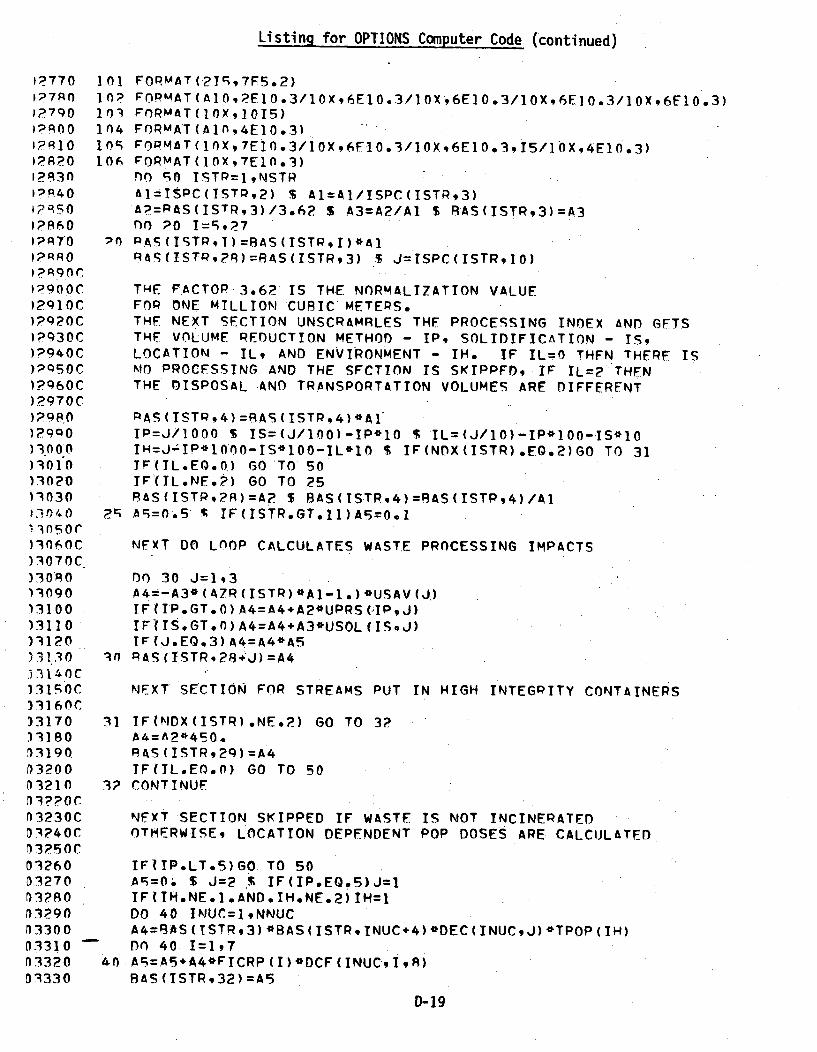
Listing for OPTIONS Computer Code (continued)

1;?770 101 FORMAT(?IS,7F5.2)?7R0 1 in? FOPMAT (A] ,?EIO,3/lOX,6E1O.3/IOX96E]0.3/lOX.6EI O.3/lOX,6E1O .3)

I?'790 10" FORMAT(IOX,1015)iRA0 104 FORMAT(AlnO,4E10.3),P?'R0 JO FOPMAT (I nXT7E1.3/IOX96FI0.3/OX,6EI0.3,is//lOX,4EI0.3)I?82O 106 FORMAT(lOX,7Eln.3)12R30 nO 50 ISTP=1,NSTRIPP.40 AI=ISPC(ISTQ,2) $ AI=A1/ISPC(ISTR,3)i-)R5O A7=PAS(ISTR,3)/3o62 S A3=A2/A1 $ FAS(ISTR,3)=A3J?8AO nO PO T=5,271PT70 70 PA5 (ISTP, I) =8AS (ISTPq, I)*AlOPR•O RAS(ISTPqR)=RAS(ISTR,3) $ J=ISPC(ISTR,10)

)290o0c THE FACTOP 3.62 IS THE NORMALIZATION VALUE)2qI0C FOP ONE MILLION CURIC METERS.)?.QpOC THE NEXT SECTION UNSCRAMRLES THE PROCESSING INDEX AND GETS)?930C THE VOLUME REDUCTION METHOD - IP, SOLIDIFICATION - IS,)?940C LOCATION - IL, AND ENVIRONMENT - IH. IF IL=O THFN THERE IS)7Q50C NO PROCESSING AND THE SFCTION IS SKIPPFDl, IF IL=2 THEN)?Q6OC THE DISPOSAL AND TRANSPORTATION VOLUMES ARE DIFFERENT)2970C)pgFo -0 PAS (ISTP,4)=RAS(ISTR,4)*Al")2Q9O IP=J/1000 s IS=(J/lOO)-IP*10 S IL=(J/10)-IP*10O-IS*lo)3000 IH=J-IP*100O-IS*100-IL*no $ IF(NDX(ISTR).EO.2)GO TO 31)301f0 Tr(IL.EO.0.) GO TO 50)3020 IF(IL.NE.?) GO TO 251'030 RAS(ISTR,2R)=A? $ BAS(ISTR,4)=8AS(ISTP,4)/Al1) 4•0 25 A5=0.5 T, IF(ISTR.GT.11)A5=0.1

!3•nsor

)100;0C NEXT DO LnOP CALCULATES WASTE PROCESSING IMPACTS)3070C)3090 Do 30 J=193111090 h4=-A3*(A7R(ISTR)*Al-l.)4IUSAV(J)131.00 TF(IP.GT.O) A4=A4+A2*UPRS(IPJ))3110 IFl(IS.GT.,) A4=A4+A3*USOL (ISeJ))31n0 IF(J.EQ.3)A4=A4*A5) 13.0 3in AS(ISTR,?8+.J)=A4)l3140C3315OC NEXT SECTION FOR STREAMS PUT IN HIGH INTEGPITY CONTAINERS)3160C33170 31 IFINDX(ISTR).NE.2) GO TO 32.33180 A4=A2*45O...03190 RAS(ISTR,29)=A433200 IF(ILEO.n) GO TO 5013210 3? CONTINUE

33230C NEXT SECTION SKIPPED IF WASTE IS NOT INCINERATEDDI?40C OTHERWISE, LOCATION DEPENDENT POP DOSES ARE CALCULATED33?90C03260 IFIP.LT,5)GO. TO 50D3270 A5=O. $ J=2 S IF(IPEQ,)J=l03?80 IF(TH.NE.1.AND.IH.NE.2) IH=113290 DO 40 INUC=1,NNUC33300 A4=9AS(ISTR,3)*BAS(ISTRINUC+4)*DEC(INUCJ)*TPOP(IH)D3310 DO 40 1=1•703320 40 Ag,=AS+A4*FICRP(I)*DCF(INUC, IA)03330 8AS(ISTR,32)=A5

D-19

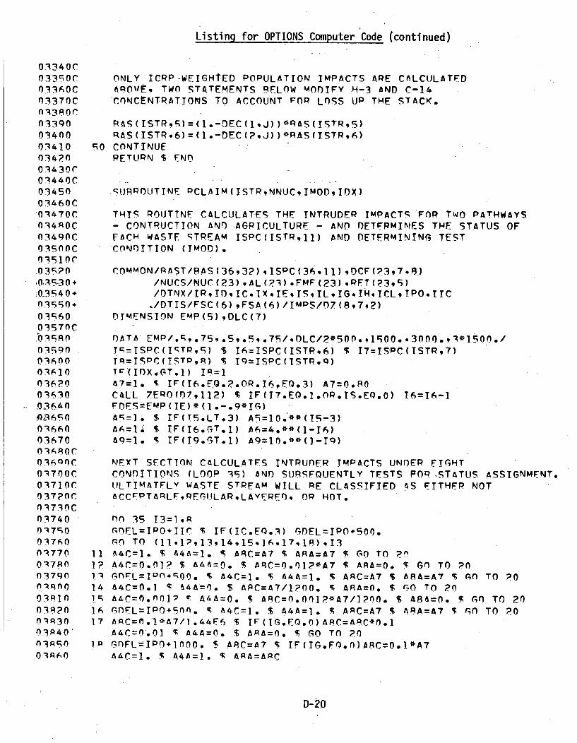
Listing for OPTIONS Computer Code (continued)

03340C03390C03360Cn4337 0 Cfl3370C

n33900340001410034?n03 430C03440C0345n03'L60C0 34 70COR44ROC03440C

035n1C03510C003110.

so0l53 0+

.03540÷

035600357nC

07b3 6 no0359003600

03,610036?f003630

03640

03660

03670O3AROC

0•700C03710C037?OC

03730C03740

0•7•0

03760n3770

0 3790o -Rnon03a1ln03R?0

03P40'0 .3 R 40n3p•o

03RP0

0 -4 R6

ONLY ICRP-WEIGHTED POPULATION IMPACTS APE CALCULATFDAROVE9 TWO STATEMENTS 9FLOW MODIFY H-3 AND C-14CONCtNTRATIONS TO ACCOUNT FOR LOSS ULP THE STACK.

RAS(ISTR5)=(l.-DEC(1,J))*RAS(ISTR.5)RAS(ISTR.6)=(I.-DEC(?.J))*RAS(ISTR,6)

90 CONTINUERETURN $ END

.Sk)POUTINE PCLAIM ( ISTRNNUC, IMOD, lOX)

THITS ROUTINE CALCULATES THE INTRUDER IMPACTS FOR TWO PATHWAYS- CONTRUCTION AND AGRICULTURE - AND DETFRMINES THE STATUS OFFACH WASTE STREAM ISPC(ISTP,11) AND DETERMINING TESTCONDITION (IMOD).

COMMON/RAST/RAS(36,32)qISPC(36.11),OCF(?3,7.F8)/NUCS/NUC(23),AL(?3).FMF(23),RFT(?3,5)/DTNX/IRIDIC.IX.IEISILIG.IM.ICLIPO.IIC

./DTIS/FSC(6),FSA(6)/IMPS/f7(8,7,2)DIMENSION EMP(5),DLC(7)

DATA+ EMP/.C;,.75. .5, .F5..75;/.DLC/2*500.,1SC00. .3000.,3 *1c-0nt)ITISPC(IqTPq.) $ 16=ISPC(ISTP96) $ 17=ISPC(ISTR,7)IR=ISPC(ISTPP) $ 19=ISPC(ISTP.Q)Tr'(IrX.fGT.I) IP=l

47=I* 1 IF(16.eQ.?.OR.16.EQ.3) A7=0.80CALL 7EPO(M7,112) % IF(17.EQ.I.OR.IS.EQ.O) 16=T6-1rFDES=EMP(IE)*(.-s.9*IG)AE=]. $.IF(T5.LT.3) A5=10.**(I5-3)A6=1i' $ IF(16.GT.1) A6=4.**(1I-6)A9=1* T IF(19*GT.1) Ag=ln.**(1-I9)

NVXT SECTION CALCULATES INTRUDER IMPACTS UNDER EIGHTCONDITIONS (LOOP 35) AND SURSEQUENTLY TESTS FOQ.STATUS ASSIGNMENT.[.LTIMATFLY WASTE STPEAM WILL RE CLASSIFIED -S EITHER NOTACCEPTARLF.REGI.ILAR.LAVERED. OR HOT.

nn 35 13=l.pGDEL-IPO+IIr $ IF(IC.EQ.3) GDEL=IPO+500.CGO TO (11*1;),13,14qj5%j(6.17,1P) 13

11 A4C=1. $ A4A=le. I AAC=A7 $ ARA=A7 T GO TO ?

I? A4C=O.f? s A4A=O. S ARC=nO,1?*A7 S AAA=O. T GO TO '01.; rnrL=ITO÷+ o. $ A4C=I. % A4A=I. % ARC=A7 $ ASA=A7 C GO TO P0

14 A4C=O.1 $ A4A=O. $ APC=A7/1?O0. T APA=n. $ C0 TO 201c. AhC=0o.07 Qý A&A=O. $ A9C=O.Onj?*A7/1?AO. $ A88=0 S GO TO 2016 GnFLrPO4o~nf. T A4C=]. t A4A=1. % AAC=A7 $ AAA=A7 S GO TO ?017 AAC=n.I*A7/1.44E6 % IF(IG.FQ.O)APC=ApC*n.i

A4CA=O.,O ' A4A=n. $ AqA=n. % GO TO ?0IP GfFL=IPO÷IOO0. $ A8C=A7 $ IF(IG.EO.o)ARC=O.l*A7

A4C=I. T A4A=1. S AAA=ARC

D-20

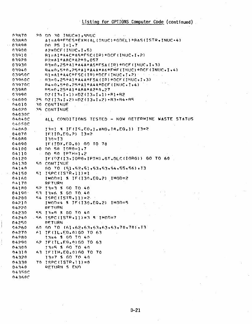
Listing for OPTIONS Computer Code (continued)

01870

03900

039?003930039400399OC0396OC03970Cn3sRO

039900400004010040?0040 30C04040C

04060.04070040300409004100.04110041?0041300414004150041600 "•170

041A004190-04?00

0421004??004230042400425004?600-4970

n4;800429004300O 431 00432004330043400439R0C04360C

n0 on 30 TNUC=1,NNUC

A1=Aq*F0ES*FXM(AL(IN•UC)*GfEFL)*RAS(ISTRINUC+4)no 25 T=197

A?=DCF( INLUC,1,5)R1=A1*A4C*A5*FSC(IR)*DCF(INUCI. ,)P?=Al*ARC*A?*0.057p3=0.?5*A].*A4A*A5*FSA(IP)*nCF(INUC,I,3)R4= L 9*0n. 9*AI*A4A*A6*FMF(INiUC) *CF(INUC,!,4)RI=Ai*A4C*FSC(IP) *CF(INUCIT) .P93=ý.25*AI*A4A*FSA(IR)*DCF( CINUCI, 93)P4=0.5n*0.?9*AI*A4A*DCF(INIJCI,4)Pq=0 25*A1*ASA*A?•A .27

n7(I, 191)=DZ(13,,1))+P÷+R2?g 07(3,1,?2)=DZ((13,1,?)+R3+R4+R930 CONTINUE

39 CONTINUE

ALL CONDITIONS TESTED - NOW DETEPMINE WASTE STATUS

l=l1 % IFfISEO.1.AND.TP.EQ.1) 13=?IF(IP.EO.?) 13=?130I13IF(IDXOFQ.0) GO TO 70

40 no g0 IORG=1,7no 50 IPTH=1,2IF(l(I3(3IOPGIPTH).GT.DLC(IORG)) GO TO 60

g0 CONTINUEGO TO (5.19?451,53,53,54,55,56),13

ql ISPC(ISTR,11)=l1Mnf=l $ IF(130.EQ.2) IMOD=2RFTIJRKN

9? 13=3 $ GO TO4093 13=6, $ GO TO.40q4 ISPC(ISTR,11)=2

IM0n=4 $ IF(130.EQ.2) IMOD=SPFrT9IRN

99 TI=R $ GO TO 4096 ISPC(ISTPoI1)=3 ' I1OM=7

PFTIJRN

60 G0 TO (61962,63,63,63,63,70,70),1361 IF(IL.EO.O)GO TO 63

73=4 $ GO TO 406? .FF(TL.EO.n)GO TO 63

T1=5 S GO TO 4063 IFC(IH.EO.0)rO TO 70

13=7 $ GO'TO 4070 lSPC(ISTP,11)=0

PFTURN . END

D-21

Listing for OPTIONS Computer Code (continued)

04370n4390C043QnC

n4400C0441oC0442004430+04440+04450÷04460+04470.044P004490045000451 oC04r?20C04530C04540045900456004570045A0045q004600

,04610046200463004640C04650C04660C04670C040R0Cn46q0C04700C04710047200473004740047c50 r0476AC04770C047R0047900480004P10

0442004R3004S40o4 8500496004P7004QRO

SURPOUTINE ACCEXP(NSTRgNNUCqNOX)

THIS ROUTINE CALCULATES THE EXPOSURE AND ACCIDENT IMPACTSFOR 7 PATHWAYS (4 EXPOSURE AND 3 ACCIDENT) AND 7 ORGANS,

COMMONfRAST/RAS(36932),ISPC(369,11),DCF(23,7.8)'/NUCS/NUC(23),AL(?3),FMF(23),RET(23,5)/DTNX/IRRgID, IC,IX,IE,ISILqIGIHICLIPO,1C/DTIS/FSC(6),FSA(6),PRC(6,2),#QFC(6,3),TTM(6,3),TOC(6,3) ,RGF(693),POP(6,3),DTTM(6),DTPC(6),TOO(6,,),NRET(6)/IMPS/DZDM(168),DZA(797),DZS(36,792)

.DTMENSION EMP(5),EFF(?),SEFF(?),gNX(36)nATA EMP/.5,o75,.9,.5,9o.7/,FlFF/6o4,o7.0/SEFF/O.q0.35/VTOP•O $ VTOT=O. $ VHOT=O. % GREC=IPO+IIC

FROSION TIME SCALE DEPFNDENT ON COVER USFD AT DISPOSAL SITE

GFRP=IPOP+?000.TFlIC.E*.2) GEPO=IPO+3000.IF(IC.EO.3) GEPO=IPO.10000.IFIID.Eo.p) GFPO=IpOOlO000.on i. ISTP=INSTRTII=TtýC(ITSTP-11)

IFII1.EOQ.I)VTOP=VTOP+RAS(ISTR,3)IFITI..EQ.I.OR.Ii.EO.2)VTOT=VTOT+RAS(ISTR,3)IFtII.EO.3)\VHOT=VHOT÷RAS(ISTP,3)

10 CONTINUE

VTOP IS JUST PFGULAP WASTEVTOT IS REGULAR + LAYERED WASTE

NEXT SECTION ESTARLISHES AREAL FACTORS FOR 4 EXPOSURE PATHWAYS

FRA=5.7?F-5*POP(IR91)*l.8E~l $ VUP=EMP(IE)*EFF(ID)*SEFF(ID)FEA=9.OqE-6*POP(IR,?)*VTOT/VUPFPW=1.15E-44*POP(IR.3) *19A.PEFFW=1.15F-4*POP(IR,3)*VTOT/VUP

MAIN LOOP FOR EXPOSURE IMPACTS

nO 40 ISTP=1,NSTRA1=-90: $ III=ISPC(ISTR,11) $ IF(I1I.EQ.O)G0 TO 40IT=ISPC(ISTP,5) $ A5=1. % IF(I5.LT.3) A5=10.**(15-1)IQ=ISPC(ISTR,9) S A9=1. S IF(19.GT.1) A9=10.**(1I-9)IA=ISPC(ITRP) % IF(NI)X(ISTR).GT.]) I=1-TF(TP.FO. IAND, IS.EO.I) Al=O.Ol2/9.

IF(Tl.EO.?.OR.I".EOP.?) A=Al*O.01*IF ( I Il °o.3) 41=1 oE-9/9,

A?=FMP(IF)*SEFF (ID)*RAS(ISTTP,3)/VTOPAI=A?*VTOP/(VTOT+VHOT) $ IF(TI1.GTol)A2=0.

IF(Tf.EQ.?.AND.Ill.NF.P) A?='A3

D-22

Listing for OPTIONS Computer Code (continued)

04R90 DO 30 INUC=1,NNUC04900 A6=EXM.(GREC*AL(INUC)) $ A7=EXM(GFRO*AL(INUC))04910 AP=RAS(ISTR,INUC÷4)04920 RI=FRA*A1•A3*A6*A8*A5 $ R2=FEA*A?*A7*A804930 RI=FPW*c1*A3*A6*A8*A9 $ R4=FEW*A2*A7*A804940 nO ?0 IORG=I,704950 O7A(IORG'1)=D07A(IOG,1) +I*DCF(INUC,IORG,8)04960 DZA(IOPG,?}=DZA.(IOPG,?)+P2*DCF(INUCIO~rG,)04970 D7A(IOPG,3)=DZA(IORG,3)+÷3*DCF(INUCIORG,7)04980 D7A(IORG,4)=DZA(IORG,4)+R4*DCF(INUC, ORc,7)

04990 ?0 CONTINUE05000 10 CONTINUE05010 40 CONTINUF00?OC05030C END EXPOSURF LOOP05040C05050 VSC=O. $ VFP=O.

6 060Cn5070C MAIN LOOP OF ACCIDENT IMPACTS

050 0C05090 DO Ro ISTP=1,NSTR05100 13=ISPC(ISTRll) $ IF(13.EQ.O.OR.I3.EQ.3)GO TO AO05110. I4=ISDC(ISTP,4) $ T6=ISPC(ISTR96) $ I9=ISPC(ISTRq)05120 A5=RAS(ISTR,3) S IF(19.GT.1) GO TO PO0}130 FAF=TPO(IP,1) $ FAS=TPO(IR,?)05140 IF(16.GT.1) FAS=FAS*(10*.ý*(116))05150 IF(14.LT.3) FAF=FAF*(?0.**(I4-3))09160 IF(IS.EQ.I.AND.I4.NE.3.) FAF=0.0T170Co0iPnC DISTINGUISH RETWEEN SINGLE CONTAINER AND FIRE ACCIDENTS09190C05200 VFR=VFR*AS0521.0 VSC=VSC+A5n52P0 DO 70 INUC=19NNUC05230 AIS=FAS*RAS(ISTRINUC÷4)*A505240 AIF=FAF*BAS(ISTR,INUC,4)*A505250 DO 70 IORG=1,705260 D7S ( ISTR, IORG, 1) =D7S ( ISTR, ITOR , 1) +AiS*DCF INUCp IORG• 1)A505?70 DZS(ISTPTOPG,2)=D7S(ISTR, IOG,?2)+AIF*DCF(IiUCIORG,1)/A505280 07A(IORG,5)=DZA(IOPG,5)+AIS*DCF(INUC,IORG,1)05290 70 D7A(IORG,6)=D•A(IORG,6)+AlF*DCF(INUC,IOP6,1)05300 R0 CONTINUE05310 C05320C END OF ACCIDENT LOOP0 5330 C05340C05350C LAST PATHWAY IS AVERAGED ACCIDENT05360C05370 DO 90 IORG=1,705380. D7A(IORG,7)=(DZA(IOPG,5)÷DZA(IORG,6))/(VSC.VFR)o03qO TFjVSC.GT.0.) DZA(IORG,5)=7ZA(IOPG,5)/VSC05400 IF(VFP.GT.0.) DZA(IORG,6)=OZA(IORG,6)/VFR05410 QO CONTINUF0c420 PETIIRN $ END05430C-_

D-2a

Listing for OPTIONS Computer Code (Continued)

05440C

O9450054 60 C0 r,4 6n0(7nc;470Coc;4Rnc

054 90C

OS•OOC05510C

o054005550÷

0570r

05 60 0C

0610C

0 95 C) 0 C0 5;6 3) 0 C

0460C0S70C

nq~rQOCOSA9OC

09710C057?nC0573OC

OCS74nfl57•OC05760Cn c; 75 0 C05f70C

OSR 1OC

OFROCo7POc

nc;A40nc5q90OFu60+

o5;9O n

n 9030+

05Q4 nf0Tn30+

n5qAO÷Os O0+

0596nncR7 nn59 Pn

cn OQn

SURPOUTINF TPANSP(TTMP.NSTP)

THIS ROUTINE DETERMINES THE TRANSPORTATION SCHEMF FOP ALLWASTE STRFAMS 9ASED PRIMARILY ON THE PACKAG'ING INDFX OF

THE SPECTRUM FTLFS AND THE ACTIVITY CONCENTRATIONS OF THE

INDIVIDUAL STREAMS. ULTIMATE PFSULT IS THE TRANSPORTATION

TMPACTS (TIMP).

COMMON/RAST/BAS(36,3?),ISPC(3A,11)/DTNX/IRID,IC,IX,IE

DIMENSION PCAP(6,3),PPAK(PA),KON(IR),TYM(2,18),KWT(lS),

ODZ (2,3),DKV(5),TfZ(,9?) ,TCST(2,3).TITMP(6), TVOL(5,3),n I.JMi (3) ,OUM?(3) DJM3 (3, 3) .nIST (6) ,STPS (6) ,C ASK (6)

THF APOVE ARRAYSPCAR (6,3)

PPAK(8.6)

KON(]8)

,TYM(?,].8)

.TCST(?.3)

PI<V (;),KWT(IR)

DIST(6)

STPS (A)

CAqK(6)

AND MATRICES APE EXPLAINEr) RELOW:: CONTAINS A DISTRI9UTIONS OF I CARP TYPES.: CONTAINS R DISTRIRIJTIONS OF q PACKING

CONTAINFRS + A POSITIONING INDEX,: MULTIPLE INDFX WHICH DESCRIRFS PACKING

CAPARILITIFS FOR 3 CARE TYPES AND SCONTAINERS.

: TIME IN MINUTES FOR UNLOAnING OF WASTE(CONTACT TIME) - CORRESPONDING TO THFIP KON INDICES APOVE.

: TRANSPOPTATION COST ($) PER MILF.: PADIOLOGICAL COST (DOSE) PER HOUR OF

CONTACT TIME WITH WASTE.: TWO PART TPANSPOPTATION DOSE: PFP MILE.

AND LIJMP SUM PAPAMFTFRS.:VOLUMF CAPACITY FOP EACH OF r CONTAINERS.: INDFX TO PFLATF TRANSPORT VrHICLF OVFP-

WFIGHT STATUS TO EACH OF KON INDICFS.: TRAVEL DISTANCE TO DISPOSAL SITF IN

VARIOUS REGIONS.: STATE INSPECTION STOPS TO RE FXPFCTFD

WITHIN A PARTICULAR PEGION,NUMREP OF DAYS A CASK WOULD RE PFOUIPEDIN A DAPTICULAR REGION.

OTHER ARRAYS ANfl MATRICES DESCPIRED FURTHFR ON IN PROGRAM.

DATA DDAK/O.n.?39*0•o•, g.og .O,.O?5q5*0.,.9Q,6Q,.975,.?,].,30.,. A• .. .0., .,052*0.. 16,4*0., .,1. *,0. .3.,j. ,?.,43. /

)ATA KOm/ I n304, 1104076,1?36100,137n100*141.1100,-15OhI109?1O3]0O,??36Oq•.,-?o•OO4,?37OO4R,-?3i4051,-?30A0OO.,-24OlnO,-?50l100,-iio~ogi,-33nl04g,-34O210n,-iq01100/

DATA TYv/pOO.9P4..,7.4.*1?O. ,1A.,?4.gA.,?4.-.3A.,161,1?nn0.,1440.,300.,3A0. ,2j.,q.,?50. .300., 1.O.,P.,6.,.15.20.O.,312..

15On. o1 P./,TCST/1.6,9.IP?,1.47, .14,9.17.1.OP/nfTA RD7/IOO.,O750.9,1?0.,iROO.,??OO.,?pOo./TD7/1.RE-?,

?.9-,?,./,DKV/3.6?'-;g.49-,.?n A, 1.41 A 4.P14/

DATA KWT/ MP6*0,P*I/ )IST/900. q400. 600. ,F100on. .2*400./

CALL 7FRO(TIMP,96) $ CALL ZERO(TVOL*19)

D-24

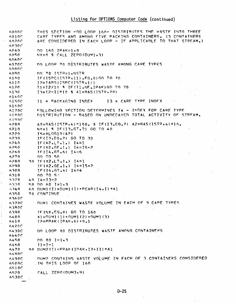
Listing for OPTIONS Computer Code (continued)

60;0- n (76010o60 20 C6030C

6040

606n C6n7OrKAORC60900;lno

611o

61?n0

6]ISOC;10;C61 7nC

0 006?1 06??o

6?306? 40

6706?6O6?7O

63006310

640

6430C

637oc

64400641064?OC

64 30 C6440C

6470

6490C

650C6 ;3 0 C

THIS SECTIOn -DO LOOP 16n- DISTPIPIJTFS THE WASTF INTO THREECARE TYPES AND AMONG FIVE PACKING CONTAINERS. (3 CONTAINERSAPE CONSIDEPED IN EACH LOOP - IF APPLICARLE TO THAT STPEAM.)

no 160 IPAK=1.9NtY=n $ CALL 7EPO(DUMI,3)

nO LOOP 70 DISTRIRUTES WASTE AMONG CAPE TYPES

n0 70 ISTP=1,NSTRTF(ISPC(ISTPl1).FQ.O)GO TO 70I=TARS(ISPC(ISTR,1))11=12/10 T IF(Il.NF.IPAK)GO TO 70I3=T2-I1*10 $ Al=RAS(ISTP.?8)

TI = PACKAGING INDEX 13 = CARE TYPE INDEX

FOLLOWING SECTION DETERMINES 14 - ITtMEX FOR CARE TYPEnISTPIRUTION - RASED ON UNnECAYED TOTAL ACTIVITY OF STPFAM.

A?=RAS(ISTPo4)*100. $ IF(I3.EO.?) A2=RAS(ISTR,4)*10.NtX1= % IF(I3.GT.?) GO TO 401•=ALOG1O (A?)IP(13.EO.P) GO TO 30IF(A?.LT.].) 14=1IF(A?.GE.1.) 14=15+?Ir(14.GT.6) 14=6GO TO 50

3n IF(A2.LT.1.) 14=1IF(A2.GE.I.) 14=15+?IF(14.GT.4) 14=4GO TO 9'f

4n 14=13-?co no 60 T=1,3r0 n UMI (I) =DUMI (1) +CAP (14,1) *AI70 CONTINUE

ntiml CONTAINES WASTE VOLUME IN EACH OF I CARE TYPEq

TF(NX.EO.O) GO TO 160A1=nUl I(1)+nUml(2)*DUMl(3)iT=PPAK(IPAK,6)+O.]

DO LOOP 80 DISTRIRUTES WASTE AMONG CONTAINEPS

DO RO I=1,3TT=T-I

90 DJM?•(I)=PPAK(IPAK.I•?+I1)lA

nlJm? CONTAINS WASTE VOLUME IN EACH OF 3 CONTAINERS CONSI.DEPEDIN THIS LOOP OF 160

CALL ZERO(DIJM3,9)

D-25

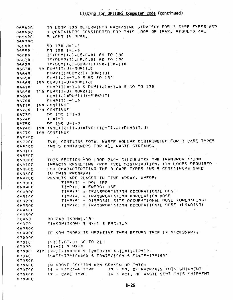
Listing for OPTIONS Computer Code (continued).

06540C no LOOP 130 DETERMINFS PACKAGING STRATEGY FOR 3 CARE TYPES AND

06c5;;0C 3 CONTATNEPS CONSIDERED FOR THIS LOOP OF IPAK. RESUILTS ARE

06560C PLACED IN DUM3.

06SP0 00 130 J=19306490 nO 120 I=1,3n6600 IF(0UMI(J).LF.0.) GO TO 13n

O$610 TF(DUM,?(I)LE.0.0) GO TO 12006620 TF'(rUMI (j)-r)UM?(I))goq1n0,11I06630 QO DUM3 ( I ,J) =01)MI (J)06640 nl!MP (I)=D0JM?(I)-Ot.JM I (J)0n650 mIM1i(J)=-in $ GO TO 130

•A60 lrn 1 fiJMa (I J) =OIM1 (J)0667n e.IM?(I)=-1. 0 % DUMI(J)=-I.0 $ GO TO 130n06•8 rtýn I ntmjI 3 IJ) =DUM2 (I.)

n66qO nUM1(J)=DUmI(J) -DUM?(I)0l700 O!•?(I)=-1.00671n Ip0 rONTINUJF06720 1.n rnONTINUE

06730. yD 10 In=,306740 IT=T-10(790 0 15 0 J-193

00-760 l1n TVOL (I?+II,J):VOL (12+TIJ)+DUM3(IJ)0I770 1-n CONTINUF

n67g0C TVOL CONTAINS TOTAL WASTF VOLUME nISTRIPUTED FOP 3 CAPE TYPESOAPO0C AND 9 CONTATNERS FOR ALL WASTE STFEAMS..06P1 OCn~pinc

06•30C THIS SECTION -1)o LOOP -40- CALCULATES THE TRANSPORTATION

06o40C IMPACTS RFSIJLTING FROM TVOL nIrSTPIPUTION. (IR LOOPS REOUIRFt)

06950C FOR CHARACTFRIZING THE 3 CAPE TYPES 'NP S CONTATINFPS USEDnoR6,OC TN THIS PROGPAM)0 OP70C PESIJLTS APE PLACED IN TIM0 ARRAY, WH•ER:08Ro0C TIMAP(I) = DOLLAPS

06Q0oC TIMP(?) = ENERGY USE06O00oC TIMP(3) = TOANSPOPTATION OCCUPATIONAL OSFnOglOC TIMP(4) = TRANSPORTATION POPULATION DOSE06qlC TIMP(9) = DISPOSAL SITE OCCUPATIONAL DOSE (UINLOADING)

06930C TIMP(6) = TQANSPOPTATTON OCCUPATIONAL 0O0SF (LOADING)nOAQ4nr

06qo0 DO P40 IKON=I,18'04,Q70 IT=KOM(IKON) $ NX1I $ FPC:1.0

oAQ9OC IF" KON TINDEX I; NFGATIVE TH.EN PETURN TRIP Tq NECESSARY.07000C

07010 IT(TI.GT.f) GO TO ?in070?() TT=-II T, MY=?~

07030 ?In T'=TI/.n OnnO % I•:=In/1 It .I1=I3-I?*1f.n7040 lI=ll-13*10000n $ 13=1l/100n ' I4:lq-I3*100l0 70 9OC

07060C IN pAROVF qErTTON (KON qROKFN UP TNTO:07070C T'i --= DP(AGF" TYPE TA = 1O. OF PACKAGES THIS SHTPMFNIT

07opOC T? CAPE TYPE T4 = PCT. OF WASTE SF"'T THIS SHIPMENT

07090CD- 26

Listing for OPTIONS Computer Code (continued)

17100n TF {(12*g. I) .OR. (I?.FQ.?>. AiN.NX-FO.?) ) F-RC=n. I.711.0 FRS=14/100 $ AI=TVOLfIlI?)*FRS)7120 IF(AI.LT.1.F-06) GO TO 240)7130 KSHP=A1/(l,3*PKV(I1) )+1.01714n A?=KSHP*DIST(IR) $ A3=A?*NX)7150 TTMP(?)=TIMP(P)+A3/6.M7 60C17170C TN ABOVE EQUATION 6 PEPRFSFNTS MILES PER GALLON FUEL CONSUMPTION,)71ROC171 q0 TTIMP(4)=TIMP(4)+(A2*TD.)7(1 l)+KSHP*Tl7(1I?•)-*STPS(IR) )*FR"37?n00 TIMP(3)=-TIMP( 3)+(A?•*Tr7( ?.,)+)KSHP*TDZ( ??.)*STPS(IR))*FRC1721n NC=l $ IF(DIST(IR).GT.400..AN.D-IST(IR)-LT-]O00-) Nr=?'17??0 IF(DIST(IP).LF.400.) NC=117?30 TIMP(1)=TIMP(1) +A3*TCST(NX,NC)*I.-I,17P40C17?S0C IN NEXT SECTION CASK PFNTAL FEE AND OVERWEIGHT FEE ADDED-.17?0C IF APPLICABLE.17?70C172P0 IF(NX.FO.I) GO TO 2?O17?90 TIMP(1)=TIMP(1)+KSHP*CASK(IR)*2;O.117300 TF"(WT(IKON).GT.O)TIMP(1)=TIMP(1)+A2*0.76+61)-*STPS(IR)17310 220 KPAK=Al/PKV(I1)+1.0.17320 NY=P $ IF(IF.EQ.l.OR.IE.EO4) NX=117130 FPC=1.0 $ IF(IE.EQ.3) FPC=?.O1734-0 Ap?=PAK*TYM(NX,IKON)/60.,1735) TIMP (9) =TIMP (9) +A2*FRC*RPZ (NX, 12) * ,E-317360 TIMP(6)=TIMP(6) +A2*RD7(2,I?)*1 .F-317370 240 CONTINUF,73.B0 PFTIRN S END173QOC

4. ,0 C)74 10 SUBROUTINE ECON(NSTR,RI,RJCOSTNDX)174?20C)7430C THIS ROUTINE CALCULATES THE DISPOSAL IMPACTS BASED LARGELY17440C. ON THE INPUTED VALUES FOR THE DISPOSAL TECHNOLOGY INDICFS.)7450C THE RESULTS OF THIS ROUTINE ARE PLACED IN ARRAY .COqT, WHERE:17460C COST(1), = PRE-OP AND OPERATIONAL DOLLAPS17470C COST(2) = OCCUPATIONAL DOSE174P0C COST(3) = ENERGY USE!7490C COST(4) = LAND USE17500C COST(5) = POST-OP DOLLARS1751 oC175?0 COMMON/RAST/RAS(36,32),ISPC(36,11l)17C;30 COMMONIDTNX! IR., I0), TC, !XIEIS, IL,,Ir,,IH, ICL, IPO, lC

n7540 COMMON/VOL/VREG, VLAYVHOT'17550 lIMENSION EMpP(S;),EFF(2) oAMULT(?P),CONT(6),.COST(S),•SEFF(?).17R60 DIMENSION NDX(36)17970C17S5PnC THE SIGNIFICANT APPAYS ABOVE ARE:17590C AMULT(2) = CAPITAL AND OPERATIONS COST ($) MULTIPLIERS.1)7600C CONT.(3) = CONTINGENCY COST FOR SOIL PERMFABILITY CONnITIONS.17f10C COST(5) = CONTAINS RESULTANT IMPACTS - IN TERMS OF $,176,?0C OCCUPATIONAL OOSE, ENERGY USE, LAND USE, AND17630C POST OPEPATIONAL $.

)7640C

D-27

Listing for OPTIONS Computer Code (continued)

n7;6n0C PT ANn QJ PAPAmFTERS APE INTFPEST AND INFLATION PATES, RESPECTIVELY.nTATOC

07P0 nAT.4 C(Th'T/I007. ,367o,367,. f 6. A6Ro,10n7.o/IToF/?O, .nIr/n 7 r 0O n 4Tt . F M4OI c. 7. c; . 5 9. 7 1;I F FFI/6. 4 97.01 A M LI. T/ 10.3 9 1 56 9

n7700+ '-FFF/. o 9. ..

n77.0 CALL 7FOn(COST,5)n77-P:0 \I5TAR=n. % \UNS=N. • OECON=n.n-774-0 nn IqTP=I.NSTP07740 TI]=TSOC(TSTPpjl) $ I2=ISO(ISTPR)n77r0 IF(MfDX(ISTP).GT.1) TP=.07760 TF(Ill.EO.OQ.OP.Ill.F0.3) GO TO ;n7770 TF(TE.F0.3.AND.I2.Fo.N) DECnN=DFCON+RAS(ISTP,3)077R0 -I•(T.EO.n) VSTAR=VSTAQ+RAS(ISTP,3)0770n Tf(T?.FO.1) VUNS=VUNS+RAS(TSTP.3)07QO0 S CONTINI.IF

n7Qjn TF(TE.ED.3) IS=107RpnC

07630C \/qTAP %_ VUNS CONTAIN STARLF AND UNSTARLE WASTE VOLUMFSRESPECTIVELY07;840C

07.TAf.n nPEC,=(VPEC+\/LAY)*].E-06 $ DHoT=VHOT*l.E-06n7RA60 nLAY=VLAY-1.E-06 $ nFFCON=nECON*l.E-ni07P70 DVOL=0RFG/EM P(IE) $ nAPFA=DVOL/(FFF(ID-)*SFFF(ID))07Ppn G\I= ( I .- FP ( TF) ) *rVOL $ VTOT=VPEG+VLAY+VHOT07 Q0 SV=nREG* (( 1.•67/EMP (iE )) -)n7QONCN79OC VnLIJME AND AREA VALUES ARE EXPRESSED IN UNITS OF MILLION. M3 OR M?07POC FDP USE IN COST EVALUATTnNS. GV IS GROUT VOLUME. SV IS SAND VOLUME.n7Q0C

n7Q40 rnST(4)= (MAREP + (DHOT/l.84))*1.EF6n7q90 S1=(VSTAP/VPEG)*DAPFA T SP=(VUlNS/VRwG)*ARFA07.960C

07Q70C IN FOLLOWING SECTION CT.C?, AND C3 WILL ACCUMULATE THE DOLLAR,n7lqaoc DnOSE, ANDl ENFRGY COSTS THROUGH THE VARIOUS DHASFS OF THF SITE LIFE.n7qono...o0qnonr

OpolOC PPE-OPEPATTONAL (CAPITAL) COSTS

nq030C ******** REFERENCE RASF CASE ********

0Q040 Cl=745?. r COST(3)=212.nOqnOC ******** ADnITIVF ALTEPNATIVFS ******

nOn0n TF(ID.EO.P) C1=CI+593.Sn0070 TF(IF.EO.' .OR.IE.EQ.5) 01=C0+225.5onp()o Tc(TS.EQ.l) Cl=CI÷O.c)Qr)q pQ n IF(TL.E0.I) Cl=CI÷132.--..

OR0I0 IF(IE.EO.3) CI=CI+q:4.'nplIn IF(TH..Fr.) C1=Cl+?99.4nqlPn TF(IG.EO.I) C1=Cl+5,.

oR13n TF(IC.EO.1) C1=CI+PO.5n0l4n IF(IX.FO.') Cl=C÷g9.9np]n rCAp=CI*ANIILT(1)

OPI 70C

D- 28

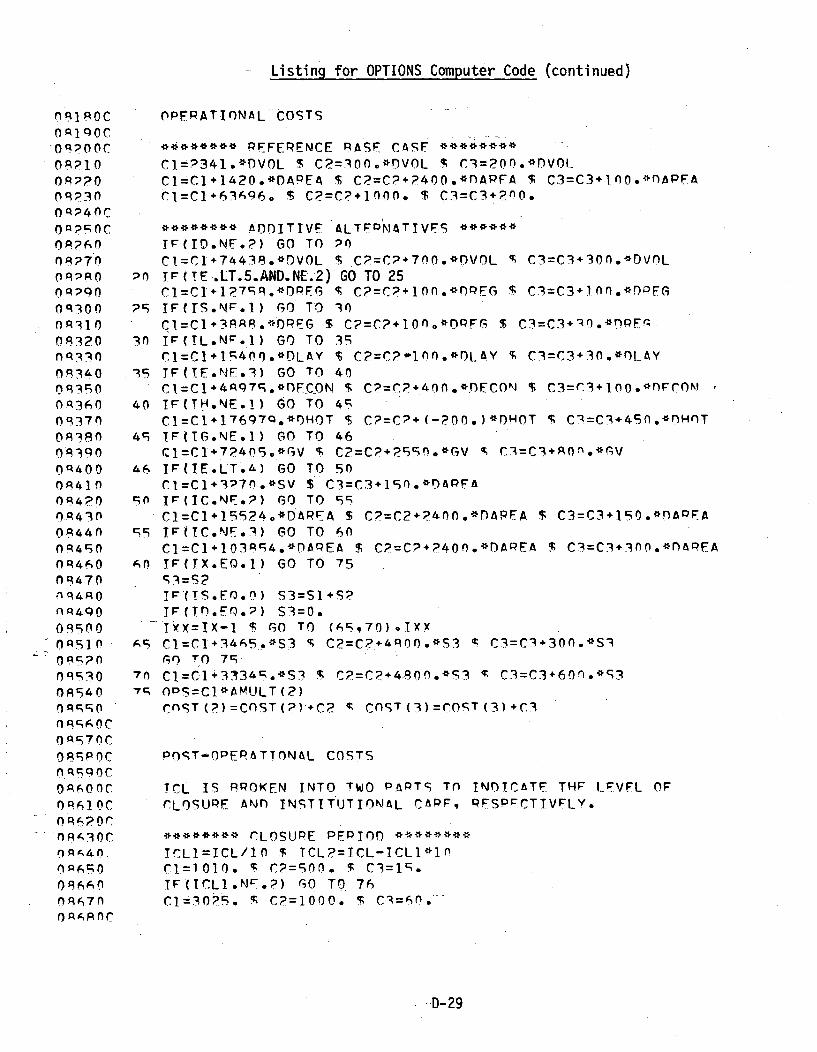
Listing for OPTIONS Computer Code (continued)

n A QOCoq1o0C

OR?10OpPO3

O0q40COnp2 C

nA?7n

oq300

0R320

OR36n09370

OR3O0

0A41 n0R4]? 0() q430OR44n

Oq 4 5O

nq470

nq400

n Rc;AnC

OqRSPOC

0•P61 OC

ORA?0COR~aOC

ORROC

n r -7nrnOr,4C

ODEPATIONAL COSTS

******** REFERENCE RASE ciSF ******** '

C1:?341,*DVOL $ C2=300.*0VOL • C1=200.*nVOI..CI=C1+1420.*DAPEA $ C2=C?+?400.*PAPFA % C3=C3+loo.*OAPFACl=CI÷63166. S C?=C?.1000. $ C3=C3+?')0.

******** A'DITIVE ALTEIONATIVS*IF(IO.NF,?) GO TO ?0

C1=C1+744313.*DVOL ~ C?=CP.7nn.*DVOL % C3=C3+30n.*DVOLP0 In(!E TLT.5,AND.NE.2) GO TO 25

C C=CI+1I7AR.*OPEG , Cp=Cplnn.*OPFG ' C3=C3+1.nf.*rOFGC5 IFfIS.NF.1) GO TO 30

CI=CI÷3RRP.*OPEG $ C?:Cp+IOno*OPFG $ C3=C3÷.0.*flPFf,30 IF(IL.NF-.1) GO TO 35

Cl:Cl÷lq400.*DLAY % C?:C?-10A.*DLAY % C!:C3+30.*nLAY15 TF(TF.NE.1) GO TO 40

C1=Cl4A97q.*OFCON $ C7=C?.40.*DECON $ C3=C3÷O00.*nFrCOm40 IF(TH.NE.1) GO TO 4q

CI=CL÷17697Q.e*HOT $ C?=C?+(-?O0.)*DHOT $ C7=CI+450.*OHOT49 IF(IG.NE.°) GO TO 46

CjI:C1+7?405.*GV $ C?=C2,?5n0°*GV • C3=C3+POn°*G\I

46 IF(IE.LT.&) GO TO 50CI=C1+.°70.*SV $ C3=C3÷190.*OAPFA

90 IF(IC.NF.?) GO TO 59C1=CI+l559?4*DAPEA $ C?=C2+?40O.*DAPEA $ C3=C3+150.*APEA

q9 IF(TC.hNF.!) Go TO 60CI=C+l03Aq4.*nAAPEA $ C?=CC+?4÷.*f.APEA T CA=c.300.*nAPEA

s') TF(IX.EQ.l) GO TO 75

!TF(TS.EO.0) S3=Sl+S?TF(TO.FQ.?) S3=0.

. TYX=IX-l $ GO TO (65,70) ,TXXAR C1=C1÷3465.*S3 % C2=C?.+4R00.*S3 T C3=C3÷300.*Si

(0 TO 7c.7n CI:ClI+3434.*S3 T C2=CP÷4800.*S3 ' C3=C3+60n.*53

-r c ODS=Cl*AMULT (.2)COST(?)=COST()÷+CP c COST(3)=COST(3)+C3

DOST-OPERATTONAL COSTS

TCL IS PROKEN INTO TWO PAPT( Tn INDTCATF THF LFVFL OF

rLOSUPE ANn INSTITUTIONAL CAPF, QFSPrCTIVFLY.

******** CLOSUPE PFPIOr *

PCLI=ICL/ln $ TCL?=TCL-ICLI*lO(1=1010. q C?=00. T C3=l5.TF(TCL1.NP.2) GO TO 76Cl=30?5. T C2=1000. s C4=6n.

D-29

Listing for OPTIONS CompUter Code (continued)

nqo~qnrC0 9 70 orPlR71OCOR7?OCnq730nR7400n750097600n7700'A7FkOR79009Q00

ORR40

nqPso

00A70

OR90O

OR940

0q960ncqnooc

0•o70

OOOC

0004n09030fl0040

fn O5o0OQ00

0 9 1 1 0n01?0091.30

091 0C0915o091 AoCn0n1 70h9l pOf0] 9flnonO00nflO.

0Q??0f

INSTITUTIONAL PERIOh*

DOLLAR COST SECTION

7f CAI-=15 T CR=63. $ CC:S1.-IF(ICL?.NE.?) GO TO 77 a .CA=103 4 $ C9=190. $ CC=63.

77 IF(ICLP.NF.3) 'GO TO 7P-rA=A404+CONT(IR) $ CR:301. % CC=150.

7'I SI=n' % S?=:O S $3=0.

r) = O N = o

-E=N

f :=(1.,PJ)**E $ D2:(I.÷QI)**F;n s,=s:+Or/D?

nI:(I..iPJ)**E D2=(I..+PT)*eE

no 90 N=?AIIC

nl](1..PJ)**E $ D2=(Io.RI)**Fq0 =:3+DI/D2

PV9n=CA*SI+C8*S2+CC*S3M==POITOFm=M $ EITO=ITO S EIpO=IPO01:(I.;PJ)**EITO $ D2=(I.÷PJ)**Fmn3=(1.PRI)**EITO s n4=(I.+RT )**EIPOIJI=(EITO*PVPO*D2*RI)/((D'-1.)*D4)U3r(EITO*CI*nl*F) + U3CO-ST(1)=CAP+OPS $ COST(.)=:U

FNFPGY USE SECTION

TTCC=(IIC-26•)+Go TO (100,110,1?0).ICL?

i1n C=C3:+10*.•.1S*3.+IICC*1,rC TO lp?

110 C3=C3+.0*10.÷1S"5.,IICC-3.GO TO 1?.

1?O C3=C3+10n*1.+195*0.+IIrC*5.IPS CONTINUE

COST (1) =COST (1) *100n.COST (?) =COST(2)+C2 $ COST(S)=COST(5)*1,000,CnfT (3) =COST (3) +C3 % COST (3) =COST (3)*100l ,PFTIlJPN w, FN.

UTTLITY SIJRPOUTTNES

'URPOlTT-NF 7FPO(AN)

O•T'ANSION .(N)-Do 10 1=IN

1) A(I):n.PFTIJtPN S FNn

*1I

D-30

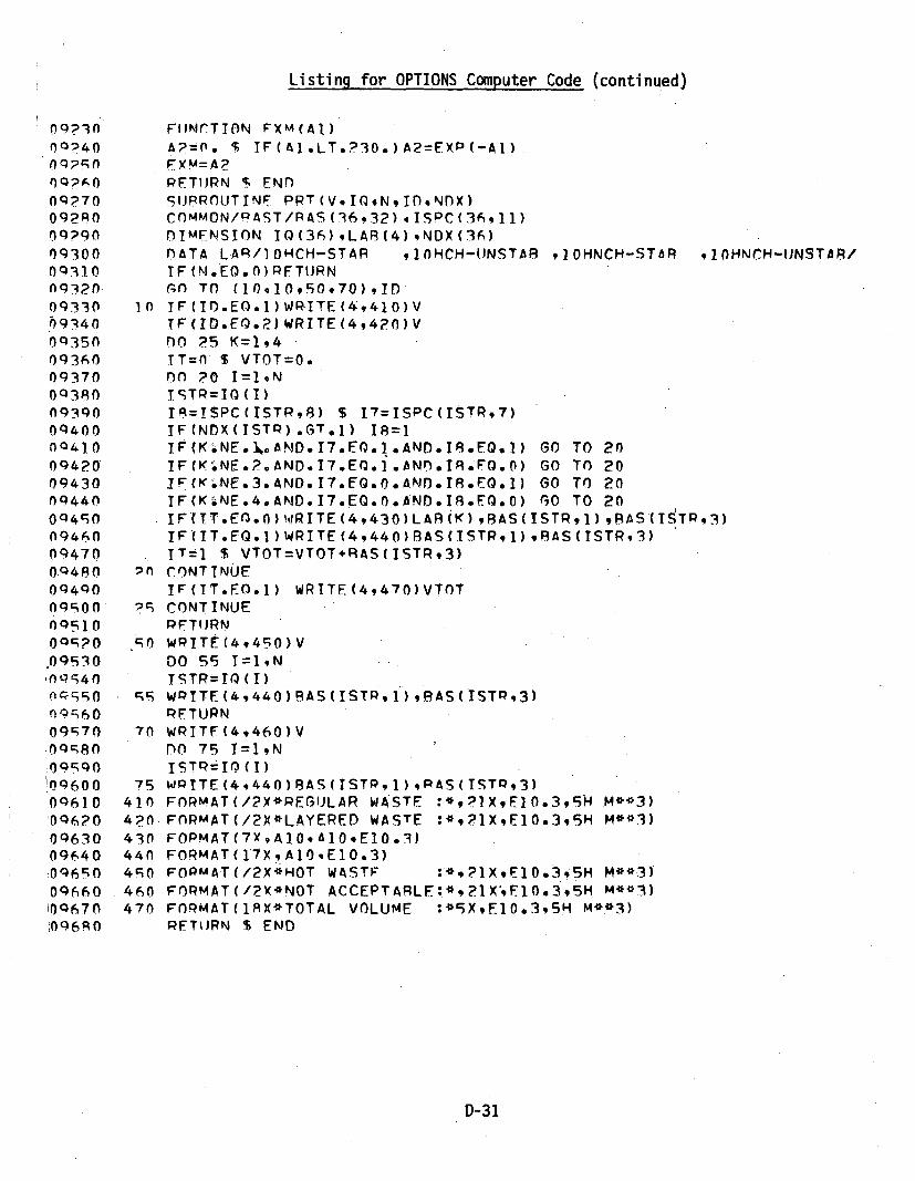
Listing for OPTIONS Computer Code (continued)

09?3000?40

OQ?70092p0

')9300

0931.0

09330.)934000350093600937000300

09400

Oq42O

0943009440

09460094700.0480

09910

.00930.Oq140nlc~l o

0 0?60

09•70.09980

!096000961 00976?0

0963009A4009690096600067000670

FliNrTION FXM(Al)A?=O. % IF(AI.LT.?30.)A2=EXP(-Al)FXM=A2PETIHRN $ EN1SUPROUTINF PRT(V.ITQNIO.NnX)COMMON/PAST/RAS(36.32),ISPC(36,11)lIMFNSION IQ(36),LAR(4),NDX(36)

OATA LAR/]OHCH-STAR ,lOHCH-UNSTA8 ,1OHNCH-STAR ,lOHNCH-UNSTAR/IF(N.EQ.0)RFTUlJRNGO TO (10,10,90,70),Il

in IF(I.EO.I) WRITE (4,410)VTF(ID.EQ.2)WRITE(4,4?O)VDO ?5 K=1,4TT=f s VTOT=O.

O PO I=19NTSTR=IO(1)I8=ISPC(ISTR,8) $ 17=ISPC(ISTR,7)IF(NDX(ISTP).GT.1) I8=1IF(K.NE.I,.AND.I7.EO.I.ANn.I8.EQO.1) GO TO 20IF(KNE.?.AND.17.EO.].ANf.IAFO.0) GO TO 20XF(K.NE.3.AND.17.EQ.O.AND.IA.EO.1) GO TO 20IF(K.NE.4.AND.17.EQ.0.AND.I8.EQ.O) GO TO 20IF(IT.EO.O})wRITE(4,430)LAAiK),BAS(ISTRl),BAS(ISTP,3)IF(IT.EQ.1)WRITE(49440ýBAS(ISTRl),RAS(TSTR,3)TT=l $ VTOT=VTOT+RAS(ISTR,3)

P0 CONTINUEIF(IT.EO.I) WRITE(4,470)VTOT

'9 CONTINUEPFTI.JRN

.90 WPITE(49490)V00 55 I=1,NTSTR:19 (I)

qq WP!TE(4,440)RAS(ISTP,1) ,AS(ISTP,3)PFTURN

70 WRITF(4,460)Vn0 79 T=lNISTP=IO (I)

75 WPITE(4,440)8AS(ISTP,1)gAS(ISTP,3)410 FORMAT(/?X*REGIJLAR WASTE :*,21XFlO.3,SH HM**3)420 FOPMAT(/2X*LAYERED WASTE :*,?lXEIO.3,SH M**3)430 FOPMAT(7XA10,A10*E10.3)440 FORMAT(17X, A10,El0.3)490 FOPMAT(/2X*HOT WASTF :*,9?XqElO.3,5H M**3)460 FORMAT(/2X*NOT ACCEPTARLF:*,?1X',ELO.3,SH M**3)470 FOPMAT(JPX*TOTAL VOLUME :*5X-E1O.3,5H M**3)

RETlJRN S END

D-31

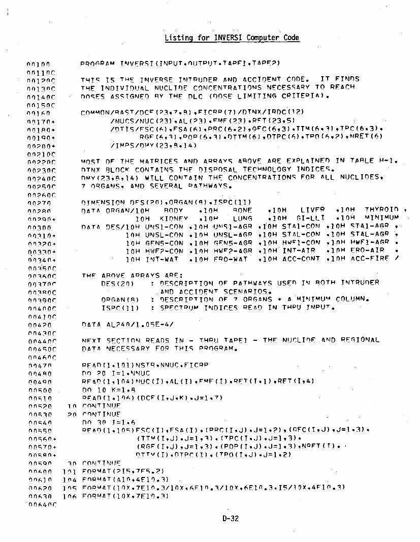
Listing for INVERSI Computer Code

nnion PpoSPAM TNVERST(INPUT.nOJTPijT.TAPFI,TAPF?)001 lOCnlNlOC THT- IS TwE INVERSE INTPUDER AND ACCIDENT CODE. IT FINnS

nnl3nC THE INDIVIDUAL NUCLITE CONCENTRATIONIS NFCESSARY TO RFACHnol0nC nnqFS ASSTGNEO RY THE nLC. (DOSE LIMITING CRITERIA).

nn1 o0 COMMON/,AST/flCr (237.pt) ,FTCPP (7) /DTNX/IRDC (12)n0070+ /NUCS/NUC(,3),AL(P3) ,rMF(?3)*RFT(2395)nolR0o /DTTS/FSC(A),FSA(6),PPC(6,2),ý3C(693).TTM(63)g)TPC(6,3),

rOV]QQ+ PGF(69,),POD(6,),DTTM(6),!TPC(A),TPO(6,2),N*IRET(6).002n0+ /IMOS/DYrY (23?R,]4)

nn0?Cn MOST OF THE MATRICES AND ARRAYS AROVE ARE EYPLAINEfl IN TAPLE H-1.0023nC PTNX BLOCK CONTAINS. THE DISPOSAL TECHNOLOGY INDICES.fl024fNC nMY(?3,1,14) WTLL CONTAIN THE CONCENTRATIONS FOP ALL NUCLIPES,

nn0?25O 7 ORGANS, AND SEVERAL DATHWAYS.

no070 PIMENSION OVFS(?0),OPGAN(9),!S C(11)nnPRn DATA ORGAN/1OH RODY ,*OH PONF 01OH LIVFP ,1OH THYROInnnpqn+ 1OH KI(INFY .10H LUNG ,]OH GI-LLI ,1OH MINIMUMnn030 PATA DES/1OH UNSI-CON ,IOH *UKIJN-AGR ,IOH STAI-CON ,IOH rTAI-AGP ,nn310+ InH UNSL-CON ,10H UNSL-AGP ,9OH STAL-CON ,10H STAL-AGPnnOOW GNS-CON ,1OH GFN5-AGR ,9OH HWFI-CON 1OH HWFl-A;,P

in330+ IOH HWFI-CON .InH HWF?-AGP ,1OH INT-AIR .0NH FRO-AIR

n340n+ lOH INT-WAT ,.10 EPO-WAT ,10H ACC-CONT ,vOH ACC-FIRF /

9 o A c Twr AROVE ARPAYS APE:0017nr FDS(20) : OESCRIPTION OF PATHWAYS USF' IN ROTH INTRUDERon3ROC AND ACCIDENT SCENARIOS.

n Q nC OPGAN(I) : DESCRIPTION OF 7 ORGANS + A MINIMUA COLIJMN.rOO00r ISPC(ll) : SPFCTPIJM INDICES REAP IN THPU TKIPUT.nnalo•~

nn4?0 DATA AL?40/1.OSE-4/

0o44OrC MNYT SECTTOiN RADS IN - THPIJ TAPEI -THF NUrLIflF AND REGIONALnnfcl04 DATA NECESSARY FOR THIS PROGRAM.

f)47n PFAn(Ij0I)NSTRpNNUCFICPP004R0 nO ?0 I=IlNNUCn04Qfl RFAP(1,04)N)UC(I),AL(I),FMF(I),PFT(I,) ,RFT(I,4)nnc;o0 On 10 K=IR

nnoos PFAO(I-.]A)(DCF(IJK),J=l,7)n nc;o) n n CrNTINU!F

no3 20 nrnNTINIt[ Fonc04 nn 30 =Jo.,n n•5 co;o An(IINv-)FS'C(1)qFSA(T),i(rPC(I*J),J:l,?)g(,(FC(IJ)gj:1,3),

nn c ,n 4 . (TTM-(TqJ).J:1q1),(TPr,(TJ),J=1,3),00c;70+ (RG)F(TJ),J=1,3),(POD(TgJ),J=1,3),NPFT(T).'

nnoQn+ nTTY(T),flTnPC(T),(TPO(IJ),J=I,2)n;Q n i0 r On!TTNI).

nnAron 101 FOPMAT(PIq,7F5.?)ln(]fl 104 FnPUAT(A1n,4El'ln3)

nn0420 I r~c FOOQMAT ( I y ,7E10 ,3/1 nx tFln1O./1 Oxq6FE1n.3 15/1 IX,4F0n.1)nnr0A3 In(, FORMAT(1OX,7FI0.3)0nOA44

D-32

Listing for INVERSI Computer Code (continued)

oo~ocfl0'f)60C

n0690('(700

00710

00730C

nn740C

nnvl~or

no770Cno7Por

nnRiO

00780

nOR4000850

00860

00R70

o04090 40009000

0 0 93 10 C

004950009600097000980

00990

(flolO •0

0tO0 100301030 100401040 101001 O'0.+

0 10870 +Of

01100+

01110+

0 1 lOC01130r

011 i0c0115001 160C

01170C

0] iRCm

01 ?OOCO1?1OC

NEXTi THE I? DISPOSAL TFCHNOLOGY AND 6 SPECTRUM INDICES AREPFAr) IN THP11 IF~TPUT.

PEADIRDCPFAB,(ISPC(J),J=4,q)WPITE(?90,10)IRDC $ W RITF(2,1020)(ISPC(J),J=499)CALL ZERO(DMY,?576) '. CALL RINV(ISPCNNUC) $ CALL MIN(DMY,14)

ApOnvI SURPOUTINE RTNV WAS CALLED TO CALCULATE CONCENTRATIONSWHTCH APE RETURNED IN n4Y MATRIX. SURROUT.INF MIN FINDSSMALLEST CONCENTRATION FOR EACH NUCLIDE - OVER ALL 7 ORGANS.

LOOP 40 CONSIDERS DAUGHTER IN-GROWTH AND PRINTS OU , INTRUDERCONCENTPATIONS TO TAPE?.

DO 40 K=1,14Ai=nMY(V7A*,K) $ A2=DMY(22?8qK)*AL'(17)/AL(2?)IF(Al.GT.A?) OMY(17q,8K)=A?Al=nMY(17,19K) $ A?=Dmv(23qBK)*AL240/AL(23)IF'(Al.GT.A2) DMY(17,BK)=A2

A1=flMY(?0,RK) S A2=DMy(1RQRK) *AL (20)/AL(lR)IF(AI.GT.A2) DMY (?08wK)=A?WPITE(2,1003) DES(K),(ORGAN(J),J=l,8)WPITE?(2,1004)(NUC(I),(DMY(IJK) J=18) ,I=1,NNIJC)CONTINUETF(I.NE.-l)GO TO 80

NEXT SECTION SIMILAR TO ONE ABOVE - ONLY NOW FO9 ACCIDENTSCENARIOS.

CALL ZERO(DMYqI840) S CALL'AINV(ISPCNNUC) S CALL MIN(DMYI,6)DO 50 K=1,6KK=K+14WRITE(2,1003) DES(KK),(ORGAN(J),J=1,P)WRITE(2,ln04)(NUC(T)9(DMY(IJgK),J=1,8)91=1,NNU})CONTINUNECONTINUEFOPMAT(//?XA9,2XqA1O)FOPMAT(?X,A1OPE1O.2)FORMAT(IHI/2X9*DISPOSAL TECHNOLOGY INDICES*!?X

*IR =*12* ID =*12 IC =*12* IX =*12/2X*IE =*12" IS =*I;* IL.=*I2* IG =*I?/2X*TH =*12* ICL=*I?* IPO=*I;* IIC=*14)

FnRMAT(/?X*SPECTRAL INDICES*/?X*FLAM =*I?* DISP =*I2/2X*LEACH =*12* CHEM =*I2/?X*STARI =*12* ACCFS =*12/)

STOP $ END

UBRPOUTINE PINV(ISPCqNNUC)

THIS ROUTINF DOES MOST OF THE WORK IN CALCULATIPG THE,CONCENTRATIONS. IT IS SIMILAR-TO SUBROUTINE RCL IM INTHE OPTIONS CODE EXCEPT THE PATHWAY EQUATIONS H VE BEENMOOIFIED TO FIND THE CONCENTRATIONS WHEN THE DOSES AREGIVEN.

D-33

Listing for INVERSI Computer Code (continued)

01. pnrfll?3o0 CnM4ON/RAST/DCF (?3,7,) /DOTI'/FSC (6) 9FS A (6) /IMPS/nMY (?13,8,14)nl,;40+ /NLJCS/NUC(23),AL(?3)qFMF(pl)gPFT(?395)01) 1; 0;+ /nTýIX/IRIDICIXIEISILIGIHICLTPOIIC.

n I >fTmFNISION FMP(3),ISPC(I1),r)LC(7)01?70 DATA EMP/.S,.75 .5/,'DLC/2*0o0.,1900.,3000. ,3*1SfO0./

n0.?pgC THE A8OVE ARRAYS APF:

0130nn FMP(3) : VOLUMF FMPLACFMENT EFFICIENCTES01310C 1SPC(II) : SPECTRUM INDICES PASSED FROM MAIN PQOGPAMnl3;?C DLC(7) : DOSE LIMITING ,CRITERIA FOR 7 ORGANSn1.330C01'40 Tq=ISDC( 1 ) T I6=ISPC(6) IT7=ISPr(7)

Oi3ln 19=ITSC(g) % I9=ISPC(g) T NSTP=O01360 IF(1R.EQ.1.AND.IS.EQ.1)NST8=j01370 A7='1 $ 1F(I6.FQ.?.OR.I•.EO.3) a7:0.80

01,380 IF(17.EO.1.OR.IS.EQ.n) IT=I6-101390 FDESE=MP(IE)*(1.-.9*IG)01400 A.•=1 $ IF(15.LT.3) AS=10.**(T5-3)n1410 A6=l - %I(T6.GT.1) A=4.**(1-T6)014?O AQI=. % IF(I9.GT.1) Ag=l.**(l-IQ)0143AC01440C OUTSIDE LOOP IN CONCENTRATION CALCULATIONS -SETS UiP

l4c0rC PARAMETERS NEEDED FOP TFSTING WASTE STRFAMS AT ALL THPEF01460r CLASSIFICATION LEVELS:PFGULAR, LAYEPEnD AND HOT.01470Cn 14P0 Dn O 013=197014f 0 CGO TO (1I,?913,14,15,1f,17),130100 11 GDEL:IOO+llC S IF(IC.EO.3) GnFL=IPO+0nn.-01510 A4C=]. I A4A=l. $ A8C=A7 % ARA=A7 $ GO TO'•2nipO I' GDFL=IPO+IIC $ IF(IC.EF.3)GfFL=IPO+÷S0.01'30 A4C=O.OI $ A.4A=0. $ AAC=O.nIP*A7 $ AAA=0s S GO TO ?0015&0 13 GDEL=IPO+ITC $ IF(IC.FO.3) GOFL=IPO.50n,01I550 A4C=O°. $ A4A=O. $ APC=A7/1?0. I ARA=n. $ GO TO 2n

01560 14 GFEL=IPn+IIC $ SIF(IC.FO.3)GDEL=IPO+tOfl.OI151 A4C=n.O°ll7 $ A4A=n. S AqC:O.nn1*A7/1?0n. $ AAA=O. % GO TO ?00Is0O iq GDEL=IPO+.00.ol;qO A4C=1. m A4A=4 . $ A8C=A7 $ AA7 GO TO ?nfl1'n IA GDFL=IPO+IIC $ IF(IC.FO.l)nFL=IPO+÷nn.n1610 A4C=O.nl • ARC=0.1*A7/1.44E6 I IF(IG.EO.o)AoC=n..*RC.On1oAp A4A=O. ' ARA=0. $ GO TO P001nA30 17 ,EL=IDO+1000.01'A4f Ai-'=1. CARC=A7 1S IF(IG.EO.0)AF4C=0.1*AqCnlic•qp A4A=l It AR=A1C

o167nC MAIN CALCULATION LOOPn1r6qnr

nl'on •n no 4A I0 JUC=1,MNUCn0.700 A1=Aq*PE S* FxM(AL(INUC)*e-nFL)01710 nOn 4+ T=1,7nly7?0 A?=DCF(TNIJCI,9)01730 •I=1I*AC*At*FSC (IR) *fCF (INIIC, I,?)

0174n P?=Al*AAC*A?*O.0O701.79-l 0S=n.P*AI*A4A*A•*FSA(Ip)*nCF(TIIlClqq3)01760 P4=O.5*O.?S*A1*A4A*AA*FMr(INU.IC)*DCF(INtJC, A)

D: 34

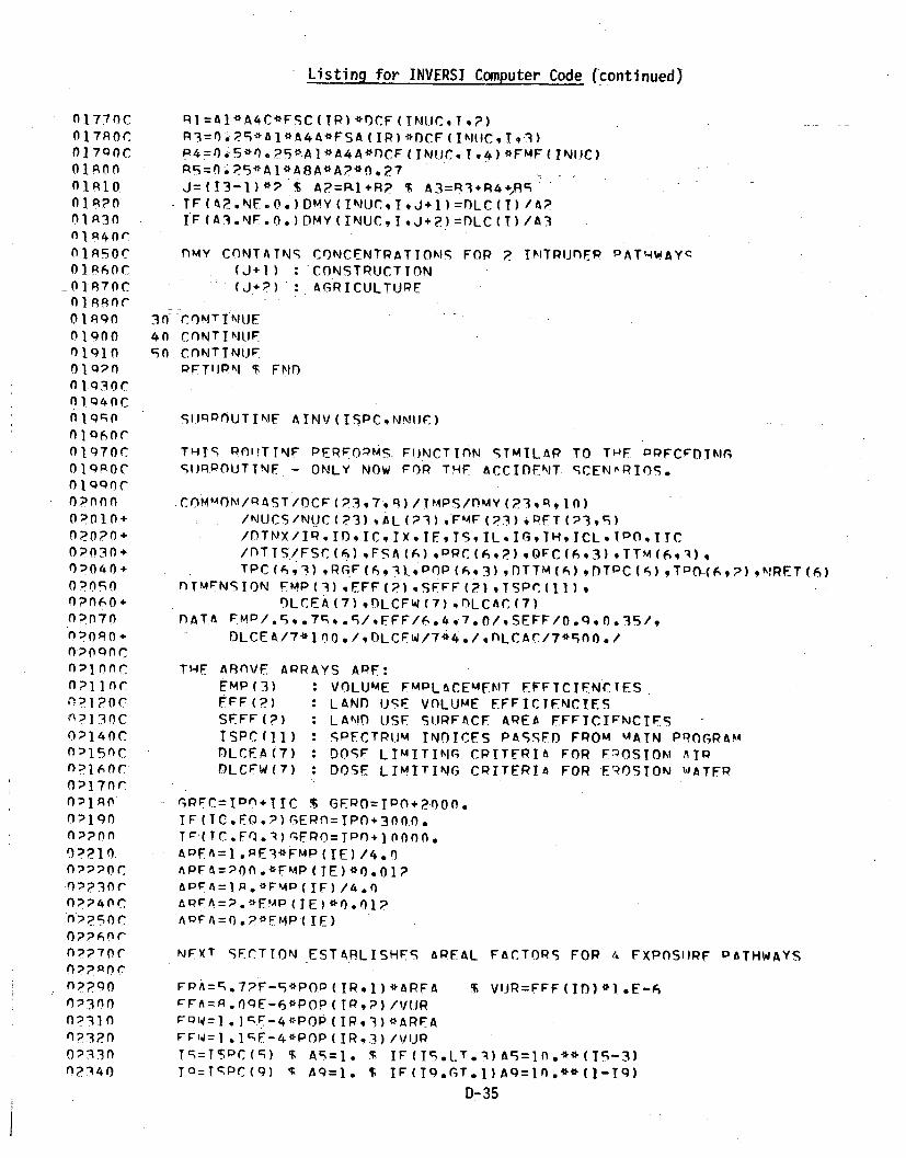
Listing for INVERSI Computer Code (continued)

n1770c017R0C

01700C

n 1 R 10.

019R3n

- I R7nC

01900

n 1q3. 9

ni 940G

01 970C01 OROC

0) >040 +0 0nC~

0)070

nl1 ?OC

On;6O +C

nl14nC0'150C

O)1730C

Ol1 ROC

O0?30÷O)040+

0))70C

n;: Ion (

0)•P30C

02340C

n I I n

OPI 7nrn,>1I A

-O~p3nrn;)?4 no">?5nr

O??6nr

n?3200;•30In2•4o2

RI =AI*A4C*FSC (IR) *OCF (INUC, I)R3=n ?7*A41*44A*FSA( IPR) *DCF ( INtC,I ,.3)P4=0.5*0.?5*AI*A4A*nCF(TINUC, 94)*FMF(INIIC)PS=n-?5*Al*A8A*A?*0.2?7J=(T3-1)*P % A?=R1+R? % A3=R3+R4+,R "TF(A?.NE.O.).DMY(INUJCIJ+I)=nLC(T)/A?IF(A3.NE.O.)DMY(INUCIJ÷2)=DLC(I)/A3

nMY CONTATNS CONCENTRATIONS FOR ? TITRIJnFP PATHWAYC(J+]) :CONSTRUCTION(J+?) : AGRICULTUPE

3040;0

CONT INUE

CONTI NUECONTINUEPFTIIPN $ FNn

S1.1RPOUTINE AINV(ISPC.NNtU)

THIS POi!TTNF PERFOPMS. FUJNCTION SIMILAR TO TNF oPFCF.TNiSIJRPOUTINF - ONLY NOW FOR THE ACCIDENT SCENARIOS.

•COMMON/PAST/DCF(239,7,cR)/T!MPS/rMY (73 ,1O)/NUCS/NUC(?3),AL(?3),FMF(?3),PET(;3,S)/DTNX/IP.ID,ICIX,IE,TS,ILIG,IH,ICLIDOIIC/TTIS./FSr(6),FSA(A),,mRC(6,oP),oQFC(693),PTTM(6,•4),

TPC(A,ý9') RG-F(6,3-),*POP(6,93),DTTM(6),flTPC(f,),TPOn(6,,),N!RFT(6)nTMINSION PMP(C),EFF(?),SFFF(?),ISPC(I1),

OLCEA(7)qDLCEW(7),nLCAC(7)fAT.A FMP/.5,.75,.S/,FFF/6.4,7.0/,SEFF/0.9,0.35/,

DLCEA/7* O. /,DLCFW/7*4./,nLCAC/7*900./

THE ABOVE APRAYS APE:EMP(3) : VOLUME FMPL4CEMENT EFFICIENCrES.EFF(?) : LAND IJSE VOLUME EFFICIENCIESSEFF(?) : LAND USE SURFACE APEA EFFICIFNCIFSISPC(1i) : SPECTRIJM INDICES PASSED FROM UAIN PqRnPAk4fLCEA(7) : DOSF LIMITING CRITERIA FOR F3OSION AIP

DLCFW(7) : DOSE LIMITING CRITERIA FOR EROSTON 4ATEP

GPFC=IPn+IIC $ GEPO=IPO+÷000.

IF(IC.EO.?)GEPO=IPO+300n.nTc'(TCFQ.3)r'EPn=IPO+jnnnn.APFA=I.PE3*FMP(IE)/4.0APFA=Pon.*EMP(IE)*0,0?APFA= p.*FMP (IF.)/4.0

AQFA=O.?*PMP(IE)

NEXT SECTION ESTARLISHES AREAL FACTORS FOP 4 FXPOSiRF PATHWAYS

FPA=.7?F-rS*PO.P(IR,1)*APFA $ VIJR=FFF(It))*].E-6FFA=A.0rE-6*POP( TP,2)/V'JR

FVWI ].cF--4*POP(IR,3)*AREAFFw= .lqE-4*POP(IR,3) /VIJR

Tr=ISPC(9) $ A9=1. T IF(IS.LT.I)AS=lO.**(Ic-3)IOQ=TPC(9) ' AQ=l. $ IF(Ig.GT.I)Ag=I0.**(I-Tg)

D-35

Listing for INVERSI Computer Code (continued)

02.3F0Cn or00?370C

02400

0?410n'4?O02430

0;440

024700240002490C0 ,;14 A

O•Or

ngni no

n') 3 nC

02440nnq

n;)0

n;70Ar0

02730.02740

0•770

027P0

n?tp1nr~

02040

02070

020o0

02010

0 2020n

MAIN LOOP rOP EXPOSURE CONCENTRATION CALCULATIONS

no P0 IMUC=I9NNUC -

•k,=FXM(GREC*AL(INUC)) $ A7=EXM(GFRO*AL(INUC))no 10 IORG=1,7F'I=FA*A6*DCF(INUC9 TORG,9)*A.5*Aq $ F_=FEA*A7*DCF(,INUCpTORG 8)Fl=FPW*A.*DCF(INUCIORG,7)*A5 $ F4=FEW*A7*DCF(TiNUCIORcG,7)TF(FI.NEO.) DMY ( INUC, IOPG, I) =DLCEA (IORG)/FITF(F3.NE..) D'YY(INUC.IORG,3)=DLCEW(IORG)/FIIF (F'2_I.rE. 0. 'lqY ( TINUCqIOPG92) =nLCEA(IORG)/F?

IF(F4.NE.no) DMY ( INUC, IOPG,4) =DLCEW'( IOPG) /F4COMTINUFrONTINUJE

10

NFXT SECTION SFTS UP PARAMETERS FOR FIRF(FAF) AND SINGLECO..ITAINER(FAS) ACCIDENTS.

raF=TPO(IP,1) $ FAS=TPO(IPs) .I'g=ISPC(6) $ IF(16.GT.I) FAS=FAS*(lI n (1-IT)JT4=ISPC(4) % IF(14,LT,3) FAF=FAF*(20.**(I4-3))A.=I• I 19=TSPC(9) $ IF(I9.T.1)A9=10.**(lI-9)IF(IS.EQ.I .AND.I4.NE.3) FAF=-.

M4ATN LOOP FOP ACCIDENT CONCENTRATION CALCULATIONS

Do 70 IMUC=1,NNUCnO 70 1OPG=197

Al =AQ*FAs•DCF (INUC9 IORG, I.)A,=AQ*FAF*rCF ( INUC IOPOG, I)IF(AI.NF.'.) DMY(INUCqIOPG,5)=DLCAC(IORG)/AlIF (?.NF. n.). DrMY( INJC, IOPG,6 =DLCAC(TIOPG)/A2

7n CrnT I NIJFPFTIJRN S -FN

.SIIPQOIJTINF 7ERO(AgN) -TuFNSI.ON A(N)

no In I=lJ ',

PF T'PR!I•N S END)

FUJNCTTON FXM(A1.)

A?0=. $ IF'(A1.LT.230.)A?=EXP(-AI)FY V:,= A?PF"TIMM% ';F5

.SIJPPOIJTINF MIN(DN)nlTMFNSION fl(?3,*,14)XM(7)nn 10 I=i,?3no i0n K'=.Nno q J=197X(.J)=O(IqJrK)IF'(Y(J),FO.'),) X(J)=lFE÷OQ

cCONKT INEF

r(IT ,A K) =F TN1(X (1),X (P) X(3) X (4) 9X (5) X (6) X (7)10 CoNJ'rIN!.F

Pg:-tJI•N •-ENO•D-36

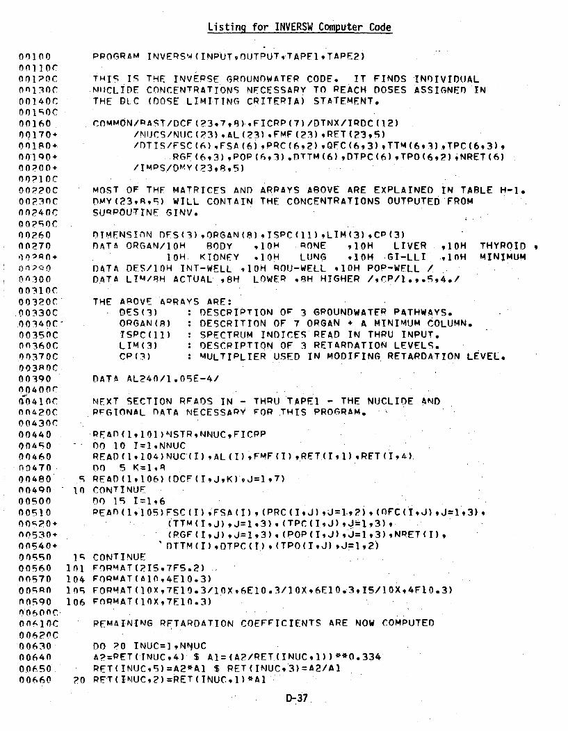
Listing for INVERSW Computer Code

oion0 PPOGRAM INVEPS'•(INPUTOtJTPUTTAPF1,TAPE2)001l]OC

01?OC THIT I; THE INVERSE GROUNDWATER CODE. IT FINDS INDIVIDUAL0n130C NIICLIDE CONCENTRATIONS NECESSARY TO REACH DOSES ASSIGNED IN00140C THE DL.C (DOSE LIMITING CRITERIA) STATEMENT.O01;OC.

00160 CnMMON/PAST/DCF(?3,793) ,FICRP(7)/DTNX/IRDC(12)00170+ /NUJCS/NtIC(?3),AL(23),FMF(?3),RET(23,r)OO1PO+ /DTIS/FSC(6),FSA(6)gPRC(6,2),QFC(6,3),TTM(6,3).,TPC(6,3),0090+ •RGF(6,3),POP(693).,TTM(6)gDTPC(6),TPO(69,)}NRET(6)

OOPO+ /IMPS/D"YY(?3,R,5)

O0??OC MOST OF THE MATRICES AND ARRAYS ABOVE-ARE EXPLAINED IN TABLE H-1.00?30C DMY(23,9,'r) WILL CONTAIN THE CONCENTRATIONS OUTPUTED FROM00n40C SUPPOUTINE GINV.

00260 DIMENSInN DFS(3),ORGAN(8)gTSPC(11),LIM(3),CP(3)n0270 DATA ORGAN/1OH BODY ,1OH RONE ,9OH LIVER 010H THYROID11f,>A0+ 1OH KIDNEY %1OH LUNG ,IOH .GI-LLI 9,1OH MINIMUMonPO DATA DES/1OH INT-WELL 910H ROU-WELL P10H POP-WELL /O0.300 D.ATA LIM/PH ACTUAL ,8H LOWER ,BH HIGHER /,CP/1.,.5,4./

00310 C003OC THE AROVE ARRAYS ARE:00330C DES(3) : DESCRIPTION OF 3 GROUNDWATER PATHWAYS..00340C' OPGAN(B) : DESCRITION OF 7 ORGAN + A MINIMUM COLUMN.00350C ISPC(11) : SPECTRUM INDICES READ IN THRU INPUT.0n360C LIM(3) : DESCRIPTION OF 3 RETARDATION LEVELS..00370C CP(3) : MULTIPLIER USED IN MODIFING RETARDATION LEVEL.003••C00390 DATA AL?40/I.09E-4/0040 OC00410C NEXT SECTION RFADS IN - THRU TAPEI - THE NUCLIDE ANDnn420C RFGIONAL DATA NECESSARY FOR THIS PROGRAM.00430C00440 PEAD(1,101 )NSTRNNUCFICPP00A50 DO 10 I:1,NNUC00460. READ(IIO4)NUC"(I),AL(1),FMF(1)9.RET.(Igl),RFT(TI4}

00470- DO 5 K=IA00480 S READ(1,106)(DCF(I,J,K)qJ=1,7)004n0 - 10 CONTINUE00500 on IS I~1=600r510 PEAn)(I,10S)FSC(I},FSA(1),(PRC(IJ),O=I-'?},(OFC(TJ}.,J=I,)3),

00•2 ÷:('TTM (I ,J )9,J= I ,3 ) ,(TPC (I-)J ) ,Jý-l ,3 ),P-00530+ (RGF(IJ),J=I,3),(POP(IJ),J=193),NPET(1),

0n540+ "DTTM(I),DTPC(I),(TPO(I,J),J=1,2)00550 1 CONTINUE00560 101 FORMAT(?15,T7F5.2)00570 104 FOPMAT(AIO,4EIO.3)009,A-0 105 FORMAT( 10X,7ElO.3/1OX,6E1O.3/lOX,6E10.3,IS/IOX,4F1O.3)059O0 106 FORMAT(1OX,q7Ej.3)

nnOjo.C REMAINING RFTARDATION COEFFICIENTS ARE NOW COMPUTED006?OC

00630 DO ?0 INUC=],NNUC00640 AP=PET(INUC,4)-$ A1=(A?/RET.(INUC,1))**0.33406 S0 PET(INUC,5)=A2*Al $ RET(INUC,3)=A2/A100660 ?0 RET (INUCP)=RET(INUC,1) *A'

D-37

Listing for INVERSW Computer Code (continued)

n0h7AC

I n 6pnC THE 12 DISPOSAL TECHNOLOGY INDICES AND 6 NECESSAPY SPFCTRUMnofQ0C INDICES ARE READ IN THPU INPU T .

nn710 PFAnOPOC $ READ,(ISPC(J),J=4,9)o --) 7pr WPTTE(2,IOIn)TRDc S WRITF(2,IO20)(ISPC(J),J= ,qc))

nn71nr

nA74nC LOOP 35 FINDS THE GROUNDWATER CoNCENTPATIONq FOP ECH OFnn7cfOC THF S PETARDATION COEFFICIENTS. SURROUTINE rIN%. DOFS MOST OFnn760C CALCULATIONS INVOLVED. DAUGHTFR IN-GPOWTH IS ALSO TAKFNnn770C INTO CONSIDFRATION,nA7Anr

007Q0 DO 19 IPET=1I5nnO0o WPITE(?,1005) TRET S CALL zFRO(fMYqqp0)nnol) CALL GIK!V(ISPCNNUC,IFT) $ CALL MIN(TMY,3)oon n nn 30 K=1,3AnAl0 Al=nMY(17,qK) $ A?=DMv(??,qK)*AL(17)/AL(2?)nAnA4 TF(AI.GT.A?) nMY(17R,AK)=A?n qpcQ;n Ai=nMY(179R,K) $ AP=nMY(?3,RK)*AL240/Ai_.(23)nqnR• TF(A1.GT.A?) DlY(179AK)=A2

nng7O Al=nmY(?0,*AK) $ AP=flMY(1q,9,K)*AL(?p)/AL(IP)nno~ IF (Al.GT.A?) DMY(COR.K)=A?nnaoo WPTTE(p,]003) iES(K),(ORGAN(J),J=jq)n n ) n WP T TF I? n 004 ) (MNiJ C ( T n, (mY ( T -pJ .K ) , J = 1• • A 91 l 9N N II)

n001 3I CONTIMUEnof)o an CONTINI.IF

nc4An 4n IQ=IPOC(l) $ NP=NRFT(TQ)

n n Q6nr t.oOP 60 FINDS THE GrPOLINDWATFR CONCENTRATIONS FOP THF

OnAQ7nC PFTAPnATION COFFFICIFNT AS TMPLIFn RY THE IT IImnFX OFAonqpoC nTPOýAL TECHNOLOGY. THIS LOOP HOWFVFR VARIFS THF PFPCOLATIONnnqqOC VALIuE. IT UI.IES THF VALUF IMOLIED RY IR AS WeLL AS HALF THISnlonnC VALIIF AND OI(.JPLE THIS VALUE.nln]nrnl 1 Ofnn n K=g01A] 00 D 60 Khl=1e3

(In3n A1=DMY(l7,R,K) € Ap=MY(2?,qK)*AL(17)/AL(??)01lei0 TF(Al.GT.A2) fDMY(l7,F*K)=A?nlOSO A]=DMY(17.%PK) $ A?=DMV(P3P,,K)*AL24n/AL(23)OinAP IF(Al.GT.AP) oMycl7i.qKe=AP01070 Al=OMY(?OqAK) $ A?=DMv(R(,RqK)*AL(?0)/AL(I)AIOR Ip F(AI.GT.PA?) DMy(?fl.RK)=A;)nIoon WPTTF(?,0OOA) LIM(KN) $ CALL 7FPOt(MYq?O)fln100 PC(IR, )=PPC(IRl)*CP(KN) $ PPC(IP,?)=PRC(JR,')*CD(KN)0l110 CALL GIMV(ISPCNNUCqNP) A CALL MIN(DMY,3)

n113) WRITE(?,10oO) 0ES(K)q(OPGAN(J),J=1q,)01140 WRITE(? 9 1004)(NUC(I) 9 (nMY(I,JK),J=..R),I=],NNUJr)01150 ;0 CONTINUF

116n0 60 CONTINUEAl1170C

Oh]IO 1001 FORMAT(12T3)0llQO 1003 FOPMAT(//?X.A9q,8A0)01?00 1004 FORMAT(Al0,IEI0.?)0]pl10 100 FOPMAT(//?X,*RETARDATION COFFF. *,Ig)n1220 1006 FORnMAT(//?XA7,*PERC0LATION VALUE•.)

D-38

Listing for INVERSW Computer Code (continued)

O1?30 101001240+01 250+01?60.01?77 .i O;O

01280+

n1300+01310n1320C01330C

-n13400 1 3-0ci01360Cn137nC01 3ROC0.1390-01400+01410+014.20+0 1430+0144001450014A001470C01 .48C014Q0C01500C

n151oC015?0C01530C01540Cn issOC.015600.1570o-1.5Rn01 •0

01600016100162001630016400165001660 ?001670016800169001700017100172001730C

FORMAT(?Xq*DISPOSAL TECHNOLOGY INDICES*/?X.*IP =*,I?,* In =*,I?,* -IC =*9I2,**IE =*,I?,* IS =*9I.* IL =*,I2,**TH =TI* CL=*-.I?,* TPO=*, I?,*

FORMAT(/2X,*SPECTRAL INDICES*/2X,4*FLAM *,In,* DISP =*,I?/?X*LEACH 49,I?,* CHEM =*9,?/?X,*STA8I = jI?,* ACCES =*,I?)

STOP $ EN•

TX =*.I?/2X,IG =*gI?/2X,

IIC=*, 14)

SURPOUTINF GIN%/(ISPCqNNUCNPT)

THIS ROUTINE CONTAINS THE ACTUAL CALCULATION OF THFCONCENTRATIONS.

COMMfN/RAST/DCF(239T7R)/IMPS/DMY(?3,8,5)/NIJCS/NUC(?3),AL(P?)qFMF(?3),RFT(39,3)/DTNX/IRIDIC,IXoITF, ISlLIlqIHICLIPO, IIC

/DTIS/FSC(6)gFSA(6),PRC(6,?),QFC(6,3).TTM(6,3),TPC(6,3),RGF(6,3)oPOP(693)oDTTM(6) ,TPC(6) ,TO(6,P),NRET(6)

DIMENSION EMP(3),EFF(2)9SEFF(?),flLC(7,1),ISPC(11)DATA NSEC/IO*.7LC/5.O o.I,*,OO.3ISOtp3*?.2,97*4°/DATA EMP/.:5,.75' .S/,EFF/6.4,7.0/,SFFF/Oq,0o.35/

THE MATRICESEMp(3)EFF(2)SEFF(P)DLC (7p3)

AND ARRAYS AROVE ARE:: VOLUME FMPLACFMENT FFFICIENCIES: LAND USE VOLUlMF FFFICIENCIFS: LAND USE SURFACE ARFA EFFICTENCIFS: DOSE LIMITING CPITEPIA FOR I ORGANSAND 3 PATHWAYS,PAPTITIONE INTO.

GnFEL0.- S VIJR=I.l/(FMP(IF)*FFF(In))IF(IC.EQ.1)PRCD=PRC(IR. 1)TF(TC6GT.1)DRCD=PRC(TIRq)IF(IX.EO.i)PRCD=4.*PRC(CIP,)IF'(IX.GT.1)PRCD=?.?S*PRC-16=ISPC(6) S 17=ISPC(7) 5 T8=ISPC(R) $ Ig=IqPC(9)PERC=PRCO $ IF(IS°EQ.l.OR.17.Q.I1)1=I6-1IF(I8.NE.1.OR.IS.NE.1)GO TO ?0IF(IC.EQ.°)PERC=PRC(IR,1)IF (IC.GT.1)PERC=PRC(IR,?)TVOL=357?OfO.*SQRT (PR( IP,1 ) *27.8)IF(TD.EO.2.oR.IH.EO.1)PERC=PRC(IP,2)/16.PERC=PERC*(I.0-0.9*IG)A6=1' S IF(16.GT.1.)A6= 4.**(1-6)AQ=1. $ IF(I.CGT.1)A9=10.**(C-Iq)Ii=NPT$ IF(IS.EQ.0.OR.17.Fn.)II=I1-lTDUtMj=I,/(PERC*VUR*A6*A9) S IF(II.LE.0)I.=1

D.-39

Listing for INVERSW Computer Code (continued).

n,1740C MAIN LOOP - GROUNDWATER PATHWAY EOUATIONS MA'NIPtILATEn SO01750C AS TO FIND CONCENTRATIONS WHEN THE nOSF IS GIVEN.nl 760"01770 !0 90 INUC=1,NNUCn17P0 TDUP=TDUM/FMF(INUC)01790 pA 70 IPTH=1,301n00 I?=A $ IF(TPTH.EO.3) I?=701plo P?=RP(F(IP eTPTH.)/(QFC(IRIPTH)*NSFC*TIUR)01PO IF(TVOL.GT.OFC(IR,IPTH))R?=R?*OFC(IRIPTH)/TVOLOl1. 0 A3=-O- $ TNRT=RET(INUCIT.)*TTM(IP.,IDTH)n1940 0o 40 ISEC=INSECnlQ70 R3=TNRT+÷ET (INUCgIi).*(TSEC-1)*DTTM(IR)01P•l IF( .GE.TIRTT+TDIJR)GO TO 90

n1l7f0 A4=TSEC*EYM,(AL(INUC)*Rl)01iP0 A3=AMAXI(A3.A4)0l000 40 CONTTNI.JEO1QO 0 q0 no 60 IOPG=1,701910 AD: IE6*AI*R?*DCF(INUCIORGI?)n1. ? A.=n0T $ IF(AD.NE.O.) AI=OLC(TORG,IPTH)/An'01030 o;0 Yr)Y(INI ,1IORG,TPTH)=A H....01040 70 rONTINUEnfl50 RP CONTINUEn196n RET'.JPN S END0.970C

nigQo SURPOUTINE 7FPO(AN)0 000 nTMENSION AMN)07010. 00 10 I=lNOn720 10 A(I)=A.07030 PFTURN $ ENO

"l050 FUNCTION FXM(A1)070n60 A?=O $ IF(AI.LT.230.)A?=FXP(-Al)0'070 FXM=A?.

?OR0 PFTI.IPI A FND

07A10C02100n qlU~RoUTINlF MIN(DqN)

nA.nC TH•I POUTINE RETURNS THE SMALLEST CONCENTRATION - OVER

n;].30C ALL 7 ORGANS - FOP FACH NtJCLInF.

n071g nIMFNSTON D(?3,8,5).x(7)0160 DO 10 I=1I?,02170 DO 10 K=1.Nn? IPP r0 . J= I *7n l O p )0y(J)= 1IJ,9K)

n>? n n TF(X(J).EO.0.) X(J)=l.r+qqn?210 q CONTINIJE

S(I, K)AMIN I(X (1) ,X •) X (3) .X (4) ,X (S) ,X (6) ,X (7)n;?3n in CONTINUFn?140 PFTIjRPN t FNn

D-40

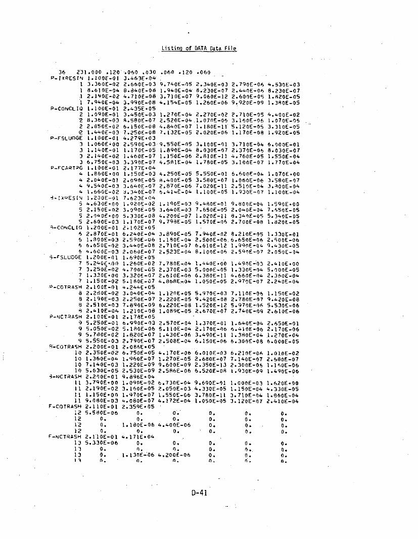
Listing of DATA Data File

36 231.000 .120-.060 .030P-IXPESINI 1.100E-01 3.463E-04

I 3.360E-02 2.660E-03I 8.610E-04 8.840E-08.1 2.190E-02 4.710E-08I 7.940E-04 3.990E-08

P-CONCLIO 1.100E-01 2.435E.052 1.OqOE-01 3.450E-032 8.360E-03 8.580E-07" 2 2.850E-02 6.150E-08e 1.440E-03 7.250E-08

P-FSLUOGE 1.100E-01 4.279E.033 1.060E400 2.590E-033 1.140E-01 1.170E-053 2.140E-02 1.460E-073 6.750E-03 3.390E-07

P-FCARTPG 1.100E-01 2.177E+041.860E.00 1.150E-03

4 2.040E-01 2.090E-054 9.540E-03 3.640E-074 1.660E-02 3.340E-07

.- IXPESIN 1.200E-01 7.623E0C45 4.630E-00 1.920E-025 2.150E-02 3.OqOE-055 2.140E.00 5.330E-085 2.600E-03 1.1.70E-07

3-CONCLIQ 1.200E-01 2.102E-056 2.870E-01 6.240E-046 1.300E-03 2.59OE-U66 b.650E-02 3.44OE-08- 4.600E-03 2.060E-07

.i-FSLLJDGE 1.200E-01 1.690E*057 5.240E..Oo 1.260E-027 3.250E-02 4.700E-G57 1.330E-00 3.320E-077 1.150E-02 5S.180E-07

P-COTRASH 2.IOOE-01 4.24&E+058 2.260E-02 3.040E-048 2.190E-03 2.250E-07B 2.510E-03 7.8qOE-098 2.41OE-04 1.210E-08

P-NCTRASH 2.100E-01 2.178E-059 5.250E-01 6.990E-039 5.050E-02 5.180E-069 5.780E-02 1.820E-079 5.550E-03 2.790E-07

9B-COTRASH 2.200E-01 2.086E-0510 2.350E-02 6.750E-0510 1.360E-04 1.960E-0710 7.140E-03 1.220E-0910 5.b30E-05 2.530E-09

i-NCTRASH 2.200E-01 9.896E.0411 3.790E.00 1.090E-0211 2.190E-02 3.160E-0511 1.150E-o0 1.970E-07II 9.080E-03 4.080E-07

F-COTRASH 2.110E-01 2.359E-0512 5.580E-06 0.12 0. 0.12 0. 1.180E-0612 0. 0.

F-NCTRASH 2.11OE-01 4.171E-0413 5.330E-06 0.13 0. n.13 0. 1.130E-061 4 n. n.

.060 .120 .060

9.740E-05 2.340E-031.940E-04 8.230E-073.710E-07 9.060E-124.154E-05 1.260E-06

1.270E-04 2.270E-022.520E-04.1.070E-064.840E-07 I.I80E-117.132E-05 2.020E-06

9.550E-05 3.100E-011.890E-04 8.030E-071.150E-06 2.810E-1l4.581E-04 1.780E-05

4.250E-05 5.550E-018.400E-05 3.580E-072.870E-06 7.020E-115.414E-04 1.100E-05

1.Iq0E-03 9.480E-013.640E-03 7.650E-054.200t-07 1.020E-119.798E-05 1.570E-06

3.890E-05 7.940E-021.180E-04 2.500E-062.710E-07 6.610E-122.523E-04 S.1OOE-06

7.780E-04 1.440E-002.370E-03 5.OOOE-052.610E-06 6.380E-ll4.868E-04 A.050E-05

1.120E-05 5.970E-032.220E-05 9.420E-086.220E-08 1.520E-121.089E-05 2.670E-07

2.570E-04 1.370E-015.110E-04 2.170E-061.430E-06 3.490E-112.508E-04 6.150E-06

4.170E-06 6.010E-031.270E-05 2.680E-079.600E-09 2.350E-132.586E-06 6.520E-08

6.730E-04 9.690E-012.050E-03 4.330E-051.550E-06 3.780E-114.172E-04 1.050E-05

0. 0.0. 0.

4.400E-06 0.0. 0.

0. 0..0. 0.

4.200E-06 0.n. n.

2.790E-062.440E-062.600E-059. 920E-09

2. 710E-053. 160E-06S. 120E-051.170E-08

3.710E-042.370E-064.760E-053.1 OOE-07

6.600E-0O1.060E-062.510E-041 .930E-07

9.800E-042.040E-048. 340E-052.700E-08

8.210E-056.650E-061.990E-042.SqE-07

1.490E-031.330E-044.660E-042.970E-07

7.1 1OE-062.780E-075.970E-062.7&0E-09

1.640E-046.410E-061.380E-046.300E-08

6.21lE-067. 140E-072.300E-051.930E-09

I .OOE-031.150E-043.710E-043. 120E-07

0.0.0.0.

0.

0.

A0.

4.530E-038.230E-071.820E-051.380E-05

4.40OE-021.070E-063.310E-051.920E-05

6.OOE-0O8.030E-071.550E-041.770E-04

1.070E003.580E-073.OOE-041 . 1 OOE-04

1.590E*007.65oE-055.340E-051.820E-05

1.330E-012.500E-069.430E-052.050E-04

2.4 1OE+O05.000E-OS2.36oE-042.2'OE-04

1.150E-029.4,20E-085.530E-062.610E-06

2.650E-012. 170E-061 .270E-046.00OE-05

1 .0I.OE-022.580E-071.160E-06I.490E-06

1.620E+004.330E-051.860E-042.410E-04

0.0.0.0.

0.0.0.

D-41

Listing of DATA Data File (Continued)

I-COTRASH 2.030E-01 1.407E.o "14 1.130E-01 9.130E-02 5.260E-03 0. O. 1.04OE-02147 0. 0. 1.450E-03 3.390E-09 0. 0.14 4.560E-03 0. 0o 0. 0. 0.14 0. 0. 4.820E-06 0. 0. 0.

I.COTRASH.2.030E-01 1.407E*0515 I.IjOE-01 9.130E-02 5.26OE-03 0. 0. 1.040E-0215. 0. 0. 1.450E-03 3.390E-09 a. 0.15 4.560E-03 0. 0. 0. 0. 0.15 0. 0. 4.820E-06 0. 0. 0.

N-SSTRASH 2.0O6E-01 1.796E*0516 1.120E-OS 0. 0. 0. 0. 0.16 0. 0. a. o. 0. a.16 0. 2.360E-06 8.800E-06 0. 0. 0.lb 0. 0. 0. 0. a. a.

N*SSTRASH 2.060E-01 1.796E+0517 1.120E-05 0. 0. 0. 0. 0.17 0. r). 0. 0. ,.17 0. 2.360E-06 8.800E-06 0. a. a.17 0. a. O. 0. a .

N-LOTRASH 2.070E-01 5.064E+0418 3.530E-02 2.850E-02 1.640E-03 0. 0. 3.250E-0318 0. 0. 4.530E-04 1.060E-Oq a. 0.18 1.420E-03 0. 0. 0. 0. a.13 0. 0. 1.510E-06 0. 0. 0.

N*LOTRASH 2.070E-01 5.064E*0419 3.530E-02 2.350E-02 1.640E-03 0. 0. 3.250E-0319 0. 0. 4.530E-04 1.060E-09 a. 0.19 1.420E-03 0. 0. 0. 0. 0.19 0. 0. 1.5L0E-06 0. 0. 0.

F-PROCESS 3.110E-01 7.816E-0420 1.080E-O& 0. 0. 0. 0. 0.20 0. n. O. 0. a. a.20 0. 2.300E-05 8.540E-05 0. 0. 0.20 0. 0. 0. 0. a. 0.

u-PROCESS 3.120E-01 2.811E+0421 3.800E-04 0. 0. 0. 0. 0.21 0. 0. 0. 0. 0. 0.21 0. 1.650E-05 3.640E-04 0. 0. 0.21 0. 0. 0. O. 0. 0.

I-LOSCNVL 3.030E-01 4.914E-0422 9.600E-03 5.010E-03 2.510E-04 0. 0. 0.22 0. 0. 4.340E-03 0. 0. 0.22 0. 0. 0. 0. 0. 0.22 0. 0. 0. 0. 0. 0.

IoLQSCNVL 3.030E-01 4.9I4E-0423 9.bO0E-03 5.010E-03 2.510E-04 0. 0. 0.23 0. 0. 4.340E-03 0. 0. 0.23 0. 0. 0. 0. 0. 0.23 0. 0. 0. 0. 0. 0.

I-ABSLIOD 3.030E-01 5.585E#0324 1.990E-01 1.420E-01 8.160E-03 0. n. 3.120E-0224 0. 0. 4.340E-03 1.020E-08 0. 0.24 1.370E-02 0. 0. 0. 0. 0.24 0. 0. 0. 0. 0. 0.

I*ABSLIQD 3.030E-01 5.585E.0325 1.990E-01 1.420E-01 8.160E-03 0. 0. 3.120E-0225 0. 0. 4.340E-03 1.020t-09 0. 0.25 1.370E-02 0. 0. 0. 0. 0.25 0. 0. 0. 0. 0. 0.

1-8IOWAST 3.030E-01 1.571E*0426 2.060E-01 1.750E-01 1.010E-02 0. 0. 3.990E-0326 0. 0. a.330E-03 6.51CE-09 ). 0.26 8.760E-03 0. 0. 0. 0. 0.26 0. 0. 0. 0. 0. 0.

T#RTnW•T I.A•F-ni l.q71F*A4•

D-42

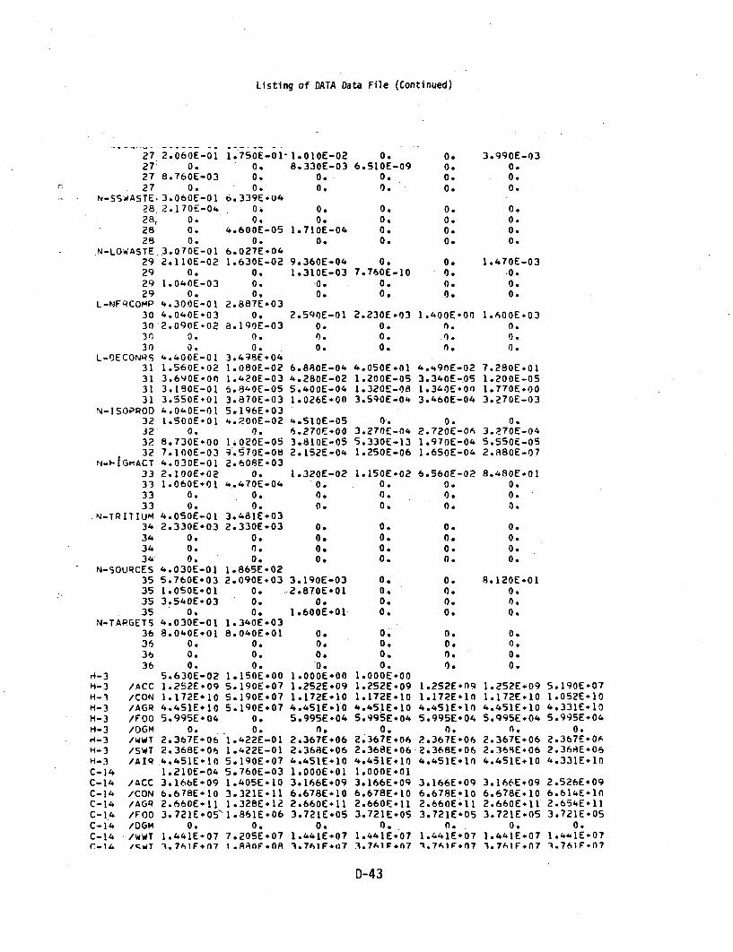
Listing of DATA Data File (Continued)

27 2.060E-0127 0.27 8.760E-0327 0.

N-SSWASTE. 3.00E-0128. 2..170E-0428, 0.28 0.28 0.

N-LOWASTE. 3.070E-0129 2.110E-0229 0.29 1.040E-0329 0.

L-NFRCOMP 4.300E-0130 4.040E+0330 2.090E-023 0, 0.30 0.

L-DECONRS 4.400E-0131 1.560E.02

.31 3.6YOE-0031 3.180E-0131 3.550E*01

N-ISOPPOD 4.010E-0132 1.500E60132 0.3? 8.730E-0032 7.100E-03

."1-HIGHACT 4.030E-0133 2.100E#0233 1.060E+0133 0.33 0.

.N-TRITIUM 4.050E-0134 2.330E*0334 0.34 0.34, 0.

N-SOURCES 4.030E-0135 5.760E,0335 1.050E-0135 3.540Eo0335 0.

N-TAPGETS 4.030E-0136 8.040E0136 0.36 0.36 0.

H-3 5.630E-02H-3 /ACC 1.252E+09H-3 /CON 1.172E*10H-3 /AGR 4.451E+10H-3 /FOO 5.995E*04H-3 /OGM 0.H-3 /WWT 2.367E*06H-3 /SWT 2.368E*06H-3 /AIR .4.451E 10C-14 1.210E-04C-14 /ACC 3.16bE409C-14 /CON 6.678E*,10C-14 /AGR 2.660E+11C-14 /FOO 3.721E05'C-14 /DGM 0.C-14 /wWT 1.441E-07C- 1 & /c•wT -. 761F÷n7

1.750E-01-1.010E-020. 8.330E-030.

,0.'

6. 339E+040.0.

4.600E-050.

6.027E÷041.630E-02

0.0.0.

2.887E-030.

8.190E-030.0.

3.498E*041.080E-021.42OE-036.840E-053.870E-035. 196E*034.2-0OE-02

0.1 i02OE-059.570E-082.608E-03

0.4.470E-04

0.0.

3.481E*032.330E-03

0.0.0.

1.865E#022.090E*03

0.0.0.

1.340E*038.040E*01

0.0.0.

1.150E*005.190E*075.190E*075.190E*07

0.0.

1.422E-011.422E-015.190E*075.760E-031.405E*103.321E*111.328E*12

"1 .861E.06

0.7.205E+071.RAfFOflR

0.

0.

0.1.710E-04

0.

9.360E-041.310E-03

0.0.

2.590E-010.0.0.

6.880E-044.280E-025.400E-041.026E*00

4.510E-056.270E-003.810E-052. 152E-04

1.320E-020.0.0.

0.0.0.0.

3.190E-03.2.870E-01

0.

1.600E-01

0.

0.*0.

I .OOOE*001.252E*091.172E*104.451E*I05.995E*04

0.2.367E*062.368E+064.451E#101 .OOOE*013. 166E*096.678E*102.660E+113.721E.05

0.1.441E.07

.761 F+07

0.6.S1OE-09

0.0.

0.0.0.0.

0.7.760E-10

.0.0.

2.230E*030.0.0.

4.050Eo011.200E-051.320E-083.590E-04

0.3.270E-045.330E-131.250E-06

l.150E-020.0.0.

0.0.0.0.

0.0.0.0.

0,000.06

I.O00E001.252E.091. 172E# 104.45!E*105.995E.04

' 0.2.367E÷062.368E*064.4i5E.101.O00E013.166E*096.678E*102.660E+113.721E+05

0.1.441E*073.TAlFfn7

0.0.0.0.

0.0.0.0.

0.0.0.0.

1.400E÷000.

.0.

4.490E-023.340E-.051.340E*003.460E-04

0.2.720E-0S1.970E-041.650E-04

6.560E-020.0.0.

0.0.0.0.

0.0.0.0.

0.

0.

1 .252Eofl91. 172E. 104.45 1 E*105. 995E. 04

0.2.367E-06ý2. 368E. 064.451E+10

3. 166E*096.678E*102. 660E0 113.72 1E*05

0.1 .441E*07

O,0IF n

3.990E-030.0.0.

0.0.0.0.

1.470E-03.0.0.0.

1.600E+030.0.0.

7.280E#011.200E-051.770E#003. 270E-03

0.3.Z70E-045.550E-052.880E-07

8.480E010.0.0.

0.0.0.0.

8.120E÷010.0.

0.

0.0.0.0.

1.252E*091.172E#104.451E+ 105.995E+04

2.367E+062.369E.064.451E10

3.166EE096.678E. 10.2.660E+113.721E÷05

0.1.441E*071.761F+07

5. 190E-071.052E÷104.331E-105.995E*04

0.2.367E#062.368E*064.331E*10

2.526E096.61E÷1n2.654E*113.721E#05

0.1.4'1E*071.761F+07

D-43

Listing of DATA Data File (Continued)

C-14*

FE-55FE-55FE-55FE-55FE-55FE-55FE-55FE-55FE-55NE-59NI-59NI-59NI-59

NI-59-M1-59N! -59

NI-59N 1-59

CO-60CO-60CO-60CO-60CO-60

CO-60CO-60CO-60N 1-63NI-63

NI-63NI -63NI-63N1-63NI-63NI-63

NB-94NB-94NB-94NB-94NB-94NB-94NB-94NH-94NB -94SR-90SP-90SR-90SP-QO0SR-90SR-9OSR-RnSR-90SR-90TC-99TC-99TC-90TC-99TC-99TC-99TC-99TC-99TC-99

1-129T-I PQ

/AIR

/ACC/CON/AGRiFoO

/'4WT/SWT-

/AIR

/ACC/CON/AGR/FOO/OGM/WWT

/S4T/AIR

/ACC/CON/AGR/FO0

/OGM/W-WT/SWT/AIR

/ACC/CON/AGR/FOO/OGM

/SWT/AIR

/ACC/CON/AGR/FOO/0GM/WWT/SWT/AIR

/ACC/CON/AGR/FO0/IGM/WWT/S.WT

/AIR

/ACC/CON/AGR/FO0/DGMIWWT/SWT

/AIR

/arcr

2.66O0E-112.670E-011.805E*109.283E#093.219E*103.482E+01

0.2. 727E#064.450E÷064.827E +108.660E-063.698E-103.872Elo1.247E-113.693E#036.200E#038.537E+069.825E*061.505E#11.320E-012.358E. 121.237E-113.695E#I I5.274E#031.540E*071.432E+081.45"E*082.683E*127.530E-033.056E+101. 04OE+ 113.341E+II9.878E*03

0.1.915E*072.260E-073.341E+I I3.470E-056.102E*111.389E*101.399E-102.116E*009.630E*063.193E#073.232E*076.103E*II2.470E-022.417E*136.394E+131.891E146.407E#073.060E*049.564E-091.014E-101.892E*143.270E-061. 176E-092.960E-09b.548E096.566E-03

0.4.186E054.240E+058.548E094.080E-089.1 1QF. il

1.328E-121.4W8E-021.885E.104.816E*101.903E.112. 15IE-02

0.1 .244E+072.314E+072.064E 111.480E-029;378E-102.325E. 117.476E- 112.21 1E÷046.200E*034.425E*075.196E-077.733E- II1.480E-022.336E. 122.280E*102.280E+10

0.1..540E*071.238E+081.238Eo082.336E-121.480E-029.602E* 113. 150E*121.OO1E*132.945E#05

0.5.71 1E+086.738E.081.O01E*131 .I1OE-026.114E-ll1.515E+101.548E#107.078E.009.630E*063.196E+073.324E°076. 118E+1 I9.860E-039.617E#132.588E*147.686E+142.61 IE-083.060Eo043.895E 104.128E*107.688E* 141-.15OE-019.680E*085.41 1E.09-1 .933E+101.635E*04

0.1.042E+061.056E+061 .933E*101.150E-O1A * q1 C;F.) I

2.660E#116.300E*022.413E#103.94lE*101.376E#111.493E.020.

8.863E*061.625E*071.537Eo114.200E#025.058E#108.130E+102.581E+1 I7.590E*036.200E+031.609E#071.874E+072..83RE.I I4.200E+022.353E.127.599E+101.874E+112.391E.031.540E*071.326E+081.338E#082.500E+124.200Eo026.576E*102.176E.116.931E.112.041E.04

0.3.958E.074.670E.076.931E+111.000E#036. 108E*1I1.454E101.472E#103.937E#009.630E*063. 194E+073.266E*076.11 1E.1I9.000E.001.668E-1I11.760E*091.760E#09

0.3.060E*048.835E*068.835E-061.668E+1I2.000E*002.280E#098.890E+092.960E#102.433E*04

O.1.551E*061.571E*062.960E*102.000E*00A.q1EF*11

2.660E+1I5.400E*031.613E*105.080E.075.080E.07

0.0.

8.609E*058.609E. 051.613E*103.600E*032-578E.-105,980E*075.980E.07

0.6.200E+031.377E-061.377E.062.578E*103.600E*032.336E-122.290E#102.280E10

1.540E*071.238E#081.238E*082.336E+123.600E#031.560E*081.560E+081.560E*08

0.0.

4.276E-014.276E-011.560E4081.000E*046.09SE*111.320E.101.320E*10

0.9.630E*063.192E+073.192E*076.095E*1I7.300E4011.668E-111.760E+091.760E#09

0.3.060E+048.835E-068.835E*061.668E+115.000E.007.600E.087.60OE*087.600E*08

0.0.

2.083E+002.083E-007.600E*085.000E.00ci. I AF. 1

2.660E11 2.660E11 2.654E+11

1.613E*105.080E*075.080E*07

0.n .

8.609E+058.609E*051.613E*10

2.578E105.980E.075.980E*07

0.6.200E.031.377E-061.377E*OA2.578E+10

2.336E*122. 2BOE*102.280E-10

0.1.540E+071.238E+081.238E*082.336E+12

1.560E+081.560E*OF1.560E#08

0..0.

4.276E-014.276E-011.560E+03

6.107E*111.446E+10

-1-. 464E-.-10-3.892E+009.630E.063. 194E-073.265E-076.110E11

1.668E*1I1.760E*091.760E-09

0.3.060E*048.835E#068.835E*061.668E+11

1.996E-101.031E+113.636E*1l3.061E.05

0.1.951E*071.976E+073.636E*11

2.081E+1 12.095E* 112.644E* 118.331E+01

0.5.326E4069.449E.062.804E+11

5.778E+103.206E#103.206E+10

. 0.

6.200E*031.377E+061.377E*065.778E+10

2.634E-132.402E*132.402E*13

0.1.540E*071.239E*081.239E+082.634E*13

8.816E.108.816E+108.816E.10

0.0.

2.416E.022.416E+028.816E.10

1.330E*127.332E+1 1-7.-332E-+ 1-1

0.9.630E+063.192E-073.192E.071.330E-12

1.980E.113.296E 103.296E+10

0.3.060E*048.835E+068.835E.061O.980E11

7.400E.097.962E*099.720E*092.067E+03

0.1.318E+051.335E#059.721E+09

1.925E#102.116E+107.752E 108.566E*01

0.5.452E+069.692E.069.360E*10

2.850E*101, 441E-105. 082E. 101.563E*036.200E#034.408E*064.953E*067. 654E.* 1

2.504E*128. 593E * I2.953E*124.492E*041.540E-072.893E.083.112E#085.266E+12

7.436E-093.911E+I01.383E-II4.259E403

0.8.258E*069.743E+061.383E+11

6.839E*114.432E*111.557E-122.390E-049.630E-061.466E#084.496E*092.153E#12

1.892E4114.727E*121.946E+137.543E-063.060E#041.134E*091.201E#091.962E+13

7.880E-092.240E*1I9.008E+117.953E#05

0.5.069E+075.135E.079.008E*11

A.rIcZF+ll A.c;7PF*ll A.q;)IF*ll

D-44

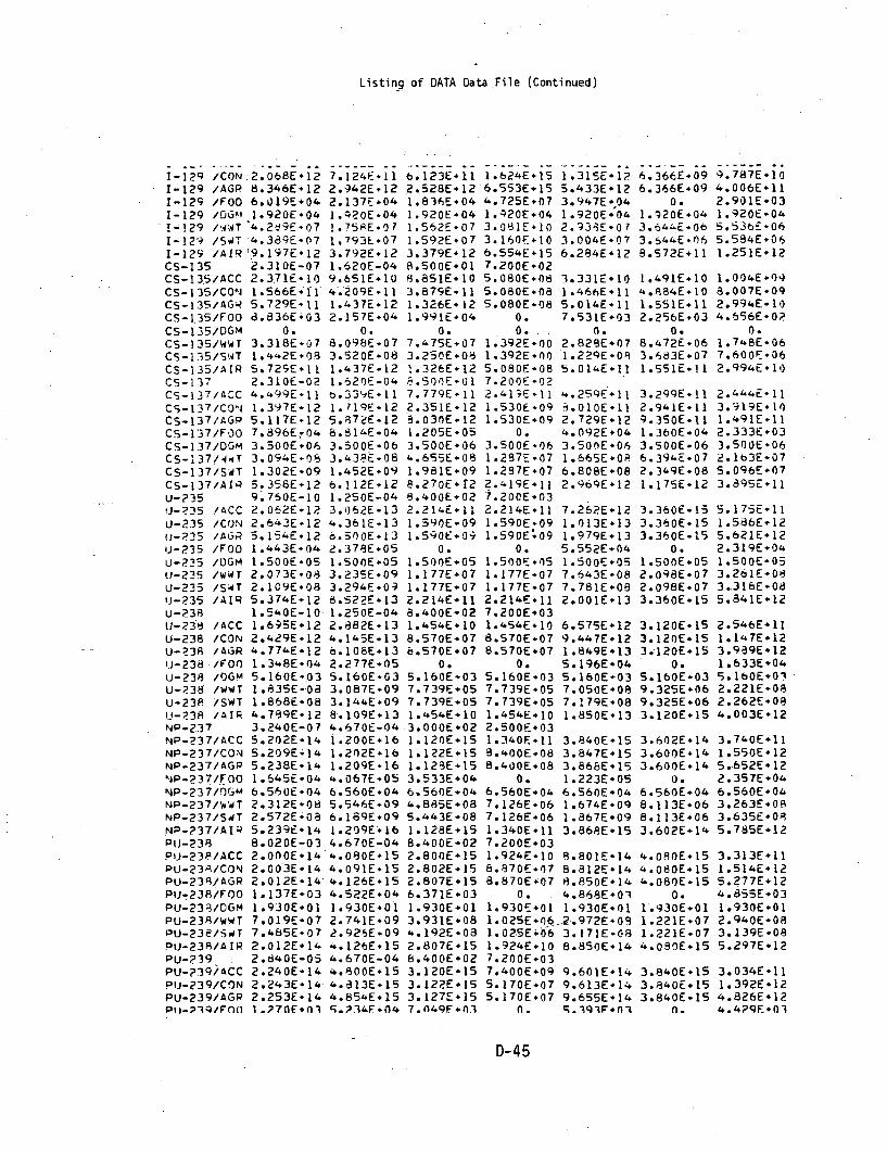
Listing of DATA Data File (Continued)

1-12q /CON:2.068E1I21-129 /AGP 8.346E+121-129 /FOO 6.019E÷041-129 /0Gkl 1.920E#041-129 /wWT 4.2tý9E.071-129 /SWT 4.389E-071-129 /AIR'9.197E.12CS-135 2.310E-07CS-135/ACC. 2.371E-10CS-135/CON 1.5e6E.-11CS-135/AGq 5.729E-11CS-135/FOO a.836E-03CS-135/DG.4 0.CS-135/WWT 3.318E-07CS-135/SWT 1.442E.08CS-135/AIR 5.729E+11CS-137 2.310E-02CS-137/ACC 4.499E*l1CS-137/C0Oj 1.397E-12CS-137/AGO 5.117E-12CS-137/Fo0 7.896E704CS-137/DGM 3.500E+06CS-137/4T 3.094E-08CS-137/SWT 1.302E-09CS-137/AIP 5.358E÷12U-P]5 9.750E-10'J-?35 /ACC 2.062E*12U-235 /CON 2.643Eo12u-235 /AGR 5.154E-12U-235 /F00 1.443E-04U-225 /UGM 1.S00E.050-235 /WWT 2.073E.080-235 /SWT 2.109E.08IJ-235 /AIR 5.374E-12U-238 1.540E-10U-238 /ACC 1.695E-12U-238 /CON 2.429E-12U-239 /AGR 4.77'E-12UJ-238 /FOO 1.348E-04u-238 /0GM 5.160E-.03U-239 /WWT 1.835E-.08U-238 /SWT 1.868E*08U-238 /AIR 4.739E÷12NP-237 3.240E-07NP-?37/ACC 5.202E-14NP-237/CON 5.209E-14NP-237/AGP 5.238E.l1NP-237/FOO 1.545E.04NP-237/0GM 6.560E*04NP-237/WWT 2.312E+08NP-237/SWT 2.572Eo0ONP-?37/AIQ 5.239E*14P|J-238 8.020E-03Pij-23P/ACC 2.000E+14PU-231/CON 2.003E.14PUJ-239/AGR 2.012E14'PU-238/FOO 1.137E-03PU-233/0G'M 1.930E+01PU-238/WWT 7.019E-07.PU-238/SWT 7.465E-07PU-238/AIR 2.012E*14PU-?39 2.d•4OE-05PU-?39/ACC 2.240E-14PU-239/CON 2.243E-14PU-239/AGP 2.253E*14PUj-;)Q/F0fl 1 .270E~nl

7.124E- 112.942E+122.137F*04I.Q2OE-041.75PE-07

1. 793E+073.792E+121.620E-049.6551+I04.209E- 111.437E-122.157E+04

0.8.09BE.073.520E-081.437E+121.620E-04b.339E. 111. 719E-125.872E-128. 814E. 043.50OE÷*063.438E+081 .452E+096. 112E.121.250E-043.06E+E134.361E-136.500E+132.378E+051.500E+053.235E.093.294E.098.522E-131.250E-042.882E°134.145E+136.108E*132.277E-05S. 160E-033.087E+093. 144E+098.1 09E.134.670E-041.200E*161.202E-161.209E-164..067E+056.560E-045.546E.096. 189E+091.209E-164.670E-044.080E#154.091E- 154. 126E- 154.522E.041.930E.012.741E.092.925E.094.126E.154.670E-044.800E. 154..313E. 154.854E*15C;. 234F - %4

6. 123E÷I I2.528E÷121.836E-041.920E-041.562E-071.592E.073. 379E- 128.500E-018.851E 103.879E- 111.326E+ 121.991E04

0.7.475E+073.250E+081.326E- 125.SOOE-u17.779E+ 112.351E* 12B.030E-121.205E-053.500E°064.655E-081.981E+098.270E- r28.400E+022.214E+111.590E.09I.590;EO9

0. .1.500E-05I. 1 77E*071. 177E.072.214E-118.400E-02I.454E+ 108.570E-078.570E*07

0.5. 160E-037.739E*057.739E-051.454E*1013.00 OE021. 120E-151. 122E* 151. 123E+153.533E÷046.560E.044.885E-085.443E-081. 128E÷158.400E-022.8OnE*152.802E# 152.807E#156.371E+031.930E+013.931E+084. 192E.082.807E- 158.400E*023. 120E- 153. 122E+153. 127E+157. fl49Fn.0.

1.624E+156.553E+154.725E+071.'420E*043.081E-103.160F÷106.554E÷15.7.200E-025.080E.085.080E÷085.080E-08

0.

1.315E*125.433E*123.947E 041.920E.042.93ý3E073.004E-076.284E÷12

3.331E-101.466E115.0514E117. 531E .03

0. 01.392E*00 2.828E+071.392E.0O 1.229E-OA5.080E-08 5.014E117.200E-022.41;E-11 4.259E-111.530E-09 1.010E÷111.530E.09 2.729E*12

0. 4.092E+043.500E-06 3.500E+061.287E-07 1.665E.0R1.287E+07 6.808E*082.419E-11 2.9b9E÷1277.200E*032.214E*11 7.262E-121.590E-09 1.013E-131.590E*09 1.979E-13

0. 5.552E÷041.500-E.5 1.500E+051.177E-07 7.643E-081.177E.07 7.781E-082.214E+11 2.001E+137.200E+031.454E+10 6.575E*128.570E-07 9.447E-128.570E*07 1.849E*13

0. 5.196E.045.160E-03 5.160E-037.739E+05 7.050E*087.739E.05 7.179E+081.454E-10 1.850E*132.500E+031.340E.11 3.840E-158.400E-08 3.847E÷158.400E÷08 3.866E+15

0. 1.223E*056.560E04 6.560E-04-7.126E*06 1.674E+097.126E-06 1.867E*091.340E+11 3.868E-157.200E+031.924E.-0 8.801E+148.870E-.7 8.812E*148.870E*07 8.850E-14

0. 4.868E*011.930E+01 1.930E+011.025E*06.2..972E+091.025E-.06 3.171E-081.924E.10 8.850E÷147.200E+037.400E+09 9.601E-145.170E.07 9.613E#145.170E+07 9.655E-14

n.* 1; - 19 IF + n

6.366E.096.366E+09

0.1.920E+043.644E*063.544E.068.572E.11

I.491E.1014.884E- 101.551E.112.256E*03

0.8.472E÷063.683E.071.551E 11

3.299E- 112.941E.119.350E-111.360E÷043.500E+066.394E-072. 349E-081. 175E- 12

3.360E-153.360E-153.360E-15

0.1.500E+052.098E*072.098E-073.360E.15

3.120E#153.120E4153.p120E+ 15

0.5.160E-039.325E+069.325E*063.120E+15

3.602E.143.600E+ 143.600E*14

0.6.560E-048.113E-068.113E-063.602E-14

4.080E÷ 154.080E* 154.080E- 15

0.1 .930E-011.221E+071.221E-074.08OE÷15

3. 840E+ 153.840E+153.840E.15

n0.

9.787E#104.006E.112.901E#031.920E.045.53b6E065.584E+061.251E+12

1.004E*098.007E.092.994E+104.556E-0?

0.1.748E-067.600E*062.994E11l

2.41-4E+11I3.919E-101.491E112.333E÷033.500E-062.163E°075. 096E# 073.895E+11

5.175E-111.586E+125.621E-122.319E+041.500E-053.26iE-083.316E-085.841E412

2.546E4111.147E-123.939E-121.633E*045.160E*0E2.221E-082.262E+084.003E-12

3.740E-111.550E+125.652E*122.357E*046.560E-043.263E*083.635E-085.785E*12

3.313E.111.514E-125.277E÷124.1355E-031.930E÷012.940E-083.139E*085.297E*12

3.034E-111.392E*124.826E÷124.4?9E.01

D-45

Listing of DATA Data File (Continued)

Ptj-239/DGm' 9.390E*01 9.390E*01PU-239/WWT 7.765E*07 3.172E-09Pu-239/SWT 8.286E-07 3.386E-09Pti-239/AIP 2.253E-14 .. 854E-15PU-241 . 5.250E-02 4.670E-040'j-241/ICC 3.040E-12 7.440E-13PU-24!l/CON, 3.046E-12 7.467E13PU-241/AGR 3.063E#12 7.552E.13PU-241/FOO 2.208E+01 1.097E+03Pij-241/OGM 3.430E-01 3.430E-01PfJ-241/wWT 1.341E-06 6.642E-07PU-241/SWT 1.431E+06 7.091E+07PU-241/AIR 3.063E#12 7.553E.13PU-242 2.4dOE-06 4.670E-04PIj-242/ACC 2.160E+14 4.480E+15

PU-242/CON 2.163E-14 4.492E.15Pii-242/AGR 2.173E-14 4.530E-15O.J-242/F')O 1.224E-03 4.88dE-04PD-p?42/0GM 0. 0.Pu-242/w4T 7.520E-07 2.938Eo09PU-242/S.T 8.021E+07 3.137E-09PU-242/AIR 2.173E*14 4.530Eo15AM-241 1.510E-03 4.1IOE-03AM-241/ACC 5.04lE14 7.120E+15A&4-241/CON 5.049E*14 7.134E-15A-4-?41/AGR 5.077E-14 7.176E+15A'4-p•I/FOO 3,599E*O4 5,448E+05

Am-24 I/OGM 7.710E-04 ?1.?fOE-04

Am-241/WwT 2.247E-08 3.340E+09A-?41/SoT 3.721E.08 5.572Eo09A-2.41/AI/ 5.078E+14 7.176E#15AM-243 e.720E-05 4.110E-03414-2"1/ACC 4.961E+14 7.1&0E÷15

AM-243/CON 4.969E+14 7.054E-15AA•-243/AGP 4.996E+14 7.096E+15

Am-243/FOO 3.525Eo04 5.44lE+05AM-243/QGM 1.860E-05 1.860E-05A#4-243/WWT 2.208E-08 3.337E.09AM-243/SWT 3.653E-08 5.566Eo09AM-243/AIP 4.997E+14 7.096E15CM-?43 2.170E-02 4.670E-04Cmý243/ACC 3.843E-14 6.161E#15CM-243/CON 3.846E*14 o.17lE*15CM-243/AGR 3.866E+14 6.204E-15CM-2'3/FOO 1.113E+04 l.A97E*05CM-243/'DGM 3.820E+05 3.320E+05CM-243/WWT 1.647E-08 2.598E*09Cm-241/SWT 2.087E.0I 3.347E+09Cm-243/AIP 3.868E-14 6.204E+15CM-244 3.940E-02 4.670E-04CM-244/ACC 2.00E*1 4.400E*15C-?24-/CON 2.805E*14 4.'.OBE'15CMP44-/AGR 2.820E+14 4.433E.15CH4-24/F0O 8.520E-03 1.434E+05CMj-24/DGM 5.640E+01 5.640E*01CM-244/WWT 1.170E+O 1.954E+09C4P?4•/SwT 1.501E+08 2.521E+09Cm-244/AIP 2.820E-14 4.433E+15REGION I 9.180E-12 2.960E-11

2.OOOE*02 S.000E.03l.OOOE00 1.OOOEo00'..OOOE*02 8.OOOE+02

REGION 2 2.O1OE-11 3.180E-l14.200E*01 4.OOOE#02l.OOOE+OO l.OO0E+.0h.40nF+01 I.AnnFf03

9.390E-014.343E÷Od4.632E*083.127E- 158.400E-024.560E*134.561E+134.566E#135.613E-013.430E-013.512E-063. 7,42E*064.566EE136.40OE+023.04OC• 153.042E-153.04 7E.-156. 7A3E-03

0.".184E-084.4b2E.083.047E- 153. 00GE02b.6-OE.156. 645E -15,.660E- 151 .916E+057.710E-04I . I 49E -091.974EF096.660E-153. 000) E - 026.480E-156.4135E-156.499E+151 .8&9E#051.860E#051.* 1483E+091 .906E-096.499E#153.OOOEo025.60 1E+155.604E+155.616E+157. 155E-043.82OE÷059.970E*081.280E-095.61 7E+ 153.OOOE.024.160ES154. 163E* 154. 174E.156. 145E -045.640E-018.443E+081.087E*094.174E- 151.970E-04l.OOOE.04I.OOOE001.830E-101.160E-03e.OOOE.02I. O00E00iAw3nF-in

9.390E.013.934E*053.934E*057.4noE*097.20OE.034.730E+074.780E-074.780E#07

0.3.430E-011.310E-nI1.31OE-014.780E-077.200E-031 .441E-106.930E°075.930E-07

0.0.

7.674E-057.674E-051.!#41E-In2.5OOE.n37.669E+103.300E.083.600E-08

0.7.710E-04

-. 192E-067.869E.102.500Eo034.096E°106.090E.086.090E-08

0.1.860E-054.837E 064.837E-069. 096E- 102.500E*032.444E+ II2.260E°092.260OE - 09

0.3.820E+051.29bE*071.296E.072.444E- I112.500E+031.706E.l17.230E#077.230Eo07

0.5.640E+019.093E+059. 093E+05I.706E-104.930E-054.OOOE+02I.OIOE-092.bIOE-123.240E-n51.300E-033.500E-103. -I? F- 1

9.390E-013.285E083.506E*089.656E+ 14

1.440E-131 .4 3E +131.450E+131.017E°023.430E-016.1 79E-066.596E-061.450E+13

9.60 1E.149.613E- 149.653E- 145.1 ;4E-03

Q.3. 168E.OP3. 36 1E+089.654E+ 14

3.1n3AE. 153.64 7E-153.868E- 152.707E-357.710E.4r4I .663E*(92.772E+093.86AE-15

1.76nE.153.767E. 153.787E+152.654E-051.860E*0O1.631E-092.7 18E-093-7.788E+15

1.760E*151.763E-151.772E-155. 195E*043.320E-057.212Eo089.264E+081..772E+15

1.280E+151.282E-151.289E*153.978E+045.640E+Gl5.4•30E+O7.00IE+081.289E*157. 700E-031 .O00E+01.510E-09

7.700E-031.O00EoO045.250E-10

9.390E+011.092E#07I.092E-073.140E- 15

6.,300E+126. 3OOE- 126.800E 12

0.3.430E-0 11.864E-041.o36'.E -046.8OEo 12

3.680E-153.680E+ 153.680E- 15

0.0.

1.085E-071.085E-073.680E- 15

4.24JE14.240E.144.2-40E# 14.

0.7.7 1OE.045. 354Y. 065.354E-064. ?26 1 E* 14

4.0.0 IE- 144.oooE - 144.OOOE- 14

0.1.860E-055.933E- 065.933Eo064.OOIE- 14

4.403E. 144.400E°144.400E + 14

0.3.-120GE -051.417E*071.417E.074.403E- 14

4.400E. 144.400E- 144.400E* 14

0.5.640E*0 12.115E*062.1 15E+064.400E. 042.00EOE052.000Eo041. 120E-07

2.00GE°052. 000GE*0-1.120E-07

9.390E-012.676E+042.858E4084.833E-12

5.56aE092.861E-I01.008E+1I9.310E*013.430E-015.618EOA5.999E-061.008E+11

2.944E1I11.355E*124.722F>124.34.3E-03

0.2.62SE°082.806E°OS4.736E+12

3.5A7E- 11.5083E125.355E '124.43bE.047.7T1OE.43.047E-085.069E-Of5.434E+12

3.b3OE-111.713E+126.223E*1?5.787Eo0'.I.860E*053.572E.OA5.942E+086.313E+12

5.4•4E#111.594E*I25.629Eo122.319E#043.820E053.269E#084.184E+085.971E*12

3.051E+11I.533E*I15.434E*122.241E*045.6.0E.013.044E-083.929E.0A5.451E-124.500E-06

3

4.500O7 *06

3

D-46

C.

Listing of DATA Data File (Continued)

REGION 3 2.510E-111.400E+021.OOOE001;bOOE*02

REQIo'I 4. 2.640E-101S500E-011 .000E+008.000EO00

REGION 5 2.010E-113.200E*011 .OOOE-006.400E÷01

QEGIO1N 6 2.010E-119.200E-011.000E+006..OOE*01

3.260E-112.900E-031I OOE00E01.000E-02

8.060E-113.OOOE+02I .OOOE008.0OOE.023. 18nE- 113.900E*02I .OOOE+001.600Eo033.180E-114.500E-021 . 00OE-001.600t703

9.0OE-055.800E+03I .OOOE+001.830E-101.300E-066.OOOE-02I .O00EO01.830E-10I. 160E-047.900E*021 .000E+001.830E-101.160E-02A.500E.021.OAOE001.830E-10

2.250E-054. O00E+023.860E-102.550E-123.250E-071.300E.032.660E- 1I1.790E-123.240E-061.300E-033.030E-103.323E-123.240E-041.]OOE*033.030E-103.323E-12

7.770E-031.250E*045. 790E-1in

7.700E+013.O00E+043.990E-I I

7.700E-03l.O00E*044.550E-10

7.700E.031 .00nE-044.550E-10

2.000E*05 4.500E:+062.500E*041.120E-07

2.OOOE05 ".50W07-066. 00OE-41.120E-07 2

2.o0oE.05 4.SOoE.O#2.000E+041.120E-07 2

2.OOOE÷05 4.500E.062.nOoE.041.120E-07

D-47

Listing of DATAD Data File

36 231.000 .120 .060 .030 .060.120 .060P-IXPESLN 1.100E-01 3.463E-+04

1 3.360E-02 1.840E-03 9.730E-05 7.300E-04 2.790E-06 2.170E-03I 8.1SOE-04 8.840E-08 1.630E-04 8.230E-07 2.440E-06 8.P30E-07I 1.BO0E-02 4.710E-08 3.710E-07 9.060E-12 2.450E-05 1.820E-05

"1 5.630E-04 3.990E-08 4.134E-05 1.260E-06 8.520E-09 1.060E-05P-CONCLIQ 1.1OOE-O1 2.435E.05

,2 1.090E-01 2..390E-03 1.270E-04 7.080E-03 2.710E-05 2.110E-022 7.920E-038.580E-07 2.120E-04 1.O70E-n6 3.16nE-06 1.070E-062 2.430E-02 6.150E-08 4.840E-07 Io.BOE-11 4.830E-05 3.310E-052 1.020E-03 7.250E-08 7.102E-05 2.020E-06 1.010E-08 1.470E-05

P-FSLUDGE 1.100E-01 4.279E-033 1.060E-00 1.790E-03 9.540E-05 9.670E-02 3.710E-04 2.880E-013 1.080E-01 1.170E-05 1.590E-04 8.030E-07 2.370E-06 8.030E-073 1.820E-02 1.460E-07 1.150E-06 2.810E-11 4.490E-05 1.550E-043 4.790E-03 3.390E-07 4.551E-64& 1.780E-05 2.660E-07 1.360E-04

P-FCARTRG 1.100E-OI 2.177E+044 1.860EoO 7.970E-04 4.250E-05 1.730E-01 6.6onE-04 5.140E-014 1.930E-01 2.090E-05 7.070E-05 3.5BOE-07 1.060E-06 3.580E-074 8.120E-03 3.640E-07 2.870E-06 7.020E-11 2.370E-04 3.a00E-044 1.180E-02 d.346E-07 6.394E-04 1.IOOE-05 1.660E-07 8.440E-05

•-IXPESIN 1.200E-01 7.623Eo0-5 4.630E-00 1.340E-02 1.190E-03 2.990E-01 9.800E-04 7.700E-015 2.040E-02 3.090E-05 3.080E-03 7.650E-05 2.040E-04 7.650E-055 1.74OEoO0 5.330E-08 4.200E-07 1.020E-11 7.880E-05 S.340E-055 1.850E-03 1.170E-07 9.768E-05 1.570E-06 2.330E-08 1.400E-05

4-CONCLIQ 1.200E-01 2.102E+056 2.870E-01 4.3SOE-04 3.890E-05 2.500E-02 A.21OE-05 6.440E-026 1.710E-03 2.590E-06 9.970E-05 2.500E-06 6.650E-06 2.500E-066 5.670E-02 3.440E-08 2,710E-07 6.610E-12 1.880E-04 9.430E-05b 3..280E-03 2.060E-07 *2.513E-04 8.U90E-06 2.230E-07 1.580E-04

8-FSLUDGE 1.200E-01 1.690E-057 5.240E°00 8.7SOE-03 7.770E-04 4.540E-01 1.490E-03 1.170E*00.7 3.080E-02 4.700E-05 2.000E-03 5.OOOE-05. 1.330E-04 5.noOE-057 1.130Eo00 3.320E-07 2.610E-06 -6.380E-11. 4.400E-04 2.360E-047 8.200E-03 5.180E-07 4.848E-04 1.0SOE-05 2.560E-07 1.720E-04

P-COTRASH 2.100E-01 4.2'4E.OS8 2.280E-02 2.110E-04 1.120E-05 1.860E-03 7.110E-06 5.520E-038 2.070E-03 2.250E-07 1.870E-05 9.420E-08 2.780E-07 9.420E-088 2.140E-03 7.890E-09 6.220E-08 1.520E-12 5.640E-06 5.530E-068 1.710E-04 1.210E-08 1.085E-05 2.670E-07 2.350E-0Q 2.000E-06

P-NCTRASH 2.1OOE-01 2.178E-059 5.250E-01 4.A40E-03 2.570E-04 4.270E-02 1.640E-04 1.270E-019 4.780E-02 5.180E-06 4.300E-04 2.170E-06 6.410E-06 2.170E-069 4.920E-02 1.820E-07 1.430E-06 3.490E-11 1.300E-04 1.270E-049 3.930E-032.790E-07 2.498E-04 6.140E-06 5.410E-08 4.600E-05

8-COTRASH 2.200E-01 2.086E#05 -10 2.350E-02 4.700E-05 4.170E-06 1.890E-03 6.210E-06 4.890E-03101.290E-04 1.960E-07 1.070E-05 2.680E-07 7.140E-07 2.680E-0710 6.090E-03 1.220E-09 9.600E-09 2.350E-13 2.170E-06 1.160E-3610 4.010E-05 2.530E-09 2.575E-06 6.510E-08 1.66nE-09 1.150E-06

B-NCTRASH 2.200E-01 9.896E+0411 3.790E*00 7.600E-03 6.720E-04 3.050E-01 1.0OOE-03 7.840E-0111 2.080E-02 3.160E-05 1.730E-03 4.330E-05 1.150E-04 4.330E-0511 9.810E-01 1.970E-07 1.550E-06 3.780E-11 3.510E-04 1.860E-0411 6.470E-03 4.080E-07 4.152E-.04 .OSOE-05 2.690E-07 1.860E-04

F-COTRASH 2.110E-Of 2.359E*0512 5.580E-06 0. 0. 0. 0. 0.12 0. 0. 0. 0. 0. 0.12 0. 1.180E-06 4.400E-06 0. 0. 0.12 0. 0. 0. 0. 0. 0.

F-NCTRASH 2.110E-01 4.171E-0413 5.330E-06 0. 0. 0. 0. 0.13 0. 0. 0. 0. 0. 0.-13 0. 1.13OE-06 4.200E-06 0. 0. 0.

D-48

Listing of DATAD Data File (Continued)

.1-COTRASH:141414

I .COTPASH

1515-1515

N-SSTRASHlb1616

w.SST4ASH17171717

N-LOTRASH18181818

N+LOTPASH19

1919

F-oRUCESS20202020

J-PPOCESS21212121

I-LOSCNVL22222222

IL+LOSCNVL23232323

-I-A8SLINO24242424

I-A8SLI1D25252525

I-.81IAAST25262626

T .RTWAqT

2.030E-011.1JOE-0I

0.3.780E-03

0.2.030E-011. 1 30E-01

0..3-780E- 03

0.2,060E-011 . 120E-05

0.0.0.

-2 . 060E-0 11.*120E-05

0.0.0.

2.070E-013.530E-02

0.1 .1 60E-03

0.2 .070E-0 13 .530E-02

0.11 I80E-03

0.3 .I IE-0 II . OBOE-04

0.0.0).

3. 120E-013.S0OOE-04

0.0.0.

3 .030E-019.600E-03

0.0.0.

3.030E-019.600OE-03

O.0.

0.

3.030E-011.990E-01

0.1 . 140E-02

0.3.030E-011 .990E-01

0.1 . 1 0E-02

0.3.030E-012.060E-01

0.7.260E-03

0.I. :IOF-n I

1.407E-055.950E-02

0.0.0.

1.407E-055.950E-02

0.0.0.

1.796E*050.0.

2.360E-06

0.

1 .796E.05

0.0.

5. 064E+04

1.860E-020.

0.0.

5,064E.04

2.360E-020.0.0.

7-,811 E+040.0.

2.300E-050.

2.91 IE÷040.0.

1I,650E-05

0.4.9l4EoO43.270E-03

0.0.0.

4.951E*043.270E-03

0.0.0.

5.585E.039.260E-02

0.0.0.

1.571E-039.260E-02

0.0.0.

1 .571E041,.1•OE-01

0.0.0.

5.250E-031.190E-03

0.4.760E-06

5.250E-03I. I190E-03

0..4.760E-06

0.0.

8.80OE-06

0.0.

9.800E-060.

1 .6'0E-033.710E-04

9.1 . 490E-06

1.640E-033.71 OE-04

0.1.490E-06

0.0.

8.540E-050.

0.0.

3.640E-040.

2.510E-043.550E-03

0.0.

2.51 OE-043.550E-03

0.0.

8.150E-033.S50E-03

0..0.

.1SOE-033.550E-03

0.0.

1 .010E-026.820E-03

0.0.

0.3.390E-09

- 0.0.

-0.3.390E-09

0.

0.

0.0.

0.

0.

0.

0.0.

0.1.*060E-09

0.0.

0.

0.0.

0.0.0..0.

0.0.0.

- 0.

0.0.0.

0.

0.

ý0.0.

0.1,*020E-091

*0.0.

0.6 .510E-09

0.0.

0.0.

0.0.0.

0.0..0.0.

0.0.

0.

0).0.0.

0.

0.0.

'0.

0.

0.

0.

0.

0.

0.0.0.

0.

0.

0.

0.0.

0.0.

0.

0.0.0.

0.

0.0.

0.

0.

0.O.0.

0.n,n,

4.410E-030.0.0.

4.410E-030.0.0.

0.0.0.0.

0.0.0.0.

1.380E-030.0.0.

1 . 330E-030.

0.

0.0.0.0.

0.0.0.0.

0.0.0.0.

0.0.0.0.

0.1.320E-02

0.0.0.

1.320E-020.0.0.

1 .690E-030.0.0.

D-49

Listing of DATAD Data File (Continued)

21272727

N-SSWASTE28282828

N-LOWASTE2929292q

L-NFPCOMP30303030

L-DECONPS31313131

N-I5nPROn32323232

N.-HIGHACT33333333

-N-TRITIUM34343434

N-SOURCES35353535

N-TAPGETS3h363636

H-3

H-3 /ACCH-3 ICONH-3 /AGRH1-3 IFO0H-3 /DGMH-3 /WWTH-3 /SWTH-3 /AIRC-I4C-14 /ACCC-14 /CONC-14 /AGPC-14 /FO(0C-14 /DGHC-14 /WWTC-14 /IqWT

2.OOE-010.

7.260E-030.

3.060E-012.170E-04

0.0.0.

3.070E-012.11OE-02

0.8.620E-04

0.4.300E-0I4.04OE+031.980E*02

0.0.

4.4OOE-011 .5OE*+023.490E+002.710E-012.S20E+014.04OE-011.500E.OI

0.7.240Eo004.750E-034.030E-012.1 OOEE029.950E+00

0.0.

4.050E-012.330E÷03

0.0.0.

4.030E-015.760E+039.860E+002.930E-03

0.4.030E-018.040E+01

0.0.0.

5.630E-021.252E*091.172E*104.451E-105.995E-04

0.2.367E*062.368E#064.451E÷ 101.210E-043.166E-096.678E+102.660E 113.721E*05

0.1.441E*073.76IF n7

1.140E-010.

0.

6.339E+040.0.

4.600E-050.

6.027E*041.060E-02

0.0.0.

2.887E+030.

8.190E-030.0.

3.498E+047.510E-031.420E-036.840E-053.870E-035.196E+032.740E-02

0.1.020E-059.570E-082.608E.03

0.4.470E-04

0.n .

3.481E-031.520E.03

0.0.0.

1.865E.021.360E+03

0.0.0.

1.340E-035.240E÷01

0.0.0.

1. 1SOE.005. 190E+075. 190E*075. 190E-07

0.0.

1.422E-01

5.190E+075.760E-031.405E+1O3.321E 111.32RE÷121 B61E-06

0.

1 .OIOE-026..820E-03

0.0.

0.0.

1.710E-040.

9. 350E-041.070E-03

0.0.

2.590E-010.0.0.

6.870E-043.610E-025.400E-041.026E*00

4.510E-055. 140E-003.81OE-052. 151E-04

1.320E-020.0.0.

0.0.0.0.

3. 190E-032.350E-0l

0.1.580E-01

0.0.0.0.

I .OOOE.001.252E+091.172E-104.451E+105.945E-04

0.2.367E*062.368E+064.451E+101 .O00E+013.166E*096.678EO102.660E 1*13.721E-05

0.

0.6.510E-09

0.0.

0.0.0.0.

0.7.760E-10

0.0.

6.980E*020.0.0.

1.270E*011.200-051.320E-083.59OE-04

0..3.270E-045.330E-131.250E-06

2.970E÷0!0.0.0.

0.0.0.0.

0.0.0.0.

0.0.0.0.

1.009F-nO1.252E+091. 172E- 104.451E+ 105.995E-04

0.2.367E-062. 368E-064.451E+ 101.OOOE-013.166E.096.678EE102.660E 113.721E*05

0.1.441 E-071. 7A 1 9. 7

0.0.0.0.

0.0.0.

0.0.

0.

I.400EO000.0.0.

4..-9nE-n23.34nE-051.260E-002.980E-04

0.2.720E-06I.840E-04I .380E-04

6.560E-020.0.0.

0.0.0.0.

0.0.0.0.

0.0.0.

1.252E#091.172E-ln4.451E-105.995E-04

0.2.367E-062.368E*064.451E-10

3.166E096.678E£102.660E 113.721E-05

n.1./41E#07'.7F1F.l7

1.690E-030.0.n.

0.0.0.0.

6. ?30E-040.0.0.

7.700E*020.0.

3.50E*011.200E-051.770E#002.SlOE-03

0.3.270E-045.550E-052.11OE-07

3.600E#010.0.0.

0.0.

0.0.

3.440E010.0.0.

0.0.0.0.

1.252E+091 . I 72E- 104.451E.105.995E.04

5.190E.071.052E-104.331E- 105.995E 04

0.2. 367E+0,52. 368E+0ý4.331E+10

2.367E#062.368E.064.451E.10

3.166E-096.678E*102.660E+113.721E-05'0.

1.441E-071. 761 F*i7

2.526E*096.bl4E+102.554E oII3.721E*05

0.1.44IE+071. 7611F.07

7.205E.07 1.441E+071.99AF*08? 1.7A1F.07

D-50

Listing of DAIA)) Dtl itHe (Continued)

C-14FE-55FE-55FE-935

F;:-55FE-55FE-55FE-55FE-55

NI-59NI-5')NI-59NI-59NI-54

N I -$5N I-59

NI-59C0.-60CO-6OCO-floC0)-60CO-60C0-60CO-60CO-60Cn-60NI-63NI-63NI-63NI-63NI-63NI -63N 1-453N1I-63NI -A•N8-94NFR-94

N8 -94

NB3-94NB-94N8-94NH-94'4-94

NQ-g0

SN-90SP-9O

SR-90SR-QOSP-90S-4-90TC-9OTC-99TC-99TC-99TC-99TC-99TC-99TC-99TC-991-129T -1I Q

/AIR

/ACC/CON/AGi/FOiD/0GM/WWT

/SWT/AIR

/ACC/CON/AGRIF0)O/0GM

/,. w T/AIR

/ACC/CON/AGR/FO0/OOM.

/w W T/SWT/A jP

/ACC/CON/IGR/F00/OGM/WWT/S.WT/AIR

/ACC/CON/AGP/FO0/DGM/wWT

/SWT/AIR

/4CC/CON/AGR/FOO/0GM/WWT/SWT/AIR

/ACC/CON/AGI,FOO/DGM/WWT/SWT/AIR

laicc

2. 660E+ 112.670E-0I1 .805E+ 104.283E*093.219E 1i03.482E + 0 1

0.2. 727E+ 064.450E+06-4.827E+ 108.660E-063.698E+103.872E.ln1.247E+ll3.693E+036.2OE÷03d.537E-069.825E +01 .505E- 111.320E-O12.358E121 .237E- II3.695E*115.274E+031 .540E.071 .432E-0ý1 .458E+082.6;i3E. 127.530E-033.056E 101.040E-113.31E+ I I9.878E+03

0.1.915E*072.260E#073.341E*113.470E-056.102E*ll1.389E-101.399E*102.116E+009.630E+063.193E+073.232E*076.103E.l I2.470E-022.417E*136.394E#131.891E*146.40,7E073.060E+049.564E#091.014E.I01.892E*143.270E-061.176E*092.960E+098.548E÷096.566E*03

0.4.186E+054.240E+058.548E+094.080E-08q. 119F *+Ii

1.328E.12I.480E-021.8855F* 104. A6E. 101 .903E- 112.161E-02

0.1.244E+072.314E*072.064E. 111.480E-029.378Eo 102.325E- 117.476E* 112.2111E-046.200E-03-. 425E*075. 196E-077.733E.II1.480E-022.336E-122.250E+ 102.280£*I0

0.1.540E+071.239E-081.238E÷082. 336E. 12I.430E-029.602E.1 13. 1SOE+121.001E132.945E*05

0.5.71 1E÷086.738E*081.001E+13

1. 110E-026.1 14E* 11.515E101.548E.107.078E009.630E*063. 196E.073.324E+076.11E-! 119.860E-039.617E.132.588E.147.686E+142.611E083.0606E043.9SE*104.128E+107.688E.141.150E-019.680E+085.41 1E+091.933E+101.635E-04.

0.1.042E061.056E-061.933E101 . I50E-0 1R.El CF,1 I1

2.b660 • | !6.300V 0.

2.41 Ift-.

0.8.863F *)h1 .625E. oII .537E *I I4.200E.-O/5.058E - 1)8.130E * I o2.5B1L. I I7.590t.- I-;.200E-' I1 .609E.6 1i.c74E,.a)2.135E.I IZ.200E .0/2.353E I.?7.599E-* 101.874E. 12.39 IE*•31.540Eo.uI .326E -.11.338E-.)2.500E - I?4.200E -)26.576E* 102.176E*1 16.931E.1 12.04IE-0

0.3.958E#074.670E-076.931E-1 1I .OOOE-036.1 08EO II1.454E.101.472E*103.937Eo009.630E.063. 194E*073.266E*076.11 IE*I1I9.000E-001.66RE-1 11.760E+091.760E-09

0.3.060E+048.835E.068.835E.061.668E 112.OOOE.002.280E-096.890E*092.960E* 102.433E+04

0.1.551E.061.S71E÷062.960E. 102.OO0E-00A.Z1'F.1I

1 .NiOF * 1P

- '. 1' - () I 3n1.'•1 1 .1)

-. 1i t -07

0*0.

DI•.,€)',04 •05i.nq1'F-.05

01., if *10I.,,001 -()3

"I 4f falI .03,*. 4' - f 7)0A *IOqu .07

1. ''I. .fA%

*'..MIt .lA0•

' I IIf r *.1 -,

I.1' 4f1 .1n0

*10, '..)t) * IO

It k Id0,' .)I

7., f'O -. I

I Sh'OF) *01 1

1 .. V0* 100. .

9.6 lot .0'13. 1')?F.0 r)3. 1Y? E -n76. ý)'4,I.1 17. 3 0 0 .011 .6Iit . 111.700h .n91 . 76OF .09

0.3.0?OF .048.85 3F-06O8.1 8 F.On

5. 300-F.007 .6 0 0 E 0

1.760t.'

7 . 6 00 F n 0Pi7.760F.0O

0.

2.Odlt3 - 02.083E5.0n7.600o .,5.000E.00'=, 1 -F I P W.

2.660E*11 2.660E-11 2.b54E~ll

1 .613E* 10-. 080E-075.080E*07

0.0.

8.609E-05A.609E+051.613E-10

2. 578E -105.980E*075.980E.07

n .h.?00E-031.377E+061. 377E-0A?.97RE-10

2.336E-12P.280EI101?.280E.10

0.

1.540Eý07

I .?38E08..

,'.'136E- 1?

I .%6nE-0

I .'600nRo0.0.

'.* 76F -01

o. 107E. II.446E 10

1.464E-103 . w9?F. on9. h0 F * 061. 194F.07i. ?65E .076.1 1nE-II

I* 668E * I1I1. 7fOE-O9I . 75OF -09

0.i. ohOF.04A.A35E#06

.4 H35E.06I . h6RE *- 1

l.996E*101.031E-113.636E 113.061E+05

0.I.951E-071.976E-073.b36E11

A*; 1 F. I I1

2.081E+ 112.095E+ 112.644E. 118. 331E+01

0.5. 326E+069.449E+06

2.804.E- 11

5. 778E- 103.206E. 103.206E. 10

0.5.20nE+031.177E-061.377E-065. 778E* 10

2.634E.132.402E.132.402E*13

0.I .S40E07I .'39E+081.239E.082.634E+-13

3. ;16E* 108.816E-108.816E-10

0.0.

2.416E-022.416E-02

8.816E+10

1.330E+127.332E+117. 332E. 11

0.9.63JE-063. 192E*073. 192E+071.330E-12

1.980E*113.296E 103.296E.10

0.3.060E.048.835E+068.835E*061.980E- 11

7.400E.097.962E 099. 720E.092.067E.03

0.1.318E+051.335E-059. 721E-09

1.925E*102. 116E-1-l7.752E+1;08.566E.-.1

0.5.452E.069.692E-069.360Eo10

2.850E- 101.441E.-105. 082E. 101.563E+0l6.200 F-014.40 £+064. 953E-O07.654E 10

2.504E +129.593E+ 112.953E* 124.492E041.540E#072.893E-0@3.1 12E-065.266E-1;?

7.436E-093.91 1E 101 .383E+ 114.259E*.03

0.8.256E÷069.743E-061.383E.11

6.839E-114.432E+ II1 .557E* 122.390E-049.630E-061 .466E*084.496E*092. 153E- 12

1 .892E- I14.727E*12

1.946E*137.543E-063.060E#041 . 1 34F+091 .201E.091.9b2E÷13

7.880E.0Q2.240E+ 119.008E 1 I7.953E+05

0.5. 069E 075.135E079.008E- 1I

A.;7PF+. 1 .C.?1F.1 1

D-51

Listing of DATAD Data File (Continued)

1-129 /CON 2.068E.12 7.124E-II 6.123E*11 1.624E*15 1.315E*12 6.366E*09 9.787E*101-129 /AGP 8.346E-12 2.942E-12 2.528E+12 6.553E415 5.433E+12 6.366E*09 4.006E*111-129 /FOG 6.019E+04 2.137E.04 1.836E*04 4.725E*07 3.947E.04 0. 2.901E-03I-l9 /0GM 1.920E*04 1.920E+04 1.920E*04 1.920E*0'4 1.920E04 1.920E.04 1.920E*041-19 /1mT 4.239E-07 1.758E.07 1.56?E*07 3.081E*10 2.93AE.07 3.644E#06 5.536E.061-129 /SWT 4.389E+07 1.793E+07 1.592E-07 3.160E*10 3.004E-07 3.t4aEoE16 5.Sd4E+061-129 /AIR s.197E-12 3.7.92E-12 3.379E-12 6.554E-15 6.284E*12 8.572E+11 1.251E-12CS-135 2.310E-07 1.620E-04-8.500E01 7.200E-02CS-135/ACC 2.371E+10 9.651E+10 8.851E*10 5.080E+08 3.331E#10 1.491E+10 1.004E÷OqCS-'I3S/CON 1.566E.11 4.209E+11 3.879E+11 5.080E+08 1.466E+11 4.884E+10 8.007E*09CS-135/AGR S.729E*-I 1.437E+12 1.326E*12 5.080E-08 5.014E+l1 1.551E+11 2.994E+10CS-135/FOO 8.836E-03 2.157E-04 1.991E-04 0.. 7.531E-03 2.256E*03 4.656E.02CS-135/DG' 0. 0. 0. 0. 0. 0. 0.CS-135/wwT 3.318E*07 8.098E*07 7.475E*07 1.392E÷no 2.829E.07 8.472E.Ob 1.748F-06CS-135/SwT 1.442E+08 3.520E.08 3.250E-08 1.392E-an 1.229E÷08 3.683E.07 7.600E-06CS-135/AIR 5.729E.11 1.437E+12 1.326E*12 5.080E-08 5.014E+11 1.551E+11 2.994E*10CS-137 2.310E-02 1.620E-04 8.50oE-O1 7.200E+02Cc-137/4CC 4.499E+11 6.339E÷11 7.779E+I1 2.419E-11 4.259E-l1 3.299E+11 2.444E+11CS-L37/CON I.397E÷12 1.719E.12 2.351E÷12 1.530E*09 8.010E-l1 2.941E+11 3.919E-10CS-137/AGR 5.117E÷12 5.872E.12 8.030E*12 1.S30E÷09 2.729E#12 9.3SOE.11 1.491E*11CS-137/FOO 7.896E.04 8.81LE.04 1.205E#05 0. '-.092E*04 1.360E.04 2.333E*03CS-137/OGM 3.500E÷O6 3.500E÷06 3.500E06 3.500E+06 3.500E*06 3.500E+06 3.500E÷06CS-137/wwT 3.094E+08 3.438E-08 ".655E.08 1.287E*07 1.665E*08 6.394E#07 2.163E*07CS-137/SWT 1.302E*09 1.452E.09 1.981E+09 1.287E-07 6.808E+08 2.349E.08 5.096E-07C:-137/A1Q 5.358E+12 o.ll2E+12 8.27nE*12 2.419E,11 2.969E*12 1.L7SE.12 3.895E.1l.J-235 9.760E-10 1.250E-04 8.400E-02 7.200E-03.J-.?33 /ACC 2.062E12 3.062E*13 2.214E-11 2.214E+11 7.262E*12 3.36fE15 S.175E+111-?35 /CON 2.643E.12 4.361E-13 1.590E-09 1.5QOE-09 1.O13E13 3.360E.15 i.586E*12U-_;-3 /AG4 5.15"P-412 8.300E.13 1.590E-09 1.590E+09 1.979E-13 3.360E*15 S.621E12U-235 /FOO 1.443E*04 2.37•E+05 0. 0. 5.552E+04 0. 2:319E-04u-235 /0GM 1.500E+05 1.50nE.05 1.500E÷05 1.500E.05 I.SOE÷05 1.500E.05 1.500E*05)-?35 /,,iT 2.07J3E08 3.235E*091.177E+07 1.177E-07 7.643E÷08 2.098E÷07 3.261E-08U-235 /SwT 2.109E*08 3.294E+09 1.177E.07 1.177E.07 7.781E*08 2.098E.07 3.318E*08u-235 /ATP 5.374E+12 8.522E.13 2.214E-11 2.214E-11 2.001E*13 3.360E-15 5.841E-12IJ-239 - - 1.540E-10 1.250E-04 8.400E.02 7.200E÷03(J-?31 /ACC 1.695E+12 2.882E+13 1.454E10 1.454E.1O 6.575E.12 3.120E-15 2.546Ee11tJ-238 /CON 2.429E#12 4.145E-13 8.570E.07 8.570E÷07 9.447E*12 3.120E*15 1.147E÷12U-238 /AGR 4.774E*12 8.10RE*13 9.570E*07 8.570E+07 1.349E*13 3.120E÷15 3.989E*12U-23A /FOO 1.348E+04 2.277E÷05 0. 0. 5.196E-04 0. 1.633E*04U-23d /DGM S.160E*03 5.160E#03 5.160E*03 5.160E#03 5.160E*03 5.160E*03 5.160E.031-238 /WWT 1.835E#08 3.o87E.09 7.739E*05 7.739E.05 7.050E.08 9.325E*06 2.221E*08U-;38 /SWT 1.868E*08 3.144E÷09 7.739E*05 7.739E-05 7.179E-08 9.325E*06 2.262E*ORU-238 /AIR 4.789E*12 8.109E*13 l.454E÷l0 1.454E*10 l.S50Eo13 3.120E#15 4.003E#12NP-237 3.240E-07 4.670E-04 3.000E*02 2.500E+03NP-237/ACC 5.202E-14 1.200E*16 1.120E*15 1.340E*11 3.40OE+15 3.602E.14 3.740E+11NP-237/CON.5.209E+14 1.202E+16 1.122E+15 8.400E-08 3.847E+15 3.600E°I4 1.550Eo12K.IP-237/AGR 5.238E*14 1.209Eo16 1.128E+15 8.OOE08 3.86RE-15 3.600E41 5.652E*12NP-237/FOO 1.b645E04 4.067E#05 3.533E*04 0. 1.223E-05 0. 2.357E*04NP-237/DGA 6.560E04 6.560E.04 6.560E+04 6.560E*n4 6.560E*04 6.560E*04 6.560E*04NP-237/WWT 2.312E+08 5.546E.09 4.885E*08 7.126E*06 1.674E+0O 8.113E.06 3.263E-08NP-237/SWT 2.572E*08 6.189E-09 5.443E08 7.126E*O6 1.867E*09 8.113E*06 3.635E÷08NP-237/AIR 5.239E+14 1.209E*16 1.128E*1S 1.340E+11 3.86E*15 3.602E*14 5.785E#12PU-238 8.020E-03 +.670E-04 8.400E÷02 7.200E.03QU-238/ACC 2.000E+14 4.080E°15 2.800E÷15 1.924E÷10 A.801E14 4.080E+1S 3.313E*l1PU-?38/CON 2.003E÷14 4.091E+15 2.802E*15 8.870E.07 8.812E14 4.n8oE÷15 1.514E*12PIJ-238/AGR 2.012E-14 4.126E-15 2.807E÷158.87OE÷07 8.850E#14 4.080E-15 5.277E.12PU-238/FOO 1.137E*03 4.522E÷04 6.371E03 0. 4.868E÷03 - 0. 4.85SE.03PU-2?J/DGNM 1.930E+01 I.q30E.01.93nE+Ol 1.930E÷0l l.93oE-01 l.930E+0l 1.930E-01Pu-238/WWT 7.019E+07 2.741E+09 3.931E+08 1.025E*06 2.972Eo08 1.221E-07 2.940E08PUt-236/SWT 7.485E÷07 2.926E+09 4.192E*08 1.025E°06 3.171E*08 1.221E*07 3.139E0#OPi)-23/A /q 2.012E+14 4.126E*15 2.807E#15 1.924E-10 8.850E*14 4.080E.IS 5.297E*12PU'-239 2.840E-05. 4.670E-04 8.400E+02 7.200E.03PU-239/ACC 2.240E*14 4.800E+15 3.120E-15 7.400E.O 9.601E°14 3.R40E*15 3.034E+11PCI-239/CON 2.243E*14 4.813E+15 3.122E°15 5.170E÷07 9.613E-I4 3.840E+15 1.392E*12P1i-239/AGR 2.253E*14 4.854E#15 3.127E+15 5.170E*07 9.655E*14 3.840E+15 4.826E*12

D-52 I Dr 1- I/7

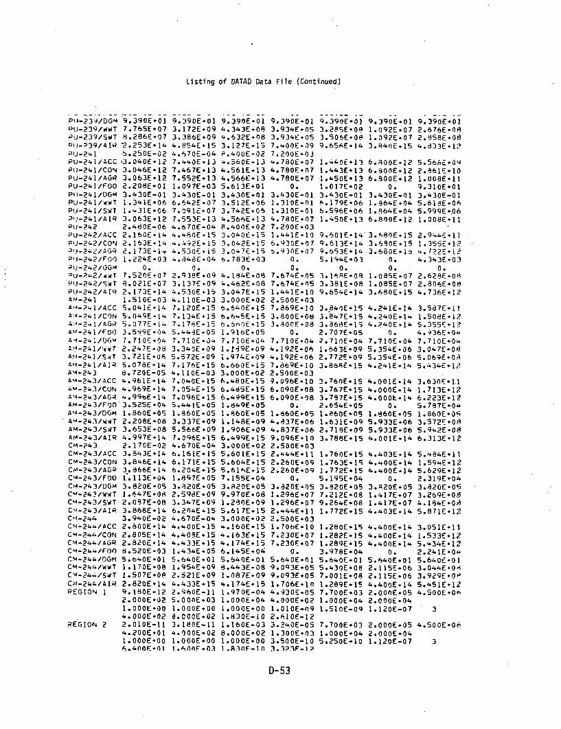
Listing of DATAD Data File (Continued)

PII-239/DGM 9.390E*01PUJ-239/WWT 7.765E.07PU-239/SWT 8.286E÷07D",-'39/AIR '2.253E*14PU-241 .5.250E-02PU-241/ACC 3.040E÷12PI)-241/CON 3.046E-12PU-241/AGR 3.063E*12PU-241/F00 2.208E-01PI,-241/DGM 3.430E-01PU-241/WWT 1.341E-06PU-241/SWT 1.431E0G6P!j-241/AI 3.063E.12PU-242 2.480E-06PU-242/ACC 2.160E.14PlJ-242/CON 2.163E-14-),.I- 2i 2 /AG 9 2.173E÷1.+P11-242/F00 1.224E-03

PlU-242/OG,4 0.DU-?42/WwT 7.520E-07PIJ-242/SWT 8.021E-07PU-242/AIR 2.173E-14AA--241 1.510E-03Ath-241/ACC 5.041E#14

A:x-441/CON 5.049E*14A:A-241/AGR S.377PE-!"

AM-241/FO0 3.599E*O3Ax1-2z41/06m 7. 710OE -04

A'-2411/wT 2.247E-08AM-241/SNT 3.721E*0oAl-•41/AIR 5.078E-14A4-243 8.720E-05Am-243/ACC 4.961E-14Am- 243/CON 4.969E414A'4-243/AG4 4.99bE*1'AM-243/FOO 3.525E+04A'4-243/DGM 1.860E-09Am-243/w4T 2.208E-08AN-243/SWT 3.653E*08AtA-243/AIR 4.997E-14CM-?43 2.170E-02CM-243/ACC 3.843E*14Cv-243/CON 3.846E÷14C.11-243/AGP 3..866E*14CM-243/FO0 1.113E*04Ct4-243/DGM 3.820E+05CM-2431,jWT 1.647E.08CM-243/SWT 2.087E*08C,'--243/AIR 3.868E-14CM-244 3.940E-02C%1-244/ACC 2.800E.14Cm-244/CON 2.805E#14CM-244/AGR 2.820E+14C4-24-/F0O 8.520E-03CM-244/DGM 5.b'OE+O1Cl-244/wWT 1.170E-08CM-244/SWT 1.507E.O0CM-244/AIR 2.820E#14PEGION 1 9.180E-12

2. OOGE.)22.000E.001I*OOOE*O0

4.OOOEo02REGION 2 2.010E-11

4.200E÷01I.O00EO006.400fF.n1

9.390E-013.172E+093.386E+094.854E*154.670E-047.4D0E÷137.467E +137.552E*131.097E*033.430E-016.642E-077.091÷*077.553E*134.670E-044.480E*154.492E-154.530F. i54.8~48E+04

0.2.93,2E÷093.137E-094.530E.154.110E-037.120E+157.134E*157.17AE.155.443E+057.710E-0.3.340E*095.572E+097.176E-154.11OE-037.0OE÷157.054E-157.096E#155.441E4051.860E-053.337E+095.566E.097.096E-154.67 0E-04b.161E*156.171E*156.204E.151.897E+053. i20E-052.S98E*093.347E+096.2n4E*154.670E-044."00EE-154.408E*154.433E-151.4.34E+055.640E-011.954E+092.521E*094.433E+152.960E-115.00AE.031.O00E008.0OE-023.ISOE-I14.OOOE*021.O00E-001 .601IF-03

9.390E-014.343E÷084.632E#083.127E+15F.40OE÷024.560E+134.561E+134.566E+135.613E*013.430E-013.512E+063.742E*064.566E*138.400E+023.0400E-5i3.0&2E.153.047E-156.783E#03

0.4..34E+084.462E+083.047E+ 153.OOOE.026.640E# 15b.6.5E*15

. 56.E - 151.916E.057. llO7E04I *. Z9E#091 .974E 096.660E*153.000GE026.480E.156.485E+156.499E.151.849E.051.860E+051.148E+091.906E096.499E+ 153.000GE025.60 1E.155.604E÷155.616E*157.155E+043.820E+059.970E*081.280E-095.617E.153.000E-024. 160E+154.163E154.174E+156.145E-045.640E-018.443E-081.087E-094.174E+ 151.970E-041.OOE.04I.O00E-001.830E-101.160E-038.000GE021.O00E-001 .R3AnF-In

9.390E-013.934E-053.9 34E.057.400E 097.200E+034. 780E*074.780E÷n74.780E*07

0.3.430E-011.310E-nl1.310E-014. 780E.077. 200E'031.441E-106.93GE÷07b.93OE.07

0.0.

7.674E-057.674E.051.441E-102.500E-037.869E* 103.800E÷083.80FE-08

0.7. 710E .044. 192E#064.192E-067.869E+102.500E-039.096E106.090E+086.090E.08

0.1.860E*05'.'37E*064.837E+069.096E*102.500E-032.444E+ 112.260E+092. 260GE+09

0.3.820E+051.296E.071.296E.072.444E-I I2.500E+031.70bE-107.230E*077.230E.07

0.5.640EOlI9.Oq3E.059.093E4051.706E.1l4.930E-054.000E+02I.OIOE-092.610E-123.240E-051.300E-033.500E-103.3?3F-I?

9..390E+013. 285E-.93.506E+089.65E.* 14

1.440GE+ 131 .443E* 131.450E*131.017E*023.430E-01A. 179E*06b.596E+061.450E-13

9.601E149.613E.149. 653E 145.14'E-03

0.3. 168E-083.381E*089. 654E- 14

3. 841E4153.847E-153.868E152.707E-05W.710E041.663E092.772E*093.869E*15

2.760E*153. 767E* 153.787E*152.654E-051 .60E*051.631E-092.718E+093.788E-15

1.760E.15I .763E*191.772E*155.195E-043.820E*057.212E*089.264E*081.772E.15

1.280E-15I .282E- 151.289E-153.978E*045.640E-015.430E-087.001E+081.289E+157.70oE+031 .OOOE041.510E-09

7.700E-03l.OOOE045.250E-10

9.390E÷011.092E+071.3 92E+073.4R0E) 15

6.AOOE.126.800E*126.SOOE-12

0.3.430E-01I .,364E -041.864E-046.8n0E*12

3.680E.153.6S0E.153.680E. 15

0.0.

1 .08SE.071.085E+073.680E+15

4.241E-144. 24 OE.* 14.4.p4OE 14

0.7.710E.045. 354E- 065.354E-064. 241E - 14

4. 0 1E.+ 144.OO0E-144.000G + 14

0.1.860E*055.933E-065.933E#064.00IE-14

4. 40 3E * 144.400E+144.4 0 OE - 14

0.3.P20E*051.417E*071.417E+074.403E+14

4.400E144.400E+ 144.400E* 14

0.5.640E*012. 115E*062.1 15E.064.400E+142.00nE.052.000E.041. 120E-07

2.00GE.052.000E+041.120E-07

9.390E-012.676E+082.858E-084.833E * 1;?

5.56,E. 092.861E-101.008E+119.310E÷013.430E-015.61 8E-065.99qE÷.061 . OOBE. 11

2.944;E-111.35SE.124.722E-1?

4.343E-03

0.2.628E-OA2.806E-084.736E-12

3.587E-1 I1.50EE-125.355E+1'?4. 936E-0'.7. 710E*0'3. 047E-08S. 069E.0'5.434-E*I

3.630E 1.11.713E*126.223E*125.787E-0"1.860E+093.572E+085.942E-086.313E+12

5.484E+1 I1.594E-125.629E*122.319E+o03.820E*053.269E.084. 184E+085.8 7E-12

3.051E-1 I1.533E÷1I5.434E.122.241E÷0"5.64C0E-013.044E+0O43.929E40P5.451ElEI14.500E*Oh

3

4.500E-06

3

D-53

Listing of DATAD Data File (Continued)

PEGIO'q 3 2.510E-111. 40OE021oO 00E001.600E402

REGIONi 4 2.640E-101.500E#011.OOOE0O

- 8.OOOE*00qEGION 5 2.010E-11

3.200E+011.O00EO006.400E+01

PEGIOtp 6 2.010E-119.200E-011 . OOOE-00b.400E01

3.280E-112.90OE-031 . OOOE*008.oooE-028.060E-1 I3.0OOE-021.300-O008.000E+023.180E-113.90OE-02I .OOOE-00I.O00EO033. ISOPE- 114.500E-021 . OnnE.00I.tOOE-03

9.OUOE-05 2.250E-055.OOE03-4.000E.021.O00Eo00 3.860E-101.830E-10 2.550E-121.j30E-06 3.250E-07bOO0OE-02 1.300Eo031.O00E400 2.660E-111.830E-I0 1.790E-121.160E-O4 3.240E-067.900E-02 1.300E-03I.OOOEO00 3.030E-101.830E-10 3.323E-121.160E-02 3.240E-048.SnO0#02 1.300E-031.OOE.-00 3.03]E-1O1.830E-10 3.323E-12

7.770E*011.250E-045.790E-10

7.700E-033.O00O0E43.990E-I I

7.700E*03I .OOOE-044.550E-10

7.7OnE.03I .OOnE04'..550E-l1l

2.000E.05 4.500E+062.500E-041.120E-07 4

2.oOOOE0S 4.500E-066.O00QE-01.120E-07 2

2.OOOEo052. OOOE04-1.120E-07

4.500E-06

2

2.OOOE-05 4.500E-062.0OOE.041.120E-07

D- 54

Ll '. t 10 1 -1 It I W1 '- 1141,1 111 e

H-3H-3H-3H-3H-3

H-3H-3

H-31C-1C-1C-.C-1

C-1C-IC-1C-1C-1

FE-FE-FE-FE-

36 23 1.00 .125.630E-02

/ACC 1.252E*09/CON 1.172E-Io/AGQ 4.4SIE*IO

* /FOO S,95qE*04/DGm 0./w4T 2.367E+06/SmT 2.36dE-06I/AIR 4.451E-10

4 1.210E-044 /ACC 3.166E-094 /CON 6.678E.I0I /AGR 2.660E+114 /FOO 3.721E+054 /DGM 0.4 /WWT 1.441E-074 /SWT 3.761E+074 /AIQ 2.660E-1195 2.670E-O155 /ACC 1.805E-1055 /CON 4.283E+09-5i /AGP 3.219E+10-55 /FOO 3.482E+01

FE-55FE-55Fr-55

4I1-934NI-q9ý41-59

NI-59NI-54NI-59

NI-59NI-59

CO-60CO-60CO-60CO-60CO-60Go- 60CO-00CO-60NI-63NI-63NI-633

NI-63NI-63NI-63NI-63NI -63NI-63

N!-94NB-94NS-94

.48-94N9-94

NR-194NB-94NB-94SR-90Sr ;- Q

/OGM

JSWT/AIR

/ACC

/CON/AG,?/FO0/DGM/WWT/SWT/AIR

/ACC/CON/AGR/FO0/DGM/WIT/SWT/AIR

/ACC/CON/AGR/FO0/DGM/wwT

/AIR

/ACC/CON

/FO0/DGMIWWT/SWT/AIR

/ACr

0.2.727E.0b'4.450E+~064.827E-I10

8.6BOE-063.698E-I03.8Z2E10I .24 7E* II3.693E.036.200E.038.537E÷+O9.825E+06I .505E +II1.320E-012.358E*121.237E*l13.695E+II5.274E+031.540E+071.432E.0B1.458E#082.683E*127.530E-033.056E- 101 .040E* 113.341E II9.878E+03

0.1.915E*072.260E*073.341E+ I13.470E-056.102E-II1.389E.I01.399E-I02.116E.o09.630E*063. 193E+073.232E 076. 103E*112.470E-022.41 7F#1 1

.06 .031.150E-b0

5.190E*07S. 190E.07

0.0.

1 .422E-0oI .422E-0 I5.190E+015.760E-031 .405E 103.321E+ II1.328E-IeI .'361E.Oh

0.7.205E*071.R88OEOM1 .328E*I?1.480E-OeI.985E-10i.816E. 101 .903E. 112. 161E-02

0.1 .244E.+()72.314E-072.064E.1 1I .480E-O?9.378E. 102.325E +II7.476E+II2.211E.O6.200EOJ4.425E+075.196E-077.733E. 11I .480E-022.336E.122.280E.102.280E10

0.1 .540E.071.238E.081 .238E.0"2.336E*121 .480E-029.602E. 113. 150E. 121 01. E*I132.945E#O5

0.5.71 IE*086.738E*08I.OOIE* J1 .1lOE-026.114E I I1.515E+ 101.54AE.1O7.07AE÷009.630E*063.196E*073.324E.076.119E.I I9.860E-OJ9..h17F-I I

1 0 1 . . I.'

* ,JJ*,Il * l'.

I4 .I1l * |,

* II,I * 0 ,11 * )II

,'. I t..f • *

#,*W',I •0 Ill

,?. 1" I it

I. I. I.t,* ,il*

I.,7'.II ,.1

?. I 'll ,I

?.,4 IIt .01

I..I s•o |II

SI.. * , I . II

I I * II

?i*.If, It * lie,

6.4lit,. .It

I . Ill "I I*i (3,Il *| el'1

'4 . N 1 i1 1)t

0 ,.ot o I I

I II*'.',OIt .* li

I.lt .It 1

I .S'.0t Oilw

, *I0140 I .'

1)*?, I'+1 * I

/. I ~.I * II194.•sJ III *•II

'4. tr, tt •.1 IC, .'i ll V* It

1 1(1 *I) ,

I * .'.I *~ .||I .UI /.II *I In

I .1",,.I .t| II . ,ei'l.,* ll0.1111 *I ll

'9. 0'lfl . Ill*I.hPt,* I -II

*. J6 1

a-I .1 1.00

I , r)1 Il" roqI I,/',,:1' ,CO

*. *'i',t * 04

00

,.It, Ill .~f,

I. I '.t .10'..A, ltl . CO•*' C.•,,I • IIl

(I,I I... to * 10

I.1'II,| .0,

0* 1',lt A I I

' 0 I ') t *( 0*l.'lI~t . 0 7

**..'II Iflt .07of

0.

91 . 1 1hiJ 1 o

'.mi II -I0* *. icltl * Cf

*' *9t109 * |0)

*,IDI1t AN0

•* .. 0t1 I) I

I Sr I * I)P 401'I *- 1

,O. IlrOl * 10SA. I'of • A 0

, *.'O .100.

I.I'4nt .fllI ,1 INI' *flI

*. I.~9 *)I•

1,%o~t .03l

I .',At .AM

0.

h. e -) I

I P~'.t .0n4I .000t.'04

*.I~. III. I*,OI. .IC)1 . 101 - to

0.A., lot . nh

I •l,' - 07i -)?t .0)7

01. O4Lht * l7. 1on09.0nI .AAMI . 9t

1.252E+09I. 172E÷ 104.51E*10S.995E-04

0..3f7E * 06

?.368E-064.451E10

3. 166E+09h.678E'11)?. 660E *II3.721E*05

0.

1.441E-073. 7,TE+07*J1 h66E - I11

1 .613E+101. 0SOE*07S.0110E-07

0.0.

.8609E*054.6OgEý05

1.61 3E- 10

/.57HF -10

n.h.?WOE03

I. 177f* 061.3177L'0o

?.S7HF. 10

?. 336F -12?.?HOE*IOA..?tioE. 10*.180E .10

0.1.5109E#07I.?JPE#08

?.336E-12

I .560E.08.,560E-08

0.0.

4.27fE-0I4.27hE-011.60E•0O

h.10792.11I.446Eo101.464E92I0

. 892E*009.630E*063.1 94E:073.?65E+07b.1 1lIE*ll

I .h1,A9F.lI1

1.252E+091.172E*104.451E.105.995E.04

0.2.367E4062.368E-064.451E+10

3.166E*096.678E102.660E+113.721E+05

0.I.441E073.761E+072.660E+11

2.081E-1I2.095E*112.644E+118.331E+01

0.5.326E+069.449E*062.i04E+I1

5.778E#103.206E.103.206E-10

0.6.200E*031.377E40b1.377E*065.778E410

2.634E*132.402E*132.402E*13

0.1.540E*071.239E*081.239E÷082.634E*13

8.316E.108.816E÷108.816E+10

O00.

2.4lbE.022.4169E028.816E+10

1.330E9127.332E9117.332Eo11

0.9.630E+063.192E9073.192E*071.330E.12

5.190E*071.052E+104.331E*105.995E+04

.0.2.3675E062.368E+064.331E.10

2.526E-096.614E*102.654E9113.721E*05

0.1.4.1E+073.761E*072.654E11

1.925E.lO2.116E+107.752E+108.566E+01

0.5.452E2069.692E+069.36092.10

2.850E-101.441E9 1)5.082E9101.563E9036.200E+034.408E-064.953E*067.654E÷.0

2.504E-128.593E.112.953E+124.492E*041.540E9072.893E#083.112E-045.266E*12

7.436Eg093.91,IE*Io1.383E*l14.259E#03

0.8.258E#069.743E*061.383E*11

6.839E-114.432E+111.557E9122.390Eo049.630E*061.466E9084.496E+092.153E9212

I.qtlnF.11 1.g9?F.11

Listing of NUCS Data File (Continued)

SP-90 /CONSR-90 /AGRSR-90 /FOOSR-90 /DGMSR-90 /WVTSR-90 /SATSQ-90 /AIRTC-99 I

TC-99 /ACCTC-99 /CONTC-99 /AGqTC-99 /F90TC-99 /DGMTC-g9 /WWTTC-99 /SWTTC-99 /AI[1-1291-129 /ACC1-129 /CON1-129 /AGR1-129 /FOO1-129 /DGM1-129 /WWT1-129 /SWT1-129 /AIRCS-I ';CS-133/ACCCS-I 35/CONCS-135/AGPCS-135/FOOCS-135/DGMCS-135/WWTCS-135/SWTCS-I35/AIRCS-137CS-137/ACCCS-I 37/CONCS-137/AGRCS-137/FOOCS-i 37/DGMCS-137/WWTCS-137/SWTCS-] 37/AIRU-235U-235 /ACCW-235 /CONIJ-235 /AGRIJ-235 /FOOU-235 /OGMU-235 /WWTU-235 /SWT'U-235 /AIRU-23,IJ-238 /ACCU-238 /CONU-238 /AGRIJ-?38 /FOOUJ-238 /OGMU-238 /WWTU-238 /SWTU-238 lAIRNP-237NP-?37/ACCNP-237/CONNP-237/AGP

6.394E*131.891E*146.407E+073.060E-049.564E-091 .014E*101 .892E÷ 143.270E-061. 176E÷092.960E+098.548E096.566E-03

0.4.186E-054.240E÷058.548E+094.080E-089. 139E- 112.068E+12d.346E126.019E-041.920E*044.289E+074.369E*079. 197E+ 122.31 GE-072.371E 101.566E- 115.729E+ 118.836E-03

0.3.318E-071.442E408S.729E* I12.310E-024.499E +II1.397E-125. 117E+127.896E-043.500E-063.094E+081.302E-095.358E+129.760E-102.062E+122.643E. 125.154E*121.443E+041.500E-052.073Eo082.109E-085.374E. 121.540E-101.695E+122.429E* 124.774E+ 121.348E*045. 160E-031.835E+081.868E*084.789E- 123.240E-075.202E-145.209E- 145.238E-14

2.588E*147.686E +142.61 1E÷08.3.060E-043.895E. 10,.12PE-107.68E+E 141. 150E-019.680E.085.41 1E.091.933E.101 .63.5E+04

0.1.042E.061.056E-061.933E10I.1SOE-018.515E1I17.124E- 112. 942E- 122.137E-041.920E+041.758E÷071.793E÷073.792E*121.620E:049.651E#104.209E*I I1.437E-122.157E+04

0.8.09HE-073.520E.081.437E+121.620E-046.339E+111.7 19E+125.872E+128.814E-043.500E+063.438E*081.452E-096.112E*121.250E-043.062E#134.36 1E. 138.500E.132.37BE-051.500E-053.235E.093.294E*098.522E-131.250E-042.882E*134.145E.138.108E+132.277E*055.160EG033.087E*093. 144E*098.109E+134..670E-041.200E-161.202E-161.209E.1b4. A67F. 05

1.760E.091.760E+09

0.3.060E048.835E*068.835E*061.668E-112.OOOE002.280E+098.890E*092.9bOE.102.433E+04

0.1.551E+061.571E+062.960E*102.O0OEO00

6.123E- 112.528E- 121 .836E-041.920E-041.562E+071.592E-073.379E*128.500E-018.851E- 103.879E+ 111.326 E-121.991E.04

0.7.475E-073.250E+081.326E,128.500E*017.779E*i I2.351E- 128.030E+ 121.205E.053.500E+064.655E-081.981E.098.270E-128.400E+022.214E- II1.590E-091.59uE*09

0.1.500E-051.177E.071.177E*072.214E*118.400E*021 .454E*108.570E*078.570E+07

0.5.160E-037.739E*057.739E+051.454E.103.000GE021.120E-151.122E+151.128Eo15

1.761.76

3.068.836.831.665.007.607.607.60

2.082.087.605.005.121.625.554.721.923.083.166.557.205.085.085.08

1.391.395.08

OE-09 1.760E-090E+09 1.760E-090. 0.OE04 3.060E-04

35E-06 8.835E-065E-006 8.835E+0658E+11 1.668E#11OE.00OE.08 1.996EF10)OE*08 1.031E+11,OE*0B 3.636E*1i0. 3.061E-050. 0.'3E-00 1.951E*073E-00 1.976E*070OE÷08 3.636E-11OE-00RE-13 8.515E-1l'4E*15 1.315E+123E-15 5.433E+125E*07 3.947E*040E*04 1.920E-04IE-10 2.938E-07OE.10 3.004E*074E-15 6.284E*12OE+02OE-08 3.331E#10OE-08 I.466E+11OE.08 5.014E*110. 7.531E*030. 0.2E.nf 2.828E-072E400 1.229E÷08OEo08 5.014E-11

3.296E-103.296E-10

0.3.060E+04B.q35EO68.835E÷061.980E-11

7.400E+097.962E.099.720E÷092.067E*03

0.1.318E#051.335E-059.721E+09

8.572E-116.366E+096. 366E-09

0.1.920E043.644E-063.644E+0b8.572E+11

1.491E*104.884E.101.551E +I12.256E.03

0.8.472E-063.683E.071.551E-1l

3.299E.1#12.941E l119.350E +111.160E.043.500E-066. 394E+072.349E-081.175E -12

3.360E÷153.360E.153. 360E. 15

0.1.500E052.098E.072.098E+073.360E+15

3. 120E* 153.120E.153.120E+15

0.5. 160E-039.325E.069.325E+063.120E+15

3.602E#143.600E+ 143.600E+14

n .

4.727E*121.946E+137.543E*063.060E-041. 134E.-01.201E-091.962E.13

7.880Eo092.240E+1 I9.008D*E17.953Eo05

0.5.069E*075.135E#079.008E#11

8.l521E' I9.787E* 104.006E*1 I2.901E+031.920E-045.536E*065.584E*061.251E.12

I.O0O4EOQ8.007E-092.99'E-I04.656E*02

0.1.74 8E. 067.600E#062.994E-10

2.444E*l 13.919E101.491E -112.333E-033.500E÷062.163E#075.096E-073.895E.1 1

5.175E*1I1.586E*125.621E*122. 319E*0'1.500E*053.261E°083. 318E#085.841E*12

2.546E 1*1

1. 147E. 123.989E +121.633E*045.160E-032.221E*082.262E.084.003E-12

3.7'0E.I I1.550E÷1:5.652E*12

P.IS7F#fl4

7.200E+022.'619E I11.530E*091.530E+09

0.3.500E.061.287E-071.287E.072.419E -117.200E-032.214E+1 I1.590E*091.590E+09

0.1 .500E*051.177E*071. 177E-072.214E*1 I7.200E-031.454E+108.570E+078.570E+07

0.5. 160E.037.739E+057. 739E+051.454E.102.500E+031. 340E- 1I8.400E-088.400E-08

0.

4.259E* I18.0 1fE*l I2.729E*1?4.092E*043.500E*061.665E-086.808E.082.969E- 12

7.262E+ 121.013E#131.979E-135.552E+041.500E+057.643E.087.781E+082.001E.13

b.575E-129.447E*121.849E*135.196E.045. 160E-037.050E*087. 179E-081.850E*13

3.840E* 153.847E+153.868E* 15I .PPIF.or,

NP-P17/FnA 1.645F,04

D- 56

Listing of. NUCS Data File (Continued)

NP-237/DGM 6.560E-04 6.560E04 6.560E+04 6.560E÷04 6.560E+04 6.560E÷04 6.560E-04NP-237/WWT 2.312E-08 5.546r-.9 4.885E+08 7.126E-06 1.674E-O9 8.113E÷06 3.263E*ORNP-237/SWT 2.572E*08 6.189E+09 5.443E+08 7.126E+06 1.867E09 a.113E+06 3.635E+08NP-237/AIR 5.239E÷14 1.209E.16 1.12.IE'15 1.340E+11 3.86AE-15 3.602E-14 5.785E+12Pil-238 8.020E-03 4.670E-04 8.400E*02 7.200E.03PUJ-238/hCC 2.OOOE.14 "o.OOE-15 2.80CE,15 1.924E.10 8.,01ElE14 4.0oE.15 3.313E1l1PtU-238/CON 2.003E+14 4.O91E-I5 2.802E-15 8.1ý70E-07 9,Sl2E*14 4.n8OE-I5 1.514E+12

PIJ-238/AGP 2.012E*14 %.126E+15 2.807E-15 8.870E+07 8.850E14 4.0806415 5.277E+12PU-238/F00 1.137E+03 4.522E÷04 6.371E.03 0. 4.868E-03 0. 4.S55E*03PIJ-23:/OGM 1.930E÷01 1.930E*01 1.930E01 1.930E÷nl 1.930E-01 1.930E-01 1.930E-01PIJ-238/WWT 7.019E+07 2.741E*09 3.931E+08 1.025E.n6 2.972E*OR 1.221E+07 2.940E*09PU-23;/SWT 7.485E+07 2.926E.09 4.192E+08 1.025E06 3.171E+08 1.221E+07 3.139E.0OPU-P38/AIR 2.012E+14 4.126E-15 2.807E15 1.924E÷10 8.850E*14 4.O80E+1S 5.297E+12PIJ-239 2.340E-05 4.670E-04 8.400E+02 7.200E.(3Pu-219/ACC 2.240E14 4.8O0E+15 3.120E*15 7.400E+09 9.601E-14 3.804oE15 3.034E11Pli-239/CON 2.243E÷14 4.813E+15 3.122E-15 5.170E.07 9.613E-14 3.840E*15 1.392E*12DI-23'/AGQ 2.253E14 4.854E-15 3.127E-15 5.170E.07 9.659E14 3.840E+15 4.826E+12oij-..3g/FrO) 1.270E-03 5.234E.04 7.04;E-03 0. 5.393E*03 0. 4.42;E*03PU'-23g/DGA 9.3qOE-01 9.390E-01 9.390E01 9.390E-01 9.39AE-0O 9.390E-01 9.390E.01PU-23Q/WWT 7.765E.07 3.172E-09 4.343E+08 3.934E-05 3.285E-08 1.092E-07 2.676E-08PU-239/SWT 4.266E+07 3.38AE-09 4.632E-08 3.934E+05 3.506E*OA 1.092E*07 2.858E+O0PiJ-239/AIR 2.2S3E+14 4.854E+15 3.127E-15 7.400E-09 9.656E+14 3.840E+15 4.833E*12P'J-241 5.250E-02 4.670E-04 8.400E02 7.200E+03PIJ-241/ACC 3.040E+12 7.44IE-13 4.560E+13 4.780E+07 1.44OE1i3 6.800E-12 5.568Eo09PIJ-241/CON 3.0468E12 7.467E+13 4.561E+13 4.780E+07 1.443E+1I 6.900E+12 2.861E+10DU-241/AGQ 3.063E-12 7.552E÷13 4.566E+13 4.780:÷07 1.450nE13 6.800E-12 1.008E-11PU-241/FOO 2.208E+01 1.097E403 5.613E-01 0. 1.017E602 0. 9.310E-01P'j-241/DGM 3.430E-01 3.430E-01 3.430E-01 3.430F-01 3.430E-01 3.430E-01 3.430E-01PJ-241/wWT 1.241E÷06 6.6426E07 3.512E÷.61.310E-01 6.179E÷06 1.9646E04 5.b186E06PU-241/S5T i.431E#06 7.091E-07 3.742E-06 1.310E-01 6.596&E06 1.64•.0O4 5.999E*06PU-24l/AIR 3.063E612 7.553E.13 4.566E-13 4.780.E07 1.450E*13 6.i0OE÷12 1.008E+11PIJ-242 2.480E-06 4.670E-04 8.400E+02 7.200.E03P.J-242/ACC 2.160E-14 4.480E.15 3.040E615 1.4416E10 9.601E614 3.680E.15 2.944E+11OU-P42/CON 2.163E614 4.492E615 3.042E*15 6.930E+07 9.613E614 3.680E+15 1.355E612PU-2'2/AGR 2.173E-14 4.530E+15 3.047E.15 6.930E+07 9.653E-14 3.680E-15 4.722E-12PI.i-242/FOO 1.224Eo03 4.848E.04 6.783E*03 0. 5.194E*03 0. 4.343E+03PU3-242/OGM 0. 0. 0. 0. n. 0. 0.PU-242/WWT 7.520E+07 2.938E#09 4.184E.08 7.674E.05 3.168E+08 1.085E607 2.628E60OP!J-242/SWT 8.021E*07 3.137E609 4.462E+08 7.674E6.05 3.381E+08 1.085E*07 2.806E*08PU-242/AIR 2.173E÷14 4.530E#15 3.047E.15 1.4416E10 9.654E*14 3.680E615 4.736E612A!1-241 1.510E-03 4.110E-03 3.000E+02 2.500E+03AM-24!/ACC 5.041E+14 7.120E*15 6.640E-15 7.8696.10 3.840E*15 4.241E*14 3.587E+11AM-241/CON 5.049E614 7.134E*15 6.6456E15 3.800E608 3.847E+15 4.24nE*14 1.508E612AM-241/AGP 5.077E-14 7.176E+15 6.660E615 3.800.E08 3.868E*15 4.240E-14 5.355E*12AM-241/FOO 3.599E.04 5.448E+05 1.916E605 0. 2.707E+0S 0. 4.936E-04AM-P41/DG'4 7.710Eo04 7.710E60O 7.710E604 7.710E.04 7.710E-04 7.710E+04 7.710E604AM-241/WWT 2.247E-08 3.340E+09 1.189E609 4.192E-06 1.663E*O9 5.354E+06 3.047E-08AM-241/SWT 3.721E608 5.572E-09 1.974E+09 4.192E.06 2.772E*09 5.354E606 5.069E#08IM-241/AIP 5.078E÷14 7.176E-15 6.660E*15 7.869E.10 3.868E-15 4.241E14 5.434E*12APA-243 8.720E-05 4.110E-03 3.OOOE-02 2.500E03A4-243/ACC 4.961E*14 7.040E.15 6.480E.15 9.096E.10 3.760E+15 4.001E+14 3.630E+11AM-243/CON 4.969E614 7.054E+15 6.485E.15 6.090E.08 3.767E+15 4.000E614 1.713E612.Am-?43/AGR 4.996E-14 7.096E.15 6.499E+15 6.090E.08 3.787E+15 4.000E+14 6.223E*12AM-243/FOO 3.525E604 5.441E+05 1.8496E05 0. 2.654E-05 0. 5.787E#04AM-243/OGM 1.860.E05 1.860E05 1.860E605 1.860E605 1.860E05 1.8606E05 1.860E+05AM-243/WWT 2.208E+08 3.337E.09 1.148•E09 4.837E.06 1.631E-09 5.933E606 3.572E-08AM-243/SWT 3.653E-08 5.566E.09 1.906Eo09 4.837E.06 2.718E*09 5.933E606 5.9'2E*08AM-243/AIR 4.997E614 7.096E615 6.499,E15 9.096E.10 3.7a8E+15 4.001E+14 6.313E+12C-4-243 2.170E-02 4.670E-04 3.0006E02 2.S00E-03CM-243/ACC 3.843E*14 6.1blE.I5 5.601E615 2.444E+11 1.760E615 4.403E+14 5.484E+11CM-243/C0N 3.846E-14 6.171E#15 5.604E615 2.260E609 1.763E-15 4.400E-14 1.594E612Cm-243/AGP 3.866E614 6.204E-15 5.616E-15 2.260E÷09 1.772E615 4.400E*14 5.629E-12CM-243/FOO 1.113E04 1.897E-05 7.155E+04 0. 5.195E-04 0. 2.319E604CM-243•DGM 3.820E-05 3.820E÷05 3.820Eo05 3.820E605 3.A20EOE5 3.920E*05 3.820E+05CM-243/WWT 1.647E608 2.598E09 9.970E*08 1.296E*07 7.212E-08 1.417E*07 3.269E608rm-•i/IWT -. fl87F*A A.T47F.ng ).?AF+.F9 I.PY6F+f7 Q.?6A4F.OA 1.417F407 4.184F.*A

D- 57

Listing of NUCS Data File (Continued)

Cm-?43/AIP 3.868E.14CM-244 3.940E-02C4-24./ACC 2.800E*14CM-244/CON 2.805E*14CM-244/AGQ 2.820E+14Cm-244/FO0 8.520E-03CM-;)4z/DGM,5.6"OE-01C.M-?.4/WWT.j.I7OE*08

CM-244/ST.jI.SO7E+OCM-244/AlR 2.820E*14PEGION I 9.180E-12

2.0O0E+02I.OOOE÷004.00OE÷O?

REGIO-I 2 2.010E-114.200E-01I .O00E006.400E*01

PEGTOm 3 2.510E-111.400E-02I.O00E001.600E-02

PEGIO•m 4 2.640E-1O1.500E-0I1.OOOE-008.000E+90

Q EGIO1" 5 2.010E-113.200E-01I .COO 0E -0 00.400E-01

PEGI(Th 6 2.010E-119.200*011 .000E.006...3CE.G1

6.2 0'.E15

4.b70E-044.400E+ 154.408E*154.433E+151 .434E*0)5

2.521E÷09,4.433E*152.960E-1 15.OO0E.031.OOOE.008. 000E023. 1b0E-1 I'..OOOE*02I.*OOE*001.600E-033. OE-I I2.)OIE.031.OOOE-008.000E.028.060E-113.000E-021.OOOE+008.000E-023.18nE-113. 00÷E 021.OOOE-001.600E-033.1HnE-l1,,0SGE *021 .OOE+001.600E÷03

5.617E÷153.000E-024. 160E.154.163E*15

-4.1I 74E. 156. 145E.045.640E*018.443E-od41. 087E*094.1 74E. 151.970E-04I .OOOE041.OOE.001.930E-101. 160E-038.000GE02I .000E-001.830E-109.OOE-055. i80 E*-031 . OOOE-001.830E-101.300E-06b.000E-02I .OOOE-001.830E-101. 160E-047.900E.021.OOnE-001.330E-101. 1 60E-02

O.50OE-021 .O00E.001.830E-10

2.444E.2.500÷E031.706E-107.230E-07.7.230E.07

0.

9. 093E-059.093E÷051.706E#104.930E-054.O00E+021.01OE-092.610E-123.24OE-n51.300E+033.500E-I03.323E-122.250E-054. 006fF. .0?3.360E-102.550E-123.250E-071.300E+032.660E- 111.790E-123.240E-061.30CE.033.O1OE-103.323E-123.2"O0-041.300E-033.030E-103.323E-12

1.772E-15 4.40.3E-14 5.871E-12

1.280E#151.282E*I51.289E*153.978E*045.650E-015.430E.087.001E-081.289E*157.700E*03-1.OOOE*041.510E-09

7.700E-01I .OOOE.045.250E-10

7.770E#011.2tNEO045.79()E-10

7.700oE013.00GE-043.99nE-1 1

7.70 E.031 OOCE-044.550E-1l

7.70onE-031 .00rE*04-. 550E-10

4.400E-14 3.051E#114.4OOE*14 1.533E*124.40oE-14 5.434E+120. 2.241E04

5.A4OE.01 5.640E.012.115E-06 3.04E+042.11SE-Ob 3.929E.084.400E-14 5.451E.122.000E05 '.500ESO.02.000E+041.120E-07 3

2.OOE.05 4.500E+062.000E*041.120E-07 3

2.nooE.05 -. 500E.062.730E-O01.120E-07 4

2.0OOE.05 4.SOOE.OA6.00GE-041.120E-07 2

2.OOOE+05.0.500E+062.000E-O"1.120E-07 2

2.OOOE+05 4.500EO062.OOE+041.120E-07 4

D- 58

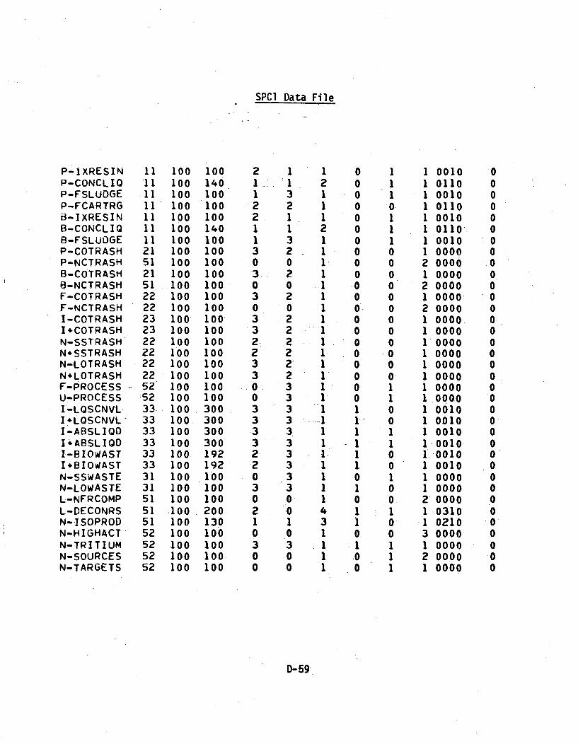
SPCI Data File

P-iXRESIN 11 100 100 2 1 1 0 1 1 0010 0P-CONCLIQ 11 100 140 1 1 2 0 1 1 0110 0P-FSLUDGE 11 100 100 1 3 1 0 1 1 0010 0P-FCARTRG 11 100 100 2 2 1 0 0 1 0110 0B-IXRESIN 11 100 100 2 1 1 0 1 1 0010 0B-CONCLIQ 11 100 140 1 1 2 0 1 1 0110 0B-FSLUOGE 11 100 100 1 3 1 0 1 1 0010 0P-COTRASH 21 100 100 3 2 1 0 0 1 0000 0P-NCTRASH 51 100 100 0 0 1. 0 0 2 0000 .08-COTRASH 21 100 100 3- 2 1 0 0 1 0.000 0.B-NCTRASH 51 -100 100 0 0 1 0 0 2 0000t 0F-COTRASH 22 100 100 3 2- 1 0 0 1 0000 0F-NCTRASH 22 100 100 0 0 1 0 0 2 0000 0I-COTRASH 23 100 100 3 2 1 0 0 1 0000. 0I+COTRASH 23 100 100 3 2 1 .0 0 1 0000 0N-SSTRASH 22 100 100 2. 2 -1 0 0 1 0000 0N+SSTRASH .22 100 100 2 2 1 0 0 1 0000 0N-LOTRASH 22 100 100 3 2 1 0 0 1 0000 0N+LOTRASH 22 100 100 3 2 1 0 0 1 0000 0F-PROCESS 52 100 100 -0. 3 1 0 1 1 0000 0U-PROCESS :52 100 100 0 3 1 0 1 1 0000 0I-LQSCNVL 33- 100 300 3 .3 1 1 0 1 0010 0I+LQSCNVL- 33 100 300 3 3 - -1 1 0 1 0010 0I-ABSLIOD 33 100 300 3 3. 1 1 1 1 0010 0I+'ABSLIQD 33 100 300 3 3 1 1 1 1 0010 0I-BIOWAST 33 100 192 2 3 1 1 0 1-0010 0I1BIOWAST 33 100 192 2 3 1 1. 0 1 0010 0N-SSWASTE 31 100 100 0 3 1 0 1 1 0000 0N-LOWASTE 31 100 100 3 3 1 1 0 1 0000 0L-NFRCOMP 51 100 100 0 0 1 0 0 2 0000 0L-DECONRS 51 100 200 2 0 4 1 1 1 0310 0N-ISOPROD 51 100 130 1 1 3 1 0 1 0210 0N-HIGHACT 52 100 100 0 0 1 0 0 3 0000 0N-TRITIUM 52 100 100 3 3 1 1 1 1 0000 0N-SOURCES 52 100 100 0 0 1 -0 1 2 0000 0N-TARGETS 52 100 100 0 0 1 0 1 1 0000 0

D-59

SPC2 Data File

P-IXRESIN 11 100 165 1 1 3 0 1 1 0210 0P-CONCLIQ 11 600 182 1 1 3 0 1 1 4210 0P-FSLUDGE 11 100 165 1 1 3 0 1 1 0210 0P-FCARTRG 11 100 100 1 1 3 0 1 1 0210 0B-IXRESIN 11 100 165 1 1 3 0 1 1 0210 0B-CONCLIQ 11 240 156 1 1 3 0 1 1 4210 0B-FSLUDGE 11 100 165 1 1 3 0 1 1 0210 0P-COTRASH 21 200 100 3 2 1 0 0 1 1010 0P-NCTRASH 51 100 100 0 0 1 0 1 2 0000 0B-COTRASH 21 200 100 3 2 1 0 0 1 1010 0B-NCTRASH 51 100 100 0 0 1 0 1 2 0000 0F-COTRASH 22 150 100 3 2 1 0 0 1 1010 0F-NCTRASH 22 100 100 0 0 1 0 0 2 0000 0I-COTRASH 23 200 100 3 2 1 0 0 1 1010 0I+COTRASH 23 400 100 3 2 1 0 0 1 2020 0N-SSTRASH 22 150 100 2 2 1 0 0 1 1010 0N+SSTRASH 22 300 100 2 2 1 0 0 1 2020 0N-LOTRASH 22 200 100 3 2 1 0 0 1 1010 0N+LOTRASH 22 400 100 3 2 1 0 0 1 2020 0F-PROCESS 52 100 100 0 3 1 0 1 1 0000 0U-PROCESS 52 100 100 0 3 1 0 1 1 0000 0I-LQSCNVL 33 128 300 3 3 1 1 1 1 1010 0I+LQSCNVL 33 100 300 3 3 1 1 0 1 0010 0I-ABSLIQO 33 100 165 3 3 3 0 1 1 0210 0I÷ABSLIQD 33 100 300 3 3 1 1 1 1 0010 0I-BIOWAST 33 100 192 2 3 1 1 0 1 0010 0I+BIOWAST 33 100 192 2 3 1 1 0 1 0010 0N-SSWASTE 31 100 100 0 3 1 0 1 1 0000 0N-LOWASTE 31 100 100 3 3 1 1 0, 1 0000 0L-NFRCOMP 51 100 100 0 0 1 0 1 2 0000 0L-DECONRS 51 100 200 2 0 4 1 1 1 0310 0N-ISOPROD 51 100 200 1 0 4 1 1 1 0310 0N-HIGHACT 52 100 100 0 0 1 0 1 3 0000 0N-TRITIUM 52 100 100 3 3 1 1 1 1 0000 0N-SOURCES 52 100 100 0 0 1 0 1 2 0000 0N-TARGETS 52 100 100 0 0 1 0 1 1 0000 0

D-60

SPC3 DateFile

P-IXRESIN -11. l00 200 2 0 4 0 A1 1 0310 0P-CONCLIQ 11 600 200 2 0 4 0 1 1 4310 0P-FSLUDGE 11 100 200 1 0 4 0 1 1 0310 0P-FCARTRG 11 100 100 2 0 4 0 1 1 0310 0B-IXRESIN 11 100 200 2 0 4 0 1 1 0310 0B-CONCLIQ 11 240 200 1 0 4 0 1 1 4310 0B-FSLUDGE .11 100 200 1 0 4 0 1 1 0310 0P-COTRASH 61 8000 200 0 0 4 0 1 1 6312 0P-NCTRASH 51 100 100 0 0 1 0 1 2 0000 08-COTRASH 61 8000 200 0 0 4 0 1 1 6312 0

•B-NCTRASH 51 100 100 0 0 1 0 1 2 0000 0F-COTRASH 62 4000 200 0 0 4 0 1 1 6311 0F-NCTRASH 22 100 100 -- 0 0 1 0 0 2 0000 0I.COTRASH 23 2000 200 0 0 4- 0 1 1 5311 0I+COTRASH 23 8000 200 3 0 4 0 1 1 7322 0N-SSTRASH 22 1000 200 0 0 4 0 1 1 5311 0N*SSTRASH- 22 4000 200: 2 0 4 0 1 1 7322 0N-LOTRASH 22 2000 200 0 0 4 0 1 1 5311 0N+LOTRASH 22 8000 200- 3 0 4 0 1 1 7322' 0F-PROCESS- 52 100 100 0 3 1 0 1 1 0000 0U-PROCESS 52 100. 100 0 3 1 -0 -1 .1 0000 0I-LOSCNVL 33 '452 200 0 0 4 0 1 1 5311 0I.LQSCNVL 33 100 300 3 3 1 1 0 1 0010 0I-ABSLIQD 33 100 200 0 0 4 0 1 1 0310 0I+ABSLIQD 33 100 300 3 3 -1 1 1 1 0010 0I-BIOWAST '33 1500 200 0 0 4 0 1 1 5311 0I+BIOWAST 33 100 192 2 0 1 1 0 1 0010 0N-SSWASTE 31 100 100 0 3 1 0 1 1 0000 0N-LOWASTE 31 100 100 3 3 1 1 0 1 0000 0L-NFRCOMP 51 100 100 0 0 1 0 1 2 0000 0L-DECONRS 51 1800 200 1 0 4 0 1 1 6312 0N-ISOPROD 51 100 200 1 0 4 1 1 1 0310 0N-HIGHACT 52 100 100 0 0 1 0 1 .3 0000 0N-TRITIUM 52 100 100 3 3 1 1 1 1 0000 0N-SOURCES 52 100 100 0 0• 1 0 - 1 2 0000 0N-TARGETS 52 100 100 0 0 1 0 1 1 0000 0

D-61

SPC4 Data File

P-IXRESIN 71 1800 200 1 0 4 0 1 1 6312 0P-CONCLIQ 71 800 200 1 0 4 0 1 1 6312 0P-FSLUDGE 71 500 200 1 0 4 0 1 1 6312 0P-FCARTRG 71 100 100 2 0 4 0 1 1 0310 0B-IXRESIN 71 1800 200 1 0 4 0 1 1 6312 0B-CONCLIQ 71 640 200 1 0 4 0 1 1 6312 0B-FSLUDGE 71 500 200 1 0 4 0 1 1 6312 0P-COTRASH 71 8000 200 1 0 4 0 1 1 6312 0P-NCTRASH 51 600 100 0 0 1 0 1 2 3010 0B-COTRASH 71 8000 200 1 0 4 0 1 1 6312 0B-NCTR.ASH 51 600 100 0 0 1 0 1 2 3010 0F-COTRASH 72 4000 200 0 0 4 0 1 1.6311 0F-NCTRASH 52 600 100 0 0 1 0 1 2 3020 0I-COTRASH 63 2000 200 0 0 4 0 1 1 5311 0I*COTRASH 73 8000 200 3 0 4 0 1 1 7322 0N-SSTRASH 62 1000 200 0 0 4 0 1 1 5311 0N+SSTRASH 72 4000 200 2 0 4 0 1 1 7322 0N-LOTRASH 62 2000 200 0 0 4 0 1 1 5311 0N+LOTRASH 72 8000 200 3 0 4 0 1 1 7322 0F-PROCESS 52 100 100 0 3 1 0 1 1 0000 0U-PROCESS 52 100 100 0 3 1 0 1 1 0000 0I-LQSCNVL 63 452 200 0 0 4 0 1 1 5311 0I÷LQSCNVL 33 100 300 3 3 1 1 0 1 0010 0I-ABSLIQO 6310000 200 0 0 4 0 1 1 5311 0I*ABSLIQD 33 100 300 3 3 1 1 1 1 0010 0I-BIOWAST 63 1500 200 0 0 4 0 1 1 5311 0I÷BIOWAST 73 100 192 2 0 1 1 0 1 0010 0N-SSWASTE 31 100 100 0 3 1 0 1 1 0000 0N-LOWASTE 31 100 100 3 3 1 1 1 1 0000 0L-NFRCOMP 51 100 100 0 0. 1 0 1 2 0000 0L-DECONRS 71 1800 200 0 0 4 0 1 1 6312 0N-ISOPROD 51 '100 200 1 0 4 1 1 1 0310 0N-HIGHACT 52 100 100 0 0 1 0 1 3 0000 0N-TRITIUM 52 100 100 3 3 1 1 1 1 0000 0N-SOURCES 52 100 100 0 0 1 0 1 2 0000 0N-TARGETS 52 100 100 0 0 1 0 1 1 0000 0

D-62

NRC FORM 335 1. REPORT NUMBER (,Asigned by DDC)17-77) U.S. NUCLEAR REGULATORY COMMISSION

BIBLIOGRAPHIC DATA SHEET NUREG/CR-'I759 , Vol. 3

4. TITLE AND SUBTITLE (Add Volume No.. if aprcorfau) 2. (Leave blank)

DATA BASE. FOR -RADIOACTIVE -WASTEMANAGEMENT3. RECIPIENT'S ACCESSION NO.

Impacts Analyses Methodology Report7. AUTHORIS) 5. DATE REPORT COMPLETED

0. I. Oztunali, G. C. Re, P. M. Moskowitz, E. D. Picazo, +C.J. P-itt A___g ____t 1981_ _

9. PERFORMING ORGANIZATION NAME AND MAILING ADDRESS (include Zip Code) DATE REPORT ISSUED

Dames and Moore, Inc. MONTI4 IYEAR

20 Haarlem Ave. November 1 lQR1White Plains, -NY 10603 - 6, (Leave blank)

8, (Leave blank)

12. SPONSORING ORGANIZATION NAME AND MAILING ADDRESS (Include Zip-Code)

w~ivsionof Wste anagment10. PROJECT/TASK/W ORK .UNIT NO.aDivision of Waste Management

0fficeofNuclear Material Safety and Safeguards 11. CONTRACT NO.U. S. Nuclear Regulatory Commission'Washington, D.C. 20555 FIN B6420

13. TYPE OF REPORT PERIOD COVERED (Inclusive da) sJ -

Formal I

15. SUPPLEMENTARY NOTES 14. (Leave blank)

16. ABSTRACT 2000 words or less)

This document is prepared in three volumes and provides part of the technical supportto the draft environmental impact. statement (NUREG-0782) on a proposed regulation,1OCFR Part 61, setting forth licensing requirements for land disposal of low levelradioactive waste. Volume 1 is a summary and analysis of the history of low levelwaste disposal-at both commercial and government disposal facilities. Volume 2

-provides.a summary of low level waste volumes and characteristics as projectedto the year 2000, in addition to characterizing treatment options for thiswaste. Volume 3 provides a methodology for analyzing the impacts of handlingand disposing of low level waste based upon consideration of alternative wasteforms, disposal facility design and operating practices, disposal facilityenvironmental characteristic~s, and institutional, control considerations.

17. KEY WORDS AND DOCUMENT ANALYSIS 17a. DESCRIPTORS

low-level waste waste form historyland disposal waste packaging disposal sitessocial commitment waste volumesground water migration institutional controlsinadvertent intrusion radioactive waste10 CFR Part 61 disposal technologies

17b. IDENTIFIERS/OPEN-ENDED TERMS

18. AVAILABILITY STATEMENT 19. TY C SSdTh,s report) 21. NO.OF PAGES

Unlimited 20. TsMsfd Th,, poge 22. PRICE

I O 3SNRC FORM 335 01777)

U.S. GOVERNMENT PRINTING OFFICE: 1981- 361.297:1447

Printedon recyclied

paper

UNITED STATESNUCLEAR REGULATORY COMMISSION

WASHINGTON, DC 20555-0001

OFFICIAL BUSINESS