arX

iv:1

108.

2295

v1 [

mat

h.N

A]

10

Aug

201

1 Numerical simulation of salt migration

– Large deformation in viscoelastic

solid bodies

I-Shih Liu1∗, Rolci A. Cipolatti1,Mauro A. Rincon1, Luiz A. Palermo2

1Instituto de Matematica, Universidade Federaldo Rio de Janeiro, Brasil

2CENPES/Petrobras, Rio de Janeiro, Brasil

Abstract

We consider instability of a two layered solid body of a denser mate-rial on top of a lighter one. This problem is widely known to geoscientistin sediment-salt migration as salt diapirism. In the literature, this prob-lem has often been treated as Raleigh-Taylor instability in viscous fluidsinstead of solid bodies. In this paper, we propose a successive linear ap-proximation method for large deformation in viscoelastic solids as a modelfor salt migration.

Keywords: Large deformation, viscoelastic solids, successive linear ap-proximation, boundary value problem, incremental method, numericalsimulation.

1 Introduction

The behavior for large deformation is characterized by some nonlinear constitu-tive relations, which leads to a system of nonlinear partial differential equations.To solve boundary value problems of this nonlinear system for large deforma-tion, we propose a method in a successively updated referential formulation oflinear approximation.

The method is based on the well-known problem of small deformation su-perposed on finite deformation in the literature [1]. Roughly speaking, at each

∗Corresponding author: I-Shih Liu, e-mail: liu@im.ufrj.br

1

step, the constitutive functions are calculated at the present state of deforma-tion which will be regarded as the reference configuration for the next state, andassuming the deformation to the next state is small, the constitutive functionscan be linearized. In this manner, it becomes a linear problem from one stateto the next state successively with small deformations.

Numerical simulations for elastic bodies with this method have been success-fully compared with some exact solutions for large deformations [2, 3]. In thispaper, we consider the instability of a two-layered solid body of a denser elasticmaterial on top of a lighter viscoelastic one. This problem is widely knownto geophysicists in sediment-salt migration as salt diapirism. Due to techni-cal difficulties in dealing with large deformations in solid bodies, the problemhas often been treated as Raleigh-Taylor instability in viscous fluids (see forexample, [4, 5]) instead of solid bodies.

We will show in our numerical simulation with finite element method theformation of diapirs with viscoelastic solid models. The mesh of the calculationdomain is updated as the body deforms at every step, however, up to very largedeformation we have found that re-meshing is almost unnecessary.

Remark 1:

For numerical computation of large deformations in finite elasticity, to obviatethe difficulty of handling nonlinearities, incremental methods are widely dis-cussed, for example, in the books by Ciarlet [6], Oden [7], and Ogden [8]. Thesemethods consist in letting the boundary forces vary by small increments fromzero to the given ones and to compute corresponding approximate solutions bysuccessive linearization. The general idea seems to be of purely mathematicalconcern regarding linearization between successive boundary value problems.The problems are usually formulated with domains in the initial reference con-figuration, i.e., in (total) Lagrangian formulation. This is the essential differencefrom the method proposed in this paper with “updated” Lagrangian formula-tion, namely, the reference configuration is updated to the present state at eachstep. However, we refrain from calling the proposed method as an updated La-

grangian formulation (UL), because UL formulation is widely known in numer-ical methods albeit frequently with quite different tenets (see for example [9])in which the basic equations and numerical treatment of boundary conditionsare quite different.

The present approach has an additional advantage that the assignment ofboundary data is simpler and straightforward. They are prescribed on thepresent state and the difference between prescribing the corresponding bound-ary data on the surface of the consecutive states is of higher order which isinsignificant in the linear approximation. Therefore, unlike the usual incremen-tal method in Lagrangian formulation, which needs to prescribe the incrementalboundary data on the surface of the initial reference state with values depend-ing on the deformed geometry of the body, we are totally free from any suchcomplicated concerns (see [2, 3]).

2

Remark 2:

For large deformations, systems of governing partial different equations are gen-erally nonlinear. The boundary value problems are usually formulated in ref-erential (Lagrangian) or spatial (Eulerian) coordinates, and numerical solutionof nonlinear systems of algebraic equations by Newton’s type methods. In thispaper, we formulate boundary value problems in the coordinates relative to theconfiguration at the present time. In other words, we shall describe deformationsrelative to the current configuration, instead of a fixed reference configurationin the Lagrangian formulation. Note that this is not an Eulerian formulationeither. The Eulerian coordinates are fixed coordinates in space. We shall callthis a relative-descriptional formulation [3].

The advantage of using the relative-descriptional formulation is that we canconsider a small time step from the present state, so that the constitutive func-tions can be linearized relative to the present state, and the equation of motionbecomes linear in relative displacement. When the present state proceeds intime, a nonlinear finite deformation can be treated as a sequence of small defor-mations in the same manner as the usual Euler’s method for solving differentialequations, i.e., successively at each state, the tangent is calculated and used toextrapolate the neighboring state.

The essential idea of the proposed method is based on the approach of smalldeformation superposed on large deformation [1]. Although the small-on-large

idea is very well-known, to my knowledge, numerical implementations of Euler’stype successive approximation based on this idea have not been explored.

On the other hand, computational literature based on the small-on-large

idea, typically the methods introduced in [10], [11], and [12] are very well docu-mented. Such methods, in which the nonlinear algebraic systems resulting fromthe variational formulation of the nonlinear boundary value problem are solvedby Newton’s method, employ the tangent operator obtained from small-on-largelinearization of the constitutive functions and boundary conditions. Such meth-ods are quite different from the one proposed in this paper concerning the useof the small-on-large approach.

2 The present configuration

Let κ0 be a reference configuration of the body B, and κt be its deformedconfiguration at the present time t, Let

x = χ(X, t) X ∈ κ0(B),

andF (X, t) = ∇X(χ(X, t))

be the deformation and the deformation gradient from κ0 to κt.Now, at some time τ , consider the deformed configuration κτ ,

ξ = χ(X, τ) := ξ(x, τ) ∈ κτ (B), x = χ(X, t) ∈ κt(B).

3

It can also be regarded as the relative deformation at time τ with respect to thepresent configuration at time t denoted as ξ(x, τ). We also define the relativedisplacement vector as

u(x, τ) = ξ(x, τ) − x.

Note that

∇xξ(x, τ) = ∇X(χ(X, τ))∇X(χ(X, t))−1 = F (X, τ)F (X, t)−1,

hence, we have∇xu(x, τ) = F (X, τ)F (X, t)−1 − I,

or simply asF (τ) = (I +H(τ))F (t), (1)

where I is the identity tensor and

H(x, τ) = ∇xu(x, τ) (2)

is the relative displacement gradient at time τ with respect to the present con-figuration κt (emphasize, not κ0). Moreover, by taking the time derivative withrespect to τ , it gives

F (τ) = H(τ)F (t). (3)

In these expressions and hereafter, we shall often denote a function F as F (t)to emphasize its value at time t when its spatial variable is self-evident.

In summary, we can represent the deformation and deformation gradientschematically in the following diagram:

X ∈ κ0(B)

x ∈ κt(B) ξ ∈ κτ (B)I +H(τ)

F (t) F (τ)

ξ = x+ u

3 Linearized constitutive equations

Let κ0 be the preferred reference configuration of a viscoelastic body B, and letthe Cauchy stress T (X, t) be given by the constitutive equation in the configu-ration κ0,

T (X, t) = T (F (X, t), F (X, t)). (4)

For large deformations, the constitutive function T is generally a nonlinearfunction of the deformation gradient F .

We shall regard the present configuration κt as an updated reference config-uration, and consider a small deformation relative to the present state κt(B) attime τ = t+∆t. In other words, we shall assume that the relative displacement

4

gradient H is small, |H | ≪ 1, so that we can linearize the constitutive equation(4) at time τ relative to the updated reference configuration at time t, namely,

T (τ) = T (F (τ), F (τ)) = T (F (t), 0)

+ ∂FT (F (t), 0)[F (τ) − F (t)] + ∂FT (F (t), 0)[F (τ)] + o(2),

or by the use of (3),

T (τ) = Te(t) + ∂FT (F (t), 0)[H(τ)F (t)] + ∂FT (F (t), 0)[H(τ)F (t)] + o(2).

whereTe(t) = T (F (t), 0)

is the elastic Cauchy stress at the present time t and o(2) represents higherorder terms in the small displacement gradient |H |.

The linearized constitutive equation can now be written as

T (τ) = Te(t) + L(F (t))[H(τ)] +M(F (t))[H(τ)], (5)

where

L(F )[H ] := ∂F T (F, 0)[HF ], M(F )[H ] := ∂FT (F, 0)[HF ], (6)

define the fourth order elasticity tensor L(F ) and viscosity tensor M(F ) relativeto the present configuration κt.

The above general definition of the elasticity and the viscosity tensors for anyconstitutive class of viscoelastic materials T = T (F, F ), relative to the updatedpresent configuration, will be explicitly determined in the following sections fora particular class, namely a Mooney-Rivlin type materials.

3.1 Compressible and nearly incompressible bodies

For a viscoelastic body, without loss of generality, the constitutive equation (4)relative to the preferred reference configuration κ0 can be written as

T = T (F, F ) = −p(F )I + T (F, F ). (7)

However, for an incompressible body, the pressure p depends also on the bound-ary conditions, and because it cannot be determined from the deformation ofthe body alone, it is called an indeterminate pressure, which is an indepen-dent variable in addition to the displacement vector variable for boundary valueproblems.

For compressible bodies, we shall assume that the pressure depend on thedeformation gradient only through the determinant, or by the use of the massbalance, depend only on the mass density,

p = p(detF ) = p(ρ), ρ =ρ0

detF,

5

where ρ0 is the mass density in the reference configuration κ0. We have

ρ(τ) − ρ(t) = ρ0(detF (τ)−1 − detF (t)−1) = ρ(t)(det(F (τ)−1F (t))− 1)

= ρ(t)(det(I +H(τ))−1 − 1) = −ρ(t) trH(τ) + o(2),

in which the relation (1) has been used.Therefore, it follows that

p(τ) − p(t) =(dpdρ

)

t(ρ(τ) − ρ(t)) + o(2) = −

(ρdp

dρ

)

ttrH(τ) + o(2),

orp(τ) = p(t)− β trH(τ) + o(2), (8)

where β :=(ρ dp

dρ

)tis a material parameter evaluated at the present time t.

From (7) and (1), let

C(F (t))[H(τ)] := ∂F T (F (t), 0)[F (τ) − F (t)] = ∂F T (F (t), 0)[H(τ)F (t)],

then from (6)1, the elasticity tensor becomes

L(F )[H ] = β(trH)I + C(F )[H ]. (9)

We call a body nearly incompressible if its density is nearly insensitive to thechange of pressure. Therefore, if we regard the density as a function of pressure,ρ = ρ(p), then its derivative with respect to the pressure is nearly zero. In otherwords, for nearly incompressible bodies, we shall assume that β is a materialparameter much greater than 1,

β ≫ 1. (10)

Note that for compressible or nearly incompressible body, the elasticity ten-sor does not contain the pressure explicitly. It is only a function of the defor-mation gradient and the material parameter β at the present time t.

3.2 A viscoelastic material model

As an example, we shall consider a nearly incompressible viscoelastic materialwith the following constitutive equation,

T = −p I + T (F, F ),

T (F, F ) = s1B + s2B−1

+ λ(trD)I + 2µ1D + µ2(DB +BD) + µ3(DB−1 +B−1D),(11)

where B = FFT is the left Cauchy-Green strain tensor and D is the rateof strain tensor. The material parameters s1 through µ3 are assumed to beconstants. This material model will be referred to as a Mooney-Rivlin type

6

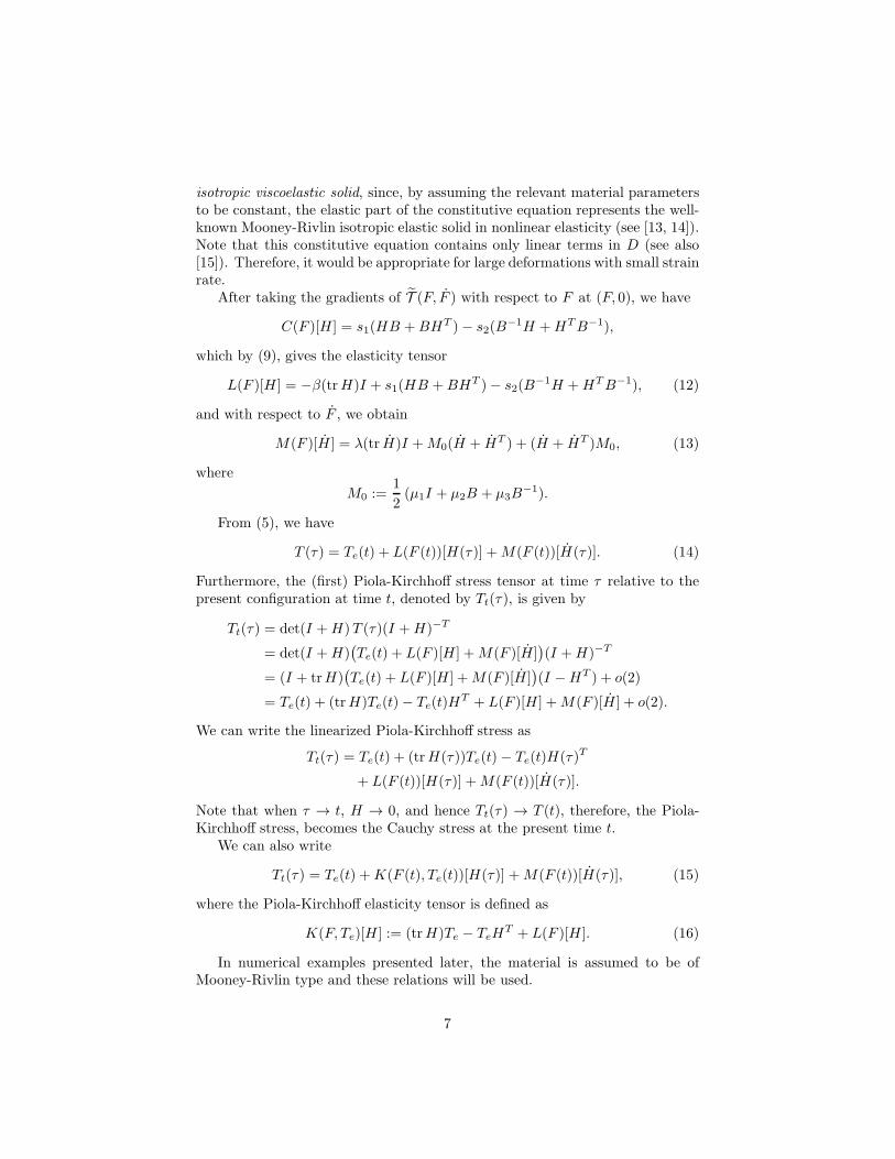
isotropic viscoelastic solid, since, by assuming the relevant material parametersto be constant, the elastic part of the constitutive equation represents the well-known Mooney-Rivlin isotropic elastic solid in nonlinear elasticity (see [13, 14]).Note that this constitutive equation contains only linear terms in D (see also[15]). Therefore, it would be appropriate for large deformations with small strainrate.

After taking the gradients of T (F, F ) with respect to F at (F, 0), we have

C(F )[H ] = s1(HB +BHT )− s2(B−1H +HTB−1),

which by (9), gives the elasticity tensor

L(F )[H ] = −β(trH)I + s1(HB +BHT )− s2(B−1H +HTB−1), (12)

and with respect to F , we obtain

M(F )[H ] = λ(tr H)I +M0(H + HT ) + (H + HT )M0, (13)

where

M0 :=1

2(µ1I + µ2B + µ3B

−1).

From (5), we have

T (τ) = Te(t) + L(F (t))[H(τ)] +M(F (t))[H(τ)]. (14)

Furthermore, the (first) Piola-Kirchhoff stress tensor at time τ relative to thepresent configuration at time t, denoted by Tt(τ), is given by

Tt(τ) = det(I +H)T (τ)(I +H)−T

= det(I +H)(Te(t) + L(F )[H ] +M(F )[H]

)(I +H)−T

= (I + trH)(Te(t) + L(F )[H ] +M(F )[H ]

)(I −HT ) + o(2)

= Te(t) + (trH)Te(t)− Te(t)HT + L(F )[H ] +M(F )[H ] + o(2).

We can write the linearized Piola-Kirchhoff stress as

Tt(τ) = Te(t) + (trH(τ))Te(t)− Te(t)H(τ)T

+ L(F (t))[H(τ)] +M(F (t))[H(τ)].

Note that when τ → t, H → 0, and hence Tt(τ) → T (t), therefore, the Piola-Kirchhoff stress, becomes the Cauchy stress at the present time t.

We can also write

Tt(τ) = Te(t) +K(F (t), Te(t))[H(τ)] +M(F (t))[H(τ)], (15)

where the Piola-Kirchhoff elasticity tensor is defined as

K(F, Te)[H ] := (trH)Te − TeHT + L(F )[H ]. (16)

In numerical examples presented later, the material is assumed to be ofMooney-Rivlin type and these relations will be used.

7

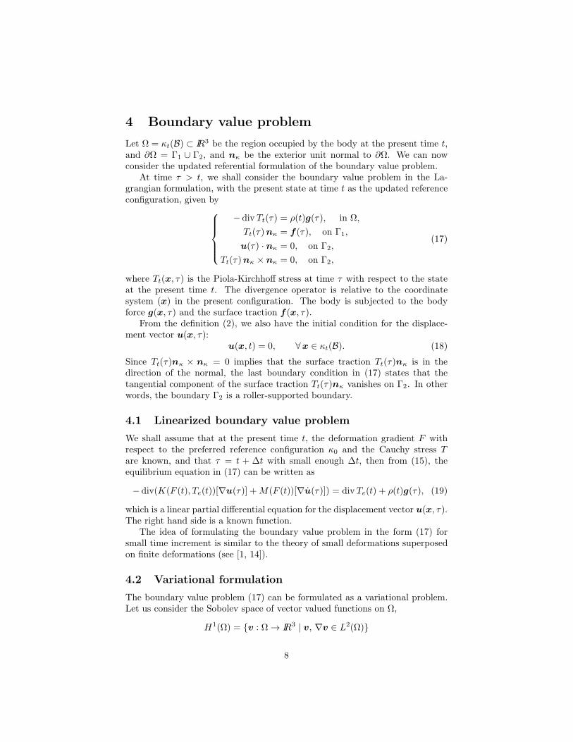
4 Boundary value problem

Let Ω = κt(B) ⊂ IR3 be the region occupied by the body at the present time t,and ∂Ω = Γ1 ∪ Γ2, and nκ be the exterior unit normal to ∂Ω. We can nowconsider the updated referential formulation of the boundary value problem.

At time τ > t, we shall consider the boundary value problem in the La-grangian formulation, with the present state at time t as the updated referenceconfiguration, given by

− div Tt(τ) = ρ(t)g(τ), in Ω,

Tt(τ)nκ = f(τ), on Γ1,

u(τ) · nκ = 0, on Γ2,

Tt(τ)nκ × nκ = 0, on Γ2,

(17)

where Tt(x, τ) is the Piola-Kirchhoff stress at time τ with respect to the stateat the present time t. The divergence operator is relative to the coordinatesystem (x) in the present configuration. The body is subjected to the bodyforce g(x, τ) and the surface traction f (x, τ).

From the definition (2), we also have the initial condition for the displace-ment vector u(x, τ):

u(x, t) = 0, ∀x ∈ κt(B). (18)

Since Tt(τ)nκ × nκ = 0 implies that the surface traction Tt(τ)nκ is in thedirection of the normal, the last boundary condition in (17) states that thetangential component of the surface traction Tt(τ)nκ vanishes on Γ2. In otherwords, the boundary Γ2 is a roller-supported boundary.

4.1 Linearized boundary value problem

We shall assume that at the present time t, the deformation gradient F withrespect to the preferred reference configuration κ0 and the Cauchy stress T

are known, and that τ = t + ∆t with small enough ∆t, then from (15), theequilibrium equation in (17) can be written as

− div(K(F (t), Te(t))[∇u(τ)] +M(F (t))[∇u(τ)]) = div Te(t) + ρ(t)g(τ), (19)

which is a linear partial differential equation for the displacement vector u(x, τ).The right hand side is a known function.

The idea of formulating the boundary value problem in the form (17) forsmall time increment is similar to the theory of small deformations superposedon finite deformations (see [1, 14]).

4.2 Variational formulation

The boundary value problem (17) can be formulated as a variational problem.Let us consider the Sobolev space of vector valued functions on Ω,

H1(Ω) = v : Ω → IR3 | v, ∇v ∈ L2(Ω)

8

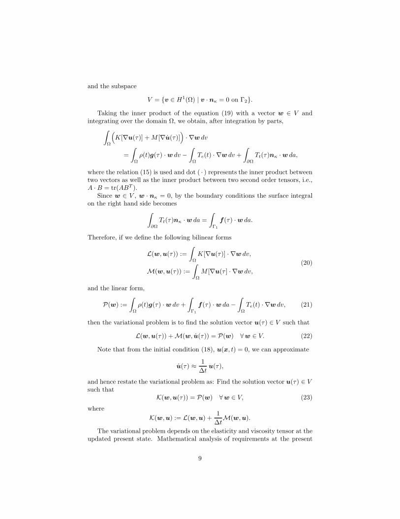
and the subspace

V = v ∈ H1(Ω) | v · nκ = 0 on Γ2.

Taking the inner product of the equation (19) with a vector w ∈ V andintegrating over the domain Ω, we obtain, after integration by parts,

∫

Ω

(K[∇u(τ)] +M [∇u(τ)]

)· ∇w dv

=

∫

Ω

ρ(t)g(τ) ·w dv −

∫

Ω

Te(t) · ∇w dv +

∫

∂Ω

Tt(τ)nκ ·w da,

where the relation (15) is used and dot ( · ) represents the inner product betweentwo vectors as well as the inner product between two second order tensors, i.e.,A · B = tr(ABT ).

Since w ∈ V , w · nκ = 0, by the boundary conditions the surface integralon the right hand side becomes

∫

∂Ω

Tt(τ)nκ ·w da =

∫

Γ1

f(τ) ·w da.

Therefore, if we define the following bilinear forms

L(w,u(τ)) :=

∫

Ω

K[∇u(τ)] · ∇w dv,

M(w,u(τ)) :=

∫

Ω

M [∇u(τ ] · ∇w dv,

(20)

and the linear form,

P(w) :=

∫

Ω

ρ(t)g(τ) ·w dv +

∫

Γ1

f(τ) ·w da−

∫

Ω

Te(t) · ∇w dv, (21)

then the variational problem is to find the solution vector u(τ) ∈ V such that

L(w,u(τ)) +M(w, u(τ)) = P(w) ∀w ∈ V. (22)

Note that from the initial condition (18), u(x, t) = 0, we can approximate

u(τ) ≈1

∆tu(τ),

and hence restate the variational problem as: Find the solution vector u(τ) ∈ V

such thatK(w,u(τ)) = P(w) ∀w ∈ V, (23)

where

K(w,u) := L(w,u) +1

∆tM(w,u).

The variational problem depends on the elasticity and viscosity tensor at theupdated present state. Mathematical analysis of requirements at the present

9

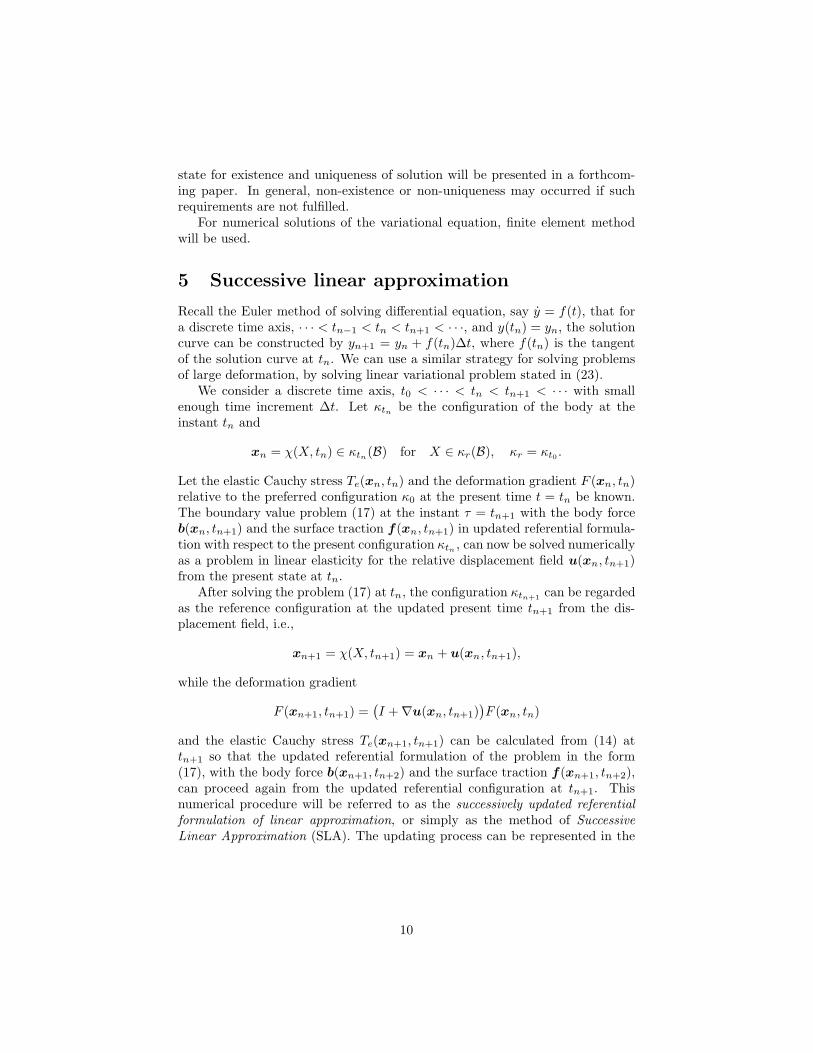
state for existence and uniqueness of solution will be presented in a forthcom-ing paper. In general, non-existence or non-uniqueness may occurred if suchrequirements are not fulfilled.

For numerical solutions of the variational equation, finite element methodwill be used.

5 Successive linear approximation

Recall the Euler method of solving differential equation, say y = f(t), that fora discrete time axis, · · · < tn−1 < tn < tn+1 < · · ·, and y(tn) = yn, the solutioncurve can be constructed by yn+1 = yn + f(tn)∆t, where f(tn) is the tangentof the solution curve at tn. We can use a similar strategy for solving problemsof large deformation, by solving linear variational problem stated in (23).

We consider a discrete time axis, t0 < · · · < tn < tn+1 < · · · with smallenough time increment ∆t. Let κtn be the configuration of the body at theinstant tn and

xn = χ(X, tn) ∈ κtn(B) for X ∈ κr(B), κr = κt0 .

Let the elastic Cauchy stress Te(xn, tn) and the deformation gradient F (xn, tn)relative to the preferred configuration κ0 at the present time t = tn be known.The boundary value problem (17) at the instant τ = tn+1 with the body forceb(xn, tn+1) and the surface traction f(xn, tn+1) in updated referential formula-tion with respect to the present configuration κtn , can now be solved numericallyas a problem in linear elasticity for the relative displacement field u(xn, tn+1)from the present state at tn.

After solving the problem (17) at tn, the configuration κtn+1can be regarded

as the reference configuration at the updated present time tn+1 from the dis-placement field, i.e.,

xn+1 = χ(X, tn+1) = xn + u(xn, tn+1),

while the deformation gradient

F (xn+1, tn+1) =(I +∇u(xn, tn+1)

)F (xn, tn)

and the elastic Cauchy stress Te(xn+1, tn+1) can be calculated from (14) attn+1 so that the updated referential formulation of the problem in the form(17), with the body force b(xn+1, tn+2) and the surface traction f(xn+1, tn+2),can proceed again from the updated referential configuration at tn+1. Thisnumerical procedure will be referred to as the successively updated referential

formulation of linear approximation, or simply as the method of Successive

Linear Approximation (SLA). The updating process can be represented in the

10

following schematic diagram:

BVPκr(B)−

fintelydeforms

→κt = κtn

κtn(B)—−→

κτ = κtn+1

κtn+1(B)

update ⇓

BVPκt = κtn+1

κtn+1(B)

—−→κτ = κtn+2

κtn+2(B)

update ⇓

κt = κtn+2

· · · · · ·

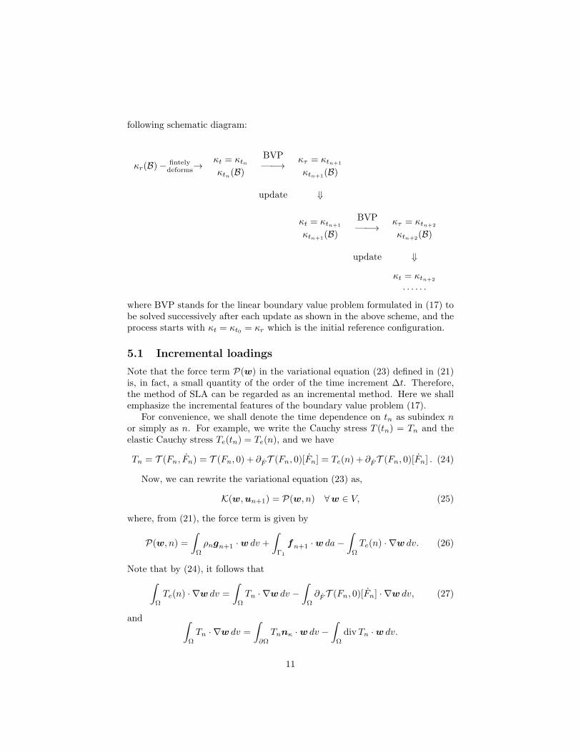
where BVP stands for the linear boundary value problem formulated in (17) tobe solved successively after each update as shown in the above scheme, and theprocess starts with κt = κt0 = κr which is the initial reference configuration.

5.1 Incremental loadings

Note that the force term P(w) in the variational equation (23) defined in (21)is, in fact, a small quantity of the order of the time increment ∆t. Therefore,the method of SLA can be regarded as an incremental method. Here we shallemphasize the incremental features of the boundary value problem (17).

For convenience, we shall denote the time dependence on tn as subindex n

or simply as n. For example, we write the Cauchy stress T (tn) = Tn and theelastic Cauchy stress Te(tn) = Te(n), and we have

Tn = T (Fn, Fn) = T (Fn, 0) + ∂FT (Fn, 0)[Fn] = Te(n) + ∂FT (Fn, 0)[Fn] . (24)

Now, we can rewrite the variational equation (23) as,

K(w,un+1) = P(w, n) ∀w ∈ V, (25)

where, from (21), the force term is given by

P(w, n) =

∫

Ω

ρngn+1 ·w dv +

∫

Γ1

fn+1 ·w da−

∫

Ω

Te(n) · ∇w dv. (26)

Note that by (24), it follows that∫

Ω

Te(n) · ∇w dv =

∫

Ω

Tn · ∇w dv −

∫

Ω

∂F T (Fn, 0)[Fn] · ∇w dv, (27)

and ∫

Ω

Tn · ∇w dv =

∫

∂Ω

Tnnκ ·w dv −

∫

Ω

div Tn ·w dv.

11

On the other hand, noting that Ttn(tn) = Tn is the Cauchy stress at tn, from(17) we have the following boundary value problem at the present time tn,

− divTn = ρngn, in Ω,

Tnnκ = fn, on Γ1,

Tnnκ × nκ = 0, on Γ2,

which leads to∫

Ω

Tn · ∇w dv =

∫

Γ1

fn ·w dv +

∫

Ω

ρngn ·w dv. (28)

Combing (26), (27), and (28), we obtain

P(w, n) = I1(w, n) + I2(w, n) + I3(w, n), (29)

which contains three types of loading for the variational equation (25), namely,

I1(w, n) =

∫

Ω

ρn(gn+1 − gn) ·w dv,

I2(w, n) =

∫

Γ1

(fn+1 − fn) ·w da,

I3(w, n) =

∫

Ω

∂F T (Fn, 0)[Fn] · ∇w dv.

(30)

The integral I1 represents the incremental body force and I2 is the incrementalsurface traction between time steps tn and tn+1. The third one I3 is due to theviscous effect of the material body.

5.2 Incremental approximation for large deformations

If we assume that the functions g(x, t) and f(x, t) are smooth in t, then theirincrements, gn+1 − gn and fn+1 − fn, are of the order of ∆t = tn+1 − tn, andsince the variational equation is linear, the solution vector u(x, tn+1) is also ofthe same order. For elastic material bodies, these are the two possible types ofincremental loading.

Starting from an initial solution and applying the method of SLA with properloading conditions at each time step, the problem of large deformation canbe obtained. Numerical examples employing the SLA method for incrementalsurface traction of pure shear and of gradually bending a rectangular blockinto a circular section have been considered in [2, 3] for Mooney Rivlin elasticmaterials.

For viscoelastic material bodies, there is a possible loading due to the inte-gral I3. To see this, we shall consider the case without surface traction f = 0and time-independent body force g so that I1 = I2 = 0, hence the integral I3is the only possible incremental loading.

12

To begin with, for n = 0, assume that at the initial time t0, we have a staticequilibrium solution so that we have the initial conditions: F0 = I and F0 = 0.Therefore, from (25), (29) and (30)3, we have

K(w,u1) = I3(w, 0) = 0, ∀w ∈ V,

which implies that the solution vector u1(x) = 0. Consequently, u1 = 1∆t

u1 = 0

and H1 = ∇u1 = 0. Then, from (3), F1 = H1F0 = 0, which, in turn, leads to

K(w,u2) = I3(w, 1) = 0, ∀w ∈ V,

and implies that u2 must also vanish and so on. In other words, if the initialsolution is an equilibrium solution, the solution remains valid for all time. How-ever, this conclusion may not be true since the initial solution may not be astable equilibrium solution in general.

Therefore, in order to study the stability, a small perturbation of the initialsolution is needed so that u1 6= 0, and hence I3(w, 1) 6= 0, to trigger thesuccessive evolution of deformations. Two such examples are considered in thefollowing sections.

6 Salt migration

As an example of large deformation, we shall consider a body consisting of twodifferent layers initially, with the mass density of the upper layer, the overburdensediment, greater than that of the bottom layer, the rock salt.

In a similar situation for viscous fluids, the inversion of density leads to theso-called Rayleigh-Taylor instability due to buoyancy effect of gravity. In thenumerical simulation by the use of SLA method, we shall present the resultsconfirming the existence of similar instability for viscoelastic solid bodies.

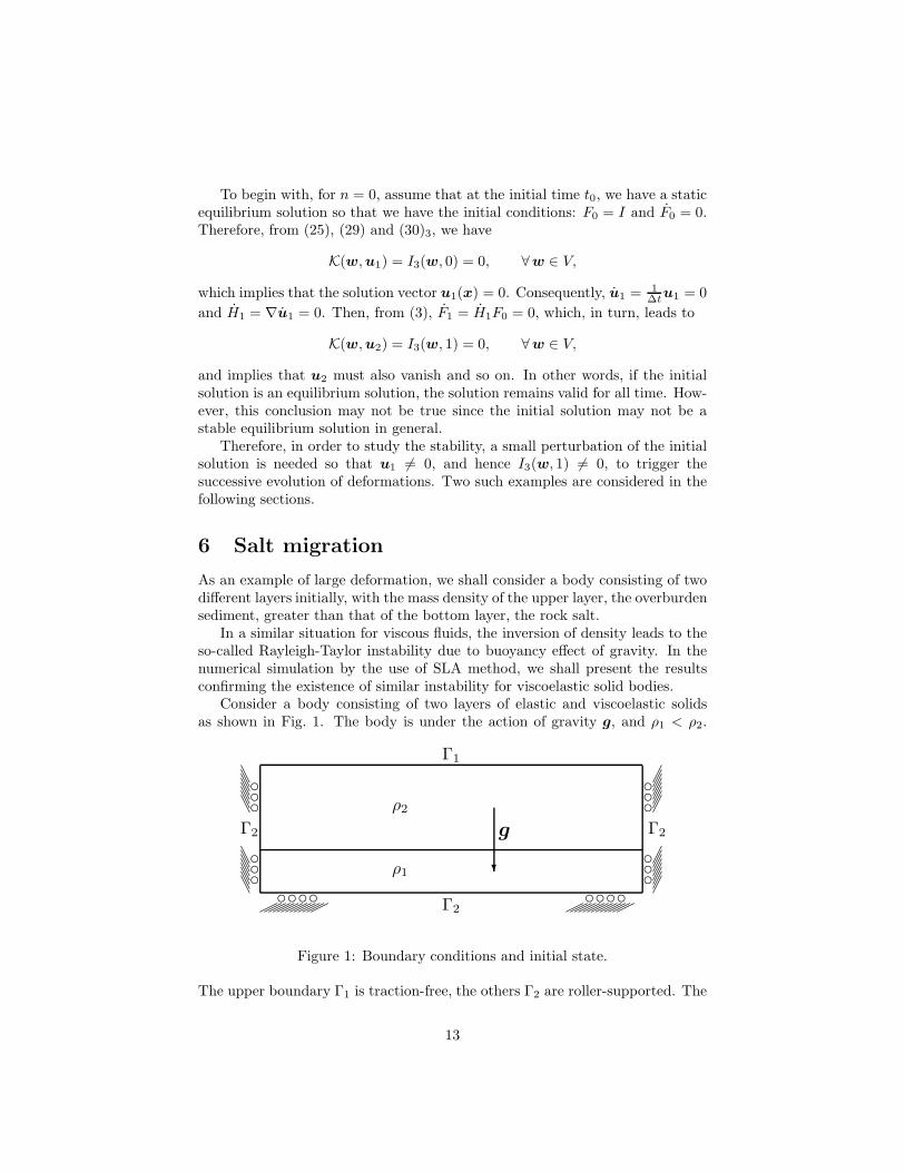
Consider a body consisting of two layers of elastic and viscoelastic solidsas shown in Fig. 1. The body is under the action of gravity g, and ρ1 < ρ2.

ρ1

ρ2

g

Γ2

Γ1

Γ2Γ2

Figure 1: Boundary conditions and initial state.

The upper boundary Γ1 is traction-free, the others Γ2 are roller-supported. The

13

initial state is an unstable equilibrium state, the movement of the salt-sedimentinterface can be initiated by a small perturbation.

For illustrative purpose, we shall present numerical simulations in a two-dimensional domain for a Mooney-Rivlin type material. The proposed methodhas been applied to three-dimensional domain and some different class of vis-coelastic solid bodies with similar results.

6.1 Formation of a salt diapir

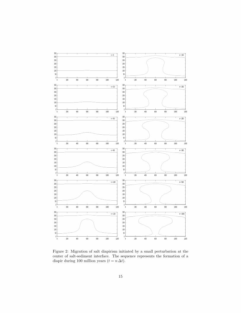
In this example we consider formation of a salt diapir initiated by a smallperturbation at a very small region centered at the salt-sediment interface.

• The dimension of the initial state is: length = 1,200 m, height of saltlayer = 100 m, height of sediment layer = 200 m.

• The material parameters for rock salt are:ρ0 = 2.2×103 Kg/m3, s1 = 0, s2 = -0.2×103 Pa,λ = -10.0×103 PaMa, µ1 = 15.0×103 PaMa, µ2 = µ3 = 0, β = 109 Pa.

• The material parameters for overburden sediment are:ρ0 = 3.0×103 Kg/m3, s1 = 2.5×103 Pa, s2 = -7.5×103 Pa,λ = µ1 = µ2 = µ3 = 0, β = 109 Pa.

• The incremental time: ∆t = 0.1 Ma.

The material data are of convenient choice for demonstration only. No attempthas been made to match the data to real properties of relevant materials.

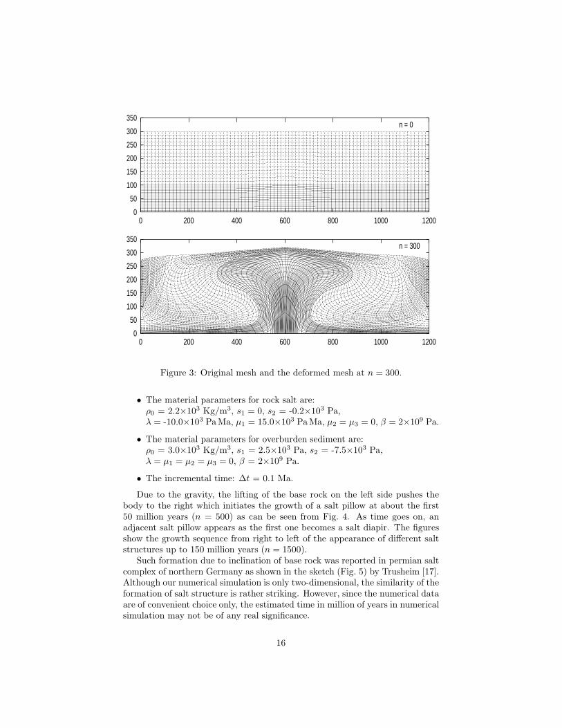
In Fig. 2, various stages of migration of the salt-sediment interface are shown,where n is the time step. One can easily see the formation of salt diapir as timestep increases. The effect is primarily due to buoyancy force of density inversion.The diapir reaches its maximum height at about 20 Ma (million years) at n= 200with almost no change afterward as the diapir becomes mature. The formationof diapir is a result of very large deformation of the initial mesh as can be seenfrom Fig. 3 at n = 300. The deformed mesh is quite similar to the experimentalresults of silicone putty model of a diapir formed by spinning the model in acentrifuge by Dixon [16].

6.2 Salt migration due to inclination

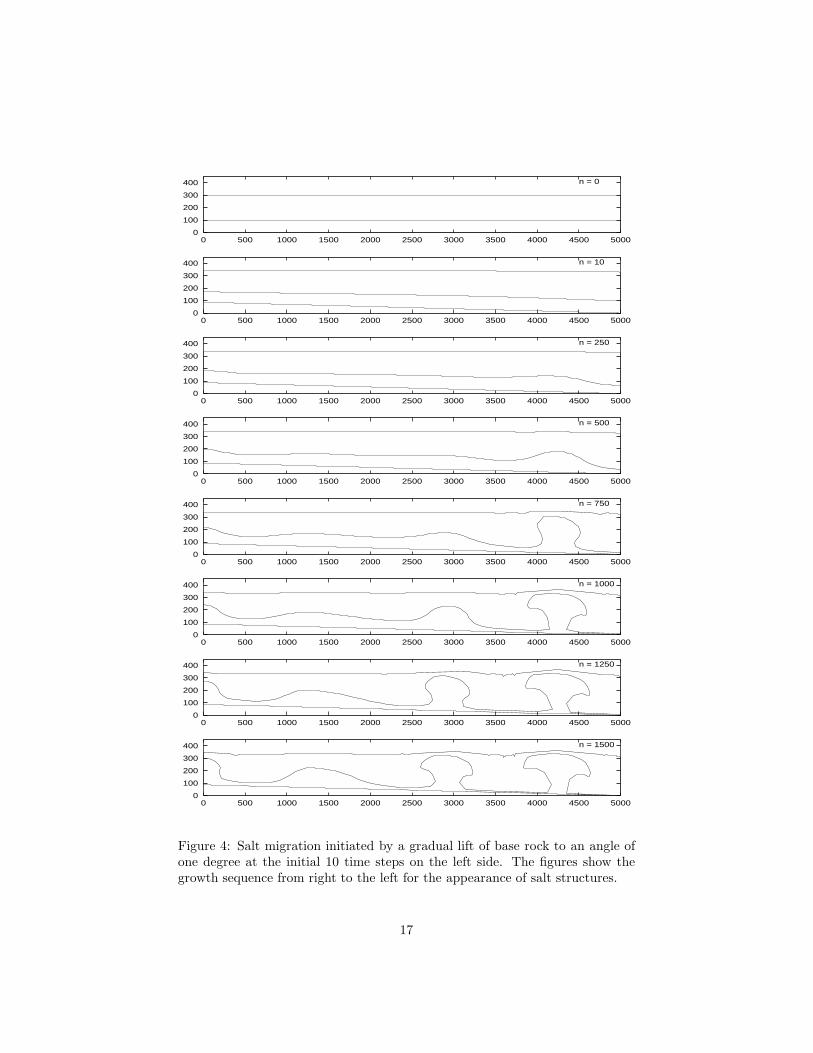
In the second example, we consider two-layer structure of a greater extension,so that there are enough rock salt in the bottom layer to develop multi-diapirs.The migration is initiated by gradually lifting the base rock, which supports thesalt layer, up to an inclination at an angle of one degree during the initial onemillion years (n = 10).

• The dimension of the initial state is: length = 5,000 m, height of saltlayer = 100 m, height of sediment layer = 200 m.

14

0

50

100

150

200

250

300

350

0 200 400 600 800 1000 1200

n = 0

0

50

100

150

200

250

300

350

0 200 400 600 800 1000 1200

n = 150

0

50

100

150

200

250

300

350

0 200 400 600 800 1000 1200

n = 20

0

50

100

150

200

250

300

350

0 200 400 600 800 1000 1200

n = 200

0

50

100

150

200

250

300

350

0 200 400 600 800 1000 1200

n = 50

0

50

100

150

200

250

300

350

0 200 400 600 800 1000 1200

n = 250

0

50

100

150

200

250

300

350

0 200 400 600 800 1000 1200

n = 80

0

50

100

150

200

250

300

350

0 200 400 600 800 1000 1200

n = 300

0

50

100

150

200

250

300

350

0 200 400 600 800 1000 1200

n = 100

0

50

100

150

200

250

300

350

0 200 400 600 800 1000 1200

n = 500

0

50

100

150

200

250

300

350

0 200 400 600 800 1000 1200

n = 120

0

50

100

150

200

250

300

350

0 200 400 600 800 1000 1200

n = 1000

Figure 2: Migration of salt diapirism initiated by a small perturbation at thecenter of salt-sediment interface. The sequence represents the formation of adiapir during 100 million years (t = n∆t).

15

0

50

100

150

200

250

300

350

0 200 400 600 800 1000 1200

n = 0

0

50

100

150

200

250

300

350

0 200 400 600 800 1000 1200

n = 300

Figure 3: Original mesh and the deformed mesh at n = 300.

• The material parameters for rock salt are:ρ0 = 2.2×103 Kg/m3, s1 = 0, s2 = -0.2×103 Pa,λ = -10.0×103 PaMa, µ1 = 15.0×103 PaMa, µ2 = µ3 = 0, β = 2×109 Pa.

• The material parameters for overburden sediment are:ρ0 = 3.0×103 Kg/m3, s1 = 2.5×103 Pa, s2 = -7.5×103 Pa,λ = µ1 = µ2 = µ3 = 0, β = 2×109 Pa.

• The incremental time: ∆t = 0.1 Ma.

Due to the gravity, the lifting of the base rock on the left side pushes thebody to the right which initiates the growth of a salt pillow at about the first50 million years (n = 500) as can be seen from Fig. 4. As time goes on, anadjacent salt pillow appears as the first one becomes a salt diapir. The figuresshow the growth sequence from right to left of the appearance of different saltstructures up to 150 million years (n = 1500).

Such formation due to inclination of base rock was reported in permian saltcomplex of northern Germany as shown in the sketch (Fig. 5) by Trusheim [17].Although our numerical simulation is only two-dimensional, the similarity of theformation of salt structure is rather striking. However, since the numerical dataare of convenient choice only, the estimated time in million of years in numericalsimulation may not be of any real significance.

16

0

100

200

300

400

0 500 1000 1500 2000 2500 3000 3500 4000 4500 5000

n = 0

0

100

200

300

400

0 500 1000 1500 2000 2500 3000 3500 4000 4500 5000

n = 10

0

100

200

300

400

0 500 1000 1500 2000 2500 3000 3500 4000 4500 5000

n = 250

0

100

200

300

400

0 500 1000 1500 2000 2500 3000 3500 4000 4500 5000

n = 500

0

100

200

300

400

0 500 1000 1500 2000 2500 3000 3500 4000 4500 5000

n = 750

0

100

200

300

400

0 500 1000 1500 2000 2500 3000 3500 4000 4500 5000

n = 1000

0

100

200

300

400

0 500 1000 1500 2000 2500 3000 3500 4000 4500 5000

n = 1250

0

100

200

300

400

0 500 1000 1500 2000 2500 3000 3500 4000 4500 5000

n = 1500

Figure 4: Salt migration initiated by a gradual lift of base rock to an angle ofone degree at the initial 10 time steps on the left side. The figures show thegrowth sequence from right to the left for the appearance of salt structures.

17

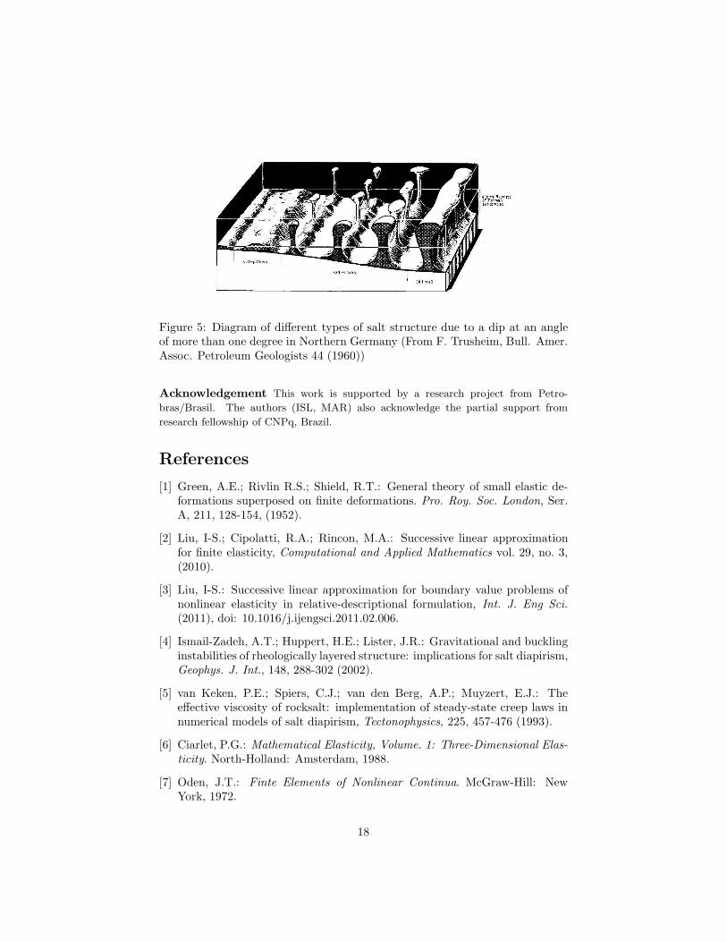
Figure 5: Diagram of different types of salt structure due to a dip at an angleof more than one degree in Northern Germany (From F. Trusheim, Bull. Amer.Assoc. Petroleum Geologists 44 (1960))

Acknowledgement This work is supported by a research project from Petro-

bras/Brasil. The authors (ISL, MAR) also acknowledge the partial support from

research fellowship of CNPq, Brazil.

References

[1] Green, A.E.; Rivlin R.S.; Shield, R.T.: General theory of small elastic de-formations superposed on finite deformations. Pro. Roy. Soc. London, Ser.A, 211, 128-154, (1952).

[2] Liu, I-S.; Cipolatti, R.A.; Rincon, M.A.: Successive linear approximationfor finite elasticity, Computational and Applied Mathematics vol. 29, no. 3,(2010).

[3] Liu, I-S.: Successive linear approximation for boundary value problems ofnonlinear elasticity in relative-descriptional formulation, Int. J. Eng Sci.

(2011), doi: 10.1016/j.ijengsci.2011.02.006.

[4] Ismail-Zadeh, A.T.; Huppert, H.E.; Lister, J.R.: Gravitational and bucklinginstabilities of rheologically layered structure: implications for salt diapirism,Geophys. J. Int., 148, 288-302 (2002).

[5] van Keken, P.E.; Spiers, C.J.; van den Berg, A.P.; Muyzert, E.J.: Theeffective viscosity of rocksalt: implementation of steady-state creep laws innumerical models of salt diapirism, Tectonophysics, 225, 457-476 (1993).

[6] Ciarlet, P.G.: Mathematical Elasticity, Volume. 1: Three-Dimensional Elas-

ticity. North-Holland: Amsterdam, 1988.

[7] Oden, J.T.: Finte Elements of Nonlinear Continua. McGraw-Hill: NewYork, 1972.

18

[8] Ogden, R.W.: Non-Linear Elastic Deformations, Ellis Horwood: New York,1984.

[9] Belytschko, T.; Liu, W.K.; Moran, B.: Nonlinear Finite Elements for Con-tinua and Structures, John Wiley & Sons: Chichester, (2000).

[10] Simo, J.C.; Taylor, R.L.: Quasi-incompressible finite elasticity in principalstretches, continuum basis and numerical algorithms. Computer Methods in

Applied Mechanics and Engineering (1991), 85: 273-310.

[11] Simo, J.C.; Hughes, T.J.R.: Computational Inelasticity, Springer: 1998.

[12] Zienkiewicz, O.C.; Taylor, R.L.: The Finite Element Method, Vol. 2: SolidMechanics, Butterworth-Heinemann: Oxford, 2000.

[13] Liu, I-S.: Continuum Mechanics, Springer: Berlin Heidelberg, 2002.

[14] Truesdell, C.; Noll, W.: The Non-Linear Field Theories of Mechanics, 3rdedition. Springer: Berlin, 2004.

[15] Hutter, K.; Johnk, K.: Continuum Methods of Physical Modeling: Contin-

uum Mechanics, Dimensional Analysis, Turbulence, Springer, 2004.

[16] Dixon, J.M.: Finite strain and progressive deformation in models of diapiricstructures, Tectonophysics, 28, 89-124 (1975).

[17] Trusheim, F.: Mechanism of salt migration in northern Germany, Bull.

Amer. Assoc. Petroleum Geologists, 44, 1519-1540 (1960).

19