Numerical simulation of rising droplets in liquid-liquid

systems: A comparison of continuous and sharp

interfacial force modelsI

Roland F. Engberga, Eugeny Y. Keniga,b,∗

aChair of Fluid Process Engineering, University of Paderborn, Pohlweg 55, 33098Paderborn, Germany

bGubkin Russian State University of Oil and Gas, Moscow, Russian Federation

Abstract

Simulations of single droplets rising in a quiescent liquid were performed forvarious initial droplet diameters. The continuous phase was water and thedispersed phase was either n-butanol, n-butyl acetate or toluene, thus re-sulting in three standard test systems for liquid-liquid extraction. For thesimulations, a level set based code was developed and implemented in theopen-source computational fluid dynamics (CFD) package OpenFOAM®. Toprevent volume (or mass) loss during the reinitialisation of the level set func-tion, two methods published recently were used in the code. The contiuumsurface force (CSF) model and the ghost fluid method (GFM) were appliedto model interfacial forces, and their influence on grid convergence, dropletshapes and rise velocities was investigated. Grid convergence studies showa reasonable behaviour of the GFM, whereas the CSF model is less reliable,especially for systems with high interfacial tension. The results for dropletshape and terminal rise velocity are in excellent agreement with experimen-tal and numerical investigations from literature. The onset of oscillations is

INotice: This is the author’s version of a work that was accepted for publicationin the International Journal of Heat and Fluid Flow. Changes resulting from the pub-lishing process, such as peer review, editing, corrections, structural formatting, andother quality control mechanisms may not be reflected in this document. Changesmay have been made to this work since it was submitted for publication. A defini-tive version was subsequently published in Int. J. Heat Fluid Flow 50 (2014), 16–26,http://dx.doi.org/10.1016/j.ijheatfluidflow.2014.05.003.

∗Corresponding authorEmail address: eugeny.kenig@upb.de (Eugeny Y. Kenig)

Preprint submitted to International Journal of Heat and Fluid Flow November 23, 2014

correctly predicted, and the influence of the smoothing of interfacial forceson velocity oscillations is studied. Simulations of oscillating droplets remainstable, but the frequencies of the velocity oscillations differ from experimentalresults.

Keywords: Droplet, Liquid-liquid extraction, Terminal velocity, CFD,Level set, Interfacial force model

1. Introduction

Transport phenomena at moving boundaries are crucial in various unitoperations of process engineering, e.g. condensation, absorption and liquid-liquid extraction. Therefore, moving boundaries have been studied exten-sively for several decades, both experimentally and theoretically, and remainsubject of ongoing research. Mass transfer in liquid-liquid extraction columnsoccurs at moving boundaries of rising droplets. Thus, fluid dynamics of andmass transfer in droplet swarms are essential for the design of liquid-liquidextraction. To capture these complex phenomena properly, fluid dynamicsof single moving droplets should be fully understood and mastered first.Fluid dynamics of a single droplet is governed by physical properties of thesystem and the size of the droplet. Relatively small droplets remain spheri-cal and reach their terminal rise velocity after a short period of acceleration.Increasing the droplet diameter leads to higher terminal velocities. Conse-quently, the forces acting upon the droplet grow and deform the droplet toan ellipsoidal or oblate shape. Droplets of even larger size begin to oscillate.Apart from the physical properties of both liquid phases, the terminal veloc-ity also depends on the purity of the system. In pure systems, the interfaceremains mobile and the shear forces acting there lead to internal circulations,i.e. toroidal flow patterns in the droplet. In contrast, impurities accumulatedat the interface inhibit the development of internal circulations. Thus, shearforces increase and the resulting terminal velocities are lower than in puresystems. For this reason, carefully purified systems were used in recent ex-perimental investigations.This work focusses on the numerical simulation of rising droplets. The mostwidely-used methods to simulate moving boundaries are moving mesh, fronttracking and front capturing methods. Moving mesh methods (e.g. Baumleret al., 2011; Tukovic and Jasak, 2012) employ a boundary fitted grid which ismoved to keep the grid nodes exactly at the interface. Thus, boundary con-

2

ditions at the interface can be implemented directly, resulting in a very exactand sharp representation of the two-phase flow. Problems may arise whenthe interface undergoes significant topological changes, such as strong dropletdeformations or the coalescence of two droplets. Front tracking methods (Un-verdi and Tryggvason, 1992) describe the interface with a moving mesh on afixed grid. This approach is very accurate but requires dynamic restructuringof the interface mesh. Front capturing methods employ markers or indicatorfunctions to locate the interface of a two-phase system. The movement of theinterface is then described with a simple advection equation for the indicatorfunction, which can be readily discretised with standard numerical methods,e.g., finite element methods (FEM) or finite volume methods (FVM). Hence,front capturing methods are robust and especially suitable for the simulationof strong interface deformations whereupon no time-consuming mesh move-ment or smoothing algorithms are necessary. While various front capturingmethods have been proposed, the prevailing approaches of this category arethe volume of fluid (VOF) method introduced by Hirt and Nichols (1981)and the level set method by Osher and Sethian (1988).The interfacial forces are of utmost importance for the dynamic behaviour ofmoving boundaries. Consequently, the implementation of interfacial forcesare crucial for the performance of a CFD code for two-phase flows, andvarious methods have been introduced. One of the earliest methods is thecontinuous surface stress (CSS) model of Lafaurie et al. (2000) and Gueyffieret al. (1999). Owing to its simplicity and robustness, the contiuum surfaceforce (CSF) model of Brackbill et al. (1992) is probably the most widely-usedinterfacial force model. By spreading the interfacial forces over a volume, theCSF model leads to a smooth transition in pressure at the interface. In con-trast, the ghost fluid method (GFM) of Liu et al. (2000) and Kang et al.(2000) leads to a sharp pressure jump.Dijkhuizen et al. (2005) used a front tracking model to simulate toluenedroplets with intial diameters of 4 to 12.5 mm rising in water. Comparedwith the experimental data of Wegener et al. (2010) for the same system, ve-locity oscillations occured for larger diameters in the simulations and showeddifferent amplitudes and frequencies. Moreover, the rise velocities were lowerin the simulations than in the experiments of Wegener et al. (2010).Wang et al. (2008) studied mass transfer from droplets in a n-butanol/watersystem. The moving boundary was described with the level set method andthe interfacial forces were implemented with the CSF model. For one dropletdiameter, numerical results for the rise velocity and a comparison of the sim-

3

ulated and experimental droplet rise height were shown.Bertakis et al. (2010) published terminal velocities of n-butanol droplets ris-ing in water obtained with the academic code DROPS (cf. Gross et al., 2006).This code employs a level set formulation of the two-phase flow discretisedwith finite elements; the interfacial forces are implemented with the CSFmodel. The results were in excellent agreement with the authors’ own exper-imental data. However, the simulated rise time was rather short and coveredonly the onset of velocity oscillations.Eiswirth et al. (2011) studied toluene droplets rising in water using the com-mercial finite-element code COMSOL Multiphysics 3.3a. The two-phase flowwas described with a modified level set method suggested by Olsson andKreiss (2005) which is, in fact, very similar to a VOF approach. The CSFmodel was used for interfacial forces. Comparing the terminal velocitieswith their own experimental results and those published by Wegener et al.(2007), Eiswirth et al. (2011) found very good agreement for small droplets(< 1.5 mm) and large droplets (> 3mm) as well as satisfactory agreement formedium-size droplets. Moreover, experimental and simulated droplet shapeswere in excellent accordance. However, the simulated rise time was too shortto show oscillations which were, consequently, not discussed.Baumler et al. (2011) investigated the rise of single droplets experimentallyand numerically. The simulations of three standard test systems for liquid-liquid extraction were carried out with moving mesh method implemented inthe academic code Navier. The code uses finite element discretisation, andinterfacial conditions, including the interfacial forces, are implemented witha subgrid projection method. Experimental results were taken from Wegeneret al. (2010) (toluene/water) and Bertakis et al. (2010) (n-butanol/water).Additionally, experiments for n-butyl acetate droplets rising in water wereperformed. The agreement of numerical and experimental results was excel-lent for all systems and over the whole range of droplet diameters. However,oscillations of large droplets led to strong mesh deformation and, eventually,to a collapse of the simulations.The results presented in this publication were obtained with a CFD-codebased on a level set formulation of the two-phase flow. The code was imple-mented in the open source CFD package OpenFOAM® (Open Source FieldOperation and Manipulation, www.openfoam.com, cf. Weller et al. (1998)).It includes two recent methods to overcome the volume loss frequently foundin level set based methods. Simulations of rising droplets in three standardstandard test systems for liquid/liquid extraction (n-butanol/water, n-butyl

4

acetate/water and toluene/water) were performed with the continuous inter-facial force model of Brackbill et al. (1992) and with the sharp model of Kanget al. (2000). The influence of the interfacial force model on grid convergence,droplet shape, rise velocity and the onset of oscillations was studied. Fur-thermore, the simulation results were compared with recent numerical andexperimental investigations. In this context, a comparison with the preciseboundary fitted moving mesh method of Baumler et al. (2011) is particularlyinteresting.

2. Mathematical model and numerical method

The CFD code used for this publication was recently employed to studythe influence of Marangoni convection on single rising droplets (Engberg etal., 2014a). In the following sections, the mathematical framework of thelevel set approach, the governing equations and the numerical details areoutlined.

2.1. Level set method

The fundamental idea of the level set approach is to employ a functionto indicate whether a point x is located in the continuous phase Ωc or in thedispersed phase Ωd. For this purpose, the indicator or level set function isdefined as follows:

ψ(x, t) < 0 if x ∈ Ωd (1)

ψ(x, t) > 0 if x ∈ Ωc (2)

Thus, the interface ∂Ω = ∂Ωc ∩ ∂Ωd is defined implicitly by the isocontourψ(xI) = 0, where xI is an arbitrary point on the interface.In principle, any sufficiently smooth function could be chosen as a level setfunction. However, it has been shown that a signed distance function is aparticularly advantageous choice (cf. Osher and Fedkiw, 2003). It has thefollowing properties:

|ψ(x)| = min(|x− xI |) for all xI ∈ ∂Ω (3)

|∇ψ| = 1 (4)

The movement of an interface in a velocity field v can be described with thefollowing advection equation for the level set function ψ:

∂ψ

∂t+ v · ∇ψ = 0 (5)

5

Due to the advection, the level set function becomes distorted and loses itsproperties as a signed distance function (Eqs. (3), (4)).The procedure to restore ψ as a signed distance function is called reinitiali-sation and is realised by solving the following partial differential equation:

∂ψ

∂τ=

ψ0√ψ2

0 + ∆x2(ψ0)(1− |∇ψ|) + F (6)

where τ is pseudo-time, ∆x is grid spacing and ψ0 is the initial condition

ψ0 = ψ(x, τ = 0) (7)

It has been shown that the zero level set contour (ψ(x) = 0) is often displacedduring the reinitialisation (cf. Sussman and Fatemi, 1999). To prevent theseartificial volume changes, a forcing term F recently suggested by Hartmannet al. (2010) is included in the reinitialisation equation (6). The formulationof the term F can be found in Hartmann et al. (2010).Equation (6) is discretised in pseudo-time with a simple explicit Euler schemewith a predictor-corrector procedure for the forcing term F . For the spatialderivatives, the third-order WENO scheme of Jiang and Peng (2000) is used.To reinitialise ψ, 10 pseudo-time steps with a step size of ∆τ = ∆x

2were

performed for each (physical) time step.Despite the forcing term F , preliminary simulations showed that the volumewas not conserved. As the droplet size has a significant influence on theterminal velocity, it is very important to conserve the droplet volume exactly.Hence, an interface shift was implemented as proposed by Gross (2008). Afterthe reinitialisation, a new level set function ψnew is calculated by substractinga correction ψ from the reinitialised level set function ψ:

ψnew = ψ(x, t)− ψ (8)

The correction ψ is determined iteratively in such a way that the volumedescribed by ψnew is equal to the initial droplet volume. The shifted levelset field ψnew is then defined as the new level set function and used forthe subsequent calculations. It was found that a rather small correction ofψ ≈ 10−3 ∆x applied every second time step was required to conserve thevolume. Thus, one may safely assume that the solution is not disturbed bythe interface shift.Peng et al. (1999) introduced the concept of a localised level set function:

6

They pointed out that it is sufficient when the level set function is a dis-tance function in the vicinity of the interface. Consequently, only cells in aconfined region close to the interface have to be reinitialised, reducing thecomputational effort substantially. Outside the reinitialised region, the levelset function is set to a constant value. In this work, the level set functionwas reinitialised in four consecutive cells on each side of the interface.

2.2. Navier-Stokes equations and moving reference frame

In this work, three systems, each consisting of two immiscible isothermalliquids, are studied. The liquids can be considered as Newtonian and incom-pressible. Hence, the fluid dynamics is described with the mass continuityand the Navier-Stokes equations. The equations describing the two-phasesystem are applied in single-field formulation, i.e. one set of equations forthe whole domain including both the continuous and dispersed phase:

∇ · v = 0 (9)

∂(ρv)

∂t+ ρa + (ρv · ∇)v = ∇ ·

(η(∇v +∇vT

))−∇p− ρg + Fσ (10)

where ρ denotes density, η viscosity, p pressure and g gravitational accelera-tion. A modified pressure without hydrostatic contribution p∗ = p− ρg ·x isused in the simulations to simplify the specification of boundary conditions(cf. Rusche, 2002). To simulate long rise times, the centre of the computa-tional domain is kept approximately at the centre of mass of the droplet. Theacceleration term a in the momentum equation (10) accounts for this movingreference frame and is determined with a procedure based on a method givenby Rusche (2002) (cf. Engberg et al., 2014b).In the present work, the discontinuities of physical properties at the interfaceare “smeared” over a small area to ensure numerical stability. Therefore, asmoothed Heaviside function is employed:

Hε(ψ) =

0 if ψ < −ε12

+ ψ2ε

+ 12π

sin(πψε

)if |ψ| ≤ ε

1 if ψ > ε(11)

In equation (11), parameter ε determines the thickness of the transition re-gion from one phase to another. In terms of the grid spacing ∆x, a typicalvalue of the smoothing parameter of ε = 1.5∆x was chosen for the simula-tions.

7

The density ρ is calculated by

ρ = ρd + (ρc − ρd)Hε(ψ) (12)

The viscosity η is interpolated with a method sugggested by Kothe (1998).For this purpose, the arithmetic and the harmonic mean of viscosities arecalculated with the Heaviside function (11) interpolated to the cell faces (cf.Fig. 1). These mean values are then averaged according to the relativeorientation of the interface normal and the cell face normal.Two different models are used for the the surface force at the interface dueto the interfacial tension Fσ: the contiuum surface force (CSF) model ofBrackbill et al. (1992) and the ghost fluid method (GFM) of Kang et al.(2000).For the CSF model, the interfacial force is multiplied with a smoothed deltafunction δε and, consequently, tranformed into a volume force acting in asmall region at the interface:

Fσ = (σκ∇ψ)δε(ψ) (13)

where σ denotes the interfacial tension and κ the curvature of the interface.The smoothed delta function δε is calculated with

δε(ψ) =

0 if |ψ| > ε12ε

+ 12ε

cos(πψε

)if |ψ| ≤ ε

(14)

The curvature κ is defined as the divergence of the interface unit normal nIcalculated from the level set function:

nI =∇ψ|∇ψ| (15)

κ = −∇ · nI (16)

To obtain a cell averaged value, the curvature is integrated over each finitevolume Vi :

κi = − 1

Vi

∫Vi

∇ · nI dV (17)

Applying the Gaussian theorem yields:

κi = − 1

Vi

∫S

nI · dS (18)

8

𝐼 (𝜓 = 0)

𝜓 > 0 𝜓 < 0

𝜎𝜅

𝑝

𝑥 𝑖 + 1 𝑖 𝑖 + 1/2

cell 𝑖, 𝑗

𝑖 + 1, 𝑗

interface 𝐼 (𝜓 = 0)

𝑖 + 2, 𝑗

cell face 𝑖 + 3

2 , 𝑗

𝑖 + 3/2 𝑖 + 2

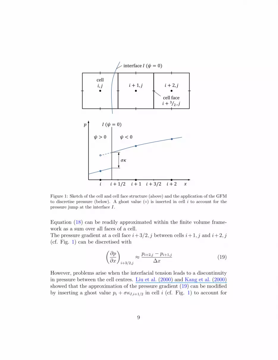
Figure 1: Sketch of the cell and cell face structure (above) and the application of the GFMto discretise pressure (below). A ghost value () is inserted in cell i to account for thepressure jump at the interface I.

Equation (18) can be readily approximated within the finite volume frame-work as a sum over all faces of a cell.The pressure gradient at a cell face i+3/2, j between cells i+1, j and i+2, j(cf. Fig. 1) can be discretised with(

∂p

∂x

)i+3/2,j

≈ pi+2,j − pi+1,j

∆x(19)

However, problems arise when the interfacial tension leads to a discontinuityin pressure between the cell centres. Liu et al. (2000) and Kang et al. (2000)showed that the approximation of the pressure gradient (19) can be modifiedby inserting a ghost value pi + σκI,i+1/2 in cell i (cf. Fig. 1) to account for

9

the discontinuity. Thus, the following expression is obtained:(∂p

∂x

)i+1/2

≈ pi+1 − pi∆x

− σκI,i+1/2

∆x(20)

where κI,i+1/2 is the curvature interpolated to the interface (cf. Liu et al.,2000; Francois et al., 2006):

κI,i+1/2 =κi|ψi+1|+ κi+1|ψi||ψi|+ |ψi+1|

(21)

Brackbill et al. (1992) derived the CSF model under the assumption of agradual change in pressure at the interface. In contrast, the GFM is a dis-cretisation technique which takes a sharp pressure jump at the interface intoaccount. Therefore, the CSF model leads to a smooth transition in pressurebetween the phases, whereas the GFM produces a pressure jump from onecell to another, which is closer to reality. Both models are used in conjunctionwith single-field formulations of the mass continuity and the Navier-Stokesequations.The implementation of the GFM is more demanding and increases the com-putational effort. While the CSF model can be easily applied to arbitrarygrids, the GFM, as currently implemented, is limited to structured orthog-onal grids. With appropriate interpolation techniques, however, the GFMmay be extended to arbitrary grids.

2.3. Discretisation, grid and boundary conditions

Eqs. (5), (9) and 10 were solved within a finite volume framework. Asis customary in OpenFOAM®, a collocated variable arrangement was used,i.e. level set function, pressure and velocities were stored at the cell centres.Convective terms (v · ∇) in Eqs. (5) and (10) were discretised with the NVDGamma scheme introduced by Jasak et al. (1999) and time was discretisedwith a first-order accurate implicit Euler scheme. The time steps were con-stant during the simulations and in the range of 10 to 100 ms leading tomaximum Courant numbers of 0.25.The pressure-velocity coupling is achieved with a Pressure Implicit with Split-ting of Operators (PISO)-algorithm (cf. Issa, 1986) adopted from the VOF-code interFoam provided with OpenFOAM® 1.7.1. For this algorithm, thecontinuity equation (9) is reformulated as a Poisson equation for pressure,

10

𝑥 𝑦

𝑧

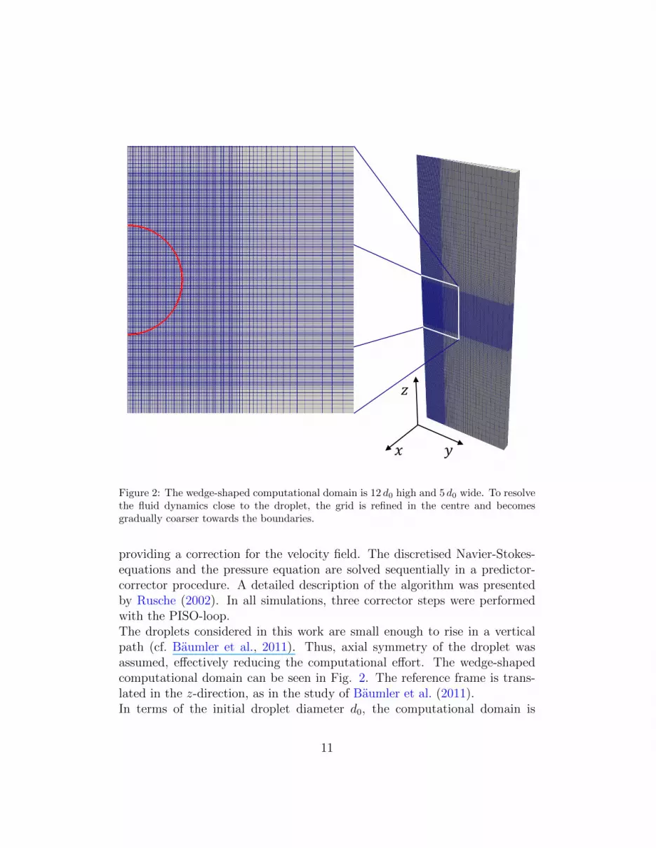
Figure 2: The wedge-shaped computational domain is 12 d0 high and 5 d0 wide. To resolvethe fluid dynamics close to the droplet, the grid is refined in the centre and becomesgradually coarser towards the boundaries.

providing a correction for the velocity field. The discretised Navier-Stokes-equations and the pressure equation are solved sequentially in a predictor-corrector procedure. A detailed description of the algorithm was presentedby Rusche (2002). In all simulations, three corrector steps were performedwith the PISO-loop.The droplets considered in this work are small enough to rise in a verticalpath (cf. Baumler et al., 2011). Thus, axial symmetry of the droplet wasassumed, effectively reducing the computational effort. The wedge-shapedcomputational domain can be seen in Fig. 2. The reference frame is trans-lated in the z-direction, as in the study of Baumler et al. (2011).In terms of the initial droplet diameter d0, the computational domain is

11

𝐯 = 𝐯𝐹 𝜕𝑝∗

𝜕𝑛 = 0

𝜕𝜓

𝜕𝑛 = 0

𝐯 = 𝐯𝐹 𝜕𝑝∗

𝜕𝑛 = 0

𝜕𝜓

𝜕𝑛 = 0

𝐧 ⋅ ∇ 𝐯 = 𝟎 𝑝∗ = 0 𝜕𝜓

𝜕𝑛 = 0

𝑔

𝑧

𝑦

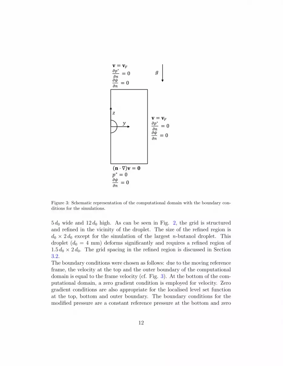
Figure 3: Schematic representation of the computational domain with the boundary con-ditions for the simulations.

5 d0 wide and 12 d0 high. As can be seen in Fig. 2, the grid is structuredand refined in the vicinity of the droplet. The size of the refined region isd0 × 2 d0 except for the simulation of the largest n-butanol droplet. Thisdroplet (d0 = 4 mm) deforms significantly and requires a refined region of1.5 d0 × 2 d0. The grid spacing in the refined region is discussed in Section3.2.The boundary conditions were chosen as follows: due to the moving referenceframe, the velocity at the top and the outer boundary of the computationaldomain is equal to the frame velocity (cf. Fig. 3). At the bottom of the com-putational domain, a zero gradient condition is employed for velocity. Zerogradient conditions are also appropriate for the localised level set functionat the top, bottom and outer boundary. The boundary conditions for themodified pressure are a constant reference pressure at the bottom and zero

12

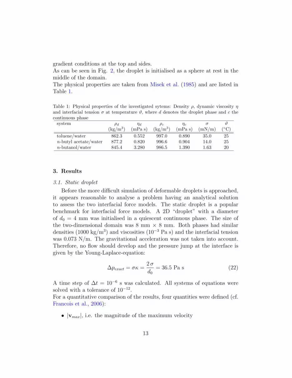
gradient conditions at the top and sides.As can be seen in Fig. 2, the droplet is initialised as a sphere at rest in themiddle of the domain.The physical properties are taken from Misek et al. (1985) and are listed inTable 1.

Table 1: Physical properties of the investigated sytems: Density ρ, dynamic viscosity ηand interfacial tension σ at temperature ϑ, where d denotes the droplet phase and c thecontinuous phase

system ρd ηd ρc ηc σ ϑ(kg/m3) (mPa s) (kg/m3) (mPa s) (mN/m) (C)

toluene/water 862.3 0.552 997.0 0.890 35.0 25n-butyl acetate/water 877.2 0.820 996.6 0.904 14.0 25n-butanol/water 845.4 3.280 986.5 1.390 1.63 20

3. Results

3.1. Static droplet

Before the more difficult simulation of deformable droplets is approached,it appears reasonable to analyse a problem having an analytical solutionto assess the two interfacial force models. The static droplet is a popularbenchmark for interfacial force models. A 2D “droplet” with a diameterof d0 = 4 mm was initialised in a quiescent continuous phase. The size ofthe two-dimensional domain was 8 mm × 8 mm. Both phases had similardensities (1000 kg/m3) and viscosities (10−3 Pa s) and the interfacial tensionwas 0.073 N/m. The gravitational acceleration was not taken into account.Therefore, no flow should develop and the pressure jump at the interface isgiven by the Young-Laplace-equation:

∆pexact = σκ =2σ

d0

= 36.5 Pa s (22)

A time step of ∆t = 10−6 s was calculated. All systems of equations weresolved with a tolerance of 10−12.For a quantitative comparison of the results, four quantities were defined (cf.Francois et al., 2006):

• |vmax|, i.e. the magnitude of the maximum velocity

13

• ∆ptot = pd − pc, where pd and pc are the arithmetic averages of thepressures in the dispersed (ψ ≤ 0, Nd cells) and the continuous (ψ > 0,Nc cells) phase, respectively: pd = 1

Nd

∑Nd

i=1 pi and pc = 1Nc

∑Nc

i=1 pi

• ∆ppart = ppart,d − ppart,c For the arithmetic averages, only cells withHε,i = 0 (for ppart,d) or Hε,i = 1 (for ppart,c) are taken into account.Thereby, the transition region of the CSF model is not included.

• ∆pmax = pmax − pmin, where pmax is the maximum and pmin the mini-mum pressure in the computational domain.

The relative error E of the pressure differences was calculated according to

E =|∆p−∆pexact|

∆pexact(23)

The results for various grid spacings are compiled in Table 2. Regarding themaximum velocities, the results indicate that spurious currents are reducedwith grid refinement when the GFM is used. In contrast, with the CSFmodel, grid refinement increases the magnitude of the maximum velocity.Moreover, |vmax| is in all cases larger with the CSF model than with theGFM.Due to the transition region, Etot is large for the CSF model on coarse gridsand decreases with grid refinement. Consequently, the error is significantlysmaller when the transition region is not included (Epart), and a reasonableagreement with the exact pressure jump is achieved. Nevertheless, the errorincreases with the last level of refinement. The same conclusions apply toEmax.For the GFM, Etot is relatively small in all cases and decrease consistentlywith grid refinement. A comparison of Etot and Epart shows that no sig-nificant deviations from the exact pressure difference occur at the interface.

Table 2: Comparison of the CSF model and the GFM for the static droplet test case.∆x CSF: |vmax| Etot Epart Emax GFM: |vmax| Etot Epart Emax

[µm] [µm/s] [%] [%] [%] [µm/s] [%] [%] [%]

400 2.17 12.5 1.085 1.929 1.140 0.971 0.961 3.546200 4.15 6.55 0.183 0.822 0.294 0.230 0.232 0.988100 9.83 3.48 0.017 0.664 0.119 0.055 0.055 0.27050 19.7 1.56 0.050 0.782 0.044 0.025 0.026 0.071

14

While Emax is larger for the GFM than for the CSF model on coarse grids,it shows a better grid convergence with the GFM. On the finest mesh, Emaxobtained with the GFM is one order of magnitude smaller than the corre-sponding error of the CSF model.For this simple test case, results obtained with the GFM are quantitativelybetter in most cases. In contrast to the CSF model, the GFM shows abetter and more consistent convergence with grid refinement. These conclu-sions disagree with those of Francois et al. (2006) who observed a similarbehaviour of both models when a good curvature approximation was used.At the same time, our results are in accordance with the conclusions of Kanget al. (2000), as well as some other works. In comparison with the numericalresults of Francois et al. (2006), two factors might contribute to the differ-ent findings: Francois et al. (2006) used a discretisation procedure which ledto an exact balance of interfacial and pressure forces in the static case. Asnoted by Rusche (2002), however, this is not guaranteed for the current im-plementation of the PISO-algorithm. Moreover, the smoothed delta functionwith ε = 1.5∆x distributes interfacial forces over a broader region than theVOF-code of Francois et al. (2006). The results show that under these cir-cumstances, a sharp approach leads to a better balancing of interfacial andpressure forces and, consequently, to a reliable grid convergence.

3.2. Grid convergence of the terminal rise velocity

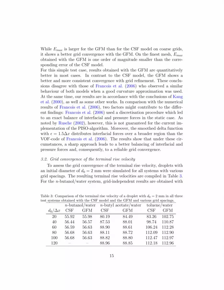
To assess the grid convergence of the terminal rise velocity, droplets withan initial diameter of d0 = 2 mm were simulated for all systems with variousgrid spacings. The resulting terminal rise velocities are compiled in Table 3.For the n-butanol/water system, grid-independent results are obtained with

Table 3: Comparison of the terminal rise velocity of a droplet with d0 = 2 mm in all threetest systems obtained with the CSF model and the GFM and various grid spacings.

n-butanol/water n-butyl acetate/water toluene/waterd0/∆x CSF GFM CSF GFM CSF GFM

20 55.92 55.98 80.19 84.49 83.26 102.7540 56.44 56.57 87.53 88.01 98.74 110.8760 56.59 56.63 88.90 88.61 106.24 112.2880 56.68 56.63 88.11 88.72 112.09 112.90100 56.68 56.63 88.82 88.80 112.47 112.97120 – – 88.96 88.85 112.18 112.96

15

a grid spacing of d0/∆x = 60 and d0/∆x = 80 for the GFM and the CSFmodel, respectively.Slightly finer grids are required for the n-butyl acetate/water system. Theinterfacial tension of the n-butyl acetate/water system is almost one order ofmagnitude higher than that of the n-butanol/water system. Consequently,the interfacial force model is far more important in this case. While theGFM shows reasonable grid convergence, the convergence behaviour of theCSF model is less clear.The toluene/water system possesses the highest interfacial tension among thethree systems investigated. Therefore, it is the most challenging test systemfor the interfacial force models in this study. The results show a very goodconvergence for the GFM, but a less reliable behaviour of the CSF model.The grid convergence study affirms the conclusion of the static droplet testcase: while grid convergence was achieved with the GFM in all cases, theCSF model was less reliable. This finding reflects the consistent reduction ofspurious currents with grid refinement achieved with the GFM – a qualitywhich is particularly important for systems with high interfacial tension (e.g.toluene/water).Furthermore, the results show that a grid spacing of d0/∆x = 80 leads togood results which deviate only marginally from those obtained with thefiner grids. This conclusion was also confirmed for other droplet diameters.Hence, the simulation results presented in following sections were obtainedwith this grid spacing.

3.3. Droplet shape

The droplet shape is defined by the isocontour ψ(x, t) = 0 which can beobtained in the post processing procedure. In Fig. 4, some droplet shapesfor the n-butanol/water system are shown. The shapes agree well with thosepresented by Bertakis et al. (2010). In accordance with Baumler et al. (2011),we observed a vortex in the wake of droplets with d0 > 2 mm. Furthermore,we found a secondary internal circulation for d0 = 3.48 mm and d0 = 4 mmwhich is presented in Fig. 5. This phenomenon can be explained by the veryflat shape in conjunction with the vortex in the wake of these droplets.The aspect ratio E , i.e. the ratio of the two principal axes, was determinedgraphically from the droplet shapes. Both for the CSF model and the GFM,the agreement with the simulation results of Baumler et al. (2011) is excellent,as can be seen in Table 4. Oscillations were observed for droplets withd0 ≥ 3 mm. This is in line with Bertakis et al. (2010) and Baumler et al.

16

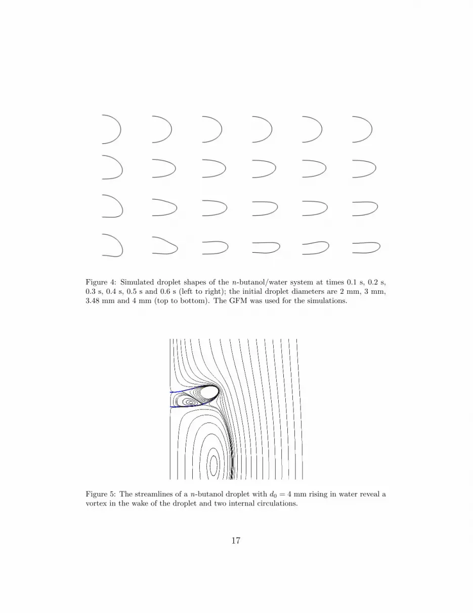
Figure 4: Simulated droplet shapes of the n-butanol/water system at times 0.1 s, 0.2 s,0.3 s, 0.4 s, 0.5 s and 0.6 s (left to right); the initial droplet diameters are 2 mm, 3 mm,3.48 mm and 4 mm (top to bottom). The GFM was used for the simulations.

Figure 5: The streamlines of a n-butanol droplet with d0 = 4 mm rising in water reveal avortex in the wake of the droplet and two internal circulations.

17

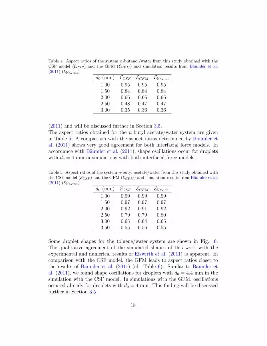
Table 4: Aspect ratios of the system n-butanol/water from this study obtained with theCSF model (ECSF ) and the GFM (EGFM ) and simulation results from Baumler et al.(2011) (ENavier)

d0 (mm) ECSF EGFM ENavier

1.00 0.95 0.95 0.951.50 0.84 0.84 0.842.00 0.66 0.66 0.662.50 0.48 0.47 0.473.00 0.35 0.36 0.36

(2011) and will be discussed further in Section 3.5.The aspect ratios obtained for the n-butyl acetate/water system are givenin Table 5. A comparison with the aspect ratios determined by Baumler etal. (2011) shows very good agreement for both interfacial force models. Inaccordance with Baumler et al. (2011), shape oscillations occur for dropletswith d0 = 4 mm in simulations with both interfacial force models.

Table 5: Aspect ratios of the system n-butyl acetate/water from this study obtained withthe CSF model (ECSF ) and the GFM (EGFM ) and simulation results from Baumler et al.(2011) (ENavier)

d0 (mm) ECSF EGFM ENavier

1.00 0.99 0.99 0.991.50 0.97 0.97 0.972.00 0.92 0.91 0.922.50 0.79 0.79 0.803.00 0.65 0.64 0.653.50 0.55 0.56 0.55

Some droplet shapes for the toluene/water system are shown in Fig. 6.The qualitative agreement of the simulated shapes of this work with theexperimental and numerical results of Eiswirth et al. (2011) is apparent. Incomparison with the CSF model, the GFM leads to aspect ratios closer tothe results of Baumler et al. (2011) (cf. Table 6). Similar to Baumler etal. (2011), we found shape oscillations for droplets with d0 = 4.4 mm in thesimulation with the CSF model. In simulations with the GFM, oscillationsoccured already for droplets with d0 = 4 mm. This finding will be discussedfurther in Section 3.5.

18

Figure 6: Simulated droplet shapes of the toluene/water system at times 0.1 s, 0.2 s, 0.3 s,0.4 s, 0.5 s and 0.6 s (left to right); the initial droplet diameters are 2 mm, 3 mm and4 mm (top to bottom). The GFM was used for the simulations.

Table 6: Aspect ratios of the system toluene/water from this study obtained with the CSFmodel (ECSF ) and the GFM (EGFM ) and simulation results from Baumler et al. (2011)(ENavier)

d0 (mm) ECSF EGFM ENavier

1.00 1.00 1.00 1.001.50 0.99 0.99 0.982.00 0.96 0.95 0.952.50 0.89 0.88 0.883.00 0.77 0.76 0.753.50 0.65 0.65 0.644.00 0.58 – 0.57

19

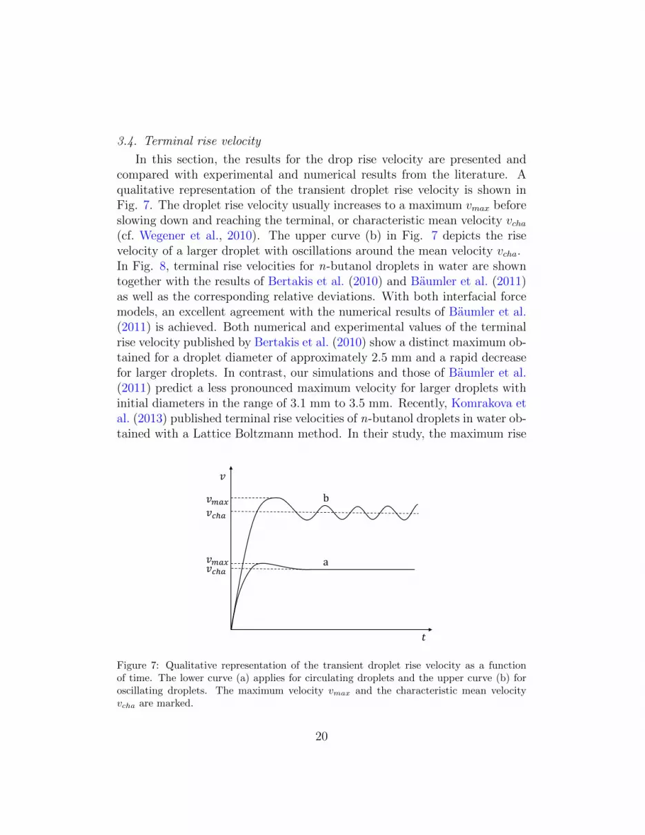
3.4. Terminal rise velocity

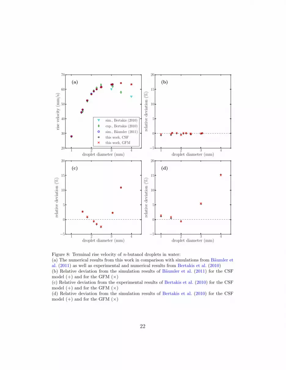
In this section, the results for the drop rise velocity are presented andcompared with experimental and numerical results from the literature. Aqualitative representation of the transient droplet rise velocity is shown inFig. 7. The droplet rise velocity usually increases to a maximum vmax beforeslowing down and reaching the terminal, or characteristic mean velocity vcha(cf. Wegener et al., 2010). The upper curve (b) in Fig. 7 depicts the risevelocity of a larger droplet with oscillations around the mean velocity vcha.In Fig. 8, terminal rise velocities for n-butanol droplets in water are showntogether with the results of Bertakis et al. (2010) and Baumler et al. (2011)as well as the corresponding relative deviations. With both interfacial forcemodels, an excellent agreement with the numerical results of Baumler et al.(2011) is achieved. Both numerical and experimental values of the terminalrise velocity published by Bertakis et al. (2010) show a distinct maximum ob-tained for a droplet diameter of approximately 2.5 mm and a rapid decreasefor larger droplets. In contrast, our simulations and those of Baumler et al.(2011) predict a less pronounced maximum velocity for larger droplets withinitial diameters in the range of 3.1 mm to 3.5 mm. Recently, Komrakova etal. (2013) published terminal rise velocities of n-butanol droplets in water ob-tained with a Lattice Boltzmann method. In their study, the maximum rise

𝑡

𝑣𝑐ℎ𝑎

𝑣

𝑣𝑚𝑎𝑥

𝑣𝑐ℎ𝑎

𝑣𝑚𝑎𝑥 a

b

Figure 7: Qualitative representation of the transient droplet rise velocity as a functionof time. The lower curve (a) applies for circulating droplets and the upper curve (b) foroscillating droplets. The maximum velocity vmax and the characteristic mean velocityvcha are marked.

20

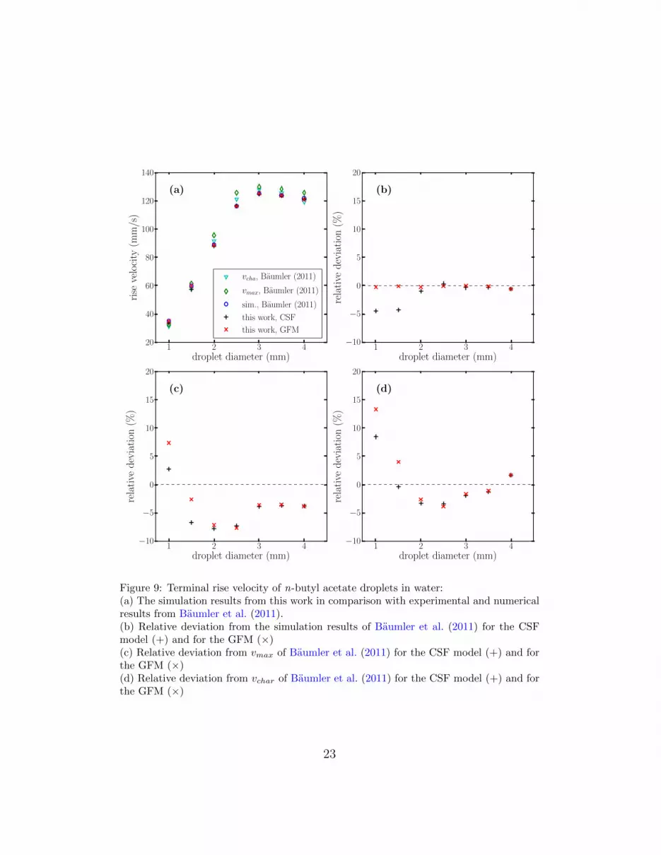
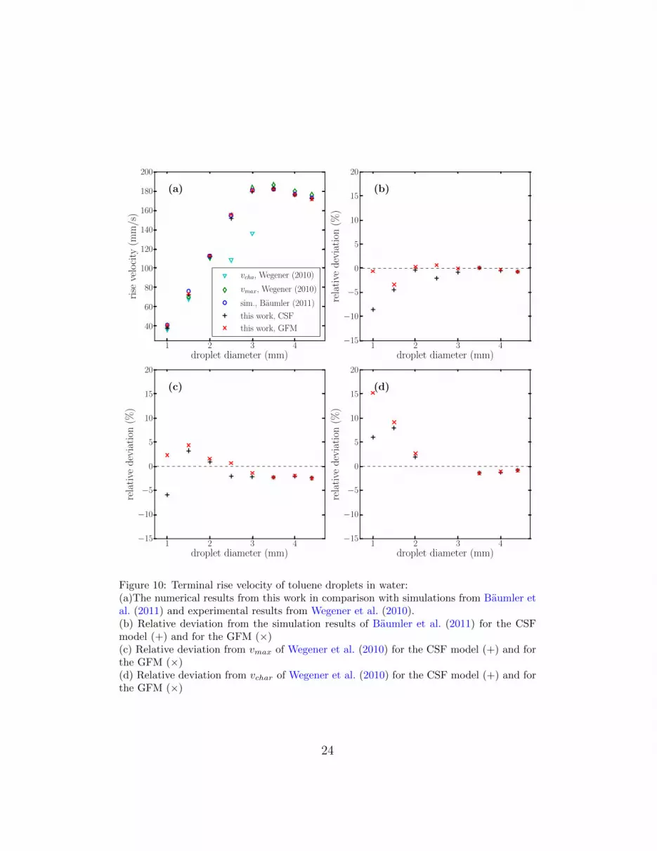
velocity was found for the droplet with d0 = 3.8 mm. As noted by Baumleret al. (2011), the simulated times of Bertakis et al. (2010) were slightly tooshort to reach the terminal rise velocity for large droplets. Consequently,deviations are found for droplets with d0 ≥ 3 mm.The terminal rise velocities for n-butyl acetate droplets in water from thiswork, the results of Baumler et al. (2011) and their relative deviations areshown in Fig. 9. The results for the n-butyl acetate/water system show thedifference between the interfacial force models more clearly: A very goodagreement with the simulation results of Baumler et al. (2011) is obtainedwith the GFM, while the CSF model leads to larger deviations, cf. Fig. 9(b). The maximum deviation is found for the smallest droplet (d0 = 1 mm)which possesses the highest jump in pressure at the interface. Furthermore, areasonable agreement with the experimental results of Baumler et al. (2011)is achieved with both models, cf. Fig. 9 (c), (d).Our results for the terminal rise velocities for toluene droplets in water andthose of Wegener et al. (2010) and Baumler et al. (2011) as well as theirrelative deviations are shown in Fig. 10. The results obtained with the CSFmodel deviate distinctly from those with the GFM and the data of Baumleret al. (2011). Similar to the previous system, the result for the smallestdroplet (d0 = 1 mm) obtained with the CSF model shows the largest devi-ations, cf. Fig. 10 (b). With the GFM, a very good agreement with thesimulation results of Baumler et al. (2011) is achieved. For both interfacialforce models, the simulated terminal rise velocities agree well with the ex-perimental maximum velocities of Wegener et al. (2010).Transient rise velocities of toluene droplets with d0 = 2 mm and d0 = 3.5 mmsimulated with the GFM are presented in Fig. 11 with the correspondingexperimental data of Wegener et al. (2010). In both cases, a good agreementis achieved. Deviations during the acceleration phase can be explained withdifferent initial conditions: While the simulated droplets are initialised asspheres, the experimental droplets are produced with a capillary and deformduring the detachment. In all cases, the acceleration phase is terminatedafter 1 s or less.The results presented in this section are in line with the findings of Section3.1: In comparison with the CSF model, the GFM reduces spurious currents.This is especially important in cases with high interfacial tension and largecurvatures (i.e. for small droplets).The numerical values for the terminal rise velocity of all cases considered inthis work are compiled in Table 7.

21

1 2 3 4droplet diameter (mm)

20

30

40

50

60

70

rise

velo

city

(mm

/s)

(a)

sim., Bertakis (2010)

exp., Bertakis (2010)

sim., Baumler (2011)

this work, CSF

this work, GFM

1 2 3 4droplet diameter (mm)

−5

0

5

10

15

20

rela

tive

dev

iati

on(%

)

(b)

1 2 3 4droplet diameter (mm)

−5

0

5

10

15

20

rela

tive

dev

iati

on(%

)

(c)

1 2 3 4droplet diameter (mm)

−5

0

5

10

15

20

rela

tive

dev

iati

on(%

)

(d)

Figure 8: Terminal rise velocity of n-butanol droplets in water:(a) The numerical results from this work in comparison with simulations from Baumler etal. (2011) as well as experimental and numerical results from Bertakis et al. (2010)(b) Relative deviation from the simulation results of Baumler et al. (2011) for the CSFmodel (+) and for the GFM (×)(c) Relative deviation from the experimental results of Bertakis et al. (2010) for the CSFmodel (+) and for the GFM (×)(d) Relative deviation from the simulation results of Bertakis et al. (2010) for the CSFmodel (+) and for the GFM (×)

22

1 2 3 4droplet diameter (mm)

20

40

60

80

100

120

140

rise

velo

city

(mm

/s)

(a)

vcha, Baumler (2011)

vmax, Baumler (2011)

sim., Baumler (2011)

this work, CSF

this work, GFM

1 2 3 4droplet diameter (mm)

−10

−5

0

5

10

15

20

rela

tive

dev

iati

on(%

)

(b)

1 2 3 4droplet diameter (mm)

−10

−5

0

5

10

15

20

rela

tive

dev

iati

on(%

)

(c)

1 2 3 4droplet diameter (mm)

−10

−5

0

5

10

15

20

rela

tive

dev

iati

on(%

)

(d)

Figure 9: Terminal rise velocity of n-butyl acetate droplets in water:(a) The simulation results from this work in comparison with experimental and numericalresults from Baumler et al. (2011).(b) Relative deviation from the simulation results of Baumler et al. (2011) for the CSFmodel (+) and for the GFM (×)(c) Relative deviation from vmax of Baumler et al. (2011) for the CSF model (+) and forthe GFM (×)(d) Relative deviation from vchar of Baumler et al. (2011) for the CSF model (+) and forthe GFM (×)

23

1 2 3 4droplet diameter (mm)

40

60

80

100

120

140

160

180

200

rise

velo

city

(mm

/s)

(a)

vcha, Wegener (2010)

vmax, Wegener (2010)

sim., Baumler (2011)

this work, CSF

this work, GFM

1 2 3 4droplet diameter (mm)

−15

−10

−5

0

5

10

15

20

rela

tive

dev

iati

on(%

)

(b)

1 2 3 4droplet diameter (mm)

−15

−10

−5

0

5

10

15

20

rela

tive

dev

iati

on(%

)

(c)

1 2 3 4droplet diameter (mm)

−15

−10

−5

0

5

10

15

20

rela

tive

dev

iati

on(%

)

(d)

Figure 10: Terminal rise velocity of toluene droplets in water:(a)The numerical results from this work in comparison with simulations from Baumler etal. (2011) and experimental results from Wegener et al. (2010).(b) Relative deviation from the simulation results of Baumler et al. (2011) for the CSFmodel (+) and for the GFM (×)(c) Relative deviation from vmax of Wegener et al. (2010) for the CSF model (+) and forthe GFM (×)(d) Relative deviation from vchar of Wegener et al. (2010) for the CSF model (+) and forthe GFM (×)

24

0 1 2 3 4time (s)

0

50

100

150

200

velo

city

(mm

/s)

d0 = 2 mm, Wegener et al. (2010)

d0 = 3.5 mm, Wegener et al. (2010)

d0 = 2 mm, this work

d0 = 3.5 mm, this work

Figure 11: Transient rise velocity of toluene droplets in water: Simulation results with theGFM (lines) and experimental data of Wegener et al. (2010) (symbols).

25

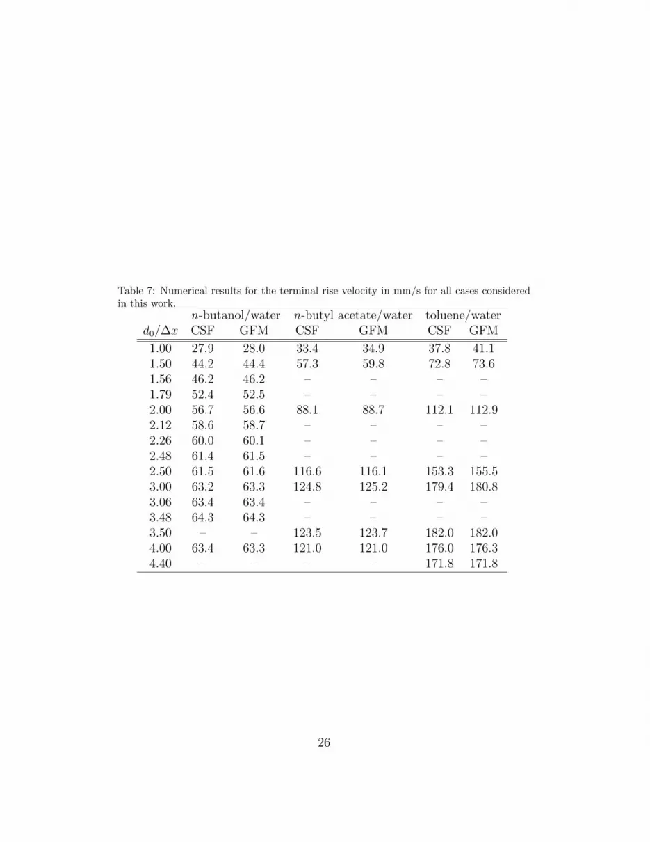
Table 7: Numerical results for the terminal rise velocity in mm/s for all cases consideredin this work.

n-butanol/water n-butyl acetate/water toluene/waterd0/∆x CSF GFM CSF GFM CSF GFM

1.00 27.9 28.0 33.4 34.9 37.8 41.11.50 44.2 44.4 57.3 59.8 72.8 73.61.56 46.2 46.2 – – – –1.79 52.4 52.5 – – – –2.00 56.7 56.6 88.1 88.7 112.1 112.92.12 58.6 58.7 – – – –2.26 60.0 60.1 – – – –2.48 61.4 61.5 – – – –2.50 61.5 61.6 116.6 116.1 153.3 155.53.00 63.2 63.3 124.8 125.2 179.4 180.83.06 63.4 63.4 – – – –3.48 64.3 64.3 – – – –3.50 – – 123.5 123.7 182.0 182.04.00 63.4 63.3 121.0 121.0 176.0 176.34.40 – – – – 171.8 171.8

26

3.5. Oscillations and stability

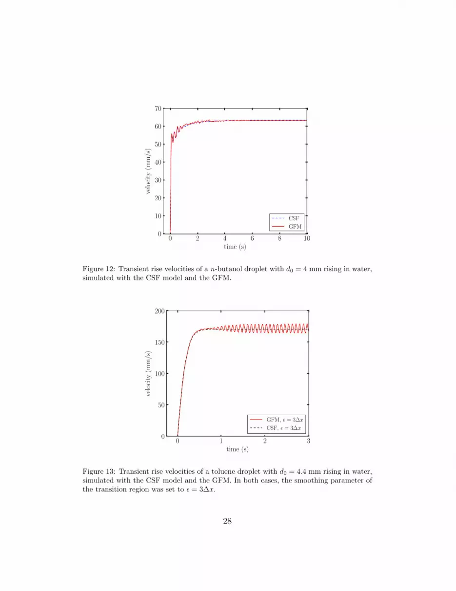
In simulations of the n-butanol/water system, oscillations occur for dropletswith d0 ≥ 3 mm. However, the amplitude of the oscillations decreases andeventually, a constant rise velocity and droplet shape is reached. This be-haviour is shown in Fig. 12 for a droplet with d0 = 4 mm, simulated withboth the CSF model and the GFM.In contrast, the n-butyl acetate droplet with d0 = 4 mm and the toluenedroplet with d0 = 4.4 mm show oscillations with constant amplitude andfrequency. As mentioned in Section 3.3, toluene droplets with an initial di-ameter of 4.4 mm show oscillations when the CSF model is used, whereaswith the GFM, oscillations occur for smaller droplets (d0 = 4 mm). Thisfinding can be explained with Fig. 13. In the simulations discussed pre-viously, the smoothing parameter of the transition region was ε = 1.5∆x.When the smoothing parameter is increased to ε = 3∆x, toluene dropletswith d0 = 4.4 mm simulated with the CSF model do not oscillate. In con-trast, oscillations are found in the rise velocity simulated with the GFM.Apparently, simulation results are very sensitive to the smoothing of interfa-cial forces and excessive smoothing may even lead to an erroneous predictionof droplet dynamics.Comparing the simulated rise velocities with the experimental results ofWegener et al. (2010), we find a similar amplitude of approximately 10 to15 mm/s in the velocity oscillations. Nevertheless, the frequencies (or peri-ods) of the velocity oscillations obtained from the simulations are very dif-ferent from experimental results: The order of magnitude of the periods inour simulations is 0.1 s, whereas Wegener et al. (2010) determined periods ofapproximately 1 s experimentally. For oscillating droplets, axial symmetrycannot be assumed and droplets should be simulated fully three-dimensional.Consequently, it is likely that 3D effects which cannot be reproduced in oursimulations are responsible for the different frequencies.

27

0 2 4 6 8 10time (s)

0

10

20

30

40

50

60

70

velo

city

(mm

/s)

CSF

GFM

Figure 12: Transient rise velocities of a n-butanol droplet with d0 = 4 mm rising in water,simulated with the CSF model and the GFM.

0 1 2 3time (s)

0

50

100

150

200

velo

city

(mm

/s)

GFM, ε = 3∆x

CSF, ε = 3∆x

Figure 13: Transient rise velocities of a toluene droplet with d0 = 4.4 mm rising in water,simulated with the CSF model and the GFM. In both cases, the smoothing parameter ofthe transition region was set to ε = 3∆x.

28

4. Conclusions

In this paper, the results of numerical simulations of single droplets risingin a quiescent liquid are presented. Three standard test systems for liquid-liquid extraction were investigated: n-butanol/water, n-butyl acetate/waterand toluene/water in which water represents the continuous phase. Assumingaxial symmetry of the droplet, we simulated droplets with various diametersup to the onset of oscillations. For the simulations, a CFD code based on alevel set formulation of the two-phase flow was developed and implemented inthe open-source CFD package OpenFOAM®. A well-known drawback of thelevel set method is the volume change during reinitialisation. Applying tworecently published methods, we were able to overcome this problem. Further-more, two interfacial force models were applied in this work: the widely-usedCSF model, which leads to a smooth transition in pressure at the interface,and the GFM, which results in a sharp jump. The influence of the interfacialforce model on the shape and the dynamic behaviour of the droplets wasstudied.For the theoretical test case of a static droplet as well as for rising dropletsin all three test systems, grid convergence was achieved with the GFM. Incontrast, the CSF model showed a less reliable behaviour with respect to gridrefinement.Regarding droplet shapes and terminal rise velocities, good agreement withrecent numerical investigations by Baumler et al. (2011) and Bertakis et al.(2010) was found with both interfacial force models. The results obtainedwith the GFM agree particularly well with the numerical results of Baumleret al. (2011). The comparison of terminal rise velocities, droplet shapes andonset of oscillations obtained from our simulations with experimental resultspublished by Bertakis et al. (2010), Wegener et al. (2010) and Baumler etal. (2011) is equally satisfactory for both interfacial force models. The onlydistinct discrepancy was found in the n-butanol/water system for dropletswith d0 ≥ 3 mm. Bertakis et al. (2010) found a pronounced maximum in theterminal rise velocity for droplets with d0 ≈ 2.5 mm, both experimentallyand numerically. Similar to Baumler et al. (2011), our simulations show aless pronounced maximum velocity for larger droplets with initial diametersin the range of 3.1 mm to 3.5 mm. Komrakova et al. (2013) found the max-imum rise velocity for droplets with d0 = 3.8 mm. Future experimental andnumerical investigations should clarify the tendency for larger droplets inthis system.

29

The onset of oscillations predicted with our simulations compares favourablywith numerical and experimental results from literature (Baumler et al., 2011;Bertakis et al., 2010; Wegener et al., 2010). However, it was shown that ex-cessive smoothing of interfacial forces with the CSF model can lead to anunphysical stabilisation of the droplet. In contrast, this problem does notoccur with the GFM.The results presented in this paper show that a satisfactory simulation ofdroplets can be achieved with both the CSF model and the GFM. Never-theless, the GFM results in lower spurious currents which, furthermore, areconsistently reduced with grid refinement. These properties are reflected inthe simulated rise velocities and in a reliable performance with respect togrid refinement.

5. Acknowledgement

We would like to thank Dr. Mirco Wegener for the experimental data.

30

References

K. Baumler, M. Wegener, A. R. Paschedag, E. Bansch, Drop rise velocitiesand fluid dynamic behavior in standard test systems for liquid/liquid ex-traction – experimental and numerical investigations. Chem. Eng. Sci. 66(3) (2011) 426-439.

E. Bertakis, S. Groß, J. Grande, O. Fortmeier, A. Reusken, A. Pfennig, Vali-dated simulation of droplet sedimentation with finite-element and level-setmethods. Chem. Eng. Sci. 65 (6) (2010) 2037-2051.

J. U. Brackbill, D. B. Kothe, C. Zemach, A continuum method for modelingsurface tension. J. Comput. Phys. 100 (2) (1992) 335-354.

W. Dijkhuizen, M. Van Sint Annaland, H. Kuipers, Numerical investigationof closures for interface forces in dispersed flows using a 3D front trackingmodel. In: Proceedings of 4th International Conference on CFD in the Oiland Gas, Metallurgical & Process Industries. SINTEF / NTNU, 6-8 June2005, Trondheim, Norway.

R. T. Eiswirth, H. J. Bart, T. Atmakidis, E. Y. Kenig, Experimental andnumerical investigation of a free rising droplet. Chem. Eng. Process. 50 (7)(2011) 718-727.

R. F. Engberg, M. Wegener, E. Y. Kenig, Numerische Simulation der konzen-trationsinduzierten Marangonikonvektion an Einzeltropfen mit verform-barer Phasengrenze. Chem. Ing. Tech. 86 (2014a) 185-195.

R. F. Engberg, M. Wegener, E. Y. Kenig, The impact of Marangoni con-vection on fluid dynamics and mass transfer at deformable single risingdroplets – A numerical study. Chem. Eng. Sci. 116 (2014b) 208-222.

M. M. Francois, S. J. Cummins, E. D. Dendy, D. B. Kothe, J. M. Sicilian,M. W. Williams”, A balanced-force algorithm for continuous and sharpinterfacial surface tension models within a volume tracking framework. J.Comput. Phys. 213 (1) (2006) 141-173.

S. Gross, Numerical Methods for three-dimensional incompressible two-phaseflow problems, PhD Thesis, RWTH Aachen, Germany, 2008.

S. Gross, V. Reichelt, A. Reusken, A finite element based level set method fortwo-phase incompressible flows, Comput. Visual. Sci. 9 (4) (2006) 239-257.

31

D. Gueyffier, J. Li, A. Nadim, R. Scardovelli, S. Zaleski, Volume-of-fluid interface tracking with smoothed surface stress methods for three-dimensional flows. J. Comput. Phys. (1999) 152 (2) 423-456.

D. Hartmann, M. Meinke, W. Schroder, The constrained reinitializationequation for level set methods. J. Comput. Phys. 229 (5) (2010) 1514-1535.

C. W. Hirt, B. Nichols, Volume of fluid (VOF) method for dynamics of freeboundaries. J. Comput. Phys. 39 (1) (1981) 201-225.

R. I. Issa, Solution of the implicitly discretized fluid flow equations byoperator-splitting. J. Comput. Phys. 62 (1) (1986) 40-65.

H. Jasak, H. G. Weller, A. D. Gosman, High resolution NVD differencingscheme for arbitrarily unstructured meshes. Int. J. Numer. Meth. Fluids,31 (2) (1999) 431-449.

G. S. Jiang, D. Peng, Weighted ENO schemes for Hamilton-Jacobi equations.SIAM J. Sci. Comput. 21 (6) (2000) 2126-2143.

M. Kang, R. P. Fedkiw, X.-D. Liu, A boundary condition caption method formultiphase incompressible flow. J. Sci. Comput., 15 (3) (2000) 323-360.

A. E. Komrakova, D. Eskin, J. J. Derksen, Lattice Boltzmann simulations ofa single n-butanol drop rising in water. Phys. Fluids 25 (4) (2013) 042102.

D. B. Kothe, Perspective on Eulerian finite-volume methods for incompress-ible interfacial flows. In: H. C. Kuhlmann and H. Rath (Eds.), Free SurfaceFlows, CISM Courses and Lectures 391 (1998) 267-331, Springer, Berlin.

B. Lafaurie, C. Nardone, R. Scardovelli, S. Zaleski, G. Zanetti, Modellingmerging and fragmentation in multiphase flows with SURFER. J. Comput.Phys. 113 (1)(1994) 134-147.

X. D. Liu, R. P. Fedkiw, M. J. Kang, A boundary condition capturing methodfor Poisson’s equation on irregular domains. J. Comput. Phys. 160 (1)(2000) 151-178.

T. Misek, R. Berger, J. Schroter, Standard test systems for liquid extraction.Inst. Chem. Eng., EFCE Publication Series, 46 (1985).

32

E. Olsson, G. Kreiss, A conservative level set method for two phase flow. J.Comput. Phys. 210 (1) (2005) 225246.

S. Osher, R. Fedkiw, Level set methods and dynamic implicit surfaces.Springer, New York, 2003.

S. Osher, J. Sethian, Fronts propagating with curvature-dependent speed:algorithms based on Hamilton-Jacobi formulations. J. Comput. Phys. 79(1) (1988) 12-49.

D. Peng, B. Merriman, S. Osher, H. Zhao, M. Kang, A PDE-based fast locallevel set method. J. Comput. Phys. 155 (2) (1999) 410-438.

H. Rusche, Computational fluid dynamics of dispersed two-phase flows athigh phase fractions. PhD Thesis, Imperial College of Science, Technology& Medicine, London, 2002.

M. Sussman, E. Fatemi, An efficient, interface-preserving level set redistanc-ing algorithm and its application to interfacial incompressible fluid flow.SIAM J. Sci. Comput. 20 (4) (1999) 1165-1191.

Z. Tukovic, H. Jasak, A moving mesh finite volume interface tracking methodfor surface tension dominated interfacial fluid flow. Comput. Fluids 55(2012) 70-84.

S. O. Unverdi, G. Tryggvason, A front-tracking method for viscous, incom-pressible, multi-fluid flows. J. Comput. Phys. 100 (1) (1992) 25-37.

J. Wang, P. Liu, Z. Wang, C. Yang, Z.-S. Mao, Numerical simulation ofunsteady mass transfer by the level set method. Chem. Eng. Sci. 63 (12)(2008) 3141-3151.

M. Wegener, J. Grunig, J. Stuber, A. R. Paschedag, M. Kraume, Transientrise velocity and mass transfer of a single drop with interfacial instabilities- experimental investigations. Chem. Eng. Sci. 62 (11) (2007) 2967-2978.

M. Wegener, M. Kraume, A. R. Paschedag, Terminal and transient drop risevelocity of single toluene droplets in water. AIChE J. 56 (1) (2010) 2-10.

H. G. Weller, G. Tabor, H. Jasak, C. Fureby, A tensorial approach to com-putational continuum mechanics using object-oriented techniques. Comp.Phys. 12 (6) (1998) 520-632.

33