IOP PUBLISHING PHYSICA SCRIPTA

Phys. Scr. T155 (2013) 014016 (8pp) doi:10.1088/0031-8949/2013/T155/014016

Numerical simulation of aRichtmyer–Meshkov instability with anadaptive central-upwind sixth-orderWENO schemeV K Tritschler, X Y Hu, S Hickel and N A Adams

Institute of Aerodynamics and Fluid Mechanics, Technische Universitat Munchen, 85748 Munchen,Germany

E-mail: volker.tritschler@aer.mw.tum.de

Received 21 February 2012Accepted for publication 12 May 2012Published 16 July 2013Online at stacks.iop.org/PhysScr/T155/014016

AbstractTwo-dimensional simulations of the single-mode Richtmyer–Meshkov instability (RMI) areconducted and compared to experimental results of Jacobs and Krivets (2005 Phys. Fluids17 034105). The employed adaptive central-upwind sixth-order weighted essentiallynon-oscillatory (WENO) scheme (Hu et al 2010 J. Comput. Phys. 229 8952–65) introducesonly very small numerical dissipation while preserving the good shock-capturing properties ofother standard WENO schemes. Hence, it is well suited for simulations with both small-scalefeatures and strong gradients. A generalized Roe average is proposed to make themulticomponent model of Shyue (1998 J. Comput. Phys. 142 208–42) suitable for high-orderaccurate reconstruction schemes. A first sequence of single-fluid simulations is conducted andcompared to the experiment. We find that the WENO-CU6 method better resolves small-scalestructures, leading to earlier symmetry breaking and increased mixing. The first simulation,however, fails to correctly predict the global characteristic structures of the RMI. This is dueto a mismatch of the post-shock parameters in single-fluid simulations when the pre-shockstates are matched with the experiment. When the post-shock parameters are matched, muchbetter agreement with the experimental data is achieved. In a sequence of multifluidsimulations, the uncertainty in the density gradient associated with transition between thefluids is assessed. Thereby the multifluid simulations show a considerable improvement overthe single-fluid simulations.

PACS numbers: 47.20.Lz, 47.20.Ma, 47.20.Cq, 47.51.+a

(Some figures may appear in colour only in the online journal)

1. Introduction

1.1. Richtmyer–Meshkov instability (RMI)

The RMI occurs when the perturbed interface of two fluidswith different densities is accelerated impulsively, e.g. by ashock wave [4, 5]. Therefore it is considered as the impulsivelimit of the Rayleigh–Taylor instability [6]. The misalignmentof the pressure gradient ∇ p (associated with the shock wave)and the density gradient ∇ρ between the two fluids causes

baroclinic generation of vorticity on the interface. Baroclinicvorticity deposition is the initial driving force for thedevelopment of the primary instabilities. Following the shockpassage the disturbances initially present on the interface willgrow linearly in time. Nonlinear growth follows when theamplitude of the perturbation becomes important comparedto its characteristic wavelength. The nonlinear growth of RMIis characterized by the development of asymmetric ‘bubbles’and ‘spikes’. Eventually, Kelvin–Helmholtz instability givesrise to the development of small scales. If the initial

0031-8949/13/014016+08$33.00 1 © 2013 The Royal Swedish Academy of Sciences Printed in the UK

Phys. Scr. T155 (2013) 014016 V K Tritschler et al

energy input is sufficient, a turbulent mixing zone establishesbetween the fluids where the large-scale structures areprogressively broken down into smaller scales. The broadbandspectrum of motions present in RMI is one of themain reasons why numerical treatment is challenging.A fundamental understanding of the amplification of initialinterface perturbations along with the associated mixingprocess is of crucial importance for both man-made andnatural phenomena. According to Arnett [7], RMI is thereason for the lack of stratification of the supernova 1987aand needs to be taken into account in stellar evolutionmodels. An engineering application of RMI is the strongenhancement of mixing processes, such as the mixing offuel with an oxidizer in supersonic propulsion engines [8].A comprehensive description of RMI is given by Brouillette[9] and Zabusky [10] in their reviews.

In recent decades, RMI has been widely studiedanalytically, numerically and experimentally. In the numericalinvestigation by Latini et al [11, 12], the authors emphasizedthe importance of high-order reconstruction methods for thesimulation of RMI. They found that lower-order methodspreserve large-scale structures and symmetry to late times,while higher-order methods could time efficiently resolvesmall-scale structures, leading to symmetry breaking andincreased mixing. This finding that higher-order methodsare more time efficient in resolving the broad range ofwavelengths present in RMI was one of the motivationsto apply the sixth-order adaptive central-upwind weightedessentially non-oscillatory scheme (WENO-CU6) of Huet al [2] to RMI in the present study. Latini et al usedthe experimental study of Collins and Jacobs [13] asthe reference. Collins and Jacobs made use of a newtechnique that allows the development of a defined gas–gasinterface without the use of a membrane. This membrane-freetechnique was first employed by Jones and Jacobs [14]. Inthe shock-tube experiment of Collins and Jacobs a moderateshock wave interacts with a sinusoidally perturbed materialinterface of air–acetone. When the shock wave impacts onthe interface, baroclinic vorticity production on the interfacegives rise to a single-mode RMI. After the first impact theshock wave travels downstream before it is reflected at theend wall of the tube and hits the interface a second time.Later, Jacobs and Krivets [1] used the same experimentalsetup to redo the experiment at higher Mach numbers. Ashigher Mach numbers led to faster growth, they were able toobtain valuable information on the late-time development ofthe single-mode instability, leading to a turbulent mixing zonebetween the fluids. This experiment is used as the reference inour numerical study.

1.2. Numerical schemes for accelerated compressiblemulticomponent flows

The broad range of scales present in RMI makes numericalsimulations difficult. The numerical discretization methodneeds to capture steep gradients such as shocks and contactsurfaces and should be non-dissipative in smooth flow regions.The RMI is also a multicomponent flow and therefore needsa numerical treatment that is somewhat more complex thanfor single-component flows. The fluid dynamic properties

of multicomponent flows are conventionally modeled bysolving additional transport equations for ‘informationquantities’ that account for the presence of different speciesin the flow. Attempts to attribute conservative propertiesto these ‘information quantities’ often suffered fromstrong unphysical oscillations across the material interface.The occurrence of these numerical inaccuracies led toseveral publications [15–19] employing non-conservativeor quasi-conservative models. In the literature there arealso other proposals to maintain pressure equilibriumacross material interfaces in a conservative form [20, 21].Except for Marquina and Pulet’s [20] conservativeflux-splitting algorithm (they use a conventional WENO-5reconstruction) all published simulations used low-orderreconstruction schemes and effectively fail when combinedwith a low-dissipation scheme such as WENO-CU6. Some ofthe proposed models could not properly suppress oscillationswhen a high-order scheme was applied and some introducedexcessive dissipation around the material interface. However,we found the quasi-conservative volume fraction-based modelof Abgrall [16], which was later extended from polytropicgases to stiffened gases by Shyue [3], most suitable for use incombination with WENO-CU6. Allaire et al [19] generalizedthe four-equation model of Shyue to a five-equation modelthat allows the simulation with general equations of state,including tabulated laws. The WENO-CU6 scheme [2] is anattempt to overcome the dissipative nature of other upwindbiased WENO schemes; for a review see [22]. WENO-CU6 isbased on a new smoothness measure that adapts the numericalstencil between a nonlinear convex combination of lowerthird-order upwind stencils in regions with steep gradientsand a sixth-order central stencil in smooth flow regions. TheWENO-CU6 method exhibits enough dissipation close todiscontinuities to preserve stability, but allows the stencilto transform to a sixth-order central stencil in smooth flowregions. WENO-CU6 is therefore much less dissipative thanother WENO methods. This makes the WENO-CU6 methodbetter suited for direct numerical simulation of RMI with itscharacteristic broad wavenumber spectrum.

1.3. Scope of the present study

The Euler equations are solved on a two-dimensional (2D)grid. In the computational domain a shock wave firsttravels through air and then impacts a sinusoidally perturbedinterface to SF6. A single-fluid and a multifluid simulationare conducted and compared to the experiments of Jacobsand Krivets [1]. The aim of this paper is (i) to assessthe performance of the WENO-CU6 method for acceleratedcompressible flows, (ii) to show the importance of using amulticomponent model for the RMI simulation instead of asingle-component model, and (iii) to modify the multifluidmodel such that it ensures pressure equilibrium across thematerial interface also for high-order methods.

Section 2 presents the governing equations of theproblem. Viscous terms are neglected. In section 3, theWENO-CU6 method used for space discretization is outlinedtogether with modifications done to the generalized Roeaverage of Hu et al [23]. These modifications were necessaryin order to make the multicomponent model suitable for

2

Phys. Scr. T155 (2013) 014016 V K Tritschler et al

the sixth-order method. The initial conditions are discussedin section 5 along with a description of the computationaldomain in section 5.1 and the non-dimensionalization insection 5.2. The results of both single-component andmulticomponent simulations are presented and compared toexperiments in section 6, pointing out the importance ofa multicomponent model and the use of a low dissipativediscretization method for flows where molecular transportplays a weak role. The key findings of this study are thendiscussed and summarized in section 7.

2. Governing equations

The compressible Euler equations for an ideal binary gasmixture can be written as

∂ρ

∂t+ ∇ · (ρu) = 0, (2.1)

∂(ρu)

∂t+ ∇ · (ρuu + pδ) = 0, (2.2)

∂ E∂t

+ ∇ · [(E + p)u] = 0, (2.3)

∂zSF6

∂t+ ∇ · (uzSF6) = zSF6∇ · u, (2.4)

where ρ is the mixture density, u is the velocity, p is thepressure, E is the total energy, zSF6 is the volume fraction ofSF6 gas and δ is the unit tensor. The volume fraction of air iseasily obtained by zair = 1 − zSF6 . The equation of state (EOS)for an ideal gas mixture is used

p(ρe, z) = (γ (z) − 1)ρe, (2.5)

where γ is the ratio of specific heats of the gas mixturewith [3]

1γ − 1

=�

i

zi

γi − 1. (2.6)

The internal energy of the system is denoted as e and isdefined as

e = Eρ

− 12

u2. (2.7)

3. Numerical scheme

In the 1D case, system (2.1)–(2.3) can be written in theconservative form as

U t + F(U)x = 0 (3.1)

with U = (ρ, ρu, E)T and F(U) = (ρu, p +ρu2, u(E + p))T.We solve (3.1) in characteristic form. The eigensystem of

fluxes in (3.1) is obtained from the Roe-averaged Jacobian,which yields the left and right eigenvectors. The lefteigenvectors project the fluxes onto the characteristic field,and the eigenvalues of the Jacobian are used to ensureupwinding.

To obtain high-order accurate numerical fluxes at thecell boundaries f i±1/2, the WENO-CU6 method is employedto reconstruct these values from cell averages. Finally, the

reconstructed numerical fluxes at the cell face are projectedback onto the physical field using the right eigenvectors.An entropy fix is implemented by the Lax–Friedrichs fluxsplitting. For more details of Riemann solvers, see [24]. Theleft-hand side of (3.1) is evolved in time using a third-ordertotal variation diminishing Runge–Kutta scheme.

3.1. The adaptive central-upwind sixth-order WENO scheme

The motivation for Hu et al [2] to develop the WENO-CU6discretization scheme was that standard WENO schemesexhibit excessive dissipation and accordingly overwhelmlarge amounts of the small-scale structure in a flow.The principle of the WENO-CU6 method is to use anon-dissipative sixth-order central method in smooth flowregions and a nonlinear convex combination of third-orderapproximation polynomials in regions with steep gradients.This new weighting strategy preserves the good shockcapturing properties of other WENO methods, while itcan achieve very low numerical dissipation in smooth flowregions.

The reconstructed numerical fluxes at the cell boundariesare computed from

f i+1/2 =3�

k=0

ωk f k,i+1/2, (3.2)

where ωk is the weight assigned to stencil k withthe second-degree reconstruction polynomial approximationf k,i+1/2. In the WENO-CU6 framework the weights ωk aregiven by

ωk = αk�3k=0 αk

, αk = dk

�C +

τ6

βk + �

�. (3.3)

The optimal weights dk are chosen such that the methodrecovers the sixth-order central method. C is a constant withC � 1. A new smoothness measure τ6 can be found from alinear combination of the other smoothness measures βk with

τ6 = β6 − 16(β0 + β2 + 4β1) (3.4)

and

βk =2�

j=0

�x2 j−1� xi+1/2

x−1/2

�d j

dx jf k(x)

�2

dx . (3.5)

β6 is also calculated from (3.5) but with the six-pointstencil for the sixth-order interpolation. The full methodis given in [2] and with modifications for scale separationin [25].

3.2. The modified general Roe average for an idealgas mixture

The general Roe average used in the present study is anextension of the Roe average for generalized EOS, but unlikethose of Liou et al [26] and Shyue [27], the method issimple and satisfies the U-property exactly. Moreover, itdoes not introduce artificial states like that of Glaister [28]and predicts the averages directly from the adjacent states.

3

Phys. Scr. T155 (2013) 014016 V K Tritschler et al

0 0.2 0.4 0.6 0.8 10

0.2

0.4

0.6

0.8

1

1.2

1.4

0 0.2 0.4 0.6 0.8 10

0.2

0.4

0.6

0.8

1

0 0.2 0.4 0.6 0.8 10

0.2

0.4

0.6

0.8

1

0 0.2 0.4 0.6 0.8 11.2

1.25

1.3

1.35

1.4

Velocity

Pressure

γDensity

xx

xx

Figure 1. Results of Sod’s two-material shock-tube problem for the WENO-CU6 scheme (�) on a 200-point grid compared to thereference solution (—) obtained with the WENO-5 scheme on a high-resolution 6000-point grid.

Here we apply this method with the Riemann solver ofRoe. Additional challenges arise from the fact that the linearapproximation between the average state and the adjacentstate for a single-phase interaction, which has been assumedby Hu et al [23], does not hold in the present study.

According to Glaister [28], the averages of ρ, u and Hcan be obtained from

ρ = √ρlρr, f = µ( f ) =

√ρl fl +

√ρr fr√

ρl + ρr, f = u,H

(3.6)and �

pρ

�= µ

�pρ

�+

ρ

2

�ur − ul√ρl +

√ρr

�2

. (3.7)

The average pressure can be evaluated from (3.7) as p =ρ( p

ρ). For a general EOS p = p(ρ, e), the speed of sound c is

given by

c2 = ∂p∂ρ

����e

+pρ2

∂p∂e

����ρ

= � + �pρ

, (3.8)

where � is the Gruneisen coefficient and � defines thematerial properties. Following Roe [29] and Glaister’s [28]approach, one obtains the condition for the pressure differencebetween two adjacent states as

�p = ��ρ + �[�(ρe) − e�ρ] (3.9)

with appropriately defined average states for the Gruneisencoefficient � and the parameter defining the materialproperties �.

Unlike Hu et al [23], we cannot assume a linearapproximation between the average and the adjacentstates, which would reduce the equation for the pressuredifference (3.9) to

�p = ��ρ + �ρ�e, (3.10)

but we need to find the averages � and � based on (3.9).One way to calculate � and � is to assume that one of

them obeys the same averaging as f in (3.6) and calculate theother one from (3.9). This would lead to

��e = �p − µ(�)�ρ

�(ρe) − e�ρ(3.11)

and

��ρ = �p − µ(�)[�(ρe) − e�ρ]�ρ

, (3.12)

respectively. The averaged internal energy for an ideal gas canbe found as

e = µ(�)

µ(�). (3.13)

However, (3.11) and (3.12) are undefined if �(ρe) −e�ρ = 0 or �ρ = 0. The singularities can be removed ifit is assumed that � = µ(�) when �(ρe) − e�ρ = 0 and� = µ(�) when �ρ = 0. Thus the modified generalizeddefinitions of � and � can be expressed as

� = µ(�)(we + �) + ��ρwρ

we + wρ + �, � = µ(�)(wρ + �) + ��ewe

we + wρ + �(3.14)

4

Phys. Scr. T155 (2013) 014016 V K Tritschler et al

0 0.2 0.4 0.6 0.8 10

0.2

0.4

0 0.2 0.4 0.6 0.8 10.2

0.4

0.6

0.8

1

1.2

1.4

0 0.2 0.4 0.6 0.8 11

1.2

1.4

0 0.2 0.4 0.6 0.8 11.4

1.45

1.5

1.55

1.6

1.65

Velocity

Pressure

γDe nsit y

xx

xx

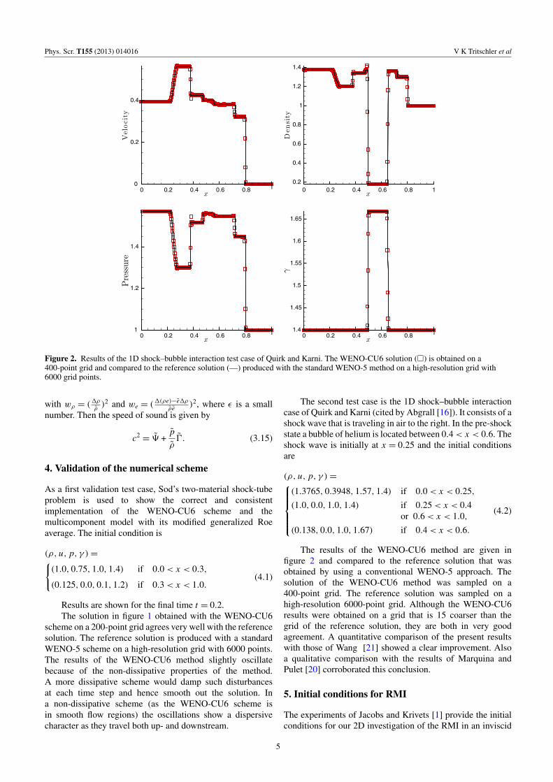
Figure 2. Results of the 1D shock–bubble interaction test case of Quirk and Karni. The WENO-CU6 solution (�) is obtained on a400-point grid and compared to the reference solution (—) produced with the standard WENO-5 method on a high-resolution grid with6000 grid points.

with wρ = (�ρρ

)2 and we = (�(ρe)−e�ρρe )2, where � is a small

number. Then the speed of sound is given by

c2 = � +pρ

�. (3.15)

4. Validation of the numerical scheme

As a first validation test case, Sod’s two-material shock-tubeproblem is used to show the correct and consistentimplementation of the WENO-CU6 scheme and themulticomponent model with its modified generalized Roeaverage. The initial condition is

(ρ, u, p, γ ) =�

(1.0, 0.75, 1.0, 1.4) if 0.0 < x < 0.3,

(0.125, 0.0, 0.1, 1.2) if 0.3 < x < 1.0.(4.1)

Results are shown for the final time t = 0.2.The solution in figure 1 obtained with the WENO-CU6

scheme on a 200-point grid agrees very well with the referencesolution. The reference solution is produced with a standardWENO-5 scheme on a high-resolution grid with 6000 points.The results of the WENO-CU6 method slightly oscillatebecause of the non-dissipative properties of the method.A more dissipative scheme would damp such disturbancesat each time step and hence smooth out the solution. Ina non-dissipative scheme (as the WENO-CU6 scheme isin smooth flow regions) the oscillations show a dispersivecharacter as they travel both up- and downstream.

The second test case is the 1D shock–bubble interactioncase of Quirk and Karni (cited by Abgrall [16]). It consists of ashock wave that is traveling in air to the right. In the pre-shockstate a bubble of helium is located between 0.4 < x < 0.6. Theshock wave is initially at x = 0.25 and the initial conditionsare

(ρ, u, p, γ ) =

(1.3765, 0.3948, 1.57, 1.4) if 0.0 < x < 0.25,

(1.0, 0.0, 1.0, 1.4) if 0.25 < x < 0.4or 0.6 < x < 1.0,

(0.138, 0.0, 1.0, 1.67) if 0.4 < x < 0.6.

(4.2)

The results of the WENO-CU6 method are given infigure 2 and compared to the reference solution that wasobtained by using a conventional WENO-5 approach. Thesolution of the WENO-CU6 method was sampled on a400-point grid. The reference solution was sampled on ahigh-resolution 6000-point grid. Although the WENO-CU6results were obtained on a grid that is 15 coarser than thegrid of the reference solution, they are both in very goodagreement. A quantitative comparison of the present resultswith those of Wang [21] showed a clear improvement. Alsoa qualitative comparison with the results of Marquina andPulet [20] corroborated this conclusion.

5. Initial conditions for RMI

The experiments of Jacobs and Krivets [1] provide the initialconditions for our 2D investigation of the RMI in an inviscid

5

Phys. Scr. T155 (2013) 014016 V K Tritschler et al

regime. The vertical shock tube used in the experiment hasa driver section that is filled with air at ambient pressureand temperature. In the test section an interface of air–SF6 isformed as the heavier SF6 flows upwards and collides with airflowing from top to down. Both gases exit through horizontalslots in the test section. A sinusoidal interface between thetwo gases is formed by oscillating the entire shock tube in thehorizontal direction. This membrane-less technique was firstproposed by Jones and Jacobs [14].

The initial conditions of the experimental setupconsidered in the present numerical study are as follows:The shock wave has a strength of Ms = 1.3 in air. Thesinusoidal interface of air–SF6 has a pre-shock amplitude ofa−

0 = 2.9 mm and a wavelength of λ = 59 mm. The locationof the material interface is then calculated from η = xi +a−

0 cos(2πy). The diffusion layer between the fluids is givenby [30]

f (δ) = fl(1 − δ) + frδ,

δ =(1 + tanh(�R

�))

2, (5.1)

� = D�

�xi�yi

and f = ρ, zSF6 . �R is the distance from the materialinterface. The densities of air and SF6 in ambient conditionsled to a pre-shock Atwood number of A− = 0.605. Theinterface is initialized at xI = 30 mm and the shock at xs =10 mm. The time is initialized to zero (t = 0) when the shockfirst impacts the SF6 gas.

5.1. Computational domain

The 2D computational domain is discretized by a Cartesiangrid. We use for all simulations a mesh size of 256 cellsper initial wavelength λ. The ‘numerical test section’ issurrounded by layers of coarser grids in order to avoid shockreflections at the inlet and outlet.

5.2. Non-dimensionalization

The reference scales to non-dimensionalize the governingequations are defined here. The reference density is setto the pre-shock density of air ρref = ρair = 1.351 kg m−3.Accordingly, the reference pressure is chosen to be the pre-shock pressure pref = 0.956 bar. The reference length scale isthe initial wavelength of the sinusoidal interface L ref = λ =59 mm and the reference time scale is tref =

�ρrefpref

L ref.

6. Numerical results

6.1. Single-fluid algorithm

In this subsection, the ratio of specific heats γ in (2.5) isassumed to be constant with the same value of γ = 1.276for both air and SF6 and hence is referred to as single-fluidalgorithm. Figure 3 shows the experimental results of Jacobsand Krivets [1] along with our numerical results obtained withthe standard WENO-5 and the WENO-CU6 method at threedifferent times t = 3.06 ms, t = 4.16 ms and t = 6.06 ms.

(a) (b) (c)

Figure 3. Experimental results of Jacobs and Krivets [1](a) compared to the single-fluid results obtained with the standardWENO-5 method (b) and the WENO-CU6 method (c) at threedifferent times t = 3.06 ms, t = 4.16 ms and t = 6.06 ms.

(a) (b) (c)

Figure 4. In (b) the post-shock conditions of the experiment arematched, whereas in (c) the pre-shock conditions are matched andcompared to the experiment (a) at times t = 4.16 ms andt = 6.06 ms.

The comparison shows that the lower-order WENO-5 methodpreserves large-scale structures and symmetry to later times,while WENO-CU6 better resolves small-scale structures,leading to symmetry breaking and increased mixing. Thisbetter behavior is in agreement with the findings ofLatini et al [11].

WENO-5 cannot reproduce the secondary instabilitieson the mushroom stem, whereas WENO-CU6 clearly showsthe same typical stem disturbances as the experiment at t =6.06 ms. On the other hand, it also shows instabilities on top ofthe mushroom which are not observed in the experiment. Webelieve that the origin of these numerical instabilities couldbe because of neglecting viscous effects, which makes theWENO-CU6 scheme less dissipative than the real physicalmechanisms. On the other hand, other numerical schemesapparently are too dissipative. Both discretization schemesare unable to predict correctly the large-scale structure such

6

Phys. Scr. T155 (2013) 014016 V K Tritschler et al

(a) (b) (c) (d)

Figure 5. Investigation of the impact of the diffusion layer on the late-time Richtmyer–Meshkov development with increasing the diffusionlayer thickness from (b) D = 4 to (c) D = 8 to (d) D = 16 at times t = 4.16 ms and t = 6.06 ms.

as the mushroom head diameter and stem diameter of theRMI experiment.

Richtmyer described the early linear growth rate of theinstability as a function of the post-shock parameters, a+

0the post-shock amplitude, A+ the post-shock Atwood number,the velocity jump �U0 associated with the shock passage andk the initial perturbation wavelength

ka(t) = ka+0 + k2a+

0 A+�U0t. (6.1)

From (6.1) it immediately follows that in order to matchthe correct initial growth rate and accordingly the laterdevelopment, one needs to reproduce the correct post-shockparameters. As the single-fluid method assumes constant γ , itis not possible to have matching pre- and post-shock states.Thus, it is preferable to match the post-shock state in order toimprove the agreement in the large-scale structures betweenexperiments and numerics at late times.

Figure 4(b) shows the result when the post-shockconditions of the experiment are matched. The pre-shockconditions are matched in figure 4(c). Comparing figures 4(b)and (c) to the experiment given in figure 4(a), a clearimprovement of the large-scale structure is observed infigure 4(b). It shows a wider mushroom head and a thinnerstem, which captures better the global characteristics of theRMI experiments.

6.2. Multifluid algorithm

In this subsection, γ is not assumed to be constant butcomputed from (2.6) with γair = 1.276 and γSF6 = 1.093.A transport equation is solved for the volume fraction (2.4)to account for the variable ratio of specific heats. By meansof (2.4) and the modified general Roe average of section 3.2we are able to simulate the material interface without theappearance of spurious pressure oscillations.

As the initial driving force of RMI is the vorticitydeposition on the material interface caused by the misalignedpressure and density gradient, it is of crucial importance toproperly match the pressure gradient and the density gradient.The pressure gradient is associated with the Mach numberof the incident shock wave and therefore is much betterquantifiable than the density gradient.

(a) (b) (c)

Figure 6. Comparison of the multifluid (b) and single-fluid(c) algorithms to the experiments (a) at times t = 4.16 ms andt = 6.06 ms.

In order to quantify the uncertainty of the densitydistribution across the interface, three different diffusion layerthicknesses are considered. Figure 5 shows a sequence ofsimulations with increasing diffusion layer thicknesses D = 4,D = 8 and D = 16, see (5.1). The vorticity deposited onthe interface decreases as the density gradient is reducedfrom the left, figure 5(b), to the right, figure 5(d). Althoughthe mushroom stem in figure 5(d) shows a non-sinusoidalperturbation the overall shape agrees best with the experiment.D = 16 is therefore used for making a comparison to theresults obtained using WENO-CU6 and a constant ratio ofspecific heats in figure 6.

Figure 6 reveals a clear improvement of the multifluidalgorithm over the single-fluid algorithm. The globalcharacteristics are captured much better in figure 6(b) thanin figure 6(c). When the late-time development of the RMIis of interest the correct compressibility of the fluids involvedneeds to be captured, which requires a multifluid simulationwith variable material properties.

7. Concluding remarks

The 2D simulations of the single-mode RMI using the recentlydeveloped WENO-CU6 reconstruction method of Hu et al [2]

7

Phys. Scr. T155 (2013) 014016 V K Tritschler et al

were conducted and compared with the experiments of Jacobsand Krivets [1]. The multicomponent model for stiffenedgases by Shyue [3] was used to account for multiple species.However, the high-order method employed made it necessaryto modify the general Roe average of Hu et al [23] in order tocapture material interfaces without the occurrence of spuriouspressure oscillations. In two 1D test cases it was shownthat the WENO-CU6 method together with the modifiedgeneral Roe average was capable of capturing accuratelymaterial interfaces without introducing undesirable amountsof numerical dissipation.

In a first sequence of simulations the ratio of specificheats γ was assumed to be constant for both fluids. The fluxeswere reconstructed with the WENO-CU6 and the standardWENO-5 method and compared to the experiments. It wasconcluded that the lower-order WENO-5 method preserveslarge-scale structures and symmetry to later times, while theWENO-CU6 better resolves small-scale structures, leadingto earlier symmetry breaking and increased mixing. Thisbetter behavior is in agreement with the findings of Latiniet al [11]. However, the global characteristic structures of RMIwere matched neither by the WENO-CU6 method nor by theWENO-5 method. This is due to the fact that the linear growthrate of RMI essentially depends on the post-shock state ofthe instability. A mismatch of the post-shock state essentiallyleads to wrong prediction of the late-time development. Thus,in terms of accuracy, it is much more preferable to matchthe post-shock state than the pre-shock state in single-fluidsimulations.

The initial driving force of RMI is the vorticity depositionon the material interface caused by the non-parallel pressureand density gradient. However, unlike the pressure gradient,the density gradient associated with the material interface isnot easy to quantify in experiments. Therefore, a sequenceof multifluid simulations with different diffusion layerthicknesses were conducted to assess the uncertainty inthe density gradient. The multifluid simulations showed aconsiderable improvement over the single-fluid simulationswhere the pre-shock state is matched.

Acknowledgments

VKT is a member of the TUM Graduate School andacknowledges the support he received.

References

[1] Jacobs J W and Krivets V V 2005 Experiments on thelate-time development of single-mode Richtmyer–Meshkovinstability Phys. Fluids 17 034105

[2] Hu X Y, Wang Q and Adams N A 2010 An adaptivecentral-upwind weighted essentially non-oscillatory schemeJ. Comput. Phys. 229 8952–65

[3] Shyue K-M 1998 An efficient shock-capturing algorithm forcompressible multicomponent problems J. Comput. Phys.142 208–42

[4] Richtmyer R D 1960 Taylor instability in shock acceleration ofcompressible fluids Commun. Pure Appl. Math.XIII 297–319

[5] Meshkov E E 1969 Instability of the interface of two gasesaccelerated by a shock wave Fluid Dyn. 4 101–4

[6] Taylor G I 1950 The instability of liquid surfaces whenaccelerated in a direction perpendicular to their planes Proc.R. Soc. A 201 192

[7] Arnett D 2000 The role of mixing in astrophysics Appl. J.Suppl. 127 213–17

[8] Yang J, Kubota T and Zukoski E E 1993 Applications ofshock-induced mixing to supersonic combustion AIAA J.31 854–62

[9] Brouillette M 2002 The Richtmyer-Meshkov instability Annu.Rev. Fluid Mech. 34 445–68

[10] Zabusky N 1999 Vortex paradigm for acceleratedinhomogenous flows: visiometrics for the Rayleigh–Taylorand Richtmyer–Meshkov environments Annu. Rev. FluidMech. 31 495

[11] Latini M, Schilling O and Don W S 2007 Effects of WENOflux reconstruction order and spatial resolution on reshockedtwo-dimensional Richtmyer–Meshkov instability J. Comput.Phys. 221 805–36

[12] Latini M, Schilling O and Don W S 2007 High-resolutionsimulations and modeling of reshocked single-modeRichtmyer–Meshkov instability: comparison toexperimental data and to amplitude growth modelpredictions Phys. Fluids 19 024104

[13] Collins B D and Jacobs J W 2002 PLIF flow visualization andmeasurements of the Richtmyer–Meshkov instability of anair/SF6 interface J. Fluid Mech. 464 113–36

[14] Jones M A and Jacobs J W 1997 A membraneless experimentfor the study of Richtmyer–Meshkov instability of ashock-accelerated gas interface Phys. Fluids 9 3078–85

[15] Karni S 1994 Multicomponent flow calculations by aconsistent primitive algorithm J. Comput. Phys. 112 31–43

[16] Abgrall R 1996 How to prevent pressure oscillations inmulticomponent flow calculations: a quasi conservativeapproach J. Comput. Phys. 125 150–60

[17] Karni S 1996 Hybrid multifluid algorithms SIAM J. Sci.Comput. 17 1019

[18] Abgrall R 2001 Computations of compressible multifluidsJ. Comput. Phys. 169 594–623

[19] Allaire G, Clerc S and Kokh S 2002 A five equation model forthe simulation of the interface between compressible fluidsJ. Comput. Phys. 181 577–616

[20] Marquina A and Pulet P 2003 A flux-split algorithm applied toconservative models for multicomponent compressible flowsJ. Comput. Phys. 185 120–38

[21] Wang S 2004 A thermodynamically consistent and fullyconservative treatment of contact discontinuities forcompressible multicomponent flows J. Comput. Phys.195 528–59

[22] Shu C-W 1997 Essentially non-oscillatory and weightedessentially non-oscillatory schemes for hyperbolicconservation laws ICASE Report no. 97-65

[23] Hu X Y, Adams N A and Iaccarino G 2009 On the HLLCRiemann solver for interface interaction in compressiblemulti-fluid flow J. Comput. Phys. 228 6572–89

[24] Toro E F 1999 Riemann Solvers and Numerical Methods forFluid Dynamics (Berlin: Springer)

[25] Hu X Y and Adams N A 2011 Scale separation for implicitlarge eddy simulation J. Comput. Phys. 230 7240–9

[26] Liou M S, B van Leer and Shuen J S 1990 Splitting forinviscid fluces for real gas J. Comput. Phys. 87 1–24

[27] Shyue K M 2001 A fluid-mixture type algorithm forcompressible multicomponent flow with Mie–Gruneisenequation of state J. Comput. Phys. 171 678–707

[28] Glaister P 1988 An approximate linearised Riemann solver forthe Euler equations for real gases J. Comput. Phys.74 382–408

[29] Roe P L 1981 Approximate Riemann solvers, parameter anddifference schemes J. Comput. Phys. 43 357–72

[30] Shankar S K, Kawai S and Lele S K 2010 Numericalsimulation of multicomponent shock accelerated flows andmixing using localized artificial diffusivity method 4th AIAAAerospace Science Meeting

8