arX

iv:q

uant

-ph/

0608

194v

2 2

8 A

ug 2

006

Numerical simulation of Quantum Teleportation in a chain of three nuclear spins system

taking into account second neighbor iteration

G.V. Lopez and L. LaraDepartamento de Fısica, Universidad de Guadalajara

Apartado Postal 4-137, 44410 Guadalajara, Jalisco, Mexico

PACS: 03.67.-a, 03.67.Lx, 03.67.Dd, 03.67.Hk

ABSTRACT

For a one-dimensional chain of three nuclear spins (one half), we make the numericalsimulation of quantum teleportation of a given state from one end of the chain tothe other end, taking into account first and second neighbor interactions among thespins. It is shown that a well defined teleportation protocol is achieved for a ratioof the first to second neighbor interaction coupling constant of J ′/J ≥ 0.04. Wealso show that the optimum Rabi’s frequency to control the non-resonant effects isdominated by the second neighbor interaction coupling parameter (J ′).

1

1. Introduction

Quantum teleportation is a technique which allows us to move a quantum state of ourquantum system from one location to another location using quantum computationor quantum information [1]. Quantum computation or quantum information usesquantum bits (called qubits) to handle the information on the quantum system. Aqubit is a superposition of any two quantum basic states of the system (called |0〉and |1〉), Ψ = C0|0〉 + C1|1〉, such that |C0|2 + |C1|2 = 1. One may call |0〉 and|1〉 the basic qubits of the system. The L-tensorial product of L-basic qubits forman L-register of L-qubits, |x〉 = |iL−1, . . . , i0〉 with ij = 0, 1 for j = 0, . . . , L − 1(”0” for ground state and ”1” for exited state). The set of these L-registers makesup the 2L-dimensional Hilbert space where the quantum computer and quantuminformation work. A typical element of this space is Ψ =

∑Cx|x〉, where

∑ |Cx|2 =1, and |Cx|2 gives us the probability of having the state |x〉 after measurement.We are interested in studying the phenomena of quantum teleportation in a solidstate quantum computer formed by a one-dimensional chain of nuclear spins [2],where a preliminary study of this technique was done using two-qubit registersand considering first neighbor interaction between spins [3]. In this paper, we willconsider also the second neighbor interaction among the spins in a chain of threenuclear spins system. Thus, the phenomena of quantum teleportation from one endof the chain of spins to the other end is studied numerically. Adding a quantum state(qubit) to our chain of three nuclear spins means to add another nuclear spin at oneend, having, then, a quantum computer working with four-qubit registers. We studythe well performance of the quantum teleportation algorithm through the fidelityparameter and determine the minimum value of the second neighbor interactioncoupling constant to do this. Finally, we also see the modification that the so called2πk-method could have with the consideration of second neighbor iteration and itsimplication in our simulation

2. Equation of Motion

Consider a one-dimensional chain of four equally spaced nuclear-spins system (spinone half) making an angle cos θ = 1/

√3 with respect the z-component of the mag-

netic field (chosen in this way to kill the dipole-dipole interaction between spins)and having an rf-magnetic field in the transversal plane. The magnetic field is givenby

B = (b cos(ωt + ϕ),−b sin(ωt + ϕ), B(z)) , (1)

where b, ω and ϕ are the amplitude, the angular frequency and the phase of therf-field, which could be different for different pulses. B(z) is the amplitude of the z-component of the magnetic field. Thus, the Hamiltonian of the system up to secondneighbor interaction is given by

H = −3∑

k=0

µk · Bk − 2Jh2∑

k=0

IzkIz

k+1 − 2J ′h1∑

k=0

IzkIz

k+2 , (2)

where µk represents the magnetic moment of the kth-nucleus which is given in termsof the nuclear spin as µk = hγ(Ix

k , Iyk , Iz

k), being γ the proton gyromagnetic ratio.Bk represents the magnetic field at the location of the kth-spin. The second term

2

at the right side of (2) represents the first neighbor spin interaction, and the thirdterm represents the second neighbor spin interaction. J and J ′ are the couplingconstants for these interactions. This Hamiltonian can be written in the followingway

H = H0 + W , (3a)

where H0 and W are given by

H0 = −h

3∑

k=0

ωkIzk + 2J(Iz

0 Iz1 + Iz

1Iz2 + Iz

2Iz3 ) + 2J ′(Iz

0Iz2 + Iz

1Iz3 )

(3b)

and

W = − hΩ

2

3∑

k=0

[eiωtI+

k + e−iωtI−k

], (3c)

where ωk = γB(zk) is the Larmore frequency of the kth-spin, Ω = γb is the Rabi’sfrequency, and I±k = Ix

k ± iIyk represents the ascend operator (+) or the descend

operator (-). The Hamiltonian H0 is diagonal on the basis |i3i2i1i0〉, where ij =0, 1 (zero for the ground state and one for the exited state),

H0|i3i2i1i0〉 = Ei3i2i1i0 |i3i2i1i0〉 . (4a)

The eigenvalues Ei3i2i1i0 are given by

Ei3i2i1i0 = − h

2

3∑

k=0

(1)ikωk + J

2∑

k=0

(−1)ik+ik+1 + J ′

1∑

k=0

(−1)ik+ik+2

. (4b)

The term (3c) of the Hamiltonian allows to have a single spin transitions on theabove eigenstates by choosing the proper resonant frequency.

To solve the Schrodinger equation

ih∂Ψ

∂t= HΨ , (5)

let us propose a solution of the form

Ψ(t) =15∑

k=0

Ck(t)|k〉 , (6)

where we have used decimal notation for the eigenstates in (4a), H0|k〉 = Ek|k〉.Substituting (6) in (5), multiplying for the bra 〈m|, and using the orthogonalityrelation 〈m|k〉 = δmk, we get the following equation for the coefficients

ihCm = EmCm +15∑

k=0

Ck〈m|W |k〉 m = 0, . . . , 15. (7)

Now, using the following transformation

Cm = Dme−iEmt/h , (8)

3

the fast oscillation term EmCm of Eq. (7) is removed (this is equivalent to go-ing to the interaction representation), and the following equation is gotten for thecoefficients Dm

iDm =1

h

15∑

k=0

WmkDkeiωmkt , (9a)

where Wmk denotes the matrix elements 〈m|W |k〉, and ωmk are defined as

ωmk =Em − Ek

h. (9b)

Eq. (9a) represents a set of sixteen real coupling ordinary differential equationswhich can be solved numerically, and where W ′

mks are given by

(W ) = − hΩ

2× 0, z, ”or” z∗ , (9c)

where z is defined as z = ei(ωt+ϕ), and z∗ is its complex conjugated.

A pulse of time length τ , phase ϕ, and resonant frequency ω = ωi,j will be denotedby Ri,j(Ωτ, ϕ), and it is understood that such a pulse implies the solution of Eq.(9a) with given initial conditions.

3. Quantum teleportation and numerical simulation

The basic idea of quantum teleportation [1] is that Alice (left end qubit in our chainof three qubits) and Bob (the other end qubit) are related through and entangledstate,

Ψe =1√2

(|0A00B〉 + |1A01B〉

). (10)

So, neglecting decoherence effects which could destroy this entangled state, we adjointo Alice an arbitrary state Ψx ,

Ψx = Cx0 |0〉 + Cx

1 |1〉 , (11)

resulting the quantum state (Ψ1 = Ψx ⊗ Ψe)

Ψ1 =1√2

[Cx

0 |0000〉 + Cx0 |0101〉 + Cx

1 |1000〉 + Cx1 |1101〉

]. (12)

Then, one applies a Controlled-Not (CN) operation in this added stated and Alice,

CN23|i3, i2, i1, i0〉 = |i3, i2 ⊕ i3, i2, i0〉 , (13)

where i2 ⊕ i3 = i2 + i3(mod 2), resulting the state (Ψ2 = CN23Ψ1)

Ψ2 =1√2

[Cx

0 |0000〉 + Cx0 |0101〉 + Cx

1 |1100〉 + Cx1 |1001〉

]. (14)

Finally, one applies a superposition (Hadamar) operation in the added state location,

A3

|0000〉|1000〉 =

1√2

|0000〉 + |1000〉|0000〉 − |1000〉 , (15)

4

resulting, after some rearrangements, the state (Ψ3 = A3Ψ2)

Ψ3 =1

2

|00〉 ⊗ |0〉

(Cx

0 |0〉 + Cx1 |1〉

)+ |01〉 ⊗ |0〉 ⊗

(Cx

0 |1〉 + Cx1 |0〉

)

+|10〉 ⊗ |0〉 ⊗(

Cx0 |0〉 − Cx

1 |1〉)

+ |11〉 ⊗ |0〉 ⊗(

Cx0 |1〉 − Cx

1 |0〉)

.

(16)

When Alice measures both of her qubits, there are four possible cases (|00〉, |01〉,|10〉, and |11〉), and for each case Bob will get the original Ψx state by applying aproper operation to his state: identity, Not (N), σz, or σzN , where the action ofthese operators are as follows: N |0〉 = |1〉, N |1〉 = |0〉, σz|0〉 = |0〉, and σz|1〉 = −|1〉.The most important features in this algorithm are that Alice and Bob do not needto know the state Ψx, and there are always four possibilities for Alice measurement.

Now, the algorithm we need to implement this quantum teleportation techniquein our one-dimensional three nuclear spins system varies a little from the schemepresented above since our three-qubits quantum computer will start from the groundstate

Ψ00 = |000〉 . (17a)

Therefore, one needs first to attach the unknown state (11) to (17a) to get the initialfour-spins wave function (Ψ0 = Ψx ⊗ Ψ00),

Ψ0 = Cx0 |0000〉 + Cx

1 |1000〉 , (17b)

where |Cx0 |2 + |Cx

1 |2 = 1. The entangled state (12) is obtained with the followingthree pulses

Ψ1 = R4,5(π,−3π/2)R8,12(π/2,−π/2)R0,4(π/2,−π/2)Ψ0 . (16c)

The Controlled-Not operation CN23Ψ1 is gotten through the following two pulses

Ψ2 = R9,13(π, 3π/2)R8,12(π,−3π/2)Ψ1 . (17d)

Finally, the wave function (16) is gotten after the application of the following twopulses to the above wave function

Ψ3 = R4,12(π/2,−3π/2)R1,9(π/2,−3π/2)Ψ2 . (17e)

To make the numerical simulation of this algorithm, we have chosen the followingparameters in units of 2π×Mhz,

ω0 = 100 , ω1 = 200 , ω2 = 400 , ω3 = 800, J = 10 , J ′ = 0.4 , Ω = 0.1 . (18a)

These parameters were chosen in this way to have a clear definition on our Zeemanspectrum and transitions among them. Of course, our main results are applied tothe actual current design parameters of reference [4]. On the other hand, we selectedthe state (11) with the following coefficients

Cx0 =

1

3and Cx

1 =

√8

3. (18b)

5

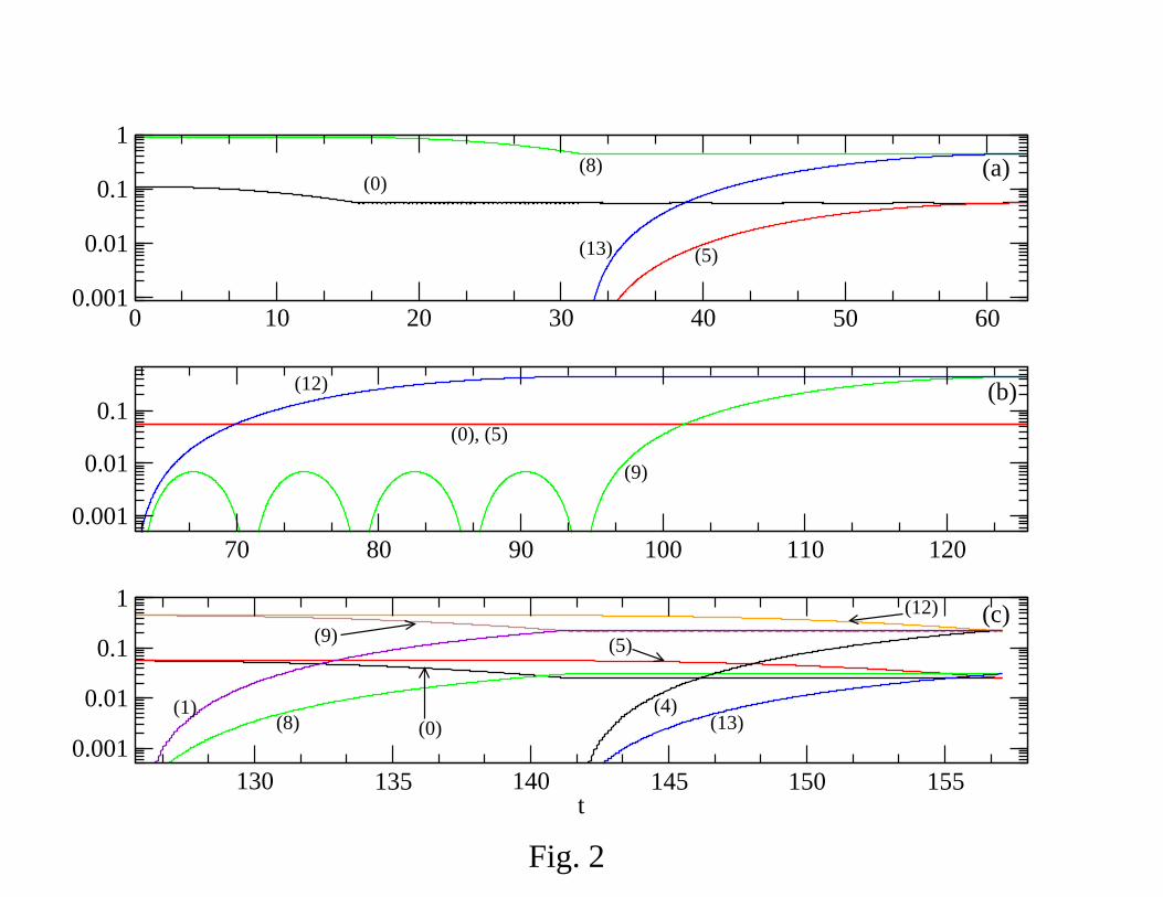
Fig. 1 shows the Zeeman spectrum of the four nuclear spins system with the tran-sitions used during our teleportation simulation. Fig. 2a shows the probabilities|C0|2, |C5|2, |C8|2 and |C13|2 during the first three pulses, where the formation ofthe entangled wave function (12) is shown, from the initial state (17b). Fig. 2bshows the probabilities |C0|2, |C5|2, |C9|2 and |C12|2 during the following two pulsesto get at the end the wave function (14). Fig. 2c shows the probabilities |C0|2, |C8|2,|C5|2, |C13|2, |C12|2, |C4|2, |C9|2 and |C1|2 during the last two pulses to get at theend the desired function (16). Note that at the end of our algorithm one expectsthe following values for these probabilities

|C0|2 = |C8|2 = |C5|2 = |C13|2 =|Cx

0 |24

, (19a)

and

|C12|2 = |C4|2 = |C9|2 = |C1|2 =|Cx

1 |24

(19b)

To get a better feeling what is going on on each process, we calculate the z-component of the expected values of the spin for each qubit. These expected valuesare given by

〈Iz0 〉 =

1

2

15∑

k=0

(−1)k|Ck(t)|2 , (20a)

〈Iz1 〉 =

1

2

|C0|2 + |C1|2 − |C2|2 − |C3|2 + |C4|2 + |C5|2 − |C6|2 − |C7|2

+|C8|2 + |C9|2 − |C10|2 − |C11|2 + |C12|2 + |C13|2 − |C14|2 − |C15|2

,

(20b)

〈Iz2 〉 =

1

2

|C0|2 + |C1|2 + |C2|2 + |C3|2 − |C4|2 − |C5|2 − |C6|2 − |C7|2

+|C8|2 + |C9|2 + |C10|2 + |C11|2 − |C12|2 − |C13|2 − |C14|2 − |C15|2

,

(20c)

and

〈Iz3 〉 =

1

2

7∑

k=0

|Ck|2 −1

2

15∑

k=8

|Ck|2 . (20d)

Figs. 3a, 3b, and 3c show these expected values during entangled formation, controlled-not operation, and final teleportation. As one can see, these behavior is what onecould expected for each process. Fig. 4a shows the probabilities (19a) and (19b) atthe end of the teleportation (wave function (16)), and Fig. 4b shows the probabilitiesof the non-resonant states involved in the dynamics.

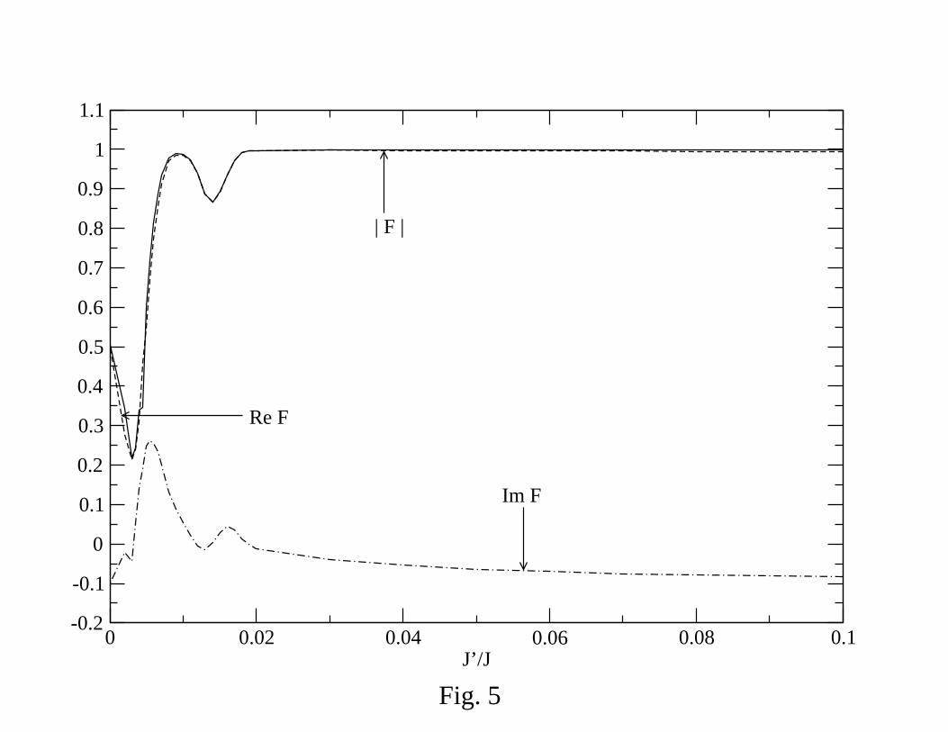
To see the values of the second neighbor interaction coupling parameter from whichone could have a well defined teleportation algorithm, we study the fidelity param-eter [5],

F = 〈Ψexpected|Ψ〉 , (21)

6

where Ψexpected is the ideal wave function (16). Fig. 5 shows this fidelity parameteras a function of the ratio of second to first neighbor coupling parameters (J ′/J). Asone can see, a well defined teleportation algorithm is gotten for J ′/J ≥ 0.04.

4. Quantum teleportation and the 2πk-method

One of the important results from the consideration of first neighbor interactionand the selection of the parameter as J/∆ω ≪ 1 and Ω/∆ω ≪ 1 is the possibilityto choose the Rabi’s frequency Ω in such a way that the non-resonant effects areeliminated. This procedure is called the 2πk-method [4], and this Rabi’s frequencyis chosen as Ω = |∆|/

√4k2 − 1 for a π-pulse, where k is an integer number, ∆ is the

detuning parameter (∆ = (Ep − Em)/h − ω) between the states |p〉 and |m〉 whenthe resonant frequency is ω, and this detuning parameter is proportional to the firstneighbor coupling constant J . Let us see how this detuning parameter could bemodified due to second neighbor interaction. Assuming that the states |p〉 and |m〉are are the only ones involved in the dynamics, from Eq. (9a), one has

iDm =Wmp

hDpe

iωmpt , and iDp =Wpm

hDmeiωpmt . (22)

Thus, given the initial conditions Dp(0) = Cp(0) and Dm(0) = Cm(0), the solutionis readily given by

Dp(t) =

Cp(0)

[cos

Ωet

2− i

∆

Ωesin

Ωet

2

]+ i

ΩCm(0)

Ωesin

Ωet

2

e

i∆t2 (23a)

and

Dm(t) =

Cm(0)

[cos

Ωet

2− i

∆

Ωesin

Ωet

2

]+ i

ΩCp(0)

Ωesin

Ωet

2

e

−i∆t2 , (23b)

where Ωe is defined as Ωe =√

Ω2 + ∆2. For a π-pulse (t = τ = π/Ω), one canselect the term Ωeπ/2Ω to be equal to any multiple of π, Ωeπ/2Ω = kπ, to get thecondition Ω = |∆|/

√4k2 − 1. this condition gets rid of the non-resonant terms since

from Eqs. (20a) and (20b) one gets

Dp(τ) = (−1)kCp(0)ei∆π/2Ω , and Dm(τ) = (−1)kCm(0)e−i∆π/2Ω .

For a π/2-pulse (t = τ = π/2Ω), one can select the term Ωeπ/4Ω to be equal toany multiple of π, Ωeπ/4Ω = kπ, to get the condition Ω = |∆|/

√16k2 − 1. this

condition gets rid also of the non-resonant terms.

Now, if for example one selects a resonant transition which contains the Larmorefrequency ω0, these frequencies could be ω0 + J + J ′, ω0 − J + J ′, ω0 − J − J ′ orω0 +J−J ′ which correspond to the transitions (decimal notation) |0〉 ↔ |1〉 (|10〉 ↔|11〉), |2〉 ↔ |3〉, |6〉 ↔ |7〉, and |2〉 ↔ |3〉. So, all of these states are pertubated,and the frequency difference ∆ may have the values 2J , 2J ′, 2J + 2J ′, or 2J − 2J ′.For other Larmore frequencies the additional values of the detuning parameter are

4J , and 4J + 2J ′. Thus, let us denote by Ω(k)∆ the Rabi’s frequency selected by this

method,

Ω(k)∆ =

|∆|√4k2 − 1

, π-pulse (24a)

7

and

Ω(k)∆ =

|∆|√16k2 − 1

, π/2-pulse (24b)

where ∆ can have the values 4J+2J ′, 4J , 2J+2J ′, 2J or 2J ′. To see the dependenceof our teleportation algorithm with respect the Rabi’s frequency, we use again thefidelity parameter parameter (21). With the same values for our parameters as (18a)but Ω, Fig. 6 shows the fidelity parameter as a function of the Rabi’s frequency.Dashed vertical lines mark the omega values where the peaks ocurres. These peakscorrespond to some specific omega defined through the 2πk-method. For example,the line (1), (2) and (3) correspond to the following Rabi’s frequency values

Ω(202)4J+2J ′ ≈ Ω

(199)4J ≈ Ω

(103)2J+2J ′ ≈ Ω

(100)2J ≈ Ω

(4)2J ′ = 0.10079 ,

Ω(305)4J+2J ′ ≈ Ω

(304)4J ≈ Ω

(156)2J+2J ′ ≈ Ω

(150)2J ≈ Ω

(6)2J ′ = 0.066889 ,

andΩ

(407)4J+2J ′ ≈ Ω

(400)4J ≈ Ω

(208)2J+2J ′ ≈ Ω

(200)2J ≈ Ω

(8)2J ′ = 0.050098 .

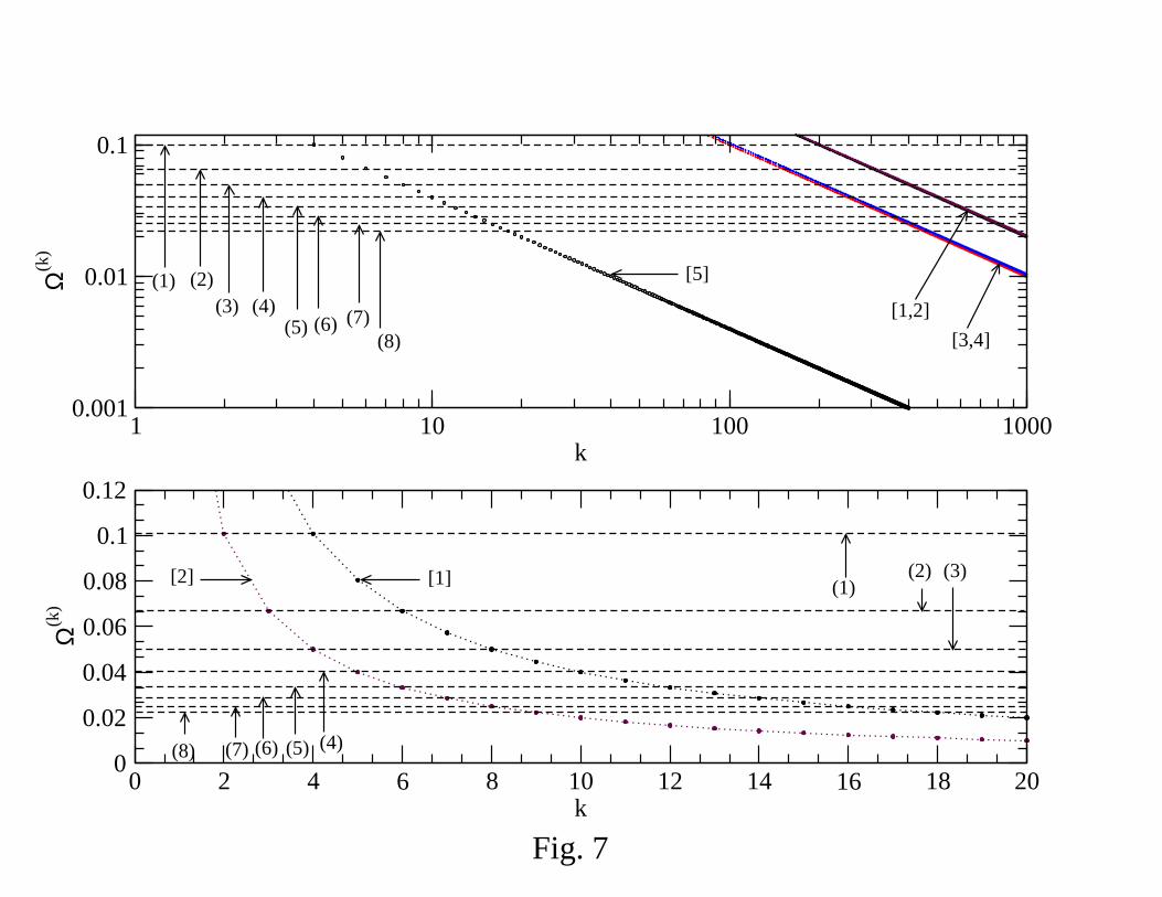
As one can see in Fig. 7a, where we have plotted Ω(k)∆ (for the detuning values

mentioned above) and where the corresponding dashed vertical lines of Fig. 6 have

been drawn, around these lines there are several other values of Ω(k)4J+2J ′ , Ω

(k)4J ,

Ω(k)2J+2J ′ and Ω

(k)2J which, in principle, should cause a peak in the fidelity parameter

(because they belong to the 2πk-method). However, they do not appear at all on Fig.6. This means that the peaks values on the fidelity parameter are fully dominatedby the second neighbor coupling interaction parameter (J ′). On the other hand, the

reason why only even numbers of k appears for these peaks for Ω(k)2J ′ can be seen in

Fig. 7b where Ω(k)2J ′ and Ω

(k)2J ′ have been plotted as a function of k. On this plot one

sees that the jth-dashed lines correspond to Ω(j)2J ′ = Ω2j

2J ′ . Therefore, the peaks onfidelity correspond to 2πk-method dominated by J ′ and by π/2-pulses. This seemsreasonable since our teleportation algorithm starts with π/2-pulses and finishes withπ/2-pulses.

8

5. Conclusions

We have made a numerical simulation of teleportation in a solid state quantumcomputer modeled by one-dimensional chain of three nuclear spins (one half), andconsidering first and second neighbor interactions. We have shown that a good tele-portation algorithm can be gotten if the ratio of second to first neighbor interactionconstants is chosen such that J ′/J ≥ 0.04. We also studied the effect of the sec-ond neighbor interaction on the detuning parameter which is used in the so called2πk-method to eliminate non-resonant transitions, and we have shown that the ap-plication of this method in our teleportation algorithm is not so simple since thedetuning parameter varies with both parameters J and J ′ (first and second neighborcoupling interactions). However, the peaks on the fidelity parameter are dominatedby the second neighbor coupling parameter and the π/2-pulses.

Acknowledgements

This work was supported by SEP under the contract PROMEP/103.5/04/1911 andthe University of Guadalajara.

9

Figure Captions

Fig. 1 Energy levels and resonant frequencies used within the algorithm.

Fig. 2 Probabilities |Ck|2 : (k). (a) Formation of the entangled state, wave function(12). (b) Formation of the wave function (14). (c) Formation the wave function(16).

Fig. 3 Expected values 〈Izk〉: (k=0,1,2,3). (a) During formation of wave function

(12). (b) During formation of the wave function (14). (c) During formation of thewave function (16).

Fig. 4 Probabilities |Ck|2. (a) For the expected registers k = 0, 8, 5, 13, 12, 4, 9, 1.(b) For the non-resonant states k = 2, 3, 6, 7, 10, 11, 14, 15.

Fig. 5 Fidelity parameter as a function of J ′/J .

Fig. 6 Fidelity parameter as a function of Ω.

Fig. 7 (a): Rabi frequency Ω(k)∆ as a function of k for ∆ = 4J + 2J ′ [1], ∆ = 4J

[2], ∆ = 2J + 2J ′ [3], ∆ = 2J [4], ∆ = 2J ′ [5]. Dashed lines (j) for j = 1, . . . , 8

correspond to Fig. 6. (b): Rabi frequency Ω(k)∆ [1] and Ω

(k)∆ [2] as a function of k.

Dashed lines (j) for j = 1, . . . , 8 correspond to Fig. 6.

10

References

1. C.H. Benneth, G. Brassard, C. Crepeau, R. Jozsa, A. Peres, and W. WoottersPhys. Rev. Lett., 70 (1993) 1895.

2. S. Lloyd, Science, 261 (1995) 1569.S. Lloyd, Sci. Amer., 273 (1995) 140.G.P. Berman, G.D. Doolen, D.J. Kamenev, G.V. Lopez, and V.I. TsifrinovichPhys. Rev. A, 6106 (2000) 2305.

3. G.P. Berman, G.D. Doolen, G.V. Lopez, and V.I. Tsifrinovich,quant-ph/9802015 (1998).

4. G.P. Berman, G.D. Doolen, D.J. Kamenev, G.V. Lopez, and V.I. TsifrinovichContemporary Mathematics, 305 (2002) 13.

5. A. Peres, Phys. Rev. A 30 (1984) 1610.B. Schumacher, Phys. Rev. A.,51 (1995) 2738.

11

-800

-400

0

400

800

2π M

Hz

|0000>

|0001>

|0010>

|0011>

|0100>

|0101>

|0110>

|0111>

|1000>

|1001>

|1010>

|1011>

|1100>

|1101>

|1110>

|1111>

Fig. 1

0 10 20 30 40 50 600.001

0.01

0.1

1

70 80 90 100 110 1200.001

0.01

0.1

130 135 140 145 150 155t

0.001

0.01

0.1

1

(0)

(5)

(8)

(13)

(0), (5)

(9)

(12)

(13)(4)

(12)

(8)

(5)

(1)(0)

(9)

(a)

(b)

(c)

Fig. 2

0 10 20 30 40 50 60-0.6

-0.45-0.3

-0.150

0.150.3

0.450.6

70 80 90 100 110 120-0.6

-0.45-0.3

-0.150

0.150.3

0.450.6

130 135 140 145 150 155t

-0.6-0.45

-0.3-0.15

00.150.3

0.450.6

(0)(1)

(2)

(3)

(1)

(0)

(2)(3)

(0), (2)

(1)

(3)

(a)

(b)

(c)

Fig. 3

0 1 2 3 4 5 6 7 8 9 10 11 12 13 14 15 16states

0

0.05

0.1

0.15

0.2

0.25

0 1 2 3 4 5 6 7 8 9 10 11 12 13 14 15 16states

1e-08

1e-07

1e-06

(a)

(b)

Fig. 4

0 0.02 0.04 0.06 0.08 0.1J’/J

-0.2

-0.1

0

0.1

0.2

0.3

0.4

0.5

0.6

0.7

0.8

0.9

1

1.1

Im F

Re F

| F |

Fig. 5

0 0.02 0.04 0.06 0.08 0.1 0.12 0.14Ω

0.86

0.88

0.9

0.92

0.94

0.96

0.98

1

| F |

(1)(2)(3)

(4)

(5)

(6)

(7)

(8)

Fig. 6

1 10 100 1000k

0.001

0.01

0.1

Ω(k

)

0 2 4 6 8 10 12 14 16 18 20k

0

0.02

0.04

0.06

0.08

0.1

0.12

Ω(k

)

Fig. 7

(1) (2)(3) (4)

(5) (6) (7)(8)

[1,2]

[3,4]

[5]

(1)(2) (3)

(4)(5)(6)(7)(8)

[1][2]