arX

iv1

110

2996

v1 [

astr

o-ph

IM

] 1

3 O

ct 2

011

Numerical Results for the System Noise Temperature of an

Aperture Array Tile and Comparison with Measurements

MV Ivashina lowast1 EEM Woestenburg dagger2 L Bakker Dagger2 and RH Witvers sect 2

1Department of Earth and Space Sciences Chalmers University of Technology Sweden2The Netherlands Institue for Radio Astronomy (ASTRON)

October 15 2011

1 Introduction

This work has been supported in part by the Netherlands Organization for Scientific Research (APERTIFproject funded by NWOGroot) the Swedish Agency for Innovation Systems VINNOVA and Chalmers Uni-versity of Technology (VINNMER - Marie Curie Actions international qualification fellowship) Some resultsof this work have been recently published in [1 2]

This report is a shortened version of the original ASTRON report (RP324 2011) which is publicallyavailible upon request The purpose of this report is to document the noise performance of the Apertifarray receiver which has been used to measure its performance as an aperture array and to characterizethe recently developed noise measurement facility THACO The receiver system is the second prototype ofAPERTIF (DIGESTIF2) [3 4] that includes the array antenna of 144 dual-polarized TSA elements 144 LowNoise Amplifiers (LNAs) (Tmin =35-40K) and the data recordingstoring facilities of the initial test stationthat allow for off-line digital beamforming

The primary goal of this study is to compare the measured receiver noise temperatures with the simulatedvalues for several practical beamformers and to predict the associated receiver noise coupling contributionantenna thermal noise and ground noise pick-up (due to the back radiation) The measurements wereperformed over a wide frequency band and scan range In the course of the measurements the 4 16 25and 49 active antenna elements were used in beamforming while the remaining elements were connected tothe LNAs with the outputs terminated in matched loads The experimental results were obtained when thereceiver with 4- and 16-element analog beamformers was placed inside THACO (a metal shielding cabin whichwas designed to mitigate the noise contributions due to the ground and trees) and in the open environmentat Westerbork near the Westerbork Synthesis Radio Telescope (WSRT) using digital beamforming Thedetails of these measurements can be found in [2]

Since the digital data recording-storing facilities are available for the DIGESTIF array receiver onecan also evaluate the system noise temperature for beamforming scenarios that are based on standard signalprocessing algorithms [5]ndash[6] and the noise correlation coefficients between the array channels In this reportwe therefore show the range of the realized system noise temperatures when an embedded element only and all

lowastivashinachalmerssedaggerwoestenburgastronnlDaggerbakkerastronnlsectwitversastronnl

1

array elements are used in beamforming These results demonstrate the pros and cons of the considered low-gain antenna and high gain digital array receivers for the purpose of the noise temperature characterizationin an open environment and inside a shielding cabin such as THACO

2 The model of the array antenna

The array consists of 2times 72 aluminium Tapered Slot Antenna (TSA) elements with a pitch of 11 cm (052λat 1420 MHz) on a rectangular 8times 9 grid Each TSA is fed by a wideband microstrip feed which has beenintegrated with an LNA on a printed circuit board This design features a very short transmission linebetween the antenna and the LNA since the circular slotline cavity has been moved sideways More detailson the array design and the numerical approach used for the EM-analysis of the antenna can be found in [7]and [6 8] respectively The simulations of the antenna have been carried out using CAESAR software thatis an array system simulator developed at ASTRON [9] Note that these simulations did not take intoaccount the effect of the contributions from obstacles (trees and telescopesbuildings) near the horizon

3 The noise model of the receiver system

The noise model used in this study is based on the equivalent system representation as described in [10]According to this representation the sensitivity of the array receiver can be computed as follows

Aeff

Tsys

=Aphηap

Text +

(

1minus ηradηrad

)

Tamb +

(

1

ηrad

)

TLNAEq

(1)

where Aph and Tsys are the physical antenna area and system noise temperature respectively The latterconsists of three main contributions (i) The external noise contribution - the ground noise picked up due toantenna back radiation which was computed from the simulated illumination pattern of the antenna arrayfor the specified beam former weights (ii) the thermal antenna noise due to the losses in the conductorand dielectric materials of TSAs and microstrip feeds The conductor losses are computed through theevaluation of the antenna radiation efficiency using the methodology detailed in [11] and the dielectric lossesare computed based on the experimental evaluation of the feed loss [12] and (iii) the noise due to LNAswhich is dependent upon the noise properties of LNAs and active reflection coefficients seen at the portsof the antenna array Note that by using this definition of Tsys all noise temperature contributions arereferenced to the sky (in front of the antenna aperture)

It is important to note that the system noise temperature which is calculated from the measured Y-factoris also referenced to the sky Therefore to distinguish between the external noise antenna thermal noise andreceiver contributions one needs to know the beam shape (to compute Text) and radiation efficiency ηrad ofthe antenna which are in general dependent on the beamformer weights

4 The model of the beamformer used to compute the optimal

weights

The beamformer model used in this study is based on the mathematical framework which has been describedin [6] Within this framework the array receiver system is subdivided into two blocks (i) the front-end including the array antenna Low Noise Amplifiers (LNAs) and (ii) the beamformer with complexconjugated weights wlowast

nNn=1 and an ideal (noiselessreflectionless) power combiner realized in software

Here wH = [wlowast

1 wlowast

N ] is the beamformer weight vector H is the Hermitian transpose and the asteriskdenotes the complex conjugate Furthermore a = [a1 aN ]T is the vector holding the transmission-linevoltage-wave amplitudes at the beamformer input (the N LNAs outputs) Hence the fictitious beamformeroutput voltage v (across Z0) can be written as v = wHa and the receiver output power as |v|2 = vvlowast =

2

(wHa)(wHa)lowast = (wHa)(aTwlowast)lowast = wHaaHw where the proportionality constant has been dropped as thisis customary in array signal processing and because we will consider only ratios of powers

Although each subsystem can be rather complex and contains multiple internal signalnoise sources itis characterized externally (at its accessible ports) by a scattering matrix in conjunction with a noise- andsignal-wave correlation matrix In this manner the system analysis and weight optimization becomes a purelylinear microwave circuit problem The sensitivity metric AeffTsys which is the effective area of the antennasystem divided by the system equivalent noise temperature can be expressed in terms of the Signal-to-NoiseRatio (SNR) and the normalized flux density Ssource of the source (in Jansky 1 [Jy] = 10minus26 [Wmminus2Hzminus1])as

Aeff

Tsys

=2kB

Ssource

SNR where SNR =wHPw

wHCw (2)

and where kB is Boltzmannrsquos constant The SNR function is defined as a ratio of quadratic forms where C

is a Hermitian spectral noise-wave correlation matrix holding the correlation coefficients between the arrayreceiver channels ie Cmk = Ecmclowastk = cmclowastk (for km = 1 N) Here cm is the complex-valued voltageamplitude of the noise wave emanating from channel m (see [13] and references therein) which includes theexternal and internal noise contributions inside the frontend block We consider only a narrow frequencyband and assume that the statistical noise sources are (wide-sense) stationary random processes whichexhibit ergodicity so that the statistical expectation can be replaced by a time average (as also exploitedin hardware correlators) C is nonzero if noise sources are present in the external environment and insidethe system due to eg the ground LNAs and sky For a single point source on the sky the signal-wavecorrelation matrix P = eeH is a one-rank positive semidefinite matrix The vector e = [e1 e2 eN ]T

holds the signal-wave amplitudes at the receiver outputs and arises due to an externally applied planeelectromagnetic wave Ei

41 Maximum Sensitivity

Maximizing Eq (2) amounts to solving the largest root of the determinantal equation [5] det (Pminus SNRC) =0 (cf [14]) Next the optimum beamfomer weight vector wMaxSNR is found through solving the correspond-ing generalized eigenvalue equation PwMaxSNR = SNRCwMaxSNR for the largest eigenvalue (SNR) as de-termined in the previous step The well-known closed-form solution for the point source case where P is ofrank 1 is given by [14]

wMaxSNR = Cminus1

e with SNR = eHwMaxSNR (3)

where the eigenvector e corresponds to the largest eigenvalue of P

42 Maximum output power or the Conjugate Field Matching (CFM) condition

When C equals the identity matrix I (thus equal and uncorrelated output noise powers) the receiver outputnoise power wHCw = wHw becomes independent of w in case its 2-norm wHw is a constant value typicallychosen to be unity With reference to (3) the weight vector that maximizes the received power and thusrealizes a maximum directive gain (and effective area) in the direction of observation is therefore

wCFM = e (4)

These weights optimally satisfy the Conjugate Field Matching (CFM) condition [15 16 17]

43 Minimum system noise temperature

Similarly one can develop an expression for computing the beamformer weights for the minimum Tsys thatis the case when the source of interest has no contribution and thus independent on the weights For this

3

case the optimal beamformer is described as

wMinTsys = Cminus1

eo (5)

where eo = 1

5 Numerical results for the 144-channel (full-polarization) beam-former

51 Simulation details

The simulations were performed with the newly developed numerical tool box for the CAESAR software[8] This toolbox was initially aimed at the analysis and optimization of the PAF systems and has beeninterfaced with GRASP to compute the overall noise wave scattering matrix due to external and internalnoise sources as well as the secondary array patterns after the scattering from the dish For the presentstudy we have used the pre-processor of this software to determine the optimal beamformer weights (soas to account for the non-uniform noise distribution of the environment) and to evaluate the receiver noisecontributions due to internal noise sources according to the model presented in [10] and [11]

4

52 The array beam noise temperature and its contributions

1 11 12 13 14 15 16

40

50

60

70

80

90

100

110

120

Frequency [GHz]

Tem

per

atu

re [

K]

Receiver noise temperature

Tmin of LNAAn embedded elementAperture array (W=1)Aperture array (MaxSNR)Aperture array (MaxGain)Aperture array (MinTsys)

1 11 12 13 14 15 160

10

20

30

40

50

60

70

80

90

100

Frequency [GHz]

Tem

per

atu

re [

K]

Noise coupling contribution

An embedded elementAperture array (W=1)Aperture array (MaxSNR)Aperture array (MinTsys)Aperture array (MaxGain)

(a) (b)

1 11 12 13 14 15 160

5

10

15

20

25

Frequency [GHz]

Tem

per

atu

re [

K]

Noise contribution due to the antenna ohmic loss

An embedded elementAperture array (W=1)Aperture array (MaxSNR)Aperture array (MaxGain)Aperture array (MinTsys)

1 11 12 13 14 15 160

5

10

15

20

25

Frequency [GHz]

Tem

per

atu

re [

K]

Ground noise contribution

An embedded elementAperture array (W=1)Aperture array (MaxSNR)Aperture array (MaxGain)Aperture array (MinTsys)

(c) (d)

Figure 1 (a) The simulated array beam noise temperature versus frequency and its contributions due to (b)the noise coupling effects in the receiver (c) the ohmic losses of the antenna and (d) the external noise dueto the ground (due to the back radiation of the array when θ ge 90o)

6 Results for experimental (bi-scalar) beamformers with 4 16 25and 49 channels

This chapter shows the simulated array antenna properties and compares them with measured receivernoise temperatures versus frequency and scan angle for various beamformer configurations It starts witha description of the measurement setups and method It then presents the simulation results for the arrayantenna patterns and the array beam noise temperatures and its contributions Finally the results of cross-comparison of the measured Trec at Westerbork and inside THACO are presented

5

61 Measurement method and setups at Westerbork and inside THACO

For the noise measurements of the APERTIF tile as an aperture array the Y-factor hotcold method has beenused [18]ndash[19] During the measurement the tile is placed horizontally on the ground for the measurement inWesterbork (in the open area) or inside the big shielding facility for the Y-factor hotcold measurements thatis called THACO Two methods were followed one using analog beam forming with 2x2 and 4x4 elements forthe measurements inside THACO the other using digital beam forming for various beam configurations atthe WSRT location The output signals from the LNAs of a 2x2 and 4x4 array in the centre of the tile insideTHACO were added with in-phase combiners forming broadside beams The analog output signals of thebeam formers were fed to the input of an Agilent Noise Figure Meter 8970B and the noise temperature wasdetermined with the Y-factor method using the cold sky as a rsquocoldrsquo load and the roof of THACO coveredwith absorbing material as the rsquohotrsquo load The digital beam forming and processing of the APERTIFprototype system at the WSRT provided a much more flexible system with which beams could be formedwith a larger number of elements pointing in any desired direction For the digital processing method atotal of 49 individual antenna elements and LNAs (limited by the number of available receivers at the timeof measurements) are connected via 25 m long coaxial cables to the back-end The back-end electronicsis located in a shielded cabin together with the down converter modules and digital processing hardware[20] Data are taken with the array facing the (cold) sky as rsquocoldrsquo load after which a room temperatureabsorber is placed over the array for the measurement with the rsquohotrsquo load The data processing takes intoaccount correlations between data from individual elements The results are stored in a covariance matrix asa function of frequency Using off-line digital processing beams with a combination of any of the 49 activeelements can be formed and beams may be scanned in any direction by applying weights to the elements ofthe covariance matrix In this way the equivalent beam noise temperature as a function of frequency from10 to 18 GHz has been determined for 2x2 4x4 5x5 and 7x7 element arrays looking at broadside Alsothe equivalent beam noise temperatures as a function of scan angle for the 4x4 and 7x7 element arrays havebeen determined

62 Simulated antenna beam directivity and noise temperatures

In this section we present the numerical results for practical beamformers for the frequencies ranging from1 GHz to 16 GHz and over the scan range within which θ changes from 0o to 85o and φ = 0 minus 360oThe practical beamformers combine the signals received by 4 16 25 and 49 elements The numericalresults include the directivity of the array antenna (see Fig 2 and the receiver noise temperature and itscontributions due to noise coupling effect antenna ohmic loss and ground noise due to back radiation (seeFig 3ndash)

Figure 3(a) shows the receiver noise temperatures of the DIGESTIF tile that were computed for theboresight direction of observation at 8 frequency points within the bandwidth of 1-16 GHz These resultsclearly demonstrate that for all practical beamformers the on-axis beam noise temperature is weakly depen-dent on frequency and takes values between 42 and 61 K that are 5-30 higher than the minimum noisetemperature of LNAs (Tmin = 35 minus 40)K The noise contributions due to the receiver noise coupling effectsTcoup antenna ohmic losses Trad and external (ground) noise pick-up Text as shown on fig 3(b) 3(c) and3(d) do not exceed 13 35 and 65 K respectively At 142 GHz - the frequency at which the array design wasoptimized - the temperatures Tcoup and Text and the total receiver temperature take the minimum valueswithin the operational bandwidth as the result of the minimized impedance mismatch loss and relativelylow side and back radiation levels Figure 4(a)-(d) shows how the receiver noise and its weight-dependentnoise components vary with scan angle for beamformers with 16 and 49 elements at 1 GHz and 142 GHzFor these beamformers respectively the increase of the noise temperatures is less than 20 when the scanangle is smaller than sim 30o and sim 40o off boresight direction For larger scan angles however Trec rapidlyincreases and becomes as high as 80-160 K depending on the number of active antenna elements scan planeand frequency Such high values are mainly due to the strong mutual coupling between antenna elementsat low frequencies (causing the rise of the receiver noise coupling contribution as observed on fig 5(c)) andhigh side-lobe levels at high frequencies for scanned beams

6

61 Measurement method and setups at Westerbork and inside THACO

For the noise measurements of the APERTIF tile as an aperture array the Y-factor hotcold method has beenused [18]ndash[19] During the measurement the tile is placed horizontally on the ground for the measurement inWesterbork (in the open area) or inside the big shielding facility for the Y-factor hotcold measurements thatis called THACO Two methods were followed one using analog beam forming with 2x2 and 4x4 elements forthe measurements inside THACO the other using digital beam forming for various beam configurations atthe WSRT location The output signals from the LNAs of a 2x2 and 4x4 array in the centre of the tile insideTHACO were added with in-phase combiners forming broadside beams The analog output signals of thebeam formers were fed to the input of an Agilent Noise Figure Meter 8970B and the noise temperature wasdetermined with the Y-factor method using the cold sky as a rsquocoldrsquo load and the roof of THACO coveredwith absorbing material as the rsquohotrsquo load The digital beam forming and processing of the APERTIFprototype system at the WSRT provided a much more flexible system with which beams could be formedwith a larger number of elements pointing in any desired direction For the digital processing method atotal of 49 individual antenna elements and LNAs (limited by the number of available receivers at the timeof measurements) are connected via 25 m long coaxial cables to the back-end The back-end electronicsis located in a shielded cabin together with the down converter modules and digital processing hardware[20] Data are taken with the array facing the (cold) sky as rsquocoldrsquo load after which a room temperatureabsorber is placed over the array for the measurement with the rsquohotrsquo load The data processing takes intoaccount correlations between data from individual elements The results are stored in a covariance matrix asa function of frequency Using off-line digital processing beams with a combination of any of the 49 activeelements can be formed and beams may be scanned in any direction by applying weights to the elements ofthe covariance matrix In this way the equivalent beam noise temperature as a function of frequency from10 to 18 GHz has been determined for 2x2 4x4 5x5 and 7x7 element arrays looking at broadside Alsothe equivalent beam noise temperatures as a function of scan angle for the 4x4 and 7x7 element arrays havebeen determined

62 Simulated antenna beam directivity and noise temperatures

In this section we present the numerical results for practical beamformers for the frequencies ranging from1 GHz to 16 GHz and over the scan range within which θ changes from 0o to 85o and φ = 0 minus 360oThe practical beamformers combine the signals received by 4 16 25 and 49 elements The numericalresults include the directivity of the array antenna (see Fig 2 and the receiver noise temperature and itscontributions due to noise coupling effect antenna ohmic loss and ground noise due to back radiation (seeFig 3ndash)

Figure 3(a) shows the receiver noise temperatures of the DIGESTIF tile that were computed for theboresight direction of observation at 8 frequency points within the bandwidth of 1-16 GHz These resultsclearly demonstrate that for all practical beamformers the on-axis beam noise temperature is weakly depen-dent on frequency and takes values between 42 and 61 K that are 5-30 higher than the minimum noisetemperature of LNAs (Tmin = 35 minus 40)K The noise contributions due to the receiver noise coupling effectsTcoup antenna ohmic losses Trad and external (ground) noise pick-up Text as shown on fig 3(b) 3(c) and3(d) do not exceed 13 35 and 65 K respectively At 142 GHz - the frequency at which the array design wasoptimized - the temperatures Tcoup and Text and the total receiver temperature take the minimum valueswithin the operational bandwidth as the result of the minimized impedance mismatch loss and relativelylow side and back radiation levels Figure 4(a)-(d) shows how the receiver noise and its weight-dependentnoise components vary with scan angle for beamformers with 16 and 49 elements at 1 GHz and 142 GHzFor these beamformers respectively the increase of the noise temperatures is less than 20 when the scanangle is smaller than sim 30o and sim 40o off boresight direction For larger scan angles however Trec rapidlyincreases and becomes as high as 80-160 K depending on the number of active antenna elements scan planeand frequency Such high values are mainly due to the strong mutual coupling between antenna elementsat low frequencies (causing the rise of the receiver noise coupling contribution as observed on fig 5(c)) andhigh side-lobe levels at high frequencies for scanned beams

6

1 11 12 13 14 15 165

10

15

20

25

30

Frequency [GHz]

D0 [

dB

]

1 element4 elements16 elements25 elements49 elements

Figure 2 The array directivity versus frequency

63 Comparison with measurements in the open environment at Westerbork

This subsection compares the predicted and measured receiver noise temperatures versus frequency Theresults of cross-comparison of the measured Trec at Westerbork (in the open environment) and inside THACO(which is expected to shield the receiver from the ground noise) are presented Also the measured andmodeled noise temperatures of a single Vivaldi element receiver inside THACO are shown

Upon collecting the simulation and measurement results we can compute the relative difference betweenthe modeled and measured receiver noise temperatures Figures 6-7 show both the simulated and measuredTrec as well as their relative difference as a function of frequency and scan angle As one can see on fig6(c)the relative difference between simulations and measurements is smaller than 20 over the entire frequencyrange for all practical beamformers except for the beamformer with 4 active channels in the region of 1-12GHz At these frequencies the 4-element subarray has a rather low gain (lt10 dB) and thus the experimentalreceiver picks up the noise due to the buildings and trees that are present in the actual environment butwere not accounted for in the model This reasoning is supported by the measurements which were doneinside the shielding cabin (THACO) (see fig8(c)) For the latter tests the measured noise temperaturesfor the 4-channel beamformer lie within the region of the simulated values with 15-20 difference at mostfrequencies

The agreement between the simulated and measured noise temperatures over the scan range is also goodand for the beamformers with 16 and 49 channels was found to be at the level of lt25 within the scan rangeof plusmn(40 minus 45o) For larger off-axis angles the measured temperatures are much higher with the differenceup to 50 relatively to the corresponding simulated values

7

1 11 12 13 14 15 1640

45

50

55

60

65

70

75

80

Frequency [GHz]

Tem

per

atu

re [

K]

Receiver noise temperature

4 elements16 elements25 elements49 elements

1 11 12 13 14 15 160

5

10

15

Frequency [GHz]

Tem

per

atu

re [

K]

Noise coupling contribution

4 elements16 elements25 elements49 elements

(a) (b)

1 11 12 13 14 15 160

1

2

3

4

5

6

7

8

9

10

Frequency [GHz]

Tem

per

atu

re [

K]

Noise contribution due to the antenna ohmic loss

4 elements16 elements25 elements49 elements

1 11 12 13 14 15 160

1

2

3

4

5

6

7

8

9

10

Frequency [GHz]

Tem

per

atu

re [

K]

Ground noise contribution

4 elements16 elements25 elements49 elements

(c) (d)

Figure 3 (a) The simulated receiver noise temperature versus frequency and its contributions due to (b)the noise coupling effects in the receiver (c) the ohmic losses of the antenna and (d) the external noise dueto the ground (due to the back radiation of the array when θ ge 90o) All temperatures are for broad sidebeams

64 Comparison with measurements inside THACO

8

00 200 400 600 80040

60

80

100

120

140

160

180

θφ [deg]

Tem

per

atu

re [

K]

Receiverm noise temperature (16 antenna elements)

Trec (φ=0o) f=1 GHz

Trec (φ=45o) f=1 GHz

Trec (φ=90o) f=1 GHz

00 200 400 600 800

40

60

80

100

120

140

160

180

θφ [deg]

Tem

per

atu

re [

K]

Receiver noise temperature (16 antenna elements)

Trec (φ=0o) 142 GHz

Trec (φ=45o) 142 GHz

Trec (φ=90o) 142 GHz

(a) (b)

00 200 400 600 80040

60

80

100

120

140

160

180

θ [deg]

Tem

per

atu

re [

K]

Receiver noise temperature (49 antenna elements)

Trec (φ=0) f=1 GHzTrec (φ=90) f=1 GHzTrec (φ=45) f=1 GHz

00 200 400 600 800

40

60

80

100

120

140

160

180

θφ [deg]

Tem

per

atu

re [

K]

Receiver noise temperature (49 antenna elements)

Trec (φ=0) 142 GHzTrec (φ=90) 142 GHzTrec (φ=45) 142 GHz

(c) (d)

Figure 4 The simulated receiver noise temperatures versus scan angle in three scan planes for beamformerswith (ab) 16 and (cd) 49 active antenna elements at 10 GHz and 142 GHz

7 Conclusions

The noise performance of the aperture array tile receiver has been simulated and compared to the experi-mental results as obtained though the lsquohot-coldrsquo measurement procedure inside a shielding cabin (THACO)and in the open environment near WSRT The measurements have been carried out for several practicalbeamformers (with 4 16 25 and 49 active channels) over the frequency band from 1 to 16 GHz and awide 3D beam scan range The presented numerical results include the antenna patterns and system noisetemperatures Tsys for all considered practical situations as well as separate noise contributions due to thereceiver noise coupling effects Tcoup antenna ohmic loss Trad and external (sky and ground) noise Text

The numerical results demonstrate that the on-axis beam noise temperatures take values ranging be-tween 42 and 61 K within the frequency bandwidth and are maximum 30 higher than the minimum noisetemperature of LNAs (Tmin = 35 minus 40)K The noise contributions Tcoup Trad and Text do not exceed 1335 and 65 K respectively for broad side beams At 142 GHz - the frequency at which the antenna wasoptimized - Tsys is lowest as the result of the minimized impedance mismatch loss and relatively low sideand back radiation levels

9

(a)

(b) (c)

Figure 5 (a) The simulated receiver noise temperature ([K]) over scan angle at 10 GHz and its contributionsdue to (b) the noise coupling effects in the receiver (c) the ohmic losses of the antenna and (d) the externalnoise due to the ground (due to the back radiation of the array when θ ge 90o)

The receiver noise temperature exhibits a strong dependence on the beamformer weights and degradeswhen scanning far off boresight direction For beamformers with 16 and 49 channels respectively the relativeincrease of Trec was found to be less than 20 for the scan angles smaller than sim 30o and sim 40o and afactor 2-4 for larger angles depending on frequency and beamformer Such high values of Trec are mainlydue to the strong mutual coupling between antenna elements at low frequencies (causing the rise of Tcoup

and high side-lobe levels at high frequencies for scanned beamsThere is a good agreement between simulations and measurements that were performed in the open

environment at Westerbork The relative difference between the modeled and measured TSYS is smallerthan 20-25 over the entire frequency band and within the scan range of plusmn(40 minus 45o) except for the 4-channel beamformer for which this difference can be twice as large For the latter beamformer case theantenna pattern is rather broad (the gain is lt10 dB) and thus the experimental receiver can pick up anadditional noise component due to the buildings and trees that are present in the actual environment butwere not accounted for in the model This reasoning is supported by the measurements inside the shieldingcabin (THACO) for which the agreement with simulations significantly improves Furthermore for largeoff boresight scan angles the temperatures as measured in the open environment are much higher than the

10

1 11 12 13 14 15 1640

50

60

70

80

90

100

Frequency [deg]

TS

YS [

K]

Simulations

4 elements16 elements25 elements49 elements

1 11 12 13 14 15 1640

50

60

70

80

90

100

Frequency [deg]

TS

YS [

K]

Measurements

4 elements16 elements25 elements49 elements

(a) (b)

1 11 12 13 14 15 160

20

40

60

80

100

Frequency [deg]

Rel

ativ

e di

ffere

nce

[]

Relative difference between simulations and measurements

4 elements16 elements25 elements49 elements

(c)

Figure 6 (a) The simulated and (b) measured system noise temperatures (TSYS = Trec + Tsky) versusfrequency and (c) the relative difference between them

simulated ones most likely due to the above mentioned effects of the noisy environment of which the exacttemperature distribution is not well known

8 Acknowledgements

This work has been supported in part by the Netherlands Organization for Scientific Research (APER-TIF project funded by NWOGroot) the Swedish Agency for Innovation Systems VINNOVA and ChalmersUniversity of Technology (VINNMER - Marie Curie Actions international qualification fellowship)

11

minus80 minus60 minus40 minus20 0 20 40 60 8040

60

80

100

120

140

160

180

200

Scan angle [deg]

TS

YS [

K]

System noise temperature TSYS

=TREC

+TSKY

Simulations (16 elements)Measurements (16 elements)Simulations (49 elements)Measurements (49 elements)

minus50 minus40 minus30 minus20 minus10 0 10 20 30 40 5040

50

60

70

80

90

100

Scan angle [deg]

TS

YS [

K]

System noise temperature TSYS

=TREC

+TSKY

Simulations (16 elements)Measurements (16 elements)Simulations (49 elements)Measurements (49 elements)

(a) (b)

minus90 minus70 minus50 minus30 minus10 10 30 50 70 900

20

40

60

80

100

Scan angle [deg]

Rel

ativ

e di

ffere

nce

[]

Relative difference between simulations and measurements

16 elements49 elements

(c)

Figure 7 The simulated and measured receiver noise temperatures versus scan angle for (a) a large and (b)small scan range and (c) the relative difference between them

References

[1] E E M Woestenburg L Bakker M Ruiter M V Ivashina and R H Witvers ldquoThaco a test facilityfor characterizing the noise performance of active antenna arraysrdquo in in Proc of European MicrowaveWeek (EuMW2011) Manchester UK Oct 9-14 2011

[2] E E M Woestenburg L Bakker and M V Ivashina ldquoExperimental results for the sensitivity of alow noise aperture array tilerdquo accepted to IEEE Trans Antennas Propagat 2011

[3] MVerheijen M A W Oosterloo LBakker M Ivashina and J van der Hulst ldquoApertif a focalplane array for the wsrtrdquo in The Evolution of Galaxies through the Neutral Hydrogen Window AreciboObservatory Puerto Rico Feb 1-3 2008 [Online] Available httparXivorg08060234

[4] W A van Cappellen L Bakker and T A Oosterloo ldquoExperimental results of a 112 element phasedarray feed for the westerbork synthesis radio telescoperdquo in Proc IEEE AP-S International SymposiumCharleston USA June 2009 pp 1522ndash3965

12

1 11 12 13 14 15 1640

45

50

55

60

65

70

75

80

Frequency [GHz]

Tem

per

atu

re [

K]

Receiver noise temperature

4 elements16 elements25 elements49 elements

1 11 12 13 14 15 160

5

10

15

Frequency [GHz]

Tem

per

atu

re [

K]

Noise coupling contribution

4 elements16 elements25 elements49 elements

(a) (b)

1 11 12 13 14 15 160

1

2

3

4

5

6

7

8

9

10

Frequency [GHz]

Tem

per

atu

re [

K]

Noise contribution due to the antenna ohmic loss

4 elements16 elements25 elements49 elements

1 11 12 13 14 15 160

1

2

3

4

5

6

7

8

9

10

Frequency [GHz]

Tem

per

atu

re [

K]

Ground noise contribution

4 elements16 elements25 elements49 elements

(c) (d)

Figure 3 (a) The simulated receiver noise temperature versus frequency and its contributions due to (b)the noise coupling effects in the receiver (c) the ohmic losses of the antenna and (d) the external noise dueto the ground (due to the back radiation of the array when θ ge 90o) All temperatures are for broad sidebeams

64 Comparison with measurements inside THACO

8

00 200 400 600 80040

60

80

100

120

140

160

180

θφ [deg]

Tem

per

atu

re [

K]

Receiverm noise temperature (16 antenna elements)

Trec (φ=0o) f=1 GHz

Trec (φ=45o) f=1 GHz

Trec (φ=90o) f=1 GHz

00 200 400 600 800

40

60

80

100

120

140

160

180

θφ [deg]

Tem

per

atu

re [

K]

Receiver noise temperature (16 antenna elements)

Trec (φ=0o) 142 GHz

Trec (φ=45o) 142 GHz

Trec (φ=90o) 142 GHz

(a) (b)

00 200 400 600 80040

60

80

100

120

140

160

180

θ [deg]

Tem

per

atu

re [

K]

Receiver noise temperature (49 antenna elements)

Trec (φ=0) f=1 GHzTrec (φ=90) f=1 GHzTrec (φ=45) f=1 GHz

00 200 400 600 800

40

60

80

100

120

140

160

180

θφ [deg]

Tem

per

atu

re [

K]

Receiver noise temperature (49 antenna elements)

Trec (φ=0) 142 GHzTrec (φ=90) 142 GHzTrec (φ=45) 142 GHz

(c) (d)

Figure 4 The simulated receiver noise temperatures versus scan angle in three scan planes for beamformerswith (ab) 16 and (cd) 49 active antenna elements at 10 GHz and 142 GHz

7 Conclusions

The noise performance of the aperture array tile receiver has been simulated and compared to the experi-mental results as obtained though the lsquohot-coldrsquo measurement procedure inside a shielding cabin (THACO)and in the open environment near WSRT The measurements have been carried out for several practicalbeamformers (with 4 16 25 and 49 active channels) over the frequency band from 1 to 16 GHz and awide 3D beam scan range The presented numerical results include the antenna patterns and system noisetemperatures Tsys for all considered practical situations as well as separate noise contributions due to thereceiver noise coupling effects Tcoup antenna ohmic loss Trad and external (sky and ground) noise Text

The numerical results demonstrate that the on-axis beam noise temperatures take values ranging be-tween 42 and 61 K within the frequency bandwidth and are maximum 30 higher than the minimum noisetemperature of LNAs (Tmin = 35 minus 40)K The noise contributions Tcoup Trad and Text do not exceed 1335 and 65 K respectively for broad side beams At 142 GHz - the frequency at which the antenna wasoptimized - Tsys is lowest as the result of the minimized impedance mismatch loss and relatively low sideand back radiation levels

9

(a)

(b) (c)

Figure 5 (a) The simulated receiver noise temperature ([K]) over scan angle at 10 GHz and its contributionsdue to (b) the noise coupling effects in the receiver (c) the ohmic losses of the antenna and (d) the externalnoise due to the ground (due to the back radiation of the array when θ ge 90o)

The receiver noise temperature exhibits a strong dependence on the beamformer weights and degradeswhen scanning far off boresight direction For beamformers with 16 and 49 channels respectively the relativeincrease of Trec was found to be less than 20 for the scan angles smaller than sim 30o and sim 40o and afactor 2-4 for larger angles depending on frequency and beamformer Such high values of Trec are mainlydue to the strong mutual coupling between antenna elements at low frequencies (causing the rise of Tcoup

and high side-lobe levels at high frequencies for scanned beamsThere is a good agreement between simulations and measurements that were performed in the open

environment at Westerbork The relative difference between the modeled and measured TSYS is smallerthan 20-25 over the entire frequency band and within the scan range of plusmn(40 minus 45o) except for the 4-channel beamformer for which this difference can be twice as large For the latter beamformer case theantenna pattern is rather broad (the gain is lt10 dB) and thus the experimental receiver can pick up anadditional noise component due to the buildings and trees that are present in the actual environment butwere not accounted for in the model This reasoning is supported by the measurements inside the shieldingcabin (THACO) for which the agreement with simulations significantly improves Furthermore for largeoff boresight scan angles the temperatures as measured in the open environment are much higher than the

10

1 11 12 13 14 15 1640

50

60

70

80

90

100

Frequency [deg]

TS

YS [

K]

Simulations

4 elements16 elements25 elements49 elements

1 11 12 13 14 15 1640

50

60

70

80

90

100

Frequency [deg]

TS

YS [

K]

Measurements

4 elements16 elements25 elements49 elements

(a) (b)

1 11 12 13 14 15 160

20

40

60

80

100

Frequency [deg]

Rel

ativ

e di

ffere

nce

[]

Relative difference between simulations and measurements

4 elements16 elements25 elements49 elements

(c)

Figure 6 (a) The simulated and (b) measured system noise temperatures (TSYS = Trec + Tsky) versusfrequency and (c) the relative difference between them

simulated ones most likely due to the above mentioned effects of the noisy environment of which the exacttemperature distribution is not well known

8 Acknowledgements

This work has been supported in part by the Netherlands Organization for Scientific Research (APER-TIF project funded by NWOGroot) the Swedish Agency for Innovation Systems VINNOVA and ChalmersUniversity of Technology (VINNMER - Marie Curie Actions international qualification fellowship)

11

minus80 minus60 minus40 minus20 0 20 40 60 8040

60

80

100

120

140

160

180

200

Scan angle [deg]

TS

YS [

K]

System noise temperature TSYS

=TREC

+TSKY

Simulations (16 elements)Measurements (16 elements)Simulations (49 elements)Measurements (49 elements)

minus50 minus40 minus30 minus20 minus10 0 10 20 30 40 5040

50

60

70

80

90

100

Scan angle [deg]

TS

YS [

K]

System noise temperature TSYS

=TREC

+TSKY

Simulations (16 elements)Measurements (16 elements)Simulations (49 elements)Measurements (49 elements)

(a) (b)

minus90 minus70 minus50 minus30 minus10 10 30 50 70 900

20

40

60

80

100

Scan angle [deg]

Rel

ativ

e di

ffere

nce

[]

Relative difference between simulations and measurements

16 elements49 elements

(c)

Figure 7 The simulated and measured receiver noise temperatures versus scan angle for (a) a large and (b)small scan range and (c) the relative difference between them

References

[1] E E M Woestenburg L Bakker M Ruiter M V Ivashina and R H Witvers ldquoThaco a test facilityfor characterizing the noise performance of active antenna arraysrdquo in in Proc of European MicrowaveWeek (EuMW2011) Manchester UK Oct 9-14 2011

[2] E E M Woestenburg L Bakker and M V Ivashina ldquoExperimental results for the sensitivity of alow noise aperture array tilerdquo accepted to IEEE Trans Antennas Propagat 2011

[3] MVerheijen M A W Oosterloo LBakker M Ivashina and J van der Hulst ldquoApertif a focalplane array for the wsrtrdquo in The Evolution of Galaxies through the Neutral Hydrogen Window AreciboObservatory Puerto Rico Feb 1-3 2008 [Online] Available httparXivorg08060234

[4] W A van Cappellen L Bakker and T A Oosterloo ldquoExperimental results of a 112 element phasedarray feed for the westerbork synthesis radio telescoperdquo in Proc IEEE AP-S International SymposiumCharleston USA June 2009 pp 1522ndash3965

12

00 200 400 600 80040

60

80

100

120

140

160

180

θφ [deg]

Tem

per

atu

re [

K]

Receiverm noise temperature (16 antenna elements)

Trec (φ=0o) f=1 GHz

Trec (φ=45o) f=1 GHz

Trec (φ=90o) f=1 GHz

00 200 400 600 800

40

60

80

100

120

140

160

180

θφ [deg]

Tem

per

atu

re [

K]

Receiver noise temperature (16 antenna elements)

Trec (φ=0o) 142 GHz

Trec (φ=45o) 142 GHz

Trec (φ=90o) 142 GHz

(a) (b)

00 200 400 600 80040

60

80

100

120

140

160

180

θ [deg]

Tem

per

atu

re [

K]

Receiver noise temperature (49 antenna elements)

Trec (φ=0) f=1 GHzTrec (φ=90) f=1 GHzTrec (φ=45) f=1 GHz

00 200 400 600 800

40

60

80

100

120

140

160

180

θφ [deg]

Tem

per

atu

re [

K]

Receiver noise temperature (49 antenna elements)

Trec (φ=0) 142 GHzTrec (φ=90) 142 GHzTrec (φ=45) 142 GHz

(c) (d)

Figure 4 The simulated receiver noise temperatures versus scan angle in three scan planes for beamformerswith (ab) 16 and (cd) 49 active antenna elements at 10 GHz and 142 GHz

7 Conclusions

The noise performance of the aperture array tile receiver has been simulated and compared to the experi-mental results as obtained though the lsquohot-coldrsquo measurement procedure inside a shielding cabin (THACO)and in the open environment near WSRT The measurements have been carried out for several practicalbeamformers (with 4 16 25 and 49 active channels) over the frequency band from 1 to 16 GHz and awide 3D beam scan range The presented numerical results include the antenna patterns and system noisetemperatures Tsys for all considered practical situations as well as separate noise contributions due to thereceiver noise coupling effects Tcoup antenna ohmic loss Trad and external (sky and ground) noise Text

The numerical results demonstrate that the on-axis beam noise temperatures take values ranging be-tween 42 and 61 K within the frequency bandwidth and are maximum 30 higher than the minimum noisetemperature of LNAs (Tmin = 35 minus 40)K The noise contributions Tcoup Trad and Text do not exceed 1335 and 65 K respectively for broad side beams At 142 GHz - the frequency at which the antenna wasoptimized - Tsys is lowest as the result of the minimized impedance mismatch loss and relatively low sideand back radiation levels

9

(a)

(b) (c)

Figure 5 (a) The simulated receiver noise temperature ([K]) over scan angle at 10 GHz and its contributionsdue to (b) the noise coupling effects in the receiver (c) the ohmic losses of the antenna and (d) the externalnoise due to the ground (due to the back radiation of the array when θ ge 90o)

The receiver noise temperature exhibits a strong dependence on the beamformer weights and degradeswhen scanning far off boresight direction For beamformers with 16 and 49 channels respectively the relativeincrease of Trec was found to be less than 20 for the scan angles smaller than sim 30o and sim 40o and afactor 2-4 for larger angles depending on frequency and beamformer Such high values of Trec are mainlydue to the strong mutual coupling between antenna elements at low frequencies (causing the rise of Tcoup

and high side-lobe levels at high frequencies for scanned beamsThere is a good agreement between simulations and measurements that were performed in the open

environment at Westerbork The relative difference between the modeled and measured TSYS is smallerthan 20-25 over the entire frequency band and within the scan range of plusmn(40 minus 45o) except for the 4-channel beamformer for which this difference can be twice as large For the latter beamformer case theantenna pattern is rather broad (the gain is lt10 dB) and thus the experimental receiver can pick up anadditional noise component due to the buildings and trees that are present in the actual environment butwere not accounted for in the model This reasoning is supported by the measurements inside the shieldingcabin (THACO) for which the agreement with simulations significantly improves Furthermore for largeoff boresight scan angles the temperatures as measured in the open environment are much higher than the

10

1 11 12 13 14 15 1640

50

60

70

80

90

100

Frequency [deg]

TS

YS [

K]

Simulations

4 elements16 elements25 elements49 elements

1 11 12 13 14 15 1640

50

60

70

80

90

100

Frequency [deg]

TS

YS [

K]

Measurements

4 elements16 elements25 elements49 elements

(a) (b)

1 11 12 13 14 15 160

20

40

60

80

100

Frequency [deg]

Rel

ativ

e di

ffere

nce

[]

Relative difference between simulations and measurements

4 elements16 elements25 elements49 elements

(c)

Figure 6 (a) The simulated and (b) measured system noise temperatures (TSYS = Trec + Tsky) versusfrequency and (c) the relative difference between them

simulated ones most likely due to the above mentioned effects of the noisy environment of which the exacttemperature distribution is not well known

8 Acknowledgements

This work has been supported in part by the Netherlands Organization for Scientific Research (APER-TIF project funded by NWOGroot) the Swedish Agency for Innovation Systems VINNOVA and ChalmersUniversity of Technology (VINNMER - Marie Curie Actions international qualification fellowship)

11

minus80 minus60 minus40 minus20 0 20 40 60 8040

60

80

100

120

140

160

180

200

Scan angle [deg]

TS

YS [

K]

System noise temperature TSYS

=TREC

+TSKY

Simulations (16 elements)Measurements (16 elements)Simulations (49 elements)Measurements (49 elements)

minus50 minus40 minus30 minus20 minus10 0 10 20 30 40 5040

50

60

70

80

90

100

Scan angle [deg]

TS

YS [

K]

System noise temperature TSYS

=TREC

+TSKY

Simulations (16 elements)Measurements (16 elements)Simulations (49 elements)Measurements (49 elements)

(a) (b)

minus90 minus70 minus50 minus30 minus10 10 30 50 70 900

20

40

60

80

100

Scan angle [deg]

Rel

ativ

e di

ffere

nce

[]

Relative difference between simulations and measurements

16 elements49 elements

(c)

Figure 7 The simulated and measured receiver noise temperatures versus scan angle for (a) a large and (b)small scan range and (c) the relative difference between them

References

[1] E E M Woestenburg L Bakker M Ruiter M V Ivashina and R H Witvers ldquoThaco a test facilityfor characterizing the noise performance of active antenna arraysrdquo in in Proc of European MicrowaveWeek (EuMW2011) Manchester UK Oct 9-14 2011

[2] E E M Woestenburg L Bakker and M V Ivashina ldquoExperimental results for the sensitivity of alow noise aperture array tilerdquo accepted to IEEE Trans Antennas Propagat 2011

[3] MVerheijen M A W Oosterloo LBakker M Ivashina and J van der Hulst ldquoApertif a focalplane array for the wsrtrdquo in The Evolution of Galaxies through the Neutral Hydrogen Window AreciboObservatory Puerto Rico Feb 1-3 2008 [Online] Available httparXivorg08060234

[4] W A van Cappellen L Bakker and T A Oosterloo ldquoExperimental results of a 112 element phasedarray feed for the westerbork synthesis radio telescoperdquo in Proc IEEE AP-S International SymposiumCharleston USA June 2009 pp 1522ndash3965

12

(a)

(b) (c)

Figure 5 (a) The simulated receiver noise temperature ([K]) over scan angle at 10 GHz and its contributionsdue to (b) the noise coupling effects in the receiver (c) the ohmic losses of the antenna and (d) the externalnoise due to the ground (due to the back radiation of the array when θ ge 90o)

The receiver noise temperature exhibits a strong dependence on the beamformer weights and degradeswhen scanning far off boresight direction For beamformers with 16 and 49 channels respectively the relativeincrease of Trec was found to be less than 20 for the scan angles smaller than sim 30o and sim 40o and afactor 2-4 for larger angles depending on frequency and beamformer Such high values of Trec are mainlydue to the strong mutual coupling between antenna elements at low frequencies (causing the rise of Tcoup

and high side-lobe levels at high frequencies for scanned beamsThere is a good agreement between simulations and measurements that were performed in the open

environment at Westerbork The relative difference between the modeled and measured TSYS is smallerthan 20-25 over the entire frequency band and within the scan range of plusmn(40 minus 45o) except for the 4-channel beamformer for which this difference can be twice as large For the latter beamformer case theantenna pattern is rather broad (the gain is lt10 dB) and thus the experimental receiver can pick up anadditional noise component due to the buildings and trees that are present in the actual environment butwere not accounted for in the model This reasoning is supported by the measurements inside the shieldingcabin (THACO) for which the agreement with simulations significantly improves Furthermore for largeoff boresight scan angles the temperatures as measured in the open environment are much higher than the

10

1 11 12 13 14 15 1640

50

60

70

80

90

100

Frequency [deg]

TS

YS [

K]

Simulations

4 elements16 elements25 elements49 elements

1 11 12 13 14 15 1640

50

60

70

80

90

100

Frequency [deg]

TS

YS [

K]

Measurements

4 elements16 elements25 elements49 elements

(a) (b)

1 11 12 13 14 15 160

20

40

60

80

100

Frequency [deg]

Rel

ativ

e di

ffere

nce

[]

Relative difference between simulations and measurements

4 elements16 elements25 elements49 elements

(c)

Figure 6 (a) The simulated and (b) measured system noise temperatures (TSYS = Trec + Tsky) versusfrequency and (c) the relative difference between them

simulated ones most likely due to the above mentioned effects of the noisy environment of which the exacttemperature distribution is not well known

8 Acknowledgements

This work has been supported in part by the Netherlands Organization for Scientific Research (APER-TIF project funded by NWOGroot) the Swedish Agency for Innovation Systems VINNOVA and ChalmersUniversity of Technology (VINNMER - Marie Curie Actions international qualification fellowship)

11

minus80 minus60 minus40 minus20 0 20 40 60 8040

60

80

100

120

140

160

180

200

Scan angle [deg]

TS

YS [

K]

System noise temperature TSYS

=TREC

+TSKY

Simulations (16 elements)Measurements (16 elements)Simulations (49 elements)Measurements (49 elements)

minus50 minus40 minus30 minus20 minus10 0 10 20 30 40 5040

50

60

70

80

90

100

Scan angle [deg]

TS

YS [

K]

System noise temperature TSYS

=TREC

+TSKY

Simulations (16 elements)Measurements (16 elements)Simulations (49 elements)Measurements (49 elements)

(a) (b)

minus90 minus70 minus50 minus30 minus10 10 30 50 70 900

20

40

60

80

100

Scan angle [deg]

Rel

ativ

e di

ffere

nce

[]

Relative difference between simulations and measurements

16 elements49 elements

(c)

Figure 7 The simulated and measured receiver noise temperatures versus scan angle for (a) a large and (b)small scan range and (c) the relative difference between them

References

[1] E E M Woestenburg L Bakker M Ruiter M V Ivashina and R H Witvers ldquoThaco a test facilityfor characterizing the noise performance of active antenna arraysrdquo in in Proc of European MicrowaveWeek (EuMW2011) Manchester UK Oct 9-14 2011

[2] E E M Woestenburg L Bakker and M V Ivashina ldquoExperimental results for the sensitivity of alow noise aperture array tilerdquo accepted to IEEE Trans Antennas Propagat 2011

[3] MVerheijen M A W Oosterloo LBakker M Ivashina and J van der Hulst ldquoApertif a focalplane array for the wsrtrdquo in The Evolution of Galaxies through the Neutral Hydrogen Window AreciboObservatory Puerto Rico Feb 1-3 2008 [Online] Available httparXivorg08060234

[4] W A van Cappellen L Bakker and T A Oosterloo ldquoExperimental results of a 112 element phasedarray feed for the westerbork synthesis radio telescoperdquo in Proc IEEE AP-S International SymposiumCharleston USA June 2009 pp 1522ndash3965

12

1 11 12 13 14 15 1640

50

60

70

80

90

100

Frequency [deg]

TS

YS [

K]

Simulations

4 elements16 elements25 elements49 elements

1 11 12 13 14 15 1640

50

60

70

80

90

100

Frequency [deg]

TS

YS [

K]

Measurements

4 elements16 elements25 elements49 elements

(a) (b)

1 11 12 13 14 15 160

20

40

60

80

100

Frequency [deg]

Rel

ativ

e di

ffere

nce

[]

Relative difference between simulations and measurements

4 elements16 elements25 elements49 elements

(c)

Figure 6 (a) The simulated and (b) measured system noise temperatures (TSYS = Trec + Tsky) versusfrequency and (c) the relative difference between them

simulated ones most likely due to the above mentioned effects of the noisy environment of which the exacttemperature distribution is not well known

8 Acknowledgements

This work has been supported in part by the Netherlands Organization for Scientific Research (APER-TIF project funded by NWOGroot) the Swedish Agency for Innovation Systems VINNOVA and ChalmersUniversity of Technology (VINNMER - Marie Curie Actions international qualification fellowship)

11

minus80 minus60 minus40 minus20 0 20 40 60 8040

60

80

100

120

140

160

180

200

Scan angle [deg]

TS

YS [

K]

System noise temperature TSYS

=TREC

+TSKY

Simulations (16 elements)Measurements (16 elements)Simulations (49 elements)Measurements (49 elements)

minus50 minus40 minus30 minus20 minus10 0 10 20 30 40 5040

50

60

70

80

90

100

Scan angle [deg]

TS

YS [

K]

System noise temperature TSYS

=TREC

+TSKY

Simulations (16 elements)Measurements (16 elements)Simulations (49 elements)Measurements (49 elements)

(a) (b)

minus90 minus70 minus50 minus30 minus10 10 30 50 70 900

20

40

60

80

100

Scan angle [deg]

Rel

ativ

e di

ffere

nce

[]

Relative difference between simulations and measurements

16 elements49 elements

(c)

Figure 7 The simulated and measured receiver noise temperatures versus scan angle for (a) a large and (b)small scan range and (c) the relative difference between them

References

[1] E E M Woestenburg L Bakker M Ruiter M V Ivashina and R H Witvers ldquoThaco a test facilityfor characterizing the noise performance of active antenna arraysrdquo in in Proc of European MicrowaveWeek (EuMW2011) Manchester UK Oct 9-14 2011

[2] E E M Woestenburg L Bakker and M V Ivashina ldquoExperimental results for the sensitivity of alow noise aperture array tilerdquo accepted to IEEE Trans Antennas Propagat 2011

[3] MVerheijen M A W Oosterloo LBakker M Ivashina and J van der Hulst ldquoApertif a focalplane array for the wsrtrdquo in The Evolution of Galaxies through the Neutral Hydrogen Window AreciboObservatory Puerto Rico Feb 1-3 2008 [Online] Available httparXivorg08060234

[4] W A van Cappellen L Bakker and T A Oosterloo ldquoExperimental results of a 112 element phasedarray feed for the westerbork synthesis radio telescoperdquo in Proc IEEE AP-S International SymposiumCharleston USA June 2009 pp 1522ndash3965

12

minus80 minus60 minus40 minus20 0 20 40 60 8040

60

80

100

120

140

160

180

200

Scan angle [deg]

TS

YS [

K]

System noise temperature TSYS

=TREC

+TSKY

Simulations (16 elements)Measurements (16 elements)Simulations (49 elements)Measurements (49 elements)

minus50 minus40 minus30 minus20 minus10 0 10 20 30 40 5040

50

60

70

80

90

100

Scan angle [deg]

TS

YS [

K]

System noise temperature TSYS

=TREC

+TSKY

Simulations (16 elements)Measurements (16 elements)Simulations (49 elements)Measurements (49 elements)

(a) (b)

minus90 minus70 minus50 minus30 minus10 10 30 50 70 900

20

40

60

80

100

Scan angle [deg]

Rel

ativ

e di

ffere

nce

[]

Relative difference between simulations and measurements

16 elements49 elements

(c)

Figure 7 The simulated and measured receiver noise temperatures versus scan angle for (a) a large and (b)small scan range and (c) the relative difference between them

References

[1] E E M Woestenburg L Bakker M Ruiter M V Ivashina and R H Witvers ldquoThaco a test facilityfor characterizing the noise performance of active antenna arraysrdquo in in Proc of European MicrowaveWeek (EuMW2011) Manchester UK Oct 9-14 2011

[2] E E M Woestenburg L Bakker and M V Ivashina ldquoExperimental results for the sensitivity of alow noise aperture array tilerdquo accepted to IEEE Trans Antennas Propagat 2011

[3] MVerheijen M A W Oosterloo LBakker M Ivashina and J van der Hulst ldquoApertif a focalplane array for the wsrtrdquo in The Evolution of Galaxies through the Neutral Hydrogen Window AreciboObservatory Puerto Rico Feb 1-3 2008 [Online] Available httparXivorg08060234

[4] W A van Cappellen L Bakker and T A Oosterloo ldquoExperimental results of a 112 element phasedarray feed for the westerbork synthesis radio telescoperdquo in Proc IEEE AP-S International SymposiumCharleston USA June 2009 pp 1522ndash3965

12

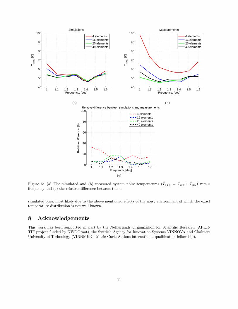
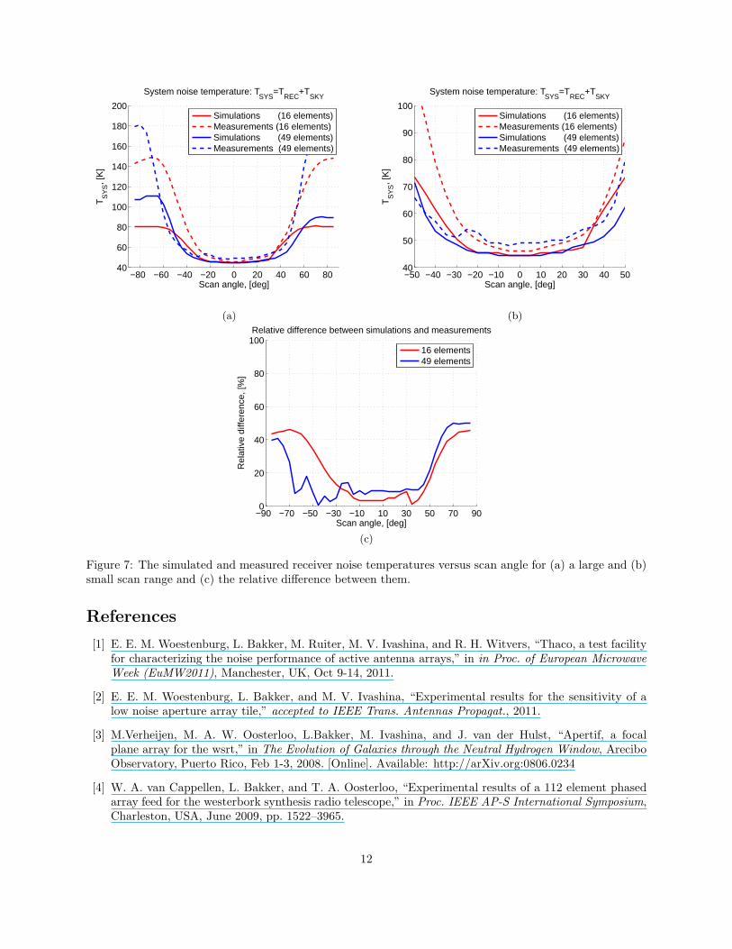
1 11 12 13 14 15 1640

50

60

70

80

90

100

Frequency [deg]

TS

YS [

K]

4 elements

Measurements (WSRT)Measurements (THACO)Simulations

1 11 12 13 14 15 1640

50

60

70

80

90

100

Frequency [deg]

TS

YS [

K]

16 elements

Measurements (WSRT)Measurements (THACO)Simulations

(a) (b)

1 11 12 13 14 15 160

20

40

60

80

100

Frequency [deg]

Rel

ativ

e di

ffere

nce

[]

4 elements

Sim vs Meas (WSRT)Sim vs Meas (THACO)

1 11 12 13 14 15 160

20

40

60

80

100

Frequency [deg]

Rel

ativ

e di

ffere

nce

[]

16 elements

Sim vs Meas (WSRT)Sim vs Meas (THACO)

(c) (d)

Figure 8 The simulated and measured receiver noise temperatures versus frequency for (a) 4-element and(b) 16-element beamformers and (cd) the relative difference between the measurements and simulations forthe corresponding beamformers

[5] H L van Trees Optimum Array Processing New York John Wiley and Sons Inc 2002

[6] M V Ivashina O Iupikov R Maaskant W A van Cappellen and T Oosterloo ldquoAn optimal beam-forming strategy for wide-field surveys with phased-array-fed reflector antennasrdquo IEEE Trans AntennasPropag vol 59 no 6 pp 1864ndash1875 June 2011

[7] M Arts M Ivashina O Iupikov L Bakker and R van den Brink ldquoDesign of a low-loss low-noisetapered slot phased array feed for reflector antennasrdquo in Proc European Conference on Antennas andPropag (EuCAP) Barcelona Spain Apr 2010

[8] M Ivashina O Iupikov and W van Cappellen ldquoExtending the capabilities of the grasp and caesarsoftware to analyze and optimize active beamforming array feeds for reflector systemsrdquo in Proc IntConf on Electromagn in Adv Applicat (ICEAA) Syndey Sept 2010 pp 197ndash200

13

[9] R Maaskant and B Yang ldquoA combined electromagnetic and microwave antenna system simulator forradio astronomyrdquo in Proc European Conference on Antennas and Propag (EuCAP) Nice FranceNov 2006 pp 1ndash4

[10] M V Ivashina R Maaskant and B Woestenburg ldquoEquivalent system representation to model thebeam sensitivity of receiving antenna arraysrdquo IEEE Antennas Wireless Propag Lett vol 7 no 1 pp733ndash737 2008

[11] R Maaskant D J Bekers M J Arts W A van Cappellen and M V Ivashina ldquoEvaluation of theradiation efficiency and the noise temperature of low-loss antennasrdquo IEEE Antennas Wireless PropagLett vol 8 no 1 pp 1166ndash1170 Dec 2009

[12] M V Ivashina E A Redkina and R Maaskant ldquoAn accurate model of a wide-band microstrip feedfor slot antenna arraysrdquo in Proc IEEE AP-S International Symposium Hawaii USA June 2007 pp1953ndash1956

[13] S W Wedge and D B Rutledge ldquoWave techniques for noise modeling and measurementrdquo IEEE TransAntennas Propag vol 40 no 11 pp 2004ndash2012 Nov 1992

[14] D K Cheng and F I Tseng ldquoMaximisation of directive gain for circular and elliptical arraysrdquo ProcInst Elec Eng pp 589ndash594 May 1967

[15] M V Ivashina M Ng Mou Kehn and P-S Kildal ldquoOptimal number of elements and element spacingof wide-band focal plane arrays for a new generation radio telescoperdquo in Proc European Conference onAntennas and Propag (EuCAP) Edinburg UK Nov 2007 pp 1ndash4

[16] M V Ivashina M Kehn P-S Kildal and R Maaskant ldquoDecoupling efficiency of a wideband vivaldifocal plane array feeding a reflector antennardquo IEEE Trans Antennas Propag vol 57 no 2 pp 373ndash382 Feb 2009

[17] P J Wood Reflector antenna analysis and design Stevenage UK and New York IEE PeterPeregrinus LTD 1980

[18] E E M Woestenburg and K F Dijkstra ldquoNoise characterization of a phased array tilerdquo in ProcEuropean Microwave Conference Germany 2003

[19] K F Warnick B D Jeffs J Landon J Waldron R Fisher and R Norrod ldquoByunrao 19-elementphased array feed modeling and experimental resultsrdquo in Proc URSI General Assembly Chicago 2007

[20] W A van Cappellen and L Bakker ldquoApertif Phased array feeds for the westerbork synthesis radiotelescoperdquo in IEEE Int Symp on Phased Array Systems and Technology Boston 2010

14