
Numerical Prediction of Particle Distribution of Solid-Liquid Slurries in Straight Pipes and Bends
17
Engineering Applications of Computational Fluid Mechanics Vol. 8, No. 3, pp. 356-372 (2014) Received: 31 Jan. 2013; Revised: 25 Feb. 2014; Accepted: 5 Mar. 2014 356 NUMERICAL PREDICTION OF PARTICLE DISTRIBUTION OF SOLID- LIQUID SLURRIES IN STRAIGHT PIPES AND BENDS Gianandrea Vittorio Messa* and Stefano Malavasi Dipt. I.C.A., Piazza Leonardo da Vinci, 32, 20133 Milano, Italy *E-Mail: [email protected] (Corresponding Author) ABSTRACT: Turbulent solid-liquid slurry flows in pipes are encountered in many engineering fields, such as mining. In particular, the distribution of the solids is a serious concern to engineers, but its determination involves considerable technical and economic difficulties. A two-fluid model for the numerical prediction of this parameter is presented. The model is robust and numerically stable, and requires relatively short computer time to provide a converged steady-state solution. The novelty of the proposed model and its better performance compared to similar ones reside in the method of accounting for some key physical mechanisms governing these flows, namely turbulent dispersion, interphase friction, and viscous and mechanical contributions to friction. The model is first validated by comparison with many experimental data available in literature regarding the horizontal pipe case over a wide range of operating conditions: delivered solid volume fraction between 9 and 40%; slurry velocity between 1 m/s and 5.5 m/s; and pipe diameter between 50 and 160 mm. A further comparison was performed with respect to recent experiments concerning a horizontal 90° bend. Keywords: two-fluid model, numerical analysis, slurries, two-phase flow, horizontal pipes, pipe bends 1. INTRODUCTION Pipe flows of solid-liquid mixtures in the form of slurry are commonly encountered in many applications. A significant example is given by the slurry pipelines, used to transport mineral concentrate from a mineral processing plant near a mine. Pressure gradient and concentration distribution have been the most serious concern of researchers, as they dictate the selection of pump capacity and may be used to determine parameters of direct importance (mixture and solid flow rates) as well as secondary effects like wall abrasion and particle degradation. The flow of solid-liquid mixtures is very complex. Doron and Barnea (1996) identified the flow patterns that characterize the flow of slurries through horizontal pipes. If the flow rate is sufficiently high, turbulence is effective in keeping all the solids suspended (fully suspended flow); otherwise the particles accumulate at the pipe bottom and form a packed bed, either sliding (flow with a moving bed) or not (flow with a stationary bed). The transitions between flow patterns are not always so clear and they are usually identified by post-processing analysis of the measured data in terms of solid volume fraction profile and pressure gradient (Albunaga, 2002). Numerous experimental investigations have been carried out to determine the main features of slurry flows in pipes. Almost all of them concern the case of horizontal pipes; the dispersed phase is usually sand (Roco and Shook, 1983; Colwell and Shook, 1988; Shaan et al., 2000; Matousek, 2000 and 2002; Gillies et al., 2004; Skudarnov et al., 2004; Kim et al., 2008), but spherical glass beads (Kaushal and Tomita, 2003 and 2007; Kaushal et al., 2005 and 2012), ash (Kumar et al., 2003), and solid nitrogen particles (Jiang and Zhang, 2012) have also been considered. Only few studies were focused on vertical pipes (Shook and Bartosik, 1994) and bends (Hsu, 1981; Turian et al., 1998; Kaushal et al., 2013). The distribution of the solids is very hard to determine experimentally. Local values of solid volume fraction can be measured by isokinetic probe sampling, but these techniques may produce significant errors near both the pipe wall (Nasr-el-Din et al., 1984) and the pipe axis (Colwell and Shook, 1988). More accurate results – but with uncertainties of a few percent – are obtained using expensive gamma- ray density gauges, which are used to determine chord-average values of solids concentration. The mean volumetric concentration of the slurry is characterized in different ways by researchers. Kaushal and Tomita (2003 and 2007) and Kaushal et al. (2005) considered an overall-area average concentration, evaluated by integrating the local concentration profile measured by an isokinetic sampling probe. Matousek (2000 and 2002) measured the delivered solid volume
Transcript of Numerical Prediction of Particle Distribution of Solid-Liquid Slurries in Straight Pipes and Bends
Engineering Applications of Computational Fluid Mechanics Vol 8 No 3 pp 356-372 (2014)
Received 31 Jan 2013 Revised 25 Feb 2014 Accepted 5 Mar 2014
356
NUMERICAL PREDICTION OF PARTICLE DISTRIBUTION OF SOLID-
LIQUID SLURRIES IN STRAIGHT PIPES AND BENDS
Gianandrea Vittorio Messa and Stefano Malavasi
Dipt ICA Piazza Leonardo da Vinci 32 20133 Milano Italy
E-Mail gianandreavittoriomessapolimiit (Corresponding Author)
ABSTRACT Turbulent solid-liquid slurry flows in pipes are encountered in many engineering fields such as
mining In particular the distribution of the solids is a serious concern to engineers but its determination involves
considerable technical and economic difficulties A two-fluid model for the numerical prediction of this parameter is
presented The model is robust and numerically stable and requires relatively short computer time to provide a
converged steady-state solution The novelty of the proposed model and its better performance compared to similar
ones reside in the method of accounting for some key physical mechanisms governing these flows namely turbulent
dispersion interphase friction and viscous and mechanical contributions to friction The model is first validated by
comparison with many experimental data available in literature regarding the horizontal pipe case over a wide range
of operating conditions delivered solid volume fraction between 9 and 40 slurry velocity between 1 ms and 55
ms and pipe diameter between 50 and 160 mm A further comparison was performed with respect to recent
experiments concerning a horizontal 90deg bend
Keywords two-fluid model numerical analysis slurries two-phase flow horizontal pipes pipe bends
1 INTRODUCTION
Pipe flows of solid-liquid mixtures in the form of
slurry are commonly encountered in many applications A significant example is given by
the slurry pipelines used to transport mineral
concentrate from a mineral processing plant near
a mine Pressure gradient and concentration distribution have been the most serious concern of
researchers as they dictate the selection of pump
capacity and may be used to determine parameters of direct importance (mixture and solid flow
rates) as well as secondary effects like wall
abrasion and particle degradation
The flow of solid-liquid mixtures is very complex Doron and Barnea (1996) identified the
flow patterns that characterize the flow of slurries
through horizontal pipes If the flow rate is sufficiently high turbulence is effective in
keeping all the solids suspended (fully suspended
flow) otherwise the particles accumulate at the pipe bottom and form a packed bed either sliding
(flow with a moving bed) or not (flow with a
stationary bed) The transitions between flow
patterns are not always so clear and they are usually identified by post-processing analysis of
the measured data in terms of solid volume
fraction profile and pressure gradient (Albunaga 2002)
Numerous experimental investigations have been
carried out to determine the main features of
slurry flows in pipes Almost all of them concern the case of horizontal pipes the dispersed phase is
usually sand (Roco and Shook 1983 Colwell and
Shook 1988 Shaan et al 2000 Matousek 2000 and 2002 Gillies et al 2004 Skudarnov et al
2004 Kim et al 2008) but spherical glass beads
(Kaushal and Tomita 2003 and 2007 Kaushal et
al 2005 and 2012) ash (Kumar et al 2003) and solid nitrogen particles (Jiang and Zhang 2012)
have also been considered Only few studies were
focused on vertical pipes (Shook and Bartosik 1994) and bends (Hsu 1981 Turian et al 1998
Kaushal et al 2013) The distribution of the
solids is very hard to determine experimentally
Local values of solid volume fraction can be measured by isokinetic probe sampling but these
techniques may produce significant errors near
both the pipe wall (Nasr-el-Din et al 1984) and the pipe axis (Colwell and Shook 1988) More
accurate results ndash but with uncertainties of a few
percent ndash are obtained using expensive gamma-ray density gauges which are used to determine
chord-average values of solids concentration The
mean volumetric concentration of the slurry is
characterized in different ways by researchers Kaushal and Tomita (2003 and 2007) and
Kaushal et al (2005) considered an overall-area
average concentration evaluated by integrating the local concentration profile measured by an
isokinetic sampling probe Matousek (2000 and
2002) measured the delivered solid volume
Engineering Applications of Computational Fluid Mechanics Vol 8 No 3 (2014)
357
fraction in the pipeline by a counter flow meter
Other authors (Shaan et al 2000 Gillies et al 2004) have made reference to a mean in-situ
volume fraction obtained by adding weighted
quantities of solids to the loop whose volume
was known In all cases the uncertainty about this parameter must be considered when making
reference to literature data
In the past simplified models have been developed based on a global formulation to
predict the pressure gradient of slurries in
horizontal pipes for all the flow configurations equivalent liquid models for fully-suspended flow
(Matousek 2002 Pecker and Helvaci 2008)
two-layer models for flows with a moving bed
(Gillies and Shook 2000 Gillies et al 2004 Doron et al 1987) three layer models for flows
with a stationary deposit (Doron and Barnea
1993 and 1995 Matousek 2009) Improved versions have been proposed to account for the
presence of multi-sized particles (Kumar et al
2003) the influence of particle shape (Shaan et al 2000) the additional stresses due to particle-wall
interactions (Pecker and Helvaci 2008) and the
repulsion of particles from the wall observed
under certain conditions (Wilson et al 2010) Using those models the major losses in horizontal
pipes can be estimated easily and the predictions
agree with the experimental evidence over a wide range of operating conditions Therefore these
models represent a very powerful tool for most
engineering applications However their global
formulation makes them unsuitable for predicting the solids concentration distribution as well as for
application to more complex flows meeting these
needs requires the development and validation of distributed models
CFD has been used to investigate slurry flows in
pipes mostly with regard to the horizontal pipe case Anyway the development of a model that is
both reliable over a wide range of flow conditions
and computationally economical ndash therefore
attractive to engineers ndash is a goal which has not been completely reached yet
The majority of existing CFD models employs an
Eulerian-Eulerian approach since Eulerian-Lagrangian models are not applicable to dense
mixtures due to their excessive computational
cost Some workers studied the problem by means of the Algebraic Slip Model (ASM) which solves
the momentum equation for the mixture rather
than for both phases thereby saving
computational time However the ASM assumes that local equilibrium is achieved between the
phases over short spatial length scales Therefore
it can be used only for very low values of the
Stokes number Also when applicable the ASM
proved inadequate to estimate the pressure drop even for fully-suspended flows in straight pipes
(Kaushal et al 2012) and it does not seem very
accurate in predicting the solid volume fraction
distribution (Ling et al 2003 Kaushal et al 2012 Pathak 2011)
Other authors made use of an Eulerian two-fluid
model with closures derived either from empirical or semi-empirical relations (Chen 1994) or from
kinetic theory of granular flow (KTGF) (Chen et
al 2009 Ekambara et al 2009 Lahiri and Ghanta 2010 Kaushal et al 2012 and 2013)
Anyway even for straight pipe flows the existing
two-fluid models show some problems which
may complicate their application to more complex flows of engineering interest such as those
through bends and pipeline fittings The first
impression is that these models are easily susceptible to numerical instabilities which often
result in solutions characterized by non-physical
asymmetry (Kaushal et al 2012) or oscillations (Lahiri and Ghanta 2010) In some cases the
simulations are very time-consuming for
example Ekambara and co-workers (2009)
attained a stable steady-state solution performing a U-RANS simulation and then averaged the
solution over a considerable time interval A
similar procedure may not be easily applicable when dealing with complex geometries since the
calculation time would probably become
prohibitively expensive In other cases the
validation of these models with respect to the experimental evidence is often rather poor in the
sense that the comparison is either limited to a
few flow conditions (Chen et al 2009 Kaushal et al 2012) or highlights a occasionally excellent
capacity of the model to describe adequately the
main features of the flow (Lahiri and Ghantha 2010)
Within the flow conditions commonly
encountered in slurry pipelines the recent work of
Kaushal et al (2013) seems the only application of a two-fluid model to a more complex flow
configuration (ie through a 90deg bend in a
horizontal pipe) with the predictions compared with experimental data
In the present work a mathematical model is
presented for the numerical prediction of the particle distribution of solid-liquid slurry flows in
pipes which is based on an Euler-Euler approach
that uses the Inter-Phase Slip Algorithm (IPSA)
of Spalding (1980) The proposed model shows comparable or better agreement with the
experimental evidence than similar models
(Ekambara et al 2009 Lahiri and Ghanta 2010
Engineering Applications of Computational Fluid Mechanics Vol 8 No 3 (2014)
358
Kaushal et al 2012 and 2013) and it also
overcomes the main limitations inferred from inspection of these earlier papers namely
susceptibility to numerical instability and high
computational cost In fact the new model
requires relatively short computer time to attain a converged steady-state solution and is capable of
providing a numerical solution without non-
physical asymmetries or oscillations The novelty of the proposed model which is the basis for its
good performance resides in the combined use of
modelling strategies previously developed but never employed simultaneously to the flows
considered in this paper phase diffusion fluxes
are introduced in all conservation equations to
reproduce the effect of the turbulent dispersion of particles the presence of other particles on the
interfacial momentum transfer is taken into
account by considering their effect on a mixture viscosity a wall function is employed to model
the viscous (due to the fluid) and mechanical (due
to the particles) contributions to the wall shear stress The model is considerably simpler and
solves one transport equation fewer than those
based on the KTGF
In the interests of guaranteeing the widest possible applicability the model predictions of
the concentration distribution are validated with
respect to various sets of experimental data from the literature The measurements from Roco and
Shook (1983) Shaan et al (2000) Matousek
(2000 and 2002) and Gillies et al (2004) allow
establishing the predictive capacity of the model in the horizontal pipe case over different flow
configurations (fully-suspended flow and flow
with a moving bed) and a large range of operating conditions delivered solid volume fraction
between 9 and 40 particle size between 90 and
520 μm slurry velocity between 1 ms and 55 ms pipe diameter between 50 and 160 mm
Finally the model was applied to a more complex
flow which is that through a 90deg bend in a
horizontal pipe and the predictions were successfully compared with the experiments from
Kaushal et al (2013) The uncertainties of both
computations and measurements are discussed when comparing the numerical results with
experimental data
2 MATHEMATICAL MODEL
21 Conservation equations
The two-phase flow is represented by using an Eulerian approach in which both phases are
treated as interpenetrating continua The flow is
assumed to be statistically steady in the sense that
Reynolds-averaging has been applied and so the
continuity equation for phase k C p takes the
following form
k k k k kD U (1)
where the subscript k is a phase indicator
parameter which is equal to C for the carrier fluid
and p for the particles Moreover k is the
volume fraction k is the density kU is the
velocity vector and D is a phase diffusion coefficient which appears in the phase diffusion
term that represents the turbulent flux associated
with correlations between fluctuating velocity and volume fraction The phase diffusion fluxes are
modeled in terms of a gradient diffusion
approximation with the phase-diffusion coefficient D given by
t CD
(2)
where t C is the turbulent kinematic viscosity of
the carrier fluid phase determined by turbulence
modeling and is the turbulent Schmidt number
for volume fractions The turbulent Schmidt
number for volume fractions is not well established in the sense that no single constant
value of σα can be used in the numerical
simulations to match the various sets of experimental data (Shirolkar et al 1996) but
rather previous workers (Chen 1994 Chen et al
2011) have found that different constant values
are needed for different cases These values typically fall in the range of 02 to 09 In the
present work a constant value was used in the
simulations and as will be discussed later the choice of a unique value procured good overall
agreement with the various sets of experimental
data The presence of phase diffusion fluxes in all conservation equations which has the advantage
of promoting numerical stability distinguishes the
present model from similar ones applied to slurry
flows The mean global continuity is given by the equation that states that the two volume fractions
must sum to unity
The momentum equation for phase k C p is
k k k k
k k k t k k k
k k k k
P
D
U U
g
M U
T T (3)
where P is the pressure shared by the phases g
is the gravitational acceleration kT and t kT are
the viscous and turbulent stress tensors
respectively and kM is the generalized drag force
per unit volume which will be discussed later
Engineering Applications of Computational Fluid Mechanics Vol 8 No 3 (2014)
359
The stress tensors are given by
2 2k k l k k t k k t k k T D T D (4)
where l k and t k are the laminar and turbulent
kinematic viscosity of phase k respectively and
kD is the deformation tensor equal to
05k k k
U UD (5)
where the superscript ldquo+rdquo indicates that the
transpose of the dyadic kU is taken
Two viscosities appear in Eq (4) for the particle
phase namely the turbulent eddy viscosity t p
and the laminar viscosity l p The former is
determined from a turbulence model as will be discussed later The latter is commonly associated
with the inter-granular stresses which characterize
bed flows (Chen et al 2011) the model of
Ahilan and Sleath (1987) for l p was briefly
explored but finally l p was set to 0 after
discovering the negligible influence of the term
pT on the predictions of the solids volume
fraction for all the flow conditions simulated This
can be explained by the fact that the laminar
viscosity of the particles is small compared to the
eddy viscosity except very close to the pipe bottom where however the interfacial
momentum transfer term dominates
The interfacial momentum transfer term accounts for the momentum transfer between phases and is
given by stationary drag lift added mass history
and other forces (Ishii and Mishima 1984) The two-fluid model represents the turbulent
dispersion of particles by means of a turbulent
diffusion term in the phasic continuity equation
(Eq (1)) and so an explicit turbulent-dispersion force term does not appear in the momentum
equation A literature review revealed that the
history force is negligible for the flows considered here (Chung and Troutt 1988) and
therefore was not included in this model Under
the assumption of mono-dispersed spherical
particles the interfacial momentum transfer term is given by
3
6 p
C p d l vm
pd
M M F F F (6)
where Fd Fl and Fvm are the drag lift and virtual
mass forces calculated respectively as follows
2
1=
2 4
p
d d C p C p C
dC
F U U U U (7)
3=l l C p p C CC d F U U U (8)
3
4=
3 8
p
vm vm C p p C C
dC
F U U U U (9)
where dp is the particle diameter Cd is the drag
coefficient which will be discussed later Cl is the lift coefficient and Cvm is the virtual mass
coefficient As per the indications of Kaushal et al
(2012) both Cl and Cvm were set equal to 05
The drag coefficient is given by the well known Schiller and Naumann (1935) formula
068724C max 1 015Re 044
Red p
p
(10)
in which Rep is the particle Reynolds number The
use of alternative correlations (Clift et al 1978
Ishii and Mishima 1984) does not seem to have significant impact on the results as they do not
differ very much from Eq (10) in the range of Rep
considered Following a well-established
approach (Barnea and Mizrahi 1973 Ishii and Mishima 1984) to account for the presence of
other particles the particle Reynolds number is
defined as Rep = ρCdp|Ur|μm where μm is the viscosity of the mixture Several correlations for
the mixture viscosity are available in literature
(Clift el al 1978) They are basically empirical or semi-empirical and they depend on parameters
that account for the shape and size distribution of
the particles In the present work use is made of
the Mooney (1951) formula
exp
1
p
m C l C
p pm
(11)
in which the two fitting parameters are the
maximum packing concentration αpm and the intrinsic viscosity [η] The former accounts for
the shape and size distribution of the particles as
well as the shear rate (Pecker and Helvaci 2008)
whereas the latter accounts for particle shape For the first time the mixture viscosity approach is
employed in a two-fluid model for the simulation
of slurry flows in pipes In particular the asymptotic behaviour of the viscosity of the
mixture which tends to infinity as the solids
volume fraction approaches the maximum packing one sets an upper limit to the
concentration of particles preventing the solids
from over-packing This avoids the need to
introduce a collisional pressure term in the dispersed phase momentum equations The
absence of this term contributes to the numerical
stability of the present model Some authors have argued for the existence of a
wall lubrication force in the generalized drag term
to account for the repulsion of particles from the
pipe wall observed in some experiments (Matousek 2002 Kaushal and Tomita 2007) but
this effect is not considered in the present work A
semi-theoretical model for this force was derived
Engineering Applications of Computational Fluid Mechanics Vol 8 No 3 (2014)
360
by Antal et al (1991) for air-water bubbly flow in
the laminar regime but it proved unsuitable for slurry flows confirming the observations of
Ekambara et al (2009) Wilson and Sellgren
(2003) and Wilson et al (2010) proposed a model
for the wall-lubrication force in slurry flows but the global nature of its formulation precludes its
implementation in a CFD code
22 Turbulence modeling
The following modified form of the k-ε model is
used for turbulence modeling of the fluid phase
C C C
t C
C C l C C C k
k
t C
C C
k
k P
k
U
(12)
1 2
C C C
t C
C C l C
t C
C C k C CC P Ck
U
(13)
2
t C
kC
(14)
in which 2 k t C C CP UD is the volumetric
production rate of k due to the working of the
Reynolds stresses against the mean flow The usual values of the model constants are employed
namely 10k 1314 009C
1 144C and 2 192C
There appears to be no simple model of general
validity for evaluation of the particle eddy
viscosity t p in dense particle flows
Nevertheless even the simple model of t p t C
indicated by Issa and Oliveira (1997) was found to yield accurate predictions of the solid volume
fraction distribution which is the focus of this
paper
23 Computational domain and boundary
conditions
Two validation cases are considered in this work
namely a straight horizontal pipe and a horizontal 90deg pipe bend The two computational domains
are reported in Figs 1 and 2 respectively In the
straight pipe case (Fig 1) the flow and geometrical symmetry of the phenomenon about
the vertical axis (Roco and Shook 1983 Kaushal
et al 2005) has been exploited by solving only
over one half of the pipe section
In both cases a fully-developed turbulent flow
profile is specified at the pipe inlet with the distribution of the axial velocity turbulence
kinetic energy and dissipation rate determined
from Nikuradses boundary-layer theory
(Schlichting 1960) for single-phase flow in straight pipes No slip is assumed between the
phases at the inlet section therefore the same
velocity distribution is applied to the fluid and the particles
1
2
2
1 2 1 2 11
2
182log Re 164 Re
N
in in
C z p z s
p
s p
l C
N N ru u V N
DN f
V Df
(15)
Fig 1 Computational domain and boundary
conditions for horizontal pipe
Fig 2 Computational domain boundary conditions
and reference sections for 90deg bend (S1=bend
inlet S2=bend centre S3=bend exit S4=5Dp
from bend exit S5=25Dp from bend exit
S6=50Dp from bend exit)
Engineering Applications of Computational Fluid Mechanics Vol 8 No 3 (2014)
361
3
2 2 2 10 21
8 3 3
in
s
p p
f r rk V
D D
(16)
32
4
01643
2 2014 008 006
2
in
m
p
m
p p
k
l
D r rl
D D
(17)
In Eq (15) sV is the superficial velocity of the
slurry which is the ratio between the volumetric
slurry flow rate and the pipe area The inlet
volume fractions of both phases are taken as uniformly distributed At the outlet the normal
gradients of all variables and the value of the
pressure are set to zero The length of the
computational domain in the straight pipe case is 100Dp to ensure that fully-developed flow
conditions are attained which typically occurs
some 50Dp downstream of the inlet confirming the results of previous workers (Ling et al 2003)
For this reason 50Dp of straight pipe were
simulated upstream the 90deg bend (Fig 2) whilst
the outlet boundary is located about 50Dp downstream the bend exit in order to analyze the
development of the flow downstream the bend
and compare the numerical results with the experimental evidence
At the pipe wall no slip conditions are imposed to
both phases and the equilibrium wall function of Launder and Spalding (1972) is employed to
evaluate the velocity component parallel to the
wall for the two phases
w
k C pu the turbulence
kinetic energy wk and its dissipation rate w in the
near wall cells
1ln
w
k k
k l C
u u yE
u
(18)
w Cu
kC
(19)
3234w wk
Cy
(20)
where
ku is the friction velocity of phase
k C p 041 is von Karman constant E
is a roughness parameter and y is the normal
distance of the first grid point from the wall The parameter E is considered as a function of the
roughness Reynolds number
Re r C l Cu r
where r is the equivalent sand-grain roughness
height The formula for E developed by
Jayatillika (1969) is as follows
12
2
Re 37
Re 137 Re 100
Re 100Re
m r
rr
m
r
r
E
aE a
b E
b
(21)
where 86mE is the value of E appropriate for
smooth walls and a and b are given by
3 2
0564
100 Re1 2 3 002248 297
Re
r
r
a x x x b
(22)
24 Computational methodology and consistency
of numerical solution
The general-purpose commercial CFD code
PHOENICS was employed for the numerical
solution of the finite-volume analogue of the
mathematical described above This was done by using the built-in Eulerian two-fluid Inter-Phase
Slip Algorithm (IPSA) of Spalding (1980)
together with user-defined functions for implementation of specific constitutive equations
and boundary conditions The calculations are
performed following the elliptic-staggered
formulation in which the scalar variables are evaluated at the cell centers and the velocity
components at the cell faces Central differencing
is employed for the diffusion terms while the convection terms are discretized using the hybrid
differencing scheme of Spalding (1972) for the
straight pipe case and the MINMOD scheme (Versteeg and Malalasekera 2007) for the 90deg
bend The finite-volume equations are solved
iteratively by means of the SIMPLEST and IPSA
algorithms of Spalding (1980) The calculation procedure is organized in a slab-by-slab manner
in which all the dependent variables are solved at
the current slab before the solver routine moves to the next slab
The PHOENICS solver was run until the sum of
the absolute residual sources over the whole solution domain is less than 1 per cent of
reference quantities based on the total inflow of
the variable in question An additional
requirement is that the values of the monitored dependent variables at a selected location do not
change by more than 01 between subsequent
iteration cycles The consistency of the numerical solution with
respect to the domain discretization is now
discussed for the two scenarios simulated A
cylindrical-polar structured mesh was employed
Engineering Applications of Computational Fluid Mechanics Vol 8 No 3 (2014)
362
in the straight pipe case A grid sensitivity study
was performed to determine the optimum discretization of the domain by reference to the
predicted solids volume fraction profiles For this
purpose the following case was taken from Roco
and Shook (1983) pipe diameter = 507 mm particle diameter = 520 μm delivered solid
volume fraction = 02473 slurry superficial
velocity = 200 ms The pipe is assumed
hydraulically smooth ( 0r ) This case exhibits a
high degree of slurry stratification which is
expected to enhance the effect of mesh resolution
Three different meshes were employed as
follows 9 angular by 12 radial by 85 axial (Grid 1) 12 by 19 by 126 (Grid 2) 15 by 30 by 200
(Grid 3) and 20 by 40 by 300 (Grid 4) cells For
consistency with measurements made using γ-ray density gauges the predicted solids volume
fraction at a distance y from the pipe bottom is
evaluated by using the chord-average value ie
chord
0
1( ) ( )
x
p py x y dxx
(23)
where x accounts for the horizontal variation of
concentration in the pipe cross-section (Fig 1) The predicted volume fraction profiles for each
grid are shown in Fig 3 The solutions obtained
on the three finest meshes (Grids 2 3 and 4) are very close to each other whilst that for Grid 1
deviates slightly from the finer grid solutions
The Grid 3 solution is considered adequate
for comparison with the experiments For
each vertical location y the difference chord chord
4 3( ) ( )p py y - in which chord
3p and chord
4p
are the values obtained on Grids 3 and 4
respectively - is assumed an indicator of the effect of further mesh refinement The quantity
chord chord
4 3( ) ( )p py y was found to be lower than
0005 for all yDp less than the error usually associated with the measurements The
application of the method proposed by Eccedila and
Hoekstra (2006) for estimating the grid discretization error confirmed the reliability of
Grid 3
A curvilinear structured mesh in body-fitted
coordinates was instead employed in the 90deg bend case The grid independence study was performed
with respect to the following flow condition
particle diameter = 2645 kgm3 delivered solid
volume fraction = 00882 slurry superficial
velocity = 267 ms pipe roughness = 0015 mm
The four meshes used consisted of 300 slabwise by 300 axial (Grid 1) 600 by 350 (Grid 2) 1040
by 450 (Grid 3 details of which are shown in Fig
4) and 1170 by 500 (Grid 4) cells For consistency
Fig3 Solid volume fraction profiles calculated on
three different grid levels for straight pipe
case
Fig4 Details of mesh for 90deg bend
Fig5 Vertical solid volume fraction profiles at
distance of 5Dp downstream bend exit (Section S4 in Fig 2) calculated on different grid
levels The Grid 3 solution has error bars
corresponding to the grid discretization error
estimated by the method of Eccedila and Hoekstra
(2006)
Engineering Applications of Computational Fluid Mechanics Vol 8 No 3 (2014)
363
with the sampling probe measurements of
Kaushal et al (2013) the predicted solids volume fraction at a distance y from the pipe bottom is
now evaluated by using the value along the
vertical diameter ie
axis ( ) 0p py y (24)
The predicted volume fraction profiles for each
grid at a distance of 5Dp downstream the bend exit (Section S4 in Fig 2) are shown in Fig 5
and indicate that Grid 3 is capable to procure a
consistent numerical solution the difference axis axis
4 3( ) ( )p py y being less than 0014 for all y
In Fig 5 the Grid 3 solution has error bars
corresponding to the grid discretization error estimated following the method of Eccedila and
Hoekstra (2006) Grid 3 was used in the
simulations
25 Governing terms and calibration of
numerical constants
In the two-fluid model different empirical sub-
models are employed for the inter-phase processes and closure of the various turbulence
correlations These submodels contain adjustable
coefficients which are in practice treated as calibration parameters their values being
determined by matching computations with
experiments The submodels which mainly affect
the solid volume fraction distribution refer to two main terms The former is the phase diffusion of
each conserved property ( 1 for mass
conservation) equal to k kD in which
the phase-diffusion coefficient D is given by Eq
(2) The phase diffusion besides making the
model numerically more stable and thereby
contributing to its speed in attaining convergence
has a smoothing effect on the solids concentration profile reducing its variation along the vertical
direction The impact of phase diffusion is
controlled by an empirical parameter which is the
turbulent Schmidt number for volume fractions
which appear in Eq (2) A sensitivity analysis to
quantify the influence of on the solid volume
fraction profile was performed
The results are depicted in Fig 6 for horizontal
pipe flows with very different flow conditions both taken from Roco and Shook (1983) A) pipe
diameter = 515 mm particle diameter = 165 μm
particle density = 2650 kgm3 delivered solid
volume fraction = 009 slurry superficial velocity = 378 ms B) pipe diameter = 507 mm particle
diameter = 520 μm particle density = 2650
kgm3 delivered solid volume fraction = 02473
slurry superficial velocity = 200 ms In both
cases the pipe is regarded is hydraulically
smooth It is observed that a reduction of
results in a flatter profile as a consequence of the
increase in diffusivity The latter term which most influences the solid
volume fraction profile is the interfacial
momentum transfer (Eq (6)) and particularly the drag force (Eq (7)) As already noticed the
definition of the particle Reynolds number with
respect to the viscosity of the mixture m instead
of that of the fluid phase C puts an upper limit
to the solids concentration due to the asymptotic
trend of m (Eq (11)) The mixture viscosity as
derived from the correlation of Mooney (Eq (11)) depends on two empirical parameters the
intrinsic viscosity and the maximum packing
concentration pm The effect of and pm on
Fig 6 Effect of turbulent Schmidt number for volume fractions on solid volume fraction profiles for two flow
conditions ( experiments from Roco and Shook (1983) ndashndashndash 03 ndashndashndash 05 ndashndashndash 07 ndashndashndash
09 )
Engineering Applications of Computational Fluid Mechanics Vol 8 No 3 (2014)
364
Fig 7 Effect of parameters [η] and pm in mixture viscosity correlation of Mooney (Eq 11) on solid volume fraction
profiles for two flow conditions ( experiments from Roco and Shook (1983) continuous lines predictions)
The dependence on [η] is studied for 07pm that on pm for [η] = 25
Table 1 Flow conditions considered for comparison
Reference System [mm]pD
[-]pr D [ ]pd m []C [ms]sV 3 [kgm ]p
Roco and Shook (1983) Pipe 507-515 - 165-520 90-296 190-433 2650
Gillies et al (2004) Pipe 1030 2∙10-5 90-280 106-407 133-540 2650
Matousek (2000 and 2002) Pipe 1500 - 120-370 250-430 204-600 -
Shaan et al (2000) Pipe 1585 6∙10-6 90 150-320 140-300 2655
Kaushal et al (2013) 90deg Bend 530 3∙10-4 450 882 267 2645
the solid volume fraction profile is analyzed one at a time in Fig 7 for the two above mentioned
flow conditions from Roco and Shook (1983) In
particular the results highlight that pm affects
the behaviour of the mixture only at high
concentration therefore as a direct effect on the prevention of particle over-packing As already
mentioned this avoids the need to introduce a
collisional pressure term in the momentum equation of the solid phase further promoting the
numerical stability of the model and the rapid
achievement of a converged solution Our investigations showed that a unique
combination of the three empirical parameters ndash
07 25 and 07pm (all within the
range of variability found in literature) ndash produced estimations of the solids concentration
profile in good agreement with the experimental
evidence for all the flow conditions considered in the present work referring to both the horizontal
pipe case and the 90deg bend case This feature
together with the numerical stability and the
relatively short computer time required contributes to make the model particularly useful
for the applications
3 RESULTS
The numerical model is validated by comparing
the results of the simulations against experimental
data reported by the authors listed in Table 1 This
Engineering Applications of Computational Fluid Mechanics Vol 8 No 3 (2014)
365
table provides the flow conditions for each set of
measurements As already mentioned two scenarios have been considered namely a straight
horizontal pipe and a 90deg bend which will be
discussed in separate sub-sections
31 Straight horizontal pipe
The predictions of the model have been compared with experimental data for 26 flow conditions
summarized in Table 2 which differ in terms of
pipe diameter pipe roughness particle size slurry superficial velocity and delivered solid volume
fraction Each set of measurements allows an
assessment of the models capability for
reproducing the influence of specific features affecting the distribution of the solid volume
fraction The data of Roco and Shook (1983) and
Gillies et al (2004) are used to investigate the effect of particle diameter and slurry velocity with
different delivered solid volume fraction The
measurements of Matousek (2000 2002) provide the opportunity to extend the validity of the model
up to a pipe Reynolds number Re (Eq (15)) of
about 106 Finally the data of Shaan et al (2000)
are used to assess the performance of the model in
case of natural sands with irregularly-shaped grains Almost all the data refer to configurations
in which all the solids are kept suspended but
moving bed flows have also been briefly explored
to check how far one can go in employing the model for the purpose of achieving useful
information from an engineering point of view
Measurements of solids concentration ndash either bulk-mean or local ndash are subjected to errors
depending mainly on the instrumentation used as
discussed in Section 1 All the data reported in Table 2 are obtained using gamma-ray absorption
methods perhaps the technique which provides
the highest accuracy attainable with errors of the
order of a few percentage points Since this technique allows measuring chord-average values
of solid volume fraction the computed volume
fraction profile was evaluated by means of Eq (23) In the experiments from Roco and Shook
(1983) ndash cases A1 to A5 in Table 2 ndash the
dispersed phase consists of three kinds of sand with narrow size distribution and mean particle
diameters of 165 and 520 μm The solids density
is 2650 kgm3 the pipe diameter is about 51 mm
Table 2 Details of experimental conditions for straight pipe case (A1 to A5 experimental data from Roco and Shook (1983) B1 to B12 experimental data from Gillies et al (2004) C1 to C6 experimental data from Matousek
(2000 and 2002) D1 to D4 experimental data from Shaan et al (2000) values not declared by
experimenters)
Test ID [mm]pD
[-]pr D [ ]pd m []C [ms]sV 3 [kgm ]p
Flow pattern
A1 515 0 165 9 378 2650 FS
A2 515 0 165 19 417 2650 FS
A3 515 0 165 28 433 2650 FS
A4 507 0 520 1212 190 2650 MB
A5 507 0 520 2473 200 2650 MB
B1 103 2∙10-5 90 198 133 2650 FS
B2 103 2∙10-5 90 283 133 2650 FS
B3 103 2∙10-5 90 19 300 2650 FS
B4 103 2∙10-5 90 284 300 2650 FS B5 103 2∙10-5 280 12 255 2650 FS
B6 103 2∙10-5 280 208 260 2650 FS
B7 103 2∙10-5 280 310 250 2650 FS
B8 103 2∙10-5 280 407 260 2650 FS
B9 103 2∙10-5 280 106 540 2650 FS
B10 103 2∙10-5 280 203 540 2650 FS
B11 103 2∙10-5 280 301 540 2650 FS
B12 103 2∙10-5 280 405 540 2650 FS
C1 150 0 120 25 204 2650 FS
C2 150 0 120 35 204 2650 -
C3 150 0 120 34 600 2650 -
C4 150 0 370 25 600 2650 FS
C5 150 0 370 34 600 2650 - C6 150 0 370 43 600 2650 MB
D1 1585 6∙10-6 90 15 15 2655 FS
D2 1585 6∙10-6 90 32 14 2655 FS
D3 1585 6∙10-6 90 15 30 2655 FS
D4 1585 6∙10-6 90 32 30 2655 FS
Engineering Applications of Computational Fluid Mechanics Vol 8 No 3 (2014)
366
the slurry bulk-mean velocity varies from 190 to
433 ms and the pipe Reynolds number from between 9610
4 and 2110
5 The delivered solid
volume fraction ranges from 9 to 30 The
authors did not indicate the roughness of the pipe
which was assumed hydraulically smooth No evaluation of measurement uncertainty was
reported by the experimenters and they did not
identify the flow patterns according to the more recent classification of Doron and Barnea (1996)
However for the smallest particle diameter the
data suggest suspended flow whereas for the largest diameter the indications are for moving-
bed flow Fig 8 compares the computed and
measured solid volume fraction profiles The good agreement between computation and
measurements reveals the ability of the model to
reproduce the effect of particle diameter on the
particle distribution for slurries with different delivered solid volume fraction The simple two-
fluid model proposed in this work appears
capable to predict with reasonable accuracy the solid volume fraction profile not only in case of
fully-suspended flow but also in case of moving
bed flows This indicates that the asymptotic trend of the interfacial momentum transfer term
Fig 8 Solids concentration profiles for flow conditions A1 to A5 in Table 2 ( experiments from Roco and
Shook (1983) ndashndashndash predictions)
Fig 9 Solids concentration profile for flow conditions B1 to B12 in Table 2 ( experiments from Gillies et al
(2004) ndashndashndash predictions)
Engineering Applications of Computational Fluid Mechanics Vol 8 No 3 (2014)
367
produces on the solid volume fraction profile the
same effect that is traditionally achieved by the
collisional pressure and the tensor kT
Gillies et al (2004) measured the concentration
profiles of sand-water slurries in a 103 mm
diameter pipe using gamma-ray absorption
gauges without reporting the uncertainty The roughness of the pipe is 2 nm Two kinds of sand
were considered with narrow size distribution
and mean particle diameter of 90 and 280 μm In both cases the particle density was 2650 kgm
3
and the slurry superficial velocity varies from
133 to 54 ms (corresponding to a pipe Reynolds
number between 14105 and 5610
5) The
delivered solid volume fraction varies from about
10 to about 45 Details of the flow conditions
considered for comparison are reported in Table 2 cases B1 to B12 From an examination of the
measured data for the pressure gradient it can be
inferred that in all cases the flow is fully-suspended This is a good test for the modelrsquos
ability to predict the combined effect of slurry
velocity solids loading and particle diameter in a
larger pipe Fig 9 shows comparison of the computational and the experimental results for the
vertical distribution of the solid volume fraction
The model produces good overall agreement with the data The largest deviations are observed near
the pipe wall for the small particles at high
concentration (cases B2 and B4 in Table 4) but as noted by the authors themselves these
measurements are subject to the largest
experimental error
Matousek (2000 and 2002) measured the concentration profiles of sand-water slurries in a
150 mm diameter pipe using gamma-ray
absorption method quantifying a 4 uncertainty of the data We reproduced numerically the flow
conditions reported in Table 2 (cases C1 to C6)
in which the dispersed phase consists of two kinds
of sand with narrow size distribution and mean particle diameters of 120 and 370 μm
Unfortunately neither the density of the solid
particles nor the pipe roughness are reported in the experiments of Matousek (2000 and 2002)
and so in the simulations the former was set to
2650 kgm3 which is the value declared by Roco
and Shook (1983) and Gillies et al (2004) and
the pipe was regarded as hydraulically smooth
The slurry superficial velocity was 2 or 6 ms
corresponding to a pipe Reynolds number up to 10
6 The delivered solid volume fraction ranged
between 25 and 43 According to the author
the flows are either fully suspended or with a moving bed but only for three cases the flow
pattern could be clearly identified from the plot of
pressure gradient versus slurry superficial
velocity Fig 10 compares the computed and measured solid volume fraction profiles each set
of experimental data has error bars indicating the
uncertainty declared by the experimenter The
rather good agreement between computations and measurements confirm the reliability of the model
for high pipe Reynolds numbers A closer
inspection reveals that for case C6 the computed concentration is lower than the experimental
results in the lower part of the pipe and higher in
the upper region However the pressure gradient curve clearly reveals that in case C6 a moving bed
of particles is formed It is again confirmed that
the proposed model is capable to procure a rough
indication of the distribution of the solid also for flows in which the inter-granular stresses play an
important role
Moreover in the case of highly dense slurries like case C6 the experimental data are subject to the
most uncertainty and the numerical solutions are
sensitive to the empirical parameters pm and
which appear in the mixture viscosity correlation
(Eq (11)) For the same case the measured solids concentration profile shows a drop near the pipe
bottom This reversal is not predicted by the
numerical model which is probably due to the absence of the wall lift force discussed earlier in
Section 21 The same limitation was reported by
Ekambara et al (2009) The paper of Shaan et al (2000) focuses on the
effect of particle shape upon pressure gradient and
deposition velocity but these workers also
reported some measurements of the solid volume fraction profiles Shaan et al (2000) quantified
the particle shape by reference to the following
quantities evaluated from photos of the particles the axes ratio ie the ratio between the major and
minor axes of an ellipse circumscribing the
grains the circularity index ie the ratio between
the area of the particle multiplied by 4π and its perimeter The sand particles have a very irregular
shape as can be inferred by comparing the
measured values of axes ratio (16) and circularity (062) against typical values reported in the
literature for sand grains The mass-median value
of the particle size distribution curve is taken as the characteristic particle diameter The flow
conditions reported in Table 2 (cases D1 to D4)
were reproduced to check the behaviour of the
model for the case of irregularly-shaped sand particles The pipe diameter (1585 mm)
delivered solid volume fraction (15 or 35)
slurry superficial velocity (14 or 3 ms) particle density (2655 Kgm
3) and particle diameter (90
μm) are all approximately within the range
Engineering Applications of Computational Fluid Mechanics Vol 8 No 3 (2014)
368
Fig 10 Solids concentration profiles for flow conditions C1 to C6 in Table 2 ( experiments from Matousek
(2000 and 2002) ndashndashndash predictions)
Fig 11 Solids concentration profiles for flow conditions D1 to D4 in Table 2 ( experiments from Shaan et al
(2000) ndashndashndash predictions)
covered by the earlier simulations The numerical and experimental results are
compared in Fig 11 The agreement between the
numerical predictions and the experimental
evidence is fairly good inadequacies of the numerical model ndash especially in the wall
boundary conditions for the solid phase ndash and
measurements error can both contribute to the discrepancies observed near the pipe bottom for
case D2 The results seem to indicate that the
numerical model is a suitable tool for predicting the solid volume fraction distribution produced by
sands with a very irregular shape
32 Horizontal 90deg bend
The predictions of the model have been compared
with the recent experiments of Kaushal et al (2013) regarding a horizontal 90deg bend Among
the different flow conditions considered by these
authors reference is made to those characterized
by delivered solid volume fraction of 882 within the range of interest in this work The
experimenters used a sampling probe to measure
the volume fraction profile of the slurry in the 53
mm diameter pipe along the vertical axis at distances of 5Dp 25Dp and 50Dp downstream the
bend exit (referred to as sections S4 S5 and S6 in
Fig 2 respectively) They quantified a 2
uncertainty of the data The solid phase consists of silica sand particles with narrow size
distribution and mean particle diameter of 450
μm The slurry superficial velocity is 178 267 or 356 ms
The flow within the bend is much more complex
compared to that through the straight pipe since secondary motions develop in the crosswise
direction These motions affect significantly the
distribution of the solids and as a consequence
the volume fraction distribution is no longer constant over horizontal planes This is evident in
Fig 12 which shows the color plot of the solids
volumetric concentration over the six cross sections highlighted in Fig 2 As shown in Fig
13 the predictions of our model generally agree
with the experimental data available Greater
discrepancies are observed for the highest superficial velocity (356 ms) where the model
seems to underestimate the quantity of particles
dragged by the secondary motions This is
Engineering Applications of Computational Fluid Mechanics Vol 8 No 3 (2014)
369
Fig 12 Solid volume fraction distributions on sections
S1 to S6 in Fig 2 for delivered solid volume
fraction of 882 Left hand side is the outer
wall of the pipe
opposite to the KTGF based model of Kaushal et
al (2013) which tends to over-enhance the effect
of the secondary motions on the solids for the
lowest velocities Fig 13 also reveals that our model tends to overestimate the solids volume
fraction close to the pipe bottom far from the
bend exit It is expected that the predictions could
be improved if the effect of the wall lubrication force for which a suitable model does not exist at
present were accounted for
4 CONCLUSIONS
A mathematical model has been described for the
estimation of solid volume fraction distribution of
solid-liquid slurry flows in horizontal pipes and bends The model is based on an Eulerian-
Eulerian approach and uses the Inter-Phase Slip
Algorithm (IPSA) of Spalding (1980) The
novelty of this model resides in the combined use of existing modelling strategies never previously
employed simultaneously for the predictions of
slurry flows In order to account for turbulent dispersion of particles phase diffusion terms have
been included in the phase continuity equations
together with all the conservation equations The mixture viscosity approach is adopted to model
the effect of multiple particles on the inter-phase
friction A wall function is employed to model the
flow in the near-wall region in case of both hydraulically smooth and rough walls All these
strategies result in a model which despite being
simpler that those commonly used for addressing solid-liquid slurry flows shows comparable or
even better predictive capacity Moreover this
model is robust and numerically stable and
requires relatively short CPU time to procure converged steady-state solutions
The model has been first validated by comparison
with experimental data for the horizontal pipe case over a wide range of operating conditions
delivered solid volume fraction between 10 and
40 by volume mean particle diameter between 90 and 520 μm slurry superficial velocity
between 1 ms and 55 ms and pipe diameter
between 50 and 158 mm The model predictions
were found to be in good agreement with the experimental evidence for all the flow conditions
considered for comparison Even if the model is
originally intended to address fully-suspended flows the results indicated its capability to
provide rough indications of the solid volume
fraction distribution also in case of bed flows At last the comparison with the recent
measurements of Kaushal et al (2013) revealed
that this model is capable to procure reliable
predictions of the particle distribution downstream a 90deg bend in a horizontal pipe
Engineering Applications of Computational Fluid Mechanics Vol 8 No 3 (2014)
370
Fig 13 Solid volume fraction along vertical diameter on sections S4 to S6 in Fig 2 for delivered solid volume fraction
of 882 ( experiments from Kaushal et al (2013) ndashndashndash predictions)
ACKNOWLEDGEMENTS The authors would acknowledge the CINECA and
the Regione Lombardia award under the LISA
initiative for the availability of high performance computing resources and support The authors
would like to thank CHAM Ltd for supporting
this research and acknowledge Dr Randy Gillies of Saskatchewan Research Council for providing
his experimental data
REFERENCES
1 Ahilan RV Sleath J (1987) Sediment
transport in oscillatory flow over flat beds Journal of Hydraulic Engineering 113 308-
322
2 Albunaga BE (2002) Slurry Systems Handbook McGraw-Hill
3 Antal S Lahey R Flaherty J (1991) Analysis
of phase distribution in fully-developed
laminar bubbly two phase flow International Journal of Multiphase Flow 17(5) 635-652
4 Barnea E Mizrahi J (1973) A Generalized
Approach to the Fluid Dynamics of
Particulate Systems Chemical Engineering
Science 5(2) 171-189 5 Chen L Duan Y Pu W Zhao C (2009) CFD
simulation of coal-water slurry flowing in
horizontal pipelines Korean Journal of Chemical Engineering 26(4) 1144-1154
6 Chen RC (1994) Analysis of homogeneous
slurry pipe flow Journal of Marine Science and Technology 2(1) 37-45
7 Chen X Li Y Niu X Li M Chen D Yu X
(2011) A general two-phase turbulent flow
model applied to the study of sediment transport in open channels International
Journal of Multiphase Flow 37(9) 1099-
1108 8 Chung JN Troutt TR (1988) Simulation of
particle dispersion in an axisymmetric jet
Journal of Fluid Mechanics 186 199-222 9 Clift R Grace JR Weber ME (1978)
Bubbles Drops and Particles Academic
Press
10 Colwell JM Shook CA (1988) The Entry Length for Slurries in Horizontal Pipeline
Flow Canadian Journal of Chemical
Engineering 66(5) 714-720
Engineering Applications of Computational Fluid Mechanics Vol 8 No 3 (2014)
371
11 Doron P Barnea D (1993) A three layer
model for solid-liquid flow in horizontal pipes International Journal of Multiphase
Flow 19(6) 1029-1043
12 Doron P Barnea D (1995) Pressure drop and
limit deposit velocity for solid-liquid flow in pipes Chemical Engineering and Science
50(10) 1595-1604
13 Doron P Barnea D (1996) Flow pattern maps for solid-liquid flow in pipes International
Journal of Multiphase Flow 22(2) 273-283
14 Doron P Granica D Barnea D (1987) Slurry flow in horizontal pipes ndash experimental and
modeling International Journal of
Multiphase Flow 13(4) 535ndash547
15 Eccedila L Hoekstra M (2006) Discretization uncertainty estimation based on a least
squares version of the grid convergence
index Proceedings of the 2nd
Workshop on CFD Uncertainty Analysis Oct 19-20
Lisbon Portugal
16 Ekambara K Sanders RS Nandakumar K Masliyah JH (2009) Hydrodynamic
simulation of horizontal slurry pipeline flow
using ANSYS-CFX Industrial amp
Engineering Chemistry Research 48(17) 8159-8171
17 Gillies RG Shook CA (2000) Modelling
High Concentration Settling Slurry Flows Canadian Journal of Chemical Engineering
78(4) 709-716
18 Gillies RG Shook CA Xu J (2004)
Modelling Heterogeneous Slurry Flow at High Velocities Canadian Journal of
Chemical Engineering 82(5) 1060-1065
19 Hsu FLG (1981) Flow of Fine-particle Suspensions in Bends Fittings and Valves
MS Thesis Texas Tech University Lubbock
Texas USA 20 Ishii M Mishima K (1984) Two-fluid model
and hydrodynamic constitutive relations
Nuclear Engineering and Design 82(2-3)
107-126 21 Issa RI Oliveira PJ (1997) Assessment of a
particle-turbulence interaction model in
conjunction with an Eulerian two-phase flow formulation Proceedings of the 2
nd
International Symposium on Turbulence
Heat and Mass Transfer June 9-12 Delft Netherlands 759-770
22 Jayatillika CLV (1969) The influence of the
Prandtl number and surface roughness on the
resistance of the sublayer to momentum and heat transfer Progress in Heat amp Mass
Transfer 1 193-329
23 Jiang YY Zhang P (2012) Pressure drop and
flow pattern of slush nitrogen in a horizontal pipe AIChE Journal doi 10002aic13927
24 Kaushal DR Kumar A Tomita Y Juchii S
Tsukamoto H (2013) Flow of mono-
dispersed particles through horizontal bend International Journal of Multiphase Flow 52
71-91
25 Kaushal DR Sato K Toyota T Funatsu K Tomita Y (2005) Effect of particle size
distribution on pressure drop and
concentration profile in pipeline flow of highly concentrated slurry International
Journal of Multiphase Flow 31(7) 809-823
26 Kaushal DR Thinglas T Tomita Y Juchii S
Tsukamoto H (2012) CFD modeling for pipeline flow of fine particles at high
concentration International Journal of
Multiphase Flow 43 85-100 27 Kaushal DR Tomita Y (2003) Comparative
study of pressure drop in multisized
particulate slurry flow through pipe and rectangular duct International Journal of
Multiphase Flow 29(9) 1473-1487
28 Kaushal DR Tomita Y (2007) Experimental
investigation for near-wall lift of coarser particles in slurry pipeline using γ-ray
densitometer Powder Technology 172(3)
177-187 29 Kim C Lee M Han C (2008) Hydraulic
transport of sand-water mixtures in pipelines
Part I Experiment Journal of Mechanical
Science and Technology 22(12) 2534-2541 30 Kumar U Mishra R Singh SN Seshadri V
(2003) Effect of particle gradation on flow
characteristics of ash disposal pipelines Powder Technology 132(1) 39-51
31 Lahiri SK Ghanta KC (2010) Slurry flow
modeling by CFD Chemical Industry amp Chemical Engineering Quarterly 16(4) 295-
308
32 Launder BE Spalding DB (1972)
Mathematical models of turbulence Academic Press
33 Ling J Skudarnov PV Lin CX Ebadian MA
(2003) Numerical investigations of solid-liquid slurry flows in a fully developed flow
region International Journal of Heat and
Fluid Flow 24(3) 389-398 34 Matousek V (2000) Concentration
distribution in pipeline flow of sand-water
mixtures Journal of Hydrology and
Hydromechanics 48(3) 180-196 35 Matousek V (2002) Pressure drops and flow
patterns in sand-mixture pipes Experimental
Engineering Applications of Computational Fluid Mechanics Vol 8 No 3 (2014)
372
Thermal and Fluid Science 26(6-7) 693-702
36 Matousek V (2009) Predictive model for frictional pressure drop in settling-slurry pipe
with stationary deposit Powder Technology
192(3) 367-374
37 Mooney M (1951) The viscosity of a concentrated suspension of spherical
particles Journal of Colloid Science 6(2)
162-170 38 Nasr-el-Din H Shook CA Esmail MN
(1984) Isokinetic Probe Sampling From
Slurry Pipelines Canadian Journal of Chemical Engineering 62(2) 179-185
39 Pathak M (2011) Computational
investigations of solid-liquid particle
interaction in a two-phase flow around a ducted obstruction Journal of Hydraulic
Research 49(1) 96-104
40 Pecker SM Helvaci SS (2008) Solid-Liquid Two-Phase Flow Elsevier
41 Roco MC Shook CA (1983) Modeling of
Slurry Flow The Effect of Particle Size Canadian Journal of Chemical Engineering
61(4) 494-503
42 Schlichting H (1960) Boundary Layer
Theory McGraw-Hill 43 Shaan J Sumner RJ Gillies RG Shook CA
(2000) The Effect of Particle Shape on
Pipeline Friction for Newtonian Slurries of Fine Particles Canadian Journal of Chemical
Engineering 78(4) 717-725
44 Shiller L Naumann A (1935) A drag
coefficient correlation Zeitschrift des Vereines Deutscher Ingenieure 77 318-320
45 Shirolkar JS Coimbra CFM McQuay MQ
(1996) Fundamental aspects of modelling turbulent particle dispersion in dilute flows
Progress in Energy and Combustion Science
22(4) 363-399 46 Shook CA Bartosik AS (1994) Particle-wall
stresses in vertical slurry flows Powder
Technology 81(2) 117-124
47 Skudarnov PV Lin CX Ebadian MA (2004) Double-Species Slurry Flow in a Horizontal
Pipeline ASME Journal of Fluids
Engineering 126(1) 125-132 48 Spalding DB (1972) A novel finite-
difference formulation for differential
expressions involving both first and second derivatives International Journal of
Numerical Methods in Engineering 4(4) 551-
559
49 Spalding DB (1980) Numerical computation of multi-phase fluid flow and heat transfer In
Taylor C Morgan K (Eds) Recent Advances
in Numerical Methods in Fluids Pineridge
Press Limited 139-168 50 Turian RM Ma TW Hsu FLG Sung MDJ
Plackmann GW (1998) Flow of concentrated
non-Newtonian slurries 2 Friction losses in
bends fittings valves and Venturi meters International Journal of Multiphase Flow
24(2) 243-269
51 Versteeg HK Malalasekera W (2007) An Introduction to Computational Fluid
Dynamics The Finite Volume Method
Pearson Prentice Hall 52 Wilson KC Sanders RS Gillies RG Shook
CA (2010) Verification of the near-wall
model for slurry flow Powder Technology
197(3) 247-253 53 Wilson KC Sellgren A (2003) Interaction of
Particles and Near-Wall Lift in Slurry
Pipelines Journal of Hydraulic Engineering 129(1) 73-76
- Figures13
-
- Fig 1 Computational domain and boundaryconditions for horizontal pipe
- Fig 2 Computational domain boundary conditionsand reference sections for 90deg bend (S1=bendinlet S2=bend centre S3=bend exit S4=5Dpfrom bend exit S5=25Dp from bend exitS6=50Dp from bend exit)
- Fig3 Solid volume fraction profiles calculated onthree different grid levels for straight pipecase
- Fig4 Details of mesh for 90deg bend
- Fig5 Vertical solid volume fraction profiles atdistance of 5Dp downstream bend exit (SectionS4 in Fig 2) calculated on different gridlevels The Grid 3 solution has error barscorresponding to the grid discretization errorestimated by the method of Eccedila and Hoekstra(2006)
- Fig 6 Effect of turbulent Schmidt number for volume fractions a s on solid volume fraction profiles for two flowconditions (r experiments from Roco and Shook (1983) ndashndashndash 03 a s = ndashndashndash 05 a s = ndashndashndash 07 a s = ndashndashndash09 a s = )
- Fig 7 Effect of parameters [η] and pm a in mixture viscosity correlation of Mooney (Eq 11) on solid volume fractionprofiles for two flow conditions (r experiments from Roco and Shook (1983) continuous lines predictions)The dependence on [η] is studied for 07 pm a = that on pm a for [η] = 25
- Fig 8 Solids concentration profiles for flow conditions A1 to A5 in Table 2 (rbull experiments from Roco and Shook (1983) ndashndashndash predictions)
- Fig 9 Solids concentration profile for flow conditions B1 to B12 in Table 2 (rbulls experiments from Gillies et al (2004) ndashndashndash predictions)
- Fig 10 Solids concentration profiles for flow conditions C1 to C6 in Table 2 (rbull experiments from Matousek (2000 and 2002) ndashndashndash predictions)
- Fig 11 Solids concentration profiles for flow conditions D1 to D4 in Table 2 (rbull experiments from Shaan et al (2000) ndashndashndash predictions)
- Fig 12 Solid volume fraction distributions on sections S1 to S6 in Fig 2 for delivered solid volume fraction of 882 Left hand side is the outer wall of the pipe
- Fig 13 Solid volume fraction along vertical diameter on sections S4 to S6 in Fig 2 for delivered solid volume fraction of 882 (r experiments from Kaushal et al (2013) ndashndashndash predictions)
-
- Tables13
-
- Table 1 Flow conditions considered for comparison
- Table 2 Details of experimental conditions for straight pipe case (A1 to A5 experimental data from Roco and Shook(1983) B1 to B12 experimental data from Gillies et al (2004) C1 to C6 experimental data from Matousek(2000 and 2002) D1 to D4 experimental data from Shaan et al (2000) values not declared byexperimenters)
-
- 1 INTRODUCTION
- 2 MATHEMATICAL MODEL
-
- 21 Conservation equations
- 22 Turbulence modeling
- 23 Computational domain and boundaryconditions
- 24 Computational methodology and consistencyof numerical solution
- 25 Governing terms and calibration ofnumerical constants
-
- 3 RESULTS
-
- 31 Straight horizontal pipe
- 32 Horizontal 90deg bend
-
- 4 CONCLUSIONS
- ACKNOWLEDGEMENTS
- REFERENCES
-
Engineering Applications of Computational Fluid Mechanics Vol 8 No 3 (2014)
359
The stress tensors are given by
2 2k k l k k t k k t k k T D T D (4)
where l k and t k are the laminar and turbulent
kinematic viscosity of phase k respectively and
kD is the deformation tensor equal to
05k k k
U UD (5)
where the superscript ldquo+rdquo indicates that the
transpose of the dyadic kU is taken
Two viscosities appear in Eq (4) for the particle
phase namely the turbulent eddy viscosity t p
and the laminar viscosity l p The former is
determined from a turbulence model as will be discussed later The latter is commonly associated
with the inter-granular stresses which characterize
bed flows (Chen et al 2011) the model of
Ahilan and Sleath (1987) for l p was briefly
explored but finally l p was set to 0 after
discovering the negligible influence of the term
pT on the predictions of the solids volume
fraction for all the flow conditions simulated This
can be explained by the fact that the laminar
viscosity of the particles is small compared to the
eddy viscosity except very close to the pipe bottom where however the interfacial
momentum transfer term dominates
The interfacial momentum transfer term accounts for the momentum transfer between phases and is
given by stationary drag lift added mass history
and other forces (Ishii and Mishima 1984) The two-fluid model represents the turbulent
dispersion of particles by means of a turbulent
diffusion term in the phasic continuity equation
(Eq (1)) and so an explicit turbulent-dispersion force term does not appear in the momentum
equation A literature review revealed that the
history force is negligible for the flows considered here (Chung and Troutt 1988) and
therefore was not included in this model Under
the assumption of mono-dispersed spherical
particles the interfacial momentum transfer term is given by
3
6 p
C p d l vm
pd
M M F F F (6)
where Fd Fl and Fvm are the drag lift and virtual
mass forces calculated respectively as follows
2
1=
2 4
p
d d C p C p C
dC
F U U U U (7)
3=l l C p p C CC d F U U U (8)
3
4=
3 8
p
vm vm C p p C C
dC
F U U U U (9)
where dp is the particle diameter Cd is the drag
coefficient which will be discussed later Cl is the lift coefficient and Cvm is the virtual mass
coefficient As per the indications of Kaushal et al
(2012) both Cl and Cvm were set equal to 05
The drag coefficient is given by the well known Schiller and Naumann (1935) formula
068724C max 1 015Re 044
Red p
p
(10)
in which Rep is the particle Reynolds number The
use of alternative correlations (Clift et al 1978
Ishii and Mishima 1984) does not seem to have significant impact on the results as they do not
differ very much from Eq (10) in the range of Rep
considered Following a well-established
approach (Barnea and Mizrahi 1973 Ishii and Mishima 1984) to account for the presence of
other particles the particle Reynolds number is
defined as Rep = ρCdp|Ur|μm where μm is the viscosity of the mixture Several correlations for
the mixture viscosity are available in literature
(Clift el al 1978) They are basically empirical or semi-empirical and they depend on parameters
that account for the shape and size distribution of
the particles In the present work use is made of
the Mooney (1951) formula
exp
1
p
m C l C
p pm
(11)
in which the two fitting parameters are the
maximum packing concentration αpm and the intrinsic viscosity [η] The former accounts for
the shape and size distribution of the particles as
well as the shear rate (Pecker and Helvaci 2008)
whereas the latter accounts for particle shape For the first time the mixture viscosity approach is
employed in a two-fluid model for the simulation
of slurry flows in pipes In particular the asymptotic behaviour of the viscosity of the
mixture which tends to infinity as the solids
volume fraction approaches the maximum packing one sets an upper limit to the
concentration of particles preventing the solids
from over-packing This avoids the need to
introduce a collisional pressure term in the dispersed phase momentum equations The
absence of this term contributes to the numerical
stability of the present model Some authors have argued for the existence of a
wall lubrication force in the generalized drag term
to account for the repulsion of particles from the
pipe wall observed in some experiments (Matousek 2002 Kaushal and Tomita 2007) but
this effect is not considered in the present work A
semi-theoretical model for this force was derived
Engineering Applications of Computational Fluid Mechanics Vol 8 No 3 (2014)
360
by Antal et al (1991) for air-water bubbly flow in
the laminar regime but it proved unsuitable for slurry flows confirming the observations of
Ekambara et al (2009) Wilson and Sellgren
(2003) and Wilson et al (2010) proposed a model
for the wall-lubrication force in slurry flows but the global nature of its formulation precludes its
implementation in a CFD code
22 Turbulence modeling
The following modified form of the k-ε model is
used for turbulence modeling of the fluid phase
C C C
t C
C C l C C C k
k
t C
C C
k
k P
k
U
(12)
1 2
C C C
t C
C C l C
t C
C C k C CC P Ck
U
(13)
2
t C
kC
(14)
in which 2 k t C C CP UD is the volumetric
production rate of k due to the working of the
Reynolds stresses against the mean flow The usual values of the model constants are employed
namely 10k 1314 009C
1 144C and 2 192C
There appears to be no simple model of general
validity for evaluation of the particle eddy
viscosity t p in dense particle flows
Nevertheless even the simple model of t p t C
indicated by Issa and Oliveira (1997) was found to yield accurate predictions of the solid volume
fraction distribution which is the focus of this
paper
23 Computational domain and boundary
conditions
Two validation cases are considered in this work
namely a straight horizontal pipe and a horizontal 90deg pipe bend The two computational domains
are reported in Figs 1 and 2 respectively In the
straight pipe case (Fig 1) the flow and geometrical symmetry of the phenomenon about
the vertical axis (Roco and Shook 1983 Kaushal
et al 2005) has been exploited by solving only
over one half of the pipe section
In both cases a fully-developed turbulent flow
profile is specified at the pipe inlet with the distribution of the axial velocity turbulence
kinetic energy and dissipation rate determined
from Nikuradses boundary-layer theory
(Schlichting 1960) for single-phase flow in straight pipes No slip is assumed between the
phases at the inlet section therefore the same
velocity distribution is applied to the fluid and the particles
1
2
2
1 2 1 2 11
2
182log Re 164 Re
N
in in
C z p z s
p
s p
l C
N N ru u V N
DN f
V Df
(15)
Fig 1 Computational domain and boundary
conditions for horizontal pipe
Fig 2 Computational domain boundary conditions
and reference sections for 90deg bend (S1=bend
inlet S2=bend centre S3=bend exit S4=5Dp
from bend exit S5=25Dp from bend exit
S6=50Dp from bend exit)
Engineering Applications of Computational Fluid Mechanics Vol 8 No 3 (2014)
361
3
2 2 2 10 21
8 3 3
in
s
p p
f r rk V
D D
(16)
32
4
01643
2 2014 008 006
2
in
m
p
m
p p
k
l
D r rl
D D
(17)
In Eq (15) sV is the superficial velocity of the
slurry which is the ratio between the volumetric
slurry flow rate and the pipe area The inlet
volume fractions of both phases are taken as uniformly distributed At the outlet the normal
gradients of all variables and the value of the
pressure are set to zero The length of the
computational domain in the straight pipe case is 100Dp to ensure that fully-developed flow
conditions are attained which typically occurs
some 50Dp downstream of the inlet confirming the results of previous workers (Ling et al 2003)
For this reason 50Dp of straight pipe were
simulated upstream the 90deg bend (Fig 2) whilst
the outlet boundary is located about 50Dp downstream the bend exit in order to analyze the
development of the flow downstream the bend
and compare the numerical results with the experimental evidence
At the pipe wall no slip conditions are imposed to
both phases and the equilibrium wall function of Launder and Spalding (1972) is employed to
evaluate the velocity component parallel to the
wall for the two phases
w
k C pu the turbulence
kinetic energy wk and its dissipation rate w in the
near wall cells
1ln
w
k k
k l C
u u yE
u
(18)
w Cu
kC
(19)
3234w wk
Cy
(20)
where
ku is the friction velocity of phase
k C p 041 is von Karman constant E
is a roughness parameter and y is the normal
distance of the first grid point from the wall The parameter E is considered as a function of the
roughness Reynolds number
Re r C l Cu r
where r is the equivalent sand-grain roughness
height The formula for E developed by
Jayatillika (1969) is as follows
12
2
Re 37
Re 137 Re 100
Re 100Re
m r
rr
m
r
r
E
aE a
b E
b
(21)
where 86mE is the value of E appropriate for
smooth walls and a and b are given by
3 2
0564
100 Re1 2 3 002248 297
Re
r
r
a x x x b
(22)
24 Computational methodology and consistency
of numerical solution
The general-purpose commercial CFD code
PHOENICS was employed for the numerical
solution of the finite-volume analogue of the
mathematical described above This was done by using the built-in Eulerian two-fluid Inter-Phase
Slip Algorithm (IPSA) of Spalding (1980)
together with user-defined functions for implementation of specific constitutive equations
and boundary conditions The calculations are
performed following the elliptic-staggered
formulation in which the scalar variables are evaluated at the cell centers and the velocity
components at the cell faces Central differencing
is employed for the diffusion terms while the convection terms are discretized using the hybrid
differencing scheme of Spalding (1972) for the
straight pipe case and the MINMOD scheme (Versteeg and Malalasekera 2007) for the 90deg
bend The finite-volume equations are solved
iteratively by means of the SIMPLEST and IPSA
algorithms of Spalding (1980) The calculation procedure is organized in a slab-by-slab manner
in which all the dependent variables are solved at
the current slab before the solver routine moves to the next slab
The PHOENICS solver was run until the sum of
the absolute residual sources over the whole solution domain is less than 1 per cent of
reference quantities based on the total inflow of
the variable in question An additional
requirement is that the values of the monitored dependent variables at a selected location do not
change by more than 01 between subsequent
iteration cycles The consistency of the numerical solution with
respect to the domain discretization is now
discussed for the two scenarios simulated A
cylindrical-polar structured mesh was employed
Engineering Applications of Computational Fluid Mechanics Vol 8 No 3 (2014)
362
in the straight pipe case A grid sensitivity study
was performed to determine the optimum discretization of the domain by reference to the
predicted solids volume fraction profiles For this
purpose the following case was taken from Roco
and Shook (1983) pipe diameter = 507 mm particle diameter = 520 μm delivered solid
volume fraction = 02473 slurry superficial
velocity = 200 ms The pipe is assumed
hydraulically smooth ( 0r ) This case exhibits a
high degree of slurry stratification which is
expected to enhance the effect of mesh resolution
Three different meshes were employed as
follows 9 angular by 12 radial by 85 axial (Grid 1) 12 by 19 by 126 (Grid 2) 15 by 30 by 200
(Grid 3) and 20 by 40 by 300 (Grid 4) cells For
consistency with measurements made using γ-ray density gauges the predicted solids volume
fraction at a distance y from the pipe bottom is
evaluated by using the chord-average value ie
chord
0
1( ) ( )
x
p py x y dxx
(23)
where x accounts for the horizontal variation of
concentration in the pipe cross-section (Fig 1) The predicted volume fraction profiles for each
grid are shown in Fig 3 The solutions obtained
on the three finest meshes (Grids 2 3 and 4) are very close to each other whilst that for Grid 1
deviates slightly from the finer grid solutions
The Grid 3 solution is considered adequate
for comparison with the experiments For
each vertical location y the difference chord chord
4 3( ) ( )p py y - in which chord
3p and chord
4p
are the values obtained on Grids 3 and 4
respectively - is assumed an indicator of the effect of further mesh refinement The quantity
chord chord
4 3( ) ( )p py y was found to be lower than
0005 for all yDp less than the error usually associated with the measurements The
application of the method proposed by Eccedila and
Hoekstra (2006) for estimating the grid discretization error confirmed the reliability of
Grid 3
A curvilinear structured mesh in body-fitted
coordinates was instead employed in the 90deg bend case The grid independence study was performed
with respect to the following flow condition
particle diameter = 2645 kgm3 delivered solid
volume fraction = 00882 slurry superficial
velocity = 267 ms pipe roughness = 0015 mm
The four meshes used consisted of 300 slabwise by 300 axial (Grid 1) 600 by 350 (Grid 2) 1040
by 450 (Grid 3 details of which are shown in Fig
4) and 1170 by 500 (Grid 4) cells For consistency
Fig3 Solid volume fraction profiles calculated on
three different grid levels for straight pipe
case
Fig4 Details of mesh for 90deg bend
Fig5 Vertical solid volume fraction profiles at
distance of 5Dp downstream bend exit (Section S4 in Fig 2) calculated on different grid
levels The Grid 3 solution has error bars
corresponding to the grid discretization error
estimated by the method of Eccedila and Hoekstra
(2006)
Engineering Applications of Computational Fluid Mechanics Vol 8 No 3 (2014)
363
with the sampling probe measurements of
Kaushal et al (2013) the predicted solids volume fraction at a distance y from the pipe bottom is
now evaluated by using the value along the
vertical diameter ie
axis ( ) 0p py y (24)
The predicted volume fraction profiles for each
grid at a distance of 5Dp downstream the bend exit (Section S4 in Fig 2) are shown in Fig 5
and indicate that Grid 3 is capable to procure a
consistent numerical solution the difference axis axis
4 3( ) ( )p py y being less than 0014 for all y
In Fig 5 the Grid 3 solution has error bars
corresponding to the grid discretization error estimated following the method of Eccedila and
Hoekstra (2006) Grid 3 was used in the
simulations
25 Governing terms and calibration of
numerical constants
In the two-fluid model different empirical sub-
models are employed for the inter-phase processes and closure of the various turbulence
correlations These submodels contain adjustable
coefficients which are in practice treated as calibration parameters their values being
determined by matching computations with
experiments The submodels which mainly affect
the solid volume fraction distribution refer to two main terms The former is the phase diffusion of
each conserved property ( 1 for mass
conservation) equal to k kD in which
the phase-diffusion coefficient D is given by Eq
(2) The phase diffusion besides making the
model numerically more stable and thereby
contributing to its speed in attaining convergence
has a smoothing effect on the solids concentration profile reducing its variation along the vertical
direction The impact of phase diffusion is
controlled by an empirical parameter which is the
turbulent Schmidt number for volume fractions
which appear in Eq (2) A sensitivity analysis to
quantify the influence of on the solid volume
fraction profile was performed
The results are depicted in Fig 6 for horizontal
pipe flows with very different flow conditions both taken from Roco and Shook (1983) A) pipe
diameter = 515 mm particle diameter = 165 μm
particle density = 2650 kgm3 delivered solid
volume fraction = 009 slurry superficial velocity = 378 ms B) pipe diameter = 507 mm particle
diameter = 520 μm particle density = 2650
kgm3 delivered solid volume fraction = 02473
slurry superficial velocity = 200 ms In both
cases the pipe is regarded is hydraulically
smooth It is observed that a reduction of
results in a flatter profile as a consequence of the
increase in diffusivity The latter term which most influences the solid
volume fraction profile is the interfacial
momentum transfer (Eq (6)) and particularly the drag force (Eq (7)) As already noticed the
definition of the particle Reynolds number with
respect to the viscosity of the mixture m instead
of that of the fluid phase C puts an upper limit
to the solids concentration due to the asymptotic
trend of m (Eq (11)) The mixture viscosity as
derived from the correlation of Mooney (Eq (11)) depends on two empirical parameters the
intrinsic viscosity and the maximum packing
concentration pm The effect of and pm on
Fig 6 Effect of turbulent Schmidt number for volume fractions on solid volume fraction profiles for two flow
conditions ( experiments from Roco and Shook (1983) ndashndashndash 03 ndashndashndash 05 ndashndashndash 07 ndashndashndash
09 )
Engineering Applications of Computational Fluid Mechanics Vol 8 No 3 (2014)
364
Fig 7 Effect of parameters [η] and pm in mixture viscosity correlation of Mooney (Eq 11) on solid volume fraction
profiles for two flow conditions ( experiments from Roco and Shook (1983) continuous lines predictions)
The dependence on [η] is studied for 07pm that on pm for [η] = 25
Table 1 Flow conditions considered for comparison
Reference System [mm]pD
[-]pr D [ ]pd m []C [ms]sV 3 [kgm ]p
Roco and Shook (1983) Pipe 507-515 - 165-520 90-296 190-433 2650
Gillies et al (2004) Pipe 1030 2∙10-5 90-280 106-407 133-540 2650
Matousek (2000 and 2002) Pipe 1500 - 120-370 250-430 204-600 -
Shaan et al (2000) Pipe 1585 6∙10-6 90 150-320 140-300 2655
Kaushal et al (2013) 90deg Bend 530 3∙10-4 450 882 267 2645
the solid volume fraction profile is analyzed one at a time in Fig 7 for the two above mentioned
flow conditions from Roco and Shook (1983) In
particular the results highlight that pm affects
the behaviour of the mixture only at high
concentration therefore as a direct effect on the prevention of particle over-packing As already
mentioned this avoids the need to introduce a
collisional pressure term in the momentum equation of the solid phase further promoting the
numerical stability of the model and the rapid
achievement of a converged solution Our investigations showed that a unique
combination of the three empirical parameters ndash
07 25 and 07pm (all within the
range of variability found in literature) ndash produced estimations of the solids concentration
profile in good agreement with the experimental
evidence for all the flow conditions considered in the present work referring to both the horizontal
pipe case and the 90deg bend case This feature
together with the numerical stability and the
relatively short computer time required contributes to make the model particularly useful
for the applications
3 RESULTS
The numerical model is validated by comparing
the results of the simulations against experimental
data reported by the authors listed in Table 1 This
Engineering Applications of Computational Fluid Mechanics Vol 8 No 3 (2014)
365
table provides the flow conditions for each set of
measurements As already mentioned two scenarios have been considered namely a straight
horizontal pipe and a 90deg bend which will be
discussed in separate sub-sections
31 Straight horizontal pipe
The predictions of the model have been compared with experimental data for 26 flow conditions
summarized in Table 2 which differ in terms of
pipe diameter pipe roughness particle size slurry superficial velocity and delivered solid volume
fraction Each set of measurements allows an
assessment of the models capability for
reproducing the influence of specific features affecting the distribution of the solid volume
fraction The data of Roco and Shook (1983) and
Gillies et al (2004) are used to investigate the effect of particle diameter and slurry velocity with
different delivered solid volume fraction The
measurements of Matousek (2000 2002) provide the opportunity to extend the validity of the model
up to a pipe Reynolds number Re (Eq (15)) of
about 106 Finally the data of Shaan et al (2000)
are used to assess the performance of the model in
case of natural sands with irregularly-shaped grains Almost all the data refer to configurations
in which all the solids are kept suspended but
moving bed flows have also been briefly explored
to check how far one can go in employing the model for the purpose of achieving useful
information from an engineering point of view
Measurements of solids concentration ndash either bulk-mean or local ndash are subjected to errors
depending mainly on the instrumentation used as
discussed in Section 1 All the data reported in Table 2 are obtained using gamma-ray absorption
methods perhaps the technique which provides
the highest accuracy attainable with errors of the
order of a few percentage points Since this technique allows measuring chord-average values
of solid volume fraction the computed volume
fraction profile was evaluated by means of Eq (23) In the experiments from Roco and Shook
(1983) ndash cases A1 to A5 in Table 2 ndash the
dispersed phase consists of three kinds of sand with narrow size distribution and mean particle
diameters of 165 and 520 μm The solids density
is 2650 kgm3 the pipe diameter is about 51 mm
Table 2 Details of experimental conditions for straight pipe case (A1 to A5 experimental data from Roco and Shook (1983) B1 to B12 experimental data from Gillies et al (2004) C1 to C6 experimental data from Matousek
(2000 and 2002) D1 to D4 experimental data from Shaan et al (2000) values not declared by
experimenters)
Test ID [mm]pD
[-]pr D [ ]pd m []C [ms]sV 3 [kgm ]p
Flow pattern
A1 515 0 165 9 378 2650 FS
A2 515 0 165 19 417 2650 FS
A3 515 0 165 28 433 2650 FS
A4 507 0 520 1212 190 2650 MB
A5 507 0 520 2473 200 2650 MB
B1 103 2∙10-5 90 198 133 2650 FS
B2 103 2∙10-5 90 283 133 2650 FS
B3 103 2∙10-5 90 19 300 2650 FS
B4 103 2∙10-5 90 284 300 2650 FS B5 103 2∙10-5 280 12 255 2650 FS
B6 103 2∙10-5 280 208 260 2650 FS
B7 103 2∙10-5 280 310 250 2650 FS
B8 103 2∙10-5 280 407 260 2650 FS
B9 103 2∙10-5 280 106 540 2650 FS
B10 103 2∙10-5 280 203 540 2650 FS
B11 103 2∙10-5 280 301 540 2650 FS
B12 103 2∙10-5 280 405 540 2650 FS
C1 150 0 120 25 204 2650 FS
C2 150 0 120 35 204 2650 -
C3 150 0 120 34 600 2650 -
C4 150 0 370 25 600 2650 FS
C5 150 0 370 34 600 2650 - C6 150 0 370 43 600 2650 MB
D1 1585 6∙10-6 90 15 15 2655 FS
D2 1585 6∙10-6 90 32 14 2655 FS
D3 1585 6∙10-6 90 15 30 2655 FS
D4 1585 6∙10-6 90 32 30 2655 FS
Engineering Applications of Computational Fluid Mechanics Vol 8 No 3 (2014)
366
the slurry bulk-mean velocity varies from 190 to
433 ms and the pipe Reynolds number from between 9610
4 and 2110
5 The delivered solid
volume fraction ranges from 9 to 30 The
authors did not indicate the roughness of the pipe
which was assumed hydraulically smooth No evaluation of measurement uncertainty was
reported by the experimenters and they did not
identify the flow patterns according to the more recent classification of Doron and Barnea (1996)
However for the smallest particle diameter the
data suggest suspended flow whereas for the largest diameter the indications are for moving-
bed flow Fig 8 compares the computed and
measured solid volume fraction profiles The good agreement between computation and
measurements reveals the ability of the model to
reproduce the effect of particle diameter on the
particle distribution for slurries with different delivered solid volume fraction The simple two-
fluid model proposed in this work appears
capable to predict with reasonable accuracy the solid volume fraction profile not only in case of
fully-suspended flow but also in case of moving
bed flows This indicates that the asymptotic trend of the interfacial momentum transfer term
Fig 8 Solids concentration profiles for flow conditions A1 to A5 in Table 2 ( experiments from Roco and
Shook (1983) ndashndashndash predictions)
Fig 9 Solids concentration profile for flow conditions B1 to B12 in Table 2 ( experiments from Gillies et al
(2004) ndashndashndash predictions)
Engineering Applications of Computational Fluid Mechanics Vol 8 No 3 (2014)
367
produces on the solid volume fraction profile the
same effect that is traditionally achieved by the
collisional pressure and the tensor kT
Gillies et al (2004) measured the concentration
profiles of sand-water slurries in a 103 mm
diameter pipe using gamma-ray absorption
gauges without reporting the uncertainty The roughness of the pipe is 2 nm Two kinds of sand
were considered with narrow size distribution
and mean particle diameter of 90 and 280 μm In both cases the particle density was 2650 kgm
3
and the slurry superficial velocity varies from
133 to 54 ms (corresponding to a pipe Reynolds
number between 14105 and 5610
5) The
delivered solid volume fraction varies from about
10 to about 45 Details of the flow conditions
considered for comparison are reported in Table 2 cases B1 to B12 From an examination of the
measured data for the pressure gradient it can be
inferred that in all cases the flow is fully-suspended This is a good test for the modelrsquos
ability to predict the combined effect of slurry
velocity solids loading and particle diameter in a
larger pipe Fig 9 shows comparison of the computational and the experimental results for the
vertical distribution of the solid volume fraction
The model produces good overall agreement with the data The largest deviations are observed near
the pipe wall for the small particles at high
concentration (cases B2 and B4 in Table 4) but as noted by the authors themselves these
measurements are subject to the largest
experimental error
Matousek (2000 and 2002) measured the concentration profiles of sand-water slurries in a
150 mm diameter pipe using gamma-ray
absorption method quantifying a 4 uncertainty of the data We reproduced numerically the flow
conditions reported in Table 2 (cases C1 to C6)
in which the dispersed phase consists of two kinds
of sand with narrow size distribution and mean particle diameters of 120 and 370 μm
Unfortunately neither the density of the solid
particles nor the pipe roughness are reported in the experiments of Matousek (2000 and 2002)
and so in the simulations the former was set to
2650 kgm3 which is the value declared by Roco
and Shook (1983) and Gillies et al (2004) and
the pipe was regarded as hydraulically smooth
The slurry superficial velocity was 2 or 6 ms
corresponding to a pipe Reynolds number up to 10
6 The delivered solid volume fraction ranged
between 25 and 43 According to the author
the flows are either fully suspended or with a moving bed but only for three cases the flow
pattern could be clearly identified from the plot of
pressure gradient versus slurry superficial
velocity Fig 10 compares the computed and measured solid volume fraction profiles each set
of experimental data has error bars indicating the
uncertainty declared by the experimenter The
rather good agreement between computations and measurements confirm the reliability of the model
for high pipe Reynolds numbers A closer
inspection reveals that for case C6 the computed concentration is lower than the experimental
results in the lower part of the pipe and higher in
the upper region However the pressure gradient curve clearly reveals that in case C6 a moving bed
of particles is formed It is again confirmed that
the proposed model is capable to procure a rough
indication of the distribution of the solid also for flows in which the inter-granular stresses play an
important role
Moreover in the case of highly dense slurries like case C6 the experimental data are subject to the
most uncertainty and the numerical solutions are
sensitive to the empirical parameters pm and
which appear in the mixture viscosity correlation
(Eq (11)) For the same case the measured solids concentration profile shows a drop near the pipe
bottom This reversal is not predicted by the
numerical model which is probably due to the absence of the wall lift force discussed earlier in
Section 21 The same limitation was reported by
Ekambara et al (2009) The paper of Shaan et al (2000) focuses on the
effect of particle shape upon pressure gradient and
deposition velocity but these workers also
reported some measurements of the solid volume fraction profiles Shaan et al (2000) quantified
the particle shape by reference to the following
quantities evaluated from photos of the particles the axes ratio ie the ratio between the major and
minor axes of an ellipse circumscribing the
grains the circularity index ie the ratio between
the area of the particle multiplied by 4π and its perimeter The sand particles have a very irregular
shape as can be inferred by comparing the
measured values of axes ratio (16) and circularity (062) against typical values reported in the
literature for sand grains The mass-median value
of the particle size distribution curve is taken as the characteristic particle diameter The flow
conditions reported in Table 2 (cases D1 to D4)
were reproduced to check the behaviour of the
model for the case of irregularly-shaped sand particles The pipe diameter (1585 mm)
delivered solid volume fraction (15 or 35)
slurry superficial velocity (14 or 3 ms) particle density (2655 Kgm
3) and particle diameter (90
μm) are all approximately within the range
Engineering Applications of Computational Fluid Mechanics Vol 8 No 3 (2014)
368
Fig 10 Solids concentration profiles for flow conditions C1 to C6 in Table 2 ( experiments from Matousek
(2000 and 2002) ndashndashndash predictions)
Fig 11 Solids concentration profiles for flow conditions D1 to D4 in Table 2 ( experiments from Shaan et al
(2000) ndashndashndash predictions)
covered by the earlier simulations The numerical and experimental results are
compared in Fig 11 The agreement between the
numerical predictions and the experimental
evidence is fairly good inadequacies of the numerical model ndash especially in the wall
boundary conditions for the solid phase ndash and
measurements error can both contribute to the discrepancies observed near the pipe bottom for
case D2 The results seem to indicate that the
numerical model is a suitable tool for predicting the solid volume fraction distribution produced by
sands with a very irregular shape
32 Horizontal 90deg bend
The predictions of the model have been compared
with the recent experiments of Kaushal et al (2013) regarding a horizontal 90deg bend Among
the different flow conditions considered by these
authors reference is made to those characterized
by delivered solid volume fraction of 882 within the range of interest in this work The
experimenters used a sampling probe to measure
the volume fraction profile of the slurry in the 53
mm diameter pipe along the vertical axis at distances of 5Dp 25Dp and 50Dp downstream the
bend exit (referred to as sections S4 S5 and S6 in
Fig 2 respectively) They quantified a 2
uncertainty of the data The solid phase consists of silica sand particles with narrow size
distribution and mean particle diameter of 450
μm The slurry superficial velocity is 178 267 or 356 ms
The flow within the bend is much more complex
compared to that through the straight pipe since secondary motions develop in the crosswise
direction These motions affect significantly the
distribution of the solids and as a consequence
the volume fraction distribution is no longer constant over horizontal planes This is evident in
Fig 12 which shows the color plot of the solids
volumetric concentration over the six cross sections highlighted in Fig 2 As shown in Fig
13 the predictions of our model generally agree
with the experimental data available Greater
discrepancies are observed for the highest superficial velocity (356 ms) where the model
seems to underestimate the quantity of particles
dragged by the secondary motions This is
Engineering Applications of Computational Fluid Mechanics Vol 8 No 3 (2014)
369
Fig 12 Solid volume fraction distributions on sections
S1 to S6 in Fig 2 for delivered solid volume
fraction of 882 Left hand side is the outer
wall of the pipe
opposite to the KTGF based model of Kaushal et
al (2013) which tends to over-enhance the effect
of the secondary motions on the solids for the
lowest velocities Fig 13 also reveals that our model tends to overestimate the solids volume
fraction close to the pipe bottom far from the
bend exit It is expected that the predictions could
be improved if the effect of the wall lubrication force for which a suitable model does not exist at
present were accounted for
4 CONCLUSIONS
A mathematical model has been described for the
estimation of solid volume fraction distribution of
solid-liquid slurry flows in horizontal pipes and bends The model is based on an Eulerian-
Eulerian approach and uses the Inter-Phase Slip
Algorithm (IPSA) of Spalding (1980) The
novelty of this model resides in the combined use of existing modelling strategies never previously
employed simultaneously for the predictions of
slurry flows In order to account for turbulent dispersion of particles phase diffusion terms have
been included in the phase continuity equations
together with all the conservation equations The mixture viscosity approach is adopted to model
the effect of multiple particles on the inter-phase
friction A wall function is employed to model the
flow in the near-wall region in case of both hydraulically smooth and rough walls All these
strategies result in a model which despite being
simpler that those commonly used for addressing solid-liquid slurry flows shows comparable or
even better predictive capacity Moreover this
model is robust and numerically stable and
requires relatively short CPU time to procure converged steady-state solutions
The model has been first validated by comparison
with experimental data for the horizontal pipe case over a wide range of operating conditions
delivered solid volume fraction between 10 and
40 by volume mean particle diameter between 90 and 520 μm slurry superficial velocity
between 1 ms and 55 ms and pipe diameter
between 50 and 158 mm The model predictions
were found to be in good agreement with the experimental evidence for all the flow conditions
considered for comparison Even if the model is
originally intended to address fully-suspended flows the results indicated its capability to
provide rough indications of the solid volume
fraction distribution also in case of bed flows At last the comparison with the recent
measurements of Kaushal et al (2013) revealed
that this model is capable to procure reliable
predictions of the particle distribution downstream a 90deg bend in a horizontal pipe
Engineering Applications of Computational Fluid Mechanics Vol 8 No 3 (2014)
370
Fig 13 Solid volume fraction along vertical diameter on sections S4 to S6 in Fig 2 for delivered solid volume fraction
of 882 ( experiments from Kaushal et al (2013) ndashndashndash predictions)
ACKNOWLEDGEMENTS The authors would acknowledge the CINECA and
the Regione Lombardia award under the LISA
initiative for the availability of high performance computing resources and support The authors
would like to thank CHAM Ltd for supporting
this research and acknowledge Dr Randy Gillies of Saskatchewan Research Council for providing
his experimental data
REFERENCES
1 Ahilan RV Sleath J (1987) Sediment
transport in oscillatory flow over flat beds Journal of Hydraulic Engineering 113 308-
322
2 Albunaga BE (2002) Slurry Systems Handbook McGraw-Hill
3 Antal S Lahey R Flaherty J (1991) Analysis
of phase distribution in fully-developed
laminar bubbly two phase flow International Journal of Multiphase Flow 17(5) 635-652
4 Barnea E Mizrahi J (1973) A Generalized
Approach to the Fluid Dynamics of
Particulate Systems Chemical Engineering
Science 5(2) 171-189 5 Chen L Duan Y Pu W Zhao C (2009) CFD
simulation of coal-water slurry flowing in
horizontal pipelines Korean Journal of Chemical Engineering 26(4) 1144-1154
6 Chen RC (1994) Analysis of homogeneous
slurry pipe flow Journal of Marine Science and Technology 2(1) 37-45
7 Chen X Li Y Niu X Li M Chen D Yu X
(2011) A general two-phase turbulent flow
model applied to the study of sediment transport in open channels International
Journal of Multiphase Flow 37(9) 1099-
1108 8 Chung JN Troutt TR (1988) Simulation of
particle dispersion in an axisymmetric jet
Journal of Fluid Mechanics 186 199-222 9 Clift R Grace JR Weber ME (1978)
Bubbles Drops and Particles Academic
Press
10 Colwell JM Shook CA (1988) The Entry Length for Slurries in Horizontal Pipeline
Flow Canadian Journal of Chemical
Engineering 66(5) 714-720
Engineering Applications of Computational Fluid Mechanics Vol 8 No 3 (2014)
371
11 Doron P Barnea D (1993) A three layer
model for solid-liquid flow in horizontal pipes International Journal of Multiphase
Flow 19(6) 1029-1043
12 Doron P Barnea D (1995) Pressure drop and
limit deposit velocity for solid-liquid flow in pipes Chemical Engineering and Science
50(10) 1595-1604
13 Doron P Barnea D (1996) Flow pattern maps for solid-liquid flow in pipes International
Journal of Multiphase Flow 22(2) 273-283
14 Doron P Granica D Barnea D (1987) Slurry flow in horizontal pipes ndash experimental and
modeling International Journal of
Multiphase Flow 13(4) 535ndash547
15 Eccedila L Hoekstra M (2006) Discretization uncertainty estimation based on a least
squares version of the grid convergence
index Proceedings of the 2nd
Workshop on CFD Uncertainty Analysis Oct 19-20
Lisbon Portugal
16 Ekambara K Sanders RS Nandakumar K Masliyah JH (2009) Hydrodynamic
simulation of horizontal slurry pipeline flow
using ANSYS-CFX Industrial amp
Engineering Chemistry Research 48(17) 8159-8171
17 Gillies RG Shook CA (2000) Modelling
High Concentration Settling Slurry Flows Canadian Journal of Chemical Engineering
78(4) 709-716
18 Gillies RG Shook CA Xu J (2004)
Modelling Heterogeneous Slurry Flow at High Velocities Canadian Journal of
Chemical Engineering 82(5) 1060-1065
19 Hsu FLG (1981) Flow of Fine-particle Suspensions in Bends Fittings and Valves
MS Thesis Texas Tech University Lubbock
Texas USA 20 Ishii M Mishima K (1984) Two-fluid model
and hydrodynamic constitutive relations
Nuclear Engineering and Design 82(2-3)
107-126 21 Issa RI Oliveira PJ (1997) Assessment of a
particle-turbulence interaction model in
conjunction with an Eulerian two-phase flow formulation Proceedings of the 2
nd
International Symposium on Turbulence
Heat and Mass Transfer June 9-12 Delft Netherlands 759-770
22 Jayatillika CLV (1969) The influence of the
Prandtl number and surface roughness on the
resistance of the sublayer to momentum and heat transfer Progress in Heat amp Mass
Transfer 1 193-329
23 Jiang YY Zhang P (2012) Pressure drop and
flow pattern of slush nitrogen in a horizontal pipe AIChE Journal doi 10002aic13927
24 Kaushal DR Kumar A Tomita Y Juchii S
Tsukamoto H (2013) Flow of mono-
dispersed particles through horizontal bend International Journal of Multiphase Flow 52
71-91
25 Kaushal DR Sato K Toyota T Funatsu K Tomita Y (2005) Effect of particle size
distribution on pressure drop and
concentration profile in pipeline flow of highly concentrated slurry International
Journal of Multiphase Flow 31(7) 809-823
26 Kaushal DR Thinglas T Tomita Y Juchii S
Tsukamoto H (2012) CFD modeling for pipeline flow of fine particles at high
concentration International Journal of
Multiphase Flow 43 85-100 27 Kaushal DR Tomita Y (2003) Comparative
study of pressure drop in multisized
particulate slurry flow through pipe and rectangular duct International Journal of
Multiphase Flow 29(9) 1473-1487
28 Kaushal DR Tomita Y (2007) Experimental
investigation for near-wall lift of coarser particles in slurry pipeline using γ-ray
densitometer Powder Technology 172(3)
177-187 29 Kim C Lee M Han C (2008) Hydraulic
transport of sand-water mixtures in pipelines
Part I Experiment Journal of Mechanical
Science and Technology 22(12) 2534-2541 30 Kumar U Mishra R Singh SN Seshadri V
(2003) Effect of particle gradation on flow
characteristics of ash disposal pipelines Powder Technology 132(1) 39-51
31 Lahiri SK Ghanta KC (2010) Slurry flow
modeling by CFD Chemical Industry amp Chemical Engineering Quarterly 16(4) 295-
308
32 Launder BE Spalding DB (1972)
Mathematical models of turbulence Academic Press
33 Ling J Skudarnov PV Lin CX Ebadian MA
(2003) Numerical investigations of solid-liquid slurry flows in a fully developed flow
region International Journal of Heat and
Fluid Flow 24(3) 389-398 34 Matousek V (2000) Concentration
distribution in pipeline flow of sand-water
mixtures Journal of Hydrology and
Hydromechanics 48(3) 180-196 35 Matousek V (2002) Pressure drops and flow
patterns in sand-mixture pipes Experimental
Engineering Applications of Computational Fluid Mechanics Vol 8 No 3 (2014)
372
Thermal and Fluid Science 26(6-7) 693-702
36 Matousek V (2009) Predictive model for frictional pressure drop in settling-slurry pipe
with stationary deposit Powder Technology
192(3) 367-374
37 Mooney M (1951) The viscosity of a concentrated suspension of spherical
particles Journal of Colloid Science 6(2)
162-170 38 Nasr-el-Din H Shook CA Esmail MN
(1984) Isokinetic Probe Sampling From
Slurry Pipelines Canadian Journal of Chemical Engineering 62(2) 179-185
39 Pathak M (2011) Computational
investigations of solid-liquid particle
interaction in a two-phase flow around a ducted obstruction Journal of Hydraulic
Research 49(1) 96-104
40 Pecker SM Helvaci SS (2008) Solid-Liquid Two-Phase Flow Elsevier
41 Roco MC Shook CA (1983) Modeling of
Slurry Flow The Effect of Particle Size Canadian Journal of Chemical Engineering
61(4) 494-503
42 Schlichting H (1960) Boundary Layer
Theory McGraw-Hill 43 Shaan J Sumner RJ Gillies RG Shook CA
(2000) The Effect of Particle Shape on
Pipeline Friction for Newtonian Slurries of Fine Particles Canadian Journal of Chemical
Engineering 78(4) 717-725
44 Shiller L Naumann A (1935) A drag
coefficient correlation Zeitschrift des Vereines Deutscher Ingenieure 77 318-320
45 Shirolkar JS Coimbra CFM McQuay MQ
(1996) Fundamental aspects of modelling turbulent particle dispersion in dilute flows
Progress in Energy and Combustion Science
22(4) 363-399 46 Shook CA Bartosik AS (1994) Particle-wall
stresses in vertical slurry flows Powder
Technology 81(2) 117-124
47 Skudarnov PV Lin CX Ebadian MA (2004) Double-Species Slurry Flow in a Horizontal
Pipeline ASME Journal of Fluids
Engineering 126(1) 125-132 48 Spalding DB (1972) A novel finite-
difference formulation for differential
expressions involving both first and second derivatives International Journal of
Numerical Methods in Engineering 4(4) 551-
559
49 Spalding DB (1980) Numerical computation of multi-phase fluid flow and heat transfer In
Taylor C Morgan K (Eds) Recent Advances
in Numerical Methods in Fluids Pineridge
Press Limited 139-168 50 Turian RM Ma TW Hsu FLG Sung MDJ
Plackmann GW (1998) Flow of concentrated
non-Newtonian slurries 2 Friction losses in
bends fittings valves and Venturi meters International Journal of Multiphase Flow
24(2) 243-269
51 Versteeg HK Malalasekera W (2007) An Introduction to Computational Fluid
Dynamics The Finite Volume Method
Pearson Prentice Hall 52 Wilson KC Sanders RS Gillies RG Shook
CA (2010) Verification of the near-wall
model for slurry flow Powder Technology
197(3) 247-253 53 Wilson KC Sellgren A (2003) Interaction of
Particles and Near-Wall Lift in Slurry
Pipelines Journal of Hydraulic Engineering 129(1) 73-76
- Figures13
-
- Fig 1 Computational domain and boundaryconditions for horizontal pipe
- Fig 2 Computational domain boundary conditionsand reference sections for 90deg bend (S1=bendinlet S2=bend centre S3=bend exit S4=5Dpfrom bend exit S5=25Dp from bend exitS6=50Dp from bend exit)
- Fig3 Solid volume fraction profiles calculated onthree different grid levels for straight pipecase
- Fig4 Details of mesh for 90deg bend
- Fig5 Vertical solid volume fraction profiles atdistance of 5Dp downstream bend exit (SectionS4 in Fig 2) calculated on different gridlevels The Grid 3 solution has error barscorresponding to the grid discretization errorestimated by the method of Eccedila and Hoekstra(2006)
- Fig 6 Effect of turbulent Schmidt number for volume fractions a s on solid volume fraction profiles for two flowconditions (r experiments from Roco and Shook (1983) ndashndashndash 03 a s = ndashndashndash 05 a s = ndashndashndash 07 a s = ndashndashndash09 a s = )
- Fig 7 Effect of parameters [η] and pm a in mixture viscosity correlation of Mooney (Eq 11) on solid volume fractionprofiles for two flow conditions (r experiments from Roco and Shook (1983) continuous lines predictions)The dependence on [η] is studied for 07 pm a = that on pm a for [η] = 25
- Fig 8 Solids concentration profiles for flow conditions A1 to A5 in Table 2 (rbull experiments from Roco and Shook (1983) ndashndashndash predictions)
- Fig 9 Solids concentration profile for flow conditions B1 to B12 in Table 2 (rbulls experiments from Gillies et al (2004) ndashndashndash predictions)
- Fig 10 Solids concentration profiles for flow conditions C1 to C6 in Table 2 (rbull experiments from Matousek (2000 and 2002) ndashndashndash predictions)
- Fig 11 Solids concentration profiles for flow conditions D1 to D4 in Table 2 (rbull experiments from Shaan et al (2000) ndashndashndash predictions)
- Fig 12 Solid volume fraction distributions on sections S1 to S6 in Fig 2 for delivered solid volume fraction of 882 Left hand side is the outer wall of the pipe
- Fig 13 Solid volume fraction along vertical diameter on sections S4 to S6 in Fig 2 for delivered solid volume fraction of 882 (r experiments from Kaushal et al (2013) ndashndashndash predictions)
-
- Tables13
-
- Table 1 Flow conditions considered for comparison
- Table 2 Details of experimental conditions for straight pipe case (A1 to A5 experimental data from Roco and Shook(1983) B1 to B12 experimental data from Gillies et al (2004) C1 to C6 experimental data from Matousek(2000 and 2002) D1 to D4 experimental data from Shaan et al (2000) values not declared byexperimenters)
-
- 1 INTRODUCTION
- 2 MATHEMATICAL MODEL
-
- 21 Conservation equations
- 22 Turbulence modeling
- 23 Computational domain and boundaryconditions
- 24 Computational methodology and consistencyof numerical solution
- 25 Governing terms and calibration ofnumerical constants
-
- 3 RESULTS
-
- 31 Straight horizontal pipe
- 32 Horizontal 90deg bend
-
- 4 CONCLUSIONS
- ACKNOWLEDGEMENTS
- REFERENCES
-
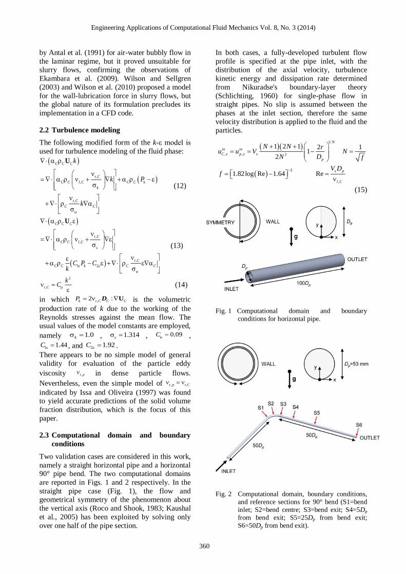
Engineering Applications of Computational Fluid Mechanics Vol 8 No 3 (2014)
360
by Antal et al (1991) for air-water bubbly flow in
the laminar regime but it proved unsuitable for slurry flows confirming the observations of
Ekambara et al (2009) Wilson and Sellgren
(2003) and Wilson et al (2010) proposed a model
for the wall-lubrication force in slurry flows but the global nature of its formulation precludes its
implementation in a CFD code
22 Turbulence modeling
The following modified form of the k-ε model is
used for turbulence modeling of the fluid phase
C C C
t C
C C l C C C k
k
t C
C C
k
k P
k
U
(12)
1 2
C C C
t C
C C l C
t C
C C k C CC P Ck
U
(13)
2
t C
kC
(14)
in which 2 k t C C CP UD is the volumetric
production rate of k due to the working of the
Reynolds stresses against the mean flow The usual values of the model constants are employed
namely 10k 1314 009C
1 144C and 2 192C
There appears to be no simple model of general
validity for evaluation of the particle eddy
viscosity t p in dense particle flows
Nevertheless even the simple model of t p t C
indicated by Issa and Oliveira (1997) was found to yield accurate predictions of the solid volume
fraction distribution which is the focus of this
paper
23 Computational domain and boundary
conditions
Two validation cases are considered in this work
namely a straight horizontal pipe and a horizontal 90deg pipe bend The two computational domains
are reported in Figs 1 and 2 respectively In the
straight pipe case (Fig 1) the flow and geometrical symmetry of the phenomenon about
the vertical axis (Roco and Shook 1983 Kaushal
et al 2005) has been exploited by solving only
over one half of the pipe section
In both cases a fully-developed turbulent flow
profile is specified at the pipe inlet with the distribution of the axial velocity turbulence
kinetic energy and dissipation rate determined
from Nikuradses boundary-layer theory
(Schlichting 1960) for single-phase flow in straight pipes No slip is assumed between the
phases at the inlet section therefore the same
velocity distribution is applied to the fluid and the particles
1
2
2
1 2 1 2 11
2
182log Re 164 Re
N
in in
C z p z s
p
s p
l C
N N ru u V N
DN f
V Df
(15)
Fig 1 Computational domain and boundary
conditions for horizontal pipe
Fig 2 Computational domain boundary conditions
and reference sections for 90deg bend (S1=bend
inlet S2=bend centre S3=bend exit S4=5Dp
from bend exit S5=25Dp from bend exit
S6=50Dp from bend exit)
Engineering Applications of Computational Fluid Mechanics Vol 8 No 3 (2014)
361
3
2 2 2 10 21
8 3 3
in
s
p p
f r rk V
D D
(16)
32
4
01643
2 2014 008 006
2
in
m
p
m
p p
k
l
D r rl
D D
(17)
In Eq (15) sV is the superficial velocity of the
slurry which is the ratio between the volumetric
slurry flow rate and the pipe area The inlet
volume fractions of both phases are taken as uniformly distributed At the outlet the normal
gradients of all variables and the value of the
pressure are set to zero The length of the
computational domain in the straight pipe case is 100Dp to ensure that fully-developed flow
conditions are attained which typically occurs
some 50Dp downstream of the inlet confirming the results of previous workers (Ling et al 2003)
For this reason 50Dp of straight pipe were
simulated upstream the 90deg bend (Fig 2) whilst
the outlet boundary is located about 50Dp downstream the bend exit in order to analyze the
development of the flow downstream the bend
and compare the numerical results with the experimental evidence
At the pipe wall no slip conditions are imposed to
both phases and the equilibrium wall function of Launder and Spalding (1972) is employed to
evaluate the velocity component parallel to the
wall for the two phases
w
k C pu the turbulence
kinetic energy wk and its dissipation rate w in the
near wall cells
1ln
w
k k
k l C
u u yE
u
(18)
w Cu
kC
(19)
3234w wk
Cy
(20)
where
ku is the friction velocity of phase
k C p 041 is von Karman constant E
is a roughness parameter and y is the normal
distance of the first grid point from the wall The parameter E is considered as a function of the
roughness Reynolds number
Re r C l Cu r
where r is the equivalent sand-grain roughness
height The formula for E developed by
Jayatillika (1969) is as follows
12
2
Re 37
Re 137 Re 100
Re 100Re
m r
rr
m
r
r
E
aE a
b E
b
(21)
where 86mE is the value of E appropriate for
smooth walls and a and b are given by
3 2
0564
100 Re1 2 3 002248 297
Re
r
r
a x x x b
(22)
24 Computational methodology and consistency
of numerical solution
The general-purpose commercial CFD code
PHOENICS was employed for the numerical
solution of the finite-volume analogue of the
mathematical described above This was done by using the built-in Eulerian two-fluid Inter-Phase
Slip Algorithm (IPSA) of Spalding (1980)
together with user-defined functions for implementation of specific constitutive equations
and boundary conditions The calculations are
performed following the elliptic-staggered
formulation in which the scalar variables are evaluated at the cell centers and the velocity
components at the cell faces Central differencing
is employed for the diffusion terms while the convection terms are discretized using the hybrid
differencing scheme of Spalding (1972) for the
straight pipe case and the MINMOD scheme (Versteeg and Malalasekera 2007) for the 90deg
bend The finite-volume equations are solved
iteratively by means of the SIMPLEST and IPSA
algorithms of Spalding (1980) The calculation procedure is organized in a slab-by-slab manner
in which all the dependent variables are solved at
the current slab before the solver routine moves to the next slab
The PHOENICS solver was run until the sum of
the absolute residual sources over the whole solution domain is less than 1 per cent of
reference quantities based on the total inflow of
the variable in question An additional
requirement is that the values of the monitored dependent variables at a selected location do not
change by more than 01 between subsequent
iteration cycles The consistency of the numerical solution with
respect to the domain discretization is now
discussed for the two scenarios simulated A
cylindrical-polar structured mesh was employed
Engineering Applications of Computational Fluid Mechanics Vol 8 No 3 (2014)
362
in the straight pipe case A grid sensitivity study
was performed to determine the optimum discretization of the domain by reference to the
predicted solids volume fraction profiles For this
purpose the following case was taken from Roco
and Shook (1983) pipe diameter = 507 mm particle diameter = 520 μm delivered solid
volume fraction = 02473 slurry superficial
velocity = 200 ms The pipe is assumed
hydraulically smooth ( 0r ) This case exhibits a
high degree of slurry stratification which is
expected to enhance the effect of mesh resolution
Three different meshes were employed as
follows 9 angular by 12 radial by 85 axial (Grid 1) 12 by 19 by 126 (Grid 2) 15 by 30 by 200
(Grid 3) and 20 by 40 by 300 (Grid 4) cells For
consistency with measurements made using γ-ray density gauges the predicted solids volume
fraction at a distance y from the pipe bottom is
evaluated by using the chord-average value ie
chord
0
1( ) ( )
x
p py x y dxx
(23)
where x accounts for the horizontal variation of
concentration in the pipe cross-section (Fig 1) The predicted volume fraction profiles for each
grid are shown in Fig 3 The solutions obtained
on the three finest meshes (Grids 2 3 and 4) are very close to each other whilst that for Grid 1
deviates slightly from the finer grid solutions
The Grid 3 solution is considered adequate
for comparison with the experiments For
each vertical location y the difference chord chord
4 3( ) ( )p py y - in which chord
3p and chord
4p
are the values obtained on Grids 3 and 4
respectively - is assumed an indicator of the effect of further mesh refinement The quantity
chord chord
4 3( ) ( )p py y was found to be lower than
0005 for all yDp less than the error usually associated with the measurements The
application of the method proposed by Eccedila and
Hoekstra (2006) for estimating the grid discretization error confirmed the reliability of
Grid 3
A curvilinear structured mesh in body-fitted
coordinates was instead employed in the 90deg bend case The grid independence study was performed
with respect to the following flow condition
particle diameter = 2645 kgm3 delivered solid
volume fraction = 00882 slurry superficial
velocity = 267 ms pipe roughness = 0015 mm
The four meshes used consisted of 300 slabwise by 300 axial (Grid 1) 600 by 350 (Grid 2) 1040
by 450 (Grid 3 details of which are shown in Fig
4) and 1170 by 500 (Grid 4) cells For consistency
Fig3 Solid volume fraction profiles calculated on
three different grid levels for straight pipe
case
Fig4 Details of mesh for 90deg bend
Fig5 Vertical solid volume fraction profiles at
distance of 5Dp downstream bend exit (Section S4 in Fig 2) calculated on different grid
levels The Grid 3 solution has error bars
corresponding to the grid discretization error
estimated by the method of Eccedila and Hoekstra
(2006)
Engineering Applications of Computational Fluid Mechanics Vol 8 No 3 (2014)
363
with the sampling probe measurements of
Kaushal et al (2013) the predicted solids volume fraction at a distance y from the pipe bottom is
now evaluated by using the value along the
vertical diameter ie
axis ( ) 0p py y (24)
The predicted volume fraction profiles for each
grid at a distance of 5Dp downstream the bend exit (Section S4 in Fig 2) are shown in Fig 5
and indicate that Grid 3 is capable to procure a
consistent numerical solution the difference axis axis
4 3( ) ( )p py y being less than 0014 for all y
In Fig 5 the Grid 3 solution has error bars
corresponding to the grid discretization error estimated following the method of Eccedila and
Hoekstra (2006) Grid 3 was used in the
simulations
25 Governing terms and calibration of
numerical constants
In the two-fluid model different empirical sub-
models are employed for the inter-phase processes and closure of the various turbulence
correlations These submodels contain adjustable
coefficients which are in practice treated as calibration parameters their values being
determined by matching computations with
experiments The submodels which mainly affect
the solid volume fraction distribution refer to two main terms The former is the phase diffusion of
each conserved property ( 1 for mass
conservation) equal to k kD in which
the phase-diffusion coefficient D is given by Eq
(2) The phase diffusion besides making the
model numerically more stable and thereby
contributing to its speed in attaining convergence
has a smoothing effect on the solids concentration profile reducing its variation along the vertical
direction The impact of phase diffusion is
controlled by an empirical parameter which is the
turbulent Schmidt number for volume fractions
which appear in Eq (2) A sensitivity analysis to
quantify the influence of on the solid volume
fraction profile was performed
The results are depicted in Fig 6 for horizontal
pipe flows with very different flow conditions both taken from Roco and Shook (1983) A) pipe
diameter = 515 mm particle diameter = 165 μm
particle density = 2650 kgm3 delivered solid
volume fraction = 009 slurry superficial velocity = 378 ms B) pipe diameter = 507 mm particle
diameter = 520 μm particle density = 2650
kgm3 delivered solid volume fraction = 02473
slurry superficial velocity = 200 ms In both
cases the pipe is regarded is hydraulically
smooth It is observed that a reduction of
results in a flatter profile as a consequence of the
increase in diffusivity The latter term which most influences the solid
volume fraction profile is the interfacial
momentum transfer (Eq (6)) and particularly the drag force (Eq (7)) As already noticed the
definition of the particle Reynolds number with
respect to the viscosity of the mixture m instead
of that of the fluid phase C puts an upper limit
to the solids concentration due to the asymptotic
trend of m (Eq (11)) The mixture viscosity as
derived from the correlation of Mooney (Eq (11)) depends on two empirical parameters the
intrinsic viscosity and the maximum packing
concentration pm The effect of and pm on
Fig 6 Effect of turbulent Schmidt number for volume fractions on solid volume fraction profiles for two flow
conditions ( experiments from Roco and Shook (1983) ndashndashndash 03 ndashndashndash 05 ndashndashndash 07 ndashndashndash
09 )
Engineering Applications of Computational Fluid Mechanics Vol 8 No 3 (2014)
364
Fig 7 Effect of parameters [η] and pm in mixture viscosity correlation of Mooney (Eq 11) on solid volume fraction
profiles for two flow conditions ( experiments from Roco and Shook (1983) continuous lines predictions)
The dependence on [η] is studied for 07pm that on pm for [η] = 25
Table 1 Flow conditions considered for comparison
Reference System [mm]pD
[-]pr D [ ]pd m []C [ms]sV 3 [kgm ]p
Roco and Shook (1983) Pipe 507-515 - 165-520 90-296 190-433 2650
Gillies et al (2004) Pipe 1030 2∙10-5 90-280 106-407 133-540 2650
Matousek (2000 and 2002) Pipe 1500 - 120-370 250-430 204-600 -
Shaan et al (2000) Pipe 1585 6∙10-6 90 150-320 140-300 2655
Kaushal et al (2013) 90deg Bend 530 3∙10-4 450 882 267 2645
the solid volume fraction profile is analyzed one at a time in Fig 7 for the two above mentioned
flow conditions from Roco and Shook (1983) In
particular the results highlight that pm affects
the behaviour of the mixture only at high
concentration therefore as a direct effect on the prevention of particle over-packing As already
mentioned this avoids the need to introduce a
collisional pressure term in the momentum equation of the solid phase further promoting the
numerical stability of the model and the rapid
achievement of a converged solution Our investigations showed that a unique
combination of the three empirical parameters ndash
07 25 and 07pm (all within the
range of variability found in literature) ndash produced estimations of the solids concentration
profile in good agreement with the experimental
evidence for all the flow conditions considered in the present work referring to both the horizontal
pipe case and the 90deg bend case This feature
together with the numerical stability and the
relatively short computer time required contributes to make the model particularly useful
for the applications
3 RESULTS
The numerical model is validated by comparing
the results of the simulations against experimental
data reported by the authors listed in Table 1 This
Engineering Applications of Computational Fluid Mechanics Vol 8 No 3 (2014)
365
table provides the flow conditions for each set of
measurements As already mentioned two scenarios have been considered namely a straight
horizontal pipe and a 90deg bend which will be
discussed in separate sub-sections
31 Straight horizontal pipe
The predictions of the model have been compared with experimental data for 26 flow conditions
summarized in Table 2 which differ in terms of
pipe diameter pipe roughness particle size slurry superficial velocity and delivered solid volume
fraction Each set of measurements allows an
assessment of the models capability for
reproducing the influence of specific features affecting the distribution of the solid volume
fraction The data of Roco and Shook (1983) and
Gillies et al (2004) are used to investigate the effect of particle diameter and slurry velocity with
different delivered solid volume fraction The
measurements of Matousek (2000 2002) provide the opportunity to extend the validity of the model
up to a pipe Reynolds number Re (Eq (15)) of
about 106 Finally the data of Shaan et al (2000)
are used to assess the performance of the model in
case of natural sands with irregularly-shaped grains Almost all the data refer to configurations
in which all the solids are kept suspended but
moving bed flows have also been briefly explored
to check how far one can go in employing the model for the purpose of achieving useful
information from an engineering point of view
Measurements of solids concentration ndash either bulk-mean or local ndash are subjected to errors
depending mainly on the instrumentation used as
discussed in Section 1 All the data reported in Table 2 are obtained using gamma-ray absorption
methods perhaps the technique which provides
the highest accuracy attainable with errors of the
order of a few percentage points Since this technique allows measuring chord-average values
of solid volume fraction the computed volume
fraction profile was evaluated by means of Eq (23) In the experiments from Roco and Shook
(1983) ndash cases A1 to A5 in Table 2 ndash the
dispersed phase consists of three kinds of sand with narrow size distribution and mean particle
diameters of 165 and 520 μm The solids density
is 2650 kgm3 the pipe diameter is about 51 mm
Table 2 Details of experimental conditions for straight pipe case (A1 to A5 experimental data from Roco and Shook (1983) B1 to B12 experimental data from Gillies et al (2004) C1 to C6 experimental data from Matousek
(2000 and 2002) D1 to D4 experimental data from Shaan et al (2000) values not declared by
experimenters)
Test ID [mm]pD
[-]pr D [ ]pd m []C [ms]sV 3 [kgm ]p
Flow pattern
A1 515 0 165 9 378 2650 FS
A2 515 0 165 19 417 2650 FS
A3 515 0 165 28 433 2650 FS
A4 507 0 520 1212 190 2650 MB
A5 507 0 520 2473 200 2650 MB
B1 103 2∙10-5 90 198 133 2650 FS
B2 103 2∙10-5 90 283 133 2650 FS
B3 103 2∙10-5 90 19 300 2650 FS
B4 103 2∙10-5 90 284 300 2650 FS B5 103 2∙10-5 280 12 255 2650 FS
B6 103 2∙10-5 280 208 260 2650 FS
B7 103 2∙10-5 280 310 250 2650 FS
B8 103 2∙10-5 280 407 260 2650 FS
B9 103 2∙10-5 280 106 540 2650 FS
B10 103 2∙10-5 280 203 540 2650 FS
B11 103 2∙10-5 280 301 540 2650 FS
B12 103 2∙10-5 280 405 540 2650 FS
C1 150 0 120 25 204 2650 FS
C2 150 0 120 35 204 2650 -
C3 150 0 120 34 600 2650 -
C4 150 0 370 25 600 2650 FS
C5 150 0 370 34 600 2650 - C6 150 0 370 43 600 2650 MB
D1 1585 6∙10-6 90 15 15 2655 FS
D2 1585 6∙10-6 90 32 14 2655 FS
D3 1585 6∙10-6 90 15 30 2655 FS
D4 1585 6∙10-6 90 32 30 2655 FS
Engineering Applications of Computational Fluid Mechanics Vol 8 No 3 (2014)
366
the slurry bulk-mean velocity varies from 190 to
433 ms and the pipe Reynolds number from between 9610
4 and 2110
5 The delivered solid
volume fraction ranges from 9 to 30 The
authors did not indicate the roughness of the pipe
which was assumed hydraulically smooth No evaluation of measurement uncertainty was
reported by the experimenters and they did not
identify the flow patterns according to the more recent classification of Doron and Barnea (1996)
However for the smallest particle diameter the
data suggest suspended flow whereas for the largest diameter the indications are for moving-
bed flow Fig 8 compares the computed and
measured solid volume fraction profiles The good agreement between computation and
measurements reveals the ability of the model to
reproduce the effect of particle diameter on the
particle distribution for slurries with different delivered solid volume fraction The simple two-
fluid model proposed in this work appears
capable to predict with reasonable accuracy the solid volume fraction profile not only in case of
fully-suspended flow but also in case of moving
bed flows This indicates that the asymptotic trend of the interfacial momentum transfer term
Fig 8 Solids concentration profiles for flow conditions A1 to A5 in Table 2 ( experiments from Roco and
Shook (1983) ndashndashndash predictions)
Fig 9 Solids concentration profile for flow conditions B1 to B12 in Table 2 ( experiments from Gillies et al
(2004) ndashndashndash predictions)
Engineering Applications of Computational Fluid Mechanics Vol 8 No 3 (2014)
367
produces on the solid volume fraction profile the
same effect that is traditionally achieved by the
collisional pressure and the tensor kT
Gillies et al (2004) measured the concentration
profiles of sand-water slurries in a 103 mm
diameter pipe using gamma-ray absorption
gauges without reporting the uncertainty The roughness of the pipe is 2 nm Two kinds of sand
were considered with narrow size distribution
and mean particle diameter of 90 and 280 μm In both cases the particle density was 2650 kgm
3
and the slurry superficial velocity varies from
133 to 54 ms (corresponding to a pipe Reynolds
number between 14105 and 5610
5) The
delivered solid volume fraction varies from about
10 to about 45 Details of the flow conditions
considered for comparison are reported in Table 2 cases B1 to B12 From an examination of the
measured data for the pressure gradient it can be
inferred that in all cases the flow is fully-suspended This is a good test for the modelrsquos
ability to predict the combined effect of slurry
velocity solids loading and particle diameter in a
larger pipe Fig 9 shows comparison of the computational and the experimental results for the
vertical distribution of the solid volume fraction
The model produces good overall agreement with the data The largest deviations are observed near
the pipe wall for the small particles at high
concentration (cases B2 and B4 in Table 4) but as noted by the authors themselves these
measurements are subject to the largest
experimental error
Matousek (2000 and 2002) measured the concentration profiles of sand-water slurries in a
150 mm diameter pipe using gamma-ray
absorption method quantifying a 4 uncertainty of the data We reproduced numerically the flow
conditions reported in Table 2 (cases C1 to C6)
in which the dispersed phase consists of two kinds
of sand with narrow size distribution and mean particle diameters of 120 and 370 μm
Unfortunately neither the density of the solid
particles nor the pipe roughness are reported in the experiments of Matousek (2000 and 2002)
and so in the simulations the former was set to
2650 kgm3 which is the value declared by Roco
and Shook (1983) and Gillies et al (2004) and
the pipe was regarded as hydraulically smooth
The slurry superficial velocity was 2 or 6 ms
corresponding to a pipe Reynolds number up to 10
6 The delivered solid volume fraction ranged
between 25 and 43 According to the author
the flows are either fully suspended or with a moving bed but only for three cases the flow
pattern could be clearly identified from the plot of
pressure gradient versus slurry superficial
velocity Fig 10 compares the computed and measured solid volume fraction profiles each set
of experimental data has error bars indicating the
uncertainty declared by the experimenter The
rather good agreement between computations and measurements confirm the reliability of the model
for high pipe Reynolds numbers A closer
inspection reveals that for case C6 the computed concentration is lower than the experimental
results in the lower part of the pipe and higher in
the upper region However the pressure gradient curve clearly reveals that in case C6 a moving bed
of particles is formed It is again confirmed that
the proposed model is capable to procure a rough
indication of the distribution of the solid also for flows in which the inter-granular stresses play an
important role
Moreover in the case of highly dense slurries like case C6 the experimental data are subject to the
most uncertainty and the numerical solutions are
sensitive to the empirical parameters pm and
which appear in the mixture viscosity correlation
(Eq (11)) For the same case the measured solids concentration profile shows a drop near the pipe
bottom This reversal is not predicted by the
numerical model which is probably due to the absence of the wall lift force discussed earlier in
Section 21 The same limitation was reported by
Ekambara et al (2009) The paper of Shaan et al (2000) focuses on the
effect of particle shape upon pressure gradient and
deposition velocity but these workers also
reported some measurements of the solid volume fraction profiles Shaan et al (2000) quantified
the particle shape by reference to the following
quantities evaluated from photos of the particles the axes ratio ie the ratio between the major and
minor axes of an ellipse circumscribing the
grains the circularity index ie the ratio between
the area of the particle multiplied by 4π and its perimeter The sand particles have a very irregular
shape as can be inferred by comparing the
measured values of axes ratio (16) and circularity (062) against typical values reported in the
literature for sand grains The mass-median value
of the particle size distribution curve is taken as the characteristic particle diameter The flow
conditions reported in Table 2 (cases D1 to D4)
were reproduced to check the behaviour of the
model for the case of irregularly-shaped sand particles The pipe diameter (1585 mm)
delivered solid volume fraction (15 or 35)
slurry superficial velocity (14 or 3 ms) particle density (2655 Kgm
3) and particle diameter (90
μm) are all approximately within the range
Engineering Applications of Computational Fluid Mechanics Vol 8 No 3 (2014)
368
Fig 10 Solids concentration profiles for flow conditions C1 to C6 in Table 2 ( experiments from Matousek
(2000 and 2002) ndashndashndash predictions)
Fig 11 Solids concentration profiles for flow conditions D1 to D4 in Table 2 ( experiments from Shaan et al
(2000) ndashndashndash predictions)
covered by the earlier simulations The numerical and experimental results are
compared in Fig 11 The agreement between the
numerical predictions and the experimental
evidence is fairly good inadequacies of the numerical model ndash especially in the wall
boundary conditions for the solid phase ndash and
measurements error can both contribute to the discrepancies observed near the pipe bottom for
case D2 The results seem to indicate that the
numerical model is a suitable tool for predicting the solid volume fraction distribution produced by
sands with a very irregular shape
32 Horizontal 90deg bend
The predictions of the model have been compared
with the recent experiments of Kaushal et al (2013) regarding a horizontal 90deg bend Among
the different flow conditions considered by these
authors reference is made to those characterized
by delivered solid volume fraction of 882 within the range of interest in this work The
experimenters used a sampling probe to measure
the volume fraction profile of the slurry in the 53
mm diameter pipe along the vertical axis at distances of 5Dp 25Dp and 50Dp downstream the
bend exit (referred to as sections S4 S5 and S6 in
Fig 2 respectively) They quantified a 2
uncertainty of the data The solid phase consists of silica sand particles with narrow size
distribution and mean particle diameter of 450
μm The slurry superficial velocity is 178 267 or 356 ms
The flow within the bend is much more complex
compared to that through the straight pipe since secondary motions develop in the crosswise
direction These motions affect significantly the
distribution of the solids and as a consequence
the volume fraction distribution is no longer constant over horizontal planes This is evident in
Fig 12 which shows the color plot of the solids
volumetric concentration over the six cross sections highlighted in Fig 2 As shown in Fig
13 the predictions of our model generally agree
with the experimental data available Greater
discrepancies are observed for the highest superficial velocity (356 ms) where the model
seems to underestimate the quantity of particles
dragged by the secondary motions This is
Engineering Applications of Computational Fluid Mechanics Vol 8 No 3 (2014)
369
Fig 12 Solid volume fraction distributions on sections
S1 to S6 in Fig 2 for delivered solid volume
fraction of 882 Left hand side is the outer
wall of the pipe
opposite to the KTGF based model of Kaushal et
al (2013) which tends to over-enhance the effect
of the secondary motions on the solids for the
lowest velocities Fig 13 also reveals that our model tends to overestimate the solids volume
fraction close to the pipe bottom far from the
bend exit It is expected that the predictions could
be improved if the effect of the wall lubrication force for which a suitable model does not exist at
present were accounted for
4 CONCLUSIONS
A mathematical model has been described for the
estimation of solid volume fraction distribution of
solid-liquid slurry flows in horizontal pipes and bends The model is based on an Eulerian-
Eulerian approach and uses the Inter-Phase Slip
Algorithm (IPSA) of Spalding (1980) The
novelty of this model resides in the combined use of existing modelling strategies never previously
employed simultaneously for the predictions of
slurry flows In order to account for turbulent dispersion of particles phase diffusion terms have
been included in the phase continuity equations
together with all the conservation equations The mixture viscosity approach is adopted to model
the effect of multiple particles on the inter-phase
friction A wall function is employed to model the
flow in the near-wall region in case of both hydraulically smooth and rough walls All these
strategies result in a model which despite being
simpler that those commonly used for addressing solid-liquid slurry flows shows comparable or
even better predictive capacity Moreover this
model is robust and numerically stable and
requires relatively short CPU time to procure converged steady-state solutions
The model has been first validated by comparison
with experimental data for the horizontal pipe case over a wide range of operating conditions
delivered solid volume fraction between 10 and
40 by volume mean particle diameter between 90 and 520 μm slurry superficial velocity
between 1 ms and 55 ms and pipe diameter
between 50 and 158 mm The model predictions
were found to be in good agreement with the experimental evidence for all the flow conditions
considered for comparison Even if the model is
originally intended to address fully-suspended flows the results indicated its capability to
provide rough indications of the solid volume
fraction distribution also in case of bed flows At last the comparison with the recent
measurements of Kaushal et al (2013) revealed
that this model is capable to procure reliable
predictions of the particle distribution downstream a 90deg bend in a horizontal pipe
Engineering Applications of Computational Fluid Mechanics Vol 8 No 3 (2014)
370
Fig 13 Solid volume fraction along vertical diameter on sections S4 to S6 in Fig 2 for delivered solid volume fraction
of 882 ( experiments from Kaushal et al (2013) ndashndashndash predictions)
ACKNOWLEDGEMENTS The authors would acknowledge the CINECA and
the Regione Lombardia award under the LISA
initiative for the availability of high performance computing resources and support The authors
would like to thank CHAM Ltd for supporting
this research and acknowledge Dr Randy Gillies of Saskatchewan Research Council for providing
his experimental data
REFERENCES
1 Ahilan RV Sleath J (1987) Sediment
transport in oscillatory flow over flat beds Journal of Hydraulic Engineering 113 308-
322
2 Albunaga BE (2002) Slurry Systems Handbook McGraw-Hill
3 Antal S Lahey R Flaherty J (1991) Analysis
of phase distribution in fully-developed
laminar bubbly two phase flow International Journal of Multiphase Flow 17(5) 635-652
4 Barnea E Mizrahi J (1973) A Generalized
Approach to the Fluid Dynamics of
Particulate Systems Chemical Engineering
Science 5(2) 171-189 5 Chen L Duan Y Pu W Zhao C (2009) CFD
simulation of coal-water slurry flowing in
horizontal pipelines Korean Journal of Chemical Engineering 26(4) 1144-1154
6 Chen RC (1994) Analysis of homogeneous
slurry pipe flow Journal of Marine Science and Technology 2(1) 37-45
7 Chen X Li Y Niu X Li M Chen D Yu X
(2011) A general two-phase turbulent flow
model applied to the study of sediment transport in open channels International
Journal of Multiphase Flow 37(9) 1099-
1108 8 Chung JN Troutt TR (1988) Simulation of
particle dispersion in an axisymmetric jet
Journal of Fluid Mechanics 186 199-222 9 Clift R Grace JR Weber ME (1978)
Bubbles Drops and Particles Academic
Press
10 Colwell JM Shook CA (1988) The Entry Length for Slurries in Horizontal Pipeline
Flow Canadian Journal of Chemical
Engineering 66(5) 714-720
Engineering Applications of Computational Fluid Mechanics Vol 8 No 3 (2014)
371
11 Doron P Barnea D (1993) A three layer
model for solid-liquid flow in horizontal pipes International Journal of Multiphase
Flow 19(6) 1029-1043
12 Doron P Barnea D (1995) Pressure drop and
limit deposit velocity for solid-liquid flow in pipes Chemical Engineering and Science
50(10) 1595-1604
13 Doron P Barnea D (1996) Flow pattern maps for solid-liquid flow in pipes International
Journal of Multiphase Flow 22(2) 273-283
14 Doron P Granica D Barnea D (1987) Slurry flow in horizontal pipes ndash experimental and
modeling International Journal of
Multiphase Flow 13(4) 535ndash547
15 Eccedila L Hoekstra M (2006) Discretization uncertainty estimation based on a least
squares version of the grid convergence
index Proceedings of the 2nd
Workshop on CFD Uncertainty Analysis Oct 19-20
Lisbon Portugal
16 Ekambara K Sanders RS Nandakumar K Masliyah JH (2009) Hydrodynamic
simulation of horizontal slurry pipeline flow
using ANSYS-CFX Industrial amp
Engineering Chemistry Research 48(17) 8159-8171
17 Gillies RG Shook CA (2000) Modelling
High Concentration Settling Slurry Flows Canadian Journal of Chemical Engineering
78(4) 709-716
18 Gillies RG Shook CA Xu J (2004)
Modelling Heterogeneous Slurry Flow at High Velocities Canadian Journal of
Chemical Engineering 82(5) 1060-1065
19 Hsu FLG (1981) Flow of Fine-particle Suspensions in Bends Fittings and Valves
MS Thesis Texas Tech University Lubbock
Texas USA 20 Ishii M Mishima K (1984) Two-fluid model
and hydrodynamic constitutive relations
Nuclear Engineering and Design 82(2-3)
107-126 21 Issa RI Oliveira PJ (1997) Assessment of a
particle-turbulence interaction model in
conjunction with an Eulerian two-phase flow formulation Proceedings of the 2
nd
International Symposium on Turbulence
Heat and Mass Transfer June 9-12 Delft Netherlands 759-770
22 Jayatillika CLV (1969) The influence of the
Prandtl number and surface roughness on the
resistance of the sublayer to momentum and heat transfer Progress in Heat amp Mass
Transfer 1 193-329
23 Jiang YY Zhang P (2012) Pressure drop and
flow pattern of slush nitrogen in a horizontal pipe AIChE Journal doi 10002aic13927
24 Kaushal DR Kumar A Tomita Y Juchii S
Tsukamoto H (2013) Flow of mono-
dispersed particles through horizontal bend International Journal of Multiphase Flow 52
71-91
25 Kaushal DR Sato K Toyota T Funatsu K Tomita Y (2005) Effect of particle size
distribution on pressure drop and
concentration profile in pipeline flow of highly concentrated slurry International
Journal of Multiphase Flow 31(7) 809-823
26 Kaushal DR Thinglas T Tomita Y Juchii S
Tsukamoto H (2012) CFD modeling for pipeline flow of fine particles at high
concentration International Journal of
Multiphase Flow 43 85-100 27 Kaushal DR Tomita Y (2003) Comparative
study of pressure drop in multisized
particulate slurry flow through pipe and rectangular duct International Journal of
Multiphase Flow 29(9) 1473-1487
28 Kaushal DR Tomita Y (2007) Experimental
investigation for near-wall lift of coarser particles in slurry pipeline using γ-ray
densitometer Powder Technology 172(3)
177-187 29 Kim C Lee M Han C (2008) Hydraulic
transport of sand-water mixtures in pipelines
Part I Experiment Journal of Mechanical
Science and Technology 22(12) 2534-2541 30 Kumar U Mishra R Singh SN Seshadri V
(2003) Effect of particle gradation on flow
characteristics of ash disposal pipelines Powder Technology 132(1) 39-51
31 Lahiri SK Ghanta KC (2010) Slurry flow
modeling by CFD Chemical Industry amp Chemical Engineering Quarterly 16(4) 295-
308
32 Launder BE Spalding DB (1972)
Mathematical models of turbulence Academic Press
33 Ling J Skudarnov PV Lin CX Ebadian MA
(2003) Numerical investigations of solid-liquid slurry flows in a fully developed flow
region International Journal of Heat and
Fluid Flow 24(3) 389-398 34 Matousek V (2000) Concentration
distribution in pipeline flow of sand-water
mixtures Journal of Hydrology and
Hydromechanics 48(3) 180-196 35 Matousek V (2002) Pressure drops and flow
patterns in sand-mixture pipes Experimental
Engineering Applications of Computational Fluid Mechanics Vol 8 No 3 (2014)
372
Thermal and Fluid Science 26(6-7) 693-702
36 Matousek V (2009) Predictive model for frictional pressure drop in settling-slurry pipe
with stationary deposit Powder Technology
192(3) 367-374
37 Mooney M (1951) The viscosity of a concentrated suspension of spherical
particles Journal of Colloid Science 6(2)
162-170 38 Nasr-el-Din H Shook CA Esmail MN
(1984) Isokinetic Probe Sampling From
Slurry Pipelines Canadian Journal of Chemical Engineering 62(2) 179-185
39 Pathak M (2011) Computational
investigations of solid-liquid particle
interaction in a two-phase flow around a ducted obstruction Journal of Hydraulic
Research 49(1) 96-104
40 Pecker SM Helvaci SS (2008) Solid-Liquid Two-Phase Flow Elsevier
41 Roco MC Shook CA (1983) Modeling of
Slurry Flow The Effect of Particle Size Canadian Journal of Chemical Engineering
61(4) 494-503
42 Schlichting H (1960) Boundary Layer
Theory McGraw-Hill 43 Shaan J Sumner RJ Gillies RG Shook CA
(2000) The Effect of Particle Shape on
Pipeline Friction for Newtonian Slurries of Fine Particles Canadian Journal of Chemical
Engineering 78(4) 717-725
44 Shiller L Naumann A (1935) A drag
coefficient correlation Zeitschrift des Vereines Deutscher Ingenieure 77 318-320
45 Shirolkar JS Coimbra CFM McQuay MQ
(1996) Fundamental aspects of modelling turbulent particle dispersion in dilute flows
Progress in Energy and Combustion Science
22(4) 363-399 46 Shook CA Bartosik AS (1994) Particle-wall
stresses in vertical slurry flows Powder
Technology 81(2) 117-124
47 Skudarnov PV Lin CX Ebadian MA (2004) Double-Species Slurry Flow in a Horizontal
Pipeline ASME Journal of Fluids
Engineering 126(1) 125-132 48 Spalding DB (1972) A novel finite-
difference formulation for differential
expressions involving both first and second derivatives International Journal of
Numerical Methods in Engineering 4(4) 551-
559
49 Spalding DB (1980) Numerical computation of multi-phase fluid flow and heat transfer In
Taylor C Morgan K (Eds) Recent Advances
in Numerical Methods in Fluids Pineridge
Press Limited 139-168 50 Turian RM Ma TW Hsu FLG Sung MDJ
Plackmann GW (1998) Flow of concentrated
non-Newtonian slurries 2 Friction losses in
bends fittings valves and Venturi meters International Journal of Multiphase Flow
24(2) 243-269
51 Versteeg HK Malalasekera W (2007) An Introduction to Computational Fluid
Dynamics The Finite Volume Method
Pearson Prentice Hall 52 Wilson KC Sanders RS Gillies RG Shook
CA (2010) Verification of the near-wall
model for slurry flow Powder Technology
197(3) 247-253 53 Wilson KC Sellgren A (2003) Interaction of
Particles and Near-Wall Lift in Slurry
Pipelines Journal of Hydraulic Engineering 129(1) 73-76
- Figures13
-
- Fig 1 Computational domain and boundaryconditions for horizontal pipe
- Fig 2 Computational domain boundary conditionsand reference sections for 90deg bend (S1=bendinlet S2=bend centre S3=bend exit S4=5Dpfrom bend exit S5=25Dp from bend exitS6=50Dp from bend exit)
- Fig3 Solid volume fraction profiles calculated onthree different grid levels for straight pipecase
- Fig4 Details of mesh for 90deg bend
- Fig5 Vertical solid volume fraction profiles atdistance of 5Dp downstream bend exit (SectionS4 in Fig 2) calculated on different gridlevels The Grid 3 solution has error barscorresponding to the grid discretization errorestimated by the method of Eccedila and Hoekstra(2006)
- Fig 6 Effect of turbulent Schmidt number for volume fractions a s on solid volume fraction profiles for two flowconditions (r experiments from Roco and Shook (1983) ndashndashndash 03 a s = ndashndashndash 05 a s = ndashndashndash 07 a s = ndashndashndash09 a s = )
- Fig 7 Effect of parameters [η] and pm a in mixture viscosity correlation of Mooney (Eq 11) on solid volume fractionprofiles for two flow conditions (r experiments from Roco and Shook (1983) continuous lines predictions)The dependence on [η] is studied for 07 pm a = that on pm a for [η] = 25
- Fig 8 Solids concentration profiles for flow conditions A1 to A5 in Table 2 (rbull experiments from Roco and Shook (1983) ndashndashndash predictions)
- Fig 9 Solids concentration profile for flow conditions B1 to B12 in Table 2 (rbulls experiments from Gillies et al (2004) ndashndashndash predictions)
- Fig 10 Solids concentration profiles for flow conditions C1 to C6 in Table 2 (rbull experiments from Matousek (2000 and 2002) ndashndashndash predictions)
- Fig 11 Solids concentration profiles for flow conditions D1 to D4 in Table 2 (rbull experiments from Shaan et al (2000) ndashndashndash predictions)
- Fig 12 Solid volume fraction distributions on sections S1 to S6 in Fig 2 for delivered solid volume fraction of 882 Left hand side is the outer wall of the pipe
- Fig 13 Solid volume fraction along vertical diameter on sections S4 to S6 in Fig 2 for delivered solid volume fraction of 882 (r experiments from Kaushal et al (2013) ndashndashndash predictions)
-
- Tables13
-
- Table 1 Flow conditions considered for comparison
- Table 2 Details of experimental conditions for straight pipe case (A1 to A5 experimental data from Roco and Shook(1983) B1 to B12 experimental data from Gillies et al (2004) C1 to C6 experimental data from Matousek(2000 and 2002) D1 to D4 experimental data from Shaan et al (2000) values not declared byexperimenters)
-
- 1 INTRODUCTION
- 2 MATHEMATICAL MODEL
-
- 21 Conservation equations
- 22 Turbulence modeling
- 23 Computational domain and boundaryconditions
- 24 Computational methodology and consistencyof numerical solution
- 25 Governing terms and calibration ofnumerical constants
-
- 3 RESULTS
-
- 31 Straight horizontal pipe
- 32 Horizontal 90deg bend
-
- 4 CONCLUSIONS
- ACKNOWLEDGEMENTS
- REFERENCES
-
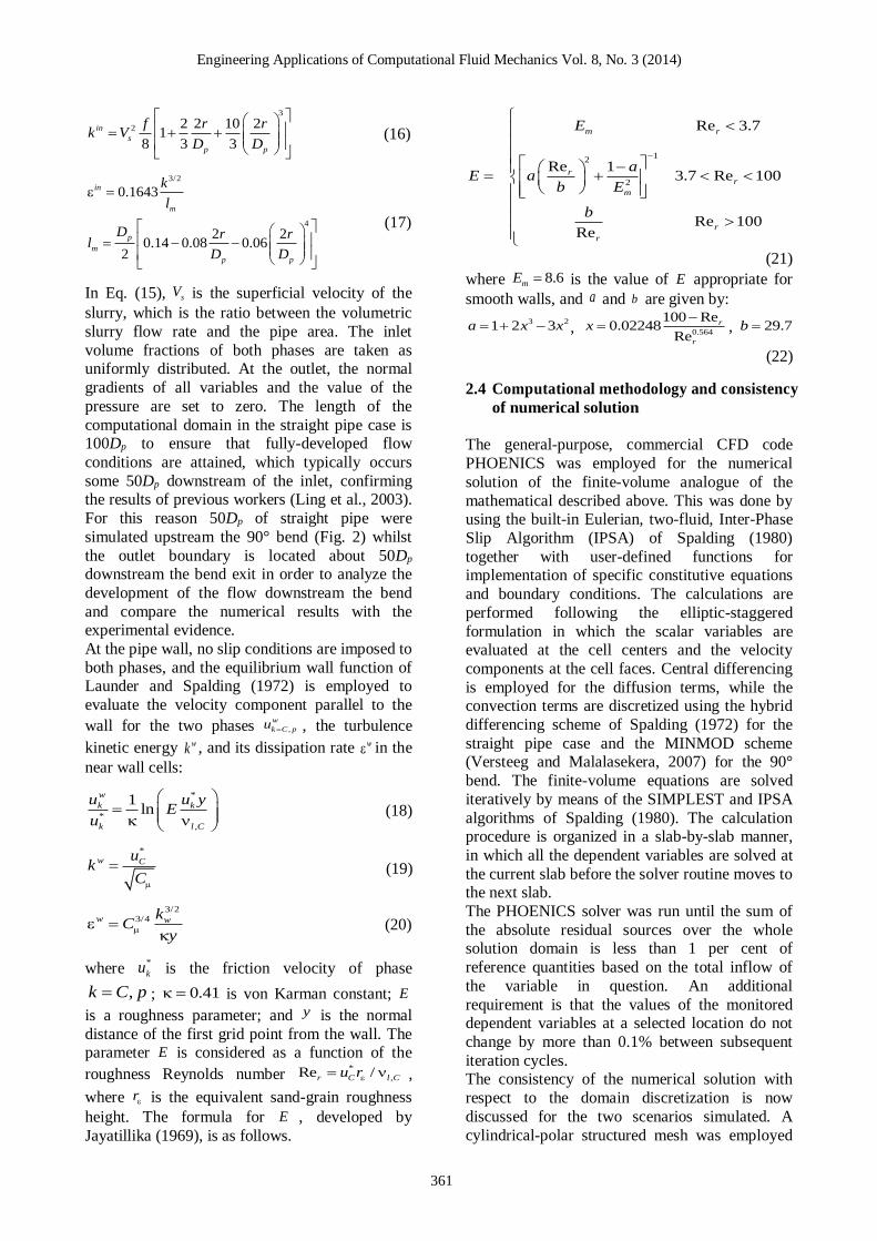
Engineering Applications of Computational Fluid Mechanics Vol 8 No 3 (2014)
361
3
2 2 2 10 21
8 3 3
in
s
p p
f r rk V
D D
(16)
32
4
01643
2 2014 008 006
2
in
m
p
m
p p
k
l
D r rl
D D
(17)
In Eq (15) sV is the superficial velocity of the
slurry which is the ratio between the volumetric
slurry flow rate and the pipe area The inlet
volume fractions of both phases are taken as uniformly distributed At the outlet the normal
gradients of all variables and the value of the
pressure are set to zero The length of the
computational domain in the straight pipe case is 100Dp to ensure that fully-developed flow
conditions are attained which typically occurs
some 50Dp downstream of the inlet confirming the results of previous workers (Ling et al 2003)
For this reason 50Dp of straight pipe were
simulated upstream the 90deg bend (Fig 2) whilst
the outlet boundary is located about 50Dp downstream the bend exit in order to analyze the
development of the flow downstream the bend
and compare the numerical results with the experimental evidence
At the pipe wall no slip conditions are imposed to
both phases and the equilibrium wall function of Launder and Spalding (1972) is employed to
evaluate the velocity component parallel to the
wall for the two phases
w
k C pu the turbulence
kinetic energy wk and its dissipation rate w in the
near wall cells
1ln
w
k k
k l C
u u yE
u
(18)
w Cu
kC
(19)
3234w wk
Cy
(20)
where
ku is the friction velocity of phase
k C p 041 is von Karman constant E
is a roughness parameter and y is the normal
distance of the first grid point from the wall The parameter E is considered as a function of the
roughness Reynolds number
Re r C l Cu r
where r is the equivalent sand-grain roughness
height The formula for E developed by
Jayatillika (1969) is as follows
12
2
Re 37
Re 137 Re 100
Re 100Re
m r
rr
m
r
r
E
aE a
b E
b
(21)
where 86mE is the value of E appropriate for
smooth walls and a and b are given by
3 2
0564
100 Re1 2 3 002248 297
Re
r
r
a x x x b
(22)
24 Computational methodology and consistency
of numerical solution
The general-purpose commercial CFD code
PHOENICS was employed for the numerical
solution of the finite-volume analogue of the
mathematical described above This was done by using the built-in Eulerian two-fluid Inter-Phase
Slip Algorithm (IPSA) of Spalding (1980)
together with user-defined functions for implementation of specific constitutive equations
and boundary conditions The calculations are
performed following the elliptic-staggered
formulation in which the scalar variables are evaluated at the cell centers and the velocity
components at the cell faces Central differencing
is employed for the diffusion terms while the convection terms are discretized using the hybrid
differencing scheme of Spalding (1972) for the
straight pipe case and the MINMOD scheme (Versteeg and Malalasekera 2007) for the 90deg
bend The finite-volume equations are solved
iteratively by means of the SIMPLEST and IPSA
algorithms of Spalding (1980) The calculation procedure is organized in a slab-by-slab manner
in which all the dependent variables are solved at
the current slab before the solver routine moves to the next slab
The PHOENICS solver was run until the sum of
the absolute residual sources over the whole solution domain is less than 1 per cent of
reference quantities based on the total inflow of
the variable in question An additional
requirement is that the values of the monitored dependent variables at a selected location do not
change by more than 01 between subsequent
iteration cycles The consistency of the numerical solution with
respect to the domain discretization is now
discussed for the two scenarios simulated A
cylindrical-polar structured mesh was employed
Engineering Applications of Computational Fluid Mechanics Vol 8 No 3 (2014)
362
in the straight pipe case A grid sensitivity study
was performed to determine the optimum discretization of the domain by reference to the
predicted solids volume fraction profiles For this
purpose the following case was taken from Roco
and Shook (1983) pipe diameter = 507 mm particle diameter = 520 μm delivered solid
volume fraction = 02473 slurry superficial
velocity = 200 ms The pipe is assumed
hydraulically smooth ( 0r ) This case exhibits a
high degree of slurry stratification which is
expected to enhance the effect of mesh resolution
Three different meshes were employed as
follows 9 angular by 12 radial by 85 axial (Grid 1) 12 by 19 by 126 (Grid 2) 15 by 30 by 200
(Grid 3) and 20 by 40 by 300 (Grid 4) cells For
consistency with measurements made using γ-ray density gauges the predicted solids volume
fraction at a distance y from the pipe bottom is
evaluated by using the chord-average value ie
chord
0
1( ) ( )
x
p py x y dxx
(23)
where x accounts for the horizontal variation of
concentration in the pipe cross-section (Fig 1) The predicted volume fraction profiles for each
grid are shown in Fig 3 The solutions obtained
on the three finest meshes (Grids 2 3 and 4) are very close to each other whilst that for Grid 1
deviates slightly from the finer grid solutions
The Grid 3 solution is considered adequate
for comparison with the experiments For
each vertical location y the difference chord chord
4 3( ) ( )p py y - in which chord
3p and chord
4p
are the values obtained on Grids 3 and 4
respectively - is assumed an indicator of the effect of further mesh refinement The quantity
chord chord
4 3( ) ( )p py y was found to be lower than
0005 for all yDp less than the error usually associated with the measurements The
application of the method proposed by Eccedila and
Hoekstra (2006) for estimating the grid discretization error confirmed the reliability of
Grid 3
A curvilinear structured mesh in body-fitted
coordinates was instead employed in the 90deg bend case The grid independence study was performed
with respect to the following flow condition
particle diameter = 2645 kgm3 delivered solid
volume fraction = 00882 slurry superficial
velocity = 267 ms pipe roughness = 0015 mm
The four meshes used consisted of 300 slabwise by 300 axial (Grid 1) 600 by 350 (Grid 2) 1040
by 450 (Grid 3 details of which are shown in Fig
4) and 1170 by 500 (Grid 4) cells For consistency
Fig3 Solid volume fraction profiles calculated on
three different grid levels for straight pipe
case
Fig4 Details of mesh for 90deg bend
Fig5 Vertical solid volume fraction profiles at
distance of 5Dp downstream bend exit (Section S4 in Fig 2) calculated on different grid
levels The Grid 3 solution has error bars
corresponding to the grid discretization error
estimated by the method of Eccedila and Hoekstra
(2006)
Engineering Applications of Computational Fluid Mechanics Vol 8 No 3 (2014)
363
with the sampling probe measurements of
Kaushal et al (2013) the predicted solids volume fraction at a distance y from the pipe bottom is
now evaluated by using the value along the
vertical diameter ie
axis ( ) 0p py y (24)
The predicted volume fraction profiles for each
grid at a distance of 5Dp downstream the bend exit (Section S4 in Fig 2) are shown in Fig 5
and indicate that Grid 3 is capable to procure a
consistent numerical solution the difference axis axis
4 3( ) ( )p py y being less than 0014 for all y
In Fig 5 the Grid 3 solution has error bars
corresponding to the grid discretization error estimated following the method of Eccedila and
Hoekstra (2006) Grid 3 was used in the
simulations
25 Governing terms and calibration of
numerical constants
In the two-fluid model different empirical sub-
models are employed for the inter-phase processes and closure of the various turbulence
correlations These submodels contain adjustable
coefficients which are in practice treated as calibration parameters their values being
determined by matching computations with
experiments The submodels which mainly affect
the solid volume fraction distribution refer to two main terms The former is the phase diffusion of
each conserved property ( 1 for mass
conservation) equal to k kD in which
the phase-diffusion coefficient D is given by Eq
(2) The phase diffusion besides making the
model numerically more stable and thereby
contributing to its speed in attaining convergence
has a smoothing effect on the solids concentration profile reducing its variation along the vertical
direction The impact of phase diffusion is
controlled by an empirical parameter which is the
turbulent Schmidt number for volume fractions
which appear in Eq (2) A sensitivity analysis to
quantify the influence of on the solid volume
fraction profile was performed
The results are depicted in Fig 6 for horizontal
pipe flows with very different flow conditions both taken from Roco and Shook (1983) A) pipe
diameter = 515 mm particle diameter = 165 μm
particle density = 2650 kgm3 delivered solid
volume fraction = 009 slurry superficial velocity = 378 ms B) pipe diameter = 507 mm particle
diameter = 520 μm particle density = 2650
kgm3 delivered solid volume fraction = 02473
slurry superficial velocity = 200 ms In both
cases the pipe is regarded is hydraulically
smooth It is observed that a reduction of
results in a flatter profile as a consequence of the
increase in diffusivity The latter term which most influences the solid
volume fraction profile is the interfacial
momentum transfer (Eq (6)) and particularly the drag force (Eq (7)) As already noticed the
definition of the particle Reynolds number with
respect to the viscosity of the mixture m instead
of that of the fluid phase C puts an upper limit
to the solids concentration due to the asymptotic
trend of m (Eq (11)) The mixture viscosity as
derived from the correlation of Mooney (Eq (11)) depends on two empirical parameters the
intrinsic viscosity and the maximum packing
concentration pm The effect of and pm on
Fig 6 Effect of turbulent Schmidt number for volume fractions on solid volume fraction profiles for two flow
conditions ( experiments from Roco and Shook (1983) ndashndashndash 03 ndashndashndash 05 ndashndashndash 07 ndashndashndash
09 )
Engineering Applications of Computational Fluid Mechanics Vol 8 No 3 (2014)
364
Fig 7 Effect of parameters [η] and pm in mixture viscosity correlation of Mooney (Eq 11) on solid volume fraction
profiles for two flow conditions ( experiments from Roco and Shook (1983) continuous lines predictions)
The dependence on [η] is studied for 07pm that on pm for [η] = 25
Table 1 Flow conditions considered for comparison
Reference System [mm]pD
[-]pr D [ ]pd m []C [ms]sV 3 [kgm ]p
Roco and Shook (1983) Pipe 507-515 - 165-520 90-296 190-433 2650
Gillies et al (2004) Pipe 1030 2∙10-5 90-280 106-407 133-540 2650
Matousek (2000 and 2002) Pipe 1500 - 120-370 250-430 204-600 -
Shaan et al (2000) Pipe 1585 6∙10-6 90 150-320 140-300 2655
Kaushal et al (2013) 90deg Bend 530 3∙10-4 450 882 267 2645
the solid volume fraction profile is analyzed one at a time in Fig 7 for the two above mentioned
flow conditions from Roco and Shook (1983) In
particular the results highlight that pm affects
the behaviour of the mixture only at high
concentration therefore as a direct effect on the prevention of particle over-packing As already
mentioned this avoids the need to introduce a
collisional pressure term in the momentum equation of the solid phase further promoting the
numerical stability of the model and the rapid
achievement of a converged solution Our investigations showed that a unique
combination of the three empirical parameters ndash
07 25 and 07pm (all within the
range of variability found in literature) ndash produced estimations of the solids concentration
profile in good agreement with the experimental
evidence for all the flow conditions considered in the present work referring to both the horizontal
pipe case and the 90deg bend case This feature
together with the numerical stability and the
relatively short computer time required contributes to make the model particularly useful
for the applications
3 RESULTS
The numerical model is validated by comparing
the results of the simulations against experimental
data reported by the authors listed in Table 1 This
Engineering Applications of Computational Fluid Mechanics Vol 8 No 3 (2014)
365
table provides the flow conditions for each set of
measurements As already mentioned two scenarios have been considered namely a straight
horizontal pipe and a 90deg bend which will be
discussed in separate sub-sections
31 Straight horizontal pipe
The predictions of the model have been compared with experimental data for 26 flow conditions
summarized in Table 2 which differ in terms of
pipe diameter pipe roughness particle size slurry superficial velocity and delivered solid volume
fraction Each set of measurements allows an
assessment of the models capability for
reproducing the influence of specific features affecting the distribution of the solid volume
fraction The data of Roco and Shook (1983) and
Gillies et al (2004) are used to investigate the effect of particle diameter and slurry velocity with
different delivered solid volume fraction The
measurements of Matousek (2000 2002) provide the opportunity to extend the validity of the model
up to a pipe Reynolds number Re (Eq (15)) of
about 106 Finally the data of Shaan et al (2000)
are used to assess the performance of the model in
case of natural sands with irregularly-shaped grains Almost all the data refer to configurations
in which all the solids are kept suspended but
moving bed flows have also been briefly explored
to check how far one can go in employing the model for the purpose of achieving useful
information from an engineering point of view
Measurements of solids concentration ndash either bulk-mean or local ndash are subjected to errors
depending mainly on the instrumentation used as
discussed in Section 1 All the data reported in Table 2 are obtained using gamma-ray absorption
methods perhaps the technique which provides
the highest accuracy attainable with errors of the
order of a few percentage points Since this technique allows measuring chord-average values
of solid volume fraction the computed volume
fraction profile was evaluated by means of Eq (23) In the experiments from Roco and Shook
(1983) ndash cases A1 to A5 in Table 2 ndash the
dispersed phase consists of three kinds of sand with narrow size distribution and mean particle
diameters of 165 and 520 μm The solids density
is 2650 kgm3 the pipe diameter is about 51 mm
Table 2 Details of experimental conditions for straight pipe case (A1 to A5 experimental data from Roco and Shook (1983) B1 to B12 experimental data from Gillies et al (2004) C1 to C6 experimental data from Matousek
(2000 and 2002) D1 to D4 experimental data from Shaan et al (2000) values not declared by
experimenters)
Test ID [mm]pD
[-]pr D [ ]pd m []C [ms]sV 3 [kgm ]p
Flow pattern
A1 515 0 165 9 378 2650 FS
A2 515 0 165 19 417 2650 FS
A3 515 0 165 28 433 2650 FS
A4 507 0 520 1212 190 2650 MB
A5 507 0 520 2473 200 2650 MB
B1 103 2∙10-5 90 198 133 2650 FS
B2 103 2∙10-5 90 283 133 2650 FS
B3 103 2∙10-5 90 19 300 2650 FS
B4 103 2∙10-5 90 284 300 2650 FS B5 103 2∙10-5 280 12 255 2650 FS
B6 103 2∙10-5 280 208 260 2650 FS
B7 103 2∙10-5 280 310 250 2650 FS
B8 103 2∙10-5 280 407 260 2650 FS
B9 103 2∙10-5 280 106 540 2650 FS
B10 103 2∙10-5 280 203 540 2650 FS
B11 103 2∙10-5 280 301 540 2650 FS
B12 103 2∙10-5 280 405 540 2650 FS
C1 150 0 120 25 204 2650 FS
C2 150 0 120 35 204 2650 -
C3 150 0 120 34 600 2650 -
C4 150 0 370 25 600 2650 FS
C5 150 0 370 34 600 2650 - C6 150 0 370 43 600 2650 MB
D1 1585 6∙10-6 90 15 15 2655 FS
D2 1585 6∙10-6 90 32 14 2655 FS
D3 1585 6∙10-6 90 15 30 2655 FS
D4 1585 6∙10-6 90 32 30 2655 FS
Engineering Applications of Computational Fluid Mechanics Vol 8 No 3 (2014)
366
the slurry bulk-mean velocity varies from 190 to
433 ms and the pipe Reynolds number from between 9610
4 and 2110
5 The delivered solid
volume fraction ranges from 9 to 30 The
authors did not indicate the roughness of the pipe
which was assumed hydraulically smooth No evaluation of measurement uncertainty was
reported by the experimenters and they did not
identify the flow patterns according to the more recent classification of Doron and Barnea (1996)
However for the smallest particle diameter the
data suggest suspended flow whereas for the largest diameter the indications are for moving-
bed flow Fig 8 compares the computed and
measured solid volume fraction profiles The good agreement between computation and
measurements reveals the ability of the model to
reproduce the effect of particle diameter on the
particle distribution for slurries with different delivered solid volume fraction The simple two-
fluid model proposed in this work appears
capable to predict with reasonable accuracy the solid volume fraction profile not only in case of
fully-suspended flow but also in case of moving
bed flows This indicates that the asymptotic trend of the interfacial momentum transfer term
Fig 8 Solids concentration profiles for flow conditions A1 to A5 in Table 2 ( experiments from Roco and
Shook (1983) ndashndashndash predictions)
Fig 9 Solids concentration profile for flow conditions B1 to B12 in Table 2 ( experiments from Gillies et al
(2004) ndashndashndash predictions)
Engineering Applications of Computational Fluid Mechanics Vol 8 No 3 (2014)
367
produces on the solid volume fraction profile the
same effect that is traditionally achieved by the
collisional pressure and the tensor kT
Gillies et al (2004) measured the concentration
profiles of sand-water slurries in a 103 mm
diameter pipe using gamma-ray absorption
gauges without reporting the uncertainty The roughness of the pipe is 2 nm Two kinds of sand
were considered with narrow size distribution
and mean particle diameter of 90 and 280 μm In both cases the particle density was 2650 kgm
3
and the slurry superficial velocity varies from
133 to 54 ms (corresponding to a pipe Reynolds
number between 14105 and 5610
5) The
delivered solid volume fraction varies from about
10 to about 45 Details of the flow conditions
considered for comparison are reported in Table 2 cases B1 to B12 From an examination of the
measured data for the pressure gradient it can be
inferred that in all cases the flow is fully-suspended This is a good test for the modelrsquos
ability to predict the combined effect of slurry
velocity solids loading and particle diameter in a
larger pipe Fig 9 shows comparison of the computational and the experimental results for the
vertical distribution of the solid volume fraction
The model produces good overall agreement with the data The largest deviations are observed near
the pipe wall for the small particles at high
concentration (cases B2 and B4 in Table 4) but as noted by the authors themselves these
measurements are subject to the largest
experimental error
Matousek (2000 and 2002) measured the concentration profiles of sand-water slurries in a
150 mm diameter pipe using gamma-ray
absorption method quantifying a 4 uncertainty of the data We reproduced numerically the flow
conditions reported in Table 2 (cases C1 to C6)
in which the dispersed phase consists of two kinds
of sand with narrow size distribution and mean particle diameters of 120 and 370 μm
Unfortunately neither the density of the solid
particles nor the pipe roughness are reported in the experiments of Matousek (2000 and 2002)
and so in the simulations the former was set to
2650 kgm3 which is the value declared by Roco
and Shook (1983) and Gillies et al (2004) and
the pipe was regarded as hydraulically smooth
The slurry superficial velocity was 2 or 6 ms
corresponding to a pipe Reynolds number up to 10
6 The delivered solid volume fraction ranged
between 25 and 43 According to the author
the flows are either fully suspended or with a moving bed but only for three cases the flow
pattern could be clearly identified from the plot of
pressure gradient versus slurry superficial
velocity Fig 10 compares the computed and measured solid volume fraction profiles each set
of experimental data has error bars indicating the
uncertainty declared by the experimenter The
rather good agreement between computations and measurements confirm the reliability of the model
for high pipe Reynolds numbers A closer
inspection reveals that for case C6 the computed concentration is lower than the experimental
results in the lower part of the pipe and higher in
the upper region However the pressure gradient curve clearly reveals that in case C6 a moving bed
of particles is formed It is again confirmed that
the proposed model is capable to procure a rough
indication of the distribution of the solid also for flows in which the inter-granular stresses play an
important role
Moreover in the case of highly dense slurries like case C6 the experimental data are subject to the
most uncertainty and the numerical solutions are
sensitive to the empirical parameters pm and
which appear in the mixture viscosity correlation
(Eq (11)) For the same case the measured solids concentration profile shows a drop near the pipe
bottom This reversal is not predicted by the
numerical model which is probably due to the absence of the wall lift force discussed earlier in
Section 21 The same limitation was reported by
Ekambara et al (2009) The paper of Shaan et al (2000) focuses on the
effect of particle shape upon pressure gradient and
deposition velocity but these workers also
reported some measurements of the solid volume fraction profiles Shaan et al (2000) quantified
the particle shape by reference to the following
quantities evaluated from photos of the particles the axes ratio ie the ratio between the major and
minor axes of an ellipse circumscribing the
grains the circularity index ie the ratio between
the area of the particle multiplied by 4π and its perimeter The sand particles have a very irregular
shape as can be inferred by comparing the
measured values of axes ratio (16) and circularity (062) against typical values reported in the
literature for sand grains The mass-median value
of the particle size distribution curve is taken as the characteristic particle diameter The flow
conditions reported in Table 2 (cases D1 to D4)
were reproduced to check the behaviour of the
model for the case of irregularly-shaped sand particles The pipe diameter (1585 mm)
delivered solid volume fraction (15 or 35)
slurry superficial velocity (14 or 3 ms) particle density (2655 Kgm
3) and particle diameter (90
μm) are all approximately within the range
Engineering Applications of Computational Fluid Mechanics Vol 8 No 3 (2014)
368
Fig 10 Solids concentration profiles for flow conditions C1 to C6 in Table 2 ( experiments from Matousek
(2000 and 2002) ndashndashndash predictions)
Fig 11 Solids concentration profiles for flow conditions D1 to D4 in Table 2 ( experiments from Shaan et al
(2000) ndashndashndash predictions)
covered by the earlier simulations The numerical and experimental results are
compared in Fig 11 The agreement between the
numerical predictions and the experimental
evidence is fairly good inadequacies of the numerical model ndash especially in the wall
boundary conditions for the solid phase ndash and
measurements error can both contribute to the discrepancies observed near the pipe bottom for
case D2 The results seem to indicate that the
numerical model is a suitable tool for predicting the solid volume fraction distribution produced by
sands with a very irregular shape
32 Horizontal 90deg bend
The predictions of the model have been compared
with the recent experiments of Kaushal et al (2013) regarding a horizontal 90deg bend Among
the different flow conditions considered by these
authors reference is made to those characterized
by delivered solid volume fraction of 882 within the range of interest in this work The
experimenters used a sampling probe to measure
the volume fraction profile of the slurry in the 53
mm diameter pipe along the vertical axis at distances of 5Dp 25Dp and 50Dp downstream the
bend exit (referred to as sections S4 S5 and S6 in
Fig 2 respectively) They quantified a 2
uncertainty of the data The solid phase consists of silica sand particles with narrow size
distribution and mean particle diameter of 450
μm The slurry superficial velocity is 178 267 or 356 ms
The flow within the bend is much more complex
compared to that through the straight pipe since secondary motions develop in the crosswise
direction These motions affect significantly the
distribution of the solids and as a consequence
the volume fraction distribution is no longer constant over horizontal planes This is evident in
Fig 12 which shows the color plot of the solids
volumetric concentration over the six cross sections highlighted in Fig 2 As shown in Fig
13 the predictions of our model generally agree
with the experimental data available Greater
discrepancies are observed for the highest superficial velocity (356 ms) where the model
seems to underestimate the quantity of particles
dragged by the secondary motions This is
Engineering Applications of Computational Fluid Mechanics Vol 8 No 3 (2014)
369
Fig 12 Solid volume fraction distributions on sections
S1 to S6 in Fig 2 for delivered solid volume
fraction of 882 Left hand side is the outer
wall of the pipe
opposite to the KTGF based model of Kaushal et
al (2013) which tends to over-enhance the effect
of the secondary motions on the solids for the
lowest velocities Fig 13 also reveals that our model tends to overestimate the solids volume
fraction close to the pipe bottom far from the
bend exit It is expected that the predictions could
be improved if the effect of the wall lubrication force for which a suitable model does not exist at
present were accounted for
4 CONCLUSIONS
A mathematical model has been described for the
estimation of solid volume fraction distribution of
solid-liquid slurry flows in horizontal pipes and bends The model is based on an Eulerian-
Eulerian approach and uses the Inter-Phase Slip
Algorithm (IPSA) of Spalding (1980) The
novelty of this model resides in the combined use of existing modelling strategies never previously
employed simultaneously for the predictions of
slurry flows In order to account for turbulent dispersion of particles phase diffusion terms have
been included in the phase continuity equations
together with all the conservation equations The mixture viscosity approach is adopted to model
the effect of multiple particles on the inter-phase
friction A wall function is employed to model the
flow in the near-wall region in case of both hydraulically smooth and rough walls All these
strategies result in a model which despite being
simpler that those commonly used for addressing solid-liquid slurry flows shows comparable or
even better predictive capacity Moreover this
model is robust and numerically stable and
requires relatively short CPU time to procure converged steady-state solutions
The model has been first validated by comparison
with experimental data for the horizontal pipe case over a wide range of operating conditions
delivered solid volume fraction between 10 and
40 by volume mean particle diameter between 90 and 520 μm slurry superficial velocity
between 1 ms and 55 ms and pipe diameter
between 50 and 158 mm The model predictions
were found to be in good agreement with the experimental evidence for all the flow conditions
considered for comparison Even if the model is
originally intended to address fully-suspended flows the results indicated its capability to
provide rough indications of the solid volume
fraction distribution also in case of bed flows At last the comparison with the recent
measurements of Kaushal et al (2013) revealed
that this model is capable to procure reliable
predictions of the particle distribution downstream a 90deg bend in a horizontal pipe
Engineering Applications of Computational Fluid Mechanics Vol 8 No 3 (2014)
370
Fig 13 Solid volume fraction along vertical diameter on sections S4 to S6 in Fig 2 for delivered solid volume fraction
of 882 ( experiments from Kaushal et al (2013) ndashndashndash predictions)
ACKNOWLEDGEMENTS The authors would acknowledge the CINECA and
the Regione Lombardia award under the LISA
initiative for the availability of high performance computing resources and support The authors
would like to thank CHAM Ltd for supporting
this research and acknowledge Dr Randy Gillies of Saskatchewan Research Council for providing
his experimental data
REFERENCES
1 Ahilan RV Sleath J (1987) Sediment
transport in oscillatory flow over flat beds Journal of Hydraulic Engineering 113 308-
322
2 Albunaga BE (2002) Slurry Systems Handbook McGraw-Hill
3 Antal S Lahey R Flaherty J (1991) Analysis
of phase distribution in fully-developed
laminar bubbly two phase flow International Journal of Multiphase Flow 17(5) 635-652
4 Barnea E Mizrahi J (1973) A Generalized
Approach to the Fluid Dynamics of
Particulate Systems Chemical Engineering
Science 5(2) 171-189 5 Chen L Duan Y Pu W Zhao C (2009) CFD
simulation of coal-water slurry flowing in
horizontal pipelines Korean Journal of Chemical Engineering 26(4) 1144-1154
6 Chen RC (1994) Analysis of homogeneous
slurry pipe flow Journal of Marine Science and Technology 2(1) 37-45
7 Chen X Li Y Niu X Li M Chen D Yu X
(2011) A general two-phase turbulent flow
model applied to the study of sediment transport in open channels International
Journal of Multiphase Flow 37(9) 1099-
1108 8 Chung JN Troutt TR (1988) Simulation of
particle dispersion in an axisymmetric jet
Journal of Fluid Mechanics 186 199-222 9 Clift R Grace JR Weber ME (1978)
Bubbles Drops and Particles Academic
Press
10 Colwell JM Shook CA (1988) The Entry Length for Slurries in Horizontal Pipeline
Flow Canadian Journal of Chemical
Engineering 66(5) 714-720
Engineering Applications of Computational Fluid Mechanics Vol 8 No 3 (2014)
371
11 Doron P Barnea D (1993) A three layer
model for solid-liquid flow in horizontal pipes International Journal of Multiphase
Flow 19(6) 1029-1043
12 Doron P Barnea D (1995) Pressure drop and
limit deposit velocity for solid-liquid flow in pipes Chemical Engineering and Science
50(10) 1595-1604
13 Doron P Barnea D (1996) Flow pattern maps for solid-liquid flow in pipes International
Journal of Multiphase Flow 22(2) 273-283
14 Doron P Granica D Barnea D (1987) Slurry flow in horizontal pipes ndash experimental and
modeling International Journal of
Multiphase Flow 13(4) 535ndash547
15 Eccedila L Hoekstra M (2006) Discretization uncertainty estimation based on a least
squares version of the grid convergence
index Proceedings of the 2nd
Workshop on CFD Uncertainty Analysis Oct 19-20
Lisbon Portugal
16 Ekambara K Sanders RS Nandakumar K Masliyah JH (2009) Hydrodynamic
simulation of horizontal slurry pipeline flow
using ANSYS-CFX Industrial amp
Engineering Chemistry Research 48(17) 8159-8171
17 Gillies RG Shook CA (2000) Modelling
High Concentration Settling Slurry Flows Canadian Journal of Chemical Engineering
78(4) 709-716
18 Gillies RG Shook CA Xu J (2004)
Modelling Heterogeneous Slurry Flow at High Velocities Canadian Journal of
Chemical Engineering 82(5) 1060-1065
19 Hsu FLG (1981) Flow of Fine-particle Suspensions in Bends Fittings and Valves
MS Thesis Texas Tech University Lubbock
Texas USA 20 Ishii M Mishima K (1984) Two-fluid model
and hydrodynamic constitutive relations
Nuclear Engineering and Design 82(2-3)
107-126 21 Issa RI Oliveira PJ (1997) Assessment of a
particle-turbulence interaction model in
conjunction with an Eulerian two-phase flow formulation Proceedings of the 2
nd
International Symposium on Turbulence
Heat and Mass Transfer June 9-12 Delft Netherlands 759-770
22 Jayatillika CLV (1969) The influence of the
Prandtl number and surface roughness on the
resistance of the sublayer to momentum and heat transfer Progress in Heat amp Mass
Transfer 1 193-329
23 Jiang YY Zhang P (2012) Pressure drop and
flow pattern of slush nitrogen in a horizontal pipe AIChE Journal doi 10002aic13927
24 Kaushal DR Kumar A Tomita Y Juchii S
Tsukamoto H (2013) Flow of mono-
dispersed particles through horizontal bend International Journal of Multiphase Flow 52
71-91
25 Kaushal DR Sato K Toyota T Funatsu K Tomita Y (2005) Effect of particle size
distribution on pressure drop and
concentration profile in pipeline flow of highly concentrated slurry International
Journal of Multiphase Flow 31(7) 809-823
26 Kaushal DR Thinglas T Tomita Y Juchii S
Tsukamoto H (2012) CFD modeling for pipeline flow of fine particles at high
concentration International Journal of
Multiphase Flow 43 85-100 27 Kaushal DR Tomita Y (2003) Comparative
study of pressure drop in multisized
particulate slurry flow through pipe and rectangular duct International Journal of
Multiphase Flow 29(9) 1473-1487
28 Kaushal DR Tomita Y (2007) Experimental
investigation for near-wall lift of coarser particles in slurry pipeline using γ-ray
densitometer Powder Technology 172(3)
177-187 29 Kim C Lee M Han C (2008) Hydraulic
transport of sand-water mixtures in pipelines
Part I Experiment Journal of Mechanical
Science and Technology 22(12) 2534-2541 30 Kumar U Mishra R Singh SN Seshadri V
(2003) Effect of particle gradation on flow
characteristics of ash disposal pipelines Powder Technology 132(1) 39-51
31 Lahiri SK Ghanta KC (2010) Slurry flow
modeling by CFD Chemical Industry amp Chemical Engineering Quarterly 16(4) 295-
308
32 Launder BE Spalding DB (1972)
Mathematical models of turbulence Academic Press
33 Ling J Skudarnov PV Lin CX Ebadian MA
(2003) Numerical investigations of solid-liquid slurry flows in a fully developed flow
region International Journal of Heat and
Fluid Flow 24(3) 389-398 34 Matousek V (2000) Concentration
distribution in pipeline flow of sand-water
mixtures Journal of Hydrology and
Hydromechanics 48(3) 180-196 35 Matousek V (2002) Pressure drops and flow
patterns in sand-mixture pipes Experimental
Engineering Applications of Computational Fluid Mechanics Vol 8 No 3 (2014)
372
Thermal and Fluid Science 26(6-7) 693-702
36 Matousek V (2009) Predictive model for frictional pressure drop in settling-slurry pipe
with stationary deposit Powder Technology
192(3) 367-374
37 Mooney M (1951) The viscosity of a concentrated suspension of spherical
particles Journal of Colloid Science 6(2)
162-170 38 Nasr-el-Din H Shook CA Esmail MN
(1984) Isokinetic Probe Sampling From
Slurry Pipelines Canadian Journal of Chemical Engineering 62(2) 179-185
39 Pathak M (2011) Computational
investigations of solid-liquid particle
interaction in a two-phase flow around a ducted obstruction Journal of Hydraulic
Research 49(1) 96-104
40 Pecker SM Helvaci SS (2008) Solid-Liquid Two-Phase Flow Elsevier
41 Roco MC Shook CA (1983) Modeling of
Slurry Flow The Effect of Particle Size Canadian Journal of Chemical Engineering
61(4) 494-503
42 Schlichting H (1960) Boundary Layer
Theory McGraw-Hill 43 Shaan J Sumner RJ Gillies RG Shook CA
(2000) The Effect of Particle Shape on
Pipeline Friction for Newtonian Slurries of Fine Particles Canadian Journal of Chemical
Engineering 78(4) 717-725
44 Shiller L Naumann A (1935) A drag
coefficient correlation Zeitschrift des Vereines Deutscher Ingenieure 77 318-320
45 Shirolkar JS Coimbra CFM McQuay MQ
(1996) Fundamental aspects of modelling turbulent particle dispersion in dilute flows
Progress in Energy and Combustion Science
22(4) 363-399 46 Shook CA Bartosik AS (1994) Particle-wall
stresses in vertical slurry flows Powder
Technology 81(2) 117-124
47 Skudarnov PV Lin CX Ebadian MA (2004) Double-Species Slurry Flow in a Horizontal
Pipeline ASME Journal of Fluids
Engineering 126(1) 125-132 48 Spalding DB (1972) A novel finite-
difference formulation for differential
expressions involving both first and second derivatives International Journal of
Numerical Methods in Engineering 4(4) 551-
559
49 Spalding DB (1980) Numerical computation of multi-phase fluid flow and heat transfer In
Taylor C Morgan K (Eds) Recent Advances
in Numerical Methods in Fluids Pineridge
Press Limited 139-168 50 Turian RM Ma TW Hsu FLG Sung MDJ
Plackmann GW (1998) Flow of concentrated
non-Newtonian slurries 2 Friction losses in
bends fittings valves and Venturi meters International Journal of Multiphase Flow
24(2) 243-269
51 Versteeg HK Malalasekera W (2007) An Introduction to Computational Fluid
Dynamics The Finite Volume Method
Pearson Prentice Hall 52 Wilson KC Sanders RS Gillies RG Shook
CA (2010) Verification of the near-wall
model for slurry flow Powder Technology
197(3) 247-253 53 Wilson KC Sellgren A (2003) Interaction of
Particles and Near-Wall Lift in Slurry
Pipelines Journal of Hydraulic Engineering 129(1) 73-76
- Figures13
-
- Fig 1 Computational domain and boundaryconditions for horizontal pipe
- Fig 2 Computational domain boundary conditionsand reference sections for 90deg bend (S1=bendinlet S2=bend centre S3=bend exit S4=5Dpfrom bend exit S5=25Dp from bend exitS6=50Dp from bend exit)
- Fig3 Solid volume fraction profiles calculated onthree different grid levels for straight pipecase
- Fig4 Details of mesh for 90deg bend
- Fig5 Vertical solid volume fraction profiles atdistance of 5Dp downstream bend exit (SectionS4 in Fig 2) calculated on different gridlevels The Grid 3 solution has error barscorresponding to the grid discretization errorestimated by the method of Eccedila and Hoekstra(2006)
- Fig 6 Effect of turbulent Schmidt number for volume fractions a s on solid volume fraction profiles for two flowconditions (r experiments from Roco and Shook (1983) ndashndashndash 03 a s = ndashndashndash 05 a s = ndashndashndash 07 a s = ndashndashndash09 a s = )
- Fig 7 Effect of parameters [η] and pm a in mixture viscosity correlation of Mooney (Eq 11) on solid volume fractionprofiles for two flow conditions (r experiments from Roco and Shook (1983) continuous lines predictions)The dependence on [η] is studied for 07 pm a = that on pm a for [η] = 25
- Fig 8 Solids concentration profiles for flow conditions A1 to A5 in Table 2 (rbull experiments from Roco and Shook (1983) ndashndashndash predictions)
- Fig 9 Solids concentration profile for flow conditions B1 to B12 in Table 2 (rbulls experiments from Gillies et al (2004) ndashndashndash predictions)
- Fig 10 Solids concentration profiles for flow conditions C1 to C6 in Table 2 (rbull experiments from Matousek (2000 and 2002) ndashndashndash predictions)
- Fig 11 Solids concentration profiles for flow conditions D1 to D4 in Table 2 (rbull experiments from Shaan et al (2000) ndashndashndash predictions)
- Fig 12 Solid volume fraction distributions on sections S1 to S6 in Fig 2 for delivered solid volume fraction of 882 Left hand side is the outer wall of the pipe
- Fig 13 Solid volume fraction along vertical diameter on sections S4 to S6 in Fig 2 for delivered solid volume fraction of 882 (r experiments from Kaushal et al (2013) ndashndashndash predictions)
-
- Tables13
-
- Table 1 Flow conditions considered for comparison
- Table 2 Details of experimental conditions for straight pipe case (A1 to A5 experimental data from Roco and Shook(1983) B1 to B12 experimental data from Gillies et al (2004) C1 to C6 experimental data from Matousek(2000 and 2002) D1 to D4 experimental data from Shaan et al (2000) values not declared byexperimenters)
-
- 1 INTRODUCTION
- 2 MATHEMATICAL MODEL
-
- 21 Conservation equations
- 22 Turbulence modeling
- 23 Computational domain and boundaryconditions
- 24 Computational methodology and consistencyof numerical solution
- 25 Governing terms and calibration ofnumerical constants
-
- 3 RESULTS
-
- 31 Straight horizontal pipe
- 32 Horizontal 90deg bend
-
- 4 CONCLUSIONS
- ACKNOWLEDGEMENTS
- REFERENCES
-
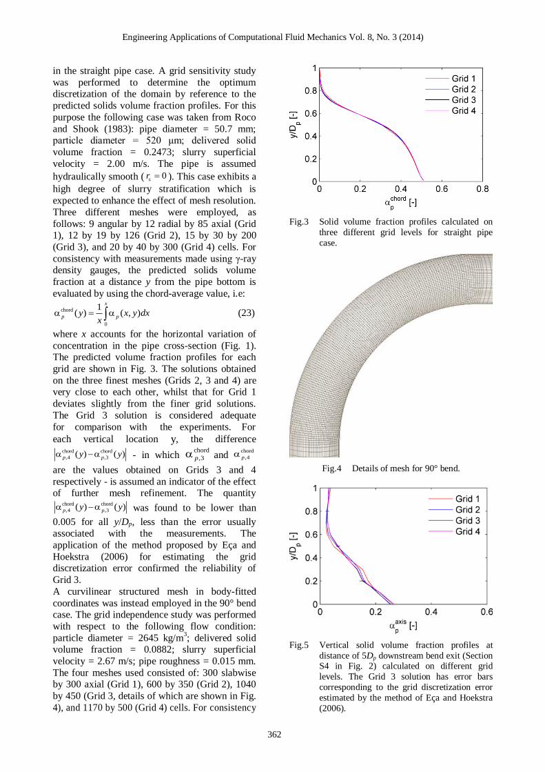
Engineering Applications of Computational Fluid Mechanics Vol 8 No 3 (2014)
362
in the straight pipe case A grid sensitivity study
was performed to determine the optimum discretization of the domain by reference to the
predicted solids volume fraction profiles For this
purpose the following case was taken from Roco
and Shook (1983) pipe diameter = 507 mm particle diameter = 520 μm delivered solid
volume fraction = 02473 slurry superficial
velocity = 200 ms The pipe is assumed
hydraulically smooth ( 0r ) This case exhibits a
high degree of slurry stratification which is
expected to enhance the effect of mesh resolution
Three different meshes were employed as
follows 9 angular by 12 radial by 85 axial (Grid 1) 12 by 19 by 126 (Grid 2) 15 by 30 by 200
(Grid 3) and 20 by 40 by 300 (Grid 4) cells For
consistency with measurements made using γ-ray density gauges the predicted solids volume
fraction at a distance y from the pipe bottom is
evaluated by using the chord-average value ie
chord
0
1( ) ( )
x
p py x y dxx
(23)
where x accounts for the horizontal variation of
concentration in the pipe cross-section (Fig 1) The predicted volume fraction profiles for each
grid are shown in Fig 3 The solutions obtained
on the three finest meshes (Grids 2 3 and 4) are very close to each other whilst that for Grid 1
deviates slightly from the finer grid solutions
The Grid 3 solution is considered adequate
for comparison with the experiments For
each vertical location y the difference chord chord
4 3( ) ( )p py y - in which chord
3p and chord
4p
are the values obtained on Grids 3 and 4
respectively - is assumed an indicator of the effect of further mesh refinement The quantity
chord chord
4 3( ) ( )p py y was found to be lower than
0005 for all yDp less than the error usually associated with the measurements The
application of the method proposed by Eccedila and
Hoekstra (2006) for estimating the grid discretization error confirmed the reliability of
Grid 3
A curvilinear structured mesh in body-fitted
coordinates was instead employed in the 90deg bend case The grid independence study was performed
with respect to the following flow condition
particle diameter = 2645 kgm3 delivered solid
volume fraction = 00882 slurry superficial
velocity = 267 ms pipe roughness = 0015 mm
The four meshes used consisted of 300 slabwise by 300 axial (Grid 1) 600 by 350 (Grid 2) 1040
by 450 (Grid 3 details of which are shown in Fig
4) and 1170 by 500 (Grid 4) cells For consistency
Fig3 Solid volume fraction profiles calculated on
three different grid levels for straight pipe
case
Fig4 Details of mesh for 90deg bend
Fig5 Vertical solid volume fraction profiles at
distance of 5Dp downstream bend exit (Section S4 in Fig 2) calculated on different grid
levels The Grid 3 solution has error bars
corresponding to the grid discretization error
estimated by the method of Eccedila and Hoekstra
(2006)
Engineering Applications of Computational Fluid Mechanics Vol 8 No 3 (2014)
363
with the sampling probe measurements of
Kaushal et al (2013) the predicted solids volume fraction at a distance y from the pipe bottom is
now evaluated by using the value along the
vertical diameter ie
axis ( ) 0p py y (24)
The predicted volume fraction profiles for each
grid at a distance of 5Dp downstream the bend exit (Section S4 in Fig 2) are shown in Fig 5
and indicate that Grid 3 is capable to procure a
consistent numerical solution the difference axis axis
4 3( ) ( )p py y being less than 0014 for all y
In Fig 5 the Grid 3 solution has error bars
corresponding to the grid discretization error estimated following the method of Eccedila and
Hoekstra (2006) Grid 3 was used in the
simulations
25 Governing terms and calibration of
numerical constants
In the two-fluid model different empirical sub-
models are employed for the inter-phase processes and closure of the various turbulence
correlations These submodels contain adjustable
coefficients which are in practice treated as calibration parameters their values being
determined by matching computations with
experiments The submodels which mainly affect
the solid volume fraction distribution refer to two main terms The former is the phase diffusion of
each conserved property ( 1 for mass
conservation) equal to k kD in which
the phase-diffusion coefficient D is given by Eq
(2) The phase diffusion besides making the
model numerically more stable and thereby
contributing to its speed in attaining convergence
has a smoothing effect on the solids concentration profile reducing its variation along the vertical
direction The impact of phase diffusion is
controlled by an empirical parameter which is the
turbulent Schmidt number for volume fractions
which appear in Eq (2) A sensitivity analysis to
quantify the influence of on the solid volume
fraction profile was performed
The results are depicted in Fig 6 for horizontal
pipe flows with very different flow conditions both taken from Roco and Shook (1983) A) pipe
diameter = 515 mm particle diameter = 165 μm
particle density = 2650 kgm3 delivered solid
volume fraction = 009 slurry superficial velocity = 378 ms B) pipe diameter = 507 mm particle
diameter = 520 μm particle density = 2650
kgm3 delivered solid volume fraction = 02473
slurry superficial velocity = 200 ms In both
cases the pipe is regarded is hydraulically
smooth It is observed that a reduction of
results in a flatter profile as a consequence of the
increase in diffusivity The latter term which most influences the solid
volume fraction profile is the interfacial
momentum transfer (Eq (6)) and particularly the drag force (Eq (7)) As already noticed the
definition of the particle Reynolds number with
respect to the viscosity of the mixture m instead
of that of the fluid phase C puts an upper limit
to the solids concentration due to the asymptotic
trend of m (Eq (11)) The mixture viscosity as
derived from the correlation of Mooney (Eq (11)) depends on two empirical parameters the
intrinsic viscosity and the maximum packing
concentration pm The effect of and pm on
Fig 6 Effect of turbulent Schmidt number for volume fractions on solid volume fraction profiles for two flow
conditions ( experiments from Roco and Shook (1983) ndashndashndash 03 ndashndashndash 05 ndashndashndash 07 ndashndashndash
09 )
Engineering Applications of Computational Fluid Mechanics Vol 8 No 3 (2014)
364
Fig 7 Effect of parameters [η] and pm in mixture viscosity correlation of Mooney (Eq 11) on solid volume fraction
profiles for two flow conditions ( experiments from Roco and Shook (1983) continuous lines predictions)
The dependence on [η] is studied for 07pm that on pm for [η] = 25
Table 1 Flow conditions considered for comparison
Reference System [mm]pD
[-]pr D [ ]pd m []C [ms]sV 3 [kgm ]p
Roco and Shook (1983) Pipe 507-515 - 165-520 90-296 190-433 2650
Gillies et al (2004) Pipe 1030 2∙10-5 90-280 106-407 133-540 2650
Matousek (2000 and 2002) Pipe 1500 - 120-370 250-430 204-600 -
Shaan et al (2000) Pipe 1585 6∙10-6 90 150-320 140-300 2655
Kaushal et al (2013) 90deg Bend 530 3∙10-4 450 882 267 2645
the solid volume fraction profile is analyzed one at a time in Fig 7 for the two above mentioned
flow conditions from Roco and Shook (1983) In
particular the results highlight that pm affects
the behaviour of the mixture only at high
concentration therefore as a direct effect on the prevention of particle over-packing As already
mentioned this avoids the need to introduce a
collisional pressure term in the momentum equation of the solid phase further promoting the
numerical stability of the model and the rapid
achievement of a converged solution Our investigations showed that a unique
combination of the three empirical parameters ndash
07 25 and 07pm (all within the
range of variability found in literature) ndash produced estimations of the solids concentration
profile in good agreement with the experimental
evidence for all the flow conditions considered in the present work referring to both the horizontal
pipe case and the 90deg bend case This feature
together with the numerical stability and the
relatively short computer time required contributes to make the model particularly useful
for the applications
3 RESULTS
The numerical model is validated by comparing
the results of the simulations against experimental
data reported by the authors listed in Table 1 This
Engineering Applications of Computational Fluid Mechanics Vol 8 No 3 (2014)
365
table provides the flow conditions for each set of
measurements As already mentioned two scenarios have been considered namely a straight
horizontal pipe and a 90deg bend which will be
discussed in separate sub-sections
31 Straight horizontal pipe
The predictions of the model have been compared with experimental data for 26 flow conditions
summarized in Table 2 which differ in terms of
pipe diameter pipe roughness particle size slurry superficial velocity and delivered solid volume
fraction Each set of measurements allows an
assessment of the models capability for
reproducing the influence of specific features affecting the distribution of the solid volume
fraction The data of Roco and Shook (1983) and
Gillies et al (2004) are used to investigate the effect of particle diameter and slurry velocity with
different delivered solid volume fraction The
measurements of Matousek (2000 2002) provide the opportunity to extend the validity of the model
up to a pipe Reynolds number Re (Eq (15)) of
about 106 Finally the data of Shaan et al (2000)
are used to assess the performance of the model in
case of natural sands with irregularly-shaped grains Almost all the data refer to configurations
in which all the solids are kept suspended but
moving bed flows have also been briefly explored
to check how far one can go in employing the model for the purpose of achieving useful
information from an engineering point of view
Measurements of solids concentration ndash either bulk-mean or local ndash are subjected to errors
depending mainly on the instrumentation used as
discussed in Section 1 All the data reported in Table 2 are obtained using gamma-ray absorption
methods perhaps the technique which provides
the highest accuracy attainable with errors of the
order of a few percentage points Since this technique allows measuring chord-average values
of solid volume fraction the computed volume
fraction profile was evaluated by means of Eq (23) In the experiments from Roco and Shook
(1983) ndash cases A1 to A5 in Table 2 ndash the
dispersed phase consists of three kinds of sand with narrow size distribution and mean particle
diameters of 165 and 520 μm The solids density
is 2650 kgm3 the pipe diameter is about 51 mm
Table 2 Details of experimental conditions for straight pipe case (A1 to A5 experimental data from Roco and Shook (1983) B1 to B12 experimental data from Gillies et al (2004) C1 to C6 experimental data from Matousek
(2000 and 2002) D1 to D4 experimental data from Shaan et al (2000) values not declared by
experimenters)
Test ID [mm]pD
[-]pr D [ ]pd m []C [ms]sV 3 [kgm ]p
Flow pattern
A1 515 0 165 9 378 2650 FS
A2 515 0 165 19 417 2650 FS
A3 515 0 165 28 433 2650 FS
A4 507 0 520 1212 190 2650 MB
A5 507 0 520 2473 200 2650 MB
B1 103 2∙10-5 90 198 133 2650 FS
B2 103 2∙10-5 90 283 133 2650 FS
B3 103 2∙10-5 90 19 300 2650 FS
B4 103 2∙10-5 90 284 300 2650 FS B5 103 2∙10-5 280 12 255 2650 FS
B6 103 2∙10-5 280 208 260 2650 FS
B7 103 2∙10-5 280 310 250 2650 FS
B8 103 2∙10-5 280 407 260 2650 FS
B9 103 2∙10-5 280 106 540 2650 FS
B10 103 2∙10-5 280 203 540 2650 FS
B11 103 2∙10-5 280 301 540 2650 FS
B12 103 2∙10-5 280 405 540 2650 FS
C1 150 0 120 25 204 2650 FS
C2 150 0 120 35 204 2650 -
C3 150 0 120 34 600 2650 -
C4 150 0 370 25 600 2650 FS
C5 150 0 370 34 600 2650 - C6 150 0 370 43 600 2650 MB
D1 1585 6∙10-6 90 15 15 2655 FS
D2 1585 6∙10-6 90 32 14 2655 FS
D3 1585 6∙10-6 90 15 30 2655 FS
D4 1585 6∙10-6 90 32 30 2655 FS
Engineering Applications of Computational Fluid Mechanics Vol 8 No 3 (2014)
366
the slurry bulk-mean velocity varies from 190 to
433 ms and the pipe Reynolds number from between 9610
4 and 2110
5 The delivered solid
volume fraction ranges from 9 to 30 The
authors did not indicate the roughness of the pipe
which was assumed hydraulically smooth No evaluation of measurement uncertainty was
reported by the experimenters and they did not
identify the flow patterns according to the more recent classification of Doron and Barnea (1996)
However for the smallest particle diameter the
data suggest suspended flow whereas for the largest diameter the indications are for moving-
bed flow Fig 8 compares the computed and
measured solid volume fraction profiles The good agreement between computation and
measurements reveals the ability of the model to
reproduce the effect of particle diameter on the
particle distribution for slurries with different delivered solid volume fraction The simple two-
fluid model proposed in this work appears
capable to predict with reasonable accuracy the solid volume fraction profile not only in case of
fully-suspended flow but also in case of moving
bed flows This indicates that the asymptotic trend of the interfacial momentum transfer term
Fig 8 Solids concentration profiles for flow conditions A1 to A5 in Table 2 ( experiments from Roco and
Shook (1983) ndashndashndash predictions)
Fig 9 Solids concentration profile for flow conditions B1 to B12 in Table 2 ( experiments from Gillies et al
(2004) ndashndashndash predictions)
Engineering Applications of Computational Fluid Mechanics Vol 8 No 3 (2014)
367
produces on the solid volume fraction profile the
same effect that is traditionally achieved by the
collisional pressure and the tensor kT
Gillies et al (2004) measured the concentration
profiles of sand-water slurries in a 103 mm
diameter pipe using gamma-ray absorption
gauges without reporting the uncertainty The roughness of the pipe is 2 nm Two kinds of sand
were considered with narrow size distribution
and mean particle diameter of 90 and 280 μm In both cases the particle density was 2650 kgm
3
and the slurry superficial velocity varies from
133 to 54 ms (corresponding to a pipe Reynolds
number between 14105 and 5610
5) The
delivered solid volume fraction varies from about
10 to about 45 Details of the flow conditions
considered for comparison are reported in Table 2 cases B1 to B12 From an examination of the
measured data for the pressure gradient it can be
inferred that in all cases the flow is fully-suspended This is a good test for the modelrsquos
ability to predict the combined effect of slurry
velocity solids loading and particle diameter in a
larger pipe Fig 9 shows comparison of the computational and the experimental results for the
vertical distribution of the solid volume fraction
The model produces good overall agreement with the data The largest deviations are observed near
the pipe wall for the small particles at high
concentration (cases B2 and B4 in Table 4) but as noted by the authors themselves these
measurements are subject to the largest
experimental error
Matousek (2000 and 2002) measured the concentration profiles of sand-water slurries in a
150 mm diameter pipe using gamma-ray
absorption method quantifying a 4 uncertainty of the data We reproduced numerically the flow
conditions reported in Table 2 (cases C1 to C6)
in which the dispersed phase consists of two kinds
of sand with narrow size distribution and mean particle diameters of 120 and 370 μm
Unfortunately neither the density of the solid
particles nor the pipe roughness are reported in the experiments of Matousek (2000 and 2002)
and so in the simulations the former was set to
2650 kgm3 which is the value declared by Roco
and Shook (1983) and Gillies et al (2004) and
the pipe was regarded as hydraulically smooth
The slurry superficial velocity was 2 or 6 ms
corresponding to a pipe Reynolds number up to 10
6 The delivered solid volume fraction ranged
between 25 and 43 According to the author
the flows are either fully suspended or with a moving bed but only for three cases the flow
pattern could be clearly identified from the plot of
pressure gradient versus slurry superficial
velocity Fig 10 compares the computed and measured solid volume fraction profiles each set
of experimental data has error bars indicating the
uncertainty declared by the experimenter The
rather good agreement between computations and measurements confirm the reliability of the model
for high pipe Reynolds numbers A closer
inspection reveals that for case C6 the computed concentration is lower than the experimental
results in the lower part of the pipe and higher in
the upper region However the pressure gradient curve clearly reveals that in case C6 a moving bed
of particles is formed It is again confirmed that
the proposed model is capable to procure a rough
indication of the distribution of the solid also for flows in which the inter-granular stresses play an
important role
Moreover in the case of highly dense slurries like case C6 the experimental data are subject to the
most uncertainty and the numerical solutions are
sensitive to the empirical parameters pm and
which appear in the mixture viscosity correlation
(Eq (11)) For the same case the measured solids concentration profile shows a drop near the pipe
bottom This reversal is not predicted by the
numerical model which is probably due to the absence of the wall lift force discussed earlier in
Section 21 The same limitation was reported by
Ekambara et al (2009) The paper of Shaan et al (2000) focuses on the
effect of particle shape upon pressure gradient and
deposition velocity but these workers also
reported some measurements of the solid volume fraction profiles Shaan et al (2000) quantified
the particle shape by reference to the following
quantities evaluated from photos of the particles the axes ratio ie the ratio between the major and
minor axes of an ellipse circumscribing the
grains the circularity index ie the ratio between
the area of the particle multiplied by 4π and its perimeter The sand particles have a very irregular
shape as can be inferred by comparing the
measured values of axes ratio (16) and circularity (062) against typical values reported in the
literature for sand grains The mass-median value
of the particle size distribution curve is taken as the characteristic particle diameter The flow
conditions reported in Table 2 (cases D1 to D4)
were reproduced to check the behaviour of the
model for the case of irregularly-shaped sand particles The pipe diameter (1585 mm)
delivered solid volume fraction (15 or 35)
slurry superficial velocity (14 or 3 ms) particle density (2655 Kgm
3) and particle diameter (90
μm) are all approximately within the range
Engineering Applications of Computational Fluid Mechanics Vol 8 No 3 (2014)
368
Fig 10 Solids concentration profiles for flow conditions C1 to C6 in Table 2 ( experiments from Matousek
(2000 and 2002) ndashndashndash predictions)
Fig 11 Solids concentration profiles for flow conditions D1 to D4 in Table 2 ( experiments from Shaan et al
(2000) ndashndashndash predictions)
covered by the earlier simulations The numerical and experimental results are
compared in Fig 11 The agreement between the
numerical predictions and the experimental
evidence is fairly good inadequacies of the numerical model ndash especially in the wall
boundary conditions for the solid phase ndash and
measurements error can both contribute to the discrepancies observed near the pipe bottom for
case D2 The results seem to indicate that the
numerical model is a suitable tool for predicting the solid volume fraction distribution produced by
sands with a very irregular shape
32 Horizontal 90deg bend
The predictions of the model have been compared
with the recent experiments of Kaushal et al (2013) regarding a horizontal 90deg bend Among
the different flow conditions considered by these
authors reference is made to those characterized
by delivered solid volume fraction of 882 within the range of interest in this work The
experimenters used a sampling probe to measure
the volume fraction profile of the slurry in the 53
mm diameter pipe along the vertical axis at distances of 5Dp 25Dp and 50Dp downstream the
bend exit (referred to as sections S4 S5 and S6 in
Fig 2 respectively) They quantified a 2
uncertainty of the data The solid phase consists of silica sand particles with narrow size
distribution and mean particle diameter of 450
μm The slurry superficial velocity is 178 267 or 356 ms
The flow within the bend is much more complex
compared to that through the straight pipe since secondary motions develop in the crosswise
direction These motions affect significantly the
distribution of the solids and as a consequence
the volume fraction distribution is no longer constant over horizontal planes This is evident in
Fig 12 which shows the color plot of the solids
volumetric concentration over the six cross sections highlighted in Fig 2 As shown in Fig
13 the predictions of our model generally agree
with the experimental data available Greater
discrepancies are observed for the highest superficial velocity (356 ms) where the model
seems to underestimate the quantity of particles
dragged by the secondary motions This is
Engineering Applications of Computational Fluid Mechanics Vol 8 No 3 (2014)
369
Fig 12 Solid volume fraction distributions on sections
S1 to S6 in Fig 2 for delivered solid volume
fraction of 882 Left hand side is the outer
wall of the pipe
opposite to the KTGF based model of Kaushal et
al (2013) which tends to over-enhance the effect
of the secondary motions on the solids for the
lowest velocities Fig 13 also reveals that our model tends to overestimate the solids volume
fraction close to the pipe bottom far from the
bend exit It is expected that the predictions could
be improved if the effect of the wall lubrication force for which a suitable model does not exist at
present were accounted for
4 CONCLUSIONS
A mathematical model has been described for the
estimation of solid volume fraction distribution of
solid-liquid slurry flows in horizontal pipes and bends The model is based on an Eulerian-
Eulerian approach and uses the Inter-Phase Slip
Algorithm (IPSA) of Spalding (1980) The
novelty of this model resides in the combined use of existing modelling strategies never previously
employed simultaneously for the predictions of
slurry flows In order to account for turbulent dispersion of particles phase diffusion terms have
been included in the phase continuity equations
together with all the conservation equations The mixture viscosity approach is adopted to model
the effect of multiple particles on the inter-phase
friction A wall function is employed to model the
flow in the near-wall region in case of both hydraulically smooth and rough walls All these
strategies result in a model which despite being
simpler that those commonly used for addressing solid-liquid slurry flows shows comparable or
even better predictive capacity Moreover this
model is robust and numerically stable and
requires relatively short CPU time to procure converged steady-state solutions
The model has been first validated by comparison
with experimental data for the horizontal pipe case over a wide range of operating conditions
delivered solid volume fraction between 10 and
40 by volume mean particle diameter between 90 and 520 μm slurry superficial velocity
between 1 ms and 55 ms and pipe diameter
between 50 and 158 mm The model predictions
were found to be in good agreement with the experimental evidence for all the flow conditions
considered for comparison Even if the model is
originally intended to address fully-suspended flows the results indicated its capability to
provide rough indications of the solid volume
fraction distribution also in case of bed flows At last the comparison with the recent
measurements of Kaushal et al (2013) revealed
that this model is capable to procure reliable
predictions of the particle distribution downstream a 90deg bend in a horizontal pipe
Engineering Applications of Computational Fluid Mechanics Vol 8 No 3 (2014)
370
Fig 13 Solid volume fraction along vertical diameter on sections S4 to S6 in Fig 2 for delivered solid volume fraction
of 882 ( experiments from Kaushal et al (2013) ndashndashndash predictions)
ACKNOWLEDGEMENTS The authors would acknowledge the CINECA and
the Regione Lombardia award under the LISA
initiative for the availability of high performance computing resources and support The authors
would like to thank CHAM Ltd for supporting
this research and acknowledge Dr Randy Gillies of Saskatchewan Research Council for providing
his experimental data
REFERENCES
1 Ahilan RV Sleath J (1987) Sediment
transport in oscillatory flow over flat beds Journal of Hydraulic Engineering 113 308-
322
2 Albunaga BE (2002) Slurry Systems Handbook McGraw-Hill
3 Antal S Lahey R Flaherty J (1991) Analysis
of phase distribution in fully-developed
laminar bubbly two phase flow International Journal of Multiphase Flow 17(5) 635-652
4 Barnea E Mizrahi J (1973) A Generalized
Approach to the Fluid Dynamics of
Particulate Systems Chemical Engineering
Science 5(2) 171-189 5 Chen L Duan Y Pu W Zhao C (2009) CFD
simulation of coal-water slurry flowing in
horizontal pipelines Korean Journal of Chemical Engineering 26(4) 1144-1154
6 Chen RC (1994) Analysis of homogeneous
slurry pipe flow Journal of Marine Science and Technology 2(1) 37-45
7 Chen X Li Y Niu X Li M Chen D Yu X
(2011) A general two-phase turbulent flow
model applied to the study of sediment transport in open channels International
Journal of Multiphase Flow 37(9) 1099-
1108 8 Chung JN Troutt TR (1988) Simulation of
particle dispersion in an axisymmetric jet
Journal of Fluid Mechanics 186 199-222 9 Clift R Grace JR Weber ME (1978)
Bubbles Drops and Particles Academic
Press
10 Colwell JM Shook CA (1988) The Entry Length for Slurries in Horizontal Pipeline
Flow Canadian Journal of Chemical
Engineering 66(5) 714-720
Engineering Applications of Computational Fluid Mechanics Vol 8 No 3 (2014)
371
11 Doron P Barnea D (1993) A three layer
model for solid-liquid flow in horizontal pipes International Journal of Multiphase
Flow 19(6) 1029-1043
12 Doron P Barnea D (1995) Pressure drop and
limit deposit velocity for solid-liquid flow in pipes Chemical Engineering and Science
50(10) 1595-1604
13 Doron P Barnea D (1996) Flow pattern maps for solid-liquid flow in pipes International
Journal of Multiphase Flow 22(2) 273-283
14 Doron P Granica D Barnea D (1987) Slurry flow in horizontal pipes ndash experimental and
modeling International Journal of
Multiphase Flow 13(4) 535ndash547
15 Eccedila L Hoekstra M (2006) Discretization uncertainty estimation based on a least
squares version of the grid convergence
index Proceedings of the 2nd
Workshop on CFD Uncertainty Analysis Oct 19-20
Lisbon Portugal
16 Ekambara K Sanders RS Nandakumar K Masliyah JH (2009) Hydrodynamic
simulation of horizontal slurry pipeline flow
using ANSYS-CFX Industrial amp
Engineering Chemistry Research 48(17) 8159-8171
17 Gillies RG Shook CA (2000) Modelling
High Concentration Settling Slurry Flows Canadian Journal of Chemical Engineering
78(4) 709-716
18 Gillies RG Shook CA Xu J (2004)
Modelling Heterogeneous Slurry Flow at High Velocities Canadian Journal of
Chemical Engineering 82(5) 1060-1065
19 Hsu FLG (1981) Flow of Fine-particle Suspensions in Bends Fittings and Valves
MS Thesis Texas Tech University Lubbock
Texas USA 20 Ishii M Mishima K (1984) Two-fluid model
and hydrodynamic constitutive relations
Nuclear Engineering and Design 82(2-3)
107-126 21 Issa RI Oliveira PJ (1997) Assessment of a
particle-turbulence interaction model in
conjunction with an Eulerian two-phase flow formulation Proceedings of the 2
nd
International Symposium on Turbulence
Heat and Mass Transfer June 9-12 Delft Netherlands 759-770
22 Jayatillika CLV (1969) The influence of the
Prandtl number and surface roughness on the
resistance of the sublayer to momentum and heat transfer Progress in Heat amp Mass
Transfer 1 193-329
23 Jiang YY Zhang P (2012) Pressure drop and
flow pattern of slush nitrogen in a horizontal pipe AIChE Journal doi 10002aic13927
24 Kaushal DR Kumar A Tomita Y Juchii S
Tsukamoto H (2013) Flow of mono-
dispersed particles through horizontal bend International Journal of Multiphase Flow 52
71-91
25 Kaushal DR Sato K Toyota T Funatsu K Tomita Y (2005) Effect of particle size
distribution on pressure drop and
concentration profile in pipeline flow of highly concentrated slurry International
Journal of Multiphase Flow 31(7) 809-823
26 Kaushal DR Thinglas T Tomita Y Juchii S
Tsukamoto H (2012) CFD modeling for pipeline flow of fine particles at high
concentration International Journal of
Multiphase Flow 43 85-100 27 Kaushal DR Tomita Y (2003) Comparative
study of pressure drop in multisized
particulate slurry flow through pipe and rectangular duct International Journal of
Multiphase Flow 29(9) 1473-1487
28 Kaushal DR Tomita Y (2007) Experimental
investigation for near-wall lift of coarser particles in slurry pipeline using γ-ray
densitometer Powder Technology 172(3)
177-187 29 Kim C Lee M Han C (2008) Hydraulic
transport of sand-water mixtures in pipelines
Part I Experiment Journal of Mechanical
Science and Technology 22(12) 2534-2541 30 Kumar U Mishra R Singh SN Seshadri V
(2003) Effect of particle gradation on flow
characteristics of ash disposal pipelines Powder Technology 132(1) 39-51
31 Lahiri SK Ghanta KC (2010) Slurry flow
modeling by CFD Chemical Industry amp Chemical Engineering Quarterly 16(4) 295-
308
32 Launder BE Spalding DB (1972)
Mathematical models of turbulence Academic Press
33 Ling J Skudarnov PV Lin CX Ebadian MA
(2003) Numerical investigations of solid-liquid slurry flows in a fully developed flow
region International Journal of Heat and
Fluid Flow 24(3) 389-398 34 Matousek V (2000) Concentration
distribution in pipeline flow of sand-water
mixtures Journal of Hydrology and
Hydromechanics 48(3) 180-196 35 Matousek V (2002) Pressure drops and flow
patterns in sand-mixture pipes Experimental
Engineering Applications of Computational Fluid Mechanics Vol 8 No 3 (2014)
372
Thermal and Fluid Science 26(6-7) 693-702
36 Matousek V (2009) Predictive model for frictional pressure drop in settling-slurry pipe
with stationary deposit Powder Technology
192(3) 367-374
37 Mooney M (1951) The viscosity of a concentrated suspension of spherical
particles Journal of Colloid Science 6(2)
162-170 38 Nasr-el-Din H Shook CA Esmail MN
(1984) Isokinetic Probe Sampling From
Slurry Pipelines Canadian Journal of Chemical Engineering 62(2) 179-185
39 Pathak M (2011) Computational
investigations of solid-liquid particle
interaction in a two-phase flow around a ducted obstruction Journal of Hydraulic
Research 49(1) 96-104
40 Pecker SM Helvaci SS (2008) Solid-Liquid Two-Phase Flow Elsevier
41 Roco MC Shook CA (1983) Modeling of
Slurry Flow The Effect of Particle Size Canadian Journal of Chemical Engineering
61(4) 494-503
42 Schlichting H (1960) Boundary Layer
Theory McGraw-Hill 43 Shaan J Sumner RJ Gillies RG Shook CA
(2000) The Effect of Particle Shape on
Pipeline Friction for Newtonian Slurries of Fine Particles Canadian Journal of Chemical
Engineering 78(4) 717-725
44 Shiller L Naumann A (1935) A drag
coefficient correlation Zeitschrift des Vereines Deutscher Ingenieure 77 318-320
45 Shirolkar JS Coimbra CFM McQuay MQ
(1996) Fundamental aspects of modelling turbulent particle dispersion in dilute flows
Progress in Energy and Combustion Science
22(4) 363-399 46 Shook CA Bartosik AS (1994) Particle-wall
stresses in vertical slurry flows Powder
Technology 81(2) 117-124
47 Skudarnov PV Lin CX Ebadian MA (2004) Double-Species Slurry Flow in a Horizontal
Pipeline ASME Journal of Fluids
Engineering 126(1) 125-132 48 Spalding DB (1972) A novel finite-
difference formulation for differential
expressions involving both first and second derivatives International Journal of
Numerical Methods in Engineering 4(4) 551-
559
49 Spalding DB (1980) Numerical computation of multi-phase fluid flow and heat transfer In
Taylor C Morgan K (Eds) Recent Advances
in Numerical Methods in Fluids Pineridge
Press Limited 139-168 50 Turian RM Ma TW Hsu FLG Sung MDJ
Plackmann GW (1998) Flow of concentrated
non-Newtonian slurries 2 Friction losses in
bends fittings valves and Venturi meters International Journal of Multiphase Flow
24(2) 243-269
51 Versteeg HK Malalasekera W (2007) An Introduction to Computational Fluid
Dynamics The Finite Volume Method
Pearson Prentice Hall 52 Wilson KC Sanders RS Gillies RG Shook
CA (2010) Verification of the near-wall
model for slurry flow Powder Technology
197(3) 247-253 53 Wilson KC Sellgren A (2003) Interaction of
Particles and Near-Wall Lift in Slurry
Pipelines Journal of Hydraulic Engineering 129(1) 73-76
- Figures13
-
- Fig 1 Computational domain and boundaryconditions for horizontal pipe
- Fig 2 Computational domain boundary conditionsand reference sections for 90deg bend (S1=bendinlet S2=bend centre S3=bend exit S4=5Dpfrom bend exit S5=25Dp from bend exitS6=50Dp from bend exit)
- Fig3 Solid volume fraction profiles calculated onthree different grid levels for straight pipecase
- Fig4 Details of mesh for 90deg bend
- Fig5 Vertical solid volume fraction profiles atdistance of 5Dp downstream bend exit (SectionS4 in Fig 2) calculated on different gridlevels The Grid 3 solution has error barscorresponding to the grid discretization errorestimated by the method of Eccedila and Hoekstra(2006)
- Fig 6 Effect of turbulent Schmidt number for volume fractions a s on solid volume fraction profiles for two flowconditions (r experiments from Roco and Shook (1983) ndashndashndash 03 a s = ndashndashndash 05 a s = ndashndashndash 07 a s = ndashndashndash09 a s = )
- Fig 7 Effect of parameters [η] and pm a in mixture viscosity correlation of Mooney (Eq 11) on solid volume fractionprofiles for two flow conditions (r experiments from Roco and Shook (1983) continuous lines predictions)The dependence on [η] is studied for 07 pm a = that on pm a for [η] = 25
- Fig 8 Solids concentration profiles for flow conditions A1 to A5 in Table 2 (rbull experiments from Roco and Shook (1983) ndashndashndash predictions)
- Fig 9 Solids concentration profile for flow conditions B1 to B12 in Table 2 (rbulls experiments from Gillies et al (2004) ndashndashndash predictions)
- Fig 10 Solids concentration profiles for flow conditions C1 to C6 in Table 2 (rbull experiments from Matousek (2000 and 2002) ndashndashndash predictions)
- Fig 11 Solids concentration profiles for flow conditions D1 to D4 in Table 2 (rbull experiments from Shaan et al (2000) ndashndashndash predictions)
- Fig 12 Solid volume fraction distributions on sections S1 to S6 in Fig 2 for delivered solid volume fraction of 882 Left hand side is the outer wall of the pipe
- Fig 13 Solid volume fraction along vertical diameter on sections S4 to S6 in Fig 2 for delivered solid volume fraction of 882 (r experiments from Kaushal et al (2013) ndashndashndash predictions)
-
- Tables13
-
- Table 1 Flow conditions considered for comparison
- Table 2 Details of experimental conditions for straight pipe case (A1 to A5 experimental data from Roco and Shook(1983) B1 to B12 experimental data from Gillies et al (2004) C1 to C6 experimental data from Matousek(2000 and 2002) D1 to D4 experimental data from Shaan et al (2000) values not declared byexperimenters)
-
- 1 INTRODUCTION
- 2 MATHEMATICAL MODEL
-
- 21 Conservation equations
- 22 Turbulence modeling
- 23 Computational domain and boundaryconditions
- 24 Computational methodology and consistencyof numerical solution
- 25 Governing terms and calibration ofnumerical constants
-
- 3 RESULTS
-
- 31 Straight horizontal pipe
- 32 Horizontal 90deg bend
-
- 4 CONCLUSIONS
- ACKNOWLEDGEMENTS
- REFERENCES
-
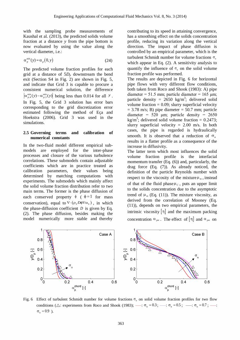
Engineering Applications of Computational Fluid Mechanics Vol 8 No 3 (2014)
363
with the sampling probe measurements of
Kaushal et al (2013) the predicted solids volume fraction at a distance y from the pipe bottom is
now evaluated by using the value along the
vertical diameter ie
axis ( ) 0p py y (24)
The predicted volume fraction profiles for each
grid at a distance of 5Dp downstream the bend exit (Section S4 in Fig 2) are shown in Fig 5
and indicate that Grid 3 is capable to procure a
consistent numerical solution the difference axis axis
4 3( ) ( )p py y being less than 0014 for all y
In Fig 5 the Grid 3 solution has error bars
corresponding to the grid discretization error estimated following the method of Eccedila and
Hoekstra (2006) Grid 3 was used in the
simulations
25 Governing terms and calibration of
numerical constants
In the two-fluid model different empirical sub-
models are employed for the inter-phase processes and closure of the various turbulence
correlations These submodels contain adjustable
coefficients which are in practice treated as calibration parameters their values being
determined by matching computations with
experiments The submodels which mainly affect
the solid volume fraction distribution refer to two main terms The former is the phase diffusion of
each conserved property ( 1 for mass
conservation) equal to k kD in which
the phase-diffusion coefficient D is given by Eq
(2) The phase diffusion besides making the
model numerically more stable and thereby
contributing to its speed in attaining convergence
has a smoothing effect on the solids concentration profile reducing its variation along the vertical
direction The impact of phase diffusion is
controlled by an empirical parameter which is the
turbulent Schmidt number for volume fractions
which appear in Eq (2) A sensitivity analysis to
quantify the influence of on the solid volume
fraction profile was performed
The results are depicted in Fig 6 for horizontal
pipe flows with very different flow conditions both taken from Roco and Shook (1983) A) pipe
diameter = 515 mm particle diameter = 165 μm
particle density = 2650 kgm3 delivered solid
volume fraction = 009 slurry superficial velocity = 378 ms B) pipe diameter = 507 mm particle
diameter = 520 μm particle density = 2650
kgm3 delivered solid volume fraction = 02473
slurry superficial velocity = 200 ms In both
cases the pipe is regarded is hydraulically
smooth It is observed that a reduction of
results in a flatter profile as a consequence of the
increase in diffusivity The latter term which most influences the solid
volume fraction profile is the interfacial
momentum transfer (Eq (6)) and particularly the drag force (Eq (7)) As already noticed the
definition of the particle Reynolds number with
respect to the viscosity of the mixture m instead
of that of the fluid phase C puts an upper limit
to the solids concentration due to the asymptotic
trend of m (Eq (11)) The mixture viscosity as
derived from the correlation of Mooney (Eq (11)) depends on two empirical parameters the
intrinsic viscosity and the maximum packing
concentration pm The effect of and pm on
Fig 6 Effect of turbulent Schmidt number for volume fractions on solid volume fraction profiles for two flow
conditions ( experiments from Roco and Shook (1983) ndashndashndash 03 ndashndashndash 05 ndashndashndash 07 ndashndashndash
09 )
Engineering Applications of Computational Fluid Mechanics Vol 8 No 3 (2014)
364
Fig 7 Effect of parameters [η] and pm in mixture viscosity correlation of Mooney (Eq 11) on solid volume fraction
profiles for two flow conditions ( experiments from Roco and Shook (1983) continuous lines predictions)
The dependence on [η] is studied for 07pm that on pm for [η] = 25
Table 1 Flow conditions considered for comparison
Reference System [mm]pD
[-]pr D [ ]pd m []C [ms]sV 3 [kgm ]p
Roco and Shook (1983) Pipe 507-515 - 165-520 90-296 190-433 2650
Gillies et al (2004) Pipe 1030 2∙10-5 90-280 106-407 133-540 2650
Matousek (2000 and 2002) Pipe 1500 - 120-370 250-430 204-600 -
Shaan et al (2000) Pipe 1585 6∙10-6 90 150-320 140-300 2655
Kaushal et al (2013) 90deg Bend 530 3∙10-4 450 882 267 2645
the solid volume fraction profile is analyzed one at a time in Fig 7 for the two above mentioned
flow conditions from Roco and Shook (1983) In
particular the results highlight that pm affects
the behaviour of the mixture only at high
concentration therefore as a direct effect on the prevention of particle over-packing As already
mentioned this avoids the need to introduce a
collisional pressure term in the momentum equation of the solid phase further promoting the
numerical stability of the model and the rapid
achievement of a converged solution Our investigations showed that a unique
combination of the three empirical parameters ndash
07 25 and 07pm (all within the
range of variability found in literature) ndash produced estimations of the solids concentration
profile in good agreement with the experimental
evidence for all the flow conditions considered in the present work referring to both the horizontal
pipe case and the 90deg bend case This feature
together with the numerical stability and the
relatively short computer time required contributes to make the model particularly useful
for the applications
3 RESULTS
The numerical model is validated by comparing
the results of the simulations against experimental
data reported by the authors listed in Table 1 This
Engineering Applications of Computational Fluid Mechanics Vol 8 No 3 (2014)
365
table provides the flow conditions for each set of
measurements As already mentioned two scenarios have been considered namely a straight
horizontal pipe and a 90deg bend which will be
discussed in separate sub-sections
31 Straight horizontal pipe
The predictions of the model have been compared with experimental data for 26 flow conditions
summarized in Table 2 which differ in terms of
pipe diameter pipe roughness particle size slurry superficial velocity and delivered solid volume
fraction Each set of measurements allows an
assessment of the models capability for
reproducing the influence of specific features affecting the distribution of the solid volume
fraction The data of Roco and Shook (1983) and
Gillies et al (2004) are used to investigate the effect of particle diameter and slurry velocity with
different delivered solid volume fraction The
measurements of Matousek (2000 2002) provide the opportunity to extend the validity of the model
up to a pipe Reynolds number Re (Eq (15)) of
about 106 Finally the data of Shaan et al (2000)
are used to assess the performance of the model in
case of natural sands with irregularly-shaped grains Almost all the data refer to configurations
in which all the solids are kept suspended but
moving bed flows have also been briefly explored
to check how far one can go in employing the model for the purpose of achieving useful
information from an engineering point of view
Measurements of solids concentration ndash either bulk-mean or local ndash are subjected to errors
depending mainly on the instrumentation used as
discussed in Section 1 All the data reported in Table 2 are obtained using gamma-ray absorption
methods perhaps the technique which provides
the highest accuracy attainable with errors of the
order of a few percentage points Since this technique allows measuring chord-average values
of solid volume fraction the computed volume
fraction profile was evaluated by means of Eq (23) In the experiments from Roco and Shook
(1983) ndash cases A1 to A5 in Table 2 ndash the
dispersed phase consists of three kinds of sand with narrow size distribution and mean particle
diameters of 165 and 520 μm The solids density
is 2650 kgm3 the pipe diameter is about 51 mm
Table 2 Details of experimental conditions for straight pipe case (A1 to A5 experimental data from Roco and Shook (1983) B1 to B12 experimental data from Gillies et al (2004) C1 to C6 experimental data from Matousek
(2000 and 2002) D1 to D4 experimental data from Shaan et al (2000) values not declared by
experimenters)
Test ID [mm]pD
[-]pr D [ ]pd m []C [ms]sV 3 [kgm ]p
Flow pattern
A1 515 0 165 9 378 2650 FS
A2 515 0 165 19 417 2650 FS
A3 515 0 165 28 433 2650 FS
A4 507 0 520 1212 190 2650 MB
A5 507 0 520 2473 200 2650 MB
B1 103 2∙10-5 90 198 133 2650 FS
B2 103 2∙10-5 90 283 133 2650 FS
B3 103 2∙10-5 90 19 300 2650 FS
B4 103 2∙10-5 90 284 300 2650 FS B5 103 2∙10-5 280 12 255 2650 FS
B6 103 2∙10-5 280 208 260 2650 FS
B7 103 2∙10-5 280 310 250 2650 FS
B8 103 2∙10-5 280 407 260 2650 FS
B9 103 2∙10-5 280 106 540 2650 FS
B10 103 2∙10-5 280 203 540 2650 FS
B11 103 2∙10-5 280 301 540 2650 FS
B12 103 2∙10-5 280 405 540 2650 FS
C1 150 0 120 25 204 2650 FS
C2 150 0 120 35 204 2650 -
C3 150 0 120 34 600 2650 -
C4 150 0 370 25 600 2650 FS
C5 150 0 370 34 600 2650 - C6 150 0 370 43 600 2650 MB
D1 1585 6∙10-6 90 15 15 2655 FS
D2 1585 6∙10-6 90 32 14 2655 FS
D3 1585 6∙10-6 90 15 30 2655 FS
D4 1585 6∙10-6 90 32 30 2655 FS
Engineering Applications of Computational Fluid Mechanics Vol 8 No 3 (2014)
366
the slurry bulk-mean velocity varies from 190 to
433 ms and the pipe Reynolds number from between 9610
4 and 2110
5 The delivered solid
volume fraction ranges from 9 to 30 The
authors did not indicate the roughness of the pipe
which was assumed hydraulically smooth No evaluation of measurement uncertainty was
reported by the experimenters and they did not
identify the flow patterns according to the more recent classification of Doron and Barnea (1996)
However for the smallest particle diameter the
data suggest suspended flow whereas for the largest diameter the indications are for moving-
bed flow Fig 8 compares the computed and
measured solid volume fraction profiles The good agreement between computation and
measurements reveals the ability of the model to
reproduce the effect of particle diameter on the
particle distribution for slurries with different delivered solid volume fraction The simple two-
fluid model proposed in this work appears
capable to predict with reasonable accuracy the solid volume fraction profile not only in case of
fully-suspended flow but also in case of moving
bed flows This indicates that the asymptotic trend of the interfacial momentum transfer term
Fig 8 Solids concentration profiles for flow conditions A1 to A5 in Table 2 ( experiments from Roco and
Shook (1983) ndashndashndash predictions)
Fig 9 Solids concentration profile for flow conditions B1 to B12 in Table 2 ( experiments from Gillies et al
(2004) ndashndashndash predictions)
Engineering Applications of Computational Fluid Mechanics Vol 8 No 3 (2014)
367
produces on the solid volume fraction profile the
same effect that is traditionally achieved by the
collisional pressure and the tensor kT
Gillies et al (2004) measured the concentration
profiles of sand-water slurries in a 103 mm
diameter pipe using gamma-ray absorption
gauges without reporting the uncertainty The roughness of the pipe is 2 nm Two kinds of sand
were considered with narrow size distribution
and mean particle diameter of 90 and 280 μm In both cases the particle density was 2650 kgm
3
and the slurry superficial velocity varies from
133 to 54 ms (corresponding to a pipe Reynolds
number between 14105 and 5610
5) The
delivered solid volume fraction varies from about
10 to about 45 Details of the flow conditions
considered for comparison are reported in Table 2 cases B1 to B12 From an examination of the
measured data for the pressure gradient it can be
inferred that in all cases the flow is fully-suspended This is a good test for the modelrsquos
ability to predict the combined effect of slurry
velocity solids loading and particle diameter in a
larger pipe Fig 9 shows comparison of the computational and the experimental results for the
vertical distribution of the solid volume fraction
The model produces good overall agreement with the data The largest deviations are observed near
the pipe wall for the small particles at high
concentration (cases B2 and B4 in Table 4) but as noted by the authors themselves these
measurements are subject to the largest
experimental error
Matousek (2000 and 2002) measured the concentration profiles of sand-water slurries in a
150 mm diameter pipe using gamma-ray
absorption method quantifying a 4 uncertainty of the data We reproduced numerically the flow
conditions reported in Table 2 (cases C1 to C6)
in which the dispersed phase consists of two kinds
of sand with narrow size distribution and mean particle diameters of 120 and 370 μm
Unfortunately neither the density of the solid
particles nor the pipe roughness are reported in the experiments of Matousek (2000 and 2002)
and so in the simulations the former was set to
2650 kgm3 which is the value declared by Roco
and Shook (1983) and Gillies et al (2004) and
the pipe was regarded as hydraulically smooth
The slurry superficial velocity was 2 or 6 ms
corresponding to a pipe Reynolds number up to 10
6 The delivered solid volume fraction ranged
between 25 and 43 According to the author
the flows are either fully suspended or with a moving bed but only for three cases the flow
pattern could be clearly identified from the plot of
pressure gradient versus slurry superficial
velocity Fig 10 compares the computed and measured solid volume fraction profiles each set
of experimental data has error bars indicating the
uncertainty declared by the experimenter The
rather good agreement between computations and measurements confirm the reliability of the model
for high pipe Reynolds numbers A closer
inspection reveals that for case C6 the computed concentration is lower than the experimental
results in the lower part of the pipe and higher in
the upper region However the pressure gradient curve clearly reveals that in case C6 a moving bed
of particles is formed It is again confirmed that
the proposed model is capable to procure a rough
indication of the distribution of the solid also for flows in which the inter-granular stresses play an
important role
Moreover in the case of highly dense slurries like case C6 the experimental data are subject to the
most uncertainty and the numerical solutions are
sensitive to the empirical parameters pm and
which appear in the mixture viscosity correlation
(Eq (11)) For the same case the measured solids concentration profile shows a drop near the pipe
bottom This reversal is not predicted by the
numerical model which is probably due to the absence of the wall lift force discussed earlier in
Section 21 The same limitation was reported by
Ekambara et al (2009) The paper of Shaan et al (2000) focuses on the
effect of particle shape upon pressure gradient and
deposition velocity but these workers also
reported some measurements of the solid volume fraction profiles Shaan et al (2000) quantified
the particle shape by reference to the following
quantities evaluated from photos of the particles the axes ratio ie the ratio between the major and
minor axes of an ellipse circumscribing the
grains the circularity index ie the ratio between
the area of the particle multiplied by 4π and its perimeter The sand particles have a very irregular
shape as can be inferred by comparing the
measured values of axes ratio (16) and circularity (062) against typical values reported in the
literature for sand grains The mass-median value
of the particle size distribution curve is taken as the characteristic particle diameter The flow
conditions reported in Table 2 (cases D1 to D4)
were reproduced to check the behaviour of the
model for the case of irregularly-shaped sand particles The pipe diameter (1585 mm)
delivered solid volume fraction (15 or 35)
slurry superficial velocity (14 or 3 ms) particle density (2655 Kgm
3) and particle diameter (90
μm) are all approximately within the range
Engineering Applications of Computational Fluid Mechanics Vol 8 No 3 (2014)
368
Fig 10 Solids concentration profiles for flow conditions C1 to C6 in Table 2 ( experiments from Matousek
(2000 and 2002) ndashndashndash predictions)
Fig 11 Solids concentration profiles for flow conditions D1 to D4 in Table 2 ( experiments from Shaan et al
(2000) ndashndashndash predictions)
covered by the earlier simulations The numerical and experimental results are
compared in Fig 11 The agreement between the
numerical predictions and the experimental
evidence is fairly good inadequacies of the numerical model ndash especially in the wall
boundary conditions for the solid phase ndash and
measurements error can both contribute to the discrepancies observed near the pipe bottom for
case D2 The results seem to indicate that the
numerical model is a suitable tool for predicting the solid volume fraction distribution produced by
sands with a very irregular shape
32 Horizontal 90deg bend
The predictions of the model have been compared
with the recent experiments of Kaushal et al (2013) regarding a horizontal 90deg bend Among
the different flow conditions considered by these
authors reference is made to those characterized
by delivered solid volume fraction of 882 within the range of interest in this work The
experimenters used a sampling probe to measure
the volume fraction profile of the slurry in the 53
mm diameter pipe along the vertical axis at distances of 5Dp 25Dp and 50Dp downstream the
bend exit (referred to as sections S4 S5 and S6 in
Fig 2 respectively) They quantified a 2
uncertainty of the data The solid phase consists of silica sand particles with narrow size
distribution and mean particle diameter of 450
μm The slurry superficial velocity is 178 267 or 356 ms
The flow within the bend is much more complex
compared to that through the straight pipe since secondary motions develop in the crosswise
direction These motions affect significantly the
distribution of the solids and as a consequence
the volume fraction distribution is no longer constant over horizontal planes This is evident in
Fig 12 which shows the color plot of the solids
volumetric concentration over the six cross sections highlighted in Fig 2 As shown in Fig
13 the predictions of our model generally agree
with the experimental data available Greater
discrepancies are observed for the highest superficial velocity (356 ms) where the model
seems to underestimate the quantity of particles
dragged by the secondary motions This is
Engineering Applications of Computational Fluid Mechanics Vol 8 No 3 (2014)
369
Fig 12 Solid volume fraction distributions on sections
S1 to S6 in Fig 2 for delivered solid volume
fraction of 882 Left hand side is the outer
wall of the pipe
opposite to the KTGF based model of Kaushal et
al (2013) which tends to over-enhance the effect
of the secondary motions on the solids for the
lowest velocities Fig 13 also reveals that our model tends to overestimate the solids volume
fraction close to the pipe bottom far from the
bend exit It is expected that the predictions could
be improved if the effect of the wall lubrication force for which a suitable model does not exist at
present were accounted for
4 CONCLUSIONS
A mathematical model has been described for the
estimation of solid volume fraction distribution of
solid-liquid slurry flows in horizontal pipes and bends The model is based on an Eulerian-
Eulerian approach and uses the Inter-Phase Slip
Algorithm (IPSA) of Spalding (1980) The
novelty of this model resides in the combined use of existing modelling strategies never previously
employed simultaneously for the predictions of
slurry flows In order to account for turbulent dispersion of particles phase diffusion terms have
been included in the phase continuity equations
together with all the conservation equations The mixture viscosity approach is adopted to model
the effect of multiple particles on the inter-phase
friction A wall function is employed to model the
flow in the near-wall region in case of both hydraulically smooth and rough walls All these
strategies result in a model which despite being
simpler that those commonly used for addressing solid-liquid slurry flows shows comparable or
even better predictive capacity Moreover this
model is robust and numerically stable and
requires relatively short CPU time to procure converged steady-state solutions
The model has been first validated by comparison
with experimental data for the horizontal pipe case over a wide range of operating conditions
delivered solid volume fraction between 10 and
40 by volume mean particle diameter between 90 and 520 μm slurry superficial velocity
between 1 ms and 55 ms and pipe diameter
between 50 and 158 mm The model predictions
were found to be in good agreement with the experimental evidence for all the flow conditions
considered for comparison Even if the model is
originally intended to address fully-suspended flows the results indicated its capability to
provide rough indications of the solid volume
fraction distribution also in case of bed flows At last the comparison with the recent
measurements of Kaushal et al (2013) revealed
that this model is capable to procure reliable
predictions of the particle distribution downstream a 90deg bend in a horizontal pipe
Engineering Applications of Computational Fluid Mechanics Vol 8 No 3 (2014)
370
Fig 13 Solid volume fraction along vertical diameter on sections S4 to S6 in Fig 2 for delivered solid volume fraction
of 882 ( experiments from Kaushal et al (2013) ndashndashndash predictions)
ACKNOWLEDGEMENTS The authors would acknowledge the CINECA and
the Regione Lombardia award under the LISA
initiative for the availability of high performance computing resources and support The authors
would like to thank CHAM Ltd for supporting
this research and acknowledge Dr Randy Gillies of Saskatchewan Research Council for providing
his experimental data
REFERENCES
1 Ahilan RV Sleath J (1987) Sediment
transport in oscillatory flow over flat beds Journal of Hydraulic Engineering 113 308-
322
2 Albunaga BE (2002) Slurry Systems Handbook McGraw-Hill
3 Antal S Lahey R Flaherty J (1991) Analysis
of phase distribution in fully-developed
laminar bubbly two phase flow International Journal of Multiphase Flow 17(5) 635-652
4 Barnea E Mizrahi J (1973) A Generalized
Approach to the Fluid Dynamics of
Particulate Systems Chemical Engineering
Science 5(2) 171-189 5 Chen L Duan Y Pu W Zhao C (2009) CFD
simulation of coal-water slurry flowing in
horizontal pipelines Korean Journal of Chemical Engineering 26(4) 1144-1154
6 Chen RC (1994) Analysis of homogeneous
slurry pipe flow Journal of Marine Science and Technology 2(1) 37-45
7 Chen X Li Y Niu X Li M Chen D Yu X
(2011) A general two-phase turbulent flow
model applied to the study of sediment transport in open channels International
Journal of Multiphase Flow 37(9) 1099-
1108 8 Chung JN Troutt TR (1988) Simulation of
particle dispersion in an axisymmetric jet
Journal of Fluid Mechanics 186 199-222 9 Clift R Grace JR Weber ME (1978)
Bubbles Drops and Particles Academic
Press
10 Colwell JM Shook CA (1988) The Entry Length for Slurries in Horizontal Pipeline
Flow Canadian Journal of Chemical
Engineering 66(5) 714-720
Engineering Applications of Computational Fluid Mechanics Vol 8 No 3 (2014)
371
11 Doron P Barnea D (1993) A three layer
model for solid-liquid flow in horizontal pipes International Journal of Multiphase
Flow 19(6) 1029-1043
12 Doron P Barnea D (1995) Pressure drop and
limit deposit velocity for solid-liquid flow in pipes Chemical Engineering and Science
50(10) 1595-1604
13 Doron P Barnea D (1996) Flow pattern maps for solid-liquid flow in pipes International
Journal of Multiphase Flow 22(2) 273-283
14 Doron P Granica D Barnea D (1987) Slurry flow in horizontal pipes ndash experimental and
modeling International Journal of
Multiphase Flow 13(4) 535ndash547
15 Eccedila L Hoekstra M (2006) Discretization uncertainty estimation based on a least
squares version of the grid convergence
index Proceedings of the 2nd
Workshop on CFD Uncertainty Analysis Oct 19-20
Lisbon Portugal
16 Ekambara K Sanders RS Nandakumar K Masliyah JH (2009) Hydrodynamic
simulation of horizontal slurry pipeline flow
using ANSYS-CFX Industrial amp
Engineering Chemistry Research 48(17) 8159-8171
17 Gillies RG Shook CA (2000) Modelling
High Concentration Settling Slurry Flows Canadian Journal of Chemical Engineering
78(4) 709-716
18 Gillies RG Shook CA Xu J (2004)
Modelling Heterogeneous Slurry Flow at High Velocities Canadian Journal of
Chemical Engineering 82(5) 1060-1065
19 Hsu FLG (1981) Flow of Fine-particle Suspensions in Bends Fittings and Valves
MS Thesis Texas Tech University Lubbock
Texas USA 20 Ishii M Mishima K (1984) Two-fluid model
and hydrodynamic constitutive relations
Nuclear Engineering and Design 82(2-3)
107-126 21 Issa RI Oliveira PJ (1997) Assessment of a
particle-turbulence interaction model in
conjunction with an Eulerian two-phase flow formulation Proceedings of the 2
nd
International Symposium on Turbulence
Heat and Mass Transfer June 9-12 Delft Netherlands 759-770
22 Jayatillika CLV (1969) The influence of the
Prandtl number and surface roughness on the
resistance of the sublayer to momentum and heat transfer Progress in Heat amp Mass
Transfer 1 193-329
23 Jiang YY Zhang P (2012) Pressure drop and
flow pattern of slush nitrogen in a horizontal pipe AIChE Journal doi 10002aic13927
24 Kaushal DR Kumar A Tomita Y Juchii S
Tsukamoto H (2013) Flow of mono-
dispersed particles through horizontal bend International Journal of Multiphase Flow 52
71-91
25 Kaushal DR Sato K Toyota T Funatsu K Tomita Y (2005) Effect of particle size
distribution on pressure drop and
concentration profile in pipeline flow of highly concentrated slurry International
Journal of Multiphase Flow 31(7) 809-823
26 Kaushal DR Thinglas T Tomita Y Juchii S
Tsukamoto H (2012) CFD modeling for pipeline flow of fine particles at high
concentration International Journal of
Multiphase Flow 43 85-100 27 Kaushal DR Tomita Y (2003) Comparative
study of pressure drop in multisized
particulate slurry flow through pipe and rectangular duct International Journal of
Multiphase Flow 29(9) 1473-1487
28 Kaushal DR Tomita Y (2007) Experimental
investigation for near-wall lift of coarser particles in slurry pipeline using γ-ray
densitometer Powder Technology 172(3)
177-187 29 Kim C Lee M Han C (2008) Hydraulic
transport of sand-water mixtures in pipelines
Part I Experiment Journal of Mechanical
Science and Technology 22(12) 2534-2541 30 Kumar U Mishra R Singh SN Seshadri V
(2003) Effect of particle gradation on flow
characteristics of ash disposal pipelines Powder Technology 132(1) 39-51
31 Lahiri SK Ghanta KC (2010) Slurry flow
modeling by CFD Chemical Industry amp Chemical Engineering Quarterly 16(4) 295-
308
32 Launder BE Spalding DB (1972)
Mathematical models of turbulence Academic Press
33 Ling J Skudarnov PV Lin CX Ebadian MA
(2003) Numerical investigations of solid-liquid slurry flows in a fully developed flow
region International Journal of Heat and
Fluid Flow 24(3) 389-398 34 Matousek V (2000) Concentration
distribution in pipeline flow of sand-water
mixtures Journal of Hydrology and
Hydromechanics 48(3) 180-196 35 Matousek V (2002) Pressure drops and flow
patterns in sand-mixture pipes Experimental
Engineering Applications of Computational Fluid Mechanics Vol 8 No 3 (2014)
372
Thermal and Fluid Science 26(6-7) 693-702
36 Matousek V (2009) Predictive model for frictional pressure drop in settling-slurry pipe
with stationary deposit Powder Technology
192(3) 367-374
37 Mooney M (1951) The viscosity of a concentrated suspension of spherical
particles Journal of Colloid Science 6(2)
162-170 38 Nasr-el-Din H Shook CA Esmail MN
(1984) Isokinetic Probe Sampling From
Slurry Pipelines Canadian Journal of Chemical Engineering 62(2) 179-185
39 Pathak M (2011) Computational
investigations of solid-liquid particle
interaction in a two-phase flow around a ducted obstruction Journal of Hydraulic
Research 49(1) 96-104
40 Pecker SM Helvaci SS (2008) Solid-Liquid Two-Phase Flow Elsevier
41 Roco MC Shook CA (1983) Modeling of
Slurry Flow The Effect of Particle Size Canadian Journal of Chemical Engineering
61(4) 494-503
42 Schlichting H (1960) Boundary Layer
Theory McGraw-Hill 43 Shaan J Sumner RJ Gillies RG Shook CA
(2000) The Effect of Particle Shape on
Pipeline Friction for Newtonian Slurries of Fine Particles Canadian Journal of Chemical
Engineering 78(4) 717-725
44 Shiller L Naumann A (1935) A drag
coefficient correlation Zeitschrift des Vereines Deutscher Ingenieure 77 318-320
45 Shirolkar JS Coimbra CFM McQuay MQ
(1996) Fundamental aspects of modelling turbulent particle dispersion in dilute flows
Progress in Energy and Combustion Science
22(4) 363-399 46 Shook CA Bartosik AS (1994) Particle-wall
stresses in vertical slurry flows Powder
Technology 81(2) 117-124
47 Skudarnov PV Lin CX Ebadian MA (2004) Double-Species Slurry Flow in a Horizontal
Pipeline ASME Journal of Fluids
Engineering 126(1) 125-132 48 Spalding DB (1972) A novel finite-
difference formulation for differential
expressions involving both first and second derivatives International Journal of
Numerical Methods in Engineering 4(4) 551-
559
49 Spalding DB (1980) Numerical computation of multi-phase fluid flow and heat transfer In
Taylor C Morgan K (Eds) Recent Advances
in Numerical Methods in Fluids Pineridge
Press Limited 139-168 50 Turian RM Ma TW Hsu FLG Sung MDJ
Plackmann GW (1998) Flow of concentrated
non-Newtonian slurries 2 Friction losses in
bends fittings valves and Venturi meters International Journal of Multiphase Flow
24(2) 243-269
51 Versteeg HK Malalasekera W (2007) An Introduction to Computational Fluid
Dynamics The Finite Volume Method
Pearson Prentice Hall 52 Wilson KC Sanders RS Gillies RG Shook
CA (2010) Verification of the near-wall
model for slurry flow Powder Technology
197(3) 247-253 53 Wilson KC Sellgren A (2003) Interaction of
Particles and Near-Wall Lift in Slurry
Pipelines Journal of Hydraulic Engineering 129(1) 73-76
- Figures13
-
- Fig 1 Computational domain and boundaryconditions for horizontal pipe
- Fig 2 Computational domain boundary conditionsand reference sections for 90deg bend (S1=bendinlet S2=bend centre S3=bend exit S4=5Dpfrom bend exit S5=25Dp from bend exitS6=50Dp from bend exit)
- Fig3 Solid volume fraction profiles calculated onthree different grid levels for straight pipecase
- Fig4 Details of mesh for 90deg bend
- Fig5 Vertical solid volume fraction profiles atdistance of 5Dp downstream bend exit (SectionS4 in Fig 2) calculated on different gridlevels The Grid 3 solution has error barscorresponding to the grid discretization errorestimated by the method of Eccedila and Hoekstra(2006)
- Fig 6 Effect of turbulent Schmidt number for volume fractions a s on solid volume fraction profiles for two flowconditions (r experiments from Roco and Shook (1983) ndashndashndash 03 a s = ndashndashndash 05 a s = ndashndashndash 07 a s = ndashndashndash09 a s = )
- Fig 7 Effect of parameters [η] and pm a in mixture viscosity correlation of Mooney (Eq 11) on solid volume fractionprofiles for two flow conditions (r experiments from Roco and Shook (1983) continuous lines predictions)The dependence on [η] is studied for 07 pm a = that on pm a for [η] = 25
- Fig 8 Solids concentration profiles for flow conditions A1 to A5 in Table 2 (rbull experiments from Roco and Shook (1983) ndashndashndash predictions)
- Fig 9 Solids concentration profile for flow conditions B1 to B12 in Table 2 (rbulls experiments from Gillies et al (2004) ndashndashndash predictions)
- Fig 10 Solids concentration profiles for flow conditions C1 to C6 in Table 2 (rbull experiments from Matousek (2000 and 2002) ndashndashndash predictions)
- Fig 11 Solids concentration profiles for flow conditions D1 to D4 in Table 2 (rbull experiments from Shaan et al (2000) ndashndashndash predictions)
- Fig 12 Solid volume fraction distributions on sections S1 to S6 in Fig 2 for delivered solid volume fraction of 882 Left hand side is the outer wall of the pipe
- Fig 13 Solid volume fraction along vertical diameter on sections S4 to S6 in Fig 2 for delivered solid volume fraction of 882 (r experiments from Kaushal et al (2013) ndashndashndash predictions)
-
- Tables13
-
- Table 1 Flow conditions considered for comparison
- Table 2 Details of experimental conditions for straight pipe case (A1 to A5 experimental data from Roco and Shook(1983) B1 to B12 experimental data from Gillies et al (2004) C1 to C6 experimental data from Matousek(2000 and 2002) D1 to D4 experimental data from Shaan et al (2000) values not declared byexperimenters)
-
- 1 INTRODUCTION
- 2 MATHEMATICAL MODEL
-
- 21 Conservation equations
- 22 Turbulence modeling
- 23 Computational domain and boundaryconditions
- 24 Computational methodology and consistencyof numerical solution
- 25 Governing terms and calibration ofnumerical constants
-
- 3 RESULTS
-
- 31 Straight horizontal pipe
- 32 Horizontal 90deg bend
-
- 4 CONCLUSIONS
- ACKNOWLEDGEMENTS
- REFERENCES
-
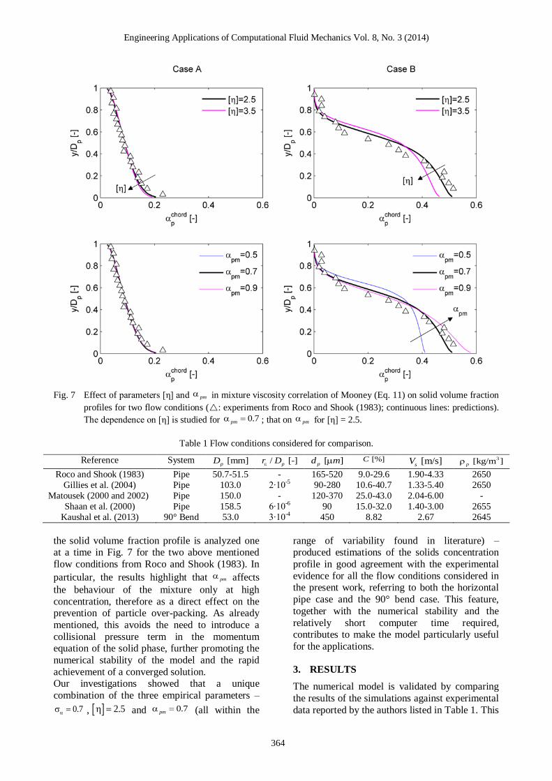
Engineering Applications of Computational Fluid Mechanics Vol 8 No 3 (2014)
364
Fig 7 Effect of parameters [η] and pm in mixture viscosity correlation of Mooney (Eq 11) on solid volume fraction
profiles for two flow conditions ( experiments from Roco and Shook (1983) continuous lines predictions)
The dependence on [η] is studied for 07pm that on pm for [η] = 25
Table 1 Flow conditions considered for comparison
Reference System [mm]pD
[-]pr D [ ]pd m []C [ms]sV 3 [kgm ]p
Roco and Shook (1983) Pipe 507-515 - 165-520 90-296 190-433 2650
Gillies et al (2004) Pipe 1030 2∙10-5 90-280 106-407 133-540 2650
Matousek (2000 and 2002) Pipe 1500 - 120-370 250-430 204-600 -
Shaan et al (2000) Pipe 1585 6∙10-6 90 150-320 140-300 2655
Kaushal et al (2013) 90deg Bend 530 3∙10-4 450 882 267 2645
the solid volume fraction profile is analyzed one at a time in Fig 7 for the two above mentioned
flow conditions from Roco and Shook (1983) In
particular the results highlight that pm affects
the behaviour of the mixture only at high
concentration therefore as a direct effect on the prevention of particle over-packing As already
mentioned this avoids the need to introduce a
collisional pressure term in the momentum equation of the solid phase further promoting the
numerical stability of the model and the rapid
achievement of a converged solution Our investigations showed that a unique
combination of the three empirical parameters ndash
07 25 and 07pm (all within the
range of variability found in literature) ndash produced estimations of the solids concentration
profile in good agreement with the experimental
evidence for all the flow conditions considered in the present work referring to both the horizontal
pipe case and the 90deg bend case This feature
together with the numerical stability and the
relatively short computer time required contributes to make the model particularly useful
for the applications
3 RESULTS
The numerical model is validated by comparing
the results of the simulations against experimental
data reported by the authors listed in Table 1 This
Engineering Applications of Computational Fluid Mechanics Vol 8 No 3 (2014)
365
table provides the flow conditions for each set of
measurements As already mentioned two scenarios have been considered namely a straight
horizontal pipe and a 90deg bend which will be
discussed in separate sub-sections
31 Straight horizontal pipe
The predictions of the model have been compared with experimental data for 26 flow conditions
summarized in Table 2 which differ in terms of
pipe diameter pipe roughness particle size slurry superficial velocity and delivered solid volume
fraction Each set of measurements allows an
assessment of the models capability for
reproducing the influence of specific features affecting the distribution of the solid volume
fraction The data of Roco and Shook (1983) and
Gillies et al (2004) are used to investigate the effect of particle diameter and slurry velocity with
different delivered solid volume fraction The
measurements of Matousek (2000 2002) provide the opportunity to extend the validity of the model
up to a pipe Reynolds number Re (Eq (15)) of
about 106 Finally the data of Shaan et al (2000)
are used to assess the performance of the model in
case of natural sands with irregularly-shaped grains Almost all the data refer to configurations
in which all the solids are kept suspended but
moving bed flows have also been briefly explored
to check how far one can go in employing the model for the purpose of achieving useful
information from an engineering point of view
Measurements of solids concentration ndash either bulk-mean or local ndash are subjected to errors
depending mainly on the instrumentation used as
discussed in Section 1 All the data reported in Table 2 are obtained using gamma-ray absorption
methods perhaps the technique which provides
the highest accuracy attainable with errors of the
order of a few percentage points Since this technique allows measuring chord-average values
of solid volume fraction the computed volume
fraction profile was evaluated by means of Eq (23) In the experiments from Roco and Shook
(1983) ndash cases A1 to A5 in Table 2 ndash the
dispersed phase consists of three kinds of sand with narrow size distribution and mean particle
diameters of 165 and 520 μm The solids density
is 2650 kgm3 the pipe diameter is about 51 mm
Table 2 Details of experimental conditions for straight pipe case (A1 to A5 experimental data from Roco and Shook (1983) B1 to B12 experimental data from Gillies et al (2004) C1 to C6 experimental data from Matousek
(2000 and 2002) D1 to D4 experimental data from Shaan et al (2000) values not declared by
experimenters)
Test ID [mm]pD
[-]pr D [ ]pd m []C [ms]sV 3 [kgm ]p
Flow pattern
A1 515 0 165 9 378 2650 FS
A2 515 0 165 19 417 2650 FS
A3 515 0 165 28 433 2650 FS
A4 507 0 520 1212 190 2650 MB
A5 507 0 520 2473 200 2650 MB
B1 103 2∙10-5 90 198 133 2650 FS
B2 103 2∙10-5 90 283 133 2650 FS
B3 103 2∙10-5 90 19 300 2650 FS
B4 103 2∙10-5 90 284 300 2650 FS B5 103 2∙10-5 280 12 255 2650 FS
B6 103 2∙10-5 280 208 260 2650 FS
B7 103 2∙10-5 280 310 250 2650 FS
B8 103 2∙10-5 280 407 260 2650 FS
B9 103 2∙10-5 280 106 540 2650 FS
B10 103 2∙10-5 280 203 540 2650 FS
B11 103 2∙10-5 280 301 540 2650 FS
B12 103 2∙10-5 280 405 540 2650 FS
C1 150 0 120 25 204 2650 FS
C2 150 0 120 35 204 2650 -
C3 150 0 120 34 600 2650 -
C4 150 0 370 25 600 2650 FS
C5 150 0 370 34 600 2650 - C6 150 0 370 43 600 2650 MB
D1 1585 6∙10-6 90 15 15 2655 FS
D2 1585 6∙10-6 90 32 14 2655 FS
D3 1585 6∙10-6 90 15 30 2655 FS
D4 1585 6∙10-6 90 32 30 2655 FS
Engineering Applications of Computational Fluid Mechanics Vol 8 No 3 (2014)
366
the slurry bulk-mean velocity varies from 190 to
433 ms and the pipe Reynolds number from between 9610
4 and 2110
5 The delivered solid
volume fraction ranges from 9 to 30 The
authors did not indicate the roughness of the pipe
which was assumed hydraulically smooth No evaluation of measurement uncertainty was
reported by the experimenters and they did not
identify the flow patterns according to the more recent classification of Doron and Barnea (1996)
However for the smallest particle diameter the
data suggest suspended flow whereas for the largest diameter the indications are for moving-
bed flow Fig 8 compares the computed and
measured solid volume fraction profiles The good agreement between computation and
measurements reveals the ability of the model to
reproduce the effect of particle diameter on the
particle distribution for slurries with different delivered solid volume fraction The simple two-
fluid model proposed in this work appears
capable to predict with reasonable accuracy the solid volume fraction profile not only in case of
fully-suspended flow but also in case of moving
bed flows This indicates that the asymptotic trend of the interfacial momentum transfer term
Fig 8 Solids concentration profiles for flow conditions A1 to A5 in Table 2 ( experiments from Roco and
Shook (1983) ndashndashndash predictions)
Fig 9 Solids concentration profile for flow conditions B1 to B12 in Table 2 ( experiments from Gillies et al
(2004) ndashndashndash predictions)
Engineering Applications of Computational Fluid Mechanics Vol 8 No 3 (2014)
367
produces on the solid volume fraction profile the
same effect that is traditionally achieved by the
collisional pressure and the tensor kT
Gillies et al (2004) measured the concentration
profiles of sand-water slurries in a 103 mm
diameter pipe using gamma-ray absorption
gauges without reporting the uncertainty The roughness of the pipe is 2 nm Two kinds of sand
were considered with narrow size distribution
and mean particle diameter of 90 and 280 μm In both cases the particle density was 2650 kgm
3
and the slurry superficial velocity varies from
133 to 54 ms (corresponding to a pipe Reynolds
number between 14105 and 5610
5) The
delivered solid volume fraction varies from about
10 to about 45 Details of the flow conditions
considered for comparison are reported in Table 2 cases B1 to B12 From an examination of the
measured data for the pressure gradient it can be
inferred that in all cases the flow is fully-suspended This is a good test for the modelrsquos
ability to predict the combined effect of slurry
velocity solids loading and particle diameter in a
larger pipe Fig 9 shows comparison of the computational and the experimental results for the
vertical distribution of the solid volume fraction
The model produces good overall agreement with the data The largest deviations are observed near
the pipe wall for the small particles at high
concentration (cases B2 and B4 in Table 4) but as noted by the authors themselves these
measurements are subject to the largest
experimental error
Matousek (2000 and 2002) measured the concentration profiles of sand-water slurries in a
150 mm diameter pipe using gamma-ray
absorption method quantifying a 4 uncertainty of the data We reproduced numerically the flow
conditions reported in Table 2 (cases C1 to C6)
in which the dispersed phase consists of two kinds
of sand with narrow size distribution and mean particle diameters of 120 and 370 μm
Unfortunately neither the density of the solid
particles nor the pipe roughness are reported in the experiments of Matousek (2000 and 2002)
and so in the simulations the former was set to
2650 kgm3 which is the value declared by Roco
and Shook (1983) and Gillies et al (2004) and
the pipe was regarded as hydraulically smooth
The slurry superficial velocity was 2 or 6 ms
corresponding to a pipe Reynolds number up to 10
6 The delivered solid volume fraction ranged
between 25 and 43 According to the author
the flows are either fully suspended or with a moving bed but only for three cases the flow
pattern could be clearly identified from the plot of
pressure gradient versus slurry superficial
velocity Fig 10 compares the computed and measured solid volume fraction profiles each set
of experimental data has error bars indicating the
uncertainty declared by the experimenter The
rather good agreement between computations and measurements confirm the reliability of the model
for high pipe Reynolds numbers A closer
inspection reveals that for case C6 the computed concentration is lower than the experimental
results in the lower part of the pipe and higher in
the upper region However the pressure gradient curve clearly reveals that in case C6 a moving bed
of particles is formed It is again confirmed that
the proposed model is capable to procure a rough
indication of the distribution of the solid also for flows in which the inter-granular stresses play an
important role
Moreover in the case of highly dense slurries like case C6 the experimental data are subject to the
most uncertainty and the numerical solutions are
sensitive to the empirical parameters pm and
which appear in the mixture viscosity correlation
(Eq (11)) For the same case the measured solids concentration profile shows a drop near the pipe
bottom This reversal is not predicted by the
numerical model which is probably due to the absence of the wall lift force discussed earlier in
Section 21 The same limitation was reported by
Ekambara et al (2009) The paper of Shaan et al (2000) focuses on the
effect of particle shape upon pressure gradient and
deposition velocity but these workers also
reported some measurements of the solid volume fraction profiles Shaan et al (2000) quantified
the particle shape by reference to the following
quantities evaluated from photos of the particles the axes ratio ie the ratio between the major and
minor axes of an ellipse circumscribing the
grains the circularity index ie the ratio between
the area of the particle multiplied by 4π and its perimeter The sand particles have a very irregular
shape as can be inferred by comparing the
measured values of axes ratio (16) and circularity (062) against typical values reported in the
literature for sand grains The mass-median value
of the particle size distribution curve is taken as the characteristic particle diameter The flow
conditions reported in Table 2 (cases D1 to D4)
were reproduced to check the behaviour of the
model for the case of irregularly-shaped sand particles The pipe diameter (1585 mm)
delivered solid volume fraction (15 or 35)
slurry superficial velocity (14 or 3 ms) particle density (2655 Kgm
3) and particle diameter (90
μm) are all approximately within the range
Engineering Applications of Computational Fluid Mechanics Vol 8 No 3 (2014)
368
Fig 10 Solids concentration profiles for flow conditions C1 to C6 in Table 2 ( experiments from Matousek
(2000 and 2002) ndashndashndash predictions)
Fig 11 Solids concentration profiles for flow conditions D1 to D4 in Table 2 ( experiments from Shaan et al
(2000) ndashndashndash predictions)
covered by the earlier simulations The numerical and experimental results are
compared in Fig 11 The agreement between the
numerical predictions and the experimental
evidence is fairly good inadequacies of the numerical model ndash especially in the wall
boundary conditions for the solid phase ndash and
measurements error can both contribute to the discrepancies observed near the pipe bottom for
case D2 The results seem to indicate that the
numerical model is a suitable tool for predicting the solid volume fraction distribution produced by
sands with a very irregular shape
32 Horizontal 90deg bend
The predictions of the model have been compared
with the recent experiments of Kaushal et al (2013) regarding a horizontal 90deg bend Among
the different flow conditions considered by these
authors reference is made to those characterized
by delivered solid volume fraction of 882 within the range of interest in this work The
experimenters used a sampling probe to measure
the volume fraction profile of the slurry in the 53
mm diameter pipe along the vertical axis at distances of 5Dp 25Dp and 50Dp downstream the
bend exit (referred to as sections S4 S5 and S6 in
Fig 2 respectively) They quantified a 2
uncertainty of the data The solid phase consists of silica sand particles with narrow size
distribution and mean particle diameter of 450
μm The slurry superficial velocity is 178 267 or 356 ms
The flow within the bend is much more complex
compared to that through the straight pipe since secondary motions develop in the crosswise
direction These motions affect significantly the
distribution of the solids and as a consequence
the volume fraction distribution is no longer constant over horizontal planes This is evident in
Fig 12 which shows the color plot of the solids
volumetric concentration over the six cross sections highlighted in Fig 2 As shown in Fig
13 the predictions of our model generally agree
with the experimental data available Greater
discrepancies are observed for the highest superficial velocity (356 ms) where the model
seems to underestimate the quantity of particles
dragged by the secondary motions This is
Engineering Applications of Computational Fluid Mechanics Vol 8 No 3 (2014)
369
Fig 12 Solid volume fraction distributions on sections
S1 to S6 in Fig 2 for delivered solid volume
fraction of 882 Left hand side is the outer
wall of the pipe
opposite to the KTGF based model of Kaushal et
al (2013) which tends to over-enhance the effect
of the secondary motions on the solids for the
lowest velocities Fig 13 also reveals that our model tends to overestimate the solids volume
fraction close to the pipe bottom far from the
bend exit It is expected that the predictions could
be improved if the effect of the wall lubrication force for which a suitable model does not exist at
present were accounted for
4 CONCLUSIONS
A mathematical model has been described for the
estimation of solid volume fraction distribution of
solid-liquid slurry flows in horizontal pipes and bends The model is based on an Eulerian-
Eulerian approach and uses the Inter-Phase Slip
Algorithm (IPSA) of Spalding (1980) The
novelty of this model resides in the combined use of existing modelling strategies never previously
employed simultaneously for the predictions of
slurry flows In order to account for turbulent dispersion of particles phase diffusion terms have
been included in the phase continuity equations
together with all the conservation equations The mixture viscosity approach is adopted to model
the effect of multiple particles on the inter-phase
friction A wall function is employed to model the
flow in the near-wall region in case of both hydraulically smooth and rough walls All these
strategies result in a model which despite being
simpler that those commonly used for addressing solid-liquid slurry flows shows comparable or
even better predictive capacity Moreover this
model is robust and numerically stable and
requires relatively short CPU time to procure converged steady-state solutions
The model has been first validated by comparison
with experimental data for the horizontal pipe case over a wide range of operating conditions
delivered solid volume fraction between 10 and
40 by volume mean particle diameter between 90 and 520 μm slurry superficial velocity
between 1 ms and 55 ms and pipe diameter
between 50 and 158 mm The model predictions
were found to be in good agreement with the experimental evidence for all the flow conditions
considered for comparison Even if the model is
originally intended to address fully-suspended flows the results indicated its capability to
provide rough indications of the solid volume
fraction distribution also in case of bed flows At last the comparison with the recent
measurements of Kaushal et al (2013) revealed
that this model is capable to procure reliable
predictions of the particle distribution downstream a 90deg bend in a horizontal pipe
Engineering Applications of Computational Fluid Mechanics Vol 8 No 3 (2014)
370
Fig 13 Solid volume fraction along vertical diameter on sections S4 to S6 in Fig 2 for delivered solid volume fraction
of 882 ( experiments from Kaushal et al (2013) ndashndashndash predictions)
ACKNOWLEDGEMENTS The authors would acknowledge the CINECA and
the Regione Lombardia award under the LISA
initiative for the availability of high performance computing resources and support The authors
would like to thank CHAM Ltd for supporting
this research and acknowledge Dr Randy Gillies of Saskatchewan Research Council for providing
his experimental data
REFERENCES
1 Ahilan RV Sleath J (1987) Sediment
transport in oscillatory flow over flat beds Journal of Hydraulic Engineering 113 308-
322
2 Albunaga BE (2002) Slurry Systems Handbook McGraw-Hill
3 Antal S Lahey R Flaherty J (1991) Analysis
of phase distribution in fully-developed
laminar bubbly two phase flow International Journal of Multiphase Flow 17(5) 635-652
4 Barnea E Mizrahi J (1973) A Generalized
Approach to the Fluid Dynamics of
Particulate Systems Chemical Engineering
Science 5(2) 171-189 5 Chen L Duan Y Pu W Zhao C (2009) CFD
simulation of coal-water slurry flowing in
horizontal pipelines Korean Journal of Chemical Engineering 26(4) 1144-1154
6 Chen RC (1994) Analysis of homogeneous
slurry pipe flow Journal of Marine Science and Technology 2(1) 37-45
7 Chen X Li Y Niu X Li M Chen D Yu X
(2011) A general two-phase turbulent flow
model applied to the study of sediment transport in open channels International
Journal of Multiphase Flow 37(9) 1099-
1108 8 Chung JN Troutt TR (1988) Simulation of
particle dispersion in an axisymmetric jet
Journal of Fluid Mechanics 186 199-222 9 Clift R Grace JR Weber ME (1978)
Bubbles Drops and Particles Academic
Press
10 Colwell JM Shook CA (1988) The Entry Length for Slurries in Horizontal Pipeline
Flow Canadian Journal of Chemical
Engineering 66(5) 714-720
Engineering Applications of Computational Fluid Mechanics Vol 8 No 3 (2014)
371
11 Doron P Barnea D (1993) A three layer
model for solid-liquid flow in horizontal pipes International Journal of Multiphase
Flow 19(6) 1029-1043
12 Doron P Barnea D (1995) Pressure drop and
limit deposit velocity for solid-liquid flow in pipes Chemical Engineering and Science
50(10) 1595-1604
13 Doron P Barnea D (1996) Flow pattern maps for solid-liquid flow in pipes International
Journal of Multiphase Flow 22(2) 273-283
14 Doron P Granica D Barnea D (1987) Slurry flow in horizontal pipes ndash experimental and
modeling International Journal of
Multiphase Flow 13(4) 535ndash547
15 Eccedila L Hoekstra M (2006) Discretization uncertainty estimation based on a least
squares version of the grid convergence
index Proceedings of the 2nd
Workshop on CFD Uncertainty Analysis Oct 19-20
Lisbon Portugal
16 Ekambara K Sanders RS Nandakumar K Masliyah JH (2009) Hydrodynamic
simulation of horizontal slurry pipeline flow
using ANSYS-CFX Industrial amp
Engineering Chemistry Research 48(17) 8159-8171
17 Gillies RG Shook CA (2000) Modelling
High Concentration Settling Slurry Flows Canadian Journal of Chemical Engineering
78(4) 709-716
18 Gillies RG Shook CA Xu J (2004)
Modelling Heterogeneous Slurry Flow at High Velocities Canadian Journal of
Chemical Engineering 82(5) 1060-1065
19 Hsu FLG (1981) Flow of Fine-particle Suspensions in Bends Fittings and Valves
MS Thesis Texas Tech University Lubbock
Texas USA 20 Ishii M Mishima K (1984) Two-fluid model
and hydrodynamic constitutive relations
Nuclear Engineering and Design 82(2-3)
107-126 21 Issa RI Oliveira PJ (1997) Assessment of a
particle-turbulence interaction model in
conjunction with an Eulerian two-phase flow formulation Proceedings of the 2
nd
International Symposium on Turbulence
Heat and Mass Transfer June 9-12 Delft Netherlands 759-770
22 Jayatillika CLV (1969) The influence of the
Prandtl number and surface roughness on the
resistance of the sublayer to momentum and heat transfer Progress in Heat amp Mass
Transfer 1 193-329
23 Jiang YY Zhang P (2012) Pressure drop and
flow pattern of slush nitrogen in a horizontal pipe AIChE Journal doi 10002aic13927
24 Kaushal DR Kumar A Tomita Y Juchii S
Tsukamoto H (2013) Flow of mono-
dispersed particles through horizontal bend International Journal of Multiphase Flow 52
71-91
25 Kaushal DR Sato K Toyota T Funatsu K Tomita Y (2005) Effect of particle size
distribution on pressure drop and
concentration profile in pipeline flow of highly concentrated slurry International
Journal of Multiphase Flow 31(7) 809-823
26 Kaushal DR Thinglas T Tomita Y Juchii S
Tsukamoto H (2012) CFD modeling for pipeline flow of fine particles at high
concentration International Journal of
Multiphase Flow 43 85-100 27 Kaushal DR Tomita Y (2003) Comparative
study of pressure drop in multisized
particulate slurry flow through pipe and rectangular duct International Journal of
Multiphase Flow 29(9) 1473-1487
28 Kaushal DR Tomita Y (2007) Experimental
investigation for near-wall lift of coarser particles in slurry pipeline using γ-ray
densitometer Powder Technology 172(3)
177-187 29 Kim C Lee M Han C (2008) Hydraulic
transport of sand-water mixtures in pipelines
Part I Experiment Journal of Mechanical
Science and Technology 22(12) 2534-2541 30 Kumar U Mishra R Singh SN Seshadri V
(2003) Effect of particle gradation on flow
characteristics of ash disposal pipelines Powder Technology 132(1) 39-51
31 Lahiri SK Ghanta KC (2010) Slurry flow
modeling by CFD Chemical Industry amp Chemical Engineering Quarterly 16(4) 295-
308
32 Launder BE Spalding DB (1972)
Mathematical models of turbulence Academic Press
33 Ling J Skudarnov PV Lin CX Ebadian MA
(2003) Numerical investigations of solid-liquid slurry flows in a fully developed flow
region International Journal of Heat and
Fluid Flow 24(3) 389-398 34 Matousek V (2000) Concentration
distribution in pipeline flow of sand-water
mixtures Journal of Hydrology and
Hydromechanics 48(3) 180-196 35 Matousek V (2002) Pressure drops and flow
patterns in sand-mixture pipes Experimental
Engineering Applications of Computational Fluid Mechanics Vol 8 No 3 (2014)
372
Thermal and Fluid Science 26(6-7) 693-702
36 Matousek V (2009) Predictive model for frictional pressure drop in settling-slurry pipe
with stationary deposit Powder Technology
192(3) 367-374
37 Mooney M (1951) The viscosity of a concentrated suspension of spherical
particles Journal of Colloid Science 6(2)
162-170 38 Nasr-el-Din H Shook CA Esmail MN
(1984) Isokinetic Probe Sampling From
Slurry Pipelines Canadian Journal of Chemical Engineering 62(2) 179-185
39 Pathak M (2011) Computational
investigations of solid-liquid particle
interaction in a two-phase flow around a ducted obstruction Journal of Hydraulic
Research 49(1) 96-104
40 Pecker SM Helvaci SS (2008) Solid-Liquid Two-Phase Flow Elsevier
41 Roco MC Shook CA (1983) Modeling of
Slurry Flow The Effect of Particle Size Canadian Journal of Chemical Engineering
61(4) 494-503
42 Schlichting H (1960) Boundary Layer
Theory McGraw-Hill 43 Shaan J Sumner RJ Gillies RG Shook CA
(2000) The Effect of Particle Shape on
Pipeline Friction for Newtonian Slurries of Fine Particles Canadian Journal of Chemical
Engineering 78(4) 717-725
44 Shiller L Naumann A (1935) A drag
coefficient correlation Zeitschrift des Vereines Deutscher Ingenieure 77 318-320
45 Shirolkar JS Coimbra CFM McQuay MQ
(1996) Fundamental aspects of modelling turbulent particle dispersion in dilute flows
Progress in Energy and Combustion Science
22(4) 363-399 46 Shook CA Bartosik AS (1994) Particle-wall
stresses in vertical slurry flows Powder
Technology 81(2) 117-124
47 Skudarnov PV Lin CX Ebadian MA (2004) Double-Species Slurry Flow in a Horizontal
Pipeline ASME Journal of Fluids
Engineering 126(1) 125-132 48 Spalding DB (1972) A novel finite-
difference formulation for differential
expressions involving both first and second derivatives International Journal of
Numerical Methods in Engineering 4(4) 551-
559
49 Spalding DB (1980) Numerical computation of multi-phase fluid flow and heat transfer In
Taylor C Morgan K (Eds) Recent Advances
in Numerical Methods in Fluids Pineridge
Press Limited 139-168 50 Turian RM Ma TW Hsu FLG Sung MDJ
Plackmann GW (1998) Flow of concentrated
non-Newtonian slurries 2 Friction losses in
bends fittings valves and Venturi meters International Journal of Multiphase Flow
24(2) 243-269
51 Versteeg HK Malalasekera W (2007) An Introduction to Computational Fluid
Dynamics The Finite Volume Method
Pearson Prentice Hall 52 Wilson KC Sanders RS Gillies RG Shook
CA (2010) Verification of the near-wall
model for slurry flow Powder Technology
197(3) 247-253 53 Wilson KC Sellgren A (2003) Interaction of
Particles and Near-Wall Lift in Slurry
Pipelines Journal of Hydraulic Engineering 129(1) 73-76
- Figures13
-
- Fig 1 Computational domain and boundaryconditions for horizontal pipe
- Fig 2 Computational domain boundary conditionsand reference sections for 90deg bend (S1=bendinlet S2=bend centre S3=bend exit S4=5Dpfrom bend exit S5=25Dp from bend exitS6=50Dp from bend exit)
- Fig3 Solid volume fraction profiles calculated onthree different grid levels for straight pipecase
- Fig4 Details of mesh for 90deg bend
- Fig5 Vertical solid volume fraction profiles atdistance of 5Dp downstream bend exit (SectionS4 in Fig 2) calculated on different gridlevels The Grid 3 solution has error barscorresponding to the grid discretization errorestimated by the method of Eccedila and Hoekstra(2006)
- Fig 6 Effect of turbulent Schmidt number for volume fractions a s on solid volume fraction profiles for two flowconditions (r experiments from Roco and Shook (1983) ndashndashndash 03 a s = ndashndashndash 05 a s = ndashndashndash 07 a s = ndashndashndash09 a s = )
- Fig 7 Effect of parameters [η] and pm a in mixture viscosity correlation of Mooney (Eq 11) on solid volume fractionprofiles for two flow conditions (r experiments from Roco and Shook (1983) continuous lines predictions)The dependence on [η] is studied for 07 pm a = that on pm a for [η] = 25
- Fig 8 Solids concentration profiles for flow conditions A1 to A5 in Table 2 (rbull experiments from Roco and Shook (1983) ndashndashndash predictions)
- Fig 9 Solids concentration profile for flow conditions B1 to B12 in Table 2 (rbulls experiments from Gillies et al (2004) ndashndashndash predictions)
- Fig 10 Solids concentration profiles for flow conditions C1 to C6 in Table 2 (rbull experiments from Matousek (2000 and 2002) ndashndashndash predictions)
- Fig 11 Solids concentration profiles for flow conditions D1 to D4 in Table 2 (rbull experiments from Shaan et al (2000) ndashndashndash predictions)
- Fig 12 Solid volume fraction distributions on sections S1 to S6 in Fig 2 for delivered solid volume fraction of 882 Left hand side is the outer wall of the pipe
- Fig 13 Solid volume fraction along vertical diameter on sections S4 to S6 in Fig 2 for delivered solid volume fraction of 882 (r experiments from Kaushal et al (2013) ndashndashndash predictions)
-
- Tables13
-
- Table 1 Flow conditions considered for comparison
- Table 2 Details of experimental conditions for straight pipe case (A1 to A5 experimental data from Roco and Shook(1983) B1 to B12 experimental data from Gillies et al (2004) C1 to C6 experimental data from Matousek(2000 and 2002) D1 to D4 experimental data from Shaan et al (2000) values not declared byexperimenters)
-
- 1 INTRODUCTION
- 2 MATHEMATICAL MODEL
-
- 21 Conservation equations
- 22 Turbulence modeling
- 23 Computational domain and boundaryconditions
- 24 Computational methodology and consistencyof numerical solution
- 25 Governing terms and calibration ofnumerical constants
-
- 3 RESULTS
-
- 31 Straight horizontal pipe
- 32 Horizontal 90deg bend
-
- 4 CONCLUSIONS
- ACKNOWLEDGEMENTS
- REFERENCES
-
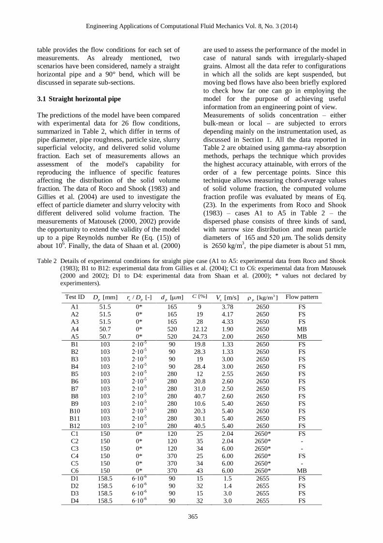
Engineering Applications of Computational Fluid Mechanics Vol 8 No 3 (2014)
365
table provides the flow conditions for each set of
measurements As already mentioned two scenarios have been considered namely a straight
horizontal pipe and a 90deg bend which will be
discussed in separate sub-sections
31 Straight horizontal pipe
The predictions of the model have been compared with experimental data for 26 flow conditions
summarized in Table 2 which differ in terms of
pipe diameter pipe roughness particle size slurry superficial velocity and delivered solid volume
fraction Each set of measurements allows an
assessment of the models capability for
reproducing the influence of specific features affecting the distribution of the solid volume
fraction The data of Roco and Shook (1983) and
Gillies et al (2004) are used to investigate the effect of particle diameter and slurry velocity with
different delivered solid volume fraction The
measurements of Matousek (2000 2002) provide the opportunity to extend the validity of the model
up to a pipe Reynolds number Re (Eq (15)) of
about 106 Finally the data of Shaan et al (2000)
are used to assess the performance of the model in
case of natural sands with irregularly-shaped grains Almost all the data refer to configurations
in which all the solids are kept suspended but
moving bed flows have also been briefly explored
to check how far one can go in employing the model for the purpose of achieving useful
information from an engineering point of view
Measurements of solids concentration ndash either bulk-mean or local ndash are subjected to errors
depending mainly on the instrumentation used as
discussed in Section 1 All the data reported in Table 2 are obtained using gamma-ray absorption
methods perhaps the technique which provides
the highest accuracy attainable with errors of the
order of a few percentage points Since this technique allows measuring chord-average values
of solid volume fraction the computed volume
fraction profile was evaluated by means of Eq (23) In the experiments from Roco and Shook
(1983) ndash cases A1 to A5 in Table 2 ndash the
dispersed phase consists of three kinds of sand with narrow size distribution and mean particle
diameters of 165 and 520 μm The solids density
is 2650 kgm3 the pipe diameter is about 51 mm
Table 2 Details of experimental conditions for straight pipe case (A1 to A5 experimental data from Roco and Shook (1983) B1 to B12 experimental data from Gillies et al (2004) C1 to C6 experimental data from Matousek
(2000 and 2002) D1 to D4 experimental data from Shaan et al (2000) values not declared by
experimenters)
Test ID [mm]pD
[-]pr D [ ]pd m []C [ms]sV 3 [kgm ]p
Flow pattern
A1 515 0 165 9 378 2650 FS
A2 515 0 165 19 417 2650 FS
A3 515 0 165 28 433 2650 FS
A4 507 0 520 1212 190 2650 MB
A5 507 0 520 2473 200 2650 MB
B1 103 2∙10-5 90 198 133 2650 FS
B2 103 2∙10-5 90 283 133 2650 FS
B3 103 2∙10-5 90 19 300 2650 FS
B4 103 2∙10-5 90 284 300 2650 FS B5 103 2∙10-5 280 12 255 2650 FS
B6 103 2∙10-5 280 208 260 2650 FS
B7 103 2∙10-5 280 310 250 2650 FS
B8 103 2∙10-5 280 407 260 2650 FS
B9 103 2∙10-5 280 106 540 2650 FS
B10 103 2∙10-5 280 203 540 2650 FS
B11 103 2∙10-5 280 301 540 2650 FS
B12 103 2∙10-5 280 405 540 2650 FS
C1 150 0 120 25 204 2650 FS
C2 150 0 120 35 204 2650 -
C3 150 0 120 34 600 2650 -
C4 150 0 370 25 600 2650 FS
C5 150 0 370 34 600 2650 - C6 150 0 370 43 600 2650 MB
D1 1585 6∙10-6 90 15 15 2655 FS
D2 1585 6∙10-6 90 32 14 2655 FS
D3 1585 6∙10-6 90 15 30 2655 FS
D4 1585 6∙10-6 90 32 30 2655 FS
Engineering Applications of Computational Fluid Mechanics Vol 8 No 3 (2014)
366
the slurry bulk-mean velocity varies from 190 to
433 ms and the pipe Reynolds number from between 9610
4 and 2110
5 The delivered solid
volume fraction ranges from 9 to 30 The
authors did not indicate the roughness of the pipe
which was assumed hydraulically smooth No evaluation of measurement uncertainty was
reported by the experimenters and they did not
identify the flow patterns according to the more recent classification of Doron and Barnea (1996)
However for the smallest particle diameter the
data suggest suspended flow whereas for the largest diameter the indications are for moving-
bed flow Fig 8 compares the computed and
measured solid volume fraction profiles The good agreement between computation and
measurements reveals the ability of the model to
reproduce the effect of particle diameter on the
particle distribution for slurries with different delivered solid volume fraction The simple two-
fluid model proposed in this work appears
capable to predict with reasonable accuracy the solid volume fraction profile not only in case of
fully-suspended flow but also in case of moving
bed flows This indicates that the asymptotic trend of the interfacial momentum transfer term
Fig 8 Solids concentration profiles for flow conditions A1 to A5 in Table 2 ( experiments from Roco and
Shook (1983) ndashndashndash predictions)
Fig 9 Solids concentration profile for flow conditions B1 to B12 in Table 2 ( experiments from Gillies et al
(2004) ndashndashndash predictions)
Engineering Applications of Computational Fluid Mechanics Vol 8 No 3 (2014)
367
produces on the solid volume fraction profile the
same effect that is traditionally achieved by the
collisional pressure and the tensor kT
Gillies et al (2004) measured the concentration
profiles of sand-water slurries in a 103 mm
diameter pipe using gamma-ray absorption
gauges without reporting the uncertainty The roughness of the pipe is 2 nm Two kinds of sand
were considered with narrow size distribution
and mean particle diameter of 90 and 280 μm In both cases the particle density was 2650 kgm
3
and the slurry superficial velocity varies from
133 to 54 ms (corresponding to a pipe Reynolds
number between 14105 and 5610
5) The
delivered solid volume fraction varies from about
10 to about 45 Details of the flow conditions
considered for comparison are reported in Table 2 cases B1 to B12 From an examination of the
measured data for the pressure gradient it can be
inferred that in all cases the flow is fully-suspended This is a good test for the modelrsquos
ability to predict the combined effect of slurry
velocity solids loading and particle diameter in a
larger pipe Fig 9 shows comparison of the computational and the experimental results for the
vertical distribution of the solid volume fraction
The model produces good overall agreement with the data The largest deviations are observed near
the pipe wall for the small particles at high
concentration (cases B2 and B4 in Table 4) but as noted by the authors themselves these
measurements are subject to the largest
experimental error
Matousek (2000 and 2002) measured the concentration profiles of sand-water slurries in a
150 mm diameter pipe using gamma-ray
absorption method quantifying a 4 uncertainty of the data We reproduced numerically the flow
conditions reported in Table 2 (cases C1 to C6)
in which the dispersed phase consists of two kinds
of sand with narrow size distribution and mean particle diameters of 120 and 370 μm
Unfortunately neither the density of the solid
particles nor the pipe roughness are reported in the experiments of Matousek (2000 and 2002)
and so in the simulations the former was set to
2650 kgm3 which is the value declared by Roco
and Shook (1983) and Gillies et al (2004) and
the pipe was regarded as hydraulically smooth
The slurry superficial velocity was 2 or 6 ms
corresponding to a pipe Reynolds number up to 10
6 The delivered solid volume fraction ranged
between 25 and 43 According to the author
the flows are either fully suspended or with a moving bed but only for three cases the flow
pattern could be clearly identified from the plot of
pressure gradient versus slurry superficial
velocity Fig 10 compares the computed and measured solid volume fraction profiles each set
of experimental data has error bars indicating the
uncertainty declared by the experimenter The
rather good agreement between computations and measurements confirm the reliability of the model
for high pipe Reynolds numbers A closer
inspection reveals that for case C6 the computed concentration is lower than the experimental
results in the lower part of the pipe and higher in
the upper region However the pressure gradient curve clearly reveals that in case C6 a moving bed
of particles is formed It is again confirmed that
the proposed model is capable to procure a rough
indication of the distribution of the solid also for flows in which the inter-granular stresses play an
important role
Moreover in the case of highly dense slurries like case C6 the experimental data are subject to the
most uncertainty and the numerical solutions are
sensitive to the empirical parameters pm and
which appear in the mixture viscosity correlation
(Eq (11)) For the same case the measured solids concentration profile shows a drop near the pipe
bottom This reversal is not predicted by the
numerical model which is probably due to the absence of the wall lift force discussed earlier in
Section 21 The same limitation was reported by
Ekambara et al (2009) The paper of Shaan et al (2000) focuses on the
effect of particle shape upon pressure gradient and
deposition velocity but these workers also
reported some measurements of the solid volume fraction profiles Shaan et al (2000) quantified
the particle shape by reference to the following
quantities evaluated from photos of the particles the axes ratio ie the ratio between the major and
minor axes of an ellipse circumscribing the
grains the circularity index ie the ratio between
the area of the particle multiplied by 4π and its perimeter The sand particles have a very irregular
shape as can be inferred by comparing the
measured values of axes ratio (16) and circularity (062) against typical values reported in the
literature for sand grains The mass-median value
of the particle size distribution curve is taken as the characteristic particle diameter The flow
conditions reported in Table 2 (cases D1 to D4)
were reproduced to check the behaviour of the
model for the case of irregularly-shaped sand particles The pipe diameter (1585 mm)
delivered solid volume fraction (15 or 35)
slurry superficial velocity (14 or 3 ms) particle density (2655 Kgm
3) and particle diameter (90
μm) are all approximately within the range
Engineering Applications of Computational Fluid Mechanics Vol 8 No 3 (2014)
368
Fig 10 Solids concentration profiles for flow conditions C1 to C6 in Table 2 ( experiments from Matousek
(2000 and 2002) ndashndashndash predictions)
Fig 11 Solids concentration profiles for flow conditions D1 to D4 in Table 2 ( experiments from Shaan et al
(2000) ndashndashndash predictions)
covered by the earlier simulations The numerical and experimental results are
compared in Fig 11 The agreement between the
numerical predictions and the experimental
evidence is fairly good inadequacies of the numerical model ndash especially in the wall
boundary conditions for the solid phase ndash and
measurements error can both contribute to the discrepancies observed near the pipe bottom for
case D2 The results seem to indicate that the
numerical model is a suitable tool for predicting the solid volume fraction distribution produced by
sands with a very irregular shape
32 Horizontal 90deg bend
The predictions of the model have been compared
with the recent experiments of Kaushal et al (2013) regarding a horizontal 90deg bend Among
the different flow conditions considered by these
authors reference is made to those characterized
by delivered solid volume fraction of 882 within the range of interest in this work The
experimenters used a sampling probe to measure
the volume fraction profile of the slurry in the 53
mm diameter pipe along the vertical axis at distances of 5Dp 25Dp and 50Dp downstream the
bend exit (referred to as sections S4 S5 and S6 in
Fig 2 respectively) They quantified a 2
uncertainty of the data The solid phase consists of silica sand particles with narrow size
distribution and mean particle diameter of 450
μm The slurry superficial velocity is 178 267 or 356 ms
The flow within the bend is much more complex
compared to that through the straight pipe since secondary motions develop in the crosswise
direction These motions affect significantly the
distribution of the solids and as a consequence
the volume fraction distribution is no longer constant over horizontal planes This is evident in
Fig 12 which shows the color plot of the solids
volumetric concentration over the six cross sections highlighted in Fig 2 As shown in Fig
13 the predictions of our model generally agree
with the experimental data available Greater
discrepancies are observed for the highest superficial velocity (356 ms) where the model
seems to underestimate the quantity of particles
dragged by the secondary motions This is
Engineering Applications of Computational Fluid Mechanics Vol 8 No 3 (2014)
369
Fig 12 Solid volume fraction distributions on sections
S1 to S6 in Fig 2 for delivered solid volume
fraction of 882 Left hand side is the outer
wall of the pipe
opposite to the KTGF based model of Kaushal et
al (2013) which tends to over-enhance the effect
of the secondary motions on the solids for the
lowest velocities Fig 13 also reveals that our model tends to overestimate the solids volume
fraction close to the pipe bottom far from the
bend exit It is expected that the predictions could
be improved if the effect of the wall lubrication force for which a suitable model does not exist at
present were accounted for
4 CONCLUSIONS
A mathematical model has been described for the
estimation of solid volume fraction distribution of
solid-liquid slurry flows in horizontal pipes and bends The model is based on an Eulerian-
Eulerian approach and uses the Inter-Phase Slip
Algorithm (IPSA) of Spalding (1980) The
novelty of this model resides in the combined use of existing modelling strategies never previously
employed simultaneously for the predictions of
slurry flows In order to account for turbulent dispersion of particles phase diffusion terms have
been included in the phase continuity equations
together with all the conservation equations The mixture viscosity approach is adopted to model
the effect of multiple particles on the inter-phase
friction A wall function is employed to model the
flow in the near-wall region in case of both hydraulically smooth and rough walls All these
strategies result in a model which despite being
simpler that those commonly used for addressing solid-liquid slurry flows shows comparable or
even better predictive capacity Moreover this
model is robust and numerically stable and
requires relatively short CPU time to procure converged steady-state solutions
The model has been first validated by comparison
with experimental data for the horizontal pipe case over a wide range of operating conditions
delivered solid volume fraction between 10 and
40 by volume mean particle diameter between 90 and 520 μm slurry superficial velocity
between 1 ms and 55 ms and pipe diameter
between 50 and 158 mm The model predictions
were found to be in good agreement with the experimental evidence for all the flow conditions
considered for comparison Even if the model is
originally intended to address fully-suspended flows the results indicated its capability to
provide rough indications of the solid volume
fraction distribution also in case of bed flows At last the comparison with the recent
measurements of Kaushal et al (2013) revealed
that this model is capable to procure reliable
predictions of the particle distribution downstream a 90deg bend in a horizontal pipe
Engineering Applications of Computational Fluid Mechanics Vol 8 No 3 (2014)
370
Fig 13 Solid volume fraction along vertical diameter on sections S4 to S6 in Fig 2 for delivered solid volume fraction
of 882 ( experiments from Kaushal et al (2013) ndashndashndash predictions)
ACKNOWLEDGEMENTS The authors would acknowledge the CINECA and
the Regione Lombardia award under the LISA
initiative for the availability of high performance computing resources and support The authors
would like to thank CHAM Ltd for supporting
this research and acknowledge Dr Randy Gillies of Saskatchewan Research Council for providing
his experimental data
REFERENCES
1 Ahilan RV Sleath J (1987) Sediment
transport in oscillatory flow over flat beds Journal of Hydraulic Engineering 113 308-
322
2 Albunaga BE (2002) Slurry Systems Handbook McGraw-Hill
3 Antal S Lahey R Flaherty J (1991) Analysis
of phase distribution in fully-developed
laminar bubbly two phase flow International Journal of Multiphase Flow 17(5) 635-652
4 Barnea E Mizrahi J (1973) A Generalized
Approach to the Fluid Dynamics of
Particulate Systems Chemical Engineering
Science 5(2) 171-189 5 Chen L Duan Y Pu W Zhao C (2009) CFD
simulation of coal-water slurry flowing in
horizontal pipelines Korean Journal of Chemical Engineering 26(4) 1144-1154
6 Chen RC (1994) Analysis of homogeneous
slurry pipe flow Journal of Marine Science and Technology 2(1) 37-45
7 Chen X Li Y Niu X Li M Chen D Yu X
(2011) A general two-phase turbulent flow
model applied to the study of sediment transport in open channels International
Journal of Multiphase Flow 37(9) 1099-
1108 8 Chung JN Troutt TR (1988) Simulation of
particle dispersion in an axisymmetric jet
Journal of Fluid Mechanics 186 199-222 9 Clift R Grace JR Weber ME (1978)
Bubbles Drops and Particles Academic
Press
10 Colwell JM Shook CA (1988) The Entry Length for Slurries in Horizontal Pipeline
Flow Canadian Journal of Chemical
Engineering 66(5) 714-720
Engineering Applications of Computational Fluid Mechanics Vol 8 No 3 (2014)
371
11 Doron P Barnea D (1993) A three layer
model for solid-liquid flow in horizontal pipes International Journal of Multiphase
Flow 19(6) 1029-1043
12 Doron P Barnea D (1995) Pressure drop and
limit deposit velocity for solid-liquid flow in pipes Chemical Engineering and Science
50(10) 1595-1604
13 Doron P Barnea D (1996) Flow pattern maps for solid-liquid flow in pipes International
Journal of Multiphase Flow 22(2) 273-283
14 Doron P Granica D Barnea D (1987) Slurry flow in horizontal pipes ndash experimental and
modeling International Journal of
Multiphase Flow 13(4) 535ndash547
15 Eccedila L Hoekstra M (2006) Discretization uncertainty estimation based on a least
squares version of the grid convergence
index Proceedings of the 2nd
Workshop on CFD Uncertainty Analysis Oct 19-20
Lisbon Portugal
16 Ekambara K Sanders RS Nandakumar K Masliyah JH (2009) Hydrodynamic
simulation of horizontal slurry pipeline flow
using ANSYS-CFX Industrial amp
Engineering Chemistry Research 48(17) 8159-8171
17 Gillies RG Shook CA (2000) Modelling
High Concentration Settling Slurry Flows Canadian Journal of Chemical Engineering
78(4) 709-716
18 Gillies RG Shook CA Xu J (2004)
Modelling Heterogeneous Slurry Flow at High Velocities Canadian Journal of
Chemical Engineering 82(5) 1060-1065
19 Hsu FLG (1981) Flow of Fine-particle Suspensions in Bends Fittings and Valves
MS Thesis Texas Tech University Lubbock
Texas USA 20 Ishii M Mishima K (1984) Two-fluid model
and hydrodynamic constitutive relations
Nuclear Engineering and Design 82(2-3)
107-126 21 Issa RI Oliveira PJ (1997) Assessment of a
particle-turbulence interaction model in
conjunction with an Eulerian two-phase flow formulation Proceedings of the 2
nd
International Symposium on Turbulence
Heat and Mass Transfer June 9-12 Delft Netherlands 759-770
22 Jayatillika CLV (1969) The influence of the
Prandtl number and surface roughness on the
resistance of the sublayer to momentum and heat transfer Progress in Heat amp Mass
Transfer 1 193-329
23 Jiang YY Zhang P (2012) Pressure drop and
flow pattern of slush nitrogen in a horizontal pipe AIChE Journal doi 10002aic13927
24 Kaushal DR Kumar A Tomita Y Juchii S
Tsukamoto H (2013) Flow of mono-
dispersed particles through horizontal bend International Journal of Multiphase Flow 52
71-91
25 Kaushal DR Sato K Toyota T Funatsu K Tomita Y (2005) Effect of particle size
distribution on pressure drop and
concentration profile in pipeline flow of highly concentrated slurry International
Journal of Multiphase Flow 31(7) 809-823
26 Kaushal DR Thinglas T Tomita Y Juchii S
Tsukamoto H (2012) CFD modeling for pipeline flow of fine particles at high
concentration International Journal of
Multiphase Flow 43 85-100 27 Kaushal DR Tomita Y (2003) Comparative
study of pressure drop in multisized
particulate slurry flow through pipe and rectangular duct International Journal of
Multiphase Flow 29(9) 1473-1487
28 Kaushal DR Tomita Y (2007) Experimental
investigation for near-wall lift of coarser particles in slurry pipeline using γ-ray
densitometer Powder Technology 172(3)
177-187 29 Kim C Lee M Han C (2008) Hydraulic
transport of sand-water mixtures in pipelines
Part I Experiment Journal of Mechanical
Science and Technology 22(12) 2534-2541 30 Kumar U Mishra R Singh SN Seshadri V
(2003) Effect of particle gradation on flow
characteristics of ash disposal pipelines Powder Technology 132(1) 39-51
31 Lahiri SK Ghanta KC (2010) Slurry flow
modeling by CFD Chemical Industry amp Chemical Engineering Quarterly 16(4) 295-
308
32 Launder BE Spalding DB (1972)
Mathematical models of turbulence Academic Press
33 Ling J Skudarnov PV Lin CX Ebadian MA
(2003) Numerical investigations of solid-liquid slurry flows in a fully developed flow
region International Journal of Heat and
Fluid Flow 24(3) 389-398 34 Matousek V (2000) Concentration
distribution in pipeline flow of sand-water
mixtures Journal of Hydrology and
Hydromechanics 48(3) 180-196 35 Matousek V (2002) Pressure drops and flow
patterns in sand-mixture pipes Experimental
Engineering Applications of Computational Fluid Mechanics Vol 8 No 3 (2014)
372
Thermal and Fluid Science 26(6-7) 693-702
36 Matousek V (2009) Predictive model for frictional pressure drop in settling-slurry pipe
with stationary deposit Powder Technology
192(3) 367-374
37 Mooney M (1951) The viscosity of a concentrated suspension of spherical
particles Journal of Colloid Science 6(2)
162-170 38 Nasr-el-Din H Shook CA Esmail MN
(1984) Isokinetic Probe Sampling From
Slurry Pipelines Canadian Journal of Chemical Engineering 62(2) 179-185
39 Pathak M (2011) Computational
investigations of solid-liquid particle
interaction in a two-phase flow around a ducted obstruction Journal of Hydraulic
Research 49(1) 96-104
40 Pecker SM Helvaci SS (2008) Solid-Liquid Two-Phase Flow Elsevier
41 Roco MC Shook CA (1983) Modeling of
Slurry Flow The Effect of Particle Size Canadian Journal of Chemical Engineering
61(4) 494-503
42 Schlichting H (1960) Boundary Layer
Theory McGraw-Hill 43 Shaan J Sumner RJ Gillies RG Shook CA
(2000) The Effect of Particle Shape on
Pipeline Friction for Newtonian Slurries of Fine Particles Canadian Journal of Chemical
Engineering 78(4) 717-725
44 Shiller L Naumann A (1935) A drag
coefficient correlation Zeitschrift des Vereines Deutscher Ingenieure 77 318-320
45 Shirolkar JS Coimbra CFM McQuay MQ
(1996) Fundamental aspects of modelling turbulent particle dispersion in dilute flows
Progress in Energy and Combustion Science
22(4) 363-399 46 Shook CA Bartosik AS (1994) Particle-wall
stresses in vertical slurry flows Powder
Technology 81(2) 117-124
47 Skudarnov PV Lin CX Ebadian MA (2004) Double-Species Slurry Flow in a Horizontal
Pipeline ASME Journal of Fluids
Engineering 126(1) 125-132 48 Spalding DB (1972) A novel finite-
difference formulation for differential
expressions involving both first and second derivatives International Journal of
Numerical Methods in Engineering 4(4) 551-
559
49 Spalding DB (1980) Numerical computation of multi-phase fluid flow and heat transfer In
Taylor C Morgan K (Eds) Recent Advances
in Numerical Methods in Fluids Pineridge
Press Limited 139-168 50 Turian RM Ma TW Hsu FLG Sung MDJ
Plackmann GW (1998) Flow of concentrated
non-Newtonian slurries 2 Friction losses in
bends fittings valves and Venturi meters International Journal of Multiphase Flow
24(2) 243-269
51 Versteeg HK Malalasekera W (2007) An Introduction to Computational Fluid
Dynamics The Finite Volume Method
Pearson Prentice Hall 52 Wilson KC Sanders RS Gillies RG Shook
CA (2010) Verification of the near-wall
model for slurry flow Powder Technology
197(3) 247-253 53 Wilson KC Sellgren A (2003) Interaction of
Particles and Near-Wall Lift in Slurry
Pipelines Journal of Hydraulic Engineering 129(1) 73-76
- Figures13
-
- Fig 1 Computational domain and boundaryconditions for horizontal pipe
- Fig 2 Computational domain boundary conditionsand reference sections for 90deg bend (S1=bendinlet S2=bend centre S3=bend exit S4=5Dpfrom bend exit S5=25Dp from bend exitS6=50Dp from bend exit)
- Fig3 Solid volume fraction profiles calculated onthree different grid levels for straight pipecase
- Fig4 Details of mesh for 90deg bend
- Fig5 Vertical solid volume fraction profiles atdistance of 5Dp downstream bend exit (SectionS4 in Fig 2) calculated on different gridlevels The Grid 3 solution has error barscorresponding to the grid discretization errorestimated by the method of Eccedila and Hoekstra(2006)
- Fig 6 Effect of turbulent Schmidt number for volume fractions a s on solid volume fraction profiles for two flowconditions (r experiments from Roco and Shook (1983) ndashndashndash 03 a s = ndashndashndash 05 a s = ndashndashndash 07 a s = ndashndashndash09 a s = )
- Fig 7 Effect of parameters [η] and pm a in mixture viscosity correlation of Mooney (Eq 11) on solid volume fractionprofiles for two flow conditions (r experiments from Roco and Shook (1983) continuous lines predictions)The dependence on [η] is studied for 07 pm a = that on pm a for [η] = 25
- Fig 8 Solids concentration profiles for flow conditions A1 to A5 in Table 2 (rbull experiments from Roco and Shook (1983) ndashndashndash predictions)
- Fig 9 Solids concentration profile for flow conditions B1 to B12 in Table 2 (rbulls experiments from Gillies et al (2004) ndashndashndash predictions)
- Fig 10 Solids concentration profiles for flow conditions C1 to C6 in Table 2 (rbull experiments from Matousek (2000 and 2002) ndashndashndash predictions)
- Fig 11 Solids concentration profiles for flow conditions D1 to D4 in Table 2 (rbull experiments from Shaan et al (2000) ndashndashndash predictions)
- Fig 12 Solid volume fraction distributions on sections S1 to S6 in Fig 2 for delivered solid volume fraction of 882 Left hand side is the outer wall of the pipe
- Fig 13 Solid volume fraction along vertical diameter on sections S4 to S6 in Fig 2 for delivered solid volume fraction of 882 (r experiments from Kaushal et al (2013) ndashndashndash predictions)
-
- Tables13
-
- Table 1 Flow conditions considered for comparison
- Table 2 Details of experimental conditions for straight pipe case (A1 to A5 experimental data from Roco and Shook(1983) B1 to B12 experimental data from Gillies et al (2004) C1 to C6 experimental data from Matousek(2000 and 2002) D1 to D4 experimental data from Shaan et al (2000) values not declared byexperimenters)
-
- 1 INTRODUCTION
- 2 MATHEMATICAL MODEL
-
- 21 Conservation equations
- 22 Turbulence modeling
- 23 Computational domain and boundaryconditions
- 24 Computational methodology and consistencyof numerical solution
- 25 Governing terms and calibration ofnumerical constants
-
- 3 RESULTS
-
- 31 Straight horizontal pipe
- 32 Horizontal 90deg bend
-
- 4 CONCLUSIONS
- ACKNOWLEDGEMENTS
- REFERENCES
-
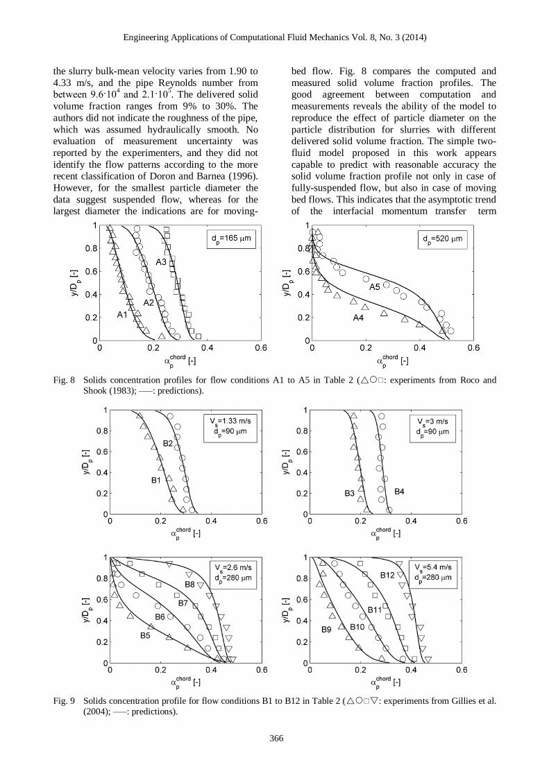
Engineering Applications of Computational Fluid Mechanics Vol 8 No 3 (2014)
366
the slurry bulk-mean velocity varies from 190 to
433 ms and the pipe Reynolds number from between 9610
4 and 2110
5 The delivered solid
volume fraction ranges from 9 to 30 The
authors did not indicate the roughness of the pipe
which was assumed hydraulically smooth No evaluation of measurement uncertainty was
reported by the experimenters and they did not
identify the flow patterns according to the more recent classification of Doron and Barnea (1996)
However for the smallest particle diameter the
data suggest suspended flow whereas for the largest diameter the indications are for moving-
bed flow Fig 8 compares the computed and
measured solid volume fraction profiles The good agreement between computation and
measurements reveals the ability of the model to
reproduce the effect of particle diameter on the
particle distribution for slurries with different delivered solid volume fraction The simple two-
fluid model proposed in this work appears
capable to predict with reasonable accuracy the solid volume fraction profile not only in case of
fully-suspended flow but also in case of moving
bed flows This indicates that the asymptotic trend of the interfacial momentum transfer term
Fig 8 Solids concentration profiles for flow conditions A1 to A5 in Table 2 ( experiments from Roco and
Shook (1983) ndashndashndash predictions)
Fig 9 Solids concentration profile for flow conditions B1 to B12 in Table 2 ( experiments from Gillies et al
(2004) ndashndashndash predictions)
Engineering Applications of Computational Fluid Mechanics Vol 8 No 3 (2014)
367
produces on the solid volume fraction profile the
same effect that is traditionally achieved by the
collisional pressure and the tensor kT
Gillies et al (2004) measured the concentration
profiles of sand-water slurries in a 103 mm
diameter pipe using gamma-ray absorption
gauges without reporting the uncertainty The roughness of the pipe is 2 nm Two kinds of sand
were considered with narrow size distribution
and mean particle diameter of 90 and 280 μm In both cases the particle density was 2650 kgm
3
and the slurry superficial velocity varies from
133 to 54 ms (corresponding to a pipe Reynolds
number between 14105 and 5610
5) The
delivered solid volume fraction varies from about
10 to about 45 Details of the flow conditions
considered for comparison are reported in Table 2 cases B1 to B12 From an examination of the
measured data for the pressure gradient it can be
inferred that in all cases the flow is fully-suspended This is a good test for the modelrsquos
ability to predict the combined effect of slurry
velocity solids loading and particle diameter in a
larger pipe Fig 9 shows comparison of the computational and the experimental results for the
vertical distribution of the solid volume fraction
The model produces good overall agreement with the data The largest deviations are observed near
the pipe wall for the small particles at high
concentration (cases B2 and B4 in Table 4) but as noted by the authors themselves these
measurements are subject to the largest
experimental error
Matousek (2000 and 2002) measured the concentration profiles of sand-water slurries in a
150 mm diameter pipe using gamma-ray
absorption method quantifying a 4 uncertainty of the data We reproduced numerically the flow
conditions reported in Table 2 (cases C1 to C6)
in which the dispersed phase consists of two kinds
of sand with narrow size distribution and mean particle diameters of 120 and 370 μm
Unfortunately neither the density of the solid
particles nor the pipe roughness are reported in the experiments of Matousek (2000 and 2002)
and so in the simulations the former was set to
2650 kgm3 which is the value declared by Roco
and Shook (1983) and Gillies et al (2004) and
the pipe was regarded as hydraulically smooth
The slurry superficial velocity was 2 or 6 ms
corresponding to a pipe Reynolds number up to 10
6 The delivered solid volume fraction ranged
between 25 and 43 According to the author
the flows are either fully suspended or with a moving bed but only for three cases the flow
pattern could be clearly identified from the plot of
pressure gradient versus slurry superficial
velocity Fig 10 compares the computed and measured solid volume fraction profiles each set
of experimental data has error bars indicating the
uncertainty declared by the experimenter The
rather good agreement between computations and measurements confirm the reliability of the model
for high pipe Reynolds numbers A closer
inspection reveals that for case C6 the computed concentration is lower than the experimental
results in the lower part of the pipe and higher in
the upper region However the pressure gradient curve clearly reveals that in case C6 a moving bed
of particles is formed It is again confirmed that
the proposed model is capable to procure a rough
indication of the distribution of the solid also for flows in which the inter-granular stresses play an
important role
Moreover in the case of highly dense slurries like case C6 the experimental data are subject to the
most uncertainty and the numerical solutions are
sensitive to the empirical parameters pm and
which appear in the mixture viscosity correlation
(Eq (11)) For the same case the measured solids concentration profile shows a drop near the pipe
bottom This reversal is not predicted by the
numerical model which is probably due to the absence of the wall lift force discussed earlier in
Section 21 The same limitation was reported by
Ekambara et al (2009) The paper of Shaan et al (2000) focuses on the
effect of particle shape upon pressure gradient and
deposition velocity but these workers also
reported some measurements of the solid volume fraction profiles Shaan et al (2000) quantified
the particle shape by reference to the following
quantities evaluated from photos of the particles the axes ratio ie the ratio between the major and
minor axes of an ellipse circumscribing the
grains the circularity index ie the ratio between
the area of the particle multiplied by 4π and its perimeter The sand particles have a very irregular
shape as can be inferred by comparing the
measured values of axes ratio (16) and circularity (062) against typical values reported in the
literature for sand grains The mass-median value
of the particle size distribution curve is taken as the characteristic particle diameter The flow
conditions reported in Table 2 (cases D1 to D4)
were reproduced to check the behaviour of the
model for the case of irregularly-shaped sand particles The pipe diameter (1585 mm)
delivered solid volume fraction (15 or 35)
slurry superficial velocity (14 or 3 ms) particle density (2655 Kgm
3) and particle diameter (90
μm) are all approximately within the range
Engineering Applications of Computational Fluid Mechanics Vol 8 No 3 (2014)
368
Fig 10 Solids concentration profiles for flow conditions C1 to C6 in Table 2 ( experiments from Matousek
(2000 and 2002) ndashndashndash predictions)
Fig 11 Solids concentration profiles for flow conditions D1 to D4 in Table 2 ( experiments from Shaan et al
(2000) ndashndashndash predictions)
covered by the earlier simulations The numerical and experimental results are
compared in Fig 11 The agreement between the
numerical predictions and the experimental
evidence is fairly good inadequacies of the numerical model ndash especially in the wall
boundary conditions for the solid phase ndash and
measurements error can both contribute to the discrepancies observed near the pipe bottom for
case D2 The results seem to indicate that the
numerical model is a suitable tool for predicting the solid volume fraction distribution produced by
sands with a very irregular shape
32 Horizontal 90deg bend
The predictions of the model have been compared
with the recent experiments of Kaushal et al (2013) regarding a horizontal 90deg bend Among
the different flow conditions considered by these
authors reference is made to those characterized
by delivered solid volume fraction of 882 within the range of interest in this work The
experimenters used a sampling probe to measure
the volume fraction profile of the slurry in the 53
mm diameter pipe along the vertical axis at distances of 5Dp 25Dp and 50Dp downstream the
bend exit (referred to as sections S4 S5 and S6 in
Fig 2 respectively) They quantified a 2
uncertainty of the data The solid phase consists of silica sand particles with narrow size
distribution and mean particle diameter of 450
μm The slurry superficial velocity is 178 267 or 356 ms
The flow within the bend is much more complex
compared to that through the straight pipe since secondary motions develop in the crosswise
direction These motions affect significantly the
distribution of the solids and as a consequence
the volume fraction distribution is no longer constant over horizontal planes This is evident in
Fig 12 which shows the color plot of the solids
volumetric concentration over the six cross sections highlighted in Fig 2 As shown in Fig
13 the predictions of our model generally agree
with the experimental data available Greater
discrepancies are observed for the highest superficial velocity (356 ms) where the model
seems to underestimate the quantity of particles
dragged by the secondary motions This is
Engineering Applications of Computational Fluid Mechanics Vol 8 No 3 (2014)
369
Fig 12 Solid volume fraction distributions on sections
S1 to S6 in Fig 2 for delivered solid volume
fraction of 882 Left hand side is the outer
wall of the pipe
opposite to the KTGF based model of Kaushal et
al (2013) which tends to over-enhance the effect
of the secondary motions on the solids for the
lowest velocities Fig 13 also reveals that our model tends to overestimate the solids volume
fraction close to the pipe bottom far from the
bend exit It is expected that the predictions could
be improved if the effect of the wall lubrication force for which a suitable model does not exist at
present were accounted for
4 CONCLUSIONS
A mathematical model has been described for the
estimation of solid volume fraction distribution of
solid-liquid slurry flows in horizontal pipes and bends The model is based on an Eulerian-
Eulerian approach and uses the Inter-Phase Slip
Algorithm (IPSA) of Spalding (1980) The
novelty of this model resides in the combined use of existing modelling strategies never previously
employed simultaneously for the predictions of
slurry flows In order to account for turbulent dispersion of particles phase diffusion terms have
been included in the phase continuity equations
together with all the conservation equations The mixture viscosity approach is adopted to model
the effect of multiple particles on the inter-phase
friction A wall function is employed to model the
flow in the near-wall region in case of both hydraulically smooth and rough walls All these
strategies result in a model which despite being
simpler that those commonly used for addressing solid-liquid slurry flows shows comparable or
even better predictive capacity Moreover this
model is robust and numerically stable and
requires relatively short CPU time to procure converged steady-state solutions
The model has been first validated by comparison
with experimental data for the horizontal pipe case over a wide range of operating conditions
delivered solid volume fraction between 10 and
40 by volume mean particle diameter between 90 and 520 μm slurry superficial velocity
between 1 ms and 55 ms and pipe diameter
between 50 and 158 mm The model predictions
were found to be in good agreement with the experimental evidence for all the flow conditions
considered for comparison Even if the model is
originally intended to address fully-suspended flows the results indicated its capability to
provide rough indications of the solid volume
fraction distribution also in case of bed flows At last the comparison with the recent
measurements of Kaushal et al (2013) revealed
that this model is capable to procure reliable
predictions of the particle distribution downstream a 90deg bend in a horizontal pipe
Engineering Applications of Computational Fluid Mechanics Vol 8 No 3 (2014)
370
Fig 13 Solid volume fraction along vertical diameter on sections S4 to S6 in Fig 2 for delivered solid volume fraction
of 882 ( experiments from Kaushal et al (2013) ndashndashndash predictions)
ACKNOWLEDGEMENTS The authors would acknowledge the CINECA and
the Regione Lombardia award under the LISA
initiative for the availability of high performance computing resources and support The authors
would like to thank CHAM Ltd for supporting
this research and acknowledge Dr Randy Gillies of Saskatchewan Research Council for providing
his experimental data
REFERENCES
1 Ahilan RV Sleath J (1987) Sediment
transport in oscillatory flow over flat beds Journal of Hydraulic Engineering 113 308-
322
2 Albunaga BE (2002) Slurry Systems Handbook McGraw-Hill
3 Antal S Lahey R Flaherty J (1991) Analysis
of phase distribution in fully-developed
laminar bubbly two phase flow International Journal of Multiphase Flow 17(5) 635-652
4 Barnea E Mizrahi J (1973) A Generalized
Approach to the Fluid Dynamics of
Particulate Systems Chemical Engineering
Science 5(2) 171-189 5 Chen L Duan Y Pu W Zhao C (2009) CFD
simulation of coal-water slurry flowing in
horizontal pipelines Korean Journal of Chemical Engineering 26(4) 1144-1154
6 Chen RC (1994) Analysis of homogeneous
slurry pipe flow Journal of Marine Science and Technology 2(1) 37-45
7 Chen X Li Y Niu X Li M Chen D Yu X
(2011) A general two-phase turbulent flow
model applied to the study of sediment transport in open channels International
Journal of Multiphase Flow 37(9) 1099-
1108 8 Chung JN Troutt TR (1988) Simulation of
particle dispersion in an axisymmetric jet
Journal of Fluid Mechanics 186 199-222 9 Clift R Grace JR Weber ME (1978)
Bubbles Drops and Particles Academic
Press
10 Colwell JM Shook CA (1988) The Entry Length for Slurries in Horizontal Pipeline
Flow Canadian Journal of Chemical
Engineering 66(5) 714-720
Engineering Applications of Computational Fluid Mechanics Vol 8 No 3 (2014)
371
11 Doron P Barnea D (1993) A three layer
model for solid-liquid flow in horizontal pipes International Journal of Multiphase
Flow 19(6) 1029-1043
12 Doron P Barnea D (1995) Pressure drop and
limit deposit velocity for solid-liquid flow in pipes Chemical Engineering and Science
50(10) 1595-1604
13 Doron P Barnea D (1996) Flow pattern maps for solid-liquid flow in pipes International
Journal of Multiphase Flow 22(2) 273-283
14 Doron P Granica D Barnea D (1987) Slurry flow in horizontal pipes ndash experimental and
modeling International Journal of
Multiphase Flow 13(4) 535ndash547
15 Eccedila L Hoekstra M (2006) Discretization uncertainty estimation based on a least
squares version of the grid convergence
index Proceedings of the 2nd
Workshop on CFD Uncertainty Analysis Oct 19-20
Lisbon Portugal
16 Ekambara K Sanders RS Nandakumar K Masliyah JH (2009) Hydrodynamic
simulation of horizontal slurry pipeline flow
using ANSYS-CFX Industrial amp
Engineering Chemistry Research 48(17) 8159-8171
17 Gillies RG Shook CA (2000) Modelling
High Concentration Settling Slurry Flows Canadian Journal of Chemical Engineering
78(4) 709-716
18 Gillies RG Shook CA Xu J (2004)
Modelling Heterogeneous Slurry Flow at High Velocities Canadian Journal of
Chemical Engineering 82(5) 1060-1065
19 Hsu FLG (1981) Flow of Fine-particle Suspensions in Bends Fittings and Valves
MS Thesis Texas Tech University Lubbock
Texas USA 20 Ishii M Mishima K (1984) Two-fluid model
and hydrodynamic constitutive relations
Nuclear Engineering and Design 82(2-3)
107-126 21 Issa RI Oliveira PJ (1997) Assessment of a
particle-turbulence interaction model in
conjunction with an Eulerian two-phase flow formulation Proceedings of the 2
nd
International Symposium on Turbulence
Heat and Mass Transfer June 9-12 Delft Netherlands 759-770
22 Jayatillika CLV (1969) The influence of the
Prandtl number and surface roughness on the
resistance of the sublayer to momentum and heat transfer Progress in Heat amp Mass
Transfer 1 193-329
23 Jiang YY Zhang P (2012) Pressure drop and
flow pattern of slush nitrogen in a horizontal pipe AIChE Journal doi 10002aic13927
24 Kaushal DR Kumar A Tomita Y Juchii S
Tsukamoto H (2013) Flow of mono-
dispersed particles through horizontal bend International Journal of Multiphase Flow 52
71-91
25 Kaushal DR Sato K Toyota T Funatsu K Tomita Y (2005) Effect of particle size
distribution on pressure drop and
concentration profile in pipeline flow of highly concentrated slurry International
Journal of Multiphase Flow 31(7) 809-823
26 Kaushal DR Thinglas T Tomita Y Juchii S
Tsukamoto H (2012) CFD modeling for pipeline flow of fine particles at high
concentration International Journal of
Multiphase Flow 43 85-100 27 Kaushal DR Tomita Y (2003) Comparative
study of pressure drop in multisized
particulate slurry flow through pipe and rectangular duct International Journal of
Multiphase Flow 29(9) 1473-1487
28 Kaushal DR Tomita Y (2007) Experimental
investigation for near-wall lift of coarser particles in slurry pipeline using γ-ray
densitometer Powder Technology 172(3)
177-187 29 Kim C Lee M Han C (2008) Hydraulic
transport of sand-water mixtures in pipelines
Part I Experiment Journal of Mechanical
Science and Technology 22(12) 2534-2541 30 Kumar U Mishra R Singh SN Seshadri V
(2003) Effect of particle gradation on flow
characteristics of ash disposal pipelines Powder Technology 132(1) 39-51
31 Lahiri SK Ghanta KC (2010) Slurry flow
modeling by CFD Chemical Industry amp Chemical Engineering Quarterly 16(4) 295-
308
32 Launder BE Spalding DB (1972)
Mathematical models of turbulence Academic Press
33 Ling J Skudarnov PV Lin CX Ebadian MA
(2003) Numerical investigations of solid-liquid slurry flows in a fully developed flow
region International Journal of Heat and
Fluid Flow 24(3) 389-398 34 Matousek V (2000) Concentration
distribution in pipeline flow of sand-water
mixtures Journal of Hydrology and
Hydromechanics 48(3) 180-196 35 Matousek V (2002) Pressure drops and flow
patterns in sand-mixture pipes Experimental
Engineering Applications of Computational Fluid Mechanics Vol 8 No 3 (2014)
372
Thermal and Fluid Science 26(6-7) 693-702
36 Matousek V (2009) Predictive model for frictional pressure drop in settling-slurry pipe
with stationary deposit Powder Technology
192(3) 367-374
37 Mooney M (1951) The viscosity of a concentrated suspension of spherical
particles Journal of Colloid Science 6(2)
162-170 38 Nasr-el-Din H Shook CA Esmail MN
(1984) Isokinetic Probe Sampling From
Slurry Pipelines Canadian Journal of Chemical Engineering 62(2) 179-185
39 Pathak M (2011) Computational
investigations of solid-liquid particle
interaction in a two-phase flow around a ducted obstruction Journal of Hydraulic
Research 49(1) 96-104
40 Pecker SM Helvaci SS (2008) Solid-Liquid Two-Phase Flow Elsevier
41 Roco MC Shook CA (1983) Modeling of
Slurry Flow The Effect of Particle Size Canadian Journal of Chemical Engineering
61(4) 494-503
42 Schlichting H (1960) Boundary Layer
Theory McGraw-Hill 43 Shaan J Sumner RJ Gillies RG Shook CA
(2000) The Effect of Particle Shape on
Pipeline Friction for Newtonian Slurries of Fine Particles Canadian Journal of Chemical
Engineering 78(4) 717-725
44 Shiller L Naumann A (1935) A drag
coefficient correlation Zeitschrift des Vereines Deutscher Ingenieure 77 318-320
45 Shirolkar JS Coimbra CFM McQuay MQ
(1996) Fundamental aspects of modelling turbulent particle dispersion in dilute flows
Progress in Energy and Combustion Science
22(4) 363-399 46 Shook CA Bartosik AS (1994) Particle-wall
stresses in vertical slurry flows Powder
Technology 81(2) 117-124
47 Skudarnov PV Lin CX Ebadian MA (2004) Double-Species Slurry Flow in a Horizontal
Pipeline ASME Journal of Fluids
Engineering 126(1) 125-132 48 Spalding DB (1972) A novel finite-
difference formulation for differential
expressions involving both first and second derivatives International Journal of
Numerical Methods in Engineering 4(4) 551-
559
49 Spalding DB (1980) Numerical computation of multi-phase fluid flow and heat transfer In
Taylor C Morgan K (Eds) Recent Advances
in Numerical Methods in Fluids Pineridge
Press Limited 139-168 50 Turian RM Ma TW Hsu FLG Sung MDJ
Plackmann GW (1998) Flow of concentrated
non-Newtonian slurries 2 Friction losses in
bends fittings valves and Venturi meters International Journal of Multiphase Flow
24(2) 243-269
51 Versteeg HK Malalasekera W (2007) An Introduction to Computational Fluid
Dynamics The Finite Volume Method
Pearson Prentice Hall 52 Wilson KC Sanders RS Gillies RG Shook
CA (2010) Verification of the near-wall
model for slurry flow Powder Technology
197(3) 247-253 53 Wilson KC Sellgren A (2003) Interaction of
Particles and Near-Wall Lift in Slurry
Pipelines Journal of Hydraulic Engineering 129(1) 73-76
- Figures13
-
- Fig 1 Computational domain and boundaryconditions for horizontal pipe
- Fig 2 Computational domain boundary conditionsand reference sections for 90deg bend (S1=bendinlet S2=bend centre S3=bend exit S4=5Dpfrom bend exit S5=25Dp from bend exitS6=50Dp from bend exit)
- Fig3 Solid volume fraction profiles calculated onthree different grid levels for straight pipecase
- Fig4 Details of mesh for 90deg bend
- Fig5 Vertical solid volume fraction profiles atdistance of 5Dp downstream bend exit (SectionS4 in Fig 2) calculated on different gridlevels The Grid 3 solution has error barscorresponding to the grid discretization errorestimated by the method of Eccedila and Hoekstra(2006)
- Fig 6 Effect of turbulent Schmidt number for volume fractions a s on solid volume fraction profiles for two flowconditions (r experiments from Roco and Shook (1983) ndashndashndash 03 a s = ndashndashndash 05 a s = ndashndashndash 07 a s = ndashndashndash09 a s = )
- Fig 7 Effect of parameters [η] and pm a in mixture viscosity correlation of Mooney (Eq 11) on solid volume fractionprofiles for two flow conditions (r experiments from Roco and Shook (1983) continuous lines predictions)The dependence on [η] is studied for 07 pm a = that on pm a for [η] = 25
- Fig 8 Solids concentration profiles for flow conditions A1 to A5 in Table 2 (rbull experiments from Roco and Shook (1983) ndashndashndash predictions)
- Fig 9 Solids concentration profile for flow conditions B1 to B12 in Table 2 (rbulls experiments from Gillies et al (2004) ndashndashndash predictions)
- Fig 10 Solids concentration profiles for flow conditions C1 to C6 in Table 2 (rbull experiments from Matousek (2000 and 2002) ndashndashndash predictions)
- Fig 11 Solids concentration profiles for flow conditions D1 to D4 in Table 2 (rbull experiments from Shaan et al (2000) ndashndashndash predictions)
- Fig 12 Solid volume fraction distributions on sections S1 to S6 in Fig 2 for delivered solid volume fraction of 882 Left hand side is the outer wall of the pipe
- Fig 13 Solid volume fraction along vertical diameter on sections S4 to S6 in Fig 2 for delivered solid volume fraction of 882 (r experiments from Kaushal et al (2013) ndashndashndash predictions)
-
- Tables13
-
- Table 1 Flow conditions considered for comparison
- Table 2 Details of experimental conditions for straight pipe case (A1 to A5 experimental data from Roco and Shook(1983) B1 to B12 experimental data from Gillies et al (2004) C1 to C6 experimental data from Matousek(2000 and 2002) D1 to D4 experimental data from Shaan et al (2000) values not declared byexperimenters)
-
- 1 INTRODUCTION
- 2 MATHEMATICAL MODEL
-
- 21 Conservation equations
- 22 Turbulence modeling
- 23 Computational domain and boundaryconditions
- 24 Computational methodology and consistencyof numerical solution
- 25 Governing terms and calibration ofnumerical constants
-
- 3 RESULTS
-
- 31 Straight horizontal pipe
- 32 Horizontal 90deg bend
-
- 4 CONCLUSIONS
- ACKNOWLEDGEMENTS
- REFERENCES
-
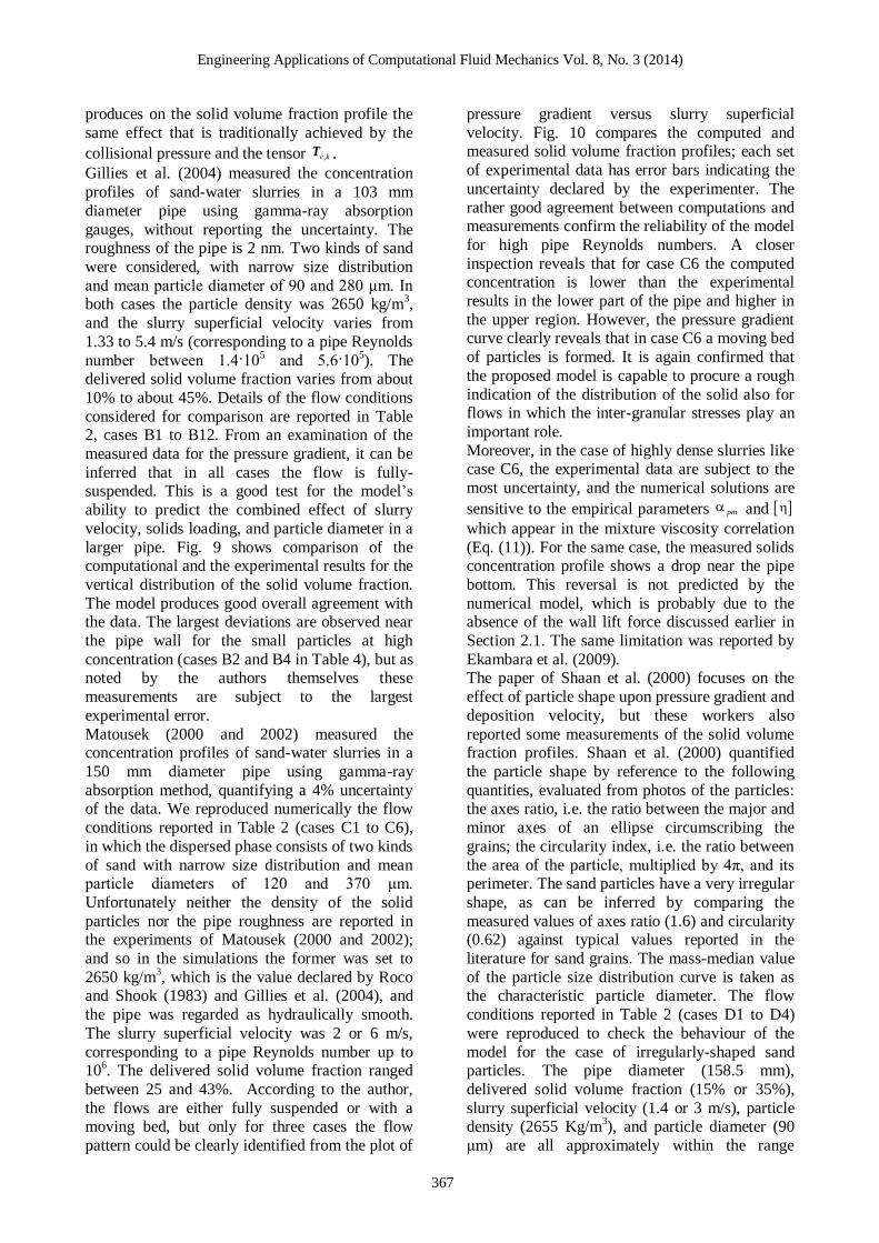
Engineering Applications of Computational Fluid Mechanics Vol 8 No 3 (2014)
367
produces on the solid volume fraction profile the
same effect that is traditionally achieved by the
collisional pressure and the tensor kT
Gillies et al (2004) measured the concentration
profiles of sand-water slurries in a 103 mm
diameter pipe using gamma-ray absorption
gauges without reporting the uncertainty The roughness of the pipe is 2 nm Two kinds of sand
were considered with narrow size distribution
and mean particle diameter of 90 and 280 μm In both cases the particle density was 2650 kgm
3
and the slurry superficial velocity varies from
133 to 54 ms (corresponding to a pipe Reynolds
number between 14105 and 5610
5) The
delivered solid volume fraction varies from about
10 to about 45 Details of the flow conditions
considered for comparison are reported in Table 2 cases B1 to B12 From an examination of the
measured data for the pressure gradient it can be
inferred that in all cases the flow is fully-suspended This is a good test for the modelrsquos
ability to predict the combined effect of slurry
velocity solids loading and particle diameter in a
larger pipe Fig 9 shows comparison of the computational and the experimental results for the
vertical distribution of the solid volume fraction
The model produces good overall agreement with the data The largest deviations are observed near
the pipe wall for the small particles at high
concentration (cases B2 and B4 in Table 4) but as noted by the authors themselves these
measurements are subject to the largest
experimental error
Matousek (2000 and 2002) measured the concentration profiles of sand-water slurries in a
150 mm diameter pipe using gamma-ray
absorption method quantifying a 4 uncertainty of the data We reproduced numerically the flow
conditions reported in Table 2 (cases C1 to C6)
in which the dispersed phase consists of two kinds
of sand with narrow size distribution and mean particle diameters of 120 and 370 μm
Unfortunately neither the density of the solid
particles nor the pipe roughness are reported in the experiments of Matousek (2000 and 2002)
and so in the simulations the former was set to
2650 kgm3 which is the value declared by Roco
and Shook (1983) and Gillies et al (2004) and
the pipe was regarded as hydraulically smooth
The slurry superficial velocity was 2 or 6 ms
corresponding to a pipe Reynolds number up to 10
6 The delivered solid volume fraction ranged
between 25 and 43 According to the author
the flows are either fully suspended or with a moving bed but only for three cases the flow
pattern could be clearly identified from the plot of
pressure gradient versus slurry superficial
velocity Fig 10 compares the computed and measured solid volume fraction profiles each set
of experimental data has error bars indicating the
uncertainty declared by the experimenter The
rather good agreement between computations and measurements confirm the reliability of the model
for high pipe Reynolds numbers A closer
inspection reveals that for case C6 the computed concentration is lower than the experimental
results in the lower part of the pipe and higher in
the upper region However the pressure gradient curve clearly reveals that in case C6 a moving bed
of particles is formed It is again confirmed that
the proposed model is capable to procure a rough
indication of the distribution of the solid also for flows in which the inter-granular stresses play an
important role
Moreover in the case of highly dense slurries like case C6 the experimental data are subject to the
most uncertainty and the numerical solutions are
sensitive to the empirical parameters pm and
which appear in the mixture viscosity correlation
(Eq (11)) For the same case the measured solids concentration profile shows a drop near the pipe
bottom This reversal is not predicted by the
numerical model which is probably due to the absence of the wall lift force discussed earlier in
Section 21 The same limitation was reported by
Ekambara et al (2009) The paper of Shaan et al (2000) focuses on the
effect of particle shape upon pressure gradient and
deposition velocity but these workers also
reported some measurements of the solid volume fraction profiles Shaan et al (2000) quantified
the particle shape by reference to the following
quantities evaluated from photos of the particles the axes ratio ie the ratio between the major and
minor axes of an ellipse circumscribing the
grains the circularity index ie the ratio between
the area of the particle multiplied by 4π and its perimeter The sand particles have a very irregular
shape as can be inferred by comparing the
measured values of axes ratio (16) and circularity (062) against typical values reported in the
literature for sand grains The mass-median value
of the particle size distribution curve is taken as the characteristic particle diameter The flow
conditions reported in Table 2 (cases D1 to D4)
were reproduced to check the behaviour of the
model for the case of irregularly-shaped sand particles The pipe diameter (1585 mm)
delivered solid volume fraction (15 or 35)
slurry superficial velocity (14 or 3 ms) particle density (2655 Kgm
3) and particle diameter (90
μm) are all approximately within the range
Engineering Applications of Computational Fluid Mechanics Vol 8 No 3 (2014)
368
Fig 10 Solids concentration profiles for flow conditions C1 to C6 in Table 2 ( experiments from Matousek
(2000 and 2002) ndashndashndash predictions)
Fig 11 Solids concentration profiles for flow conditions D1 to D4 in Table 2 ( experiments from Shaan et al
(2000) ndashndashndash predictions)
covered by the earlier simulations The numerical and experimental results are
compared in Fig 11 The agreement between the
numerical predictions and the experimental
evidence is fairly good inadequacies of the numerical model ndash especially in the wall
boundary conditions for the solid phase ndash and
measurements error can both contribute to the discrepancies observed near the pipe bottom for
case D2 The results seem to indicate that the
numerical model is a suitable tool for predicting the solid volume fraction distribution produced by
sands with a very irregular shape
32 Horizontal 90deg bend
The predictions of the model have been compared
with the recent experiments of Kaushal et al (2013) regarding a horizontal 90deg bend Among
the different flow conditions considered by these
authors reference is made to those characterized
by delivered solid volume fraction of 882 within the range of interest in this work The
experimenters used a sampling probe to measure
the volume fraction profile of the slurry in the 53
mm diameter pipe along the vertical axis at distances of 5Dp 25Dp and 50Dp downstream the
bend exit (referred to as sections S4 S5 and S6 in
Fig 2 respectively) They quantified a 2
uncertainty of the data The solid phase consists of silica sand particles with narrow size
distribution and mean particle diameter of 450
μm The slurry superficial velocity is 178 267 or 356 ms
The flow within the bend is much more complex
compared to that through the straight pipe since secondary motions develop in the crosswise
direction These motions affect significantly the
distribution of the solids and as a consequence
the volume fraction distribution is no longer constant over horizontal planes This is evident in
Fig 12 which shows the color plot of the solids
volumetric concentration over the six cross sections highlighted in Fig 2 As shown in Fig
13 the predictions of our model generally agree
with the experimental data available Greater
discrepancies are observed for the highest superficial velocity (356 ms) where the model
seems to underestimate the quantity of particles
dragged by the secondary motions This is
Engineering Applications of Computational Fluid Mechanics Vol 8 No 3 (2014)
369
Fig 12 Solid volume fraction distributions on sections
S1 to S6 in Fig 2 for delivered solid volume
fraction of 882 Left hand side is the outer
wall of the pipe
opposite to the KTGF based model of Kaushal et
al (2013) which tends to over-enhance the effect
of the secondary motions on the solids for the
lowest velocities Fig 13 also reveals that our model tends to overestimate the solids volume
fraction close to the pipe bottom far from the
bend exit It is expected that the predictions could
be improved if the effect of the wall lubrication force for which a suitable model does not exist at
present were accounted for
4 CONCLUSIONS
A mathematical model has been described for the
estimation of solid volume fraction distribution of
solid-liquid slurry flows in horizontal pipes and bends The model is based on an Eulerian-
Eulerian approach and uses the Inter-Phase Slip
Algorithm (IPSA) of Spalding (1980) The
novelty of this model resides in the combined use of existing modelling strategies never previously
employed simultaneously for the predictions of
slurry flows In order to account for turbulent dispersion of particles phase diffusion terms have
been included in the phase continuity equations
together with all the conservation equations The mixture viscosity approach is adopted to model
the effect of multiple particles on the inter-phase
friction A wall function is employed to model the
flow in the near-wall region in case of both hydraulically smooth and rough walls All these
strategies result in a model which despite being
simpler that those commonly used for addressing solid-liquid slurry flows shows comparable or
even better predictive capacity Moreover this
model is robust and numerically stable and
requires relatively short CPU time to procure converged steady-state solutions
The model has been first validated by comparison
with experimental data for the horizontal pipe case over a wide range of operating conditions
delivered solid volume fraction between 10 and
40 by volume mean particle diameter between 90 and 520 μm slurry superficial velocity
between 1 ms and 55 ms and pipe diameter
between 50 and 158 mm The model predictions
were found to be in good agreement with the experimental evidence for all the flow conditions
considered for comparison Even if the model is
originally intended to address fully-suspended flows the results indicated its capability to
provide rough indications of the solid volume
fraction distribution also in case of bed flows At last the comparison with the recent
measurements of Kaushal et al (2013) revealed
that this model is capable to procure reliable
predictions of the particle distribution downstream a 90deg bend in a horizontal pipe
Engineering Applications of Computational Fluid Mechanics Vol 8 No 3 (2014)
370
Fig 13 Solid volume fraction along vertical diameter on sections S4 to S6 in Fig 2 for delivered solid volume fraction
of 882 ( experiments from Kaushal et al (2013) ndashndashndash predictions)
ACKNOWLEDGEMENTS The authors would acknowledge the CINECA and
the Regione Lombardia award under the LISA
initiative for the availability of high performance computing resources and support The authors
would like to thank CHAM Ltd for supporting
this research and acknowledge Dr Randy Gillies of Saskatchewan Research Council for providing
his experimental data
REFERENCES
1 Ahilan RV Sleath J (1987) Sediment
transport in oscillatory flow over flat beds Journal of Hydraulic Engineering 113 308-
322
2 Albunaga BE (2002) Slurry Systems Handbook McGraw-Hill
3 Antal S Lahey R Flaherty J (1991) Analysis
of phase distribution in fully-developed
laminar bubbly two phase flow International Journal of Multiphase Flow 17(5) 635-652
4 Barnea E Mizrahi J (1973) A Generalized
Approach to the Fluid Dynamics of
Particulate Systems Chemical Engineering
Science 5(2) 171-189 5 Chen L Duan Y Pu W Zhao C (2009) CFD
simulation of coal-water slurry flowing in
horizontal pipelines Korean Journal of Chemical Engineering 26(4) 1144-1154
6 Chen RC (1994) Analysis of homogeneous
slurry pipe flow Journal of Marine Science and Technology 2(1) 37-45
7 Chen X Li Y Niu X Li M Chen D Yu X
(2011) A general two-phase turbulent flow
model applied to the study of sediment transport in open channels International
Journal of Multiphase Flow 37(9) 1099-
1108 8 Chung JN Troutt TR (1988) Simulation of
particle dispersion in an axisymmetric jet
Journal of Fluid Mechanics 186 199-222 9 Clift R Grace JR Weber ME (1978)
Bubbles Drops and Particles Academic
Press
10 Colwell JM Shook CA (1988) The Entry Length for Slurries in Horizontal Pipeline
Flow Canadian Journal of Chemical
Engineering 66(5) 714-720
Engineering Applications of Computational Fluid Mechanics Vol 8 No 3 (2014)
371
11 Doron P Barnea D (1993) A three layer
model for solid-liquid flow in horizontal pipes International Journal of Multiphase
Flow 19(6) 1029-1043
12 Doron P Barnea D (1995) Pressure drop and
limit deposit velocity for solid-liquid flow in pipes Chemical Engineering and Science
50(10) 1595-1604
13 Doron P Barnea D (1996) Flow pattern maps for solid-liquid flow in pipes International
Journal of Multiphase Flow 22(2) 273-283
14 Doron P Granica D Barnea D (1987) Slurry flow in horizontal pipes ndash experimental and
modeling International Journal of
Multiphase Flow 13(4) 535ndash547
15 Eccedila L Hoekstra M (2006) Discretization uncertainty estimation based on a least
squares version of the grid convergence
index Proceedings of the 2nd
Workshop on CFD Uncertainty Analysis Oct 19-20
Lisbon Portugal
16 Ekambara K Sanders RS Nandakumar K Masliyah JH (2009) Hydrodynamic
simulation of horizontal slurry pipeline flow
using ANSYS-CFX Industrial amp
Engineering Chemistry Research 48(17) 8159-8171
17 Gillies RG Shook CA (2000) Modelling
High Concentration Settling Slurry Flows Canadian Journal of Chemical Engineering
78(4) 709-716
18 Gillies RG Shook CA Xu J (2004)
Modelling Heterogeneous Slurry Flow at High Velocities Canadian Journal of
Chemical Engineering 82(5) 1060-1065
19 Hsu FLG (1981) Flow of Fine-particle Suspensions in Bends Fittings and Valves
MS Thesis Texas Tech University Lubbock
Texas USA 20 Ishii M Mishima K (1984) Two-fluid model
and hydrodynamic constitutive relations
Nuclear Engineering and Design 82(2-3)
107-126 21 Issa RI Oliveira PJ (1997) Assessment of a
particle-turbulence interaction model in
conjunction with an Eulerian two-phase flow formulation Proceedings of the 2
nd
International Symposium on Turbulence
Heat and Mass Transfer June 9-12 Delft Netherlands 759-770
22 Jayatillika CLV (1969) The influence of the
Prandtl number and surface roughness on the
resistance of the sublayer to momentum and heat transfer Progress in Heat amp Mass
Transfer 1 193-329
23 Jiang YY Zhang P (2012) Pressure drop and
flow pattern of slush nitrogen in a horizontal pipe AIChE Journal doi 10002aic13927
24 Kaushal DR Kumar A Tomita Y Juchii S
Tsukamoto H (2013) Flow of mono-
dispersed particles through horizontal bend International Journal of Multiphase Flow 52
71-91
25 Kaushal DR Sato K Toyota T Funatsu K Tomita Y (2005) Effect of particle size
distribution on pressure drop and
concentration profile in pipeline flow of highly concentrated slurry International
Journal of Multiphase Flow 31(7) 809-823
26 Kaushal DR Thinglas T Tomita Y Juchii S
Tsukamoto H (2012) CFD modeling for pipeline flow of fine particles at high
concentration International Journal of
Multiphase Flow 43 85-100 27 Kaushal DR Tomita Y (2003) Comparative
study of pressure drop in multisized
particulate slurry flow through pipe and rectangular duct International Journal of
Multiphase Flow 29(9) 1473-1487
28 Kaushal DR Tomita Y (2007) Experimental
investigation for near-wall lift of coarser particles in slurry pipeline using γ-ray
densitometer Powder Technology 172(3)
177-187 29 Kim C Lee M Han C (2008) Hydraulic
transport of sand-water mixtures in pipelines
Part I Experiment Journal of Mechanical
Science and Technology 22(12) 2534-2541 30 Kumar U Mishra R Singh SN Seshadri V
(2003) Effect of particle gradation on flow
characteristics of ash disposal pipelines Powder Technology 132(1) 39-51
31 Lahiri SK Ghanta KC (2010) Slurry flow
modeling by CFD Chemical Industry amp Chemical Engineering Quarterly 16(4) 295-
308
32 Launder BE Spalding DB (1972)
Mathematical models of turbulence Academic Press
33 Ling J Skudarnov PV Lin CX Ebadian MA
(2003) Numerical investigations of solid-liquid slurry flows in a fully developed flow
region International Journal of Heat and
Fluid Flow 24(3) 389-398 34 Matousek V (2000) Concentration
distribution in pipeline flow of sand-water
mixtures Journal of Hydrology and
Hydromechanics 48(3) 180-196 35 Matousek V (2002) Pressure drops and flow
patterns in sand-mixture pipes Experimental
Engineering Applications of Computational Fluid Mechanics Vol 8 No 3 (2014)
372
Thermal and Fluid Science 26(6-7) 693-702
36 Matousek V (2009) Predictive model for frictional pressure drop in settling-slurry pipe
with stationary deposit Powder Technology
192(3) 367-374
37 Mooney M (1951) The viscosity of a concentrated suspension of spherical
particles Journal of Colloid Science 6(2)
162-170 38 Nasr-el-Din H Shook CA Esmail MN
(1984) Isokinetic Probe Sampling From
Slurry Pipelines Canadian Journal of Chemical Engineering 62(2) 179-185
39 Pathak M (2011) Computational
investigations of solid-liquid particle
interaction in a two-phase flow around a ducted obstruction Journal of Hydraulic
Research 49(1) 96-104
40 Pecker SM Helvaci SS (2008) Solid-Liquid Two-Phase Flow Elsevier
41 Roco MC Shook CA (1983) Modeling of
Slurry Flow The Effect of Particle Size Canadian Journal of Chemical Engineering
61(4) 494-503
42 Schlichting H (1960) Boundary Layer
Theory McGraw-Hill 43 Shaan J Sumner RJ Gillies RG Shook CA
(2000) The Effect of Particle Shape on
Pipeline Friction for Newtonian Slurries of Fine Particles Canadian Journal of Chemical
Engineering 78(4) 717-725
44 Shiller L Naumann A (1935) A drag
coefficient correlation Zeitschrift des Vereines Deutscher Ingenieure 77 318-320
45 Shirolkar JS Coimbra CFM McQuay MQ
(1996) Fundamental aspects of modelling turbulent particle dispersion in dilute flows
Progress in Energy and Combustion Science
22(4) 363-399 46 Shook CA Bartosik AS (1994) Particle-wall
stresses in vertical slurry flows Powder
Technology 81(2) 117-124
47 Skudarnov PV Lin CX Ebadian MA (2004) Double-Species Slurry Flow in a Horizontal
Pipeline ASME Journal of Fluids
Engineering 126(1) 125-132 48 Spalding DB (1972) A novel finite-
difference formulation for differential
expressions involving both first and second derivatives International Journal of
Numerical Methods in Engineering 4(4) 551-
559
49 Spalding DB (1980) Numerical computation of multi-phase fluid flow and heat transfer In
Taylor C Morgan K (Eds) Recent Advances
in Numerical Methods in Fluids Pineridge
Press Limited 139-168 50 Turian RM Ma TW Hsu FLG Sung MDJ
Plackmann GW (1998) Flow of concentrated
non-Newtonian slurries 2 Friction losses in
bends fittings valves and Venturi meters International Journal of Multiphase Flow
24(2) 243-269
51 Versteeg HK Malalasekera W (2007) An Introduction to Computational Fluid
Dynamics The Finite Volume Method
Pearson Prentice Hall 52 Wilson KC Sanders RS Gillies RG Shook
CA (2010) Verification of the near-wall
model for slurry flow Powder Technology
197(3) 247-253 53 Wilson KC Sellgren A (2003) Interaction of
Particles and Near-Wall Lift in Slurry
Pipelines Journal of Hydraulic Engineering 129(1) 73-76
- Figures13
-
- Fig 1 Computational domain and boundaryconditions for horizontal pipe
- Fig 2 Computational domain boundary conditionsand reference sections for 90deg bend (S1=bendinlet S2=bend centre S3=bend exit S4=5Dpfrom bend exit S5=25Dp from bend exitS6=50Dp from bend exit)
- Fig3 Solid volume fraction profiles calculated onthree different grid levels for straight pipecase
- Fig4 Details of mesh for 90deg bend
- Fig5 Vertical solid volume fraction profiles atdistance of 5Dp downstream bend exit (SectionS4 in Fig 2) calculated on different gridlevels The Grid 3 solution has error barscorresponding to the grid discretization errorestimated by the method of Eccedila and Hoekstra(2006)
- Fig 6 Effect of turbulent Schmidt number for volume fractions a s on solid volume fraction profiles for two flowconditions (r experiments from Roco and Shook (1983) ndashndashndash 03 a s = ndashndashndash 05 a s = ndashndashndash 07 a s = ndashndashndash09 a s = )
- Fig 7 Effect of parameters [η] and pm a in mixture viscosity correlation of Mooney (Eq 11) on solid volume fractionprofiles for two flow conditions (r experiments from Roco and Shook (1983) continuous lines predictions)The dependence on [η] is studied for 07 pm a = that on pm a for [η] = 25
- Fig 8 Solids concentration profiles for flow conditions A1 to A5 in Table 2 (rbull experiments from Roco and Shook (1983) ndashndashndash predictions)
- Fig 9 Solids concentration profile for flow conditions B1 to B12 in Table 2 (rbulls experiments from Gillies et al (2004) ndashndashndash predictions)
- Fig 10 Solids concentration profiles for flow conditions C1 to C6 in Table 2 (rbull experiments from Matousek (2000 and 2002) ndashndashndash predictions)
- Fig 11 Solids concentration profiles for flow conditions D1 to D4 in Table 2 (rbull experiments from Shaan et al (2000) ndashndashndash predictions)
- Fig 12 Solid volume fraction distributions on sections S1 to S6 in Fig 2 for delivered solid volume fraction of 882 Left hand side is the outer wall of the pipe
- Fig 13 Solid volume fraction along vertical diameter on sections S4 to S6 in Fig 2 for delivered solid volume fraction of 882 (r experiments from Kaushal et al (2013) ndashndashndash predictions)
-
- Tables13
-
- Table 1 Flow conditions considered for comparison
- Table 2 Details of experimental conditions for straight pipe case (A1 to A5 experimental data from Roco and Shook(1983) B1 to B12 experimental data from Gillies et al (2004) C1 to C6 experimental data from Matousek(2000 and 2002) D1 to D4 experimental data from Shaan et al (2000) values not declared byexperimenters)
-
- 1 INTRODUCTION
- 2 MATHEMATICAL MODEL
-
- 21 Conservation equations
- 22 Turbulence modeling
- 23 Computational domain and boundaryconditions
- 24 Computational methodology and consistencyof numerical solution
- 25 Governing terms and calibration ofnumerical constants
-
- 3 RESULTS
-
- 31 Straight horizontal pipe
- 32 Horizontal 90deg bend
-
- 4 CONCLUSIONS
- ACKNOWLEDGEMENTS
- REFERENCES
-
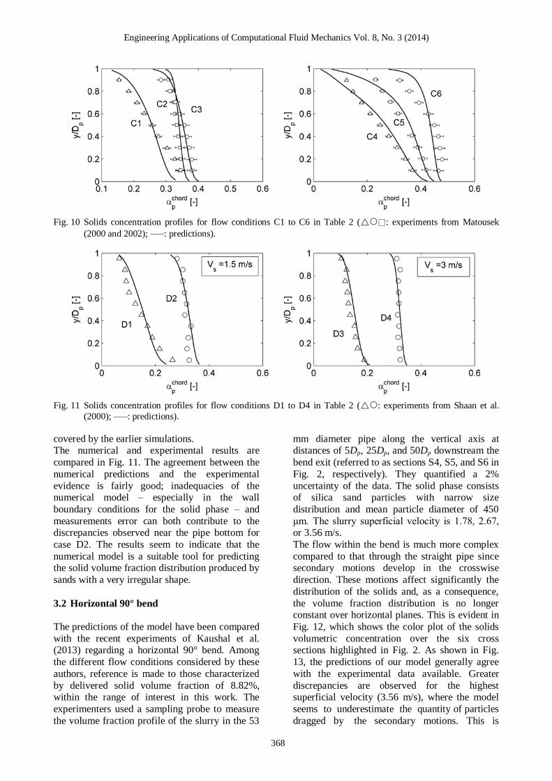
Engineering Applications of Computational Fluid Mechanics Vol 8 No 3 (2014)
368
Fig 10 Solids concentration profiles for flow conditions C1 to C6 in Table 2 ( experiments from Matousek
(2000 and 2002) ndashndashndash predictions)
Fig 11 Solids concentration profiles for flow conditions D1 to D4 in Table 2 ( experiments from Shaan et al
(2000) ndashndashndash predictions)
covered by the earlier simulations The numerical and experimental results are
compared in Fig 11 The agreement between the
numerical predictions and the experimental
evidence is fairly good inadequacies of the numerical model ndash especially in the wall
boundary conditions for the solid phase ndash and
measurements error can both contribute to the discrepancies observed near the pipe bottom for
case D2 The results seem to indicate that the
numerical model is a suitable tool for predicting the solid volume fraction distribution produced by
sands with a very irregular shape
32 Horizontal 90deg bend
The predictions of the model have been compared
with the recent experiments of Kaushal et al (2013) regarding a horizontal 90deg bend Among
the different flow conditions considered by these
authors reference is made to those characterized
by delivered solid volume fraction of 882 within the range of interest in this work The
experimenters used a sampling probe to measure
the volume fraction profile of the slurry in the 53
mm diameter pipe along the vertical axis at distances of 5Dp 25Dp and 50Dp downstream the
bend exit (referred to as sections S4 S5 and S6 in
Fig 2 respectively) They quantified a 2
uncertainty of the data The solid phase consists of silica sand particles with narrow size
distribution and mean particle diameter of 450
μm The slurry superficial velocity is 178 267 or 356 ms
The flow within the bend is much more complex
compared to that through the straight pipe since secondary motions develop in the crosswise
direction These motions affect significantly the
distribution of the solids and as a consequence
the volume fraction distribution is no longer constant over horizontal planes This is evident in
Fig 12 which shows the color plot of the solids
volumetric concentration over the six cross sections highlighted in Fig 2 As shown in Fig
13 the predictions of our model generally agree
with the experimental data available Greater
discrepancies are observed for the highest superficial velocity (356 ms) where the model
seems to underestimate the quantity of particles
dragged by the secondary motions This is
Engineering Applications of Computational Fluid Mechanics Vol 8 No 3 (2014)
369
Fig 12 Solid volume fraction distributions on sections
S1 to S6 in Fig 2 for delivered solid volume
fraction of 882 Left hand side is the outer
wall of the pipe
opposite to the KTGF based model of Kaushal et
al (2013) which tends to over-enhance the effect
of the secondary motions on the solids for the
lowest velocities Fig 13 also reveals that our model tends to overestimate the solids volume
fraction close to the pipe bottom far from the
bend exit It is expected that the predictions could
be improved if the effect of the wall lubrication force for which a suitable model does not exist at
present were accounted for
4 CONCLUSIONS
A mathematical model has been described for the
estimation of solid volume fraction distribution of
solid-liquid slurry flows in horizontal pipes and bends The model is based on an Eulerian-
Eulerian approach and uses the Inter-Phase Slip
Algorithm (IPSA) of Spalding (1980) The
novelty of this model resides in the combined use of existing modelling strategies never previously
employed simultaneously for the predictions of
slurry flows In order to account for turbulent dispersion of particles phase diffusion terms have
been included in the phase continuity equations
together with all the conservation equations The mixture viscosity approach is adopted to model
the effect of multiple particles on the inter-phase
friction A wall function is employed to model the
flow in the near-wall region in case of both hydraulically smooth and rough walls All these
strategies result in a model which despite being
simpler that those commonly used for addressing solid-liquid slurry flows shows comparable or
even better predictive capacity Moreover this
model is robust and numerically stable and
requires relatively short CPU time to procure converged steady-state solutions
The model has been first validated by comparison
with experimental data for the horizontal pipe case over a wide range of operating conditions
delivered solid volume fraction between 10 and
40 by volume mean particle diameter between 90 and 520 μm slurry superficial velocity
between 1 ms and 55 ms and pipe diameter
between 50 and 158 mm The model predictions
were found to be in good agreement with the experimental evidence for all the flow conditions
considered for comparison Even if the model is
originally intended to address fully-suspended flows the results indicated its capability to
provide rough indications of the solid volume
fraction distribution also in case of bed flows At last the comparison with the recent
measurements of Kaushal et al (2013) revealed
that this model is capable to procure reliable
predictions of the particle distribution downstream a 90deg bend in a horizontal pipe
Engineering Applications of Computational Fluid Mechanics Vol 8 No 3 (2014)
370
Fig 13 Solid volume fraction along vertical diameter on sections S4 to S6 in Fig 2 for delivered solid volume fraction
of 882 ( experiments from Kaushal et al (2013) ndashndashndash predictions)
ACKNOWLEDGEMENTS The authors would acknowledge the CINECA and
the Regione Lombardia award under the LISA
initiative for the availability of high performance computing resources and support The authors
would like to thank CHAM Ltd for supporting
this research and acknowledge Dr Randy Gillies of Saskatchewan Research Council for providing
his experimental data
REFERENCES
1 Ahilan RV Sleath J (1987) Sediment
transport in oscillatory flow over flat beds Journal of Hydraulic Engineering 113 308-
322
2 Albunaga BE (2002) Slurry Systems Handbook McGraw-Hill
3 Antal S Lahey R Flaherty J (1991) Analysis
of phase distribution in fully-developed
laminar bubbly two phase flow International Journal of Multiphase Flow 17(5) 635-652
4 Barnea E Mizrahi J (1973) A Generalized
Approach to the Fluid Dynamics of
Particulate Systems Chemical Engineering
Science 5(2) 171-189 5 Chen L Duan Y Pu W Zhao C (2009) CFD
simulation of coal-water slurry flowing in
horizontal pipelines Korean Journal of Chemical Engineering 26(4) 1144-1154
6 Chen RC (1994) Analysis of homogeneous
slurry pipe flow Journal of Marine Science and Technology 2(1) 37-45
7 Chen X Li Y Niu X Li M Chen D Yu X
(2011) A general two-phase turbulent flow
model applied to the study of sediment transport in open channels International
Journal of Multiphase Flow 37(9) 1099-
1108 8 Chung JN Troutt TR (1988) Simulation of
particle dispersion in an axisymmetric jet
Journal of Fluid Mechanics 186 199-222 9 Clift R Grace JR Weber ME (1978)
Bubbles Drops and Particles Academic
Press
10 Colwell JM Shook CA (1988) The Entry Length for Slurries in Horizontal Pipeline
Flow Canadian Journal of Chemical
Engineering 66(5) 714-720
Engineering Applications of Computational Fluid Mechanics Vol 8 No 3 (2014)
371
11 Doron P Barnea D (1993) A three layer
model for solid-liquid flow in horizontal pipes International Journal of Multiphase
Flow 19(6) 1029-1043
12 Doron P Barnea D (1995) Pressure drop and
limit deposit velocity for solid-liquid flow in pipes Chemical Engineering and Science
50(10) 1595-1604
13 Doron P Barnea D (1996) Flow pattern maps for solid-liquid flow in pipes International
Journal of Multiphase Flow 22(2) 273-283
14 Doron P Granica D Barnea D (1987) Slurry flow in horizontal pipes ndash experimental and
modeling International Journal of
Multiphase Flow 13(4) 535ndash547
15 Eccedila L Hoekstra M (2006) Discretization uncertainty estimation based on a least
squares version of the grid convergence
index Proceedings of the 2nd
Workshop on CFD Uncertainty Analysis Oct 19-20
Lisbon Portugal
16 Ekambara K Sanders RS Nandakumar K Masliyah JH (2009) Hydrodynamic
simulation of horizontal slurry pipeline flow
using ANSYS-CFX Industrial amp
Engineering Chemistry Research 48(17) 8159-8171
17 Gillies RG Shook CA (2000) Modelling
High Concentration Settling Slurry Flows Canadian Journal of Chemical Engineering
78(4) 709-716
18 Gillies RG Shook CA Xu J (2004)
Modelling Heterogeneous Slurry Flow at High Velocities Canadian Journal of
Chemical Engineering 82(5) 1060-1065
19 Hsu FLG (1981) Flow of Fine-particle Suspensions in Bends Fittings and Valves
MS Thesis Texas Tech University Lubbock
Texas USA 20 Ishii M Mishima K (1984) Two-fluid model
and hydrodynamic constitutive relations
Nuclear Engineering and Design 82(2-3)
107-126 21 Issa RI Oliveira PJ (1997) Assessment of a
particle-turbulence interaction model in
conjunction with an Eulerian two-phase flow formulation Proceedings of the 2
nd
International Symposium on Turbulence
Heat and Mass Transfer June 9-12 Delft Netherlands 759-770
22 Jayatillika CLV (1969) The influence of the
Prandtl number and surface roughness on the
resistance of the sublayer to momentum and heat transfer Progress in Heat amp Mass
Transfer 1 193-329
23 Jiang YY Zhang P (2012) Pressure drop and
flow pattern of slush nitrogen in a horizontal pipe AIChE Journal doi 10002aic13927
24 Kaushal DR Kumar A Tomita Y Juchii S
Tsukamoto H (2013) Flow of mono-
dispersed particles through horizontal bend International Journal of Multiphase Flow 52
71-91
25 Kaushal DR Sato K Toyota T Funatsu K Tomita Y (2005) Effect of particle size
distribution on pressure drop and
concentration profile in pipeline flow of highly concentrated slurry International
Journal of Multiphase Flow 31(7) 809-823
26 Kaushal DR Thinglas T Tomita Y Juchii S
Tsukamoto H (2012) CFD modeling for pipeline flow of fine particles at high
concentration International Journal of
Multiphase Flow 43 85-100 27 Kaushal DR Tomita Y (2003) Comparative
study of pressure drop in multisized
particulate slurry flow through pipe and rectangular duct International Journal of
Multiphase Flow 29(9) 1473-1487
28 Kaushal DR Tomita Y (2007) Experimental
investigation for near-wall lift of coarser particles in slurry pipeline using γ-ray
densitometer Powder Technology 172(3)
177-187 29 Kim C Lee M Han C (2008) Hydraulic
transport of sand-water mixtures in pipelines
Part I Experiment Journal of Mechanical
Science and Technology 22(12) 2534-2541 30 Kumar U Mishra R Singh SN Seshadri V
(2003) Effect of particle gradation on flow
characteristics of ash disposal pipelines Powder Technology 132(1) 39-51
31 Lahiri SK Ghanta KC (2010) Slurry flow
modeling by CFD Chemical Industry amp Chemical Engineering Quarterly 16(4) 295-
308
32 Launder BE Spalding DB (1972)
Mathematical models of turbulence Academic Press
33 Ling J Skudarnov PV Lin CX Ebadian MA
(2003) Numerical investigations of solid-liquid slurry flows in a fully developed flow
region International Journal of Heat and
Fluid Flow 24(3) 389-398 34 Matousek V (2000) Concentration
distribution in pipeline flow of sand-water
mixtures Journal of Hydrology and
Hydromechanics 48(3) 180-196 35 Matousek V (2002) Pressure drops and flow
patterns in sand-mixture pipes Experimental
Engineering Applications of Computational Fluid Mechanics Vol 8 No 3 (2014)
372
Thermal and Fluid Science 26(6-7) 693-702
36 Matousek V (2009) Predictive model for frictional pressure drop in settling-slurry pipe
with stationary deposit Powder Technology
192(3) 367-374
37 Mooney M (1951) The viscosity of a concentrated suspension of spherical
particles Journal of Colloid Science 6(2)
162-170 38 Nasr-el-Din H Shook CA Esmail MN
(1984) Isokinetic Probe Sampling From
Slurry Pipelines Canadian Journal of Chemical Engineering 62(2) 179-185
39 Pathak M (2011) Computational
investigations of solid-liquid particle
interaction in a two-phase flow around a ducted obstruction Journal of Hydraulic
Research 49(1) 96-104
40 Pecker SM Helvaci SS (2008) Solid-Liquid Two-Phase Flow Elsevier
41 Roco MC Shook CA (1983) Modeling of
Slurry Flow The Effect of Particle Size Canadian Journal of Chemical Engineering
61(4) 494-503
42 Schlichting H (1960) Boundary Layer
Theory McGraw-Hill 43 Shaan J Sumner RJ Gillies RG Shook CA
(2000) The Effect of Particle Shape on
Pipeline Friction for Newtonian Slurries of Fine Particles Canadian Journal of Chemical
Engineering 78(4) 717-725
44 Shiller L Naumann A (1935) A drag
coefficient correlation Zeitschrift des Vereines Deutscher Ingenieure 77 318-320
45 Shirolkar JS Coimbra CFM McQuay MQ
(1996) Fundamental aspects of modelling turbulent particle dispersion in dilute flows
Progress in Energy and Combustion Science
22(4) 363-399 46 Shook CA Bartosik AS (1994) Particle-wall
stresses in vertical slurry flows Powder
Technology 81(2) 117-124
47 Skudarnov PV Lin CX Ebadian MA (2004) Double-Species Slurry Flow in a Horizontal
Pipeline ASME Journal of Fluids
Engineering 126(1) 125-132 48 Spalding DB (1972) A novel finite-
difference formulation for differential
expressions involving both first and second derivatives International Journal of
Numerical Methods in Engineering 4(4) 551-
559
49 Spalding DB (1980) Numerical computation of multi-phase fluid flow and heat transfer In
Taylor C Morgan K (Eds) Recent Advances
in Numerical Methods in Fluids Pineridge
Press Limited 139-168 50 Turian RM Ma TW Hsu FLG Sung MDJ
Plackmann GW (1998) Flow of concentrated
non-Newtonian slurries 2 Friction losses in
bends fittings valves and Venturi meters International Journal of Multiphase Flow
24(2) 243-269
51 Versteeg HK Malalasekera W (2007) An Introduction to Computational Fluid
Dynamics The Finite Volume Method
Pearson Prentice Hall 52 Wilson KC Sanders RS Gillies RG Shook
CA (2010) Verification of the near-wall
model for slurry flow Powder Technology
197(3) 247-253 53 Wilson KC Sellgren A (2003) Interaction of
Particles and Near-Wall Lift in Slurry
Pipelines Journal of Hydraulic Engineering 129(1) 73-76
- Figures13
-
- Fig 1 Computational domain and boundaryconditions for horizontal pipe
- Fig 2 Computational domain boundary conditionsand reference sections for 90deg bend (S1=bendinlet S2=bend centre S3=bend exit S4=5Dpfrom bend exit S5=25Dp from bend exitS6=50Dp from bend exit)
- Fig3 Solid volume fraction profiles calculated onthree different grid levels for straight pipecase
- Fig4 Details of mesh for 90deg bend
- Fig5 Vertical solid volume fraction profiles atdistance of 5Dp downstream bend exit (SectionS4 in Fig 2) calculated on different gridlevels The Grid 3 solution has error barscorresponding to the grid discretization errorestimated by the method of Eccedila and Hoekstra(2006)
- Fig 6 Effect of turbulent Schmidt number for volume fractions a s on solid volume fraction profiles for two flowconditions (r experiments from Roco and Shook (1983) ndashndashndash 03 a s = ndashndashndash 05 a s = ndashndashndash 07 a s = ndashndashndash09 a s = )
- Fig 7 Effect of parameters [η] and pm a in mixture viscosity correlation of Mooney (Eq 11) on solid volume fractionprofiles for two flow conditions (r experiments from Roco and Shook (1983) continuous lines predictions)The dependence on [η] is studied for 07 pm a = that on pm a for [η] = 25
- Fig 8 Solids concentration profiles for flow conditions A1 to A5 in Table 2 (rbull experiments from Roco and Shook (1983) ndashndashndash predictions)
- Fig 9 Solids concentration profile for flow conditions B1 to B12 in Table 2 (rbulls experiments from Gillies et al (2004) ndashndashndash predictions)
- Fig 10 Solids concentration profiles for flow conditions C1 to C6 in Table 2 (rbull experiments from Matousek (2000 and 2002) ndashndashndash predictions)
- Fig 11 Solids concentration profiles for flow conditions D1 to D4 in Table 2 (rbull experiments from Shaan et al (2000) ndashndashndash predictions)
- Fig 12 Solid volume fraction distributions on sections S1 to S6 in Fig 2 for delivered solid volume fraction of 882 Left hand side is the outer wall of the pipe
- Fig 13 Solid volume fraction along vertical diameter on sections S4 to S6 in Fig 2 for delivered solid volume fraction of 882 (r experiments from Kaushal et al (2013) ndashndashndash predictions)
-
- Tables13
-
- Table 1 Flow conditions considered for comparison
- Table 2 Details of experimental conditions for straight pipe case (A1 to A5 experimental data from Roco and Shook(1983) B1 to B12 experimental data from Gillies et al (2004) C1 to C6 experimental data from Matousek(2000 and 2002) D1 to D4 experimental data from Shaan et al (2000) values not declared byexperimenters)
-
- 1 INTRODUCTION
- 2 MATHEMATICAL MODEL
-
- 21 Conservation equations
- 22 Turbulence modeling
- 23 Computational domain and boundaryconditions
- 24 Computational methodology and consistencyof numerical solution
- 25 Governing terms and calibration ofnumerical constants
-
- 3 RESULTS
-
- 31 Straight horizontal pipe
- 32 Horizontal 90deg bend
-
- 4 CONCLUSIONS
- ACKNOWLEDGEMENTS
- REFERENCES
-
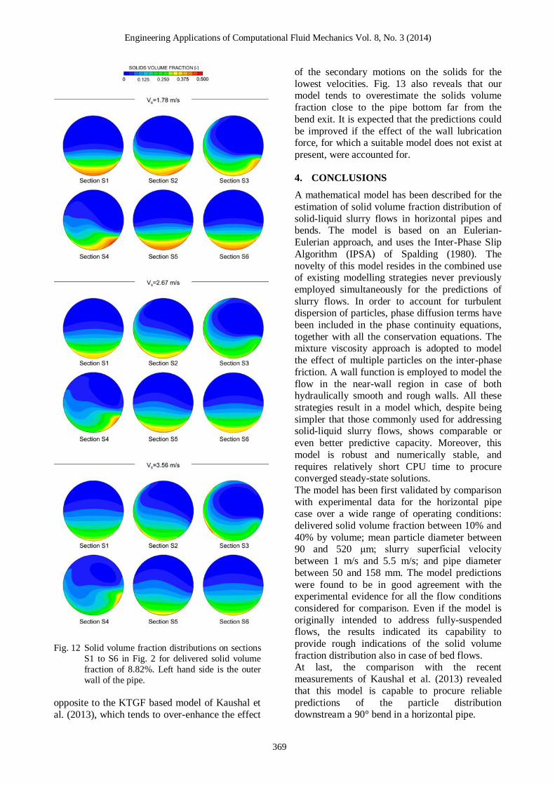
Engineering Applications of Computational Fluid Mechanics Vol 8 No 3 (2014)
369
Fig 12 Solid volume fraction distributions on sections
S1 to S6 in Fig 2 for delivered solid volume
fraction of 882 Left hand side is the outer
wall of the pipe
opposite to the KTGF based model of Kaushal et
al (2013) which tends to over-enhance the effect
of the secondary motions on the solids for the
lowest velocities Fig 13 also reveals that our model tends to overestimate the solids volume
fraction close to the pipe bottom far from the
bend exit It is expected that the predictions could
be improved if the effect of the wall lubrication force for which a suitable model does not exist at
present were accounted for
4 CONCLUSIONS
A mathematical model has been described for the
estimation of solid volume fraction distribution of
solid-liquid slurry flows in horizontal pipes and bends The model is based on an Eulerian-
Eulerian approach and uses the Inter-Phase Slip
Algorithm (IPSA) of Spalding (1980) The
novelty of this model resides in the combined use of existing modelling strategies never previously
employed simultaneously for the predictions of
slurry flows In order to account for turbulent dispersion of particles phase diffusion terms have
been included in the phase continuity equations
together with all the conservation equations The mixture viscosity approach is adopted to model
the effect of multiple particles on the inter-phase
friction A wall function is employed to model the
flow in the near-wall region in case of both hydraulically smooth and rough walls All these
strategies result in a model which despite being
simpler that those commonly used for addressing solid-liquid slurry flows shows comparable or
even better predictive capacity Moreover this
model is robust and numerically stable and
requires relatively short CPU time to procure converged steady-state solutions
The model has been first validated by comparison
with experimental data for the horizontal pipe case over a wide range of operating conditions
delivered solid volume fraction between 10 and
40 by volume mean particle diameter between 90 and 520 μm slurry superficial velocity
between 1 ms and 55 ms and pipe diameter
between 50 and 158 mm The model predictions
were found to be in good agreement with the experimental evidence for all the flow conditions
considered for comparison Even if the model is
originally intended to address fully-suspended flows the results indicated its capability to
provide rough indications of the solid volume
fraction distribution also in case of bed flows At last the comparison with the recent
measurements of Kaushal et al (2013) revealed
that this model is capable to procure reliable
predictions of the particle distribution downstream a 90deg bend in a horizontal pipe
Engineering Applications of Computational Fluid Mechanics Vol 8 No 3 (2014)
370
Fig 13 Solid volume fraction along vertical diameter on sections S4 to S6 in Fig 2 for delivered solid volume fraction
of 882 ( experiments from Kaushal et al (2013) ndashndashndash predictions)
ACKNOWLEDGEMENTS The authors would acknowledge the CINECA and
the Regione Lombardia award under the LISA
initiative for the availability of high performance computing resources and support The authors
would like to thank CHAM Ltd for supporting
this research and acknowledge Dr Randy Gillies of Saskatchewan Research Council for providing
his experimental data
REFERENCES
1 Ahilan RV Sleath J (1987) Sediment
transport in oscillatory flow over flat beds Journal of Hydraulic Engineering 113 308-
322
2 Albunaga BE (2002) Slurry Systems Handbook McGraw-Hill
3 Antal S Lahey R Flaherty J (1991) Analysis
of phase distribution in fully-developed
laminar bubbly two phase flow International Journal of Multiphase Flow 17(5) 635-652
4 Barnea E Mizrahi J (1973) A Generalized
Approach to the Fluid Dynamics of
Particulate Systems Chemical Engineering
Science 5(2) 171-189 5 Chen L Duan Y Pu W Zhao C (2009) CFD
simulation of coal-water slurry flowing in
horizontal pipelines Korean Journal of Chemical Engineering 26(4) 1144-1154
6 Chen RC (1994) Analysis of homogeneous
slurry pipe flow Journal of Marine Science and Technology 2(1) 37-45
7 Chen X Li Y Niu X Li M Chen D Yu X
(2011) A general two-phase turbulent flow
model applied to the study of sediment transport in open channels International
Journal of Multiphase Flow 37(9) 1099-
1108 8 Chung JN Troutt TR (1988) Simulation of
particle dispersion in an axisymmetric jet
Journal of Fluid Mechanics 186 199-222 9 Clift R Grace JR Weber ME (1978)
Bubbles Drops and Particles Academic
Press
10 Colwell JM Shook CA (1988) The Entry Length for Slurries in Horizontal Pipeline
Flow Canadian Journal of Chemical
Engineering 66(5) 714-720
Engineering Applications of Computational Fluid Mechanics Vol 8 No 3 (2014)
371
11 Doron P Barnea D (1993) A three layer
model for solid-liquid flow in horizontal pipes International Journal of Multiphase
Flow 19(6) 1029-1043
12 Doron P Barnea D (1995) Pressure drop and
limit deposit velocity for solid-liquid flow in pipes Chemical Engineering and Science
50(10) 1595-1604
13 Doron P Barnea D (1996) Flow pattern maps for solid-liquid flow in pipes International
Journal of Multiphase Flow 22(2) 273-283
14 Doron P Granica D Barnea D (1987) Slurry flow in horizontal pipes ndash experimental and
modeling International Journal of
Multiphase Flow 13(4) 535ndash547
15 Eccedila L Hoekstra M (2006) Discretization uncertainty estimation based on a least
squares version of the grid convergence
index Proceedings of the 2nd
Workshop on CFD Uncertainty Analysis Oct 19-20
Lisbon Portugal
16 Ekambara K Sanders RS Nandakumar K Masliyah JH (2009) Hydrodynamic
simulation of horizontal slurry pipeline flow
using ANSYS-CFX Industrial amp
Engineering Chemistry Research 48(17) 8159-8171
17 Gillies RG Shook CA (2000) Modelling
High Concentration Settling Slurry Flows Canadian Journal of Chemical Engineering
78(4) 709-716
18 Gillies RG Shook CA Xu J (2004)
Modelling Heterogeneous Slurry Flow at High Velocities Canadian Journal of
Chemical Engineering 82(5) 1060-1065
19 Hsu FLG (1981) Flow of Fine-particle Suspensions in Bends Fittings and Valves
MS Thesis Texas Tech University Lubbock
Texas USA 20 Ishii M Mishima K (1984) Two-fluid model
and hydrodynamic constitutive relations
Nuclear Engineering and Design 82(2-3)
107-126 21 Issa RI Oliveira PJ (1997) Assessment of a
particle-turbulence interaction model in
conjunction with an Eulerian two-phase flow formulation Proceedings of the 2
nd
International Symposium on Turbulence
Heat and Mass Transfer June 9-12 Delft Netherlands 759-770
22 Jayatillika CLV (1969) The influence of the
Prandtl number and surface roughness on the
resistance of the sublayer to momentum and heat transfer Progress in Heat amp Mass
Transfer 1 193-329
23 Jiang YY Zhang P (2012) Pressure drop and
flow pattern of slush nitrogen in a horizontal pipe AIChE Journal doi 10002aic13927
24 Kaushal DR Kumar A Tomita Y Juchii S
Tsukamoto H (2013) Flow of mono-
dispersed particles through horizontal bend International Journal of Multiphase Flow 52
71-91
25 Kaushal DR Sato K Toyota T Funatsu K Tomita Y (2005) Effect of particle size
distribution on pressure drop and
concentration profile in pipeline flow of highly concentrated slurry International
Journal of Multiphase Flow 31(7) 809-823
26 Kaushal DR Thinglas T Tomita Y Juchii S
Tsukamoto H (2012) CFD modeling for pipeline flow of fine particles at high
concentration International Journal of
Multiphase Flow 43 85-100 27 Kaushal DR Tomita Y (2003) Comparative
study of pressure drop in multisized
particulate slurry flow through pipe and rectangular duct International Journal of
Multiphase Flow 29(9) 1473-1487
28 Kaushal DR Tomita Y (2007) Experimental
investigation for near-wall lift of coarser particles in slurry pipeline using γ-ray
densitometer Powder Technology 172(3)
177-187 29 Kim C Lee M Han C (2008) Hydraulic
transport of sand-water mixtures in pipelines
Part I Experiment Journal of Mechanical
Science and Technology 22(12) 2534-2541 30 Kumar U Mishra R Singh SN Seshadri V
(2003) Effect of particle gradation on flow
characteristics of ash disposal pipelines Powder Technology 132(1) 39-51
31 Lahiri SK Ghanta KC (2010) Slurry flow
modeling by CFD Chemical Industry amp Chemical Engineering Quarterly 16(4) 295-
308
32 Launder BE Spalding DB (1972)
Mathematical models of turbulence Academic Press
33 Ling J Skudarnov PV Lin CX Ebadian MA
(2003) Numerical investigations of solid-liquid slurry flows in a fully developed flow
region International Journal of Heat and
Fluid Flow 24(3) 389-398 34 Matousek V (2000) Concentration
distribution in pipeline flow of sand-water
mixtures Journal of Hydrology and
Hydromechanics 48(3) 180-196 35 Matousek V (2002) Pressure drops and flow
patterns in sand-mixture pipes Experimental
Engineering Applications of Computational Fluid Mechanics Vol 8 No 3 (2014)
372
Thermal and Fluid Science 26(6-7) 693-702
36 Matousek V (2009) Predictive model for frictional pressure drop in settling-slurry pipe
with stationary deposit Powder Technology
192(3) 367-374
37 Mooney M (1951) The viscosity of a concentrated suspension of spherical
particles Journal of Colloid Science 6(2)
162-170 38 Nasr-el-Din H Shook CA Esmail MN
(1984) Isokinetic Probe Sampling From
Slurry Pipelines Canadian Journal of Chemical Engineering 62(2) 179-185
39 Pathak M (2011) Computational
investigations of solid-liquid particle
interaction in a two-phase flow around a ducted obstruction Journal of Hydraulic
Research 49(1) 96-104
40 Pecker SM Helvaci SS (2008) Solid-Liquid Two-Phase Flow Elsevier
41 Roco MC Shook CA (1983) Modeling of
Slurry Flow The Effect of Particle Size Canadian Journal of Chemical Engineering
61(4) 494-503
42 Schlichting H (1960) Boundary Layer
Theory McGraw-Hill 43 Shaan J Sumner RJ Gillies RG Shook CA
(2000) The Effect of Particle Shape on
Pipeline Friction for Newtonian Slurries of Fine Particles Canadian Journal of Chemical
Engineering 78(4) 717-725
44 Shiller L Naumann A (1935) A drag
coefficient correlation Zeitschrift des Vereines Deutscher Ingenieure 77 318-320
45 Shirolkar JS Coimbra CFM McQuay MQ
(1996) Fundamental aspects of modelling turbulent particle dispersion in dilute flows
Progress in Energy and Combustion Science
22(4) 363-399 46 Shook CA Bartosik AS (1994) Particle-wall
stresses in vertical slurry flows Powder
Technology 81(2) 117-124
47 Skudarnov PV Lin CX Ebadian MA (2004) Double-Species Slurry Flow in a Horizontal
Pipeline ASME Journal of Fluids
Engineering 126(1) 125-132 48 Spalding DB (1972) A novel finite-
difference formulation for differential
expressions involving both first and second derivatives International Journal of
Numerical Methods in Engineering 4(4) 551-
559
49 Spalding DB (1980) Numerical computation of multi-phase fluid flow and heat transfer In
Taylor C Morgan K (Eds) Recent Advances
in Numerical Methods in Fluids Pineridge
Press Limited 139-168 50 Turian RM Ma TW Hsu FLG Sung MDJ
Plackmann GW (1998) Flow of concentrated
non-Newtonian slurries 2 Friction losses in
bends fittings valves and Venturi meters International Journal of Multiphase Flow
24(2) 243-269
51 Versteeg HK Malalasekera W (2007) An Introduction to Computational Fluid
Dynamics The Finite Volume Method
Pearson Prentice Hall 52 Wilson KC Sanders RS Gillies RG Shook
CA (2010) Verification of the near-wall
model for slurry flow Powder Technology
197(3) 247-253 53 Wilson KC Sellgren A (2003) Interaction of
Particles and Near-Wall Lift in Slurry
Pipelines Journal of Hydraulic Engineering 129(1) 73-76
- Figures13
-
- Fig 1 Computational domain and boundaryconditions for horizontal pipe
- Fig 2 Computational domain boundary conditionsand reference sections for 90deg bend (S1=bendinlet S2=bend centre S3=bend exit S4=5Dpfrom bend exit S5=25Dp from bend exitS6=50Dp from bend exit)
- Fig3 Solid volume fraction profiles calculated onthree different grid levels for straight pipecase
- Fig4 Details of mesh for 90deg bend
- Fig5 Vertical solid volume fraction profiles atdistance of 5Dp downstream bend exit (SectionS4 in Fig 2) calculated on different gridlevels The Grid 3 solution has error barscorresponding to the grid discretization errorestimated by the method of Eccedila and Hoekstra(2006)
- Fig 6 Effect of turbulent Schmidt number for volume fractions a s on solid volume fraction profiles for two flowconditions (r experiments from Roco and Shook (1983) ndashndashndash 03 a s = ndashndashndash 05 a s = ndashndashndash 07 a s = ndashndashndash09 a s = )
- Fig 7 Effect of parameters [η] and pm a in mixture viscosity correlation of Mooney (Eq 11) on solid volume fractionprofiles for two flow conditions (r experiments from Roco and Shook (1983) continuous lines predictions)The dependence on [η] is studied for 07 pm a = that on pm a for [η] = 25
- Fig 8 Solids concentration profiles for flow conditions A1 to A5 in Table 2 (rbull experiments from Roco and Shook (1983) ndashndashndash predictions)
- Fig 9 Solids concentration profile for flow conditions B1 to B12 in Table 2 (rbulls experiments from Gillies et al (2004) ndashndashndash predictions)
- Fig 10 Solids concentration profiles for flow conditions C1 to C6 in Table 2 (rbull experiments from Matousek (2000 and 2002) ndashndashndash predictions)
- Fig 11 Solids concentration profiles for flow conditions D1 to D4 in Table 2 (rbull experiments from Shaan et al (2000) ndashndashndash predictions)
- Fig 12 Solid volume fraction distributions on sections S1 to S6 in Fig 2 for delivered solid volume fraction of 882 Left hand side is the outer wall of the pipe
- Fig 13 Solid volume fraction along vertical diameter on sections S4 to S6 in Fig 2 for delivered solid volume fraction of 882 (r experiments from Kaushal et al (2013) ndashndashndash predictions)
-
- Tables13
-
- Table 1 Flow conditions considered for comparison
- Table 2 Details of experimental conditions for straight pipe case (A1 to A5 experimental data from Roco and Shook(1983) B1 to B12 experimental data from Gillies et al (2004) C1 to C6 experimental data from Matousek(2000 and 2002) D1 to D4 experimental data from Shaan et al (2000) values not declared byexperimenters)
-
- 1 INTRODUCTION
- 2 MATHEMATICAL MODEL
-
- 21 Conservation equations
- 22 Turbulence modeling
- 23 Computational domain and boundaryconditions
- 24 Computational methodology and consistencyof numerical solution
- 25 Governing terms and calibration ofnumerical constants
-
- 3 RESULTS
-
- 31 Straight horizontal pipe
- 32 Horizontal 90deg bend
-
- 4 CONCLUSIONS
- ACKNOWLEDGEMENTS
- REFERENCES
-
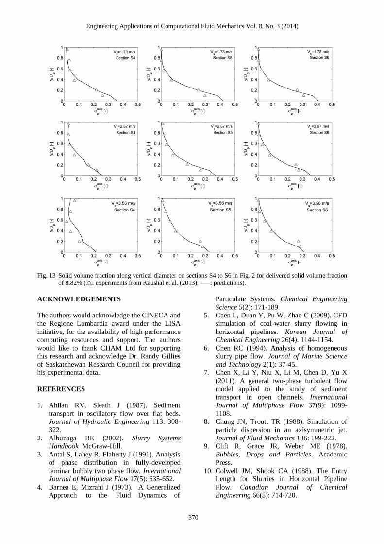
Engineering Applications of Computational Fluid Mechanics Vol 8 No 3 (2014)
370
Fig 13 Solid volume fraction along vertical diameter on sections S4 to S6 in Fig 2 for delivered solid volume fraction
of 882 ( experiments from Kaushal et al (2013) ndashndashndash predictions)
ACKNOWLEDGEMENTS The authors would acknowledge the CINECA and
the Regione Lombardia award under the LISA
initiative for the availability of high performance computing resources and support The authors
would like to thank CHAM Ltd for supporting
this research and acknowledge Dr Randy Gillies of Saskatchewan Research Council for providing
his experimental data
REFERENCES
1 Ahilan RV Sleath J (1987) Sediment
transport in oscillatory flow over flat beds Journal of Hydraulic Engineering 113 308-
322
2 Albunaga BE (2002) Slurry Systems Handbook McGraw-Hill
3 Antal S Lahey R Flaherty J (1991) Analysis
of phase distribution in fully-developed
laminar bubbly two phase flow International Journal of Multiphase Flow 17(5) 635-652
4 Barnea E Mizrahi J (1973) A Generalized
Approach to the Fluid Dynamics of
Particulate Systems Chemical Engineering
Science 5(2) 171-189 5 Chen L Duan Y Pu W Zhao C (2009) CFD
simulation of coal-water slurry flowing in
horizontal pipelines Korean Journal of Chemical Engineering 26(4) 1144-1154
6 Chen RC (1994) Analysis of homogeneous
slurry pipe flow Journal of Marine Science and Technology 2(1) 37-45
7 Chen X Li Y Niu X Li M Chen D Yu X
(2011) A general two-phase turbulent flow
model applied to the study of sediment transport in open channels International
Journal of Multiphase Flow 37(9) 1099-
1108 8 Chung JN Troutt TR (1988) Simulation of
particle dispersion in an axisymmetric jet
Journal of Fluid Mechanics 186 199-222 9 Clift R Grace JR Weber ME (1978)
Bubbles Drops and Particles Academic
Press
10 Colwell JM Shook CA (1988) The Entry Length for Slurries in Horizontal Pipeline
Flow Canadian Journal of Chemical
Engineering 66(5) 714-720
Engineering Applications of Computational Fluid Mechanics Vol 8 No 3 (2014)
371
11 Doron P Barnea D (1993) A three layer
model for solid-liquid flow in horizontal pipes International Journal of Multiphase
Flow 19(6) 1029-1043
12 Doron P Barnea D (1995) Pressure drop and
limit deposit velocity for solid-liquid flow in pipes Chemical Engineering and Science
50(10) 1595-1604
13 Doron P Barnea D (1996) Flow pattern maps for solid-liquid flow in pipes International
Journal of Multiphase Flow 22(2) 273-283
14 Doron P Granica D Barnea D (1987) Slurry flow in horizontal pipes ndash experimental and
modeling International Journal of
Multiphase Flow 13(4) 535ndash547
15 Eccedila L Hoekstra M (2006) Discretization uncertainty estimation based on a least
squares version of the grid convergence
index Proceedings of the 2nd
Workshop on CFD Uncertainty Analysis Oct 19-20
Lisbon Portugal
16 Ekambara K Sanders RS Nandakumar K Masliyah JH (2009) Hydrodynamic
simulation of horizontal slurry pipeline flow
using ANSYS-CFX Industrial amp
Engineering Chemistry Research 48(17) 8159-8171
17 Gillies RG Shook CA (2000) Modelling
High Concentration Settling Slurry Flows Canadian Journal of Chemical Engineering
78(4) 709-716
18 Gillies RG Shook CA Xu J (2004)
Modelling Heterogeneous Slurry Flow at High Velocities Canadian Journal of
Chemical Engineering 82(5) 1060-1065
19 Hsu FLG (1981) Flow of Fine-particle Suspensions in Bends Fittings and Valves
MS Thesis Texas Tech University Lubbock
Texas USA 20 Ishii M Mishima K (1984) Two-fluid model
and hydrodynamic constitutive relations
Nuclear Engineering and Design 82(2-3)
107-126 21 Issa RI Oliveira PJ (1997) Assessment of a
particle-turbulence interaction model in
conjunction with an Eulerian two-phase flow formulation Proceedings of the 2
nd
International Symposium on Turbulence
Heat and Mass Transfer June 9-12 Delft Netherlands 759-770
22 Jayatillika CLV (1969) The influence of the
Prandtl number and surface roughness on the
resistance of the sublayer to momentum and heat transfer Progress in Heat amp Mass
Transfer 1 193-329
23 Jiang YY Zhang P (2012) Pressure drop and
flow pattern of slush nitrogen in a horizontal pipe AIChE Journal doi 10002aic13927
24 Kaushal DR Kumar A Tomita Y Juchii S
Tsukamoto H (2013) Flow of mono-
dispersed particles through horizontal bend International Journal of Multiphase Flow 52
71-91
25 Kaushal DR Sato K Toyota T Funatsu K Tomita Y (2005) Effect of particle size
distribution on pressure drop and
concentration profile in pipeline flow of highly concentrated slurry International
Journal of Multiphase Flow 31(7) 809-823
26 Kaushal DR Thinglas T Tomita Y Juchii S
Tsukamoto H (2012) CFD modeling for pipeline flow of fine particles at high
concentration International Journal of
Multiphase Flow 43 85-100 27 Kaushal DR Tomita Y (2003) Comparative
study of pressure drop in multisized
particulate slurry flow through pipe and rectangular duct International Journal of
Multiphase Flow 29(9) 1473-1487
28 Kaushal DR Tomita Y (2007) Experimental
investigation for near-wall lift of coarser particles in slurry pipeline using γ-ray
densitometer Powder Technology 172(3)
177-187 29 Kim C Lee M Han C (2008) Hydraulic
transport of sand-water mixtures in pipelines
Part I Experiment Journal of Mechanical
Science and Technology 22(12) 2534-2541 30 Kumar U Mishra R Singh SN Seshadri V
(2003) Effect of particle gradation on flow
characteristics of ash disposal pipelines Powder Technology 132(1) 39-51
31 Lahiri SK Ghanta KC (2010) Slurry flow
modeling by CFD Chemical Industry amp Chemical Engineering Quarterly 16(4) 295-
308
32 Launder BE Spalding DB (1972)
Mathematical models of turbulence Academic Press
33 Ling J Skudarnov PV Lin CX Ebadian MA
(2003) Numerical investigations of solid-liquid slurry flows in a fully developed flow
region International Journal of Heat and
Fluid Flow 24(3) 389-398 34 Matousek V (2000) Concentration
distribution in pipeline flow of sand-water
mixtures Journal of Hydrology and
Hydromechanics 48(3) 180-196 35 Matousek V (2002) Pressure drops and flow
patterns in sand-mixture pipes Experimental
Engineering Applications of Computational Fluid Mechanics Vol 8 No 3 (2014)
372
Thermal and Fluid Science 26(6-7) 693-702
36 Matousek V (2009) Predictive model for frictional pressure drop in settling-slurry pipe
with stationary deposit Powder Technology
192(3) 367-374
37 Mooney M (1951) The viscosity of a concentrated suspension of spherical
particles Journal of Colloid Science 6(2)
162-170 38 Nasr-el-Din H Shook CA Esmail MN
(1984) Isokinetic Probe Sampling From
Slurry Pipelines Canadian Journal of Chemical Engineering 62(2) 179-185
39 Pathak M (2011) Computational
investigations of solid-liquid particle
interaction in a two-phase flow around a ducted obstruction Journal of Hydraulic
Research 49(1) 96-104
40 Pecker SM Helvaci SS (2008) Solid-Liquid Two-Phase Flow Elsevier
41 Roco MC Shook CA (1983) Modeling of
Slurry Flow The Effect of Particle Size Canadian Journal of Chemical Engineering
61(4) 494-503
42 Schlichting H (1960) Boundary Layer
Theory McGraw-Hill 43 Shaan J Sumner RJ Gillies RG Shook CA
(2000) The Effect of Particle Shape on
Pipeline Friction for Newtonian Slurries of Fine Particles Canadian Journal of Chemical
Engineering 78(4) 717-725
44 Shiller L Naumann A (1935) A drag
coefficient correlation Zeitschrift des Vereines Deutscher Ingenieure 77 318-320
45 Shirolkar JS Coimbra CFM McQuay MQ
(1996) Fundamental aspects of modelling turbulent particle dispersion in dilute flows
Progress in Energy and Combustion Science
22(4) 363-399 46 Shook CA Bartosik AS (1994) Particle-wall
stresses in vertical slurry flows Powder
Technology 81(2) 117-124
47 Skudarnov PV Lin CX Ebadian MA (2004) Double-Species Slurry Flow in a Horizontal
Pipeline ASME Journal of Fluids
Engineering 126(1) 125-132 48 Spalding DB (1972) A novel finite-
difference formulation for differential
expressions involving both first and second derivatives International Journal of
Numerical Methods in Engineering 4(4) 551-
559
49 Spalding DB (1980) Numerical computation of multi-phase fluid flow and heat transfer In
Taylor C Morgan K (Eds) Recent Advances
in Numerical Methods in Fluids Pineridge
Press Limited 139-168 50 Turian RM Ma TW Hsu FLG Sung MDJ
Plackmann GW (1998) Flow of concentrated
non-Newtonian slurries 2 Friction losses in
bends fittings valves and Venturi meters International Journal of Multiphase Flow
24(2) 243-269
51 Versteeg HK Malalasekera W (2007) An Introduction to Computational Fluid
Dynamics The Finite Volume Method
Pearson Prentice Hall 52 Wilson KC Sanders RS Gillies RG Shook
CA (2010) Verification of the near-wall
model for slurry flow Powder Technology
197(3) 247-253 53 Wilson KC Sellgren A (2003) Interaction of
Particles and Near-Wall Lift in Slurry
Pipelines Journal of Hydraulic Engineering 129(1) 73-76
- Figures13
-
- Fig 1 Computational domain and boundaryconditions for horizontal pipe
- Fig 2 Computational domain boundary conditionsand reference sections for 90deg bend (S1=bendinlet S2=bend centre S3=bend exit S4=5Dpfrom bend exit S5=25Dp from bend exitS6=50Dp from bend exit)
- Fig3 Solid volume fraction profiles calculated onthree different grid levels for straight pipecase
- Fig4 Details of mesh for 90deg bend
- Fig5 Vertical solid volume fraction profiles atdistance of 5Dp downstream bend exit (SectionS4 in Fig 2) calculated on different gridlevels The Grid 3 solution has error barscorresponding to the grid discretization errorestimated by the method of Eccedila and Hoekstra(2006)
- Fig 6 Effect of turbulent Schmidt number for volume fractions a s on solid volume fraction profiles for two flowconditions (r experiments from Roco and Shook (1983) ndashndashndash 03 a s = ndashndashndash 05 a s = ndashndashndash 07 a s = ndashndashndash09 a s = )
- Fig 7 Effect of parameters [η] and pm a in mixture viscosity correlation of Mooney (Eq 11) on solid volume fractionprofiles for two flow conditions (r experiments from Roco and Shook (1983) continuous lines predictions)The dependence on [η] is studied for 07 pm a = that on pm a for [η] = 25
- Fig 8 Solids concentration profiles for flow conditions A1 to A5 in Table 2 (rbull experiments from Roco and Shook (1983) ndashndashndash predictions)
- Fig 9 Solids concentration profile for flow conditions B1 to B12 in Table 2 (rbulls experiments from Gillies et al (2004) ndashndashndash predictions)
- Fig 10 Solids concentration profiles for flow conditions C1 to C6 in Table 2 (rbull experiments from Matousek (2000 and 2002) ndashndashndash predictions)
- Fig 11 Solids concentration profiles for flow conditions D1 to D4 in Table 2 (rbull experiments from Shaan et al (2000) ndashndashndash predictions)
- Fig 12 Solid volume fraction distributions on sections S1 to S6 in Fig 2 for delivered solid volume fraction of 882 Left hand side is the outer wall of the pipe
- Fig 13 Solid volume fraction along vertical diameter on sections S4 to S6 in Fig 2 for delivered solid volume fraction of 882 (r experiments from Kaushal et al (2013) ndashndashndash predictions)
-
- Tables13
-
- Table 1 Flow conditions considered for comparison
- Table 2 Details of experimental conditions for straight pipe case (A1 to A5 experimental data from Roco and Shook(1983) B1 to B12 experimental data from Gillies et al (2004) C1 to C6 experimental data from Matousek(2000 and 2002) D1 to D4 experimental data from Shaan et al (2000) values not declared byexperimenters)
-
- 1 INTRODUCTION
- 2 MATHEMATICAL MODEL
-
- 21 Conservation equations
- 22 Turbulence modeling
- 23 Computational domain and boundaryconditions
- 24 Computational methodology and consistencyof numerical solution
- 25 Governing terms and calibration ofnumerical constants
-
- 3 RESULTS
-
- 31 Straight horizontal pipe
- 32 Horizontal 90deg bend
-
- 4 CONCLUSIONS
- ACKNOWLEDGEMENTS
- REFERENCES
-
Engineering Applications of Computational Fluid Mechanics Vol 8 No 3 (2014)
372
Thermal and Fluid Science 26(6-7) 693-702
36 Matousek V (2009) Predictive model for frictional pressure drop in settling-slurry pipe
with stationary deposit Powder Technology
192(3) 367-374
37 Mooney M (1951) The viscosity of a concentrated suspension of spherical
particles Journal of Colloid Science 6(2)
162-170 38 Nasr-el-Din H Shook CA Esmail MN
(1984) Isokinetic Probe Sampling From
Slurry Pipelines Canadian Journal of Chemical Engineering 62(2) 179-185
39 Pathak M (2011) Computational
investigations of solid-liquid particle
interaction in a two-phase flow around a ducted obstruction Journal of Hydraulic
Research 49(1) 96-104
40 Pecker SM Helvaci SS (2008) Solid-Liquid Two-Phase Flow Elsevier
41 Roco MC Shook CA (1983) Modeling of
Slurry Flow The Effect of Particle Size Canadian Journal of Chemical Engineering
61(4) 494-503
42 Schlichting H (1960) Boundary Layer
Theory McGraw-Hill 43 Shaan J Sumner RJ Gillies RG Shook CA
(2000) The Effect of Particle Shape on
Pipeline Friction for Newtonian Slurries of Fine Particles Canadian Journal of Chemical
Engineering 78(4) 717-725
44 Shiller L Naumann A (1935) A drag
coefficient correlation Zeitschrift des Vereines Deutscher Ingenieure 77 318-320
45 Shirolkar JS Coimbra CFM McQuay MQ
(1996) Fundamental aspects of modelling turbulent particle dispersion in dilute flows
Progress in Energy and Combustion Science
22(4) 363-399 46 Shook CA Bartosik AS (1994) Particle-wall
stresses in vertical slurry flows Powder
Technology 81(2) 117-124
47 Skudarnov PV Lin CX Ebadian MA (2004) Double-Species Slurry Flow in a Horizontal
Pipeline ASME Journal of Fluids
Engineering 126(1) 125-132 48 Spalding DB (1972) A novel finite-
difference formulation for differential
expressions involving both first and second derivatives International Journal of
Numerical Methods in Engineering 4(4) 551-
559
49 Spalding DB (1980) Numerical computation of multi-phase fluid flow and heat transfer In
Taylor C Morgan K (Eds) Recent Advances
in Numerical Methods in Fluids Pineridge
Press Limited 139-168 50 Turian RM Ma TW Hsu FLG Sung MDJ
Plackmann GW (1998) Flow of concentrated
non-Newtonian slurries 2 Friction losses in
bends fittings valves and Venturi meters International Journal of Multiphase Flow
24(2) 243-269
51 Versteeg HK Malalasekera W (2007) An Introduction to Computational Fluid
Dynamics The Finite Volume Method
Pearson Prentice Hall 52 Wilson KC Sanders RS Gillies RG Shook
CA (2010) Verification of the near-wall
model for slurry flow Powder Technology
197(3) 247-253 53 Wilson KC Sellgren A (2003) Interaction of
Particles and Near-Wall Lift in Slurry
Pipelines Journal of Hydraulic Engineering 129(1) 73-76
- Figures13
-
- Fig 1 Computational domain and boundaryconditions for horizontal pipe
- Fig 2 Computational domain boundary conditionsand reference sections for 90deg bend (S1=bendinlet S2=bend centre S3=bend exit S4=5Dpfrom bend exit S5=25Dp from bend exitS6=50Dp from bend exit)
- Fig3 Solid volume fraction profiles calculated onthree different grid levels for straight pipecase
- Fig4 Details of mesh for 90deg bend
- Fig5 Vertical solid volume fraction profiles atdistance of 5Dp downstream bend exit (SectionS4 in Fig 2) calculated on different gridlevels The Grid 3 solution has error barscorresponding to the grid discretization errorestimated by the method of Eccedila and Hoekstra(2006)
- Fig 6 Effect of turbulent Schmidt number for volume fractions a s on solid volume fraction profiles for two flowconditions (r experiments from Roco and Shook (1983) ndashndashndash 03 a s = ndashndashndash 05 a s = ndashndashndash 07 a s = ndashndashndash09 a s = )
- Fig 7 Effect of parameters [η] and pm a in mixture viscosity correlation of Mooney (Eq 11) on solid volume fractionprofiles for two flow conditions (r experiments from Roco and Shook (1983) continuous lines predictions)The dependence on [η] is studied for 07 pm a = that on pm a for [η] = 25
- Fig 8 Solids concentration profiles for flow conditions A1 to A5 in Table 2 (rbull experiments from Roco and Shook (1983) ndashndashndash predictions)
- Fig 9 Solids concentration profile for flow conditions B1 to B12 in Table 2 (rbulls experiments from Gillies et al (2004) ndashndashndash predictions)
- Fig 10 Solids concentration profiles for flow conditions C1 to C6 in Table 2 (rbull experiments from Matousek (2000 and 2002) ndashndashndash predictions)
- Fig 11 Solids concentration profiles for flow conditions D1 to D4 in Table 2 (rbull experiments from Shaan et al (2000) ndashndashndash predictions)
- Fig 12 Solid volume fraction distributions on sections S1 to S6 in Fig 2 for delivered solid volume fraction of 882 Left hand side is the outer wall of the pipe
- Fig 13 Solid volume fraction along vertical diameter on sections S4 to S6 in Fig 2 for delivered solid volume fraction of 882 (r experiments from Kaushal et al (2013) ndashndashndash predictions)
-
- Tables13
-
- Table 1 Flow conditions considered for comparison
- Table 2 Details of experimental conditions for straight pipe case (A1 to A5 experimental data from Roco and Shook(1983) B1 to B12 experimental data from Gillies et al (2004) C1 to C6 experimental data from Matousek(2000 and 2002) D1 to D4 experimental data from Shaan et al (2000) values not declared byexperimenters)
-
- 1 INTRODUCTION
- 2 MATHEMATICAL MODEL
-
- 21 Conservation equations
- 22 Turbulence modeling
- 23 Computational domain and boundaryconditions
- 24 Computational methodology and consistencyof numerical solution
- 25 Governing terms and calibration ofnumerical constants
-
- 3 RESULTS
-
- 31 Straight horizontal pipe
- 32 Horizontal 90deg bend
-
- 4 CONCLUSIONS
- ACKNOWLEDGEMENTS
- REFERENCES
-