Numerical modelling of Glacial Lake Outburst Floods using physically based dam-breach models

ESURFD2, 1–57, 2014

Numerical modellingof Glacial Lake

Outburst Floods

M. J. Westoby et al.

Title Page

Abstract Introduction

Conclusions References

Tables Figures

J I

J I

Back Close

Full Screen / Esc

Printer-friendly Version

Interactive Discussion

Discussion

Paper

|D

iscussionP

aper|

Discussion

Paper

|D

iscussionP

aper|

Earth Surf. Dynam. Discuss., 2, 1–57, 2014www.earth-surf-dynam-discuss.net/2/1/2014/doi:10.5194/esurfd-2-1-2014© Author(s) 2014. CC Attribution 3.0 License.

This discussion paper is/has been under review for the journal Earth Surface Dynamics (ESurfD).Please refer to the corresponding final paper in ESurf if available.

Numerical modelling of Glacial LakeOutburst Floods using physically baseddam-breach modelsM. J. Westoby1, J. Brasington2, N. F. Glasser3, M. J. Hambrey1, J. M. Reynolds3,and M. A. A. M. Hassan4

1Department of Geography and Earth Sciences, Aberystwyth University, UK2School of Geography, Queen Mary, University of London, UK3Reynolds International Ltd, Suite 2, Broncoed House, Broncoed Business Park, Mold, UK4HR Wallingford Ltd, Howberry Park, Wallingford, Oxfordshire, UK

Received: 9 May 2014 – Accepted: 2 June 2014 – Published:

Correspondence to: M. J. Westoby ([email protected])

Published by Copernicus Publications on behalf of the European Geosciences Union.

1

http://www.earth-surf-dynam-discuss.net

http://www.earth-surf-dynam-discuss.net/2/1/2014/esurfd-2-1-2014-print.pdf

http://www.earth-surf-dynam-discuss.net/2/1/2014/esurfd-2-1-2014-discussion.html

http://creativecommons.org/licenses/by/3.0/

ESURFD2, 1–57, 2014


Outburst Floods


Title Page



Tables Figures

J I

J I

Back Close

Full Screen / Esc



Discussion

Paper

|D

iscussionP

aper|

Discussion

Paper

|D

iscussionP

aper|

Abstract

The rapid development and instability of moraine-dammed proglacial lakes is increas-ing the potential for the occurrence of catastrophic Glacial Lake Outburst Floods(GLOFs) in high-mountain regions. Advanced, physically-based numerical dam-breachmodels represent an improvement over existing methods for the derivation of breach5

outflow hydrographs. However, significant uncertainty surrounds the initial parameteri-sation of such models, and remains largely unexplored. We use a unique combinationof numerical dam-breach and two-dimensional hydrodynamic modelling, employed witha Generalised Likelihood Uncertainty Estimation (GLUE) framework to quantify the de-gree of equifinality in dam-breach model output for the reconstruction of the failure10

of Dig Tsho, Nepal. Monte Carlo analysis was used to sample the model parameterspace, and morphological descriptors of the moraine breach were used to evaluatemodel performance. Equifinal breach morphologies were produced by parameter en-sembles associated with differing breach initiation mechanisms, including overtoppingwaves and mechanical failure of the dam face. The material roughness coefficient was15

discovered to exert a dominant influence over model performance. Percentile breachhydrographs derived from cumulative distribution function hydrograph data under- oroverestimated total hydrograph volume and were deemed to be inappropriate for in-put to hydrodynamic modelling. Our results support the use of a Total Variation Di-minishing solver for outburst flood modelling, which was found to be largely free of20

numerical instability and flow oscillation. Routing of scenario-specific optimal breachhydrographs revealed prominent differences in the timing and extent of inundation. AGLUE-based method for constructing likelihood-weighted maps of GLOF inundationextent, flow depth, and hazard is presented, and represents an effective tool for com-municating uncertainty and equifinality in GLOF hazard assessment. However, future25

research should focus on the utility of the approach for predictive, as opposed to re-constructive GLOF modelling.

2





ESURFD2, 1–57, 2014


Outburst Floods


Title Page



Tables Figures

J I

J I

Back Close

Full Screen / Esc



Discussion

Paper

|D

iscussionP

aper|

Discussion

Paper

|D

iscussionP

aper|

1 Introduction

Glacier recession has been observed on a global scale as a result of recent climaticchange (Oerlemans, 1994; Kaser et al., 2006; Zemp et al., 2009; Bolch et al., 2011,2012). The exposure of terminal and lateral (combined: “latero-terminal”) moraine com-plexes is becoming increasingly commonplace as a result of glacier recession, particu-5

larly in high-mountain regions. Latero-terminal moraines reflect the historical maximumextent of a given glacier, and are typically composed of poorly-consolidated glacial ma-terial.

Moraine-dammed lakes form through one of two mechanisms, namely: recession ofthe glacier terminus and ponding of water in the proglacial moraine basin (Frey et al.,10

2010), or via the coalescence and expansion of supraglacial ponds on heavily debris-covered glaciers (Reynolds, 1998, 2000; Richardson and Reynolds, 2000; Benn et al.,2001, 2012; Thompson et al., 2012). Following expansion, such lakes are capable ofimpounding volumes of water in excess of 106–107 m3 (Lliboutry, 1977a; Vuichard andZimmerman, 1987; Watanabe et al., 1995; Sakai et al., 2000; Jansky et al., 2009).15

Moraine breaching may result in the generation of a Glacial Lake Outburst Flood(GLOF) (Lliboutry, 1977a; Vuichard and Zimmerman, 1987; Clague and Evans, 2000;Kershaw et al., 2005; Harrison et al., 2006; Osti and Egashira, 2009; Worni et al., 2012;Westoby et al., 2014). These sudden-onset outburst floods represent high-magnitude,low-frequency catastrophic phenomena that have enormous potential for geomorpho-20

logical reworking of channel and floodplain environments (Cenderelli and Wohl, 2003)including the destruction of land, buildings and infrastructure in, or adjacent to the floodpath, and can result in human fatalities (Vuichard and Zimmerman, 1987; Lliboutryet al., 1977a; Watanabe and Rothacher, 1996). Of the various glacial hazards (Richard-son and Reynolds, 2000; Kääb et al., 2005; Quincey et al., 2005, 2007), GLOFs have25

the most far-reaching impacts, with destruction often reported tens or hundreds of kilo-metres from their source (Vuichard and Zimmerman, 1987; Clague and Evans, 2000;Richardson and Reynolds, 2000).

3





ESURFD2, 1–57, 2014


Outburst Floods


Title Page



Tables Figures

J I

J I

Back Close

Full Screen / Esc



Discussion

Paper

|D

iscussionP

aper|

Discussion

Paper

|D

iscussionP

aper|

2 Study site

The Dig Tsho moraine-dammed lake complex is located at the head of the Langmochevalley in the western sector of Sagarmatha (Mt. Everest) National Park in the KhumbuHimal (Solukhumbu District), Nepal (Fig. 1; 27◦52′23.89′′ N, 86◦35′14.91′′ E). A relictmoraine-dammed lake, oriented west-east, is impounded by a latero-terminal moraine5

complex to the north and east. The basin is bounded by a near-vertical bedrock face tothe south. The parent Langmoche Glacier has receded significantly since its Neoglacialmaximum terminus position and is now confined to the upper north-east faces of TangiRagi Tau (6940 m).

The moraine possesses steep (25–30◦) faces on all ice-distal sides and on ice-10

proximal sides along the northern lateral moraine. In contrast, proximal faces of theterminal moraine are generally shallower, although ice-proximal faces are more topo-graphically complex than their distal counterparts. The moraine is composed of sandyboulder-gravel, and includes rare large (> 10 m diameter) boulders. A sizeable (200 mwide, 400 m long, 60 m deep) breach dissects the northern sector of the terminal15

moraine (Fig. 1; Vuichard and Zimmerman, 1987; Westoby et al., 2012).On 4 August 1985 an ice avalanche from the receding Langmoche Glacier traversed

the steep (∼ 30◦) avalanche and debris cone which terminates in the moraine-dammedlake and triggered a displacement wave that was transmitted along its length. This initialwave is believed to have overtopped the moraine dam, thereby initiating its failure.20

Although not observed first-hand, full breach formation was estimated to have taken4–6 h (Vuichard and Zimmerman, 1987).

The geomorphological effects of the Dig Tsho GLOF have been well documented(Vuichard and Zimmerman, 1986, 1987; Cenderelli and Wohl, 2001, 2003). A newly-completed hydro-electric power installation adjacent to the village of Thamo was com-25

pletely destroyed (∼ 11.5 km from source). All trekking bridges for a distance of > 30 kmwere destroyed and up to 5 people are reported to have been killed (Galay, 1985).

4





ESURFD2, 1–57, 2014


Outburst Floods


Title Page



Tables Figures

J I

J I

Back Close

Full Screen / Esc



Discussion

Paper

|D

iscussionP

aper|

Discussion

Paper

|D

iscussionP

aper|

Existing observational data for the site include first-hand descriptions of the condi-tion of the glacial lake prior to, and immediately following moraine dam failure in 1985,as well as a description of the pre-GLOF nature of the valley floor sedimentology im-mediately downstream (Vuichard and Zimmerman, 1987). Existing estimates state themass of material removed from the breach as being 9×105 m3, and the drained vol-5

ume of the moraine basin as being 5×106 m3. It is envisaged that the vast majorityof the dam material eroded during breach development was deposited within 2 km ofthe moraine. Field investigation and photogrammetric reconstruction of the moraine byWestoby et al. (2012) has revealed the volume of the contemporary breach (surveyedin 2010) to be approximately 5.8×105 m3, and the volume of water released by the10

1985 GLOF to be ∼ 7.3×106 m3. Sedimentological (D50) sampling of matrix materialexposed in the breach sidewalls was undertaken during field investigation, and wasused to aid dam-breach model parameterisation.

3 Quantifying equifinality and uncertainty in a numerical dam-breach model

3.1 Motivation for this study15

Numerous sources of uncertainty are associated with the parameterisation of contem-porary numerical dam-breach and hydrodynamic models for reconstructive or predic-tive GLOF simulation (Westoby et al., 2014). Few studies have sought to explore thesensitivity of dam-breach models to parametric uncertainty (e.g. Wang et al., 2012;Worni et al., 2012) and the extent and significance of model equifinality for GLOF inun-20

dation and hazard mapping. This article seeks to address this increasingly conspicuousresearch gap through the development and demonstration of a unifying framework forcascading uncertainty and equifinality in the GLOF model chain through the recon-struction of a historical GLOF in the Nepalese Himalaya.

5





ESURFD2, 1–57, 2014


Outburst Floods


Title Page



Tables Figures

J I

J I

Back Close

Full Screen / Esc



Discussion

Paper

|D

iscussionP

aper|

Discussion

Paper

|D

iscussionP

aper|

3.2 The role of uncertainty and equifinality in dam-breach modelling

Equifinality is where identical or similar end states in an open system are achievedfrom many different combinations of input parameters, initial conditions, and modelstructures (e.g. Beven and Binley, 1992; Beven and Freer, 2001; Beven, 2005). In ge-omorphological investigation, equifinality explains how a single landform or landform5

assemblage may have formed through a range of differing, but equally plausible pro-cess combinations (e.g. Nicholas and Quine, 2010; Stokes et al., 2011). Equifinalityhas its origins in systems theory (von Bertalanffy, 1968), and has been recognised andquantified in a range of geoscience applications (e.g. Beven and Binley, 1992; Kuczeraand Parent, 1998; Lamb et al., 1998; Romanowicz and Beven, 1998; Beven and Freer,10

2001; Blazkova and Beven, 2004; Hunter et al., 2005; Cameron, 2007; Hassan et al.,2008; Rojas et al., 2008; Vasquez et al., 2009; Vrugt et al., 2009; Franz and Hogue,2011).

Uncertainty abounds at both the dam-breach and hydrodynamic, flood-routingstages of the GLOF model chain (Westoby et al., 2014). In the case of the former,15

appreciable uncertainty surrounds the establishment of initial conditions (e.g. dam ge-ometry, reservoir hypsometry), dam material parameterisation (e.g. grain-size distribu-tion curves, material porosity, density, cohesion, roughness coefficients, internal angleof friction) and the establishment of computational constraints (e.g. model time stepand grid discretisation).20

Variability in hydrodynamic model output may be attributed to model dimensionality(e.g. Alho and Aaltonen, 2008; Bohorquez and Darby, 2008), grid discretisation andquality (e.g. Sanders, 2007; Huggel et al., 2008) the spacing of cross-sections usedto represent floodplain geometry in 1-D hydrodynamic models (e.g. Castellarin et al.,2009), as well as uncertainty surrounding the parameterisation of in-channel and flood-25

plain roughness coefficients (Wohl, 1998; Hall et al., 2005; Pappenberger et al., 2005),boundary condition data (e.g. Pappenberger et al., 2006) and stage–discharge relation-ships (e.g. Di Baldassarre and Claps, 2011). Recent studies have undertaken various

6





ESURFD2, 1–57, 2014


Outburst Floods


Title Page



Tables Figures

J I

J I

Back Close

Full Screen / Esc



Discussion

Paper

|D

iscussionP

aper|

Discussion

Paper

|D

iscussionP

aper|

forms of sensitivity analyses and uncertainty estimation to quantify the effects of un-certainty on numerical dam-breach model output (e.g. IMPACT, 2004; Xin et al., 2008;Dewals et al., 2011; Zhong et al., 2011; Worni et al., 2012). However, to date issues ofequifinality remain largely unexplored.

4 Method5

We approach the problem of developing a framework for embracing and propagatingparameter uncertainty through the GLOF model chain by using a sequence of methods.In the order that they are encountered in our modelling chain, these include: (i) digitalterrain modelling using terrestrial photogrammetry to reconstruct pre-existing moraineand floodplain topography and extraction of glacial lake bathymetry and dam geome-10

try data, (ii) parameterisation of a numerical dam-breach model using material prop-erties obtained through field investigation and from published literature, (iii) stochas-tic dam-breach model parameter sampling and model execution to obtain a series ofscenario-specific dam-breach hydrographs, (iv) the application of Bayesian statistics,based on geometric descriptors of observed, post-GLOF breach topography, to eval-15

uate the performance of individual dam-breach simulations, and, (v) the application ofa two-dimensional hydrodynamic solver to model the downstream propagation of re-tained GLOF hydrographs and provide inundation extent, flow velocity, and flow depthdata for use as input to probabilistic GLOF hazard mapping. The following sectionsdescribe each method in detail.20

4.1 Topographic data acquisition

Structure-from-Motion (SfM) photogrammetry, combined with Multi-View Stereo (MVS)methods (James and Robson, 2012; Westoby et al., 2012; Fonstad et al., 2013; Javer-nick et al., 2014) was used to reconstruct floodplain topography for a distance of ∼ 2 kmdownstream of Dig Tsho. The SfM method requires the acquisition of photosets with25

7





ESURFD2, 1–57, 2014


Outburst Floods


Title Page



Tables Figures

J I

J I

Back Close

Full Screen / Esc



Discussion

Paper

|D

iscussionP

aper|

Discussion

Paper

|D

iscussionP

aper|

a high degree of image overlap and feature coverage from a range of perspectives,followed by the application of feature extraction (e.g. Lowe, 2004) and bundle adjust-ment algorithms (e.g. Snavely, 2008; Snavely et al., 2008) for the sparse and densereconstruction of 3-D scene geometry.

Reconstruction of moraine topography using SfM-MVS methods is described in de-5

tail in Westoby et al. (2012). Here, we use their SfM-derived terrain model of the DigTsho moraine to extract metric data describing to moraine geometry and lake basinhypsometry (Fig. 2) for the establishment of initial conditions for numerical dam-breachmodelling.

To reconstruct post-GLOF valley-floor topography, two photosets, numbering 22610

and 303 photographs for south- and north-facing perspectives respectively, were ac-quired from successive elevated positions on the valley flanks using a Panasonic DMC-G10 (12 MP) digital camera with automatic focusing and exposure settings enabled.The freely-available software bundle SFMToolkit3 (Astre, 2010) was used to processthe input images using feature extraction (Lowe, 2004) and sparse and dense SfM-15

MVS reconstruction algorithms. Following manual outlier removal and editing, finaldense point clouds numbered 4.8×106 and 1.3×106 points for north- and south-facingphotosets respectively. Data transformation was achieved through the identification ofclearly-identifiable boulders from kite aerial photography and an existing SfM-derivedDigital Terrain Model (DTM) of the easternmost sector of the floodplain domain, as well20

as boulders visible in the georeferenced DTM of the moraine dam. Averaged georegis-tration residual errors for both dense point clouds were 1.37 m, 0.30 m and 0.06 m forxyz dimensions respectively.

Georeferenced point cloud data were merged and decimated to improve data han-dling whilst preserving sub-grid statistics using the C++/Python-based Topographic25

Point-Cloud Analysis Toolkit (Brasington et al., 2012; Rychkov et al., 2012). A bare-earth DTM at 8 m spatial resolution was extracted for hydrodynamic GLOF routing.Sensitivity analyses have previously revealed this particular grid discretisation to pro-duce time-varying inundation extents and wetting-front travel times of comparable

8





ESURFD2, 1–57, 2014


Outburst Floods


Title Page



Tables Figures

J I

J I

Back Close

Full Screen / Esc



Discussion

Paper

|D

iscussionP

aper|

Discussion

Paper

|D

iscussionP

aper|

(relative) accuracies to those produced using finer grid resolutions, and of higher ac-curacy than coarser grids (Westoby et al., 2014).

4.2 Numerical dam-breach modelling using HR BREACH

HR BREACH is a physically-based, numerical dam-breach model that predicts thegrowth of a dam breach arising from the overtopping of non-cohesive and cohesive em-5

bankment materials, as well as via piping mechanisms (Morris et al., 2008; Westoby,2013; Westoby et al., 2014). In contrast with analytical- or parametric-type models, HRBREACH combines a range of hydraulic, sediment erosion and discrete embankmentstability analyses to facilitate the “free” formation of breach geometry and generation ofthe outflow hydrograph (Morris et al., 2008). Crucially, it has not been directly calibrated10

to data from one or more specific events.HR BREACH handles breach enlargement through the interaction of two mecha-

nisms, namely: (i) continuous erosion of submerged sediment through the applicationof equilibrium sediment transport equations or erosion-depth equations, and, (ii) dis-crete mass failures due to side-slope instability (Mohamed et al., 2002). Erosion-depth15

equations are deemed to be highly appropriate for simulating dam breaching as theyare deemed to be more physically representative of the hydraulic and sediment trans-port processes in operation during breach development. We use the erosion-depthequation for non-cohesive embankments, as forwarded by Chen and Anderson (1986):

εr = Kd(τe − τc)a (1)20

where εr is the detachment rate per unit area (e.g. m3 s−1 m2), τe the flow shear stress(kN) at the breach boundary, τc is the critical shear stress required to initiate particledetachment (kN), and Kd and a are dimensionless coefficients based on the sedimentproperties. Bending (tensional) failure is represented by a moment of force, Mo:25

Mo =We+Wses +Wueu +H2e2 −H1e1 (2)

9





ESURFD2, 1–57, 2014


Outburst Floods


Title Page



Tables Figures

J I

J I

Back Close

Full Screen / Esc



Discussion

Paper

|D

iscussionP

aper|

Discussion

Paper

|D

iscussionP

aper|

where W is the weight of a dry block of soil, Ws is the weight of a saturated block of soil,Wu is the weight of a submerged block of soil, H1 is the hydrostatic pressure force inthe breach channel, H2 is the hydrostatic pressure force inside the dam structure, e, esand eu are weight force eccentricities, e1 and e2 are hydrostatic pressure force eccen-tricities (Hassan and Morris, 2012). The occurrence of shear-type failure is evaluated5

through the analysis of Factor of Safety (FoS) values using the following equation:

FoS =cL+H1 tanΦ

W +Ws +Wu +H2 tanΦ(3)

where c is soil cohesion, L is the length of the failure plane and Φ is the soil angle offriction.10

Subaerial, steady-state breach flow is simulated using a one-dimensional flow model(Mohamed et al., 2002; Morris et al., 2008). This method combines a weir dischargeequation and a simplified version of the Saint Venant equations (de St-Venant, 1871)to simulate breach flow, and flow descending the distal face of the dam, respectively.HR BREACH is capable of using variable weir discharge coefficients, which are auto-15

matically updated, based on the changing profile of the dam crest (Hassan and Morris,2012) and is intended to compensate for the significant flow complexity which arisesduring breach development.

4.3 Generalised Likelihood Uncertainty Estimation (GLUE)

For event-specific flood reconstruction, systematic calibration of input parameters to20

produce best-fit, or optimal flood conditions is often practiced (e.g. Kidson et al., 2006;Cao and Carling, 2002). Model calibration typically comprises the adjustment of individ-ual or multiple model parameters to provide a best-fit solution to an observed dataset(e.g. Refsgaard, 1997; Beven and Freer, 2001; Hunter et al., 2005; Westerberg et al.,2011) and may serve to inform their choice for hypothetical future events (e.g. Horritt25

and Bates, 2002).

10





ESURFD2, 1–57, 2014


Outburst Floods


Title Page



Tables Figures

J I

J I

Back Close

Full Screen / Esc



Discussion

Paper

|D

iscussionP

aper|

Discussion

Paper

|D

iscussionP

aper|

Where there is insufficient quantitative or qualitative information pertaining to themodel parameterisation or simulation constraints, any combination of model inputthat reproduces the observed outcome, within acceptable limits, must be consideredequally likely as a simulator of the system under investigation (Beven and Binley, 1992).This is the underlying principle of the Generalised Likelihood Uncertainty Estimation5

(GLUE) method (Beven and Binley, 1992; Beven, 2005). The following sections de-scribe its application to quantifying equifinality in moraine-dam failure reconstructionusing HR BREACH.

4.3.1 Parameter choice, prior distributions, and stochastic sampling

The first step in the GLUE workflow is to establish the parameters for inclusion and their10

respective ranges. In the absence of any prior information regarding parameter andrange choice, all available input parameters and their entire simulation range shouldbe included. In practice, complete uncertainty regarding parameter and range choiceis unlikely, since a combination of initial sensitivity analyses, modelling guidelines, aswell as basic intuition and reasoning can typically be used to assist in constraining their15

choice (Beven and Binley, 1992). The parameters and their ranges used in this study(including computational settings) are displayed in Table 1.

Information regarding initial, or a priori, parameter distributions is also required, re-flecting the modeller’s prior knowledge of the parameter space (Beven and Binley,1992). In the absence of any information pertaining to a priori parameter probability20

distributions at Dig Tsho, uniform distributions were used for stochastic sampling of allavailable parameter spaces.

Although a range of stochastic sampling methods are available for use in the GLUEworkflow (e.g. Metropolis, 1987; Iman and Helton, 2006), perhaps the most widely usedapproach is Monte Carlo analysis (e.g. Beven and Binley, 1992; Kuczera and Parent,25

1998; Aronica et al., 1998, 2002; Blazkova and Beven, 2004). Using the Monte Carlomethod, values from individual parameter spaces are sampled randomly, thereby elim-inating any subjectivity which might be introduced at this stage. The method is fully

11





ESURFD2, 1–57, 2014


Outburst Floods


Title Page



Tables Figures

J I

J I

Back Close

Full Screen / Esc



Discussion

Paper

|D

iscussionP

aper|

Discussion

Paper

|D

iscussionP

aper|

capable of accounting for predefined probability distribution data, making it a simpleyet effective tool for rapidly generating the random parameter ensembles required formodel input. However, with a poorly-defined prior distribution, or a small number ofmodel simulations, point clustering in specific regions of the parameter space may oc-cur. Clustering can be easily avoided by undertaking a straightforward investigation5

into patterns of histogram convergence of an output variable (or variables), wherebythe minimum number of simulations required for the production of an acceptable levelof convergence is established. In our study, continued histogram convergence becameminimal after the execution of 1000 model runs. This number of simulations was there-fore deemed acceptable for stochastic sampling.10

4.3.2 Likelihood measures and functions

Model evaluation is achieved through quantification of how well a parameter ensembleperforms at reproducing a series of observable system state variables, or likelihoodmeasures. Parameter ensembles that are unable to do so are deemed to be non-behavioural and are assigned a likelihood score of zero. In contrast, ensembles that15

reproduce these variables within acceptable limits are deemed to be behavioural andaccepted for further analysis. It is not uncommon for all ensembles to be rejected (e.g.Parkin et al., 1996; Freer et al., 2002), thereby suggesting that it is in fact the modelstructure that is incapable of reproducing the observed data, instead of individual pa-rameter combinations (Beven and Binley, 1992). Such a situation may be overcome by20

widening the limits of acceptability, but at the potential cost of decreasing confidencein any newly-accepted ensembles (Beven and Binley, 1992).

Behavioural ensembles were assigned positive likelihood values in the range 0–1,where 1 represents an ensemble that is capable of perfectly replicating the observeddata. Likelihood functions are specific to each likelihood measure used for model eval-25

uation. Three likelihood measures were used to evaluate HR BREACH model perfor-mance: (i) final upstream breach depth (LH1), (ii) the residual sum of squared errors ofthe final longitudinal elevation profile of the breach (LH2), and, (iii) the location of the

12





ESURFD2, 1–57, 2014


Outburst Floods


Title Page



Tables Figures

J I

J I

Back Close

Full Screen / Esc



Discussion

Paper

|D

iscussionP

aper|

Discussion

Paper

|D

iscussionP

aper|

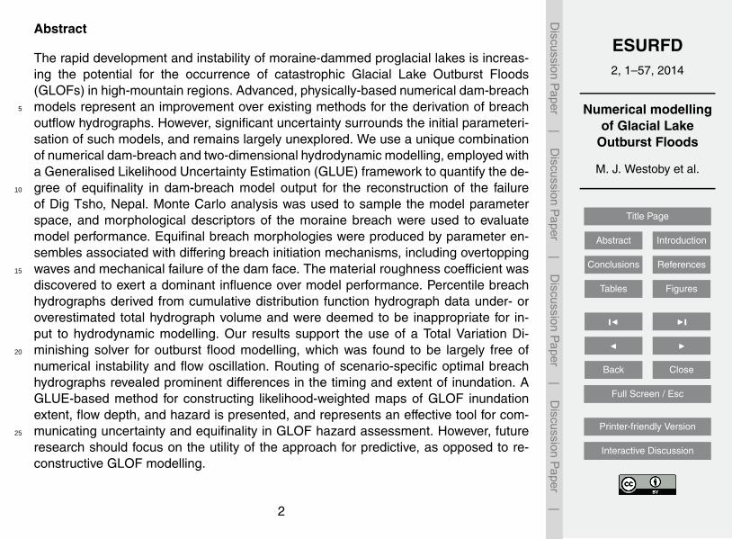
critical flow constriction (LH3; Fig. 3). These morphological variables are directly quan-tifiable through the comparison of final modelled breach geometry with that extractedfrom the SfM-DTM of the breached moraine-dam.

An observed breach depth of 16±2 m was used. The error range was designed toaccount for observed SfM model georegistration errors, which may have resulted in5

elevation of the lake exit being under- or overestimated, as well as any post-GLOF lakelowering or seasonal variations in lake level, which remain unquantified. A triangularlikelihood function was used, with an observed breach depth of 16 m and upper andlower limits defined as 14 m and 18 m respectively.

The second likelihood measure took the form of a direct comparison between ob-10

served (post-GLOF) and modelled elevation profiles of the breach thalweg. This mea-sure represents an effective, distributed method of quantifying the performance of HRBREACH in producing post-GLOF thalweg elevation profiles that mirror, or significantlydiffer from that observed in the field. Thalweg elevation data were directly extractedfrom the SfM-DTM (Fig. 12a, Westoby et al., 2012). The residual sum of squares (RSS)15

method was used to quantify the deviation between the observed and modelled data:

RSS =n∑

i=1

(Zobs −Zpred.)2 (4)

where Zobs is the observed elevation (m) of the breach thalweg and Zpred. is the el-evation of the modelled thalweg. For the attribution of a scaled likelihood value, an20

RSS of 0 corresponded to a likelihood score of 1, whilst the lowest RSS for all scenar-ios (169 221; dimensionless) was used to represent the lower, non-behavioural limit.A simple linear likelihood function was applied.

Choice of an observed value for the location of the critical flow constriction was com-plicated by the asymmetry of the observed breach planform, whereby flow constrictions25

on either side of the breach are offset by a distance of approximately 40 m. Preciselywhy this asymmetry exists is inexplicable in the absence of any detailed observationsof breach development, but is most likely a function of complex flow hydraulics and

13





ESURFD2, 1–57, 2014


Outburst Floods


Title Page



Tables Figures

J I

J I

Back Close

Full Screen / Esc



Discussion

Paper

|D

iscussionP

aper|

Discussion

Paper

|D

iscussionP

aper|

patterns of erosion of the moraine during breach expansion. Use of a trapezoidallikelihood function would have been possible, whereby any modelled values that fellbetween the observed constriction “offset zone” would be assigned a likelihood of 1.However, such an approach was deemed inappropriate, because it would render a sig-nificant proportion of parameter ensembles as absolutely behavioural. Instead, a trian-5

gular likelihood function was used. The mid-point of the observed offset was used asthe central, observed value, and a range of ±40 m was applied to encompass observedasymmetry in flow constriction location.

4.3.3 Likelihood updating

Where multiple likelihood measures are used, it is necessary to arrive at a final, global10

likelihood value for each behavioural parameter ensemble. Bayesian updating repre-sents a statistically robust method for combining multiple likelihood values, as it is ableto account for the influence of prior likelihood values on the generation of updatedvalues as more data become available. Implementation of the Bayesian updating ap-proach used here is summarised as (modified from Lamb et al., 1998):15

L(Θi|Y1,2) =L(Θi|Y1)L(Θi|Y2)

C(5)

with:

C = (L(Θi|Y1)L(Θi|Y2))+ (L(Θi|Y i1)L(Θi|Y i

2)) (6)20

where L(Θi|Y1,2) is the conditional posterior likelihood for a parameter ensemble, Θi,conditioned on two sets of observations, Y1 and Y2, L(Θi|Y1). is the likelihood of Θiconditioned on an initial set of observations (Y1), L(Θi|Y2) becomes the likelihood con-ditioned on a second, or additional set of observations (Y2), and C is a conditionaloperator, or scaling constant, to ensure the cumulative posterior likelihood equals unity25

(Lamb et al., 1998; Hunter et al., 2005). The ‘i’ superscript refers to the inverse of therelevant conditional likelihood values.

14





ESURFD2, 1–57, 2014


Outburst Floods


Title Page



Tables Figures

J I

J I

Back Close

Full Screen / Esc



Discussion

Paper

|D

iscussionP

aper|

Discussion

Paper

|D

iscussionP

aper|

4.3.4 Cumulative Distribution Function generation

Final likelihood values associated with each behavioural parameter ensemble reflectthe confidence of the modeller in the ability of each ensemble to reproduce an ob-served dataset. Considering the cumulative distribution of these global likelihood val-ues as a probabilistic function facilitates an assessment of the degree of uncertainty5

associated with the behavioural predictions (Beven and Binley, 1992). These data arereferred to as Cumulative Distribution Functions (CDFs).

Measure-specific likelihood values for each behavioural ensemble are were re-scaled to sum to unity. The final measure can be treated as a surrogate for true prob-ability, but cannot be used for subsequent statistical inference (Hunter et al., 2005).10

Weighted and re-scaled ensembles are ranked and plotted as a CDF curve (Fig. 4),from which cumulative prediction limit data can be extracted (Beven and Binley, 1992).The generation of weighted CDFs is unique to the GLUE approach and representsa multivariate, additive method that accounts for ensemble performance.

4.4 Model perturbations15

A control scenario was formulated, in which breach formation was initiated throughdown-cutting of an existing spillway as a result of flow produced by the pressure headassociated with our specified initial lake level (which mirrored the modelled dam crestelevation of 4356 m a.s.l.) The modelled spiillway measured 0.5 m wide and 0.5 m deepand extended from the upstream end of the moraine crest, to the dam toe. We note that20

in the absence of detailed observations of the spillway prior to dam failure (Vuichardand Zimmerman, 1987), these dimensions are hypothetical and do not necessarilyreplicate the precise spillway conditions prior to dam failure in 1985.

In addition to a control scenario (DT_control), two styles of system perturbation sce-nario were introduced to the dam-breach models to explore and quantify the impact of25

system-scale perturbations on model output. These perturbations were: (i) the intro-duction of overtopping waves of varying magnitude, and, (ii) the instantaneous removal

15





ESURFD2, 1–57, 2014


Outburst Floods


Title Page



Tables Figures

J I

J I

Back Close

Full Screen / Esc



Discussion

Paper

|D

iscussionP

aper|

Discussion

Paper

|D

iscussionP

aper|

of material from the downstream face of the dam immediately prior to breach develop-ment

4.4.1 Overtopping waves

The failure of Dig Tsho has been attributed to the overtopping of the terminalmoraine by waves produced by an ice avalanche from the receding Langmoche5

Glacier (Vuichard and Zimmerman, 1987). Presently, most numerical dam-breach mod-els, including HR BREACH, are unable to explicitly simulate the dynamic effects ofavalanche-lake interactions. This necessitated an inventive, yet relatively simple ap-proach to reconstructing overtopping behaviour in HR BREACH. Instead of simulatingthe passage of a series of gradually attenuating displacement or seiche waves and10

dynamic interaction with the dam structure, a solution was devised which involved therapid increase and subsequent decrease of the lake water surface elevation, whichprompted short-lived overtopping of the dam structure at predefined intervals. Tem-porary increases in lake level were achieved through systematic variation of reservoirinflow to introduce maximum overtopping discharges of 4659 m3 s−1, 3171 m3 s−1 and15

1809 m3 s−1, representing initial volumes of the triggering avalanche of 2.0×105 m3,1.5×105 m3 and 1.0×105 m3, respectively (and reflecting the estimated volumetricrange provided by Vuichard and Zimmerman, 1987), with each followed by successivewaves of exponentially-decaying magnitude. Overtopping wave scenarios were namedDT_overtop_min, DT_overtop_mid, and DT_overtop_max, respectively.20

4.4.2 Instantaneous mass removal

Richardson and Reynolds (2000) suggest that the initial failure of a moraine dam maybe “explosive” in nature. This explosive force is reflected by the mass of individualclasts, which can exceed > 100 t (Richardson and Reynolds, 2000). Osti et al. (2011)documented the destabilisation and landsliding of morainic material from the Tam25

Pokhari moraine dam, Nepal, as a result of seismic activity and excessive rainfall, which

16





ESURFD2, 1–57, 2014


Outburst Floods


Title Page



Tables Figures

J I

J I

Back Close

Full Screen / Esc



Discussion

Paper

|D

iscussionP

aper|

Discussion

Paper

|D

iscussionP

aper|

caused oversaturation and subsequent partial failure of a section of the proximal damstructure, which contributed to its eventual failure and the generation of a GLOF.

HR BREACH requires that the user specify an initial breach spillway in the dam crestand downstream face of the dam. To simulate the instantaneous removal of materialfrom the dam structure, three mass-removal scenarios were developed. The default5

spillway dimensions used in the control and overtopping experiments were 0.5 m wideand 0.5 m deep. Perturbed spillways cross-sectional dimensions were 1 m2, 3 m2 and5 m2, representing respective total removal volumes of 159 m3, 1435 m3, and 3987 m3

of material and named DT_instant_1, DT_instant_3 and DT_instant_5, respectively.

4.5 Two-dimensional hydrodynamic modelling10

4.5.1 ISIS 2-D

The shallow-water flow model ISIS 2-D (Halcrow, 2012) was used to simulate GLOFpropagation. The model includes Alternating Direction Implicit (ADI) and MacCormack-Total Variation Diminishing (TVD) two-dimensional solvers for hydrodynamic simula-tion. The ADI scheme solves the shallow-water equations (SWEs) over a regular grid15

of square cells. Water depth is calculated at cell centres, and flow discharges at cellboundaries. The SWEs are solved by sub-dividing the computation into x- and y-dimensions. Water depth (m) and discharge (qx; per unit width) are solved in thex-dimension in the first half of the time step. Water depth and discharge (qy ) in they-dimension are solved in the latter half of the time step. Other variables are repre-20

sented explicitly for each stage. Since water depths are calculated at the cell centre,depths at cell boundaries are interpolated. Different interpolation methods are used,depending on water depth (Liang et al., 2006). Treatment of the friction term is alsodepth-dependent, such that below a user-defined threshold, a semi-implicit scheme isused to improve model stability with decreasing flow depth (Halcrow, 2012). The ADI25

scheme provides accurate solutions for flows where spatial variations are smooth. Sud-den changes in water elevation and flow velocity may give rise to numerical oscillations,

17





ESURFD2, 1–57, 2014


Outburst Floods


Title Page



Tables Figures

J I

J I

Back Close

Full Screen / Esc



Discussion

Paper

|D

iscussionP

aper|

Discussion

Paper

|D

iscussionP

aper|

making it largely unsuitable for the simulation of transcritical flow regimes (Liang et al.,2006).

In contrast, the MacCormack-TVD scheme uses predictor and corrector steps tocompute depth and discharge for successive time steps. A TVD term, Var(h), is addedat the corrector step to supress numerical oscillations near sharp gradients, making it5

highly suited for the simulations of rapidly evolving, transcritical and supercritical flows(Liang et al., 2006), including sudden-onset floods arising from dam-breach (Lianget al., 2007; Liao et al., 2007). Var(h) is calculated as:

Var(h) =∫ ∣∣∣∣δhδx

∣∣∣∣dx (7)10

A far smaller time step is required to achieve numerical stability, resulting in extendedmodel run times (Halcrow, 2012).

5 Results

5.1 Hydrodynamic solver comparison

A straightforward comparison was carried out to assess which of the two-dimensional15

solvers would be more appropriate for GLOF simulation. The comparison comprisedthe simulation of a single dam-breach hydrograph across a reconstructed DTM of theLangmoche Khola (Fig. 5). A 4 m2 grid discretisation was used, in conjunction with a0.1 s and 0.04 s time step for the ADI and TVD schemes, respectively (following guid-ance in the model documentation). A global Manning’s n roughness coefficient of 0.0520

was used and reflects a channel bed and margins composed predominantly of grav-els, cobbles and large boulders, which is characteristic of floodplains in alpine settings.The spatial resolution of the valley-floor grid was finer than that used for subsequentprobabilistic GLOF mapping, and was intended to represent the finest amount of topo-graphic complexity on the floodplain. An ASTER GDEM-derived digital elevation model25

18





ESURFD2, 1–57, 2014


Outburst Floods


Title Page



Tables Figures

J I

J I

Back Close

Full Screen / Esc



Discussion

Paper

|D

iscussionP

aper|

Discussion

Paper

|D

iscussionP

aper|

(corrected for vertical inaccuracy) was appended to the downstream boundary of theSfM-derived DTM of the Langmoche Khola in order to allow water to exit the domain ofinterest unimpeded and eliminate any artificial upstream tailwater effects.

Routing of a breach hydrograph of 5 h duration took approximately 2.5 and 0.5 h ofsimulation time for the TVD and ADI solvers, respectively. The computational burden of5

the ISIS 2-D TVD solver far exceeds that of the ADI scheme for identical model setups,owing to the finer temporal resolution required by the TVD solver. Depth-based inunda-tion maps for the results of each solver were created in ISIS Mapper® and exported fordisplay in ArcGIS (Fig. 6). A difference image of inundation was also created. Floodwa-ters follow the channel thalweg for both solvers during the 1 h. Thereafter, increasing10

flow stage results in the inundation of a wide reach between 1.1–1.7 km. Total inunda-tion of this particular reach is achieved by 1:15 h for the ADI solver, and ∼ 2:00 h for theTVD solver. In the early stages of the GLOF (0–45 min), the travel distance of the floodwave front is slightly greater for the TVD solver. After 1 h, areas of floodplain inundatedexclusively by the TVD code are confined to a zone immediately south of the moraine15

breach. This difference becomes increasingly evident following the onset of floodwaterrecession (∼ 3 h onwards).

The inundated area is greater for the ADI solver for all time steps (Fig. 6). Maximumdifference in inundation extent (122 816 m2) coincides with the upstream flood peak at2.5 h. Significant dynamic differences also arise between the two solvers. The most20

prominent of these is the onset of severe oscillatory behaviour from an early stage(∼ 0.5 h) in the ADI data (Fig. 6). These oscillations, which are represented by discrete,arcuate “waves” of excessive flow depth (often > 10 m) are oriented perpendicular toflow, span the entire width of the main channel in places and occur at regularly spacedintervals. These features in fact signify dramatic numerical oscillations in the ADI code25

(e.g. Meselhe and Holly, 1997; Venutelli et al., 2002). In contrast, the TVD data repro-duce flow channelization far more clearly, apparently free of any significant oscillatorybehaviour.

19





ESURFD2, 1–57, 2014


Outburst Floods


Title Page



Tables Figures

J I

J I

Back Close

Full Screen / Esc



Discussion

Paper

|D

iscussionP

aper|

Discussion

Paper

|D

iscussionP

aper|

Our results support the use of the two-dimensonal TVD solver for GLOF simulation.The lack of any significant numerical instability, otherwise prevalent in the ADI results,is the predominant advantage of the TVD solver. Although processing times are con-siderably lengthier for the TVD solver, these were deemed acceptable. We note that thesolver used in this study simulates only clear-water flows, with no consideration of sed-5

iment entrainment, transfer and depositional dynamics, including any impact on flowrheology. In addition, the DTM that was used to represent the floodplain domain imme-diately downstream of the moraine dam reflects post-GLOF valley-floor topography. Assuch, derived maps of inundation and flow depth should not be taken as indicative ofthe passage of the 1985 GLOF.10

5.2 Dam-breach modelling

5.2.1 Model evaluation

Simulations that were deemed non-behavioural (Sect. 4.3.2) were assigned a likelihoodvalue of 0, and not considered for further analysis (Table 2). Analysis of parameter-specific likelihood data reveal that weak correlations exist for all input parameters ex-15

cept Manning’s n (Fig. 7), although this inverse relationship is evident only for the firstand second likelihood measures. Near-identical relationships were identified for all ad-ditional, perturbation-focused scenarios. Behavioural parameter ensembles possesseda low range of peak discharge (Qp) values relative to the entire range of uncondi-

tioned data; maximum non-behavioural Qp values exceeded 18 000 m3 s−1 for most20

scenarios, whereas maximum behavioural Qp was found typically to be approximately

∼ 2000 m3 s−1 (Fig. 10). Whilst the number of simulations retained for the overtoppingscenarios was broadly similar, the rather more extended range possessed by the in-stantaneous mass-failure scenarios reflects an inverse correlation between the initialvolume of material removed and number of simulations retained as behavioural. Full hy-25

drographs were obtained for each of the retained simulations. The range of behavioural

20





ESURFD2, 1–57, 2014


Outburst Floods


Title Page



Tables Figures

J I

J I

Back Close

Full Screen / Esc



Discussion

Paper

|D

iscussionP

aper|

Discussion

Paper

|D

iscussionP

aper|

peak discharges of similar magnitude to previous estimates provided for the Dig TshoGLOF (Vuichard and Zimmerman, 1987; Cenderelli and Wohl, 2001, 2003) and areof equivalent or lower magnitude to palaeo-GLOFs reported from other regions (e.g.Clague and Evans, 2000; Kershaw et al., 2005; Worni et al., 2012).

Maximum and minimum behavioural likelihood scores after the data had been con-5

ditioned using the RMSE of modelled elevation profile of the breach thalweg variedfrom 0.97 to 0.014. Within this range, the distribution of likelihood scores was com-parable for the control scenario and all overtopping scenarios (0.970, 0.969, 0.969and 0.970 for DT_control and min, mid and max overtopping scenarios respectively).Whilst the maximum likelihood for DT_instant_1 was almost equally as high (.821),10

this value decreases with increasing volume of mass removed (0.819 and 0.744 forDT_instant_3 and DT_instant_5). All of these scenarios possessed minimum likelihoodscores that were appreciably lower than the control and overtopping scenarios. Withinthese ranges, likelihoods were distributed relatively evenly. Accordingly, the instanta-neous mass-removal scenarios, particularly DT_instant_3 and DT_instant_5 exhibited15

the poorest performance against this likelihood function.Behavioural elevation profiles are displayed in Fig. 8. The well-defined break in slope

which is identifiable in the observed data at ∼ 550 m is reproduced by the output fromHR BREACH. However, HR BREACH almost consistently underestimates the distancealong the breach at which this break occurs. The majority of modelled profiles in the be-20

havioural DT_instant_3 and DT_instant_5 simulations are located ∼ 50–100 m furtherupstream than the equivalent SfM-derived, observed profile (Fig. 8). It is unclear whythis systematic underestimation occurs, although an important consideration is thatthe observed centreline profile, viewed from above, is not linear. Instead, the breachthalweg meanders along its length, having exploited localised weaknesses in the de-25

grading dam structure and breach flow dynamics as it developed. Consequently, theobserved and modelled profiles are not truly comparable, introducing a fundamentalsource of error into the resulting likelihood scores (and also accounting for the discretezone of variance between 300–370 m on all plots, Fig. 8).

21





ESURFD2, 1–57, 2014


Outburst Floods


Title Page



Tables Figures

J I

J I

Back Close

Full Screen / Esc



Discussion

Paper

|D

iscussionP

aper|

Discussion

Paper

|D

iscussionP

aper|

Modelled planforms are broadly similar in form both between and within each sce-nario (Fig. 9). Observed and modelled planforms gradually taper towards a flow con-striction, beyond which the breach width expands to form a bell-shaped exit. Flow-constriction location varies considerably, with a substantial number of parameter en-sembles deemed non-behavioural following conditioning using this likelihood measure5

(Table 2).The majority of non-behavioural simulations located the flow constriction upstream

of the behavioural limit (Fig. 9). However, no discernible relationship between inputparameters and flow constriction location was identified in the parameter-specific like-lihood data. Only seven DT_control parameter ensembles were retained (0.7 % of the10

original simulation pool), following conditioning on this likelihood measure, and only two(0.2 %) of the DT_instant_5 simulations remained. Further reductions in the number ofretained simulations were imposed for all scenarios (Table 2).

5.2.2 Percentile hydrograph extraction

CDF curves were extracted from behavioural, scenario-specific likelihood data (Fig. 4).15

Using these data, time step-specific percentile discharges were extracted and com-bined to construct probabilistic breach outflow hydrographs for each scenario (Fig. 10).Similarities between the percentile hydrographs for each scenario are striking, partic-ularly between data conditioned on modelled final breach depth (LH1) and modelledfinal breach depth and breach centreline elevation profile data (LH1+2). All 95th per-20

centile hydrographs possess steep rising limbs, comparatively shallower falling limbs,and generally trace the upper boundary of the behavioural hydrograph envelope. Ex-ceptions to this rule are DT_overtop_min, DT_overtop_max and DT_instant_1, whosehydrographs dip below this upper bound by a noticeable margin. DT_instant_3 andDT_instant_5 possess shorter duration hydrographs; a direct consequence of the form25

of the behavioural envelope from which the CDF were derived. Shortening of the hydro-graph duration results in greater concentration of all percentile hydrographs for these

22





ESURFD2, 1–57, 2014


Outburst Floods


Title Page



Tables Figures

J I

J I

Back Close

Full Screen / Esc



Discussion

Paper

|D

iscussionP

aper|

Discussion

Paper

|D

iscussionP

aper|

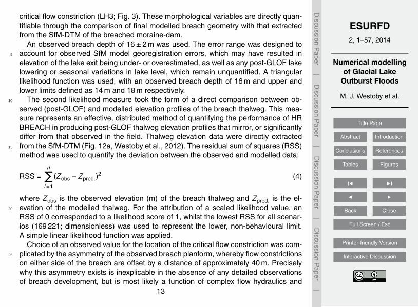
scenarios, with the result being reduced variation in percentile-specific Qp and Qvol(Table 3).

Individual overtopping waves are preserved for each percentile in the relevant sce-narios (Fig. 10). Median (50th) percentile hydrographs exhibit slightly more variation,both between scenarios, and following conditioning using the second likelihood mea-5

sure. This conditioning step results in a decrease in median percentile Qp for controland overtopping scenarios, but has a negligible effect on the mass-removal simula-tions (Fig. 10). For all scenarios, 5th percentile hydrographs generally trace the lowerboundary of the behavioural hydrograph envelope, and appear to be largely unaffectedby additional conditioning using the elevation profile of the breach centreline.10

The most noticeable impact on percentile hydrograph form is caused by the ad-ditional conditioning of the data on the final likelihood measure. Mass-removal sce-narios appear to be affected to a far lesser degree than the control and overtoppingscenarios. The exception is DT_instant_5, where discharges for 50th and 5th per-centile hydrographs are increased in the first ∼ 80 min, and after which 95th percentile15

discharges decrease, resulting in substantial concentration of the percentile hydro-graphs (Fig. 10). Conditioning on this final likelihood measure causes increased Qp forDT_overtop_min and DT_overtop_mid median percentile hydrographs, whilst the hy-drograph for DT_overtop_max is perturbed between 140–200 min. Notably, DT_controlexhibits increased discharges for the 5th and 50th percentiles, coupled with decreased20

Qp and steepening of the falling limb of the 95th percentile hydrograph.Crucially, percentile hydrograph form is dictated by the time step-specific CDF data.

In turn, CDF form is determined by variations in the likelihood of individual behaviouralhydrographs, and the cumulative distribution of their associated discharges (for eachtime step). The vast number of simulations which, following conditioning on flow con-25

striction location, were subsequently deemed to be non-behavioural (Table 1) servesto alter the form of scenario-specific CDFs. This effect is particularly dramatic forDT_control, where the number of behavioural simulations reduces from 76 to 7 fol-lowing conditioning on final breach depth, breach centreline elevation profile, and flow

23





ESURFD2, 1–57, 2014


Outburst Floods


Title Page



Tables Figures

J I

J I

Back Close

Full Screen / Esc



Discussion

Paper

|D

iscussionP

aper|

Discussion

Paper

|D

iscussionP

aper|

constriction location (LH1+2+3). Similarly, CDF data for DT_instant_5 are derivedfrom just two behavioural hydrographs, which explains both the smaller hydrographenvelope and the high concentration of the percentile hydrographs (Fig. 10).

5.2.3 Data clustering

Issues of mass conservation arose with the extraction of behavioural, percentile-5

derived breach hydrographs. Both 5th and 50th percentile hydrographs for all scenariosconsistently under-predicted the volume of lake water released during breach develop-ment (∼ 7.3×106 m3), whereas volumetric integration of 95th percentile hydrographdata produced substantially increased values of Qvol (Table 3). The median percentileperforms best at replicating total flood volume, under-predicting Qvol by between 0.2–10

0.7×106 m3, 0.4–0.7×106 m3 and 0.1–1.3×106 m3 for LH1, LH1+2, and LH1+2+3,respectively (Table 3).

From a hydrodynamic modelling perspective, an additional and equally important ob-servation is the form of the percentile hydrographs, which generally do not mirror theform of any of the behavioural hydrographs used as input. Combined, issues of mass15

conservation, and the unrepresentative form of the percentile breach hydrographs ren-der them largely unsuitable for use as an upstream boundary condition for subsequenthydrodynamic modelling.

In an effort to further refine the behavioural simulations and improve the represen-tativeness of the derived percentile hydrographs, all behavioural data were clustered,20

regardless of their inclusion of any modelled system perturbations (Fig. 11). Data clus-tering was undertaken in an effort to characterise “styles” of breaching (for example,low peak discharge magnitude and lengthy time to peak, or high peak discharge andshort, sharp, rise to peak) using Qp and Tp data, and independent of the various breach-ing scenarios that were modelled. An automated, subtractive clustering algorithm was25

applied to the unified Qp and time to peak (Tp) data. This method identifies natural clus-ter centroids in raw point datasets, and quantifies the density of points relative to oneanother. Each point is assumed to represent a potential cluster centroid and a measure

24





ESURFD2, 1–57, 2014


Outburst Floods


Title Page



Tables Figures

J I

J I

Back Close

Full Screen / Esc



Discussion

Paper

|D

iscussionP

aper|

Discussion

Paper

|D

iscussionP

aper|

of likelihood is calculated, based on the density of surrounding points. Following initialcluster identification, the density function is revised and subsequent cluster centresidentified in the same manner until a sufficient number of natural clusters are deemedto have been obtained (Hammouda and Karray, 2000; Mathworks, 2012). Point-clustermembership was determined by calculation of the minimum Euclidean distance be-5

tween each data-point and cluster centre. The subtractive method eliminates any sub-jectivity associated with manual cluster identification.

Clusters are broadly defined by Tp range. Cluster 1 contains all simulations with Tp ofapproximately 60–130 min, Cluster 2 is defined by Tp of ∼ 130–170 min, and Cluster 3possesses Tp values in the range ∼ 170–270 min. Ranges of Qp overlap substan-10

tially between Cluster 1 and Cluster 2 (∼ 900–2100 m3 s−1, and ∼ 700–1800 m3 s−1,respectively), and to a lesser degree between Cluster 2 and Cluster 3. These clustersmay be taken as approximately representing a number of “types” of breach hydro-graph, namely: (relatively) high-magnitude, short-duration (Cluster 1), moderate peakmagnitude and mid-range duration (Cluster 2) and low-magnitude, extended duration15

(Cluster 3) GLOF hydrographs.Cluster membership, is not as clear-cut as might be anticipated (Fig. 11). The clus-

tering results appear to imply that pigeonholing different breaching scenarios by hy-drograph type, or style, is virtually impossible. However, the exceptions to this rule arethe instantaneous mass-removal scenarios, which almost exclusively produce high-20

magnitude, short-duration hydrographs. This finding would appear to imply that alter-native factors are required to explain the similarity in the range of hydrograph formsthat are produced by each scenario.

Percentile hydrographs were also extracted from the clustered data. Deviations be-tween observed and modelled median percentile Qvol data are in the range −41 to25

−6 %, demonstrating a minimal improvement over unclustered and scenario-specificvalues of modelled Qvol (Table 3). Clustered 5th and 95th percentile Qvol data vastlyunder- and over-estimate observed Qvol.

25





ESURFD2, 1–57, 2014


Outburst Floods


Title Page



Tables Figures

J I

J I

Back Close

Full Screen / Esc



Discussion

Paper

|D

iscussionP

aper|

Discussion

Paper

|D

iscussionP

aper|

Clustering was largely unsuccessful at improving the utility of percentile-basedbreach hydrographs for use as hydrodynamic input, thereby necessitating the ex-ploration of alternative methods for cascading likelihood-weighted estimates of dam-breach parameter ensemble performance through to the simulation and mapping ofGLOF inundation and hazard.5

5.3 Hydrodynamic modelling

5.3.1 The optimal hydrograph

Deterministic approaches to flood reconstruction require the identification of the opti-mal model, and its subsequent use for predictive flood forecasting. To illustrate the vari-ability between scenario-specific optimal hydrograph routing patterns, the optimal hy-10

drographs for DT_control, DT_overtop_max and DT_instant_5 were used as upstreaminput for simulation in ISIS 2-D. Maps of inundation extent and flow depth (Fig. 12) re-veal prominent inter-scenario differences in the spatial extent of inundation as the re-spective hydrographs and GLOF floodwaters progress downstream. Variations of noteinclude the initial downstream transmission of the DT_overtop_max overtopping wave,15

which triggers rapid inundation of the entire reach (Fig. 12). However, initially high flowstages are not maintained, and only rise once again with increasing breach dischargeassociated with breach expansion. Use of the DT_instant_5 hydrograph produces spa-tial and temporal patterns of inundation and wetting front travel time similar to that ofDT_overtop_max (Fig. 12).20

5.3.2 GLUE-based GLOF reconstruction

Probabilistic maps of inundation extent and flow depth were constructed through theretention and evaluation of scenario-specific and likelihood-weighted breach hydro-graphs. In the example presented herein, we simulated the propagation of 76 individualmoraine-breach hydrographs using the ISIS 2-D TVD solver (with an 8 m topographic25

26





ESURFD2, 1–57, 2014


Outburst Floods


Title Page



Tables Figures

J I

J I

Back Close

Full Screen / Esc



Discussion

Paper

|D

iscussionP

aper|

Discussion

Paper

|D

iscussionP

aper|

grid discretisation and a 0.04 s time step), representing the behavioural DT_control pa-rameter ensembles after conditioning on final breach depth. However, the method isequally applicable to the use of several, hundreds, or thousands of individual simula-tions. For each time step, Per-cell CDF curves of flow depth were assembled, fromwhich percentile flow depths were extracted and plotted (Fig. 13). Given the inherent5

uncertainty surrounding the precise mode of moraine-dam failure and outflow hydro-graph form, these data effectively convey the resulting variability in likelihood-weightedpredictions of reconstructed inundation extent, whilst preserving time step-specific per-centile flow depths. Due to the nature of their construction, these data do not relate toa specific event or hydrograph, but instead provide an indication as to the potential10

uncertainty in GLOF inundation extents and flow depths associated with a range ofbehavioural breach hydrographs.

5.3.3 Probabilistic hazard mapping

The final output of a GLOF hazard assessment comprises the production of maps offlood hazard, conditioned by one or more directly-quantifiable flood-intensity indicators15

(e.g. Aronica et al., 2012). Whilst inundation depth is arguably the most significantflood-intensity indicator for predicting monetary losses associated with individual floodevents (Merz and Thieken, 2004; Vorogushyn et al., 2010, 2011), its combination withflow velocity is regarded as an improved indicator of hazard to human life (Aronicaet al., 2012).20

A global hazard index proposed by Aronica et al. (2012) was used to construct mapsof GLOF hazard (Fig. 14). Taking probabilistic flow depth and velocity data as input,probabilistic GLOF hazard maps were produced for the DT_control scenario. Four haz-ard classes are defined and shaded for distinction (H1 to H4; in order of increasing haz-ard). Hazard distribution is characterised by extensive zones of H1 for the 5th and 50th25

percentiles in the first 0.5 h, with higher hazard classes becoming increasingly preva-lent in the 95th percentile data (Fig. 14). As breach outflow increases and the maxi-mum inundation extent is approached, the zone immediately adjacent to the channel

27





ESURFD2, 1–57, 2014


Outburst Floods


Title Page



Tables Figures

J I

J I

Back Close

Full Screen / Esc



Discussion

Paper

|D

iscussionP

aper|

Discussion

Paper

|D

iscussionP

aper|

thalweg is classed as “very high” (H4) hazard, and is associated with flow depths inexcess of 1.5 m and regardless of velocity. Classes H1, H3 and H4 dominate for all timesteps, whilst H2 is noticeably underrepresented. Inundated channel-marginal areas aregenerally classed as being of low hazard, whilst the classification of the remaining in-undated area as H3 or H4 indicates the presence of flow velocities that either exceed5

the prescribed product of depth and velocity (0.7 m2 s−1), or depths in excess of 1.5 m.

6 Discussion

6.1 Elucidating the key controls on breach development

The inherent uncertainty associated with moraine dam-breach model parameterisationhas a significant influence on the magnitude and characteristics of modelled breach10

hydrographs. This has significant implications for GLOF reconstruction efforts, andparticularly for subsequent hydrodynamic modelling. We have demonstrated that thepropagation, or cascading, of the parametric uncertainty and equifinality through thedam-breach and hydrodynamic modelling elements of the GLOF model chain is notonly possible, but may be of considerable value to flood risk practitioners. The method-15

ological framework developed and demonstrated in this study is summarised in Fig. 15.Our results highlight the primary influence of moraine material roughness in dictat-

ing HR BREACH parameter ensemble (and therefore breach hydrograph) performance.Specifically, behavioural Manning’s n coefficients were found to be in the range 0.020–

0.029 m−1/3 s (Fig. 7), representing a significant refinement of the a priori parameter20

range (0.02–0.05 m−1/3 s). In contrast, no significant refinement of the remaining ma-terial characteristic parameters was made following model evaluation.

However, posterior Manning’s n values appear to be highly unrealistic; the Dig Tshomoraine is composed predominantly of gravel-, cobble- and boulder-sized material,which is more likely to be associated with larger roughness coefficient values (Chow,25

1959). Precisely why this occurs is unclear. However, the physicality of the numerical28





ESURFD2, 1–57, 2014


Outburst Floods


Title Page



Tables Figures

J I

J I

Back Close

Full Screen / Esc



Discussion

Paper

|D

iscussionP

aper|

Discussion

Paper

|D

iscussionP

aper|

dam-breach model used in this research undoubtedly represents an improvement overempirical or analytical models. It should also be noted that many of the geometric andmaterial characteristics of the moraine and lake complex remain highly simplified.

6.2 The utility of behavioural GLOF modelling

The computational restrictions that dominate both the recovery of high-resolution topo-5

graphic moraine and valley-floor data and the use of higher-order hydrodynamic codeswere appreciable in this study, where access to a suite of powerful computing resourceswas not an issue. However, options for streamlining the framework are being consid-ered. The most computationally-demanding step in the model chain is currently thetwo-dimensional hydrodynamic modelling component. Consequently, one avenue for10

exploration might be the use of reduced-complexity hydrodynamic codes, which pre-serve much of the physicality of “full” 2-D codes, but at a much-reduced computationalburden (e.g. McMillan and Brasington, 2007; Yu and Lane, 2006).

Whilst the extraction of percentile maps of inundation extent and flow depth is notnecessarily an entirely new concept (e.g. McMillan and Brasington, 2007, 2008; Voro-15

gusyhn et al., 2010, 2011), the application to GLOF reconstruction presented here is anoriginal and novel one. This approach represents a significant improvement in the ef-fective communication of the likelihood associated with a range of moraine-dam failurescenarios, and the production of meaningful, probability-based flood hazard maps.

The likelihood of multiple GLOFs occurring from an individual moraine-dammed lake20

complex is extremely low, since in the majority of cases, the breached moraine damcan comfortably accommodate relict lake discharges. Therefore, the identification anduse of posterior parameter distribution data for predictive GLOF forecasting is of limitedutility if these ranges prove to be highly site-specific (which this additional data wouldappear to suggest). Ultimately, the identification of a suite of universal or region-specific25

material characteristics and their probabilistic distributions would facilitate their use inpredictive GLOF simulation efforts, and should be a focus of future research.

29





ESURFD2, 1–57, 2014


Outburst Floods


Title Page



Tables Figures

J I

J I

Back Close

Full Screen / Esc



Discussion

Paper

|D

iscussionP

aper|

Discussion

Paper

|D

iscussionP

aper|

In considering the source of uncertainty in the GLOF modelling process, we havefocused on its influence over the moraine dam-failure process. However, numerousadditional sources of uncertainty are present at various stages in the workflow (e.g.reconstruction of drained lake-basin bathymetry and extraction of hypsometric data)and merit further investigation (Westoby et al., 2014). The logistical impracticalities of5

identifying and addressing all sources of uncertainty in the GLOF model chain are likelyto prove a significant hindrance to applied modelling efforts. However, simple sensitivityanalyses remain of value to quantify the impacts of individual sources of uncertaintyon numerical dam-breach and hydrodynamic simulation, and might be incorporatedstraightforwardly into the framework (Fig. 15).10

Probabilistic approaches have clear advantages over the deterministic approachestraditionally used for GLOF reconstruction such as the use of paleohydraulic tech-niques for at-a-point, or reach-scale peak discharge estimation (e.g. Cenderelli andWohl, 2003; Kershaw et al., 2005; Bohorquez and Darby, 2008). Probabilistic meth-ods embrace and attempt to convey the influence of uncertainty and equifinality in15

model input on subsequent output, and it might be argued that their value outweighsthe additional processing time required for their implementation, which may involve theexecution of hundreds or thousands of individual simulations.

7 Conclusions

This paper has outlined and presented results from a workflow for cascading uncer-20

tainty and equifinality through the Glacial Lake Outburst Flood (GLOF) model chainusing a combination of advanced, physically-based numerical dam-breach and hydro-dynamic models. Dam material roughness is the dominant influence on outflow hy-drograph form. We have demonstrated that morphological characteristics of a GLOFbreach are appropriate measures for assessing the performance of individual simula-25

tions, or parameter ensembles, at reproducing observed breach morphology. Breachmorphology is reproducible by parameter ensembles associated with differing breach

30





ESURFD2, 1–57, 2014


Outburst Floods


Title Page



Tables Figures

J I

J I

Back Close

Full Screen / Esc



Discussion

Paper

|D

iscussionP

aper|

Discussion

Paper

|D

iscussionP

aper|

initiation scenarios, lending support for the adoption of probabilistic, as opposed to de-terministic methods for dam-breach outburst flood reconstruction. We also demonstratean effective approach for cascading dam-breach simulation likelihood data through tothe construction of probability-based maps of GLOF inundation extent and flow depth,and the subsequent derivation of event-specific maps of flood hazard. Future research5

should focus on the suitability of probabilistic methods for predictive, as opposed toreconstructive, GLOF simulation and hazard assessment.

Acknowledgements. MJW was funded by a NERC Open CASE Award (NE/G011443/1) in part-nership with Reynolds International Ltd. Additional funding to support field activities from theDepartment of Geography and Earth Sciences Postgraduate Discretionary Fund (Aberystwyth10

University) is duly acknowledged. J. Balfour, P. Cowley, S. Doyle, H. Sevestre, C. Souness, R.Taylor and guides and porters from Summit Trekking, Kathmandu, assisted with data collec-tion in the Khumbu Himal. HR Wallingford Ltd and the Halcrow Group Ltd are thanked for theprovision of academic licences for the use of HR BREACH and ISIS 2D, respectively. GeoEyeimagery (Fig. 1b) was provided free of charge by the GeoEye Foundation. ASTER GDEM data15

were downloaded free of charge from http://asterweb.jpl.nasa.gov/gdem.asp. Breach hydro-graph data clustering was undertaken in MathWorks’ MATLAB®.

References

Alho, P. and Aaltonen, J.: Comparing a 1D hydraulic model with a 2D hydraulic model for thesimulation of extreme glacial outburst floods, Hydrol. Process., 22, 1537–1547, 2008.20

Aronica, G., Hankin, B., and Beven, K.: Uncertainty and equifinality in calibrating distributedroughness coefficients in a flood propagation model with limited data, Adv. Water Resour.,22, 349–365, 1998.

Aronica, G., Bates, P. D., and Horritt, M. S.: Assessing the uncertainty in distributed modelpredictions using observed binary pattern information within GLUE, Hydrol. Process., 16,25

2001–2016, 2002.Aronica, G., Candela, A., Fabio, P., and Santoro, M.: Estimation of flood inundation probabilities

using global hazard indexes based on hydrodynamic variables, Phys. Chem. Earth, 42–44,119–129, 2012.

31





http://asterweb.jpl.nasa.gov/gdem.asp

ESURFD2, 1–57, 2014


Outburst Floods


Title Page



Tables Figures

J I

J I

Back Close

Full Screen / Esc



Discussion

Paper

|D

iscussionP

aper|

Discussion

Paper

|D

iscussionP

aper|

Astre, H.: SFMToolkit3, available at: http://www.visual-experiments.com/demos/sfmtoolkit (lastaccess: 12 June 2014), 2010.

Bajracharya, B., Shrestha, A. B., and Rajbhandar, L.: Glacial Lake Outburst Floods in theSagarmatha Region, Mt. Res. Dev., 27, 336–344, 2007.

Barré de St-Venant, A. J. C.: Théorie et Equations Générales du Mouvement Non Permanent5

des Eaux Courantes, Comptes Rendus des séances de l’Académie des Sciences, 73, 147–154, 1871.

Bates, P. D., Marks, K. J., and Horritt, M. S.: Optimal use of high-resolution topographic data inflood inundation models, Hydrol. Process., 17, 537–557, 2003.

Benn, D. I., Wiseman, S., and Hands, K. A.: Growth and drainage of supraglacial lakes on10

debris-mantled Ngozumpa Glacier, Khumbu Himal, Nepal, J. Glaciol., 47, 626–638, 2001.Benn, D. I., Bolch, T., Hands, K., Gulley, J., Luckman, A., Nicholson, L. I., Quincey, D. J., Thomp-

son, S., Toumi, R., and Wiseman, S.: Response of debris-covered glaciers in the MountEverest region to recent warming and implications for outburst flood hazards, Earth-Sci.Rev., 114, 156–174, 2012.15

Beven, K.: A manifesto for the equifinality thesis, J. Hydrol., 320, 18–36, 2005.Beven, K. and Binley, A.: The future of distribution models: model calibration and uncertainty

prediction, Hydrol. Process., 6, 279–298, 1992.Beven, K. and Freer, J.: Equifinality, data assimilation, and uncertainty estimation in mechanistic

modelling of complex environmental systems using the GLUE methodology, J. Hydrol., 249,20

11–29, 2001.Blazkova, S. and Beven, K.: Flood frequency estimation by continuous simulation of subcatch-

ment rainfalls and discharges with the aim of improving dam safety assessment in a largebasin in the Czech Republic, J. Hydrol., 292, 153–172, 2004.

Bohorquez, P. and Darby, S. E.: The use of one- and two-dimensional hydraulic modelling to25

reconstruct a glacial outburst flood in a steep Alpine valley, J. Hydrol., 361, 240–261, 2008.Bolch, T., Pieczonka, T., and Benn, D. I.: Multi-decadal mass loss of glaciers in the Everest area

(Nepal Himalaya) derived from stereo imagery, The Cryosphere, 5, 349–358, doi:10.5194/tc-5-349-2011, 2011.

Bolch, T., Kulkarni, A., Kääb, A., Huggel, C., Paul, F., Cogley, J. G., Frey, H., Kargel, J. S.,30

Fujita, K., Scheel, M., Bajracharya, S., and Stoffel, M.: The state and fate of Himalayanglaciers, Science, 336, 310–314, 2012.

32





http://www.visual-experiments.com/demos/sfmtoolkit

http://dx.doi.org/10.5194/tc-5-349-2011

http://dx.doi.org/10.5194/tc-5-349-2011

http://dx.doi.org/10.5194/tc-5-349-2011

ESURFD2, 1–57, 2014


Outburst Floods


Title Page



Tables Figures

J I

J I

Back Close

Full Screen / Esc



Discussion

Paper

|D

iscussionP

aper|

Discussion

Paper

|D

iscussionP

aper|

Cameron, D.: Flow, frequency, and uncertainty estimation for an extreme historical flood eventin the Highlands of Scotland, UK, Hydrol. Process., 21, 1460–1470, 2007.

Cao, Z. and Carling, P.: Mathematical modelling of alluvial rivers: reality and myth, Part 1:general overview, Mar. Eng., 154, 207–219, 2002.

Casas, A., Lane, S. N., Yu, D., and Benito, G.: A method for parameterising roughness and5

topographic sub-grid scale effects in hydraulic modelling from LiDAR data, Hydrol. EarthSyst. Sci., 14, 1567–1579, doi:10.5194/hess-14-1567-2010, 2010.

Castellarin, A., Merz, R., and Bloschl, G.: Probabilistic envelope curves for extreme rainfallevents, J. Hydrol., 378, 263–271, 2009.

Cenderelli, D. A. and Wohl, E. E.: Peak discharge estimates of glacial-lake outburst floods and10

“normal” climatic floods in the Mount Everest region, Nepal, Geomorphology, 40, 57–90,2001.

Cenderelli, D. A. and Wohl, E. E.: Flow hydraulics and geomorphic effects of glacial-lake out-burst floods in the Mount Everest region, Nepal, Earth Surf. Proc. Land., 28, 385–407, 2003.

Chen, Y. H. and Anderson, B. A.: Development of a methodology for estimating embank-15

ment damage due to flood overtopping, US Federal Highway Administration Report No,FHWA/RD-86/126, 1986.

Chow, V. T.: Open-Channel Hydraulics, McGraw-Hill, New York, 677 pp., 1959.Clague, J. J. and Evans, S. G.: A review of catastrophic drainage of moraine-dammed lakes in

British Columbia, Quaternary Sci. Rev., 19, 1763–1783, 2000.20

Dewals, B., Erpicum, S., Detrembleur, S., Archambeau, P., and Pirotton, M.: Failure of damsarranged in series or in complex, Nat. Hazards, 56, 917–939, 2011.

Di Baldassarre, G. and Claps, P.: A hydraulic study on the applicability of flood rating curves,Hydrol. Res., 42, 10–19, 2011.

Fonstad, M. A., Dietrich, J. T., Courville, B. C., Jensen, J. L., and Carbonneau, P. E.: Topo-25

graphic structure from motion: a new development in photogrammetric development, EarthSurf. Proc. Land., 38, 421–430, 2013.

Franz, K. J. and Hogue, T. S.: Evaluating uncertainty estimates in hydrologic models: borrowingmeasures from the forecast verification community, Hydrol. Earth Syst. Sci., 15, 3367–3382,doi:10.5194/hess-15-3367-2011, 2011.30

Freer, J., Beven, K. J., and Peters, N. E.: Multivariate seasonal period model rejection within thegeneralised likelihood uncertainty estimation procedure, in: Calibration of Watershed Models,

33





http://dx.doi.org/10.5194/hess-14-1567-2010


ESURFD2, 1–57, 2014


Outburst Floods


Title Page



Tables Figures

J I

J I

Back Close

Full Screen / Esc



Discussion

Paper

|D

iscussionP

aper|

Discussion

Paper

|D

iscussionP

aper|

edited by: Duan, Q., Gupta, H., Sorooshian, S., Rousseau, A. N., and Turcotte, R., AGUBooks, Washington, 69–87, 2002.

Frey, H., Haeberli, W., Linsbauer, A., Huggel, C., and Paul, F.: A multi-level strategy for antic-ipating future glacier lake formation and associated hazard potentials, Nat. Hazards EarthSyst. Sci., 10, 339–352, doi:10.5194/nhess-10-339-2010, 2010.5

Galay, V.: Glacier Lake Outburst Flood (Jökulhlaup) on the Bothe/Dudh Kosi, 4 August 1985.Internal Report, Water and Energy Committee, Ministry of Water Resources, His Majesty’sGovernment of Nepal, Kathmandu, Nepal, 1985.

Halcrow: ISIS 2D by Halcrow, overview available at: www.halcrow.com/isis/ (last access: 12June 2014), 2012.10

Hall, J., Tarantola, S., Bates, P. D., and Horritt, M.: Distributed sensitivity analysis of flood inun-dation model calibration, J. Hydraul. Eng., 131, 117–126, 2005.

Hanson, G. J. and Cook, K. R.: Apparatus, test procedures, and analytical methods to measuresoil erodibility in situ, Appl. Eng. Agric., 20, 455–462, 2004.

Harrison, S., Glasser, N. F., Winchester, V., Haresign, E., Warren, C., and Jansson, K.: A glacial15

lake outburst flood associated with recent mountain glacier retreat, Patagonian Andes,Holocene, 16, 611–620, 2006.

Hassan, A. E., Bekhit, H., and Chapman, J. B.: Uncertainty assessment of a stochastic ground-water flow model using GLUE analysis, J. Hydrol., 362, 89–109, 2008.

Hassan, M. and Morris, M.: HR-BREACH Model Documentation, HR Wallingford Ltd, Walling-20

ford, Oxfordshire, UK, 2012.Horritt, M. S. and Bates, P. D.: Evaluation of 1D and 2D numerical models for predicting river

flood inundation, J. Hydrol., 268, 87–99, 2002.Hunter, N. M., Bates, P. D., Horritt, M. S., De Roo, A. P. J., and Werner, M. G. F.: Utility of

different data types for calibrating flood inundation models within a GLUE framework, Hydrol.25

Earth Syst. Sci., 9, 412–430, doi:10.5194/hess-9-412-2005, 2005.Iman, R. L. and Helon, J. C.: An investigation of uncertainty and sensitivity analysis techniques

for computer models, Risk Anal., 8, 71–90, 2006.IMPACT: Investigation of Extreme Flood Processes and Uncertainty: Risk and Uncertainty

(WP5) – Technical Report, 44 pp., available at: www.impact-project.net (last access: 12 June30

2014), 2004.

34





www.halcrow.com/isis/


www.impact-project.net

ESURFD2, 1–57, 2014


Outburst Floods


Title Page



Tables Figures

J I

J I

Back Close

Full Screen / Esc



Discussion

Paper

|D

iscussionP

aper|

Discussion

Paper

|D

iscussionP

aper|

James, M. R. and Robson, S.: Straightforward reconstruction of 3D surfaces and topogra-phy with a camera: accuracy and geoscience applications, J. Geophys. Res., 117, F03017,doi:10.1029/2011JF002289, 2012.

Jansky, B., Engel, Z., Šobr, M., Beneš, V., Špaček, K., and Yerokhin, S.: The evolution of Petrovlake and moraine dam rupture risk (Tien-Shan, Kyrgyzstan), Nat. Hazards, 50, 83–96, 2009.5

Javernick, L., Brasington, J., and Caruso, B.: Modelling the topography of shallowbraided rivers using Structure-from-Motion photogrammetry, Geomorphology, 213, 166–182,doi:10.1016/j.geomorph.2014.01.006, 2014.

Kääb, A., Huggel, C., Fischer, L., Guex, S., Paul, F., Roer, I., Salzmann, N., Schlaefli, S.,Schmutz, K., Schneider, D., Strozzi, T., and Weidmann, Y.: Remote sensing of glacier- and10

permafrost-related hazards in high mountains: an overview, Nat. Hazards Earth Syst. Sci.,5, 527–554, doi:10.5194/nhess-5-527-2005, 2005.

Kaser, G., Cogley, J. G., Dyurgerov, B., Meier, M. F., and Ohmura, A.: Mass balance of glaciersand ice caps: consensus estimates for 1961–2004, Geophys. Res. Lett., 33, 1–5, 2006.

Kershaw, J. A., Clague, J. J., and Evans, S. G.: Geomorphic and sedimentological signature15

of a two-phase outburst flood from moraine-dammed Queen Bess Lake, British Columbia,Canada, Earth Surf. Proc. Land., 30, 1–25, 2005.

Kidson, R. L., Richards, K. S., and Carling, P. A.: Hydraulic model calibration for extreme floodsin bedrock-confined channels: case study from northern Thailand, Hydrol. Process., 20, 329–344, 2006.20

Kuczera, G. and Parent, E.: Monte Carlo assessment of parameter uncertainty in conceptualcatchment models: the Metropolis algorithm, J. Hydrol., 211, 69–85, 1998.

Lamb, R., Beven, K., and Myrabo, S.: Use of spatially distributed water table observations toconstrain uncertainty in a rainfall–runoff model, Adv. Water Resour., 22, 305–317, 1998.

Lebourg, T., Riss, J., and Pirard, E.: Influence of morphological characteristics of heteroge-25

neous moraine formations on their mechanical behaviour using image and statistical analy-sis, Eng. Geol., 73, 37–50, 2004.

Liang, D., Falconer, R. A., and Lin, B.: Comparison between TVD-MacCormack and ADI-typesolvers of the shallow water equations, Adv. Water Resour., 29, 1833–1845, 2006.

Liang, D., Lin, B., and Falconer, R. A.: Simulation of rapidly varying flow using an efficient TVD-30

MacCormack scheme, Int. J. Numer. Method. H., 53, 811–826, 2007.Liao, C. B., Wu, M. S., and Liang, S. J.: Numerical simulation of a dam break for an actual river

terrain environment, Hydrol. Process., 21, 447–460, 2007.

35





http://dx.doi.org/10.1029/2011JF002289

http://dx.doi.org/10.1016/j.geomorph.2014.01.006

http://dx.doi.org/10.5194/nhess-5-527-2005

ESURFD2, 1–57, 2014


Outburst Floods


Title Page



Tables Figures

J I

J I

Back Close

Full Screen / Esc



Discussion

Paper

|D

iscussionP

aper|

Discussion

Paper

|D

iscussionP

aper|

Lliboutry, L., Morales, B., Pautre, A., and Schneider, B.: Glaciological problems set by the con-trol of dangerous lakes in Cordillera Blanca, Peru, I: Historical failure of morainic dams, theircauses and prevention, J. Glaciol., 18, 239–254, 1977.

Lowe, D. G.: Distinctive image features from scale-invariant keypoints, Int. J. Comput. Vision,60, 91–110, 2004.5

Mathworks®: MATLAB (version 7.6), available at: www.mathworks.co.uk 2012.McMillan, H. K. and Brasington, J.: Reduced complexity strategies for modelling urban flood-

plain inundation, Geomorphology, 90, 226–243, 2007.McMillan, H. K. and Brasington, J.: End-to-end flood risk assessment: a coupled model cascade

with uncertainty estimation, Water Resour. Res., 44, W03419, doi:10.1029/2007WR005995,10

2008.Merz, B. and Thieken, A.: Flood risk analysis: concepts and challenge, Oesterreeichische

Wasser Abfallwirtscht, 56, 27–34, 2004.Meselhe, E. A. and Holly Jr., F. M.: Invalidity of Preissmann scheme for transcritical flow, J.

Hydraul. Eng., 123, 652–655, 1997.15

Metropolis, N.: The beginning of the Monte Carlo method, Los Alamos Science, 1987 SpecialIssue, 125–130, 1987.

Mohamed, M. A. A., Samuels, P. G., Morris, M., and Ghataora, G. S.: Improving the accuracy ofprediction of breach formation through embankment dams and flood embankments, in: RiverFlow 2002: 1st International Conference on Fluvial Hydraulics, edited by: Bousmar, D. and20

Zech, Y., Louvain-la-Neuve, Belgium, 3–6 September, 10 pp., 2002.Morris, M., Hanson, G., and Hassan, M. A. A.: Improving the accuracy of breach modelling:

why are we not progressing faster?, J. Flood Risk Manage., 1, 150–161, 2008.Nicholas, A. P. and Quine, T. A.: Quantitative assessment of landform equifinality and palaeoen-

vironmental reconstruction using geomorphic models, Geomorphology, 121, 167–183, 2010.25

Oerlemans, J.: Quantifying global warming from the retreat of glacier, Science, 264, 243–245,1994.

Osti, R. and Egashira, S.: Hydrodynamic characteristics of the Tam Pokhari Glacial Lake out-burst flood in the Mt. Everest region, Nepal, Hydrol. Process., 23, 2943–2955, 2009.

Osti, R., Bhattarai, T. N., and Miyake, K.: Causes of catastrophic failure of Tam Pokhari moraine30

dam in the Mt. Everest region, Nat. Hazards, 58, 1209–1223, 2011.Pappenberger, F., Beven, K. J., Hunter, N. M., Bates, P. D., Gouweleeuw, B. T., Thielen, J.,

and de Roo, A. P. J.: Cascading model uncertainty from medium range weather forecasts

36





www.mathworks.co.uk

http://dx.doi.org/10.1029/2007WR005995

ESURFD2, 1–57, 2014


Outburst Floods


Title Page



Tables Figures

J I

J I

Back Close

Full Screen / Esc



Discussion

Paper

|D

iscussionP

aper|

Discussion

Paper

|D

iscussionP

aper|

(10 days) through a rainfall-runoff model to flood inundation predictions within the EuropeanFlood Forecasting System (EFFS), Hydrol. Earth Syst. Sci., 9, 381–393, doi:10.5194/hess-9-381-2005, 2005.

Pappenberger, F., Matgen, P., Beven, K. J., Henry, J. B., Pfister, L., and Fraipont de, P.: Influenceof uncertain boundary conditions and model structure on flood inundation predictions, Adv.5

Water Resour., 29, 1430–1449, 2006.Parkin, G., O’Donnell, G., Ewen, J., Bathurst, J. C., O’Connell, P. E., and Lavabre, J.:Validation

of catchment models for predicting land-use and climate change impacts: 2. Case study fora Mediterranean catchment, J. Hydrol., 175, 595–613, 1996.

Quincey, D. J., Lucas, R. M., Richardson, S. D., Glasser, N. F., Hambrey, M. J., and10

Reynolds, J. M.: Optical remote sensing techniques in high-mountain environments: applica-tion to glacial hazards, Prog. Phys. Geogr., 29, 475–505, 2005.

Quincey, D. J., Richardson, S. D., Luckman, A., Lucas, R. M., Reynolds, J. M., Hambrey, M. J.,and Glasser, N. F.: Early recognition of glacial lake hazards in the Himalaya using remotesensing datasets, Global Planet. Change, 56, 137–152, 2007.15

Refsgaard, J. C.: Parameterisation, calibration and validation of distributed hydrological models,J. Hydrol., 198, 69–97, 1997.

Richardson, S. D. and Reynolds, J. M.: An overview of glacial hazards in the Himalayas,Quatern. Int., 65/66, 31–47, 2000.

Rojas, R., Feyen, L., and Dassargues, A.: Conceptual model uncertainty in groundwater mod-20

elling: combing generalized likelihood uncertainty estimation and Bayesian model averaging,Water Resour. Res., 44, W12418, doi:10.1029/2008WR006908, 2008.

Romanowicz, R. and Beven, K.: Dynamic real-time prediction of flood inundation probabilities,Hydrolog. Sci. J., 43, 181–196, 1998.

Rychkov, I., Brasington, J., and Vericat, D.: Computational and methodological aspects of ter-25

restrial surface analysis based on point clouds, Comput. Geosci., 42, 64–70, 2012.Sakai, A., Chikita, K., and Yamada, T.: Expansion of a moraine-dammed glacial lake, Tsho

Rolpa, in Rolwaling Himal, Nepal Himalaya, Limnol. Oceanogr., 45, 1401–1408, 2000.Sanders, B. F.: Evaluation of on-line DEMs for flood inundation modelling, Adv. Water Resour.,

30, 1831–1843, 2007.30

Snavely, N.: Scene Reconstruction and Visualization from Internet Photo Collections, unpub-lished Ph.D. thesis, University of Washington, USA, 2008.

37








http://dx.doi.org/10.1029/2008WR006908

ESURFD2, 1–57, 2014


Outburst Floods


Title Page



Tables Figures

J I

J I

Back Close

Full Screen / Esc



Discussion

Paper

|D

iscussionP

aper|

Discussion

Paper

|D

iscussionP

aper|

Snavely, N., Seitz, S. N., and Szeliski, R.: Modelling the world from internet photo collections,Int. J. Comput. Vision 80, 189–210, 2008.

Spetsakis, M. E., Aloimonos, Y.: A multi-frame approach to visual motion perception, Int. J.Comput. Vision, 6, 245–255, 1991.

Stokes, C. R., Spagnolo, M., and Clark, C. D.: The composition and internal structure of drum-5

lins: complexity, commonality, and implications for a unifying theory of their formation, Earth-Sci. Rev., 107, 398–422, 2011.

Thompson, S. S., Benn, D. I., Dennis, K., and Luckman, A.: A rapidly-growing moraine-dammedglacial lake on Ngozumpa Glacier, Nepal, Geomorphology, 145–146, 1–11, 2012.

Vasquez, R. F., Beven, K., and Feyen, J.: GLUE based assessment on the overall predictions10

of a MIKE SHE application, Water Resour. Manag., 23, 1325–1349, 2009.Venutelli, M.: Stability and accuracy of weighted four-point implicit finite difference schemes for

open channel flow, J. Hydraul. Eng., 128, 281–288, 2002.von Bertalanffy, L.: General System Theory – Foundations, Development, Applications, 2nd

Edn., George Braziller, New York, 295 pp., 1968.15

Vorogushyn, S., Merz, B., Lindenschmidt, K. E., and Apel, H.: A new methodology forflood hazard assessment considering dike breaches, Water Resour. Res., 46, W08541,doi:10.1029/2009WR008475, 2010.

Vorogushyn, S., Apel, H., and Merz, B.: The impact of the uncertainty of dike breach develop-ment time on flood hazard, Phys. Chem. Earth, 36, 319–323, 2011.20

Vrugt, J. A., ter Braak, C. J. F., Gupta, H. V., and Robinson, B. A.: Equifinality of formal (DREAM)and informal (GLUE) Bayesian approaches in hydrologic modelling?, Stoch. Env. Res. RiskA., 23, 1011–1026, 2009.

Vuichard, D., and Zimmerman, M.: The Langmoche flash-flood, Khumbu Himal, Nepal, Mt. Res.Dev., 6, 90–94, 1986.25

Vuichard, D., and Zimmerman, M.: The 1985 catastrophic drainage of a moraine-dammed lake,Khumbu Himal, Nepal: cause and consequences, Mt. Res. Dev., 7, 91–110, 1987.

Wahl, T.: Prediction of embankment dam breach parameters: a literature review and needsassessment, Report no. DSO-98–004, Water Resources Research Laboratory, Dam SafetyOffice, Department of the Interior, 67 pp., Denver, Colorado, 1998.30

Wang, W., Yang, X., and Yao, T.: Evaluation of ASTER GDEM and SRTM and their suitability inhydraulic modelling of a glacial lake outburst flood in southeast Tibet, Hydrol. Process., 26,213–225, 2012.

38





http://dx.doi.org/10.1029/2009WR008475

ESURFD2, 1–57, 2014


Outburst Floods


Title Page



Tables Figures

J I

J I

Back Close

Full Screen / Esc



Discussion

Paper

|D

iscussionP

aper|

Discussion

Paper

|D

iscussionP

aper|

Watanabe, T. and Rothacher, D.: The 1994 Lugge Tsho Glacial Lake Outburst Flood, BhutanHimalaya, Mt. Res. Dev., 16, 77–81., 1996.

Watanabe, T., Kameyama, S., and Sato, T.: Imja Glacier dead-ice melt rates and changes ina supraglacial lake, 1989–1994, Khumbu Himal, Nepal: danger of lake drainage, Mt. Res.Dev., 15, 293–300, 1995.5

Westerberg, I. K., Guerrero, J.-L., Younger, P. M., Beven, K. J., Seibert, J., Halldin, S., Freer,J. E., and Xu, C.-Y.: Calibration of hydrological models using flow-duration curves, Hydrol.Earth Syst. Sci., 15, 2205–2227, doi:10.5194/hess-15-2205-2011, 2011.

Westoby, M. J.: The Development of a Unified Framework for Low-Cost Glacial Lake OutburstFlood Hazard Assessment, unpublished Ph.D. thesis, Department of Geography, History and10

Politics, Aberystwyth University, 456 pp., 2013.Westoby, M. J., Brasington, J., Glasser, N. F., Hambrey, M. J., and Reynolds, J. M.: “Structure-

from-Motion” photogrammetry: a low-cost, effective tool for geoscience applications, Geo-morphology, 179, 300–314, 2012.

Westoby, M. J., Glasser, N. F., Brasington, J., Hambrey, M. J., Quincey, D. J., and15

Reynolds, J. M.: Modelling outburst floods from moraine-dammed glacial lakes, Earth-Sci.Rev., 134, 137–159, doi:10.1016/j.earscirev.2014.03.009, 2014.

Wohl, E. E.: Uncertainty in flood estimates associated with roughness coefficient, J. Hydraul.Eng., 124, 219–223, 1998.

Worni, R., Stoffel, M., Huggel, C., Volz, C., Casteller, A., and Luckman, B.: Anal-20

ysis and dynamic modelling of a moraine failure and glacier lake outburst floodat Ventisquero Negro, Patagonian Andes (Argentina), J. Hydrol.,444–445, 134–145,doi:10.1016/j.jhydrol.2012.04.013, 2012.

Xin, W., Shlyln, L., Wanqin, G., and Junll, X.: Assessment and simulation of Glacier Lake Out-burst Floods for Longbasaba and Pida Lakes, China, Mt. Res. Dev., 28, 310–317, 2008.25

Yu, D. and Lane, S. N.: Urban fluvial flood modelling using a two-dimensional diffusion-wavetreatment, part 2: development of a sub-grid-scale treatment, Hydrol. Process., 20, 1567–1583, 2006.

Zemp, M., Hoelzle, M., and Haeberli, W.: Six decades of glacier mass balance observations –a review of the worldwide monitoring network, Ann. Glaciol., 50, 101–111, 2009.30

Zhang, S. and Duan, J. G.: 1D finite volume model of unsteady flow over mobile bed, J. Hydrol.,405, 57–68, 2011.

39





http://dx.doi.org/10.1016/j.earscirev.2014.03.009

http://dx.doi.org/10.1016/j.jhydrol.2012.04.013

ESURFD2, 1–57, 2014


Outburst Floods


Title Page



Tables Figures

J I

J I

Back Close

Full Screen / Esc



Discussion

Paper

|D

iscussionP

aper|

Discussion

Paper

|D

iscussionP

aper|

Table 1. Parameter ranges and geometric characteristics of the Dig Tsho moraine dam usedfor input to the HR BREACH numerical dam-breach model. Input parameter ranges were es-tablished from a combination of initial experimentation and parameter sensitivity analysis (E),in situ field observation (F) and data from similar sites stated in the literature (L). All dam ge-ometry data were extracted from the SfM-DTMs of the moraine and floodplain (SfM-DTM),with the exception of downstream Manning’s n, which reflects a sedimentological valley floorcharacterisation of gravels, cobbles and rare large boulders (after Chow, 1959).

Input parameter/geometric characteristic Range/value Source (E/F/L)

Parameter

Sediment flow factor 0.8–1.2 EErosion width : depth ratio 0.5–2 ED50 (mm) 28–200 F; L (Worni et al., 2012; Xin et al., 2004)Porosity (% voids) 0.01–0.3 EDensity (kN m−3) 19–24 E

Manning’s n (m−1/3 s) 0.02–0.05 F; LInternal angle of friction (◦) 25–42 E; L (Lebourg et al., 2004)Cohesion (kN m−2) 0–100 E

Dam geometry

Crest level (m OD) 4356

SfM-DTM

Foundation level (m OD) 4316Crest length (m) 250Crest width (m) 30Distal face slope (1 : x) 3.1Proximal face slope (1 : x) 15.2Downstream valley slope (1 : x) 0.19Downstream Manning’s n 0.04 L (Chow, 1959)

40





ESURFD2, 1–57, 2014


Outburst Floods


Title Page



Tables Figures

J I

J I

Back Close

Full Screen / Esc



Discussion

Paper

|D

iscussionP

aper|

Discussion

Paper

|D

iscussionP

aper|

Table 2. Scenario-specific behavioural simulation count for individual likelihood measures.Note: all simulations deemed to be behavioural after application of LH1 (final breach depth)were retained for conditioning on LH2 (breach thalweg elevation profile.

LH1, LH2 LH3

DT_control 76 7DT_overtop_min 98 33DT_overtop_mid 93 33DT_overtop_max 91 29DT_instant_1 90 49DT_instant_3 55 17DT_instant_5 20 2

41





ESURFD2, 1–57, 2014


Outburst Floods


Title Page



Tables Figures

J I

J I

Back Close

Full Screen / Esc



Discussion

Paper

|D

iscussionP

aper|

Discussion

Paper

|D

iscussionP

aper|

Table 3. Total percentile hydrograph outflow volumes for individual scenarios and followingclustering.

Total percentile hydrograph volume (×106 m3)LH1 LH1+2 LH1+2+3

Scenario/Cluster 5th 50th 95th 5th 50th 95th 5th 50th 95thDT_control 2.2 6.6 13.1 2.2 6.6 13.3 4.8 7.0 9.5DT_overtop_min 1.8 6.5 14.4 1.7 6.5 14.2 1.2 6.6 15.2DT_overtop_mid 1.5 6.4 15.0 1.5 6.2 14.6 1.3 6.3 16.0DT_overtop_max 1.9 6.5 14.2 1.8 6.5 13.8 1.7 6.0 14.1DT_instant_1 1.0 6.4 15.2 1.1 6.5 14.6 1.8 6.9 13.4DT_instant_3 3.2 6.9 11.8 3.4 6.8 11.3 3.6 6.8 11.1DT_instant_5 4.4 7.1 10.2 3.6 6.9 10.2 5.7 7.3 8.8

Cluster 1 2.1 6.6 13.8 2.4 6.8 12.9 1.6 4.4 8.8Cluster 2 3.2 6.8 11.5 3.2 6.8 11.6 2.5 6.9 12.1Cluster 3 3.2 6.8 11.2 3.1 6.8 11.5 3.0 6.7 11.6

42





ESURFD2, 1–57, 2014


Outburst Floods


Title Page



Tables Figures

J I

J I

Back Close

Full Screen / Esc



Discussion

Paper

|D

iscussionP

aper|

Discussion

Paper

|D

iscussionP

aper|

Figure 1. The Dig Tsho moraine dam and upper reaches of the Langmoche Khola. 1

(a) True colour GeoEye imagery of the study site. Extensive reworking of the valley-2

floor by escaping floodwaters is evident immediately downstream of the moraine 3

breach. Red dashes indicate two-dimensional model domain. (b) The moraine-dam 4

breach, formed by the 1985 GLOF. For scale, the boulder indicated by the black 5

arrow is >10 m in height and diameter. The breach is ~200 m at its widest point, and 6

has a maximum depth of 60 m. The relict Dig Tsho glacial lake is visible in the 7

background (DT). 8

9

10

11

12

DT

Dig Tsho

b

Breach

Langmoche

Figure 1. The Dig Tsho moraine dam and upper reaches of the Langmoche Khola. (a) Truecolour GeoEye imagery of the study site. Extensive reworking of the valley-floor by escapingfloodwaters is evident immediately downstream of the moraine breach. Red dashes indicatetwo-dimensional model domain. (b) The moraine-dam breach, formed by the 1985 GLOF. Forscale, the boulder indicated by the black arrow is > 10 m in height and diameter. The breach is∼ 200 m at its widest point, and has a maximum depth of 60 m. The relict Dig Tsho glacial lakeis visible in the background (DT).

43





ESURFD2, 1–57, 2014


Outburst Floods


Title Page



Tables Figures

J I

J I

Back Close

Full Screen / Esc



Discussion

Paper

|D

iscussionP

aper|

Discussion

Paper

|D

iscussionP

aper|

a b

Figure 2. Bathymetric data describing (a) volume-stage, and; (b) area-stage relationships, ex-tracted from a fine-resolution, Structure-from-Motion-derived digital terrain model of the DigTsho moraine-dammed lake basin (Westoby et al., 2012).

44





ESURFD2, 1–57, 2014


Outburst Floods


Title Page



Tables Figures

J I

J I

Back Close

Full Screen / Esc



Discussion

Paper

|D

iscussionP

aper|

Discussion

Paper

|D

iscussionP

aper|

Figure 3. Schematic diagrams of initial (pre-flood) and an example of post-flood geometry for the Dig Tsho moraine dam (left and 1

right columns, respectively), as modelled by HR BREACH. Initial dam face slope angle is represented as a ratio of the form 1:x. 2

White arrows indicate flow direction. Solid black arrows (post-flood, plan view panel) highlight location of the critical flow constriction 3

and used as a likelihood measure for model evaluation. Note vertical exaggeration of dam elevation. 4

5 H

eig

ht

(m)

He

igh

t (m

)

Distance (m) Distance (m)

Figure 3. Schematic diagrams of initial (pre-flood) and an example of post-flood geometry forthe Dig Tsho moraine dam (left and right columns, respectively), as modelled by HR BREACH.Initial dam face slope angle is represented as a ratio of the form 1 : x. White arrows indicate flowdirection. Solid black arrows (post-flood, plan view panel) highlight location of the critical flowconstriction and used as a likelihood measure for model evaluation. Note vertical exaggerationof dam elevation.

45





ESURFD2, 1–57, 2014


Outburst Floods


Title Page



Tables Figures

J I

J I

Back Close

Full Screen / Esc



Discussion

Paper

|D

iscussionP

aper|

Discussion

Paper

|D

iscussionP

aper|

Figure 4. DT_control Cumulative Density Function (CDF) data for T = 150 min (solid 1

line). Changes to likelihood values resulting from Bayesian updating are ultimately 2

translated to changes in the form of the CDF curve, from which percentile Q data are 3

extracted at 5%, 50% and 95% confidence intervals (dashes). LH1 = final breach 4

depth; LH1+2 = final breach depth + centreline elevation profile; LH1+2+3 = final 5

breach depth + centreline elevation profile + flow constriction location. 6

7

8

9

10

11

12

13

14

15

16

17

18

1

0

0.2

0.4

0.6

0.8

1

0 500 1000 1500

Lik

eli

ho

od

(L

H1

+2

+3

)

Q (m3 s-1)

95% 726 m3

s-1

50% 698 m3

s-1

5% 595 m3

s-1

0

0.2

0.4

0.6

0.8

1

0 500 1000 1500

Lik

eli

ho

od

(L

H1

)

Q (m3 s-1)

95% 1381 m3 s-1 50% 1016 m3s-1

5% 492 m3 s-1

0

0.2

0.4

0.6

0.8

1

0 500 1000 1500

Lik

eli

ho

od

(L

H1

+2

)

Q (m3 s-1)

95% 1300 m3

s-1

50% 1122 m3

s-1

5% 265 m3

s-1

Figure 4. DT_control Cumulative Density Function (CDF) data for T = 150 min (solid line).Changes to likelihood values resulting from Bayesian updating are ultimately translated tochanges in the form of the CDF curve, from which percentile Q data are extracted at 5, 50and 95 % confidence intervals (dashes). LH1= final breach depth; LH1+2 = final breach depth+ centreline elevation profile; LH1+2+3 = final breach depth+ centreline elevation profile+ flowconstriction location.

46





ESURFD2, 1–57, 2014


Outburst Floods


Title Page



Tables Figures

J I

J I

Back Close

Full Screen / Esc



Discussion

Paper

|D

iscussionP

aper|

Discussion

Paper

|D

iscussionP

aper|

Figure 5. Hillshaded DTM of the Langmoche Valley floor (0 – 2.2 km from breach), 1

produced using terrestrial photography from the valley flanks in combination with 2

Structure-from-Motion photogrammetric processing techniques. Elevation data were 3

extracted at 1 m2 grid resolution (from detrended mean cell elevation) from the geo-4

referenced data (UTM Zone 45N). DTMs of the breached moraine-dam complex are 5

displayed in Westoby et al. (2012). Individual boulders up to ~5 m in diameter are 6

resolved. Areas of weak reconstruction to the south-east of the domain are attributed 7

to poor photographic density and topographic obscurement. 8

9

10

`11

1

Moraine breach

Langmoche

Figure 5. Hillshaded DTM of the Langmoche Valley floor (0–2.2 km from breach), producedusing terrestrial photography from the valley flanks in combination with Structure-from-Motionphotogrammetric processing techniques. Elevation data were extracted at 1 m2 grid resolution(from detrended mean cell elevation) from the geo-referenced data (UTM Zone 45N). DTMs ofthe breached moraine-dam complex are displayed in Westoby et al. (2012). Individual bouldersup to ∼ 5 m in diameter are resolved. Areas of weak reconstruction to the south-east of thedomain are attributed to poor photographic density and topographic obscurement.

47





ESURFD2, 1–57, 2014


Outburst Floods


Title Page



Tables Figures

J I

J I

Back Close

Full Screen / Esc



Discussion

Paper

|D

iscussionP

aper|

Discussion

Paper

|D

iscussionP

aper|

Figure 6. Comparison of GLOF inundation in the upper reaches of the Langmoche 1

Khola using the ISIS 2D Alternating Implicit Direction (ADI) and Total Variation 2

Diminishing (TVD) solvers at selected time steps. Also shown is a difference image 3

of inundation, where black and grey shading corresponds to areas inundated 4

exclusively by the TVD and ADI solvers, respectively. See Figure 1a for location. 5

Inset tick marks spaced at 200 m intervals. 6

7

8

9

10

11

12

0:15 h

0:45 h

1:15 h

1:45 h

2:15 h

ADI TVD Difference image

Depth (m)

10

0

Figure 6. Comparison of GLOF inundation in the upper reaches of the Langmoche Khola usingthe ISIS 2-D Alternating Implicit Direction (ADI) and Total Variation Diminishing (TVD) solversat selected time steps. Also shown is a difference image of inundation, where black and greyshading corresponds to areas inundated exclusively by the TVD and ADI solvers, respectively.See Fig. 1a for location. Inset tick marks spaced at 200 m intervals.

48





ESURFD2, 1–57, 2014


Outburst Floods


Title Page



Tables Figures

J I

J I

Back Close

Full Screen / Esc



Discussion

Paper

|D

iscussionP

aper|

Discussion

Paper

|D

iscussionP

aper|

Figure 7. Scatter, or ‘dotty’ plots, of likelihood values for HR BREACH input parameters for 1

behavioural Monte Carlo simulations of DT_control, conditioned on final breach depth. 2

Bottom two plots represent the Manning’s n likelihood surface for results conditioned on final 3

breach depth and residual slope error (left), and final breach depth, residual centreline 4

elevation error and final flow constriction location (right). 5

6

7

8

9

10

0

0.2

0.4

0.6

0.8

1

0.5 0.7 0.9

Lik

eli

ho

od

Erosion width:depth ratio

0

0.2

0.4

0.6

0.8

1

0.8 0.9 1 1.1 1.2

Lik

eli

ho

od

Sediment flow factor

0

0.2

0.4

0.6

0.8

1

28 78 128 178

Lik

eli

ho

od

D50 (mm)

0

0.2

0.4

0.6

0.8

1

0 0.1 0.2 0.3

Lik

eli

ho

od

Porosity (%)

0

0.2

0.4

0.6

0.8

1

19 21 23

Lik

eli

ho

od

Density (kN/m3)

0

0.2

0.4

0.6

0.8

1

0.02 0.03 0.04 0.05

Lik

eli

ho

od

Manning's n

0

0.2

0.4

0.6

0.8

1

25 30 35 40 45

Lik

eli

ho

od

Internal angle of friction (°)

0

0.2

0.4

0.6

0.8

1

0 50 100

Lik

eli

ho

od

Cohesion (kN/m2)

0

0.2

0.4

0.6

0.8

1

0.02 0.03 0.04 0.05

Lik

eli

ho

od

Manning's n

0

0.2

0.4

0.6

0.8

1

0.02 0.03 0.04 0.05

Lik

eli

ho

od

Manning's n

Figure 7. Scatter, or “dotty” plots, of likelihood values for HR BREACH input parameters forbehavioural Monte Carlo simulations of DT_control, conditioned on final breach depth. Bottomtwo plots represent the Manning’s n likelihood surface for results conditioned on final breachdepth and residual slope error (left), and final breach depth, residual centreline elevation errorand final flow constriction location (right).

49





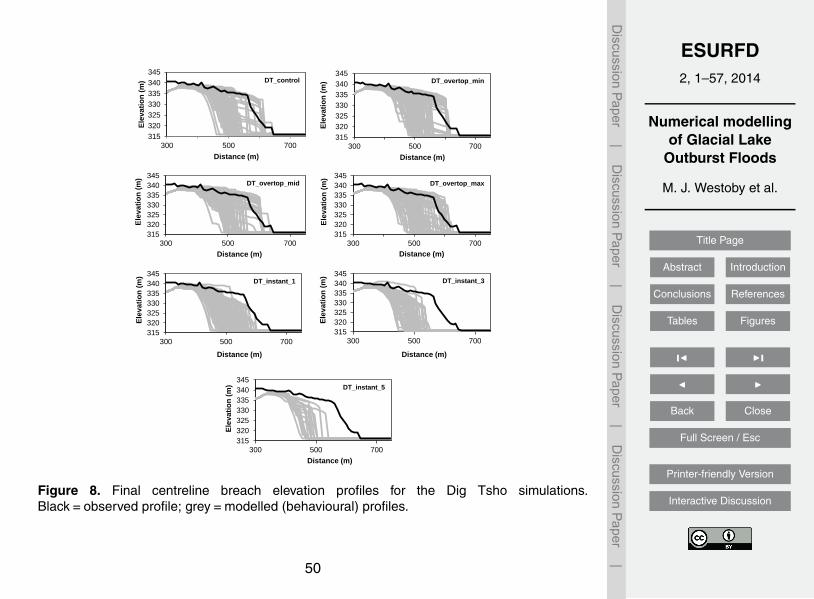
ESURFD2, 1–57, 2014


Outburst Floods


Title Page



Tables Figures

J I

J I

Back Close

Full Screen / Esc



Discussion

Paper

|D

iscussionP

aper|

Discussion

Paper

|D

iscussionP

aper|

Figure 8. Final centreline breach elevation profiles for the Dig Tsho simulations. 1

Black = observed profile; grey = modelled (behavioural) profiles. 2

3

4

5

6

7

8

315

320

325

330

335

340

345

300 500 700E

leva

tio

n (

m)

Distance (m)

315

320

325

330

335

340

345

300 500 700

Ele

va

tio

n (

m)

Distance (m)

315

320

325

330

335

340

345

300 500 700

Ele

va

tio

n (

m)

Distance (m)

315

320

325

330

335

340

345

300 500 700

Ele

va

tio

n (

m)

Distance (m)

315

320

325

330

335

340

345

300 500 700

Ele

va

tio

n (

m)

Distance (m)

315

320

325

330

335

340

345

300 500 700

Ele

va

tio

n (

m)

Distance (m)

315

320

325

330

335

340

345

300 500 700

Ele

va

tio

n (

m)

Distance (m)

D

B

B

DT_instant_5

F

DT_instant_3 DT_instant_1

DT_instant_3

DT_overtop_max DT_overtop_mid

DT_overtop_min DT_control

Figure 8. Final centreline breach elevation profiles for the Dig Tsho simulations.Black=observed profile; grey=modelled (behavioural) profiles.

50





ESURFD2, 1–57, 2014


Outburst Floods


Title Page



Tables Figures

J I

J I

Back Close

Full Screen / Esc



Discussion

Paper

|D

iscussionP

aper|

Discussion

Paper

|D

iscussionP

aper|

Figure 9. Final breach planforms (grey lines) for all modelled scenarios. Precise 1

locations of critical flow constriction are highlighted by black dots. Simulations 2

possessing flow constriction locations that fell between the red dashed lines 3

(distance 505-585 m) were deemed to be behavioural and assigned positive 4

likelihood values. 5

6

7

8

9

10

11

0

50

100

150

200

250

300 400 500 600 700 800

Wid

th (

m)

Distance (m)

0

50

100

150

200

250

300 400 500 600 700 800

Wid

th (

m)

Distance (m)

0

50

100

150

200

250

300 400 500 600 700 800

Wid

th (

m)

Distance (m)

0

50

100

150

200

250

300 400 500 600 700 800

Wid

th (

m)

DIstance (m)

0

50

100

150

200

250

300 400 500 600 700 800

Wid

th (

m)

Distance (m)

0

50

100

150

200

250

300 400 500 600 700 800

Wid

th (

m)

Distance (m)

0

50

100

150

200

250

300 400 500 600 700 800

WId

th (

m)

Distance (m)

DT_overtop_max DT_overtop_mid

DT_control DT_overtop_min

DT_instant_1 DT_instant_3

DT_instant_5

Figure 9. Final breach planforms (grey lines) for all modelled scenarios. Precise locations ofcritical flow constriction are highlighted by black dots. Simulations possessing flow constrictionlocations that fell between the red dashed lines (distance 505–585 m) were deemed to bebehavioural and assigned positive likelihood values.

51





ESURFD2, 1–57, 2014


Outburst Floods


Title Page



Tables Figures

J I

J I

Back Close

Full Screen / Esc



Discussion

Paper

|D

iscussionP

aper|

Discussion

Paper

|D

iscussionP

aper|

Figure 10. Percentile hydrographs derived from behavioural Dig Tsho simulations, 1

for successive likelihood updating steps (‘LH1’, ‘LH1+2’, ‘LH1+2+3’). 5th percentile = 2

small dashes; 50th (median) percentile = long dashes; 95th percentile = solid black. 3

Behavioural hydrograph envelope is displayed in grey. 4

5

6

7

8

9

10

11

12

0

500

1000

1500

2000

2500

Q (

m3 s

-1)

T (mins)

0

500

1000

1500

2000

2500

Q (

m3 s

-1)

T (mins)

0

500

1000

1500

2000

2500

Q (

m3 s

-1)

T (mins)

0

500

1000

1500

2000

2500

Q (

m3 s

-1)

T (mins)

0

500

1000

1500

2000

2500

Q (

m3 s

-1)

T (mins)

0

500

1000

1500

2000

2500

Q (

m3 s

-1)

T (mins)

0

500

1000

1500

2000

2500

Q (

m3 s

-1)

T (mins)

0

500

1000

1500

2000

2500

Q (

m3 s

-1)

T (mins)

0

500

1000

1500

2000

2500

Q (

m3 s

-1)

T (mins)

0

500

1000

1500

2000

2500

Q (

m3 s

-1)

T (mins)

0

500

1000

1500

2000

2500

Q (

m3 s

-1)

T (mins)

0

500

1000

1500

2000

2500

Q (

m3 s

-1)

T (mins)

0

500

1000

1500

2000

2500

Q (

m3 s

-1)

T (mins)

0

500

1000

1500

2000

2500

Q (

m3 s

-1)

T (mins)

0

500

1000

1500

2000

2500

Q (

m3 s

-1)

T (mins)

0

500

1000

1500

2000

2500

Q (

m3 s

-1)

T (mins)

0

500

1000

1500

2000

2500

Q (

m3 s

-1)

T (mins)

0

500

1000

1500

2000

2500

Q (

m3 s

-1)

T (mins)

0

500

1000

1500

2000

2500

Q (

m3 s

-1)

T (mins)

0

500

1000

1500

2000

2500

Q (

m3 s

-1)

T (mins)

0

500

1000

1500

2000

2500

Q (

m3 s

-1)

T (mins)

DT_control LH1

DT_control LH1+2

DT_control LH1+2+3

DT_overtop_min LH1

DT_overtop_min LH1+2

DT_overtop_min LH1+2+3

DT_overtop_mid LH1

DT_overtop_mid LH1+2

DT_overtop_mid LH1+2+3

DT_overtop_max LH1

DT_overtop_max LH1+2

DT_overtop_max LH1+2+3

DT_instant_1 LH1

DT_instant_1 LH1+2

DT_instant_1 LH1+2+3

DT_instant_3 LH1

DT_instant_3 LH1+2


DT_instant_5 LH1

DT_instant_5 LH1+2


Figure 10. Percentile hydrographs derived from behavioural Dig Tsho simulations, for succes-sive likelihood updating steps (“LH1”, “LH1+2”, “LH1+2+3”). 5th percentile= small dashes;50th (median) percentile= long dashes; 95th percentile= solid black. Behavioural hydrographenvelope is displayed in grey.

52





ESURFD2, 1–57, 2014


Outburst Floods


Title Page



Tables Figures

J I

J I

Back Close

Full Screen / Esc



Discussion

Paper

|D

iscussionP

aper|

Discussion

Paper

|D

iscussionP

aper|

Figure 11. Data clustering. (a) Cluster membership following application of a 1

subtractive clustering algorithm in MATLAB®; (b) Cluster membership as a function 2

of total scenario-specific behavioural simulations (%). For key see (a). 3

4

5

6

7 8 9 10 11 12 13

0

500

1000

1500

2000

2500

0 50 100 150 200 250 300

Qp (

m3 s

-1)

Tp (mins)

Series2Series3Series4Series1

0

20

40

60

80

100

% s

ce

na

rio to

tal

Cluster 1

Cluster 2

Cluster 3

Centroid

a

b

Figure 11. Data clustering. (a) Cluster membership following application of a subtractive clus-tering algorithm in MATLAB®; (b) Cluster membership as a function of total scenario-specificbehavioural simulations (%). For key see (a).

53





ESURFD2, 1–57, 2014


Outburst Floods


Title Page



Tables Figures

J I

J I

Back Close

Full Screen / Esc



Discussion

Paper

|D

iscussionP

aper|

Discussion

Paper

|D

iscussionP

aper|

Figure 12. Inundation extent and flow depth distribution for selected time-steps for 1

the DT_control, DT_overtop_max and DT_instant_5 optimal flood even. See Figure 2

1a for location. Inset tick marks spaced at 200 m intervals. 3

4

5

6

7

8

9

10

5 min

0:15 h

0:30 h

1:00 h

1:30 h

2:00 h

DT_control DT_overtop_max DT_instant_5

Depth (m)

10

0

Figure 12. Inundation extent and flow depth distribution for selected time-steps for theDT_control, DT_overtop_max and DT_instant_5 optimal flood even. See Fig. 1a for location.Inset tick marks spaced at 200 m intervals.

54





ESURFD2, 1–57, 2014


Outburst Floods


Title Page



Tables Figures

J I

J I

Back Close

Full Screen / Esc



Discussion

Paper

|D

iscussionP

aper|

Discussion

Paper

|D

iscussionP

aper|

Figure 13. GLUE-based percentile maps of inundation for DT_control. 5th, 50th and 1

95th percentiles maps of inundation represent the water depth that would be 2

exceeded with 95%, 50% and 5% probability, respectively. See Figure 1a for 3

location. Inset tick marks spaced at 200 m intervals. 4

5

6

7

8

9

Legend

P5_210min

P50_210min

P95_210min

5th 50th 95th

195 min 210 min

5 min 15 min

30 min 45 min

60 min 90 min

120 min 150 min

Percentile

Figure 13. GLUE-based percentile maps of inundation for DT_control. 5th, 50th and 95th per-centiles maps of inundation represent the water depth that would be exceeded with 95 %, 50 %and 5 % probability, respectively. See Fig. 1a for location. Inset tick marks spaced at 200 mintervals.

55





ESURFD2, 1–57, 2014


Outburst Floods


Title Page



Tables Figures

J I

J I

Back Close

Full Screen / Esc



Discussion

Paper

|D

iscussionP

aper|

Discussion

Paper

|D

iscussionP

aper|

Figure 14. Percentile flood-hazard maps, based on a global hazard index forwarded 1

by Aronica et al. (2012). Such data facilitate a probabilistic evaluation of the 2

evolution of GLOF flood hazard. See Figure 1a (this paper) for location, and Figure 3

1b in Aronica et al. (2012) for description of the hazard index. 4

5

6

7

8

9

10

11

15 min

30 min

60 min

90 min

120 min

135 min

5th

percentile 50th

percentile 95th

percentile

1

2

3

4

H1 H2 H3 H4

Figure 14. Percentile flood-hazard maps, based on a global hazard index forwarded by Aron-ica et al. (2012). Such data facilitate a probabilistic evaluation of the evolution of GLOF floodhazard. See Fig. 1a (this paper) for location, and Fig. 1b in Aronica et al. (2012) for descriptionof the hazard index.

56





ESURFD2, 1–57, 2014


Outburst Floods


Title Page



Tables Figures

J I

J I

Back Close

Full Screen / Esc



Discussion

Paper

|D

iscussionP

aper|

Discussion

Paper

|D

iscussionP

aper|

Figure 15. A unifying, ‘end-to-end’ framework for probabilistic GLOF reconstruction 1

incorporating high-resolution photogrammetry and probabilistic, GLUE-based 2

numerical dam-breach and hydrodynamic modelling approaches. 3

4

5

6

Figure 15. A unifying, “end-to-end” framework for probabilistic GLOF reconstruction incorpo-rating high-resolution photogrammetry and probabilistic, GLUE-based numerical dam-breachand hydrodynamic modelling approaches.

57





Numerical modelling of Glacial Lake Outburst Floods using physically based dam-breach models

Documents

Transcript of Numerical modelling of Glacial Lake Outburst Floods using physically based dam-breach models