Ultimate limit state design of sheet pile walls by finite elements and nonlinear programming
Upload
khangminh22Category
view
3download
0
Rheinisch –Westfälische Technische Hochschule Aachen
12 / 2 Baustatik - Baudynamik ISSN 1437-0840
Numerical Model for Nonlinear Analysis of Masonry Walls
Jaime Andrés Campbell Barraza


Numerical Model for Nonlinear
Analysis of Masonry Walls
Von der Fakultät für Bauingenieurwesen
der Rheinisch-Westfälischen Technischen Hochschule Aachen
zur Erlangung des akademischen Grades eines Doktors der Ingenieurwissenschaften
genehmigte Dissertation
vorgelegt von
Jaime Andrés Campbell Barraza
aus La Serena (Chile)
Berichter: Universitätsprofessor Dr.-Ing. Konstantin Meskouris Professor Dr.-Ing. Mario Durán Lillo
Tag der mündlichen Prüfung: 27. Juli 2012
Diese Dissertation ist auf den Internetseiten der Hochschulbibliothek online verfügbar.

Veröffentlicht als Heft 22 in der Reihe Mitteilungen des Lehrstuhls für Baustatik und Baudynamik Fakultät für Bauingenieur- und Vermessungswesen Rheinisch-Westfälische Technische Hochschule Aachen ISSN 1437-0840 ISBN 978-3-86130-433-3 1. Auflage 2012 D 82 (Diss. RWTH Aachen University, 2012) Herausgeber Universitätsprofessor Dr.-Ing. Konstantin Meskouris Rheinisch-Westfälische Technische Hochschule Aachen Fakultät für Bauingenieur- und Vermessungswesen Lehrstuhl für Baustatik und Baudynamik Mies-van-der-Rohe-Str. 1 D - 52056 Aachen
Die Deutsche Bibliothek verzeichnet diese Publikation in der Deutschen Nationalbibliografie; detaillierte bibliografische Daten sind im Internet über
Bibliografische Information der Deutschen Bibliothek
http://dnb.ddb.de abrufbar. Das Werk einschließlich seiner Teile ist urheberrechtlich geschützt. Jede Verwendung ist ohne die Zustimmung des Herausgebers außerhalb der engen Grenzen des Urhebergesetzes unzulässig und strafbar. Das gilt insbesondere für Vervielfältigungen, Übersetzungen, Mikroverfilmungen und die Einspeicherung und Verarbeitung in elektronischen Systemen.
Druck und Verlagshaus Mainz GmbH Vertrieb:
Süsterfeldstraße 83 52072 Aachen Tel.: 0241/87 34 34 E-mail: info@verlag-mainz
© Jaime Andrés Campbell Barraza Las Higueras 315 - Depto. 606 1711071 La Serena - Chile

Numerical Model for Nonlinear Analysis of Masonry Walls
I
Acknowledgements
This work presented here was developed between October 2009 and July 2012, during my period as research assistant of the Chair of Structural Statics and Dynamics of the Rheinisch-Westfälischen Technischen Hochschule Aachen University.
First of all, I would like to thank my supervisor Univ.-Prof. Dr.-Ing. Konstantin Meskouris, Head of the Chair of Structural Statics and Dynamics of the RWTH Aachen University, for giving me the opportunity and support to do this work. I would like to express my thanks for all his help, for his tutorship and for allowing me to carry out the research freely.
I would like to thank also Prof. Dr.-Ing. Mario Durán, Head of the Civil Engineering Department of the University of La Serena (Chile), for his constant continuing support, advice and attention given to my work, especially in the final revision stage.
Furthermore, I would like to express my acknowledgement to Univ.-Prof. Dr.-Ing. Holger Schüttrumpf, Head of the Chair and Institute of Hydraulic Engineering and Water Economy of the RWTH Aachen University, who was the chairman of the revision commission.
Additionally, I would like to thank the colleagues and members of staff of the Chair of Structural Statics and Dynamics of the RWTH Aachen University, with whom I worked during my stay in Aachen and from whom I always received attention, full collaboration and support.
I am sincerely grateful to the authorities and all those colleagues and friends of the University of La Serena, the Faculty of Engineering and the Civil Engineering Department, who in one way or another helped me to reach this academic goal.
I would like also to thank CONICYT and DAAD for awarding me with the scholarship which made it possible to carry out this doctoral thesis in Germany.
Finally, I am sincerely and deeply grateful to my family. To my wife Fabiola, for her patience, understanding and support; to my daughter Gabriela, because she was the source of the strength necessary to reach this goal; and to my parents Carmen and Jaime and my brothers Malcolm and José Miguel for their permanent support, help and care.
Aachen, July 2012 Jaime Andrés Campbell Barraza

Numerical Model for Nonlinear Analysis of Masonry Walls
II
Danksagung
Die vorliegende Arbeit entstand zwischen Oktober 2009 und Juli 2012 während meiner Tätigkeit als DAAD-Stipendiat am Lehrstuhl für Baustatik und Baudynamik der Rheinisch-Westfälischen Technischen Hochschule Aachen.
Herrn Univ.-Prof. Dr.-Ing. Konstantin Meskouris, Inhaber des Lehrstuhls für Baustatik und Baudynamik an der RWTH Aachen, gilt mein besonderer Dank für die Studienmöglichkeit und Unterstützung. Ich bedanke mich auch bei ihm für die Betreuung und Förderung, sowie die Freiheiten, die mir gewährt wurden.
Herrn Prof. Dr.-Ing. Mario Durán, Leiter der Abteilung für Bauwesen an der Universität La Serena (Chile), danke ich für seine ständige Unterstützung, manche nützlichen Anregungen und Hilfe in der Revisionsphase.
Herrn Univ.-Prof. Dr.-Ing. Holger Schüttrumpf, Inhaber des Lehrstuhls und Instituts für Wasserbau und Wasserwirtschaft an der RWTH Aachen, danke ich für die Übernahme des Prüfungsvorsitzes.
Darüber hinaus bedanke ich mich bei allen Kollegen und Mitarbeitern am Lehrstuhl für Baustatik und Baudynamik der RWTH Aachen, mit denen ich während dieser Zeit gearbeitet habe, die mich freundlich aufgenommen, mir geholfen und bei meiner Arbeit unterstützt haben.
Ein besonderer Dank gilt den Entscheidungsträgern und all jenen Kollegen und Freunden der Universität La Serena, seiner Fakultät für Ingenieurwesen und der Abteilung für Bauwesen, die mir in einer oder anderer Weise geholfen haben, dieses akademische Ziel zu erreichen.
Außerdem danke ich dem CONICYT und dem DAAD für die Verleihung des Stipendiums, das diese Doktorarbeit in Deutschland ermöglicht hat.
Schließlich möchte ich meinen ganz persönlichen und besonderen Dank meiner Familie aussprechen. Meiner Frau Fabiola für ihre Geduld, Verständnis und Unterstützung; meiner Tochter Gabriela, die Quelle der Kraft, um dieses Ziel zu erreichen; und meinen Eltern Carmen und Jaime, sowie meinen Brüdern Malcolm und José Miguel für ihre ständige Unterstützung, Umsicht und Hilfe.
Aachen, Juli 2012 Jaime Andrés Campbell Barraza

Numerical Model for Nonlinear Analysis of Masonry Walls
III
Agradecimientos
El trabajo aquí presentado fué desarrollado entre Octubre de 2009 y Julio de 2012 durante mi período de actividades como asistente de investigación en la Cátedra de Estática y Dinámica de Estructuras de la Universidad Rheinisch-Westfälischen Technischen Hochschule Aachen.
En primer lugar, agradezco la oportunidad y el apoyo entregados por el Univ.-Prof. Dr.-Ing. Konstantin Meskouris, titular de la Cátedra de Estática y Dinámica de Estructuras de la Universidad RWTH Aachen. Le agradezco, además, por la tutoría y la ayuda en el trabajo, así como por la libertad con que me permitió desarrollarlo.
Quisiera también agradecer al Prof. Dr.-Ing. Mario Durán, Director del Departamento de Ingeniería en Obras Civiles de la Universidad de La Serena (Chile), por su permanente apoyo, aportes al desarrollo del trabajo y ayuda en la fase de revisión final.
Además, expreso mis agradecimientos al Univ.-Prof. Dr.-Ing. Holger Schüttrumpf, titular de la Cátedra e Instituto de Hidráulica y Economía de Aguas de la Universidad RWTH Aachen, por su desempeño como presidente de la comisión revisora.
Del mismo modo, agradezco a los colegas y colaboradores de la Cátedra de Estática y Dinámica de Estructuras de la Universidad RWTH Aachen, junto a quienes trabajé durante todo este tiempo y de quienes siempre recibí un trato cordial, colaboración y gestos de apoyo.
Agradezco especialmente a las autoridades y a todos aquellos colegas y amigos de la Universidad de La Serena, de su Facultad de Ingeniería y del Departamento de Ingeniería en Obras Civiles que de una u otra forma me ayudaron a concretar este objetivo académico.
Por otra parte, expreso mi gratitud a CONICYT y al DAAD por otorgame la beca que hizo posible el desarrollo de este trabajo de doctorado en Alemania.
Finalmente, agradezco de la manera más especial a mi familia. A mi esposa Fabiola, por su paciencia, comprensión y apoyo; a mi hija Gabriela, por ser la fuente de la fuerza necesaria para cumplir esta meta; y a mis padres Carmen y Jaime y mis hermanos Malcolm y José Miguel, por su permanente apoyo, ayuda y procupación.
Aachen, Julio de 2012 Jaime Andrés Campbell Barraza

Numerical Model for Nonlinear Analysis of Masonry Walls
IV

Numerical Model for Nonlinear Analysis of Masonry Walls
V
Abstract
In this thesis a new proposal to represent the in-plane non-linear structural behaviour of masonry is presented. The proposal is explained and evaluated in order to determine its quality.
The model has the ability to represent unreinforced, reinforced and confined masonry walls, considering different wall configurations. The wall configurations can take into account different dimensions for the wall and sizes for bricks and joints. Additionally, the model is able to consider different bricks, mortar and interface brick-mortar material properties.
The most important point in the proposal is the implementation of the joint model. The joint model is defined as a special connection considering two non-linear springs (one longitudinal and one transversal to the joint connected in parallel) and one contact element (connected in series with the springs). This configuration is able to simulate almost all the failure possibilities in the joint. The bricks are implemented considering solid finite elements, taking into account a non-linear material behaviour.
The model is implemented in ANSYS and then used to simulate the structural behaviour of a group of walls previously tested in laboratory in other research projects carried out in Europe (ESECMaSE) and Chile (U. of La Serena). For the seven walls considered, the results obtained with the proposed model have a good agreement with those obtained in the laboratory tests.

Numerical Model for Nonlinear Analysis of Masonry Walls
VI
Kurzfassung
In dieser Arbeit wird ein neues Modell vorgeschlagen, mit dem das nichtlineare Verhalten von Mauerwerksschubwänden mit Belastung in der Wandebene beschrieben werden kann. Dieses Modell wird detailliert erläutert und mit Labortests verglichen, um seine Qualität zu beurteilen.
Mit dem vorgestellten Modell können unbewehrte, bewehrte und eingefasste Mauerwerkswände mit verschiedenen Mauerstein- und Fugengrößen modelliert werden. Darüber hinaus können verschiedene Materialeigenschaften für die Mauersteine und den Mörtel definiert werden sowie verschiedene Kontakteigenschaften für die Modellierung der Mauerstein-Mörtel-Interaktion.
Der zentrale Aspekt der Arbeit ist die Formulierung des Fugenmodells. Die Fuge wird als eine spezielle Verbindung mit zwei parallelgeschalteten nichtlinearen Federelementen (eines senkrecht und eines parallel zur Fugenrichtung) und einem Kontaktelement, das mit den Federn in Reihe geschaltet ist, abgebildet. Mit dieser Zusammensetzung können nahezu alle möglichen Fuge-Versagensformen simuliert werden. Die Mauersteine werden als Festkörper finite Elemente mit einem nichtlinearen Materialgesetz abgebildet.
Dieses Modell wird in ANSYS implementiert, um das Verhalten einer Gruppe von zuvor getesteten Mauern zu simulieren. Die Wände wurden im Rahmen von Forschungsprojekten in Labors in Europa (ESECMaSE) und Chile (Univ. La Serena) getestet. Für die sieben ausgewählten Mauerwerkswände zeigen die Ergebnisse der Simulationen mit dem hier vorgestellten Modell eine gute Übereinstimmung mit den Ergebnissen der Labortests.
Numerical Model for Nonlinear Analysis of Masonry Walls
VII
Resumen
En esta tesis se presenta una nueva propuesta para representar el comportamiento estructural no-lineal de muros de albañilería en su propio plano. La propuesta es explicada y evaluada con el objeto de determinar su calidad.
El modelo tiene la capacidad de representar albañilería simple, armada y confinada, considerando diferentes configuraciones de muro. Las configuraciones de muro pueden tener en cuenta distintas dimensiones del muro y tamaños de ladrillos y juntas. Además, el modelo tiene la capacidad de tener en cuenta distintas propiedades de materiales para ladrillos, morteros e interfaces ladrillo-mortero.
El aspecto más importante de la propuesta es la implementación del modelo de junta. El modelo de junta es definido como una conexión especial teniendo en cuenta dos resortes no-lineales (uno longitudinal y uno transversal a la junta, conectados en paralelo) y un elemento de contacto (conectado en serie con los resortes). Esta configuración es capaz de simular casi todas las formas posibles de falla en la junta. Los ladrillos son implementados como elementos finitos sólidos, teniendo en cuenta un material de comportamiento no-lineal.
El modelo es implementado en ANSYS y luego aplicado para simular el comportamiento estructural de un grupo de muros previamente ensayados en laboratorio en otros proyectos de investigación llevados a cabo en Europa (ESECMaSE) y Chile (U. de La Serena). Para los siete muros considerados, los resultados obtenidos con el modelo propuesto y los de los ensayos de laboratorio muestran un buen grado de similitud.

Numerical Model for Nonlinear Analysis of Masonry Walls
VIII

Numerical Model for Nonlinear Analysis of Masonry Walls
IX
Contents
Acknowledgements ........................................................................................................... I
Danksagung .................................................................................................................... II
Agradecimientos ............................................................................................................ III
Abstract ........................................................................................................................... V
Kurzfassung ................................................................................................................... VI
Resumen ........................................................................................................................ VII
Contents ......................................................................................................................... IX
1 Introduction .............................................................................................................. 1
1.1 Motivation .......................................................................................................... 1
1.2 Goal setting ........................................................................................................ 3
1.3 Overview of the dissertation .............................................................................. 3
2 Structural behaviour of masonry ............................................................................. 5
2.1 Constituents elements of masonry .................................................................... 5
2.1.1 Bricks and blocks ........................................................................................ 5
2.1.2 Mortar ......................................................................................................... 9
2.1.3 Contact (interface) between brick and mortar ......................................... 11
2.1.4 Masonry .................................................................................................... 12
2.1.5 Concrete and steel .................................................................................... 13
2.1.6 Disposition of bricks or blocks .................................................................. 15
2.2 Types of Failure ............................................................................................... 16
2.2.1 Sliding shear failure ................................................................................. 16
2.2.2 Shear failure ............................................................................................. 17
2.2.3 Bending failure ......................................................................................... 18
2.3 Design codes ..................................................................................................... 19
2.3.1 German codes ............................................................................................ 20

Numerical Model for Nonlinear Analysis of Masonry Walls
X
2.3.2 Chilean codes ............................................................................................ 20
2.3.3 Codes of U.S.A. ......................................................................................... 21
2.3.4 European codes ......................................................................................... 21
2.4 Types of masonry ............................................................................................. 22
2.4.1 Unreinforced masonry .............................................................................. 22
2.4.2 Reinforced masonry .................................................................................. 23
2.4.3 Confined masonry .................................................................................... 24
3 Types of models and other proposals .................................................................... 27
3.1 Types of models ............................................................................................... 27
3.2 Other proposals to describe the structural behavior of masonry ................... 28
3.2.1 Proposals of Page ...................................................................................... 29
3.2.2 Proposals of Lourenço .............................................................................. 30
3.2.3 Proposal of Park, El-Deib, Butenweg and Gellert ................................... 30
3.2.4 Other reviewed proposals ......................................................................... 31
4 Proposed model ...................................................................................................... 33
4.1 Description of the model ................................................................................. 33
4.1.1 Ansys elements ......................................................................................... 35
4.1.2 Interaction between nonlinear springs and contact elements ................ 46
4.1.3 Self weight of the walls ............................................................................ 47
4.2 Structural alternatives .................................................................................... 47
4.3 Input parameters ............................................................................................ 48
4.4 Numerical solution .......................................................................................... 50
4.5 Graphical output ............................................................................................. 51
5 Laboratory tests ..................................................................................................... 53
5.1 ESECMaSE Project tests ................................................................................ 53
5.1.1 Test of Wall CS05 ..................................................................................... 53
5.1.2 Test of Wall CL05 ..................................................................................... 56
5.1.3 Test of Wall CL06 ..................................................................................... 58
5.2 Chilean tests (U. of La Serena) ....................................................................... 60
5.2.1 Tests for reinforced masonry walls .......................................................... 60
Numerical Model for Nonlinear Analysis of Masonry Walls
XI
5.2.2 Tests for confined masonry walls ............................................................. 63
5.3 Nominal shear force according to MSJC ......................................................... 66
6 Implementation of the model ................................................................................. 69
6.1 ESECMaSE Project walls ................................................................................ 69
6.1.1 Wall CS05 ................................................................................................. 69
6.1.2 Wall CL05 ................................................................................................. 71
6.1.3 Wall CL06 ................................................................................................. 73
6.2 Chilean walls (U. of La Serena) ...................................................................... 75
6.2.1 Reinforced masonry walls ......................................................................... 75
6.2.2 Confined masonry walls ........................................................................... 77
6.3 Remarks about the stresses and forces distribution ....................................... 85
7 Comparison between model and tests ................................................................... 87
7.1 Bilinearization process .................................................................................... 87
7.2 Wall CS05 ........................................................................................................ 88
7.3 Wall CL05 ........................................................................................................ 90
7.4 Wall CL06 ........................................................................................................ 92
7.5 Walls Nr. 1, 2 and 3 ......................................................................................... 93
7.6 Wall MV1 ......................................................................................................... 97
7.7 Wall MV2 ......................................................................................................... 98
7.8 Wall MV3 ....................................................................................................... 100
7.9 Remarks about the results ............................................................................ 102
Summary and Outlook ................................................................................................. 103
Zusammenfassung und Ausblick ................................................................................. 105
Sinopsis y Perspectivas ................................................................................................ 107
Appendixes ................................................................................................................... 109
A.1 Graphics for wall CS05 (U. of Pavia) ................................................................ 110
A.2 Graphics for wall CL05 (U. of Pavia) ................................................................ 116
A.3 Graphics for wall CL06 (U. of Pavia) ................................................................ 122
A.4 Graphics for walls Nr. 1, 2 and 3 (U. of La Serena) .......................................... 128

Numerical Model for Nonlinear Analysis of Masonry Walls
XII
A.5 Graphics for wall MV1 (U. of La Serena) ......................................................... 135
A.6 Graphics for wall MV2 (U. of La Serena) ......................................................... 143
A.7 Graphics for wall MV3 (U. of La Serena) ......................................................... 151
References and Bibliography ...................................................................................... 159
List of Figures .............................................................................................................. 165
List of Tables ............................................................................................................... 169
Symbols and Abbreviations ......................................................................................... 171
Curriculum Vitae ......................................................................................................... 173
Lebenslauf ................................................................................................................... 174
Curriculum Vitae ......................................................................................................... 175
Chapter 1: Introduction
1
1 Introduction
1.1 Motivation
For many centuries and in different ways, masonry is one of the most commonly used and important construction materials around the world. Despite this, nowadays there is a lack of information and research to characterize its mechanical properties and structural performance.
The problems to adequately define the mechanical properties of masonry are related, amongst other reasons, to the possibility of finding the elements needed to build masonry almost everywhere. This situation makes it possible to build masonry in many different ways, methods and qualities. Because of this, the input parameters to define the mechanical properties of masonry are wide and its properties are many and various.
According to many studies, around 50% of the world’s population live in earthquake prone areas (Uzoegbo, 2011) (see Figure 1.1) and the effects of earthquakes worldwide have claimed approximately 8 million lives over the last 2.000 years (Jaiswal & Wald, 2008).
Figure 1.1: Earthquake prone areas in the world.
Moreover, around 40% of urban the population live in houses made of masonry and this number increases in under developed countries. In Chile, for instance, the percentage rises to about 50% (Lüders, 1990). Additionally, unreinforced masonry is

Chapter 1: Introduction
2
responsible for approximately 60% of human casualties due to structural damage caused by earthquakes all over the world (Mayorca & Meguro, 2003).
Taking these facts into account, it is clear that more research and development about the mechanical properties and structural performance of masonry is needed, in order to improve its safety against seismic demands.
In the last decades a new line of research has been defined in the field of earthquake engineering, trying to implement non-linear structural analysis in order to give more accuracy and safety to buildings and consistency between the analysis and design methods (Priestley, Calvi, & Kowalsky, 2007). Nowadays, these new methods are complementary to the old classic ones (Clough & Penzien, 2003), (Meskouris, 2000), (Chopra, 2007). In most of these new methods, the “pushover curve” of a structure is a very important element to be obtained.
At present, a lot of research has been made to characterize the non-linear structural behaviour of reinforced concrete and steel buildings and, according to these advances, not only “single pushover analysis” has been developed, but also “multimodal pushover analysis”. This technique considers the influence of many modes on the definition of the “pushover curve”. These advances are widely described in reports and technical papers (Chopra & Goel, 2002), (Campbell, Durán, & Guendelman, 2005), (Kalkan & Kunnath, 2006). Having defined this “pushover curve” and considering the seismic demand in the form of a “reduced earthquake spectra” (Wu & Hanson, 1989), (Vidic, Fajfar, & Fischinger, 1994), (Ordaz & Pérez, 1998), the “performance point” of the structure can be obtained, following the steps given in the different methods.
The “performance point” defines the base shear and top displacement reached by the structure during the action of the seismic demand. This point determines the structural situation of the building after the earthquake, and, therefore, a performance evaluation can be made according to some predefined parameters or limit states (SEAOC, 1995), (FEMA, 1997).
Unfortunately, for masonry there is still no clear model to describe the nonlinear behaviour of this material, because of its complexity and wide variety of forms and, therefore, it is not easy to determine the “pushover curve” of a masonry structure. Some efforts have been made in order to solve this situation (Gellert, 2010), (Norda, Reindl, & Meskouris, 2010), but the results are still not conclusive.
In order to contribute to this research field, in this thesis a numerical model to characterize the in-plane behaviour of masonry under lateral loads (seismic loads) is developed. The main product of this numerical model is the “pushover curve” of a masonry wall.

Chapter 1: Introduction
3
1.2 Goal setting
The main goals of this thesis can be summarized as follows:
• Define a numerical model to reproduce the in-plane structural behaviour of masonry walls.
• Implement different types of structural masonry (unreinforced, reinforced and confined) in this numerical model.
• Obtain the Pushover Curve of different types of masonry walls using the numerical model.
• Evaluate the quality of this model against different results obtained in natural scale laboratory tests.
1.3 Overview of the dissertation
This thesis is organized into 7 chapters and 7 appendixes. A general overview of the chapters and appendixes is given in the following paragraphs.
In Chapter 1 (Introduction) a general overview of the problem and its importance and the aims of the thesis are shown. Additionally, a general overview of the dissertation is presented.
The Chapter 2 (Structural behaviour of masonry) explains some fundamental aspects concerning masonry as structural material and its constituents. A short review of the types of masonry, types of failures in masonry and the design codes is also shown.
A general description of the different types of models and proposals to describe structural behaviour of masonry is shown in Chapter 3 (Types of models and other proposals).
In Chapter 4 (Proposed model) the fundamentals and details of the proposed model are explained and the types of elements and its mechanical properties are shown.
To compare the quality of the proposed model, in Chapter 5 (Laboratory tests) some results of laboratory tests are displayed. These tests were selected from research projects carried out in Europe and Chile.
In Chapter 6 (Implementation of the model) the proposed model is used to simulate the behaviour of the walls presented in Chapter 5.
Finally, in Chapter 7 (Comparison between model and tests) the results of Chapter 5 and Chapter 6 are compared in order to verify the quality of the proposed model.

Chapter 1: Introduction
4
The paragraph Summary and Outlook is a short abstract of the dissertation, the results and the quality of the proposed model. There are also some commentaries on how this research could continue.
Finally, other graphics with regard to the stresses and forces in the different element types of the proposed model for the last iteration are showed in the Appendixes. There is one appendix for every wall studied.
Chapter 2: Structural behaviour of masonry
5
2 Structural behaviour of masonry
Masonry is a complex material, because it is defined as a composition of bricks and mortar. The possibility of combining these elements with different qualities and geometry give masonry a wide range of alternatives of mechanical behaviour and structural performance.
It is well known that masonry has a good performance when resisting and transmitting compressive loads and a poor performance to resist tensile demands.
In particular, the constituent elements of masonry (bricks and mortar) have a strong non-linear response when subjected to high demand loads and, normally, have an anisotropic behaviour. There is also a special issue to define the mechanical behaviour of the contact zone between brick and mortar, which is highly non-linear. Moreover, normally earthquake loads demand a non-linear response in buildings and their structural components.
In order to understand better the structural behaviour of masonry, in the following paragraphs a short description of some characteristics and properties of the constituent elements of masonry and their failure modes are explained.
To complete this chapter, a short comment on some requirements for different masonry design codes is given.
2.1 Constituents elements of masonry
As already stated, masonry is a complex material that shows different properties depending on the geometrical disposition and the quality of the constituents (bricks and mortar). Usually, the properties of bricks and mortar are independently defined through experimental tests. These tests are widely described in literature and codes (D.I.N., 2011), (D.I.N., 2007). There are also experimental tests to determine the properties of masonry as a whole, considering a special geometric configuration and quality of materials. These tests are also widely reported in literature and codes (D.I.N., 1998), (I.N.N., 1993), (I.N.N., 1997).
2.1.1 Bricks and blocks
The properties of bricks vary in a wide range of values, depending on the quality of clay (or concrete in the case of blocks) or manufacture. Additionally, the mechanical behaviour of bricks is not necessarily homogeneous and isotropic (especially for hollow or perforated bricks). This means that the properties are not the same in different

Chapter 2: Structural behaviour of masonry
6
directions and are also not the same in tension or compression. Normally, the behaviour of bricks is described as elastic-brittle.
To describe the mechanical behaviour of bricks or blocks, usually a simple compression test is made. In order to have a complete characterization of bricks, normally these tests are made considering different directions (the three orthogonal directions of the block, parallel or perpendicular to holes, for example). From this test the stress-strain curve of the brick is obtained, associated with the direction of the applied load and measured deformation, and characteristic compression strength. To determine the traction strength of bricks, there are tests like the “uniaxial tensile strength test”, the “splitting tensile test”, the “flexural tensile strength” and the “uniaxial tensile strength of bone-shaped specimens” (only for solid blocks). Some of these tests are shown in Figure 2.1, Figure 2.2 and Figure 2.3. As already mentioned, these tests are widely and clearly described in literature (Lourenço, 1996), (Grabowski, 2005a), (Bergami, 2007), (Charry, 2010), (Barbosa & Hanai, 2009), (Hossain, Ali, & Rahman, 1997).
Figure 2.1: Simple compression test on a brick specimen (Bergami, 2007).

Chapter 2: Structural behaviour of masonry
7
Figure 2.2: Splitting tensile test on a brick specimen (Grabowski, 2005a).
Figure 2.3: Flexural tensile strength test on a brick specimen (Charry, 2010).
A typical stress-strain curve for compression in bricks is shown in Figure 2.4.

Chapter 2: Structural behaviour of masonry
8
Figure 2.4: Typical stress-strain curve for compression in bricks (Kaushik, Rai, & Jain, 2007).
To estimate the elasticity module (Eb) of clay bricks, (Kaushik, Rai, & Jain, 2007) recommends a range of values depending on the compression strength of the brick (fb). These values are:
This relationship is graphically showed in Figure 2.5.
Figure 2.5: Relationship between compressive strength an elasticity module for bricks (Kaushik, Rai, & Jain, 2007).
According to Mauerwerk-Kalender (Irmschler, Schubert, & Jäger, 2004), for calcium-silicate bricks the elasticity module can be estimated as:
150 ∙ fb ≤ Eb ≤ 500 ∙ fb (Equation 2.1)
Eb = 355 ∙ fb (Equation 2.2)

Chapter 2: Structural behaviour of masonry
9
2.1.2 Mortar
Mortar has many similarities with concrete, but difficulties arise from the different proportion of the components (cement, sand, lime and gypsum), which is the key point in order to determine its mechanical properties. In many cases, it is better to have a good bond between mortar and brick than a high resistance mortar.
To describe the mechanical behaviour of mortar, different tests can be used. The first, and maybe the most typical and important one, is the simple compression test. This test can be made using a cubic or a cylindrical specimen. From this test the stress-strain curve of the mortar is obtained and a characteristic compression strength. To determine the tensile strength of mortar, different tests can be used. Some of these tests are: the “uniaxial tensile strength test”, the “splitting tensile test” and the “flexural tensile strength”. See Figure 2.6 and Figure 2.7. All these tests are also widely and clearly described in literature (Lourenço, 1996), (Grabowski, 2005a), (Bergami, 2007), (Charry, 2010).
Figure 2.6: Simple compression test on a mortar cubic specimen (Galleguillos & Valenzuela, 2009).

Chapter 2: Structural behaviour of masonry
10
Figure 2.7: Flexural tensile strength test on a mortar specimen (Bergami, 2007).
Usually, depending on the type of brick, different types of mortar can be used: general purpose mortar, thin layer mortar or lightweight mortar. General purpose mortar is the traditional mortar used in joints with a thickness larger than 3,0 or 4,0 mm and in which only dense aggregate is used. Thin layer mortar is used normally when joints are 1,0 to 3,0 mm thick and when specific requirements must be fulfilled. Lightweight mortars are also designed to fulfil specific requirements of masonry and are made using special lightweight materials (Tomazevic, 1999).
A typical stress-strain curve for compression in bricks is shown in Figure 2.8.
Figure 2.8: Typical stress-strain curve for compression in mortar (Kaushik, Rai, & Jain, 2007).
To estimate the elasticity module (Em) of mortar, (Kaushik, Rai, & Jain, 2007) recommends a range of values depending on the compression strength of the mortar (fm). These values are:

Chapter 2: Structural behaviour of masonry
11
This relationship is graphically showed in Figure 2.9.
Figure 2.9: Relationship between compressive strength an elasticity module for mortar (Kaushik, Rai, & Jain, 2007).
From theory of elasticity (Gere & Timoshenko, 1986), the shear elasticity module (Gm) is estimated as:
Where “νm” is the Poisson’s module of mortar.
2.1.3 Contact (interface) between brick and mortar
The mechanical properties of the contact between brick and mortar can also be estimated from laboratory tests. To determine the tensile behaviour of the interface between brick and mortar, the “tensile bond test” may be used (see Figure 2.10). On the other hand, the estimation of the shear-behaviour of the interface between brick and mortar is made using the “shear bond test” (see Figure 2.11). In this test the failure can occur either on the interface or in the mortar. The main result of both tests is the maximum strength (tensile or shear). All these tests are also widely and clearly described in literature (Lourenço, 1996), (Grabowski, 2005a), (Bergami, 2007), (Charry, 2010).
100 ∙ fm ≤ Em ≤ 400 ∙ fm (Equation 2.3)
Gm =Em
2(1 + νm) (Equation 2.4)

Chapter 2: Structural behaviour of masonry
12
Figure 2.10: Tensile bond test for the brick- mortar interface (Grabowski, 2005a).
Figure 2.11: Shear bond test for the brick- mortar interface (Charry, 2010).
2.1.4 Masonry
Sometimes it is important to take into account the properties of masonry as a whole. The important thing in these cases is that the interaction between bricks and mortar and the geometrical disposition of the units is considered. In this case, there are many tests which can be carried out. One of these tests is the compression test for Rilem specimen, from which a stress-strain curve can be obtained (see Figure 2.12). Another test to estimate some properties of masonry is the diagonal compression test on walls (see Figure 2.13). An interesting alternative in this test is to investigate how the results vary when the direction of the load in relation to the bed joint is changed in order to evaluate the influence of this parameter. Extensive investigation of these
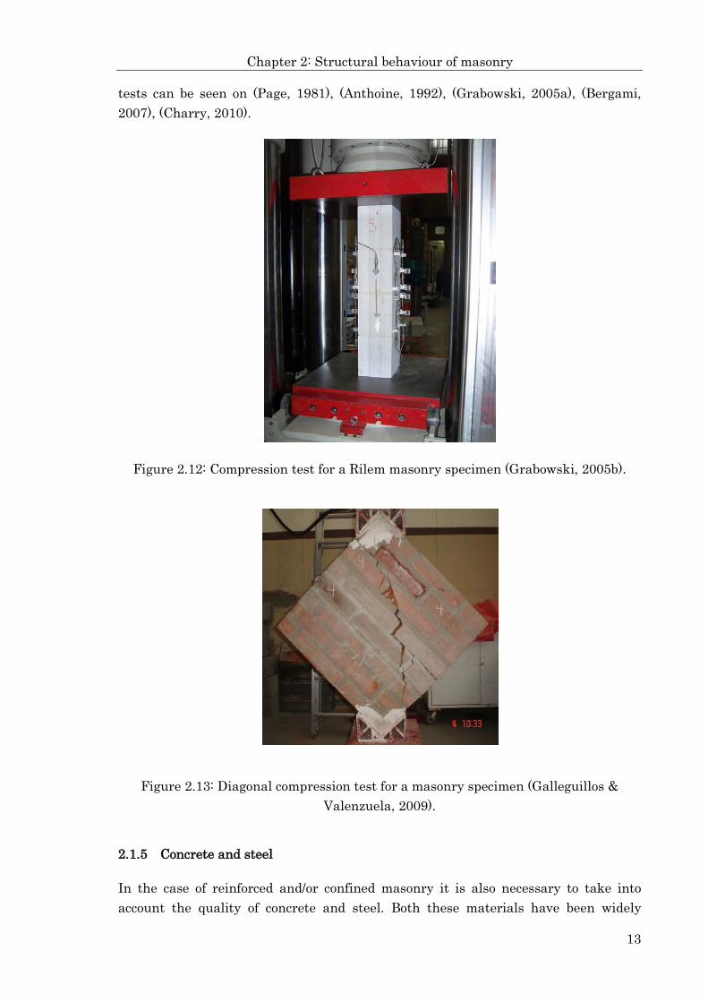
Chapter 2: Structural behaviour of masonry
13
tests can be seen on (Page, 1981), (Anthoine, 1992), (Grabowski, 2005a), (Bergami, 2007), (Charry, 2010).
Figure 2.12: Compression test for a Rilem masonry specimen (Grabowski, 2005b).
Figure 2.13: Diagonal compression test for a masonry specimen (Galleguillos & Valenzuela, 2009).
2.1.5 Concrete and steel
In the case of reinforced and/or confined masonry it is also necessary to take into account the quality of concrete and steel. Both these materials have been widely

Chapter 2: Structural behaviour of masonry
14
studied and there is enough information of their properties in codes and literature (ACI, 2008).
A typical stress-strain curve for concrete is shown in Figure 2.14.
Figure 2.14: Typical stress-strain curve for concrete.
The elasticity module of concrete “Ec” is determined according to (ACI, 2008) with (in kN/m2):
Where “fc” is the compression strength of concrete.
A typical stress-strain curve for reinforcing steel is shown in Figure 2.15.
Stre
ssσ
Strain ε
0,001 ε ≈0,003
fc
ε
σ
Fracture
ProportionalLimit
cuf
cuε ≈0,002o
Ec = 140.000�fc (Equation 2.5)

Chapter 2: Structural behaviour of masonry
15
Figure 2.15: Typical stress-strain curve for reinforcing steel.
The elasticity module of reinforcing steel is considered to be Es=210.000.000 kN/m2.
2.1.6 Disposition of bricks or blocks
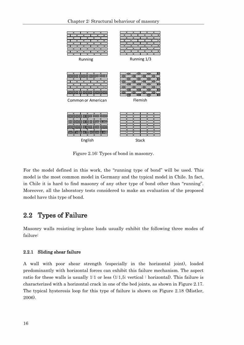
Another important factor to take into account for the determination of the behavior of masonry is the disposition of bricks or type of bond. Masonry is an organized disposition of bricks bonded with mortar and the way the bricks are organized may determine the structural response of the wall. A general description of some of the most recognized types of bond are those shown in Figure 2.16. It is possible to find some variations in these types of bonds, with regard to the vertical joints, which may or may not be filled with mortar.
Chapter 2: Structural behaviour of masonry
16
Figure 2.16: Types of bond in masonry.
For the model defined in this work, the “running type of bond” will be used. This model is the most common model in Germany and the typical model in Chile. In fact, in Chile it is hard to find masonry of any other type of bond other than “running”. Moreover, all the laboratory tests considered to make an evaluation of the proposed model have this type of bond.
2.2 Types of Failure
Masonry walls resisting in-plane loads usually exhibit the following three modes of failure:
2.2.1 Sliding shear failure
A wall with poor shear strength (especially in the horizontal joint), loaded predominantly with horizontal forces can exhibit this failure mechanism. The aspect ratio for these walls is usually 1:1 or less (1:1,5; vertical : horizontal). This failure is characterized with a horizontal crack in one of the bed joints, as shown in Figure 2.17. The typical hysteresis loop for this type of failure is shown on Figure 2.18 (Mistler, 2006).
Running Running 1/3
Common or American Flemish
English Stack

Chapter 2: Structural behaviour of masonry
17
Figure 2.17: Typical sliding shear failure.
Figure 2.18: Typical hysteresis loops for sliding shear failure.
2.2.2 Shear failure
Shear failure is exhibited when a wall is loaded with significant vertical as well as horizontal forces. This is the most common mode of failure. The aspect ratio for such walls is usually about 1:1. Shear failure can also occur in panels with a larger aspect ratio, i.e. 2:1, in cases with big vertical loads. This failure is characterized by a diagonal crack, which crosses joints and bricks or follows the line of bed and head joints (see Figure 2.19). The typical hysteresis loop for this type of failure is shown on Figure 2.20 (Mistler, 2006).
Sliding shearfailure

Chapter 2: Structural behaviour of masonry
18
Figure 2.19: Typical shear failure.
Figure 2.20: Typical hysteresis loops for shear failure.
2.2.3 Bending failure
This type of failure can occur where walls have improved shear resistance. For larger aspect ratios i.e. 2:1 bending failure can occur due to small vertical loads, rather than high shear resistance. In this mode of failure the masonry panel can rock like a rigid body (in cases of low vertical loads). This failure is characterized by a toe-crushing on the lower side of the wall and/or an opening on the other side. For a better understanding see Figure 2.21. The typical hysteresis loop for this type of failure is shown on Figure 2.22 (Mistler, 2006).
Shear failure

Chapter 2: Structural behaviour of masonry
19
Figure 2.21: Typical bending failure.
Figure 2.22: Typical hysteresis loops for bending failure.
It is possible also, according to the structural conditions (loads, materials, geometry, etc.) to have a form of failure defined as a combination of these three basic forms.
2.3 Design codes
Technical codes usually characterize masonry by some basic structural parameters. Normally, these parameters are, amongst others, elasticity module, Poisson’s module, compression strength, shear strength, etc. To take into account the non-linear behaviour of masonry, the codes also consider many factors, to represent the different complexities in this situation. These factors are defined from practical experience and research.
Opening
Toe crushing

Chapter 2: Structural behaviour of masonry
20
In general, the codes describe two different design methods: allowable stresses design and limit states design. In the case of allowable stresses design, the main condition to be fulfilled is that stresses due to applied loads must be less than or equal to the allowable stresses. On the other hand, in the case of limit states design, the main condition to be fulfilled is that stresses due to applied loads multiplied by an amplifying factor must be less than or equal to the nominal stresses multiplied by a capacity reduction factor.
2.3.1 German codes
The code for the design of masonry in Germany is the (D.I.N., 1996). In this code there are two alternative methods for the design of masonry: allowable stresses design or limit states design. This code is oriented to the calculation of unreinforced and reinforced masonry structures.
In this code, the definition of the basic parameters of masonry depends on the quality of the brick and mortar, which are indicated in tables according to an empirical classification. The classification of bricks and mortar can be made according to specific tests defined in (D.I.N., 2011) and (D.I.N., 2007), respectively. Different combinations of brick and mortar are also taken into account to define the basic strength of masonry. Additionally, some properties of masonry can be defined from the tests indicated in (D.I.N., 1998).
According to the type of design chosen (allowable stresses or limit state), the basic parameters of masonry and the applied loads are different. In the case of allowable stresses design the strength values are reduced (with respect to the characteristic values) and considerably lower than the same parameters oriented to limit states design. On the other hand, the applied loads for the limit states design are usually magnified in order to increase the safety of the design. The modification factors to increase or reduce the properties or applied loads, depend on the type and geometry of the structure, type of load, type of stress, safety, etc.
There is also another code in Germany for the calculation and design of masonry (D.I.N., 2006), which is the national version of (CEN, 2005b), see paragraph “2.3.4 European codes”.
2.3.2 Chilean codes
In Chile the normative for masonry is separated into two documents, one regarding reinforced masonry (I.N.N., 1993) and the other regarding confined masonry (I.N.N., 1997). There is no code for unreinforced masonry, because this type of masonry is prohibited by Chilean law. Both documents establish the elastic or allowable stresses

Chapter 2: Structural behaviour of masonry
21
design method. Additionally, amongst other considerations, they establish that masonry is a homogeneous material, the elasticity module of masonry and reinforcement remain constant and that masonry has no capacity to resist tension. In both documents the basic compression and shear strength and elastic module of masonry are determined through experimental tests or from a recommended value defined in the same code. According to these codes, allowable stresses may be augmented in case of seismic solicitations. There are some additional requirements for the design of masonry according to Chilean Seismic Code (I.N.N., 1996).
The fact that Chilean codes do not take into account explicitly the non linear behavior of masonry concerns about what happens when the structures reach stresses beyond allowable limits and goes into inelastic ranges in cases of, for example, seismic solicitations. In fact, there are no indications in order to define a non-linear stress-strain relationship for bricks, mortars or masonry panels. In particular, the codes do not define the ultimate strength and/or deformation capacity and, as a consequence, they do not allow to predict the mode of failure.
2.3.3 Codes of U.S.A.
One of the most important codes for masonry design in U.S.A. is the MSJC code (Masonry Society, 2003). This code offers the possibility to choose between allowable stresses design or limit states design. The code establishes the general ideas and methods for the design of unreinforced, reinforced and confined masonry (Klingner, 2003).
For the definition of the basic properties of bricks, mortar, masonry and other reinforcing elements, the code shows classification tables and equations to obtain the respective values. As a complement, the code gives complementary information to carry out laboratory tests according to other specific codes.
In the case of allowable stresses design, the allowable stresses are calculated as the failure stresses divided by a safety factor, which depends on the type of load and stress, material, geometry, etc. For limit states design, the factors depend on the type of load and stress, material, geometry, etc. It is important to say, that the limit states design method for masonry described in this code is very similar to the design method described in (ACI, 2008).
2.3.4 European codes
The European code for masonry (CEN, 2005b) is similar to the German code.

Chapter 2: Structural behaviour of masonry
22
As the German code, there is the possibility to choose between allowable stresses design or limit state design, considering similar rules and general ideas for the definition of material properties and factors.
The code also offers the possibility of using a simplified or a more accurate method to carry out the design of masonry. To decide which method to use it is necessary to know the height of the masonry building, distance between support points of the slabs, etc.
The code is part of a wider group of codes (Eurocodes 0 to 8), especially oriented to the analysis and design of different types of structures. Especially important in this code are the references to (CEN, 2005a) and (CEN, 2002). The group of codes considers, as an alternative, the possibility to include national annexes in order to take into account parameters which are particular for a specific country.
2.4 Types of masonry
Depending on the regions of the world, and also the building traditions of the country, masonry has different configurations as a structural element. These configurations vary from unreinforced masonry, to reinforced and confined masonry. The type of masonry used is related to the amount of seismicity, for example in countries with very low seismic activity, unreinforced masonry is used. On the other hand, in countries with mid to high seismic activity, reinforced or confined masonry is used (Blondet, 2005).
2.4.1 Unreinforced masonry
Unreinforced masonry is the typical configuration of masonry in countries with low or without seismic demand. It is characterized because it has no steel reinforcement and no reinforced concrete confinement.
This type of masonry is a traditional form for construction of low-rise houses that has been extensively practiced in almost every part of the world. With the increased popularity and availability of reinforced concrete, improved masonry forms of construction, like confined and reinforced masonry became more common for low-rise houses. However, traditional houses with a load-bearing system of unreinforced burnt clay brick walls are still being constructed in many areas of Asia, the Indian Subcontinent and Latin America. This type of masonry is very vulnerable to the earthquake shaking (www.staff.city.ac.uk/earthquakes/MasonryBrick/). Many codes (D.I.N., 2006) consider that this type of masonry is not earthquake resistant.

Chapter 2: Structural behaviour of masonry
23
For this type of masonry general purpose mortar or thin layer mortar may be used. In case of using general purpose mortar, the recommended thickness of the joints should be about 1,0 or 1,5 cm in order to avoid structural problems. For solid blocks a thin layer mortar may be used and this type of mortar is usually 1,0 or 2,0 mm thick.
In Figure 2.23 a simple scheme of unreinforced masonry is showed.
Figure 2.23: Unreinforced masonry.
2.4.2 Reinforced masonry
This type of masonry takes into account reinforcement by steel bars embedded in the mortar. This reinforcement is placed in the horizontal joints and/or in the brick holes and then filled with grout. The horizontal reinforcement helps to improve the resistance to horizontal loads (shear failure) and the vertical reinforcement helps to improve the flexural resistance. In seismic countries, this type of masonry is widely used and, sometimes, obligatory. Unfortunately, in most under developed countries, this type of masonry is not used well, especially because the grout filling for vertical bars is not well done. In Chile there is a specific code to carry out the design of structures considering this type of masonry (I.N.N., 1997). A general scheme of reinforced masonry is displayed in Figure 2.24.

Chapter 2: Structural behaviour of masonry
24
Figure 2.24: Reinforced masonry.
2.4.3 Confined masonry
This is a special type of masonry which takes into account the confinement of the masonry within a reinforced concrete frame. This confinement is materialized with vertical tie columns and a horizontal bond beam. Normally, the codes define the requirements for the maximum area to be confined in order to have a good structural performance. In seismic countries, this type of masonry is widely used and, sometimes, obligatory. In this type of masonry the distribution of steel reinforcement on the intersections between tie columns and bond beams is very important.
It is also important to note that there are differences in this type of masonry, depending on how the wall is built. If the masonry is built before the reinforced concrete frame, then the structural system masonry is called “confined masonry”. If the masonry is built after the reinforced concrete frame, then the structural system is called “infilled frame”. This difference may lead to different structural behaviour because of the “toothed wall edge” materialized in the “confined masonry” (Blondet, 2005).
In Chile there is a specific code to carry out the design of structures considering this type of masonry (I.N.N., 1993). A general scheme of confined masonry is displayed in Figure 2.25.
Verticalreinforcement
Horizontalreinforcement

Chapter 2: Structural behaviour of masonry
25
Figure 2.25: Confined masonry.
Reinforcedconcrete


Chapter 3: Types of models and other proposals
27
3 Types of models and other proposals
In this chapter a brief explanation of the different types of models for masonry is showed. Additionally, some other proposals to describe the structural behavior of masonry are presented.
3.1 Types of models
According to many authors, there are different possibilities to solve the problem of modeling masonry. These alternatives depend on how detailed is the modeling, and, as a consequence of that, if the model is able to describe accurately different types of failure (Lourenço, 1996), (López, Oller, & Oñate, 1998). Usually, the alternatives are classified as: detailed micro model, simplified micro model and macro model.
Figure 3.1: Types of models for masonry.
The first alternative in describing a masonry model is the “detailed micro model” (Figure 3.1 b). This type of modeling considers the bricks and mortar as continuum elements with defined failure criteria. The interface between bricks and mortar is modeled by special elements that represent the discontinuities. In this case, the geometry of the wall is completely reproduced. Because of the level of detail of this model, it is supposed that it can represent most failure mechanisms in masonry.
In the second alternative, the “simplified micro model” (Figure 3.1 c), the bricks are kept as in the “detailed micro model”, but the mortar joints and interface elements are
Head jointBrick
Bed joint
Composed element
Brick element Head joint element
Bed jointelement
Interface elements
Brick element
Joint elements
(a) (b)
(c) (d)
Chapter 3: Types of models and other proposals
28
re-defined as individual elements to represent a contact area. This means that the general geometry is maintained, but the individual elements that represent joints and interface are not able to describe the Poisson’s effect of mortar over bricks. Because of this last example, some types of failure mechanisms cannot be reproduced in this type of model.
The last alternative is the “macro model” (Figure 3.1 d). In this case, the masonry panel (or a part of it) is considered as a homogeneous element. Because of its characteristics, this type of model should be able to reproduce the general structural behavior of a masonry panel but it is not able to reproduce all the types of failure mechanisms.
It is clear that the more detailed the model, the harder to implement. This situation is very important when deciding which model to use for a defined type of study. In the case of detailed micro models, they are adequate to study single walls or special problems, such as windows or door openings or wall intersections. On the other hand, macro models are better to represent the behavior of a whole building, since they are simpler to implement.
In general, the micro models require more detailed information of the material properties than macro models. This information should be obtained, preferably, from specific laboratory tests. In case this type of information is not available, the information should be obtained from literature. This condition makes micro models harder to implement than macro models.
3.2 Other proposals to describe the structural behavior of masonry
There are many proposals in order to characterize the structural behaviour of the different types of masonry. These proposals require different parameters as input, considering more or less detail in the information related to geometry, quality of brick, mortar or the contact zone between them. They also have different ways to define the models, considering finite elements, non-linear springs, especially defined elements, etc. Moreover, they consider the non-linearity of the model in a variety of forms, distributed in the elements, concentrated in some of them, etc. In the next paragraphs a short description of some proposals is given.

Chapter 3: Types of models and other proposals
29
3.2.1 Proposals of Page
One of the first models to represent the nonlinear behaviour of masonry was proposed by Page (Page, 1978). This model considers masonry as a two-phase material which represents brick and mortar.
In the case of bricks, these are represented with plane stress quadrilateral finite elements, with eight nodes and four degrees of freedom per node. The element is suppose to have isotropic elastic properties. The elements are chosen quadrilateral, because they fit easily into the typical geometry of masonry. The mechanical properties (modulus of elasticity and Poisson’s ratio) of these elements are obtained from laboratory tests on bricks and transformed in order to take into account the thickness of the wall.
The mortar joints are represented by linkage elements. This element can only deform in normal and shear directions. The stiffness of these elements is determined minimizing the potential energy with respect to the element displacements. For the determination of the failure criteria for joint elements laboratory tests results are used. In general, these type of elements have a low tensile capacity, a high compression strength and variable shear capacity, which depends on the simultaneous acting compression.
The finite element model is verified comparing its results against bending tests on a masonry deep beam.
This model was an important advance at the time it was developed, because proposed a more realistic alternative compared with the analysis based on isotropic elastic behaviour. It is also very versatile, in terms that can be applied and adapted to any geometry and material properties.
Page proposed also a finite element model to represent masonry (Page, Kleeman, & Dhanasekar, 1985). The model is based on a nonlinear material model implemented with a finite element to describe the behaviour of masonry. For the definition of the nonlinear material model, a large number of biaxial tests on half scale brick masonry panels were considered. The panels were tested taking into account different orientations of the bed joint to the edges and a wide range of biaxial stress states.
Using the information of the tests on masonry panels, nonlinear stress-strain relationships to reproduce the inelastic behaviour of masonry are derived. These relationships are able to reproduce different forms of failure of masonry, taking into account the orientation of the joints.
The finite element adopted to implement the model is an eight node iso-parametric finite element with four Gauss integration points.
Chapter 3: Types of models and other proposals
30
The model was also adapted to simulate the behaviour of masonry infilled frames. In order to implement this option, joint elements to model the joint between the masonry infill and frame, and frame elements to model the frame. The joint element is a six node iso-parametric one dimensional element and the frame element is a typical two node elastic beam with three degrees of freedom for each node.
The quality of the proposed model was verified comparing its results with laboratory tests on masonry infilled frames under horizontal load on the top. The results reported showed good agreement.
3.2.2 Proposals of Lourenço
In his doctoral research (Lourenço, 1996) has proposed two models to describe the nonlinear behaviour of masonry. One of these models is a micro model and the other one is a macro model. Amongst the aims of this contribution was to compare the applicability of the two different types of strategies.
The micro model is defined through joints which concentrate the inelastic behaviour of the masonry. The plasticity model of the joints is able to reproduce three different types of failure mechanisms: tension cut-off, Coulomb friction model and compression (considering an elliptical cap) and combined shear-compression failure. The same author concludes that the results given by the model have a good agreement with laboratory tests. As a drawback, this type of models requires a huge amount of time and memory and, because of that, it is recommended for the study of small structures and structural details.
Taking into account the reasons given in the previous paragraph, Lourenço proposed a second model, specially oriented for the use with large structures. This model is defined by considering an orthotropic continuum model for masonry which takes into account a Rankine type yield criterion for tensile failure (cracking) and a Hill type yield criterion for compressive failure (crushing). This model requires many input parameters related to tension and compression tests in different directions and fracture energy (also in tension and compression).
3.2.3 Proposal of Park, El-Deib, Butenweg and Gellert
The main goal of this proposal is to take into account the effects of wall-slab interaction in the seismic design and verification of masonry structures (Park, El-Deib, Butenweg, & Gellert, 2011).
The proposed macro element represents a complete wall panel and is composed of three beams connected in an “I-shape” form, that is to say, two horizontal beams (at the top and bottom of the element) and one vertical beam connecting rigidly the first

Chapter 3: Types of models and other proposals
31
two. The length of the two horizontal beams is equal to the length of the wall and the length of the vertical beam is equal to the height of the wall. The horizontal beams are connected to the adjacent slabs with nonlinear springs that simulate the rocking behavior of the wall. In the middle of the vertical beam there is a shear spring that reproduces the bed-joint sliding and the diagonal tension failures. The springs are defined by considering a force-displacement relationship which is defined according to the masonry wall material and geometry properties.
The model was compared with laboratory tests in order to evaluate its quality. Analyses of single shear walls and an entire masonry building were performed, giving a good agreement between model and tests.
3.2.4 Other reviewed proposals
There are many other proposals to represent the nonlinear structural behavior of masonry. These proposals include different types of modeling strategies and are oriented to different types of masonry. Some of these proposals are the macro model of (Pietruszczak & Niu, 1992), the homogenized model of (Anthoine, 1995), the homogenized model of (López, Oller, & Oñate, 1998), the micro-mechanical model for homogenization of (Zucchini & Lourenço, 2002), the macro model of (Chen, Moon, & Yi, 2008) and the macro model of (Crisafulli, 1997) for confined masonry walls.
Obviously, there are many other proposals in literature considering other types of modeling strategies and masonry types.


Chapter 4: Proposed model
33
4 Proposed model
In this chapter, the proposed model to represent the non-linear structural behaviour of masonry walls will be described. First of all, a general description of the model will be given, in terms of geometry and structural function. After that, a description of every part of the model will be presented. Finally, the structural alternatives of the model are shown (reinforced and confined masonry).
The model was completely implemented in ANSYS (www.ansys.com) (ANSYS, 2009c), which is a strong software package oriented to solve complex problems in many fields of civil engineering. In this case, the structural and nonlinear applications were used.
4.1 Description of the model
According to many authors (Page, 1978), (Lourenço, 1996), mortar and bond between bricks and mortar is responsible for significant nonlinear behaviour of masonry. Following this argument, the most effort in the construction of this model was put on the definition of the type of elements to represent mortar and contact between brick and mortar.
The proposed model could be classified as a “Simplified micro model”, according to the definitions given by (Lourenço, 1996), (López, Oller, & Oñate, 1998) and in “3.1 Types of models”. This means that bricks are represented by solid finite elements blocks and mortar and bond between bricks and mortar, in this case, are represented by nonlinear springs and contact elements.
The main point in the definition of the model is the representation of horizontal and vertical joints. For this purpose, a group of nonlinear springs and a contact element is used. These elements are combined in order to describe the mechanical and structural behaviour of a typical joint.
The joint model is built using two nonlinear spring elements (connected in parallel) and one contact element (in series with the the spring elements), see Figure 4.1. The two springs represent the axial and transversal behaviour of mortar, respectively, and its properties are directly determined from those of this material. The contact elements represent the bond between brick and mortar and its properties, which are also associated to mortar, but it considers also the friction and the adherence limit between these two elements. The mechanical properties of the springs are determined taking into account the tributary area of the brick over the node.

Chapter 4: Proposed model
34
Obviously, not all possible modes of failure are featured in the proposed model for the joint between bricks and mortar, but the most fundamental ones are covered.
Figure 4.1: Detail of the model for joint between bricks and mortar.
Additionally, the model can reproduce many different alternatives types of masonry and structural situations. It can represent unreinforced, reinforced and confined masonry, as well as different load conditions.
Moreover, the model can take into account many different possibilities of the discretization of the wall. Each brick can be separated into many small solid elements and this condition determines that more elements reproduce the contact between bricks (see Figure 4.2).
Figure 4.2: Alternatives for the discretization of the model.
It is important to note that the model does not necessarily define its discretization considering solid blocks with size more or less similar to those of the original bricks. In fact, the model may also be defined with user-defined sizes for the solid blocks. In this case, the model internally determines the size of the joints proportional to the size of the original brick/joint relationship. Obviously, better discretization should be made considering sizes of blocks similar to the original brick elements.
Contactelement
Nonlineartransversal spring
Nonlinearlongitudinal spring

Chapter 4: Proposed model
35
The model is defined using different types of elements to reproduce the structural behaviour of a masonry wall. All elements are defined according to existing elements in ANSYS (ANSYS, 2009b). The keypoint is how to combine the different types of elements. In this case, the elements considered to constitute the model are of type “solid finite element”, “nonlinear spring element” and “contact element”.
In this model, for every type of element, a different type of material (linear or nonlinear) and failure criteria or stress-strain relationship was considered. An important detail is that the model needs as input the mechanical properties of every structural component (bricks, mortar, bond and, eventually, concrete and steel).
The blocks of the model are organized considering a “running” type of bond, which is the typical type of bond found in the laboratory tests that will be used to evaluate the model. This type of bond is used to have a more accurate response of the model and to reproduce better the cinematic and tensional behaviour of blocks and joints, see Figure 4.3.
Figure 4.3: Cinematic behaviour of a group of bricks under lateral loads.
4.1.1 Ansys elements
Solid elements for bricks and reinforced concrete
The model considers solid elements to represent bricks and reinforced concrete. These solid elements are of type SOLID65 in ANSYS (ANSYS, 2009b), (ANSYS, 2009d).
SOLID65 is an element for modeling 3-D solids considering the possibility to include reinforcing bars. The reinforcing bars may be defined in three different directions to represent, in this case, the steel in reinforced concrete and is assumed to be smeared throughout the element.
This element was chosen because is the only one with the ability to interact with the material “Concrete” and is capable of cracking in tension and crushing in compression.

Chapter 4: Proposed model
36
The element is a hexahedron with 8 nodes on the corners and has 3 degrees of freedom at each node (translations in x, y and z directions). The element has 8 integration points (see Figure 4.4).
Figure 4.4: Geometry of element SOLID65.
The shape functions for this element are presented in (Equation 4.1), (Equation 4.2) and (Equation 4.3).
u =18 �
uI(1− s)(1 − t)(1 − r) + uJ(1 + s)(1− t)(1 − r)�
+uK(1 + s)(1 + t)(1 − r) + uL(1− s)(1 + t)(1 − r) +uM(1 − s)(1 − t)(1 + r) + uN(1 + s)(1 − t)(1 + r) �+uO(1 + s)(1 + t)(1 + r) + uP(1− s)(1 + t)(1 + r)]
+u1(1− s2) + u2(1− t2) + u3(1 − r2)
(Equation 4.1)
v =18 �
vI(1 − s)(1− t)(1 − r) + vJ(1 + s)(1 − t)(1 − r)�
+vK(1 + s)(1 + t)(1 − r) + vL(1 − s)(1 + t)(1 − r) +vM(1 − s)(1 − t)(1 + r) + vN(1 + s)(1− t)(1 + r) �+vO(1 + s)(1 + t)(1 + r) + vP(1 − s)(1 + t)(1 + r)]
+v1(1− s2) + v2(1 − t2) + v3(1 − r2)
(Equation 4.2)

Chapter 4: Proposed model
37
Where ui, vi and wi are the displacements on the respective nodes (I, J, K, L, M, N, O and P) and uj, vj and wj are the displacements associated to the extra shape functions (1, 2 and 3).
The stresses and strains in linear behaviour are related through:
Where [σ] is the stress vector and [ε] is the strain vector. These vectors are defined as follows:
The stress-strain matrix [D] for this element is defined as:
Where 𝑉𝑖𝑅 is the ratio of volume of reinforcement material to total volume of element, [Dc] is the stress-strain matrix for concrete or brick and [Dr] is the stress-strain matrix for reinforcement. The formula shows a weighting between concrete and reinforcing material. The stress-strain matrices are defined as follows:
w =18 �
wI(1− s)(1 − t)(1 − r) + wJ(1 + s)(1 − t)(1 − r)�
+wK(1 + s)(1 + t)(1 − r) + wL(1− s)(1 + t)(1 − r) +wM(1 − s)(1 − t)(1 + r) + wN(1 + s)(1 − t)(1 + r) �+wO(1 + s)(1 + t)(1 + r) + wP(1 − s)(1 + t)(1 + r)]
+w1(1− s2) + w2(1− t2) + w3(1− r2)
(Equation 4.3)
[σ] = [D][ε] (Equation 4.4)
[σ] = [σxx σyy σzz σxy σyz σzx]T (Equation 4.5)
[ε] = [εxx εyy εzz εxy εyz εzx]T (Equation 4.6)
[D] = �1 −�ViRNr
i=1
� [Dc] + �ViRNr
i=1
[Dr]i (Equation 4.7)

Chapter 4: Proposed model
38
Where “E” is the elasticity modulus of concrete or brick, “ν” is the Poisson’s ratio of concrete or brick and “Er” is the elasticity modulus of reinforcement material.
More details on linear behavior equations for this element can be seen on (ANSYS, 2009d).
The nonlinear behavior of this type element is also a combination of nonlinear behavior of the main material and the reinforcing material. In this case, the main material is “concrete” and the reinforcing material is “steel”.
To represent the nonlinear behavior of concrete or brick, the model has the ability to predict and modify the stress-strain relationships by the introduction of “cracks” (tension) and “crushes” (compression). This is, the model introduces a plane of weakness in the normal direction of the crack face or assumes degradation of material strength for crushing. The model also considers a reduction factor to represent the degradation of shear strength across the crack face. The presence of cracking or crushing inside an element is verified at the integration points.
In order to define the failure of a material is essential to have a “failure criteria”. For concrete, it is widely accepted the criteria showed in Figure 4.5. This figure shows the different combinations of principal stresses that produces failure of the material.
[Dc] =E
(1 + ν)(1 − 2ν)
⎣⎢⎢⎢⎢⎡(1 − ν) ν ν
ν (1 − ν) νν ν (1 − ν)
000
000
000
000
000
000
(0,5 − ν) 0 00 (0,5 − ν) 00 0 (0,5 − ν)⎦
⎥⎥⎥⎥⎤
(Eq. 4.8)
[Dr] =
⎣⎢⎢⎢⎢⎡Er 0 00 0 00 0 0
0 0 00 0 00 0 0
0 0 00 0 00 0 0
0 0 00 0 00 0 0⎦
⎥⎥⎥⎥⎤
(Equation 4.9)

Chapter 4: Proposed model
39
Figure 4.5: Failure criteria for concrete according to ANSYS.
All these failure possibilities are controlled through a group of parameters and coefficients defined especially for the material.
To see more details about this topic, especially the failure criteria for every domain, see (ANSYS, 2009d).
The nonlinear behavior of the reinforcement is considered as a different material. For this purpose, the stress-strain relationship of the material must be defined. It is important to say, that the reinforcement can only fail in tension or compression.
In the proposed model, bricks are represented by SOLID65 taking into account the properties of the considered bricks. If necessary (confined masonry), reinforced concrete elements are represented by SOLID65 taking into account the properties of the considered concrete and steel reinforcement.
For the implementation of the proposed model, the following (simplified) stress-strain curves for bricks and concrete were considered (Figure 4.6 and Figure 4.7). Obviously, depending on the quality of the bricks or concrete, these curves may be changed.

Chapter 4: Proposed model
40
Figure 4.6: Simplified compression stress-strain curve for bricks.
Figure 4.7: Simplified compression stress-strain for concrete.
The behavior in tension is considered linear-elastic up to a stress equal to 1/10 of the compression maximum strength, taking into account the same initial elasticity module considered for compression. After this point, the behavior turns to ideal-plastic.
Nonlinear spring elements
For the modeling of mortar and reinforcing bars in masonry, nonlinear spring elements were used. For this purpose the element COMBIN39 of ANSYS was chosen. This type of element is a nonlinear unidirectional spring with a generalized multilinear force-deflection law (ANSYS, 2009b), (ANSYS, 2009d).
0,004 0,006 0,007 0,010 0,012
σ
ε
fb
0,85·fb
0,20·fb
0,33·fb
Eb
0,0020 0,0025 0,0035
σ
ε
fc
0,80·fc
0,55·fc
Ec

Chapter 4: Proposed model
41
The element is defined as a single bar with two nodes (see Figure 4.8) and has up to three degrees of freedom at each node (translations in x, y and z directions).
Figure 4.8: Geometry of element COMBIN39.
The structural behavior of the element is defined through a multilinear force-deflection curve (Figure 4.9). The points on this curve represent the internal force in the element versus relative translation between the nodes.
The curve has some simple restrictions: it must be completely defined in the first and third quadrants and have a point at the origin (0,0), any segments towards vertical should be avoided and the last segment must be positive.
Depending on the characteristics of the curve, this type of element could have convergence problems.
Figure 4.9: Force-Deflection curve for element COMBIN39.
The stiffness matrix of this element is:
[Ke] = Ktg � 1 −1−1 1 � (Equation 4.10)

Chapter 4: Proposed model
42
Where “Ktg” is the stiffness on the active segment of previous iteration.
a) Springs for mortar joints (longitudinal and transversal)
For the definition of nonlinear springs to represent longitudinal and transversal structural behavior of mortar, the mechanical properties of mortar and the geometry of masonry are used.
In this case, the force-deflection curve of these elements is defined taking into account the stress-strain curve of mortar, the tributary area of the brick over the node and the thickness of the joint. The force for every point of the force-deflection curves is defined considering the stress multiplied by the tributary area (see Figure 4.10) and the deflection is defined taking into account the strain multiplied by the length of the spring. This length is taken as 9/10 of the thickness of the joint, considering that the length of contact elements is 1/10 of the thickness of the joint. This idea is valid for longitudinal and transversal springs.
Figure 4.10: Tributary area on nodes for nonlinear springs.
b) Springs for reinforcing bars in masonry (vertical and horizontal)
The definition of nonlinear springs to represent vertical and horizontal reinforcing bars in masonry, the mechanical properties of steel are used.
In this case, the force-deflection curve of these elements is defined taking into account the stress-strain curve of steel and the cross section area of every bar. The force for every point of the force-deflection curves is defined considering the stress multiplied by cross section area and the deflection is defined considering the strain multiplied by the length of the bar.

Chapter 4: Proposed model
43
The nonlinear springs to represent vertical reinforcement bars were defined as one single element from the bottom of the wall to the top. This situation is justified because in Chile is very usual to built masonry with vertical reinforcement without mortar filling in the holes where the bars are placed. Obviously, the Chilean code as much as other international codes establish that the holes must be filled.
For the implementation of the proposed model, the following (simplified) stress-strain curves for mortar and steel were considered (Figure 4.11, Figure 4.12 and Figure 4.13). Obviously, depending on the quality of the mortar or steel, these curves may be changed.
Figure 4.11: Simplified compression stress-strain curve for mortar.
Figure 4.12: Simplified shear stress-strain curve for mortar.
0,005 0,010 0,012
σ
ε
fm
0,75·fm
0,33·fm
Em
0,0020 0,0023
τ
ϒ
τm
0,33·τm
Gm

Chapter 4: Proposed model
44
Figure 4.13: Simplified tension stress-strain curve for steel.
The behavior in tension of mortar is considered linear-elastic up to a stress equal to 1/10 of the compression maximum strength, taking into account the same initial elasticity module considered in compression. After this point, the behavior turns to ideal-plastic. If the tension strength between brick and mortar is lower than this limit (1/10 of compression strength), the upper limit of the tension branch is modified up to the tension strength between brick and mortar.
Due to the lack of information about the shear stress-strain behavior of mortar, the shear stress-strain curve was defined similar and proportional to the curve for compression. The maximum shear strength was considered equal to 1/10 of the compression maximum strength. After this point, the behavior turns to ideal-plastic. If the adherence strength between brick and mortar is lower than this limit (1/10 of compression strength), the upper limit is modified up to the adherence strength between brick and mortar. The shear module “Gm“ is determined according to the formula given in “2.1.2 Mortar”.
The behavior in compression of steel for vertical reinforcement is considered linear, taking into account the same initial elasticity module up to a stress equal to the buckling stress of a simple supported column. After this point, the behavior turns to ideal-plastic.
Contact elements
For the modeling of the interface between brick and mortar, node-to-node elements were used. For this purpose the element CONTA178 of ANSYS (ANSYS, 2009a) was
0,006 0,010 0,020 0,021
σ
ε
Es
f r
f y
fm

Chapter 4: Proposed model
45
chosen. This type of element represents contact and sliding between two nodes (ANSYS, 2009b), (ANSYS, 2009d).
The element is defined by two nodes, an initial gap between the nodes and an initial status of the contact. Each node has up to three degrees of freedom (translations in x, y and z directions). The interface is assumed to be perpendicular to the I-J line (see Figure 4.14).
Figure 4.14: Geometry of element CONTA178.
Element CONTA178 has infinite strength and a user defined stiffness in compression (normal to the contact surface). For convergence and stability reasons, stiffness in tension can be regulated as a percentage of the compression stiffness (“weak spring”). The element is able to support friction in the tangential direction (tangential to the contact surface). For this purpose, this element has many options for contact algorithm. In this model, the “Pure penalty method” was chosen.
The normal force is calculated as:
Fn = � 0 if Un > 0 KnUn if Un ≤ 0
� (Equation 4.11)
Where “Kn” is the contact normal stiffness and “Un” is the contact gap size. The normal stiffness is calculated as:
Kn =Em ∙ Atrib
L (Equation 4.12)

Chapter 4: Proposed model
46
Where “Em” is the initial elasticity module of mortar, “Atrib” is the tributary area of the brick over the node of the contact element and “L” is the longitude of the contact element (in this case 1/10 of the thickness of the joint).
The tangential force is calculated as:
Fsy =
⎩⎨
⎧ KsUy if �Fsy2 + Fsz2 − µ Fn < 0 (sticking)
µ KnUn if �Fsy2 + Fsz2 − µ Fn = 0 (sliding)� (Equation 4.13)
Where “Ks” is the contact tangential stiffness, “Uy” is the contact slip distance in “y” direction and “μ” is the coefficient of friction. The tangential stiffness is calculated as:
Ks =Gm ∙ Atrib
L (Equation 4.14)
Where “Gm” is the initial shear elasticity module of mortar.
As can be seen, for the definition of normal and tangential stiffness, the mechanical properties of mortar and the geometry of masonry are used. This is similar to the idea applied for nonlinear springs for mortar joints, but considering only the initial properties.
4.1.2 Interaction between nonlinear springs and contact elements
The interaction between nonlinear (longitudinal and transversal) springs and contact elements has many advantages for the model in terms of representing in a good way the behavior of the bed and/or head mortar joints.
It is clear that the contact element itself is not able to fail in compression and has no strength in tension. In order to fix this problem, a longitudinal nonlinear spring is connected in series to control the compression and tension capacity of the unit, taking into account a small rigidity in tension of the contact element for stability reasons. The limits of the longitudinal nonlinear spring are determined by the compression capacity of the mortar and by the tension capacity of the mortar and/or the bond strength between brick and mortar.
On the other hand, the contact element connected in series with the transversal nonlinear spring is able to capture the shear failure of the mortar and/or the shear sliding failure between brick and mortar due to adherence deficiency.

Chapter 4: Proposed model
47
Is important to note that using this configuration of elements to represent the joints, the friction is also limited because compression is limited to the mortar strength, which implies that friction is also limited to this compression strength times the friction factor.
Unfortunately, all these advantages for the interaction between contact elements and nonlinear spring elements have one drawback: the nonlinear spring must have a final rigidity equal or greater than zero after reaching its maximum value of force. Because of this reason, the nonlinear springs connected to contact elements are represented with a nonlinear force-deflection curve which ends in a horizontal plateau after reaching the maximum value of force. If this condition is not considered, the model turns very unstable.
4.1.3 Self weight of the walls
As is indicated on ANSYS manuals, only the solid elements have an associated self weight, this situation would determine an underestimated self weight of the wall. To correct this situation, the model considers a fictitious density for bricks which is an increased self weight, taking into account additionally the self weight of the mortar joints.
4.2 Structural alternatives
Many different structural alternatives have been implemented in this model. In the following paragraphs some of these alternatives will be described.
First of all, the model considers the possibility to choose between different types of masonry: unreinforced, reinforced and confined.
For the reinforced masonry, there is the possibility to take into account horizontal and/or vertical reinforcement. Both types of reinforcement are uniformly distributed in the respective dimension, so the total area of reinforcement must be given.
For the confined masonry, width of tie columns and different longitudinal reinforcement for tie columns and bond beam must be defined. Unfortunately, the model makes no consideration of transversal reinforcement (stirrups) for columns and beam. The influence of this reinforcement could be important in some cases, especially for high compression force demands at the bottom of tie columns. Anyway, this is a very specific issue in reinforced concrete and is out of the scope of this work.
Chapter 4: Proposed model
48
It is also possible to vary the vertical load to apply to the wall (additional to self weight), in order to simulate different load and structural conditions. This load must be given as force per unit length and is applied on the horizontal bond beam.
Another alternative given in the model is the possibility to modify the restrictions of the upper side of the wall. The possibilities for the upper side are: nodes are completely free to move (cantilever), rotation is restrained (fixed, vertical displacement is coupled and horizontal is permitted) and vertical displacement and rotation are restrained (fixed, only horizontal displacement is permitted).
Finally, the model offers two possibilities to control the simulation: displacement or force. The type of control determines different responses of the model. Usually, the laboratory tests are carried out considering displacement control, because it is easy to control the form of failure of the specimen and is safer than the force control.
4.3 Input parameters
To define the model properly, an input file has been prepared for its use in ANSYS. The parameters to put in this file are related with the type masonry, the quality of materials, type of control of the analysis, geometry of the wall and of the individual elements, etc.
The input parameters (separated according to the type of variable) of the proposed model are listed on the following lines.
Geometrical parameters
The input file requires the following geometrical parameters to define the model:
bmx: Longitude of the wall (in m)
hmy: Height of the wall (in m)
emz: Thickness of the wall (in m)
hcc: Height of the bond beam (in m)
bpc: Width of the tie column (in m)
blx: Horizontal dimension of the brick (in m)
hly: Vertical dimension of the brick (in m)
bjx: Thickness of the head joint (in m)
hjy: Thickness of the bed joint (in m)
AArmC: Steel reinforcement of bond beam (in m2)

Chapter 4: Proposed model
49
AArmP: Steel reinforcement of tie column for confined masonry (in m2)
AArmV: Steel vertical reinforcement for reinforced masonry (in m2)
AArmH: Steel horizontal reinforcement for reinforced masonry (in m2)
Discretization of the model
The input file requires the following parameters to define the discretization of the model:
nbx: Number of blocks in horizontal direction
nby: Number of blocks in vertical direction
nex: Number of elements per block in horizontal direction
ney: Number of elements per block in vertical direction
Structural options
The following parameters are required to define the structural conditions of the model:
Fuerza: Maximum horizontal force to apply, if force controls (in kN)
DeltaF: Force step, if force controls (in kN)
Desplaz: Maximum horizontal displacement to apply, if displacement controls (in m)
DeltaD: Displacement step, if displacement controls (in m)
SCarga: Vertical load, additional to self weight (in kN/m)
RBS: Switches the boundary condition of bond beam (upper side)
BRV: To consider or not vertical steel reinforcement
BRH: To consider or not horizontal steel reinforcement
CNF: To consider or not reinforced concrete confinement
Properties of materials
For the definition of the material’s quality, the following parameters are required:
fcL: Maximum compression strength of bricks (in kN/m2)
E_L: Elasticity modulus of bricks (in kN/m2)
nu_L: Poisson’s modulus for bricks

Chapter 4: Proposed model
50
Dens_A: Specific mass of masonry (in T/m2)
fcM: Maximum compression strength of mortar (in kN/m2)
E_M: Elasticity modulus of mortar (in kN/m2)
nu_M: Poisson’s modulus for mortar
mu_M: Friction modulus for mortar
fadM: Bond strength (sliding adherence) between mortar and brick (in kN/m2)
ftM: Bond strength (tension) between mortar and brick (in kN/m2)
E_Ace: Elasticity modulus of steel (in kN/m2)
nu_Ace: Poisson’s modulus for steel
Sig_f: Yield tension of steel (in kN/m2)
Sig_m: Maximum (ultimate) tension of steel (in kN/m2)
Sig_r: Fracture tension of steel (in kN/m2)
fcH: Maximum compression strength of concrete (in kN/m2)
E_H: Elasticity modulus of concrete (in kN/m2)
nu_H: Poisson’s modulus for concrete
Dens_H: Specific mass of concrete (in T/m2)
For the definition of the materials considered in the model, it is also necessary to define the stress-strain curves of bricks, mortar, concrete and steel. These parameters must be given in the definition of the respective elements which use them.
4.4 Numerical solution
The numerical solution of the model is carried out into two steps: vertical load and horizontal load, because for these two load processes different numerical conditions are required.
For the vertical load, an “auto time stepping” is used. This means that the program defines internally the time step to consider in the iterative solution. The solution is obtained by using a Newton-Raphson scheme to solve the nonlinear equations.
For the horizontal load, a predefined time stepping is used. This means that the user defines the time step to consider in the iterative solution. The solution is obtained using a Newton-Raphson scheme to solve the nonlinear equations.

Chapter 4: Proposed model
51
Obviously, the efficiency of the resolution of a model is highly dependent on the time step considered and on the type of discretization used. In general, the time step in the model is defined as 1/1000 of the maximum horizontal force (for force control) or maximum horizontal displacement (for displacement control). Other values of time steps may be used, but the quality of the results decreases (longer time steps) or the efficiency of the numerical resolution decreases (shorter time steps).
4.5 Graphical output
The most important result of the analysis is the “pushover curve” of the wall tested. This curve represents the structural (horizontal force at the basement versus horizontal displacement at the top) behavior of the wall under a horizontal load (displacement or force) applied at the top.
Through the input file there is also the possibility to control which graphics to obtain as a result of the analysis: internal stresses, internal forces, general displacements, internal deformations, contacts situation, etc.


Chapter 5: Laboratory tests
53
5 Laboratory tests
To make an evaluation of the quality and the accuracy of the proposed model, a group of laboratory tests have been chosen, to be taken as reference in a comparative analysis. These tests has been chosen considering the type of tests carried out, the geometrical characteristics of the walls, the material properties and the quality of the information available to have, at least, the data necessary to implement them in the proposed model.
The tests considered for unreinforced masonry walls were collected from the ESECMaSE project (Magenes, Morandi, & Penna, 2008). The tests considered for reinforced and confined masonry walls were taken from two different research projects carried out at the University of La Serena (Chile) (Díaz, Arancibia, Vicencio, Durán, & Campbell, 2005) (Galleguillos, Valenzuela, & Díaz, 2010).
5.1 ESECMaSE Project tests
ESECMaSE (Enhanced Safety and Efficient Construction of Masonry Structures in Europe) was an extensive collective project carried out in Europe during the years 2004 to 2008 to investigate the structural behaviour of masonry walls (www.esecmase.org). In this research project many European universities participated and collaborated in different areas and stages. Amongst these universities is the University of Pavia (Italy), which has carried out the masonry walls tests considered in this work. This project considers many laboratory tests, including different tests for bricks, blocks, mortar and masonry specimens and walls. The tests from this project considered in this work are those compatible with the implemented numerical model (Magenes, Morandi, & Penna, 2008).
The tests were carried out in the Eucentre Laboratory for Seismic Testing of Large Structures. The horizontal load was applied with an initial force-controlled phase, followed by a displacement-controlled phase, performing three cycles for each target displacement level.
5.1.1 Test of Wall CS05
This is a calcium-silicate brick (KS-R) masonry wall. The sizes of the units are 248x175x248 mm3. The bed and head joints are filled with thin layer mortar (M10) and 2,0 mm thick. The boundary conditions of the wall is double fixed and the vertical load is 1,0 MPa, in addition to self weight. Other tests to verify the compressive strength of bricks and the diagonal compression on masonry square specimens were
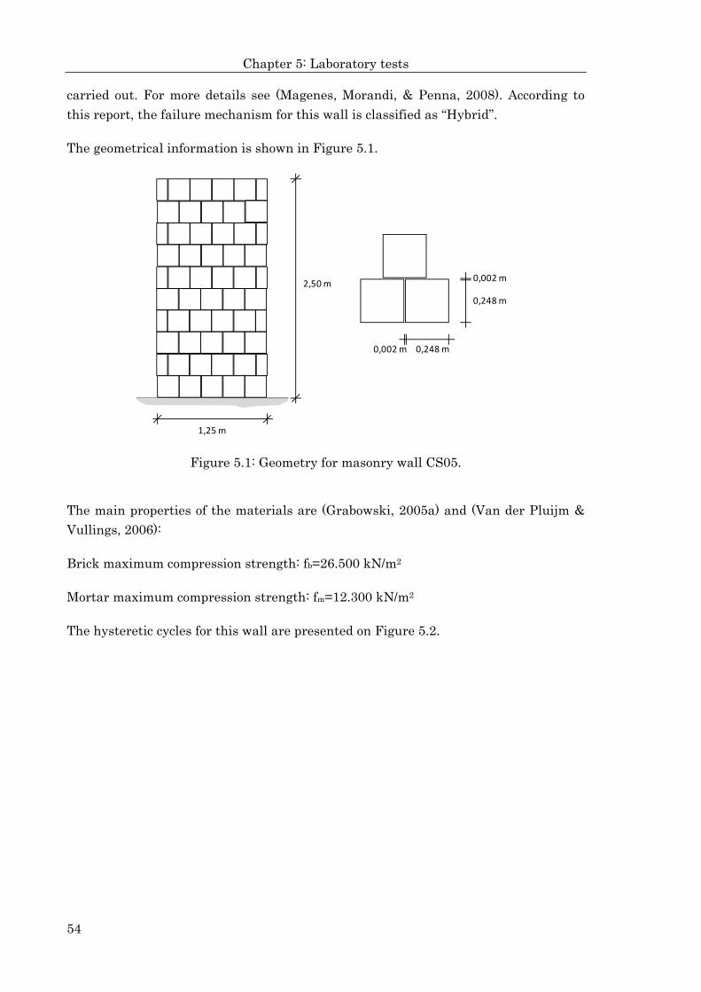
Chapter 5: Laboratory tests
54
carried out. For more details see (Magenes, Morandi, & Penna, 2008). According to
this report, the failure mechanism for this wall is classified as “Hybrid”.
The geometrical information is shown in Figure 5.1.
Figure 5.1: Geometry for masonry wall CS05.
The main properties of the materials are (Grabowski, 2005a) and (Van der Pluijm &
Vullings, 2006):
Brick maximum compression strength: fb=26.500 kN/m2
Mortar maximum compression strength: fm=12.300 kN/m2
The hysteretic cycles for this wall are presented on Figure 5.2.
2,50 m
1,25 m
0,248 m
0,248 m
0,002 m
0,002 m
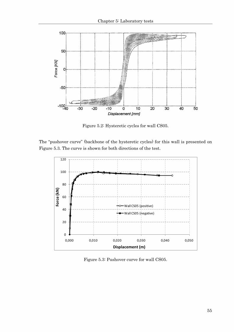
Chapter 5: Laboratory tests
55
Figure 5.2: Hysteretic cycles for wall CS05.
The “pushover curve” (backbone of the hysteretic cycles) for this wall is presented on Figure 5.3. The curve is shown for both directions of the test.
Figure 5.3: Pushover curve for wall CS05.
0
20
40
60
80
100
120
0,000 0,010 0,020 0,030 0,040 0,050
Forc
e (k
N)
Displacement (m)
Wall CS05 (positive)
Wall CS05 (negative)

Chapter 5: Laboratory tests
56
5.1.2 Test of Wall CL05
This is an Italian clay brick (Alveolater 45) masonry wall. The size of the units is 250x300x190 mm3 with vertical holes. The bed and head joints are filled with pre-mixed general purpose mortar (M5) and 1,0 cm thick. The boundary conditions of the wall is double fixed and the vertical load is 0,68 MPa, in addition to self weight. Other tests to verify the compressive strength of bricks and the diagonal compression on masonry square specimens were carried out. For more details see (Magenes, Morandi, & Penna, 2008). According to this report, the failure mechanism for this wall is classified as “Shear”.
The geometrical information is shown in Figure 5.4.
Figure 5.4: Geometry for masonry wall CL05.
The main properties of the materials are (Grabowski, 2005a) and (Magenes, Morandi, & Penna, 2008):
Brick maximum compression strength: fb=15.000 kN/m2
Mortar maximum compression strength: fm=7.400 kN/m2
The hysteretic cycles for this wall are presented on Figure 5.5.
2,60 m
2,50 m
0,250 m
0,190 m
0,010 m
0,010 m

Chapter 5: Laboratory tests
57
Figure 5.5: Hysteretic cycles for wall CL05.
The “pushover curve” (backbone of the hysteretic cycles) for this wall is presented on Figure 5.6. The curve is shown for both directions of the test.
Figure 5.6: Pushover curve for wall CL05.
0
50
100
150
200
250
300
350
400
0,000 0,001 0,002 0,003 0,004 0,005 0,006 0,007 0,008
Forc
e (k
N)
Displacement (m)
Wall CL05 (positive)
Wall CL05 (negative)

Chapter 5: Laboratory tests
58
5.1.3 Test of Wall CL06
This is an Italian clay brick (Alveolater 45) masonry wall. The size of the units is 250x300x190 mm3 with vertical holes. The bed and head joints are filled with pre-mixed general purpose mortar (M5) and 1,0 cm thick. The boundary conditions of the wall is double fixed and the vertical load is 0,50 MPa, in addition to self weight. Other tests to verify the compressive strength of bricks and the diagonal compression on masonry square specimens were carried out. For more details see (Magenes, Morandi, & Penna, 2008). According to this report, the failure mechanism for this wall is classified as “Flexural”.
The geometrical information is shown in Figure 5.7.
Figure 5.7: Geometry for masonry wall CL06.
The main properties of the materials are (Grabowski, 2005a) and (Magenes, Morandi, & Penna, 2008):
Brick maximum compression strength: fb=15.000 kN/m2
Mortar maximum compression strength: fm=7.400 kN/m2
The hysteretic cycles for this wall are presented on Figure 5.8.
2,60 m
0,250 m
0,190 m
0,010 m
0,010 m
1,25 m

Chapter 5: Laboratory tests
59
Figure 5.8: Hysteretic cycles for wall CL06.
The “pushover curve” (backbone of the hysteretic cycles) for this wall is presented on Figure 5.9. The curve is shown for both directions of the test.
Figure 5.9: Pushover curve for wall CL06.
0
10
20
30
40
50
60
70
80
90
0,000 0,010 0,020 0,030 0,040 0,050 0,060
Forc
e (k
N)
Displacement (m)
Wall CL06 (positive)
Wall CL06 (negative)

Chapter 5: Laboratory tests
60
5.2 Chilean tests (U. of La Serena)
The tests of reinforced and confined masonry were taken from two different research projects carried out in the Laboratory of Structures at the Civil Engineering Department of the University of La Serena (Chile). The project for reinforced masonry walls (Díaz, Arancibia, Vicencio, Durán, & Campbell, 2005) was carried out between years 2004-2005. The project for confined masonry walls (Galleguillos, Valenzuela, & Díaz, 2010) was carried out between years 2008-2009.
All tests were dynamic and controlled by displacement. The tests were carried out considering a variable horizontal displacement on the top of the wall with a frequency of 0,5 Hz. This displacement was incremented after a pre-determined number of cycles in 0,2 mm until the wall was sufficiently damaged to stop the test and not until it collapsed. The only vertical load was the self weight of the walls. The masonry walls are set free at the top (cantilever system). See Figure 5.10.
Figure 5.10: General view of a wall test at the University of La Serena (Galleguillos & Valenzuela, 2009).
5.2.1 Tests for reinforced masonry walls
This was a series of three tests on three walls (Nr.1, Nr.2 and Nr.3) with identical geometrical and material characteristics and steel reinforcement. The walls were designed according to the provisions given in Chilean code (I.N.N., 1993) “Reinforced masonry – Requirements for structural design”.
The three walls were made using typical Chilean clay bricks of 75x140x290 mm3 with vertical holes (MqHv3). The bed and head joints are 1,3 cm thick with a composition

Chapter 5: Laboratory tests
61
of 4:8:1 (cement:sand:lime). The steel used for reinforcement was type A44-28H (according to Chilean nomenclature). The quality of bricks and mortar was tested for compression according to Chilean codes. For more details see (Díaz, Arancibia, Vicencio, Durán, & Campbell, 2005). According to this report, the failure mechanism for the three walls is classified as “Flexural”.
The geometrical information is shown in Figure 5.11.
Figure 5.11: Geometry for reinforced masonry walls.
The main properties of the materials are (Díaz, Arancibia, Vicencio, Durán, & Campbell, 2005):
Brick maximum compression strength: fb=21.800 kN/m2
Mortar maximum compression strength: fm=22.600 kN/m2
Steel elasticity module: Es=210.000.000 kN/m2
Yield tension of steel: fy=280.000 kN/m2
Ultimate tension of steel: fu=440.000 kN/m2
Fracture tension of steel: fr=220.000 kN/m2
The “pushover curves” (backbone of the hysteretic cycles) for these walls are presented on Figure 5.12, Figure 5.13 and Figure 5.14. The curves are shown for both directions (positive and negative) of the tests.
1φ10
1,98 m
1,67 m
0,290 m
0,075 m0,013 m
0,013 m
0,24 m
1φ12
1φ12
1φ10
1φ10

Chapter 5: Laboratory tests
62
Figure 5.12: Pushover curves for wall Nr. 1.
Figure 5.13: Pushover curves for wall Nr. 2.
0
10
20
30
40
50
60
70
0,000 0,001 0,002 0,003 0,004 0,005 0,006 0,007 0,008
Forc
e (k
N)
Displacement (m)
Wall Nr.1 (positive)
Wall Nr.1 (negative)
0
10
20
30
40
50
60
70
0,000 0,001 0,002 0,003 0,004 0,005 0,006 0,007 0,008 0,009
Forc
e (k
N)
Displacement (m)
Wall Nr.2 (positive)
Wall Nr.2 (negative)

Chapter 5: Laboratory tests
63
Figure 5.14: Pushover curves for wall Nr. 3.
5.2.2 Tests for confined masonry walls
This was a series of three tests on three walls with the same material characteristics and slightly different geometrical dimensions. The walls were designed according to the provisions given in the Chilean code (I.N.N., 1997) “Confined masonry – Requirements for structural design”, considering some special variations in the size of the confining frame.
The three walls were made using typical Chilean bricks of 70x140x290 mm3 with vertical holes MqHv3. The bed and head joints are 1,4 cm thick with a composition of 4:8:1 (cement:sand:lime). The steel used for reinforcement was type A63-42H. The quality of bricks, mortar and concrete was tested for compression according to Chilean codes. Masonry square specimens were also tested for “diagonal compression” in order to determine some general properties. For more details see (Galleguillos, Valenzuela, & Díaz, 2010). According to this report, the failure mechanism for these walls is classified as “Shear” with damage of joints between tie columns and bond beam.
The geometrical information is shown in Figure 5.15.
0
10
20
30
40
50
60
70
0,000 0,001 0,002 0,003 0,004 0,005 0,006 0,007 0,008
Forc
e (k
N)
Displacement (m)
Wall Nr.3 (positive)
Wall Nr. 3 (negative)

Chapter 5: Laboratory tests
64
Figure 5.15: Geometry for confined masonry walls.
The main properties of the materials are (Galleguillos, Valenzuela, & Díaz, 2010):
Brick maximum compression strength: fb=20.000 kN/m2
Mortar maximum compression strength: fm=27.000 kN/m2
Steel elasticity module: Es=210.000.000 kN/m2
Yield tension of steel: fy=420.000 kN/m2
Ultimate tension of steel: fu=630.000 kN/m2
Fracture tension of steel: fr=315.000 kN/m2
Concrete maximum compression strength: fc=28.000 kN/m2
The width of the tie columns is 0,20 m for MV1; 0,14 m for MV2 and 0,30 m for MV3.
The longitudinal reinforcement in tie columns is 4φ12 and in bond beam is 4φ10. The transversal reinforcements (stirrups) on tie columns and bond beam are shown on Table 5.1:
Table 5.1: Stirrups on reinforcement concrete for confined walls.
Wall Normal section
Critical section
MV1 φ6@20 φ6@10
MV2 φ6@15 φ6@15
2,02 m
2,20 m
0,290 m
0,070 m0,014 m
0,014 m
0,25 m
var. var.

Chapter 5: Laboratory tests
65
MV3 φ6@15 φ6@15
The “pushover curves” (backbone of the hysteretic cycles) for these walls are presented on Figure 5.16, Figure 5.17 and Figure 5.18. The curves are shown for both directions (positive and negative) of the tests.
Figure 5.16: Pushover curves for wall MV1.
Figure 5.17: Pushover curves for wall MV2.
0
20
40
60
80
100
120
0,000 0,002 0,004 0,006 0,008 0,010 0,012 0,014
Forc
e (k
N)
Displacement (m)
Wall MV1 (positive)
Wall MV1 (negative)
0
20
40
60
80
100
120
140
0,000 0,002 0,004 0,006 0,008 0,010 0,012 0,014
Forc
e (k
N)
Displacement (m)
Wall MV2 (positive)
Wall MV2 (negative)

Chapter 5: Laboratory tests
66
Figure 5.18: Pushover curves for wall MV3.
5.3 Nominal shear force according to MSJC
In the following table (Table 5.2) the nominal shear force Vn and the controlling type of failure for every tested wall is given. This shear force was calculated considering the information and according to the regulations of the MSJC (Masonry Society, 2003).
Table 5.2: Nominal shear force and controlling failure.
Wall Nominal shear force Vn (kN)
Controlling failure
CS05 61,6 Flexion
CL05 267,1 Flexion
CL06 55,9 Flexion
Nr.1, 2, 3 65,6 Flexion
MV1 106,2 Shear
MV2 115,0 Shear
MV3 94,4 Shear
Observing the Table 5.2 and the pushover curves of the tested walls, it can be easily noted that the values of nominal shear force “Vn“ for the walls tested in the ESECMaSE Project (CS05, CL05 and CL06) are notoriously underestimated (about -
0
20
40
60
80
100
120
140
160
0,000 0,002 0,004 0,006 0,008 0,010 0,012 0,014 0,016 0,018 0,020 0,022
Forc
e (k
N)
Displacement (m)
Wall MV3 (positive)
Wall MV3 (negative)

Chapter 5: Laboratory tests
67
30%) in comparison with the tests results. This situation can be explained because the controlling type of failure for these walls is “Flexion”, and this type of failure is totally defined through the “fracture module of masonry”, which is the tension capacity of the masonry. Due to the lack of information of this parameter for these walls, the value considered in the calculations was the one recommended in MSJC.
There is another comment to make about this table. The nominal shear force for walls MV1, MV2 and MV3 are different because, as it was already mentioned, these three walls have different width of tie columns. The code MSJC defines the shear capacity considering only the shear capacity of masonry, excluding the contribution of tie columns which only contribute in flexion. According to this situation and taking into account that these three walls fail in shear, the wall with the larger tie column width has the smaller shear capacity.


Chapter 6: Implementation of the model
69
6 Implementation of the model
The proposed model was implemented and applied to seven walls, which were tested previously in other research projects (see “Chapter 5 Laboratory tests”). These tests include different general geometry, quality of materials and type of masonry, in order to validate a wide range of cases.
The details of these models and its results are presented in this chapter. In the next paragraphs the most important results for each model are shown, especially, the general displacement, the pushover curve and some stress diagrams. More details of stresses and other results for every wall can be seen in Appendixes A1 to A7.
The parameters related to geometry are taken from the information given in “Chapter 5 Laboratory tests” as well as some other information related to the properties of the materials. Other parameters, such as elasticity module (longitudinal and transversal), tension and shear strength, friction and adherence in the contact zone between brick and mortar, are estimated from the tables presented on (Irmschler, Schubert, & Jäger, 2004), as it was indicated in “Chapter 4 Proposed model”.
The units valid for all the figures are kN-m.
6.1 ESECMaSE Project walls
6.1.1 Wall CS05
The mechanical properties for the materials considered in this model were the following:
From (Grabowski, 2005a) and (Van der Pluijm & Vullings, 2006):
Brick maximum compression strength: fb=26.500 kN/m2
Mortar maximum compression strength: fm=12.300 kN/m2
From the formula given in “2.1.1 Bricks and blocks” (Equation 2.2):
Brick initial elasticity module: Eb=355· fb=9,408·106 kN/m2
From the formula given in “2.1.2 Mortar” (Equation 2.3):
Mortar initial elasticity module: Em=200· fm=2,460·106 kN/m2

Chapter 6: Implementation of the model
70
From Mauerwerk-Kalender (Irmschler, Schubert, & Jäger, 2004):
Maximum adherence strength between brick-mortar: fab-m=1.270 kN/m2
Maximum tension strength brick-mortar: ftb-m=610 kN/m2
Poisson’s coefficient for bricks: νb=0,20
Poisson’s coefficient for mortar: νm=0,15
Friction coefficient brick-mortar: μb-m=0,50
The general displacements in the last step and the pushover curve for Wall CS05 are shown in Figure 6.1 and Figure 6.2.
Figure 6.1: General displacements on the last step for Wall CS05.

Chapter 6: Implementation of the model
71
Figure 6.2: Pushover curve for Wall CS05.
6.1.2 Wall CL05
The mechanical properties for the materials considered in this model were the following:
From (Grabowski, 2005a) and (Magenes, Morandi, & Penna, 2008):
Brick maximum compression strength: fb=15.000 kN/m2
Mortar maximum compression strength: fm=7.400 kN/m2
From the formula given in “2.1.1 Bricks and blocks” (Equation 2.1):
Brick initial elasticity module: Eb=300· fb=4,500·106 kN/m2
From the formula given in “2.1.2 Mortar” (Equation 2.3):
Mortar initial elasticity module: Em=200· fm=1,480·106 kN/m2
From Mauerwerk-Kalender (Irmschler, Schubert, & Jäger, 2004):
Maximum adherence strength between brick-mortar: fab-m=500 kN/m2

Chapter 6: Implementation of the model
72
Maximum tension strength brick-mortar: ftb-m=480 kN/m2
Poisson’s coefficient for bricks: νb=0,20
Poisson’s coefficient for mortar: νm=0,15
Friction coefficient brick-mortar: μb-m=0,50
The general displacements in the last step and the pushover curve for Wall CL05 are shown in Figure 6.3 and Figure 6.4.
Figure 6.3: General displacements on the last step for Wall CL05.

Chapter 6: Implementation of the model
73
Figure 6.4: Pushover curve for Wall CL05.
6.1.3 Wall CL06
The mechanical properties for the materials considered in this model were the following:
From (Grabowski, 2005a) and (Magenes, Morandi, & Penna, 2008):
Brick maximum compression strength: fb=15.000 kN/m2
Mortar maximum compression strength: fm=7.400 kN/m2
From the formula given in “2.1.1 Bricks and blocks” (Equation 2.1):
Brick initial elasticity module: Eb=300· fb=4,500·106 kN/m2
From the formula given in “2.1.2 Mortar” (Equation 2.3):
Mortar initial elasticity module: Em=200· fm=1,480·106 kN/m2
From Mauerwerk-Kalender (Irmschler, Schubert, & Jäger, 2004):
Maximum adherence strength between brick-mortar: fab-m=500 kN/m2

Chapter 6: Implementation of the model
74
Maximum tension strength brick-mortar: ftb-m=480 kN/m2
Poisson’s coefficient for bricks: νb=0,20
Poisson’s coefficient for mortar: νm=0,15
Friction coefficient brick-mortar: μb-m=0,50
The general displacements in the last step and the pushover curve for Wall CL06 are shown in Figure 6.5 and Figure 6.6.
Figure 6.5: General displacements on the last step for Wall CL06.

Chapter 6: Implementation of the model
75
Figure 6.6: Pushover curve for Wall CL06.
6.2 Chilean walls (U. of La Serena)
6.2.1 Reinforced masonry walls
The mechanical properties for the materials considered in this model were the following:
From (Díaz, Arancibia, Vicencio, Durán, & Campbell, 2005):
Brick maximum compression strength: fb=21.800 kN/m2
Mortar maximum compression strength: fm=22.600 kN/m2
From the formula given in “2.1.1 Bricks and blocks” (Equation 2.1):
Brick initial elasticity module: Eb=250· fb=5,450·106 kN/m2
From the formula given in “2.1.2 Mortar” (Equation 2.3):
Mortar initial elasticity module: Em=200· fm=4,520·106 kN/m2
From Mauerwerk-Kalender (Irmschler, Schubert, & Jäger, 2004):

Chapter 6: Implementation of the model
76
Maximum adherence strength between brick-mortar: fab-m=500 kN/m2
Maximum tension strength brick-mortar: ftb-m=480 kN/m2
Poisson’s coefficient for bricks: νb=0,20
Poisson’s coefficient for mortar: νm=0,15
Friction coefficient brick-mortar: μb-m=0,50
From (Díaz, Arancibia, Vicencio, Durán, & Campbell, 2005):
Yield tension of steel: fy=280.000 kN/m2
Ultimate tension of steel: fu=440.000 kN/m2
Fracture tension of steel: fr=220.000 kN/m2
From the value given in “2.1.5 Concrete and steel”:
Steel elasticity module: Es=210.000.000 kN/m2
The general displacements in the last step and the pushover curve for the Reinforced wall are shown in Figure 6.7 and Figure 6.8.
Figure 6.7: General displacements on the last step for Reinforced wall.

Chapter 6: Implementation of the model
77
Figure 6.8: Pushover curve for Reinforced wall.
6.2.2 Confined masonry walls
Wall MV1
The mechanical properties for the materials considered in this model were the following:
From (Galleguillos, Valenzuela, & Díaz, 2010):
Brick maximum compression strength: fb=20.000 kN/m2
Mortar maximum compression strength: fm=27.000 kN/m2
From the formula given in “2.1.1 Bricks and blocks” (Equation 2.1):
Brick initial elasticity module: Eb=250· fb=5,000·106 kN/m2
From the formula given in “2.1.2 Mortar” (Equation 2.3):
Mortar initial elasticity module: Em=150· fm=4,050·106 kN/m2
From Mauerwerk-Kalender (Irmschler, Schubert, & Jäger, 2004):

Chapter 6: Implementation of the model
78
Maximum adherence strength between brick-mortar: fab-m=500 kN/m2
Maximum tension strength brick-mortar: ftb-m=480 kN/m2
Poisson’s coefficient for bricks: νb=0,20
Poisson’s coefficient for mortar: νm=0,15
Friction coefficient brick-mortar: μb‐m=0,50
From (Galleguillos, Valenzuela, & Díaz, 2010):
Yield tension of steel: fy=420.000 kN/m2
Ultimate tension of steel: fu=630.000 kN/m2
Fracture tension of steel: fr=315.000 kN/m2
Concrete maximum compression strength: fc=28.000 kN/m2
From the formula and value given in “2.1.5 Concrete and steel” (Equation 2.5):
Concrete elasticity module: Ec=140.000 f =23.426.480 kN/m2
Steel elasticity module: Es=210.000.000 kN/m2
Poisson’s coefficient for concrete: νc=0,16
The general displacements in the last step and the pushover curve for the Wall MV1
are shown in Figure 6.9 and Figure 6.10.

Chapter 6: Implementation of the model
79
Figure 6.9: General displacements on the last step for Wall MV1.
Figure 6.10: Pushover curve for Wall MV1.

Chapter 6: Implementation of the model
80
Wall MV2
The mechanical properties for the materials considered in this model were the
following:
From (Galleguillos, Valenzuela, & Díaz, 2010):
Brick maximum compression strength: fb=20.000 kN/m2
Mortar maximum compression strength: fm=27.000 kN/m2
From the formula given in “2.1.1 Bricks and blocks” (Equation 2.1):
Brick initial elasticity module: Eb=250· fb=5,000∙106 kN/m2
From the formula given in “2.1.2 Mortar” (Equation 2.3):
Mortar initial elasticity module: Em=150· fm=4,050∙106 kN/m2
From Mauerwerk-Kalender (Irmschler, Schubert, & Jäger, 2004):
Maximum adherence strength between brick-mortar: fab-m=500 kN/m2
Maximum tension strength brick-mortar: ftb-m=480 kN/m2
Poisson’s coefficient for bricks: νb=0,20
Poisson’s coefficient for mortar: νm=0,15
Friction coefficient brick-mortar: μb‐m=0,50
From (Galleguillos, Valenzuela, & Díaz, 2010):
Yield tension of steel: fy=420.000 kN/m2
Ultimate tension of steel: fu=630.000 kN/m2
Fracture tension of steel: fr=315.000 kN/m2
Concrete maximum compression strength: fc=28.000 kN/m2
From the formula and value given in “2.1.5 Concrete and steel” (Equation 2.5):
Concrete elasticity module: Ec=140.000 f =23.426.480 kN/m2
Steel elasticity module: Es=210.000.000 kN/m2
Poisson’s coefficient for concrete: νc=0,16

Chapter 6: Implementation of the model
81
The general displacements in the last step and the pushover curve for the Wall MV2 are shown in Figure 6.11 and Figure 6.12.
Figure 6.11: General displacements on the last step for Wall MV2.
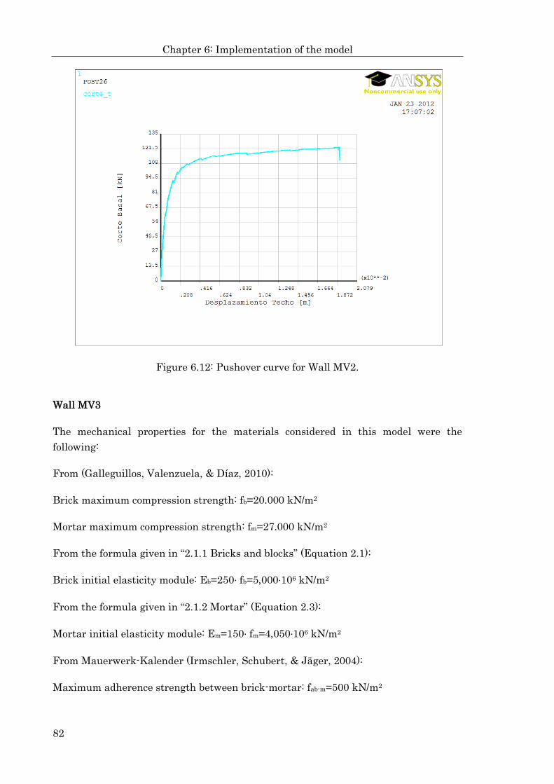
Chapter 6: Implementation of the model
82
Figure 6.12: Pushover curve for Wall MV2.
Wall MV3
The mechanical properties for the materials considered in this model were the following:
From (Galleguillos, Valenzuela, & Díaz, 2010):
Brick maximum compression strength: fb=20.000 kN/m2
Mortar maximum compression strength: fm=27.000 kN/m2
From the formula given in “2.1.1 Bricks and blocks” (Equation 2.1):
Brick initial elasticity module: Eb=250· fb=5,000·106 kN/m2
From the formula given in “2.1.2 Mortar” (Equation 2.3):
Mortar initial elasticity module: Em=150· fm=4,050·106 kN/m2
From Mauerwerk-Kalender (Irmschler, Schubert, & Jäger, 2004):
Maximum adherence strength between brick-mortar: fab-m=500 kN/m2

Chapter 6: Implementation of the model
83
Maximum tension strength brick-mortar: ftb-m=480 kN/m2
Poisson’s coefficient for bricks: νb=0,20
Poisson’s coefficient for mortar: νm=0,15
Friction coefficient brick-mortar: μb-m=0,50
From (Galleguillos, Valenzuela, & Díaz, 2010):
Yield tension of steel: fy=420.000 kN/m2
Ultimate tension of steel: fu=630.000 kN/m2
Fracture tension of steel: fr=315.000 kN/m2
Concrete maximum compression strength: fc=28.000 kN/m2
From the formula and value given in “2.1.5 Concrete and steel” (Equation 2.5):
Concrete elasticity module: Ec=140.000 f =23.426.480 kN/m2
Steel elasticity module: Es=210.000.000 kN/m2
Poisson’s coefficient for concrete: νc=0,16
The general displacements in the last step and the pushover curve for the Wall MV3
are shown in Figure 6.13 and Figure 6.14.

Chapter 6: Implementation of the model
84
Figure 6.13: General displacements on the last step for Wall MV3.
Figure 6.14: Pushover curve for Wall MV3.

Chapter 6: Implementation of the model
85
6.3 Remarks about the stresses and forces distribution
In Appendixes A.1 to A.7 more figures showing stresses and forces results for the last iteration step are presented. These results are presented separately for bricks, non-linear springs, contact elements and, eventually, for reinforcing steel bars and confining concrete.
As it can be seen observing the graphics in appendixes, most of the nonlinear response of the walls is concentrated in mortar joints (non-linear springs and contact elements). There are only few brick elements under stresses beyond its tension maximum strength (CL05; CL06: Nr. 1, 2 and 3; and MV3) and no elements fail under compression.
According to the graphics shown in the appendixes, the situation for every wall in the last iteration is:
Wall CS05
Only some vertical non-linear springs reach the maximum shear strength. Additionally, the most vertical contact elements in the bottom and top lines are slightly open, which indicate a bending failure.
Wall CL05
Few bricks reach the maximum tension strength. Some vertical non-linear springs reach the maximum tension strength and many vertical non-linear springs reach the maximum shear strength. Some horizontal non-linear springs fail in tension. Additionally, almost all the inferior and superior lines are under compression and only a small part is under tension. This indicates a shear failure for this wall.
Wall CL06
Few bricks reach the maximum tension strength. Some vertical non-linear springs reach the maximum compression, tension and shear strength. Only some horizontal non-linear springs fail in tension. Additionally, the most vertical contact elements in the bottom and top lines are slightly open, which indicate a bending failure.
Walls Nr. 1, 2 and 3
Few bricks reach the maximum tension strength. Some vertical non-linear springs reach the maximum tension strength and more of them fail in shear. Only some horizontal non-linear springs fail in tension. Moreover, two or three vertical

Chapter 6: Implementation of the model
86
reinforcing bars yield. Additionally, the most vertical contact elements in the bottom and top lines are slightly open, which indicate a bending failure.
Wall MV1
Some vertical and horizontal non-linear springs reach the maximum tension and shear strength. Moreover, few concrete elements fail in tension. Additionally, the highest tension forces in vertical and horizontal springs are concentrated in the upper left corner and in the lower right corner, suggesting, probably, a diagonal shear failure. In this case it is clear that the tie columns resist the bending moment working as a force couple.
Wall MV2
Some vertical and horizontal non-linear springs reach the maximum tension and shear strength, especially in the vertical edges. Moreover, few concrete elements fail in tension. Additionally, the highest tension forces in vertical and horizontal springs are concentrated in the upper left corner and in the lower right corner, which suggest, probably, a diagonal shear failure. In this case it is clear that the tie columns resist the bending moment working as a force couple.
Wall MV3
Few bricks reach the maximum tension strength. Some vertical and horizontal non-linear springs reach the maximum tension and shear strength, especially in the vertical edges. Moreover, few concrete elements fail in tension. Additionally, the highest transversal forces in vertical springs are concentrated in the right edge, which suggest, probably, a shear failure in this zone. In this case it is clear that the tie columns resist the bending moment working as a force couple.

Chapter 7: Comparison between model and tests
87
7 Comparison between model and
tests
In this chapter a comparison between the results given by the model and the
laboratory tests is made. The comparisons are made in terms of graphics and tables.
The graphics show the original and bilinear pushover curves of the models, laboratory
tests and the design shear force for every wall. The tables show the main values for
every case: forces, displacements, rigidity and ductility.
7.1 Bilinearization process
For the use of pushover curves in nonlinear static procedures (NSP) it is necessary to
transform the original curves into a bilinear format. This format permits the
definition of a yielding point (maximum linear-elastic displacement and force) and,
subsequently, the definition of ductility, which is an important parameter in these
nonlinear static procedures.
There are many ways to determine the bilinear format of a pushover curve. In this
contribution the concept of equivalent areas is used and the bilinear format is
considered as linear-elastic - ideal-plastic. This means that the bilinear curve has a
linear elastic segment and then a horizontal segment.
The steps to define the bilinear curve of a pushover curve are the following:
1) Determine the total area under the original pushover curve.
2) Determine the maximum force in the original pushover curve.
3) Define the linear-elastic segment of the bilinear curve considering the secant
between the origin and a pre-defined point in the original curve. This point is
determined as a specific fraction of the maximum force and its respective
displacement. This point enables to determine the elastic rigidity of the bilinear
curve (Ke).
4) The maximum displacement of the bilinear curve is the same of that in the
original curve (Dmax).
5) To determine the maximum force of the bilinear idealization (Fmax) an iterative
process must be made. In this process the maximum force is changed until the
area under the bilinear curve is equal to the area under the original curve.
6) The elastic displacement (De) and the ductility (μ) of the bilinear idealization are
calculated as D F /K and μ D /D .

Chapter 7: Comparison between model and tests
88
It is necessary to clarify two important details in this bilinearization process.
Firstly, in case that in the original curve the final force is much smaller than the maximum force, the curve is usually limited up to the point with a final force value equal to 80% of the maximum force. This is to avoid strong degradation of the curve after reaching its maximum force value. In this research, the original test curves of walls MV1, MV2 and MV3 has been corrected (see and compare Figure 5.16, Figure 5.17, Figure 5.18 and Figure 7.10, Figure 7.12, Figure 7.14, respectively).
Secondly, there are different proposals to define the point associated to the elastic secant of the bilinear idealization (step 3 of the process). In the reports of the ESECMaSE Project, the value of force considered was 70% of the maximum force of the original curve and in this research the same value was considered. For the Chilean walls, a value of force 60% of the maximum force was considered, as recommended by (Chopra & Goel, 2002).
7.2 Wall CS05
In Figure 7.1 the original pushover curves from test (positive and negative directions) and model for the wall CS05 are shown. In the figure can also be seen the nominal shear force calculated according to MSJC (Masonry Society, 2003).
Figure 7.1: Original pushover curves (model and tests) for wall CS05.
In the Figure 7.2 the bilinear pushover curves from test (positive and negative) and model for the wall CS05 are shown.
0
10
20
30
40
50
60
70
80
90
100
110
120
130
0,000 0,005 0,010 0,015 0,020 0,025 0,030 0,035 0,040 0,045 0,050 0,055 0,060
Forc
e (k
N)
Displacement (m)
Wall CS05 ANSYS
Wall CS05 (positive)
Wall CS05 (negative)
Nominal Shear Force
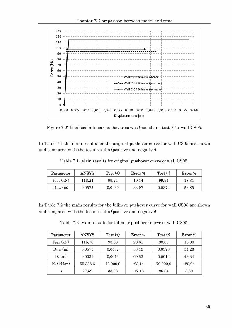
Chapter 7: Comparison between model and tests
89
Figure 7.2: Idealized bilinear pushover curves (model and tests) for wall CS05.
In Table 7.1 the main results for the original pushover curve for wall CS05 are shown and compared with the tests results (positive and negative).
Table 7.1: Main results for original pushover curve of wall CS05.
Parameter ANSYS Test (+) Error % Test (-) Error %
Fmax (kN) 118,24 99,24 19,14 99,94 18,31
Dmax (m) 0,0575 0,0430 33,97 0,0374 53,85
In Table 7.2 the main results for the bilinear pushover curve for wall CS05 are shown and compared with the tests results (positive and negative).
Table 7.2: Main results for bilinear pushover curve of wall CS05.
Parameter ANSYS Test (+) Error % Test (-) Error %
Fmax (kN) 115,70 93,60 23,61 98,00 18,06
Dmax (m) 0,0575 0,0432 33,19 0,0373 54,26
De (m) 0,0021 0,0013 60,83 0,0014 49,34
Ke (kN/m) 55.338,6 72.000,0 -23,14 70.000,0 -20,94
μ 27,52 33,23 -17,18 26,64 3,30
0
10
20
30
40
50
60
70
80
90
100
110
120
130
0,000 0,005 0,010 0,015 0,020 0,025 0,030 0,035 0,040 0,045 0,050 0,055 0,060
Forc
e (k
N)
Displacement (m)
Wall CS05 Bilinear ANSYS
Wall CS05 Bilinear (positive)
Wall CS05 Bilinear (negative)

Chapter 7: Comparison between model and tests
90
7.3 Wall CL05
In Figure 7.3 the original pushover curves from test (positive and negative directions) and model for the wall CL05 are shown. In the figure can also be seen the nominal shear force calculated according to MSJC (Masonry Society, 2003).
Figure 7.3: Original pushover curves (model and tests) for wall CL05.
In the Figure 7.4 the bilinear pushover curves from test (positive and negative) and model for the wall CL05 are shown.
0
40
80
120
160
200
240
280
320
360
400
0,000 0,001 0,002 0,003 0,004 0,005 0,006 0,007 0,008 0,009 0,010
Forc
e (k
N)
Displacement (m)
Wall CL05 ANSYS
Wall CL05 (positive)
Wall CL05 (negative)
Nominal Shear Force
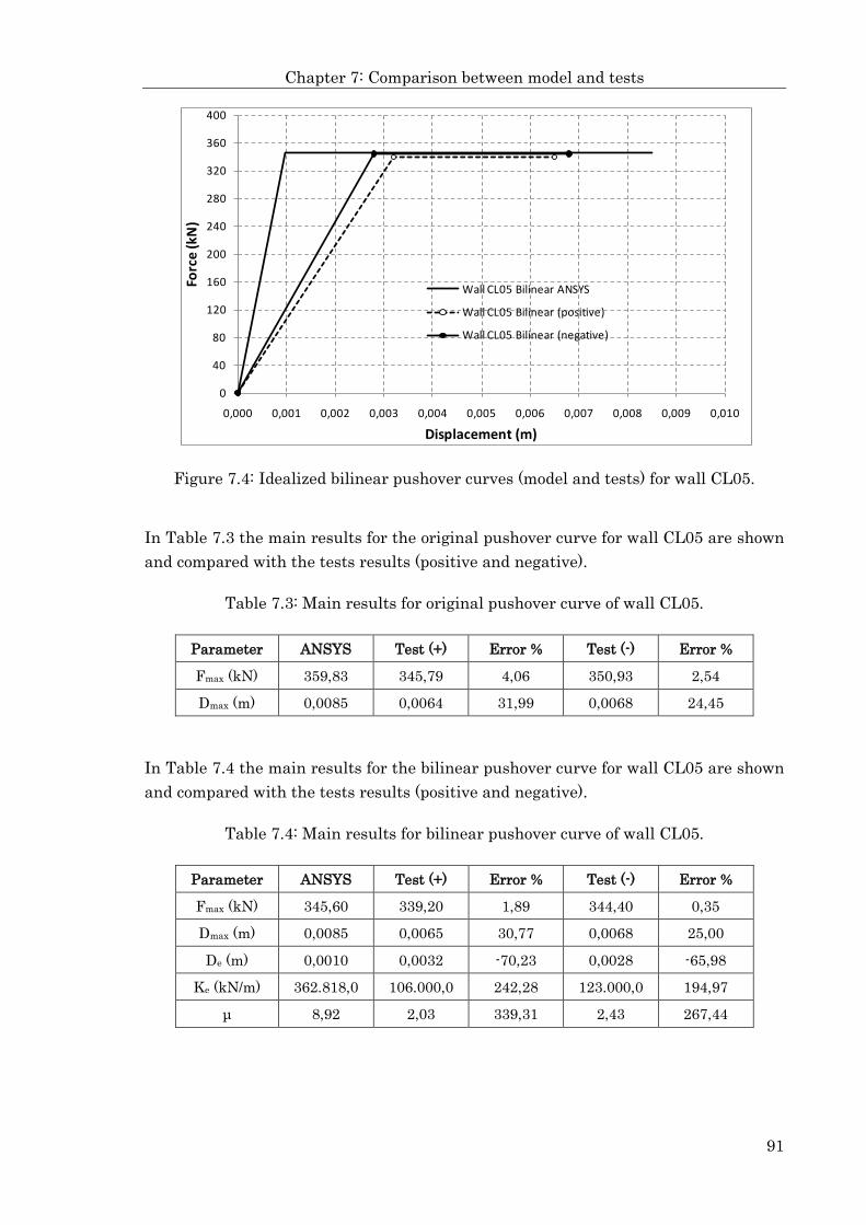
Chapter 7: Comparison between model and tests
91
Figure 7.4: Idealized bilinear pushover curves (model and tests) for wall CL05.
In Table 7.3 the main results for the original pushover curve for wall CL05 are shown and compared with the tests results (positive and negative).
Table 7.3: Main results for original pushover curve of wall CL05.
Parameter ANSYS Test (+) Error % Test (-) Error %
Fmax (kN) 359,83 345,79 4,06 350,93 2,54
Dmax (m) 0,0085 0,0064 31,99 0,0068 24,45
In Table 7.4 the main results for the bilinear pushover curve for wall CL05 are shown and compared with the tests results (positive and negative).
Table 7.4: Main results for bilinear pushover curve of wall CL05.
Parameter ANSYS Test (+) Error % Test (-) Error %
Fmax (kN) 345,60 339,20 1,89 344,40 0,35
Dmax (m) 0,0085 0,0065 30,77 0,0068 25,00
De (m) 0,0010 0,0032 -70,23 0,0028 -65,98
Ke (kN/m) 362.818,0 106.000,0 242,28 123.000,0 194,97
μ 8,92 2,03 339,31 2,43 267,44
0
40
80
120
160
200
240
280
320
360
400
0,000 0,001 0,002 0,003 0,004 0,005 0,006 0,007 0,008 0,009 0,010
Forc
e (k
N)
Displacement (m)
Wall CL05 Bilinear ANSYS
Wall CL05 Bilinear (positive)
Wall CL05 Bilinear (negative)

Chapter 7: Comparison between model and tests
92
7.4 Wall CL06
In Figure 7.5 the original pushover curves from test (positive and negative directions) and model for the wall CL06 are shown. In the figure can also be seen the nominal shear force calculated according to MSJC (Masonry Society, 2003).
Figure 7.5: Original pushover curves (model and tests) for wall CL06.
In Figure 7.6 the bilinear pushover curves from test (positive and negative) and model for the wall CL06 are shown.
Figure 7.6: Idealized bilinear pushover curves (model and tests) for wall CL06.
0
10
20
30
40
50
60
70
80
90
100
110
0,000 0,010 0,020 0,030 0,040 0,050 0,060 0,070 0,080
Forc
e (k
N)
Displacement (m)
Wall CL06 ANSYS
Wall CL06 (positive)
Wall CL06 (negative)
Nominal Shear Force
0
10
20
30
40
50
60
70
80
90
100
110
0,000 0,010 0,020 0,030 0,040 0,050 0,060 0,070 0,080
Forc
e (k
N)
Displacement (m)
Wall CL06 Bilinear ANSYS
Wall CL06 Bilinear (positive)
Wall CL06 Bilinear (negative)

Chapter 7: Comparison between model and tests
93
In Table 7.5 the main results for the original pushover curve for wall CL06 are shown and compared with the tests results (positive and negative).
Table 7.5: Main results for original pushover curve of wall CL06.
Parameter ANSYS Test (+) Error % Test (-) Error %
Fmax (kN) 93,76 84,42 11,06 84,88 10,46
Dmax (m) 0,0801 0,0514 55,84 0,0510 57,00
In Table 7.6 the main results for the bilinear pushover curve for wall CL06 are shown and compared with the tests results (positive and negative).
Table 7.6: Main results for bilinear pushover curve of wall CL06.
Parameter ANSYS Test (+) Error % Test (-) Error %
Fmax (kN) 91,80 80,00 14,75 80,00 14,75
Dmax (m) 0,0801 0,0515 55,53 0,0508 57,68
De (m) 0,0017 0,0020 -13,43 0,0020 -13,43
Ke (kN/m) 53.018,0 40.000,0 32,54 40.000,0 32,54
μ 46,26 25,75 79,65 25,40 82,13
7.5 Walls Nr. 1, 2 and 3
In Figure 7.7 the original pushover curves from test (positive and negative directions) and model for the walls Nr. 1, 2 and 3 are shown. In the figure can also be seen the nominal shear force calculated according to MSJC (Masonry Society, 2003).
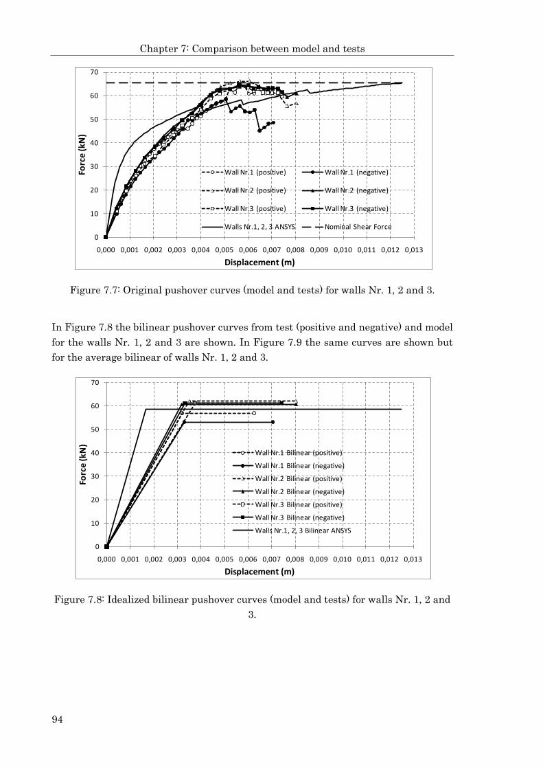
Chapter 7: Comparison between model and tests
94
Figure 7.7: Original pushover curves (model and tests) for walls Nr. 1, 2 and 3.
In Figure 7.8 the bilinear pushover curves from test (positive and negative) and model for the walls Nr. 1, 2 and 3 are shown. In Figure 7.9 the same curves are shown but for the average bilinear of walls Nr. 1, 2 and 3.
Figure 7.8: Idealized bilinear pushover curves (model and tests) for walls Nr. 1, 2 and 3.
0
10
20
30
40
50
60
70
0,000 0,001 0,002 0,003 0,004 0,005 0,006 0,007 0,008 0,009 0,010 0,011 0,012 0,013
Forc
e (k
N)
Displacement (m)
Wall Nr.1 (positive) Wall Nr.1 (negative)
Wall Nr.2 (positive) Wall Nr.2 (negative)
Wall Nr.3 (positive) Wall Nr.3 (negative)
Walls Nr.1, 2, 3 ANSYS Nominal Shear Force
0
10
20
30
40
50
60
70
0,000 0,001 0,002 0,003 0,004 0,005 0,006 0,007 0,008 0,009 0,010 0,011 0,012 0,013
Forc
e (k
N)
Displacement (m)
Wall Nr.1 Bilinear (positive)
Wall Nr.1 Bilinear (negative)
Wall Nr.2 Bilinear (positive)
Wall Nr.2 Bilinear (negative)
Wall Nr.3 Bilinear (positive)
Wall Nr.3 Bilinear (negative)
Walls Nr.1, 2, 3 Bilinear ANSYS

Chapter 7: Comparison between model and tests
95
Figure 7.9: Idealized bilinear pushover curves (model and tests) for average walls Nr. 1, 2 and 3.
In Table 7.7, Table 7.8 and Table 7.9 the main results for the original pushover curve for wall walls Nr. 1, 2 and 3 are shown and compared with the tests results (positive and negative).
Table 7.7: Main results for original pushover curve of wall Nr. 1.
Parameter ANSYS Test (+) Error % Test (-) Error %
Fmax (kN) 65,37 65,00 0,58 58,54 11,68
Dmax (m) 0,0125 0,0062 100,08 0,0071 77,00
Table 7.8: Main results for original pushover curve of wall Nr. 2.
Parameter ANSYS Test (+) Error % Test (-) Error %
Fmax (kN) 65,37 66,08 -1,07 64,01 2,13
Dmax (m) 0,0125 0,0080 55,62 0,0080 55,67
Table 7.9: Main results for original pushover curve of wall Nr. 3.
Parameter ANSYS Test (+) Error % Test (-) Error %
Fmax (kN) 65,37 64,40 1,52 64,41 1,49
Dmax (m) 0,0125 0,0074 68,02 0,0074 67,99
0
10
20
30
40
50
60
70
0,000 0,001 0,002 0,003 0,004 0,005 0,006 0,007 0,008 0,009 0,010 0,011 0,012 0,013
Forc
e (k
N)
Displacement (m)
Average Walls Nr.1, 2, 3
Average Walls Nr.1, 2, 3
Walls Nr.1, 2, 3 Bilinear ANSYS

Chapter 7: Comparison between model and tests
96
In Table 7.10, Table 7.11, Table 7.12 and Table 7.13 the main results for the bilinear pushover curve for wall walls Nr. 1, 2 , 3 and average are shown and compared with the tests results (positive and negative).
Table 7.10: Main results for bilinear pushover curve of wall Nr. 1.
Parameter ANSYS Test (+) Error % Test (-) Error %
Fmax (kN) 58,60 56,90 2,99 53,10 10,36
Dmax (m) 0,0125 0,0062 100,08 0,0071 77,00
De (m) 0,0017 0,0032 -47,98 0,0033 -49,43
Ke (kN/m) 35.269,0 17.814,9 97,98 16.161,7 118,23
μ 7,52 1,96 284,61 2,15 250,01
Table 7.11: Main results for bilinear pushover curve of wall Nr. 2.
Parameter ANSYS Test (+) Error % Test (-) Error %
Fmax (kN) 58,60 61,90 -5,33 60,70 -3,46
Dmax (m) 0,0125 0,0080 55,62 0,0080 55,67
De (m) 0,0017 0,0035 -52,67 0,0032 -47,73
Ke (kN/m) 35.269,0 17.634,2 100,00 19.097,0 84,68
μ 7,52 2,29 228,77 2,53 197,81
Table 7.12: Main results for bilinear pushover curve of wall Nr. 3.
Parameter ANSYS Test (+) Error % Test (-) Error %
Fmax (kN) 58,60 61,20 -4,25 61,20 -4,25
Dmax (m) 0,0125 0,0074 68,02 0,0074 67,99
De (m) 0,0017 0,0037 -55,69 0,0033 -49,95
Ke (kN/m) 35.269,0 16.320,4 116,10 18.434,9 91,32
μ 7,52 1,98 279,21 2,24 235,65 Table 7.13: Main results for bilinear pushover curve for average of walls Nr. 1, 2 and
3.
Parameter ANSYS Test (+) Error % Test (-) Error %
Fmax (kN) 58,60 60,00 -2,33 58,33 0,46
Dmax (m) 0,0125 0,0072 72,65 0,0075 66,42
De (m) 0,0017 0,0035 -52,32 0,0033 -49,05
Ke (kN/m) 35.269,0 17.218,1 104,84 17.886,6 97,18
μ 7,52 2,08 262,11 2,30 226,66

Chapter 7: Comparison between model and tests
97
7.6 Wall MV1
In Figure 7.10 the original pushover curves from test (positive and negative directions) and model for the wall MV1 are shown. In the figure can also be seen the nominal shear force calculated according to MSJC (Masonry Society, 2003).
Figure 7.10: Original pushover curves (model and tests) for wall MV1.
In Figure 7.11 the bilinear pushover curves from test (positive and negative) and model for the wall MV1 are shown.
Figure 7.11: Idealized bilinear pushover curves (model and tests) for wall MV2.
0
10
20
30
40
50
60
70
80
90
100
110
120
130
0,000 0,002 0,004 0,006 0,008 0,010 0,012 0,014 0,016 0,018 0,020 0,022 0,024
Forc
e (k
N)
Displacement (m)
Wall MV1 ANSYS
Wall MV1 (positive)
Wall MV1 (negative)
Nominal Shear Force
0
10
20
30
40
50
60
70
80
90
100
110
120
130
0,000 0,002 0,004 0,006 0,008 0,010 0,012 0,014 0,016 0,018 0,020 0,022 0,024
Forc
e (k
N)
Displacement (m)
Wall MV1 Bilinear ANSYS
Wall MV1 Bilinear (positive)
Wall MV1 Bilinear (negative)

Chapter 7: Comparison between model and tests
98
In Table 7.14 the main results for the original pushover curve for wall MV1 are shown and compared with the tests results (positive and negative).
Table 7.14: Main results for original pushover curve of wall MV1.
Parameter ANSYS Test (+) Error % Test (-) Error %
Fmax (kN) 117,47 109,76 7,02 107,53 9,24
Dmax (m) 0,0228 0,0092 147,42 0,0126 80,55
In Table 7.15 the main results for the bilinear pushover curve for wall MV1 are shown and compared with the tests results (positive and negative).
Table 7.15: Main results for bilinear pushover curve of wall MV1.
Parameter ANSYS Test (+) Error % Test (-) Error %
Fmax (kN) 105,20 101,40 3,75 98,40 6,91
Dmax (m) 0,0228 0,0092 147,42 0,0126 80,55
De (m) 0,0013 0,0024 -45,80 0,0027 -52,05
Ke (kN/m) 81.028,4 42.328,1 91,43 36.343,2 122,95
μ 17,56 3,85 356,53 4,66 276,51
7.7 Wall MV2
In Figure 7.12 the original pushover curves from test (positive and negative directions) and model for the wall MV2 are shown. In the figure can also be seen the nominal shear force calculated according to MSJC (Masonry Society, 2003).

Chapter 7: Comparison between model and tests
99
Figure 7.12: Original pushover curves (model and tests) for wall MV2.
In Figure 7.13 the bilinear pushover curves from test (positive and negative) and model for the wall MV2 are shown.
Figure 7.13: Idealized bilinear pushover curves (model and tests) for wall MV2.
In Table 7.16 the main results for the original pushover curve for wall MV2 are shown and compared with the tests results (positive and negative).
0
10
20
30
40
50
60
70
80
90
100
110
120
130
140
0,000 0,002 0,004 0,006 0,008 0,010 0,012 0,014 0,016 0,018 0,020
Forc
e (k
N)
Displacement (m)
Wall MV2 ANSYS
Wall MV2 (positive)
Wall MV2 (negative)
Nominal Shear Force
0
10
20
30
40
50
60
70
80
90
100
110
120
130
140
0,000 0,002 0,004 0,006 0,008 0,010 0,012 0,014 0,016 0,018 0,020
Forc
e (k
N)
Displacement (m)
Wall MV2 Bilinear ANSYS
Wall MV2 Bilinear (positive)
Wall MV2 Bilinear (negative)

Chapter 7: Comparison between model and tests
100
Table 7.16: Main results for original pushover curve of wall MV2.
Parameter ANSYS Test (+) Error % Test (-) Error %
Fmax (kN) 122,61 121,66 0,78 120,15 2,05
Dmax (m) 0,0190 0,0117 62,80 0,0080 137,50
In Table 7.17 the main results for the bilinear pushover curve for wall MV2 are shown
and compared with the tests results (positive and negative).
Table 7.17: Main results for bilinear pushover curve of wall MV2.
Parameter ANSYS Test (+) Error % Test (-) Error %
Fmax (kN) 116,10 114,30 1,57 110,70 4,88
Dmax (m) 0,0190 0,0117 62,80 0,0080 137,50
De (m) 0,0012 0,0030 -59,37 0,0019 -37,54
Ke (kN/m) 96.251,9 38.499,3 150,01 57.324,3 67,91
μ 15,75 3,93 300,71 4,14 280,24
7.8 Wall MV3
In Figure 7.14 the original pushover curves from test (positive and negative
directions) and model for the wall MV3 are shown. In the figure can also be seen the
nominal shear force calculated according to MSJC (Masonry Society, 2003).
Figure 7.14: Original pushover curves (model and tests) for wall MV3.
0
10
20
30
40
50
60
70
80
90
100
110
120
130
140
150
0,000 0,002 0,004 0,006 0,008 0,010 0,012 0,014 0,016 0,018 0,020
Force (kN)
Displacement (m)
Wall MV3 ANSYS
Wall MV3 (positive)
Wall MV3 (negative)
Nominal Shear Force

Chapter 7: Comparison between model and tests
101
In Figure 7.15 the bilinear pushover curves from test (positive and negative) and model for the wall MV3 are shown.
Figure 7.15: Idealized bilinear pushover curves (model and tests) for wall MV3.
In Table 7.18 the main results for the original pushover curve for wall MV3 are shown and compared with the tests results (positive and negative).
Table 7.18: Main results for original pushover curve of wall MV3.
Parameter ANSYS Test (+) Error % Test (-) Error %
Fmax (kN) 129,97 140,12 -7,24 121,43 7,03
Dmax (m) 0,0193 0,0194 -0,31 0,0200 -3,41
In Table 7.19 the main results for the bilinear pushover curve for wall MV3 are shown and compared with the tests results (positive and negative).
Table 7.19: Main results for bilinear pushover curve of wall MV3.
Parameter ANSYS Test (+) Error % Test (-) Error %
Fmax (kN) 110,90 121,70 -8,87 103,50 7,15
Dmax (m) 0,0193 0,0194 -0,31 0,0200 -3,41
De (m) 0,0019 0,0032 -41,75 0,0029 -34,58
Ke (kN/m) 59.068,1 37.755,5 56,45 36.062,4 63,79
μ 10,28 6,01 71,16 6,96 47,66
0102030405060708090
100110120130140150
0,000 0,002 0,004 0,006 0,008 0,010 0,012 0,014 0,016 0,018 0,020
Forc
e (k
N)
Displacement (m)
Wall MV3 Bilinear ANSYS
Wall MV3 Bilinear (positive)
Wall MV3 Bilinear (negative)

Chapter 7: Comparison between model and tests
102
7.9 Remarks about the results
Observing the results of the proposed model (pushover curves and tables), it is easy to notice that, in general, force (Fmax) is much better approached than displacements (De and Dmax). These results for displacements determine the quality of the results for stiffness (Ke) and ductility (μ). This situation may be explained because the quality of the materials is usually defined as the compression or tension strength of the material, which is directly related with stress or force. The properties of the materials which are directly related to displacement (elasticity module E and yielding, ultimate or fracture deformations or displacements) are only estimated according to the recommendations found on codes or other studies.
The quality of the results (pushover curves and tables) of the implemented model for the different walls is variable. For the wall CL05 the results are good in terms of force but quite faulty in terms of displacements. It is important to say that this wall has an aspect ratio of around 1, which tends to fail in shear. Maybe the model is not able to represent properly this type of failure in unreinforced walls or the decisive mechanical properties of the materials for this case were not well estimated. On the other hand, the better results were obtained in the model for wall MV3. The results are good in terms of force and displacements. This wall is the one with the strongest reinforced concrete confinement.
Most of the results for final displacements are overestimated. A possible explanation for this subject is that most of the laboratory tests are stopped before the complete collapse of the wall, because of safety reasons for the laboratory equipment and personnel.
It is interesting to note that some results in laboratory tests and the proposed model show similarities. For unreinforced walls with aspect ratio around 2 (CS05 and CL06), the pushover curves have a clearly linear-elastic branch followed by an almost horizontal post-fluency branch. For confined walls (MV1, MV2 and MV3) it is interesting to notice that the bigger the width of tie columns (stiffer tie columns) the more the post-fluency branch is inclined. In this case it would be interesting to consider a different type of bilinearization, in terms of taking into account a non ideal-plastic post-fluency branch.

Summary and Outlook
103
Summary and Outlook
In this dissertation a new proposal to describe numerically the in-plane non-linear
structural behaviour of masonry walls has been presented, explained and evaluated.
The main objectives of the thesis were reached:
A numerical model to reproduce the in-plane structural behaviour of masonry
walls was defined.
Different types of structural masonry (unreinforced, reinforced and confined)
were implemented in this numerical model.
The Pushover Curve of different types of masonry walls using the numerical
model was obtained.
The quality of this model was evaluated comparing its results against different
results obtained in natural scale laboratory tests.
The proposed model showed good agreement with the results of the laboratory tests
and may be considered as appropriate to represent the non-linear behaviour of a
single masonry wall, taking into account the alternatives of unreinforced, reinforced
and confined masonry.
One of the most important advantages of the proposed model is that it can represent a
wide variety of different wall configurations in terms of materials quality (bricks,
mortar and interface between brick and mortar) and geometry (general and specific).
This thesis is also a contribution to improve the design of masonry structures and to
get the most of the inelastic properties of masonry under seismic loads. This step is
especially relevant for the limit state design of masonry. Additionally, this
contribution could help for the implementation of the limit state design of masonry
structures in Chile, where nowadays the codes only consider the allowable stresses
method for the design of masonry structures.
As further steps, after this research, it would be very interesting to develop an
element able to comprise all the properties and mechanical characteristics of the unit
“contact – nonlinear-spring”, in order to represent the joint behaviour.
Additionally, it would be also interesting to probe the proposed model under the
action of explicitly dynamic loads and/or taking into account a bigger model of
structure, with more than a single masonry wall.

Summary and Outlook
104
Another relevant aspect to take into account in further investigations is to find the
way to consider the influence of Poisson’s module in the interaction between bricks
and mortar.
Finally, the results may vary considerably (supposedly for better) if the mechanical
properties of the materials were estimated accurately taking into account specific
laboratory tests, especially for those parameters which were estimated only from the
recommendations given in literature (tension and adherence strength between brick
and mortar, tension strength for brick and mortar, shear strength for mortar and
friction coefficients).

Summary and Outlook
105
Zusammenfassung und Ausblick
In dieser Doktorarbeit wurde ein neuer numerisches Modell für die Beschreibung des
nichtlinearen Verhaltens von Mauerwerkswänden in Wandebene vorgestellt,
erläutert und bewertet.
Die wichtigsten Ziele dieser Arbeit wurden erreicht:
Es wurde ein numerisches Modell entwickelt um das Tragverhalten von
Mauerwerkswänden unter Belastung in Wandebene nachzubilden.
Im numerischen Modell wurden unterschiedliche Mauerwerkstypen
(unbewehrtes, bewehrtes und eingefasstes Mauerwerk) implementiert und
modelliert.
Unter Verwendung des numerischen Modells wurden für verschiedene
Mauerwerkstypen entsprechende „Pushover Kurven“ berechnet bzw.
abgeleitet.
Die Qualität des Modells wurde durch Vergleiche mit Ergebnissen aus
Labortests für Mauerwerkswände im Maßstab 1:1 beurteilt.
Das vorgeschlagene Modell zeigt eine gute Übereinstimmung mit den Ergebnissen der
Labortests und kann für die Beschreibung des nichtlinearen Verhaltens von
Mauerwerkswänden (unbewehrt, bewehrt und eingefasst) als geeignet angesehen
werden.
Einer der wichtigsten Vorteile des vorgeschlagenen Modells ist die Möglichkeit
verschiedene Zusammensetzungen der Mauerwerkswände bezogen auf ihre Elemente
(Mauerstein, Mörtel und Mauerstein-Mörtel-Interaktion) und ihre Geometrie
(allgemein und spezifisch) zu modellieren.
Diese Doktorarbeit stellt auch einen Beitrag zur Optimierung der Bemessung von
Mauerwerk und zur besseren Nutzung der inelastischen Reserven von Mauerwerk
unter seismischen Belastungen dar. Dieser Schritt ist besonders wichtig für die
Bemessung im Grenzzustand der Tragfähigkeit. Darüber hinaus könnte dieser
Beitrag zur Verbesserung der Erfassung des Grenzzustandes der Tragfähigkeit bei
der Bemessung von Mauerwerkskonstruktionen in Chile dienen. Die dortige Norm
berücksichtigt für Mauerwerk derzeit nur die Bemessung über zulässige Spannungen.
Im Ausblick als zukünftige Forschungsarbeiten wäre ein weiterer Schritt die
Entwicklung eines einteiligen Elementes welches alle mechanischen Eigenschaften
der Einheit „Kontaktelement - nichtlineare Feder“ berücksichtigt.

Summary and Outlook
106
Darüber hinaus könnte das vorgeschlagene Modell unter expliziten dynamischen
Belastungen und/oder unter Berücksichtigung einer komplexeren Struktur (mit
mehreren Mauerwerkswänden) angewendet werden.
Ein weiterer wichtiger Aspekt für die zukünftige Forschung ist die Berücksichtigung
des Einflusses des Poisson-Moduls in der Wechselwirkung zwischen Mauerstein und
Mörtel.
Für die Berechnungen wurden einige Materialparameter aus der Literatur
entnommen (Zugfestigkeit und Haftung zwischen Mauerstein und Mörtel,
Zugfestigkeit von Mauerstein und Mörtel, Schubfestigkeit des Mörtels und
Reibungsbeiwerte). Die Ermittlung der mechanischen Eigenschaften auf Basis von
Laboruntersuchungen ist wünschenswert und wurde voraussichtlich zu einer
Verbesserung der Genauigkeit der Berechnungsergebnisse führen.

Summary and Outlook
107
Sinopsis y Perspectivas
En esta disertación se ha presentado, explicado y evaluado una nueva propuesta para describir numéricamente el comportamiento estructural no-lineal de muros de albañilería en su propio plano.
Los principales objetivos de esta tesis han sido alcanzados:
• Se ha definido un modelo numérico para reproducir el comportamiento estructural de muros de albañilería en su plano.
• Se han implementado en el modelo numérico diferentes tipos de albañilería estructural (simple, armada y confinada).
• Se ha obtenido la “Curva Pushover” usando el modelo numérico para diferentes tipos de muros de albañilería.
• Se ha evaluado la calidad del modelo comparándolo con diferentes resultados obtenidos en ensayos de muros a escala natural.
El modelo propuesto muestra un buen grado de coincidencia con los resultados obtenidos en ensayos de laboratorio y puede ser considerado como apropiado para representar el comportamiento no-lineal de un muro de albañilería, ya sea simple, armada o confinada.
Una de las ventajas más interesantes del modelo propuesto es que puede representar un amplia variedad de configuraciones de muros en términos de calidad de materiales (ladrillos, mortero e interface ladrillo-mortero) y geometría (general y específica).
Esta tesis es también una contribución para mejorar el diseño de estructuras de albañilería y para aprovechar de mejor forma las propiedades inelásticas de la albañilería sujeta a cargas sísmicas. Este paso es especialmente relevante para el diseño de albañilería en estado límite último. Por otra parte, esta contribución podría ayudar en la implementación del diseño de albañilería por estado límite último en Chile, donde actualmente la normativa sólo considera el método de tensiones admisibles para estructuras de albañilería.
Como siguiente paso luego de esta investigación, sería muy interesante desarrollar un elemento único que sea capaz de incorporar todas las propiedades y características mecánicas del conjunto “contacto – resorte no-lineal”, con el objeto de representar el comportamiento de la junta.
Adicionalmente, sería también interesante probar el modelo propuesto bajo la acción de cargas dinámicas explícitas y/o teniendo en cuenta un modelo de estructura mayor, considerando más de un solo muro de albañilería.

Summary and Outlook
108
Otro aspecto relevante para tener en cuenta en investigaciones futuras sería encontrar la forma de considerar la influencia del módulo de Poisson en la interacción entre el ladrillo y el mortero.
Finalmente, los resultados podrían variar considerablemente (supuestamente para mejor) si las propiedades mecánicas de los materiales fueran mejor estimadas teniendo en cuenta ensayos de laboratorio más específicos, especialmente para aquellos parámetros que han sido estimados a partir de las recomendaciones encontradas en la literatura (resistencia a tracción y adherencia entre ladrillo y mortero, resistencia de tracción del ladrillo y el mortero, resistencia de corte del mortero y coeficientes de roce).

Appendixes
109
Appendixes
In these appendixes other additional graphical outputs for the studied walls and proposed model are shown.
The information is presented in the following order:
A.1 Graphics for wall CS05 (U. of Pavia)
A.2 Graphics for wall CL05 (U. of Pavia)
A.3 Graphics for wall CL06 (U. of Pavia)
A.4 Graphics for walls Nr. 1, 2 and 3 (U. of La Serena)
A.5 Graphics for wall MV1 (U. of La Serena)
A.6 Graphics for wall MV2 (U. of La Serena)
A.7 Graphics for wall MV3 (U. of La Serena)
The units valid for all graphics are kN-m.
The graphics show the situation of the respective stress, force or contact situation for the last iteration step.
For all types of elements (except contact), the scale and code of colors are presented under the graphics and are easy to understand.
In particular, for contact elements there is a color and number code to represent the contact state of the element. The number “0” represents a very open contact. The number “1” or “blue” represents a slightly open contact. The number “2” or green represents a contact closed and sliding. The number “3” or red represents a closed contact.
In general, the graphics presented are: stresses (x, y, xy) for solid elements, principal stresses (1, 2, 3) for solid elements, internal forces for non-linear springs (longitudinal and transversal) and contact situation for contact elements.

Appendixes
110
A.1 Graphics for wall CS05 (U. of Pavia)
Figure A.1.1: Stresses σx in bricks for wall CS05.
Figure A.1.2: Stresses σy in bricks for wall CS05.

Appendixes
111
Figure A.1.3: Stresses σxy in bricks for wall CS05.
Figure A.1.4: First principal stresses in bricks for wall CS05.
Figure A.1.5: Second principal stresses in bricks for wall CS05.

Appendixes
112
Figure A.1.6: Third principal stresses in bricks for wall CS05.
Figure A.1.7: Axial force in vertical contacts for wall CS05.
Figure A.1.8: Axial force in horizontal contacts for wall CS05.

Appendixes
113
Figure A.1.9: Axial force in vertical springs for wall CS05.
Figure A.1.10: Axial force in horizontal springs for wall CS05.
Figure A.1.11: Friction force in vertical contacts for wall CS05.

Appendixes
114
Figure A.1.12: Friction force in horizontal contacts for wall CS05.
Figure A.1.13: Transversal force in vertical springs for wall CS05.
Figure A.1.14: Transversal force in horizontal springs for wall CS05.

Appendixes
115
Figure A.1.15: Contact situation in vertical contacts for wall CS05.
Figure A.1.16: Contact situation in horizontal contacts for wall CS05.
Figure A.1.17: Vector diagram for principal stresses in wall CS05.

Appendixes
116
A.2 Graphics for wall CL05 (U. of Pavia)
Figure A.2.1: Stresses σx in bricks for wall CL05.
Figure A.2.2: Stresses σy in bricks for wall CL05.

Appendixes
117
Figure A.2.3: Stresses σxy in bricks for wall CL05.
Figure A.2.4: First principal stresses in bricks for wall CL05.
Figure A.2.5: Second principal stresses in bricks for wall CL05.

Appendixes
118
Figure A.2.6: Third principal stresses in bricks for wall CL05.
Figure A.2.7: Axial force in vertical contacts for wall CL05.
Figure A.2.8: Axial force in horizontal contacts for wall CL05.

Appendixes
119
Figure A.2.9: Axial force in vertical springs for wall CL05.
Figure A.2.10: Axial force in horizontal springs for wall CL05.
Figure A.2.11: Friction force in vertical contacts for wall CL05.

Appendixes
120
Figure A.2.12: Friction force in horizontal contacts for wall CL05.
Figure A.2.13: Transversal force in vertical springs for wall CL05.
Figure A.2.14: Transversal force in horizontal springs for wall CL05.

Appendixes
121
Figure A.2.15: Contact situation in vertical contacts for wall CL05.
Figure A.2.16: Contact situation in horizontal contacts for wall CL05.
Figure A.2.17: Vector diagram for principal stresses in wall CL05.

Appendixes
122
A.3 Graphics for wall CL06 (U. of Pavia)
Figure A.3.1: Stresses σx in bricks for wall CL06.
Figure A.3.2: Stresses σy in bricks for wall CL06.

Appendixes
123
Figure A.3.3: Stresses σxy in bricks for wall CL06.
Figure A.3.4: First principal stresses in bricks for wall CL06.
Figure A.3.5: Second principal stresses in bricks for wall CL06.

Appendixes
124
Figure A.3.6: Third principal stresses in bricks for wall CL06.
Figure A.3.7: Axial force in vertical contacts for wall CL06.
Figure A.3.8: Axial force in horizontal contacts for wall CL06.

Appendixes
125
Figure A.3.9: Axial force in vertical springs for wall CL06.
Figure A.3.10: Axial force in horizontal springs for wall CL06.
Figure A.3.11: Friction force in vertical contacts for wall CL06.

Appendixes
126
Figure A.3.12: Friction force in horizontal contacts for wall CL06.
Figure A.3.13: Transversal force in vertical springs for wall CL06.
Figure A.3.14: Transversal force in horizontal springs for wall CL06.

Appendixes
127
Figure A.3.15: Contact situation in vertical contacts for wall CL06.
Figure A.3.16: Contact situation in horizontal contacts for wall CL06.
Figure A.3.17: Vector diagram for principal stresses in wall CL06.

Appendixes
128
A.4 Graphics for walls Nr. 1, 2 and 3 (U. of La Serena)
Figure A.4.1: Stresses σx in bricks for walls Nr.1, 2 and 3.
Figure A.4.2: Stresses σy in bricks for walls Nr.1, 2 and 3.

Appendixes
129
Figure A.4.3: Stresses σxy in bricks for walls Nr.1, 2 and 3.
Figure A.4.4: First principal stresses in bricks for walls Nr.1, 2 and 3.
Figure A.4.5: Second principal stresses in bricks for walls Nr.1, 2 and 3.

Appendixes
130
Figure A.4.6: Third principal stresses in bricks for walls Nr.1, 2 and 3.
Figure A.4.7: Axial force in vertical contacts for walls Nr.1, 2 and 3.
Figure A.4.8: Axial force in horizontal contacts for walls Nr.1, 2 and 3.

Appendixes
131
Figure A.4.9: Axial force in vertical springs for walls Nr.1, 2 and 3.
Figure A.4.10: Axial force in horizontal springs for walls Nr.1, 2 and 3.
Figure A.4.11: Friction force in vertical contacts for walls Nr.1, 2 and 3.
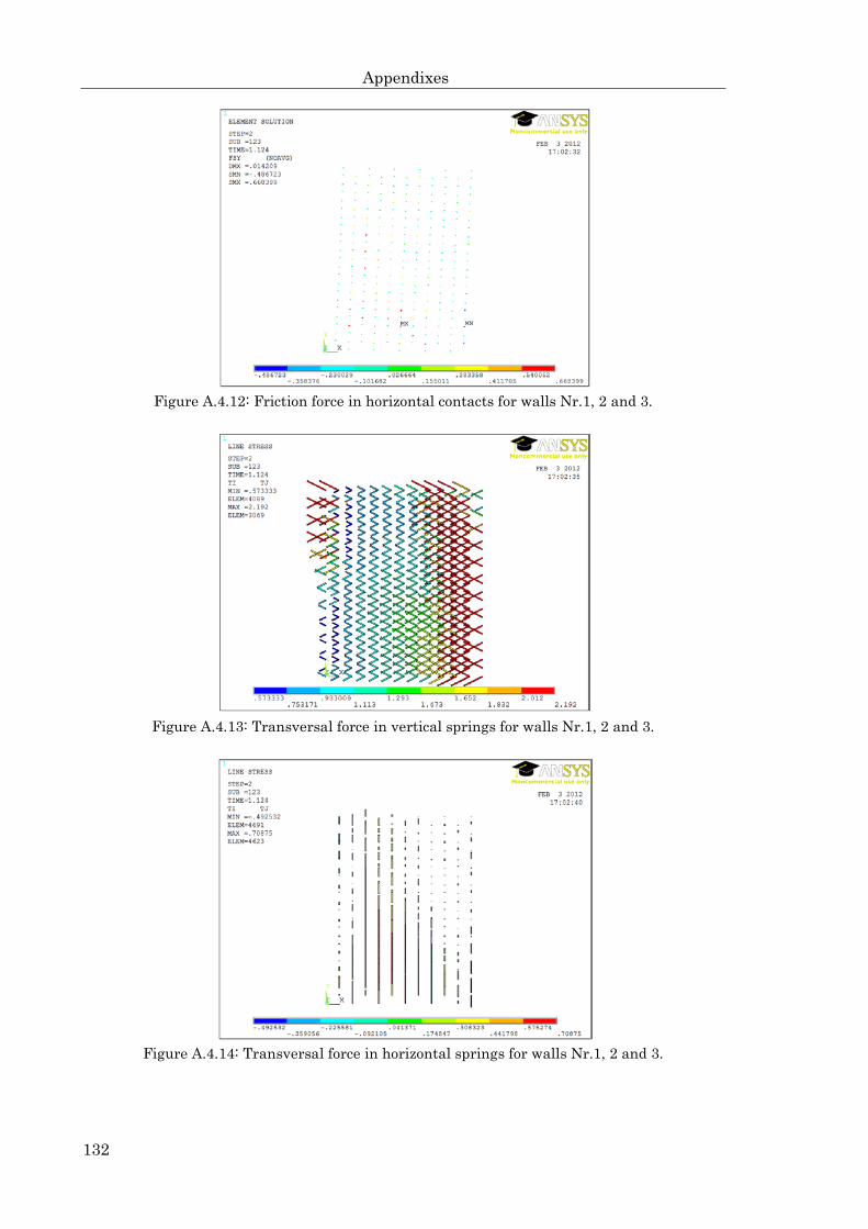
Appendixes
132
Figure A.4.12: Friction force in horizontal contacts for walls Nr.1, 2 and 3.
Figure A.4.13: Transversal force in vertical springs for walls Nr.1, 2 and 3.
Figure A.4.14: Transversal force in horizontal springs for walls Nr.1, 2 and 3.

Appendixes
133
Figure A.4.15: Contact situation in vertical contacts for walls Nr.1, 2 and 3.
Figure A.4.16: Contact situation in horizontal contacts for walls Nr.1, 2 and 3.
Figure A.4.17: Axial force in vertical reinforcing bars for walls Nr.1, 2 and 3.

Appendixes
134
Figure A.4.18: Vector diagram for principal stresses in walls Nr.1, 2 and 3.

Appendixes
135
A.5 Graphics for wall MV1 (U. of La Serena)
Figure A.5.1: Stresses σx in bricks for wall MV1.
Figure A.5.2: Stresses σy in bricks for wall MV1.

Appendixes
136
Figure A.5.3: Stresses σxy in bricks for wall MV1.
Figure A.5.4: First principal stresses in bricks for wall MV1.
Figure A.5.5: Second principal stresses in bricks for wall MV1.

Appendixes
137
Figure A.5.6: Third principal stresses in bricks for wall MV1.
Figure A.5.7: Axial force in vertical contacts for wall MV1.
Figure A.5.8: Axial force in horizontal contacts for wall MV1.

Appendixes
138
Figure A.5.9: Axial force in vertical springs for wall MV1.
Figure A.5.10: Axial force in horizontal springs for wall MV1.
Figure A.5.11: Friction force in vertical contacts for wall MV1.
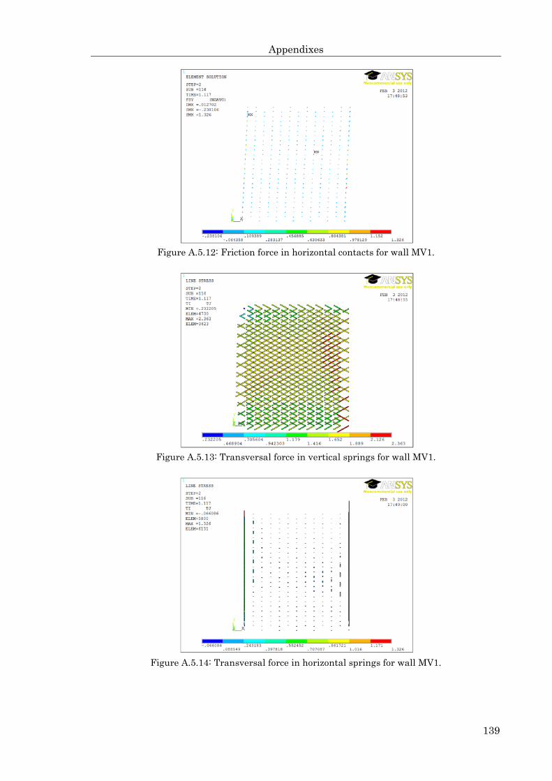
Appendixes
139
Figure A.5.12: Friction force in horizontal contacts for wall MV1.
Figure A.5.13: Transversal force in vertical springs for wall MV1.
Figure A.5.14: Transversal force in horizontal springs for wall MV1.

Appendixes
140
Figure A.5.15: Contact situation in vertical contacts for wall MV1.
Figure A.5.16: Contact situation in horizontal contacts for wall MV1.
Figure A.5.17: Vector diagram for principal stresses in wall MV1.

Appendixes
141
Figure A.5.18: Stresses σx in reinforced concrete for wall MV1.
Figure A.5.19: Stresses σy in reinforced concrete for wall MV1.
Figure A.5.20: Stresses σxy in reinforced concrete for wall MV1.

Appendixes
142
Figure A.5.21: First principal stresses in reinforced concrete for wall MV1.
Figure A.5.22: Second principal stresses in reinforced concrete for wall MV1.
Figure A.5.23: Third principal stresses in reinforced concrete for wall MV1.
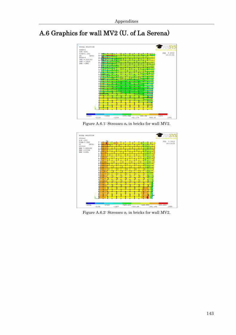
Appendixes
143
A.6 Graphics for wall MV2 (U. of La Serena)
Figure A.6.1: Stresses σx in bricks for wall MV2.
Figure A.6.2: Stresses σy in bricks for wall MV2.

Appendixes
144
Figure A.6.3: Stresses σxy in bricks for wall MV2.
Figure A.6.4: First principal stresses in bricks for wall MV2.
Figure A.6.5: Second principal stresses in bricks for wall MV2.

Appendixes
145
Figure A.6.6: Third principal stresses in bricks for wall MV2.
Figure A.6.7: Axial force in vertical contacts for wall MV2.
Figure A.6.8: Axial force in horizontal contacts for wall MV2.

Appendixes
146
Figure A.6.9: Axial force in vertical springs for wall MV2.
Figure A.6.10: Axial force in horizontal springs for wall MV2.
Figure A.6.11: Friction force in vertical contacts for wall MV2.

Appendixes
147
Figure A.6.12: Friction force in horizontal contacts for wall MV2.
Figure A.6.13: Transversal force in vertical springs for wall MV2.
Figure A.6.14: Transversal force in horizontal springs for wall MV2.

Appendixes
148
Figure A.6.15: Contact situation in vertical contacts for wall MV2.
Figure A.6.16: Contact situation in horizontal contacts for wall MV2.
Figure A.6.17: Vector diagram for principal stresses in wall MV2.

Appendixes
149
Figure A.6.18: Stresses σx in reinforced concrete for wall MV2.
Figure A.6.19: Stresses σy in reinforced concrete for wall MV2.
Figure A.6.20: Stresses σxy in reinforced concrete for wall MV2.
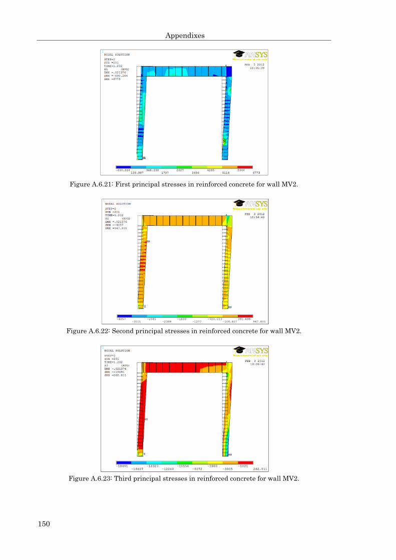
Appendixes
150
Figure A.6.21: First principal stresses in reinforced concrete for wall MV2.
Figure A.6.22: Second principal stresses in reinforced concrete for wall MV2.
Figure A.6.23: Third principal stresses in reinforced concrete for wall MV2.

Appendixes
151
A.7 Graphics for wall MV3 (U. of La Serena)
Figure A.7.1: Stresses σx in bricks for wall MV3.
Figure A.7.2: Stresses σy in bricks for wall MV3.

Appendixes
152
Figure A.7.3: Stresses σxy in bricks for wall MV3.
Figure A.7.4: First principal stresses in bricks for wall MV3.
Figure A.7.5: Second principal stresses in bricks for wall MV3.

Appendixes
153
Figure A.7.6: Third principal stresses in bricks for wall MV3.
Figure A.7.7: Axial force in vertical contacts for wall MV3.
Figure A.7.8: Axial force in horizontal contacts for wall MV3.

Appendixes
154
Figure A.7.9: Axial force in vertical springs for wall MV3.
Figure A.7.10: Axial force in horizontal springs for wall MV3.
Figure A.7.11: Friction force in vertical contacts for wall MV3.

Appendixes
155
Figure A.7.12: Friction force in horizontal contacts for wall MV3.
Figure A.7.13: Transversal force in vertical springs for wall MV3.
Figure A.7.14: Transversal force in horizontal springs for wall MV3.

Appendixes
156
Figure A.7.15: Contact situation in vertical contacts for wall MV3.
Figure A.7.16: Contact situation in horizontal contacts for wall MV3.
Figure A.7.17: Vector diagram for principal stresses in wall MV3.

Appendixes
157
Figure A.7.18: Stresses σx in reinforced concrete for wall MV3.
Figure A.7.19: Stresses σy in reinforced concrete for wall MV3.
Figure A.7.20: Stresses σxy in reinforced concrete for wall MV3.

Appendixes
158
Figure A.7.21: First principal stresses in reinforced concrete for wall MV3.
Figure A.7.22: Second principal stresses in reinforced concrete for wall MV3.
Figure A.7.23: Third principal stresses in reinforced concrete for wall MV3.

References and Bibliography
159
References and Bibliography
ACI. (2008). ACI 318-08 Building code requirements for structural concrete and commentary. U.S.A.: American Concrete Institute.
ANSYS. (2009a). ANSYS - Contact technology guide. U.S.A.
ANSYS. (2009b). ANSYS - Element reference. U.S.A.
ANSYS. (2009c). ANSYS - Structural analysis guide. U.S.A.
ANSYS. (2009d). ANSYS - Theory reference for the mechanical APDL and mechanical applications. U.S.A.
Anthoine, A. (1992). In-plane behaviour of masonry: A literature review. Luxembourg: Commission of the European Communities.
Anthoine, A. (1995). Derivation of the in-plane elastic characteristics of masonry through homogeneization theory. Journal of Solid Structures , S. 137-163.
Barbosa, C. S., & Hanai, J. B. (2009). Strength and deformability of hollow concrete blocks: correlation of block and cylindrical sample test results. Revista Ibracon de estruturas e materiais , S. 85-99.
Bergami, A. V. (2007). Implementation and experimental verification of models for nonlinear analysis of masonry infilled R.C. frames. Roma, Italia: Università degli Studi Roma Tre.
Blondet, M. (2005). Construction and maintenance of masonry houses. Lima, Perú: Pontificia Universidad Católica de Perú.
Campbell, J., Durán, M., & Guendelman, T. (2005). Procedimiento Demanda-Capacidad Multimodal. ACHISINA 2005. Concepción, Chile: ACHISINA.
Campbell, J., Norda, H., & Meskouris, K. (2010). Improved methods for multimodal pushover analysis. 14th European Conference on Earthquake Engineering. Ohrid, Macedonia: MAEE and EAEE.
CEN. (2002). Eurocode 1 - Actions on Structures. Brussels, Belgium: European Committe for Standarization.
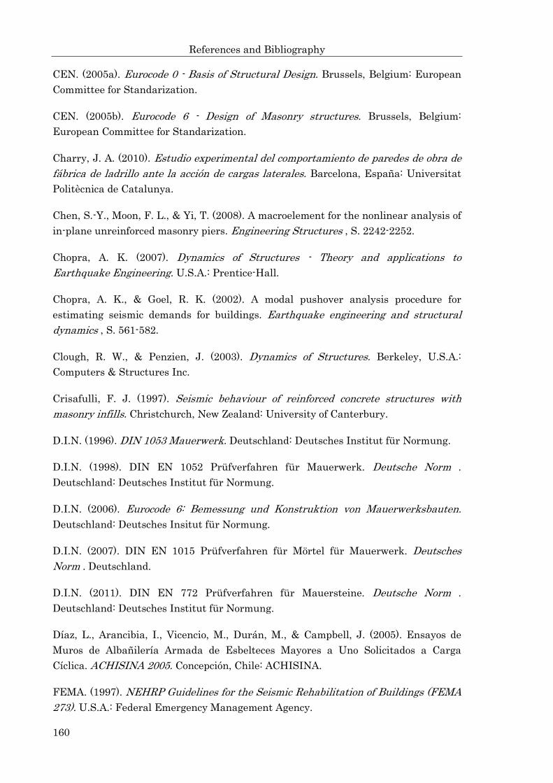
References and Bibliography
160
CEN. (2005a). Eurocode 0 - Basis of Structural Design. Brussels, Belgium: European Committee for Standarization.
CEN. (2005b). Eurocode 6 - Design of Masonry structures. Brussels, Belgium: European Committee for Standarization.
Charry, J. A. (2010). Estudio experimental del comportamiento de paredes de obra de fábrica de ladrillo ante la acción de cargas laterales. Barcelona, España: Universitat Politècnica de Catalunya.
Chen, S.-Y., Moon, F. L., & Yi, T. (2008). A macroelement for the nonlinear analysis of in-plane unreinforced masonry piers. Engineering Structures , S. 2242-2252.
Chopra, A. K. (2007). Dynamics of Structures - Theory and applications to Earthquake Engineering. U.S.A.: Prentice-Hall.
Chopra, A. K., & Goel, R. K. (2002). A modal pushover analysis procedure for estimating seismic demands for buildings. Earthquake engineering and structural dynamics , S. 561-582.
Clough, R. W., & Penzien, J. (2003). Dynamics of Structures. Berkeley, U.S.A.: Computers & Structures Inc.
Crisafulli, F. J. (1997). Seismic behaviour of reinforced concrete structures with masonry infills. Christchurch, New Zealand: University of Canterbury.
D.I.N. (1996). DIN 1053 Mauerwerk. Deutschland: Deutsches Institut für Normung.
D.I.N. (1998). DIN EN 1052 Prüfverfahren für Mauerwerk. Deutsche Norm . Deutschland: Deutsches Institut für Normung.
D.I.N. (2006). Eurocode 6: Bemessung und Konstruktion von Mauerwerksbauten. Deutschland: Deutsches Insitut für Normung.
D.I.N. (2007). DIN EN 1015 Prüfverfahren für Mörtel für Mauerwerk. Deutsches Norm . Deutschland.
D.I.N. (2011). DIN EN 772 Prüfverfahren für Mauersteine. Deutsche Norm . Deutschland: Deutsches Institut für Normung.
Díaz, L., Arancibia, I., Vicencio, M., Durán, M., & Campbell, J. (2005). Ensayos de Muros de Albañilería Armada de Esbelteces Mayores a Uno Solicitados a Carga Cíclica. ACHISINA 2005. Concepción, Chile: ACHISINA.
FEMA. (1997). NEHRP Guidelines for the Seismic Rehabilitation of Buildings (FEMA 273). U.S.A.: Federal Emergency Management Agency.

References and Bibliography
161
Galleguillos, M., & Valenzuela, C. (2009). Estudio experimental de muros de albañilería confinada a escala natural sometidos a carga cíclica. La Serena, Chile: Universidad de La Serena.
Galleguillos, M., Valenzuela, C., & Díaz, L. (2010). Estudio Experimental de Muros de Albañilería Confinada a Escala Natural Solicitados a Carga Cíclica Horizontal. ACHISINA 2010. Santiago, Chile: ACHISINA.
Gellert, C. (2010). Nichtlinearer Nachweis von unbewerten Mauerwerksbauten unter Erdbebeneinwirkung. Aachen, Deutschland: Univ.-Prof. Dr.-Ing. Konstantin Meskouris.
Gere, J. M., & Timoshenko, S. (1986). Mecánica de Materiales. México: Grupo Editorial Iberoamérica.
Grabowski, S. (2005a). ESECMaSE - Material properties for the test in WP 7 and 8 and the verification of the design model of WP 4. Munich, Germany: ESECMaSE-Technische Universität München.
Grabowski, S. (2005b). ESECMaSE - Stress-strain-relation of calcium silicate bricks. Munich, Germany: ESECMaSE-Technische Universität München.
Hossain, M. M., Ali, S. S., & Rahman, M. A. (1997). Properties of masonry constituents. Journal of Civil Engineering , S. 135-155.
I.N.N. (1993). NCh1928.Of93 Albañilería Reforzada-Requisitos de Diseño Estructural. Norma Chilena Oficial . Chile: Instituto Nacional de Normalización.
I.N.N. (1996). NCh433.Of96 Diseño sísmico de edificios. Norma Chilena Oficial . Chile: Instituto Nacional de Normalización.
I.N.N. (1997). NCh2123.Of97 Albañilería Armada-Requisitos de Diseño Estructural. Chile: Instituto Nacional de Normalización.
Irmschler, H.-J., Schubert, P., & Jäger, W. (2004). Mauerwerk Kalender. Deutschland: Ernst & Sohn.
Jaiswal, K., & Wald, D. J. (2008). Creating a global building inventory for earthquake loss assessment and risk management. U.S.A.: U.S. Geological Survey.
Kalkan, E., & Kunnath, S. (2006). Adaptive modal combination procedure for nonlinear static analysis of buildings structures. Journal of Structural Engineering , S. 1721-1731.

References and Bibliography
162
Kaushik, H. B., Rai, D. C., & Jain, S. K. (2007). Stress-strain characteristics of clay brick masonry under uniaxial compression. Journal of materials in civil engineering , S. 728-739.
Klingner, R. (2003). Especificación, Diseño y Cálculo de Mampostería. Simposio sobre Diseño en Mampostería. Santiago, Chile: Instituto Chileno del Cemento y del Hormigón.
López, J., Oller, S., & Oñate, E. (1998). Cálculo del Comportamiento de la Mampostería Mediante Elementos Finitos. Barcelona, Espana: CIMNE.
Lourenço, P. (1996). Computational Strategies for Masonry Structures. Delft, The Netherlands: Delft University Press.
Lüders, C. (1990). Técnicas de reparación y refuerzo de muros de albañilería armada. Santiago, Chile: Pontificia Universidad Católica de Chile.
Magenes, G., Morandi, P., & Penna, A. (2008). ESECMaSE - Tests results on the behaviour of masonry under static cyclic in plane loads. Pavia, Italy: ESECMaSE-University of Pavia.
Masonry Society. (2003). Masonry designer's guide-Fourth edition, based on building code requirements for masonry structures. Colorado, U.S.A.: The Masonry Society.
Mayorca, P., & Meguro, K. (2003). Proposal of a new economic retrofitting method for masonry structures. JSCE Journal of Earthquake Engineering , S. 1-4.
Meskouris, K. (2000). Structural Dynamics-Models, Methods, Examples. Germany: Ernst & Sohn Verlag.
Mistler, M. (2006). Verformungsbasiertes seismisches Bemessungskonzept für Mauerwerksbauten. Aachen, Deutschland: Univ.-Prof. Dr.-Ing. Konstantin Meskouris.
Norda, H., Reindl, L., & Meskouris, K. (2010). A nonlinear multimodal procedure for masonry buildings. 10th International Conference on Computational Structures Technology. Valencia, Spain: Civil-Comp Press.
Ordaz, M., & Pérez, E. (1998). Estimation of Strength Reduction Factors for Elastoplastic Systems, New Approach. Earthquake Engineering and Structural Dynamics .
Page, A. (1978). Finite element model for masonry. Journal of the structural division ASCE , S. 1267-1285.

References and Bibliography
163
Page, A. (1981). The biaxial compressive strength of brick masonry. Proceedings of Institution of Civil Engineers (S. 893-906). London, England: Institution of Civil Engineers.
Page, A. W., Kleeman, P. W., & Dhanasekar, M. (1985). An in-plane finite element model for brick masonry. New York, U.S.A.: American Society of Civil Engineers.
Park, J., El-Deib, K., Butenweg, C., & Gellert, C. (2011). A novel macroelement approach for masonry walls. 8th International Conference on Structural Dynamics Eurodyn (S. 3281-3286). Leuven, Belgium: G. De Roeck, G. Degrande, G. Lombaert and G. Müller.
Park, R., & Paulay, T. (2000). Estructuras de Concreto Reforzado. México: Editorial Limusa.
Pietruszczak, S., & Niu, X. (1992). A mathematical description of macroscopic behaviour of brick masonry. Journal of Solid Structures , S. 531-546.
Priestley, M. J., Calvi, G. M., & Kowalsky, M. J. (2007). Displacement-Based Design of Structures. Pavia, Italia: Istituto Universitario di Studi Superiori.
SEAOC. (1995). Vision 2000 Report on Structural Performance Based Seismic Engineering of Buildings. California, U.S.A.: Structural Engineers Associaton of California.
Tomazevic, M. (1999). Earthquake-Resistant Design of Masonry Buildings. London, England: Imperial College Press.
Uzoegbo, H. C. (2011). Seismic behaviour of single-story URM buildings with light weight steel roof. International Journal of Advanced Technology in Civil Engineering , S. 28-35.
Van der Pluijm, R., & Vullings, M. W. (2006). ESECMaSE - Work package 5, deliverable D5.2 to D5.5. Delft, Netherlands: TNO Built Environment and Geosciences.
Vidic, T., Fajfar, P., & Fischinger, M. (1994). Consistent Inelastic Design Spectra: Strength and Displacement. Earthquake Engineering and Structural Dynamics .
Viviescas, A. (2009). Modelos simples para el análisis de obra de fábrica cargados en su plano. Barcelona, España: Universitat Politècnica de Catalunya.
Wu, J., & Hanson, R. (1989). Study of Inelastic Spectra with High Damping. Journal of Structural Engineering .

References and Bibliography
164
www.ansys.com. (kein Datum).
www.esecmase.org. (kein Datum).
www.staff.city.ac.uk/earthquakes/MasonryBrick/. (kein Datum).
Zienkiewicz, O. C., & Taylor, R. L. (2005). The Finite Element Method. Elsevier.
Zucchini, A., & Lourenço, P. B. (2002). A micro-mechanical model for the homogenisation of masonry. International Journal of Solids and Structures , S. 3233-3255.

List of Figures
165
List of Figures
Figure 1.1: Earthquake prone areas in the world. .......................................................... 1
Figure 2.1: Simple compression test on a brick specimen (Bergami, 2007). .................. 6
Figure 2.2: Splitting tensile test on a brick specimen (Grabowski, 2005a). ................... 7
Figure 2.3: Flexural tensile strength test on a brick specimen (Charry, 2010). ............ 7
Figure 2.4: Typical stress-strain curve for compression in bricks (Kaushik, Rai, & Jain, 2007). .................................................................................................... 8
Figure 2.5: Relationship between compressive strength an elasticity module for bricks (Kaushik, Rai, & Jain, 2007). ........................................................................ 8
Figure 2.6: Simple compression test on a mortar cubic specimen (Galleguillos & Valenzuela, 2009). ......................................................................................... 9
Figure 2.7: Flexural tensile strength test on a mortar specimen (Bergami, 2007). ..... 10
Figure 2.8: Typical stress-strain curve for compression in mortar (Kaushik, Rai, & Jain, 2007). .................................................................................................. 10
Figure 2.9: Relationship between compressive strength an elasticity module for mortar (Kaushik, Rai, & Jain, 2007). .......................................................... 11
Figure 2.10: Tensile bond test for the brick- mortar interface (Grabowski, 2005a). .... 12
Figure 2.11: Shear bond test for the brick- mortar interface (Charry, 2010). .............. 12
Figure 2.12: Compression test for a Rilem masonry specimen (Grabowski, 2005b). ... 13
Figure 2.13: Diagonal compression test for a masonry specimen (Galleguillos & Valenzuela, 2009). ....................................................................................... 13
Figure 2.14: Typical stress-strain curve for concrete. ................................................... 14
Figure 2.15: Typical stress-strain curve for reinforcing steel. ...................................... 15
Figure 2.16: Types of bond in masonry. ........................................................................ 16
Figure 2.17: Typical sliding shear failure. .................................................................... 17
Figure 2.18: Typical hysteresis loops for sliding shear failure. .................................... 17
Figure 2.19: Typical shear failure. ................................................................................ 18
Figure 2.20: Typical hysteresis loops for shear failure. ................................................ 18
Figure 2.21: Typical bending failure. ............................................................................ 19
Figure 2.22: Typical hysteresis loops for bending failure. ............................................ 19
Figure 2.23: Unreinforced masonry. .............................................................................. 23

List of Figures
166
Figure 2.24: Reinforced masonry. ................................................................................. 24
Figure 2.25: Confined masonry. .................................................................................... 25
Figure 3.1: Types of models for masonry. ..................................................................... 27
Figure 4.1: Detail of the model for joint between bricks and mortar. .......................... 34
Figure 4.2: Alternatives for the discretization of the model. ........................................ 34
Figure 4.3: Cinematic behaviour of a group of bricks under lateral loads. .................. 35
Figure 4.4: Geometry of element SOLID65. ................................................................. 36
Figure 4.5: Failure criteria for concrete according to ANSYS. ..................................... 39
Figure 4.6: Simplified compression stress-strain curve for bricks. .............................. 40
Figure 4.7: Simplified compression stress-strain for concrete. .................................... 40
Figure 4.8: Geometry of element COMBIN39. ............................................................. 41
Figure 4.9: Force-Deflection curve for element COMBIN39. ....................................... 41
Figure 4.10: Tributary area on nodes for nonlinear springs. ....................................... 42
Figure 4.11: Simplified compression stress-strain curve for mortar. ........................... 43
Figure 4.12: Simplified shear stress-strain curve for mortar. ...................................... 43
Figure 4.13: Simplified tension stress-strain curve for steel. ...................................... 44
Figure 4.14: Geometry of element CONTA178. ............................................................ 45
Figure 5.1: Geometry for masonry wall CS05. .............................................................. 54
Figure 5.2: Hysteretic cycles for wall CS05. ................................................................. 55
Figure 5.3: Pushover curve for wall CS05. ................................................................... 55
Figure 5.4: Geometry for masonry wall CL05. ............................................................. 56
Figure 5.5: Hysteretic cycles for wall CL05. ................................................................. 57
Figure 5.6: Pushover curve for wall CL05. ................................................................... 57
Figure 5.7: Geometry for masonry wall CL06. ............................................................. 58
Figure 5.8: Hysteretic cycles for wall CL06. ................................................................. 59
Figure 5.9: Pushover curve for wall CL06. ................................................................... 59
Figure 5.10: General view of a wall test at the University of La Serena (Galleguillos & Valenzuela, 2009). ....................................................................................... 60
Figure 5.11: Geometry for reinforced masonry walls. .................................................. 61
Figure 5.12: Pushover curves for wall Nr. 1. ................................................................ 62
Figure 5.13: Pushover curves for wall Nr. 2. ................................................................ 62

List of Figures
167
Figure 5.14: Pushover curves for wall Nr. 3. ................................................................. 63
Figure 5.15: Geometry for confined masonry walls. ..................................................... 64
Figure 5.16: Pushover curves for wall MV1. ................................................................. 65
Figure 5.17: Pushover curves for wall MV2. ................................................................. 65
Figure 5.18: Pushover curves for wall MV3. ................................................................. 66
Figure 6.1: General displacements on the last step for Wall CS05. ............................. 70
Figure 6.2: Pushover curve for Wall CS05. ................................................................... 71
Figure 6.3: General displacements on the last step for Wall CL05. ............................. 72
Figure 6.4: Pushover curve for Wall CL05. ................................................................... 73
Figure 6.5: General displacements on the last step for Wall CL06. ............................. 74
Figure 6.6: Pushover curve for Wall CL06. ................................................................... 75
Figure 6.7: General displacements on the last step for Reinforced wall. ..................... 76
Figure 6.8: Pushover curve for Reinforced wall. ........................................................... 77
Figure 6.9: General displacements on the last step for Wall MV1. .............................. 79
Figure 6.10: Pushover curve for Wall MV1. .................................................................. 79
Figure 6.11: General displacements on the last step for Wall MV2. ............................ 81
Figure 6.12: Pushover curve for Wall MV2. .................................................................. 82
Figure 6.13: General displacements on the last step for Wall MV3. ............................ 84
Figure 6.14: Pushover curve for Wall MV3. .................................................................. 84
Figure 7.1: Original pushover curves (model and tests) for wall CS05. ....................... 88
Figure 7.2: Idealized bilinear pushover curves (model and tests) for wall CS05. ........ 89
Figure 7.3: Original pushover curves (model and tests) for wall CL05. ....................... 90
Figure 7.4: Idealized bilinear pushover curves (model and tests) for wall CL05. ........ 91
Figure 7.5: Original pushover curves (model and tests) for wall CL06. ....................... 92
Figure 7.6: Idealized bilinear pushover curves (model and tests) for wall CL06. ........ 92
Figure 7.7: Original pushover curves (model and tests) for walls Nr. 1, 2 and 3. ........ 94
Figure 7.8: Idealized bilinear pushover curves (model and tests) for walls Nr. 1, 2 and 3. ................................................................................................................... 94
Figure 7.9: Idealized bilinear pushover curves (model and tests) for average walls Nr. 1, 2 and 3. ..................................................................................................... 95
Figure 7.10: Original pushover curves (model and tests) for wall MV1. ...................... 97

List of Figures
168
Figure 7.11: Idealized bilinear pushover curves (model and tests) for wall MV2. ...... 97
Figure 7.12: Original pushover curves (model and tests) for wall MV2. ..................... 99
Figure 7.13: Idealized bilinear pushover curves (model and tests) for wall MV2. ...... 99
Figure 7.14: Original pushover curves (model and tests) for wall MV3. ................... 100
Figure 7.15: Idealized bilinear pushover curves (model and tests) for wall MV3. .... 101

List of Tables
169
List of Tables
Table 5.1: Stirrups on reinforcement concrete for confined walls. ............................... 64
Table 5.2: Nominal shear force and controlling failure. ............................................... 66
Table 7.1: Main results for original pushover curve of wall CS05. ............................... 89
Table 7.2: Main results for bilinear pushover curve of wall CS05. .............................. 89
Table 7.3: Main results for original pushover curve of wall CL05. .............................. 91
Table 7.4: Main results for bilinear pushover curve of wall CL05. .............................. 91
Table 7.5: Main results for original pushover curve of wall CL06. .............................. 93
Table 7.6: Main results for bilinear pushover curve of wall CL06. .............................. 93
Table 7.7: Main results for original pushover curve of wall Nr. 1. ............................... 95
Table 7.8: Main results for original pushover curve of wall Nr. 2. ............................... 95
Table 7.9: Main results for original pushover curve of wall Nr. 3. ............................... 95
Table 7.10: Main results for bilinear pushover curve of wall Nr. 1. ............................. 96
Table 7.11: Main results for bilinear pushover curve of wall Nr. 2. ............................. 96
Table 7.12: Main results for bilinear pushover curve of wall Nr. 3. ............................. 96
Table 7.13: Main results for bilinear pushover curve for average of walls Nr. 1, 2 and 3. ................................................................................................................... 96
Table 7.14: Main results for original pushover curve of wall MV1. ............................. 98
Table 7.15: Main results for bilinear pushover curve of wall MV1. ............................. 98
Table 7.16: Main results for original pushover curve of wall MV2. ........................... 100
Table 7.17: Main results for bilinear pushover curve of wall MV2. ........................... 100
Table 7.18: Main results for original pushover curve of wall MV3. ........................... 101
Table 7.19: Main results for bilinear pushover curve of wall MV3. ........................... 101


Symbols and Abbreviations
171
Symbols and Abbreviations
Greek
ϒ Shear deformation ε Longitudinal deformation εij Cartesian components of deformation vector [ε] Deformation vector μ Ductility μ Coefficient of friction μb-m Friction coefficient between brick and mortar ν Poisson’s coefficient νb Poisson’s coefficient for bricks νm Poisson’s coefficient for mortar σ Longitudinal stress σij Cartesian components of stress vector [σ] Stress vector τ Shear stress τm Maximum shear stress for mortar
Latin
Atrib Tributary area of brick over spring or contact elements D Displacement on the “pushover curve” De Elastic displacement on the bilinear “pushover curve” Dmax Maximum displacement on the “pushover curve” [D] Stress-strain matrix for solid elements [Dc] Stress-strain matrix for concrete or bricks in solid elements [Dr] Stress-strain matrix for reinforcement in solid elements E Elasticity module for solid elements Eb Elasticity module for bricks Ec Elasticity module for concrete Em Elasticity module for mortar Er Elasticity module for reinforcing material in solid elements

Symbols and Abbreviations
172
Es Elasticity module for steel F Force on the “pushover curve” fab-m Maximum adherence strength between brick and mortar fb Maximum compression strength for bricks fc Maximum compression strength for concrete fm Maximum compression strength for mortar Fmax Maximum force on the “pushover curve” Fn Normal force in contact elements fr Fracture tension of steel Fsy Tangential force in contact elements (“y” direction) Fsz Tangential force in contact elements (“z” direction) ft Maximum tension strength for concrete (or bricks) ftb-m Maximum tension strength between brick and mortar fu Ultimate tension of steel fy Yield tension of steel Gm Shear elasticity module for mortar I, J, K, L, M, N, O Nodes index for solid, spring or contact elements Ke Stiffness on the elastic branch of bilinear “pushover curve” [Ke] Stiffness matrix for non-linear spring elements Kn Normal stiffness for contact elements Ks Tangential stiffness for contact elements Ktg Stiffness on the active segment of non-linear spring elements L Length of contact elements r, s, t Local Cartesian coordinates in solid elements u, v, w Displacements in Cartesian coordinates in solid elements Un Gap size in contact elements Uy Slip distance in contact elements ViR Ratio of volume of reinforcement in solid elements x, y, z Cartesian coordinates

Curriculum Vitae
173
Curriculum Vitae
Personal
Surnames: CAMPBELL BARRAZA Names: Jaime Andrés Date of Birth: July 4th 1972 Place of Birth: La Serena, Chile Marital Status: Married with Fabiola CELIS CORRALES
Gabriela CAMPBELL CELIS (daughter)
School
Primary School “Serena” Private School(1978-1982) “Gerónimo Rendic” Private School (1983-1985)
High School “Gerónimo Rendic” Private School (1986-1989)
University
Undergraduate Civil Engineering, University of La Serena (1990-1996) Master Numerical Methods for Computation and Design in
Engineering, Polytechnic University of Catalonia (2001-2002)
Profesional Experience
January 1998-April 1999 Civil Engineer, Municipality of La Serena April 1999- Lecturer at the Civil Engineering Department, University
of La Serena January 1998- Consultant of engineering for different public and private
institutions

Curriculum Vitae
174
Lebenslauf
Persönliches
Familiennamen: CAMPBELL BARRAZA Namen: Jaime Andrés Geburtsdatum: 04. Juli 1972 Geburtsort: La Serena, Chile Familie: Verheiratet mit Fabiola CELIS CORRALES
Tochter Gabriela CAMPBELL CELIS
Schulausbildung
Grundschule “Serena” Privatschule (1978-1982) “Gerónimo Rendic” Privatschule (1983-1985)
Gymnasium “Gerónimo Rendic” Privatschule (1986-1989)
Studium
Diplom Bauingenieurwesen, Universität La Serena (1990-1996) Master Numerische Methoden für Berechnung und Bemessung
im Ingenieurwesen, Polytechnische Universität Kataloniens (2001-2002)
Berufsweg
Januar 1998-April 1999 Bauingenieur in der Abteilung für Projektentwicklung der Stadt La Serena
April 1999- Vollteildozent in der Abteilung Bauingenieurwesen an der Universität La Serena
Januar 1998- Ingenieurtätigkeit bei verschiedene öffentlichen und privaten Bauvorhaben

Curriculum Vitae
175
Curriculum Vitae
Antecedentes Personales
Apellidos: CAMPBELL BARRAZA Nombres: Jaime Andrés Fecha de Nacimiento: 04 de Julio de 1972 Lugar de Nacimiento: La Serena, Chile Estado Civil: Casado con Fabiola CELIS CORRALES
Gabriela CAMPBELL CELIS (hija)
Antecedentes Escolares
Educación Básica Colegio Particular “Serena” (1978-1982) Colegio Particular “Gerónimo Rendic” (1983-1985)
Educación Media Colegio Particular “Gerónimo Rendic” (1986-1989)
Antecedentes Universitarios
Pregrado Ingeniería Civil, Universidad de La Serena (1990-1996) Master Métodos Numéricos para Cálculo y Diseño en Ingeniería,
Universidad Politécnica de Cataluña (2001-2002)
Antecedentes Laborales
Enero 1998-Abril 1999 Ingeniero Civil, Ilustre Municipalidad de La Serena Abril 1999- Académico Departamento de Ingeniería en Obras Civiles,
Universidad de La Serena Enero 1998- Consultor de proyectos de ingeniería para instituciones
públicas y privadas
Copyright © 2022 FDOKUMEN