
ns-3 Model Library
537
ns-3 Model Library Release ns-3.29 ns-3 project Jan 08, 2019
-
Upload
khangminh22 -
Category
Documents
-
view
1 -
download
0
Transcript of ns-3 Model Library
ns-3 Model LibraryRelease ns-3.29
ns-3 project
Jan 08, 2019


CONTENTS
1 Organization 3
2 Animation 5
3 Antenna Module 13
4 Ad Hoc On-Demand Distance Vector (AODV) 17
5 3GPP HTTP applications 19
6 Bridge NetDevice 27
7 BRITE Integration 29
8 Buildings Module 33
9 Click Modular Router Integration 47
10 CSMA NetDevice 51
11 DSDV Routing 57
12 DSR Routing 59
13 Emulation Overview 63
14 Energy Framework 67
15 File Descriptor NetDevice 73
16 Flow Monitor 81
17 Internet Models (IP, TCP, Routing, UDP, Internet Applications) 85
18 Low-Rate Wireless Personal Area Network (LR-WPAN) 143
19 LTE Module 151
20 Wi-Fi Mesh Module Documentation 343
21 MPI for Distributed Simulation 347
22 Mobility 353
i
23 Network Module 361
24 Nix-Vector Routing Documentation 387
25 Optimized Link State Routing (OLSR) 389
26 OpenFlow switch support 393
27 PointToPoint NetDevice 397
28 Propagation 401
29 Spectrum Module 411
30 6LoWPAN: Transmission of IPv6 Packets over IEEE 802.15.4 Networks 421
31 Tap NetDevice 425
32 Topology Input Readers 431
33 Traffic Control Layer 433
34 UAN Framework 459
35 WAVE models 471
36 Wi-Fi Module 485
37 Wimax NetDevice 517
Bibliography 527
Index 533
ii

ns-3 Model Library, Release ns-3.29
This is the ns-3 Model Library documentation. Primary documentation for the ns-3 project is available in five forms:
• ns-3 Doxygen: Documentation of the public APIs of the simulator
• Tutorial, Manual, and Model Library (this document) for the latest release and development tree
• ns-3 wiki
This document is written in reStructuredText for Sphinx and is maintained in the doc/models directory of ns-3’ssource code.
CONTENTS 1

ns-3 Model Library, Release ns-3.29
2 CONTENTS

CHAPTER
ONE
ORGANIZATION
This manual compiles documentation for ns-3 models and supporting software that enable users to construct networksimulations. It is important to distinguish between modules and models:
• ns-3 software is organized into separate modules that are each built as a separate software library. Individualns-3 programs can link the modules (libraries) they need to conduct their simulation.
• ns-3 models are abstract representations of real-world objects, protocols, devices, etc.
An ns-3 module may consist of more than one model (for instance, the internet module contains models for bothTCP and UDP). In general, ns-3 models do not span multiple software modules, however.
This manual provides documentation about the models of ns-3. It complements two other sources of documentationconcerning models:
• the model APIs are documented, from a programming perspective, using Doxygen. Doxygen for ns-3 models isavailable on the project web server.
• the ns-3 core is documented in the developer’s manual. ns-3 models make use of the facilities of the core, suchas attributes, default values, random numbers, test frameworks, etc. Consult the main web site to find copies ofthe manual.
Finally, additional documentation about various aspects of ns-3 may exist on the project wiki.
A sample outline of how to write model library documentation can be found by executing the create-module.pyprogram and looking at the template created in the file new-module/doc/new-module.rst.
$ cd src$ ./create-module.py new-module
The remainder of this document is organized alphabetically by module name.
If you are new to ns-3, you might first want to read below about the network module, which contains some fundamentalmodels for the simulator. The packet model, models for different address formats, and abstract base classes for objectssuch as nodes, net devices, channels, sockets, and applications are discussed there.
3

ns-3 Model Library, Release ns-3.29
4 Chapter 1. Organization

CHAPTER
TWO
ANIMATION
Animation is an important tool for network simulation. While ns-3 does not contain a default graphical animationtool, we currently have two ways to provide animation, namely using the PyViz method or the NetAnim method. ThePyViz method is described in http://www.nsnam.org/wiki/PyViz.
We will describe the NetAnim method briefly here.
2.1 NetAnim
NetAnim is a standalone, Qt4-based software executable that uses a trace file generated during an ns-3 simulation todisplay the topology and animate the packet flow between nodes.
Fig. 1: An example of packet animation on wired-links
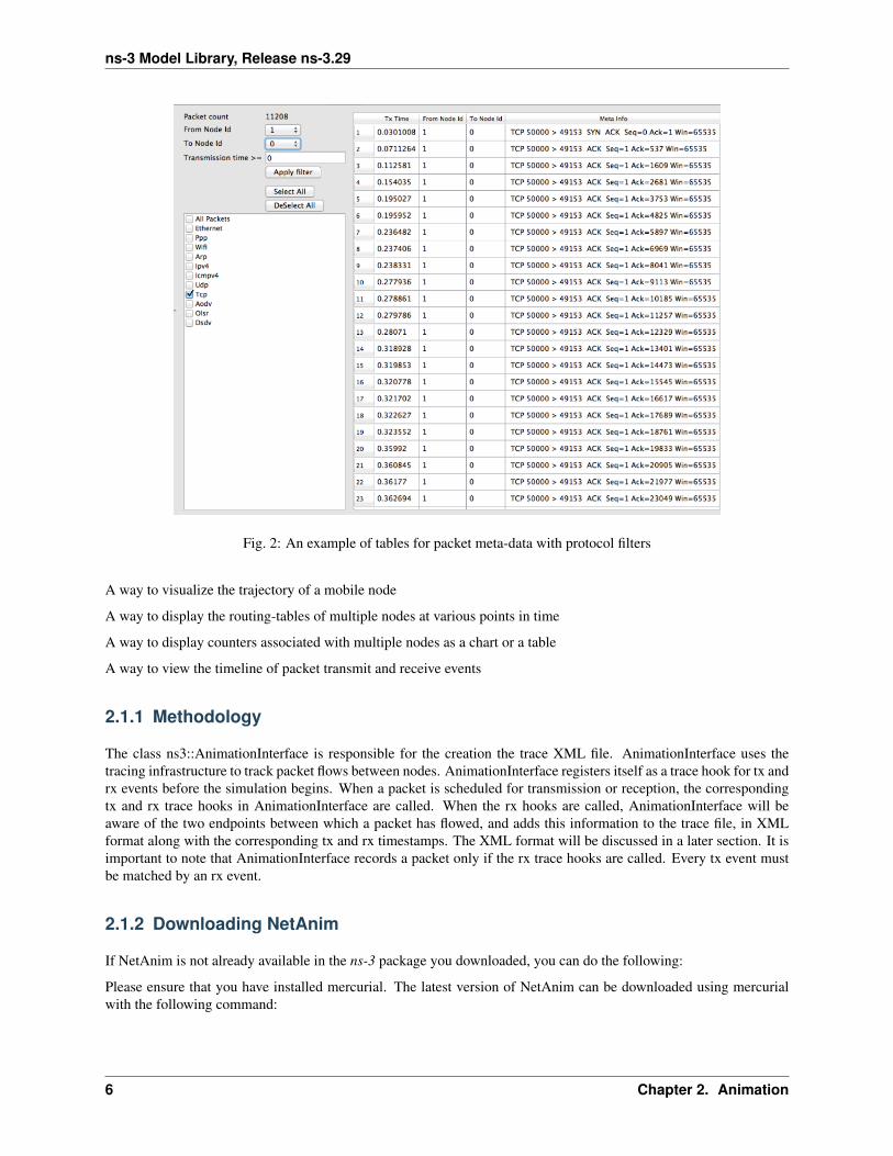
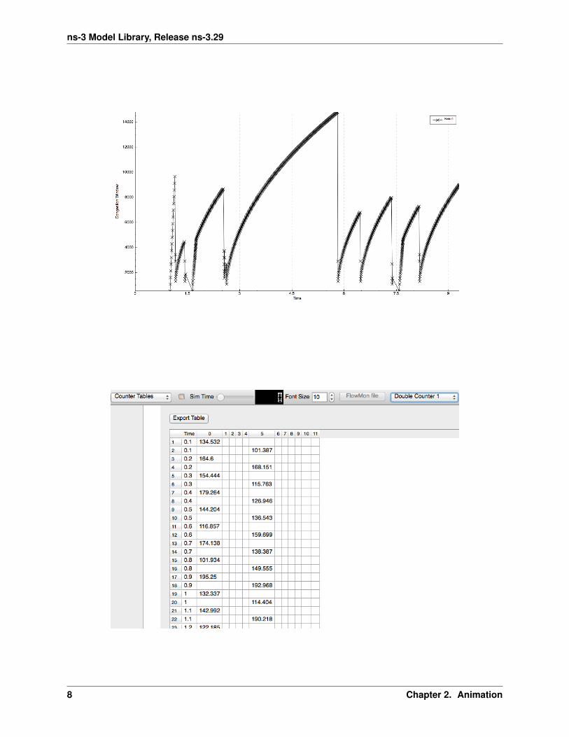
In addition, NetAnim also provides useful features such as tables to display meta-data of packets like the image below
5
ns-3 Model Library, Release ns-3.29
Fig. 2: An example of tables for packet meta-data with protocol filters
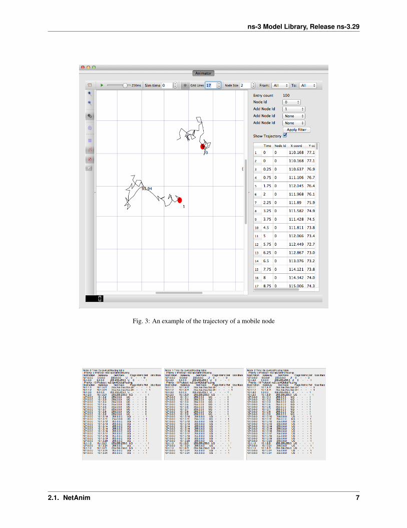
A way to visualize the trajectory of a mobile node
A way to display the routing-tables of multiple nodes at various points in time
A way to display counters associated with multiple nodes as a chart or a table
A way to view the timeline of packet transmit and receive events
2.1.1 Methodology
The class ns3::AnimationInterface is responsible for the creation the trace XML file. AnimationInterface uses thetracing infrastructure to track packet flows between nodes. AnimationInterface registers itself as a trace hook for tx andrx events before the simulation begins. When a packet is scheduled for transmission or reception, the correspondingtx and rx trace hooks in AnimationInterface are called. When the rx hooks are called, AnimationInterface will beaware of the two endpoints between which a packet has flowed, and adds this information to the trace file, in XMLformat along with the corresponding tx and rx timestamps. The XML format will be discussed in a later section. It isimportant to note that AnimationInterface records a packet only if the rx trace hooks are called. Every tx event mustbe matched by an rx event.
2.1.2 Downloading NetAnim
If NetAnim is not already available in the ns-3 package you downloaded, you can do the following:
Please ensure that you have installed mercurial. The latest version of NetAnim can be downloaded using mercurialwith the following command:
6 Chapter 2. Animation
ns-3 Model Library, Release ns-3.29
Fig. 3: An example of the trajectory of a mobile node
2.1. NetAnim 7
ns-3 Model Library, Release ns-3.29
8 Chapter 2. Animation

ns-3 Model Library, Release ns-3.29
$ hg clone http://code.nsnam.org/netanim
2.1.3 Building NetAnim
Prerequisites
Qt5 (5.4 and over) is required to build NetAnim. This can be obtained using the following ways:
For Ubuntu Linux distributions:
$ apt-get install qt5-default
For Red Hat/Fedora based distribution:
$ yum install qt5$ yum install qt5-devel
For Mac/OSX, see http://qt.nokia.com/downloads/
Build steps
To build NetAnim use the following commands:
$ cd netanim$ make clean$ qmake NetAnim.pro$ make
Note: qmake could be “qmake-qt5” in some systems
This should create an executable named “NetAnim” in the same directory:
$ ls -l NetAnim-rwxr-xr-x 1 john john 390395 2012-05-22 08:32 NetAnim
2.1. NetAnim 9
ns-3 Model Library, Release ns-3.29
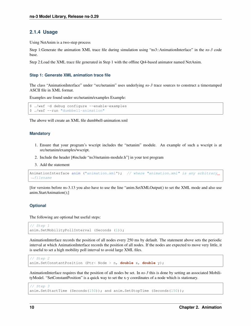
2.1.4 Usage
Using NetAnim is a two-step process
Step 1:Generate the animation XML trace file during simulation using “ns3::AnimationInterface” in the ns-3 codebase.
Step 2:Load the XML trace file generated in Step 1 with the offline Qt4-based animator named NetAnim.
Step 1: Generate XML animation trace file
The class “AnimationInterface” under “src/netanim” uses underlying ns-3 trace sources to construct a timestampedASCII file in XML format.
Examples are found under src/netanim/examples Example:
$ ./waf -d debug configure --enable-examples$ ./waf --run "dumbbell-animation"
The above will create an XML file dumbbell-animation.xml
Mandatory
1. Ensure that your program’s wscript includes the “netanim” module. An example of such a wscript is atsrc/netanim/examples/wscript.
2. Include the header [#include “ns3/netanim-module.h”] in your test program
3. Add the statement
AnimationInterface anim ("animation.xml"); // where "animation.xml" is any arbitrary↪→filename
[for versions before ns-3.13 you also have to use the line “anim.SetXMLOutput() to set the XML mode and also useanim.StartAnimation();]
Optional
The following are optional but useful steps:
// Step 1anim.SetMobilityPollInterval (Seconds (1));
AnimationInterface records the position of all nodes every 250 ms by default. The statement above sets the periodicinterval at which AnimationInterface records the position of all nodes. If the nodes are expected to move very little, itis useful to set a high mobility poll interval to avoid large XML files.
// Step 2anim.SetConstantPosition (Ptr< Node > n, double x, double y);
AnimationInterface requires that the position of all nodes be set. In ns-3 this is done by setting an associated Mobili-tyModel. “SetConstantPosition” is a quick way to set the x-y coordinates of a node which is stationary.
// Step 3anim.SetStartTime (Seconds(150)); and anim.SetStopTime (Seconds(150));
10 Chapter 2. Animation

ns-3 Model Library, Release ns-3.29
AnimationInterface can generate large XML files. The above statements restricts the window between which Ani-mationInterface does tracing. Restricting the window serves to focus only on relevant portions of the simulation andcreating manageably small XML files
// Step 4AnimationInterface anim ("animation.xml", 50000);
Using the above constructor ensures that each animation XML trace file has only 50000 packets. For example, ifAnimationInterface captures 150000 packets, using the above constructor splits the capture into 3 files
• animation.xml - containing the packet range 1-50000
• animation.xml-1 - containing the packet range 50001-100000
• animation.xml-2 - containing the packet range 100001-150000
// Step 5anim.EnablePacketMetadata (true);
With the above statement, AnimationInterface records the meta-data of each packet in the xml trace file. Metadatacan be used by NetAnim to provide better statistics and filter, along with providing some brief information about thepacket such as TCP sequence number or source & destination IP address during packet animation.
CAUTION: Enabling this feature will result in larger XML trace files. Please do NOT enable this feature when usingWimax links.
// Step 6anim.UpdateNodeDescription (5, "Access-point");
With the above statement, AnimationInterface assigns the text “Access-point” to node 5.
// Step 7anim.UpdateNodeSize (6, 1.5, 1.5);
With the above statement, AnimationInterface sets the node size to scale by 1.5. NetAnim automatically scales thegraphics view to fit the oboundaries of the topology. This means that NetAnim, can abnormally scale a node’s size toohigh or too low. Using AnimationInterface::UpdateNodeSize allows you to overwrite the default scaling in NetAnimand use your own custom scale.
// Step 8anim.UpdateNodeCounter (89, 7, 3.4);
With the above statement, AnimationInterface sets the counter with Id == 89, associated with Node 7 with the value3.4. The counter with Id 89 is obtained using AnimationInterface::AddNodeCounter. An example usage for this is insrc/netanim/examples/resource-counters.cc.
Step 2: Loading the XML in NetAnim
1. Assuming NetAnim was built, use the command “./NetAnim” to launch NetAnim. Please review the section“Building NetAnim” if NetAnim is not available.
2. When NetAnim is opened, click on the File open button at the top-left corner, select the XML file generatedduring Step 1.
3. Hit the green play button to begin animation.
Here is a video illustrating this http://www.youtube.com/watch?v=tz_hUuNwFDs
2.1. NetAnim 11

ns-3 Model Library, Release ns-3.29
2.1.5 Wiki
For detailed instructions on installing “NetAnim”, F.A.Qs and loading the XML trace file (mentioned earlier) usingNetAnim please refer: http://www.nsnam.org/wiki/NetAnim
12 Chapter 2. Animation
CHAPTER
THREE
ANTENNA MODULE
3.1 Design documentation
3.1.1 Overview
The Antenna module provides:
1. a new base class (AntennaModel) that provides an interface for the modeling of the radiation pattern of anantenna;
2. a set of classes derived from this base class that each models the radiation pattern of different types of antennas.
3.1.2 AntennaModel
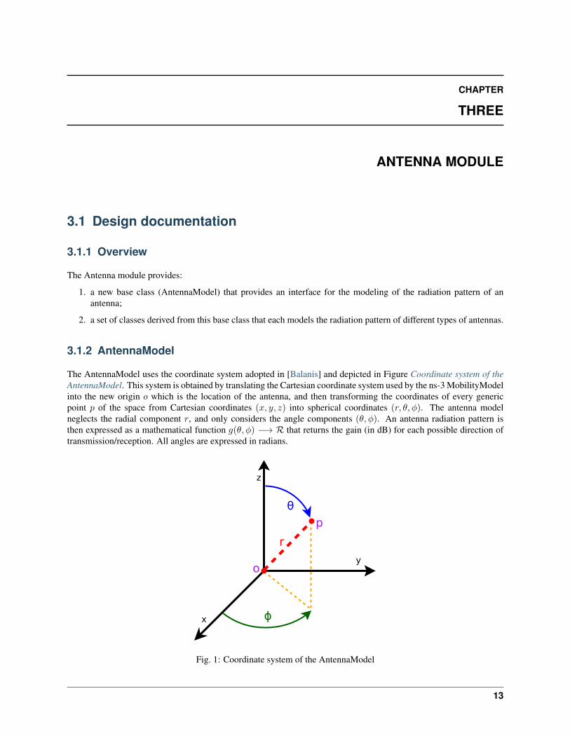
The AntennaModel uses the coordinate system adopted in [Balanis] and depicted in Figure Coordinate system of theAntennaModel. This system is obtained by translating the Cartesian coordinate system used by the ns-3 MobilityModelinto the new origin o which is the location of the antenna, and then transforming the coordinates of every genericpoint p of the space from Cartesian coordinates (x, y, z) into spherical coordinates (r, θ, φ). The antenna modelneglects the radial component r, and only considers the angle components (θ, φ). An antenna radiation pattern isthen expressed as a mathematical function g(θ, φ) −→ R that returns the gain (in dB) for each possible direction oftransmission/reception. All angles are expressed in radians.
Fig. 1: Coordinate system of the AntennaModel
13
ns-3 Model Library, Release ns-3.29
3.1.3 Provided models
In this section we describe the antenna radiation pattern models that are included within the antenna module.
IsotropicAntennaModel
This antenna radiation pattern model provides a unitary gain (0 dB) for all direction.
CosineAntennaModel
This is the cosine model described in [Chunjian]: the antenna gain is determined as:
g(φ, θ) = cosn(φ− φ0
2
)where φ0 is the azimuthal orientation of the antenna (i.e., its direction of maximum gain) and the exponential
n = − 3
20 log10
(cos φ3dB
4
)determines the desired 3dB beamwidth φ3dB . Note that this radiation pattern is independent of the inclination angle θ.
A major difference between the model of [Chunjian] and the one implemented in the class CosineAntennaModel is thatonly the element factor (i.e., what described by the above formulas) is considered. In fact, [Chunjian] also consideredan additional antenna array factor. The reason why the latter is excluded is that we expect that the average user woulddesire to specify a given beamwidth exactly, without adding an array factor at a latter stage which would in practicealter the effective beamwidth of the resulting radiation pattern.
ParabolicAntennaModel
This model is based on the parabolic approximation of the main lobe radiation pattern. It is often used in the contextof cellular system to model the radiation pattern of a cell sector, see for instance [R4-092042a] and [Calcev]. Theantenna gain in dB is determined as:
gdB(φ, θ) = −min
(12
(φ− φ0φ3dB
)2
, Amax
)
where φ0 is the azimuthal orientation of the antenna (i.e., its direction of maximum gain), φ3dB is its 3 dB beamwidth,and Amax is the maximum attenuation in dB of the antenna. Note that this radiation pattern is independent of theinclination angle θ.
3.2 User Documentation
The antenna modeled can be used with all the wireless technologies and physical layer models that support it. Cur-rently, this includes the physical layer models based on the SpectrumPhy. Please refer to the documentation of each ofthese models for details.
3.3 Testing Documentation
In this section we describe the test suites included with the antenna module that verify its correct functionality.
14 Chapter 3. Antenna Module
ns-3 Model Library, Release ns-3.29
3.3.1 Angles
The unit test suite angles verifies that the Angles class is constructed properly by correct conversion from 3DCartesian coordinates according to the available methods (construction from a single vector and from a pair of vectors).For each method, several test cases are provided that compare the values (φ, θ) determined by the constructor to knownreference values. The test passes if for each case the values are equal to the reference up to a tolerance of 10−10 whichaccounts for numerical errors.
3.3.2 DegreesToRadians
The unit test suite degrees-radians verifies that the methods DegreesToRadians andRadiansToDegrees work properly by comparing with known reference values in a number of test cases.Each test case passes if the comparison is equal up to a tolerance of 10−10 which accounts for numerical errors.
3.3.3 IsotropicAntennaModel
The unit test suite isotropic-antenna-model checks that the IsotropicAntennaModel class works prop-erly, i.e., returns always a 0dB gain regardless of the direction.
3.3.4 CosineAntennaModel
The unit test suite cosine-antenna-model checks that the CosineAntennaModel class works properly.Several test cases are provided that check for the antenna gain value calculated at different directions and for differentvalues of the orientation, the reference gain and the beamwidth. The reference gain is calculated by hand. Each testcase passes if the reference gain in dB is equal to the value returned by CosineAntennaModel within a toleranceof 0.001, which accounts for the approximation done for the calculation of the reference values.
3.3.5 ParabolicAntennaModel
The unit test suite parabolic-antenna-model checks that the ParabolicAntennaModel class works prop-erly. Several test cases are provided that check for the antenna gain value calculated at different directions and fordifferent values of the orientation, the maximum attenuation and the beamwidth. The reference gain is calculated byhand. Each test case passes if the reference gain in dB is equal to the value returned by ParabolicAntennaModelwithin a tolerance of 0.001, which accounts for the approximation done for the calculation of the reference values.
3.3. Testing Documentation 15

ns-3 Model Library, Release ns-3.29
16 Chapter 3. Antenna Module

CHAPTER
FOUR
AD HOC ON-DEMAND DISTANCE VECTOR (AODV)
This model implements the base specification of the Ad Hoc On-Demand Distance Vector (AODV) protocol. Theimplementation is based on RFC 3561.
The model was written by Elena Buchatskaia and Pavel Boyko of ITTP RAS, and is based on the ns-2 AODV modeldeveloped by the CMU/MONARCH group and optimized and tuned by Samir Das and Mahesh Marina, University ofCincinnati, and also on the AODV-UU implementation by Erik Nordström of Uppsala University.
4.1 Model Description
The source code for the AODV model lives in the directory src/aodv.
4.1.1 Design
Class ns3::aodv::RoutingProtocol implements all functionality of service packet exchange and inheritsfrom ns3::Ipv4RoutingProtocol. The base class defines two virtual functions for packet routing and for-warding. The first one, ns3::aodv::RouteOutput, is used for locally originated packets, and the second one,ns3::aodv::RouteInput, is used for forwarding and/or delivering received packets.
Protocol operation depends on many adjustable parameters. Parameters for this functionality are attributes ofns3::aodv::RoutingProtocol. Parameter default values are drawn from the RFC and allow the en-abling/disabling protocol features, such as broadcasting HELLO messages, broadcasting data packets and so on.
AODV discovers routes on demand. Therefore, the AODV model buffers all packets whilea route request packet (RREQ) is disseminated. A packet queue is implemented in aodv-rqueue.cc. A smart pointer to the packet, ns3::Ipv4RoutingProtocol::ErrorCallback,ns3::Ipv4RoutingProtocol::UnicastForwardCallback, and the IP header are stored in thisqueue. The packet queue implements garbage collection of old packets and a queue size limit.
The routing table implementation supports garbage collection of old entries and state machine, defined in the standard.It is implemented as a STL map container. The key is a destination IP address.
Some elements of protocol operation aren’t described in the RFC. These elements generally concern cooperation ofdifferent OSI model layers. The model uses the following heuristics:
• This AODV implementation can detect the presence of unidirectional links and avoid them if necessary. If thenode the model receives an RREQ for is a neighbor, the cause may be a unidirectional link. This heuristic istaken from AODV-UU implementation and can be disabled.
• Protocol operation strongly depends on broken link detection mechanism. The model implements two suchheuristics. First, this implementation support HELLO messages. However HELLO messages are not a goodway to perform neighbor sensing in a wireless environment (at least not over 802.11). Therefore, one may ex-perience bad performance when running over wireless. There are several reasons for this: 1) HELLO messages
17

ns-3 Model Library, Release ns-3.29
are broadcasted. In 802.11, broadcasting is often done at a lower bit rate than unicasting, thus HELLO messagescan travel further than unicast data. 2) HELLO messages are small, thus less prone to bit errors than data trans-missions, and 3) Broadcast transmissions are not guaranteed to be bidirectional, unlike unicast transmissions.Second, we use layer 2 feedback when possible. Link are considered to be broken if frame transmission resultsin a transmission failure for all retries. This mechanism is meant for active links and works faster than the firstmethod.
The layer 2 feedback implementation relies on the TxErrHeader trace source, currently supported in AdhocWifiMaconly.
4.1.2 Scope and Limitations
The model is for IPv4 only. The following optional protocol optimizations are not implemented:
1. Local link repair.
2. RREP, RREQ and HELLO message extensions.
These techniques require direct access to IP header, which contradicts the assertion from the AODV RFC that AODVworks over UDP. This model uses UDP for simplicity, hindering the ability to implement certain protocol optimiza-tions. The model doesn’t use low layer raw sockets because they are not portable.
4.1.3 Future Work
No announced plans.
18 Chapter 4. Ad Hoc On-Demand Distance Vector (AODV)
CHAPTER
FIVE
3GPP HTTP APPLICATIONS
5.1 Model Description
The model is a part of the applications library. The HTTP model is based on a commonly used 3GPP model instandardization [4].
5.1.1 Design
This traffic generator simulates web browsing traffic using the Hypertext Transfer Protocol (HTTP). It consists of oneor more ThreeGppHttpClient applications which connect to a ThreeGppHttpServer application. The clientmodels a web browser which requests web pages to the server. The server is then responsible to serve the web pagesas requested. Please refer to ThreeGppHttpClientHelper and ThreeGppHttpServerHelper for usageinstructions.
Technically speaking, the client transmits request objects to demand a service from the server. Depending on the typeof request received, the server transmits either:
• a main object, i.e., the HTML file of the web page; or
• an embedded object, e.g., an image referenced by the HTML file.
The main and embedded object sizes are illustrated in figures 3GPP HTTP main object size histogram and 3GPPHTTP embedded object size histogram.
A major portion of the traffic pattern is reading time, which does not generate any traffic. Because of this, one may needto simulate a good number of clients and/or sufficiently long simulation duration in order to generate any significanttraffic in the system. Reading time is illustrated in 3GPP HTTP reading time histogram.
3GPP HTTP server description
3GPP HTTP server is a model application which simulates the traffic of a web server. This application works inconjunction with ThreeGppHttpClient applications.
The application works by responding to requests. Each request is a small packet of data which containsThreeGppHttpHeader. The value of the content type field of the header determines the type of object that theclient is requesting. The possible type is either a main object or an embedded object.
The application is responsible to generate the right type of object and send it back to the client. The size of each objectto be sent is randomly determined (see ThreeGppHttpVariables). Each object may be sent as multiple packetsdue to limited socket buffer space.
To assist with the transmission, the application maintains several instances of ThreeGppHttpServerTxBuffer.Each instance keeps track of the object type to be served and the number of bytes left to be sent.
19

ns-3 Model Library, Release ns-3.29
Fig. 1: 3GPP HTTP main object size histogram
20 Chapter 5. 3GPP HTTP applications

ns-3 Model Library, Release ns-3.29
Fig. 2: 3GPP HTTP embedded object size histogram
5.1. Model Description 21

ns-3 Model Library, Release ns-3.29
Fig. 3: 3GPP HTTP reading time histogram
22 Chapter 5. 3GPP HTTP applications

ns-3 Model Library, Release ns-3.29
The application accepts connection request from clients. Every connection is kept open until the client disconnects.
Maximum transmission unit (MTU) size is configurable in ThreeGppHttpServer or inThreeGppHttpVariables. By default, the low variant is 536 bytes and high variant is 1460 bytes. Thedefault values are set with the intention of having a TCP header (size of which is 40 bytes) added in the packet in suchway that lower layers can avoid splitting packets. The change of MTU sizes affects all TCP sockets after the serverapplication has started. It is mainly visible in sizes of packets received by ThreeGppHttpClient applications.
3GPP HTTP client description
3GPP HTTP client is a model application which simulates the traffic of a web browser. This application works inconjunction with an ThreeGppHttpServer application.
In summary, the application works as follows.
1. Upon start, it opens a connection to the destination web server (ThreeGppHttpServer).
2. After the connection is established, the application immediately requests a main object from the server bysending a request packet.
3. After receiving a main object (which can take some time if it consists of several packets), the application “parses”the main object. Parsing time is illustrated in figure 3GPP HTTP parsing time histogram.
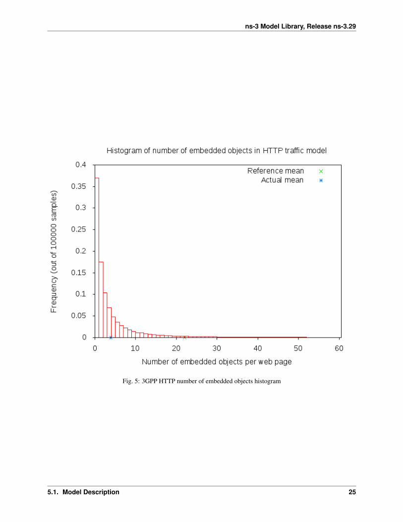
4. The parsing takes a short time (randomly determined) to determine the number of embedded objects (alsorandomly determined) in the web page. Number of embedded object is illustrated in 3GPP HTTP number ofembedded objects histogram.
• If at least one embedded object is determined, the application requests the first embedded objectfrom the server. The request for the next embedded object follows after the previous embedded objecthas been completely received.
• If there is no more embedded object to request, the application enters the reading time.
5. Reading time is a long delay (again, randomly determined) where the application does not induce any networktraffic, thus simulating the user reading the downloaded web page.
6. After the reading time is finished, the process repeats to step #2.
The client models HTTP persistent connection, i.e., HTTP 1.1, where the connection to the server is maintained andused for transmitting and receiving all objects.
Each request by default has a constant size of 350 bytes. A ThreeGppHttpHeader is attached to each requestpacket. The header contains information such as the content type requested (either main object or embedded object)and the timestamp when the packet is transmitted (which will be used to compute the delay and RTT of the packet).
5.1.2 References
Many aspects of the traffic are randomly determined by ThreeGppHttpVariables. A separate instance of thisobject is used by the HTTP server and client applications. These characteristics are based on a legacy 3GPP specifica-tion. The description can be found in the following references:
[1] 3GPP TR 25.892, “Feasibility Study for Orthogonal Frequency Division Multiplexing (OFDM) for UTRAN en-hancement”
[2] IEEE 802.16m, “Evaluation Methodology Document (EMD)”, IEEE 802.16m-08/004r5, July 2008.
[3] NGMN Alliance, “NGMN Radio Access Performance Evaluation Methodology”, v1.0, January 2008.
[4] 3GPP2-TSGC5, “HTTP, FTP and TCP models for 1xEV-DV simulations”, 2001.
5.1. Model Description 23

ns-3 Model Library, Release ns-3.29
Fig. 4: 3GPP HTTP parsing time histogram
24 Chapter 5. 3GPP HTTP applications
ns-3 Model Library, Release ns-3.29
Fig. 5: 3GPP HTTP number of embedded objects histogram
5.1. Model Description 25
ns-3 Model Library, Release ns-3.29
5.2 Usage
The three-gpp-http-example can be referenced to see basic usage of the HTTP applications. In summary, us-ing the ThreeGppHttpServerHelper and ThreeGppHttpClientHelper allow the user to easily installThreeGppHttpServer and ThreeGppHttpClient applications to nodes. The helper objects can be used toconfigure attribute values for the client and server objects, but not for the ThreeGppHttpVariables object. Con-figuration of variables is done by modifying attributes of ThreeGppHttpVariables, which should be done priorto helpers installing applications to nodes.
The client and server provide a number of ns-3 trace sources such as “Tx”, “Rx”, “RxDelay”, and “State-Transition” on the server side, and a large number on the client side (“ConnectionEstablished”, “Connection-Closed”,”TxMainObjectRequest”, “TxEmbeddedObjectRequest”, “RxMainObjectPacket”, “RxMainObject”, “Rx-EmbeddedObjectPacket”, “RxEmbeddedObject”, “Rx”, “RxDelay”, “RxRtt”, “StateTransition”).
5.2.1 Building the 3GPP HTTP applications
Building the applications does not require any special steps to be taken. It suffices to enable the applications module.
5.2.2 Examples
For an example demonstrating HTTP applications run:
$ ./waf --run 'three-gpp-http-example'
By default, the example will print out the web page requests of the client and responses of the server and clientreceiving content packets by using LOG_INFO of ThreeGppHttpServer and ThreeGppHttpClient.
5.2.3 Tests
For testing HTTP applications, three-gpp-http-client-server-test is provided. Run:
$ ./test.py -s three-gpp-http-client-server-test
The test consists of simple Internet nodes having HTTP server and client applications installed. Multiple variantscenarios are tested: delay is 3ms, 30ms or 300ms, bit error rate 0 or 5.0*10^(-6), MTU size 536 or 1460 bytes andeither IPV4 or IPV6 is used. A simulation with each combination of these parameters is run multiple times to verifyfunctionality with different random variables.
Test cases themselves are rather simple: test verifies that HTTP object packet bytes sent match total bytes received bythe client, and that ThreeGppHttpHeader matches the expected packet.
26 Chapter 5. 3GPP HTTP applications

CHAPTER
SIX
BRIDGE NETDEVICE
Placeholder chapter
Some examples of the use of Bridge NetDevice can be found in examples/csma/ directory.
27

ns-3 Model Library, Release ns-3.29
28 Chapter 6. Bridge NetDevice

CHAPTER
SEVEN
BRITE INTEGRATION
This model implements an interface to BRITE, the Boston university Representative Internet Topology gEnerator1.BRITE is a standard tool for generating realistic internet topologies. The ns-3 model, described herein, providesa helper class to facilitate generating ns-3 specific topologies using BRITE configuration files. BRITE builds theoriginal graph which is stored as nodes and edges in the ns-3 BriteTopolgyHelper class. In the ns-3 integration ofBRITE, the generator generates a topology and then provides access to leaf nodes for each AS generated. ns-3 userscan than attach custom topologies to these leaf nodes either by creating them manually or using topology generatorsprovided in ns-3.
There are three major types of topologies available in BRITE: Router, AS, and Hierarchical which is a combination ofAS and Router. For the purposes of ns-3 simulation, the most useful are likely to be Router and Hierarchical. Routerlevel topologies be generated using either the Waxman model or the Barabasi-Albert model. Each model has differentparameters that effect topology creation. For flat router topologies, all nodes are considered to be in the same AS.
BRITE Hierarchical topologies contain two levels. The first is the AS level. This level can be also be created byusing either the Waxman model or the Barabasi-Albert model. Then for each node in the AS topology, a routerlevel topology is constructed. These router level topologies can again either use the Waxman model or the Barbasi-Albert model. BRITE interconnects these separate router topologies as specified by the AS level topology. Once thehierarchical topology is constructed, it is flattened into a large router level topology.
Further information can be found in the BRITE user manual: http://www.cs.bu.edu/brite/publications/usermanual.pdf
7.1 Model Description
The model relies on building an external BRITE library, and then building some ns-3 helpers that call out to the library.The source code for the ns-3 helpers lives in the directory src/brite/helper.
7.1.1 Design
To generate the BRITE topology, ns-3 helpers call out to the external BRITE library, and using a standard BRITEconfiguration file, the BRITE code builds a graph with nodes and edges according to this configuration file. Please seethe BRITE documentation or the example configuration files in src/brite/examples/conf_files to get a better grasp ofBRITE configuration options. The graph built by BRITE is returned to ns-3, and a ns-3 implementation of the graphis built. Leaf nodes for each AS are available for the user to either attach custom topologies or install ns-3 applicationsdirectly.
1 Alberto Medina, Anukool Lakhina, Ibrahim Matta, and John Byers. BRITE: An Approach to Universal Topology Generation. In Proceedingsof the International Workshop on Modeling, Analysis and Simulation of Computer and Telecommunications Systems- MASCOTS ‘01, Cincinnati,Ohio, August 2001.
29

ns-3 Model Library, Release ns-3.29
7.1.2 References
7.2 Usage
The brite-generic-example can be referenced to see basic usage of the BRITE interface. In summary, the BriteTopol-ogyHelper is used as the interface point by passing in a BRITE configuration file. Along with the configuration file aBRITE formatted random seed file can also be passed in. If a seed file is not passed in, the helper will create a seedfile using ns-3’s UniformRandomVariable. Once the topology has been generated by BRITE, BuildBriteTopology()is called to create the ns-3 representation. Next IP Address can be assigned to the topology using either Assig-nIpv4Addresses() or AssignIpv6Addresses(). It should be noted that each point-to-point link in the topology willbe treated as a new network therefore for IPV4 a /30 subnet should be used to avoid wasting a large amount of theavailable address space.
Example BRITE configuration files can be found in /src/brite/examples/conf_files/. ASBarbasi and ASWaxman areexamples of AS only topologies. The RTBarabasi and RTWaxman files are examples of router only topologies. Finallythe TD_ASBarabasi_RTWaxman configuration file is an example of a Hierarchical topology that uses the Barabasi-Albert model for the AS level and the Waxman model for each of the router level topologies. Information on theBRITE parameters used in these files can be found in the BRITE user manual.
7.2.1 Building BRITE Integration
The first step is to download and build the ns-3 specific BRITE repository:
$ hg clone http://code.nsnam.org/BRITE$ cd BRITE$ make
This will build BRITE and create a library, libbrite.so, within the BRITE directory.
Once BRITE has been built successfully, we proceed to configure ns-3 with BRITE support. Change to your ns-3directory:
$ ./waf configure --with-brite=/your/path/to/brite/source --enable-examples
Make sure it says ‘enabled’ beside ‘BRITE Integration’. If it does not, then something has gone wrong. Either youhave forgotten to build BRITE first following the steps above, or ns-3 could not find your BRITE directory.
Next, build ns-3:
$ ./waf
7.2.2 Examples
For an example demonstrating BRITE integration run:
$ ./waf --run 'brite-generic-example'
By enabling the verbose parameter, the example will print out the node and edge information in a similar formatto standard BRITE output. There are many other command-line parameters including confFile, tracing, and nix,described below:
confFile A BRITE configuration file. Many different BRITE configuration file examples exist inthe src/brite/examples/conf_files directory, for example, RTBarabasi20.conf and RTWaxman.conf.Please refer to the conf_files directory for more examples.
30 Chapter 7. BRITE Integration

ns-3 Model Library, Release ns-3.29
tracing Enables ascii tracing.
nix Enables nix-vector routing. Global routing is used by default.
The generic BRITE example also support visualization using pyviz, assuming python bindings in ns-3 are enabled:
$ ./waf --run brite-generic-example --vis
Simulations involving BRITE can also be used with MPI. The total number of MPI instances is passed to the BRITEtopology helper where a modulo divide is used to assign the nodes for each AS to a MPI instance. An example can befound in src/brite/examples:
$ mpirun -np 2 ./waf --run brite-MPI-example
Please see the ns-3 MPI documentation for information on setting up MPI with ns-3.
7.2. Usage 31

ns-3 Model Library, Release ns-3.29
32 Chapter 7. BRITE Integration

CHAPTER
EIGHT
BUILDINGS MODULE
cd .. include:: replace.txt
8.1 Design documentation
8.1.1 Overview
The Buildings module provides:
1. a new class (Building) that models the presence of a building in a simulation scenario;
2. a new class (MobilityBuildingInfo) that allows to specify the location, size and characteristics of build-ings present in the simulated area, and allows the placement of nodes inside those buildings;
3. a container class with the definition of the most useful pathloss models and the correspondent variables calledBuildingsPropagationLossModel.
4. a new propagation model (HybridBuildingsPropagationLossModel) working with the mobilitymodel just introduced, that allows to model the phenomenon of indoor/outdoor propagation in the presenceof buildings.
5. a simplified model working only with Okumura Hata (OhBuildingsPropagationLossModel) consid-ering the phenomenon of indoor/outdoor propagation in the presence of buildings.
The models have been designed with LTE in mind, though their implementation is in fact independent from anyLTE-specific code, and can be used with other ns-3 wireless technologies as well (e.g., wifi, wimax).
The HybridBuildingsPropagationLossModel pathloss model included is obtained through a combinationof several well known pathloss models in order to mimic different environmental scenarios such as urban, suburbanand open areas. Moreover, the model considers both outdoor and indoor indoor and outdoor communication has to beincluded since HeNB might be installed either within building and either outside. In case of indoor communication,the model has to consider also the type of building in outdoor <-> indoor communication according to some generalcriteria such as the wall penetration losses of the common materials; moreover it includes some general configurationfor the internal walls in indoor communications.
The OhBuildingsPropagationLossModel pathloss model has been created for simplifying the previous oneremoving the thresholds for switching from one model to other. For doing this it has been used only one propagationmodel from the one available (i.e., the Okumura Hata). The presence of building is still considered in the model;therefore all the considerations of above regarding the building type are still valid. The same consideration can bedone for what concern the environmental scenario and frequency since both of them are parameters of the modelconsidered.
33

ns-3 Model Library, Release ns-3.29
8.1.2 The Building class
The model includes a specific class called Building which contains a ns3 Box class for defining the dimension ofthe building. In order to implements the characteristics of the pathloss models included, the Building class supportsthe following attributes:
• building type:
– Residential (default value)
– Office
– Commercial
• external walls type
– Wood
– ConcreteWithWindows (default value)
– ConcreteWithoutWindows
– StoneBlocks
• number of floors (default value 1, which means only ground-floor)
• number of rooms in x-axis (default value 1)
• number of rooms in y-axis (default value 1)
The Building class is based on the following assumptions:
• a buildings is represented as a rectangular parallelepiped (i.e., a box)
• the walls are parallel to the x, y, and z axis
• a building is divided into a grid of rooms, identified by the following parameters:
– number of floors
– number of rooms along the x-axis
– number of rooms along the y-axis
• the z axis is the vertical axis, i.e., floor numbers increase for increasing z axis values
• the x and y room indices start from 1 and increase along the x and y axis respectively
• all rooms in a building have equal size
8.1.3 The MobilityBuildingInfo class
The MobilityBuildingInfo class, which inherits from the ns3 class Object, is in charge of main-taining information about the position of a node with respect to building. The information managed byMobilityBuildingInfo is:
• whether the node is indoor or outdoor
• if indoor:
– in which building the node is
– in which room the node is positioned (x, y and floor room indices)
34 Chapter 8. Buildings Module

ns-3 Model Library, Release ns-3.29
The class MobilityBuildingInfo is used by BuildingsPropagationLossModel class, which inheritsfrom the ns3 class PropagationLossModel and manages the pathloss computation of the single components andtheir composition according to the nodes’ positions. Moreover, it implements also the shadowing, that is the loss dueto obstacles in the main path (i.e., vegetation, buildings, etc.).
It is to be noted that, MobilityBuildingInfo can be used by any other propagation model. However, based onthe information at the time of this writing, only the ones defined in the building module are designed for consideringthe constraints introduced by the buildings.
8.1.4 ItuR1238PropagationLossModel
This class implements a building-dependent indoor propagation loss model based on the ITU P.1238 model, whichincludes losses due to type of building (i.e., residential, office and commercial). The analytical expression is given inthe following.
Ltotal = 20 log f +N log d+ Lf (n)− 28[dB]
where:
N =
28 residential30 office22 commercial
: power loss coefficient [dB]
Lf =
4n residential15 + 4(n− 1) office6 + 3(n− 1) commercial
n : number of floors between base station and mobile (n ≥ 1)
f : frequency [MHz]
d : distance (where d > 1) [m]
8.1.5 BuildingsPropagationLossModel
The BuildingsPropagationLossModel provides an additional set of building-dependent pathloss model elements thatare used to implement different pathloss logics. These pathloss model elements are described in the following subsec-tions.
External Wall Loss (EWL)
This component models the penetration loss through walls for indoor to outdoor communications and vice-versa. Thevalues are taken from the [cost231] model.
• Wood ~ 4 dB
• Concrete with windows (not metallized) ~ 7 dB
• Concrete without windows ~ 15 dB (spans between 10 and 20 in COST231)
• Stone blocks ~ 12 dB
8.1. Design documentation 35
ns-3 Model Library, Release ns-3.29
Internal Walls Loss (IWL)
This component models the penetration loss occurring in indoor-to-indoor communications within the same build-ing. The total loss is calculated assuming that each single internal wall has a constant penetration loss Lsiw, andapproximating the number of walls that are penetrated with the manhattan distance (in number of rooms) between thetransmitter and the receiver. In detail, let x1, y1, x2, y2 denote the room number along the x and y axis respectivelyfor user 1 and 2; the total loss LIWL is calculated as
LIWL = Lsiw(|x1 − x2|+ |y1 − y2|)
Height Gain Model (HG)
This component model the gain due to the fact that the transmitting device is on a floor above the ground. In theliterature [turkmani] this gain has been evaluated as about 2 dB per floor. This gain can be applied to all the indoor tooutdoor communications and vice-versa.
Shadowing Model
The shadowing is modeled according to a log-normal distribution with variable standard deviation as function of therelative position (indoor or outdoor) of the MobilityModel instances involved. One random value is drawn for eachpair of MobilityModels, and stays constant for that pair during the whole simulation. Thus, the model is appropriatefor static nodes only.
The model considers that the mean of the shadowing loss in dB is always 0. For the variance, the model considersthree possible values of standard deviation, in detail:
• outdoor (m_shadowingSigmaOutdoor, defaul value of 7 dB)→ XO ∼ N(µO, σ2O).
• indoor (m_shadowingSigmaIndoor, defaul value of 10 dB)→ XI ∼ N(µI, σ2I ).
• external walls penetration (m_shadowingSigmaExtWalls, default value 5 dB)→ XW ∼ N(µW, σ2W)
The simulator generates a shadowing value per each active link according to nodes’ position the first time the linkis used for transmitting. In case of transmissions from outdoor nodes to indoor ones, and vice-versa, the standarddeviation (σIO) has to be calculated as the square root of the sum of the quadratic values of the standard deviatio incase of outdoor nodes and the one for the external walls penetration. This is due to the fact that that the componentsproducing the shadowing are independent of each other; therefore, the variance of a distribution resulting from thesum of two independent normal ones is the sum of the variances.
X ∼ N(µ, σ2) and Y ∼ N(ν, τ2)
Z = X + Y ∼ Z(µ+ ν, σ2 + τ2)
⇒ σIO =√σ2O + σ2
W
8.1.6 Pathloss logics
In the following we describe the different pathloss logic that are implemented by inheriting from BuildingsPropaga-tionLossModel.
HybridBuildingsPropagationLossModel
The HybridBuildingsPropagationLossModel pathloss model included is obtained through a combinationof several well known pathloss models in order to mimic different outdoor and indoor scenarios, as well as indoor-
36 Chapter 8. Buildings Module

ns-3 Model Library, Release ns-3.29
to-outdoor and outdoor-to-indoor scenarios. In detail, the class HybridBuildingsPropagationLossModelintegrates the following pathloss models:
• OkumuraHataPropagationLossModel (OH) (at frequencies > 2.3 GHz substituted byKun2600MhzPropagationLossModel)
• ItuR1411LosPropagationLossModel and ItuR1411NlosOverRooftopPropagationLossModel (I1411)
• ItuR1238PropagationLossModel (I1238)
• the pathloss elements of the BuildingsPropagationLossModel (EWL, HG, IWL)
The following pseudo-code illustrates how the different pathloss model elements described above are integrated inHybridBuildingsPropagationLossModel:
if (txNode is outdoor)thenif (rxNode is outdoor)
thenif (distance > 1 km)then
if (rxNode or txNode is below the rooftop)thenL = I1411
elseL = OH
elseL = I1411
else (rxNode is indoor)if (distance > 1 km)then
if (rxNode or txNode is below the rooftop)L = I1411 + EWL + HG
elseL = OH + EWL + HG
elseL = I1411 + EWL + HG
else (txNode is indoor)if (rxNode is indoor)thenif (same building)
thenL = I1238 + IWL
elseL = I1411 + 2*EWL
else (rxNode is outdoor)if (distance > 1 km)
thenif (rxNode or txNode is below the rooftop)
thenL = I1411 + EWL + HG
elseL = OH + EWL + HG
elseL = I1411 + EWL
We note that, for the case of communication between two nodes below rooftop level with distance is greater then 1km, we still consider the I1411 model, since OH is specifically designed for macro cells and therefore for antennasabove the roof-top level.
8.1. Design documentation 37

ns-3 Model Library, Release ns-3.29
For the ITU-R P.1411 model we consider both the LOS and NLoS versions. In particular, we considers the LoSpropagation for distances that are shorted than a tunable threshold (m_itu1411NlosThreshold). In case onNLoS propagation, the over the roof-top model is taken in consideration for modeling both macro BS and SC. In caseon NLoS several parameters scenario dependent have been included, such as average street width, orientation, etc. Thevalues of such parameters have to be properly set according to the scenario implemented, the model does not calculatenatively their values. In case any values is provided, the standard ones are used, apart for the height of the mobile andBS, which instead their integrity is tested directly in the code (i.e., they have to be greater then zero). In the followingwe give the expressions of the components of the model.
We also note that the use of different propagation models (OH, I1411, I1238 with their variants) in HybridBuild-ingsPropagationLossModel can result in discontinuities of the pathloss with respect to distance. A proper tuning ofthe attributes (especially the distance threshold attributes) can avoid these discontinuities. However, since the behaviorof each model depends on several other parameters (frequency, node height, etc), there is no default value of thesethresholds that can avoid the discontinuities in all possible configurations. Hence, an appropriate tuning of theseparameters is left to the user.
OhBuildingsPropagationLossModel
The OhBuildingsPropagationLossModel class has been created as a simple means to solve the discontinuityproblems of HybridBuildingsPropagationLossModel without doing scenario-specific parameter tuning.The solution is to use only one propagation loss model (i.e., Okumura Hata), while retaining the structure of thepathloss logic for the calculation of other path loss components (such as wall penetration losses). The result is a modelthat is free of discontinuities (except those due to walls), but that is less realistic overall for a generic scenario withbuildings and outdoor/indoor users, e.g., because Okumura Hata is not suitable neither for indoor communications norfor outdoor communications below rooftop level.
In detail, the class OhBuildingsPropagationLossModel integrates the following pathloss models:
• OkumuraHataPropagationLossModel (OH)
• the pathloss elements of the BuildingsPropagationLossModel (EWL, HG, IWL)
The following pseudo-code illustrates how the different pathloss model elements described above are integrated inOhBuildingsPropagationLossModel:
if (txNode is outdoor)thenif (rxNode is outdoor)
thenL = OH
else (rxNode is indoor)L = OH + EWL
else (txNode is indoor)if (rxNode is indoor)thenif (same building)
thenL = OH + IWL
elseL = OH + 2*EWL
else (rxNode is outdoor)L = OH + EWL
We note that OhBuildingsPropagationLossModel is a significant simplification with respect to HybridBuildingsProp-agationLossModel, due to the fact that OH is used always. While this gives a less accurate model in some scenarios(especially below rooftop and indoor), it effectively avoids the issue of pathloss discontinuities that affects Hybrid-BuildingsPropagationLossModel.
38 Chapter 8. Buildings Module

ns-3 Model Library, Release ns-3.29
8.2 User Documentation
8.2.1 How to use buildings in a simulation
In this section we explain the basic usage of the buildings model within a simulation program.
Include the headers
Add this at the beginning of your simulation program:
#include <ns3/buildings-module.h>
Create a building
As an example, let’s create a residential 10 x 20 x 10 building:
double x_min = 0.0;double x_max = 10.0;double y_min = 0.0;double y_max = 20.0;double z_min = 0.0;double z_max = 10.0;Ptr<Building> b = CreateObject <Building> ();b->SetBoundaries (Box (x_min, x_max, y_min, y_max, z_min, z_max));b->SetBuildingType (Building::Residential);b->SetExtWallsType (Building::ConcreteWithWindows);b->SetNFloors (3);b->SetNRoomsX (3);b->SetNRoomsY (2);
This building has three floors and an internal 3 x 2 grid of rooms of equal size.
The helper class GridBuildingAllocator is also available to easily create a set of buildings with identical characteristicsplaced on a rectangular grid. Here’s an example of how to use it:
Ptr<GridBuildingAllocator> gridBuildingAllocator;gridBuildingAllocator = CreateObject<GridBuildingAllocator> ();gridBuildingAllocator->SetAttribute ("GridWidth", UintegerValue (3));gridBuildingAllocator->SetAttribute ("LengthX", DoubleValue (7));gridBuildingAllocator->SetAttribute ("LengthY", DoubleValue (13));gridBuildingAllocator->SetAttribute ("DeltaX", DoubleValue (3));gridBuildingAllocator->SetAttribute ("DeltaY", DoubleValue (3));gridBuildingAllocator->SetAttribute ("Height", DoubleValue (6));gridBuildingAllocator->SetBuildingAttribute ("NRoomsX", UintegerValue (2));gridBuildingAllocator->SetBuildingAttribute ("NRoomsY", UintegerValue (4));gridBuildingAllocator->SetBuildingAttribute ("NFloors", UintegerValue (2));gridBuildingAllocator->SetAttribute ("MinX", DoubleValue (0));gridBuildingAllocator->SetAttribute ("MinY", DoubleValue (0));gridBuildingAllocator->Create (6);
This will create a 3x2 grid of 6 buildings, each 7 x 13 x 6 m with 2 x 4 rooms inside and 2 foors; the buildings arespaced by 3 m on both the x and the y axis.
8.2. User Documentation 39

ns-3 Model Library, Release ns-3.29
Setup nodes and mobility models
Nodes and mobility models are configured as usual, however in order to use them with the buildings model you needan additional call to BuildingsHelper::Install(), so as to let the mobility model include the information ontheir position w.r.t. the buildings. Here is an example:
MobilityHelper mobility;mobility.SetMobilityModel ("ns3::ConstantPositionMobilityModel");ueNodes.Create (2);mobility.Install (ueNodes);BuildingsHelper::Install (ueNodes);
It is to be noted that any mobility model can be used. However, the user is advised to make sure that the behaviorof the mobility model being used is consistent with the presence of Buildings. For example, using a simple randommobility over the whole simulation area in presence of buildings might easily results in node moving in and out ofbuildings, regardless of the presence of walls.
Place some nodes
You can place nodes in your simulation using several methods, which are described in the following.
Legacy positioning methods
Any legacy ns-3 positioning method can be used to place node in the simulation. The important additional step is toFor example, you can place nodes manually like this:
Ptr<ConstantPositionMobilityModel> mm0 = enbNodes.Get (0)->GetObject↪→<ConstantPositionMobilityModel> ();Ptr<ConstantPositionMobilityModel> mm1 = enbNodes.Get (1)->GetObject↪→<ConstantPositionMobilityModel> ();mm0->SetPosition (Vector (5.0, 5.0, 1.5));mm1->SetPosition (Vector (30.0, 40.0, 1.5));
MobilityHelper mobility;mobility.SetMobilityModel ("ns3::ConstantPositionMobilityModel");ueNodes.Create (2);mobility.Install (ueNodes);BuildingsHelper::Install (ueNodes);mm0->SetPosition (Vector (5.0, 5.0, 1.5));mm1->SetPosition (Vector (30.0, 40.0, 1.5));
Alternatively, you could use any existing PositionAllocator class. The coordinates of the node will determine whetherit is placed outdoor or indoor and, if indoor, in which building and room it is placed.
Building-specific positioning methods
The following position allocator classes are available to place node in special positions with respect to buildings:
• RandomBuildingPositionAllocator: Allocate each position by randomly choosing a building fromthe list of all buildings, and then randomly choosing a position inside the building.
• RandomRoomPositionAllocator: Allocate each position by randomly choosing a room from the list ofrooms in all buildings, and then randomly choosing a position inside the room.
40 Chapter 8. Buildings Module

ns-3 Model Library, Release ns-3.29
• SameRoomPositionAllocator: Walks a given NodeContainer sequentially, and for each node allocate anew position randomly in the same room of that node.
• FixedRoomPositionAllocator: Generate a random position uniformly distributed in the volume of achosen room inside a chosen building.
Make the Mobility Model Consistent
Important: whenever you use buildings, you have to issue the following command after we have placed all nodes andbuildings in the simulation:
BuildingsHelper::MakeMobilityModelConsistent ();
This command will go through the lists of all nodes and of all buildings, determine for each user if it is indoor oroutdoor, and if indoor it will also determine the building in which the user is located and the corresponding floor andnumber inside the building.
Building-aware pathloss model
After you placed buildings and nodes in a simulation, you can use a building-aware pathloss model in a simulationexactly in the same way you would use any regular path loss model. How to do this is specific for the wirelessmodule that you are considering (lte, wifi, wimax, etc.), so please refer to the documentation of that model for specificinstructions.
8.2.2 Main configurable attributes
The Building class has the following configurable parameters:
• building type: Residential, Office and Commercial.
• external walls type: Wood, ConcreteWithWindows, ConcreteWithoutWindows and StoneBlocks.
• building bounds: a Box class with the building bounds.
• number of floors.
• number of rooms in x-axis and y-axis (rooms can be placed only in a grid way).
The BuildingMobilityLossModel parameter configurable with the ns3 attribute system is represented by thebound (string Bounds) of the simulation area by providing a Box class with the area bounds. Moreover, by means ofits methods the following parameters can be configured:
• the number of floor the node is placed (default 0).
• the position in the rooms grid.
The BuildingPropagationLossModel class has the following configurable parameters configurable with theattribute system:
• Frequency: reference frequency (default 2160 MHz), note that by setting the frequency the wavelength is setaccordingly automatically and viceversa).
• Lambda: the wavelength (0.139 meters, considering the above frequency).
• ShadowSigmaOutdoor: the standard deviation of the shadowing for outdoor nodes (defaul 7.0).
• ShadowSigmaIndoor: the standard deviation of the shadowing for indoor nodes (default 8.0).
• ShadowSigmaExtWalls: the standard deviation of the shadowing due to external walls penetration foroutdoor to indoor communications (default 5.0).
8.2. User Documentation 41

ns-3 Model Library, Release ns-3.29
• RooftopLevel: the level of the rooftop of the building in meters (default 20 meters).
• Los2NlosThr: the value of distance of the switching point between line-of-sigth and non-line-of-sight prop-agation model in meters (default 200 meters).
• ITU1411DistanceThr: the value of distance of the switching point between short range (ITU 1211) com-munications and long range (Okumura Hata) in meters (default 200 meters).
• MinDistance: the minimum distance in meters between two nodes for evaluating the pathloss (consideredneglictible before this threshold) (default 0.5 meters).
• Environment: the environment scenario among Urban, SubUrban and OpenAreas (default Urban).
• CitySize: the dimension of the city among Small, Medium, Large (default Large).
In order to use the hybrid mode, the class to be used is the HybridBuildingMobilityLossModel, which allowsthe selection of the proper pathloss model according to the pathloss logic presented in the design chapter. However,this solution has the problem that the pathloss model switching points might present discontinuities due to the differentcharacteristics of the model. This implies that according to the specific scenario, the threshold used for switching haveto be properly tuned. The simple OhBuildingMobilityLossModel overcome this problem by using only theOkumura Hata model and the wall penetration losses.
8.3 Testing Documentation
8.3.1 Overview
To test and validate the ns-3 Building Pathloss module, some test suites is provided which are integrated with the ns-3test framework. To run them, you need to have configured the build of the simulator in this way:
$ ./waf configure --enable-tests --enable-modules=buildings$ ./test.py
The above will run not only the test suites belonging to the buildings module, but also those belonging to all the otherns-3 modules on which the buildings module depends. See the ns-3 manual for generic information on the testingframework.
You can get a more detailed report in HTML format in this way:
$ ./test.py -w results.html
After the above command has run, you can view the detailed result for each test by opening the file results.htmlwith a web browser.
You can run each test suite separately using this command:
$ ./test.py -s test-suite-name
For more details about test.py and the ns-3 testing framework, please refer to the ns-3 manual.
8.3.2 Description of the test suites
BuildingsHelper test
The test suite buildings-helper checks that the method BuildingsHelper::MakeAllInstancesConsistent() works properly, i.e., that the BuildingsHelper is successful in locating if nodes are outdoor or indoor, and if indoorthat they are located in the correct building, room and floor. Several test cases are provided with different buildings
42 Chapter 8. Buildings Module

ns-3 Model Library, Release ns-3.29
(having different size, position, rooms and floors) and different node positions. The test passes if each every node islocated correctly.
BuildingPositionAllocator test
The test suite building-position-allocator feature two test cases that check that respectively Random-RoomPositionAllocator and SameRoomPositionAllocator work properly. Each test cases involves a single 2x3x2room building (total 12 rooms) at known coordinates and respectively 24 and 48 nodes. Both tests check that thenumber of nodes allocated in each room is the expected one and that the position of the nodes is also correct.
Buildings Pathloss tests
The test suite buildings-pathloss-model provides different unit tests that compare the expected results ofthe buildings pathloss module in specific scenarios with pre calculated values obtained offline with an Octave script(test/reference/buildings-pathloss.m). The tests are considered passed if the two values are equal up to a tolerance of0.1, which is deemed appropriate for the typical usage of pathloss values (which are in dB).
In the following we detailed the scenarios considered, their selection has been done for covering the wide set ofpossible pathloss logic combinations. The pathloss logic results therefore implicitly tested.
Test #1 Okumura Hata
In this test we test the standard Okumura Hata model; therefore both eNB and UE are placed outside at a distanceof 2000 m. The frequency used is the E-UTRA band #5, which correspond to 869 MHz (see table 5.5-1 of 36.101).The test includes also the validation of the areas extensions (i.e., urban, suburban and open-areas) and of the city size(small, medium and large).
Test #2 COST231 Model
This test is aimed at validating the COST231 model. The test is similar to the Okumura Hata one, except that thefrequency used is the EUTRA band #1 (2140 MHz) and that the test can be performed only for large and small citiesin urban scenarios due to model limitations.
Test #3 2.6 GHz model
This test validates the 2.6 GHz Kun model. The test is similar to Okumura Hata one except that the frequency is theEUTRA band #7 (2620 MHz) and the test can be performed only in urban scenario.
Test #4 ITU1411 LoS model
This test is aimed at validating the ITU1411 model in case of line of sight within street canyons transmissions. In thiscase the UE is placed at 100 meters far from the eNB, since the threshold for switching between LoS and NLoS is leftto default one (i.e., 200 m.).
8.3. Testing Documentation 43
ns-3 Model Library, Release ns-3.29
Test #5 ITU1411 NLoS model
This test is aimed at validating the ITU1411 model in case of non line of sight over the rooftop transmissions. In thiscase the UE is placed at 900 meters far from the eNB, in order to be above the threshold for switching between LoSand NLoS is left to default one (i.e., 200 m.).
Test #6 ITUP1238 model
This test is aimed at validating the ITUP1238 model in case of indoor transmissions. In this case both the UE and theeNB are placed in a residential building with walls made of concrete with windows. Ue is placed at the second floorand distances 30 meters far from the eNB, which is placed at the first floor.
Test #7 Outdoor -> Indoor with Okumura Hata model
This test validates the outdoor to indoor transmissions for large distances. In this case the UE is placed in a residentialbuilding with wall made of concrete with windows and distances 2000 meters from the outdoor eNB.
Test #8 Outdoor -> Indoor with ITU1411 model
This test validates the outdoor to indoor transmissions for short distances. In this case the UE is placed in a residentialbuilding with walls made of concrete with windows and distances 100 meters from the outdoor eNB.
Test #9 Indoor -> Outdoor with ITU1411 model
This test validates the outdoor to indoor transmissions for very short distances. In this case the eNB is placed in thesecond floor of a residential building with walls made of concrete with windows and distances 100 meters from theoutdoor UE (i.e., LoS communication). Therefore the height gain has to be included in the pathloss evaluation.
Test #10 Indoor -> Outdoor with ITU1411 model
This test validates the outdoor to indoor transmissions for short distances. In this case the eNB is placed in the secondfloor of a residential building with walls made of concrete with windows and distances 500 meters from the outdoorUE (i.e., NLoS communication). Therefore the height gain has to be included in the pathloss evaluation.
Buildings Shadowing Test
The test suite buildings-shadowing-test is a unit test intended to verify the statistical distribution of theshadowing model implemented by BuildingsPathlossModel. The shadowing is modeled according to a nor-mal distribution with mean µ = 0 and variable standard deviation σ, according to models commonly used in lit-erature. Three test cases are provided, which cover the cases of indoor, outdoor and indoor-to-outdoor commu-nications. Each test case generates 1000 different samples of shadowing for different pairs of MobilityModel in-stances in a given scenario. Shadowing values are obtained by subtracting from the total loss value returned byHybridBuildingsPathlossModel the path loss component which is constant and pre-determined for each testcase. The test verifies that the sample mean and sample variance of the shadowing values fall within the 99% confi-dence interval of the sample mean and sample variance. The test also verifies that the shadowing values returned atsuccessive times for the same pair of MobilityModel instances is constant.
44 Chapter 8. Buildings Module

ns-3 Model Library, Release ns-3.29
8.4 References
8.4. References 45

ns-3 Model Library, Release ns-3.29
46 Chapter 8. Buildings Module

CHAPTER
NINE
CLICK MODULAR ROUTER INTEGRATION
Click is a software architecture for building configurable routers. By using different combinations of packet processingunits called elements, a Click router can be made to perform a specific kind of functionality. This flexibility providesa good platform for testing and experimenting with different protocols.
9.1 Model Description
The source code for the Click model lives in the directory src/click.
9.1.1 Design
ns-3’s design is well suited for an integration with Click due to the following reasons:
• Packets in ns-3 are serialised/deserialised as they move up/down the stack. This allows ns-3 packets to be passedto and from Click as they are.
• This also means that any kind of ns-3 traffic generator and transport should work easily on top of Click.
• By striving to implement click as an Ipv4RoutingProtocol instance, we can avoid significant changes to the LLand MAC layer of the ns-3 code.
The design goal was to make the ns-3-click public API simple enough such that the user needs to merely add anIpv4ClickRouting instance to the node, and inform each Click node of the Click configuration file (.click file) that it isto use.
This model implements the interface to the Click Modular Router and provides the Ipv4ClickRouting class to allow anode to use Click for external routing. Unlike normal Ipv4RoutingProtocol sub types, Ipv4ClickRouting doesn’t use aRouteInput() method, but instead, receives a packet on the appropriate interface and processes it accordingly. Note thatyou need to have a routing table type element in your Click graph to use Click for external routing. This is needed bythe RouteOutput() function inherited from Ipv4RoutingProtocol. Furthermore, a Click based node uses a different kindof L3 in the form of Ipv4L3ClickProtocol, which is a trimmed down version of Ipv4L3Protocol. Ipv4L3ClickProtocolpasses on packets passing through the stack to Ipv4ClickRouting for processing.
Developing a Simulator API to allow ns-3 to interact with Click
Much of the API is already well defined, which allows Click to probe for information from the simulator (like a Node’sID, an Interface ID and so forth). By retaining most of the methods, it should be possible to write new implementationsspecific to ns-3 for the same functionality.
Hence, for the Click integration with ns-3, a class named Ipv4ClickRouting will handle the interaction with Click. Thecode for the same can be found in src/click/model/ipv4-click-routing.{cc,h}.
47

ns-3 Model Library, Release ns-3.29
Packet hand off between ns-3 and Click
There are four kinds of packet hand-offs that can occur between ns-3 and Click.
• L4 to L3
• L3 to L4
• L3 to L2
• L2 to L3
To overcome this, we implement Ipv4L3ClickProtocol, a stripped down version of Ipv4L3Protocol.Ipv4L3ClickProtocol passes packets to and from Ipv4ClickRouting appropriately to perform routing.
9.1.2 Scope and Limitations
• In its current state, the NS-3 Click Integration is limited to use only with L3, leaving NS-3 to handle L2. We arecurrently working on adding Click MAC support as well. See the usage section to make sure that you designyour Click graphs accordingly.
• Furthermore, ns-3-click will work only with userlevel elements. The complete list of elements are available athttp://read.cs.ucla.edu/click/elements. Elements that have ‘all’, ‘userlevel’ or ‘ns’ mentioned beside them maybe used.
• As of now, the ns-3 interface to Click is Ipv4 only. We will be adding Ipv6 support in the future.
9.1.3 References
• Eddie Kohler, Robert Morris, Benjie Chen, John Jannotti, and M. Frans Kaashoek. The click modular router.ACM Transactions on Computer Systems 18(3), August 2000, pages 263-297.
• Lalith Suresh P., and Ruben Merz. Ns-3-click: click modular router integration for ns-3. In Proc. of 3rdInternational ICST Workshop on NS-3 (WNS3), Barcelona, Spain. March, 2011.
• Michael Neufeld, Ashish Jain, and Dirk Grunwald. Nsclick: bridging network simulation and deployment.MSWiM ‘02: Proceedings of the 5th ACM international workshop on Modeling analysis and simulation ofwireless and mobile systems, 2002, Atlanta, Georgia, USA. http://doi.acm.org/10.1145/570758.570772
9.2 Usage
9.2.1 Building Click
The first step is to clone Click from the github repository and build it:
$ git clone https://github.com/kohler/click$ cd click/$ ./configure --disable-linuxmodule --enable-nsclick --enable-wifi$ make
The –enable-wifi flag may be skipped if you don’t intend on using Click with Wifi. * Note: You don’t need to do a‘make install’.
Once Click has been built successfully, change into the ns-3 directory and configure ns-3 with Click Integrationsupport:
48 Chapter 9. Click Modular Router Integration

ns-3 Model Library, Release ns-3.29
$ ./waf configure --enable-examples --enable-tests --with-nsclick=/path/to/click/↪→source
Hint: If you have click installed one directory above ns-3 (such as in the ns-3-allinone directory), and the name ofthe directory is ‘click’ (or a symbolic link to the directory is named ‘click’), then the –with-nsclick specifier is notnecessary; the ns-3 build system will successfully find the directory.
If it says ‘enabled’ beside ‘NS-3 Click Integration Support’, then you’re good to go. Note: If running modular ns-3,the minimum set of modules required to run all ns-3-click examples is wifi, csma and config-store.
Next, try running one of the examples:
$ ./waf --run nsclick-simple-lan
You may then view the resulting .pcap traces, which are named nsclick-simple-lan-0-0.pcap and nsclick-simple-lan-0-1.pcap.
9.2.2 Click Graph Instructions
The following should be kept in mind when making your Click graph:
• Only userlevel elements can be used.
• You will need to replace FromDevice and ToDevice elements with FromSimDevice and ToSimDevice elements.
• Packets to the kernel are sent up using ToSimDevice(tap0,IP).
• For any node, the device which sends/receives packets to/from the kernel, is named ‘tap0’. The remaininginterfaces should be named eth0, eth1 and so forth (even if you’re using wifi). Please note that the devicenumbering should begin from 0. In future, this will be made flexible so that users can name devices in theirClick file as they wish.
• A routing table element is a mandatory. The OUTports of the routing table element should correspond to theinterface number of the device through which the packet will ultimately be sent out. Violating this rule will leadto really weird packet traces. This routing table element’s name should then be passed to the Ipv4ClickRoutingprotocol object as a simulation parameter. See the Click examples for details.
• The current implementation leaves Click with mainly L3 functionality, with ns-3 handling L2. We will soonbegin working to support the use of MAC protocols on Click as well. This means that as of now, Click’s Wifispecific elements cannot be used with ns-3.
9.2.3 Debugging Packet Flows from Click
From any point within a Click graph, you may use the Print (http://read.cs.ucla.edu/click/elements/print) element andits variants for pretty printing of packet contents. Furthermore, you may generate pcap traces of packets flowingthrough a Click graph by using the ToDump (http://read.cs.ucla.edu/click/elements/todump) element as well. Forinstance:
myarpquerier-> Print(fromarpquery,64)-> ToDump(out_arpquery,PER_NODE 1)-> ethout;
and . . . will print the contents of packets that flow out of the ArpQuerier, then generate a pcap trace file which willhave a suffix ‘out_arpquery’, for each node using the Click file, before pushing packets onto ‘ethout’.
9.2. Usage 49
ns-3 Model Library, Release ns-3.29
9.2.4 Helper
To have a node run Click, the easiest way would be to use the ClickInternetStackHelper class in your simulation script.For instance:
ClickInternetStackHelper click;click.SetClickFile (myNodeContainer, "nsclick-simple-lan.click");click.SetRoutingTableElement (myNodeContainer, "u/rt");click.Install (myNodeContainer);
The example scripts inside src/click/examples/ demonstrate the use of Click based nodes in different scenar-ios. The helper source can be found inside src/click/helper/click-internet-stack-helper.{h,cc}
9.2.5 Examples
The following examples have been written, which can be found in src/click/examples/:
• nsclick-simple-lan.cc and nsclick-raw-wlan.cc: A Click based node communicating with a normal ns-3 nodewithout Click, using Csma and Wifi respectively. It also demonstrates the use of TCP on top of Click, somethingwhich the original nsclick implementation for NS-2 couldn’t achieve.
• nsclick-udp-client-server-csma.cc and nsclick-udp-client-server-wifi.cc: A 3 node LAN (Csma and Wifi respec-tively) wherein 2 Click based nodes run a UDP client, that sends packets to a third Click based node running aUDP server.
• nsclick-routing.cc: One Click based node communicates to another via a third node that acts as an IP router(using the IP router Click configuration). This demonstrates routing using Click.
Scripts are available within <click-dir>/conf/ that allow you to generate Click files for some common sce-narios. The IP Router used in nsclick-routing.cc was generated from the make-ip-conf.pl file and slightlyadapted to work with ns-3-click.
9.3 Validation
This model has been tested as follows:
• Unit tests have been written to verify the internals of Ipv4ClickRouting. This can be found in src/click/ipv4-click-routing-test.cc. These tests verify whether the methods inside Ipv4ClickRouting whichdeal with Device name to ID, IP Address from device name and Mac Address from device name bindings workas expected.
• The examples have been used to test Click with actual simulation scenarios. These can be found in src/click/examples/. These tests cover the following: the use of different kinds of transports on top of Click,TCP/UDP, whether Click nodes can communicate with non-Click based nodes, whether Click nodes can com-municate with each other, using Click to route packets using static routing.
• Click has been tested with Csma, Wifi and Point-to-Point devices. Usage instructions are available in the pre-ceding section.
50 Chapter 9. Click Modular Router Integration
CHAPTER
TEN
CSMA NETDEVICE
This is the introduction to CSMA NetDevice chapter, to complement the CSMA model doxygen.
10.1 Overview of the CSMA model
The ns-3 CSMA device models a simple bus network in the spirit of Ethernet. Although it does not model any realphysical network you could ever build or buy, it does provide some very useful functionality.
Typically when one thinks of a bus network Ethernet or IEEE 802.3 comes to mind. Ethernet uses CSMA/CD (Car-rier Sense Multiple Access with Collision Detection with exponentially increasing backoff to contend for the sharedtransmission medium. The ns-3 CSMA device models only a portion of this process, using the nature of the globallyavailable channel to provide instantaneous (faster than light) carrier sense and priority-based collision “avoidance.”Collisions in the sense of Ethernet never happen and so the ns-3 CSMA device does not model collision detection, norwill any transmission in progress be “jammed.”
10.1.1 CSMA Layer Model
There are a number of conventions in use for describing layered communications architectures in the literature and intextbooks. The most common layering model is the ISO seven layer reference model. In this view the CsmaNetDeviceand CsmaChannel pair occupies the lowest two layers – at the physical (layer one), and data link (layer two) positions.Another important reference model is that specified by RFC 1122, “Requirements for Internet Hosts – CommunicationLayers.” In this view the CsmaNetDevice and CsmaChannel pair occupies the lowest layer – the link layer. There isalso a seemingly endless litany of alternative descriptions found in textbooks and in the literature. We adopt the namingconventions used in the IEEE 802 standards which speak of LLC, MAC, MII and PHY layering. These acronyms aredefined as:
• LLC: Logical Link Control;
• MAC: Media Access Control;
• MII: Media Independent Interface;
• PHY: Physical Layer.
In this case the LLC and MAC are sublayers of the OSI data link layer and the MII and PHY are sublayers of the OSIphysical layer.
The “top” of the CSMA device defines the transition from the network layer to the data link layer. This transition isperformed by higher layers by calling either CsmaNetDevice::Send or CsmaNetDevice::SendFrom.
In contrast to the IEEE 802.3 standards, there is no precisely specified PHY in the CSMA model in the sense of wiretypes, signals or pinouts. The “bottom” interface of the CsmaNetDevice can be thought of as as a kind of MediaIndependent Interface (MII) as seen in the “Fast Ethernet” (IEEE 802.3u) specifications. This MII interface fits into a
51

ns-3 Model Library, Release ns-3.29
corresponding media independent interface on the CsmaChannel. You will not find the equivalent of a 10BASE-T ora 1000BASE-LX PHY.
The CsmaNetDevice calls the CsmaChannel through a media independent interface. There is a method defined to tellthe channel when to start “wiggling the wires” using the method CsmaChannel::TransmitStart, and a method to tellthe channel when the transmission process is done and the channel should begin propagating the last bit across the“wire”: CsmaChannel::TransmitEnd.
When the TransmitEnd method is executed, the channel will model a single uniform signal propagation delay in themedium and deliver copes of the packet to each of the devices attached to the packet via the CsmaNetDevice::Receivemethod.
There is a “pin” in the device media independent interface corresponding to “COL” (collision). The state of the channelmay be sensed by calling CsmaChannel::GetState. Each device will look at this “pin” before starting a send and willperform appropriate backoff operations if required.
Properly received packets are forwarded up to higher levels from the CsmaNetDevice via a callback mechanism.The callback function is initialized by the higher layer (when the net device is attached) using CsmaNetDe-vice::SetReceiveCallback and is invoked upon “proper” reception of a packet by the net device in order to forwardthe packet up the protocol stack.
10.2 CSMA Channel Model
The class CsmaChannel models the actual transmission medium. There is no fixed limit for the number of devicesconnected to the channel. The CsmaChannel models a data rate and a speed-of-light delay which can be accessed viathe attributes “DataRate” and “Delay” respectively. The data rate provided to the channel is used to set the data ratesused by the transmitter sections of the CSMA devices connected to the channel. There is no way to independently setdata rates in the devices. Since the data rate is only used to calculate a delay time, there is no limitation (other thanby the data type holding the value) on the speed at which CSMA channels and devices can operate; and no restrictionbased on any kind of PHY characteristics.
The CsmaChannel has three states, IDLE, TRANSMITTING and PROPAGATING. These three states are “seen” in-stantaneously by all devices on the channel. By this we mean that if one device begins or ends a simulated transmission,all devices on the channel are immediately aware of the change in state. There is no time during which one device maysee an IDLE channel while another device physically further away in the collision domain may have begun transmit-ting with the associated signals not propagated down the channel to other devices. Thus there is no need for collisiondetection in the CsmaChannel model and it is not implemented in any way.
We do, as the name indicates, have a Carrier Sense aspect to the model. Since the simulator is single threaded, accessto the common channel will be serialized by the simulator. This provides a deterministic mechanism for contendingfor the channel. The channel is allocated (transitioned from state IDLE to state TRANSMITTING) on a first-comefirst-served basis. The channel always goes through a three state process:
IDLE -> TRANSMITTING -> PROPAGATING -> IDLE
The TRANSMITTING state models the time during which the source net device is actually wiggling the signals on thewire. The PROPAGATING state models the time after the last bit was sent, when the signal is propagating down thewire to the “far end.”
The transition to the TRANSMITTING state is driven by a call to CsmaChannel::TransmitStart which is called bythe net device that transmits the packet. It is the responsibility of that device to end the transmission with a call toCsmaChannel::TransmitEnd at the appropriate simulation time that reflects the time elapsed to put all of the packetbits on the wire. When TransmitEnd is called, the channel schedules an event corresponding to a single speed-of-light delay. This delay applies to all net devices on the channel identically. You can think of a symmetrical hub inwhich the packet bits propagate to a central location and then back out equal length cables to the other devices on thechannel. The single “speed of light” delay then corresponds to the time it takes for: 1) a signal to propagate from one
52 Chapter 10. CSMA NetDevice

ns-3 Model Library, Release ns-3.29
CsmaNetDevice through its cable to the hub; plus 2) the time it takes for the hub to forward the packet out a port; plus3) the time it takes for the signal in question to propagate to the destination net device.
The CsmaChannel models a broadcast medium so the packet is delivered to all of the devices on the channel (includingthe source) at the end of the propagation time. It is the responsibility of the sending device to determine whether ornot it receives a packet broadcast over the channel.
The CsmaChannel provides following Attributes:
• DataRate: The bitrate for packet transmission on connected devices;
• Delay: The speed of light transmission delay for the channel.
10.3 CSMA Net Device Model
The CSMA network device appears somewhat like an Ethernet device. The CsmaNetDevice provides following At-tributes:
• Address: The Mac48Address of the device;
• SendEnable: Enable packet transmission if true;
• ReceiveEnable: Enable packet reception if true;
• EncapsulationMode: Type of link layer encapsulation to use;
• RxErrorModel: The receive error model;
• TxQueue: The transmit queue used by the device;
• InterframeGap: The optional time to wait between “frames”;
• Rx: A trace source for received packets;
• Drop: A trace source for dropped packets.
The CsmaNetDevice supports the assignment of a “receive error model.” This is an ErrorModel object that is used tosimulate data corruption on the link.
Packets sent over the CsmaNetDevice are always routed through the transmit queue to provide a trace hook for packetssent out over the network. This transmit queue can be set (via attribute) to model different queuing strategies.
Also configurable by attribute is the encapsulation method used by the device. Every packet gets an EthernetHeaderthat includes the destination and source MAC addresses, and a length/type field. Every packet also gets an Ethernet-Trailer which includes the FCS. Data in the packet may be encapsulated in different ways.
By default, or by setting the “EncapsulationMode” attribute to “Dix”, the encapsulation is according to the DEC,Intel, Xerox standard. This is sometimes called EthernetII framing and is the familiar destination MAC, source MAC,EtherType, Data, CRC format.
If the “EncapsulationMode” attribute is set to “Llc”, the encapsulation is by LLC SNAP. In this case, a SNAP headeris added that contains the EtherType (IP or ARP).
The other implemented encapsulation modes are IP_ARP (set “EncapsulationMode” to “IpArp”) in which the lengthtype of the Ethernet header receives the protocol number of the packet; or ETHERNET_V1 (set “EncapsulationMode”to “EthernetV1”) in which the length type of the Ethernet header receives the length of the packet. A “Raw” encapsu-lation mode is defined but not implemented – use of the RAW mode results in an assertion.
Note that all net devices on a channel must be set to the same encapsulation mode for correct results. The encapsulationmode is not sensed at the receiver.
The CsmaNetDevice implements a random exponential backoff algorithm that is executed if the channel is determinedto be busy (TRANSMITTING or PPROPAGATING) when the device wants to start propagating. This results in a
10.3. CSMA Net Device Model 53

ns-3 Model Library, Release ns-3.29
random delay of up to pow (2, retries) - 1 microseconds before a retry is attempted. The default maximum number ofretries is 1000.
10.4 Using the CsmaNetDevice
The CSMA net devices and channels are typically created and configured using the associated CsmaHelper object.The various ns-3 device helpers generally work in a similar way, and their use is seen in many of our example programs.
The conceptual model of interest is that of a bare computer “husk” into which you plug net devices. The bare computersare created using a NodeContainer helper. You just ask this helper to create as many computers (we call themNodes) as you need on your network:
NodeContainer csmaNodes;csmaNodes.Create (nCsmaNodes);
Once you have your nodes, you need to instantiate a CsmaHelper and set any attributes you may want to change.:
CsmaHelper csma;csma.SetChannelAttribute ("DataRate", StringValue ("100Mbps"));csma.SetChannelAttribute ("Delay", TimeValue (NanoSeconds (6560)));
csma.SetDeviceAttribute ("EncapsulationMode", StringValue ("Dix"));csma.SetDeviceAttribute ("FrameSize", UintegerValue (2000));
Once the attributes are set, all that remains is to create the devices and install them on the required nodes, and toconnect the devices together using a CSMA channel. When we create the net devices, we add them to a container toallow you to use them in the future. This all takes just one line of code.:
NetDeviceContainer csmaDevices = csma.Install (csmaNodes);
We recommend thinking carefully about changing these Attributes, since it can result in behavior that surprises users.We allow this because we believe flexibility is important. As an example of a possibly surprising effect of changingAttributes, consider the following:
The Mtu Attribute indicates the Maximum Transmission Unit to the device. This is the size of the largest Protocol DataUnit (PDU) that the device can send. This Attribute defaults to 1500 bytes and corresponds to a number found in RFC894, “A Standard for the Transmission of IP Datagrams over Ethernet Networks.” The number is actually derived fromthe maximum packet size for 10Base5 (full-spec Ethernet) networks – 1518 bytes. If you subtract DIX encapsulationoverhead for Ethernet packets (18 bytes) you will end up with a maximum possible data size (MTU) of 1500 bytes.One can also find that the MTU for IEEE 802.3 networks is 1492 bytes. This is because LLC/SNAP encapsulationadds an extra eight bytes of overhead to the packet. In both cases, the underlying network hardware is limited to 1518bytes, but the MTU is different because the encapsulation is different.
If one leaves the Mtu Attribute at 1500 bytes and changes the encapsulation mode Attribute to Llc, the result will be anetwork that encapsulates 1500 byte PDUs with LLC/SNAP framing resulting in packets of 1526 bytes. This wouldbe illegal in many networks, but we allow you do do this. This results in a simulation that quite subtly does not reflectwhat you might be expecting since a real device would balk at sending a 1526 byte packet.
There also exist jumbo frames (1500 < MTU <= 9000 bytes) and super-jumbo (MTU > 9000 bytes) frames thatare not officially sanctioned by IEEE but are available in some high-speed (Gigabit) networks and NICs. In theCSMA model, one could leave the encapsulation mode set to Dix, and set the Mtu to 64000 bytes – even though anassociated CsmaChannel DataRate was left at 10 megabits per second (certainly not Gigabit Ethernet). This wouldessentially model an Ethernet switch made out of vampire-tapped 1980s-style 10Base5 networks that support super-jumbo datagrams, which is certainly not something that was ever made, nor is likely to ever be made; however it isquite easy for you to configure.
54 Chapter 10. CSMA NetDevice

ns-3 Model Library, Release ns-3.29
Be careful about assumptions regarding what CSMA is actually modelling and how configuration (Attributes) mayallow you to swerve considerably away from reality.
10.5 CSMA Tracing
Like all ns-3 devices, the CSMA Model provides a number of trace sources. These trace sources can be hooked usingyour own custom trace code, or you can use our helper functions to arrange for tracing to be enabled on devices youspecify.
10.5.1 Upper-Level (MAC) Hooks
From the point of view of tracing in the net device, there are several interesting points to insert trace hooks. A con-vention inherited from other simulators is that packets destined for transmission onto attached networks pass througha single “transmit queue” in the net device. We provide trace hooks at this point in packet flow, which corresponds(abstractly) only to a transition from the network to data link layer, and call them collectively the device MAC hooks.
When a packet is sent to the CSMA net device for transmission it always passes through the transmit queue. Thetransmit queue in the CsmaNetDevice inherits from Queue, and therefore inherits three trace sources:
• An Enqueue operation source (see Queue::m_traceEnqueue);
• A Dequeue operation source (see Queue::m_traceDequeue);
• A Drop operation source (see Queue::m_traceDrop).
The upper-level (MAC) trace hooks for the CsmaNetDevice are, in fact, exactly these three trace sources on the singletransmit queue of the device.
The m_traceEnqueue event is triggered when a packet is placed on the transmit queue. This happens at the time thatCsmaNetDevice::Send or CsmaNetDevice::SendFrom is called by a higher layer to queue a packet for transmission.
The m_traceDequeue event is triggered when a packet is removed from the transmit queue. Dequeues from the trans-mit queue can happen in three situations: 1) If the underlying channel is idle when the CsmaNetDevice::Send orCsmaNetDevice::SendFrom is called, a packet is dequeued from the transmit queue and immediately transmitted; 2)If the underlying channel is idle, a packet may be dequeued and immediately transmitted in an internal TransmitCom-pleteEvent that functions much like a transmit complete interrupt service routine; or 3) from the random exponentialbackoff handler if a timeout is detected.
Case (3) implies that a packet is dequeued from the transmit queue if it is unable to be transmitted according to thebackoff rules. It is important to understand that this will appear as a Dequeued packet and it is easy to incorrectlyassume that the packet was transmitted since it passed through the transmit queue. In fact, a packet is actually droppedby the net device in this case. The reason for this behavior is due to the definition of the Queue Drop event. Them_traceDrop event is, by definition, fired when a packet cannot be enqueued on the transmit queue because it is full.This event only fires if the queue is full and we do not overload this event to indicate that the CsmaChannel is “full.”
10.5.2 Lower-Level (PHY) Hooks
Similar to the upper level trace hooks, there are trace hooks available at the lower levels of the net device. We callthese the PHY hooks. These events fire from the device methods that talk directly to the CsmaChannel.
The trace source m_dropTrace is called to indicate a packet that is dropped by the device. This happens in two cases:First, if the receive side of the net device is not enabled (see CsmaNetDevice::m_receiveEnable and the associatedattribute “ReceiveEnable”).
The m_dropTrace is also used to indicate that a packet was discarded as corrupt if a receive error model is used (seeCsmaNetDevice::m_receiveErrorModel and the associated attribute “ReceiveErrorModel”).
10.5. CSMA Tracing 55
ns-3 Model Library, Release ns-3.29
The other low-level trace source fires on reception of an accepted packet (see CsmaNetDevice::m_rxTrace). A packetis accepted if it is destined for the broadcast address, a multicast address, or to the MAC address assigned to the netdevice.
10.6 Summary
The ns3 CSMA model is a simplistic model of an Ethernet-like network. It supports a Carrier-Sense function andallows for Multiple Access to a shared medium. It is not physical in the sense that the state of the medium is instan-taneously shared among all devices. This means that there is no collision detection required in this model and noneis implemented. There will never be a “jam” of a packet already on the medium. Access to the shared channel is ona first-come first-served basis as determined by the simulator scheduler. If the channel is determined to be busy bylooking at the global state, a random exponential backoff is performed and a retry is attempted.
Ns-3 Attributes provide a mechanism for setting various parameters in the device and channel such as addresses,encapsulation modes and error model selection. Trace hooks are provided in the usual manner with a set of upper levelhooks corresponding to a transmit queue and used in ASCII tracing; and also a set of lower level hooks used in pcaptracing.
Although the ns-3 CsmaChannel and CsmaNetDevice does not model any kind of network you could build or buy, itdoes provide us with some useful functionality. You should, however, understand that it is explicitly not Ethernet orany flavor of IEEE 802.3 but an interesting subset.
56 Chapter 10. CSMA NetDevice
CHAPTER
ELEVEN
DSDV ROUTING
Destination-Sequenced Distance Vector (DSDV) routing protocol is a pro-active, table-driven routing protocol forMANETs developed by Charles E. Perkins and Pravin Bhagwat in 1994. It uses the hop count as metric in routeselection.
This model was developed by the ResiliNets research group at the University of Kansas. A paper on this model existsat this URL.
11.1 DSDV Routing Overview
DSDV Routing Table: Every node will maintain a table listing all the other nodes it has known either directly orthrough some neighbors. Every node has a single entry in the routing table. The entry will have information aboutthe node’s IP address, last known sequence number and the hop count to reach that node. Along with these details thetable also keeps track of the nexthop neighbor to reach the destination node, the timestamp of the last update receivedfor that node.
The DSDV update message consists of three fields, Destination Address, Sequence Number and Hop Count.
Each node uses 2 mechanisms to send out the DSDV updates. They are,
1. Periodic Updates Periodic updates are sent out after every m_periodicUpdateInterval(default:15s). In this up-date the node broadcasts out its entire routing table.
2. Trigger Updates Trigger Updates are small updates in-between the periodic updates. These updates are sentout whenever a node receives a DSDV packet that caused a change in its routing table. The original paperdid not clearly mention when for what change in the table should a DSDV update be sent out. The currentimplementation sends out an update irrespective of the change in the routing table.
The updates are accepted based on the metric for a particular node. The first factor determining the acceptance of anupdate is the sequence number. It has to accept the update if the sequence number of the update message is higherirrespective of the metric. If the update with same sequence number is received, then the update with least metric(hopCount) is given precedence.
In highly mobile scenarios, there is a high chance of route fluctuations, thus we have the concept of weighted settlingtime where an update with change in metric will not be advertised to neighbors. The node waits for the settling timeto make sure that it did not receive the update from its old neighbor before sending out that update.
The current implementation covers all the above features of DSDV. The current implementation also has a requestqueue to buffer packets that have no routes to destination. The default is set to buffer up to 5 packets per destination.
11.2 References
Link to the Paper: http://portal.acm.org/citation.cfm?doid=190314.190336
57

ns-3 Model Library, Release ns-3.29
58 Chapter 11. DSDV Routing
CHAPTER
TWELVE
DSR ROUTING
Dynamic Source Routing (DSR) protocol is a reactive routing protocol designed specifically for use in multi-hopwireless ad hoc networks of mobile nodes.
This model was developed by the ResiliNets research group at the University of Kansas.
12.1 DSR Routing Overview
This model implements the base specification of the Dynamic Source Routing (DSR) protocol. Implementation isbased on RFC 4728, with some extensions and modifications to the RFC specifications.
DSR operates on a on-demand behavior. Therefore, our DSR model buffers all packets while a route request packet(RREQ) is disseminated. We implement a packet buffer in dsr-rsendbuff.cc. The packet queue implements garbagecollection of old packets and a queue size limit. When the packet is sent out from the send buffer, it will be queued inmaintenance buffer for next hop acknowledgment.
The maintenance buffer then buffers the already sent out packets and waits for the notification of packet delivery.Protocol operation strongly depends on broken link detection mechanism. We implement the three heuristics recom-mended based the RFC as follows:
First, we use link layer feedback when possible, which is also the fastest mechanism of these three to detect link errors.A link is considered to be broken if frame transmission results in a transmission failure for all retries. This mechanismis meant for active links and works much faster than in its absence. DSR is able to detect the link layer transmissionfailure and notify that as broken. Recalculation of routes will be triggered when needed. If user does not want to uselink layer acknowledgment, it can be tuned by setting “LinkAcknowledgment” attribute to false in “dsr-routing.cc”.
Second, passive acknowledgment should be used whenever possible. The node turns on “promiscuous” receive mode,in which it can receive packets not destined for itself, and when the node assures the delivery of that data packet to itsdestination, it cancels the passive acknowledgment timer.
Last, we use a network layer acknowledge scheme to notify the receipt of a packet. Route request packet will not beacknowledged or retransmitted.
The Route Cache implementation support garbage collection of old entries and state machine, as defined in the stan-dard. It implements as a STL map container. The key is the destination IP address.
DSR operates with direct access to IP header, and operates between network and transport layer. When packet is sentout from transport layer, it passes itself to DSR and DSR header is appended.
We have two caching mechanisms: path cache and link cache. The path cache saves the whole path in the cache. Thepaths are sorted based on the hop count, and whenever one path is not able to be used, we change to the next path.The link cache is a slightly better design in the sense that it uses different subpaths and uses Implemented Link Cacheusing Dijkstra algorithm, and this part is implemented by Song Luan <[email protected]>.
The following optional protocol optimizations aren’t implemented:
59

ns-3 Model Library, Release ns-3.29
• Flow state
• First Hop External (F), Last Hop External (L) flags
• Handling unknown DSR options
• Two types of error headers:
1. flow state not supported option
2. unsupported option (not going to happen in simulation)
12.1.1 DSR update in ns-3.17
We originally used “TxErrHeader” in Ptr<WifiMac> to indicate the transmission error of a specific packet in link layer,however, it was not working quite correctly since even when the packet was dropped, this header was not recorded inthe trace file. We used to a different path on implementing the link layer notification mechanism. We look into thetrace file by finding packet receive event. If we find one receive event for the data packet, we count that as the indicatorfor successful data delivery.
12.1.2 Useful parameters
+------------------------- +------------------------------------+-------------+| Parameter | Description | Default |+==========================+====================================+=============+| MaxSendBuffLen | Maximum number of packets that can | 64 || | be stored in send buffer | |+------------------------- +------------------------------------+-------------+| MaxSendBuffTime | Maximum time packets can be queued | Seconds(30) || | in the send buffer | |+------------------------- +------------------------------------+-------------+| MaxMaintLen | Maximum number of packets that can | 50 || | be stored in maintenance buffer | |+------------------------- +------------------------------------+-------------+| MaxMaintTime | Maximum time packets can be queued | Seconds(30) || | in maintenance buffer | |+------------------------- +------------------------------------+-------------+| MaxCacheLen | Maximum number of route entries | 64 || | that can be stored in route cache | |+------------------------- +------------------------------------+-------------+| RouteCacheTimeout | Maximum time the route cache can | Seconds(300)|| | be queued in route cache | |+------------------------- +------------------------------------+-------------+| RreqRetries | Maximum number of retransmissions | 16 || | for request discovery of a route | |+------------------------- +------------------------------------+-------------+| CacheType | Use Link Cache or use Path Cache | "LinkCache" || | | |+------------------------- +------------------------------------+-------------+| LinkAcknowledgment | Enable Link layer acknowledgment | True || | mechanism | |+------------------------- +------------------------------------+-------------+
60 Chapter 12. DSR Routing
ns-3 Model Library, Release ns-3.29
12.1.3 Implementation modification
• The DsrFsHeader has added 3 fields: message type, source id, destination id, and these changes only for post-processing
1. Message type is used to identify the data packet from control packet
2. source id is used to identify the real source of the data packet since we have to deliver the packethop-by-hop and the Ipv4Header is not carrying the real source and destination ip address as needed
3. destination id is for same reason of above
• Route Reply header is not word-aligned in DSR RFC, change it to word-aligned in implementation
• DSR works as a shim header between transport and network protocol, it needs its own forwarding mechanism,we are changing the packet transmission to hop-by-hop delivery, so we added two fields in dsr fixed header tonotify packet delivery
12.1.4 Current Route Cache implementation
This implementation used “path cache”, which is simple to implement and ensures loop-free paths:
• the path cache has automatic expire policy
• the cache saves multiple route entries for a certain destination and sort the entries based on hop counts
• the MaxEntriesEachDst can be tuned to change the maximum entries saved for a single destination
• when adding multiple routes for one destination, the route is compared based on hop-count and expire time, theone with less hop count or relatively new route is favored
• Future implementation may include “link cache” as another possibility
12.2 DSR Instructions
The following should be kept in mind when running DSR as routing protocol:
• NodeTraversalTime is the time it takes to traverse two neighboring nodes and should be chosen to fit the trans-mission range
• PassiveAckTimeout is the time a packet in maintenance buffer wait for passive acknowledgment, normally setas two times of NodeTraversalTime
• RouteCacheTimeout should be set smaller value when the nodes’ velocity become higher. The default value is300s.
12.3 Helper
To have a node run DSR, the easiest way would be to use the DsrHelper and DsrMainHelpers in your simulation script.For instance:
DsrHelper dsr;DsrMainHelper dsrMain;dsrMain.Install (dsr, adhocNodes);
12.2. DSR Instructions 61

ns-3 Model Library, Release ns-3.29
The example scripts inside src/dsr/examples/ demonstrate the use of DSR based nodes in different scenar-ios. The helper source can be found inside src/dsr/helper/dsr-main-helper.{h,cc} and src/dsr/helper/dsr-helper.{h,cc}
12.4 Examples
The example can be found in src/dsr/examples/:
• dsr.cc use DSR as routing protocol within a traditional MANETs environment[3].
DSR is also built in the routing comparison case in examples/routing/:
• manet-routing-compare.cc is a comparison case with built in MANET routing protocols and can gen-erate its own results.
12.5 Validation
This model has been tested as follows:
• Unit tests have been written to verify the internals of DSR. This can be found in src/dsr/test/dsr-test-suite.cc. These tests verify whether the methods inside DSR module which deal with packetbuffer, headers work correctly.
• Simulation cases similar to [3] have been tested and have comparable results.
• manet-routing-compare.cc has been used to compare DSR with three of other routing protocols.
A paper was presented on these results at the Workshop on ns-3 in 2011.
12.6 Limitations
The model is not fully compliant with RFC 4728. As an example, Dsr fixed size header has been extended and it isfour octets longer then the RFC specification. As a consequence, the DSR headers can not be correctly decoded byWireshark.
The model full compliance with the RFC is planned for the future.
12.7 References
[1] Original paper: http://www.monarch.cs.rice.edu/monarch-papers/dsr-chapter00.pdf
[2] RFC 4728 http://www6.ietf.org/rfc/rfc4728.txt
[3] Broch’s comparison paper: http://www.monarch.cs.rice.edu/monarch-papers/mobicom98.ps
62 Chapter 12. DSR Routing

CHAPTER
THIRTEEN
EMULATION OVERVIEW
ns-3 has been designed for integration into testbed and virtual machine environments. We have addressed this need byproviding two kinds of net devices. The first kind of device is a file descriptor net device (FdNetDevice), which isa generic device type that can read and write from a file descriptor. By associating this file descriptor with differentthings on the host system, different capabilities can be provided. For instance, the FdNetDevice can be associatedwith an underlying packet socket to provide emulation capabilities. This allows ns-3 simulations to send data on a“real” network. The second kind, called a TapBridge NetDevice allows a “real” host to participate in an ns-3simulation as if it were one of the simulated nodes. An ns-3 simulation may be constructed with any combination ofsimulated or emulated devices.
Note: Prior to ns-3.17, the emulation capability was provided by a special device called an Emu NetDevice; the EmuNetDevice has been replaced by the FdNetDevice.
One of the use-cases we want to support is that of a testbed. A concrete example of an environment of this kind isthe ORBIT testbed. ORBIT is a laboratory emulator/field trial network arranged as a two dimensional grid of 400802.11 radio nodes. We integrate with ORBIT by using their “imaging” process to load and run ns-3 simulations onthe ORBIT array. We can use our EmuFdNetDevice to drive the hardware in the testbed and we can accumulateresults either using the ns-3 tracing and logging functions, or the native ORBIT data gathering techniques. See http://www.orbit-lab.org/ for details on the ORBIT testbed.
A simulation of this kind is shown in the following figure:
You can see that there are separate hosts, each running a subset of a “global” simulation. Instead of an ns-3 channelconnecting the hosts, we use real hardware provided by the testbed. This allows ns-3 applications and protocol stacksattached to a simulation node to communicate over real hardware.
We expect the primary use for this configuration will be to generate repeatable experimental results in a real-worldnetwork environment that includes all of the ns-3 tracing, logging, visualization and statistics gathering tools.
In what can be viewed as essentially an inverse configuration, we allow “real” machines running native applicationsand protocol stacks to integrate with an ns-3 simulation. This allows for the simulation of large networks connected toa real machine, and also enables virtualization. A simulation of this kind is shown in the following figure:
Here, you will see that there is a single host with a number of virtual machines running on it. An ns-3 simulation isshown running in the virtual machine shown in the center of the figure. This simulation has a number of nodes withassociated ns-3 applications and protocol stacks that are talking to an ns-3 channel through native simulated ns-3 netdevices.
There are also two virtual machines shown at the far left and far right of the figure. These VMs are running native(Linux) applications and protocol stacks. The VM is connected into the simulation by a Linux Tap net device. Theuser-mode handler for the Tap device is instantiated in the simulation and attached to a proxy node that represents thenative VM in the simulation. These handlers allow the Tap devices on the native VMs to behave as if they were ns-3net devices in the simulation VM. This, in turn, allows the native software and protocol suites in the native VMs tobelieve that they are connected to the simulated ns-3 channel.
63
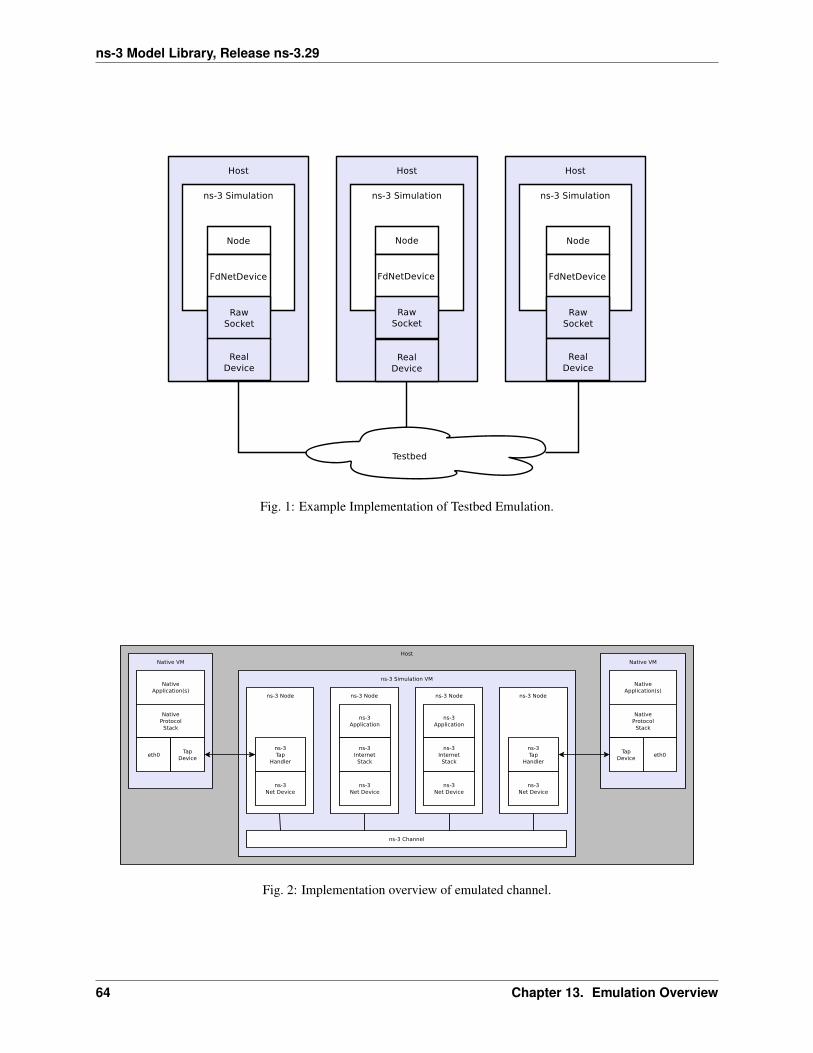
ns-3 Model Library, Release ns-3.29
Fig. 1: Example Implementation of Testbed Emulation.
Fig. 2: Implementation overview of emulated channel.
64 Chapter 13. Emulation Overview

ns-3 Model Library, Release ns-3.29
We expect the typical use case for this environment will be to analyze the behavior of native applications and protocolsuites in the presence of large simulated ns-3 networks.
For more details:
• FdNetDevice chapter.
• TapBridge chapter.
65

ns-3 Model Library, Release ns-3.29
66 Chapter 13. Emulation Overview

CHAPTER
FOURTEEN
ENERGY FRAMEWORK
Energy consumption is a key issue for wireless devices, and wireless network researchers often need to investigate theenergy consumption at a node or in the overall network while running network simulations in ns-3. This requires ns-3to support energy consumption modeling. Further, as concepts such as fuel cells and energy scavenging are becomingviable for low power wireless devices, incorporating the effect of these emerging technologies into simulations requiressupport for modeling diverse energy sources in ns-3. The ns-3 Energy Framework provides the basis for energyconsumption, energy source and energy harvesting modeling.
14.1 Model Description
The source code for the Energy Framework is currently at: src/energy.
14.1.1 Design
The ns-3 Energy Framework is composed of 3 parts: Energy Source, Device Energy Model and Energy Harvester.The framework is implemented into the src/energy/models folder.
Energy Source
The Energy Source represents the power supply on each node. A node can have one or more energy sources, andeach energy source can be connected to multiple device energy models. Connecting an energy source to a deviceenergy model implies that the corresponding device draws power from the source. The basic functionality of theEnergy Source is to provide energy for devices on the node. When energy is completely drained from the EnergySource, it notifies the devices on node such that each device can react to this event. Further, each node can access theEnergy Source Objects for information such as remaining energy or energy fraction (battery level). This enables theimplementation of energy aware protocols in ns-3.
In order to model a wide range of power supplies such as batteries, the Energy Source must be able to capture charac-teristics of these supplies. There are 2 important characteristics or effects related to practical batteries:
Rate Capacity Effect Decrease of battery lifetime when the current draw is higher than the rated value of the battery.
Recovery Effect Increase of battery lifetime when the battery is alternating between discharge and idle states.
In order to incorporate the Rate Capacity Effect, the Energy Source uses current draw from all the devices on the samenode to calculate energy consumption. Moreover, multiple Energy Harvesters can be connected to the Energy Sourcein order to replenish its energy. The Energy Source periodically polls all the devices and energy harvesters on thesame node to calculate the total current drain and hence the energy consumption. When a device changes state, itscorresponding Device Energy Model will notify the Energy Source of this change and new total current draw will becalculated. Similarly, every Energy Harvester update triggers an update to the connected Energy Source.
67

ns-3 Model Library, Release ns-3.29
The Energy Source base class keeps a list of devices (Device Energy Model objects) and energy harvesters (EnergyHarvester objects) that are using the particular Energy Source as power supply. When energy is completely drained,the Energy Source will notify all devices on this list. Each device can then handle this event independently, based onthe desired behavior that should be followed in case of power outage.
Device Energy Model
The Device Energy Model is the energy consumption model of a device installed on the node. It is designed to be astate based model where each device is assumed to have a number of states, and each state is associated with a powerconsumption value. Whenever the state of the device changes, the corresponding Device Energy Model will notifythe Energy Source of the new current draw of the device. The Energy Source will then calculate the new total currentdraw and update the remaining energy.
The Device Energy Model can also be used for devices that do not have finite number of states. For example, in anelectric vehicle, the current draw of the motor is determined by its speed. Since the vehicle’s speed can take continuousvalues within a certain range, it is infeasible to define a set of discrete states of operation. However, by converting thespeed value into current directly, the same set of Device Energy Model APIs can still be used.
Energy Harvester
The energy harvester represents the elements that harvest energy from the environment and recharge the Energy Sourceto which it is connected. The energy harvester includes the complete implementation of the actual energy harvestingdevice (e.g., a solar panel) and the environment (e.g., the solar radiation). This means that in implementing an energyharvester, the energy contribution of the environment and the additional energy requirements of the energy harvestingdevice such as the conversion efficiency and the internal power consumption of the device needs to be jointly modeled.
WiFi Radio Energy Model
The WiFi Radio Energy Model is the energy consumption model of a Wifi net device. It provides a state for each of theavailable states of the PHY layer: Idle, CcaBusy, Tx, Rx, ChannelSwitch, Sleep, Off. Each of such states is associatedwith a value (in Ampere) of the current draw (see below for the corresponding attribute names). A Wifi Radio EnergyModel PHY Listener is registered to the Wifi PHY in order to be notified of every Wifi PHY state transition. At everytransition, the energy consumed in the previous state is computed and the energy source is notified in order to updateits remaining energy.
The Wifi Tx Current Model gives the possibility to compute the current draw in the transmit state as a functionof the nominal tx power (in dBm), as observed in several experimental measurements. To this purpose, the WifiRadio Energy Model PHY Listener is notified of the nominal tx power used to transmit the current frame and passessuch a value to the Wifi Tx Current Model which takes care of updating the current draw in the Tx state. Hence,the energy consumption is correctly computed even if the Wifi Remote Station Manager performs per-frame powercontrol. Currently, a Linear Wifi Tx Current Model is implemented which computes the tx current as a linear function(according to parameters that can be specified by the user) of the nominal tx power in dBm.
The Wifi Radio Energy Model offers the possibility to specify a callback that is invoked when the energy source isdepleted. If such a callback is not specified when the Wifi Radio Energy Model Helper is used to install the model ona device, a callback is implicitly made so that the Wifi PHY is put in the OFF mode (hence no frame is transmitted norreceived afterwards) when the energy source is depleted. Likewise, it is possible to specify a callback that is invokedwhen the energy source is recharged (which might occur in case an energy harvester is connected to the energy source).If such a callback is not specified when the Wifi Radio Energy Model Helper is used to install the model on a device, acallback is implicitly made so that the Wifi PHY is resumed from the OFF mode when the energy source is recharged.
68 Chapter 14. Energy Framework

ns-3 Model Library, Release ns-3.29
14.1.2 Future Work
For Device Energy Models, we are planning to include support for other PHY layer models provided in ns-3 such asWiMAX, and to model the energy consumptions of other non communicating devices, like a generic sensor and a CPU.For Energy Sources, we are planning to included new types of Energy Sources such as Supercapacitor and Nickel-Metal Hydride (Ni-MH) battery. For the Energy Harvesters, we are planning to implement an energy harvester thatrecharges the energy sources according to the power levels defined in a user customizable dataset of real measurements.
14.1.3 References
14.2 Usage
The main way that ns-3 users will typically interact with the Energy Framework is through the helper API and throughthe publicly visible attributes of the framework. The helper API is defined in src/energy/helper/*.h.
In order to use the energy framework, the user must install an Energy Source for the node of interest, the correspondingDevice Energy Model for the network devices and, if necessary, the one or more Energy Harvester. Energy Source(objects) are aggregated onto each node by the Energy Source Helper. In order to allow multiple energy sources pernode, we aggregate an Energy Source Container rather than directly aggregating a source object.
The Energy Source object keeps a list of Device Energy Model and Energy Harvester objects using the source aspower supply. Device Energy Model objects are installed onto the Energy Source by the Device Energy Model Helper,while Energy Harvester object are installed by the Energy Harvester Helper. User can access the Device Energy Modelobjects through the Energy Source object to obtain energy consumption information of individual devices. Moreover,the user can access to the Energy Harvester objects in order to gather information regarding the current harvestablepower and the total energy harvested by the harvester.
14.2.1 Examples
The example directories, src/examples/energy and examples/energy, contain some basic code that showshow to set up the framework.
14.2.2 Helpers
Energy Source Helper
Base helper class for Energy Source objects, this helper Aggregates Energy Source object onto a node. Child imple-mentation of this class creates the actual Energy Source object.
Device Energy Model Helper
Base helper class for Device Energy Model objects, this helper attaches Device Energy Model objects onto EnergySource objects. Child implementation of this class creates the actual Device Energy Model object.
Energy Harvesting Helper
Base helper class for Energy Harvester objects, this helper attaches Energy Harvester objects onto Energy Sourceobjects. Child implementation of this class creates the actual Energy Harvester object.
14.2. Usage 69

ns-3 Model Library, Release ns-3.29
14.2.3 Attributes
Attributes differ between Energy Sources, Devices Energy Models and Energy Harvesters implementations, pleaselook at the specific child class for details.
Basic Energy Source
• BasicEnergySourceInitialEnergyJ: Initial energy stored in basic energy source.
• BasicEnergySupplyVoltageV: Initial supply voltage for basic energy source.
• PeriodicEnergyUpdateInterval: Time between two consecutive periodic energy updates.
RV Battery Model
• RvBatteryModelPeriodicEnergyUpdateInterval: RV battery model sampling interval.
• RvBatteryModelOpenCircuitVoltage: RV battery model open circuit voltage.
• RvBatteryModelCutoffVoltage: RV battery model cutoff voltage.
• RvBatteryModelAlphaValue: RV battery model alpha value.
• RvBatteryModelBetaValue: RV battery model beta value.
• RvBatteryModelNumOfTerms: The number of terms of the infinite sum for estimating battery level.
WiFi Radio Energy Model
• IdleCurrentA: The default radio Idle current in Ampere.
• CcaBusyCurrentA: The default radio CCA Busy State current in Ampere.
• TxCurrentA: The radio Tx current in Ampere.
• RxCurrentA: The radio Rx current in Ampere.
• SwitchingCurrentA: The default radio Channel Switch current in Ampere.
• SleepCurrentA: The radio Sleep current in Ampere.
• TxCurrentModel: A pointer to the attached tx current model.
Basic Energy Harvester
• PeriodicHarvestedPowerUpdateInterval: Time between two consecutive periodic updates of theharvested power.
• HarvestablePower: Random variables that represents the amount of power that is provided by the energyharvester.
14.2.4 Tracing
Traced values differ between Energy Sources, Devices Energy Models and Energy Harvesters implementations, pleaselook at the specific child class for details.
70 Chapter 14. Energy Framework

ns-3 Model Library, Release ns-3.29
Basic Energy Source
• RemainingEnergy: Remaining energy at BasicEnergySource.
RV Battery Model
• RvBatteryModelBatteryLevel: RV battery model battery level.
• RvBatteryModelBatteryLifetime: RV battery model battery lifetime.
WiFi Radio Energy Model
• TotalEnergyConsumption: Total energy consumption of the radio device.
Basic Energy Harvester
• HarvestedPower: Current power provided by the BasicEnergyHarvester.
• TotalEnergyHarvested: Total energy harvested by the BasicEnergyHarvester.
14.2.5 Validation
Comparison of the Energy Framework against actual devices have not been performed. Current implementation of theEnergy Framework is checked numerically for computation errors. The RV battery model is validated by comparingresults with what was presented in the original RV battery model paper.
14.2. Usage 71

ns-3 Model Library, Release ns-3.29
72 Chapter 14. Energy Framework

CHAPTER
FIFTEEN
FILE DESCRIPTOR NETDEVICE
The src/fd-net-device module provides the FdNetDevice class, which is able to read and write traffic usinga file descriptor provided by the user. This file descriptor can be associated to a TAP device, to a raw socket, to a userspace process generating/consuming traffic, etc. The user has full freedom to define how external traffic is generatedand ns-3 traffic is consumed.
Different mechanisms to associate a simulation to external traffic can be provided through helper classes. Threespecific helpers are provided:
• EmuFdNetDeviceHelper (to associate the ns-3 device with a physical device in the host machine)
• TapFdNetDeviceHelper (to associate the ns-3 device with the file descriptor from a tap device in the host ma-chine)
• PlanteLabFdNetDeviceHelper (to automate the creation of tap devices in PlanetLab nodes, enabling ns-3 simu-lations that can send and receive traffic though the Internet using PlanetLab resource.
15.1 Model Description
The source code for this module lives in the directory src/fd-net-device.
The FdNetDevice is a special type of ns-3 NetDevice that reads traffic to and from a file descriptor. That is, unlike puresimulation NetDevice objects that write frames to and from a simulated channel, this FdNetDevice directs frames outof the simulation to a file descriptor. The file descriptor may be associated to a Linux TUN/TAP device, to a socket,or to a user-space process.
It is up to the user of this device to provide a file descriptor. The type of file descriptor being provided determineswhat is being modelled. For instance, if the file descriptor provides a raw socket to a WiFi card on the host machine,the device being modelled is a WiFi device.
From the conceptual “top” of the device looking down, it looks to the simulated node like a device supporting a 48-bitIEEE MAC address that can be bridged, supports broadcast, and uses IPv4 ARP or IPv6 Neighbor Discovery, althoughthese attributes can be tuned on a per-use-case basis.
15.1.1 Design
The FdNetDevice implementation makes use of a reader object, extended from the FdReader class in the ns-3 src/core module, which manages a separate thread from the main ns-3 execution thread, in order to read traffic from thefile descriptor.
Upon invocation of the StartDevice method, the reader object is initialized and starts the reading thread. Beforedevice start, a file descriptor must be previously associated to the FdNetDevice with the SetFileDescriptorinvocation.
73

ns-3 Model Library, Release ns-3.29
The creation and configuration of the file descriptor can be left to a number of helpers, described in more detail below.When this is done, the invocation of SetFileDescriptor is responsibility of the helper and must not be directlyinvoked by the user.
Upon reading an incoming frame from the file descriptor, the reader will pass the frame to the ReceiveCallbackmethod, whose task it is to schedule the reception of the frame by the device as a ns-3 simulation event. Since the newframe is passed from the reader thread to the main ns-3 simulation thread, thread-safety issues are avoided by usingthe ScheduleWithContext call instead of the regular Schedule call.
In order to avoid overwhelming the scheduler when the incoming data rate is too high, a counter is kept with thenumber of frames that are currently scheduled to be received by the device. If this counter reaches the value given bythe RxQueueSize attribute in the device, then the new frame will be dropped silently.
The actual reception of the new frame by the device occurs when the scheduled FordwarUp method is invoked bythe simulator. This method acts as if a new frame had arrived from a channel attached to the device. The devicethen decapsulates the frame, removing any layer 2 headers, and forwards it to upper network stack layers of the node.The ForwardUp method will remove the frame headers, according to the frame encapsulation type defined by theEncapsulationMode attribute, and invoke the receive callback passing an IP packet.
An extra header, the PI header, can be present when the file descriptor is associated to a TAP device that was createdwithout setting the IFF_NO_PI flag. This extra header is removed if EncapsulationMode is set to DIXPI value.
In the opposite direction, packets generated inside the simulation that are sent out through the device, will be passed tothe Send method, which will in turn invoke the SendFrom method. The latter method will add the necessary layer2 headers, and simply write the newly created frame to the file descriptor.
15.1.2 Scope and Limitations
Users of this device are cautioned that there is no flow control across the file descriptor boundary, when using inemulation mode. That is, in a Linux system, if the speed of writing network packets exceeds the ability of theunderlying physical device to buffer the packets, backpressure up to the writing application will be applied to avoidlocal packet loss. No such flow control is provided across the file descriptor interface, so users must be aware of thislimitation.
As explained before, the RxQueueSize attribute limits the number of packets that can be pending to be received by thedevice. Frames read from the file descriptor while the number of pending packets is in its maximum will be silentlydropped.
The mtu of the device defaults to the Ethernet II MTU value. However, helpers are supposed to set the mtu to the rightvalue to reflect the characteristics of the network interface associated to the file descriptor. If no helper is used, thenthe responsibility of setting the correct mtu value for the device falls back to the user. The size of the read buffer onthe file descriptor reader is set to the mtu value in the StartDevice method.
The FdNetDevice class currently supports three encapsulation modes, DIX for Ethernet II frames, LLC for 802.2LLC/SNAP frames, and DIXPI for Ethernet II frames with an additional TAP PI header. This means that traffictraversing the file descriptor is expected to be Ethernet II compatible. IEEE 802.1q (VLAN) tagging is not supported.Attaching an FdNetDevice to a wireless interface is possible as long as the driver provides Ethernet II frames to thesocket API. Note that to associate a FdNetDevice to a wireless card in ad-hoc mode, the MAC address of the devicemust be set to the real card MAC address, else any incoming traffic a fake MAC address will be discarded by thedriver.
As mentioned before, three helpers are provided with the fd-net-device module. Each individual helper (file descriptortype) may have platform limitations. For instance, threading, real-time simulation mode, and the ability to createTUN/TAP devices are prerequisites to using the provided helpers. Support for these modes can be found in the outputof the waf configure step, e.g.:
74 Chapter 15. File Descriptor NetDevice

ns-3 Model Library, Release ns-3.29
Threading Primitives : enabledReal Time Simulator : enabledEmulated Net Device : enabledTap Bridge : enabled
It is important to mention that while testing the FdNetDevice we have found an upper bound limit for TCP through-put when using 1Gb Ethernet links of 60Mbps. This limit is most likely due to the processing power of the computersinvolved in the tests.
15.2 Usage
The usage pattern for this type of device is similar to other net devices with helpers that install to node pointers ornode containers. When using the base FdNetDeviceHelper the user is responsible for creating and setting the filedescriptor by himself.
FdNetDeviceHelper fd;NetDeviceContainer devices = fd.Install (nodes);
// file descriptor generation...
device->SetFileDescriptor (fd);
Most commonly a FdNetDevice will be used to interact with the host system. In these cases it is almost certain thatthe user will want to run in real-time emulation mode, and to enable checksum computations. The typical programstatements are as follows:
GlobalValue::Bind ("SimulatorImplementationType", StringValue (↪→"ns3::RealtimeSimulatorImpl"));GlobalValue::Bind ("ChecksumEnabled", BooleanValue (true));
The easiest way to set up an experiment that interacts with a Linux host system is to user the Emu and Tap helpers.Perhaps the most unusual part of these helper implementations relates to the requirement for executing some of thecode with super-user permissions. Rather than force the user to execute the entire simulation as root, we provide asmall “creator” program that runs as root and does any required high-permission sockets work. The easiest way toset the right privileges for the “creator” programs, is by enabling the --enable-sudo flag when performing wafconfigure.
We do a similar thing for both the Emu and the Tap devices. The high-level view is that theCreateFileDescriptor method creates a local interprocess (Unix) socket, forks, and executes the small cre-ation program. The small program, which runs as suid root, creates a raw socket and sends back the raw socket filedescriptor over the Unix socket that is passed to it as a parameter. The raw socket is passed as a control message(sometimes called ancillary data) of type SCM_RIGHTS.
15.2.1 Helpers
EmuFdNetDeviceHelper
The EmuFdNetDeviceHelper creates a raw socket to an underlying physical device, and provides the socket descriptorto the FdNetDevice. This allows the ns-3 simulation to read frames from and write frames to a network device on thehost.
The emulation helper permits to transparently integrate a simulated ns-3 node into a network composed of real nodes.
15.2. Usage 75

ns-3 Model Library, Release ns-3.29
+----------------------+ +-----------------------+| host 1 | | host 2 |+----------------------+ +-----------------------+| ns-3 simulation | | |+----------------------+ | Linux || ns-3 Node | | Network Stack || +----------------+ | | +----------------+ || | ns-3 TCP | | | | TCP | || +----------------+ | | +----------------+ || | ns-3 IP | | | | IP | || +----------------+ | | +----------------+ || | FdNetDevice | | | | | || | 10.1.1.1 | | | | | || +----------------+ | | + ETHERNET + || | raw socket | | | | | ||--+----------------+--| | +----------------+ || | eth0 | | | | eth0 | |+-------+------+-------+ +--------+------+-------+
10.1.1.11 10.1.1.12
| |+----------------------------+
This helper replaces the functionality of the EmuNetDevice found in ns-3 prior to ns-3.17, by bringing this type ofdevice into the common framework of the FdNetDevice. The EmuNetDevice was deprecated in favor of this newhelper.
The device is configured to perform MAC spoofing to separate simulation network traffic from other network trafficthat may be flowing to and from the host.
One can use this helper in a testbed situation where the host on which the simulation is running has a specific interfaceof interest which drives the testbed hardware. You would also need to set this specific interface into promiscuous modeand provide an appropriate device name to the ns-3 simulation. Additionally, hardware offloading of segmentation andchecksums should be disabled.
The helper only works if the underlying interface is up and in promiscuous mode. Packets will be sent out over thedevice, but we use MAC spoofing. The MAC addresses will be generated (by default) using the OrganizationallyUnique Identifier (OUI) 00:00:00 as a base. This vendor code is not assigned to any organization and so should notconflict with any real hardware.
It is always up to the user to determine that using these MAC addresses is okay on your network and won’t conflictwith anything else (including another simulation using such devices) on your network. If you are using the emulatedFdNetDevice configuration in separate simulations, you must consider global MAC address assignment issues andensure that MAC addresses are unique across all simulations. The emulated net device respects the MAC addressprovided in the Address attribute so you can do this manually. For larger simulations, you may want to set the OUIin the MAC address allocation function.
Before invoking the Install method, the correct device name must be configured on the helper using theSetDeviceName method. The device name is required to identify which physical device should be used to open theraw socket.
EmuFdNetDeviceHelper emu;emu.SetDeviceName (deviceName);NetDeviceContainer devices = emu.Install (node);Ptr<NetDevice> device = devices.Get (0);device->SetAttribute ("Address", Mac48AddressValue (Mac48Address::Allocate ()));
76 Chapter 15. File Descriptor NetDevice
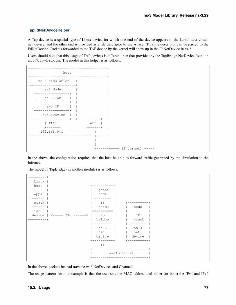
ns-3 Model Library, Release ns-3.29
TapFdNetDeviceHelper
A Tap device is a special type of Linux device for which one end of the device appears to the kernel as a virtualnet_device, and the other end is provided as a file descriptor to user-space. This file descriptor can be passed to theFdNetDevice. Packets forwarded to the TAP device by the kernel will show up in the FdNetDevice in ns-3.
Users should note that this usage of TAP devices is different than that provided by the TapBridge NetDevice found insrc/tap-bridge. The model in this helper is as follows:
+-------------------------------------+| host |+-------------------------------------+| ns-3 simulation | |+----------------------+ || ns-3 Node | || +----------------+ | || | ns-3 TCP | | || +----------------+ | || | ns-3 IP | | || +----------------+ | || | FdNetDevice | | ||--+----------------+--+ +------+ || | TAP | | eth0 | || +------+ +------+ || 192.168.0.1 | |+-------------------------------|-----+
||------------ (Internet) -----
In the above, the configuration requires that the host be able to forward traffic generated by the simulation to theInternet.
The model in TapBridge (in another module) is as follows:
+--------+| Linux || host | +----------+| ------ | | ghost || apps | | node || ------ | | -------- || stack | | IP | +----------+| ------ | | stack | | node || TAP | |==========| | -------- || device | <----- IPC ------> | tap | | IP |+--------+ | bridge | | stack |
| -------- | | -------- || ns-3 | | ns-3 || net | | net || device | | device |+----------+ +----------+
|| ||+---------------------------+| ns-3 channel |+---------------------------+
In the above, packets instead traverse ns-3 NetDevices and Channels.
The usage pattern for this example is that the user sets the MAC address and either (or both) the IPv4 and IPv6
15.2. Usage 77
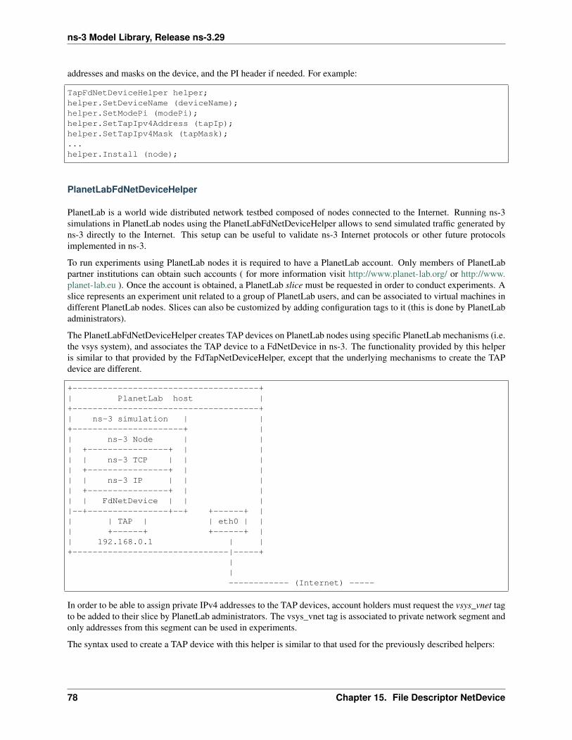
ns-3 Model Library, Release ns-3.29
addresses and masks on the device, and the PI header if needed. For example:
TapFdNetDeviceHelper helper;helper.SetDeviceName (deviceName);helper.SetModePi (modePi);helper.SetTapIpv4Address (tapIp);helper.SetTapIpv4Mask (tapMask);...helper.Install (node);
PlanetLabFdNetDeviceHelper
PlanetLab is a world wide distributed network testbed composed of nodes connected to the Internet. Running ns-3simulations in PlanetLab nodes using the PlanetLabFdNetDeviceHelper allows to send simulated traffic generated byns-3 directly to the Internet. This setup can be useful to validate ns-3 Internet protocols or other future protocolsimplemented in ns-3.
To run experiments using PlanetLab nodes it is required to have a PlanetLab account. Only members of PlanetLabpartner institutions can obtain such accounts ( for more information visit http://www.planet-lab.org/ or http://www.planet-lab.eu ). Once the account is obtained, a PlanetLab slice must be requested in order to conduct experiments. Aslice represents an experiment unit related to a group of PlanetLab users, and can be associated to virtual machines indifferent PlanetLab nodes. Slices can also be customized by adding configuration tags to it (this is done by PlanetLabadministrators).
The PlanetLabFdNetDeviceHelper creates TAP devices on PlanetLab nodes using specific PlanetLab mechanisms (i.e.the vsys system), and associates the TAP device to a FdNetDevice in ns-3. The functionality provided by this helperis similar to that provided by the FdTapNetDeviceHelper, except that the underlying mechanisms to create the TAPdevice are different.
+-------------------------------------+| PlanetLab host |+-------------------------------------+| ns-3 simulation | |+----------------------+ || ns-3 Node | || +----------------+ | || | ns-3 TCP | | || +----------------+ | || | ns-3 IP | | || +----------------+ | || | FdNetDevice | | ||--+----------------+--+ +------+ || | TAP | | eth0 | || +------+ +------+ || 192.168.0.1 | |+-------------------------------|-----+
||------------ (Internet) -----
In order to be able to assign private IPv4 addresses to the TAP devices, account holders must request the vsys_vnet tagto be added to their slice by PlanetLab administrators. The vsys_vnet tag is associated to private network segment andonly addresses from this segment can be used in experiments.
The syntax used to create a TAP device with this helper is similar to that used for the previously described helpers:
78 Chapter 15. File Descriptor NetDevice
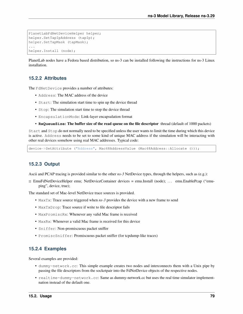
ns-3 Model Library, Release ns-3.29
PlanetLabFdNetDeviceHelper helper;helper.SetTapIpAddress (tapIp);helper.SetTapMask (tapMask);...helper.Install (node);
PlanetLab nodes have a Fedora based distribution, so ns-3 can be installed following the instructions for ns-3 Linuxinstallation.
15.2.2 Attributes
The FdNetDevice provides a number of attributes:
• Address: The MAC address of the device
• Start: The simulation start time to spin up the device thread
• Stop: The simulation start time to stop the device thread
• EncapsulationMode: Link-layer encapsulation format
• RxQueueSize: The buffer size of the read queue on the file descriptor thread (default of 1000 packets)
Start and Stop do not normally need to be specified unless the user wants to limit the time during which this deviceis active. Address needs to be set to some kind of unique MAC address if the simulation will be interacting withother real devices somehow using real MAC addresses. Typical code:
device->SetAttribute ("Address", Mac48AddressValue (Mac48Address::Allocate ()));
15.2.3 Output
Ascii and PCAP tracing is provided similar to the other ns-3 NetDevice types, through the helpers, such as (e.g.):
:: EmuFdNetDeviceHelper emu; NetDeviceContainer devices = emu.Install (node); . . . emu.EnablePcap (“emu-ping”, device, true);
The standard set of Mac-level NetDevice trace sources is provided.
• MaxTx: Trace source triggered when ns-3 provides the device with a new frame to send
• MaxTxDrop: Trace source if write to file descriptor fails
• MaxPromiscRx: Whenever any valid Mac frame is received
• MaxRx: Whenever a valid Mac frame is received for this device
• Sniffer: Non-promiscuous packet sniffer
• PromiscSniffer: Promiscuous packet sniffer (for tcpdump-like traces)
15.2.4 Examples
Several examples are provided:
• dummy-network.cc: This simple example creates two nodes and interconnects them with a Unix pipe bypassing the file descriptors from the socketpair into the FdNetDevice objects of the respective nodes.
• realtime-dummy-network.cc: Same as dummy-network.cc but uses the real time simulator implement-nation instead of the default one.
15.2. Usage 79
ns-3 Model Library, Release ns-3.29
• fd2fd-onoff.cc: This example is aimed at measuring the throughput of the FdNetDevice in a pure simu-lation. For this purpose two FdNetDevices, attached to different nodes but in a same simulation, are connectedusing a socket pair. TCP traffic is sent at a saturating data rate.
• fd-emu-onoff.cc: This example is aimed at measuring the throughput of the FdNetDevice when using theEmuFdNetDeviceHelper to attach the simulated device to a real device in the host machine. This is achieved bysaturating the channel with TCP traffic.
• fd-emu-ping.cc: This example uses the EmuFdNetDeviceHelper to send ICMP traffic over a real channel.
• fd-emu-udp-echo.cc: This example uses the EmuFdNetDeviceHelper to send UDP traffic over a realchannel.
• fd-planetlab-ping.cc: This example shows how to set up an experiment to send ICMP traffic from aPlanetLab node to the Internet.
• fd-tap-ping.cc: This example uses the TapFdNetDeviceHelper to send ICMP traffic over a real channel.
80 Chapter 15. File Descriptor NetDevice
CHAPTER
SIXTEEN
FLOW MONITOR
16.1 Model Description
The source code for the new module lives in the directory src/flow-monitor.
The Flow Monitor module goal is to provide a flexible system to measure the performance of network protocols. Themodule uses probes, installed in network nodes, to track the packets exchanged by the nodes, and it will measure anumber of parameters. Packets are divided according to the flow they belong to, where each flow is defined accordingto the probe’s characteristics (e.g., for IP, a flow is defined as the packets with the same {protocol, source (IP, port),destination (IP, port)} tuple.
The statistics are collected for each flow can be exported in XML format. Moreover, the user can access the probesdirectly to request specific stats about each flow.
16.1.1 Design
Flow Monitor module is designed in a modular way. It can be extended by subclassing ns3::FlowProbe andns3::FlowClassifier.
The full module design is described in [FlowMonitor]
16.1.2 Scope and Limitations
At the moment, probes and classifiers are available for IPv4 and IPv6.
Each probe will classify packets in four points:
• When a packet is sent (SendOutgoing IPv[4,6] traces)
• When a packet is forwarded (UnicastForward IPv[4,6] traces)
• When a packet is received (LocalDeliver IPv[4,6] traces)
• When a packet is dropped (Drop IPv[4,6] traces)
Since the packets are tracked at IP level, any retransmission caused by L4 protocols (e.g., TCP) will be seen by theprobe as a new packet.
A Tag will be added to the packet (ns3::Ipv[4,6]FlowProbeTag). The tag will carry basic packet’s data,useful for the packet’s classification.
It must be underlined that only L4 (TCP, UDP) packets are, so far, classified. Moreover, only unicast packets will beclassified. These limitations may be removed in the future.
The data collected for each flow are:
81

ns-3 Model Library, Release ns-3.29
• timeFirstTxPacket: when the first packet in the flow was transmitted;
• timeLastTxPacket: when the last packet in the flow was transmitted;
• timeFirstRxPacket: when the first packet in the flow was received by an end node;
• timeLastRxPacket: when the last packet in the flow was received;
• delaySum: the sum of all end-to-end delays for all received packets of the flow;
• jitterSum: the sum of all end-to-end delay jitter (delay variation) values for all received packets of the flow, asdefined in RFC 3393;
• txBytes, txPackets: total number of transmitted bytes / packets for the flow;
• rxBytes, rxPackets: total number of received bytes / packets for the flow;
• lostPackets: total number of packets that are assumed to be lost (not reported over 10 seconds);
• timesForwarded: the number of times a packet has been reportedly forwarded;
• delayHistogram, jitterHistogram, packetSizeHistogram: histogram versions for the delay, jitter, and packet sizes,respectively;
• packetsDropped, bytesDropped: the number of lost packets and bytes, divided according to the loss reason code(defined in the probe).
It is worth pointing out that the probes measure the packet bytes including IP headers. The L2 headers are not includedin the measure.
These stats will be written in XML form upon request (see the Usage section).
16.1.3 References
16.2 Usage
The module usage is extremely simple. The helper will take care of about everything.
The typical use is:
// Flow monitorPtr<FlowMonitor> flowMonitor;FlowMonitorHelper flowHelper;flowMonitor = flowHelper.InstallAll();
Simulator::Stop (Seconds(stop_time));Simulator::Run ();
flowMonitor->SerializeToXmlFile("NameOfFile.xml", true, true);
the SerializeToXmlFile () function 2nd and 3rd parameters are used respectively to activate/deactivate thehistograms and the per-probe detailed stats.
Other possible alternatives can be found in the Doxygen documentation.
16.2.1 Helpers
The helper API follows the pattern usage of normal helpers. Through the helper you can install the monitor in thenodes, set the monitor attributes, and print the statistics.
82 Chapter 16. Flow Monitor

ns-3 Model Library, Release ns-3.29
One important thing is: the ns3::FlowMonitorHelper must be instantiated only once in the main.
16.2.2 Attributes
The module provides the following attributes in ns3::FlowMonitor:
• MaxPerHopDelay (Time, default 10s): The maximum per-hop delay that should be considered;
• StartTime (Time, default 0s): The time when the monitoring starts;
• DelayBinWidth (double, default 0.001): The width used in the delay histogram;
• JitterBinWidth (double, default 0.001): The width used in the jitter histogram;
• PacketSizeBinWidth (double, default 20.0): The width used in the packetSize histogram;
• FlowInterruptionsBinWidth (double, default 0.25): The width used in the flowInterruptions histogram;
• FlowInterruptionsMinTime (double, default 0.5): The minimum inter-arrival time that is considered a flowinterruption.
16.2.3 Output
The main model output is an XML formatted report about flow statistics. An example is:
<?xml version="1.0" ?><FlowMonitor>
<FlowStats><Flow flowId="1" timeFirstTxPacket="+0.0ns" timeFirstRxPacket="+20067198.0ns"
↪→timeLastTxPacket="+2235764408.0ns" timeLastRxPacket="+2255831606.0ns" delaySum=↪→"+138731526300.0ns" jitterSum="+1849692150.0ns" lastDelay="+20067198.0ns" txBytes=↪→"2149400" rxBytes="2149400" txPackets="3735" rxPackets="3735" lostPackets="0"↪→timesForwarded="7466"></Flow></FlowStats><Ipv4FlowClassifier><Flow flowId="1" sourceAddress="10.1.3.1" destinationAddress="10.1.2.2" protocol="6
↪→" sourcePort="49153" destinationPort="50000" /></Ipv4FlowClassifier><Ipv6FlowClassifier></Ipv6FlowClassifier><FlowProbes><FlowProbe index="0"><FlowStats flowId="1" packets="3735" bytes="2149400" delayFromFirstProbeSum="+0.
↪→0ns" ></FlowStats>
</FlowProbe><FlowProbe index="2"><FlowStats flowId="1" packets="7466" bytes="2224020" delayFromFirstProbeSum=
↪→"+199415389258.0ns" ></FlowStats>
</FlowProbe><FlowProbe index="4"><FlowStats flowId="1" packets="3735" bytes="2149400" delayFromFirstProbeSum=
↪→"+138731526300.0ns" ></FlowStats>
</FlowProbe>
(continues on next page)
16.2. Usage 83
ns-3 Model Library, Release ns-3.29
(continued from previous page)
</FlowProbes></FlowMonitor>
The output was generated by a TCP flow from 10.1.3.1 to 10.1.2.2.
It is worth noticing that the index 2 probe is reporting more packets and more bytes than the other probes. That’s aperfectly normal behaviour, as packets are fragmented at IP level in that node.
It should also be observed that the receiving node’s probe (index 4) doesn’t count the fragments, as the reassembly isdone before the probing point.
16.2.4 Examples
The examples are located in src/flow-monitor/examples.
Moreover, the following examples use the flow-monitor module:
• examples/matrix-topology/matrix-topology.cc
• examples/routing/manet-routing-compare.cc
• examples/routing/simple-global-routing.cc
• examples/tcp/tcp-variants-comparison.cc
• examples/wireless/multirate.cc
• examples/wireless/wifi-hidden-terminal.cc
16.2.5 Troubleshooting
Do not define more than one ns3::FlowMonitorHelper in the simulation.
16.3 Validation
The paper in the references contains a full description of the module validation against a test network.
Tests are provided to ensure the Histogram correct functionality.
84 Chapter 16. Flow Monitor

CHAPTER
SEVENTEEN
INTERNET MODELS (IP, TCP, ROUTING, UDP, INTERNETAPPLICATIONS)
17.1 Internet Stack
17.1.1 Internet stack aggregation
A bare class Node is not very useful as-is; other objects must be aggregated to it to provide useful node functionality.
The ns-3 source code directory src/internet provides implementation of TCP/IPv4- and IPv6-related compo-nents. These include IPv4, ARP, UDP, TCP, IPv6, Neighbor Discovery, and other related protocols.
Internet Nodes are not subclasses of class Node; they are simply Nodes that have had a bunch of IP-related objects ag-gregated to them. They can be put together by hand, or via a helper function InternetStackHelper::Install() which does the following to all nodes passed in as arguments:
voidInternetStackHelper::Install (Ptr<Node> node) const{
if (m_ipv4Enabled){
/* IPv4 stack */if (node->GetObject<Ipv4> () != 0)
{NS_FATAL_ERROR ("InternetStackHelper::Install (): Aggregating "
"an InternetStack to a node with an existing Ipv4 object");return;
}
CreateAndAggregateObjectFromTypeId (node, "ns3::ArpL3Protocol");CreateAndAggregateObjectFromTypeId (node, "ns3::Ipv4L3Protocol");CreateAndAggregateObjectFromTypeId (node, "ns3::Icmpv4L4Protocol");// Set routingPtr<Ipv4> ipv4 = node->GetObject<Ipv4> ();Ptr<Ipv4RoutingProtocol> ipv4Routing = m_routing->Create (node);ipv4->SetRoutingProtocol (ipv4Routing);
}
if (m_ipv6Enabled){
/* IPv6 stack */if (node->GetObject<Ipv6> () != 0)
{NS_FATAL_ERROR ("InternetStackHelper::Install (): Aggregating "
(continues on next page)
85

ns-3 Model Library, Release ns-3.29
(continued from previous page)
"an InternetStack to a node with an existing Ipv6 object");return;
}
CreateAndAggregateObjectFromTypeId (node, "ns3::Ipv6L3Protocol");CreateAndAggregateObjectFromTypeId (node, "ns3::Icmpv6L4Protocol");// Set routingPtr<Ipv6> ipv6 = node->GetObject<Ipv6> ();Ptr<Ipv6RoutingProtocol> ipv6Routing = m_routingv6->Create (node);ipv6->SetRoutingProtocol (ipv6Routing);
/* register IPv6 extensions and options */ipv6->RegisterExtensions ();ipv6->RegisterOptions ();
}
if (m_ipv4Enabled || m_ipv6Enabled){
/* UDP and TCP stacks */CreateAndAggregateObjectFromTypeId (node, "ns3::UdpL4Protocol");node->AggregateObject (m_tcpFactory.Create<Object> ());Ptr<PacketSocketFactory> factory = CreateObject<PacketSocketFactory> ();node->AggregateObject (factory);
}}
Where multiple implementations exist in ns-3 (TCP, IP routing), these objects are added by a factory object (TCP) orby a routing helper (m_routing).
Note that the routing protocol is configured and set outside this function. By default, the following protocols are added:
void InternetStackHelper::Initialize (){
SetTcp ("ns3::TcpL4Protocol");Ipv4StaticRoutingHelper staticRouting;Ipv4GlobalRoutingHelper globalRouting;Ipv4ListRoutingHelper listRouting;Ipv6ListRoutingHelper listRoutingv6;Ipv6StaticRoutingHelper staticRoutingv6;listRouting.Add (staticRouting, 0);listRouting.Add (globalRouting, -10);listRoutingv6.Add (staticRoutingv6, 0);SetRoutingHelper (listRouting);SetRoutingHelper (listRoutingv6);
}
By default, IPv4 and IPv6 are enabled.
Internet Node structure
An IP-capable Node (an ns-3 Node augmented by aggregation to have one or more IP stacks) has the following internalstructure.
86 Chapter 17. Internet Models (IP, TCP, Routing, UDP, Internet Applications)

ns-3 Model Library, Release ns-3.29
Layer-3 protocols
At the lowest layer, sitting above the NetDevices, are the “layer 3” protocols, including IPv4, IPv6, ARP and so on.The class Ipv4L3Protocol is an implementation class whose public interface is typically class Ipv4, but theIpv4L3Protocol public API is also used internally at present.
In class Ipv4L3Protocol, one method described below is Receive ():
/*** Lower layer calls this method after calling L3Demux::Lookup
* The ARP subclass needs to know from which NetDevice this
* packet is coming to:
* - implement a per-NetDevice ARP cache
* - send back arp replies on the right device
*/void Receive( Ptr<NetDevice> device, Ptr<const Packet> p, uint16_t protocol,const Address &from, const Address &to, NetDevice::PacketType packetType);
First, note that the Receive () function has a matching signature to the ReceiveCallback in the class Node. Thisfunction pointer is inserted into the Node’s protocol handler when AddInterface () is called. The actual regis-tration is done with a statement such as follows:
RegisterProtocolHandler ( MakeCallback (&Ipv4Protocol::Receive, ipv4),Ipv4L3Protocol::PROT_NUMBER, 0);
The Ipv4L3Protocol object is aggregated to the Node; there is only one such Ipv4L3Protocol object. Higher-layerprotocols that have a packet to send down to the Ipv4L3Protocol object can call GetObject<Ipv4L3Protocol>() to obtain a pointer, as follows:
Ptr<Ipv4L3Protocol> ipv4 = m_node->GetObject<Ipv4L3Protocol> ();if (ipv4 != 0)
{ipv4->Send (packet, saddr, daddr, PROT_NUMBER);
}
This class nicely demonstrates two techniques we exploit in ns-3 to bind objects together: callbacks, and objectaggregation.
Once IPv4 routing has determined that a packet is for the local node, it forwards it up the stack. This is done with thefollowing function:
voidIpv4L3Protocol::LocalDeliver (Ptr<const Packet> packet, Ipv4Header const&ip, uint32_t↪→iif)
The first step is to find the right Ipv4L4Protocol object, based on IP protocol number. For instance, TCP is reg-istered in the demux as protocol number 6. Finally, the Receive() function on the Ipv4L4Protocol (such asTcpL4Protocol::Receive is called.
We have not yet introduced the class Ipv4Interface. Basically, each NetDevice is paired with an IPv4 representationof such device. In Linux, this class Ipv4Interface roughly corresponds to the struct in_device; the mainpurpose is to provide address-family specific information (addresses) about an interface.
All the classes have appropriate traces in order to track sent, received and lost packets. The users is encouraged touse them so to find out if (and where) a packet is dropped. A common mistake is to forget the effects of local queueswhen sending packets, e.g., the ARP queue. This can be particularly puzzling when sending jumbo packets or packetbursts using UDP. The ARP cache pending queue is limited (3 datagrams) and IP packets might be fragmented, easily
17.1. Internet Stack 87
ns-3 Model Library, Release ns-3.29
overfilling the ARP cache queue size. In those cases it is useful to increase the ARP cache pending size to a propervalue, e.g.:
Config::SetDefault ("ns3::ArpCache::PendingQueueSize", UintegerValue (MAX_BURST_SIZE/↪→L2MTU*3));
The IPv6 implementation follows a similar architecture. Dual-stacked nodes (one with support for both IPv4 and IPv6)will allow an IPv6 socket to receive IPv4 connections as a standard dual-stacked system does. A socket bound andlistening to an IPv6 endpoint can receive an IPv4 connection and will return the remote address as an IPv4-mappedaddress. Support for the IPV6_V6ONLY socket option does not currently exist.
Layer-4 protocols and sockets
We next describe how the transport protocols, sockets, and applications tie together. In summary, each transportprotocol implementation is a socket factory. An application that needs a new socket
For instance, to create a UDP socket, an application would use a code snippet such as the following:
Ptr<Udp> udpSocketFactory = GetNode ()->GetObject<Udp> ();Ptr<Socket> m_socket = socketFactory->CreateSocket ();m_socket->Bind (m_local_address);...
The above will query the node to get a pointer to its UDP socket factory, will create one such socket, and will use thesocket with an API similar to the C-based sockets API, such as Connect () and Send (). The address passed tothe Bind (), Connect (), or Send () functions may be a Ipv4Address, Ipv6Address, or Address. Ifa Address is passed in and contains anything other than a Ipv4Address or Ipv6Address, these functions willreturn an error. The Bind (void) and Bind6 (void) functions bind to “0.0.0.0” and “::” respectively.
The socket can also be bound to a specific NetDevice though the BindToNetDevice (Ptr<NetDevice>netdevice) function. BindToNetDevice (Ptr<NetDevice> netdevice) will bind the socket to“0.0.0.0” and “::” (equivalent to calling Bind () and Bind6 (), unless the socket has been already bound to aspecific address. Summarizing, the correct sequence is:
Ptr<Udp> udpSocketFactory = GetNode ()->GetObject<Udp> ();Ptr<Socket> m_socket = socketFactory->CreateSocket ();m_socket->BindToNetDevice (n_netDevice);
...
or:
Ptr<Udp> udpSocketFactory = GetNode ()->GetObject<Udp> ();Ptr<Socket> m_socket = socketFactory->CreateSocket ();m_socket->Bind (m_local_address);m_socket->BindToNetDevice (n_netDevice);...
The following raises an error:
Ptr<Udp> udpSocketFactory = GetNode ()->GetObject<Udp> ();Ptr<Socket> m_socket = socketFactory->CreateSocket ();m_socket->BindToNetDevice (n_netDevice);m_socket->Bind (m_local_address);...
See the chapter on ns-3 sockets for more information.
88 Chapter 17. Internet Models (IP, TCP, Routing, UDP, Internet Applications)

ns-3 Model Library, Release ns-3.29
We have described so far a socket factory (e.g. class Udp) and a socket, which may be specialized (e.g., classUdpSocket). There are a few more key objects that relate to the specialized task of demultiplexing a packet to oneor more receiving sockets. The key object in this task is class Ipv4EndPointDemux. This demultiplexer storesobjects of class Ipv4EndPoint. This class holds the addressing/port tuple (local port, local address, destination port,destination address) associated with the socket, and a receive callback. This receive callback has a receive functionregistered by the socket. The Lookup () function to Ipv4EndPointDemux returns a list of Ipv4EndPoint objects(there may be a list since more than one socket may match the packet). The layer-4 protocol copies the packet to eachIpv4EndPoint and calls its ForwardUp () method, which then calls the Receive () function registered by thesocket.
An issue that arises when working with the sockets API on real systems is the need to manage the reading from asocket, using some type of I/O (e.g., blocking, non-blocking, asynchronous, . . . ). ns-3 implements an asynchronousmodel for socket I/O; the application sets a callback to be notified of received data ready to be read, and the callbackis invoked by the transport protocol when data is available. This callback is specified as follows:
void Socket::SetRecvCallback (Callback<void, Ptr<Socket>,Ptr<Packet>,const Address&> receivedData);
The data being received is conveyed in the Packet data buffer. An example usage is in class PacketSink:
m_socket->SetRecvCallback (MakeCallback(&PacketSink::HandleRead, this));
To summarize, internally, the UDP implementation is organized as follows:
• a UdpImpl class that implements the UDP socket factory functionality
• a UdpL4Protocol class that implements the protocol logic that is socket-independent
• a UdpSocketImpl class that implements socket-specific aspects of UDP
• a class called Ipv4EndPoint that stores the addressing tuple (local port, local address, destination port,destination address) associated with the socket, and a receive callback for the socket.
IP-capable node interfaces
Many of the implementation details, or internal objects themselves, of IP-capable Node objects are not exposed at thesimulator public API. This allows for different implementations; for instance, replacing the native ns-3 models withported TCP/IP stack code.
The C++ public APIs of all of these objects is found in the src/network directory, including principally:
• address.h
• socket.h
• node.h
• packet.h
These are typically base class objects that implement the default values used in the implementation, implement accessmethods to get/set state variables, host attributes, and implement publicly-available methods exposed to clients suchas CreateSocket.
Example path of a packet
These two figures show an example stack trace of how packets flow through the Internet Node objects.
17.1. Internet Stack 89

ns-3 Model Library, Release ns-3.29
Fig. 1: Send path of a packet.
Fig. 2: Receive path of a packet.
90 Chapter 17. Internet Models (IP, TCP, Routing, UDP, Internet Applications)

ns-3 Model Library, Release ns-3.29
17.2 IPv4
This chapter describes the ns-3 IPv4 address assignment and basic components tracking.
17.2.1 IPv4 addresses assignment
In order to use IPv4 on a network, the first thing to do is assigning IPv4 addresses.
Any IPv4-enabled ns-3 node will have at least one NetDevice: the ns3::LoopbackNetDevice. The loopbackdevice address is 127.0.0.1. All the other NetDevices will have one (or more) IPv4 addresses.
Note that, as today, ns-3 does not have a NAT module, and it does not follows the rules about filtering private addresses(RFC 1918): 10.0.0.0/8, 172.16.0.0/12, and 192.168.0.0/16. These addresses are routed as any other address. Thisbehaviour could change in the future.
IPv4 global addresses can be:
• manually assigned
• assigned though DHCP
ns-3 can use both methods, and it’s quite important to understand the implications of both.
Manually assigned IPv4 addresses
This is probably the easiest and most used method. As an example:
Ptr<Node> n0 = CreateObject<Node> ();Ptr<Node> n1 = CreateObject<Node> ();NodeContainer net (n0, n1);CsmaHelper csma;NetDeviceContainer ndc = csma.Install (net);
NS_LOG_INFO ("Assign IPv4 Addresses.");Ipv4AddressHelper ipv4;ipv4.SetBase (Ipv4Address ("192.168.1.0"), NetMask ("/24"));Ipv4InterfaceContainer ic = ipv4.Assign (ndc);
This method will add two global IPv4 addresses to the nodes.
Note that the addresses are assigned in sequence. As a consequence, the first Node / NetDevice will have“192.168.1.1”, the second “192.168.1.2” and so on.
It is possible to repeat the above to assign more than one address to a node. However, due to theIpv4AddressHelper singleton nature, one should first assign all the addresses of a network, then change thenetwork base (SetBase), then do a new assignment.
Alternatively, it is possible to assign a specific address to a node:
Ptr<Node> n0 = CreateObject<Node> ();NodeContainer net (n0);CsmaHelper csma;NetDeviceContainer ndc = csma.Install (net);
NS_LOG_INFO ("Specifically Assign an IPv4 Address.");Ipv4AddressHelper ipv4;Ptr<NetDevice> device = ndc.Get (0);
(continues on next page)
17.2. IPv4 91

ns-3 Model Library, Release ns-3.29
(continued from previous page)
Ptr<Node> node = device->GetNode ();Ptr<Ipv4> ipv4proto = node->GetObject<Ipv4> ();int32_t ifIndex = 0;ifIndex = ipv4proto->GetInterfaceForDevice (device);Ipv4InterfaceAddress ipv4Addr = Ipv4InterfaceAddress (Ipv4Address ("192.168.1.42"),↪→NetMask ("/24"));ipv4proto->AddAddress (ifIndex, ipv4Addr);
DHCP assigned IPv4 addresses
DHCP is available in the internet-apps module. In order to use DHCP you have to have a DhcpServer applicationin a node (the DHC server node) and a DhcpClient application in each of the nodes. Note that it not necessary thatall the nodes in a subnet use DHCP. Some nodes can have static addresses.
All the DHCP setup is performed though the DhcpHelper class. A complete example is in src/internet-apps/examples/dhcp-example.cc.
Further info about the DHCP functionalities can be found in the internet-apps model documentation.
17.2.2 Tracing in the IPv4 Stack
The internet stack provides a number of trace sources in its various protocol implementations. These trace sources canbe hooked using your own custom trace code, or you can use our helper functions in some cases to arrange for tracingto be enabled.
Tracing in ARP
ARP provides two trace hooks, one in the cache, and one in the layer three protocol. The trace accessor in the cacheis given the name “Drop.” When a packet is transmitted over an interface that requires ARP, it is first queued fortransmission in the ARP cache until the required MAC address is resolved. There are a number of retries that may bedone trying to get the address, and if the maximum retry count is exceeded the packet in question is dropped by ARP.The single trace hook in the ARP cache is called,
• If an outbound packet is placed in the ARP cache pending address resolution and no resolution can be madewithin the maximum retry count, the outbound packet is dropped and this trace is fired;
A second trace hook lives in the ARP L3 protocol (also named “Drop”) and may be called for a number of reasons.
• If an ARP reply is received for an entry that is not waiting for a reply, the ARP reply packet is dropped and thistrace is fired;
• If an ARP reply is received for a non-existent entry, the ARP reply packet is dropped and this trace is fired;
• If an ARP cache entry is in the DEAD state (has timed out) and an ARP reply packet is received, the replypacket is dropped and this trace is fired.
• Each ARP cache entry has a queue of pending packets. If the size of the queue is exceeded, the outbound packetis dropped and this trace is fired.
Tracing in IPv4
The IPv4 layer three protocol provides three trace hooks. These are the “Tx” (ns3::Ipv4L3Protocol::m_txTrace), “Rx”(ns3::Ipv4L3Protocol::m_rxTrace) and “Drop” (ns3::Ipv4L3Protocol::m_dropTrace) trace sources.
92 Chapter 17. Internet Models (IP, TCP, Routing, UDP, Internet Applications)
ns-3 Model Library, Release ns-3.29
The “Tx” trace is fired in a number of situations, all of which indicate that a given packet is about to be sent down toa given ns3::Ipv4Interface.
• In the case of a packet destined for the broadcast address, the Ipv4InterfaceList is iterated and for every interfacethat is up and can fragment the packet or has a large enough MTU to transmit the packet, the trace is hit. Seens3::Ipv4L3Protocol::Send.
• In the case of a packet that needs routing, the “Tx” trace may be fired just before a packet is sent to the interfaceappropriate to the default gateway. See ns3::Ipv4L3Protocol::SendRealOut.
• Also in the case of a packet that needs routing, the “Tx” trace may be fired just before a packet is sent to theoutgoing interface appropriate to the discovered route. See ns3::Ipv4L3Protocol::SendRealOut.
The “Rx” trace is fired when a packet is passed from the device up to the ns3::Ipv4L3Protocol::Receive function.
• In the receive function, the Ipv4InterfaceList is iterated, and if the Ipv4Interface corresponding to the receivingdevice is fount to be in the UP state, the trace is fired.
The “Drop” trace is fired in any case where the packet is dropped (in both the transmit and receive paths).
• In the ns3::Ipv4Interface::Receive function, the packet is dropped and the drop trace is hit if the interface corre-sponding to the receiving device is in the DOWN state.
• Also in the ns3::Ipv4Interface::Receive function, the packet is dropped and the drop trace is hit if the checksumis found to be bad.
• In ns3::Ipv4L3Protocol::Send, an outgoing packet bound for the broadcast address is dropped and the “Drop”trace is fired if the “don’t fragment” bit is set and fragmentation is available and required.
• Also in ns3::Ipv4L3Protocol::Send, an outgoing packet destined for the broadcast address is dropped and the“Drop” trace is hit if fragmentation is not available and is required (MTU < packet size).
• In the case of a broadcast address, an outgoing packet is cloned for each outgoing interface. If any of theinterfaces is in the DOWN state, the “Drop” trace event fires with a reference to the copied packet.
• In the case of a packet requiring a route, an outgoing packet is dropped and the “Drop” trace event fires if noroute to the remote host is found.
• In ns3::Ipv4L3Protocol::SendRealOut, an outgoing packet being routed is dropped and the “Drop” trace is firedif the “don’t fragment” bit is set and fragmentation is available and required.
• Also in ns3::Ipv4L3Protocol::SendRealOut, an outgoing packet being routed is dropped and the “Drop” trace ishit if fragmentation is not available and is required (MTU < packet size).
• An outgoing packet being routed is dropped and the “Drop” trace event fires if the required Ipv4Interface is inthe DOWN state.
• If a packet is being forwarded, and the TTL is exceeded (see ns3::Ipv4L3Protocol::DoForward), the packet isdropped and the “Drop” trace event is fired.
17.2.3 Explicit Congestion Notification (ECN) bits
• In IPv4, ECN bits are the last 2 bits in TOS field and occupy 14th and 15th bits in the header.
• The IPv4 header class defines an EcnType enum with all four ECN codepoints (ECN_NotECT, ECN_ECT1,ECN_ECT0, ECN_CE) mentioned in RFC 3168, and also a setter and getter method to handle ECN values inthe TOS field.
17.2. IPv4 93
ns-3 Model Library, Release ns-3.29
17.2.4 Ipv4QueueDiscItem
The traffic control sublayer in ns-3 handles objects of class QueueDiscItem which are used to hold an ns3::Packetand an ns3::Header. This is done to facilitate the marking of packets for Explicit Congestion Notification. TheMark () method is implemented in Ipv4QueueDiscItem. It returns true if marking the packet is successful, i.e., itsuccessfully sets the CE bit in the IPv4 header. The Mark () method will return false, however, if the IPv4 headerindicates the ECN_NotECT codepoint.
17.3 IPv6
This chapter describes the ns-3 IPv6 model capabilities and limitations along with its usage and examples.
17.3.1 IPv6 model description
The IPv6 model is loosely patterned after the Linux implementation; the implementation is not complete as somefeatures of IPv6 are not of much interest to simulation studies, and some features of IPv6 are simply not modeled yetin ns-3.
The base class Ipv6 defines a generic API, while the class Ipv6L3Protocol is the actual class implementing theprotocol. The actual classes used by the IPv6 stack are located mainly in the directory src/internet.
The implementation of IPv6 is contained in the following files:
src/internet/model/icmpv6-header.{cc,h}src/internet/model/icmpv6-l4-protocol.{cc,h}src/internet/model/ipv6.{cc,h}src/internet/model/ipv6-address-generator.{cc,h}src/internet/model/ipv6-autoconfigured-prefix.{cc,h}src/internet/model/ipv6-end-point.{cc,h}src/internet/model/ipv6-end-point-demux.{cc,h}src/internet/model/ipv6-extension.{cc,h}src/internet/model/ipv6-extension-demux.{cc,h}src/internet/model/ipv6-extension-header.{cc,h}src/internet/model/ipv6-header.{cc,h}src/internet/model/ipv6-interface.{cc,h}src/internet/model/ipv6-interface-address.{cc,h}src/internet/model/ipv6-l3-protocol.{cc,h}src/internet/model/ipv6-list-routing.{cc,h}src/internet/model/ipv6-option.{cc,h}src/internet/model/ipv6-option-demux.{cc,h}src/internet/model/ipv6-option-header.{cc,h}src/internet/model/ipv6-packet-info-tag.{cc,h}src/internet/model/ipv6-pmtu-cache.{cc,h}src/internet/model/ipv6-raw-socket-factory.{cc,h}src/internet/model/ipv6-raw-socket-factory-impl.{cc,h}src/internet/model/ipv6-raw-socket-impl.{cc,h}src/internet/model/ipv6-route.{cc,h}src/internet/model/ipv6-routing-protocol.{cc,h}src/internet/model/ipv6-routing-table-entry.{cc,h}src/internet/model/ipv6-static-routing.{cc,h}src/internet/model/ndisc-cache.{cc,h}src/network/utils/inet6-socket-address.{cc,h}src/network/utils/ipv6-address.{cc,h}
Also some helpers are involved with IPv6:
94 Chapter 17. Internet Models (IP, TCP, Routing, UDP, Internet Applications)

ns-3 Model Library, Release ns-3.29
src/internet/helper/internet-stack-helper.{cc,h}src/internet/helper/ipv6-address-helper.{cc,h}src/internet/helper/ipv6-interface-container.{cc,h}src/internet/helper/ipv6-list-routing-helper.{cc,h}src/internet/helper/ipv6-routing-helper.{cc,h}src/internet/helper/ipv6-static-routing-helper.{cc,h}
The model files can be roughly divided into:
• protocol models (e.g., ipv6, ipv6-l3-protocol, icmpv6-l4-protocol, etc.)
• routing models (i.e., anything with ‘routing’ in its name)
• sockets and interfaces (e.g., ipv6-raw-socket, ipv6-interface, ipv6-end-point, etc.)
• address-related things
• headers, option headers, extension headers, etc.
• accessory classes (e.g., ndisc-cache)
17.3.2 Usage
The following description is based on using the typical helpers found in the example code.
IPv6 does not need to be activated in a node. it is automatically added to the available protocols once the InternetStack is installed.
In order to not install IPv6 along with IPv4, it is possible to use ns3::InternetStackHelper methodSetIpv6StackInstall (bool enable) before installing the InternetStack in the nodes.
Note that to have an IPv6-only network (i.e., to not install the IPv4 stack in a node) one should usens3::InternetStackHelper method SetIpv4StackInstall (bool enable) before the stack installation.
As an example, in the following code node 0 will have both IPv4 and IPv6, node 1 only only IPv6 and node 2 onlyIPv4:
NodeContainer n;n.Create (3);
InternetStackHelper internet;InternetStackHelper internetV4only;InternetStackHelper internetV6only;
internetV4only.SetIpv6StackInstall (false);internetV6only.SetIpv4StackInstall (false);
internet.Install (n.Get (0));internetV6only.Install (n.Get (1));internetV4only.Install (n.Get (2));
IPv6 addresses assignment
In order to use IPv6 on a network, the first thing to do is assigning IPv6 addresses.
Any IPv6-enabled ns-3 node will have at least one NetDevice: the ns3::LoopbackNetDevice. The loopbackdevice address is ::1. All the other NetDevices will have one or more IPv6 addresses:
17.3. IPv6 95
ns-3 Model Library, Release ns-3.29
• One link-local address: fe80::interface ID, where interface ID is derived from the NetDeviceMAC address.
• Zero or more global addresses, e.g., 2001:db8::1.
Typically the first address on an interface will be the link-local one, with the global address(es) being the followingones.
IPv6 global addresses might be:
• manually assigned
• auto-generated
ns-3 can use both methods, and it’s quite important to understand the implications of both.
Manually assigned IPv6 addresses
This is probably the easiest and most used method. As an example:
Ptr<Node> n0 = CreateObject<Node> ();Ptr<Node> n1 = CreateObject<Node> ();NodeContainer net (n0, n1);CsmaHelper csma;NetDeviceContainer ndc = csma.Install (net);
NS_LOG_INFO ("Assign IPv6 Addresses.");Ipv6AddressHelper ipv6;ipv6.SetBase (Ipv6Address ("2001:db8::"), Ipv6Prefix (64));Ipv6InterfaceContainer ic = ipv6.Assign (ndc);
This method will add two global IPv6 addresses to the nodes. Note that, as usual for IPv6, all the nodes will also havea link-local address. Typically the first address on an interface will be the link-local one, with the global address(es)being the following ones.
Note that the global addresses will be derived from the MAC address. As a consequence, expect to have addressessimilar to 2001:db8::200:ff:fe00:1.
It is possible to repeat the above to assign more than one global address to a node. However, due to theIpv6AddressHelper singleton nature, one should first assign all the addresses of a network, then change thenetwork base (SetBase), then do a new assignment.
Alternatively, it is possible to assign a specific address to a node:
Ptr<Node> n0 = CreateObject<Node> ();NodeContainer net (n0);CsmaHelper csma;NetDeviceContainer ndc = csma.Install (net);
NS_LOG_INFO ("Specifically Assign an IPv6 Address.");Ipv6AddressHelper ipv6;Ptr<NetDevice> device = ndc.Get (0);Ptr<Node> node = device->GetNode ();Ptr<Ipv6> ipv6proto = node->GetObject<Ipv6> ();int32_t ifIndex = 0;ifIndex = ipv6proto->GetInterfaceForDevice (device);Ipv6InterfaceAddress ipv6Addr = Ipv6InterfaceAddress (Ipv6Address (↪→"2001:db8:f00d:cafe::42"), Ipv6Prefix (64));ipv6proto->AddAddress (ifIndex, ipv6Addr);
96 Chapter 17. Internet Models (IP, TCP, Routing, UDP, Internet Applications)
ns-3 Model Library, Release ns-3.29
Auto-generated IPv6 addresses
This is accomplished by relying on the RADVD protocol, implemented by the class Radvd. A helper class is avail-able, which can be used to ease the most common tasks, e.g., setting up a prefix on an interface, if it is announcedperiodically, and if the router is the default router for that interface.
A fine grain configuration is possible though the RadvdInterface class, which allows to setup every parameter ofthe announced router advertisement on a given interface.
It is worth mentioning that the configurations must be set up before installing the application in the node.
Upon using this method, the nodes will acquire dynamically (i.e., during the simulation) one (or more) global ad-dress(es) according to the RADVD configuration. These addresses will be bases on the RADVD announced prefix andthe node’s EUI-64.
Examples of RADVD use are shown in examples/ipv6/radvd.cc and examples/ipv6/radvd-two-prefix.cc.
Random-generated IPv6 addresses
While IPv6 real nodes will use randomly generated addresses to protect privacy, ns-3 does NOT have this capability.This feature haven’t been so far considered as interesting for simulation.
Duplicate Address Detection (DAD)
Nodes will perform DAD (it can be disabled using an Icmpv6L4Protocol attribute). Upon receiving a DAD,however, nodes will not react to it. As is: DAD reaction is incomplete so far. The main reason relies on the missingrandom-generated address capability. Moreover, since ns-3 nodes will usually be well-behaving, there shouldn’t be anyDuplicate Address. This might be changed in the future, so as to avoid issues with real-world integrated simulations.
Explicit Congestion Notification (ECN) bits in IPv6
• In IPv6, ECN bits are the last 2 bits of the Traffic class and occupy 10th and 11th bit in the header.
• The IPv6 header class defines an EcnType enum with all four ECN codepoints (ECN_NotECT, ECN_ECT1,ECN_ECT0, ECN_CE) mentioned in RFC 3168, and also a setter and getter method to handle ECN values inthe Traffic Class field.
17.3.3 Ipv6QueueDiscItem
The traffic control sublayer in ns-3 handles objects of class QueueDiscItem which are used to hold an ns3::Packetand an ns3::Header. This is done to facilitate the marking of packets for Explicit Congestion Notification. TheMark () method is implemented in Ipv6QueueDiscItem. It returns true if marking the packet is successful, i.e., itsuccessfully sets the CE bit in the IPv6 header. The Mark () method will return false, however, if the IPv6 headerindicates the ECN_NotECT codepoint.
Host and Router behaviour in IPv6 and ns-3
In IPv6 there is a clear distinction between routers and hosts. As one might expect, routers can forward packets froman interface to another interface, while hosts drop packets not directed to them.
17.3. IPv6 97

ns-3 Model Library, Release ns-3.29
Unfortunately, forwarding is not the only thing affected by this distinction, and forwarding itself might be fine-tuned,e.g., to forward packets incoming from an interface and drop packets from another interface.
In ns-3 a node is configured to be an host by default. There are two main ways to change this behaviour:
• Using ns3::Ipv6InterfaceContainer SetForwarding(uint32_t i, bool router) where i is the interfaceindex in the container.
• Changing the ns3::Ipv6 attribute IpForward.
Either one can be used during the simulation.
A fine-grained setup can be accomplished by using ns3::Ipv6Interface SetForwarding (bool forward); whichallows to change the behaviour on a per-interface-basis.
Note that the node-wide configuration only serves as a convenient method to enable/disable thens3::Ipv6Interface specific setting. An Ipv6Interface added to a node with forwarding enabled will beset to be forwarding as well. This is really important when a node has interfaces added during the simulation.
According to the ns3::Ipv6Interface forwarding state, the following happens:
• Forwarding OFF
• The node will NOT reply to Router Solicitation
• The node will react to Router Advertisement
• The node will periodically send Router Solicitation
• Routing protocols MUST DROP packets not directed to the node
• Forwarding ON
• The node will reply to Router Solicitation
• The node will NOT react to Router Advertisement
• The node will NOT send Router Solicitation
• Routing protocols MUST forward packets
The behaviour is matching ip-sysctl.txt (http://www.kernel.org/doc/Documentation/networking/ip-sysctl.txt) with thedifference that it’s not possible to override the behaviour using esoteric settings (e.g., forwarding but accept routeradvertisements, accept_ra=2, or forwarding but send router solicitations forwarding=2).
Consider carefully the implications of packet forwarding. As an example, a node will NOT send ICMPv6PACKET_TOO_BIG messages from an interface with forwarding off. This is completely normal, as the Routingprotocol will drop the packet before attempting to forward it.
Helpers
Typically the helpers used in IPv6 setup are:
• ns3::InternetStackHelper
• ns3::Ipv6AddressHelper
• ns3::Ipv6InterfaceContainer
The use is almost identical to the corresponding IPv4 case, e.g.:
NodeContainer n;n.Create (4);
(continues on next page)
98 Chapter 17. Internet Models (IP, TCP, Routing, UDP, Internet Applications)
ns-3 Model Library, Release ns-3.29
(continued from previous page)
NS_LOG_INFO ("Create IPv6 Internet Stack");InternetStackHelper internetv6;internetv6.Install (n);
NS_LOG_INFO ("Create channels.");CsmaHelper csma;NetDeviceContainer d = csma.Install (n);
NS_LOG_INFO ("Create networks and assign IPv6 Addresses.");Ipv6AddressHelper ipv6;ipv6.SetBase (Ipv6Address ("2001:db8::"), Ipv6Prefix (64));Ipv6InterfaceContainer iic = ipv6.Assign (d);
Additionally, a common task is to enable forwarding on one of the nodes and to setup a default route toward it in theother nodes, e.g.:
iic.SetForwarding (0, true);iic.SetDefaultRouteInAllNodes (0);
This will enable forwarding on the node 0 and will setup a default route in ns3::Ipv6StaticRouting on all theother nodes. Note that this requires that Ipv6StaticRouting is present in the nodes.
The IPv6 routing helpers enable the user to perform specific tasks on the particular routing algorithm and to print therouting tables.
Attributes
Many classes in the ns-3 IPv6 implementation contain attributes. The most useful ones are:
• ns3::Ipv6
• IpForward, boolean, default false. Globally enable or disable IP forwarding for all current and future IPv6devices.
• MtuDiscover, boolean, default true. If disabled, every interface will have its MTU set to 1280 bytes.
• ns3::Ipv6L3Protocol
• DefaultTtl, uint8_t, default 64. The TTL value set by default on all outgoing packets generated on this node.
• SendIcmpv6Redirect, boolean, default true. Send the ICMPv6 Redirect when appropriate.
• ns3::Icmpv6L4Protocol
• DAD, boolean, default true. Always do DAD (Duplicate Address Detection) check.
• ns3::NdiscCache
• UnresolvedQueueSize, uint32_t, default 3. Size of the queue for packets pending an NA reply.
Output
The IPv6 stack provides some useful trace sources:
• ns3::Ipv6L3Protocol
• Tx, Send IPv6 packet to outgoing interface.
• Rx, Receive IPv6 packet from incoming interface.
17.3. IPv6 99

ns-3 Model Library, Release ns-3.29
• Drop, Drop IPv6 packet.
• ns3::Ipv6Extension
• Drop, Drop IPv6 packet.
The latest trace source is generated when a packet contains an unknown option blocking its processing.
Mind that ns3::NdiscCache could drop packets as well, and they are not logged in a trace source (yet). Thismight generate some confusion in the sent/received packets counters.
Advanced Usage
IPv6 maximum transmission unit (MTU) and fragmentation
ns-3 NetDevices define the MTU according to the L2 simulated Device. IPv6 requires that the minimum MTU is 1280bytes, so all NetDevices are required to support at least this MTU. This is the link-MTU.
In order to support different MTUs in a source-destination path, ns-3 IPv6 model can perform fragmentation. Thiscan be either triggered by receiving a packet bigger than the link-MTU from the L4 protocols (UDP, TCP, etc.), orby receiving an ICMPv6 PACKET_TOO_BIG message. The model mimics RFC 1981, with the following notableexceptions:
• L4 protocols are not informed of the Path MTU change
• TCP can not change its Segment Size according to the Path-MTU.
Both limitations are going to be removed in due time.
The Path-MTU cache is currently based on the source-destination IPv6 addresses. Further classifications (e.g., flowlabel) are possible but not yet implemented.
The Path-MTU default validity time is 10 minutes. After the cache entry expiration, the Path-MTU information isremoved and the next packet will (eventually) trigger a new ICMPv6 PACKET_TOO_BIG message. Note that 1) thisis consistent with the RFC specification and 2) L4 protocols are responsible for retransmitting the packets.
Examples
The examples for IPv6 are in the directory examples/ipv6. These examples focus on the most interesting IPv6peculiarities, such as fragmentation, redirect and so on.
Moreover, most TCP and UDP examples located in examples/udp, examples/tcp, etc. have a command-lineoption to use IPv6 instead of IPv4.
Troubleshooting
There are just a few pitfalls to avoid while using ns-3 IPv6.
Routing loops
Since the only (so far) routing scheme available for IPv6 is ns3::Ipv6StaticRouting, default router have to besetup manually. When there are two or more routers in a network (e.g., node A and node B), avoid using the helperfunction SetDefaultRouteInAllNodes for more than one router.
The consequence would be to install a default route to B in A and a default route pointing to A in B, generating a loop.
100 Chapter 17. Internet Models (IP, TCP, Routing, UDP, Internet Applications)
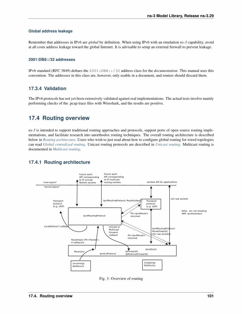
ns-3 Model Library, Release ns-3.29
Global address leakage
Remember that addresses in IPv6 are global by definition. When using IPv6 with an emulation ns-3 capability, avoidat all costs address leakage toward the global Internet. It is advisable to setup an external firewall to prevent leakage.
2001:DB8::/32 addresses
IPv6 standard (RFC 3849) defines the 2001:DB8::/32 address class for the documentation. This manual uses thisconvention. The addresses in this class are, however, only usable in a document, and routers should discard them.
17.3.4 Validation
The IPv6 protocols has not yet been extensively validated against real implementations. The actual tests involve mainlyperforming checks of the .pcap trace files with Wireshark, and the results are positive.
17.4 Routing overview
ns-3 is intended to support traditional routing approaches and protocols, support ports of open source routing imple-mentations, and facilitate research into unorthodox routing techniques. The overall routing architecture is describedbelow in Routing architecture. Users who wish to just read about how to configure global routing for wired topologiescan read Global centralized routing. Unicast routing protocols are described in Unicast routing. Multicast routing isdocumented in Multicast routing.
17.4.1 Routing architecture
Fig. 3: Overview of routing
17.4. Routing overview 101
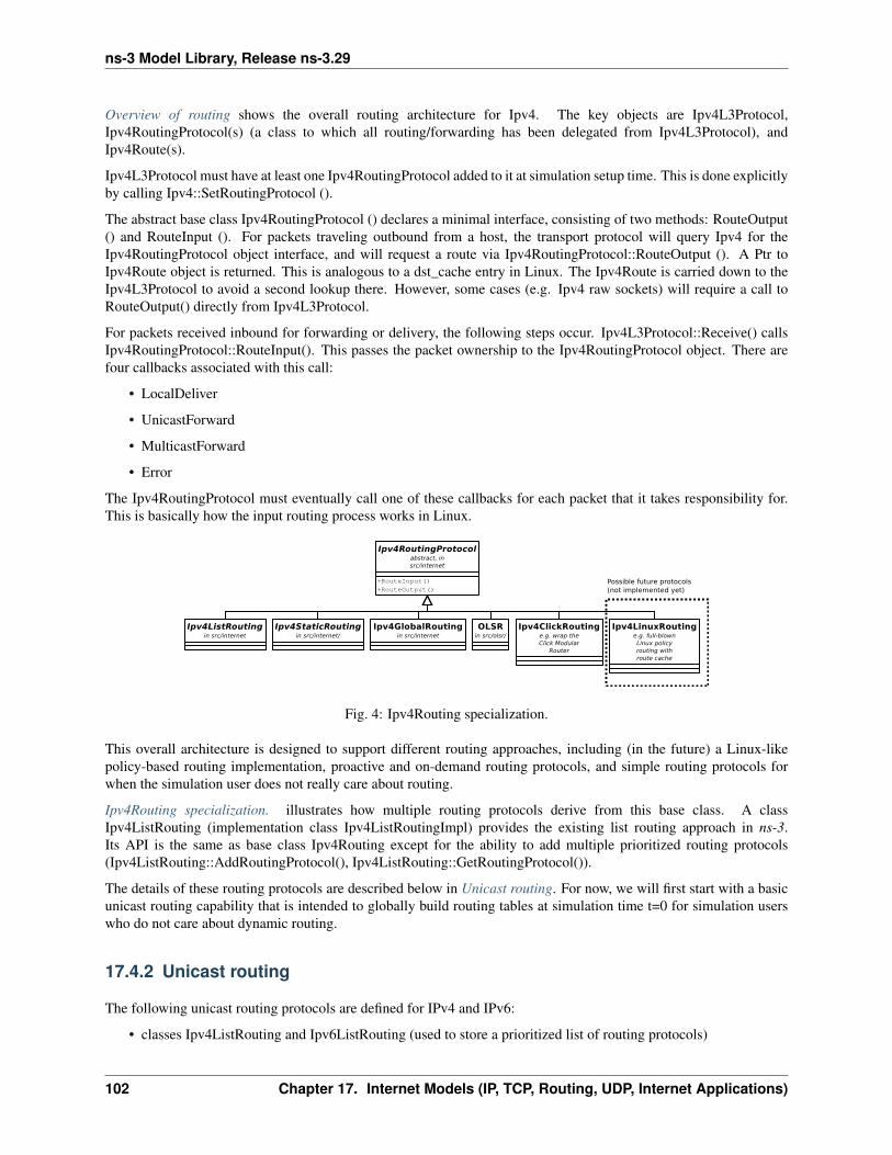
ns-3 Model Library, Release ns-3.29
Overview of routing shows the overall routing architecture for Ipv4. The key objects are Ipv4L3Protocol,Ipv4RoutingProtocol(s) (a class to which all routing/forwarding has been delegated from Ipv4L3Protocol), andIpv4Route(s).
Ipv4L3Protocol must have at least one Ipv4RoutingProtocol added to it at simulation setup time. This is done explicitlyby calling Ipv4::SetRoutingProtocol ().
The abstract base class Ipv4RoutingProtocol () declares a minimal interface, consisting of two methods: RouteOutput() and RouteInput (). For packets traveling outbound from a host, the transport protocol will query Ipv4 for theIpv4RoutingProtocol object interface, and will request a route via Ipv4RoutingProtocol::RouteOutput (). A Ptr toIpv4Route object is returned. This is analogous to a dst_cache entry in Linux. The Ipv4Route is carried down to theIpv4L3Protocol to avoid a second lookup there. However, some cases (e.g. Ipv4 raw sockets) will require a call toRouteOutput() directly from Ipv4L3Protocol.
For packets received inbound for forwarding or delivery, the following steps occur. Ipv4L3Protocol::Receive() callsIpv4RoutingProtocol::RouteInput(). This passes the packet ownership to the Ipv4RoutingProtocol object. There arefour callbacks associated with this call:
• LocalDeliver
• UnicastForward
• MulticastForward
• Error
The Ipv4RoutingProtocol must eventually call one of these callbacks for each packet that it takes responsibility for.This is basically how the input routing process works in Linux.
Fig. 4: Ipv4Routing specialization.
This overall architecture is designed to support different routing approaches, including (in the future) a Linux-likepolicy-based routing implementation, proactive and on-demand routing protocols, and simple routing protocols forwhen the simulation user does not really care about routing.
Ipv4Routing specialization. illustrates how multiple routing protocols derive from this base class. A classIpv4ListRouting (implementation class Ipv4ListRoutingImpl) provides the existing list routing approach in ns-3.Its API is the same as base class Ipv4Routing except for the ability to add multiple prioritized routing protocols(Ipv4ListRouting::AddRoutingProtocol(), Ipv4ListRouting::GetRoutingProtocol()).
The details of these routing protocols are described below in Unicast routing. For now, we will first start with a basicunicast routing capability that is intended to globally build routing tables at simulation time t=0 for simulation userswho do not care about dynamic routing.
17.4.2 Unicast routing
The following unicast routing protocols are defined for IPv4 and IPv6:
• classes Ipv4ListRouting and Ipv6ListRouting (used to store a prioritized list of routing protocols)
102 Chapter 17. Internet Models (IP, TCP, Routing, UDP, Internet Applications)

ns-3 Model Library, Release ns-3.29
• classes Ipv4StaticRouting and Ipv6StaticRouting (covering both unicast and multicast)
• class Ipv4GlobalRouting (used to store routes computed by the global route manager, if that is used)
• class Ipv4NixVectorRouting (a more efficient version of global routing that stores source routes in a packetheader field)
• class Rip - the IPv4 RIPv2 protocol (RFC 2453)
• class RipNg - the IPv6 RIPng protocol (RFC 2080)
• IPv4 Optimized Link State Routing (OLSR) (a MANET protocol defined in RFC 3626)
• IPv4 Ad Hoc On Demand Distance Vector (AODV) (a MANET protocol defined in RFC 3561)
• IPv4 Destination Sequenced Distance Vector (DSDV) (a MANET protocol)
• IPv4 Dynamic Source Routing (DSR) (a MANET protocol)
In the future, this architecture should also allow someone to implement a Linux-like implementation with routingcache, or a Click modular router, but those are out of scope for now.
Ipv[4,6]ListRouting
This section describes the current default ns-3 Ipv[4,6]RoutingProtocol. Typically, multiple routing protocols are sup-ported in user space and coordinate to write a single forwarding table in the kernel. Presently in ns-3, the implementa-tion instead allows for multiple routing protocols to build/keep their own routing state, and the IP implementation willquery each one of these routing protocols (in some order determined by the simulation author) until a route is found.
We chose this approach because it may better facilitate the integration of disparate routing approaches that may bedifficult to coordinate the writing to a single table, approaches where more information than destination IP address(e.g., source routing) is used to determine the next hop, and on-demand routing approaches where packets must becached.
Ipv[4,6]ListRouting::AddRoutingProtocol
Classes Ipv4ListRouting and Ipv6ListRouting provides a pure virtual function declaration for the method that allowsone to add a routing protocol:
void AddRoutingProtocol (Ptr<Ipv4RoutingProtocol> routingProtocol,int16_t priority);
void AddRoutingProtocol (Ptr<Ipv6RoutingProtocol> routingProtocol,int16_t priority);
These methods are implemented respectively by class Ipv4ListRoutingImpl and by class Ipv6ListRoutingImpl in theinternet module.
The priority variable above governs the priority in which the routing protocols are inserted. Notice that it is asigned int. By default in ns-3, the helper classes will instantiate a Ipv[4,6]ListRoutingImpl object, and add to itan Ipv[4,6]StaticRoutingImpl object at priority zero. Internally, a list of Ipv[4,6]RoutingProtocols is stored, and andthe routing protocols are each consulted in decreasing order of priority to see whether a match is found. Therefore,if you want your Ipv4RoutingProtocol to have priority lower than the static routing, insert it with priority less than 0;e.g.:
Ptr<MyRoutingProtocol> myRoutingProto = CreateObject<MyRoutingProtocol> ();listRoutingPtr->AddRoutingProtocol (myRoutingProto, -10);
17.4. Routing overview 103

ns-3 Model Library, Release ns-3.29
Upon calls to RouteOutput() or RouteInput(), the list routing object will search the list of routing protocols, in priorityorder, until a route is found. Such routing protocol will invoke the appropriate callback and no further routing protocolswill be searched.
Global centralized routing
Global centralized routing is sometimes called “God” routing; it is a special implementation that walks the simulationtopology and runs a shortest path algorithm, and populates each node’s routing tables. No actual protocol overhead(on the simulated links) is incurred with this approach. It does have a few constraints:
• Wired only: It is not intended for use in wireless networks.
• Unicast only: It does not do multicast.
• Scalability: Some users of this on large topologies (e.g. 1000 nodes) have noticed that the current implemen-tation is not very scalable. The global centralized routing will be modified in the future to reduce computationsand runtime performance.
Presently, global centralized IPv4 unicast routing over both point-to-point and shared (CSMA) links is supported.
By default, when using the ns-3 helper API and the default InternetStackHelper, global routing capability will be addedto the node, and global routing will be inserted as a routing protocol with lower priority than the static routes (i.e.,users can insert routes via Ipv4StaticRouting API and they will take precedence over routes found by global routing).
Global Unicast Routing API
The public API is very minimal. User scripts include the following:
#include "ns3/internet-module.h"
If the default InternetStackHelper is used, then an instance of global routing will be aggregated to each node. After IPaddresses are configured, the following function call will cause all of the nodes that have an Ipv4 interface to receiveforwarding tables entered automatically by the GlobalRouteManager:
Ipv4GlobalRoutingHelper::PopulateRoutingTables ();
Note: A reminder that the wifi NetDevice will work but does not take any wireless effects into account. For wireless,we recommend OLSR dynamic routing described below.
It is possible to call this function again in the midst of a simulation using the following additional public function:
Ipv4GlobalRoutingHelper::RecomputeRoutingTables ();
which flushes the old tables, queries the nodes for new interface information, and rebuilds the routes.
For instance, this scheduling call will cause the tables to be rebuilt at time 5 seconds:
Simulator::Schedule (Seconds (5),&Ipv4GlobalRoutingHelper::RecomputeRoutingTables);
There are two attributes that govern the behavior. The first is Ipv4GlobalRouting::RandomEcmpRouting. If set to true,packets are randomly routed across equal-cost multipath routes. If set to false (default), only one route is consistentlyused. The second is Ipv4GlobalRouting::RespondToInterfaceEvents. If set to true, dynamically recompute the globalroutes upon Interface notification events (up/down, or add/remove address). If set to false (default), routing may breakunless the user manually calls RecomputeRoutingTables() after such events. The default is set to false to preservelegacy ns-3 program behavior.
104 Chapter 17. Internet Models (IP, TCP, Routing, UDP, Internet Applications)
ns-3 Model Library, Release ns-3.29
Global Routing Implementation
This section is for those readers who care about how this is implemented. A singleton object (GlobalRouteManager)is responsible for populating the static routes on each node, using the public Ipv4 API of that node. It queries eachnode in the topology for a “globalRouter” interface. If found, it uses the API of that interface to obtain a “linkstate advertisement (LSA)” for the router. Link State Advertisements are used in OSPF routing, and we follow theirformatting.
It is important to note that all of these computations are done before packets are flowing in the network. In particular,there are no overhead or control packets being exchanged when using this implementation. Instead, this global routemanager just walks the list of nodes to build the necessary information and configure each node’s routing table.
The GlobalRouteManager populates a link state database with LSAs gathered from the entire topology. Then, foreach router in the topology, the GlobalRouteManager executes the OSPF shortest path first (SPF) computation on thedatabase, and populates the routing tables on each node.
The quagga (http://www.quagga.net) OSPF implementation was used as the basis for the routing computation logic.One benefit of following an existing OSPF SPF implementation is that OSPF already has defined link state advertise-ments for all common types of network links:
• point-to-point (serial links)
• point-to-multipoint (Frame Relay, ad hoc wireless)
• non-broadcast multiple access (ATM)
• broadcast (Ethernet)
Therefore, we think that enabling these other link types will be more straightforward now that the underlying OSPFSPF framework is in place.
Presently, we can handle IPv4 point-to-point, numbered links, as well as shared broadcast (CSMA) links. Equal-costmultipath is also supported. Although wireless link types are supported by the implementation, note that due to thenature of this implementation, any channel effects will not be considered and the routing tables will assume that everynode on the same shared channel is reachable from every other node (i.e. it will be treated like a broadcast CSMAlink).
The GlobalRouteManager first walks the list of nodes and aggregates a GlobalRouter interface to each one as follows:
typedef std::vector < Ptr<Node> >::iterator Iterator;for (Iterator i = NodeList::Begin (); i != NodeList::End (); i++){Ptr<Node> node = *i;Ptr<GlobalRouter> globalRouter = CreateObject<GlobalRouter> (node);node->AggregateObject (globalRouter);
}
This interface is later queried and used to generate a Link State Advertisement for each router, and this link statedatabase is fed into the OSPF shortest path computation logic. The Ipv4 API is finally used to populate the routesthemselves.
RIP and RIPng
The RIPv2 protocol for IPv4 is described in the RFC 2453, and it consolidates a number of improvements over thebase protocol defined in RFC 1058.
This IPv6 routing protocol (RFC 2080) is the evolution of the well-known RIPv1 (see RFC 1058 and RFC 1723)routing protocol for IPv4.
The protocols are very simple, and are normally suitable for flat, simple network topologies.
17.4. Routing overview 105

ns-3 Model Library, Release ns-3.29
RIPv1, RIPv2, and RIPng have the very same goals and limitations. In particular, RIP considers any route with ametric equal or greater than 16 as unreachable. As a consequence, the maximum number of hops is the network mustbe less than 15 (the number of routers is not set). Users are encouraged to read RFC 2080 and RFC 1058 to fullyunderstand RIP behaviour and limitations.
Routing convergence
RIP uses a Distance-Vector algorithm, and routes are updated according to the Bellman-Ford algorithm (sometimesknown as Ford-Fulkerson algorithm). The algorithm has a convergence time of O(|V|*|E|) where |V| and |E| are thenumber of vertices (routers) and edges (links) respectively. It should be stressed that the convergence time is thenumber of steps in the algorithm, and each step is triggered by a message. Since Triggered Updates (i.e., when a routeis changed) have a 1-5 seconds cooldown, the topology can require some time to be stabilized.
Users should be aware that, during routing tables construction, the routers might drop packets. Data traffic should besent only after a time long enough to allow RIP to build the network topology. Usually 80 seconds should be enoughto have a suboptimal (but working) routing setup. This includes the time needed to propagate the routes to the mostdistant router (16 hops) with Triggered Updates.
If the network topology is changed (e.g., a link is broken), the recovery time might be quite high, and it might beeven higher than the initial setup time. Moreover, the network topology recovery is affected by the Split Horizoningstrategy.
The examples examples/routing/ripng-simple-network.cc and examples/routing/rip-simple-network.cc shows both the network setup and network recovery phases.
Split Horizoning
Split Horizon is a strategy to prevent routing instability. Three options are possible:
• No Split Horizon
• Split Horizon
• Poison Reverse
In the first case, routes are advertised on all the router’s interfaces. In the second case, routers will not advertise a routeon the interface from which it was learned. Poison Reverse will advertise the route on the interface from which it waslearned, but with a metric of 16 (infinity). For a full analysis of the three techniques, see RFC 1058, section 2.2.
The examples are based on the network topology described in the RFC, but it does not show the effect described there.
The reason are the Triggered Updates, together with the fact that when a router invalidates a route, it will immediatelypropagate the route unreachability, thus preventing most of the issues described in the RFC.
However, with complex toplogies, it is still possible to have route instability phenomena similar to the one describedin the RFC after a link failure. As a consequence, all the considerations about Split Horizon remanins valid.
Default routes
RIP protocol should be installed only on routers. As a consequence, nodes will not know what is the default router.
To overcome this limitation, users should either install the default route manually (e.g., by resorting toIpv4StaticRouting or Ipv6StaticRouting), or by using RADVd (in case of IPv6). RADVd is available in ns-3 inthe Applications module, and it is strongly suggested.
106 Chapter 17. Internet Models (IP, TCP, Routing, UDP, Internet Applications)
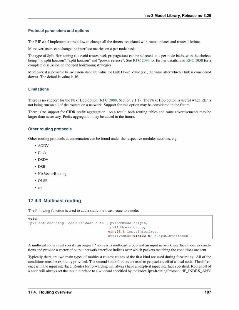
ns-3 Model Library, Release ns-3.29
Protocol parameters and options
The RIP ns-3 implementations allow to change all the timers associated with route updates and routes lifetime.
Moreover, users can change the interface metrics on a per-node basis.
The type of Split Horizoning (to avoid routes back-propagation) can be selected on a per-node basis, with the choicesbeing “no split horizon”, “split horizon” and “poison reverse”. See RFC 2080 for further details, and RFC 1058 for acomplete discussion on the split horizoning strategies.
Moreover, it is possible to use a non-standard value for Link Down Value (i.e., the value after which a link is considereddown). The defaul is value is 16.
Limitations
There is no support for the Next Hop option (RFC 2080, Section 2.1.1). The Next Hop option is useful when RIP isnot being run on all of the routers on a network. Support for this option may be considered in the future.
There is no support for CIDR prefix aggregation. As a result, both routing tables and route advertisements may belarger than necessary. Prefix aggregation may be added in the future.
Other routing protocols
Other routing protocols documentation can be found under the respective modules sections, e.g.:
• AODV
• Click
• DSDV
• DSR
• NixVectorRouting
• OLSR
• etc.
17.4.3 Multicast routing
The following function is used to add a static multicast route to a node:
voidIpv4StaticRouting::AddMulticastRoute (Ipv4Address origin,
Ipv4Address group,uint32_t inputInterface,std::vector<uint32_t> outputInterfaces);
A multicast route must specify an origin IP address, a multicast group and an input network interface index as condi-tions and provide a vector of output network interface indices over which packets matching the conditions are sent.
Typically there are two main types of multicast routes: routes of the first kind are used during forwarding. All of theconditions must be explicitly provided. The second kind of routes are used to get packets off of a local node. The differ-ence is in the input interface. Routes for forwarding will always have an explicit input interface specified. Routes off ofa node will always set the input interface to a wildcard specified by the index Ipv4RoutingProtocol::IF_INDEX_ANY.
17.4. Routing overview 107

ns-3 Model Library, Release ns-3.29
For routes off of a local node wildcards may be used in the origin and multicast group addresses. The wildcard usedfor Ipv4Adresses is that address returned by Ipv4Address::GetAny () – typically “0.0.0.0”. Usage of a wildcard allowsone to specify default behavior to varying degrees.
For example, making the origin address a wildcard, but leaving the multicast group specific allows one (in the case ofa node with multiple interfaces) to create different routes using different output interfaces for each multicast group.
If the origin and multicast addresses are made wildcards, you have created essentially a default multicast address thatcan forward to multiple interfaces. Compare this to the actual default multicast address that is limited to specifying asingle output interface for compatibility with existing functionality in other systems.
Another command sets the default multicast route:
voidIpv4StaticRouting::SetDefaultMulticastRoute (uint32_t outputInterface);
This is the multicast equivalent of the unicast version SetDefaultRoute. We tell the routing system what to do in thecase where a specific route to a destination multicast group is not found. The system forwards packets out the specifiedinterface in the hope that “something out there” knows better how to route the packet. This method is only used ininitially sending packets off of a host. The default multicast route is not consulted during forwarding – exact routesmust be specified using AddMulticastRoute for that case.
Since we’re basically sending packets to some entity we think may know better what to do, we don’t pay attentionto “subtleties” like origin address, nor do we worry about forwarding out multiple interfaces. If the default multicastroute is set, it is returned as the selected route from LookupStatic irrespective of origin or multicast group if anotherspecific route is not found.
Finally, a number of additional functions are provided to fetch and remove multicast routes:
uint32_t GetNMulticastRoutes (void) const;
Ipv4MulticastRoute *GetMulticastRoute (uint32_t i) const;
Ipv4MulticastRoute *GetDefaultMulticastRoute (void) const;
bool RemoveMulticastRoute (Ipv4Address origin,Ipv4Address group,uint32_t inputInterface);
void RemoveMulticastRoute (uint32_t index);
17.5 TCP models in ns-3
This chapter describes the TCP models available in ns-3.
17.5.1 Overview of support for TCP
ns-3 was written to support multiple TCP implementations. The implementations inherit from a few common headerclasses in the src/network directory, so that user code can swap out implementations with minimal changes to thescripts.
There are two important abstract base classes:
• class TcpSocket: This is defined in src/internet/model/tcp-socket.{cc,h}. This class existsfor hosting TcpSocket attributes that can be reused across different implementations. For instance, the attributeInitialCwnd can be used for any of the implementations that derive from class TcpSocket.
108 Chapter 17. Internet Models (IP, TCP, Routing, UDP, Internet Applications)
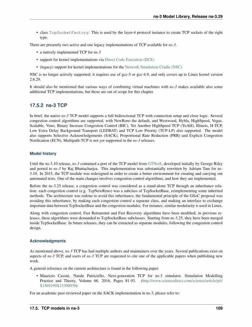
ns-3 Model Library, Release ns-3.29
• class TcpSocketFactory: This is used by the layer-4 protocol instance to create TCP sockets of the righttype.
There are presently two active and one legacy implementations of TCP available for ns-3.
• a natively implemented TCP for ns-3
• support for kernel implementations via Direct Code Execution (DCE)
• (legacy) support for kernel implementations for the Network Simulation Cradle (NSC)
NSC is no longer actively supported; it requires use of gcc-5 or gcc-4.9, and only covers up to Linux kernel version2.6.29.
It should also be mentioned that various ways of combining virtual machines with ns-3 makes available also someadditional TCP implementations, but those are out of scope for this chapter.
17.5.2 ns-3 TCP
In brief, the native ns-3 TCP model supports a full bidirectional TCP with connection setup and close logic. Severalcongestion control algorithms are supported, with NewReno the default, and Westwood, Hybla, HighSpeed, Vegas,Scalable, Veno, Binary Increase Congestion Control (BIC), Yet Another HighSpeed TCP (YeAH), Illinois, H-TCP,Low Extra Delay Background Transport (LEDBAT) and TCP Low Priority (TCP-LP) also supported. The modelalso supports Selective Acknowledgements (SACK), Proportional Rate Reduction (PRR) and Explicit CongestionNotification (ECN). Multipath-TCP is not yet supported in the ns-3 releases.
Model history
Until the ns-3.10 release, ns-3 contained a port of the TCP model from GTNetS, developed initially by George Rileyand ported to ns-3 by Raj Bhattacharjea. This implementation was substantially rewritten by Adriam Tam for ns-3.10. In 2015, the TCP module was redesigned in order to create a better environment for creating and carrying outautomated tests. One of the main changes involves congestion control algorithms, and how they are implemented.
Before the ns-3.25 release, a congestion control was considered as a stand-alone TCP through an inheritance rela-tion: each congestion control (e.g. TcpNewReno) was a subclass of TcpSocketBase, reimplementing some inheritedmethods. The architecture was redone to avoid this inheritance, the fundamental principle of the GSoC proposal wasavoiding this inheritance, by making each congestion control a separate class, and making an interface to exchangeimportant data between TcpSocketBase and the congestion modules. For instance, similar modularity is used in Linux.
Along with congestion control, Fast Retransmit and Fast Recovery algorithms have been modified; in previous re-leases, these algorithms were demanded to TcpSocketBase subclasses. Starting from ns-3.25, they have been mergedinside TcpSocketBase. In future releases, they can be extracted as separate modules, following the congestion controldesign.
Acknowledgments
As mentioned above, ns-3 TCP has had multiple authors and maintainers over the years. Several publications exist onaspects of ns-3 TCP, and users of ns-3 TCP are requested to cite one of the applicable papers when publishing newwork.
A general reference on the current architecture is found in the following paper:
• Maurizio Casoni, Natale Patriciello, Next-generation TCP for ns-3 simulator, Simulation ModellingPractice and Theory, Volume 66, 2016, Pages 81-93. (http://www.sciencedirect.com/science/article/pii/S1569190X15300939)
For an academic peer-reviewed paper on the SACK implementation in ns-3, please refer to:
17.5. TCP models in ns-3 109
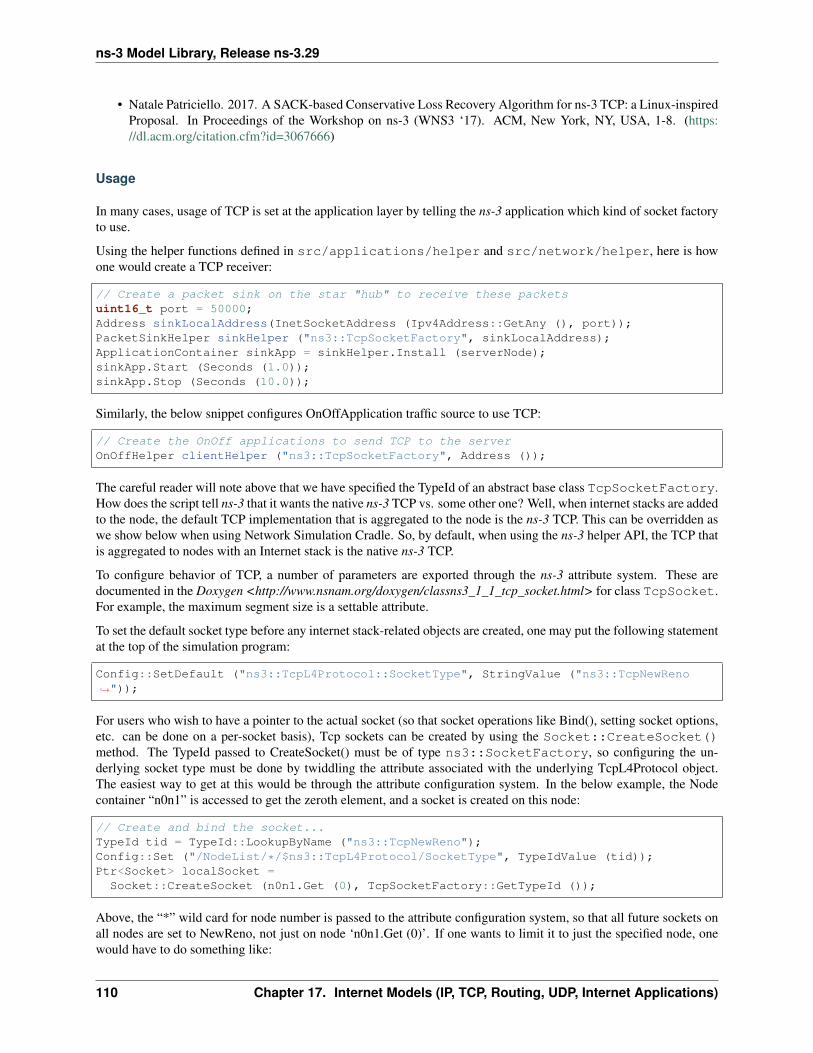
ns-3 Model Library, Release ns-3.29
• Natale Patriciello. 2017. A SACK-based Conservative Loss Recovery Algorithm for ns-3 TCP: a Linux-inspiredProposal. In Proceedings of the Workshop on ns-3 (WNS3 ‘17). ACM, New York, NY, USA, 1-8. (https://dl.acm.org/citation.cfm?id=3067666)
Usage
In many cases, usage of TCP is set at the application layer by telling the ns-3 application which kind of socket factoryto use.
Using the helper functions defined in src/applications/helper and src/network/helper, here is howone would create a TCP receiver:
// Create a packet sink on the star "hub" to receive these packetsuint16_t port = 50000;Address sinkLocalAddress(InetSocketAddress (Ipv4Address::GetAny (), port));PacketSinkHelper sinkHelper ("ns3::TcpSocketFactory", sinkLocalAddress);ApplicationContainer sinkApp = sinkHelper.Install (serverNode);sinkApp.Start (Seconds (1.0));sinkApp.Stop (Seconds (10.0));
Similarly, the below snippet configures OnOffApplication traffic source to use TCP:
// Create the OnOff applications to send TCP to the serverOnOffHelper clientHelper ("ns3::TcpSocketFactory", Address ());
The careful reader will note above that we have specified the TypeId of an abstract base class TcpSocketFactory.How does the script tell ns-3 that it wants the native ns-3 TCP vs. some other one? Well, when internet stacks are addedto the node, the default TCP implementation that is aggregated to the node is the ns-3 TCP. This can be overridden aswe show below when using Network Simulation Cradle. So, by default, when using the ns-3 helper API, the TCP thatis aggregated to nodes with an Internet stack is the native ns-3 TCP.
To configure behavior of TCP, a number of parameters are exported through the ns-3 attribute system. These aredocumented in the Doxygen <http://www.nsnam.org/doxygen/classns3_1_1_tcp_socket.html> for class TcpSocket.For example, the maximum segment size is a settable attribute.
To set the default socket type before any internet stack-related objects are created, one may put the following statementat the top of the simulation program:
Config::SetDefault ("ns3::TcpL4Protocol::SocketType", StringValue ("ns3::TcpNewReno↪→"));
For users who wish to have a pointer to the actual socket (so that socket operations like Bind(), setting socket options,etc. can be done on a per-socket basis), Tcp sockets can be created by using the Socket::CreateSocket()method. The TypeId passed to CreateSocket() must be of type ns3::SocketFactory, so configuring the un-derlying socket type must be done by twiddling the attribute associated with the underlying TcpL4Protocol object.The easiest way to get at this would be through the attribute configuration system. In the below example, the Nodecontainer “n0n1” is accessed to get the zeroth element, and a socket is created on this node:
// Create and bind the socket...TypeId tid = TypeId::LookupByName ("ns3::TcpNewReno");Config::Set ("/NodeList/*/$ns3::TcpL4Protocol/SocketType", TypeIdValue (tid));Ptr<Socket> localSocket =
Socket::CreateSocket (n0n1.Get (0), TcpSocketFactory::GetTypeId ());
Above, the “*” wild card for node number is passed to the attribute configuration system, so that all future sockets onall nodes are set to NewReno, not just on node ‘n0n1.Get (0)’. If one wants to limit it to just the specified node, onewould have to do something like:
110 Chapter 17. Internet Models (IP, TCP, Routing, UDP, Internet Applications)
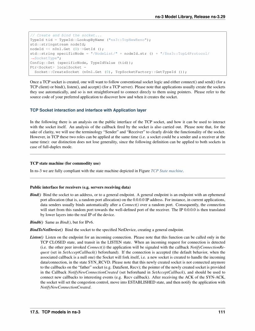
ns-3 Model Library, Release ns-3.29
// Create and bind the socket...TypeId tid = TypeId::LookupByName ("ns3::TcpNewReno");std::stringstream nodeId;nodeId << n0n1.Get (0)->GetId ();std::string specificNode = "/NodeList/" + nodeId.str () + "/$ns3::TcpL4Protocol/↪→SocketType";Config::Set (specificNode, TypeIdValue (tid));Ptr<Socket> localSocket =
Socket::CreateSocket (n0n1.Get (0), TcpSocketFactory::GetTypeId ());
Once a TCP socket is created, one will want to follow conventional socket logic and either connect() and send() (for aTCP client) or bind(), listen(), and accept() (for a TCP server). Please note that applications usually create the socketsthey use automatically, and so is not straightforward to connect direcly to them using pointers. Please refer to thesource code of your preferred application to discover how and when it creates the socket.
TCP Socket interaction and interface with Application layer
In the following there is an analysis on the public interface of the TCP socket, and how it can be used to interactwith the socket itself. An analysis of the callback fired by the socket is also carried out. Please note that, for thesake of clarity, we will use the terminology “Sender” and “Receiver” to clearly divide the functionality of the socket.However, in TCP these two roles can be applied at the same time (i.e. a socket could be a sender and a receiver at thesame time): our distinction does not lose generality, since the following definition can be applied to both sockets incase of full-duplex mode.
TCP state machine (for commodity use)
In ns-3 we are fully compliant with the state machine depicted in Figure TCP State machine.
Public interface for receivers (e.g. servers receiving data)
Bind() Bind the socket to an address, or to a general endpoint. A general endpoint is an endpoint with an ephemeralport allocation (that is, a random port allocation) on the 0.0.0.0 IP address. For instance, in current applications,data senders usually binds automatically after a Connect() over a random port. Consequently, the connectionwill start from this random port towards the well-defined port of the receiver. The IP 0.0.0.0 is then translatedby lower layers into the real IP of the device.
Bind6() Same as Bind(), but for IPv6.
BindToNetDevice() Bind the socket to the specified NetDevice, creating a general endpoint.
Listen() Listen on the endpoint for an incoming connection. Please note that this function can be called only in theTCP CLOSED state, and transit in the LISTEN state. When an incoming request for connection is detected(i.e. the other peer invoked Connect()) the application will be signaled with the callback NotifyConnectionRe-quest (set in SetAcceptCallback() beforehand). If the connection is accepted (the default behavior, when theassociated callback is a null one) the Socket will fork itself, i.e. a new socket is created to handle the incomingdata/connection, in the state SYN_RCVD. Please note that this newly created socket is not connected anymoreto the callbacks on the “father” socket (e.g. DataSent, Recv); the pointer of the newly created socket is providedin the Callback NotifyNewConnectionCreated (set beforehand in SetAcceptCallback), and should be used toconnect new callbacks to interesting events (e.g. Recv callback). After receiving the ACK of the SYN-ACK,the socket will set the congestion control, move into ESTABLISHED state, and then notify the application withNotifyNewConnectionCreated.
17.5. TCP models in ns-3 111
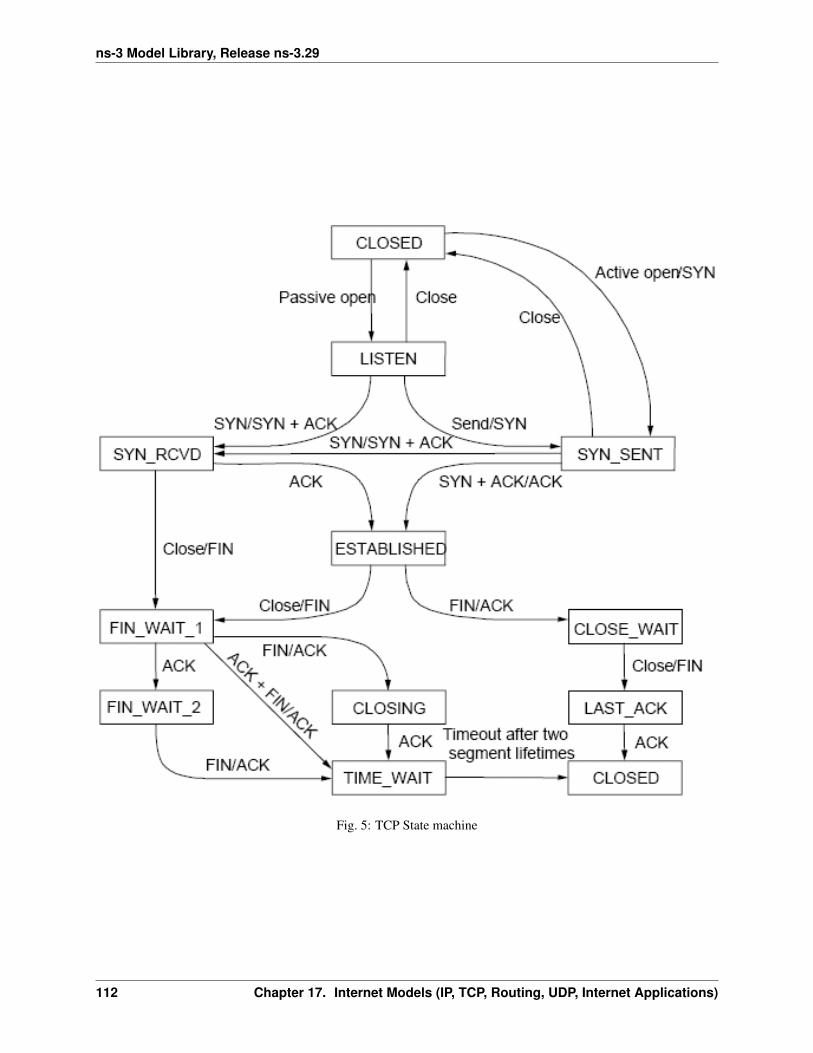
ns-3 Model Library, Release ns-3.29
Fig. 5: TCP State machine
112 Chapter 17. Internet Models (IP, TCP, Routing, UDP, Internet Applications)
ns-3 Model Library, Release ns-3.29
ShutdownSend() Signal a termination of send, or in other words revents data from being added to the buffer. Afterthis call, if buffer is already empty, the socket will send a FIN, otherwise FIN will go when buffer empties.Please note that this is useful only for modeling “Sink” applications. If you have data to transmit, please referto the Send() / Close() combination of API.
GetRxAvailable() Get the amount of data that could be returned by the Socket in one or multiple call to Recv orRecvFrom. Please use the Attribute system to configure the maximum available space on the receiver buffer(property “RcvBufSize”).
Recv() Grab data from the TCP socket. Please remember that TCP is a stream socket, and it is allowed to concatenatemultiple packets into bigger ones. If no data is present (i.e. GetRxAvailable returns 0) an empty packet is re-turned. Set the callback RecvCallback through SetRecvCallback() in order to have the application automaticallynotified when some data is ready to be read. It’s important to connect that callback to the newly created socketin case of forks.
RecvFrom() Same as Recv, but with the source address as parameter.
Public interface for senders (e.g. clients uploading data)
Connect() Set the remote endpoint, and try to connect to it. The local endpoint should be set before this call, orotherwise an ephemeral one will be created. The TCP then will be in the SYN_SENT state. If a SYN-ACK isreceived, the TCP will setup the congestion control, and then call the callback ConnectionSucceeded.
GetTxAvailable() Return the amount of data that can be stored in the TCP Tx buffer. Set this property through theAttribute system (“SndBufSize”).
Send() Send the data into the TCP Tx buffer. From there, the TCP rules will decide if, and when, this data will betransmitted. Please note that, if the tx buffer has enough data to fill the congestion (or the receiver) window,dynamically varying the rate at which data is injected in the TCP buffer does not have any noticeable effect onthe amount of data transmitted on the wire, that will continue to be decided by the TCP rules.
SendTo() Same as Send().
Close() Terminate the local side of the connection, by sending a FIN (after all data in the tx buffer has been trans-mitted). This does not prevent the socket in receiving data, and employing retransmit mechanism if losses aredetected. If the application calls Close() with unread data in its rx buffer, the socket will send a reset. If the socketis in the state SYN_SENT, CLOSING, LISTEN, FIN_WAIT_2, or LAST_ACK, after that call the applicationwill be notified with NotifyNormalClose(). In other cases, the notification is delayed (see NotifyNormalClose()).
Public callbacks
These callbacks are called by the TCP socket to notify the application of interesting events. We will refer to these withthe protected name used in socket.h, but we will provide the API function to set the pointers to these callback as well.
NotifyConnectionSucceeded: SetConnectCallback, 1st argument Called in the SYN_SENT state, before moving toESTABLISHED. In other words, we have sent the SYN, and we received the SYN-ACK: the socket prepare thesequence numbers, send the ACK for the SYN-ACK, try to send out more data (in another segment) and theninvoke this callback. After this callback, it invokes the NotifySend callback.
NotifyConnectionFailed: SetConnectCallback, 2nd argument Called after the SYN retransmission count goes to 0.SYN packet is lost multiple time, and the socket give up.
NotifyNormalClose: SetCloseCallbacks, 1st argument A normal close is invoked. A rare case is when we receivean RST segment (or a segment with bad flags) in normal states. All other cases are: - The application tries toConnect() over an already connected socket - Received an ACK for the FIN sent, with or without the FIN bitset (we are in LAST_ACK) - The socket reaches the maximum amount of retries in retransmitting the SYN(*) - We receive a timeout in the LAST_ACK state - Upon entering the TIME_WAIT state, before waiting the2*Maximum Segment Lifetime seconds to finally deallocate the socket.
17.5. TCP models in ns-3 113
ns-3 Model Library, Release ns-3.29
NotifyErrorClose: SetCloseCallbacks, 2nd argument Invoked when we send an RST segment (for whatever reason)or we reached the maximum amount of data retries.
NotifyConnectionRequest: SetAcceptCallback, 1st argument Invoked in the LISTEN state, when we receive a SYN.The return value indicates if the socket should accept the connection (return true) or should ignore it (returnfalse).
NotifyNewConnectionCreated: SetAcceptCallback, 2nd argument Invoked when from SYN_RCVD the socketpasses to ESTABLISHED, and after setting up the congestion control, the sequence numbers, and processedthe incoming ACK. If there is some space in the buffer, NotifySend is called shortly after this callback. TheSocket pointer, passed with this callback, is the newly created socket, after a Fork().
NotifyDataSent: SetDataSentCallback The Socket notifies the application that some bytes has been transmitted onthe IP level. These bytes could still be lost in the node (traffic control layer) or in the network.
NotifySend: SetSendCallback Invoked if there is some space in the tx buffer when entering the ESTABLISHED state(e.g. after the ACK for SYN-ACK is received), after the connection succeeds (e.g. after the SYN-ACK isreceived) and after each new ack (i.e. that advances SND.UNA).
NotifyDataRecv: SetRecvCallback Called when in the receiver buffere there are in-order bytes, and when inFIN_WAIT_1 or FIN_WAIT_2 the socket receive a in-sequence FIN (that can carry data).
Congestion Control Algorithms
Here follows a list of supported TCP congestion control algorithms. For an academic peer-reviewed paper on thesecongestion control algorithms, see http://dl.acm.org/citation.cfm?id=2756518 .
New Reno
New Reno algorithm introduces partial ACKs inside the well-established Reno algorithm. This and other modificationsare described in RFC 6582. We have two possible congestion window increment strategy: slow start and congestionavoidance. Taken from RFC 5681:
During slow start, a TCP increments cwnd by at most SMSS bytes for each ACK received that cumu-latively acknowledges new data. Slow start ends when cwnd exceeds ssthresh (or, optionally, when itreaches it, as noted above) or when congestion is observed. While traditionally TCP implementationshave increased cwnd by precisely SMSS bytes upon receipt of an ACK covering new data, we REC-OMMEND that TCP implementations increase cwnd, per Equation (17.1), where N is the number ofpreviously unacknowledged bytes acknowledged in the incoming ACK.
cwnd+ = min(N,SMSS) (17.1)
During congestion avoidance, cwnd is incremented by roughly 1 full-sized segment per round-trip time (RTT), and foreach congestion event, the slow start threshold is halved.
High Speed
TCP HighSpeed is designed for high-capacity channels or, in general, for TCP connections with large congestionwindows. Conceptually, with respect to the standard TCP, HighSpeed makes the cWnd grow faster during the probingphases and accelerates the cWnd recovery from losses. This behavior is executed only when the window growsbeyond a certain threshold, which allows TCP Highspeed to be friendly with standard TCP in environments withheavy congestion, without introducing new dangers of congestion collapse.
Mathematically:
cWnd = cWnd+a(cWnd)
cWnd
114 Chapter 17. Internet Models (IP, TCP, Routing, UDP, Internet Applications)
ns-3 Model Library, Release ns-3.29
The function a() is calculated using a fixed RTT the value 100 ms (the lookup table for this function is taken from RFC3649). For each congestion event, the slow start threshold is decreased by a value that depends on the size of the slowstart threshold itself. Then, the congestion window is set to such value.
cWnd = (1− b(cWnd)) · cWnd
The lookup table for the function b() is taken from the same RFC. More information at: http://dl.acm.org/citation.cfm?id=2756518
Hybla
The key idea behind TCP Hybla is to obtain for long RTT connections the same instantaneous transmission rate ofa reference TCP connection with lower RTT. With analytical steps, it is shown that this goal can be achieved bymodifying the time scale, in order for the throughput to be independent from the RTT. This independence is obtainedthrough the use of a coefficient rho.
This coefficient is used to calculate both the slow start threshold and the congestion window when in slow start and incongestion avoidance, respectively.
More information at: http://dl.acm.org/citation.cfm?id=2756518
Westwood
Westwood and Westwood+ employ the AIAD (Additive Increase/Adaptive Decrease)· congestion control paradigm.When a congestion episode happens,· instead of halving the cwnd, these protocols try to estimate the network’s band-width and use the estimated value to adjust the cwnd.· While Westwood performs the bandwidth sampling every ACKreception,· Westwood+ samples the bandwidth every RTT.
More information at: http://dl.acm.org/citation.cfm?id=381704 and http://dl.acm.org/citation.cfm?id=2512757
Vegas
TCP Vegas is a pure delay-based congestion control algorithm implementing a proactive scheme that tries to preventpacket drops by maintaining a small backlog at the bottleneck queue. Vegas continuously samples the RTT andcomputes the actual throughput a connection achieves using Equation (1) and compares it with the expected throughputcalculated in Equation (2). The difference between these 2 sending rates in Equation (3) reflects the amount of extrapackets being queued at the bottleneck.
actual =cWnd
RTT
expected =cWnd
BaseRTTdiff = expected− actual
To avoid congestion, Vegas linearly increases/decreases its congestion window to ensure the diff value fall betweenthe two predefined thresholds, alpha and beta. diff and another threshold, gamma, are used to determine when Vegasshould change from its slow-start mode to linear increase/decrease mode. Following the implementation of Vegas inLinux, we use 2, 4, and 1 as the default values of alpha, beta, and gamma, respectively, but they can be modifiedthrough the Attribute system.
More information at: http://dx.doi.org/10.1109/49.464716
17.5. TCP models in ns-3 115
ns-3 Model Library, Release ns-3.29
Scalable
Scalable improves TCP performance to better utilize the available bandwidth of a highspeed wide area network byaltering NewReno congestion window adjustment algorithm. When congestion has not been detected, for each ACKreceived in an RTT, Scalable increases its cwnd per:
cwnd = cwnd+ 0.01
Following Linux implementation of Scalable, we use 50 instead of 100 to account for delayed ACK.
On the first detection of congestion in a given RTT, cwnd is reduced based on the following equation:
cwnd = cwnd− ceil(0.125 · cwnd)
More information at: http://dl.acm.org/citation.cfm?id=956989
Veno
TCP Veno enhances Reno algorithm for more effectively dealing with random packet loss in wireless access networksby employing Vegas’s method in estimating the backlog at the bottleneck queue to distinguish between congestive andnon-congestive states.
The backlog (the number of packets accumulated at the bottleneck queue) is calculated using Equation (1):
N = Actual · (RTT −BaseRTT )
= Diff ·BaseRTT
where:
Diff = Expected−Actual
=cWnd
BaseRTT− cWnd
RTT
Veno makes decision on cwnd modification based on the calculated N and its predefined threshold beta.
Specifically, it refines the additive increase algorithm of Reno so that the connection can stay longer in the stablestate by incrementing cwnd by 1/cwnd for every other new ACK received after the available bandwidth has been fullyutilized, i.e. when N exceeds beta. Otherwise, Veno increases its cwnd by 1/cwnd upon every new ACK receipt as inReno.
In the multiplicative decrease algorithm, when Veno is in the non-congestive state, i.e. when N is less than beta,Veno decrements its cwnd by only 1/5 because the loss encountered is more likely a corruption-based loss than acongestion-based. Only when N is greater than beta, Veno halves its sending rate as in Reno.
More information at: http://dx.doi.org/10.1109/JSAC.2002.807336
Bic
In TCP Bic the congestion control problem is viewed as a search problem. Taking as a starting point the currentwindow value and as a target point the last maximum window value (i.e. the cWnd value just before the loss event) abinary search technique can be used to update the cWnd value at the midpoint between the two, directly or using anadditive increase strategy if the distance from the current window is too large.
This way, assuming a no-loss period, the congestion window logarithmically approaches the maximum value of cWnduntil the difference between it and cWnd falls below a preset threshold. After reaching such a value (or the maximum
116 Chapter 17. Internet Models (IP, TCP, Routing, UDP, Internet Applications)
ns-3 Model Library, Release ns-3.29
window is unknown, i.e. the binary search does not start at all) the algorithm switches to probing the new maximumwindow with a ‘slow start’ strategy.
If a loss occur in either these phases, the current window (before the loss) can be treated as the new maximum, and thereduced (with a multiplicative decrease factor Beta) window size can be used as the new minimum.
More information at: http://ieeexplore.ieee.org/xpl/articleDetails.jsp?arnumber=1354672
YeAH
YeAH-TCP (Yet Another HighSpeed TCP) is a heuristic designed to balance various requirements of a state-of-the-artcongestion control algorithm:
1. fully exploit the link capacity of high BDP networks while inducing a small number of congestion events
2. compete friendly with Reno flows
3. achieve intra and RTT fairness
4. robust to random losses
5. achieve high performance regardless of buffer size
YeAH operates between 2 modes: Fast and Slow mode. In the Fast mode when the queue occupancy is small andthe network congestion level is low, YeAH increments its congestion window according to the aggressive STCP rule.When the number of packets in the queue grows beyond a threshold and the network congestion level is high, YeAHenters its Slow mode, acting as Reno with a decongestion algorithm. YeAH employs Vegas’ mechanism for calculatingthe backlog as in Equation (17.2). The estimation of the network congestion level is shown in Equation (17.3).
Q = (RTT −BaseRTT ) · cWnd
RTT(17.2)
L =RTT −BaseRTT
BaseRTT(17.3)
To ensure TCP friendliness, YeAH also implements an algorithm to detect the presence of legacy Reno flows. Uponthe receipt of 3 duplicate ACKs, YeAH decreases its slow start threshold according to Equation (3) if it’s not competingwith Reno flows. Otherwise, the ssthresh is halved as in Reno:
ssthresh = min(max(cWnd
8, Q),
cWnd
2)
More information: http://www.csc.lsu.edu/~sjpark/cs7601/4-YeAH_TCP.pdf
Illinois
TCP Illinois is a hybrid congestion control algorithm designed for high-speed networks. Illinois implements aConcave-AIMD (or C-AIMD) algorithm that uses packet loss as the primary congestion signal to determine the direc-tion of window update and queueing delay as the secondary congestion signal to determine the amount of change.
The additive increase and multiplicative decrease factors (denoted as alpha and beta, respectively) are functions ofthe current average queueing delay da as shown in Equations (1) and (2). To improve the protocol robustness againstsudden fluctuations in its delay sampling, Illinois allows the increment of alpha to alphaMax only if da stays below d1
17.5. TCP models in ns-3 117
ns-3 Model Library, Release ns-3.29
for a some (theta) amount of time.
alpha =
{alphaMax if da <= d1
k1/(k2 + da) otherwise
beta =
betaMin if da <= d2
k3 + k4 da if d2 < da < d3
betaMax otherwise
where the calculations of k1, k2, k3, and k4 are shown in the following:
k1 =(dm− d1) · alphaMin · alphaMax
alphaMax− alphaMin
k2 =(dm− d1) · alphaMin
alphaMax− alphaMin− d1
k3 =alphaMin · d3− alphaMax · d2
d3− d2
k4 =alphaMax− alphaMin
d3− d2
Other parameters include da (the current average queueing delay), and Ta (the average RTT, calculated as sumRtt /cntRtt in the implementation) and Tmin (baseRtt in the implementation) which is the minimum RTT ever seen. dm isthe maximum (average) queueing delay, and Tmax (maxRtt in the implementation) is the maximum RTT ever seen.
da = Ta− Tmindm = Tmax− Tmindi = etai · dm
Illinois only executes its adaptation of alpha and beta when cwnd exceeds a threshold called winThresh. Otherwise, itsets alpha and beta to the base values of 1 and 0.5, respectively.
Following the implementation of Illinois in the Linux kernel, we use the following default parameter settings:
• alphaMin = 0.3 (0.1 in the Illinois paper)
• alphaMax = 10.0
• betaMin = 0.125
• betaMax = 0.5
• winThresh = 15 (10 in the Illinois paper)
• theta = 5
• eta1 = 0.01
• eta2 = 0.1
• eta3 = 0.8
More information: http://www.doi.org/10.1145/1190095.1190166
118 Chapter 17. Internet Models (IP, TCP, Routing, UDP, Internet Applications)
ns-3 Model Library, Release ns-3.29
H-TCP
H-TCP has been designed for high BDP (Bandwidth-Delay Product) paths. It is a dual mode protocol. In normalconditions, it works like traditional TCP with the same rate of increment and decrement for the congestion window.However, in high BDP networks, when it finds no congestion on the path after deltal seconds, it increases thewindow size based on the alpha function in the following:
alpha(delta) = 1 + 10(delta− deltal) + 0.5(delta− deltal)2
where deltal is a threshold in seconds for switching between the modes and delta is the elapsed time from the lastcongestion. During congestion, it reduces the window size by multiplying by beta function provided in the referencepaper. The calculated throughput between the last two consecutive congestion events is considered for beta calculation.
The transport TcpHtcp can be selected in the program examples/tcp/tcp-variants/comparison to per-form an experiment with H-TCP, although it is useful to increase the bandwidth in this example (e.g. to 20 Mb/s) tocreate a higher BDP link, such as
./waf --run "tcp-variants-comparison --transport_prot=TcpHtcp --bandwidth=20Mbps --↪→duration=10"
More information (paper): http://www.hamilton.ie/net/htcp3.pdf
More information (Internet Draft): https://tools.ietf.org/html/draft-leith-tcp-htcp-06
LEDBAT
Low Extra Delay Background Transport (LEDBAT) is an experimental delay-based congestion control algorithm thatseeks to utilize the available bandwidth on an end-to-end path while limiting the consequent increase in queueing delayon that path. LEDBAT uses changes in one-way delay measurements to limit congestion that the flow itself induces inthe network.
As a first approximation, the LEDBAT sender operates as shown below:
on receipt of an ACK:
currentdelay = acknowledgement.delaybasedelay = min(basedelay, currentdelay)queuingdelay = currentdelay − basedelayofftarget = (TARGET − queuingdelay)/TARGETcWnd+ = GAIN ∗ offtarget ∗ bytesnewlyacked ∗MSS/cWnd
TARGET is the maximum queueing delay that LEDBAT itself may introduce in the network, and GAIN determinesthe rate at which the cwnd responds to changes in queueing delay; offtarget is a normalized value representingthe difference between the measured current queueing delay and the predetermined TARGET delay. offtarget can bepositive or negative; consequently, cwnd increases or decreases in proportion to offtarget.
Following the recommendation of RFC 6817, the default values of the parameters are:
• TargetDelay = 100
• baseHistoryLen = 10
• noiseFilterLen = 4
• Gain = 1
To enable LEDBAT on all TCP sockets, the following configuration can be used:
Config::SetDefault ("ns3::TcpL4Protocol::SocketType", TypeIdValue↪→(TcpLedbat::GetTypeId ()));
To enable LEDBAT on a chosen TCP socket, the following configuration can be used:
17.5. TCP models in ns-3 119
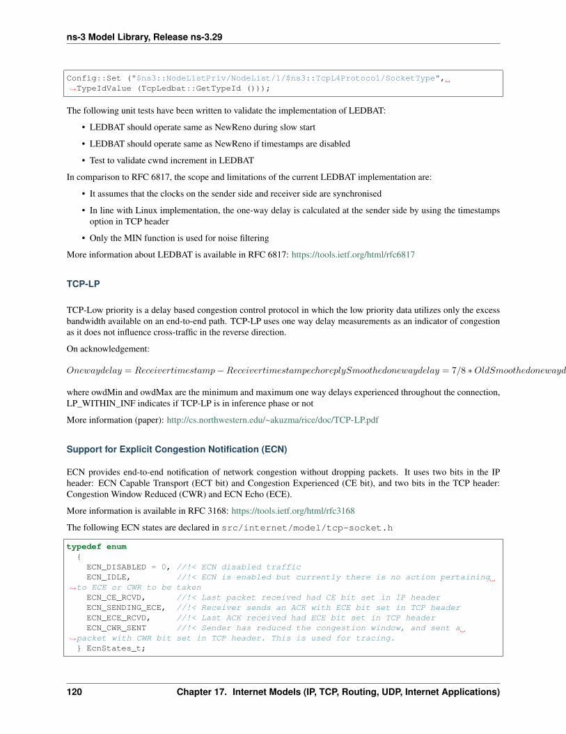
ns-3 Model Library, Release ns-3.29
Config::Set ("$ns3::NodeListPriv/NodeList/1/$ns3::TcpL4Protocol/SocketType",↪→TypeIdValue (TcpLedbat::GetTypeId ()));
The following unit tests have been written to validate the implementation of LEDBAT:
• LEDBAT should operate same as NewReno during slow start
• LEDBAT should operate same as NewReno if timestamps are disabled
• Test to validate cwnd increment in LEDBAT
In comparison to RFC 6817, the scope and limitations of the current LEDBAT implementation are:
• It assumes that the clocks on the sender side and receiver side are synchronised
• In line with Linux implementation, the one-way delay is calculated at the sender side by using the timestampsoption in TCP header
• Only the MIN function is used for noise filtering
More information about LEDBAT is available in RFC 6817: https://tools.ietf.org/html/rfc6817
TCP-LP
TCP-Low priority is a delay based congestion control protocol in which the low priority data utilizes only the excessbandwidth available on an end-to-end path. TCP-LP uses one way delay measurements as an indicator of congestionas it does not influence cross-traffic in the reverse direction.
On acknowledgement:
Onewaydelay = Receivertimestamp−ReceivertimestampechoreplySmoothedonewaydelay = 7/8 ∗OldSmoothedonewaydelay + 1/8 ∗ onewaydelayIfsmoothedonewaydelay > owdMin+ 15 ∗ (owdMax− owdMin)/100ifLPW ITHININFcwnd = 1elsecwnd = cwnd/2Inferencetimerisset
where owdMin and owdMax are the minimum and maximum one way delays experienced throughout the connection,LP_WITHIN_INF indicates if TCP-LP is in inference phase or not
More information (paper): http://cs.northwestern.edu/~akuzma/rice/doc/TCP-LP.pdf
Support for Explicit Congestion Notification (ECN)
ECN provides end-to-end notification of network congestion without dropping packets. It uses two bits in the IPheader: ECN Capable Transport (ECT bit) and Congestion Experienced (CE bit), and two bits in the TCP header:Congestion Window Reduced (CWR) and ECN Echo (ECE).
More information is available in RFC 3168: https://tools.ietf.org/html/rfc3168
The following ECN states are declared in src/internet/model/tcp-socket.h
typedef enum{ECN_DISABLED = 0, //!< ECN disabled trafficECN_IDLE, //!< ECN is enabled but currently there is no action pertaining
↪→to ECE or CWR to be takenECN_CE_RCVD, //!< Last packet received had CE bit set in IP headerECN_SENDING_ECE, //!< Receiver sends an ACK with ECE bit set in TCP headerECN_ECE_RCVD, //!< Last ACK received had ECE bit set in TCP headerECN_CWR_SENT //!< Sender has reduced the congestion window, and sent a
↪→packet with CWR bit set in TCP header. This is used for tracing.} EcnStates_t;
120 Chapter 17. Internet Models (IP, TCP, Routing, UDP, Internet Applications)
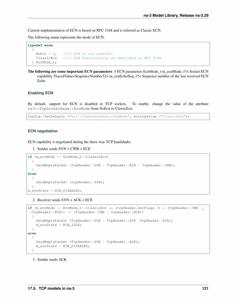
ns-3 Model Library, Release ns-3.29
Current implementation of ECN is based on RFC 3168 and is referred as Classic ECN.
The following enum represents the mode of ECN:
typedef enum{NoEcn = 0, //!< ECN is not enabled.ClassicEcn //!< ECN functionality as described in RFC 3168.
} EcnMode_t;
The following are some important ECN parameters // ECN parameters EcnMode_t m_ecnMode; //!< Socket ECNcapability TracedValue<SequenceNumber32> m_ecnEchoSeq; //!< Sequence number of the last received ECNEcho
Enabling ECN
By default, support for ECN is disabled in TCP sockets. To enable, change the value of the attributens3::TcpSocketBase::EcnMode from NoEcn to ClassicEcn.
Config::SetDefault ("ns3::TcpSocketBase::EcnMode", StringValue ("ClassicEcn"))
ECN negotiation
ECN capability is negotiated during the three-way TCP handshake:
1. Sender sends SYN + CWR + ECE
if (m_ecnMode == EcnMode_t::ClassicEcn){SendEmptyPacket (TcpHeader::SYN | TcpHeader::ECE | TcpHeader::CWR);
}else
{SendEmptyPacket (TcpHeader::SYN);
}m_ecnState = ECN_DISABLED;
2. Receiver sends SYN + ACK + ECE
if (m_ecnMode == EcnMode_t::ClassicEcn && (tcpHeader.GetFlags () & (TcpHeader::CWR |↪→TcpHeader::ECE)) == (TcpHeader::CWR | TcpHeader::ECE)){SendEmptyPacket (TcpHeader::SYN | TcpHeader::ACK |TcpHeader::ECE);m_ecnState = ECN_IDLE;
}else
{SendEmptyPacket (TcpHeader::SYN | TcpHeader::ACK);m_ecnState = ECN_DISABLED;
}
3. Sender sends ACK
17.5. TCP models in ns-3 121
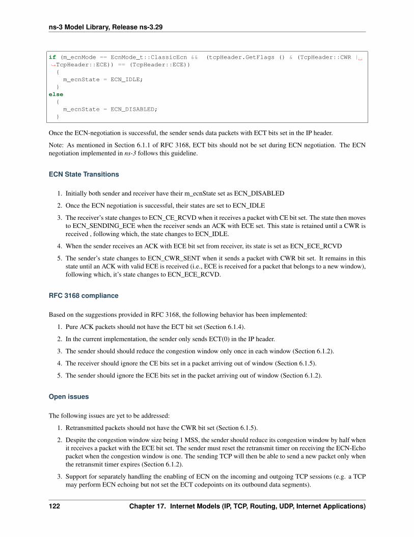
ns-3 Model Library, Release ns-3.29
if (m_ecnMode == EcnMode_t::ClassicEcn && (tcpHeader.GetFlags () & (TcpHeader::CWR |↪→TcpHeader::ECE)) == (TcpHeader::ECE)){m_ecnState = ECN_IDLE;
}else
{m_ecnState = ECN_DISABLED;
}
Once the ECN-negotiation is successful, the sender sends data packets with ECT bits set in the IP header.
Note: As mentioned in Section 6.1.1 of RFC 3168, ECT bits should not be set during ECN negotiation. The ECNnegotiation implemented in ns-3 follows this guideline.
ECN State Transitions
1. Initially both sender and receiver have their m_ecnState set as ECN_DISABLED
2. Once the ECN negotiation is successful, their states are set to ECN_IDLE
3. The receiver’s state changes to ECN_CE_RCVD when it receives a packet with CE bit set. The state then movesto ECN_SENDING_ECE when the receiver sends an ACK with ECE set. This state is retained until a CWR isreceived , following which, the state changes to ECN_IDLE.
4. When the sender receives an ACK with ECE bit set from receiver, its state is set as ECN_ECE_RCVD
5. The sender’s state changes to ECN_CWR_SENT when it sends a packet with CWR bit set. It remains in thisstate until an ACK with valid ECE is received (i.e., ECE is received for a packet that belongs to a new window),following which, it’s state changes to ECN_ECE_RCVD.
RFC 3168 compliance
Based on the suggestions provided in RFC 3168, the following behavior has been implemented:
1. Pure ACK packets should not have the ECT bit set (Section 6.1.4).
2. In the current implementation, the sender only sends ECT(0) in the IP header.
3. The sender should should reduce the congestion window only once in each window (Section 6.1.2).
4. The receiver should ignore the CE bits set in a packet arriving out of window (Section 6.1.5).
5. The sender should ignore the ECE bits set in the packet arriving out of window (Section 6.1.2).
Open issues
The following issues are yet to be addressed:
1. Retransmitted packets should not have the CWR bit set (Section 6.1.5).
2. Despite the congestion window size being 1 MSS, the sender should reduce its congestion window by half whenit receives a packet with the ECE bit set. The sender must reset the retransmit timer on receiving the ECN-Echopacket when the congestion window is one. The sending TCP will then be able to send a new packet only whenthe retransmit timer expires (Section 6.1.2).
3. Support for separately handling the enabling of ECN on the incoming and outgoing TCP sessions (e.g. a TCPmay perform ECN echoing but not set the ECT codepoints on its outbound data segments).
122 Chapter 17. Internet Models (IP, TCP, Routing, UDP, Internet Applications)
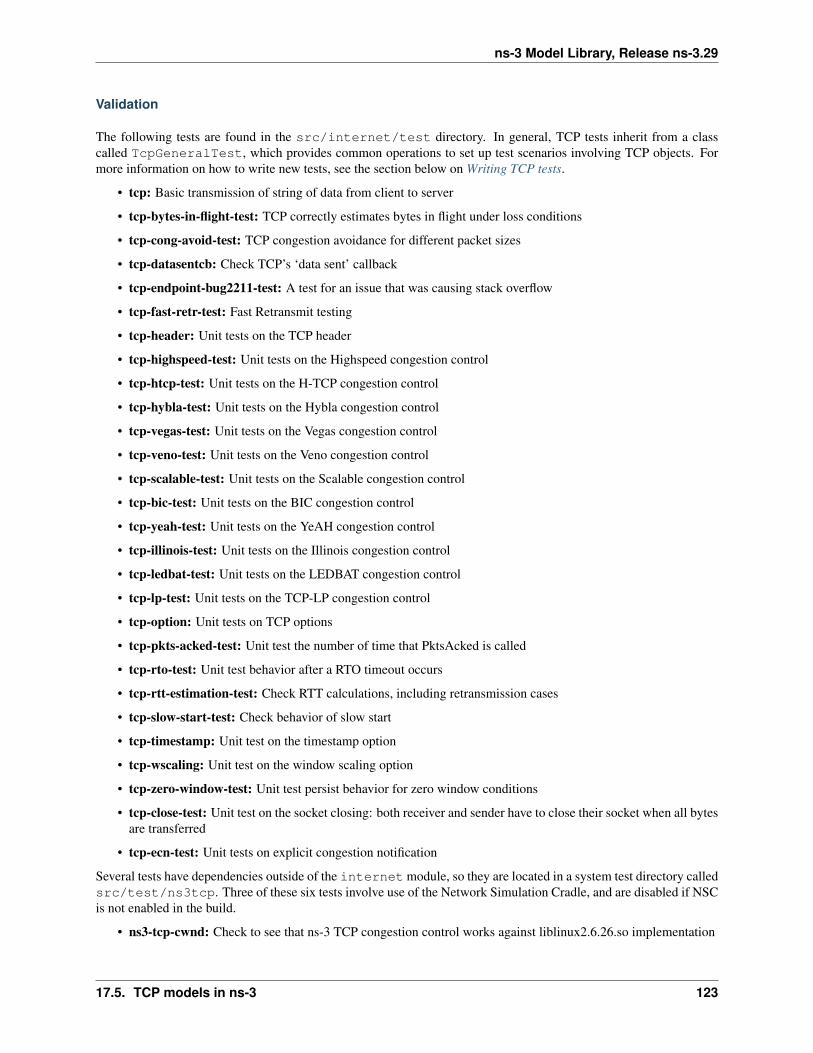
ns-3 Model Library, Release ns-3.29
Validation
The following tests are found in the src/internet/test directory. In general, TCP tests inherit from a classcalled TcpGeneralTest, which provides common operations to set up test scenarios involving TCP objects. Formore information on how to write new tests, see the section below on Writing TCP tests.
• tcp: Basic transmission of string of data from client to server
• tcp-bytes-in-flight-test: TCP correctly estimates bytes in flight under loss conditions
• tcp-cong-avoid-test: TCP congestion avoidance for different packet sizes
• tcp-datasentcb: Check TCP’s ‘data sent’ callback
• tcp-endpoint-bug2211-test: A test for an issue that was causing stack overflow
• tcp-fast-retr-test: Fast Retransmit testing
• tcp-header: Unit tests on the TCP header
• tcp-highspeed-test: Unit tests on the Highspeed congestion control
• tcp-htcp-test: Unit tests on the H-TCP congestion control
• tcp-hybla-test: Unit tests on the Hybla congestion control
• tcp-vegas-test: Unit tests on the Vegas congestion control
• tcp-veno-test: Unit tests on the Veno congestion control
• tcp-scalable-test: Unit tests on the Scalable congestion control
• tcp-bic-test: Unit tests on the BIC congestion control
• tcp-yeah-test: Unit tests on the YeAH congestion control
• tcp-illinois-test: Unit tests on the Illinois congestion control
• tcp-ledbat-test: Unit tests on the LEDBAT congestion control
• tcp-lp-test: Unit tests on the TCP-LP congestion control
• tcp-option: Unit tests on TCP options
• tcp-pkts-acked-test: Unit test the number of time that PktsAcked is called
• tcp-rto-test: Unit test behavior after a RTO timeout occurs
• tcp-rtt-estimation-test: Check RTT calculations, including retransmission cases
• tcp-slow-start-test: Check behavior of slow start
• tcp-timestamp: Unit test on the timestamp option
• tcp-wscaling: Unit test on the window scaling option
• tcp-zero-window-test: Unit test persist behavior for zero window conditions
• tcp-close-test: Unit test on the socket closing: both receiver and sender have to close their socket when all bytesare transferred
• tcp-ecn-test: Unit tests on explicit congestion notification
Several tests have dependencies outside of the internet module, so they are located in a system test directory calledsrc/test/ns3tcp. Three of these six tests involve use of the Network Simulation Cradle, and are disabled if NSCis not enabled in the build.
• ns3-tcp-cwnd: Check to see that ns-3 TCP congestion control works against liblinux2.6.26.so implementation
17.5. TCP models in ns-3 123
ns-3 Model Library, Release ns-3.29
• ns3-tcp-interoperability: Check to see that ns-3 TCP interoperates with liblinux2.6.26.so implementation
• ns3-tcp-loss: Check behavior of ns-3 TCP upon packet losses
• nsc-tcp-loss: Check behavior of NSC TCP upon packet losses
• ns3-tcp-no-delay: Check that ns-3 TCP Nagle”s algorithm works correctly and that it can be disabled
• ns3-tcp-socket: Check that ns-3 TCP successfully transfers an application data write of various sizes
• ns3-tcp-state: Check the operation of the TCP state machine for several cases
Several TCP validation test results can also be found in the wiki page describing this implementation.
TCP ECN operation is tested in the ARED and RED tests that are documented in the traffic-control module documen-tation.
Writing a new congestion control algorithm
Writing (or porting) a congestion control algorithms from scratch (or from other systems) is a process completelyseparated from the internals of TcpSocketBase.
All operations that are delegated to a congestion control are contained in the class TcpCongestionOps. It mimics thestructure tcp_congestion_ops of Linux, and the following operations are defined:
virtual std::string GetName () const;virtual uint32_t GetSsThresh (Ptr<const TcpSocketState> tcb, uint32_t bytesInFlight);virtual void IncreaseWindow (Ptr<TcpSocketState> tcb, uint32_t segmentsAcked);virtual void PktsAcked (Ptr<TcpSocketState> tcb, uint32_t segmentsAcked,const Time&↪→rtt);virtual Ptr<TcpCongestionOps> Fork ();virtual void CwndEvent (Ptr<TcpSocketState> tcb, const TcpSocketState::TcpCaEvent_t↪→event);
The most interesting methods to write are GetSsThresh and IncreaseWindow. The latter is called when TcpSocketBasedecides that it is time to increase the congestion window. Much information is available in the Transmission ControlBlock, and the method should increase cWnd and/or ssThresh based on the number of segments acked.
GetSsThresh is called whenever the socket needs an updated value of the slow start threshold. This happens after aloss; congestion control algorithms are then asked to lower such value, and to return it.
PktsAcked is used in case the algorithm needs timing information (such as RTT), and it is called each time an ACK isreceived.
CwndEvent is used in case the algorithm needs the state of socket during different congestion window event.
TCP SACK and non-SACK
To avoid code duplication and the effort of maintaining two different versions of the TCP core, namely RFC 6675(TCP-SACK) and RFC 5681 (TCP congestion control), we have merged RFC 6675 in the current code base. If thereceiver supports the option, the sender bases its retransmissions over the received SACK information. However, inthe absence of that option, the best it can do is to follow the RFC 5681 specification (on Fast Retransmit/Recovery)and employing NewReno modifications in case of partial ACKs.
A similar concept is used in Linux with the function tcp_add_reno_sack. Our implementation resides in the Tcp-TxBuffer class that implements a scoreboard through two different lists of segments. TcpSocketBase actively uses theAPI provided by TcpTxBuffer to query the scoreboard; please refer to the Doxygen documentation (and to in-codecomments) if you want to learn more about this implementation.
124 Chapter 17. Internet Models (IP, TCP, Routing, UDP, Internet Applications)
ns-3 Model Library, Release ns-3.29
For an academic peer-reviewed paper on the SACK implementation in ns-3, please refer to https://dl.acm.org/citation.cfm?id=3067666.
Loss Recovery Algorithms
The following loss recovery algorithms are supported in ns-3 TCP:
Classic Recovery
Classic Recovery refers to the combination of NewReno algorithm described in RFC 6582 along with SACK basedloss recovery algorithm mentioned in RFC 6675. SACK based loss recovery is used when sender and receiver supportSACK options. In the case when SACK options are disabled, the NewReno modification handles the recovery.
At the start of recovery phase the congestion window is reduced diffently for NewReno and SACK based recovery.For NewReno the reduction is done as given below:
cWnd = ssThresh
For SACK based recovery, this is done as follows:
cWnd = ssThresh+ (dupAckCount ∗ segmentSize)
While in the recovery phase, the congestion window is inflated by segmentSize on arrival of every ACK whenNewReno is used. The congestion window is kept same when SACK based loss recovery is used.
Proportional Rate Reduction
Proportional Rate Reduction (PRR) is the fast recovery algorithm described in RFC 6937 and currently used in Linux.The design of PRR helps in avoiding excess window adjustments and aims to keep the congestion window as close aspossible to ssThresh.
PRR updates the congestion window by comparing the values of bytesInFlight and ssThresh. If the value of bytesIn-Flight is greater than ssThresh, congestion window is updated as shown below:
sndcnt = CEIL(prrDelivered ∗ ssThresh/RecoverFS)− prrOut
cWnd = pipe+ sndcnt
where RecoverFS is the value of bytesInFlight at the start of recovery phase, prrDelivered is the total bytesdelivered during recovery phase, prrOut is the total bytes sent during recovery phase and sndcnt represents thenumber of bytes to be sent in response to each ACK.
Otherwise, the congestion window is updated by either using Conservative Reduction Bound (CRB) or Slow Start Re-duction Bound (SSRB) with SSRB being the default Reduction Bound. Each Reduction Bound calculates a maximumdata sending limit. For CRB, the limit is calculated as shown below:
limit = prrDelivered− prrout
For SSRB, it is calculated as:
limit = MAX(prrDelivered− prrOut,DeliveredData) +MSS
where DeliveredData represets the total number of bytes delivered to the receiver as indicated by the current ACKand MSS is the maximum segment size.
17.5. TCP models in ns-3 125
ns-3 Model Library, Release ns-3.29
After limit calculation, the cWnd is updated as given below:
sndcnt = MIN(ssThresh− pipe, limit)
cWnd = pipe+ sndcnt
More information (paper): https://dl.acm.org/citation.cfm?id=2068832
More information (RFC): https://tools.ietf.org/html/rfc6937
Adding a new loss recovery algorithm in ns-3
Writing (or porting) a loss recovery algorithms from scratch (or from other systems) is a process completely separatedfrom the internals of TcpSocketBase.
All operations that are delegated to a loss recovery are contained in the class TcpRecoveryOps and are given below:
virtual std::string GetName () const;virtual void EnterRecovery (Ptr<const TcpSocketState> tcb, uint32_t unAckDataCount,
bool isSackEnabled, uint32_t dupAckCount,uint32_t bytesInFlight, uint32_t lastDeliveredBytes);
virtual void DoRecovery (Ptr<const TcpSocketState> tcb, uint32_t unAckDataCount,bool isSackEnabled, uint32_t dupAckCount,uint32_t bytesInFlight, uint32_t lastDeliveredBytes);
virtual void ExitRecovery (Ptr<TcpSocketState> tcb, uint32_t bytesInFlight);virtual void UpdateBytesSent (uint32_t bytesSent);virtual Ptr<TcpRecoveryOps> Fork ();
EnterRecovery is called when packet loss is detected and recovery is triggered. While in recovery phase, each timewhen an ACK arrives, DoRecovery is called which performs the necessary congestion window changes as per therecovery algorithm. ExitRecovery is called just prior to exiting recovery phase in order to perform the requiredcongestion window ajustments. UpdateBytesSent is used to keep track of bytes sent and is called whenever a datapacket is sent during recovery phase.
Current limitations
• TcpCongestionOps interface does not contain every possible Linux operation
Writing TCP tests
The TCP subsystem supports automated test cases on both socket functions and congestion control algorithms. Toshow how to write tests for TCP, here we explain the process of creating a test case that reproduces a bug (#1571 inthe project bug tracker).
The bug concerns the zero window situation, which happens when the receiver can not handle more data. In this case,it advertises a zero window, which causes the sender to pause transmission and wait for the receiver to increase thewindow.
The sender has a timer to periodically check the receiver’s window: however, in modern TCP implementations, whenthe receiver has freed a “significant” amount of data, the receiver itself sends an “active” window update, meaning thatthe transmission could be resumed. Nevertheless, the sender timer is still necessary because window updates can belost.
Note: During the text, we will assume some knowledge about the general design of the TCP test infrastructure, whichis explained in detail into the Doxygen documentation. As a brief summary, the strategy is to have a class that sets
126 Chapter 17. Internet Models (IP, TCP, Routing, UDP, Internet Applications)
ns-3 Model Library, Release ns-3.29
up a TCP connection, and that calls protected members of itself. In this way, subclasses can implement the necessarymembers, which will be called by the main TcpGeneralTest class when events occur. For example, after processingan ACK, the method ProcessedAck will be invoked. Subclasses interested in checking some particular things whichmust have happened during an ACK processing, should implement the ProcessedAck method and check the interestingvalues inside the method. To get a list of available methods, please check the Doxygen documentation.
We describe the writing of two test case, covering both situations: the sender’s zero-window probing and the receiver“active” window update. Our focus will be on dealing with the reported problems, which are:
• an ns-3 receiver does not send “active” window update when its receive buffer is being freed;
• even if the window update is artificially crafted, the transmission does not resume.
However, other things should be checked in the test:
• Persistent timer setup
• Persistent timer teardown if rWnd increases
To construct the test case, one first derives from the TcpGeneralTest class:
The code is the following:
TcpZeroWindowTest::TcpZeroWindowTest (const std::string &desc): TcpGeneralTest (desc)
{}
Then, one should define the general parameters for the TCP connection, which will be one-sided (one node is actingas SENDER, while the other is acting as RECEIVER):
• Application packet size set to 500, and 20 packets in total (meaning a stream of 10k bytes)
• Segment size for both SENDER and RECEIVER set to 500 bytes
• Initial slow start threshold set to UINT32_MAX
• Initial congestion window for the SENDER set to 10 segments (5000 bytes)
• Congestion control: NewReno
We have also to define the link properties, because the above definition does not work for every combination ofpropagation delay and sender application behavior.
• Link one-way propagation delay: 50 ms
• Application packet generation interval: 10 ms
• Application starting time: 20 s after the starting point
To define the properties of the environment (e.g. properties which should be set before the object creation, such aspropagation delay) one next implements ehe method ConfigureEnvironment:
voidTcpZeroWindowTest::ConfigureEnvironment (){
TcpGeneralTest::ConfigureEnvironment ();SetAppPktCount (20);SetMTU (500);SetTransmitStart (Seconds (2.0));SetPropagationDelay (MilliSeconds (50));
}
17.5. TCP models in ns-3 127
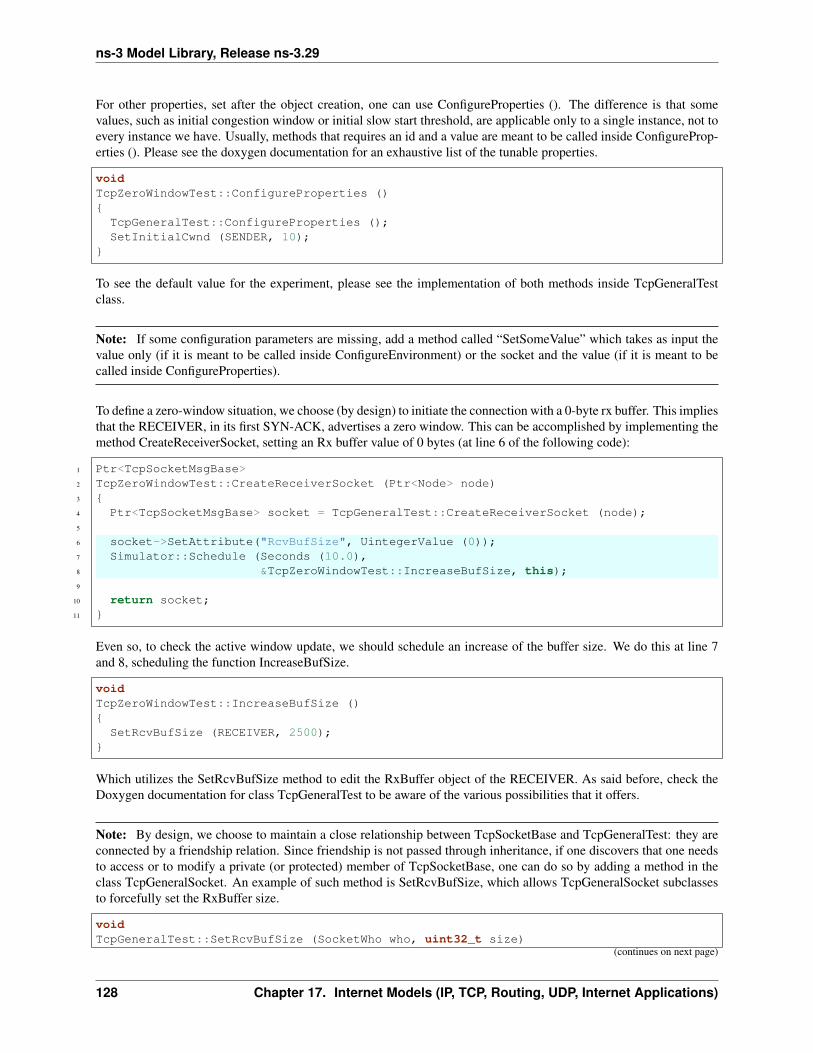
ns-3 Model Library, Release ns-3.29
For other properties, set after the object creation, one can use ConfigureProperties (). The difference is that somevalues, such as initial congestion window or initial slow start threshold, are applicable only to a single instance, not toevery instance we have. Usually, methods that requires an id and a value are meant to be called inside ConfigureProp-erties (). Please see the doxygen documentation for an exhaustive list of the tunable properties.
voidTcpZeroWindowTest::ConfigureProperties (){
TcpGeneralTest::ConfigureProperties ();SetInitialCwnd (SENDER, 10);
}
To see the default value for the experiment, please see the implementation of both methods inside TcpGeneralTestclass.
Note: If some configuration parameters are missing, add a method called “SetSomeValue” which takes as input thevalue only (if it is meant to be called inside ConfigureEnvironment) or the socket and the value (if it is meant to becalled inside ConfigureProperties).
To define a zero-window situation, we choose (by design) to initiate the connection with a 0-byte rx buffer. This impliesthat the RECEIVER, in its first SYN-ACK, advertises a zero window. This can be accomplished by implementing themethod CreateReceiverSocket, setting an Rx buffer value of 0 bytes (at line 6 of the following code):
1 Ptr<TcpSocketMsgBase>2 TcpZeroWindowTest::CreateReceiverSocket (Ptr<Node> node)3 {4 Ptr<TcpSocketMsgBase> socket = TcpGeneralTest::CreateReceiverSocket (node);5
6 socket->SetAttribute("RcvBufSize", UintegerValue (0));7 Simulator::Schedule (Seconds (10.0),8 &TcpZeroWindowTest::IncreaseBufSize, this);9
10 return socket;11 }
Even so, to check the active window update, we should schedule an increase of the buffer size. We do this at line 7and 8, scheduling the function IncreaseBufSize.
voidTcpZeroWindowTest::IncreaseBufSize (){
SetRcvBufSize (RECEIVER, 2500);}
Which utilizes the SetRcvBufSize method to edit the RxBuffer object of the RECEIVER. As said before, check theDoxygen documentation for class TcpGeneralTest to be aware of the various possibilities that it offers.
Note: By design, we choose to maintain a close relationship between TcpSocketBase and TcpGeneralTest: they areconnected by a friendship relation. Since friendship is not passed through inheritance, if one discovers that one needsto access or to modify a private (or protected) member of TcpSocketBase, one can do so by adding a method in theclass TcpGeneralSocket. An example of such method is SetRcvBufSize, which allows TcpGeneralSocket subclassesto forcefully set the RxBuffer size.
voidTcpGeneralTest::SetRcvBufSize (SocketWho who, uint32_t size)
(continues on next page)
128 Chapter 17. Internet Models (IP, TCP, Routing, UDP, Internet Applications)
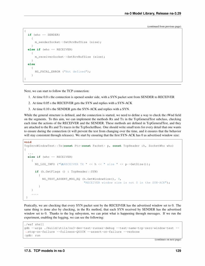
ns-3 Model Library, Release ns-3.29
(continued from previous page)
{if (who == SENDER){
m_senderSocket->SetRcvBufSize (size);}
else if (who == RECEIVER){
m_receiverSocket->SetRcvBufSize (size);}
else{
NS_FATAL_ERROR ("Not defined");}
}
Next, we can start to follow the TCP connection:
1. At time 0.0 s the connection is opened sender side, with a SYN packet sent from SENDER to RECEIVER
2. At time 0.05 s the RECEIVER gets the SYN and replies with a SYN-ACK
3. At time 0.10 s the SENDER gets the SYN-ACK and replies with a SYN.
While the general structure is defined, and the connection is started, we need to define a way to check the rWnd fieldon the segments. To this aim, we can implement the methods Rx and Tx in the TcpGeneralTest subclass, checkingeach time the actions of the RECEIVER and the SENDER. These methods are defined in TcpGeneralTest, and theyare attached to the Rx and Tx traces in the TcpSocketBase. One should write small tests for every detail that one wantsto ensure during the connection (it will prevent the test from changing over the time, and it ensures that the behaviorwill stay consistent through releases). We start by ensuring that the first SYN-ACK has 0 as advertised window size:
voidTcpZeroWindowTest::Tx(const Ptr<const Packet> p, const TcpHeader &h, SocketWho who){
...else if (who == RECEIVER){
NS_LOG_INFO ("\tRECEIVER TX " << h << " size " << p->GetSize());
if (h.GetFlags () & TcpHeader::SYN){NS_TEST_ASSERT_MSG_EQ (h.GetWindowSize(), 0,
"RECEIVER window size is not 0 in the SYN-ACK");}
}....
}
Pratically, we are checking that every SYN packet sent by the RECEIVER has the advertised window set to 0. Thesame thing is done also by checking, in the Rx method, that each SYN received by SENDER has the advertisedwindow set to 0. Thanks to the log subsystem, we can print what is happening through messages. If we run theexperiment, enabling the logging, we can see the following:
./waf shellgdb --args ./build/utils/ns3-dev-test-runner-debug --test-name=tcp-zero-window-test --↪→stop-on-failure --fullness=QUICK --assert-on-failure --verbose(gdb) run
(continues on next page)
17.5. TCP models in ns-3 129

ns-3 Model Library, Release ns-3.29
(continued from previous page)
0.00s TcpZeroWindowTestSuite:Tx(): 0.00 SENDER TX 49153 > 4477 [SYN] Seq=0 Ack=0↪→Win=32768 ns3::TcpOptionWinScale(2) ns3::TcpOptionTS(0;0) size 360.05s TcpZeroWindowTestSuite:Rx(): 0.05 RECEIVER RX 49153 > 4477 [SYN] Seq=0↪→Ack=0 Win=32768 ns3::TcpOptionWinScale(2) ns3::TcpOptionTS(0;0)↪→ns3::TcpOptionEnd(EOL) size 00.05s TcpZeroWindowTestSuite:Tx(): 0.05 RECEIVER TX 4477 > 49153 [SYN|ACK] Seq=0↪→Ack=1 Win=0 ns3::TcpOptionWinScale(0) ns3::TcpOptionTS(50;0) size 360.10s TcpZeroWindowTestSuite:Rx(): 0.10 SENDER RX 4477 > 49153 [SYN|ACK] Seq=0↪→Ack=1 Win=0 ns3::TcpOptionWinScale(0) ns3::TcpOptionTS(50;0) ns3::TcpOptionEnd(EOL)↪→size 00.10s TcpZeroWindowTestSuite:Tx(): 0.10 SENDER TX 49153 > 4477 [ACK] Seq=1 Ack=1↪→Win=32768 ns3::TcpOptionTS(100;50) size 320.15s TcpZeroWindowTestSuite:Rx(): 0.15 RECEIVER RX 49153 > 4477 [ACK] Seq=1↪→Ack=1 Win=32768 ns3::TcpOptionTS(100;50) ns3::TcpOptionEnd(EOL) size 0(...)
The output is cut to show the threeway handshake. As we can see from the headers, the rWnd of RECEIVER is setto 0, and thankfully our tests are not failing. Now we need to test for the persistent timer, which should be started bythe SENDER after it receives the SYN-ACK. Since the Rx method is called before any computation on the receivedpacket, we should utilize another method, namely ProcessedAck, which is the method called after each processedACK. In the following, we show how to check if the persistent event is running after the processing of the SYN-ACK:
voidTcpZeroWindowTest::ProcessedAck (const Ptr<const TcpSocketState> tcb,
const TcpHeader& h, SocketWho who){
if (who == SENDER){
if (h.GetFlags () & TcpHeader::SYN){EventId persistentEvent = GetPersistentEvent (SENDER);NS_TEST_ASSERT_MSG_EQ (persistentEvent.IsRunning (), true,
"Persistent event not started");}
}}
Since we programmed the increase of the buffer size after 10 simulated seconds, we expect the persistent timer to firebefore any rWnd changes. When it fires, the SENDER should send a window probe, and the receiver should replyreporting again a zero window situation. At first, we investigates on what the sender sends:
1 if (Simulator::Now ().GetSeconds () <= 6.0)2 {3 NS_TEST_ASSERT_MSG_EQ (p->GetSize () - h.GetSerializedSize(), 0,4 "Data packet sent anyway");5 }6 else if (Simulator::Now ().GetSeconds () > 6.0 &&7 Simulator::Now ().GetSeconds () <= 7.0)8 {9 NS_TEST_ASSERT_MSG_EQ (m_zeroWindowProbe, false, "Sent another probe");
10
11 if (! m_zeroWindowProbe)12 {13 NS_TEST_ASSERT_MSG_EQ (p->GetSize () - h.GetSerializedSize(), 1,14 "Data packet sent instead of window probe");
(continues on next page)
130 Chapter 17. Internet Models (IP, TCP, Routing, UDP, Internet Applications)
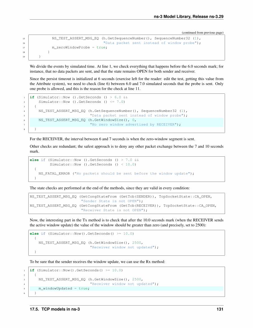
ns-3 Model Library, Release ns-3.29
(continued from previous page)
15 NS_TEST_ASSERT_MSG_EQ (h.GetSequenceNumber(), SequenceNumber32 (1),16 "Data packet sent instead of window probe");17 m_zeroWindowProbe = true;18 }19 }
We divide the events by simulated time. At line 1, we check everything that happens before the 6.0 seconds mark; forinstance, that no data packets are sent, and that the state remains OPEN for both sender and receiver.
Since the persist timeout is initialized at 6 seconds (exercise left for the reader: edit the test, getting this value fromthe Attribute system), we need to check (line 6) between 6.0 and 7.0 simulated seconds that the probe is sent. Onlyone probe is allowed, and this is the reason for the check at line 11.
1 if (Simulator::Now ().GetSeconds () > 6.0 &&2 Simulator::Now ().GetSeconds () <= 7.0)3 {4 NS_TEST_ASSERT_MSG_EQ (h.GetSequenceNumber(), SequenceNumber32 (1),5 "Data packet sent instead of window probe");6 NS_TEST_ASSERT_MSG_EQ (h.GetWindowSize(), 0,7 "No zero window advertised by RECEIVER");8 }
For the RECEIVER, the interval between 6 and 7 seconds is when the zero-window segment is sent.
Other checks are redundant; the safest approach is to deny any other packet exchange between the 7 and 10 secondsmark.
else if (Simulator::Now ().GetSeconds () > 7.0 &&Simulator::Now ().GetSeconds () < 10.0)
{NS_FATAL_ERROR ("No packets should be sent before the window update");
}
The state checks are performed at the end of the methods, since they are valid in every condition:
NS_TEST_ASSERT_MSG_EQ (GetCongStateFrom (GetTcb(SENDER)), TcpSocketState::CA_OPEN,"Sender State is not OPEN");
NS_TEST_ASSERT_MSG_EQ (GetCongStateFrom (GetTcb(RECEIVER)), TcpSocketState::CA_OPEN,"Receiver State is not OPEN");
Now, the interesting part in the Tx method is to check that after the 10.0 seconds mark (when the RECEIVER sendsthe active window update) the value of the window should be greater than zero (and precisely, set to 2500):
else if (Simulator::Now().GetSeconds() >= 10.0){NS_TEST_ASSERT_MSG_EQ (h.GetWindowSize(), 2500,
"Receiver window not updated");}
To be sure that the sender receives the window update, we can use the Rx method:
1 if (Simulator::Now().GetSeconds() >= 10.0)2 {3 NS_TEST_ASSERT_MSG_EQ (h.GetWindowSize(), 2500,4 "Receiver window not updated");5 m_windowUpdated = true;6 }
17.5. TCP models in ns-3 131
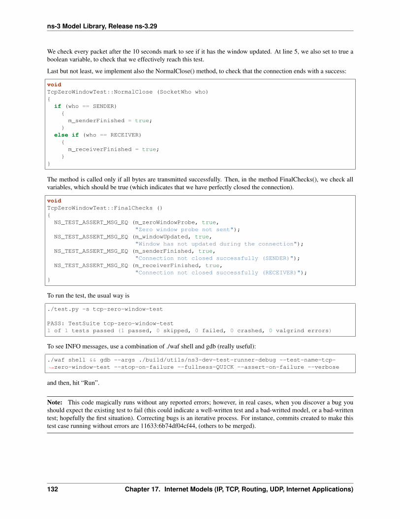
ns-3 Model Library, Release ns-3.29
We check every packet after the 10 seconds mark to see if it has the window updated. At line 5, we also set to true aboolean variable, to check that we effectively reach this test.
Last but not least, we implement also the NormalClose() method, to check that the connection ends with a success:
voidTcpZeroWindowTest::NormalClose (SocketWho who){
if (who == SENDER){
m_senderFinished = true;}
else if (who == RECEIVER){
m_receiverFinished = true;}
}
The method is called only if all bytes are transmitted successfully. Then, in the method FinalChecks(), we check allvariables, which should be true (which indicates that we have perfectly closed the connection).
voidTcpZeroWindowTest::FinalChecks (){
NS_TEST_ASSERT_MSG_EQ (m_zeroWindowProbe, true,"Zero window probe not sent");
NS_TEST_ASSERT_MSG_EQ (m_windowUpdated, true,"Window has not updated during the connection");
NS_TEST_ASSERT_MSG_EQ (m_senderFinished, true,"Connection not closed successfully (SENDER)");
NS_TEST_ASSERT_MSG_EQ (m_receiverFinished, true,"Connection not closed successfully (RECEIVER)");
}
To run the test, the usual way is
./test.py -s tcp-zero-window-test
PASS: TestSuite tcp-zero-window-test1 of 1 tests passed (1 passed, 0 skipped, 0 failed, 0 crashed, 0 valgrind errors)
To see INFO messages, use a combination of ./waf shell and gdb (really useful):
./waf shell && gdb --args ./build/utils/ns3-dev-test-runner-debug --test-name=tcp-↪→zero-window-test --stop-on-failure --fullness=QUICK --assert-on-failure --verbose
and then, hit “Run”.
Note: This code magically runs without any reported errors; however, in real cases, when you discover a bug youshould expect the existing test to fail (this could indicate a well-written test and a bad-writted model, or a bad-writtentest; hopefully the first situation). Correcting bugs is an iterative process. For instance, commits created to make thistest case running without errors are 11633:6b74df04cf44, (others to be merged).
132 Chapter 17. Internet Models (IP, TCP, Routing, UDP, Internet Applications)

ns-3 Model Library, Release ns-3.29
17.5.3 Network Simulation Cradle
The Network Simulation Cradle (NSC) is a framework for wrapping real-world network code into simulators, allowingsimulation of real-world behavior at little extra cost. This work has been validated by comparing situations using atest network with the same situations in the simulator. To date, it has been shown that the NSC is able to produceextremely accurate results. NSC supports four real world stacks: FreeBSD, OpenBSD, lwIP and Linux. Emphasishas been placed on not changing any of the network stacks by hand. Not a single line of code has been changedin the network protocol implementations of any of the above four stacks. However, a custom C parser was built toprogrammatically change source code.
NSC has previously been ported to ns-2 and OMNeT++, and was was added to ns-3 in September 2008 (ns-3.2 release).This section describes the ns-3 port of NSC and how to use it.
NSC has been obsoleted by the Linux kernel support within Direct Code Execution (DCE). However, NSC is stillavailable through the bake build system. NSC supports Linux kernels 2.6.18 and 2.6.26, and an experimental versionof 2.6.29 exists on ns-3’s code server (http://code.nsnam.org/fw/nsc-linux-2.6.29/), but newer versions of the kernelhave not been ported.
Prerequisites
Presently, NSC has been tested and shown to work on these platforms: Linux i386 and Linux x86-64. NSC does notsupport powerpc. Use on FreeBSD or OS X is unsupported (although it may be able to work).
Building NSC requires the packages flex and bison.
NSC requires use of gcc-4.9 or gcc-5 series, and will not build on newer systems lacking the older compilers.
Configuring and Downloading
NSC must either be downloaded separately from its own repository, or downloading when using the bake build systemof ns-3.
For ns-3.17 through ns-3.28 releases, when using bake, one obtains NSC implicitly as part of an “allinone” configura-tion, such as:
$ cd bake$ python bake.py configure -e ns-allinone-3.27$ python bake.py download$ python bake.py build
For ns-3.29 and later versions, including the ‘ns-3-allinone’ development version, one must explicitly add NSC (‘nsc-0.5.3’) to the bake configuration, such as:
$ cd bake$ python bake.py configure -e ns-allinone-3.29 -e nsc-0.5.3$ python bake.py download$ python bake.py build
Instead of a released version, one may use the ns-3 development version by specifying “ns-3-allinone” to the configurestep above.
NSC may also be downloaded from its download site using Mercurial:
$ hg clone https://secure.wand.net.nz/mercurial/nsc
Prior to the ns-3.17 release, NSC was included in the allinone tarball and the released version did not need to beseparately downloaded.
17.5. TCP models in ns-3 133
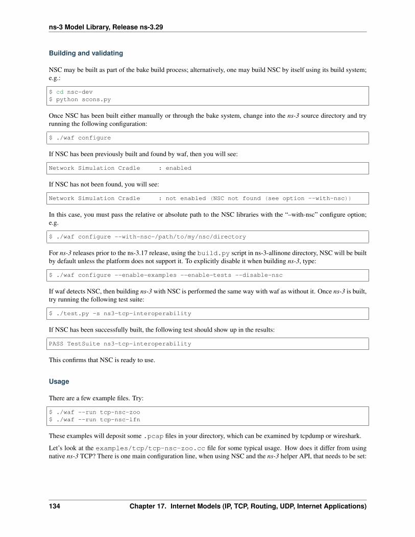
ns-3 Model Library, Release ns-3.29
Building and validating
NSC may be built as part of the bake build process; alternatively, one may build NSC by itself using its build system;e.g.:
$ cd nsc-dev$ python scons.py
Once NSC has been built either manually or through the bake system, change into the ns-3 source directory and tryrunning the following configuration:
$ ./waf configure
If NSC has been previously built and found by waf, then you will see:
Network Simulation Cradle : enabled
If NSC has not been found, you will see:
Network Simulation Cradle : not enabled (NSC not found (see option --with-nsc))
In this case, you must pass the relative or absolute path to the NSC libraries with the “–with-nsc” configure option;e.g.
$ ./waf configure --with-nsc=/path/to/my/nsc/directory
For ns-3 releases prior to the ns-3.17 release, using the build.py script in ns-3-allinone directory, NSC will be builtby default unless the platform does not support it. To explicitly disable it when building ns-3, type:
$ ./waf configure --enable-examples --enable-tests --disable-nsc
If waf detects NSC, then building ns-3 with NSC is performed the same way with waf as without it. Once ns-3 is built,try running the following test suite:
$ ./test.py -s ns3-tcp-interoperability
If NSC has been successfully built, the following test should show up in the results:
PASS TestSuite ns3-tcp-interoperability
This confirms that NSC is ready to use.
Usage
There are a few example files. Try:
$ ./waf --run tcp-nsc-zoo$ ./waf --run tcp-nsc-lfn
These examples will deposit some .pcap files in your directory, which can be examined by tcpdump or wireshark.
Let’s look at the examples/tcp/tcp-nsc-zoo.cc file for some typical usage. How does it differ from usingnative ns-3 TCP? There is one main configuration line, when using NSC and the ns-3 helper API, that needs to be set:
134 Chapter 17. Internet Models (IP, TCP, Routing, UDP, Internet Applications)
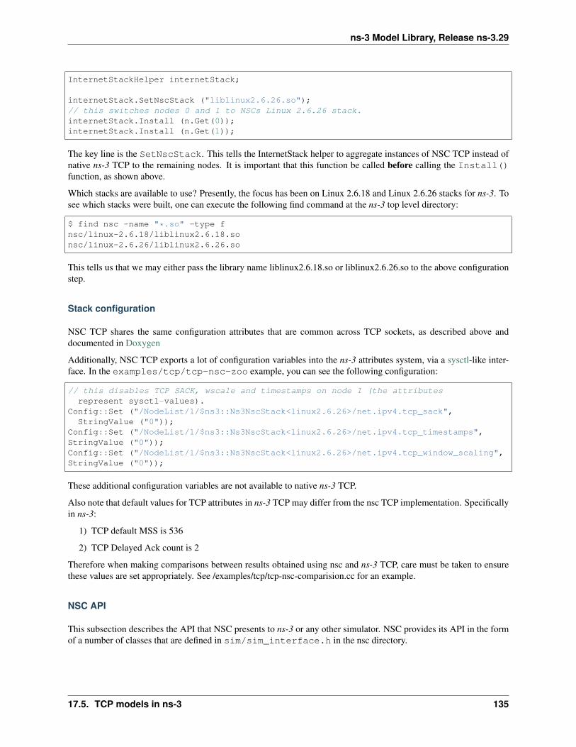
ns-3 Model Library, Release ns-3.29
InternetStackHelper internetStack;
internetStack.SetNscStack ("liblinux2.6.26.so");// this switches nodes 0 and 1 to NSCs Linux 2.6.26 stack.internetStack.Install (n.Get(0));internetStack.Install (n.Get(1));
The key line is the SetNscStack. This tells the InternetStack helper to aggregate instances of NSC TCP instead ofnative ns-3 TCP to the remaining nodes. It is important that this function be called before calling the Install()function, as shown above.
Which stacks are available to use? Presently, the focus has been on Linux 2.6.18 and Linux 2.6.26 stacks for ns-3. Tosee which stacks were built, one can execute the following find command at the ns-3 top level directory:
$ find nsc -name "*.so" -type fnsc/linux-2.6.18/liblinux2.6.18.sonsc/linux-2.6.26/liblinux2.6.26.so
This tells us that we may either pass the library name liblinux2.6.18.so or liblinux2.6.26.so to the above configurationstep.
Stack configuration
NSC TCP shares the same configuration attributes that are common across TCP sockets, as described above anddocumented in Doxygen
Additionally, NSC TCP exports a lot of configuration variables into the ns-3 attributes system, via a sysctl-like inter-face. In the examples/tcp/tcp-nsc-zoo example, you can see the following configuration:
// this disables TCP SACK, wscale and timestamps on node 1 (the attributesrepresent sysctl-values).
Config::Set ("/NodeList/1/$ns3::Ns3NscStack<linux2.6.26>/net.ipv4.tcp_sack",StringValue ("0"));
Config::Set ("/NodeList/1/$ns3::Ns3NscStack<linux2.6.26>/net.ipv4.tcp_timestamps",StringValue ("0"));Config::Set ("/NodeList/1/$ns3::Ns3NscStack<linux2.6.26>/net.ipv4.tcp_window_scaling",StringValue ("0"));
These additional configuration variables are not available to native ns-3 TCP.
Also note that default values for TCP attributes in ns-3 TCP may differ from the nsc TCP implementation. Specificallyin ns-3:
1) TCP default MSS is 536
2) TCP Delayed Ack count is 2
Therefore when making comparisons between results obtained using nsc and ns-3 TCP, care must be taken to ensurethese values are set appropriately. See /examples/tcp/tcp-nsc-comparision.cc for an example.
NSC API
This subsection describes the API that NSC presents to ns-3 or any other simulator. NSC provides its API in the formof a number of classes that are defined in sim/sim_interface.h in the nsc directory.
17.5. TCP models in ns-3 135

ns-3 Model Library, Release ns-3.29
• INetStack INetStack contains the ‘low level’ operations for the operating system network stack, e.g. in andoutput functions from and to the network stack (think of this as the ‘network driver interface’. There are alsofunctions to create new TCP or UDP sockets.
• ISendCallback This is called by NSC when a packet should be sent out to the network. This simulator shoulduse this callback to re-inject the packet into the simulator so the actual data can be delivered/routed to itsdestination, where it will eventually be handed into Receive() (and eventually back to the receivers NSC instancevia INetStack->if_receive() ).
• INetStreamSocket This is the structure defining a particular connection endpoint (file descriptor). It containsmethods to operate on this endpoint, e.g. connect, disconnect, accept, listen, send_data/read_data, . . .
• IInterruptCallback This contains the wakeup callback, which is called by NSC whenever something of in-terest happens. Think of wakeup() as a replacement of the operating systems wakeup function: Whenever theoperating system would wake up a process that has been waiting for an operation to complete (for example theTCP handshake during connect()), NSC invokes the wakeup() callback to allow the simulator to check for statechanges in its connection endpoints.
ns-3 implementation
The ns-3 implementation makes use of the above NSC API, and is implemented as follows.
The three main parts are:
• ns3::NscTcpL4Protocol: a subclass of Ipv4L4Protocol (and two nsc classes: ISendCallback and IInter-ruptCallback)
• ns3::NscTcpSocketImpl: a subclass of TcpSocket
• ns3::NscTcpSocketFactoryImpl: a factory to create new NSC sockets
src/internet/model/nsc-tcp-l4-protocol is the main class. Upon Initialization, it loads an nsc networkstack to use (via dlopen()). Each instance of this class may use a different stack. The stack (=shared library) to useis set using the SetNscLibrary() method (at this time its called indirectly via the internet stack helper). The nsc stackis then set up accordingly (timers etc). The NscTcpL4Protocol::Receive() function hands the packet it receives (mustbe a complete tcp/ip packet) to the nsc stack for further processing. To be able to send packets, this class implementsthe nsc send_callback method. This method is called by nsc whenever the nsc stack wishes to send a packet out tothe network. Its arguments are a raw buffer, containing a complete TCP/IP packet, and a length value. This methodtherefore has to convert the raw data to a Ptr<Packet> usable by ns-3. In order to avoid various ipv4 header issues, thensc ip header is not included. Instead, the tcp header and the actual payload are put into the Ptr<Packet>, after this thePacket is passed down to layer 3 for sending the packet out (no further special treatment is needed in the send codepath).
This class calls ns3::NscTcpSocketImpl both from the nsc wakeup() callback and from the Receive path (toensure that possibly queued data is scheduled for sending).
src/internet/model/nsc-tcp-socket-impl implements the nsc socket interface. Each instance has itsown nscTcpSocket. Data that is Send() will be handed to the nsc stack via m_nscTcpSocket->send_data(). (andnot to nsc-tcp-l4, this is the major difference compared to ns-3 TCP). The class also queues up data that is Send()before the underlying descriptor has entered an ESTABLISHED state. This class is called from the nsc-tcp-l4 class,when the nsc-tcp-l4 wakeup() callback is invoked by nsc. nsc-tcp-socket-impl then checks the current connection state(SYN_SENT, ESTABLISHED, LISTEN. . . ) and schedules appropriate callbacks as needed, e.g. a LISTEN socketwill schedule Accept to see if a new connection must be accepted, an ESTABLISHED socket schedules any pendingdata for writing, schedule a read callback, etc.
Note that ns3::NscTcpSocketImpl does not interact with nsc-tcp directly: instead, data is redirected to nsc.nsc-tcp calls the nsc-tcp-sockets of a node when its wakeup callback is invoked by nsc.
136 Chapter 17. Internet Models (IP, TCP, Routing, UDP, Internet Applications)

ns-3 Model Library, Release ns-3.29
Limitations
• NSC only works on single-interface nodes; attempting to run it on a multi-interface node will cause a programerror.
• Cygwin and OS X PPC are not supported; OS X Intel is not supported but may work
• The non-Linux stacks of NSC are not supported in ns-3
• Not all socket API callbacks are supported
For more information, see this wiki page.
17.6 UDP model in ns-3
This chapter describes the UDP model available in ns-3.
17.6.1 Generic support for UDP
ns-3 supports a native implementation of UDP. It provides a connectionless, unreliable datagram packet service. Pack-ets may be reordered or duplicated before they arrive. UDP calculates and checks checksums to catch transmissionerrors.
This implementation inherits from a few common header classes in the src/network directory, so that user codecan swap out implementations with minimal changes to the scripts.
Here are the important abstract base classes:
• class UdpSocket: This is defined in: src/internet/model/udp-socket.{cc,h} This is an abstractbase class of all UDP sockets. This class exists solely for hosting UdpSocket attributes that can be reusedacross different implementations, and for declaring UDP-specific multicast API.
• class UdpSocketImpl: This class subclasses UdpSocket, and provides a socket interface to ns-3’s imple-mentation of UDP.
• class UdpSocketFactory: This is used by the layer-4 protocol instance to create UDP sockets.
• class UdpSocketFactoryImpl: This class is derived from SocketFactory and implements the API forcreating UDP sockets.
• class UdpHeader: This class contains fields corresponding to those in a network UDP header (port numbers,payload size, checksum) as well as methods for serialization to and deserialization from a byte buffer.
• class UdpL4Protocol: This is a subclass of IpL4Protocol and provides an implementation of the UDPprotocol.
17.6.2 ns-3 UDP
This is an implementation of the User Datagram Protocol described in RFC 768. UDP uses a simple connectionlesscommunication model with a minimum of protocol mechanism. The implementation provides checksums for dataintegrity, and port numbers for addressing different functions at the source and destination of the datagram. It has nohandshaking dialogues, and thus exposes the user’s data to any unreliability of the underlying network. There is noguarantee of data delivery, ordering, or duplicate protection.
17.6. UDP model in ns-3 137
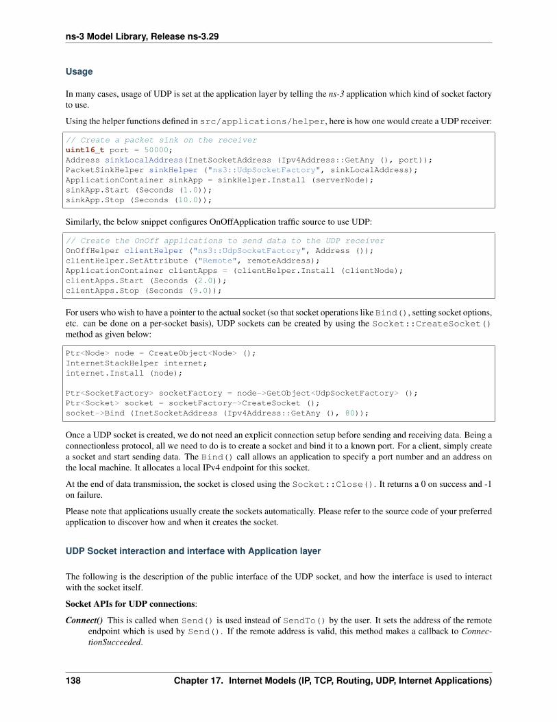
ns-3 Model Library, Release ns-3.29
Usage
In many cases, usage of UDP is set at the application layer by telling the ns-3 application which kind of socket factoryto use.
Using the helper functions defined in src/applications/helper, here is how one would create a UDP receiver:
// Create a packet sink on the receiveruint16_t port = 50000;Address sinkLocalAddress(InetSocketAddress (Ipv4Address::GetAny (), port));PacketSinkHelper sinkHelper ("ns3::UdpSocketFactory", sinkLocalAddress);ApplicationContainer sinkApp = sinkHelper.Install (serverNode);sinkApp.Start (Seconds (1.0));sinkApp.Stop (Seconds (10.0));
Similarly, the below snippet configures OnOffApplication traffic source to use UDP:
// Create the OnOff applications to send data to the UDP receiverOnOffHelper clientHelper ("ns3::UdpSocketFactory", Address ());clientHelper.SetAttribute ("Remote", remoteAddress);ApplicationContainer clientApps = (clientHelper.Install (clientNode);clientApps.Start (Seconds (2.0));clientApps.Stop (Seconds (9.0));
For users who wish to have a pointer to the actual socket (so that socket operations like Bind(), setting socket options,etc. can be done on a per-socket basis), UDP sockets can be created by using the Socket::CreateSocket()method as given below:
Ptr<Node> node = CreateObject<Node> ();InternetStackHelper internet;internet.Install (node);
Ptr<SocketFactory> socketFactory = node->GetObject<UdpSocketFactory> ();Ptr<Socket> socket = socketFactory->CreateSocket ();socket->Bind (InetSocketAddress (Ipv4Address::GetAny (), 80));
Once a UDP socket is created, we do not need an explicit connection setup before sending and receiving data. Being aconnectionless protocol, all we need to do is to create a socket and bind it to a known port. For a client, simply createa socket and start sending data. The Bind() call allows an application to specify a port number and an address onthe local machine. It allocates a local IPv4 endpoint for this socket.
At the end of data transmission, the socket is closed using the Socket::Close(). It returns a 0 on success and -1on failure.
Please note that applications usually create the sockets automatically. Please refer to the source code of your preferredapplication to discover how and when it creates the socket.
UDP Socket interaction and interface with Application layer
The following is the description of the public interface of the UDP socket, and how the interface is used to interactwith the socket itself.
Socket APIs for UDP connections:
Connect() This is called when Send() is used instead of SendTo() by the user. It sets the address of the remoteendpoint which is used by Send(). If the remote address is valid, this method makes a callback to Connec-tionSucceeded.
138 Chapter 17. Internet Models (IP, TCP, Routing, UDP, Internet Applications)
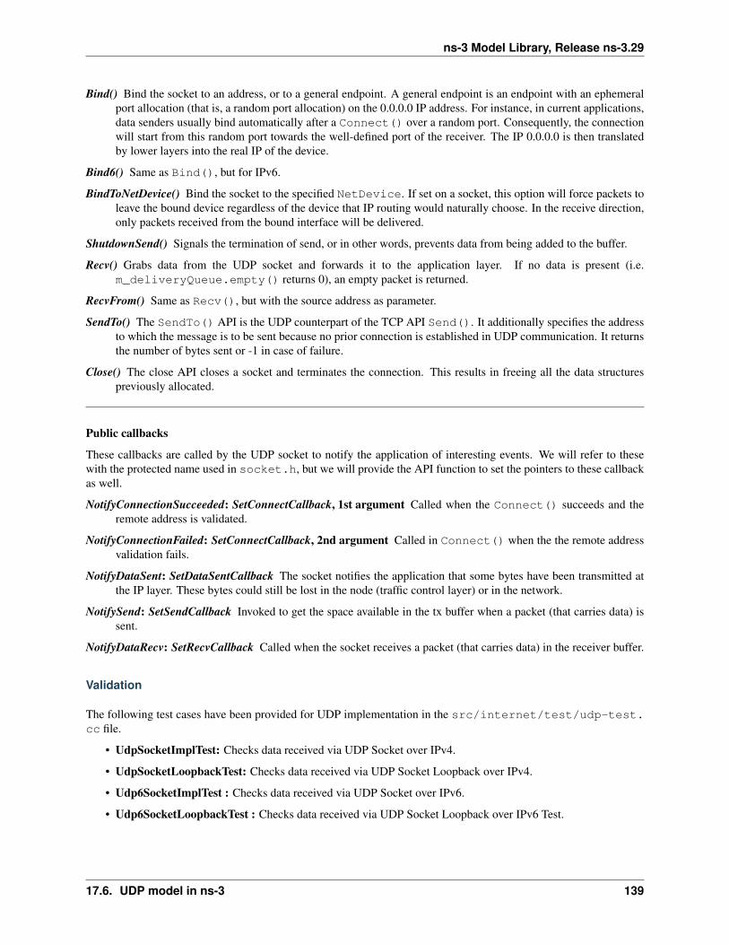
ns-3 Model Library, Release ns-3.29
Bind() Bind the socket to an address, or to a general endpoint. A general endpoint is an endpoint with an ephemeralport allocation (that is, a random port allocation) on the 0.0.0.0 IP address. For instance, in current applications,data senders usually bind automatically after a Connect() over a random port. Consequently, the connectionwill start from this random port towards the well-defined port of the receiver. The IP 0.0.0.0 is then translatedby lower layers into the real IP of the device.
Bind6() Same as Bind(), but for IPv6.
BindToNetDevice() Bind the socket to the specified NetDevice. If set on a socket, this option will force packets toleave the bound device regardless of the device that IP routing would naturally choose. In the receive direction,only packets received from the bound interface will be delivered.
ShutdownSend() Signals the termination of send, or in other words, prevents data from being added to the buffer.
Recv() Grabs data from the UDP socket and forwards it to the application layer. If no data is present (i.e.m_deliveryQueue.empty() returns 0), an empty packet is returned.
RecvFrom() Same as Recv(), but with the source address as parameter.
SendTo() The SendTo() API is the UDP counterpart of the TCP API Send(). It additionally specifies the addressto which the message is to be sent because no prior connection is established in UDP communication. It returnsthe number of bytes sent or -1 in case of failure.
Close() The close API closes a socket and terminates the connection. This results in freeing all the data structurespreviously allocated.
Public callbacks
These callbacks are called by the UDP socket to notify the application of interesting events. We will refer to thesewith the protected name used in socket.h, but we will provide the API function to set the pointers to these callbackas well.
NotifyConnectionSucceeded: SetConnectCallback, 1st argument Called when the Connect() succeeds and theremote address is validated.
NotifyConnectionFailed: SetConnectCallback, 2nd argument Called in Connect() when the the remote addressvalidation fails.
NotifyDataSent: SetDataSentCallback The socket notifies the application that some bytes have been transmitted atthe IP layer. These bytes could still be lost in the node (traffic control layer) or in the network.
NotifySend: SetSendCallback Invoked to get the space available in the tx buffer when a packet (that carries data) issent.
NotifyDataRecv: SetRecvCallback Called when the socket receives a packet (that carries data) in the receiver buffer.
Validation
The following test cases have been provided for UDP implementation in the src/internet/test/udp-test.cc file.
• UdpSocketImplTest: Checks data received via UDP Socket over IPv4.
• UdpSocketLoopbackTest: Checks data received via UDP Socket Loopback over IPv4.
• Udp6SocketImplTest : Checks data received via UDP Socket over IPv6.
• Udp6SocketLoopbackTest : Checks data received via UDP Socket Loopback over IPv6 Test.
17.6. UDP model in ns-3 139

ns-3 Model Library, Release ns-3.29
Limitations
• UDP_CORK is presently not the part of this implementation.
• NotifyNormalClose, NotifyErrorClose, NotifyConnectionRequest andNotifyNewConnectionCreated socket API callbacks are not supported.
17.7 Internet Applications Module Documentation
The goal of this module is to hold all the Internet-specific applications, and most notably some very specific appli-cations (e.g., ping) or daemons (e.g., radvd). Other non-Internet-specific applications such as packet generators arecontained in other modules.
The source code for the new module lives in the directory src/internet-apps.
Each application has its own goals, limitations and scope, which are briefly explained in the following.
All the applications are extensively used in the top-level examples directories. The users are encouraged to checkthe scripts therein to have a clear overview of the various options and usage tricks.
17.7.1 V4Ping
This app mimics a “ping” (ICMP Echo) using IPv4. The application allows the following attributes to be set:
• Remote address
• Verbose mode
• Packet size (default 56 bytes)
• Packet interval (default 1 second)
Moreover, the user can access the measured RTT value (as a Traced Source).
17.7.2 Ping6
This app mimics a “ping” (ICMP Echo) using IPv6. The application allows the following attributes to be set:
• Remote address
• Local address (sender address)
• Packet size (default 56 bytes)
• Packet interval (default 1 second)
• Max number of packets to send
17.7.3 Radvd
This app mimics a “RADVD” daemon. I.e., the daemon responsible for IPv6 routers advertisements. All the IPv6routers should have a RADVD daemon installed.
The configuration of the Radvd application mimics the one of the radvd Linux program.
140 Chapter 17. Internet Models (IP, TCP, Routing, UDP, Internet Applications)
ns-3 Model Library, Release ns-3.29
17.7.4 DHCPv4
The ns-3 implementation of Dynamic Host Configuration Protocol (DHCP) follows the specifications of RFC 2131and RFC 2132.
The source code for DHCP is located in src/internet-apps/model and consists of the following 6 files:
• dhcp-server.h,
• dhcp-server.cc,
• dhcp-client.h,
• dhcp-client.cc,
• dhcp-header.h and
• dhcp-header.cc
Helpers
The following two files have been added to src/internet-apps/helper for DHCP:
• dhcp-helper.h and
• dhcp-helper.cc
Tests
The tests for DHCP can be found at src/internet-apps/test/dhcp-test.cc
Examples
The examples for DHCP can be found at src/internet-apps/examples/dhcp-example.cc
Scope and Limitations
The server should be provided with a network address, mask and a range of address for the pool. One client applicationcan be installed on only one netdevice in a node, and can configure address for only that netdevice.
The following five basic DHCP messages are supported:
• DHCP DISCOVER
• DHCP OFFER
• DHCP REQUEST
• DHCP ACK
• DHCP NACK
Also, the following eight options of BootP are supported:
• 1 (Mask)
• 50 (Requested Address)
• 51 (Address Lease Time)
• 53 (DHCP message type)
17.7. Internet Applications Module Documentation 141
ns-3 Model Library, Release ns-3.29
• 54 (DHCP server identifier)
• 58 (Address renew time)
• 59 (Address rebind time)
• 255 (end)
The client identifier option (61) can be implemented in near future.
In the current implementation, a DHCP client can obtain IPv4 address dynamically from the DHCP server, and canrenew it within a lease time period.
Multiple DHCP servers can be configured, but the implementation does not support the use of a DHCP Relay yet.
PageBreak
142 Chapter 17. Internet Models (IP, TCP, Routing, UDP, Internet Applications)

CHAPTER
EIGHTEEN
LOW-RATE WIRELESS PERSONAL AREA NETWORK (LR-WPAN)
This chapter describes the implementation of ns-3 models for the low-rate, wireless personal area network (LR-WPAN)as specified by IEEE standard 802.15.4 (2006).
18.1 Model Description
The source code for the lr-wpan module lives in the directory src/lr-wpan.
18.1.1 Design
The model design closely follows the standard from an architectural standpoint.
Fig. 1: Architecture and scope of lr-wpan models
The grey areas in the figure (adapted from Fig 3. of IEEE Std. 802.15.4-2006) show the scope of the model.
143

ns-3 Model Library, Release ns-3.29
The Spectrum NetDevice from Nicola Baldo is the basis for the implementation.
The implementation also plans to borrow from the ns-2 models developed by Zheng and Lee in the future.
APIs
The APIs closely follow the standard, adapted for ns-3 naming conventions and idioms. The APIs are organized aroundthe concept of service primitives as shown in the following figure adapted from Figure 14 of IEEE Std. 802.15.4-2006.
Fig. 2: Service primitives
The APIs are organized around four conceptual services and service access points (SAP):
• MAC data service (MCPS)
• MAC management service (MLME)
• PHY data service (PD)
• PHY management service (PLME)
In general, primitives are standardized as follows (e.g. Sec 7.1.1.1.1 of IEEE 802.15.4-2006)::
MCPS-DATA.request (SrcAddrMode,DstAddrMode,DstPANId,DstAddr,msduLength,msdu,msduHandle,TxOptions,SecurityLevel,KeyIdMode,KeySource,KeyIndex)
This maps to ns-3 classes and methods such as::
struct McpsDataRequestParameters{
uint8_t m_srcAddrMode;uint8_t m_dstAddrMode;...
(continues on next page)
144 Chapter 18. Low-Rate Wireless Personal Area Network (LR-WPAN)
ns-3 Model Library, Release ns-3.29
(continued from previous page)
};
voidLrWpanMac::McpsDataRequest (McpsDataRequestParameters params){...}
MAC
The MAC at present implements the unslotted CSMA/CA variant, without beaconing. Currently there is no supportfor coordinators and the relevant APIs.
The implemented MAC is similar to Contiki’s NullMAC, i.e., a MAC without sleep features. The radio is assumedto be always active (receiving or transmitting), of completely shut down. Frame reception is not disabled whileperforming the CCA.
The main API supported is the data transfer API (McpsDataRequest/Indication/Confirm). CSMA/CA according to Stc802.15.4-2006, section 7.5.1.4 is supported. Frame reception and rejection according to Std 802.15.4-2006, section7.5.6.2 is supported, including acknowledgements. Only short addressing completely implemented. Various tracesources are supported, and trace sources can be hooked to sinks.
PHY
The physical layer components consist of a Phy model, an error rate model, and a loss model. The error rate modelpresently models the error rate for IEEE 802.15.4 2.4 GHz AWGN channel for OQPSK; the model description can befound in IEEE Std 802.15.4-2006, section E.4.1.7. The Phy model is based on SpectrumPhy and it follows specifica-tion described in section 6 of IEEE Std 802.15.4-2006. It models PHY service specifications, PPDU formats, PHYconstants and PIB attributes. It currently only supports the transmit power spectral density mask specified in 2.4 GHzper section 6.5.3.1. The noise power density assumes uniformly distributed thermal noise across the frequency bands.The loss model can fully utilize all existing simple (non-spectrum phy) loss models. The Phy model uses the existingsingle spectrum channel model. The physical layer is modeled on packet level, that is, no preamble/SFD detection isdone. Packet reception will be started with the first bit of the preamble (which is not modeled), if the SNR is morethan -5 dB, see IEEE Std 802.15.4-2006, appendix E, Figure E.2. Reception of the packet will finish after the packetwas completely transmitted. Other packets arriving during reception will add up to the interference/noise.
Currently the receiver sensitivity is set to a fixed value of -106.58 dBm. This corresponds to a packet error rate of 1%for 20 byte reference packets for this signal power, according to IEEE Std 802.15.4-2006, section 6.1.7. In the futurewe will provide support for changing the sensitivity to different values.
NetDevice
Although it is expected that other technology profiles (such as 6LoWPAN and ZigBee) will write their own NetDeviceclasses, a basic LrWpanNetDevice is provided, which encapsulates the common operations of creating a genericLrWpan device and hooking things together.
18.1.2 Scope and Limitations
Future versions of this document will contain a PICS proforma similar to Appendix D of IEEE 802.15.4-2006. Thecurrent emphasis is on the unslotted mode of 802.15.4 operation for use in Zigbee, and the scope is limited to enabling a
18.1. Model Description 145
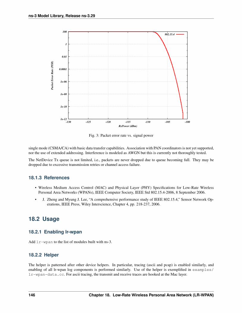
ns-3 Model Library, Release ns-3.29
1e-12
1e-10
1e-08
1e-06
0.0001
0.01
1
100
-130 -125 -120 -115 -110 -105 -100
Packet
Err
or
Rate
(P
ER
)
RxPower (dBm)
802.15.4
Fig. 3: Packet error rate vs. signal power
single mode (CSMA/CA) with basic data transfer capabilities. Association with PAN coordinators is not yet supported,nor the use of extended addressing. Interference is modeled as AWGN but this is currently not thoroughly tested.
The NetDevice Tx queue is not limited, i.e., packets are never dropped due to queue becoming full. They may bedropped due to excessive transmission retries or channel access failure.
18.1.3 References
• Wireless Medium Access Control (MAC) and Physical Layer (PHY) Specifications for Low-Rate WirelessPersonal Area Networks (WPANs), IEEE Computer Society, IEEE Std 802.15.4-2006, 8 September 2006.
• J. Zheng and Myung J. Lee, “A comprehensive performance study of IEEE 802.15.4,” Sensor Network Op-erations, IEEE Press, Wiley Interscience, Chapter 4, pp. 218-237, 2006.
18.2 Usage
18.2.1 Enabling lr-wpan
Add lr-wpan to the list of modules built with ns-3.
18.2.2 Helper
The helper is patterned after other device helpers. In particular, tracing (ascii and pcap) is enabled similarly, andenabling of all lr-wpan log components is performed similarly. Use of the helper is exemplified in examples/lr-wpan-data.cc. For ascii tracing, the transmit and receive traces are hooked at the Mac layer.
146 Chapter 18. Low-Rate Wireless Personal Area Network (LR-WPAN)

ns-3 Model Library, Release ns-3.29
The default propagation loss model added to the channel, when this helper is used, is the LogDistancePropagation-LossModel with default parameters.
18.2.3 Examples
The following examples have been written, which can be found in src/lr-wpan/examples/:
• lr-wpan-data.cc: A simple example showing end-to-end data transfer.
• lr-wpan-error-distance-plot.cc: An example to plot variations of the packet success ratio as afunction of distance.
• lr-wpan-error-model-plot.cc: An example to test the phy.
• lr-wpan-packet-print.cc: An example to print out the MAC header fields.
• lr-wpan-phy-test.cc: An example to test the phy.
In particular, the module enables a very simplified end-to-end data transfer scenario, implemented inlr-wpan-data.cc. The figure shows a sequence of events that are triggered when the MAC receives a DataRe-quest from the higher layer. It invokes a Clear Channel Assessment (CCA) from the PHY, and if successful, sends theframe down to the PHY where it is transmitted over the channel and results in a DataIndication on the peer node.
Fig. 4: Data example for simple LR-WPAN data transfer end-to-end
The example lr-wpan-error-distance-plot.cc plots the packet success ratio (PSR) as a function of dis-tance, using the default LogDistance propagation loss model and the 802.15.4 error model. The channel (default11), packet size (default 20 bytes) and transmit power (default 0 dBm) can be varied by command line arguments.The program outputs a file named 802.15.4-psr-distance.plt. Loading this file into gnuplot yields a file802.15.4-psr-distance.eps, which can be converted to pdf or other formats. The default output is shownbelow.
18.2. Usage 147

ns-3 Model Library, Release ns-3.29
0
0.2
0.4
0.6
0.8
1
0 50 100 150 200
Pack
et S
ucc
ess
Rate
(P
SR
)
distance (m)
Packet (MSDU) size = 20 bytes; tx power = 0 dBm; channel = 11
802.15.4-psr-vs-distance
Fig. 5: Default output of the program lr-wpan-error-distance-plot.cc
18.2.4 Tests
The following tests have been written, which can be found in src/lr-wpan/tests/:
• lr-wpan-ack-test.cc: Check that acknowledgments are being used and issued in the correct order.
• lr-wpan-collision-test.cc: Test correct reception of packets with interference and collisions.
• lr-wpan-error-model-test.cc: Check that the error model gives predictable values.
• lr-wpan-packet-test.cc: Test the 802.15.4 MAC header/trailer classes
• lr-wpan-pd-plme-sap-test.cc: Test the PLME and PD SAP per IEEE 802.15.4
• lr-wpan-spectrum-value-helper-test.cc: Test that the conversion between power (expressed asa scalar quantity) and spectral power, and back again, falls within a 25% tolerance across the range of possiblechannels and input powers.
18.3 Validation
The model has not been validated against real hardware. The error model has been validated against the data in IEEEStd 802.15.4-2006, section E.4.1.7 (Figure E.2). The MAC behavior (CSMA backoff) has been validated by handagainst expected behavior. The below plot is an example of the error model validation and can be reproduced byrunning lr-wpan-error-model-plot.cc:
148 Chapter 18. Low-Rate Wireless Personal Area Network (LR-WPAN)
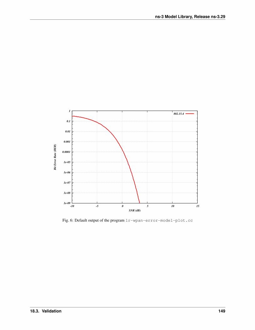
ns-3 Model Library, Release ns-3.29
1e-09
1e-08
1e-07
1e-06
1e-05
0.0001
0.001
0.01
0.1
1
-10 -5 0 5 10 15
Bit
Err
or
Rate
(B
ER
)
SNR (dB)
802.15.4
Fig. 6: Default output of the program lr-wpan-error-model-plot.cc
18.3. Validation 149

ns-3 Model Library, Release ns-3.29
150 Chapter 18. Low-Rate Wireless Personal Area Network (LR-WPAN)

CHAPTER
NINETEEN
LTE MODULE
19.1 Design Documentation
19.1.1 Overview
An overview of the LTE-EPC simulation model is depicted in the figure Overview of the LTE-EPC simulation model.There are two main components:
• the LTE Model. This model includes the LTE Radio Protocol stack (RRC, PDCP, RLC, MAC, PHY). Theseentities reside entirely within the UE and the eNB nodes.
• the EPC Model. This models includes core network interfaces, protocols and entities. These entities and proto-cols reside within the SGW, PGW and MME nodes, and partially within the eNB nodes.
Fig. 1: Overview of the LTE-EPC simulation model
19.1.2 Design Criteria
LTE Model
The LTE model has been designed to support the evaluation of the following aspects of LTE systems:
• Radio Resource Management
• QoS-aware Packet Scheduling
• Inter-cell Interference Coordination
• Dynamic Spectrum Access
151

ns-3 Model Library, Release ns-3.29
In order to model LTE systems to a level of detail that is sufficient to allow a correct evaluation of the above mentionedaspects, the following requirements have been considered:
1. At the radio level, the granularity of the model should be at least that of the Resource Block (RB). In fact,this is the fundamental unit being used for resource allocation. Without this minimum level of granularity, it isnot possible to model accurately packet scheduling and inter-cell-interference. The reason is that, since packetscheduling is done on a per-RB basis, an eNB might transmit on a subset only of all the available RBs, henceinterfering with other eNBs only on those RBs where it is transmitting. Note that this requirement rules out theadoption of a system level simulation approach, which evaluates resource allocation only at the granularity ofcall/bearer establishment.
2. The simulator should scale up to tens of eNBs and hundreds of User Equipment (UEs). This rules out the use ofa link level simulator, i.e., a simulator whose radio interface is modeled with a granularity up to the symbol level.This is because to have a symbol level model it is necessary to implement all the PHY layer signal processing,whose huge computational complexity severely limits simulation. In fact, link-level simulators are normallylimited to a single eNB and one or a few UEs.
3. It should be possible within the simulation to configure different cells so that they use different carrier frequen-cies and system bandwidths. The bandwidth used by different cells should be allowed to overlap, in order tosupport dynamic spectrum licensing solutions such as those described in [Ofcom2600MHz] and [RealWireless].The calculation of interference should handle appropriately this case.
4. To be more representative of the LTE standard, as well as to be as close as possible to real-world implemen-tations, the simulator should support the MAC Scheduler API published by the FemtoForum [FFAPI]. Thisinterface is expected to be used by femtocell manufacturers for the implementation of scheduling and RadioResource Management (RRM) algorithms. By introducing support for this interface in the simulator, we makeit possible for LTE equipment vendors and operators to test in a simulative environment exactly the same algo-rithms that would be deployed in a real system.
5. The LTE simulation model should contain its own implementation of the API defined in [FFAPI]. Neitherbinary nor data structure compatibility with vendor-specific implementations of the same interface are expected;hence, a compatibility layer should be interposed whenever a vendor-specific MAC scheduler is to be used withthe simulator. This requirement is necessary to allow the simulator to be independent from vendor-specificimplementations of this interface specification. We note that [FFAPI] is a logical specification only, and itsimplementation (e.g., translation to some specific programming language) is left to the vendors.
6. The model is to be used to simulate the transmission of IP packets by the upper layers. With this respect, itshall be considered that in LTE the Scheduling and Radio Resource Management do not work with IP packetsdirectly, but rather with RLC PDUs, which are obtained by segmentation and concatenation of IP packets doneby the RLC entities. Hence, these functionalities of the RLC layer should be modeled accurately.
EPC Model
The main objective of the EPC model is to provides means for the simulation of end-to-end IP connectivity over theLTE model. To this aim, it supports for the interconnection of multiple UEs to the Internet, via a radio access networkof multiple eNBs connected to a single SGW/PGW node, as shown in Figure Overview of the LTE-EPC simulationmodel.
The following design choices have been made for the EPC model:
1. The Packet Data Network (PDN) type supported is both IPv4 and IPv6.
2. The SGW and PGW functional entities are implemented within a single node, which is hence referred to as theSGW/PGW node.
3. The scenarios with inter-SGW mobility are not of interests. Hence, a single SGW/PGW node will be present inall simulations scenarios
152 Chapter 19. LTE Module

ns-3 Model Library, Release ns-3.29
4. A requirement for the EPC model is that it can be used to simulate the end-to-end performance of realisticapplications. Hence, it should be possible to use with the EPC model any regular ns-3 application working ontop of TCP or UDP.
5. Another requirement is the possibility of simulating network topologies with the presence of multiple eNBs,some of which might be equipped with a backhaul connection with limited capabilities. In order to simulatesuch scenarios, the user data plane protocols being used between the eNBs and the SGW/PGW should bemodeled accurately.
6. It should be possible for a single UE to use different applications with different QoS profiles. Hence, multipleEPS bearers should be supported for each UE. This includes the necessary classification of TCP/UDP trafficover IP done at the UE in the uplink and at the PGW in the downlink.
7. The focus of the EPC model is mainly on the EPC data plane. The accurate modeling of the EPC control planeis, for the time being, not a requirement; hence, the necessary control plane interactions can be modeled in asimplified way by leveraging on direct interaction among the different simulation objects via the provided helperobjects.
8. The focus of the EPC model is on simulations of active users in ECM connected mode. Hence, all the function-ality that is only relevant for ECM idle mode (in particular, tracking area update and paging) are not modeled atall.
9. The model should allow the possibility to perform an X2-based handover between two eNBs.
19.1.3 Architecture
LTE Model
UE architecture
The architecture of the LTE radio protocol stack model of the UE is represented in the figures LTE radio protocol stackarchitecture for the UE on the data plane and LTE radio protocol stack architecture for the UE on the control planewhich highlight respectively the data plane and the control plane.
The architecture of the PHY/channel model of the UE is represented in figure PHY and channel model architecturefor the UE.
eNB architecture
The architecture of the LTE radio protocol stack model of the eNB is represented in the figures LTE radio protocolstack architecture for the eNB on the data plane and LTE radio protocol stack architecture for the eNB on the controlplane which highlight respectively the data plane and the control plane.
The architecture of the PHY/channel model of the eNB is represented in figure PHY and channel model architecturefor the eNB.
EPC Model
EPC data plane
In Figure LTE-EPC data plane protocol stack, we represent the end-to-end LTE-EPC data plane protocol stack as itis modeled in the simulator. From the figure, it is evident that the biggest simplification introduced in the data planemodel is the inclusion of the SGW and PGW functionality within a single SGW/PGW node, which removes the need
19.1. Design Documentation 153
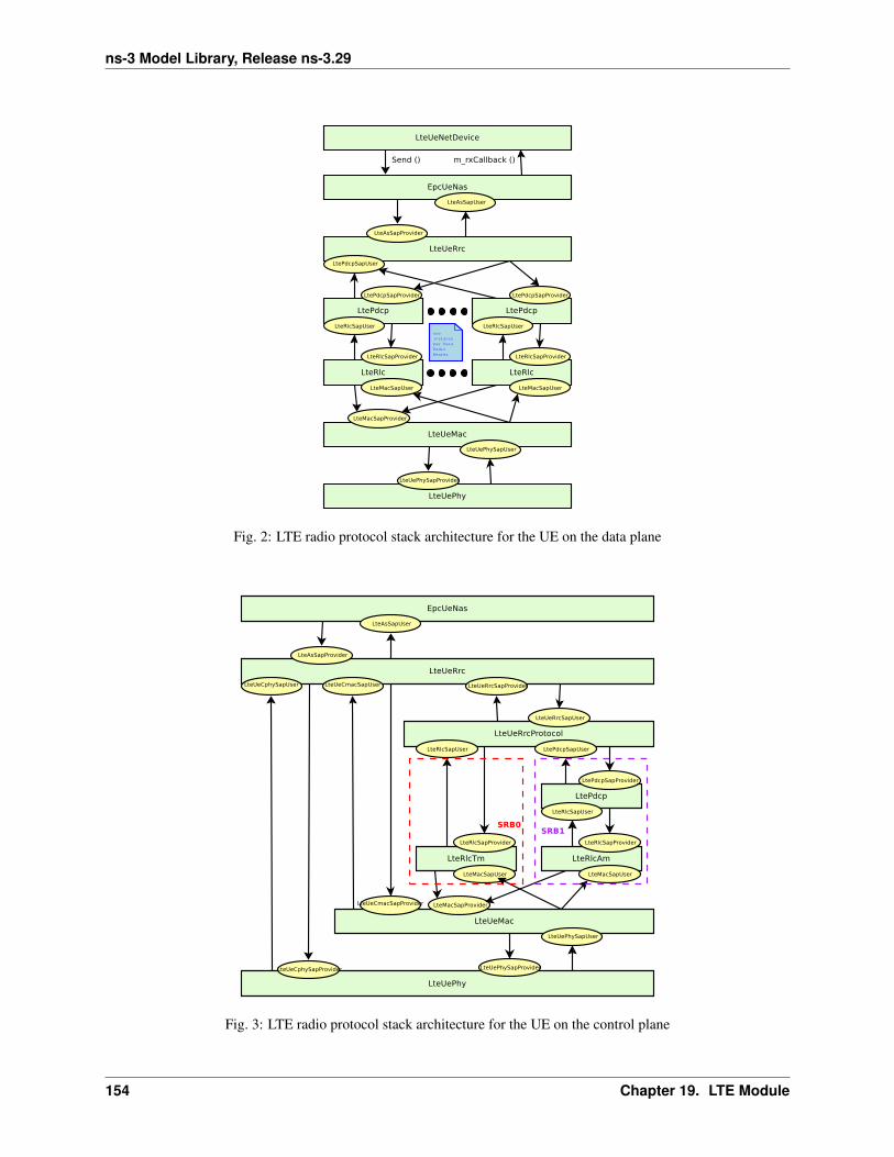
ns-3 Model Library, Release ns-3.29
Fig. 2: LTE radio protocol stack architecture for the UE on the data plane
Fig. 3: LTE radio protocol stack architecture for the UE on the control plane
154 Chapter 19. LTE Module

ns-3 Model Library, Release ns-3.29
Fig. 4: PHY and channel model architecture for the UE
Fig. 5: LTE radio protocol stack architecture for the eNB on the data plane
19.1. Design Documentation 155
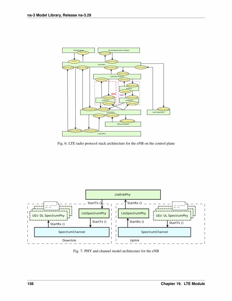
ns-3 Model Library, Release ns-3.29
Fig. 6: LTE radio protocol stack architecture for the eNB on the control plane
Fig. 7: PHY and channel model architecture for the eNB
156 Chapter 19. LTE Module

ns-3 Model Library, Release ns-3.29
for the S5 or S8 interfaces specified by 3GPP. On the other hand, for both the S1-U protocol stack and the LTE radioprotocol stack all the protocol layers specified by 3GPP are present.
Fig. 8: LTE-EPC data plane protocol stack
EPC control plane
The architecture of the implementation of the control plane model is shown in figure EPC control model. The controlinterfaces that are modeled explicitly are the S1-AP, the X2-AP and the S11 interfaces.
We note that the S1-AP and the S11 interfaces are modeled in a simplified fashion, by using just one pair of interfaceclasses to model the interaction between entities that reside on different nodes (the eNB and the MME for the S1-AP interface, and the MME and the SGW for the S11 interface). In practice, this means that the primitives of theseinterfaces are mapped to a direct function call between the two objects. On the other hand, the X2-AP interface isbeing modeled using protocol data units sent over an X2 link (modeled as a point-to-point link); for this reason, theX2-AP interface model is more realistic.
19.1. Design Documentation 157

ns-3 Model Library, Release ns-3.29
Fig. 9: EPC control model
158 Chapter 19. LTE Module

ns-3 Model Library, Release ns-3.29
19.1.4 Channel and Propagation
For channel modeling purposes, the LTE module uses the SpectrumChannel interface provided by thespectrum module. At the time of this writing, two implementations of such interface are available:SingleModelSpectrumChannel and MultiModelSpectrumChannel, and the LTE module requiresthe use of the MultiModelSpectrumChannel in order to work properly. This is because of theneed to support different frequency and bandwidth configurations. All the propagation models supported byMultiModelSpectrumChannel can be used within the LTE module.
Use of the Buildings model with LTE
The recommended propagation model to be used with the LTE module is the one provided by the Buildings mod-ule, which was in fact designed specifically with LTE (though it can be used with other wireless technologies aswell). Please refer to the documentation of the Buildings module for generic information on the propagation model itprovides.
In this section we will highlight some considerations that specifically apply when the Buildings module is used togetherwith the LTE module.
The naming convention used in the following will be:
• User equipment: UE
• Macro Base Station: MBS
• Small cell Base Station (e.g., pico/femtocell): SC
The LTE module considers FDD only, and implements downlink and uplink propagation separately. As a consequence,the following pathloss computations are performed
• MBS <-> UE (indoor and outdoor)
• SC (indoor and outdoor) <-> UE (indoor and outdoor)
The LTE model does not provide the following pathloss computations:
• UE <-> UE
• MBS <-> MBS
• MBS <-> SC
• SC <-> SC
The Buildings model does not know the actual type of the node; i.e., it is not aware of whether a transmitter node is aUE, a MBS, or a SC. Rather, the Buildings model only cares about the position of the node: whether it is indoor andoutdoor, and what is its z-axis respect to the rooftop level. As a consequence, for an eNB node that is placed outdoorand at a z-coordinate above the rooftop level, the propagation models typical of MBS will be used by the Buildingsmodule. Conversely, for an eNB that is placed outdoor but below the rooftop, or indoor, the propagation models typicalof pico and femtocells will be used.
For communications involving at least one indoor node, the corresponding wall penetration losses will be calculatedby the Buildings model. This covers the following use cases:
• MBS <-> indoor UE
• outdoor SC <-> indoor UE
• indoor SC <-> indoor UE
• indoor SC <-> outdoor UE
Please refer to the documentation of the Buildings module for details on the actual models used in each case.
19.1. Design Documentation 159

ns-3 Model Library, Release ns-3.29
Fading Model
The LTE module includes a trace-based fading model derived from the one developed during the GSoC 2010[Piro2011]. The main characteristic of this model is the fact that the fading evaluation during simulation run-timeis based on per-calculated traces. This is done to limit the computational complexity of the simulator. On the otherhand, it needs huge structures for storing the traces; therefore, a trade-off between the number of possible parametersand the memory occupancy has to be found. The most important ones are:
• users’ speed: relative speed between users (affects the Doppler frequency, which in turns affects the time-variance property of the fading)
• number of taps (and relative power): number of multiple paths considered, which affects the frequency propertyof the fading.
• time granularity of the trace: sampling time of the trace.
• frequency granularity of the trace: number of values in frequency to be evaluated.
• length of trace: ideally large as the simulation time, might be reduced by windowing mechanism.
• number of users: number of independent traces to be used (ideally one trace per user).
With respect to the mathematical channel propagation model, we suggest the one provided by the rayleighchanfunction of Matlab, since it provides a well accepted channel modelization both in time and frequency domain. Formore information, the reader is referred to [mathworks].
The simulator provides a matlab script (src/lte/model/fading-traces/fading-trace-generator.m) for generating traces based on the format used by the simulator. In detail, the channel object created with therayleighchan function is used for filtering a discrete-time impulse signal in order to obtain the channel impulse re-sponse. The filtering is repeated for different TTI, thus yielding subsequent time-correlated channel responses (oneper TTI). The channel response is then processed with the pwelch function for obtaining its power spectral densityvalues, which are then saved in a file with the proper format compatible with the simulator model.
Since the number of variable it is pretty high, generate traces considering all of them might produce a high numberof traces of huge size. On this matter, we considered the following assumptions of the parameters based on the 3GPPfading propagation conditions (see Annex B.2 of [TS36104]):
• users’ speed: typically only a few discrete values are considered, i.e.:
– 0 and 3 kmph for pedestrian scenarios
– 30 and 60 kmph for vehicular scenarios
– 0, 3, 30 and 60 for urban scenarios
• channel taps: only a limited number of sets of channel taps are normally considered, for example three modelsare mentioned in Annex B.2 of [TS36104].
• time granularity: we need one fading value per TTI, i.e., every 1 ms (as this is the granularity in time of the ns-3LTE PHY model).
• frequency granularity: we need one fading value per RB (which is the frequency granularity of the spectrummodel used by the ns-3 LTE model).
• length of the trace: the simulator includes the windowing mechanism implemented during the GSoC 2011,which consists of picking up a window of the trace each window length in a random fashion.
• per-user fading process: users share the same fading trace, but for each user a different starting point in the traceis randomly picked up. This choice was made to avoid the need to provide one fading trace per user.
160 Chapter 19. LTE Module

ns-3 Model Library, Release ns-3.29
According to the parameters we considered, the following formula express in detail the total size Straces of the fadingtraces:
Straces = Ssample ×NRB ×TtraceTsample
×Nscenarios [bytes]
where Ssample is the size in bytes of the sample (e.g., 8 in case of double precision, 4 in case of float precision), NRBis the number of RB or set of RBs to be considered, Ttrace is the total length of the trace, Tsample is the time resolutionof the trace (1 ms), and Nscenarios is the number of fading scenarios that are desired (i.e., combinations of differentsets of channel taps and user speed values). We provide traces for 3 different scenarios one for each taps configurationdefined in Annex B.2 of [TS36104]:
• Pedestrian: with nodes’ speed of 3 kmph.
• Vehicular: with nodes’ speed of 60 kmph.
• Urban: with nodes’ speed of 3 kmph.
hence Nscenarios = 3. All traces have Ttrace = 10 s and RBNUM = 100. This results in a total 24 MB bytes oftraces.
Antennas
Being based on the SpectrumPhy, the LTE PHY model supports antenna modeling via the ns-3 AntennaModelclass. Hence, any model based on this class can be associated with any eNB or UE instance. For instance, the use ofthe CosineAntennaModel associated with an eNB device allows to model one sector of a macro base station. Bydefault, the IsotropicAntennaModel is used for both eNBs and UEs.
19.1. Design Documentation 161
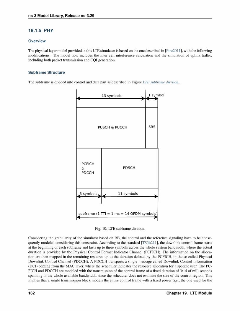
ns-3 Model Library, Release ns-3.29
19.1.5 PHY
Overview
The physical layer model provided in this LTE simulator is based on the one described in [Piro2011], with the followingmodifications. The model now includes the inter cell interference calculation and the simulation of uplink traffic,including both packet transmission and CQI generation.
Subframe Structure
The subframe is divided into control and data part as described in Figure LTE subframe division..
Fig. 10: LTE subframe division.
Considering the granularity of the simulator based on RB, the control and the reference signaling have to be conse-quently modeled considering this constraint. According to the standard [TS36211], the downlink control frame startsat the beginning of each subframe and lasts up to three symbols across the whole system bandwidth, where the actualduration is provided by the Physical Control Format Indicator Channel (PCFICH). The information on the alloca-tion are then mapped in the remaining resource up to the duration defined by the PCFICH, in the so called PhysicalDownlink Control Channel (PDCCH). A PDCCH transports a single message called Downlink Control Information(DCI) coming from the MAC layer, where the scheduler indicates the resource allocation for a specific user. The PC-FICH and PDCCH are modeled with the transmission of the control frame of a fixed duration of 3/14 of millisecondsspanning in the whole available bandwidth, since the scheduler does not estimate the size of the control region. Thisimplies that a single transmission block models the entire control frame with a fixed power (i.e., the one used for the
162 Chapter 19. LTE Module

ns-3 Model Library, Release ns-3.29
PDSCH) across all the available RBs. According to this feature, this transmission represents also a valuable supportfor the Reference Signal (RS). This allows of having every TTI an evaluation of the interference scenario since all theeNB are transmitting (simultaneously) the control frame over the respective available bandwidths. We note that, themodel does not include the power boosting since it does not reflect any improvement in the implemented model of thechannel estimation.
The Sounding Reference Signal (SRS) is modeled similar to the downlink control frame. The SRS is periodicallyplaced in the last symbol of the subframe in the whole system bandwidth. The RRC module already includes an algo-rithm for dynamically assigning the periodicity as function of the actual number of UEs attached to a eNB accordingto the UE-specific procedure (see Section 8.2 of [TS36213]).
MAC to Channel delay
To model the latency of real MAC and PHY implementations, the PHY model simulates a MAC-to-channel delay inmultiples of TTIs (1ms). The transmission of both data and control packets are delayed by this amount.
CQI feedback
The generation of CQI feedback is done accordingly to what specified in [FFAPI]. In detail, we considered thegeneration of periodic wideband CQI (i.e., a single value of channel state that is deemed representative of all RBs inuse) and inband CQIs (i.e., a set of value representing the channel state for each RB).
The CQI index to be reported is obtained by first obtaining a SINR measurement and then passing this SINR measure-ment to the Adaptive Modulation and Coding module which will map it to the CQI index.
In downlink, the SINR used to generate CQI feedback can be calculated in two different ways:
1. Ctrl method: SINR is calculated combining the signal power from the reference signals (which in the simulationis equivalent to the PDCCH) and the interference power from the PDCCH. This approach results in consider-ing any neighboring eNB as an interferer, regardless of whether this eNB is actually performing any PDSCHtransmission, and regardless of the power and RBs used for eventual interfering PDSCH transmissions.
2. Mixed method: SINR is calculated combining the signal power from the reference signals (which in the sim-ulation is equivalent to the PDCCH) and the interference power from the PDSCH. This approach results inconsidering as interferers only those neighboring eNBs that are actively transmitting data on the PDSCH, andallows to generate inband CQIs that account for different amounts of interference on different RBs accordingto the actual interference level. In the case that no PDSCH transmission is performed by any eNB, this methodconsider that interference is zero, i.e., the SINR will be calculated as the ratio of signal to noise only.
To switch between this two CQI generation approaches, LteHelper::UsePdschForCqiGeneration needs tobe configured: false for first approach and true for second approach (true is default value):
Config::SetDefault ("ns3::LteHelper::UsePdschForCqiGeneration", BooleanValue (true));
In uplink, two types of CQIs are implemented:
• SRS based, periodically sent by the UEs.
• PUSCH based, calculated from the actual transmitted data.
The scheduler interface include an attribute system called UlCqiFilter for managing the filtering of the CQIsaccording to their nature, in detail:
• SRS_UL_CQI for storing only SRS based CQIs.
• PUSCH_UL_CQI for storing only PUSCH based CQIs.
• ALL_UL_CQI for storing all the CQIs received.
19.1. Design Documentation 163
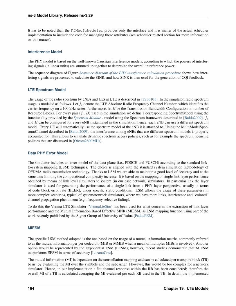
ns-3 Model Library, Release ns-3.29
It has to be noted that, the FfMacScheduler provides only the interface and it is matter of the actual schedulerimplementation to include the code for managing these attributes (see scheduler related section for more informationon this matter).
Interference Model
The PHY model is based on the well-known Gaussian interference models, according to which the powers of interfer-ing signals (in linear units) are summed up together to determine the overall interference power.
The sequence diagram of Figure Sequence diagram of the PHY interference calculation procedure shows how inter-fering signals are processed to calculate the SINR, and how SINR is then used for the generation of CQI feedback.
LTE Spectrum Model
The usage of the radio spectrum by eNBs and UEs in LTE is described in [TS36101]. In the simulator, radio spectrumusage is modeled as follows. Let fc denote the LTE Absolute Radio Frequency Channel Number, which identifies thecarrier frequency on a 100 kHz raster; furthermore, let B be the Transmission Bandwidth Configuration in number ofResource Blocks. For every pair (fc, B) used in the simulation we define a corresponding SpectrumModel using thefunctionality provided by the Spectrum Module . model using the Spectrum framework described in [Baldo2009]. fcand B can be configured for every eNB instantiated in the simulation; hence, each eNB can use a different spectrummodel. Every UE will automatically use the spectrum model of the eNB it is attached to. Using the MultiModelSpec-trumChannel described in [Baldo2009], the interference among eNBs that use different spectrum models is properlyaccounted for. This allows to simulate dynamic spectrum access policies, such as for example the spectrum licensingpolicies that are discussed in [Ofcom2600MHz].
Data PHY Error Model
The simulator includes an error model of the data plane (i.e., PDSCH and PUSCH) according to the standard link-to-system mapping (LSM) techniques. The choice is aligned with the standard system simulation methodology ofOFDMA radio transmission technology. Thanks to LSM we are able to maintain a good level of accuracy and at thesame time limiting the computational complexity increase. It is based on the mapping of single link layer performanceobtained by means of link level simulators to system (in our case network) simulators. In particular link the layersimulator is used for generating the performance of a single link from a PHY layer perspective, usually in termsof code block error rate (BLER), under specific static conditions. LSM allows the usage of these parameters inmore complex scenarios, typical of system/network simulators, where we have more links, interference and “colored”channel propagation phenomena (e.g., frequency selective fading).
To do this the Vienna LTE Simulator [ViennaLteSim] has been used for what concerns the extraction of link layerperformance and the Mutual Information Based Effective SINR (MIESM) as LSM mapping function using part of thework recently published by the Signet Group of University of Padua [PaduaPEM].
MIESM
The specific LSM method adopted is the one based on the usage of a mutual information metric, commonly referredto as the mutual information per per coded bit (MIB or MMIB when a mean of multiples MIBs is involved). Anotheroption would be represented by the Exponential ESM (EESM); however, recent studies demonstrate that MIESMoutperforms EESM in terms of accuracy [LozanoCost].
The mutual information (MI) is dependent on the constellation mapping and can be calculated per transport block (TB)basis, by evaluating the MI over the symbols and the subcarrier. However, this would be too complex for a networksimulator. Hence, in our implementation a flat channel response within the RB has been considered; therefore theoverall MI of a TB is calculated averaging the MI evaluated per each RB used in the TB. In detail, the implemented
164 Chapter 19. LTE Module

ns-3 Model Library, Release ns-3.29
Scheduler SpectrumChannel LteSpectrumPhy LteInterferenceLteCqiSinrChunkProcess
or LtePhy
at 0.001s: StartRx(signal1)
StartRx(interferer)
AddSignal()
at 0.001s: StartRx(signal2)
at 0.001s: StartRx(signal2)
AddSignal(signal2)
StartRx(signal2)
Schedule (EndRx)
at 0.001s: StartRx(signal3)
StartRx(signal3)
AddSignal(signal3)
at 0.002s: EndRx()
EndRx()
EvaluateSinrChunk()
End()
GenerateCqiFeedback(SINR of signal2)
Fig. 11: Sequence diagram of the PHY interference calculation procedure
19.1. Design Documentation 165

ns-3 Model Library, Release ns-3.29
0 1 2 3 4 5 6 7 810
−3
10−2
10−1
100
SNR
BLE
R
TB = 6000 (AWGN)
TB = 6000 (estimated)
TB = 4000 (AWGN)
TB = 4000 (estimated)
TB = 2560 (AWGN)
TB = 2560 (estimated)
TB = 1024 (AWGN)
TB = 1024 (estimated)
TB = 512 (AWGN)
TB = 512 (estimated)
TB = 256 (AWGN)
TB = 256 (estimated)
TB = 160 (AWGN)
TB = 160 (estimated)
0
1
2
3
4
5
6
-20 -15 -10 -5 0 5 10 15 20 25 30
RB
IR
Signal-to-noise ratio SNR [dB]
QPSK16QAM64QAM
4 4.5 5 5.5 6 6.5 7 7.5 8 8.5 910
−3
10−2
10−1
100
SNR
BLE
R
TB = 6000 (AWGN)
TB = 6000 (estimated)
TB = 4000 (AWGN)
TB = 4000 (estimated)
TB = 2560 (AWGN)
TB = 2560 (estimated)
TB = 1024 (AWGN)
TB = 1024 (estimated)
TB = 512 (AWGN)
TB = 512 (estimated)
TB = 256 (AWGN)
TB = 256 (estimated)
4 4.5 5 5.5 6 6.5 7 7.5 8 8.5 910
−3
10−2
10−1
100
SNR
BLE
R
TB = 6000 (AWGN)
TB = 6000 (estimated)
TB = 4000 (AWGN)
TB = 4000 (estimated)
TB = 2560 (AWGN)
TB = 2560 (estimated)
TB = 1024 (AWGN)
TB = 1024 (estimated)
TB = 512 (AWGN)
TB = 512 (estimated)
TB = 256 (AWGN)
TB = 256 (estimated)
SINR#1
SINR#2
SINR#3
SINR#N
I#1
I#2
I#3
Modulation Model
Informationcollection & correction
MI−metric
MI
TB length MCS ECRPerformance
(tables)
Coding Model
I#N
64QAM
Vienna LTE Simulator Mapping
16QAM
QPSK
SINR
RB
IR
Fig. 12: MIESM computational procedure diagram
scheme is depicted in Figure MIESM computational procedure diagram, where we see that the model starts by evalu-ating the MI value for each RB, represented in the figure by the SINR samples. Then the equivalent MI is evaluatedper TB basis by averaging the MI values. Finally, a further step has to be done since the link level simulator returnsthe performance of the link in terms of block error rate (BLER) in a addive white gaussian noise (AWGN) channel,where the blocks are the code blocks (CBs) independently encoded/decoded by the turbo encoder. On this matter thestandard 3GPP segmentation scheme has been used for estimating the actual CB size (described in section 5.1.2 of[TS36212]). This scheme divides the TB in NK− blocks of size K− and NK+ blocks of size K+. Therefore theoverall TB BLER (TBLER) can be expressed as
TBLER = 1−C∏i=1
(1− CBLERi)
where the CBLERi is the BLER of the CB i obtained according to the link level simulator CB BLER curves. Forestimating the CBLERi, the MI evaluation has been implemented according to its numerical approximation definedin [wimaxEmd]. Moreover, for reducing the complexity of the computation, the approximation has been convertedinto lookup tables. In detail, Gaussian cumulative model has been used for approximating the AWGN BLER curveswith three parameters which provides a close fit to the standard AWGN performances, in formula:
CBLERi =1
2
[1− erf
(x− bECR√
2cECR
)]where x is the MI of the TB, bECR represents the “transition center” and cECR is related to the “transition width”of the Gaussian cumulative distribution for each Effective Code Rate (ECR) which is the actual transmission rateaccording to the channel coding and MCS. For limiting the computational complexity of the model we consideredonly a subset of the possible ECRs in fact we would have potentially 5076 possible ECRs (i.e., 27 MCSs and 188 CBsizes). On this respect, we will limit the CB sizes to some representative values (i.e., 40, 140, 160, 256, 512, 1024,2048, 4032, 6144), while for the others the worst one approximating the real one will be used (i.e., the smaller CBsize value available respect to the real one). This choice is aligned to the typical performance of turbo codes, wherethe CB size is not strongly impacting on the BLER. However, it is to be notes that for CB sizes lower than 1000 bitsthe effect might be relevant (i.e., till 2 dB); therefore, we adopt this unbalanced sampling interval for having moreprecision where it is necessary. This behaviour is confirmed by the figures presented in the Annes Section.
BLER Curves
On this respect, we reused part of the curves obtained within [PaduaPEM]. In detail, we introduced the CB size depen-dency to the CB BLER curves with the support of the developers of [PaduaPEM] and of the LTE Vienna Simulator.
166 Chapter 19. LTE Module

ns-3 Model Library, Release ns-3.29
In fact, the module released provides the link layer performance only for what concerns the MCSs (i.e, with a givenfixed ECR). In detail the new error rate curves for each has been evaluated with a simulation campaign with the linklayer simulator for a single link with AWGN noise and for CB size of 104, 140, 256, 512, 1024, 2048, 4032 and6144. These curves has been mapped with the Gaussian cumulative model formula presented above for obtaining thecorrespondents bECR and cECR parameters.
The BLER performance of all MCS obtained with the link level simulator are plotted in the following figures (bluelines) together with their correspondent mapping to the Gaussian cumulative distribution (red dashed lines).
Integration of the BLER curves in the ns-3 LTE module
The model implemented uses the curves for the LSM of the recently LTE PHY Error Model released in the ns3 com-munity by the Signet Group [PaduaPEM] and the new ones generated for different CB sizes. The LteSpectrumPhyclass is in charge of evaluating the TB BLER thanks to the methods provided by the LteMiErrorModel class, whichis in charge of evaluating the TB BLER according to the vector of the perceived SINR per RB, the MCS and the sizein order to proper model the segmentation of the TB in CBs. In order to obtain the vector of the perceived SINR twoinstances of LtePemSinrChunkProcessor (child of LteChunkProcessor dedicated to evaluate the SINRfor obtaining physical error performance) have been attached to UE downlink and eNB uplink LteSpectrumPhymodules for evaluating the error model distribution respectively of PDSCH (UE side) and ULSCH (eNB side).
The model can be disabled for working with a zero-losses channel by setting the PemEnabled attribute of theLteSpectrumPhy class (by default is active). This can be done according to the standard ns3 attribute systemprocedure, that is:
Config::SetDefault ("ns3::LteSpectrumPhy::DataErrorModelEnabled", BooleanValue↪→(false));
Control Channels PHY Error Model
The simulator includes the error model for downlink control channels (PCFICH and PDCCH), while in uplink it isassumed and ideal error-free channel. The model is based on the MIESM approach presented before for consideringthe effects of the frequency selective channel since most of the control channels span the whole available bandwidth.
PCFICH + PDCCH Error Model
The model adopted for the error distribution of these channels is based on an evaluation study carried out in the RAN4of 3GPP, where different vendors investigated the demodulation performance of the PCFICH jointly with PDCCH.This is due to the fact that the PCFICH is the channel in charge of communicating to the UEs the actual dimension ofthe PDCCH (which spans between 1 and 3 symbols); therefore the correct decodification of the DCIs depends on thecorrect interpretation of both ones. In 3GPP this problem have been evaluated for improving the cell-edge performance[FujitsuWhitePaper], where the interference among neighboring cells can be relatively high due to signal degradation.A similar problem has been notices in femto-cell scenario and, more in general, in HetNet scenarios the bottleneck hasbeen detected mainly as the PCFICH channel [Bharucha2011], where in case of many eNBs are deployed in the sameservice area, this channel may collide in frequency, making impossible the correct detection of the PDCCH channel,too.
In the simulator, the SINR perceived during the reception has been estimated according to the MIESM model presentedabove in order to evaluate the error distribution of PCFICH and PDCCH. In detail, the SINR samples of all the RBs areincluded in the evaluation of the MI associated to the control frame and, according to this values, the effective SINR(eSINR) is obtained by inverting the MI evaluation process. It has to be noted that, in case of MIMO transmission, bothPCFICH and the PDCCH use always the transmit diversity mode as defined by the standard. According to the eSINRperceived the decodification error probability can be estimated as function of the results presented in [R4-081920].
19.1. Design Documentation 167
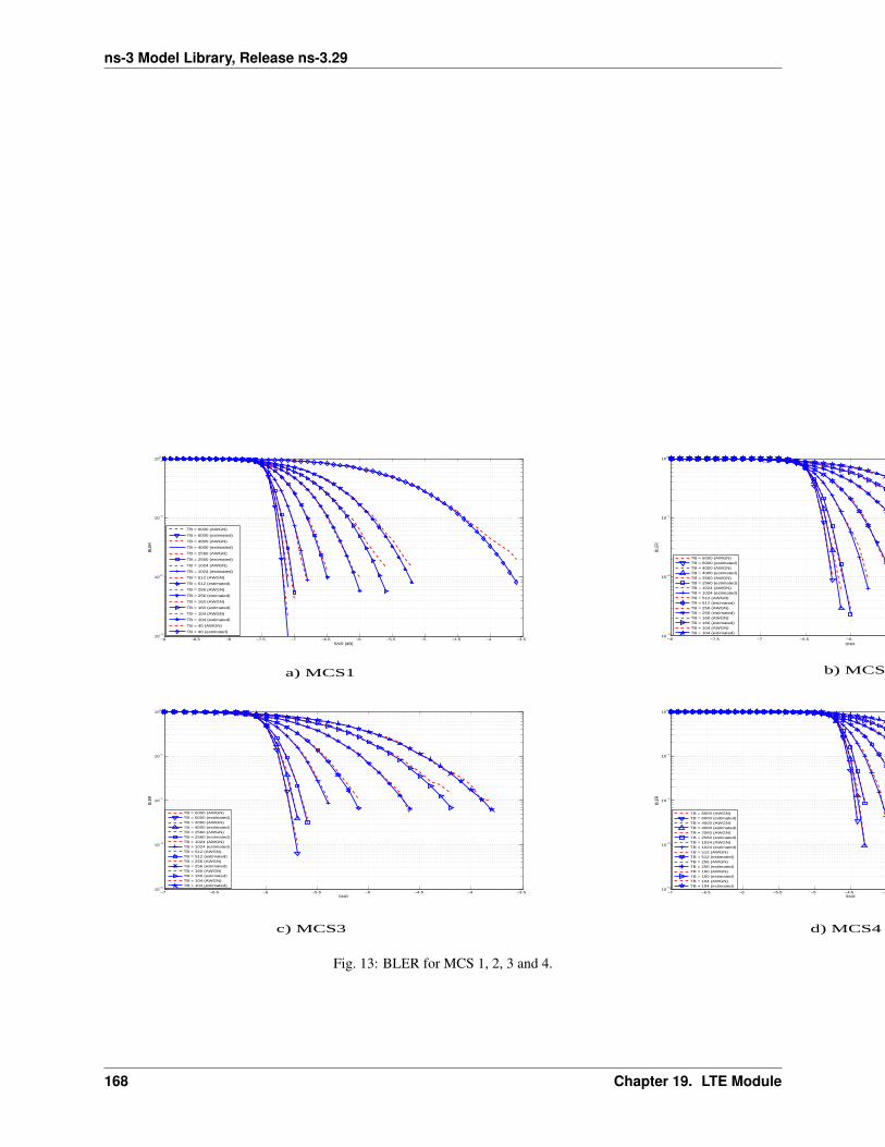
ns-3 Model Library, Release ns-3.29
−9 −8.5 −8 −7.5 −7 −6.5 −6 −5.5 −5 −4.5 −4 −3.510
−3
10−2
10−1
100
SNR [dB]
BLER
TB = 6000 (AWGN)
TB = 6000 (estimated)
TB = 4000 (AWGN)
TB = 4000 (estimated)
TB = 2560 (AWGN)
TB = 2560 (estimated)
TB = 1024 (AWGN)
TB = 1024 (estimated)
TB = 512 (AWGN)
TB = 512 (estimated)
TB = 256 (AWGN)
TB = 256 (estimated)
TB = 160 (AWGN)
TB = 160 (estimated)
TB = 104 (AWGN)
TB = 104 (estimated)
TB = 40 (AWGN)
TB = 40 (estimated)
−8 −7.5 −7 −6.5 −6 −5.5 −5 −4.5 −410
−3
10−2
10−1
100
SNR
BLER
TB = 6000 (AWGN)TB = 6000 (estimated)TB = 4000 (AWGN)TB = 4000 (estimated)TB = 2560 (AWGN)TB = 2560 (estimated)TB = 1024 (AWGN)TB = 1024 (estimated)TB = 512 (AWGN)TB = 512 (estimated)TB = 256 (AWGN)TB = 256 (estimated)TB = 160 (AWGN)TB = 160 (estimated)TB = 104 (AWGN)TB = 104 (estimated)
−7 −6.5 −6 −5.5 −5 −4.5 −4 −3.510
−4
10−3
10−2
10−1
100
SNR
BLER
TB = 6000 (AWGN)TB = 6000 (estimated)TB = 4000 (AWGN)TB = 4000 (estimated)TB = 2560 (AWGN)TB = 2560 (estimated)TB = 1024 (AWGN)TB = 1024 (estimated)TB = 512 (AWGN)TB = 512 (estimated)TB = 256 (AWGN)TB = 256 (estimated)TB = 160 (AWGN)TB = 160 (estimated)TB = 104 (AWGN)TB = 104 (estimated)
−7 −6.5 −6 −5.5 −5 −4.5 −4 −3.5 −3 −2.5 −210
−4
10−3
10−2
10−1
100
SNR
BLER
TB = 6000 (AWGN)TB = 6000 (estimated)TB = 4000 (AWGN)TB = 4000 (estimated)TB = 2560 (AWGN)TB = 2560 (estimated)TB = 1024 (AWGN)TB = 1024 (estimated)TB = 512 (AWGN)TB = 512 (estimated)TB = 256 (AWGN)TB = 256 (estimated)TB = 160 (AWGN)TB = 160 (estimated)TB = 104 (AWGN)TB = 104 (estimated)
a) MCS1 b) MCS2
c) MCS3 d) MCS4
Fig. 13: BLER for MCS 1, 2, 3 and 4.
168 Chapter 19. LTE Module
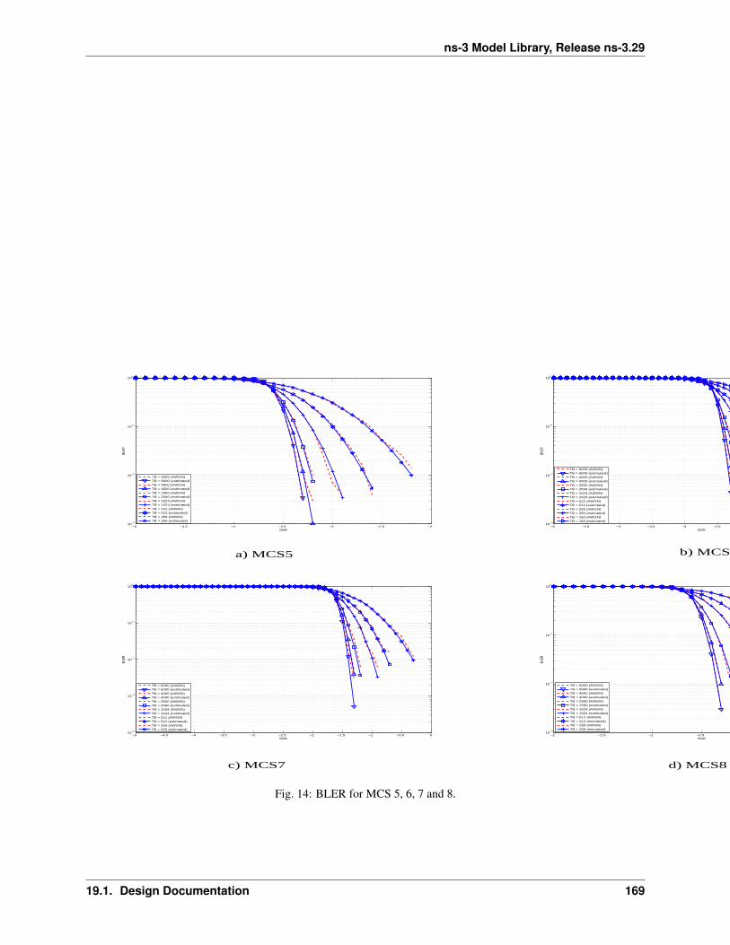
ns-3 Model Library, Release ns-3.29
−5 −4.5 −4 −3.5 −3 −2.5 −210
−3
10−2
10−1
100
SNR
BLER
TB = 6000 (AWGN)TB = 6000 (estimated)TB = 4000 (AWGN)TB = 4000 (estimated)TB = 2560 (AWGN)TB = 2560 (estimated)TB = 1024 (AWGN)TB = 1024 (estimated)TB = 512 (AWGN)TB = 512 (estimated)TB = 256 (AWGN)TB = 256 (estimated)
−5 −4.5 −4 −3.5 −3 −2.5 −2 −1.5 −1 −0.510
−3
10−2
10−1
100
SNR
BLER
TB = 6000 (AWGN)TB = 6000 (estimated)TB = 4000 (AWGN)TB = 4000 (estimated)TB = 2560 (AWGN)TB = 2560 (estimated)TB = 1024 (AWGN)TB = 1024 (estimated)TB = 512 (AWGN)TB = 512 (estimated)TB = 256 (AWGN)TB = 256 (estimated)TB = 160 (AWGN)TB = 160 (estimated)
−5 −4.5 −4 −3.5 −3 −2.5 −2 −1.5 −1 −0.5 010
−4
10−3
10−2
10−1
100
SNR
BLER
TB = 6000 (AWGN)TB = 6000 (estimated)TB = 4000 (AWGN)TB = 4000 (estimated)TB = 2560 (AWGN)TB = 2560 (estimated)TB = 1024 (AWGN)TB = 1024 (estimated)TB = 512 (AWGN)TB = 512 (estimated)TB = 256 (AWGN)TB = 256 (estimated)
−2 −1.5 −1 −0.5 0 0.5 110
−3
10−2
10−1
100
SNR
BLER
TB = 6000 (AWGN)TB = 6000 (estimated)TB = 4000 (AWGN)TB = 4000 (estimated)TB = 2560 (AWGN)TB = 2560 (estimated)TB = 1024 (AWGN)TB = 1024 (estimated)TB = 512 (AWGN)TB = 512 (estimated)TB = 256 (AWGN)TB = 256 (estimated)
a) MCS5 b) MCS6
c) MCS7 d) MCS8
Fig. 14: BLER for MCS 5, 6, 7 and 8.
19.1. Design Documentation 169
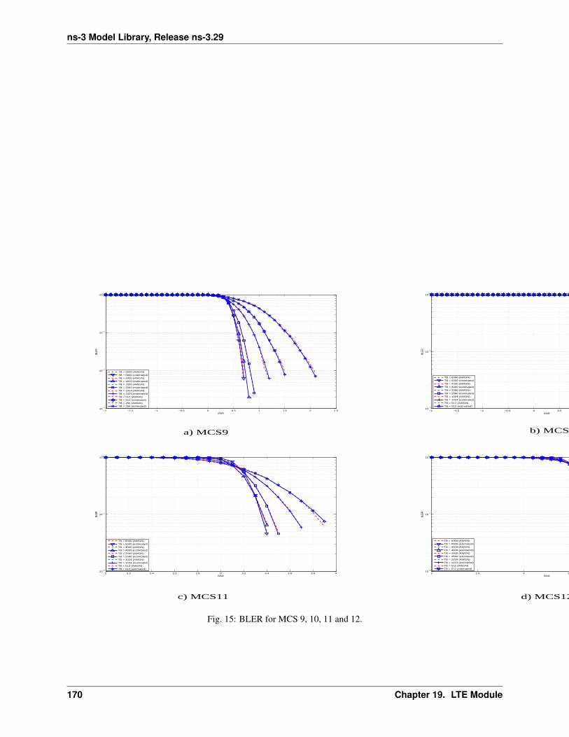
ns-3 Model Library, Release ns-3.29
−2 −1.5 −1 −0.5 0 0.5 1 1.5 2 2.510
−3
10−2
10−1
100
SNR
BLER
TB = 6000 (AWGN)TB = 6000 (estimated)TB = 4000 (AWGN)TB = 4000 (estimated)TB = 2560 (AWGN)TB = 2560 (estimated)TB = 1024 (AWGN)TB = 1024 (estimated)TB = 512 (AWGN)TB = 512 (estimated)TB = 256 (AWGN)TB = 256 (estimated)
−2 −1.5 −1 −0.5 0 0.5 1 1.5 2 2.510
−2
10−1
100
SNR
BLER
TB = 6000 (AWGN)TB = 6000 (estimated)TB = 4000 (AWGN)TB = 4000 (estimated)TB = 2560 (AWGN)TB = 2560 (estimated)TB = 1024 (AWGN)TB = 1024 (estimated)TB = 512 (AWGN)TB = 512 (estimated)
2 2.2 2.4 2.6 2.8 3 3.2 3.4 3.6 3.8 410
−2
10−1
100
SNR
BLER
TB = 6000 (AWGN)TB = 6000 (estimated)TB = 4000 (AWGN)TB = 4000 (estimated)TB = 2560 (AWGN)TB = 2560 (estimated)TB = 1024 (AWGN)TB = 1024 (estimated)TB = 512 (AWGN)TB = 512 (estimated)
2 2.5 3 3.5 4 4.510
−2
10−1
100
SNR
BLER
TB = 6000 (AWGN)TB = 6000 (estimated)TB = 4000 (AWGN)TB = 4000 (estimated)TB = 2560 (AWGN)TB = 2560 (estimated)TB = 1024 (AWGN)TB = 1024 (estimated)TB = 512 (AWGN)TB = 512 (estimated)
a) MCS9 b) MCS10
c) MCS11 d) MCS12
Fig. 15: BLER for MCS 9, 10, 11 and 12.
170 Chapter 19. LTE Module
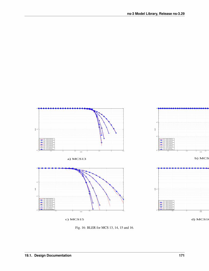
ns-3 Model Library, Release ns-3.29
2 2.5 3 3.5 4 4.5 5 5.510
−2
10−1
100
SNR
BLER
TB = 6000 (AWGN)TB = 6000 (estimated)TB = 4000 (AWGN)TB = 4000 (estimated)TB = 2560 (AWGN)TB = 2560 (estimated)TB = 1024 (AWGN)TB = 1024 (estimated)TB = 512 (AWGN)TB = 512 (estimated)
2 2.5 3 3.5 4 4.5 5 5.5 6 6.510
−3
10−2
10−1
100
SNR
BLER
TB = 6000 (AWGN)TB = 6000 (estimated)TB = 4000 (AWGN)TB = 4000 (estimated)TB = 2560 (AWGN)TB = 2560 (estimated)TB = 1024 (AWGN)TB = 1024 (estimated)TB = 512 (AWGN)TB = 512 (estimated)
5 5.5 6 6.5 7 7.510
−3
10−2
10−1
100
SNR
BLER
TB = 6000 (AWGN)TB = 6000 (estimated)TB = 4000 (AWGN)TB = 4000 (estimated)TB = 2560 (AWGN)TB = 2560 (estimated)TB = 1024 (AWGN)TB = 1024 (estimated)TB = 512 (AWGN)TB = 512 (estimated)
5 5.5 6 6.5 7 7.5 810
−2
10−1
100
SNR
BLER
TB = 6000 (AWGN)TB = 6000 (estimated)TB = 4000 (AWGN)TB = 4000 (estimated)TB = 2560 (AWGN)TB = 2560 (estimated)TB = 1024 (AWGN)TB = 1024 (estimated)
b) MCS14
c) MCS15 d) MCS16
a) MCS13
Fig. 16: BLER for MCS 13, 14, 15 and 16.
19.1. Design Documentation 171
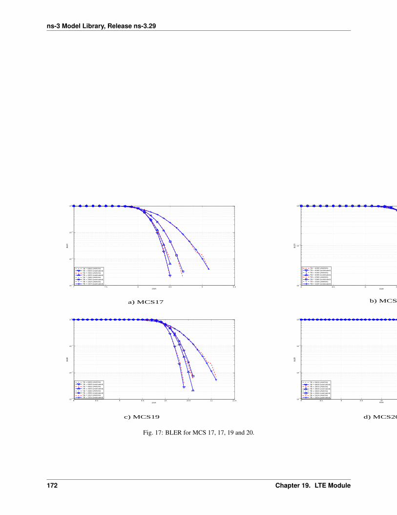
ns-3 Model Library, Release ns-3.29
7 7.5 8 8.5 9 9.510
−3
10−2
10−1
100
SNR
BLER
TB = 6000 (AWGN)TB = 6000 (estimated)TB = 4000 (AWGN)TB = 4000 (estimated)TB = 2560 (AWGN)TB = 2560 (estimated)TB = 1024 (AWGN)TB = 1024 (estimated)
8 8.5 9 9.5 10 10.510
−2
10−1
100
SNR
BLER
TB = 6000 (AWGN)TB = 6000 (estimated)TB = 4000 (AWGN)TB = 4000 (estimated)TB = 2560 (AWGN)TB = 2560 (estimated)TB = 1024 (AWGN)TB = 1024 (estimated)
8 8.5 9 9.5 10 10.5 11 11.510
−3
10−2
10−1
100
SNR
BLER
TB = 6000 (AWGN)TB = 6000 (estimated)TB = 4000 (AWGN)TB = 4000 (estimated)TB = 2560 (AWGN)TB = 2560 (estimated)TB = 1024 (AWGN)TB = 1024 (estimated)
8 8.5 9 9.5 10 10.5 11 11.5 1210
−3
10−2
10−1
100
SNR
BLER
TB = 6000 (AWGN)TB = 6000 (estimated)TB = 4000 (AWGN)TB = 4000 (estimated)TB = 2560 (AWGN)TB = 2560 (estimated)TB = 1024 (AWGN)TB = 1024 (estimated)
b) MCS18
c) MCS19 d) MCS20
a) MCS17
Fig. 17: BLER for MCS 17, 17, 19 and 20.
172 Chapter 19. LTE Module

ns-3 Model Library, Release ns-3.29
10 10.5 11 11.5 12 12.5 1310
−3
10−2
10−1
100
SNR
BLER
TB = 6000 (AWGN)TB = 6000 (estimated)TB = 4000 (AWGN)TB = 4000 (estimated)TB = 2560 (AWGN)TB = 2560 (estimated)TB = 1024 (AWGN)TB = 1024 (estimated)
10 10.5 11 11.5 12 12.5 13 13.5 1410
−3
10−2
10−1
100
SNR
BLER
TB = 6000 (AWGN)TB = 6000 (estimated)TB = 4000 (AWGN)TB = 4000 (estimated)TB = 2560 (AWGN)TB = 2560 (estimated)TB = 1024 (AWGN)TB = 1024 (estimated)
12 12.5 13 13.5 14 14.5 1510
−3
10−2
10−1
100
SNR
BLER
TB = 6000 (AWGN)TB = 6000 (estimated)TB = 4000 (AWGN)TB = 4000 (estimated)TB = 2560 (AWGN)TB = 2560 (estimated)TB = 1024 (AWGN)TB = 1024 (estimated)
12 12.5 13 13.5 14 14.5 15 15.5 1610
−3
10−2
10−1
100
SNR
BLER
TB = 6000 (AWGN)TB = 6000 (estimated)TB = 4000 (AWGN)TB = 4000 (estimated)TB = 2560 (AWGN)TB = 2560 (estimated)TB = 1024 (AWGN)TB = 1024 (estimated)
d) MCS24
a) MCS21 b) MCS22
c) MCS23
Fig. 18: BLER for MCS 21, 22, 23 and 24.
19.1. Design Documentation 173

ns-3 Model Library, Release ns-3.29
14 14.5 15 15.5 16 16.510
−3
10−2
10−1
100
SNR
BLER
TB = 6000 (AWGN)TB = 6000 (estimated)TB = 4000 (AWGN)TB = 4000 (estimated)TB = 2560 (AWGN)TB = 2560 (estimated)
14 14.5 15 15.5 16 16.5 17 17.510
−3
10−2
10−1
100
SNR
BLER
TB = 6000 (AWGN)TB = 6000 (estimated)TB = 4000 (AWGN)TB = 4000 (estimated)TB = 2560 (AWGN)TB = 2560 (estimated)
16 16.5 17 17.5 18 18.510
−3
10−2
10−1
100
SNR
BLER
TB = 6000 (AWGN)TB = 6000 (estimated)TB = 4000 (AWGN)TB = 4000 (estimated)TB = 2560 (AWGN)TB = 2560 (estimated)
16 16.5 17 17.5 18 18.5 19 19.510
−3
10−2
10−1
100
SNR
BLER
TB = 6000 (AWGN)TB = 6000 (estimated)TB = 4000 (AWGN)TB = 4000 (estimated)TB = 2560 (AWGN)TB = 2560 (estimated)
d) MCS28
b) MCS26
c) MCS27
a) MCS25
Fig. 19: BLER for MCS 25, 26, 27 and 28.
174 Chapter 19. LTE Module
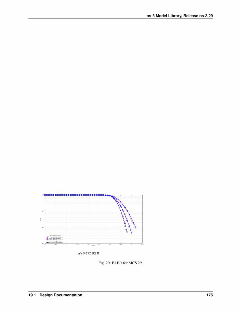
ns-3 Model Library, Release ns-3.29
16 16.5 17 17.5 18 18.5 19 19.5 20 20.510
−3
10−2
10−1
100
SNR
BLER
TB = 6000 (AWGN)TB = 6000 (estimated)TB = 4000 (AWGN)TB = 4000 (estimated)TB = 2560 (AWGN)TB = 2560 (estimated)
a) MCS29
Fig. 20: BLER for MCS 29.
19.1. Design Documentation 175
ns-3 Model Library, Release ns-3.29
In case an error occur, the DCIs discarded and therefore the UE will be not able to receive the correspondent Tbs,therefore resulting lost.
MIMO Model
The use of multiple antennas both at transmitter and receiver side, known as multiple-input and multiple-output(MIMO), is a problem well studied in literature during the past years. Most of the work concentrate on evaluatinganalytically the gain that the different MIMO schemes might have in term of capacity; however someones provide alsoinformation of the gain in terms of received power [CatreuxMIMO].
According to the considerations above, a model more flexible can be obtained considering the gain that MIMO schemesbring in the system from a statistical point of view. As highlighted before, [CatreuxMIMO] presents the statistical gainof several MIMO solutions respect to the SISO one in case of no correlation between the antennas. In the work thegain is presented as the cumulative distribution function (CDF) of the output SINR for what concern SISO, MIMO-Alamouti, MIMO-MMSE, MIMO-OSIC-MMSE and MIMO-ZF schemes. Elaborating the results, the output SINRdistribution can be approximated with a log-normal one with different mean and variance as function of the schemeconsidered. However, the variances are not so different and they are approximatively equal to the one of the SISOmode already included in the shadowing component of the BuildingsPropagationLossModel, in detail:
• SISO: µ = 13.5 and σ = 20 [dB].
• MIMO-Alamouti: µ = 17.7 and σ = 11.1 [dB].
• MIMO-MMSE: µ = 10.7 and σ = 16.6 [dB].
• MIMO-OSIC-MMSE: µ = 12.6 and σ = 15.5 [dB].
• MIMO-ZF: µ = 10.3 and σ = 12.6 [dB].
Therefore the PHY layer implements the MIMO model as the gain perceived by the receiver when using a MIMOscheme respect to the one obtained using SISO one. We note that, these gains referred to a case where there is nocorrelation between the antennas in MIMO scheme; therefore do not model degradation due to paths correlation.
UE PHY Measurements Model
According to [TS36214], the UE has to report a set of measurements of the eNBs that the device is able to perceive:the reference signal received power (RSRP) and the reference signal received quality (RSRQ). The former is a measureof the received power of a specific eNB, while the latter includes also channel interference and thermal noise. The UEhas to report the measurements jointly with the physical cell identity (PCI) of the cell. Both the RSRP and RSRQ mea-surements are performed during the reception of the RS, while the PCI is obtained with the Primary SynchronizationSignal (PSS). The PSS is sent by the eNB each 5 subframes and in detail in the subframes 1 and 6. In real systems,only 504 distinct PCIs are available, and hence it could occur that two nearby eNBs use the same PCI; however, in thesimulator we model PCIs using simulation metadata, and we allow up to 65535 distinct PCIs, thereby avoiding PCIcollisions provided that less that 65535 eNBs are simulated in the same scenario.
According to [TS36133] sections 9.1.4 and 9.1.7, RSRP is reported by PHY layer in dBm while RSRQ indB. The values of RSRP and RSRQ are provided to higher layers through the C-PHY SAP (by means ofUeMeasurementsParameters struct) every 200 ms as defined in [TS36331]. Layer 1 filtering is performedby averaging the all the measurements collected during the last window slot. The periodicity of reporting can beadjusted for research purposes by means of the LteUePhy::UeMeasurementsFilterPeriod attribute.
The formulas of the RSRP and RSRQ can be simplified considering the assumption of the PHY layer that the channelis flat within the RB, the finest level of accuracy. In fact, this implies that all the REs within a RB have the same power,therefore:
RSRP =
∑K−1k=0
∑M−1m=0 (P (k,m))
M
K=
∑K−1k=0
(M×P (k))M
K=
∑K−1k=0 (P (k))
K
176 Chapter 19. LTE Module

ns-3 Model Library, Release ns-3.29
where P (k,m) represents the signal power of the REm within the RB k, which, as observed before, is constant withinthe same RB and equal to P (k), M is the number of REs carrying the RS in a RB and K is the number of RBs. It isto be noted that P (k), and in general all the powers defined in this section, is obtained in the simulator from the PSDof the RB (which is provided by the LteInterferencePowerChunkProcessor), in detail:
P (k) = PSDRB(k) ∗ 180000/12
where PSDRB(k) is the power spectral density of the RB k, 180000 is the bandwidth in Hz of the RB and 12 is thenumber of REs per RB in an OFDM symbol. Similarly, for RSSI we have
RSSI =
K−1∑k=0
∑S−1s=0
∑R−1r=0 (P (k, s, r) + I(k, s, r) +N(k, s, r))
S
where S is the number of OFDM symbols carrying RS in a RB and R is the number of REs carrying a RS in aOFDM symbol (which is fixed to 2) while P (k, s, r), I(k, s, r) and N(k, s, r) represent respectively the perceivedpower of the serving cell, the interference power and the noise power of the RE r in symbol s. As for RSRP, themeasurements within a RB are always equals among each others according to the PHY model; therefore P (k, s, r) =P (k), I(k, s, r) = I(k) and N(k, s, r) = N(k), which implies that the RSSI can be calculated as:
RSSI =
K−1∑k=0
S × 2× (P (k) + I(k) +N(k))
S=
K−1∑k=0
2× (P (k) + I(k) +N(k))
Considering the constraints of the PHY reception chain implementation, and in order to maintain the level ofcomputational complexity low, only RSRP can be directly obtained for all the cells. This is due to the fact thatLteSpectrumPhy is designed for evaluating the interference only respect to the signal of the serving eNB. This im-plies that the PHY layer is optimized for managing the power signals information with the serving eNB as a reference.However, RSRP and RSRQ of neighbor cell i can be extracted by the current information available of the serving cellj as detailed in the following:
RSRPi =
∑K−1k=0 (Pi(k))
K
RSSIi = RSSIj =
K−1∑k=0
2× (Ij(k) + Pj(k) +Nj(k))
RSRQji = K ×RSRPi/RSSIj
where RSRPi is the RSRP of the neighbor cell i, Pi(k) is the power perceived at any RE within the RB k, K is thetotal number of RBs, RSSIi is the RSSI of the neighbor cell i when the UE is attached to cell j (which, since it isthe sum of all the received powers, coincides with RSSIj), Ij(k) is the total interference perceived by UE in anyRE of RB k when attached to cell i (obtained by the LteInterferencePowerChunkProcessor), Pj(k) is thepower perceived of cell j in any RE of the RB k and N is the power noise spectral density in any RE. The sample isconsidered as valid in case of the RSRQ evaluated is above the LteUePhy::RsrqUeMeasThreshold attribute.
19.1.6 HARQ
The HARQ scheme implemented is based on a incremental redundancy (IR) solutions combined with multiple stop-and-wait processes for enabling a continuous data flow. In detail, the solution adopted is the soft combining hybridIR Full incremental redundancy (also called IR Type II), which implies that the retransmissions contain only newinformation respect to the previous ones. The resource allocation algorithm of the HARQ has been implemented withinthe respective scheduler classes (i.e., RrFfMacScheduler and PfFfMacScheduler, refer to their correspondentsections for more info), while the decodification part of the HARQ has been implemented in the LteSpectrumPhyand LteHarqPhy classes which will be detailed in this section.
According to the standard, the UL retransmissions are synchronous and therefore are allocated 7 ms after the originaltransmission. On the other hand, for the DL, they are asynchronous and therefore can be allocated in a more flexible
19.1. Design Documentation 177
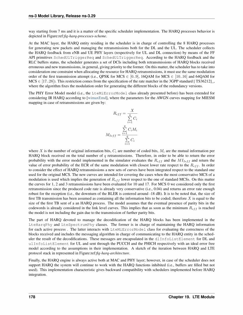
ns-3 Model Library, Release ns-3.29
way starting from 7 ms and it is a matter of the specific scheduler implementation. The HARQ processes behavior isdepicted in Figure:ref:fig-harq-processes-scheme.
At the MAC layer, the HARQ entity residing in the scheduler is in charge of controlling the 8 HARQ processesfor generating new packets and managing the retransmissions both for the DL and the UL. The scheduler collectsthe HARQ feedback from eNB and UE PHY layers (respectively for UL and DL connection) by means of the FFAPI primitives SchedUlTriggerReq and SchedUlTriggerReq. According to the HARQ feedback and theRLC buffers status, the scheduler generates a set of DCIs including both retransmissions of HARQ blocks receivederroneous and new transmissions, in general, giving priority to the former. On this matter, the scheduler has to take intoconsideration one constraint when allocating the resource for HARQ retransmissions, it must use the same modulationorder of the first transmission attempt (i.e., QPSK for MCS ∈ [0..9], 16QAM for MCS ∈ [10..16] and 64QAM forMCS ∈ [17..28]). This restriction comes from the specification of the rate matcher in the 3GPP standard [ TS36212]_,where the algorithm fixes the modulation order for generating the different blocks of the redundancy versions.
The PHY Error Model model (i.e., the LteMiErrorModel class already presented before) has been extended forconsidering IR HARQ according to [wimaxEmd], where the parameters for the AWGN curves mapping for MIESMmapping in case of retransmissions are given by:
Reff =Xq∑i=1
Ci
MIeff =
q∑i=1
CiMi
q∑i=1
Ci
where X is the number of original information bits, Ci are number of coded bits, Mi are the mutual information perHARQ block received on the total number of q retransmissions. Therefore, in order to be able to return the errorprobability with the error model implemented in the simulator evaluates the Reff and the MIIeff and return thevalue of error probability of the ECR of the same modulation with closest lower rate respect to the Reff . In orderto consider the effect of HARQ retransmissions a new sets of curves have been integrated respect to the standard oneused for the original MCS. The new curves are intended for covering the cases when the most conservative MCS of amodulation is used which implies the generation of Reff lower respect to the one of standard MCSs. On this matterthe curves for 1, 2 and 3 retransmissions have been evaluated for 10 and 17. For MCS 0 we considered only the firstretransmission since the produced code rate is already very conservative (i.e., 0.04) and returns an error rate enoughrobust for the reception (i.e., the downturn of the BLER is centered around -18 dB). It is to be noted that, the size offirst TB transmission has been assumed as containing all the information bits to be coded; therefore X is equal to thesize of the first TB sent of a an HARQ process. The model assumes that the eventual presence of parity bits in thecodewords is already considered in the link level curves. This implies that as soon as the minimum Reff is reachedthe model is not including the gain due to the transmission of further parity bits.
The part of HARQ devoted to manage the decodification of the HARQ blocks has been implemented in theLteHarqPhy and LteSpectrumPhy classes. The former is in charge of maintaining the HARQ informationfor each active process . The latter interacts with LteMiErrorModel class for evaluating the correctness of theblocks received and includes the messaging algorithm in charge of communicating to the HARQ entity in the sched-uler the result of the decodifications. These messages are encapsulated in the dlInfoListElement for DL andulInfoListElement for UL and sent through the PUCCH and the PHICH respectively with an ideal error freemodel according to the assumptions in their implementation. A sketch of the iteration between HARQ and LTEprotocol stack in represented in Figure:ref:fig-harq-architecture.
Finally, the HARQ engine is always active both at MAC and PHY layer; however, in case of the scheduler does notsupport HARQ the system will continue to work with the HARQ functions inhibited (i.e., buffers are filled but notused). This implementation characteristic gives backward compatibility with schedulers implemented before HARQintegration.
178 Chapter 19. LTE Module
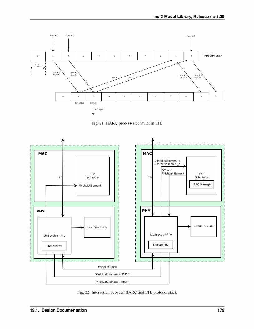
ns-3 Model Library, Release ns-3.29
Fig. 21: HARQ processes behavior in LTE
Fig. 22: Interaction between HARQ and LTE protocol stack
19.1. Design Documentation 179
ns-3 Model Library, Release ns-3.29
19.1.7 MAC
Resource Allocation Model
We now briefly describe how resource allocation is handled in LTE, clarifying how it is modeled in the simulator. Thescheduler is in charge of generating specific structures called Data Control Indication (DCI) which are then transmittedby the PHY of the eNB to the connected UEs, in order to inform them of the resource allocation on a per subframebasis. In doing this in the downlink direction, the scheduler has to fill some specific fields of the DCI structure withall the information, such as: the Modulation and Coding Scheme (MCS) to be used, the MAC Transport Block (TB)size, and the allocation bitmap which identifies which RBs will contain the data transmitted by the eNB to each user.
For the mapping of resources to physical RBs, we adopt a localized mapping approach (see [Sesia2009], Section9.2.2.1); hence in a given subframe each RB is always allocated to the same user in both slots. The allocation bitmapcan be coded in different formats; in this implementation, we considered the Allocation Type 0 defined in [TS36213],according to which the RBs are grouped in Resource Block Groups (RBG) of different size determined as a functionof the Transmission Bandwidth Configuration in use.
For certain bandwidth values not all the RBs are usable, since the group size is not a common divisor of the group.This is for instance the case when the bandwidth is equal to 25 RBs, which results in a RBG size of 2 RBs, andtherefore 1 RB will result not addressable. In uplink the format of the DCIs is different, since only adjacent RBs canbe used because of the SC-FDMA modulation. As a consequence, all RBs can be allocated by the eNB regardless ofthe bandwidth configuration.
Adaptive Modulation and Coding
The simulator provides two Adaptive Modulation and Coding (AMC) models: one based on the GSoC model[Piro2011] and one based on the physical error model (described in the following sections).
The former model is a modified version of the model described in [Piro2011], which in turn is inspired from [Seo2004].Our version is described in the following. Let i denote the generic user, and let γi be its SINR. We get the spectralefficiency ηi of user i using the following equations:
BER = 0.00005
Γ =− ln (5 ∗ BER)
1.5
ηi = log2
(1 +
γiΓ
)The procedure described in [R1-081483] is used to get the corresponding MCS scheme. The spectral efficiency isquantized based on the channel quality indicator (CQI), rounding to the lowest value, and is mapped to the corre-sponding MCS scheme.
Finally, we note that there are some discrepancies between the MCS index in [R1-081483] and that indicated by thestandard: [TS36213] Table 7.1.7.1-1 says that the MCS index goes from 0 to 31, and 0 appears to be a valid MCSscheme (TB size is not 0) but in [R1-081483] the first useful MCS index is 1. Hence to get the value as intended bythe standard we need to subtract 1 from the index reported in [R1-081483].
The alternative model is based on the physical error model developed for this simulator and explained in the followingsubsections. This scheme is able to adapt the MCS selection to the actual PHY layer performance according tothe specific CQI report. According to their definition, a CQI index is assigned when a single PDSCH TB with themodulation coding scheme and code rate correspondent to that CQI index in table 7.2.3-1 of [TS36213] can be receivedwith an error probability less than 0.1. In case of wideband CQIs, the reference TB includes all the RBGs available inorder to have a reference based on the whole available resources; while, for subband CQIs, the reference TB is sizedas the RBGs.
180 Chapter 19. LTE Module
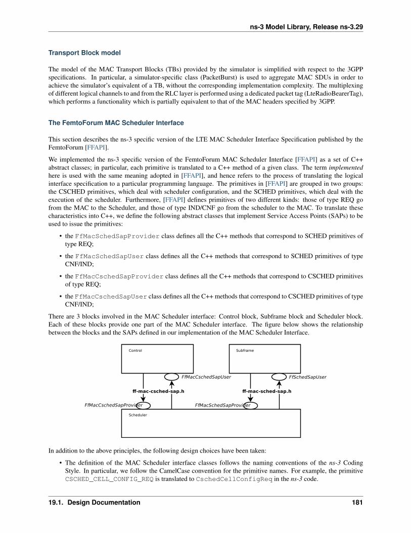
ns-3 Model Library, Release ns-3.29
Transport Block model
The model of the MAC Transport Blocks (TBs) provided by the simulator is simplified with respect to the 3GPPspecifications. In particular, a simulator-specific class (PacketBurst) is used to aggregate MAC SDUs in order toachieve the simulator’s equivalent of a TB, without the corresponding implementation complexity. The multiplexingof different logical channels to and from the RLC layer is performed using a dedicated packet tag (LteRadioBearerTag),which performs a functionality which is partially equivalent to that of the MAC headers specified by 3GPP.
The FemtoForum MAC Scheduler Interface
This section describes the ns-3 specific version of the LTE MAC Scheduler Interface Specification published by theFemtoForum [FFAPI].
We implemented the ns-3 specific version of the FemtoForum MAC Scheduler Interface [FFAPI] as a set of C++abstract classes; in particular, each primitive is translated to a C++ method of a given class. The term implementedhere is used with the same meaning adopted in [FFAPI], and hence refers to the process of translating the logicalinterface specification to a particular programming language. The primitives in [FFAPI] are grouped in two groups:the CSCHED primitives, which deal with scheduler configuration, and the SCHED primitives, which deal with theexecution of the scheduler. Furthermore, [FFAPI] defines primitives of two different kinds: those of type REQ gofrom the MAC to the Scheduler, and those of type IND/CNF go from the scheduler to the MAC. To translate thesecharacteristics into C++, we define the following abstract classes that implement Service Access Points (SAPs) to beused to issue the primitives:
• the FfMacSchedSapProvider class defines all the C++ methods that correspond to SCHED primitives oftype REQ;
• the FfMacSchedSapUser class defines all the C++ methods that correspond to SCHED primitives of typeCNF/IND;
• the FfMacCschedSapProvider class defines all the C++ methods that correspond to CSCHED primitivesof type REQ;
• the FfMacCschedSapUser class defines all the C++ methods that correspond to CSCHED primitives of typeCNF/IND;
There are 3 blocks involved in the MAC Scheduler interface: Control block, Subframe block and Scheduler block.Each of these blocks provide one part of the MAC Scheduler interface. The figure below shows the relationshipbetween the blocks and the SAPs defined in our implementation of the MAC Scheduler Interface.
In addition to the above principles, the following design choices have been taken:
• The definition of the MAC Scheduler interface classes follows the naming conventions of the ns-3 CodingStyle. In particular, we follow the CamelCase convention for the primitive names. For example, the primitiveCSCHED_CELL_CONFIG_REQ is translated to CschedCellConfigReq in the ns-3 code.
19.1. Design Documentation 181
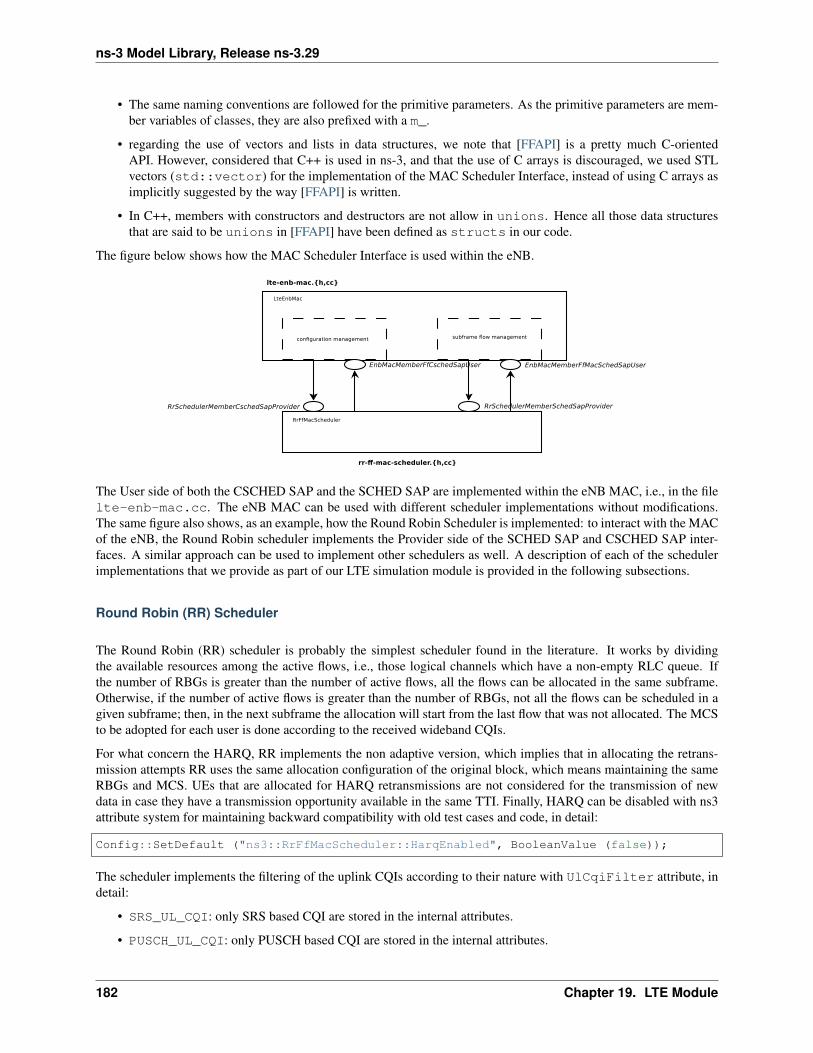
ns-3 Model Library, Release ns-3.29
• The same naming conventions are followed for the primitive parameters. As the primitive parameters are mem-ber variables of classes, they are also prefixed with a m_.
• regarding the use of vectors and lists in data structures, we note that [FFAPI] is a pretty much C-orientedAPI. However, considered that C++ is used in ns-3, and that the use of C arrays is discouraged, we used STLvectors (std::vector) for the implementation of the MAC Scheduler Interface, instead of using C arrays asimplicitly suggested by the way [FFAPI] is written.
• In C++, members with constructors and destructors are not allow in unions. Hence all those data structuresthat are said to be unions in [FFAPI] have been defined as structs in our code.
The figure below shows how the MAC Scheduler Interface is used within the eNB.
The User side of both the CSCHED SAP and the SCHED SAP are implemented within the eNB MAC, i.e., in the filelte-enb-mac.cc. The eNB MAC can be used with different scheduler implementations without modifications.The same figure also shows, as an example, how the Round Robin Scheduler is implemented: to interact with the MACof the eNB, the Round Robin scheduler implements the Provider side of the SCHED SAP and CSCHED SAP inter-faces. A similar approach can be used to implement other schedulers as well. A description of each of the schedulerimplementations that we provide as part of our LTE simulation module is provided in the following subsections.
Round Robin (RR) Scheduler
The Round Robin (RR) scheduler is probably the simplest scheduler found in the literature. It works by dividingthe available resources among the active flows, i.e., those logical channels which have a non-empty RLC queue. Ifthe number of RBGs is greater than the number of active flows, all the flows can be allocated in the same subframe.Otherwise, if the number of active flows is greater than the number of RBGs, not all the flows can be scheduled in agiven subframe; then, in the next subframe the allocation will start from the last flow that was not allocated. The MCSto be adopted for each user is done according to the received wideband CQIs.
For what concern the HARQ, RR implements the non adaptive version, which implies that in allocating the retrans-mission attempts RR uses the same allocation configuration of the original block, which means maintaining the sameRBGs and MCS. UEs that are allocated for HARQ retransmissions are not considered for the transmission of newdata in case they have a transmission opportunity available in the same TTI. Finally, HARQ can be disabled with ns3attribute system for maintaining backward compatibility with old test cases and code, in detail:
Config::SetDefault ("ns3::RrFfMacScheduler::HarqEnabled", BooleanValue (false));
The scheduler implements the filtering of the uplink CQIs according to their nature with UlCqiFilter attribute, indetail:
• SRS_UL_CQI: only SRS based CQI are stored in the internal attributes.
• PUSCH_UL_CQI: only PUSCH based CQI are stored in the internal attributes.
182 Chapter 19. LTE Module

ns-3 Model Library, Release ns-3.29
• ALL_UL_CQI: all CQIs are stored in the same internal attribute (i.e., the last CQI received is stored indepen-dently from its nature).
Proportional Fair (PF) Scheduler
The Proportional Fair (PF) scheduler [Sesia2009] works by scheduling a user when its instantaneous channel qualityis high relative to its own average channel condition over time. Let i, j denote generic users; let t be the subframeindex, and k be the resource block index; let Mi,k(t) be MCS usable by user i on resource block k according to whatreported by the AMC model (see Adaptive Modulation and Coding); finally, let S(M,B) be the TB size in bits asdefined in [TS36213] for the case where a number B of resource blocks is used. The achievable rate Ri(k, t) in bit/sfor user i on resource block group k at subframe t is defined as
Ri(k, t) =S (Mi,k(t), 1)
τ
where τ is the TTI duration. At the start of each subframe t, each RBG is assigned to a certain user. In detail, theindex ik(t) to which RBG k is assigned at time t is determined as
ik(t) = argmaxj=1,...,N
(Rj(k, t)
Tj(t)
)where Tj(t) is the past througput performance perceived by the user j. According to the above scheduling algorithm,a user can be allocated to different RBGs, which can be either adjacent or not, depending on the current condition ofthe channel and the past throughput performance Tj(t). The latter is determined at the end of the subframe t using thefollowing exponential moving average approach:
Tj(t) = (1− 1
α)Tj(t− 1) +
1
αTj(t)
where α is the time constant (in number of subframes) of the exponential moving average, and Tj(t) is the actualthroughput achieved by the user i in the subframe t. Tj(t) is measured according to the following procedure. First wedetermine the MCS Mj(t) actually used by user j:
Mj(t) = mink:ik(t)=j
Mj,k(t)
then we determine the total number Bj(t) of RBGs allocated to user j:
Bj(t) =∣∣∣{k : ik(t) = j}
∣∣∣where | · | indicates the cardinality of the set; finally,
Tj(t) =S(Mj(t), Bj(t)
)τ
For what concern the HARQ, PF implements the non adaptive version, which implies that in allocating the retrans-mission attempts the scheduler uses the same allocation configuration of the original block, which means maintainingthe same RBGs and MCS. UEs that are allocated for HARQ retransmissions are not considered for the transmissionof new data in case they have a transmission opportunity available in the same TTI. Finally, HARQ can be disabledwith ns3 attribute system for maintaining backward compatibility with old test cases and code, in detail:
Config::SetDefault ("ns3::PfFfMacScheduler::HarqEnabled", BooleanValue (false));
19.1. Design Documentation 183
ns-3 Model Library, Release ns-3.29
Maximum Throughput (MT) Scheduler
The Maximum Throughput (MT) scheduler [FCapo2012] aims to maximize the overall throughput of eNB. It allo-cates each RB to the user that can achieve the maximum achievable rate in the current TTI. Currently, MT scheduler inNS-3 has two versions: frequency domain (FDMT) and time domain (TDMT). In FDMT, every TTI, MAC schedulerallocates RBGs to the UE who has highest achievable rate calculated by subband CQI. In TDMT, every TTI, MACscheduler selects one UE which has highest achievable rate calculated by wideband CQI. Then MAC scheduler allo-cates all RBGs to this UE in current TTI. The calculation of achievable rate in FDMT and TDMT is as same as theone in PF. Let i, j denote generic users; let t be the subframe index, and k be the resource block index; let Mi,k(t) beMCS usable by user i on resource block k according to what reported by the AMC model (see Adaptive Modulationand Coding); finally, let S(M,B) be the TB size in bits as defined in [TS36213] for the case where a number B ofresource blocks is used. The achievable rate Ri(k, t) in bit/s for user i on resource block k at subframe t is defined as
Ri(k, t) =S (Mi,k(t), 1)
τ
where τ is the TTI duration. At the start of each subframe t, each RB is assigned to a certain user. In detail, the indexik(t) to which RB k is assigned at time t is determined as
ik(t) = argmaxj=1,...,N
(Rj(k, t))
When there are several UEs having the same achievable rate, current implementation always selects the first UE createdin script. Although MT can maximize cell throughput, it cannot provide fairness to UEs in poor channel condition.
Throughput to Average (TTA) Scheduler
The Throughput to Average (TTA) scheduler [FCapo2012] can be considered as an intermediate between MT and PF.The metric used in TTA is calculated as follows:
ik(t) = argmaxj=1,...,N
(Rj(k, t)
Rj(t)
)Here, Ri(k, t) in bit/s represents the achievable rate for user i on resource block k at subframe t. The calculationmethod already is shown in MT and PF. Meanwhile, Ri(t) in bit/s stands for the achievable rate for i at subframe t.The difference between those two achievable rates is how to get MCS. For Ri(k, t), MCS is calculated by subbandCQI while Ri(t) is calculated by wideband CQI. TTA scheduler can only be implemented in frequency domain (FD)because the achievable rate of particular RBG is only related to FD scheduling.
Blind Average Throughput Scheduler
The Blind Average Throughput scheduler [FCapo2012] aims to provide equal throughput to all UEs under eNB. Themetric used in TTA is calculated as follows:
ik(t) = argmaxj=1,...,N
(1
Tj(t)
)where Tj(t) is the past throughput performance perceived by the user j and can be calculated by the same methodin PF scheduler. In the time domain blind average throughput (TD-BET), the scheduler selects the UE with largestpriority metric and allocates all RBGs to this UE. On the other hand, in the frequency domain blind average throughput(FD-BET), every TTI, the scheduler first selects one UE with lowest pastAverageThroughput (largest priority metric).Then scheduler assigns one RBG to this UE, it calculates expected throughput of this UE and uses it to compare withpast average throughput Tj(t) of other UEs. The scheduler continues to allocate RBG to this UE until its expectedthroughput is not the smallest one among past average throughput Tj(t) of all UE. Then the scheduler will use the sameway to allocate RBG for a new UE which has the lowest past average throughput Tj(t) until all RBGs are allocated toUEs. The principle behind this is that, in every TTI, the scheduler tries the best to achieve the equal throughput amongall UEs.
184 Chapter 19. LTE Module
ns-3 Model Library, Release ns-3.29
Token Bank Fair Queue Scheduler
Token Bank Fair Queue (TBFQ) is a QoS aware scheduler which derives from the leaky-bucket mechanism. In TBFQ,a traffic flow of user i is characterized by following parameters:
• ti: packet arrival rate (byte/sec )
• ri: token generation rate (byte/sec)
• pi: token pool size (byte)
• Ei: counter that records the number of token borrowed from or given to the token bank by flow i ; Ei can besmaller than zero
Each K bytes data consumes k tokens. Also, TBFQ maintains a shared token bank (B) so as to balance the trafficbetween different flows. If token generation rate ri is bigger than packet arrival rate ti, then tokens overflowing fromtoken pool are added to the token bank, and Ei is increased by the same amount. Otherwise, flow i needs to withdrawtokens from token bank based on a priority metric fracEiri, and Ei is decreased. Obviously, the user contributesmore on token bank has higher priority to borrow tokens; on the other hand, the user borrows more tokens from bankhas lower priority to continue to withdraw tokens. Therefore, in case of several users having the same token generationrate, traffic rate and token pool size, user suffers from higher interference has more opportunity to borrow tokens frombank. In addition, TBFQ can police the traffic by setting the token generation rate to limit the throughput. Additionally,TBFQ also maintains following three parameters for each flow:
• Debt limit di: if Ei belows this threshold, user i cannot further borrow tokens from bank. This is for preventingmalicious UE to borrow too much tokens.
• Credit limit ci: the maximum number of tokens UE i can borrow from the bank in one time.
• Credit threshold C: once Ei reaches debt limit, UE i must store C tokens to bank in order to further borrowtoken from bank.
LTE in NS-3 has two versions of TBFQ scheduler: frequency domain TBFQ (FD-TBFQ) and time domain TBFQ (TD-TBFQ). In FD-TBFQ, the scheduler always select UE with highest metric and allocates RBG with highest subbandCQI until there are no packets within UE’s RLC buffer or all RBGs are allocated [FABokhari2009]. In TD-TBFQ,after selecting UE with maximum metric, it allocates all RBGs to this UE by using wideband CQI [WKWong2004].
Priority Set Scheduler
Priority set scheduler (PSS) is a QoS aware scheduler which combines time domain (TD) and frequency domain (FD)packet scheduling operations into one scheduler [GMonghal2008]. It controls the fairness among UEs by a specifiedTarget Bit Rate (TBR).
In TD scheduler part, PSS first selects UEs with non-empty RLC buffer and then divide them into two sets based onthe TBR:
• set 1: UE whose past average throughput is smaller than TBR; TD scheduler calculates their priority metric inBlind Equal Throughput (BET) style:
ik(t) = argmaxj=1,...,N
(1
Tj(t)
)• set 2: UE whose past average throughput is larger (or equal) than TBR; TD scheduler calculates their priority
metric in Proportional Fair (PF) style:
ik(t) = argmaxj=1,...,N
(Rj(k, t)
Tj(t)
)UEs belonged to set 1 have higher priority than ones in set 2. Then PSS will select Nmux UEs with highest metric intwo sets and forward those UE to FD scheduler. In PSS, FD scheduler allocates RBG k to UE n that maximums thechosen metric. Two PF schedulers are used in PF scheduler:
19.1. Design Documentation 185
ns-3 Model Library, Release ns-3.29
• Proportional Fair scheduled (PFsch)
Mschk(t) = argmaxj=1,...,N
(Rj(k, t)
Tschj(t)
)• Carrier over Interference to Average (CoIta)
Mcoik(t) = argmaxj=1,...,N
(CoI[j, k]∑NRBG
k=0 CoI[j, k]
)where Tschj(t) is similar past throughput performance perceived by the user j, with the difference that it is updatedonly when the i-th user is actually served. CoI[j, k] is an estimation of the SINR on the RBG k of UE j. Both PFschand CoIta is for decoupling FD metric from TD scheduler. In addition, PSS FD scheduler also provide a weight metricW[n] for helping controlling fairness in case of low number of UEs.
W [n] = max(1,TBR
Tj(t))
where Tj(t) is the past throughput performance perceived by the user j . Therefore, on RBG k, the FD schedulerselects the UE j that maximizes the product of the frequency domain metric (Msch, MCoI) by weight W [n]. Thisstrategy will guarantee the throughput of lower quality UE tend towards the TBR.
Config::SetDefault ("ns3::PfFfMacScheduler::HarqEnabled", BooleanValue (false));
The scheduler implements the filtering of the uplink CQIs according to their nature with UlCqiFilter attribute, indetail:
• SRS_UL_CQI: only SRS based CQI are stored in the internal attributes.
• PUSCH_UL_CQI: only PUSCH based CQI are stored in the internal attributes.
• ALL_UL_CQI: all CQIs are stored in the same internal attribute (i.e., the last CQI received is stored indepen-dently from its nature).
Channel and QoS Aware Scheduler
The Channel and QoS Aware (CQA) Scheduler [Bbojovic2014] is an LTE MAC downlink scheduling algorithm thatconsiders the head of line (HOL) delay, the GBR parameters and channel quality over different subbands. The CQAscheduler is based on joint TD and FD scheduling.
In the TD (at each TTI) the CQA scheduler groups users by priority. The purpose of grouping is to enforce the FDscheduling to consider first the flows with highest HOL delay. The grouping metric mtd for user j = 1, ..., N isdefined in the following way:
mjtd(t) = d
djhol(t)
ge ,
where djhol(t) is the current value of HOL delay of flow j, and g is a grouping parameter that determines granularityof the groups, i.e. the number of the flows that will be considered in the FD scheduling iteration.
The groups of flows selected in the TD iteration are forwarded to the FD scheduling starting from the flows withthe highest value of the mtd metric until all RBGs are assigned in the corresponding TTI. In the FD, for each RBGk = 1, ...,K, the CQA scheduler assigns the current RBG to the user j that has the maximum value of the FD metricwhich we define in the following way:
m(k,j)fd (t) = djHOL(t) ·mj
GBR(t) ·mk,jca (t) ,
186 Chapter 19. LTE Module

ns-3 Model Library, Release ns-3.29
where mjGBR(t) is calculated as follows:
mjGBR(t) =
GBRj
Rj(t)=
GBRj
(1− α) ·Rj(t− 1) + α · rj(t),
whereGBRj is the bit rate specified in EPS bearer of the flow j,Rj(t) is the past averaged throughput that is calculatedwith a moving average, rj(t) is the throughput achieved at the time t, and α is a coefficient such that 0 ≤ α ≤ 1.
For m(k,j)ca (t) we consider two different metrics: m(k,j)
pf (t) and m(k,j)ff (t). mpf is the Proportional Fair metric which
is defined as follows:
m(k,j)pf (t) =
R(k,j)e
Rj(t),
where R(k,j)e (t) is the estimated achievable throughput of user j over RBG k calculated by the Adaptive Modulation
and Coding (AMC) scheme that maps the channel quality indicator (CQI) value to the transport block size in bits.
The other channel awareness metric that we consider is mff which is proposed in [GMonghal2008] and it representsthe frequency selective fading gains over RBG k for user j and is calculated in the following way:
m(k,j)ff (t) =
CQI(k,j)(t)∑Kk=1 CQI(t)(k,j)
,
where CQI(k,j)(t) is the last reported CQI value from user j for the k-th RBG.
The user can select whether mpf or mff is used by setting the attributens3::CqaFfMacScheduler::CqaMetric respectively to "CqaPf" or "CqaFf".
Random Access
The LTE model includes a model of the Random Access procedure based on some simplifying assumptions, whichare detailed in the following for each of the messages and signals described in the specs [TS36321].
• Random Access (RA) preamble: in real LTE systems this corresponds to a Zadoff-Chu (ZC) sequence usingone of several formats available and sent in the PRACH slots which could in principle overlap with PUSCH.PRACH Configuration Index 14 is assumed, i.e., preambles can be sent on any system frame number andsubframe number. The RA preamble is modeled using the LteControlMessage class, i.e., as an ideal messagethat does not consume any radio resources. The collision of preamble transmission by multiple UEs in thesame cell are modeled using a protocol interference model, i.e., whenever two or more identical preambles aretransmitted in same cell at the same TTI, no one of these identical preambles will be received by the eNB. Otherthan this collision model, no error model is associated with the reception of a RA preamble.
• Random Access Response (RAR): in real LTE systems, this is a special MAC PDU sent on the DL-SCH.Since MAC control elements are not accurately modeled in the simulator (only RLC and above PDUs are), theRAR is modeled as an LteControlMessage that does not consume any radio resources. Still, during the RAprocedure, the LteEnbMac will request to the scheduler the allocation of resources for the RAR using the FFMAC Scheduler primitive SCHED_DL_RACH_INFO_REQ. Hence, an enhanced scheduler implementation(not available at the moment) could allocate radio resources for the RAR, thus modeling the consumption ofRadio Resources for the transmission of the RAR.
• Message 3: in real LTE systems, this is an RLC TM SDU sent over resources specified in the UL Grant in theRAR. In the simulator, this is modeled as a real RLC TM RLC PDU whose UL resources are allocated by thescheduler upon call to SCHED_DL_RACH_INFO_REQ.
• Contention Resolution (CR): in real LTE system, the CR phase is needed to address the case where two ormore UE sent the same RA preamble in the same TTI, and the eNB was able to detect this preamble in spite ofthe collision. Since this event does not occur due to the protocol interference model used for the reception of
19.1. Design Documentation 187

ns-3 Model Library, Release ns-3.29
RA preambles, the CR phase is not modeled in the simulator, i.e., the CR MAC CE is never sent by the eNB andthe UEs consider the RA to be successful upon reception of the RAR. As a consequence, the radio resourcesconsumed for the transmission of the CR MAC CE are not modeled.
Figure Sequence diagram of the Contention-based MAC Random Access procedure and Sequence diagram of the Non-contention-based MAC Random Access procedure shows the sequence diagrams of respectively the contention-basedand non-contention-based MAC random access procedure, highlighting the interactions between the MAC and theother entities.
188 Chapter 19. LTE Module
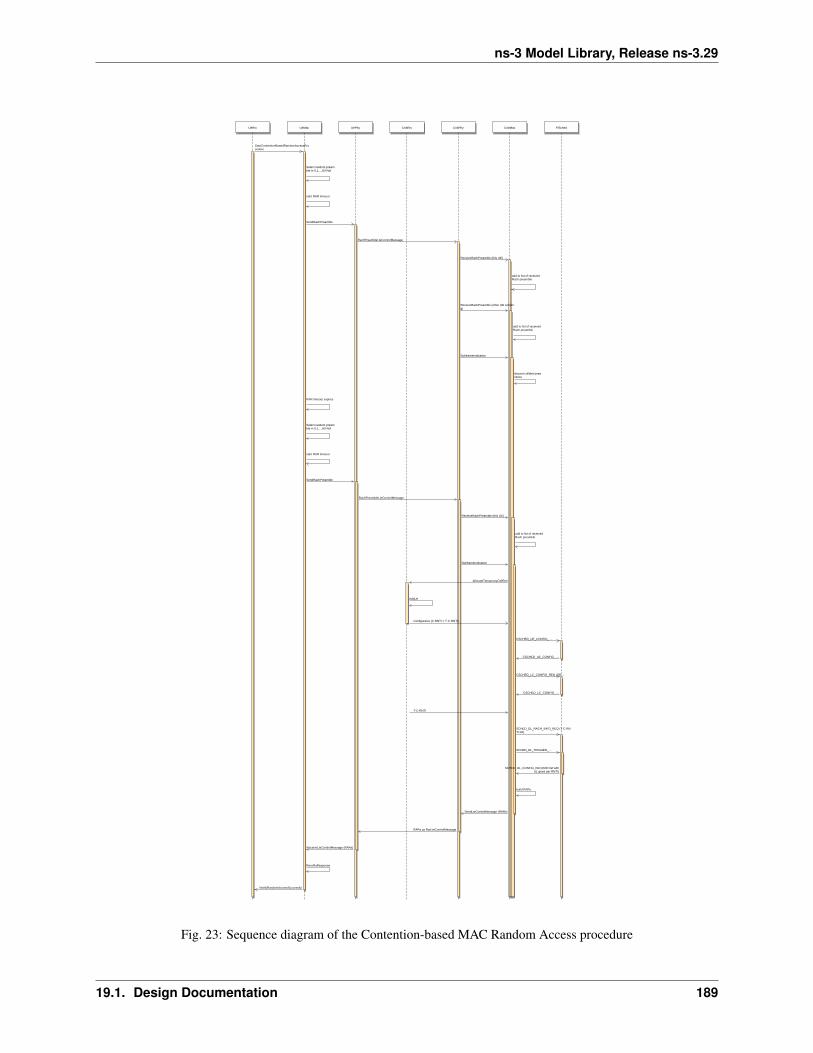
ns-3 Model Library, Release ns-3.29
UeRrc UeMac UePhy EnbRrc EnbPhy EnbMac FfSched
StartContentionBasedRandomAccessProcedure
Select random preamble in 0,1,...,63-Ncf
start RAR timeout
SendRachPreamble
RachPreambleLteControlMessage
ReceiveRachPreamble (this UE)
add to list of receivedRach preamble
ReceiveRachPreamble (other UE colliding)
add to list of receivedRach preamble
SubframeIndication
discard collided preambles
RAR timeout expires
Select random preamble in 0,1,...,63-Ncf
start RAR timeout
SendRachPreamble
RachPreambleLteControlMessage
ReceiveRachPreamble (this UE)
add to list of receivedRach preamble
SubframeIndication
AllocateTemporaryCellRnti
AddUe
ConfigureUe (C-RNTI = T-C-RNTI)
CSCHED_UE_CONFIG_ ...
CSCHED_UE_CONFIG_ ...
CSCHED_LC_CONFIG_REQ (SR ...
CSCHED_LC_CONFIG_ ...
T-C-RNTI
SCHED_DL_RACH_INFO_REQ (T-C-RNTI list)
SCHED_DL_TRIGGER_ ...
SCHED_DL_CONFIG_IND (RAR list withUL grant per RNTI)
build RARs
SendLteControlMessage (RARs)
RARs as RarLteControlMessage
ReceiveLteControlMessage (RARs)
RecvRaResponse
NotifyRandomAccessSuccessful
Fig. 23: Sequence diagram of the Contention-based MAC Random Access procedure
19.1. Design Documentation 189

ns-3 Model Library, Release ns-3.29
UeRrc UeMac UePhy EnbRrc EnbPhy EnbMac FfSched
AddUe
ConfigureUe (C-RNTI = T-C-RNTI)
CSCHED_UE_CONFIG_REQ
CSCHED_UE_CONFIG_CNF
CSCHED_LC_CONFIG_REQ (SRB1)
CSCHED_LC_CONFIG_CNF
AllocateNcRaPreamble (T-C-RNTI)
rach preamble id
rach preamble id (e.g., within handoverCommand inside X2 HO REQ ACK
StartNonContentionBasedRandomAccessProcedure
start RAR timeout
SendRachPreamble
RachPreambleLteControlMessage
ReceiveRachPreamble (this UE)
add to list of received Rach preamble
SubframeIndication
preamble matches known T-C-RNTI
SCHED_DL_RACH_INFO_REQ (T-C-RNTI list)
SCHED_DL_TRIGGER_REQ
SCHED_DL_CONFIG_IND (RAR list with UL grant per RNTI)
build RARs
SendLteControlMessage (RARs)
RARs as RarLteControlMessage
ReceiveLteControlMessage (RARs)
RecvRaResponse
NotifyRandomAccessSuccessful
Fig. 24: Sequence diagram of the Non-contention-based MAC Random Access procedure
190 Chapter 19. LTE Module
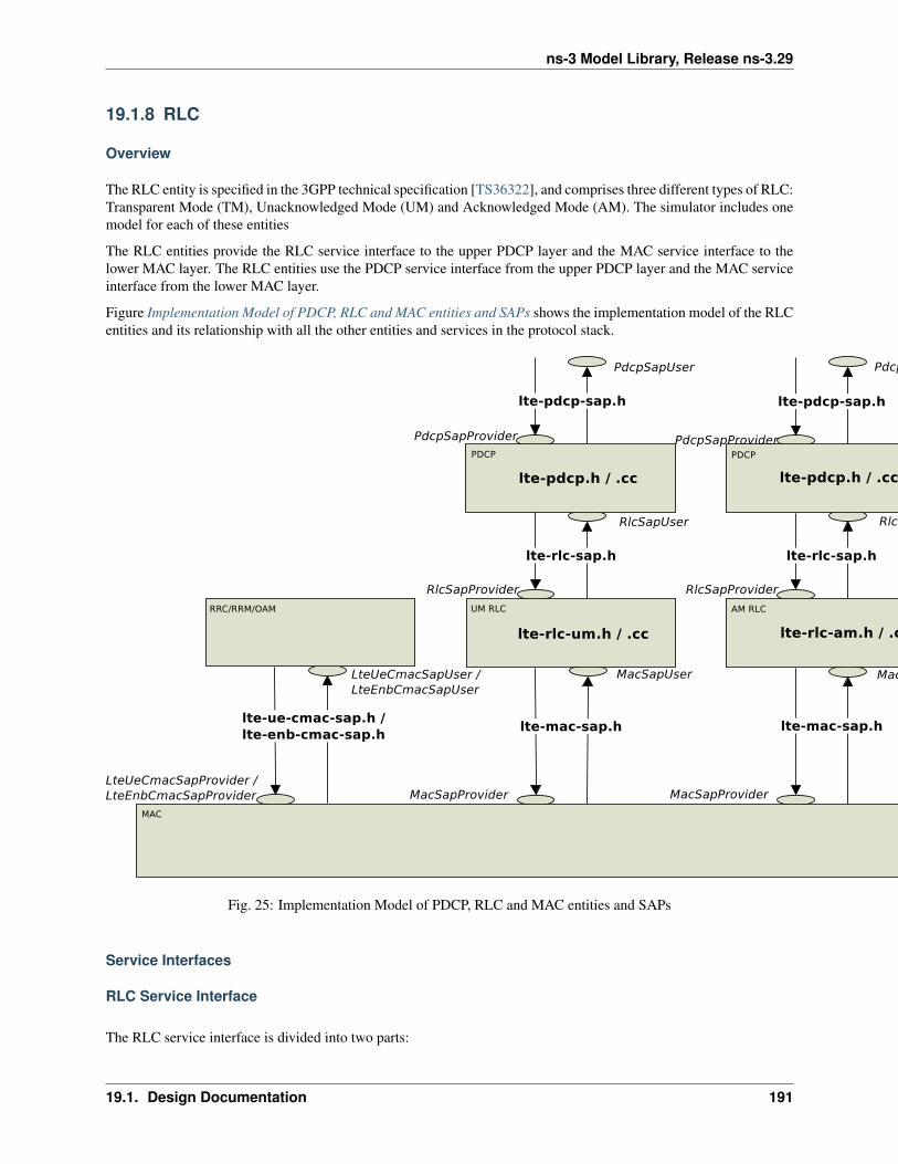
ns-3 Model Library, Release ns-3.29
19.1.8 RLC
Overview
The RLC entity is specified in the 3GPP technical specification [TS36322], and comprises three different types of RLC:Transparent Mode (TM), Unacknowledged Mode (UM) and Acknowledged Mode (AM). The simulator includes onemodel for each of these entities
The RLC entities provide the RLC service interface to the upper PDCP layer and the MAC service interface to thelower MAC layer. The RLC entities use the PDCP service interface from the upper PDCP layer and the MAC serviceinterface from the lower MAC layer.
Figure Implementation Model of PDCP, RLC and MAC entities and SAPs shows the implementation model of the RLCentities and its relationship with all the other entities and services in the protocol stack.
Fig. 25: Implementation Model of PDCP, RLC and MAC entities and SAPs
Service Interfaces
RLC Service Interface
The RLC service interface is divided into two parts:
19.1. Design Documentation 191

ns-3 Model Library, Release ns-3.29
• the RlcSapProvider part is provided by the RLC layer and used by the upper PDCP layer and
• the RlcSapUser part is provided by the upper PDCP layer and used by the RLC layer.
Both the UM and the AM RLC entities provide the same RLC service interface to the upper PDCP layer.
RLC Service Primitives
The following list specifies which service primitives are provided by the RLC service interfaces:
• RlcSapProvider::TransmitPdcpPdu
– The PDCP entity uses this primitive to send a PDCP PDU to the lower RLC entity in the transmitter peer
• RlcSapUser::ReceivePdcpPdu
– The RLC entity uses this primitive to send a PDCP PDU to the upper PDCP entity in the receiver peer
MAC Service Interface
The MAC service interface is divided into two parts:
• the MacSapProvider part is provided by the MAC layer and used by the upper RLC layer and
• the MacSapUser part is provided by the upper RLC layer and used by the MAC layer.
MAC Service Primitives
The following list specifies which service primitives are provided by the MAC service interfaces:
• MacSapProvider::TransmitPdu
– The RLC entity uses this primitive to send a RLC PDU to the lower MAC entity in the transmitter peer
• MacSapProvider::ReportBufferStatus
– The RLC entity uses this primitive to report the MAC entity the size of pending buffers in the transmitterpeer
• MacSapUser::NotifyTxOpportunity
– The MAC entity uses this primitive to notify the RLC entity a transmission opportunity
• MacSapUser::ReceivePdu
– The MAC entity uses this primitive to send an RLC PDU to the upper RLC entity in the receiver peer
AM RLC
The processing of the data transfer in the Acknowledge Mode (AM) RLC entity is explained in section 5.1.3 of[TS36322]. In this section we describe some details of the implementation of the RLC entity.
Buffers for the transmit operations
Our implementation of the AM RLC entity maintains 3 buffers for the transmit operations:
192 Chapter 19. LTE Module

ns-3 Model Library, Release ns-3.29
• Transmission Buffer: it is the RLC SDU queue. When the AM RLC entity receives a SDU in the TransmitPd-cpPdu service primitive from the upper PDCP entity, it enqueues it in the Transmission Buffer. We put a limiton the RLC buffer size and just silently drop SDUs when the buffer is full.
• Transmitted PDUs Buffer: it is the queue of transmitted RLC PDUs for which an ACK/NACK has not beenreceived yet. When the AM RLC entity sends a PDU to the MAC entity, it also puts a copy of the transmittedPDU in the Transmitted PDUs Buffer.
• Retransmission Buffer: it is the queue of RLC PDUs which are considered for retransmission (i.e., they havebeen NACKed). The AM RLC entity moves this PDU to the Retransmission Buffer, when it retransmits a PDUfrom the Transmitted Buffer.
Transmit operations in downlink
The following sequence diagram shows the interactions between the different entities (RRC, PDCP, AM RLC, MACand MAC scheduler) of the eNB in the downlink to perform data communications.
Figure Sequence diagram of data PDU transmission in downlink shows how the upper layers send data PDUs and howthe data flow is processed by the different entities/services of the LTE protocol stack.
The PDCP entity calls the Transmit_PDCP_PDU service primitive in order to send a data PDU. The AMRLC entity processes this service primitive according to the AM data transfer procedures defined in section 5.1.3 of[TS36322].
When the Transmit_PDCP_PDU service primitive is called, the AM RLC entity performs the following operations:
• Put the data SDU in the Transmission Buffer.
• Compute the size of the buffers (how the size of buffers is computed will be explained afterwards).
• Call the Report_Buffer_Status service primitive of the eNB MAC entity in order to notify to the eNBMAC entity the sizes of the buffers of the AM RLC entity. Then, the eNB MAC entity updates the buffer statusin the MAC scheduler using the SchedDlRlcBufferReq service primitive of the FF MAC Scheduler API.
Afterwards, when the MAC scheduler decides that some data can be sent, the MAC entity notifies it to the RLC entity,i.e. it calls the Notify_Tx_Opportunity service primitive, then the AM RLC entity does the following:
• Create a single data PDU by segmenting and/or concatenating the SDUs in the Transmission Buffer.
• Move the data PDU from the Transmission Buffer to the Transmitted PDUs Buffer.
• Update state variables according section 5.1.3.1.1 of [TS36322].
• Call the Transmit_PDU primitive in order to send the data PDU to the MAC entity.
Retransmission in downlink
The sequence diagram of Figure Sequence diagram of data PDU retransmission in downlink shows the interactionsbetween the different entities (AM RLC, MAC and MAC scheduler) of the eNB in downlink when data PDUs mustbe retransmitted by the AM RLC entity.
The transmitting AM RLC entity can receive STATUS PDUs from the peer AM RLC entity. STATUS PDUs are sentaccording section 5.3.2 of [TS36322] and the processing of reception is made according section 5.2.1 of [TS36322].
When a data PDUs is retransmitted from the Transmitted PDUs Buffer, it is also moved to the Retransmission Buffer.
19.1. Design Documentation 193

ns-3 Model Library, Release ns-3.29
Fig. 26: Sequence diagram of data PDU transmission in downlink
194 Chapter 19. LTE Module
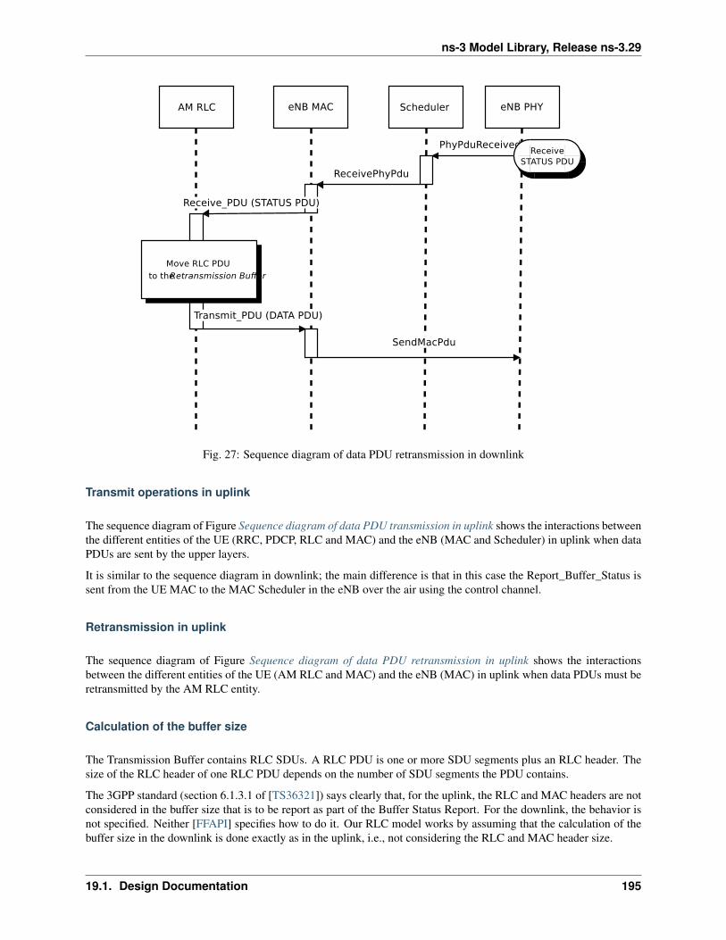
ns-3 Model Library, Release ns-3.29
Fig. 27: Sequence diagram of data PDU retransmission in downlink
Transmit operations in uplink
The sequence diagram of Figure Sequence diagram of data PDU transmission in uplink shows the interactions betweenthe different entities of the UE (RRC, PDCP, RLC and MAC) and the eNB (MAC and Scheduler) in uplink when dataPDUs are sent by the upper layers.
It is similar to the sequence diagram in downlink; the main difference is that in this case the Report_Buffer_Status issent from the UE MAC to the MAC Scheduler in the eNB over the air using the control channel.
Retransmission in uplink
The sequence diagram of Figure Sequence diagram of data PDU retransmission in uplink shows the interactionsbetween the different entities of the UE (AM RLC and MAC) and the eNB (MAC) in uplink when data PDUs must beretransmitted by the AM RLC entity.
Calculation of the buffer size
The Transmission Buffer contains RLC SDUs. A RLC PDU is one or more SDU segments plus an RLC header. Thesize of the RLC header of one RLC PDU depends on the number of SDU segments the PDU contains.
The 3GPP standard (section 6.1.3.1 of [TS36321]) says clearly that, for the uplink, the RLC and MAC headers are notconsidered in the buffer size that is to be report as part of the Buffer Status Report. For the downlink, the behavior isnot specified. Neither [FFAPI] specifies how to do it. Our RLC model works by assuming that the calculation of thebuffer size in the downlink is done exactly as in the uplink, i.e., not considering the RLC and MAC header size.
19.1. Design Documentation 195
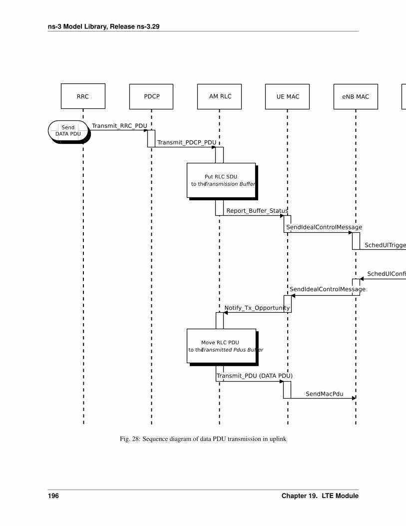
ns-3 Model Library, Release ns-3.29
Fig. 28: Sequence diagram of data PDU transmission in uplink
196 Chapter 19. LTE Module
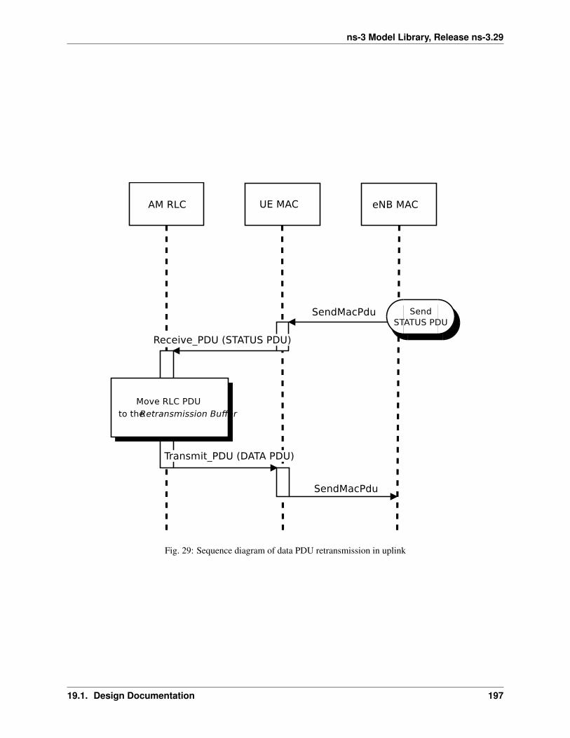
ns-3 Model Library, Release ns-3.29
Fig. 29: Sequence diagram of data PDU retransmission in uplink
19.1. Design Documentation 197

ns-3 Model Library, Release ns-3.29
We note that this choice affects the interoperation with the MAC scheduler, since, in response to theNotify_Tx_Opportunity service primitive, the RLC is expected to create a PDU of no more than the sizerequested by the MAC, including RLC overhead. Hence, unneeded fragmentation can occur if (for example) the MACnotifies a transmission exactly equal to the buffer size previously reported by the RLC. We assume that it is left tothe Scheduler to implement smart strategies for the selection of the size of the transmission opportunity, in order toeventually avoid the inefficiency of unneeded fragmentation.
Concatenation and Segmentation
The AM RLC entity generates and sends exactly one RLC PDU for each transmission opportunity even if it is smallerthan the size reported by the transmission opportunity. So for instance, if a STATUS PDU is to be sent, then only thisPDU will be sent in that transmission opportunity.
The segmentation and concatenation for the SDU queue of the AM RLC entity follows the same philosophy as thesame procedures of the UM RLC entity but there are new state variables (see [TS36322] section 7.1) only present inthe AM RLC entity.
It is noted that, according to the 3GPP specs, there is no concatenation for the Retransmission Buffer.
Re-segmentation
The current model of the AM RLC entity does not support the re-segmentation of the retransmission buffer. Rather,the AM RLC entity just waits to receive a big enough transmission opportunity.
Unsupported features
We do not support the following procedures of [TS36322] :
• “Send an indication of successful delivery of RLC SDU” (See section 5.1.3.1.1)
• “Indicate to upper layers that max retransmission has been reached” (See section 5.2.1)
• “SDU discard procedures” (See section 5.3)
• “Re-establishment procedure” (See section 5.4)
We do not support any of the additional primitives of RLC SAP for AM RLC entity. In particular:
• no SDU discard notified by PDCP
• no notification of successful / failed delivery by AM RLC entity to PDCP entity
UM RLC
In this section we describe the implementation of the Unacknowledged Mode (UM) RLC entity.
Transmit operations in downlink
The transmit operations of the UM RLC are similar to those of the AM RLC previously described in Section Transmitoperations in downlink, with the difference that, following the specifications of [TS36322], retransmission are notperformed, and there are no STATUS PDUs.
198 Chapter 19. LTE Module

ns-3 Model Library, Release ns-3.29
Transmit operations in uplink
The transmit operations in the uplink are similar to those of the downlink, with the main difference that the Re-port_Buffer_Status is sent from the UE MAC to the MAC Scheduler in the eNB over the air using the control channel.
Calculation of the buffer size
The calculation of the buffer size for the UM RLC is done using the same approach of the AM RLC, please refer tosection Calculation of the buffer size for the corresponding description.
TM RLC
In this section we describe the implementation of the Transparent Mode (TM) RLC entity.
Transmit operations in downlink
In the simulator, the TM RLC still provides to the upper layers the same service interface provided by the AM andUM RLC entities to the PDCP layer; in practice, this interface is used by an RRC entity (not a PDCP entity) for thetransmission of RLC SDUs. This choice is motivated by the fact that the services provided by the TM RLC to theupper layers, according to [TS36322], is a subset of those provided by the UM and AM RLC entities to the PDCPlayer; hence, we reused the same interface for simplicity.
The transmit operations in the downlink are performed as follows. When the Transmit_PDCP_PDU serviceprimitive is called by the upper layers, the TM RLC does the following:
• put the SDU in the Transmission Buffer
• compute the size of the Transmission Buffer
• call the Report_Buffer_Status service primitive of the eNB MAC entity
Afterwards, when the MAC scheduler decides that some data can be sent by the logical channel to which the TM RLCentity belongs, the MAC entity notifies it to the TM RLC entity by calling the Notify_Tx_Opportunity serviceprimitive. Upon reception of this primitive, the TM RLC entity does the following:
• if the TX opportunity has a size that is greater than or equal to the size of the head-of-line SDU in the Transmis-sion Buffer
– dequeue the head-of-line SDU from the Transmission Buffer
– create one RLC PDU that contains entirely that SDU, without any RLC header
– Call the Transmit_PDU primitive in order to send the RLC PDU to the MAC entity.
Transmit operations in uplink
The transmit operations in the uplink are similar to those of the downlink, with the main difference that a transmissionopportunity can also arise from the assignment of the UL GRANT as part of the Random Access procedure, withoutan explicit Buffer Status Report issued by the TM RLC entity.
19.1. Design Documentation 199
ns-3 Model Library, Release ns-3.29
Calculation of the buffer size
As per the specifications [TS36322], the TM RLC does not add any RLC header to the PDUs being transmitted.Because of this, the buffer size reported to the MAC layer is calculated simply by summing the size of all packets inthe transmission buffer, thus notifying to the MAC the exact buffer size.
SM RLC
In addition to the AM, UM and TM implementations that are modeled after the 3GPP specifications, a simplified RLCmodel is provided, which is called Saturation Mode (SM) RLC. This RLC model does not accept PDUs from any abovelayer (such as PDCP); rather, the SM RLC takes care of the generation of RLC PDUs in response to the notificationof transmission opportunities notified by the MAC. In other words, the SM RLC simulates saturation conditions, i.e.,it assumes that the RLC buffer is always full and can generate a new PDU whenever notified by the scheduler.
The SM RLC is used for simplified simulation scenarios in which only the LTE Radio model is used, without the EPCand hence without any IP networking support. We note that, although the SM RLC is an unrealistic traffic model,it still allows for the correct simulation of scenarios with multiple flows belonging to different (non real-time) QoSclasses, in order to test the QoS performance obtained by different schedulers. This can be done since it is the task ofthe Scheduler to assign transmission resources based on the characteristics (e.g., Guaranteed Bit Rate) of each RadioBearer, which are specified upon the definition of each Bearer within the simulation program.
As for schedulers designed to work with real-time QoS traffic that has delay constraints, the SM RLC is probablynot an appropriate choice. This is because the absence of actual RLC SDUs (replaced by the artificial generation ofBuffer Status Reports) makes it not possible to provide the Scheduler with meaningful head-of-line-delay information,which is often the metric of choice for the implementation of scheduling policies for real-time traffic flows. For thesimulation and testing of such schedulers, it is advisable to use either the UM or the AM RLC models instead.
19.1.9 PDCP
PDCP Model Overview
The reference document for the specification of the PDCP entity is [TS36323]. With respect to this specification, thePDCP model implemented in the simulator supports only the following features:
• transfer of data (user plane or control plane);
• maintenance of PDCP SNs;
• transfer of SN status (for use upon handover);
The following features are currently not supported:
• header compression and decompression of IP data flows using the ROHC protocol;
• in-sequence delivery of upper layer PDUs at re-establishment of lower layers;
• duplicate elimination of lower layer SDUs at re-establishment of lower layers for radio bearers mapped on RLCAM;
• ciphering and deciphering of user plane data and control plane data;
• integrity protection and integrity verification of control plane data;
• timer based discard;
• duplicate discarding.
200 Chapter 19. LTE Module
ns-3 Model Library, Release ns-3.29
PDCP Service Interface
The PDCP service interface is divided into two parts:
• the PdcpSapProvider part is provided by the PDCP layer and used by the upper layer and
• the PdcpSapUser part is provided by the upper layer and used by the PDCP layer.
PDCP Service Primitives
The following list specifies which service primitives are provided by the PDCP service interfaces:
• PdcpSapProvider::TransmitPdcpSdu
– The RRC entity uses this primitive to send an RRC PDU to the lower PDCP entity in the transmitter peer
• PdcpSapUser::ReceivePdcpSdu
– The PDCP entity uses this primitive to send an RRC PDU to the upper RRC entity in the receiver peer
19.1. Design Documentation 201

ns-3 Model Library, Release ns-3.29
19.1.10 RRC
Features
The RRC model implemented in the simulator provides the following functionality:
• generation (at the eNB) and interpretation (at the UE) of System Information (in particular the Master Informa-tion Block and, at the time of this writing, only System Information Block Type 1 and 2)
• initial cell selection
• RRC connection establishment procedure
• RRC reconfiguration procedure, supporting the following use cases: + reconfiguration of the SRS configurationindex + reconfiguration of the PHY TX mode (MIMO) + reconfiguration of UE measurements + data radiobearer setup + handover
• RRC connection re-establishment, supporting the following use cases: + handover
Architecture
The RRC model is divided into the following components:
• the RRC entities LteUeRrc and LteEnbRrc, which implement the state machines of the RRC entities respectivelyat the UE and the eNB;
• the RRC SAPs LteUeRrcSapProvider, LteUeRrcSapUser, LteEnbRrcSapProvider, LteEnbRrcSapUser, whichallow the RRC entities to send and receive RRC messages and information elmenents;
• the RRC protocol classes LteUeRrcProtocolIdeal, LteEnbRrcProtocolIdeal, LteUeRrcProtocolReal, LteEnbR-rcProtocolReal, which implement two different models for the transmission of RRC messages.
Additionally, the RRC components use various other SAPs in order to interact with the rest of the protocol stack. Arepresentation of all the SAPs that are used is provided in the figures LTE radio protocol stack architecture for the UEon the data plane, LTE radio protocol stack architecture for the UE on the control plane, LTE radio protocol stackarchitecture for the eNB on the data plane and LTE radio protocol stack architecture for the eNB on the control plane.
UE RRC State Machine
In Figure UE RRC State Machine we represent the state machine as implemented in the RRC UE entity.
It is to be noted that most of the states are transient, i.e., once the UE goes into one of the CONNECTED states it willnever switch back to any of the IDLE states. This choice is done for the following reasons:
• as discussed in the section Design Criteria, the focus of the LTE-EPC simulation model is on CONNECTEDmode
• radio link failure is not currently modeled, as discussed in the section Radio Link Failure, so an UE cannot goIDLE because of radio link failure
• RRC connection release is currently never triggered neither by the EPC nor by the NAS
Still, we chose to model explicitly the IDLE states, because:
• a realistic UE RRC configuration is needed for handover, which is a required feature, and in order to have acleaner implementation it makes sense to use the same UE RRC configuration also for the initial connectionestablishment
• it makes easier to implement idle mode cell selection in the future, which is a highly desirable feature
202 Chapter 19. LTE Module
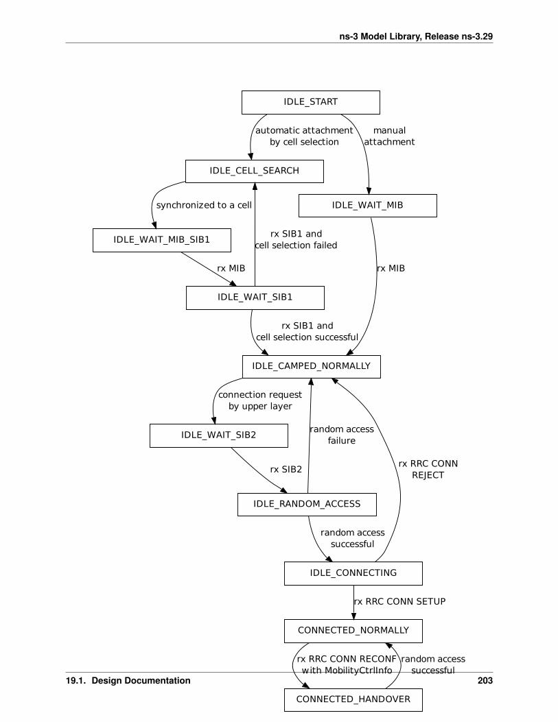
ns-3 Model Library, Release ns-3.29
IDLE_START
IDLE_CELL_SEARCH
automatic attachmentby cell selection
IDLE_WAIT_MIB
manualattachment
IDLE_WAIT_MIB_SIB1
synchronized to a cell
IDLE_WAIT_SIB1
rx MIB
IDLE_CAMPED_NORMALLY
rx MIB
rx SIB1 andcell selection failed
rx SIB1 andcell selection successful
IDLE_WAIT_SIB2
connection requestby upper layer
IDLE_RANDOM_ACCESS
rx SIB2
random accessfailure
IDLE_CONNECTING
random accesssuccessful
rx RRC CONNREJECT
CONNECTED_NORMALLY
rx RRC CONN SETUP
CONNECTED_HANDOVER
rx RRC CONN RECONFwith MobilityCtrlInfo
random accesssuccessful
Fig. 30: UE RRC State Machine
19.1. Design Documentation 203
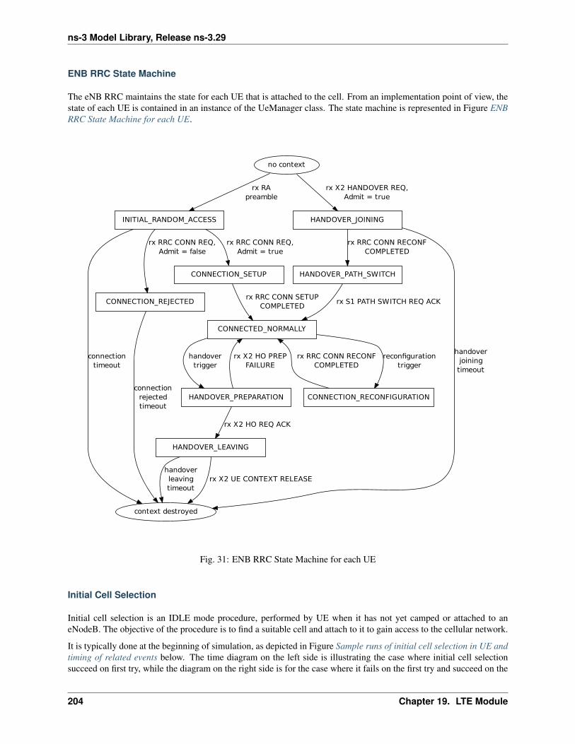
ns-3 Model Library, Release ns-3.29
ENB RRC State Machine
The eNB RRC maintains the state for each UE that is attached to the cell. From an implementation point of view, thestate of each UE is contained in an instance of the UeManager class. The state machine is represented in Figure ENBRRC State Machine for each UE.
no context
INITIAL_RANDOM_ACCESS
rx RApreamble
HANDOVER_JOINING
rx X2 HANDOVER REQ,Admit = true
CONNECTION_SETUP
rx RRC CONN REQ,Admit = true
CONNECTION_REJECTED
rx RRC CONN REQ,Admit = false
context destroyed
connectiontimeout
CONNECTED_NORMALLY
rx RRC CONN SETUPCOMPLETED
connectionrejectedtimeout
CONNECTION_RECONFIGURATION
reconfigurationtrigger
HANDOVER_PREPARATION
handovertrigger
rx RRC CONN RECONFCOMPLETED
rx X2 HO PREPFAILURE
HANDOVER_LEAVING
rx X2 HO REQ ACK
HANDOVER_PATH_SWITCH
rx RRC CONN RECONFCOMPLETED
handoverjoining
timeout
rx S1 PATH SWITCH REQ ACK
rx X2 UE CONTEXT RELEASEhandoverleavingtimeout
Fig. 31: ENB RRC State Machine for each UE
Initial Cell Selection
Initial cell selection is an IDLE mode procedure, performed by UE when it has not yet camped or attached to aneNodeB. The objective of the procedure is to find a suitable cell and attach to it to gain access to the cellular network.
It is typically done at the beginning of simulation, as depicted in Figure Sample runs of initial cell selection in UE andtiming of related events below. The time diagram on the left side is illustrating the case where initial cell selectionsucceed on first try, while the diagram on the right side is for the case where it fails on the first try and succeed on the
204 Chapter 19. LTE Module

ns-3 Model Library, Release ns-3.29
second try. The timing assumes the use of real RRC protocol model (see RRC protocol models) and no transmissionerror.
Fig. 32: Sample runs of initial cell selection in UE and timing of related events
The functionality is based on 3GPP IDLE mode specifications, such as in [TS36300], [TS36304], and [TS36331].However, a proper implementation of IDLE mode is still missing in the simulator, so we reserve several simplifyingassumptions:
• multiple carrier frequency is not supported;
• multiple Public Land Mobile Network (PLMN) identities (i.e. multiple network operators) is not supported;
• RSRQ measurements are not utilized;
19.1. Design Documentation 205

ns-3 Model Library, Release ns-3.29
• stored information cell selection is not supported;
• “Any Cell Selection” state and camping to an acceptable cell is not supported;
• marking a cell as barred or reserved is not supported;
• cell reselection is not supported, hence it is not possible for UE to camp to a different cell after the initial camphas been placed; and
• UE’s Closed Subscriber Group (CSG) white list contains only one CSG identity.
Also note that initial cell selection is only available for EPC-enabled simulations. LTE-only simulations must use themanual attachment method. See section Network Attachment of the User Documentation for more information on theirdifferences in usage.
The next subsections cover different parts of initial cell selection, namely cell search, broadcast of system information,and cell selection evaluation.
Cell Search
Cell search aims to detect surrounding cells and measure the strength of received signal from each of these cells. Oneof these cells will become the UE’s entry point to join the cellular network.
The measurements are based on the RSRP of the received PSS, averaged by Layer 1 filtering, and performed by thePHY layer, as previously described in more detail in section UE PHY Measurements Model. PSS is transmitted byeNodeB over the central 72 sub-carriers of the DL channel (Section 5.1.7.3 [TS36300]), hence we model cell searchto operate using a DL bandwidth of 6 RBs. Note that measurements of RSRQ are not available at this point of timein simulation. As a consequence, the LteUePhy::RsrqUeMeasThreshold attribute does not apply during cellsearch.
By using the measured RSRP, the PHY entity is able to generate a list of detected cells, each with its correspondingcell ID and averaged RSRP. This list is periodically pushed via CPHY SAP to the RRC entity as a measurement report.
The RRC entity inspects the report and simply choose the cell with the strongest RSRP, as also indicated in Section5.2.3.1 of [TS36304]. Then it instructs back the PHY entity to synchronize to this particular cell. The actual operatingbandwidth of the cell is still unknown at this time, so the PHY entity listens only to the minimum bandwidth of 6 RBs.Nevertheless, the PHY entity will be able to receive system broadcast message from this particular eNodeB, which isthe topic of the next subsection.
Broadcast of System Information
System information blocks are broadcasted by eNodeB to UEs at predefined time intervals, adapted from Section5.2.1.2 of [TS36331]. The supported system information blocks are:
• Master Information Block (MIB) Contains parameters related to the PHY layer, generated during cell config-uration and broadcasted every 10 ms at the beginning of radio frame as a control message.
• System Information Block Type 1 (SIB1) Contains information regarding network access, broadcasted every20 ms at the middle of radio frame as a control message. Not used in manual attachment method. UE musthave decoded MIB before it can receive SIB1.
• System Information Block Type 2 (SIB2) Contains UL- and RACH-related settings, scheduled to transmitvia RRC protocol at 16 ms after cell configuration, and then repeats every 80 ms (configurable throughLteEnbRrc::SystemInformationPeriodicity attribute. UE must be camped to a cell in order to be able toreceive its SIB2.
Reception of system information is fundamental for UE to advance in its lifecycle. MIB enables the UE to increase theinitial DL bandwidth of 6 RBs to the actual operating bandwidth of the network. SIB1 provides information necessary
206 Chapter 19. LTE Module

ns-3 Model Library, Release ns-3.29
for cell selection evaluation (explained in the next section). And finally SIB2 is required before the UE is allowed toswitch to CONNECTED state.
Cell Selection Evaluation
UE RRC reviews the measurement report produced in Cell Search and the cell access information provided by SIB1.Once both information is available for a specific cell, the UE triggers the evaluation process. The purpose of thisprocess is to determine whether the cell is a suitable cell to camp to.
The evaluation process is a slightly simplified version of Section 5.2.3.2 of [TS36304]. It consists of the followingcriteria:
• Rx level criterion; and
• closed subscriber group (CSG) criterion.
The first criterion, Rx level, is based on the cell’s measured RSRP Qrxlevmeas, which has to be higher than a requiredminimum Qrxlevmin in order to pass the criterion:
Qrxlevmeas −Qrxlevmin > 0
where Qrxlevmin is determined by each eNodeB and is obtainable by UE from SIB1.
The last criterion, CSG, is a combination of a true-or-false parameter called CSG indication and a simple numberCSG identity. The basic rule is that UE shall not camp to eNodeB with a different CSG identity. But this rule is onlyenforced when CSG indication is valued as true. More details are provided in Section Network Attachment of the UserDocumentation.
When the cell passes all the above criteria, the cell is deemed as suitable. Then UE camps to it(IDLE_CAMPED_NORMALLY state).
After this, upper layer may request UE to enter CONNECTED mode. Please refer to section RRC connection estab-lishment for details on this.
On the other hand, when the cell does not pass the CSG criterion, then the cell is labeled as acceptable (Section10.1.1.1 [TS36300]). In this case, the RRC entity will tell the PHY entity to synchronize to the second strongest celland repeat the initial cell selection procedure using that cell. As long as no suitable cell is found, the UE will repeatthese steps while avoiding cells that have been identified as acceptable.
Radio Admission Control
Radio Admission Control is supported by having the eNB RRC reply to an RRC CONNECTION REQUEST messagesent by the UE with either an RRC CONNECTION SETUP message or an RRC CONNECTION REJECT message,depending on whether the new UE is to be admitted or not. In the current implementation, the behavior is determinedby the boolean attribute ns3::LteEnbRrc::AdmitRrcConnectionRequest. There is currently no RadioAdmission Control algorithm that dynamically decides whether a new connection shall be admitted or not.
Radio Bearer Configuration
Some implementation choices have been made in the RRC regarding the setup of radio bearers:
• three Logical Channel Groups (out of four available) are configured for uplink buffer status report purposes,according to the following policy:
– LCG 0 is for signaling radio bearers
– LCG 1 is for GBR data radio bearers
– LCG 2 is for Non-GBR data radio bearers
19.1. Design Documentation 207
ns-3 Model Library, Release ns-3.29
Radio Link Failure
Since at this stage the RRC supports the CONNECTED mode only, Radio Link Failure (RLF) is not handled. Thereason is that one of the possible outcomes of RLF (when RRC re-establishment is unsuccessful) is to leave RRCCONNECTED notifying the NAS of the RRC connection failure. In order to model RLF properly, RRC IDLE modeshould be supported, including in particular idle mode cell (re-)selection.
With the current model, an UE that experiences bad link quality and that does not perform handover (because of, e.g.,no neighbor cells, handover disabled, handover thresholds misconfigured) will just stay associated with the same eNB,and the scheduler will stop allocating resources to it for communications.
UE RRC Measurements Model
UE RRC measurements support
The UE RRC entity provides support for UE measurements; in particular, it implements the procedures described inSection 5.5 of [TS36331], with the following simplifying assumptions:
• only E-UTRA intra-frequency measurements are supported, which implies:
– only one measurement object is used during the simulation;
– measurement gaps are not needed to perform the measurements;
– Event B1 and B2 are not implemented;
• only reportStrongestCells purpose is supported, while reportCGI and reportStrongestCellsForSON purposes arenot supported;
• s-Measure is not supported;
• carrier aggregation is now supported in the LTE module - Event A6 is not implemented;
• speed dependent scaling of time-to-trigger (Section 5.5.6.2 of [TS36331]) is not supported.
Overall design
The model is based on the concept of UE measurements consumer, which is an entity that may request an eNodeBRRC entity to provide UE measurement reports. Consumers are, for example, Handover algorithm, which computehandover decision based on UE measurement reports. Test cases and user’s programs may also become consumers.Figure Relationship between UE measurements and its consumers depicts the relationship between these entities.
The whole UE measurements function at the RRC level is divided into 4 major parts:
1. Measurement configuration (handled by LteUeRrc::ApplyMeasConfig)
2. Performing measurements (handled by LteUeRrc::DoReportUeMeasurements)
3. Measurement report triggering (handled by LteUeRrc::MeasurementReportTriggering)
4. Measurement reporting (handled by LteUeRrc::SendMeasurementReport)
The following sections will describe each of the parts above.
208 Chapter 19. LTE Module
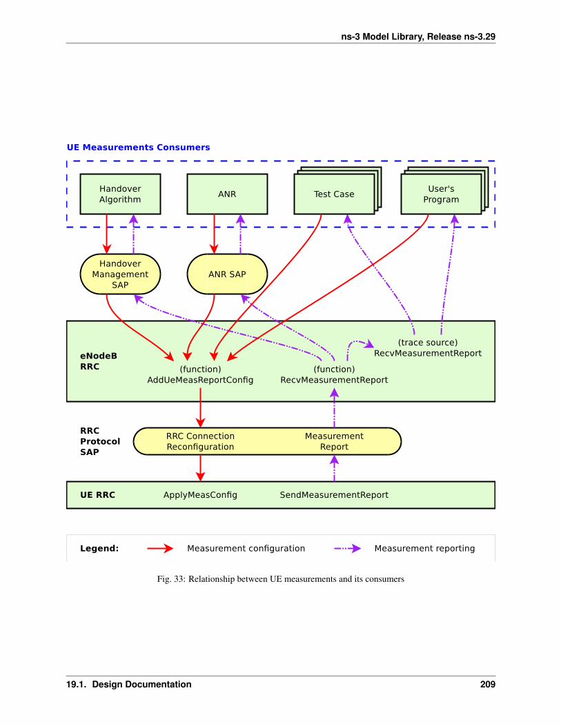
ns-3 Model Library, Release ns-3.29
Fig. 33: Relationship between UE measurements and its consumers
19.1. Design Documentation 209
ns-3 Model Library, Release ns-3.29
Measurement configuration
An eNodeB RRC entity configures UE measurements by sending the configuration parameters to the UE RRC en-tity. This set of parameters are defined within the MeasConfig Information Element (IE) of the RRC ConnectionReconfiguration message (RRC connection reconfiguration).
The eNodeB RRC entity implements the configuration parameters and procedures described in Section 5.5.2 of[TS36331], with the following simplifying assumption:
• configuration (i.e. addition, modification, and removal) can only be done before the simulation begins;
• all UEs attached to the eNodeB will be configured the same way, i.e. there is no support for configuring specificmeasurement for specific UE; and
• it is assumed that there is a one-to-one mapping between the PCI and the E-UTRAN Global Cell Identifier(EGCI). This is consistent with the PCI modeling assumptions described in UE PHY Measurements Model.
The eNodeB RRC instance here acts as an intermediary between the consumers and the attached UEs. At the beginningof simulation, each consumer provides the eNodeB RRC instance with the UE measurements configuration that itrequires. After that, the eNodeB RRC distributes the configuration to attached UEs.
Users may customize the measurement configuration using several methods. Please refer to Section Configure UEmeasurements of the User Documentation for the description of these methods.
Performing measurements
UE RRC receives both RSRP and RSRQ measurements on periodical basis from UE PHY, as described in UE PHYMeasurements Model. Layer 3 filtering will be applied to these received measurements. The implementation of thefiltering follows Section 5.5.3.2 of [TS36331]:
Fn = (1− a)× Fn−1 + a×Mn
where:
• Mn is the latest received measurement result from the physical layer;
• Fn is the updated filtered measurement result;
• Fn−1 is the old filtered measurement result, where F0 = M1 (i.e. the first measurement is not filtered); and
• a = ( 12 )
k4 , where k is the configurable filterCoefficent provided by the QuantityConfig;
k = 4 is the default value, but can be configured by setting the RsrpFilterCoefficient and RsrqFilterCoefficient at-tributes in LteEnbRrc.
Therefore k = 0 will disable Layer 3 filtering. On the other hand, past measurements can be granted more influenceon the filtering results by using larger value of k.
Measurement reporting triggering
In this part, UE RRC will go through the list of active measurement configuration and check whether the triggeringcondition is fulfilled in accordance with Section 5.5.4 of [TS36331]. When at least one triggering condition from all theactive measurement configuration is fulfilled, the measurement reporting procedure (described in the next subsection)will be initiated.
3GPP defines two kinds of triggerType: periodical and event-based. At the moment, only event-based criterion issupported. There are various events that can be selected, which are briefly described in the table below:
210 Chapter 19. LTE Module
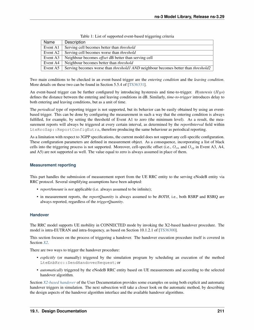
ns-3 Model Library, Release ns-3.29
Table 1: List of supported event-based triggering criteriaName DescriptionEvent A1 Serving cell becomes better than thresholdEvent A2 Serving cell becomes worse than thresholdEvent A3 Neighbour becomes offset dB better than serving cellEvent A4 Neighbour becomes better than thresholdEvent A5 Serving becomes worse than threshold1 AND neighbour becomes better than threshold2
Two main conditions to be checked in an event-based trigger are the entering condition and the leaving condition.More details on these two can be found in Section 5.5.4 of [TS36331].
An event-based trigger can be further configured by introducing hysteresis and time-to-trigger. Hysteresis (Hys)defines the distance between the entering and leaving conditions in dB. Similarly, time-to-trigger introduces delay toboth entering and leaving conditions, but as a unit of time.
The periodical type of reporting trigger is not supported, but its behavior can be easily obtained by using an event-based trigger. This can be done by configuring the measurement in such a way that the entering condition is alwaysfulfilled, for example, by setting the threshold of Event A1 to zero (the minimum level). As a result, the mea-surement reports will always be triggered at every certain interval, as determined by the reportInterval field withinLteRrcSap::ReportConfigEutra, therefore producing the same behaviour as periodical reporting.
As a limitation with respect to 3GPP specifications, the current model does not support any cell-specific configuration.These configuration parameters are defined in measurement object. As a consequence, incorporating a list of blackcells into the triggering process is not supported. Moreover, cell-specific offset (i.e., Ocn and Ocp in Event A3, A4,and A5) are not supported as well. The value equal to zero is always assumed in place of them.
Measurement reporting
This part handles the submission of measurement report from the UE RRC entity to the serving eNodeB entity viaRRC protocol. Several simplifying assumptions have been adopted:
• reportAmount is not applicable (i.e. always assumed to be infinite);
• in measurement reports, the reportQuantity is always assumed to be BOTH, i.e., both RSRP and RSRQ arealways reported, regardless of the triggerQuantity.
Handover
The RRC model supports UE mobility in CONNECTED mode by invoking the X2-based handover procedure. Themodel is intra-EUTRAN and intra-frequency, as based on Section 10.1.2.1 of [TS36300].
This section focuses on the process of triggering a handover. The handover execution procedure itself is covered inSection X2.
There are two ways to trigger the handover procedure:
• explicitly (or manually) triggered by the simulation program by scheduling an execution of the methodLteEnbRrc::SendHandoverRequest; or
• automatically triggered by the eNodeB RRC entity based on UE measurements and according to the selectedhandover algorithm.
Section X2-based handover of the User Documentation provides some examples on using both explicit and automatichandover triggers in simulation. The next subsection will take a closer look on the automatic method, by describingthe design aspects of the handover algorithm interface and the available handover algorithms.
19.1. Design Documentation 211

ns-3 Model Library, Release ns-3.29
Handover algorithm
Handover in 3GPP LTE has the following properties:
• UE-assisted The UE provides input to the network in the form of measurement reports. This is handled by theUE RRC Measurements Model.
• Network-controlled The network (i.e. the source eNodeB and the target eNodeB) decides when to trigger thehandover and oversees its execution.
The handover algorithm operates at the source eNodeB and is responsible in making handover decisions in an “au-tomatic” manner. It interacts with an eNodeB RRC instance via the Handover Management SAP interface. Theserelationships are illustrated in Figure Relationship between UE measurements and its consumers from the previoussection.
The handover algorithm interface consists of the following methods:
• AddUeMeasReportConfigForHandover (Handover Algorithm -> eNodeB RRC) Used by the handoveralgorithm to request measurement reports from the eNodeB RRC entity, by passing the desired reportingconfiguration. The configuration will be applied to all future attached UEs.
• ReportUeMeas (eNodeB RRC -> Handover Algorithm) Based on the UE measurements configured earlierin AddUeMeasReportConfigForHandover, UE may submit measurement reports to the eNodeB.The eNodeB RRC entity uses the ReportUeMeas interface to forward these measurement reports to thehandover algorithm.
• TriggerHandover (Handover Algorithm -> eNodeB RRC) After examining the measurement reports (butnot necessarily), the handover algorithm may declare a handover. This method is used to notify the eNodeBRRC entity about this decision, which will then proceed to commence the handover procedure.
One note for the AddUeMeasReportConfigForHandover. The method will return the measId (measurementidentity) of the newly created measurement configuration. Typically a handover algorithm would store this uniquenumber. It may be useful in the ReportUeMeas method, for example when more than one configuration has beenrequested and the handover algorithm needs to differentiate incoming reports based on the configuration that triggeredthem.
A handover algorithm is implemented by writing a subclass of the LteHandoverAlgorithm abstract superclassand implementing each of the above mentioned SAP interface methods. Users may develop their own handoveralgorithm this way, and then use it in any simulation by following the steps outlined in Section X2-based handover ofthe User Documentation.
Alternatively, users may choose to use one of the 3 built-in handover algorithms provided by the LTE module: no-op,A2-A4-RSRQ, and strongest cell handover algorithm. They are ready to be used in simulations or can be taken as anexample of implementing a handover algorithm. Each of these built-in algorithms is covered in each of the followingsubsections.
No-op handover algorithm
The no-op handover algorithm (NoOpHandoverAlgorithm class) is the simplest possible implementation of han-dover algorithm. It basically does nothing, i.e., does not call any of the Handover Management SAP interface methods.Users may choose this handover algorithm if they wish to disable automatic handover trigger in their simulation.
A2-A4-RSRQ handover algorithm
The A2-A4-RSRQ handover algorithm provides the functionality of the default handover algorithm orig-inally included in LENA M6 (ns-3.18), ported to the Handover Management SAP interface as theA2A4RsrqHandoverAlgorithm class.
212 Chapter 19. LTE Module
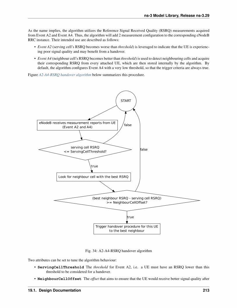
ns-3 Model Library, Release ns-3.29
As the name implies, the algorithm utilizes the Reference Signal Received Quality (RSRQ) measurements acquiredfrom Event A2 and Event A4. Thus, the algorithm will add 2 measurement configuration to the corresponding eNodeBRRC instance. Their intended use are described as follows:
• Event A2 (serving cell’s RSRQ becomes worse than threshold) is leveraged to indicate that the UE is experienc-ing poor signal quality and may benefit from a handover.
• Event A4 (neighbour cell’s RSRQ becomes better than threshold) is used to detect neighbouring cells and acquiretheir corresponding RSRQ from every attached UE, which are then stored internally by the algorithm. Bydefault, the algorithm configures Event A4 with a very low threshold, so that the trigger criteria are always true.
Figure A2-A4-RSRQ handover algorithm below summarizes this procedure.
START
eNodeB receives measurement reports from UE(Event A2 and A4)
serving cell RSRQ<= ServingCellThreshold?
false
Look for neighbour cell with the best RSRQ
true
(best neighbour RSRQ - serving cell RSRQ)>= NeighbourCellOffset?
false
Trigger handover procedure for this UEto the best neighbour
true
Fig. 34: A2-A4-RSRQ handover algorithm
Two attributes can be set to tune the algorithm behaviour:
• ServingCellThreshold The threshold for Event A2, i.e. a UE must have an RSRQ lower than thisthreshold to be considered for a handover.
• NeighbourCellOffset The offset that aims to ensure that the UE would receive better signal quality after
19.1. Design Documentation 213
ns-3 Model Library, Release ns-3.29
the handover. A neighbouring cell is considered as a target cell for the handover only if its RSRQ is higherthan the serving cell’s RSRQ by the amount of this offset.
The value of both attributes are expressed as RSRQ range (Section 9.1.7 of [TS36133]), which is an integer between0 and 34, with 0 as the lowest RSRQ.
Strongest cell handover algorithm
The strongest cell handover algorithm, or also sometimes known as the traditional power budget (PBGT) algorithm,is developed using [Dimou2009] as reference. The idea is to provide each UE with the best possible Reference SignalReceived Power (RSRP). This is done by performing a handover as soon as a better cell (i.e. with stronger RSRP) isdetected.
Event A3 (neighbour cell’s RSRP becomes better than serving cell’s RSRP) is chosen to realize this concept. TheA3RsrpHandoverAlgorithm class is the result of the implementation. Handover is triggered for the UE to thebest cell in the measurement report.
A simulation which uses this algorithm is usually more vulnerable to ping-pong handover (consecutive handover tothe previous source eNodeB within short period of time), especially when the Fading Model is enabled. This problemis typically tackled by introducing a certain delay to the handover. The algorithm does this by including hysteresis andtime-to-trigger parameters (Section 6.3.5 of [TS36331]) to the UE measurements configuration.
Hysteresis (a.k.a. handover margin) delays the handover in regard of RSRP. The value is expressed in dB, rangesbetween 0 to 15 dB, and have a 0.5 dB accuracy, e.g., an input value of 2.7 dB is rounded to 2.5 dB.
On the other hand, time-to-trigger delays the handover in regard of time. 3GPP defines 16 valid values for time-to-trigger (all in milliseconds): 0, 40, 64, 80, 100, 128, 160, 256, 320, 480, 512, 640, 1024, 1280, 2560, and 5120.
The difference between hysteresis and time-to-trigger is illustrated in Figure Effect of hysteresis and time-to-trigger instrongest cell handover algorithm below, which is taken from the lena-x2-handover-measures example. It depicts theperceived RSRP of serving cell and a neighbouring cell by a UE which moves pass the border of the cells.
By default, the algorithm uses a hysteresis of 3.0 dB and time-to-trigger of 256 ms. These values can be tuned throughthe Hysteresis and TimeToTrigger attributes of the A3RsrpHandoverAlgorithm class.
Neighbour Relation
LTE module supports a simplified Automatic Neighbour Relation (ANR) function. This is handled by the LteAnrclass, which interacts with an eNodeB RRC instance through the ANR SAP interface.
Neighbour Relation Table
The ANR holds a Neighbour Relation Table (NRT), similar to the description in Section 22.3.2a of [TS36300]. Eachentry in the table is called a Neighbour Relation (NR) and represents a detected neighbouring cell, which contains thefollowing boolean fields:
• No Remove Indicates that the NR shall not be removed from the NRT. This is true by default for user-providedNR and false otherwise.
• No X2 Indicates that the NR shall not use an X2 interface in order to initiate procedures towards the eNodeBparenting the target cell. This is false by default for user-provided NR, and true otherwise.
• No HO Indicates that the NR shall not be used by the eNodeB for handover reasons. This is true in most cases,except when the NR is both user-provided and network-detected.
Each NR entry may have at least one of the following properties:
214 Chapter 19. LTE Module
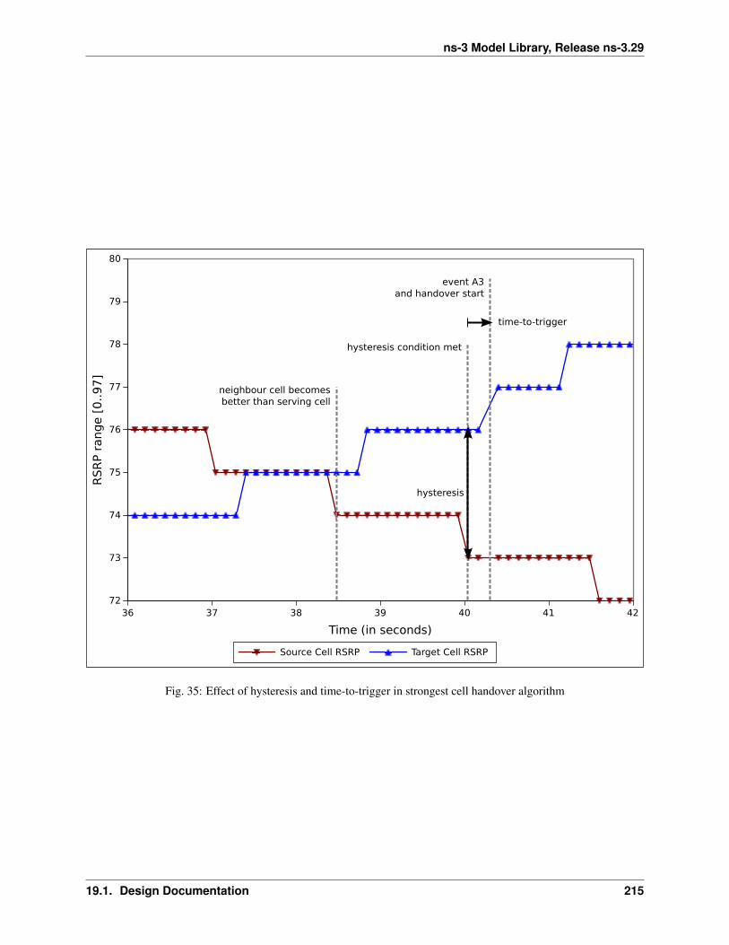
ns-3 Model Library, Release ns-3.29
event A3
and handover start
time-to-trigger
neighbour cell becomes
better than serving cell
hysteresis
hysteresis condition met
Fig. 35: Effect of hysteresis and time-to-trigger in strongest cell handover algorithm
19.1. Design Documentation 215

ns-3 Model Library, Release ns-3.29
• User-provided This type of NR is created as instructed by the simulation user. For example, a NR is cre-ated automatically upon a user-initiated establishment of X2 connection between 2 eNodeBs, e.g. asdescribed in Section X2-based handover. Another way to create a user-provided NR is to call theAddNeighbourRelation function explicitly.
• Network-detected This type of NR is automatically created during the simulation as a result of the discoveryof a nearby cell.
In order to automatically create network-detected NR, ANR utilizes UE measurements. In other words, ANR is aconsumer of UE measurements, as depicted in Figure Relationship between UE measurements and its consumers.RSRQ and Event A4 (neighbour becomes better than threshold) are used for the reporting configuration. The defaultEvent A4 threshold is set to the lowest possible, i.e., maximum detection capability, but can be changed by settingthe Threshold attribute of LteAnr class. Note that the A2-A4-RSRQ handover algorithm also utilizes a similarreporting configuration. Despite the similarity, when both ANR and this handover algorithm are active in the eNodeB,they use separate reporting configuration.
Also note that automatic setup of X2 interface is not supported. This is the reason why the No X2 and No HO fieldsare true in a network-detected but not user-detected NR.
Role of ANR in Simulation
The ANR SAP interface provides the means of communication between ANR and eNodeB RRC. Some interfacefunctions are used by eNodeB RRC to interact with the NRT, as shown below:
• AddNeighbourRelation (eNodeB RRC -> ANR) Add a new user-provided NR entry into the NRT.
• GetNoRemove (eNodeB RRC -> ANR) Get the value of No Remove field of an NR entry of the given cell ID.
• GetNoHo (eNodeB RRC -> ANR) Get the value of No HO field of an NR entry of the given cell ID.
• GetNoX2 (eNodeB RRC -> ANR) Get the value of No X2 field of an NR entry of the given cell ID.
Other interface functions exist to support the role of ANR as a UE measurements consumer, as listed below:
• AddUeMeasReportConfigForAnr (ANR -> eNodeB RRC) Used by the ANR to request measurementreports from the eNodeB RRC entity, by passing the desired reporting configuration. The configurationwill be applied to all future attached UEs.
• ReportUeMeas (eNodeB RRC -> ANR) Based on the UE measurements configured earlier inAddUeMeasReportConfigForAnr, UE may submit measurement reports to the eNodeB. The eN-odeB RRC entity uses the ReportUeMeas interface to forward these measurement reports to the ANR.
Please refer to the corresponding API documentation for LteAnrSap class for more details on the usage and therequired parameters.
The ANR is utilized by the eNodeB RRC instance as a data structure to keep track of the situation of nearby neigh-bouring cells. The ANR also helps the eNodeB RRC instance to determine whether it is possible to execute a handoverprocedure to a neighbouring cell. This is realized by the fact that eNodeB RRC will only allow a handover procedureto happen if the NR entry of the target cell has both No HO and No X2 fields set to false.
ANR is enabled by default in every eNodeB instance in the simulation. It can be disabled by setting the AnrEnabledattribute in LteHelper class to false.
RRC sequence diagrams
In this section we provide some sequence diagrams that explain the most important RRC procedures being modeled.
216 Chapter 19. LTE Module
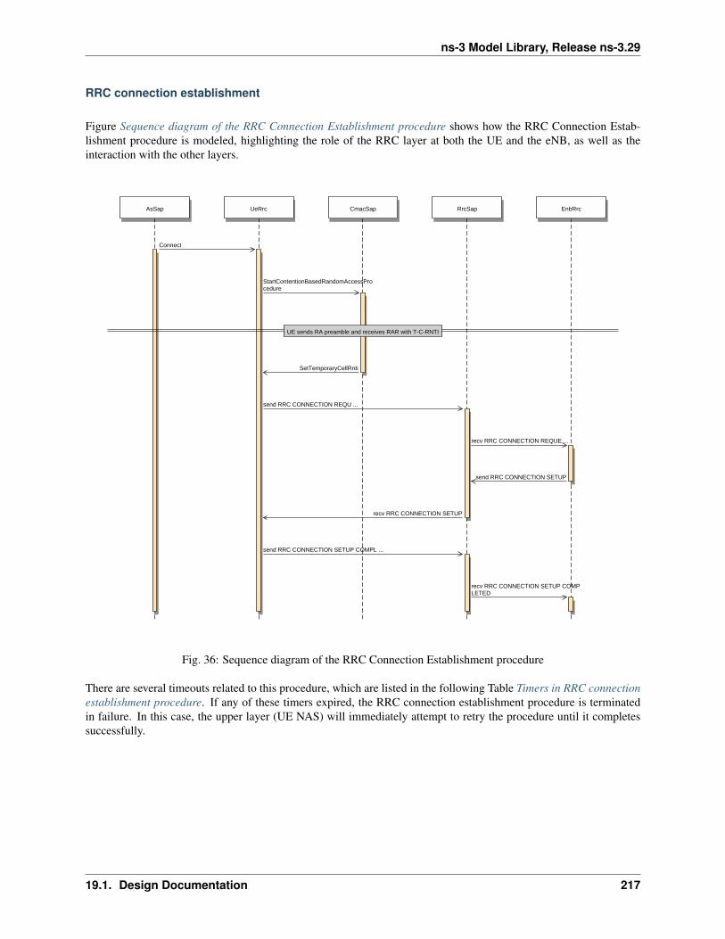
ns-3 Model Library, Release ns-3.29
RRC connection establishment
Figure Sequence diagram of the RRC Connection Establishment procedure shows how the RRC Connection Estab-lishment procedure is modeled, highlighting the role of the RRC layer at both the UE and the eNB, as well as theinteraction with the other layers.
AsSap UeRrc CmacSap RrcSap EnbRrc
Connect
StartContentionBasedRandomAccessProcedure
SetTemporaryCellRnti
send RRC CONNECTION REQU ...
recv RRC CONNECTION REQUE ...
send RRC CONNECTION SETUP
recv RRC CONNECTION SETUP
send RRC CONNECTION SETUP COMPL ...
recv RRC CONNECTION SETUP COMPLETED
UE sends RA preamble and receives RAR with T-C-RNTI
Fig. 36: Sequence diagram of the RRC Connection Establishment procedure
There are several timeouts related to this procedure, which are listed in the following Table Timers in RRC connectionestablishment procedure. If any of these timers expired, the RRC connection establishment procedure is terminatedin failure. In this case, the upper layer (UE NAS) will immediately attempt to retry the procedure until it completessuccessfully.
19.1. Design Documentation 217
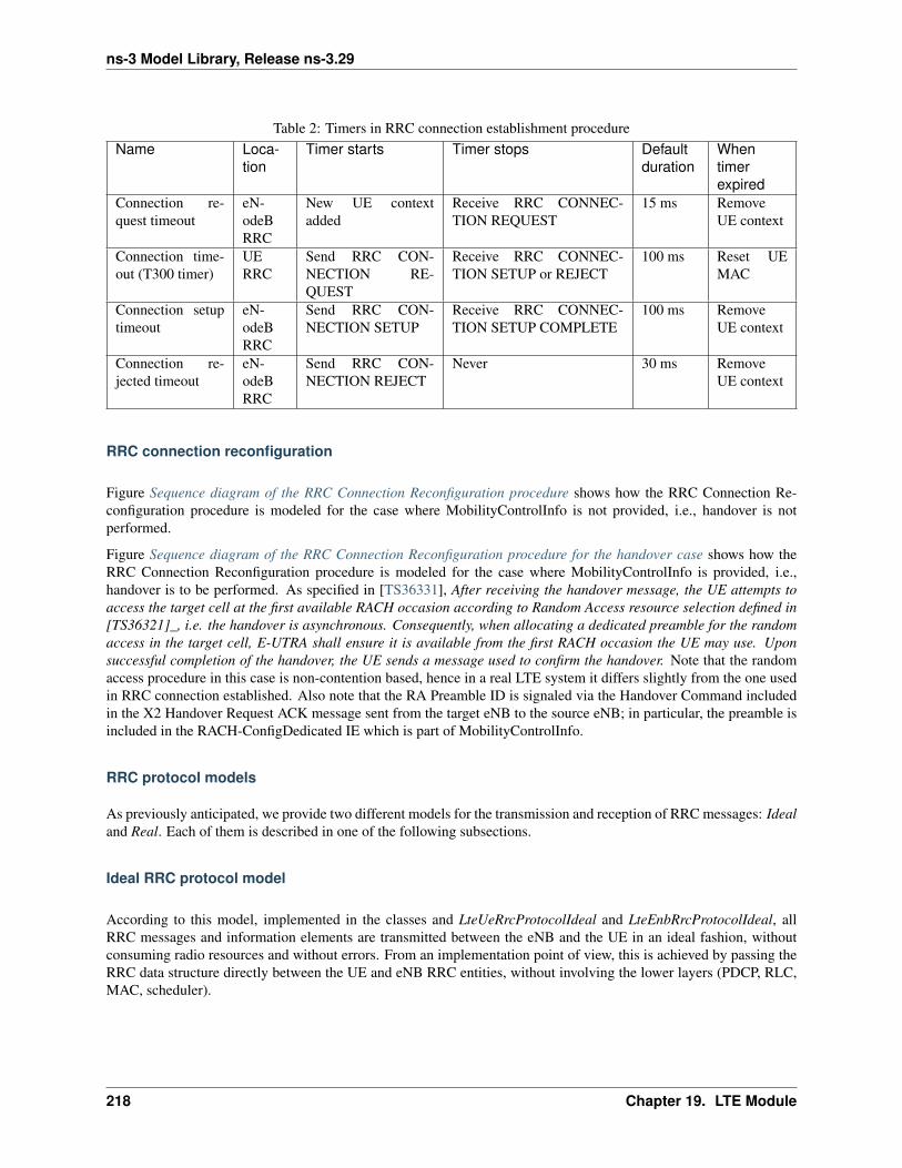
ns-3 Model Library, Release ns-3.29
Table 2: Timers in RRC connection establishment procedureName Loca-
tionTimer starts Timer stops Default
durationWhentimerexpired
Connection re-quest timeout
eN-odeBRRC
New UE contextadded
Receive RRC CONNEC-TION REQUEST
15 ms RemoveUE context
Connection time-out (T300 timer)
UERRC
Send RRC CON-NECTION RE-QUEST
Receive RRC CONNEC-TION SETUP or REJECT
100 ms Reset UEMAC
Connection setuptimeout
eN-odeBRRC
Send RRC CON-NECTION SETUP
Receive RRC CONNEC-TION SETUP COMPLETE
100 ms RemoveUE context
Connection re-jected timeout
eN-odeBRRC
Send RRC CON-NECTION REJECT
Never 30 ms RemoveUE context
RRC connection reconfiguration
Figure Sequence diagram of the RRC Connection Reconfiguration procedure shows how the RRC Connection Re-configuration procedure is modeled for the case where MobilityControlInfo is not provided, i.e., handover is notperformed.
Figure Sequence diagram of the RRC Connection Reconfiguration procedure for the handover case shows how theRRC Connection Reconfiguration procedure is modeled for the case where MobilityControlInfo is provided, i.e.,handover is to be performed. As specified in [TS36331], After receiving the handover message, the UE attempts toaccess the target cell at the first available RACH occasion according to Random Access resource selection defined in[TS36321]_, i.e. the handover is asynchronous. Consequently, when allocating a dedicated preamble for the randomaccess in the target cell, E-UTRA shall ensure it is available from the first RACH occasion the UE may use. Uponsuccessful completion of the handover, the UE sends a message used to confirm the handover. Note that the randomaccess procedure in this case is non-contention based, hence in a real LTE system it differs slightly from the one usedin RRC connection established. Also note that the RA Preamble ID is signaled via the Handover Command includedin the X2 Handover Request ACK message sent from the target eNB to the source eNB; in particular, the preamble isincluded in the RACH-ConfigDedicated IE which is part of MobilityControlInfo.
RRC protocol models
As previously anticipated, we provide two different models for the transmission and reception of RRC messages: Idealand Real. Each of them is described in one of the following subsections.
Ideal RRC protocol model
According to this model, implemented in the classes and LteUeRrcProtocolIdeal and LteEnbRrcProtocolIdeal, allRRC messages and information elements are transmitted between the eNB and the UE in an ideal fashion, withoutconsuming radio resources and without errors. From an implementation point of view, this is achieved by passing theRRC data structure directly between the UE and eNB RRC entities, without involving the lower layers (PDCP, RLC,MAC, scheduler).
218 Chapter 19. LTE Module

ns-3 Model Library, Release ns-3.29
EnbRrc EnbRlcAm UeRlcAm UeRrc UeMac
SendPdu (RrcConnectionReconfiguration)
AM transfer of RLC SDU over DCCH1
RecvPdu (RrcConnectionReconfiguration)
perform reconfiguration
SendPdu (RrcConnectionReconfigurationCompleted)
AM transfer of RLC SDU over DCCH1
RecvPdu (RrcConnectionReconfigurationCompleted)
Fig. 37: Sequence diagram of the RRC Connection Reconfiguration procedure
19.1. Design Documentation 219

ns-3 Model Library, Release ns-3.29
sourceEnbRrc UeRrc UeMac UePhy EnbPhy EnbMac FfSched EnbRrc
X2: HO req
HandoverRequest (newly allocated C-RNTI + LC list)
CSCHED_UE_CONFIG_REQ
CSCHED_UE_CONFIG_CNF
CSCHED_LC_CONFIG_REQ (all active DRBs)
CSCHED_LC_CONFIG_CNF
HandoverConfirm (PRACH ID in 63-Ncf,..., 63 + PRACH mask
X2: HO ack incl. MobilityControlInfo
RrcConnectionReconfiguration with MobilityControlInfo (incl. RACH-ConfigDedicated over SRB1
Handover (new C-RNTI, PRACH ID+Mask)
SendOverCcch (RrcConnectionReconfigurationRequest)
SendRachPreamble (PRACH ID)
RachPreamble over RACH
NotifyRxRachPreamble (PRACH ID)
SCHED_DL_RACH_INFO_REQ (RNTI list)
SubframeIndication
SCHED_DL_TRIGGER_REQ
SCHED_DL_CONFIG_IND (RAR list with UL grant per RNTI))
determine RA-RNTI from PRACH ID
Send RAR with RA-RNTI identifying preambleId
RAR over PDSCH
Rx RAR
NotifyRandomAccessProcedureEndOk
SendOverUlsch (RrcConnectionReconfigurationCompleted)
TX over PUSCH
RxOverUlsch (RrcConnectionReconfigurationCompleted)
RxOverCcch (RrcConnectionReconfigurationCompleted)
start non-contention based MAC Random Access Procedure
end non-contention based MAC Random Access Procedure
Fig. 38: Sequence diagram of the RRC Connection Reconfiguration procedure for the handover case220 Chapter 19. LTE Module

ns-3 Model Library, Release ns-3.29
Real RRC protocol model
This model is implemented in the classes LteUeRrcProtocolReal and LteEnbRrcProtocolReal and aims at modelingthe transmission of RRC PDUs as commonly performed in real LTE systems. In particular:
• for every RRC message being sent, a real RRC PDUs is created following the ASN.1 encoding of RRC PDUsand information elements (IEs) specified in [TS36331]. Some simplification are made with respect to the IEsincluded in the PDU, i.e., only those IEs that are useful for simulation purposes are included. For a detailed list,please see the IEs defined in lte-rrc-sap.h and compare with [TS36331].
• the encoded RRC PDUs are sent on Signaling Radio Bearers and are subject to the same transmission modelingused for data communications, thus including scheduling, radio resource consumption, channel errors, delays,retransmissions, etc.
Signaling Radio Bearer model
We now describe the Signaling Radio Bearer model that is used for the Real RRC protocol model.
• SRB0 messages (over CCCH):
– RrcConnectionRequest: in real LTE systems, this is an RLC TM SDU sent over resources specified inthe UL Grant in the RAR (not in UL DCIs); the reason is that C-RNTI is not known yet at this stage. In thesimulator, this is modeled as a real RLC TM RLC PDU whose UL resources are allocated by the schedulerupon call to SCHED_DL_RACH_INFO_REQ.
– RrcConnectionSetup: in the simulator this is implemented as in real LTE systems, i.e.,with an RLC TM SDU sent over resources indicated by a regular UL DCI, allocated withSCHED_DL_RLC_BUFFER_REQ triggered by the RLC TM instance that is mapped to LCID 0 (theCCCH).
• SRB1 messages (over DCCH):
– All the SRB1 messages modeled in the simulator (e.g., RrcConnectionCompleted) are implemented as inreal LTE systems, i.e., with a real RLC SDU sent over RLC AM using DL resources allocated via BufferStatus Reports. See the RLC model documentation for details.
• SRB2 messages (over DCCH):
– According to [TS36331], “SRB1 is for RRC messages (which may include a piggybacked NAS message) aswell as for NAS messages prior to the establishment of SRB2, all using DCCH logical channel”, whereas“SRB2 is for NAS messages, using DCCH logical channel” and “SRB2 has a lower-priority than SRB1 andis always configured by E-UTRAN after security activation”. Modeling security-related aspects is not arequirement of the LTE simulation model, hence we always use SRB1 and never activate SRB2.
ASN.1 encoding of RRC IE’s
The messages defined in RRC SAP, common to all Ue/Enb SAP Users/Providers, are transported in a transparentcontainer to/from a Ue/Enb. The encoding format for the different Information Elements are specified in [TS36331],using ASN.1 rules in the unaligned variant. The implementation in Ns3/Lte has been divided in the following classes:
• Asn1Header : Contains the encoding / decoding of basic ASN types
• RrcAsn1Header : Inherits Asn1Header and contains the encoding / decoding of common IE’s defined in[TS36331]
• Rrc specific messages/IEs classes : A class for each of the messages defined in RRC SAP header
19.1. Design Documentation 221
ns-3 Model Library, Release ns-3.29
Asn1Header class - Implementation of base ASN.1 types
This class implements the methods to Serialize / Deserialize the ASN.1 types being used in [TS36331], according tothe packed encoding rules in ITU-T X.691. The types considered are:
• Boolean : a boolean value uses a single bit (1=true, 0=false).
• Integer : a constrained integer (with min and max values defined) uses the minimum amount of bits to encodeits range (max-min+1).
• Bitstring : a bistring will be copied bit by bit to the serialization buffer.
• Octetstring : not being currently used.
• Sequence : the sequence generates a preamble indicating the presence of optional and default fields. It also addsa bit indicating the presence of extension marker.
• Sequence. . . Of : the sequence. . . of type encodes the number of elements of the sequence as an integer (thesubsequent elements will need to be encoded afterwards).
• Choice : indicates which element among the ones in the choice set is being encoded.
• Enumeration : is serialized as an integer indicating which value is used, among the ones in the enumeration,with the number of elements in the enumeration as upper bound.
• Null : the null value is not encoded, although its serialization function is defined to provide a clearer mapbetween specification and implementation.
The class inherits from ns-3 Header, but Deserialize() function is declared pure virtual, thus inherited classes having toimplement it. The reason is that deserialization will retrieve the elements in RRC messages, each of them containingdifferent information elements.
Additionally, it has to be noted that the resulting byte length of a specific type/message can vary, according to thepresence of optional fields, and due to the optimized encoding. Hence, the serialized bits will be processed usingPreSerialize() function, saving the result in m_serializationResult Buffer. As the methods to read/write in a ns3 bufferare defined in a byte basis, the serialization bits are stored into m_serializationPendingBits attribute, until the 8 bits areset and can be written to buffer iterator. Finally, when invoking Serialize(), the contents of the m_serializationResultattribute will be copied to Buffer::Iterator parameter
RrcAsn1Header : Common IEs
As some Information Elements are being used for several RRC messages, this class implements the following commonIE’s:
• SrbToAddModList
• DrbToAddModList
• LogicalChannelConfig
• RadioResourceConfigDedicated
• PhysicalConfigDedicated
• SystemInformationBlockType1
• SystemInformationBlockType2
• RadioResourceConfigCommonSIB
222 Chapter 19. LTE Module
ns-3 Model Library, Release ns-3.29
Rrc specific messages/IEs classes
The following RRC SAP have been implemented:
• RrcConnectionRequest
• RrcConnectionSetup
• RrcConnectionSetupCompleted
• RrcConnectionReconfiguration
• RrcConnectionReconfigurationCompleted
• HandoverPreparationInfo
• RrcConnectionReestablishmentRequest
• RrcConnectionReestablishment
• RrcConnectionReestablishmentComplete
• RrcConnectionReestablishmentReject
• RrcConnectionRelease
19.1. Design Documentation 223

ns-3 Model Library, Release ns-3.29
19.1.11 NAS
The focus of the LTE-EPC model is on the NAS Active state, which corresponds to EMM Registered, ECM connected,and RRC connected. Because of this, the following simplifications are made:
• EMM and ECM are not modeled explicitly; instead, the NAS entity at the UE will interact directly with theMME to perform actions that are equivalent (with gross simplifications) to taking the UE to the states EMMConnected and ECM Connected;
• the NAS also takes care of multiplexing uplink data packets coming from the upper layers into the appropriateEPS bearer by using the Traffic Flow Template classifier (TftClassifier).
• the NAS does not support PLMN and CSG selection
• the NAS does not support any location update/paging procedure in idle mode
Figure Sequence diagram of the attach procedure shows how the simplified NAS model implements the attach proce-dure. Note that both the default and eventual dedicated EPS bearers are activated as part of this procedure.
224 Chapter 19. LTE Module

ns-3 Model Library, Release ns-3.29
EpcUeNas LteUeRrc LteEnbRrc EpcEnbApplication EpcSgwPgwApplication EpcMme
ForceCampedOnEnb (CellId)
Connect
RRC Connection Request
initial UE message
S1-AP INITIAL UE MESSAGE
store IMSI->eNB UEid (RNTI) mapping
S11 CREATE SESSION
setup S1-U bearers
S11 CREATE SESSION RESPO ...
S1-AP INITIAL CONTEXT SETUP (bearers to be created)
S1-AP INITIAL CONTEXT SETUP RESPONSE
setup S1-U bearers
DataRadioBearerSetupRequest
setup data radio bearers
RRC Connection Reconfiguration
setup data radio bearers
RRC Connection Reconfiguration Completed
Fig. 39: Sequence diagram of the attach procedure
19.1. Design Documentation 225

ns-3 Model Library, Release ns-3.29
19.1.12 S1
S1-U
The S1-U interface is modeled in a realistic way by encapsulating data packets over GTP/UDP/IP, as done in real LTE-EPC systems. The corresponding protocol stack is shown in Figure LTE-EPC data plane protocol stack. As shownin the figure, there are two different layers of IP networking. The first one is the end-to-end layer, which providesend-to-end connectivity to the users; this layers involves the UEs, the PGW and the remote host (including eventualinternet routers and hosts in between), but does not involve the eNB. In this version of LTE, the EPC supports bothIPv4 and IPv6 type users. The 3GPP unique 64 bit IPv6 prefix allocation process for each UE and PGW is followedhere. Each EPC is assigned an unique 16 bit IPv4 and a 48 bit IPv6 network address from the pool of 7.0.0.0/8 and7777:f00d::/32 respectively. In the end-to-end IP connection between UE and PGW, all addresses are configured usingthese prefixes. The PGW’s address is used by all UEs as the gateway to reach the internet.
The second layer of IP networking is the EPC local area network. This involves all eNB nodes and the SGW/PGWnode. This network is implemented as a set of point-to-point links which connect each eNB with the SGW/PGW node;thus, the SGW/PGW has a set of point-to-point devices, each providing connectivity to a different eNB. By default,a 10.x.y.z/30 subnet is assigned to each point-to-point link (a /30 subnet is the smallest subnet that allows for twodistinct host addresses).
As specified by 3GPP, the end-to-end IP communications is tunneled over the local EPC IP network usingGTP/UDP/IP. In the following, we explain how this tunneling is implemented in the EPC model. The explanationis done by discussing the end-to-end flow of data packets.
Fig. 40: Data flow in the downlink between the internet and the UE
To begin with, we consider the case of the downlink, which is depicted in Figure Data flow in the downlink betweenthe internet and the UE. Downlink IPv4/IPv6 packets are generated from a generic remote host, and addressed to oneof the UE device. Internet routing will take care of forwarding the packet to the generic NetDevice of the SGW/PGWnode which is connected to the internet (this is the Gi interface according to 3GPP terminology). The SGW/PGWhas a VirtualNetDevice which is assigned the base IPv4 address of the EPC network; hence, static routing rules willcause the incoming packet from the internet to be routed through this VirtualNetDevice. In case of IPv6 address asdestination, a manual route towards the VirtualNetDevice is inserted in the routing table, containing the 48 bit IPv6prefix from which all the IPv6 addresses of the UEs and PGW are configured. Such device starts the GTP/UDP/IPtunneling procedure, by forwarding the packet to a dedicated application in the SGW/PGW node which is calledEpcSgwPgwApplication. This application does the following operations:
1. it determines the eNB node to which the UE is attached, by looking at the IP destination address (which is theaddress of the UE);
226 Chapter 19. LTE Module
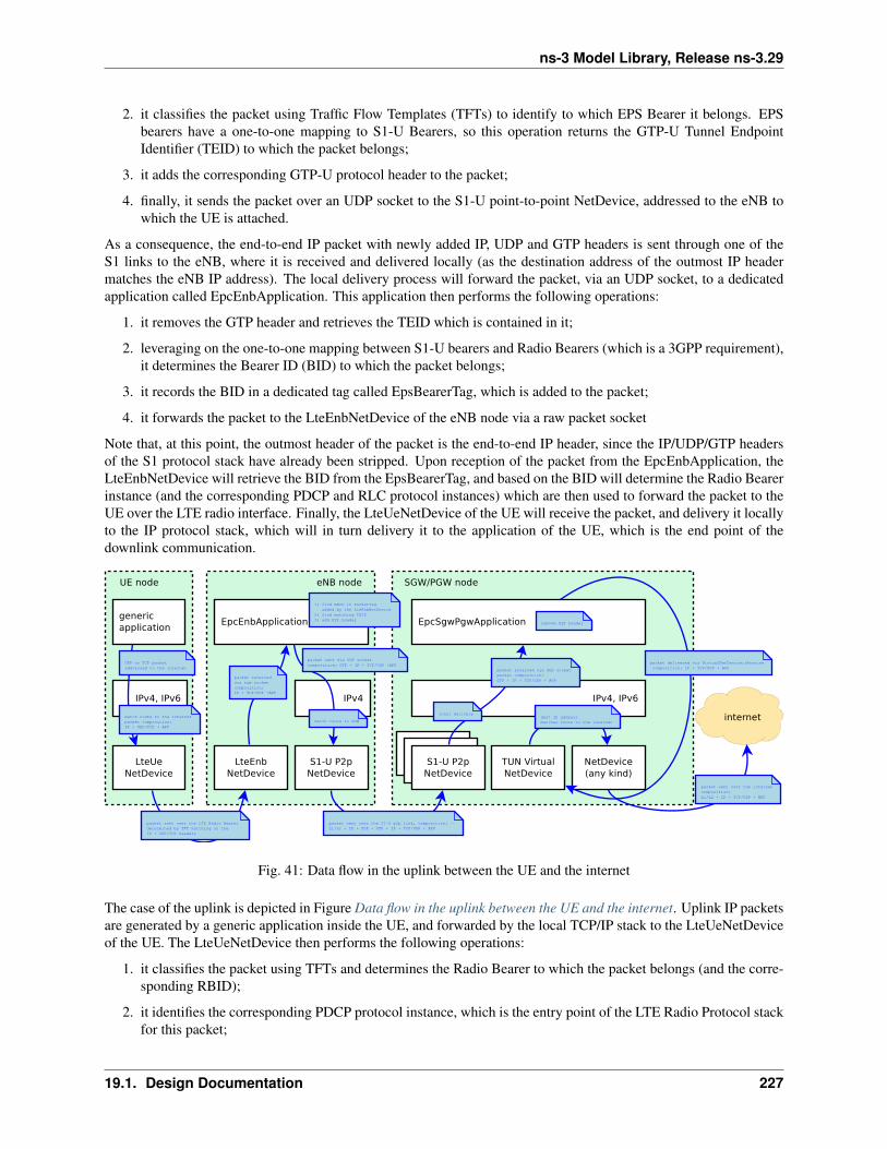
ns-3 Model Library, Release ns-3.29
2. it classifies the packet using Traffic Flow Templates (TFTs) to identify to which EPS Bearer it belongs. EPSbearers have a one-to-one mapping to S1-U Bearers, so this operation returns the GTP-U Tunnel EndpointIdentifier (TEID) to which the packet belongs;
3. it adds the corresponding GTP-U protocol header to the packet;
4. finally, it sends the packet over an UDP socket to the S1-U point-to-point NetDevice, addressed to the eNB towhich the UE is attached.
As a consequence, the end-to-end IP packet with newly added IP, UDP and GTP headers is sent through one of theS1 links to the eNB, where it is received and delivered locally (as the destination address of the outmost IP headermatches the eNB IP address). The local delivery process will forward the packet, via an UDP socket, to a dedicatedapplication called EpcEnbApplication. This application then performs the following operations:
1. it removes the GTP header and retrieves the TEID which is contained in it;
2. leveraging on the one-to-one mapping between S1-U bearers and Radio Bearers (which is a 3GPP requirement),it determines the Bearer ID (BID) to which the packet belongs;
3. it records the BID in a dedicated tag called EpsBearerTag, which is added to the packet;
4. it forwards the packet to the LteEnbNetDevice of the eNB node via a raw packet socket
Note that, at this point, the outmost header of the packet is the end-to-end IP header, since the IP/UDP/GTP headersof the S1 protocol stack have already been stripped. Upon reception of the packet from the EpcEnbApplication, theLteEnbNetDevice will retrieve the BID from the EpsBearerTag, and based on the BID will determine the Radio Bearerinstance (and the corresponding PDCP and RLC protocol instances) which are then used to forward the packet to theUE over the LTE radio interface. Finally, the LteUeNetDevice of the UE will receive the packet, and delivery it locallyto the IP protocol stack, which will in turn delivery it to the application of the UE, which is the end point of thedownlink communication.
Fig. 41: Data flow in the uplink between the UE and the internet
The case of the uplink is depicted in Figure Data flow in the uplink between the UE and the internet. Uplink IP packetsare generated by a generic application inside the UE, and forwarded by the local TCP/IP stack to the LteUeNetDeviceof the UE. The LteUeNetDevice then performs the following operations:
1. it classifies the packet using TFTs and determines the Radio Bearer to which the packet belongs (and the corre-sponding RBID);
2. it identifies the corresponding PDCP protocol instance, which is the entry point of the LTE Radio Protocol stackfor this packet;
19.1. Design Documentation 227

ns-3 Model Library, Release ns-3.29
3. it sends the packet to the eNB over the LTE Radio Protocol stack.
The eNB receives the packet via its LteEnbNetDevice. Since there is a single PDCP and RLC protocol instance foreach Radio Bearer, the LteEnbNetDevice is able to determine the BID of the packet. This BID is then recorded onto anEpsBearerTag, which is added to the packet. The LteEnbNetDevice then forwards the packet to the EpcEnbApplicationvia a raw packet socket.
Upon receiving the packet, the EpcEnbApplication performs the following operations:
1. it retrieves the BID from the EpsBearerTag in the packet;
2. it determines the corresponding EPS Bearer instance and GTP-U TEID by leveraging on the one-to-one mappingbetween S1-U bearers and Radio Bearers;
3. it adds a GTP-U header on the packet, including the TEID determined previously;
4. it sends the packet to the SGW/PGW node via the UDP socket connected to the S1-U point-to-point net device.
At this point, the packet contains the S1-U IP, UDP and GTP headers in addition to the original end-to-end IP header.When the packet is received by the corresponding S1-U point-to-point NetDevice of the SGW/PGW node, it is deliv-ered locally (as the destination address of the outmost IP header matches the address of the point-to-point net device).The local delivery process will forward the packet to the EpcSgwPgwApplication via the corresponding UDP socket.The EpcSgwPgwApplication then removes the GTP header and forwards the packet to the VirtualNetDevice. At thispoint, the outmost header of the packet is the end-to-end IP header. Hence, if the destination address within this headeris a remote host on the internet, the packet is sent to the internet via the corresponding NetDevice of the SGW/PGW.In the event that the packet is addressed to another UE, the IP stack of the SGW/PGW will redirect the packet againto the VirtualNetDevice, and the packet will go through the dowlink delivery process in order to reach its destinationUE.
Note that the EPS Bearer QoS is not enforced on the S1-U links, it is assumed that the overprovisioning of the linkbandwidth is sufficient to meet the QoS requirements of all bearers.
S1AP
The S1-AP interface provides control plane interaction between the eNB and the MME. In the simulator, this inter-face is modeled in an ideal fashion, with direct interaction between the eNB and the MME objects, without actuallyimplementing the encoding of S1AP messages and information elements specified in [TS36413] and without actuallytransmitting any PDU on any link.
The S1-AP primitives that are modeled are:
• INITIAL UE MESSAGE
• INITIAL CONTEXT SETUP REQUEST
• INITIAL CONTEXT SETUP RESPONSE
• PATH SWITCH REQUEST
• PATH SWITCH REQUEST ACKNOWLEDGE
228 Chapter 19. LTE Module
ns-3 Model Library, Release ns-3.29
19.1.13 X2
The X2 interface interconnects two eNBs [TS36420]. From a logical point of view, the X2 interface is a point-to-pointinterface between the two eNBs. In a real E-UTRAN, the logical point-to-point interface should be feasible even inthe absence of a physical direct connection between the two eNBs. In the X2 model implemented in the simulator, theX2 interface is a point-to-point link between the two eNBs. A point-to-point device is created in both eNBs and thetwo point-to-point devices are attached to the point-to-point link.
For a representation of how the X2 interface fits in the overall architecture of the LENA simulation model, the readeris referred to the figure Overview of the LTE-EPC simulation model.
The X2 interface implemented in the simulator provides detailed implementation of the following elementary proce-dures of the Mobility Management functionality [TS36423]:
• Handover Request procedure
• Handover Request Acknowledgement procedure
• SN Status Transfer procedure
• UE Context Release procedure
These procedures are involved in the X2-based handover. You can find the detailed description of the handover insection 10.1.2.1 of [TS36300]. We note that the simulator model currently supports only the seamless handover asdefined in Section 2.6.3.1 of [Sesia2009]; in particular, lossless handover as described in Section 2.6.3.2 of [Sesia2009]is not supported at the time of this writing.
Figure Sequence diagram of the X2-based handover below shows the interaction of the entities of the X2 model in thesimulator. The shaded labels indicate the moments when the UE or eNodeB transition to another RRC state.
The figure also shows two timers within the handover procedure: the handover leaving timer is maintained by thesource eNodeB, while the handover joining timer by the target eNodeB. The duration of the timers can be configuredin the HandoverLeavingTimeoutDuration and HandoverJoiningTimeoutDuration attributes of therespective LteEnbRrc instances. When one of these timers expire, the handover procedure is considered as failed.
However, there is no proper handling of handover failure in the current version of LTE module. Users should tunethe simulation properly in order to avoid handover failure, otherwise unexpected behaviour may occur. Please refer toSection Tuning simulation with handover of the User Documentation for some tips regarding this matter.
The X2 model is an entity that uses services from:
• the X2 interfaces,
– They are implemented as Sockets on top of the point-to-point devices.
– They are used to send/receive X2 messages through the X2-C and X2-U interfaces (i.e. the point-to-pointdevice attached to the point-to-point link) towards the peer eNB.
• the S1 application.
– Currently, it is the EpcEnbApplication.
– It is used to get some information needed for the Elementary Procedures of the X2 messages.
and it provides services to:
• the RRC entity (X2 SAP)
– to send/receive RRC messages. The X2 entity sends the RRC message as a transparent container in the X2message. This RRC message is sent to the UE.
Figure Implementation Model of X2 entity and SAPs shows the implementation model of the X2 entity and its rela-tionship with all the other entities and services in the protocol stack.
19.1. Design Documentation 229
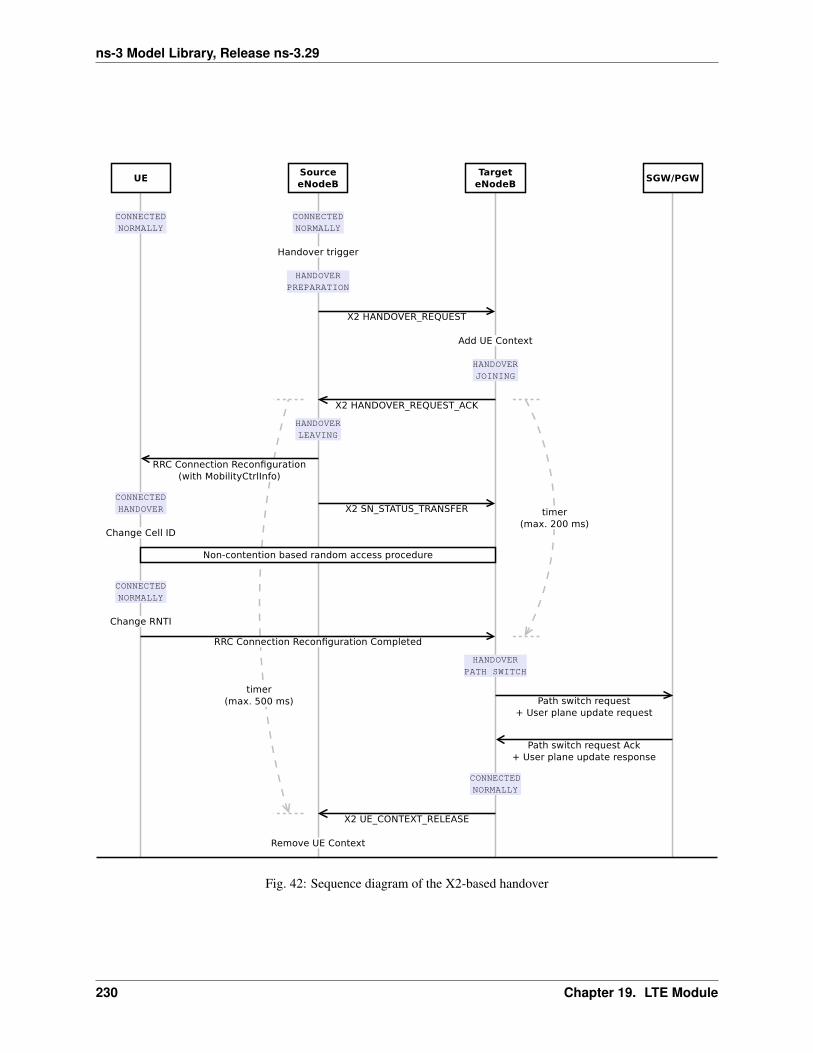
ns-3 Model Library, Release ns-3.29
Fig. 42: Sequence diagram of the X2-based handover
230 Chapter 19. LTE Module
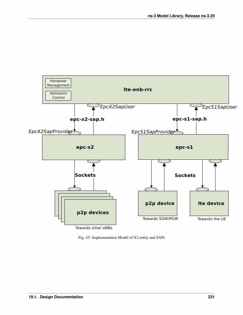
ns-3 Model Library, Release ns-3.29
Fig. 43: Implementation Model of X2 entity and SAPs
19.1. Design Documentation 231

ns-3 Model Library, Release ns-3.29
The RRC entity manages the initiation of the handover procedure. This is done in the Handover Management sub-module of the eNB RRC entity. The target eNB may perform some Admission Control procedures. This is done in theAdmission Control submodule. Initially, this submodule will accept any handover request.
X2 interfaces
The X2 model contains two interfaces:
• the X2-C interface. It is the control interface and it is used to send the X2-AP PDUs (i.e. the elementaryprocedures).
• the X2-U interface. It is used to send the bearer data when there is DL forwarding.
Figure X2 interface protocol stacks shows the protocol stacks of the X2-U interface and X2-C interface modeled inthe simulator.
Fig. 44: X2 interface protocol stacks
X2-C
The X2-C interface is the control part of the X2 interface and it is used to send the X2-AP PDUs (i.e. the elementaryprocedures).
In the original X2 interface control plane protocol stack, SCTP is used as the transport protocol but currently, theSCTP protocol is not modeled in the ns-3 simulator and its implementation is out-of-scope of the project. The UDPprotocol is used as the datagram oriented protocol instead of the SCTP protocol.
X2-U
The X2-U interface is used to send the bearer data when there is DL forwarding during the execution of the X2-basedhandover procedure. Similarly to what done for the S1-U interface, data packets are encapsulated over GTP/UDP/IPwhen being sent over this interface. Note that the EPS Bearer QoS is not enforced on the X2-U links, it is assumedthat the overprovisioning of the link bandwidth is sufficient to meet the QoS requirements of all bearers.
232 Chapter 19. LTE Module

ns-3 Model Library, Release ns-3.29
X2 Service Interface
The X2 service interface is used by the RRC entity to send and receive messages of the X2 procedures. It is dividedinto two parts:
• the EpcX2SapProvider part is provided by the X2 entity and used by the RRC entity and
• the EpcX2SapUser part is provided by the RRC entity and used by the RRC enity.
The primitives that are supported in our X2-C model are described in the following subsections.
X2-C primitives for handover execution
The following primitives are used for the X2-based handover:
• HANDOVER REQUEST
• HANDOVER REQUEST ACK
• HANDOVER PREPARATION FAILURE
• SN STATUS STRANSFER
• UE CONTEXT RELEASE
all the above primitives are used by the currently implemented RRC model during the preparation and execution ofthe handover procedure. Their usage interacts with the RRC state machine; therefore, they are not meant to be usedfor code customization, at least unless it is desired to modify the RRC state machine.
X2-C SON primitives
The following primitives can be used to implement Self-Organized Network (SON) functionalities:
• LOAD INFORMATION
• RESOURCE STATUS UPDATE
note that the current RRC model does not actually use these primitives, they are included in the model just to make itpossible to develop SON algorithms included in the RRC logic that make use of them.
As a first example, we show here how the load information primitive can be used. We assume that the LteEnbRrc hasbeen modified to include the following new member variables:
std::vector<EpcX2Sap::UlInterferenceOverloadIndicationItem>m_currentUlInterferenceOverloadIndicationList;
std::vector <EpcX2Sap::UlHighInterferenceInformationItem>m_currentUlHighInterferenceInformationList;
EpcX2Sap::RelativeNarrowbandTxBand m_currentRelativeNarrowbandTxBand;
for a detailed description of the type of these variables, we suggest to consult the file epc-x2-sap.h, the corre-sponding doxygen documentation, and the references therein to the relevant sections of 3GPP TS 36.423. Now, assumethat at run time these variables have been set to meaningful values following the specifications just mentioned. Then,you can add the following code in the LteEnbRrc class implementation in order to send a load information primitive:
EpcX2Sap::CellInformationItem cii;cii.sourceCellId = m_cellId;cii.ulInterferenceOverloadIndicationList = m_↪→currentUlInterferenceOverloadIndicationList;cii.ulHighInterferenceInformationList = m_currentUlHighInterferenceInformationList;
(continues on next page)
19.1. Design Documentation 233

ns-3 Model Library, Release ns-3.29
(continued from previous page)
cii.relativeNarrowbandTxBand = m_currentRelativeNarrowbandTxBand;
EpcX2Sap::LoadInformationParams params;params.targetCellId = cellId;params.cellInformationList.push_back (cii);m_x2SapProvider->SendLoadInformation (params);
The above code allows the source eNB to send the message. The methodLteEnbRrc::DoRecvLoadInformation will be called when the target eNB receives the message. Thedesired processing of the load information should therefore be implemented within that method.
In the following second example we show how the resource status update primitive is used. We assume that theLteEnbRrc has been modified to include the following new member variable:
EpcX2Sap::CellMeasurementResultItem m_cmri;
similarly to before, we refer to epc-x2-sap.h and the references therein for detailed information about this variabletype. Again, we assume that the variable has been already set to a meaningful value. Then, you can add the followingcode in order to send a resource status update:
EpcX2Sap::ResourceStatusUpdateParams params;params.targetCellId = cellId;params.cellMeasurementResultList.push_back (m_cmri);m_x2SapProvider->SendResourceStatusUpdate (params);
The method eEnbRrc::DoRecvResourceStatusUpdate will be called when the target eNB receives the re-source status update message. The desired processing of this message should therefore be implemented within thatmethod.
Finally, we note that the setting and processing of the appropriate values for the variable passed to the above de-scribed primitives is deemed to be specific of the SON algorithm being implemented, and hence is not covered by thisdocumentation.
Unsupported primitives
Mobility Robustness Optimization primitives such as Radio Link Failure indication and Handover Report are notsupported at this stage.
234 Chapter 19. LTE Module

ns-3 Model Library, Release ns-3.29
19.1.14 S11
The S11 interface provides control plane interaction between the SGW and the MME using the GTPv2-C protocolspecified in [TS29274]. In the simulator, this interface is modeled in an ideal fashion, with direct interaction betweenthe SGW and the MME objects, without actually implementing the encoding of the messages and without actuallytransmitting any PDU on any link.
The S11 primitives that are modeled are:
• CREATE SESSION REQUEST
• CREATE SESSION RESPONSE
• MODIFY BEARER REQUEST
• MODIFY BEARER RESPONSE
Of these primitives, the first two are used upon initial UE attachment for the establishment of the S1-U bearers; theother two are used during handover to switch the S1-U bearers from the source eNB to the target eNB as a consequenceof the reception by the MME of a PATH SWITCH REQUEST S1-AP message.
19.1. Design Documentation 235
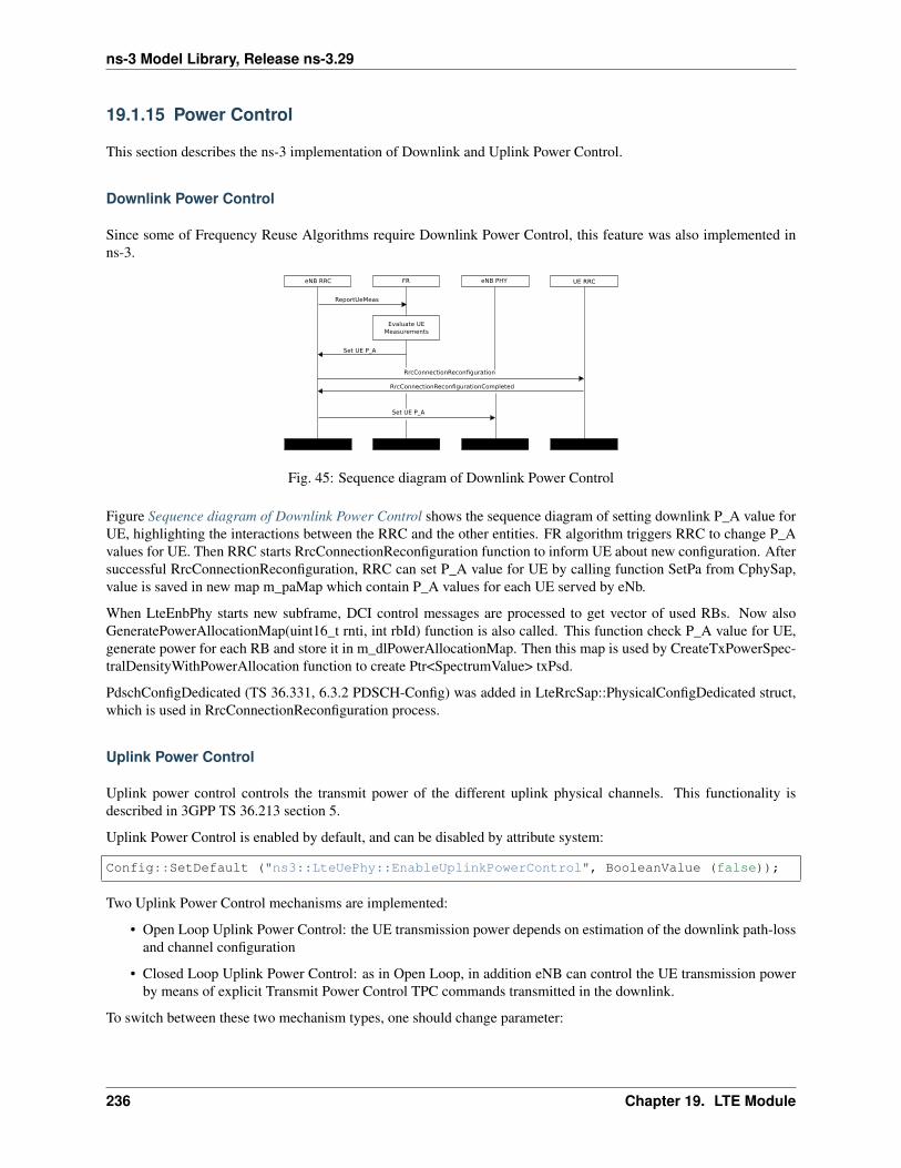
ns-3 Model Library, Release ns-3.29
19.1.15 Power Control
This section describes the ns-3 implementation of Downlink and Uplink Power Control.
Downlink Power Control
Since some of Frequency Reuse Algorithms require Downlink Power Control, this feature was also implemented inns-3.
Fig. 45: Sequence diagram of Downlink Power Control
Figure Sequence diagram of Downlink Power Control shows the sequence diagram of setting downlink P_A value forUE, highlighting the interactions between the RRC and the other entities. FR algorithm triggers RRC to change P_Avalues for UE. Then RRC starts RrcConnectionReconfiguration function to inform UE about new configuration. Aftersuccessful RrcConnectionReconfiguration, RRC can set P_A value for UE by calling function SetPa from CphySap,value is saved in new map m_paMap which contain P_A values for each UE served by eNb.
When LteEnbPhy starts new subframe, DCI control messages are processed to get vector of used RBs. Now alsoGeneratePowerAllocationMap(uint16_t rnti, int rbId) function is also called. This function check P_A value for UE,generate power for each RB and store it in m_dlPowerAllocationMap. Then this map is used by CreateTxPowerSpec-tralDensityWithPowerAllocation function to create Ptr<SpectrumValue> txPsd.
PdschConfigDedicated (TS 36.331, 6.3.2 PDSCH-Config) was added in LteRrcSap::PhysicalConfigDedicated struct,which is used in RrcConnectionReconfiguration process.
Uplink Power Control
Uplink power control controls the transmit power of the different uplink physical channels. This functionality isdescribed in 3GPP TS 36.213 section 5.
Uplink Power Control is enabled by default, and can be disabled by attribute system:
Config::SetDefault ("ns3::LteUePhy::EnableUplinkPowerControl", BooleanValue (false));
Two Uplink Power Control mechanisms are implemented:
• Open Loop Uplink Power Control: the UE transmission power depends on estimation of the downlink path-lossand channel configuration
• Closed Loop Uplink Power Control: as in Open Loop, in addition eNB can control the UE transmission powerby means of explicit Transmit Power Control TPC commands transmitted in the downlink.
To switch between these two mechanism types, one should change parameter:
236 Chapter 19. LTE Module
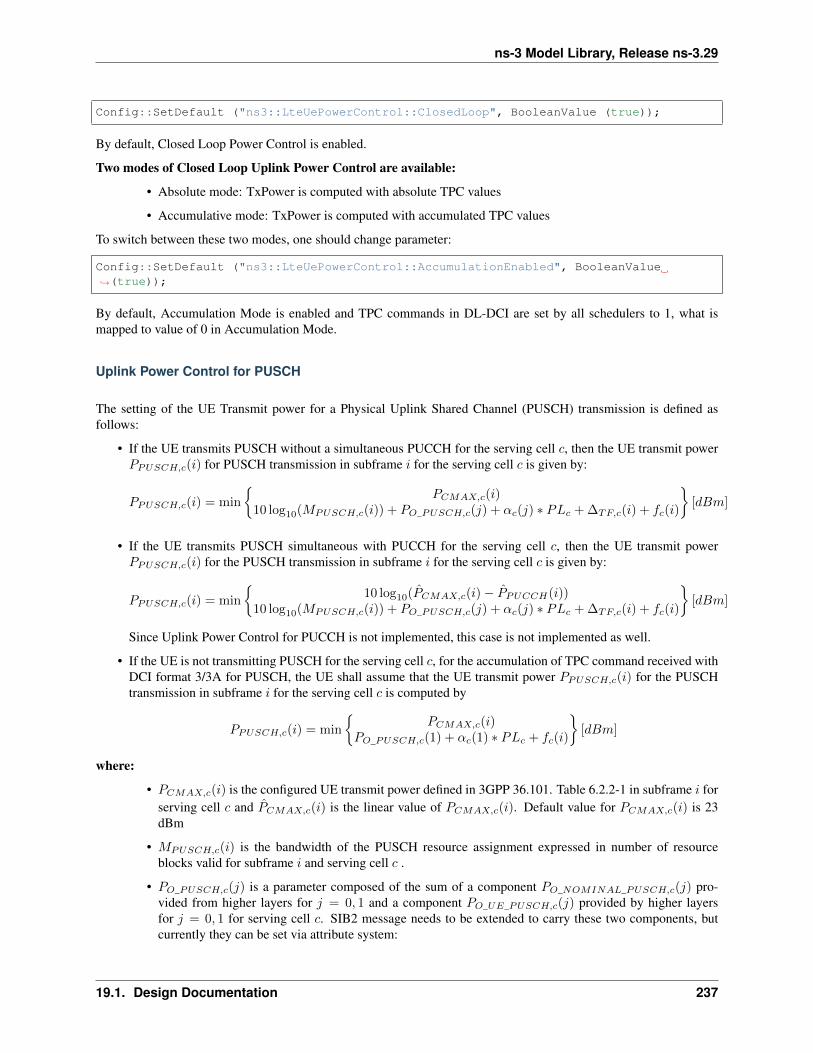
ns-3 Model Library, Release ns-3.29
Config::SetDefault ("ns3::LteUePowerControl::ClosedLoop", BooleanValue (true));
By default, Closed Loop Power Control is enabled.
Two modes of Closed Loop Uplink Power Control are available:
• Absolute mode: TxPower is computed with absolute TPC values
• Accumulative mode: TxPower is computed with accumulated TPC values
To switch between these two modes, one should change parameter:
Config::SetDefault ("ns3::LteUePowerControl::AccumulationEnabled", BooleanValue↪→(true));
By default, Accumulation Mode is enabled and TPC commands in DL-DCI are set by all schedulers to 1, what ismapped to value of 0 in Accumulation Mode.
Uplink Power Control for PUSCH
The setting of the UE Transmit power for a Physical Uplink Shared Channel (PUSCH) transmission is defined asfollows:
• If the UE transmits PUSCH without a simultaneous PUCCH for the serving cell c, then the UE transmit powerPPUSCH,c(i) for PUSCH transmission in subframe i for the serving cell c is given by:
PPUSCH,c(i) = min
{PCMAX,c(i)
10 log10(MPUSCH,c(i)) + PO_PUSCH,c(j) + αc(j) ∗ PLc + ∆TF,c(i) + fc(i)
}[dBm]
• If the UE transmits PUSCH simultaneous with PUCCH for the serving cell c, then the UE transmit powerPPUSCH,c(i) for the PUSCH transmission in subframe i for the serving cell c is given by:
PPUSCH,c(i) = min
{10 log10(PCMAX,c(i)− PPUCCH(i))
10 log10(MPUSCH,c(i)) + PO_PUSCH,c(j) + αc(j) ∗ PLc + ∆TF,c(i) + fc(i)
}[dBm]
Since Uplink Power Control for PUCCH is not implemented, this case is not implemented as well.
• If the UE is not transmitting PUSCH for the serving cell c, for the accumulation of TPC command received withDCI format 3/3A for PUSCH, the UE shall assume that the UE transmit power PPUSCH,c(i) for the PUSCHtransmission in subframe i for the serving cell c is computed by
PPUSCH,c(i) = min
{PCMAX,c(i)
PO_PUSCH,c(1) + αc(1) ∗ PLc + fc(i)
}[dBm]
where:
• PCMAX,c(i) is the configured UE transmit power defined in 3GPP 36.101. Table 6.2.2-1 in subframe i forserving cell c and PCMAX,c(i) is the linear value of PCMAX,c(i). Default value for PCMAX,c(i) is 23dBm
• MPUSCH,c(i) is the bandwidth of the PUSCH resource assignment expressed in number of resourceblocks valid for subframe i and serving cell c .
• PO_PUSCH,c(j) is a parameter composed of the sum of a component PO_NOMINAL_PUSCH,c(j) pro-vided from higher layers for j = 0, 1 and a component PO_UE_PUSCH,c(j) provided by higher layersfor j = 0, 1 for serving cell c. SIB2 message needs to be extended to carry these two components, butcurrently they can be set via attribute system:
19.1. Design Documentation 237
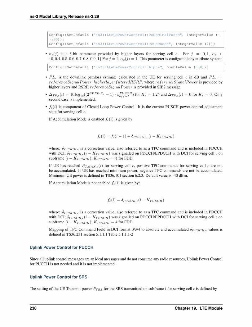
ns-3 Model Library, Release ns-3.29
Config::SetDefault ("ns3::LteUePowerControl::PoNominalPusch", IntegerValue (-↪→90));Config::SetDefault ("ns3::LteUePowerControl::PoUePusch", IntegerValue (7));
• αc(j) is a 3-bit parameter provided by higher layers for serving cell c. For j = 0, 1, αc ∈{0, 0.4, 0.5, 0.6, 0.7, 0.8, 0.9, 1} For j = 2, αc(j) = 1. This parameter is configurable by attribute system:
Config::SetDefault ("ns3::LteUePowerControl::Alpha", DoubleValue (0.8));
• PLc is the downlink pathloss estimate calculated in the UE for serving cell c in dB and PLc =referenceSignalPower˘higherlayerfilteredRSRP , where referenceSignalPower is provided byhigher layers and RSRP. referenceSignalPower is provided in SIB2 message
• ∆TF,c(i) = 10 log10((2BPRE·Ks − 1) · βPUSCHoffset ) for Ks = 1.25 and ∆TF,c(i) = 0 for Ks = 0. Onlysecond case is implemented.
• fc(i) is component of Closed Loop Power Control. It is the current PUSCH power control adjustmentstate for serving cell c.
If Accumulation Mode is enabled fc(i) is given by:
fc(i) = fc(i− 1) + δPUSCH,c(i−KPUSCH)
where: δPUSCH,c is a correction value, also referred to as a TPC command and is included in PDCCHwith DCI; δPUSCH,c(i −KPUSCH) was signalled on PDCCH/EPDCCH with DCI for serving cell c onsubframe (i−KPUSCH); KPUSCH = 4 for FDD.
If UE has reached PCMAX,c(i) for serving cell c, positive TPC commands for serving cell c are notbe accumulated. If UE has reached minimum power, negative TPC commands are not be accumulated.Minimum UE power is defined in TS36.101 section 6.2.3. Default value is -40 dBm.
If Accumulation Mode is not enabled fc(i) is given by:
fc(i) = δPUSCH,c(i−KPUSCH)
where: δPUSCH,c is a correction value, also referred to as a TPC command and is included in PDCCHwith DCI; δPUSCH,c(i −KPUSCH) was signalled on PDCCH/EPDCCH with DCI for serving cell c onsubframe (i−KPUSCH); KPUSCH = 4 for FDD.
Mapping of TPC Command Field in DCI format 0/3/4 to absolute and accumulated δPUSCH,c values isdefined in TS36.231 section 5.1.1.1 Table 5.1.1.1-2
Uplink Power Control for PUCCH
Since all uplink control messages are an ideal messages and do not consume any radio resources, Uplink Power Controlfor PUCCH is not needed and it is not implemented.
Uplink Power Control for SRS
The setting of the UE Transmit power PSRS for the SRS transmitted on subframe i for serving cell c is defined by
238 Chapter 19. LTE Module
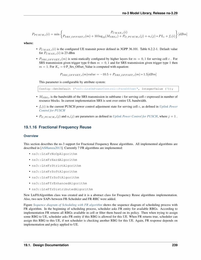
ns-3 Model Library, Release ns-3.29
PPUSCH,c(i) = min
{PCMAX,c(i)
PSRS_OFFSET,c(m) + 10 log10(MSRS,c) + PO_PUSCH,c(j) + αc(j) ∗ PLc + fc(i)
}[dBm]
where:
• PCMAX,c(i) is the configured UE transmit power defined in 3GPP 36.101. Table 6.2.2-1. Default valuefor PCMAX,c(i) is 23 dBm
• PSRS_OFFSET,c(m) is semi-statically configured by higher layers for m = 0, 1 for serving cell c . ForSRS transmission given trigger type 0 then m = 0, 1 and for SRS transmission given trigger type 1 thenm = 1. For Ks = 0 P_Srs_Offset_Value is computed with equation:
PSRS_OFFSET,c(m)value = −10.5 + PSRS_OFFSET,c(m) ∗ 1.5[dBm]
This parameter is configurable by attribute system:
Config::SetDefault ("ns3::LteUePowerControl::PsrsOffset", IntegerValue (7));
• MSRS,c is the bandwidth of the SRS transmission in subframe i for serving cell c expressed in number ofresource blocks. In current implementation SRS is sent over entire UL bandwidth.
• fc(i) is the current PUSCH power control adjustment state for serving cell c, as defined in Uplink PowerControl for PUSCH
• PO_PUSCH,c(j) and αc(j) are parameters as defined in Uplink Power Control for PUSCH, where j = 1 .
19.1.16 Fractional Frequency Reuse
Overview
This section describes the ns-3 support for Fractional Frequency Reuse algorithms. All implemented algorithms aredescribed in [ASHamza2013]. Currently 7 FR algorithms are implemented:
• ns3::LteFrNoOpAlgorithm
• ns3::LteFrHardAlgorithm
• ns3::LteFrStrictAlgorithm
• ns3::LteFrSoftAlgorithm
• ns3::LteFfrSoftAlgorithm
• ns3::LteFfrEnhancedAlgorithm
• ns3::LteFfrDistributedAlgorithm
New LteFfrAlgorithm class was created and it is a abstract class for Frequency Reuse algorithms implementation.Also, two new SAPs between FR-Scheduler and FR-RRC were added.
Figure Sequence diagram of Scheduling with FR algorithm shows the sequence diagram of scheduling process withFR algorithm. In the beginning of scheduling process, scheduler asks FR entity for available RBGs. According toimplementation FR returns all RBGs available in cell or filter them based on its policy. Then when trying to assignsome RBG to UE, scheduler asks FR entity if this RBG is allowed for this UE. When FR returns true, scheduler canassign this RBG to this UE, if not scheduler is checking another RBG for this UE. Again, FR response depends onimplementation and policy applied to UE.
19.1. Design Documentation 239
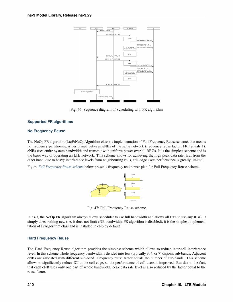
ns-3 Model Library, Release ns-3.29
Fig. 46: Sequence diagram of Scheduling with FR algorithm
Supported FR algorithms
No Frequency Reuse
The NoOp FR algorithm (LteFrNoOpAlgorithm class) is implementation of Full Frequency Reuse scheme, that meansno frequency partitioning is performed between eNBs of the same network (frequency reuse factor, FRF equals 1).eNBs uses entire system bandwidth and transmit with uniform power over all RBGs. It is the simplest scheme and isthe basic way of operating an LTE network. This scheme allows for achieving the high peak data rate. But from theother hand, due to heavy interference levels from neighbouring cells, cell-edge users performance is greatly limited.
Figure Full Frequency Reuse scheme below presents frequency and power plan for Full Frequency Reuse scheme.
Fig. 47: Full Frequency Reuse scheme
In ns-3, the NoOp FR algorithm always allows scheduler to use full bandwidth and allows all UEs to use any RBG. Itsimply does nothing new (i.e. it does not limit eNB bandwidth, FR algorithm is disabled), it is the simplest implemen-tation of FrAlgorithm class and is installed in eNb by default.
Hard Frequency Reuse
The Hard Frequency Reuse algorithm provides the simplest scheme which allows to reduce inter-cell interferencelevel. In this scheme whole frequency bandwidth is divided into few (typically 3, 4, or 7) disjoint sub-bands. AdjacenteNBs are allocated with different sub-band. Frequency reuse factor equals the number of sub-bands. This schemeallows to significantly reduce ICI at the cell edge, so the performance of cell-users is improved. But due to the fact,that each eNB uses only one part of whole bandwidth, peak data rate level is also reduced by the factor equal to thereuse factor.
240 Chapter 19. LTE Module

ns-3 Model Library, Release ns-3.29
Figure Hard Frequency Reuse scheme below presents frequency and power plan for Hard Frequency Reuse scheme.
Fig. 48: Hard Frequency Reuse scheme
In our implementation, the Hard FR algorithm has only vector of RBGs available for eNB and pass it to MAC Sched-uler during scheduling functions. When scheduler ask, if RBG is allowed for specific UE it always return true.
Strict Frequency Reuse
Strict Frequency Reuse scheme is combination of Full and Hard Frequency Reuse schemes. It consists of dividingthe system bandwidth into two parts which will have different frequency reuse. One common sub-band of the systembandwidth is used in each cell interior (frequency reuse-1), while the other part of the bandwidth is divided among theneighboring eNBs as in hard frequency reuse (frequency reuse-N, N>1), in order to create one sub-band with a lowinter-cell interference level in each sector. Center UEs will be granted with the fully-reused frequency chunks, whilecell-edge UEs with orthogonal chunks. It means that interior UEs from one cell do not share any spectrum with edgeUEs from second cell, which reduces interference for both. As can be noticed, Strict FR requires a total of N + 1sub-bands, and allows to achieve RFR in the middle between 1 and 3.
Figure Strict Frequency Reuse scheme below presents frequency and power plan for Strict Frequency Reuse schemewith a cell-edge reuse factor of N = 3.
Fig. 49: Strict Frequency Reuse scheme
In our implementation, Strict FR algorithm has two maps, one for each sub-band. If UE can be served within privatesub-band, its RNTI is added to m_privateSubBandUe map. If UE can be served within common sub-band, its RNTIis added to m_commonSubBandUe map. Strict FR algorithm needs to decide within which sub-band UE should beserved. It uses UE measurements provided by RRB and compare them with signal quality threshold (this parametercan be easily tuned by attribute mechanism). Threshold has influence on interior to cell radius ratio.
Soft Frequency Reuse
In Soft Frequency Reuse (SFR) scheme each eNb transmits over the entire system bandwidth, but there are two sub-bands, within UEs are served with different power level. Since cell-center UEs share the bandwidth with neighboringcells, they usually transmit at lower power level than the cell-edge UEs. SFR is more bandwidth efficient than StrictFR, because it uses entire system bandwidth, but it also results in more interference to both cell interior and edge users.
There are two possible versions of SFR scheme:
• In first version, the sub-band dedicated for the cell-edge UEs may also be used by the cell-center UEs but withreduced power level and only if it is not occupied by the cell-edge UEs. Cell-center sub-band is available to the
19.1. Design Documentation 241

ns-3 Model Library, Release ns-3.29
centre UEs only. Figure Soft Frequency Reuse scheme version 1 below presents frequency and power plan forthis version of Soft Frequency Reuse scheme.
Fig. 50: Soft Frequency Reuse scheme version 1
• In second version, cell-center UEs do not have access to cell-edge sub-band. In this way, each cell can use thewhole system bandwidth while reducing the interference to the neighbors cells. From the other hand, lowerICI level at the cell-edge is achieved at the expense of lower spectrum utilization. Figure Soft Frequency Reusescheme version 2 below presents frequency and power plan for this version of Soft Frequency Reuse scheme.
Fig. 51: Soft Frequency Reuse scheme version 2
SFR algorithm maintain two maps. If UE should be served with lower power level, its RNTI is addedto m_lowPowerSubBandUe map. If UE should be served with higher power level, its RNTI is added tom_highPowerSubBandUe map. To decide with which power level UE should be served SFR algorithm utilize UEmeasurements, and compares them to threshold. Signal quality threshold and PdschConfigDedicated (i.e. P_A value)for inner and outer area can be configured by attributes system. SFR utilizes Downlink Power Control described here.
Soft Fractional Frequency Reuse
Soft Fractional Frequency Reuse (SFFR) is an combination of Strict and Soft Frequency Reuse schemes. While StrictFR do not use the subbands allocated for outer region in the adjacent cells, soft FFR uses these subbands for the innerUEs with low transmit power. As a result, the SFFR, like SFR, use the subband with high transmit power level andwith low transmit power level. Unlike the Soft FR and like Strict FR, the Soft FFR uses the common sub-band whichcan enhance the throughput of the inner users.
Figure Soft Fractional Fractional Frequency Reuse scheme below presents frequency and power plan for Soft Frac-tional Frequency Reuse.
Fig. 52: Soft Fractional Fractional Frequency Reuse scheme
242 Chapter 19. LTE Module

ns-3 Model Library, Release ns-3.29
Enhanced Fractional Frequency Reuse
Enhanced Fractional Frequency Reuse (EFFR) described in [ZXie2009] defines 3 cell-types for directly neighboringcells in a cellular system, and reserves for each cell-type a part of the whole frequency band named Primary Segment,which among different type cells should be orthogonal. The remaining subchannels constitute the Secondary Segment.The Primary Segment of a cell-type is at the same time a part of the Secondary Segments belonging to the other twocell-types. Each cell can occupy all subchannels of its Primary Segment at will, whereas only a part of subchannels inthe Secondary Segment can be used by this cell in an interference-aware manner.The Primary Segment of each cell isdivided into a reuse-3 part and reuse-1 part. The reuse-1 part can be reused by all types of cells in the system, whereasreuse-3 part can only be exclusively reused by other same type cells( i.e. the reuse-3 subchannels cannot be reusedby directly neighboring cells). On the Secondary Segment cell acts as a guest, and occupying secondary subchannelsis actually reuse the primary subchannels belonging to the directly neighboring cells, thus reuse on the SecondarySegment by each cell should conform to two rules:
• monitor before use
• resource reuse based on SINR estimation
Each cell listens on every secondary subchannel all the time. And before occupation, it makes SINR evaluationaccording to the gathered channel quality information (CQI) and chooses resources with best estimation values forreuse. If CQI value for RBG is above configured threshold for some user, transmission for this user can be performedusing this RBG.
In [ZXie2009] scheduling process is described, it consist of three steps and two scheduling polices. Since none ofcurrently implemented schedulers allow for this behaviour, some simplification were applied. In our implementationreuse-1 subchannels can be used only by cell center users. Reuse-3 subchannels can be used by edge users, and onlyif there is no edge user, transmission for cell center users can be served in reuse-3 subchannels.
Figure Enhanced Fractional Fractional Frequency Reuse scheme below presents frequency and power plan for En-hanced Fractional Frequency Reuse.
Fig. 53: Enhanced Fractional Fractional Frequency Reuse scheme
Distributed Fractional Frequency Reuse
This Distributed Fractional Frequency Reuse Algorithm was presented in [DKimura2012]. It automatically optimizescell-edge sub-bands by focusing on user distribution (in particular, receive-power distribution). This algorithm adap-tively selects RBs for cell-edge sub-band on basis of coordination information from adjecent cells and notifies the basestations of the adjacent cells, which RBs it selected to use in edge sub-band. The base station of each cell uses thereceived information and the following equation to compute cell-edge-band metric Ak for each RB.
Ak =∑j∈J
wjXj,k
where J is a set of neighbor cells, Xj,k = {0, 1} is the RNTP from the j-th neighbor cell. It takes a value of 1 whenthe k-th RB in the j-th neighbor cell is used as a cell-edge sub-band and 0 otherwise. The symbol wj denotes weightwith respect to adjacent cell j, that is, the number of users for which the difference between the power of the signalreceived from the serving cell i and the power of the signal received from the adjacent cell j is less than a threshold
19.1. Design Documentation 243

ns-3 Model Library, Release ns-3.29
value (i.e., the number of users near the cell edge in the service cell). A large received power difference means thatcell-edge users in the i-th cell suffer strong interference from the j-th cell.
The RB for which metric Ak is smallest is considered to be least affected by interference from another cell. Servingcell selects a configured number of RBs as cell-edge sub-band in ascending order of Ak. As a result, the RBs in whicha small number of cell-edge users receive high interference from adjacent base stations are selected.
The updated RNTP is then sent to all the neighbor cells. In order to avoid the meaningless oscillation of cell-edge-bandselection, a base station ignores an RNTP from another base station that has larger cell ID than the base station.
Repeating this process across all cells enables the allocation of RBs to cell-edge areas to be optimized over the systemand to be adjusted with changes in user distribution.
Figure Sequence diagram of Distributed Frequency Reuse Scheme below presents sequence diagram of DistributedFractional Frequency Reuse Scheme.
Fig. 54: Sequence diagram of Distributed Frequency Reuse Scheme
244 Chapter 19. LTE Module

ns-3 Model Library, Release ns-3.29
19.1.17 Carrier Aggregation
Overview
This section describes the ns-3 support for Carrier Aggregation. The references in the standard are [TS36211],[TS36213] and [TS36331].
Note: Carrier Aggregation was introduced in release 3.27 and currently, only works in downlink.
3GPP standardizes, in release R10, the Carrier Aggregation (CA) technology.
This technology consists of the possibility, to aggregate radio resources belonging to different carriers, in order tohave more bandwidth available, and to achieve a higher throughput. Carrier Aggregation as defined by 3GPP can beused with both TDD and FDD. Since ns-3 only supports FDD LTE implementation, we will consider only this casein this section. Each aggregated carrier is referred to as a component carrier, CC. The component carrier can have abandwidth of 1.4, 3, 5, 10, 15 or 20 MHz and a maximum of five component carriers can be aggregated, hence themaximum aggregated bandwidth is 100 MHz. In FDD the number of aggregated carriers can be different in DL andUL. However, the number of UL component carriers is always equal to or lower than the number of DL componentcarriers. The individual component carriers can also be of different bandwidths. When carrier aggregation is usedthere are a number of serving cells, one for each component carrier. The coverage of the serving cells may differ, forexample due to that CCs on different frequency bands will experience different pathloss. The RRC connection is onlyhandled by one cell, the Primary serving cell, served by the Primary component carrier (DL and UL PCC). It is alsoon the DL PCC that the UE receives NAS information, such as security parameters.
3GPP defines three different CA bandwidth classes in releases 10 and 11 (where ATBC is Aggregated TransmissionBandwidth Configuration):
Class A: ATBC ≤ 100, maximum number of CC = 1
Class B: ATBC ≤ 100, maximum number of CC = 2
Class C: 100 ≤ ATBC ≤ 200, maximum number of CC = 2
Figure CA impact on different layers of LTE protocol stack (from 3gpp.org) (from 3gpp.org) shows the main impactof CA technology on the different layers of the LTE protocol stack. Introduction of carrier aggregation influencesmainly the MAC and new RRC messages are introduced. In order to keep R8/R9 compatibility the protocol changeswill be kept to a minimum. Basically each component carrier is treated as an R8 carrier. However some changes arerequired, such as new RRC messages in order to handle the secondary component carrier (SCC), and MAC must beable to handle scheduling on a number of CCs. In the following we describe the impact of the carrier aggregationimplementation on the different layers of the LTE protocol stack in ns-3.
Impact on RRC layer
The main impacts on the RRC layer are related to secondary carrier configuration and measurements reporting. Toenable these features we have enhanced the already existing procedures for the RRC Connection Reconfiguration andUE RRC Measurements Model.
The carrier aggregation enabling procedure is shown in figure A schematic overview of the secondary carrier enablingprocedure. As per 3GPP definition, the secondary cell is a cell, operating on a secondary frequency, which may beconfigured once an RRC connection is established and which may be used to provide additional radio resources.Hence, the procedure starts when the UE is in the CONNECTED_NORMALLY state (see the RRC state machinedescription). This part of the procedure is the same as in the previous architecture. In order to simplify the imple-mentation, the UE Capability Inquiry and UE Capability Information are not implemented. This implies to assumethat each UE can support the carrier aggregation, and any specific configuration provided by the eNB to which isattached. The eNB RRC sends to the UE the secondary carrier configuration parameters through the RRC ConnectionReconfiguration procedure. This procedure may be used for various purposes related to modifications of the RRCconnection, e.g. to establish, modify or release RBs, to perform handover, to setup, modify or release measurements,
19.1. Design Documentation 245
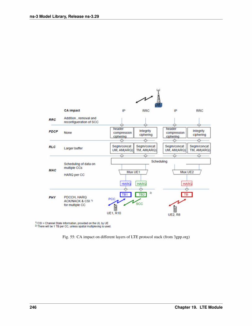
ns-3 Model Library, Release ns-3.29
Fig. 55: CA impact on different layers of LTE protocol stack (from 3gpp.org)
246 Chapter 19. LTE Module
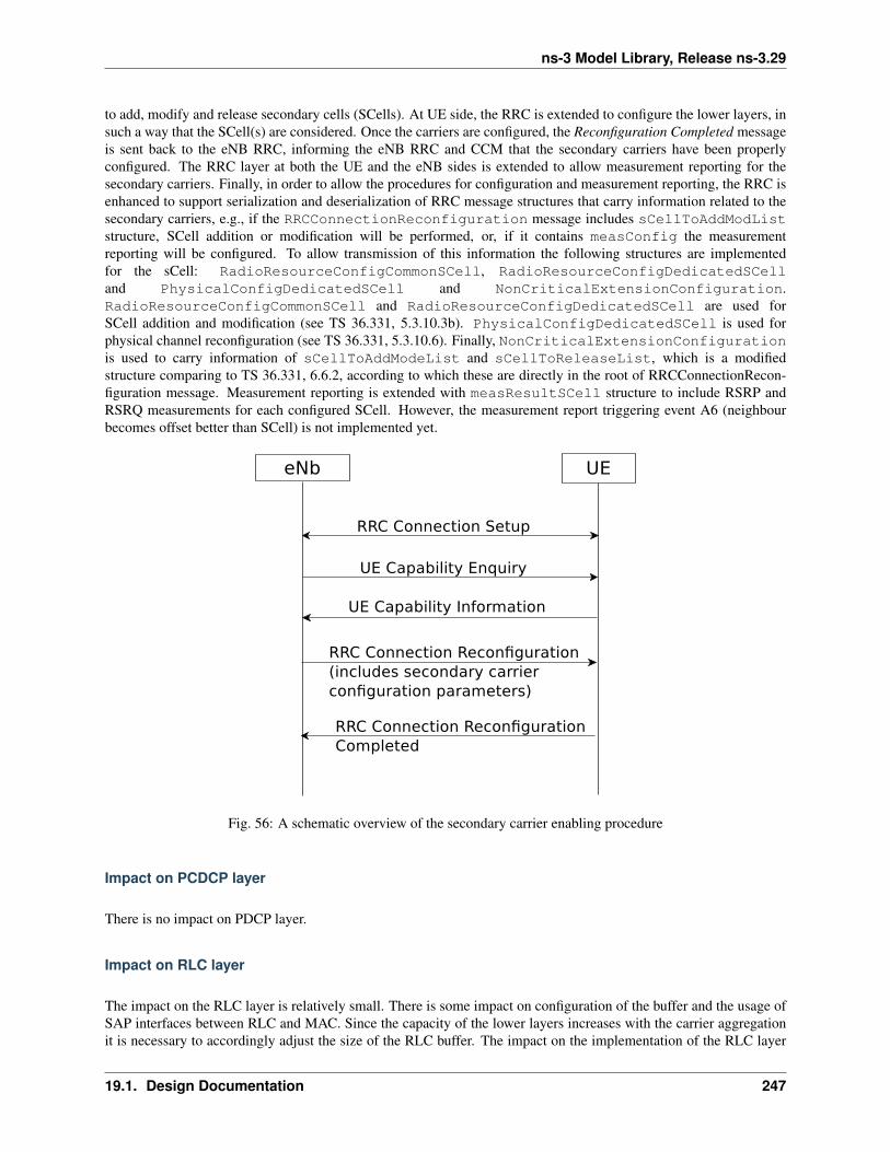
ns-3 Model Library, Release ns-3.29
to add, modify and release secondary cells (SCells). At UE side, the RRC is extended to configure the lower layers, insuch a way that the SCell(s) are considered. Once the carriers are configured, the Reconfiguration Completed messageis sent back to the eNB RRC, informing the eNB RRC and CCM that the secondary carriers have been properlyconfigured. The RRC layer at both the UE and the eNB sides is extended to allow measurement reporting for thesecondary carriers. Finally, in order to allow the procedures for configuration and measurement reporting, the RRC isenhanced to support serialization and deserialization of RRC message structures that carry information related to thesecondary carriers, e.g., if the RRCConnectionReconfiguration message includes sCellToAddModListstructure, SCell addition or modification will be performed, or, if it contains measConfig the measurementreporting will be configured. To allow transmission of this information the following structures are implementedfor the sCell: RadioResourceConfigCommonSCell, RadioResourceConfigDedicatedSCelland PhysicalConfigDedicatedSCell and NonCriticalExtensionConfiguration.RadioResourceConfigCommonSCell and RadioResourceConfigDedicatedSCell are used forSCell addition and modification (see TS 36.331, 5.3.10.3b). PhysicalConfigDedicatedSCell is used forphysical channel reconfiguration (see TS 36.331, 5.3.10.6). Finally, NonCriticalExtensionConfigurationis used to carry information of sCellToAddModeList and sCellToReleaseList, which is a modifiedstructure comparing to TS 36.331, 6.6.2, according to which these are directly in the root of RRCConnectionRecon-figuration message. Measurement reporting is extended with measResultSCell structure to include RSRP andRSRQ measurements for each configured SCell. However, the measurement report triggering event A6 (neighbourbecomes offset better than SCell) is not implemented yet.
Fig. 56: A schematic overview of the secondary carrier enabling procedure
Impact on PCDCP layer
There is no impact on PDCP layer.
Impact on RLC layer
The impact on the RLC layer is relatively small. There is some impact on configuration of the buffer and the usage ofSAP interfaces between RLC and MAC. Since the capacity of the lower layers increases with the carrier aggregationit is necessary to accordingly adjust the size of the RLC buffer. The impact on the implementation of the RLC layer
19.1. Design Documentation 247
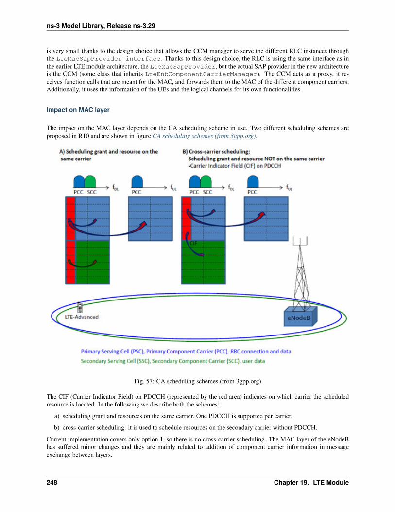
ns-3 Model Library, Release ns-3.29
is very small thanks to the design choice that allows the CCM manager to serve the different RLC instances throughthe LteMacSapProvider interface. Thanks to this design choice, the RLC is using the same interface as inthe earlier LTE module architecture, the LteMacSapProvider, but the actual SAP provider in the new architectureis the CCM (some class that inherits LteEnbComponentCarrierManager). The CCM acts as a proxy, it re-ceives function calls that are meant for the MAC, and forwards them to the MAC of the different component carriers.Additionally, it uses the information of the UEs and the logical channels for its own functionalities.
Impact on MAC layer
The impact on the MAC layer depends on the CA scheduling scheme in use. Two different scheduling schemes areproposed in R10 and are shown in figure CA scheduling schemes (from 3gpp.org).
Fig. 57: CA scheduling schemes (from 3gpp.org)
The CIF (Carrier Indicator Field) on PDCCH (represented by the red area) indicates on which carrier the scheduledresource is located. In the following we describe both the schemes:
a) scheduling grant and resources on the same carrier. One PDCCH is supported per carrier.
b) cross-carrier scheduling: it is used to schedule resources on the secondary carrier without PDCCH.
Current implementation covers only option 1, so there is no cross-carrier scheduling. The MAC layer of the eNodeBhas suffered minor changes and they are mainly related to addition of component carrier information in messageexchange between layers.
248 Chapter 19. LTE Module

ns-3 Model Library, Release ns-3.29
Impact on PHY layer
The impact on PHY layer is minor. There is an instance of PHY layer per each component carrier and the SAP interfacefunctions remain unchanged. As shown in CA scheduling schemes (from 3gpp.org) the difference is that since there aremultiple PHY instances, there are also multiple instances of PDCCH, HARQ, ACK/NACK and CSI per carrier. So, atthe eNB PHY, the changes are related to the addition of the component carrier id information, while at the UE PHY theinformation of the Component Carrier is used for some functionalities that depend on the Component Carrier to whichthe PHY instance belongs. For example, the UE PHY is extended to allow disabling of the sounding reference signal(SRS) at the secondary carriers. This is necessary because there is one UE PHY instance per component carrier, butaccording to CA scheduling schemes (from 3gpp.org), only a single carrier is used and the uplink traffic is transmittedonly over the primary carrier.
Code Structure Design
This section briefly introduces the software design and implementation of the carrier aggregation functionality.
Both LteEnbNetDevice and LteUeNetDevice are created by the LteHelper using the methodInstallSingleEnbDevice and InstallSingleUeDevice. These functions are now extended to allowthe carrier aggregation configuration. In the following we explain the main differences comparing to the previousarchitecture.
Figure Changes in LteEnbNetDevice to support CA shows the attributes and associations of the LteEnbNetDevicethat are affected by the implementation, or are created in order to support the carrier aggregation functional-ity. Since LteEnbNetDevice may have several component carriers, the attributes that were formerly partof the LteEnbNetDevice and are carrier specific are migrated to the ComponentCarrier class, e.g. physi-cal layer configuration parameters. The attributes that are specific for the eNB component carrier are migratedto ComponentCarrierEnb, e.g. pointers to MAC, PHY, scheduler, fractional frequency reuse instances.LteEnbNetDevice can contain pointers to several ComponentCarrierEnb instances. This architecture allowsthat each CC may have its own configuration for PHY, MAC, scheduling algorithm and franctional frequency reusealgorithm. These attributes are currently maintained also in the LteEnbNetDevice for backward compatibilitypurpose. By default the LteEnbNetDevice attributes are the same as the primary carrier attributes.
Figure Changes in LteUeNetDevice to support CA shows the attributes and associations of LteUeNetDevice thatare affected by the carrier aggregation implementation. Similarly, to the changes in LteEnbNetDevice, pointersthat are specific to UE component carrier are migrated to the ComponentCarrierUe class. LteUeNetDevicehas maintained m_dlEarfcn for initial cell selection purposes.
CA impact on data plane of eNodeB
Figure eNB Data Plane Architecture shows the class diagram of the data plane at the eNB.
The main impact is the insertion of the LteEnbComponentCarrierManager class in the middle of the LTEprotocol stack. During the design phase it was decided to keep the same SAP interfaces design that existed be-tween MAC and RLC in order to avoid unnecessary changes in these parts of protocol stack. To achieve this theLteEnbComponentCarrierManager implements all functions that were previously exposed by RLC to MACthrough LteMacSapUser interface. It also implements functions that were previously exposed by MAC to RLCthrough the LteMacSapProvider interface. In this way, the carrier aggregation is transparent to upper and lowerlayers. The only difference is that the MAC instance sees now only one LteMacSapUser, whereas formerly it wasseeing only one LteMacSapUser per RLC instance.
The LteEnbComponentCarrierManager is responsible for the forwarding messages in both directions. In thecurrent implementation, a PDCP and a RLC instances are activated each time a new data radio bearer is configured.The correspondence between a new data radio bearer and a RLC instance is one to one. In order to maintain the same
19.1. Design Documentation 249

ns-3 Model Library, Release ns-3.29
Fig. 58: Changes in LteEnbNetDevice to support CA
Fig. 59: Changes in LteUeNetDevice to support CA
250 Chapter 19. LTE Module
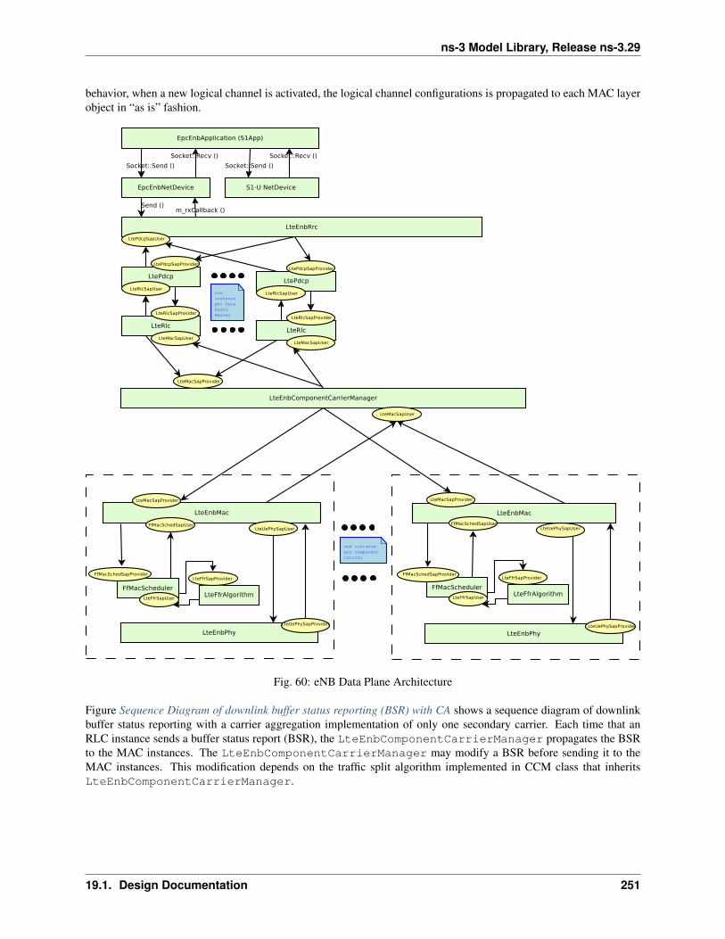
ns-3 Model Library, Release ns-3.29
behavior, when a new logical channel is activated, the logical channel configurations is propagated to each MAC layerobject in “as is” fashion.
Fig. 60: eNB Data Plane Architecture
Figure Sequence Diagram of downlink buffer status reporting (BSR) with CA shows a sequence diagram of downlinkbuffer status reporting with a carrier aggregation implementation of only one secondary carrier. Each time that anRLC instance sends a buffer status report (BSR), the LteEnbComponentCarrierManager propagates the BSRto the MAC instances. The LteEnbComponentCarrierManager may modify a BSR before sending it to theMAC instances. This modification depends on the traffic split algorithm implemented in CCM class that inheritsLteEnbComponentCarrierManager.
19.1. Design Documentation 251

ns-3 Model Library, Release ns-3.29
LtePdcp at eNb LteRlc at eNbLteEnbComponentCarrie
rManager LteEnbMac0 LteEnbMac1
DoTransmitPdcpPdu ()
ReportBufferStatus ()
ReportBufferStatus (x%)
ReportBufferStatus ((100-x)%)
NotifyTxOpportunity ()
NotifyTxOpportunity ()
NotifyTx Oportunity (Mac0)
NotifyTxOpportunity (Mac1)
TransmitPdu ()
TransmitPdu ()
TransmitPdu ()
TransmitPdu ()
Fig. 61: Sequence Diagram of downlink buffer status reporting (BSR) with CA
252 Chapter 19. LTE Module

ns-3 Model Library, Release ns-3.29
CA impact on control plane of eNodeB
Figure eNB Control Plane Architecture shows the class diagram of the control plane at the eNB. During the designphase it was decided to maintain the same hooks as in the former architecture. To do so, at each component carrier thePHY and the MAC are directly associated to the RRC instance. However, the RRC instance is additionally connectedto the LteEnbComponentCarrierManager, which is responsible for enabling and disabling the componentcarriers. When the simulation starts, the number of component carrier is fixed, but only the primary carrier componentis enabled. Depending on the LteEnbComponentCarrierManager algorithm the other carrier componentscould be activated or not.
Fig. 62: eNB Control Plane Architecture
Figure Sequence Diagram of Data Radio Bearer Setup shows how the Radio Bearer are configured.
CA impact on data plane of UE
Figure UE Data Plane Architecture shows the relation between the different classes related to the UEdata plane. The UE data plane architecture is similar to the eNB data plane implementation. TheLteUeComponentCarrierManager is responsible to (re)map each MacSapUserProvider to the corre-sponding RLC instance or to the proper MAC instance. The channel remapping depends on algorithm used asLteUeComponentCarrierManager. A particular case is represented by the UE buffer status report (BSR) toeNB. Since, i) the standard does not specify how the BSR has to be reported on each component carrier and ii) it isdecided to map one-to-one the logical channel to each MAC layer, the only way to send BSRs to the eNB is throughthe primary carrier. Figure Uplink buffer status reporting with CA shows the sequence diagram. Each time a BSR isgenerated, the LteUeComponentCarrierManager sends it through the primary carrier component. When theprimary component carrier at the eNB receives the BSR, it sends it to LteEnbComponentCarrierManager. Thelatter, according to algorithm dependent policies, forwards a BSR to component carriers. The communication betweenthe LteEnbMac and the LteEnbComponentCarrierManager is done through a specific set of SAP functionswhich are implemented in the LteUlCcmRrcSapUser and the LteUlCcmRrcSapProvider.
CA impact on control plane of UE
Figure UE Control Plane Architecture shows the relation between the different classes associated to the UE controlplane. The control plane implementation at the UE is basically the same as the eNB control plane implementation.
19.1. Design Documentation 253

ns-3 Model Library, Release ns-3.29
LteEpc LteEnbRrcLteEnbComponentCarrie
rManager LteEnbMac0 LteEnbMac1
SetupDataRadioBearer ()
SetupDataRadioBearer ()
AddLc (std::vector<LcConfiguration>)
AddLc ()
AddLc ()
MeasurementReport ()
Decide Activation
AddLc (std::vector<LcConfiguration>)
AddLc ()
AddLc ()
Fig. 63: Sequence Diagram of Data Radio Bearer Setup
254 Chapter 19. LTE Module

ns-3 Model Library, Release ns-3.29
Fig. 64: UE Data Plane Architecture
19.1. Design Documentation 255
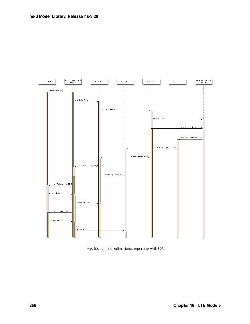
ns-3 Model Library, Release ns-3.29
Fig. 65: Uplink buffer status reporting with CA
256 Chapter 19. LTE Module
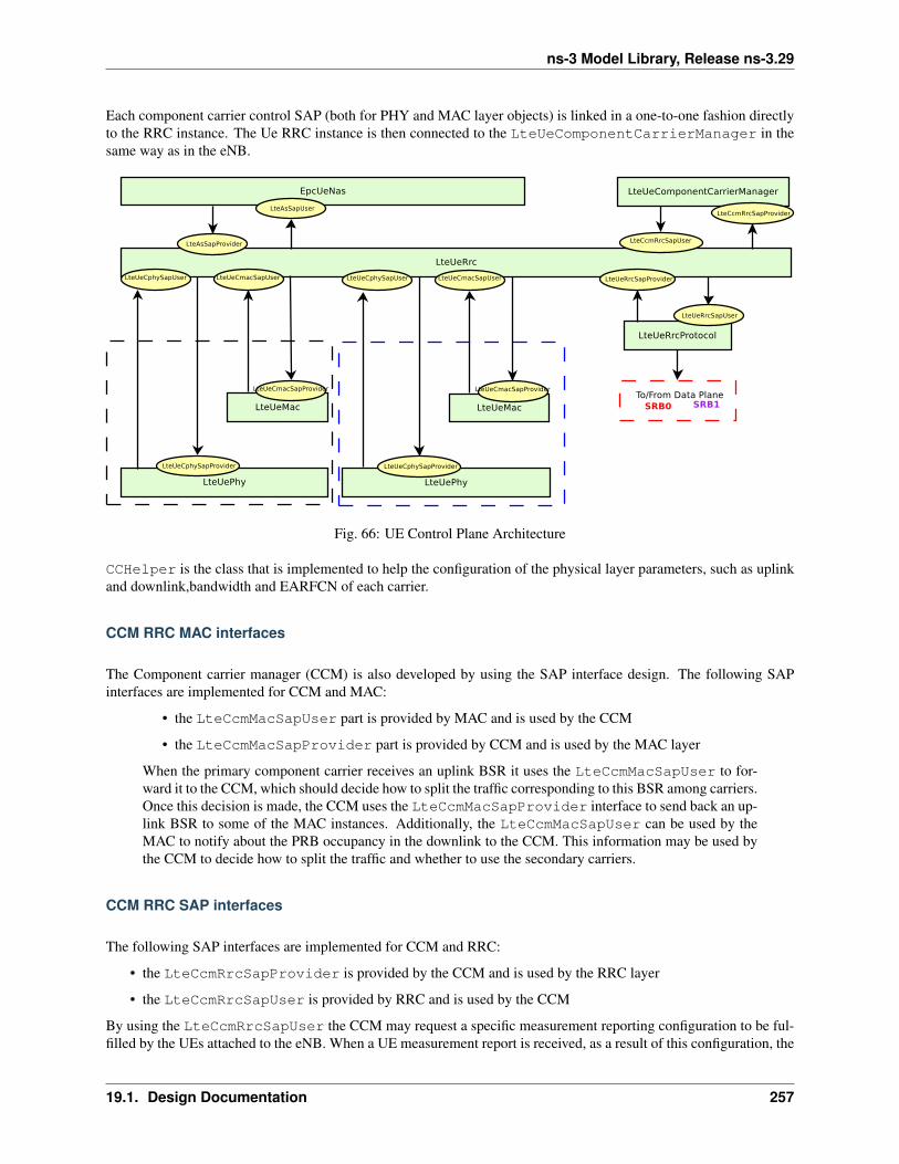
ns-3 Model Library, Release ns-3.29
Each component carrier control SAP (both for PHY and MAC layer objects) is linked in a one-to-one fashion directlyto the RRC instance. The Ue RRC instance is then connected to the LteUeComponentCarrierManager in thesame way as in the eNB.
Fig. 66: UE Control Plane Architecture
CCHelper is the class that is implemented to help the configuration of the physical layer parameters, such as uplinkand downlink,bandwidth and EARFCN of each carrier.
CCM RRC MAC interfaces
The Component carrier manager (CCM) is also developed by using the SAP interface design. The following SAPinterfaces are implemented for CCM and MAC:
• the LteCcmMacSapUser part is provided by MAC and is used by the CCM
• the LteCcmMacSapProvider part is provided by CCM and is used by the MAC layer
When the primary component carrier receives an uplink BSR it uses the LteCcmMacSapUser to for-ward it to the CCM, which should decide how to split the traffic corresponding to this BSR among carriers.Once this decision is made, the CCM uses the LteCcmMacSapProvider interface to send back an up-link BSR to some of the MAC instances. Additionally, the LteCcmMacSapUser can be used by theMAC to notify about the PRB occupancy in the downlink to the CCM. This information may be used bythe CCM to decide how to split the traffic and whether to use the secondary carriers.
CCM RRC SAP interfaces
The following SAP interfaces are implemented for CCM and RRC:
• the LteCcmRrcSapProvider is provided by the CCM and is used by the RRC layer
• the LteCcmRrcSapUser is provided by RRC and is used by the CCM
By using the LteCcmRrcSapUser the CCM may request a specific measurement reporting configuration to be ful-filled by the UEs attached to the eNB. When a UE measurement report is received, as a result of this configuration, the
19.1. Design Documentation 257

ns-3 Model Library, Release ns-3.29
eNB RRC entity shall forward this report to the CCM through the LteCcmRrcSapProvider::ReportUeMeasSAP function. Additionally, the LteCcmRrcSapProvider offers different functions to the RRC that can be usedto add and remove of UEs, setup or release of radio bearer, configuration of the signalling bearer, etc.
Component carrier managers
Currently, there are two component carrier manager implementations available. The first one is theNoOpComponentCarrierManager, which is the default CCM choice. When this CCM is used the carrier aggre-gation feature is disabled. This CCM forwards all traffic, the uplink and the downlink, over the primary carrier, anddoes not use secondary carriers. Another implementation is the RrComponentCarrierManager, which splits thetraffic equally among carriers, by diving the buffer status report among different carriers. SRB0 and SRB1 flows willbe forwarded only over primary carrier.
19.1.18 Helpers
Two helper objects are used to setup simulations and configure the various components. These objects are:
• LteHelper, which takes care of the configuration of the LTE radio access network, as well as of coordi-nating the setup and release of EPS bearers. The LteHelper class provides both the API definition and itsimplementation.
• EpcHelper, which takes care of the configuration of the Evolved Packet Core. The EpcHelper class is anabstract base class, which only provides the API definition; the implementation is delegated to the child classesin order to allow for different EPC network models.
• CcHelper, which takes care of the configuration of the LteEnbComponentCarrierMap,basically, it creates a user specified number of LteEnbComponentCarrier.LteUeComponentCarrierMap is currently created starting from the LteEnbComponentCarrierMap.LteHelper:InstallSingleUeDevice, in this implementation, is needed to invoke after theLteHelper:InstallSingleEnbDevice to ensure that the LteEnbComponentCarrierMap isproperly initialized.
It is possible to create a simple LTE-only simulations by using the LteHelper alone, or to create complete LTE-EPC simulations by using both LteHelper and EpcHelper. When both helpers are used, they interact in amaster-slave fashion, with the LteHelper being the Master that interacts directly with the user program, and theEpcHelper working “under the hood” to configure the EPC upon explicit methods called by the LteHelper. Theexact interactions are displayed in the Figure Sequence diagram of the interaction between LteHelper and EpcHelper..
19.2 User Documentation
19.2.1 Background
We assume the reader is already familiar with how to use the ns-3 simulator to run generic simulation programs. Ifthis is not the case, we strongly recommend the reader to consult [ns3tutorial].
19.2.2 Usage Overview
The ns-3 LTE model is a software library that allows the simulation of LTE networks, optionally including the EvolvedPacket Core (EPC). The process of performing such simulations typically involves the following steps:
1. Define the scenario to be simulated
258 Chapter 19. LTE Module
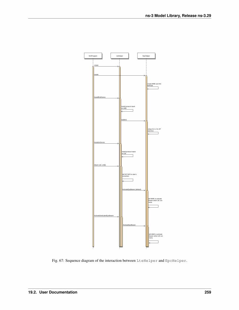
ns-3 Model Library, Release ns-3.29
SimProgram LteHelper EpcHelper
create
create
create MME and SGW/PGW
InstallEnbDevice
install protocol stack on eNB
AddEnb
setup S1-U, S1-AP and S11
InstallUeDevice
install protocol stack on UE
Attach (UE, eNB)
tell UE NAS to start connection
ActivateEpsBearer (default)
tell MME to activate bearer when UE connects
ActivateDedicatedEpsBearer
ActivateEpsBearer
tell MME to activate bearer when UE connects
Fig. 67: Sequence diagram of the interaction between LteHelper and EpcHelper.
19.2. User Documentation 259

ns-3 Model Library, Release ns-3.29
2. Write a simulation program that recreates the desired scenario topology/architecture. This is done accessing thens-3 LTE model library using the ns3::LteHelper API defined in src/lte/helper/lte-helper.h.
3. Specify configuration parameters of the objects that are being used for the simulation. This can be done usinginput files (via the ns3::ConfigStore) or directly within the simulation program.
4. Configure the desired output to be produced by the simulator
5. Run the simulation.
All these aspects will be explained in the following sections by means of practical examples.
19.2.3 Basic simulation program
Here is the minimal simulation program that is needed to do an LTE-only simulation (without EPC).
1. Initial boilerplate:
#include <ns3/core-module.h>#include <ns3/network-module.h>#include <ns3/mobility-module.h>#include <ns3/lte-module.h>
using namespace ns3;
int main (int argc, char *argv[]){// the rest of the simulation program follows
2. Create an LteHelper object:
Ptr<LteHelper> lteHelper = CreateObject<LteHelper> ();
This will instantiate some common objects (e.g., the Channel object) and provide the methods to add eNBs andUEs and configure them.
3. Create Node objects for the eNB(s) and the UEs:
NodeContainer enbNodes;enbNodes.Create (1);NodeContainer ueNodes;ueNodes.Create (2);
Note that the above Node instances at this point still don’t have an LTE protocol stack installed; they’re justempty nodes.
4. Configure the Mobility model for all the nodes:
MobilityHelper mobility;mobility.SetMobilityModel ("ns3::ConstantPositionMobilityModel");mobility.Install (enbNodes);mobility.SetMobilityModel ("ns3::ConstantPositionMobilityModel");mobility.Install (ueNodes);
The above will place all nodes at the coordinates (0,0,0). Please refer to the documentation of the ns-3 mobilitymodel for how to set your own position or configure node movement.
5. Install an LTE protocol stack on the eNB(s):
260 Chapter 19. LTE Module
ns-3 Model Library, Release ns-3.29
NetDeviceContainer enbDevs;enbDevs = lteHelper->InstallEnbDevice (enbNodes);
6. Install an LTE protocol stack on the UEs:
NetDeviceContainer ueDevs;ueDevs = lteHelper->InstallUeDevice (ueNodes);
7. Attach the UEs to an eNB. This will configure each UE according to the eNB configuration, and create an RRCconnection between them:
lteHelper->Attach (ueDevs, enbDevs.Get (0));
8. Activate a data radio bearer between each UE and the eNB it is attached to:
enum EpsBearer::Qci q = EpsBearer::GBR_CONV_VOICE;EpsBearer bearer (q);lteHelper->ActivateDataRadioBearer (ueDevs, bearer);
this method will also activate two saturation traffic generators for that bearer, one in uplink and one in downlink.
9. Set the stop time:
Simulator::Stop (Seconds (0.005));
This is needed otherwise the simulation will last forever, because (among others) the start-of-subframe event isscheduled repeatedly, and the ns-3 simulator scheduler will hence never run out of events.
10. Run the simulation:
Simulator::Run ();
11. Cleanup and exit:
Simulator::Destroy ();return 0;}
For how to compile and run simulation programs, please refer to [ns3tutorial].
19.2.4 Configuration of LTE model parameters
All the relevant LTE model parameters are managed through the ns-3 attribute system. Please refer to the [ns3tutorial]and [ns3manual] for detailed information on all the possible methods to do it (environmental variables, C++ API,GtkConfigStore. . . ).
In the following, we just briefly summarize how to do it using input files together with the ns-3 ConfigStore. First ofall, you need to put the following in your simulation program, right after main () starts:
CommandLine cmd;cmd.Parse (argc, argv);ConfigStore inputConfig;inputConfig.ConfigureDefaults ();// parse again so you can override default values from the command linecmd.Parse (argc, argv);
19.2. User Documentation 261
ns-3 Model Library, Release ns-3.29
for the above to work, make sure you also #include "ns3/config-store.h". Now create a text file named(for example) input-defaults.txt specifying the new default values that you want to use for some attributes:
default ns3::LteHelper::Scheduler "ns3::PfFfMacScheduler"default ns3::LteHelper::PathlossModel "ns3::FriisSpectrumPropagationLossModel"default ns3::LteEnbNetDevice::UlBandwidth "25"default ns3::LteEnbNetDevice::DlBandwidth "25"default ns3::LteEnbNetDevice::DlEarfcn "100"default ns3::LteEnbNetDevice::UlEarfcn "18100"default ns3::LteUePhy::TxPower "10"default ns3::LteUePhy::NoiseFigure "9"default ns3::LteEnbPhy::TxPower "30"default ns3::LteEnbPhy::NoiseFigure "5"
Supposing your simulation program is called src/lte/examples/lte-sim-with-input, you can now passthese settings to the simulation program in the following way:
./waf --command-template="%s --ns3::ConfigStore::Filename=input-defaults.txt --↪→ns3::ConfigStore::Mode=Load --ns3::ConfigStore::FileFormat=RawText" --run src/lte/↪→examples/lte-sim-with-input
Furthermore, you can generate a template input file with the following command:
./waf --command-template="%s --ns3::ConfigStore::Filename=input-defaults.txt --↪→ns3::ConfigStore::Mode=Save --ns3::ConfigStore::FileFormat=RawText" --run src/lte/↪→examples/lte-sim-with-input
note that the above will put in the file input-defaults.txt all the default values that are registered in yourparticular build of the simulator, including lots of non-LTE attributes.
19.2.5 Configure LTE MAC Scheduler
There are several types of LTE MAC scheduler user can choose here. User can use following codes to define schedulertype:
Ptr<LteHelper> lteHelper = CreateObject<LteHelper> ();lteHelper->SetSchedulerType ("ns3::FdMtFfMacScheduler"); // FD-MT schedulerlteHelper->SetSchedulerType ("ns3::TdMtFfMacScheduler"); // TD-MT schedulerlteHelper->SetSchedulerType ("ns3::TtaFfMacScheduler"); // TTA schedulerlteHelper->SetSchedulerType ("ns3::FdBetFfMacScheduler"); // FD-BET schedulerlteHelper->SetSchedulerType ("ns3::TdBetFfMacScheduler"); // TD-BET schedulerlteHelper->SetSchedulerType ("ns3::FdTbfqFfMacScheduler"); // FD-TBFQ schedulerlteHelper->SetSchedulerType ("ns3::TdTbfqFfMacScheduler"); // TD-TBFQ schedulerlteHelper->SetSchedulerType ("ns3::PssFfMacScheduler"); //PSS scheduler
TBFQ and PSS have more parameters than other schedulers. Users can define those parameters in following way:
* TBFQ scheduler::
Ptr<LteHelper> lteHelper = CreateObject<LteHelper> ();lteHelper->SetSchedulerAttribute("DebtLimit", IntegerValue(yourvalue)); // default↪→value -625000 bytes (-5Mb)lteHelper->SetSchedulerAttribute("CreditLimit", UintegerValue(yourvalue)); //↪→default value 625000 bytes (5Mb)lteHelper->SetSchedulerAttribute("TokenPoolSize", UintegerValue(yourvalue)); //↪→default value 1 byte
(continues on next page)
262 Chapter 19. LTE Module
ns-3 Model Library, Release ns-3.29
(continued from previous page)
lteHelper->SetSchedulerAttribute("CreditableThreshold", UintegerValue(yourvalue)); //↪→ default value 0
* PSS scheduler::
Ptr<LteHelper> lteHelper = CreateObject<LteHelper> ();lteHelper->SetSchedulerAttribute("nMux", UIntegerValue(yourvalue)); // the maximum↪→number of UE selected by TD schedulerlteHelper->SetSchedulerAttribute("PssFdSchedulerType", StringValue("CoItA")); // PF↪→scheduler type in PSS
In TBFQ, default values of debt limit and credit limit are set to -5Mb and 5Mb respectively based on paper[FABokhari2009]. Current implementation does not consider credit threshold (C = 0). In PSS, if user does notdefine nMux, PSS will set this value to half of total UE. The default FD scheduler is PFsch.
In addition, token generation rate in TBFQ and target bit rate in PSS need to be configured by Guarantee Bit Rate(GBR) or Maximum Bit Rate (MBR) in epc bearer QoS parameters. Users can use following codes to define GBR andMBR in both downlink and uplink:
Ptr<LteHelper> lteHelper = CreateObject<LteHelper> ();enum EpsBearer::Qci q = EpsBearer::yourvalue; // define Qci typeGbrQosInformation qos;qos.gbrDl = yourvalue; // Downlink GBRqos.gbrUl = yourvalue; // Uplink GBRqos.mbrDl = yourvalue; // Downlink MBRqos.mbrUl = yourvalue; // Uplink MBREpsBearer bearer (q, qos);lteHelper->ActivateDedicatedEpsBearer (ueDevs, bearer, EpcTft::Default ());
In PSS, TBR is obtained from GBR in bearer level QoS parameters. In TBFQ, token generation rate is obtained fromthe MBR setting in bearer level QoS parameters, which therefore needs to be configured consistently. For constant bitrate (CBR) traffic, it is suggested to set MBR to GBR. For variance bit rate (VBR) traffic, it is suggested to set MBRk times larger than GBR in order to cover the peak traffic rate. In current implementation, k is set to three based onpaper [FABokhari2009]. In addition, current version of TBFQ does not consider RLC header and PDCP header lengthin MBR and GBR. Another parameter in TBFQ is packet arrival rate. This parameter is calculated within schedulerand equals to the past average throughput which is used in PF scheduler.
Many useful attributes of the LTE-EPC model will be described in the following subsections. Still, there are manyattributes which are not explicitly mentioned in the design or user documentation, but which are clearly documentedusing the ns-3 attribute system. You can easily print a list of the attributes of a given object together with theirdescription and default value passing --PrintAttributes= to a simulation program, like this:
./waf --run lena-simple --command-template="%s --PrintAttributes=ns3::LteHelper"
You can try also with other LTE and EPC objects, like this:
./waf --run lena-simple --command-template="%s --PrintAttributes=ns3::LteEnbNetDevice"
./waf --run lena-simple --command-template="%s --PrintAttributes=ns3::LteEnbMac"
./waf --run lena-simple --command-template="%s --PrintAttributes=ns3::LteEnbPhy"
./waf --run lena-simple --command-template="%s --PrintAttributes=ns3::LteUePhy"
./waf --run lena-simple --command-template="%s --↪→PrintAttributes=ns3::PointToPointEpcHelper"
19.2. User Documentation 263

ns-3 Model Library, Release ns-3.29
19.2.6 Simulation Output
The ns-3 LTE model currently supports the output to file of PHY, MAC, RLC and PDCP level Key PerformanceIndicators (KPIs). You can enable it in the following way:
Ptr<LteHelper> lteHelper = CreateObject<LteHelper> ();
// configure all the simulation scenario here...
lteHelper->EnablePhyTraces ();lteHelper->EnableMacTraces ();lteHelper->EnableRlcTraces ();lteHelper->EnablePdcpTraces ();
Simulator::Run ();
RLC and PDCP KPIs are calculated over a time interval and stored on ASCII files, two for RLC KPIs and two forPDCP KPIs, in each case one for uplink and one for downlink. The time interval duration can be controlled using theattribute ns3::RadioBearerStatsCalculator::EpochDuration.
The columns of the RLC KPI files is the following (the same for uplink and downlink):
1. start time of measurement interval in seconds since the start of simulation
2. end time of measurement interval in seconds since the start of simulation
3. Cell ID
4. unique UE ID (IMSI)
5. cell-specific UE ID (RNTI)
6. Logical Channel ID
7. Number of transmitted RLC PDUs
8. Total bytes transmitted.
9. Number of received RLC PDUs
10. Total bytes received
11. Average RLC PDU delay in seconds
12. Standard deviation of the RLC PDU delay
13. Minimum value of the RLC PDU delay
14. Maximum value of the RLC PDU delay
15. Average RLC PDU size, in bytes
16. Standard deviation of the RLC PDU size
17. Minimum RLC PDU size
18. Maximum RLC PDU size
Similarly, the columns of the PDCP KPI files is the following (again, the same for uplink and downlink):
1. start time of measurement interval in seconds since the start of simulation
2. end time of measurement interval in seconds since the start of simulation
3. Cell ID
4. unique UE ID (IMSI)
264 Chapter 19. LTE Module
ns-3 Model Library, Release ns-3.29
5. cell-specific UE ID (RNTI)
6. Logical Channel ID
7. Number of transmitted PDCP PDUs
8. Total bytes transmitted.
9. Number of received PDCP PDUs
10. Total bytes received
11. Average PDCP PDU delay in seconds
12. Standard deviation of the PDCP PDU delay
13. Minimum value of the PDCP PDU delay
14. Maximum value of the PDCP PDU delay
15. Average PDCP PDU size, in bytes
16. Standard deviation of the PDCP PDU size
17. Minimum PDCP PDU size
18. Maximum PDCP PDU size
MAC KPIs are basically a trace of the resource allocation reported by the scheduler upon the start of every subframe.They are stored in ASCII files. For downlink MAC KPIs the format is the following:
1. Simulation time in seconds at which the allocation is indicated by the scheduler
2. Cell ID
3. unique UE ID (IMSI)
4. Frame number
5. Subframe number
6. cell-specific UE ID (RNTI)
7. MCS of TB 1
8. size of TB 1
9. MCS of TB 2 (0 if not present)
10. size of TB 2 (0 if not present)
while for uplink MAC KPIs the format is:
1. Simulation time in seconds at which the allocation is indicated by the scheduler
2. Cell ID
3. unique UE ID (IMSI)
4. Frame number
5. Subframe number
6. cell-specific UE ID (RNTI)
7. MCS of TB
8. size of TB
19.2. User Documentation 265

ns-3 Model Library, Release ns-3.29
The names of the files used for MAC KPI output can be customized viathe ns-3 attributes ns3::MacStatsCalculator::DlOutputFilename andns3::MacStatsCalculator::UlOutputFilename.
PHY KPIs are distributed in seven different files, configurable through the attributes
1. ns3::PhyStatsCalculator::DlRsrpSinrFilename
2. ns3::PhyStatsCalculator::UeSinrFilename
3. ns3::PhyStatsCalculator::InterferenceFilename
4. ns3::PhyStatsCalculator::DlTxOutputFilename
5. ns3::PhyStatsCalculator::UlTxOutputFilename
6. ns3::PhyStatsCalculator::DlRxOutputFilename
7. ns3::PhyStatsCalculator::UlRxOutputFilename
In the RSRP/SINR file, the following content is available:
1. Simulation time in seconds at which the allocation is indicated by the scheduler
2. Cell ID
3. unique UE ID (IMSI)
4. RSRP
5. Linear average over all RBs of the downlink SINR in linear units
The contents in the UE SINR file are:
1. Simulation time in seconds at which the allocation is indicated by the scheduler
2. Cell ID
3. unique UE ID (IMSI)
4. uplink SINR in linear units for the UE
In the interference filename the content is:
1. Simulation time in seconds at which the allocation is indicated by the scheduler
2. Cell ID
3. List of interference values per RB
In UL and DL transmission files the parameters included are:
1. Simulation time in milliseconds
2. Cell ID
3. unique UE ID (IMSI)
4. RNTI
5. Layer of transmission
6. MCS
7. size of the TB
8. Redundancy version
9. New Data Indicator flag
And finally, in UL and DL reception files the parameters included are:
266 Chapter 19. LTE Module

ns-3 Model Library, Release ns-3.29
1. Simulation time in milliseconds
2. Cell ID
3. unique UE ID (IMSI)
4. RNTI
5. Transmission Mode
6. Layer of transmission
7. MCS
8. size of the TB
9. Redundancy version
10. New Data Indicator flag
11. Correctness in the reception of the TB
19.2.7 Fading Trace Usage
In this section we will describe how to use fading traces within LTE simulations.
Fading Traces Generation
It is possible to generate fading traces by using a dedicated matlab script provided with the code (/lte/model/fading-traces/fading-trace-generator.m). This script already includes the typical taps configurationsfor three 3GPP scenarios (i.e., pedestrian, vehicular and urban as defined in Annex B.2 of [TS36104]); however userscan also introduce their specific configurations. The list of the configurable parameters is provided in the following:
• fc : the frequency in use (it affects the computation of the doppler speed).
• v_km_h : the speed of the users
• traceDuration : the duration in seconds of the total length of the trace.
• numRBs : the number of the resource block to be evaluated.
• tag : the tag to be applied to the file generated.
The file generated contains ASCII-formatted real values organized in a matrix fashion: every row corresponds to adifferent RB, and every column correspond to a different temporal fading trace sample.
It has to be noted that the ns-3 LTE module is able to work with any fading trace file that complies with the abovedescribed ASCII format. Hence, other external tools can be used to generate custom fading traces, such as for exampleother simulators or experimental devices.
Fading Traces Usage
When using a fading trace, it is of paramount importance to specify correctly the trace parameters in the simulation,so that the fading model can load and use it correctly. The parameters to be configured are:
• TraceFilename : the name of the trace to be loaded (absolute path, or relative path w.r.t. the path fromwhere the simulation program is executed);
• TraceLength : the trace duration in seconds;
• SamplesNum : the number of samples;
19.2. User Documentation 267
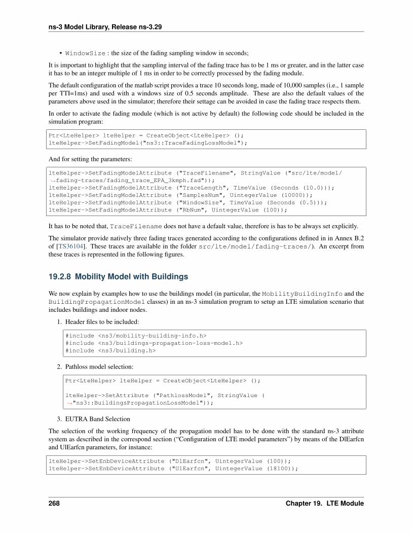
ns-3 Model Library, Release ns-3.29
• WindowSize : the size of the fading sampling window in seconds;
It is important to highlight that the sampling interval of the fading trace has to be 1 ms or greater, and in the latter caseit has to be an integer multiple of 1 ms in order to be correctly processed by the fading module.
The default configuration of the matlab script provides a trace 10 seconds long, made of 10,000 samples (i.e., 1 sampleper TTI=1ms) and used with a windows size of 0.5 seconds amplitude. These are also the default values of theparameters above used in the simulator; therefore their settage can be avoided in case the fading trace respects them.
In order to activate the fading module (which is not active by default) the following code should be included in thesimulation program:
Ptr<LteHelper> lteHelper = CreateObject<LteHelper> ();lteHelper->SetFadingModel("ns3::TraceFadingLossModel");
And for setting the parameters:
lteHelper->SetFadingModelAttribute ("TraceFilename", StringValue ("src/lte/model/↪→fading-traces/fading_trace_EPA_3kmph.fad"));lteHelper->SetFadingModelAttribute ("TraceLength", TimeValue (Seconds (10.0)));lteHelper->SetFadingModelAttribute ("SamplesNum", UintegerValue (10000));lteHelper->SetFadingModelAttribute ("WindowSize", TimeValue (Seconds (0.5)));lteHelper->SetFadingModelAttribute ("RbNum", UintegerValue (100));
It has to be noted that, TraceFilename does not have a default value, therefore is has to be always set explicitly.
The simulator provide natively three fading traces generated according to the configurations defined in in Annex B.2of [TS36104]. These traces are available in the folder src/lte/model/fading-traces/). An excerpt fromthese traces is represented in the following figures.
19.2.8 Mobility Model with Buildings
We now explain by examples how to use the buildings model (in particular, the MobilityBuildingInfo and theBuildingPropagationModel classes) in an ns-3 simulation program to setup an LTE simulation scenario thatincludes buildings and indoor nodes.
1. Header files to be included:
#include <ns3/mobility-building-info.h>#include <ns3/buildings-propagation-loss-model.h>#include <ns3/building.h>
2. Pathloss model selection:
Ptr<LteHelper> lteHelper = CreateObject<LteHelper> ();
lteHelper->SetAttribute ("PathlossModel", StringValue (↪→"ns3::BuildingsPropagationLossModel"));
3. EUTRA Band Selection
The selection of the working frequency of the propagation model has to be done with the standard ns-3 attributesystem as described in the correspond section (“Configuration of LTE model parameters”) by means of the DlEarfcnand UlEarfcn parameters, for instance:
lteHelper->SetEnbDeviceAttribute ("DlEarfcn", UintegerValue (100));lteHelper->SetEnbDeviceAttribute ("UlEarfcn", UintegerValue (18100));
268 Chapter 19. LTE Module

ns-3 Model Library, Release ns-3.29
020
4060
80100
0
50
100−50
−40
−30
−20
−10
0
10
time [ms]RB index
Am
plit
ude [dB
]
Fig. 68: Excerpt of the fading trace included in the simulator for a pedestrian scenario (speed of 3 kmph).
19.2. User Documentation 269
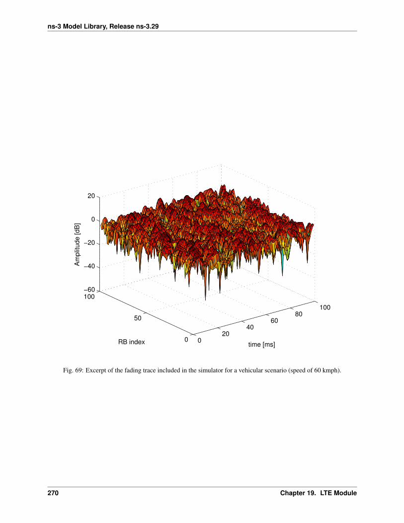
ns-3 Model Library, Release ns-3.29
020
4060
80100
0
50
100−60
−40
−20
0
20
time [ms]RB index
Am
plit
ude [dB
]
Fig. 69: Excerpt of the fading trace included in the simulator for a vehicular scenario (speed of 60 kmph).
270 Chapter 19. LTE Module
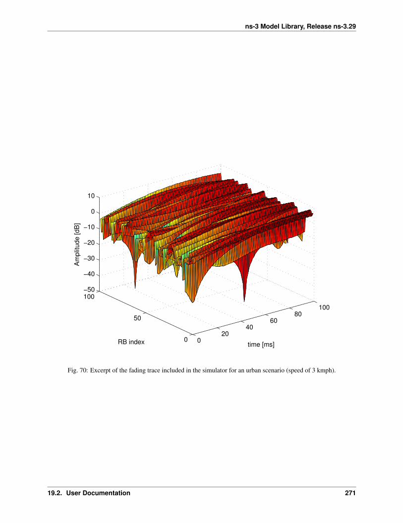
ns-3 Model Library, Release ns-3.29
020
4060
80100
0
50
100−50
−40
−30
−20
−10
0
10
time [ms]RB index
Am
plit
ude [dB
]
Fig. 70: Excerpt of the fading trace included in the simulator for an urban scenario (speed of 3 kmph).
19.2. User Documentation 271
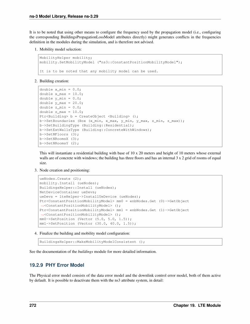
ns-3 Model Library, Release ns-3.29
It is to be noted that using other means to configure the frequency used by the propagation model (i.e., configuringthe corresponding BuildingsPropagationLossModel attributes directly) might generates conflicts in the frequenciesdefinition in the modules during the simulation, and is therefore not advised.
1. Mobility model selection:
MobilityHelper mobility;mobility.SetMobilityModel ("ns3::ConstantPositionMobilityModel");
It is to be noted that any mobility model can be used.
2. Building creation:
double x_min = 0.0;double x_max = 10.0;double y_min = 0.0;double y_max = 20.0;double z_min = 0.0;double z_max = 10.0;Ptr<Building> b = CreateObject <Building> ();b->SetBoundaries (Box (x_min, x_max, y_min, y_max, z_min, z_max));b->SetBuildingType (Building::Residential);b->SetExtWallsType (Building::ConcreteWithWindows);b->SetNFloors (3);b->SetNRoomsX (3);b->SetNRoomsY (2);
This will instantiate a residential building with base of 10 x 20 meters and height of 10 meters whose externalwalls are of concrete with windows; the building has three floors and has an internal 3 x 2 grid of rooms of equalsize.
3. Node creation and positioning:
ueNodes.Create (2);mobility.Install (ueNodes);BuildingsHelper::Install (ueNodes);NetDeviceContainer ueDevs;ueDevs = lteHelper->InstallUeDevice (ueNodes);Ptr<ConstantPositionMobilityModel> mm0 = enbNodes.Get (0)->GetObject↪→<ConstantPositionMobilityModel> ();Ptr<ConstantPositionMobilityModel> mm1 = enbNodes.Get (1)->GetObject↪→<ConstantPositionMobilityModel> ();mm0->SetPosition (Vector (5.0, 5.0, 1.5));mm1->SetPosition (Vector (30.0, 40.0, 1.5));
4. Finalize the building and mobility model configuration:
BuildingsHelper::MakeMobilityModelConsistent ();
See the documentation of the buildings module for more detailed information.
19.2.9 PHY Error Model
The Physical error model consists of the data error model and the downlink control error model, both of them activeby default. It is possible to deactivate them with the ns3 attribute system, in detail:
272 Chapter 19. LTE Module

ns-3 Model Library, Release ns-3.29
Config::SetDefault ("ns3::LteSpectrumPhy::CtrlErrorModelEnabled", BooleanValue↪→(false));Config::SetDefault ("ns3::LteSpectrumPhy::DataErrorModelEnabled", BooleanValue↪→(false));
19.2.10 MIMO Model
Is this subsection we illustrate how to configure the MIMO parameters. LTE defines 7 types of transmission modes:
• Transmission Mode 1: SISO.
• Transmission Mode 2: MIMO Tx Diversity.
• Transmission Mode 3: MIMO Spatial Multiplexity Open Loop.
• Transmission Mode 4: MIMO Spatial Multiplexity Closed Loop.
• Transmission Mode 5: MIMO Multi-User.
• Transmission Mode 6: Closer loop single layer precoding.
• Transmission Mode 7: Single antenna port 5.
According to model implemented, the simulator includes the first three transmission modes types. The default oneis the Transmission Mode 1 (SISO). In order to change the default Transmission Mode to be used, the attributeDefaultTransmissionMode of the LteEnbRrc can be used, as shown in the following:
Config::SetDefault ("ns3::LteEnbRrc::DefaultTransmissionMode", UintegerValue (0)); //↪→SISOConfig::SetDefault ("ns3::LteEnbRrc::DefaultTransmissionMode", UintegerValue (1)); //↪→MIMO Tx diversity (1 layer)Config::SetDefault ("ns3::LteEnbRrc::DefaultTransmissionMode", UintegerValue (2)); //↪→MIMO Spatial Multiplexity (2 layers)
For changing the transmission mode of a certain user during the simulation a specific interface has been implementedin both standard schedulers:
void TransmissionModeConfigurationUpdate (uint16_t rnti, uint8_t txMode);
This method can be used both for developing transmission mode decision engine (i.e., for optimizing the transmissionmode according to channel condition and/or user’s requirements) and for manual switching from simulation script. Inthe latter case, the switching can be done as shown in the following:
Ptr<LteEnbNetDevice> lteEnbDev = enbDevs.Get (0)->GetObject<LteEnbNetDevice> ();PointerValue ptrval;enbNetDev->GetAttribute ("FfMacScheduler", ptrval);Ptr<RrFfMacScheduler> rrsched = ptrval.Get<RrFfMacScheduler> ();Simulator::Schedule (Seconds (0.2), &↪→RrFfMacScheduler::TransmissionModeConfigurationUpdate, rrsched, rnti, 1);
Finally, the model implemented can be reconfigured according to different MIMO models by updating the gain values(the only constraints is that the gain has to be constant during simulation run-time and common for the layers). Thegain of each Transmission Mode can be changed according to the standard ns3 attribute system, where the attributesare: TxMode1Gain, TxMode2Gain, TxMode3Gain, TxMode4Gain, TxMode5Gain, TxMode6Gain andTxMode7Gain. By default only TxMode1Gain, TxMode2Gain and TxMode3Gain have a meaningful value,that are the ones derived by _[CatreuxMIMO] (i.e., respectively 0.0, 4.2 and -2.8 dB).
19.2. User Documentation 273

ns-3 Model Library, Release ns-3.29
19.2.11 Use of AntennaModel
We now show how associate a particular AntennaModel with an eNB device in order to model a sector of a macroeNB. For this purpose, it is convenient to use the CosineAntennaModel provided by the ns-3 antenna module. Theconfiguration of the eNB is to be done via the LteHelper instance right before the creation of the EnbNetDevice,as shown in the following:
lteHelper->SetEnbAntennaModelType ("ns3::CosineAntennaModel");lteHelper->SetEnbAntennaModelAttribute ("Orientation", DoubleValue (0));lteHelper->SetEnbAntennaModelAttribute ("Beamwidth", DoubleValue (60);lteHelper->SetEnbAntennaModelAttribute ("MaxGain", DoubleValue (0.0));
the above code will generate an antenna model with a 60 degrees beamwidth pointing along the X axis. The orientationis measured in degrees from the X axis, e.g., an orientation of 90 would point along the Y axis, and an orientationof -90 would point in the negative direction along the Y axis. The beamwidth is the -3 dB beamwidth, e.g, for a 60degree beamwidth the antenna gain at an angle of ±30 degrees from the direction of orientation is -3 dB.
To create a multi-sector site, you need to create different ns-3 nodes placed at the same position, and to configureseparate EnbNetDevice with different antenna orientations to be installed on each node.
19.2.12 Radio Environment Maps
By using the class RadioEnvironmentMapHelper it is possible to output to a file a Radio Environment Map(REM), i.e., a uniform 2D grid of values that represent the Signal-to-noise ratio in the downlink with respect to theeNB that has the strongest signal at each point. It is possible to specify if REM should be generated for data or controlchannel. Also user can set the RbId, for which REM will be generated. Default RbId is -1, what means that REM willgenerated with averaged Signal-to-noise ratio from all RBs.
To do this, you just need to add the following code to your simulation program towards the end, right before the callto Simulator::Run ():
Ptr<RadioEnvironmentMapHelper> remHelper = CreateObject<RadioEnvironmentMapHelper> ();remHelper->SetAttribute ("ChannelPath", StringValue ("/ChannelList/0"));remHelper->SetAttribute ("OutputFile", StringValue ("rem.out"));remHelper->SetAttribute ("XMin", DoubleValue (-400.0));remHelper->SetAttribute ("XMax", DoubleValue (400.0));remHelper->SetAttribute ("XRes", UintegerValue (100));remHelper->SetAttribute ("YMin", DoubleValue (-300.0));remHelper->SetAttribute ("YMax", DoubleValue (300.0));remHelper->SetAttribute ("YRes", UintegerValue (75));remHelper->SetAttribute ("Z", DoubleValue (0.0));remHelper->SetAttribute ("UseDataChannel", BooleanValue (true));remHelper->SetAttribute ("RbId", IntegerValue (10));remHelper->Install ();
By configuring the attributes of the RadioEnvironmentMapHelper object as shown above, you can tune theparameters of the REM to be generated. Note that each RadioEnvironmentMapHelper instance can generateonly one REM; if you want to generate more REMs, you need to create one separate instance for each REM.
Note that the REM generation is very demanding, in particular:
• the run-time memory consumption is approximately 5KB per pixel. For example, a REM with a resolutionof 500x500 would need about 1.25 GB of memory, and a resolution of 1000x1000 would need needs about5 GB (too much for a regular PC at the time of this writing). To overcome this issue, the REM is generatedat successive steps, with each step evaluating at most a number of pixels determined by the value of the theattribute RadioEnvironmentMapHelper::MaxPointsPerIteration.
274 Chapter 19. LTE Module
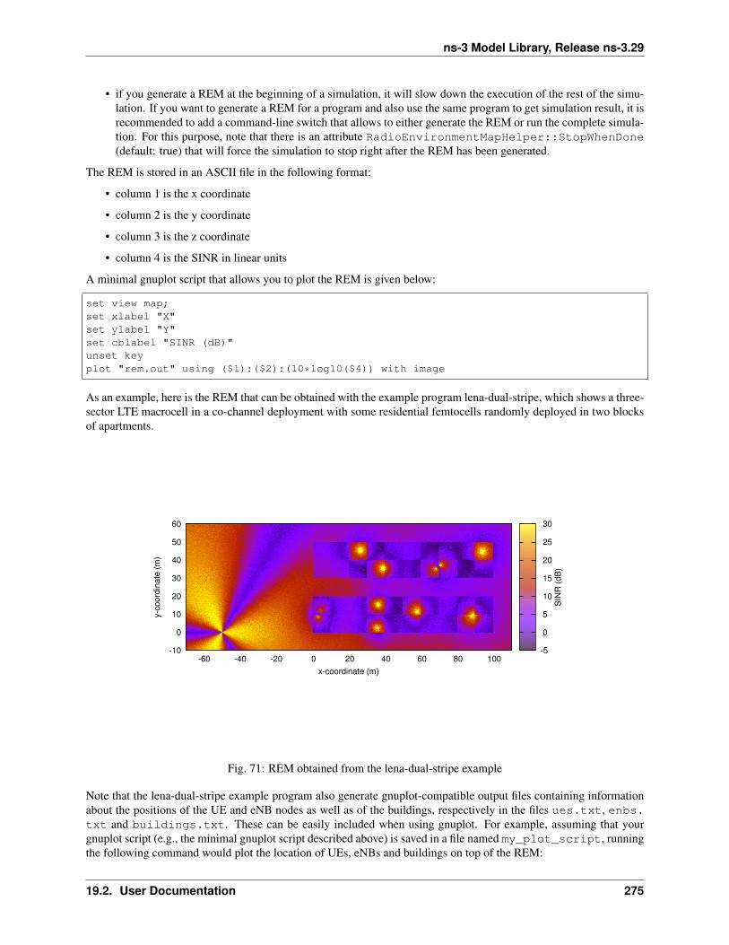
ns-3 Model Library, Release ns-3.29
• if you generate a REM at the beginning of a simulation, it will slow down the execution of the rest of the simu-lation. If you want to generate a REM for a program and also use the same program to get simulation result, it isrecommended to add a command-line switch that allows to either generate the REM or run the complete simula-tion. For this purpose, note that there is an attribute RadioEnvironmentMapHelper::StopWhenDone(default: true) that will force the simulation to stop right after the REM has been generated.
The REM is stored in an ASCII file in the following format:
• column 1 is the x coordinate
• column 2 is the y coordinate
• column 3 is the z coordinate
• column 4 is the SINR in linear units
A minimal gnuplot script that allows you to plot the REM is given below:
set view map;set xlabel "X"set ylabel "Y"set cblabel "SINR (dB)"unset keyplot "rem.out" using ($1):($2):(10*log10($4)) with image
As an example, here is the REM that can be obtained with the example program lena-dual-stripe, which shows a three-sector LTE macrocell in a co-channel deployment with some residential femtocells randomly deployed in two blocksof apartments.
-10
0
10
20
30
40
50
60
-60 -40 -20 0 20 40 60 80 100
y-c
oord
ina
te (
m)
x-coordinate (m)
-5
0
5
10
15
20
25
30
SIN
R (
dB
)
Fig. 71: REM obtained from the lena-dual-stripe example
Note that the lena-dual-stripe example program also generate gnuplot-compatible output files containing informationabout the positions of the UE and eNB nodes as well as of the buildings, respectively in the files ues.txt, enbs.txt and buildings.txt. These can be easily included when using gnuplot. For example, assuming that yourgnuplot script (e.g., the minimal gnuplot script described above) is saved in a file named my_plot_script, runningthe following command would plot the location of UEs, eNBs and buildings on top of the REM:
19.2. User Documentation 275

ns-3 Model Library, Release ns-3.29
gnuplot -p enbs.txt ues.txt buildings.txt my_plot_script
19.2.13 AMC Model and CQI Calculation
The simulator provides two possible schemes for what concerns the selection of the MCSs and correspondingly thegeneration of the CQIs. The first one is based on the GSoC module [Piro2011] and works per RB basis. This modelcan be activated with the ns3 attribute system, as presented in the following:
Config::SetDefault ("ns3::LteAmc::AmcModel", EnumValue (LteAmc::PiroEW2010));
While, the solution based on the physical error model can be controlled with:
Config::SetDefault ("ns3::LteAmc::AmcModel", EnumValue (LteAmc::MiErrorModel));
Finally, the required efficiency of the PiroEW2010 AMC module can be tuned thanks to the Ber attribute (), forinstance:
Config::SetDefault ("ns3::LteAmc::Ber", DoubleValue (0.00005));
19.2.14 Evolved Packet Core (EPC)
We now explain how to write a simulation program that allows to simulate the EPC in addition to the LTE radio accessnetwork. The use of EPC allows to use IPv4 and IPv6 networking with LTE devices. In other words, you will be ableto use the regular ns-3 applications and sockets over IPv4 and IPv6 over LTE, and also to connect an LTE network toany other IPv4 and IPv6 network you might have in your simulation.
First of all, in addition to LteHelper that we already introduced in Basic simulation program, you need to use anadditional EpcHelper class, which will take care of creating the EPC entities and network topology. Note that youcan’t use EpcHelper directly, as it is an abstract base class; instead, you need to use one of its child classes, whichprovide different EPC topology implementations. In this example we will consider PointToPointEpcHelper,which implements an EPC based on point-to-point links. To use it, you need first to insert this code in your simulationprogram:
Ptr<LteHelper> lteHelper = CreateObject<LteHelper> ();Ptr<PointToPointEpcHelper> epcHelper = CreateObject<PointToPointEpcHelper> ();
Then, you need to tell the LTE helper that the EPC will be used:
lteHelper->SetEpcHelper (epcHelper);
the above step is necessary so that the LTE helper will trigger the appropriate EPC configuration in correspondencewith some important configuration, such as when a new eNB or UE is added to the simulation, or an EPS bearer iscreated. The EPC helper will automatically take care of the necessary setup, such as S1 link creation and S1 bearersetup. All this will be done without the intervention of the user.
Calling lteHelper->SetEpcHelper (epcHelper) enables the use of EPC, and has the side effect that anynew LteEnbRrc that is created will have the EpsBearerToRlcMapping attribute set to RLC_UM_ALWAYSinstead of RLC_SM_ALWAYS if the latter was the default; otherwise, the attribute won’t be changed (e.g., if youchanged the default to RLC_AM_ALWAYS, it won’t be touched).
It is to be noted that the EpcHelper will also automatically create the PGW node and configure it so that it canproperly handle traffic from/to the LTE radio access network. Still, you need to add some explicit code to connectthe PGW to other IPv4/IPv6 networks (e.g., the internet, another EPC). Here is a very simple example about how toconnect a single remote host (IPv4 type) to the PGW via a point-to-point link:
276 Chapter 19. LTE Module

ns-3 Model Library, Release ns-3.29
Ptr<Node> pgw = epcHelper->GetPgwNode ();
// Create a single RemoteHostNodeContainer remoteHostContainer;remoteHostContainer.Create (1);Ptr<Node> remoteHost = remoteHostContainer.Get (0);InternetStackHelper internet;internet.Install (remoteHostContainer);
// Create the internetPointToPointHelper p2ph;p2ph.SetDeviceAttribute ("DataRate", DataRateValue (DataRate ("100Gb/s")));p2ph.SetDeviceAttribute ("Mtu", UintegerValue (1500));p2ph.SetChannelAttribute ("Delay", TimeValue (Seconds (0.010)));NetDeviceContainer internetDevices = p2ph.Install (pgw, remoteHost);Ipv4AddressHelper ipv4h;ipv4h.SetBase ("1.0.0.0", "255.0.0.0");Ipv4InterfaceContainer internetIpIfaces = ipv4h.Assign (internetDevices);// interface 0 is localhost, 1 is the p2p deviceIpv4Address remoteHostAddr = internetIpIfaces.GetAddress (1);
Ipv4StaticRoutingHelper ipv4RoutingHelper;Ptr<Ipv4StaticRouting> remoteHostStaticRouting = ipv4RoutingHelper.GetStaticRouting↪→(remoteHost->GetObject<Ipv4> ());remoteHostStaticRouting->AddNetworkRouteTo (epcHelper->GetEpcIpv4NetworkAddress (),↪→Ipv4Mask ("255.255.0.0"), 1);
Now, you should go on and create LTE eNBs and UEs as explained in the previous sections. You can of courseconfigure other LTE aspects such as pathloss and fading models. Right after you created the UEs, you should alsoconfigure them for IP networking. This is done as follows. We assume you have a container for UE and eNodeB nodeslike this:
NodeContainer ueNodes;NodeContainer enbNodes;
to configure an LTE-only simulation, you would then normally do something like this:
NetDeviceContainer ueLteDevs = lteHelper->InstallUeDevice (ueNodes);lteHelper->Attach (ueLteDevs, enbLteDevs.Get (0));
in order to configure the UEs for IP networking, you just need to additionally do like this:
// we install the IP stack on the UEsInternetStackHelper internet;internet.Install (ueNodes);
// assign IP address to UEsfor (uint32_t u = 0; u < ueNodes.GetN (); ++u)
{Ptr<Node> ue = ueNodes.Get (u);Ptr<NetDevice> ueLteDevice = ueLteDevs.Get (u);Ipv4InterfaceContainer ueIpIface = epcHelper->AssignUeIpv4Address
↪→(NetDeviceContainer (ueLteDevice));// set the default gateway for the UEPtr<Ipv4StaticRouting> ueStaticRouting = ipv4RoutingHelper.GetStaticRouting (ue->
↪→GetObject<Ipv4> ());
(continues on next page)
19.2. User Documentation 277
ns-3 Model Library, Release ns-3.29
(continued from previous page)
ueStaticRouting->SetDefaultRoute (epcHelper->GetUeDefaultGatewayAddress (), 1);}
The activation of bearers is done in a slightly different way with respect to what done for an LTE-only simulation.First, the method ActivateDataRadioBearer is not to be used when the EPC is used. Second, when EPC is used, thedefault EPS bearer will be activated automatically when you call LteHelper::Attach (). Third, if you want to setupdedicated EPS bearer, you can do so using the method LteHelper::ActivateDedicatedEpsBearer (). This method takesas a parameter the Traffic Flow Template (TFT), which is a struct that identifies the type of traffic that will be mappedto the dedicated EPS bearer. Here is an example for how to setup a dedicated bearer for an application at the UEcommunicating on port 1234:
Ptr<EpcTft> tft = Create<EpcTft> ();EpcTft::PacketFilter pf;pf.localPortStart = 1234;pf.localPortEnd = 1234;tft->Add (pf);lteHelper->ActivateDedicatedEpsBearer (ueLteDevs, EpsBearer (EpsBearer::NGBR_VIDEO_↪→TCP_DEFAULT), tft);
you can of course use custom EpsBearer and EpcTft configurations, please refer to the doxygen documentation forhow to do it.
Finally, you can install applications on the LTE UE nodes that communicate with remote applications over the internet.This is done following the usual ns-3 procedures. Following our simple example with a single remoteHost, here ishow to setup downlink communication, with an UdpClient application on the remote host, and a PacketSink on theLTE UE (using the same variable names of the previous code snippets)
uint16_t dlPort = 1234;PacketSinkHelper packetSinkHelper ("ns3::UdpSocketFactory",
InetSocketAddress (Ipv4Address::GetAny (),↪→dlPort));ApplicationContainer serverApps = packetSinkHelper.Install (ue);serverApps.Start (Seconds (0.01));UdpClientHelper client (ueIpIface.GetAddress (0), dlPort);ApplicationContainer clientApps = client.Install (remoteHost);clientApps.Start (Seconds (0.01));
That’s all! You can now start your simulation as usual:
Simulator::Stop (Seconds (10.0));Simulator::Run ();
19.2.15 Using the EPC with emulation mode
In the previous section we used PointToPoint links for the connection between the eNBs and the SGW (S1-U interface)and among eNBs (X2-U and X2-C interfaces). The LTE module supports using emulated links instead of PointToPointlinks. This is achieved by just replacing the creation of LteHelper and EpcHelper with the following code:
Ptr<LteHelper> lteHelper = CreateObject<LteHelper> ();Ptr<EmuEpcHelper> epcHelper = CreateObject<EmuEpcHelper> ();lteHelper->SetEpcHelper (epcHelper);epcHelper->Initialize ();
The attributes ns3::EmuEpcHelper::sgwDeviceName and ns3::EmuEpcHelper::enbDeviceNameare used to set the name of the devices used for transporting the S1-U, X2-U and X2-C interfaces at the SGW
278 Chapter 19. LTE Module
ns-3 Model Library, Release ns-3.29
and eNB, respectively. We will now show how this is done in an example where we execute the example programlena-simple-epc-emu using two virtual ethernet interfaces.
First of all we build ns-3 appropriately:
# configure./waf configure --enable-sudo --enable-modules=lte,fd-net-device --enable-examples
# build./waf
Then we setup two virtual ethernet interfaces, and start wireshark to look at the traffic going through:
# note: you need to be root
# create two paired veth devicesip link add name veth0 type veth peer name veth1ip link show
# enable promiscuous modeip link set veth0 promisc onip link set veth1 promisc on
# bring interfaces upip link set veth0 upip link set veth1 up
# start wireshark and capture on veth0wireshark &
We can now run the example program with the simulated clock:
./waf --run lena-simple-epc-emu --command="%s --↪→ns3::EmuEpcHelper::sgwDeviceName=veth0 --ns3::EmuEpcHelper::enbDeviceName=veth1"
Using wireshark, you should see ARP resolution first, then some GTP packets exchanged both in uplink and downlink.
The default setting of the example program is 1 eNB and 1UE. You can change this via command line parameters,e.g.:
./waf --run lena-simple-epc-emu --command="%s --↪→ns3::EmuEpcHelper::sgwDeviceName=veth0 --ns3::EmuEpcHelper::enbDeviceName=veth1 --↪→nEnbs=2 --nUesPerEnb=2"
To get a list of the available parameters:
./waf --run lena-simple-epc-emu --command="%s --PrintHelp"
To run with the realtime clock: it turns out that the default debug build is too slow for realtime. Softening the real timeconstraints with the BestEffort mode is not a good idea: something can go wrong (e.g., ARP can fail) and, if so, youwon’t get any data packets out. So you need a decent hardware and the optimized build with statically linked modules:
./waf configure -d optimized --enable-static --enable-modules=lte --enable-examples --↪→enable-sudo
Then run the example program like this:
./waf --run lena-simple-epc-emu --command="%s --↪→ns3::EmuEpcHelper::sgwDeviceName=veth0 --ns3::EmuEpcHelper::enbDeviceName=veth1 --↪→simulatorImplementationType=ns3::RealtimeSimulatorImpl --↪→ns3::RealtimeSimulatorImpl::SynchronizationMode=HardLimit"
(continues on next page)
19.2. User Documentation 279
ns-3 Model Library, Release ns-3.29
(continued from previous page)
note the HardLimit setting, which will cause the program to terminate if it cannot keep up with real time.
The approach described in this section can be used with any type of net device. For instance, [Baldo2014] describeshow it was used to run an emulated LTE-EPC network over a real multi-layer packet-optical transport network.
19.2.16 Network Attachment
As shown in the basic example in section Basic simulation program, attaching a UE to an eNodeB is done by callingLteHelper::Attach function.
There are 2 possible ways of network attachment. The first method is the “manual” one, while the second one has amore “automatic” sense on it. Each of them will be covered in this section.
Manual attachment
This method uses the LteHelper::Attach function mentioned above. It has been the only available networkattachment method in earlier versions of LTE module. It is typically invoked before the simulation begins:
lteHelper->Attach (ueDevs, enbDev); // attach one or more UEs to a single eNodeB
LteHelper::InstallEnbDevice and LteHelper::InstallUeDevice functions must have been calledbefore attaching. In an EPC-enabled simulation, it is also required to have IPv4/IPv6 properly pre-installed in the UE.
This method is very simple, but requires you to know exactly which UE belongs to to which eNodeB before thesimulation begins. This can be difficult when the UE initial position is randomly determined by the simulation script.
One may choose the distance between the UE and the eNodeB as a criterion for selecting the appropriate cell. It isquite simple (at least from the simulator’s point of view) and sometimes practical. But it is important to note thatsometimes distance does not make a single correct criterion. For instance, the eNodeB antenna directivity should beconsidered as well. Besides that, one should also take into account the channel condition, which might be fluctuatingif there is fading or shadowing in effect. In these kind of cases, network attachment should not be based on distancealone.
In real life, UE will automatically evaluate certain criteria and select the best cell to attach to, without manual inter-vention from the user. Obviously this is not the case in this LteHelper::Attach function. The other networkattachment method uses more “automatic” approach to network attachment, as will be described next.
Automatic attachment using Idle mode cell selection procedure
The strength of the received signal is the standard criterion used for selecting the best cell to attach to. The use of thiscriterion is implemented in the initial cell selection process, which can be invoked by calling another version of theLteHelper::Attach function, as shown below:
lteHelper->Attach (ueDevs); // attach one or more UEs to a strongest cell
The difference with the manual method is that the destination eNodeB is not specified. The procedure will find thebest cell for the UEs, based on several criteria, including the strength of the received signal (RSRP).
After the method is called, the UE will spend some time to measure the neighbouring cells, and then attempt to attachto the best one. More details can be found in section Initial Cell Selection of the Design Documentation.
It is important to note that this method only works in EPC-enabled simulations. LTE-only simulations must resort tomanual attachment method.
280 Chapter 19. LTE Module
ns-3 Model Library, Release ns-3.29
Closed Subscriber Group
An interesting use case of the initial cell selection process is to setup a simulation environment with Closed SubscriberGroup (CSG).
For example, a certain eNodeB, typically a smaller version such as femtocell, might belong to a private owner (e.g. ahousehold or business), allowing access only to some UEs which have been previously registered by the owner. TheeNodeB and the registered UEs altogether form a CSG.
The access restriction can be simulated by “labeling” the CSG members with the same CSG ID. This is done throughthe attributes in both eNodeB and UE, for example using the following LteHelper functions:
// label the following eNodeBs with CSG identity of 1 and CSG indication enabledlteHelper->SetEnbDeviceAttribute ("CsgId", UintegerValue (1));lteHelper->SetEnbDeviceAttribute ("CsgIndication", BooleanValue (true));
// label one or more UEs with CSG identity of 1lteHelper->SetUeDeviceAttribute ("CsgId", UintegerValue (1));
// install the eNodeBs and UEsNetDeviceContainer csgEnbDevs = lteHelper->InstallEnbDevice (csgEnbNodes);NetDeviceContainer csgUeDevs = lteHelper->InstallUeDevice (csgUeNodes);
Then enable the initial cell selection procedure on the UEs:
lteHelper->Attach (csgUeDevs);
This is necessary because the CSG restriction only works with automatic method of network attachment, but not inthe manual method.
Note that setting the CSG indication of an eNodeB as false (the default value) will disable the restriction, i.e., any UEscan connect to this eNodeB.
19.2.17 Configure UE measurements
The active UE measurement configuration in a simulation is dictated by the selected so called “consumers”, such ashandover algorithm. Users may add their own configuration into action, and there are several ways to do so:
1. direct configuration in eNodeB RRC entity;
2. configuring existing handover algorithm; and
3. developing a new handover algorithm.
This section will cover the first method only. The second method is covered in Automatic handover trigger, while thethird method is explained in length in Section Handover algorithm of the Design Documentation.
Direct configuration in eNodeB RRC works as follows. User begins by creating a newLteRrcSap::ReportConfigEutra instance and pass it to the LteEnbRrc::AddUeMeasReportConfigfunction. The function will return the measId (measurement identity) which is a unique reference of the con-figuration in the eNodeB instance. This function must be called before the simulation begins. The measurementconfiguration will be active in all UEs attached to the eNodeB throughout the duration of the simulation. Dur-ing the simulation, user can capture the measurement reports produced by the UEs by listening to the existingLteEnbRrc::RecvMeasurementReport trace source.
The structure ReportConfigEutra is in accord with 3GPP specification. Definition of the structure and each memberfield can be found in Section 6.3.5 of [TS36331].
The code sample below configures Event A1 RSRP measurement to every eNodeB within the container devs:
19.2. User Documentation 281

ns-3 Model Library, Release ns-3.29
LteRrcSap::ReportConfigEutra config;config.eventId = LteRrcSap::ReportConfigEutra::EVENT_A1;config.threshold1.choice = LteRrcSap::ThresholdEutra::THRESHOLD_RSRP;config.threshold1.range = 41;config.triggerQuantity = LteRrcSap::ReportConfigEutra::RSRP;config.reportInterval = LteRrcSap::ReportConfigEutra::MS480;
std::vector<uint8_t> measIdList;
NetDeviceContainer::Iterator it;for (it = devs.Begin (); it != devs.End (); it++){
Ptr<NetDevice> dev = *it;Ptr<LteEnbNetDevice> enbDev = dev->GetObject<LteEnbNetDevice> ();Ptr<LteEnbRrc> enbRrc = enbDev->GetRrc ();
uint8_t measId = enbRrc->AddUeMeasReportConfig (config);measIdList.push_back (measId); // remember the measId created
enbRrc->TraceConnect ("RecvMeasurementReport","context",MakeCallback (&RecvMeasurementReportCallback));
}
Note that thresholds are expressed as range. In the example above, the range 41 for RSRP corresponds to -100 dBm. The conversion from and to the range format is due to Section 9.1.4 and 9.1.7 of [TS36133]. TheEutranMeasurementMapping class has several static functions that can be used for this purpose.
The corresponding callback function would have a definition similar as below:
voidRecvMeasurementReportCallback (std::string context,
uint64_t imsi,uint16_t cellId,uint16_t rnti,LteRrcSap::MeasurementReport measReport);
This method will register the callback function as a consumer of UE measurements. In the case where there aremore than one consumers in the simulation (e.g. handover algorithm), the measurements intended for other con-sumers will also be captured by this callback function. Users may utilize the the measId field, contained within theLteRrcSap::MeasurementReport argument of the callback function, to tell which measurement configurationhas triggered the report.
In general, this mechanism prevents one consumer to unknowingly intervene with another consumer’s reporting con-figuration.
Note that only the reporting configuration part (i.e. LteRrcSap::ReportConfigEutra) of the UE measure-ments parameter is open for consumers to configure, while the other parts are kept hidden. The intra-frequencylimitation is the main motivation behind this API implementation decision:
• there is only one, unambiguous and definitive measurement object, thus there is no need to configure it;
• measurement identities are kept hidden because of the fact that there is one-to-one mapping between reportingconfiguration and measurement identity, thus a new measurement identity is set up automatically when a newreporting configuration is created;
• quantity configuration is configured elsewhere, see Performing measurements; and
• measurement gaps are not supported, because it is only applicable for inter-frequency settings;
282 Chapter 19. LTE Module

ns-3 Model Library, Release ns-3.29
19.2.18 X2-based handover
As defined by 3GPP, handover is a procedure for changing the serving cell of a UE in CONNECTED mode. The twoeNodeBs involved in the process are typically called the source eNodeB and the target eNodeB.
In order to enable the execution of X2-based handover in simulation, there are two requirements that must be met.Firstly, EPC must be enabled in the simulation (see Evolved Packet Core (EPC)).
Secondly, an X2 interface must be configured between the two eNodeBs, which needs to be done explicitly within thesimulation program:
lteHelper->AddX2Interface (enbNodes);
where enbNodes is a NodeContainer that contains the two eNodeBs between which the X2 interface is to beconfigured. If the container has more than two eNodeBs, the function will create an X2 interface between every pairof eNodeBs in the container.
Lastly, the target eNodeB must be configured as “open” to X2 HANDOVER REQUEST. Every eNodeB is openby default, so no extra instruction is needed in most cases. However, users may set the eNodeB to “closed” bysetting the boolean attribute LteEnbRrc::AdmitHandoverRequest to false. As an example, you can run thelena-x2-handover program and setting the attribute in this way:
NS_LOG=EpcX2:LteEnbRrc ./waf --run lena-x2-handover --command="%s --↪→ns3::LteEnbRrc::AdmitHandoverRequest=false"
After the above three requirements are fulfilled, the handover procedure can be triggered manually or automatically.Each will be presented in the following subsections.
Manual handover trigger
Handover event can be triggered “manually” within the simulation program by scheduling an explicit handover event.The LteHelper object provides a convenient method for the scheduling of a handover event. As an example, letus assume that ueLteDevs is a NetDeviceContainer that contains the UE that is to be handed over, and thatenbLteDevs is another NetDeviceContainer that contains the source and the target eNB. Then, a handover at0.1s can be scheduled like this:
lteHelper->HandoverRequest (Seconds (0.100),ueLteDevs.Get (0),enbLteDevs.Get (0),enbLteDevs.Get (1));
Note that the UE needs to be already connected to the source eNB, otherwise the simulation will terminate with anerror message.
For an example with full source code, please refer to the lena-x2-handover example program.
Automatic handover trigger
Handover procedure can also be triggered “automatically” by the serving eNodeB of the UE. The logic behind thetrigger depends on the handover algorithm currently active in the eNodeB RRC entity. Users may select and configurethe handover algorithm that will be used in the simulation, which will be explained shortly in this section. Users mayalso opt to write their own implementation of handover algorithm, as described in Section Handover algorithm of theDesign Documentation.
Selecting a handover algorithm is done via the LteHelper object and its SetHandoverAlgorithmTypemethodas shown below:
19.2. User Documentation 283
ns-3 Model Library, Release ns-3.29
Ptr<LteHelper> lteHelper = CreateObject<LteHelper> ();lteHelper->SetHandoverAlgorithmType ("ns3::A2A4RsrqHandoverAlgorithm");
The selected handover algorithm may also provide several configurable attributes, which can be set as follows:
lteHelper->SetHandoverAlgorithmAttribute ("ServingCellThreshold",UintegerValue (30));
lteHelper->SetHandoverAlgorithmAttribute ("NeighbourCellOffset",UintegerValue (1));
Three options of handover algorithm are included in the LTE module. The A2-A4-RSRQ handover algorithm (namedas ns3::A2A4RsrqHandoverAlgorithm) is the default option, and the usage has already been shown above.
Another option is the strongest cell handover algorithm (named as ns3::A3RsrpHandoverAlgorithm), whichcan be selected and configured by the following code:
lteHelper->SetHandoverAlgorithmType ("ns3::A3RsrpHandoverAlgorithm");lteHelper->SetHandoverAlgorithmAttribute ("Hysteresis",
DoubleValue (3.0));lteHelper->SetHandoverAlgorithmAttribute ("TimeToTrigger",
TimeValue (MilliSeconds (256)));
The last option is a special one, called the no-op handover algorithm, which basically disables automatic handovertrigger. This is useful for example in cases where manual handover trigger need an exclusive control of all handoverdecision. It does not have any configurable attributes. The usage is as follows:
lteHelper->SetHandoverAlgorithmType ("ns3::NoOpHandoverAlgorithm");
For more information on each handover algorithm’s decision policy and their attributes, please refer to their respectivesubsections in Section Handover algorithm of the Design Documentation.
Finally, the InstallEnbDevice function of LteHelper will instantiate one instance of the selected handoveralgorithm for each eNodeB device. In other words, make sure to select the right handover algorithm before finalizingit in the following line of code:
NetDeviceContainer enbLteDevs = lteHelper->InstallEnbDevice (enbNodes);
Example with full source code of using automatic handover trigger can be found in thelena-x2-handover-measures example program.
Tuning simulation with handover
As mentioned in the Design Documentation, the current implementation of handover model may produce unpredictedbehaviour when handover failure occurs. This subsection will focus on the steps that should be taken into account byusers if they plan to use handover in their simulations.
The major cause of handover failure that we will tackle is the error in transmitting handover-related signaling mes-sages during the execution of a handover procedure. As apparent from the Figure Sequence diagram of the X2-basedhandover from the Design Documentation, there are many of them and they use different interfaces and protocols.For the sake of simplicity, we can safely assume that the X2 interface (between the source eNodeB and the targeteNodeB) and the S1 interface (between the target eNodeB and the SGW/PGW) are quite stable. Therefore we willfocus our attention to the RRC protocol (between the UE and the eNodeBs) and the Random Access procedure, whichare normally transmitted through the air and susceptible to degradation of channel condition.
A general tips to reduce transmission error is to ensure high enough SINR level in every UE. This can be done by aproper planning of the network topology that minimizes network coverage hole. If the topology has a known coveragehole, then the UE should be configured not to venture to that area.
284 Chapter 19. LTE Module

ns-3 Model Library, Release ns-3.29
Another approach to keep in mind is to avoid too-late handovers. In other words, handover should happen before theUE’s SINR becomes too low, otherwise the UE may fail to receive the handover command from the source eNodeB.Handover algorithms have the means to control how early or late a handover decision is made. For example, A2-A4-RSRQ handover algorithm can be configured with a higher threshold to make it decide a handover earlier. Similarly,smaller hysteresis and/or shorter time-to-trigger in the strongest cell handover algorithm typically results in earlierhandovers. In order to find the right values for these parameters, one of the factors that should be considered is the UEmovement speed. Generally, a faster moving UE requires the handover to be executed earlier. Some research workhave suggested recommended values, such as in [Lee2010].
The above tips should be enough in normal simulation uses, but in the case some special needs arise then an extrememeasure can be taken into consideration. For instance, users may consider disabling the channel error models. Thiswill ensure that all handover-related signaling messages will be transmitted successfully, regardless of distance andchannel condition. However, it will also affect all other data or control packets not related to handover, which may bean unwanted side effect. Otherwise, it can be done as follows:
Config::SetDefault ("ns3::LteSpectrumPhy::CtrlErrorModelEnabled", BooleanValue↪→(false));Config::SetDefault ("ns3::LteSpectrumPhy::DataErrorModelEnabled", BooleanValue↪→(false));
By using the above code, we disable the error model in both control and data channels and in both directions (downlinkand uplink). This is necessary because handover-related signaling messages are transmitted using these channels. Anexception is when the simulation uses the ideal RRC protocol. In this case, only the Random Access procedure is leftto be considered. The procedure consists of control messages, therefore we only need to disable the control channel’serror model.
Handover traces
The RRC model, in particular the LteEnbRrc and LteUeRrc objects, provide some useful traces which can behooked up to some custom functions so that they are called upon start and end of the handover execution phase at boththe UE and eNB side. As an example, in your simulation program you can declare the following methods:
voidNotifyHandoverStartUe (std::string context,
uint64_t imsi,uint16_t cellId,uint16_t rnti,uint16_t targetCellId)
{std::cout << Simulator::Now ().GetSeconds () << " " << context
<< " UE IMSI " << imsi<< ": previously connected to CellId " << cellId<< " with RNTI " << rnti<< ", doing handover to CellId " << targetCellId<< std::endl;
}
voidNotifyHandoverEndOkUe (std::string context,
uint64_t imsi,uint16_t cellId,uint16_t rnti)
{std::cout << Simulator::Now ().GetSeconds () << " " << context
<< " UE IMSI " << imsi<< ": successful handover to CellId " << cellId
(continues on next page)
19.2. User Documentation 285
ns-3 Model Library, Release ns-3.29
(continued from previous page)
<< " with RNTI " << rnti<< std::endl;
}
voidNotifyHandoverStartEnb (std::string context,
uint64_t imsi,uint16_t cellId,uint16_t rnti,uint16_t targetCellId)
{std::cout << Simulator::Now ().GetSeconds () << " " << context
<< " eNB CellId " << cellId<< ": start handover of UE with IMSI " << imsi<< " RNTI " << rnti<< " to CellId " << targetCellId<< std::endl;
}
voidNotifyHandoverEndOkEnb (std::string context,
uint64_t imsi,uint16_t cellId,uint16_t rnti)
{std::cout << Simulator::Now ().GetSeconds () << " " << context
<< " eNB CellId " << cellId<< ": completed handover of UE with IMSI " << imsi<< " RNTI " << rnti<< std::endl;
}
Then, you can hook up these methods to the corresponding trace sources like this:
Config::Connect ("/NodeList/*/DeviceList/*/LteEnbRrc/HandoverStart",MakeCallback (&NotifyHandoverStartEnb));
Config::Connect ("/NodeList/*/DeviceList/*/LteUeRrc/HandoverStart",MakeCallback (&NotifyHandoverStartUe));
Config::Connect ("/NodeList/*/DeviceList/*/LteEnbRrc/HandoverEndOk",MakeCallback (&NotifyHandoverEndOkEnb));
Config::Connect ("/NodeList/*/DeviceList/*/LteUeRrc/HandoverEndOk",MakeCallback (&NotifyHandoverEndOkUe));
The example program src/lte/examples/lena-x2-handover.cc illustrates how the all above instructionscan be integrated in a simulation program. You can run the program like this:
./waf --run lena-x2-handover
and it will output the messages printed by the custom handover trace hooks. In order additionally visualize somemeaningful logging information, you can run the program like this:
NS_LOG=LteEnbRrc:LteUeRrc:EpcX2 ./waf --run lena-x2-handover
286 Chapter 19. LTE Module
ns-3 Model Library, Release ns-3.29
19.2.19 Frequency Reuse Algorithms
In this section we will describe how to use Frequency Reuse Algorithms in eNb within LTE simulations. There are twopossible ways of configuration. The first approach is the “manual” one, it requires more parameters to be configured,but allow user to configure FR algorithm as he/she needs. The second approach is more “automatic”. It is veryconvenient, because is the same for each FR algorithm, so user can switch FR algorithm very quickly by changingonly type of FR algorithm. One drawback is that “automatic” approach uses only limited set of configurations for eachalgorithm, what make it less flexible, but is sufficient for most of cases.
These two approaches will be described more in following sub-section.
If user do not configure Frequency Reuse algorithm, default one (i.e. LteFrNoOpAlgorithm) is installed in eNb. It actsas if FR algorithm was disabled.
One thing that should be mentioned is that most of implemented FR algorithms work with cell bandwidth greater orequal than 15 RBs. This limitation is caused by requirement that at least three continuous RBs have to be assigned toUE for transmission.
Manual configuration
Frequency reuse algorithm can be configured “manually” within the simulation program by setting type of FR algo-rithm and all its attributes. Currently, seven FR algorithms are implemented:
• ns3::LteFrNoOpAlgorithm
• ns3::LteFrHardAlgorithm
• ns3::LteFrStrictAlgorithm
• ns3::LteFrSoftAlgorithm
• ns3::LteFfrSoftAlgorithm
• ns3::LteFfrEnhancedAlgorithm
• ns3::LteFfrDistributedAlgorithm
Selecting a FR algorithm is done via the LteHelper object and its SetFfrAlgorithmType method as shownbelow:
Ptr<LteHelper> lteHelper = CreateObject<LteHelper> ();lteHelper->SetFfrAlgorithmType ("ns3::LteFrHardAlgorithm");
Each implemented FR algorithm provide several configurable attributes. Users do not have to care about UL and DLbandwidth configuration, because it is done automatically during cell configuration. To change bandwidth for FRalgorithm, configure required values for LteEnbNetDevice:
uint8_t bandwidth = 100;lteHelper->SetEnbDeviceAttribute ("DlBandwidth", UintegerValue (bandwidth));lteHelper->SetEnbDeviceAttribute ("UlBandwidth", UintegerValue (bandwidth));
Now, each FR algorithms configuration will be described.
Hard Frequency Reuse Algorithm
As described in Section Hard Frequency Reuse of the Design Documentation ns3::LteFrHardAlgorithm usesone sub-band. To configure this sub-band user need to specify offset and bandwidth for DL and UL in number of RBs.
Hard Frequency Reuse Algorithm provides following attributes:
19.2. User Documentation 287
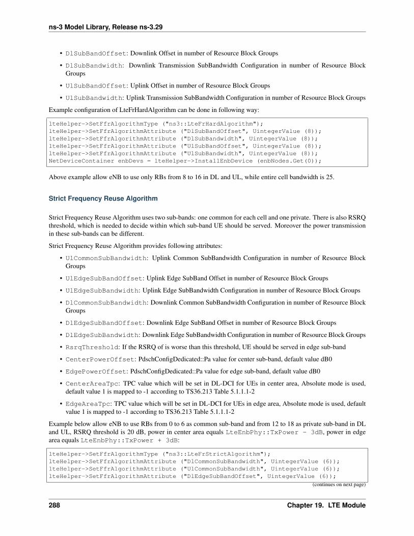
ns-3 Model Library, Release ns-3.29
• DlSubBandOffset: Downlink Offset in number of Resource Block Groups
• DlSubBandwidth: Downlink Transmission SubBandwidth Configuration in number of Resource BlockGroups
• UlSubBandOffset: Uplink Offset in number of Resource Block Groups
• UlSubBandwidth: Uplink Transmission SubBandwidth Configuration in number of Resource Block Groups
Example configuration of LteFrHardAlgorithm can be done in following way:
lteHelper->SetFfrAlgorithmType ("ns3::LteFrHardAlgorithm");lteHelper->SetFfrAlgorithmAttribute ("DlSubBandOffset", UintegerValue (8));lteHelper->SetFfrAlgorithmAttribute ("DlSubBandwidth", UintegerValue (8));lteHelper->SetFfrAlgorithmAttribute ("UlSubBandOffset", UintegerValue (8));lteHelper->SetFfrAlgorithmAttribute ("UlSubBandwidth", UintegerValue (8));NetDeviceContainer enbDevs = lteHelper->InstallEnbDevice (enbNodes.Get(0));
Above example allow eNB to use only RBs from 8 to 16 in DL and UL, while entire cell bandwidth is 25.
Strict Frequency Reuse Algorithm
Strict Frequency Reuse Algorithm uses two sub-bands: one common for each cell and one private. There is also RSRQthreshold, which is needed to decide within which sub-band UE should be served. Moreover the power transmissionin these sub-bands can be different.
Strict Frequency Reuse Algorithm provides following attributes:
• UlCommonSubBandwidth: Uplink Common SubBandwidth Configuration in number of Resource BlockGroups
• UlEdgeSubBandOffset: Uplink Edge SubBand Offset in number of Resource Block Groups
• UlEdgeSubBandwidth: Uplink Edge SubBandwidth Configuration in number of Resource Block Groups
• DlCommonSubBandwidth: Downlink Common SubBandwidth Configuration in number of Resource BlockGroups
• DlEdgeSubBandOffset: Downlink Edge SubBand Offset in number of Resource Block Groups
• DlEdgeSubBandwidth: Downlink Edge SubBandwidth Configuration in number of Resource Block Groups
• RsrqThreshold: If the RSRQ of is worse than this threshold, UE should be served in edge sub-band
• CenterPowerOffset: PdschConfigDedicated::Pa value for center sub-band, default value dB0
• EdgePowerOffset: PdschConfigDedicated::Pa value for edge sub-band, default value dB0
• CenterAreaTpc: TPC value which will be set in DL-DCI for UEs in center area, Absolute mode is used,default value 1 is mapped to -1 according to TS36.213 Table 5.1.1.1-2
• EdgeAreaTpc: TPC value which will be set in DL-DCI for UEs in edge area, Absolute mode is used, defaultvalue 1 is mapped to -1 according to TS36.213 Table 5.1.1.1-2
Example below allow eNB to use RBs from 0 to 6 as common sub-band and from 12 to 18 as private sub-band in DLand UL, RSRQ threshold is 20 dB, power in center area equals LteEnbPhy::TxPower - 3dB, power in edgearea equals LteEnbPhy::TxPower + 3dB:
lteHelper->SetFfrAlgorithmType ("ns3::LteFrStrictAlgorithm");lteHelper->SetFfrAlgorithmAttribute ("DlCommonSubBandwidth", UintegerValue (6));lteHelper->SetFfrAlgorithmAttribute ("UlCommonSubBandwidth", UintegerValue (6));lteHelper->SetFfrAlgorithmAttribute ("DlEdgeSubBandOffset", UintegerValue (6));
(continues on next page)
288 Chapter 19. LTE Module

ns-3 Model Library, Release ns-3.29
(continued from previous page)
lteHelper->SetFfrAlgorithmAttribute ("DlEdgeSubBandwidth", UintegerValue (6));lteHelper->SetFfrAlgorithmAttribute ("UlEdgeSubBandOffset", UintegerValue (6));lteHelper->SetFfrAlgorithmAttribute ("UlEdgeSubBandwidth", UintegerValue (6));lteHelper->SetFfrAlgorithmAttribute ("RsrqThreshold", UintegerValue (20));lteHelper->SetFfrAlgorithmAttribute ("CenterPowerOffset",
UintegerValue (LteRrcSap::PdschConfigDedicated::dB_3));lteHelper->SetFfrAlgorithmAttribute ("EdgePowerOffset",
UintegerValue (LteRrcSap::PdschConfigDedicated::dB3));lteHelper->SetFfrAlgorithmAttribute ("CenterAreaTpc", UintegerValue (1));lteHelper->SetFfrAlgorithmAttribute ("EdgeAreaTpc", UintegerValue (2));NetDeviceContainer enbDevs = lteHelper->InstallEnbDevice (enbNodes.Get(0));
Soft Frequency Reuse Algorithm
With Soft Frequency Reuse Algorithm, eNb uses entire cell bandwidth, but there are two sub-bands, within UEs areserved with different power level.
Soft Frequency Reuse Algorithm provides following attributes:
• UlEdgeSubBandOffset: Uplink Edge SubBand Offset in number of Resource Block Groups
• UlEdgeSubBandwidth: Uplink Edge SubBandwidth Configuration in number of Resource Block Groups
• DlEdgeSubBandOffset: Downlink Edge SubBand Offset in number of Resource Block Groups
• DlEdgeSubBandwidth: Downlink Edge SubBandwidth Configuration in number of Resource Block Groups
• AllowCenterUeUseEdgeSubBand: If true center UEs can receive on edge sub-band RBGs, otherwiseedge sub-band is allowed only for edge UEs, default value is true
• RsrqThreshold: If the RSRQ of is worse than this threshold, UE should be served in edge sub-band
• CenterPowerOffset: PdschConfigDedicated::Pa value for center sub-band, default value dB0
• EdgePowerOffset: PdschConfigDedicated::Pa value for edge sub-band, default value dB0
• CenterAreaTpc: TPC value which will be set in DL-DCI for UEs in center area, Absolute mode is used,default value 1 is mapped to -1 according to TS36.213 Table 5.1.1.1-2
• EdgeAreaTpc: TPC value which will be set in DL-DCI for UEs in edge area, Absolute mode is used, defaultvalue 1 is mapped to -1 according to TS36.213 Table 5.1.1.1-2
Example below configures RBs from 8 to 16 to be used by cell edge UEs and this sub-band is not available for cellcenter users. RSRQ threshold is 20 dB, power in center area equals LteEnbPhy::TxPower, power in edge areaequals LteEnbPhy::TxPower + 3dB:
lteHelper->SetFfrAlgorithmType ("ns3::LteFrSoftAlgorithm");lteHelper->SetFfrAlgorithmAttribute ("DlEdgeSubBandOffset", UintegerValue (8));lteHelper->SetFfrAlgorithmAttribute ("DlEdgeSubBandwidth", UintegerValue (8));lteHelper->SetFfrAlgorithmAttribute ("UlEdgeSubBandOffset", UintegerValue (8));lteHelper->SetFfrAlgorithmAttribute ("UlEdgeSubBandwidth", UintegerValue (8));lteHelper->SetFfrAlgorithmAttribute ("AllowCenterUeUseEdgeSubBand", BooleanValue↪→(false));lteHelper->SetFfrAlgorithmAttribute ("RsrqThreshold", UintegerValue (20));lteHelper->SetFfrAlgorithmAttribute ("CenterPowerOffset",
UintegerValue (LteRrcSap::PdschConfigDedicated::dB0));lteHelper->SetFfrAlgorithmAttribute ("EdgePowerOffset",
UintegerValue (LteRrcSap::PdschConfigDedicated::dB3));NetDeviceContainer enbDevs = lteHelper->InstallEnbDevice (enbNodes.Get(0));
19.2. User Documentation 289
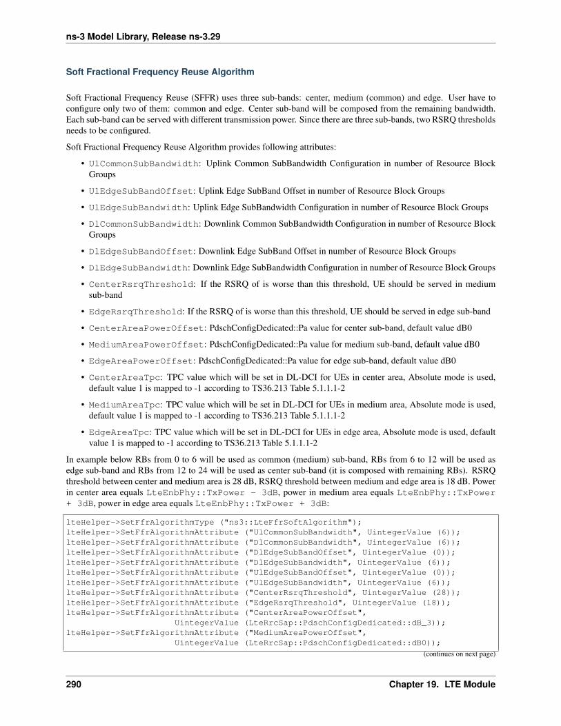
ns-3 Model Library, Release ns-3.29
Soft Fractional Frequency Reuse Algorithm
Soft Fractional Frequency Reuse (SFFR) uses three sub-bands: center, medium (common) and edge. User have toconfigure only two of them: common and edge. Center sub-band will be composed from the remaining bandwidth.Each sub-band can be served with different transmission power. Since there are three sub-bands, two RSRQ thresholdsneeds to be configured.
Soft Fractional Frequency Reuse Algorithm provides following attributes:
• UlCommonSubBandwidth: Uplink Common SubBandwidth Configuration in number of Resource BlockGroups
• UlEdgeSubBandOffset: Uplink Edge SubBand Offset in number of Resource Block Groups
• UlEdgeSubBandwidth: Uplink Edge SubBandwidth Configuration in number of Resource Block Groups
• DlCommonSubBandwidth: Downlink Common SubBandwidth Configuration in number of Resource BlockGroups
• DlEdgeSubBandOffset: Downlink Edge SubBand Offset in number of Resource Block Groups
• DlEdgeSubBandwidth: Downlink Edge SubBandwidth Configuration in number of Resource Block Groups
• CenterRsrqThreshold: If the RSRQ of is worse than this threshold, UE should be served in mediumsub-band
• EdgeRsrqThreshold: If the RSRQ of is worse than this threshold, UE should be served in edge sub-band
• CenterAreaPowerOffset: PdschConfigDedicated::Pa value for center sub-band, default value dB0
• MediumAreaPowerOffset: PdschConfigDedicated::Pa value for medium sub-band, default value dB0
• EdgeAreaPowerOffset: PdschConfigDedicated::Pa value for edge sub-band, default value dB0
• CenterAreaTpc: TPC value which will be set in DL-DCI for UEs in center area, Absolute mode is used,default value 1 is mapped to -1 according to TS36.213 Table 5.1.1.1-2
• MediumAreaTpc: TPC value which will be set in DL-DCI for UEs in medium area, Absolute mode is used,default value 1 is mapped to -1 according to TS36.213 Table 5.1.1.1-2
• EdgeAreaTpc: TPC value which will be set in DL-DCI for UEs in edge area, Absolute mode is used, defaultvalue 1 is mapped to -1 according to TS36.213 Table 5.1.1.1-2
In example below RBs from 0 to 6 will be used as common (medium) sub-band, RBs from 6 to 12 will be used asedge sub-band and RBs from 12 to 24 will be used as center sub-band (it is composed with remaining RBs). RSRQthreshold between center and medium area is 28 dB, RSRQ threshold between medium and edge area is 18 dB. Powerin center area equals LteEnbPhy::TxPower - 3dB, power in medium area equals LteEnbPhy::TxPower+ 3dB, power in edge area equals LteEnbPhy::TxPower + 3dB:
lteHelper->SetFfrAlgorithmType ("ns3::LteFfrSoftAlgorithm");lteHelper->SetFfrAlgorithmAttribute ("UlCommonSubBandwidth", UintegerValue (6));lteHelper->SetFfrAlgorithmAttribute ("DlCommonSubBandwidth", UintegerValue (6));lteHelper->SetFfrAlgorithmAttribute ("DlEdgeSubBandOffset", UintegerValue (0));lteHelper->SetFfrAlgorithmAttribute ("DlEdgeSubBandwidth", UintegerValue (6));lteHelper->SetFfrAlgorithmAttribute ("UlEdgeSubBandOffset", UintegerValue (0));lteHelper->SetFfrAlgorithmAttribute ("UlEdgeSubBandwidth", UintegerValue (6));lteHelper->SetFfrAlgorithmAttribute ("CenterRsrqThreshold", UintegerValue (28));lteHelper->SetFfrAlgorithmAttribute ("EdgeRsrqThreshold", UintegerValue (18));lteHelper->SetFfrAlgorithmAttribute ("CenterAreaPowerOffset",
UintegerValue (LteRrcSap::PdschConfigDedicated::dB_3));lteHelper->SetFfrAlgorithmAttribute ("MediumAreaPowerOffset",
UintegerValue (LteRrcSap::PdschConfigDedicated::dB0));
(continues on next page)
290 Chapter 19. LTE Module

ns-3 Model Library, Release ns-3.29
(continued from previous page)
lteHelper->SetFfrAlgorithmAttribute ("EdgeAreaPowerOffset",UintegerValue (LteRrcSap::PdschConfigDedicated::dB3));
NetDeviceContainer enbDevs = lteHelper->InstallEnbDevice (enbNodes.Get(0));
Enhanced Fractional Frequency Reuse Algorithm
Enhanced Fractional Frequency Reuse (EFFR) reserve part of system bandwidth for each cell (typically there are 3cell types and each one gets 1/3 of system bandwidth). Then part of this subbandwidth it used as Primary Segmentwith reuse factor 3 and as Secondary Segment with reuse factor 1. User has to configure (for DL and UL) offset of thecell subbandwidth in number of RB, number of RB which will be used as Primary Segment and number of RB whichwill be used as Secondary Segment. Primary Segment is used by cell at will, but RBs from Secondary Segment can beassigned to UE only is CQI feedback from this UE have higher value than configured CQI threshold. UE is consideredas edge UE when its RSRQ is lower than RsrqThreshold.
Since each eNb needs to know where are Primary and Secondary of other cell types, it will calculate them assumingconfiguration is the same for each cell and only subbandwidth offsets are different. So it is important to divide availablesystem bandwidth equally to each cell and apply the same configuration of Primary and Secondary Segments to them.
Enhanced Fractional Frequency Reuse Algorithm provides following attributes:
• UlSubBandOffset: Uplink SubBand Offset for this cell in number of Resource Block Groups
• UlReuse3SubBandwidth: Uplink Reuse 3 SubBandwidth Configuration in number of Resource BlockGroups
• UlReuse1SubBandwidth: Uplink Reuse 1 SubBandwidth Configuration in number of Resource BlockGroups
• DlSubBandOffset: Downlink SubBand Offset for this cell in number of Resource Block Groups
• DlReuse3SubBandwidth: Downlink Reuse 3 SubBandwidth Configuration in number of Resource BlockGroups
• DlReuse1SubBandwidth: Downlink Reuse 1 SubBandwidth Configuration in number of Resource BlockGroups
• RsrqThreshold: If the RSRQ of is worse than this threshold, UE should be served in edge sub-band
• CenterAreaPowerOffset: PdschConfigDedicated::Pa value for center sub-band, default value dB0
• EdgeAreaPowerOffset: PdschConfigDedicated::Pa value for edge sub-band, default value dB0
• DlCqiThreshold: If the DL-CQI for RBG of is higher than this threshold, transmission on RBG is possible
• UlCqiThreshold: If the UL-CQI for RBG of is higher than this threshold, transmission on RBG is possible
• CenterAreaTpc: TPC value which will be set in DL-DCI for UEs in center area, Absolute mode is used,default value 1 is mapped to -1 according to TS36.213 Table 5.1.1.1-2
• EdgeAreaTpc: TPC value which will be set in DL-DCI for UEs in edge area, Absolute mode is used, defaultvalue 1 is mapped to -1 according to TS36.213 Table 5.1.1.1-2
In example below offset in DL and UL is 0 RB, 4 RB will be used in Primary Segment and Secondary Segment. RSRQthreshold between center and edge area is 25 dB. DL and UL CQI thresholds are set to value of 10. Power in centerarea equals LteEnbPhy::TxPower - 6dB, power in edge area equals LteEnbPhy::TxPower + 0dB:
lteHelper->SetFfrAlgorithmType("ns3::LteFfrEnhancedAlgorithm");lteHelper->SetFfrAlgorithmAttribute("RsrqThreshold", UintegerValue (25));lteHelper->SetFfrAlgorithmAttribute("DlCqiThreshold", UintegerValue (10));
(continues on next page)
19.2. User Documentation 291
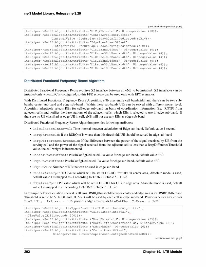
ns-3 Model Library, Release ns-3.29
(continued from previous page)
lteHelper->SetFfrAlgorithmAttribute("UlCqiThreshold", UintegerValue (10));lteHelper->SetFfrAlgorithmAttribute("CenterAreaPowerOffset",
UintegerValue (LteRrcSap::PdschConfigDedicated::dB_6));lteHelper->SetFfrAlgorithmAttribute("EdgeAreaPowerOffset",
UintegerValue (LteRrcSap::PdschConfigDedicated::dB0));lteHelper->SetFfrAlgorithmAttribute("UlSubBandOffset", UintegerValue (0));lteHelper->SetFfrAlgorithmAttribute("UlReuse3SubBandwidth", UintegerValue (4));lteHelper->SetFfrAlgorithmAttribute("UlReuse1SubBandwidth", UintegerValue (4));lteHelper->SetFfrAlgorithmAttribute("DlSubBandOffset", UintegerValue (0));lteHelper->SetFfrAlgorithmAttribute("DlReuse3SubBandwidth", UintegerValue (4));lteHelper->SetFfrAlgorithmAttribute("DlReuse1SubBandwidth", UintegerValue (4));
Distributed Fractional Frequency Reuse Algorithm
Distributed Fractional Frequency Reuse requires X2 interface between all eNB to be installed. X2 interfaces can beinstalled only when EPC is configured, so this FFR scheme can be used only with EPC scenarios.
With Distributed Fractional Frequency Reuse Algorithm, eNb uses entire cell bandwidth and there can be two sub-bands: center sub-band and edge sub-band . Within these sub-bands UEs can be served with different power level.Algorithm adaptively selects RBs for cell-edge sub-band on basis of coordination information (i.e. RNTP) fromadjecent cells and notifies the base stations of the adjacent cells, which RBs it selected to use in edge sub-band. Ifthere are no UE classified as edge UE in cell, eNB will not use any RBs as edge sub-band.
Distributed Fractional Frequency Reuse Algorithm provides following attributes:
• CalculationInterval: Time interval between calculation of Edge sub-band, Default value 1 second
• RsrqThreshold: If the RSRQ of is worse than this threshold, UE should be served in edge sub-band
• RsrpDifferenceThreshold: If the difference between the power of the signal received by UE from theserving cell and the power of the signal received from the adjacent cell is less than a RsrpDifferenceThresholdvalue, the cell weight is incremented
• CenterPowerOffset: PdschConfigDedicated::Pa value for edge sub-band, default value dB0
• EdgePowerOffset: PdschConfigDedicated::Pa value for edge sub-band, default value dB0
• EdgeRbNum: Number of RB that can be used in edge sub-band
• CenterAreaTpc: TPC value which will be set in DL-DCI for UEs in center area, Absolute mode is used,default value 1 is mapped to -1 according to TS36.213 Table 5.1.1.1-2
• EdgeAreaTpc: TPC value which will be set in DL-DCI for UEs in edge area, Absolute mode is used, defaultvalue 1 is mapped to -1 according to TS36.213 Table 5.1.1.1-2
In example below calculation interval is 500 ms. RSRQ threshold between center and edge area is 25. RSRP DifferenceThreshold is set to be 5. In DL and UL 6 RB will be used by each cell in edge sub-band. Power in center area equalsLteEnbPhy::TxPower - 0dB, power in edge area equals LteEnbPhy::TxPower + 3dB:
lteHelper->SetFfrAlgorithmType("ns3::LteFfrDistributedAlgorithm");lteHelper->SetFfrAlgorithmAttribute("CalculationInterval",↪→TimeValue(MilliSeconds(500)));lteHelper->SetFfrAlgorithmAttribute ("RsrqThreshold", UintegerValue (25));lteHelper->SetFfrAlgorithmAttribute ("RsrpDifferenceThreshold", UintegerValue (5));lteHelper->SetFfrAlgorithmAttribute ("EdgeRbNum", UintegerValue (6));lteHelper->SetFfrAlgorithmAttribute ("CenterPowerOffset",
UintegerValue (LteRrcSap::PdschConfigDedicated::dB0));
(continues on next page)
292 Chapter 19. LTE Module

ns-3 Model Library, Release ns-3.29
(continued from previous page)
lteHelper->SetFfrAlgorithmAttribute ("EdgePowerOffset",UintegerValue (LteRrcSap::PdschConfigDedicated::dB3));
Automatic configuration
Frequency Reuse algorithms can also be configured in more “automatic” way by setting only the bandwidth andFrCellTypeId. During initialization of FR instance, configuration for set bandwidth and FrCellTypeId will be takenfrom configuration table. It is important that only sub-bands will be configured, thresholds and transmission powerwill be set to default values. If one wants, he/she can change thresholds and transmission power as show in previoussub-section.
There are three FrCellTypeId : 1, 2, 3, which correspond to three different configurations for each bandwidth.Three configurations allow to have different configurations in neighbouring cells in hexagonal eNB layout. If userneeds to have more different configuration for neighbouring cells, he/she need to use manual configuration.
Example below show automatic FR algorithm configuration:
lteHelper->SetFfrAlgorithmType("ns3::LteFfrSoftAlgorithm");lteHelper->SetFfrAlgorithmAttribute("FrCellTypeId", UintegerValue (1));NetDeviceContainer enbDevs = lteHelper->InstallEnbDevice (enbNodes.Get(0));
19.2.20 Uplink Power Control
Uplink Power Control functionality is enabled by default. User can disable it by setting the boolean attributens3::LteUePhy::EnableUplinkPowerControl to true.
User can switch between Open Loop Power Control and Closed Loop Power Control mechanisms by setting theboolean attribute ns3::LteUePowerControl::ClosedLoop. By default Closed Loop Power Control withAccumulation Mode is enabled.
Path-loss is key component of Uplink Power Control. It is computed as difference between filtered RSRP and Refer-enceSignalPower parameter. ReferenceSignalPower is sent with SIB2.
Attributes available in Uplink Power Control:
• ClosedLoop: if true Closed Loop Uplink Power Control mode is enabled and Open Loop Power Controlotherwise, default value is false
• AccumulationEnabled: if true Accumulation Mode is enabled and Absolute mode otherwise, default valueis false
• Alpha: the path loss compensation factor, default value is 1.0
• Pcmin: minimal UE TxPower, default value is -40 dBm
• Pcmax: maximal UE TxPower, default value is 23 dBm
• PoNominalPusch: this parameter should be set by higher layers, but currently it needs to be configured byattribute system, possible values are integers in range (-126 . . . 24), Default value is -80
• PoUePusch: this parameter should be set by higher layers, but currently it needs to be configured by attributesystem, possible values are integers in range (-8 . . . 7), Default value is 0
• PsrsOffset: this parameter should be set by higher layers, but currently it needs to be configured by attributesystem, possible values are integers in range (0 . . . 15), Default value is 7, what gives P_Srs_Offset_Value = 0
Traced values in Uplink Power Control:
19.2. User Documentation 293

ns-3 Model Library, Release ns-3.29
• ReportPuschTxPower: Current UE TxPower for PUSCH
• ReportPucchTxPower: Current UE TxPower for PUCCH
• ReportSrsTxPower: Current UE TxPower for SRS
Example configuration is presented below:
Config::SetDefault ("ns3::LteUePhy::EnableUplinkPowerControl", BooleanValue (true));Config::SetDefault ("ns3::LteEnbPhy::TxPower", DoubleValue (30));Config::SetDefault ("ns3::LteUePowerControl::ClosedLoop", BooleanValue (true));Config::SetDefault ("ns3::LteUePowerControl::AccumulationEnabled", BooleanValue↪→(true));
As an example, user can take a look and run the lena-uplink-power-control program.
19.2.21 Examples Programs
The directory src/lte/examples/ contains some example simulation programs that show how to simulate dif-ferent LTE scenarios.
19.2.22 Reference scenarios
There is a vast amount of reference LTE simulation scenarios which can be found in the literature. Here we list someof them:
• The system simulation scenarios mentioned in section A.2 of [TR36814].
• The dual stripe model [R4-092042], which is partially implemented in the example program src/lte/examples/lena-dual-stripe.cc. This example program features a lot of configurable parameterswhich can be customized by changing the corresponding global variables. To get a list of all these globalvariables, you can run this command:
./waf --run lena-dual-stripe --command-template="%s --PrintGlobals"
The following subsection presents an example of running a simulation campaign using this example program.
Handover simulation campaign
In this subsection, we will demonstrate an example of running a simulation campaign using the LTE module of ns-3.The objective of the campaign is to compare the effect of each built-in handover algorithm of the LTE module.
The campaign will use the lena-dual-stripe example program. First, we have to modify the example programto produce the output that we need. In this occasion, we want to produce the number of handovers, user averagethroughput, and average SINR.
The number of handovers can be obtained by counting the number of times the HandoverEndOk Handover traces isfired. Then the user average throughput can be obtained by enabling the RLC Simulation Output. Finally, SINR canbe obtained by enabling the PHY simulation output. The following sample code snippet shows one possible way toobtain the above:
voidNotifyHandoverEndOkUe (std::string context, uint64_t imsi,
uint16_t cellId, uint16_t rnti){
std::cout << "Handover IMSI " << imsi << std::endl;
(continues on next page)
294 Chapter 19. LTE Module
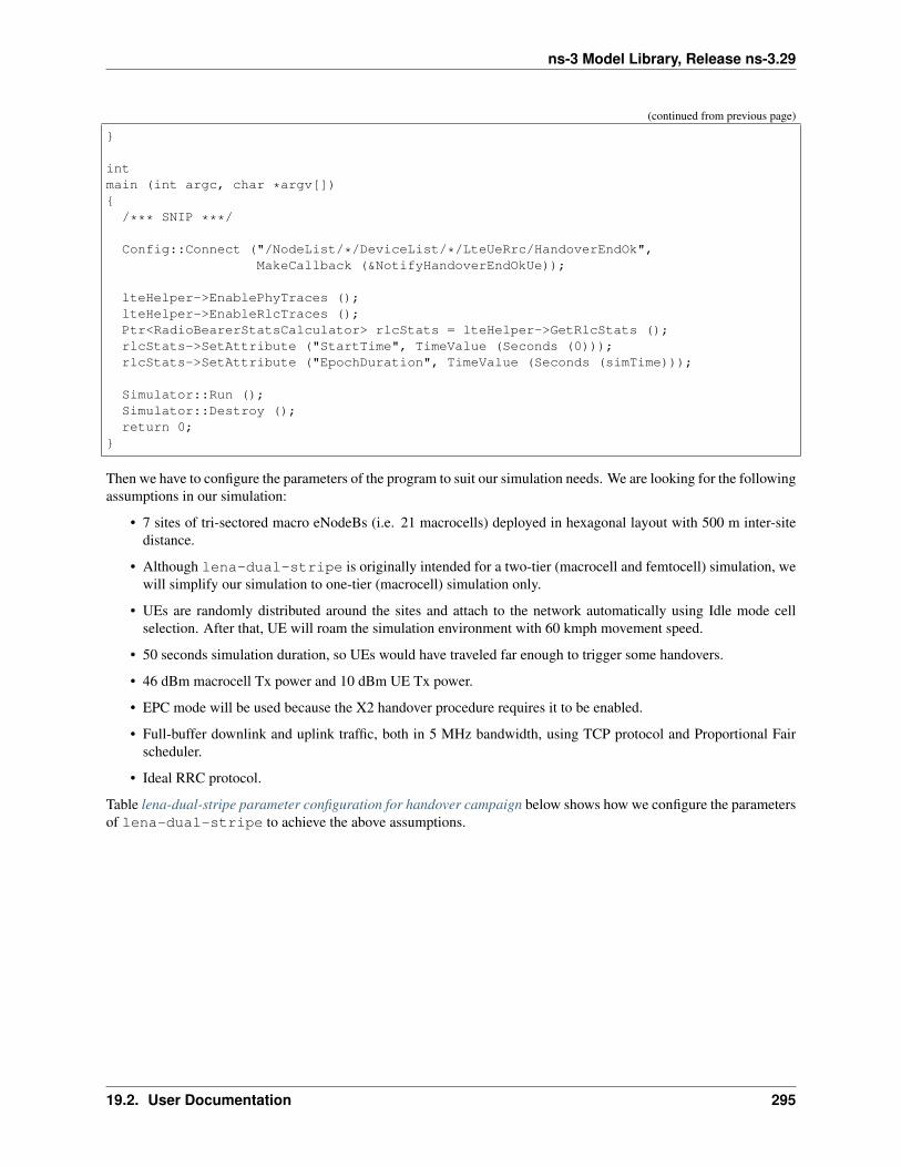
ns-3 Model Library, Release ns-3.29
(continued from previous page)
}
intmain (int argc, char *argv[]){
/*** SNIP ***/
Config::Connect ("/NodeList/*/DeviceList/*/LteUeRrc/HandoverEndOk",MakeCallback (&NotifyHandoverEndOkUe));
lteHelper->EnablePhyTraces ();lteHelper->EnableRlcTraces ();Ptr<RadioBearerStatsCalculator> rlcStats = lteHelper->GetRlcStats ();rlcStats->SetAttribute ("StartTime", TimeValue (Seconds (0)));rlcStats->SetAttribute ("EpochDuration", TimeValue (Seconds (simTime)));
Simulator::Run ();Simulator::Destroy ();return 0;
}
Then we have to configure the parameters of the program to suit our simulation needs. We are looking for the followingassumptions in our simulation:
• 7 sites of tri-sectored macro eNodeBs (i.e. 21 macrocells) deployed in hexagonal layout with 500 m inter-sitedistance.
• Although lena-dual-stripe is originally intended for a two-tier (macrocell and femtocell) simulation, wewill simplify our simulation to one-tier (macrocell) simulation only.
• UEs are randomly distributed around the sites and attach to the network automatically using Idle mode cellselection. After that, UE will roam the simulation environment with 60 kmph movement speed.
• 50 seconds simulation duration, so UEs would have traveled far enough to trigger some handovers.
• 46 dBm macrocell Tx power and 10 dBm UE Tx power.
• EPC mode will be used because the X2 handover procedure requires it to be enabled.
• Full-buffer downlink and uplink traffic, both in 5 MHz bandwidth, using TCP protocol and Proportional Fairscheduler.
• Ideal RRC protocol.
Table lena-dual-stripe parameter configuration for handover campaign below shows how we configure the parametersof lena-dual-stripe to achieve the above assumptions.
19.2. User Documentation 295
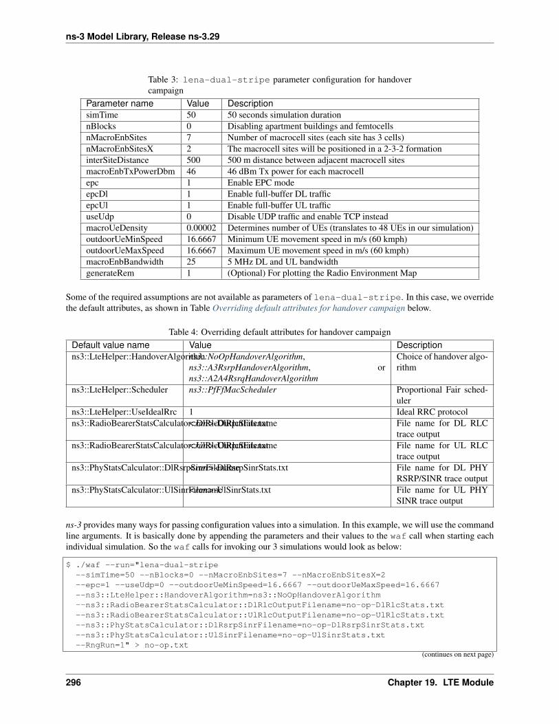
ns-3 Model Library, Release ns-3.29
Table 3: lena-dual-stripe parameter configuration for handovercampaign
Parameter name Value DescriptionsimTime 50 50 seconds simulation durationnBlocks 0 Disabling apartment buildings and femtocellsnMacroEnbSites 7 Number of macrocell sites (each site has 3 cells)nMacroEnbSitesX 2 The macrocell sites will be positioned in a 2-3-2 formationinterSiteDistance 500 500 m distance between adjacent macrocell sitesmacroEnbTxPowerDbm 46 46 dBm Tx power for each macrocellepc 1 Enable EPC modeepcDl 1 Enable full-buffer DL trafficepcUl 1 Enable full-buffer UL trafficuseUdp 0 Disable UDP traffic and enable TCP insteadmacroUeDensity 0.00002 Determines number of UEs (translates to 48 UEs in our simulation)outdoorUeMinSpeed 16.6667 Minimum UE movement speed in m/s (60 kmph)outdoorUeMaxSpeed 16.6667 Maximum UE movement speed in m/s (60 kmph)macroEnbBandwidth 25 5 MHz DL and UL bandwidthgenerateRem 1 (Optional) For plotting the Radio Environment Map
Some of the required assumptions are not available as parameters of lena-dual-stripe. In this case, we overridethe default attributes, as shown in Table Overriding default attributes for handover campaign below.
Table 4: Overriding default attributes for handover campaignDefault value name Value Descriptionns3::LteHelper::HandoverAlgorithmns3::NoOpHandoverAlgorithm,
ns3::A3RsrpHandoverAlgorithm, orns3::A2A4RsrqHandoverAlgorithm
Choice of handover algo-rithm
ns3::LteHelper::Scheduler ns3::PfFfMacScheduler Proportional Fair sched-uler
ns3::LteHelper::UseIdealRrc 1 Ideal RRC protocolns3::RadioBearerStatsCalculator::DlRlcOutputFilename<run>-DlRlcStats.txt File name for DL RLC
trace outputns3::RadioBearerStatsCalculator::UlRlcOutputFilename<run>-UlRlcStats.txt File name for UL RLC
trace outputns3::PhyStatsCalculator::DlRsrpSinrFilename<run>-DlRsrpSinrStats.txt File name for DL PHY
RSRP/SINR trace outputns3::PhyStatsCalculator::UlSinrFilename<run>-UlSinrStats.txt File name for UL PHY
SINR trace output
ns-3 provides many ways for passing configuration values into a simulation. In this example, we will use the commandline arguments. It is basically done by appending the parameters and their values to the waf call when starting eachindividual simulation. So the waf calls for invoking our 3 simulations would look as below:
$ ./waf --run="lena-dual-stripe--simTime=50 --nBlocks=0 --nMacroEnbSites=7 --nMacroEnbSitesX=2--epc=1 --useUdp=0 --outdoorUeMinSpeed=16.6667 --outdoorUeMaxSpeed=16.6667--ns3::LteHelper::HandoverAlgorithm=ns3::NoOpHandoverAlgorithm--ns3::RadioBearerStatsCalculator::DlRlcOutputFilename=no-op-DlRlcStats.txt--ns3::RadioBearerStatsCalculator::UlRlcOutputFilename=no-op-UlRlcStats.txt--ns3::PhyStatsCalculator::DlRsrpSinrFilename=no-op-DlRsrpSinrStats.txt--ns3::PhyStatsCalculator::UlSinrFilename=no-op-UlSinrStats.txt--RngRun=1" > no-op.txt
(continues on next page)
296 Chapter 19. LTE Module

ns-3 Model Library, Release ns-3.29
(continued from previous page)
$ ./waf --run="lena-dual-stripe--simTime=50 --nBlocks=0 --nMacroEnbSites=7 --nMacroEnbSitesX=2--epc=1 --useUdp=0 --outdoorUeMinSpeed=16.6667 --outdoorUeMaxSpeed=16.6667--ns3::LteHelper::HandoverAlgorithm=ns3::A3RsrpHandoverAlgorithm--ns3::RadioBearerStatsCalculator::DlRlcOutputFilename=a3-rsrp-DlRlcStats.txt--ns3::RadioBearerStatsCalculator::UlRlcOutputFilename=a3-rsrp-UlRlcStats.txt--ns3::PhyStatsCalculator::DlRsrpSinrFilename=a3-rsrp-DlRsrpSinrStats.txt--ns3::PhyStatsCalculator::UlSinrFilename=a3-rsrp-UlSinrStats.txt--RngRun=1" > a3-rsrp.txt
$ ./waf --run="lena-dual-stripe--simTime=50 --nBlocks=0 --nMacroEnbSites=7 --nMacroEnbSitesX=2--epc=1 --useUdp=0 --outdoorUeMinSpeed=16.6667 --outdoorUeMaxSpeed=16.6667--ns3::LteHelper::HandoverAlgorithm=ns3::A2A4RsrqHandoverAlgorithm--ns3::RadioBearerStatsCalculator::DlRlcOutputFilename=a2-a4-rsrq-DlRlcStats.txt--ns3::RadioBearerStatsCalculator::UlRlcOutputFilename=a2-a4-rsrq-UlRlcStats.txt--ns3::PhyStatsCalculator::DlRsrpSinrFilename=a2-a4-rsrq-DlRsrpSinrStats.txt--ns3::PhyStatsCalculator::UlSinrFilename=a2-a4-rsrq-UlSinrStats.txt--RngRun=1" > a2-a4-rsrq.txt
Some notes on the execution:
• Notice that some arguments are not specified because they are already the same as the default values. We alsokeep the handover algorithms on each own default settings.
• Note the file names of simulation output, e.g. RLC traces and PHY traces, because we have to make sure thatthey are not overwritten by the next simulation run. In this example, we specify the names one by one using thecommand line arguments.
• The --RngRun=1 argument at the end is used for setting the run number used by the random number generatorused in the simulation. We re-run the same simulations with different RngRun values, hence creating severalindependent replications of the same simulations. Then we average the results obtained from these replicationsto achieve some statistical confidence.
• We can add a --generateRem=1 argument to generate the files necessary for generating the Radio Environ-ment Map (REM) of the simulation. The result is Figure REM obtained from a simulation in handover campaignbelow, which can be produced by following the steps described in Section Radio Environment Maps. This figurealso shows the position of eNodeBs and UEs at the beginning of a simulation using RngRun = 1. Other valuesof RngRun may produce different UE position.
After hours of running, the simulation campaign will eventually end. Next we will perform some post-processing onthe produced simulation output to obtain meaningful information out of it.
In this example, we use GNU Octave to assist the processing of throughput and SINR data, as demonstrated in asample GNU Octave script below:
% RxBytes is the 10th columnDlRxBytes = load ("no-op-DlRlcStats.txt") (:,10);DlAverageThroughputKbps = sum (DlRxBytes) * 8 / 1000 / 50
% RxBytes is the 10th columnUlRxBytes = load ("no-op-UlRlcStats.txt") (:,10);UlAverageThroughputKbps = sum (UlRxBytes) * 8 / 1000 / 50
% Sinr is the 6th columnDlSinr = load ("no-op-DlRsrpSinrStats.txt") (:,6);% eliminate NaN values
(continues on next page)
19.2. User Documentation 297

ns-3 Model Library, Release ns-3.29
Fig. 72: REM obtained from a simulation in handover campaign
(continued from previous page)
idx = isnan (DlSinr);DlSinr (idx) = 0;DlAverageSinrDb = 10 * log10 (mean (DlSinr)) % convert to dB
% Sinr is the 5th columnUlSinr = load ("no-op-UlSinrStats.txt") (:,5);% eliminate NaN valuesidx = isnan (UlSinr);UlSinr (idx) = 0;UlAverageSinrDb = 10 * log10 (mean (UlSinr)) % convert to dB
As for the number of handovers, we can use simple shell scripting to count the number of occurrences of string“Handover” in the log file:
$ grep "Handover" no-op.txt | wc -l
Table Results of handover campaign below shows the complete statistics after we are done with post-processing onevery individual simulation run. The values shown are the average of the results obtained from RngRun of 1, 2, 3,and 4.
298 Chapter 19. LTE Module

ns-3 Model Library, Release ns-3.29
Table 5: Results of handover campaignStatistics No-op A2-A4-RSRQ Strongest cellAverage DL system throughput 6 615 kbps 20 509 kbps 19 709 kbpsAverage UL system throughput 4 095 kbps 5 705 kbps 6 627 kbpsAverage DL SINR -0.10 dB 5.19 dB 5.24 dBAverage UL SINR 9.54 dB 81.57 dB 79.65 dBNumber of handovers per UE per second 0 0.05694 0.04771
The results show that having a handover algorithm in a mobility simulation improves both user throughput and SINRsignificantly. There is little difference between the two handover algorithms in this campaign scenario. It would beinteresting to see their performance in different scenarios, such as scenarios with home eNodeBs deployment.
Frequency Reuse examples
There are two examples showing Frequency Reuse Algorithms functionality.
lena-frequency-reuse is simple example with 3 eNBs in triangle layout. There are 3 cell edge UEs, whichare located in the center of this triangle and 3 cell center UEs (one near each eNB). User can also specify the numberof randomly located UEs. FR algorithm is installed in eNBs and each eNB has different FrCellTypeId, what meanseach eNB uses different FR configuration. User can run lena-frequency-reuse with 6 different FR algorithms:NoOp, Hard FR, Strict FR, Soft FR, Soft FFR and Enhanced FFR. To run scenario with Distributed FFR algorithm,user should use lena-distributed-ffr. These two examples are very similar, but they were split becauseDistributed FFR requires EPC to be used, and other algorithms do not.
To run lena-frequency-reuse with different Frequency Reuse algorithms, user needs to specify FR al-gorithm by overriding the default attribute ns3::LteHelper::FfrAlgorithm. Example command to runlena-frequency-reuse with Soft FR algorithm is presented below:
$ ./waf --run "lena-frequency-reuse --↪→ns3::LteHelper::FfrAlgorithm=ns3::LteFrSoftAlgorithm"
In these examples functionality to generate REM and spectrum analyzer trace was added. User can enable generationof it by setting generateRem and generateSpectrumTrace attributes.
Command to generate REM for RB 1 in data channel from lena-frequency-reuse scenario with Soft FRalgorithm is presented below:
$ ./waf --run "lena-frequency-reuse --↪→ns3::LteHelper::FfrAlgorithm=ns3::LteFrSoftAlgorithm--generateRem=true --remRbId=1"
Radio Environment Map for Soft FR is presented in Figure REM for RB 1 obtained from lena-frequency-reuse examplewith Soft FR algorithm enabled.
Command to generate spectrum trace from lena-frequency-reuse scenario with Soft FFR algorithm is pre-sented below (Spectrum Analyzer position needs to be configured inside script):
$ ./waf --run "lena-frequency-reuse --↪→ns3::LteHelper::FfrAlgorithm=ns3::LteFfrSoftAlgorithm--generateSpectrumTrace=true"
Example spectrum analyzer trace is presented in figure Spectrum Analyzer trace obtained from lena-frequency-reuseexample with Soft FFR algorithm enabled. Spectrum Analyzer was located need eNB with FrCellTypeId 2.. As can beseen, different data channel subbands are sent with different power level (according to configuration), while controlchannel is transmitted with uniform power along entire system bandwidth.
19.2. User Documentation 299
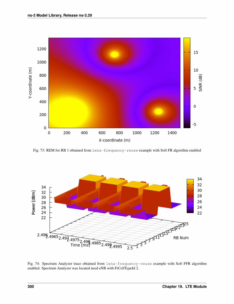
ns-3 Model Library, Release ns-3.29
Fig. 73: REM for RB 1 obtained from lena-frequency-reuse example with Soft FR algorithm enabled
Fig. 74: Spectrum Analyzer trace obtained from lena-frequency-reuse example with Soft FFR algorithmenabled. Spectrum Analyzer was located need eNB with FrCellTypeId 2.
300 Chapter 19. LTE Module
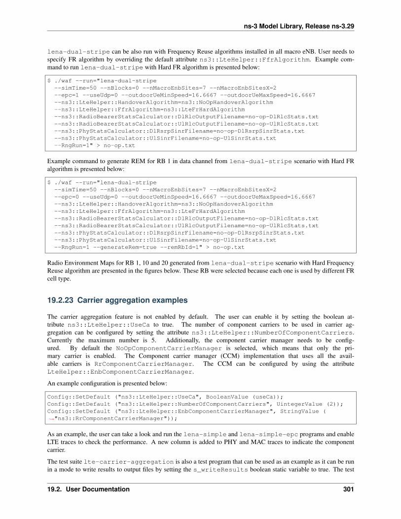
ns-3 Model Library, Release ns-3.29
lena-dual-stripe can be also run with Frequency Reuse algorithms installed in all macro eNB. User needs tospecify FR algorithm by overriding the default attribute ns3::LteHelper::FfrAlgorithm. Example com-mand to run lena-dual-stripe with Hard FR algorithm is presented below:
$ ./waf --run="lena-dual-stripe--simTime=50 --nBlocks=0 --nMacroEnbSites=7 --nMacroEnbSitesX=2--epc=1 --useUdp=0 --outdoorUeMinSpeed=16.6667 --outdoorUeMaxSpeed=16.6667--ns3::LteHelper::HandoverAlgorithm=ns3::NoOpHandoverAlgorithm--ns3::LteHelper::FfrAlgorithm=ns3::LteFrHardAlgorithm--ns3::RadioBearerStatsCalculator::DlRlcOutputFilename=no-op-DlRlcStats.txt--ns3::RadioBearerStatsCalculator::UlRlcOutputFilename=no-op-UlRlcStats.txt--ns3::PhyStatsCalculator::DlRsrpSinrFilename=no-op-DlRsrpSinrStats.txt--ns3::PhyStatsCalculator::UlSinrFilename=no-op-UlSinrStats.txt--RngRun=1" > no-op.txt
Example command to generate REM for RB 1 in data channel from lena-dual-stripe scenario with Hard FRalgorithm is presented below:
$ ./waf --run="lena-dual-stripe--simTime=50 --nBlocks=0 --nMacroEnbSites=7 --nMacroEnbSitesX=2--epc=0 --useUdp=0 --outdoorUeMinSpeed=16.6667 --outdoorUeMaxSpeed=16.6667--ns3::LteHelper::HandoverAlgorithm=ns3::NoOpHandoverAlgorithm--ns3::LteHelper::FfrAlgorithm=ns3::LteFrHardAlgorithm--ns3::RadioBearerStatsCalculator::DlRlcOutputFilename=no-op-DlRlcStats.txt--ns3::RadioBearerStatsCalculator::UlRlcOutputFilename=no-op-UlRlcStats.txt--ns3::PhyStatsCalculator::DlRsrpSinrFilename=no-op-DlRsrpSinrStats.txt--ns3::PhyStatsCalculator::UlSinrFilename=no-op-UlSinrStats.txt--RngRun=1 --generateRem=true --remRbId=1" > no-op.txt
Radio Environment Maps for RB 1, 10 and 20 generated from lena-dual-stripe scenario with Hard FrequencyReuse algorithm are presented in the figures below. These RB were selected because each one is used by different FRcell type.
19.2.23 Carrier aggregation examples
The carrier aggregation feature is not enabled by default. The user can enable it by setting the boolean at-tribute ns3::LteHelper::UseCa to true. The number of component carriers to be used in carrier ag-gregation can be configured by setting the attribute ns3::LteHelper::NumberOfComponentCarriers.Currently the maximum number is 5. Additionally, the component carrier manager needs to be config-ured. By default the NoOpComponentCarrierManager is selected, which means that only the pri-mary carrier is enabled. The Component carrier manager (CCM) implementation that uses all the avail-able carriers is RrComponentCarrierManager. The CCM can be configured by using the attributeLteHelper::EnbComponentCarrierManager.
An example configuration is presented below:
Config::SetDefault ("ns3::LteHelper::UseCa", BooleanValue (useCa));Config::SetDefault ("ns3::LteHelper::NumberOfComponentCarriers", UintegerValue (2));Config::SetDefault ("ns3::LteHelper::EnbComponentCarrierManager", StringValue (↪→"ns3::RrComponentCarrierManager"));
As an example, the user can take a look and run the lena-simple and lena-simple-epc programs and enableLTE traces to check the performance. A new column is added to PHY and MAC traces to indicate the componentcarrier.
The test suite lte-carrier-aggregation is also a test program that can be used as an example as it can be runin a mode to write results to output files by setting the s_writeResults boolean static variable to true. The test
19.2. User Documentation 301
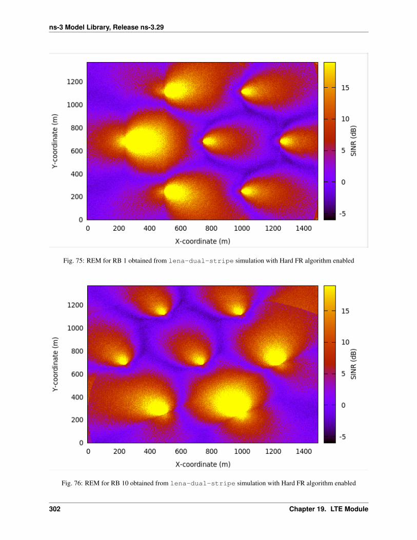
ns-3 Model Library, Release ns-3.29
Fig. 75: REM for RB 1 obtained from lena-dual-stripe simulation with Hard FR algorithm enabled
Fig. 76: REM for RB 10 obtained from lena-dual-stripe simulation with Hard FR algorithm enabled
302 Chapter 19. LTE Module
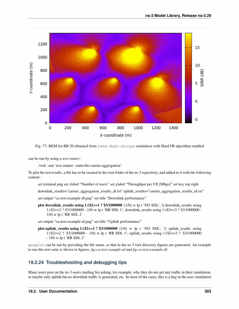
ns-3 Model Library, Release ns-3.29
Fig. 77: REM for RB 20 obtained from lena-dual-stripe simulation with Hard FR algorithm enabled
can be run by using a test-runner:
./waf –run ‘test-runner –suite=lte-carrier-aggregation’
To plot the test results, a file has to be created in the root folder of the ns-3 repository, and added to it with the followingcontent :
set terminal png set xlabel “Number of users” set ylabel “Throughput per UE [Mbps]” set key top right
downlink_results=”carrier_aggregation_results_dl.txt” uplink_results=”carrier_aggregation_results_ul.txt”
set output “ca-test-example-dl.png” set title “Downlink performance”
plot downlink_results using 1:($2==1 ? $3/1000000 [1/0) w lp t ‘NO SDL’, \] downlink_results using1:($2==2 ? $3/1000000 : 1/0) w lp t ‘RR SDL 1’, downlink_results using 1:($2==3 ? $3/1000000 :1/0) w lp t ‘RR SDL 2’
set output “ca-test-example-ul.png” set title “Uplink performance”
plot uplink_results using 1:($2==1 ? $3/1000000 [1/0) w lp t ‘NO SDL’, \] uplink_results using1:($2==2 ? $3/1000000 : 1/0) w lp t ‘RR SDL 1’, uplink_results using 1:($2==3 ? $3/1000000: 1/0) w lp t ‘RR SDL 2’
gnuplot can be run by providing the file name, so that in the ns-3 root directory figures are generated. An exampleto run this test suite is shown in figures: fig-ca-test-example-ul and fig-ca-test-example-dl.
19.2.24 Troubleshooting and debugging tips
Many users post on the ns-3-users mailing list asking, for example, why they do not get any traffic in their simulation,or maybe only uplink but no downlink traffic is generated, etc. In most of the cases, this is a bug in the user simulation
19.2. User Documentation 303

ns-3 Model Library, Release ns-3.29
Fig. 78: Example of CA test performance in the uplink
Fig. 79: Example of CA test performance in the downlink
304 Chapter 19. LTE Module

ns-3 Model Library, Release ns-3.29
program. Here the reader can find some tips to debug the program and find out the cause of the problem.
The general approach is to selectively and incrementally enable the logging of relevant LTE module components,verifying upon each activation that the output is as expected. In detail:
• first check the control plane, in particular the RRC connection establishment procedure, by enabling the logcomponents LteUeRrc and LteEnbRrc
• then check packet transmissions on the data plane, starting by enabling the log components LteUeNetDeviceand the EpcSgwPgwApplication, then EpcEnbApplication, then moving down the LTE radio stack (PDCP, RLC,MAC, and finally PHY). All this until you find where packets stop being processed / forwarded.
19.3 Testing Documentation
19.3.1 Overview
To test and validate the ns-3 LTE module, several test suites are provided which are integrated with the ns-3 testframework. To run them, you need to have configured the build of the simulator in this way:
$ ./waf configure --enable-tests --enable-modules=lte --enable-examples$ ./test.py
The above will run not only the test suites belonging to the LTE module, but also those belonging to all the other ns-3modules on which the LTE module depends. See the ns-3 manual for generic information on the testing framework.
You can get a more detailed report in HTML format in this way:
$ ./test.py -w results.html
After the above command has run, you can view the detailed result for each test by opening the file results.htmlwith a web browser.
You can run each test suite separately using this command:
$ ./test.py -s test-suite-name
For more details about test.py and the ns-3 testing framework, please refer to the ns-3 manual.
19.3.2 Description of the test suites
Unit Tests
SINR calculation in the Downlink
The test suite lte-downlink-sinr checks that the SINR calculation in downlink is performed correctly. TheSINR in the downlink is calculated for each RB assigned to data transmissions by dividing the power of the intendedsignal from the considered eNB by the sum of the noise power plus all the transmissions on the same RB coming fromother eNBs (the interference signals):
γ =Psignal
Pnoise +∑Pinterference
In general, different signals can be active during different periods of time. We define a chunk as the time intervalbetween any two events of type either start or end of a waveform. In other words, a chunk identifies a time intervalduring which the set of active waveforms does not change. Let i be the generic chunk, Ti its duration and SINRi
19.3. Testing Documentation 305
ns-3 Model Library, Release ns-3.29
its SINR, calculated with the above equation. The calculation of the average SINR γ to be used for CQI feedbackreporting uses the following formula:
γ =
∑i γiTi∑i Ti
The test suite checks that the above calculation is performed correctly in the simulator. The test vectors are obtainedoffline by an Octave script that implements the above equation, and that recreates a number of random transmittedsignals and interference signals that mimic a scenario where an UE is trying to decode a signal from an eNB whilefacing interference from other eNBs. The test passes if the calculated values are equal to the test vector within atolerance of 10−7. The tolerance is meant to account for the approximation errors typical of floating point arithmetic.
SINR calculation in the Uplink
The test suite lte-uplink-sinr checks that the SINR calculation in uplink is performed correctly. This test suiteis identical to lte-downlink-sinr described in the previous section, with the difference than both the signal andthe interference now refer to transmissions by the UEs, and reception is performed by the eNB. This test suite recreatesa number of random transmitted signals and interference signals to mimic a scenario where an eNB is trying to decodethe signal from several UEs simultaneously (the ones in the cell of the eNB) while facing interference from other UEs(the ones belonging to other cells).
The test vectors are obtained by a dedicated Octave script. The test passes if the calculated values are equal to thetest vector within a tolerance of 10−7 which, as for the downlink SINR test, deals with floating point arithmeticapproximation issues.
E-UTRA Absolute Radio Frequency Channel Number (EARFCN)
The test suite lte-earfcn checks that the carrier frequency used by the LteSpectrumValueHelper class (whichimplements the LTE spectrum model) is done in compliance with [TS36101], where the E-UTRA Absolute RadioFrequency Channel Number (EARFCN) is defined. The test vector for this test suite comprises a set of EARFCNvalues and the corresponding carrier frequency calculated by hand following the specification of [TS36101]. The testpasses if the carrier frequency returned by LteSpectrumValueHelper is the same as the known value for each elementin the test vector.
System Tests
Dedicated Bearer Deactivation Tests
The test suite ‘lte-test-deactivate-bearer’ creates test case with single EnodeB and Three UE’s. Each UE consists ofone Default and one Dedicated EPS bearer with same bearer specification but with different ARP. Test Case Flow isas follows: Attach UE -> Create Default+Dedicated Bearer -> Deactivate one of the Dedicated bearer
Test case further deactivates dedicated bearer having bearer ID 2(LCID=BearerId+2) of First UE (UE_ID=1) User canschedule bearer deactivation after specific time delay using Simulator::Schedule () method.
Once the test case execution ends it will create DlRlcStats.txt and UlRlcStats.txt. Key fields that need tobe checked in statistics are:
|Start | end | Cell ID | IMSI | RNTI | LCID | TxBytes | RxBytes |
Test case executes in three epochs:
1. In first Epoch (0.04s-1.04s) All UE’s and corresponding bearers gets attached and packet flow over the dedicatedbearers activated.
306 Chapter 19. LTE Module
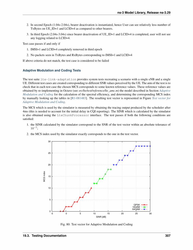
ns-3 Model Library, Release ns-3.29
2. In second Epoch (1.04s-2.04s), bearer deactivation is instantiated, hence User can see relatively less number ofTxBytes on UE_ID=1 and LCID=4 as compared to other bearers.
3. In third Epoch (2.04s-3.04s) since bearer deactivation of UE_ID=1 and LCID=4 is completed, user will not seeany logging related to LCID=4.
Test case passes if and only if
1. IMSI=1 and LCID=4 completely removed in third epoch
2. No packets seen in TxBytes and RxBytes corresponding to IMSI=1 and LCID=4
If above criteria do not match, the test case is considered to be failed
Adaptive Modulation and Coding Tests
The test suite lte-link-adaptation provides system tests recreating a scenario with a single eNB and a singleUE. Different test cases are created corresponding to different SNR values perceived by the UE. The aim of the test is tocheck that in each test case the chosen MCS corresponds to some known reference values. These reference values areobtained by re-implementing in Octave (see src/lte/test/reference/lte_amc.m) the model described in Section AdaptiveModulation and Coding for the calculation of the spectral efficiency, and determining the corresponding MCS indexby manually looking up the tables in [R1-081483]. The resulting test vector is represented in Figure Test vector forAdaptive Modulation and Coding.
The MCS which is used by the simulator is measured by obtaining the tracing output produced by the scheduler after4ms (this is needed to account for the initial delay in CQI reporting). The SINR which is calculated by the simulatoris also obtained using the LteChunkProcessor interface. The test passes if both the following conditions aresatisfied:
1. the SINR calculated by the simulator correspond to the SNR of the test vector within an absolute tolerance of10−7;
2. the MCS index used by the simulator exactly corresponds to the one in the test vector.
0
5
10
15
20
25
30
-5 0 5 10 15 20 25 30
MC
S index
SINR [dB]
QPSK16QAM64QAM
Fig. 80: Test vector for Adaptive Modulation and Coding
19.3. Testing Documentation 307
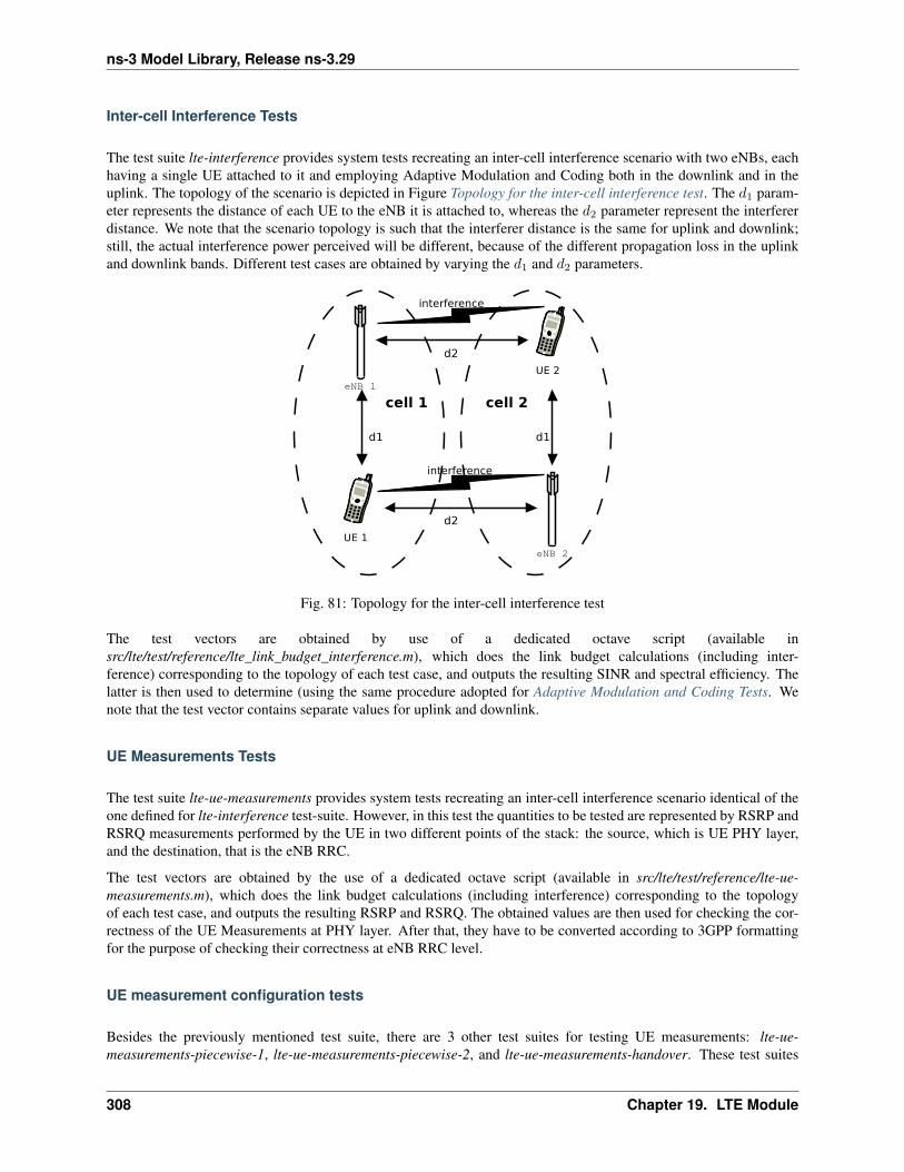
ns-3 Model Library, Release ns-3.29
Inter-cell Interference Tests
The test suite lte-interference provides system tests recreating an inter-cell interference scenario with two eNBs, eachhaving a single UE attached to it and employing Adaptive Modulation and Coding both in the downlink and in theuplink. The topology of the scenario is depicted in Figure Topology for the inter-cell interference test. The d1 param-eter represents the distance of each UE to the eNB it is attached to, whereas the d2 parameter represent the interfererdistance. We note that the scenario topology is such that the interferer distance is the same for uplink and downlink;still, the actual interference power perceived will be different, because of the different propagation loss in the uplinkand downlink bands. Different test cases are obtained by varying the d1 and d2 parameters.
Fig. 81: Topology for the inter-cell interference test
The test vectors are obtained by use of a dedicated octave script (available insrc/lte/test/reference/lte_link_budget_interference.m), which does the link budget calculations (including inter-ference) corresponding to the topology of each test case, and outputs the resulting SINR and spectral efficiency. Thelatter is then used to determine (using the same procedure adopted for Adaptive Modulation and Coding Tests. Wenote that the test vector contains separate values for uplink and downlink.
UE Measurements Tests
The test suite lte-ue-measurements provides system tests recreating an inter-cell interference scenario identical of theone defined for lte-interference test-suite. However, in this test the quantities to be tested are represented by RSRP andRSRQ measurements performed by the UE in two different points of the stack: the source, which is UE PHY layer,and the destination, that is the eNB RRC.
The test vectors are obtained by the use of a dedicated octave script (available in src/lte/test/reference/lte-ue-measurements.m), which does the link budget calculations (including interference) corresponding to the topologyof each test case, and outputs the resulting RSRP and RSRQ. The obtained values are then used for checking the cor-rectness of the UE Measurements at PHY layer. After that, they have to be converted according to 3GPP formattingfor the purpose of checking their correctness at eNB RRC level.
UE measurement configuration tests
Besides the previously mentioned test suite, there are 3 other test suites for testing UE measurements: lte-ue-measurements-piecewise-1, lte-ue-measurements-piecewise-2, and lte-ue-measurements-handover. These test suites
308 Chapter 19. LTE Module
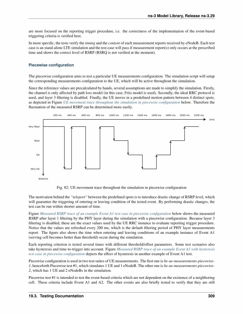
ns-3 Model Library, Release ns-3.29
are more focused on the reporting trigger procedure, i.e. the correctness of the implementation of the event-basedtriggering criteria is verified here.
In more specific, the tests verify the timing and the content of each measurement reports received by eNodeB. Each testcase is an stand-alone LTE simulation and the test case will pass if measurement report(s) only occurs at the prescribedtime and shows the correct level of RSRP (RSRQ is not verified at the moment).
Piecewise configuration
The piecewise configuration aims to test a particular UE measurements configuration. The simulation script will setupthe corresponding measurements configuration to the UE, which will be active throughout the simulation.
Since the reference values are precalculated by hands, several assumptions are made to simplify the simulation. Firstly,the channel is only affected by path loss model (in this case, Friis model is used). Secondly, the ideal RRC protocol isused, and layer 3 filtering is disabled. Finally, the UE moves in a predefined motion pattern between 4 distinct spots,as depicted in Figure UE movement trace throughout the simulation in piecewise configuration below. Therefore thefluctuation of the measured RSRP can be determined more easily.
Fig. 82: UE movement trace throughout the simulation in piecewise configuration
The motivation behind the “teleport” between the predefined spots is to introduce drastic change of RSRP level, whichwill guarantee the triggering of entering or leaving condition of the tested event. By performing drastic changes, thetest can be run within shorter amount of time.
Figure Measured RSRP trace of an example Event A1 test case in piecewise configuration below shows the measuredRSRP after layer 1 filtering by the PHY layer during the simulation with a piecewise configuration. Because layer 3filtering is disabled, these are the exact values used by the UE RRC instance to evaluate reporting trigger procedure.Notice that the values are refreshed every 200 ms, which is the default filtering period of PHY layer measurementsreport. The figure also shows the time when entering and leaving conditions of an example instance of Event A1(serving cell becomes better than threshold) occur during the simulation.
Each reporting criterion is tested several times with different threshold/offset parameters. Some test scenarios alsotake hysteresis and time-to-trigger into account. Figure Measured RSRP trace of an example Event A1 with hysteresistest case in piecewise configuration depicts the effect of hysteresis in another example of Event A1 test.
Piecewise configuration is used in two test suites of UE measurements. The first one is lte-ue-measurements-piecewise-1, henceforth Piecewise test #1, which simulates 1 UE and 1 eNodeB. The other one is lte-ue-measurements-piecewise-2, which has 1 UE and 2 eNodeBs in the simulation.
Piecewise test #1 is intended to test the event-based criteria which are not dependent on the existence of a neighboringcell. These criteria include Event A1 and A2. The other events are also briefly tested to verify that they are still
19.3. Testing Documentation 309
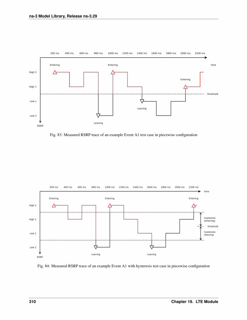
ns-3 Model Library, Release ns-3.29
Fig. 83: Measured RSRP trace of an example Event A1 test case in piecewise configuration
Fig. 84: Measured RSRP trace of an example Event A1 with hysteresis test case in piecewise configuration
310 Chapter 19. LTE Module
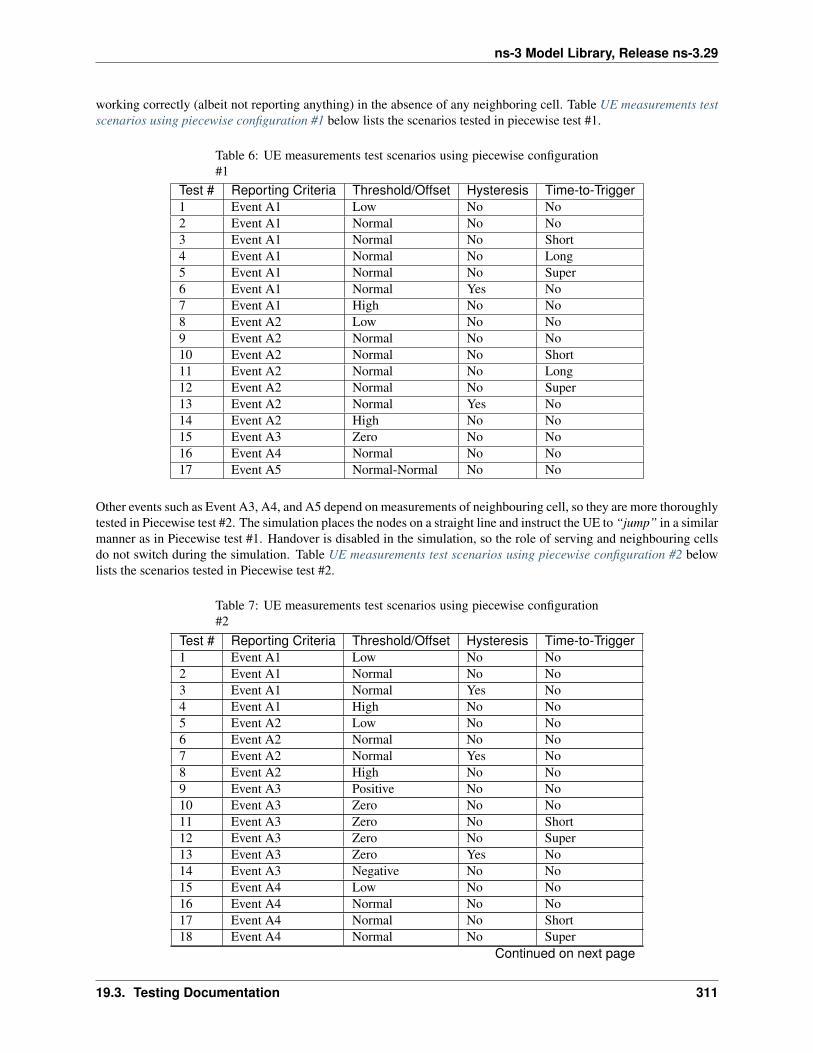
ns-3 Model Library, Release ns-3.29
working correctly (albeit not reporting anything) in the absence of any neighboring cell. Table UE measurements testscenarios using piecewise configuration #1 below lists the scenarios tested in piecewise test #1.
Table 6: UE measurements test scenarios using piecewise configuration#1
Test # Reporting Criteria Threshold/Offset Hysteresis Time-to-Trigger1 Event A1 Low No No2 Event A1 Normal No No3 Event A1 Normal No Short4 Event A1 Normal No Long5 Event A1 Normal No Super6 Event A1 Normal Yes No7 Event A1 High No No8 Event A2 Low No No9 Event A2 Normal No No10 Event A2 Normal No Short11 Event A2 Normal No Long12 Event A2 Normal No Super13 Event A2 Normal Yes No14 Event A2 High No No15 Event A3 Zero No No16 Event A4 Normal No No17 Event A5 Normal-Normal No No
Other events such as Event A3, A4, and A5 depend on measurements of neighbouring cell, so they are more thoroughlytested in Piecewise test #2. The simulation places the nodes on a straight line and instruct the UE to “jump” in a similarmanner as in Piecewise test #1. Handover is disabled in the simulation, so the role of serving and neighbouring cellsdo not switch during the simulation. Table UE measurements test scenarios using piecewise configuration #2 belowlists the scenarios tested in Piecewise test #2.
Table 7: UE measurements test scenarios using piecewise configuration#2
Test # Reporting Criteria Threshold/Offset Hysteresis Time-to-Trigger1 Event A1 Low No No2 Event A1 Normal No No3 Event A1 Normal Yes No4 Event A1 High No No5 Event A2 Low No No6 Event A2 Normal No No7 Event A2 Normal Yes No8 Event A2 High No No9 Event A3 Positive No No10 Event A3 Zero No No11 Event A3 Zero No Short12 Event A3 Zero No Super13 Event A3 Zero Yes No14 Event A3 Negative No No15 Event A4 Low No No16 Event A4 Normal No No17 Event A4 Normal No Short18 Event A4 Normal No Super
Continued on next page
19.3. Testing Documentation 311
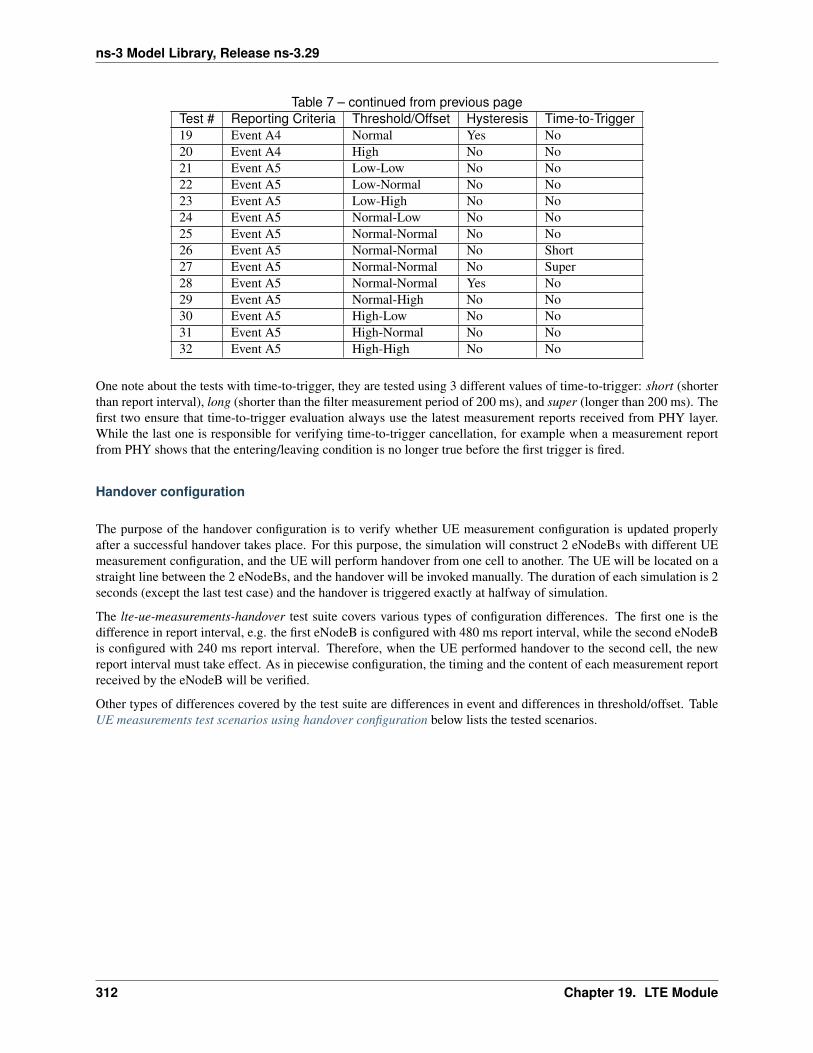
ns-3 Model Library, Release ns-3.29
Table 7 – continued from previous pageTest # Reporting Criteria Threshold/Offset Hysteresis Time-to-Trigger19 Event A4 Normal Yes No20 Event A4 High No No21 Event A5 Low-Low No No22 Event A5 Low-Normal No No23 Event A5 Low-High No No24 Event A5 Normal-Low No No25 Event A5 Normal-Normal No No26 Event A5 Normal-Normal No Short27 Event A5 Normal-Normal No Super28 Event A5 Normal-Normal Yes No29 Event A5 Normal-High No No30 Event A5 High-Low No No31 Event A5 High-Normal No No32 Event A5 High-High No No
One note about the tests with time-to-trigger, they are tested using 3 different values of time-to-trigger: short (shorterthan report interval), long (shorter than the filter measurement period of 200 ms), and super (longer than 200 ms). Thefirst two ensure that time-to-trigger evaluation always use the latest measurement reports received from PHY layer.While the last one is responsible for verifying time-to-trigger cancellation, for example when a measurement reportfrom PHY shows that the entering/leaving condition is no longer true before the first trigger is fired.
Handover configuration
The purpose of the handover configuration is to verify whether UE measurement configuration is updated properlyafter a successful handover takes place. For this purpose, the simulation will construct 2 eNodeBs with different UEmeasurement configuration, and the UE will perform handover from one cell to another. The UE will be located on astraight line between the 2 eNodeBs, and the handover will be invoked manually. The duration of each simulation is 2seconds (except the last test case) and the handover is triggered exactly at halfway of simulation.
The lte-ue-measurements-handover test suite covers various types of configuration differences. The first one is thedifference in report interval, e.g. the first eNodeB is configured with 480 ms report interval, while the second eNodeBis configured with 240 ms report interval. Therefore, when the UE performed handover to the second cell, the newreport interval must take effect. As in piecewise configuration, the timing and the content of each measurement reportreceived by the eNodeB will be verified.
Other types of differences covered by the test suite are differences in event and differences in threshold/offset. TableUE measurements test scenarios using handover configuration below lists the tested scenarios.
312 Chapter 19. LTE Module

ns-3 Model Library, Release ns-3.29
Table 8: UE measurements test scenarios using handover configurationTest # Test Subject Initial Configuration Post-Handover Configuration1 Report interval 480 ms 240 ms2 Report interval 120 ms 640 ms3 Event Event A1 Event A24 Event Event A2 Event A15 Event Event A3 Event A46 Event Event A4 Event A37 Event Event A2 Event A38 Event Event A3 Event A29 Event Event A4 Event A510 Event Event A5 Event A411 Threshold/offset RSRP range 52 (Event A1) RSRP range 56 (Event A1)12 Threshold/offset RSRP range 52 (Event A2) RSRP range 56 (Event A2)13 Threshold/offset A3 offset -30 (Event A3) A3 offset +30 (Event A3)14 Threshold/offset RSRP range 52 (Event A4) RSRP range 56 (Event A4)15 Threshold/offset RSRP range 52-52 (Event A5) RSRP range 56-56 (Event A5)16 Time-to-trigger 1024 ms 100 ms17 Time-to-trigger 1024 ms 640 ms
Round Robin scheduler performance
The test suite lte-rr-ff-mac-scheduler creates different test cases with a single eNB and several UEs, allhaving the same Radio Bearer specification. In each test case, the UEs see the same SINR from the eNB; differenttest cases are implemented by using different distance among UEs and the eNB (i.e., therefore having different SINRvalues) and different numbers of UEs. The test consists on checking that the obtained throughput performance isequal among users and matches a reference throughput value obtained according to the SINR perceived within a giventolerance.
The test vector is obtained according to the values of transport block size reported in table 7.1.7.2.1-1 of [TS36213],considering an equal distribution of the physical resource block among the users using Resource Allocation Type 0as defined in Section 7.1.6.1 of [TS36213]. Let τ be the TTI duration, N be the number of UEs, B the transmissionbandwidth configuration in number of RBs, G the RBG size, M the modulation and coding scheme in use at the givenSINR and S(M,B) be the transport block size in bits as defined by 3GPP TS 36.213. We first calculate the number Lof RBGs allocated to each user as
L =
⌊B
NG
⌋The reference throughput T in bit/s achieved by each UE is then calculated as
T =S(M,LG)
8 τ
The test passes if the measured throughput matches with the reference throughput within a relative tolerance of 0.1.This tolerance is needed to account for the transient behavior at the beginning of the simulation (e.g., CQI feedback isonly available after a few subframes) as well as for the accuracy of the estimator of the average throughput performanceover the chosen simulation time (0.4s). This choice of the simulation time is justified by the need to follow the ns-3guidelines of keeping the total execution time of the test suite low, in spite of the high number of test cases. In anycase, we note that a lower value of the tolerance can be used when longer simulations are run.
In Figure fig-lenaThrTestCase1, the curves labeled “RR” represent the test values calculated for the RR scheduler test,as a function of the number of UEs and of the MCS index being used in each test case.
19.3. Testing Documentation 313
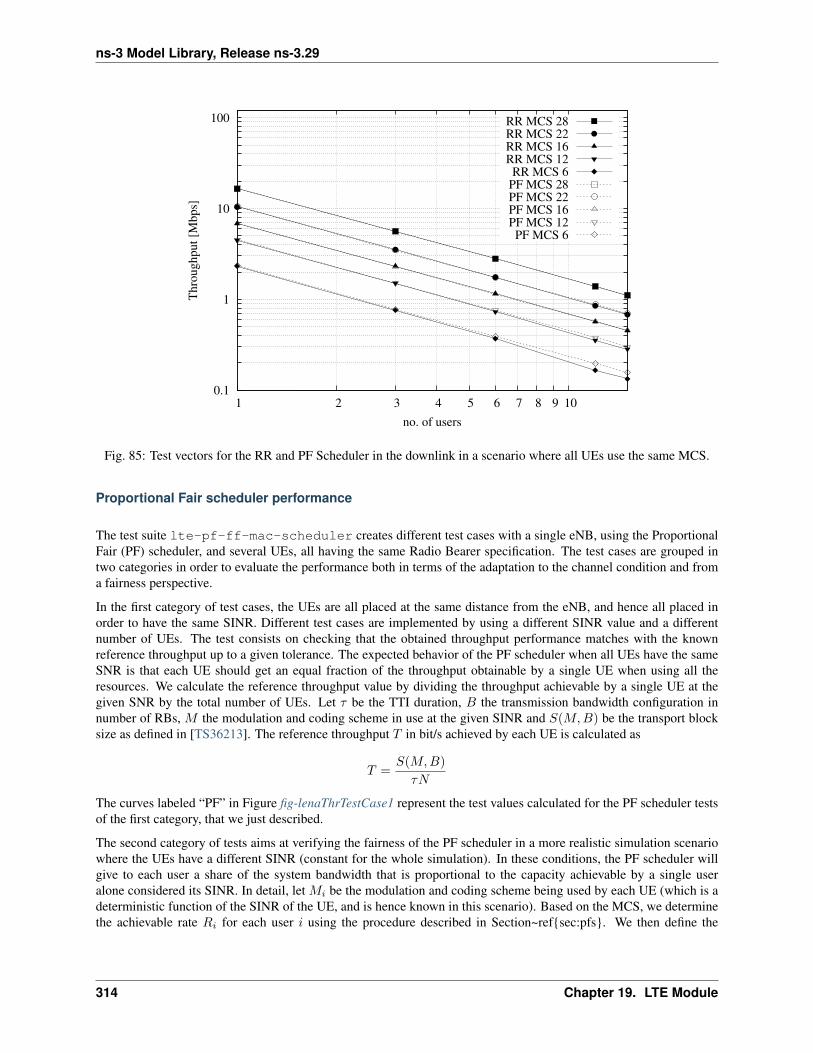
ns-3 Model Library, Release ns-3.29
0.1
1
10
100
1 2 3 4 5 6 7 8 9 10
Thro
ughput
[Mbps]
no. of users
RR MCS 28RR MCS 22RR MCS 16RR MCS 12RR MCS 6
PF MCS 28PF MCS 22PF MCS 16PF MCS 12PF MCS 6
Fig. 85: Test vectors for the RR and PF Scheduler in the downlink in a scenario where all UEs use the same MCS.
Proportional Fair scheduler performance
The test suite lte-pf-ff-mac-scheduler creates different test cases with a single eNB, using the ProportionalFair (PF) scheduler, and several UEs, all having the same Radio Bearer specification. The test cases are grouped intwo categories in order to evaluate the performance both in terms of the adaptation to the channel condition and froma fairness perspective.
In the first category of test cases, the UEs are all placed at the same distance from the eNB, and hence all placed inorder to have the same SINR. Different test cases are implemented by using a different SINR value and a differentnumber of UEs. The test consists on checking that the obtained throughput performance matches with the knownreference throughput up to a given tolerance. The expected behavior of the PF scheduler when all UEs have the sameSNR is that each UE should get an equal fraction of the throughput obtainable by a single UE when using all theresources. We calculate the reference throughput value by dividing the throughput achievable by a single UE at thegiven SNR by the total number of UEs. Let τ be the TTI duration, B the transmission bandwidth configuration innumber of RBs, M the modulation and coding scheme in use at the given SINR and S(M,B) be the transport blocksize as defined in [TS36213]. The reference throughput T in bit/s achieved by each UE is calculated as
T =S(M,B)
τN
The curves labeled “PF” in Figure fig-lenaThrTestCase1 represent the test values calculated for the PF scheduler testsof the first category, that we just described.
The second category of tests aims at verifying the fairness of the PF scheduler in a more realistic simulation scenariowhere the UEs have a different SINR (constant for the whole simulation). In these conditions, the PF scheduler willgive to each user a share of the system bandwidth that is proportional to the capacity achievable by a single useralone considered its SINR. In detail, let Mi be the modulation and coding scheme being used by each UE (which is adeterministic function of the SINR of the UE, and is hence known in this scenario). Based on the MCS, we determinethe achievable rate Ri for each user i using the procedure described in Section~ref{sec:pfs}. We then define the
314 Chapter 19. LTE Module

ns-3 Model Library, Release ns-3.29
achievable rate ratio ρR,i of each user i as
ρR,i =Ri∑Nj=1Rj
Let now Ti be the throughput actually achieved by the UE i , which is obtained as part of the simulation output. Wedefine the obtained throughput ratio ρT,i of UE i as
ρT,i =Ti∑Nj=1 Tj
The test consists of checking that the following condition is verified:
ρR,i = ρT,i
if so, it means that the throughput obtained by each UE over the whole simulation matches with the steady-statethroughput expected by the PF scheduler according to the theory. This test can be derived from [Holtzman2000] asfollows. From Section 3 of [Holtzman2000], we know that
TiRi
= c, ∀i
where c is a constant. By substituting the above into the definition of ρT,i given previously, we get
Ti∑Nj=1 Tj
=cRi∑Nj=1 cRj
=cRi
c∑Nj=1Rj
=Ri∑Nj=1Rj
which is exactly the expression being used in the test.
Figure Throughput ratio evaluation for the PF scheduler in a scenario where the UEs have MCS index 28, 24, 16, 12,6 presents the results obtained in a test case with UEs i = 1, . . . , 5 that are located at a distance from the base stationsuch that they will use respectively the MCS index 28, 24, 16, 12, 6. From the figure, we note that, as expected, theobtained throughput is proportional to the achievable rate. In other words, the PF scheduler assign more resources tothe users that use a higher MCS index.
Maximum Throughput scheduler performance
Test suites lte-fdmt-ff-mac-scheduler and lte-tdmt-ff-mac-scheduler create different test caseswith a single eNB and several UEs, all having the same Radio Bearer specification, using the Frequency DomainMaximum Throughput (FDMT) scheduler and Time Domain Maximum Throughput (TDMT) scheduler respectively.In other words, UEs are all placed at the same distance from the eNB, and hence all placed in order to have the sameSNR. Different test cases are implemented by using a different SNR values and a different number of UEs. The testconsists on checking that the obtained throughput performance matches with the known reference throughput up toa given tolerance.The expected behavior of both FDMT and TDMT scheduler when all UEs have the same SNR isthat scheduler allocates all RBGs to the first UE defined in script. This is because the current FDMT and TDMTimplementation always select the first UE to serve when there are multiple UEs having the same SNR value. Wecalculate the reference throughput value for first UE by the throughput achievable of a single UE at the given SNR,while reference throughput value for other UEs by zero. Let τ be the TTI duration, B the transmission bandwidthconfiguration in number of RBs, M the modulation and coding scheme in use at the given SNR and S(M,B) be thetransport block size as defined in [TS36213]. The reference throughput T in bit/s achieved by each UE is calculatedas
T =S(M,B)
τ
19.3. Testing Documentation 315
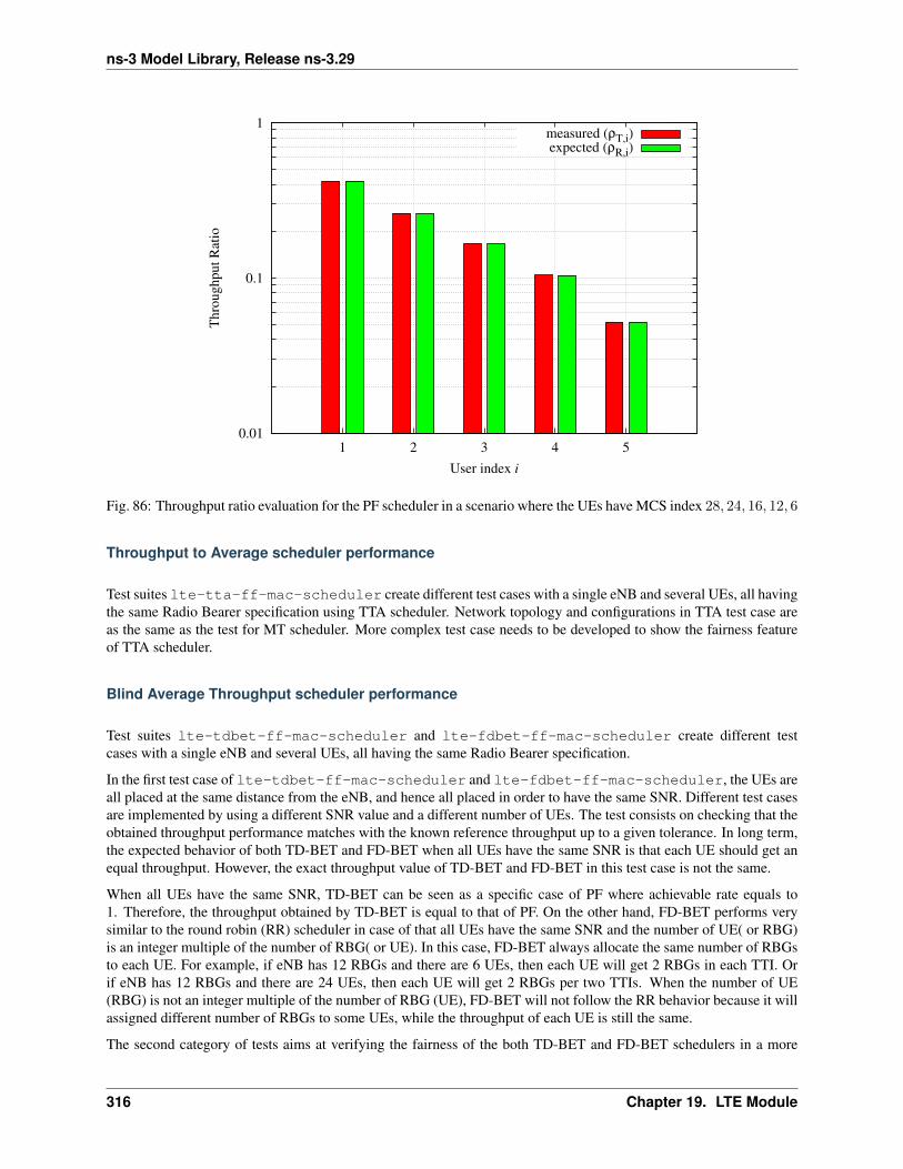
ns-3 Model Library, Release ns-3.29
0.01
0.1
1
1 2 3 4 5
Thro
ughput
Rat
io
User index i
measured (ρT,i)expected (ρR,i)
Fig. 86: Throughput ratio evaluation for the PF scheduler in a scenario where the UEs have MCS index 28, 24, 16, 12, 6
Throughput to Average scheduler performance
Test suites lte-tta-ff-mac-scheduler create different test cases with a single eNB and several UEs, all havingthe same Radio Bearer specification using TTA scheduler. Network topology and configurations in TTA test case areas the same as the test for MT scheduler. More complex test case needs to be developed to show the fairness featureof TTA scheduler.
Blind Average Throughput scheduler performance
Test suites lte-tdbet-ff-mac-scheduler and lte-fdbet-ff-mac-scheduler create different testcases with a single eNB and several UEs, all having the same Radio Bearer specification.
In the first test case of lte-tdbet-ff-mac-scheduler and lte-fdbet-ff-mac-scheduler, the UEs areall placed at the same distance from the eNB, and hence all placed in order to have the same SNR. Different test casesare implemented by using a different SNR value and a different number of UEs. The test consists on checking that theobtained throughput performance matches with the known reference throughput up to a given tolerance. In long term,the expected behavior of both TD-BET and FD-BET when all UEs have the same SNR is that each UE should get anequal throughput. However, the exact throughput value of TD-BET and FD-BET in this test case is not the same.
When all UEs have the same SNR, TD-BET can be seen as a specific case of PF where achievable rate equals to1. Therefore, the throughput obtained by TD-BET is equal to that of PF. On the other hand, FD-BET performs verysimilar to the round robin (RR) scheduler in case of that all UEs have the same SNR and the number of UE( or RBG)is an integer multiple of the number of RBG( or UE). In this case, FD-BET always allocate the same number of RBGsto each UE. For example, if eNB has 12 RBGs and there are 6 UEs, then each UE will get 2 RBGs in each TTI. Orif eNB has 12 RBGs and there are 24 UEs, then each UE will get 2 RBGs per two TTIs. When the number of UE(RBG) is not an integer multiple of the number of RBG (UE), FD-BET will not follow the RR behavior because it willassigned different number of RBGs to some UEs, while the throughput of each UE is still the same.
The second category of tests aims at verifying the fairness of the both TD-BET and FD-BET schedulers in a more
316 Chapter 19. LTE Module
ns-3 Model Library, Release ns-3.29
realistic simulation scenario where the UEs have a different SNR (constant for the whole simulation). In this case,both scheduler should give the same amount of averaged throughput to each user.
Specifically, for TD-BET, let Fi be the fraction of time allocated to user i in total simulation time, Rfbi be the fullbandwidth achievable rate for user i and Ti be the achieved throughput of user i. Then we have:
Ti = FiRfbi
In TD-BET, the sum of Fi for all user equals one. In long term, all UE has the same Ti so that we replace Ti by T .Then we have:
T =1∑N
i=11
Rfbi
Token Band Fair Queue scheduler performance
Test suites lte-fdtbfq-ff-mac-scheduler and lte-tdtbfq-ff-mac-scheduler create different testcases for testing three key features of TBFQ scheduler: traffic policing, fairness and traffic balance. Constant Bit RateUDP traffic is used in both downlink and uplink in all test cases. The packet interval is set to 1ms to keep the RLCbuffer non-empty. Different traffic rate is achieved by setting different packet size. Specifically, two classes of flowsare created in the test suites:
• Homogeneous flow: flows with the same token generation rate and packet arrival rate
• Heterogeneous flow: flows with different packet arrival rate, but with the same token generation rate
In test case 1 verifies traffic policing and fairness features for the scenario that all UEs are placed at the same distancefrom the eNB. In this case, all Ues have the same SNR value. Different test cases are implemented by using a differentSNR value and a different number of UEs. Because each flow have the same traffic rate and token generation rate,TBFQ scheduler will guarantee the same throughput among UEs without the constraint of token generation rate. Inaddition, the exact value of UE throughput is depended on the total traffic rate:
• If total traffic rate <= maximum throughput, UE throughput = traffic rate
• If total traffic rate > maximum throughput, UE throughput = maximum throughput / N
Here, N is the number of UE connected to eNodeB. The maximum throughput in this case equals to the rate thatall RBGs are assigned to one UE(e.g., when distance equals 0, maximum throughput is 2196000 byte/sec). Whenthe traffic rate is smaller than max bandwidth, TBFQ can police the traffic by token generation rate so that the UEthroughput equals its actual traffic rate (token generation rate is set to traffic generation rate); On the other hand, whentotal traffic rate is bigger than the max throughput, eNodeB cannot forward all traffic to UEs. Therefore, in each TTI,TBFQ will allocate all RBGs to one UE due to the large packets buffered in RLC buffer. When a UE is scheduledin current TTI, its token counter is decreased so that it will not be scheduled in the next TTI. Because each UE hasthe same traffic generation rate, TBFQ will serve each UE in turn and only serve one UE in each TTI (both in TDTBFQ and FD TBFQ). Therefore, the UE throughput in the second condition equals to the evenly share of maximumthroughput.
Test case 2 verifies traffic policing and fairness features for the scenario that each UE is placed at the different distancefrom the eNB. In this case, each UE has the different SNR value. Similar to test case 1, UE throughput in test case2 is also depended on the total traffic rate but with a different maximum throughput. Suppose all UEs have a hightraffic load. Then the traffic will saturate the RLC buffer in eNodeB. In each TTI, after selecting one UE with highestmetric, TBFQ will allocate all RBGs to this UE due to the large RLC buffer size. On the other hand, once RLC bufferis saturated, the total throughput of all UEs cannot increase any more. In addition, as we discussed in test case 1,for homogeneous flows which have the same t_i and r_i, each UE will achieve the same throughput in long term.Therefore, we can use the same method in TD BET to calculate the maximum throughput:
T =N∑N
i=11
Rfbi
19.3. Testing Documentation 317

ns-3 Model Library, Release ns-3.29
Here, T is the maximum throughput. Rfbi be the full bandwidth achievable rate for user i. N is the number of UE.
When the total traffic rate is bigger than T , the UE throughput equals to TN . Otherwise, UE throughput equals to its
traffic generation rate.
In test case 3, three flows with different traffic rate are created. Token generation rate for each flow is the same andequals to the average traffic rate of three flows. Because TBFQ use a shared token bank, tokens contributed by UE withlower traffic load can be utilized by UE with higher traffic load. In this way, TBFQ can guarantee the traffic rate foreach flow. Although we use heterogeneous flow here, the calculation of maximum throughput is as same as that in testcase 2. In calculation max throughput of test case 2, we assume that all UEs suffer high traffic load so that scheduleralways assign all RBGs to one UE in each TTI. This assumes is also true in heterogeneous flow case. In other words,whether those flows have the same traffic rate and token generation rate, if their traffic rate is bigger enough, TBFQperforms as same as it in test case 2. Therefore, the maximum bandwidth in test case 3 is as same as it in test case 2.
In test case 3, in some flows, token generate rate does not equal to MBR, although all flows are CBR traffic. This isnot accorded with our parameter setting rules. Actually, the traffic balance feature is used in VBR traffic. Becausedifferent UE’s peak rate may occur in different time, TBFQ use shared token bank to balance the traffic among thoseVBR traffics. Test case 3 use CBR traffic to verify this feature. But in the real simulation, it is recommended to settoken generation rate to MBR.
Priority Set scheduler performance
Test suites lte-pss-ff-mac-scheduler create different test cases with a single eNB and several UEs. In alltest cases, we select PFsch in FD scheduler. Same testing results can also be obtained by using CoItA scheduler. Inaddition, all test cases do not define nMux so that TD scheduler in PSS will always select half of total UE.
In the first class test case of lte-pss-ff-mac-scheduler, the UEs are all placed at the same distance from theeNB, and hence all placed in order to have the same SNR. Different test cases are implemented by using a differentTBR for each UEs. In each test cases, all UEs have the same Target Bit Rate configured by GBR in EPS bear setting.The expected behavior of PSS is to guarantee that each UE’s throughput at least equals its TBR if the total flow rate isblow maximum throughput. Similar to TBFQ, the maximum throughput in this case equals to the rate that all RBGsare assigned to one UE. When the traffic rate is smaller than max bandwidth, the UE throughput equals its actual trafficrate; On the other hand, UE throughput equals to the evenly share of the maximum throughput.
In the first class of test cases, each UE has the same SNR. Therefore, the priority metric in PF scheduler will bedetermined by past average throughput Tj(t) because each UE has the same achievable throughput Rj(k, t) in PFschor same CoI[k, n] in CoItA. This means that PSS will performs like a TD-BET which allocates all RBGs to one UEin each TTI. Then the maximum value of UE throughput equals to the achievable rate that all RBGs are allocated tothis UE.
In the second class of test case of lte-pss-ff-mac-scheduler, the UEs are all placed at the same distancefrom the eNB, and hence all placed in order to have the same SNR. Different TBR values are assigned to each UE.There also exist an maximum throughput in this case. Once total traffic rate is bigger than this threshold, there will besome UEs that cannot achieve their TBR. Because there is no fading, subband CQIs for each RBGs frequency are thesame. Therefore, in FD scheduler,in each TTI, priority metrics of UE for all RBGs are the same. This means that FDscheduler will always allocate all RBGs to one user. Therefore, in the maximum throughput case, PSS performs like aTD-BET. Then we have:
T =N∑N
i=11
Rfbi
Here, T is the maximum throughput. Rfbi be the full bandwidth achievable rate for user i. N is the number of UE.
318 Chapter 19. LTE Module
ns-3 Model Library, Release ns-3.29
Channel and QoS aware scheduler performance
The performance of the Channel and QoS aware scheduler can be tested in the similar way to performance of PrioritySet scheduler when GBR flows are not delay sensitive by measuring if the achieved throughput at RLC layer is closeto the TBR. Having this in mind, the performance of the CQA scheduler is tested by using the same test cases as thelte-pss-ff-mac-scheduler. Additionally, in [Bbojovic2014] can be found performance evaluation of CQAscheduler when the GBR flows are delay sensitive by considering different QoE metrics.
Building Propagation Loss Model
The aim of the system test is to verify the integration of the BuildingPathlossModel with the lte module. The testexploits a set of three pre calculated losses for generating the expected SINR at the receiver counting the trans-mission and the noise powers. These SINR values are compared with the results obtained from a LTE simula-tion that uses the BuildingPathlossModel. The reference loss values are calculated off-line with an Octave script(/test/reference/lte_pathloss.m). Each test case passes if the reference loss value is equal to the value calculated by thesimulator within a tolerance of 0.001 dB, which accounts for numerical errors in the calculations.
Physical Error Model
The test suite lte-phy-error-model generates different test cases for evaluating both data and control errormodels. For what concern the data, the test consists of six test cases with single eNB and a various number of UEs,all having the same Radio Bearer specification. Each test is designed for evaluating the error rate perceived by aspecific TB size in order to verify that it corresponds to the expected values according to the BLER generated for CBsize analog to the TB size. This means that, for instance, the test will check that the performance of a TB of N bitsis analogous to the one of a CB size of N bits by collecting the performance of a user which has been forced thegeneration of a such TB size according to the distance to eNB. In order to significantly test the BLER at MAC level,we configured the Adaptive Modulation and Coding (AMC) module, the LteAmc class, for making it less robust tochannel conditions by using the PiroEW2010 AMC model and configuring it to select the MCS considering a targetBER of 0.03 (instead of the default value of 0.00005). We note that these values do not reflect the actual BER, sincethey come from an analytical bound which does not consider all the transmission chain aspects; therefore the BER andBLER actually experienced at the reception of a TB is in general different.
The parameters of the six test cases are reported in the following:
1. 4 UEs placed 1800 meters far from the eNB, which implies the use of MCS 2 (SINR of -5.51 dB) and a TB of256 bits, that in turns produce a BLER of 0.33 (see point A in figure BLER for tests 1, 2, 3.).
2. 2 UEs placed 1800 meters far from the eNB, which implies the use of MCS 2 (SINR of -5.51 dB) and a TB of528 bits, that in turns produce a BLER of 0.11 (see point B in figure BLER for tests 1, 2, 3.).
3. 1 UE placed 1800 meters far from the eNB, which implies the use of MCS 2 (SINR of -5.51 dB) and a TB of1088 bits, that in turns produce a BLER of 0.02 (see point C in figure BLER for tests 1, 2, 3.).
4. 1 UE placed 600 meters far from the eNB, which implies the use of MCS 12 (SINR of 4.43 dB) and a TB of4800 bits, that in turns produce a BLER of 0.3 (see point D in figure BLER for tests 4, 5.).
5. 3 UEs placed 600 meters far from the eNB, which implies the use of MCS 12 (SINR of 4.43 dB) and a TB of1632 bits, that in turns produce a BLER of 0.55 (see point E in figure BLER for tests 4, 5.).
6. 1 UE placed 470 meters far from the eNB, which implies the use of MCS 16 (SINR of 8.48 dB) and a TB of7272 bits (segmented in 2 CBs of 3648 and 3584 bits), that in turns produce a BLER of 0.14, since each CB hasCBLER equal to 0.075 (see point F in figure BLER for test 6.).
The test condition verifies that in each test case the expected number of packets received correctly corresponds to aBernoulli distribution with a confidence interval of 99%, where the probability of success in each trail is p = 1−BERand n is the total number of packets sent.
19.3. Testing Documentation 319
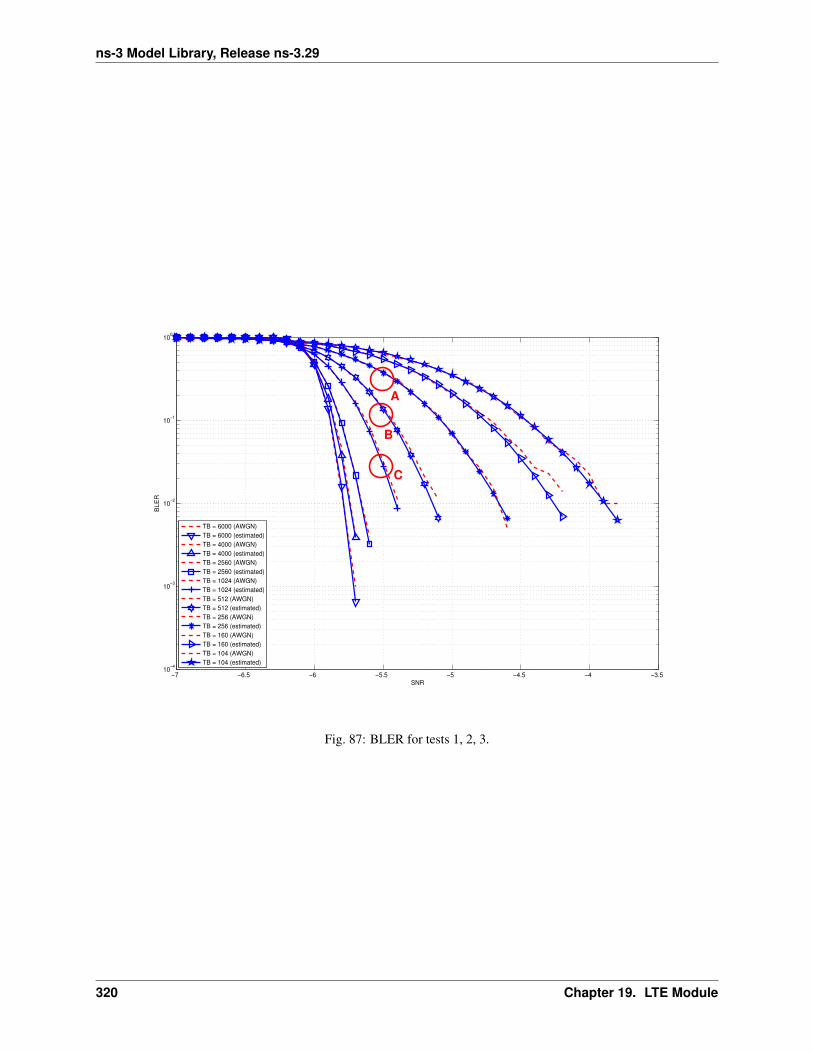
ns-3 Model Library, Release ns-3.29
−7 −6.5 −6 −5.5 −5 −4.5 −4 −3.510
−4
10−3
10−2
10−1
100
SNR
BL
ER
TB = 6000 (AWGN)
TB = 6000 (estimated)
TB = 4000 (AWGN)
TB = 4000 (estimated)
TB = 2560 (AWGN)
TB = 2560 (estimated)
TB = 1024 (AWGN)
TB = 1024 (estimated)
TB = 512 (AWGN)
TB = 512 (estimated)
TB = 256 (AWGN)
TB = 256 (estimated)
TB = 160 (AWGN)
TB = 160 (estimated)
TB = 104 (AWGN)
TB = 104 (estimated)
A
B
C
Fig. 87: BLER for tests 1, 2, 3.
320 Chapter 19. LTE Module

ns-3 Model Library, Release ns-3.29
2 2.5 3 3.5 4 4.5 5 5.510
−2
10−1
100
SNR
BL
ER
TB = 6000 (AWGN)
TB = 6000 (estimated)
TB = 4000 (AWGN)
TB = 4000 (estimated)
TB = 2560 (AWGN)
TB = 2560 (estimated)
TB = 1024 (AWGN)
TB = 1024 (estimated)
TB = 512 (AWGN)
TB = 512 (estimated)
E
D
Fig. 88: BLER for tests 4, 5.
19.3. Testing Documentation 321
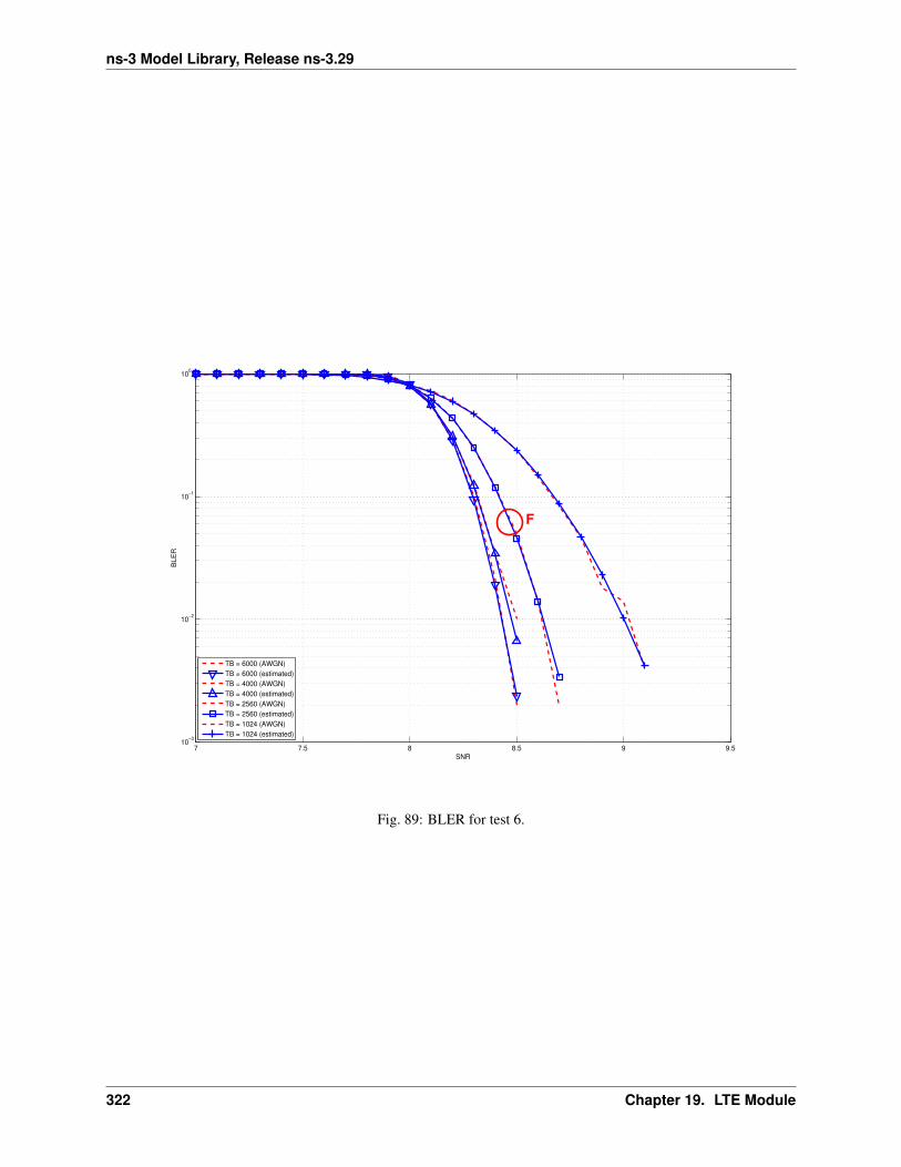
ns-3 Model Library, Release ns-3.29
7 7.5 8 8.5 9 9.510
−3
10−2
10−1
100
SNR
BL
ER
TB = 6000 (AWGN)
TB = 6000 (estimated)
TB = 4000 (AWGN)
TB = 4000 (estimated)
TB = 2560 (AWGN)
TB = 2560 (estimated)
TB = 1024 (AWGN)
TB = 1024 (estimated)
F
Fig. 89: BLER for test 6.
322 Chapter 19. LTE Module

ns-3 Model Library, Release ns-3.29
The error model of PCFICH-PDCCH channels consists of 4 test cases with a single UE and several eNBs, where theUE is connected to only one eNB in order to have the remaining acting as interfering ones. The errors on data aredisabled in order to verify only the ones due to erroneous decodification of PCFICH-PDCCH. As before, the systemhas been forced on working in a less conservative fashion in the AMC module for appreciating the results in bordersituations. The parameters of the 4 tests cases are reported in the following:
1. 2 eNBs placed 1078 meters far from the UE, which implies a SINR of -2.00 dB and a TB of 217 bits, that inturns produce a BLER of 0.007.
2. 3 eNBs placed 1040 meters far from the UE, which implies a SINR of -4.00 dB and a TB of 217 bits, that inturns produce a BLER of 0.045.
3. 4 eNBs placed 1250 meters far from the UE, which implies a SINR of -6.00 dB and a TB of 133 bits, that inturns produce a BLER of 0.206.
4. 5 eNBs placed 1260 meters far from the UE, which implies a SINR of -7.00 dB and a TB of 81 bits, that in turnsproduce a BLER of 0.343.
The test condition verifies that in each test case the expected number of packets received correct corresponds to aBernoulli distribution with a confidence interval of 99.8%, where the probability of success in each trail is p =1 − BER and n is the total number of packet sent. The larger confidence interval is due to the errors that might beproduced in quantizing the MI and the error curve.
HARQ Model
The test suite lte-harq includes two tests for evaluating the HARQ model and the related extension in the errormodel. The test consists on checking whether the amount of bytes received during the simulation corresponds to theexpected ones according to the values of transport block and the HARQ dynamics. In detail, the test checks whetherthe throughput obtained after one HARQ retransmission is the expected one. For evaluating the expected throughputthe expected TB delivering time has been evaluated according to the following formula:
T = P 1s × 1 + P 2
s × 2 + (1− P 2s )× 3
where P is is the probability of receiving with success the HARQ block at the attempt i (i.e., the RV with 3GPP naming).According to the scenarios, in the test we always have P 1
s equal to 0.0, while P 2s varies in the two tests, in detail:
Ttest−1 = 0.0× 1 + 0.926× 2 + 0.074× 3 = 2.074
Ttest−2 = 0.0× 1 + 0.752× 2 + 0.248× 3 = 2.248
The expected throughput is calculted by counting the number of transmission slots available during the simulation(e.g., the number of TTIs) and the size of the TB in the simulation, in detail:
Thrtest−i =TTINUMTtest−i
TBsize =
1000
2.07466 = 31822 bps for test-1
1000
2.248472 = 209964 bps for test-2
where TTINUM is the total number of TTIs in 1 second. The test is performed both for Round Robin scheduler. Thetest passes if the measured throughput matches with the reference throughput within a relative tolerance of 0.1. Thistolerance is needed to account for the transient behavior at the beginning of the simulation and the on-fly blocks at theend of the simulation.
MIMO Model
The test suite lte-mimo aims at verifying both the effect of the gain considered for each Transmission Mode onthe system performance and the Transmission Mode switching through the scheduler interface. The test consists on
19.3. Testing Documentation 323

ns-3 Model Library, Release ns-3.29
checking whether the amount of bytes received during a certain window of time (0.1 seconds in our case) correspondsto the expected ones according to the values of transport block size reported in table 7.1.7.2.1-1 of [TS36213], similarlyto what done for the tests of the schedulers.
The test is performed both for Round Robin and Proportional Fair schedulers. The test passes if the measured through-put matches with the reference throughput within a relative tolerance of 0.1. This tolerance is needed to account forthe transient behavior at the beginning of the simulation and the transition phase between the Transmission Modes.
Antenna Model integration
The test suite lte-antenna checks that the AntennaModel integrated with the LTE model works correctly. This testsuite recreates a simulation scenario with one eNB node at coordinates (0,0,0) and one UE node at coordinates (x,y,0).The eNB node is configured with an CosineAntennaModel having given orientation and beamwidth. The UE insteaduses the default IsotropicAntennaModel. The test checks that the received power both in uplink and downlink accountfor the correct value of the antenna gain, which is determined offline; this is implemented by comparing the uplink anddownlink SINR and checking that both match with the reference value up to a tolerance of 10−6 which accounts fornumerical errors. Different test cases are provided by varying the x and y coordinates of the UE, and the beamwidthand the orientation of the antenna of the eNB.
RLC
Two test suites lte-rlc-um-transmitter and lte-rlc-am-transmitter check that the UM RLC andthe AM RLC implementation work correctly. Both these suites work by testing RLC instances connected to specialtest entities that play the role of the MAC and of the PDCP, implementing respectively the LteMacSapProvider andLteRlcSapUser interfaces. Different test cases (i.e., input test vector consisting of series of primitive calls by the MACand the PDCP) are provided that check the behavior in the following cases:
1. one SDU, one PDU: the MAC notifies a TX opportunity causes the creation of a PDU which exactly contains awhole SDU
2. segmentation: the MAC notifies multiple TX opportunities that are smaller than the SDU size stored in thetransmission buffer, which is then to be fragmented and hence multiple PDUs are generated;
3. concatenation: the MAC notifies a TX opportunity that is bigger than the SDU, hence multiple SDUs areconcatenated in the same PDU
4. buffer status report: a series of new SDUs notifications by the PDCP is inteleaved with a series of TX opportunitynotification in order to verify that the buffer status report procedure is correct.
In all these cases, an output test vector is determine manually from knowledge of the input test vector and knowledgeof the expected behavior. These test vector are specialized for UM RLC and AM RLC due to their different behavior.Each test case passes if the sequence of primitives triggered by the RLC instance being tested is exactly equal to theoutput test vector. In particular, for each PDU transmitted by the RLC instance, both the size and the content of thePDU are verified to check for an exact match with the test vector.
The AM RLC implementation features an additional test suite, lte-rlc-am-e2e, which test the correct retrans-mission of RLC PDUs in presence of channel losses. The test instantiates an RLC AM transmitter and a receiver,and interposes a channel that randomly drops packet according to a fixed loss probability. Different test cases areinstantiated using different RngRun values and different loss probability values. Each test case passes if at the end ofthe simulation all SDUs are correctly delivered to the upper layers of the receiving RLC AM entity.
RRC
The test suite lte-rrc tests the correct functionality of the following aspects:
324 Chapter 19. LTE Module
ns-3 Model Library, Release ns-3.29
1. MAC Random Access
2. RRC System Information Acquisition
3. RRC Connection Establishment
4. RRC Reconfiguration
The test suite considers a type of scenario with four eNBs aligned in a square layout with 100-meter edges. MultipleUEs are located at a specific spot on the diagonal of the square and are instructed to connect to the first eNB. Each testcase implements an instance of this scenario with specific values of the following parameters:
• number of UEs
• number of Data Radio Bearers to be activated for each UE
• time tc0 at which the first UE is instructed to start connecting to the eNB
• time interval di between the start of connection of UE n and UE n+ 1; the time at which user n connects is thusdetermined as tcn = tc0 + ndi sdf
• the relative position of the UEs on the diagonal of the square, where higher values indicate larger distance fromthe serving eNodeB, i.e., higher interference from the other eNodeBs
• a boolean flag indicating whether the ideal or the real RRC protocol model is used
Each test cases passes if a number of test conditions are positively evaluated for each UE after a delay de from thetime it started connecting to the eNB. The delay de is determined as
de = dsi + dra + dce + dcr
where:
• dsi is the max delay necessary for the acquisition of System Information. We set it to 90ms accounting for 10msfor the MIB acquisition and 80ms for the subsequent SIB2 acquisition
• dra is the delay for the MAC Random Access (RA) procedure. This depends on preamble collisions as well as onthe availability of resources for the UL grant allocation. The total amount of necessary RA attempts depends onpreamble collisions and failures to allocate the UL grant because of lack of resources. The number of collisionsdepends on the number of UEs that try to access simultaneously; we estimated that for a 0.99 RA success proba-bility, 5 attempts are sufficient for up to 20 UEs, and 10 attempts for up to 50 UEs. For the UL grant, consideredthe system bandwidth and the default MCS used for the UL grant (MCS 0), at most 4 UL grants can be assignedin a TTI; so for n UEs trying to do RA simultaneously the max number of attempts due to the UL grant issue isdn/4e. The time for a RA attempt is determined by 3ms + the value of LteEnbMac::RaResponseWindowSize,which defaults to 3ms, plus 1ms for the scheduling of the new transmission.
• dce is the delay required for the transmission of RRC CONNECTION SETUP + RRC CONNECTION SETUPCOMPLETED. We consider a round trip delay of 10ms plus d2n/4e considering that 2 RRC packets have to betransmitted and that at most 4 such packets can be transmitted per TTI. In cases where interference is high, weaccommodate one retry attempt by the UE, so we double the dce value and then add dsi on top of it (because thetimeout has reset the previously received SIB2).
• dcr is the delay required for eventually needed RRC CONNECTION RECONFIGURATION transactions. Thenumber of transactions needed is 1 for each bearer activation. Similarly to what done for dce, for each transactionwe consider a round trip delay of 10ms plus d2n/4e. delay of 20ms.
The base version of the test LteRrcConnectionEstablishmentTestCase tests for correct RRC connectionestablishment in absence of channel errors. The conditions that are evaluated for this test case to pass are, for eachUE:
• the RRC state at the UE is CONNECTED_NORMALLY
• the UE is configured with the CellId, DlBandwidth, UlBandwidth, DlEarfcn and UlEarfcn of the eNB
19.3. Testing Documentation 325

ns-3 Model Library, Release ns-3.29
• the IMSI of the UE stored at the eNB is correct
• the number of active Data Radio Bearers is the expected one, both at the eNB and at the UE
• for each Data Radio Bearer, the following identifiers match between the UE and the eNB: EPS bearer id, DRBid, LCID
The test variant LteRrcConnectionEstablishmentErrorTestCase is similar except for the presence oferrors in the transmission of a particular RRC message of choice during the first connection attempt. The error isobtained by temporarily moving the UE to a far away location; the time of movement has been determined empiricallyfor each instance of the test case based on the message that it was desired to be in error. the test case checks that atleast one of the following conditions is false at the time right before the UE is moved back to the original location:
• the RRC state at the UE is CONNECTED_NORMALLY
• the UE context at the eNB is present
• the RRC state of the UE Context at the eNB is CONNECTED_NORMALLY
Additionally, all the conditions of the LteRrcConnectionEstablishmentTestCase are evaluated - they areespected to be true because of the NAS behavior of immediately re-attempting the connection establishment if it fails.
Initial cell selection
The test suite lte-cell-selection is responsible for verifying the Initial Cell Selection procedure. The test is a simulationof a small network of 2 non-CSG cells and 2 non-CSG cells. Several static UEs are then placed at predefined locations.The UEs enter the simulation without being attached to any cell. Initial cell selection is enabled for these UEs, so eachUE will find the best cell and attach to it by themselves.
At predefined check points time during the simulation, the test verifies that every UE is attached to the right cell.Moreover, the test also ensures that the UE is properly connected, i.e., its final state is CONNECTED_NORMALLY.Figure Sample result of cell selection test depicts the network layout and the expected result. When a UE is depictedas having 2 successful cell selections (e.g., UE #3 and #4), any of them is accepted by the test case.
The figure shows that CSG members may attach to either CSG or non-CSG cells, and simply choose the stronger one.On the other hand, non-members can only attach to non-CSG cells, even when they are actually receiving strongersignal from a CSG cell.
For reference purpose, Table UE error rate in Initial Cell Selection test shows the error rate of each UE when receivingtransmission from the control channel. Based on this information, the check point time for UE #3 is done at a latertime than the others to compensate for its higher risk of failure.
Table 9: UE error rate in Initial Cell Selection testUE # Error rate1 0.00%2 1.44%3 12.39%4 0.33%5 0.00%6 0.00%
The test uses the default Friis path loss model and without any channel fading model.
326 Chapter 19. LTE Module
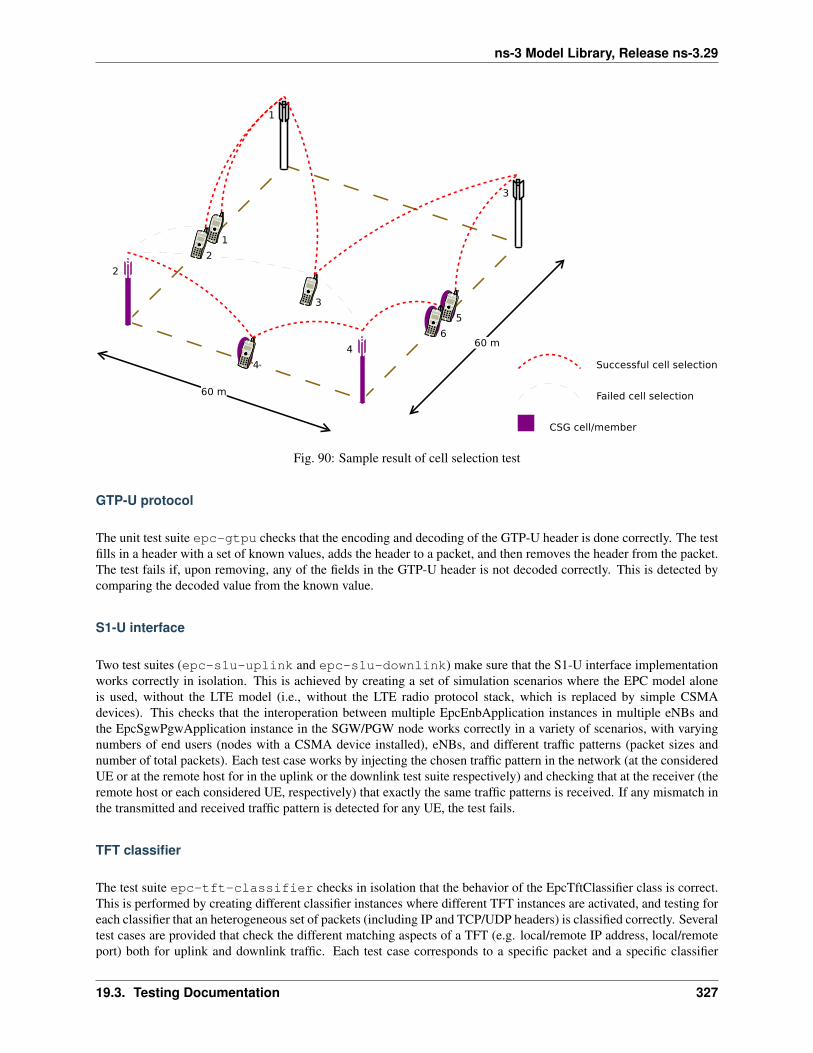
ns-3 Model Library, Release ns-3.29
Fig. 90: Sample result of cell selection test
GTP-U protocol
The unit test suite epc-gtpu checks that the encoding and decoding of the GTP-U header is done correctly. The testfills in a header with a set of known values, adds the header to a packet, and then removes the header from the packet.The test fails if, upon removing, any of the fields in the GTP-U header is not decoded correctly. This is detected bycomparing the decoded value from the known value.
S1-U interface
Two test suites (epc-s1u-uplink and epc-s1u-downlink) make sure that the S1-U interface implementationworks correctly in isolation. This is achieved by creating a set of simulation scenarios where the EPC model aloneis used, without the LTE model (i.e., without the LTE radio protocol stack, which is replaced by simple CSMAdevices). This checks that the interoperation between multiple EpcEnbApplication instances in multiple eNBs andthe EpcSgwPgwApplication instance in the SGW/PGW node works correctly in a variety of scenarios, with varyingnumbers of end users (nodes with a CSMA device installed), eNBs, and different traffic patterns (packet sizes andnumber of total packets). Each test case works by injecting the chosen traffic pattern in the network (at the consideredUE or at the remote host for in the uplink or the downlink test suite respectively) and checking that at the receiver (theremote host or each considered UE, respectively) that exactly the same traffic patterns is received. If any mismatch inthe transmitted and received traffic pattern is detected for any UE, the test fails.
TFT classifier
The test suite epc-tft-classifier checks in isolation that the behavior of the EpcTftClassifier class is correct.This is performed by creating different classifier instances where different TFT instances are activated, and testing foreach classifier that an heterogeneous set of packets (including IP and TCP/UDP headers) is classified correctly. Severaltest cases are provided that check the different matching aspects of a TFT (e.g. local/remote IP address, local/remoteport) both for uplink and downlink traffic. Each test case corresponds to a specific packet and a specific classifier
19.3. Testing Documentation 327
ns-3 Model Library, Release ns-3.29
instance with a given set of TFTs. The test case passes if the bearer identifier returned by the classifier exactly matcheswith the one that is expected for the considered packet.
End-to-end LTE-EPC data plane functionality
The test suite lte-epc-e2e-data ensures the correct end-to-end functionality of the LTE-EPC data plane. Foreach test case in this suite, a complete LTE-EPC simulation scenario is created with the following characteristics:
• a given number of eNBs
• for each eNB, a given number of UEs
• for each UE, a given number of active EPS bearers
• for each active EPS bearer, a given traffic pattern (number of UDP packets to be transmitted and packet size)
Each test is executed by transmitting the given traffic pattern both in the uplink and in the downlink, at subsequenttime intervals. The test passes if all the following conditions are satisfied:
• for each active EPS bearer, the transmitted and received traffic pattern (respectively at the UE and the remotehost for uplink, and vice versa for downlink) is exactly the same
• for each active EPS bearer and each direction (uplink or downlink), exactly the expected number of packet flowsover the corresponding RadioBearer instance
X2 handover
The test suite lte-x2-handover checks the correct functionality of the X2 handover procedure. The scenariobeing tested is a topology with two eNBs connected by an X2 interface. Each test case is a particular instance of thisscenario defined by the following parameters:
• the number of UEs that are initially attached to the first eNB
• the number of EPS bearers activated for each UE
• a list of handover events to be triggered, where each event is defined by: + the start time of the handover trigger+ the index of the UE doing the handover + the index of the source eNB + the index of the target eNB
• a boolean flag indicating whether the target eNB admits the handover or not
• a boolean flag indicating whether the ideal RRC protocol is to be used instead of the real RRC protocol
• the type of scheduler to be used (RR or PF)
Each test case passes if the following conditions are true:
• at time 0.06s, the test CheckConnected verifies that each UE is connected to the first eNB
• for each event in the handover list:
– at the indicated event start time, the indicated UE is connected to the indicated source eNB
– 0.1s after the start time, the indicated UE is connected to the indicated target eNB
– 0.6s after the start time, for each active EPS bearer, the uplink and downlink sink applications of theindicated UE have achieved a number of bytes which is at least half the number of bytes transmitted bythe corresponding source applications
The condition “UE is connected to eNB” is evaluated positively if and only if all the following conditions are met:
• the eNB has the context of the UE (identified by the RNTI value retrieved from the UE RRC)
• the RRC state of the UE at the eNB is CONNECTED_NORMALLY
328 Chapter 19. LTE Module

ns-3 Model Library, Release ns-3.29
• the RRC state at the UE is CONNECTED_NORMALLY
• the UE is configured with the CellId, DlBandwidth, UlBandwidth, DlEarfcn and UlEarfcn of the eNB
• the IMSI of the UE stored at the eNB is correct
• the number of active Data Radio Bearers is the expected one, both at the eNB and at the UE
• for each Data Radio Bearer, the following identifiers match between the UE and the eNB: EPS bearer id, DRBid, LCID
Automatic X2 handover
The test suite lte-x2-handover-measures checks the correct functionality of the handover algorithm. Thescenario being tested is a topology with two, three or four eNBs connected by an X2 interface. The eNBs are locatedin a straight line in the X-axes. A UE moves along the X-axes going from the neighborhood of one eNB to the nexteNB. Each test case is a particular instance of this scenario defined by the following parameters:
• the number of eNBs in the X-axes
• the number of UEs
• the number of EPS bearers activated for the UE
• a list of check point events to be triggered, where each event is defined by: + the time of the first check pointevent + the time of the last check point event + interval time between two check point events + the index of theUE doing the handover + the index of the eNB where the UE must be connected
• a boolean flag indicating whether UDP traffic is to be used instead of TCP traffic
• the type of scheduler to be used
• the type of handover algorithm to be used
• a boolean flag indicating whether handover is admitted by default
• a boolean flag indicating whether the ideal RRC protocol is to be used instead of the real RRC protocol
The test suite consists of many test cases. In fact, it has been one of the most time-consuming test suite in ns-3. Thetest cases run with some combination of the following variable parameters:
• number of eNBs: 2, 3, 4;
• number of EPS bearers: 0, 1, 2;
• RRC: ideal, real (see RRC protocol models);
• MAC scheduler: round robin, proportional fair (see The FemtoForum MAC Scheduler Interface); and
• handover algorithm: A2-A4-RSRQ, strongest cell (see Handover algorithm).
Each test case passes if the following conditions are true:
• at time 0.08s, the test CheckConnected verifies that each UE is connected to the first eNB
• for each event in the check point list:
– at the indicated check point time, the indicated UE is connected to the indicated eNB
– 0.5s after the check point, for each active EPS bearer, the uplink and downlink sink applications of the UEhave achieved a number of bytes which is at least half the number of bytes transmitted by the correspondingsource applications
The condition “UE is connected to eNB” is evaluated positively if and only if all the following conditions are met:
• the eNB has the context of the UE (identified by the RNTI value retrieved from the UE RRC)
19.3. Testing Documentation 329
ns-3 Model Library, Release ns-3.29
• the RRC state of the UE at the eNB is CONNECTED_NORMALLY
• the RRC state at the UE is CONNECTED_NORMALLY
• the UE is configured with the CellId, DlBandwidth, UlBandwidth, DlEarfcn and UlEarfcn of the eNB
• the IMSI of the UE stored at the eNB is correct
• the number of active Data Radio Bearers is the expected one, both at the eNB and at the UE
• for each Data Radio Bearer, the following identifiers match between the UE and the eNB: EPS bearer id, DRBid, LCID
Handover delays
Handover procedure consists of several message exchanges between UE, source eNodeB, and target eNodeB over bothRRC protocol and X2 interface. Test suite lte-handover-delay verifies that this procedure consistently spendsthe same amount of time.
The test suite will run several handover test cases. Each test case is an individual simulation featuring a handover at aspecified time in simulation. For example, the handover in the first test case is invoked at time +0.100s, while in thesecond test case it is at +0.101s. There are 10 test cases, each testing a different subframe in LTE. Thus the last testcase has the handover at +0.109s.
The simulation scenario in the test cases is as follow:
• EPC is enabled
• 2 eNodeBs with circular (isotropic) antenna, separated by 1000 meters
• 1 static UE positioned exactly in the center between the eNodeBs
• no application installed
• no channel fading
• default path loss model (Friis)
• 0.300s simulation duration
The test case runs as follow. At the beginning of the simulation, the UE is attached to the first eNodeB. Then at thetime specified by the test case input argument, a handover request will be explicitly issued to the second eNodeB. Thetest case will then record the starting time, wait until the handover is completed, and then record the completion time.If the difference between the completion time and starting time is less than a predefined threshold, then the test passes.
A typical handover in the current ns-3 implementation takes 4.2141 ms when using Ideal RRC protocol model, and19.9283 ms when using Real RRC protocol model. Accordingly, the test cases use 5 ms and 20 ms as the maximumthreshold values. The test suite runs 10 test cases with Ideal RRC protocol model and 10 test cases with Real RRCprotocol model. More information regarding these models can be found in Section RRC protocol models.
The motivation behind using subframes as the main test parameters is the fact that subframe index is one of the factorsfor calculating RA-RNTI, which is used by Random Access during the handover procedure. The test cases verifythis computation, utilizing the fact that the handover will be delayed when this computation is broken. In the defaultsimulation configuration, the handover delay observed because of a broken RA-RNTI computation is typically 6 ms.
Selection of target cell in handover algorithm
eNodeB may utilize Handover algorithm to automatically create handover decisions during simulation. The decisionincludes the UE which should do the handover and the target cell where the UE should perform handover to.
330 Chapter 19. LTE Module

ns-3 Model Library, Release ns-3.29
The test suite lte-handover-target verifies that the handover algorithm is making the right decision, in partic-ular, in choosing the right target cell. It consists of several short test cases for different network topology (2×2 gridand 3×2 grid) and types of handover algorithm (the A2-A4-RSRQ handover algorithm and the strongest cell handoveralgorithm).
Each test case is a simulation of a micro-cell environment with the following parameter:
• EPC is enabled
• several circular (isotropic antenna) micro-cell eNodeBs in a rectangular grid layout, with 130 m distance be-tween each adjacent point
• 1 static UE, positioned close to and attached to the source cell
• no control channel error model
• no application installed
• no channel fading
• default path loss model (Friis)
• 1s simulation duration
To trigger a handover, the test case “shutdowns” the source cell at +0.5s simulation time. Figure lte-handover-targettest scenario in a 2×2 grid below illustrates the process. This is done by setting the source cell’s Tx power to a verylow value. As a result, the handover algorithm notices that the UE deserves a handover and several neighboring cellsbecome candidates of target cell at the same time.
Fig. 91: lte-handover-target test scenario in a 2×2 grid
The test case then verifies that the handover algorithm, when faced with more than one options of target cells, is ableto choose the right one.
Downlink Power Control
The test suite lte-downlink-power-control checks correctness of Downlink Power Control in three differentways:
• LteDownlinkPowerControlSpectrumValue test case check if LteSpectrumValueHelper::CreateTxPowerSpectralDensityis creating correct spectrum value for PSD for downlink transmission. The test vector contain EARFCN,system bandwidth, TX power, TX power for each RB, active RBs, and expected TxPSD. The test passes if
19.3. Testing Documentation 331
ns-3 Model Library, Release ns-3.29
TxPDS generated by LteSpectrumValueHelper::CreateTxPowerSpectralDensity is equal toexpected TxPSD.
• LteDownlinkPowerControlTestCase test case check if TX power difference between data and control chan-nel is equal to configured PdschConfigDedicated::P_A value. TX power of control channel is measuredby LteTestSinrChunkProcessor added to RsPowerChunkProcessor list in UE DownlinkSpec-trumPhy. Tx power of data channel is measured in similar way, but it had to be implemented. NowLteTestSinrChunkProcessor is added to DataPowerChunkProcessor list in UE DownlinkSpec-trumPhy. Test vector contain a set of all available P_A values. Test pass if power difference equals P_A value.
• LteDownlinkPowerControlRrcConnectionReconfiguration test case check if RrcConnectionReconfiguration isperformed correctly. When FR entity gets UE measurements, it immediately calls function to change P_Avalue for this UE and also triggers callback connected with this event. Then, test check if UE gets RrcConnec-tionReconfiguration message (it trigger callback). Finally, it checks if eNB receive RrcConnectionReconfigu-rationCompleted message, what also trigger callback. The test passes if all event have occurred. The test isperformed two times, with IdealRrcProtocol and with RealRrcProtocol.
Uplink Power Control Tests
UE uses Uplink Power Control to automatically change Tx Power level for Uplink Physical Channels. Tx Power iscomputed based on path-loss, number of RB used for transmission, some configurable parameters and TPC commandfrom eNB.
The test suite lte-uplink-power-control verifies if Tx Power is computed correctly. There are three differenttest cases:
• LteUplinkOpenLoopPowerControlTestCase test case checks Uplink Power Control functionality in Open Loopmechanism. UE is attached to eNB and is transmitting data in Downlink and Uplink. Uplink Power Controlwith Open Loop mechanism is enabled and UE changes position each 100 ms. In each position Uplink PowerControl entity is calculating new Tx Power level for all uplink channels. These values are traced and test passesif Uplink Tx Power for PUSCH, PUCCH and SRS in each UE position are equal to expected values.
• LteUplinkClosedLoopPowerControlAbsoluteModeTestCase test case checks Uplink Power Control functional-ity with Closed Loop mechanism and Absolute Mode enabled. UE is attached to eNB and is transmitting data inDownlink and Uplink. Uplink Power Control with Closed Loop mechanism and Absolute Mode is enabled. UEis located 100 m from eNB and is not changing its position. LteFfrSimple algorithm is used on eNB side to setTPC values in DL-DCI messages. TPC configuration in eNB is changed every 100 ms, so every 100 ms UplinkPower Control entity in UE should calculate different Tx Power level for all uplink channels. These values aretraced and test passes if Uplink Tx Power for PUSCH, PUCCH and SRS computed with all TCP values areequal to expected values.
• LteUplinkClosedLoopPowerControlAccumulatedModeTestCase test case checks Closed Loop Uplink PowerControl functionality with Closed Loop mechanism and Accumulative Mode enabled. UE is attached to eNBand is transmitting data in Downlink and Uplink. Uplink Power Control with Closed Loop mechanism andAccumulative Mode is enabled. UE is located 100 m from eNB and is not changing its position. As in abovetest case, LteFfrSimple algorithm is used on eNB side to set TPC values in DL-DCI messages, but in this caseTPC command are set in DL-DCI only configured number of times, and after that TPC is set to be 1, what ismapped to value of 0 in Accumulative Mode (TS36.213 Table 5.1.1.1-2). TPC configuration in eNB is changedevery 100 ms. UE is accumulating these values and calculates Tx Power levels for all uplink channels based onaccumulated value. If computed Tx Power level is lower than minimal UE Tx Power, UE should transmit withits minimal Tx Power. If computed Tx Power level is higher than maximal UE Tx Power, UE should transmitwith its maximal Tx Power. Tx Power levels for PUSCH, PUCCH and SRS are traced and test passes if they areequal to expected values.
332 Chapter 19. LTE Module
ns-3 Model Library, Release ns-3.29
Frequency Reuse Algorithms
The test suite lte-frequency-reuse contain two types of test cases.
First type of test cases check if RBGs are used correctly according to FR algorithm policy. We are testing if scheduleruse only RBGs allowed by FR configuration. To check which RBGs are used LteSimpleSpectrumPhy is at-tached to Downlink Channel. It notifies when data downlink channel transmission has occurred and pass signal TxPsdspectrum value to check which RBs were used for transmission. The test vector comprise a set of configuration forHard and Strict FR algorithms (there is no point to check other FR algorithms in this way because they use entire cellbandwidth). Test passes if none of not allowed RBGs are used.
Second type of test cases check if UE is served within proper sub-band and with proper transmission power. Inthis test scenario, there are two eNBs.There are also two UEs and each eNB is serving one. One uses FrequencyReuse algorithm and second one does not. Second eNB is responsible for generating interferences in whole systembandwidth. UE served by first eNB is changing position each few second (rather slow because time is needed toreport new UE Measurements). To check which RBGs are used for this UE LteSimpleSpectrumPhy is attachedto Downlink Channel. It notifies when data downlink channel transmission in cell 1 has occurred and pass signalTxPsd spectrum value to check which RBs were used for transmission and their power level. The same approach isapplied in Uplink direction and second LteSimpleSpectrumPhy is attached to Uplink Channel. Test passes ifUE served by eNB with FR algorithm is served in DL and UL with expected RBs and with expected power level. Testvector comprise a configuration for Strict FR, Soft FR, Soft FFR, Enhanced FFR. Each FR algorithm is tested with allschedulers, which support FR (i.e. PF, PSS, CQA, TD-TBFQ, FD-TBFQ). (Hard FR do not use UE measurements, sothere is no point to perform this type of test for Hard FR).
Test case for Distributed FFR algorithm is quite similar to above one, but since eNBs need to exchange some infor-mation, scenario with EPC enabled and X2 interfaces is considered. Moreover, both eNB are using Distributed FFRalgorithm. There are 2 UE in first cell, and 1 in second cell. Position of each UE is changed (rather slow because timeis needed to report new UE Measurements), to obtain different result from calculation in Distributed FFR algorithmentities. To check which RBGs are used for UE transmission LteSimpleSpectrumPhy is attached to DownlinkChannel. It notifies when data downlink channel transmission has occurred and pass signal TxPsd spectrum value tocheck which RBs were used for transmission and their power level. The same approach is applied in Uplink directionand second LteSimpleSpectrumPhy is attached to Uplink Channel. Test passes if UE served by eNB in cell 2,is served in DL and UL with expected RBs and with expected power level. Test vector comprise a configuration forDistributed FFR. Test is performed with all schedulers, which support FR (i.e. PF, PSS, CQA, TD-TBFQ, FD-TBFQ).
Inter-cell Interference with FR algorithms Tests
The test suite lte-interference-fr is very similar to lte-interference. Topology (Figure Topology forthe inter-cell interference test) is the same and test checks interference level. The difference is that, in this test caseFrequency Reuse algorithms are enabled and we are checking interference level on different RBGs (not only on one).For example, when we install Hard FR algorithm in eNbs, and first half of system bandwidth is assigned to one eNb,and second half to second eNb, interference level should be much lower compared to legacy scenario. The test vectorcomprise a set of configuration for all available Frequency Reuse Algorithms. Test passes if calculated SINR onspecific RBs is equal to these obtained by Octave script.
Carrier aggregation test
The test suite lte-carrier-aggregation is a system test program that creates different test cases with a singleeNB and several UEs, all having the same radio bearer specification. Different test cases are implemented by usingdifferent SINR values and different numbers of UEs. eNBs and UEs are configured to use the secondary carrier and thecomponent carrier manager is configured to split the data uniformly between primary and secondary carrier. The testconsists of checking that the throughput obtained over the different carriers are equal considering a given tolerance.For more details about this test, see the section Carrier aggregation usage example.
19.3. Testing Documentation 333

ns-3 Model Library, Release ns-3.29
Carrier aggregation test for eNB and UE configuration
The test suite carrier-aggregation-config-test is a system test program, which verifies the followingtwo cases:
• When carrier aggregation is enabled and UE carriers configuration is different than the default configurationdone in LteHelper, we check that the UE(s) is configured properly once it receives RRC Connection Reconfig-uration message from eNB.
• A user can configure 2 or more eNBs and UEs with different configuration parameters, i.e., each eNB and UEcan have different EARFCN and Bandwidths and a UE connects to an eNB with similar DL EARFCN. In thistest, we check with CA enabled but the end results will be the same if carrier aggregation is not enabled and wehave more than one eNBs and UEs with different configurations.
Since, we do not need EPC to test the configuration, this test only simulates the LTE radio access with RLC SM. Thereare two test cases, Test 1 tests that the UE is configured properly after receiving RRC Connection Reconfigurationmessage from the eNB, which will overwrite UE default configuration done in LteHelper for the sake of creating PHYand MAC instances equal to the number of component carriers. Test 2 tests that every eNB or UE in a simulationscenario can be configured with different EARFCNs and Bandwidths. For both test cases, it also counts the number oftimes the hooked trace source SCarrierConfigured get triggered. As, it reflects how many UEs got attached totheir respective eNB. If the count is not equal to the number of UEs in the scenario, the test fails, which could be theresult of improper UE configuration.
19.4 Profiling Documentation
19.4.1 Overview and objectives
The main objective of the profiling carried out is to assess the simulator performance on a broad set of scenarios. Thisevaluation provides reference values for simulation running times and memory consumption figures. It also helps toidentify potential performance improvements and to check for scalability problems when increasing the number ofeNodeB and UEs attached to those.
In the following sections, a detailed description of the general profiling framework employed to perform the study isintroduced. It also includes details on the main performed tests and its results evaluation.
19.4.2 Framework description
Simulation scripts
The simulation script used for all the E-UTRAN results showed in this documentation is located at src/lte/examples/lena-profiling.cc. It uses the complete PHY and MAC UE/eNodeB implementation with a sim-plified RLC implementation on top. This script generates a squared grid topology, placing a eNodeB at the centre ofeach square. UEs attached to this node are scattered randomly across the square (using a random uniform distributionalong X and Y axis). If BuildingPropagationModel is used, the squares are replaced by rooms. To generate the ULand DL traffic, the RLC implementation always report data to be transferred.
For the EPC results, the script is src/lte/examples/lena-simple-epc.cc. It uses a complete E-UTRANimplementation (PHY+MAC+RLC/UM+PDCP) and the most relevant EPC user plane entities the PGW and SGW,including GTP-U tunneling. This script generates a given number of eNodeBs, distributed across a line and attaches asingle UE to every eNodeB. It also creates an EPC network and an external host connected to it through the Internet.Each UE sends and receives data to and from the remote host. In addition, each UE is also sending data to the UEcamped in the adjacent eNodeB.
334 Chapter 19. LTE Module
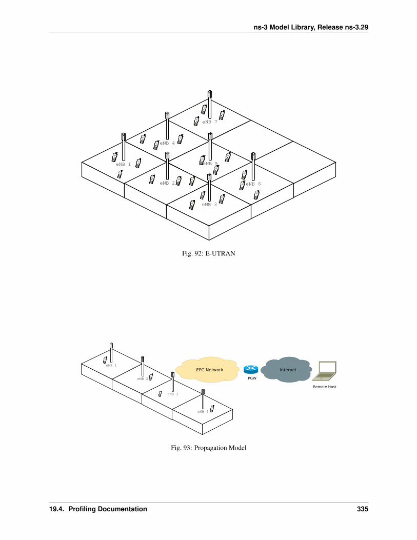
ns-3 Model Library, Release ns-3.29
Fig. 92: E-UTRAN
Fig. 93: Propagation Model
19.4. Profiling Documentation 335
ns-3 Model Library, Release ns-3.29
RLC and MAC traces are enabled for all UEs and all eNodeBs and those traces are written to disk directly. The MACscheduler used is round robin.
Simulation input parameters
The lena-profiling simulation script accepts the following input parameters:
• simTime: time to simulate (in seconds)
• nUe: number of UEs attached to each eNodeB
• nEnb: number of eNodeB composing the grid per floor
• nFloors: number of floors, 0 for Friis propagation model (no walls), 1 or greater for Building propagationmodel generating a nFloors-storey building.
• traceDirectory: destination directory where simulation traces will be stored
The lena-simple-epc script accepts those other parameters:
• simTime: time to simulate (in seconds)
• numberOfNodes: number of eNodeB + UE pairs created
Time measurement
Running time is measured using default Linux shell command time. This command counts how much user time theexecution of a program takes.
Perl script
To simplify the process of running the profiling script for a wide range of values and collecting its timing data, a simplePerl script to automate the complete process is provided. It is placed in src/lte/test/lte-test-run-time.pl for lena-profiling and in src/lte/epc-test-run-time.pl for lena-simple-epc. It simply runs a batch ofsimulations with a range of parameters and stores the timing results in a CSV file called lteTimes.csv and epcTimes.csvrespectively. The range of values each parameter sweeps can be modified editing the corresponding script.
Requirements
The following Perl modules are required to use the provided script, all of them available from CPAN:
• IO::CaptureOutput
• Statistics::Descriptive
For installing the modules, simply use the following command:
perl -MCPAN -e 'install moduleName'
Plotting results
To plot the results obtained from running the Perl scripts, two gnuplot scripts are provided, in src/lte/test/lte-test-run-plot and src/lte/test/epc-test-run-plot. Most of the plots availablein this documentation can be reproduced with those, typing the commands gnuplot < src/lte/test/lte-test-run-plot and gnuplot < src/lte/test/epc-test-run-plot.
336 Chapter 19. LTE Module

ns-3 Model Library, Release ns-3.29
Reference software and equipment
All timing tests had been run in a Intel Pentium IV 3.00 GHz machine with 512 Mb of RAM memory running FedoraCore 10 with a 2.6.27.41-170.2.117 kernel, storing the traces directly to the hard disk.
Also, as a reference configuration, the build has been configured static and optimized. The exact waf command issuedis:
CXXFLAGS="-O3 -w" ./waf -d optimized configure --enable-static--enable-examples --enable-modules=lte
19.4.3 Results
E-UTRAN
The following results and figures had been obtained with LENA changeset 2c5b0d697717.
Running time
This scenario, evaluates the running time for a fixed simulation time (10s) and Friis propagation mode increasing thenumber of UEs attached to each eNodeB and the number of planted eNodeBs in the scenario.
0
500
1000
1500
2000
2500
3000
3500
4000
0 5 10 15 20 25 30
Runnin
g tim
e [s]
Number of UEs per eNodeB
Simulation time = 10 s - Friis Model
1 eNodeB2 eNodeB4 eNodeB6 eNodeB8 eNodeB
12 eNodeB14 eNodeB18 eNodeB22 eNodeB
Fig. 94: Running time
The figure shows the expected behaviour, since it increases linearly respect the number of UEs per eNodeB andquadratically respect the total number of eNodeBs.
19.4. Profiling Documentation 337

ns-3 Model Library, Release ns-3.29
Propagation model
The objective of this scenario is to evaluate the impact of the propagation model complexity in the overall run timefigures. Therefore, the same scenario is simulated twice: once using the more simple Friis model, once with the morecomplex Building model. The rest of the parameters (e.g. number of eNodeB and of UE attached per eNodeB) weremaintained. The timing results for both models are compared in the following figure.
0
1000
2000
3000
4000
5000
6000
0 5 10 15 20 25 30
Runnin
g tim
e [s]
Number of UEs per eNodeB
Simulation time = 10 s
4 eNodeB - Friis4 eNodeB - Building
8 eNodeB - Friis8 eNodeB - Building
12 eNodeB - Friis12 eNodeB - Building
14 eNodeB - Friis14 eNodeB - Building
18 eNodeB - Friis18 eNodeB - Building
22 eNodeB - Friis22 eNodeB - Building
Fig. 95: Propagation Model
In this situation, results are also coherent with what is expected. The more complex the model, the higher the runningtime. Moreover, as the number of computed path losses increases (i.e. more UEs per eNodeB or more eNodeBs) theextra complexity of the propagation model drives the running time figures further apart.
Simulation time
In this scenario, for a fixed set of UEs per eNodeB, different simulation times had been run. As the simulation timeincreases, running time should also increase linearly, i.e. for a given scenario, simulate four seconds should take twicetimes what it takes to simulate two seconds. The slope of this line is a function of the complexity of the scenario: themore eNodeB / UEs placed, the higher the slope of the line.
Memory usage
Massif tool to profile memory consumption
EPC
The following results and figures had been obtained with LENA changeset e8b3ccdf6673. The rationale behind thetwo scenarios profiled on this section is the same than for the E-UTRA part.
338 Chapter 19. LTE Module

ns-3 Model Library, Release ns-3.29
0
500
1000
1500
2000
2500
3000
0 2 4 6 8 10 12 14 16
Runnin
g tim
e [s]
Simulation time
Friis propagation model 15 UE per eNodeB
1 eNodeB2 eNodeB4 eNodeB6 eNodeB8 eNodeB
12 eNodeB14 eNodeB18 eNodeB22 eNodeB
Fig. 96: Simulation time
0
200
400
600
800
1000
1200
1400
1600
1800
2000
2 3 4 5 6 7 8 9 10
Mem
ory
(K
iB)
Number of UEs
Peak Memory (Simulation Time = 1s)
Number of eNBs2 - Friis468102 - Building46810
Fig. 97: Memory profile
19.4. Profiling Documentation 339
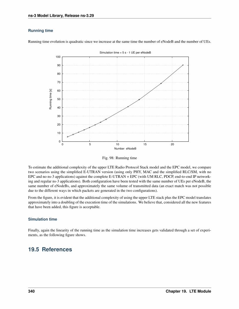
ns-3 Model Library, Release ns-3.29
Running time
Running time evolution is quadratic since we increase at the same time the number of eNodeB and the number of UEs.
0
10
20
30
40
50
60
70
80
90
100
0 5 10 15 20
Runnin
g tim
e [s]
Number eNodeB
Simulation time = 5 s - 1 UE per eNodeB
Fig. 98: Running time
To estimate the additional complexity of the upper LTE Radio Protocol Stack model and the EPC model, we comparetwo scenarios using the simplified E-UTRAN version (using only PHY, MAC and the simplified RLC/SM, with noEPC and no ns-3 applications) against the complete E-UTRAN + EPC (with UM RLC, PDCP, end-to-end IP network-ing and regular ns-3 applications). Both configuration have been tested with the same number of UEs per eNodeB, thesame number of eNodeBs, and approximately the same volume of transmitted data (an exact match was not possibledue to the different ways in which packets are generated in the two configurations).
From the figure, it is evident that the additional complexity of using the upper LTE stack plus the EPC model translatesapproximately into a doubling of the execution time of the simulations. We believe that, considered all the new featuresthat have been added, this figure is acceptable.
Simulation time
Finally, again the linearity of the running time as the simulation time increases gets validated through a set of experi-ments, as the following figure shows.
19.5 References
340 Chapter 19. LTE Module
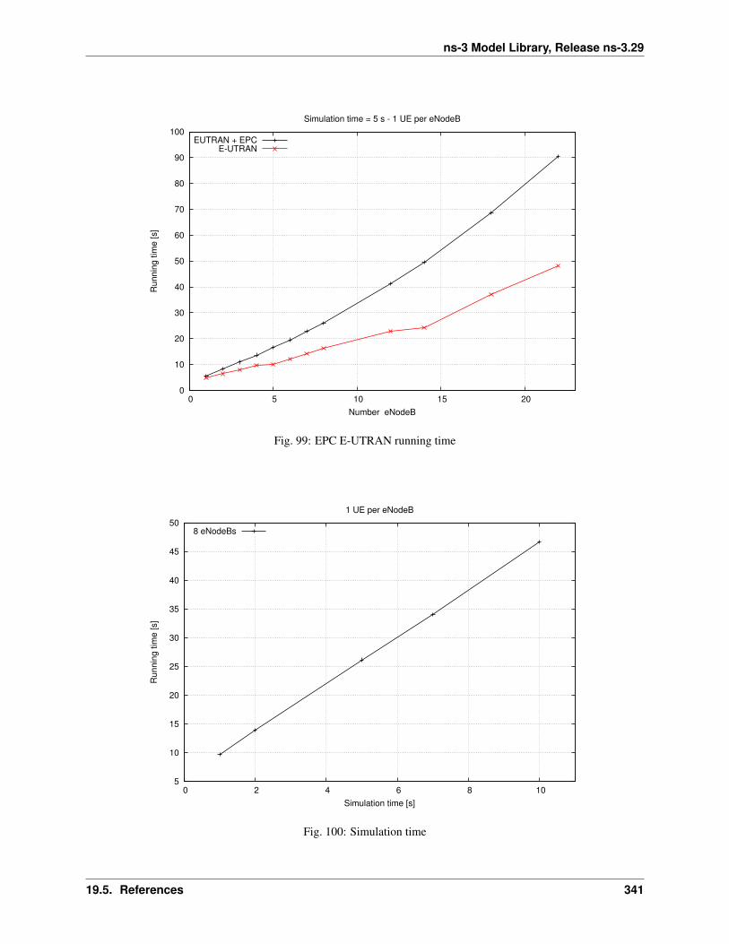
ns-3 Model Library, Release ns-3.29
0
10
20
30
40
50
60
70
80
90
100
0 5 10 15 20
Runnin
g tim
e [s]
Number eNodeB
Simulation time = 5 s - 1 UE per eNodeB
EUTRAN + EPCE-UTRAN
Fig. 99: EPC E-UTRAN running time
5
10
15
20
25
30
35
40
45
50
0 2 4 6 8 10
Runnin
g tim
e [s]
Simulation time [s]
1 UE per eNodeB
8 eNodeBs
Fig. 100: Simulation time
19.5. References 341

ns-3 Model Library, Release ns-3.29
342 Chapter 19. LTE Module
CHAPTER
TWENTY
WI-FI MESH MODULE DOCUMENTATION
20.1 Design Documentation
20.1.1 Overview
The ns-3 mesh module extends the ns-3 wifi module to provide mesh networking capabilities according to the IEEE802.11s standard [ieee80211s].
The basic purpose of IEEE 802.11s is to define a mode of operation for Wi-Fi that permits frames to be forwarded overmultiple radio hops transparent to higher layer protocols such as IP. To accomplish this, mesh-capable stations form aMesh Basic Service Set (MBSS) by running a pair-wise peering protocol to establish forwarding associations, and byrunning a routing protocol to find paths through the network. A special gateway device called a mesh gate allows aMBSS to interconnect with a Distribution System (DS).
The basic enhancements defined by IEEE 802.11s include:
• discovery services
• peering management
• security
• beaconing and synchronization
• the Mesh Coordination Function (MCF)
• power management
• channel switching
• extended frame formats
• path selection and forwarding
• interworking (proxy mesh gateways)
• intra-mesh congestion control, and
• emergency service support.
The ns-3 models implement only a subset of the above service extensions, focusing mainly on those items related topeering and routing/forwarding of data frames through the mesh.
The Mesh NetDevice based on 802.11s D3.0 draft standard was added in ns-3.6 and includes the Mesh PeeringManagement Protocol and HWMP (routing) protocol implementations. An overview presentation by Kirill Andreevwas published at the Workshop on ns-3 in 2009 [And09]. An overview paper is available at [And10].
As of ns-3.23 release, the model has been updated to the 802.11s-2012 standard [ieee80211s] with regard to packetformats, based on the contribution in [Hep15].
343

ns-3 Model Library, Release ns-3.29
These changes include:
• Category codes and the categories compliant to IEEE-802.11-2012 Table 8-38—Category values.
• Information Elements (An adjustment of the element ID values was needed according to Table 8-54 of IEEE-802.11-2012).
• Mesh Peering Management element format changed according to IEEE-802.11-2012 Figure 8-370.
• Mesh Configuration element format changed according to IEEE-802.11-2012 Figure 8-363.
• PERR element format changed according to IEEE-802.11-2012 Figure 8-394.
With these changes the messages of the Peering Management Protocol and Hybrid Wireless Mesh Protocol will betransmitted compliant to IEEE802.11-2012 and the resulting pcap trace files can be analyzed by Wireshark.
The multi-interface mesh points are supported as an extension of IEEE draft version 3.0. Note that corresponding ns-3mesh device helper creates a single interface station by default.
Overview of IEEE 802.11s
The implementation of the 802.11s extension consists of two main parts: the Peer Management Protocol (PMP) andHybrid Wireless Mesh Protocol (HWMP).
The tasks of the peer management protocol are the following:
• opening links, detecting beacons, and starting peer link finite state machine, and
• closing peer links due to transmission failures or beacon loss.
If a peer link between the sender and receiver does not exist, a frame will be dropped. So, the plug-in to the peermanagement protocol (PMP) is the first in the list of ns3::MeshWifiInterfaceMacPlugins to be used.
Peer management protocol
The peer management protocol consists of three main parts:
• the protocol itself, ns3::dot11s::PeerManagementProtocol, which keeps all active peer links oninterfaces, handles all changes of their states and notifies the routing protocol about link failures.
• the MAC plug-in, ns3::dot11s::PeerManagementProtocolMac, which drops frames if there is nopeer link, and peeks all needed information from management frames and information elements from beacons.
• the peer link, ns3::dot11s::PeerLink, which keeps finite state machine of each peer link, keeps beaconloss counter and counter of successive transmission failures.
The procedure of closing a peer link is not described in detail in the standard, so in the model the link may be closedby:
• beacon loss (see an appropriate attribute of ns3::dot11s::PeerLink class)
• transmission failure – when a predefined number of successive packets have failed to transmit, the link will beclosed.
The peer management protocol is also responsible for beacon collision avoidance, because itkeeps beacon timing elements from all neighbours. Note that the PeerManagementProtocol isnot attached to the MeshPointDevice as a routing protocol, but the structure is similar: the up-per tier of the protocol is ns3::dot11s::PeerManagementProtocol and its plug-in isns3::dot11s::PeerManagementProtocolMac.
344 Chapter 20. Wi-Fi Mesh Module Documentation

ns-3 Model Library, Release ns-3.29
Hybrid Wireless Mesh Protocol
HWMP is implemented in both modes, reactive and proactive, although path maintenance is not implemented (soactive routes may time out and need to be rebuilt, causing packet loss). Also the model implements an ability totransmit broadcast data and management frames as unicasts (see appropriate attributes). This feature is disabled at astation when the number of neighbors of the station is more than a threshold value.
20.1.2 Scope and Limitations
Supported features
• Peering Management Protocol (PMP), including link close heuristics and beacon collision avoidance.
• Hybrid Wireless Mesh Protocol (HWMP), including proactive and reactive modes, unicast/broadcast propaga-tion of management traffic, multi-radio extensions.
• 802.11e compatible airtime link metric.
Verification
• Comes with the custom Wireshark dissector.
• Linux kernel mac80211 layer compatible message formats.
Unsupported features
• Mesh Coordinated Channel Access (MCCA).
• Internetworking: mesh access point and mesh portal.
• Security.
• Power save.
• Path maintenance (sending PREQ proactively before a path expires)
• Though multi-radio operation is supported, no channel assignment protocol is proposed for now. (Correctchannel switching is not implemented)
Models yet to be created
• Mesh access point (QoS + non-QoS?)
• Mesh portal (QoS + non-QoS?)
Open issues
A bug exists in the Wi-Fi module that manifests itself as performance degradation in large mesh networks, due toincorrect duplicate frame detection for QoS data frames (bug 2326).
Mesh does not work for 802.11n/ac stations (bug 2276).
Energy module can not be used on mesh devices (bug 2265).
IE11S_MESH_PEERING_PROTOCOL_VERSION should be removed as per standard. Protocol ID should actuallybe part of the Mesh Peering Management IE (bug 2600).
20.1. Design Documentation 345
ns-3 Model Library, Release ns-3.29
Node packet processing times are not modeled; some evaluation of the impact of packet processing delays is discussedin [Hep16].
20.2 User Documentation
20.2.1 Using the MeshNetDevice
20.3 Testing Documentation
20.4 References
346 Chapter 20. Wi-Fi Mesh Module Documentation
CHAPTER
TWENTYONE
MPI FOR DISTRIBUTED SIMULATION
Parallel and distributed discrete event simulation allows the execution of a single simulation program on multipleprocessors. By splitting up the simulation into logical processes, LPs, each LP can be executed by a different proces-sor. This simulation methodology enables very large-scale simulations by leveraging increased processing power andmemory availability. In order to ensure proper execution of a distributed simulation, message passing between LPsis required. To support distributed simulation in ns-3, the standard Message Passing Interface (MPI) is used, alongwith a new distributed simulator class. Currently, dividing a simulation for distributed purposes in ns-3 can only occuracross point-to-point links.
21.1 Current Implementation Details
During the course of a distributed simulation, many packets must cross simulator boundaries. In other words, a packetthat originated on one LP is destined for a different LP, and in order to make this transition, a message containing thepacket contents must be sent to the remote LP. Upon receiving this message, the remote LP can rebuild the packetand proceed as normal. The process of sending an receiving messages between LPs is handled easily by the new MPIinterface in ns-3.
Along with simple message passing between LPs, a distributed simulator is used on each LP to determine whichevents to process. It is important to process events in time-stamped order to ensure proper simulation execution. If aLP receives a message containing an event from the past, clearly this is an issue, since this event could change otherevents which have already been executed. To address this problem, two conservative synchronization algorithm withlookahead are used in ns-3. For more information on different synchronization approaches and parallel and distributedsimulation in general, please refer to “Parallel and Distributed Simulation Systems” by Richard Fujimoto.
The default parallel synchronization strategy implemented in the DistributedSimulatorImpl class is based on a globallysynchronized algorithm using an MPI collective operation to synchronize simulation time across all LPs. A secondsynchronization strategy based on local communication and null messages is implemented in the NullMessageSimula-torImpl class, For the null message strategy the global all to all gather is not required; LPs only need to communicationwith LPs that have shared point-to-point links. The algorithm to use is controlled by which the ns-3 global value Sim-ulatorImplementationType.
The best algorithm to use is dependent on the communication and event scheduling pattern for the application. Ingeneral, null message synchronization algorithms will scale better due to local communication scaling better than aglobal all-to-all gather that is required by DistributedSimulatorImpl. There are two known cases where the globalsynchronization performs better. The first is when most LPs have point-to-point link with most other LPs, in otherwords the LPs are nearly fully connected. In this case the null message algorithm will generate more message passingtraffic than the all-to-all gather. A second case where the global all-to-all gather is more efficient is when there arelong periods of simulation time when no events are occurring. The all-to-all gather algorithm is able to quicklydetermine then next event time globally. The nearest neighbor behavior of the null message algorithm will requiremore communications to propagate that knowledge; each LP is only aware of neighbor next event times.
347

ns-3 Model Library, Release ns-3.29
21.1.1 Remote point-to-point links
As described in the introduction, dividing a simulation for distributed purposes in ns-3 currently can only occur acrosspoint-to-point links; therefore, the idea of remote point-to-point links is very important for distributed simulation inns-3. When a point-to-point link is installed, connecting two nodes, the point-to-point helper checks the system id, orrank, of both nodes. The rank should be assigned during node creation for distributed simulation and is intended tosignify on which LP a node belongs. If the two nodes are on the same rank, a regular point-to-point link is created. If,however, the two nodes are on different ranks, then these nodes are intended for different LPs, and a remote point-to-point link is used. If a packet is to be sent across a remote point-to-point link, MPI is used to send the message to theremote LP.
21.1.2 Distributing the topology
Currently, the full topology is created on each rank, regardless of the individual node system ids. Only the applica-tions are specific to a rank. For example, consider node 1 on LP 1 and node 2 on LP 2, with a traffic generator onnode 1. Both node 1 and node 2 will be created on both LP1 and LP2; however, the traffic generator will only beinstalled on LP1. While this is not optimal for memory efficiency, it does simplify routing, since all current routingimplementations in ns-3 will work with distributed simulation.
21.2 Running Distributed Simulations
21.2.1 Prerequisites
Ensure that MPI is installed, as well as mpic++. In Ubuntu repositories, these are openmpi-bin, openmpi-common,openmpi-doc, libopenmpi-dev. In Fedora, these are openmpi and openmpi-devel.
Note:
There is a conflict on some Fedora systems between libotf and openmpi. A possible “quick-fix” is to yum removelibotf before installing openmpi. This will remove conflict, but it will also remove emacs. Alternatively, these stepscould be followed to resolve the conflict:
1) Rename the tiny otfdump which emacs says it needs:
$ mv /usr/bin/otfdump /usr/bin/otfdump.emacs-version
2) Manually resolve openmpi dependencies:
$ sudo yum install libgfortran libtorque numactl
3) Download rpm packages:
openmpi-1.3.1-1.fc11.i586.rpmopenmpi-devel-1.3.1-1.fc11.i586.rpmopenmpi-libs-1.3.1-1.fc11.i586.rpmopenmpi-vt-1.3.1-1.fc11.i586.rpm
from http://mirrors.kernel.org/fedora/releases/11/Everything/i386/os/Packages/
4) Force the packages in:
$ sudo rpm -ivh --force \openmpi-1.3.1-1.fc11.i586.rpm \openmpi-libs-1.3.1-1.fc11.i586.rpm \
(continues on next page)
348 Chapter 21. MPI for Distributed Simulation
ns-3 Model Library, Release ns-3.29
(continued from previous page)
openmpi-devel-1.3.1-1.fc11.i586.rpm \openmpi-vt-1.3.1-1.fc11.i586.rpm
Also, it may be necessary to add the openmpi bin directory to PATH in order to execute mpic++ and mpirun from thecommand line. Alternatively, the full path to these executables can be used. Finally, if openmpi complains about theinability to open shared libraries, such as libmpi_cxx.so.0, it may be necessary to add the openmpi lib directory toLD_LIBRARY_PATH.
Here is an example of setting up PATH and LD_LIBRARY_PATH using a bash shell:
• For a 32-bit Linux distribution:
$ export PATH=$PATH:/usr/lib/openmpi/bin$ export LD_LIBRARY_PATH=$LD_LIBRARY_PATH:/usr/lib/openmpi/lib
For a 64-bit Linux distribution:
$ export PATH=$PATH:/usr/lib64/openmpi/bin$ export LD_LIBRARY_PATH=$LD_LIBRARY_PATH:/usr/lib64/openmpi/lib
These lines can be added into ~/.bash_profile or ~/.bashrc to avoid having to retype them when a new shell is opened.
21.2.2 Building and Running Examples
If you already built ns-3 without MPI enabled, you must re-build:
$ ./waf distclean
Configure ns-3 with the –enable-mpi option:
$ ./waf -d debug configure --enable-examples --enable-tests --enable-mpi
Ensure that MPI is enabled by checking the optional features shown from the output of configure.
Next, build ns-3:
$ ./waf
After building ns-3 with mpi enabled, the example programs are now ready to run with mpirun. Here are a fewexamples (from the root ns-3 directory):
$ mpirun -np 2 ./waf --run simple-distributed$ mpirun -np 4 -machinefile mpihosts ./waf --run 'nms-udp-nix --LAN=2 --CN=4 --nix=1'
An examle using the null message synchronization algorithm:
$ mpirun -np 2 ./waf --run simple-distributed --nullmsg
The np switch is the number of logical processors to use. The machinefile switch is which machines to use. In orderto use machinefile, the target file must exist (in this case mpihosts). This can simply contain something like:
localhostlocalhostlocalhost...
21.2. Running Distributed Simulations 349
ns-3 Model Library, Release ns-3.29
Or if you have a cluster of machines, you can name them.
NOTE: Some users have experienced issues using mpirun and waf together. An alternative way to run distributedexamples is shown below:
$ ./waf shell$ cd build/debug$ mpirun -np 2 src/mpi/examples/simple-distributed
21.2.3 Setting synchronization algorithm to use
The global value SimulatorImplementationType is used to set the synchronization algorithm to use. This value mustbe set before the MpiInterface::Enable method is invoked if the default DistributedSimulatorImpl is not used. Hereis an example code snippet showing how to add a command line argument to control the synchronization algorithmchoice::
cmd.AddValue ("nullmsg", "Enable the use of null-message synchronization", nullmsg);if(nullmsg)
{GlobalValue::Bind ("SimulatorImplementationType",
StringValue ("ns3::NullMessageSimulatorImpl"));}
else{GlobalValue::Bind ("SimulatorImplementationType",
StringValue ("ns3::DistributedSimulatorImpl"));}
// Enable parallel simulator with the command line argumentsMpiInterface::Enable (&argc, &argv);
21.2.4 Creating custom topologies
The example programs in src/mpi/examples give a good idea of how to create different topologies for distributedsimulation. The main points are assigning system ids to individual nodes, creating point-to-point links where thesimulation should be divided, and installing applications only on the LP associated with the target node.
Assigning system ids to nodes is simple and can be handled two different ways. First, a NodeContainer can be used tocreate the nodes and assign system ids:
NodeContainer nodes;nodes.Create (5, 1); // Creates 5 nodes with system id 1.
Alternatively, nodes can be created individually, assigned system ids, and added to a NodeContainer. This is useful ifa NodeContainer holds nodes with different system ids:
NodeContainer nodes;Ptr<Node> node1 = CreateObject<Node> (0); // Create node1 with system id 0Ptr<Node> node2 = CreateObject<Node> (1); // Create node2 with system id 1nodes.Add (node1);nodes.Add (node2);
Next, where the simulation is divided is determined by the placement of point-to-point links. If a point-to-point link iscreated between two nodes with different system ids, a remote point-to-point link is created, as described in CurrentImplementation Details.
350 Chapter 21. MPI for Distributed Simulation

ns-3 Model Library, Release ns-3.29
Finally, installing applications only on the LP associated with the target node is very important. For example, if atraffic generator is to be placed on node 0, which is on LP0, only LP0 should install this application. This is easilyaccomplished by first checking the simulator system id, and ensuring that it matches the system id of the target nodebefore installing the application.
21.3 Tracing During Distributed Simulations
Depending on the system id (rank) of the simulator, the information traced will be different, since traffic originatingon one simulator is not seen by another simulator until it reaches nodes specific to that simulator. The easiest way tokeep track of different traces is to just name the trace files or pcaps differently, based on the system id of the simulator.For example, something like this should work well, assuming all of these local variables were previously defined:
if (MpiInterface::GetSystemId () == 0){pointToPoint.EnablePcapAll ("distributed-rank0");phy.EnablePcap ("distributed-rank0", apDevices.Get (0));csma.EnablePcap ("distributed-rank0", csmaDevices.Get (0), true);
}else if (MpiInterface::GetSystemId () == 1)
{pointToPoint.EnablePcapAll ("distributed-rank1");phy.EnablePcap ("distributed-rank1", apDevices.Get (0));csma.EnablePcap ("distributed-rank1", csmaDevices.Get (0), true);
}
21.3. Tracing During Distributed Simulations 351

ns-3 Model Library, Release ns-3.29
352 Chapter 21. MPI for Distributed Simulation

CHAPTER
TWENTYTWO
MOBILITY
The mobility support in ns-3 includes:
• a set of mobility models which are used to track and maintain the current cartesian position and speed of anobject.
• a “course change notifier” trace source which can be used to register listeners to the course changes of a mobilitymodel
• a number of helper classes which are used to place nodes and setup mobility models (including parsers for somemobility definition formats).
22.1 Model Description
The source code for mobility lives in the directory src/mobility.
22.1.1 Design
The design includes mobility models, position allocators, and helper functions.
In ns-3, special MobilityModel objects track the evolution of position with respect to a (cartesian) co-ordinate system. The mobility model is typically aggregated to an ns3::Node object and queried usingGetObject<MobilityModel> (). The base class ns3::MobilityModel is subclassed for different mo-tion behaviors.
The initial position of objects is typically set with a PositionAllocator. These types of objects will lay out the positionon a notional canvas. Once the simulation starts, the position allocator may no longer be used, or it may be used topick future mobility “waypoints” for such mobility models.
Most users interact with the mobility system using mobility helper classes. The MobilityHelper combines a mobilitymodel and position allocator, and can be used with a node container to install mobility capability on a set of nodes.
We first describe the coordinate system and issues surrounding multiple coordinate systems.
Coordinate system
There are many possible coordinate systems and possible translations between them. ns-3 uses the Cartesian coordinatesystem only, at present.
The question has arisen as to how to use the mobility models (supporting Cartesian coordinates) with different coor-dinate systems. This is possible if the user performs conversion between the ns-3 Cartesian and the other coordinatesystem. One possible library to assist is the proj4 http://trac.osgeo.org/proj/ library for projections and reverse projec-tions.
353

ns-3 Model Library, Release ns-3.29
If we support converting between coordinate systems, we must adopt a reference. It has been suggested to use thegeocentric Cartesian coordinate system as a reference. Contributions are welcome in this regard.
The question has arisen about adding a new mobility model whose motion is natively implemented in a differentcoordinate system (such as an orbital mobility model implemented using spherical coordinate system). We adviseto create a subclass with the APIs desired (such as Get/SetSphericalPosition), and new position allocators, and im-plement the motion however desired, but must also support the conversion to cartesian (by supporting the cartesianGet/SetPosition).
Coordinates
The base class for a coordinate is called ns3::Vector. While positions are normally described as coordinates andnot vectors in the literature, it is possible to reuse the same data structure to represent position (x,y,z) and velocity(magnitude and direction from the current position). ns-3 uses class Vector for both.
There are also some additional related structures used to support mobility models.
• Rectangle
• Box
• Waypoint
MobilityModel
Describe base class
• GetPosition ()
• Position and Velocity attributes
• GetDistanceFrom ()
• CourseChangeNotification
MobilityModel Subclasses
• ConstantPosition
• ConstantVelocity
• ConstantAcceleration
• GaussMarkov
• Hierarchical
• RandomDirection2D
• RandomWalk2D
• RandomWaypoint
• SteadyStateRandomWaypoint
• Waypoint
354 Chapter 22. Mobility
ns-3 Model Library, Release ns-3.29
PositionAllocator
Position allocators usually used only at beginning, to lay out the nodes initial position. However, some mobility models(e.g. RandomWaypoint) will use a position allocator to pick new waypoints.
• ListPositionAllocator
• GridPositionAllocator
• RandomRectanglePositionAllocator
• RandomBoxPositionAllocator
• RandomDiscPositionAllocator
• UniformDiscPositionAllocator
Helper
A special mobility helper is provided that is mainly aimed at supporting the installation of mobility to a Node container(when using containers at the helper API level). The MobilityHelper class encapsulates a MobilityModel factory objectand a PositionAllocator used for initial node layout.
ns-2 MobilityHelper
The ns-2 mobility format is a widely used mobility trace format. The documentation is available at: http://www.isi.edu/nsnam/ns/doc/node172.html
Valid trace files use the following ns2 statements:
$node set X_ x1$node set Y_ y1$node set Z_ z1$ns at $time $node setdest x2 y2 speed$ns at $time $node set X_ x1$ns at $time $node set Y_ Y1$ns at $time $node set Z_ Z1
In the above, the initial positions are set using the set statements. Also, this set can be specified for a future time,such as in the last three statements above.
The command setdest instructs the simulation to start moving the specified node towards the coordinate (x2, y2) atthe specified time. Note that the node may never get to the destination, but will proceed towards the destination at thespecified speed until it either reaches the destination (where it will pause), is set to a new position (via set), or senton another course change (via setdest).
Note that in ns-3, movement along the Z dimension is not supported.
Some examples of external tools that can export in this format include:
• BonnMotion
– Installation instructions and
– Documentation for using BonnMotion with ns-3
• SUMO
• TraNS
• ns-2 setdest utility
22.1. Model Description 355

ns-3 Model Library, Release ns-3.29
A special Ns2MobilityHelper object can be used to parse these files and convert the statements into ns-3 mobilityevents. The underlying ConstantVelocityMobilityModel is used to model these movements.
See below for additional usage instructions on this helper.
22.1.2 Scope and Limitations
• only cartesian coordinates are presently supported
22.1.3 References
TBD
22.2 Usage
Most ns-3 program authors typically interact with the mobility system only at configuration time. However, variousns-3 objects interact with mobility objects repeatedly during runtime, such as a propagation model trying to determinethe path loss between two mobile nodes.
22.2.1 Helper
A typical usage pattern can be found in the third.cc program in the tutorial.
First, the user instantiates a MobilityHelper object and sets some Attributes controlling the “position allo-cator” functionality.
MobilityHelper mobility;
mobility.SetPositionAllocator ("ns3::GridPositionAllocator","MinX", DoubleValue (0.0),"MinY", DoubleValue (0.0),"DeltaX", DoubleValue (5.0),"DeltaY", DoubleValue (10.0),"GridWidth", UintegerValue (3),"LayoutType", StringValue ("RowFirst"));
This code tells the mobility helper to use a two-dimensional grid to initially place the nodes. The first argument is anns-3 TypeId specifying the type of mobility model; the remaining attribute/value pairs configure this position allocator.
Next, the user typically sets the MobilityModel subclass; e.g.:
mobility.SetMobilityModel ("ns3::RandomWalk2dMobilityModel","Bounds", RectangleValue (Rectangle (-50, 50, -50, 50)));
Once the helper is configured, it is typically passed a container, such as:
mobility.Install (wifiStaNodes);
A MobilityHelper object may be reconfigured and reused for different NodeContainers during the configuration of anns-3 scenario.
356 Chapter 22. Mobility
ns-3 Model Library, Release ns-3.29
22.2.2 Ns2MobilityHelper
Two example programs are provided demonstrating the use of the ns-2 mobility helper:
• ns2-mobility-trace.cc
• bonnmotion-ns2-example.cc
ns2-mobility-trace
The ns2-mobility-trace.cc program is an example of loading an ns-2 trace file that specifies the movementsof two nodes over 100 seconds of simulation time. It is paired with the file default.ns_movements.
The program behaves as follows:
• a Ns2MobilityHelper object is created, with the specified trace file.
• A log file is created, using the log file name argument.
• A node container is created with the number of nodes specified in the command line. For this particular tracefile, specify the value 2 for this argument.
• the Install() method of Ns2MobilityHelper to set mobility to nodes. At this moment, the file is read line by line,and the movement is scheduled in the simulator.
• A callback is configured, so each time a node changes its course a log message is printed.
The example prints out messages generated by each read line from the ns2 movement trace file. For each line, it showsif the line is correct, or of it has errors and in this case it will be ignored.
Example usage:
$ ./waf --run "ns2-mobility-trace \--traceFile=src/mobility/examples/default.ns_movements \--nodeNum=2 \--duration=100.0 \--logFile=ns2-mob.log"
Sample log file output:
+0.0ns POS: x=150, y=93.986, z=0; VEL:0, y=50.4038, z=0+0.0ns POS: x=195.418, y=150, z=0; VEL:50.1186, y=0, z=0+104727357.0ns POS: x=200.667, y=150, z=0; VEL:50.1239, y=0, z=0+204480076.0ns POS: x=205.667, y=150, z=0; VEL:0, y=0, z=0
bonnmotion-ns2-example
The bonnmotion-ns2-example.cc program, which models the movement of a single mobile node for 1000seconds of simulation time, has a few associated files:
• bonnmotion.ns_movements is the ns-2-formatted mobility trace
• bonnmotion.params is a BonnMotion-generated file with some metadata about the mobility trace
• bonnmotion.ns_params is another BonnMotion-generated file with ns-2-related metadata.
Neither of the latter two files is used by ns-3, although they are generated as part of the BonnMotion process to outputns-2-compatible traces.
The program bonnmotion-ns2-example.cc will output the following to stdout:
22.2. Usage 357

ns-3 Model Library, Release ns-3.29
At 0.00 node 0: Position(329.82, 66.06, 0.00); Speed(0.53, -0.22, 0.00)At 100.00 node 0: Position(378.38, 45.59, 0.00); Speed(0.00, 0.00, 0.00)At 200.00 node 0: Position(304.52, 123.66, 0.00); Speed(-0.92, 0.97, 0.00)At 300.00 node 0: Position(274.16, 131.67, 0.00); Speed(-0.53, -0.46, 0.00)At 400.00 node 0: Position(202.11, 123.60, 0.00); Speed(-0.98, 0.35, 0.00)At 500.00 node 0: Position(104.60, 158.95, 0.00); Speed(-0.98, 0.35, 0.00)At 600.00 node 0: Position(31.92, 183.87, 0.00); Speed(0.76, -0.51, 0.00)At 700.00 node 0: Position(107.99, 132.43, 0.00); Speed(0.76, -0.51, 0.00)At 800.00 node 0: Position(184.06, 80.98, 0.00); Speed(0.76, -0.51, 0.00)At 900.00 node 0: Position(250.08, 41.76, 0.00); Speed(0.60, -0.05, 0.00)
The motion of the mobile node is sampled every 100 seconds, and its position and speed are printed out. This outputmay be compared to the output of a similar ns-2 program (found in the ns-2 tcl/ex/ directory of ns-2) running fromthe same mobility trace.
The next file is generated from ns-2 (users will have to download and install ns-2 and run this Tcl program to seethis output). The output of the ns-2 bonnmotion-example.tcl program is shown below for comparison (filebonnmotion-example.tr):
M 0.00000 0 (329.82, 66.06, 0.00), (378.38, 45.59), 0.57M 100.00000 0 (378.38, 45.59, 0.00), (378.38, 45.59), 0.57M 119.37150 0 (378.38, 45.59, 0.00), (286.69, 142.52), 1.33M 200.00000 0 (304.52, 123.66, 0.00), (286.69, 142.52), 1.33M 276.35353 0 (286.69, 142.52, 0.00), (246.32, 107.57), 0.70M 300.00000 0 (274.16, 131.67, 0.00), (246.32, 107.57), 0.70M 354.65589 0 (246.32, 107.57, 0.00), (27.38, 186.94), 1.04M 400.00000 0 (202.11, 123.60, 0.00), (27.38, 186.94), 1.04M 500.00000 0 (104.60, 158.95, 0.00), (27.38, 186.94), 1.04M 594.03719 0 (27.38, 186.94, 0.00), (241.02, 42.45), 0.92M 600.00000 0 (31.92, 183.87, 0.00), (241.02, 42.45), 0.92M 700.00000 0 (107.99, 132.43, 0.00), (241.02, 42.45), 0.92M 800.00000 0 (184.06, 80.98, 0.00), (241.02, 42.45), 0.92M 884.77399 0 (241.02, 42.45, 0.00), (309.59, 37.22), 0.60M 900.00000 0 (250.08, 41.76, 0.00), (309.59, 37.22), 0.60
The output formatting is slightly different, and the course change times are additionally plotted, but it can be seen thatthe position vectors are the same between the two traces at intervals of 100 seconds.
The mobility computations performed on the ns-2 trace file are slightly different in ns-2 and ns-3, and floating-pointarithmetic is used, so there is a chance that the position in ns-2 may be slightly different than the respective positionwhen using the trace file in ns-3.
22.2.3 Use of Random Variables
A typical use case is to evaluate protocols on a mobile topology that involves some randomness in the motion or initialposition allocation. To obtain random motion and positioning that is not affected by the configuration of the rest of thescenario, it is recommended to use the “AssignStreams” facility of the random number system.
Class MobilityModel and class PositionAllocator both have public API to assign streams to underlyingrandom variables:
/*** Assign a fixed random variable stream number to the random variables
* used by this model. Return the number of streams (possibly zero) that
* have been assigned.
*(continues on next page)
358 Chapter 22. Mobility
ns-3 Model Library, Release ns-3.29
(continued from previous page)
* \param stream first stream index to use
* \return the number of stream indices assigned by this model
*/int64_t AssignStreams (int64_t stream);
The class MobilityHelper also provides this API. The typical usage pattern when using the helper is:
int64_t streamIndex = /*some positive integer */MobilityHelper mobility;... (configure mobility)mobility.Install (wifiStaNodes);int64_t streamsUsed = mobility.AssignStreams (wifiStaNodes, streamIndex);
If AssignStreams is called before Install, it will not have any effect.
22.2.4 Advanced Usage
A number of external tools can be used to generate traces read by the Ns2MobilityHelper.
ns-2 scengen
TBD
BonnMotion
http://net.cs.uni-bonn.de/wg/cs/applications/bonnmotion/
SUMO
http://sourceforge.net/apps/mediawiki/sumo/index.php?title=Main_Page
TraNS
http://trans.epfl.ch/
22.2.5 Examples
• main-random-topology.cc
• main-random-walk.cc
• main-grid-topology.cc
• ns2-mobility-trace.cc
• ns2-bonnmotion.cc
22.3 Validation
TBD
22.3. Validation 359

ns-3 Model Library, Release ns-3.29
360 Chapter 22. Mobility
CHAPTER
TWENTYTHREE
NETWORK MODULE
23.1 Packets
The design of the Packet framework of ns was heavily guided by a few important use-cases:
• avoid changing the core of the simulator to introduce new types of packet headers or trailers
• maximize the ease of integration with real-world code and systems
• make it easy to support fragmentation, defragmentation, and, concatenation which are important, especially inwireless systems.
• make memory management of this object efficient
• allow actual application data or dummy application bytes for emulated applications
Each network packet contains a byte buffer, a set of byte tags, a set of packet tags, and metadata.
The byte buffer stores the serialized content of the headers and trailers added to a packet. The serialized representationof these headers is expected to match that of real network packets bit for bit (although nothing forces you to do this)which means that the content of a packet buffer is expected to be that of a real packet.
Fragmentation and defragmentation are quite natural to implement within this context: since we have a buffer of realbytes, we can split it in multiple fragments and re-assemble these fragments. We expect that this choice will make itreally easy to wrap our Packet data structure within Linux-style skb or BSD-style mbuf to integrate real-world kernelcode in the simulator. We also expect that performing a real-time plug of the simulator to a real-world network will beeasy.
One problem that this design choice raises is that it is difficult to pretty-print the packet headers without context. Thepacket metadata describes the type of the headers and trailers which were serialized in the byte buffer. The maintenanceof metadata is optional and disabled by default. To enable it, you must call Packet::EnablePrinting() and this will allowyou to get non-empty output from Packet::Print and Packet::Print.
Also, developers often want to store data in packet objects that is not found in the real packets (such as timestamps orflow-ids). The Packet class deals with this requirement by storing a set of tags (class Tag). We have found two classesof use cases for these tags, which leads to two different types of tags. So-called ‘byte’ tags are used to tag a subset ofthe bytes in the packet byte buffer while ‘packet’ tags are used to tag the packet itself. The main difference betweenthese two kinds of tags is what happens when packets are copied, fragmented, and reassembled: ‘byte’ tags followbytes while ‘packet’ tags follow packets. Another important difference between these two kinds of tags is that bytetags cannot be removed and are expected to be written once, and read many times, while packet tags are expected to bewritten once, read many times, and removed exactly once. An example of a ‘byte’ tag is a FlowIdTag which containsa flow id and is set by the application generating traffic. An example of a ‘packet’ tag is a cross-layer QoS class id setby an application and processed by a lower-level MAC layer.
Memory management of Packet objects is entirely automatic and extremely efficient: memory for the application-levelpayload can be modeled by a virtual buffer of zero-filled bytes for which memory is never allocated unless explicitlyrequested by the user or unless the packet is fragmented or serialized out to a real network device. Furthermore,
361

ns-3 Model Library, Release ns-3.29
copying, adding, and, removing headers or trailers to a packet has been optimized to be virtually free through atechnique known as Copy On Write.
Packets (messages) are fundamental objects in the simulator and their design is important from a performance andresource management perspective. There are various ways to design the simulation packet, and tradeoffs among thedifferent approaches. In particular, there is a tension between ease-of-use, performance, and safe interface design.
23.1.1 Packet design overview
Unlike ns-2, in which Packet objects contain a buffer of C++ structures corresponding to protocol headers, eachnetwork packet in ns-3 contains a byte Buffer, a list of byte Tags, a list of packet Tags, and a PacketMetadata object:
• The byte buffer stores the serialized content of the chunks added to a packet. The serialized representation ofthese chunks is expected to match that of real network packets bit for bit (although nothing forces you to dothis) which means that the content of a packet buffer is expected to be that of a real packet. Packets can also becreated with an arbitrary zero-filled payload for which no real memory is allocated.
• Each list of tags stores an arbitrarily large set of arbitrary user-provided data structures in the packet. Each Tagis uniquely identified by its type; only one instance of each type of data structure is allowed in a list of tags.These tags typically contain per-packet cross-layer information or flow identifiers (i.e., things that you wouldn’tfind in the bits on the wire).
Fig. 1: Implementation overview of Packet class.
Figure Implementation overview of Packet class. is a high-level overview of the Packet implementation; more detail onthe byte Buffer implementation is provided later in Figure Implementation overview of a packet’s byte Buffer.. In ns-3,the Packet byte buffer is analogous to a Linux skbuff or BSD mbuf; it is a serialized representation of the actual datain the packet. The tag lists are containers for extra items useful for simulation convenience; if a Packet is converted toan emulated packet and put over an actual network, the tags are stripped off and the byte buffer is copied directly intoa real packet.
362 Chapter 23. Network Module
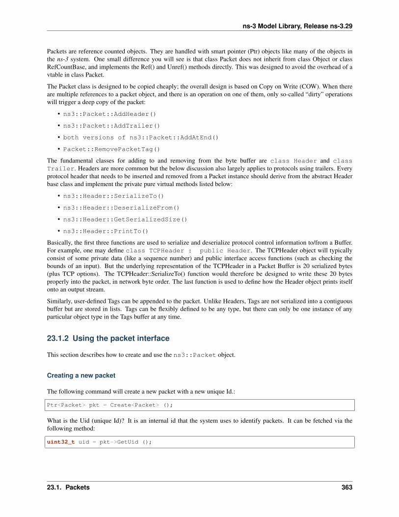
ns-3 Model Library, Release ns-3.29
Packets are reference counted objects. They are handled with smart pointer (Ptr) objects like many of the objects inthe ns-3 system. One small difference you will see is that class Packet does not inherit from class Object or classRefCountBase, and implements the Ref() and Unref() methods directly. This was designed to avoid the overhead of avtable in class Packet.
The Packet class is designed to be copied cheaply; the overall design is based on Copy on Write (COW). When thereare multiple references to a packet object, and there is an operation on one of them, only so-called “dirty” operationswill trigger a deep copy of the packet:
• ns3::Packet::AddHeader()
• ns3::Packet::AddTrailer()
• both versions of ns3::Packet::AddAtEnd()
• Packet::RemovePacketTag()
The fundamental classes for adding to and removing from the byte buffer are class Header and classTrailer. Headers are more common but the below discussion also largely applies to protocols using trailers. Everyprotocol header that needs to be inserted and removed from a Packet instance should derive from the abstract Headerbase class and implement the private pure virtual methods listed below:
• ns3::Header::SerializeTo()
• ns3::Header::DeserializeFrom()
• ns3::Header::GetSerializedSize()
• ns3::Header::PrintTo()
Basically, the first three functions are used to serialize and deserialize protocol control information to/from a Buffer.For example, one may define class TCPHeader : public Header. The TCPHeader object will typicallyconsist of some private data (like a sequence number) and public interface access functions (such as checking thebounds of an input). But the underlying representation of the TCPHeader in a Packet Buffer is 20 serialized bytes(plus TCP options). The TCPHeader::SerializeTo() function would therefore be designed to write these 20 bytesproperly into the packet, in network byte order. The last function is used to define how the Header object prints itselfonto an output stream.
Similarly, user-defined Tags can be appended to the packet. Unlike Headers, Tags are not serialized into a contiguousbuffer but are stored in lists. Tags can be flexibly defined to be any type, but there can only be one instance of anyparticular object type in the Tags buffer at any time.
23.1.2 Using the packet interface
This section describes how to create and use the ns3::Packet object.
Creating a new packet
The following command will create a new packet with a new unique Id.:
Ptr<Packet> pkt = Create<Packet> ();
What is the Uid (unique Id)? It is an internal id that the system uses to identify packets. It can be fetched via thefollowing method:
uint32_t uid = pkt->GetUid ();
23.1. Packets 363

ns-3 Model Library, Release ns-3.29
But please note the following. This uid is an internal uid and cannot be counted on to provide an accurate counter ofhow many “simulated packets” of a particular protocol are in the system. It is not trivial to make this uid into such acounter, because of questions such as what should the uid be when the packet is sent over broadcast media, or whenfragmentation occurs. If a user wants to trace actual packet counts, he or she should look at e.g. the IP ID field ortransport sequence numbers, or other packet or frame counters at other protocol layers.
We mentioned above that it is possible to create packets with zero-filled payloads that do not actually require a memoryallocation (i.e., the packet may behave, when delays such as serialization or transmission delays are computed, to havea certain number of payload bytes, but the bytes will only be allocated on-demand when needed). The command to dothis is, when the packet is created:
Ptr<Packet> pkt = Create<Packet> (N);
where N is a positive integer.
The packet now has a size of N bytes, which can be verified by the GetSize() method:
/*** \returns the size in bytes of the packet (including the zero-filled
* initial payload)
*/uint32_t GetSize (void) const;
You can also initialize a packet with a character buffer. The input data is copied and the input buffer is untouched. Theconstructor applied is:
Packet (uint8_t const *buffer, uint32_t size);
Here is an example:
Ptr<Packet> pkt1 = Create<Packet> (reinterpret_cast<const uint8_t*> ("hello"), 5);
Packets are freed when there are no more references to them, as with all ns-3 objects referenced by the Ptr class.
Adding and removing Buffer data
After the initial packet creation (which may possibly create some fake initial bytes of payload), all subsequent bufferdata is added by adding objects of class Header or class Trailer. Note that, even if you are in the application layer,handling packets, and want to write application data, you write it as an ns3::Header or ns3::Trailer. If you add aHeader, it is prepended to the packet, and if you add a Trailer, it is added to the end of the packet. If you have no datain the packet, then it makes no difference whether you add a Header or Trailer. Since the APIs and classes for headerand trailer are pretty much identical, we’ll just look at class Header here.
The first step is to create a new header class. All new Header classes must inherit from class Header, and implementthe following methods:
• Serialize ()
• Deserialize ()
• GetSerializedSize ()
• Print ()
To see a simple example of how these are done, look at the UdpHeader class headers src/internet/model/udp-header.cc.There are many other examples within the source code.
Once you have a header (or you have a preexisting header), the following Packet API can be used to add or removesuch headers.:
364 Chapter 23. Network Module
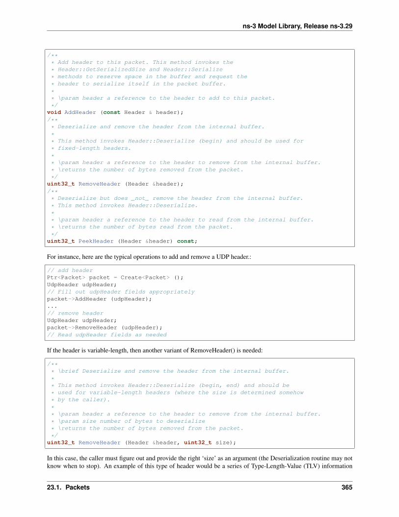
ns-3 Model Library, Release ns-3.29
/*** Add header to this packet. This method invokes the
* Header::GetSerializedSize and Header::Serialize
* methods to reserve space in the buffer and request the
* header to serialize itself in the packet buffer.
** \param header a reference to the header to add to this packet.
*/void AddHeader (const Header & header);/*** Deserialize and remove the header from the internal buffer.
** This method invokes Header::Deserialize (begin) and should be used for
* fixed-length headers.
** \param header a reference to the header to remove from the internal buffer.
* \returns the number of bytes removed from the packet.
*/uint32_t RemoveHeader (Header &header);/*** Deserialize but does _not_ remove the header from the internal buffer.
* This method invokes Header::Deserialize.
** \param header a reference to the header to read from the internal buffer.
* \returns the number of bytes read from the packet.
*/uint32_t PeekHeader (Header &header) const;
For instance, here are the typical operations to add and remove a UDP header.:
// add headerPtr<Packet> packet = Create<Packet> ();UdpHeader udpHeader;// Fill out udpHeader fields appropriatelypacket->AddHeader (udpHeader);...// remove headerUdpHeader udpHeader;packet->RemoveHeader (udpHeader);// Read udpHeader fields as needed
If the header is variable-length, then another variant of RemoveHeader() is needed:
/*** \brief Deserialize and remove the header from the internal buffer.
** This method invokes Header::Deserialize (begin, end) and should be
* used for variable-length headers (where the size is determined somehow
* by the caller).
** \param header a reference to the header to remove from the internal buffer.
* \param size number of bytes to deserialize
* \returns the number of bytes removed from the packet.
*/uint32_t RemoveHeader (Header &header, uint32_t size);
In this case, the caller must figure out and provide the right ‘size’ as an argument (the Deserialization routine may notknow when to stop). An example of this type of header would be a series of Type-Length-Value (TLV) information
23.1. Packets 365
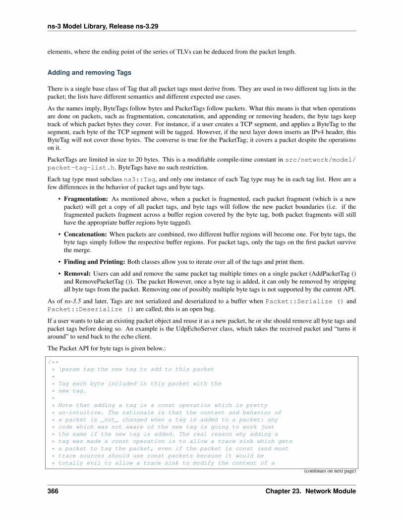
ns-3 Model Library, Release ns-3.29
elements, where the ending point of the series of TLVs can be deduced from the packet length.
Adding and removing Tags
There is a single base class of Tag that all packet tags must derive from. They are used in two different tag lists in thepacket; the lists have different semantics and different expected use cases.
As the names imply, ByteTags follow bytes and PacketTags follow packets. What this means is that when operationsare done on packets, such as fragmentation, concatenation, and appending or removing headers, the byte tags keeptrack of which packet bytes they cover. For instance, if a user creates a TCP segment, and applies a ByteTag to thesegment, each byte of the TCP segment will be tagged. However, if the next layer down inserts an IPv4 header, thisByteTag will not cover those bytes. The converse is true for the PacketTag; it covers a packet despite the operationson it.
PacketTags are limited in size to 20 bytes. This is a modifiable compile-time constant in src/network/model/packet-tag-list.h. ByteTags have no such restriction.
Each tag type must subclass ns3::Tag, and only one instance of each Tag type may be in each tag list. Here are afew differences in the behavior of packet tags and byte tags.
• Fragmentation: As mentioned above, when a packet is fragmented, each packet fragment (which is a newpacket) will get a copy of all packet tags, and byte tags will follow the new packet boundaries (i.e. if thefragmented packets fragment across a buffer region covered by the byte tag, both packet fragments will stillhave the appropriate buffer regions byte tagged).
• Concatenation: When packets are combined, two different buffer regions will become one. For byte tags, thebyte tags simply follow the respective buffer regions. For packet tags, only the tags on the first packet survivethe merge.
• Finding and Printing: Both classes allow you to iterate over all of the tags and print them.
• Removal: Users can add and remove the same packet tag multiple times on a single packet (AddPacketTag ()and RemovePacketTag ()). The packet However, once a byte tag is added, it can only be removed by strippingall byte tags from the packet. Removing one of possibly multiple byte tags is not supported by the current API.
As of ns-3.5 and later, Tags are not serialized and deserialized to a buffer when Packet::Serialize () andPacket::Deserialize () are called; this is an open bug.
If a user wants to take an existing packet object and reuse it as a new packet, he or she should remove all byte tags andpacket tags before doing so. An example is the UdpEchoServer class, which takes the received packet and “turns itaround” to send back to the echo client.
The Packet API for byte tags is given below.:
/*** \param tag the new tag to add to this packet
** Tag each byte included in this packet with the
* new tag.
** Note that adding a tag is a const operation which is pretty
* un-intuitive. The rationale is that the content and behavior of
* a packet is _not_ changed when a tag is added to a packet: any
* code which was not aware of the new tag is going to work just
* the same if the new tag is added. The real reason why adding a
* tag was made a const operation is to allow a trace sink which gets
* a packet to tag the packet, even if the packet is const (and most
* trace sources should use const packets because it would be
* totally evil to allow a trace sink to modify the content of a
(continues on next page)
366 Chapter 23. Network Module

ns-3 Model Library, Release ns-3.29
(continued from previous page)
* packet).
*/void AddByteTag (const Tag &tag) const;/*** \returns an iterator over the set of byte tags included in this packet.
*/ByteTagIterator GetByteTagIterator (void) const;/*** \param tag the tag to search in this packet
* \returns true if the requested tag type was found, false otherwise.
** If the requested tag type is found, it is copied in the user's
* provided tag instance.
*/bool FindFirstMatchingByteTag (Tag &tag) const;
/*** Remove all the tags stored in this packet.
*/void RemoveAllByteTags (void);
/*** \param os output stream in which the data should be printed.
** Iterate over the tags present in this packet, and
* invoke the Print method of each tag stored in the packet.
*/void PrintByteTags (std::ostream &os) const;
The Packet API for packet tags is given below.:
/*** \param tag the tag to store in this packet
** Add a tag to this packet. This method calls the
* Tag::GetSerializedSize and, then, Tag::Serialize.
** Note that this method is const, that is, it does not
* modify the state of this packet, which is fairly
* un-intuitive.
*/void AddPacketTag (const Tag &tag) const;/*** \param tag the tag to remove from this packet
* \returns true if the requested tag is found, false
* otherwise.
** Remove a tag from this packet. This method calls
* Tag::Deserialize if the tag is found.
*/bool RemovePacketTag (Tag &tag);/*** \param tag the tag to search in this packet
* \returns true if the requested tag is found, false
* otherwise.
** Search a matching tag and call Tag::Deserialize if it is found.
(continues on next page)
23.1. Packets 367

ns-3 Model Library, Release ns-3.29
(continued from previous page)
*/bool PeekPacketTag (Tag &tag) const;/*** Remove all packet tags.
*/void RemoveAllPacketTags (void);
/*** \param os the stream in which we want to print data.
** Print the list of 'packet' tags.
** \sa Packet::AddPacketTag, Packet::RemovePacketTag, Packet::PeekPacketTag,
* Packet::RemoveAllPacketTags
*/void PrintPacketTags (std::ostream &os) const;
/*** \returns an object which can be used to iterate over the list of
* packet tags.
*/PacketTagIterator GetPacketTagIterator (void) const;
Here is a simple example illustrating the use of tags from the code in src/internet/model/udp-socket-impl.cc:
Ptr<Packet> p; // pointer to a pre-existing packetSocketIpTtlTag tagtag.SetTtl (m_ipMulticastTtl); // Convey the TTL from UDP layer to IP layerp->AddPacketTag (tag);
This tag is read at the IP layer, then stripped (src/internet/model/ipv4-l3-protocol.cc):
uint8_t ttl = m_defaultTtl;SocketIpTtlTag tag;bool found = packet->RemovePacketTag (tag);if (found)
{ttl = tag.GetTtl ();
}
Fragmentation and concatenation
Packets may be fragmented or merged together. For example, to fragment a packet p of 90 bytes into two packets, onecontaining the first 10 bytes and the other containing the remaining 80, one may call the following code:
Ptr<Packet> frag0 = p->CreateFragment (0, 10);Ptr<Packet> frag1 = p->CreateFragment (10, 90);
As discussed above, the packet tags from p will follow to both packet fragments, and the byte tags will follow the byteranges as needed.
Now, to put them back together:
frag0->AddAtEnd (frag1);
368 Chapter 23. Network Module

ns-3 Model Library, Release ns-3.29
Now frag0 should be equivalent to the original packet p. If, however, there were operations on the fragments beforebeing reassembled (such as tag operations or header operations), the new packet will not be the same.
Enabling metadata
We mentioned above that packets, being on-the-wire representations of byte buffers, present a problem to print outin a structured way unless the printing function has access to the context of the header. For instance, consider atcpdump-like printer that wants to pretty-print the contents of a packet.
To enable this usage, packets may have metadata enabled (disabled by default for performance reasons). This class isused by the Packet class to record every operation performed on the packet’s buffer, and provides an implementationof Packet::Print () method that uses the metadata to analyze the content of the packet’s buffer.
The metadata is also used to perform extensive sanity checks at runtime when performing operations on a Packet. Forexample, this metadata is used to verify that when you remove a header from a packet, this same header was actuallypresent at the front of the packet. These errors will be detected and will abort the program.
To enable this operation, users will typically insert one or both of these statements at the beginning of their programs:
Packet::EnablePrinting ();Packet::EnableChecking ();
23.1.3 Sample programs
See src/network/examples/main-packet-header.cc and src/network/examples/main-packet-tag.cc.
23.1.4 Implementation details
Private member variables
A Packet object’s interface provides access to some private data:
Buffer m_buffer;ByteTagList m_byteTagList;PacketTagList m_packetTagList;PacketMetadata m_metadata;mutable uint32_t m_refCount;static uint32_t m_globalUid;
Each Packet has a Buffer and two Tags lists, a PacketMetadata object, and a ref count. A static member variable keepstrack of the UIDs allocated. The actual uid of the packet is stored in the PacketMetadata.
Note: that real network packets do not have a UID; the UID is therefore an instance of data that normally would bestored as a Tag in the packet. However, it was felt that a UID is a special case that is so often used in simulations thatit would be more convenient to store it in a member variable.
Buffer implementation
Class Buffer represents a buffer of bytes. Its size is automatically adjusted to hold any data prepended or appendedby the user. Its implementation is optimized to ensure that the number of buffer resizes is minimized, by creating newBuffers of the maximum size ever used. The correct maximum size is learned at runtime during use by recording themaximum size of each packet.
23.1. Packets 369

ns-3 Model Library, Release ns-3.29
Authors of new Header or Trailer classes need to know the public API of the Buffer class. (add summary here)
The byte buffer is implemented as follows:
struct BufferData {uint32_t m_count;uint32_t m_size;uint32_t m_initialStart;uint32_t m_dirtyStart;uint32_t m_dirtySize;uint8_t m_data[1];
};struct BufferData *m_data;uint32_t m_zeroAreaSize;uint32_t m_start;uint32_t m_size;
• BufferData::m_count: reference count for BufferData structure
• BufferData::m_size: size of data buffer stored in BufferData structure
• BufferData::m_initialStart: offset from start of data buffer where data was first inserted
• BufferData::m_dirtyStart: offset from start of buffer where every Buffer which holds a reference tothis BufferData instance have written data so far
• BufferData::m_dirtySize: size of area where data has been written so far
• BufferData::m_data: pointer to data buffer
• Buffer::m_zeroAreaSize: size of zero area which extends before m_initialStart
• Buffer::m_start: offset from start of buffer to area used by this buffer
• Buffer::m_size: size of area used by this Buffer in its BufferData structure
This data structure is summarized in Figure Implementation overview of a packet’s byte Buffer.. Each Buffer holdsa pointer to an instance of a BufferData. Most Buffers should be able to share the same underlying BufferData andthus simply increase the BufferData’s reference count. If they have to change the content of a BufferData inside theDirty Area, and if the reference count is not one, they first create a copy of the BufferData and then complete theirstate-changing operation.
Tags implementation
(XXX revise me)
Tags are implemented by a single pointer which points to the start of a linked list ofTagData data structures. EachTagData structure points to the next TagData in the list (its next pointer contains zero to indicate the end of the linkedlist). Each TagData contains an integer unique id which identifies the type of the tag stored in the TagData.:
struct TagData {struct TagData *m_next;uint32_t m_id;uint32_t m_count;uint8_t m_data[Tags::SIZE];
};class Tags {
struct TagData *m_next;};
370 Chapter 23. Network Module
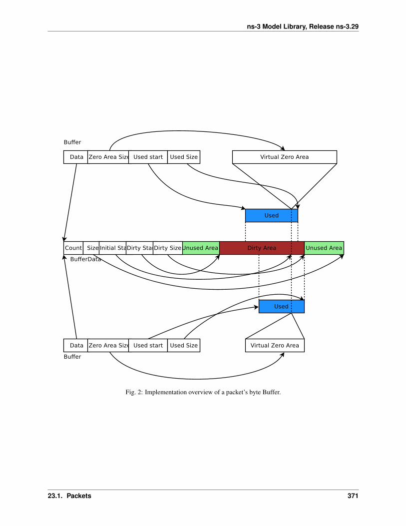
ns-3 Model Library, Release ns-3.29
Fig. 2: Implementation overview of a packet’s byte Buffer.
23.1. Packets 371
ns-3 Model Library, Release ns-3.29
Adding a tag is a matter of inserting a new TagData at the head of the linked list. Looking at a tag requires you to findthe relevant TagData in the linked list and copy its data into the user data structure. Removing a tag and updating thecontent of a tag requires a deep copy of the linked list before performing this operation. On the other hand, copying aPacket and its tags is a matter of copying the TagData head pointer and incrementing its reference count.
Tags are found by the unique mapping between the Tag type and its underlying id. This is why at most one instanceof any Tag can be stored in a packet. The mapping between Tag type and underlying id is performed by a registrationas follows:
/* A sample Tag implementation
*/struct MyTag {
uint16_t m_streamId;};
Memory management
Describe dataless vs. data-full packets.
Copy-on-write semantics
The current implementation of the byte buffers and tag list is based on COW (Copy On Write). An introduction toCOW can be found in Scott Meyer’s “More Effective C++”, items 17 and 29). This design feature and aspects ofthe public interface borrows from the packet design of the Georgia Tech Network Simulator. This implementation ofCOW uses a customized reference counting smart pointer class.
What COW means is that copying packets without modifying them is very cheap (in terms of CPU and memory usage)and modifying them can be also very cheap. What is key for proper COW implementations is being able to detectwhen a given modification of the state of a packet triggers a full copy of the data prior to the modification: COWsystems need to detect when an operation is “dirty” and must therefore invoke a true copy.
Dirty operations:
• ns3::Packet::AddHeader
• ns3::Packet::AddTrailer
• both versions of ns3::Packet::AddAtEnd
• ns3::Packet::RemovePacketTag
Non-dirty operations:
• ns3::Packet::AddPacketTag
• ns3::Packet::PeekPacketTag
• ns3::Packet::RemoveAllPacketTags
• ns3::Packet::AddByteTag
• ns3::Packet::FindFirstMatchingByteTag
• ns3::Packet::RemoveAllByteTags
• ns3::Packet::RemoveHeader
• ns3::Packet::RemoveTrailer
• ns3::Packet::CreateFragment
• ns3::Packet::RemoveAtStart
372 Chapter 23. Network Module
ns-3 Model Library, Release ns-3.29
• ns3::Packet::RemoveAtEnd
• ns3::Packet::CopyData
Dirty operations will always be slower than non-dirty operations, sometimes by several orders of magnitude. How-ever, even the dirty operations have been optimized for common use-cases which means that most of the time, theseoperations will not trigger data copies and will thus be still very fast.
23.2 Error Model
This section documents a few error model objects, typically associated with NetDevice models, that are maintained aspart of the network module:
• RateErrorModel
• ListErrorModel
• ReceiveListErrorModel
• BurstErrorModel
Error models are used to indicate that a packet should be considered to be errored, according to the underlying (possiblystochastic or empirical) error model.
23.2.1 Model Description
The source code for error models live in the directory src/packet/utils.
Two types of error models are generally provided. The first are stochastic models. In this case, packets are erroredaccording to underlying random variable distributions. An example of this is the RateErrorModel. The othertype of model is a deterministic or empirical model, in which packets are errored according to a particular prescribedpattern. An example is the ListErrorModel that allows users to specify the list of packets to be errored, by listingthe specific packet UIDs.
The ns3::RateErrorModel errors packets according to an underlying random variable distribution, which is bydefault a UniformRandomVariable distributed between 0.0 and 1.0. The error rate and error units (bit, byte, or packet)are set by the user. For instance, by setting ErrorRate to 0.1 and ErrorUnit to “Packet”, in the long run, around 10% ofthe packets will be lost.
Design
Error models are ns-3 objects and can be created using the typical pattern of CreateObject<>(). They haveconfiguration attributes.
An ErrorModel can be applied anywhere, but are commonly deployed on NetDevice models so that artificial losses(mimicking channel losses) can be induced.
Scope and Limitations
No known limitations. There are no existing models that try to modify the packet contents (e.g. apply bit or byte errorsto the byte buffers). This type of operation will likely be performance-expensive, and existing Packet APIs may noteasily support it.
The ns-3 spectrum model and devices that derive from it (e.g. LTE) have their own error model base class, found in
23.2. Error Model 373

ns-3 Model Library, Release ns-3.29
References
The initial ns-3 error models were ported from ns-2 (queue/errmodel.{cc,h})
23.2.2 Usage
The base class API is as follows:
• bool ErrorModel::IsCorrupt (Ptr<Packet> pkt): Evaluate the packet and return true or falsewhether the packet should be considered errored or not. Some models could potentially alter the contents of thepacket bit buffer.
• void ErrorModel::Reset (void): Reset any state.
• void ErrorModel::Enable (void): Enable the model
• void ErrorModel::Disble (void): Disable the model; IsCorrupt() will always return false.
• bool ErrorModel::IsEnabled (void) const: Return the enabled state
Many ns-3 NetDevices contain attributes holding pointers to error models. The error model is applied in the notionalphysical layer processing chain of the device, and drops should show up on the PhyRxDrop trace source of thedevice. The following are known to include an attribute with a pointer available to hold this type of error model:
• SimpleNetDevice
• PointToPointNetDevice
• CsmaNetDevice
• VirtualNetDevice
However, the ErrorModel could be used anywhere where packets are used
Helpers
This model is typically not used with helpers.
Attributes
The RateErrorModel contains the following attributes:
Output
What kind of data does the model generate? What are the key trace sources? What kind of logging output can beenabled?
Examples
Error models are used in the tutorial fifth and sixth programs.
The directory examples/error-model/ contains an example simple-error-model.cc that exercises theRate and List error models.
The TCP example examples/tcp/tcp-nsc-lfn.cc uses the Rate error model.
374 Chapter 23. Network Module

ns-3 Model Library, Release ns-3.29
Troubleshooting
No known issues.
23.2.3 Validation
The error-model unit test suite provides a single test case of of a particular combination of ErrorRate and ErrorUnitfor the RateErrorModel applied to a SimpleNetDevice.
23.2.4 Acknowledgements
The basic ErrorModel, RateErrorModel, and ListErrorModel classes were ported from ns-2 to ns-3 in 2007. TheReceiveListErrorModel was added at that time.
The burst error model is due to Truc Anh N. Nguyen at the University of Kansas (James P.G. Sterbenz<[email protected]>, director, ResiliNets Research Group (http://wiki.ittc.ku.edu/resilinets), Information and Telecom-munication Technology Center (ITTC) and Department of Electrical Engineering and Computer Science, The Univer-sity of Kansas Lawrence, KS USA). Work supported in part by NSF FIND (Future Internet Design) Program undergrant CNS-0626918 (Postmodern Internet Architecture), NSF grant CNS-1050226 (Multilayer Network ResilienceAnalysis and Experimentation on GENI), US Department of Defense (DoD), and ITTC at The University of Kansas.
23.3 Node and NetDevices Overview
This chapter describes how ns-3 nodes are put together, and provides a walk-through of how packets traverse aninternet-based Node.
In ns-3, nodes are instances of ns3::Node. This class may be subclassed, but instead, the conceptual model is thatwe aggregate or insert objects to it rather than define subclasses.
One might think of a bare ns-3 node as a shell of a computer, to which one may add NetDevices (cards) and otherinnards including the protocols and applications. High-level node architecture illustrates that ns3::Node objectscontain a list of ns3::Application instances (initially, the list is empty), a list of ns3::NetDevice instances(initially, the list is empty), a list of ns3::Node::ProtocolHandler instances, a unique integer ID, and a systemID (for distributed simulation).
The design tries to avoid putting too many dependencies on the class ns3::Node, ns3::Application, orns3::NetDevice for the following:
• IP version, or whether IP is at all even used in the ns3::Node.
• implementation details of the IP stack.
From a software perspective, the lower interface of applications corresponds to the C-based sockets API. The upper in-terface of ns3::NetDevice objects corresponds to the device independent sublayer of the Linux stack. Everythingin between can be aggregated and plumbed together as needed.
Let’s look more closely at the protocol demultiplexer. We want incoming frames at layer-2 to be delivered to the rightlayer-3 protocol such as IPv4. The function of this demultiplexer is to register callbacks for receiving packets. Thecallbacks are indexed based on the EtherType in the layer-2 frame.
Many different types of higher-layer protocols may be connected to the NetDevice, such as IPv4, IPv6, ARP, MPLS,IEEE 802.1x, and packet sockets. Therefore, the use of a callback-based demultiplexer avoids the need to use acommon base class for all of these protocols, which is problematic because of the different types of objects (includingpacket sockets) expected to be registered there.
23.3. Node and NetDevices Overview 375
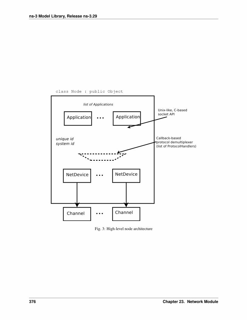
ns-3 Model Library, Release ns-3.29
Fig. 3: High-level node architecture
376 Chapter 23. Network Module

ns-3 Model Library, Release ns-3.29
23.4 Sockets APIs
The sockets API is a long-standing API used by user-space applications to access network services in the kernel. Asocket is an abstraction, like a Unix file handle, that allows applications to connect to other Internet hosts and exchangereliable byte streams and unreliable datagrams, among other services.
ns-3 provides two types of sockets APIs, and it is important to understand the differences between them. The first is anative ns-3 API, while the second uses the services of the native API to provide a POSIX-like API as part of an overallapplication process. Both APIs strive to be close to the typical sockets API that application writers on Unix systemsare accustomed to, but the POSIX variant is much closer to a real system’s sockets API.
23.4.1 ns-3 sockets API
The native sockets API for ns-3 provides an interface to various types of transport protocols (TCP, UDP) as well as topacket sockets and, in the future, Netlink-like sockets. However, users are cautioned to understand that the semanticsare not the exact same as one finds in a real system (for an API which is very much aligned to real systems, see thenext section).
ns3::Socket is defined in src/network/model/socket.h. Readers will note that many public memberfunctions are aligned with real sockets function calls, and all other things being equal, we have tried to align with aPosix sockets API. However, note that:
• ns-3 applications handle a smart pointer to a Socket object, not a file descriptor;
• there is no notion of synchronous API or a blocking API; in fact, the model for interaction between applicationand socket is one of asynchronous I/O, which is not typically found in real systems (more on this below);
• the C-style socket address structures are not used;
• the API is not a complete sockets API, such as supporting all socket options or all function variants;
• many calls use ns3::Packet class to transfer data between application and socket. This may seem peculiarto pass Packets across a stream socket API, but think of these packets as just fancy byte buffers at this level(more on this also below).
Basic operation and calls
Creating sockets
An application that wants to use sockets must first create one. On real systems using a C-based API, this is accom-plished by calling socket()
int socket(int domain, int type, int protocol);
which creates a socket in the system and returns an integer descriptor.
In ns-3, we have no equivalent of a system call at the lower layers, so we adopt the following model. There are certainfactory objects that can create sockets. Each factory is capable of creating one type of socket, and if sockets of aparticular type are able to be created on a given node, then a factory that can create such sockets must be aggregatedto the Node:
static Ptr<Socket> CreateSocket (Ptr<Node> node, TypeId tid);
Examples of TypeIds to pass to this method are ns3::TcpSocketFactory, ns3::PacketSocketFactory,and ns3::UdpSocketFactory.
This method returns a smart pointer to a Socket object. Here is an example:
23.4. Sockets APIs 377
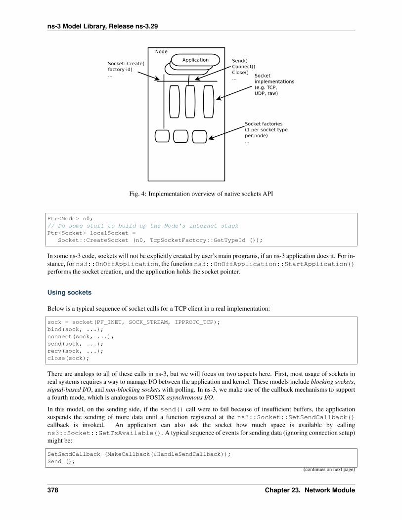
ns-3 Model Library, Release ns-3.29
Fig. 4: Implementation overview of native sockets API
Ptr<Node> n0;// Do some stuff to build up the Node's internet stackPtr<Socket> localSocket =
Socket::CreateSocket (n0, TcpSocketFactory::GetTypeId ());
In some ns-3 code, sockets will not be explicitly created by user’s main programs, if an ns-3 application does it. For in-stance, for ns3::OnOffApplication, the function ns3::OnOffApplication::StartApplication()performs the socket creation, and the application holds the socket pointer.
Using sockets
Below is a typical sequence of socket calls for a TCP client in a real implementation:
sock = socket(PF_INET, SOCK_STREAM, IPPROTO_TCP);bind(sock, ...);connect(sock, ...);send(sock, ...);recv(sock, ...);close(sock);
There are analogs to all of these calls in ns-3, but we will focus on two aspects here. First, most usage of sockets inreal systems requires a way to manage I/O between the application and kernel. These models include blocking sockets,signal-based I/O, and non-blocking sockets with polling. In ns-3, we make use of the callback mechanisms to supporta fourth mode, which is analogous to POSIX asynchronous I/O.
In this model, on the sending side, if the send() call were to fail because of insufficient buffers, the applicationsuspends the sending of more data until a function registered at the ns3::Socket::SetSendCallback()callback is invoked. An application can also ask the socket how much space is available by callingns3::Socket::GetTxAvailable(). A typical sequence of events for sending data (ignoring connection setup)might be:
SetSendCallback (MakeCallback(&HandleSendCallback));Send ();
(continues on next page)
378 Chapter 23. Network Module
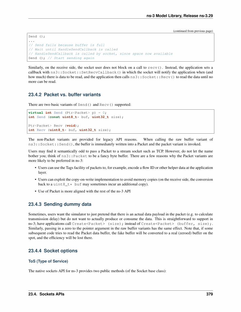
ns-3 Model Library, Release ns-3.29
(continued from previous page)
Send ();...// Send fails because buffer is full// Wait until HandleSendCallback is called// HandleSendCallback is called by socket, since space now availableSend (); // Start sending again
Similarly, on the receive side, the socket user does not block on a call to recv(). Instead, the application sets acallback with ns3::Socket::SetRecvCallback() in which the socket will notify the application when (andhow much) there is data to be read, and the application then calls ns3::Socket::Recv() to read the data until nomore can be read.
23.4.2 Packet vs. buffer variants
There are two basic variants of Send() and Recv() supported:
virtual int Send (Ptr<Packet> p) = 0;int Send (const uint8_t* buf, uint32_t size);
Ptr<Packet> Recv (void);int Recv (uint8_t* buf, uint32_t size);
The non-Packet variants are provided for legacy API reasons. When calling the raw buffer variant ofns3::Socket::Send(), the buffer is immediately written into a Packet and the packet variant is invoked.
Users may find it semantically odd to pass a Packet to a stream socket such as TCP. However, do not let the namebother you; think of ns3::Packet to be a fancy byte buffer. There are a few reasons why the Packet variants aremore likely to be preferred in ns-3:
• Users can use the Tags facility of packets to, for example, encode a flow ID or other helper data at the applicationlayer.
• Users can exploit the copy-on-write implementation to avoid memory copies (on the receive side, the conversionback to a uint8_t* buf may sometimes incur an additional copy).
• Use of Packet is more aligned with the rest of the ns-3 API
23.4.3 Sending dummy data
Sometimes, users want the simulator to just pretend that there is an actual data payload in the packet (e.g. to calculatetransmission delay) but do not want to actually produce or consume the data. This is straightforward to support inns-3; have applications call Create<Packet> (size); instead of Create<Packet> (buffer, size);.Similarly, passing in a zero to the pointer argument in the raw buffer variants has the same effect. Note that, if somesubsequent code tries to read the Packet data buffer, the fake buffer will be converted to a real (zeroed) buffer on thespot, and the efficiency will be lost there.
23.4.4 Socket options
ToS (Type of Service)
The native sockets API for ns-3 provides two public methods (of the Socket base class):
23.4. Sockets APIs 379
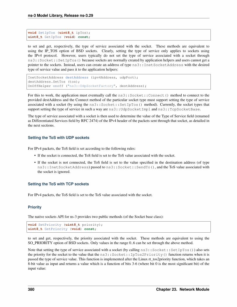
ns-3 Model Library, Release ns-3.29
void SetIpTos (uint8_t ipTos);uint8_t GetIpTos (void) const;
to set and get, respectively, the type of service associated with the socket. These methods are equivalent tousing the IP_TOS option of BSD sockets. Clearly, setting the type of service only applies to sockets usingthe IPv4 protocol. However, users typically do not set the type of service associated with a socket throughns3::Socket::SetIpTos() because sockets are normally created by application helpers and users cannot get apointer to the sockets. Instead, users can create an address of type ns3::InetSocketAddress with the desiredtype of service value and pass it to the application helpers:
InetSocketAddress destAddress (ipv4Address, udpPort);destAddress.SetTos (tos);OnOffHelper onoff ("ns3::UdpSocketFactory", destAddress);
For this to work, the application must eventually call the ns3::Socket::Connect() method to connect to theprovided destAddress and the Connect method of the particular socket type must support setting the type of serviceassociated with a socket (by using the ns3::Socket::SetIpTos() method). Currently, the socket types thatsupport setting the type of service in such a way are ns3::UdpSocketImpl and ns3::TcpSocketBase.
The type of service associated with a socket is then used to determine the value of the Type of Service field (renamedas Differentiated Services field by RFC 2474) of the IPv4 header of the packets sent through that socket, as detailed inthe next sections.
Setting the ToS with UDP sockets
For IPv4 packets, the ToS field is set according to the following rules:
• If the socket is connected, the ToS field is set to the ToS value associated with the socket.
• If the socket is not connected, the ToS field is set to the value specified in the destination address (of typens3::InetSocketAddress) passed to ns3::Socket::SendTo(), and the ToS value associated withthe socket is ignored.
Setting the ToS with TCP sockets
For IPv4 packets, the ToS field is set to the ToS value associated with the socket.
Priority
The native sockets API for ns-3 provides two public methods (of the Socket base class):
void SetPriority (uint8_t priority);uint8_t GetPriority (void) const;
to set and get, respectively, the priority associated with the socket. These methods are equivalent to using theSO_PRIORITY option of BSD sockets. Only values in the range 0..6 can be set through the above method.
Note that setting the type of service associated with a socket (by calling ns3::Socket::SetIpTos()) also setsthe priority for the socket to the value that the ns3::Socket::IpTos2Priority() function returns when it ispassed the type of service value. This function is implemented after the Linux rt_tos2priority function, which takes an8-bit value as input and returns a value which is a function of bits 3-6 (where bit 0 is the most significant bit) of theinput value:
380 Chapter 23. Network Module
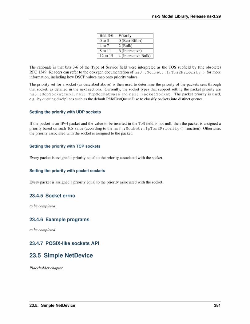
ns-3 Model Library, Release ns-3.29
Bits 3-6 Priority0 to 3 0 (Best Effort)4 to 7 2 (Bulk)8 to 11 6 (Interactive)12 to 15 4 (Interactive Bulk)
The rationale is that bits 3-6 of the Type of Service field were interpreted as the TOS subfield by (the obsolete)RFC 1349. Readers can refer to the doxygen documentation of ns3::Socket::IpTos2Priority() for moreinformation, including how DSCP values map onto priority values.
The priority set for a socket (as described above) is then used to determine the priority of the packets sent throughthat socket, as detailed in the next sections. Currently, the socket types that support setting the packet priority arens3::UdpSocketImpl, ns3::TcpSocketBase and ns3::PacketSocket. The packet priority is used,e.g., by queuing disciplines such as the default PfifoFastQueueDisc to classify packets into distinct queues.
Setting the priority with UDP sockets
If the packet is an IPv4 packet and the value to be inserted in the ToS field is not null, then the packet is assigned apriority based on such ToS value (according to the ns3::Socket::IpTos2Priority() function). Otherwise,the priority associated with the socket is assigned to the packet.
Setting the priority with TCP sockets
Every packet is assigned a priority equal to the priority associated with the socket.
Setting the priority with packet sockets
Every packet is assigned a priority equal to the priority associated with the socket.
23.4.5 Socket errno
to be completed
23.4.6 Example programs
to be completed
23.4.7 POSIX-like sockets API
23.5 Simple NetDevice
Placeholder chapter
23.5. Simple NetDevice 381
ns-3 Model Library, Release ns-3.29
23.6 Queues
This section documents the queue object, which is typically used by NetDevices and QueueDiscs to store packets.
Packets stored in a queue can be managed according to different policies. Currently, only the DropTail policy isavailable.
23.6.1 Model Description
The source code for the new module lives in the directory src/network/utils.
ns3::Queue has been redesigned as a template class object to allow us to instantiate queues storing different types ofitems. The unique template type parameter specifies the type of items stored in the queue. The only requirement onthe item type is that it must provide a GetSize () method which returns the size of the packet included in the item.Currently, queue items can be objects of the following classes:
• Packet
• QueueItem and subclasses (e.g., QueueDiscItem)
• WifiMacQueueItem
The internal queues of the queue discs are of type Queue<QueueDiscItem> (an alias of which being InternalQueue).A number of network devices (SimpleNetDevice, PointToPointNetDevice, CsmaNetDevice) use a Queue<Packet> tostore packets to be transmitted. WifiNetDevices use instead queues of type WifiMacQueue, which is a subclass ofQueue storing objects of type WifiMacQueueItem. Other devices, such as WiMax and LTE, use specialized queues.
Design
The Queue class derives from the QueueBase class, which is a non-template class providing all the methods that areindependent of the type of the items stored in the queue. The Queue class provides instead all the operations thatdepend on the item type, such as enqueue, dequeue, peek and remove. The Queue class also provides the ability totrace certain queue operations such as enqueuing, dequeuing, and dropping.
Queue is an abstract base class and is subclassed for specific scheduling and drop policies. Subclasses need to definethe following public methods:
• bool Enqueue (Ptr<Item> item): Enqueue a packet
• Ptr<Item> Dequeue (void): Dequeue a packet
• Ptr<Item> Remove (void): Remove a packet
• Ptr<const Item> Peek (void): Peek a packet
The Enqueue method does not allow to store a packet if the queue capacity is exceeded. Subclasses may also definespecialized public methods. For instance, the WifiMacQueue class provides a method to dequeue a packet based onits tid and MAC address.
There are five trace sources that may be hooked:
• Enqueue
• Dequeue
• Drop
• DropBeforeEnqueue
• DropAfterDequeue
382 Chapter 23. Network Module

ns-3 Model Library, Release ns-3.29
Also, the QueueBase class defines one attribute:
• MaxSize: the maximum queue size
and two trace sources:
• PacketsInQueue
• BytesInQueue
DropTail
This is a basic first-in-first-out (FIFO) queue that performs a tail drop when the queue is full.
23.6.2 Usage
Helpers
A typical usage pattern is to create a device helper and to configure the queue type and attributes from the helper, suchas this example:
PointToPointHelper p2p;
p2p.SetQueue ("ns3::DropTailQueue");p2p.SetDeviceAttribute ("DataRate", StringValue ("10Mbps"));p2p.SetChannelAttribute ("Delay", StringValue ("2ms"));NetDeviceContainer devn0n2 = p2p.Install (n0n2);
p2p.SetQueue ("ns3::DropTailQueue");p2p.SetDeviceAttribute ("DataRate", StringValue ("10Mbps"));p2p.SetChannelAttribute ("Delay", StringValue ("3ms"));NetDeviceContainer devn1n2 = p2p.Install (n1n2);
p2p.SetQueue ("ns3::DropTailQueue","MaxSize", StringValue ("50p"));
p2p.SetDeviceAttribute ("DataRate", StringValue (linkDataRate));p2p.SetChannelAttribute ("Delay", StringValue (linkDelay));NetDeviceContainer devn2n3 = p2p.Install (n2n3);
Please note that the SetQueue method of the PointToPointHelper class allows to specify “ns3::DropTailQueue” in-stead of “ns3::DropTailQueue<Packet>”. The same holds for CsmaHelper, SimpleNetDeviceHelper and TrafficCon-trolHelper.
Output
The ns-3 ascii trace helpers used by many of the NetDevices will hook the Enqueue, Dequeue, and Drop traces ofthese queues and print out trace statements, such as the following from examples/udp/udp-echo.cc:
+ 2 /NodeList/0/DeviceList/1/$ns3::CsmaNetDevice/TxQueue/Enqueue ns3::EthernetHeader( length/type=0x806, source=00:00:00:00:00:01, destination=ff:ff:ff:ff:ff:ff)ns3::ArpHeader (request source mac: 00-06-00:00:00:00:00:01 source ipv4: 10.1.1.1dest ipv4: 10.1.1.2) Payload (size=18) ns3::EthernetTrailer (fcs=0)- 2 /NodeList/0/DeviceList/1/$ns3::CsmaNetDevice/TxQueue/Dequeue ns3::EthernetHeader( length/type=0x806, source=00:00:00:00:00:01, destination=ff:ff:ff:ff:ff:ff)
(continues on next page)
23.6. Queues 383

ns-3 Model Library, Release ns-3.29
(continued from previous page)
ns3::ArpHeader (request source mac: 00-06-00:00:00:00:00:01 source ipv4: 10.1.1.1dest ipv4: 10.1.1.2) Payload (size=18) ns3::EthernetTrailer (fcs=0)
which shows an enqueue “+” and dequeue “-” event at time 2 seconds.
Users are, of course, free to define and hook their own trace sinks to these trace sources.
Examples
The drop-tail queue is used in several examples, such as examples/udp/udp-echo.cc.
23.7 Queue limits
This section documents the queue limits model, which is used by the traffic control to limit the NetDevices queueingdelay. It operates on the transmission path of the network node.
The reduction of the NetDevices queueing delay is essential to improve the effectiveness of Active Queue Management(AQM) algorithms. Careful assessment of the queueing delay includes a byte-based measure of the NetDevices queuelength. In this design, traffic control can use different byte-based schemes to limit the queueing delay. Currently theonly available scheme is DynamicQueueLimits, which is modelled after the dynamic queue limit library of Linux.
23.7.1 Model Description
The source code for the model lives in the directory src/network/utils.
The model allows a byte-based measure of the netdevice queue. The byte-based measure more accurately approximatesthe time required to empty the queue than a packet-based measure.
To inform the upper layers about the transmission of packets, NetDevices can call a couple of functions:
• void NotifyQueuedBytes (uint32_t bytes): Report the number of bytes queued to the devicequeue
• void NotifyTransmittedBytes (uint32_t bytes): Report the number of bytes transmitted bydevice
Based on this information, the QueueLimits object can stop the transmission queue.
In case of multiqueue NetDevices this mechanism is available for each queue.
The QueueLimits model can be used on any NetDevice modelled in ns-3.
Design
An abstract base class, class QueueLimits, is subclassed for specific byte-based limiting strategies.
Common operations provided by the base class QueueLimits include:
• void Reset (): Reset queue limits state
• void Completed (uint32_t count): Record the number of completed bytes and recalculate the limit
• int32_t Available () const: Return how many bytes can be queued
• void Queued (uint32_t count): Record number of bytes queued
384 Chapter 23. Network Module
ns-3 Model Library, Release ns-3.29
DynamicQueueLimits
Dynamic queue limits (DQL) is a basic library implemented in the Linux kernel to limit the Ethernet queueing delay.DQL is a general purpose queue length controller. The goal of DQL is to calculate the limit as the minimum numberof bytes needed to prevent starvation.
Three attributes are defined in the DynamicQueueLimits class:
• HoldTime: The DQL algorithm hold time
• MaxLimit: Maximum limit
• MinLimit: Minimum limit
The DQL algorithm hold time is 1 s. Reducing the HoldTime increases the responsiveness of DQL with consequentgreater number of limit variation events. Conversely, increasing the HoldTime decreases the responsiveness of DQLwith a minor number of limit variation events. The limit calculated by DQL is in the range from MinLimit to MaxLimit.The default values are respectively 0 and DQL_MAX_LIMIT. Increasing the MinLimit is recommended in case ofhigher NetDevice transmission rate (e.g. 1 Gbps) while reducing the MaxLimit is recommended in case of lowerNetDevice transmission rate (e.g. 500 Kbps).
There is one trace source in DynamicQueueLimits class that may be hooked:
• Limit: Limit value calculated by DQL
23.7.2 Usage
Helpers
A typical usage pattern is to create a traffic control helper and configure the queue limits type and attributes from thehelper, such as this example:
TrafficControlHelper tch;uint32_t handle = tch.SetRootQueueDisc ("ns3::PfifoFastQueueDisc", "Limit",↪→UintegerValue (1000));
tch.SetQueueLimits ("ns3::DynamicQueueLimits", "HoldTime", StringValue ("4ms"));
then install the configuration on a NetDevices container
tch.Install (devices);
23.7. Queue limits 385

ns-3 Model Library, Release ns-3.29
386 Chapter 23. Network Module
CHAPTER
TWENTYFOUR
NIX-VECTOR ROUTING DOCUMENTATION
Nix-vector routing is a simulation specific routing protocol and is intended for large network topologies. The on-demand nature of this protocol as well as the low-memory footprint of the nix-vector provides improved performancein terms of memory usage and simulation run time when dealing with a large number of nodes.
24.1 Model Description
The source code for the NixVectorRouting module lives in the directory src/nix-vector-routing.
ns-3 nix-vector-routing performs on-demand route computation using a breadth-first search and an efficient route-storage data structure known as a nix-vector.
When a packet is generated at a node for transmission, the route is calculated, and the nix-vector is built. The nix-vector stores an index for each hop along the path, which corresponds to the neighbor-index. This index is used todetermine which net-device and gateway should be used. To route a packet, the nix-vector must be transmitted withthe packet. At each hop, the current node extracts the appropriate neighbor-index from the nix-vector and transmitsthe packet through the corresponding net-device. This continues until the packet reaches the destination.
24.1.1 Scope and Limitations
Currently, the ns-3 model of nix-vector routing supports IPv4 p2p links as well as CSMA links. It does not (yet)provide support for efficient adaptation to link failures. It simply flushes all nix-vector routing caches. Finally, IPv6 isnot supported.
24.2 Usage
The usage pattern is the one of all the Internet routing protocols. Since NixVectorRouting is not in-stalled by default in the Internet stack, it is necessary to set it in the Internet Stack helper by usingInternetStackHelper::SetRoutingHelper
24.2.1 Examples
The examples for the NixVectorRouting module lives in the directory src/nix-vector-routing/examples.
387

ns-3 Model Library, Release ns-3.29
388 Chapter 24. Nix-Vector Routing Documentation
CHAPTER
TWENTYFIVE
OPTIMIZED LINK STATE ROUTING (OLSR)
This model implements the base specification of the Optimized Link State Routing (OLSR) protocol, which is a dy-namic mobile ad hoc unicast routing protocol. It has been developed at the University of Murcia (Spain) by FranciscoJ. Ros for NS-2, and was ported to NS-3 by Gustavo Carneiro at INESC Porto (Portugal).
The implementation is based on OLSR Version 1 (RFC 3626) and it is not compliant with OLSR Version 2 (RFC7181) or any of the Version 2 extensions.
25.1 Model Description
The source code for the OLSR model lives in the directory src/olsr. As stated before, the model is based on RFC3626. Moreover, many design choices are based on the previous ns2 model.
25.1.1 Scope and Limitations
The model is for IPv4 only.
• Mostly compliant with OLSR as documented in RFC 3626,
• The use of multiple interfaces was not supported by the NS-2 version, but is supported in NS-3;
• OLSR does not respond to the routing event notifications corresponding to dy-namic interface up and down (ns3::RoutingProtocol::NotifyInterfaceUpand ns3::RoutingProtocol::NotifyInterfaceDown) or address in-sertion/removal ns3::RoutingProtocol::NotifyAddAddress andns3::RoutingProtocol::NotifyRemoveAddress).
• Unlike the NS-2 version, does not yet support MAC layer feedback as described in RFC 3626;
Host Network Association (HNA) is supported in this implementation of OLSR. Refer to examples/olsr-hna.cc to see how the API is used.
25.1.2 References
25.2 Usage
The usage pattern is the one of all the Internet routing protocols. Since OLSR is not installedby default in the Internet stack, it is necessary to set it in the Internet Stack helper by usingInternetStackHelper::SetRoutingHelper
389
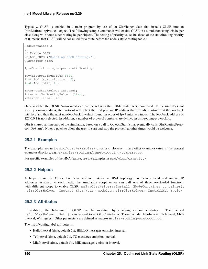
ns-3 Model Library, Release ns-3.29
Typically, OLSR is enabled in a main program by use of an OlsrHelper class that installs OLSR into anIpv4ListRoutingProtocol object. The following sample commands will enable OLSR in a simulation using this helperclass along with some other routing helper objects. The setting of priority value 10, ahead of the staticRouting priorityof 0, means that OLSR will be consulted for a route before the node’s static routing table.:
NodeContainer c:...// Enable OLSRNS_LOG_INFO ("Enabling OLSR Routing.");OlsrHelper olsr;
Ipv4StaticRoutingHelper staticRouting;
Ipv4ListRoutingHelper list;list.Add (staticRouting, 0);list.Add (olsr, 10);
InternetStackHelper internet;internet.SetRoutingHelper (list);internet.Install (c);
Once installed,the OLSR “main interface” can be set with the SetMainInterface() command. If the user does notspecify a main address, the protocol will select the first primary IP address that it finds, starting first the loopbackinterface and then the next non-loopback interface found, in order of Ipv4 interface index. The loopback address of127.0.0.1 is not selected. In addition, a number of protocol constants are defined in olsr-routing-protocol.cc.
Olsr is started at time zero of the simulation, based on a call to Object::Start() that eventually calls OlsrRoutingProto-col::DoStart(). Note: a patch to allow the user to start and stop the protocol at other times would be welcome.
25.2.1 Examples
The examples are in the src/olsr/examples/ directory. However, many other examples esists in the generalexamples directory, e.g., examples/routing/manet-routing-compare.cc.
For specific examples of the HNA feature, see the examples in src/olsr/examples/.
25.2.2 Helpers
A helper class for OLSR has been written. After an IPv4 topology has been created and unique IPaddresses assigned to each node, the simulation script writer can call one of three overloaded functionswith different scope to enable OLSR: ns3::OlsrHelper::Install (NodeContainer container);ns3::OlsrHelper::Install (Ptr<Node> node); or ns3::OlsrHelper::InstallAll (void)
25.2.3 Attributes
In addition, the behavior of OLSR can be modified by changing certain attributes. The methodns3::OlsrHelper::Set () can be used to set OLSR attributes. These include HelloInterval, TcInterval, Mid-Interval, Willingness. Other parameters are defined as macros in olsr-routing-protocol.cc.
The list of configurabel attributes is:
• HelloInterval (time, default 2s), HELLO messages emission interval.
• TcInterval (time, default 5s), TC messages emission interval.
• MidInterval (time, default 5s), MID messages emission interval.
390 Chapter 25. Optimized Link State Routing (OLSR)
ns-3 Model Library, Release ns-3.29
• HnaInterval (time, default 5s), HNA messages emission interval.
• Willingness (enum, default OLSR_WILL_DEFAULT), Willingness of a node to carry and forward traffic forother nodes.
25.2.4 Tracing
The available traces are:
• Rx: Receive OLSR packet.
• Tx: Send OLSR packet.
• RoutingTableChanged: The OLSR routing table has changed.
25.2.5 Caveats
Presently, OLSR is limited to use with an Ipv4ListRouting object, and does not respond to dynamic changes to adevice’s IP address or link up/down notifications; i.e. the topology changes are due to loss/gain of connectivity over awireless channel.
The code does not present any known issue.
25.3 Validation
The code validationhas been done through Wireshark message compliance and unit testings.
25.3. Validation 391

ns-3 Model Library, Release ns-3.29
392 Chapter 25. Optimized Link State Routing (OLSR)
CHAPTER
TWENTYSIX
OPENFLOW SWITCH SUPPORT
ns-3 simulations can use OpenFlow switches (McKeown et al.1), widely used in research. OpenFlow switches are con-figurable via the OpenFlow API, and also have an MPLS extension for quality-of-service and service-level-agreementsupport. By extending these capabilities to ns-3 for a simulated OpenFlow switch that is both configurable and canuse the MPLS extension, ns-3 simulations can accurately simulate many different switches.
The OpenFlow software implementation distribution is hereby referred to as the OFSID. This is a demonstration ofrunning OpenFlow in software that the OpenFlow research group has made available. There is also an OFSID thatEricsson researchers created to add MPLS capabilities; this is the OFSID currently used with ns-3. The design willallow the users to, with minimal effort, switch in a different OFSID that may include more efficient code than aprevious OFSID.
26.1 Model Description
The model relies on building an external OpenFlow switch library (OFSID), and then building some ns-3 wrappersthat call out to the library. The source code for the ns-3 wrappers lives in the directory src/openflow/model.
26.1.1 Design
The OpenFlow module presents a OpenFlowSwitchNetDevice and a OpenFlowSwitchHelper for installing it on nodes.Like the Bridge module, it takes a collection of NetDevices to set up as ports, and it acts as the intermediary betweenthem, receiving a packet on one port and forwarding it on another, or all but the received port when flooding. Likean OpenFlow switch, it maintains a configurable flow table that can match packets by their headers and do differentactions with the packet based on how it matches. The module’s understanding of OpenFlow configuration messagesare kept the same format as a real OpenFlow-compatible switch, so users testing Controllers via ns-3 won’t have torewrite their Controller to work on real OpenFlow-compatible switches.
The ns-3 OpenFlow switch device models an OpenFlow-enabled switch. It is designed to express basic use of theOpenFlow protocol, with the maintaining of a virtual Flow Table and TCAM to provide OpenFlow-like results.
The functionality comes down to the Controllers, which send messages to the switch that configure its flows, pro-ducing different effects. Controllers can be added by the user, under the ofi namespace extending ofi::Controller. Todemonstrate this, a DropController, which creates flows for ignoring every single packet, and LearningController,which effectively makes the switch a more complicated BridgeNetDevice. A user versed in a standard OFSID, and/orOF protocol, can write virtual controllers to create switches of all kinds of types.
1 McKeown, N.; Anderson, T.; Balakrishan, H.; Parulkar, G.; Peterson, L.; Rexford, J.; Shenker, S.; Turner, J.; OpenFlow: enabling innovationin campus networks, ACM SIGCOMM Computer Communication Review, Vol. 38, Issue 2, April 2008.
393
ns-3 Model Library, Release ns-3.29
OpenFlow switch Model
The OpenFlow switch device behaves somewhat according to the diagram setup as a classical OFSID switch, with afew modifications made for a proper simulation environment.
Normal OF-enabled Switch:
| Secure Channel | <--OF Protocol--> | Controller is external || Hardware or Software Flow Table |
ns-3 OF-enabled Switch (module):
| m_controller->ReceiveFromSwitch() | <--OF Protocol--> | Controller is internal || Software Flow Table, virtual TCAM |
In essence, there are two differences:
1) No SSL, Embedded Controller: Instead of a secure channel and connecting to an outside location for the Controllerprogram/machine, we currently only allow a Controller extended from ofi::Controller, an extension of an ns3::Object.This means ns-3 programmers cannot model the SSL part of the interface or possibility of network failure. Theconnection to the OpenFlowSwitch is local and there aren’t any reasons for the channel/connection to break down.<<This difference may be an option in the future. Using EmuNetDevices, it should be possible to engage an externalController program/machine, and thus work with controllers designed outside of the ns-3 environment, that simply usethe proper OF protocol when communicating messages to the switch through a tap device.>>
2) Virtual Flow Table, TCAM: Typical OF-enabled switches are implemented on a hardware TCAM. The OFSIDwe turn into a library includes a modelled software TCAM, that produces the same results as a hardware TCAM.We include an attribute FlowTableLookupDelay, which allows a simple delay of using the TCAM to be modelled.We don’t endeavor to make this delay more complicated, based on the tasks we are running on the TCAM, that is apossible future improvement.
The OpenFlowSwitch network device is aimed to model an OpenFlow switch, with a TCAM and a connection to acontroller program. With some tweaking, it can model every switch type, per OpenFlow’s extensibility. It outsourcesthe complexity of the switch ports to NetDevices of the user’s choosing. It should be noted that these NetDevices mustbehave like practical switch ports, i.e. a Mac Address is assigned, and nothing more. It also must support a SendFromfunction so that the OpenFlowSwitch can forward across that port.
26.1.2 Scope and Limitations
All MPLS capabilities are implemented on the OFSID side in the OpenFlowSwitchNetDevice, but ns-3-mpls hasn’tbeen integrated, so ns-3 has no way to pass in proper MPLS packets to the OpenFlowSwitch. If it did, one would onlyneed to make BufferFromPacket pick up the MplsLabelStack or whatever the MPLS header is called on the Packet,and build the MPLS header into the ofpbuf.
26.1.3 Future Work
26.1.4 References
26.2 Usage
The OFSID requires libxml2 (for MPLS FIB xml file parsing), libdl (for address fault checking), and boost (for assert)libraries to be installed.
394 Chapter 26. OpenFlow switch support
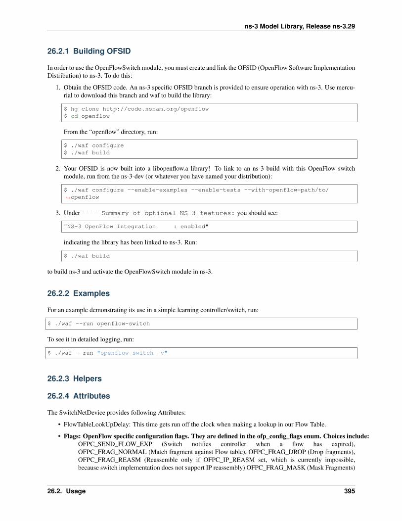
ns-3 Model Library, Release ns-3.29
26.2.1 Building OFSID
In order to use the OpenFlowSwitch module, you must create and link the OFSID (OpenFlow Software ImplementationDistribution) to ns-3. To do this:
1. Obtain the OFSID code. An ns-3 specific OFSID branch is provided to ensure operation with ns-3. Use mercu-rial to download this branch and waf to build the library:
$ hg clone http://code.nsnam.org/openflow$ cd openflow
From the “openflow” directory, run:
$ ./waf configure$ ./waf build
2. Your OFSID is now built into a libopenflow.a library! To link to an ns-3 build with this OpenFlow switchmodule, run from the ns-3-dev (or whatever you have named your distribution):
$ ./waf configure --enable-examples --enable-tests --with-openflow=path/to/↪→openflow
3. Under ---- Summary of optional NS-3 features: you should see:
"NS-3 OpenFlow Integration : enabled"
indicating the library has been linked to ns-3. Run:
$ ./waf build
to build ns-3 and activate the OpenFlowSwitch module in ns-3.
26.2.2 Examples
For an example demonstrating its use in a simple learning controller/switch, run:
$ ./waf --run openflow-switch
To see it in detailed logging, run:
$ ./waf --run "openflow-switch -v"
26.2.3 Helpers
26.2.4 Attributes
The SwitchNetDevice provides following Attributes:
• FlowTableLookUpDelay: This time gets run off the clock when making a lookup in our Flow Table.
• Flags: OpenFlow specific configuration flags. They are defined in the ofp_config_flags enum. Choices include:OFPC_SEND_FLOW_EXP (Switch notifies controller when a flow has expired),OFPC_FRAG_NORMAL (Match fragment against Flow table), OFPC_FRAG_DROP (Drop fragments),OFPC_FRAG_REASM (Reassemble only if OFPC_IP_REASM set, which is currently impossible,because switch implementation does not support IP reassembly) OFPC_FRAG_MASK (Mask Fragments)
26.2. Usage 395

ns-3 Model Library, Release ns-3.29
• FlowTableMissSendLength: When the packet doesn’t match in our Flow Table, and we forward to the controller,this sets # of bytes forwarded (packet is not forwarded in its entirety, unless specified).
Note: TODO
26.2.5 Tracing
Note: TODO
26.2.6 Logging
Note: TODO
26.2.7 Caveats
Note: TODO
26.3 Validation
This model has one test suite which can be run as follows:
$ ./test.py --suite=openflow
396 Chapter 26. OpenFlow switch support

CHAPTER
TWENTYSEVEN
POINTTOPOINT NETDEVICE
This is the introduction to PointToPoint NetDevice chapter, to complement the PointToPoint model doxygen.
27.1 Overview of the PointToPoint model
The ns-3 point-to-point model is of a very simple point to point data link connecting exactly two PointToPointNetDe-vice devices over an PointToPointChannel. This can be viewed as equivalent to a full duplex RS-232 or RS-422 linkwith null modem and no handshaking.
Data is encapsulated in the Point-to-Point Protocol (PPP – RFC 1661), however the Link Control Protocol (LCP) andassociated state machine is not implemented. The PPP link is assumed to be established and authenticated at all times.
Data is not framed, therefore Address and Control fields will not be found. Since the data is not framed, there isno need to provide Flag Sequence and Control Escape octets, nor is a Frame Check Sequence appended. All that isrequired to implement non-framed PPP is to prepend the PPP protocol number for IP Version 4 which is the sixteen-bitnumber 0x21 (see http://www.iana.org/assignments/ppp-numbers).
The PointToPointNetDevice provides following Attributes:
• Address: The ns3::Mac48Address of the device (if desired);
• DataRate: The data rate (ns3::DataRate) of the device;
• TxQueue: The transmit queue (ns3::Queue) used by the device;
• InterframeGap: The optional ns3::Time to wait between “frames”;
• Rx: A trace source for received packets;
• Drop: A trace source for dropped packets.
The PointToPointNetDevice models a transmitter section that puts bits on a corresponding channel “wire.” TheDataRate attribute specifies the number of bits per second that the device will simulate sending over the channel.In reality no bits are sent, but an event is scheduled for an elapsed time consistent with the number of bits in eachpacket and the specified DataRate. The implication here is that the receiving device models a receiver section that canreceive any any data rate. Therefore there is no need, nor way to set a receive data rate in this model. By setting theDataRate on the transmitter of both devices connected to a given PointToPointChannel one can model a symmetricchannel; or by setting different DataRates one can model an asymmetric channel (e.g., ADSL).
The PointToPointNetDevice supports the assignment of a “receive error model.” This is an ErrorModel object that isused to simulate data corruption on the link.
397
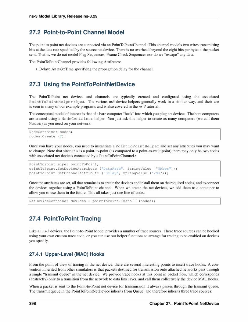
ns-3 Model Library, Release ns-3.29
27.2 Point-to-Point Channel Model
The point to point net devices are connected via an PointToPointChannel. This channel models two wires transmittingbits at the data rate specified by the source net device. There is no overhead beyond the eight bits per byte of the packetsent. That is, we do not model Flag Sequences, Frame Check Sequences nor do we “escape” any data.
The PointToPointChannel provides following Attributes:
• Delay: An ns3::Time specifying the propagation delay for the channel.
27.3 Using the PointToPointNetDevice
The PointToPoint net devices and channels are typically created and configured using the associatedPointToPointHelper object. The various ns3 device helpers generally work in a similar way, and their useis seen in many of our example programs and is also covered in the ns-3 tutorial.
The conceptual model of interest is that of a bare computer “husk” into which you plug net devices. The bare computersare created using a NodeContainer helper. You just ask this helper to create as many computers (we call themNodes) as you need on your network:
NodeContainer nodes;nodes.Create (2);
Once you have your nodes, you need to instantiate a PointToPointHelper and set any attributes you may wantto change. Note that since this is a point-to-point (as compared to a point-to-multipoint) there may only be two nodeswith associated net devices connected by a PointToPointChannel.:
PointToPointHelper pointToPoint;pointToPoint.SetDeviceAttribute ("DataRate", StringValue ("5Mbps"));pointToPoint.SetChannelAttribute ("Delay", StringValue ("2ms"));
Once the attributes are set, all that remains is to create the devices and install them on the required nodes, and to connectthe devices together using a PointToPoint channel. When we create the net devices, we add them to a container toallow you to use them in the future. This all takes just one line of code.:
NetDeviceContainer devices = pointToPoint.Install (nodes);
27.4 PointToPoint Tracing
Like all ns-3 devices, the Point-to-Point Model provides a number of trace sources. These trace sources can be hookedusing your own custom trace code, or you can use our helper functions to arrange for tracing to be enabled on devicesyou specify.
27.4.1 Upper-Level (MAC) Hooks
From the point of view of tracing in the net device, there are several interesting points to insert trace hooks. A con-vention inherited from other simulators is that packets destined for transmission onto attached networks pass througha single “transmit queue” in the net device. We provide trace hooks at this point in packet flow, which corresponds(abstractly) only to a transition from the network to data link layer, and call them collectively the device MAC hooks.
When a packet is sent to the Point-to-Point net device for transmission it always passes through the transmit queue.The transmit queue in the PointToPointNetDevice inherits from Queue, and therefore inherits three trace sources:
398 Chapter 27. PointToPoint NetDevice
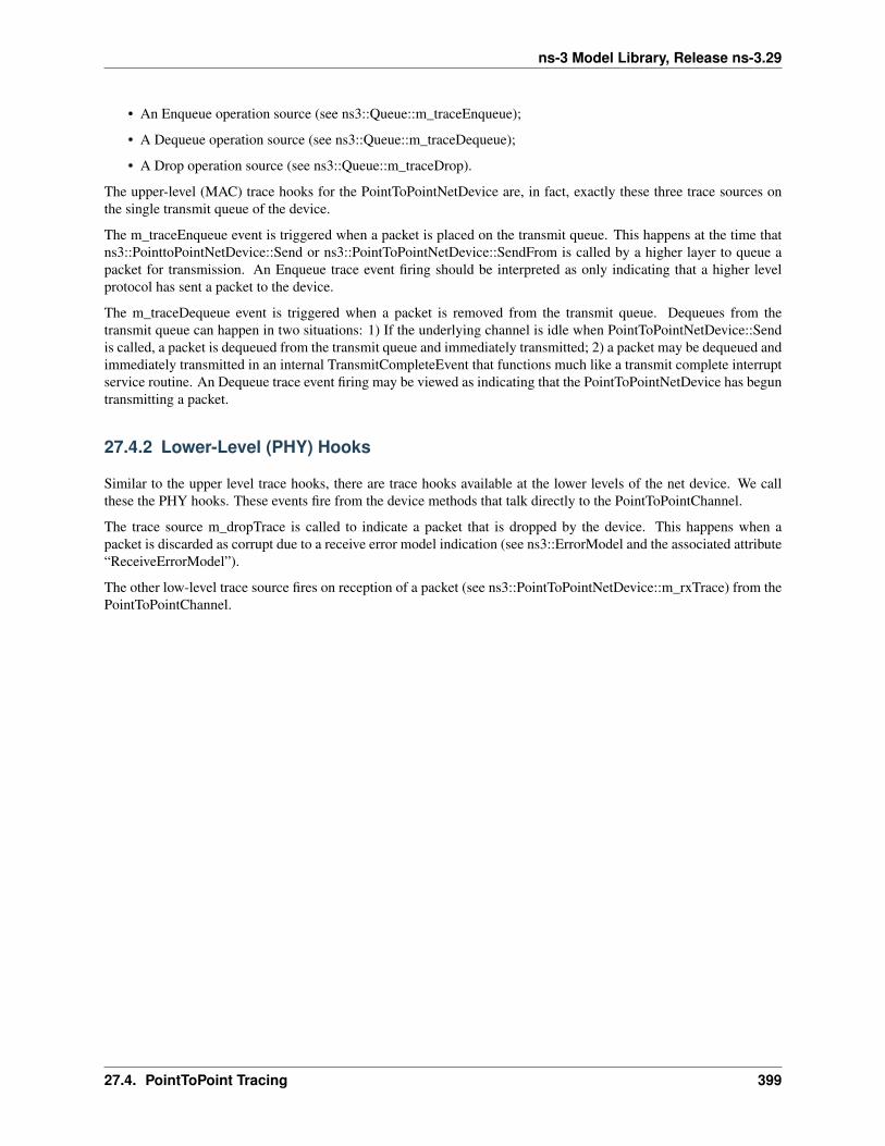
ns-3 Model Library, Release ns-3.29
• An Enqueue operation source (see ns3::Queue::m_traceEnqueue);
• A Dequeue operation source (see ns3::Queue::m_traceDequeue);
• A Drop operation source (see ns3::Queue::m_traceDrop).
The upper-level (MAC) trace hooks for the PointToPointNetDevice are, in fact, exactly these three trace sources onthe single transmit queue of the device.
The m_traceEnqueue event is triggered when a packet is placed on the transmit queue. This happens at the time thatns3::PointtoPointNetDevice::Send or ns3::PointToPointNetDevice::SendFrom is called by a higher layer to queue apacket for transmission. An Enqueue trace event firing should be interpreted as only indicating that a higher levelprotocol has sent a packet to the device.
The m_traceDequeue event is triggered when a packet is removed from the transmit queue. Dequeues from thetransmit queue can happen in two situations: 1) If the underlying channel is idle when PointToPointNetDevice::Sendis called, a packet is dequeued from the transmit queue and immediately transmitted; 2) a packet may be dequeued andimmediately transmitted in an internal TransmitCompleteEvent that functions much like a transmit complete interruptservice routine. An Dequeue trace event firing may be viewed as indicating that the PointToPointNetDevice has beguntransmitting a packet.
27.4.2 Lower-Level (PHY) Hooks
Similar to the upper level trace hooks, there are trace hooks available at the lower levels of the net device. We callthese the PHY hooks. These events fire from the device methods that talk directly to the PointToPointChannel.
The trace source m_dropTrace is called to indicate a packet that is dropped by the device. This happens when apacket is discarded as corrupt due to a receive error model indication (see ns3::ErrorModel and the associated attribute“ReceiveErrorModel”).
The other low-level trace source fires on reception of a packet (see ns3::PointToPointNetDevice::m_rxTrace) from thePointToPointChannel.
27.4. PointToPoint Tracing 399

ns-3 Model Library, Release ns-3.29
400 Chapter 27. PointToPoint NetDevice

CHAPTER
TWENTYEIGHT
PROPAGATION
The ns-3 propagation module defines two generic interfaces, namely PropagationLossModel andPropagationDelayModel, for the modeling of respectively propagation loss and propagation delay.
28.1 PropagationLossModel
Propagation loss models calculate the Rx signal power considering the Tx signal power and the mutual Rx and Txantennas positions.
A propagation loss model can be “chained” to another one, making a list. The final Rx power takes into account allthe chained models. In this way one can use a slow fading and a fast fading model (for example), or model separatelydifferent fading effects.
The following propagation delay models are implemented:
• Cost231PropagationLossModel
• FixedRssLossModel
• FriisPropagationLossModel
• ItuR1411LosPropagationLossModel
• ItuR1411NlosOverRooftopPropagationLossModel
• JakesPropagationLossModel
• Kun2600MhzPropagationLossModel
• LogDistancePropagationLossModel
• MatrixPropagationLossModel
• NakagamiPropagationLossModel
• OkumuraHataPropagationLossModel
• RandomPropagationLossModel
• RangePropagationLossModel
• ThreeLogDistancePropagationLossModel
• TwoRayGroundPropagationLossModel
Other models could be available thanks to other modules, e.g., the building module.
Each of the available propagation loss models of ns-3 is explained in one of the following subsections.
401
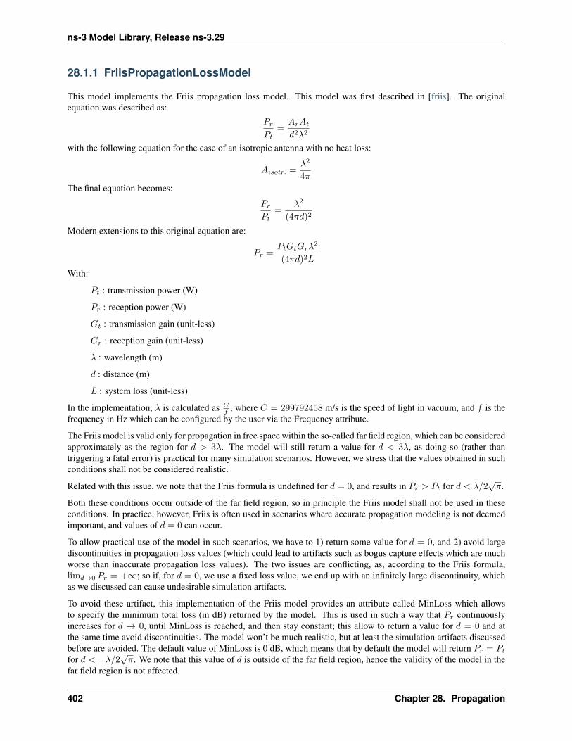
ns-3 Model Library, Release ns-3.29
28.1.1 FriisPropagationLossModel
This model implements the Friis propagation loss model. This model was first described in [friis]. The originalequation was described as:
PrPt
=ArAtd2λ2
with the following equation for the case of an isotropic antenna with no heat loss:
Aisotr. =λ2
4π
The final equation becomes:
PrPt
=λ2
(4πd)2
Modern extensions to this original equation are:
Pr =PtGtGrλ
2
(4πd)2L
With:
Pt : transmission power (W)
Pr : reception power (W)
Gt : transmission gain (unit-less)
Gr : reception gain (unit-less)
λ : wavelength (m)
d : distance (m)
L : system loss (unit-less)
In the implementation, λ is calculated as Cf , where C = 299792458 m/s is the speed of light in vacuum, and f is the
frequency in Hz which can be configured by the user via the Frequency attribute.
The Friis model is valid only for propagation in free space within the so-called far field region, which can be consideredapproximately as the region for d > 3λ. The model will still return a value for d < 3λ, as doing so (rather thantriggering a fatal error) is practical for many simulation scenarios. However, we stress that the values obtained in suchconditions shall not be considered realistic.
Related with this issue, we note that the Friis formula is undefined for d = 0, and results in Pr > Pt for d < λ/2√π.
Both these conditions occur outside of the far field region, so in principle the Friis model shall not be used in theseconditions. In practice, however, Friis is often used in scenarios where accurate propagation modeling is not deemedimportant, and values of d = 0 can occur.
To allow practical use of the model in such scenarios, we have to 1) return some value for d = 0, and 2) avoid largediscontinuities in propagation loss values (which could lead to artifacts such as bogus capture effects which are muchworse than inaccurate propagation loss values). The two issues are conflicting, as, according to the Friis formula,limd→0 Pr = +∞; so if, for d = 0, we use a fixed loss value, we end up with an infinitely large discontinuity, whichas we discussed can cause undesirable simulation artifacts.
To avoid these artifact, this implementation of the Friis model provides an attribute called MinLoss which allowsto specify the minimum total loss (in dB) returned by the model. This is used in such a way that Pr continuouslyincreases for d → 0, until MinLoss is reached, and then stay constant; this allow to return a value for d = 0 and atthe same time avoid discontinuities. The model won’t be much realistic, but at least the simulation artifacts discussedbefore are avoided. The default value of MinLoss is 0 dB, which means that by default the model will return Pr = Ptfor d <= λ/2
√π. We note that this value of d is outside of the far field region, hence the validity of the model in the
far field region is not affected.
402 Chapter 28. Propagation
ns-3 Model Library, Release ns-3.29
28.1.2 TwoRayGroundPropagationLossModel
This model implements a Two-Ray Ground propagation loss model ported from NS2
The Two-ray ground reflection model uses the formula
Pr =Pt ∗Gt ∗Gr ∗ (H2
t ∗H2r )
d4 ∗ L
The original equation in Rappaport’s book assumes L = 1. To be consistent with the free space equation, L is addedhere.
Ht and Hr are set at the respective nodes z coordinate plus a model parameter set via SetHeightAboveZ.
The two-ray model does not give a good result for short distances, due to the oscillation caused by constructive anddestructive combination of the two rays. Instead the Friis free-space model is used for small distances.
The crossover distance, below which Friis is used, is calculated as follows:
dCross =(4 ∗ π ∗Ht ∗Hr)
λ
In the implementation, λ is calculated as Cf , where C = 299792458 m/s is the speed of light in vacuum, and f is the
frequency in Hz which can be configured by the user via the Frequency attribute.
28.1.3 LogDistancePropagationLossModel
This model implements a log distance propagation model.
The reception power is calculated with a so-called log-distance propagation model:
L = L0 + 10n log(d
d0)
where:
n : the path loss distance exponent
d0 : reference distance (m)
L0 : path loss at reference distance (dB)
d : - distance (m)
L : path loss (dB)
When the path loss is requested at a distance smaller than the reference distance, the tx power is returned.
28.1.4 ThreeLogDistancePropagationLossModel
This model implements a log distance path loss propagation model with three distance fields. This model is the sameas ns3::LogDistancePropagationLossModel except that it has three distance fields: near, middle and far with differentexponents.
Within each field the reception power is calculated using the log-distance propagation equation:
L = L0 + 10 · n0 log10(d
d0)
Each field begins where the previous ends and all together form a continuous function.
28.1. PropagationLossModel 403

ns-3 Model Library, Release ns-3.29
There are three valid distance fields: near, middle, far. Actually four: the first from 0 to the reference distance is invalidand returns txPowerDbm.
0 · · · · · ·︸ ︷︷ ︸=0
d0 · · · · · ·︸ ︷︷ ︸n0
d1 · · · · · ·︸ ︷︷ ︸n1
d2 · · · · · ·︸ ︷︷ ︸n2
∞
Complete formula for the path loss in dB:
L =
0 d < d0
L0 + 10 · n0 log10( dd0 ) d0 ≤ d < d1
L0 + 10 · n0 log10(d1d0 ) + 10 · n1 log10( dd1 ) d1 ≤ d < d2
L0 + 10 · n0 log10(d1d0 ) + 10 · n1 log10(d2d1 ) + 10 · n2 log10( dd2 ) d2 ≤ d
where:
d0, d1, d2 : three distance fields (m)
n0, n1, n2 : path loss distance exponent for each field (unitless)
L0 : path loss at reference distance (dB)
d : - distance (m)
L : path loss (dB)
When the path loss is requested at a distance smaller than the reference distance d0, the tx power (with no path loss)is returned. The reference distance defaults to 1m and reference loss defaults to FriisPropagationLossModelwith 5.15 GHz and is thus L0 = 46.67 dB.
28.1.5 JakesPropagationLossModel
ToDo
28.1.6 RandomPropagationLossModel
The propagation loss is totally random, and it changes each time the model is called. As a consequence, all the packets(even those between two fixed nodes) experience a random propagation loss.
28.1.7 NakagamiPropagationLossModel
This propagation loss model implements the Nakagami-m fast fading model, which accounts for the variations insignal strength due to multipath fading. The model does not account for the path loss due to the distance traveled bythe signal, hence for typical simulation usage it is recommended to consider using it in combination with other modelsthat take into account this aspect.
The Nakagami-m distribution is applied to the power level. The probability density function is defined as
p(x;m,ω) =2mm
Γ(m)ωmx2m−1e−
mω x
2
)
with m the fading depth parameter and ω the average received power.
It is implemented by either a GammaRandomVariable or a ErlangRandomVariable random variable.
The implementation of the model allows to specify different values of them parameter (and hence different fast fadingprofiles) for three different distance ranges:
0 · · · · · ·︸ ︷︷ ︸m0
d1 · · · · · ·︸ ︷︷ ︸m1
d2 · · · · · ·︸ ︷︷ ︸m2
∞
404 Chapter 28. Propagation

ns-3 Model Library, Release ns-3.29
For m = 1 the Nakagami-m distribution equals the Rayleigh distribution. Thus this model also implements Rayleighdistribution based fast fading.
28.1.8 FixedRssLossModel
This model sets a constant received power level independent of the transmit power.
The received power is constant independent of the transmit power; the user must set received power level. Note that ifthis loss model is chained to other loss models, it should be the first loss model in the chain. Else it will disregard thelosses computed by loss models that precede it in the chain.
28.1.9 MatrixPropagationLossModel
The propagation loss is fixed for each pair of nodes and doesn’t depend on their actual positions. This model shouldbe useful for synthetic tests. Note that by default the propagation loss is assumed to be symmetric.
28.1.10 RangePropagationLossModel
This propagation loss depends only on the distance (range) between transmitter and receiver.
The single MaxRange attribute (units of meters) determines path loss. Receivers at or within MaxRange meters receivethe transmission at the transmit power level. Receivers beyond MaxRange receive at power -1000 dBm (effectivelyzero).
28.1.11 OkumuraHataPropagationLossModel
This model is used to model open area pathloss for long distance (i.e., > 1 Km). In order to include all the possiblefrequencies usable by LTE we need to consider several variants of the well known Okumura Hata model. In fact, theoriginal Okumura Hata model [hata] is designed for frequencies ranging from 150 MHz to 1500 MHz, the COST231[cost231] extends it for the frequency range from 1500 MHz to 2000 MHz. Another important aspect is the scenariosconsidered by the models, in fact the all models are originally designed for urban scenario and then only the stan-dard one and the COST231 are extended to suburban, while only the standard one has been extended to open areas.Therefore, the model cannot cover all scenarios at all frequencies. In the following we detail the models adopted.
The pathloss expression of the COST231 OH is:
L = 46.3 + 33.9 log f − 13.82 log hb + (44.9− 6.55 log hb) log d− F (hM) + C
where
F (hM) =
{(1.1 log(f))− 0.7× hM − (1.56× log(f)− 0.8) for medium and small size cities3.2× (log (11.75× hM))2 for large cities
C =
{0dB for medium-size cities and suburban areas3dB for large cities
and
f : frequency [MHz]
hb : eNB height above the ground [m]
hM : UE height above the ground [m]
d : distance [km]
log : is a logarithm in base 10 (this for the whole document)
28.1. PropagationLossModel 405

ns-3 Model Library, Release ns-3.29
This model is only for urban scenarios.
The pathloss expression of the standard OH in urban area is:
L = 69.55 + 26.16 log f − 13.82 log hb + (44.9− 6.55 log hb) log d− CH
where for small or medium sized city
CH = 0.8 + (1.1 log f − 0.7)hM − 1.56 log f
and for large cities
CH =
{8.29(log (1.54hM ))2 − 1.1 if 150 ≤ f ≤ 2003.2(log (11.75hM ))2 − 4.97 if 200 < f ≤ 1500
There extension for the standard OH in suburban is
LSU = LU − 2
(log
f
28
)2
− 5.4
where
LU : pathloss in urban areas
The extension for the standard OH in open area is
LO = LU − 4.70(log f)2 + 18.33 log f − 40.94
The literature lacks of extensions of the COST231 to open area (for suburban it seems that we can just impose C = 0);therefore we consider it a special case fo the suburban one.
28.1.12 Cost231PropagationLossModel
ToDo
28.1.13 ItuR1411LosPropagationLossModel
This model is designed for Line-of-Sight (LoS) short range outdoor communication in the frequency range 300 MHzto 100 GHz. This model provides an upper and lower bound respectively according to the following formulas
LLoS,l = Lbp +
{20 log d
Rbpfor d ≤ Rbp
40 log dRbp
for d > Rbp
LLoS,u = Lbp + 20 +
{25 log d
Rbpfor d ≤ Rbp
40 log dRbp
for d > Rbp
where the breakpoint distance is given by
Rbp ≈4hbhmλ
and the above parameters are
λ : wavelength [m]
hb : eNB height above the ground [m]
hm : UE height above the ground [m]
d : distance [m]
406 Chapter 28. Propagation
ns-3 Model Library, Release ns-3.29
and Lbp is the value for the basic transmission loss at the break point, defined as:
Lbp =
∣∣∣∣20 log
(λ2
8πhbhm
)∣∣∣∣The value used by the simulator is the average one for modeling the median pathloss.
28.1.14 ItuR1411NlosOverRooftopPropagationLossModel
This model is designed for Non-Line-of-Sight (LoS) short range outdoor communication over rooftops in the frequencyrange 300 MHz to 100 GHz. This model includes several scenario-dependent parameters, such as average street width,orientation, etc. It is advised to set the values of these parameters manually (using the ns-3 attribute system) accordingto the desired scenario.
In detail, the model is based on [walfisch] and [ikegami], where the loss is expressed as the sum of free-space loss(Lbf ), the diffraction loss from rooftop to street (Lrts) and the reduction due to multiple screen diffraction past rowsof building (Lmsd). The formula is:
LNLOS1 =
{Lbf + Lrts + Lmsd for Lrts + Lmsd > 0Lbf for Lrts + Lmsd ≤ 0
The free-space loss is given by:
Lbf = 32.4 + 20 log (d/1000) + 20 log (f)
where:
f : frequency [MHz]
d : distance (where d > 1) [m]
The term Lrts takes into account the width of the street and its orientation, according to the formulas
Lrts = −8.2− 10 log (w) + 10 log (f) + 20 log (∆hm) + Lori
Lori =
−10 + 0.354ϕ for 0◦ ≤ ϕ < 35◦
2.5 + 0.075(ϕ− 35) for 35◦ ≤ ϕ < 55◦
4.0− 0.114(ϕ− 55) for 55◦ϕ ≤ 90◦
∆hm = hr − hm
where:
hr : is the height of the rooftop [m]
hm : is the height of the mobile [m]
ϕ : is the street orientation with respect to the direct path (degrees)
The multiple screen diffraction loss depends on the BS antenna height relative to the building height and on theincidence angle. The former is selected as the higher antenna in the communication link. Regarding the latter, the“settled field distance” is used for select the proper model; its value is given by
ds =λd2
∆h2b
with
∆hb = hb − hm
28.1. PropagationLossModel 407

ns-3 Model Library, Release ns-3.29
Therefore, in case of l > ds (where l is the distance over which the building extend), it can be evaluated according to
Lmsd = Lbsh + ka + kd log (d/1000) + kf log (f)− 9 log (b)
Lbsh =
{−18 log (1 + ∆hb) for hb > hr0 for hb ≤ hhr
ka =
71.4 for hb > hr and f > 2000 MHz54 for hb > hr and f ≤ 2000 MHz54− 0.8∆hb for hb ≤ hr and d ≥ 500 m54− 1.6∆hb for hb ≤ hr and d < 500 m
kd =
{18 for hb > hr18− 15Δhb
hrfor hb ≤ hr
kf =
−8 for f > 2000 MHz−4 + 0.7(f/925− 1) for medium city and suburban centres andf ≤ 2000 MHz−4 + 1.5(f/925− 1) for metropolitan centres and f ≤ 2000 MHz
Alternatively, in case of l < ds, the formula is:
Lmsd = −10 log(Q2M
)where
QM =
2.35
(Δhb
d
√bλ
)0.9
for hb > hr
bd for hb ≈ hrb
2πd
√λρ
(1θ −
12π+θ
)for hb < hr
where:
θ = arctan
(∆hbb
)ρ =
√∆h2b + b2
28.1.15 Kun2600MhzPropagationLossModel
This is the empirical model for the pathloss at 2600 MHz for urban areas which is described in [kun2600mhz]. Themodel is as follows. Let d be the distance between the transmitter and the receiver in meters; the pathloss L in dB iscalculated as:
L = 36 + 26 log d
28.2 PropagationDelayModel
The following propagation delay models are implemented:
• ConstantSpeedPropagationDelayModel
• RandomPropagationDelayModel
28.2.1 ConstantSpeedPropagationDelayModel
In this model, the signal travels with constant speed. The delay is calculated according with the transmitter and receiverpositions. The Euclidean distance between the Tx and Rx antennas is used. Beware that, according to this model, theEarth is flat.
408 Chapter 28. Propagation
ns-3 Model Library, Release ns-3.29
28.2.2 RandomPropagationDelayModel
The propagation delay is totally random, and it changes each time the model is called. All the packets (even thosebetween two fixed nodes) experience a random delay. As a consequence, the packets order is not preserved.
28.3 References
28.3. References 409

ns-3 Model Library, Release ns-3.29
410 Chapter 28. Propagation
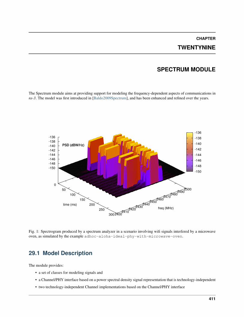
CHAPTER
TWENTYNINE
SPECTRUM MODULE
The Spectrum module aims at providing support for modeling the frequency-dependent aspects of communications inns-3. The model was first introduced in [Baldo2009Spectrum], and has been enhanced and refined over the years.
0
50
100
150
200
250
300 2400 2410
2420 2430
2440 2450
2460 2470
2480 2490
2500
-150
-148
-146
-144
-142
-140
-138
-136
PSD (dBW/Hz)
time (ms)freq (MHz)
PSD (dBW/Hz)
-150
-148
-146
-144
-142
-140
-138
-136
Fig. 1: Spectrogram produced by a spectrum analyzer in a scenario involving wifi signals interfered by a microwaveoven, as simulated by the example adhoc-aloha-ideal-phy-with-microwave-oven.
29.1 Model Description
The module provides:
• a set of classes for modeling signals and
• a Channel/PHY interface based on a power spectral density signal representation that is technology-independent
• two technology-independent Channel implementations based on the Channel/PHY interface
411
ns-3 Model Library, Release ns-3.29
• a set of basic PHY model implementations based on the Channel/PHY interface
The source code for the spectrum module is located at src/spectrum.
29.1.1 Design
Signal model
The signal model is implemented by the SpectrumSignalParameters class. This class provides the followinginformation for a signal being transmitted/received by PHY devices:
• a reference to the transmitting PHY device
• a reference to the antenna model used by the transmitting PHY device to transmit this signal
• the duration of the signal
• its Power Spectral Density (PSD) of the signal, which is assumed to be constant for the duration of the signal.
The PSD is represented as a set of discrete scalar values each corresponding to a certain subband in frequency. Theset of frequency subbands to which the PSD refers to is defined by an instance of the SpectrumModel class. ThePSD itself is implemented as an instance of the SpectrumValue class which contains a reference to the associatedSpectrumModel class instance. The SpectrumValue class provides several arithmetic operators to allow toperform calculations with PSD instances. Additionally, the SpectrumConverter class provides means for theconversion of SpectrumValue instances from one SpectrumModel to another.
For a more formal mathematical description of the signal model just described, the reader is referred to[Baldo2009Spectrum].
The SpectrumSignalParameters class is meant to include only information that is valid for all signals; assuch, it is not meant to be modified to add technology-specific information (such as type of modulation and codingschemes used, info on preambles and reference signals, etc). Instead, such information shall be put in a new classthat inherits from SpectrumSignalParameters and extends it with any technology-specific information that isneeded. This design is intended to model the fact that in the real world we have signals of different technologies beingsimultaneously transmitted and received over the air.
Channel/PHY interface
The spectrum Channel/PHY interface is defined by the base classes SpectrumChannel and SpectrumPhy. Theirinteraction simulates the transmission and reception of signals over the medium. The way this interaction works isdepicted in Sequence diagram showing the interaction between SpectrumPhy and SpectrumChannel:
Spectrum Channel implementations
The module provides two SpectrumChannel implementations: SingleModelSpectrumChannel andMultiModelSpectrumChannel. They both provide this functionality:
• Propagation loss modeling, in two forms:
– you can plug models based on PropagationLossModel on these channels. Only linear models (wherethe loss value does not depend on the transmission power) can be used. These models are single-frequencyin the sense that the loss value is applied equally to all components of the power spectral density.
– you can plug models based on SpectrumPropagationLossModel on these channels. These modelscan have frequency-dependent loss, i.e., a separate loss value is calculated and applied to each componentof the power spectral density.
412 Chapter 29. Spectrum Module
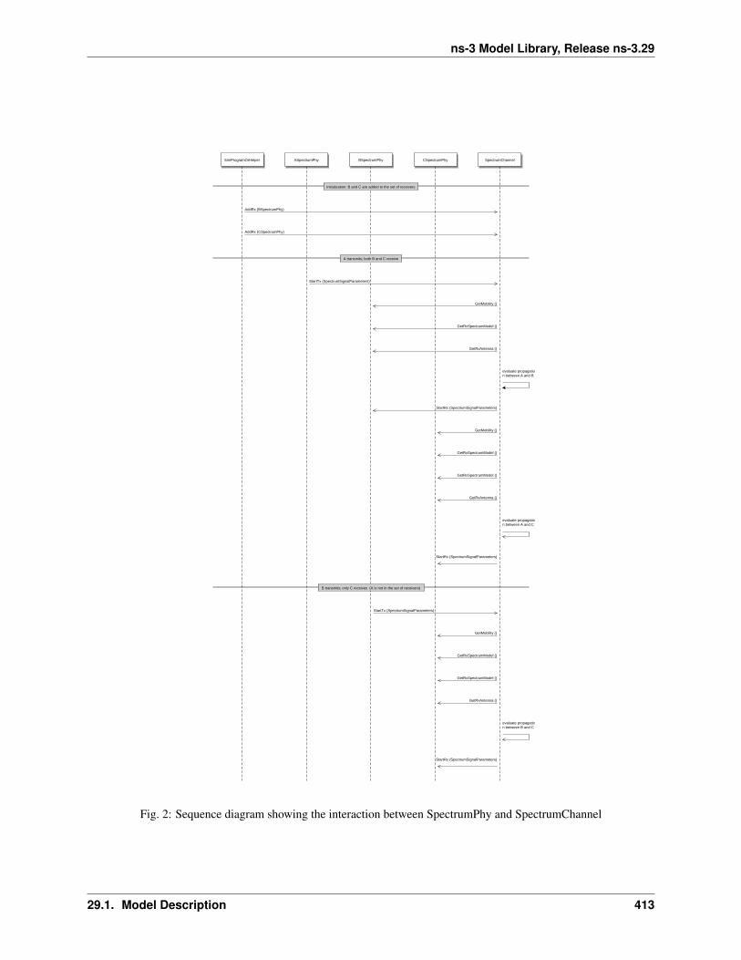
ns-3 Model Library, Release ns-3.29
SimProgramOrHelper ASpectrumPhy BSpectrumPhy CSpectrumPhy SpectrumChannel
AddRx (BSpectrumPhy)
AddRx (CSpectrumPhy)
StartTx (SpectrumSignalParameters)
GetMobility ()
GetRxSpectrumModel ()
GetRxAntenna ()
evaluate propagation between A and B
StartRx (SpectrumSignalParameters)
GetMobility ()
GetRxSpectrumModel ()
GetRxSpectrumModel ()
GetRxAntenna ()
evaluate propagation between A and C
StartRx (SpectrumSignalParameters)
StartTx (SpectrumSignalParameters)
GetMobility ()
GetRxSpectrumModel ()
GetRxSpectrumModel ()
GetRxAntenna ()
evaluate propagation between B and C
StartRx (SpectrumSignalParameters)
initialization: B and C are added to the set of receivers
A transmits; both B and C receive
B transmits; only C receives (A is not in the set of receivers)
Fig. 2: Sequence diagram showing the interaction between SpectrumPhy and SpectrumChannel
29.1. Model Description 413
ns-3 Model Library, Release ns-3.29
• Propagation delay modeling, by plugging a model based on PropagationDelayModel. The delay is inde-pendent of frequency and applied to the signal as a whole. Delay modeling is implemented by scheduling theStartRx event with a delay respect to the StartTx event.
SingleModelSpectrumChannel and MultiModelSpectrumChannel are quite similar, the main differ-ence is that MultiModelSpectrumChannel allows to use different SpectrumModel instances with the samechannel instance, by automatically taking care of the conversion of PSDs among the different models.
Example model implementations
The spectrum module provides some basic implementation of several components that are mainly intended as a proof-of-concept and as an example for building custom models with the spectrum module. Here is a brief list of the availableimplementations:
• SpectrumModel300Khz300GhzLog and SpectrumModelIsm2400MhzRes1Mhz are two exampleSpectrumModel implementations
• HalfDuplexIdealPhy: a basic PHY model using a gaussian interference model (implemented inSpectrumInterference) together with an error model based on Shannon capacity (described in[Baldo2009Spectrum] and implemented in SpectrumErrorModel. This PHY uses the GenericPhy inter-face. Its addditional custom signal parameters are defined in HalfDuplexIdealPhySignalParameters.
• WifiSpectrumValueHelper is an helper object that makes it easy to create SpectrumValues repre-senting PSDs and RF filters for the wifi technology.
• AlohaNoackNetDevice: a minimal NetDevice that allows to send packets over HalfDuplexIdealPhy(or other PHY model based on the GenericPhy interface).
• SpectrumAnalyzer, WaveformGenerator and MicrowaveOven are examples of PHY models otherthan communication devices - the names should be self-explaining.
29.1.2 References
29.2 Usage
The main use case of the spectrum model is for developers who want to develop a new model for the PHY layer ofsome wireless technology to be used within ns-3. Here are some notes on how the spectrum module is expected to beused.
• SpectrumPhy and SpectrumChannel are abstract base classes. Real code will use classes that inheritfrom these classes.
• If you are implementing a new model for some wireless technology of your interest, and want to use the spectrummodule, you’ll typically create your own module and make it depend on the spectrum module. Then youtypically have to implement:
– a child class of SpectrumModel which defines the (sets of) frequency subbands used by the consideredwireless technology. Note: instances of SpectrumModel are typically statically allocated, in order toallow several SpectrumValue instances to reference the same SpectrumModel instance.
– a child class of SpectrumPhy which will handle transmission and reception of signals (including, ifappropriate, interference and error modeling).
– a child class of SpectrumSignalParameters which will contain all the information needed tomodel the signals for the wireless technology being considered that is not already provided by the baseSpectrumSignalParameters class. Examples of such information are the type of modulation andcoding schemes used, the PHY preamble format, info on the pilot/reference signals, etc.
414 Chapter 29. Spectrum Module
ns-3 Model Library, Release ns-3.29
• The available SpectrumChannel implementations (SingleModelSpectrumChannel andMultiModelSpectrumChannel, are quite generic. Chances are you can use them as-is. Whetheryou prefer one or the other it is just a matter of whether you will have a single SpectrumModel or multiple onesin your simulations.
• Typically, there will be a single SpectrumChannel instance to which several SpectrumPhy instances are plugged.The rule of thumb is that all PHYs that are interfering with each other shall be plugged on the same channel.Multiple SpectrumChannel instances are expected to be used mainly when simulating completely orthogonalchannels; for example, when simulating the uplink and downlink of a Frequency Division Duplex system, it is agood choice to use two SpectrumChannel instances in order to reduce computational complexity.
• Different types of SpectrumPhy (i.e., instances of different child classes) can be plugged on the same Spec-trumChannel instance. This is one of the main features of the spectrum module, to support inter-technologyinterference. For example, if you implement a WifiSpectrumPhy and a BluetoohSpectrumPhy, and plug both ona SpectrumChannel, then you’ll be able to simulate interference between wifi and bluetooth and vice versa.
• Different child classes of SpectrumSignalParameters can coexist in the same simulation, and be trans-mitted over the same channel object. Again, this is part of the support for inter-technology interference. A PHYdevice model is expected to use the DynamicCast<> operator to determine if a signal is of a certain type itcan attempt to receive. If not, the signal is normally expected to be considered as interference.
29.2.1 Helpers
The helpers provided in src/spectrum/helpers are mainly intended for the example implementations describedin Example model implementations. If you are developing your custom model based on the spectrum framework, youwill probably prefer to define your own helpers.
29.2.2 Attributes
• Both SingleModelSpectrumChannel and MultiModelSpectrumChannel have an attributeMaxLossDb which can use to avoid propagating signals affected by very high propagation loss. You canuse this to reduce the complexity of interference calculations. Just be careful to choose a value that does notmake the interference calculations inaccurate.
• The example implementations described in Example model implementations also have several attributes.
29.2.3 Output
• Both SingleModelSpectrumChannel and MultiModelSpectrumChannel provide a trace sourcecalled PathLoss which is fired whenever a new path loss value is calclulated. Note: only single-frequencypath loss is accounted for, see the attribute description.
• The example implementations described in Example model implementations also provide some trace sources.
• The helper class SpectrumAnalyzerHelper can be conveniently used to generate an out-put text file containing the spectrogram produced by a SpectrumAnalyzer instance. The for-mat is designed to be easily plotted with gnuplot. For example, if your run the ex-ample adhoc-aloha-ideal-phy-with-microwave-oven you will get an output file calledspectrum-analyzer-output-3-0.tr. From this output file, you can generate a figure similar to Spec-trogram produced by a spectrum analyzer in a scenario involving wifi signals interfered by a microwave oven,as simulated by the example adhoc-aloha-ideal-phy-with-microwave-oven. by executing the following gnuplotcommands:
29.2. Usage 415
ns-3 Model Library, Release ns-3.29
unset surfaceset pm3d at sset paletteset key offset view 50,50set xlabel "time (ms)"set ylabel "freq (MHz)"set zlabel "PSD (dBW/Hz)" offset 15,0,0splot "./spectrum-analyzer-output-3-0.tr" using ($1*1000.0):($2/1e6):(10*log10($3))
29.2.4 Examples
The example programs in src/spectrum/examples/ allow to see the example implementations described inExample model implementations in action.
29.2.5 Troubleshooting
• Disclaimer on inter-technology interference: the spectrum model makes it very easy to implement an inter-technology interference model, but this does not guarantee that the resulting model is accurate. For example,the gaussian interference model implemented in the SpectrumInterference class can be used to calculateinter-technology interference, however the results might not be valid in some scenarios, depending on the actualwaveforms involved, the number of interferers, etc. Moreover, it is very important to use error models that areconsistent with the interference model. The responsibility of ensuring that the models being used are correct isleft to the user.
29.3 Testing
In this section we describe the test suites that are provided within the spectrum module.
29.3.1 SpectrumValue test
The test suite spectrum-value verifies the correct functionality of the arithmetic operators implemented by theSpectrumValue class. Each test case corresponds to a different operator. The test passes if the result provided bythe operator implementation is equal to the reference values which were calculated offline by hand. Equality is verifiedwithin a tolerance of 10−6 which is to account for numerical errors.
29.3.2 SpectrumConverter test
The test suite spectrum-converter verifies the correct functionality of the SpectrumConverter class. Dif-ferent test cases correspond to the conversion of different SpectrumValue instances to different SpectrumModelinstances. Each test passes if the SpectrumValue instance resulting from the conversion is equal to the referencevalues which were calculated offline by hand. Equality is verified within a tolerance of 10−6 which is to account fornumerical errors.
Describe how the model has been tested/validated. What tests run in the test suite? How much API and code is coveredby the tests? Again, references to outside published work may help here.
416 Chapter 29. Spectrum Module

ns-3 Model Library, Release ns-3.29
29.3.3 Interference test
The test suite spectrum-interference verifies the correct functionality of the SpectrumInterferenceand ShannonSpectrumErrorModel in a scenario involving four signals (an intended signal plus three interfer-ers). Different test cases are created corresponding to different PSDs of the intended signal and different amount oftransmitted bytes. The test passes if the output of the error model (successful or failed) coincides with the expectedone which was determine offline by manually calculating the achievable rate using Shannon’s formula.
29.3.4 IdealPhy test
The test verifies that AlohaNoackNetDevice and HalfDuplexIdealPhy work properly when installed in anode. The test recreates a scenario with two nodes (a TX and a RX) affected by a path loss such that a certain SNRis obtained. The TX node transmits with a pre-determined PHY rate and with an application layer rate which islarger than the PHY rate, so as to saturate the channel. PacketSocket is used in order to avoid protocol overhead.Different test cases correspond to different PHY rate and SNR values. For each test case, we calculated offline (usingShannon’s formula) whether the PHY rate is achievable or not. Each test case passes if the following conditions aresatisfied:
• if the PHY rate is achievable, the application throughput shall be within 1% of the PHY rate;
• if the PHY rate is not achievable, the application throughput shall be zero.
29.4 Additional Models
29.4.1 TV Transmitter Model
A TV Transmitter model is implemented by the TvSpectrumTransmitter class. This model enables transmis-sion of realistic TV signals to be simulated and can be used for interference modeling. It provides a customizablepower spectral density (PSD) model, with configurable attributes including the type of modulation (with models foranalog, 8-VSB, and COFDM), signal bandwidth, power spectral density level, frequency, and transmission duration.A helper class, TvSpectrumTransmitterHelper, is also provided to assist users in setting up simulations.
Main Model Class
The main TV Transmitter model class, TvSpectrumTransmitter, provides a user-configurable PSD model thatcan be transmitted on the SpectrumChannel. It inherits from SpectrumPhy and is comprised of attributes andmethods to create and transmit the signal on the channel.
One of the user-configurable attributes is the type of modulation for the TV transmitter to use. The options are 8-VSB(Eight-Level Vestigial Sideband Modulation) which is notably used in the North America ATSC digital televisionstandard, COFDM (Coded Orthogonal Frequency Division Multiplexing) which is notably used in the DVB-T andISDB-T digital television standards adopted by various countries around the world, and analog modulation whichis a legacy technology but is still being used by some countries today. To accomplish realistic PSD models forthese modulation types, the signals’ PSDs were approximated from real standards and developed into models that arescalable by frequency and power. The COFDM PSD is approximated from Figure 12 (8k mode) of [KoppCOFDM],the 8-VSB PSD is approximated from Figure 3 of [Baron8VSB], and the analog PSD is approximated from Figure4 of [QualcommAnalog]. Note that the analog model is approximated from the NTSC standard, but other analogmodulation standards such as PAL have similar signals. The approximated COFDM PSD model is in 8K mode. Theother configurable attributes are the start frequency, signal/channel bandwidth, base PSD, antenna type, starting time,and transmit duration.
29.4. Additional Models 417
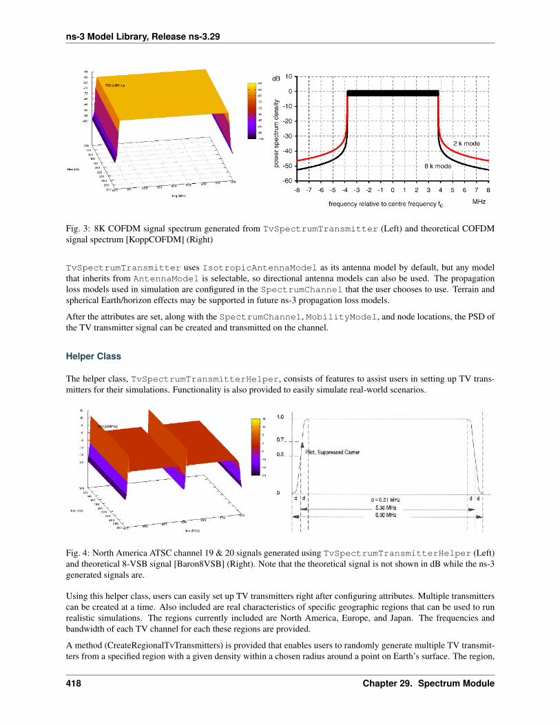
ns-3 Model Library, Release ns-3.29
Fig. 3: 8K COFDM signal spectrum generated from TvSpectrumTransmitter (Left) and theoretical COFDMsignal spectrum [KoppCOFDM] (Right)
TvSpectrumTransmitter uses IsotropicAntennaModel as its antenna model by default, but any modelthat inherits from AntennaModel is selectable, so directional antenna models can also be used. The propagationloss models used in simulation are configured in the SpectrumChannel that the user chooses to use. Terrain andspherical Earth/horizon effects may be supported in future ns-3 propagation loss models.
After the attributes are set, along with the SpectrumChannel, MobilityModel, and node locations, the PSD ofthe TV transmitter signal can be created and transmitted on the channel.
Helper Class
The helper class, TvSpectrumTransmitterHelper, consists of features to assist users in setting up TV trans-mitters for their simulations. Functionality is also provided to easily simulate real-world scenarios.
Fig. 4: North America ATSC channel 19 & 20 signals generated using TvSpectrumTransmitterHelper (Left)and theoretical 8-VSB signal [Baron8VSB] (Right). Note that the theoretical signal is not shown in dB while the ns-3generated signals are.
Using this helper class, users can easily set up TV transmitters right after configuring attributes. Multiple transmitterscan be created at a time. Also included are real characteristics of specific geographic regions that can be used to runrealistic simulations. The regions currently included are North America, Europe, and Japan. The frequencies andbandwidth of each TV channel for each these regions are provided.
A method (CreateRegionalTvTransmitters) is provided that enables users to randomly generate multiple TV transmit-ters from a specified region with a given density within a chosen radius around a point on Earth’s surface. The region,
418 Chapter 29. Spectrum Module
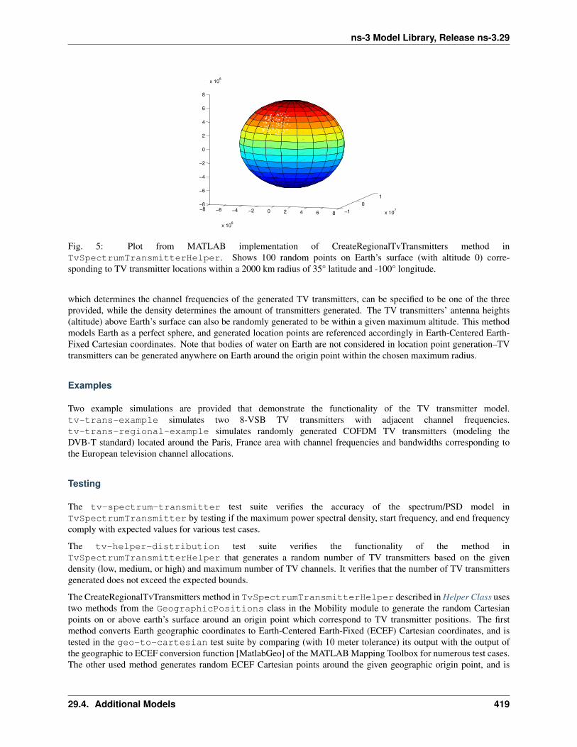
ns-3 Model Library, Release ns-3.29
−8 −6 −4 −2 0 2 4 6 8
x 106
−1
0
1
x 107
−8
−6
−4
−2
0
2
4
6
8
x 106
Fig. 5: Plot from MATLAB implementation of CreateRegionalTvTransmitters method inTvSpectrumTransmitterHelper. Shows 100 random points on Earth’s surface (with altitude 0) corre-sponding to TV transmitter locations within a 2000 km radius of 35° latitude and -100° longitude.
which determines the channel frequencies of the generated TV transmitters, can be specified to be one of the threeprovided, while the density determines the amount of transmitters generated. The TV transmitters’ antenna heights(altitude) above Earth’s surface can also be randomly generated to be within a given maximum altitude. This methodmodels Earth as a perfect sphere, and generated location points are referenced accordingly in Earth-Centered Earth-Fixed Cartesian coordinates. Note that bodies of water on Earth are not considered in location point generation–TVtransmitters can be generated anywhere on Earth around the origin point within the chosen maximum radius.
Examples
Two example simulations are provided that demonstrate the functionality of the TV transmitter model.tv-trans-example simulates two 8-VSB TV transmitters with adjacent channel frequencies.tv-trans-regional-example simulates randomly generated COFDM TV transmitters (modeling theDVB-T standard) located around the Paris, France area with channel frequencies and bandwidths corresponding tothe European television channel allocations.
Testing
The tv-spectrum-transmitter test suite verifies the accuracy of the spectrum/PSD model inTvSpectrumTransmitter by testing if the maximum power spectral density, start frequency, and end frequencycomply with expected values for various test cases.
The tv-helper-distribution test suite verifies the functionality of the method inTvSpectrumTransmitterHelper that generates a random number of TV transmitters based on the givendensity (low, medium, or high) and maximum number of TV channels. It verifies that the number of TV transmittersgenerated does not exceed the expected bounds.
The CreateRegionalTvTransmitters method in TvSpectrumTransmitterHelper described in Helper Class usestwo methods from the GeographicPositions class in the Mobility module to generate the random Cartesianpoints on or above earth’s surface around an origin point which correspond to TV transmitter positions. The firstmethod converts Earth geographic coordinates to Earth-Centered Earth-Fixed (ECEF) Cartesian coordinates, and istested in the geo-to-cartesian test suite by comparing (with 10 meter tolerance) its output with the output ofthe geographic to ECEF conversion function [MatlabGeo] of the MATLAB Mapping Toolbox for numerous test cases.The other used method generates random ECEF Cartesian points around the given geographic origin point, and is
29.4. Additional Models 419

ns-3 Model Library, Release ns-3.29
tested in the rand-cart-around-geo test suite by verifying that the generated points do not exceed the givenmaximum distance radius from the origin point.
References
420 Chapter 29. Spectrum Module
CHAPTER
THIRTY
6LOWPAN: TRANSMISSION OF IPV6 PACKETS OVER IEEE 802.15.4NETWORKS
This chapter describes the implementation of ns-3 model for the compression of IPv6 packets over IEEE 802.15.4-Based Networks as specified by RFC 4944 and RFC 6282.
30.1 Model Description
The source code for the sixlowpan module lives in the directory src/sixlowpan.
30.1.1 Design
The model design does not follow strictly the standard from an architectural standpoint, as it does extend it beyond theoriginal scope by supporting also other kinds of networks.
Other than that, the module strictly follows RFC 4944 and RFC 6282, with the following exceptions:
• MESH and LOWPAN_BC0 dispatch types are not supported
• HC2 encoding is not supported
• IPHC’s SAC and DAC are not supported
The MESH and LOWPAN_BC0 are not supported as they do apply only to mesh-under architecture, which is not oneof the goals of the module development.
The HC2 encoding is not supported, as it has been superseded by IPHC and NHC compression type (RFC 6282).
IPHC SAC and DAC are not yet supported, as they do require RFC 6775 for full compliance. It is planned to supportthem in the future.
NetDevice
The whole module is developed as a transparent NetDevice, which can act as a proxy between IPv6 and any NetDevice(the module has been successfully tested with PointToPointNedevice, CsmaNetDevice and LrWpanNetDevice).
For this reason, the module implements a virtual NetDevice, and all the calls are passed without modifications to theunderlying NetDevice. The only important difference is in GetMtu behaviour. It will always return at least 1280 bytes,as is the minimum IPv6 MTU.
The module does provide some attributes and some tracesources. The attributes are:
• Rfc6282 (boolean, default true), used to activate HC1 (RFC 4944) or IPHC (RFC 6282) compression.
• OmitUdpChecksum (boolean, default true), used to activate UDP checksum compression in IPHC.
421
ns-3 Model Library, Release ns-3.29
• FragmentReassemblyListSize (integer, default 0), indicating the number of packets that can be reassembled atthe same time. If the limit is reached, the oldest packet is discarded. Zero means infinite.
• FragmentExpirationTimeout (Time, default 60 seconds), being the timeout to wait for further fragments beforediscarding a partial packet.
• CompressionThreshold (unsigned 32 bits integer, default 0), minimum compressed payload size.
• ForceEtherType (boolean, default false), and
• EtherType (unsigned 16 bits integer, default 0xFFFF), to force a particular L2 EtherType.
The CompressionThreshold attribute is similar to Contiki’s SICSLOWPAN_CONF_MIN_MAC_PAYLOAD option.If a compressed packet size is less than the threshold, the uncompressed version is used (plus one byte for the correctdispatch header). This option is useful when a MAC requires a minimum frame size (e.g., ContikiMAC) and thecompression would violate the requirement.
The last two attributes are needed to use the module with a NetDevice other than 802.15.4, as neither IANA orIEEE did reserve an EtherType for 6LoWPAN. As a consequence there might be a conflict with the L2 multi-plexer/demultiplexer which is based on EtherType. The default value is 0xFFFF, which is reserved by IEEE (see[IANA802] and [Ethertype]). The default module behaviour is to not change the EtherType, however this would notwork with any NetDevice actually understanding and using the EtherType.
Note that the ForceEtherType parameter have also a direct effect on the MAC address kind the module is expectingto handle: * ForceEtherType true: Mac48Address (Ethernet, WiFi, etc.). * ForceEtherType false: Mac16Address orMac64Address (IEEE 802.15.4).
Note that using 6LoWPAN over any NetDevice other than 802.15.4 will produce valid .pcap files, but they will notbe correctly dissected by Wireshark. The reason lies on the fact that 6LoWPAN was really meant to be used onlyover 802.15.4, so Wireshark dissectors will not even try to decode 6LoWPAN headers on top of protocols other than802.15.4.
The Trace sources are:
• Tx - exposing packet (including 6LoWPAN header), SixLoWPanNetDevice Ptr, interface index.
• Rx - exposing packet (including 6LoWPAN header), SixLoWPanNetDevice Ptr, interface index.
• Drop - exposing DropReason, packet (including 6LoWPAN header), SixLoWPanNetDevice Ptr, interface index.
The Tx and Rx traces are called as soon as a packet is received or sent. The Drop trace is invoked when a packet (or afragment) is discarded.
30.1.2 Scope and Limitations
Future versions of this module will support RFC 6775, however no timeframe is guaranteed.
Using 6LoWPAN with IPv4 (or other L3 protocols)
As the name implies, 6LoWPAN can handle only IPv6 packets. Any other protocol will be discarded. Moreover,6LoWPAN assumes that the network is uniform, as is all the devices connected by the same same channel are using6LoWPAN. Mixed environments are not supported by the standard. The reason is simple: 802.15.4 frame doesn’thave a “protocol” field. As a consequence, there is no demultiplexing at MAC layer and the protocol carried by L2frames must be known in advance.
In the ns-3 implementation it is possible, but not advisable, to violate this requirement if the underlying NetDevice iscapable of discriminating different protocols. As an example, CsmaNetDevice can carry IPv4 and 6LoWPAN at thesame time. However, this configuration has not been tested.
422 Chapter 30. 6LoWPAN: Transmission of IPv6 Packets over IEEE 802.15.4 Networks

ns-3 Model Library, Release ns-3.29
30.1.3 References
30.2 Usage
30.2.1 Enabling sixlowpan
Add sixlowpan to the list of modules built with ns-3.
30.2.2 Helper
The helper is patterned after other device helpers.
30.2.3 Examples
The following example can be found in src/sixlowpan/examples/:
• example-sixlowpan.cc: A simple example showing end-to-end data transfer.
In particular, the example enables a very simplified end-to-end data transfer scenario, with a CSMA network forced tocarry 6LoWPAN compressed packets.
30.2.4 Tests
The test provided checks the connection between two UDP clients and the correctness of the received packets.
30.3 Validation
The model has been validated against WireShark, checking whatever the packets are correctly interpreted and vali-dated.
30.2. Usage 423

ns-3 Model Library, Release ns-3.29
424 Chapter 30. 6LoWPAN: Transmission of IPv6 Packets over IEEE 802.15.4 Networks
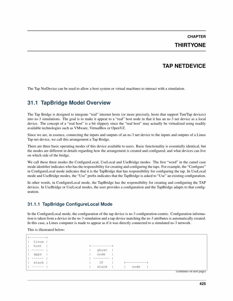
CHAPTER
THIRTYONE
TAP NETDEVICE
The Tap NetDevice can be used to allow a host system or virtual machines to interact with a simulation.
31.1 TapBridge Model Overview
The Tap Bridge is designed to integrate “real” internet hosts (or more precisely, hosts that support Tun/Tap devices)into ns-3 simulations. The goal is to make it appear to a “real” host node in that it has an ns-3 net device as a localdevice. The concept of a “real host” is a bit slippery since the “real host” may actually be virtualized using readilyavailable technologies such as VMware, VirtualBox or OpenVZ.
Since we are, in essence, connecting the inputs and outputs of an ns-3 net device to the inputs and outputs of a LinuxTap net device, we call this arrangement a Tap Bridge.
There are three basic operating modes of this device available to users. Basic functionality is essentially identical, butthe modes are different in details regarding how the arrangement is created and configured; and what devices can liveon which side of the bridge.
We call these three modes the ConfigureLocal, UseLocal and UseBridge modes. The first “word” in the camel casemode identifier indicates who has the responsibility for creating and configuring the taps. For example, the “Configure”in ConfigureLocal mode indicates that it is the TapBridge that has responsibility for configuring the tap. In UseLocalmode and UseBridge modes, the “Use” prefix indicates that the TapBridge is asked to “Use” an existing configuration.
In other words, in ConfigureLocal mode, the TapBridge has the responsibility for creating and configuring the TAPdevices. In UseBridge or UseLocal modes, the user provides a configuration and the TapBridge adapts to that config-uration.
31.1.1 TapBridge ConfigureLocal Mode
In the ConfigureLocal mode, the configuration of the tap device is ns-3 configuration-centric. Configuration informa-tion is taken from a device in the ns-3 simulation and a tap device matching the ns-3 attributes is automatically created.In this case, a Linux computer is made to appear as if it was directly connected to a simulated ns-3 network.
This is illustrated below:
+--------+| Linux || host | +----------+| ------ | | ghost || apps | | node || ------ | | -------- || stack | | IP | +----------+| ------ | | stack | | node |
(continues on next page)
425

ns-3 Model Library, Release ns-3.29
(continued from previous page)
| TAP | |==========| | -------- || device | <----- IPC ------> | tap | | IP |+--------+ | bridge | | stack |
| -------- | | -------- || ns-3 | | ns-3 || net | | net || device | | device |+----------+ +----------+
|| ||+---------------------------+| ns-3 channel |+---------------------------+
In this case, the “ns-3 net device” in the “ghost node” appears as if it were actually replacing the TAP device in theLinux host. The ns-3 simulation creates the TAP device on the underlying Linux OS and configures the IP and MACaddresses of the TAP device to match the values assigned to the simulated ns-3 net device. The “IPC” link shownabove is the network tap mechanism in the underlying OS. The whole arrangement acts as a conventional bridge; buta bridge between devices that happen to have the same shared MAC and IP addresses.
Here, the user is not required to provide any configuration information specific to the tap. A tap device will be createdand configured by ns-3 according to its defaults, and the tap device will have its name assigned by the underlyingoperating system according to its defaults.
If the user has a requirement to access the created tap device, he or she may optionally provide a “DeviceName”attribute. In this case, the created OS tap device will be named accordingly.
The ConfigureLocal mode is the default operating mode of the Tap Bridge.
31.1.2 TapBridge UseLocal Mode
The UseLocal mode is quite similar to the ConfigureLocal mode. The significant difference is, as the mode nameimplies, the TapBridge is going to “Use” an existing tap device previously created and configured by the user. Thismode is particularly useful when a virtualization scheme automatically creates tap devices and ns-3 is used to providesimulated networks for those devices.
+--------+| Linux || host | +----------+| ------ | | ghost || apps | | node || ------ | | -------- || stack | | IP | +----------+| ------ | | stack | | node || TAP | |==========| | -------- || device | <----- IPC ------> | tap | | IP || MAC X | | bridge | | stack |+--------+ | -------- | | -------- |
| ns-3 | | ns-3 || net | | net || device | | device || MAC Y | | MAC Z |+----------+ +----------+
|| ||+---------------------------+| ns-3 channel |+---------------------------+
426 Chapter 31. Tap NetDevice

ns-3 Model Library, Release ns-3.29
In this case, the pre-configured MAC address of the “Tap device” (MAC X) will not be the same as that of the bridged“ns-3 net device” (MAC Y) shown in the illustration above. In order to bridge to ns-3 net devices which do not supportSendFrom() (especially wireless STA nodes) we impose a requirement that only one Linux device (with one uniqueMAC address – here X) generates traffic that flows across the IPC link. This is because the MAC addresses of trafficacross the IPC link will be “spoofed” or changed to make it appear to Linux and ns-3 that they have the same address.That is, traffic moving from the Linux host to the ns-3 ghost node will have its MAC address changed from X to Yand traffic from the ghost node to the Linux host will have its MAC address changed from Y to X. Since there is aone-to-one correspondence between devices, there may only be one MAC source flowing from the Linux side. Thismeans that Linux bridges with more than one net device added are incompatible with UseLocal mode.
In UseLocal mode, the user is expected to create and configure a tap device completely outside the scope of the ns-3simulation using something like:
$ sudo tunctl -t tap0$ sudo ifconfig tap0 hw ether 08:00:2e:00:00:01$ sudo ifconfig tap0 10.1.1.1 netmask 255.255.255.0 up
To tell the TapBridge what is going on, the user will set either directly into the TapBridge or via the TapBridgeHelper,the “DeviceName” attribute. In the case of the configuration above, the “DeviceName” attribute would be set to “tap0”and the “Mode” attribute would be set to “UseLocal”.
One particular use case for this mode is in the OpenVZ environment. There it is possible to create a Tap device on the“Hardware Node” and move it into a Virtual Private Server. If the TapBridge is able to use an existing tap device it isthen possible to avoid the overhead of an OS bridge in that environment.
31.1.3 TapBridge UseBridge Mode
The simplest mode for those familiar with Linux networking is the UseBridge mode. Again, the “Use” prefix indicatesthat the TapBridge is going to Use an existing configuration. In this case, the TapBridge is going to logically extend aLinux bridge into ns-3.
This is illustrated below:
+---------+| Linux | +----------+| ------- | | ghost || apps | | node || ------- | | -------- || stack | | IP | +----------+| ------- | +--------+ | stack | | node || Virtual | | TAP | |==========| | -------- || Device | | Device | <---- IPC -----> | tap | | IP |+---------+ +--------+ | bridge | | stack |
|| || | -------- | | -------- |+--------------------+ | ns-3 | | ns-3 || OS (brctl) Bridge | | net | | net |+--------------------+ | device | | device |
+----------+ +----------+|| ||
+---------------------------+| ns-3 channel |+---------------------------+
In this case, a computer running Linux applications, protocols, etc., is connected to a ns-3 simulated network in sucha way as to make it appear to the Linux host that the TAP device is a real network device participating in the Linuxbridge.
31.1. TapBridge Model Overview 427

ns-3 Model Library, Release ns-3.29
In the ns-3 simulation, a TapBridge is created to match each TAP Device. The name of the TAP Device is assigned tothe Tap Bridge using the “DeviceName” attribute. The TapBridge then logically extends the OS bridge to encompassthe ns-3 net device.
Since this mode logically extends an OS bridge, there may be many Linux net devices on the non-ns-3 side of thebridge. Therefore, like a net device on any bridge, the ns-3 net device must deal with the possibly of many sourceaddresses. Thus, ns-3 devices must support SendFrom() (NetDevice::SupportsSendFrom() must return true) in orderto be configured for use in UseBridge mode.
It is expected that the user will do something like the following to configure the bridge and tap completely outsidens-3:
$ sudo brctl addbr mybridge$ sudo tunctl -t mytap$ sudo ifconfig mytap hw ether 00:00:00:00:00:01$ sudo ifconfig mytap 0.0.0.0 up$ sudo brctl addif mybridge mytap$ sudo brctl addif mybridge ...$ sudo ifconfig mybridge 10.1.1.1 netmask 255.255.255.0 up
To tell the TapBridge what is going on, the user will set either directly into the TapBridge or via the TapBridgeHelper,the “DeviceName” attribute. In the case of the configuration above, the “DeviceName” attribute would be set to“mytap” and the “Mode” attribute would be set to “UseBridge”.
This mode is especially useful in the case of virtualization where the configuration of the virtual hosts may be dictatedby another system and not be changeable to suit ns-3. For example, a particular VM scheme may create virtual “vethx”or “vmnetx” devices that appear local to virtual hosts. In order to connect to such systems, one would need to manuallycreate TAP devices on the host system and brigde these TAP devices to the existing (VM) virtual devices. The job ofthe Tap Bridge in this case is to extend the bridge to join a ns-3 net device.
31.1.4 TapBridge ConfigureLocal Operation
In ConfigureLocal mode, the TapBridge and therefore its associated ns-3 net device appears to the Linux host computeras a network device just like any arbitrary “eth0” or “ath0” might appear. The creation and configuration of the TAPdevice is done by the ns-3 simulation and no manual configuration is required by the user. The IP addresses, MACaddresses, gateways, etc., for created TAP devices are extracted from the simulation itself by querying the configurationof the ns-3 device and the TapBridge Attributes.
Since the MAC addresses are identical on the Linux side and the ns-3 side, we can use Send() on the ns-3 devicewhich is available on all ns-3 net devices. Since the MAC addresses are identical there is no requirement to hook thepromiscuous callback on the receive side. Therefore there are no restrictions on the kinds of net device that are usablein ConfigureLocal mode.
The TapBridge appears to an ns-3 simulation as a channel-less net device. This device must not have an IP addressassociated with it, but the bridged (ns-3) net device must have an IP address. Be aware that this is the inverse of anns-3 BridgeNetDevice (or a conventional bridge in general) which demands that its bridge ports not have IP addresses,but allows the bridge device itself to have an IP address.
The host computer will appear in a simulation as a “ghost” node that contains one TapBridge for each NetDevicethat is being bridged. From the perspective of a simulation, the only difference between a ghost node and any othernode will be the presence of the TapBridge devices. Note however, that the presence of the TapBridge does affect theconnectivity of the net device to the IP stack of the ghost node.
Configuration of address information and the ns-3 devices is not changed in any way if a TapBridge is present. ATapBridge will pick up the addressing information from the ns-3 net device to which it is connected (its “bridged” netdevice) and use that information to create and configure the TAP device on the real host.
428 Chapter 31. Tap NetDevice
ns-3 Model Library, Release ns-3.29
The end result of this is a situation where one can, for example, use the standard ping utility on a real host to ping asimulated ns-3 node. If correct routes are added to the internet host (this is expected to be done automatically in futurens-3 releases), the routing systems in ns-3 will enable correct routing of the packets across simulated ns-3 networks.For an example of this, see the example program, tap-wifi-dumbbell.cc in the ns-3 distribution.
The Tap Bridge lives in a kind of a gray world somewhere between a Linux host and an ns-3 bridge device. From theLinux perspective, this code appears as the user mode handler for a TAP net device. In ConfigureLocal mode, this Tapdevice is automatically created by the ns-3 simulation. When the Linux host writes to one of these automatically cre-ated /dev/tap devices, the write is redirected into the TapBridge that lives in the ns-3 world; and from this perspective,the packet write on Linux becomes a packet read in the Tap Bridge. In other words, a Linux process writes a packet toa tap device and this packet is redirected by the network tap mechanism toan ns-3 process where it is received by theTapBridge as a result of a read operation there. The TapBridge then writes the packet to the ns-3 net device to which itis bridged; and therefore it appears as if the Linux host sent a packet directly through an ns-3 net device onto an ns-3network.
In the other direction, a packet received by the ns-3 net device connected to the Tap Bridge is sent via a receive callbackto the TapBridge. The TapBridge then takes that packet and writes it back to the host using the network tap mechanism.This write to the device will appear to the Linux host as if a packet has arrived on a net device; and therefore as if apacket received by the ns-3 net device during a simulation has appeared on a real Linux net device.
The upshot is that the Tap Bridge appears to bridge a tap device on a Linux host in the “real world” to an ns-3 netdevice in the simulation. Because the TAP device and the bridged ns-3 net device have the same MAC address and thenetwork tap IPC link is not externalized, this particular kind of bridge makes it appear that a ns-3 net device is actuallyinstalled in the Linux host.
In order to implement this on the ns-3 side, we need a “ghost node” in the simulation to hold the bridged ns-3 netdevice and the TapBridge. This node should not actually do anything else in the simulation since its job is simply tomake the net device appear in Linux. This is not just arbitrary policy, it is because:
• Bits sent to the TapBridge from higher layers in the ghost node (using the TapBridge Send method) are com-pletely ignored. The TapBridge is not, itself, connected to any network, neither in Linux nor in ns-3. You cannever send nor receive data over a TapBridge from the ghost node.
• The bridged ns-3 net device has its receive callback disconnected from the ns-3 node and reconnected to the TapBridge. All data received by a bridged device will then be sent to the Linux host and will not be received by thenode. From the perspective of the ghost node, you can send over this device but you cannot ever receive.
Of course, if you understand all of the issues you can take control of your own destiny and do whatever you want –we do not actively prevent you from using the ghost node for anything you decide. You will be able to perform typicalns-3 operations on the ghost node if you so desire. The internet stack, for example, must be there and functional onthat node in order to participate in IP address assignment and global routing. However, as mentioned above, interfacestalking to any TapBridge or associated bridged net devices will not work completely. If you understand exactly whatyou are doing, you can set up other interfaces and devices on the ghost node and use them; or take advantage of theoperational send side of the bridged devices to create traffic generators. We generally recommend that you treat thisnode as a ghost of the Linux host and leave it to itself, though.
31.1.5 TapBridge UseLocal Mode Operation
As described in above, the TapBridge acts like a bridge from the “real” world into the simulated ns-3 world. In thecase of the ConfigureLocal mode, life is easy since the IP address of the Tap device matches the IP address of the ns-3device and the MAC address of the Tap device matches the MAC address of the ns-3 device; and there is a one-to-onerelationship between the devices.
Things are slightly complicated when a Tap device is externally configured with a different MAC address than the ns-3net device. The conventional way to deal with this kind of difference is to use promiscuous mode in the bridged deviceto receive packets destined for the different MAC address and forward them off to Linux. In order to move packets
31.1. TapBridge Model Overview 429
ns-3 Model Library, Release ns-3.29
the other way, the conventional solution is SendFrom() which allows a caller to “spoof” or change the source MACaddress to match the different Linux MAC address.
We do have a specific requirement to be able to bridge Linux Virtual Machines onto wireless STA nodes. Unfor-tunately, the 802.11 spec doesn’t provide a good way to implement SendFrom(), so we have to work around thatproblem.
To this end, we provided the UseLocal mode of the Tap Bridge. This mode allows you approach the problem as ifyou were creating a bridge with a single net device. A single allowed address on the Linux side is remembered inthe TapBridge, and all packets coming from the Linux side are repeated out the ns-3 side using the ns-3 device MACsource address. All packets coming in from the ns-3 side are repeated out the Linux side using the remembered MACaddress. This allows us to use Send() on the ns-3 device side which is available on all ns-3 net devices.
UseLocal mode is identical to the ConfigureLocal mode except for the creation and configuration of the tap device andthe MAC address spoofing.
31.1.6 TapBridge UseBridge Operation
As described in the ConfigureLocal mode section, when the Linux host writes to one of the /dev/tap devices, the writeis redirected into the TapBridge that lives in the ns-3 world. In the case of the UseBridge mode, these packets willneed to be sent out on the ns-3 network as if they were sent on a device participating in the Linux bridge. This meanscalling the SendFrom() method on the bridged device and providing the source MAC address found in the packet.
In the other direction, a packet received by an ns-3 net device is hooked via callback to the TapBridge. This must bedone in promiscuous mode since the goal is to bridge the ns-3 net device onto the OS (brctl) bridge of which the TAPdevice is a part.
For these reasons, only ns-3 net devices that support SendFrom() and have a hookable promiscuous receive callbackare allowed to participate in UseBridge mode TapBridge configurations.
31.2 Tap Bridge Channel Model
There is no channel model associated with the Tap Bridge. In fact, the intention is make it appear that the real internethost is connected to the channel of the bridged net device.
31.3 Tap Bridge Tracing Model
Unlike most ns-3 devices, the TapBridge does not provide any standard trace sources. This is because the bridge is anintermediary that is essentially one function call away from the bridged device. We expect that the trace hooks in thebridged device will be sufficient for most users,
31.4 Using the TapBridge
We expect that most users will interact with the TapBridge device through the TapBridgeHelper. Users of other helperclasses, such as CSMA or Wifi, should be comfortable with the idioms used there.
430 Chapter 31. Tap NetDevice
CHAPTER
THIRTYTWO
TOPOLOGY INPUT READERS
The topology modules aim at reading a topology file generated by an automatic topology generator.
The process is divided in two steps:
• running a topology generator to build a topology file
• reading the topology file and build a ns-3 simulation
Hence, model is focused on being able to read correctly the various topology formats.
Currently there are three models:
• ns3::OrbisTopologyReader for Orbis 0.7 traces
• ns3::InetTopologyReader for Inet 3.0 traces
• ns3::RocketfuelTopologyReader for Rocketfuel traces
An helper ns3::TopologyReaderHelper is provided to assist on trivial tasks.
A good source for topology data is also Archipelago.
The current Archipelago Measurements, monthly updated, are stored in the CAIDA website using a complete notationand triple data source, one for each working group.
A different and more compact notation reporting only the AS-relationships (a sort of more Orbis-like format) is here:as-relationships.
The compact notation can be easily stripped down to a pure Orbis format, just removing the double relationships (thecompact format use one-way links, while Orbis use two-way links) and pruning the 3rd parameter. Note that with thecompact data Orbis can then be used create a rescaled version of the topology, thus being the most effective way (tomy best knowledge) to make an internet-like topology.
Examples can be found in the directory src/topology-read/examples/
431

ns-3 Model Library, Release ns-3.29
432 Chapter 32. Topology Input Readers
CHAPTER
THIRTYTHREE
TRAFFIC CONTROL LAYER
33.1 Traffic Control Layer
The Traffic Control layer aims at introducing an equivalent of the Linux Traffic Control infrastructure into ns-3.The Traffic Control layer sits in between the NetDevices (L2) and any network protocol (e.g. IP). It is in charge ofprocessing packets and performing actions on them: scheduling, dropping, marking, policing, etc.
33.1.1 Introducing the Traffic Control Layer
The Traffic Control layer intercepts both outgoing packets flowing downwards from the network layer to the networkdevice and incoming packets flowing in the opposite direction. Currently, only outgoing packets are processed by theTraffic Control layer. In particular, outgoing packets are enqueued in a queuing discipline, which can perform multipleactions on them.
In the following, more details are given about how the Traffic Control layer intercepts outgoing and incoming packetsand, more in general, about how the packets traverse the network stack.
Transmitting packets
The IPv{4,6} interfaces uses the aggregated object TrafficControlLayer to send down packets, instead of calling Net-Device::Send() directly. After the analysis and the process of the packet, when the backpressure mechanism allows it,TrafficControlLayer will call the Send() method on the right NetDevice.
Receiving packets
The callback chain that (in the past) involved IPv{4,6}L3Protocol and NetDevices, through ReceiveCallback, is ex-tended to involve TrafficControlLayer. When an IPv{4,6}Interface is added in the IPv{4,6}L3Protocol, the callbackchain is configured to have the following packet exchange:
NetDevice –> Node –> TrafficControlLayer –> IPv{4,6}L3Protocol
33.1.2 Brief description of old node/device/protocol interactions
The main question that we would like to answer in the following paragraphs is: how a ns-3 node can send/receivepackets?
If we analyze any example out there, the ability of the node to receive/transmit packets derives from the interaction oftwo helper:
• L2 Helper (something derived from NetDevice)
433
ns-3 Model Library, Release ns-3.29
• L3 Helper (usually from Internet module)
L2 Helper main operations
Any good L2 Helper will do the following operations:
• Create n netdevices (n>1)
• Attach a channel between these devices
• Call Node::AddDevice ()
Obviously the last point is the most important.
Node::AddDevice (network/model/node.cc:128) assigns an interface index to the device, calls NetDevice::SetNode,sets the receive callback of the device to Node::NonPromiscReceiveFromDevice. Then, it schedules NetDe-vice::Initialize() method at Seconds(0.0), then notify the registered DeviceAdditionListener handlers (not used BYANYONE).
Node::NonPromiscReceiveFromDevice calls Node::ReceiveFromDevice.
Node::ReceiveFromDevice iterates through ProtocolHandlers, which are callbacks which accept as signature:
ProtocolHandler (Ptr<NetDevice>, Ptr<const Packet>, protocol, from_addr, to_addr, packetType).
If device, protocol number and promiscuous flag corresponds, the handler is invoked.
Who is responsible to set ProtocolHandler ? We will analyze that in the next section.
L3 Helper
We have only internet which provides network protocol (IP). That module splits the operations between two helpers:InternetStackHelper and Ipv{4,6}AddressHelper.
InternetStackHelper::Install (internet/helper/internet-stack-helper.cc:423) creates and aggregates proto-cols {ArpL3,Ipv4L3,Icmpv4}Protocol. It creates the routing protocol, and if Ipv6 is enabled it adds{Ipv6L3,Icmpv6L4}Protocol. In any case, it instantiates and aggregates an UdpL4Protocol object, along witha PacketSocketFactory. Ultimately, it creates the required objects and aggregates them to the node.
Let’s assume an Ipv4 environment (things are the same for Ipv6).
Ipv4AddressHelper::Assign (src/internet/helper/ipv4-address-helper.cc:131) registers the handlers. The process is abit long. The method is called with a list of NetDevice. For each of them, the node and Ipv4L3Protocol pointers areretrieved; if an Ipv4Interface is already registered for the device, on that the address is set. Otherwise, the methodIpv4L3Protocol::AddInterface is called, before adding the address.
IP interfaces
In Ipv4L3Protocol::AddInterface (src/internet/model/ipv4-l3-protocol.cc:300) two protocol handlers are installed:one that react to ipv4 protocol number, and one that react to arp protocol number (Ipv4L3Protocol::Receive andArpL3Protocol::Receive, respectively). The interface is then created, initialized, and returned.
Ipv4L3Protocol::Receive (src/internet/model/ipv4-l3-protocol.cc:472) iterates through the interface. Once it finds theIpv4Interface which has the same device as the one passed as argument, invokes the rxTrace callback. If the inter-face is down, the packet is dropped. Then, it removes the header and trim any residual frame padding. If check-sum is not OK, it drops the packet. Otherwise, forward the packet to the raw sockets (not used). Then, it ask therouting protocol what is the destiny of that packet. The choices are: Ipv4L3Protocol::{IpForward, IpMulticastFor-ward,LocalDeliver,RouteInputError}.
434 Chapter 33. Traffic Control Layer

ns-3 Model Library, Release ns-3.29
33.2 Queue disciplines
33.2.1 Model Description
Packets received by the Traffic Control layer for transmission to a netdevice can be passed to a queueing discipline(queue disc) to perform scheduling and policing. The ns-3 term “queue disc” corresponds to what Linux calls a“qdisc”. A netdevice can have a single (root) queue disc installed on it. Installing a queue disc on a netdevice is notmandatory. If a netdevice does not have a queue disc installed on it, the traffic control layer sends the packets directlyto the netdevice. This is the case, for instance, of the loopback netdevice.
As in Linux, queue discs may be simple queues or may be complicated hierarchical structures. A queue disc maycontain distinct elements:
• queues, which actually store the packets waiting for transmission
• classes, which permit the definition of different treatments for different subdivisions of traffic
• filters, which determine the queue or class which a packet is destined to
Linux uses the terminology “classful qdiscs” or “classless qdiscs” to describe how packets are handled. This use ofthe term “class” should be distinguished from the C++ language “class”. In general, the below discussion uses “class”in the Linux, not C++, sense, but there are some uses of the C++ term, so please keep in mind the dual use of this termin the below text.
Notice that a child queue disc must be attached to every class and a packet filter is only able to classify packets ofa single protocol. Also, while in Linux some queue discs (e.g., fq-codel) use an internal classifier and do not makeuse of packet filters, in ns-3 every queue disc including multiple queues or multiple classes needs an external filter toclassify packets (this is to avoid having the traffic-control module depend on other modules such as internet).
Queue disc configuration vary from queue disc to queue disc. A typical taxonomy divides queue discs in classful (i.e.,support classes) and classless (i.e., do not support classes). More recently, after the appearance of multi-queue devices(such as Wi-Fi), some multi-queue aware queue discs have been introduced. Multi-queue aware queue discs handleas many queues (or queue discs – without using classes) as the number of transmission queues used by the device onwhich the queue disc is installed. An attempt is made, also, to enqueue each packet in the “same” queue both withinthe queue disc and within the device.
The traffic control layer interacts with a queue disc in a simple manner: after requesting to enqueue a packet, thetraffic control layer requests the qdisc to “run”, i.e., to dequeue a set of packets, until a predefined number (“quota”) ofpackets is dequeued or the netdevice stops the queue disc. A netdevice shall stop the queue disc when its transmissionqueue does not have room for another packet. Also, a netdevice shall wake the queue disc when it detects that thereis room for another packet in its transmission queue, but the transmission queue is stopped. Waking a queue disc isequivalent to make it run.
Every queue disc collects statistics about the total number of packets/bytes received from the upper layers (in case ofroot queue disc) or from the parent queue disc (in case of child queue disc), enqueued, dequeued, requeued, dropped,dropped before enqueue, dropped after dequeue, stored in the queue disc and sent to the netdevice or to the parentqueue disc. Note that packets that are dequeued may be requeued, i.e., retained by the traffic control infrastructure, ifthe netdevice is not ready to receive them. Requeued packets are not part of the queue disc. The following identitieshold:
• dropped = dropped before enqueue + dropped after dequeue
• received = dropped before enqueue + enqueued
• queued = enqueued - dequeued
• sent = dequeued - dropped after dequeue (- 1 if there is a requeued packet)
Separate counters are also kept for each possible reason to drop a packet. When a packet is dropped by an internalqueue, e.g., because the queue is full, the reason is “Dropped by internal queue”. When a packet is dropped by a child
33.2. Queue disciplines 435
ns-3 Model Library, Release ns-3.29
queue disc, the reason is “(Dropped by child queue disc) ” followed by the reason why the child queue disc droppedthe packet.
The QueueDisc base class provides the SojournTime trace source, which provides the sojourn time of every packetdequeued from a queue disc, including packets that are dropped or requeued after being dequeued. The sojourn timeis taken when the packet is dequeued from the queue disc, hence it does not account for the additional time the packetis retained within the queue disc in case it is requeued.
Design
A C++ abstract base class, class QueueDisc, is subclassed to implement a specific queue disc. A subclass is requiredto implement the following methods:
• bool DoEnqueue (Ptr<QueueDiscItem> item): Enqueue a packet
• Ptr<QueueDiscItem> DoDequeue (void): Dequeue a packet
• bool CheckConfig (void) const: Check if the configuration is correct
• void InitializeParams (void): Initialize queue disc parameters
and may optionally override the default implementation of the following method:
• Ptr<const QueueDiscItem> DoPeek (void) const: Peek the next packet to extract
The default implementation of the DoPeek method is based on the qdisc_peek_dequeued function of the Linuxkernel, which dequeues a packet and retains it in the queue disc as a requeued packet. This approach is recommendedespecially for queue discs for which it is not obvious what is the next packet that will be dequeued (e.g., queue discshaving multiple internal queues or child queue discs or queue discs that drop packets after dequeue). Therefore, unlessthe subclass redefines the DoPeek method, calling Peek causes the next packet to be dequeued from the queue disc,though the packet is still considered to be part of the queue disc and the dequeue trace is fired when Dequeue is calledand the packet is actually extracted from the queue disc.
The C++ base class QueueDisc implements:
• methods to add/get a single queue, class or filter and methods to get the number of installed queues, classes orfilters
• a Classify method which classifies a packet by processing the list of filters until a filter able to classify thepacket is found
• methods to extract multiple packets from the queue disc, while handling transmission (to the device) failures byrequeuing packets
The base class QueueDisc provides many trace sources:
• Enqueue
• Dequeue
• Requeue
• Drop
• PacketsInQueue
• BytesInQueue
The C++ base class QueueDisc holds the list of attached queues, classes and filter by means of three vectors accessiblethrough attributes (InternalQueueList, QueueDiscClassList and PacketFilterList).
Internal queues are implemented as (subclasses of) Queue objects. A Queue stores QueueItem objects, which consistof just a Ptr<Packet>. Since a queue disc has to store at least the destination address and the protocol number for eachenqueued packet, a new C++ class, QueueDiscItem, is derived from QueueItem to store such additional information
436 Chapter 33. Traffic Control Layer
ns-3 Model Library, Release ns-3.29
for each packet. Thus, internal queues are implemented as Queue objects storing QueueDiscItem objects. Also,there could be the need to store further information depending on the network layer protocol of the packet. Forinstance, for IPv4 and IPv6 packets it is needed to separately store the header and the payload, so that header fieldscan be manipulated, e.g., to support Explicit Congestion Notification as defined in RFC 3168. To this end, subclassesIpv4QueueDiscItem and Ipv6QueueDiscItem are derived from QueueDiscItem to additionally store theIP header and provide protocol specific operations such as ECN marking.
Classes (in the Linux sense of the term) are implemented via the QueueDiscClass class, which consists of a pointer tothe attached queue disc. Such a pointer is accessible through the QueueDisc attribute. Classful queue discs needing toset parameters for their classes can subclass QueueDiscClass and add the required parameters as attributes.
An abstract base class, PacketFilter, is subclassed to implement specific filters. Subclasses are required to implementtwo virtual private pure methods:
• bool CheckProtocol (Ptr<QueueDiscItem> item) const: check whether the filter is able toclassify packets of the same protocol as the given packet
• int32_t DoClassify (Ptr<QueueDiscItem> item) const: actually classify the packet
PacketFilter provides a public method, Classify, which first calls CheckProtocol to check that the protocol ofthe packet matches the protocol of the filter and then calls DoClassify. Specific filters subclassed from PacketFiltershould not be placed in the traffic-control module but in the module corresponding to the protocol of the classifiedpackets.
33.2.2 Usage
By default, the InternetStackHelper aggregates a TrafficControlLayer object to every node. When invoked to assignan IPv{4,6} address to a device, the Ipv{4,6}AddressHelper, besides creating a Ipv{4,6}Interface, also installs thedefault qdisc, PfifoFastQueueDisc, on the device, unless a queue disc has been already installed. Thus, devices get thedefault queue disc installed even if they are added to the node after the Internet stack has been installed on the node.
To install a queue disc other than the default one, it is necessary to install such queue disc before an IP addressis assigned to the device. Alternatively, the default queue disc can be removed from the device after assigning anIP address, by using the convenient Uninstall method of the TrafficControlHelper C++ class, and then installing adifferent queue disc on the device. Clearly, it is also possible to have no queue disc installed on a device.
Helpers
A typical usage pattern is to create a traffic control helper and to configure type and attributes of queue discs, queues,classes and filters from the helper, For example, the default pfifo_fast can be configured as follows:
TrafficControlHelper tch;uint16_t handle = tch.SetRootQueueDisc ("ns3::PfifoFastQueueDisc");tch.AddInternalQueues (handle, 3, "ns3::DropTailQueue", "MaxSize", StringValue ("1000p↪→"));QueueDiscContainer qdiscs = tch.Install (devices);
The above code adds three internal queues and a packet filter to the root queue disc of type PfifoFast. With the aboveconfiguration, the config path of the root queue disc installed on the j-th device of the i-th node (the index of a deviceis the same as in DeviceList) is:
/NodeList/[i]/$ns3::TrafficControlLayer/RootQueueDiscList/[j]
and the config path of the second internal queue is:
/NodeList/[i]/$ns3::TrafficControlLayer/RootQueueDiscList/[j]/InternalQueueList/1
33.2. Queue disciplines 437
ns-3 Model Library, Release ns-3.29
33.2.3 Implementation details
In Linux, the struct netdev_queue is used to store information about a single transmission queue of a device: status(i.e., whether it has been stopped or not), data used by techniques such as Byte Queue Limits and a qdisc pointer fieldthat is mainly used to solve the following problems:
• if a device transmission queue is (almost) empty, identify the queue disc to wake
• if a packet will be enqueued in a given device transmission queue, identify the queue disc which the packet mustbe enqueued into
The latter problem arises because Linux attempts to determine the device transmission queue which a packet will beenqueued into before passing the packet to a queue disc. This is done by calling a specific function of the device driver,if implemented, or by employing fallback mechanisms (such as hashing of the addresses) otherwise. The identifierof the selected device transmission queue is stored in the queue_mapping field of the struct sk_buff, so that both thequeue disc and the device driver can get the same information. In ns-3, such identifier is stored in a member of theQueueDiscItem class.
The NetDeviceQueue class in ns-3 is the equivalent of the Linux struct netdev_queue. The qdisc field of the Linuxstruct netdev_queue, however, cannot be similarly stored in a NetDeviceQueue object, because it would make thenetwork module depend on the traffic-control module. Instead, this information is stored in the TrafficControlLayerobject aggregated to each node. In particular, a TrafficControlLayer object holds a struct NetDeviceInfo which stores,for each NetDevice, a pointer to the root queue disc installed on the device, a pointer to the netdevice queue interface(see below) aggregated to the device, and a vector of pointers (one for each device transmission queue) to the queuediscs to activate when the above problems occur. The traffic control layer takes care of configuring such a vectorat initialization time, based on the “wake mode” of the root queue disc. If the wake mode of the root queue disc isWAKE_ROOT, then all the elements of the vector are pointers to the root queue disc. If the wake mode of the rootqueue disc is WAKE_CHILD, then each element of the vector is a pointer to a distinct child queue disc. This requiresthat the number of child queue discs matches the number of netdevice queues. It follows that the wake mode of aclassless queue disc must necessarily be WAKE_ROOT. These two configurations are illustrated by the figures below.
Setup of a queue disc (wake mode: WAKE_ROOT) below shows how the TrafficControlLayer map looks like in caseof a classful root queue disc whose wake mode is WAKE_ROOT.
Setup of a multi-queue aware queue disc below shows instead how the TrafficControlLayer map looks like in case ofa classful root queue disc whose wake mode is WAKE_CHILD.
A NetDeviceQueueInterface object is used by the traffic control layer to access the information stored in the NetDe-viceQueue objects, retrieve the number of transmission queues of the device and get the transmission queue selectedfor the transmission of a given packet. A NetDeviceQueueInterface object must be therefore aggregated to all thedevices having an interface supporting the traffic control layer (i.e., an IPv4 or IPv6 interface). In particular:
• a NetDeviceQueueInterface object is aggregated to all the devices as soon as an IPv4/v6 interface is added to thedevice. This is because Ipv{4,6}AddressHelper::Assign calls Ipv{4,6}L3Protocol::AddInterface, which callsTrafficControlLayer::SetupDevice, which creates the queue interface and aggregates it to device.
• when notified that a netdevice queue interface has been aggregated, traffic control aware devices can cache thepointer to the netdevice queue interface created by the traffic control layer into a member variable. Also, multi-queue devices can set the number of device transmission queues and set the select queue callback through thenetdevice queue interface
• at initialization time, the traffic control (after calling device->Initialize () to ensure that the netdevice has set thenumber of device transmission queues, if it has to do so) completes the installation of the queue discs by settingthe wake callbacks on the device transmission queues (through the netdevice queue interface). Also, the trafficcontrol calls the Initialize method of the root queue discs.
438 Chapter 33. Traffic Control Layer

ns-3 Model Library, Release ns-3.29
Fig. 1: Setup of a queue disc (wake mode: WAKE_ROOT)
33.2. Queue disciplines 439
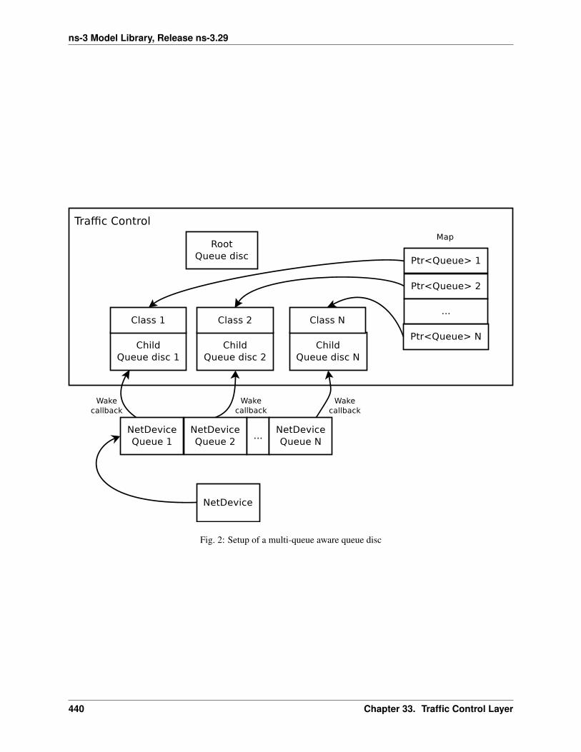
ns-3 Model Library, Release ns-3.29
Fig. 2: Setup of a multi-queue aware queue disc
440 Chapter 33. Traffic Control Layer
ns-3 Model Library, Release ns-3.29
Requeue
In Linux, a packet dequeued from a queue disc can be requeued (i.e., stored somewhere and sent to the device at a latertime) in some circumstances. Firstly, the function used to dequeue a packet (dequeue_skb) actually dequeues a packetonly if the device is multi-queue or the (unique) device queue is not stopped. If a packet has been dequeued from thequeue disc, it is passed to the sch_direct_xmit function for transmission to the device. This function checks whetherthe device queue the packet is destined to is stopped, in which case the packet is requeued. Otherwise, the packet issent to the device. If the device returns NETDEV_TX_BUSY, the packet is requeued. However, it is advised that thefunction called to send a packet to the device (ndo_start_xmit) should always return NETDEV_TX_OK, which meansthat the packet is consumed by the device driver and thus needs not to be requeued. However, the ndo_start_xmitfunction of the device driver is allowed to return NETDEV_TX_BUSY (and hence the packet is requeued) when thereis no room for the received packet in the device queue, despite the queue is not stopped. This case is considered as acorner case or an hard error, and should be avoided.
ns-3 implements the requeue mechanism in a similar manner, the only difference being that packets are not requeuedwhen such corner cases occur. Basically, the method used to dequeue a packet (QueueDisc::DequeuePacket) actuallydequeues a packet only if the device is multi-queue or the (unique) device queue is not stopped. If a packet has beendequeued from the queue disc, it is passed to the QueueDisc::Transmit method for transmission to the device. Thismethod checks whether the device queue the packet is destined to is stopped, in which case the packet is requeued.Otherwise, the packet is sent to the device. We request netdevices to stop a device queue when it is not able to storeanother packet, so as to avoid the situation in which a packet is received that cannot be enqueued while the devicequeue is not stopped. Should such a corner case occur, the netdevice drops the packet but, unlike Linux, the valuereturned by NetDevice::Send is ignored and the packet is not requeued.
The way the requeue mechanism is implemented in ns-3 has the following implications:
• if the underlying device has a single queue, no packet will ever be requeued. Indeed, if the device queue is notstopped when QueueDisc::DequeuePacket is called, it will not be stopped also when QueueDisc::Transmit iscalled, hence the packet is not requeued (recall that a packet is not requeued after being sent to the device, as thevalue returned by NetDevice::Send is ignored).
• if the underlying device does not implement flow control, i.e., it does not stop its queue(s), no packet will everbe requeued (recall that a packet is only requeued by QueueDisc::Transmit when the device queue the packet isdestined to is stopped)
It turns out that packets may only be requeued when the underlying device is multi-queue and supports flow control.
33.3 Fifo queue disc
33.3.1 Model Description
FifoQueueDisc implements the FIFO (First-In First-Out) policy. Packets are enqueued in the unique internal queue,which is implemented as a DropTail queue. The queue disc capacity can be specified in terms of either packets orbytes, depending on the value of the Mode attribute.
User is allowed to provide an internal queue before the queue disc is initialized. If no internal queue is provided, oneDropTail queue having the same capacity of the queue disc is created by default. No packet filter can be added to aFifoQueueDisc.
Attributes
The FifoQueueDisc class holds the following attribute:
• MaxSize: The maximum number of packets/bytes the queue disc can hold. The default value is 1000 packets.
33.3. Fifo queue disc 441

ns-3 Model Library, Release ns-3.29
33.3.2 Validation
The fifo model is tested using FifoQueueDiscTestSuite class defined in src/traffic-control/test/fifo-queue-disc-test-suite.cc. The test aims to check that the capacity of the queue disc is not exceededand packets are dequeued in the correct order.
33.4 pfifo_fast queue disc
33.4.1 Model Description
PfifoFastQueueDisc behaves like pfifo_fast, which is the default queue disc enabled on Linux systems (init systemssuch as systemd may override such default setting). Packets are enqueued in three priority bands (implemented asFIFO droptail queues) based on their priority (users can read Socket options for details on how to set packet priority).The four least significant bits of the priority are used to determine the selected band according to the following table:
Priority & 0xf Band0 11 22 23 24 15 26 07 08 19 110 111 112 113 114 115 1
The system behaves similar to three ns3::DropTail queues operating together, in which packets from higher prioritybands are always dequeued before a packet from a lower priority band is dequeued.
The queue disc capacity, i.e., the maximum number of packets that can be enqueued in the queue disc, is set throughthe MaxSize attribute, which plays the same role as txqueuelen in Linux. If no internal queue is provided, threeDropTail queues having each a capacity equal to MaxSize are created by default. User is allowed to provide queues,but they must be three, operate in packet mode and each have a capacity not less than MaxSize. No packet filter canbe added to a PfifoFastQueueDisc.
Attributes
The PfifoFastQueueDisc class holds a single attribute:
• MaxSize: The maximum number of packets accepted by the queue disc. The default value is 1000.
442 Chapter 33. Traffic Control Layer
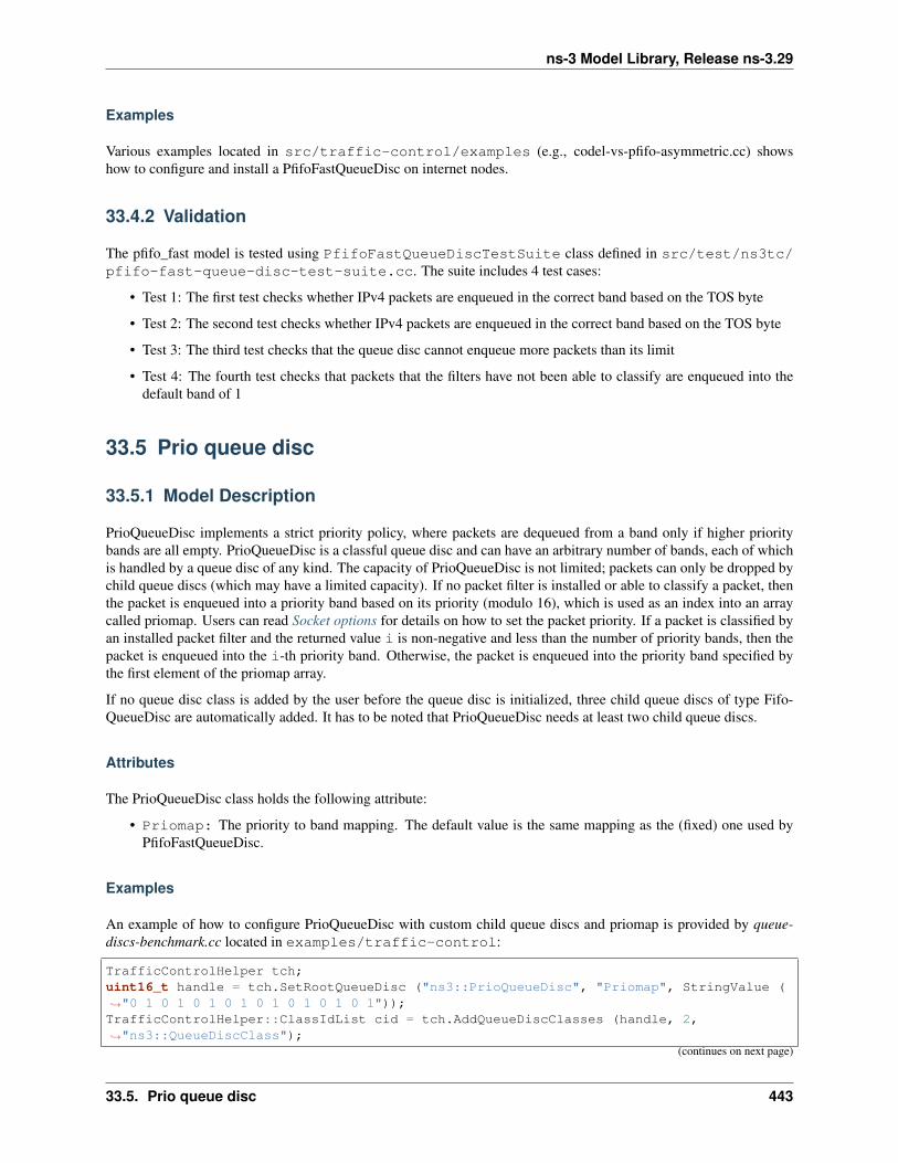
ns-3 Model Library, Release ns-3.29
Examples
Various examples located in src/traffic-control/examples (e.g., codel-vs-pfifo-asymmetric.cc) showshow to configure and install a PfifoFastQueueDisc on internet nodes.
33.4.2 Validation
The pfifo_fast model is tested using PfifoFastQueueDiscTestSuite class defined in src/test/ns3tc/pfifo-fast-queue-disc-test-suite.cc. The suite includes 4 test cases:
• Test 1: The first test checks whether IPv4 packets are enqueued in the correct band based on the TOS byte
• Test 2: The second test checks whether IPv4 packets are enqueued in the correct band based on the TOS byte
• Test 3: The third test checks that the queue disc cannot enqueue more packets than its limit
• Test 4: The fourth test checks that packets that the filters have not been able to classify are enqueued into thedefault band of 1
33.5 Prio queue disc
33.5.1 Model Description
PrioQueueDisc implements a strict priority policy, where packets are dequeued from a band only if higher prioritybands are all empty. PrioQueueDisc is a classful queue disc and can have an arbitrary number of bands, each of whichis handled by a queue disc of any kind. The capacity of PrioQueueDisc is not limited; packets can only be dropped bychild queue discs (which may have a limited capacity). If no packet filter is installed or able to classify a packet, thenthe packet is enqueued into a priority band based on its priority (modulo 16), which is used as an index into an arraycalled priomap. Users can read Socket options for details on how to set the packet priority. If a packet is classified byan installed packet filter and the returned value i is non-negative and less than the number of priority bands, then thepacket is enqueued into the i-th priority band. Otherwise, the packet is enqueued into the priority band specified bythe first element of the priomap array.
If no queue disc class is added by the user before the queue disc is initialized, three child queue discs of type Fifo-QueueDisc are automatically added. It has to be noted that PrioQueueDisc needs at least two child queue discs.
Attributes
The PrioQueueDisc class holds the following attribute:
• Priomap: The priority to band mapping. The default value is the same mapping as the (fixed) one used byPfifoFastQueueDisc.
Examples
An example of how to configure PrioQueueDisc with custom child queue discs and priomap is provided by queue-discs-benchmark.cc located in examples/traffic-control:
TrafficControlHelper tch;uint16_t handle = tch.SetRootQueueDisc ("ns3::PrioQueueDisc", "Priomap", StringValue (↪→"0 1 0 1 0 1 0 1 0 1 0 1 0 1 0 1"));TrafficControlHelper::ClassIdList cid = tch.AddQueueDiscClasses (handle, 2,↪→"ns3::QueueDiscClass");
(continues on next page)
33.5. Prio queue disc 443

ns-3 Model Library, Release ns-3.29
(continued from previous page)
tch.AddChildQueueDisc (handle, cid[0], "ns3::FifoQueueDisc");tch.AddChildQueueDisc (handle, cid[1], "ns3::RedQueueDisc");
The code above adds two classes (bands) to a PrioQueueDisc. The highest priority one is a FifoQueueDisc, the otherone is a RedQueueDisc. The attribute Priomap is set to an array containing only 0 and 1 (since PrioQueueDisc onlyhas two bands).
33.5.2 Validation
PrioQueueDisc is tested using PrioQueueDiscTestSuite class defined in src/traffic-control/test/prio-queue-disc-test-suite.cc. The test aims to check that: i) packets are enqueued in the correct bandbased on their priority and the priomap or according to the value returned by the installed packet filter; ii) packets aredequeued in the correct order.
The test suite can be run using the following commands:
$ ./waf configure --enable-examples --enable-tests$ ./waf build$ ./test.py -s prio-queue-disc
or
$ NS_LOG="PrioQueueDisc" ./waf --run "test-runner --suite=prio-queue-disc"
33.6 TBF queue disc
This chapter describes the TBF ([Ref1]) queue disc implementation in ns-3. The TBF model in ns-3 is ported basedon Linux kernel code implemented by A. Kuznetsov and D. Torokhov.
TBF is a qdisc that allows controlling the bandwidth of the output according to a set rate with the possibility ofmanaging burst conditions also. The TBF implementation consists of a bucket (buffer) having a limited capacity intowhich tokens (normally representing a unit of bytes or a single packet of predetermined size) are added at a fixed rate‘r’ called the token rate. Whenever a packet arrives into the tx queue (fifo by default), the bucket is checked to see ifthere are appropriate number of tokens that is equivalent to the length of the packet in bytes. If yes, then the tokensare removed and the packet is passed for transmission. If no, then packets will have to wait until there are sufficienttokens in the bucket. This data conformance can be thus put into three possible scenarios [Ref3]:
1. Data rate = Token rate : Packets pass without delay.
2. Data rate < Token rate : The tokens might accumulate and the bucket might become full. Then, the next packetsto enter TBF will be transmitted right away without having any limit applied to them, until the bucket is empty.This is called a burst condition and in TBF the burst parameter defines the size of the bucket. In order toovercome this problem and provide better control over the bursts, TBF implements a second bucket which issmaller and generally the same size as the MTU. This second bucket cannot store large amount of tokens, butits replenishing rate will be a lot faster than the one of the big bucket. This second rate is called ‘peakRate’ andit will determine the maximum rate of a burst.
3. Data rate > Token rate : This causes the TBF algorithm to throttle itself for a while as soon as the bucket getsempty. This is called an ‘overlimit situation’ [Ref2]. In this situation, some of the packets will be blocked untilenough tokens are available at which time a schedule for the waking of the queue will be done. If packets keepcoming in, at a larger rate, then the packets will start to get dropped when the total number of bytes exceeds theQueueLimit.
444 Chapter 33. Traffic Control Layer

ns-3 Model Library, Release ns-3.29
33.6.1 Model Description
The TBF queue disc does not require packet filters, does not admit internal queues and uses a single child queue disc.If the user does not provide a child queue disc, a Fifo queue disc operating in the same mode (packet or byte) as theTBF queue disc and having a size equal to the TBF QueueLimit attribute is created. Otherwise, the capacity of theTBF queue disc is determined by the capacity of the child queue disc.
There are two token buckets: first bucket and second bucket. The size of the first bucket called ‘Burst’ should alwaysbe greater than the size of the second bucket called the Mtu (which is usually the size of a single packet). But the‘PeakRate’ which is the second bucket’s token rate should be always greater than the ‘Rate’ which is the first bucket’stoken rate.
If the PeakRate is zero, then the second bucket does not exist. In order to activate the second bucket, both the Mtuand PeakRate values have to be greater than zero. If the Mtu value is zero at initialization time, then if a NetDeviceexits, the Mtu’s value will be equal to the Mtu of the NetDevice. But if no NetDevice exists, then the QueueDisc willcomplain thus prompting the user to set the Mtu value.
The source code for the TBF model is located in the directory src/traffic-control/model and consists of 2files tbf-queue-disc.h and tbf-queue-disc.cc defining a TbfQueueDisc class.
• class TbfQueueDisc: This class implements the main TBF algorithm:
– TbfQueueDisc::DoEnqueue (): This routine enqueue’s the incoming packet if the queue is not fulland drops the packet otherwise.
– TbfQueueDisc::DoPeek (): This routine peeks for the top item in the queue and if the queue is notempty, it returns the topmost item.
– TbfQueueDisc::DoDequeue (): This routine performs the dequeuing of packets according to thefollowing logic:
* It calls TbfQueueDisc::Peek () and calculates the size of the packet to be dequeued in bytes.
* Then it calculates the time difference ‘delta’, which is the time elapsed since the last update of tokensin the buckets.
* If the second bucket exists, the number of tokens are updated according to the ‘PeakRate’ and ‘delta’.
* From this second bucket a number of tokens equal to the size of the packet to be dequeued is sub-tracted.
* Now the number of tokens in the first bucket are updated according to ‘Rate’ and ‘delta’.
* From this first bucket a number of tokens equal to the size of the packet to be dequeued is subtracted.
* If after this, both the first and second buckets have tokens greater than zero, then the packet is de-queued.
* Else, an event to QueueDisc::Run () is scheduled after a time period when enough tokens willbe present for the dequeue operation.
References
Attributes
The key attributes that the TbfQueueDisc class holds include the following:
• MaxSize: The maximum number of packets/bytes the queue disc can hold. The default value is 1000 packets.
• Burst: Size of the first bucket, in bytes. The default value is 125000 bytes.
• Mtu: Size of second bucket defaults to the MTU of the attached NetDevice, if any, or 0 otherwise.
33.6. TBF queue disc 445

ns-3 Model Library, Release ns-3.29
• Rate: Rate at which tokens enter the first bucket. The default value is 125KB/s.
• PeakRate: Rate at which tokens enter the second bucket. The default value is 0KB/s, which means that thereis no second bucket.
TraceSources
The TbfQueueDisc class provides the following trace sources:
• TokensInFirstBucket: Number of First Bucket Tokens in bytes
• TokensInSecondBucket: Number of Second Bucket Tokens in bytes
Examples
The example for TBF is tbf-example.cc located in examples/traffic-control/. The command to run the file(the invocation below shows the available command-line options) is:
.. sourcecode:: bash
$ ./waf –run “tbf-example –PrintHelp” $ ./waf –run “tbf-example –burst=125000 –rate=1Mbps–peakRate=1.5Mbps”
The expected output from the previous commands are traced value changes in the number of tokens in the first andsecond buckets.
33.6.2 Validation
The TBF model is tested using TbfQueueDiscTestSuite class defined in src/traffic-control/test/tbf-queue-disc-test-suite.cc. The suite includes 4 test cases:
• Test 1: Simple Enqueue/Dequeue with verification of attribute setting and subtraction of tokens from the buckets.
• Test 2: When DataRate == FirstBucketTokenRate; packets should pass smoothly.
• Test 3: When DataRate >>> FirstBucketTokenRate; some packets should get blocked and waking of queueshould get scheduled.
• Test 4: When DataRate < FirstBucketTokenRate; burst condition, peakRate is set so that bursts are controlled.
The test suite can be run using the following commands:
.. sourcecode:: bash
$ ./waf configure –enable-examples –enable-tests $ ./waf build $ ./test.py -s tbf-queue-disc
or
.. sourcecode:: bash
$ NS_LOG=”TbfQueueDisc” ./waf –run “test-runner –suite=tbf-queue-disc”
446 Chapter 33. Traffic Control Layer

ns-3 Model Library, Release ns-3.29
33.7 RED queue disc
33.7.1 Model Description
Random Early Detection (RED) is a queue discipline that aims to provide early signals to transport protocol congestioncontrol (e.g. TCP) that congestion is imminent, so that they back off their rate gracefully rather than with a bunch oftail-drop losses (possibly incurring TCP timeout). The model in ns-3 is a port of Sally Floyd’s ns-2 RED model.
Note that, starting from ns-3.25, RED is no longer a queue variant and cannot be installed as a NetDevice queue.Instead, RED is a queue disc and must be installed in the context of the traffic control (see the examples mentionedbelow).
The RED queue disc does not require packet filters, does not admit child queue discs and uses a single internal queue.If not provided by the user, a DropTail queue operating in the same mode (packet or byte) as the queue disc and havinga size equal to the RED MaxSize attribute is created. Otherwise, the capacity of the queue disc is determined by thecapacity of the internal queue provided by the user.
Adaptive Random Early Detection (ARED)
ARED is a variant of RED with two main features: (i) automatically sets Queue weight, MinTh and MaxTh and (ii)adapts maximum drop probability. The model in ns-3 contains implementation of both the features, and is a port ofSally Floyd’s ns-2 ARED model. Note that the user is allowed to choose and explicitly configure the simulation byselecting feature (i) or feature (ii), or both.
Feng’s Adaptive RED
Feng’s Adaptive RED is a variant of RED that adapts the maximum drop probability. The model in ns-3 containsimplementation of this feature, and is a port of ns-2 Feng’s Adaptive RED model.
Nonlinear Random Early Detection (NLRED)
NLRED is a variant of RED in which the linear packet dropping function of RED is replaced by a nonlinear quadraticfunction. This approach makes packet dropping gentler for light traffic load and aggressive for heavy traffic load.
Explicit Congestion Notification (ECN)
This RED model supports an ECN mode of operation to notify endpoints of congestion that may be developing in abottleneck queue, without resorting to packet drops. Such a mode is enabled by setting the UseEcn attribute to true (itis false by default) and only affects incoming packets with the ECT bit set in their header. When the average queuelength is between the minimum and maximum thresholds, an incoming packet is marked instead of being dropped.When the average queue length is above the maximum threshold, an incoming packet is marked (instead of beingdropped) only if the UseHardDrop attribute is set to false (it is true by default).
The implementation of support for ECN marking is done in such a way as to not impose an internet module dependencyon the traffic control module. The RED model does not directly set ECN bits on the header, but delegates that job tothe QueueDiscItem class. As a result, it is possible to use RED queues for other non-IP QueueDiscItems that may ormay not support the Mark () method.
33.7. RED queue disc 447

ns-3 Model Library, Release ns-3.29
References
The RED queue disc aims to be close to the results cited in: S.Floyd, K.Fall http://icir.org/floyd/papers/redsims.ps
ARED queue implementation is based on the algorithm provided in: S. Floyd et al, http://www.icir.org/floyd/papers/adaptiveRed.pdf
Feng’s Adaptive RED queue implementation is based on the algorithm provided in: W. C. Feng et al, http://ieeexplore.ieee.org/stamp/stamp.jsp?arnumber=752150
NLRED queue implementation is based on the algorithm provided in: Kaiyu Zhou et al, http://www.sciencedirect.com/science/article/pii/S1389128606000879
The addition of explicit congestion notification (ECN) to IP: K. K. Ramakrishnan et al, https://tools.ietf.org/html/rfc3168
Attributes
The RED queue contains a number of attributes that control the RED policies:
• MaxSize
• MeanPktSize
• IdlePktSize
• Wait (time)
• Gentle mode
• MinTh, MaxTh
• Queue weight
• LInterm
• LinkBandwidth
• LinkDelay
• UseEcn
• UseHardDrop
In addition to RED attributes, ARED queue requires following attributes:
• ARED (Boolean attribute. Default: false)
• AdaptMaxP (Boolean attribute to adapt m_curMaxP. Default: false)
• Target Delay (time)
• Interval (time)
• LastSet (time)
• Top (upper limit of m_curMaxP)
• Bottom (lower limit of m_curMaxP)
• Alpha (increment parameter for m_curMaxP)
• Beta (decrement parameter for m_curMaxP)
• RTT
In addition to RED attributes, Feng’s Adaptive RED queue requires following attributes:
448 Chapter 33. Traffic Control Layer

ns-3 Model Library, Release ns-3.29
• FengAdaptive (Boolean attribute, Default: false)
• Status (status of current queue length, Default: Above)
• FengAlpha (increment parameter for m_curMaxP, Default: 3)
• FengBeta (decrement parameter for m_curMaxP, Default: 2)
The following attribute should be turned on to simulate NLRED queue disc:
• NLRED (Boolean attribute. Default: false)
Consult the ns-3 documentation for explanation of these attributes.
Simulating ARED
To switch on ARED algorithm, the attribute ARED must be set to true, as done in src/traffic-control/examples/adaptive-red-tests.cc:
Config::SetDefault ("ns3::RedQueueDisc::ARED", BooleanValue (true));
Setting ARED to true implicitly configures both: (i) automatic setting of Queue weight, MinTh and MaxTh and (ii)adapting m_curMaxP.
NOTE: To explicitly configure (i) or (ii), set ARED attribute to false and follow the procedure described next:
To configure (i); Queue weight, MinTh and MaxTh, all must be set to 0, as done in src/traffic-control/examples/adaptive-red-tests.cc:
Config::SetDefault ("ns3::RedQueueDisc::QW", DoubleValue (0.0));Config::SetDefault ("ns3::RedQueueDisc::MinTh", DoubleValue (0));Config::SetDefault ("ns3::RedQueueDisc::MaxTh", DoubleValue (0));
To configure (ii); AdaptMaxP must be set to true, as done in src/traffic-control/examples/adaptive-red-tests.cc:
Config::SetDefault ("ns3::RedQueueDisc::AdaptMaxP", BooleanValue (true));
Simulating Feng’s Adaptive RED
To switch on Feng’s Adaptive RED algorithm, the attribute FengAdaptive must be set to true, as done in examples/traffic-control/red-vs-fengadaptive.cc:
Config::SetDefault ("ns3::RedQueueDisc::FengAdaptive", BooleanValue (true));
Simulating NLRED
To switch on NLRED algorithm, the attribute NLRED must be set to true, as shown below:
Config::SetDefault ("ns3::RedQueueDisc::NLRED", BooleanValue (true));
33.7. RED queue disc 449
ns-3 Model Library, Release ns-3.29
Examples
The RED queue example is found at src/traffic-control/examples/red-tests.cc.
ARED queue examples can be found at: src/traffic-control/examples/adaptive-red-tests.ccand src/traffic-control/examples/red-vs-ared.cc
Feng’s Adaptive RED example can be found at: examples/traffic-control/red-vs-fengadaptive.cc
NLRED queue example can be found at: examples/traffic-control/red-vs-nlred.cc
33.7.2 Validation
The RED model has been validated and the report is currently stored at: https://github.com/downloads/talau/ns-3-tcp-red/report-red-ns3.pdf
33.8 CoDel queue disc
This chapter describes the CoDel ([Nic12], [Nic14]) queue disc implementation in ns-3.
Developed by Kathleen Nichols and Van Jacobson as a solution to the bufferbloat [Buf14] problem, CoDel (ControlledDelay Management) is a queuing discipline that uses a packet’s sojourn time (time in queue) to make decisions onpacket drops.
Note that, starting from ns-3.25, CoDel is no longer a queue variant and cannot be installed as a NetDevice queue.Instead, CoDel is a queue disc and must be installed in the context of the traffic control (see the examples mentionedbelow).
33.8.1 Model Description
The source code for the CoDel model is located in the directory src/traffic-control/model and consists of 2files codel-queue-disc.h and codel-queue-disc.cc defining a CoDelQueueDisc class and a helper CoDelTimestampTagclass. The code was ported to ns-3 by Andrew McGregor based on Linux kernel code implemented by Dave Täht andEric Dumazet.
• class CoDelQueueDisc: This class implements the main CoDel algorithm:
– CoDelQueueDisc::DoEnqueue (): This routine tags a packet with the current time before pushingit into the queue. The timestamp tag is used by CoDelQueue::DoDequeue() to compute the packet’ssojourn time. If the queue is full upon the packet arrival, this routine will drop the packet and record thenumber of drops due to queue overflow, which is stored in m_dropOverLimit.
– CoDelQueueDisc::ShouldDrop (): This routine is CoDelQueueDisc::DoDequeue()’shelper routine that determines whether a packet should be dropped or not based on its sojourn time. Ifthe sojourn time goes above m_target and remains above continuously for at least m_interval, the routinereturns true indicating that it is OK to drop the packet. Otherwise, it returns false.
– CoDelQueueDisc::DoDequeue (): This routine performs the actual packet drop based onCoDelQueueDisc::ShouldDrop ()’s return value and schedules the next drop.
• class CoDelTimestampTag: This class implements the timestamp tagging for a packet. This tag is used tocompute the packet’s sojourn time (the difference between the time the packet is dequeued and the time it ispushed into the queue).
There are 2 branches to CoDelQueueDisc::DoDequeue ():
450 Chapter 33. Traffic Control Layer

ns-3 Model Library, Release ns-3.29
1. If the queue is currently in the dropping state, which means the sojourn time has remained above m_target formore than m_interval, the routine determines if it’s OK to leave the dropping state or it’s time for the next drop.When CoDelQueueDisc::ShouldDrop () returns false, the queue can move out of the dropping state(set m_dropping to false). Otherwise, the queue continuously drops packets and updates the time for nextdrop (m_dropNext) until one of the following conditions is met:
1. The queue is empty, upon which the queue leaves the dropping state and exitsCoDelQueueDisc::ShouldDrop () routine;
2. CoDelQueueDisc::ShouldDrop () returns false (meaning the sojourn time goes belowm_target) upon which the queue leaves the dropping state;
3. It is not yet time for next drop (m_dropNext is less than current time) upon which the queue waits for thenext packet dequeue to check the condition again.
2. If the queue is not in the dropping state, the routine enters the dropping state and drop the first packet ifCoDelQueueDisc::ShouldDrop () returns true (meaning the sojourn time has gone above m_targetfor at least m_interval for the first time or it has gone above again after the queue leaves the dropping state).
The CoDel queue disc does not require packet filters, does not admit child queue discs and uses a single internal queue.If not provided by the user, a DropTail queue operating in the same mode (packet or byte) as the queue disc and havinga size equal to the CoDel MaxSize attribute is created. Otherwise, the capacity of the queue disc is determined by thecapacity of the internal queue provided by the user.
References
Attributes
The key attributes that the CoDelQueue class holds include the following:
• MaxSize: The maximum number of packets/bytes the queue can hold. The default value is 1500 * DE-FAULT_CODEL_LIMIT, which is 1500 * 1000 bytes.
• MinBytes: The CoDel algorithm minbytes parameter. The default value is 1500 bytes.
• Interval: The sliding-minimum window. The default value is 100 ms.
• Target: The CoDel algorithm target queue delay. The default value is 5 ms.
Examples
The first example is codel-vs-pfifo-basic-test.cc located in src/traffic-control/examples. To run the file(the first invocation below shows the available command-line options):
$ ./waf --run "codel-vs-pfifo-basic-test --PrintHelp"$ ./waf --run "codel-vs-pfifo-basic-test --queueType=CoDel --pcapFileName=codel.pcap -↪→-cwndTrFileName=cwndCodel.tr"
The expected output from the previous commands are two files: codel.pcap file and cwndCoDel.tr (ASCII trace) fileThe .pcap file can be analyzed using wireshark or tcptrace:
$ tcptrace -l -r -n -W codel.pcap
The second example is codel-vs-pfifo-asymmetric.cc located in src/traffic-control/examples. This exam-ple is intended to model a typical cable modem deployment scenario. To run the file:
$ ./waf --run "codel-vs-pfifo-asymmetric --PrintHelp"$ ./waf --run codel-vs-pfifo-asymmetric
33.8. CoDel queue disc 451
ns-3 Model Library, Release ns-3.29
The expected output from the previous commands is six pcap files:
• codel-vs-pfifo-asymmetric-CoDel-server-lan.pcap
• codel-vs-pfifo-asymmetric-CoDel-router-wan.pcap
• codel-vs-pfifo-asymmetric-CoDel-router-lan.pcap
• codel-vs-pfifo-asymmetric-CoDel-cmts-wan.pcap
• codel-vs-pfifo-asymmetric-CoDel-cmts-lan.pcap
• codel-vs-pfifo-asymmetric-CoDel-host-lan.pcap
One attribute file:
• codel-vs-pfifo-asymmetric-CoDel.attr
Five ASCII trace files:
• codel-vs-pfifo-asymmetric-CoDel-drop.tr
• codel-vs-pfifo-asymmetric-CoDel-drop-state.tr
• codel-vs-pfifo-asymmetric-CoDel-sojourn.tr
• codel-vs-pfifo-asymmetric-CoDel-length.tr
• codel-vs-pfifo-asymmetric-CoDel-cwnd.tr
33.8.2 Validation
The CoDel model is tested using CoDelQueueDiscTestSuite class defined in src/traffic-control/test/codel-queue-test-suite.cc. The suite includes 5 test cases:
• Test 1: The first test checks the enqueue/dequeue with no drops and makes sure that CoDel attributes can be setcorrectly.
• Test 2: The second test checks the enqueue with drops due to queue overflow.
• Test 3: The third test checks the NewtonStep() arithmetic against explicit port of Linux implementation
• Test 4: The fourth test checks the ControlLaw() against explicit port of Linux implementation
• Test 5: The fifth test checks the enqueue/dequeue with drops according to CoDel algorithm
The test suite can be run using the following commands:
$ ./waf configure --enable-examples --enable-tests$ ./waf build$ ./test.py -s codel-queue-disc
or
$ NS_LOG="CoDelQueueDisc" ./waf --run "test-runner --suite=codel-queue-disc"
33.9 FqCoDel queue disc
This chapter describes the FqCoDel ([Hoe16]) queue disc implementation in ns-3.
The FlowQueue-CoDel (FQ-CoDel) algorithm is a combined packet scheduler and Active Queue Management (AQM)algorithm developed as part of the bufferbloat-fighting community effort ([Buf16]). FqCoDel classifies incoming
452 Chapter 33. Traffic Control Layer

ns-3 Model Library, Release ns-3.29
packets into different queues (by default, 1024 queues are created), which are served according to a modified DeficitRound Robin (DRR) queue scheduler. Each queue is managed by the CoDel AQM algorithm. FqCoDel distinguishesbetween “new” queues (which don’t build up a standing queue) and “old” queues, that have queued enough data to bearound for more than one iteration of the round-robin scheduler.
33.9.1 Model Description
The source code for the FqCoDel queue disc is located in the directory src/traffic-control/model andconsists of 2 files fq-codel-queue-disc.h and fq-codel-queue-disc.cc defining a FqCoDelQueueDisc class and a helperFqCoDelFlow class. The code was ported to ns-3 based on Linux kernel code implemented by Eric Dumazet.
• class FqCoDelQueueDisc: This class implements the main FqCoDel algorithm:
– FqCoDelQueueDisc::DoEnqueue (): If no packet filter has been configured, this routine calls theQueueDiscItem::Hash() method to classify the given packet into an appropriate queue. Otherwise, theconfigured filters are used to classify the packet. If the filters are unable to classify the packet, the packet isdropped. Otherwise, it is handed over to the CoDel algorithm for timestamping. Then, if the queue is notcurrently active (i.e., if it is not in either the list of new or the list of old queues), it is added to the end ofthe list of new queues, and its deficit is initiated to the configured quantum. Otherwise, the queue is left inits current queue list. Finally, the total number of enqueued packets is compared with the configured limit,and if it is above this value (which can happen since a packet was just enqueued), packets are droppedfrom the head of the queue with the largest current byte count until the number of dropped packets reachesthe configured drop batch size or the backlog of the queue has been halved. Note that this in most casesmeans that the packet that was just enqueued is not among the packets that get dropped, which may evenbe from a different queue.
– FqCoDelQueueDisc::DoDequeue (): The first task performed by this routine is selecting a queuefrom which to dequeue a packet. To this end, the scheduler first looks at the list of new queues; for thequeue at the head of that list, if that queue has a negative deficit (i.e., it has already dequeued at least aquantum of bytes), it is given an additional amount of deficit, the queue is put onto the end of the list ofold queues, and the routine selects the next queue and starts again. Otherwise, that queue is selected fordequeue. If the list of new queues is empty, the scheduler proceeds down the list of old queues in the samefashion (checking the deficit, and either selecting the queue for dequeuing, or increasing deficit and puttingthe queue back at the end of the list). After having selected a queue from which to dequeue a packet, theCoDel algorithm is invoked on that queue. As a result of this, one or more packets may be discardedfrom the head of the selected queue, before the packet that should be dequeued is returned (or nothing isreturned if the queue is or becomes empty while being handled by the CoDel algorithm). Finally, if theCoDel algorithm does not return a packet, then the queue must be empty, and the scheduler does one oftwo things: if the queue selected for dequeue came from the list of new queues, it is moved to the end ofthe list of old queues. If instead it came from the list of old queues, that queue is removed from the list,to be added back (as a new queue) the next time a packet for that queue arrives. Then (since no packetwas available for dequeue), the whole dequeue process is restarted from the beginning. If, instead, thescheduler did get a packet back from the CoDel algorithm, it subtracts the size of the packet from the bytedeficit for the selected queue and returns the packet as the result of the dequeue operation.
– FqCoDelQueueDisc::FqCoDelDrop (): This routine is invoked byFqCoDelQueueDisc::DoEnqueue() to drop packets from the head of the queue with thelargest current byte count. This routine keeps dropping packets until the number of dropped packetsreaches the configured drop batch size or the backlog of the queue has been halved.
• class FqCoDelFlow: This class implements a flow queue, by keeping its current status (whether it is in the listof new queues, in the list of old queues or inactive) and its current deficit.
In Linux, by default, packet classification is done by hashing (using a Jenkins hash function) on the 5-tuple of IPprotocol, and source and destination IP addresses and port numbers (if they exist), and taking the hash value modulothe number of queues. The hash is salted by modulo addition of a random value selected at initialisation time, to
33.9. FqCoDel queue disc 453
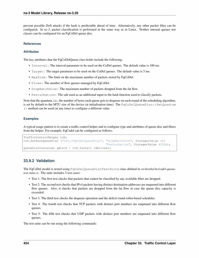
ns-3 Model Library, Release ns-3.29
prevent possible DoS attacks if the hash is predictable ahead of time. Alternatively, any other packet filter can beconfigured. In ns-3, packet classification is performed in the same way as in Linux. Neither internal queues norclasses can be configured for an FqCoDel queue disc.
References
Attributes
The key attributes that the FqCoDelQueue class holds include the following:
• Interval: The interval parameter to be used on the CoDel queues. The default value is 100 ms.
• Target: The target parameter to be used on the CoDel queues. The default value is 5 ms.
• MaxSize: The limit on the maximum number of packets stored by FqCoDel.
• Flows: The number of flow queues managed by FqCoDel.
• DropBatchSize: The maximum number of packets dropped from the fat flow.
• Perturbation: The salt used as an additional input to the hash function used to classify packets.
Note that the quantum, i.e., the number of bytes each queue gets to dequeue on each round of the scheduling algorithm,is set by default to the MTU size of the device (at initialisation time). The FqCoDelQueueDisc::SetQuantum() method can be used (at any time) to configure a different value.
Examples
A typical usage pattern is to create a traffic control helper and to configure type and attributes of queue disc and filtersfrom the helper. For example, FqCodel can be configured as follows:
TrafficControlHelper tch;tch.SetRootQueueDisc ("ns3::FqCoDelQueueDisc", "DropBatchSize", UintegerValue (1)
"Perturbation", UintegerValue (256));QueueDiscContainer qdiscs = tch.Install (devices);
33.9.2 Validation
The FqCoDel model is tested using FqCoDelQueueDiscTestSuite class defined in src/test/ns3tc/codel-queue-test-suite.cc. The suite includes 5 test cases:
• Test 1: The first test checks that packets that cannot be classified by any available filter are dropped.
• Test 2: The second test checks that IPv4 packets having distinct destination addresses are enqueued into differentflow queues. Also, it checks that packets are dropped from the fat flow in case the queue disc capacity isexceeded.
• Test 3: The third test checks the dequeue operation and the deficit round robin-based scheduler.
• Test 4: The fourth test checks that TCP packets with distinct port numbers are enqueued into different flowqueues.
• Test 5: The fifth test checks that UDP packets with distinct port numbers are enqueued into different flowqueues.
The test suite can be run using the following commands:
454 Chapter 33. Traffic Control Layer

ns-3 Model Library, Release ns-3.29
$ ./waf configure --enable-examples --enable-tests$ ./waf build$ ./test.py -s fq-codel-queue-disc
or:
$ NS_LOG="FqCoDelQueueDisc" ./waf --run "test-runner --suite=fq-codel-queue-disc"
33.10 PIE queue disc
This chapter describes the PIE ([Pan13], [Pan16]) queue disc implementation in ns-3.
Proportional Integral controller Enhanced (PIE) is a queuing discipline that aims to solve the bufferbloat [Buf14]problem. The model in ns-3 is a port of Preethi Natarajan’s ns-2 PIE model.
33.10.1 Model Description
The source code for the PIE model is located in the directory src/traffic-control/model and consists of 2files pie-queue-disc.h and pie-queue-disc.cc defining a PieQueueDisc class. The code was ported to ns-3 by Mohit P.Tahiliani, Shravya K. S. and Smriti Murali based on ns-2 code implemented by Preethi Natarajan, Rong Pan, ChiaraPiglione, Greg White and Takashi Hayakawa.
• class PieQueueDisc: This class implements the main PIE algorithm:
– PieQueueDisc::DoEnqueue (): This routine checks whether the queue is full, and if so, drops thepackets and records the number of drops due to queue overflow. If queue is not full, this routine callsPieQueueDisc::DropEarly(), and depending on the value returned, the incoming packet is eitherenqueued or dropped.
– PieQueueDisc::DropEarly (): The decision to enqueue or drop the packet is taken by invokingthis routine, which returns a boolean value; false indicates enqueue and true indicates drop.
– PieQueueDisc::CalculateP (): This routine is called at a regular interval of m_tUpdate andupdates the drop probability, which is required by PieQueueDisc::DropEarly()
– PieQueueDisc::DoDequeue (): This routine calculates the average departure rate which is re-quired for updating the drop probability in PieQueueDisc::CalculateP ()
References
Attributes
The key attributes that the PieQueue class holds include the following:
• MaxSize: The maximum number of bytes or packets the queue can hold.
• MeanPktSize: Mean packet size in bytes. The default value is 1000 bytes.
• Tupdate: Time period to calculate drop probability. The default value is 30 ms.
• Supdate: Start time of the update timer. The default value is 0 ms.
• DequeueThreshold: Minimum queue size in bytes before dequeue rate is measured. The default value is10000 bytes.
• QueueDelayReference: Desired queue delay. The default value is 20 ms.
33.10. PIE queue disc 455
ns-3 Model Library, Release ns-3.29
• MaxBurstAllowance: Current max burst allowance in seconds before random drop. The default value is0.1 seconds.
• A: Value of alpha. The default value is 0.125.
• B: Value of beta. The default value is 1.25.
Examples
The example for PIE is pie-example.cc located in src/traffic-control/examples. To run the file (the firstinvocation below shows the available command-line options):
$ ./waf --run "pie-example --PrintHelp"$ ./waf --run "pie-example --writePcap=1"
The expected output from the previous commands are 10 .pcap files.
33.10.2 Validation
The PIE model is tested using PieQueueDiscTestSuite class defined in src/traffic-control/test/pie-queue-test-suite.cc. The suite includes 5 test cases:
• Test 1: simple enqueue/dequeue with defaults, no drops
• Test 2: more data with defaults, unforced drops but no forced drops
• Test 3: same as test 2, but with higher QueueDelayReference
• Test 4: same as test 2, but with reduced dequeue rate
• Test 5: same dequeue rate as test 4, but with higher Tupdate
The test suite can be run using the following commands:
$ ./waf configure --enable-examples --enable-tests$ ./waf build$ ./test.py -s pie-queue-disc
or
$ NS_LOG="PieQueueDisc" ./waf --run "test-runner --suite=pie-queue-disc"
33.11 Mq queue disc
This chapter describes the mq queue disc implementation in ns-3.
mq is a classful multiqueue dummy scheduler developed to best fit the multiqueue traffic control API in Linux. Themq scheduler presents device transmission queues as classes, allowing to attach different queue discs to them, whichare grafted to the device transmission queues.
33.11.1 Model Description
mq is a multi-queue aware queue disc, meaning that it has as many child queue discs as the number of device trans-mission queues. Each child queue disc maps to a distinct device transmission queue. Every packet is enqueued intothe child queue disc which maps to the device transmission queue in which the device will enqueue the packet.
456 Chapter 33. Traffic Control Layer
ns-3 Model Library, Release ns-3.29
In ns-3, MqQueueDisc has a wake mode of WAKE_CHILD, which means that the traffic control layer en-queues packets directly into one of the child queue discs (multi-queue devices can provide a callback to informthe traffic control layer of the device transmission queue that will be selected for a given packet). Therefore,MqQueueDisc::DoEnqueue () shall never be called (in fact, it raises a fatal error). Given that dequeuing pack-ets is triggered by enqueuing a packet in the queue disc or by the device invoking the wake callback, it turns out thatMqQueueDisc::DoDequeue () is never called as well (in fact, it raises a fatal error, too).
The mq queue disc does not require packet filters, does not admit internal queues and must have as many child queuediscs as the number of device transmission queues.
Examples
A typical usage pattern is to create a traffic control helper used to add the required number of queue disc classes, attachchild queue discs to the classes and (if needed) add packet filters to the child queue discs. The following code showshow to install an mq queue disc having FqCodel child queue discs:
TrafficControlHelper tch;uint16_t handle = tch.SetRootQueueDisc ("ns3::MqQueueDisc");TrafficControlHelper::ClassIdList cls = tch.AddQueueDiscClasses (handle, numTxQueues,↪→"ns3::QueueDiscClass");tch.AddChildQueueDiscs (handle, cls, "ns3::FqCoDelQueueDisc");QueueDiscContainer qdiscs = tch.Install (devices);
Note that the child queue discs attached to the classes do not necessarily have to be of the same type.
33.11.2 Validation
The mq model is tested using WifiAcMappingTestSuite class defined in src/test/wifi-ac-mapping-test-suite.cc.The suite considers a node with a QoS-enabled wifi device (which has 4 transmission queues) and includes 4 testcases:
• Test 1: EF-marked packets are enqueued in the queue disc which maps to the AC_VI queue
• Test 2: AF11-marked packets are enqueued in the queue disc which maps to the AC_BK queue
• Test 3: AF32-marked packets are enqueued in the queue disc which maps to the AC_BE queue
• Test 4: CS7-marked packets are enqueued in the queue disc which maps to the AC_VO queue
The test suite can be run using the following commands:
$ ./waf configure --enable-examples --enable-tests$ ./waf build$ ./test.py -s ns3-wifi-ac-mapping
or
$ NS_LOG="WifiAcMappingTest" ./waf --run "test-runner --suite=ns3-wifi-ac-mapping"
33.11. Mq queue disc 457

ns-3 Model Library, Release ns-3.29
458 Chapter 33. Traffic Control Layer

CHAPTER
THIRTYFOUR
UAN FRAMEWORK
The main goal of the UAN Framework is to enable researchers to model a variety of underwater network scenarios.The UAN model is broken into four main parts: The channel, PHY, MAC and Autonomous Underwater Vehicle (AUV)models.
The need for underwater wireless communications exists in applications such as remote control in offshore oil indus-try1, pollution monitoring in environmental systems, speech transmission between divers, mapping of the ocean floor,mine counter measures4, seismic monitoring of ocean faults as well as climate changes monitoring. Unfortunately,making on-field measurements is very expensive and there are no commonly accepted standard to base on. Hence, thepriority to make research work going on, it is to realize a complete simulation framework that researchers can use toexperiment, make tests and make performance evaluation and comparison.
The NS-3 UAN module is a first step in this direction, trying to offer a reliable and realistic tool. In fact, the UANmodule offers accurate modelling of the underwater acoustic channel, a model of the WHOI acoustic modem (one ofthe widely used acoustic modems)[6]_ and its communications performance, and some MAC protocols.
34.1 Model Description
The source code for the UAN Framework lives in the directory src/uan and in src/energy for the contributionon the li-ion battery model.
The UAN Framework is composed of two main parts:
• the AUV mobility models, including Electric motor propelled AUV (REMUS class34 ) and Seaglider5 models
• the energy models, including AUV energy models, AUV energy sources (batteries) and an acoustic modemenergy model
As enabling component for the energy models, a Li-Ion batteries energy source has been implemented basing on78.
1 BINGHAM, D.; DRAKE, T.; HILL, A.; LOTT, R.; The Application of Autonomous Underwater Vehicle (AUV) Technology in the Oil Industry– Vision and Experiences, URL: http://www.fig.net/pub/fig_2002/Ts4-4/TS4_4_bingham_etal.pdf
4 WHOI, Autonomous Underwater Vehicle, REMUS; URL: http://www.whoi.edu/page.do?pid=298563 Hydroinc Products; URL: http://www.hydroidinc.com/products.html5 Eriksen, C.C., T.J. Osse, R.D. Light, T. Wen, T.W. Lehman, P.L. Sabin, J.W. Ballard, and A.M. Chiodi. Seaglider: A Long-Range Autonomous
Underwater Vehicle for Oceanographic Research, IEEE Journal of Oceanic Engineering, 26, 4, October 2001. URL: http://ieeexplore.ieee.org/stamp/stamp.jsp?tp=&arnumber=972073&userType=inst
7 C. M. Shepherd, “Design of Primary and Secondary Cells - Part 3. Battery discharge equation,” U.S. Naval Research Laboratory, 19638 Tremblay, O.; Dessaint, L.-A.; Dekkiche, A.-I., “A Generic Battery Model for the Dynamic Simulation of Hybrid Electric Vehicles,” Ecole de
Technologie Superieure, Universite du Quebec, 2007 URL: http://ieeexplore.ieee.org/stamp/stamp.jsp?tp=&arnumber=4544139
459
ns-3 Model Library, Release ns-3.29
34.1.1 Design
UAN Propagation Models
Modelling of the underwater acoustic channel has been an active area of research for quite some time. Given thecomplications involved, surface and bottom interactions, varying speed of sound, etc. . . , the detailed models in use forocean acoustics research are much too complex (in terms of runtime) for use in network level simulations. We haveattempted to provide the often used models as well as make an attempt to bridge, in part, the gap between complicatedocean acoustic models and network level simulation. The three propagation models included are the ideal channelmodel, the Thorp propagation model and the Bellhop propagation model (Available as an addition).
All of the Propagation Models follow the same simple interface in ns3::UanPropModel. The propagation modelsprovide a power delay profile (PDP) and pathloss information. The PDP is retrieved using the GetPdp method whichreturns type UanPdp. ns3::UanPdp utilises a tapped delay line model for the acoustic channel. The UanPdp classis a container class for Taps, each tap has a delay and amplitude member corresponding to the time of arrival (relativeto the first tap arrival time) and amplitude. The propagation model also provides pathloss between the source andreceiver in dB re 1uPa. The PDP and pathloss can then be used to find the received signal power over a durationof time (i.e. received signal power in a symbol duration and ISI which interferes with neighbouring signals). BothUanPropModelIdeal and UanPropModelThorp return a single impulse for a PDP.
a) Ideal Channel Model ns3::UanPropModelIdeal
The ideal channel model assumes 0 pathloss inside a cylindrical area with bounds set by attribute. The ideal channelmodel also assumes an impulse PDP.
b) Thorp Propagation Model ns3::UanPropModelThorp
The Thorp Propagation Model calculates pathloss using the well-known Thorp approximation. This model is similarto the underwater channel model implemented in ns2 as described here:
Harris, A. F. and Zorzi, M. 2007. Modeling the underwater acoustic channel in ns2. In Proceedings of the 2ndinternational Conference on Performance Evaluation Methodologies and Tools (Nantes, France, October 22 - 27,2007). ValueTools, vol. 321. ICST (Institute for Computer Sciences Social-Informatics and TelecommunicationsEngineering), ICST, Brussels, Belgium, 1-8.
The frequency used in calculation however, is the center frequency of the modulation as found from ns3::UanTxMode.The Thorp Propagation Model also assumes an impulse channel response.
c) Bellhop Propagation Model ns3::UanPropModelBh (Available as an addition)
The Bellhop propagation model reads propagation information from a database. A configuration file describing thelocation, and resolution of the archived information must be supplied via attributes. We have included a utility, create-dat, which can create these data files using the Bellhop Acoustic Ray Tracing software (http://oalib.hlsresearch.com/).
The create-dat utility requires a Bellhop installation to run. Bellhop takes environment information about the channel,such as sound speed profile, surface height bottom type, water depth, and uses a Gaussian ray tracing algorithm todetermine propagation information. Arrivals from Bellhop are grouped together into equal length taps (the arrivalsin a tap duration are coherently summed). The maximum taps are then aligned to take the same position in the PDP.The create-dat utility averages together several runs and then normalizes the average such that the sum of all taps is 1.The same configuration file used to create the data files using create-dat should be passed via attribute to the BellhopPropagation Model.
The Bellhop propagation model is available as a patch. The link address will be made available here when it is postedonline. Otherwise email [email protected] for more information.
UAN PHY Model Overview
The PHY has been designed to allow for relatively easy extension to new networking scenarios. We feel this isimportant as, to date, there has been no commonly accepted network level simulation model for underwater networks.
460 Chapter 34. UAN Framework

ns-3 Model Library, Release ns-3.29
The lack of commonly accepted network simulation tools has resulted in a wide array of simulators and models usedto report results in literature. The lack of standardization makes comparing results nearly impossible.
The main component of the PHY Model is the generic PHY class, ns3::UanPhyGen. The PHY class’s generalresponsibility is to handle packet acquisition, error determination, and forwarding of successful packets up to theMAC layer. The Generic PHY uses two models for determination of signal to noise ratio (SINR) and packet error rate(PER). The combination of the PER and SINR models determine successful reception of packets. The PHY modelconnects to the channel via a Transducer class. The Transducer class is responsible for tracking all arriving packetsand departing packets over the duration of the events. How the PHY class and the PER and SINR models respond topackets is based on the “Mode” of the transmission as described by the ns3::UanTxMode class.
When a MAC layer sends down a packet to the PHY for transmission it specifies a “mode number” to be used for thetransmission. The PHY class accepts, as an attribute, a list of supported modes. The mode number corresponds to anindex in the supported modes. The UanTxMode contains simple modulation information and a unique string id. Thegeneric PHY class will only acquire arriving packets which use a mode which is in the supported modes list of thePHY. The mode along with received signal power, and other pertinent attributes (e.g. possibly interfering packets andtheir modes) are passed to the SINR and PER models for calculation of SINR and probability of error.
Several simple example PER and SINR models have been created. a) The PER models - Default (simple) PER model(ns3::UanPhyPerGenDefault): The Default PER model tests the packet against a threshold and assumes error(with prob. 1) if the SINR is below the threshold or success if the SINR is above the threshold - Micromodem FH-FSKPER (ns3::UanPhyPerUmodem). The FH-FSK PER model calculates probability of error assuming a rate 1/2convolutional code with constraint length 9 and a CRC check capable of correcting up to 1 bit error. This is similar towhat is used in the receiver of the WHOI Micromodem.
b) SINR models - Default Model (ns3::UanPhyCalcSinrDefault), The default SINR model assumes that alltransmitted energy is captured at the receiver and that there is no ISI. Any received signal power from interferes actsas additional ambient noise. - FH-FSK SINR Model (ns3::UanPhyCalcSinrFhFsk), The WHOI Micromodemoperating in FH-FSK mode uses a predetermined hopping pattern that is shared by all nodes in the network. Wemodel this by only including signal energy receiving within one symbol time (as given by ns3::UanTxMode) incalculating the received signal power. A channel clearing time is given to the FH-FSK SINR model via attribute. Anysignal energy arriving in adjacent signals (after a symbol time and the clearing time) is considered ISI and is treatedas additional ambient noise. Interfering signal arrivals inside a symbol time (any symbol time) is also counted asadditional ambient noise - Frequency filtered SINR (ns3::UanPhyCalcSinrDual). This SINR model calculatesSINR in the same manner as the default model. This model however only considers interference if there is an overlapin frequency of the arriving packets as determined by UanTxMode.
In addition to the generic PHY a dual phy layer is also included (ns3::UanPhyDual). This wraps two generic phylayers together to model a net device which includes two receivers. This was primarily developed for UanMacRc,described in the next section.
UAN MAC Model Overview
Over the last several years there have been a myriad of underwater MAC proposals in the literature. We have includedthree MAC protocols with this distribution: a) CW-MAC, a MAC protocol which uses a slotted contention windowsimilar in nature to the IEEE 802.11 DCF. Nodes have a constant contention window measured in slot times (configuredvia attribute). If the channel is sensed busy, then nodes backoff by randomly (uniform distribution) choose a slot totransmit in. The slot time durations are also configured via attribute. This MAC was described in
Parrish N.; Tracy L.; Roy S. Arabshahi P.; and Fox, W., System Design Considerations for Undersea Networks:Link and Multiple Access Protocols , IEEE Journal on Selected Areas in Communications (JSAC), Special Issue onUnderwater Wireless Communications and Networks, Dec. 2008.
b) RC-MAC (ns3::UanMacRc ns3::UanMacRcGw) a reservation channel protocol which dynamically dividesthe available bandwidth into a data channel and a control channel. This MAC protocol assumes there is a gateway nodewhich all network traffic is destined for. The current implementation assumes a single gateway and a single networkneighborhood (a single hop network). RTS/CTS handshaking is used and time is divided into cycles. Non-gateway
34.1. Model Description 461
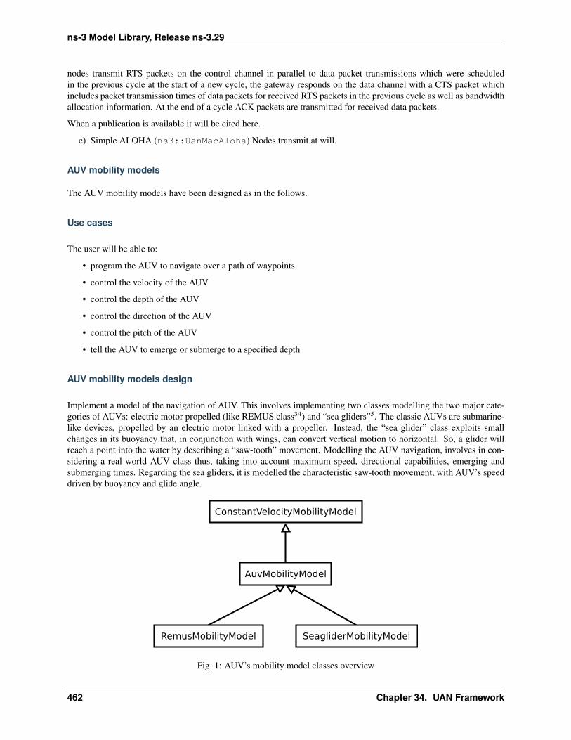
ns-3 Model Library, Release ns-3.29
nodes transmit RTS packets on the control channel in parallel to data packet transmissions which were scheduledin the previous cycle at the start of a new cycle, the gateway responds on the data channel with a CTS packet whichincludes packet transmission times of data packets for received RTS packets in the previous cycle as well as bandwidthallocation information. At the end of a cycle ACK packets are transmitted for received data packets.
When a publication is available it will be cited here.
c) Simple ALOHA (ns3::UanMacAloha) Nodes transmit at will.
AUV mobility models
The AUV mobility models have been designed as in the follows.
Use cases
The user will be able to:
• program the AUV to navigate over a path of waypoints
• control the velocity of the AUV
• control the depth of the AUV
• control the direction of the AUV
• control the pitch of the AUV
• tell the AUV to emerge or submerge to a specified depth
AUV mobility models design
Implement a model of the navigation of AUV. This involves implementing two classes modelling the two major cate-gories of AUVs: electric motor propelled (like REMUS class34) and “sea gliders”5. The classic AUVs are submarine-like devices, propelled by an electric motor linked with a propeller. Instead, the “sea glider” class exploits smallchanges in its buoyancy that, in conjunction with wings, can convert vertical motion to horizontal. So, a glider willreach a point into the water by describing a “saw-tooth” movement. Modelling the AUV navigation, involves in con-sidering a real-world AUV class thus, taking into account maximum speed, directional capabilities, emerging andsubmerging times. Regarding the sea gliders, it is modelled the characteristic saw-tooth movement, with AUV’s speeddriven by buoyancy and glide angle.
Fig. 1: AUV’s mobility model classes overview
462 Chapter 34. UAN Framework

ns-3 Model Library, Release ns-3.29
An ns3::AuvMobilityModel interface has been designed to give users a generic interface to access AUV’s nav-igation functions. The AuvMobilityModel interface is implemented by the RemusMobilityModel and the GliderMo-bilityModel classes. The AUV’s mobility models organization it is shown in AUV’s mobility model classes overview.Both models use a constant velocity movement, thus the AuvMobilityModel interface derives from the ConstantVe-locityMobilityModel. The two classes hold the navigation parameters for the two different AUVs, like maximum pitchangles, maximum operating depth, maximum and minimum speed values. The Glider model holds also some extraparameters like maximum buoyancy values, and maximum and minimum glide slopes. Both classes, RemusMobility-Model and GliderMobilityModel, handle also the AUV power consumption, utilizing the relative power models. Hasbeen modified the WaypointMobilityModel to let it use a generic underlying ConstantVelocityModel to validate thewaypoints and, to keep trace of the node’s position. The default model is the classic ConstantVelocityModel but, forexample in case of REMUS mobility model, the user can install the AUV mobility model into the waypoint model andthen validating the waypoints against REMUS navigation constraints.
Energy models
The energy models have been designed as in the follows.
Use cases
The user will be able to:
• use a specific power profile for the acoustic modem
• use a specific energy model for the AUV
• trace the power consumption of AUV navigation, through AUV’s energy model
• trace the power consumption underwater acoustic communications, through acoustic modem power profile
We have integrated the Energy Model with the UAN module, to implement energy handling. We have implemented aspecific energy model for the two AUV classes and, an energy source for Lithium batteries. This will be really usefulfor researchers to keep trace of the AUV operational life. We have implemented also an acoustic modem power profile,to keep trace of its power consumption. This can be used to compare protocols specific power performance. In orderto use such power profile, the acoustic transducer physical layer has been modified to use the modem power profile.We have decoupled the physical layer from the transducer specific energy model, to let the users change the differentenergy models without changing the physical layer.
AUV energy models
Basing on the Device Energy Model interface, it has been implemented a specific energy model for the two AUVclasses (REMUS and Seaglider). This models reproduce the AUV’s specific power consumption to give users accurateinformation. This model can be naturally used to evaluates the AUV operating life, as well as mission-related powerconsumption, etc. Have been developed two AUV energy models:
• GliderEnergyModel, computes the power consumption of the vehicle based on the current buoyancy value andvertical speed5
• RemusEnergyModel, computes the power consumption of the vehicle based on the current speed, as it is pro-pelled by a brush-less electric motor
Note: TODO extend a little bit
34.1. Model Description 463

ns-3 Model Library, Release ns-3.29
AUV energy sources
Note: [TODO]
Acoustic modem energy model
Basing on the Device Energy Model interface, has been implemented a generic energy model for acoustic modem. Themodel allows to trace four modem’s power-states: Sleep, Idle, Receiving, Transmitting. The default parameters forthe energy model are set to fit those of the WHOI µmodem. The class follows pretty closely the RadioEnergyModelclass as the transducer behaviour is pretty close to that of a Wi-Fi radio.
The default power consumption values implemented into the model are as follows [6]:
Modem State Power ConsumptionTX 50 WRX 158 mWIdle 158 mWSleep 5.8 mW
UAN module energy modifications
The UAN module has been modified in order to utilize the implemented energy classes. Specifically, it has beenmodified the physical layer of the UAN module. It Has been implemented an UpdatePowerConsumption method thattakes the modem’s state as parameter. It checks if an energy source is installed into the node and, in case, it thenuse the AcousticModemEnergyModel to update the power consumption with the current modem’s state. The modempower consumption’s update takes place whenever the modem changes its state.
A user should take into account that, if the power consumption handling is enabled (if the node has an energy sourceinstalled), all the communications processes will terminate whether the node depletes all the energy source.
Li-Ion batteries model
A generic Li-Ion battery model has been implemented based on [7][8]. The model can be fitted to any type of Li-Ionbattery simply changing the model’s parameters The default values are fitted for the Panasonic CGR18650DA Li-IonBattery [9]. [TODO insert figure] As shown in figure the model approximates very well the Li-Ion cells. RegardingSeagliders, the batteries used into the AUV are Electrochem 3B36 Lithium / Sulfuryl Chloride cells [10]. Also withthis cell type, the model seems to approximates the different discharge curves pretty well, as shown in the figure.
Note: should I insert the li-ion model deatils here? I think it is better to put them into an Energy-related chapter..
34.1.2 Scope and Limitations
The framework is designed to simulate AUV’s behaviour. We have modeled the navigation and power consumptionbehaviour of REMUS class and Seaglider AUVs. The communications stack, associated with the AUV, can be modi-fied depending on simulation needs. Usually, the default underwater stack is being used, composed of an half duplexacoustic modem, an Aloha MAC protocol and a generic physical layer.
464 Chapter 34. UAN Framework
ns-3 Model Library, Release ns-3.29
Regarding the AUV energy consumption, the user should be aware that the level of accuracy differs for the two classes:
• Seaglider, high level of accuracy, thanks to the availability of detailed information on AUV’s components andbehaviour [5] [10]. Have been modeled both the navigation power consumption and the Li battery packs (ac-cording to [5]).
• REMUS, medium level of accuracy, due to the lack of publicly available information on AUV’s components.We have approximated the power consumption of the AUV’s motor with a linear behaviour and, the energysource uses an ideal model (BasicEnergySource) with a power capacity equal to that specified in [4].
34.1.3 Future Work
Some ideas could be :
• insert a data logging capability
• modify the framework to use sockets (enabling the possibility to use applications)
• introduce some more MAC protocols
• modify the physical layer to let it consider the Doppler spread (problematic in underwater environments)
• introduce OFDM modulations
34.1.4 References
34.2 Usage
The main way that users who write simulation scripts will typically interact with the UAN Framework is through thehelper API and through the publicly visible attributes of the model.
The helper API is defined in src/uan/helper/acoustic-modem-energy-model-helper.{cc,h} andin /src/uan/helper/...{cc,h}.
The example folder src/uan/examples/ contain some basic code that shows how to set up and use the models.further examples can be found into the Unit tests in src/uan/test/...cc
34.2.1 Examples
Examples of the Framework’s usage can be found into the examples folder. There are mobility related examples andUAN related ones.
Mobility Model Examples
• auv-energy-model: In this example we show the basic usage of an AUV energy model. Specifically, weshow how to create a generic node, adding to it a basic energy source and consuming energy from theenergy source. In this example we show the basic usage of an AUV energy model.
The Seaglider AUV power consumption depends on buoyancy and vertical speed values, so we simulate a20 seconds movement at 0.3 m/s of vertical speed and 138g of buoyancy. Then a 20 seconds movement at0.2 m/s of vertical speed and 138g of buoyancy and then a stop of 5 seconds.
The required energy will be drained by the model basing on the given buoyancy/speed values, from theenergy source installed onto the node. We finally register a callback to the TotalEnergyConsumption tracedvalue.
34.2. Usage 465
ns-3 Model Library, Release ns-3.29
• auv-mobility: In this example we show how to use the AuvMobilityHelper to install an AUV mobilitymodel into a (set of) node. Then we make the AUV to submerge to a depth of 1000 meters. We then seta callback function called on reaching of the target depth. The callback then makes the AUV to emergeto water surface (0 meters). We set also a callback function called on reaching of the target depth. Theemerge callback then, stops the AUV.
During the whole navigation process, the AUV’s position is tracked by the TracePos function and plottedinto a Gnuplot graph.
• waypoint-mobility: We show how to use the WaypointMobilityModel with a non-standard ConstantVe-locityMobilityModel. We first create a waypoint model with an underlying RemusMobilityModel settingthe mobility trace with two waypoints. We then create a waypoint model with an underlying GliderMobil-ityModel setting the waypoints separately with the AddWaypoint method. The AUV’s position is printedout every seconds.
UAN Examples
• li-ion-energy-source In this simple example, we show how to create and drain energy from a LiIonEn-ergySource. We make a series of discharge calls to the energy source class, with different current drain anddurations, until all the energy is depleted from the cell (i.e. the voltage of the cell goes below the thresholdlevel). Every 20 seconds we print out the actual cell voltage to verify that it follows the discharge curve[9]. At the end of the example it is verified that after the energy depletion call, the cell voltage is below thethreshold voltage.
• uan-energy-auv This is a comprehensive example where all the project’s components are used. We setuptwo nodes, one fixed surface gateway equipped with an acoustic modem and a moving Seaglider AUV withan acoustic modem too. Using the waypoint mobility model with an underlying GliderMobilityModel, wemake the glider descend to -1000 meters and then emerge to the water surface. The AUV sends a generic17-bytes packet every 10 seconds during the navigation process. The gateway receives the packets andstores the total bytes amount. At the end of the simulation are shown the energy consumptions of the twonodes and the networking stats.
34.2.2 Helpers
In this section we give an overview of the available helpers and their behaviour.
AcousticModemEnergyModelHelper
This helper installs AcousticModemEnergyModel into UanNetDevice objects only. It requires an UanNetDevice andan EnergySource as input objects.
The helper creates an AcousticModemEnergyModel with default parameters and associate it with the given energysource. It configures an EnergyModelCallback and an EnergyDepletionCallback. The depletion callback can beconfigured as a parameter.
AuvGliderHelper
Installs into a node (or set of nodes) the Seaglider’s features:
• waypoint model with underlying glider mobility model
• glider energy model
• glider energy source
466 Chapter 34. UAN Framework

ns-3 Model Library, Release ns-3.29
• micro modem energy model
The glider mobility model is the GliderMobilityModel with default parameters. The glider energy model is the Glid-erEnergyModel with default parameters.
Regarding the energy source, the Seaglider features two battery packs, one for motor power and one for digital-analogpower. Each pack is composed of 12 (10V) and 42 (24V) lithium chloride DD-cell batteries, respectively [5]. Thetotal power capacity is around 17.5 MJ (3.9 MJ + 13.6 MJ). In the original version of the Seaglider there was 18 + 63D-cell with a total power capacity of 10MJ.
The packs design is as follows:
• 10V - 3 in-series string x 4 strings = 12 cells - typical capacity ~100 Ah
• 24V - 7 in-series-strings x 6 strings = 42 cells - typical capacity ~150 Ah
Battery cells are Electrochem 3B36, with 3.6 V nominal voltage and 30.0 Ah nominal capacity. The 10V battery packis associated with the electronic devices, while the 24V one is associated with the pump motor.
The micro modem energy model is the MicroModemEnergyModel with default parameters.
AuvRemusHelper
Install into a node (or set of nodes) the REMUS features:
• waypoint model with REMUS mobility model validation
• REMUS energy model
• REMUS energy source
• micro modem energy model
The REMUS mobility model is the RemusMobilityModel with default parameters. The REMUS energy model is theRemusEnergyModel with default parameters.
Regarding the energy source, the REMUS features a rechargeable lithium ion battery pack rated 1.1 kWh @ 27 V(40 Ah) in operating conditions (specifications from [3] and Hydroinc European salesman). Since more detailedinformation about battery pack were not publicly available, the energy source used is a BasicEnergySource.
The micro modem energy model is the MicroModemEnergyModel with default parameters.
34.2.3 Attributes
Note: TODO
34.2.4 Tracing
Note: TODO
34.2. Usage 467

ns-3 Model Library, Release ns-3.29
34.2.5 Logging
Note: TODO
34.2.6 Caveats
Note: TODO
34.3 Validation
This model has been tested with three UNIT test:
• auv-energy-model
• auv-mobility
• li-ion-energy-source
34.3.1 Auv Energy Model
Includes test cases for single packet energy consumption, energy depletion, Glider and REMUS energy consumption.The unit test can be found in src/uan/test/auv-energy-model-test.cc.
The single packet energy consumption test do the following:
• creates a two node network, one surface gateway and one fixed node at -500 m of depth
• install the acoustic communication stack with energy consumption support into the nodes
• a packet is sent from the underwater node to the gateway
• it is verified that both, the gateway and the fixed node, have consumed the expected amount of energy from theirsources
The energy depletion test do the following steps:
• create a node with an empty energy source
• try to send a packet
• verify that the energy depletion callback has been invoked
The Glider energy consumption test do the following:
• create a node with glider capabilities
• make the vehicle to move to a predetermined waypoint
• verify that the energy consumed for the navigation is correct, according to the glider specifications
The REMUS energy consumption test do the following:
• create a node with REMUS capabilities
• make the vehicle to move to a predetermined waypoint
468 Chapter 34. UAN Framework

ns-3 Model Library, Release ns-3.29
• verify that the energy consumed for the navigation is correct, according to the REMUS specifications
34.3.2 Auv Mobility
Includes test cases for glider and REMUS mobility models. The unit test can be found in src/uan/test/auv-mobility-test.cc.
• create a node with glider capabilities
• set a specified velocity vector and verify if the resulting buoyancy is the one that is supposed to be
• make the vehicle to submerge to a specified depth and verify if, at the end of the process the position is the onethat is supposed to be
• make the vehicle to emerge to a specified depth and verify if, at the end of the process the position is the onethat is supposed to be
• make the vehicle to navigate to a specified point, using direction, pitch and speed settings and, verify if at theend of the process the position is the one that is supposed to be
• make the vehicle to navigate to a specified point, using a velocity vector and, verify if at the end of the processthe position is the one that is supposed to be
The REMUS mobility model test do the following: * create a node with glider capabilities * make the vehicle tosubmerge to a specified depth and verify if, at the end of the process the position is the one that is supposed to be *make the vehicle to emerge to a specified depth and verify if, at the end of the process the position is the one that issupposed to be * make the vehicle to navigate to a specified point, using direction, pitch and speed settings and, verifyif at the end of the process the position is the one that is supposed to be * make the vehicle to navigate to a specifiedpoint, using a velocity vector and, verify if at the end of the process the position is the one that is supposed to be
34.3.3 Li-Ion Energy Source
Includes test case for Li-Ion energy source. The unit test can be found in src/energy/test/li-ion-energy-source-test.cc.
The test case verify that after a well-known discharge time with constant current drain, the cell voltage has followedthe datasheet discharge curve [9].
34.3. Validation 469

ns-3 Model Library, Release ns-3.29
470 Chapter 34. UAN Framework
CHAPTER
THIRTYFIVE
WAVE MODELS
WAVE is a system architecture for wireless-based vehicular communications, specified by the IEEE. This chapterdocuments available models for WAVE within ns-3. The focus is on the MAC layer and MAC extension layer definedby [ieee80211p] and [ieee1609dot4].
35.1 Model Description
WAVE is an overall system architecture for vehicular communications. The standards for specifying WAVE includea set of extensions to the IEEE 802.11 standard, found in IEEE Std 802.11p-2010 [ieee80211p], and the IEEE 1609standard set, consisting of four documents: resource manager: IEEE 1609.1 [ieee1609dot1], security services: IEEE1609.2 [ieee1609dot2], network and transport layer services: IEEE 1609.3 [ieee1609dot3], and multi-channel coordi-nation: IEEE 1609.4 [ieee1609dot4]. Additionally, SAE standard J2735 [saej2735] describes a Dedicated Short RangeCommunications (DSRC) application message set that allows applications to transmit information using WAVE.
In ns-3, the focus of the wave module is on both the MAC layer and the multi-channel coordination layer. Thekey design aspect of 802.11p-compilant MAC layer is that they allow communications outside the context of a basicservice set (BSS). The literature uses the acronym OCB to denote “outside the context of a BSS”, and the classns3::OcbWifiMac models this in ns-3. This MAC does not require any association between devices (similar toan adhoc WiFi MAC). Many management frames will not be used, but when used, the BSSID field needs to be setto a wildcard BSSID value. Management information is transmitted by what is called a vendor specific action (VSA)frame. With these changes, the packet transmissions (for a moving vehicle) can be fast with small delay in the MAClayer. Users can create IEEE802.11p-compliant device (the object of the class ns3::WifiNetDevice associatingwith ns3::OcbWifiMac) .
The key design aspect of the WAVE-compilant MAC layer (including 802.11p MAC layer and 1609.4 MAC extensionlayer) is that, based on OCB features, they provide devices with the capability of switching between control and servicechannels, using a single radio or using multiple radios. Therefore devices can communicate with others in single ormultiple channels, which can support both safety related and non-safety related service for vehicular environments.
At the physical layer, the biggest difference is the use of the 5.9 GHz band with a channel bandwidth of 10 MHz.These physical layer changes can make the wireless signal relatively more stable, without degrading throughput toomuch (ranging from 3 Mbps to 27 Mbps).
The source code for the WAVE MAC models lives in the directory src/wave.
For better modeling WAVE and VANET, the WAVE models for high layers (mainly [ieee1609dot3] ) are planned for alater patch.
35.1.1 Design
In ns-3, support for 802.11p involves the MAC and PHY layers. To use an 802.11p NetDevice,ns3::Wifi80211pHelper is suggested.
471
ns-3 Model Library, Release ns-3.29
In ns-3, support for WAVE involves the MAC, its MAC extension and PHY layers. To use a WAVE NetDevice,ns3::WaveHelper is suggested.
MAC layer
The classes used to model the MAC layer are ns3::OrganizationIdentifier,ns3::VendorSpecificActionHeader and ns3::OcbWifiMac.
The OrganizationIdentifier and VendorSpecificActionHeader are used to support the sending of a Vendor SpecificAction frame.
OcbWifiMac is very similar to AdhocWifiMac, with some modifications. The ns-3 AdhocWifiMac class is imple-mented very close to the 802.11p OCB mode rather than a real 802.11 ad-hoc mode. The AdhocWifiMac has no BSScontext that is defined in 802.11 standard, so it will not take time to send beacons and to authenticate, making itsbehavior similar to that of an OcbWifiMac.
1. SetBssid, GetBssid, SetSsid, GetSsid
These methods are related to 802.11 BSS context, and are unused in the OCB context.
2. SetLinkUpCallback, SetLinkDownCallback
WAVE device can send packets directly, so the WiFi link is never down.
3. SendVsc, AddReceiveVscCallback
WAVE management information shall be sent by vendor specific action frames, sent by the upper layer 1609.4standard as WSA (WAVE Service Advertisement) packets or other vendor specific information.
4. SendTimingAdvertisement (not implemented)
Although Timing Advertisement is very important and specifically defined in 802.11p standard, it is not useful ina simulation environment. Every node in ns-3 vehicular simulation is assumed to be already time synchronized(perhaps by GPS).
5. ConfigureEdca
This method will allow the user to set EDCA parameters of WAVE channels including CCH ans SCHs. And theOcbWifiMac itself also uses this method to configure default 802.11p EDCA parameters.
6. Wildcard BSSID
The Wildcard BSSID is set to “ff:ff:ff:ff:ff:ff”. As defined in IEEE 802.11-2007, a wildcard BSSID shall notbe used in the BSSID field except for management frames of subtype probe request. But Adhoc mode ofns-3 simplifies this mechanism: when stations receive packets, they will be forwarded up to the higher layer,regardless of BSSID. This process is very close to OCB mode as defined in 802.11p-2010, in which stations usethe wildcard BSSID to allow the higher layer of other stations to hear directly.
7. Enqueue, Receive
The most important methods are send and receive methods. According to the standard, we should filter theframes that are not permitted. Thus here we just identify the frames we care about; the other frames will bediscarded.
MAC extension layer
Although 1609.4 is still in the MAC layer, the implementation approach for ns-3 does not do much modification inthe source code of the wifi module. Instead, if some feature is related to wifi MAC classes, then a relevant sub-class is defined; if some feature has no relation to wifi MAC classes, then a new class will be defined. This ap-proach was selected to be non-intrusive to the ns-3 wifi module. All of these classes will be hosted in a ‘container’
472 Chapter 35. WAVE models
ns-3 Model Library, Release ns-3.29
class called ns3:: WaveNetDevice. This class is a subclass inherting from ns3::NetDeivce, composedof the objects of ns3::ChannelScheduler, ns3::ChannelManager, ns3::ChannelCoordinatorand ns3::VsaManager classes to provide the features described in 1609.4 while still containing the objects ofns3::OcbWifiMac and ns3::WifiPhy classes. Moreover, ns3::OcbWifiMac class is further extended withsupport for IEEE 1609.4 associating with ns3::HigherLayerTxVectorTag and ns3::WaveMacLow. Themain work of the WaveNetDevice is to create objects, configure, check arguments and provide new APIs for multiplechannel operation as follows:
1. AddMac, GetMac and GetMacs
Different from ns3::WifiNetDevice, the WAVE device will have multiple internal MAC entitiesrather than a single one. Each MAC entity is used to support each WAVE channel. Thus, when devicesswitch from the current channel to the next channel in different channel intervals, the packets in theinternal queue will not be flushed and the current MAC entity will perform a suspend operation untilwoken up in next appropriate channel interval.
2. AddPhy, GetPhy and GetPhys
Also in contrast to ns3::WifiNetDevice, the WAVE device here can allow more than one PHYentity, which permits the use cases of of single-PHY devices or multiple-PHY devices.
3. SetChannelScheduler and GetChannelScheduler
How to deal with multiple MAC entities and PHY entities to assign channel access for different requestsfrom higher layer? IEEE 1609.4 [ieee1609dot4] does not seem to give a very clear and detailed mecha-nism, deferring to the implementor. In this model, the class ns3::ChannelScheduler provides theAPI and delegates to the subclasses to implement the virtual methods. In the current implementation,the default assignment mechanism for channel access, called ns3::DefaultChannelScheduler,gives a simple answer that only deals with multiple channel operation in the context of a single-PHYdevice. If users define their own different assignment mechanisms such as in the context of two PHYentities, they can easily reuse models using AddPhy and SetChannelScheduler methods to import a newassignment mechanism.
4. SetChannelManager and GetChannelManager
class ns3::ChannelManager is a WAVE channel set which contains valid WAVE channel numbers.Moreover, the tx information in this channel set such as data rate and tx power level is used for transmittingmanagement frames.
5. SetVsaManager and GetVsaManager
class ns3::VsaManager is used to deal with sending and receiving VSA frames. According to dif-ferent request parameters from the higher layer, this class may transmit VSA frames repeatedly in theappropriate channel number and channel interval.
6. SetChannelCoordinator and GetChannelCoordinator
class ns3::ChannelCoordinator is used to deal with channel coordination. The WAVE device canbe aware of the channel interval at the current time or in the future. It can also notify listeners aboutincoming channel coordination events. Generally this class is used in the case of assigning alternatingCCH and SCH access.
7. StartSch and StopSch
In contrast to the basic 802.11p device that allow transmission packets immediately after the device iscreated, the WAVE device should assign channel access for sending packets. This method will call classns3::ChannelScheduler to assign radio resources for the relevant channel.
8. ChangeAddress
The WAVE device can support a change of address after devices are already initialized, which will causeall of MAC entities reset their status.
35.1. Model Description 473

ns-3 Model Library, Release ns-3.29
9. CancelTx
The WAVE device can support a request to cancel all transmissions associated with the particular categoryand channel number, which will reset the particular interval queue and drop all of the queued packets inthis queue.
10. RegisterTxProfile and DeleteTxProfile
After channel access is assigned, we still cannot send IP-based (or other protocol) packets by the Send ()method. A tx profile should be registered to specify tx parameters before transmission.
11. StartVsa, StopVsa and SetWaveVsaCallback
These methods will call an object from class ns3::VsaManager to send and receive VSA frames.Generally these methods are used by IEEE 1609.3 for WSA management information.
12. SendX
After channel access is assigned, we can send WSMP (or other protocol) packets via the SendX () method.We should specify the tx parameters for each packet, e.g. the channel number for transmit.
13. Send and SetReceiveCallback
This method is the abstract method defined in the parent class ns3::NetDevice, defined to allowthe sending of IP-based packets. The channel access should be already assigned and tx profile shouldbe registered, otherwise incoming packets from the higher layer will be discarded. No matter whetherpackets are sent by Send method or SendX method, the received packets will be only be delivered to thehigher layer by the registered ReceiveCallback.
14. other methods from its parent class ns3::NetDevice
These methods are implemented very similar to the code in ns3::WifiNetDevice.
In the above numbered list, we can categorize the methods into three types: the first type, from 1 to 6 and also 14, isthe configuration for modeling and creating a WAVE device; the second type, from 7 to 11, is the management planeof the standard; and the third type, 12 and 13, is the data plane of the standard.
Channel coordination
The class ns3::ChannelCoordinator defines the CCH Interval, SCH Interval and GuardInteval. Users can beaware of which interval the current time or future time will be in. If channel access mode is assigned to alternatingCCH and SCH access, channel interval events will be notified repeatedly for class ns3::ChannelCoordinatorto switch channels. Current default values are for CCHI with 50ms interval, SCHI with 50ms interval, and GuardIwith 4ms interval. Users can change these values by configuring the class attributes.
Channel routing
Channel routing service means different transmission approaches for WSMP data, IP datagram and managementinformation. For WSMP data, the SendX () method implements the service primitive MA-UNITDATAX, and userscan set transmission parameters for each individual packet. The parameters include channel number, priority, datarate and tx power level (expiration time is not supported now). For IP datagrams, the Send () method is a virtualmethod from ns3::NetDevice that implements the service primitive MA-UNITDATA. Users should insert QoStags into packets themselves if they want to use QoS. Moreover, a tx profile should be registered before the Sendmethod is called for transmit; the profile contains SCH number, data rate, power level and adaptable mode. Formanagement information, StartVsa method implements the service primitive MLMEX-VSA. The tx information isalready configured in ns3::ChannelManager, including data rate, power level and adaptable mode.
Channel access assignment
The channel access assignment is done by class ns3::ChannelScheduler to assign ContinuousAccess, Ex-tendedAccess and AlternatingAccess. Besides that, immediate access is achieved by enabling the “immediate” pa-rameter, in which case the request channel will be switched to immediately. However this class is a virtual parentclass. The current module provides a subclass ns3::DefaultChannelScheduler to assign channel access in
474 Chapter 35. WAVE models
ns-3 Model Library, Release ns-3.29
the context of a single-PHY device. In this subclass, if the channel access is already assigned for another request,the next coming request will fail until the previous channel access is released. Users can implement different as-signment mechanisms to deal with multiple MAC entities and multiple PHY entities by inheriting from parent classns3::ChannelScheduler. An important point is that channel access should be assigned before sending routingpackets, otherwise the packets will be discard.
Vendor Specific Action frames
When users want to send VSA repeatedly by calling WaveNetDevice::StartVsa, VSA will be sent repeatedly byns3::VsaManager. It is worth noting that if the peer MAC address is a unicast address, the VSA can only betransmitted once even there is a repeat request. The tx parameters for VSA management frames can be obtained fromthe ns3::ChannelManager.
User priority and Multi-channel synchronization
Since wifi module has already implemented a QoS mechanism, the wave module reuses the mechanism; VSA frameswill be assigned the default value with the highest AC according to the standard. Multiple-channel synchronization isvery important in practice for devices without a local timing source. However, in simulation, every node is supposedto have the same system clock, which could be provided by GPS devices in a real environment, so this feature is notmodelled in ns-3. During the guard interval, the device can only be in receive state, except for the switch state whenthe device does channel switching operation.
PHY layer
No modification or extension is made to the ns-3 PHY layer corresponding to this model.In the 802.11p standard, the PHY layer wireless technology is still 80211a OFDM with a10MHz channel width, so Wifi80211pHelper will only allow the user to set the standard toWIFI_PHY_STANDARD_80211_10MHZ or WIFI_PHY_STANDARD_80211_20MHZ, while WaveHelperwill only support WIFI_PHY_STANDARD_80211_10MHZ. The maximum station transmit power and maximumpermitted EIRP defined in 802.11p is larger than that of WiFi, so transmit range can normally become longer than theusual WiFi. However, this feature will not be implemented. Users who want to obtain longer range should configureattributes “TxPowerStart”, “TxPowerEnd” and “TxPowerLevels” of the YansWifiPhy class by themselves.
35.1.2 Scope and Limitations
1. Does the model involve vehicular mobility of some sort?
Vehicular networks involve not only communication protocols, but also a communication environment including ve-hicular mobility and propagation loss models. Because of specific features of the latter, the protocols need to change.The MAC layer model in this project just adapts MAC changes to vehicular environment. However this model doesnot involve any vehicular mobility with time limit. While users should understand that vehicular mobility is outof scope for the current WAVE module, they can use any mobility model in ns-3. For example, users may use ans3::RandomWaypointMobilityModel (RWP) for node mobilty or may generate ns-2-style playback filesusing other third-party tools and then playback those mobility traces using ns3::Ns2MobilityHelper.
2. Does this model use different propagation models?
Referring to the first issue, some more realistic propagation loss models for vehicualr environment are suggestedand welcome. Some existing propagation los models in ns-3 are also suitable. Normally, users can use Friis, Two-Ray Ground, and Nakagami models. The ns3::VanetRoutingExample example defaults to Two-Ray Groundpropagation loss with no additional fading, although adding stochastic Nakagami-m fading is parametrically supported.
3. Are there any vehicular application models to drive the code?
About vehicular application models, SAE J2375 depends on WAVE architecture and is an application message set inUS. Cooperative Awareness Messages (CAM) and Decentralized Environment Notification Messages (DENM) can besent Europe between network and application layer, and is very close to being an application model. The BSM in J2375
35.1. Model Description 475
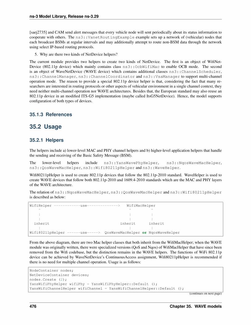
ns-3 Model Library, Release ns-3.29
[saej2735] and CAM send alert messages that every vehicle node will sent periodically about its status information tocooperate with others. The ns3::VanetRoutingExample example sets up a network of (vehicular) nodes thateach broadcast BSMs at regular intervals and may additionally attempt to route non-BSM data through the networkusing select IP-based routing protocols.
5. Why are there two kinds of NetDevice helpers?
The current module provides two helpers to create two kinds of NetDevice. The first is an object of WifiNet-Device (802.11p device) which mainly contains class ns3::OcbWifiMac to enable OCB mode. The secondis an object of WaveNetDevice (WAVE device) which contains additional classes ns3::ChannelScheduler,ns3::ChannelManager, ns3::ChannelCoordinator and ns3::VsaManager to support multi-channeloperation mode. The reason to provide a special 802.11p device helper is that, considering the fact that many re-searchers are interested in routing protocols or other aspects of vehicular environment in a single channel context, theyneed neither multi-channel operation nor WAVE architectures. Besides that, the European standard may also reuse an802.11p device in an modified ITS-G5 implementation (maybe called ItsG5NetDevice). Hence, the model supportsconfiguration of both types of devices.
35.1.3 References
35.2 Usage
35.2.1 Helpers
The helpers include a) lower-level MAC and PHY channel helpers and b) higher-level application helpers that handlethe sending and receiving of the Basic Safety Message (BSM).
The lower-level helpers include ns3::YansWavePhyHelper, ns3::NqosWaveMacHelper,ns3::QosWaveMacHelper, ns3::Wifi80211pHelper and ns3::WaveHelper.
Wifi80211pHelper is used to create 802.11p devices that follow the 802.11p-2010 standard. WaveHelper is used tocreate WAVE devices that follow both 802.11p-2010 and 1609.4-2010 standards which are the MAC and PHY layersof the WAVE architecture.
The relation of ns3::NqosWaveMacHelper, ns3::QosWaveMacHelper and ns3::Wifi80211pHelperis described as below:
WifiHelper ------------use--------------> WifiMacHelper^ ^ ^| | || | |
inherit inherit inherit| | |
Wifi80211pHelper ------use-----> QosWaveMacHelper or NqosWaveHelper
From the above diagram, there are two Mac helper classes that both inherit from the WifiMacHelper; when the WAVEmodule was originally written, there were specialized versions (QoS and Nqos) of WifiMacHelper that have since beenremoved from the Wifi codebase, but the distinction remains in the WAVE helpers. The functions of WiFi 802.11pdevice can be achieved by WaveNetDevice’s ContinuousAccess assignment, Wifi80211pHelper is recommended ifthere is no need for multiple channel operation. Usage is as follows:
NodeContainer nodes;NetDeviceContainer devices;nodes.Create (2);YansWifiPhyHelper wifiPhy = YansWifiPhyHelper::Default ();YansWifiChannelHelper wifiChannel = YansWifiChannelHelper::Default ();
(continues on next page)
476 Chapter 35. WAVE models

ns-3 Model Library, Release ns-3.29
(continued from previous page)
wifiPhy.SetChannel (wifiChannel.Create ());NqosWave80211pMacHelper wifi80211pMac = NqosWaveMacHelper::Default();Wifi80211pHelper 80211pHelper = Wifi80211pHelper::Default ();devices = 80211pHelper.Install (wifiPhy, wifi80211pMac, nodes);
The relation of ns3::YansWavePhyHelper, ns3::QosWaveMacHelper and ns3::WaveHelper is de-scribed as below:
WifiMacHelper^|
inherit|
WaveHelper -------- only use --------> QosWaveMacHelper
From the above diagram, WaveHelper is not the subclass of WifiHelper and should only use QosWaveMacHelperbecause WAVE MAC layer is based on QoS mechanism. But the WaveHelper is recommended if there is a need formultiple channel operation. Usage is as follows:
NodeContainer nodes;NetDeviceContainer devices;nodes.Create (2);YansWifiChannelHelper wifiChannel = YansWifiChannelHelper::Default ();YansWavePhyHelper wavePhy = YansWavePhyHelper::Default ();wavePhy.SetChannel (wifiChannel.Create ());QosWaveMacHelper waveMac = QosWaveMacHelper::Default ();WaveHelper waveHelper = WaveHelper::Default ();devices = waveHelper.Install (wavePhy, waveMac, nodes);
The higher-level helpers include ns3::WaveBsmStats and ns3::WaveBsmHelper.
WaveBsmStats is used to collect and manage statistics, such as packet and byte counts and Packet Delivery Ratio(PDR), regarding the sending and receiving of WAVE BSM packets. WaveBsmHelper is used by applications thatwish to send and receive BSMs.
The relation of ns3::WaveBsmHelper and WaveBsmStats is described below:
<Your Vanet Routing Application> ----use----> WaveBsmHelper ----use----> WaveBsmStats
From <Your Vanet Routing Application>, usage is as follows:
// declare WAVE BSM helper instance WaveBsmHelper m_waveBsmHelper;
// the following are passed to the WaveBsmHelpe::Install() // method, and they are thus assumed to becreated and // initialized themselves, based on the user’s // simulation setup criteria. // container of net-work node NodeContainer m_adhocTxNodes; // (transmitting) devices (1 per node) NetDeviceContainerm_adhocTxDevices; // IPv4 interfaces (1 per device) Ipv4InterfaceContainer m_adhocTxInterfaces; // to-tal simulation time (in seconds) double m_TotalSimTime; // WAVE BSM broadcast interval. E.g., 100ms= 0.1 seconds double m_waveInterval; // seconds // time-synchronization accuracy of GPS devices. E.g.,+/- 40ns double m_gpsAccuracyNs; // array of distances (m) at which safety PDR shall be determined,// e.g. 50m, 100m, 200m, 300m, 400m, 500m, 600m, 800m, 1000m, and 1500m std::vector <double>m_txSafetyRanges; // used to get consistent random numbers across scenarios int64_t m_streamIndex;
m_waveBsmHelper.Install (m_adhocTxNodes, m_adhocTxDevices, m_adhocTxInterfaces, Sec-onds(m_TotalSimTime), m_wavePacketSize, Seconds(m_waveInterval), // convert GPS accuracy,in ns, to Time Seconds(m_gpsAccuracyNs / 1000000.0), m_txSafetyRanges);
// fix random number streams m_streamIndex += m_waveBsmHelper.AssignStreams (m_streamIndex);
35.2. Usage 477
ns-3 Model Library, Release ns-3.29
Example usages of BSM statistics are as follows:
// Get the cumulative PDR of the first safety Tx range (i.e, 50m in the // m_txSafetyRanges exampleabove). double bsm_pdr1 = m_waveBsmHelper.GetWaveBsmStats ()->GetBsmPdr (1);
// total WAVE BSM bytes sent uint32_t cumulativeWaveBsmBytes =m_waveBsmHelper.GetWaveBsmStats ()->GetTxByteCount ();
// get number of WAVE BSM packets sent int wavePktsSent = m_waveBsmHelper.GetWaveBsmStats()->GetTxPktCount ();
// get number of WAVE BSM packets received int wavePktsReceived =m_waveBsmHelper.GetWaveBsmStats ()->GetRxPktCount ();
// reset count of WAVE BSM packets received m_waveBsmHelper.GetWaveBsmStats ()->SetRxPktCount(0);
// reset count of WAVE BSM packets sent m_waveBsmHelper.GetWaveBsmStats ()->SetTxPktCount (0);
// indicate that a node (nodeId) is moving. (set to 0 to “stop” node) WaveB-smHelper::GetNodesMoving()[nodeId] = 1;
35.2.2 APIs
MAC layer
The 802.11p device can allow the upper layer to send different information over Vendor Specific Action managementframes by using different OrganizationIdentifier fields to identify differences.
1. create some Node objects and WifiNetDevice objects, e.g. one sender and one receiver.
2. receiver defines an OrganizationIdentifier
uint8_t oi_bytes[5] = {0x00, 0x50, 0xC2, 0x4A, 0x40};OrganizationIdentifier oi(oi_bytes,5);
3. receiver defines a Callback for the defined OrganizationIdentifier
VscCallback vsccall = MakeCallback (&VsaExample::GetWsaAndOi, this);
4. receiver registers this identifier and function
Ptr<WifiNetDevice> device1 = DynamicCast<WifiNetDevice>(nodes.Get (i)->↪→GetDevice (0));Ptr<OcbWifiMac> ocb1 = DynamicCast<OcbWifiMac>(device->GetMac ());ocb1->AddReceiveVscCallback (oi, vsccall);
5. sender transmits management information over VSA frames
Ptr<Packet> vsc = Create<Packet> ();ocb2->SendVsc (vsc, Mac48Address::GetBroadcast (), m_16093oi);
6. then registered callbacks in the receiver will be called.
MAC extension layer
The WAVE devices allow the upper layer to route packets in different control approaches. However dedicated APIsand invocation sequences should be followed; otherwise, the packets may be discarded by devices.
478 Chapter 35. WAVE models

ns-3 Model Library, Release ns-3.29
1. create some Node objects and WaveNetDevice objects by helpers, e.g. one sender and one receiver.
2. receiver registers the receive callback if WSMP and IP-based packets are supposed to be received.
// the class ``ns3::WaveNetDeviceExample``here will has a receive method↪→"Receive" to be registered.receiver->SetReceiveCallback (MakeCallback (&WaveNetDeviceExample::Receive,↪→this));
3. receiver registers the receive callback if WSA frames are supposed to be received.
// the class ``ns3::WaveNetDeviceExample``here will has a receive method↪→"ReceiveVsa" to be registered.receiver->SetWaveVsaCallback (MakeCallback (&↪→WaveNetDeviceExample::ReceiveVsa, this));
4. sender and receiver assign channel access by StartSch method.
// in this case that alternating access with non-immediate mode is assigned↪→for sender and receiver devices.const SchInfo schInfo = SchInfo (SCH1, false, EXTENDED_ALTERNATING);Simulator::Schedule (Seconds (0.0), &WaveNetDevice::StartSch, sender,↪→schInfo);Simulator::Schedule (Seconds (0.0), &WaveNetDevice::StartSch, receiver,↪→schInfo);
or
// in this case that continuous access with immediate mode is assigned for↪→sender and receiver devices.const SchInfo schInfo = SchInfo (SCH1, true, EXTENDED_CONTINUOUS);Simulator::Schedule (Seconds (0.0), &WaveNetDevice::StartSch, sender,↪→schInfo);Simulator::Schedule (Seconds (0.0), &WaveNetDevice::StartSch, receiver,↪→schInfo)
or
// in this case that extended access with non-immediate mode is assigned for↪→sender and receiver devices.const SchInfo schInfo = SchInfo (SCH1, false, 100);Simulator::Schedule (Seconds (0.0), &WaveNetDevice::StartSch, sender,↪→schInfo);Simulator::Schedule (Seconds (0.0), &WaveNetDevice::StartSch, receiver,↪→schInfo)
5. sender registers a tx profile if IP-based packets are planned to be transmitted
// the IP-based packets will be transmitted in SCH1 with 6Mbps and 4↪→txPowerLevel with adaptable mode.const TxProfile txProfile = TxProfile (SCH1, true, 4, WifiMode(↪→"OfdmRate6MbpsBW10MHz"));Simulator::Schedule (Seconds (2.0), &WaveNetDevice::RegisterTxProfile,↪→sender, txProfile);
6. sender transmits WSMP packets by SendX method.
35.2. Usage 479
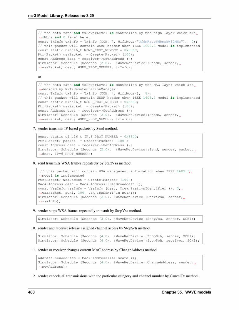
ns-3 Model Library, Release ns-3.29
// the data rate and txPowerLevel is controlled by the high layer which are↪→6Mbps and 0 level here.const TxInfo txInfo = TxInfo (CCH, 7, WifiMode("OfdmRate6MbpsBW10MHz"), 0);// this packet will contain WSMP header when IEEE 1609.3 model is implementedconst static uint16_t WSMP_PROT_NUMBER = 0x88DC;Ptr<Packet> wsaPacket = Create<Packet> (100);const Address dest = receiver->GetAddress ();Simulator::Schedule (Seconds (2.0), &WaveNetDevice::SendX, sender,↪→wsaPacket, dest, WSMP_PROT_NUMBER, txInfo);
or
// the data rate and txPowerLevel is controlled by the MAC layer which are↪→decided by WifiRemoteStationManagerconst TxInfo txInfo = TxInfo (CCH, 7, WifiMode(), 8);// this packet will contain WSMP header when IEEE 1609.3 model is implementedconst static uint16_t WSMP_PROT_NUMBER = 0x88DC;Ptr<Packet> wsaPacket = Create<Packet> (100);const Address dest = receiver->GetAddress ();Simulator::Schedule (Seconds (2.0), &WaveNetDevice::SendX, sender,↪→wsaPacket, dest, WSMP_PROT_NUMBER, txInfo);
7. sender transmits IP-based packets by Send method.
const static uint16_t IPv6_PROT_NUMBER = 0x86DD;Ptr<Packet> packet = Create<Packet> (100);const Address dest = receiver->GetAddress ();Simulator::Schedule (Seconds (2.0), &WaveNetDevice::Send, sender, packet,↪→dest, IPv6_PROT_NUMBER);
8. send transmits WSA frames repeatedly by StartVsa method.
// this packet will contain WSA management information when IEEE 1609.3↪→model is implementedPtr<Packet> wsaPacket = Create<Packet> (100);Mac48Address dest = Mac48Address::GetBroadcast ();const VsaInfo vsaInfo = VsaInfo (dest, OrganizationIdentifier (), 0,↪→wsaPacket, SCH1, 100, VSA_TRANSMIT_IN_BOTHI);Simulator::Schedule (Seconds (2.0), &WaveNetDevice::StartVsa, sender,↪→vsaInfo);
9. sender stops WSA frames repeatedly transmit by StopVsa method.
Simulator::Schedule (Seconds (3.0), &WaveNetDevice::StopVsa, sender, SCH1);
10. sender and receiver release assigned channel access by StopSch method.
Simulator::Schedule (Seconds (4.0), &WaveNetDevice::StopSch, sender, SCH1);Simulator::Schedule (Seconds (4.0), &WaveNetDevice::StopSch, receiver, SCH1);
11. sender or receiver changes current MAC address by ChangeAddress method.
Address newAddress = Mac48Address::Allocate ();Simulator::Schedule (Seconds (4.0), &WaveNetDevice::ChangeAddress, sender,↪→newAddress);
12. sender cancels all transmissions with the particular category and channel number by CancelTx method.
480 Chapter 35. WAVE models
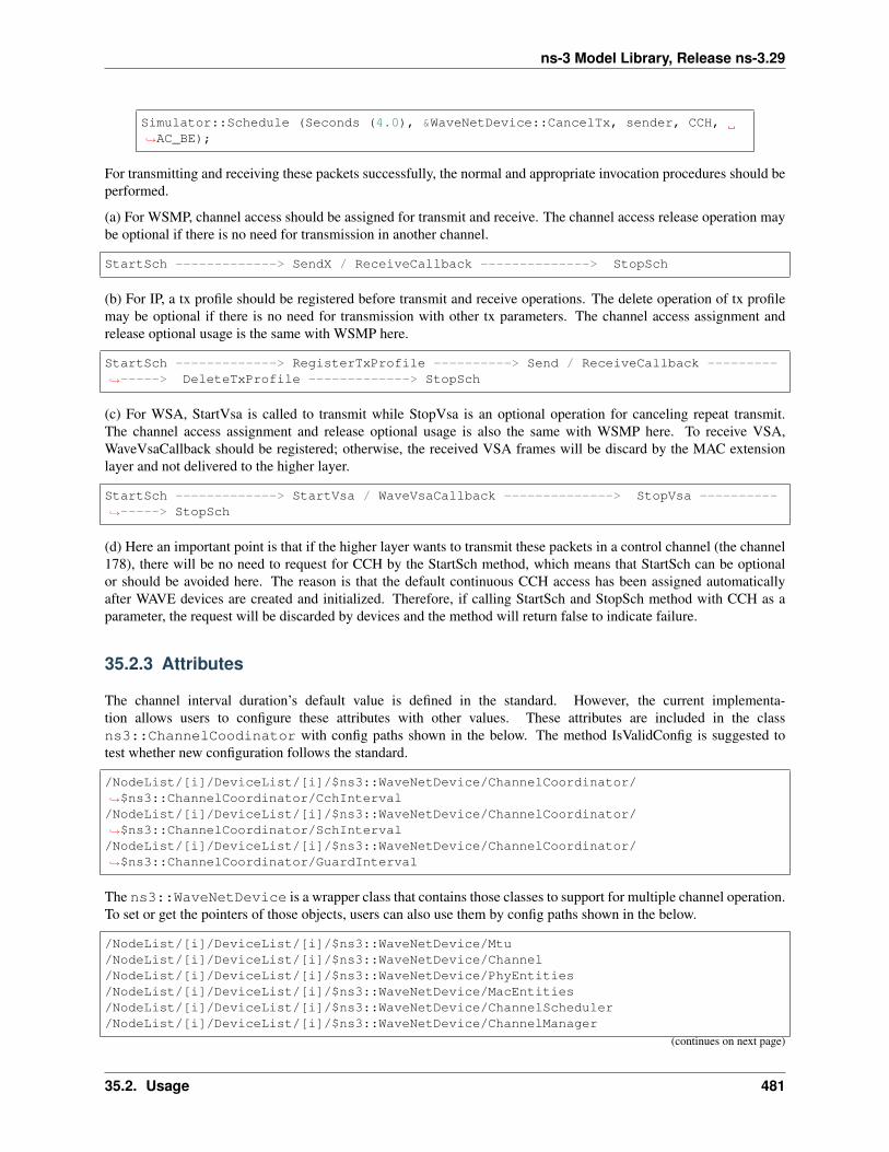
ns-3 Model Library, Release ns-3.29
Simulator::Schedule (Seconds (4.0), &WaveNetDevice::CancelTx, sender, CCH,↪→AC_BE);
For transmitting and receiving these packets successfully, the normal and appropriate invocation procedures should beperformed.
(a) For WSMP, channel access should be assigned for transmit and receive. The channel access release operation maybe optional if there is no need for transmission in another channel.
StartSch -------------> SendX / ReceiveCallback --------------> StopSch
(b) For IP, a tx profile should be registered before transmit and receive operations. The delete operation of tx profilemay be optional if there is no need for transmission with other tx parameters. The channel access assignment andrelease optional usage is the same with WSMP here.
StartSch -------------> RegisterTxProfile ----------> Send / ReceiveCallback ---------↪→-----> DeleteTxProfile -------------> StopSch
(c) For WSA, StartVsa is called to transmit while StopVsa is an optional operation for canceling repeat transmit.The channel access assignment and release optional usage is also the same with WSMP here. To receive VSA,WaveVsaCallback should be registered; otherwise, the received VSA frames will be discard by the MAC extensionlayer and not delivered to the higher layer.
StartSch -------------> StartVsa / WaveVsaCallback --------------> StopVsa ----------↪→-----> StopSch
(d) Here an important point is that if the higher layer wants to transmit these packets in a control channel (the channel178), there will be no need to request for CCH by the StartSch method, which means that StartSch can be optionalor should be avoided here. The reason is that the default continuous CCH access has been assigned automaticallyafter WAVE devices are created and initialized. Therefore, if calling StartSch and StopSch method with CCH as aparameter, the request will be discarded by devices and the method will return false to indicate failure.
35.2.3 Attributes
The channel interval duration’s default value is defined in the standard. However, the current implementa-tion allows users to configure these attributes with other values. These attributes are included in the classns3::ChannelCoodinator with config paths shown in the below. The method IsValidConfig is suggested totest whether new configuration follows the standard.
/NodeList/[i]/DeviceList/[i]/$ns3::WaveNetDevice/ChannelCoordinator/↪→$ns3::ChannelCoordinator/CchInterval/NodeList/[i]/DeviceList/[i]/$ns3::WaveNetDevice/ChannelCoordinator/↪→$ns3::ChannelCoordinator/SchInterval/NodeList/[i]/DeviceList/[i]/$ns3::WaveNetDevice/ChannelCoordinator/↪→$ns3::ChannelCoordinator/GuardInterval
The ns3::WaveNetDevice is a wrapper class that contains those classes to support for multiple channel operation.To set or get the pointers of those objects, users can also use them by config paths shown in the below.
/NodeList/[i]/DeviceList/[i]/$ns3::WaveNetDevice/Mtu/NodeList/[i]/DeviceList/[i]/$ns3::WaveNetDevice/Channel/NodeList/[i]/DeviceList/[i]/$ns3::WaveNetDevice/PhyEntities/NodeList/[i]/DeviceList/[i]/$ns3::WaveNetDevice/MacEntities/NodeList/[i]/DeviceList/[i]/$ns3::WaveNetDevice/ChannelScheduler/NodeList/[i]/DeviceList/[i]/$ns3::WaveNetDevice/ChannelManager
(continues on next page)
35.2. Usage 481
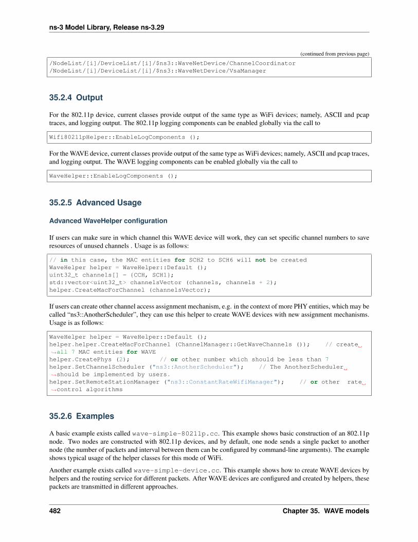
ns-3 Model Library, Release ns-3.29
(continued from previous page)
/NodeList/[i]/DeviceList/[i]/$ns3::WaveNetDevice/ChannelCoordinator/NodeList/[i]/DeviceList/[i]/$ns3::WaveNetDevice/VsaManager
35.2.4 Output
For the 802.11p device, current classes provide output of the same type as WiFi devices; namely, ASCII and pcaptraces, and logging output. The 802.11p logging components can be enabled globally via the call to
Wifi80211pHelper::EnableLogComponents ();
For the WAVE device, current classes provide output of the same type as WiFi devices; namely, ASCII and pcap traces,and logging output. The WAVE logging components can be enabled globally via the call to
WaveHelper::EnableLogComponents ();
35.2.5 Advanced Usage
Advanced WaveHelper configuration
If users can make sure in which channel this WAVE device will work, they can set specific channel numbers to saveresources of unused channels . Usage is as follows:
// in this case, the MAC entities for SCH2 to SCH6 will not be createdWaveHelper helper = WaveHelper::Default ();uint32_t channels[] = {CCH, SCH1};std::vector<uint32_t> channelsVector (channels, channels + 2);helper.CreateMacForChannel (channelsVector);
If users can create other channel access assignment mechanism, e.g. in the context of more PHY entities, which may becalled “ns3::AnotherScheduler”, they can use this helper to create WAVE devices with new assignment mechanisms.Usage is as follows:
WaveHelper helper = WaveHelper::Default ();helper.helper.CreateMacForChannel (ChannelManager::GetWaveChannels ()); // create↪→all 7 MAC entities for WAVEhelper.CreatePhys (2); // or other number which should be less than 7helper.SetChannelScheduler ("ns3::AnotherScheduler"); // The AnotherScheduler↪→should be implemented by users.helper.SetRemoteStationManager ("ns3::ConstantRateWifiManager"); // or other rate↪→control algorithms
35.2.6 Examples
A basic example exists called wave-simple-80211p.cc. This example shows basic construction of an 802.11pnode. Two nodes are constructed with 802.11p devices, and by default, one node sends a single packet to anothernode (the number of packets and interval between them can be configured by command-line arguments). The exampleshows typical usage of the helper classes for this mode of WiFi.
Another example exists called wave-simple-device.cc. This example shows how to create WAVE devices byhelpers and the routing service for different packets. After WAVE devices are configured and created by helpers, thesepackets are transmitted in different approaches.
482 Chapter 35. WAVE models

ns-3 Model Library, Release ns-3.29
Another example exists called vanet-routing-compare.cc. This example shows how to create mobility nodesin a VANET scenario and send Basic Safety Message (BSM) packets are regular intervals and/or additional data trafficto be routed between nodes. BSMs are transmitted assuming the WAVE Short Message Protocol (WSMP), whereasnon-BSM data packets are relayed by using one of several different IP-based routing protocols (e.g., AODV, OLSR,DSDV, or DSR).
35.2.7 Troubleshooting
To be defined.
35.3 Validation
A test suite named wifi-80211p-ocb is defined. This test case consists of a stationary node and a mobile node.The mobile node moves towards the stationary mode, and time points are checked at which time the physical layerstarts to receive packets (and whether the MAC becomes associated, if applicable). The same physical experiment isrepeated for normal WiFi NetDevices in AP/STA mode, in Adhoc mode, and the new OCB mode.
Another test suite named wave-mac-extension is defined. This test suite has four test cases, includingchannel-coordination, channel-routing, channel-access and annex-c. The first case is to testchannel coordination feature. The second case is to test channel routing for three types of packets. The third caseis to test four channel access assignments. And the fourth case is to test the implemented feature described inthe Annex C of the standard. It is worth noting that the channel-routing and channel-access test casesare both in the context of single-PHY device, which depends on the default channel access assignment mechanismns3:DefaultChannelScheduler, thus they may not be suitable for testing when other channel access assign-ment mechanisms are used. Although they are test cases, they are also good examples to show usage.
The ns3::VanetRoutingExample example was studied using mobility trace files in the Raleigh, NC USA areagenerated using Simulation for Urban Mobility (SUMO). Three environments were studied: a) an open highwayscenario, b) a residential neighborhood scenario, and c) and urban downtown scenario. For each environment, aconstant number of 50-750 vehicles was maintained for 2000 simulation seconds (> 30 minutes). The mobility tracefile were played back using ns3::Ns2MobilityHelper. All vehicular nodes transmitted a 200-byte BSM at 10Hz and the PDR was determined for transmission ranges of 50-1500m. No additional non-BSM data was injected/ routed through the network. The default propagation loss model used was Two-Ray Ground. Different fading/ shadowing models were evaluated, including a) no fading, b) stochastic Nakagami-m fading, and c) an obstacleshadowing model (to be contributed to ns-3). 30 trials of each scenario were run in the North Carolina State University(NCSU) High Performance Computing (HPC) center, with each trial requiring from 8 hours to 6 days of CPU timeto complete. Preliminary results were presented at the PhD Forum, 22nd IEEE International Conference on NetworkProtocols (ICNP), October 24, 2014, Research Triangle Park, NC. See: http://www4.ncsu.edu/~scarpen/Research_files/Final-PHD_Forum_SE_Carpenter_2014.pdf
35.3. Validation 483

ns-3 Model Library, Release ns-3.29
484 Chapter 35. WAVE models
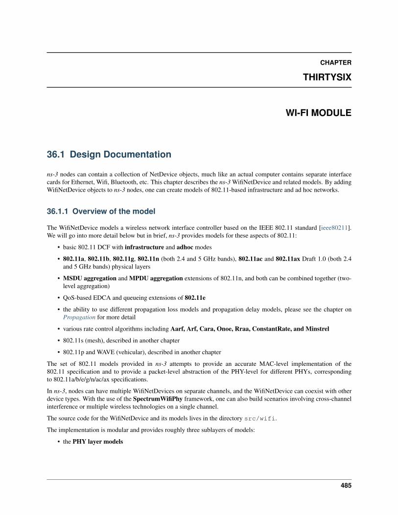
CHAPTER
THIRTYSIX
WI-FI MODULE
36.1 Design Documentation
ns-3 nodes can contain a collection of NetDevice objects, much like an actual computer contains separate interfacecards for Ethernet, Wifi, Bluetooth, etc. This chapter describes the ns-3 WifiNetDevice and related models. By addingWifiNetDevice objects to ns-3 nodes, one can create models of 802.11-based infrastructure and ad hoc networks.
36.1.1 Overview of the model
The WifiNetDevice models a wireless network interface controller based on the IEEE 802.11 standard [ieee80211].We will go into more detail below but in brief, ns-3 provides models for these aspects of 802.11:
• basic 802.11 DCF with infrastructure and adhoc modes
• 802.11a, 802.11b, 802.11g, 802.11n (both 2.4 and 5 GHz bands), 802.11ac and 802.11ax Draft 1.0 (both 2.4and 5 GHz bands) physical layers
• MSDU aggregation and MPDU aggregation extensions of 802.11n, and both can be combined together (two-level aggregation)
• QoS-based EDCA and queueing extensions of 802.11e
• the ability to use different propagation loss models and propagation delay models, please see the chapter onPropagation for more detail
• various rate control algorithms including Aarf, Arf, Cara, Onoe, Rraa, ConstantRate, and Minstrel
• 802.11s (mesh), described in another chapter
• 802.11p and WAVE (vehicular), described in another chapter
The set of 802.11 models provided in ns-3 attempts to provide an accurate MAC-level implementation of the802.11 specification and to provide a packet-level abstraction of the PHY-level for different PHYs, correspondingto 802.11a/b/e/g/n/ac/ax specifications.
In ns-3, nodes can have multiple WifiNetDevices on separate channels, and the WifiNetDevice can coexist with otherdevice types. With the use of the SpectrumWifiPhy framework, one can also build scenarios involving cross-channelinterference or multiple wireless technologies on a single channel.
The source code for the WifiNetDevice and its models lives in the directory src/wifi.
The implementation is modular and provides roughly three sublayers of models:
• the PHY layer models
485

ns-3 Model Library, Release ns-3.29
• the so-called MAC low models: they model functions such as medium access (DCF and EDCA), RTS/CTS andACK. In ns-3, the lower-level MAC is further subdivided into a MAC low and MAC middle sublayering, withchannel access grouped into the MAC middle.
• the so-called MAC high models: they implement non-time-critical processes in Wifi such as the MAC-levelbeacon generation, probing, and association state machines, and a set of Rate control algorithms. In the litera-ture, this sublayer is sometimes called the upper MAC and consists of more software-oriented implementationsvs. time-critical hardware implementations.
Next, we provide an design overview of each layer, shown in Figure WifiNetDevice architecture..
Fig. 1: WifiNetDevice architecture.
MAC high models
There are presently three MAC high models that provide for the three (non-mesh; the mesh equivalent, which is asibling of these with common parent ns3::RegularWifiMac, is not discussed here) Wi-Fi topological elements -Access Point (AP) (ns3::ApWifiMac), non-AP Station (STA) (ns3::StaWifiMac), and STA in an IndependentBasic Service Set (IBSS - also commonly referred to as an ad hoc network (ns3::AdhocWifiMac).
The simplest of these is ns3::AdhocWifiMac, which implements a Wi-Fi MAC that does not perform any kindof beacon generation, probing, or association. The ns3::StaWifiMac class implements an active probing andassociation state machine that handles automatic re-association whenever too many beacons are missed. Finally,ns3::ApWifiMac implements an AP that generates periodic beacons, and that accepts every attempt to associate.
486 Chapter 36. Wi-Fi Module

ns-3 Model Library, Release ns-3.29
These three MAC high models share a common parent in ns3::RegularWifiMac, which exposes, amongother MAC configuration, an attribute QosSupported that allows configuration of 802.11e/WMM-style QoSsupport, an attribute HtSupported that allows configuration of 802.11n High Throughput style support, an at-tribute VhtSupported that allows configuration of 802.11ac Very High Throughput style support and an attributeHeSupported that allows configuration of 802.11ax High Efficiency style support.
There are also several rate control algorithms that can be used by the MAC low layer. A complete list of availablerate control algorithms is provided in a separate section.
MAC low layer
The MAC low layer is split into three main components:
1. ns3::MacLow which takes care of RTS/CTS/DATA/ACK transactions and also performs MPDU aggregation.
2. ns3::ChannelAccessManager and ns3::DcfState which implements the DCF and EDCAF func-tions.
3. ns3::Txop and ns3::QosTxop which handle the packet queue, packet fragmentation, and packet retrans-missions if they are needed. The ns3::Txop object is used by high MACs that are not QoS-enabled, and fortransmission of frames (e.g., of type Management) that the standard says should access the medium using theDCF. ns3::QosTxop is is used by QoS-enabled high MACs and also performs MSDU aggregation.
PHY layer models
In short, the physical layer models are mainly responsible for modeling the reception of packets and for trackingenergy consumption. There are typically three main components to packet reception:
• each packet received is probabilistically evaluated for successful or failed reception. The probability dependson the modulation, on the signal to noise (and interference) ratio for the packet, and on the state of the physicallayer (e.g. reception is not possible while transmission or sleeping is taking place);
• an object exists to track (bookkeeping) all received signals so that the correct interference power for each packetcan be computed when a reception decision has to be made; and
• one or more error models corresponding to the modulation and standard are used to look up probability ofsuccessful reception.
ns-3 offers users a choice between two physical layer models, with a base interface defined in the ns3::WifiPhyclass. The YansWifiPhy class has been the only physical layer model until recently; the model implemented thereis described in a paper entitled Yet Another Network Simulator The acronym Yans derives from this paper title. TheSpectrumWifiPhy class is an alternative implementation based on the Spectrum framework used for other ns-3 wirelessmodels. Spectrum allows a fine-grained frequency decomposition of the signal, and permits scenarios to includemultiple technologies coexisting on the same channel.
36.1.2 Scope and Limitations
The IEEE 802.11 standard [ieee80211] is a large specification, and not all aspects are covered by ns-3; the docu-mentation of ns-3’s conformance by itself would lead to a very long document. This section attempts to summarizecompliance with the standard and with behavior found in practice.
The physical layer and channel models operate on a per-packet basis, with no frequency-selective propagation orinterference effects when using the default YansWifiPhy model. Directional antennas are also not supported at thistime. For additive white Gaussian noise (AWGN) scenarios, or wideband interference scenarios, performance isgoverned by the application of analytical models (based on modulation and factors such as channel width) to thereceived signal-to-noise ratio, where noise combines the effect of thermal noise and of interference from other Wi-Fi
36.1. Design Documentation 487

ns-3 Model Library, Release ns-3.29
packets. Moreover, interference from other technologies is not modeled. The following details pertain to the physicallayer and channel models:
• 802.11ax is still in draft phase, not all functionalities are implemented yet
• 802.11ax does not contain any of the high-density improvement
• 802.11ax MU-OFDMA is not supported
• 802.11ax can only be used with Constant rate control algorithm
• 802.11ax only supports SU PPDU format
• 802.11ac/ax MU-MIMO is not supported, and no more than 4 antennas can be configured
• 802.11n/ac/ax beamforming is not supported
• 802.11 HCF/HCCA are not implemented
• 802.11 PCF implementation currently assumes a DTIM interval equal to the beacon interval
• Authentication and encryption are missing
• Processing delays are not modeled
• PLCP preamble reception is not modeled
• PHY_RXSTART is not supported
• The current implementation assumes that secondary channels are always higher than primary channels
• Cases where RTS/CTS and ACK are transmitted using HT/VHT/HE formats are not supported
• Energy consumption model does not consider MIMO
At the MAC layer, most of the main functions found in deployed Wi-Fi equipment for 802.11a/b/e/g/n/ac/ax areimplemented, but there are scattered instances where some limitations in the models exist. Support for 802.11n and acis evolving.
Some implementation choices that are not imposed by the standard are listed below:
• BSSBasicRateSet for 802.11b has been assumed to be 1-2 Mbit/s
• BSSBasicRateSet for 802.11a/g has been assumed to be 6-12-24 Mbit/s
• The wifi manager always selects the lowest basic rate for management frames.
36.1.3 Design Details
The remainder of this section is devoted to more in-depth design descriptions of some of the Wi-Fi models. Usersinterested in skipping to the section on usage of the wifi module (User Documentation) may do so at this point. Weorganize these more detailed sections from the bottom-up, in terms of layering, by describing the channel and PHYmodels first, followed by the MAC models.
We focus first on the choice between physical layer frameworks. ns-3 contains support for a Wi-Fi-only physical layermodel called YansWifiPhy that offers no frequency-level decomposition of the signal. For simulations that involveonly Wi-Fi signals on the Wi-Fi channel, and that do not involve frequency-dependent propagation loss or fadingmodels, the default YansWifiPhy framework is a suitable choice. For simulations involving mixed technologies on thesame channel, or frequency dependent effects, the SpectrumWifiPhy is more appropriate. The two frameworks arevery similarly configured.
The SpectrumWifiPhy framework uses the Spectrum channel framework, which is not documented herein but in theSpectrum module documentation.
488 Chapter 36. Wi-Fi Module

ns-3 Model Library, Release ns-3.29
The YansWifiChannel is the only concrete channel model class in the ns-3 wifi module. Thens3::YansWifiChannel implementation uses the propagation loss and delay models provided within the ns-3 Propagation module. In particular, a number of propagation models can be added (chained together, if multi-ple loss models are added) to the channel object, and a propagation delay model also added. Packets sent froma ns3::YansWifiPhy object onto the channel with a particular signal power, are copied to all of the otherns3::YansWifiPhy objects after the signal power is reduced due to the propagation loss model(s), and after adelay corresponding to transmission (serialization) delay and propagation delay due any channel propagation delaymodel (typically due to speed-of-light delay between the positions of the devices).
Only objects of ns3::YansWifiPhy may be attached to a ns3::YansWifiChannel; therefore, objects mod-eling other (interfering) technologies such as LTE are not allowed. Furthermore, packets from different channels donot interact; if a channel is logically configured for e.g. channels 5 and 6, the packets do not cause adjacent channelinterference (even if their channel numbers overlap).
WifiPhy and related models
The ns3::WifiPhy is an abstract base class representing the 802.11 physical layer functions. Packets passed tothis object (via a SendPacket() method are sent over a channel object, and upon reception, the receiving PHYobject decides (based on signal power and interference) whether the packet was successful or not. This class alsoprovides a number of callbacks for notifications of physical layer events, exposes a notion of a state machine that canbe monitored for MAC-level processes such as carrier sense, and handles sleep/wake models and energy consumption.The ns3::WifiPhy hooks to the ns3::MacLow object in the WifiNetDevice.
There are currently two implementations of the WifiPhy: the ns3::YansWifiPhy and thens3::SpectrumWifiPhy. They each work in conjunction with three other objects:
• WifiPhyStateHelper: Maintains the PHY state machine
• InterferenceHelper: Tracks all packets observed on the channel
• ErrorModel: Computes a probability of error for a given SNR
YansWifiPhy and WifiPhyStateHelper
Class ns3::YansWifiPhy is responsible for taking packets passed to it from the MAC (the ns3::MacLow object)and sending them onto the ns3::YansWifiChannel to which it is attached. It is also responsible to receive packetsfrom that channel, and, if reception is deemed to have been successful, to pass them up to the MAC.
Class ns3::WifiPhyStateHelpermanages the state machine of the PHY layer, and allows other objects to hookas listeners to monitor PHY state. The main use of listeners is for the MAC layer to know when the PHY is busy ornot (for transmission and collision avoidance).
The PHY layer can be in one of six states:
1. TX: the PHY is currently transmitting a signal on behalf of its associated MAC
2. RX: the PHY is synchronized on a signal and is waiting until it has received its last bit to forward it to the MAC.
3. IDLE: the PHY is not in the TX, RX, or CCA BUSY states.
4. CCA Busy: the PHY is not in TX or RX state but the measured energy is higher than the energy detectionthreshold.
5. SWITCHING: the PHY is switching channels.
6. SLEEP: the PHY is in a power save mode and cannot send nor receive frames.
36.1. Design Documentation 489

ns-3 Model Library, Release ns-3.29
Packet reception works as follows. The YansWifiPhy attribute CcaMode1Threshold corresponds to what the stan-dard calls the “ED threshold” for CCA Mode 1. In section 16.4.8.5: “CCA Mode 1: Energy above threshold. CCAshall report a busy medium upon detection of any energy above the ED threshold.”
There is a “noise ED threshold” in the standard for non-Wi-Fi signals, and this is usually set to 20 dB greater than the“carrier sense ED threshold”. However, the model doesn’t support this, because there are no ‘foreign’ signals in theYansWifi model– everything is a Wi-Fi signal.
In the standard, there is also what is called the “minimum modulation and coding rate sensitivity” in section 18.3.10.6CCA requirements. This is the -82 dBm requirement for 20 MHz channels. This is analogous to the EnergyDetection-Threshold attribute in YansWifiPhy. CCA busy state is not raised in this model when this threshold is exceeded butinstead RX state is immediately reached, since it is assumed that PLCP sync always succeeds in this model. Even ifthe PLCP header reception fails, the channel state is still held in RX until YansWifiPhy::EndReceive().
In ns-3, the values of these attributes are set to small default values (-96 dBm for EnergyDetectionThreshold and -99dBm for CcaMode1Threshold). So, if a signal comes in at > -96 dBm and the state is IDLE or CCA BUSY, this modelwill lock onto it for the signal duration and raise RX state. If it comes in at <= -96 dBm but >= -99 dBm, it willdefinitely raise CCA BUSY but not RX state. If it comes in < -99 dBm, it gets added to the interference tracker and,by itself, it will not raise CCA BUSY, but maybe a later signal will contribute more power so that the threshold of -99dBm is reached at a later time.
The energy of the signal intended to be received is calculated from the transmission power and adjusted based on theTx gain of the transmitter, Rx gain of the receiver, and any path loss propagation model in effect.
The packet reception occurs in two stages. First, an event is scheduled for when the PLCP header has been received.PLCP header is often transmitted at a lower modulation rate than is the payload. The portion of the packet correspond-ing to the PLCP header is evaluated for probability of error based on the observed SNR. The InterferenceHelper objectreturns a value for “probability of error (PER)” for this header based on the SNR that has been tracked by the Interfer-enceHelper. The YansWifiPhy then draws a random number from a uniform distribution and compares it againstthe PER and decides success or failure. The process is again repeated after the payload has been received (possiblywith a different error model applied for the different modulation). If both the header and payload are successfullyreceived, the packet is passed up to the MacLow object.
Even if packet objects received by the PHY are not part of the reception process, they are remembered by the Interfer-enceHelper object for purposes of SINR computation and making clear channel assessment decisions.
InterferenceHelper
The InterferenceHelper is an object that tracks all incoming packets and calculates probability of error values forpackets being received, and also evaluates whether energy on the channel rises above the CCA threshold.
The basic operation of probability of error calculations is shown in Figure SNIR function over time.. Packets arerepresented as bits (not symbols) in the ns-3 model, and the InterferenceHelper breaks the packet into one or more“chunks” each with a different signal to noise (and interference) ratio (SNIR). Each chunk is separately evaluated byasking for the probability of error for a given number of bits from the error model in use. The InterferenceHelperbuilds an aggregate “probability of error” value based on these chunks and their duration, and returns this back to theYansWifiPhy for a reception decision.
From the SNIR function we can derive the Bit Error Rate (BER) and Packet Error Rate (PER) for the modulation andcoding scheme being used for the transmission.
ErrorModel
The error models are described in more detail in outside references. Please refer to [pei80211ofdm], [pei80211b],[lacage2006yans], [Haccoun] and [Frenger] for a detailed description of the available BER/PER models.
490 Chapter 36. Wi-Fi Module
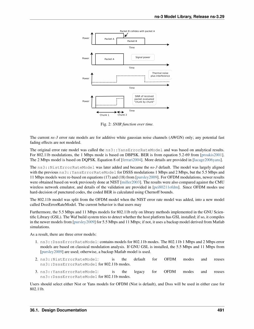
ns-3 Model Library, Release ns-3.29
Fig. 2: SNIR function over time.
The current ns-3 error rate models are for additive white gaussian noise channels (AWGN) only; any potential fastfading effects are not modeled.
The original error rate model was called the ns3::YansErrorRateModel and was based on analytical results.For 802.11b modulations, the 1 Mbps mode is based on DBPSK. BER is from equation 5.2-69 from [proakis2001].The 2 Mbps model is based on DQPSK. Equation 8 of [ferrari2004]. More details are provided in [lacage2006yans].
The ns3::NistErrorRateModel was later added and became the ns-3 default. The model was largely alignedwith the previous ns3::YansErrorRateModel for DSSS modulations 1 Mbps and 2 Mbps, but the 5.5 Mbps and11 Mbps models were re-based on equations (17) and (18) from [pursley2009]. For OFDM modulations, newer resultswere obtained based on work previously done at NIST [miller2003]. The results were also compared against the CMUwireless network emulator, and details of the validation are provided in [pei80211ofdm]. Since OFDM modes usehard-decision of punctured codes, the coded BER is calculated using Chernoff bounds.
The 802.11b model was split from the OFDM model when the NIST error rate model was added, into a new modelcalled DsssErrorRateModel. The current behavior is that users may
Furthermore, the 5.5 Mbps and 11 Mbps models for 802.11b rely on library methods implemented in the GNU Scien-tific Library (GSL). The Waf build system tries to detect whether the host platform has GSL installed; if so, it compilesin the newer models from [pursley2009] for 5.5 Mbps and 11 Mbps; if not, it uses a backup model derived from Matlabsimulations.
As a result, there are three error models:
1. ns3::DsssErrorRateModel: contains models for 802.11b modes. The 802.11b 1 Mbps and 2 Mbps errormodels are based on classical modulation analysis. If GNU GSL is installed, the 5.5 Mbps and 11 Mbps from[pursley2009] are used; otherwise, a backup Matlab model is used.
2. ns3::NistErrorRateModel: is the default for OFDM modes and reusesns3::DsssErrorRateModel for 802.11b modes.
3. ns3::YansErrorRateModel: is the legacy for OFDM modes and reusesns3::DsssErrorRateModel for 802.11b modes.
Users should select either Nist or Yans models for OFDM (Nist is default), and Dsss will be used in either case for802.11b.
36.1. Design Documentation 491
ns-3 Model Library, Release ns-3.29
SpectrumWifiPhy
This section describes the implementation of the SpectrumWifiPhy class that can be found in src/wifi/model/spectrum-wifi-phy.{cc,h}.
The implementation also makes use of additional classes found in the same directory:
• wifi-spectrum-phy-interface.{cc,h}
• wifi-spectrum-signal-parameters.{cc,h}
and classes found in the spectrum module:
• wifi-spectrum-value-helper.{cc,h}
The current SpectrumWifiPhy class reuses the existing interference manager and error rate models originally builtfor YansWifiPhy, but allows, as a first step, foreign (non Wi-Fi) signals to be treated as additive noise.
Two main changes were needed to adapt the Spectrum framework to Wi-Fi. First, the physical layer must send signalscompatible with the Spectrum channel framework, and in particular, the MultiModelSpectrumChannel thatallows signals from different technologies to coexist. Second, the InterferenceHelper must be extended to support theinsertion of non-Wi-Fi signals and to add their received power to the noise, in the same way that unintended Wi-Fisignals (perhaps from a different SSID or arriving late from a hidden node) are added to the noise.
Third, the default value for CcaMode1Threshold attribute is -62 dBm rather than the value of -99 dBm used forYansWifiPhy. This is because, unlike YansWifiPhy, where there are no foreign signals, CCA BUSY state will beraised for foreign signals that are higher than this ‘energy detection’ threshold (see section 16.4.8.5 in the 802.11-2012standard for definition of CCA Mode 1).
To support the Spectrum channel, the YansWifiPhy transmit and receive methods were adapted to usethe Spectrum channel API. This required developing a few SpectrumModel-related classes. The classWifiSpectrumValueHelper is used to create Wi-Fi signals with the spectrum framework and spread their en-ergy across the bands. The spectrum is sub-divided into sub-bands (the width of an OFDM subcarrier, which dependson the technology). The power allocated to a particular channel is spread across the sub-bands roughly according tohow power would be allocated to sub-carriers. Adjacent channels are models by the use of OFDM transmit spectrummasks as defined in the standards.
To support an easier user configuration experience, the existing YansWifi helper classes (in src/wifi/helper)were copied and adapted to provide equivalent SpectrumWifi helper classes.
Finally, for reasons related to avoiding C++ multiple inheritance issues, a small forwarding class calledWifiSpectrumPhyInterfacewas inserted as a shim between the SpectrumWifiPhy and the Spectrum chan-nel.
The MAC model
Infrastructure association
Association in infrastructure (IBSS) mode is a high-level MAC function. Either active probing or passive scanning isused (default is passive scan). At the start of the simulation, Wi-Fi network devices configured as STA will attempt toscan the channel. Depends on whether passive or active scanning is selected, STA will attempt to gather beacons, orsend a probe request and gather probe responses until the respective timeout occurs. The end result will be a list ofcandidate AP to associate to. STA will then try to associate to the best AP (i.e., best SNR).
If association is rejected by the AP for some reason, the STA will try to associate to the next best AP until thecandidate list is exhausted which then sends STA to ‘REFUSED’ state. If this occurs, the simulation user will needto force reassociation retry in some way, perhaps by changing configuration (i.e. the STA will not persistently try toassociate upon a refusal).
492 Chapter 36. Wi-Fi Module

ns-3 Model Library, Release ns-3.29
When associated, if the configuration is changed by the simulation user, the STA will try to reassociate with theexisting AP.
If the number of missed beacons exceeds the threshold, the STA will notify the rest of the device that the link is down(association is lost) and restart the scanning process. Note that this can also happen when an association request failswithout explicit refusal (i.e., the AP fails to respond to association request).
Roaming
Roaming at layer-2 (i.e. a STA migrates its association from one AP to another) is not presently supported. Becauseof that, the Min/Max channel dwelling time implementation as described by the IEEE 802.11 standard [ieee80211] isalso omitted, since it is only meaningful on the context of channel roaming.
Channel access
The 802.11 Distributed Coordination Function is used to calculate when to grant access to the transmission medium.While implementing the DCF would have been particularly easy if we had used a recurring timer that expired everyslot, we chose to use the method described in [ji2004sslswn] where the backoff timer duration is lazily calculatedwhenever needed since it is claimed to have much better performance than the simpler recurring timer solution.
The backoff procedure of DCF is described in section 9.2.5.2 of [ieee80211].
• “The backoff procedure shall be invoked for a STA to transfer a frame when finding the medium busy as indi-cated by either the physical or virtual CS mechanism.”
• “A backoff procedure shall be performed immediately after the end of every transmission with the More Frag-ments bit set to 0 of an MPDU of type Data, Management, or Control with subtype PS-Poll, even if no additionaltransmissions are currently queued.”
Thus, if the queue is empty, a newly arrived packet should be transmitted immediately after channel is sensed idle forDIFS. If queue is not empty and after a successful MPDU that has no more fragments, a node should also start thebackoff timer.
Some users have observed that the 802.11 MAC with an empty queue on an idle channel will transmit the first framearriving to the model immediately without waiting for DIFS or backoff, and wonder whether this is compliant. Accord-ing to the standard, “The backoff procedure shall be invoked for a STA to transfer a frame when finding the mediumbusy as indicated by either the physical or virtual CS mechanism.” So in this case, the medium is not found to be busyin recent past and the station can transmit immediately.
The higher-level MAC functions are implemented in a set of other C++ classes and deal with:
• packet fragmentation and defragmentation,
• use of the RTS/CTS protocol,
• rate control algorithm,
• connection and disconnection to and from an Access Point,
• the MAC transmission queue,
• beacon generation,
• MSDU aggregation,
• etc.
36.1. Design Documentation 493
ns-3 Model Library, Release ns-3.29
Rate control algorithms
Multiple rate control algorithms are available in ns-3. Some rate control algorithms are modeled after real algorithmsused in real devices; others are found in literature. The following rate control algorithms can be used by the MAC lowlayer:
Algorithms found in real devices:
• ArfWifiManager (default for WifiHelper)
• OnoeWifiManager
• ConstantRateWifiManager
• MinstrelWifiManager
Algorithms in literature:
• IdealWifiManager
• AarfWifiManager [lacage2004aarfamrr]
• AmrrWifiManager [lacage2004aarfamrr]
• CaraWifiManager [kim2006cara]
• RraaWifiManager [wong2006rraa]
• AarfcdWifiManager [maguolo2008aarfcd]
• ParfWifiManager [akella2007parf]
• AparfWifiManager [chevillat2005aparf]
ConstantRateWifiManager
The constant rate control algorithm always uses the same transmission mode for every packet. Users can set a desired‘DataMode’ for all ‘unicast’ packets and ‘ControlMode’ for all ‘request’ control packets (e.g. RTS).
To specify different data mode for non-unicast packets, users must set the ‘NonUnicastMode’ attribute of the WifiRe-moteStationManager. Otherwise, WifiRemoteStationManager will use a mode with the lowest rate for non-unicastpackets.
The 802.11 standard is quite clear on the rules for selection of transmission parameters for control response frames(e.g. CTS and ACK). ns-3 follows the standard and selects the rate of control response frames from the set of basicrates or mandatory rates. This means that control response frames may be sent using different rate even thoughthe ConstantRateWifiManager is used. The ControlMode attribute of the ConstantRateWifiManager is used for RTSframes only. The rate of CTS and ACK frames are selected according to the 802.11 standard. However, users can stillmanually add WifiMode to the basic rate set that will allow control response frames to be sent at other rates. Pleaseconsult the project wiki on how to do this.
Available attributes:
• DataMode (default WifiMode::OfdmRate6Mbps): specify a mode for all non-unicast packets
• ControlMode (default WifiMode::OfdmRate6Mbps): specify a mode for all ‘request’ control packets
IdealWifiManager
The ideal rate control algorithm selects the best mode according to the SNR of the previous packet sent. Considernode A sending a unicast packet to node B. When B successfully receives the packet sent from A, B records the SNR of
494 Chapter 36. Wi-Fi Module
ns-3 Model Library, Release ns-3.29
the received packet into a ns3::SnrTag and adds the tag to an ACK back to A. By doing this, A is able to learn theSNR of the packet sent to B using an out-of-band mechanism (thus the name ‘ideal’). A then uses the SNR to select atransmission mode based on a set of SNR thresholds, which was built from a target BER and mode-specific SNR/BERcurves.
Available attribute:
• BerThreshold (default 10e-6): The maximum Bit Error Rate that is used to calculate the SNR threshold for eachmode.
MinstrelWifiManager
The minstrel rate control algorithm is a rate control algorithm originated from madwifi project. It is currently thedefault rate control algorithm of the Linux kernel.
Minstrel keeps track of the probability of successfully sending a frame of each available rate. Minstrel then calculatesthe expected throughput by multiplying the probability with the rate. This approach is chosen to make sure that lowerrates are not selected in favor of the higher rates (since lower rates are more likely to have higher probability).
In minstrel, roughly 10 percent of transmissions are sent at the so-called lookaround rate. The goal of the lookaroundrate is to force minstrel to try higher rate than the currently used rate.
For a more detailed information about minstrel, see [linuxminstrel].
Modifying Wifi model
Modifying the default wifi model is one of the common tasks when performing research. We provide an overview ofhow to make changes to the default wifi model in this section. Depending on your goal, the common tasks are (in noparticular order):
• Creating or modifying the default Wi-Fi frames/headers by making changes to wifi-mac-header.*.
• MAC low modification. For example, handling new/modified control frames (think RTS/CTS/ACK/BlockACK), making changes to two-way transaction/four-way transaction. Users usually make changes tomac-low.* to accomplish this. Handling of control frames is performed in MacLow::ReceiveOk.
• MAC high modification. For example, handling new management frames (think beacon/probe), beacon/probegeneration. Users usually make changes to regular-wifi-mac.*, infrastructure-wifi-mac.*,‘‘sta-wifi-mac.*‘‘, ap-wifi-mac.*, or adhoc-wifi-mac.* to accomplish this.
• Wi-Fi queue management. The files txop.* and qos-txop.* are of interested for this task.
• Channel access management. Users should modify the files channel-access-manager.*, which grantaccess to Txop and QosTxop.
• Fragmentation and RTS threholds are handled by Wi-Fi remote station manager. Note that Wi-Fi remote sta-tion manager simply indicates if fragmentation and RTS are needed. Fragmentation is handled by Txop orQosTxop while RTS/CTS transaction is handled by MacLow.
• Modifying or creating new rate control algorithms can be done by creating a new child class of Wi-Fi remotestation manager or modifying the existing ones.
36.1. Design Documentation 495

ns-3 Model Library, Release ns-3.29
36.2 User Documentation
36.2.1 Using the WifiNetDevice
The modularity provided by the implementation makes low-level configuration of the WifiNetDevice powerful butcomplex. For this reason, we provide some helper classes to perform common operations in a simple matter, andleverage the ns-3 attribute system to allow users to control the parametrization of the underlying models.
Users who use the low-level ns-3 API and who wish to add a WifiNetDevice to their node must create an in-stance of a WifiNetDevice, plus a number of constituent objects, and bind them together appropriately (the WifiNet-Device is very modular in this regard, for future extensibility). At the low-level API, this can be done withabout 20 lines of code (see ns3::WifiHelper::Install, and ns3::YansWifiPhyHelper::Create).They also must create, at some point, a Channel, which also contains a number of constituent objects (seens3::YansWifiChannelHelper::Create).
However, a few helpers are available for users to add these devices and channels with only a few lines of code, if theyare willing to use defaults, and the helpers provide additional API to allow the passing of attribute values to changedefault values. Commonly used attribute values are listed in the Attributes section. The scripts in examples/wireless can be browsed to see how this is done. Next, we describe the common steps to create a WifiNetDevicefrom the bottom layer (Channel) up to the device layer (WifiNetDevice).
To create a WifiNetDevice, users need to follow these steps:
• Decide on which physical layer framework, the SpectrumWifiPhy or YansWifiPhy, to use. This willaffect which Channel and Phy type to use.
• Configure the Channel: Channel takes care of getting signal from one device to other devices on the same Wi-Fichannel. The main configurations of WifiChannel are propagation loss model and propagation delay model.
• Configure the WifiPhy: WifiPhy takes care of actually sending and receiving wireless signal from Channel.Here, WifiPhy decides whether each frame will be successfully decoded or not depending on the received signalstrength and noise. Thus, the main configuration of WifiPhy is the error rate model, which is the one that actuallycalculates the probability of successfully decoding the frame based on the signal.
• Configure WifiMac: this step is more on related to the architecture and device level. The users configure the wifiarchitecture (i.e. ad-hoc or ap-sta) and whether QoS (802.11e), HT (802.11n) and/or VHT (802.11ac) and/orHE (802.11ax) features are supported or not.
• Create WifiDevice: at this step, users configure the desired wifi standard (e.g. 802.11b, 802.11g, 802.11a,802.11n, 802.11ac or 802.11ax) and rate control algorithm
• Configure mobility: finally, mobility model is (usually) required before WifiNetDevice can be used.
The following sample code illustrates a typical configuration using mostly default values in the simulator, and infras-tructure mode:
NodeContainer wifiStaNode;wifiStaNode.Create (10); // Create 10 station node objectsNodeContainer wifiApNode;wifiApNode.Create (1); // Create 1 access point node object
// Create a channel helper and phy helper, and then create the channelYansWifiChannelHelper channel = YansWifiChannelHelper::Default ();YansWifiPhyHelper phy = YansWifiPhyHelper::Default ();phy.SetChannel (channel.Create ());
// Create a WifiMacHelper, which is reused across STA and AP configurationsWifiMacHelper mac;
(continues on next page)
496 Chapter 36. Wi-Fi Module
ns-3 Model Library, Release ns-3.29
(continued from previous page)
// Create a WifiHelper, which will use the above helpers to create// and install Wifi devices. Configure a Wifi standard to use, which// will align various parameters in the Phy and Mac to standard defaults.WifiHelper wifi;wifi.SetStandard (WIFI_PHY_STANDARD_80211n_5GHZ);// Declare NetDeviceContainers to hold the container returned by the helperNetDeviceContainer wifiStaDevices;NetDeviceContainer wifiApDevice;
// Perform the installationmac.SetType ("ns3::StaWifiMac");wifiStaDevices = wifi.Install (phy, mac, wifiStaNodes);mac.SetType ("ns3::ApWifiMac");wifiApDevice = wifi.Install (phy, mac, wifiApNode);
At this point, the 11 nodes have Wi-Fi devices configured, attached to a common channel. The rest of this sectiondescribes how additional configuration may be performed.
YansWifiChannelHelper
The YansWifiChannelHelper has an unusual name. Readers may wonder why it is named this way. The reference is tothe yans simulator from which this model is taken. The helper can be used to create a YansWifiChannel with a defaultPropagationLoss and PropagationDelay model.
Users will typically type code such as:
YansWifiChannelHelper wifiChannelHelper = YansWifiChannelHelper::Default ();Ptr<Channel> wifiChannel = wifiChannelHelper.Create ();
to get the defaults. Specifically, the default is a channel model with a propagation delay equal to a constant, the speedof light (ns3::ConstantSpeedPropagationDelayModel), and a propagation loss based on a default logdistance model (ns3::LogDistancePropagationLossModel)), using a default exponent of 3. Please notethat the default log distance model is configured with a reference loss of 46.6777 dB at reference distance of 1m. Thereference loss of 46.6777 dB was calculated using Friis propagation loss model at 5.15 GHz. The reference loss mustbe changed if 802.11b, 802.11g, 802.11n (at 2.4 GHz) or 802.11ax (at 2.4 GHz) are used since they operate at 2.4Ghz.
Note the distinction above in creating a helper object vs. an actual simulation object. In ns-3, helper objects (used atthe helper API only) are created on the stack (they could also be created with operator new and later deleted). However,the actual ns-3 objects typically inherit from class ns3::Object and are assigned to a smart pointer. See thechapter in the ns-3 manual for a discussion of the ns-3 object model, if you are not familiar with it.
The following two methods are useful when configuring YansWifiChannelHelper:
• YansWifiChannelHelper::AddPropagationLoss adds a PropagationLossModel to a chain of Prop-agationLossModel
• YansWifiChannelHelper::SetPropagationDelay sets a PropagationDelayModel
YansWifiPhyHelper
Physical devices (base class ns3::WifiPhy) connect to ns3::YansWifiChannel models in ns-3. We need tocreate WifiPhy objects appropriate for the YansWifiChannel; here the YansWifiPhyHelper will do the work.
36.2. User Documentation 497
ns-3 Model Library, Release ns-3.29
The YansWifiPhyHelper class configures an object factory to create instances of a YansWifiPhy and adds someother objects to it, including possibly a supplemental ErrorRateModel and a pointer to a MobilityModel. The usercode is typically:
YansWifiPhyHelper wifiPhyHelper = YansWifiPhyHelper::Default ();wifiPhyHelper.SetChannel (wifiChannel);
The default YansWifiPhyHelper is configured with NistErrorRateModel (ns3::NistErrorRateModel). You canchange the error rate model by calling the YansWifiPhyHelper::SetErrorRateModel method.
Optionally, if pcap tracing is needed, a user may use the following command to enable pcap tracing:
YansWifiPhyHelper::SetPcapDataLinkType (enum SupportedPcapDataLinkTypes dlt)
ns-3 supports RadioTap and Prism tracing extensions for 802.11.
Note that we haven’t actually created any WifiPhy objects yet; we’ve just prepared the YansWifiPhyHelper by tellingit which channel it is connected to. The Phy objects are created in the next step.
802.11n/ac PHY layer can use either either long (800 ns) or short (400 ns) OFDM guard intervals. To configure thisparameter, the following line of code could be used (in this example, it enables the support of a short guard interval):
wifiPhyHelper.Set ("ShortGuardEnabled", BooleanValue(true));
802.11ax PHY layer can use either either 3200 ns, 1600 ns or 800 ns OFDM guard intervals. To configure thisparameter, the following line of code could be used (in this example, it enables the support of 1600 ns guard interval):
wifiPhyHelper.Set ("GuardInterval", TimeValue(NanoSeconds (1600)));
In order to enable 802.11n/ac/ax MIMO, the number of antennas as well as the number of supported spatial streamsneed to be configured. For example, this code enables MIMO with 2 antennas and 2 spatial streams:
wifiPhyHelper.Set ("Antennas", UintegerValue (2));wifiPhyHelper.Set ("MaxSupportedTxSpatialStreams", UintegerValue (2));wifiPhyHelper.Set ("MaxSupportedRxSpatialStreams", UintegerValue (2));
It is also possible to configure less streams than the number of antennas in order to benefit from diversity gain, and todefine different MIMO capabilities for downlink and uplink. For example, this code configures a node with 3 antennasthat supports 2 spatial streams in downstream and 1 spatial stream in upstream:
wifiPhyHelper.Set ("Antennas", UintegerValue (3));wifiPhyHelper.Set ("MaxSupportedTxSpatialStreams", UintegerValue (2));wifiPhyHelper.Set ("MaxSupportedRxSpatialStreams", UintegerValue (1));
Furthermore, 802.11n provides an optional mode (GreenField mode) to reduce preamble durations and which is onlycompatible with 802.11n devices. This mode is enabled as follows:
wifiPhyHelper.Set ("GreenfieldEnabled",BooleanValue(true));
802.11n PHY layer can support both 20 (default) or 40 MHz channel width, and 802.11ac/ax PHY layer can use either20, 40, 80 (default) or 160 MHz channel width. See below for further documentation on setting the frequency, channelwidth, and channel number.
WifiHelper wifi;wifi.SetStandard (WIFI_PHY_STANDARD_80211ac);wifi.SetRemoteStationManager ("ns3::ConstantRateWifiManager",
"DataMode", StringValue ("VhtMcs9"),"ControlMode", StringValue ("VhtMcs0"));
(continues on next page)
498 Chapter 36. Wi-Fi Module

ns-3 Model Library, Release ns-3.29
(continued from previous page)
//Install PHY and MACSsid ssid = Ssid ("ns3-wifi");WifiMacHelper mac;
mac.SetType ("ns3::StaWifiMac","Ssid", SsidValue (ssid),"ActiveProbing", BooleanValue (false));
NetDeviceContainer staDevice;staDevice = wifi.Install (phy, mac, wifiStaNode);
mac.SetType ("ns3::ApWifiMac","Ssid", SsidValue (ssid));
NetDeviceContainer apDevice;apDevice = wifi.Install (phy, mac, wifiApNode);
Channel, frequency, and channel width configuration
There are a few ns3::WifiPhy parameters that are related, and cannot be set completely independently, concerningthe frequency and channel width that the device is tuned to. These are:
• WifiPhyStandard: For example, 802.11b, 802.11n, etc.
• Frequency
• ChannelWidth
• ChannelNumber
It is possible to set the above to incompatible combinations (e.g. channel number 1 with 40 MHz channel width onfrequency 4915 MHz). In addition, the latter three values above are attributes; it is possible to set them in a number ofways:
• by setting global configuration default; e.g.
Config::SetDefault ("ns3::WifiPhy::ChannelNumber", UintegerValue (3));
• by setting an attribute value in the helper; e.g.
YansWifiPhyHelper wifiPhyHelper = YansWifiPhyHelper::Default ();wifiPhyHelper.Set ("ChannelNumber", UintegerValue (3));
• by setting the WifiHelper::SetStandard (enum WifiPhyStandard) method; and
• by performing post-installation configuration of the option, either via a Ptr to the WifiPhy object, or through theConfig namespace; e.g.:
Config::Set ("/NodeList/0/DeviceList/*/$ns3::WifiNetDevice/Phy/$ns3::WifiPhy/↪→ChannelNumber",
UintegerValue (3));
This section provides guidance on how to configure these settings in a coherent manner, and what happens if non-standard values are chosen.
36.2. User Documentation 499

ns-3 Model Library, Release ns-3.29
WifiHelper::SetStandard()
WifiHelper::SetStandard () is a method to set various parameters in the Mac and Phy to standard values andsome reasonable defaults. For example, SetStandard (WIFI_PHY_STANDARD_80211a) will set the WifiPhyto Channel 36 in the 5 GHz band, among other settings.
The following values for WifiPhyStandard are defined in src/wifi/model/wifi-phy-standard.h:
/** OFDM PHY for the 5 GHz band (Clause 17) */WIFI_PHY_STANDARD_80211a,/** DSSS PHY (Clause 15) and HR/DSSS PHY (Clause 18) */WIFI_PHY_STANDARD_80211b,/** ERP-OFDM PHY (Clause 19, Section 19.5) */WIFI_PHY_STANDARD_80211g,/** OFDM PHY for the 5 GHz band (Clause 17 with 10 MHz channel bandwidth) */WIFI_PHY_STANDARD_80211_10MHZ,/** OFDM PHY for the 5 GHz band (Clause 17 with 5 MHz channel bandwidth) */WIFI_PHY_STANDARD_80211_5MHZ,/** This is intended to be the configuration used in this paper:
* Gavin Holland, Nitin Vaidya and Paramvir Bahl, "A Rate-Adaptive
* MAC Protocol for Multi-Hop Wireless Networks", in Proc. of
* ACM MOBICOM, 2001.
*/WIFI_PHY_STANDARD_holland,/** HT OFDM PHY for the 2.4 GHz band (clause 20) */WIFI_PHY_STANDARD_80211n_2_4GHZ,/** HT OFDM PHY for the 5 GHz band (clause 20) */WIFI_PHY_STANDARD_80211n_5GHZ,/** VHT OFDM PHY (clause 22) */WIFI_PHY_STANDARD_80211ac,/** HE PHY for the 2.4 GHz band (clause 26) */WIFI_PHY_STANDARD_80211ax_2_4GHZ,/** HE PHY for the 5 GHz band (clause 26) */WIFI_PHY_STANDARD_80211ax_5GHZ
In addition, a value WIFI_PHY_STANDARD_UNSPECIFIED is defined to indicate that the user has not set a stan-dard.
By default, the WifiPhy will be initialized to WIFI_PHY_STANDARD_UNSPECIFIED, when it is created directlyby CreateObject (i.e. not by WifiHelper). However, the WifiHelper (the typical use case for WifiPhy creation)will configure the WIFI_PHY_STANDARD_80211a standard by default. Other values for standards should be passedexplicitly to the WifiHelper object.
If user has not already separately configured Frequency or ChannelNumber when SetStandard is called, the userobtains default values, in addition (e.g. channel 1 for 802.11b/g, or channel 36 for a/n), in addition to an appropriateChannelWidth value for the standard (typically, 20 MHz, but 80 MHz for 802.11ac/ax).
WifiPhy attribute interactions
Users should keep in mind that the two attributes that matter most within the model code areWifiPhy::Frequency and WifiPhy::ChannelWidth; these are the ones directly used to set transmissionparameters. WifiPhy::ChannelNumber and WifiHelper::SetStandard () are convenience shorthandsfor setting frequency and channel width. The ns3::WifiPhy contains code to keep these values aligned and togenerate runtime errors in some cases if users set these attributes to incompatible values.
The pair (WifiPhyStandard, ChannelNumber) is an alias for a pair of (Frequency/ChannelWidth) items. Valid com-binations are stored in a map within WifiPhy that is populated with well-known values but that can be dynamically
500 Chapter 36. Wi-Fi Module

ns-3 Model Library, Release ns-3.29
extended at runtime.
WifiPhy::Frequency
The WifiPhy channel center frequency is set by the attribute Frequency in the class WifiPhy. It is expressed inunits of MHz. By default, this attribute is set to the value 0 to indicate that no value is configured.
Note that this is a change in definition from ns-3.25 and earlier releases, where this attribute referred to the start of theoverall frequency band on which the channel resides, not the specific channel center frequency.
WifiPhy::ChannelWidth
The WifiPhy channel width is set by the attribute ChannelWidth in the class WifiPhy. It is expressed in units ofMHz. By default, this attribute is set to the value 20. Allowable values are 5, 10, 20, 22, 40, 80, or 160 (MHz).
WifiPhy::ChannelNumber
Several channel numbers are defined and well-known in practice. However, valid channel numbers vary by geograph-ical region around the world, and there is some overlap between the different standards.
In ns-3, the class WifiPhy contains an attribute ChannelNumber that is, by default, set to the value 0. The value0 indicates that no channel number has been set by the user.
In ns-3, a ChannelNumber may be defined or unknown. These terms are not found in the code; they are just used todescribe behavior herein.
If a ChannelNumber is defined, it means that WifiPhy has stored a map of ChannelNumber to the center frequencyand channel width commonly known for that channel in practice. For example:
• Channel 1, when IEEE 802.11b is configured, corresponds to a channel width of 22 MHz and a center frequencyof 2412 MHz.
• Channel 36, when IEEE 802.11n is configured at 5GHz, corresponds to a channel width of 20 MHz and a centerfrequency of 5180 MHz.
The following channel numbers are well-defined for 2.4 GHz standards:
• channels 1-14 with ChannelWidth of 22 MHz for 802.11b
• channels 1-14 with ChannelWidth of 20 MHz for 802.11n-2.4GHz and 802.11g
The following channel numbers are well-defined for 5 GHz standards:
ChannelWidth ChannelNumber20 MHz 36, 40, 44, 48, 52, 56, 60, 64, 100, 104, 108, 112, 116, 120, 124, 128, 132, 136, 140, 144, 149,
153, 161, 165, 16940 MHz 38, 46, 54, 62, 102, 110, 118, 126, 134, 142, 151, 15980 MHz 42, 58, 106, 122, 138, 155160 MHz 50, 11410 MHz(802.11p)
172, 174, 176, 178, 180, 182, 184
The channel number may be set either before or after creation of the WifiPhy object.
If an unknown channel number (other than zero) is configured, the simulator will exit with an error; for instance, suchas:
36.2. User Documentation 501

ns-3 Model Library, Release ns-3.29
Ptr<WifiPhy> wifiPhy = ...;wifiPhy->SetAttribute ("ChannelNumber", UintegerValue (1321));
The known channel numbers are defined in the implementation file src/wifi/model/wifi-phy.cc. Of course,this file may be edited by users to extend to additional channel numbers. Below, we describe how new channel numbersmay be defined dynamically at run-time.
If a known channel number is configured against an incorrect value of the WifiPhyStandard, the simulator will exitwith an error; for instance, such as:
WifiHelper wifi;wifi.SetStandard (WIFI_PHY_STANDARD_80211n_5GHZ);...Ptr<WifiPhy> wifiPhy = ...;wifiPhy->SetAttribute ("ChannelNumber", UintegerValue (14));
In the above, while channel number 14 is well-defined in practice for 802.11b only, it is for 2.4 GHz band, not 5 GHzband.
Defining a new channel number
Users may define their own channel number so that they can later refer to the channel by number.
The method is WifiPhy::DefineChannelNumber () and it takes the following arguments:
• uint16_t channelNumber
• enum WifiPhyStandard standard
• uint32_t frequency
• uint32_t channelWidth
The pair of (channelNumber, standard) are used as an index to a map that returns a Frequency and ChannelWidth. Bycalling this method, one can dynamically add members to the map. For instance, let’s suppose that you previouslyconfigured WIFI_PHY_STANDARD_80211a, and wanted to deine a new channel number ‘34’ of width 20 MHz andat center frequency 5160 MHz.
If you try to simply configure ChannelNumber to the value 34, it will fail, since 34 is undefined. However, you canuse DefineChannelNumber as follows:
Ptr<WifiPhy> wifiPhy = ...;wifiPhy->DefineChannelNumber (34, WIFI_PHY_STANDARD_80211a, 5160, 20);
and then later you can refer to channel number 34 in your program, which will configure a center operating frequencyof 5160 MHz and a width of 20 MHz.
The steps can be repeated to explicitly configure the same channel for multiple standards:
wifiPhy->DefineChannelNumber (34, WIFI_PHY_STANDARD_80211a, 5160, 20);wifiPhy->DefineChannelNumber (34, WIFI_PHY_STANDARD_80211n_5GHZ, 5160, 20);
or for a wildcard, unspecified standard:
wifiPhy->DefineChannelNumber (34, WIFI_PHY_STANDARD_UNSPECIFIED, 5160, 20);
502 Chapter 36. Wi-Fi Module
ns-3 Model Library, Release ns-3.29
Order of operation issues
Depending on the default values used and the order of operation in setting the values for the standard, channel width,frequency, and channel number, different configurations can be obtained. Below are some common use cases.
• (accepting the standard defaults): If a user has not already separately configured frequency or channel numberwhen WifiHelper::SetStandard () is called, the user gets default values (e.g. channel 1 for 802.11b/gor channel 36 for a/n, with 20 MHz channel widths)
• (overwriting the standard channel): If the user has previously configured (e.g. via SetDefault) either fre-quency or channel number when SetStandard is called, and the frequency or channel number are appropriate forthe standard being configured, they are not overwritten
• (changing the standard channel after Install): The user may also call WifiHelper::SetStandard ()after Install () and either configure the frequency to something different, or configure the channel numberto something different. Note that if the channel number is undefined for the standard that was previously set, anerror will occur.
• (changing to non-standard frequency): If the user configures a frequency outside the standardized frequencyrange for the current WifiPhyStandard, this is OK. This allows users to experiment with wifi on e.g. whitespacefrequencies but still use SetStandard to set all of the other configuration details.
• (interaction between channel number and frequency): If the user the user sets Frequency to a different valuethan the currently configured ChannelNumber (or if ChannelNumber is zero), then the ChannelNumber is set toa new channel number if known, or to zero if unknown.
– example: ChannelNumber previously set to 36, user sets Frequency to 5200, then ChannelNumber getsautomatically set to 40
– example: ChannelNumber set to 36, user later sets Frequency to 5185, ChannelNumber gets reset to 0
In summary, ChannelNumber and Frequency follow each other. ChannelNumber sets both Frequency and Channel-Width if the channel number has been defined for the standard. Setting ChannelWidth has no effect on Frequency orChannelNumber. Setting Frequency will set ChannelNumber to either the defined value for that Wi-Fi standard, or tothe value 0 if undefined.
SpectrumWifiPhyHelper
The API for this helper closely tracks the API of the YansWifiPhyHelper, with the exception that a channel of typens3::SpectrumChannel instead of type ns3::YansWifiChannel must be used with it.
WifiMacHelper
The next step is to configure the MAC model. We use WifiMacHelper to accomplish this. WifiMacHelper takescare of both the MAC low model and MAC high model, and configures an object factory to create instances of ans3::WifiMac. It is used to configure MAC parameters like type of MAC, and to select whether 802.11/WMM-style QoS and/or 802.11n-style High Throughput (HT) and/or 802.11ac-style Very High Throughput (VHT) supportand/or 802.11ax-style High Efficiency (HE) support are/is required.
By default, it creates an ad-hoc MAC instance that does not have 802.11e/WMM-style QoS nor 802.11n-style HighThroughput (HT) nor 802.11ac-style Very High Throughput (VHT) nor 802.11ax-style High Efficiency (HE) supportenabled.
For example the following user code configures a non-QoS and non-HT/non-VHT/non-HE MAC that will be a non-APSTA in an infrastructure network where the AP has SSID ns-3-ssid:
36.2. User Documentation 503
ns-3 Model Library, Release ns-3.29
WifiMacHelper wifiMacHelper;Ssid ssid = Ssid ("ns-3-ssid");wifiMacHelper.SetType ("ns3::StaWifiMac",
"Ssid", SsidValue (ssid),"ActiveProbing", BooleanValue (false));
The following code shows how to create an AP with QoS enabled:
WifiMacHelper wifiMacHelper;wifiMacHelper.SetType ("ns3::ApWifiMac",
"Ssid", SsidValue (ssid),"QosSupported", BooleanValue (true),"BeaconGeneration", BooleanValue (true),"BeaconInterval", TimeValue (Seconds (2.5)));
To create ad-hoc MAC instances, simply use ns3::AdhocWifiMac instead of ns3::StaWifiMac orns3::ApWifiMac.
In infrastructure mode without QoS enabled, it is also possible to enable PCF support. The following code shows howto create a CF-pollable station:
WifiMacHelper wifiMacHelper;wifiMacHelper.SetType ("ns3::StaWifiMac",
"Ssid", SsidValue (ssid),"PcfSupported", BooleanValue (true));
PCF also supports an option to change the maximum duration of the contention-free period (which must be a multipleof 1024 microseconds). The following code shows how to create an AP with a custom PCF configuration:
WifiMacHelper wifiMacHelper;wifiMacHelper.SetType ("ns3::ApWifiMac",
"Ssid", SsidValue (ssid),"PcfSupported", BooleanValue (true),"CfpMaxDuration", TimeValue (MicroSeconds (20480)));
With QoS-enabled MAC models it is possible to work with traffic belonging to four different Access Categories (ACs):AC_VO for voice traffic, AC_VI for video traffic, AC_BE for best-effort traffic and AC_BK for background traffic.
When selecting 802.11n as the desired wifi standard, both 802.11e/WMM-style QoS and 802.11n-style High Through-put (HT) support gets enabled. Similarly when selecting 802.11ac as the desired wifi standard, 802.11e/WMM-styleQoS, 802.11n-style High Throughput (HT) and 802.11ac-style Very High Throughput (VHT) support gets enabled.And when selecting 802.11ax as the desired wifi standard, 802.11e/WMM-style QoS, 802.11n-style High Throughput(HT), 802.11ac-style Very High Throughput (VHT) and 802.11ax-style High Efficiency (HE) support gets enabled.
For MAC instances that have QoS support enabled, the ns3::WifiMacHelper can be also used to set:
• block ack threshold (number of packets for which block ack mechanism should be used);
• block ack inactivity timeout.
For example the following user code configures a MAC that will be a non-AP STA with QoS enabled and a block ackthreshold for AC_BE set to 2 packets, in an infrastructure network where the AP has SSID ns-3-ssid:
WifiMacHelper wifiMacHelper;Ssid ssid = Ssid ("ns-3-ssid");wifiMacHelper.SetType ("ns3::StaWifiMac",
"Ssid", SsidValue (ssid),"QosSupported", BooleanValue (true),
(continues on next page)
504 Chapter 36. Wi-Fi Module

ns-3 Model Library, Release ns-3.29
(continued from previous page)
"BE_BlockAckThreshold", UintegerValue (2),"ActiveProbing", BooleanValue (false));
For MAC instances that have 802.11n-style High Throughput (HT) and/or 802.11ac-style Very High Throughput(VHT) and/or 802.11ax-style High Efficiency (HE) support enabled, the ns3::WifiMacHelper can be also usedto set:
• MSDU aggregation parameters for a particular Access Category (AC) in order to use 802.11n/ac A-MSDUfeature;
• MPDU aggregation parameters for a particular Access Category (AC) in order to use 802.11n/ac A-MPDUfeature.
By default, MSDU aggregation feature is disabled for all ACs and MPDU aggregation is enabled for AC_VI andAC_BE, with a maximum aggregation size of 65535 bytes.
For example the following user code configures a MAC that will be a non-AP STA with HT and QoS enabled, MPDUaggregation enabled for AC_VO with a maximum aggregation size of 65535 bytes, and MSDU aggregation enabledfor AC_BE with a maximum aggregation size of 7935 bytes, in an infrastructure network where the AP has SSIDns-3-ssid:
WifiHelper wifi;wifi.SetStandard (WIFI_PHY_STANDARD_80211n_5GHZ);
WifiMacHelper wifiMacHelper;Ssid ssid = Ssid ("ns-3-ssid");wifiMacHelper.SetType ("ns3::StaWifiMac",
"Ssid", SsidValue (ssid),"VO_MaxAmpduSize", UintegerValue (65535),"BE_MaxAmsduSize", UintegerValue (7935),"ActiveProbing", BooleanValue (false));
Selection of the Access Category (AC)
Since ns-3.26, the QosTag is no longer used to assign a user priority to an MSDU. Instead, the selection of theAccess Category (AC) for an MSDU is based on the value of the DS field in the IP header of the packet (ToSfield in case of IPv4, Traffic Class field in case of IPv6). Details on how to set the ToS field of IPv4 packets aregiven in the ToS (Type of Service) section of the documentation. In summary, users can create an address of typens3::InetSocketAddress with the desired type of service value and pass it to the application helpers:
InetSocketAddress destAddress (ipv4Address, udpPort);destAddress.SetTos (tos);OnOffHelper onoff ("ns3::UdpSocketFactory", destAddress);
Mapping the values of the DS field onto user priorities is performed similarly to the Linux mac80211 subsystem.Basically, the ns3::WifiNetDevice::SelectQueue() method sets the user priority (UP) of an MSDU to thethree most significant bits of the DS field. The Access Category is then determined based on the user priority accordingto the following table:
36.2. User Documentation 505

ns-3 Model Library, Release ns-3.29
UP Access Category7 AC_VO6 AC_VO5 AC_VI4 AC_VI3 AC_BE0 AC_BE2 AC_BK1 AC_BK
TOS and DSCP values map onto user priorities and access categories according to the following table.
DiffServ PHB TOS (binary) UP Access CategoryEF 101110xx 5 AC_VIAF11 001010xx 1 AC_BKAF21 010010xx 2 AC_BKAF31 011010xx 3 AC_BEAF41 100010xx 4 AC_VIAF12 001100xx 1 AC_BKAF22 010100xx 2 AC_BKAF32 011100xx 3 AC_BEAF42 100100xx 4 AC_VIAF13 001110xx 1 AC_BKAF23 010110xx 2 AC_BKAF33 011110xx 3 AC_BEAF43 100110xx 4 AC_VICS0 000000xx 0 AC_BECS1 001000xx 1 AC_BKCS2 010000xx 2 AC_BKCS3 011000xx 3 AC_BECS4 100000xx 4 AC_VICS5 101000xx 5 AC_VICS6 110000xx 6 AC_VOCS7 111000xx 7 AC_VO
So, for example,:
destAddress.SetTos (0xc0);
will map to CS6, User Priority 6, and Access Category AC_VO. Also, the ns3-wifi-ac-mapping test suite (defined insrc/test/ns3wifi/wifi-ac-mapping-test-suite.cc) can provide additional useful information.
Note that ns3::WifiNetDevice::SelectQueue() also sets the packet priority to the user priority, thus over-writing the value determined by the socket priority (users can read Socket options for details on how to set the packetpriority). Also, given that the Traffic Control layer calls ns3::WifiNetDevice::SelectQueue() before en-queuing the packet into a queue disc, it turns out that queuing disciplines (such as the default PfifoFastQueueDisc) thatclassifies packets based on their priority will use the user priority instead of the socket priority.
WifiHelper
We’re now ready to create WifiNetDevices. First, let’s create a WifiHelper with default settings:
506 Chapter 36. Wi-Fi Module

ns-3 Model Library, Release ns-3.29
WifiHelper wifiHelper;
What does this do? It sets the default wifi standard to 802.11a and sets the RemoteStationMan-ager to ns3::ArfWifiManager. You can change the RemoteStationManager by calling theWifiHelper::SetRemoteStationManager method. To change the wifi standard, call theWifiHelper::SetStandard method with the desired standard.
Now, let’s use the wifiPhyHelper and wifiMacHelper created above to install WifiNetDevices on a set of nodes in aNodeContainer “c”:
NetDeviceContainer wifiContainer = WifiHelper::Install (wifiPhyHelper, wifiMacHelper,↪→c);
This creates the WifiNetDevice which includes also a WifiRemoteStationManager, a WifiMac, and a WifiPhy (con-nected to the matching Channel).
The WifiHelper::SetStandard method set various default timing parameters as defined in the selected stan-dard version, overwriting values that may exist or have been previously configured. In order to change parameters thatare overwritten by WifiHelper::SetStandard, this should be done post-install using Config::Set:
WifiHelper wifi;wifi.SetStandard (WIFI_PHY_STANDARD_80211n_2_4GHZ);wifi.SetRemoteStationManager ("ns3::ConstantRateWifiManager", "DataMode", StringValue(↪→"HtMcs7"), "ControlMode", StringValue("HtMcs0"));
//Install PHY and MACSsid ssid = Ssid ("ns3-wifi");
WifiMacHelper mac;mac.SetType ("ns3::StaWifiMac","Ssid", SsidValue (ssid),"ActiveProbing", BooleanValue (false));
NetDeviceContainer staDevice;staDevice = wifi.Install (phy, mac, wifiStaNode);
mac.SetType ("ns3::ApWifiMac","Ssid", SsidValue (ssid));
NetDeviceContainer apDevice;apDevice = wifi.Install (phy, mac, wifiApNode);
//Once install is done, we overwrite the standard timing valuesConfig::Set ("/NodeList/*/DeviceList/*/$ns3::WifiNetDevice/Mac/Slot", TimeValue↪→(MicroSeconds (slot)));Config::Set ("/NodeList/*/DeviceList/*/$ns3::WifiNetDevice/Mac/Sifs", TimeValue↪→(MicroSeconds (sifs)));Config::Set ("/NodeList/*/DeviceList/*/$ns3::WifiNetDevice/Mac/AckTimeout", TimeValue↪→(MicroSeconds (ackTimeout)));Config::Set ("/NodeList/*/DeviceList/*/$ns3::WifiNetDevice/Mac/CtsTimeout", TimeValue↪→(MicroSeconds (ctsTimeout)));Config::Set ("/NodeList/*/DeviceList/*/$ns3::WifiNetDevice/Mac/Rifs", TimeValue↪→(MicroSeconds (rifs)));Config::Set ("/NodeList/*/DeviceList/*/$ns3::WifiNetDevice/Mac/BasicBlockAckTimeout",↪→TimeValue (MicroSeconds (basicBlockAckTimeout)));Config::Set ("/NodeList/*/DeviceList/*/$ns3::WifiNetDevice/Mac/↪→CompressedBlockAckTimeout", TimeValue (MicroSeconds (compressedBlockAckTimeout)));
36.2. User Documentation 507
ns-3 Model Library, Release ns-3.29
There are many ns-3 attributes that can be set on the above helpers to deviate from the default behavior; the examplescripts show how to do some of this reconfiguration.
Mobility configuration
Finally, a mobility model must be configured on each node with Wi-Fi device. Mobility model is used for calculatingpropagation loss and propagation delay. Two examples are provided in the next section. Users are referred to thechapter on Mobility module for detailed information.
Example configuration
We provide two typical examples of how a user might configure a Wi-Fi network – one example with an ad-hocnetwork and one example with an infrastructure network. The two examples were modified from the two examplesin the examples/wireless folder (wifi-simple-adhoc.cc and wifi-simple-infra.cc). Users areencouraged to see examples in the examples/wireless folder.
AdHoc WifiNetDevice configuration
In this example, we create two ad-hoc nodes equipped with 802.11a Wi-Fi devices. We usethe ns3::ConstantSpeedPropagationDelayModel as the propagation delay model andns3::LogDistancePropagationLossModel with the exponent of 3.0 as the propagation loss model.Both devices are configured with ConstantRateWifiManager at the fixed rate of 12Mbps. Finally, we manuallyplace them by using the ns3::ListPositionAllocator:
std::string phyMode ("OfdmRate12Mbps");
NodeContainer c;c.Create (2);
WifiHelper wifi;wifi.SetStandard (WIFI_PHY_STANDARD_80211a);
YansWifiPhyHelper wifiPhy = YansWifiPhyHelper::Default ();// ns-3 supports RadioTap and Prism tracing extensions for 802.11wifiPhy.SetPcapDataLinkType (WifiPhyHelper::DLT_IEEE802_11_RADIO);
YansWifiChannelHelper wifiChannel;wifiChannel.SetPropagationDelay ("ns3::ConstantSpeedPropagationDelayModel");wifiChannel.AddPropagationLoss ("ns3::LogDistancePropagationLossModel",
"Exponent", DoubleValue (3.0));wifiPhy.SetChannel (wifiChannel.Create ());
// Add a non-QoS upper mac, and disable rate control (i.e. ConstantRateWifiManager)WifiMacHelper wifiMac;wifi.SetRemoteStationManager ("ns3::ConstantRateWifiManager",
"DataMode",StringValue (phyMode),"ControlMode",StringValue (phyMode));
// Set it to adhoc modewifiMac.SetType ("ns3::AdhocWifiMac");NetDeviceContainer devices = wifi.Install (wifiPhy, wifiMac, c);
// Configure mobilityMobilityHelper mobility;
(continues on next page)
508 Chapter 36. Wi-Fi Module
ns-3 Model Library, Release ns-3.29
(continued from previous page)
Ptr<ListPositionAllocator> positionAlloc = CreateObject<ListPositionAllocator> ();positionAlloc->Add (Vector (0.0, 0.0, 0.0));positionAlloc->Add (Vector (5.0, 0.0, 0.0));mobility.SetPositionAllocator (positionAlloc);mobility.SetMobilityModel ("ns3::ConstantPositionMobilityModel");mobility.Install (c);
// other set up (e.g. InternetStack, Application)
Infrastructure (access point and clients) WifiNetDevice configuration
This is a typical example of how a user might configure an access point and a set of clients. In this example, we createone access point and two clients. Each node is equipped with 802.11b Wi-Fi device:
std::string phyMode ("DsssRate1Mbps");
NodeContainer ap;ap.Create (1);NodeContainer sta;sta.Create (2);
WifiHelper wifi;wifi.SetStandard (WIFI_PHY_STANDARD_80211b);
YansWifiPhyHelper wifiPhy = YansWifiPhyHelper::Default ();// ns-3 supports RadioTap and Prism tracing extensions for 802.11wifiPhy.SetPcapDataLinkType (WifiPhyHelper::DLT_IEEE802_11_RADIO);
YansWifiChannelHelper wifiChannel;// reference loss must be changed since 802.11b is operating at 2.4GHzwifiChannel.SetPropagationDelay ("ns3::ConstantSpeedPropagationDelayModel");wifiChannel.AddPropagationLoss ("ns3::LogDistancePropagationLossModel",
"Exponent", DoubleValue (3.0),"ReferenceLoss", DoubleValue (40.0459));
wifiPhy.SetChannel (wifiChannel.Create ());
// Add a non-QoS upper mac, and disable rate controlWifiMacHelper wifiMac;wifi.SetRemoteStationManager ("ns3::ConstantRateWifiManager",
"DataMode",StringValue (phyMode),"ControlMode",StringValue (phyMode));
// Setup the rest of the upper macSsid ssid = Ssid ("wifi-default");// setup ap.wifiMac.SetType ("ns3::ApWifiMac",
"Ssid", SsidValue (ssid));NetDeviceContainer apDevice = wifi.Install (wifiPhy, wifiMac, ap);NetDeviceContainer devices = apDevice;
// setup sta.wifiMac.SetType ("ns3::StaWifiMac",
"Ssid", SsidValue (ssid),"ActiveProbing", BooleanValue (false));
NetDeviceContainer staDevice = wifi.Install (wifiPhy, wifiMac, sta);(continues on next page)
36.2. User Documentation 509
ns-3 Model Library, Release ns-3.29
(continued from previous page)
devices.Add (staDevice);
// Configure mobilityMobilityHelper mobility;Ptr<ListPositionAllocator> positionAlloc = CreateObject<ListPositionAllocator> ();positionAlloc->Add (Vector (0.0, 0.0, 0.0));positionAlloc->Add (Vector (5.0, 0.0, 0.0));positionAlloc->Add (Vector (0.0, 5.0, 0.0));mobility.SetPositionAllocator (positionAlloc);mobility.SetMobilityModel ("ns3::ConstantPositionMobilityModel");mobility.Install (ap);mobility.Install (sta);
// other set up (e.g. InternetStack, Application)
36.3 Testing Documentation
At present, most of the available documentation about testing and validation exists in publications, some of which arereferenced below.
36.3.1 Error model
Validation results for the 802.11b error model are available in this technical report
Two clarifications on the results should be noted. First, Figure 1-4 of the above reference corresponds to the ns-3 NISTBER model. In the program in the Appendix of the paper (80211b.c), there are two constants used to generate thedata. The first, packet size, is set to 1024 bytes. The second, “noise”, is set to a value of 7 dB; this was empiricallypicked to align the curves the best with the reported data from the CMU testbed. Although a value of 1.55 dB wouldcorrespond to the reported -99 dBm noise floor from the CMU paper, a noise figure of 7 dB results in the best fit withthe CMU experimental data. This default of 7 dB is the RxNoiseFigure in the ns3::YansWifiPhy model. Othervalues for noise figure will shift the curves leftward or rightward but not change the slope.
The curves can be reproduced by running the wifi-clear-channel-cmu.cc example program in theexamples/wireless directory, and the figure produced (when GNU Scientific Library (GSL) is enabled) is re-produced below in Figure Clear channel (AWGN) error model for 802.11b.
Validation results for the 802.11a/g OFDM error model are available in this technical report. The curves can bereproduced by running the ofdm-validation.cc example program in the examples/wireless directory,and the figure is reproduced below in Figure Frame error rate (NIST model) for 802.11a/g (OFDM) Wi-Fi.
Similar curves for 802.11n/ac/ax can be obtained by running the ofdm-ht-validation.cc,ofdm-vht-validation.cc and ofdm-he-validation.cc example programs in the examples/wireless directory, and the figures are reproduced below in Figure Frame error rate (NIST model) for 802.11n (HTOFDM) Wi-Fi, Figure Frame error rate (NIST model) for 802.11ac (VHT OFDM) Wi-Fi and Figure Frame error rate(NIST model) for 802.11ax (HE OFDM) Wi-Fi, respectively. There is no validation for those curves yet.
36.3.2 MAC validation
Validation of the 802.11 DCF MAC layer has been performed in [baldo2010].
802.11 PCF operation has been verified by running ‘wifi-pcf’ example with PCAP files generation enabled, and ob-serving the frame exchange using Wireshark.
510 Chapter 36. Wi-Fi Module
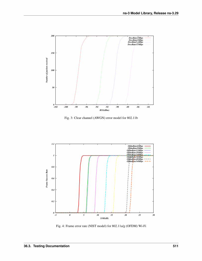
ns-3 Model Library, Release ns-3.29
0
50
100
150
200
-102 -100 -98 -96 -94 -92 -90 -88 -86 -84
Nu
mb
er o
f p
ack
ets
rece
ived
RSS(dBm)
DsssRate1MbpsDsssRate2Mbps
DsssRate55MbpsDsssRate11Mbps
Fig. 3: Clear channel (AWGN) error model for 802.11b
0
0.2
0.4
0.6
0.8
1
1.2
-5 0 5 10 15 20 25 30
Fra
me
Su
cces
s R
ate
SNR(dB)
OfdmRate6MbpsOfdmRate9Mbps
OfdmRate12MbpsOfdmRate18MbpsOfdmRate24MbpsOfdmRate36MbpsOfdmRate48MbpsOfdmRate54Mbps
Fig. 4: Frame error rate (NIST model) for 802.11a/g (OFDM) Wi-Fi
36.3. Testing Documentation 511
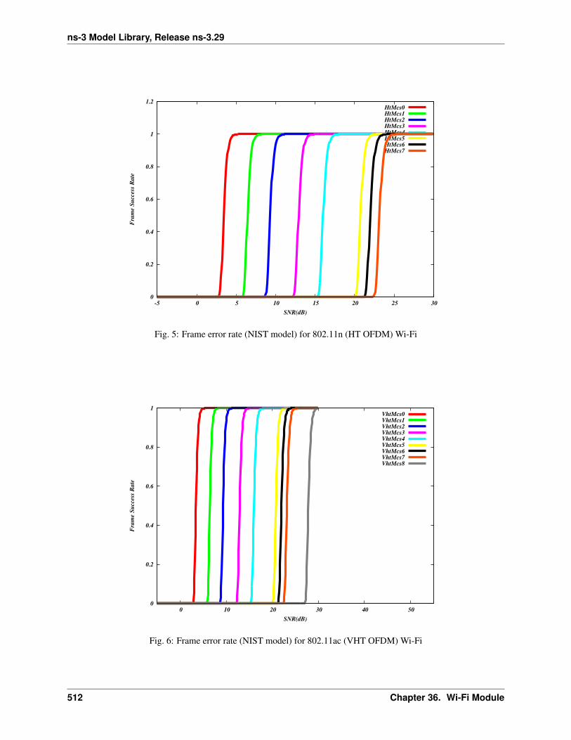
ns-3 Model Library, Release ns-3.29
0
0.2
0.4
0.6
0.8
1
1.2
-5 0 5 10 15 20 25 30
Fra
me S
uccess
Ra
te
SNR(dB)
HtMcs0HtMcs1HtMcs2HtMcs3HtMcs4HtMcs5HtMcs6HtMcs7
Fig. 5: Frame error rate (NIST model) for 802.11n (HT OFDM) Wi-Fi
0
0.2
0.4
0.6
0.8
1
0 10 20 30 40 50
Fra
me S
uccess
Ra
te
SNR(dB)
VhtMcs0VhtMcs1VhtMcs2VhtMcs3VhtMcs4VhtMcs5VhtMcs6VhtMcs7VhtMcs8
Fig. 6: Frame error rate (NIST model) for 802.11ac (VHT OFDM) Wi-Fi
512 Chapter 36. Wi-Fi Module

ns-3 Model Library, Release ns-3.29
0
0.2
0.4
0.6
0.8
1
0 10 20 30 40 50
Fra
me S
uccess
Ra
te
SNR(dB)
HeMcs0HeMcs1HeMcs2HeMcs3HeMcs4HeMcs5HeMcs6HeMcs7HeMcs8HeMcs9
HeMcs10HeMcs11
Fig. 7: Frame error rate (NIST model) for 802.11ax (HE OFDM) Wi-Fi
36.3.3 SpectrumWiFiPhy
The SpectrumWifiPhy implementation has been verified to produce equivalent results to the legacy YansWifiPhy byusing the saturation and packet error rate programs (described below) and toggling the implementation between thetwo physical layers.
A basic unit test is provided using injection of hand-crafted packets to a receiving Phy object, controlling the timingand receive power of each packet arrival and checking the reception results. However, most of the testing of this Phyimplementation has been performed using example programs described below, and during the course of a (separate)LTE/Wi-Fi coexistence study not documented herein.
Saturation performance
The program examples/wireless/wifi-spectrum-saturation-example.cc allows user to select ei-ther the SpectrumWifiPhy or YansWifiPhy for saturation tests. The wifiType can be toggled by the argument'--wifiType=ns3::YansWifiPhy' or --wifiType=ns3::SpectrumWifiPhy'
There isn’t any difference in the output, which is to be expected because this test is more of a test of the DCF than thephysical layer.
By default, the program will use the SpectrumWifiPhy and will run for 10 seconds of saturating UDP data, with 802.11nfeatures enabled. It produces this output for the main 802.11n rates (with short and long guard intervals):
wifiType: ns3::SpectrumWifiPhy distance: 1mindex MCS width Rate (Mb/s) Tput (Mb/s) Received
0 0 20 6.5 5.81381 49371 1 20 13 11.8266 100432 2 20 19.5 17.7935 151103 3 20 26 23.7958 202074 4 20 39 35.7331 303445 5 20 52 47.6174 40436
(continues on next page)
36.3. Testing Documentation 513
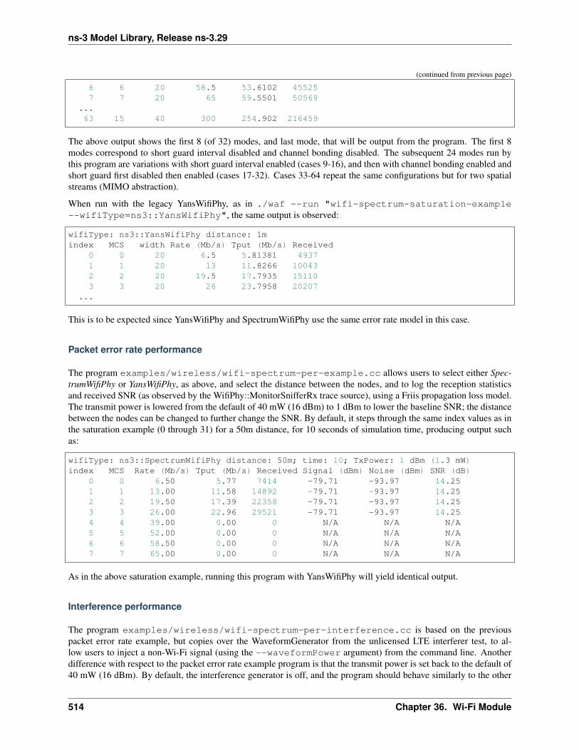
ns-3 Model Library, Release ns-3.29
(continued from previous page)
6 6 20 58.5 53.6102 455257 7 20 65 59.5501 50569
...63 15 40 300 254.902 216459
The above output shows the first 8 (of 32) modes, and last mode, that will be output from the program. The first 8modes correspond to short guard interval disabled and channel bonding disabled. The subsequent 24 modes run bythis program are variations with short guard interval enabled (cases 9-16), and then with channel bonding enabled andshort guard first disabled then enabled (cases 17-32). Cases 33-64 repeat the same configurations but for two spatialstreams (MIMO abstraction).
When run with the legacy YansWifiPhy, as in ./waf --run "wifi-spectrum-saturation-example--wifiType=ns3::YansWifiPhy", the same output is observed:
wifiType: ns3::YansWifiPhy distance: 1mindex MCS width Rate (Mb/s) Tput (Mb/s) Received
0 0 20 6.5 5.81381 49371 1 20 13 11.8266 100432 2 20 19.5 17.7935 151103 3 20 26 23.7958 20207
...
This is to be expected since YansWifiPhy and SpectrumWifiPhy use the same error rate model in this case.
Packet error rate performance
The program examples/wireless/wifi-spectrum-per-example.cc allows users to select either Spec-trumWifiPhy or YansWifiPhy, as above, and select the distance between the nodes, and to log the reception statisticsand received SNR (as observed by the WifiPhy::MonitorSnifferRx trace source), using a Friis propagation loss model.The transmit power is lowered from the default of 40 mW (16 dBm) to 1 dBm to lower the baseline SNR; the distancebetween the nodes can be changed to further change the SNR. By default, it steps through the same index values as inthe saturation example (0 through 31) for a 50m distance, for 10 seconds of simulation time, producing output suchas:
wifiType: ns3::SpectrumWifiPhy distance: 50m; time: 10; TxPower: 1 dBm (1.3 mW)index MCS Rate (Mb/s) Tput (Mb/s) Received Signal (dBm) Noise (dBm) SNR (dB)
0 0 6.50 5.77 7414 -79.71 -93.97 14.251 1 13.00 11.58 14892 -79.71 -93.97 14.252 2 19.50 17.39 22358 -79.71 -93.97 14.253 3 26.00 22.96 29521 -79.71 -93.97 14.254 4 39.00 0.00 0 N/A N/A N/A5 5 52.00 0.00 0 N/A N/A N/A6 6 58.50 0.00 0 N/A N/A N/A7 7 65.00 0.00 0 N/A N/A N/A
As in the above saturation example, running this program with YansWifiPhy will yield identical output.
Interference performance
The program examples/wireless/wifi-spectrum-per-interference.cc is based on the previouspacket error rate example, but copies over the WaveformGenerator from the unlicensed LTE interferer test, to al-low users to inject a non-Wi-Fi signal (using the --waveformPower argument) from the command line. Anotherdifference with respect to the packet error rate example program is that the transmit power is set back to the default of40 mW (16 dBm). By default, the interference generator is off, and the program should behave similarly to the other
514 Chapter 36. Wi-Fi Module

ns-3 Model Library, Release ns-3.29
packet error rate example, but by adding small amounts of power (e.g. --waveformPower=0.001), one will startto observe SNR degradation and frame loss.
Some sample output with default arguments (no interference) is:
./waf --run "wifi-spectrum-per-interference"
wifiType: ns3::SpectrumWifiPhy distance: 50m; time: 10; TxPower: 16 dBm (40 mW)index MCS Rate (Mb/s) Tput (Mb/s) Received Signal (dBm)Noi+Inf(dBm) SNR (dB)
0 0 6.50 5.77 7414 -64.69 -93.97 29.271 1 13.00 11.58 14892 -64.69 -93.97 29.272 2 19.50 17.39 22358 -64.69 -93.97 29.273 3 26.00 23.23 29875 -64.69 -93.97 29.274 4 39.00 34.90 44877 -64.69 -93.97 29.275 5 52.00 46.51 59813 -64.69 -93.97 29.276 6 58.50 52.39 67374 -64.69 -93.97 29.277 7 65.00 58.18 74819 -64.69 -93.97 29.27
...
while a small amount of waveform power will cause frame losses to occur at higher order modulations, due to lowerSNR:
./waf --run "wifi-spectrum-per-interference --waveformPower=0.001"
wifiType: ns3::SpectrumWifiPhy distance: 50m; sent: 1000 TxPower: 16 dBm (40 mW)index MCS Rate (Mb/s) Tput (Mb/s) Received Signal (dBm)Noi+Inf(dBm) SNR (dB)
0 0 6.50 5.77 7414 -64.69 -80.08 15.381 1 13.00 11.58 14892 -64.69 -80.08 15.382 2 19.50 17.39 22358 -64.69 -80.08 15.383 3 26.00 23.23 29873 -64.69 -80.08 15.384 4 39.00 0.41 531 -64.69 -80.08 15.385 5 52.00 0.00 0 N/A N/A N/A6 6 58.50 0.00 0 N/A N/A N/A7 7 65.00 0.00 0 N/A N/A N/A
...
If ns3::YansWifiPhy is selected as the wifiType, the waveform generator will not be enabled because only transmittersof type YansWifiPhy may be connected to a YansWifiChannel.
The interference signal as received by the sending node is typically below the default -62 dBm CCA Mode 1 thresholdin this example. If it raises above, the sending node will suppress all transmissions.
36.4 References
36.4. References 515

ns-3 Model Library, Release ns-3.29
516 Chapter 36. Wi-Fi Module

CHAPTER
THIRTYSEVEN
WIMAX NETDEVICE
This chapter describes the ns-3 WimaxNetDevice and related models. By adding WimaxNetDevice objects to ns-3 nodes, one can create models of 802.16-based networks. Below, we list some more details about what the ns-3WiMAX models cover but, in summary, the most important features of the ns-3 model are:
• a scalable and realistic physical layer and channel model
• a packet classifier for the IP convergence sublayer
• efficient uplink and downlink schedulers
• support for Multicast and Broadcast Service (MBS), and
• packet tracing functionality
The source code for the WiMAX models lives in the directory src/wimax.
There have been two academic papers published on this model:
• M.A. Ismail, G. Piro, L.A. Grieco, and T. Turletti, “An Improved IEEE 802.16 WiMAX Module for the NS-3Simulator”, SIMUTools 2010 Conference, March 2010.
• J. Farooq and T. Turletti, “An IEEE 802.16 WiMAX module for the NS-3 Simulator,” SIMUTools 2009 Confer-ence, March 2009.
37.1 Scope of the model
From a MAC perspective, there are two basic modes of operation, that of a Subscriber Station (SS) or aBase Station (BS). These are implemented as two subclasses of the base class ns3::NetDevice, classSubscriberStationNetDevice and class BaseStationNetDevice. As is typical in ns-3, there is alsoa physical layer class WimaxPhy and a channel class WimaxChannel which serves to hold the references to all ofthe attached Phy devices. The main physical layer class is the SimpleOfdmWimaxChannel class.
Another important aspect of WiMAX is the uplink and downlink scheduler, and there are three primary schedulertypes implemented:
• SIMPLE: a simple priority based FCFS scheduler
• RTPS: a real-time polling service (rtPS) scheduler
• MBQOS: a migration-based uplink scheduler
The following additional aspects of the 802.16 specifications, as well as physical layer and channel models, are mod-elled:
• leverages existing ns-3 wireless propagation loss and delay models, as well as ns-3 mobility models
• Point-to-Multipoint (PMP) mode and the WirelessMAN-OFDM PHY layer
517
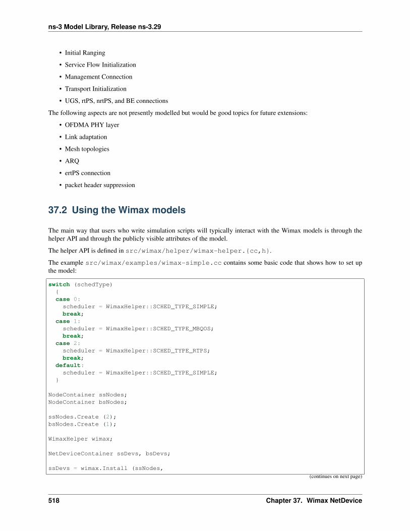
ns-3 Model Library, Release ns-3.29
• Initial Ranging
• Service Flow Initialization
• Management Connection
• Transport Initialization
• UGS, rtPS, nrtPS, and BE connections
The following aspects are not presently modelled but would be good topics for future extensions:
• OFDMA PHY layer
• Link adaptation
• Mesh topologies
• ARQ
• ertPS connection
• packet header suppression
37.2 Using the Wimax models
The main way that users who write simulation scripts will typically interact with the Wimax models is through thehelper API and through the publicly visible attributes of the model.
The helper API is defined in src/wimax/helper/wimax-helper.{cc,h}.
The example src/wimax/examples/wimax-simple.cc contains some basic code that shows how to set upthe model:
switch (schedType){case 0:scheduler = WimaxHelper::SCHED_TYPE_SIMPLE;break;
case 1:scheduler = WimaxHelper::SCHED_TYPE_MBQOS;break;
case 2:scheduler = WimaxHelper::SCHED_TYPE_RTPS;break;
default:scheduler = WimaxHelper::SCHED_TYPE_SIMPLE;
}
NodeContainer ssNodes;NodeContainer bsNodes;
ssNodes.Create (2);bsNodes.Create (1);
WimaxHelper wimax;
NetDeviceContainer ssDevs, bsDevs;
ssDevs = wimax.Install (ssNodes,
(continues on next page)
518 Chapter 37. Wimax NetDevice

ns-3 Model Library, Release ns-3.29
(continued from previous page)
WimaxHelper::DEVICE_TYPE_SUBSCRIBER_STATION,WimaxHelper::SIMPLE_PHY_TYPE_OFDM,scheduler);
bsDevs = wimax.Install (bsNodes, WimaxHelper::DEVICE_TYPE_BASE_STATION,↪→WimaxHelper::SIMPLE_PHY_TYPE_OFDM, scheduler);
This example shows that there are two subscriber stations and one base station created. The helper method Installallows the user to specify the scheduler type, the physical layer type, and the device type.
Different variants of Install are available; for instance, the example src/wimax/examples/wimax-multicast.cc shows how to specify a non-default channel or propagation model:
channel = CreateObject<SimpleOfdmWimaxChannel> ();channel->SetPropagationModel (SimpleOfdmWimaxChannel::COST231_PROPAGATION);ssDevs = wimax.Install (ssNodes,
WimaxHelper::DEVICE_TYPE_SUBSCRIBER_STATION,WimaxHelper::SIMPLE_PHY_TYPE_OFDM,channel,scheduler);
Ptr<WimaxNetDevice> dev = wimax.Install (bsNodes.Get (0),WimaxHelper::DEVICE_TYPE_BASE_STATION,WimaxHelper::SIMPLE_PHY_TYPE_OFDM,channel,scheduler);
Mobility is also supported in the same way as in Wifi models; see the src/wimax/examples/wimax-multicast.cc.
Another important concept in WiMAX is that of a service flow. This is a unidirectional flow of packets with a set ofQoS parameters such as traffic priority, rate, scheduling type, etc. The base station is responsible for issuing serviceflow identifiers and mapping them to WiMAX connections. The following code from src/wimax/examples/wimax-multicast.cc shows how this is configured from a helper level:
ServiceFlow MulticastServiceFlow = wimax.CreateServiceFlow (ServiceFlow::SF_DIRECTION_↪→DOWN,
ServiceFlow::SF_TYPE_UGS,MulticastClassifier);
bs->GetServiceFlowManager ()->AddMulticastServiceFlow (MulticastServiceFlow,↪→WimaxPhy::MODULATION_TYPE_QPSK_12);
37.3 Wimax Attributes
The WimaxNetDevice makes heavy use of the ns-3 attributes subsystem for configuration and default value manage-ment. Presently, approximately 60 values are stored in this system.
For instance, class ns-3::SimpleOfdmWimaxPhy exports these attributes:
• NoiseFigure: Loss (dB) in the Signal-to-Noise-Ratio due to non-idealities in the receiver.
• TxPower: Transmission power (dB)
• G: The ratio of CP time to useful time
• txGain: Transmission gain (dB)
• RxGain: Reception gain (dB)
37.3. Wimax Attributes 519

ns-3 Model Library, Release ns-3.29
• Nfft: FFT size
• TraceFilePath: Path to the directory containing SNR to block error rate files
For a full list of attributes in these models, consult the Doxygen page that lists all attributes for ns-3.
37.4 Wimax Tracing
ns-3 has a sophisticated tracing infrastructure that allows users to hook into existing trace sources, or to define andexport new ones.
Many ns-3 users use the built-in Pcap or Ascii tracing, and the WimaxHelper has similar APIs:
AsciiTraceHelper ascii;WimaxHelper wimax;wimax.EnablePcap ("wimax-program", false);wimax.EnableAsciiAll (ascii.CreateFileStream ("wimax-program.tr");
Unlike other helpers, there is also a special EnableAsciiForConnection() method that limits the ascii tracingto a specific device and connection.
These helpers access the low level trace sources that exist in the WiMAX physical layer, net device, and queue models.Like other ns-3 trace sources, users may hook their own functions to these trace sources if they want to do customizedthings based on the packet events. See the Doxygen List of trace sources for a complete list of these sources.
37.5 Wimax MAC model
The 802.16 model provided in ns-3 attempts to provide an accurate MAC and PHY level implementation of the 802.16specification with the Point-to-Multipoint (PMP) mode and the WirelessMAN-OFDM PHY layer. The model is mainlycomposed of three layers:
• The convergence sublayer (CS)
• The MAC CP Common Part Sublayer (MAC-CPS)
• Physical (PHY) layer
The following figure WiMAX architecture shows the relationships of these models.
37.5.1 Convergence Sublayer
The Convergence sublayer (CS) provided with this module implements the Packet CS, designed to work with thepacket-based protocols at higher layers. The CS is responsible of receiving packet from the higher layer and frompeer stations, classifying packets to appropriate connections (or service flows) and processing packets. It keeps amapping of transport connections to service flows. This enables the MAC CPS identifying the Quality of Service(QoS) parameters associated to a transport connection and ensuring the QoS requirements. The CS currently employsan IP classifier.
37.5.2 IP Packet Classifier
An IP packet classifier is used to map incoming packets to appropriate connections based on a set of criteria. Theclassifier maintains a list of mapping rules which associate an IP flow (src IP address and mask, dst IP address andmask, src port range, dst port range and protocol) to one of the service flows. By analyzing the IP and the TCP/UDP
520 Chapter 37. Wimax NetDevice
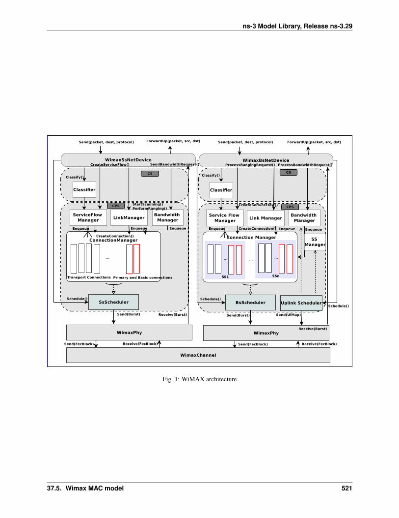
ns-3 Model Library, Release ns-3.29
Fig. 1: WiMAX architecture
37.5. Wimax MAC model 521
ns-3 Model Library, Release ns-3.29
headers the classifier will append the incoming packet (from the upper layer) to the queue of the appropriate WiMAXconnection. Class IpcsClassifier and class IpcsClassifierRecord implement the classifier module forboth SS and BS
37.5.3 MAC Common Part Sublayer
The MAC Common Part Sublayer (CPS) is the main sublayer of the IEEE 802.16 MAC and performs the fundamentalfunctions of the MAC. The module implements the Point-Multi-Point (PMP) mode. In PMP mode BS is respon-sible of managing communication among multiple SSs. The key functionalities of the MAC CPS include framingand addressing, generation of MAC management messages, SS initialization and registration, service flow manage-ment, bandwidth management and scheduling services. Class WimaxNetDevice represents the MAC layer of aWiMAX network device. This class extends the class NetDevice of the ns-3 API that provides abstraction ofa network device. Class WimaxNetDevice is further extended by class BaseStationNetDevice and classSubscriberStationNetDevice, defining MAC layers of BS and SS, respectively. Besides these main classes,the key functions of MAC are distributed to several other classes.
37.5.4 Framing and Management Messages
The module implements a frame as a fixed duration of time, i.e., frame boundaries are defined with respect to time.Each frame is further subdivided into downlink (DL) and uplink (UL) subframes. The module implements the TimeDivision Duplex (TDD) mode where DL and UL operate on same frequency but are separated in time. A number ofDL and UL bursts are then allocated in DL and UL subframes, respectively. Since the standard allows sending andreceiving bursts of packets in a given DL or UL burst, the unit of transmission at the MAC layer is a packet burst. Themodule implements a special PacketBurst data structure for this purpose. A packet burst is essentially a list of packets.The BS downlink and uplink schedulers, implemented by class BSScheduler and class UplinkScheduler,are responsible of generating DL and UL subframes, respectively. In the case of DL, the subframe is simulated bytransmitting consecutive bursts (instances PacketBurst). In case of UL, the subframe is divided, with respect to time,into a number of slots. The bursts transmitted by the SSs in these slots are then aligned to slot boundaries. The frame isdivided into integer number of symbols and Physical Slots (PS) which helps in managing bandwidth more effectively.The number of symbols per frame depends on the underlying implementation of the PHY layer. The size of a DL orUL burst is specified in units of symbols.
37.5.5 Network Entry and Initialization
The network entry and initialization phase is basically divided into two sub-phases, (1) scanning and synchronizationand (2) initial ranging. The entire phase is performed by the LinkManager component of SS and BS. Once an SSwants to join the network, it first scans the downlink frequencies to search for a suitable channel. The search iscomplete as soon as it detects a PHY frame. The next step is to establish synchronization with the BS. Once SSreceives a Downlink-MAP (DL-MAP) message the synchronization phase is complete and it remains synchronized aslong as it keeps receiving DL-MAP and Downlink Channel Descriptor (DCD) messages. After the synchronization isestablished, SS waits for a Uplink Channel Descriptor (UCD) message to acquire uplink channel parameters. Onceacquired, the first sub-phase of the network entry and initialization is complete. Once synchronization is achieved, theSS waits for a UL-MAP message to locate a special grant, called initial ranging interval, in the UL subframe. Thisgrant is allocated by the BS Uplink Scheduler at regular intervals. Currently this interval is set to 0.5 ms, however theuser is enabled to modify its value from the simulation script.
37.5.6 Connections and Addressing
All communication at the MAC layer is carried in terms of connections. The standard defines a connection as aunidirectional mapping between the SS and BS’s MAC entities for the transmission of traffic. The standard defines two
522 Chapter 37. Wimax NetDevice
ns-3 Model Library, Release ns-3.29
types of connections: management connections for transmitting control messages and transport connections for datatransmission. A connection is identified by a 16-bit Connection Identifier (CID). Class WimaxConnection and classCid implement the connection and CID, respectively. Note that each connection maintains its own transmission queuewhere packets to transmit on that connection are queued. The ConnectionManager component of BS is responsible ofcreating and managing connections for all SSs.
The two key management connections defined by the standard, namely the Basic and Primary management con-nections, are created and allocated to the SS during the ranging process. Basic connection plays an important rolethroughout the operation of SS also because all (unicast) DL and UL grants are directed towards SS’s Basic CID. Inaddition to management connections, an SS may have one or more transport connections to send data packets. TheConnection Manager component of SS manages the connections associated to SS. As defined by the standard, a man-agement connection is bidirectional, i.e., a pair of downlink and uplink connections is represented by the same CID.This feature is implemented in a way that one connection (in DL direction) is created by the BS and upon receivingthe CID the SS then creates an identical connection (in UL direction) with the same CID.
37.5.7 Scheduling Services
The module supports the four scheduling services defined by the 802.16-2004 standard:
• Unsolicited Grant Service (UGS)
• Real-Time Polling Services (rtPS)
• Non Real-Time Polling Services (nrtPS)
• Best Effort (BE)
These scheduling services behave differently with respect to how they request bandwidth as well as how the it isgranted. Each service flow is associated to exactly one scheduling service, and the QoS parameter set associated to aservice flow actually defines the scheduling service it belongs to. When a service flow is created the UplinkSchedulercalculates necessary parameters such as grant size and grant interval based on QoS parameters associated to it.
37.5.8 WiMAX Uplink Scheduler Model
Uplink Scheduler at the BS decides which of the SSs will be assigned uplink allocations based on the QoS parametersassociated to a service flow (or scheduling service) and bandwidth requests from the SSs. Uplink scheduler togetherwith Bandwidth Manager implements the complete scheduling service functionality. The standard defines up to fourscheduling services (BE, UGS, rtPS, nrtPS) for applications with different types of QoS requirements. The serviceflows of these scheduling services behave differently with respect to how they request for bandwidth as well as howthe bandwidth is granted. The module supports all four scheduling services. Each service flow is associated to exactlyone transport connection and one scheduling service. The QoS parameters associated to a service flow actually definethe scheduling service it belongs to. Standard QoS parameters for UGS, rtPS, nrtPS and BE services, as specified inTables 111a to 111d of the 802.16e amendment, are supported. When a service flow is created the uplink schedulercalculates necessary parameters such as grant size and allocation interval based on QoS parameters associated to it.The current WiMAX module provides three different versions of schedulers.
• The first one is a simple priority-based First Come First Serve (FCFS). For the real-time services (UGS andrtPS) the BS then allocates grants/polls on regular basis based on the calculated interval. For the non real-timeservices (nrtPS and BE) only minimum reserved bandwidth is guaranteed if available after servicing real-timeflows. Note that not all of these parameters are utilized by the uplink scheduler. Also note that currently onlyservice flow with fixed-size packet size are supported, as currently set up in simulation scenario with OnOffapplication of fixed packet size. This scheduler is implemented by class BSSchedulerSimple and classUplinkSchedulerSimple.
• The second one is similar to first scheduler except by rtPS service flow. All rtPS Connections are able totransmit all packet in the queue according to the available bandwidth. The bandwidth saturation control has
37.5. Wimax MAC model 523

ns-3 Model Library, Release ns-3.29
been implemented to redistribute the effective available bandwidth to all rtPS that have at least one packet totransmit. The remaining bandwidth is allocated to nrtPS and BE Connections. This scheduler is implementedby class BSSchedulerRtps and class UplinkSchedulerRtps.
• The third one is a Migration-based Quality of Service uplink scheduler This uplink scheduler uses three queues,the low priority queue, the intermediate queue and the high priority queue. The scheduler serves the requestsin strict priority order from the high priority queue to the low priority queue. The low priority queue stores thebandwidth requests of the BE service flow. The intermediate queue holds bandwidth requests sent by rtPS andby nrtPS connections. rtPS and nrtPS requests can migrate to the high priority queue to guarantee that their QoSrequirements are met. Besides the requests migrated from the intermediate queue, the high priority queue storesperiodic grants and unicast request opportunities that must be scheduled in the following frame. To guaranteethe maximum delay requirement, the BS assigns a deadline to each rtPS bandwidth request in the intermediatequeue. The minimum bandwidth requirement of both rtPS and nrtPS connections is guaranteed over a windowof duration T. This scheduler is implemented by class UplinkSchedulerMBQoS.
37.5.9 WiMAX Outbound Schedulers Model
Besides the uplink scheduler these are the outbound schedulers at BS and SS side (BSScheduler and SSScheduler). Theoutbound schedulers decide which of the packets from the outbound queues will be transmitted in a given allocation.The outbound scheduler at the BS schedules the downlink traffic, i.e., packets to be transmitted to the SSs in thedownlink subframe. Similarly the outbound scheduler at a SS schedules the packet to be transmitted in the uplinkallocation assigned to that SS in the uplink subframe. All three schedulers have been implemented to work as FCFSscheduler, as they allocate grants starting from highest priority scheduling service to the lower priority one (UGS>rtPS> nrtPS> BE). The standard does not suggest any scheduling algorithm and instead leaves this decision up to themanufacturers. Of course more sophisticated algorithms can be added later if required.
37.6 WimaxChannel and WimaxPhy models
The module implements the Wireless MAN OFDM PHY specifications as the more relevant for implementation as itis the schema chosen by the WiMAX Forum. This specification is designed for non-light-of-sight (NLOS) includingfixed and mobile broadband wireless access. The proposed model uses a 256 FFT processor, with 192 data subcarriers.It supports all the seven modulation and coding schemes specified by Wireless MAN-OFDM. It is composed of twoparts: the channel model and the physical model.
37.7 Channel model
The channel model we propose is implemented by the class SimpleOFDMWimaxChannel which extends the classwimaxchannel. The channel entity has a private structure named m_phyList which handles all the physical devicesconnected to it. When a physical device sends a packet (FEC Block) to the channel, the channel handles the packet,and then for each physical device connected to it, it calculates the propagation delay, the path loss according to agiven propagation model and eventually forwards the packet to the receiver device. The channel class uses the methodGetDistanceFrom() to calculate the distance between two physical entities according to their 3D coordinates. Thedelay is computed as delay = distance/C, where C is the speed of the light.
37.8 Physical model
The physical layer performs two main operations: (i) It receives a burst from a channel and forwards it to the MAClayer, (ii) it receives a burst from the MAC layer and transmits it on the channel. In order to reduce the simulationcomplexity of the WiMAX physical layer, we have chosen to model offline part of the physical layer. More specifically
524 Chapter 37. Wimax NetDevice
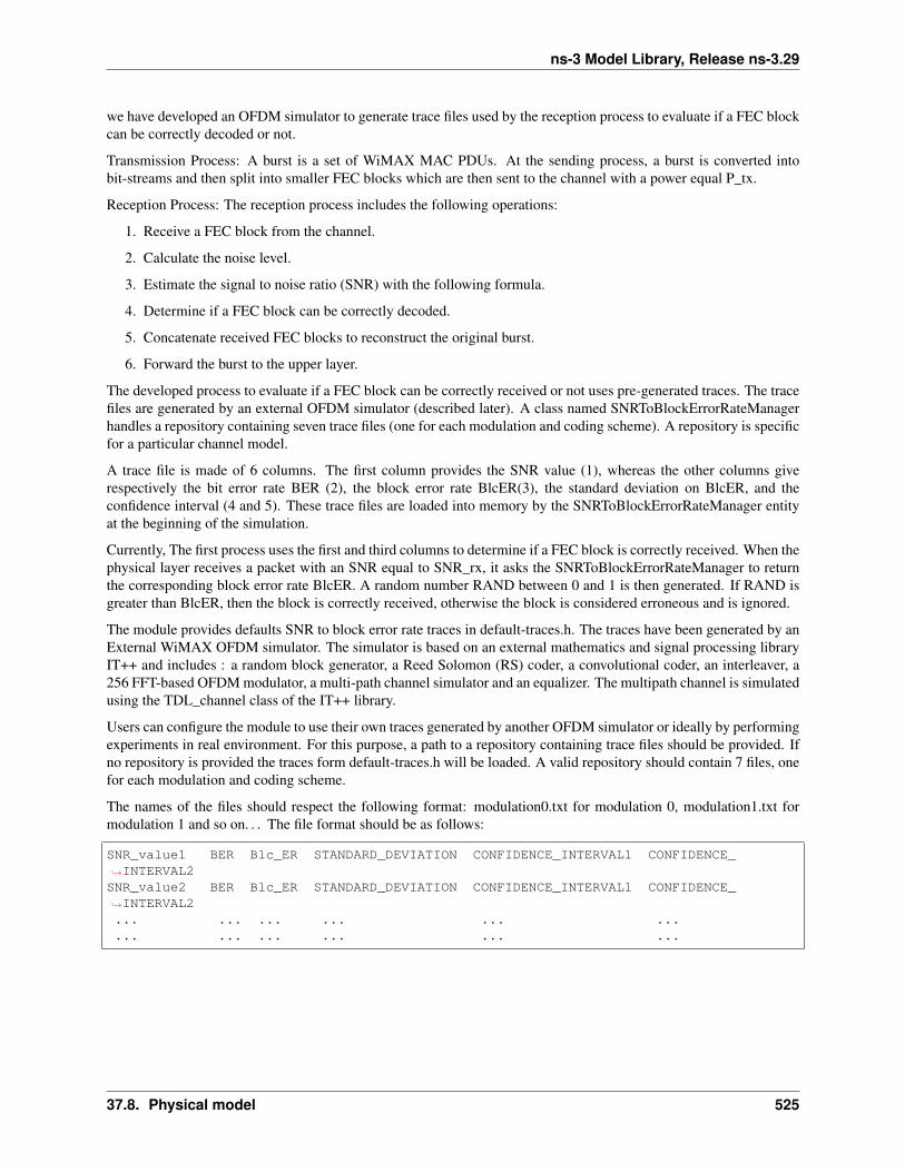
ns-3 Model Library, Release ns-3.29
we have developed an OFDM simulator to generate trace files used by the reception process to evaluate if a FEC blockcan be correctly decoded or not.
Transmission Process: A burst is a set of WiMAX MAC PDUs. At the sending process, a burst is converted intobit-streams and then split into smaller FEC blocks which are then sent to the channel with a power equal P_tx.
Reception Process: The reception process includes the following operations:
1. Receive a FEC block from the channel.
2. Calculate the noise level.
3. Estimate the signal to noise ratio (SNR) with the following formula.
4. Determine if a FEC block can be correctly decoded.
5. Concatenate received FEC blocks to reconstruct the original burst.
6. Forward the burst to the upper layer.
The developed process to evaluate if a FEC block can be correctly received or not uses pre-generated traces. The tracefiles are generated by an external OFDM simulator (described later). A class named SNRToBlockErrorRateManagerhandles a repository containing seven trace files (one for each modulation and coding scheme). A repository is specificfor a particular channel model.
A trace file is made of 6 columns. The first column provides the SNR value (1), whereas the other columns giverespectively the bit error rate BER (2), the block error rate BlcER(3), the standard deviation on BlcER, and theconfidence interval (4 and 5). These trace files are loaded into memory by the SNRToBlockErrorRateManager entityat the beginning of the simulation.
Currently, The first process uses the first and third columns to determine if a FEC block is correctly received. When thephysical layer receives a packet with an SNR equal to SNR_rx, it asks the SNRToBlockErrorRateManager to returnthe corresponding block error rate BlcER. A random number RAND between 0 and 1 is then generated. If RAND isgreater than BlcER, then the block is correctly received, otherwise the block is considered erroneous and is ignored.
The module provides defaults SNR to block error rate traces in default-traces.h. The traces have been generated by anExternal WiMAX OFDM simulator. The simulator is based on an external mathematics and signal processing libraryIT++ and includes : a random block generator, a Reed Solomon (RS) coder, a convolutional coder, an interleaver, a256 FFT-based OFDM modulator, a multi-path channel simulator and an equalizer. The multipath channel is simulatedusing the TDL_channel class of the IT++ library.
Users can configure the module to use their own traces generated by another OFDM simulator or ideally by performingexperiments in real environment. For this purpose, a path to a repository containing trace files should be provided. Ifno repository is provided the traces form default-traces.h will be loaded. A valid repository should contain 7 files, onefor each modulation and coding scheme.
The names of the files should respect the following format: modulation0.txt for modulation 0, modulation1.txt formodulation 1 and so on. . . The file format should be as follows:
SNR_value1 BER Blc_ER STANDARD_DEVIATION CONFIDENCE_INTERVAL1 CONFIDENCE_↪→INTERVAL2SNR_value2 BER Blc_ER STANDARD_DEVIATION CONFIDENCE_INTERVAL1 CONFIDENCE_↪→INTERVAL2... ... ... ... ... ...... ... ... ... ... ...
37.8. Physical model 525

ns-3 Model Library, Release ns-3.29
526 Chapter 37. Wimax NetDevice

BIBLIOGRAPHY
[Balanis] C.A. Balanis, “Antenna Theory - Analysis and Design”, Wiley, 2nd Ed.
[Chunjian] Li Chunjian, “Efficient Antenna Patterns for Three-Sector WCDMA Systems”, Master of Science Thesis,Chalmers University of Technology, Göteborg, Sweden, 2003
[Calcev] George Calcev and Matt Dillon, “Antenna Tilt Control in CDMA Networks”, in Proc. of the 2nd AnnualInternational Wireless Internet Conference (WICON), 2006
[R4-092042a] 3GPP TSG RAN WG4 (Radio) Meeting #51, R4-092042, Simulation assumptions and parameters forFDD HeNB RF requirements.
[turkmani] Turkmani A.M.D., J.D. Parson and D.G. Lewis, “Radio propagation into buildings at 441, 900 and 1400MHz”, in Proc. of 4th Int. Conference on Land Mobile Radio, 1987.
[FlowMonitor] G. Carneiro, P. Fortuna, and M. Ricardo. 2009. FlowMonitor: a network monitoring frameworkfor the network simulator 3 (NS-3). In Proceedings of the Fourth International ICST Conference onPerformance Evaluation Methodologies and Tools (VALUETOOLS ‘09). http://dx.doi.org/10.4108/ICST.VALUETOOLS2009.7493
[TS25814] 3GPP TS 25.814 “Physical layer aspect for evolved Universal Terrestrial Radio Access”
[TS29274] 3GPP TS 29.274 “Tunnelling Protocol for Control plane (GTPv2-C)”
[TS36101] 3GPP TS 36.101 “E-UTRA User Equipment (UE) radio transmission and reception”
[TS36104] 3GPP TS 36.104 “E-UTRA Base Station (BS) radio transmission and reception”
[TS36133] 3GPP TS 36.133 “E-UTRA Requirements for support of radio resource management”
[TS36211] 3GPP TS 36.211 “E-UTRA Physical Channels and Modulation”
[TS36212] 3GPP TS 36.212 “E-UTRA Multiplexing and channel coding”
[TS36213] 3GPP TS 36.213 “E-UTRA Physical layer procedures”
[TS36214] 3GPP TS 36.214 “E-UTRA Physical layer – Measurements”
[TS36300] 3GPP TS 36.300 “E-UTRA and E-UTRAN; Overall description; Stage 2”
[TS36304] 3GPP TS 36.304 “E-UTRA User Equipment (UE) procedures in idle mode”
[TS36321] 3GPP TS 36.321 “E-UTRA Medium Access Control (MAC) protocol specification”
[TS36322] 3GPP TS 36.322 “E-UTRA Radio Link Control (RLC) protocol specification”
[TS36323] 3GPP TS 36.323 “E-UTRA Packet Data Convergence Protocol (PDCP) specification”
[TS36331] 3GPP TS 36.331 “E-UTRA Radio Resource Control (RRC) protocol specification”
[TS36413] 3GPP TS 36.413 “E-UTRAN S1 application protocol (S1AP)”
527

ns-3 Model Library, Release ns-3.29
[TS36420] 3GPP TS 36.420 “E-UTRAN X2 general aspects and principles”
[TS36423] 3GPP TS 36.423 “E-UTRAN X2 application protocol (X2AP)”
[TR36814] 3GPP TR 36.814 “E-UTRA Further advancements for E-UTRA physical layer aspects”
[R1-081483] 3GPP R1-081483 “Conveying MCS and TB size via PDCCH”
[R4-092042] 3GPP R4-092042 “Simulation assumptions and parameters for FDD HeNB RF requirements”
[FFAPI] FemtoForum “LTE MAC Scheduler Interface Specification v1.11”
[ns3tutorial] “The ns-3 Tutorial”
[ns3manual] “The ns-3 Manual”
[Sesia2009] S. Sesia, I. Toufik and M. Baker, “LTE - The UMTS Long Term Evolution - from theory to practice”,Wiley, 2009
[Baldo2009] N. Baldo and M. Miozzo, “Spectrum-aware Channel and PHY layer modeling for ns3”, Proceedings ofICST NSTools 2009, Pisa, Italy
[Piro2010] Giuseppe Piro, Luigi Alfredo Grieco, Gennaro Boggia, and Pietro Camarda, “A Two-level SchedulingAlgorithm for QoS Support in the Downlink of LTE Cellular Networks”, Proc. of European Wireless,EW2010, Lucca, Italy, Apr., 2010
[Holtzman2000] J.M. Holtzman, “CDMA forward link waterfilling power control”, in Proc. of IEEE VTC Spring,2000.
[Piro2011] G. Piro, N. Baldo. M. Miozzo, “An LTE module for the ns-3 network simulator”, in Proc. of Wns3 2011(in conjunction with SimuTOOLS 2011), March 2011, Barcelona (Spain)
[Seo2004] H. Seo, B. G. Lee. “A proportional-fair power allocation scheme for fair and efficient multiuser OFDMsystems”, in Proc. of IEEE GLOBECOM, December 2004. Dallas (USA)
[Ofcom2600MHz] Ofcom, “Consultation on assessment of future mobile competition and proposals for the award of800 MHz and 2.6 GHz spectrum and related issues”, March 2011
[RealWireless] RealWireless, “Low-power shared access to spectrum for mobile broadband”, Final Report, OfcomProject MC/073, 18th March 2011
[PaduaPEM] “Ns-developers - LTE error model contribution”
[ViennaLteSim] “The Vienna LTE Simulators”
[LozanoCost] Joan Olmos, Silvia Ruiz, Mario García-Lozano and David Martín-Sacristán, “Link Abstraction ModelsBased on Mutual Information for LTE Downlink”, COST 2100 TD(10)11052 Report
[wimaxEmd] WiMAX Forum White Paper, “WiMAX System Evaluation Methodology”, July 2008.
[mathworks] Matlab R2011b Documentation Communications System Toolbox, “Methodology for Simulating Mul-tipath Fading Channels”
[CatreuxMIMO] S. Catreux, L.J. Greenstein, V. Erceg, “Some results and insights on the performance gains of MIMOsystems,” Selected Areas in Communications, IEEE Journal on , vol.21, no.5, pp. 839- 847, June 2003
[Ikuno2010] J.C. Ikuno, M. Wrulich, M. Rupp, “System Level Simulation of LTE Networks,” Vehicular TechnologyConference (VTC 2010-Spring), 2010 IEEE 71st , vol., no., pp.1-5, 16-19 May 2010
[Milos2012] J. Milos, “Performance Analysis Of PCFICH LTE Control Channel”, Proceedings of the 19th Confer-ence STUDENT EEICT 2012, Brno, CZ, 2012.
[FujitsuWhitePaper] “Enhancing LTE Cell-Edge Performance via PDCCH ICIC”.
528 Bibliography

ns-3 Model Library, Release ns-3.29
[Bharucha2011] Z. Bharucha, G. Auer, T. Abe, N. Miki, “Femto-to-Macro Control Channel Interference Mitigationvia Cell ID Manipulation in LTE,” Vehicular Technology Conference (VTC Fall), 2011 IEEE , vol., no.,pp.1-6, 5-8 Sept. 2011
[R4-081920] 3GPP R4-081920 “LTE PDCCH/PCFICH Demodulation Performance Results with ImplementationMargin”
[FCapo2012] F.Capozzi, G.Piro, L.A. Grieco, G.Boggia, P.Camarda, “Downlink Packet Scheduling in LTE CellularNetworks: Key Design Issues and a Survey”, IEEE Comm. Surveys and Tutorials, vol.2012, no.99, pp.1-23, Jun. 2012
[FABokhari2009] F.A. Bokhari, H. Yanikomeroglu, W.K. Wong, M. Rahman, “Cross-Layer Resource Scheduling forVideo Traffic in the Downlink of OFDMA-Based Wireless 4G Networks”, EURASIP J. Wirel. Commun.Netw., vol.2009, no.3, pp. 1-10, Jan. 2009.
[WKWong2004] W.K. Wong, H.Y. Tang, V.C.M, Leung, “Token bank fair queuing: a new scheduling algorithm forwireless multimedia services”, Int. J. Commun. Syst., vol.17, no.6, pp.591-614, Aug.2004.
[GMonghal2008] G. Mongha, K.I. Pedersen, I.Z. Kovacs, P.E. Mogensen, “QoS Oriented Time and Frequency Do-main Packet Schedulers for The UTRAN Long Term Evolution”, In Proc. IEEE VTC, 2008.
[Dimou2009] K. Dimou, M. Wang, Y. Yang, M. Kazmi, A. Larmo, J. Pettersson, W. Muller, Y. Timner, “Handoverwithin 3GPP LTE: Design Principles and Performance”, Vehicular Technology Conference Fall (VTC2009-Fall), 2009 IEEE 70th, pp.1-5, 20-23 Sept. 2009
[Lee2010] Y.J. Lee, B.J. Shin, J.C. Lim, D.H. Hong, “Effects of time-to-trigger parameter on handover performance inSON-based LTE systems”, Communications (APCC), 2010 16th Asia-Pacific Conference on, pp.492-496,Oct. 31 2010–Nov. 3 2010
[Bbojovic2014] B. Bojovic, N. Baldo, “A new Channel and QoS Aware Scheduler to enhance the capacity of Voiceover LTE systems”, in Proceedings of 11th International Multi-Conference on Systems, Signals & Devices(SSD’14), Castelldefels, 11-14 February 2014, Castelldefels (Spain).
[Baldo2014] N. Baldo, R. Martínez, P. Dini, R. Vilalta, M. Miozzo, R. Casellas, R. Muñoz, “A Testbed for FixedMobile Convergence Experimentation: ADRENALINE-LENA Integration”, in Proceedings of EuropeanWireless 2014, 14-16 May 2014, Barcelona (Spain).
[ASHamza2013] Abdelbaset S. Hamza, Shady S. Khalifa, Haitham S. Hamza, and Khaled Elsayed, “A Survey onInter-Cell Interference Coordination Techniques in OFDMA-based Cellular Networks”, IEEE Communi-cations Surveys & Tutorials, March 19, 2013
[ZXie2009] Zheng Xie, Bernhard Walke, “Enhanced Fractional Frequency Reuse to Increase Capacity of OFDMASystems”, Proceedings of the 3rd international conference on New technologies, mobility and security,NTMS 2009
[DKimura2012] D. Kimura, H. Seki, “Inter-Cell Interference Coordination (ICIC) Technology”, FUJITSU Sci.Tech. J., Vol. 48, No. 1 (January 2012)
[And09] K. Andreev, Realization of IEEE802.11s draft standard in NS-3.
[And10] K. Andreev and P. Boyko, IEEE 802.11s Mesh Networking NS-3 Model.
[Hep15] C. Hepner and A. Witt and R. Muenzner, Validation of the ns-3 802.11s model and proposed changescompliant to IEEE 802.11-2012, Poster at 2015 Workshop on ns-3, May 2015.
[Hep16] C. Hepner and S. Moll and R. Muenzner, Influence of Processing Delays on the VoIP Performance for IEEE802.11s Multihop Wireless Mesh Networks: Comparison of ns-3 Network Simulations with HardwareMeasurements, Proceedings of SIMUTOOLS 16, August, 2016.
[ieee80211s] IEEE Standard for Information Technology, Telecommunications and information exchange betweensystems, Local and metropolitan area networks, Specific requirements, Part 11: Wireless LAN Medium
Bibliography 529

ns-3 Model Library, Release ns-3.29
Access Control (MAC) and Physical Layer (PHY) specifications, Amendment 10: Mesh Networking, 10September 2011.
[rfc3626] RFC 3626 Optimized Link State Routing
[rfc7181] RFC 7181 The Optimized Link State Routing Protocol Version 2
[friis] Friis, H.T., “A Note on a Simple Transmission Formula,” Proceedings of the IRE , vol.34, no.5, pp.254,256,May 1946
[hata] M.Hata, “Empirical formula for propagation loss in land mobile radio services”, IEEE Trans. on VehicularTechnology, vol. 29, pp. 317-325, 1980
[cost231] “Digital Mobile Radio: COST 231 View on the Evolution Towards 3rd Generation Systems”, Commissionof the European Communities, L-2920, Luxembourg, 1989
[walfisch] J.Walfisch and H.L. Bertoni, “A Theoretical model of UHF propagation in urban environments,” in IEEETrans. Antennas Propagat., vol.36, 1988, pp.1788- 1796
[ikegami] F.Ikegami, T.Takeuchi, and S.Yoshida, “Theoretical prediction of mean field strength for Urban MobileRadio”, in IEEE Trans. Antennas Propagat., Vol.39, No.3, 1991
[kun2600mhz] Sun Kun, Wang Ping, Li Yingze, “Path loss models for suburban scenario at 2.3GHz, 2.6GHz and3.5GHz”, in Proc. of the 8th International Symposium on Antennas, Propagation and EM Theory (ISAPE),Kunming, China, Nov 2008.
[Baldo2009Spectrum] N. Baldo and M. Miozzo, “Spectrum-aware Channel and PHY layer modeling for ns3”, Pro-ceedings of ICST NSTools 2009, Pisa, Italy
[Baron8VSB] Baron, Stanley. “First-Hand:Digital Television: The Digital Terrestrial Television Broadcast-ing (DTTB) Standard.” IEEE Global History Network. <http://www.ieeeghn.org/wiki/index.php/First-Hand:Digital_Television:_The_Digital_Terrestrial_Television_Broadcasting_(DTTB)_Standard>.
[KoppCOFDM] Kopp, Carlo. “High Definition Television.” High Definition Television. Air Power Australia. <http://www.ausairpower.net/AC-1100.html>.
[MatlabGeo] “Geodetic2ecef.” Convert Geodetic to Geocentric (ECEF) Coordinates. The MathWorks, Inc. <http://www.mathworks.com/help/map/ref/geodetic2ecef.html>.
[QualcommAnalog] Stephen Shellhammer, Ahmed Sadek, and Wenyi Zhang. “Technical Challenges for CognitiveRadio in the TV White Space Spectrum.” Qualcomm Incorporated.
[RFC4944] RFC 4944, “Transmission of IPv6 Packets over IEEE 802.15.4 Networks”
[RFC6282] RFC 6282, “Compression Format for IPv6 Datagrams over IEEE 802.15.4-Based Networks”
[RFC6775] RFC 6775, “Neighbor Discovery Optimization for IPv6 over Low-Power Wireless Personal Area Net-works (6LoWPANs)”
[IANA802] IANA, assigned IEEE 802 numbers: http://www.iana.org/assignments/ieee-802-numbers/ieee-802-numbers.xml
[Ethertype] IEEE Ethertype numbers: http://standards.ieee.org/develop/regauth/ethertype/eth.txt
[Ref1] A. Kuznetsov and D. Torokhov; Linux Cross Reference Source Code; Available online at http://lxr.free-electrons.com/source/net/sched/sch_tbf.c.
[Ref2] J. Vehent; Journey to the Center of the Linux Kernel: Traffic Control, Shaping and QoS; Avail-able online at http://wiki.linuxwall.info/doku.php/en:resources:dossiers:networking:traffic_control#tbf_-_token_bucket_filter.
[Ref3] Practical IP Network QoS: TBF queuing discipline; Available online at http://web.opalsoft.net/qos/default.php?p=ds-24.
530 Bibliography

ns-3 Model Library, Release ns-3.29
[Nic12] K. Nichols and V. Jacobson, Controlling Queue Delay, ACM Queue, Vol. 10 No. 5, May 2012. Availableonline at http://queue.acm.org/detail.cfm?id=2209336.
[Nic14] K. Nichols and V. Jacobson, Internet-Draft: Controlled Delay Active Queue Management, March 2014.Available online at http://tools.ietf.org/html/draft-nichols-tsvwg-codel-02.
[Buf14] Bufferbloat.net. Available online at http://www.bufferbloat.net/.
[Hoe16] T. Hoeiland-Joergensen, P. McKenney, D. Taht, J. Gettys and E. Dumazet, The FlowQueue-CoDelPacket Scheduler and Active Queue Management Algorithm, IETF draft. Available online at https://tools.ietf.org/html/draft-ietf-aqm-fq-codel
[Buf16] Bufferbloat.net. Available online at http://www.bufferbloat.net/.
[Pan13] Pan, R., Natarajan, P., Piglione, C., Prabhu, M. S., Subramanian, V., Baker, F., & VerSteeg, B. (2013, July).PIE: A lightweight control scheme to address the bufferbloat problem. In High Performance Switching andRouting (HPSR), 2013 IEEE 14th International Conference on (pp. 148-155). IEEE. Available online athttps://www.ietf.org/mail-archive/web/iccrg/current/pdfB57AZSheOH.pdf.
[Pan16] R. Pan, P. Natarajan, F. Baker, G. White, B. VerSteeg, M.S. Prabhu, C. Piglione, V. Subramanian,Internet-Draft: PIE: A lightweight control scheme to address the bufferbloat problem, April 2016.Available online at https://tools.ietf.org/html/draft-ietf-aqm-pie-07.
[ieee80211p] IEEE Std 802.11p-2010 “IEEE Standard for Information technology– Local and metropolitan area net-works– Specific requirements– Part 11: Wireless LAN Medium Access Control (MAC) and Physical Layer(PHY) Specifications Amendment 6: Wireless Access in Vehicular Environments”
[ieee1609dot1] IEEE Std 1609.1-2010 “IEEE Standard for Wireless Access in Vehicular Environments (WAVE) -Resource Manager, 2010”
[ieee1609dot2] IEEE Std 1609.2-2010 “IEEE Standard for Wireless Access in Vehicular Environments (WAVE) -Security Services for Applications and Management Messages, 2010”
[ieee1609dot3] IEEE Std 1609.3-2010 “IEEE Standard for Wireless Access in Vehicular Environments (WAVE) -Networking Services, 2010”
[ieee1609dot4] IEEE Std 1609.4-2010 “IEEE Standard for Wireless Access in Vehicular Environments (WAVE) -Multi-Channel Operation, 2010”
[saej2735] SAE Std J2735 “J2735 dedicated short range communications (DSRC) message set dictionary. 2009”
[ieee80211] IEEE Std 802.11-2012, Part 11: Wireless LAN Medium Access Control (MAC) and Physical Layer (PHY)Specifications
[pei80211b] G. Pei and Tom Henderson, Validation of ns-3 802.11b PHY model
[pei80211ofdm] G. Pei and Tom Henderson, Validation of OFDM error rate model in ns-3
[lacage2006yans] M. Lacage and T. Henderson, Yet another Network Simulator
[Haccoun] D. Haccoun and G. Begin, High-Rate Punctured Convolutional Codes for Viterbi Sequential Decoding,IEEE Transactions on Communications, Vol. 32, Issue 3, pp.315-319.
[Frenger] Pâl Frenger et al., “Multi-rate Convolutional Codes”.
[ji2004sslswn] Z. Ji, J. Zhou, M. Takai and R. Bagrodia, Scalable simulation of large-scale wireless networks withbounded inaccuracies, in Proc. of the Seventh ACM Symposium on Modeling, Analysis and Simulationof Wireless and Mobile Systems, October 2004.
[linuxminstrel] minstrel linux wireless
[lacage2004aarfamrr] M. Lacage, H. Manshaei, and T. Turletti, IEEE 802.11 rate adaptation: a practical approach,in Proc. 7th ACM International Symposium on Modeling, Analysis and Simulation of Wireless and MobileSystems, 2004.
Bibliography 531
ns-3 Model Library, Release ns-3.29
[kim2006cara] J. Kim, S. Kim, S. Choi, and D. Qiao, CARA: Collision-Aware Rate Adaptation for IEEE 802.11WLANs, in Proc. 25th IEEE International Conference on Computer Communications, 2006
[wong2006rraa] S. Wong, H. Yang, S. Lu, and V. Bharghavan, Robust Rate Adaptation for 802.11 Wireless Networks,in Proc. 12th Annual International Conference on Mobile Computing and Networking, 2006
[maguolo2008aarfcd] F. Maguolo, M. Lacage, and T. Turletti, Efficient collision detection for auto rate fallback algo-rithm, in IEEE Symposium on Computers and Communications, 2008
[proakis2001] J. Proakis, Digital Communications, Wiley, 2001.
[miller2003] L. E. Miller, “Validation of 802.11a/UWB Coexistence Simulation.” Technical Report, October 2003.Available online
[ferrari2004] G. Ferrari and G. Corazza, “Tight bounds and accurate approximations for DQPSK transmission biterror rate”, Electronics Letters, 40(20):1284-85, September 2004.
[pursley2009] M. Pursley and T. Royster, “Properties and performance of the IEEE 802.11b complementary code keysignal sets,” IEEE Transactions on Communications, 57(2);440-449, February 2009.
[akella2007parf] A. Akella, G. Judd, S. Seshan, and P. Steenkiste, ‘Self-management in chaotic wireless deploy-ments’, in Wireless Networks, Kluwer Academic Publishers, 2007, 13, 737-755. http://www.cs.odu.edu/~nadeem/classes/cs795-WNS-S13/papers/enter-006.pdf
[chevillat2005aparf] Chevillat, P.; Jelitto, J., and Truong, H. L., ‘Dynamic data rate and transmit power adjustment inIEEE 802.11 wireless LANs’, in International Journal of Wireless Information Networks, Springer, 2005,12, 123-145. http://www.cs.mun.ca/~yzchen/papers/papers/rate_adaptation/80211_dynamic_rate_power_adjustment_chevillat_j2005.pdf
[hepner2015] C. Hepner, A. Witt, and R. Muenzner, “In depth analysis of the ns-3 physical layer abstraction forWLAN systems and evaluation of its influences on network simulation results”, BW-CAR Symposiumon Information and Communication Systems (SInCom) 2015. http://sincom.informatik.hs-furtwangen.de/index.php?id=85
[baldo2010] N. Baldo et al., “Validation of the ns-3 IEEE 802.11 model using the EXTREME testbed”, Proceedingsof SIMUTools Conference, March 2010.
532 Bibliography
INDEX
RRFC
RFC 1058, 105–107RFC 1723, 105RFC 1918, 91RFC 2080, 103, 105–107RFC 2131, 141RFC 2132, 141RFC 2453, 103, 105RFC 3393, 82RFC 3561, 17, 103RFC 3626, 103, 389, 530RFC 4728, 59, 62RFC 4944, 421, 530RFC 6282, 421, 530RFC 6775, 421, 422, 530RFC 7181, 389, 530
533