1

Normal stress effects in the gravity driven flow of granular

materials

Wei-Tao Wu1, Nadine Aubry2, James F. Antaki1, Mehrdad Massoudi3*

1. Department of Biomedical Engineering, Carnegie Mellon University,

Pittsburgh, PA, 15213, USA

2. Department of Mechanical and Industrial Engineering, Northeastern University,

Boston, MA 02115, USA

3. U. S. Department of Energy, National Energy Technology Laboratory (NETL),

Pittsburgh, PA, 15236, USA

Address for correspondence:

Mehrdad Massoudi, PhD,

U. S. Department of Energy,

National Energy Technology Laboratory (NETL),

626 Cochrans Mill Road, P.O. Box 10940,

Pittsburgh, PA. 15236.

Email: Mehrdad.Massoudi@NETL.DOE.GOV

2

Abstract

In this paper, we study the fully developed gravity-driven flow of granular materials between

two inclined planes. We assume that the granular materials can be represented by a modified

form of the second-grade fluid where the viscosity depends on the shear rate and volume

fraction and the normal stress coefficients depend on the volume fraction. We also propose a

new isotropic (spherical) part of the stress tensor which can be related to the compactness of

the (rigid) particles. This new term ensures that the rigid solid particles cannot be compacted

beyond a point, namely when the volume fraction has reached the critical/maximum packing

value. The numerical results indicate that the newly proposed stress tensor has an obvious and

physically meaningful effects on both the velocity and the volume fraction fields.

Keywords: Granular materials; normal-stress effects; Maximum packing; Shear-thinning

fluid; Second grade fluids; continuum mechanics.

1. Introduction

Granular materials are discrete solid macroscopic particles of different shapes and sizes with

interstices filled with a fluid. Granular materials occur in many natural processes, such as the

flow of rock, sand, snow and ice. In industrial applications, water and granular materials (grains,

powders, coals, etc.[1]) are the first and the second mostly used materials. A granular medium

does not behave as a classical solid continuum since it deforms to (takes) the shape of the vessel

containing it; it is not exactly like a liquid, even though it can flow, for it can be piled into

heaps; and it is not a gas since it will not expand to fill the container. In many ways the bulk

solids resemble non-Newtonian (non-linear) fluids [2]. The behavior of granular materials, in

general, is determined by interparticle cohesion, friction, collisions, etc [3]. A granular medium

includes granular powders and granular solids with components ranging in size from about

10 μm up to 3 mm. According to many researchers, a powder is composed of particles up to

100 μm (diameter) with further subdivision into ultrafine (0.1 to 1.0 μm), superfine (1 to

10 μm), or granular (10 to 100 μm) particles, whereas a granular solid consists of particles

ranging from about 100 to 3,000 μm [Brown and Richards (1970) [4]].

Granular materials present a multi-disciplinary field; they can be studied from different

perspectives. For example, in order to characterize their rheological behavior, one can study

the mechanics (or physics) of these complex materials by performing experiments, which are

oftentimes very complicated. Recent review articles by Savage (1984) [5], Hutter and

3

Rajagopal (1994) [6], and de Gennes (1998) [7], and books by Mehta (1994) [8], Duran (2000)

[9], and Antony et al. (2004) [10] point to many of the important issues in modeling granular

materials. From a theoretical perspective, there are two distinct, yet related methods that can

be used: the statistical theories and the continuum theories. There are many recent review

articles discussing the statistical theories [Herrmann (1999) [11], Herrmann and Luding (1998)

[12]], and the kinetic theories as applied to granular materials [Goldhirsch (2003) [13] and

Boyle and Massoudi (1990) [14]].

In this paper, we model the granular materials as a single phase continuum, ignoring the effects

of the interstitial fluid. However, it should be pointed out that in many applications, the effect

of the interstitial fluid is important and the problem should be studied using a multi-component

method [see Rajagopal and Tao (1995) [15], Massoudi (2010) [16]]. In section 2, we will

present the governing equations. In section 3, we will discuss the constitutive equations. In

section 4, we introduce the geometry and kinematics of the problem. In section 5, we discuss

the numerical results through a parametric study of the non-linear ordinary equations for the

gravity driven flow of the granular materials between two inclined plates.

2. Governing Equations

We model the granular materials as a single component non-linear fluid. That is, we ignore the

presence of the interstitial fluid and assume that the assembly of the densely-packed particles

form a continuum. Let 𝑿 denote the position of this continuum body. The motion can be

represented as

𝒙 = 𝝌(𝑿, 𝑡) (1)

while the kinematical quantities associated with this motion are

𝒗 =𝑑𝒙

𝑑𝑡 (2)

𝑫 =1

2(

𝜕𝒗

𝜕𝒙+ (

𝜕𝒗

𝜕𝒙)

𝑇

) (3)

where 𝒗 is the velocity field, 𝑫 is the symmetric part of velocity gradient, and 𝑑

𝑑𝑡 denotes

differentiation with respect to time holding 𝑿 fixed and superscript ‘𝑇’ designates the transpose

of a tensor. The bulk density field, 𝜌, is

𝜌 = (1 − 𝜙)𝜌0 (4)

4

where 𝜌0 is the pure density of granular materials, in the reference configuration; 𝜙 is the

volume fraction, where 0 ≤ 𝜙 < 𝜙𝑚𝑎𝑥 < 1. The function 𝜙 is represented as a continuous

function of position and time; in reality, 𝜙 is either one or zero at any position and at any given

time. That is, in a sense, we have performed a homogenization process (see Collins(2005) [17])

whereby the shape and sizes of the particles in this idealized body have disappeared except

through the presence of the volume fraction. For details see Massoudi (2001) [18] and

Massoudi and Mehrabadi (2001) [19]. In reality, 𝜙 is never equal to one; its maximum value,

generally designated as the maximum packing fraction, depends on the shape, size, method of

packing, etc.

Having defined the basic kinematical parameters, we now look at the conservation equations.

In the absence of any thermo-chemical and electro-magnetic effects, the governing equations

for the flow of a single-component material are the conservation equations for mass, linear

momentum, and angular momentum [20]. As we are only considering a purely mechanical

system, the energy equation and the entropy inequality are not considered.

Conservation of mass

The conservation of mass is:

𝜕𝜌

𝜕𝑡+ 𝑑𝑖𝑣(𝜌𝒗) = 0 (5)

where ∂/∂t is the derivative with respect to time, 𝑑𝑖𝑣 is the divergence operator.

Conservation of linear momentum

Let 𝑻 represent the Cauchy stress tensor for the granular materials. Then the balance of the

linear momentum is:

𝜌𝑑𝒗

𝑑𝑡= 𝑑𝑖𝑣𝑻 + 𝜌𝒃 (6)

where 𝑑𝒗

𝑑𝑡=

𝜕𝒗

𝜕𝑡+ (𝑔𝑟𝑎𝑑𝒗)𝒗 and 𝒃 stands for the body force.

Conservation of Angular Momentum

𝑻 = 𝑻𝑇 (7)

5

The above equation implies that in absence of couple stresses the Cauchy stress tensor is

symmetric. The constitutive relation for the stress tensor need to be specified before any

problem can be solved. In the next section, we will discuss this issue.

3. Constitutive Equation: The stress tensor

Most granular materials exhibit two unusual and peculiar characteristics: (i) normal stress

differences, and (ii) yield criterion1. Reynolds (1885) [21] observed that in a bed of closely

packed particles, the bed must expand if a shearing motion is to occur; this happens in order to

increase the volume of the voids. Reynolds (1886) [22] called this phenomenon ‘dilatancy’ and

he was able to describe the capillary action in wet sand. The concept of dilatancy, which in a

larger context, is related to the normal stress differences in non-linear materials, is related the

expansion of the void volumes in a packed granular arrangement when it is subjected to a

deformation. This can be explained for an idealized case: in a bed of closely packed spheres,

for a shearing motion to occur, for example, between two flat plates, the bed must expand by

increasing its void volume. Reiner (1945, 1948) [23,24] used a non-Newtonian model to predict

dilatancy in wet sand [see Massoudi (2011, 2013) [25,26]]. Perhaps the simplest constitutive

equation which can describe the normal stress effects in non-linear fluids (related to

phenomena such as ‘die-swell’ and ‘rod-climbing’, which are manifestations of the stresses

that develop orthogonal to planes of shear) is the second-grade fluid, or the Rivlin-Ericksen

fluid of grade two [Rivlin and Ericksen (1955) [27], Truesdell and Noll (1992) [28]]. This

model is a special case of fluids of differential type [Dunn and Rajagopal (1995) [29]]. For a

second-grade fluid, the Cauchy stress tensor is given by [30]:

𝑻 = −𝑝𝑰 + 𝜇𝑨1 + 𝛼1𝑨2 + 𝛼2𝑨12 (8)

where 𝑝 is the indeterminate part of the stress due to the constraint of incompressibility. 𝜇 is

the coefficient of viscosity which may depends on shear rate, volume fraction, pressure,

temperature, etc. [31–33], and 𝛼1 and 𝛼2 are material moduli which are commonly referred to

as the normal stress coefficients [34]. The kinematical tensors 𝑨1 and 𝑨2 are defined through

{

𝑨1 = 𝑳 + 𝑳𝑇

𝑨2 =𝑑𝑨1

𝑑𝑡+ 𝑨1𝑳 + 𝑳𝑇𝑨1

𝑳 = 𝑔𝑟𝑎𝑑 𝒗

(9)

1 In this paper, we do not discuss the yield stress.

6

where 𝑳 is the velocity gradient. The thermodynamics and stability of fluids of second grade

have been studied in detail by Dunn and Fosdick (1974) [35]. They concluded that if the fluid

is to be thermodynamically consistent in the sense that all motions of the fluid meet the

Clausius-Duhem inequality and that the specific Helmholtz free energy be a minimum in

equilibrium, then

𝜇 ≥ 0 (10)a

𝛼1 ≥ 0 (10)b

𝛼1 + 𝛼2 = 0 (10)c

It is known that for many non-linear fluids which are assumed to follow Equation (8), the

experimental values reported for 𝛼1 and 𝛼2 do not satisfy the restriction2 of equations (10)b

and (10)c. For further details on this and other relevant issues in fluids of differential type, we

refer the reader to the review article by Dunn and Rajagopal (1995) [29].For some applications,

such as flow of ice or coal slurries, where the fluid is known to be shear-thinning (or shear-

thickening), modified (or generalized) forms of the second-grade fluid have been proposed [see

Man (1992) [36], Massoudi and Vaidya (2008) [37], Man and Massoudi (2010) [38]].

In this paper, we assume that the (flowing) granular materials can be modeled as a non-linear

fluid (of second-grade type) capable of exhibiting normal stress effects, where the shear

viscosity depends on the volume fraction and the shear rate and the normal stress coefficients

depend on the volume fraction:

𝑻 = 𝛽0𝑰 + 𝜇(𝜙, �̇�)𝑨1 + 𝛼1(𝜙)𝑨2 + 𝛼2(𝜙)𝑨12 (11)

Here, 𝛽0 is the spherical (isotropic part of the) stress tensor (which includes the pressure), 𝜇 is

shear the viscosity and �̇� = √1/2tr(𝑨12) is the shear rate, 𝛼1 and 𝛼2 are material moduli,

which are commonly referred to as the normal stress coefficients. For these coefficients we

assume:

{

𝜇 = 𝜇𝑟(𝜙 + 𝜙2)

𝛼1 = 𝛼10(𝜙 + 𝜙2)

𝛼2 = 𝛼20(𝜙 + 𝜙2)

(12)

2In an important paper, Fosdick and Rajagopal (1979) [47] show that irrespective of whether 𝛼1 + 𝛼2 is positive,

the fluid is unsuitable if 𝛼1 is negative.

7

These expressions can be viewed as the Taylor series approximation for the material

parameters [Rajagopal, et al (1994)[39]]. The above equations ensure that the stress vanishes

as 𝜙 → 0.

In general, 𝛽0 is treated as the spherical (the isotropic) part of the stress tensor which includes

terms related to the pressure. In this paper, we propose that once the volume fraction has

reached a critical value, further compacting, which can be measured as the increase in the local

particles concentration, would lead to an additional term related to the isotropic spherical stress

preventing further increase in the local volume fraction3. Therefore, we suggest that 𝛽0 can be

decomposed into two parts: one term is to account for the mechanism related to the pressure,

while the second term is to account for the compacting of the particles,

𝛽0 = (𝛽𝑝 + 𝛽𝑟(𝜙))𝜙 (13)

Based on our previous studies (Rajagopal and Massoudi (1990) [40]), we assume

𝛽𝑝 = 𝛽00 < 0 (14)

as compression should lead to densification of the materials, see [40,41].

We further propose that 𝛽𝑟(𝜙)term can be given by:

𝛽𝑟 = ℎ(𝜙)𝐶𝑟𝑔(𝜙) (15)

ℎ(𝜙) = {0, 𝜙 < 𝜙𝑐 1, 𝜙 ≥ 𝜙𝑐

(16)

where 𝜙𝑐 is the critical value of the volume fraction; where 𝜙 ≥ 𝜙𝑐 the term 𝛽𝑟 appears in the

equation. The values of 𝜙𝑐 may depend on various factors, such as the shape and the size

distributions of the particles. In this paper, we assume 𝑔(𝜙) = 𝜙. 𝐶𝑟 is a material parameter

related to how much the particles can be compacted. For very rigid particles, 𝐶𝑟 is large,

ensuring that the volume fraction of the granular materials cannot be larger than 𝜙𝑐 .

Furthermore, for ease of numerical calculations, we replace ℎ(𝜙) in equation (16) with a

smooth step function, such that

ℎ(𝜙) =1

1 + exp (−2𝑆(𝜙 − 𝜙𝑐)) (17)

3 When the particles are large and heavy, there is a tendency for them to settle under the action of gravity [48,49].

During the sedimentation process, the volume fraction of the particles reaches a critical value beyond which the

particles cannot be compacted any further (due to the rigidity of the particles).

8

where 𝑆 is a parameter related to the slope of the step function. For example, if 𝑆 is chosen as

3000, then ℎ(𝜙𝑐 − 0.001)/ℎ(𝜙𝑐) < 0.01 and ℎ(𝜙𝑐 − 0.005)~𝑜(10−13) , therefore 𝛽𝑟 is

negligible when 𝜙 is close to 𝜙𝑐.

The viscosity is assumed to be modeled as a Carreau-type fluid viscosity, where the viscosity

depends on the shear rate. When the shear rate is close to zero, the viscosity approaches a lower

limit, 𝜇0; when the shear rate is close to infinity, the viscosity approaches an upper limit, 𝜇∞

Following Yeleswarapu (1994)[42], we assume 𝜇𝑟 is given by:

𝜇𝑟 = 𝜇∞ + (𝜇0 − 𝜇∞)1 + ln(1 + 𝑘�̇�)

1 + 𝑘�̇� (18)

where 𝜇0 and 𝜇∞ are the viscosities when the shear rate approaches zero and infinity,

respectively, and 𝑘 is the shear thinning parameter. Different types of solid particles can have

different functions/expressions for 𝜇0, 𝜇∞ and 𝑘.

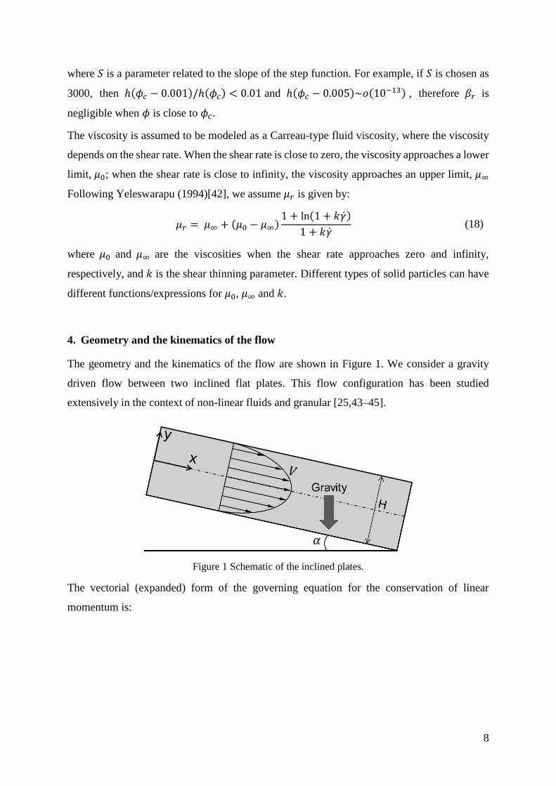
4. Geometry and the kinematics of the flow

The geometry and the kinematics of the flow are shown in Figure 1. We consider a gravity

driven flow between two inclined flat plates. This flow configuration has been studied

extensively in the context of non-linear fluids and granular [25,43–45].

Figure 1 Schematic of the inclined plates.

The vectorial (expanded) form of the governing equation for the conservation of linear

momentum is:

9

𝜙𝜌 [𝜕𝑽

𝜕𝜏+ (grad𝑽)𝑽]

= (grad𝜙)𝐵𝑝 + 𝜙grad𝐵𝑝 + (grad𝜙2)ℎ(𝜙)𝐵𝑟 + 𝜙2grad(ℎ(𝜙)𝐵𝑟)

+ [𝐵31(𝜙 + 𝜙2) + 𝐵32(𝜙 + 𝜙2)𝛱]div𝑨1 + 𝐵31𝑨1grad(𝜙 + 𝜙2)

+ 𝐵32𝑨1[𝛱grad(𝜙 + 𝜙2) + (𝜙 + 𝜙2)grad𝛱] +𝜌

𝐹𝑟𝜙𝒃

+ 𝑀1div((𝜙 + 𝜙2)𝑨2) + 𝑀2𝑑𝑖𝑣((𝜙 + 𝜙2)𝑨12)

(19)

As a results of the non-dimensionalization, we obtain the following non-dimensional

parameters:

𝑌 =𝑦

𝐻; 𝑋 =

𝑥

𝐻; 𝑽 =

𝒗

𝑢0; 𝜏 =

𝑡𝑢0

𝐻; 𝒃∗ =

𝒃

𝑔; 𝜌∗ =

𝜌

𝜌0

div∗(⋅) = 𝐻div(⋅); grad

∗(⋅) = 𝐻grad(⋅); 𝑳∗ = grad∗𝑽

𝑨1∗ = 𝑳∗ + 𝑳∗𝑇; 𝑨2

∗ =𝑑𝑨1

∗

𝑑𝜏+ 𝑨1

∗𝑳∗ + 𝑳∗𝑇𝑨1∗

𝐹𝑟 =𝑢0

2

𝐻𝑔; 𝐵𝑝 =

𝛽𝑝

𝜌0𝑢02 ; 𝐵𝑟 =

𝐶𝑟

𝜌0𝑢02 ; 𝐵31 =

𝜇∞

𝜌0𝑢0𝐻; 𝐵32 =

𝜇0 − 𝜇∞

𝜌0𝑢0𝐻;

𝑀1 =𝛼10

𝜌0𝐻2; 𝑀2 =

𝛼20

𝜌0𝐻2; 𝛱 =

1 + ln(1 + 𝑘�̇�)

1 + 𝑘�̇�

𝐺 =𝜌

𝐹𝑟; Γ =

𝐻�̇�

𝑢0; �̅� =

𝑘𝑢0

𝐻;

(20)

where 𝐻 is a reference length, for example, the distance between the two plates, and 𝑢0 is a

reference velocity. It should be noticed that in equation (19) the asterisks have been dropped

for simplicity. Among the above dimensionless numbers, 𝐵𝑝, 𝑀1 and 𝑀2 are related to the

normal stress coefficients, 𝐵𝑟 is related to the compactness effect. 𝐵𝑝 and 𝐵𝑟 are always less

than zero, implying that compression should lead to densification of the granular materials. 𝐹𝑟

is the Froude number, �̅� is a parameter related to the shear-thinning effects, 𝐵31 and 𝐵32 are

related to the viscous effects (similar to the Reynolds number).

Furthermore, we assume that the flow is steady and fully developed,

𝒗 = 𝑈(𝑌)𝒆𝑥; 𝜙 = 𝜙(𝑦) = 𝜌(𝑦)/𝜌0 (21)

where 𝒆𝑥 is the unit vector along the x-direction. With Equation (21) we have,

𝑫 =1

2(𝑔𝑟𝑎𝑑𝒗 + (𝑔𝑟𝑎𝑑𝒗)𝑇) =

1

2[

0 𝑈′ 0𝑈′ 0 00 0 0

] (22)

10

With above equations, the equations for the conservation of mass is automatically satisfied. In

other words, the granular materials are incompressible in the sense that,

tr𝑫 = div𝒗 = 0 (23)

Substituting (21) and (23) into (19), the governing equations are simplified and we obtain the

two coupled ordinary equations.

The momentum equation in the x-direction is:

2(𝜙 + 𝜙2) [𝐵31 + 𝐵32𝛱 + (𝐵32

1

𝛤

𝑑𝛱

𝑑𝛤𝑈′2)] 𝑈′′ + 2(1 + 2𝜙)𝜙′(𝐵31 + 𝐵32𝛱)𝑈′

+ 𝜙𝐺𝑠𝑖𝑛(𝛼) = 0

(24)

The momentum equation in the y-direction is:

(𝐵𝑝)𝜙′ + 2𝐵𝑟𝜙𝜙′ℎ(𝜙) + 𝐵𝑟𝜙2ℎ′(𝜙) + (2𝑀1 + 𝑀2)𝜙′𝑈′2(1 + 2𝜙)

+ 2(2𝑀1 + 𝑀2)(𝜙 + 𝜙2)𝑈′𝑈′′ − 𝜙𝐺𝑐𝑜𝑠(𝛼) = 0 (25)

where 𝑈 is the velocity and here we assume 𝑏 = 𝑔, thus 𝑏∗ = 1. It is worth pointing out that

the normal stress difference for this problem are,

𝑇𝑥𝑥 − 𝑇𝑦𝑦 = −2𝑀1(𝜙 + 𝜙2)𝑈′2

𝑇𝑦𝑦 − 𝑇𝑧𝑧 = 2𝑀1(𝜙 + 𝜙2)𝑈′2+ 𝑀2(𝜙 + 𝜙2)𝑈′2

(26)

Ordinary differential equations (24) and (25) need to be solved numerically. From these

equations, we can see that we need two boundary conditions for 𝑈 and one boundary condition

for 𝜙. In this paper, we use the no-slip velocity condition at the both boundaries:

𝑈(𝑌 = 1) = 𝑈(𝑌 = −1) = 0 (27)

For volume fraction, 𝜙, the appropriate boundary condition may be given as an average volume

fraction given in an integral form:

∫ 𝜙 𝑑𝑌 = 𝑁 1

−1

(28)

Alternatively, the value of 𝜙 could be given at 𝑌 = −1:

𝜙 → 𝛩 as 𝑌 → −1 (29)

where 𝛩 is the value of the volume fraction at the boundary. In the next section, we perform a

parametric study for a selected range of the dimensionless numbers.

11

5. Results and Discussions

In this paper, the system of the non-linear ordinary differential equations (24) and (25) with

the boundary conditions (27) and (28) are solved numerically using the MATLAB solver

bvp4c, which is a collocation boundary value problem solver[46]. The step size is

automatically adjusted by the solver. The default relative tolerance for the maximum residue

is 0.001. The boundary conditions for the average/bulk volume fraction is numerically satisfied

by using the shooting method.

5.1. The effect of the particle compactness

First, we consider the effect of the newly proposed isotropic (spherical) part of the stress tensor

due to the particle contact.

Figure 2 shows the effect of 𝐵𝑟 on the velocity and volume fraction profiles. The granular

materials with ‘harder’ solid particles have larger 𝐵𝑟. From the figures, we can see that overall,

due to gravity, more particles accumulate near the bottom plate and the particles concentration

decreases from the bottom plate to top plate; as a result of the particles distribution, the location

of the maximum velocity is closer to the top plate. The shift in the location of the maximum

velocity can be attributed to a dense particle region causing more resistance to the flow. From

the volume fraction profiles, we can see that as 𝐵𝑟 increases, the volume fraction near the

bottom plate decreases; when 𝐵𝑟 is large, for example 𝐵𝑟 = 10, the maximum volume fraction

near the bottom plate is 0.68 which is the value of 𝜙𝑐. We may infer that for granular materials

with very rigid particles, the value of 𝐵𝑟 should be large, ensuring that the volume fraction is

always bounded the value of the critical volume fraction 𝜙𝑐. As 𝐵𝑟 increases, the value of the

maximum velocity increases. [Recall that in this paper, the flow is driven by the gravity. Thus,

we consider any change in the velocity is related to the non-uniform distribution of the particles.

For a pressure driven flow, the situation may change.]

Figure 3 shows the effect of another important parameter, namely 𝜙𝑐, which represents the

critical volume fraction related to the maximum particle packing, close or above which the

granular material shows the spherical isotropic stress, 𝛽𝑟, preventing further compacting. As

𝜙𝑐 changes, the variation in the flow field becomes significant, especially for the volume

fraction profiles. When 𝜙𝑐 decreases, the volume fraction near the bottom plate changes

dramatically. Furthermore, since the bulk volume fraction is a constant (assumed to be 0.4 in

12

this paper), for larger values of 𝜙𝑐 , the thickness of the sedimentation region near the bottom

plate becomes smaller. As 𝜙𝑐 increases, the velocity decreases.

Figure 2 The effect of Br on the velocity profile (left) and the volume fraction profile (right). With

𝐵31 = 1, 𝐵32 = 5, 𝑘 = 10, (2𝑀1 + 𝑀2) = 3, 𝐵𝑝 = −1, 𝜙𝑐 = 0.68, 𝑆 = 100, 𝛼 = 20°, 𝐺 = 2.5,

𝑁 = 0.4.

Figure 3 The effect of 𝜙𝑐 on the velocity profile (left) and the volume fraction profile (right). With

𝐵31 = 1, 𝐵32 = 5, 𝑘 = 10, (2𝑀1 + 𝑀2) = 3, 𝐵𝑝 = −1, 𝐵𝑟 = −10, 𝑆 = 100, 𝛼 = 20°, 𝐺 = 2.5,

𝑁 = 0.4.

5.2. Normal stress differences and the shear-thinning effects of the viscosity

In our model, the normal stress differences are related to the parameters 𝑀1 and 𝑀2. As Figure

4 indicates, for the range of the parameters chosen, the effect of (2𝑀1 + 𝑀2) is not very

significant. As (2𝑀1 + 𝑀2) increases, namely as the effect of the normal stresses become

stronger, the volume fraction near the bottom plate does not change much. From equation (25),

13

we can see that the volume fraction distribution (along the y-direction) is determined by the

competition among the normal stresses (2𝑀1 + 𝑀2) and 𝐵𝑝, the gravity term (𝐺) and 𝐵𝑟. The

small variation of the volume fraction profile near the bottom plate may imply that gravity

dominates for the range of the dimensionless parameters considered in this case. We also see

that near the top plate, when (2𝑀1 + 𝑀2) increases, more particles seem to move towards the

top plate and therefore the volume fraction increases. Furthermore, as (2𝑀1 + 𝑀2) increases

the velocity seems to decrease. Figure 5 shows the effect of the normal stress difference, when

𝛼 = 80° (In Figure 4, 𝛼 = 20°.). As Figure 5 shows, the velocity profiles appear to be more

symmetric near the centerline where the effect of (2𝑀1 + 𝑀2) is more obvious on both the

velocity and the volume fraction profiles. As (2𝑀1 + 𝑀2) increases, more particles move

towards the plates, and especially when (2𝑀1 + 𝑀2) = 100, the volume fraction near the plate

is approaching 𝜙𝑐 Increasing (2𝑀1 + 𝑀2) causes a decrease in the velocity, possibly due to

the accumulation of particles near the plates.

Figure 4 The effect of (2𝑀1 + 𝑀2) on the velocity profile (left) and the volume fraction profile

(right). With 𝐵31 = 1, 𝐵32 = 5, 𝑘 = 10, 𝐵𝑝 = −1, 𝐵𝑟 = −10, 𝜙𝑐 = 0.68, 𝑆 = 100, 𝛼 = 20°, 𝐺 =

2.5, 𝑁 = 0.4.

14

Figure 5 The effect of (2𝑀1 + 𝑀2) on the velocity profile (left) and the volume fraction profile

(right). With 𝐵31 = 1, 𝐵32 = 5, 𝑘 = 10, 𝐵𝑝 = −1, 𝐵𝑟 = −10, 𝜙𝑐 = 0.68, 𝑆 = 100, 𝛼 = 80°, 𝐺 =

2.5, 𝑁 = 0.4.

Figure 6(left) indicates that when 𝐵31 and 𝐵32 are small, namely when the viscosity is small,

the values of the velocity are larger than the case with higher viscosities (see the cases when

𝐵31 = 1, 𝐵32 = 1, and 𝐵31 = 1.5, 𝐵32 = 20). As Figure 6(right) shows, when 𝐵31 and 𝐵32

increase, the volume fraction near the bottom plate decreases. If we look at the volume fraction

curve when 𝐵31 = 1.5 and 𝐵32 = 20, we can see that the maximum volume fraction is smaller

than 𝜙𝑐, which implies fewer particles have settled down. Near the top plate, when 𝐵31 and

𝐵32 are small, the particle concentration is higher the closer we get to the top plate.

Figure 7 shows the effect of 𝑘, the parameter related to the shear-thinning property. When 𝑘 =

0, the viscosity reduces to 𝜇0; when 𝑘 → ∞, the viscosity reduces to 𝜇∞. As Figure 7 shows,

the velocity decreases as 𝑘 decreases, since a decrease in 𝑘 implies an increase in the viscosity.

Accordingly, we can see that as 𝑘 increases, the volume fraction profiles become more non-

uniform.

15

Figure 6 The effect of 𝐵31 and 𝐵32 on the velocity profile (left) and the volume fraction profile

(right). With 𝑘 = 10, 𝑅𝑒 = 1, (2𝑀1 + 𝑀2) = 3, 𝐵𝑝 = −1, 𝐵𝑟 = −10, 𝜙𝑐 = 0.68, 𝑆 = 100, 𝛼 =

80°, 𝐺 = 2.5, 𝑁 = 0.4.

Figure 7 The effect of k on the velocity profile (left) and the volume fraction profile (right). With

𝐵31 = 1, 𝐵32 = 5, (2𝑀1 + 𝑀2) = 3, 𝐵𝑝 = −1, 𝐵𝑟 = −10, 𝜙𝑐 = 0.68, 𝑆 = 100, 𝛼 = 80°, 𝐺 = 2.5,

𝑁 = 0.4.

5.3. Gravity and bulk volume fraction

Next we consider the effect of the parameters related to the inclination angle (𝛼), gravity (𝐺),

and the bulk volume fraction (𝑁 ). Figure 8(left) shows that as 𝛼 increases, the velocity

increases and the maximum velocity moves towards the lower plate. From Figure 8(right), we

can see that as 𝛼 decreases, more and more particles accumulate near the lower plate, and a

sedimentation region with a high concentration of particles is formed; here the volume fraction

is close to 𝜙𝑐. Figure 9(left) shows that when 𝐺 increases (i.e. particles with larger density, 𝜌),

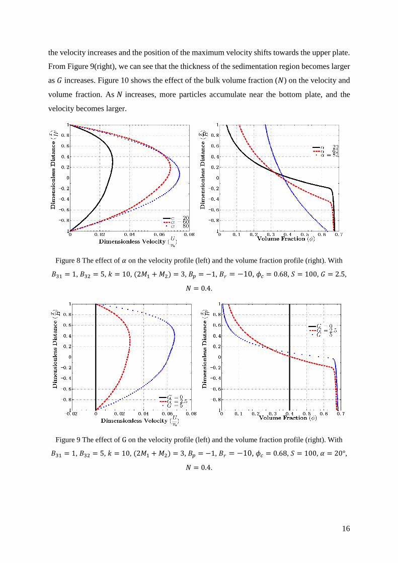
16

the velocity increases and the position of the maximum velocity shifts towards the upper plate.

From Figure 9(right), we can see that the thickness of the sedimentation region becomes larger

as 𝐺 increases. Figure 10 shows the effect of the bulk volume fraction (𝑁) on the velocity and

volume fraction. As 𝑁 increases, more particles accumulate near the bottom plate, and the

velocity becomes larger.

Figure 8 The effect of 𝛼 on the velocity profile (left) and the volume fraction profile (right). With

𝐵31 = 1, 𝐵32 = 5, 𝑘 = 10, (2𝑀1 + 𝑀2) = 3, 𝐵𝑝 = −1, 𝐵𝑟 = −10, 𝜙𝑐 = 0.68, 𝑆 = 100, 𝐺 = 2.5,

𝑁 = 0.4.

Figure 9 The effect of G on the velocity profile (left) and the volume fraction profile (right). With

𝐵31 = 1, 𝐵32 = 5, 𝑘 = 10, (2𝑀1 + 𝑀2) = 3, 𝐵𝑝 = −1, 𝐵𝑟 = −10, 𝜙𝑐 = 0.68, 𝑆 = 100, 𝛼 = 20°,

𝑁 = 0.4.

17

Figure 10 The effect of N on the velocity profile (left) and the volume fraction profile (right). With

𝐵31 = 1, 𝐵32 = 5, 𝑘 = 10, (2𝑀1 + 𝑀2 = 3), 𝐵𝑝 = −1, 𝐵𝑟 = −10, 𝜙𝑐 = 0.68, 𝑆 = 100, 𝛼 = 20°,

𝐺 = 2.5.

6. Conclusions

In this paper, we study the gravity driven fully developed flow of granular materials between

two inclined plates. The granular materials are modeled as a non-linear fluid, which includes

the effects of shear and volume fraction dependent viscosity and normal stress difference

effects. We also propose a new term in the spherical part of the stress tensor, related to the

compactness of the particles. This term is related to the critical volume fraction of the particles

(𝜙𝑐 ). This new term includes a smooth step function, and ensures that the new term only

becomes effective when the local volume fraction is approaching 𝜙𝑐. A parametric study is

performed for a selected range of dimensionless numbers.

References

[1] R.D. Marcus, L.S. Leung, G.E. Klinzing, F. Rizk, Pneumatic conveying of solids,

Chapman and Hall. London, 1990.

[2] S.A. Elaskar, L.A. Godoy, Constitutive relations for compressible granular materials

using non-Newtonian fluid mechanics, Int. J. Mech. Sci. 40 (1998) 1001–1018.

[3] R. Jackson, The dynamics of fluidized particles, Cambridge University Press, 2000.

[4] R.L. Brown, J.C. Richards, Principles of powder mechanics, Pergamon Press, London,

1970.

[5] S.B. Savage, The mechanics of rapid granular flows, Adv. Appl. Mech. 24 (1984) 289–

18

366.

[6] K. Hutter, K.R. Rajagopal, On flows of granular materials, Contin. Mech. Thermodyn.

6 (1994) 81–139.

[7] P.G. De Gennes, Reflections on the mechanics of granular matter, Phys. A Stat. Mech.

Its Appl. 261 (1998) 267–293.

[8] A. Mehta, Granular matter, Springer-Verlag, New York, 1994.

[9] J. Duran, Sands, powders, and grains, Springer-Verlag, New York, 2000.

[10] S.J. Antony, W. Hoyle, Y. Ding, Granular materials: fundamentals and applications,

Royal Society of Chemistry. Cambridge, UK, 2004.

[11] H.J. Herrmann, Statistical models for granular materials, Phys. A Stat. Mech. Its Appl.

263 (1999) 51–62.

[12] H.J. Herrmann, S. Luding, Modeling granular media on the computer, Contin. Mech.

Thermodyn. 10 (1998) 189–231.

[13] I. Goldhirsch, Rapid granular flows, Annu. Rev. Fluid Mech. 35 (2003) 267–293.

[14] E.J. Boyle, M. Massoudi, A theory for granular materials exhibiting normal stress effects

based on Enskog’s dense gas theory, Int. J. Eng. Sci. 28 (1990) 1261–1275.

[15] K.R. Rajagopal, L. Tao, Mechanics of mixtures, World Scientific Publishers, Singapore,

1995.

[16] M. Massoudi, A Mixture Theory formulation for hydraulic or pneumatic transport of

solid particles, Int. J. Eng. Sci. 48 (2010) 1440–1461.

[17] I.F. Collins, Elastic/plastic models for soils and sands, Int. J. Mech. Sci. 47 (2005) 493–

508.

[18] M. Massoudi, On the flow of granular materials with variable material properties, Int. J.

Non. Linear. Mech. 36 (2001) 25–37.

[19] M. Massoudi, M.M. Mehrabadi, A continuum model for granular materials: considering

dilatancy and the Mohr-Coulomb criterion, Acta Mech. 152 (2001) 121–138.

[20] K.R. Rajagopal, C. Truesdell, An introduction to the mechanics of fluids, Birkhauser,

2000.

[21] O. Reynolds, LVII. On the dilatancy of media composed of rigid particles in contact.

With experimental illustrations, London, Edinburgh, Dublin Philos. Mag. J. Sci. 20

(1885) 469–481.

19

[22] O. Reynolds, Experiments showing dilatancy, a property of granular material, possibly

connected with gravitation, Proc. R. Inst. GB. 11 (1886) 12.

[23] M. Reiner, A mathematical theory of dilatancy, Am. J. Math. 67 (1945) 350–362.

[24] M. Reiner, Elasticity beyond the elastic limit, Am. J. Math. 70 (1948) 433–446.

[25] W.T. Wu, N. Aubry, M. Massoudi, Flow of granular materials modeled as a non-linear

fluid, Mech. Res. Commun. 52 (2013) 62–68.

[26] M. Massoudi, A generalization of Reiner’s mathematical model for wet sand, Mech.

Res. Commun. 38 (2011) 378–381.

[27] R.S. Rivlin, J.L. Ericksen, Stress-deformation relations for isotropic materials, J. Ration.

Mech. Anal. 4 (1955) 323–425.

[28] C. Truesdell, W. Noll, The Nonlinear Field Theories of MechanicsSpringer-Verlag,

Berlin (1965 & 1992). (1992).

[29] J.E. Dunn, K.R. Rajagopal, Fluids of differential type: critical review and

thermodynamic analysis, Int. J. Eng. Sci. 33 (1995) 689–729.

[30] G. Gupta, M. Massoudi, Flow of a generalized second grade fluid between heated plates,

Acta Mech. 99 (1993) 21–33.

[31] K.R. Rajagopal, G. Saccomandi, L. Vergori, On the Oberbeck–Boussinesq

approximation for fluids with pressure dependent viscosities, Nonlinear Anal. Real

World Appl. 10 (2009) 1139–1150.

[32] B.J. Briscoe, P.F. Luckham, S.R. Ren, The properties of drilling muds at high pressures

and high temperatures, Philos. Trans. R. Soc. London A Math. Phys. Eng. Sci. 348

(1994) 179–207.

[33] K.R. Rajagopal, G. Saccomandi, L. Vergori, Stability analysis of the Rayleigh–Bénard

convection for a fluid with temperature and pressure dependent viscosity, Zeitschrift Für

Angew. Math. Und Phys. 60 (2009) 739–755.

[34] K.R. Rajagopal, A.S. Wineman, A note on the temperature dependence of the normal

stress moduli, Int. J. Eng. Sci. 19 (1981) 237–241.

[35] J.E. Dunn, R.L. Fosdick, Thermodynamics, stability, and boundedness of fluids of

complexity 2 and fluids of second grade, Arch. Ration. Mech. Anal. 56 (1974) 191–252.

[36] C.-S. Man, Nonsteady channel flow of ice as a modified second-order fluid with power-

law viscosity, Arch. Ration. Mech. Anal. 119 (1992) 35–57.

20

[37] M. Massoudi, A. Vaidya, On some generalizations of the second grade fluid model,

Nonlinear Anal. Real World Appl. 9 (2008) 1169–1183.

[38] C.-S. Man, M. Massoudi, On the thermodynamics of some generalized second-grade

fluids, Contin. Mech. Thermodyn. 22 (2010) 27–46.

[39] K.R. Rajagopal, M. Massoudi, A.S. Wineman, Flow of granular materials between

rotating disks, Mech. Res. Commun. 21 (1994) 629–634.

[40] K.R. Rajagopal, M. Massoudi, A method for measuring the material moduli of granular

materials: flow in an orthogonal rheometer (No. DOE/PETC/TR-90/3), USDOE

Pittsburgh Energy Technology Center, PA (USA), 1990.

[41] K.R. Rajagopal, W. Troy, M. Massoudi, Existence of solutions to the equations

governing the flow of granular materials, Eur. J. Mech. B. Fluids. 11 (1992) 265–276.

[42] K.K. Yeleswarapu, J.F. Antaki, M. V Kameneva, K.R. Rajagopal, A generalized

Oldroyd-B model as constitutive equation for blood, Ann. Biomed. Eng. 22 (1994) 16.

[43] L. Miao, M. Massoudi, Heat transfer analysis and flow of a slag-type fluid: Effects of

variable thermal conductivity and viscosity, Int. J. Non. Linear. Mech. 76 (2015) 8–19.

[44] K.R. Rajagopal, G. Saccomandi, L. Vergori, Flow of fluids with pressure-and shear-

dependent viscosity down an inclined plane, J. Fluid Mech. 706 (2012) 173–189.

[45] J. Cao, G. Ahmadi, M. Massoudi, Gravity granular flows of slightly frictional particles

down an inclined bumpy chute, J. Fluid Mech. 316 (1996) 197–221.

[46] M.U. Guide, The mathworks, Inc., Natick, MA. 5 (1998) 333.

[47] R.L. Fosdick, K.R. Rajagopal, Anomalous features in the model of “second order

fluids,” Arch. Ration. Mech. Anal. 70 (1979) 145–152.

[48] T. Hsu, P.A. Traykovski, G.C. Kineke, On modeling boundary layer and gravity‐driven

fluid mud transport, J. Geophys. Res. Ocean. 112 (2007).

[49] N. Morita, A.D. Black, G.F. Guh, Theory of lost circulation pressure, in: SPE Annu.

Tech. Conf. Exhib., Society of Petroleum Engineers, 1990.