Nonlinear analysis of capillary instability with heat and mass transfer

Commun Nonlinear Sci Numer Simulat 17 (2012) 2463–2475

Contents lists available at SciVerse ScienceDirect

Commun Nonlinear Sci Numer Simulat

journal homepage: www.elsevier .com/locate /cnsns

Nonlinear analysis of capillary instability with heat and mass transfer

Mukesh Kumar Awasthi ⇑, G.S. AgrawalDepartment of Mathematics, Indian Institute of Technology Roorkee, Roorkee 247667, India

a r t i c l e i n f o

Article history:Received 13 June 2011Received in revised form 23 August 2011Accepted 17 October 2011Available online 24 October 2011

Keywords:Viscous potential flowNonlinear analysisCapillary instabilityIncompressible fluidsHeat and mass transfer

1007-5704/$ - see front matter � 2011 Elsevier B.Vdoi:10.1016/j.cnsns.2011.10.015

⇑ Corresponding author.E-mail address: [email protected] (M

a b s t r a c t

The nonlinear capillary instability of the cylindrical interface between the vapor and liquidphases of a fluid is studied when there is heat and mass transfer across the interface, usingviscous potential flow theory. The fluids are considered to be viscous and incompressiblewith different kinematic viscosities. Both asymmetric and axisymmetric disturbances areconsidered. The analysis is based on the method of multiple scale perturbation and thenonlinear stability is governed by first-order nonlinear partial differential equation. Thestability conditions are obtained and discussed theoretically as well as numerically.Regions of stability and instability have been shown graphically indicating the effect of var-ious parameters. It has been observed that the heat and mass transfer has stabilizing effecton the stability of the system in the nonlinear analysis for both axisymmetric as well asasymmetric disturbances.

� 2011 Elsevier B.V. All rights reserved.

1. Introduction

Capillary instability arises when a liquid cylinder in an infinite fluid collapses under the action of capillary forces due tosurface tension [1,2]. The capillary instabilities of the two fluids interface play an important role in film boiling, film wisecondensation and in breaking of liquid jet. Plateau [3] studied the axisymmetric disturbances of capillary instability andobserved that a long cylinder of liquid is unstable to the axisymmetric disturbances with wavelengths greater than 2pR.Rayleigh [4] considered the stability of viscous liquid under capillary forces but he neglected the effect of surrounding fluid.Weber [5] studied the stability of a laminar jet considering the effect of viscosity and the surrounding air and concluded thatthe viscosity does not changes the cut-off wave number predicated by the inviscid theory. Tomotica [6] considered thestability of a long cylindrical column of viscous liquid in the viscous fluid.

Viscous potential flow theory has played an important role in studying various stability problems. Tangential stresses arenot considered in viscous potential theory and viscosity enters through normal stress balance [7]. The no slip condition at theboundary is not enforced in the viscous potential theory. Funada and Joseph [8] studied the viscous potential flow analysis ofcapillary instability and observed that viscous potential flow is better approximation of the exact solution than the inviscidmodel. Funada and Joseph [9] extended their work of capillary instability for viscoelastic fluids and observed that the growthrates are larger for viscoelastic fluids than for the equivalent Newtonian fluids.

When two fluids are divided by an interface, the interfacial instability is usually discussed without considering heat andmass transfer across the interface. On the other hand, the transfer of mass and heat across the interface is very important inmany situations such as boiling heat transfer in chemical engineering and in geophysical problems. Hsieh [10,11] formulatedthe problem of Rayleigh–Taylor instability and Kelvin–Helmholtz instability with heat and mass transfer across the liquid va-por interface. Hsieh [11] found that when the vapor layer is hotter than the liquid layer, the effect of heat and mass transfer

. All rights reserved.

.K. Awasthi).

http://dx.doi.org/10.1016/j.cnsns.2011.10.015

mailto:[email protected]

http://dx.doi.org/10.1016/j.cnsns.2011.10.015

http://www.sciencedirect.com/science/journal/10075704

http://www.elsevier.com/locate/cnsns

2464 M.K. Awasthi, G.S. Agrawal / Commun Nonlinear Sci Numer Simulat 17 (2012) 2463–2475

tends to inhibit the growth of instability. Nayak and Chakrborty [12] established the formulation of Kelvin–Helmholtz insta-bility of the cylindrical interface between the liquid and vapor phases with heat and mass transfer.

The viscous potential flow analysis of Kelvin–Helmholtz instability with heat and mass transfer in plane geometry hasbeen carried out by Asthana and Agrawal [13]. They observed that the heat and mass transfer has a stabilizing effect whenthe lower fluid viscosity is high and destabilizing effect when the lower fluid viscosity is low. Kim et al. [14] investigated thecapillary instability problem of vapor liquid system in an annular configuration with heat and mass transfer using viscouspotential flow for axisymmetric disturbances. They observed that for irrotational motion of two viscous fluids, heat and masstransfer phenomenon completely stabilizes the interface against capillary effects.

Nonlinear theory is very important as most of the flows are nonlinear in nature. Hsieh [10] has studied the nonlinear Ray-leigh–Taylor instability with heat and mass transfer of inviscid fluids and concluded that nonlinearity increases the stabilityrange when there is strong heat and mass transfer. Lee [15] has studied the nonlinear inviscid analysis of Rayleigh instabilityat the cylindrical interface and observed that heat and mass transfer phenomenon plays an important role in the nonlinearanalysis.

The objective of the present work is to study the nonlinear effects on the capillary instability of cylindrical interface be-tween vapor and liquid phases of a fluid when there is heat and mass transfer across the interface. Both fluids are taken asincompressible and viscous with different kinematic viscosities. We have used the method of multiple scales for the inves-tigation and a first order nonlinear partial differential equation describing the nonlinear waves is obtained. Stability is dis-cussed theoretically as well as numerically and stability regions are displayed graphically. Finally a comparative analysis hasbeen made between the results obtained in the linear theory (Kim et al. [14]) and present nonlinear analysis.

2. Problem formulation

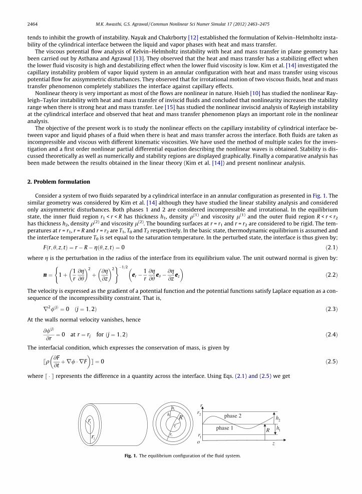
Consider a system of two fluids separated by a cylindrical interface in an annular configuration as presented in Fig. 1. Thesimilar geometry was considered by Kim et al. [14] although they have studied the linear stability analysis and consideredonly axisymmetric disturbances. Both phases 1 and 2 are considered incompressible and irrotational. In the equilibriumstate, the inner fluid region r1 < r < R has thickness h1, density q(1) and viscosity l(1) and the outer fluid region R < r < r2

has thickness h2, density q(2) and viscosity l(2). The bounding surfaces at r = r1 and r = r2 are considered to be rigid. The tem-peratures at r = r1, r = R and r = r2 are T1, T0 and T2 respectively. In the basic state, thermodynamic equilibrium is assumed andthe interface temperature T0 is set equal to the saturation temperature. In the perturbed state, the interface is thus given by;

Fðr; h; z; tÞ ¼ r � R� gðh; z; tÞ ¼ 0 ð2:1Þ

where g is the perturbation in the radius of the interface from its equilibrium value. The unit outward normal is given by:

n ¼ 1þ 1r@g@h

� �2

þ @g@z

� �2( )�1=2

er �1r@g@h

eh �@g@z

ez

� �ð2:2Þ

The velocity is expressed as the gradient of a potential function and the potential functions satisfy Laplace equation as a con-sequence of the incompressibility constraint. That is,

r2/ðjÞ ¼ 0 ðj ¼ 1;2Þ ð2:3Þ

At the walls normal velocity vanishes, hence

@/ðjÞ

@r¼ 0 at r ¼ rj for ðj ¼ 1;2Þ ð2:4Þ

The interfacial condition, which expresses the conservation of mass, is given by

sq@F@tþr/ � rF

� �t ¼ 0 ð2:5Þ

where s � t represents the difference in a quantity across the interface. Using Eqs. (2.1) and (2.5) we get

2r

1rR

2r

1r

2h

1h 2r

1r

2h

1hR

r

zo

phase 1

phase 2

Fig. 1. The equilibrium configuration of the fluid system.

M.K. Awasthi, G.S. Agrawal / Commun Nonlinear Sci Numer Simulat 17 (2012) 2463–2475 2465

sq@/@r� @g@t� 1

r2

@g@h

@/@h� @g@z

@/@z

� �t ¼ 0 at r ¼ Rþ g ð2:6Þ

The interfacial condition for energy transfer can be expressed as

Lqð1Þ@F@tþr/ð1Þ � rF

� �¼ SðgÞ at r ¼ Rþ g ð2:7Þ

where L is the latent heat released during phase transformation. S(g) constitute net heat flux from the interface.In the equilibrium state, the heat fluxes in positive radial-direction in the fluid phases 1 and 2 are expressed as

�K1(T1 � T0)/R ln(r1/R) and �K2(T0 � T2)/R ln(R/r2) respectively where K1 and K2 are heat conductivities of the two fluids.The expression for S(g) as taken by Nayak and Chakraborty [12] for the cylindrical geometry.

SðgÞ ¼ K2ðT0 � T2ÞðRþ gÞ ln r2 � lnðRþ gÞ½ � �

K1ðT1 � T0ÞðRþ gÞ½lnðRþ gÞ � ln r1�

ð2:8Þ

Expanding S(g) in a Maclaurin series about g = 0, we get,

SðgÞ ¼ Sð0Þ þ gS0ð0Þ þ 12g2S00ð0Þ þ � � � ð2:9Þ

At equilibrium state, i.e. g = 0

K2ðT0 � T2ÞR lnðr2=RÞ ¼

K1ðT1 � T0ÞR lnðR=r1Þ

¼ ðT1 � T2Þ=RlnðR=r1Þ=K1 þ lnðr2=RÞ=K2

¼ GðsayÞ ð2:10Þ

This indicates that in the equilibrium state the heat fluxes are equal across the vapor–liquid interface.Using Eq. (2.1), with the Eqs. (2.7)–(2.10), the equation of energy transfer becomes:

qð1Þ@/ð1Þ

@r� @g@t� 1

r2

@g@h

@/ð1Þ

@h� @g@z

@/ð1Þ

@z

!¼ a gþ a2g2 þ a3g3� �

ð2:11Þ

where

a ¼ G logðr2=r1ÞLR logðr2=RÞ logðR=r1Þ

; a2 ¼1R�3

2þ 1

logðr2=RÞ �1

logðR=r1Þ

� �;

a3 ¼1R2

116� 2 logðR2=r1r2Þ

logðr2=RÞ logðR=r1Þþ log3ðr2=RÞ þ log3ðR=r1Þ

logðr2=RÞ logðR=r1Þ½ �2 logðr2=r1Þ

!
Interfacial condition for the conservation of momentum is given by,
qð1Þðr/ð1Þ � rFÞ @F@tþr/ð1Þ � rF

� �¼ qð2Þðr/ð2Þ � rFÞ @F

@tþr/ð2Þ � rF

� �þ p2 � p1 � 2lð2Þn � r �r/ð2Þ � nþ 2lð1Þn � r �r/ð1Þ � nþ rr � n� �

jrFj2

ð2:12Þ

where p is the pressure, r is the surface tension coefficient and n is the unit normal vector at the interface. Surface tensionhas been assumed to be a constant, neglecting its dependence on temperature.

Eliminating pressure term using Bernoulli’s equation, Eq. (2.12) reduces to

sq@/@tþ 1

2@/@r

� �2

þ 1r@/@h

� �2

þ @/@z

� �2" #

� 1þ 1r@g@h

� �2

þ @g@z

� �2( )�1

@/@r� 1

r2

@/@h

@g@h� @g@z

@/@z

� �8<:� @/

@r� @g@t� 1

r2

@/@h

@g@h� @g@z

@/@z

� ��þ 2l 1þ 1

r@g@h

� �2

þ @g@z

� �2( )�1

@2/@r2

"� 1

r2

@g@h

@2/@r@h

þ 2r3

@g@h

� @/@hþ 1

r3

@g@h

� �2@/@rþ 1

r4

@g@h

� �2@2/

@h2 þ2r2

@g@h

@g@z

@2/@h@z

� 2@g@z

@2/@r@z

þ @g@z

� �2@2/@z2

#t

¼ �r@2g@z2 þ 1

r2@2g@h2 þ 1

r2@g@z

� �2 @2g@h2 þ 1

r2@g@h

� �2 @2g@z2 � 1

r3@g@h

� �2 þ 2r2

@g@h

@g@z

@2g@h@z

� �� 1þ 1

r@g@h

� �2 þ @g@z

� �2n o�3=2

þ rðRþ gÞ�1 1þ 1r@g@h

� �2 þ @g@z

� �2n o�1=2

264375 ð2:13Þ

We are following the approach of Lee [15] to study the nonlinear temporal stability analysis of the considered system. Let usassume the following expansion of the variables;


g ¼X3

n¼1

engnðh; z; t0; t1; t2Þ þ Oðe4Þ ð2:14Þ

/ðjÞ ¼X3

n¼1

en/ðjÞn ðr; h; z; t0; t1; t2Þ þ Oðe4Þ ð2:15Þ

where e is a small parameter indicating the order of the perturbation and tn = ent (n = 0,1,2). The variables g and /(j) appear-ing in the Eqs. (2.6), (2.11) and (2.13) are expressed in Maclaurin series around r = R. Then using the expression for g and /(j)

from Eqs. (2.14) and (2.15) in the equation so obtained. Finally equate the coefficient of equal powers in e to obtain the linearand the successive nonlinear partial differential equations of various orders (Appendix A). The mathematical procedure tofind the equations is given in the Appendix B.

3. Linear theory

The solution of Eq. (2.3) using the boundary conditions:

g1 ¼ Aðt1; t2Þei# þ Aðt1; t2Þe�i# ð3:1Þ

/ð1Þ1 ¼1k

aqð1Þ� ix

� �Aðt1; t2ÞEð1Þn ðkrÞei# þ c:c: ð3:2Þ

/ð2Þ1 ¼1k

aqð2Þ� ix

� �Aðt1; t2ÞEð2Þn ðkrÞei# þ c:c: ð3:3Þ

where

Eð1Þn ðkrÞ ¼ InðkrÞK 0nðkr1Þ � I0nðkr1ÞKnðkrÞI0nðkRÞK 0nðkr1Þ � I0nðkr1ÞK 0nðkRÞ

; ð3:4Þ

Eð2Þn ðkrÞ ¼ InðkrÞK 0nðkr2Þ � I0nðkr2ÞKnðkrÞI0nðkRÞK 0nðkr2Þ � I0nðkr2ÞK 0nðkRÞ

# ¼ kzþ nh�xt0 ð3:5Þ

with In(kr) and Kn(kr) represents the modified Bessel functions of the first and second kinds respectively.Substituting Eqs. (3.1)–(3.3) into the Eq. (A.3), we get

Dðx; k;nÞ ¼ a0x2 þ ia1xþ a2 ¼ 0 ð3:6Þ

where a0 ¼ qð1ÞEð1Þn ðkRÞ � qð2ÞEð2Þn ðkRÞ

a1 ¼ a Eð1Þn ðkRÞ � Eð2Þn ðkRÞ� �

þ 2k2 lð1ÞFð1Þn ðkRÞ � lð2ÞFð2Þn ðkRÞ� �

a2 ¼ �rk k2 þ n2 � 1R2

� �� 2k2a

lð1Þ

qð1ÞFð1Þn ðkRÞ � lð2Þ

qð2ÞFð2Þn ðkRÞ

� �Fð1Þn ðkRÞ ¼ 1þ n2

k2R2

� �Eð1Þn ðkRÞ � 1

kR; Fð2Þn ðkRÞ ¼ 1þ n2

k2R2

� �Eð2Þn ðkRÞ � 1

kR

For the axisymmetric disturbances i.e. n = 0, Eq. (3.6) reduces to the same expression as obtained by Kim et al. [14].On applying Routh–Hurwitz criteria in the Eq. (3.6), the stability condition is: a0 > 0, a1 > 0, a2 > 0.Using the properties of Modified Bessel functions, we have a0 > 0 trivially and since a, l(2) and l(1) is positive so a1 > 0.Hence the condition of stability gives rise to a2 > 0 and condition of marginal state is given by: a2 = 0i.e.:

r k2c þ

n2 � 1R2

� �þ 2kca

lð1Þ

qð1ÞFð1Þn ðkcRÞ � lð2Þ

qð2ÞFð2Þn ðkcRÞ

� �¼ 0 ð3:7Þ

4. Second-order solutions

Using the first-order solution, the equation for second order solution is given by:

r2/ðjÞ2 ¼ 0 ðj ¼ 1;2Þ ð4:1Þ


and the boundary conditions at r = R:

qðjÞ@/ðjÞ2

@r� @g2

@t0

( )� ag2 ¼ qðjÞ

aqðjÞ� ix

�1R� 2k 1þ n2

k2R2

� �EðjÞn ðkRÞ

�þ aa2

�A2e2i#

þ qðjÞ@A@t1

ei# þ c:c:þ 2a1Rþ a2

� �jAj2 ðj ¼ 1;2Þ ð4:2Þ

qð2Þ@/ð2Þ2

@r� qð1Þ

@/ð1Þ2

@r� qð2Þ � qð1Þ� @g2

@t0¼ sq

aq� ix

� �1R� 2k 1þ n2

k2R2

� �EnðkRÞ

� �tA2e2i# þ qð2Þ � qð1Þ

� @A@t1

ei#

þ c:c: ð4:3Þ

sq@/2

@t0þ 2l @

2/2

@r2 tþ r @2g2

@z2 þ1r2

@2g2

@h2 þg2

R2

!

¼ �x2

2sq 1þ n2

k2R2

� �E2

nðkRÞ � 3 �

t

þ a2

2qs1þ 1þ n2

k2R2

� �E2

nðkRÞt� iaxs 1þ n2

k2R2

� �E2

nðkRÞt

� 2lk2s

aq� ix

� �3þ 2n2 þ 2

k2R2� 5n2

k3R3þ 1

kR

� �EnðkRÞ

� �tþ r

2R3 ðR2k2 � 5n2 þ 2Þ

�A2e2ih

� sqk

aq� ix

� �EnðkRÞt @A

@t1eih þ c:c:þ sq

a2

q2 þx2� �

1� 1þ n2

k2R2

� �E2

nðkRÞ �

þ4lak2

q1� ðn

2 � 2Þk2R2

þ n2

k3R3þ 1

kR

� �EnðkRÞ

� �t� r

R3 ðR2k2 þ 5n2 � 2Þ

�jAj2 ð4:4Þ

We have assumed that the secular terms vanish, so that:
@A@t1¼ 0 ð4:5Þ
The solution of the Eqs. (4.1)–(4.4) gives rise to:

g2 ¼ �21Rþ a2

� �jAj2 þ A2A2e2i# þ A2A2e�2i# ð4:6Þ

/ðjÞ2 ¼ BðjÞ2 EðjÞ2nð2krÞA2e2i# þ c:c:þ bðjÞðt0; t1; t2Þ ðj ¼ 1;2Þ ð4:7Þ
where
A2 ¼2k

Dð2x;2k;2nÞ sqixk

E2nð2kRÞbþ q2

1þ n2

k2R2

� �E2

nðkRÞ aq� ix

� �2(

þ3x2q2 þ a2

2q�4lkbF2nð2kRÞ � 2k2l a

q� ix� �

3þ 2n2þ2ð Þk2R2 � 5n2

k3R3 þ 1kR

� �EnðkRÞ

� �tþ r

2R3 k2R2 � 5n2 þ 2� ��

ð4:8Þ

BðjÞ2 ¼1

2kbðjÞ þ a

qðjÞ� 2ix

� �A2

�ð4:9Þ

bðjÞ ¼ ka

qðjÞ� ix

� �1

kR� 2 1þ n2

k2R2


� �þ aa2

qðjÞð4:10Þ

qð2Þ@bð2Þ

@t� qð1Þ

@bð1Þ

@t¼ sq

a2

q2 þx2� �

1� 1þ n2

k2R2

� �E2

nðkRÞ �

þ 4lak2

q1þ 2

k2R2þ n2

k3R3þ 1

kR

� �EnðkRÞ

� �t� r

R3 ðR2k2 þ 3n2 � 4� 2Ra2Þ

�jAj2 ð4:11Þ

we have assumed that D(2x,2k,2n) – 0.

5. Third-order solutions

For third-order solution, we have:

r2/ðjÞ3 ¼ 0 ðj ¼ 1;2Þ ð5:1Þ
Substituting the values of g1;/
ð2Þ1 ;/ð1Þ1 from Eqs. (3.1)–(3.3) and g2;/

ð2Þ2 ;/ð1Þ2 from Eqs. (4.6), (4.7) into the Eqs. (A.7) and (A.8),

we get:

/ðjÞ3 ¼ CðjÞ3 EðjÞn ðkrÞA2Aei# þ EðjÞn ðkrÞk

@A@t2

ei# þ c:c: ðj ¼ 1;2Þ ð5:2Þ


where

CðjÞ3 ¼ �k 2 1þ n2

k2R2

� �EðjÞ2nð2kRÞ � 1

kR

�BðjÞ2 � 2 1þ n2

k2R2

� �EðjÞn ðkRÞ � 1

kR

�� a

qðjÞ� ix

� �1

kRþ a2

k

� �þ 1

21þ n2 þ 2

k2R2� 3n2

k3R3þ 1

kR


� �3aqðjÞ� ix

� �� a

qðjÞþ ix

� �1þ n2

k2R2� 2n2

k3R3EðjÞn ðkRÞ

� �þ a

qðjÞk2 4a21Rþ a2

� �� 3a3

�� a

qðjÞþ ix

� �1þ n2

k2R2

� �EðjÞn ðkRÞ þ 1

kR

� �þ 2aa2

qðjÞk

�A2

k

�ð5:3Þ

Substituting the first-order solution, second-order solution and third-order solution in the Eq. (A.9) and to avoid the non-uni-formity of the solution, suppose @A

@t1¼ 0, we get the equation:

ik@D@x

@A@t2þ qA2A ¼ 0 ð5:4Þ

where

q ¼ sq �ixC3EnðkRÞ � A2ixaqþ ix

� �þ 2kB2

aq

1þ n2

k2R2

� �EnðkRÞE2nð2kRÞ � 1

��þix 1þ n2

k2R2

� �EnðkRÞE2nð2kRÞ � 2

��þ 2ix

1Rþ a2

� �aq� ix

� �þ k 1þ n2

k2R2

� ��EnðkRÞ ix

23aq� ix

� �� n2

k3R3kE2

nðkRÞ 3x2 þ a2

q2 þ iaq

x� �

þ 12R

3x2 þ 6a2

q2 � iaq

x� ��

þ 2lk2 C3FnðkRÞ þ 4kB2n2 þ 1

k2R2� 2n2

k3R3þ 1

kR

� �E2nð2kRÞ

� �� 2

1Rþ a2

� �aq� ix

� �� 1þ n2 þ 2

k2R2� 3n2

k3R3þ 1

kR

� �EnðkRÞ

� �þ a

qþ ix

� �2� n2

k2R2� n2

k3R3� 1

kR

� �EnðkRÞ � 3

� �A2 � 2k

aqþ ix

� �1þ n2

k2R2

� �FnðkRÞ

� kaq� 3ix

� �2þ n2

k2R2

� �EnðkRÞ � 1

kR

� �� kEnðkRÞ 3a

q� 5ix

� �n4

k4R4þ n2

k2R2

4aq� 8ix

� � �þ 6n2

k3R3

aqþ 3ix

� �þ n2

k2R2

7aq� ix

� �þ1

2k

3aq� ix

� �1þ ð2n2 þ 3Þ

k2R2þ

10n4 þ 2n2� �

k4R4

� �EnðkRÞ

�� 2

kRþ ð6n2 þ 6Þ

k3R3

� ��tþ r

R4 2RA2ðk2R2 þ 4n2 � 1Þ þ 4ð1� n2ÞRa2

nþ 7� 12n2 þ 3

2n4

� �� 1

2k2R2 1� 3k2R2 � 6n2

� ��

6. Dimensionless form

Let

r ¼ rH; z ¼ z

H; t ¼ t

s; x ¼ xs; k ¼ kH; / ¼ h1

H¼ h1; bR ¼ r1 þ /;

l ¼ qð1Þ

qð2Þ; m ¼ lð1Þ

lð2Þ; j ¼ tð1Þ

tð2Þ¼ m

l; oh ¼

ffiffiffiffiffiffiffiffiffiffiffiffiffiffiffiqð2ÞrH

plð2Þ

; a ¼ aqð2Þ=s

; K ¼ 2aoh

where oh is the Ohnesorge number, a is the heat transfer capillary number, K is the alternative heat-transfer capillarydimensionless group, / ¼ h1 is the vapor thickness and j is the ratio of kinematic viscosities:

The dimensionless form of the Eq. (3.6) is given by:

Dðx; k;nÞ ¼ a0x2 þ ia1xþ a2 ¼ 0 ð6:1Þa0 ¼ lEð1Þn ðkbRÞ � Eð2Þn ðkbRÞa1 ¼ a Eð1Þn ðkbRÞ � Eð2Þn ðkbRÞ� �

þ 2k2

ohmFð1Þn ðkbRÞ � Fð2Þn ðkbRÞ� �

a2 ¼ �k k2 þn2 � 1� �bR2

� �� 2k2a

ohml

Fð1Þn ðkbRÞ � Fð2Þn ðkbRÞ� �


Eq. (3.7) in the nondimensional form can be written as:

k2c þðn2 � 1ÞbR2

� �þKkc jFð1Þn ðkc

bRÞ � Fð2Þn ðkcbRÞ� �¼ 0 ð6:2Þ

We can write the dimension less form of the Eq. (5.4) as:

i

k

@D@x

@bA@t2þ qbA2 �bA ¼ 0 ð6:3Þ

where

q ¼ �ixbC ð2Þ3 Eð2Þn ðkbRÞ � bA2ix aþ ixð Þ þ 2kbBð2Þ2 aPð2Þ1 þ ixPð2Þ2

� �þ 2ix

1bR þ a2

� �a� ixð Þ

þ k

ix2

Lð2Þ1 3a� ixð Þ

� n2

k2bR3Eð2Þn ðkbRÞ� �2

3x2 þ a2 þ iax� �

þ 1

2bR 3x2 þ 6a2 � iax� �

þ ixlbC ð1Þ3 Eð1Þn ðkbRÞ þ lbA2ixalþ ix

� �� 2lkbBð1Þ2

al

Pð1Þ1 þ ixPð1Þ2

� �� 2lix

1bR þ a2

� �al� ix

� �� lk

ix2

Lð1Þ1 3al� ix

� �þ l

n2

k2bR3Eð1Þn ðkbRÞ� �2

3x2 þ a2

l2þ i

alx

� �� l

2bR 3x2 þ 6a2

l2 � ialx

� �þ 2k2

ohbC ð2Þ3 Fð2Þn ðkbRÞ þ 4kbBð2Þ2 gð2Þ1 � 2

1bR þ a2

� �a� ixð ÞgðjÞ2 þ aþ ixð Þgð2Þ3

bA2 � 2k aþ ixð ÞLð2Þ2

� k a� 3ixð ÞLð2Þ3

� kEð2Þn ðkbRÞ 3a� 5ixð Þ n4

k4bR4þ n2

k2bR24a� 8ixð Þ þ 6n2

k3bR3aþ ixð Þ

�þ n2

k2bR37a� ixð Þ þ 1

2k 3a� ixð Þgð2Þ4

�mbC ð1Þ3 Fð1Þn ðkbRÞ � 4mkbBð1Þ2 gð1Þ1 þ 2m1bR þ a2

� �al� ix

� �gð1Þ2 �m

alþ ix

� �gð1Þ3

bA2 þ 2mkalþ ix

� �Lð1Þ2

þmkal� 3ix

� �Lð1Þ3 �mkEð1Þn ðkbRÞ 3a

l� 5ix

� �n4

k4bR4þ n2

k2bR2

4al� 8ix

� �þ 6n2

k3bR3

alþ ix

� ��m

n2

k2bR3

7al� ix

� �� 1

2mk 3

al� ix

� �gð1Þ4

�þ 1bR4

2bRbA2 k2bR2 þ 4n2 � 1� �

þ 4 1� n2� �bRa2

nþ 7� 12n2 þ 3

2n4

� �� 1

2k2bR2 1� 3k2bR2 � 6n2

� ��
Here
PðjÞ1 ¼ 1þ n2

k2bR2

� �EðjÞn kbR� �

EðjÞ2n 2kbR� �� 1

�; PðjÞ2 ¼ 1þ n2

k2bR2


EðjÞ2n 2kbR� �� 2

�;

LðjÞ1 ¼ 1þ n2

k2bR2


; LðjÞ2 ¼ 1þ n2

k2bR2


;

LðjÞ3 ¼ 2þ n2

k2bR2

� �EðjÞn ðkbRÞ � 1

kbR ; gðjÞ1 ¼n2 þ 1

k2bR2� 2n2

k3bR3þ 1

kbR� �

EðjÞ2n 2kbR� �� ;

gðjÞ2 ¼ 1þ n2 þ 2

k2bR2� 3n2

k3bR3þ 1

kbR� �

EðjÞn kbR� �� ; gðjÞ3 ¼

2� n2

k2bR2� n2

k3bR3� 1

kbR� �

EðjÞn kbR� �� 3

� �gðjÞ4 ¼ 1þ ð2n2 þ 3Þ

k2bR2þ ð10n4 þ 2n2Þ

k4bR4


� 2

kbR þ ð6n2 þ 6Þk3bR3

� ��
Eq. (6.3) can be written as:
@bA@t2þ bQ bA2 �bA ¼ 0 ð6:4Þ

Integrating the above equation, we can get:

jbAj2 ¼ 1

jbA0j�2 þ 2ðRebQ Þt2

ð6:5Þ

where RebQ is the real part of bQ and bA0 is the initial amplitude. If denominator of Eq. (6.5) vanishes, bA becomes infinite. Hencethe condition for stability reduces to

RebQ > 0 ð6:6Þ


7. Numerical results and discussions

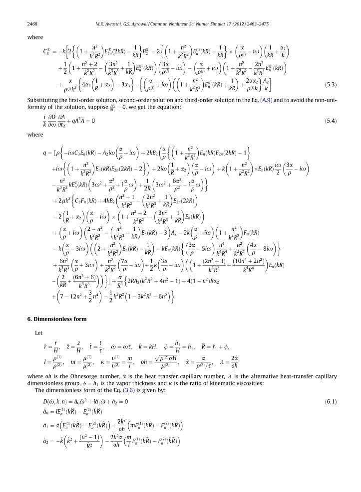
Lee [15] has done the nonlinear inviscid analysis of Rayleigh–Taylor instability of the cylindrical interface and predicts theregion of stability with upper and lower bounds while Kim et al. [14] have studied the linear analysis of capillary instabilitywith heat and mass transfer using potential flow theory and predicts the region of stability unbounded above for both vis-cous and inviscid fluids. Our analysis is based on the approach adopted by Lee [15] and predicts the stability region in theform of a band with upper and lower bounds.

In this section the numerical computation has been carried out using the stability condition (6.6). Steam and water havebeen taken as working fluids identified with phase 1 and phase 2 respectively, such that T1 > T0 > T2. In film boiling, thewater-steam interface is in saturation condition and the temperature T0 is equal to the saturation temperature.

Fig. 2.(n = 1).

Fig. 3.(n = 1).

qð1Þ ¼ 0:001 gm=cm3; qð2Þ ¼ 1:0 gm=cm3;

lð1Þ ¼ 0:00001 poise; lð2Þ ¼ 0:01 poise; r ¼ 72:3 dyne=cm

The radii of the inner and outer cylinders are 1 cm and 2 cm respectively. The stable and unstable regions have been shownin the following figures. ‘S’ and ‘U’ denote nonlinearly stable and unstable regions respectively.

Stability diagram for the system having l ¼ 0:001;m ¼ 0:001; oh ¼ 100; a ¼ 1 (a) axisymmetric disturbance (n = 0) (b) asymmetric disturbance

Stability diagram for the system having l ¼ 0:001;m ¼ 0:001; oh ¼ 100; a ¼ 5 (a) axisymmetric disturbance (n = 0) (b) asymmetric disturbance

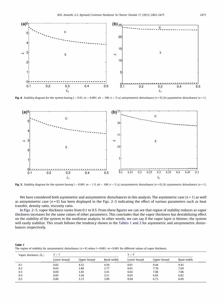
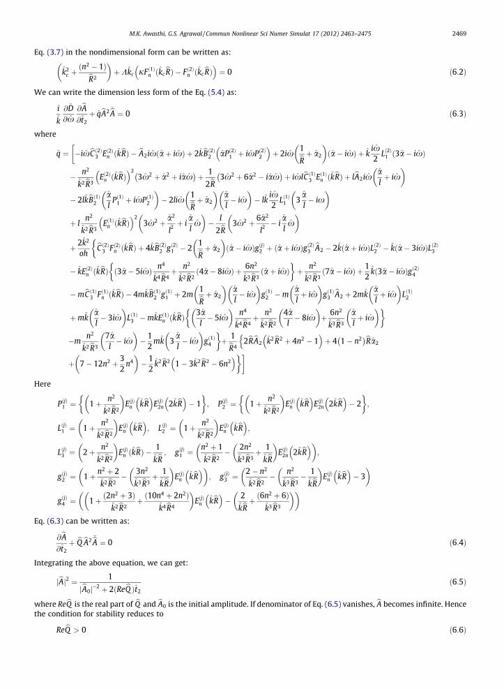
Fig. 4. Stability diagram for the system having l ¼ 0:01;m ¼ 0:001; oh ¼ 100; a ¼ 5 (a) axisymmetric disturbance (n = 0) (b) asymmetric disturbance (n = 1).

Fig. 5. Stability diagram for the system having l ¼ 0:001;m ¼ 1:5; oh ¼ 100; a ¼ 5 (a) axisymmetric disturbance (n = 0) (b) asymmetric disturbance (n = 1).


We have considered both asymmetric and axisymmetric disturbances in this analysis. The asymmetric case (n = 1) as wellas axisymmetric case (n = 0) has been displayed in the Figs. 2–5 indicating the effect of various parameters such as heattransfer, density ratio, viscosity ratio.

In Figs. 2–5, vapor thickness varies from 0.1 to 0.5. From these figures we can see that region of stability reduces as vaporthickness increases for the same values of other parameters. This concludes that the vapor thickness has destabilizing effecton the stability of the system in the nonlinear analysis. In other words, we can say if the vapor layer is thinner, the systemwill easily stabilize. This result follows the tendency shown in the Tables 1 and 2 for asymmetric and axisymmetric distur-bances respectively.

Table 1The region of stability for axisymmetric disturbance (n = 0) when l = 0.001, m = 0.001 for different values of vapor thickness.

Vapor thickness ðh1Þ a ¼ 1 a ¼ 5

Lower bound Upper bound Band width Lower bound Upper bound Band width

0.1 0.02 4.52 4.50 0.01 9.44 9.430.2 0.03 3.80 3.77 0.01 7.70 7.690.3 0.04 3.45 3.41 0.02 7.08 7.060.4 0.05 3.26 3.21 0.03 6.85 6.820.5 0.06 3.15 3.09 0.04 6.73 6.69

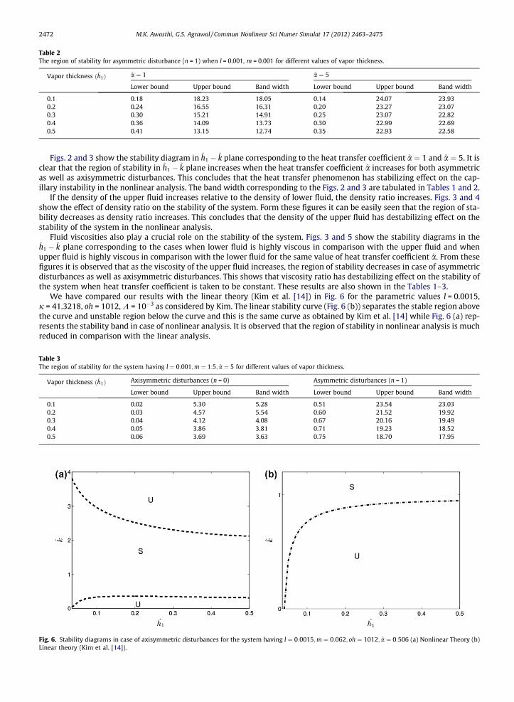
Table 2The region of stability for asymmetric disturbance (n = 1) when l = 0.001, m = 0.001 for different values of vapor thickness.

Vapor thickness ðh1Þ a ¼ 1 a ¼ 5


0.1 0.18 18.23 18.05 0.14 24.07 23.930.2 0.24 16.55 16.31 0.20 23.27 23.070.3 0.30 15.21 14.91 0.25 23.07 22.820.4 0.36 14.09 13.73 0.30 22.99 22.690.5 0.41 13.15 12.74 0.35 22.93 22.58


Figs. 2 and 3 show the stability diagram in h1 � k plane corresponding to the heat transfer coefficient a ¼ 1 and a ¼ 5. It isclear that the region of stability in h1 � k plane increases when the heat transfer coefficient a increases for both asymmetricas well as axisymmetric disturbances. This concludes that the heat transfer phenomenon has stabilizing effect on the cap-illary instability in the nonlinear analysis. The band width corresponding to the Figs. 2 and 3 are tabulated in Tables 1 and 2.

If the density of the upper fluid increases relative to the density of lower fluid, the density ratio increases. Figs. 3 and 4show the effect of density ratio on the stability of the system. Form these figures it can be easily seen that the region of sta-bility decreases as density ratio increases. This concludes that the density of the upper fluid has destabilizing effect on thestability of the system in the nonlinear analysis.

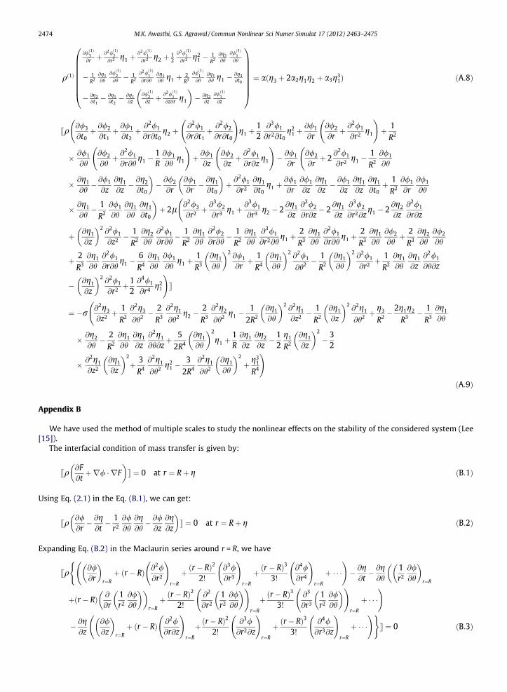
Fluid viscosities also play a crucial role on the stability of the system. Figs. 3 and 5 show the stability diagrams in theh1 � k plane corresponding to the cases when lower fluid is highly viscous in comparison with the upper fluid and whenupper fluid is highly viscous in comparison with the lower fluid for the same value of heat transfer coefficient a. From thesefigures it is observed that as the viscosity of the upper fluid increases, the region of stability decreases in case of asymmetricdisturbances as well as axisymmetric disturbances. This shows that viscosity ratio has destabilizing effect on the stability ofthe system when heat transfer coefficient is taken to be constant. These results are also shown in the Tables 1–3.

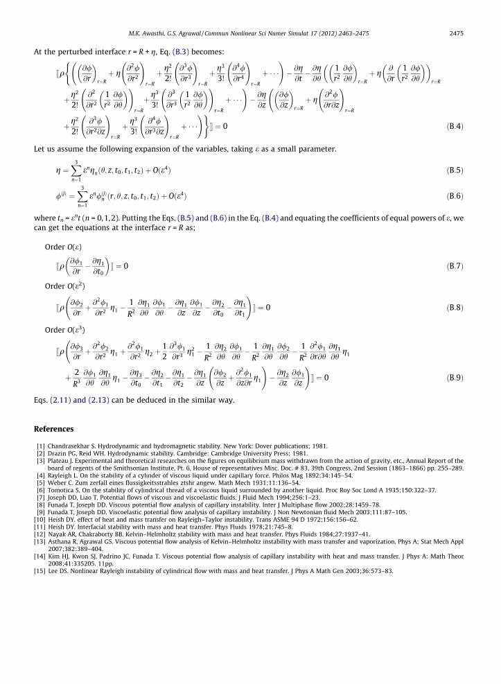
We have compared our results with the linear theory (Kim et al. [14]) in Fig. 6 for the parametric values l = 0.0015,j = 41.3218, oh = 1012, K = 10�3 as considered by Kim. The linear stability curve (Fig. 6 (b)) separates the stable region abovethe curve and unstable region below the curve and this is the same curve as obtained by Kim et al. [14] while Fig. 6 (a) rep-resents the stability band in case of nonlinear analysis. It is observed that the region of stability in nonlinear analysis is muchreduced in comparison with the linear analysis.

Table 3The region of stability for the system having l ¼ 0:001;m ¼ 1:5; a ¼ 5 for different values of vapor thickness.

Vapor thickness ðh1Þ Axisymmetric disturbances (n = 0) Asymmetric disturbances (n = 1)


0.1 0.02 5.30 5.28 0.51 23.54 23.030.2 0.03 4.57 5.54 0.60 21.52 19.920.3 0.04 4.12 4.08 0.67 20.16 19.490.4 0.05 3.86 3.81 0.71 19.23 18.520.5 0.06 3.69 3.63 0.75 18.70 17.95

Fig. 6. Stability diagrams in case of axisymmetric disturbances for the system having l ¼ 0:0015;m ¼ 0:062; oh ¼ 1012; a ¼ 0:506 (a) Nonlinear Theory (b)Linear theory (Kim et al. [14]).


A final remark on the comparison of asymmetric and axisymmetric disturbances is due. It has been observed that the sta-ble region is greater for asymmetric disturbances in comparison with axisymmetric disturbances for the same values of otherphysical parameters. Hence the asymmetric disturbances are stable than axisymmetric disturbances in the nonlinear anal-ysis as shown in Figs. 2–5.

8. Conclusion

The nonlinear capillary instability of the cylindrical interface of two viscous and incompressible fluids confined in a con-centric annulus with heat and mass transfer has been studied. Method of multiple scales has been used and a first order non-linear partial differential equation describing the nonlinear waves is obtained. Nonlinearity has important role to play on thestability of the system in the presence of heat and mass transfer. It has been observed that vapor thickness has destabilizingeffect on stability of the system. Density ratio and viscosity ratio both are playing destabilizing role in the nonlinear analysiswhile heat and mass transfer phenomenon has stabilizing effect. Asymmetric disturbances are more stable than axisymmet-ric disturbances. Nonlinearity reduces the region of stability.

Acknowledgement

Author is thankful to Council of Scientific and Industrial Research (CSIR), New Delhi (India) for their financial support dur-ing this work.

Appendix A

The interfacial conditions are given on r = R as:

Order O(e)

sq@/1

@r� @g1

@t0

� �t ¼ 0 ðA:1Þ

qð1Þ@/ð1Þ1

@r� @g1

@t0

!¼ ag1 ðA:2Þ

sq@/1

@t0

� �þ 2l @

2/1

@r2 t ¼ �r @2g1

@z2 þ1R2

@2g1

@h2 þg1

R2

!ðA:3Þ

Order O(e2)

sq@/2

@rþ @

2/1

@r2 g1 �1R2

@g1

@h@/1

@h� @g1

@z@/1

@z� @g2

@t0� @g1

@t1

!t ¼ 0 ðA:4Þ

qð1Þ@/ð1Þ2

@rþ @

2/ð1Þ1

@r2 g1 �1R2

@g1

@h@/ð1Þ1

@h� @g1

@z@/ð1Þ1

@z� @g2

@t0� @g1

@t1

!¼ aðg2 þ a2g2

1Þ ðA:5Þ

sq@/2

@t0þ @/1

@t1þ @2/1

@r@t0g1 þ

12

@/1

@r

� �2

þ 1R2

@/1

@h

� �2

þ @/1

@z

� �2" #

� @/1

@r@g1

@t0� @/1

@r

� � !

þ 2l @2/2

@r2 þ@3/1

@r3 g1 � 2@g1

@z@2/1

@r@z� 1

R2

@g1

@h@2/1

@r@hþ 2

R3

@g1

@h@/1

@h

!t

¼ �r @2g2

@z2 þ1R2

@2g2

@h2 þg2

R2 �2R3

@2g1

@h2 g1 �1

2R3

@g1

@h

� �2

þ 12R

@g1

@z

� �2

� g1

R3

!ðA:6Þ

Order O(e3)

sq@/3

@rþ @

2/2

@r2 g1 þ@2/1

@r2 g2 þ12@3/1

@r3 g21 �

1R2

@g2

@h@/1

@h� 1

R2

@g1

@h@/2

@h� 1

R2

@2/1

@r@h@g1

@hg1

þ 2R3

@/1

@h@g1

@hg1 �

@g3

@t0� @g2

@t1� @g1

@t2� @g1

@z@/2

@zþ @

2/1

@z@rg1

!� @g2

@z@/1

@z

!t ¼ 0 ðA:7Þ


qð1Þ

@/ð1Þ3@r þ

@2/ð1Þ2@r2 g1 þ

@2/ð1Þ1@r2 g2 þ 1

2@3/ð1Þ1@r3 g2

1 � 1R2

@g2@h

@/ð1Þ1@h

� 1R2

@g1@h

@/ð1Þ2@h � 1

R2

@2/ð1Þ1

@r@h@g1@h g1 þ 2

R3

@/ð1Þ1@h

@g1@h g1 �

@g3@t0

� @g2@t1� @g1

@t2� @g1

@z@/ð1Þ2@z þ

@2/ð1Þ1@z@r g1

� �� @g2

@z@/ð1Þ1@z

0BBBBBBB@

1CCCCCCCA ¼ aðg3 þ 2a2g1g2 þ a3g31Þ ðA:8Þ

sq@/3

@t0þ @/2

@t1þ @/1

@t2þ @2/1

@r@t0g2 þ

@2/1

@r@t1þ @2/2

@r@t0

!g1 þ

12@3/1

@r2@t0g2

1

þ @/1

@r@/2

@rþ @

2/1

@r2 g1

!þ 1

R2

� @/1

@h@/2

@hþ @

2/1

@r@hg1 �

1R@/1

@hg1

!þ @/1

@z@/2

@zþ @

2/1

@r@zg1

!� @/1

@r@/2

@rþ 2

@2/1

@r2 g1

� 1

R2

@/1

@h

� @g1

@h� @/1

@z@g1

@z� @g2

@t0

�� @/2

@r@/1

@r� @g1

@t0

� �þ @

2/1

@r2

@g1

@t0g1 þ

@/1

@r@/1

@z@g1

@z� @/1

@z@g1

@z@g1

@t0þ 1

R2

@/1

@r@/1

@h

� @g1

@h� 1

R2

@/1

@h@g1

@h@g1

@t0

�þ 2l @2/3

@r2 þ@3/2

@r3 g1

þ @

3/1

@r3 g2 � 2@g1

@z@2/2

@r@z� 2

@g1

@z@3/2

@r2@zg1 � 2

@g2

@z@2/1

@r@z

þ @g1

@z

� �2@2/1

@z2 �1R2

@g2

@h@2/1

@r@h� 1

R2

@g1

@h@2/2

@r@h� 1

R2

@g1

@h@3/1

@r2@hg1 þ

2R3

@g1

@h@2/1

@r@hg1 þ

2R3

@g1

@h@/2

@hþ 2

R3

@g2

@h@/2

@h

þ 2R3

@g1

@h@2/1

@r@hg1 �

6R4

@g1

@h@/1

@hg1 þ

1R3

@g1

@h

� �2@/1

@rþ 1

R4

@g1

@h

� �2@2/1

@h2 �1R2

@g1

@h

� �2@2/1

@r2 þ1R2

@g1

@h@g1

@z@2/1

@h@z

� @g1

@z

� �2@2/1

@r2 þ12@4/1

@r4 g21

!t

¼ �r @2g3

@z2 þ1R2

@2g3

@h2 �2R3

@2g1

@h2 g2

� 2

R3

@2g2

@h2 g1 �1

2R2

@g1

@h

� �2@2g1

@z2 �1R2

@g1

@z

� �2@2g1

@h2 þg3

R2 �2g1g2

R3 � 1R3

@g1

@h

� @g2

@h� 2

R2

@g1

@h@g1

@z@2g1

@h@zþ 5

2R4

@g1

@h

� �2

g1 þ1R@g1

@z@g2

@z� 1

2g1

R2

@g1

@z

� �2

� 32

� @2g1

@z2

@g1

@z

� �2

þ 3R4

@2g1

@h2 g21 �

32R4

@2g1

@h2

@g1

@h

� �2

þ g31

R4

!ðA:9Þ

Appendix B

We have used the method of multiple scales to study the nonlinear effects on the stability of the considered system (Lee[15]).

The interfacial condition of mass transfer is given by:

sq@F@tþr/ � rF

� �t ¼ 0 at r ¼ Rþ g ðB:1Þ

Using Eq. (2.1) in the Eq. (B.1), we can get:

sq@/@r� @g@t� 1

r2

@/@h

@g@h� @/@z

@g@z

� �t ¼ 0 at r ¼ Rþ g ðB:2Þ

Expanding Eq. (B.2) in the Maclaurin series around r = R, we have

sq@/@r

� �r¼R

þ ðr � RÞ @2/@r2

!r¼R

þ ðr � RÞ2

2!

@3/@r3

!r¼R

þ ðr � RÞ3

3!

@4/@r4

!r¼R

þ � � � !(

� @g@t� @g@h

1r2

@/@h

� �r¼R

�

þðr � RÞ @

@r1r2

@/@h

� �� r¼Rþ ðr � RÞ2

2!

@2

@r2

1r2

@/@h

� � !r¼R

þðr � RÞ3

3!

@3

@r3

1r2

@/@h

� � !r¼R

þ � � �!

� @g@z

@/@z

� �r¼R

þ ðr � RÞ @2/@r@z

!r¼R

þðr � RÞ2

2!

@3/@r2@z

!r¼R

þ ðr � RÞ3

3!

@4/@r3@z

!r¼R

þ � � �!)

t ¼ 0 ðB:3Þ


At the perturbed interface r = R + g, Eq. (B.3) becomes:

sq@/@r

� �r¼Rþ g

@2/@r2

!r¼R

þ g2

2!

@3/@r3

!r¼R

þ g3

3!

@4/@r4

!r¼R

þ � � � !(

� @g@t� @g@h

1r2

@/@h

� �r¼Rþ g

@

@r1r2

@/@h

� �� r¼R

�

þg2

2!

@2

@r2

1r2

@/@h

� � !r¼R

þg3

3!

@3

@r3

1r2

@/@h

� � !r¼R

þ � � �!� @g@z

@/@z

� �r¼R

þ g@2/@r@z

!r¼R

þg2

2!

@3/@r2@z

!r¼R

þ g3

3!

@4/@r3@z

!r¼R

þ � � �!)

t ¼ 0 ðB:4Þ

Let us assume the following expansion of the variables, taking e as a small parameter.

g ¼X3

n¼1

engnðh; z; t0; t1; t2Þ þ Oðe4Þ ðB:5Þ

/ðjÞ ¼X3

n¼1

en/ðjÞn ðr; h; z; t0; t1; t2Þ þ Oðe4Þ ðB:6Þ

where tn = ent (n = 0,1,2). Putting the Eqs. (B.5) and (B.6) in the Eq. (B.4) and equating the coefficients of equal powers of e, wecan get the equations at the interface r = R as;

Order O(e)

sq@/1

@r� @g1

@t0

� �t ¼ 0 ðB:7Þ

Order O(e2)

sq@/2

@rþ @

2/1

@r2 g1 �1R2

@g1

@h@/1

@h� @g1

@z@/1

@z� @g2

@t0� @g1

@t1

!t ¼ 0 ðB:8Þ

Order O(e3)

sq@/3

@rþ @

2/2

@r2 g1 þ@2/1

@r2 g2 þ12@3/1

@r3 g21 �

1R2

@g2

@h@/1

@h� 1

R2

@g1

@h@/2

@h� 1

R2

@2/1

@r@h@g1

@hg1

þ 2R3

@/1

@h@g1

@hg1 �

@g3

@t0� @g2

@t1� @g1

@t2� @g1

@z@/2

@zþ @

2/1

@z@rg1

!� @g2

@z@/1

@z

!t ¼ 0 ðB:9Þ

Eqs. (2.11) and (2.13) can be deduced in the similar way.

References

[1] Chandrasekhar S. Hydrodynamic and hydromagnetic stability. New York: Dover publications; 1981.[2] Drazin PG, Reid WH. Hydrodynamic stability. Cambridge: Cambridge University Press; 1981.[3] Plateau J. Experimental and theoretical researches on the figures on equilibrium mass withdrawn from the action of gravity, etc., Annual Report of the

board of regents of the Smithsonian Institute, Pt. 6, House of representatives Misc. Doc. # 83, 39th Congress, 2nd Session (1863–1866) pp. 255–289.[4] Rayleigh L. On the stability of a cylinder of viscous liquid under capillary force. Philos Mag 1892;34:145–54.[5] Weber C. Zum zerfall eines flussigkeitsstrahles ztshr angew. Math Mech 1931;11:136–54.[6] Tomotica S. On the stability of cylindrical thread of a viscous liquid surrounded by another liquid. Proc Roy Soc Lond A 1935;150:322–37.[7] Joseph DD, Liao T. Potential flows of viscous and viscoelastic fluids. J Fluid Mech 1994;256:1–23.[8] Funada T, Joseph DD. Viscous potential flow analysis of capillary instability. Inter J Multiphase flow 2002;28:1459–78.[9] Funada T, Joseph DD. Viscoelastic potential flow analysis of capillary instability. J Non Newtonian fluid Mech 2003;111:87–105.

[10] Heish DY. effect of heat and mass transfer on Rayleigh–Taylor instability. Trans ASME 94 D 1972;156:156–62.[11] Heish DY. Interfacial stability with mass and heat transfer. Phys Fluids 1978;21:745–8.[12] Nayak AR, Chakraborty BB. Kelvin–Helmholtz stability with mass and heat transfer. Phys Fluids 1984;27:1937–41.[13] Asthana R, Agrawal GS. Viscous potential flow analysis of Kelvin–Helmholtz instability with mass transfer and vaporization. Phys A; Stat Mech Appl

2007;382:389–404.[14] Kim HJ, Kwon SJ, Padrino JC, Funada T. Viscous potential flow analysis of capillary instability with heat and mass transfer. J Phys A: Math Theor

2008;41:335205. 11pp.[15] Lee DS. Nonlinear Rayleigh instability of cylindrical flow with mass and heat transfer. J Phys A Math Gen 2003;36:573–83.

Nonlinear analysis of capillary instability with heat and mass transfer

Documents

Transcript of Nonlinear analysis of capillary instability with heat and mass transfer