Scientia Iranica E (2012) 19 (6), 1894–1905

Sharif University of Technology

Scientia IranicaTransactions E: Industrial Engineering

www.sciencedirect.com

Non-normal multi-response optimization by multivariate processcapability indexAmirhossein Amiri ∗, Mahdi Bashiri, Hamed Mogouie, Mohammad Hadi DoroudyanDepartment of Industrial Engineering, Faculty of Engineering, Shahed University, Tehran, P.O. Box 18151/159, Iran

Received 26 December 2011; revised 3 March 2012; accepted 26 June 2012

KEYWORDSMulti responseoptimization;

Non-normal responses;NORTA inversetransformation;

Multivariate processcapability index.

Abstract Most of the researches developed for single response andmulti response optimization problemsare based on the normality assumption of responses, while this assumption does not necessarily hold inreal situations. In the real world processes, each product can contain correlated responses which followdifferent distributions. For instance, multivariate non-normal responses, multi-attribute responses or insome cases mixed continuous-discrete responses. In this paper a new approach is presented based onmultivariate process capability index and NORTA inverse transformation for multi response optimizationproblem with mixed continuous-discrete responses. In the proposed approach, assuming distributionfunction of the responses is known in advance based on historical data; first we transform themultivariatemixed continuous-discrete responses using NORTA inverse transformation to obtain multivariate normaldistributed responses. Then the multivariate process capability index is computed in each treatment.Finally, for determining the optimum treatment, the geometric mean value of multivariate ProcessCapability Index (PCI) is computed for each factor level and the most capable levels are selected as theoptimum setting. The performance of the proposedmethod is verified through a real case study in a plasticmolding process as well as simulation studies with numerical examples.

© 2012 Sharif University of Technology. Production and hosting by Elsevier B.V. All rights reserved.

1. Introduction

The competitive market has forced manufacturers to adaptthemselves with mass customization production as fast aspossible. In the past years, manufacturers had enough oppor-tunity to receive customers’ feedback about their products per-formance, and subsequently to improve the quality of theirproducts. Nowadays, they have to design and improve the qual-ity while the production is running. It means that proactiveapproaches, such as experimental design, should takemore em-phasis instead of reactive approaches.

Design of experiment is a prospering field of qualityengineering which discusses about setting the controllable

∗ Corresponding author. Tel.: +98 21 51212065; fax: +98 21 51212021.E-mail addresses: amiri@shahed.ac.ir (A. Amiri), bashiri@shahed.ac.ir

(M. Bashiri), mogouie@shahed.ac.ir (H. Mogouie), doroudyan@shahed.ac.ir(M.H. Doroudyan).Peer review under responsibility of Sharif University of Technology.

1026-3098© 2012 Sharif University of Technology. Production and hosting by Els

doi:10.1016/j.scient.2012.09.008

factors to optimize the outputs of the process known asresponses. In design of experiment, statistical knowledge iscombined with optimization methods to determine whichsetting of controllable factors that is called as treatment wouldimprove the overall quality of the process output.

The problems of design of experiments are classified intosingle and multi-response problems. Since the multi responseproblems have more applications in industry and services, it isconsidered more by researchers.

1.1. Multi response optimization

The classic experimental design focuses on a single normalresponse. However, in many applications, simultaneous opti-mization of several responses is a major concern of quality en-gineers in industrial plants, and many researchers have beenmotivated to develop new methods in this research area. Ac-cording to the review presented by Ortiz et al. [1], the studies inmulti response optimization can be categorized into threemainapproaches. The first approach is unifying responses to a singleresponse. The second approach is constrained optimization andthe third one is overlaying the contour plots. By considering theapproach presented by Chiao and Hamada [2] beside the three

evier B.V. All rights reserved.

A. Amiri et al. / Scientia Iranica, Transactions E: Industrial Engineering 19 (2012) 1894–1905 1895

Figure 1: A classification of multi response optimization studies.

mentioned categories, a comprehensive classification for multiresponse optimization can be illustrated as Figure 1.

In the first category of Multi Response Optimization (MRO)problems, the responses are converted into a single response,and then the single response, optimization methods are used.For instance, in desirability function method proposed byDerringer and Suich [3], the responses are changed to overalldesirability function or in the method proposed by Khuriand Konlon [4], the sum of distance of responses from theircorresponding target is minimized. In some other similarstudies, signal to noise ratios (SN ratios) of responses areconverted into an aggregated index, and this index is consideredas the main response of the problem [5].

In the second category known as constrained optimization,one of the responses is considered as the main responseand the other responses are considered as the constraints inmathematical modeling (see for example [6–9]). The maindrawback of this approach is that the main philosophy of multiresponse optimization which is simultaneous optimization ofresponses is neglected.

The third class of the MRO problems is overlaying con-tour plots proposed by Lind et al. [10]. This approach hasbeen criticized by several researchers such as Myres andMontgomery [11]. In this approach, the regression function ofresponses are written in terms of controllable factors and thecontour plot of each response is depicted. By overlaying the con-tour plots of different responses on each other, the commonregion where all responses meet their specification limits canbe determined. This method is applicable only in the problemswhere the response variables are independent and the numberof controllable factors is less than three. These limitations leadto inapplicability of this approach in many problems.

As a fourth category, Chiao and Hamada [2] consideredthe proportion of conforming items as the response. In thisapproach, the parameters of the multivariate normal dis-tribution, µ, Σ, which are respectively mean vector andvariance–covariance matrix of responses are considered asresponses and they are written in terms of controllable factorsby fitting linear regression functions. Then, the estimated pa-rameters are substituted in the probability density function of

multivariate normal distribution. Finally, by considering spec-ification limits of the responses, the proportion of conformingitems is optimized.

Most of researches concentrate on the first category forsolving the MRO problems, where the multiple responses areconverted into a single response. One of the approaches for thispurpose is using a Process Capability Index (PCI) as a singleresponse for each treatment. The ability of PCI to account forboth location and dispersion effects simultaneously and itsapplication in industry can be a justification for using this index.

1.2. Multivariate process capability indices

Process capability indices have been extensively studied bydifferent researchers for univariate and multivariate processes,for instance, someof themcanbe seen in [12]. Since in our paperwe are going to use multivariate (PCI), we concentrate on mul-tivariate process capabilities. Shahriari and Abdollahzadeh [13]categorized Multivariate PCIs into four main groups. The firstgroup indices are based on the ratio of tolerance region to theprocess spread region. See, for instance, the indices introducedby Wang et al. [14], Shahriari et al. [15] and Taam et al. [16].The second category computes the indices based on the prob-ability of nonconforming items such as studies by Pal [17],Chen [18] and Polansky [19]. In the third category using prin-ciple component analysis both normal and non-normal caseshave been studied for multivariate process capability indices;e.g., see Wang and Chen [20]. Some researchers introduced thefourth category based on the extension of univariate indicessuch as Chen et al. [21] and Holmes and Mergen [22].

Although several researches have been proposed for com-puting the capability indices for multivariate normal responseprocesses, very few researches have discussed about computingPCI for multivariate non-normal response ones. The main ap-proach of the mentioned researches is using proportion of con-forming items for computing multivariate non-normal PCI. Therelationship between the proportion of conforming items andthe multivariate PCI for non-normal data is shown as Eq. (1),proposed by Castagliola [23],

1896 A. Amiri et al. / Scientia Iranica, Transactions E: Industrial Engineering 19 (2012) 1894–1905

Table 1: Categorization of multivariate non-normal PCI studies.

Row Researchers Transformation/distributionfitting

1 Abbasi and Niaki [24] Root transformation2 Hosseinifard et al. [25] Root transformation, Box–Cox3 Castagliola and Castellanos [26] Johnson transformation4 Ahmad et al. [27] Burr XII5 Abbasi et al. [28] Burr XII

Cp

=

0.5 + 0.5

usl1lsl1

· · · uslνlslv

f (y1, . . . , yν)dy1 · · · dyν

3

, (1)

where Cp represents the multivariate PCI and uslj and lslj arethe upper and lower specification limits of the jth response forj = 1, 2 · · · v. If the multivariate density function of responsesis not known, either distribution fitting methods such as fittingBurr XII function on the data or simulation methods can beused to estimate the proportion of the conforming items.The researches for computing PCI of multivariate non-normalresponses are shown in Table 1.

As shown in Table 1, Abbasi and Niaki [24], Hosseinifardet al. [25] and Castagliola and Castellanos [26] have usedtransformation techniques, while Ahmad et al. [27] and Abbasiet al. [28] used distribution fitting to estimate the proportion ofthe conforming items.

Abbasi and Niaki [24] first have transformed the responsesand corresponding specification limits to multivariate normaldistribution using root transformationmethod. Next, responsesare changed to multivariate standard normal distribution;correlation matrix of transformed data is also estimated. Then,a large sample of multivariate standard normal distributedresponses is generated and the proportion of the conformingitems is estimated. Finally, the PCI is estimated using theproportion of the conforming items substituted in Eq. (2) asfollows:

C ′

P = 1/3Φ−1(PC), (2)

where PC represents the proportion of conforming items,estimated from the generated sample to evaluate the accuracyof the obtained C ′

p, and Φ−1 denotes the inverse cdf of aunivariate standard normal distribution. Abbasi and Niaki [24]used Eq. (1) to compute the Cp, and considered this valueas the reference for comparison. Hosseinifard et al. [25]applied a similar procedure using other transformations suchas Box–Cox [29].

The method presented by Castagliola and Castellanos [26]uses Johnson transformation; however, since this method hasbeenonly used formultivariate non-normal responses, its usagefor transforming discrete data may be disputable. The reasonis that Johnson transformation does not usually results in adesired transformation function with an acceptable P-value fordiscrete data.

As a comparison between the two approaches of transfor-mation and distribution fitting, it should be stated that thedistribution fittingmethod needs large sample data for estimat-ing the unknown parameters of the fitted distribution, and alsoits procedure is sophisticated for process engineers with ba-sic statistical and optimization knowledge. Hence, the methodswhich use transformation methods combined with simulationprocedure for estimating the proportion of conformance haveattracted more attention.

1.3. Process capability analysis applied in multi response opti-mization

There are some researches in the literature of multiresponse optimization where process capability indices havebeen used as an aggregation criterion to be optimized. Awadand Kovach [30] used the multivariate process capabilityindex introduced by Chan et al. [31] to optimize a multiresponse problem. In this method, the elements of mean vectorand variance–covariance matrix are written in terms of thecontrollable factors. By this manner the multivariate processcapability index is modeled as a mathematical programmingand its optimization results in the optimum factors settings.

In the method presented by Plante [32], process capabilityindex was used for uncorrelated normal responses. Eq. (3)represents the PCI used in that study and Eq. (4) representsthe mathematical modeling of the problem. In this model, i =

1, 2, . . . ,m uncorrelated responses should be optimized bysetting controllable factors (Xj’s for j = 1, 2, . . . , n). In Eqs. (3)and (4), Cpm represents the PCI value for the ith response, µ̂i

and σ̂ 2i are the mean and variance of the ith response, written

in terms of controllable factors (Xj’s).

Cpmi = Min

µ̂i − LSLi

6

σ̂ 2i +

µ̂i − Ti

2 ,

USLi − µ̂i

6

σ̂ 2i +

µ̂i − Ti

2 ,

max z =

mi=1

Cpmi

1m

. (3)

Subject to:

µ̂i − LSLi3σ̂i

≥ Cpmi ,USLi − µ̂i

3σ̂i≥ Cpmi ,

Cpmi ≥ 0, LRj ≤ Xj ≤ URj. (4)

The upper and lower specification limits of the ith response areshown as USLi and LSLi while Ti represents the target value ofthe ith response. The lower and upper technical limits of the jthcontrollable factor are shown by LRj and URj, respectively.

Lee and Yum [33] applied process capability analysis in amulti response problem, while the responses were assumed tobe uncorrelated and normally distributed. In their method, theprocess capability value of each response in each treatment iscomputed and then they are converted into desirability valuesusing Eq. (5).

d =exp(α + βc)

1 + exp(α + βc), (5)

where c represents the process capability value and α andβ are constant coefficients which can be determined by theexperimenter.

In the researches which have considered the process capa-bility as the optimization target inmulti response problems, theresponses have been assumed to be uncorrelated and normallydistributed except for the Awad and Kovach [30], where thecorrelation of responses is considered, although the responsesare still assumed to be normally distributed. In this paper, anew method is proposed which is not restricted by these twoassumptions.

A. Amiri et al. / Scientia Iranica, Transactions E: Industrial Engineering 19 (2012) 1894–1905 1897

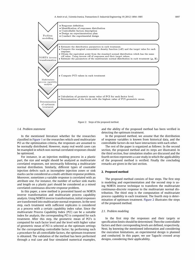
Figure 2: Steps of the proposed method.

1.4. Problem statement

In the mentioned literature whether for the researchesclassified in Figure 1 or the researches which used multivariatePCI as the optimization criteria, the responses are assumed tobe normally distributed. However, many real world cases canbe exampled in which non-normal correlated responses shouldbe optimized.

For instance, in an injection molding process in a plasticpart, the size and weight should be analyzed as multivariatecorrelated responses, not necessarily following a multivariatenormal distribution. Similarly, different types of countableinjection defects such as incomplete injection zones or sinkmarks can be considered as amulti-attribute response problem.Moreover, sometimes a variable response is correlated with anattribute one. For instance, the number of surface sink marksand length on a plastic part should be considered as a mixedcorrelated continuous-discrete response problem.

In this paper, a new method is presented based on NORTAinverse transformation and multivariate process capabilityanalysis. Using NORTA inverse transformation, initial responsesare transformed intomultivariate normal responses. In the nextstep, each treatment with sufficient replicates is consideredas a process with a certain capability index value. Since themultivariate Process Capability Index (PCI) can be a suitableindex for analysis, the corresponding PCI is computed for eachtreatment. After this step, the geometric mean of PCI’s iscomputed for each factor level and the level with higher valueof geometric mean of PCI is selected as the optimum settingsfor the corresponding controllable factor; by performing sucha procedure for all controllable factors, the optimum treatmentis obtained. The validation of the method has been performedthrough a real case and four simulated numerical examples,

and the ability of the proposed method has been verified indetecting the optimum treatment.

In the proposed method, we assume that the distributionof response variables is known from historical data, and thecontrollable factors do not have interactions with each other.

The rest of the paper is organized as follows: In the secondsection, the proposed method and its steps are illustrated. Inthe third section, four simulation studies are discussed and thefourth section represents a case study inwhich the applicabilityof the proposed method is verified. Finally the concludingremarks are given in the last section.

2. Proposed method

The proposed method consists of four steps. The first stepis modeling and experimentation and the second step is us-ing NORTA inverse technique to transform the multivariatecontinuous-discrete response to the multivariate normal dis-tribution. The third step is the computation of multivariateprocess capability in each treatment. The fourth step is deter-mination of optimum treatment. Figure 2 illustrates the stepsof the proposed method.

2.1. Problem modeling

In the first step the responses and their targets orspecification limits should be determined. Then the controllablefactors and their corresponding levels are defined, respectively.Next, by knowing the mentioned information and consideringthe execution limitations, an experimental design is plannedand conducted. In this paper, we use Taguchi crossed arraydesigns, considering their applicability.

1898 A. Amiri et al. / Scientia Iranica, Transactions E: Industrial Engineering 19 (2012) 1894–1905

Figure 3: Schematic procedure of NORTA inverse transformation.

2.2. NORTA inverse transformation

Several transformation techniques have been proposed fortransforming non-normal responses into normal or approx-imately normal responses. For instance, Box–Cox [29] andJohnson [34] are the basic methods proposed for transform-ing non-normal data to normal. Quesenberry [35] proposed theQ -transformation method, and Xie et al. [36] introduced dou-ble square root transformation. For this purpose, the most re-cent method which is NORTA inverse transformation, proposedby Niaki and Abbasi [37,38], was used for transformation ofa multi-attribute data to a multivariate normal distribution inthe area of statistical process control. NORTA inverse techniquetransforms non-normal multivariate data to approximate mul-tivariate normal distributed data.

Since the basic transformations, such as Box–Cox [29] andJohnson [34], do not usually result in acceptable transforma-tions for discrete data, root transformation technique mightbe the only counterpart of NORTA inverse for transformingdiscrete data. By considering the researches by Niaki and Ab-basi [37,38] and Doroudyan et al. [39] in which the ability ofNORTA inverse transformation has been confirmed in processmonitoring in the presence of discrete data, one can claim thecompetency of NORTA inverse for transforming discrete data tonormal distribution.

2.2.1. The method and formula of NORTA inverse transformationThe NORTA inverse transformation, by which an arbitrary

distributed vector of variables x = (x1, x2, . . . , xv)T is changed

to a vector of multivariate normal distribution (y), is defined bythe following equation:

y = (y1, y2, . . . , yν)T

=Φ−1 Fx1(x1) ,

Φ−1 Fx2(x2) , . . . , Φ−1 Fxν (xν)T

, (6)

where Fxi(xi) is the cumulative density function (cdf) of variablexi, and Φ−1 denotes the inverse cdf of a univariate standardnormal distribution. Using the transformation of Φ−1(·), itcan be ensured that y has a multivariate normal distributionwith the mean vector of zero and covariance matrix of Σy. InNORTA inverse method, the main challenge is determining thecorrelation matrix Σy [37].

In this paper, the estimation of the correlation for trans-formed response is done using moment method. To illustratethe procedure of NORTA inverse technique, refer to Figure 3.

As it can be seen in Figure 3, the NORTA inverse returnsthe equivalent point of the standardized normal distributionwhich has the same cdf value of the initial point from the initialdistribution.

The NORTA inverse technique has been used in statisticalprocess control researches,while for implementing thismethodin experimental design, some important notions should beconsidered. As the first notion, since in experimental designeach treatment can be considered as a certain process, theresponses distributions parameters should be estimated ineach treatment. The other notion is the necessity of targetstransformation in NTB (Nominal The Best) cases. Since thetarget values are needed for computing the PCI value, targetvalues should be transformed into the same scale as theresponses have been. This leads to the preservation of statisticaldistance of target values with the obtained responses in eachtreatment.

2.2.2. Evaluation and validation of NORTA inverse performanceIn this section, first we discuss the impact of NORTA inverse

on the capability properties of non-normal data, and thenpresent the Jarque and Bera (JB) normality test [40].

A numerical analysis described below shows that theoriginal properties of the responses are preserved when theinitial responses are transformed into the normal distributionusing NORTA inverse technique. Hence, the process capabilityvalue of transformed data and initial responses will beapproximately the same. As shown in Figure 4, covariancedistance is used as the comparison criterion to represent thestatistical properties of the original non-normal responses, aswell as the transformed normal responses. There are somesimilarities between the CD and the process capability. TheCovariance Distance (CD) is computed using Eq. (7):

CD =

(x − t)TΣ−1(x − t), (7)

where x and t represent the response and target vectors, respec-tively, and Σ represents the covariance matrix of responses.

A simulation analysis is conducted to assure the aboveassumption. Consider a bivariate Gamma distributed process.Using n simulated observations, the CD value of responses iscalculated. On the other hand, the simulated observations andthe mean and target vectors are transformed into standardizedbivariate normal distribution using NORTA inverse. Again, theCD value of these new transformed data is computed using thesame index. This procedure is iterated 100 runs for differentvalues of n observations ranging from5 to 100. For each value ofn the average value of CD is computed using Eq. (7). The resultsare illustrated in Figure 5 confirming that statistical propertiesof a data set are preserved during the transformation.

As shown in Figure 5, for n values greater than 30, thedifference of CD values between original and transformed

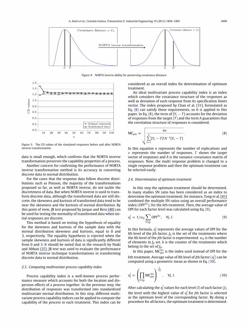
A. Amiri et al. / Scientia Iranica, Transactions E: Industrial Engineering 19 (2012) 1894–1905 1899

Figure 4: NORTA inverse ability for preserving covariance distance.

Figure 5: The CD values of the simulated responses before and after NORTAinverse transformation.

data is small enough, which confirms that the NORTA inversetransformation preserves the capability properties of a process.

Another concern for confirming the performance of NORTAinverse transformation method is its accuracy in convertingdiscrete data to normal distribution.

For the cases that the response data follow discrete distri-butions such as Poisson, the majority of the transformationsproposed so far, as well as NORTA inverse, do not tackle thediscreteness of data. But when NORTA inverse is used to trans-form discrete data, although the transformed data are still dis-crete, the skewness and kurtosis of transformed data tend to benear the skewness and the kurtosis of normal distribution. Bythis point of view, JB test proposed by Jarque and Bera [40] canbe used for testing the normality of transformed data when ini-tial responses are discrete.

This method is based on testing the hypothesis of equalityfor the skewness and kurtosis of the sample data with thenormal distribution skewness and kurtosis, equal to 0 and3, respectively. The equality hypothesis is rejected when thesample skewness and kurtosis of data is significantly differentfrom 0 and 3. It should be noted that in the research by Niakiand Abbasi [37], JB test was used to evaluate the performanceof NORTA inverse technique transformations in transformingdiscrete data to normal distribution.

2.3. Computing multivariate process capability index

Process capability index is a well-known process perfor-mance measure which accounts for both the location and dis-persion effects of a process together. In the previous step, thedistribution of responses was transformed into standardizedmultivariate normal distribution. In this step, different multi-variate process capability indices can be applied to compute thecapability of the process in each treatment. This index can be

considered as an overall index for determination of optimumtreatment.

An ideal multivariate process capability index is an indexwhich considers the covariance structure of the responses aswell as deviation of each response from its specification limitsvector. The index proposed by Chan et al. [31], formulated asEq. (8) can satisfy these requirements, so it is applied in thispaper. In Eq. (8), the term of [Yi − T ] accounts for the deviationof responses from the target (T ) and the term A guarantees thatthe correlation structure of responses is considered.

MCpm =

nvn

i=1[Yi − T ]tA−1[Yi − T ]

. (8)

In this equation n represents the number of replications andv represents the number of responses. T shows the targetvector of responses and A is the variance–covariance matrix ofresponses. Now, the multi response problem is changed to asingle response problem and then the optimum treatment canbe selected easily.

2.4. Determination of optimum treatment

In this step the optimum treatment should be determined.In many studies SN ratio has been considered as an index todetermine the optimum treatment; for instance, Tong et al. [41]combined the multiple SN ratios using an overall performanceindex (OPI(k)); for the kth treatment. Then, the average value ofOPI for each factor level was calculated using Eq. (9),

ηjl = 1/wjl

k∈Jjl

OPI(k), ∀j, l. (9)

In this formula, ηjl represents the average values of OPI for the

lth level of the jth factor. Jjl is the set of the treatments wherethe lth level of the jth factor is experimented. wjl is the numberof elements in Jjl set. k is the counter of the treatments whichbelong to the set of Jjl.

In this paper, MC(k)pm is the index used instead of OPI for the

kth treatment. Average value of lth level of jth factor (ηjl) can be

computed using a geometric mean as shown in Eq. (10).

ηjl =

k∈Jjl

MC(k)pm

1wjl

, ∀j, l. (10)

After calculating the ηjl values for each level (l) of each factor (j),

the level with the highest value of ηjl for jth factor is selected

as the optimum level of the corresponding factor. By doing aprocedure for all factors, the optimum treatment is determined.

1900 A. Amiri et al. / Scientia Iranica, Transactions E: Industrial Engineering 19 (2012) 1894–1905

Table 2: Simulation information for multivariate normal response problem in the simulation study of Section 3.1.

Response µ Σ Distribution

y1 0.5 + 0.2x1 + 0.3x2 − 0.7x3 + 0.4x4

1 0.350.35 1

Normal

y2 0.2 + 0.3x1 + 0.5x2 − 0.8x3 + 0.2x4 Normal

Factors x1 x2 x3 x4

Levels5 7 4.5 36 9.5 7 47 12 9.5 5

Table 3: Simulation information for multivariate non-normal response problems, in the simulation study of Section 3.2.

Response µ ρ Distribution

y1 exp(0.4986 + 0.5x1 + 0.06x2 − 0.7x3 + 6x4) 0.35 Gammay2 exp(0.1094 + 0.7x1 + 0.1x2 − 0.8x3 + 6x4) Gamma

Factors x1 x2 x3 x4

Levels1 30 1 0.33 50 3 0.55 70 5 0.7

3. Simulation studies

In this section, the performance of the proposed method isevaluated in four simulation studies. In the first three examples,the accuracy of the proposed method is tested for multivariatenormal, multivariate non-normal and multi-attribute responseproblems, respectively. In the fourth simulation study, the per-formance of NORTA inverse method is evaluated in comparisonwith the root transformation for computing the PCI of mixed-continuous-discrete data using the approach presented byAbbasi and Niaki [24], explained in Section 1.2.

A similar simulation procedure is used in the first threesimulation studies, which is explained as follows.

In this procedure, a full factorial experimental design isconsideredwhere the responses are generated using predefinedregression functions. Then the responses are transformed usingNORTA inverse method, and the MCpm index is computed ineach treatment using Eq. (8). The treatment with highest valueof MCpm is considered as the optimum treatment.

As the second stage of the simulation procedure, a fractionalfactorial design, for instance an L9, is performed where theresponses are generated using the same functions appliedin the full factorial experiment. Then by implementing themethod proposed in this paper, the optimum treatment isdetermined for this fractional factorial experiment. Note thatfour controllable factors with three levels for each factor areconsidered in all the simulation studies.

The accuracy of the proposedmethod in this paper is verifiedif the determined optimum treatment in the fractional factorialexperiment is the same as for the full factorial experiment. Formore validation of the procedure, the mentioned optimizationmethod is iterated 100 times for the fractional factorial, andthe percent of the success times is reported as the result of thesimulation study. The simulation studies are discussed in detailsas follows.

3.1. Evaluation of the proposed optimization method for multi-variate normal response problems

In this section for verifying the capability of the proposed op-timization method for multivariate normal response problems,

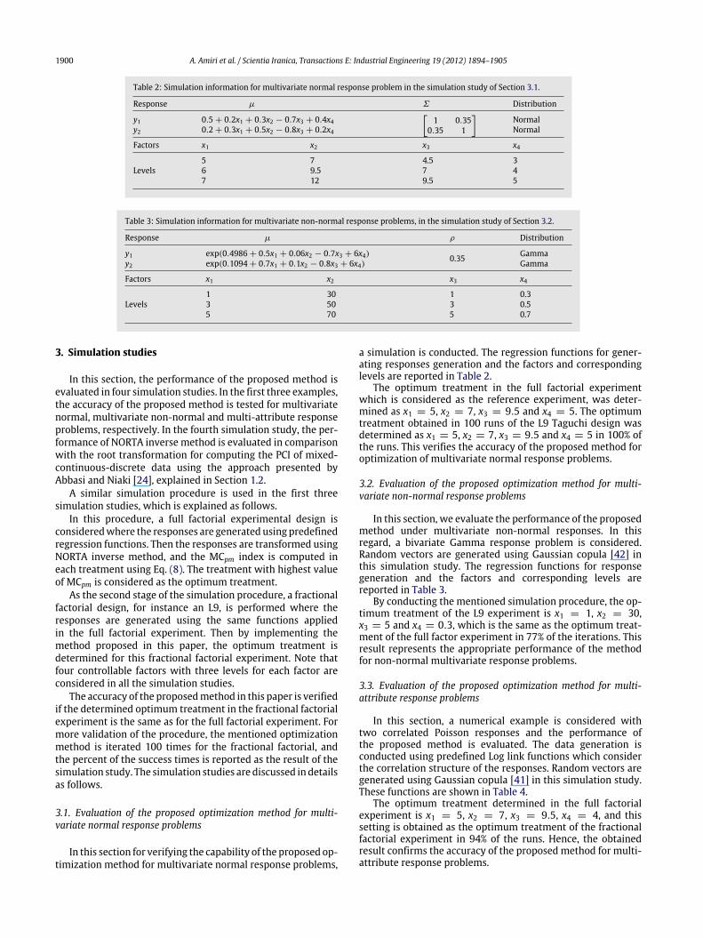
a simulation is conducted. The regression functions for gener-ating responses generation and the factors and correspondinglevels are reported in Table 2.

The optimum treatment in the full factorial experimentwhich is considered as the reference experiment, was deter-mined as x1 = 5, x2 = 7, x3 = 9.5 and x4 = 5. The optimumtreatment obtained in 100 runs of the L9 Taguchi design wasdetermined as x1 = 5, x2 = 7, x3 = 9.5 and x4 = 5 in 100% ofthe runs. This verifies the accuracy of the proposed method foroptimization of multivariate normal response problems.

3.2. Evaluation of the proposed optimization method for multi-variate non-normal response problems

In this section, we evaluate the performance of the proposedmethod under multivariate non-normal responses. In thisregard, a bivariate Gamma response problem is considered.Random vectors are generated using Gaussian copula [42] inthis simulation study. The regression functions for responsegeneration and the factors and corresponding levels arereported in Table 3.

By conducting the mentioned simulation procedure, the op-timum treatment of the L9 experiment is x1 = 1, x2 = 30,x3 = 5 and x4 = 0.3, which is the same as the optimum treat-ment of the full factor experiment in 77% of the iterations. Thisresult represents the appropriate performance of the methodfor non-normal multivariate response problems.

3.3. Evaluation of the proposed optimization method for multi-attribute response problems

In this section, a numerical example is considered withtwo correlated Poisson responses and the performance ofthe proposed method is evaluated. The data generation isconducted using predefined Log link functions which considerthe correlation structure of the responses. Random vectors aregenerated using Gaussian copula [41] in this simulation study.These functions are shown in Table 4.

The optimum treatment determined in the full factorialexperiment is x1 = 5, x2 = 7, x3 = 9.5, x4 = 4, and thissetting is obtained as the optimum treatment of the fractionalfactorial experiment in 94% of the runs. Hence, the obtainedresult confirms the accuracy of the proposed method for multi-attribute response problems.

A. Amiri et al. / Scientia Iranica, Transactions E: Industrial Engineering 19 (2012) 1894–1905 1901

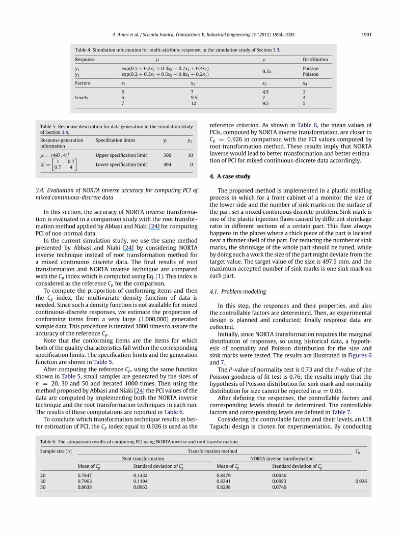
Table 4: Simulation information for multi-attribute response, in the simulation study of Section 3.3.

Response µ ρ Distribution

y1 exp(0.5 + 0.2x1 + 0.3x2 − 0.7x3 + 0.4x4) 0.35 Poissony2 exp(0.2 + 0.3x1 + 0.5x2 − 0.8x3 + 0.2x4) Poisson

Factors x1 x2 x3 x4

Levels5 7 4.5 36 9.5 7 47 12 9.5 5

Table 5: Response description for data generation in the simulation studyof Section 3.4.

Response generationinformation

Specification limits y1 y2

µ = (497, 4)T Upper specification limit 500 10

Σ =

1 0.70.7 4

Lower specification limit 494 0

3.4. Evaluation of NORTA inverse accuracy for computing PCI ofmixed continuous-discrete data

In this section, the accuracy of NORTA inverse transforma-tion is evaluated in a comparison study with the root transfor-mation method applied by Abbasi and Niaki [24] for computingPCI of non-normal data.

In the current simulation study, we use the same methodpresented by Abbasi and Niaki [24] by considering NORTAinverse technique instead of root transformation method fora mixed continuous discrete data. The final results of roottransformation and NORTA inverse technique are comparedwith the Cp index which is computed using Eq. (1). This index isconsidered as the reference Cp for the comparison.

To compute the proportion of conforming items and thenthe Cp index, the multivariate density function of data isneeded. Since such a density function is not available for mixedcontinuous-discrete responses, we estimate the proportion ofconforming items from a very large (1,000,000) generatedsample data. This procedure is iterated 1000 times to assure theaccuracy of the reference Cp.

Note that the conforming items are the items for whichboth of the quality characteristics fall within the correspondingspecification limits. The specification limits and the generationfunction are shown in Table 5.

After computing the reference Cp, using the same functionshown in Table 5, small samples are generated by the sizes ofn = 20, 30 and 50 and iterated 1000 times. Then using themethod proposed by Abbasi and Niaki [24] the PCI values of thedata are computed by implementing both the NORTA inversetechnique and the root transformation techniques in each run.The results of these computations are reported in Table 6.

To conclude which transformation technique results in bet-ter estimation of PCI, the Cp index equal to 0.926 is used as the

reference criterion. As shown in Table 6, the mean values ofPCIs, computed by NORTA inverse transformation, are closer toCp = 0.926 in comparison with the PCI values computed byroot transformation method. These results imply that NORTAinverse would lead to better transformation and better estima-tion of PCI for mixed continuous-discrete data accordingly.

4. A case study

The proposed method is implemented in a plastic moldingprocess in which for a front cabinet of a monitor the size ofthe lower side and the number of sink marks on the surface ofthe part set a mixed continuous discrete problem. Sink mark isone of the plastic injection flaws caused by different shrinkageratio in different sections of a certain part. This flaw alwayshappens in the places where a thick piece of the part is locatednear a thinner shell of the part. For reducing the number of sinkmarks, the shrinkage of the whole part should be tuned, whileby doing such awork the size of the partmight deviate from thetarget value. The target value of the size is 497.5 mm, and themaximum accepted number of sink marks is one sink mark oneach part.

4.1. Problem modeling

In this step, the responses and their properties, and alsothe controllable factors are determined. Then, an experimentaldesign is planned and conducted; finally response data arecollected.

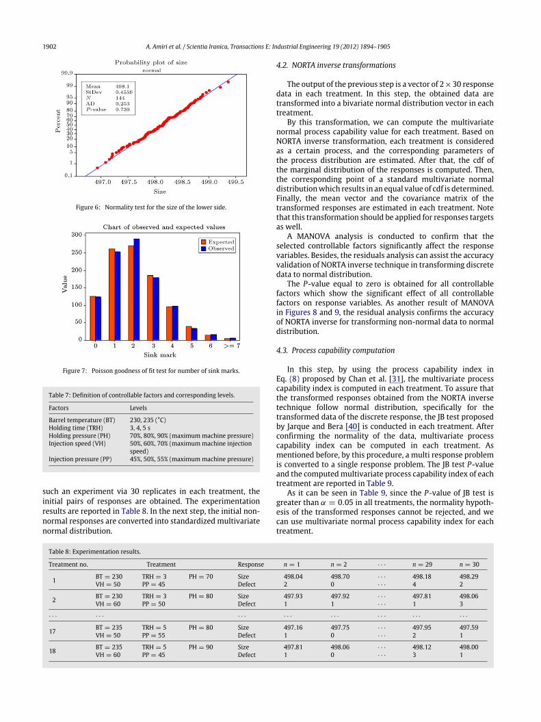
Initially, since NORTA transformation requires the marginaldistribution of responses, so using historical data, a hypoth-esis of normality and Poisson distribution for the size andsink marks were tested. The results are illustrated in Figures 6and 7.

The P-value of normality test is 0.73 and the P-value of thePoisson goodness of fit test is 0.76; the results imply that thehypothesis of Poisson distribution for sink mark and normalitydistribution for size cannot be rejected in α = 0.05.

After defining the responses, the controllable factors andcorresponding levels should be determined. The controllablefactors and corresponding levels are defined in Table 7.

Considering the controllable factors and their levels, an L18Taguchi design is chosen for experimentation. By conducting

Table 6: The comparison results of computing PCI using NORTA inverse and root transformation.

Sample size (n) Transformation method Cp

Root transformation NORTA inverse transformationMean of C ′

p Standard deviation of C ′p Mean of C ′

p Standard deviation of C ′p

20 0.7847 0.1432 0.8479 0.004630 0.7963 0.1194 0.8241 0.0983 0.92650 0.8038 0.0963 0.8298 0.0749

1902 A. Amiri et al. / Scientia Iranica, Transactions E: Industrial Engineering 19 (2012) 1894–1905

Figure 6: Normality test for the size of the lower side.

Figure 7: Poisson goodness of fit test for number of sink marks.

Table 7: Definition of controllable factors and corresponding levels.

Factors Levels

Barrel temperature (BT) 230, 235 (°C)Holding time (TRH) 3, 4, 5 sHolding pressure (PH) 70%, 80%, 90% (maximummachine pressure)Injection speed (VH) 50%, 60%, 70% (maximummachine injection

speed)Injection pressure (PP) 45%, 50%, 55% (maximummachine pressure)

such an experiment via 30 replicates in each treatment, theinitial pairs of responses are obtained. The experimentationresults are reported in Table 8. In the next step, the initial non-normal responses are converted into standardized multivariatenormal distribution.

4.2. NORTA inverse transformations

The output of the previous step is a vector of 2×30 responsedata in each treatment. In this step, the obtained data aretransformed into a bivariate normal distribution vector in eachtreatment.

By this transformation, we can compute the multivariatenormal process capability value for each treatment. Based onNORTA inverse transformation, each treatment is consideredas a certain process, and the corresponding parameters ofthe process distribution are estimated. After that, the cdf ofthe marginal distribution of the responses is computed. Then,the corresponding point of a standard multivariate normaldistributionwhich results in an equal value of cdf is determined.Finally, the mean vector and the covariance matrix of thetransformed responses are estimated in each treatment. Notethat this transformation should be applied for responses targetsas well.

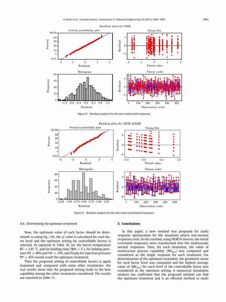
A MANOVA analysis is conducted to confirm that theselected controllable factors significantly affect the responsevariables. Besides, the residuals analysis can assist the accuracyvalidation of NORTA inverse technique in transforming discretedata to normal distribution.

The P-value equal to zero is obtained for all controllablefactors which show the significant effect of all controllablefactors on response variables. As another result of MANOVAin Figures 8 and 9, the residual analysis confirms the accuracyof NORTA inverse for transforming non-normal data to normaldistribution.

4.3. Process capability computation

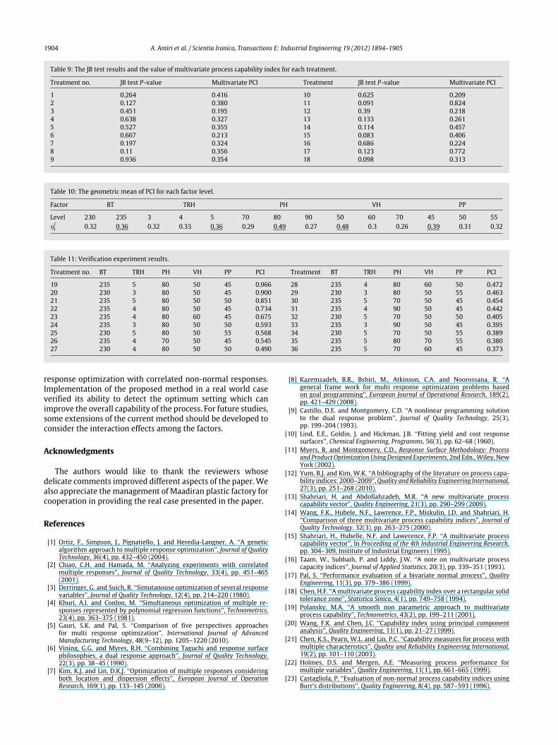
In this step, by using the process capability index inEq. (8) proposed by Chan et al. [31], the multivariate processcapability index is computed in each treatment. To assure thatthe transformed responses obtained from the NORTA inversetechnique follow normal distribution, specifically for thetransformed data of the discrete response, the JB test proposedby Jarque and Bera [40] is conducted in each treatment. Afterconfirming the normality of the data, multivariate processcapability index can be computed in each treatment. Asmentioned before, by this procedure, a multi response problemis converted to a single response problem. The JB test P-valueand the computedmultivariate process capability index of eachtreatment are reported in Table 9.

As it can be seen in Table 9, since the P-value of JB test isgreater than α = 0.05 in all treatments, the normality hypoth-esis of the transformed responses cannot be rejected, and wecan use multivariate normal process capability index for eachtreatment.

Table 8: Experimentation results.

Treatment no. Treatment Response n = 1 n = 2 · · · n = 29 n = 30

1 BT = 230 TRH = 3 PH = 70 Size 498.04 498.70 · · · 498.18 498.29VH = 50 PP = 45 Defect 2 0 · · · 4 2

2 BT = 230 TRH = 3 PH = 80 Size 497.93 497.92 · · · 497.81 498.06VH = 60 PP = 50 Defect 1 1 · · · 1 3

· · · · · · · · · · · · · · · · · · · · · · · ·

17 BT = 235 TRH = 5 PH = 80 Size 497.16 497.75 · · · 497.95 497.59VH = 50 PP = 55 Defect 1 0 · · · 2 1

18 BT = 235 TRH = 5 PH = 90 Size 497.81 498.06 · · · 498.12 498.00VH = 60 PP = 45 Defect 1 0 · · · 3 1

A. Amiri et al. / Scientia Iranica, Transactions E: Industrial Engineering 19 (2012) 1894–1905 1903

Figure 8: Residual analysis for the size transformed responses.

Figure 9: Residual analysis for the sink mark transformed responses.

4.4. Determining the optimum treatment

Now, the optimum value of each factor should be deter-mined, so using Eq. (10), the η

jl value is calculated for each fac-

tor level and the optimum setting for controllable factors isselected. As reported in Table 10, for the barrel temperatureBT = 235 °C, and for holding time TRH = 5 s, for holding pres-sure PH = 80% and VH = 50%, and finally for injection pressurePP = 45% would result the optimum treatment.

Then the proposed setting of controllable factors is againexamined and compared with some other treatments; thereal results show that the proposed setting leads to the bestcapability among the other treatments considered. The resultsare reported in Table 11.

5. Conclusions

In this paper, a new method was proposed for multiresponse optimization for the situations where non-normalresponses exist. In thismethod, using NORTA inverse, the initialcorrelated responses were transformed into the multivariatenormal responses. Then, for each treatment, the value ofmultivariate process capability (MCpm) was computed andconsidered as the single response for each treatment. Fordetermination of the optimum treatment, the geometric meanfor each factor level was computed and the highest averagevalue of (MCpm) for each level of the controllable factor wasconsidered as the optimum setting. A numerical simulationanalysis has confirmed that the proposed method can findthe optimum treatment and is an efficient method in multi

1904 A. Amiri et al. / Scientia Iranica, Transactions E: Industrial Engineering 19 (2012) 1894–1905

Table 9: The JB test results and the value of multivariate process capability index for each treatment.

Treatment no. JB test P-value Multivariate PCI Treatment JB test P-value Multivariate PCI

1 0.264 0.416 10 0.625 0.2092 0.127 0.380 11 0.091 0.8243 0.451 0.195 12 0.39 0.2184 0.638 0.327 13 0.133 0.2615 0.527 0.355 14 0.114 0.4576 0.667 0.213 15 0.083 0.4067 0.197 0.324 16 0.686 0.2248 0.11 0.356 17 0.123 0.7729 0.936 0.354 18 0.098 0.313

Table 10: The geometric mean of PCI for each factor level.

Factor BT TRH PH VH PP

Level 230 235 3 4 5 70 80 90 50 60 70 45 50 55ηjl 0.32 0.36 0.32 0.33 0.36 0.29 0.49 0.27 0.48 0.3 0.26 0.39 0.31 0.32

Table 11: Verification experiment results.

Treatment no. BT TRH PH VH PP PCI Treatment BT TRH PH VH PP PCI

19 235 5 80 50 45 0.966 28 235 4 80 60 50 0.47220 230 3 80 50 45 0.900 29 230 3 80 50 55 0.46321 235 5 80 50 50 0.851 30 235 5 70 50 45 0.45422 235 4 80 50 45 0.734 31 235 4 90 50 45 0.44223 235 4 80 60 45 0.675 32 230 5 70 50 50 0.40524 235 3 80 50 50 0.593 33 235 3 90 50 45 0.39525 230 5 80 50 55 0.568 34 230 5 70 50 55 0.38926 235 4 70 50 45 0.545 35 235 5 80 70 55 0.38027 230 4 80 50 50 0.490 36 235 5 70 60 45 0.373

response optimization with correlated non-normal responses.Implementation of the proposed method in a real world caseverified its ability to detect the optimum setting which canimprove the overall capability of the process. For future studies,some extensions of the current method should be developed toconsider the interaction effects among the factors.

Acknowledgments

The authors would like to thank the reviewers whosedelicate comments improved different aspects of the paper.Wealso appreciate the management of Maadiran plastic factory forcooperation in providing the real case presented in the paper.

References

[1] Ortiz, F., Simpson, J., Pignatiello, J. and Heredia-Langner, A. ‘‘A geneticalgorithm approach to multiple response optimization’’, Journal of QualityTechnology, 36(4), pp. 432–450 (2004).

[2] Chiao, C.H. and Hamada, M. ‘‘Analyzing experiments with correlatedmultiple responses’’, Journal of Quality Technology, 33(4), pp. 451–465(2001).

[3] Derringer, G. and Suich, R. ‘‘Simutanouse optimization of several responsevariables’’, Journal of Quality Technology, 12(4), pp. 214–220 (1980).

[4] Khuri, A.I. and Conlon, M. ‘‘Simultaneous optimization of multiple re-sponses represented by polynomial regression functions’’, Technometrics,23(4), pp. 363–375 (1981).

[5] Gauri, S.K. and Pal, S. ‘‘Comparison of five perspectives approachesfor multi response optimization’’, International Journal of AdvancedManufacturing Technology, 48(9–12), pp. 1205–1220 (2010).

[6] Vining, G.G. and Myres, R.H. ‘‘Combining Taguchi and response surfacephilosophies, a dual response approach’’, Journal of Quality Technology,22(3), pp. 38–45 (1990).

[7] Kim, K.J. and Lin, D.K.J. ‘‘Optimization of multiple responses consideringboth location and dispersion effects’’, European Journal of OperationResearch, 169(1), pp. 133–145 (2006).

[8] Kazemzadeh, B.R., Bshiri, M., Atkinson, C.A. and Noorossana, R. ‘‘Ageneral frame work for multi response optimization problems basedon goal programming’’, European Journal of Operational Research, 189(2),pp. 421–429 (2008).

[9] Castillo, D.E. and Montgomery, C.D. ‘‘A nonlinear programming solutionto the dual response problem’’, Journal of Quality Technology, 25(3),pp. 199–204 (1993).

[10] Lind, E.E., Goldin, J. and Hickman, J.B. ‘‘Fitting yield and cost responsesurfaces’’, Chemical Engineering, Programms, 56(3), pp. 62–68 (1960).

[11] Myers, R. and Montgomery, C.D., Response Surface Methodology: Processand Product OptimizationUsingDesigned Experiments, 2nd Edn.,Wiley, NewYork (2002).

[12] Yum, B.J. and Kim, W.K. ‘‘A bibliography of the literature on process capa-bility indices: 2000–2009’’,Quality andReliability Engineering International,27(3), pp. 251–268 (2010).

[13] Shahriari, H. and Abdollahzadeh, M.R. ‘‘A new multivariate processcapability vector’’, Quality Engineering, 21(3), pp. 290–299 (2009).

[14] Wang, F.K., Hubele, N.F., Lawrence, F.P., Miskulin, J.D. and Shahriari, H.‘‘Comparison of three multivariate process capability indices’’, Journal ofQuality Technology, 32(3), pp. 263–275 (2000).

[15] Shahriari, H., Hubelle, N.F. and Lawerence, F.P. ‘‘A multivariate processcapability vector’’, In Proceeding of the 4th Industrial Engineering Research,pp. 304–309, Institute of Industrial Engineers (1995).

[16] Taam, W., Subbaih, P. and Liddy, J.W. ‘‘A note on multivariate processcapacity indices’’, Journal of Applied Statistics, 20(3), pp. 339–351 (1993).

[17] Pal, S. ‘‘Performance evaluation of a bivariate normal process’’, QualityEngineering, 11(3), pp. 379–386 (1999).

[18] Chen, H.F. ‘‘Amultivariate process capability index over a rectangular solidtolerance zone’’, Statistica Sinica, 4(1), pp. 749–758 (1994).

[19] Polansky, M.A. ‘‘A smooth non parametric approach to multivariateprocess capability’’, Technometrics, 43(2), pp. 199–211 (2001).

[20] Wang, F.K. and Chen, J.C. ‘‘Capability index using principal componentanalysis’’, Quality Engineering, 11(1), pp. 21–27 (1999).

[21] Chen, K.S., Pearn, W.L. and Lin, P.C. ‘‘Capability measures for process withmultiple characteristics’’, Quality and Reliability Engineering International,19(2), pp. 101–110 (2003).

[22] Holmes, D.S. and Mergen, A.E. ‘‘Measuring process performance formultiple variables’’, Quality Engineering, 11(1), pp. 661–665 (1999).

[23] Castagliola, P. ‘‘Evaluation of non-normal process capability indices usingBurr’s distributions’’, Quality Engineering, 8(4), pp. 587–593 (1996).

A. Amiri et al. / Scientia Iranica, Transactions E: Industrial Engineering 19 (2012) 1894–1905 1905

[24] Abbasi, B. and Niaki, S.T.A. ‘‘Estimating process capability indices ofmultivariate non-normal processes’’, International Journal of AdvancedManufacturing Technology, 50(5–8), pp. 823–830 (2010).

[25] Hossenifard, S.Z., Abbasi, B., Ahmad, S. and Abdollahian, M. ‘‘A transfor-mation technique to estimate the process capability index for non-normalprocesses’’, International Journal of Advanced Manufacturing Technology,40(5–6), pp. 512–517 (2009).

[26] Castagliola, P. and Castellanos, G.J. ‘‘Process capability indices dedicatedto bivariate non-normal distributions’’, Journal of Quality in Maintenance,14(1), pp. 87–101 (2008).

[27] Ahmad, S., Abdollahian, M., Zeephongsekul, P. and Abbasi, B. ‘‘Multivariatenon-normal process capability analysis’’, International Journal of AdvancedManufacturing Technology, 44(7–8), pp. 757–765 (2009).

[28] Abbasi, B., Ahmad, S., Abdollahian, M. and Zeephongsekul, P. ‘‘Measuringprocess capability for bivariate non-normal process using the bivariateBurr distribution’’, WSEAS Transactions on Buisiness and Economics, 4(5),pp. 71–77 (2007).

[29] Box, G.E.P. and Cox, D.R. ‘‘An analysis of transformations’’, Journal of theRoyal Statistical Society, Series B, 26, pp. 211–252 (1964).

[30] Awad, I.M. and Kovach, V.J. ‘‘Multi response optimization using multivari-ate process capability index’’, Quality and Reliability Engineering Interna-tional, 27(4), pp. 465–477 (2011).

[31] Chan, L.K., Cheng, S.W. and Spiring, F.A. ‘‘Amultivariatemeasure of processcapability’’, International Journal of Modeling and Simulation, 11(1), pp. 1–6(1991).

[32] Plante, D.R. ‘‘Process capability: a criterion for optimizing multiple re-sponses product and process design’’, IIE Transactions, 33(2), pp. 497–509(2001).

[33] Lee, P.H. and Yum, J.B. ‘‘Multi characteristics parameter design: adesirability function approach based on process capability indices’’,International Journal of Reliability, Quality and Safety Engineering, 10(4),pp. 445–461 (2003).

[34] Johnson, N. ‘‘Systems of frequency curves generated by methods oftranslations’’, Biometrika, 36, pp. 149–176 (1949).

[35] Quesenberry, C.P., SPCMethods for Quality Improvement, JohnWiley& Sons,New York (1997).

[36] Xie, M., Goh, T.N. and Tang, Y. ‘‘Data transformation for geometricallydistributed quality characteristics’’, Quality and Reliability EngineeringInternational, 16(1), pp. 9–15 (2000).

[37] Niaki, S.T.A. and Abbasi, B. ‘‘On the monitoring of multi-attributes high-quality production processes’’,Metrica, 66(3), pp. 373–388 (2007).

[38] Niaki, S.T.A. and Abbasi, B. ‘‘Monitoringmulti-attribute processes based onNORTA inverse transformed vectors’’, Communication in Statistics—Theoryand Methods, 38(7), pp. 964–979 (2009).

[39] Doroudyan, M.H., Amiri, A. and Abbasi, B. ‘‘Monitoring correlated variableand attribute quality characteristics based on NORTA inverse technique’’,International Journal of Productivity and Quality Management, (2012)(submitted for publication).

[40] Jarque, C.M. and Bera, A.K. ‘‘A test for normality of observations andregression residuals’’, International Statistical Review, 55(2), pp. 163–172(1987).

[41] Tong, L.I., Wang, H.C., Chen, C.C. and Chen, C.T. ‘‘Dynamic multipleresponses by ideal solution analysis’’, European Journal of OperationalResearch, 156(2), pp. 433–444 (2004).

[42] Cherubini, U.E., Luciano, E. and Vecchiato, W., Copula Methods in Finance,John Wiley & Sons, England (2004).

Amirhossein Amiri is an Assistant Professor at Shahed University in Iran. Heholds B.S., M.S. and Ph.D. degrees in Industrial Engineering from Khajeh NasirUniversity of Technology, IranUniversity of Science andTechnology, and TarbiatModares University, respectively. He is a member of the Iranian StatisticalAssociation. His research interests include statistical quality control, profilemonitoring, and Six Sigma.

Mahdi Bashiri is an Associate Professor at Shahed University in Iran. Heholds B.S. degree in Industrial Engineering from Iran University of Science andTechnology and M.S. and Ph.D. degrees in the same field from Tarbiat ModaresUniversity. His research interests include design of experiments and multipleresponse optimization and facility location.

Hamed Mogouie is an M.S. student in Industrial Engineering at ShahedUniversity in Iran. His research interests are design of experiment, statisticalprocess control and quality management.

Mohammad Hadi Doroudyan is a Ph.D. student in Industrial Engineering atYazd University in Iran. He holds M.S. degree in Industrial Engineering fromShahed University and B.S. degree from Azad University-South Tehran Branch.His research interests are statistical quality control and design of experiments.