
Non-Intrusive Pressure Measurement in Microchannels
118
NON-INTRUSIVE PRESSURE MEASUREMENT IN MICROCHANNELS By Derek Fultz A THESIS Submitted in partial fulfillment of the requirements for the degree of Master of Science in Mechanical Engineering MICHIGAN TECHNOLOGICAL UNIVERSITY 2007 Copyright c Derek Fultz 2007
-
Upload
khangminh22 -
Category
Documents
-
view
0 -
download
0
Transcript of Non-Intrusive Pressure Measurement in Microchannels

NON-INTRUSIVE PRESSURE MEASUREMENT INMICROCHANNELS
By
Derek Fultz
A THESIS
Submitted in partial fulfillment of the requirements
for the degree of
Master of Science in Mechanical Engineering
MICHIGAN TECHNOLOGICAL UNIVERSITY
2007
Copyright c© Derek Fultz 2007

This thesis, “NON-INTRUSIVE PRESSURE MEASUREMENT IN MICROCHAN-NELS” is hereby approved in partial fulfillment of the requirements of the Degree ofMaster of Science in Mechanical Engineering.
Department of Mechanical Engineering - Engineering Mechanics
Advisor:
Jeffrey S. Allen PhD
Committee Member:
Amitabh Narain PhD
Committee Member:
Yoke Khin Yap PhD
Department Chair:
Professor William W. Predebon
Date:

ABSTRACT
NON-INTRUSIVE PRESSURE MEASUREMENT IN MICROCHANNELS
Derek FultzMichigan Technological University, 2007
A non-intrusive interferometric measurement technique has been successfully de-veloped to measure fluid compressibility in both gas and liquid phases via refractiveindex (RI) changes. The technique, consisting of an unfocused laser beam impinginga glass channel, can be used to separate and quantify cell deflection, fluid flow rates,and pressure variations in microchannels. Currently in fields such as microfluidics,pressure and flow rate measurement devices are orders of magnitude larger than thechannel cross-sections making direct pressure and fluid flow rate measurements im-possible. Due to the non-intrusive nature of this technique, such measurements arenow possible, opening the door for a myriad of new scientific research and experimen-tation.
This technique, adapted from the concept of Micro Interferometric BackscatterDetection (MIBD), boasts the ability to provide comparable sensitivities in a varietyof channel types and provides quantification capability not previously demonstratedin backscatter detection techniques. Measurement sensitivity depends heavily on ex-perimental parameters such as beam impingement angle, fluid volume, photodetectorsensitivity, and a channel’s dimensional tolerances. The current apparatus readilyquantifies fluid RI changes of 10−5 refractive index units (RIU) corresponding topressures of approximately 14 psi and 1 psi in water and air, respectively. MIBDreports detection capability as low as 10−9 RIU and the newly adapted technique hasthe potential to meet and exceed this limit providing quantification in the place ofdetection. Specific device sensitivities are discussed and suggestions are provided onhow the technique may be refined to provide optimal quantification capabilities basedon experimental conditions.

ACKNOWLEDGMENTS
I would like to thank all the family, friends, classmates, and professors who have pro-vided help and encouragement throughout my college years. Without your support,I could never have made it to this point.
Also, a special thanks to my advisor, Dr. Jeffrey Allen, for continually pushingme to test new ideas and become a better student, researcher, and engineer. Theeducational, travel, and employment opportunities you have given me have not onlyenhanced my college experience, but my life experience as well.

CONTENTS
Abstract . . . . . . . . . . . . . . . . . . . . . . . . . . . . . . . . . . . . . i
Acknowledgments . . . . . . . . . . . . . . . . . . . . . . . . . . . . . . . . ii
Table of Contents . . . . . . . . . . . . . . . . . . . . . . . . . . . . . . . . iii
List of Figures . . . . . . . . . . . . . . . . . . . . . . . . . . . . . . . . . . v
List of Tables . . . . . . . . . . . . . . . . . . . . . . . . . . . . . . . . . . x
1. Introduction . . . . . . . . . . . . . . . . . . . . . . . . . . . . . . . . . . . 1
2. Interferometry . . . . . . . . . . . . . . . . . . . . . . . . . . . . . . . . . . 32.1 Types of Interferometers . . . . . . . . . . . . . . . . . . . . . . . . . 32.2 Basic Interferometric Theory . . . . . . . . . . . . . . . . . . . . . . . 6
3. Backscattering Interferometry . . . . . . . . . . . . . . . . . . . . . . . . . 103.1 The History of Backscattering Interferometry . . . . . . . . . . . . . 103.2 The MIBD Technique . . . . . . . . . . . . . . . . . . . . . . . . . . . 103.3 Scientific Advancements from MIBD . . . . . . . . . . . . . . . . . . 13
4. Related Scientific Work and Measurement Techniques . . . . . . . . . . . . 154.1 RI Measurement Methods . . . . . . . . . . . . . . . . . . . . . . . . 154.2 Related Measurement Techniques . . . . . . . . . . . . . . . . . . . . 17
5. Experimental Description . . . . . . . . . . . . . . . . . . . . . . . . . . . 195.1 Adapted Backscattering Setup . . . . . . . . . . . . . . . . . . . . . . 195.2 Experimental Parameters - Thin Walled Channels . . . . . . . . . . . 215.3 Experimental Parameters - Thick Walled Channels . . . . . . . . . . 225.4 Fringe Formation . . . . . . . . . . . . . . . . . . . . . . . . . . . . . 235.5 Geometric Path Length Derivation . . . . . . . . . . . . . . . . . . . 26
6. Data Processing Procedures . . . . . . . . . . . . . . . . . . . . . . . . . . 296.1 Counting Fringes . . . . . . . . . . . . . . . . . . . . . . . . . . . . . 296.2 Fringe Tracking in Spotlight . . . . . . . . . . . . . . . . . . . . . . . 306.3 Fringe Tracking in Matlab . . . . . . . . . . . . . . . . . . . . . . . . 306.4 Relating the FFT to Spatial Images . . . . . . . . . . . . . . . . . . . 34

Contents iv
7. Experimental Results . . . . . . . . . . . . . . . . . . . . . . . . . . . . . . 387.1 Channel Cross-Section Less than Beam Diameter . . . . . . . . . . . 387.2 Channel Cross-Section Greater than Beam Diameter . . . . . . . . . 48
8. Verification of Results . . . . . . . . . . . . . . . . . . . . . . . . . . . . . 618.1 Laser Stability Testing . . . . . . . . . . . . . . . . . . . . . . . . . . 618.2 Deflection Testing . . . . . . . . . . . . . . . . . . . . . . . . . . . . . 648.3 Verification with Known Data . . . . . . . . . . . . . . . . . . . . . . 678.4 Description of Matlab Codes Used in Data Processing . . . . . . . . . 70
9. Device Sensitivity . . . . . . . . . . . . . . . . . . . . . . . . . . . . . . . . 719.1 Detection Limits . . . . . . . . . . . . . . . . . . . . . . . . . . . . . 719.2 Effects of Experimental Parameters . . . . . . . . . . . . . . . . . . . 719.3 Sources of Experimental Error . . . . . . . . . . . . . . . . . . . . . . 73
10. Conclusions . . . . . . . . . . . . . . . . . . . . . . . . . . . . . . . . . . . 76
Appendix 80
A. Syringe Pump Calibration . . . . . . . . . . . . . . . . . . . . . . . . . . . 81
B. Pressure Transducer Claibration . . . . . . . . . . . . . . . . . . . . . . . . 85
C. Spotlight Fringe Tracking Results . . . . . . . . . . . . . . . . . . . . . . . 87
D. Laser Stability Plots . . . . . . . . . . . . . . . . . . . . . . . . . . . . . . 90
E. Configurations for Results Verification . . . . . . . . . . . . . . . . . . . . 94E.1 Tube Pinch-Off Mechanism . . . . . . . . . . . . . . . . . . . . . . . . 94E.2 Michelson Interferometer for Deflection Testing . . . . . . . . . . . . 94
F. Fringe Tracking Program . . . . . . . . . . . . . . . . . . . . . . . . . . . . 97
G. Matlab Code for Static Pressure Test Processing . . . . . . . . . . . . . . . 102
H. Matlab External Functions . . . . . . . . . . . . . . . . . . . . . . . . . . . 108
I. Program to Find Sensitivity Using Water . . . . . . . . . . . . . . . . . . . 110
J. Program to Find Sensitivity Using Air . . . . . . . . . . . . . . . . . . . . 112

LIST OF FIGURES
2.1 The classic Michelson interferometer. . . . . . . . . . . . . . . . . . . 42.2 The Mach-Zehnder interferometer, commonly used for single pass RI
measurements. . . . . . . . . . . . . . . . . . . . . . . . . . . . . . . 52.3 The Sagnac Interferometer, commonly used in performing angular ve-
locity measurements. . . . . . . . . . . . . . . . . . . . . . . . . . . 62.4 The Fabry-Perot, commonly used to measure the wavelength of light. 7
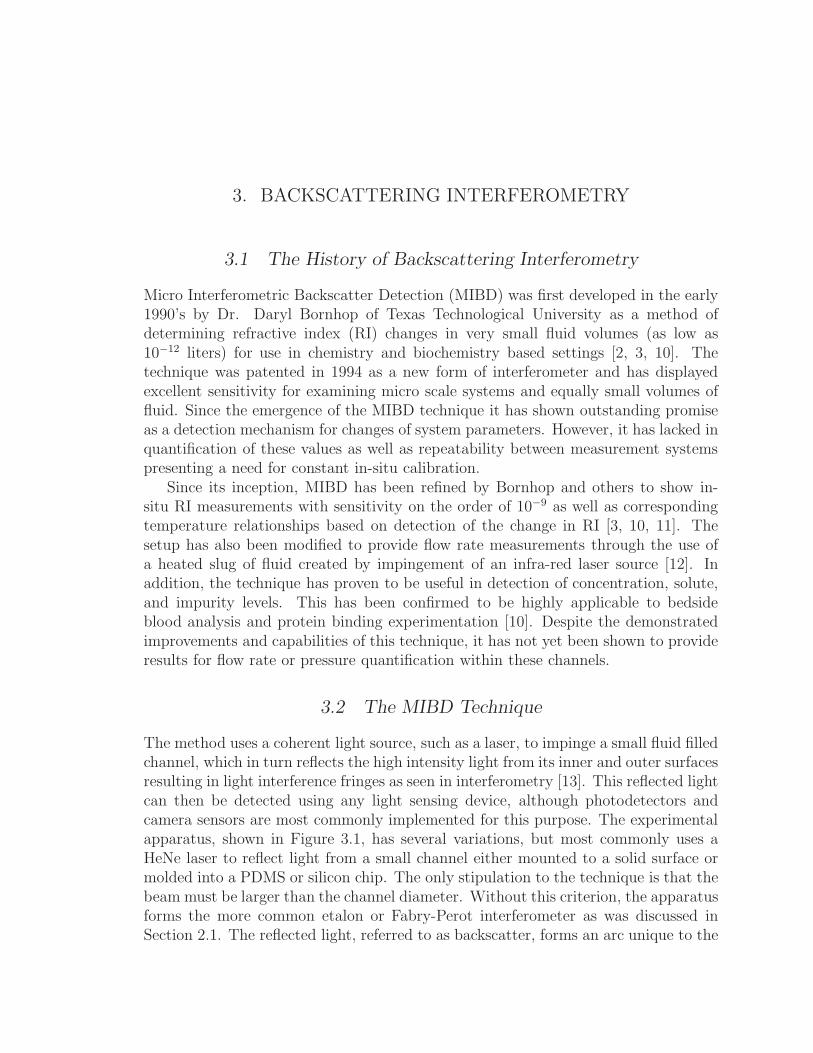
3.1 The MIBD experimental setup in which an unfocused laser beam isreflected from a capillary tube resulting in a backscattered arc of in-terference fringes [2]. . . . . . . . . . . . . . . . . . . . . . . . . . . . 11
3.2 Ray trace of the light path through a circular channel resulting inmultiple reflections. The vertical lines represent the side walls of thechannel [3]. . . . . . . . . . . . . . . . . . . . . . . . . . . . . . . . . 12
3.3 Cross sectional view of ray trace through a circular channel resultingin a 360◦ backscattered arc [3]. . . . . . . . . . . . . . . . . . . . . . 12
3.4 The use of a bicell photodetector for detection of fringe shift. Thedetector consists of two photo-sensitive sectors represented by the whiterectangles over the left fringe [1]. . . . . . . . . . . . . . . . . . . . . 13
4.1 Experimental setup for the laser-capillary-cube technique showing in-terference due to reflection and refraction of incoming light rays. . . 16
5.1 Simplified ray trace of the light path through a capillary scale channelfrom the side view. . . . . . . . . . . . . . . . . . . . . . . . . . . . . 20
5.2 Capillary tube and fringe acquisition apparatus showing beam behavioras series of green lines superimposed on the image. . . . . . . . . . . 20
5.3 Experimental apparatus used in flow testing. . . . . . . . . . . . . . 215.4 Formation of fringes caused by primary reflections from glass surface
at top and inner wall of a capillary tube (rays b and d from Figure 5.1). 225.5 Diagram of experimental apparatus used in static pressure tests of the
thick walled channels. . . . . . . . . . . . . . . . . . . . . . . . . . . 235.6 The formation of fringes from planar light waves emitted from two
sources (planar waves appear spherical at maco-scale. . . . . . . . . 255.7 Typical diversity of fringe types produced from different channel sizes
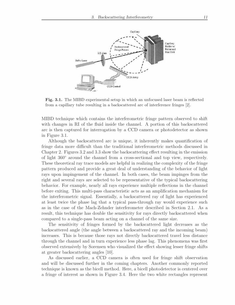
and geometries. Note that red arrows denote fringe shift direction. . 255.8 Ray trace of a beam through the thick walled rectangular channel used
in derivation of the path length difference relationship. . . . . . . . . 265.9 Formation of fringes from the thick walled channel shown in Figure 5.8 26

List of Figures vi
6.1 Typical fringe pattern captured from a 500 micron square glass capil-lary. . . . . . . . . . . . . . . . . . . . . . . . . . . . . . . . . . . . . 31
6.2 Eight areas of interest manually placed on the intensity threshold usedfor interface tracking in Spotlight. . . . . . . . . . . . . . . . . . . . 31
6.3 Filtered fringe image used to smooth laser speckle at edges and increasetracking accuracy. . . . . . . . . . . . . . . . . . . . . . . . . . . . . 32
6.4 Flow of image processing which occurs in the program to prepare fringeimages for tracking. . . . . . . . . . . . . . . . . . . . . . . . . . . . 34
6.5 FFT produced from the grayscale image. The centered FFT is char-acterized by low frequency content at its center. Upon zooming of thisarea one can distinguish the energy (white spots) associated with thefringes. . . . . . . . . . . . . . . . . . . . . . . . . . . . . . . . . . . 35
6.6 Multiplication of FFT and Gaussian low pass filter in the frequencydomain resulting in a filtered fringe image. Note that the filter is shownin both 2D and 3D for ease in viewing. . . . . . . . . . . . . . . . . 35
6.7 Threshold of filtered image set at about half the range of intensitiespresent. The eight bit images have pixel intensity values of zero to255, thus all areas above the max threshold value are set to white (255in the case of eight bit and one in the case of binary) resulting in theblack and white image shown at the right. . . . . . . . . . . . . . . . 36
6.8 Generic line patterns and their corresponding FFTs. The pattern atthe right is a sum of the previous three showing the frequency domainresult of having periodicity in three directions [4]. . . . . . . . . . . . 37
7.1 Typical thin walled capillary tube mounted with padded clamps inpreparation for flow rate testing. Note that the channel is plumbedusing plastic couplers which can be melted around in the inlet andoutlet of the channel. The outlet is open to atmospheric conditions tofacilitate pressure estimations from pressure drop calculations. . . . 40
7.2 Plot of fringe shift due to fluid flow at various velocities in a 500 micronsquare microchannel. . . . . . . . . . . . . . . . . . . . . . . . . . . 40
7.3 Plot showing fringe shift tracked by the eight AOI’s shown in Figure6.2. . . . . . . . . . . . . . . . . . . . . . . . . . . . . . . . . . . . . 41
7.4 Plot showing fringe thickness tracked by the eight AOI’s shown inFigure 6.2. . . . . . . . . . . . . . . . . . . . . . . . . . . . . . . . . 42
7.5 Plot of fringe shift with respect to an implied pressure drop in a 500 mi-cron square microchannel. Note that the outlet is open to atmosphericconditions. . . . . . . . . . . . . . . . . . . . . . . . . . . . . . . . . 42
7.6 Plot showing results of fringe tracking for three AOI’s on a round glasscapillary of 0.9375 mm inner diameter. The pump was not properlyprimed at the point where no fringe shift occurred. . . . . . . . . . . 43
7.7 Fringe tracked by Matlab program described in Chapter 6 to studyfringe morphology. Red and green borders denote areas that are trackedby the program through each frame. . . . . . . . . . . . . . . . . . . 44

List of Figures vii
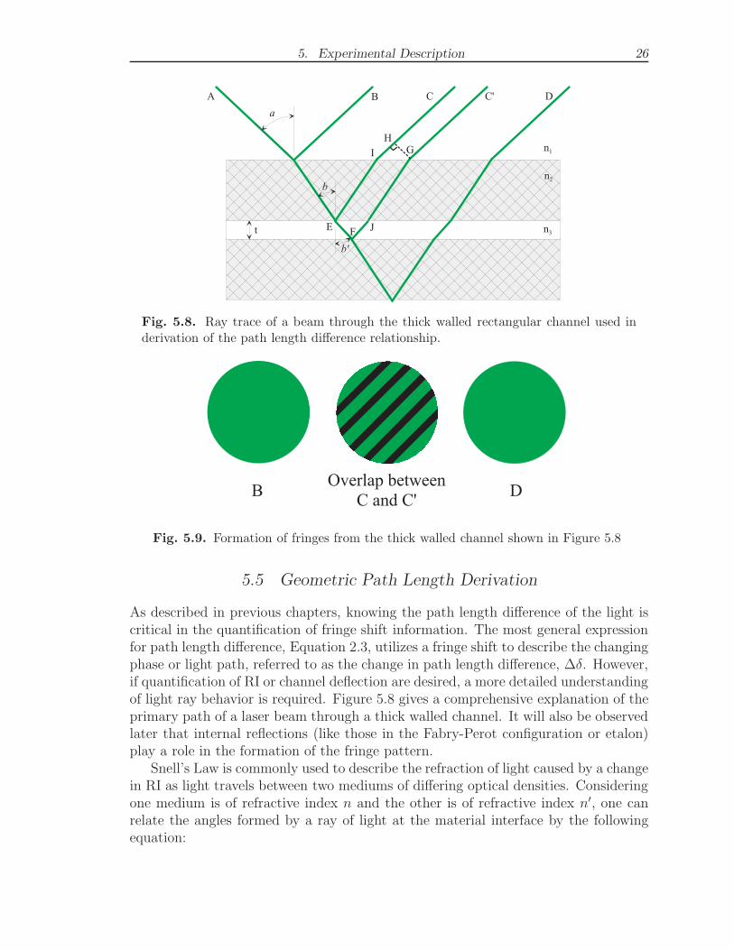
7.8 Shift of interface shown in red in Figure 7.7 through a series of 460frames. The z-direction shows the magnitude of the fringe shift. Flowwas initiated at frame 30 and extinguished at frame 300. . . . . . . . 45
7.9 Thickness change calculated from the difference between interfacesshown in red and green in Figure 7.7. The z-direction shows fringethickness which decreases as the pump is initiated at frame 30 andincreases to the original values and the pump is extinguished. . . . . 45
7.10 Thick walled square microchannel used to study effects of RI changeand channel wall deflection on fringe shift. . . . . . . . . . . . . . . . 46
7.11 Thick walled round microchannel used to isolate the effects of RIchange and channel wall deflection on fringe shift. . . . . . . . . . . 47
7.12 Rectangular channel with relatively thin walls and channel width sig-nificantly larger than the laser beam diameter. . . . . . . . . . . . . 48
7.13 Fringe shift at various fluid flow velocities for the thin walled rectan-gular channel shown in Figure 7.12. . . . . . . . . . . . . . . . . . . 49
7.14 Dimensionless shift at various static pressures for the thin walled rect-angular channel shown in Figure 7.12. As channel deflects due topressurization, the shift becomes non-linear. . . . . . . . . . . . . . . 50
7.15 Thickness change of a bright fringe at various static pressures for thethin walled rectangular channel shown in Figure 7.12. . . . . . . . . 51
7.16 Rectangular channel with thick walls and channel width significantlylarger than the laser beam diameter. . . . . . . . . . . . . . . . . . . 52
7.17 Fringe shifts due to fluid flow in a 50 micron channel with thick sidewalls for three separate test sequences. . . . . . . . . . . . . . . . . . 53
7.18 Fringe shift due to static channel pressurization using distilled waterand the test cell shown in Figure 7.16. . . . . . . . . . . . . . . . . . 54
7.19 Fringe thickness changes due to static channel pressurization usingdistilled water and the test cell shown in Figure 7.18. . . . . . . . . . 54
7.20 Fringe shift of left and right sides of interrogated fringe due to staticchannel pressurization using air and the test cell shown in Figure 7.16. 55
7.21 Dimensionless fringe shift due to static channel pressurization using airand the test cell shown in Figure 7.16. . . . . . . . . . . . . . . . . . 56
7.22 Fringe thickness changes due to static channel pressurization using airin the test cell shown in Figure 7.16. . . . . . . . . . . . . . . . . . . 56
8.1 Simple optical arrangement used in testing laser intensity fluctuations. 578.2 Shift of one side of a fringe captured at 3 fps showing error in shift
detection (manifested as variation in the z-direction) caused primarilyby intensity fluctuations and mechanical vibrations. . . . . . . . . . 58
8.3 Intensity fluctuations displayed by a 1.5 mW HeNe laser as capturedby a photodetector. . . . . . . . . . . . . . . . . . . . . . . . . . . . 59
8.4 Mirror placed on top flow channel to make up second leg of a Michelsoninterferometer and test for plate deflection in the top surface of thechannel. . . . . . . . . . . . . . . . . . . . . . . . . . . . . . . . . . . 61

List of Figures viii
8.5 FEA analysis of thick walled rectangular channel under a static pres-sure of 5 psig. Deflection of the impingement area is shown in blue andis approximately 18 nm when both sides of the cell are considered. . 62
8.6 Rotated view of Figure 8.5 showing deflection of bottom surface of cellin the z-direction. . . . . . . . . . . . . . . . . . . . . . . . . . . . . 63
8.7 Estimation of cell deflection using finite element model with a meshsize of 0.8 mm. . . . . . . . . . . . . . . . . . . . . . . . . . . . . . . 64
8.8 Behavior of deflection estimation as mesh size is decreased at a staticpressure of 5 psig. The mesh appears to converge at a value near 19nm for this pressure value, a slight overestimation of the experimentalresults as expected. . . . . . . . . . . . . . . . . . . . . . . . . . . . 64
8.9 Comparison of finite element model results with calculated deflectionsbased on experimental data for air and water. . . . . . . . . . . . . . 66
9.1 Plot of the experimental results for cell pressureization with air showingcomponents of the signal from channel deflection and fluid RI change. 70
9.2 Plot of the experimental results for cell pressurization with water show-ing components of the signal from channel deflection and fluid RIchange. . . . . . . . . . . . . . . . . . . . . . . . . . . . . . . . . . . 70
A.1 Calibration of syringe pump for use with a 50.0 cubic centimeter ca-pacity syringe. . . . . . . . . . . . . . . . . . . . . . . . . . . . . . . 78
A.2 Calibration of syringe pump for use with a 5.0 cubic centimeter capac-ity syringe. . . . . . . . . . . . . . . . . . . . . . . . . . . . . . . . . 79
B.1 Calibration of pressure transducer using an inclined manometer. . . 80
C.1 Tracking of fringe position and thickness using eight AOI’s at a pumpflow setting of 17. . . . . . . . . . . . . . . . . . . . . . . . . . . . . 81
C.2 Tracking of fringe position and thickness using eight AOI’s at a pumpflow setting of 19. . . . . . . . . . . . . . . . . . . . . . . . . . . . . 81
C.3 Tracking of fringe position and thickness using eight AOI’s at a pumpflow setting of 21. . . . . . . . . . . . . . . . . . . . . . . . . . . . . 82
C.4 Tracking of fringe position and thickness using eight AOI’s at a pumpflow setting of 23. . . . . . . . . . . . . . . . . . . . . . . . . . . . . 82
C.5 Tracking of fringe position and thickness using eight AOI’s at a pumpflow setting of 25. . . . . . . . . . . . . . . . . . . . . . . . . . . . . 82
C.6 Tracking of fringe position and thickness using eight AOI’s at a pumpflow setting of 27. . . . . . . . . . . . . . . . . . . . . . . . . . . . . 83
C.7 Tracking of fringe position and thickness using eight AOI’s at a pumpflow setting of 29. . . . . . . . . . . . . . . . . . . . . . . . . . . . . 83
D.1 Laser intensity fluctuations as captured by the photodetector approx-imately 2 minutes after laser startup. . . . . . . . . . . . . . . . . . 84
D.2 Laser intensity fluctuations as captured by the photodetector approx-imately 10 minutes after laser startup. . . . . . . . . . . . . . . . . . 85

List of Figures ix
D.3 Laser intensity fluctuations as captured by the photodetector approx-imately 16 minutes after laser startup. . . . . . . . . . . . . . . . . . 85
D.4 Laser intensity fluctuations as captured by the photodetector approx-imately 23 minutes after laser startup. . . . . . . . . . . . . . . . . . 86
D.5 Laser intensity fluctuations as captured by the photodetector approx-imately 70 minutes after laser startup. . . . . . . . . . . . . . . . . . 86
D.6 Laser intensity fluctuations as captured by the photodetector approx-imately 120 minutes after laser startup. . . . . . . . . . . . . . . . . 87
E.1 Tube pinch-off mechanism used to induce pressure increases at detec-tion point of backscatter set-up. . . . . . . . . . . . . . . . . . . . . 88
E.2 Backscatter setup showing placement of pinch-off mechanism and ob-servation channel mounting. . . . . . . . . . . . . . . . . . . . . . . . 88
E.3 Mirror placement on 50 micron channel for deflection sensing leg ofMichelson interferometer. . . . . . . . . . . . . . . . . . . . . . . . . 89
E.4 Components of the Michelson interferometer used to detect displace-ments in the glass channel under increased pressure and fluid flow. . 89

LIST OF TABLES
7.1 Various channel cross-section geometries and sizes used in testing. . 397.2 Fringe shift results for flow rate selections 3-17. Areas of interest 2,
3, and 4 were placed at the top, middle and bottom of a light-darkinterface, respectively. . . . . . . . . . . . . . . . . . . . . . . . . . . 44
7.3 Fringe shift data as well as corresponding velocity and pressure dropvalues calculated using Equation 7.2. Negative fringe shifts representexperimental error in addition to instances where the pump was notproperly primed for flow. Raw data indicated an error of plus or minustwo pixels. . . . . . . . . . . . . . . . . . . . . . . . . . . . . . . . . 49
8.1 Laser intensity fluctuation characteristics observed at various time in-tervals after startup. . . . . . . . . . . . . . . . . . . . . . . . . . . . 58
A.1 Linear velocity of syringe pump at various flow rate settings. . . . . 77A.2 Calibration using 50.0 cc Syringe. . . . . . . . . . . . . . . . . . . . 78A.3 Calibration using 5.0 cc Syringe. . . . . . . . . . . . . . . . . . . . . 79

1. INTRODUCTION
The growing field of microfluidics has proven to have applications ranging acrossscientific disciplines from biology and chemistry to materials science and mechanicalengineering. Microchannels, named after their small geometry and defined by theirlow Bond number characteristics, are used in studying surface tension driven fluidmechanics here on earth where gravity governs larger systems. In microchannels,the Bond number (essentially a dimensionless relationship between gravitational andsurface tension forces) is sufficiently low to allow surface tension to dominate thesystem. As a result of this observation, it is of interest to measure this driving forceto better understand how this phenomenon may be controlled, manipulated, and putto use. The small size of such channels renders it impossible to accurately measure theforces within such systems using modern day pressure transducers. To meet this goal,it is desirable to develop a non-contact measurement device to quantify and studysystem characteristics. A technique has recently been proven which is adaptable toachieve such ambitions.
Micro interferometric backscatter detection (MIBD) is a very simple optical tech-nique in which a laser is used to create high contrast interference fringes which shiftbased upon changes in the refractive index (RI) of a fluid within the microchannel.The details of the technique are left to Chapter 3, however, simply stated this de-tection technique is highly applicable to the study of microsystems. Sensitivity hasbeen reported to detect changes as low as 10−7 refractive index units (RIU - a changein RI) in channels ranging in size from 1 mm to 30 µm using the MIBD techniqueand 10−9 RIU using a related technique, dual capillary dual bicell MIBD (DCDBMIBD), also discussed in Chapter 3 [1, 3]. Typically, characteristics that are difficultto directly measure in microsystems such as temperature, pressure, and concentra-tion are all functions of RI, therefore, MIBD can theoretically allow for detection ofchanges in these parameters. In practice, no data has been published demonstratingthat the technique can successfully be implemented to exceed a detection capabilityand perform measurements of such characteristics except under specific, in-situ cir-cumstances. Additionally, no work has been done to implement MIBD for pressuredetection. This is believed to be due to unpredictable channel deflection caused bypressurization which typically dominates the signal, making pressure detection animpractical application.
The objective of this research was to successfully adapt the MIBD technique toperform pressure detection and measurements in microchannels. From this informa-tion, characteristics such as fluid flow rate, velocity, and acceleration can typicallybe extracted depending upon the fluid flow regime. For example, it is known thatthe refractive index of water is a function of pressure and varies by approximately

1. Introduction 2
0.000016 RIU for each atmosphere of pressure variation below 4 atm [5]. This fallswell within the detection capability of MIBD, however, at such pressures the geom-etry of a microchannel has been found to be considerably altered thus making suchdetections seemingly impossible. This presents a need for an ability to detect channeldeflection and separate the components of the signal to accurately quantify ∆RIUand channel geometry changes. Through the use of fluids with known pressure to RIrelationships, the signals have successfully been deconvolved providing an ability todetect and quantify pressure changes within microchannels. This leads to an abilityto quantify parameters that are functions of pressure such as fluid compressibility(both gas and liquid phases), fluid flow rates, and fluid velocities. This also leads toa wide variety of scientific applications for this research, perhaps the most interestingof which have not yet been realized by the extent of the work presented herein.

2. INTERFEROMETRY
Interferometry is the science of combining light waves to cause interference. As twobeams of light occupy the same space at the same time they tend to interfere with oneanother causing areas of constructive and destructive interference. This interferenceis manifested as a series of light and dark bands in 2-D space, known as fringes ininterferometry, which move based upon changes in phase. This change in phase issynonymous with the physical path length difference between the interfering wavesof light. The movement of the interference bands, referred to as a fringe shift, canbe used to quantify parameters that modify the path length traveled by the light.Such parameters may include RI, the geometry of the system, or any property thatis a function of these parameters such as temperature, pressure, and concentration.Physically, the thickness of each fringe at a given magnification represents a pathlength equal to the wavelength of the light used to create the fringes. The commonpractice is therefore to measure the fringe shift based upon the number of fringesto pass a point on an observation screen. This number of fringes is then directlyrelated to the physical path length change of the light which can be used to quantifya myriad of physical phenomena. The method used in counting fringes and thetechniques effective in the quantification of shift data are discussed in greater detailin Chapter 6.
2.1 Types of Interferometers
There are several very common types of interferometers used in both research andindustry. The simplest and oldest type, shown in Figure 2.1 is known as the Michelsoninterferometer. Historically this interferometric configuration was used in Michelsonand Morley’s attempt to study light traveling through the aether, which later resultedin disproving the aether concept altogether. Today, this type of interferometer canbe used for other scientific applications such as highly sensitive deflection, flatness,temperature and RI measurements [6]. The Michelson interferometer begins at acoherent light source such as a laser which emits a beam that is then divided by a beamsplitter, typically into two equally intense portions. These beams are then reflected bymirrors back towards the beam splitter. During this event, one beam is passed througha glass plate, as shown in the 2.1, to compensate for the phase difference caused bythe thickness of the beam splitter. When the apparatus is properly aligned, the lightwaves are then recombined causing interference fringes which can be viewed on anobservation screen or by a photodetector as shown in Figure 2.1. This interferometeris easily implemented as a deflection measurement device since one mirror can readilybe attached to a system of interest. As the mirror moves there is a path length

2. Interferometry 4
H e N e L a s e r
M i r r o r 1
O b s e r v a t i o n S c r e e n
M i r r o r 2B e a m S p l i t t e r
G l a s s P l a t e
Fig. 2.1. The classic Michelson interferometer.
difference in one arm of the interferometer causing a fringe shift. Depending uponfringe shift detection capabilities, deflection measurements have been reported as lowas 10−10 cm [7]. Implementation of this technique for detection of channel deflectionis described in Chapter 8.
In addition to the Michelson interferometer, another very common configurationis know as the Mach-Zehnder interferometer. This device, shown in Figure 2.2, iscommonly used to perform refractive index and temperature measurements. Here anincoming beam is once again divided by a beam splitter. The separate beams are thenreflected from mirrors and directed towards a second beam splitter which recombinesthe two causing interference fringes. This configuration is particularly useful for smalltransparent samples which can be placed into one arm of the interferometer, as shownin Figure 2.2. Insertion of such a sample causes a path length change between thetwo beams resulting in a fringe shift. This configuration has also proven useful inmeasuring the quality and flatness of optical components as well as the thicknessof transparent media and the index of refraction of optically transparent samples.One limitation of this arrangement is the fact that the light only makes a single passthough the sample. For other configurations such as MIBD (discussed in Chapter 3),the Michelson interferometer, and the Fabry-Perot interferometer shown in Figure 2.4,two or more passes through the sample can lead to double the detection sensitivity.
Yet another very common type of interferometer is known as the Sagnac interfer-ometer. Under this arrangement, three mirrors are used in conjunction with a beamsplitter to send the divided rays of light in opposing circular paths as shown in Figure2.3. This interferometric assembly is particularly useful in the measurement of an-gular velocity and acceleration. As the device is rotated in one particular direction,the velocity of the light in that direction is decreased relative to the light traveling in

2. Interferometry 5
H e N e L a s e r
M i r r o r 1
M i r r o r 2B e a m S p l i t t e r 1
B e a m S p l i t t e r 2
O r i g i n a l B e a m
A r m 1 A r m 2
S a m p l e
I n t e r f e r e n c e R e g i o n
O b e r v a t i o n S c r e e n / D e t e c t o r
Fig. 2.2. The Mach-Zehnder interferometer, commonly used for single pass RI mea-surements.
the opposite direction. This velocity difference is manifested as a phase shift, causinga measurable fringe shift which can be related back to the angular velocity of thedevice. A drawback to this device is the fact that is must be rotated to produce aresponse, therefore it is desired that it be miniaturized to minimize its inertial effectson the system of interest.
A final common arrangement is know as the Fabry-Perot interferometer whichis shown in Figure 2.4. This configuration uses two parallel half silvered plates toreflect a beam several times through a medium of index of refraction, n. Since theplates are only partially reflective, a portion of the light is transmitted upon eachreflection resulting in a group of transmitted rays at one side of the apparatus anda group of reflected rays at the other. Generally, either the transmitted or reflectedrays are analyzed to determine information such as the value of n, the RI of themedium between the plates, or the wavelength of the light composing the incomingbeam [8]. Since the interference pattern is constructed of multiple reflected beams,it is classified as a multiple source interference and the fringe pattern attained canlook quite unique in comparison to those produced from the previous interferometricarrangements. Since this technique is not utilized in this research, the description ofthis configuration will remain brief and further investigation will be left to the reader.
The formation of these unique fringes is dependent upon the phase of each exitingbeam. When multiple beams are in phase with one another, there is a large peakof constructive interference. Conversely, when beams are out of phase there is anarea of destructive interference. The contrast between these interference regions aswell as their width is directly related to the construction of the interferometer, whichincludes the wavelength of the light, plate spacing, RI of the material occupying theseparation, plate reflectivity, and beam impingement angle [9]. Typically these pa-rameters remain constant with the exception of the impingement angle or the plateseparation. Through modification of one of these variables, the device is most com-

2. Interferometry 6
H e N e L a s e r
M i r r o r 1
M i r r o r 3
B e a m S p l i t t e r
M i r r o r 2
O b s e r v a t i o n S c r e e n / D e t e c t o r
Fig. 2.3. The Sagnac Interferometer, commonly used in performing angular velocitymeasurements.
monly used to determine the wavelength of the incoming beam. Since the exitingbeams are constructively interfering with one another, the maximum interference willoccur when all of these beams are perfectly in phase [8]. By varying plate separa-tion until the maximum intensity of the constructive interference peaks occurs, thewavelength can be extracted through known physical relationships of the geometryof the interferometer. Succinctly put, by varying plate separation, the Fabry-Perotinterferometer is used to determine the wavelengths present in a light source.
temperature, RI, pressure, displacement, and astronomy, fiber optics, and plasmaphysics.
2.2 Basic Interferometric Theory
In this section, relationships are given to better describe the method by which in-terferometers are used in performing the measurements referred to in Section 2.1.Relationships for path length and phase changes are described for the Michelson andMach-Zehnder interferometers. In addition, the relationship for intensity of fringes,or visibility, is provided in more detail. Finally, the relationships describing mul-tiple beam interference and the Fabry-Perot interferometer are presented to bringadditional clarity to this complex phenomenon.
Once again considering the Michelson arrangement shown in Figure 2.1 one canimagine a beam of light traversing one arm of the interferometer. To complete thepath of the first arm, the light would travel from the laser source then reflect fromthe beam splitter to mirror one where it would then be reflected back to the beam

2. Interferometry 7
R e f l e c t e d R a y sO r i g i n a l B e a m
T r a n s m i t t e d R a y s
P a r t i a l l y R e f l e c t i v e S u r f a c e s
Fig. 2.4. The Fabry-Perot, commonly used to measure the wavelength of light.
splitter. At this point, the light would partially be reflected back into the laser source,referred to as retro-reflection (not shown), and the remainder would travel throughthe beam splitter to the observation screen or detector. In this case, the optical phaseof the wave propagating this path can be represented as:
Φ1 =2π
λn1L1 (2.1)
where λ is the wavelength of the light, n1 is the index of refraction of the mediumthrough which the light propagates, and L1 is the distance from the beam splitter tomirror 1. Arm two can be described in the exact same manner where the subscriptsin Equation 2.1 then describe the characteristics of path two. In the event that aphysical displacement of the mirrors is to be measured, it is often more convenientto describe the phase difference between the paths in terms of a physical path lengthdifference, δ. Initially, this can be expressed as:
δ = 2L2 − 2L1 = 2∆L (2.2)
To find this value interferometrically, one must recall that each fringe representsa path length equal to one wavelength of the light being used. Therefore, the numberof fringes, m, multiplied by the wavelength provides the physical path length differ-ence ∆L. When multiplied by two we are left with the classical formula for opticalmetrology given as:
∆δ = ∆mλ (2.3)
Where ∆δ represents the change in the path length difference, ∆m describes thenumber of fringes to pass a given point on the observation screen during a fringe

2. Interferometry 8
shift event. The technique for counting fringes to quantify path length differences isdescribed in greater detail in Section 6.1.
Additionally, the visibility of the fringes, V, used in optical analyses can be im-portant to one’s ability to accurately quantify information. This is expressed mostsimply as:
V =Imax − Imin
Imax + Imin
(2.4)
Where Imax and Imin are the maximum and minimum intensities, respectively,found from the relationship [7]:
I = I1 + I2 + 2√
I1I2 cos θ cos ∆Φ exp−∆l
lc (2.5)
where I1 and I2 are the measured intensities of the beams from arms one and two(typically a voltage output from a photo sensitive diode or detector), ∆Φ can befound using Equation 2.1 and θ is defined as the angle between the polarizationvectors. That is to say, the original beam may have polarization modes in severaldirections, typically perpendicular to one another, giving θ a value of 90◦. Finally,∆l=L1-L2 and lc is defined as the coherence length, where:
lc =λ2
∆λ(2.6)
In 2.6 λ is the wavelength of the light and ∆λ is the variation in the wavelengthof the signal. From 2.6 one can see why coherent light is preferable for interferometrysince it is primarily a single wavelength resulting in a small ∆λ and thus more visiblefringes.
The Fabry-Perot interferometer requires the inclusion of an incoming beam angle,θ, to represent the phase difference. Therefore, equation 2.1 becomes [9]:
Φ =2π
λ2nt cos θ (2.7)
where λ is once again the wavelength of the light, n is the RI of the medium separatingthe plates, t is the plate separation, and θ is the angle of the incoming beam measuredfrom the normal of the inner surface. Here the additional two is from the fact thatreflected rays travel twice (or a multiple of two) through the sample before exitingthe device as shown in Figure 2.4. The transmission equation of the device is thenfound to be [9]:
T =(1 − R)2
1 + R2 − 2R cos φ(2.8)
where R is the reflection coefficient of the planar surfaces. Knowing the transmissionof light though the interferometer, one can plot this value as a function of wavelengthto determine the wavelength of the incoming illumination source since, as discussedearlier, the transmission will be maximum when the optical path length differencebetween the transmitted beams is an integer multiple of the wavelength. In this case,the path length difference would be given by:

2. Interferometry 9
δ = 2nt cos θ (2.9)
Using these relationships one can therefore use the maximum transmission value,Tmax, from Equation 2.8 to find the wavelength of light entering the interferome-ter. Commonly referred to as a wavemeter, this configuration is most frequentlyimplemented for accurate measurement of the wavelength produced by coherent lightsources, such as lasers. In knowing the wavelength of the light being used, Equation2.9 in combination with Equation 2.3 can then be applied to study RI changes orplate separations based on a fringe shift value. A procedure very similar to this willbe utilized to quantify such values in later chapters.
3. BACKSCATTERING INTERFEROMETRY
3.1 The History of Backscattering Interferometry
Micro Interferometric Backscatter Detection (MIBD) was first developed in the early1990’s by Dr. Daryl Bornhop of Texas Technological University as a method ofdetermining refractive index (RI) changes in very small fluid volumes (as low as10−12 liters) for use in chemistry and biochemistry based settings [2, 3, 10]. Thetechnique was patented in 1994 as a new form of interferometer and has displayedexcellent sensitivity for examining micro scale systems and equally small volumes offluid. Since the emergence of the MIBD technique it has shown outstanding promiseas a detection mechanism for changes of system parameters. However, it has lacked inquantification of these values as well as repeatability between measurement systemspresenting a need for constant in-situ calibration.
Since its inception, MIBD has been refined by Bornhop and others to show in-situ RI measurements with sensitivity on the order of 10−9 as well as correspondingtemperature relationships based on detection of the change in RI [3, 10, 11]. Thesetup has also been modified to provide flow rate measurements through the use ofa heated slug of fluid created by impingement of an infra-red laser source [12]. Inaddition, the technique has proven to be useful in detection of concentration, solute,and impurity levels. This has been confirmed to be highly applicable to bedsideblood analysis and protein binding experimentation [10]. Despite the demonstratedimprovements and capabilities of this technique, it has not yet been shown to provideresults for flow rate or pressure quantification within these channels.
3.2 The MIBD Technique
The method uses a coherent light source, such as a laser, to impinge a small fluid filledchannel, which in turn reflects the high intensity light from its inner and outer surfacesresulting in light interference fringes as seen in interferometry [13]. This reflected lightcan then be detected using any light sensing device, although photodetectors andcamera sensors are most commonly implemented for this purpose. The experimentalapparatus, shown in Figure 3.1, has several variations, but most commonly uses aHeNe laser to reflect light from a small channel either mounted to a solid surface ormolded into a PDMS or silicon chip. The only stipulation to the technique is that thebeam must be larger than the channel diameter. Without this criterion, the apparatusforms the more common etalon or Fabry-Perot interferometer as was discussed inSection 2.1. The reflected light, referred to as backscatter, forms an arc unique to the
3. Backscattering Interferometry 11
Fig. 3.1. The MIBD experimental setup in which an unfocused laser beam is reflectedfrom a capillary tube resulting in a backscattered arc of interference fringes [2].
MIBD technique which contains the interferometric fringe pattern observed to shiftwith changes in RI of the fluid inside the channel. A portion of this backscatteredarc is then captured for interrogation by a CCD camera or photodetector as shownin Figure 3.1.
Although the backscattered arc is unique, it inherently makes quantification offringe data more difficult than the traditional interferometric methods discussed inChapter 2. Figures 3.2 and 3.3 show the backscattering effect resulting in the emissionof light 360◦ around the channel from a cross-sectional and top view, respectively.These theoretical ray trace models are helpful in realizing the complexity of the fringepattern produced and provide a great deal of understanding of the behavior of lightrays upon impingement of the channel. In both cases, the beam impinges from theright and several rays are selected to be representative of the typical backscatteringbehavior. For example, nearly all rays experience multiple reflections in the channelbefore exiting. This multi-pass characteristic acts as an amplification mechanism forthe interferometric signal. Essentially, a backscattered ray of light has experiencedat least twice the phase lag that a typical pass-through ray would experience suchas in the case of the Mach-Zehnder interferometer described in Section 2.1. As aresult, this technique has double the sensitivity for rays directly backscattered whencompared to a single-pass beam acting on a channel of the same size.
The sensitivity of fringes formed by the backscattered light decreases as thebackscattered angle (the angle between a backscattered ray and the incoming beam)increases. This is because those rays not directly backscattered travel less distancethrough the channel and in turn experience less phase lag. This phenomena was firstobserved extensively by Sorensen who visualized the effect showing lesser fringe shiftsat greater backscattering angles [10].
As discussed earlier, a CCD camera is often used for fringe shift observationand will be discussed further in the coming chapters. Another commonly reportedtechnique is known as the bicell method. Here, a bicell photodetector is centered overa fringe of interest as shown in Figure 3.4. Here the two white rectangles represent

3. Backscattering Interferometry 12
Fig. 3.2. Ray trace of the light path through a circular channel resulting in multiplereflections. The vertical lines represent the side walls of the channel [3].
Fig. 3.3. Cross sectional view of ray trace through a circular channel resulting in a360◦ backscattered arc [3].

3. Backscattering Interferometry 13
Fig. 3.4. The use of a bicell photodetector for detection of fringe shift. The detectorconsists of two photo-sensitive sectors represented by the white rectangles over the leftfringe [1].
the two sides or cells of the detector. It is important to note that the fringes areshown in false color representation with the greatest light intensity at their centers.Each cell of the apparatus has light detecting ability and the intensity produces avoltage which is averaged over each side of the cell. The output signal is given as:
S =A − B
A + B(3.1)
Where S is the signal of the detector in volts, A is the voltage average of one side,and B is the voltage average of the other [1]. Using this differential voltage, the move-ment of a fringe in the horizontal direction can be quantified. Depending upon fringemagnification and detector size, this method has the potential to track movementsas low as 10−6 meters. This highly sensitive tracking capability provides tremendousdetection potential, however, since the thickness of the fringe is not known, quan-tification is unfortunately limited to in-situ calibrations as reported in the results ofBornhop et al. [1, 14].
3.3 Scientific Advancements from MIBD
As discussed in Section 3.1, the sensitivity of the backscatter technique gives it wideapplicability for the measurement and detection of parameters depending upon RI.In 2002, Dmitry Markov and Bornhop successfully measured refractive index changesbeyond 10−7 RIU in fluid volumes as small as 10−9 liters [2]. Such a feat was notpossible with previous techniques since such small fluid volumes inherently present avery short distance of light travel and causing only small phase differences betweenarms of an interferometer. Traditionally, this kept detection limits at or below 10−7
RIU.

3. Backscattering Interferometry 14
Due to the unprecedented ability to detect changes in RI as well as perform in-situ measurements, MIBD (or OCIBD, the on-chip version) has also been shown todetect temperature changes as low as 10−6 ◦C [1]. As a result, “the extent of Jouleheating in chip-scale capillary electrophoresis” was measured for the first time [14].In this experiment, a silicon chip with isotropically etched channels was used in thebackscattering setup to capture the heating effects of capillary electrophoresis provingthat present theoretical models in the field were not yet adequate and underestimatedthe values measured in-situ.
Finally, the technique has also been expanded to include two channels and twophotodetectors side-by-side [1]. With this apparatus, one channel acts as a referencefor the other thus aiding to eliminate the effects of errors such as mechanical vibra-tions, laser intensity fluctuations, and thermal drift. Using this technique, referredto as DCDB MIBD, a detection limit of 6.9 x 10⁻⁹ RIU is achieved for temperatureranges between 24 and 30◦C, opening the door to a myriad of new chemistry andbiochemistry applications.

4. RELATED SCIENTIFIC WORK AND MEASUREMENT
TECHNIQUES
4.1 RI Measurement Methods
Numerous RI measurement techniques currently exist, most of which use coherentlaser light and interferometric methods to compare the phase lag between an unalteredbeam and one traveling through a medium of interest. As discussed in Chapter2, the Mach-Zehnder and Fabry-Perot interferometers are two optical instrumentscommonly used to perform RI measurements via correlation to fringe shift. Similarly,in Chapter 3 it was noted that MIBD can be used as a highly sensitive detector tochanges in RI using fringes created by light reflection from channels with micron-scalecross-sections.
Aside from those methods previously discussed, many important methods exist formeasurement of RI presenting a wide range of applicability with sensitivities as lowas 10−6 RIU. Direct measurement of the index of refraction of air has been provenusing an evacuable cell and a Fabry-Perot interferometer [15]. By placing the cellbetween the plates of the interferometer and slowly evacuating the air with a vacuumpump, the optical resonance can be utilized to determine the change in RI of theair within the cell. In the context of the discussion in Section 2.2, the transmissionmaximum changes position leading to the appearance of fringe shift which can becounted throughout the evacuation process. Similarly, a permanently evacuated cellcan be placed within part of a Fabry-Perot interferometer. Upon comparison of thewavelengths causing resonance in the evacuated and non-evacuated parts of the cell,one can determine the absolute RI or the air. These results were verified with theEdlen formula indicating a measurement range of 2 x 10⁻⁶ RIU for a laser tuningrange of 1 GHz [15].
Another RI measurement method is referred to as the laser-cube-capillary tech-nique. This instrument uses a glass cube through which a 1.0 mm hole is bored.Using a laser beam with a diameter of 0.8 mm to directly impinge a flat face of thecube, light is directed through the bored channel perpendicular to its axis. The wallthickness is chosen to be significantly thicker than that of the hole diamter to act asa thermal mass and allow RI measurements under pressure [16]. It is noted by Mennand Lotrian that the fragile nature of capillary tubes deems them un-usable for RImeasurements under pressures different than atmospheric, a conjecture proven onlypartially true by the work in this thesis.
The capillary cube method uses the detection of an interferometric fringe shiftto quantify fluid RI changes. Upon passing through the bored channel, the light

4. Related Scientific Work and Measurement Techniques 16
L i g h t I n t e n s i t y
A n g l e f r o m B e a m A x i s
C a p i l l a r y - C u b e ( T o p V i e w )
I n c o m i n g L i g h t R a y s
F r i n g e s
Fig. 4.1. Experimental setup for the laser-capillary-cube technique showing interfer-ence due to reflection and refraction of incoming light rays.
is bent slightly away from the axis of the bore when the RI of the fluid inside thechannel is lower than that of the capillary cube. This is because the light will alwaysbend toward the medium of highest RI. Since the bore is circular, this bending isexaggerated such that a portion of the light travels beyond the cross section of thechannel thus interfering with reflections of its outer wall resulting in fringes as shownin Figure 4.1 [16]. Although this technique has similarities to the adapted backscat-tering technique, it differs in several areas. First, it is a single pass-though techniquewhich results in only half the sensitivity of the double pass-through MIBD techniqueunder the same experimental parameters. In addition, this technique is not directlyapplicable for the study of flowing systems and requires a specialized cell to acquireRI information. Finally, the channel dimensions are relatively large in comparisonto the backscattering technique, an undesirable feature for studying fluid behavior insmall systems.
A final mechanism for the measurement of RI is capable of quantification to±0.0002 RIU in liquids such as water and hexane. Using two quartz plates sepa-rated by a thin layer of air one may submerge the apparatus in a liquid medium ofinterest. Upon passing a monochromatic beam through the liquid of interest as well

4. Related Scientific Work and Measurement Techniques 17
as the sandwiched plates, one can determine the absolute RI of the liquid. This isdone by carefully rotating the plates until the critical angle of the glass is reachedand the beam no longer exits the apparatus. Assuming the critical angle of the glassas well as the RI of the glass and air are well known, one can geometrically solve forthe RI or the liquid. The accuracy of the solution depends primarily on one’s abilityto determine the angle of the plates. Results from this technique have been provento match the results of others for the temperature dependency of liquid RI to as lowas 10−4 RIU [17].
4.2 Related Measurement Techniques
Several other techniques for pressure and flow rate measurement related to the adaptedbackscattering setup also exist. One very important technique is the use of a refrac-tive index detector (RID) as a pressure transducer for online viscometry in exclusionchromatography [18]. In this method, a standard differential refractive index detectoris used to measure the pressure drop in capillary tubes via changes in RI to determinefluid flow rate and viscosity. Under temperature controlled conditions in a capillaryof known dimensions, Poiseuille’s formula for laminar flow may be used to confidentlycalculate fluid flow rate or viscosity based on a measured pressure drop provided oneof the parameters is known.
In the experimental apparatus for this method, the RID is plumbed to the inlet ofthe capillary and the exit is open to a waste container. The RID is a differential unitwhich utilizes a reference or non-pressurized fluid cell in addition to the pressurizedfluid cell and provides a signal of the change in RI between between the two. Thistechnique has been reported to provide RI changes on the order of 10−6 RIU andpressure measurements on the order of hundreds of Pascals [18]. Typically liquidrefractive index changes approximately 10−5 RIU per atm indicating a much higherpressure at the inlet of the capillary in addition to the pressure drop. This workis not non-intrusive as in the case of the adapted backscattering technique since thedetector must be plumbed into the capillary system. In addition, the detection schemeuses existing RID technology which is limited to measurements of 10−6 RIU changeswhereas MIBD is capable of detection three orders of magnitude lower.
Optical techniques have also been developed for the measurement of pressure andskin friction [19]. In this technique a surface stress-sensitive film is deposited on a partto be tested in a wind tunnel. Based upon the deformation of this film, the surfacestresses and pressures can be calculated. The technique utilizes a specialized lightsource and dedicated data acquisition and processing unit. Although computationallyintensive, the method has proven to produce comparable results to those found usingpressure sensitive paints, pressure taps, and CFD [19]. Due to the versatility of thistechnique, it could be used to measure the deflection of a capillary channel underpressure and thus deduce the flow rate and pressure levels within the channel.
An alternative pressure measurement apparatus for micro-scale systems is the useof optical fibers. Micromachined drum-like membranes can be attached to the end ofsuch fibers in order to create optical interference effects based upon deflections in the

4. Related Scientific Work and Measurement Techniques 18
membrane. These devices are attached to optical fibers via a RI matched cement.The micromachined device consists of an index matched bowl shaped sheet of glassto which silicon nitride or polysilicon films are attached. The films act as a highlysensitive deflectable membrane which is able to detect changes in temperature andpressure when attached to a surface of interest [20]. Although exact sensitivities ofthis technique are not yet known, it is an excellent alternative to the problem ofmicro-scale pressure measurements.
A similar technique utilizes two optical fibers and a reflecting diaphragm to makepressure measurements as an optical microphone. In this case the minimum detectablepressure was found to be 680 micropascals per root hertz providing a dynamic rangefrom 0.01 Hz to 20 kHz, a span beyond that of the human ear [21]. Although thisdevice is too sensitive to make bulk fluid pressure measurements, it is yet anotherinteresting alternative for pressure measurement in microsystems.

5. EXPERIMENTAL DESCRIPTION
5.1 Adapted Backscattering Setup
A 5 mW green HeNe laser beam (543 nm wavelength) is passed through a neutraldensity filter then directed downward using a mirror where it impinges a fluid filledcapillary scale tube at an angle between 7◦ and 30◦ from the surface normal. Light isthen reflected off the inner and outer surfaces of the tube, as shown in Figure 5.1, re-sulting in high contrast interference fringes which shift with the changing path lengthdifference of the light. This reflected light pattern is then expanded using a -25 mmfocal length (divergent) lens, passed through a linear polarizer, and captured using aCCD sensor as displayed in Figure 5.2. A schematic of the entire setup can be seenin Figure 5.3. Using this technique, both square and round capillaries were observed,ranging in size from 0.341 to 0.9375 mm round inner diameter and 200 to 500 micronsquare inner dimensions. The entire optical train forms an interferometer, similarto a Fabry-Perot or parallel plate interferometer, and creates an arc of interferencefringes unique to the MIBD setup. It should be noted that the channel orientation isslightly different than that depicted in Figure 3.1 for the MIBD setup. This changesthe behavior of the light slightly, however, fringe formation acts on similar principlesand becomes much easier to visualize and control.
The channel is fixed to a stainless steel X-Y translational stage using a pair ofpadded clamps to minimize deflection of the detection area during testing. Thechannel is a drawn glass round or square pipette, 10 cm in length, connected toa 50 cc Hamilton syringe (model number 1050) using polyethylene tubing of thecorresponding size. The channels were connected using wax, super glue, or plasticcouplers depending upon size, geometry, and the flow rates being observed. Fluid wasforced through the system at various velocities using a Model 975 Harvard Apparatuscompact infusion pump. A listing of these flow velocities along with the correspondingpump settings can be found in the pump calibration in Appendix A.
When the laser is adjusted to impinge the channel and the CCD sensor is properlypositioned, interference fringes are displayed on a monitor. To properly position thecamera, the top and bottom reflections from the tube, rays b and d in Figure 5.1,must overlap as illustrated in Figure 5.4. The result of a partial overlap betweenthe rays backscattered from the top and bottom of a round channel can be seen herewhere the contributions from the top and bottom reflections are bounded by the redand black rectangles, respectively. One can observe a movement in these fringes whenflow is introduced into the system. This shift occurs due to an index of refractionvariation in the liquid as well as a deflection in the channel walls. An analysis of thecontribution of each of these signals is left for the discussion in Chapters 7 and 8.

5. Experimental Description 20
Fig. 5.1. Simplified ray trace of the light path through a capillary scale channel fromthe side view.
Fig. 5.2. Capillary tube and fringe acquisition apparatus showing beam behavior asseries of green lines superimposed on the image.

5. Experimental Description 21
Fig. 5.3. Experimental apparatus used in flow testing.
These detectable variations are caused, in part, by a minute pressure drop over thelength of the channel, created by the flowing liquid. This pressure change can be de-scribed mathematically using the Hagen-Poiseuille solution for steady, incompressible,laminar flow and will be expanded upon in Section 7.1.
The camera output was recorded using a PC and an EPIX framegrabber in XCAPfor Windows, an image analysis program. The video frames for each test were savedas a series of .tif images to be processed and examined later in more detail. Thepost processing techniques used in the analysis of this data are left for discussion inSection 6.2.
5.2 Experimental Parameters - Thin Walled Channels
The primary experimental apparatus used in testing of thin walled channels has beendescribed in Section 5.1, however, there are several characteristics specific to thetesting technique used on these channels. First, fluid flow was used in all thin walledchannel testing to induce pressure gradients caused by pumping a fluid through thesystem. In all flow testing described here the working fluid was distilled water at roomtemperature, however, silicon oil was also used producing similar results. The systemwas aligned by tilting the mirror over the channel (shown in Figure 5.2) until the topand bottom channel reflections were observed to overlap. This typically required animpingement angle less than 30◦ depending upon channel size since smaller channelsresult in much closer reflections. The CCD camera was mounted on an adjustablearm to allow interrogation of the entire backscattered arc and was typically placedwithin twelve inches of the channel impingement point.

5. Experimental Description 22
Fig. 5.4. Formation of fringes caused by primary reflections from glass surface at topand inner wall of a capillary tube (rays b and d from Figure 5.1).
5.3 Experimental Parameters - Thick Walled Channels
Next, modifying the experimental apparatus to study fringes produced by thick walledchannels (both round and square cross-sections) completed the adaptation of thedevice from the original MIBD apparatus to achieve pressure measurements. Theoptical train remained virtually unaltered with the exception of the channel whichrequired camera and impingement angle changes. Due to startup issues with the greenHeNe laser, a comparable 1.5 mW red HeNe laser with 633 nm wavelength was usedduring some of the testing of thick walled channels. This modification causes minorchanges in the results, but has no unique effects on the apparatus itself. To performtesting on thick walled channels where deflection was drastically reduced, both flowand static tests were performed. For flow testing, the channel was plumbed usingflexible Tygon tubing which was stretched over the inlet and outlet ports to producean air tight seal. To produce adequate fringe patterns, the impingement angle wasadjusted to be between 10◦ and 20◦ from the surface normal. The divergent lens wasreplaced by a 5x microscope objective lens which was placed at varying distancesbetween the channel and the CCD depending upon the desired magnification. Forrectangular channels in which a backscattered arc was not produced, the camerawas mounted directly in line with the plane of the beam path which was in turnperpendicular to the plane of the table. When circular thick walled channels wereused, the arc was interrogated as in the case of the thin walled channels.
As stated, static testing was also performed using thick walled channels. A dia-gram of the experimental apparatus used in this testing is shown in Figure 5.5. Here,

5. Experimental Description 23
HeNe Laser
Laser Beam
Mirror Divergent Lens
CCD Camera
Camera Adjustment Device
Hand Pump
X-Y Translational Stage
Channel
Pressure Transducer
Data Acquisition and Image Processing Unit
Fig. 5.5. Diagram of experimental apparatus used in static pressure tests of the thickwalled channels.
a miniature pressure transducer was plumbed to the outlet of the cell and a handpump was connected at its inlet. The transducer was wired to a Keithley 2700 Multi-meter / Data Acquisition System data acquisition system which transported data toan Excel spreadsheet in real time during testing. The calibration of this transducerwas verified using an inclined manometer, the results of which can be found in Ap-pendix B. Using the hand pump, the cell could be pressurized to a desired level tostudy the corresponding fringe shifts.
5.4 Fringe Formation
To better explain how the fringe formation occurs, one can first consider two beams oflight as two point sources. In the case of coherent light, such as that from a laser beam,it is a good assumption to assume the light propagates as planar waves where thereare equally spaced fronts of equal intensity. This scenario is sufficient to describe, forexample, rays b and d from the capillary tube. Therefore, if the red point sourcesshown at the left of Figure 5.6 are considered to emit planar waves as shown, one canobserve the interference effects between the wavefronts. As these waves are emitted,they tend to interfere with one another to form the light and dark bands, which arewidest at the vertical and move closer together as they reach the horizontal. Theselight and dark bands are representative of the regions of constructive and destructiveinterference, respectively.
As described by Figure 5.4, fringes are primarily formed by the combination oflight rays backscattered from the top and the bottom inner surface of the channel inthe case of capillary tubes with relatively thin walls. This type of interference is pri-marily from two sources, although additional fringes are formed from other reflectioncombinations such as rays b and c or rays c and d. These interference combinationsare responsible for the smaller fringes seen outside the primary interference region inFigure 5.4.

5. Experimental Description 24
In the case of the thick walled channels, the beams are separated a significantamount and the fringe formation explanation from Figure 5.4 is no longer valid. As aresult of this large separation, the backscattering angle can be increased such that thereflection from the top of the channel is no longer a part of the interferometric signal.This occurence has been depicted in Figure 5.9 where only the reflections caused bythe channel are included in the signal thus drastically simplifying the interferencepattern. In the case of Figure 5.9, the fringes are arbitrarily shown as diagonal,although the orientation is heavily dependent upon beam alignment.
When compared to the image formed from the impingement of a 500 micronsquare capillary tube as shown in the upper right of Figure 5.6, one can clearly seethe resemblance due to the common formation mechanism. The frequency of thefringes is a direct function of the source spacing; this observation will be utilized inlater analysis to detect the presence of transverse channel deflection. Finally, theimage in the lower right of 5.6 displays an instance where multiple source interferenceis dominant, causing a criss-cross of fringes in opposing directions.
From this discussion, it is made clear how fringe formation from a microchannelcan become very complex depending on the alignment of the system and channelorientation. The intricacy of fringe formation in microchannels has been addressedin the literature [22], however, for this application the solutions are insufficient sincethe geometry of drawn glass does not have sufficient uniformity at these scales re-sulting in unacceptable prediction error. To illustrate the extent of this complexity,Figure 5.7 shows a variety of fringe patterns captured using several channel types andorientations. It is important to note that the red arrows represent the direction offringe movement upon an increase in RI. The magnitude of this shift is dependentupon factors such as temperature, channel geometry, fringe magnification, fluid flowrate, and pressure. Three of the pictures shown were captured from a capillary tubeof circular cross section and 1 mm inner diameter. The two on the left are from thesame orientation, however, the top one is at a significantly higher magnification andhas been inverted causing the fringe shift to appear in the opposite direction. Thephoto at the lower right is from the same channel rotated 90◦ to meet the MIBDimpingement criteria. Although shifts are still observed, one can begin to see theclear advantages of the orientation in the adapted technique, not only for explainingfringe formation, but also in the symmetry and clarity of the fringes.
Figure 5.7 also shows fringe patterns formed by square and rectangular channels.In the case of the square channel the central fringe is shown. This fringe is importantsince its behavior is very close to the behavior of fringes where the beam diameter isless than the channel cross section. Correlations for this will be discussed later in thissection and it should be realized that these correlations only hold for the central fringeof the backscattered arc (that fringe positioned directly above the channel) such thatthe parallel plate assumption is sufficient to describe the fringe behavior. Finally, therectangular channel is constructed of optically flat, fused quartz plates and thereforecreates a very uniform fringe pattern in comparison to more cost effective drawn glasschannels.

5. Experimental Description 25
Fig. 5.6. The formation of fringes from planar light waves emitted from two sources(planar waves appear spherical at maco-scale.
Fig. 5.7. Typical diversity of fringe types produced from different channel sizes andgeometries. Note that red arrows denote fringe shift direction.
5. Experimental Description 26
A CB C ' Da
b
b 'F
G
E
H n 1
n 2
n 3t
I
J
Fig. 5.8. Ray trace of a beam through the thick walled rectangular channel used inderivation of the path length difference relationship.
B O v e r l a p b e t w e e n C a n d C ' D
Fig. 5.9. Formation of fringes from the thick walled channel shown in Figure 5.8
5.5 Geometric Path Length Derivation
As described in previous chapters, knowing the path length difference of the light iscritical in the quantification of fringe shift information. The most general expressionfor path length difference, Equation 2.3, utilizes a fringe shift to describe the changingphase or light path, referred to as the change in path length difference, ∆δ. However,if quantification of RI or channel deflection are desired, a more detailed understandingof light ray behavior is required. Figure 5.8 gives a comprehensive explanation of theprimary path of a laser beam through a thick walled channel. It will also be observedlater that internal reflections (like those in the Fabry-Perot configuration or etalon)play a role in the formation of the fringe pattern.
Snell’s Law is commonly used to describe the refraction of light caused by a changein RI as light travels between two mediums of differing optical densities. Consideringone medium is of refractive index n and the other is of refractive index n′, one canrelate the angles formed by a ray of light at the material interface by the followingequation:

5. Experimental Description 27
θ′ = arcsin
(
n′
nsin(θ)
)
(5.1)
Where θ and θ′ are measured from the surface normal. Applying Snell’s law to theair-glass interface in Figure 5.8:
a′ = arcsin(
n2
n1
sin(a))
(5.2)
Using Figure 5.8 once again we may calculate the path length difference δ betweenrays AEIHC and AEFJGC’ geometrically. By observation, one can determine thatrays C and C’ are identical until point E where they separate. In addition, by furtherinspection, it can be agreed upon that the difference in phase between rays C and C’ isconstant after point H on C and point G on ray C’. Therefore, the difference in phasecan be determined by the physical path length difference between these locations. Interms of geometric ray segments this can be described as
δ = (n3EF + n3FJ + n2JG) − (n2EI + n1IH) −λ
2(5.3)
where the λ/2 term is a result of a half wavelength advance in phase experiencedby the longer leg due to a reflection from a surface of higher RI than the currentmedium [8]. This phase shift effectively lowers the phase difference since it occurs onthe slower leg and therefore appears as a negative term in Equation 5.3. Consideringthat EI and JG are of equal length, these paths are found to cancel. In addition,since n1 is air in this case, it can be assumed to be very close to one. Finally, sinceEF is of equal length to FJ, Equation 5.3 simplifies to:
δ = 2n3EF − IH (5.4)
Since the segments are related to the thickness of the channel, t, they can be calculatedgeometricly and are found as follows.
EF =t
cos b′(5.5)
IH = IG sin a (5.6)
IG = 2t tan b′ (5.7)
Where IG is observed to be of equal length to EJ which is twice the geometric lengthof the projection of segment EF onto the inner surface of the channel. Substituting5.7 into 5.6 and placing this result along with 5.5 into 5.4 we find
δ =2n3t
cos b′− 2t sin a tan b′ −
λ
2(5.8)
Upon recognition of that fact that sin a is equivalent to n3 sin b′, the trigonometricidentity sin2 b′ + cos2 b′ = 1 can be used to simplify Equation 5.8 to the followingform.

5. Experimental Description 28
δ = 2n3t cos(b′) −λ
2(5.9)
Equating 2.3 with 5.9 and simplifying:
∆m =
∣
∣
∣
∣
∣
(
2n3t cos(b′)
λ
)
1
−
(
2n3t cos(b′)
λ
)
2
∣
∣
∣
∣
∣
(5.10)
Where the subscripts denote an initial and final state before and after the fringeshift event. As a result, a dimensionless fringe shift, ∆m, can effectively be correlatedto changes in channel geometry and RI. It should be noted that the angle b′ inEquation 5.10 depends on the value of n3 and therefore the equation cannot readilybe written explicitly for a value of the RI. As a result, the solution is often solved fornumerically, as will be done in Chapters 7 and 8.

6. DATA PROCESSING PROCEDURES
6.1 Counting Fringes
To quantify fringe shift information into pressure, flow rate, and deflection values, itwas required that the fringes be accurately counted and measured. Interferometricfringes are related to the physical path length difference of the light, δ, such thateach fringe represents a half wavelength path length difference. Traditionally, whencounting fringes, quantification is performed by counting the number of fringes to passa given point on the observation screen over time. Using this method, the observercounts only light or only dark fringes, resulting in a path length measurement tothe nearest fringe or nearest wavelength of the light being used. In the case ofmonocromatic light, such as that of a laser, the wavelength of the light can confidentlybe assumed to be a single value. In the case of the experiments performed here, agreen HeNe laser with a wavelength of 543 nm and a red HeNe laser of wavelength 633nm were used. Therefore, each fringe to pass a chosen point on the screen representeda physical path length difference equal to 633 nm or 543 nm depending upon the laserused.
Since the fringe shifts observed where very small (often less than one fringe) it wasimportant to quantify this shift value and divide it by the width of a light and darkfringe. Doing this not only allowed for non-dimensionalization of the fringe shift, butalso allowed for quantification of ∆m, the number of fringes to pass an observed pointover time. The widths of subsequent light and dark fringes were used since cameracontrast and brightness could be adjusted such that one fringe is much wider thanthe other. For example, if the camera is adjusted such that the light fringes are muchwider than the the dark ones, then each light and dark fringe no longer represent λ/2,however, their sum is still physically representative of λ, the wavelength of the light.Therefore, during the fringe counting portion of the data collection and analysis, itwas important to quantify both fringe thickness and shift. The fringe morphology wascaptured using a CCD camera and framegrabber and the data was quantified usingpixel values. The number of fringes to pass a chosen point is then the dimensionlessquantity of the fringe shift in pixels divided by the fringe thickness, also measured inpixels. Although digitization of the images makes it easy to quantify and post processdata, it places limitations on this quantification based on the number of pixels used.This will be discussed further in Section 9.3. The data was processed using primarilytwo methods which will be discussed in the following sections.

6. Data Processing Procedures 30
6.2 Fringe Tracking in Spotlight
To post process the fringe shift data of early experiments, a program developed atthe NASA Glenn Research Center, Spotlight 1.2, was used. This program is able tofilter out undesired pixel intensities and track a region of preferred intensity acrossthe screen as in the case of the laser interference fringes. Since the glass channels usedin these experiments were made of drawn glass, they were not optically flat whichresulted in an asymmetric interference pattern as seen in Figure 6.1. This problemwas overcome using a series of pixel filtering options in Spotlight 1.2. First, theimage was blurred twice, then it was smoothed and finally a threshold was performedto split the screen into essentially two pixel intensities, light and dark (Figure 6.3).This light to dark transition, the threshold between the regions of constructive anddestructive light interference, can easily be tacked by spotlight. Processing the datain this manner helped eliminate the speckle noise and asymmetry at the threshold,giving a smoother line and thus increasing the accuracy of the tracking process. Totrack the fringe threshold, eight areas of interest (AOI) were used. These AOI’s wereset to follow a line in the direction of the fringe shift (horizontal in the case of Figures6.2 and 6.3) and record the pixel value of the center of the box, also the light todark transition line, after each frame. The tracking results were output as a text fileproviding the pixel location of the light to dark transition, essentially tracking thefringe movement over time. Since the data was recorded in a series of .tif images andthe frame capture rate was known, the fringe movement data could easily be relatedto shift velocity, creating a fluid acceleration and velocity measuring device.
This technique, unfortunately, is very time consuming to implement. Each areaof interest must be manually placed on the image, a process sequence of blurring andsmoothing (low pass filtering) must be applied, and finally an intensity threshold mustbe specified. This leaves a great deal of room for error in selecting identical parametersbetween tests since there is no simple way to ensure they are the same. Finally, thismethod gives little insight as to what type of fringe morphology is occurring and onlyeffectively tracks eight of 480 rows and two of four possible fringe edges.
6.3 Fringe Tracking in Matlab
The new fringe tracking method required fast, autonomous, and reliable processingin addition to the ability to observe the morphology of all parts of each fringe in animage. To do this the Matlab image processing toolbox was used to create a programto loop through each image in a tagged image file (.tif) series. In setting up anautomated tracking program, each image in the file could be processed in the samemanner. In addition, each test (resulting in a series of images) could be processedin the same manner since the processing options were directly accessible to the user.This method is already a great benefit over previous methods since it allows the userto choose processing parameters with greater precision, processes each set of imagesexactly the same, and less time is required since the user only has to specify theparameters once for the program to execute indefinitely.

6. Data Processing Procedures 31
Fig. 6.1. Typical fringe pattern captured from a 500 micron square glass capillary.
Fig. 6.2. Eight areas of interest manually placed on the intensity threshold used forinterface tracking in Spotlight.

6. Data Processing Procedures 32
Fig. 6.3. Filtered fringe image used to smooth laser speckle at edges and increasetracking accuracy.
The flow of this tracking procedure is represented in Figure 6.4 where the originalimage was changed to a grayscale image, filtered using a Gaussian low pass filter andthen changed to binary using an intensity threshold function. The original image was8 bit RGB, as a result it is constructed of three matrices (one for each color) with sizescorresponding to the number of pixels in the image. Since a CCD camera was used,pixel saturation overflowed to surrounding pixels, a characteristic common in CCDsensors, thus the red and blue components contained some intensity information aswell. Rather than discard this information and process only the green matrix (sincegreen light was used), the image was converted to a single 8 bit grayscale image, amuch faster alternative than processing all three matrices separately.
To eliminate the noise and high frequency content present in the grayscale image,it was converted into the frequency domain via the fast fourier transform (FFT). Thiswas necessary since the rough edges of the fringes have continuously been problematicfor accurately tracking the shift and shape change of these types of fringes. It isnot evident from the photos, but when the images from a test are combined into amovie the camera interlacing causes this rough area to move much like static on atelevision screen making accurate tracking nearly impossible. When a low pass filter ismultiplied by the FFT, the high frequency noise in the images is attenuated leavingonly the two bright areas of interest as shown in Figure 6.4. The program whichperforms these tasks and ultimately tracks the movement of these fringes is availablewith full commenting in Appendix F and an alternative version used in static pressuretesting can be found in Appendix G.
Performing the FFT on the grayscale image involves the use of the 2D FFT. Thisuses the same principles as taking the FFT in one dimension. Matlab performs theFFT of each row in an image and replaces that row with the FFT vector. It thentakes the FFT of each column in the image, essentially completing the FFT of allthe FFT results from the other direction one frequency line at a time. The result of

6. Data Processing Procedures 33
this process is clearly shown in Figure 6.5 where the grayscale image shown in theupper left is “moved” to the frequency domain via the FFT. At this point the FFTis un-centered; this means that frequency is highest at the center and decreases inany direction outwards toward the corners where it is lowest. The image is displayedin this manner simply due to the math required in performing the discrete fouriertransform (DFT) and the placement of the origin for the displayed image. For easein viewing, the FFT is then shifted to the center meaning the origin, or point of zerofrequency content, is at the center of the FFT image and frequency increases as onediverges from this point.
This image, shown in the lower right of Figure 6.5, gives a great deal of insighton what is occurring in the spatial image. Noting that the image is split into fourquadrants with the first being positive-positive and the others following mathematicalsign convention, one can determine how many of the features of the FFT relate backto the original image. Most importantly when viewing the zoomed area from thecenter of the image shown in the lower left of Figure 6.5, one can see two bright pixelsalong the horizontal axis. These bright spots denote a great deal of energy and arecaused by the two fringes in the image, the dominant frequency in the horizontaldirection. This observation is determined by drawing an arrow from the center of theFFT to the point of interest. Since the arrow is horizontal it shows that this frequencyoccurs in the horizontal direction, and since the spots are very close to the center, itis known that they come from a very low frequency. Another feature of interest is thelines on the FFT which can be explained by leakage present in the image since thefrequencies present are far from periodic with respect to the image size. The conceptof leakage refers to the need for high frequencies to reproduce events in an imagewhich are non-periodic with respect to the image dimensions. Finally, the light spotslocated at different areas on the FFT can be related to the frequencies of the lighterlines present in the fringes themselves. This can be verified by once again drawing avector from the center of the FFT to these spots; the direction of this line providesthe direction of the frequency content in the image. This subject will be covered ingreater detail in Section 6.4.
Once the FFT has been analyzed for energy content, a low pass filter just outsidethe frequency of the fringes in the image eliminates all the unnecessary frequencycontent in the image. This low pass filter, shown in Figure 6.6 (both in 2D and 3D) issized using the distance of the frequency of interest as a percentage of the total imagesize. The filter is a Gaussian distribution and its size and sharpness are controlledin terms standard deviations from the center of the filter. In short, fewer standarddeviations give a smaller filter. The low pass filter essentially acts to blur the image,resulting in the filtered image shown in the lower right of Figure 6.6. This image isideal for tracking since its histogram is highly sinusoidal in the horizontal directionand can be given sharp edges using a threshold function.
Once the image is properly filtered, a threshold value is assigned to it based on therange of pixel intensities present. Matlab can be configured to calculate this thresholdvalue automatically, further automating the program and improving it against the useof a slider bar in the past method which proved to be inconsistent. The binary imageis the final point in the image processing cycle and at this point the fringes are tracked

6. Data Processing Procedures 34
Fig. 6.4. Flow of image processing which occurs in the program to prepare fringeimages for tracking.
through each frame.To track the fringes, a series of “if” statements were used to find the indices
where the image turned from black to white and from white to black. These “if”statements are placed within a series of “for” loops to search for the edges of thefringes in each frame. Using this data for each frame, the shift and thickness of eachfringe in the image can be calculated. For more detail on Matlab syntax utilization,fully commented versions of the codes used in fringe shift tracking can be found inAppendices F and G.
6.4 Relating the FFT to Spatial Images
One interesting and useful feature of the FFT is that periodic features, such as fringesin the case of this project, can be related to points or groups of points in the frequencydomain (leakage appears as lines, usually of varying intensity perpendicular to theirdirection). As shown in Figure 6.8, the periodic lines which construct an image havevery predictable FFT results. As in the case of the fringe FFT analyzed earliercontaining two small bright spots and a series of larger dimmer spots, the slantedlines cause a series of dots at a given frequency on the FFT. To relate this data to theimages, several different patterns and their FFTs have been included. To find how afeature of the FFT relates to its corresponding image, a vector can be drawn for thezero frequency point (origin) to the point of interest. As was the case in Figure 6.5 ofthe actual test data, the magnitude and direction of this vector directly correspondto the size and direction of the feature of interest in the image. More specifically,the FFT is divided into four quadrants which follow standard mathematical signconvention. The axes represent frequency in the horizontal and vertical directions

6. Data Processing Procedures 35
Fig. 6.5. FFT produced from the grayscale image. The centered FFT is characterizedby low frequency content at its center. Upon zooming of this area one can distinguishthe energy (white spots) associated with the fringes.
Fig. 6.6. Multiplication of FFT and Gaussian low pass filter in the frequency domainresulting in a filtered fringe image. Note that the filter is shown in both 2D and 3D forease in viewing.

6. Data Processing Procedures 36
Fig. 6.7. Threshold of filtered image set at about half the range of intensities present.The eight bit images have pixel intensity values of zero to 255, thus all areas above themax threshold value are set to white (255 in the case of eight bit and one in the caseof binary) resulting in the black and white image shown at the right.
with up and right being positive as previously stated.Assigning a meaningful number scale to the frequency axes can be simple when
the image dimensions and feature sizes are known. This method was examined,however, it was not implemented in this research since feature sizes are a functionof magnification and it is more convenient to size the filter based on the position ofthe dominant frequencies in the FFT. Using this method, the numerical value of thefrequency is not necessary thus simplifying the process of determining the filter size toproperly process an image. From Figure 6.7, it is shown from a histogram of one row ofthe filtered fringe image (lower right if Figure 6.6) that the frequency has been reducedto that of the fringes within the image. This is confirmed by the sinusoidal nature ofthe histogram which presents waves of equal period and amplitude. Since only thisfrequency is present, only the information used in creating the two prominent fringesremains in the image. Therefore, when tracking the movement the these fringes in avideo, the effects of speckle noise and secondary reflections is eliminated resulting inmore accurate fringe position quantification.

6. Data Processing Procedures 37
Fig. 6.8. Generic line patterns and their corresponding FFTs. The pattern at theright is a sum of the previous three showing the frequency domain result of havingperiodicity in three directions [4].

7. EXPERIMENTAL RESULTS
Experiments were performed under a variety of conditions using channels both widerand narrower than the diameter of the laser beam. A full listing of the channelstested is provided in Table 7.1. Results were found to show similar data trends wheredeflection of the channel walls played the largest role in the differences in sensitivityand detection capabilities. To isolate channel wall deflection, a variety of thick andthin walled channels were used with channel cross-sectional dimensions both largerand smaller than the laser beam diameter. Thick walled cells were defined as havingwall thicknesses greater than 1 mm. The results observed from testing of each typeof channel are reported in the following sections.
7.1 Channel Cross-Section Less than Beam Diameter
7.1.1 Capillary Tubes
Using the flow rates calculated from the pump speed at each flow rate selection, thepressure drop across the channels could be estimated using the Hagen-Poiseuille for-mulas for circular and rectangular channels (equations 7.1 and 7.2) [23]. The linearpump speed was verified under load using length and time measurements to an accu-racy of 0.1 mm and 0.1 second, respectively. The results of this verification, providedin Appendix A, proved the pump manufacturer’s flow rate chart was incorrect for thesyringe in use, but allowed for the calculation of actual flow rate values through thesystem based upon syringe dimensions from the manufacturer (Hamilton Co.).
Equations 7.1 and 7.2 describe the flow rate to pressure relationship within thesystem using both round and rectangular channels [23]. In this case, Q represents thevolumetric flow rate, R is the inner channel radius, µ is the dynamic viscosity of theliquid, ∆P is the pressure change over the length of the channel, and l is the channellength. In the case of Equation 7.2, a and b are the nominal inner dimensions of therectangular channel where a represents the width and b represents the height.
Q =πR4
8µ
∆P
l(7.1)
Q =4ba3
3µ
∆P
l
1 −192a
π5b
∞∑
i=1,3,5
tanh(
iπb
2a
)
i5
(7.2)
Using the experimental procedure described in Sections 5.1 and 6.2, the apparatusis able to detect average flow velocities as low as 1.8388 mm/sec in a round capillarytube of 0.9375 mm inner diameter and 0.1317 mm/sec in a 500 micron square capillary

7. Experimental Results 39
Tab. 7.1. Various channel cross-section geometries and sizes used in testing.
Geometry Inner Dimension Outer DimensionSquare 0.20 mm 0.40 mmSquare 0.50 mm 0.80 mmSquare 1.00 mm 1.60 mmSquare 0.25 mm 4.00 mmCircular 0.3410 mm 1.0947 mmCircular 0.3410 mm 1.0947 mmCircular 0.9375 mm 1.3868 mmCircular 0.008 in 0.250 in
Rectangular 9.00x0.05 mm 12.50x2.60 mmRectangular 9.00x0.10 mm 12.50x2.60 mmRectangular 9.00x0.50 mm 12.50x3.00 mmRectangular 9.00x0.05 mm 12.50x10.00 mm
tube. These velocity detection limits are defined as the fluid velocities at whichthe fringe shift magnitude (in pixels) overcomes the experimental shift error of plusor minus two pixels; other errors affecting the detection limits will be described inSection 9.1. The detection limits correspond to pressure drop values of 6.7 Pa for theround capillary and 0.094 Pa for the square capillary using Equations 7.1 and 7.2,respectively.
Before the sensitivity of this technique can be put to use, the predictability of thefringe shifts must be refined to provide a much smaller experimental error, namely,channel deflection and fringe formation must become more predictable. It has beenshown that different flow rates can be detected using the movement of interferencefringes [24], however, the repeatability and predictability of the technique have alwaysremained a problem. A series of tests were performed using the described procedurefor flow rate testing on a square channel to better quantify the shift effects when flowwas introduced. The shift results for three separate test sequences performed on a 500micron square capillary tube are shown in Figure 7.2. This plot depicts the physicalfringe shift to flow rate relationship expressed by the system at various pump speeds.It is readily observed from this plot that shift sensitivity to fluid flow rate decreasesrapidly as flow rates are increased. Based upon the results of later work describedin Section 7.2.2, this trend was found to be, in part, a result of channel deformation,the main cause of the spread between test sequences. The data from Figure 7.2 hasbeen converted to a theoretical pressure drop using Equation 7.2, demonstrating anability to achieve sub-pascal pressure resolution for this configuration.
The data points were calculated using an average pixel shift value of the eightthreshold tracking AOI’s shown in Figures 7.3 and 7.4. This same trend is alsoseen with round capillary tubes as shown in Figure 7.6. Detection capabilities differsubstantially from those reported for the square channels due to differences in channelgeometry and wall thickness. Table 7.2 provides a key for fluid flow velocity, as wellas calculated pressure drop, based upon the flow rate settings of the pump. Here,

7. Experimental Results 40
Fig. 7.1. Typical thin walled capillary tube mounted with padded clamps in prepara-tion for flow rate testing. Note that the channel is plumbed using plastic couplers whichcan be melted around in the inlet and outlet of the channel. The outlet is open to at-mospheric conditions to facilitate pressure estimations from pressure drop calculations.
Velocity (mm/sec)
0 5 10 15 20
Frin
ge S
hift
(Pi
xels
)
0
10
20
30
40
50
60
70
Sequence 1
Sequence 2
Sequence 3
Fig. 7.2. Plot of fringe shift due to fluid flow at various velocities in a 500 micronsquare microchannel.

7. Experimental Results 41
Frame
0 100 200 300 400 500
Posi
tion
(pix
els)
340
360
380
400
420
440
460
480
500
520
AOI 8
AOI 5
AOI 7
AOI 6
AOI 4
AOI 3AOI 1
AOI 2
Fig. 7.3. Plot showing fringe shift tracked by the eight AOI’s shown in Figure 6.2.
as in the case of the square capillary described previously, several AOI’s are usedto track the fringe shift. The shift values are then averaged to achieve a final shiftmagnitude in pixels. The results of the tracking of each of these AOI’s, in additionto the their average, have been displayed in Figure 7.6 to demonstrate the difficultyin accurately quantifying pressure and flow rate using fringe shift data from capillaryscale channels.
Although this data proves the feasibility of the technique in detecting flow rate,and consequently predicting pressure and pressure drops within capillary scale chan-nels, there were several problems which required exploration before the techniquecould be used confidently in making flow rate or pressure measurements. First, asthe fringes shift they slightly change in shape, later found to be primarily a resultof channel geometry changes or deflections. The change in fringe morphology is onefactor which complicates the refinement of MIBD. Data for the 500 micron squarecapillary, shown in Figures 7.3 and 7.4, demonstrates that as the fringes shift overtime, the thickness of different areas of the fringe also change.
It is depicted in Figures 7.3 and 7.4 that the change in fringe position as a resultof flow causes a significant change in fringe thickness, nearing almost half the shiftof the AOI in some cases. Since this fringe morphology has low predictability, it isthe goal of the following sections to isolate this effect, making pressure measurementspossible.
In addition to the problem of fringe morphology in creating a predictive model forpressure measurement, other problems also complicate the adaptation of MIBD foruse in pressure applications. These include the position of the camera sensor along the

7. Experimental Results 42
Frame
0 100 200 300 400 500
Posi
tion
(pix
els)
40
50
60
70
80
90
Lower Middle
Top
Upper Middle
Bottom
Top
Bottom
Fig. 7.4. Plot showing fringe thickness tracked by the eight AOI’s shown in Figure6.2.
Pressure (Pa)
0 2 4 6 8 10 12 14 16
Frin
ge S
hift
(pi
xels
)
0
10
20
30
40
50
60
70
Sequence 1
Sequence 2
Sequence 3
Fig. 7.5. Plot of fringe shift with respect to an implied pressure drop in a 500 micronsquare microchannel. Note that the outlet is open to atmospheric conditions.

7. Experimental Results 43
Flow Rate Selection
4 6 8 10 12 14 16 18
Frin
ge S
hift
(Pi
xels
)
-10
0
10
20
30
40
50
60
70
AOI 1
AOI 2
AOI 3
Average
Fig. 7.6. Plot showing results of fringe tracking for three AOI’s on a round glasscapillary of 0.9375 mm inner diameter. The pump was not properly primed at thepoint where no fringe shift occurred.
backscattered arc, structural vibrations, laser intensity fluctuations [1], impingementpoint on the channel, optical quality of the channels, variations in pump output(Appendix A), and air currents and temperature fluctuations within the room.
To explore trends in the fringe morphology observed in fluid flow testing withinsquare and circular capillary tubes, the Matlab program illustrated in Section 6.3 wasimplemented. Using this program, the entire light to dark interface was interrogatedon each fringe through the duration of a shift event. For example, when consideringthe fringes shown in Figures 6.2 through 6.7, upon completion of the image processingprocedures their edges were tracked as depicted by Figure 7.7. In this case, positionsof the edges highlighted in red and green were stored for each fringe within eachimage or video frame (two in this case). Using this analysis, fringe morphology couldaccurately be monitored and quantified for each test while simultaneously trackingfringe shifts.
The results of the fringe morphology tracking are presented in three dimensionalform as per Figures 7.8 and 7.9. In Figure 7.8 the shift of the interface highlightedin red in Figure 7.7 is effectively tracked through a series of 460 frames taken ata video capture rate of 3 fps. The vertical scale aligned with the image in Figure7.7 is synonymous with the y-axis in Figure 7.8, which provides the vertical positionof the fringe in pixel rows from the original image. Finally, the vertical, or z-axis,represents the magnitude of the fringe shift. From Figure 7.8 it is observed that

7. Experimental Results 44
Tab. 7.2. Fringe shift results for flow rate selections 3-17. Areas of interest 2, 3, and4 were placed at the top, middle and bottom of a light-dark interface, respectively.
Round Tube - Fringe Shift in PixelsFlow Selector Calculated Theoretical
Position Velocity Pressure Drop AOI 2 AOI 3 AOI 4 Averageon Pump (mm/sec) (Pa)
3 788.0734 2.869E+003 42.73 58.24 60.95 53.985 394.0367 1.435E+003 33.15 60.98 41.15 45.097 203.5856 7.412E+002 32.85 56.51 39.80 43.069 101.7928 3.706E+002 29.22 47.22 31.05 35.8311 52.5382 1.913E+002 16.98 38.27 25.22 26.8213 26.9258 9.803E+001 11.61 4.20 8.12 7.9815 13.7913 5.021E+001 0.39 0.29 -0.07 0.2017 6.8956 2.511E+001 3.46 0.54 3.59 2.53
Fig. 7.7. Fringe tracked by Matlab program described in Chapter 6 to study fringemorphology. Red and green borders denote areas that are tracked by the programthrough each frame.
flow was initiated at frame 30 and extinguished at frame 300, as represented by thesteep vertical slopes at these frame values. An interesting feature of this plot is theinformation it provides on fringe morphology. Upon observation of the y-axis, it canbe realized that the shift magnitude decreased at lower values of the vertical positionon the fringe, namely the top of the image. The large hump shown at larger verticalposition values proves that the fringe shifted a significantly larger amount at thebottom than at the top. This presents an obvious problem for accurate tracking sincethis behavior follows the same general trend, but varies significantly in magnitudebetween channel types. This plot was created from a subset of the data presentedin Figure 7.2 and therefore explains the large spread between the similar data trendsexhibited by each test sequence.
Finally, Figure 7.9 continues to explore the fringe morphology exhibited by flowtesting in these channels. In this figure, the thickness change of the same fringe
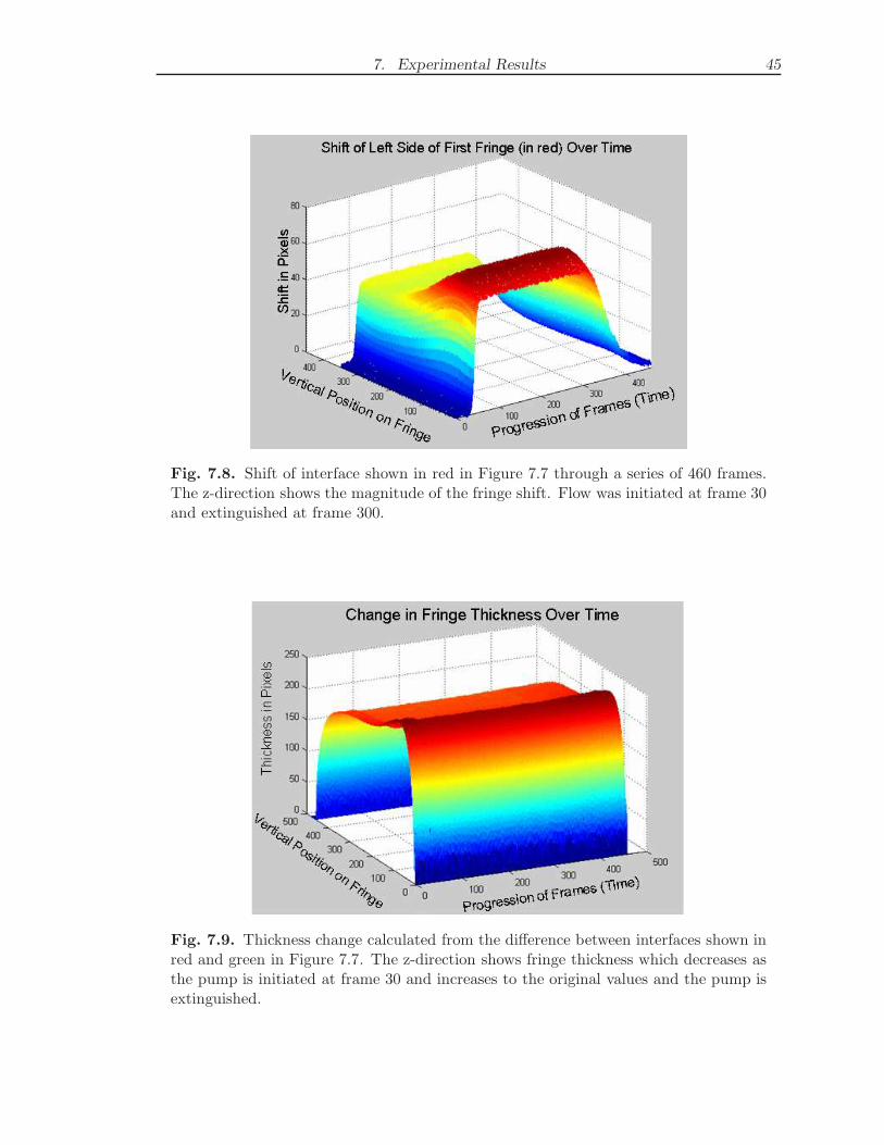
7. Experimental Results 45
Fig. 7.8. Shift of interface shown in red in Figure 7.7 through a series of 460 frames.The z-direction shows the magnitude of the fringe shift. Flow was initiated at frame 30and extinguished at frame 300.
Fig. 7.9. Thickness change calculated from the difference between interfaces shown inred and green in Figure 7.7. The z-direction shows fringe thickness which decreases asthe pump is initiated at frame 30 and increases to the original values and the pump isextinguished.

7. Experimental Results 46
Fig. 7.10. Thick walled square microchannel used to study effects of RI change andchannel wall deflection on fringe shift.
tracked in Figure 7.8 is observed. From this result, one can observe the distinctdecrease in fringe thickness which occurs at frame 30 when the pump is initialized andan increase in fringe thickness to the original position when the pump is extinguished.This element of fringe morphology also represents a general trend which varies inmagnitude between channel types and test sequences.
7.1.2 Thick Walled Microchannels
To isolate fringe morphology, the thickness of the channel walls was increased, leavingthe inner dimensions virtually unchanged. Due to increased channel rigidity, thedependence of fringe shift on channel deflection could effectively be observed. This,in turn, resulted in an increased ability to study the effects of changes in fluid RIunder cell pressurization and fluid flow conditions. Both round and square channelgeometries were tested, a listing of which may be found in Table 7.1. Examples ofthe types of thick walled microchannels implemented in this study, as well as theirmounting conditions, can be found in Figures 7.10 and 7.11. The channel shown inFigure 7.10 is of 0.25 mm square cross section in a glass cell of 4.00 by 4.00 mm outerdimensions. The round channel shown in Figure 7.11 has a diameter of 0.008 inchesand has been bored through a quarter inch glass rod. In both cases, the channel wallsare significantly thicker than in the case of the capillary tubes resulting in smallerdeformations.
Using distilled water under flowing conditions, both the circular and square chan-nel geometries were observed to produce fringe shifts. In the case of these channels,the shift sensitivity was found to be drastically lower than that reported in the previ-ous section for round and square capillary tubes. Although no experimental data has
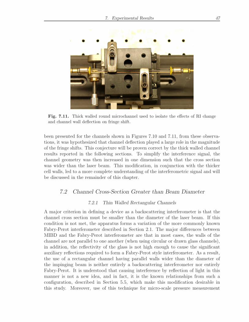
7. Experimental Results 47
Fig. 7.11. Thick walled round microchannel used to isolate the effects of RI changeand channel wall deflection on fringe shift.
been presented for the channels shown in Figures 7.10 and 7.11, from these observa-tions, it was hypothesized that channel deflection played a large role in the magnitudeof the fringe shifts. This conjecture will be proven correct by the thick walled channelresults reported in the following sections. To simplify the interference signal, thechannel geometry was then increased in one dimension such that the cross sectionwas wider than the laser beam. This modification, in conjunction with the thickercell walls, led to a more complete understanding of the interferometric signal and willbe discussed in the remainder of this chapter.
7.2 Channel Cross-Section Greater than Beam Diameter
7.2.1 Thin Walled Rectangular Channels
A major criterion in defining a device as a backscattering interferometer is that thechannel cross section must be smaller than the diameter of the laser beam. If thiscondition is not met, the apparatus forms a variation of the more commonly knownFabry-Perot interferometer described in Section 2.1. The major differences betweenMIBD and the Fabry-Perot interferometer are that in most cases, the walls of thechannel are not parallel to one another (when using circular or drawn glass channels),in addition, the reflectivity of the glass is not high enough to cause the significantauxiliary reflections required to form a Fabry-Perot style interferometer. As a result,the use of a rectangular channel having parallel walls wider than the diameter ofthe impinging beam is neither entirely a backscattering interferometer nor entirelyFabry-Perot. It is understood that causing interference by reflection of light in thismanner is not a new idea, and in fact, it is the known relationships from such aconfiguration, described in Section 5.5, which make this modification desirable inthis study. Moreover, use of this technique for micro-scale pressure measurement

7. Experimental Results 48
Fig. 7.12. Rectangular channel with relatively thin walls and channel width signifi-cantly larger than the laser beam diameter.
application has not yet been found to be demonstrated in any literature, making thesolution a desirable scientific achievement.
To modify the channel to the described predictable geometry, the cross-sectionwas made rectangular with dimensions of 9 mm by 0.05 mm. During initial testing,standard spectrometer cells were used, such as that shown in Figure 7.12, havingviewing windows approximately 1 mm in thickness. The cell was secured using fourmetal clamps, as shown in the figure, which were tightened to the maximum amountwithout promoting fracture of the glass. Under this configuration, the cell was testedunder both flowing and static conditions, allowing for fringe shift quantification basedon both pressure and fluid velocity. Since the channel was now larger than thediameter of the laser beam, the backscattered arc was eliminated thus simplifying theinterferometric signal.
The results of the fluid flow testing using distilled water in a 50 micron rectangularchannel are shown in Figure 7.13. In addition, Table 7.3 has been provided as a key toshow the theoretical pressure drop over the length of the channel as well as the pumpflow rate setting for each of the tested fluid velocities. From Figure 7.12 one can seethe results of two test sequences in which the fluid flow rate was set to various levelsand the corresponding fringe shift was determined. The results are linear for the flowvelocities below 25 mm/sec after which sensitivity begins to decrease. The significantspread in the data at flow velocities below 5 mm/sec are mainly a result of fringetracking error (± two pixels for spotlight tracking used here) and the unpredictabilityof channel deflections, which will be significantly reduced through the efforts reportedlater in this thesis.
Although the thin walled rectangular channel displayed a common data trend be-tween tests, just as in the case of the capillary tubes, the results were not reliableenough to allow for accurate quantification of fluid pressure. To study the phe-nomenon more closely, flow was eliminated from the system and static pressures were

7. Experimental Results 49
Fluid Velocity (mm/sec)
0 10 20 30 40 50
Frin
ge S
hift
(pi
xels
)
-4
-2
0
2
4
6
8
10
12
14
16
Sequence 1
Sequence 2
Fig. 7.13. Fringe shift at various fluid flow velocities for the thin walled rectangularchannel shown in Figure 7.12.
Tab. 7.3. Fringe shift data as well as corresponding velocity and pressure drop valuescalculated using Equation 7.2. Negative fringe shifts represent experimental error inaddition to instances where the pump was not properly primed for flow. Raw dataindicated an error of plus or minus two pixels.
Flow Rate Test 1 Test 2 Theoretical Velocity Theoretical PressureSetting Pixel Shift Pixel Shift (mm/sec) Drop (Pa)
13 N/A 15.0 41.3 4915 8.3 8.8 21.2 2517 4.6 3.7 10.6 1319 2.2 1.7 5.5 6.321 -1.8 1.9 2.8 3.423 0.66 0.36 1.41 1.7325 0.30 -1.08 0.71 0.88127 0.92 -0.33 0.37 0.458
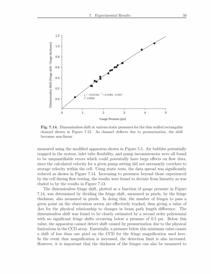
7. Experimental Results 50
Gauge Pressure (psi)
0 1 2 3 4 5
Dim
ensi
onle
ss S
hift
(fr
inge
shi
ft /
frin
ge th
ickn
ess)
0.0
0.2
0.4
0.6
0.8
1.0
1.2
y = - 0.01234x 2 + 0.3346x - 0.1827r2:0.9958
Fig. 7.14. Dimensionless shift at various static pressures for the thin walled rectangularchannel shown in Figure 7.12. As channel deflects due to pressurization, the shiftbecomes non-linear.
measured using the modified apparatus shown in Figure 5.5. Air bubbles potentiallytrapped in the system, inlet tube flexibility, and pump inconsistencies were all foundto be unquantifiable errors which could potentially have large effects on flow data,since the calculated velocity for a given pump setting did not necessarily correlate toaverage velocity within the cell. Using static tests, the data spread was significantlyreduced as shown in Figure 7.14. Increasing to pressures beyond those experiencedby the cell during flow testing, the results were found to deviate from linearity as waseluded to by the results in Figure 7.13.
The dimensionless fringe shift, plotted as a function of gauge pressure in Figure7.14, was determined by dividing the fringe shift, measured in pixels, by the fringethickness, also measured in pixels. In doing this, the number of fringes to pass agiven point on the observation screen are effectively tracked, thus giving a value of∆m for the physical relationship to changes in beam path length difference. Thedimensionless shift was found to be closely estimated by a second order polynomialwith no significant fringe shifts occurring below a pressure of 0.5 psi. Below thisvalue, the apparatus cannot detect shift caused by pressurization due to the physicallimitations in the CCD array. Essentially, a pressure below this minimum value causesa shift of less than one pixel on the CCD for the fringe magnification used here.In the event that magnification is increased, the detection limit is also increased.However, it is important that the thickness of the fringes can also be measured to

7. Experimental Results 51
Gauge Pressure (psi)
0 1 2 3 4 5
Thi
ckne
ss C
hang
e (p
ixel
s)
-5
0
5
10
15
20
25
Fig. 7.15. Thickness change of a bright fringe at various static pressures for the thinwalled rectangular channel shown in Figure 7.12.
non-dimensionalize the results. In practice this places a limitation on the maximumallowable magnification, a value directly dependent upon the physical dimensions ofthe CCD array.
Finally, the thickness change in the fringes was calculated for those tests in whicha positive fringe shift was observed. For low pressures, experimental errors such aslaser intensity fluctuations resulted in slightly negative thickness changes since celldeformation was very low. These results, depicted in Figure 7.15, show negativethickness values at low pressures and an increase in fringe thickness as cell pressurewas increased. This thickness change is a product of primarily due to channel de-formations, but also can be caused by large changes in RI as the impingement angledeviates from the surface normal. An increase in wall separation results in thickerfringes due to a larger horizontal separation in the reflecting beams. In the event thatthe beam is not directly in the center of the cell (at the apex of the deflection zone),there is also a change in fringe geometry, an effect of a tilting in the upper surface ofthe channel.
7.2.2 Thick Walled Rectangular Channels
To further reduce channel deformations, a custom variation of NSG Precision Cellsmodel Type 48 with 5 mm thick viewing windows was used. The interior cross-sectional dimensions of this cell were identical to the inner dimensions of the thin

7. Experimental Results 52
Fig. 7.16. Rectangular channel with thick walls and channel width significantly largerthan the laser beam diameter.
walled cell shown in Figure 7.16 being 9.00 mm x 0.05 mm. Figure 7.16 shows thiscell as well as the mounting and inlet/outlet conditions used in testing. This channelwas first tested under fluid flow conditions with distilled water as the working fluid,the results of which can be found in Figure 7.17. As with previous results, there issignificant spread in the data. This data spread is caused by the fluid flow; morespecifically, pump variations under load and the formation of small bubbles in thesystem which present difficulty in accurately predicting fluid flow characteristics suchas entrance losses.
Since flow variations caused results with poor repeatability, the flow was onceagain eliminated from the system and static cell pressurization was correlated to fringeshifts. Using the channel pictured in Figure 7.16, the variation of pressure under staticconditions (as opposed to flowing conditions) resulted in the plot shown in Figure 7.18.Through the elimination of fluid flow, test results collapse to a single line similar tothe case of the thin walled version of this channel. Using water as the working fluid atpressures less than 10 psig, the channel walls are now sufficiently thick that deflectionremains linear throughout the pressure range. These findings, represented in Figure7.19, demonstrate a vast increase in the predictability of the system when fringemorphology is properly controlled. In addition, the corresponding fringe thicknessvalues have been calculated and are provided in Figure 7.19. Once again, as pressurewas increased within the cell, fringe thickness increased, however, the magnitude ofthe thickness increase is much lower (less than half) than the identical channel withthin walls.
Upon comparison of these results to Figures 7.14 and 7.15, which were capturedunder nearly identical conditions, one can observe that the fringe shift no longer levelsout within the given pressure range because fringe thickness changes are reduced due

7. Experimental Results 53
Pressure Drop (psi)
0.0 0.2 0.4 0.6 0.8 1.0 1.2
Frin
ge S
hift
(pi
xels
)
0
20
40
60
80
Sequence 1
Sequence 2
Sequence 3
Fig. 7.17. Fringe shifts due to fluid flow in a 50 micron channel with thick side wallsfor three separate test sequences.
to a decrease in channel deformation. It is anticipated that testing of the thick walledcell at higher pressures would result in the same data trend as those observed for theidentical thin walled cell. However, such tests could not be performed here due to thepressure limitations of the channel.
It is also important to note the significant reduction in the data spread as celldeformations were controlled. From Figure 7.19 one can observe only two data pointswere recorded to display a fringe thickness change over four pixels. The deviationof these points from the best fit line is clearly observed upon direct comparison ofFigures 7.18 and 7.19, indicating fringe thickness change is an excellent indicator ofexperimental error. The major sources of error present in these experiments and theireffects on the data will be described in detail in Section 9.3.
To further explore fringe shift as a result of cell pressurization, the previous ex-periment was performed using air as the fluid within the channel. It is known thatthe RI of air is significantly more sensitive to pressure changes than water due tothe vast differences in their compressibilities. In performing such an experiment, theportion of the signal due to RI change and that resulting from channel deflectioncould effectively be determined. The results of static pressure testing on the samechannel filled with air are provided in Figures 7.20 through 7.22, demonstrating verysimilar data trends to the previous results.
The raw shift data, provided in Figure 7.20, was produced through fringe trackingin Matlab and shows the shift of the left and right sides of the interrogated fringe

7. Experimental Results 54
Gauge Pressure (psi)
0 2 4 6 8
Dim
ensi
onle
ss F
ring
e Sh
ift (
shif
t/thi
ckne
ss)
0.00
0.02
0.04
0.06
0.08
0.10
0.12
0.14
intercept:-4.3667e-4slope:0.0144r2:0.9994
Fig. 7.18. Fringe shift due to static channel pressurization using distilled water andthe test cell shown in Figure 7.16.
Gauge Pressure (psi)
0 2 4 6 8
Thi
ckne
ss C
hang
e (p
ixel
s)
-1
0
1
2
3
4
5
6
7
Fig. 7.19. Fringe thickness changes due to static channel pressurization using distilledwater and the test cell shown in Figure 7.18.

7. Experimental Results 55
Gauge Pressure (psi)
0 2 4 6 8
Shif
t (pi
xels
)
0
5
10
15
20
25
30
35
40
Left Side
Right Side
Fig. 7.20. Fringe shift of left and right sides of interrogated fringe due to static channelpressurization using air and the test cell shown in Figure 7.16.
through a pressure range of approximately 8 psig. Here the thickness change is ap-parent since the separation in the shift values from each side of the fringe is equalto the increase in fringe thickness produced by channel deformation. Upon averag-ing these two values for each pressure and non-dimensionalizing the data based onfringe thickness, the data can be collapsed further resulting in Figure 7.21. Here, theadvantage of a CCD array over a photodetector becomes apparent since both sidesof the fringe can be tracked, allowing for non-dimensionization of the results. With-out non-dimensionalized results, the fringes cannot universally be related to physicalquantities and instead one must calibrate the device in-situ before use.
Finally, Figure 7.22 provides the fringe thickness changes at various cell pressures.These values are comparable to those found in Figure 7.19 for the water filled channeland are consistently much less than in the case of the thin walled channel with iden-tical inner geometry. At first glance the results for air and water from this channelappear almost identical, leading the reader to believe the signal is not a function offluid RI changes.

7. Experimental Results 56
Gauge Pressure (psi)
0 2 4 6 8
Dim
ensi
onle
ss F
ring
e Sh
ift (
shif
t/thi
ckne
ss)
0.00
0.02
0.04
0.06
0.08
0.10
0.12
intercept:-3.8003e-4slope:0.01404r2:0.9998
Fig. 7.21. Dimensionless fringe shift due to static channel pressurization using air andthe test cell shown in Figure 7.16.
Gauge Pressure (psi)
0 2 4 6 8
Shif
t (pi
xels
)
-1
0
1
2
3
4
Fig. 7.22. Fringe thickness changes due to static channel pressurization using air inthe test cell shown in Figure 7.16.

8. VERIFICATION OF RESULTS
8.1 Laser Stability Testing
It is known that a HeNe laser typically displays intensity fluctuations between 0.1%and 1% of its maximum intensity as observed by Bornhop and Wang [1]. To explorehow these intensity fluctuations were affecting the experimental results, a NewportModel 818-BB-21 photodetector was placed in the path of the laser beam. Using anAgilent Model 54621A Oscilloscope as shown in Figure 8.1, the intensity fluctuationswere observed over time via the voltage output of the photodetector.
It was found that the laser intensity variations were most prominent when thelaser was first activated. This is expected since with most hardware, a startup time isrequired for the system response to stabilize as commonly observed with illuminationsources and transducers. To study the effects of the start up time and intensityfluctuations on the output of the laser, the detector signal was observed at varioustimes after startup via the oscilloscope and captured for later analysis. Signals werecaptured at times of approximately 2, 10, 16, 23, 70, and 120 minutes from startupand plotted to observe the change in fluctuation frequency and amplitude. The resultsof this test are summarized in Table 8.1, and the plots used to produce these resultscan be found in Appendix D.
A typical laser intensity fluctuation pattern from the red HeNe laser (model, SN)used in this experimentation can be seen in Figure 8.3. A green HeNe laser (Model30968, SN 6049-4705-903) was also observed to have similar fluctuations althoughextensive testing was not performed on this device since fringe shift data capturedwith this laser was not of a quantitative nature.
It can be observed from Table 8.1 that, as time progressed, the laser continuedto stabilize, demonstrating a decrease in fluctuation frequency and a relatively con-stant intensity fluctuation as a percentage of the full scale intensity. This showsthat as the laser stabilizes, the intensity fluctuations produce much less impact ontransient events, although these variations remain problematic for longer testing in-
A g i l e n t O s c i l l o s c o p eH e N e L a s e r P h o t o d e t e c t o r
Fig. 8.1. Simple optical arrangement used in testing laser intensity fluctuations.

8. Verification of Results 58
Tab. 8.1. Laser intensity fluctuation characteristics observed at various time intervalsafter startup.
Time Frequency Intensity Fluctuation(sec.) (Hz) (% of Full Scale Output)
2 0.22 5.8%10 0.17 5.2%16 0.11 5.0%23 0.07 5.7%70 0.007 6.8%120 < 0.002 7.0%
Fig. 8.2. Shift of one side of a fringe captured at 3 fps showing error in shift detection(manifested as variation in the z-direction) caused primarily by intensity fluctuationsand mechanical vibrations.

8. Verification of Results 59
Time (sec)
0 10 20 30 40 50
Phot
odet
ecto
r O
utpu
t (vo
lts)
8.4
8.5
8.6
8.7
8.8
8.9
9.0
9.1
Fig. 8.3. Intensity fluctuations displayed by a 1.5 mW HeNe laser as captured by aphotodetector.
tervals. From the plot shown in Figure 8.3, as well as those results at various timesshown in Appendix D, one can see that these fluctuations present a high degree ofunpredictability in the fringe shift results since data captured during an intensity risewould result in larger recorded shifts and data collected during an intensity declinewould result in smaller recorded fringe shifts. This issue has been addressed with no-table success by Bornhop [1] through the use of DCDB MIBD where fluctuations arecaptured by a second control detector and subtracted from a primary shift detectingsignal thus compensating for the intensity fluctuations [1]. Although this may seemto be one of the most obvious solutions, it is not without problems which includesynchronization of the signals as well as the production of an identical fringe patternto act as the control (difficult when channel geometry is not constant).
The described intensity fluctuations are manifested as an error in the fringe shiftvalue as shown in Figure 8.2. Here it is observed that as a fringe is tracked through aseries of frames, the intensity variations cause a tracking error shown by the verticalfluctuations in the plot. This tracking error has been observed to be as great asten pixels in some cases, depending upon the proximity of data collection to laserstartup and the magnification of the fringes on the CCD array. It should be notedthat the vertical fluctuations can also be attributed to mechanical vibrations in thesystem which have the potential to cause similar errors. On the whole, laser intensityfluctuations play an important role in shift quantification error although control of thisphenomenon is possible. Future shift quantification efforts will most likely address

8. Verification of Results 60
this issue more aggressively than the data displayed in this thesis, thus improving thecapability and reliability of the technique.
In some cases, the intensity fluctuations could be observed on the monitor dis-playing the CCD output. This was found to be most prominent near laser startupand at high fringe magnification. To verify the intensity fluctuations, the laser wasmounted in a mass spectrometer containing a slit diffraction wavemeter with ana-log light intensity measurement capability. Using this device, the same fluctuationpattern observed through the use of the photodetector was witnessed. No graphicalresults are provided for this test since no digital output was possible, however, thefluctuation frequency was observed to decay over time as in previous observations.Using this system, the signal was not observed to decay in magnitude, as observedin the plots from the photodector. This signal bleed off is believed to be from stabi-lization of the photodetector since it also was found to level out over time, while thelaser fluctuations remained roughly the same percentage of the full scale intensity ofthe laser.
8.2 Deflection Testing
8.2.1 Michelson Interferometer
To verify that pressure increase was causing channel deformation, two more experi-ments were performed. First, a mechanism was created to pinch off the exhaust tubeand induce a large pressure increase inside the channel. Clamps were found to beinadequate since mechanical vibration caused in hand tightening the clamp producedunwanted shifted and caused difficulty in determining results. To remedy this prob-lem, a tube pinch-off mechanism was created using a linear actuator which pressed asteel rod against the tube effectively creating a flow restriction. Figures E.1 and E.2of Appendix E show the device in its entirety. Using the mechanism to restrict orstop flow allows one to control cell pressurization without changing the experimentalsetup to the static testing configuration, which required different inlet and outlet tubetypes. To create flow restrictions, the exhaust tube was pinched by activating a linearactuator which moved a steel rod against the flow tube. Since the linear actuator wasfor optical instruments, it was highly sensitive to position allowing for very precisecontrol over the size of the flow restriction and the pressurization of the cell.
To observe the deformation in the top surface of the channel produced by cellpressurization, a Michelson interferometer was constructed next to the backscatterset-up to observe the deflection magnitude. As discussed in Section 2.1, a Michelsoninterferometer is commonly used to measure extremely small displacements (sub-micron sensitivity) through the use of two arms with a mirror at each end. A fullylabeled view of the device used in this testing can be seen in Appendix E. For thearm of the interferometer used to observe the displacement in the 50 micron channel,a mirror was placed on top the thin walled rectangular cell where it was thought todeflect as shown in Figure 8.4. The beam incident upon this mirror was retro-reflectedinto the laser aperture to produce an interferometric signal on the observation screen(see Figure E.4). Upon the introduction of flow in the cell, the fringes were observed
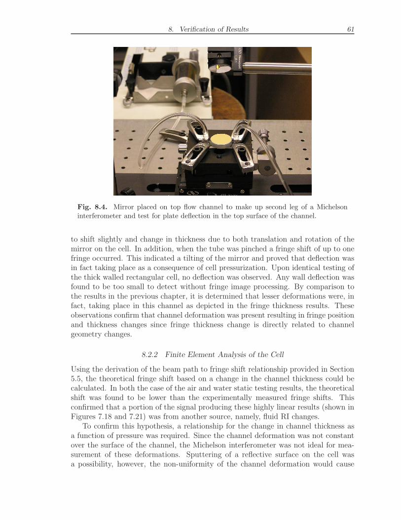
8. Verification of Results 61
Fig. 8.4. Mirror placed on top flow channel to make up second leg of a Michelsoninterferometer and test for plate deflection in the top surface of the channel.
to shift slightly and change in thickness due to both translation and rotation of themirror on the cell. In addition, when the tube was pinched a fringe shift of up to onefringe occurred. This indicated a tilting of the mirror and proved that deflection wasin fact taking place as a consequence of cell pressurization. Upon identical testing ofthe thick walled rectangular cell, no deflection was observed. Any wall deflection wasfound to be too small to detect without fringe image processing. By comparison tothe results in the previous chapter, it is determined that lesser deformations were, infact, taking place in this channel as depicted in the fringe thickness results. Theseobservations confirm that channel deformation was present resulting in fringe positionand thickness changes since fringe thickness change is directly related to channelgeometry changes.
8.2.2 Finite Element Analysis of the Cell
Using the derivation of the beam path to fringe shift relationship provided in Section5.5, the theoretical fringe shift based on a change in the channel thickness could becalculated. In both the case of the air and water static testing results, the theoreticalshift was found to be lower than the experimentally measured fringe shifts. Thisconfirmed that a portion of the signal producing these highly linear results (shown inFigures 7.18 and 7.21) was from another source, namely, fluid RI changes.
To confirm this hypothesis, a relationship for the change in channel thickness asa function of pressure was required. Since the channel deformation was not constantover the surface of the channel, the Michelson interferometer was not ideal for mea-surement of these deformations. Sputtering of a reflective surface on the cell wasa possibility, however, the non-uniformity of the channel deformation would cause

8. Verification of Results 62
Fig. 8.5. FEA analysis of thick walled rectangular channel under a static pressure of5 psig. Deflection of the impingement area is shown in blue and is approximately 18nm when both sides of the cell are considered.
asymmetric fringe formation, making accurate quantification difficult. To resolve thischallenge in a less time consuming manner (and avoid coating the cell which wouldnegate its backscattering capability), a finite element model was constructed to pre-dict the channel deformation at various pressures.
The cell was modeled in Unigraphics NX3 and a uniform pressure distribution wasapplied to the internal surfaces. The resulting cell deformation, shown in Figures 8.5and 8.6, depicts maximum deflections in the center of the channel at the impingementpoint. These results show deflection of the channel only in the z-direction (vertical)under a static pressure of 5 psi. When compared to deflection of the cell in alldirections, these results are identical, however, this simplified display was chosensince deflection in this direction is characteristic of channel separation, which directlyaffects the fringe shift results.
Boundary conditions used for this model were those of a part in free space. Sincethe clamping force used to mount the cell was very low to prevent fracture of the glass,these clamps did not exhibit a force large enough to require modeling. In addition, thedeflections calculated were on the order of tens of nanometers, a magnitude consideredto be within the free movement of the clamps (vertical tolerance in the threads). Sinceonly one of the bottom edges of the channel was fixed, the model was expected toslightly overpredict the experimental deformation results. Upon convergence of themesh this was found to be the case since a smaller mesh size gives slightly larger

8. Verification of Results 63
Fig. 8.6. Rotated view of Figure 8.5 showing deflection of bottom surface of cell inthe z-direction.
theoretical deflections, but is much more computationally expensive. As a result, theFEA predictions are found to be sufficient to accurately estimate the deformation ofthe channel.
Using this FEA model, the relationship between channel wall separation and cellpressure is displayed in Figure 8.7. Using a mesh size of 0.8 mm, the model wasfound to solve in just three minutes and provide a linear relationship such as thatdesired to fit the experimental data between 0 and 10 psi. The mesh size was foundto be sufficiently small such that the results changed by less than 1% when mesh sizewas reduced to half that of the previous value. The convergence of the mesh to asingle value is depicted by Figure 8.8 where the values approach a single y-value ina fairly linear fashion. Ideally the slope of this line would decrease as the mesh sizewas decreased, however, the results do not appear to diverge from the solution andtherefore represent a good estimation of the true channel deflection.
8.3 Verification with Known Data
8.3.1 Known Relationships for Air
Since the FEA model produced channel deformation estimations of lesser magnitudethan those predicted from the experimental data, it was hypothesized that RI changesin the fluid comprised the remainder of the signal. In the cases of both air and water,

8. Verification of Results 64
Gauge Pressure (psi)
0 2 4 6 8 10
Cha
nnel
Thi
ckne
ss I
ncre
ase
(m)
0.0
5.0e-9
1.0e-8
1.5e-8
2.0e-8
2.5e-8
3.0e-8
3.5e-8
intercept: 9.9999e-14slope:3.6151e-9r2:0.9999
Fig. 8.7. Estimation of cell deflection using finite element model with a mesh size of0.8 mm.
Mesh Size (mm)
0 1 2 3 4 5
Def
lect
ion
of I
mpi
ngem
ent P
oint
(m
)
1.3e-8
1.4e-8
1.5e-8
1.6e-8
1.7e-8
1.8e-8
1.9e-8
intercept:1.8847e-8slope:-1.0597e-9r2:0.9863
Fig. 8.8. Behavior of deflection estimation as mesh size is decreased at a static pressureof 5 psig. The mesh appears to converge at a value near 19 nm for this pressure value,a slight overestimation of the experimental results as expected.

8. Verification of Results 65
data is available for the relationship between pressure and RI. For air, the relationshiphas accurately been described by Birch and Edlen [25, 26] to be
n(T, p) = 1 + (ns − 1)
[
p(1 + p(60.1 − 0.972T )10−10)
96095.43(1 + 0.003661T )
]
(8.1)
where the RI, n, is dependent upon temperature, T, pressure, p and
ns = 1 +(
0.0472326
173.3 − σ2
)
(8.2)
The wavenumber, σ, is defined as
σ =1
λvac
(8.3)
The expression given by Equation 8.1 is linear for the temperature range of in-terest. Therefore, assuming the temperature of the fluid remains constant (a goodassumption since testing times were usually only a few seconds), the shift resultingfrom the calculated change in RI can be used to check the pressure measurementresult.
8.3.2 Known Relationships for Water
Although empirical relationships and data are extremely limited, the relationshipbetween RI and pressure was effectively observed by L. Zehnder in 1888 as reportedby Dorsey [5]. In defining a constant ∆ such that
∆ =n2 − n1
p2 − p1
(8.4)
where n1 and n2 are the RI values at pressures p1 and p2, respectively.This relationship was found to be closely approximated by the equation [5]
∆ = (16.84 − 0.129T + 0.0022T 2)10−6 (8.5)
where T is the temperature in ◦C.Upon equating 8.4 with 8.5 and rearranging we find
∆n =[
(16.84 − 0.129T + 0.0022T 2)10−6)]
(∆p) (8.6)
Using Equations 8.1 and 8.6, the change in refractive index of air and water canbe theoretically determined at various pressures. Using Equation 5.10, the theoreticalfringe shift based on a change in RI can be determined, and upon subtracting thesevalues from the experimental results, the remaining shift should be equal to the pre-dicted cell deflection. Figure 8.9 shows a comparison between the channel deflectionspredicted by the FEA model and the deflections calculated from the experimentalresults minus the contribution for the RI change due to pressure variation. The the-oretical and experimental results are found to match within 5% in the pressure rangebetween 0 and 10 psig. From this result, one can see that pressure measurement

8. Verification of Results 66
Gauge Pressure (psi)
0 2 4 6 8 10
Cal
cula
ted
Cel
l Def
lect
ion
(mm
)
0.00
5.00e-9
1.00e-8
1.50e-8
2.00e-8
2.50e-8
3.00e-8
3.50e-8
4.00e-8
FEA Data
Air Data
Water Data
Fig. 8.9. Comparison of finite element model results with calculated deflections basedon experimental data for air and water.
in microchannels is possible using the adapted backscattering setup. The signal iscomprised of two main components, fluid RI change and channel deformation, whichcan be isolated or used in combination for pressure measurement. The magnitude ofeach of these components of the signal will be described in the following chapter.
8.4 Description of Matlab Codes Used in Data Processing
Using Matlab, several codes were written to calculate channel deflection, fluid RI,dimensionless fringe shift, and detection limits based on various theoretical and ex-perimental conditions. The fully commented versions of these codes can be foundin Appendices I and J. In these codes, the known theoretical relationships for thechange in RI of air and water due to a change in pressure were utilized to verify theexperimental results, calculate the detection limits of the technique under differentoperating conditions, and find the areas where the device could be most significantlyimproved to enhance measurement sensitivity. Due to the relatively low computa-tional load of these calculations, simple loops were used in most cases to iterativelycompute unknown values to a high degree of accuracy. This avoided the need formultiple Matlab files in the form of external functions and simplifies code use forfuture users. Note that external functions were used in some instances to promotebrief and efficient coding. The results of these codes and the use of the equationsin Sections 8.3.1 and 8.3.2 provided the basis for the sensitivity results reported inChapter 9.

9. DEVICE SENSITIVITY
9.1 Detection Limits
Using the Matlab codes described in Section 8.4, the detection limits of the techniquefor measuring changes in RI of water and air were found. These detection limitswere calculated for an impingement angle of 13◦ on a fused quartz glass cell witha channel thickness of 50 µm, width of 9 mm, and length of 34 mm. Consideringthe fringe thickness corresponding to one wavelength of light (one light and one darkfringe) is 400 pixels and the shift tracking capability is to the nearest pixel, then theminimum detectable ∆m is 0.0025. This corresponds to a RI change of 1.541 · 10−5
and 1.560 · 10−5 in air and water, respectively. Using the experimental conditionsdescribed above, the RI changes correspond to 0.842 psi and 14.800 psi for air andwater, respectively. Utilizing the combination of channel deflection and fluid RIchanges, the detection limits are reduced to 0.21 psi and 0.15 psi for air and water,respectively. Although the detection limits are not overly impressive in comparisonto traditional methods, the technique is non-intrusive. In addition, there are severalsimple modifications that could be made to the device to drastically improve thedetection and measurement capabilities of this technique.
9.2 Effects of Experimental Parameters
A complete understanding how each of the experimental parameters effecting thesensitivity of the technique allows for optimization of these factors and leads to maxi-mum device sensitivity. To achieve such results, it is first important to to define thesefactors effecting the experimental outputs. As described by Equations 8.1 and 8.6, itis clear that refractive index is primarily a function of temperature and pressure. It isalso known that the composition and humidity of air play a role in RI. Likewise, thepurity of water also is important in determining its absolute RI. Since these factorsare not significantly altered during the measurement of the differential signal, theycan be neglected in this analysis.
Using the known relationships for RI as a function of temperature and pressure,Equation 5.10 becomes
∆m =
∣
∣
∣
∣
∣
(
2nT,pt cos(b′)
λ
)
1
−
(
2nT,pt cos(b′)
λ
)
2
∣
∣
∣
∣
∣
(9.1)
where nT,p is the RI of the fluid inside the channel as a function of temperature Tand pressure p, t is the thickness of the channel, b′ is the angle the light ray forms

9. Device Sensitivity 68
with the surface normal, and λ is the wavelength of the light. The subscripts 1 and2 refer to the initial and final states both before and after the fringe shift. The mainfactors effecting the sensitivity of the technique are found in Equation 9.1. Theseinclude the dimensionless fringe shift measurement δm, temperature, pressure, RI ofthe fluid used, channel impingement angle, and the wavelength of the light source. Itis important to note that this relationship is only valid for interferometric techniqueswhich follow the ray trace from Figure 5.8. In the case of this work, rectangularchannels wider than the beam diameter and the central fringe of channels of cross-sectional dimensions lesser than the beam diameter have been accurately represented.
From Equation 9.1 and the deflection predictions of the finite element model, thedependence of the experimental setup on RI of the working fluid can be demonstrated.At first it would appear that there are two unknowns, channel thickness, t and RI,n, however, since the FEA model was verified to match the experimental findings itcould be used confidently to determine the deformation of the channel thickness asa function of pressure. Therefore, using an iterative process where channel pressureis increased, the experimental ∆m can be used to determine the RI values as afunction of pressure. Plotting the relative contributions of channel deflection andRI over the experimental results, the portions of the signal coming from each sourcecan be visualized. Figures 9.1 and 9.2 show the signal contributions for the testingof air and water, respectively. The RI change of air plays a much larger role inthe formation of the signal than that for water. On the other hand, it can also bedetermined that the water filled channel results in an apparatus more sensitive to thedetection of channel deflections (as shown in the sensitivities reported in Section 9.1).The physical reason for this difference is the light path through the channel. In thecase of the air, the large change in RI at the glass-air interfaces causes a significantbending of the light, this results in an longer path length through the channel whencompared to that of the light through the water. In addition, the RI change of airas a function of pressure is much greater, resulting in a larger portion of the signalfrom this source. In the case of these tests, the impingement angle was chosen suchthat the experimental results appear almost identical to one another prior to thisanalysis. However, upon deconvolution of the results one finds that this is simplya result of improbable circumstances and in reality the RI change of air contributesapproximately 20% to the signal while the RI change of water contributes on about3% of the experimentally measured signal. That is to say, even though the plotsfor dimensionless fringe shift as a function of pressure shown in Figures 7.18 and7.21 appear to demonstrate nearly identical sensitivities, this is a result of a highersensitivity to channel deformation for water relative to air and higher sensitivity ofRI change for air relative to water.
To increase the sensitivity of the technique to changes in RI, the impingementangle should be maximized. Upon doing so the beam is forced to take the longestpossible path through the fluid resulting in the maximum phase lag for a given channelthickness and thus a maximum fringe shift. Another simple alternative to increasingthe sensitivity to RI is to increase the channel thickness. This effectively increasesthe phase lag of the light through the channel as well since the light is forced to travela greater distance at a new velocity through the medium within the channel. In

9. Device Sensitivity 69
comparison to the previously discussed parameters, temperature, barometric pressure,and wavelength of the light have relatively small effects on the results. Since thedevice is currently used to measure pressure and RI changes, these parameters donot significantly alter the experimental findings since the RI is found to be a linearfunction of these variables.
A final factor that is of paramount importance in the sensitivity of the device is theCCD sensor or photodetector used in data acquisition. In the case of the CCD sen-sor used in this experimentation, the fringes were typically set to approximately 400pixels in width due to the physical limitations of the camera. This allowed for a shiftdetection of one part in 400 or a dimensionless fringe shift of 0.0025 (shift/thickness= 1/400). On the other hand, a typical photodetector is capable of shift measure-ments as low as one part in 10−6 [7]. Using Equation 9.1 under the same conditionsused to determine the sensitivities in Section 9.1 one finds the limits are dramaticallyreduced to pressure measurements of 3.63 · 10−4 psi and 6.07 · 10−3 psi for air andwater, respectively, under ideal conditions. In reality, measurement errors such asmechanical vibrations and laser intensity fluctuations would reduce these measure-ment capabilities significantly, although the net result would still be a more sensitivedevice. In practice, it is difficult to use the photodetector for dimensionless fringeshift measurements since it does not readily allow for fringe thickness measurements.Once fringe morphology for a channel type is understood through the use of a CCD,the photodetector could be a logical addition to increase the sensitivity of the device.
Overall, to achieve optimal sensitivity, a channel of the maximum possible thick-ness should be used in conjunction with a maximum impingement angle. Control overtemperature, pressure, and wavelength should be practiced during testing intervalsand a detector of maximum spatial resolution should be utilized to quantify fringeshifts. Under these experimental conditions, the technique will display the great-est sensitivity to changes in fluid RI. As this sensitivity is increased, the effects ofexperimental error play a larger and larger role on the measurement limits.
9.3 Sources of Experimental Error
Sources of measurement error remain relatively constant between testing techniquesand channel types. Those sources of error presenting the most immediate need forsolutions are laser intensity fluctuations, isolation of air currents in the room (causeof RI changes in air between channel and detector), and inconsistency in channeldeformations at different impingement positions. Other sources of error includedthe measurement of room temperature and pressure, fluid flow rate, channel pres-sure, fringe shift, inconsistencies in impingement angle (poor ability to measure thisparameter), and finally mechanical vibrations. Through the isolation of these param-eters, the error was found to be immensely reduced as shown by a comparison betweenthe results shown in Figures 7.6 and 7.21. The results in Figure 7.21 demonstrate theimprovements in technique reliability which are reflected in the small relative errorshown in the measurements (less than 1% for those shown). Overall, precise quantifi-cation of these parameters is dependent upon the experimental parameters chosen by
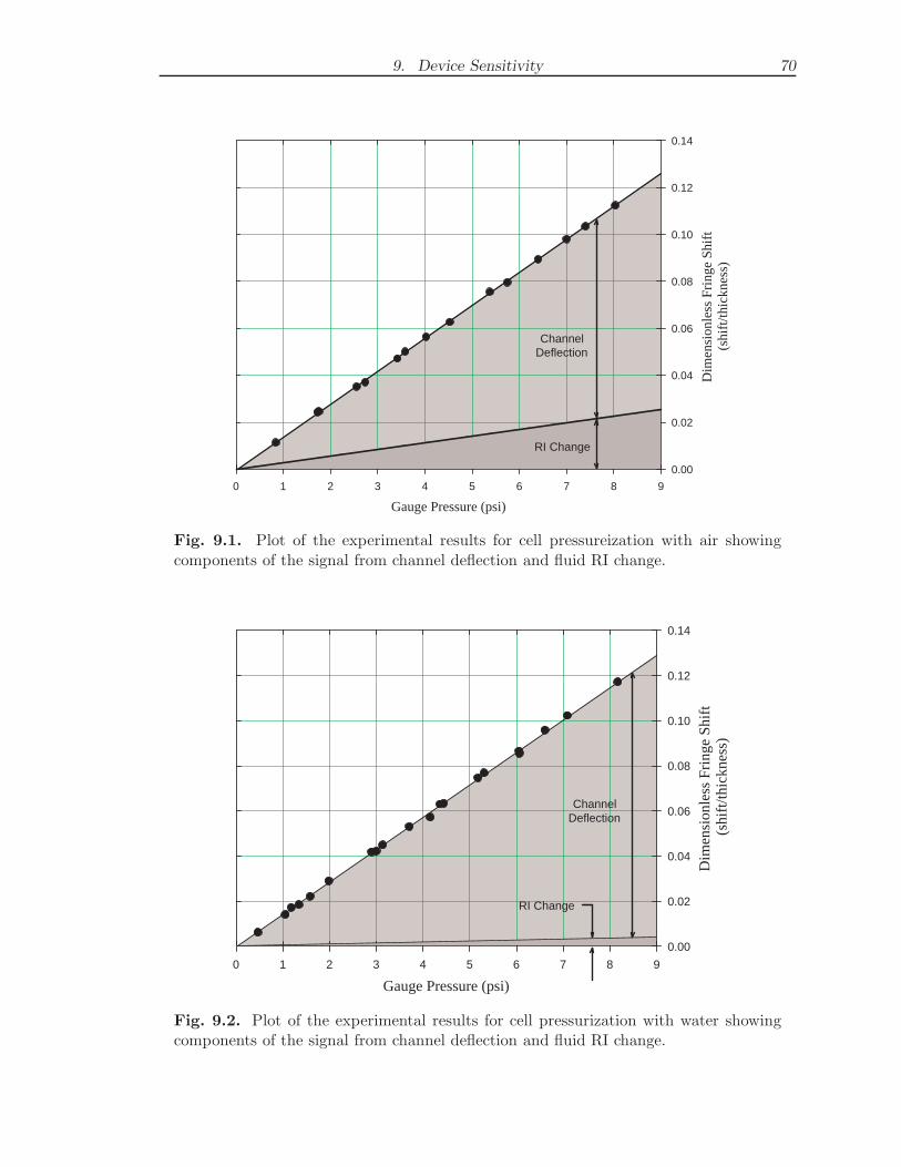
9. Device Sensitivity 70
Gauge Pressure (psi)
0 1 2 3 4 5 6 7 8 9
Dim
ensi
onle
ss F
ring
e Sh
ift
(shi
ft/th
ickn
ess)
0.00
0.02
0.04
0.06
0.08
0.10
0.12
0.14
ChannelDeflection
RI Change
Fig. 9.1. Plot of the experimental results for cell pressureization with air showingcomponents of the signal from channel deflection and fluid RI change.
Gauge Pressure (psi)
0 1 2 3 4 5 6 7 8 9
Dim
ensi
onle
ss F
ring
e Sh
ift
(sh
ift/t
hick
ness
)
0.00
0.02
0.04
0.06
0.08
0.10
0.12
0.14
ChannelDeflection
RI Change
Fig. 9.2. Plot of the experimental results for cell pressurization with water showingcomponents of the signal from channel deflection and fluid RI change.

9. Device Sensitivity 71
the user. For example, although the parameters for the static testing proves to resultin only 1% error, the use of a different camera sensor or the acquisition of data in thepresence of pump vibrations could increase this value and would require case-specificquantification.

10. CONCLUSIONS
Backscattering interferometry has successfully been proven to be adaptable for pres-sure measurement in microchannels. Upon careful impingement of a channel, a laserbeam can be made to interfere with itself as the light reflects from the inner andouter walls of the channel. This observed interferometric pattern changes with varia-tions in channel pressurization, as a result, the quantification of these changes can becorrelated to pressure and utilized as a measurement mechanism. The fringe move-ment and shape changes, also referred to as morphology, are consequences of fluid RIchanges as well as channel geometry deformations. It has been observed that asym-metric fringe morphology signifies channel deflections while symmetric morphologycan be a result of both RI changes and deformations.
The original motivation for this work was to measure pressure changes in flow-ing systems, therefore, the technique was first implemented on capillary tubes withflowing distilled water. These experiments proved the feasibility of this initiativedemonstrating common data trends and the ability to detect flow within a channel,but the technique lacked repeatability and the capacity to accurately quantify pres-sure and flow rate values. It was hypothesized that the inability to duplicate resultswas caused by deformations in the walls of the channel. Upon increasing the wallthickness, the signal was significantly dampened, however, the remaining morphologywas found to be symmetric and highly repeatable. These results were repeated usingchannels with cross sections wider than the laser beam proving that the channel didnot have to be completely encapsulated by the beam to produce a highly sensitivesignal.
The interferometric pattern was captured using a CCD array and morphologywas quantified using image processing in Matlab. When used in conjunction withinterferometric theory, this procedure resulted in an ability to quantify RI changes ofthe working fluid and variations in channel geometry. Using either known relation-ships for RI as a function of pressure, or a finite element estimation of the channeldeformation, the causes of fringe morphology can be separated and quantified. Toverify the results, both air and water were tested in a channel of known geometry.Using the known relationships for the RI changes due to pressure in conjunction witha finite element model, the experimental results were verified and found to match thetheoretical calculations within 5%.
With the results verified, the channel deformation can be subtracted from thesignal leaving only the RI change. This gives information on fluid compressibilityand can be used to study the effects of pressure on fluids with unknown propertieswithin the cell. Furthermore, if the RI change is known, channel deformations can bequantified below ten angstrom providing a highly sensitive deflection device. Detec-

10. Conclusions 73
tion and measurement limits are functions of channel size, geometry, and material aswell as photodetector and fluid type. Using this method, non-intrusive pressure andRI measurements are possible in micro-scale channels providing a capability not pre-viously available which could undoubtedly be found useful for numerous applicationsin the scientific community in the near future.
REFERENCES
[1] Wang, Z., Bornhop, D. Dual-Capillary Backscatter Interferometry for High-Sensityivity Nanoliter-Volume Refractive Index Detection with Density GradientCompensation. Analytical Chemistry, 77(24):7872-7877, 2005.
[2] Begari, D., Markov, D., Bornhop, D. Breaking the 10−7 Barrier for RI Measure-ments in Nanoliter Volumes. Analytical Chemistry, 74(20):5438-5441, 2002.
[3] Markov, D., Swinney, K., Bornhop, D. Chip Scale Universal Detection Based onBackscatter Interferometry. Analytical Chemistry, 72(13):2690-2695, 2000.
[4] Eddins, S., Gonzalez, R., Woods, R. Digital Image Processing using MATLAB.Pearson Prentice Hall, 2004.
[5] Dorsey, N.E. Properties of Ordinary Water-Substance. American Chemical So-ciety Monograph Series. Reinhold Publishing Corporation, New York, 1940.
[6] Dyson, J. Interferometry as a Measurement Tool. Hunt Barnard Printing Ltd.,Aylesbury, Great Britain, 1970.
[7] Newport Corporation. Projects in Interferometry. Newport Corporation, Irvine,Ca, Revision: B1, 1993.
[8] Francon, M. Optical Interferometry. Academic Press, New York and London,1966.
[9] Wolf, E., Born, M. Principles of Optics. Oxford: Pregamon, 6th edition, 1983.
[10] Sorensen, H. Self Calibrating Interferometric Sensor. PhD, Technical Univeristyof Denmark, 2006.
[11] Bornhop, D., Swinney, K. Noninvasive Picoliter Volume Thermometry Based onBackscatter Interferometry. Electrophoresis, 22:2032-2036, 2001.
[12] Wood, S., Bornhop, D., Markov, D., Dotson, S. Nonintrusive Fluid FlowMeasurements in Microfluidic Channels with Backscatter Interferometry. Elec-
trophoresis, 25:3805-3809, 2004.
[13] Bornhop, D. Laser-Based Refractive Index Detector using Backscatter, 1994.
[14] Swinney, K., Bornhop, D. Quantification and Evaluation of Joule Heating inOn-Chip Capillary Electrophoresis. Electrophoresis, 23:613-620, 2002.

REFERENCES 75
[15] Matousek, Lazar, Cip, Petru. Direct Measurement of Index of Refraction of Airby Means of High-Resolution Laser Interferometry. Pyysica Scripta, Vol. T118:48-50, 2005.
[16] Lotrian, J., Le Menn, M. Refraction Index Measurement by a Laser-Cube-Capillary Technique. Journal of Physics D: Applied Physics, 34:1256-1265, 2001.
[17] Lauer, Miller. An Instrument for the Measurement of the Index of Refraction ofLiquids in the Wave-Length Range 200 mµ to 1000 mµ. Journal of the Optical
Society of America, Vol. 37(8):664-668, 1947.
[18] Florea. Using a Differential Refractive Index Detector as a Pressure Transducerfor Online Viscometry in Exclusion Chomatography. Journal of Chromatography
A, 878:1-15, 2000.
[19] Crafton, Fonov, V., Fonov, S., Jones, Goss. The Development of Optical Tech-niques for the Measurement of Pressure and Skin Friction. Measurement Science
and Technology, 17:1261-1268, 2006.
[20] Greywall. Micromechanical Light Modulators, Pressure Gauges, and Thermome-ters Attached to Optical Fibers. J. Micromech. Microeng., Vol. 7:343-352, 1997.
[21] Houston, Jarzynski, Zalalutdinov, Bucaro, Lagakos, N. Miniature, High Perfor-mance, Low-Cost Fiber Optic Microphone Synopsis. JASA, 118(3):6, 2005.
[22] Kenmore, Tarigan, Neill, Bornhop, D. Capillary-Scale Refractive Index Detectionby Interferometric Backscatter. Analytical Chemistry, 68(10):1762-1770, 1996.
[23] Young, Monson, Okiishi. Fundamentals of Fluid Mechanics. Wiley, 5th edition,2006.
[24] Wood, S. Detecting Flow in a Capillary Using Backscattering Interferometry.Undergraduate Student Internship Report, NASA Glenn Research Center, 2002.
[25] Birch, Downs. An updated Edlen Equation for the Refractive Index of Air.Metrologia, 30:155-162, 1993.
[26] Edlen. The Refractive Index of Air. Metrologia, 2:71-80, 1966.

APPENDIX

A. SYRINGE PUMP CALIBRATION
The syringe pump used in flow testing could be set using a numerical scale of integervalues between one and thirty where one signified the maximum flow rate. Themanufacturer provides corresponding flow rates for select syringe types based uponthis scale, however, it was found to be inaccurate for the syringe types in use. Thepump was calibrated based on two syringe types used in experimentation. The resultshave been compared to the manufacturer’s reported values for these syringes withexcellent agreement in data trends.
Tab. A.1. Linear velocity of syringe pump at various flow rate settings.
Syringe Pump Speeds (Harvard Apparatus 975 - Tag Number 101481)Flow Rate Setting Distance Traveled Time Linear
Rate Under Load VelocitySetting (mm) (sec) (mm/sec)
1 3.87 30.8 1.26E-013 5.38 83.9 6.41E-025 4.75 144.9 3.28E-027 4.17 247.1 1.69E-029 3.94 459.3 8.58E-0311 3.37 773.2 4.36E-0313 1.6 716.5 2.23E-0315 1.6 1399.5 1.14E-0317 0.93 1608.1 5.78E-0419 0.67 2233.2 3.00E-0421 0.48 3339.9 1.44E-0423 0.23 2921.2 7.87E-0525 0.18 5017.3 3.59E-0527 0.14 7085.1 1.98E-0529 0.07 6271.9 1.12E-05

A. Syringe Pump Calibration 78
Tab. A.2. Calibration using 50.0 cc Syringe.
Hamilton 1050Predicted Flow Calculated Flow Rate Flow Rate Percent
Rate From Chart (cc/min) (mm3/sec) Difference4.60E+01 6.28E+01 1047.08 36.582.40E+01 3.21E+01 534.37 33.591.20E+01 1.64E+01 273.18 36.596.20E+00 8.44E+00 140.63 36.093.10E+00 4.29E+00 71.49 38.361.60E+00 2.18E+00 36.32 36.208.20E-01 1.12E+00 18.61 36.164.20E-01 5.72E-01 9.53 36.102.10E-01 2.89E-01 4.82 37.701.10E-01 1.50E-01 2.50 36.375.60E-02 7.19E-02 1.20 28.322.80E-02 3.94E-02 0.66 40.601.40E-02 1.79E-02 0.30 28.137.40E-03 9.88E-03 0.16 33.513.80E-03 5.58E-03 0.09 46.85
Fig. A.1. Calibration of syringe pump for use with a 50.0 cubic centimeter capacitysyringe.

A. Syringe Pump Calibration 79
Tab. A.3. Calibration using 5.0 cc Syringe.
Hamilton 1005Predicted Flow Calculated Flow Rate Flow Rate Percent
Rate From Chart (cc/min) (mm3/sec) Difference8.00E+00 6.28E+00 104.71 -21.474.10E+00 3.21E+00 53.44 -21.802.10E+00 1.64E+00 27.32 -21.951.10E+00 8.44E-01 14.06 -23.295.40E-01 4.29E-01 7.15 -20.572.80E-01 2.18E-01 3.63 -22.171.40E-01 1.12E-01 1.86 -20.257.20E-02 5.72E-02 0.95 -20.613.70E-02 2.89E-02 0.48 -21.851.80E-02 1.50E-02 0.25 -16.669.60E-03 7.19E-03 0.12 -25.154.90E-03 3.94E-03 0.07 -19.662.50E-03 1.79E-03 0.03 -28.251.30E-03 9.88E-04 0.02 -24.006.00E-04 5.58E-04 0.01 -6.99
Fig. A.2. Calibration of syringe pump for use with a 5.0 cubic centimeter capacitysyringe.

B. PRESSURE TRANSDUCER CLAIBRATION
A Kulite model XCS-062-10D pressure transducer was used for all static testing. Tocalibrate the transducer, an inclined manometer was connected to the pressurized lineof the cell. The results of the calibration can be found in Figure B.1 which showsgood agreement between the experimental and manufacturer’s sensitivities with onlya 0.17% difference between the reported values. It was found that a DC offset ofapproximately 0.002 mV was required to correct the experimental readings on the dayof the calibration. Factors effecting the DC offset include temperature and humidity,although, for differential pressure readings of the pressurized and unpressurized cell,the offset cancels out and only the sensitivity of the transducer is required.
Gauge Pressure (psi)
-0.2 -0.1 0.0 0.1 0.2 0.3 0.4 0.5
Tra
nsdu
cer
Out
put (
mV
)
-0.003
-0.002
-0.001
0.000
0.001
0.002
0.003
Manufacturer’s Sensitivity
Experimental Sensitivity
intercept:2.7105e-19slope:0.0120r2:1
intercept:-1.9793e-3slope:0.0120r2:0.9999
Fig. B.1. Calibration of pressure transducer using an inclined manometer.
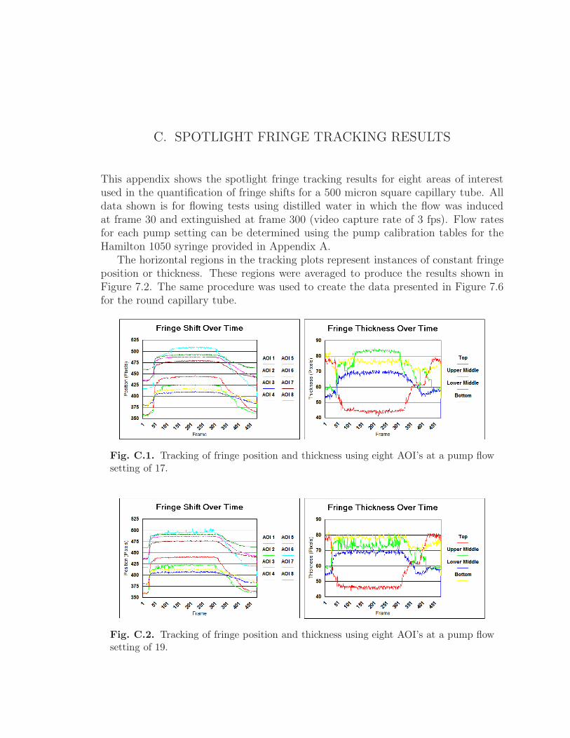
C. SPOTLIGHT FRINGE TRACKING RESULTS
This appendix shows the spotlight fringe tracking results for eight areas of interestused in the quantification of fringe shifts for a 500 micron square capillary tube. Alldata shown is for flowing tests using distilled water in which the flow was inducedat frame 30 and extinguished at frame 300 (video capture rate of 3 fps). Flow ratesfor each pump setting can be determined using the pump calibration tables for theHamilton 1050 syringe provided in Appendix A.
The horizontal regions in the tracking plots represent instances of constant fringeposition or thickness. These regions were averaged to produce the results shown inFigure 7.2. The same procedure was used to create the data presented in Figure 7.6for the round capillary tube.
Fig. C.1. Tracking of fringe position and thickness using eight AOI’s at a pump flowsetting of 17.
Fig. C.2. Tracking of fringe position and thickness using eight AOI’s at a pump flowsetting of 19.

C. Spotlight Fringe Tracking Results 82
Fig. C.3. Tracking of fringe position and thickness using eight AOI’s at a pump flowsetting of 21.
Fig. C.4. Tracking of fringe position and thickness using eight AOI’s at a pump flowsetting of 23.
Fig. C.5. Tracking of fringe position and thickness using eight AOI’s at a pump flowsetting of 25.

C. Spotlight Fringe Tracking Results 83
Fig. C.6. Tracking of fringe position and thickness using eight AOI’s at a pump flowsetting of 27.
Fig. C.7. Tracking of fringe position and thickness using eight AOI’s at a pump flowsetting of 29.

D. LASER STABILITY PLOTS
Note that after 12 minutes the neutral density filter was adjusted to lower the intensityof the beam. This effectively lowered the voltage output of the photodetector as shownin Figure D.3. This was done in an attempt to level out the signal more quickly.
Time (sec)
0 10 20 30 40 50
Phot
odet
ecto
r O
utpu
t (vo
lts)
7.3
7.4
7.5
7.6
7.7
7.8
7.9
8.0
Fig. D.1. Laser intensity fluctuations as captured by the photodetector approximately2 minutes after laser startup.
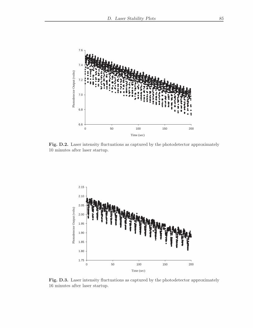
D. Laser Stability Plots 85
Time (sec)
0 50 100 150 200
Phot
odet
ecto
r O
utpu
t (vo
lts)
6.6
6.8
7.0
7.2
7.4
7.6
Fig. D.2. Laser intensity fluctuations as captured by the photodetector approximately10 minutes after laser startup.
Time (sec)
0 50 100 150 200
Phot
odet
ecto
r O
utpu
t (vo
lts)
1.75
1.80
1.85
1.90
1.95
2.00
2.05
2.10
2.15
Fig. D.3. Laser intensity fluctuations as captured by the photodetector approximately16 minutes after laser startup.

D. Laser Stability Plots 86
Time (sec)
0 50 100 150 200
Phot
odet
ecto
r O
utpu
t (vo
lts)
1.50
1.55
1.60
1.65
1.70
1.75
1.80
Fig. D.4. Laser intensity fluctuations as captured by the photodetector approximately23 minutes after laser startup.
Time (sec)
0 100 200 300 400 500
Phot
odet
ecto
r O
utpu
t (vo
lts)
1.04
1.06
1.08
1.10
1.12
1.14
1.16
1.18
Fig. D.5. Laser intensity fluctuations as captured by the photodetector approximately70 minutes after laser startup.

D. Laser Stability Plots 87
Time (sec)
0 100 200 300 400 500
Phot
odet
ecto
r O
utpu
t (vo
lts)
1.04
1.06
1.08
1.10
1.12
1.14
1.16
Fig. D.6. Laser intensity fluctuations as captured by the photodetector approximately120 minutes after laser startup.

E. CONFIGURATIONS FOR RESULTS VERIFICATION
E.1 Tube Pinch-Off Mechanism
Fig. E.1. Tube pinch-off mechanism used to induce pressure increases at detectionpoint of backscatter set-up.
Fig. E.2. Backscatter setup showing placement of pinch-off mechanism and observationchannel mounting.

E. Configurations for Results Verification 89
E.2 Michelson Interferometer for Deflection Testing
Fig. E.3. Mirror placement on 50 micron channel for deflection sensing leg of Michelsoninterferometer.
Fig. E.4. Components of the Michelson interferometer used to detect displacementsin the glass channel under increased pressure and fluid flow.
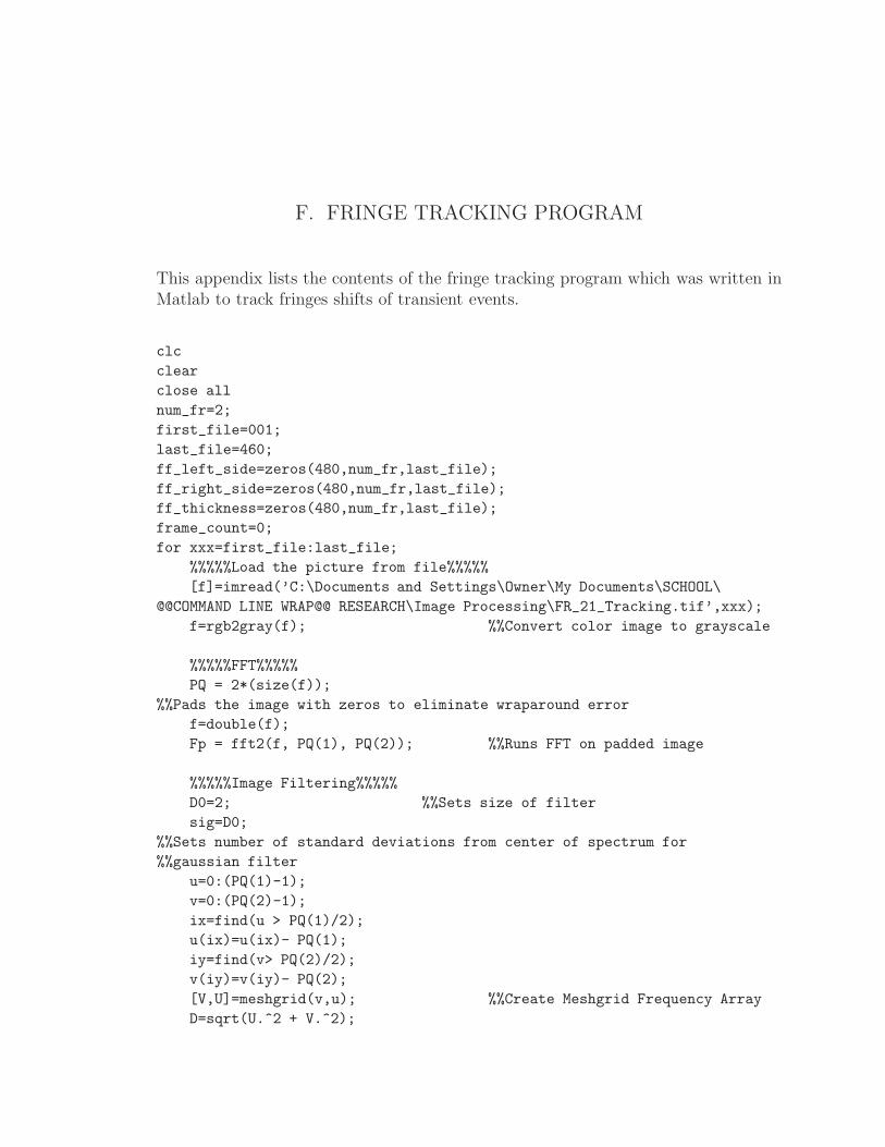
F. FRINGE TRACKING PROGRAM
This appendix lists the contents of the fringe tracking program which was written inMatlab to track fringes shifts of transient events.
clc
clear
close all
num_fr=2;
first_file=001;
last_file=460;
ff_left_side=zeros(480,num_fr,last_file);
ff_right_side=zeros(480,num_fr,last_file);
ff_thickness=zeros(480,num_fr,last_file);
frame_count=0;
for xxx=first_file:last_file;
%%%%%Load the picture from file%%%%%
[f]=imread(’C:\Documents and Settings\Owner\My Documents\SCHOOL\
@@COMMAND LINE WRAP@@ RESEARCH\Image Processing\FR_21_Tracking.tif’,xxx);
f=rgb2gray(f); %%Convert color image to grayscale
%%%%%FFT%%%%%
PQ = 2*(size(f));
%%Pads the image with zeros to eliminate wraparound error
f=double(f);
Fp = fft2(f, PQ(1), PQ(2)); %%Runs FFT on padded image
%%%%%Image Filtering%%%%%
D0=2; %%Sets size of filter
sig=D0;
%%Sets number of standard deviations from center of spectrum for
%%gaussian filter
u=0:(PQ(1)-1);
v=0:(PQ(2)-1);
ix=find(u > PQ(1)/2);
u(ix)=u(ix)- PQ(1);
iy=find(v> PQ(2)/2);
v(iy)=v(iy)- PQ(2);
[V,U]=meshgrid(v,u); %%Create Meshgrid Frequency Array
D=sqrt(U.^2 + V.^2);

F. Fringe Tracking Program 91
%%%%%Low Pass Filter%%%%%
%If using Low Pass Filter: comment out the high pass filter
Hp=exp(-(D.^2)./(2*((2*sig).^2))); %%Low Pass Filter
%%%%%High Pass Filter%%%%%
%If using the High pass filter: comment out loop used for tracking
%left side and right side fringe movement
%Hp=1-Hp;
%%High Pass Fiilter (Comment this line for Low Pass Filter)
Gp = Hp.*Fp; %%multiplies image and filter
%%%%%InverseFFT%%%%%
gp = real(ifft2(Gp));
%%Runs inverse FFT on frequency domain image
gpc = gp(1:size(f,1), 1:size(f,2)); %%Resizes image due to padding
%figure, imshow(gpc, []); %%Shows filtered image
%figure, plot(gpc(240, :));
%%Shows histogram of selected row on image (should be smooth sine wave)
%
%%%%%Create Binary Image%%%%%
gpc=uint8(gpc);
%%Converts data from double to uint8 for processing
level=(graythresh(gpc));
%%Finds the threshold level automatically
%The threshold level can also be manually set using the variable below
%level=.3;
BW = im2bw(gpc,level);
%%Converts image to binary using threshold level
%%%%%Edge Detection%%%%%
%thresh=(graythresh(f));
%%%% Edge funtion typesfor edgetype: ’sobel’,’prewitt’,
%%’roberts’,log’,’canny’
%EDGE=edgetype(gpc,’canny’,thresh,sig);
%The code below locates the fringes for tracking
left_side=zeros(length(BW(:,1)),num_fr);
right_side=zeros(length(BW(:,1)),num_fr);
Row=zeros(length(BW(1,:)));
for row_count=1:length(BW(:,1));
Row=BW(row_count,:);
column_left=1;
column_right=1;
for i=1:length(BW(1,:))-1;
if ((Row(i) == 0) & (Row(i+1) == 1));

F. Fringe Tracking Program 92
left_side(row_count,column_left)=i;
column_left=column_left+1;
elseif ((Row(i) == 1) & (Row(i+1) == 0));
right_side(row_count,column_right)=i;
column_right=column_right+1;
end;
end;
end;
%
ff_left_side(:,:,xxx)=left_side;
ff_right_side(:,:,xxx)=right_side;
%Loop calculates fringe thickness
fringe_thickness=zeros(length(left_side(:,1)),length(left_side(1,:)));
for Row=1:length(left_side(:,1));
for Column=1:length(left_side(1,:));
if left_side(Row,Column)<right_side(Row,Column);
fringe_thickness(Row,Column)=right_side(Row,Column)-
@@COMMAND LINE WRAP@@ left_side(Row,Column);
elseif right_side(Row,Column)<left_side(Row,Column) &
@@COMMAND LINE WRAP@@ right_side(Row,Column)>0;
fringe_thickness(Row,Column)=right_side(Row,Column+1)-
@@COMMAND LINE WRAP@@ left_side(Row,Column);
else;
fringe_thickness(Row,Column)=0;
end;
end;
end;
ff_thickness(:,:,xxx)=fringe_thickness;
frame_count=frame_count+1
end;
%%%%%Loop to Calculate fringe thickness difference over pixels%%%%%
left_side_shift=zeros(length(left_side(:,1)),length(left_side(1,:)),
@@COMMAND LINE WRAP@@ last_file-1);
right_side_shift=zeros(length(right_side(:,1)),length(right_side(1,:)),
@@COMMAND LINE WRAP@@ last_file-1);
for fringe_number=1:num_fr;
for frame=first_file:last_file-1;
left_side_shift(:,fringe_number,frame)=ff_left_side(:,fringe_number,
@@COMMAND LINE WRAP@@ frame+1)-ff_left_side(:,fringe_number,frame);
right_side_shift(:,fringe_number,frame)=ff_right_side(:,fringe_number,
@@COMMAND LINE WRAP@@ frame+1)-ff_right_side(:,fringe_number,frame);
end;

F. Fringe Tracking Program 93
%%%%%Loop to Calculate fringe thickness over time from reference%%%%%
for fringe_number=1:num_fr;
for frame=first_file:last_file-1;
abs_left_side_shift(:,fringe_number,frame)=ff_left_side(:,fringe_
@@COMMAND LINE WRAP@@ number,frame+1)-ff_left_side(:,fringe_number,1);
abs_right_side_shift(:,fringe_number,frame)=ff_right_side(:,fringe_
@@COMMAND LINE WRAP@@ number,frame+1)-ff_right_side(:,fringe_number,1);
end;
end;
end;
figure(1), imshow(gpc, []); %%Shows filtered image
title(’Plot of Left Side of First Fringe Through Frames’);
figure(2), plot(gpc(240, :));
%%Shows histogram of selected row on image (should be smooth sine wave)
figure(3), imshow(BW); %%Shows black and white image
%figure(4), imshow(EDGE, []);
%%%%%Plot fringe shift over time%%%%%
plot_shift_l1=left_side_shift(50:400,1,:);
plot_shift_l1=squeeze(plot_shift_l1);
figure(5), mesh(plot_shift_l1);
axis([0 460 5 450 0 10]);
title(’Plot of Left Side of First Fringe Through Frames’);
%
plot_shift_r1=right_side_shift(50:400,1,:);
plot_shift_r1=squeeze(plot_shift_r1);
figure(6), mesh(plot_shift_r1);
axis([0 460 5 450 0 10]);
title(’Plot of Right Side of First Fringe Through Frames’);
%%%%%Plot fringe shift from reference%%%%%
plot_abs_shift_l1=abs_left_side_shift(50:400,1,:);
plot_abs_shift_l1=squeeze(plot_abs_shift_l1);
figure(7), mesh(plot_abs_shift_l1);
axis([0 460 5 450 0 10]);
title(’Plot of absolute Left Side of First Fringe Through Frames’);
%
plot_abs_shift_r1=abs_right_side_shift(50:400,1,:);
plot_abs_shift_r1=squeeze(plot_abs_shift_r1);
figure(8), mesh(plot_abs_shift_r1);
axis([0 460 5 450 0 10]);
title(’Plot of absolute Right Side of First Fringe Through Frames’);
%
%Plot fringe thickness over time
%First Fringe

F. Fringe Tracking Program 94
plot_fringe_1=ff_thickness(:,1,:);
plot_fringe_1=squeeze(plot_fringe_1);
figure, mesh(plot_fringe_1);
title(’Change in Thickness of First Fringe Through Frames’);

G. MATLAB CODE FOR STATIC PRESSURE TEST
PROCESSING
The code provided in this appendix is a modified version of that found in AppendixF. Here the experimental procedure involved a capturing of two separate data files,the first containing images of unshifted fringes and the second containing images afterthe shift had occurred. The two files are processed separately and then compared todetermine shift magnitude and thickness changes. This two file method was used tosave hard drive space and reduce data processing time with equivalent results to theearlier method.
%%Derek Fultz
%%7-27-07
%
%%This program is used to process a pair of files for shifted and unshifted
%%fringes used in static pressure testing of the backscatter
%%interferometer.
%
clc
clear
%
%%%%File Inputs%%%%
%
%%Enter the number of bright fringes in the image
num_fr=1;
%
%%Enter the video frames to be processed
first_file=001;
last_file=15;
%
%
%%Create empty matrices to allocate memory and speed up program
ff_left_side=zeros(480,num_fr,last_file);
ff_right_side=zeros(480,num_fr,last_file);
ff_thickness=zeros(480,num_fr,last_file);
%%Initial Frame Counter
frame_count_unshifted=0;
%%Construct loop to process video one frame at a time
for xxx=first_file:last_file;
%%Enter first file with unshifted fringe data (file f)

G. Matlab Code for Static Pressure Test Processing 96
[f]=imread(’F:\DEREK\Static Pressure Tests 7_27_07\Test_20_Unshifted.tif’
@@COMMAND LINE WRAP@@ ,xxx);
%
%%%%Image Processing Procedures%%%%
%
f=rgb2gray(f); %%Convert color image to grayscale
PQ = paddedsize(size(f));
%%Pads the image with zeros to eliminate wraparound error
Fp = fft2(f, PQ(1), PQ(2)); %%Runs FFT on padded image
%%Choose filter size based on frequencies to be eliminated
D0=2; %%Sets size of filter
sig=D0;
%%Sets number of standard deviations from center of spectrum for
%%gausian filter
Hp = lpfilter(’gaussian’, PQ(1), PQ(2), 2*sig);
%%Performs gaussian low pass filter on image
Gp = Hp.*Fp;
%%multiplies image and filter (convolution in spatial domain)
gp = real(ifft2(Gp)); %%Runs inverse FFT on frequency domain image
gpc = gp (1:size(f,1), 1:size(f,2)); %%Resizes image due to padding
%figure, imshow(gpc, []); %%Shows filtered image
%figure, plot(gpc(240, :));
%%Shows histogram of selected row on image (should be smooth sine wave)
%
gpc=uint8(gpc);
%%Converts data from double to uint8 for processing
level=(graythresh(gpc)); %%Finds the threshold level automatically
%%The threshold level can also be manually set using the variable below
%level=.3; %%Enter manual threshold choice here
%
%%Change image to black and white only
BW = im2bw(gpc,level);
%%Converts image to binary using threshold level
figure, imshow(BW); %%Shows black and white image
title(’Black and White Image-Unshifted’);
%%Show the square wave created by the fringes
% figure, plot(BW(240, :));
% axis([-5 757 -.25 1.25]);
%
%
%%%%Locate Fringes%%%%
%
left_side=zeros(length(BW(:,1)),num_fr);
right_side=zeros(length(BW(:,1)),num_fr);
Row=zeros(length(BW(1,:)));
for row_count=1:length(BW(:,1));
Row=BW(row_count,:);

G. Matlab Code for Static Pressure Test Processing 97
column_left=1;
column_right=1;
for i=1:length(BW(1,:))-1;
if ((Row(i) == 0) & (Row(i+1) == 1));
left_side(row_count,column_left)=i;
column_left=column_left+1;
elseif ((Row(i) == 1) & (Row(i+1) == 0));
right_side(row_count,column_right)=i;
column_right=column_right+1;
end;
end;
end;
%%Store fringe locations for left and right side in each frame
ff_left_side(:,:,xxx)=left_side;
ff_right_side(:,:,xxx)=right_side;
%
%
%%%%Calculate fringe thickness of bright fringes%%%%
%
%%Note: It is recommended that this portion of code be used on a
%%cropped image
%
%%Use find command to increase the speed of these loops:
%indices=find(x(1:length(x)-1)<0.5 & x(2:length(x))>0.5);
%
fringe_thickness=zeros(length(left_side(:,1)),length(left_side(1,:)));
for Row=1:length(left_side(:,1));
for Column=1:length(left_side(1,:));
if left_side(Row,Column)<right_side(Row,Column);
fringe_thickness(Row,Column)=right_side(Row,Column)-left_side
@@COMMAND LINE WRAP@@ (Row,Column);
elseif right_side(Row,Column)<left_side(Row,Column) & right_side
@@COMMAND LINE WRAP@@ (Row,Column)>0;
fringe_thickness(Row,Column)=right_side(Row,Column+1)-left_side
@@COMMAND LINE WRAP@@ (Row,Column);
else;
fringe_thickness(Row,Column)=0;
end;
end;
end;
%%Store fringe thickness for each frame
ff_thickness(:,:,xxx)=fringe_thickness;
%
%%Advance frame counter
frame_count_unshifted=frame_count_unshifted+1
%
end;

G. Matlab Code for Static Pressure Test Processing 98
%
%%Find average values to eliminate measurement errors
for count=1:15
f_average_position_left(count)=mean(ff_left_side(210:310,1,count));
f_average_position_right(count)=mean(ff_right_side(210:310,1,count));
f_average_thickness(count)=mean(ff_thickness(210:310,1,count));
end
%%Save average values for file f
f_average_position_left=mean(f_average_position_left(:));
f_average_position_right=mean(f_average_position_right(:));
f_average_thickness=mean(f_average_thickness(:));
%%%%%%
%%%%%%
%%%%%%
%%%%%%
%
%%%%Begin tracking on frames of fringe data after shift%%%%
clc
%%Create empty matrices to speed up code and save memory
gf_left_side=zeros(480,num_fr,last_file);
gf_right_side=zeros(480,num_fr,last_file);
gf_thickness=zeros(480,num_fr,last_file);
%%Initialize counter
frame_count_shifted=0;
%
for xxx=first_file:last_file;
%%Read the shifted frame from file (file g)
[g]=imread(’F:\DEREK\Static Pressure Tests 7_27_07\Test_20_Shifted.tif’
@@COMMAND LINE WRAP@@ ,xxx);
%
%
g=rgb2gray(g); %%Convert color image to grayscale
PQ = paddedsize(size(g));
%%Pads the image with zeros to eliminate wraparound error
Fp = fft2(g, PQ(1), PQ(2)); %%Runs FFT on padded image
D0=2; %%Sets size of filter
sig=D0;
%%Sets number of standard deviations from center of spectrum for gausian
%%filter
Hp = lpfilter(’gaussian’, PQ(1), PQ(2), 2*sig);
%%Performs gaussian low pass filter on image
Gp = Hp.*Fp;
%%multiplies image and filter (convolution in spatial domain)
gp = real(ifft2(Gp)); %%Runs inverse FFT on frequency domain image
gpc = gp (1:size(g,1), 1:size(g,2)); %%Resizes image due to padding
%figure, imshow(gpc, []); %%Shows filtered image
%figure, plot(gpc(240, :));

G. Matlab Code for Static Pressure Test Processing 99
%%Shows histogram of selected row on image (should be smooth sine wave)
%
gpc=uint8(gpc);
%%Converts data from double to uint8 for processing
level=(graythresh(gpc)); %%Finds the threshold level automatically
%%The threshold level can also be manually set using the variable below
%level=.3;
%
%%Change image to black and white only
BW = im2bw(gpc,level);
%%Converts image to binary using threshold level
figure, imshow(BW); %%Shows black and white image
title(’Black and White Image-Shifted’);
%%Show the square wave created by the fringes
% figure, plot(BW(240, :));
% axis([-5 757 -.25 1.25]);
%
%
%%The code below locates the fringes for tracking
left_side=zeros(length(BW(:,1)),num_fr);
right_side=zeros(length(BW(:,1)),num_fr);
Row=zeros(length(BW(1,:)));
for row_count=1:length(BW(:,1));
Row=BW(row_count,:);
column_left=1;
column_right=1;
for i=1:length(BW(1,:))-1;
if ((Row(i) == 0) & (Row(i+1) == 1));
left_side(row_count,column_left)=i;
column_left=column_left+1;
elseif ((Row(i) == 1) & (Row(i+1) == 0));
right_side(row_count,column_right)=i;
column_right=column_right+1;
end;
end;
end;
%
gf_left_side(:,:,xxx)=left_side;
gf_right_side(:,:,xxx)=right_side;
%
%
%%The code below is used to calculate fringe thickness (bright fringes)
%%It is recommended that this portion of code be used on a cropped image
%
%%Use find command to increase the speed of these loops:
%indices=find(x(1:length(x)-1)<0.5 & x(2:length(x))>0.5);
%

G. Matlab Code for Static Pressure Test Processing 100
fringe_thickness=zeros(length(left_side(:,1)),length(left_side(1,:)));
for Row=1:length(left_side(:,1));
for Column=1:length(left_side(1,:));
if left_side(Row,Column)<right_side(Row,Column);
fringe_thickness(Row,Column)=right_side(Row,Column)-left_side
@@COMMAND LINE WRAP@@ (Row,Column);
elseif right_side(Row,Column)<left_side(Row,Column) & right_side
@@COMMAND LINE WRAP@@ (Row,Column)>0;
fringe_thickness(Row,Column)=right_side(Row,Column+1)-
@@COMMAND LINE WRAP@@ left_side(Row,Column);
else;
fringe_thickness(Row,Column)=0;
end;
end;
end;
%
gf_thickness(:,:,xxx)=fringe_thickness;
%
frame_count_shifted=frame_count_shifted+1
%
end;
%
%
%%Finding average values
for count=1:15
g_average_position_left(count)=mean(gf_left_side(210:310,1,count));
g_average_position_right(count)=mean(gf_right_side(210:310,1,count));
g_average_thickness(count)=mean(gf_thickness(210:310,1,count));
end
%
g_average_position_left=mean(g_average_position_left(:));
g_average_position_right=mean(g_average_position_right(:));
g_average_thickness=mean(g_average_thickness(:));
%%%%%%
%%%%%%
%%%%%%
%%%%%%
%%Find fringe shift and thickness changes between files f and g
final_fringe_shift_left=f_average_position_left-g_average_position_left
final_fringe_shift_right=f_average_position_right-g_average_position_right
final_fringe_thickness_change=g_average_thickness-f_average_thickness
thickness_shifted=g_average_thickness

H. MATLAB EXTERNAL FUNCTIONS
Listed below are the external user defined functions required to run the fringe trackingcodes provided in Appendices F and G. These short codes can also be found withmore detailed explanation in the Digital Image Processing Using Matlab text byR. Gonzalez [4].
%%%%%%%%%%%%%%%%%%%%%%%%%%%%%%%%%%%%%
%%%% Function to pad image %%%%
%%%%%%%%%%%%%%%%%%%%%%%%%%%%%%%%%%%%%
function PQ = paddedsize(AB,CD,PARAM)
%
if nargin==1
PQ=2*AB;
elseif nargin==2 & ~ischar(CD)
PQ=AB+CD-1;
PQ=2*ceil(PQ/2);
elseif nargin==2
m=max(AB); %Maximum dimension.
P=2^nextpow2(2*m);
PQ=[P,P];
else
error(’Wrong number of inputs’)
end
%%%%%%%%%%%%%%%%%%%%%%%%%%%%%%%%%%%%%%%%%%%%%%%%%%%%%%%%%%%%%%
%%%% Function to perform frequency domain filtering %%%%
%%%%%%%%%%%%%%%%%%%%%%%%%%%%%%%%%%%%%%%%%%%%%%%%%%%%%%%%%%%%%%
function g = dftfilt(f,H)
%
%Obtain the FFT of the padded input.
F=fft2(f,size(H,1),size(H,2));
%
%Perform filtering.
g=real(ifft2(H.*F));
%
%Crop to original size.
g=g(1:size(f,1), 1:size(f,2));

H. Matlab External Functions 102
%%%%%%%%%%%%%%%%%%%%%%%%%%%%%%%%%%%%%%%%%%%%%%%%%%%%%%%%%%%%
%%%% Function to make meshgrid frequency matrices %%%%
%%%%%%%%%%%%%%%%%%%%%%%%%%%%%%%%%%%%%%%%%%%%%%%%%%%%%%%%%%%%
function [U, V] = dftuv(M,N)
%
%Set up range of variables.
u=0:(M-1);
v=0:(N-1);
%
%Compute the indices for use in meshgrid.
idx=find(u > M/2);
u(idx) = u(idx) - M;
idy = find(v > N/2);
v(idy) = v(idy) - N;
%
%Compute the meshgrid arrays
[V, U] = meshgrid(v,u);
%%%%%%%%%%%%%%%%%%%%%%%%%%%%%%%%%%%%%%%%%%%%%%%%%%%%%%%%
%%%% Function to run low pass filter on image %%%%
%%%%%%%%%%%%%%%%%%%%%%%%%%%%%%%%%%%%%%%%%%%%%%%%%%%%%%%%
function H = lpfilter(type, M, N, D0, n)
%
%Use function dftuv to set up the meshgrid arrays needed for computing the
%required distances.
[U, V] = dftuv(M, N);
%
%Compute the distances D(U, V);
D=sqrt(U.^2 + V.^2);
%
switch type
case ’ideal’
H=double(D <= D0);
case ’btw’
if nargin ==4
n=1;
end
H = 1./(1+(D./D0).^(2*n));
case ’gaussian’
H = exp(-(D.^2)./(2*(D0^2)));
otherwise
error(’Unknown filter type’)
end

I. PROGRAM TO FIND SENSITIVITY USING WATER
This appendix lists the contents of the Matlab program used to find the sensitivityusing water under different experimental conditions.
%Derek Fultz
%10-25-06
%
%
%This program finds the minimum RI change detectable using this technique
%as well as the minimum associated pressure change detectable for water.
%
clc
clear
%
%%Experimental Inputs%%
fringe_thickness=400;
%Thickness of light and dark fringe together in pixels
min_delta_m=1/fringe_thickness;
%Minimum detectable dimensionless fringe shift
RI_glass=1.46; %Refractive index of fused quartz
RI_air=1.0003; %Approx. RI of air for angle calculation
theta_i=13; %impingement angle in degrees
theta_i=theta_i*pi/180; %impingement angle in radians
theta=asin(sin(theta_i)*(RI_air/RI_glass)); %angle through glass
p_barometric=736.4; %Pressure in mm Hg
p_barometric=p_barometric*(101325/760.0); %Pressure in pascals
temp=24; %room temperature in deg C
%
%
%%Known Values%%
lambda=633e-9; %Wavelength of the light in meters
thickness=50e-6; %Original channel thickness in meters
%
%
RI_water_exp_conditions=1.332;
%The refractive index of water under the experimental conditions
theta_prime_1=asin(sin(theta)*(RI_glass/RI_water_exp_conditions));
%angle of light in water
m_initial=(2*thickness*RI_water_exp_conditions*cos(theta_prime_1))
@@COMMAND LINE WRAP@@ /(lambda);

I. Program to Find Sensitivity Using Water 104
%inital fringe value from vacuum
%
%
new_m=m_initial+min_delta_m; %defines m with min detectable shift
%
%
new_RI_water=RI_water_exp_conditions; %sets an initial value
m=1; %sets an initial value
while m < new_m ; %uses a while loop to avoid external functions
theta_prime_2=asin(sin(theta)*(RI_glass/new_RI_water));
m=(2*thickness*new_RI_water*cos(theta_prime_2))/(lambda);
new_RI_water=new_RI_water+.0000000001;
end
%
%
new_RI_water; %displays the new refractive index of the water
RI_change=new_RI_water-RI_water_exp_conditions %min detectable RI change
%
%
%Find the pressure increase associated with the change in RI of water
p=(RI_change/((16.84-0.129*temp+0.0022*temp^2)*10^-6))*(p_barometric*
@@COMMAND LINE WRAP@@ 1.4508e-4)
%min detectable pressure based on RI change

J. PROGRAM TO FIND SENSITIVITY USING AIR
This appendix lists the contents of the Matlab program used to find the sensitivityusing air under different experimental conditions.
%Derek Fultz
%10-25-06
%
%
%This program finds the minimum RI change detectable using this technique
%as well as the minimum associated pressure change detectable for air.
%
clc
clear
%
%%Experimental Inputs%%
fringe_thickness=400;
%Thickness of light and dark fringe together in pixels
min_delta_m=1/fringe_thickness;
%Minimum detectable dimensionless fringe shift
RI_glass=1.46; %Refractive index of fused quartz
RI_air=1.0003; %Approx. RI of air for angle calculation
theta_i=13; %impingement angle in degrees
theta_i=theta_i*pi/180; %impingement angle in radians
theta=asin(sin(theta_i)*(RI_air/RI_glass)); %angle through glass
p_barometric=739.7; %Pressure in mm Hg
p_barometric=p_barometric*(101325/760.0); %Pressure in pascals
temp=23; %room temperature in deg C
%
%
%%Known Values%%
lambda=633e-9; %Wavelength of the light in Meters
thickness=50e-6; %Original Channel Thickness in Meters
%
%
%%Calculated Values%%
lambda_vac=.633; %(micrometers)
sigma=1/lambda_vac;
n_s=1+(.0472326*(173.3-sigma^2)^-1);
RI_air_exp_conditions=1+((n_s-1)*((p_barometric*(1+p_barometric*(60.1-
@@COMMAND LINE WRAP@@ .972*temp)*10^-10))/(96095.43*(1+.003661*temp))));

J. Program to Find Sensitivity Using Air 106
theta_prime=asin(sin(theta)*(RI_glass/RI_air_exp_conditions));
theta_prime_deg=theta_prime*(180/pi);
m_initial=(2*thickness*RI_air_exp_conditions*cos(theta_prime))/(lambda);
%
%
new_m=m_initial+min_delta_m;
%
%
new_RI_air=RI_air_exp_conditions;
m=1;
while m < new_m ;
theta_prime_2=asin(sin(theta)*(RI_glass/new_RI_air));
m=(2*thickness*new_RI_air*cos(theta_prime_2))/(lambda);
new_RI_air=new_RI_air+.0000000001;
end
%
%
new_RI_air;
RI_change=new_RI_air-RI_air_exp_conditions %min detectable RI change
%
%
%Find the pressure increase associated with the change in RI of water
RI_change_loop=0;
pressure=p_barometric;
while RI_change_loop<RI_change;
RI_air=1+((n_s-1)*((pressure*(1+pressure*(60.1-.972*temp)*10^-10))/
@@COMMAND LINE WRAP@@ (96095.43*(1+.003661*temp))));
RI_change_loop=RI_air-RI_air_exp_conditions;
pressure=pressure+.1; %advance pressure in Pa
end
pressure=pressure-p_barometric; %pressure in Pa
pressure=pressure*(1.4508e-4) %min detectable pressure in psi