Transportation Research Record 756

7. Operations and Procedures Manual, Vol. 4. Highway Design Division, Texas State Department of Highways and Public Transportation, Austin, 1976.

8. P.J. Strauss, B.F. McCullough, and W.R. Hudson. Continuously Reinforced Concrete Pavement: Structural Performance and Design/Construction Variables. Center for Highway Research, Univ. of Texas at Austin, Research Rept. 177-7, May 1977.

9. A. Abou-Ayyash and W.R. Hudson. Analysis of Bending Stiffness Variation at Cracks in Continuous Pavements. Center for Highway Research, Univ. of Texas at Austin, Research Rept. 56-22, April 1972.

10 . J.J. Panak and H. Matlock. A Discrete Element of Analysis for Orthogonal Slab and Grid Bridge Floor Systems. Center for Highway Research, Univ. of Texas at Austin, Research Rept. 56-25, Aug. 1971.

15

11. W.R. Hudson and H. Matlock. Discontinuous Orthotropic Plates and Pavement Slabs. Center for Highway Research, Univ. of Texas at Austin, Research Rept. 56-6, 1966.

12. IVl.G. de Velasco, B.F. McCullough, and D.W. McKenzie. Summary of Comparison of 1978 and 1974 CRCP Condition Surveys for Highways. Center for Highway Research, Univ. of Texas at Austin, Research Rept. 177-21, in preparation.

13. J.S. Dhamrait, F.K. Jacobsen, and D.R. Schwartz. Condition of Longitudinal Steel in Illinois Continuously Reinforced Concrete Pavement. Illinois Department of Transportation, Springfield, Interim Rept. IHR-36, 197 3.

Publication of this paper sponsored by Committee on Rigid Pavement Design.

Nomographs for the Design of Steel Reinforcement in Continuously Reinforced Concrete Pavement

C. S. NOBLE, B. F. McCULLOUGH, AND J. C. M. MA

This study sought to develop graphic procedures (nomographs) for the design of continuously reinforced concrete pavement (CRCP) by the Texas State Depart· ment of Highways and Public Transport~tion for a range of specified local con­ditions. This set of nomographs, when used as a supplementary design tool with the CRCP-2 computer program model, will facilitate CRCP design. This will substantially reduce both the time and the cost involved in the design process, while at the same time taking into account the effect of regional and local en­vironments. First, regression equations were developed for the prediction of three design parameters (crack spacing, crack width, and steel stress), and then principles of nomography were applied to these mathematical relations to pre­pare three corresponding nomographs. The choice of equations was made fol­lowing multiple linear and nonlinear least-squares fits to a fractional factorial of simulated observations that were output from the CRCP-2 computer program. Theoretical models, developed at the Center for Highway Research in Austin, Texas, and variations of the three design parameters with each of the relevant input variables over the range of the simulated data were considered in deciding on the form of the regression equations. Standard-error-of-residuals and R2

(proportion of variance explained by the regression equation) statistics were considered in the final choice of coefficients for the regression equations. Con­fidence prediction limits were determined by using multiple linear-regression techniques for application to nomograph predictions. A recommended pro­cedure for the use of the nomographs with appropriate limiting criteria is out­lined and an example given.

Continuously reinforced concrete pavement (CRCP) is considered a relatively new pavement type by many eng·ineers, although it has been in use since 1921, when it was first introduced by the Bureau of Public Roads on the Columbia Pike near Arlington, Virginia. The next reported use of CRCP was in 1938, when Indiana, in cooperation with the Bureau of Public J{oads, constructed an experimental pavement that involved several test sections.

Tne state highway departments of Indiana, Illinois, Texas, California, Mississippi, New Jersey, Michigan, Maryland, and Pennsylvania have laid other pavements of this type that have provided good service for a number of years. The oldest of these is approximately 30 years of age.

After there were several successful experiences with CKCP on experimental projects, the use of CRCP increased substantially, especially during the 1960s. Several research studies in rigid pavement design led to the development of the design procedures currently used for CRCP (l-5).

In 197 2, a study under the auspices of the National Cooperative Highway Research Program (NCHRP) was

conducted at the University of Texas at Austin. It comprised a review of design and construction variables, theoretical studies, field surveys, and laboratory investigations. The fundamental philosophy of this review was that, through a combination of field observations and laboratory studies, reliable procedures could be achieved to develop mathematical models that simulate CRCP field performance. Based on these mathematical models, the CRCP-1 computer program was developed to calculate the stresses in concrete and steel, crack width, and crack spacing that result from concrete volume changes due to temperature and shrinkage (6).

Generally, the engineer- is encouraged to design each pavement for the soil conditions, traffic, materials, and so forth at the given site and to be wary of inappropriate boundary values and practices. However, in order to cover such a wide variety of input variables, the engineer needs a large-scale experiment to anticipate the effects of the individual variations of the variables and the variations in groups. Thus, a sensitivity analysis of the behavior of CRCP that used the CRCP-1 model (7) was conducted for the Texas State Department oC Highways and Public Transportation (SDHPT). From the results of this study, the relative importance of about 15 input variables was determined in order to investigate the effect of changes in values of these variables on CRCP behavior. The list of the input variables includes steel properties, concrete properties, friction-movement relations, and temperature variations. In addition to establishing the relative importance of such variables, the study revealed several inconsistencies in the initial model at extreme boundary conditions that resulted in modification of the computer program.

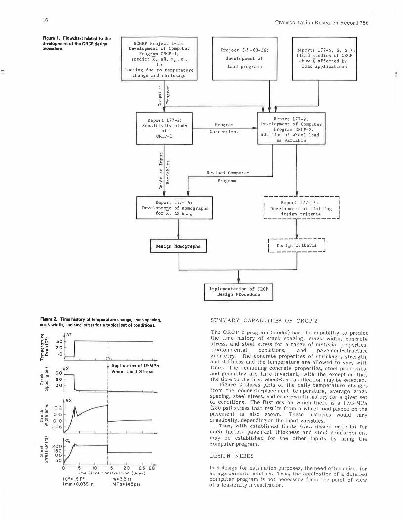
The next step was to include the effect of wheel-load stresses on crack-spacing history. The NCHRP study found that heavy volumes of 18-kip (80-kN) single-axle loads resulted in reduced crack spacings (6). The study of the effect of wheel-load stress on pavement behavior and its interaction with the other input variables is discussed in IVla and IVlcCullough (8), which describes the development of the CRCP-2 model. -This development process is outlined in flowchart form in the upper part of Figure 1.

16

Figure 1. Flowchart related to the development of the CRCP design procedure.

NCHRP Project 1-15: Development of Computer

Program CRCP-1, predict x, llX, :1 8 , a c

for loading due to temperature

change and shrinkage

Repo-rt 177-2: Sensitivity study

of CRCP-1

Report 177-16:

Transportation Research Record 7 56

Project 3-5 -63-56:

development of

load programs

R~ports 177-5, 6, & 7: field studies of CRCP

show X affected by load applications

Program

Corrections

Revised Computer

Program

I I r Report 177-9:

Development of Computer Program CRCP-2,

addition of wheel load as variable

• - -------------.., Development of nomographs

for X, llX & :; s

I Report 177-17: I I Development of limiting I

L ___ d_:~~Ic:_i_:~~ __ _ JI

~ Design Nomographs I r--- - -----, 1 Design Criteria I L----- ____ J

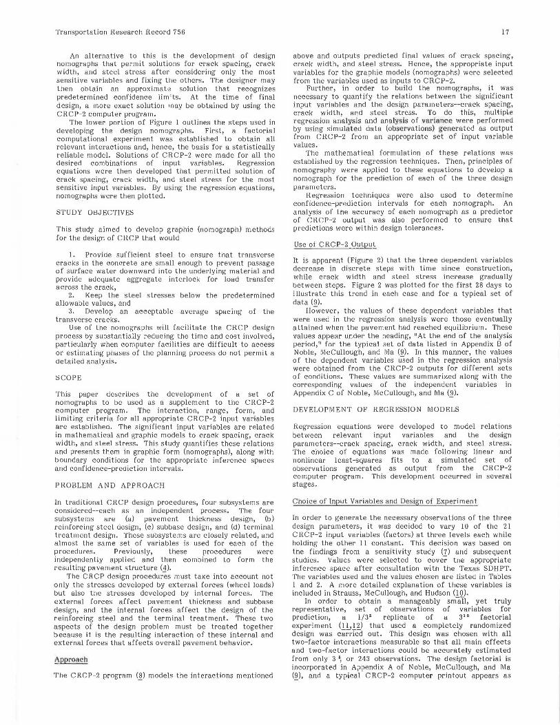
Figure 2. Time history of temperature change, crack spacing, crack width, and steel stress for a typical set of conditions.

"' ~­::J 0 -u o~ ~ c. Xe Ee ~·

e ... -;. u c o._ ~ u u 0

c. en

30 20

10

90

60 30

0.2

0.15

llT

Application of 1.9 MPa Wheel Load Stress

fdx :

0.10 ,1--------0.05 I

l IS

200 150 100 50

as I

o'-~~5~~-,~o~~~,5~~~2~0~~~2~5~2~e~

Time Since Construction (Days) 1c•=1.BF 0 lm=3.3ft lmm=0.039in IMPo=l45psi

I Implementation of CRCP . Design Procedure

SUMMARY CAPABILITIES OF CRCP-2

The CRCP-2 program (model) has the capability to predict the time history of crack spacing, crack width, concrete stress, and steel stress for a range of material properties, environmental conditions, and pavement-structure geometry. The concrete properties of shrinkage, strength, and stiffness and the temperature are allowed to vary with time. The remaining concrete properties, steel properties, and geometry are time invariant, with the exception that the time to the first wheel-load application may be selected.

Figure 2 shows plots of the daily temperature changes from the concrete-placement temperature, average crack spacing, steel stress, and crack-width history for a given set of conditions. The first day on which there is a 1.93-MPa (280-psi) stress that results from a wheel load placed on the pavement is also shown. These histories would vary drastically, depending on the input variables.

Thus, with established limits (i.e., design criteria) for each factor, pavement thickness and steel reinforcement may be established for the other inputs by using the computer program.

DESIGN NEEDS

In a design for estimation purposes, the need often arises for an approximate solution. Thus, the application of a detailed computer program is not necessary from the point of view of a feasibility investigation.

Transportation Research Record 756

An alternative to this is the development of design nomographs that permit solutions for crack spacing, crack width, and steel stress after considering only the most sensitive variables and fixing the others. The designer may then obtain an approximate solution that recognizes predetermined confidence lim ' ts. At the time of final design, a more exact solution 1nay be obtained by using the CRCP-2 computer program.

The lower portion of Figure 1 outlines the steps used in developing the design nomographs. First, a factorial computational experiment was established to obtain all relevant interactions and, hence, the basis for a statistically reliable model. Solutions of CRCP-2 were made for all the desired combinations of input variables. Regression equations were then developed that permitted solution of crack spacing, crack width, and steel stress for the most sensitive input variables. By using the regression equations, nomographs were then plotted.

STUDY OBJECTIVES

This study aimed to develop graphic (nomograph) methods for the design of CRCP that would

l. Provide sufficient steel to ensure that transverse cracks in the concrete are small enough to prevent passage of surface water downward into the underlying material and provide adequate aggregate interlock for load transfer across the crack,

2. Keep the steel stresses below the predetermined allowable values, and

3. Develop an acceptable average spacing of the transverse cracks.

Use of the nomographs will facilitate the CRCP design process by substantially reducing the time and cost involved, particularly when computer facilities are difficult to access or estimating phases of the planning process do not permit a detailed analysis.

::>COPE

This paper describes the development of a set of nomographs to be used as a supplement to the CRCP-2 computer program. The interaction, range, form, and limiting criteria for all appropriate CRCP-2 input variables are established. The significant input variables are related in mathematical and graphic models to crack spacing, crack width, and steel stress. This study quantifies these relations and presents them in graphic form (nomographs), along with boundary conditions for the appropriate inference spaces and confidence-prediction intervals.

PROBLEM AND APPROACH

In traditional CRCP design procedures, four subsystems are considered--each as an independent process. The four subsystems are (a) pavement thickness design, (b) reinforcing steel design, (c) subbase design, and (d) terminal treatrnent design. These subsystems are closely related, and almost the same set of variables is used for each of the procedures. Previously, these procedures were independently applied and then combined to form the resulting pavement structure (4).

The CRCP design procedures must take into account not only the stresses developed by external forces (wheel loads) but also the stresses developed by internal forces. The external forces affect pavement thickness and subbase design, and the internal forces affect the design of the reinforcing steel and the terminal treatment. These two aspects of the design problem must be treated together because it is the resulting interaction of these internal and external forces that affects overall pavement behavior.

~pproach

The CRCP-2 program (~) models the interactions mentioned

17

above and outputs predicted final values of crack spacing, crack width, and steel stress. Hence, the appropriate input variables for the graphic models (nomographs) were selected from the variables used as inputs to CRCP-2.

Further, in order to build the nomographs, it was necessary to quantify the relations between the significant input variables and the design parameters--crack spacing, crack width, and steel stress. To do this, multiple regression analysis and analysis of variance were performed by using simulated data (observations} generated as output from CRCP-2 from an appropriate set of input variable values.

The mathematical formulation of these relations was established by the regression techniques. Then, principles of nomography were applied to these equations to develop a nomograph for the prediction of each of the three design parameters.

Regression techniques were also used to determine confidence-prP.diction intervals for each nomograph. An analysis of the accuracy of each nomograph as a predictor of CRCP-2 output was also performed to ensure that predictions were within design tolerances.

Use of CRCP-2 Output

It is apparent (Figure 2) that the three dependent variables decrease in discrete steps with time since construction, while crack width and steel stress increase gradually between steps. Figure 2 was plotted for the first 28 days to illustrate this trend in each case and for a typical set of data (9).

However, the values of these dependent variables that were used in the regression analysis were those eventually attained when the pavement had reached equilibrium. These values appear under the heading, "At the end of the analysis period," for the typical set of data listed in Appendix B of Noble, McCullough, and Ma (9). In this manner, the values of the dependent variables used in the regression analysis were obtained from the CRCP-2 outputs for different sets of conditions. These values are summarized along with the corresponding values of the independent variables in Appendix C of Noble, McCullough, and Ma (_Q).

DEVELOPMENT OF REGRESSION MODELS

Reg·ression equations were developed to model relations between relevant input variables and the design parameters--crack spacing, crack width, and steel stress. The choice of equations was made following linear and nonlinear least-squares fits to a simulated set of observations generated as output from the CRCP-2 computer program. This development occurred in several stages.

Choice of Input Variables and Design of Experiment

In order to generate the necessary observations of the three design parameters, it was decided to vary 10 of the 21 CRCP-2 input variables (factors) at three levels each while holding the other 11 constant. This decision was based on the findings from a sensitivity study (7) and subsequent studies. Values were selected to cover the appropriate inference space after consultation with the Texas SDHPT. The variables used and the values chosen are listed in Tables I and 2. A more detailed explanation of these variables is included in Strauss, McCullough, and Hudson (10).

In order to obtain a manageably small, yet truly representative, set of observations of variables for prediction, a 1/35 replicate of a 310 factorial experiment (11, 12) that used a completely randomized design was carried out. This design was chosen with all two-factor interactions measurable so that all main effects and two-factor interactions could be accurately estimated from only 3 •, or 243 observations. The design factorial is incorporated in Appendix A of Noble, McCullough, and Ma (g), and a typical CRCP-2 computer printout appears as

18

Table 1. Values of variables used in analysis of CRCP-2.

Value for Level

Input Variable

Wheel-load stress (kPa) Daily temperature change (°C) Final temperature change (°C) Friction-movement ratio Concrete slab thickness (mm) Concrete shrinkage strain Concrete tensile strength (kPa) Thermal coefficient ratio Bar diameter (mm) Percentage of reinforcement

Symbol

aw LH; ATf F/y D z ft Ol.JOl.c <I> p

414 4 19 -10 178 2 x 10· 4

3447 0.75 13 0.40

Note: 1kPa=0.145psi;1°C=1.8°F;1 mm=0.039in ,

Table 2. Variables held constant in CRCP·2 analysis.

Variable

Type of reinforcement Yield stress of steel (MPa) Ela•l c modulus of steel (MPn) Thermal coc.rnclcnt <;>f steel (~m/mm/°C) Unit weight of concre te (kg/m ) Flexural-tensile factor Curing temperature (°C) Number of days to full-strength concrete Number of days to minimum temperature Number of days to wheel-load application Slab movement (mm)

Value

Deformed bar 413.6 199 926 l 1 x 10· 6

2403 0.86 42 28 28 14 -3.0

Note: 1MPa=145 psi;t°C = (t°F -32)/1 .B; 1mm=0.039 in; 1 kg/m3 = 0.062 lb/ft3.

2

1172 19 31 -80 254 5 x 10·4

4481 1.00 16 0.65

3

1930 33 42 -150 305 8 x w-4

5515 I.SO 19 0 .90

Appendix B (9). A summary of the complete set of observations that resulted from the experiment, which shows values of the three design parameters for each combination of values of the 10 input variables, appears in Appendix C (9).

All important combinations of the input variable values likely to be encountered in practical CRCP design were covered in the factorial, which extended over the extremes of the ranges of each variable. Hence, this experiment can also serve as the basis for a sensitivity analysis of the CRCP-2 model.

Theoretical Background to Form of Regression Models

Theoretical relations developed at the Center for Highway Research, Austin, Texas, between the design parameters (l 0) and the relevant input variables (Table l) were considered in the initial investigation of the form of the regression models. From these relations, it is apparent that crack spacing is proportional to

(fal x qiaz xaa3)/(pa4 xaa ·5) t s w

and crack width is proportional to

(fbl xqib2)/pb3xab4) t w

where a1, az, a3, a4, a5, b1, b2, b3, and b4 are positive constants and the other variables are as defined in Table l.

These theoretical trends were confirmed by an inspection of each design parameter's variation with the input variables over the appropriate range by using the simulated data set generated by the factorial experiment. This was done by using a series of plots of each design parameter against each input variable, with the other input variables held constant by using all 243 observations. From these, it was clear that

Transportation Research Record 756

1. Crack spacing increases with increasing D, fti as/ac, and t but decreases with increasing aw, l>Tj, t>Tf, F /y, Z, and p;

2. Crack width increases with increasing Z, ft, asl"c' and t but decreases with increasing aw, l>Ti, t>Tf; D, and p; and

3. Steel stress increases with increasing t>Tf, D, ft, aslac, and t but decreases with increasing aw, l>Ti, F/y, Z, and p.

Form of Independent Variables in Regression Models

In order to ensure reasonable prediction of design parameters (rom the nomographs for all values of the input variables (indepe ndent vari ables) likely to be encountered in practice, each independent variable was transformed into a format based on its extreme (boundary) values for the regression analysis. The format used for each variable is shown below:

Independent Variable aw t>Ti l>TF F/y D z ft as/ac qi p

Transformation Used l + (awll 000) l + (6TF/100) 1 + (t>TF/100) [l + (1 /200 )](F /y) l + (D/20) l + lOOOZ l + (ft/1000) [l + (1/2)] (ag/ac) l +qi l + p

For example, for the variable for wheel-load stress (aw), the transformation (1 + awll 000) was used so that the value used in the regression equation would lie between 1 and 2 for all values of aw likely to be encountered in practice (even for the zero wheel-load case).

Regression Analysis

The final choice of regression equations was then made by following multiple linear and nonlinear least-squares fits of the transformed input variables (independent variables) to the simulated set of 243 observations of the design parameters (dependent variables) previously described. Stepwise linear-regression computer programs (!.i.!.1.l were used in the linear analyses, with logarithmic transformations of both independent and dependent variables to reflect the exponential nature of the relations discussed earlier. Better fits resulted by using these transformations than any others tried (e.g., orthogonal polynomials), with more variance being explained by fewer independent variables (and less prediction error) for all three dependent variables. Also, these regression analyses confirmed the trends established by theoretical developments and plots discussed previously (~, Appendix D.l). Computer program BMD07R-Nonlinear Least Squares (U) was used for the nonlinear analysis. This second approach was adopted because, owing to the exponential nature of the relation (and the bias introduced by the transform), some improvement in fit might be obtained by nonlinear analysis, particularly if the error was additive rather than multiplicative (9, Appendix D.2).

Residual plots, standard error of estimate, and R2

statistics (proportion of variance explained by the regression equation) were considered in the final choice of coefficients in each regression equation. These final equations are summarized below:

x = {o.402 [I+ (ftf6890)] 6·7 [I+ (01,/20lc)l !.IS [I + (tfJ/25.4)] 2.19}

+ {p +(aw/6890)] 5·2 (1 +pf6 (1 + IOOOZ)l.79} (!)

ll. 2 = 90.2 percent and standard error= 0.64 m

Transportation Research Record 756

.ix= {0.003 67 [I+ (ftf6890)J 653 [I+ (</>/25.4)1220}

7 {[I+ (aw/6890)) 4.Yl (I + p)4.S5}

H. 2 = 92.7 percent and standard error= 0.33 mm

a,= {326 207 [I + (.i T/556)) o.4z5 [! + (ftf6890)) 4.09}

.;- {[I + ( aw/6890)] 3.14 (I + 1 oooz)0.494 (I + P )2.74}

R' = 92.2 percent and standard error= 67.7 MPa

where

X =crack spacing (m), llX =crack width (mm), and as= steel stress (kPa).

(2)

(3)

Analysis of variance for each equation indicated that the inclusion of further terms (independent variables) did not significantly improve either the R2 or standard error of residuals statistics.

Non linear Regression Models

In general, if linear regression is performed by using logarithmic transforms of the dependent variable (Y) and the independent variables (X 1'···• Xn), the model becomes

log Y = C + c1

log x1

+ ... +C log X +error term (E) o n n

or

y-c xc1 xcn -ol"'nE

where C0 , .. ., Cn are constants. Hence, the error term is multiplicative in this model.

However, the nonlinear model would be

Y = K xK1

1 ... xKn +error term (E) o n

where K0 , ... K 1 are constants. Hence, the error term is additive in this model.

A comparison was then made of the goodness of fit o"f both the linear and nonlinear regression models because the form of the error term was unknown in this case. The results of this comparison are summarized in Table 3. It is apparent from these that the improvement in fit owing to the use of nonlinear coefficients was not significant at the 5 percent level for crack width and at the 25 percent level for both crack spacing and steel stress. It was thus decided to use the expressions derived from the linear regression procedures.

For all three design parameters, regression analyses that

Table 3. Comparison of results of design parameter values as obtained from nomographs and regression equations.

Dependent Variable

Crack Crack Steel Type o[ Statistic Spacing Width Stress

Statistic Degrees or freedom 24 12 21 Root mean square residua] l.7 m 0.4 mm 148 MPa Coefficient of variation(%) 33 23 21

Statistic obtained when design parameters fall within <6.1 m <2 .5 mm <689 MPa

Degrees of freedom 14 10 ll Root mean square residual 36 cm 0.23 mm 45 MPa Coefficient of variation(%) 20 19 ll

Note: 1m=3.28 ft; 1mm=0.039 in; 1cm=0.39 in; 1 MP; = 145 psi .

19

were performed with major outliers removed from the data set showed no significant improvement in prediction accuracy.

Summary

Given the foregoing data, it was decided to use the regression equations summarized earlier in this paper as the basis for the construction of the nomographs. These equations gave satisfactory R2 and standard error values and agreed with the format indicated by the previous theoretical development and the summary plots from the sample data. Some slight improvement in goodness of fit to the sample data was seen for the equations developed by using the nonlinear analysis. However, this was not considered sufficiently significant to offset the uncertainty that would have been introduced if these equations were used with the confidence limits described in the next section of this paper. This uncertainty would have occurred because the confidence intervals were derived by using a linear analysis (with logarithmic transforms) and, as such, are conservative on the regression equations.

CRCP DESIGN NOMOGRAPHS AND CONFIDENCE LIMITS

Design Charts--N omographs

By using the principles of nomography (16,17) and the regression equations, separate design charts- Cnomographs) were prepared for the prediction of crack spacing, crack width, and steel stress in the design of CRCP. These are shown in Figures 3, 4, and 5, respectively.

Confidence-Prediction Limits

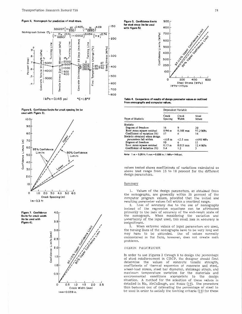
By using the CPIY linear regression program (!.§.) and logarithmic transformations of the appropriate dependent and independent variables, the 90 percent and 97 .5 percent confidence limits on each of the three design parameters--crack spacing, crack width, and steel stress--were calculated for the regression models noted earlier in this report (9, Appendix D.3). These confidence limits can then be used with the nomographs in the design procedure. To this end, graphs of the variation of these confidence limits with the value of each design parameter for the appropriate inference range appear in Figures 6, 7, and 8.

It should be noted that, because the regression equations are of an exponential form, strict confidence intervals cannot be determined by using existing computer software (e.g., from the nonlinear regression models). Hence, it is necessary to use logarithmic transformations and the linear regression techniques in the CPIY program to determine these confidence limits. Transformations of these confidence limits are then conservative for the exponential models.

In practice, use of Figures 6, 7, and 8 in conjunction with the corresponding nomographs (Figures 3, 4, and 5) enables the designer to estimate the uncertainty associated with the values of the design parameters (crack spacing, crack width, and steel stress) indicated by the nomographs. These values are for the chosen value of percentage of steel and the values of the other input variables determined by the properties of materials used and the appropriate environmental conditions. That is, a range of values in crack spacing can be determined from Figure 6 so that this parameter will be within this range, with either 80 percent or 95 percent probability. Similarly, two upper limits on each crack width and steel stress can be determined from Figures 7 and 8, respectively, so that the appropriate parameters will be below these limits, with either 90 percent or 97 .5 percent probability.

20 Transportation Research Record 756

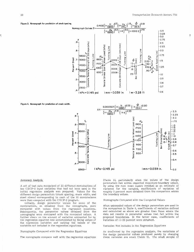
Figure 3. Nomograph for prediction of crack spacing. (

fl )6.7( a: 5 )1.1 5( cp )2 .19 0.402 I+ 6 890 I + 2 «c I +25.4

Nomog roph Solves x = - ---------"'-------( 1+ 6~0 ) 5·2 ( t+ P )4·6 ( 1+1000 z)"79

p .9 0 a.

""' 0 n_ .. .. c

"' "" :J .8 D c 'D

"' ft m D c: .. " 5500 N c: (J, ...J E Qi - '.J

'80~i :I

.7 5000 D

I-.. .c "' ;;; - c:

"' 1400 ~ - c: E c: 4500 ~ .. ;;; :I

~ I- 10 0 0 ~ . 6 .. 4 0 00 ~ 0 a.

·;; 600 ., c: "'

3500 ~ ~ iii

.5 ~ 3000 ~ .!!

u -;; '" c: 0 ~

2500 u

.4

E' E ..... E E ..

c: .. '.::i "' zc "' OOOT c: cp E'

E N ,,r .0004 0 :I I-

16 ! .0006 j 19 ~ .0008 c: D

·;: 25 0 .c ;; If) .. m ~ u c: 0 u

.. c:

'.::i E' "' c: a:s "' «c c: E u :I 2.00r [ I-

1.50 'C If)

a: ""' 1.00 u g 1:1-.... ...

.50 ....... u ti

3.5 - 3.25

3.0 2.75

2.5

2.25

2.0

1.75

1.5

1.25

1.0

0.9

0.8

0.7

I kPo = 0.145 psi I mm = 0.039 in. lm=3.2Bft 0.6

Figure 4. Nomograph for prediction of crack width.

p .9

.8

:: .7 ;;; -c: .. t.6 a.

.5

ft 5 500

000 0 a. :!!. .c

:! ~ u c:

.4 3000 8

0 .000367 ( t+- 11-)6·53 ( I +_f_ )2·

20 t:. x • 6890 . 2 5.4

( I+ 0-w )4.91( i+ )4.55 6890 p

.. c: '.::i

2.5

2.25

2.0

1.75

1.5 1.4 1.3 1.2 I.I 1.0 0.9 0 .8

0.7

0.6

0.5

0.4

2500 I kPo=0.145 psi I mm=0.039 in. 0.3

Accuracy Analys is

A set of test data comprised of 35 different combinations of the CRCP-2 input variables that had not been used in the initial regression analysis was prepared. Values for the different design parameters (crack spacing, crack width, and steel stress) corresponding to each of the 35 combinations were then computed with the CRCP-2 program.

Initially, design parameter values for some of the combinations, as obtained from the nomographs, were compared with values from the regression equations. Subsequently, the parameter values obtained from the nomographs were compared with the computed values. A further check on the amount of variation accounted for by the regression equation was accomplished by fixing values of the regression variables and varying the values of the variables not included in the regression equations.

Nomographs Compared with the Regression Equations

The nomographs compare well with the regression equations

(Table 3), particularly when the values of the design parameters fall within expected maximum-boundary values. By using the root mean square residual as an estimate of variance for the samples, coefficients of variation of roughly 5 percent were obtained from the comparison within the boundary values.

Nomographs Compared with the Computed Values

When unbounded values of the design parameters are used in the comparison in Table 4, coefficients of variation defined and calculated as above are greater than those where the data set results in parameter values that fall within the proposed boundaries. In the latter case, coefficients of variation of 11-20 percent were obtained.

Variables Not Included in the Regression Equations

As confirmed by the regression analysis, the variations of the design parameter values produced purely by changing these variables are small (Table 5). The small sample of

Transportation Research Record 756

Figure 5. Nomograph for prediction of steel stress.

Nomog ra ph Solves

0 "' e

"' c: E .. c: a.. :.J ' c: ·.:; ... E ·.:; p

.5. .9 "' 'tl "' "' 0 c: " c: c:

"' a.. 'E 0 c: ... ·e ... _J

" .8 " " 0 " t It 1-- "' CTw 1-- 1--.. "' CD "' "' N z .7 c: 'f'oo Ui 5000 ~

~ 0 1500 1f·0002 c: Ui :;: 1000 .. . 0005 ~ .6 g .<Joo

~ 4000 5 500 "' 'Zi ...

a.. "' 400 c:

c: ·;: .5 {!!. "' .c

3000 ~ (/)

!! Ui !! .4 ~ ~ "' CJ u c:

"' c: 0 c: 0 u {!!. u

I kPa = 0.145 psi 0 c=1.a°F

Figure 6. Confidence limits for crack spacing (to be used with Figure 3).

10.0

9.0

8.0

!! 6.0 .E :.J 80% Confidence

"' 5.0 \~~its 0

c:

"' :'5:! 4.0 - / c: "'<;,(_, / 0 u 3.0 "'"' / /

/ /

2.0

0 1.0 2.0 3.0 4 .0 5.0 6.0 Crack Spacing ( m)

Im =3.3 ft

Figure 7. Confidence limits for crack width (to be used with Figure 41.

'E .§

4 .0

3.5

3 .0

.~ 2 .5 E

~ 2 .0 0 c: .. ~ 1.5 c: 0 u

1.0

0 .5

0 0 .5 1.0 1.5

u " 0 a..

"' ::l;'

"' ::: c:

" ! .c u

"' LIT (/)

~ 25 20- o; o·55:f40 !'1 - (/) ., 0.

E {!!.

" c:

"-

2.0 2 .5 Crock Width (mm)

lmm=0.039in.

150

200

300

400

500

600

700

800

Figure 8. Confidence limits 900 for steel stress (to be used with Figure 5). 800

c 700 a.. ::l;'

600 ., E 500 :.J "' 4 00 0 c ., 'tl

300 ;;::: c: 0 u 200

100

0 200 400 600 Steel Stress ( M Po)

I MPa = 145 psi.

Table 4. Comparison of results of design parameter values.as outlined from nomographs and computer values.

Dependent Variable

Crack Crack Steel Type of Statistic Spacing Width Stress

Statistic Degrees of freedom 18 9 20 Root mean square residual 0.94m 0.108 mm 97.2 MPa Coefficient of variation(%) 17 6 14

Statistic obtained when design parameters fall within <6.0m <2.5 mm <690 MPa

Degrees of freedom 10 6 II Root mean square residual 0.13 m 0.013 mm 12.4 MPa Coefficient of variation (%) 5.4 1.2 3

Note: 1 m 2 3.28 ft; 1 mm 2 0.039 in; 1 MPa = 145 psi.

21

values tested shows coefficients of variations calculated as above that range from 13 to 18 percent for the different design parameters.

Summarz

1. Values of the design parameters, as obtained from the nomographs, are generally within 25 percent of the computer program values, provided that the initial and resulting parameter values fall within a practical range.

2. Loss of accuracy due to the use of nomographs instead of the regression equations can be attributed primarily to the lack of accuracy of the end-result scale of the nomograph. When considering the variation and uncertainty of the input used, this small loss in accuracy is insignificant.

3. When extreme values of input parameters are used, the turning lines of the nomographs have to be very long and may have to be extended. Use of values normally encountered in the field, however, does not create such problems.

DESIGN PiWCEDURE

In order to use Figures 3 through 8 to design the percentage of steel reinforcement in CRCP, the designer should first determine the values of concrete tensile strength, coefficients of thermal expansion of concrete and steel, wheel-load stress, steel bar diameter, shrinkage strain, and maximum temperature variation for the materials and environmental conditions appropriate to the design situation. A method for the selection of these values is detailed in Ma, McCullough, and Noble (19). The procedure then becomes one of estimating the percentage of steel to be used in order to satisfy the limiting criteria (!..~) for these

22

Table 5. Sensitivity of design parameter values (dependent variables) to changes in independent variables not included in regression equations.

Independent Variable Range

Transportation Research Record 7 56

Range of Values of Design Parameter (Dependent Variable)

Crack Spacing Crack Width (m) (mm)

Steel Stress (MPa)

Daily temperature change, AT; (0C)

Number of days to first wheel-load applicalion ~nd rinol tempera ture change. AT p (°C)

Final 1empcrnture change, i:l T p (°c) Fricl'ion·movomon t ratio , F/y Thickness of concrete, D (cm)

4 to 33 8 to~ and 31to19

1.3-1.0 1.0-0.9

0.99-0.79 0.79-0.61

430-380

42 to 19 -80 to -150 17.8 to 30.5

0.9-0.9 0.9-0.9 1.2-1.2

0.84-0.61 0.61-0.71 0.91-0.91

316-350 415-415

Notes: 1 C0 = 1.8 F0; 1 mm = 0,039 in; 1 m = 3.28 ft; 1 cm = 0.39 in; 1 MPa = 145 psi.

The coefficient of variation for crack spacing, crack width, and steel stress is 15, 18, and 13 percent, respectively.

conditions on crack width, crack spacing, and steel. stress. It should be noted here that the contemporary design slab thicknesses for CRCP range from 180 mm (7 in) to 300 mm (12 in). A selection procedure for slab thickness is also detailed in Ma, McCullough, and Noble (19).

The procedure for estimating the steel percentage to satisfy the limiting criteria, referred to above, is outlined here.

1. IVJark the values of the appropriate input variables on their respective scales on each of the three nomographs.

2. Choose a likely value of the percentage of steel to be used (p) and mark this value on the scale for p on each nomograph.

3. Working from left to right, draw a line joining the marked values on scale numbers 1 and 2 for the crack-spacing nomograph; proceed until the line intersects the first turning line.

4. Draw a new line from this point, joining it to the marked values on scale number 3; proceed until it intersects the second turning line.

5. Repeat this process for the remaining two turning lines and scale numbers 4, 5, and 6 until the value of crack spacing can be read from the scale on the far right.

6. If this value is not inside the recommended range for the appropriate environmental conditions and material properties (19), repeat steps 2 through 5 for larger percentages of steel until the limiting criteria are satisfied.

7. Repeat steps 2 through 6 for the crack-width and steel-stress nomographs and relevant limiting criteria.

8. If the values obtained in steps 6 and 7 for all three nomographs are inside the respective limiting criteria, then repeat the entire process by using successively smaller values of p until one of the three nomographs indicates a final value (of crack spacing, crack width, or steel stress) that is just inside the limits. This value of p is then the design value to be recommended.

9. The designer should then enter Figures 6, 7, and 8 on the abscissa scales with values of crack spacing, crack width, and steel stress, respectively, obtained from the corresponding nomographs for the final value of p recommended in step 8. The upper and lower confidence limits for crack spacing and the upper confidence limits for crack width and steel stress should then be read from the respective ordinate scales of each figure.

1 O. Thus, the designer should finally recommend a steel percentage, along with both the corresponding 80 and 95 percent confidence limits on crack spacing and both the 90 percent and 97 .5 percent upper confidence limits on crack width and steel stress, which use of this p will predict. That is, the designer recommends a percentage of steel, along with a range of values of crack spacing that will include the actual value 80 percent of the time (or with 80 percent certainty), as predicted by the model, as well as a slightly wider range that will include the actual value 95 percent of the time. Also, the designer recommends the corresponding upper limits on crack width and steel stress so that, for the chosen value of p, these parameters will fall below these limits 90 percent (or 97 .5 percent) of the time or with 90 percent (or 97 .5 percent) certainty. These ranges

could be used in conjunction with limiting criteria noted in McKenzie (18), if a more conservative design is required.

11. The equations should be used as a check on the nomograph design.

CONCLUSION

Based on this study, the recommendations that follow were made.

1. A set of nomographs based on regression analysis of the results computed by the CRCP-2 computer program has been prepared. The uniaxial-force equilibrium model used in the CRCP-2 computer program is the only model available that considers the internal forces caused by the difference in thermal coefficients between the concrete and the steel materials. Therefore, it is the most suitable tool available for the CRCP analysis.

2. Spacing of transverse cracks that occur in CRCPs is the most important variable affecting the behavior of the pavement. Relatively large distances between cracks result in a higher accumulation of drag forces from the subgrade due to frictional resistance, thus producing high steel stress at the crack and large crack widths. Closer crack spacing reduces the frictional restraint and, thus, the steel stress and the crack width.

3. Nomographs produced in this study can predict steel stress at the crack (where the stress is maximum), average crack spacing, and average crack width at minimum temperature.

4. The limiting design criteria for the above dependent variables are discussed in Ma, McCullough, and Nob le (19).

5. The nomographs should be used in conjunction-with the limiting design criteria (19) for the design of steel percentage in CRCP given the-materials chosen and local environmental conditions. Explicit guidelines for the selection of values of the 'nput variables to be used with the nomographs and a detailed procedure for the design of slab thickness are given in Ma, McCullough, and Noble (!..~).

6. Charts that give confidence prediction limits should be used in conjunction with the nomographs in order that the designer can specify a range on each of the variables (crack spacing, crack width, and steel stress) corresponding to the uncertainty inherent in the procedure. These limits may also be used in place of the mean values (recommended by the nomographs) if a conservative design is warranted (.!_g_).

7. This entire CRCP-design procedure should be incorporated into the Texas SDHPT's Operations and Procedures Manual.

ACKNOWLEDGMENT

The material presented in this paper is part of a research effort on the development and implementation of the design, construction, and rehabilitation of rigid pavements conducted by the Center for Transportation Research of the University of Texas at Austin and sponsored by the Texas SDHPT and the Federal Highway Administration (FHW A). The contents of this report reflect our views. We are responsible for the facts and the accuracy of the data

Transportation Research Record 756

presented herein. The contents do not necessarily reflect the official views or policies of the Texas SDHPT or FH WA. This report does not constitute a standard, specification, or regulation.

REFERENCES

1. B.F. McCullough and W.B. Ledbetter. LTS Design of Continuously Reinforced Concrete Pavements. Journal of the Highway Division, Vol. 86, No. HW4, Proc., American Society of Civil Engineers, Dec. 1960.

2. W. Zuk. Analysis of Special Problems in Continuously Reinforced Concrete Pavements. HRB, Bull. 214, 1959, pp. 1-21.

3. AASHTO Interim Guide for Design of Pavement Structures. American Association of State Highway and Transportation Officials, Washington, DC, 1972.

4. B.F. McCullough. Design Manual for Continuously Reinforced Concrete Pavement. U.S. Steel Corporation, Pittsburgh, Jan. 1970.

5. R.W. Carlson. Drying Shrinkage of Concrete as Affected by Many Factors. Proc., American Society for Testing Materials, Vol. 38, Part 2, 1938.

6. B.F. McCullough, A. Abou-Ayyash, W.R. Hudson, and J.P. Randall. Design of Continuously Reinforced Concrete Pavements for Highways. Center for Highway Research, Univ. of Texas at Austin, Res. Rept. NCHRP 1-15, Aug. 1974.

7. C. Chiang, B.F. McCullough, and W.R. Hudson. A Sensitivity Analysis of Continuously Reinforced Concrete Pavement Model CRCP-1 for Highways. Center for Highway Research, Univ. of Texas at Austin, Res. Rept. 177-2, Aug. 197 4.

8. J.C.M. Ma and B.F. McCullough. Analysis of Load, Temperature, and Shrinkage Effect on Continuously Reinforced Concrete Pavement. TRB, Transportation Research Record 671, 1978, pp. 29-39.

9. C.S. Noble, B.F. McCullough, and J.C.M. Ma. N omographs for the Design of CRCP Steel

23

Reinforcement. Center for Highway Research, Univ. of Texas.at Austin, Res. Rept. 177-16, May 1979.

10. P.J. Strauss, B.F. McCullough, and W.R. Hudson. Continuously Reinforced Concrete Pavement: Structural Performance and Design Construction Variables. Center for Highway Research, Univ. of Texas at Austin, Res. Rept. 177-7, Aug. 1979.

11. V.A. Anderson and R.A. McLean. Design of Experiments: A Realistic Approach. Marcel Dekker, Inc., New York, 1974.

12. W .S. Connor and M. Zelen. Fractional Factorial Experiment Design for Factors at Three Levels. U.S. Department of Commerce, National Bureau of Standards Applied Mathematics Series 54, May 1959.

13. N .H. Nie and others. Statistical Packages for the Social Sciences, 2nd ed. McGraw-Hill, New York, 1975.

14. STEP-01 Statistical Computer Program for Stepwise Multiple Regression. Center for Highway Research, Univ. of Texas at Austin, Oct. 1968.

15. W.J. Dixon, ed. Biomedical Computer Programs, 2nd ed. Univ. of California Press, Berkeley, 1976.

16. M.G. Van Voorhis. How to Make Alignment Charts. McGraw-Hill, New York, 1959.

17. A.S. Levens. Nomography, 2nd ed. John Wiley and Sons, New York, 1959.

18. D. Mc Kenzie. CPIY Multiple Regression Program, rev. ed. Center for Highway Research, Univ. of Texas at Austin, March 1978.

19. J.C.M. Ma, B.F. McCullough, and C.S. Noble. Limiting Criteria for the Design of CRCP. Center for Highway Research, Univ. of Texas at Austin, Res. Rept. 177-17, Aug. 1979.

Publication of this paper sponsored by Committee on Rigid Pavement Design.

Implementation of New Overlay Design Procedure in Texas STEPHEN SEEDS, B. FRANK McCULLOUGH, W. R. HUDSON, ANO MANUEL GUTIERREZ DE VELASCO

A project is under way in Texas to adapt a version of the rigid pavement over­lay design procedure developed for the Federal Highway Administration by Austin Research Engineers, Inc., into standard Texas State Department of Highways and Public Transportation (SDHPT) practice. This project is part of a cooperative research program between Texas SDHPT and the Center for Highway Research at the University of Texas. This paper provides some feed­back on the use of this procedure and documents its successful application to an interstate rehabilitation and widening project in San Antonio. This project was unique in the sense that thickness and reinforcement designs were required for five different composite pavement structures that, by their nature, are not suitable for design by past empirical methods. In documenting the de­signs, the selection of design criteria, characterization of material properties, and thickness design recommendations for each section within the project are discussed. The paper provides a general description of the design procedure, discussion of the results of the design, conclusions about the applicability of the design model, and recommendations for further work. The validity and practicality of the new procedure, as well as its applicability for nationwide use, are noted.

Many of the rigid pavements that make up much of the Interstate highway system were constructed in the 1950s and early 1960s. Most were designed to last 20 years and, consequently, are approaching the end of their design life.

Many now require extensive rehabilitation. The Federal Highway Administration (FHW A), recognizing the need for a practical design procedure for overlays of these pavements, sponsored a project for the development of such a design procedure (1 ). This project was completed in 1977.

The Texas State Department of Highways and Public Transportation (SDHPT), long interested in such a design tool, considered the new FHWA procedure workable and funded research at the Center for Highway Research (CFHR) at the University of Texas to examine the new procedure and adapt it for Texas conditions (~). The project provides for implementation of the new procedure into Texas SDHPT practice through field application on several pavement overlay projects. It also provides for incorporating other useful improvements to the design models and procedure that may aid in their implementation. This has led to further refinement of the rigid pavement overlay design model.

OBJECTIVES

The objectives of this paper are twofold: (a) to discuss the