NOI_ 65-126 - NASA Technical Reports Server
193
__ A DIVISION OF NORTHROP CORPORATION NOI_ 65-126 FINAL SUMMARY REPORT ANALYTICAL AND EXPERIMENTAL INVESTIGATIONS INT0 PROBLEMS ASSOCIATED WITH GYRO-STABILIZED PLATFORM-MOUNTED OPTICAL SENSING ELEMENTS Contract No. NAS 8-20193 George C. Marshall Space Flight Center Huntsville, Alabama 15 July 1966 Prepared by E. H. Kong, Jr. W. H. Schuck Approved by D. E. Conklin, Chief Tracking & Display Systems Form 7 (R 8454)
-
Upload
khangminh22 -
Category
Documents
-
view
1 -
download
0
Transcript of NOI_ 65-126 - NASA Technical Reports Server

__ A DIVISION OF NORTHROP CORPORATION
NOI_ 65-126
FINAL SUMMARY REPORT
ANALYTICAL AND EXPERIMENTAL INVESTIGATIONS INT0
PROBLEMS ASSOCIATED WITH GYRO-STABILIZED
PLATFORM-MOUNTED OPTICAL SENSING ELEMENTS
Contract No. NAS 8-20193
George C. Marshall Space Flight Center
Huntsville, Alabama
15 July 1966
Prepared by
E. H. Kong, Jr.
W. H. Schuck
Approved by
D. E. Conklin, Chief
Tracking & Display Systems
Form 7 (R 8454)

m_ A DIVISION OF NORTHROP CORPORATION
ABSTRACT
The use of a star tracker with the STI21_-M platform to provide long-term
drift c_npensaticu is considered. The accuracy with which platform align-
ment can be made is determined for different platform-star tracker mounting
configurations. The coordinate relationships between the star tracker
triad, the inertial triad and the terrestial triad are presented, and
the utilization of a star tracker, inertial platform and a horizon sensor
for orbital navigation and attitude control are considered,
Fundamental design concepts relating to optical tracking systems, including
considerations of different optical systems, detectors of visible energy,
and several optical modulation methods are presented. The utilizatir_ of
optical equipment in a spacecraft is discussed, and three types of optical
experiments, star tracker-platform, scientific and engineering experimentsare evaluated.
The causes and methods of reducing off-axis and background radiance in an
optical system are examined. Some techniques considered, include use of
a sun shade or multiple-celled sun shield, baffling, and the operation
of the star tracker in a space envirc_nent.
Circuit modificati_s to improve the performance of the Celestial Body
Tracker, built by Nortronics for the George C. Marshall Space Flight
Center are presented in Appendix A.
NORT 65-126
Form 7 (R 8-64)
A DIVISION OF NORTHROP CORPORATION
FOREWORD
The Aual0rtical and Experimental Investigations into Problems Associated
with 00fro-Stabilized Platform-Mounted Optical Sensing Elements at Nortronics,
was authorized under the Natinnal Aeronautics and Space Administration
Contract No. NAS8-20193 by the George C. Marshall Space Flight Center.
The comtrol number is DCN I-5-40-56222-01(IF), SI(IF). The study was
carried out over a period of twelve mcmths, sad was made possible through
the c_utributions of specialist in many technical areas. Mr. E. H. Kong
sad Mr. W. H. Schuck were the principal investigators during the program.
Mr. Kn-g was the Project Engineer, and Mr. Schuck conducted the study
comcerning the use of a star tracker with the ST 124-M platform. Other
contributors were Mr. P. T. Glamkowski, in the investigati0m ccmcerning
the use of a multiple-celled sun shield; Mr. R. E. Cornwell, in the study
of vacuum bearing lubrication; and Mr. J. M. Sacks, who is responsible
for the circuit modificatioms for the Celestial Body Tracker.
The guidance and directicm of Mr. Clyde Jcmes, Mr. George Doane, and
Mr. Joseph Parker of the Astriomics Division, George C. Marshall Space
Flight Center, Huntsville, Alabama, are gratefully acknowledged.
ii No_ 65-]a6
Form 7 (R 8-64)

_l_l_l_m A DIVISION OF NORTHROP CORPORATION
Section
1
CONTENTS
Study of Utilization of Astro-lnertial System Using
ST-124M Inertial Platform 2
i.i Analysis of Improvement in Navigation System
Accuracy with Use of A Star Tracker
i.i.i Characteristic Error Gro_h For Pure Inertial
System and Star Tracker Aided Inertial System 3
1.1.2 Utilization of Astrotracker Data for Navigation
(Terrestrial Position Determination) and
Attitude Comtrol Ii
1.1.2.1 Frames of Reference ii
1.1.2.2 Terrestrial Navigation Using A Star Tracker 16
1.1.2.3 Vehicle Attitude Correction With A Star Tracker 19
1.1.2.3.1 Derivation of Equations for Removal of Platform
Tilt Error with Star Tracker 19
1.1.2.3.2 Derivation of Correction Equations for Removalof Platform Error in Three Axes with
Star Tracker 20
1.2 Description and Anal_sis of An Orbital Navigation System
Using The STI2_-M Inertial Platform 27
i. 2. i System Configuration and Analysis 27
1.2.2 Computer Function CI (Star Tracker Pointing) 27
1.2.3 Computer Function C2 (Star Tracker Correction to l_J)301.2.3.1 Removal of Constant Gyro Drift with Star Tracker 36
1.2.3.2 Bounding of Random Gyro Drift with Star Tracker 39
1.2.3.2.1 Random Gyro Drift Error Calculation 39
1.2.3.2.2 Fixed Platform Drift Errors 43
1.2.B.3 Platform Error Due to Star Tracker Error 44
1.2.3.4 Final PlatForm Angle Error 45
1.2.4
1.2.5
1.2.6
1.2.7
1.2.8
1.2.9
1.2.9.1
1.2.10
Computer Function C3 (Relationship Between CraftAttitude and _nertial Space) 49
Computer Function C4 (Local Vertical Determination) 49
Computer Function C5 (Craft Position Determination) 50
Ccmputer Function C6 (Spacecraft Altitude) 51
Computer Function C7 (Initial Condition forHorizon Scanner) 52
Computer Function C8 (Spacecraft Attitude with
respect to Earth) 52
Orbital Gyrocompass 52
Smmaary and Conclusions, Orbital Guidance and
Navigation System 57
iii NORT 65-126
Form 7 (R 8-64)

ADIVISIONOFNORTHROPCORPORATION
Sectioni
2
3
CO_TmTS (C_t'd)
1.3 Comparison of Static Pointing Accuracy for Star TrackerMounted On and Off The Platform
1.3.1
1.3.1.1
1.3.1.2
1.3.1.3
1.3.l.h
1.3.2
1.3.3
Derivaticm of Error Equations
Preliminary DefinitionsCase i - Tracker cm Platform
Second Case - Tracker Off Platform But
No Flexure Errors
Third Case - Tracker Off Platform With
Craft Flexure
Numerical Evaluation of Platform Gimbal Errors -
Platform Gimbal Pickoff Errors
Pointing Angle Errors
l.h Coordinate Transformation for Tracker Mounted
Off The Platform
Basic Optical Tracking System Design Concepts
2.1 Optical System
2.1.1 Field Lens
2.2 Basic Detector Types
2.2.1 Single Element Detectors
2.2. I. i Photomultipliers2.2.1.2 Semiconductor Detectors
2.2.1.2.1 Silicon
2.2.1.2.2 Cadmium Sulfide
2.2.2 Extended Area Detector
2.2.2.1 Image Dissector
2.2.2.2 Radiation Tracking Transducer
2.2.3 Extended Area Detectors with Storage
2.2.3.1 Vidicon
2.2.3.2 Image Orthicon
2.3 Mechanical Modulation Methods
2.3.1
2.3.2
2.3.3
Radiation Balance System
Mechanical Optical Field Dither
Amplitude and Frequency Modulated Reticle System
Utilization of Optical Sensing Elements in a Space Vehicle
3.1 Monitoring of Platform Drift with a Star Tracker
58
595960
62
63
6h67
71
76
?6
83
86
86879o92
92
9292
92
9h
9h
97
i00
I00
102
103
i07
107
Form 7 (R 8_4)
iv NO_T 65-_6

Section
A DIVISION DF NORTHROP CORPORATION
CONTENTS (Cent 'd)
3.i.i Platform Drift During Launch
3.1.2 Platform Drift in Earth Orbit or in Deep Space
3.1.3 Equipment Required For Platform Drift Measurements
3.i.3.i Use of the Vidicc_ Star Tracker to Monitor Platform
3.1.3.2
3,1.3.3
3.1.3._
3.1.3.5
107
107
108
Drift During Vehicle Launch 109
Star Tracker Descriptica and Accuracy 109
Brightness of the Daytime Background 112
Star Avai_bility During the Launch Period 115
Effects Caused by Vented Gases and Rocket Plume 122
3.2 Optical Instrumentatic_ for Orbital Navigatien and for
Attitude Control 123
3.2.1 Earth-0riented Orbital System Using A Horizon
Sensor and A Gyrocompass 123
3.2.2 Inertially Oriented System Using Solar-lnertial
or Sun-Star Alignment 12_
3.2.3 Earth Oriented Orbital System Using A Horizen Sensor
and A Star Field Scanner 125
3.2._ Autonumous Navigatien System Using a Horizen Sensor
and Star Trackers 125
3.2.5 Precision Orbital Navigation System Using A
Landmark Tracker 127
3.2.6 Attitude Control of A Space Vehicle 127
3.2.6.1 Spin Stabilization 128
3.2.6.2 Celestial Body Tracking 128
3.2.7 Accuracy of Autonomous Navigatien System 131
3.3 Censiderations of Experiments That Can Be Performed From
An Orbiting Satellite
3.3. I Thermal Ocean Mapping
3.3. i. i Scanning Spectrometer
3.3.1.2 Dual Radiometer
3.3.1.3 Choice of System For Thermal Ocean Mapping
3.3.2 Geophysical Background Information
3.3.3 Mapping By Photographic Techniques
3.3. _ Cold Star Detection
3.3.5 Atmospheric Refractien Measurements
3.3.6 Centaminatien of Spacecraft Window
Reductien of Effects of 0ff-Axis and Background llluminance
In A Star Tracker
.i Sunshade
_.2 Multiple-Celled Sun Shield
133
134
135
138
lh0140
lh2lh2
i_3
I_3
145
145
lh6
V NORT 65-126
Form 7 (R 8-64)

AOIVISIONOF NORTHROP CORPORATION
Section CONTENTS (Cont' d)
_.3 Reduction of Glare
_.3.1 Optical Glare
•3. i. i Bubbles
_.3.1.2 Scratches
_. 3.2 Mechanical Glare
_._ Operation Of A Star Tracker Without A Window
_._.I Bearing and Brush Wear Under Space Conditinns
._. i. i Oils and Greases
_._.1.2 Laminar Solids
._. i. 3 Soft Metals
_._.i._ Plastics
._. i. 5 Ceramics and Cermet Materials
_.4.2 Space Lubricant Suppliers
_._.2.1 Vac-Kote Process By Ball Brothers
_. _.2.2 CBS
4. h.2.3 Eiectrofilm Incorporated
_._.2._ Lubeco Incorporated
_._.3 Summary of Application of Bearing Lubrication
For Space
150
152
152
153
153
15h
15h
155
156
157
158
159
159
159160
160
16o
161
Appendix A
Appendix B
Modification of Electrcaic Circuitry to Improve Performance
of Quadrant Photcmultiplier Celestial Body Tracker
Component Parts List for Celestial Body Tracker
Electronic Modification
Bib li ogr aphy
162
178
181
vi NORT 65-126
Form 7 (R 8-64)
_I_S A DIVISION OF NORTHROP CORPORATION
Figure
i.i
1.2
1.3
1,4
1.51.6
1.7
1.8
1.9
i. I0
i. ii
1.12
1.13
1.14
1.!5
1.16
1.17
1.181.19
1.20
1.21
1.22
1.23
1.24
1.25
1.261.27
1.28
1.29
2.1
2.2
2.3
2.42.5
2.6a
2.6b2.7
ILLUSTRATIONS
Typical Single-Axis Undamped Inertial Loop 4
Typical Single-Axis Inertial Loop With Star Tracker Input 6
Random Tracker Error 7
Comparison of Mean-Squared Position Error As A Function Of
Time For Pure Inertial System and Stellar-Inertial System i0
Celestial Sphere Model 12
Inertial and Earth Triad Relationship 13
Location of Vector _ with Respect To Earth Triad 14
Projection of _" into (_, E) Plane 15
Line of Sight (LOS) To Star With Respect To Observer's Triad 16
Rotation of Coordinate System Due To Verticality Error 20
Resolver Implementation To Determine E and E_ 23
Orbital Navigation and Guidance SystemmFuncti'_al Block Diagram 28
Rate Stabilization Servo 29
Single Axis Platform Stabilization Loop 31
Signal Flow Graph of Single Axis Stabilization Loop 32
Block Diagram of Relationship of Platform Gimbal Angle Error
to Gyro Drift 33
Gyro Stabilization Loop With Star Tracker Correction (Error Model)3h
Sampling Switch Input and Output Waveforms 35
Variation in Star Tracker Output Due To Constant Gyro Drift 38
Error Model For Calculation of Random Errors 39
Vidicon Star Tracker Error Profile 44
Misaligned Orbital Gyrocompass 53
Aligned Orbital Gyrocompass 53
Block Diagram of Orbital Gyrocompass (not gimbal mounted)
Precessing to Null 54
Block Diagram of Gimbal Mounted Orbital Gyrocompass 55
Signal Flow Graph For Gimbal Mounted Orbital Gyrocompass 55
Location of Pointing Vector _ with Respect To True Inertial Triad 67
Gimbal Arrangement For 3-Axis Stable Platform and Two Axis
Star Tracker Mount 72
Coordinate Change Due To Rotation About $ Axis of
Platform Gimbal 72
Representative Optical Tracking System Block Diagram 76
Field Lens System 83
Spectral Response of Five Representative Photoemissive Surfaces 88
Silicon Photovoltaic Detector 90
Spectral Response of Silicon Photovoltaic Detector 91
Spectral Response of Several Types of Clairex CdS andCdSe De%ectors 93
Variation of Resistance of CdS and CdSe with Illumination 93
Spectral Response (RCA C-73496) and Equivalent Circuit
of Vidicon 95
vii NORT 65-126
Form 7 (R 8-64)

_1_11_,1,_ A DIVISION OF NORTHROP CORPORATION
Figure
2.8a
2.8"o
2.92.10
3.1
3.2
3.3
3._
3.5
3.6
_.2
h.3
_._
A3
A_
A5
A6
A7A8
A9
AlO
ILLUSTRATIONS (Cont'd)
Image Orthiccn Schematic Arrangement
Spectral response of Westinghouse WL-7611 Image Orthiccn
Three and Four Detector Radicmetric Balance Sensors
Operating Diagram - Amplitude and Frequency Modulated
Scanning Systems
98
98
101
105
Optical Head of Vidicon Star Tracker ii0
Isolume Plot Showing Brightness of Sky at 20,000-Foot Altitude 113
Isolume Plot Showing Brightness of Sky at 40,000-Foot Altitude ii_
Star Chart Showing Primary and Secondary Navigatiou Stars 116
Star Tracker Field of View and Solar Exclusion Zone 118
Overlay Number 3 - Orientation of Center of the Field of View
With World Star Chart Right Ascension and Declination
PlusUpper Atmosphere 0bscuration 121
Sunshade Length As A Function of Angle of Incidence of
Stray Illumination
Cell Length of Multi-Celled Sun Shield As A Function of
The Angle of Incidence of Stray liiumination
Multiple-Cell Glare Shield
Diffraction Patterns Produced By Multiple Apertures
Electronic Block Diagram
Important Waveforms
Cathode Switch Array
High Voltage Rectifier
Synchronous Detector
Preamplifier
A.G.C. Rectifier
A. G.C. Amplifier
Master Oscillator and Counter Chain
Synchronous Detector Driver
lh6
I_6
i_8
151
168
169
].7o
171
172
173
iTh
175
176
177
viii NORT 65-126
Form 7 (R 8-64)

_I_CS A DIVISION OF NORTHROP CORPORATION
i.i
1.2
1.3
1.4
1.5i.6
1.7
2.1
2.2
3.1
3.2
3.3
3._
3.53.6
3.7
3.8
3.9
3.i0
TABLES
Ome Star Tracker Mounted On The Platform
One Star Tracker Off The Platform (No Craft Flexure)
One Star Tracker Off The Platform (With Craft Flexure)
Two Star Trackers Off The Platform (No Craft Flexure)
Two Star Trackers Off The Platform (With Craft Flexure)
Summary of Platform Gimbal Angle Error For Three
Different Mounting Ccnfigurations
Summary of R_3 Pointing Angle Errors With Respect To An
Absolute Reference For Three Different Pointing Vectors
h6
h7
h7h8
h8
65
7o
Representative Optical Systems
Energy Distribution of Star Image
pp T8, Tg, 8081
Vidiccm Star Tracker Accuracy
Right Ascension Monthly Schedule
Spacecraft Attitude Control Systems
Axes of Equi-Probability Ellipsoid
Autonomous Navigation Accuracy Estimate
Sensor Performance Capability Estimate
Peak of Blackbody Curve For Different Temperatures
Design Parameter For Scanning Spectrometer To Measure
Ocean TemperaturesPercentage of Blackbody Energy in Different Spectral Bands
As A Function of Temperature
Design Parameters For Dual Radiometer Ocean Temperature
Determination System
129,
III
ll7
130
131
132
133
135
136
139
139
ix NORT 65-126
Form 7 (R 8-64)

_l_m A OIVISION OF NORTHROP CORPORATION
INTRODUCTI ON
The purpose of the ccmtract was to perform analytical and experimental
investigations into alignment problems associated with gyro-stabilized
platform-mounted optical sensing elements. Specific areas that were to
be investigated included:
le Examinaticm of the problems and development of techniques for align-
ing a stabilized platform sensing axis with the reference frame of
the platform.
e Examination and recommendaticm of solutions for interference problems
caused by direct sunlight on a space vehicle optical window, when the
sensing elements utilize the visible light spectrum.
u Design changes for the celestial body tracker, produced by Nortrcmics
under Contract NAS8-5393, that will eliminate the apparent (warm-up)
time delay, decrease the error signal crosstalk, and improve the
tracker accuracy.
The study effort was divided into five distinct areas. The first was an
investigation into the use of a star tracker with a stable platform, to
provide an absolute alignment reference for the platform. The second
was a brief treatment of fundamental system concepts involved in the
design of optical tracking systems. The third was a consideration of
applications in which optical equipment can be utilized in a spacecraft.
The fourth was an examination of the effects caused by stray illumination
in an optical system and methods in which these effects can be minimized.
The fifth was the modification of electronic circuitry required to pro-
vide the desired improvement in the performance of the Celestial Body
Tracker. The study effort is reported in Sections One through Four,
and in Appendix A of this report.
-i- NORT 65-]26
Form 7 (R 8-64)

A O_VmK)NO_ NOSm_OPCOFdBOR411ON
SECTION i
STUDY OF ASTRO-INERTIAL SYSTEM USING ST-124M INERTIAL PLATFORM
In the following section, the technical considerations involved in using a
star tracker in conjunction with the STI2_-M inertial platform will be dis-
cussed and analyzed.
There exist several fairly broad areas of interest in stellar-inertial systems
toward which technical effort may be directed to achieve fruitful results.
The major areas are su_rized by the following breakdown:
A) Potential improvements in navigational and guidance capability of stellar-
inertial systems over pure inertial systems: a) For intermittent alignment
and b) continuous updating.
B) Optimum interface between star tracker and inertial platform. This area
enccapasses: a) comparison of system capability with the star tracker
mounted directly on the platform and with the star tracker mounted on
separate gimbals, and b) the design of "optimum" information filtering
and processing schemes to derive the maximum use from the star tracker
information.
c) Component Capability and Accuracy. The cost, weight, power requirements,
reliability, and accuracy of available components such as resolvers, torquers,
separate star tracker gimbal system, etc., place constraints upon the
overall improvem@nt in a guidance system that is attainable with a star
tracker. The computer space required for processing the star tracker
information is also a consideration. Furthermore, the star tracker
itself may be considered as a component with limitations in accuracy,
sensitivity, search time and acquisition time.
D) Final stellar-inertial system accuracy versus pure inertial system accuracy
and cost versus accuracy considerations.
Items A, B and C above are reasonably independent of one another; however, inorder to determine the final system accuracy (Item D), it is necessary to
perform a somewhat detailed analysis of Items A through C.
In order to arrive at perhaps two or three different system mechanizations and
perform a detailed error analysis on each system, it is necessary to apply
some system constraints to narrow the field of possible mechanizations. It
is anticipated that even a general analysis performed on Items A through C
will negate some system configurations. However, some system constraints
must be derived from the type of mission or class of missions for which the
system is intended. Therefore the system to be considered in this study will
be assumed to be intended for earth orbital type ofmissions.
:arm 7 (R 8.44)
-2- NOR 65-126

a _ OF m CORPOAA_
1.1 ANALYSIS OF IMPROVEMENTS IN NAVIGATIONAL SYSTEHACCURACY WITHSTAR TRACXER
1.1.1 C_aracteristic Error Growth,for Pure Inertial Systems an_
Star Tracker Aided Inertial Systm=
It is characteristic of pure inertial navigational systems that the inertial
reference tends to degrade as a function of time. The primary reason for thisbeing the fact that the random components of gyro drift'cannot be removed.
Over a long mission, with relatively low acceleration inputs over the major
part of the mission, the gyro drift errors will greatly predominate over the
errors due to acceleroBeter noise. A pure inertial system responds to rand_n
gyro drift components with a mean-squared error that grows with time and is
unbounded. Hence, for long missions it is generally necessary to augment the
inertial system with independent velocity or position information. Aids such
as doppler velocity, altimeter altitude, magnetic heading, etc., are frequently
used examples of external aids for inertial systems operating close to earth.
However, although it is possible to limit the growth of random noise errors
with the aids mentioned above, the only way to bound the overall system
error independent of flight time or distance traveled is to use a celestial
reference. There exist two schemes by which true inertial position fixes may
be utilized to bound inertial errors. One way is to track the guided vehicle
with earth-based tracking networks that telemeter position fixes to the vehicle.
The other scheme is to incorporate a star tracker in the vehicle and use its
outputs to directly correct the inertial system. This report is directedtoward the latter scheme.
In order to illustrate the capability of a star tracker in bounding inertial
errors due to random gyro drift, consider the sample single-axis undamped
inertial loop shown in Figure i.i.
The platform error, ¢6' due to random gyro drift, Gn, will be calculated to
demonstrate the time growth of error in an inertial system.
The transfer function ¢8(s )/Gn(S ) is given by equation 1_1 below:
ce(s) s
-- H(s) -s2 + KIK 2
'(1.1)
Writing the system impulse reponse in the time domain:
-i
h(t) = _ [H(s)] - cos_/KIK 2 t (1.2)
-3- NORT 65-126
Form 7 _ 8-64)

m_m A DIVISION OF NORTHROP CORPORATION
I
a = vehicle accelerationX
e = platform angle which contains an errorX
8T = true inertial angle
ce -- ex - (IT
G = random gyro drift inputn
At = accelerometer with a unity transfer function
KI, K2 = constants
FIGURE I.i TYPICAL SINGLE-AXIS UNDAMPED INERTIAL LOOP
-4- 65-126
Form 7 (R 8-64)

_____ __A_ i L A DIVIlION OF NOIITHIIOP COAPOiIATIOill
m
2The mean-squared position error c O as a function of time is given by equation 1.3
below: t t
/£02(t) = / h(T) dT h (X) _gn(T-_)dX {(1.3)
0 0
where @gn(T-A) = autocorrelation function of the random gyro drift noise
For simplicity the random gyro drift noise will be assumed to have a white
frequency distribution over the system bandwidth. Thus, the autocorrelation
function $(_-A) becomes:
where
Cgn(T-_) = Ngn6(T-_)
N = power density of the noise in watts/cpsgn
)(1.4)
6(-) = impulse function.
Substituting equations 1.2 and 1.4 into equation 1.3,
t t
ee2(t) : Ng n cos _ dT cos _ 6(T-_)d_
0 0
(1.5)
Performing the first integration yields,t
/¢82(t) = N cos 2
0
xdx(1.6)
Integrating again,
Et l¢02(t) = Ngn _" + 4_2(1,7)
Now consider the same inertial loop with an external position input supplied
by a star tracker. A block diagram of this loop is shown in Figure 1.2.
-5- NORT 65-126

__[:S A DIVISION OF NORTHROP CORPORATION
a
1
I<
r
S
0X
e T
Form 7 (R 8-64)
S = star tracker input
C = constant
a = vehicle accelerationX
eT = true inertial angle
ce ex - eT
G = random gyro driftn
At = accelerometer with a unity transfer function
KI, K 2 = constants
0 = platform angle which contains an errorx
FIGURE 1.2 TYPICAL SINGLE-AXIS INERTIAL LOOP WITH
STAR TRACKER INPUT
-6- NORT 65-126

A DIVISION OF NORTHROP CORPORATION
The star tracker input S may be characterized by the true positic_ parameter
S O and an error term Sn,
S = S + S (1.8)O n
% represents the component of tracker error that occurs at each star sighting.
The form of S depends upon the particular type of tracker and the trackingn
format. However, for a typical case the tracker error may be described by
the square wave with random amplitude and period shown in Figure 1.3 below.
Sn
1
V
FIGURE 1.3 RANDOM TRACKER ERROR
If the period between star readouts, Ti,is smaller than the inverse of the
system bandwidth, then the star tracker error Sn may be assumed to have a
white frequency distributicm. This assumption will be made in the following
analysis to simplify the calculations. Thus, the autocorrelaticm function of
the tracker error is given by,
¢sn(T-A) = Nsn 6(T-A) (1.9)
whe re N = power density of the tracker error in watts/cps.sn
-7- NORT 65-126

A OlVmlON OF NOmllmOP COmDORA_ON
m
The net position error, ¢8 2, for the system shown in Figure I1.2 is composed of
a random gyro drift component and a star tracker error component. The system
transfer functions between the position output and the gyro drift noise, 0p(S)/Gn(S),
and the star tracker input 8p(S)/S(s) are given by:
e(s) s .
= s 2 + s c + KIK 2
i(1.1o)
e_ (s) scs-_ = 2 (1.11)
s + sc + KIK 2
For true stellar-inertial operation of the system, the gain C should be much
higher than KIK 2. Thus, if C >> KIK2, equations I.I0 and I.Ii reduce to:
_n_ = HI(S)= _ (1.12)
s +C
= H2(s ) = _ (1.13)s + C
Transforming equations 1.12 and 1.13 into the time domain yields the
system inpulse responses,
hi(t ) = e -ct (1.14)
h2(t) = Ce -ct (1.15)
_e2(t), due to gyro drift and star trackerThe mean-s qus/'ed position error,
error is given by equation 1.16,t t t
- / / / jee2(t) = hl(W)dT hl(X) *gn (x-X) dX h2(x)dx h2(X) #sn(X-X)dX
0 0 0 0 (1.16)
Substituttn 8 equations 1.4, 1.9, 1.14, and 1.15 into equation 1.16,
-8- NORT 65-126

A OlWSlON OF NOltTI, iROID CONDOi_tTION
ammmm
Ce2(t) =
+Nsn
t t
/e-cT dT /_-c_ 6(z-_)d_
0 0
t t
Cj -cT dT/e-c 0
I(1.17)
Performing the first integration,t t
- /¢02(t) = Ng n dT + Nsn C e -2cT dr
0 0
!(1.18)
Integrating again,
Ngn( I _ e-2ct) Nsn( I __2ct)
¢02(t) = + ,2c 2
(1.19)
Letting t _ ® in equation 1.19 ylelds,-- N N
ce2(® ) = gn +s..._n
2c 2
Thus, it is seen from equation 1.20 that, when an inertial loop is aided bya star tracker, the position error is bounded.
A comparison of the position error growth for a pure Inertial system and a
stellar inertial system is shown in Figure 1.4 where equations 1.7 and 1.9are plotted.
It may be noted here that the choice of C as much greater than KIK 2 is some-
what arbitrary. In designing a specific system the value of C would be chosen
to yield an "optimum" system. That is, C would be defined by a criterion
that yields the smallest mean-squared system error. The methods of choosing
the optimum system parameters for integrating the star tracker outputs into
the overall system will be discussed and analyzed in more detail in a subse-
quent report where a star tracker will be integrated with the specific
inertial platform of interest (i.e., the ST12_-M platform).
-9- NORT 65-126
Ironn7 (N 8-e4)

A DIVISION OF NORTHROPCORPORATION
=[
r_
H
HI
I
II
I
:e:
u)
r_
I-4
H
o
H
H
Sr
÷
_1_
Platform Error -- ce 2 (t)
H
H
o
m
.D
H
O
H_
H
HI
H_mH
I H
r_
O
H
O
OH
-10- NORT 65-126
Form 7 (R 8-64)

A OIViSlON OF NOIITTHROP COFIPOR&TiON
1.1.2 UTILIZATION OF ASTROTRACKER DATA FOR NAVIGATION (TERRESTRIAL POSITION
D.'I._e4INATION) AND A A'I'±'I_DECO_THOL
For purposes of celestial navigation the earth is conceived of as the center
of a celestial sphere of infinite radius. The stars are all considered to
exist on the surface of the celestial sphere. The enormity of the distance
between the stars and the earth as compared to the radius of the earth is
the basic Justification for this celestial model.
A pictorial representation of this celestial model is given in Figure 1.5.
The following definitions of terrestrial and celestial terms are given be-
fore deriving the equations for navigation in earth coordinates and attitudereference.
L = latitude
Lo = longitude (measured west from the Greenwich meridian)
GHA : G_ecnwieb hour angle (measured west from Greenwich)
y = first point of Aries, is defined by the intersectlvn =f tb_
celestial equator and the ecliptic.
Ecliptic = plane defined by the revolution of the earth about the sun.
GHAy = the hour angle measured westward from Greenwich to 7
LH_ : local hour angle = GHA - Lo(west)
6 : declination = angle measured along the star's meridian
from the celestial equator to the star
1.1.2.1 Frames of Reference
In order to derive the necessary relationbhips for vehicle navigation and
attitude control, several triads, or coordinate systems existent within
the celestial sphere, will be defined.
Among the various possibilities available for an inertial triad, perhaps
the simplest choice for navigation close to earth is the inertial triad
composed of the following unit vectors:
-II- NORT 65-126
form 7 (R 8-64)

A ONmlON OF NOmtmOP COgmOlUTION
PN _ North Celestial Pole
Observer' s Greenwich
Celestial Celestial
Meridian Meridian
FIGURE I. 5 CELESTIAL SPHERE MODEL
-12- NORT 65-12.6
A 01VIIION OF NORTHROP COflPORATION
y = unit vector pointing from the center of the earth to the
first point of Aries on the celestial equator
p = unit vector pointing from the center of the earth to the
north celestial pole
n = unit vector normal to y and p and given by: p x y
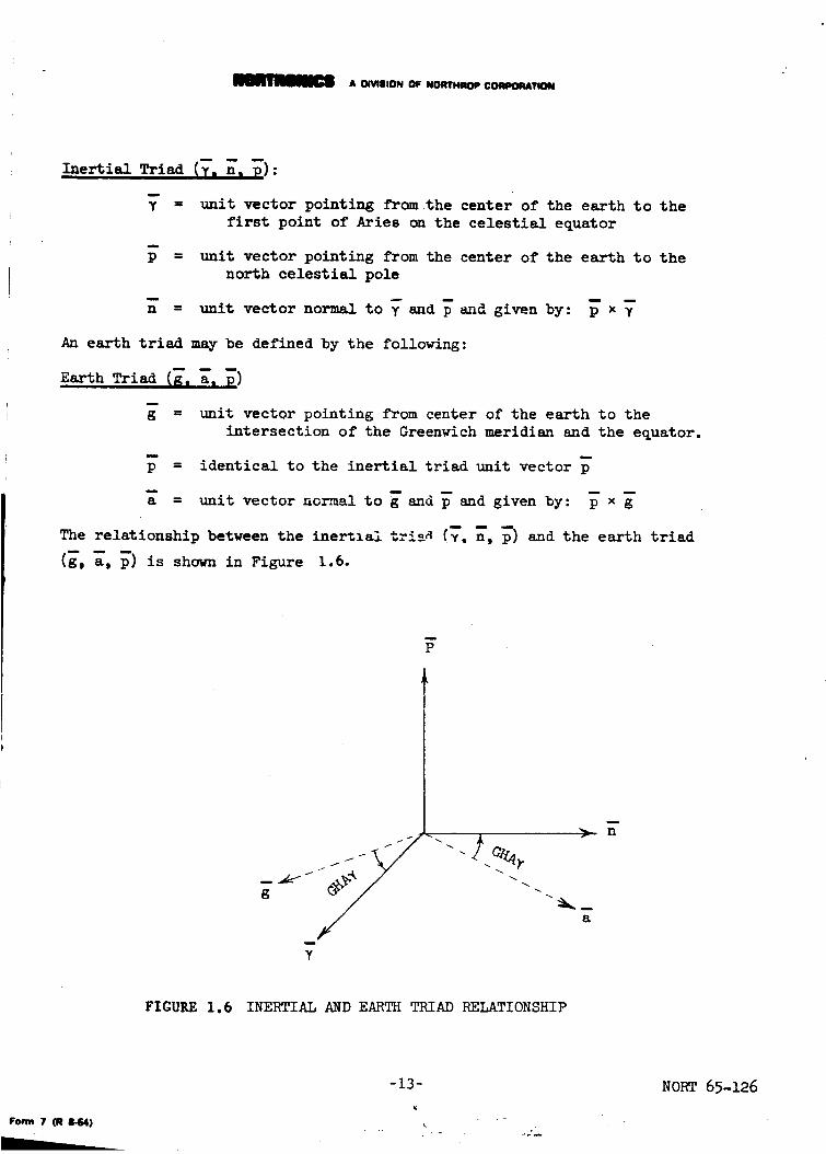
An earth triad m_y be defined by the following:
Earth Triad (_, a I _)
l
g = unit vector pointing from center of the earth to the
intersection of the Greenwich meridian and the equator.
l i
p = identical to the inertial triad unit vector p
a = unit vector normal to g and p and given by: p x g
The relationship between the inertial tri__6 (_° n, _) and the earth triad
(4, a, p) is shown in Figure 1.6.
1
P
I _ _.
i I
__i 11
g
m
¥
1
_- n
a
FIGURE 1.6 INERTIAL AND EARTH TRIAD RELATIONSHIP
-13- NORT 65-126
Form 7 OR 8-64) - "-

A OMSION OF NORTHROP CORPOtlUtTION
As seen from Fisure 1.6, the relationship between the inertial and earth
triads is siren by the matrix in equation 1.21 below,
P
r cos GHAy -sin GHA7 0
sin GHAy cos GHA7 0
l 0 0 1L
m i
7
F I i(1.n)F_ J
Conversely the above matrix may be inverted to yield the expression for the
inertial triad (7, n, P) in terms of the earth triad (g, a, p):
cos GHA7
= -sin GHA7
0t..
sin GHA7 0 -i
cos GHA7 0 i
0 1
m
a
P
(1.22)
Another important triad is the observer's triad. A convenient choice for
the observer's triad is defined by the following three unit vectors,
m
e = unit vector tangent to the ob_zvcr's latitude parallel
and pointing eastward from the observer's position
w
N unit vector tangent to the observer's meridian and
pointing northward from the observer's position
m
z unit vector pointing from the center of the earth to
the observer's position (i.e., the zenith vector)
The vector _may be derived in terms of the earth triad (_, _, _) by reference
to Figures 1.5 and 1.7
m
P
I /
g
m
> a
FIGURE 1.7 LOCATION OF VECTOR z WITH RESPECT TO EARTH TRIAD
-14- NORT 65-126
Form 7 (It 144)

A OtVNIOON O; NO_HaOP CORPO_llON
m
Thus z is given by:
z = cos L cos Log - cos L sin Lo a + sin L p I (1.23)
Figure 1.8 below may be helpful in visualizing the resolving of the vectorinto Its components along the earth triad unit vectors.
i
Z
i
P
i
N
Lo + 180 °
i
g
FIGURE 1.8 PROJECTION OF _ INTO (_, a) PLANE
From Figure 1.8 it il seen that_ is given by:
m i m i
N = -sin L cos Log + sin L sin Lo a + cos L p
m u
Now since e forms a right-hand system with z and N, it is given by:
m m
e = N x z =I m
g
-sin L cos Lo
L cos L cos Lo
la p
sin L sin Lo cos L
-cos L sin Lo sin L
(1.24)
! m u
e = sin Log + cos Lo a (1.25)
-15- NORT 65-126
Form T m 844)

& DIVIqHON OF NORTHROP C_lrlON
Equations 1.23, 1.24, and 1.25 may be summarized by the matrix relationship
given by equation 1.26 belaw:
= -sin L cos Lo
cosL L cos Lo
cos Lo 0
sin L sin Ix) cos L
-cos L sin Lo sin L
(1.26)
1.1.2.2 Terrestrial Navigation Using a Star Tracker
Referring to Figure 1.5 it is seen that the unit vecEor (_) pointing from the
center of the earth to the star is given in terms of the star's declination
(6) and Greenwich hour angle (GHA) by:
= cos 6 cos GHA g - cos 6 sin GHA a + sin'6 p
The line of sight unit vector (LOS) from the observer to the star may be
I
Z Star
I
I
II
derived from Figure 1.9 below,
m
> N
(1.27)
FIGURE 1.9 LINE OF SIGHT (LOS) TO STAR WITH RESPECT TO
OBSERVER'S TRIAD
where h = elevation angle of the star
A = azimuth angle of the star
Thus the vector LOS is given by:
LOS = cos h sin A e + cos h cos A N + sin h z (1.28)
-16- NORT 65-126
Form7 (R 844)

A OlVmlONOFNORTHROPC04MeORATION
Now since the star is very far from the earth compared to the radius of the
earth, the vectors S and LOS may be equated with only a negligible parallax
error of less than 0.1 arc-second. Equating equations 11.27 and 1.28,I
cos h sin Am + cos h cos AN + sin hz = cos 6 cos GHA - cos 6 sin GHA a + sin 6 p
I (1.29)
We can now express the vectors g, a, snd _ on the right side of equation I 1.29 byinverting the matrix relationship given by equation II.26
: o Lo sin L sin Lo -cos L sin (1.30)
cos L sin L
Substituting the expressions for _, _, and O given by equation 1.30 into
equation 1.29 and equating coefficients of the _, N and _ vectors yields:
cos h sin A = (sin Lo cos GHA - cos Do sin GHA) cos 6 _ (l.31a)
cos h cos A : sin 6 cos L - cos 6 sin L (uu_ Lo coz GH_a + sin Lo sin GHAi
(l.31b)
sin h = sin 6 sin L + cos 6 cos L (cos Lo cos GHA + sin Lo sin GHA)
i (1.31c)L
Noting that LHA = GHA - Lo (west), we can simplify equations 1.31a, 1.31b, and
1.31c to the following:
cos h sin A = -cos 6 sin I/{A (1.32a)
cos h cos A : -(cos6 sin L cos LHA - sin 6 cos L) (1.32b)
sin h = sin 6 sin L + cos 6 cos L cos LHA (1.32c)
Equations 1.32a, 1.32b, and 1.32c form the basic relationship between
i) the observer's position on earth [L and Lo], 2) the star's position on
the celestial sphere [6 and GHA], and 3) the star's position with respectto the observer [h and A].
The closed form expressions for h and A are derived from 1.32a, 1.32b, and1.32c as follows:
Dividing equation 1.32a by 1.32b yields the expression for A:
tan A =cos 6 sin I/4A
cos 6 sin L cos LKA- sin 6 cos L (1.33)
-17- NORT 65-126
Form7 (R 11-64)

A DIVIIlION OF NORTHROP CORPORATION
Equation 1.33 is in a form that is readily solvable by resolver chain
computer.
Now the expression for h given by Equation 1.32c, although quite simple,
requires some further manipulation in order to solve for h with a resolver
chain. An expression for h, derivable from equation 1.32c by trigonometric
rearrangement , that is solvable with a resolver chain is given by equation
1.34 be!_w.(1.34)
sin 6 sin L + cos _ cos L cos LHA
tan h = [(cos 6 sin LHA)2+(cos 6 sin L cos LHA- sin 6 cos L)2] I/2
If a digital computer is used for solving for h, then it is more expedient to
use Equation 1.32c rather than Equation 1.34.
We can now solve for the observer's position on earth (L and Lo) in terms of
the star's celestial coordinates (8 and GHA) and the measured azimuth (A) and
elevation (h) angles in the following manner:
Solving for LHA = GHA - Lo from Equation 1.32a,
sin LHA = sin t_u^ Lo) = -cos h sin A
cos 6
and
Lo : GHA + sin -I cos h sin A (1.35)cos 6
Multiplying Equation 1.32b by cos L and Equation 1.32c by sin L; adding the
two new equations yields:
sin 6 = cos h cos A cos L + sin h sin L
Applying the transformation: a cos x + b sin x : _a 2 + b 2 sin(x + tan -I a/b):
sin 6 = (cos 2 h COS 2 A + sin 2 h) I/2 sin (L + tan-lctn h cos A)
• -iL = sln
sin 6
(cos 2 h cos 2 A + sin 2 h)
Using the two identities on Equation 1.36:
X
tan -I x : sin -I
A/2 --tan-i ctn h cos A
(1.36)
-18- NORT 65-126
Form 7 CR 8-64)

AOnalllONOFNORTHROPCOI_OI_TION
and
sin-1 x - sin-½ : sin-1 Ix V1 - y2 _y V1- x2
sin-I [sin 6 sin h - cosC°S2hhC°Scos2AA(c°s2+sin62-h c°s2
]
h sin 2 A1 I/2 I(1.37)
In summarizing the results of this section it is seen that the basic relation-
ships between the navigational variables (h, A, L, Lo, 6, GHA) are given by
Equations 1.32a, 1.32b, and 1.32c. Equations 1.33, 1.34, 1.35, and 1.37 give
an explicit equation for azimuth (A), elevation (h), longitude (Lo), and
L (latitude) respectively. It may also be noted that these equations can
be rearranged quite readily by the use of trigonometric identities to take
on a form that lends itself best to the particular computational scheme inthe system.
1.1.2.3 Vehicle Attitude Correction with a Star Tracker
This topic is treated in two sections. The first of the following sections
considers Lh© info__nation required of a star tracker to correct a stabilization
or attitude control system that na_ an errnr in two axes. It is shown that
only one star fix is required to uniquely correct the error i_ the two axes.
Furthermore, it is shown that the correction equations require only the functional
characteristic of a single resolvcr for their solution.
In the second section it is shown that two star fixes are required for attitude
correction when there exists an error in all three of the stabilization axes.
1.1.2.3.1 Derivation of Equations for Removal of Platform Tilt Errorwith a Star Tracker
A platform tilt, or verticality error is characterized by two consecutive
rotations about the two axes that define the plane of tilt. Thus taking the
plane defined by the east and north unit vectors (_, 7) to be the plane of
tilt, and rotating an angle _ about the _axes and on angle 8 about the
axis, a tilted coordinate system is formed.
The unrotated coordinate system is shown in Figure i.i0 below,
_rn 7(R8-64)
-19- NORT 65-126
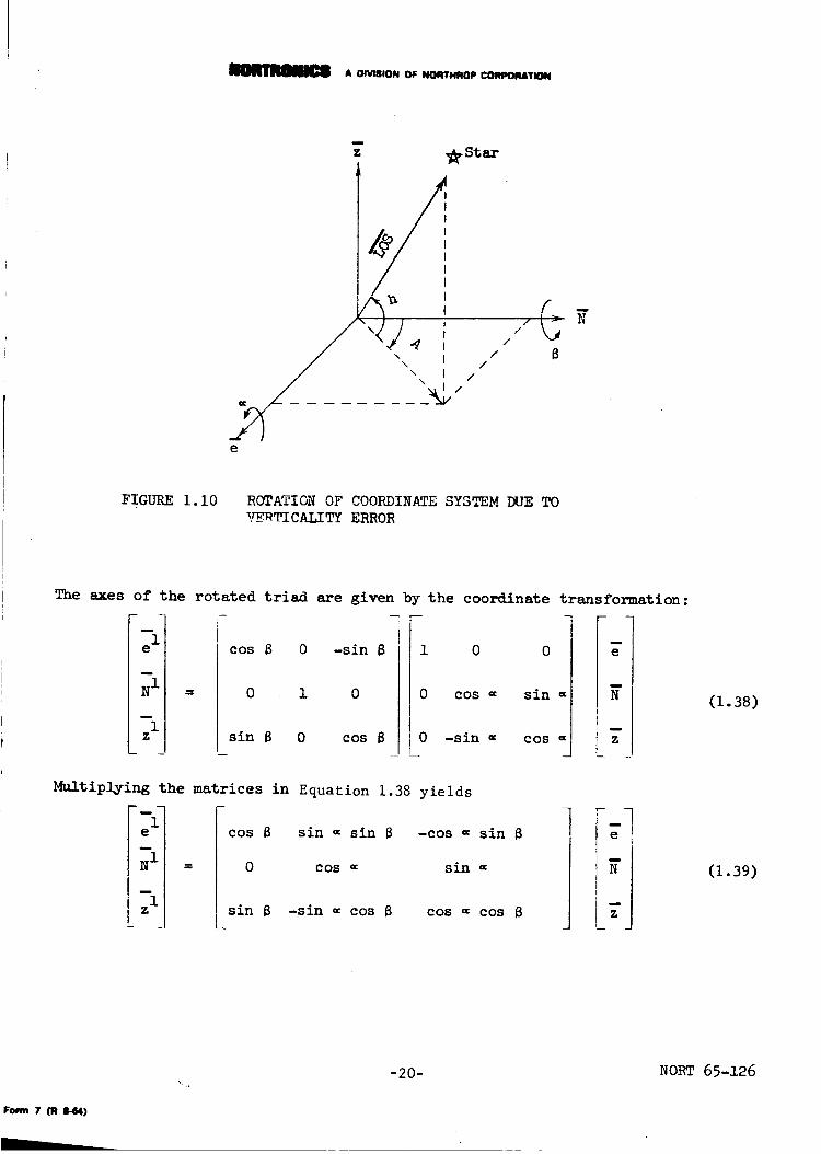
A ONISl0N OF NORTHROP CORPORATION
/
FIGURE i.i0 ROTATION OF COORDINATE SYSTEM DUE TO
_fERTICALITY ERROR
The axes of the rotated triad are given by the coordinate transformation:
--Ie
1z
cos B 0 -sin 8
0 i 0
sin B 0 cos 8
0 COS =
0 -sin =
0
sin =
COS _
m
e
N
Z
Multiplying the matrices in Equation 1.38 yields
_i cos 8
= 0
sin _ sin 8
COS _
sin B -sin = cos
-cos = sin 8
sin =
COS = COS 8
f
(1.38)
(1.39)
-20- NORT 65-126
Fe_m7 (R Ir44)

& OIVIIION OF NORTHROP COt_:OII_ATION
The line of sight vector from the coordinate origin to the star can be
written in terms of the _nrotated triad as:
m n
= COS h sin A e + cos h cos A _+ sin h z
The line of sight vector in terms of the rotated triad is given by:
i (1.40)
I m u I
LOS = cos h' sin A' e' + cos h' cos A' N' + sin h' z' (i .41)
Substituting the expressions for _' _' and _' given by Equation 1.39 into
Equation 1.41 yields:
LOS = (COS 8 cos h' sin A' + sin 8 sin h') _ (1.42)
+(sin = sin _ cos h' sin A' + cos = cos h' cos A' - sin = cos 8 sin h')_
+(-cos = sin 8 cos h' sin A' + sin = cos h' cos A' + cos= cos 8 sin h')_
Now equating the coefficients ofT, _, and _of Equations 1.40 and 1.42 yields
the following three equations:
cos h sin A = cos 8 cos h' sin A' + sin 8 sin h' (1.43a)
cos h cos A = sin = sin8 cos h' sin A' + cos = cos h' cos A' - sin= cos8 sin h'
(i .43b)
sin h = -cos _ sin8 cos h' sin A' + sin _ cos h' cos A' + cos= cosB sin h'
(1.43c)
Defining the following:
Eh = h - h' =
Ea = A- A' =
difference between true elevation and elevation
measured from the platform
difference between true azimuth and azimuth measured
from the platform
In general the angles = and B are small such that the following approximationsare valid:
sin - = = radians
sin B = B radians
cos = = i
cos 8 = i
Form 7 (R 8-44)
-21- NORT 65-]26
. !

A ON.ION OF t_ITHROp COI_POR&TION
This assumption is quite practical since, if the angles = and B are large,
the star tracker would not be able to find the star during its search mode.
Nov subtracting sin h' from both sides of Equation 1.43c and using the smallangle approximations:
sin h - sin h' = -B cos h' sin A' + = cos h' cos A'
1Using the identity: sin x - sin y = 2 sin _x-y) cos 1
noting that small angle approximations hold for Eh and Ea since _ and 8
are small.
i
Eh = -8 sin A' + _ cos A' (1.44)
The expression for Ea is obtained by first applying the small angle approxima-
tion and dividing Equation 1.43a by Equation 1.43b.
tan A =cos h' sin A' + 8 sin h'
=8 cos h' sin A' + cos h' cos A' - = sin h'
Subtracting tan A' from both sides of the above equation yields:
Ea 8 sin h' cos A' - =B cos h' sin 2 A' + = sin h' sin A'
tan A-tan A'= cos--_T_TA,= cos A'(=8 cos h' sin A' + cos h' cos A' - = sin h')
We now make the f_rther approximations:
B sin h' cos A' + = sin h' sin A' >> =8 cos h'
and cos h' cos A >> uS cos h' sin A' - = sin h'
Again these approximations are valid if = and B are small. The expression
for Ea is finally given by:
Ea = (= sin A' + 8 cos A') tan h' (1.45)
By rewriting Equations 1.44 and 1.45 in the following form, it is seen that
a single resolver and a tangent potentiometer represent the only computer
function required to relate _ and B to Ea and Eh. Equations 1.44 and 1.45
are written as:
Form 7 (R 8-64)
-22- NORT 65-126

A OIVlSlON OF NORTHROP CORPORATION
Eh = = cos A' - 8 sin A'
Ea= = sin A' + 8 cos A'
tan h'
(1.46)
(1.47)
Figure I.ii shows the resolver method of solving these equations. Since a
digital computer would probably be available aboard the vehicle, the use of a
resolver may be unnecessary, especially if high accuracy is required.
ma /
tan h' /
h !
/,.,,.
/
© >
/
A' J 8
(
> Eh
FIGURE I.Ii RESOLVER IMPLEMENTATION TO DETERMINE E a AND Eh
-23- NORT-126
Form 7 (R 11-64)
A DIVtBION OF NORTHROP CORPORATION
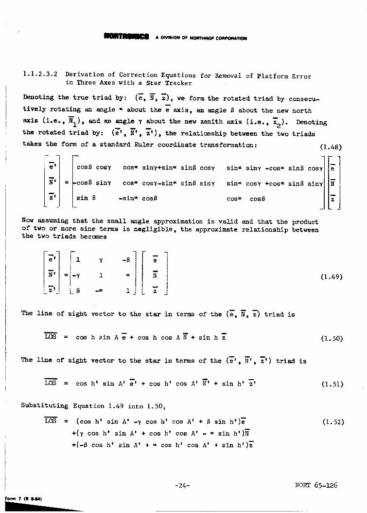
1.1.2.3.2 Derivation of Correction Equations for Removal of Platform Error
in Three Axes with a Star Tracker
Denoting the true triad by: (e, _, _'), we form the rotated triad by consecu-
tively rotating an angle = about the e axis, an angle B about the new north
axis (i.e., ), and an angle y about the new zenith axis (i.e., . Denoting
the rotated triad by: (_', , ,N' z') the relati_ship between the two triads
takes the form of a standard Euler coordinate transformation: (1.48)
cosS cosy cos= siny+sin= sins cosy sin= siny -cos = sins cos
-cos8 siny cos = cosy-sin = sins siny sin= cosy +cos = sins siny
sin B -sin =cosS cos= cosS
Now assuming that the small angle approximation is valid and that the product
of two or more sine terms is negligible, the approximate relationship betweenthe two triads becomes
]I-= 1 z J
(1.49)
The line of sight vector to the star in terms of the (_, _, _) triad is
_ _ m
LOS = cos h sin A e + cos h cos A N + sin h z (1.50)
_' [') triad isThe line of sight vector to the star in terms of the (_', ,
LOS = cos h' sin A' e' + cos h' cos A' N' + sin h' z' (1.S1)
Substituting Equation 1.49 into 1.50,
L'-_ = (cos h' sin A' -Y cos h' cos A' + B sin h')_
+(y cos h' sin A' + cos h' cos A' - = sin h')_
+(-S cos h' sin A' + = cos h' cos A' + sin h')_
(1.52)
-24- NORT 65-126

A OMEION OF NORTHROP CORPORATION
Equating coefficients of e, _, and z in Equations 1.50 and 1.52 yields,
cos h sin A = cos h' sin A' - V cos h' cos A' + B sin h'
cos h cos A : y cos h' sin A' + cos h' cos A' - = sin h'
sin h = -B cos h' sin A' + _ cos h' cos A' + sin h'
(1.53a)
(1.53b)
(1.53c)
The expressions for Eh : h - h' and Ea : A : A' may be derived from Equations
1.53a, 1.53b, and 1.53c with the same procedure as in Section 1.1.2.4.
These expressions are,
Eh = = cos A' - B sin A'
E = (= sin A' + B cos A')tan h'a - Y (l.55)
Equations 1.54 and 1.55 show that it is not possible to obtain a unique
solution for =, B, and y since there are only two equations and three unknowns.
This is due to the fact that, if all three axes are allowed to rotate, then any
rotations about the star tracker's line of sight do not require the tracking
loop to reposition the tracker gimbals. Thus, two different stars must be
tracked to obtain a unique solution for =, 8, and y. The method for obtaining
=, 8, and y from a two star fix is as follows:
On the first star fix two equations are obtained:
First Star Fix:
= = ' (I 56)Ehl cos Ai - 8 sin A1
t
' + B cos Ai)tan hI - yEal = (= sin A I (1.57)
Now assuming that the second star fix occurs immediately after the first star fix
such that =, 8, and y are the same for the second star fix:
Second Star Fix:
: -cos - sinA (1.58)
Ea2 = (= sin _ + 8 cos A_)tan b_ - y (1.59)
-25- NORT 65-126
7 (R 8-64) _.

& OMSlON OF NORTHAOP COAI_DAATION
Solving Equations 1.56 and 1.58 for _ and _ by matrix inversion
F-
b: sin A_ Cos _ - COS Ai sin _ cos A_
Letting _A' = A_ - _, = and B become:
Esin + sin
:- Si--_-_' Ehl sin AA' Eh2(1.60)
cos A_sin AA' Ehl +
cos A isin AA _ Eb2 (1.61)
We can now solve for _ by substituting Equations 1.60 and 1.61 into either
Equation 1.57 or Equation 1.59. First using 1.57, we obtain for _,
t
V = (-Ehl ctn AA' + Eh2 csc AA')tan h i - Eal(1.62)
_ow using Equation 1.59, we obtain for _,
V = (-Ehl csc AA' + Eh2 ctn AA')tan h_ - Eap
Pnus, ¥ is given by either Equation 1.62 or Equation 1.63.
(1.63)
-26-NO_T 65-126
A OIVISION OF NORTHROP CORPORATION
1.2 _ESCRIPTION AND ANALYSIS OF AN ORBITAL NAVIGATION
SYSTEM USING THE STI24-M INERTIAL PLATFORM
A navigational and guidance system for earth orbital type missions such
as that anticipated for the S-IV Saturn Booster Stage is described. The
system considered uses the STI2_-M inertial platform as the prime inertial
reference. The remainder of the system consists of one or two star trackers,
a horizon scanner, an orbital gyro compass, and a digital ccEputer. The
overall system function is to provide the following information: i) space-
craft attitude with respect to inertial space, 2) spacecraft attitude with
respect to earth, 3) spacecraft heading, and _) spacecraft position
(including altitude) with respect to earth.
The following analyses present a derivation of the system equations and
error analyses of the coupling between the inertial platform (STI2_-M)
and the star tracker. It is shown that with the inertial platform oriented
to an inertial triad the star tracker will limit both the coherent and
rand_n gyro drift errors.
1.2.1 STstem CQnfi_Aration and AnalTsis
The functional block diagram of the system under consideration is shown
in Figure 1.12. The various components of the system are shown linked
together by cumputer functiuns symbolically represented by the letter C
with a subscript. In the actual system all the computer functions are
combined into une digital computer. However, for purposes of simplicity
in describing the system, the c_nputer functions have been separated.
Each of the cumputer functions will be discussed in turn, and the system
equations will be derived.
1.2.2 Computer Function CI (Star Tracker Pointing), i i | i ii i i i i ,
Function CI serves to point the star tracker by converting the gimbal angles
of the platform and the star ephemeris data s_ored in the c_nputer into
pointing angles. The inertial platform is oriented to an inertial triad
defined by the following unit vectors :
m
Y Unit vector pointing from the center of the
earth to the first point of Aries on the
celestial equator
m
p = Unit vector pointing from the center of the
earth to the north celestial pole
n =I I
Unit vector normal to Y and p and given by:
pxv
-27- Nora: 65-126
Form 7 (R 8-64)

_m_l_m A DIVISION OF NORTHROP CORPORATION
I 8------=----.-- *el
= _0
OE-_ ,cJ_
O
I-
OL
I_° I _
00 0 ,_ --_
"_ _1_
_enJ
H "1"1
m _
r_
J
(
0
,i-_ u I:11
4-) I1
o .
!
Io
._..I .et
o
-28-
8A
m
o
I_ ,_
/"4
O4")¢,9
I'O
r...)
0
_8
0 0
m•,4 0
m
e
0 o::= r._
T
iv
1
_._o
H
0
O
H
H
H
O
A
H
_o_ 65-z26
Form 7 (R 8-64)

A DIVISION OF NORTHROP CORPORATION
The ephemeris consists of the declination (6) and the sidereal hour
angle (SHA) of the stars. The star tracker is pointed by driving the
star tracker gimbals to given angles as determined by the computer.
These gimbal angles will vary depending upon the star tracker gimbal
configuraticm, and whether the star tracker is mounted cm or off the
platform. If the star tracker is located om the platform, and an altitude-
az_h gimbal is used, then the 6 and SHA angles of the star can be used
directly to positicm the star tracker gimbals. If the star tracker is
off the platform, then two different basic system comfiguraticns for the
star tracker are possible. The star tracker may be mounted in a two-
gimbal system with two rate (or rate integrating) gyros mounted perpen-
dicular to the line of sight in order to remove relative rates between
the star and the star tracker. The other possible configuratiom is the
star tracker mounted in a four-gimbal system, where rate stabilizaticm
is derived from the inertial platform (IMU). In this configuration, the
two base or outer gimbals of the star tracker are slaved to the ecliptic
as are the IMU gimbals. The two axes that define the plane of the
ecliptic are V and n. Thus these two star tracker gimbals can be slaved
directly to the IMU gimbals. The star tracker is then mounted within
these two outer gimbals, in an SHA gimbal and a declination (6)_gimbal.
No rate stabilization is required for the 6 gimbal because the y and n
gimbals provide a stable base. The SHA loop_does require rate stabiliza-tion which can be derived directly from the p gimbal of the IMU. The
gimbal follow-up servo of the SHA channel would be of the form shown
in Figure 1.13.
ey(s)IMU gimbal angle
Star Tracker
Torquer and Gimbal
K2 I e(s)s(s + _i ) Star TrackerGimbal Angle
FIGURE 1.13 RATE STABILIZATION SERVO
The expression for e(s) in terms of SHA(s) and ey(s) is given by:
e(s) = (s2 +Kl's_l + KIK2 ) (SHA(s) + s .y(S))
-29-
(1.64)
NORT 65-126

A OtVISION OF NORTHROP CORPORATION
The SHA(s ) functio_ will be a step cc_aand of magnitude SHA. Thus,
after a period of time greater than the servo time constants, the out-
put e(t) will be given by:
me(t) = A+ yCt)
t>>T1, T 2
(1.65)
Depending upon the field of view of the star tracker and the initial
uncertainty in craft attitude, Clmay also be required to generate asearch pattern.
Other gimbal configurations for the star tracker m_y be devised but will
not, be treated here.
1.2.3 Computer Function C2 (Star Tracker Correction to IMU)
The function of computer element C2 is to use the star tracker(s) outputs
to correct the inertial platform. If the platform is used in a strapped-
down configuration, then the correction to the inertial reference is
performed in the computer rather than to the gimbals of the platform.
In either case the basic correction equations are the same.
In Section 1.1.2 the equations for correcting the platform's inertial
triad with a star tracker were derived. Since the platform considered
here is referenced to a space fixed triad (_, _, _) rather than a local
vertical triad, the pointing angles to the star are denoted by their
celestial coordinates declination (6) and sidereal hour angle (SHA),
rather than elevation and azimuth. The correction equations written
in terms of celestial coordinates (6 and SHA) are given by:
First Star Fixi
Egl = A@ I cos SHA' I - A@2 sin SHA' I
= cos - A$ 3ESH_ (_I sin SHA' I + A@ 2 SHA'l)tan 6'I
Second Star Fixi
Egl = A$I cos SHA' 2 - A@ 2 sin SHA' 2
= + cos - A@3ESHA 2 (A@l sin SHA' 2 a_2 SHA'2)tan 6'2
(1.66)
"(1.67)
(1.68)
(1.69)
-30- NORT 65-L26
Form 7 (R 8-64)

_8 A DIVISION OF NORTHROP CORPORATION
whe re SHA =
SHA' =
6 =
ESH A =
E 6 =
computed sidereal hour angle
star tracker output sidereal hour angle
computed declination
star tracker output declination
SHA- SHA'
6- _w
A¢l' &¢2' and A4,3 correction angles about the platform's
Y, n, and p axes, respectively
Solving Equations 1.64, 1.65, 1.66 and 1.67 for A¢l' &¢2" and A¢3 yields:
sin SHA' sin SHA'
2 1 (1.70)_¢i = - sin(SHA' 1 - SHA' 2) E61 + sin(SHA' 1 -'"SHA'2) E_2
cos SHA' cos SHA'
2 1 (l.71)&¢2 = - sin(SHA' I - SILA' 2) Eal + sin(SHA' 1 - SHA' 2) Ea2
[ 1
Thus the computer generates the required corrections to the inertial plat-
form from two star fixes. The star tracker correction angles (A¢I, A¢ 2 •
and A¢3 ) remove ccmstant gyro drift and bound the errors due to random
gyro drift. The manner in which the star tracker accomplishes this function
is derived in the following paragraphs.
The single axis gyro stabilization loop block diagram for the STI2h-M
inertial platform as given by NASA TN D-2983 is shown in Figure 1o14 below.
T(s)
Plat form
Gimbal
Hs
_zGUIRE1.l_
Ts(s) GyroGimbal
GN _o drift)
SINGLE AXIS PLATFORM STABILIZATION LOOP
-31- NORT 65-126
s(s)
Form 7 OR 8-64)

ADIVISIONOFNORTHROPCORPORATION
The signal flow graph for the system shown in Figure i.i_ is shown in
Figure i. 15 below:
Ts(s)
Ta(s) 1 1 Jas 2 _(s) Hs 1 1
-F(s)
B(s)o
FIGURE 1.15 SI_"_AL FLOW GRAPH OF SINGLE AXIS
STABILIZATION LOOP
The star tracEer output platform correcti_ angles (A_I , &@2" A@3 ) are
used to correct the orientation of the platform by applying a torquing
signal at the TB(s) input. Thus the transfer function of interest is
$(s)/TB(s) ; where @(s) is the gimbal output angle. This transfer function
is readily derived from the signal flow graph in Figure 1.15 and is given by:
STs_ = _ sH + F(s) )] (1.73)s[Ja JB s3 + s_ + HF(s
Since the system errors that exist after a fairly long period of time are
of interest rather than the errors after a few seconds, the transfer function
given by Equation 1.73 may be approximated by:
t*_ sHF sH
s _ o
where F = 1 F(s)S_O
-32- NORT 65-126
7 (R 8-64)

_m A DIVISION OF NORTHROP CORPORATION
The error due to gyro drift (_) can be computed from Equation 1.74.
Figure 1.16 below shows the block diagram relationship of platform gimbal
angle error to gyro drift.
FIGURE 1.16 BLOCK DIAGRAM OF RELATIONSHIP OF PLATFORM
GIMBALANGLE ERROR TO GYRO DRIFT
where ¢¢ = platform gimbal error
= gyro drift
_he constant drift component may be represented by letting _ equal a
step function (_ = +). The output ¢¢ for % = _s is a ramp function
(¢@(t) = _ t). Thus a constant gyro drift rate results in an unboundedH
attitude error when no velocity or position damping information is available.
The effect of random gyro drift, in general, may be characterized by acorrelation function of the form:
where
R (T)
R (T)
2aN
2 (1.75)= aN e-(_c
= random gyro drift correlatic_ function
= mean-squared value of random gyro drift
WC
= bandwidth of gyro drift noise
The impulse response of ¢@ to _ is given by:
-i
hcg(t) = =(1.76)
-33- NORT 65-126

_n__ A DIVISION DF NORTHROP CORPORATION
m
Thus the mean-squared error (¢@2) growth as a function of time is given
in terms of the noise autocorrelation function (Equation 1.75) and the
impulse response (Equation 1.76) as:
t t
¢02 = T e c dX0 0
t T t
-°'J [ Jo "7--']-- _- dl e-ic I e dl + e c e c dX (i.77)
O T
Evaluating the integrals in the above equation yields the following expression
for the mean-squared platform error:
°'E 1m --_ t
¢_2 = 2----_ Ct + e C - III1c
(l.78)
From Equation 1.78, it is apparent from the _ct term that the platform
error is unbounded.
A star tracker's capability to _educe and bound platform errors due togyro drift (both constant and random) will be considered next.
The star tracker correction data would be inserted into the platform
stabilization loop at the TB(s) input node as shown in Figures i.i_ and
1.15; that is, the star tracker data is used to torque the platform gyros
to a corrected position. Thus the functional block diagram of the gyro
stabilization loop with star tracker correction takes a form as shown
in Figure i.17 below,
sH
Star Tracker
Inertial
Reference
plusTracker Noise
(A¢n )
> ¢¢
FIGURE 1.17 GYRO STABILIZATION LOOP WITH STAR TRACKER
CORRECTION (ERROR MODEL)
-3_- NORT 65-126
Form 7 (R 8-64)

_l_m A DIVISION OF NORTHROP CORPORATION
where A@n = star tracker noise (i.e., correction signal error)
SI, S2 = synchrcmized switches
L(s) = optimum filter or simple gain
In the error model of Figure 1.17 the star tracker output is composed of
the instantaneous platform error -¢¢ and a noise term A¢ n which represents
the tracker error. The -¢4 term of the star tracker output is represented
by a feedback path from the gimba! out_t with a double line. The double
line is used to denote that the path is functioflal rather than wired.
The switches shown in Figure 1.17 are necessary to allow the gyro stabiliza-
tion loop to respond to craft rates whose frequency cantent are higher
than the inherent star tracker sampling frequency. If the switch remains
closed continuously (that is, if the last star tracker output is held),
the loop response to craft rates would be insufficient to prevent the
star image from smearing due to image moticm. Image motion with respect
to the tracker line of sight causes a loss of both detectivity and accuracy.
Furthermore, the Sampling Theorem states that in order to retrieve informa-
tian from a sampled signal without loss it is necessary to sample the
signal at a rate which is at least twice the highest frequency ccmpouent
of the signal. Since the star tracker output (for image forming and flying
spot scanning types of star trackers) is inherently of a sampled nature,
with a period equal to the tracker acquisition and readout time, certain
compouents of craft motion will not appear in the tracker output at the
readout times. Thus, the inertial platform serves to stabilize for
craft rates that occur in the middle to high frequency range while the
star tracker removes the low frequency errors that accumulate due to
platform drift.
Mathematically the switch is assumed to be ideal, such that its output
is an impulse with a weighting equal to the amplitude of the input signal
at the sampling instant. This is illustrated in Figure 1.18.
Input to Switch
i i i _ t2T 3T hT 5T
Output of Switch
>t
FIGURE 1.18 SAMPLING SWITCH INPUT AND OUTPUT WAVEFOR_H
-35- NO_T 65-126
Form 7 (R 8-64)
_m A DIVISION OF NORTHROP CORPORATION
If the input function to the switch is denoted by fi(t), then the output
of the switch (fo) is given by:
fo(nT) = fi(nT) 6(t - nT)
where 6 (t) = impulse function
The expressions for ¢¢(s) and e;(s) are given by Equations 1.79 and 1.80
below:
L*(s) L_J l l_ Le(s) &Sn(S)
L'(s) A%*Cs)
Note that the asterisk (m) denotes the pulse transform.
We can now write the Z transform of mS(s) as follows:
(l.79)
(1.80)
[ (Z-l) ]7[GNs(s)] + ZL(Z) ASn(Z)¢¢(Z) = H(Z-I) + ZL(Z) H(Z-I) + ZL(Z) (l.81)
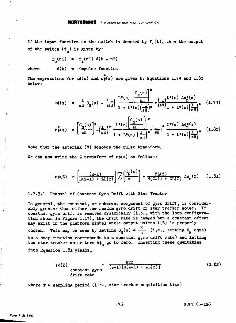
1.2.3.1 Removal of Constant Gyro Drift with Star Tracker
In general, the constant, or coherent component of gyro drift, is consider-
ably greater than either the random gyro drift or star tracker noise. If
constant gyro drift is removed dynamically (i.e., with the loop configura-
ti_ shown in Figure 1.17), the drift rate is damped but a constant offset
may exist in the platform gimbal angle output unless L(Z) is properly
chosen. This may be seen by letting GN(S) = Ks (i.e., setting _ equal
to a step function corresponds to a constant gyro drift rate) and letting
the star tracker noise term ASn go to zero. Inserting these quantities
into Equation i. 81 yields,
c¢(z) ! =constant gyrodrift rate
KTZ
(Z-l) [H(Z-I) + ZL(Z) ]
where T = sampling period (i.e., star tracker acquisition time)
(1.82)
-36- NORT 65-126
Form 7 CR 8-64)

_m A OIVISION OF NORTHROP CORPORATION
Applying the final value theorem to Equation 1.80,
Z-1 KTZe¢(nT) = lim --z (Z-1)[H(Z-1)+ ZL("Z)]
lim n ÷ m Z-_l
KT
¢_(nT) = lie [H(Z-I)+ ZL(Z)]lira n + @o Z÷I
THUS, it is seen from Equation _.v;_o9 that, if the steady state error
£$(nT) is to be zero, the denominator of the right hand side of Equaticm
1.83 must be of the form:
H(z-1) + zL(z) =Z-1
where F(Z) = polynomial in Z with no roots at Z = i.
Solving for L(Z) from Equaticm 1.8_,
F(Z) - E(Z-1),2LCz) =
Z(_l)
Now choosing F(Z) = aZ,
T(z) - -_z2+ (a+ _)z -Z(_l)
Note that L(Z) is a physically realizable transfer function.
this value of L(Z) into Equation 1.82 yields:
KTe_(z) = --
a
constant gyrodrift rate
Inserting
Equation 1.86 indicates that the error exists only at the first sampling
instant and is zero thereafter assuming that the drift rate remains
constant.
Although the proper choice of L(s) has eliminated platform error due to
constant gyro drift rate, the platform error due to random gyro drift
rate and star tracker noise, or error, remains. Furthermore, by choosing
L(s) to eliminate constant gyro drift rate, the platform response to
the random error sources will not be optimum. 0he solution to this
problem is to alter L(s) to yield an optimum system by minimizing the
platform mean-squared error due to all error sources. Another, perhaps
better, solution depending on the particular hardware utilized, is to
(1.83)
(1.8h)
(1.85)
(1.86)
-37- NORT 65-126
7 (R 8-_)

A DIVISION OF NORTHROP CORPORATION
let the system operate open loop (i.e., without star tracker correction),
determine from the star tracker output the constant gyro drift rate
(after the orbital angular rates are removed with the computer), then
apply a trim signal to the gyro torquer to eliminate the drift. The star
tracker output after being resolved into equivalent rotations about the
three inertial axes (V, n, p) would exhibit a patters as shows in Figure
1.19 if there existed a constant gyro drift rate.
A¢ l, A¢ 2, A¢ 3
Dots indicate values of
A¢ 1 (or A¢2 or A¢3) at thestar tracker readout times.
The straight line is a"best" fit to determine
gyro drift rate.
5T I0 T: > t
15 T
FIGURE 1.19 VARIATION IN STAR TRACKER OUTPUT
DUE TO CONSTANT GYRO DRIFT
Thus, with the system operating open loop, a set of star tracker read-
outs are stored. Then the data is smoothed by any of the following
three methods :
i) Least Squares Fit
2) Frequency Filtering
3) Ka/mam Filter
The smoothed data yields a straight line fit to the star tracker data.
Now a trim signal (derived from the straight line fit) is applied to the
gyro torquer to remove the constant component of gyro drift. After the
trim signal is applied to the gyro, the loop is closed around the plat-
form with the star tracker as shown in Figure 1.17. With the loop closed
the errors due to random error sources become bounded as will be shows
below. If the system is operated in this manner, it is necessary to
periodically adjust the gyro trim signal since changes in the constant
gyro drift rate will tend to occur.
Form 7 (R 8.64)
-38- N0_-¢_65-126

_r_oN|_ A DIVISION OF NORTHROP CORPORATION
1.2.3.2 Bounding of Random Gyro Drift with Star Tracker
To simplify the following analysis, the filter network L(s) will be assumed
to have a constant gain (L). The error model block diagram used to
compute the system errors due to gyro drift and tracker error is the same
as that shown in Figure 1.17, except for the shifting of the pole at
the origin. The pole is shifted into the left half s-plane in order to
avoid ambiguities in the correlation function equations of the system.
After the mean-squared error of the system is determined, the limit as
a ÷ 0 is taken to yield the t_"Je mean-squared system error. The error
model block diagram used in the following calculations is shown in
Figure 1.20.
lim
a÷O
FIGURE 1.20 ERROR MODEL FOR CALCULATION OF RANDOM ERRORS
1.2.3.2.1 Random Gyro Drift Error Calculation: The transfer function
relating the platform error, ¢¢, to gyro drift, _, in terms of the
Z-transform is given by:
-aTZ -e
c¢(z) =( H)Z -
The system correlation fUnctic_ equation may be written from Equation
1.87 as:
Ra¢(Z) = ( Z - e-aT )(L+H)Z - He -aT
where Rgg(Z )
Z-I _ e-aT
(L+H)Z_I _ He-a T / Rgg(Z)
%is the autocorrelation function of"-- in the Z-domain.
s+a
(1.87)
(lo88)
-39- NORT 65-126
Form 7 (R 8-64)

NOflTROIIICS _ o,v,s,oNoFNO..HROPCO_PO..T,ON
Assuming the gyro drift noise to be white with a spectral density equal
to ng/2, we can write Rgg(S) as:
ngl2 ng/4a + ng/4aP, (s) = =gg 2 2
--S +a s+a -s+a
(1.89)
Now taking the Z-transform of Rgg(S):
where
Rgg(Z) = Z [Rgg(S)]
R;g(S) = s + a
[_ _s) °-' ]+_, ,s) -R (o) (1.9o)
uRgg(S) ng/_a-s+a
-1
w=O
Substituting these expressions into Equation 1.90 and taking the Z-transform
yields:
n (i - -2aT)ze (1.91)
Rgg(Z) = a_T (Z - e-aT)(l - e-aTz)
Substituting Equation 1.91 into Equation 1.88 and simplifying yields:
ng (i -e -2 aT) Z
4aT(L+H)2 Z - _ _ _ 1 - _ Z
The _n-sq_ed error of the sampled output sequence, E¢, is given by:
c*¢2 Residue of RE¢(Z) Z- He-aT= ; Z = L+---_-
rlg I - e
aT(L+H)2 H2 -2aT1 - e
(L+H)2
(1o92)
(1o93)
-40- NORT 65-126
7 (R 864)

_r_s A DIVISION OF NORTHROP CORPORATION
The asterisk(*) denotes that the sampled output sequence (¢¢) is implied
rather than the continuous output.
Now taking the limit as a ÷ 0 and multiplying by T in Equation 1.93 yields
the final expression for the mean-squared continuous output error due to
random gyro drift noise.
-- ngTc¢2 = _LCT +Z_) (l.9_)
Note that, if the feedback term L is reduced to zero (i.e., no star
tracker input), the error due to gyro drift becomes infinite.
In general gyro drift may be characterized by specifying the RMS drift
rate and the bandwidth. For the gyros used in the ST124-M platform it
will be assumed that the random and fixed drift rates are as follows:
Random drift (RMS) = O.Ol°/hr = 0.01 sec/sec
Quasi fixed drift = 0.2°/hr = 0.2 se_/sec
The torquer noise (_) corresponding to a platform drift rate of 0.01 sec/sec
RMS is given by:
22 H2 (0.01 se_c/sec) 2
GN = Og =
The AB5-K8 gyro used on the ST12_-M platform has an angular momentum, H,
equal to 2.6 x i0 b gm --cm2/sec. Thus a 2 is given by:g
2 = (2.6 x 10⁶) 2 (0.01) 2 gm2 cm4 sec'_2
Og sec4
2 _ f-,22 108 _m cm sec
o = 6.76 x 4g sec
Now assuming the random torque noise to have a frequency distribution
given by:
ngl2IGN(J=)12 =
i + (,,,1=o)2
7 (R 8-64)
-41- NORT 65-126

_l_ A OIVISION OF NORTHROP CORPORATION
2
The relationship between ng and ais: g
2,1 2 o..a = .._.L
2 =0
Assuming a bandwidth of i0 cps, mO
for this type of frequency distribution
= 201, ng is given by:
,,_ . 2 _ se_c2_o.16 x 108 ) _n cm
ng = 20 _ sec 3
qg = 0.43 x 10⁸ _m2 cm 4 se_ 2sec 3
Substituting this value of ng into Equatica 1.94 yields:
¢_2 0.43 x 10⁸ T _-_2= sec (1.95)2L(L + 5.2 x 10⁶ )
In order to determine the numerical value of ¢$2 it is necessary to select
the values for T and L. If reasonably accurate data were available for
the various dynamic platform inputs, L [or L(s)] could be chosen by using
an optimum synthesis technique such as the Wiener method modified for
sampled data systems. Since such data is not at present available,
L will be chosen equal to H such that the correction signal from the
star tracker reflects as a one-to-one rotation of the platform. The
period, T, between star tracker correction inputs is dependent upon the
type of star tracker employed and whether one or two star trackers are
available. Assuming that a vidicon tracker with a field of view equalto 30 _:_mn x 15 mn. is used, the values of T for two consecutive starshots with one star tracker and for two simultaneous star shots with
two star trackers are given as:
T (2 star trackers) = 5.0 sec.
T (i star tracker) = 5 + 5 + 5 = 15 sec.
It is assumed that 5 seconds are required to slew the star tracker to the
second star. Inserting these quantities into Equation 1.95, the mean-
squared platform error due to random gyro drift becomes:
-42- NORT 65-126
Form 7 (R 8-54)

_1_|_,_ A DIVISION OF NORTHROP CORPORATION
M
¢¢2 (2 star trackers) = 0.053 x 10⁻⁴ 6_c2 (1.96a)
c¢ (2 star trackers)R_
c¢2 (i star tracker)
= 0.0023 _ (1.96b)
= 0.16 x i0-h se"_2 (1.96c)
c¢ (I star tracker)p_s = 0.004 s_e_ (io96d)
Thus the star tracker results in a negligible amount of platform error due
to random gyro drift.
1.2.3.2.2 Fixed Platform Drift Errors: Now consider the platform error
due to quasi fixed drift. The torquer noise that characterizes this type
of drift is given by:
GN (fixed drift)(0.2 s_c/sec)H
S
The expression for e¢ in terms of _ is given by (note that the pole "a"
is set equal to zero since it is not necessary to use correlation functionsfor fixed drift ):
z Z[0 ]E¢(z) = (T,'+H) Z-e
Applying the final value theorem for the Z-transform to Equation 1.97
yields the steady state platform error:
E¢(steady state) Lira Z-I [0.2 H'_F Z ]
- LZ-_I Z L + Z L+H
(1.97)
For L = H this becks,
E¢(steady state) = 0o2 T se_
Now using T = 5 sec. for two star trackers and T = 15 sec. for one star
tracker, the fixed drift platform errors are:
¢¢ (2 star trackers) = 1.0 6_
¢¢ (i star tracker) = 3,0 sec
(1.98a)
(1.geb)
-43- NO_ 65-126
Form 7 (R 8-64)

IIORTROIII£S A o,v,s,ONOFNO.T..OP CO.PO.AT,O,.
1.2.3.3 Platform Error Due To Star Tracker Error
A star tracker error torques the platform as does the star tracker cor-
rection signal. The error that is reflected into the platform angle
due to star tracker error is dependent up0a the statistics of the star
tracker error source. For purposes of analysis, a vidicon star tracker
will be assumed to be used in the system, since performance imformatic_
for this type of star tracker is readily available. With a vidicoa star
tracker, the error is dependent upon the location of the star image in
the field of view of the tracker, which results from the fact that the
major sources of error in the vidicon star tracker are coherent rather
than random in nature. The predominant errors in the vidicon star tracker
are l) scanning sweep non-linearity, 2) quantizing errors, and 3) me-
chanical misalignment errors. Thus, the error input to the platform
loop from the star tracker will consist of a series of impulses that
are fixed for a period of time. The period of time that the amplitude
of the error impulses remain fixed is dependent upon the specific track-
ing format. As a first order approximation, it will be assumed that
the period of fixed amplitude error impulses is long with respect to
the time constant of the loop. Figure 1.21 illustrates a typical star
tracker error pattern.
A_ n
ist star
where
i3i3i32nd star nth star
3rd star
A@2 A@ 2 AS2
ASn A@ n AS n
n=0
>t
FIGURE 1.21 VIDICON STAR TRACKER ERROR PROFILE
The transfer function between the star tracker error input, A@, and the
platform angle output, c@, is given in terms of the Z-transform as:
ZL _¢(Z)a¢(Z) = (L+H)Z - H
-_,4- NORT 65-126
Form 7 (R 8-64)

_JOl_l_m A DIVISION OF NORTHROP CORPORATION
Now for L = H and A¢(Z) represented by a train of impulses of Pd_8 amplitude
oT over a period of time which is long with respect to T, the platform
output error is given by:
"¢ : T = (Z-I/2)(Z-I) (io99)
Applying the final value theorem to obtain the steady-state value of
E¢ yielda :
e¢ (steady state)
e¢ (steady state)
z_i z (z-i )(_i
= oT (1.1oo)
Thus, the star tracker error reflects directly into an error in platform
angle for the particular circumstances given above.
1.2.3.h Final Platform Angle Error
2)
3)
_) Star Tracker Gimbal Pickoff Error -- ¢¢2ps
The final platform angle error is a root-sum-square summation of the
following error sources:
l) Random Gyro Drift Error --cOg 2 -- given by Equations 1.96a through 1.96d.
2Quasi-Fixed Gyro Drift -- E¢ d -- given by Equations 1.98 a and 1.98b.
2
Star Tracker Error -- ¢¢S -- given functionally by Equation l°100
and numerically in Section 1.3o
-- given in Section 1.3.
Platform Gimbal Pickoff Error (this only applies if the star tracker(s)
is1..__ocated off the platform) --2
¢¢p u given in Section 1.3.
6) Craft Flexure Errors (This only applies if the star tracker(s) is
located off the platform° )
_-_f u given in Section 1.3.
-hS- NORT 65-]26
'in. 7 (R 8-64)

A OIVISION OF NORTHROP CORPORATION
The final platform gimbal error is given by:
I'2[..... ]c.2.: .s2. .; c.:1,2= + + + (i.i01)
Tables i.I through 1.5 present a summary of the platform gimbal angle errors
for various system configurations. The star tracker errors are based upon a
two-star fix with the celestial Angles of the stars given by: 6.(declinatiom)&
= 45 °, S_ I (Sidereal Hour Angle) = 90 ° , 62 = 45 ° , SH_ = h5 ° . Details
about the star tracker errors, pickoff errors, and craft flexure errors
may be found is Section 1.3.
TABLE i.i
ERROR SOURCES
1
Random Gyro Drifti
Quasi Fixed Gyro Drifti
Star tracker Error for
2 star fix, including
tracker's gimbal pick-
off error.
Platform Gimbal
Pickoff Error
ii i
Craft Flexure Error
Net RSS Errori i ii
N.A. - not applicable
ONE STAR TRACKER MOUNTED ON THE PLATFORM
OUTER
(E4'I)RMB
sec.
o.oo_
3.0
14.2
N,A,
N.A.
14.5
GIMBAL ERROR
I MIDDLE
I_(E¢2) R.MB
g'6%.
0.004
3.0
8.2
N,A,
N.A.
8.8
INNER
(¢¢=)_
_6_.
o.oo_i i
3.0
i ii
18.3
N.A.
i i ! i
N.A.
18.6
-26- NORI' 65-126

__ A DIVISION OF NORTHROP CORPORATION
TABLE 1.2
ERROR SOURCES
i i i i m
Random Gyro Drifti i
Quasi Fixed Gyro Driftl l
Star Tracker Error -
for 2 star fix,
including tracker' s
gimbal pickoff
error
Plat form Gimbal
Pickoff Error
Craft Flexure Error
Net RSS Error
ONE STAR TRACKER OFF THE PLATFORM (NO CRAFT FLEXURE)
seci
o.oob
3.0
i i
14.2
6.5
GIMBAL ERROR
MIDDLE
sec
0.004i,
3.0
8.2
N.A,
i
10.9
Ii_ R
,i,.
secIL I II
o.oo_.I
3.0i i
18.3
6.5
TABLE i. 3 ONEi
Random Gyro Drifti H
Quasi Fixed _ro Driftil i i l
Star Tracker Error -
for 2 star fix,
including tracker' s
gimb al pickoff
error, i aiR i ill i
Platform Gimb al
Pickoff Error
|
Craft Flexure Error
Net RSS Error
STAR TRACKER OFF
0.004
3.0
14.2
i i
6.5
eCfl
"--2. ,112(253.2+¢_fi;
THE PLATFORM (WITH
, l
o.oohm i
3.0
8°2
eel2I
(118.4+¢ $_ )112
CRAFT FLEXURE
HIm
0.004i i i
3.0,i
18.3
,,, i
6.5
l
eCf3
(386.2+e¢23) i/2
-47- NORT 65-126
Form 7 (R 8-64)

_|_ A DIVISION OF NORTHROP CORPORATION
TABLE 1.4
i i
ERROR SOURCES
i i
Random Gyro Drifti ii
Quasi Fixed Gyro Drifti
Star Tracker Error -
for 2 star fix,
including tracker' s
gimbal pickoff
error
Platform Gimbal
Pickoff Error
Craft Flexure Error
,, i
Net RSS Error
i,
TWO STAR TRACKERS OFF THE PLATFORM (NO CRAFT FLEXURE)
GIMBAL ERROR
OUTERi,
(¢¢I)_
sec
0.0023
i.0
14.2
6.5
N.A.
15.7
MIDDLE
sec,i
0.0023
!.0i
8.2
6.5
N.A,
10.5
INNER
(c¢3)p_s
sec
0.0O23
1.0
18.3
| |
6,5
N.A.
19.4
i i i
TABLE i. 5 TWO
Randcu Gyro Drift
Quasi Fixed Gyro Driftii ii
Star Tracker Error -
for 2 star fix,
including tracker' s
gimbal pickoff
errori ,i , ii i
Platform Gimb al
Pickoff Errori i i ii
Craft Flexure Error
i |i i i
Net RSS Error
i
STAR TRACKERS OFF
0.0023
1.0
14.2
ii i
6.5
H
C¢fl
(245.2+¢¢2fi)I/2
THE PLATFORM (WITH
O. 0023
1.0
8.2
ii
6.5
,I
¢¢f2
(llO. h+c¢_ )1/2
,=
CRAFT FLEXURE)
i
0. O023
1.0
18.3
6.5
i i i |
z¢f3
i ii
i
_l_g.. NORT 65-126
_on'n 7 (R 8-64)

__S A DIVISION OF NORTHROP CORPORATION
1.2.4 Computer Function Cq (Relationship Between
Craft Attitude and Inertial Space)
Computer function C3 is essentially a matrix relationship that relates
the craft attitude to inertial space. The angles of rotation between
the craft triad and the inertial triad are derived from gimbal pickoffs
(or from the gyro outputs if a strapped-down configuration is used. )
Denoting the craft triad by (ic, Jc' ___) and the inertial triad by
(V, _, _) the relationship between the two triads is given by:
iy _ i xc_!n ; = M1
-ip]
(l.lO2)
where the matrix [MI] is given by:
F
cos ¢2 cos ¢3
-cos ¢2 sin ¢3
sin ¢i sin ¢2 cos ¢3 +
cos ¢i sin ¢3)
cos ¢i cos ¢3 -
sin ¢i sin $2 sin ¢3)
(1.103)
sin ¢i sin ¢3 -
cos ¢i sin ¢2 cos ¢3)
sin ¢I cos ¢3 +
cos ¢I sin ¢2 sin ¢3)
sin ¢2 -sin ¢I cos ¢2 cos ¢i cos ¢2
The angles ¢I' $2" and ¢3 are the gimbal angles with respect to their null
position.
The matrix [_] is the fixed relationship (neglecting craft flexure)
between the craft and the platform gimbals when they are caged to a
null position.
1.2.5 Computer Function C 4 (Local Vertical Determination)ii i , i i
The purpose of computer function C4 is to process the Horizon Sensor
output to improve the accuracy of the local vertical determination.
Some of the functions performed by the computer would be averaging of
the Horizon Sensor output over several orbits, to compensate for errors
due to weather and climatic effects, and determination of the local
-49- NOET 65-126
Form 7 (R 8-64)

_m A DIVISION OF NORTHROP CORPORATION
vertical, allowing for the earth oblateness and other horizon anomalies.
The two-axis gimbal system is slaved to the Horizon Scanner output such
that the orbital gyro compass is maintained in a vertical position with
respect to the earth's surface. The local vertical vector (L--_ is defined by:
_ m n
= + cos 82 Jc + cos e3 kLV cos 81 ic c(i.io4)
1.2.6 Computer Function C5 (Craft Position Determination)] i
Computer function C5 is used to compute the craft's position with respect
to earth.
The local vertical vector (L-V) may be written in terms of the craft triad
as given by the Horizon Scanner (see Equation 1.104) or in terms of earth
coordinates, GHAv, and the inertial triad (7, n, _) as follows :
m
_V = cos L cos(L + GHAT)v - cos L sin(Lo o
+ + sin (1.105)
where :
L = latitude
L
o
GHAv =
longitude measured west of Greenwich
angle between the Greenwich meridian and the meridian
that passes through the first point of Aries. This
quantity would be supplied by a clock aboard the space-
craft that reads absolute time.
Now we can solve for the craft triad (_c' Jc' kc) in terms of the inertial
triad (7, n, p) by inverting the matrix relationship in Equation 1.102.
1
C
I
Jc
m
kc
-1
y
n (i. 106 )
Substituting Equation 1.106 into 1o105 yields,
: fzV+ f2 f3T (ioi07)
-50-: NORT 65-126
m 7 (R 8-64)
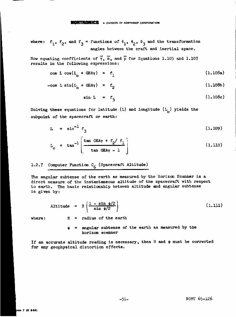
_m A DIVISION Of: NORTHROP CORPORATION
where: fl' f2" and f3 = functions of el, e2, e3 and the transformation
angles between the craft and inertial space.
m m m
Now equating coefficients of Y, n, and p for Equations 1.105 and 1.107
results in the following expressions:
cos L cos(L° + GHAV) = fl (1.1o8a)
-cos L sin(Lo + c_y) = f2 (Z.108b)
sin L = f3(1.1o8c)
Solving these equations for latitude (L) and longitude (Lo) yields the
subpoint of the spacecraft or earth:
• -i
L = szn f3
LO
itan * f2/fltan-z L tan G_Ay- 1 j
(l.1O9)
(1._0)
1.2.7 Computer Function C6 (Spacecraft Altitude)i
The angular subtense of the earth as measured bythe Horizon Scanner is a
direct measure of the instantaneous altitude of the spacecraft with respect
to earth. The basic relationship between altitude and angular subtense
is given by:
where:
Altitude = R ( I -sinsin@/2_/2)
R = radius of the earth
(1.n1)
= angular subtense of the earth as measured by the
horizon scanner
If an accurate altitude reading is necessary, then R and _ must be corrected
for any geophysical distortion effects.
-51- NORT 65-126
7 (R 8-64)

A DIVISION OF NORTHROP CORPORATION
I
1.2.8 Computer_ , Function._.............C7 (Initial Conditions For Horizon Scanner)
Since the Horizon Scanner gimbal system cannot position itself until after
it has acquired the earth, it is necessary to initially position it with
inputs from the Inertial Platform. These inputs are processed by computer
function C7.
1.2.9 Com_uter Function C8 (Spacecraft Attitude With Respect To Earth). | ii i i.l , , ini i ii i
Since the Horizon Scanner effectively defines the orientation of the space-
craft with respect to a line connecting the center of the earth and the
spacecraft, the only other information required to completely specify the
attitude of the spacecraft with respect to earth is the heading angle.
An orbital gyro compass may be used to determine the attitude of the
spacecraft with respect to its trajectory.
1.2.9.1 Orbital Gyrocompass
The orbital gyrocompass ccmsists of a rate integrating gyro whose gimbal
axis is slaved to the local vertical. This is accomplished by mounting the
gyro on a two-gimbal servo that is slaved to the local vertical by outputs
from the Horizon Scanner. Now, if the spin axis (SA) of the gyro rotor
is misaligned with the orbital angular velocity vector _, then a torque
about the gyro output axis (0A) will cause the gyro to precess until its
spin axis coincides with the orbital angular velocity vector _. The gyro
senses the orbital angular velocity because the Horizon Scanner output
causes a rotation about the gyro input axis, when the gyro is misaligned,
in order to maintain gyro gimbal axis parallel to the local vertical.
Figures 1.22 and 1.23 show a misaligned and an aligned gyro respectively.
Note that _ is the time derivative of the orbit angle.
m
If the gyro is Just allowed to precess until _ is parallel to _, the gyro
will oscillate about null. Thus the gyro output is used to torque a
platform gimbal to null. A block diagram of a gyro precessing to null
without a gimbal is shown in Figure 1.24.
-52- NORT 65-126
Form 7 (R 8-64)

_'_'_ A DIVISION OF NORTHROP CORPORATION
m
Precession Torque (T)
T = H x _ = I_ x _
!7 ! = I_ sin A
I = moment of inertia of rotor
//
f/
Ii
FIGURE 1.22
I
O_bit
MISALIGNED ORBITAL GYROCOMPASS
\
//
/
/
> IA _x_
iI
II
I0rblt
FIGURE 1.23 ALIGNED ORBITAL GYROCOMPASS
\
-53- NORT 65-]26
Form 7 (R 8-64)

_r_,_ A DIVISION OF NORTHROP CORPORATION
Js- + Fs I
FIGURE 1.24 BLOCK DIAGRAM OF ORBITAL GYROCOMPASS
(NOT GIMBAL MOUNTED) PRECESSING TO NULL
where :
= magnitude of orbital angular velocity
eR = orbit heading reference angle
B = gyro gimbal angle
Ae = sin Ae = sin (eR - S)
The transfer function AS/e R (assuming the system to be near null so that
sin Ae = Ae) is given by:
As. = H/JF 9.H
eR s2 + s y +7
If F is small as is the case for a gas bearing gyro, then the loop will
oscillate about null with a periodgiven approximately by:
Toscillatio n = 2w_fl---_
In order to damp the oscillation the gyro is mounted cn a heading gimbal
which is torqued by the signal from the gyro pickoff. Thus the heading
gimbal pickoff indicates the direction of the spacecraft heading axis
with respect to the orbit trajectory. Figure 1.25 shows a block diagram
of an orbital gyrocompass with the gyro mounted in a heading gimbal.
Note that the counter torque (_H) about the input axis due to the pre-
cessi_a of the gyro about its output axis is not shown since it is assumed
that the Horizon Scanner overrides this torque and maintains the gyro
vertical.
(l.n3)
-5_- NORT 65-126
rm 7 (R 8-64)

__ A DIVISION OF NORTHROP CORPORATION
eR
Js 2 + Fs
eP
i
J s2+F sg g
I
III
I
I 7---7 i/I I I ,
FIGURE 1.25 BLOCK DIAGRAM OF GIMBAL MOUNTED ORBITAL GYROCOMPASS
where: ep
6e
Kg
A
Kt
Jg, Fg
= heading gimbal angle
= eR - B - 8 --sin(e R - B - e )p p
= gyro pickoff
= amplifier gain
= heading gimbal torquer scale factor
= heading gimbal inertia and friction respectively
The signal flow graph for the system shown in Figure 1.25 is given in
Figure 1.26.
ORc
i
i i 6e _ H Js 2 + Fs
,/K K. A
ep
FIGURE 1.26
i
r
S
SIGNAL FLOW GRAPH FOR GIMBAL MOUNTED ORBITAL GYROCOMPASS
-55- NORT 65-126
Form 7 (R 8-64)

__ A OIVI$10N OF NORTHROP CORPORATION
The following transfer functicas may be written directly from Figure 1.26.
6O
eR
2s (s + F/J)(s + )
F RHFg+
sh+s 3 i_+ + s2 + + s jjg jjg
(1.ll_)
Bm
OR
e-_ =OR
nEs (s + F /J )/J
sh+s 3 _+ Jg + s2 _HF
_HK KtA
JJii _ i i
sh+s3 _" + Jg IJJG + +
_HK KtAg
JJg
_HK KtAg
JJg
(1.ll5)
(loll6)
Now letting 8R(S) be a step function, which corresponds to a difference
between the heading gimbal angle and the craft heading, and using the
final value theorem to obtain the steady-state values of 68, 8, and B :P
6e (steady state) IeRIeR(s) = %-
= 0 (1.llTa)
8 (steady state)
I = 0OR
oR(s) = -.;
(1.XXTb)
e (steady state)P
eR
oR(s) = "T
= eR(i.L17c)
The heading gimbal angle corresponds to the craft heading angle as shown in
Equation i.i17c. The heading angle together with the local vertical vector
(_V) define the attitude of the spacecraft with respect to earth.
-56- NORT 65-126
7 (R 8-64)

A DIVISION OF NORTHROP CORPORATION
1.2.10 Summar_ and Conclusions - Orbital Guidance and Navigational S_stem
In the foregoing analysis it was shown that an inertial platform referenced
to an inertial triad together with one or two star trackers can provide a
navigational or guidance inertial reference whose error is bounded. An
inertial system with no star tracker, an the other hand, has an error
characteristic that is unbounded. Thus for long term missions, such as
the earth orbital type intended for this system, a star tracker is necessary
unless other means of position fixing such as earth-based trackers are
employed. Note, however, that position fixes derived from earth-based
tracking systems cannot provide any attitude information.
The inertial platform gimbal angle errors are shown to be in the range
between approximately I0 to 20 arc seconds, depending upon the particular
system configuration, if no craft flexure exists between the inertialplatform and the star tracker. Different astro-inertial system con-
figurations that are feasible include locating the star tracker on or
off the platform and having one or two star trackers. In addition, if a
star tracker capable of rapid acquisition such as the vidicon star tracker
is used, then the errors due to random and fixed gyro drift are small,
compared to the gimbal pickoff errors and the star tracker error.
The addition of a horizon sensor and a gyro con_ass to the inertial plat-
form and star tracker provides a capability to permit the determination
of the position and attitude of the spacecraft with respect to earth.
-57- NORT 65-126
Form 7 (R 8-64)

IIIBRIlROIIIG8 A OIVISION OF NORTHROP CORPORATION
1.3 COMPARISON OF STATIC POINTING ACCURACY FOR STAR TRACKER
MOUNTED ON AND OFF THE PLATFORM
The static pointing accuracy of a star tracker used as an alignment reference
for a stellar monitored inertial measurement unit is considered for three
star tracker mounting coafigurations. These include :
i. Star tracker mounted directly on the platform
2. Star tracker mounted on the spacecraft superstructure, adjacent
to the platform, so that no craft flexure error is introduced.
3. Star tracker mounted on the spacecraft superstructure, remote
from the platform, so that craft flexure errors are significant.
The equations that relate the different sources of error for the three
different cases are derived, then the static pointing accuracy is de-
termined for a representative stellar-inertia! system. Assumptions made
in this system are:
I. Star tracker accuracy -- 5 arc-sec, rms
2. Resolver (platform and star tracker gimbals)
Accuracy -- +i0 arc-sec, peak-to-peak
Excitation frequency -- 1016 hz
Multipole element -- 64-pole; 32 cycle
Phase readout -- Double angle encoding
3. Digital angle quantizing
Clock rate -- 2.048 M.hz.
4. Platform initial alignment error, and platform drift corrected
by closing the platform control loop about the star tracker.
5. Star sightings made at several different angles relative to the
platform triad.
7 (R 8-64)
-58- NORT 65-126

oooo_rno_o|c_ A DIVISION OF NORTHROP CORPORATION
1.3.1 Derivation of Error Equations
1.1.3.1 Preliminary Definitions
¢la' ¢2a' #3a = true platform glmbal angles (¢la = outer
gimbal, ¢2a =middle gimbal, and ¢3a =
inner gimbal.)
61, SEA 1 (AI) = first star's angles as read out by the startracker
62, SKA9_ (_) = second star's angles as read out by the startracker
A61, A62, AAI, AA2 = difference between commanded and star trackeroutput star pointing angles
A¢ic, A¢2c, A¢3 c = star tra_er corrections to pl_form gimb_angus
The following sets of equations relating the star tracker outputs to the
platform correction angles are derived in Section 1.1.
A61 = A¢Ic cos A I - A¢2c sin AI
AA 1 = (A¢lc sin A1 + A¢2c cos A1)tan 61 - A¢3c
A62 = ' A¢I c cos _ - A¢20 sin
A_ -- (A¢Ic sin _ + A¢2c cos _)tan 62 - A¢3c
Solving these equations for A¢Ic , A¢2c , and A¢3c yields:
sin _ sin
A*zc " - ½3 "% + sinC. .
A¢2c
A6 2
cos _ cos AI
= - sin(_' " _) A61 + sin(_ - _) A62
(l.llSa)
(l.nSb)
(I.i18c)
(Z.ttSd)
(l.l19a)
(l.ngb)
OR:
A¢3c
A¢3c
-- [- A61 ctn(Al-_)+A62 cse(Al-_)] tan 61-A _
= [-A61 csc(_-_)+A62 ctn(_-_)] tan 62-AA 2
(1.119c)
(l.l19d)
-59- NORT 65-126

A DIVISION OF NORTHROP CORPDR&TION
1.3.1.2 Case 1 - Tracker on Platform
The sources of static system error with the tracker mounted on the platform
are i) inherent tracker error and 2) tracker gimbal pickoff errors. Defining
the following:
£6 and cA sec 6 = tracker error in declimation and SHA(A) respectively
£tp = tracker gimbal pickoff error
Thus let :
A61 = A6 I' + £61 + Ctp I (1.120a)
A62 = A62' + ¢62 + £tp 2 (1.120b)
: I' + catsec61+ ctp3 (1.12oc)
AA2 = AJ42' + _ A2 sec 62 + Ctp 4 (1.120d)
where A61' , A62' , AAI' , AA2'
Also let :
A¢lc =
A¢2c =
A¢3C =
where A$1 c', A$2 c', A$3 c'
= the true angular differences between
computed and measured 6 and SHA
A¢1c' + ¢¢i (1.121a)
!A¢2c + _@2 (1.121b)
A$3c' + ¢$3 (1.121c)
= the true platform correction angles
C¢l' _$2' £$3 = the errors in platform gimbal angles due to trackererror and tracker gimbal pickoff error
Now substituting equations 1.120a, b. c, d and 1.121a, b, c into equations
l.l19a, b, c, and solving for ¢$I' £¢2' and _¢3 yields:
-60- NORT 65-126
Form 7 (R 8-64)

A DMSlON OF NORTHROP COAPORATION
¢¢1 :
sin A1- sin (AI_A2) CtP 1
cosetp I ¢62+¢tp 2
(£A 1 sec _i + _tp 3)
It is seen from equations 1.122a, b, c that the platform errors (_1' ¢_2' ¢_3 )
are dependent upcm the declinatiam (6) and SHA(A) of the star (i.e., the
pointing angles of the star tracker). Thus to simplify the equatioms andobtain numerical results, the followin_ typical pointing angles are assumed:
61 = _2 = _5°
A1 = 90 °
A2 = _.5°
Substituting these values into equatin-s 1.122a, b, c yields
(I.122a)
(1.122b)
(1.122c)
¢_I : - (¢61 + etP I) + 2..__,_ (_62 + ctP2)
c@2 = - (¢61 + etp I)
¢_3 = [_ (¢61+etPl)+ 2__(_62+£tP2)i__ _( 2__aAl+CtP3)l
Note that ¢81 and c62 are different samples of the same error source and not
different error sources. The same is true of _tp 1 EtP2, _tp 3 and ¢• ' tp_
(assuming the same accuracy pickoff is on both star tracker gimbals) and of
cA I and cA 2. Thus• the mean-squared values of the samples are identical to
the mean-squared value of the error source. This is expressed by:
(1.123a)
(1.123b)
(I.123c)
-61- NOI_ 65-126
__[_8 A DIVISION OF NORTHROP CORPORATION
2 2 2 2 2
Etp = EtPl = CtP2 = CtP3 = _tph(I. 124a)
¢62 = c612 = E622 (i.124b)
n m m
2 : A12 = A22 • (1.124c)
Now assuming no cross-correlation to exist between the various error sources
or between different samples of the same error source, the root-mean-squared
(rms) errors in gimbal angles are given from equations 1.123a, b, and c as:
r F/ )2 b )_L _1/2
_,/ 2 " _ , (E61+_tPl)(E_2+CtP2)+2(¢62+CtP2 _V 'G
The rms errors'_ _¢2 an are similar in form, but will not be included
for brevity.
After the average is taken, all the cross-product terms drop out. From the
relationships given by Equations 7a, b, c, the expressions for the RMS
platform gimbal errors are obtained.
E--7)(¢¢I)p_ _ = (E6 + (I.125a)tp
(¢02)pj_ = + etp 2 (1.125b)
r _ = 2_¢3,£j_ 3 E6 2 + 5 Ctp
m
+ 2EA 2 (1.125c)
1.3.1.3 Second Case - Tracker off Platform but no Flexure Errors
When the star tracker is mounted off the platform, the position of the plat-
form gimbals (i.e., the inertial triad) are referenced to the tracker by
means of pickoffs mounted on the platform gimbals. The platform gimbal
pickoff errors are directly coupled from the platform through the star
tracker back into the platform gimbal angles. This direct coupling may be
seen by assuming a platform pickoff error in equations l.ll8a, b, c, d, determining
the star tracker misalignment error from the platform plckoff error and then
substituting the star tracker error into equations l.l19a, b, c, d. The result
is a direct coupling. Thus, the platform gimbal angle errors due to
-62- NORT 65-126
Form 7 (R 8-64)

_|r_ A OIVISION OF NORTHROP CORPORATION
star tracker error, star tracker pickoff error and platform gimbal pickoff
error are given by:
0TPT _3 + tp + _ ¢ip
NF
(i. 126a)
2 2
(_b2)P.MS ] + _tp + E:_b2p (i.126b)
I = ¢62 + 5 Ctp2 + 2 CA 2 + E$3p2(c¢3)m_s OTPT
NF
(i. 126c)
where OTPT
NF
c $p2
: Off The Platform Tracker
: No Flexure of the craft
= mean-squared platform gimbal pickoff error
(includes quantization error for digitized pickoffs).
Subscripts l, 2 and 3 refer to the gimbals
(1 = outer gimbal, 2 = middle gimbal, 3 = inner gimbal)
1.3.1.4 Third Case - Tracker off Platform with Craft Flexure
Craft flexure between platform and star tracker will cause platform mis-
alignment in exactly the same manner as platform gimbal pickoff error.
That is, flexure is a directly coupled error. Thus, the platform gimbal
angle errors due to tracker error, tracker pickoff error, platform gimbal
pickoff error and craft flexure are given by:
OTPT
OTPT
i_ m m m2) + 2 2: ( + Ctp _¢ip + ¢¢if
C- .L-7
(i.127a)
(I.127b)
-63- NORT 65-126
7 (R 8-64)

ADIVISIONOFNORTHROPCORPORATION
OTPT
y _ _ m _ m
2= 3 c6 2 + 5 Ctp 2 + 2 cA2 + + c@3f
2 2where ¢¢if ' e@2 ' ¢#3f = mean-squared craft flexure rotaticms reflected
into the three gimbal axes.
(i.127c)
1.3.2 Numerical Evaluation of Platform Gimba! Errors - Platform
Gimbal Pickoff Errors
The ST 12h-M platform uses multispeed, digitally encoded resolver pickoffs.
The pickoff parameters are:
64 pole resolvers
1016 hz excitation frequency
2.048 mega hz clock rate
+i0 arc-second mechanical accuracy
The quantizing error is given by computing the least significant bit (LBB)
as follows:
For a double angle encoding system:
IBB = 3600(3600 s'_/dea)(lOl6 hz) = 5.03 arc-sec.
2 x (64 poles)(2.048 x 10⁶ hz)
Since the quantizing error is uniformly distributed, its R_B value is given by:
(ISB)RMS _ 5.03 seP-_ = 2.9 se'--'c.
Also assuming the mechanical accuracy of the resolver to be uniformly distri-
buted yields :
RMS Resolver Error = lO sec = 5.8 sec R_B
Thus, the net gimbalpickoff error is given by:
m
: 6.5
-64- NORT 65-126
Form 7 (R 8-64)

_l_l_S A DIVISION OF NORTHROP CORPORATION
Tracker ExFor - A typical star tracker error for this type of application is :
= 5 sec
-- 5 sec
Assuming that the pickoffs on the tracker gimbals are of the same type as
that on the platform gimbals, the mean-squared pickoff error for the tracker
gimbals will be :
= 6.5 sec.
Table 1.6 below summarizes the RMS gimbal angle errors for the above specified
tracker error, tracker pickoff error, and platform gimbal pickoff error.
TABLE 1.6
Mounting
Configuration
Star Tracker
Mounted on
Plat form
i i |
Star Tracker
Mounted Off
Platform with
No Craft Flexurei ii
Star Tracker
Mounted Off
Platform
IncludingCraft Flexure
SUMMARY OF P_F0.__M GIMBAL ANGLE ERRORS
FOR THREE DIFFERENT MOUNTING CONFIGURATIONS
Outer Gimbal Error
(c*I)
sec
lb.2
15.6
V2 2h4.2 + E$1f
Middle Gimbal Error
2)rms
sec
8.2
i0.5
2
Inner Gimbal Error
Co*3)rms
i
sec
i i ill i i
18.3
19.5
2
+ ¢#3f
-65- NORT 65-126

I_m_et_ A DIVISION OF NORTHROP CORPORATION
The gimbal angle errors were calculated assuming two star fixes at angles of
61 -- 62 - 45 °, AI -- 90 ° , and _ = 45 ° . The first star shot was chosen at
an angle of 90 ° to one gimbal axis and 45° to the other two gimbal angles.
The purpose of this choice was to simplify the expression relating the error
sources in the gimbal readout and control loop. The gimbal angle errors
calculated for the outer and the middle gimbal also determine the random
alignment error that would be introduced when a single star tracker tracking
a star that is 45 degrees to the normal to the two control axes, is used to
correct drift in two axes of a practical system. A star shot normal to the
control axis is desired since the scale factor of the detected error increases
proportionately to the sine of the angle of the line of sight to the star
frc_ the control axis. The star tracker line of sight error with respectto the platform will be 16.4 arc-seconds rms when the star shot is made at
an angle of 45 degrees to the normal to the two control axes.
The second star shot is assumed to be made at an angle of 45 degrees to all
of the platform axes, which represents the worst case conditions for a second
star shot. The gimbal angle errors calculated would decrease with a better
choice of navigational stars.
No specific values have been assumed for craft flexure moments. However, if
the distance between the platform and the tracker is in the order of l0 to
15 feet, and the rigidity of the structure is similar to that of an aircraft,
flexure of several minutes of arc can be produced, under different envir_-
mental conditions. Optical methods to detect and compensate for flexure
of the spacecraft are feasible. An optical line of sight is required
between the star tracker and the platform if this method is utilized.
The angular deviation of the line of sight from the star tracker to the plat-
form and the angular rotation of the star tracker with respect to the platform
must be determined and introduced into the platform control loop as an error.
Two separate instruments would be necessary to monitor the magnitude of the
craft flexure in three axes. Since the craft flexure errors will not be
nulled out, the optical instrumentation would have to have a uniform accuracy
over the total useful range. Assuming an accuracy of +l percent for the
craft flexure instrumentation, craft flexure of +2 arc--'minutes will produce
an additional error of +2._ arc-seconds. This fl"exure error will increase
the overall gimbal angl_ error to:
i) (Z¢l) = 15.8 arc-sec.rms
2) (_¢2) = 10.7 arc-sec.
3) (c_ 3) = 19.6 arc-sec._rms
The error due to craft flexure would then be negligible provided instrumenta-
tion with the given accuracy is attainable.
-66- NORT 65-126
_, 7 (R 8-64)

A DIVISION OF NDRTHROP CORPORATION
1.3.3 Pointin_ An_le Errors
The pointing angle error due to the misalignment of the platform gimbals
with respect to the true inertial triad will be computed in this section.
Denote the true inertial triad by the three vectors V, _, and p as shown
in Figure 1.27 below.
7
m w
p R
\
\ I\ i
m
n
m
FIGURE 1.27 LOCATION OF POINTING VECTOR R WITH RESPECT TO TRUE INERTIAL TRIAD
m
The pointing vector R may be written as :
-- -- m m
R = aI 7 + a2 n + a3 p (1.128)
Where al, a2, and a3 are given in terms of the pointing angles (6, A) as:
a1 = cos 6 cos A
a 2 = -cos 6 sin A
a3 = sin 6
Now the triad defined by the position of the platform gimbals is rotated
with respect to the true inertial triad by the gimbal angles e$1 , E$2 , and
e$3. Since these error angles are small, the small angle approximation for
the sine and cosine functions are applicable. Thus, the relationship between
the two triads is given by:
(1.129)
-67- NORT 65-126
7a_
_m A DIVISION OF NORTHROP COR_RATION
m
7'
!
p'
1E¢ 3
1
-c¢ 1
-¢¢2
¢¢i
i
m
Y
i
n (1.13o)
m
Where 7', n', and p' represent the triad formed by the platform gimbals.
The pointing vector from the platform gimbal triad (_) is given by:
R'-C = alV';'+ a2 _* as p-T (1.131)
m
Substituting equation 1.130 into equation 1.131 yields the equation for R'
in terms of the true inertial triad:
R'-;"= (al-a2¢¢3*a3£¢2)T+(alE¢3+a2-a3e¢l)n'-+(-al¢¢2 + a2e¢ 1 + a3)_ (1. 132)
The pointing angle error is defined as the angle between pointing vector
from the true inertial triad (R) and the pointing vector from the triad
formed by the platform gimbals (_'r). This angle is given approximately by:
Ae = I_'x_'l (1.133)
where AS = pointing angle error.
Substituting equations 1.128 and 1.132 into equation 1.133 and simplifying,
Ae =I[ (a22 + a32)a¢l - ala2 c¢2 - ala3 ¢¢3 ] V
[ ]-+ -ala2 Eel + (a12 + a32)c¢2 - a2a3 ¢¢3 n
[ ' i* -al% _¢1- a2%e¢2÷ (_12* a22)e¢3j_ (1.134)
The values of al, a2, and a3 are dependent upon the specific pointing angles.
Therefore three typical sets of pointing angles will be chosen and the pointing
error computed. The three sets chosen are:
-68- NORT 65-126

_r_um A DIVISION OF NORTHROP CORPORATION
b)
c)
6 = O, A = O, aI = I, a2 = a3 = 0
= b,5°, A = -90 ° , a 1 = 0, a2 =--'_-, a 3 =--y"
3/T6 = 60 °, A = 0, aI = 1/2, a2 = 0, a3 =-_
The _ pointing angle errors for these three cases (assuming no cross-correlation between gimbal angle errors) are given by:
a)
b)
(AO)_ = +
L["-7= + _ ¢_2 2 + _ E_3 j
c) (ae)_
7 1/2
--Tj2 1= =:_ + ¢_2 + T ¢_
Table 1.7 summarizes the pointing angle errors for the cases outlined in
Table 1.6.
-69-NORT 65-126
Ferm 7 (R !144)

_|C8 A DIVISION OF NORTHROP CORPORATION
OE_
H
0
I-,IO
O
O
O
H
P_
r_M
O
II
IDOO
_D
#
c,O
OO
Ix:; I0
O o
H
o
140
_ o _t_ t_
_ d dC_ _
I.--I
H
_H
÷
w
÷
u'_
t_
@
÷
,--t
÷
c_
_J
w÷
+.-,1"
÷
-70- No_ 65-_26
Wm 7 (R t-_)

II1_1_1_ A DIVISION OF NORTHROP CORPORATION
i.4 COORDINATE TRANSFORMATION FOR STAR TRACKER MOUNTED OFF THE PLATFORM
A star tracker in a 2-gimbal mount that is to be used to monitor the alignment
of a stable platform mounted in a 3-gimbal system is separated from the stable
platform by 5 gimbals. Resolvers attached to the gimbals read out the gimbal
angles, and the angle between the line of sight (LOS) of the star tracker and
a given inertial reference vector can be computed using these gimbal angles.
The following analysis describes the coordinate relationsh{p between thestable platform reference and the LOS of the star tracker. Equations 1.33
and 1.35 were derived using similar transformation equations.
Figure 1.28 illustrates a three-gimbal stable platform mounted on an
unstabilized vehicle base, with a star tracker in a two-gimbal system also
mounted o_ the unstabilized vehicle base. Movement of the vehicle base
with respect to the stable platform will produce a rotational transformation
of the coordinate system. Consider a counterclockwise rotation about the
outer gimbal of the stable platform on the $ axis as shown in Figure 1.29.
The quantities Xl, x2 and x3 are the components of the vector r in the
original coordinate system. The terms x ' ' ', x and x are the componentsI 2 3
of r in the rotated coordinate system. The new coordinates are related to
the original coordinates by a set of simultaneous equations:
x ' = x cos _ + x sin1 1 2
x ' = -x sin _ + x cos2 1 2
X t = X3 S
(1.135)
These equations can be expressed in the following matrix equation:
x tI
x '
3
cos _ sin $ 0
-sin _ cos _ 0
0 0 i
x I
x2
x 3
(1.136)
The first column matrix represents the vector in terms of the rotated
coordinate system, and the last column matrix represents the vector in terms
of the original coordinates.
The matrix that relates rotation of the outer gimbal of the stable platform
to the rest of the system is:
I cos $ sin $ 0 1
[4] = -sin _ cos $ 0 (1.137)
0 0 1
IS aul Moskowitz, _Simplifying Resolver Chain Design with Matrix Notation,"
Electronic Design, March 2, 196_, pp 28-33.
-71- NORT 65-126

m_ A DIVISION OF NORTHROP CORPORATION
m
r
Stable Platform _
•_ _Star Tracker
FIGURE 1.28 GIMBAL ARRANGEMENT FOR 3-AXIS STABLE
PLATFORM AND TWO-AXIS STAR TRACKER MOUNT
\\
r2' _ r/ . .-_r I '
!
J/
FIGURE 1.29 COORDINATE CHANGE DUE TO ROTATION ABOUT
AXIS OF PLATFORM GIMBAL
-72- NORT 65-126

___'r_ A DIVISION OF NORTHROP CORPORATION
The matrix for the middle gimbal of the stable platform is :
cos @ 0 -sin
[_] = 0 i 0
sin @ 0 cos @
The matrix for the inner gimbal of the stable platform is :
I i 0 0
[p ] = 0 cos p sin
0 -sin p cos p
(1.138)
(1.139)
_ .._t_- v _n_ the outer gimbal of the tracker is :
I cos " 0 -sin ,,[-1 : o l o
! sin = 0 cos
The matrix for the inner gimbal of the tracker is
[8]
C--
I cos 8 sin B 0
-sin 8 cos B 0
0 0 it_-
(1. 140)
(1.141)
To determine the relationships between the different gimbal angles, the
reference vector r will be transformed into a vector along the axis of the
tracker by means of the transformations [-p], [-_], [-¢], [_] and [8] in
that order. The first three matrices are negative since the transformations
are clockwise. If the angles = and 8 are set so that the LOS of the tracker
is aligned with the reference vector r, this alignment conditioncan be
represented by the following matrix equation:
[8] [.,1[-¢] [-,_1I-p]
1
0
0
rl!
r!r 2
3
(1.142)
-73- NORT 65-126
£ DIVISION OF NORTHROP CORPORATION
The reference vector is normalized to unity since only the direction not the
magnitude of the vector is of interest. Therefore the components r , r andr of the reference vector are: 1 2
3
r 2 + r 2 + r 2 = i (1.143)I 2 3
Since the LOS of the star tracker must initially be pointed at the star to be
tracked, using the stable platform as a reference, the gimbal angles = and
of the tracker mount must be known in terms of the gimbal angles of thestable platform.
[--], [-_]Multiplying both sides of equation 1.142 by the transformation
= [-'1 [-'1 [-P] r 2 (1.144)
r
Substituting equations 1.137 through 1.141 into equation 1.144, and per-
forming the matrix multiplications indicated
COS "" COS
sin B
cos @ [r! cos @ + sin _ (r sin p + r cos p)]I 2 3
-sin _ [r2 cos p - r sin p]3JI
t
ilI
I
sin _ [r I cos @ + sin _ (r sin p + r cos p)]2 3
+ cos _ [r cos p - r sin p]2 3
!-sin = cos B| -r sin @ + cos @ (r sin p + r cos O)
J I 2 3
From rows i and 3 of equation 1.145:
(i. 145)
-tan = =
-r sin _ + cos _ (r sin 0 + r cos p)! 2 3
i i
cos _ [rI cos _ + sin _ (r2 sin p + r3 cos p)]/-sin _ [r cos p - r sin p]2 3
(1.146)
From row 2 of equation I. 145:
sin B = sin @ [r cos _ + sin @ (r sin p + r cos p)] +1 2 3
+ cos _ [r cos p - r sin p]2 3
(1.147)
-74- NORT 65-126

IOlllnllBlll£$ A D,ves,oNoF NOAT.nOPCORPORATIO_
Equations 1.146 and 1.147 can be implemented through a resolver chain or
the tracker gimbal angles computed using the given equations. For pur-
poses of checking platform drift through launch, all five gimbal angles
can be telemetered to the ground. The LOS of the star tracker with
respect to the platform can then be computed and the platform drift
determined from this LOS computation.
-75- NORT 65-126
,_ Form 7 (R 8-64)

AD_D_NOFNO--OPCORPORATION
2. BASIC OPTICAL __ SYSteM I_IGH CCffCEPTS
_e basic f_mcti_as of an optical tracking system can be represented by the
block diagram shown in Figure 2.1.
TARG LJ os ICFLUM A CEI IATT UATI |
iBACKGROLWDLUMINA_CK I
_COLLECTING_ LIGHT MODULA_ICHJLI LIGHT |J SIGNAL
OPTIOS J_ ENCODING _ DETECTOR _ PROCESSING
/ GIvenS I II I c oL
DRIVE ! < IELECTRCHICS _
FIGURE 2. i REPRESENTATIVE OPTICAL TRACKING SYSTEM BLOCK DIAGRAM
The block diagram of an optical tracking system is applicable for an ultra-
violet, visible or infrared tracking system, but only visible tracking systems
will be considered in this discussion. The mechanical modulation methods
described can be used for any system by selecting the proper detector for
a given spectral region. The characteristics of the different optical
detectors influences the tracking system design, and in some detectors,
the signal encoding ftmction is performed by the detector itself so this _
_,+._,_ ,_ ÷_. _In,w d_a,. _ be combined in a single block.
Schematical'ly, light from the target and the background that is incident on the
tracker is collected by an optical system, optically modulated to encode the
collected energy to separate the target and background information, then is
detected by an optical detector whose function is to convert the optically
encoded signal into an electrical signal. The signal processing electronics
consist of amplification and demodulation of the target signal to derive a
track error signal. The track error signal is used to drive the tracker
gimbal torquers, to reposition the tracker so that the optical bore-sight
of the tracker is aligned with the line-of-sight to the target.
The target and background radiance characteristics and the atmospheric
attenuation of the target energy are parameters that are determined by the
particular applicatic_ in which the tracking system is utilized and will
not be considered. In addition the control electronics and the gimbal
drive will not be discussed in this consideration of optical tracking systems.
2. i OPTICAL SYSTEM
The optical system collects the radiation from a given field of view and
either produces an image of the area within the field of view or concentrates
the total collected energy in a spot of higher flux density. In the majority
Form 7 (R 8-64)
-76- NORT 65-:126

r
A DIVISION OF NORTHROP CORPORATION
of applications of optical tracking systems, an _ing optical system is
desired, though a ncn-lmA_In_ optical system such as an ellipsoid of
revolution, or a cone channel can be used to track point sources under
specific conditic_s.
The most important factors considered in the design of an optical tracking
system are:
I. The physical size
2. The focal length and collecting aperture
3. The image quality
4. The angular field of view
5. The spectral response6. Reflective or refractive optics.
In general, all the parameters must be considered with respect to each other
in arriving at the optimum optical design for a given system. The physical
size of the optical system is a function of the focal length, the aperture,
and the mechanical arrangement of the individual elements in the optical
system. The frontal cross section of the lens is fixed by the required lens
aperture, but the length of the optical system can be compressed by proper
design. A summary of typical optical systems and the good and bad features
of the different systems are shown in Table 2. I.
T'ae ratio of the focal length of the lens to the diameter of the collecting
aperture i's the geometrical f/number of the lens, An optical system with a
small f/number is termed a fast system while an optical system with a large
f/n_Amber is termed a slow optical system. Typical fast optical systems
have f/numbers of approximately °_uity while a system with an f/number over
eight is regarded as slow. Since the apex angle of the convergent rays
is inversely proportional to the f/number, the optical design of a slow
system is simplified since the lens can be designed for a smaller range of
convergent light rays.
The f/number is an index of the light gathering power of an optica_ system
with a given focal length. In the past, the f/numbers quoted by lens menu-
facturers have related strictly to the geometrical dimensions of the lens.
Since a portion of the light collected by the lens may be absorbed by the
lens material, as in the case of a refractive lens or obscured by one of
the optical elements as in the Cassegrainian system, a T/number is some-
times used rather than an f/number to provide a more representatiVe figure
of merit in regard to light gathering power of the lens. To determine the
T/number, the geometrical aperture is reduced to an effective aperture
by multiplying the area of the aperture by the lens transmission, and the
T/number is then determined by the ratio of the focal length of the lens
to the effective aperture.
The image quality of a lens is a measure of the sharpness of the image that
is produced by the lens. For a photographic lens this image quality is
determined by using standard charts and standardized optical measuring
-77- N01_ 65-.L26
Form 7 (R 8-64)

AOIVISIONOFNORTHROPCORPORATION
¢.)HE_rJ3H
E_H
_3
-<
H
O
E_
¢/3
a)+)m
8 m
_ O_
o_% u_, _o
•,.4 rt
0 o -,_ I_,
r_ _ .,-_ 0
II %-_0 _,.-a
I_0_
I\I/i-
i I
I
! i
H
0
w
•,_ o=
o o I_0 I_ •
0 0
0 ., o
1
L, 4y'
Izl
In
_D
f_ '_ _--_ 0
0 _ (g _
¢Ik o _-,.I o
o__
_ bOO
II !1 I_
|
IX :I /I\!,/
8
-78- _ORT 65-126
7 (R 8-64)
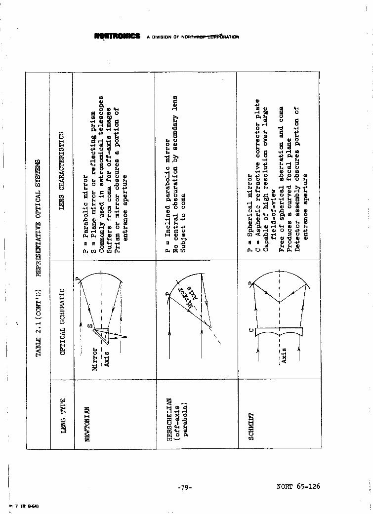
ADIVISIONOFNO--RATION
U_
crJ
C.)1-1
O
r.3v
r_i-iiz;
c.)
rtJ
[.3I-4
r_
r_i--4
[D
ma)
_ e -,-0 ,,,4
w
_o_
N 0 0 _14
m11=
8lq u0 t)I_ mf_
0
e
_ o
0 '_ _
_I> _0
_,o 81_
_,_o _o_ °0 o m
i\ i /I
I !
_o•,..I 4.)
;1 s:l o
O,r--_
\
\
k _ O I m
O
O4-_
""_ _,_
o
I : !o k I
!I
I
-79- NOR'r 65-126
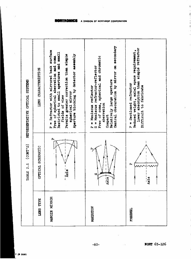
A DIVISION OF NORTHROP CORPORATION
C_
H
?E_
v
c_
C_
H
H
0
*O
omer_
O
k u m
0 _ •
_:_ r-I 0 0
_ O_a_r._
_m mk
._ 0_ b0m O
,!I
lm
II
O0 o
o®- g_
m•,4 ,,,e.i
H H • r-,4 I:3
t_,,, r,,_ _ r,,,} _:_ tu
"t t t :_
n _ "_0,,) ,,,,,,-t
I
A/,\
/'\I
_i I-r4
-80- 1_o1_ 65-_.6
7 (R 8-64)

A OIVISION OF NORTHROP CORPOR£TION
techniques. The _--_ number of lines ruled on a standard chart that can
be resolved by the lens deterz_aes the resolution of the lens.
This resolution criteria however does not yield a complete definition of the
energy distribution of the image of a point source such as a star. Assuming
that the aperture of the lens is circular, the star image formed is a brightcentral disk surrounded by a series of fainter rings. The bright central
disk is known as the "Airy" disk and the diameter of this disk is the figure
_ich is also quoted as the resolution of the lens. The radius of the
disk for a perfect lens can be determined by the following equation:
e : 1.22o! (2.1)a
where 8 is the angular radius of the ring, A is the wavelength of light
and a is the diameter of the objective lens. The linear diameter of the
Airy disk is then
d = 28f (2.2)
where d is the diameter of the Airy disk, and f the focal length of the
optical system. From the previous equations the size of the Airy disk
is shown to be inYersely proporti_al to the diameter of the lens, so
an e_remely high resolution lens must be large to reduce the diffraction
effects from the edges of the lens.
In Table 2.2 is shown the dimensions of the diffraction pattern of a star
image that is produced by a perfect lens.
TABLE 2 •2
RING
Central maximum
First d_rk
Second bright
Second dark
Third bright
Third dark
Fourth bright
Fourth dark
Fifth bright
Fifth dark
ENERGY DISTKIBDTiON OF __a-R IMAGE
i i
m
0
1.22
1.638
2.233
2.666
3.238
3.69_
_.2_l
_.722
5.2_3
Imax
1
o .017h5
O.00_15
0.00165
0.00078
Itotal
1
o.o8_
0.033
0.018
0.011
-81- NORT 65-126
Form 7 (R 864)

£ DIVISION OF NORTHROP CORPORATION
The angular separation of the different rings from the center of the pattern
can be calculgted by the relationship, •
e ffi _ (2.3)a
where e is the angular separation and m the value given in Table 2.2. The
values of I in the table are the relative intensity of the different
rings and !tota 1 is the total amount of light in the ring, both compared
to the brightness of the central disk.
The instantaneous field of view of the optical system is set by the focal
length of the lens and the size of the active area of the photodetector.
The total field coverage is the field that is swept by the detector during
a scan cycle of the optical tracker end is a function of the design of the
scanning mechanism rather than the optical system.
Reflective and refractive elements are reflecting surfaces and transmitting
elements that are used to focus the collected optical rays. The choice ofrefractive or reflective elements or a combination of the two (catadioptric
system) in the optical system design are parameters that are available to
the optical designer to achieve the size, speed, image quality, and spectral
response desired. In general a reflective optical system has the advantage
of being free of chromatic aberratinn so the lens can be used in the design
of ultra-violet, visible and infrared tracking systems by interchanging the
optical detector.
The Cassegrainian optical system is the most co_nly -used reflective
optical system. In this design, the convergent ra_-s in_ the optical system
are reflected off two mirrors, essentially folding the optical path, so
that the length of the telescope can be shortened by a factor of two over
a simple lens.
The optical efficiency of a reflective system, in a design where the optical
axis is concentric to the entrance aperture, is reduced due to blocking of
a portion of the entrance aperture by one of the reflecting surfaces as in
the case of the Cassegrainian system, or by the detector assembly as in the
case of the parabolic optical system. By utilizing only a portion of the
primary mirror (off-axis parabola), the loss in optical efficiency due to
blocking of the entrance aperture can be eliminated. However, one of the
prime advantages of the reflective system, that of compactness in mechanical
design, must be sacrificed.
The refractive optical system almost always forms an image at a plane which
is beyond the last element in the optical system. This allows easy access
to the image plane, so the optical design can proceed separately from
the mechanical design of the tracker. With the reflective system, the image
plane may fall within the optical system, so the optical modulation
-82- NORT 65-_6

A DIVISION OF NORTHROP COFIPOR&TION
mechanism and the detector must be located within the optical system.
The Cassegrain_m system provides an inure plane that is beyond the primary
mirror, permitting easy access to the image plane. However, due to the
arrangement of the reflectors in the Cassegrainian system, the usable •field of view in which no _18netting occurs is limited.
The materials used in a refractive optical system must be selected con-
sidering its optical transmission properties, index of refraction and
mechanical properties. Since the optical transmission and the index
of refraction of most optical materials vary as a function of the wave-
length of light, the performance of a refractive optical system is normally
optimized for two wavelengths, somewhere towards the ends of the desired
spectral band. To minimize the degradation of the image quality beyond and
between these design points, multiple elements with different indices of
refraction are utilized to compensate for the change in the dispersive
power of the different elements as a function of wavelength.
Combinations of refractive and reflective elements in an optical system
are useful in applications where a fast lens with high resolution over a
large field of view is required. The Schmidt optical system is the best
known catadioptric system. The feature of this system is the aspheric
ref_=ctor corrector plate. The corrector plate provides variable zone
correction of spherical aberration, so that lens resolution close to the
theoretical limit can be obtained over a field of view of 60 x 60 degrees.
The image plane produced by a Schmidt lens is spherical, so the detector
or light modulation mechanism must also be curved to properly utilize this
lens design.
2.i.i
Certain photodetectors such as photo_tipliers and photodiodes, produce the
same output regardless of the location of the target image on the sensitive
area of the photodetector. An optical tracking system utilizing a detector
of this t_pe frequently will be used in the optical configuration illustratedin Figure 2.2.
Objective
fl ' _ Field
Chopper __%__or_
FIGURE 2.2 FIELD LENS SYSTEM
-83- NORT 65-126
7 (R _4)

£ ONISION OF NORTHROP CORPOR£TION
The objective lens forms an image of the scene at the plane in which the
light chopper is located. The objective lens is defined as the lens
closest to the object being viewed. A field lens, or a lens that subtends
the field of view is placed close to the focal plane of the objective lens
to refocus the light collected by the objective onto the detector.
The field lens forms an image of the entrance aperture at the detector
plane. With this optical arrangement, the collected light is spread
uniformly Over the sensitive area of the detector and eliminates theeffects of sensitivity variations over the detector area. The use of a
field lens provides a second advantage in that the size of the detector
required to cover a given field of view with an optical system of a given
focal length can be reduced.
In the optical system shown in Figure 2.2, the diameter of the objective
lens is a, and the focal length fl' The field lens has a focal length of f2"
The location of the image produced by the field lens can be calculated
using the lens formula
i_ = I__ + 1 (2.4)
f2 fl s
where s is the distance of the image from the nodal po;nt of the lens
-flf2
s = (f2_fl) (2.5)
_he size of the image t.._a, produced by the field lens is given by
= a__ (2.6)
s fl
y = f2_fl(2.7)
The quantity V is the linear dimension of the field of view (8) of the
objective lens, and is also the required diameter of the field lens.
and
V = fl tan e (2.8)
f2 = fI_o2 (2.9)V
where fno2 is the f/number of the field lens
f2 = V fno2 = fl tan e fno2
-84- NORT 65-_-6
Form 7 (R 8-64)

A DIVISION OF NORTHROP CORPORATION
• he factor by vhich the size of the detector required to subtend a given
field of view can be rednced using a field lens is given by the ratio of
=v (f2 - fl)fltan e
(2.1o)
Substituting for f2'
Since
:_. = .....-a fno2 !
V fl(tan e fao2-i)
flm
a
fnol (2.11)
where fnol is the f/number of the objective lens,
y = -fno2V fnol(fno2 tan e - i)
(2'12)
For typical star tracker applicaticms,
8 < fnoi < 64
0.75 < fno2 < 1.5
0.5 deg. < e < 5 deg.
The reduction of the size of the detector used with an optical system with
an f/16 objective lens, an f/1 field lens and a field of view of 1 degree,
is from Equation 2.12,
y = --1
V 16(0.017h - I)= 0.0635 times
For a very fast objective lens, in the order of f/l, the use of a field
lens is not advantageous, since the image produced by the field lens
will not be substantially reduced over the size of the image produced
by the objective.
_orm 7 (R 8-64)
L
-85- NORT 65-126
£ OIVISION OF NORTHROP CORPORATION
2.2 BASIC DETECTOR TYPES
The detectors which are employed in star tracking systems fall into three
general classifications. The first type is a single element or "point"
detector which provides an electrical output signal which is independent
of the location of the incident radiant energy on the sensitive surface
of the photodetector. With this type of photodetector, the incoming
radiatic_ must be modulated by a mechanical scanning device to encode the
star location information and to provide rejection of background radiance.
The photomuitipiier and the photodiode are examples of this type of
detector.
The second type of detector is an extended area detector, whose output
is a function of the distribution of radiant energy over the sensitive
area of the detector. The image dissector is one example of an extended
area detector, and csn be considered as a matrix of single element de-tectors which are individually interrogated to determine the radiation
distribution. Another example of an extended area detector is the Radiation
Tracking Transducer (RTT), madeby Micro-Systems Incorporated. This
detector is essentially a four-terminal device which determines the
position of the incident radiation by the relative amplitude of the
photovoltaic Signal produced by the incident energy at the four terminals
of the detector. The two detectors differ, however, since an image of
the scene being viewed can be reproduced using an image dissector, but
the RTT can only indicate the centroid of the energy incident on the de-
tector surface.
±--hethird type of detector is an extended area detector which, in addition
to the proper+_ies of the second type of detector, is also capable of
integrating the incident radiant flux over a period of time to incres_q
the effective target signal. Two examples of this detector type are the
vidicon and the image orthicon. In the vidicon, storage of the electron
image is provided through the extremely high capacitance of the photo-
conductive surface which comprises the faceplate of the vidicon. In the
image orthicon, storage is provided by means of an electrostatic image
created within a special-image section of the tube. In both of these
detectors, an electron beam is used to read out the stored image.
2.2.1 SinKle Element Detectors
The majority of the optical detectors manufactured fall into the single
element category. Among these are included photodiodes, photomultipliers,
the semiconductor elements, silicon and germanium, and a number of photo-
conductive, photovoltaic and photomagnetic compounds.
-86- NORT 65-126
7 (R 8-64)

& DIVISION OF NORTHROP CORPORATION
2.2.1.I Photomultipliers
Photocl_.ocles have a photoemissive surface which emits electrons when
illuminated by light. The emitted electrons are then collected by an anode
which is biased at a higher voltage than the photosensitive emissive surface.
_he photomultiplier is a modification of the photodiode, in which the
emitted electrons are electrostatically accelerated then allowed to strike
a specially prepared surface called a dynode. The dynodes are coated
with a substance which releases secondaz_- electrons upon being bombarded
by high velocity electrons. This process can be iterated until the
electron flux is increased many orders of magnitude. As a circuit
element, the photomultiplier can be analyzed as a high impedance current
generator, whose performance limits are determined by the efficiency of
the photosensitive surface, compared to the thermionic emission of this
surface and the leakage currents in other parts of the photomultiplier.
The spectral response of the materials that exhibit photoemissive properties
fall primarily in the visible portions of the spectrum. The different
t_pes of photoemissive materials classified with respect to spectral
response exceeds 21 in number, but basically there are four to five
different photoemissive materials that are of interest. These include
the materials that provide SI, SII, and $20 response, and a new material
with ultraviolet response, for which an "S" number has not yet been
assigned. The materials used to create _ S! photocathode response
are Ag-0-Cs; the SII response, Cs-Sb; the $20 response, Sb-K-Na-Cs ;
and the bn! response Cs-Te. See Figure 2.3.
The spectral response of the SI photocathode extends past !.0 microns,
and it has the best red response of any of the photoemissive materials.
However, its quantum efficiency, or the ability to convert incident photons
to free electrons, is very low. At 0.8 microns, which is the peak of the
SI red response, the quantum efficiency is 0._ percent.
The SII spectral response ex_ends from 0.3 to 0.6 microns. The quantum
efficiency of this material that provides this response exceeds 13 percent
at the peak of its response curve, providing a very efficient photocathode.
To increase the quantum efficiency of this material, the material is deposited
on a mirrored surface to permit a second pass of the incident light through
the photosensitive material. The quantum efficiency is increased to
greater than 20 percent at the peak of the _spectral response. The Cs-Sb
photocathode with this greater quantum efficiency is designated as having
an S17 response. The maSerial comprising the SII photocathode is trans-
lucent, permitting design of photomultipliers with the photocathode de-
posited on-the rear of the entrance window of the photomultiplier, a
configuration referred to as end-on photomultiplier. To achieve the
S17 response, the photocathode is deposited on an opaque substrate,
requiring a different mechanical arrangement of the entrance window,
the photocathode and the dynodes. The net effects of this mechanical
-87- NORT 65-126
Form 7 {I1s-r,4)

__ A O!VfSION OF NORTHROP CO_PORATIQN
I00
I0
5
;!I
I
Ii
\ _c_'e_ ''-
I .fy I
'_ '( r I '
//", I
0.i
0.i 0.3 0.5 0.7 0.9 i.I
Wavelength in _crons
FIGURE 2.3 SPECTRAL RESPONSE OF FIVE REPRESENTATIVE PHOTOEMISSIVE SURFACES
-88- NORT 65-]2.6

A DIVISION OF NORTHROP CORPORATION
arrangement of the phot_nultiplier components on the design of an
optical tracking system, are that the optical system used with the
S17 phot_nultiplier must have a longer back focal length, and the
optical tracker cannot be designed with the detector package synnnetri-
cal with respect to the optical axis.
The spectral response of the Cs-Sb surface can be extended into the
ultraviolet region, by the utilization of a photocathode window that
has good ultraviolet transmission. Fhotomultipliers having $5 and
$21 responses are examples of detectors utilizing this manufacturing
technique. Some of the visible response of the Cs-Sb surface is
sacrificed te achieve sensitivity out to 0.2 micron.
The S-20 photocathode has a very high quantum efficiency and an ex-
cellent red response. In comparison with the S17 photocathode, the $20
quantum efficiency at the peak of its response curve is lower, but
its spectral response extends farther into the red region of the spectrum.
The $20 can also be utilized in a head-on configuration, so the choice
between these two detectors in a star tracking system is dependent
upon the mechanical design of the star tracker as well as the radiant
characteristics of the star.
The Cs-Te photocathode has a long wavelength cutoff at about 0.32
microns. The spectral response is limited to the ultraviolet region,
and a photomultiplier with this response of this type is useful for
making daytime ultraviolet measurements and experiments, since the photo-
multiplier is unaffected by solar radiation.
The performance of a star tracking system utilizing a photomultiplier
can be calculated from the following expression:
where
S/N
F isC
C is
B is
q is
i d is
I is
a is
b is
G is
af is
F CBC
#2q(i d + Iab )i-i + I/G)Af
the effective star flux incident on detector (lumens)
the detector response to the incident star flux (amp per lumen)
the electronic transfer characteristics of the signal amplifier
the charge of an electron (coulomb)
the photocathode dark current (amp)
the illumination on the detector due to background radiance
(foot -c Lndles )
the area of the scanning aperture (square feet)
the detector response to background flux (amp per lumen)
the gain pe r dynode stage in the photomultiplier
the electronic bandwidth (cycles)
-89- NORT 65-12.6
(R 8-64)

A OIVISION OF NORTHROP CORPORATION
2.2.1.2 Semiconductor Detectors
There are a number of photosensitive compounds and elements that changetheir electrical characteristics when illuminated by radiation in the
optical regicm of the spectrum. The more conmaon of these that are
used as detectors of optical radiation include silicon, germanium,
selenium, lead sulfide, lead selenide, lead te_luride, lead arsenide,
gallium arsenide, indium antimonide, cadmium sulfide, and cadmium selenide.
In general these detectors provide a change in electrical characteristics
across a two-terminal network, which is proportional to the total
radiant flux on the detector regardless of the location and the con-
centration of the radiant flux on the sensitive area of the detector.
The various detectors may be photovoltaic, photocc_ductive, or photo-
magnetic, and in some cases can exhibit all three characteristics.
Of the detectors listed, the detectors that show the most promise
for use in a star tracker are silicon and cadmium sulfide. The other
detectors are either sensitive to infrared energy alone, have too low
a respensivity, or are similar in characteristics to silicon and
cadmium sulfide.
2.2.1.2,1 Silicon
A silicon detector is a photovoltaic cell which is manufactured as
shown in Figure 2.4. A diffused p-n junction is formed between a thin
l_ver of P type silicon and a thicker layer of N type silicon. Nickel
electrodes are plated to the silicon to provide electrical contact.
Load_
+
I _ _p type silicon
p-n Junction
n type silicon
TNickel electro
FIGURE 2.4 SILICON PHOTOVOLTAIC DETECTOR
When light strikes the p type silicon, hole-electron pairs are created
in both the p and n regions, but the electrostatic field at the Junction
sweeps the holes into the p region and the electrons into the n region.
The unbalanced charge carrier produces a voltage difference across the
output terminals.
-90- NORT 65-126

A DIVISION OF NORTHROP CORPORATION
The sensitivity of a silicon detector is expressed in terms of D* where
De is defined as the detectivity of the cell for a detector of unity
area and unity bandwidth. The detectivity can also be expressed as
the signal-to-noise ratio produced with a radiant flux of unity incident
on the detector.
D, = AI/2/P. (c -cpsl/2/watt)
The quantity A is the area of the detector, and PN is the radiant flux
required to provide a signal-to-noise ratio of one, when the electronic
bandwidth is unity.
PN = JNA/V-Afl/2 (watts)
where
N is the rms noise voltage (volts)
J is the radiant flux density (watts/cm 2)
V is the rms signal voltage (volts)
Af is the electronic bandwidth (cycles)
The detectivity of silicon is in the order of 1012 cm - cpsl/2/watt,
and the time constant is 300 _ sec. The spectral response is shown
in Figure 2.5.
1000.801
m
0.60
/
/o.ko
0.20
0
O. 0.7 O. 0.9 1.0
Wavelength in Microns
\
2.5 SPECTRAL RESPONSE OF SILICON PHOTOVOLTAIC DETECTOR
-91- NORT 65-126

A DIVISION OF NORTHROP CORPORATION
2.2.1.2.2 Cadmium Sulfide
Cadmium sulfide and cadmium selenide are primarily photoccaductive
materials, though it is possible to manufacture detectors of these
materials with photovoltaic properties. These detectors have a very
high responsivity, and are capable of an impedance change of three
orders of magnitude when the incident radiant flux is changed from
zero to i0,000 foot-candles. These materials are affected by humidity
and temperature, and are subject to fatigue. Detector fatigue is
evidenced by the loss or reduction of detector response at low light
levels after prolonged use, or after being exposed to intense light.
For use in a star tracker, the detector would have to be enclosed in
a sealed, temperature controlled chamber, and also be provided with a
sun protection device. The spectral response and the responsivity
curves of CdS and CdSe are illustrated in Figure 2.6.
2.2.2 Extended Area Detectors
2.2.2.1 Image Dissector
The image dissector utilizes a photoemissive cathode in which the
electrons emitted by the _notosensitive s,_face are accelerated and
deflected by means of electrostatic or electromagnetic fields. The
electron emission from a given area of the photocathode is proportional
to the flux density of the light on the cathode, so an electron "image"
is produced. Thi_ electron image is scanned across a mechanical ape_ure
by changing the beam deflection fields. The electrons that enter the
mechanical aperture are then multiplied in a dynode chain.
The image dissector is identical in function to the photomultiplier
with the exception that a small area of the photocathode can be sampled
with the image dissector, rather than the complete cathode with the
photomultiplier. _Theneed for a separate scanning mechanism to encode
the optical signal is thus eliminated. The performance of a star tracker
utilizing an image dissector can be analyzed in the same manner as a
photomultiplier system.
2.2.2.2 Radiation Tracking Transducer
The sensitive area of the radiatica tracking transducer (RTT) consists
of an extended photovoltaic p-n layer. The photoeffect produced is
similar to that of the silicon photovoltaic cell. The excess electrons
in the n region of the RTT spreads out laterally and, due to the for-
ward bias conditions, recrosses the Junction and combines with the holes.
The potential difference measured between various points on the n layer
-92- NORT 65-126
7 (R 8-64)

£DIVISIONOFNORTHROPCORPORATION
CZe_rex Detector Type
1.00 i 5 7 k.Type 2 - CdS
o=0.80
Type h- CdSe
Type 5 - cas0.60 Type 7 - cds
",-4
,-4
0.40
0.20 boO.5 o. o.9
Wavelength in Microns
0
FIGURE 2.6a. SPECTRAL RESPONSE OF SEVERAL TYPES OF CLAIREX
CclS and CclSe DETECTORS
0.i
0.01 "
0. I I i0
Illumination in Foot-Candles
i00
FIGURE 2.6b. VARIATION OF RESISTANCE OF CdS and CdSe WITH ILI//MINATION
-93- NORT 65-126
Form 7 (R 8-64)

__[_ A DIVISION OF NORTHROP CORPORATION
provides a distribution that is radially sy_netrical about the light
spot. By placing electrodes at four points on then layer, the posi-
tion of the light spot relative to these four points can be determined.
The RTT provides an output that is a function of the total flux on the
detector as well as the location of the centroid of the illumination on
the detector. If the device is utilized in a tracking system, the volt-
age across the cell must be measured to determine the intensity of the
detected light and this information used to normalize the gain of ampli-
fiers used to measure the four lateral voltages in the detector.
The single advantage of this detector is the elimination of moving parts
when utilized in an optical tracking system. However, as pointed out,
accurate radiometry is required to provide off-axis pointing information,
which is required for proportional control in a closed loop tracking
system. In the presence of background radiation, the radiometric data
would be erroneous, since only a small portion of the total radiometric
signal would represent the star flux. Compensation of the background
flux by biasing the radiometrilc output is feasible, but under dynamic
tracking conditions the background flux will be variable and this tech-
nique cannot be utilized. The silicon cell used as a two-terminal device
utilizes most of the electron-hole pairs that are created to provide a
star signal. With the RTT, most of the electran-hole pairs are lost
through recombination, and the signal is _ther reduced by the require-
ment for four output channels rather than one.
±--neN_P of the detector is 5 x i0-I0 watts for a 5 cps bandwidth, and
the detector provides an output ranging from I00 to i000 volts per inch
per watt for an off-axis spot of light. The D w of the detector is 6.7 x
109 cm-cpwl/2/watt compared to a Dm of 1012 cm-cpsl/2/watt for a photo-
voltaic silicon detector used as a two-terminal device. The detector
sensitivity is thus compromised to provide positional information.
2.2.3 Extended Area Detectors With Storage
2.2.3. i Vidicon
In the RCA C-73_96 vidicon, which is a miniature vidicon developed for
high sensitivity in slow scan applications, a thin-film composed of com-
pounds of antimony and sulfur is vacuum-deposited on the back of the
entrance window. This photoccmductive layer which is about four microns
thick, is called a target. The spectral response illustrated in Figure 2.7,
peaks at 0.52 microns, and the qusntumefficiency at the spectral peak
is close to unity. The high capacitance and resistivity of the photo-
cathode provides electronic charge storage capability, and the combina-
tion of high quantum efficiency and storage capability yields a
sensitivity of 650 microamperes per lumen under moderate lightingconditions.
-94- NORT 65-126
(R 8-64)

AOIVISIONOFNORTHROPCORPORATION
Q)m
=om
-,-I
,-4a)
1.00
0.8o
0.60
0.40
0.20
o.ooo.ho o._,5 o. 50 0.55 0.60 0.65 0.70
Wavelength in Microns
Beam accelerating
F volt age
,hi,L___
------11'!'! ]
[--i h
Cathode
Transparent comducting
layer -7
............... 7- - - Glass
Scanning / Photo-
Electron/ conduct_Beam -- Target put
Signal
Target supply voltage IIl---_lli ltL
Scanning beam
resistancej _/_
Target element resistanc _ Vout
Target element capacitance _ _+RL
FIGURE 2.7 SPECTRAL RESPONSE (RCA C-73h96) AND EQUIVALENT CIRCUIT OF VIDICON
-95- NORT 65-]26
Form 7 (R 8..64)

AI DIVISION OF NORTHROP CORPOI:UtTION
The equivalent circuit of the vi_icon is illustrated in Figure 2.7.
_ae scene being viewed is imaged on the target, which is biased positively
with respect to the electron gun cathode by i0 to 15 volts. If the target
is unilluminated, the potential on the back of the target will be reduced
to that of the electron gun cathode after several scans. Subsequent
to this initial target charging period, the beam will deposit sufficient
electrons to compensate for the leakage current through the target layer
in the preceding frsme period. If the target is then illuminated, its
resistivity decreases and the current flow from the back to the front
surface of the target is increased. Since the target potential is re-
duced, the number of electrons deposited on the target by the scanning
beam will increase. This increase in deposited electrons is reflected
in the load resistor, RL, as a current flow. The current in the load
resistor comprises the output video signal.
The resistivity of the target is a function of the illumination on the
target, and at low light levels, the change in resistivity is also cumu-
lative over the frame period. In an image dissector, electrons are
continuously emitted from the photocathode, but all are discarded ex-
cept those from a limited sampled area. This storage characteristic
of the vidicon becomes useful when the star tracker is operated in the
presence of hig h sky background. Since both the star and the background
radiance are averaged over a frame period, if the total star flux inci-
dent on the vid_icon is greater than the statistical average of the back-
ground radiance, the star can be detected.
_-_ e_A_Aman_e of the vidicon star _ • system can be calculated
from the following expressi_'l :
F CSBrS/N = c a
#2q(i d + IAbS)Af
where S is the gain in sensitivity due to storage
ra is the amplitude response of the scanning beam to smallelectrostatic charges
A is the area of the photoconductive target (square feet)
The storage gain S is equal to the number of scanned elements in the
raster. Since the star image falls on one line of the raster, the star
image will be scanned once per frame, and the star signal is allowed to
accumulate between successive scans.
If the horizontal resolution is made equal to the vertical resolution,
where the vertical resolution is determined by the number of scanning
lines used in the raster, the number of elements in the raster will be
the square of number of raster lines.
-96-NORT 65-126

_m A OIVISlON OF NORTHROP CORPORATION
2.2.3.2 Image Orthicon
Four separate functions are verformed in the image orthicon tube to produce
a video output signal (figure 2.8). The image orthicon utilizes an image
section, a target mesh storage section, a scanning section and a multiplier
section to perform the four functions. In the image section, electrons
emitted by the photocathode, are linearly accelerated providing an electron
image of the scene being viewed. This electron image is then directed
onto a target composed of a glass disk which is in close proximity to a
fine mesh screen, When a target of insulating material is bombarded by
high velocity electrons, secondary electrons are excited at the surface.
An electrostatic charge pattern is established on one side of the glass
target which corresponds to the optical image on the photocathode. The
opposite side of the glass target will become charged positively with
respect to the equilibrium potential of the target. In the scanning
section the target is scanned by an electron beam, and electrons are
deposited on the target in direct proportion to the electrostatic charge
pattern on the rear side of the target. The electrons that are not
deposited on the target are collected then amplified in a multiplier
section. The output of the multiplier becomes the video output signal.
By coupling the noise-free gain of the electron multiplier and the stor-
age _ain provided by the glass target, a highly sensitive detector is
produced. The image orthicon is best suited for low light level applica-
tions. Due to the low capacity of the target, and the limited magnitude
of the electrostatic charge that can be accumulated on the target due
to the natural physical limitations of the _arget and mesh combination,
the output of the image orthicon saturates when the illumination on the
faceplate increases by two orders of magnitude. For daytime operation
against a brigh_ sky background, the image orthicon does not perform as
well as a vidicon, though for a given diameter collecting optics, the
image orthicon is capable of detecting a star that is five star magnitudes
dimmer than with the vidicon.
Since the impedance of the target is very high, the mesh is used to establish
the target equilibrium voltage. If the photocathode is dark, the scanning
electron gun will bring the rear of the _arget to the electron gun cathode
potential. The front of the target should then be at the equilibrium
potential, but since the mesh and the target are capacity rather than
direct coupled, this equilibrium cannot be achieved. If the mesh is
brought closer to the target, the potential of the front surface of the
target can be brought closer to the equilibrium potential. However, the
positioning of the mesh with respect to the target must be compromised
to permit the build-up of electrostatic charge under normal operating
conditions, so essentially minimum sensitivity is a compromise with dynamic
range,
-97- NORT 65-126
7 (R II-t4)

A 01VISION OF NORTHROP CORPORATION
Focus Vertical and Horizontal
Coil_ Deflecti_ Coils 7
Accelerator \ / Alignment _
Lens ---_ Grid -7 _ _/-- Coil
\ _\\\\\__\\\\_\____ Eiectron,_ i,,_/_.._.__1_,/////////////////////////,_ _ l--G=
NN \il/_\\\_>__\\\\\\_,\\\\\\\\\\\_ \ Ii
Ph°t°cathode-J ,/ _ X - \ / /
/ Decelerator -_ X \ Electron / /
Fine _s_ ÷ _ Be. ,A MultiplierScreen Target Focus Dynode s
FIGURE 2.8a. IMAGE 0RTHICON SCHEMATIC ARRANGEMENT
@Jm
,n
@J
1.00
0.80
0.60
0._0
0.20
i
/o_ O.h 0.5 0.6 0.7
Wavelength in Microns
FIGURE 2.8b.
_'orm 7 (R 8-64)
SPECTRAL RESPONSE OF WESTINGHOUSE WL-7611 IMAGE 0RTHICON
-98- NORT 65-126
• L

A OIVISION OF NORTHROP CORPORATION
The performance of an image orthicon star tracker can be calculated f_'om
the following expression :
S/N =
F t CSBrC a
i
gm _2q (id + tlAbS)(l + I/G)Af
where F is the effective star flux incident on detector (lumens)C
t is the transmission of the fine mesh screen which is in
front of the target in the image section
C is the detector response to the incident star flux (amp.
per lumen)
S is the gain in sensitivity due to storage
B is the electronic transfer characteristics of the signal
transfer
r is the amplitude response of the scanning beam to smalla
electrostatic charges
_= _h. increase in beam noise due to incomplete modulationg_ ....of the scanning beam
q is the charge of an electron (coulomb)
id is the photocathode dark current (amp.)
I is the illumination on the detector due to background radiance
(foot-candles)
A is the area of the photoconductive target (square feet)
b is the detector response to background flux (amp per lumen)
G is the gain per dynode stage in the photomultiplier
Af is the electronic bandwidth (cycles)
-99- NORT 65-126

A OIVISION OF NORTHROP CORPOR£TION
2.3 MECHANICAL MODULATION METHODS
The single element "point" detectors provide an output signal that is
independent of the location of the flux ccncentrati_ on the sensitive
area of the detector. When this type of detector is used in an optical
tracking system, some mechanical method of modulating the incident
radiatien must be utilized to provide an indication :of the location ofthe luminous flux relative to the center of the field of view of the
optical tracker. Some of the mechanical modulation techniques that have
been used to encode the optical signal to provide error information
include radiation balance, optical field dither, amplitude-modulated
reticle and frequency-modulated reticle systems.
2.3.I Radiation Balance System
In a radiation balance system, the radiant flux from the object that is
to be tracked is divided optically into two or more channels. The optical
tracker is designed so that it will be aligned with the target when the
signal from all the channels are equal. Different system implementations
have been used in operational systems, and while the most co_on ccnfigura-
tien is an arrangement of four detectors utilized in pairs to provide
pointing informatiun in two orthogonal -__.es, a system using three detectors
to provide two-axis control is feasible. In Figure 2.9 is illustrated a
typical four-detector radiation balance system, and a three-detector
system, both using shadowing masks to change the total flux on the
different detectors as a functien of the angle between the ts_get and
the line of sight of the optical tracker. The three-detector design
was implemented by the Jet Propulsion Laboratory in their Earth Sensor,
which was used to provide an attitude reference relative to the earth
in the Ranger series of space flights.
The X and Y axes errors in the four-detector configuration is derived by
comparing the outputs from two detectors (A-B and C-D), and the total
signal or the radiometric value (R) of the target is determined by
adding the signals frem two opposing detectors. The X axis error for
the three-detector configuration is derived by comparing the outputs
from two detectors, and the Y axis error is obtained by comparing theoutputs from all three detectors. The radiometric signal is the sum
of all three signals.
The reliability of the three detector system is greater than the four-
detector system since the compc_ent count in the system is reduced.
For good linearity and resolution, highly sensitive, matched detectors
are required in both systems. The three-detector system requires three
detectors that are matched to each other, while the four-detector system
requires two pairs of matched detectors. In the three-detector system,
the outputs of the three detectors cross-couple, so nonlinearity in de-
tector response will add an offset error to the sensor error transfer
C_e.
-I00- NORT 65-126
_rro y (R 8-64)

A OIVlSION OF NORTHROP CORPORATI_
_o
I--I
I-4
C)
r..)m
0
u0
-II
I I
L___J F-
IIL,.I:----I
I_.J
-i-] , ÷ _
o
4_
O4_
m
!
_ LY__JH II II l
k_
-i01- NORr 65-126
o_m 7 0t 8-¢,4)

_m_m A DIVISION OF NORTHROP CORPOAATION
The radicRetric balance type of sensor does not use scanning or moving
mechanisms to modulate the optical signal. The advantage of this system
is the high reliability due to the simplicity of the basic design. How-
ever this design has no background discrimination capability, and any
nonuniformity in the back_ound radiance will produce an error output. ,.
In addition, the background signal from the detector is produced by thesum of the background flux cn the detector, so the instantaneous field
of view of the detector _st be very small if a _ target is to be
acquired and tracked in the presence of background radiance. Defining
the minimum detectable star for a background limited star tracking system
as the star magnitude that will provide an illuminance at the entranceaperture of the sensor that is equal to the background luminance within
the solid angle defined by the sensor field of view, then
where FS
B'
B'F -
S
is the star illuminance in lumens/ft 2
is the background or sky brightness in foot-lamberts
is the sensor field of view in steradians
The minimum detectable star for a backgrou_d=!imite _- optical _ystem is
thus a function only of the background brightness and the field of view
of the sensor. The size of the aperture of the sensor or the ultimate
sensitivity of the detector are unimportant when the background radiance
is the primary noise source. The l_inance from a c_e foot-lambert sky
background will provide an effective background illuminance at theentrance aperture of the optical system of 2.67 x 10 -6 lumens/f_ 2 for
a sensor with a i0 arc-minute by i0 arc-minute field of view. A -1.64
magnitude star will provide this illuminance, so only celestial bodies
brighter than -1.64 magnitude are detectable under the given conditions.
Since the daytime sky brightness at sea level is approximately 500 to
i000 foot-lamberts under low sky background conditions, and Sirius, the
brightest star in the heavens is a -1.47 magnitude star, a radiation
balance star tracker is only usable as a nighttime star tracker.
2.3.2 Mechanical Optical Field Dither
The radiation balance star tracker is operated in a dc mode, so the
collected star flux must be greater than the total background flux for
the star to be detectable. Since the sky background in a limited region,
say o_e degree square is quite uniform, the sky background can be used
to establish a threshold to permit detection of a star by comparison of
one portion of the sky to another. If this comparison is performed
cyclically, the star signal will be encoded at a given frequency. The
background signal out of the detector for a uniform sky background will
-i02- loom? 65-_6
_m_s A DIVISION OF NORTHROP CORPOR£TION
be a high level signal with a frequency distribution resembling noise.
A narrow electronic bandpass centered about the repetition frequency
of the star signal can be used to attenuate the background signal.
Since the background signal is a function of the characteristics of the
detector utilized in the optical detection system, parameters such as
the modulation frequency and the electronic bandwidth will also influence
the system performance, so systems of this type must be censidered
individually to determine performance limits.
If the star signal is correlated in the frequency domain and the back-
ground signal is uncorrelated, increasing the aperture of the opticalsystem will increase the target signal to background noise ratio. The
collected star and the background flux both increase proportionately to
the square of the aperture, but if the background signal out of thedetector has a "white" noise distribution, the rms value of the back-
ground signal in a given bandwidth will increase as the square rootof the background signal. Thus the star signal with a given background
will increase linearly with the aperture size.
Instead of taking discrete samples of finite areas, the instantaneous
field of view can also be mechanically dithered to modulate the star flux.
The dither can be produced by oscillating a mirror in the optical path of
the star trackers or by moving the entire sensor head. By scanning the
dither pattern, a large field of view c_u be sesrched.
A star tracker utilizing this dither scanning principle was designed by
Nortronics for the SM 62A Snark missile, and contained a two-inch diameter
optical system with a 20-inch focal length, an RCA 7029 photomultiplier
as the detector, and a circular instantaneous field of view of _0 arc-
seconds. The system was capable of tracking third magnitude stars in the
daytime. Demonstrated tracking capability included tracking of a +1.93
magnitude star against a 1350 foot-lambert background with a peak signal
to rms noise ratio of 22"1, and tracking of a +2.75 magnitude star against
a _i0 foot-lambert background with a peak signal to rms noise ratio of
22:6. These results were obtained with very narrow electronic bandwidths,
so long search acquisition times are required, and the information rate
is low, producing a star tracker with a limited tracking rate capability.
2.3.3 Amplitude and Frequency Modulated Reticle Systems
A common technique in the design of optical tracking systems is the use
of a reticle placed at the focal plane of the optical system to modulate
the focused optical energy and to encode the target error information.
The reticle is composed of an intricate pattern of opaque and clear
segments, that combined with the proper scanning motion is capable of
providing target signal modulation and at the same time attenuating the
signal caused by background flux.
-I03- NORT 65-126
'orm 7 (R 8-64)

AOMSIONOFNORTHI_IDI:CIDI:IPO_TliDIM
In Figure 2.10 is illustrated two reticle systems that provide an amplitude
modulated (AM) and a frequency modu/xted (FM) target error signal. The
informatiom processing circuitry in these systems make use of demodula-
tion techniques co_0m to ecmmunicaticm circuitry to derive the trackerror signal.
In the AM system, a "rising sun" reticle is rotated to modulate the
target signal. The rays of the "sun" are composed of alternate clear
and opaque segments, and the other half of the reticle composed of a
50 percent transmitting surface. When the target is off-axls, the
target signal will be an AM carrier signal that is 100 percent modulated
at the reticle rotaticm frequency. The target error informatiom is
encoded in two side bands about the carrier frequency. The carrier fre-
quency is the reticle rotation frequency times twice the number of spoke
pairs in the reticle pattern, and the side bands are equal in width tothe reticle rotation frequency. The phase and the amplitude of the
envelope of the target signal are compared with a reference signal to
determine the direction and magnitude of the track error.
In the FM system, rotation of a wedge placed in the convergent lightpath of a refractive optical system, (off-axis mirror in a reflective
optical _system), will cause the target image to move in a circular
path at the focal plane of the lens. The scanning motion of the target
_e is called nu_aticm. For the AM system, the reticle is rotated,
but the reticle is stationary in the FM system and the target image is
scanned over the reticle pattern. When the target is on-axis, the nutaticm
circle will be symmetrical with respect to the center of the reticle and
the target signal modulation produced by the reticle will be an _ cartier
signal. The frequency of the FM carrier is the product of the nutation
rate and the number of spoke pairs in the reticle. When the target moves
off-axis, the nutation circle will be displaced with respect to the
center of the reticle, and the target signal will be frequency modulated
as the nutated image scans over the reticle pattern. The target signal
is amplified, limited, then demodulated to proTIde a track error signal.
The phase of the track error signal is a function of the phase relation-
ship of the high and low frequency compcflents in the target signal and
its amplitude is a fumction of the frequency deviatiom components in
the target signal.
The advantage of a reticle system is that a relatively large instantaneous
field of view can be scanned using a simple mechanical motion. The scanningis provided by rotation of an optical element, which is superior to the
dither scan system, considering the drive power requirements, and the
reaction force created by oscillating elements or movement of the entiresensor head. An ideal reticle has an average transmission of fifty
percent, so that a uniform background will produce no ac components
when scanned by the reticle.
-I04- _ORT 65-18.6
Fom_ 7 (R II-fl4)

ADNISIONOFNORTHROPCORPOR&TIOIM
o _ I _ " '
i o
_ oo _ l
- z05- _ORT 65-126
7 m 8-64)

£DIVISIONOFNORTHROPCORPOR£TION
Large background gradients will produce modulation compnnents at the basic
scan frequency, but since the system carrier frequency is much higher,on_v the lower amplitude harmonics of this signal will be within the system
bandpass. The reticle, however, cannot provide discrimination against
fine background details. In addition, manufacturing defects in the
fabrication of the reticle will produce modulation components even with
a perfectly uniform background.
With the rotating AM reticle system, the modullticn efficiency of the
reticle decreases when the target image falls in the s__ea of the reticle
where the detail in the pattern is smaller than the image size. This
effect causes the track error signal to decrease proportionately as the
target image approaches the center of the reticle. When the target is
aligned with the optical axis of the telescope, the modulation efficiency
is zero. There are two disadvantages in this loss of signal at null.
First, the system cannot provide a positive indication that the target
is being tracked, since the signal from the optical detector is the
same when the target is on-axis, as when there is no target within the
field of view. Second, the target error signal must exceed the system
input noise before the target error signal is detectable. Since every
system has a finite amount of noise, the tracking system will have a
dead band about the null point, producing a system that tends to "hunt"
when the target is on-axis.
In the FM system, a track indication sigj_al is alwaj,s present whenever
the target is within the field of view. With the target on-axis, the
detector output is an FM carrier, which can be used as a track indicator.
Since the amount of frequency modulation in the target error signal is a
function of the location of the target nutation circle with respect to
the center of the reticle, the demodulated error signal will provide a
track error signal that is proportional to the deviation of the line of
sight to the target from the optical axis of the tracker. The FM system
has superior tracking capability over the AM system in the presence of
noise, since the optical detector signal is limited, and high amplitude
noise pulses will not saturate the system. However, the AM system
utilizes a narrower system bandwidth, and has a higher system sensitivity,
and is capable of detecting dimmer targets under zero background conditions.
-I06- NORT 65-126
(R 8-64)

ADIVISIONOFNORTHROPCORPORATION
SECTION 3
UTILIZATION OF OPTICAL SENSING ELEMENTS
IN A SPACE VEHICLE
3.1 MONITORING OF PLATFORM DRIFT WITH A STAR TRACKER
The performauce of the platform under a high gravity environment and for
extended periods in a zero gravity field can be monitored by means of
celestial sightline determinations. Platform drift can be determined
and the platform updated from information obtained from several star
sightings. The same star tracker would also be capable of providing an
accurate reference for platform realignment should the platform be
tumbled in a mission, or in the event the platform is deactivated to
conserve power in an extended mission.
3.1.1 Platform Drift During Launch
To check platform drift during launch, a star tracker capable of tracking
dim stars in the presence of a relatively high ambient sky background is
required. Daytime star tracking capability is desirable so that the ex-
periment does not place ,_,ne_ssary restrictions on the launch window.
For this experiment, the tracker window must be positioned on the vehicle
so that the tracker can look upwards as the vehicle is pitched over in
the boost phase. __ne magnitude of the pitch maneuver and the size of
the optical window place restrictions on the tracking capability of the
sensor, and it is doubtful that a single star can be tracked continuously
during the complete boost period unless the trajectory and vehicle attitude
is chosen specifically to achieve this result. The star tracker must be
capable of high slew rates and rapid star acquisition capability to
provide a good celestial reference during the launch phase. A single
star sighting cannot be used to determine drift in three axes due to
cross coupling effects, so multiple star trackers or sequential star
sightings within the drift limitations of the platform are required.
A single star sighting, however, can establish the error limits in two
axes, assuming that the sighting is made at a small angle to the third
axis.
3.1.2 Platform Drift in Esa_h Orbit or in Deep Space
To check platform drift in earth orbit or in deep space, sightings on
two or three stars can be used to obtain an inertial fix which can be
compared with the platform alignment. For earth orbiting vehicles, two
star sightimgs are sufficient if vertical determination from auxiliary
equipment is sufficiently accurate to be used as the third reference
vector. The star sightlimes should be mutually perpendicular to each
other to minimize cross coupling but the window size restrictions and
star availability may preclude this desired feature.
-107- NORT 65-]26
7 OR 8..64)

A ONSOlONOFNO_ CORPORATION
To realign the platform in earth orbit when the inertial reference is lost,
rough vehicle alignment can be made by means of horizon sensors and sun
sensors. Orbital information plus the orbital time must be available to
calculate star coordinates.
The vehicle alignment using horizon and sun sensors will be sufficiently
accurate so that the star will fall in the instantaneous field of view of
a star tracker with a field of one degree by one degree. The platform
alignment can then be corrected by comparing the star shot with the plat-form orientation.
For a vehicle in solar orbit, an inertial reference can be reestablished
by rotating the vehicle about an axis that is aligned with the sun and
searching a segment of space for an easily detectable and easily recognizable
star such as Canopus. Canopus is well suited for this application since it
is close to the south ecliptic pole and this star provides a reference
vector at a large angle to the sun line. Methods by which Canopus can be
identified include color, magnitude, and relative angles between detectable
stars in the search volume. For this method to be effective, the vehicle
trajectory and the mission Lime _ust be available since the angle betweenthe sun and the star line is a function of these two variables.
3.1.3 Equipment Required for Platform Drift Measurements
The equipment required to accomplish most of the applications delineated
include a star tracker capable of tracking dim stars against a high sky
background, mounted in a two gimbal, gyro-stabilized platform. The star
tracker will be capable of automatic tracking of a star within its field
of view. The sightline to the star will be read out using precision
resolvers, and this information can be either telemetered to the ground
or fed to an on-board computer for comparison with the inertial platform
alignment. Star ephemerides must be available from an on-board storage
and a computation made to convert this data to gimbal angles, or this
information telemetered to the vehicle.
A star tracker utilizing a vidicon as the sensing element is capable of
acquiring and tracking stars against a bright sky background. This vidicon
star tracker will be considered for the platform alignment reference check
during the vehicle boost period because of this capability. The other
applications for which a star tracker is suited, such as in-orbit platform
alignment, or platform realignment following loss of the inertial reference,
can be handled by a star tracker such as the Quadrant Photomultiplier Star
Tracker developed under Contract No. NAS 8-5393.
-108- NOl_r 65-126
Form7 (n e-64)

A DIVISION OF NORTHROP CORPORATION
3.1.3.1 Use of the Vidicon Star Tracker to Monitor Platform Drift
During Launch
The use of a star tracker to monitor platform drift that may be caused by
the increased gravitational force that occurs during the vehicle boost
period, imposes the most severe test of a star tracker performance capabil-
ity. First, the star tracker must be capable of tracking accuracies
higher than the tracking accuracy of the platform, under the vibration
environment produced by the boosters, for the tests to be meaningful.
Second, the star tracker must be able to acquire and track a star in the
presence of a bright sky background, since most space launches are day-
time launches. Third, the star tracker must be capable of rapid star
acquisition, since the tracker window limitations may not permit continu-
ous tracking of one star during the total boost period, as the vehicle is
pitched over in its downrange trajectory profile. In addition, perfor-
mance degradation may be caused by the plume exhaust products or byablative materials in the vehicle shroud.
The vidicon star tracker is well suited to this mission since it is capable
of rapid star acquisition under daytime conditions, and in addition can
track a star that is located anywhere within its field of view. The star
image does not have to be aligned with the optical axis to provide good
tracki_ng accuracy, so a control system with a high response rate is not
required for the monitoring tasks.
3.1.3.2 Star Tracker Desuription and Accuracy
A miniature vidicon optimized for slow scan operation is used as thedetector for the star tracker. The outline of a vidicon star tracker is
illustrated in figure 3.1. A cassegrainian optical system with a long
back focal length is used as the collector, and provides a long focal
length lens that requires a relatively small volume. The long back focal
length (separation of the focal plane from the last element in the optical
system) permits the optical path to be folded, resulting in a compact
sensor head design.
If the sun is close to the field of view of the sensor, stray radiation that
is diffusely reflected off portions of the telescope housing may raise the
ambient illumination level to a point where the star signal cannot be
detected. Empirical determinations of this pointing limitation indicate
that the background illumination level becomes excessive for proper opera-
tion, when the sun is within 20 degrees of the optical line of sight. Pro-
tection for the vidicon faceplate from direct solar illumination is required
to prevent permanent damage to the photosensitive surface. For the vidicon
star tracker, this protection is provided by means of a sun sensor which
actuates a shutter in the optical system whenever the sun is within 20
degrees of the line of sight.
-I09- NORT 65-126
Form 7 (R 8-iK4)

A onmiJoN OF NOATHROP CORM)RATION
• j5.1" ___
I
i , I Q
SI_SOtl
I
DEFLECTION & I
FOCUS COILS
CORRECTORPLATE
TELESCOPE
BARREL
VIDICON
TUBE
VIDICON
ASSEMBLY
STOPS
ELEVATION
PIVOT AXIS
FOLDING MIRRORSHUTTER FOLDING MIRROR 2188
FIGURE 3.1 OPTICAL HEAD OF VIDICON STAR SENSOR
-ii0-
NORT 65-126

A OIVISION OF NORTHROP CORPORATION
The number of stars that can be detected against a daytime sky background
must also be considered. The net effect of the sky background radiance is
an increase in the random noise level at the output of the vidicon. As
the sky background level increases, proportionately brighter stars are
required to produce a signal-to-noise ratio sufficient to discriminate the
star signal from the background signal. The number of stars that can be
tracked will thus be inversely proportional to the sky background level.
Star brightness itself cannot be used as the sole star availability criter-
ion since the presence of two stars in the field of view that cannot be
distinguished from each other on the basis of brightness is a possibility.
Therefore, star brightness and star separation, both angular and with
respect to magnitude, are used to determine star availability.
The number of stars that can be tracked by a vidicon star tracker system
is determined by the characteristics of the optical system, the active
area of the vidicon, and the background radiation level. The system
considered has an entrance aperture of 3.5 inches or a corrected aperture
of 3.2 inches, considering optical blocking losses due to the secondary
mirror and the spider supporting the mirror in the cassegrainian optical
system. A focal length of 57 inches and an active vidicon target area of
0.16 by 0.16 inch produces an instantaneous field of view of i0 x I0 arc-
minutes. A 2.5 visual magnitude star can be tracked with this star
tracker, against a I000 foot-lambert background.
ll-_eaccuracy of the star tracker system is distributed as shown in Table 3.1.
TABLE 3.1
VIDICON STAR TRACKER ACCURACY
Vidicon resolution
Vidicon linearity (0.5%)
Angle pickoffs
Total rms error
rms arc-seconds
3.0
3.0
3.0
5.2 arc-seconds
-iii- NORT 65-126
orm 7 (R @-44)
A DIVISION OF NORTHROP CORPORATION
The system accuracy may be improved by modifying some of the system para-
meters. For example, the field of view of the tracker, which for the
system considered is i0 x i0 arc-minutes can be narrowed by extending the
focal length of the optical system. With a small field of view, the
ability of the tracker to function in the presence of a high ambient
background is improved. The accuracy will be improved proportionately to
the reduction in the field size if the rest of the star tracker design
parameters remain the same° This expediency places a more stringent
requirement on the accuracy with which the star tracker must initially be
pointed, unless time is available to perform a progran_ned search by moving
the instantaneous field of view over a larger search field of view. The
star tracker accuracy can also be improved by the use of more accurate
resolvers to read out the gimbal angles in the star tracker mount.
The telescope of the star tracker must be equipped with a window allowing
a wide field of view. The size of the window will depend upon the physical
parameters of the telescope and the gimbal system. A system with a field
of view of ± 55 degrees would require a window approximately 13 inches in
dia_meter.
The optical head complete with a two-axi_ gimbal assembly can be mounted in
a cylindrical space 13 inches in diameter by I0 inches long. A volume of
1350 cubic inches; a weight of 28 pounds; and an average power of 20 watts,
is required for the star tracker. The size of the ass_iated electronics
is about 350 cubic inches and has a weight of 18 pounds with a power consump-
tion of 19 watts.
3.1.3.3 Brightness of the Daytime Sky Background
Further information on the sky brightness problem can be obtained from a
report on the 'high Altitude Daytime Sky Background Radiation Measurement
Program, Sky Luminance, Polarization, Infrared Radiance and Albedo Data
from Research Vehicle No. I," Part I and Part 2, Technical Documentary Note
No. AL TDR 64-134, U. S. Air Force Avionics Laboratory, Research and Technol-
ogy Division, Wright-Patterson Air Force Base, Ohio - May 1964 (Unclassified).
Representative curves of daytime sky brightness at altitudes of 20,000 and
40,000 feet taken from this report are presented in Figures 3.2 and 3.3.
These curves show the magnitude of the sky brightness that will be seen
by the star tracker during the launch profile.
The brightness of the sky background increases sharply in regions close to
the horizon. In order to keep the background level below i000 foot-lamberts,
the sensor field-of-view must be restricted to look angles greater than
20 degrees above the horizon.
-i12- NORT 65-126
IForm 7 (R _,4)

A DIVIII(_i OF NORTHROP CORPOR&TION
Isolu_s in Foot-Lamberts
Albedo = 15%
I
I
I
I
2192
-4
FIGURE 3.2 ISOLUME PLOT SHOWING BRIGHTNESS OF SKY
AT 20,O00-FOOT ALTITUDE
-i13- NORT 65-126

A OIVlIlION OF NIilITI,IROP C_POIUTIION
I
I!
I
i
I
I
I
I
/I
I
I
i I
2193
FIGURE 3.3 ISOLUME PLOT SHOWING BRIGHTNESS OF SKY
AT 40, O00-FOOT ALTITUDE
-114-
NORT 65-126

A_m_-"THROPCOmmlU_
3.1.3.4 Star Availability During Launch Period
The number of stars that can be tracked frc_ either a stationary point cn
the ground or from earth orbit is dependent upon a number of parameters.
The locatian of the horizon and the sun within the celestial sphere, the
brightness of the sky background, the limits of the search field of view
of the star tracker and the sensitivity of the star tracker are some ofthe parameters involved with star availability determination. Star avail-
sbiiity should properly be determined by a computer program, but a quick
estimate can be made using a star char_ if the Star tracking requirementscan be defined. For the case where the star tracker is used to monitor
platform alignment during the launch period, the problems involved are
the locatio_ of the zenith, the horizon, the sky background and the sunwith respect to the vehicle during launch. A method is outlined to show
how the star chart with three overlays cau be used to determine star avail-
ability for a Saturn type launch from Cape Kennedy.
The star chart (Figure 3.4) depicts the location of the stars in the celes-
tial sphere in terms of hour angle and declination. Rotation of the earth on
its axis causes the star pattern to rotate with respect to a given point on
the ground at the rate of one revolution per day. In addition, the orbitalmotion of the earth about the sun causes the relative_ location of the
sun with respect to the stars to precess approximately one degree per day,
so the location of the sun and the stars in the celestial sphere is a
function of the time of the day and the day of the year. Due to the
inclination of the axis of rotation of the earth, the sun traces a path
in the celestial sphere which is designated as the ecliptic, when the path
of the sun is plotted over a period of a year.
The right ascension of a star is measured eastward along the celestial
equator from the first point of Aries to the meridian passing through the
star. This measurement is made in terms of time, and is commonly referred
to as the hour angle of the star. At the autumnal equinox, the path of
the ecliptic crosses the plane defined by the equator of the earth, as the
path of the ecliptic moves from the northern to the southern hemisphere.
The Right Ascension Hour will correspond to the time of the day that the
star will be overhead during the autumnal equinox. For other days of the
year, the right ascension hour of the stars at the zenith at midnight
must be estimated, so that the stars that will be overhead at a given
time can be determined.
The simplified Right Ascension Schedule (Table 3.1) lists the Right Ascension
Hour of the stars that will be at the zenith at midnight on the dates
indicated. The astronomical day begins at midnight of the calendar date
and continues through 2h hours. To determine the zenith with respect to
the star chart at the launch date, the time of launch computed on a sidereal
time basis must be added to the right ascension hour for midnight on the
launch date. Should the right ascension hour exceed 2h, then 2h hours
_)
-115- NORT 65-126
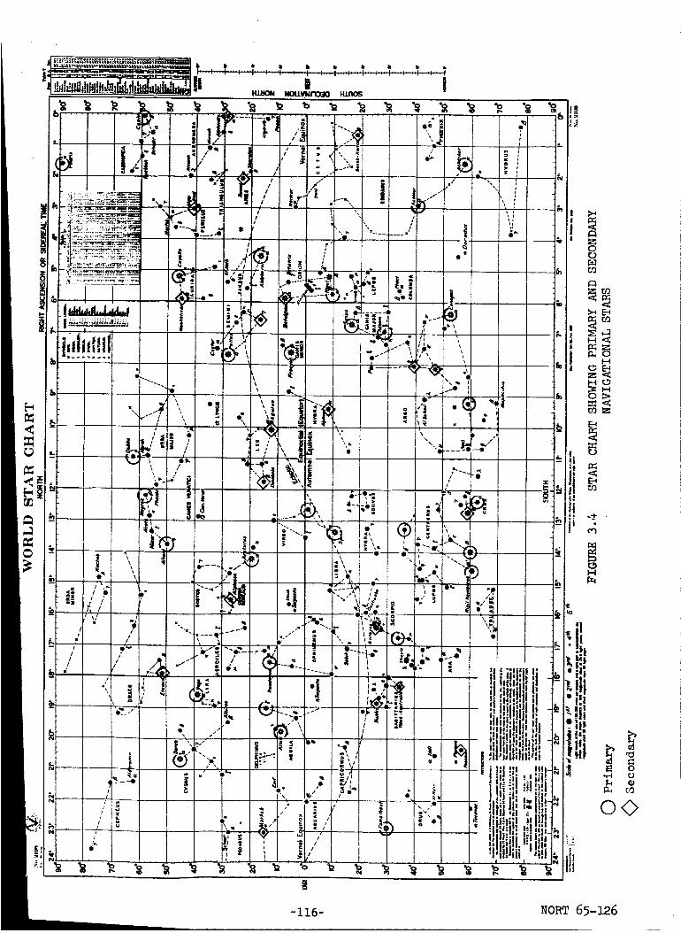
,' I i .t" i : ._il/
- __-'--iR _,_-'_,Ij. _ :_:_r'..m.t-.-._?_ ,, _ _
_-_._=: _':_.-I .... _ ..o
71
Ii LI /\,_
I , I Pd ,,'V'I,
I
I' I
i
i
##
,. "_ ._
o ;
t._e "|'_ / -i , .
' " i,et '%,I., ,:-
L t
%%% .ll_ _ al %I
_ "....".: _i ":---_'oJi-, _
tY',p..-" F
i,,, _i _..--[, , , '-+! .ti. 4 :.I _ P I
' / " " _ " "" _
/ I |r_, 'l l-. I tL ...... " iI . ill .r-,. ", $I'i ',,
i ' I ;I ",' . ,_.s ', !I ' I ;,
lltl- _ -_ t "
' j-}-._ I .--'-'._, .,:it i'! i
"0 ...... ---
/
,/! i ,'"
" '% L" ¶'_
I, --' ,', -4_ . ._#,b
. _-.: l ! '._
b':- '" '-";," -: l / is
i v" _;
/
I i #//
•_ "o t ,, "_ "t lii
it -- --x ,
.p
Iji ::li|il II! U I_ll il -_I I|ili_i! II
_i ilPilil !III titlllll II I ", ,11 ! i_l !i [ It -,,, _il!!ll, ,:III i.,lll, ! _'
'.i,:;llll! II1_ilil iollll ill
[i!llllll_!lii!l -_liillilili#ltl,
lll_llliilill_|!I 111!II Illi-I ii_ -iI i ilillI I_!ii! _ilillli ill "i! '_ i_i,i_iI hI I.I_I_-
'1 _111II_ -_-*ll,i:'i_ll'l ii I1ilii:t!; "lllll
:lll!hll !iliill-
Illd_, Ili!l#!" "'"s _ _
o
i-4
E-_
! ;
b
R o
©_
f
-116- NOI_ 65-.126

_t A OlVlONON OF NORTHROP COIWOI_TION
must be subtracted from this number to determine the hour angle of the
zenith stars at the zenith.
TABLE 3.2 RIGHT ASCENSION MONTHLY SCHEDULE
DATE JANUARY FEBRUARY MARCH APRIL
h m h m h m h m
1 6 39 8 hl i0 32 12 3h
I0 7 lh 9 17 ii 07 13 09
20 7 5h 9 56 ii _7 13 h9
MAY JUNE JULY AUGUST
1 14 32 16 5h 18 33 20 35
I0 15 08 17 i0 19 08 21 i0
20 15 47 17 h9 19 48 21 50
SEPTEMBER OCTOBER NOVEMBER DECEMBER
1 22 37 0 35 2 38 h 36
!o 23 13 1 Ii 3 13 5 II
20 23 52 i 50 J_ ___ 5. 51
The declination angle of a star is the angle between an imaginary line
drawn from the center of the earth to the star and the plane that passes
through the equator of the earth. Positive declination angles denote
stars in the northern hemisphere and negative declination angles, stars in
the southern hemisphere.
The latitude of the launch site, Cape Kennedy, corresponds to the declina-
tion angle of the star ephemeris coordinates. Thus all launches from
Cape Kennedy will originate from a line drawn through the 26th parallel
which is approximately the latitude of Cape Kennedy. For a more accurate
determination, the latitude must be corrected to compensate for the location
of the different launch pads.
The field of view of the star tracker is assumed to be circular, but
project as ellipse on the star map since the coordinates of the star
map are asymmetrical. Two ellipses representin_ fields of view of +h5 °
and +55 ° are illustrated in overlay number I, Figure 3.5. The major
horizontal divisions on the star chart are 15 degrees apart, while the
7(R 11-44)
-117- NORT 65-126

+_20
OVERLAY #2 SOLAR EXCLL_IO_ ZORE
÷
\ \
OVERLAY #i STAR TRACKER FIELD OF VIEW
FIGURE 3.5 STAR TRACKER FIELD OF VIEW AND SOLAR EXCLUSION ZONE
-i18- NORT 65-126

A O_llSION OF NOIqTMROP CCIRPOFIATIOIW
vertical d/visits are i0 degrees apart. This field of view will be aligned
normal to the zenith _ the launch pad and pointed in a westerly direction,
so that when the booster is pitched over in its dc_nrauge trajectory, thefield of view of the star tracker will be pointed towards the zenith. The
field of view of the star tracker will thus be pointed at a meridian whichis six hours from the zenith. The field of view of the star tracker at
launch will be centered about the intersection of the meridian and the
parallel which denotes the latitude of the launch pad.
On the launch pad, the earth will obscure half of the field of view of the
star tracker, The horizon of the earth projects as a vertical line through
the center of the field of view of the star tracker. The sky background
luminance further restricts the usable field to look angles that are greater
than 20 degrees above the horizon. This restrictica was determined from
considerations of sk_ brightness and star tracker performance characteristics.
The sun is located in the celestial sphere at a right ascension angle that is
twelve hours different from the right ascension hour of the stars at the zenith
at midnight. The intersection of the meridian that corresponds to the right
ascension of the sun and the ecliptic determines the location of the sun
with respect to the star chart for any day of the year. The stray solar
radiation that is specularly or diffusely reflected off portions of the
telescope housing places a limit as to the angle with which the star tracker
can be operated with respect to the sun. Empirical determinations of this
pointing limitation indicates that the background illumination from stray
solar energy becomes excessive when the sun is within 20 degrees of the
optical line of sight. In overlay number 2, Figure 3.5, this sun exclusion
zone is illustrated in the proper scale for u_e with the star chart. When
center of the ellipse depicting the sun exclusion zone is positioned as
described, all the stars falling within this zone must be excluded from the
list of available stars.
For most star tracker applications, the criteria used to determine the
suitability of a particular star as a navigational star are the brightness
of the star and the separation of the star from other stars in terms of
relative brightness and in angle. For specific applications, the star
selection criteria may be extended to include the declination of the star
and also the color, for example, Polaris and Canopus, which are often used
as the reference star for terrestrial and interplanetary navigation respectively.
On the star chart, the thirty stars that are best suited for used as navigational
stars are circled. An additional twenty stars that could be used as navigational
stars in the event that the window size allotted for the star tracker is limited,
or if two or more stars with a minimum angular separation are desired within a
limited field of view, are enscribed with a diamond outline.
Shortly after launch, the Saturn is rolled to correct the azimuth alignment,
so that the pitch and the yaw axes will be properly aligned with respect to
the chosen trajectory. For smaller missiles, this azimuth alignment can be
mm 7 4e 0.44)
-119- HOIRT 65-_6

A OlVmlON OF NO_HflOP COImeO_TIQN
accomplished on the pad by rotating the whole spacecraft, but this procedureis impractical for the Saturn. The magnitude of this roll maneuver will be
from zero to fifteen degrees depending upon the chosen trajectory. The star
tracker im assumed to be pointed west at launch and this roll maneuver will
cause the line of sight of the star tracker to rotate northward. On overlay
n_w_ber 3, Figure 3.6, the loci of the line of sight of the star tracker for
three different roll maneuvers, zero, five and fifteen degrees are plotted.The location of the centers of the field of view of the star tracker as a
function of time after launch are delineated for several discrete intervals.
By positioning the center of the ellipses that denotes the field of _ew of
the star tracker on these loci, star availability can be determined for
different intervals during the vehicle launch. The location of the horizon
and the field of view limitation imposed by the brightness of the sky back-
ground are also illustrated on overlay number 3. The location of the horizon
relative to the celestial sphere will vary as a function of the vehicle
altitude, but the change is insignificant for the 138 second launch interval
considered. However, the sky brightness changes rapidly as a function of .
vehicle altitude, so the change in the field obscuration caused by thebrightness of the sky background is also shown on overlay number 3 for several
intervals after vehicle launch. All stars to the right of a vertical line
through the sky background obscuration limit cannot be tracked.
To reiterate, the procedure for locating the overlays and determining the
stars in the system field of view is as follows :
I. From Table 3.2 determine the right ascension hour for midnight of
the calendar date of the launch.
2. Find the meridian for the hour of the flight by -----o'A_"=*,he_hour
of launch to the right ascension hour found in Table i.
. Locate Overlay number I on the World Star Chart by aligning the
Zero Declination Angle and Launch Time Meridian cfl the overlay
to the zero degree declination angle and hour meridian on the
star chart.
_. Determine the position of the sun (approximately 12 hours from
the hour found in Table 3.2 and on the ecliptic plane).
5- Determine the system field of view (_5 ° or +_55°) .
6. Determine the roll program from O degrees through 15 degrees.
To Those selected stars that fall within the system conical field
of view and to the east or to the left of the atmospheric obscuration
line are stars capable of being tracked at T = 0.
-120- NORT 65-126

,-o_amaed Roll 15 °
5°
0o
Launch Time
Meridian
Locus of Center of
, : .: [ _T:-o
Zero DegreeDeclination
AngleT+138.
T+IO0 J
_-0
Top of Atmospheric
Obscuration
RE3.6 OVERLAY NUMBER 3 ORIENTATION OF CENTER OF THE FIELD OF VIEWWITH WORLD STAR CHART RIGHT ASCENSION AND DECLINATION PLUS
UPPER ATMOSPHERIC OBSCURATION
-121- NORT 65-126

___S A OIVlS_ONOFNO_THeOeCOePORMION
3.1.3.5 Vented Gases and Plume Effects
A vehicle rising through the atmosphere can be expected to produce turbulence
and shock waves that will affect the operation of the star tracker. Refrac-
tion of the incoming stellar radiation will be produced that will cause the
star to appear displaced from its true position. The star tracker will sense
this change as a vehicle attitude error unless corrective inputs are supplied.
The refractive error can be predicted to a given extent, provided certain facts
are available. Some of the necessary data needed to calculate this effect
are: i) the vehicle velocity; 2) the altitude; 3) the air density; 4) the air
temperature, and 5) the angular relationships between the vehicle, star, and
shock wave. The magnitude of the refractive error will decrease as the
altitude increases, and will completely disappear as the craft leaves the
atmosphere.
There is one further potential source of refractive error that may cause
erroneous star position information. This potential error source is caused
by the passage of vented gases across the field of view of the tracker. Oxy-
gen, hydrogen, and helium are often used as coolants or as fuel for the booster,
and the boil-off requires venting to the atmosphere during the vehicle count-
do_ period. Location of the boil-off vents relative to the star tracker win-
dow plus air turbulence will determine if the gases will enter the field of
view while on the launch pad. Refractive errors are caused by changes in the
index of refraction over the star radiation path. The errors caused by the
vapors are random in nature and, thus cannot be programmed out. During flight
through the atmosphere, the effects of the vented gases are minimized. How-
ever, once in orbit, the boil-off of material may again become of some concern.
The gases, when they are vented, will be traveling at the _ame speed _s the
vehicle and may produce deleterious effects.
In addition to the vented gases, there has been some indications that all
exhaust products from the engines are not thrown backward away from the
vehicle. It is likely that during the first few seconds of engine firing,
exhaust products, as well as dirt and dusty may be thrown up to obscure the
star tracker field of view, and may also be deposited on the star tracker win-
dow. As the vehicle rises through the atmosphere, paint or other materials
that ablate the nose cone may also be deposited on the window. These particles
act as diffuse reflectors when illuminated, raising the effective background
radiance presented to the star tracker° The "fireflies" described by the astro-
nauts in the Mercury flights are ascribed to sunlight reflected off particles on
the window in the capsule° If the star tracker is not used during the boost
phase, the window can be covered with a protective dome, which would be dis-
carded after booster cutoff. However, coating of the window may also be
caused by exhaust products from the attitude control engines, or other engines
which may be used to modify the spacecraft orbit or trajectory, so other pre-
ventive measures may be required.
-122- NORT 65-126
Form 7 (R 8-64)

3.2 OPTICAL INSTRUMENTATION FOR ORBITAL NAVIGATION AND
FOR ATTITUDE CONTROL
The use of optical instrumentation as part of the attitude control,
vehicle alignment and orbital navigation system for a spacecraft is con-
8idered for a number of different applications. The actual type of opticalinstrumentation that would be utilized for attitude control or orbital
navigation would be dependent upon the intended application and the
accuracy requirement. Typical utilization of optical instrumentationwhile in an earth orbit would include attitude control of an earth oriented
satellite, attitude control of a solar oriented, inertially stabilized
vehicle, orbital navigation, vehicle realignment after loss of inertial
reference and the use of a star tracker to provide a stellar reference
to correct the drift of the inertial platform during an extended mission.
3.2.1 Earth-Oriented Orbital System Usin_ a Horizon Sensor
and a Gyro Compass
For a satellite whose orientation must be maintained with respect to the
ground, a horizon sensor is the most practical device to use to provide
a vertical reference. The horizon sensor will provide attitude error
information about two of the spacecraft axes, hut the attitude error about
the third axis must be provided by an additional instrument. In a coordinate
system where the axis aligned with the orbital path is the roll axis, the
axis a!i_ed with the local vertical is the yaw ax__s and the third axis
---_i provide roll and pitch con-is the pitch axis, the horizon sensor ._.
trol. However, currently no easily implemented and simple device is
available to provide a direct measure of vehicle yaw alignment. The.
most practical method of yaw control of an earth oriented satellite is
by gyro compassing. In the gyro compass, the gyro rotor is constrained
relative to the vehicle frame so that its spin axis tends to align itself
normal to the orbital plane. With vertical established by the horizon
sensor, rotation about the yaw axis will be sensed by this gyro. The
attitude control accuracy attainable is a function of the accuracy of
the horizon sensor and the accuracy of the gyro compassing technique.
A brief consideration will be given to horizon sensors but the accuracy
attainable by gyro compassing will not be considered.
Of the devices that have been proposed for vertical sensing, the horizon
sensor is the most practical. In the past an infrared detector was used
to sense the thermal gradient between the planetary disk of the earth and
space. Accuracy of the horizon determination was affected by weather
conditions, season of the year, cloud cover and other climatic effects.
Accuracy of the local vertical determination was limited to 0.2 to 0.5
degree r.m.s, with devices that operated in this manner. A major break-
through in infrared horizon sensor technology was achieved with the
decision to track the atmospheric carbon dioxide emission rather than
the earth itself. The concentration of CO2 in the upper atmosphere is
relatively constant and the greatest variation that is detectable is the
temperature rather than the distribution of the gas. Carbon dioxide has
an intense absorption band at 15 microns and can easily be distinguished
-123- NORT 65-126
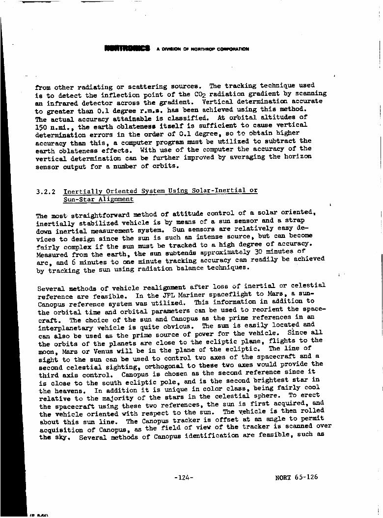
A OfVlS_ON OF IvO_ CO;MeO_llON
from other radiating or scattering sources. The tracking technique used
is to detect the inflection point of the C0 2 radiation gradient by scanningan infrared detector across the gradient. Vertical determination accurate
to greater than 0.1 degree r.m.s, has been achieved using this method.
The actual accuracy attainable is classified. At orbital altitudes of
150 n.ml., the earth oblateness itself is sufficient to cause vertical
determination errors in the order of 0.I de_ee, so to obtain higher
accuracy than this, a computer program must be utilized to subtract the
earth oblateness effects. With use of the computer the accuracy of the
vertical determination can be further improved by averaging the horizon
sensor output for a number of orbits.
3.2.2 Inertially Oriented System Usin_ Solar-Inertial orSun-Star Alignment
The most straig_htforward method of attitude control of a solar oriented,
inertia!ly stabilized vehicle is by means of a sun sensor and a strap
down inertial measurement system. Sun sensors are relatively easy de-
vices to design since the sun is such an intense source, but can become
fairly complex if the sun must be tracked to a high degree of accuracy,
Measured from the earth, the sun subtends approximately 30 minutes of
arc, and 6 minutes to one minute tracking accuracy can readily be achieved
by tracking the sun using radiation balance techniques.
Several methods of vehicle realignment after loss of inertial or celestial
reference are feasible. In the JPL Mariner spaceflight to Mars, a sun-
Caaopus reference system was utilized. This information in addition to
the orbital time and orbital parameters can be used to reorient the space-
craft. The choice of the sun and Canopus as the prime references in an
interplanetary vehicle is quite obvious. The sun is easily located and
can also be used as the prime source of power for the vehicle. Since all
the orbits of the planets are close to the ecliptic plane, flights to the
moon, Mars or Venus will be in the plane of the ecliptic. The line of
sight to the sun can be used to control two axes of the spacecraft and a
second celestial sighting, orthogonalto these two axes would provide the
third axis control. Canopus is chosen as the second reference since it
is close to the south ecliptic pole, and is the second brightest star in
the heavens. In addition it is unique in color class, being fairly cool
relative to the majority of the stars in the celestial sphere. To erect
the spacecraft using these two references, the sun is first acquired, and
the vehicle oriented with respect to the sun. The vehicle is then rolled
about this sun line. The Canopus tracker is offset at an angle to permit
acquisition of Canopus, as the field of view of the tracker is scanned over
the sky, Several methods of Canopus identification are feasible, such as
i •
- 124- NORT 65-126
tD L_a%

A OIVUlION OF NORTHROP COIIPOItATION
brightness and color. Sirius is the brightest star in the heavens and is
more than two times brighter than Canopus. The third brightest star is
almost two times dimmer than Canopus, so Canopus is readily identifiable
by brightness alone. Verification of Canopus acquisition can also be
made by mapping the stars in the conical segment that is scanned as the
vehicle is rotated about the sun line.
3.2.3 Earth-Oriented Orbital System Using Horizon Sensorand Star Field Scanner
For an application such as an orbiting space static, rotation of the
spacecraft about the sun line may not be feasible. Lack of sufficient
thrust to perform maneuvers of large magnitude may be one of the deterrents.
In addition while in orbit, the sun may be obscured by the earth for a
large portion of the orbit. If the orbit is out of the ecliptic plane,
Canopus may also be obscured during a large portion of the orbit. With
these two effects, the interval when both references are available to the
spacecraft may be very limited. The rotation rate of the Mariner space-
craft was two revolutions per hour. Thus in the time required for cue
Canopus search revolution, the vehicle would complete one-third of its
orbit assuming a 90 minute orbit. If the rotational rate utilized for
vehicle re-erection were in this order of magnitude, a high probability
would exist that one or both of the celestial references would be eclipsed
during this interval.
A horizon sensor and a star field scanner has been proposed as an alternate
vehicle re-erection system. The star field scanner would map the stars
in its field of view as the scanner is rotated. A computer would then
be required to compare the star field signature obtained to determine the
orientation of the vehicle in yaw. For applications where the yaw error
is small, as in the case where the celestial reference is lost with the
two star tracker, horizon sensor system, the attitude reference can readilyhe re-established. The star field scanner can also be used as the prime
spacecraft yaw reference if desired.
3.2.4 Autonomous Navigation System Using Horizon Sensor
and Star Trackers
If the location of the satellite relative to the earth is desired, addi-
tional instruments to those necessary simply to maintain vehicle attitude
control are required. Assuming that radar nets and beacons will not be
utilized, an autonomous navigation system using a horizon sensor and a
star tracker as the basic components are capable of determining the vehicle
position relative to the earth to an accuracy in the order of +--20n.mi.
A fairly low orbit, a horizon sensor accuracy of O.1 degree, and a star
tracker accuracy of 20 arc seconds are assumed under these conditions.
If greater accuracy is desired, filtering and smoothing of the horizon
-125- NORT 65-126
L _ aD • ml]

sens0r and Lthe star tr-acker data could reduce the error. The star tracker
location and field of view aboard the vehicle is an important question,since these factors in part determine the star availability and the inter-
val over which a star can be tracked. The computer requirements are also
important since the star ephemeris must be stored in the computer memory,then converted to yield the star tracker line-of-sight to the star relative
to the orbital position. To perform these functic_s, the orbital informa-
tion must be known to a certain degree of accura_j, and the star tracker
will then be used to upgrade the navigational computation.
Several permutations of instruments and methods of implementing an autonomous
orbital navigation system are feasible. The actual choice of a given system
would be dependent upon mission and accuracy requirements. Two of the most
common system mechanizations include first, the use of a horizon sensor and
an inertial platform with a star tracker used to update the platform align-
ment, and second, the use of a horizon sensor with two star trackers.
For extended orbital operation, the gyro drift will eventually cause the
attitude control errors to develop to the point where the errors will be
intolerable. To provide an orientatic_ reference for space navigation,
the commonly proposed solution is to supplement the gyrostabilized plat-
form with a star tracker system. The platform then is used to provide
stability under relatively high frequency distu_-bances_ such as docking
and maneuvering, and the star tracker prevents any long term drift of
the i_ertia! reference. The problem of operational lifetime of the gyros
in the platform still exists, and one of the proposed solutions is to turn
off the platform when the vehicle will be orbiting under quiescent conditions,
then re-erect the platform prior to the time when a major change in vehicle
attitude or orbit is made.
The use of two star trackers and a horizon sensor has been proposed as an
alternate system for space navigation. The two star trackers will con-
tinuously acquire and track different stars as the vehicle orbits, andthus a celestial reference will always be provided. Since the star
trackers are constantly slewing, acquiring, then tracking different stars,
the computational requirements necessary to provide the slewing commands
and to relate the star tracking data to the orbital parameters are large.
In concept, one star tracker will be tracking while the other is slewed
to the next navigational star. If the vehicle is tumbled about the primary
control axis of the star tracker that is being slewed, star acquisition and
lock-on may be delayed or even lost if the motion is greater than the
instantaneous field-of-view of the star tracker. Since the interval over
which a star can be tracked while in orbit is limited, both star trackers
may be rendered ineffective, and the attitude reference will be lost.
-126- NORT 65-126
r r,
A O_ISlONOFNORTHROPCO_eORATION
_k
3.2.5 Precision Orbital Navigation System Using a Landmark Tracker
For precision orbital navigation, sightin6s on distant bodies such as
stars limit the accuracy with which the navigational accuracy can be
determined. An angular sighting error to a star of a 20 seconds of arc
will result in a large orbital position error. In an effort to obtain a
more accurate orbital navigational system, the tracking of objects on the
ground has been proposed. Different sensors and methods are feasible,
such as the use of visual, infrared and microwave sensors and the tracking
of known and unknown landmarks. _ne problems involved with the concept
are sensor limitations, accuracy of the geodetic surveys, and computer
requirements. Cloud cover, landmark identification, and the accuracy with
which a landmark can be tracked are problems germane to the sensor. The
location of the landmarks themselves are not precisely known. The basic
geodetic references have been found to be as much as several thousand
feet in error from data obtained from orbiting vehicles. Tracking of un-
known landmarks would provide data points in the trajectory that can be
used to solve for an unknown in a matrix. By iteration and the accumulation
of multiple data points, such as local vertical, star sightings and others,
the navigational accuracy can be improved. Orbital navigation systems
utilizing landmark tracking could substantially improve the navigational
accuracy, over the horizon sensor-star tracker system.
One function that can be performed by a manned orbital satellite is the
mapping of terrestrial landmarks to improve the accuracy of the geodetic
surveys and in turn the accuracy of autonomous orbital navigation systems
utilizing landmarks. The radiation signatures of landmarks, notably,
volcanoes, islands, lakes, snow-covered peaks, hot springs and others
as viewed from space would help in the design of sensors for landmark
detection.
3.2.6 Attitude Control of A Space Vehicle
The purpose of attitude control of a space vehicle is to stabilize the space-
craft to a desired accuracy from a reference on the vehicle to an external
reference. External references that can be utilized include the local
vertical of a planet; optical sightings to celestial bodies such as the sun,
the planets and the stars; an inertial reference; and gravity gradients and
the magnetic field of the earth. The accuracy of attitude stabilization is
dependent upon the spacecraft mission, and the attitude control can be fairly
crude for applications such as a communications satellite, but must be highly
accurate for a vehicle such as the Orbiting Astronomical Laboratory. Typical
methods of attitude control that are presently being utilized, include spin-
stabilization, gyro compassing with a horizon sensor to provide local vertical
direction, horizon sensors used with sightings on celestial bodies, and
multiple celestial body sightings. Gravity gradients and magnetic field
effects are being investigated and are scheduled for testing on one of the
geophysical satellites in the near future. In Table 3.3, the attitude control
techniques utilized by different spacecraft are listed for comparison.
-127- NORT 65-126
7 i'R A-_4_I

A DIVtBiON OF NORTHROP CORPORATION
3.2.6.1 Spin Stabilization
The majority of vehicles launched prior to 1963 were spin stabilized. Spin
stabilization is simple to implement and is quite effective, being capable of
short term stabilitywithin +_i degree about two axes. The spin was imparted
to the vehicle by rotating the entire top stage of the launch vehicle prior
to injection into orbit. The advantages of spinning the payload are that the
center of gravity of the payload will lie on the axis of rotation, simplifying
the problem of alignment of the thrust axis of the booster with the c.g. of
the payload, and thespinning motion of the satellite can also be used to
generate the scanning motion for the sensors and other instruments.
A spin stabilized satellite will be oriented with respect to inertial space
and if the satellite must be maintained at a given orientation with respect
to the earth, the vehicle must be continuously precessed at a given rate to
maintain the alignment with respect to the earth. Other disadvantages to spin
stabilized satellites are disturbing torques which cause the spacecraft to
wobble, arid also the difficulty of making observations from a rotating
spacecraft.
3.2.6.2 Celestial Body Tracking
The trajecto_ of a space vehicle in the midcourse phase of its flight be-
tween two planets may vary from the nominal precomputed trajectory due to
errors in the injection velocity and due to inaccuracies of the Knowledge
of the different astronomical constants. An on-board optical system to
measure angles between lines of sight to celestial bodies to determine the
position of the spacecraft at a specified time in the trajectory was described
by Robert Stern. I Three or more measurements of the angle subtended by a pair
of celestial bodies are made in a relatively short time, and compared to the
precomputed angle for the specific time in the trajectory. Since all the
angular measurements are subject to some degree of uncertainty, the sightings
were chosen in such a manner that the smallest uncertainty in the computed
estimate of the spacecraft position is produced.
The trajectory of an interplanetary flight will lie in, or be close to the
ecliptic plane, and all tlre relatively close celestial bodies, such as the
planets, the sun and the moon are located close to the ecliptic plane.
Sightings on celestial bodies should be made to the closest celestial bodies
available, to maximize the accuracy of the navigation information that can
be obtained with each sighting. In addition, it is desirable to choose the
sightings so that the sight-lines to the celestial body form an orthogonal
*Proceedings of the National Aerospace Electronics Conference, May ii-13,196h,
Selection of O_tical Si_htin_s for Position Determination in Interplanetary
Sa_, Robert G. Stern.
-128- NORT 65-126

A 81VlWQN OF M)RTImOP L_DIqI_IATIQN
•i_
!0 loo.OeH
_o_ °
+°l +_l
H
W
oo
o
o
*r4
0
o
0¢J
0
o o
o
r-t o
mcH
m
U=
4)
o
oco
o
i<
o
ow
8=r..,
_.! Ptoo _
_ E--4
•i_ ,-t
o
_ _c0 e= o
4_ N o _
•,d q:l _:_ =_ 04o
03
0
bO0 m
o _
-129-
o
o N)
0-,-4
_ m
o
I)0
m4-_
.t-I,--I
OO3
,1¢1
03
mm
o
oJ
r_om
o
1:103(I)
m_
o
o
r_v
o
,-_
I
_o
.,.!
i--i
o
mm •
o
o
m_
o
o
v
I
o_o
o
M
0
O£'4
I:Io
o
v
_.,cd
coI
o3
o
_o
o
t_o_ 65-126
7 m 144)

7 (R I1-t14)
m
C,)
0
O Omo,_
,-__._
-,-4 e_
,-4 I0
r..)
O O
Q; m
,N
M
o
m0
o
÷1
O Om_
t/l _-t
t_
o 1¢1•r.t _
I;
3&
m
H
,0 mm
O
O
o
O4_
tD
0
m
0
0v
I
t/l
O _ _
0
A OfVWION OF NORTHROP CO_eOfl&110_
-130- _0_T 65-126

a ONmlONOFNORTHROPCORPORATION
set of vectors. The amount of near celestial bodies that are available are
limited and lie in the same plane, so at least one sighting has to be made
to a st_r that is norms/ to the ecliptic plane. Star availability also
beccaes a problem since there is no star normal to the ecliptic plane that
exhibits characteristics that make it attractive for use as a navigational
star. Canopus, which is close to the south ecliptic pole is the commonly
chosen star for space navigation.
Due to the limited availability of near celestial bodies, and to the diffi-
culty of locating good navigational stars that form an orthogonal reference
coordinate system, Stern has proposed a system inwhich three to six measure-
ments are made of the angles between a number of celestial bodies. The six
measurements would include measurements of the angles between Venus-Canopus,
Venus-Spica, Earth-Sun, Venus-Earth, Earth Pollux, and Earth-Regulus. The
uncertainties in all angular measurements are assumed to be 50 microra_lians
or approximately i0.3 arc-seconds. With this measurement t_chnique, the
positional uncertainty volume would form an ellipsoid with the dimensions
shown in Table 3.4.
TABLE 3.4 AXES OF EQUI-PROBABILITY ELLIPSOID
Largest Axis Middle Axis Smallest Axis
(Miles ) (Miles) (Miles )
3 Sightimgs 3780 1140 59h
6 Sightings 3350 610 533
An earth orbiting vehicle utilizing only celestial body tracking for naviga-
tion purposes would be subject to errors of approximately the same order of
magnitude. An orbiting satellite, that utilizes optical instrumentation in
its navigation system, should use a guidance system similar to those described
_in the next section on Autonomous Navigation Systems.
3.2.7 Accuracy of Autonomous Navigation System
Autonomous space guidance and control systems that require no assistance from
ground aids have been proposed. 2 One type of earth-orbital navigation and/or
guidance system would include star trackers, infrared horizon sensors and
inertial references. The accuracy of this system would be limited by the
2 iAdvanced Guidance Concepts, James A. Fusca, Space/Aeronautics, December 1964.
-131- NORT 65-126
(R844)
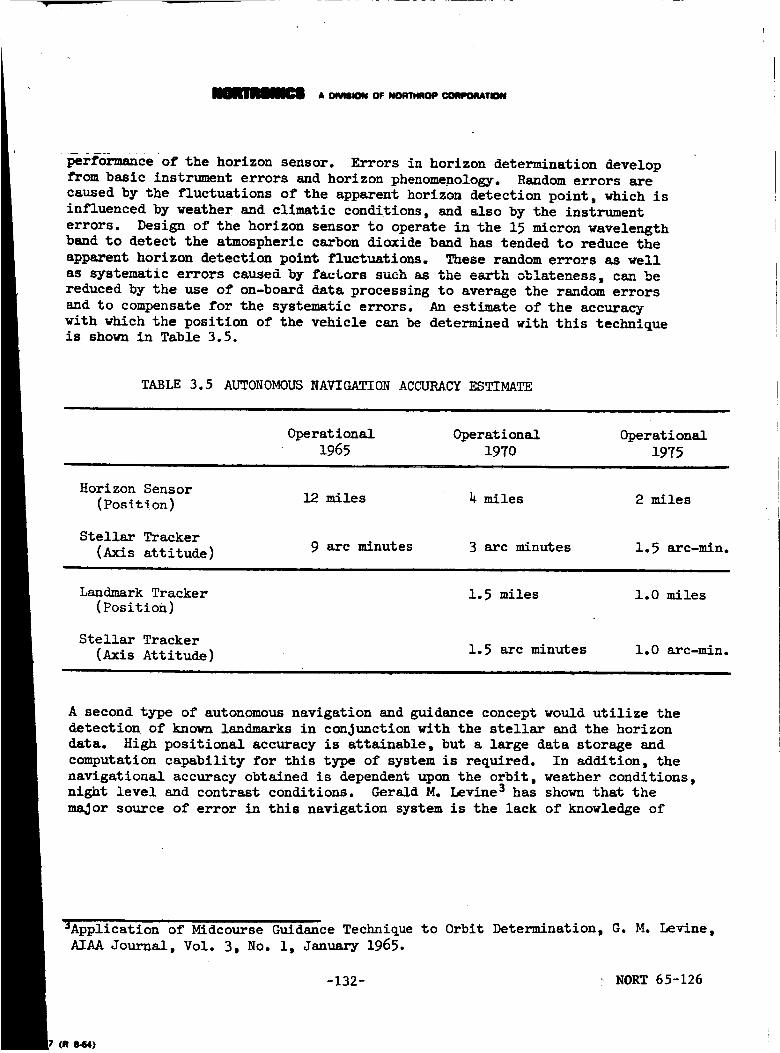
A Of VIIIION OF NOIKTHHOP COmPliCATION
perf6_nce of the horizon sensor. Errors in horizon determination develop
from basic instrument errors and horizon phenomenology. Random errors are
caused by the fluctuations of the apparent horizon detection point, which is
influenced by weather and climatic conditions, and also by the instrument
errors. Design of the horizon sensor to operate in the 15 micron wavelength
band to detect the atmospheric carbon d/oxide band has tended to reduce the
apparent horizon detection point fluctuations. These random errors as well
as systematic errors caused by factors such as the e_h oblateness, can be
reduced by the use of on-board data processing to average the random errors
and to compensate for the systematic errors. An estimate of the accuracy
with which the position of the vehicle can be determined with this techniqueis shown in Table 3.5.
TABLE 3.5 AUTONOMOUS NAVIGATION ACCURACY ESTIMATE
Operational Operational Operational
1965 1970 1975
Horizon Sensor
(Posit!on)
Stellar Tracker
(Axis attitude)
12 miles 4miles 2 miles
9 arc minutes 3 arc minutes i. 5 arc-rain.
Landmark Tracker
(Position)
Stellar Tracker
(Axis Attitude)
1.5 miles 1.0 miles
i.5 arc minutes 1.0 arc-min.
A second type of autonomous navigation and guidance concept would utilize the
detection of known landmarks in conjunction with the stellar and the horizon
data. High positional accuracy is attainable, but a large data storage and
computation capability for this type of system is required. In addition, the
navigational accuracy obtained is dependent upon the orbit, weather conditions,night level and contrast cond/tions. Gerald M. Levine S has shown that the
major source of error in this navigation system is the lack of knowledge of
_Application of Midcourse Guidance Technique to Orbit Determination, G. M. Levine,
AIAAJournal, Vol. 3, No. l, January 1965.
-132- ! NORT 65-126
(R 8.64)

A OlVtlON OFNORTHROPCOIWORATION
the exact position of the landmark, particularly when multiple landmark
observations are made. The larger the landmark uncertainty, the less worth-
while are added observations. Results using linear filtering techniques to
reduce the positional error has shown that two observations of a given land-
mark are sufficient unless the landmark position is precisely known. Using
a landmark tracker with a tracking accuracy of 1 milliradian, the spacecraft
position can be deter--mined to an accuracy of 1.5 miles as shown in Table 3.5.
The basic sensor capability of current instruments and the projected accuracythat can be attained in the future is shown in Table 3.6. The star tracker
capability is not being fully utilized in the autonomous navigation system
since the basic accuracy is limited bythe horizon sensor.
•TABLE 3.6 SENSOR PERFORMANCE CAPABILITY ESTIMATE
Operational
1965
Star Tracker 20 arc seconds
Operational Operational
197o 1975i I
I0 arc seconds 5 arc seconds
IR Horizon Sensor 6 arc minutes 2 arc minutes i arc minute
Landmark Tracker 1.0 milliradian O. 7 milliradian
Gyroscope 0.I deg. per hr. 0.03 deg. per hr. 0.01 deg. per hr.
3.3 CONSIDERATIONS OF EXPERIMENTS THAT CAN BE PERFORMED
FROM AN ORBITING SATELLITE
The type of experiments that would be considered in an orbiting satellite would
fall into tw@ general categories. The first would include scientific research"
and engineering experiments that cannot be performed except under space condi-
tions. The second would be determination of the geophysical phenomena that
can be detected from space and the accuracy with which these detections canbe made.
The use of the Saturn_IV booster as a space workshop would permit extensive
testing of Components and instruments designed to operate in a space environ-
ment, but whose environmental testing had been limited due to shortcomings of
space chambers. The testing would include the performance evaluation and
the reliability of different instruments and the effects of gamma and ultra-
violet radiation on different materials.
-133- NORT 65-126
,_n7 (R 1.64)
A OeVmtON OF NORTHROP COMeORAllON
Components that are affected by gravitational attraction include gyros,
accelerometers, and gravitometers. Instruments that are affected by
atmospheric gases include horizon sensors, sun sensors and star trackers.
For gyros and accelerometers, the errors caused by gravity can thus be
separated from the errors cause_ by spring stiffness, rotor suspension and
frictional effects. For a number of years, the accuracy of horizon sensors
and the cause of the sensor errors has been difficult to define. Observa-
tion of the weather conditions and other phenomena, in the region where
the horizon detection is being made would permit correlation of the horizon
detection point with the atmospheric effects. Sun sensor accuracy is
norsu_l_ tested on the earth with a simulated source or by using the sun
itself. Simulated sources sacrifice either collimation or intensity of
the simulated solar radiation. If the sun itself is used, atmospheric
absorption reduces the intensity of the solar radiation. Thus the per-
formance of sun sensors must be extrapolated to space conditions. Experiments
performed with star trackers could include the amount of background that is
caused by the star tracker window.
The testing of bearings, solar cells, torquers, resolvers and other materials
and components in a vacuum environment would produce data on the characteristics
of these components under vacuum conditions that cannot be reproduced and
maintained in a space cheer.
Some of the geophysical phenomena that may be observable from an orbiting
_atel!ite would be the temperature and direction of ocean currents, the
velocity and location of the Jet streams in the upper atmosphere, the
formation and movement of weather fronts, the position and radiation
signature of terrestrial landmarks, and atmospheric refraction effects.
The type of experiments that would be performed would be determined by
the phenomena that is being examined. Spectrometers or radiometers in
a number of spectral bands would be needed to determine whether ocean
currents and Jet streams could be detected. These instruments would also
be used to study weather fronts to determine the best method to detect
hurricanes and other weather disturbances, and also to determine the
signature of terrestrial landmarks. The surveying of landmarks to improve
the accuracy of the geodetic surveys could be accomplished by manual _tracking
using a sextant, or by photographic mapping techniques. The effects of
atmospheric refraction can be measured by tracking a star in the vicinity
of the horizon, and measuring the deviation of the line of sight to the
star that is caused by the atmosphere of the earth.
3.3.1 Thermal Ocean MappinK
Thermal mapping of the ocean would be beneficial to oceanographic studies,
and would permit the plotting of ocean currents, and also yield data that
can be used by the fishing industry. Several methods of determining the
wavelength at which the radiation peaks and comparing the amount of energy
in two different spectral bands. The peak of the blackbody radiation curve
moves to shorter wavelengths for warmer bodies, and this peak can be plotted
-134- NORT 65-126
om _64)

A ONmlON OF NORTHfl(_ CORPORATION
by the use of a sensitive spectrometer with high resolution. For objects
that radiate as blackbodies, the ratio of the radiant emittance in two
spectral bands can be used to determine the temperature of the body. With
two measurements only, an ambiguous result is obtained, since one of the
spectral regions chosen may lie before or after the spectral peak of theblackbody curve, and a given ratio between the radiant emittance from the
two spectral regions can be produced by blackbodies of two different temper-
atures. For thermal mapping of the ocean, the range of temperatures of
interest is bounded and so one of the possibilities can be e!in_nated as
being extraneous.
3.3.1.1 Scanning Spectrometer
To define the operating range of the instruments needed to thermally map the
ocean, assume that the temperature of the ocean may range from 1*0°F to 70°F;
that the ocean has an emissivity of 0.9 or greater, in the region about the
spectral peak; and the average atmospheric transmission in this spectral
region is greater than 80 percent. In Table I, the shift of the spectral
peak for bodies of different temperatures is shown. For temperature incre-
ments of 5°F the spectral peak shifts approximately 0.i micron. To attempt
to resolve this spectral peak, the spectral resolution of the spectrometer
must be better than 0.02 micr__. The trade-off that is of importance here
is system resolution and weight versus system sensitivity. _"i_..einfrared
detectors have a basic detectivity limit, and if the detector irradiance
is reduced by narrowing the spectral bandwidth, the collecting optic nmst
be enlarged to increase the amount of collected ener_..
TABLE 3.7 PEAK OF BLACKBODY CURVE FOR DIFFERENT TEMPERATURES
Temperature A max.
°F °C Microns
To
65
60
55
50
1,5
1.0
21.1
18.3
15.6
12.8
i0
7.22
9.850
9.91.5
10.038
i0.136
10.237
10.339
10.1.1.3
-135- NORT 65-126
_.._7 (R 8-G4)

& OWlUON OF NORTHROP COf_D_TION
For the spectrometer, assume that the optical system consists of an objective
lens that focuses the incoming energy, a condenser lens that recollimates the
energy, a monochrcmator that separates the energy spectrally, and a field lensto refocus the energy onto an infrared detector. The infrared detector is
a thermistor bolca_ter; chosen since it does not require special cooling for
operation. This detector is not as sensitive as other infrared detectors
that are available, but the complexity and maintainability of the cooling
systems required for the other infrared detectors make the choice of the
thermistor bolometer attractive when long term operation without maintenanceis contemplated.
Table 3.8 summarizes the basic parameters in the design of the scanning
spectrometer to measure ocean temperature. All parameters listed are con-
servative, so an instrument to satisfy the system requirements specified
can be built with readily available components.
TABLE 3.8 DESIGN PARAMETER FOR SCANNING SPECTROMETER
TO MEASURE OCEAN TEMPERATURES
I. Radiation Characteristics of Water
Radiation type
Temperature
EmissivityRadiance
2. InstrumentParameters
Spectral resolution
Optical efficiency
Electrical efficiency
Detector
Size
Sensitivity
Detector threshold
Field of view
Lens diameter
Resolution
3. Miscellaneous
Atmospheric transmissionVolume
Weight
Power
Blackbody
273 ° K (32 ° F)0.9
! x lO-2w/cm z_ - steradian
0.02 micron
0.5
0.35
Thermistor bolometer
0.1ram x 0.1ram
5 x I0 "II watt (25 cps
bandwidth,T = 6 msec)
S/N of Z:li x I0 "v steradian
17 cm
0.I mile at i00 miles
0.8
1400 cubic inches
40 pounds20 watts
-136- NORT 65-126
(R 8_4) !

A 041VtlQN09 _ COIM_ItATION
The radiance in a 0.02 micron bandwidth at apprc_'bnately 10 microns is
0.12 percent of the total energy emitted by a 273°K body. The effectiveradiance (F) is the product of the radiant intensity (W), the emissivity
(X), and the percentage of the energy in the spectral bandwidth (&_), or
F = WE AA
F = 10-2 x 0,9 x 0.0012
F = 1.1 x 10⁻⁵ w/cm 2 - steradian
(3.1)
The effective irradiance (R) at the detector plane is a function of the
field of view of the optical system (_), the optical efficiency (oe) , the
electrical efficiency !Ee) , the atmospheric transmission (At) , and thesignal threshold (S/N)
F _ 0e Ee Ati
R = S/N : (3.2)
i.I x 10 -5 x 10-6 x 0. 3 x 0.3_ x 0.8
R - 7
R - 2.2 x 10-iS w/cm2
The collecting aperture (C) required to produce this detector irradiance is
a function of the detector sensitivity (S) _ud is _.ven-_- _y. the following
equation;
C = S (3.3)R
= 5 x i0-II
2 _2 x 10 "13
C = 2.27 X 102 cm2
The lens diameter (D) required is then;
D = (h xw227)I/2
D = 17.0 cm
(3.4)
-137- NORT 65-]26

A OlVSBIONOIW_mATI.mOP_DmmRAl'lmm_,t1..._._ __
The estimate of veight, size and power for a spectrometer with a 0.02 micron
resolution is given in Table 3.8. These estimates do not include the gimbals,
control system and mounting fixtures required to keep the spectrometerpointed &t a specific location as the spectral scanning is being accomplished.
The field of view of 10-6 steradian chosen for the instrument has an angular
coverage of approximately one milliradian by one milliradian. At an altitude
of 100 miles this system will be capable of resolving objects that are 0.1
mile in length, The two radiometer system described in the next section is
capable of much better resolution since the angular coverage is much less.
For the c_nparison, the weight and power requirements of the two instruments
were taken to be the important factors. The differences in the desi_parameters chosen for the two instruments are caused by the utilization of
the instrument. For the radiometer, a much better signal to noise ratio
and bandwidth is desired for output stability, since the temperature de-termination is a function of the absolute value of the signal rather than
the relative value of the signs_ as in the case of the spectrometer. However,
since the radic_eters use a wide spectral band with 50 times more energy than
the spectrometer, the higher signal to noise and electronic bandwidth required
do not penalize the system.
3o3=1,2 Dual Radiometer
The spectral peak of the blackbody radiation of a 273°K blackbody is at 10.6
microns, so the percentage of the radiated energy in a given bandwidth for
wavelengths longer than the peak will rema/n re!-_tive!y constant as shown
in Table 3.9. A £_irly long wavelength, say II.5 - 12.5 microns could be
used to establish the baseline for the temperature determination, and a
second band chosen at 6.5 - 7.5 micron could be used to provide a large
differential in effective irradiance as a function of temperature. Selecting
a spectral band with wavelengths shorter than 6.5 microns is not desirable
since the amount of energy in a given bandwidth drops rapidly for wavelengths
shorter than 6.5 microns.
The dual radiometerl design for this system is simple in concept, consisting
of duplicate sets of optics, mechanical modulators or choppers, and infrared
detectors. The infrared detectors again are thermistor bolometers. Inter-
ference filters with different spectral bandpass are placed in the optical
path of the two systems to provide the difference in spectral response of
the systems. The primary system parameters are outlined in Table 3.10.
-138- _01_ 65-126

A DMSlON OF NORTImOP COIqlq_TlON
oFi
ii
7065
60
55
50
_5
_0
TABLE 3.9
6.5 -.7.5
h.8_
_.70
_.56
4.42
4.29
4.15
4.02
17
PERCENTAGE OF BLACKBODY ENERGY IN DIFFERENT SPECTRAL
BANDS AS A Ft_CTICR OF TEMPERATURE
SPECTRAL BAND (MICROWS)
•7.5- 8.5. 8.5- 9.5 9.5- 10.5 io.5- 11.5i
5.9_ _.52 6.67 6.48
5.82 6.42 6.60 6.46
5.70 6.35 6.53 6.42
5.58
5.45
5.33
5.19
12.6
6.25
6.14
6.04
5.92
9.2
6.476.40
6.33
6.26
6.15
6.38
6.34
6.29
6.25
3.5
11.5 - L?.5i
$i
6.116.10
6.09
6.08
6.06
6.04
6.02
1.5
T_LE 3:10 DESIGN P_RS FOR DUAL RADIOMETER
OCEAN TEMPERATURE DETE"_ATI_'AN SYSTE_M
!. RadiatiOn Characteristics of Water
Radiation type
Temperature
Emissivity
Radiance
B!ackbocly
273°K (32°F)
0.910 -21 x w/era _ - steradian
. Instrument Parameters
Spectral bandwidth
Optical efficiency
Electrical efficiency
Detector
Size
Sensitivity
Detector threshold
Field of view
Focal length (optics)
Lens diameter
Resolution
I micron
0.5
0.35Thermistor bolometer
0.i mm x 0.i -_
i x i0 -I0 watt (i00 cps bandwidth,
z = 6 m.sec.)
S/N of I0: i
1.6 x 10⁻⁷ steradian
25 cm
10.25 cm
0.04 mile at i00 mile
. Miscellaneous
Atmospheric transmission
Volume
Weight
Power
0.8
800 cubic inches
40 Ibs.
25 watt
7 (R 8-64)
-139- NORT 65 -126

A M_ OF _ COmPOWA_
i
The effective radiance for each radiometer is from equation t3.1,I
F = i0-2 x 0.9 x 0.06
F = 5.h x 10 -_ w/cm 2 - steradian
From equation 3.2, the effective detector irradiance is
R - _ x I0-_ x 1.6 x 10-7 x 0._ x 0._ x 0.8i0
R - 1.21x io w/=2
From equation 3.3, the collecting aperture required is
i0 -I0 2C = = 82.5 cm
1.21 x 10 -12
From equation 3.4, the lens diameter is
D = {_ x 82._ 11/2
/ " /D = 10.25 cm
The angular coverage of the radiometer pair is 0.4 miiiiradian by 0.4 m_i!!i-
radian. At an altitude of i00 miles the system is capable of resolving objects
0.04 miles in diameter om the ground.
3.3.1.3 Choice of System for Thermal Ocean Mapping
Both systems are capable of accomplishing the specific task for which the
design is intended. Were this task the sole function desired for instru-
mentation of this type, the dual radiometer system would be desirable since
the system is extremely simple, and is very sensitive. However, the scanning
spectrometer is adaptable for determination of the signature of landmarks in
the infrared and the infrared spectral characteristics of storm and weatherfronts.
3.3.2 Geophysical BackKround Information
Geodesy is the branch of geophysics that is involved with the size and
shape of the earth, the exact position of different points on the earthsurface and gravitatiunal phenomena. When a small area is surveyed for the
purpose of producing a map, the area can be assumed to be located an a
plane. For geodetic surveys, or surveys of large areas of the earthsurface, the curvature of the earth must be considered.
-140- NORT 65-126

a olvmlo_ oF _ cotat_o_11oN
Geodetic surveys are referenced to the geoid, or the equipotential surface
of the earth. In practice, the mean sea level determines the geoid. The
gr&vitational attraction of a bo_ is a function of its mass and due to
local variations of the topo_aph_ of the earth, the direction of the
gravity vector ma_ be shifted from the true vertical to the center of the
earth. The difference in the mass of a continent c_pared to the mass
deficiency of the ocean will c_ the gravitational vector to be rotatedtoward the direction of the land mass. The surface of the ocean which forms
the equipotential surface will be normal to this gravitational vector.
Thus the geoid is influenced by surface irregularities.
For the purposes of geodetic surveTs, the earth is considered to he an
ellipsoid of revolution. Due to the variations in the geoid and the
ellipticity of the earth, different ellipsoids that match the geoid of the
particular terrain have been adopted in various countries as a reference.Standard surveying techniques cannot be used over the expanse of the
oceans, so other methods must be utilized to relate the different
reference ellipsoids to each other. Seem methods attempted have been the
occultation of stars by the moon, and the position of a rocket or satellite
with respect to the star pattern. The star occultation technique is
capable of locati_ the point at which the measurement is made preciselyin terms of l_ugitude and latitude of the earth. However, the radius of
the earth at the point of measurement is still a variable and consia-erable
error between reference ellipsoids can be introduced depending upon the
aii_-ptlc_s made regarding the radius of the earth at the point of measure-
ment. The problems concerned with this measure_r.t is +_hat time exposures
must be made to obtain sufficient light to ph_ograph the star at the moment
of occultation. The image of the moon will be blurred if the telescope is
slewed to track the star. This image blurring plus the requirement for
precise measurement of the time when occultation occurs limits the accuracy
of the determination. Tracking of the moon and the stars separately has
been used to obtain sharp images of both bodies cn one photographic plate,but this method has only recently been attempted and its use is not common.
Simultaneous photograph of a flash of light from a rocket against a star
background has been used to locate several points on the earth with respect
to each other. In this case, seven observation sites at Sitka, Alaska;
Spokane, Washington; Lincoln and E1 Centro, California; and Mauna Los,Hmwaii and Kaeno, 0ahu, Hawaii were used. A flare was ignited at three
points during the trajectory of a ballistic missile, the first at 900 miles
altitude, at 1_00 miles (apogee), and at 920 miles altitude during the
rocket descent. The relative position of the rocket to the star background
in the different photographs determines the direction to the rocket for
the different sites, and the coordinates of all the observation sites can
be determined by using the distance between two observation sites as a
baseline. The accuracy of the given measurements are limited by theaccuracy with which the baseline can be determined.
A much more sophisticated geodetic surveying system, the Sequential Collation
of Range System (SECOR} has been built and test flown in a satellite.
The SECOR system measures range from a satellite to four ground stations.
-141- NOR_T 65-126
7 (R 0-64)

A_ OF _ @@RPOWaTION
A series of modulated siKnals is tran_tted from the ground station to
the satellite. A transponder on the satellite detects the phase of the
signals and retrausmit8 the phase information to the ground station. By
using triangulation methods, the geodetic position of one of the groundstations can he determined if the position of the other three stations are
known. If the ground points are close to each other, the triangulation
¢cmp_-bati_ is simple, but if the unknown point is too far apart forsimultaneous observation, the satellite orbit must be plotted and the un-
known position determined by measuring range to the satellite for a numberof orbits of the satellite. It is planned to establish gecdetic reference
points over the entire world by sequentiall_r det_ning the position ofa fourth station from three k_aown stetious.
3.3.3 MappinK b2 Photographic Technique,
Once reference points have been established by the use of geodetic surveying
techniques such as SECOR, a more accurate malt _f Ghe world could be produced
usin_ photographs of the local terraic :_a_e from _ sLtellite. The photo-
graphs would be indexed to the estebli_e_ reference poi_tts so that the
map would be a true representation of _ surface of the earth rather than
a c_---pr____ise based on a spheroidal earth. This me_ would precisely locatelandmarkm that are recognizable from orbital _]Uitude such as islands,
lakes, volcanoes and other features that may :_e u_ed as references for aself-contained orbital navigati_n slstem.
A complete photographic system consisting of several cameras and auto_atlc
film processir_ equipment would weigh approximately 800 lbs. and require
200 watts of power. Other use_ for the photographic system would be
repeated photography o_ given a(eas to collect statistical information
pertaining to Cloud _over, weather and storm formation and location of
the atmospheric Jet streem.
3.3.4 Cold Star Detection
A_ospheric absorp_i_, and the background caused by atmospheric radiance,liLtt the detection of cold stars by an observer on earth to stars with a
color temperature of over 1000oK. A sensitive, broad-band, infrared
radiometer could be used i_ a satellite to detect cold stars. Since optical
windows for infrared rsdiation are _ifficult to fabricate, this instrument
would have to be operated outside the spacecraft in a space environment.This system would have to be cryogenically cooled to achieve its maximum
sensitivity, and a closed-cycle, cryogenic cooling system would be re-
quired to _ool the sensor for ext_ded periods without maintenance. Aninfrared radiometer with an eight.-inch aperture, and a spectral responme
of 8 to 2_ microns, would weigh approximately _0 pounds and require !00watts of power. The cryogenic system, however, would weigh an additional
1_0 pounds and require _00 watts of n_wer. Weight estimates do not include
a gimbal mounting system for automatic s_uning.
-142- NORT 65-126
irm 7 (N 8-44)

_l_lO_|C_ A DIVISION OF NORTHROP CORPORATION
3.3.5 Atmospheric Refraction Measurements
Optical experiments that look through the atmosphere of the earth are
affected by atmospheric refraction° The index of refraction of air is a
function of its density and changes from a value of 1.000276, measured
at the Fraunhofer C line (6562.816X) at one standard atmosphere, to
1.000000 in a vacuum. For accurate measurements where optical sightings
through the atmosphere are required, the atmospheric refractic_ effects
must be considered. One method of obtaining data concerning atmospheric
refraction would be to measure the deviation of a sight-line to a star
from the time that the star is close to the horizon of the earth, until
it is occulted by the earth° Refraction effects would then be determined
using a model of the atmosphere of the earth. The equipment required
for this task is a precision star tracker mounted in an accurate gimbal
system.
3.3.6 Contaminatic_ of Spacecraft Window
An observation window in a spacecraft can be contaminated in a number
of ways. Atmospheric constituents such as dust, haze and salt spray
may coat the window, either by electrostatic attraction or the self-
adhesive properties of the contaminants. The lift-off splash and the
exhaust products from the booster rockets may also deposit forei_a
matter on the window. A retro-rocket is sometimes used in the staging
phase to insure separation of the different stages before the second
stage engines are fired. 7he exhaust fr_--- this retro-rocket will be
directed toward the payload stage and may deposit debris and solid ex-
haust particles directly onto an observation window located on the upper
stage. In addition, atmospheric heating of the nose cone and the shroud
causes ablation of the paint and other materials comprising the forward
section of the vehicle, and these ablative products m_v also be depositedon the window.
If the observation port is not used during the launch period, it can be
covered so it will not be contaminated in the early phases of the mission.
However, if the spacecraft is to be maneuvered after achieving orbit, the
secondary booster engines, or the attitude control engines will also be
contaminant sources, so a protective window covering, that is discarded
after launch, may not be completely successful in preventing window
contamination.
The optical transmission characteristics of a dirty window are degraded
due to absorption and scattering of light by the contaminant coating_
However, the more serious effect is caused by particles or other matter
which act as diffuse reflectors when illuminated, causing glare, or an
overall increase in the background radiance level. This glare, coupled
with the absorption and scattering effects produced by a dirty window,
I
t Form 7 (R 8-64)
-143- NORT 65-126
_m A OIVISION OF NORTHROP CORPORATION
may affect the accuracy and capability to make visual observations and
perform optical experiments from a spacecraft. The magnitude and the
possible sources of window contamination in the command module and the
payload package of the Saturn missile, should be determined if optical
observations such as star tracking, photography, spectrophotometric and
radiometric measurements are contemplated.
NORT 65-126
)rm 7 (R 8-64)

A DIVISION OF NORTHROP CORPORATION
REDUCTION OF EFFECTS OF OFF-AXIS _D BACKGROUND ILLUMIN_NCE
IN A STAR TRACKERJ r
The detection capability and tracking accuracy of a star tracker operating
against a bright background is reduced due to the system noise caused by
the background. To enable the star tracker to operate under these ccadi-
tioas, the star tracker design parameters such as the field of view and
type of optical detection method utilized must be chosen to minimize the
effects of background illumination.
Care also must be taken in the design And fabricaticn of the optical system,
to attenuate and not to accentuate glare caused by a bright sky background.
Methods of reducing glare include specifying the quality of the optical
material used in the manufacturing of refractive elements, controlling the
quality of workmanship in the fabrication of the optical elements, and
the use of baffles and traps in the optical system design to reduce the
amount of stray light in the optical cavity. In some cases, it may be
possible to remove the cause of background radiance= An optical window,
which is a potential source of background radiance if contaminated, could
be eliminated, by designing the star tracker to operate in a space environ-
ment, so a window is not required.
Another source of stray radiation is off-axis illumination from an intense
source such as the sun or the mooa. A sunshade c_a, be used to prevent off-
axis light rays from striking the entrance aperture, and the baffles used
to attenuate glare, should also be designed to be effective against spurious
off-axis illumination that does enter the optical system= The sunshade may
be a simple hollow tube, or can _ a complex array of small glass cells,
which functions simultaneously as an optical window and as a sun shield.
h. i SUNSHADE
A long cylindrical, lens shade can be used to reduce the effects of off-
axis illumination, by restricting the light rays that are permitted to
strike the entrance aperture of the lens, to those that are within the
field of view of the optiqal system. For an optical system with a two-
inch aperture and a one-degree field of view, the length of the sunshade
would have to be longer than lO0 inches, to provide effective shielding.
The length of the sunshade can be reduced by compromising the ability of
the sunshade to eliminate off-axis illumination, and if the effectiveness
of the sunshade is limited to rays with angles of incidence of greater
than lO degrees, the length of the sunshade can be reduced to ll inches°
However, if the aperture of the optical system is increased, the length
of the sunshade must also be increased to provide the same off-axis
illumination rejection capability. In Figure 4ol, is plotted the sunshade
length that is required for optical systems with different apertures, as
a function of the minimum angle at which the sun shade will be effective°
The effectiveness of a simple sunshade, however, is normally degraded
long before the off-axis light is allowed to directly illuminate the
-lhS- NORT 65-126
7 (R 8-.64)

_'__ A DIVISION OF NORTHROP CORPORATION
1OO7o! ,,!!!! ''"'"I i illll
],ll
: ..! t i - I ttlll
_ I 111111,,il!,i'_.;\ !\. , !1111
I 2 4 7 10 20 40 70 I00 200 400 700 1000
Length of Sunshade in inches
FIGURE 4.1
• -I _%w%I_LUU 1
(_70!-r4
w 40r-4
20
0
_ _0
_ 7
_ 4°T,,I
4-)
w 2
0
O.1
SUNSHADE LENGTI{AS A FUNCTION OFANGLE
OF INCIDENCE OF STRAY ILLUMINATION
I, !
_d
I
0.2
Il!_<\
\
, ill [_L i-
ill, I---xl_ I |
All\ j_.... I
tll 'k "
Ill ,_ . l i _
0.40.7 1 2 4
' ' ' I I I i I I I I II
Illi .....
Ill i ....
iiii
llll! !!!!: iiii
IIIIfillIIIIIIII
' llllIIII
7 i0 20 40 70 i00
Length of Cell in inches
FIGURE 4.2 CELL LENGTH OF MULTI - CELLED SUN SHIELD AS A FUNCTION
OF ANGLE OF INCIDENCE OF STRAY ILLUMINATION
-zh6- _¢o_ 65-1e6
Form 7 {R 8-64)

ADIVISIONOF NORTHROP CORPORATION
aperture. When the angle of the incident illumination is less than the
critical or grazing angle of the material comprising the inner walls of
the sunshade, the light will be totally reflected off the walls, and may
be directed into the field of view of the star tracker° _he incident
angle for glass with an index of refraction of io5 is 42 arc-degrees°
For materials with high indices of refraction, the critical angle is
smaller, but to be effective at angles of i0 °, the index of the wall
material must be greater thm- 5.8. The only materials exhibiting
indices of this value are certain metals, which are not usable in a
sunshade due to its high reflectivityo A practical material for the
inner housing of the lens shade would be carbon black, which is an
effective light absorber, until the angle of the incident light becomes
smaller than 25 arc-degrees.
4.2 _JLTIPLE-CELI_D SUN SHIELD
A method to reduce the length of the sunshade, and also to attenuate
light incident on the walls of the sunshade, is the use of a multi-celled
glare reducing shield placed immediately in front of the entrance aperture
of the optical system. The shield is composed of small glass cells that
are coated with a light absorbing material, whose index of refractiea
matches that of the glass. The length of each cell, in this application,
is determined by the min_--_- angle between the optical axis of the sunshade
and the sun line, for which the sunshade must be effective, the index
of refraction of the glass comprising the cells, and the cell diameter.
The geometrical relationships between different parameters of the glare
shield are plotted in Figure 4.2, assuming that the @lass that comprises
the cells has a refractive index of 1.5, and the cell diA__meters are
0.i, 0.2, 0.3, and 0.5 inch. Depending on the cell diameters used, the
length of the multi-celled glare shield is greatly reduced as compared
to the normal sunshade. A sketch of the multi-celled sunshade is shown
as Figure 4.3. The light absorbent material used between cells absorbs
off-axis radiation and is capable of attenuating light reflected off
the cell walls by factors of ten thousand.
The effect on system performance of the multi-celled light shield approach
is twofold:
a) A reduction in transmission of the overall system due to the obscura-
tion of a portion of the entering beam by the light absorbent materialbetween the cells of the sun shield°
b) A redistribution in energy and appearance of the diffractica image,,
due to the multiplicity of apertures in the entrance pupil°
Both these effects will be dependent on the cell size, the shape of each
cell (circular, square, hexagonal, etco) and the arrangement of the cells
across the aperture. The appearance and distribution of the resultant
diffraction image may be determined by the method outlined below:
-147- NORT 65-126
Form 7 (R 8-64)

ADIVISIONOFNORTHROPCORPORATION
/
\\
\\
FIGURE 14.3 MULTIPLE CELL SUN SHIELD
-1148- NORT 65-]26
Form 7 (R 8-64)

A DIVISION OF NORTHROP CORPORATION
The general expression for the intensity, I, at a given point in the focal
plane caused by diffraction of the wavefront emanating from a point source
by an aperture, is given by
I = A'2(_ + S2)
where : A '2 is a constant proportic_al to the original amplitude
C = /cos(u= + vy)dw.)
S = J sin(ux + vy)dw
x, y are the rectangular coordinates of any point in the aperture
(_.l)
w (origin in the plane of the diffracting aperture)
u = 21,; (%+%)
v = 2w_ (61+ 60)
and al, 61 and aO, 60 are the direction cosines with respect to the x, y
axis of a line from the origin to the source Q and the point Po, respectively
(for a telescc_-_ sy_Rtem, the point source Q is effecbively at infinity,
and if the light falls perpendicularly on the diffracting a_erture,
mI = 61 = 0).
To derive the intensity function for a multiplicity of diffracting apertures,
two coordinate references are established:
_, q are the coordinates of any point in one of the aperturesreferred to a local origin contained within the individual
aperture
x, y are the coordinates of the local origin with reference
to the main origin established for the entire array of
diffracting apertures.
The coordinates of any point in one of the diffracting apertures with
reference to the array origin may be expressed as :
X = xi + _; Y = Yi + n
The final intensity function for the multiplicity of diffracting apertures
is given by Equation _.i, where
c = z._fcos[u(x i +_) + v(x i + .)]d_ d. (_oS)
ands = /sin[u( i + +v(yi+ .)] d.
-i_9- NORT 65-126
Form y (R 8-64)

A DIVISION OF NORTHROP CORPORATION
Positions of zero intensity in the pattern are given when C = 0 and
S = 0 simultaneously.
The use of two reference coordinates in the solution of the intensity
function allows a further simplification by dividing the solution into
two parts:
a) Denote the integrals C and S by c and s when they are extended over
a single di_racting aperture:
C = /COS (U_ + vn)d_ dn; s = sin(u_ + v.)d_ d..J
b) Denote the summation over the array of apertures by c' and s':
vYi)" s' = Z sin(ux. + vy i)C' = Z COS(UX i + , ii i
The intensity function can now be expressed by
I = A'2(c 2 + s2)(c '2 + s '2)
Since A'2(c 2 + s2) is the intensity due to a single diffracting aperture,
the final intensity of a multiplicity of diffracting apertures is given
by the intensity due to one elemental aperture ti-___s a fantor dependent
on the number and arrangement of the multiple apertures in the array
(c ,2 + s,2). a_ example of the type of diffraction images to be expected
fr_-. --u array of apertures is shown in Figure _.4.
Use of the multi-celled sun shield, then, must be analyzed from diffraction
theory to establish the appearance and distribution of the resultant image
as a function of final cell shape, cell size and cell arrangement established
by the requirements of a particular application. The effect on system
performance of the final appearance of the diffraction image may limit
the use of the multi-celled sun shield approach. Its excellent shielding
properties, however, would be most useful in those applications where
system requirements and performance would be insensitive to the diffraction
effects produced by the multiple cells in the sun shield°
4.3 REDUCTION OF GLARE
For the purpose of analysis, the glare produced in telescope systems
has been divided into two categories :
a) Optical Glare : Glare that is produced from the active optical elements,
such as from scattering within glass elements or from imperfections
such as bubbles, digs, scratches, or dust on the optical surfaces°
_,rm 7 (R 8-64)i
-15o- NORT 65-126

FIGURE 4.4 DIFFRACTION PATTERNS PRODUCED BY _TLTIPLE APERTURES
-151- NORT 65-126

m_l_S A DIVISION OF NORTHROP CORPORATION
b) Mechanical Glare: Glare that is produced by reflection and/or diffusion
from the mechanical structure of the optical system such as the housing
walls and lens mounts=
_o 3.1 Optical Glare
Since the effect of c' ' • ,e is produced by defects that are present
within the active optical 0iameter of the system, this effect can be mini-
mized by specifying th: ' lu:.ed quality of optical materials and wor____anshipo
Bubbles, scratches, digs, and other imperfections will, to some extent, always
be present in the finished _ =Aementso A careful analysis of system
performance requirements must be performed to set acceptable limits on
the maximum optical defects to be allowed°
4.3.1.i Bubbles
If a bubble within the field of view of the telescope has sunlight incident
c_ it, light will be reflected off the bubble .and into the telescope°
Part of this reflected light will reach the focal plane within the limits
defined by the field of view. The area of the bubble that reflects light
directly into the telescope field is given by the relation o°
2 2w m r
- 16( o5)
whe re= area of bubble
= = angle defining telescope field of view (radians)
r = radius of bubble
The effective reflecting area (AEB) of the bubble is the area of the bubbleprojected in the plane that is perpendicular to the rays from the sun°
2 2=
= I = r (cos e +16(1 o6)
where e = Incident angle of the solar radiance
Since we are dealing with internal reflection of sunlight at the air-glass
interface of the bubble (nB = l), the minimum value of e for internal
reflection is given by the critical angle°
The luminous flux entering the telescope from a bubble is given by
-152- NORT 65-126

__ A DIVISION OF NORTHROP CORPORATION
FB = A,_ L s
where FB = Luminous flux entering telescope
L = Irradiance from the sunS
Alternately, this can be expressed by
2 2
FB = _ ,, r (cos e + u16 -%--)Ls
The maximum size and the number of bubbles that can be tolerated in the
optical system can now be specified from Equation 4°8 by determining the
maximum extraneous flux allowable from this type of defect.
( o8)
h.3.1.2 Scratches
When a scratch on the optical surface is in a position such that the scratch
is illuminated by direct sunlight, it is assumed that all the sunlight that
falls upon the scratch will be radiated as a diffuse source over a 2_
steradi_an field. The amount of flux that will reach the telescope focal
plane is given by
whereFR =
A =S
luminous flux in telescope field caused by 8 scratch •
area of scratch
Allowable scratches on the optical surfaces may be specified by Equation ho9
in the same manner as used above to specify bubble content°
4o3_2 Mechanical Glare,,,
By baffling the interior walls of the optical system, stray radiation
that enters the optical system can be trapped and absorbed and not affect
the system performance° Present design techniques for optical baffles
favor the use of specular rather than diffuse reflection in the baffling
chambers so that the path of off-axis radiation in the optical cavity
can be predicted and the stray radiation be more effectively trapped°
However, specularly reflective baffles can only be designed to be
effective for a given range of incident illumination, so if the stray
radiation will be incident over a wide range of angles, diffuse baffling
surfaces with low reflectances will provide more satisfactory attenuation
of the off-axis illumination.
-153- NORT 65-126
7 (R 8-64)

J_J_O_ A DIVISION OF NORTHROP CORPORATION
With a diffuse reflector, each point in the optical cavity acts as an
illumination source, and the intensity of the diffuse illuminance fr_n
an off-axis source such as the sun can be sufficient to render the system
inoperative. Under these conditions, a design combining optical cavity
baffling and a multiple-celled window may be required to reduce the off-
axis illuminatinn to a tolerable level°
_.4 OPEP_T!ON OF A STAR TRACKER WITHOUT A WINDOW
Operation of a star tracker in a pressurized controlled environment for a
space missic_ has many advantages o Some of the advantages are protection
of the instrument from coutamination during handling, launch and while in
orbit, convection cooling capability for components in the instrument that
operate at elevated temperatures, and capability of testing and check-out
of the instrument in the laboratory without special space environmental
chambers. However, the pressurized chamber must be specially designed
with a sealed flat window mounted in the housing° This design increases
the weight and complexity of the st_r tracker housing, and adds fabrica-
tion difficulties in the manufacturing and coating of the optical window
required.
If the star tracker were capable of operating in a space environment,
a simple pr_ective covering could be used to prevent contamination of
the star tracker optics during the initial launch period. Mouuting free-
dom would also be realized, and the star tracker could be positioned on
the exterior of the vehicle to provide a larger search field° A larger
ses__ch field would allow greater freedom in the choice of navigational
stars, without resorting to expediencies such _ rolling of the vehicle,
or the use of multiple star trackers to extend the total look angle of
the star tracker. However, operation of a star tracker in a space en-
vironment requires special preparation of the bearings and brushes that
are exposed to the space enviroament, to prevent excessive wear and cold
welding of the sliding surfaces due to inadequate lubrication° These
factors must all be considered in the choice of operating envircnment
for a star tracker. The problems associated with the operation of bear-
ings in a space environment are outlined to describe the nature of the
iSSUe.
_.h°l Bearing and Brush Wear Under Space Conditions
The prime problem encountered in the operation of gears, bearings and
electrical contacts in space is excessive friction and wear of the rubbing
or sliding surfaces due to inadequate lubrication° The proposed solution
is the development of a lubricant that will function in a space environ-
ment. Some of the lubricants proposed are silicoae oils and greases or
vacuum oils with low vapor pressures, laminar solids such as molybdenum
disulfide, soft metals, and plastics o
-15h- NORT 65-126
7 (R 8-64)

__ £ DIVISION OF NORTHROP CORPORATION
_.4o Io i Oils and Greases
Silicone oils and greases, and high vacuum oils and other materials used
to provide fluid lubrication of a bearing, form a thin film between the
sliding surfaces of the bearing. An insufficient amount of lubricant
or too high a bearing load will cause a partial breakage in the lubri-
cating film thickness and the bearing surfaces will ccae into direct
contact with each other, increasing the friction and the surface wear,
event_all_- ca,,,,ming bearing failure. The problems involved with the use
of oils and greases as lubricants are the loss of lubricating fluid by
evaporation, polyn_rization, and oxidation of the lubricant.
The evaporation rate of lubricating fluids that were tested by Lockheed
Aircraft to determine a suitable lubricant for use under vacuum condi-
tions is typically in the order of i x I0 -_ gm/cm2/hro, with the oil heated
to ii0 ° C and a pressure in the test chamber of 2 x 10 -7 Torro This
evaporation rate of I x i0-_ _cmd/hr., is approximately equivalent to
evaporation of a i -_ thickness ofoil in 1,000 hours. This evaporation
rate is greatest during the initial period of exposure to a vacuum. Part
of this accelerated lubricant loss is due to entrainment of droplets of
air in the escaping gas stream when the pressure in the assembly is
decreasing. Sealed bearings would serve to reduce the lubricant loss
by entrainment in the gas stream, by reducing the flow rate of the gas
stream. Creepage of the oil from the bearing surfaces to adjoining sur-
faces is enhanced by vacuum conditions. The net effect of this creepage
is that the area over which evaporatiun can occur is increased, thus
increasing the lubricant loss. The proposed solution to this problem
is to coat the bearing shafts and other surfaces with a non-wetting
material to minimize creepage of the lubricant°
Lubricant failures are sometimes accompanied by the formation of a very
heavy residue on the sliding surface of the bearing° This formation is
due to polymerization of the lubricant and is promoted by catalytic action
by bare metal surfaces exposed by frictional wear° This lubricant polymeriza-
tion increases the oil viscosity and the bearing drag, and for applications
where the bearing drag is critical such as in a gyro bearing, catastrophic
failure of the com]_onent can occur. For motors and other mechanisms where
bearing torque is less critical, frictional polymerization would not limit
the use of oils and greases in space.
Some materials provide effective lubrication by reacting with the surface
to be lubricated and forming a thin film attached to the rubbing surfaces°
The lubrication in this case is not provided by the material itself but by
the film formed by the chemical reacti_. Since the film in ,_ny cases is
a metal oxide, the reaction will not occur in absence of oxygen and the
material will be ineffective as a lubricant in space° This point must be
considered when selecting a lubricant for space°
-155- N0_ 65-_6
_m A DIVISION OF NORTHROP CORPORATION
Labyrinth sealing techniques have been proposed for bearing lubrication
in a vacuum. The labyrinth seal consists of a reservoir of oil or grease
to replenish the lubricant on the sliding surfaces° The labyrinth seal
requires more weight, volume and power than an unsealed bearing, and in
addition since the lubricant is continuously evaporating, a gas cloud
is created which may affect some scientific experiments such as ion
concentraticn which may be performed during a space mission. The ad-
vantage of the labyrinth seal is that oils and greases which are compounded
for use as lubricants in an atmospheric environment can be u_ilized, so the
behavior of the lubricant can be predicted. Silicone and vacuum oils have
low vapor pressures and have been used successfully with unsealed bearings.
Due to the higher viscosity of these oils, in particular the high vacuum
oils, the driving torque required is greater when these lubricants are
used rather than normal lubricants.
4o4.1o2 Laminar Solid
_lybdenum disulfide (MoS 2) forms a surface film which functions as a
lubricant. The film can either be burnished onto the surface or bonded
to the surface with an organic resin or an inorganic adhesive. It can
also be used as an impregnant in solids or as an additive to oils and
greases.
The crystal structure of MoS 2 is laminar, and consists essentially of
planes of molybdenum atoms alternating with planes of su!_r atoms. The
atomic arrangement in each MoS 2 layer is hexagon-_!_ and the forces that
hold the atoms together in each layer are stronger than those between
adjacent layers of sulfur atoms. This arrangement permits the planes
to slide readily over one another with low frictional resistance with-
out breaking down the molecular structure.
Molybdenum disulfide particles are platelets which tend to orient them-
selves with the surface on which they are placed° The cleavage planes
of the particles or the plane of low frictional resistance will thus be
parallel to the sliding surface to be lubricated° Rubbing or burnish-
ing increases the degree of orientation and lowers the coefficient of
friction slightly.
Graphite is a laminar solid that is widely used in normal environmental
conditions as a lubricant. Graphite contains adsorbed water vapor which
is essential to the properties of graphite used as a lubricant° In space
the adsorbed water vapor is lost and graphite no longer performs as a
lubricant. Molybdenum disulfide functions equally well under atmospheric
conditions as in a vacuum. In addition the coefficient of friction of
MoS 2 is about one-half that of graphite°
-156- NORT 65-126
7 (R 8-64)

ADIVISIONOFNORTHROPCORPORATION
The method in which laminar solid lubricants such as MoS 2 is applied
to a bearing to be lubricated is important since the amount and distri-
bution of MoS 2 in the bearing has a direct effect cn the degree and
nature of the lubricant buildup in the ball track of the bearing during
operation. The formation of sizable discrete isolated patches of MoS 2
can cause rough running of the bearing _ and a generalized buildup of MoS 2
will reduce the bearing clearance and require a higher driving torque.
With proper application of MoS2, a thin, smooth coating is formed inthe ball track.
The most highly polished metal surfaces will appear to be quite rough
when viewed under a high powered microscope. Two metal surfaces that
are placed together will touch only at the points where the high spots
of the two surfaces coincide. Therefore the effective contact area
between the two plates is much smaller than the overlapping areas of
the surfaces. If pressure is applied to force the surfaces together,
the high spots will be crushed and will suffer plastic deformation.
The number and the size of the contact area supporting the load will be
increased with this plastic defo_tion,
Moving the two surfaces with respect to each other will add frictional
heating and the combination of intense local heating and high pressure
,_ cause abrasion and seizure of the metals. The localized adhesion
or the cold welding of the metal surfaces forms Junctions which must be
sheared to permit the surfaces to slide with respect to each other. The
frictional force in the sliding surface is thus proportional to the
product of the shear strength of the Junctions and the effective con-tact area between the two surfaces.
Assume that a spherical object is in contact with a flat surface° If
the spherical object were composed of a hard material and the flat sur-
face of a soft material, the soft material will be deformed by the hard
spherical object and the area of contact between the two surfaces becomes
large. The frictional force between the two surfaces would be high
because of the large contact area.
If both objects were composed of hard materials, the contact area between
the two surfaces is small, but the strength of the Junction that is formed
is large, so the frictional force is still relatively high° However a
film of soft material with a low shear strength can be placed between the
two hard bodies to combine the beneficial characteristics of both materials°
The hard substrate material supports the load and keeps the contact area
small while the film of soft metal reduces the Junction strength.
-157- NORT 65-L?.6
7 (R 8-64)

m_ A DIVISION OF NORTHROP CORPORATION
Films of gold, silver, barium and lead have been used as lubricants due
to their low shear strength, The major problem in securing long wearlife with a metal-film lubricant is obtaining good adhesion between the
substrate and the filmo Cleaning of the surface and the method by which
the film is deposited on the substrate is important° In general, however,
the use of soft metals as lubricants is most effective for applicati_s
where the bearing loads are small, and the electrical conductivity of the
lubricating metal is advantageous for the desired application.
_._.i._ Plastics
The use of plastics for lubrication purposes is quite attractive for
many applications. The plastic itself can be self-lubricating as in
the case of teflon. Teflc_ also has very little tendency to cold-weld
to metals even under high vacuum conditinns. Plastics tend to absorb
vibration and will provide quieter running gears and bearings° Some
plastics have very good impact strength and can survive heavy shock loads
without appreciable signs of wear or brinelling. Plastics will also
deform to compensate for lower tolerances in manufacture of balls,
bearing races and gear teeth, and for inaccuracies in mounting and align-
merit. Contamination of a bearingbydust or other debris is less of a
problem since the plastic is soft and the contaminant will more likely
become embedded in the plastic rather than score the mating surface.
Plastics in addition are relatively free of corrosion effects by the
atmosphere.
However, plastics have poor thermal c_ductivity and plastic parts will
run hotter than similar parts made of steel. Their thermal coefficient
of expansion is also ten times higher than steel, and most plastics can-
not function at elevated temperature since they will soften then melt
if the temperature is raised. Plastics are also weaker than steel and
therefore have a much lower load carrying capacity than an identical
steel part.
One practical use for plastics in a precisic_ bearing would be as a
thin film over a metal surface to act solely as a lubricant and not as
part of the supporting structure. However, plastics reinforced with
fibers to provide structural strength have been employed successfully
in precision ball bearings° In this application, the balls and the
races were made of steel, but the retainers were made of teflon reinforced
with glass fiber and coated with molybdenum disulfide° These bearings
were run dry, and the only noticeable wear after considerable running
time was wear of the retainer.
Impregnating of a porous metal substratewith teflon has been attempted°
The lubricating action is similar to that of oil-impregnated bronze, in
that the frictional heating causes the teflon to flow to the surface of
-158- NORT 65-126
7 (R 8-64)

N_ A DIVISION OF NORTHROP CORPORATION
the substrate and form a thin film at the sliding surface° This combi-
nation of materials takes advantage of the low coefficient of friction
of teflon and of the high thermal conductivity, low thermal expansionand the mechanical strength of the metal substrateo
Plastics tend to decompose when subjected to hard radiation and for
applications where the spacecraft is exposed to radiation for extended
periods of time, the use of plastics may not be warranted.
h.h.l.5 Ceramics and Cermet Materials
Hard brittle materials that have a very low tendency to cold-weld to the
metal parts with which they come in contact have been considered for use
in bearings. Typical materials that can be used would be sapphire, glass,
cemented carbides and pyroceramo In general these materials are limited
to low speed and light load applications. For some of the material such
as sapphire and glass, special precautions must be taken at launch to
support the load carried by the bearing since sapphire and glass tend
to shatter under heavy loads.
' ' _ Lubrication Suuuliers
4.4.2.1 Vac-Kote Process By Ball Brothers
A number of different techniques are available for space lubricati_
of bearings and brushes° The Vac-Kote process was developed by Ball
Brothers Research Corporati_ in Boulder, Colorado, and is a conductive
lubricant that can be used for either bearings or brushes° The Vac-Kote
processes involve the application of fluid and/or solid lubricant coatings
by various methods, depending upon the device treated and its operational
requirements. The fluid lubricants are normally applied in a vacuum,
and solid lubricant coatings applied to metallic surfaces by molecular
bonding.
The Vac-Kote process permits the use of standard commercial components
in the design of an instrument for space application° To prepare the
component for use in the instrument, the component is disassembled,
cleaned, then coated with the special lubricant° The lubricant has a
low vapor pressure and does not outgas in sufficient quantities to cause
contamination of other spacecraft instrumentation. The fluid lubricant
used is an organic compound containing long chain hydrocarbon molecules,
and the solid lubricant is molybdenum disulfide°
Vac-Kote has been used successfully for many slip-ring, motor and bearing
applications. However, it is not a solution for all vacuum lubrication
problems. Each application is unique and must be considered separately@
-159- NOra?65-a26
7 (R 864)

A DIVISION OF NORTHROP CORPORATION
_o_o2o2 Columbia Broadcasting System
A space lubricant of a proprietary nature is manufactured by CBSo Bear-
ings coated with this material were tested by Thompson Ramo Woolridge
under simulated space ccnditions o The material was described as being
very slippery, and bearings coated with this material require no break-
in period as contrasted to coatings containing MoS 2 which require a
run-in period to achieve proper r,,n_nningconditions. However, over extended
periods of time, the torque required to drive the bearings coated by CBS
increased slowly while bearings coated with MoS 2 stabilized after the
run-in period and operated satisfactorily for the length of the tests
conducted by TRW which was 39 days@ A conclusion can be made that the
CBS lubricant would fail if the tests were extended, but no evidence
of failure could be determined for the MoS 2 coated bearings.
_.4.2°3 Electrofilmlncorporated
E!ectrofilm prepares a number of solid film lubricants for different appli r
cations. Most of these are mixtures of graphite and molybdenum disulfide,
that are bonded to the part to be lubricated with a resin° The resin
binds the graphite and molybdenum disulfide particles together, forming
a thin solid film with a low shear strength ov@r the surface to be lubri-
cated° The application method is to spray, dip, tumble, or spray-tumble
the parts to be lubricated in a resin-lubricant mixture, then bake the
parts to polymerize the resin.
For space applications, Electrofilmproposes using molybdenum disulfide
as the lubricant, and sodium silicate as the bonding material° This
product is being evaluated at present for performance in a vacuum environment@
_.4.2._ Lubeco, Inc.
Lubeco use a chemical binder to bond a dry lubricant to the part to be
lubricated. The proprietary binder and bonding material is named Lubeco 905,
and is a completely inorganic solid dry film lubricanto The binder is
established by electrodeposition of colloids in a suspension under the
influence of an electric field, which in the case of Lubeco 905 is generated
by an intrinsic electrolytic system° The binder serves to form a thin film
that contains particles of the actual lubricant, which for space applica-
tions would be molybdenum disulfideo
-160- NORT 65-126
_nrn 7 (R 8-64)

__S A DIVISION OF NORTHROP CORPORATION
4°4°3 Stu_ar_.of Applications of, Bear.in5 L.u.b..ric.at.io.n' for Space
Adequate lubrication of bearings and brushes under space conditions can
be accomplished in a variety of ways° The particular lubrication method
chosen would be dependent upon the particular application and there is
no universal solution to the space lubrication problem. For a star
tracker, the critical components which require lubrication are the
brushes in the torquers, the sliding sttrfaces in the bearings and the
slip rings used for signal and power transfer. Tests conducted by Ball
Brothers indicate that their Vac-Kote process is satisfactory for coating
brushes and slip rings and can provide thousands of hours of trouble-free
operation. Precision bearings are required for the star tracker gimbals
to provide the desired alignment accuracy° Close manufacturing tolerances
and pre-loading of the bearings become necessary to achieve this degree
of accuracy. The tests conducted and the experience obtained with vacuum
lubricants were with bearings of lower accuracy and smaller pre-loading
force so that operation of precision bearings for a given period cannot
be specified as having been demonstrated° However, Ball Brothers feel
that with proper coating, precision bearings could be operated satis-
factorily for extended periods in a space environment.
The differences in the solid dry film lubricants made by the different
_o_an_ufacturers would lie in the properties of the binder rather than the
actual lubricant, since for space applications, the different ma_-af_ct-_-ers
all recommend molybdenum disulfide. However the characteristics of the
binder is important since the thickness, uniformity and wear properties
of the film would determine the bearing accuracy and r_ning life that
can be expected.
-161- NORT 65-_6
7 (R 8-64)

NORTRONICS _o,v,s,o,o_.o....oPco._o.AT,oN
APPENDIX A
MODIFICATION OF ELECTRONIC CIRCUITRY TO IMPROVE PERFORMANCE
OF QUADRANT PHOTOMULTIPLIER CELESTIAL BODY TRACKER
In accordance with Contract NAS8-20193, preliminary redesign of certain
circuits in the electronics subsystem of the celestial body tracker pro-
duced by Northrop-Nortronics (under Contract NAS8-5393) has been accomplished.
Design cannot be finalized until all modifications and redesigned circuits
have been constructed and tested in the laboratory (at !_FC).
If successful, the redesign will eliminate the apparent (warm-up) time
delay, decrease the error siznal cross talk, and improve tracker accuracy,
as per paragraph (amended) 1. h.3 of Exhibit A in subject contract.
_is description and block diagr_ of the proposed modifications is
intended to supplement the necessary circuit diagrams and component
lists.
Basically the modified system includes changes in the following areas:
I. The switching means for commutating the four photocathodes of the
Quadrant Photomulti9lier 9abe (QP_) is modified to allow grounded
operation of the cathodes. The desired result is to eliminate the
time delay (warm-up) due to interelectrode and stray circuit capaci-
L_ces charging when negative high voltage is applied to the cathodes.
a Tque high voltage power supply is polarity-reversed so that the high
positive voltage may be applied to the dynodes and collector, thus
allowing the cathodes to be operated at or near ground, in accordance
with the desire to eliminate warm-up time.
. _m improved ac-coupled preamp is designed to allow operation with
the positive collector anode supply, and to improve sinai-to-noise
ratio.
4. A new synchronous detector circuit is designed to provide error-
reduced operation in both signal channels.
.
.
The A.C.C. _nplifier is modified to make it compatible with the
reversed high voltage supply.
A synchronous A.G.C. rectifier is provided to generate an A.C,.C.
error signal, since the signal processing chains are no longer dc
coupled and adc a_.plitude dependent error signal is no longer
available,
-162- NORT 65-126
7 (R 8-64)

NO_I_O_C_ ADIVISIONOFNORTHROPCORPORATION
7. Diode logic and transistor drivers are provided to properly activate
the synchronous detectors.
8. A new flip-flop counter chain is substituted for the previous design
in order to generate the required new timing and gating waveforms.
Included in this circuitry are modifications for the master oscillator to
change its frequency and to provide outputs for both polarities of its
wave form.
It is worthwhile at this point to discuss each modification in detail.
Consider first the high-voltage QPMT cathode switching circuit.
For correct operation each cathode must be switched on separately in a
pre-arranged order, as contrasted with the old system wherein the cathodes
were activated in pairs.
Furthermore, since the new system includes ac coupling between the QPMT
anode and the preamp, a "dead time" is necessary between the active "on"
periods of each consecutive pair of cathodes.
During the "on" period, each cathode must be held at ground potential;
conversely, during the "off" period of a cathode, it must be maintained
at the potential of the first dynode, which is approximately +150 V.
L_hen a cathode is at the same potential as the first d_ode, no signal
current will flow from it.
Since circuit resistances are very high (in the megohm range), inter-
electrode and stray parasitic capacitances present a charge-discharge
time constant problem which could seriously lengthen switching rise and
fall times if means were not provided to eliminate the problem.
In the new design, this difficulty is overcome by utilizing a differential
switch arrangement, which at all times charges and discharges stray circuit
capacitances through a high conductivity path; the high conductivity is
provided by complementary pairs (NPN-PNP) of switching transistors which
alternately connect each QPMT cathode to either +150V or ground.
Each switching transistor differential pair is driven from a single
ended signal source. Coupling into the switching transistors is by
capacitor, and diodes are connected between base and emitter of each
transistor to prevent the coupling capacitors from charging and thereby
adversely biasing the transistors.
-163- NORT 65-]26
7 (R 8-64)

• omo_Jc_ A OIVISION OF NORTHROP CORPORATION
Each switching circuit receives a signal which is formed by "anding"
together waveforms from each transistor flip-flop in the counter chain.
The switching circuit driving signal is comprised of pulses having 12.5
percent duty cycle with sufficient amplitude to cycle the switch transistors
between saturatica and cutoff.
Isolation resistors (R5, R6, R7, RS) are provided between each "and"
gate and its associated switching circuit to prevent excessive loading
by the switches.
To operate in the new mode, a positive high voltage is required rather
than the negative high voltage previously used.
In order to convert the present power supply to a positive voltage supply
it is merely necessary to remove the present silicon rectifiers and re-
verse their connections in the circuit. However, it is believed desirable
to replace the present rectifier diodes with improved diodes of Type IN6h9.
An improved preamp circuit has been designed for the celestial body
tracker system. This circuit features low noise, high input impedance,
and double ended (push-pull) output.
In order to achieve high input impedance and low noise, a field effect
transistor is used as m_ input stage. Tb.is stage couples into a grounded-
base stage so bhat the combination forms a cascode circuit; this preserves
bandwidth by reducing the effect of _ller capacitance in the FET stage.
The cascode output feeds a differential amplifier with emitter follower
output. Heavy negative feedback from one side of the differential stage
to a'resistor in the source circuit of the FET linearizes the amplifier
and reduces input loading (R and C).
Signal pulses from the QPMT are amplified approximately 60 db in the
preamp; the exact gain (which can be varied by changing RT) will depend
on parameters in the signal processing electronics.
The A.G.C. amplifier must be modified to take into account the positive
high voltage supply, a sample of which is applied through R2 to the
summing junction at the base of input transistor Q1. The sample of high
voltage is taken from the 150 volt tap on the QPMT high voltage bleeder
and voltage divider. An error signal, negative-going with an increase
in star signal amplitude, is applied to the same summing Junction.
-164- HORT 65-126
7 (R 8-64)

_R_|_ A DIVISION OF NORTHROP CORPORATION
Resistor R1 (nominally 500K) is chosen to limit the A.G.C. amplifier
output swing over the range of expected star signal amplitudes. This
is the only modification required in the A.G.C. amplifier circuit;
otherwise, all components remain the same as the old circuit.
No change is required in the high voltage power supply oscillator, or
in its connection to the A.G.C. amplifier output.
The synchronous A.G.C. rectifier together with its transistor driver
circuit is used for rectifying the raw composite ac signal which appears
at the proper output terminal the the preamp. This circuit achieves
rectification by clamping action.
The clamp uses an FET which grounds the output terminal of C1 between
signal pulses, thus charging C1 to the peak instantaneous value of the
signal. Resistor R1 and C2 form a low-pass smoothing filter which elimi-
nates the ac waveform from the A.G.C. error signal.
The clamp FET is turned on by a negative-going pulse applied to its gate
electrode by the actio_ of transistor driver 02. The input of Q2 is
connected to terminal A on the first flip-flop through capacitor C3and isolation resistor Rh.
Each error signal synchronous detector is comprised of five _ switches,
Two of these (F3, Fh) are used for dc restoration or c!_ing of the ac
waveforms which couple through C1 and C2 into the synchronous detectors
from the two output terminals of the preamp. F3 and Fh are driven by
the same negative-going pulse which drives Q1 in the A.G.C. rectifier
circuit (terminal X).
F1 and F2 are series switches. When keyed on by signals on D and F
respectively, EO 1 and EO 2 are alternately connected to the loop
integrator.
F5 is a dc clamp which grounds the integrator input terminal between
signal pulses in order to eliminate the effects of stray pickup inter'
ference on the error signal. It is activated by a keying signal (E)
on its gate electrode.
The advantage of using FET's in a synchronous detector is that there is
negligible offset due to currents which flow by virtue of parasitic sources
such as switching signals coupled to the signal path through leakage and
stray capacitance. Thus offset and drift errors are reduced and system
accuracy is improved.
-165- NORT 65-126
_m 7 (R 8-64)

m_l_l_8 A DIVISION OF NORTHROP CORPORATION
Signals D, E, and F are derived from the synchronous detector drivers,
which comprise driver transistors Q1, Q2, and Q3 and associated ws,ve
shaping logic.
Each driver transistor supplies a large negative-going pulse to its
respective FET gate circuit.
The waveform shaping logic comprises a pair of four-input "and" gates;
three input terminals are driven by signals from the flip-flop binary
counter chain, so that a "l" (ON) appears on the respective driver
transistor base whenever the proper coincidence occurs between counter
chain flip-flop waveforms. The fourth input is supplied by the master
oscillator multivibr_tor (terminal _). The purpose of this pulse is
to delay the instant of turn-on of F1 and F2 by an amount sufficient
to eliminate leading edge transients.
_e output clamp F5 is driven by a signal from driver Q3; the input of
Q3 comprises the sum or composite of the signals from Q1 and Q2.
The signals at D, E, F, and X are all negative-going turn-on pulses;
pulse amplitudes should lie between l0 and 15 volhs.
In the old configuration there was a 50 percent overlap between signals
from adjacent cathodes. The Q_PMT was dc couplcd to the preamp. In the
_ew configuration, each cathode is separately __nd individually interro-
gated and a 50 percent time gap is retained between interrogations to
allow the use of ac coupling.
In the old system, the master oscillator coupled to a flip-flop divider,
each of whose outputs drove an additional flip-flop divider, thus
generating gating signals whose phase differed by 90 degrees.
In the new system, a synchronous binary counter chain generates individual
signals which combine in "and" gate logic to form keying pulses, similar
to those which would be obtained from a ring-counter chain or shift
register with a single stored and shifted pulse.
The flip-flopcircuits which comprise the counter chain are identical to
those in the old system and in fact the old circuit boards can be used
in the modified system.
The logic which interconnects the flip-flops in the counter chain is,
of course, different from that of the old system. In general, the logic
comprises "an_' gates which allow synchronous triggering of all three
flip-flops.
-166- NORT 65-126
7 (R 8-64)

iioml_ia_ A DIVISION OF NORTHROP CORPORATION
The master oscillator multivibrator is modified in two respects: its
free running frequency is doubled, and isolation amplifiers are pro-
vided to allow external use of its waveforms.
Figure AI is a block diagram of the new system showing its interconnections.
Figure A2 is a waveform diagram showing the inter-relationships in time
of waveforms at various parts of the system.
Figures A3 - AIO are circuit diagrams of the new and modified circuits.
All existing circuits in the old system which are not discussed here
are retained and used as is.
Bear in mind that all circuits and modifications are tentative and cannot
be finalized until verified in the laboratory. Furthermore, laboratory
construction and test may indicate the necessity for modification or
replacement of parts of the system not contemplated at this time.
-167- NORT 65-_6
7 (R 8-54)
k

zA olvlloN OF NORTNmOP COIWOR&TION
II
I
|
_o,,,,I"
If:el
i-I
I--I
,--I
i-I
-168- NORT 65-126
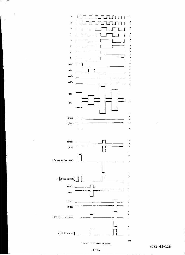
o
A
B
C
(ABe)
(A_)
(A_)
_J__rU____J!-F - i
,I--1 I l
r [
i J
+
o
+
+
1 +
+
J o
i +o
÷
o
mF--L__
F-_
EOI
E02
- (OA_C)
(_A--BC)
-(OABC)
( OABC )
- (OABC)
FIGI_RE A2 _IPORTAh_ _AVEFO_IS
_373
NORT 65-126
-169-
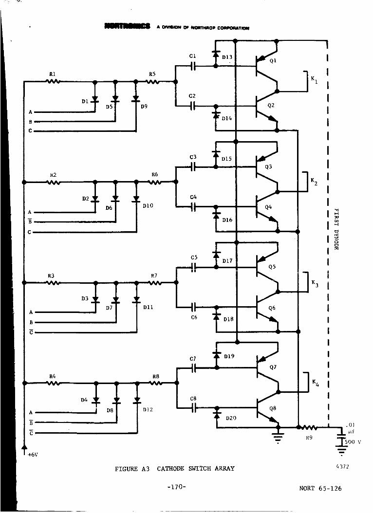
rlli_ A OIVmlON OF NOIqT_OP COiMeORATION
A
g
R4 R8
D4 C8
I D8 D12D20
Q7 I
IK4 I
I
Q8 II
R9
FIGURE A3 CATHODE SWITCH ARRAY
.0]
_f
T5oo vmm_
line
4372
-170- NORT 65-126

A DIVISION OF NORTHROP CORPOI_ATiON
+
x_-1 i-.4
_o-
o _
I o _.
Z _o _
T
-171- NORT 65-126

0or_
E
T
o
o
O---Z_0-
5_Z:_eJr_v
u_
F-4p_
-172- NORT 65-126
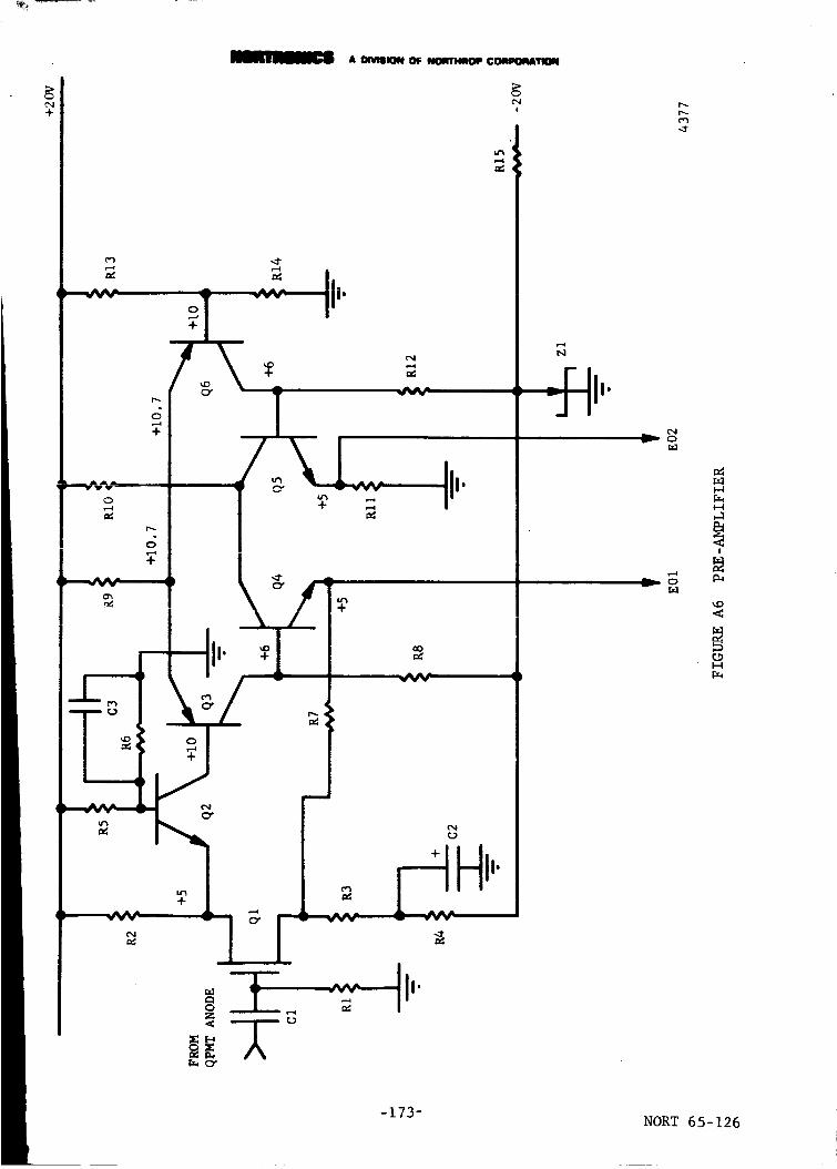
r
+
A O_nllOON OF _40WTO4aOP COqMeOmdkTaOOI
!
n_
'
r-_
m... 0v
I-I
!
p-_
,,D
l--tF_
-173- NORT 65-126
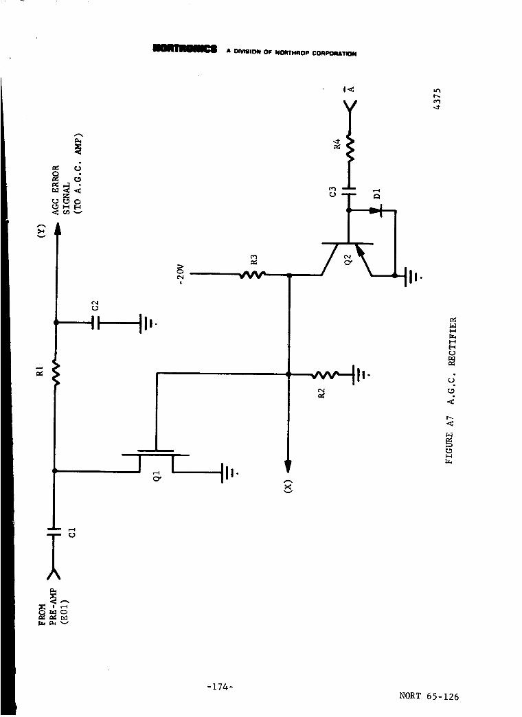
A 0_SION OF NORTHROP CORPOR4TION
F.s.fI_ v
U
i II, il'"
|
xv
P_
HE_c.}
g
r_
-174-
NORT 65-126

__,_ A DIVISION OF NORTHROP CORPORATION
>o
+
Ch
r',-
_O
O
Q
\
\ /
I
/
I
>_.._
v
llI'
_AA/"
,--I
--tI-_-il,,
I--I
i-ii-1
d
O0
,<
I--!
-175- NORT 65-126
7 (R 8-64)

ib : !
i
NORT 6 5-126
-176 =

I
+6Y
A OeVtK_I OFNOI_r_OP COIqPOAATOOI
-20V
E.3
"L'-" ..... -%a.. _ 1
I^>
B>
c>
(OR 5AI_C)
(OR OA_)
_>
B>
^>
_>
-20V
R9 RIO
Rll R12
FIGURE AI0 SYNC DETECTOR DRIVER
(2 REQ 'D)
R8
-20V
Q3
h. Dv
R7
am. Fv
4376
-177- NORT 65-126

m__ A DIVIS00N OF NORTHROP CORPORATION
COMPONENT PARTS LIST FOR CELESTIAL BODY TRACKER
ELECTR_IC MODIFICATIONS
Ao3
PART
siGH io
Cl thru C8
D1 thru I_O
QI, Q3, QS, Q7
Q6, Q8
R1 thru R8
R9
_UADRANT PHOTOMULTIPLIER CATHODE SWITCH ARRAY
PART
DEsmu i
8 0.i _f capacitors
20 IN916A Diodes
2N37h3 Hi-Volt a6e
PNP Transistors
2N37_2 Hi-Voltage
NPN Transistors
8 100K Resistors
i 3.9 meg. Resistor
MANUFACTURER
Texas Instr.
Mot orola
Motorola
FIGURE A-_i
HIGH VOLTAGE RECTIFIER
DI thru DI2 12 iN6h9 Rectifiers Texas instr.
FIGURE A-5n
SYNCHRONOUS DETECTOR
FI thru F5 l0
Cl, C2
(2 required)
FI-IO0 M0S FET
Transistors
0.01 _f Capacitors
Fairchild
FIGURE A-6 PREAMPLIFIER
R1
R2
R3R_
R5R6
R7, RII
R8, R12
R9RlO
R13, Rl_
C1
C2, C3
Q1
Q3, Q6 (Dual)
i
i
i
i
I
i
2
2
i
i
2
i
2
i
3
i
20meg68 K
300 n
30 K
15 K
6.2K
300 K
56 K
22 K
i00 K
51 K
0.001 _f, 3 KV
i0 _f, 20 V
2NBh38
2N3565
2N3801
-178-
AMELCO
Mot orola
NORT 65-126
7 (R 8-64)
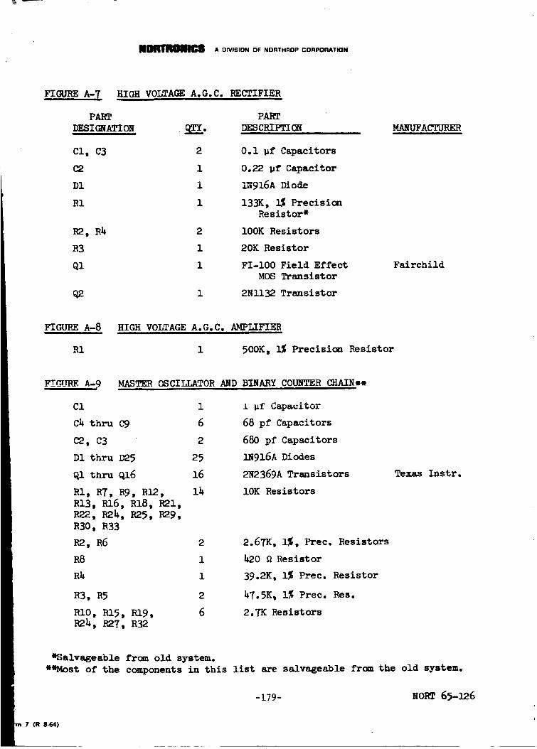
A DIVISION OF NORTHROP CORPORATION
nmmE A-?
PART
DESIGNATION
Cl, C3
C2
D1
R1
R2, R_
R3
Q1
Q2
HIGH VOLTAGE A.G.C. RECTIFIERi , _
2
1
i
1
2
1
1
1
PART
DESCRIPTI Cf_
0.i _f Capacitors
0.22 uf Capacitor
LN916A _ode
133K, 1% PrecisionResistor m
100K Resistors
20K Resistor
FI-IO0 Field Effect
MOS Transistor
2NI132 Transistor
MANUFACTURER
Fairchild
HIGH VOLTAGE A.G.C. AMPLIFIER
i 50OK, 1% Precision Resistor
F!C_3_REA-gL "
CI
cA thru O9
C2, C3
DI thru D25
Q1 thru Q16
RI, RT, Rg, R12,
RI3, RI6, RIB, R21,
R22, Pah, R25, R29,R30, R33
R2, R6
R8
R_
R3, R5
RIO, R15, RI9,R2_, R27, R32
MASTER oSCILLATORAND BINARY COUNTER CHAINw.i
i i _f Cap=citor
6 68 pf Capacitors
2 680 pf Capacitors
25 IN916A Diodes
16 2N2369A Transistors
2
i
i
2
6
10K Resistors
2.67K, i%, Prec. Resistors
_20 R Resistor
39.2K, 1% Prec. Resistor
hT.SK, 1% Prec. Res.
2.7K Resistors
Texas Instr.
eSalvageable frca old system.
W'Most of the components in this list are salvageable from the old system.
-179- SORT 65-126
rn 7 (R 8-64)

A DIVISION OF NORTHROP CORPORATION
.MASTER 0SCI_OR AND ,BINARY COUNTER CHAIR
PART
DESIGNATIGR
PART
RII, RI_, R20
R23, R28, R31
R17, R26
Z1
Z2
6
2
2.2K Resistors
20K Resistors
CD3814 Zener Diodes
CD2699 Zener Diodes
(C_t 'd)
MANUFACTURER
FIGURE, A.-IO
D1 thru D8
Rl, R2, RS, R7
R8, Rll, R12
R3, R9
Rl_, R6, RI0
QI, Q2, 03
SYNCHRONOUS DETECTOR DRIVER (2 required)
16 IN916A Diodes
14 100K Resistors
h
6
6
680K Resistors
20K Resistors
_N!I__ Transistors
-180- NORT 65-126
7 (R 8-64)rb
Jlol_rlllBiiil_lB A o,v,s,oN o_ NO.TeROPCO.PO.ATaO.
APPENDIX B BIBLI 0GRAPHY
le
2.
3.
to
o
e
_e
e
o
i0.
iio
2o
13°
14.
15.
Pitman, George, Inertial Guidance, John Wiley and Sons, 1962
Stearns, Edward V., Navisation and Guidance in Space, Prentice-Hall, 1963
Fc_andez, M. aud Mac_ber, George Ro, Inertial Guidance En_ineeriug ,Prentice-Hall, 1962
Leondes, Cornelius T., Guidance and Control of Aerospace Vehicles,McGraw-Hill, 1963
Kuo, Benjamin C., Anal[sis and sTnthesis of Sampled-Data Control S_stems,Prentice-Hall, 1963
Friedman, A. Lo, Rushman, A°, Gelb, Ao ,"Optimization of Sampling
Long-Term Inertial Navigation Systems," IEEE Transo on Aeroo and
Navo Elec., Sept° 1964, ppo 142-150
Swerling, P., Reich, Eo, "Statistical Theory of Navigation Employing
Independent Inertial and Velocity Measurements ," The Rand Corpo,
San5a _nica, Califo_ia, Rept. ]__M.-I_220,March 1954.
Kalman, R. E., "A New Approach to Linear Filtering and Prediction
Problems," _M_ J$ Basic Engineering, pp. 35-45, March, 1960
A. A. Michelson, Studies in O_tics, University of Chicago Press, 1927
Jenkins & White, Fundamentals of O_tics, McGraw-Hill, 1950
N. P. Laverty, "The Comparative Performance of Electron Tube Photo-
detectors in Terrestrial and Space Navigation Systems," IEEE TranSo
on Aerospace and Nay. Eleco, Sept° 1963.
Saul Moskowitz, "Simplifying Resolver Chain Design with Matrix Notation,"
Electronic Design, March 2,1964, pp 28-33
James Ao Fusca, "Advanced Guidance Concepts," Space/Aeronautics
Dec. 1964, Volo h2, No° 7, ppo 46-55
Robert G. Stern, "Selection of Optical Sightings for Position Determination
in Interplanetary Spsce ," Proc o of Natlo Aerospace Elec o Confo,
May ll-13, 1964, ppo 254-271
Gerald M. Levine, "Application of Midcourse Guidance Technique to
Orbit Determination," AIAA Journal, VOlo 3, Noo l, Jano 1965, pp 137-139
-181- NORT 65-126
7 (R 8-64)

n_r_m A DIVISION OF NORTHROP CORPORATION
l?.
18.
_o
20.
21.
22.
23.
24.
27.
28.
29.
James Holahan, "Attitude Control for Unmanned Spacecraft," Space/Aero-nautics, Feb o 1963, pp 78-86
J. D. Welch, "An Optical-Inertial Space Navigation System," Astro-
nautics & Aeronautics, June 1965, pp 90-9_
F. J. Clauss, "Lubricants and Self-Lubricating Materials for Spacecraft
Mechanisms," Lockheed Missiles and Space Division, _D-89hS12,
18 April 1961
J. C. Heindl and Ro J. Belanger, "OGO Solar Array Drive and Shaft
Support Bearing Tests," Space Technology Laboratories, TR2311-6026-
RU 00, 20 Sept. 1962
"Vac-Kote - - - A Vacuum Lubrication Process," Technical Memorandum
22.0, Ball Brothers Research Corporation, Feb. 1965
"Vac-Kote Capabilities," Technical Memorandum 22ol, Ball Brothers
Corp., July 1965.
"Vac-Kote Lubrication Technology for Long Space Life Bearing Applications,"
TN66-35, Ball Brothers Research Corp., March 4, 1966
R. Adamczak, R. Benzing, H. Schwe_er, "Advanced Lubricants and
Lubrication Techniques," Industrial and Engineering Chemistry,
Vol. 56, No. i, jan. ±_o_, pp -.._=.,
F. J. Clauss, W. Co Young, "Materials for Lubricated Systems,"
Space Materials Handbook, 2nd Edition, TeCho Documentary Report NOo
ML-TDR-C4-h0, Lockheed Missile and Space Company, Contract No.
AF33(657)-10107 for A. F° Matlo Lab., Wright-Patterson AF Base, Ohio
Technical Bulletins ca Solid Film Lubricants from Electrofilm Inco
B. D. McConmell, "Air Force Materials Laboratory Solid Film Lubrication
Research," Tech. Doc. Report No° ML-TDR 64-46 A.Fo Matlo Lab, Wright-
Patterson Air Force Base, Ohio, Apr. 1964
R. L. Johnson, D. Buckley, "Studies of Lubricating Materials In Vacuum"
presented at Southwest Research Institute Aerospace Bearing Comfo,
San Antcaio, Texas, Mar° 1964
T° Spalvins, D. Buckley, "Vacuum Deposited Gold Thin Films as Lubricants
in Vacuum (lO -ll mm hg)," presented at 12th Annual Vacuum Symposium,
Oct. 1965
T. Lo Ridings, "Tests of Dry Composite Lubricated Bearings for Use
in an Environmental Chamber," Aerospace Environmental Facility,
Arnold Engineering Center, Arnold Air Force Station, Tenno, Mar° 1965
-182- NORT 65-126
7 (R 8-64)

ADIVISIONOFNORTHROPCORPORATION
30.
31.
35.
36.
37.
38.
3_e
40.
Vo Hopkins, D. Gladdis, "Development of Solid Film Lubricants for
Use in Space Environments," presented at 1963 USAF Aerospace Fluids
and Lubricants Conf., San Antonio, Texas, Apr. 1963
R. Do Brown, R. A. Burton, P. M. Ku, "Long-Duration Lubrication
Studies in Simulated Space Vacuum," ASLE Transactions 7, (196_)pp 236-2
M. Devine, E. Lamson, J. Bowen, "Inorganic Solid Film Lubricants,"
Journal of Chem. and En_. Data Vol. 6, No. I, Jan. 1961, pp 79-82
"Lubeco 905 Technical Manual," Lubeco, Inc.
E. Bisson, W. Anderson, Advanced Bearing Technology, Office of
Scientific and Tech. Inf., National Aeronautics and Space Administration,NASA SP-38, 196_
F, F. Fischbach, M. E. Graves, P. B. Hays, R. G. Roble, "Satellite
Measurement of Atmospheric St_acture by Stellar Refraction," U. of
Mich., Dept. of Aeronautical and Astronautical Eng., High Alt. Eng.
Lab. Tech. Report for NASA, Goddard Space Flight Center, ContractN-aZr-5h(08), A_Dr. 1965
P. B. Hays, F. F. Fischbach, "Analytical Solution for Atmospheric
Density from Satellite Measurements of Stellar Refraction," Uo of
Mich., Dept. of Aeronautical _nd Astrona___ical Eng., High Alt. Eng.Lab. Tech. Report for NASA, Goddard Space Flight Center, ContractNo. NASw-lh0.
"SECOR, Sequential Collation of Range System," Status Report Uo S.
Army Corps of Eng., Apr. 196h
High Altitude Daytime Sky Background Radiation Measurement Program,
Sky Luminance, Polarization, Infrared Radiance and Albedo Data from
Research Vehicle No° 1," Part 1 and Part 2, Technical Documentary
Note No. AL TDR 6_-134, U.S.A.F. Avionics Lab., Research and Technology
Div., Wright-Patterson Air Force Base, Ohio, May 1964
R. J. Orange, "Autonomous Space Navigation," Space/Aer.onauticsVol. hS, No. 5, May 1966, pp 86-9ho
T. E. Rodgers, "Luxorb - A Novel Approach to the Reduction of Off-Axis
Light in Astro-Inertial Systems," paper presented at Optical Society
of America Meeting, April 3, 1959o
-183- NORT 65-126