No. 029/2020/MKT Consumer Choices Across Seemingly Disparate ...

No. 029/2020/MKT

Consumer Choices Across Seemingly Disparate Product Categories

Chen LIN*

Department of Marketing

Michigan State University

Douglas Bowman

Department of Marketing

Emory University

July 2020

––––––––––––––––––––––––––––––––––––––––

* Corresponding author: Chen LIN ([email protected]). Address: Department of Marketing, China Europe

International Business School (CEIBS), 699 Hongfeng Road, Pudong, Shanghai 201206, China.

CONSUMER DECISIONS ACROSS SEEMINLY DISPARATE CATEGORIES:

LATENT-TRAIT SEGMENTATION

Chen Lin

Michigan State University-Department of Marketing

Douglas Bowman

Emory University - Department of Marketing

May 2014

1

CONSUMER DECISIONS ACROSS SEEMINLY DISPARATE CATEGORIES:

LATENT-TRAIT SEGMENTATION

ABSTRACT

This research takes a first step in modeling latent processes that govern consumer decision

making by examining consumption across seemingly disparate categories. Marketing activities

today are coordinated in a variety of categories and in a variety of formats, and consumers

naturally shop around a globe of unrelated product categories that are beyond the traditionally

defined “shopping basket”. We propose a hierarchical multinomial processing tree model to

empirically examine the driver, which is defined as the “latent trait”, which governs consumer

choices across five seemingly disparate product categories: media consumption, automobile

purchases, financial investments, soft drinks and cell phone plans through a dataset consisting of

5,014 consumers in the United States. We further investigate how consumer behavior

systematically varies from one category to another and finally suggest new approaches to

segment and profile consumers based on latent traits across multiple categories. In doing so, this

paper contributes to the consumer decision literature in three ways: 1) theoretically, the latent-

trait approach provides rich support in examining the underlying psychological processes; 2)

methodologically, the relative merits of models with continuous versus discrete representations

of consumer heterogeneity are discussed; and, 3) substantively, new insights on targeting and

profiling based on latent processes rather than observed behavior are presented with respect to

managing across seemingly unrelated product categories.

Keywords: Seemingly Disparate Categories; Segmentation; Latent Trait

2

1 INTRODUCTION

“To look at a leopard through a tube, you can only see one spot.”

-From Ancient Chinese Idiom (422 AD)

The task for marketing managers today is increasingly complex and customer-oriented.

Traditional practice involves brand managers planning and organizing marketing activities

around individual brands, then shifting towards category managers who coordinate purchasing,

merchandising and prices of a set of brands within a category (Zenor 1994) and occasionally

across categories within the “market basket” (Bell and Lattin 1998; Seetharaman et al. 2005).

Most recently, as marketing practice embraces customer orientation and customer management,

managers note that consumer purchases are never just limited to a few brands, or grocery

shopping basket. In fact, consumers naturally shop around a globe of disparate product

categories that are more complex and diverse than the traditionally defined market basket in

retailing research. Here, the term “disparate” is similar to “non-comparable” (Johnson 1984),

which describes the degree to which choice alternatives can be represented by the same attributes,

but offers a broader and more generalized description of categories that are utterly dissimilar and

difficult to compare with each other than merely a function of the number of common and

distinctive features associated with alternatives as in comparability (Tversky 1977). For example,

consumers drive certain cars and listen to certain radio channels; they prefer certain soft drinks

and behave in certain ways when it comes to financial investments. These categories have

typically been studied in isolation, but they collectively reflect a more complete and realistic

picture of consumer demand rather than steady snapshots for consumer behavior as in previous

3

research. This research aims to examine consumer choices across seemingly disparate product

categories in order to specify a fuller model of the consumer demand problem.

Insights from understating behavior across seemingly disparate categories would be

increasingly relevant in today’s retail context for customer valuation, segmentation, cross-sell

and resource allocation (Reinartz and Kumar 2003; Shah and Kumar 2008). Marketing activities

are coordinated in a variety of categories and in a variety of formats. Supermarkets such as Wal-

Mart make assortment decisions for product categories that are not closely related, including

consumer electronics, furniture, apparel, grocery and many others. The rewards from loyalty

programs such as Air Miles can be accumulated or redeemed in many outlets, ranging from

gasoline services and package holidays to supermarket shopping. Brand extension efforts make

Virgin Group a conglomerate that builds presence across different business areas. Moreover, due

to the growing ability to track consumer purchase patterns cross categories using CRM and web-

based tools, Internet retailers (such as Amazon and Groupon) and platform providers (such as

Facebook) are proactively managing across a wide assortment of categories and having access to

a rich database of consumer behavior that was not able to be tracked traditionally. Managers are

urged to embrace the challenge of creating a broader and richer description of customer behavior

and understand the deeper underlying process of consumer decision making.

Identifying and assembling purchase patterns from individual categories can assist in

segmentation and targeting. To date, behavioral-based segmentation focuses primarily on “what

consumers did” rather than “why they did it”. The objective of this research is to help managers

get at the “why” question by studying and inferring the latent processes from observed

behavioral data that are accessible to today’s firms (rather than incurring the additional cost of

augmenting with experiments, survey data or brain scans). The genesis is that consumers are

4

alike because they share similar thought processes, not because they display similar observed

behavior as assumed in traditional segmentation approaches. Nevertheless, one reason that

previous research on cross-category behavior often restricts to related categories is due to data

availability. It is difficult to get access to customer purchase data across a wide range of

seemingly disparate categories and infer consumers’ underlying processes based on observed

behavioral patterns. Our goal is to build a theory-driven model that helps managers to understand

and measure the impact of the underlying processes that explain systematic co-variations across

seemingly disparate categories based on behavioral data.

In fact, the process of aligning decisions across seemingly unrelated categories occurs

naturally and bilaterally. Consumers constantly make choices for every aspect of their lives, from

complex decisions such as which car to purchase, in which stock to invest, and to which cell

phone plan to subscribe, to more routine ones such as which soda to drink and which television

channel to watch. There could be many types of underlying processes that explain co-variations

across categories. One famous example in the marketplace, originally to illustrate the power of

data mining (Financial Times of London, Feb 7th

, 1997), is of “Beer and Diapers”. It is observed

that beer and diapers, two categories which appear to be unrelated, tend to be purchased together

simultaneously by male customers. Traditional models on multi-category choice behavior would

only capture this phenomenon through demographics and random errors, and fail to recognize

the deeper rationale that male customers seek convenience when making shopping trips. Another

example is that we may observe certain consumers tend to be “innovators” of many categories as

they always prefer the latest new products or services, ranging from apparel and cell phones to

automotives. We may also observe that certain consumers are more inclined to purchase or hold

multiple types of products, either because of the need for variety-seeking, or because of a limited

5

capability to reach a single decision (Dowling and Uncles 1999). In this case, people are alike

not only because they coincidentally display similar observed behavior but also because they

share similar latent decision processes. While traditional segmentation research attempts to group

people of similar observed outcomes together and explain their behavior with a same-response

coefficient, assuming that “birds of a feather flock together” (Desarbo et al. 2004; 2006; Heilman

and Bowman 2002), this research provides a first step in categorizing customers as a set of

value-based process parameters for theory-driven segmentation and profiling exercises.

This research contributes to the literature in three ways. First, it takes a first step in

modeling a complete picture of consumer decision problems by examining consumption across

seemingly disparate product categories. Second, it investigates the latent processes that govern

consumer decision making across decision stages and across categories to advance our

understanding in both dimensions of customer behavior: the breadth of their consumption

portfolio, and the depth of their latent decision processes. Third, it provides richer insights on

targeting and profiling based on continuous latent processes rather than discrete observed

behavior. Specifically, we propose a hierarchical multinomial processing tree model to

empirically examine the underlying processes, which are defined as the “latent traits” that govern

consumer choices across five seemingly disparate product categories1: media consumption,

automobile purchases, financial investments, soft drinks and cell phone plans through an

asyndicated dataset consisting of 5,014 randomly selected consumers in the United States.

The model is estimated using Bayesian methods with weakly informative hyperprior

distribution and a Gibbs sampler based on two steps of data augmentation. While the latent

process structure remains the same across these categories, we further investigate how consumer

behavior systematically varies from one category to another and finally suggest new approaches

1 I will explain the selection of categories in the data section.

6

to segment and profile consumers based on collection of continuous latent traits (rather than

discrete observed behavior) across multiple categories. Lastly, we compare the latent-trait

approach with the latent-class approach and identify conditions under which they may yield in

similar or dissimilar results from a data-driven perspective.

Latent trait models have a long history in psychometric studies of psychological

constructs such as verbal and quantitative ability (see, e.g., Lord and Novick 1968; Langeheine

and Rost 1988) but have not received much attention in the marketing field. Essentially, any

person-level difficult-to-observe continuous parameters, whether well-defined or undefined,

goal-oriented or heuristic-based, can all be considered as latent traits. It can take place at many

levels of decision making. For example, at the product category level, need for convenience is

the latent trait that explains the phenomenon of beer and diapers. It is highly likely that male

consumers would exhibit the same trait when choosing brands and products, such as choosing

the most accessible diaper brand on the shelf, or choosing the beer that they are most familiar

with. Furthermore, decision processes can often be casted into a tree model in a natural and

principled manner, and latent traits can be best viewed as the branches that lead to decision

nodes at each stage. Depending on the firm’s interest in key decision variables and availability

of data, the tree structure can be adapted in a specific setting. For example, if managers are

interested in the impact of “need for convenience” on store and assortment choices, then the tree

will start from a consumer who chooses between the more “convenient” stores (i.e., stores within

a certain distance) and less convenient stores, then chooses between more “convenient”

assortments (e.g., shelf allocation in the case of beer and diapers). At each stage, the latent trait

of “need for convenience” determines the consumer’s paths in taking upper or lower decision

branches. If a firm’s interest lies in capturing the latent trait of “innovativeness” in category and

7

brand management, then the decision tree will start from a consumer choosing between the

newer (more innovative) and more established product category, followed by decisions in brands,

and finally in products.

As noted earlier, many types of latent traits may affect consumer decision making and

this research is at best offering a process for studying the impact of latent traits. For exposition

and without loss of generality, I examine one specific type of latent trait, which is defined as

“polygamy”. Polygamous loyalty has been documented in the literature to describe the behavior

of “divided loyalty” among a number of brands (Dowling and Uncles 1997; Bowman 2004).

Polygamy is the tendency of individuals to seek multiple types of products, services, or brands,

as opposed to holding to a single one. It is an idiosyncratic trait that a consumer has and, when

manifested, it can lead to interior solutions where their constrained utility is maximized on the

budget constraint with strictly positive quantities of two goods (i.e., multiple goods are chosen

from the alternative set). It is noteworthy to distinguish polygamy from variety-seeking behavior,

which can be viewed as a subset or outcome of polygamy that describes the switching behavior

among brand/product/service alternatives, as opposed to loyalty (Khan et al. 1986). While

consumers engage in variety-seeking activities merely as a result of satiation (Kim et al. 2002),

they may seek polygamy for various reasons such as sensation, diversification, convenience,

security, complementarity and/or inability to reach a single decision. Polygamy may take place at

many levels of the decision process. For example, at the product level, investors may hold

different stocks as a portfolio; at the brand level, diners may order different brands of wines at

one occasion; at the product-type level, consumers may want both a laptop and a desktop; and

finally, at the product-category level, consumers almost always hold multiple categories. In

addition, depending on the product category, consumers are likely to experience a satiation effect

8

or “heavy-user” effect when moving across layers of decision processes. For example, if

consumers purchase multiple types of automobiles, they may be less likely to purchase multiple

brands within each type. Nevertheless, for media consumers who enjoy the large variety of

website choices that Internet offers, it is more likely that they will also subscribe to multiple

television channels at a time. Such variations across levels of decision processes and product

categories allow better identification when estimating the parameters and enrich potential

insights that latent trait can generate.

In summary, by testing one specific latent trait of “polygamy”, this research takes the

first step to empirically investigate the continuous latent processes that govern consumer

behavior across seemingly broad and disparate product categories and across different decision-

making stages to advance understanding in both dimensions of customer behavior: the breadth of

their consumption portfolio and the depth of their latent decision processes. Specifically, this

research addresses: 1) whether latent trait has an impact on consumer decision making and the

magnitude of such impact, if any; 2) how a latent trait is manifested across different levels of

decision making; and 3) how the effect of a latent trait varies across seemingly disparate

categories. In doing so, this research contributes to the consumer decision literature in three ways:

1) theoretically, the latent-trait approach provides rich support in examining the high level

processes; 2) methodologically, the relative merits of models with continuous versus discrete

representations of consumer heterogeneity are discussed; and 3) substantively, by providing new

insights on targeting and profiling with respect to managing across seemingly unrelated product

categories.

The remainder of this essay is organized as follows. Section 2 reviews related streams of

literature and our general approach to modeling consumption across seemingly disparate

9

categories. This is followed by the empirical model in Section 3, a description of the data

(Section 4), and estimation and results in Section 5. We then conduct a latent-class segmentation

analysis ex-post based on the first stage latent trait parameters in Section 6, and conclude with a

discussion of key findings, implications for management, limitations and directions for future

research in Section 7.

2. LITERATURE REVIEW

Marketing research on consumer choice across seemingly disparate categories and latent

traits is scarce. Nevertheless, related literature on cross-category models of consumer choice and

decision making processes has been popular. Consistent with the shift in practice, marketing

research has progressed gradually towards examining the full picture of decision problems. The

literature on cross-category behavior evolves from standard single category choice models with

homogenous demand specifications and independent category decisions (McFadden 1980;

Guadagni and Little 1983; Bucklin and Gupta 1992; Berry 1994) to models addressing

correlations between two or three related, by and large complementary product categories

(Erdem 1998; Manchanda et al. 1999; Heilman and Bowman 2002; Chung and Rao 2003), and

most recently to multi-category choice models (aka market basket models) that describe purchase

behavior in typically eight to ten categories within grocery shopping trips (Ainslie and Rossi

1998; Bell and Lattin 1998; Seetharaman et al. 2005; Mehta, 2007). In doing so, this stream of

research uncovers the correlations in cross-category purchase outcomes and marketing mix

sensitivities from complementarity, consumer heterogeneity, state dependence and coincidences.

The genesis is that if sensitivity to marketing mix variables is a common consumer trait, then one

should expect to see similarities in sensitivity across multiple categories (Ainslie and Rossi

1998). For example, a low-income household might be price sensitive in many product

10

categories. However, the categories studied are usually within the grocery shopping basket and

are, by nature, closely related (e.g., toothbrush and toothpaste). The reality is that consumer

purchases are never limited to a grocery context and customer behavior is likely to vary

systematically across product categories as a function of more than the sources of cross-category

variations listed above. For example, the joint purchase of beer and diapers would have been

incorrectly picked up as mere coincidences by previous research. Hence, research that examines

consumption across seemingly disparate categories would provide a more realistic and

generalized approach in studying cross-category behavior. In order to study behavior in such a

broad and comprehensive consumption context, managers need a more sophisticated approach

that describes and provides a deeper understanding on consumers’ underlying preferences or

processes that govern choices.

There are many approaches, such as attitudinal or behavioral, that one can use to study

disparate categories. Decades ago, researchers typically looked at choices at an aggregate level.

Attitudinal research and survey studies on consumer “Values, Attitudes, Lifestyles” (VALS,

VALS2) have long been interested in addressing such problems. While this stream of research

often suffers from implementation difficulties such as smaller sample sizes, greater collection

efforts, and sometimes self-report bias, they provide an intriguing angle to understanding person-

factors (though mostly on attitudes and aggregated discrete segments or labels) from consumers’

perspectives. On the behavioral side, techniques such as grouping or conglomeration are

available to analyze data from aggregate responses and decompose the tabular frequencies into a

set of latent classes or segments (Desarbo et al. 1993; Wedel and Kamakura 2000). A limitation

of such an approach is that it relies on brute-force statistical fits rather than a utility-maximizing

framework, and therefore is less theoretically realistic (Wedel et al., 1999). Furthermore, it

11

imposes a fixed number of latent classes and assumes each person to be a member of one latent

class. This is often too restrictive and difficult to interpret. In many applications, a continuous

distribution of a parameter value that accommodates heterogeneity across consumers is more

realistic (Andrews, Ainslie and Currim 2002; also see Andrews, Ansari and Currim 2002).

Most recently, there is a growing interest in understanding psychological processes that

contribute to decision making (McGuire 1976). Over the past thirty years, a large stream of

experimental studies show that consumer decision making is a highly complex process that

challenges the assumption of a well-defined preference structure (or utility function) in modeling

literature (Bettman 1979). New developments in neurosciences such as CAT scans and fMRI

illustrate that different parts of the brain are active during different parts of mental life (including

consciousness, emotions, choices and morality) and exact brain regions can be pinned down for

certain types of decision making (Hedgcock and Rao 2009; Weller et al. 2009).

Despite the critical role of high-level latent processes in consumer decision making, there

is little empirical research examining its impact on consumer choice with behavioral data.

Incorporating these difficult-to-observe process parameters into well-defined quantitative models

requires a continuous distribution of the latent variables. This can be achieved through latent trait

analysis, which has received considerable attention in psychometrics and mathematical

psychology. There are a few early marketing applications discussing latent or unobserved

variables in survey research (Balasubramanian and Kamakura 1989), coupon redemption (Bawa

et al. 1997) and cross-selling of financial services (Kamakura et al. 1991) in a single category

context. Operationally, latent trait is the “person parameter” that has been defined in item

response theory. It represents the strength of an attitude and captures parameter heterogeneity

due to individual differences between persons, as opposed to parameter homogeneity in latent

12

class approach. It has two unique advantages over traditional models: to the extent that

marketing is applied psychology and applied sociology, the latent trait approach is more

theoretically grounded by investigating the underlying decision process that impacts consumer

choice; and empirically, a continuous distribution of person parameters usually leads to better fit.

3. The Empirical Model

In this research, I adopt a hierarchical multinomial processing tree model with Bayesian

methods to examine the impact of polygamy on consumer choice while incorporating

heterogeneity. Multinomial processing tree (MPT) models have been extensively used in

cognitive psychology for memory testing, perception research and reasoning (see an overview by

Batchelder and Riefer (1999)). MPT models are discrete choice models that are developed

exclusively to explicitly measure and disentangle the impact of underlying or latent cognitive

capacities with panel data resulting from multiple and confounded processes (Ansari, Vanhuele

and Zemborain 2007). The “structural” parameters represent underlying psychological processes.

Each MPT model is a re-parameterization of the decision outcome probabilities of the

multinomial distribution, with each branch of the tree representing a different hypothesized

sequence of processing stages and leading to a specific decision outcome. Hence, assumptions

about the psychological processes in a given experimental paradigm can often be cast into the

form of a processing tree structure in a natural manner (Klauer 2010).

Consistent with the choice modeling literature, the tree structure begins with a consumer

choosing among categories (or types or channels), followed by brands and products. However,

unlike choice models which rely on conditional probabilities to reach to the bottom of the

hierarchy (i.e., product choice), our latent-trait MPT approach explicitly lets the latent trait

determine the path to follow in traversing the tree structure. In addition, the latent trait for

13

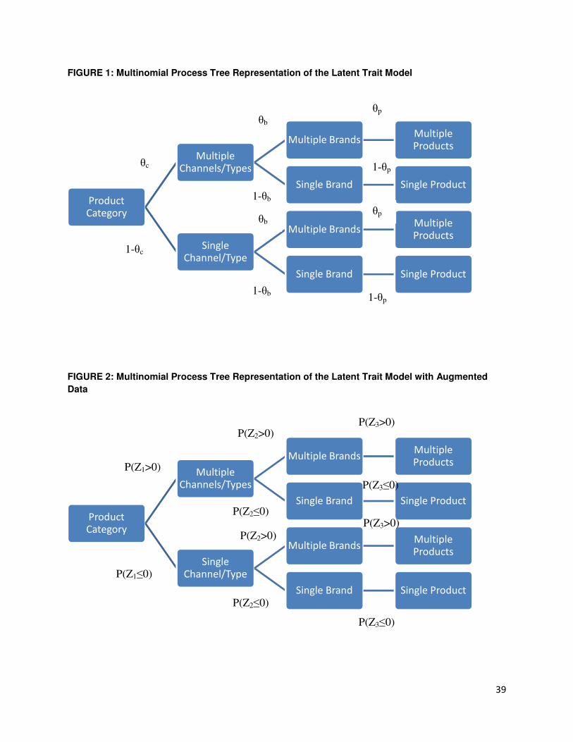
polygamy is active during every stage of the decision tree. We code polygamy separately for

channel/type (θc), brand (θb) and product (θp). Figure 1 shows the structure of the multinomial

processing tree. Each product category is modeled by separate subtrees of the multinomial model.

For a given product category, a consumer will first decide whether to choose multiple

types/channels or a single one, then decide whether to choose multiple brands, and finally

whether to choose multiple products2. Therefore, there will be up to a total of three latent trait

parameters and eight mutually exclusive decision outcomes (end nodes) for each product

category. Our model building can be viewed as a three-step hurdling process: as illustrated in Figure

1, the model starts with observed individual level decision outcome frequencies, with the paths

leading to the outcomes governed by the latent processes; then, it employs a Probit-link to transform

individual parameters to population/prior, which is further specified using a hyperprior. Lastly, data

augmentation is used for easier empirical estimation.

3.1 Person-Level Model

Specifically, for product category or subtree k, k = 1, . . . , K, j = 1, . . . , Jk , and consumer

t, t = 1, . . . , T, the decision outcome/node Ckj is mutually exclusive and has a frequency nkjt,

which follows a multinomial distribution with parameters pkjt, j = 1, . . . , Jk,. For product

category k, let Nk be the fixed number of responses. Across product categories k, the data are

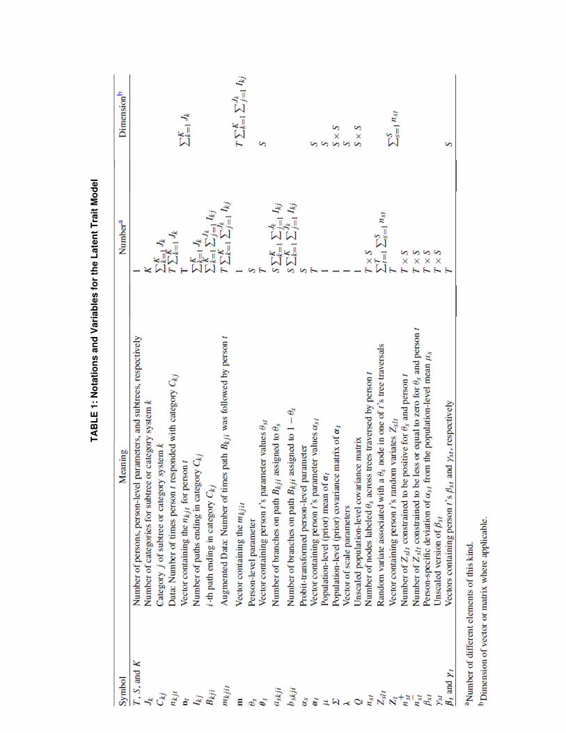
assumed to be distributed stochastically independent for each consumer t. In Table 1, an

overview of the most important symbols is given for easy reference.

Let pkjt denote the choice probabilities of reaching the end node decision outcome Ckj by

means of S structural parameters θs, s = 1, . . . , S, each θs being probabilistic and free to vary in

(0, 1) (Ansari et al. 2007; Klauer 2010):

2 We conducted robustness checks on the sequence of decision making process (e.g., product first, then brand and

lastly type) and the results do not vary significantly.

14

�� = ��), (1)

Here, θt is the vector of consumer t’s parameter values θst, s = 1, . . . , S. It represents a sequence

of latent binary events which determine the path followed in traversing the tree. The choice

probabilities P(Ckj | θ) sum to 1. We can use a simple EM algorithm for maximum-likelihood

estimation of the model parameters (Hu and Batchelder 1994). This form can be characterized by

means of the model’s representation as a processing tree (e.g., Figure 3). Let the number of paths

ending in decision outcome Ckj of subtree k be Ikj, and let the ith such path be denoted by Bkji.

The probability that path Bkji is followed by consumer t in traversing the tree is given by:

��)= ∏ ��(1 − �)�� , (2)

where askji and bskji are the number of branches on path Bkji that are assigned to parameter θs and

its complement 1−θs , respectively. The probabilities for a given node are then computed by

adding the probabilities of all paths that terminate in the respective decision outcome:

��)=∑ ∏ ��(1 − �)�� , (3)

The vector of person-level decision outcome counts nt = (n11t, . . . , n1J1t , . . . ,

nK1t, .. .,nKJKt ) is modeled by a vector-valued random variable Nt that follows a product-

multinomial distribution:

�( � =!�|��)= ∏ #$ %�&�'(…&��(*∏ [��),-�� ]&��(/0�� , (4)

The model from Equation 19 defines the person-level model. In the next sections, we will

specify the prior distribution, hyperprior distribution, and the Gibbs sampler required for the

analysis.

3.2 Prior Distribution

Ansari et al. (2007) use a logit link to transform parameters from the interval (0, 1) to the

real line and to model the transformed parameters by a multivariate normal distribution with

15

arbitrary mean µ and arbitrary covariance matrix Σ to be estimated from the data. Klauer (2010)

employs a similar approach through a probit link and a less informative hyperprior distribution

with a Gibbs sampler.

Specifically, the person-level model is re-parameterized by means of new population-

level parameters αst linked to the original personal-level parameters θst via αs = Φ−1

(θst ), s =

1, . . . , S, t = 1, . . . , T , where Φ is the cumulative distribution function of the standard normal

distribution. Let us collect the parameters αst in the vector αt. Across individual consumer t, the

parameter αt is assumed to follow a multivariate normal distribution with mean vector µ and

covariance matrix Σ:

αt ~ N(µ,Σ). (5)

That is, the person-level model is the multinomial-processing tree model with probit-

transformed model parameters. It allows for separate parameter estimates for each person, but

the population-level model constrains the individuals’ parameters to be distributed according to a

multivariate normal distribution with mean and covariance matrix to be estimated from the data.

3.3. Hyperprior Distribution

In the Bayesian framework, a hyperprior distribution is required for the population-level

parameters of the prior distribution with mean µ, which is assumed to follow an independent

normal distribution with mean zero and variance p = 100, and a covariance matrix, which is

assumed to follow a scaled Inverse–Wishart distribution. Using a new set of scale parameters λs,

s = 1, . . . ,S, they decompose Σ = (σkl) as follows:

Σ = Diag(λs)QDiag(λs ) (6)

where Q= (qkl) and σss = λs2qss. Whereas the correlations ρkl = σkl/1(2��233)are determined only

by Q, that is, ρkl = qkl/1(4��433). Assuming an Inverse–Wishart distribution for Q with S +1

16

degrees of freedom and scale matrix set to the identity matrix I therefore maintains the desirable

uniform distribution for the parameter correlations. The parameters of interest are αt, µ, and Σ.

The following hyperprior distribution results:

µ ~ N(0S, 100I),

Q ~ Inverse–WishartS+1(I),

λ ~ N(1S, 100I), (7)

where 0S and 1S are vectors of dimension S with zero and one, respectively, in each cell.

3.4 Data Augmentation for the Gibbs Sampler

The proposed model includes two steps of data augmentation that are required for the

Gibbs Sampler. First, we augment the decision outcome frequencies nkjt by the path frequencies

mkjit and collect all path frequencies in the vector m. Second, a different random variable Z is

assigned to each node. As shown in Figure 2, as the tree is traversed, the upper branch emanating

from a given node is taken if the associated Z > 0 and the lower branch if Z ≤ 0. Let Z follow an

independent normal distribution with mean αs with αs = Φ−1

(θs) and variance 1. From a theory

point of view, the decision outcomes nodes can be viewed as binary choice points with choices

driven by unobserved latent variables Zslt exceeding a given threshold or not. For example, the

choice may indicate whether a consumer’s polygamy is triggered and activated. Since each node

is assigned to one of the processes postulated by the multinomial model, and the outcome of the

process determines which choice is made in moving through the processing tree, they provide a

substantive underpinning of latent processes beyond mere technical convenience.

Specifically, each person runs through Nk trials for product category (or subtree) k, k =

1, . . . ,K. Each such trial x, x = 1, . . . ,Nk, defines Rk random variables Zkxrt , r = 1, . . . , Rk ,

where Rk is the number of nodes or decision outcomes in product category k. The vector Z

17

collects all Zkxrt in a fixed order. Each node indexed by k and r is assigned one of the person-level

parameters αs. Let the number of nodes associated with parameter αs in subtree k be oks . Across

subtrees k, there are nst =∑k Nkoks random variables Z per consumer with mean αst, consumer t’s

value on parameter αs . An alternative way to index the ∑t∑s nst elements of Z is therefore as Zslt

with Zslt being the lth element of those elements of Z that are assigned parameter αst as its mean.

Furthermore, it turns out that all conditional posterior distributions that are needed for the

Gibbs sampler, other than the conditional posterior distribution of the individual Zslt, do not

depend on the order in which the paths occurred, nor on the order in which the nst values of Zslt

were observed for each s and t (Klauer 2010). Therefore, we can work with order statistics5678 , in

which the nst variables Zslt appear in ascending order. Let Zo be the vector that stacks the order

statistics5678 , s = 1, . . . , S, t = 1, . . . , T. The double data augmentation procedure by path

frequencies m and by Zo allows the posterior distribution of the model parameters to be

expressed as a standard hierarchical linear regression with the given 56978 as the data, and

therefore facilitates straightforward adaptation of the well-understood Gibbs sampler for

analyzing standard hierarchical linear regression models in a Bayesian framework (e.g., Gelman

and Hill 2007). Thus, the remainder of the model can be analyzed as though it was the following

linear model:

Zt ~ N(Xtαt, I),

αt ~ N(µ,Σ), (8)

with (µ,Σ) distributed according to the hyperprior specified above and Xt as a design matrix

containing zeros and ones that simply assigns αst as mean to each Zslt , l = 1, . . . , nst , s = 1, . . . ,S,

t = 1, . . . , T .

18

To summarize, the double data augmentation and the probit link have two advantages.

Technically, they allow replacing observed categorical responses by continuous data with an

underlying linear Gaussian structure (Albert and Chib 1993). More importantly, they provide a

substantive underpinning of latent processes.

3.5 The Gibbs Sampler

A Gibbs sampler is a Monte Carlo–Markov chain algorithm for sampling from the

posterior distribution of the model parameters given the data n. Let us then re-parametrize the

parameters αt as follows:

αt = µ+βt ,

βt = Diag(λs )γt . (9)

The parameter µ is the prior mean of the parameters and the parameters βt are the

individual-specific systematic deviations from it. The parameters λs are the scale parameters of

the scaled Inverse–Wishart distribution and the parameter γt is an unscaled version of βt. Let γ be

the vector that stacks the vectors γt, t = 1, . . . ,T. The Gibbs sampler cycles through blocks of

parameters. For each block, one sample is drawn from the conditional distribution of the

parameters of the block given the data and the remaining parameters. The parameter blocks for

the Gibbs sampler are Q, (Zo,m), γ ,λ, and µ. The detailed conditional distributions are given

below.

Conditional Distribution of Q

The conditional distribution of Q given the data and the other parameters depends only on

the parameters γt. Let S be the sum of cross-products of the γt : S – ∑ :7:7′;�� , then

Q| m, Zo, γ, µ, λ, n ~ Inverse–WishartT+S+1(I +S), (10)

Conditional Distribution of (Zo, m)

19

The conditional distribution of (Zo,m) is sampled from by sampling the conditional

distribution of m with Zo integrated out, followed by sampling from the conditional distribution

of Zo given m, n, and the other parameters.

The conditional distribution of m given the data and the other parameters depends only

on the data n and the parameters γt, µ, and λ. For each person and decision outcome Ckj , the path

frequencies mkjit , i = 1, . . . , Ikj , follow a multinomial distribution with parameters nkjt and pi, i =

1, . . . , Ikj, as defined in Equation 7 (note that θst = Φ(µs + λsγst ), hence pi = pi(µ, γt ,λ)). Thus, m

follows a product-multinomial distribution:

m | Q, γ ,µ, λ, n ~ ⊗7�=> ⊗?�=@ ⊗A�=B

Multinomial (nkjt, (pi (µ, γt,, λ )i=1,…,Ikj)), (11)

Consider next the conditional distribution of Zo given m, γ, λ, µ, Q, and n. To derive this

distribution, consider first the conditional distribution of the (unordered) Z. Let P be a sequence

of paths, P = (Pkxt )kxt , path Pkxt being a path of subtree k assigned to individual t ’s trial x, t =

1, . . . , T , k = 1, . . . , K, x = 1, . . . , Nk . Let ξm be the set of sequences of paths P consistent with

path frequencies m, that is, with mkj it being the number of trials x with Pkxt = Bkji for each k,j,i,

and t. By definition of conditional probabilities, the density of Z is:

f (Z | m, Q, γ ,µ, λ, n) = ∑ f(5|D,E, F, :, G, H, I)P(D|E, F, :, G, H, I),K∊ME (12)

The conditional distribution of Zo given the data, the path frequencies m, and the other

parameters need to be generated only to the point that it is consistent with the path frequencies m,

and the order information is not required. Let !��N =∑ ∑ ∑ O��P��-Q��

,-,��0�� normal variates Zslt

with mean αst truncated from below at zero, !��R =∑ ∑ ∑ S��P��-Q��

,-,��0�� normal variates Zslt

with mean αst truncated from above at zero, and !�� − !��N − !��R nontruncated normal variates Zslt

with mean αs. It is sufficient to generate !��N and !��R truncated normal variates with mean αst and

variance one truncated at zero from below and above, respectively, as well as !�� − !��N −

20

!��R unconstrained normal variates with mean αst and variance one for each parameter s and

individual t.

Conditional Distribution of γ

The different γt , t = 1, . . . , T , are conditionally independent, so that they can be sampled

one after the other for a sample from the conditional distribution of γ . For each person t, the

conditional distribution of γ t can be derived as a Bayesian regression with data λs−1

(Zslt −µs), s =

1, . . . , S, l = 1, . . . , nst, that are independently normally distributed with mean γt and variance

λs−2

and with a normal prior for γt , γt ~ N(0S,Q). Thus, the conditional distribution of γt given the

data and the other parameters is multivariate normal with mean gt and covariance matrix Gt given

by

gt = GtDiag(λs)ut ,

Gt = (Q−1

+Diag(nstλs2))

−1, (13)

where ut is the vector of the sums ∑ (T�3� − G�)&��3�� , s = 1, . . . , S.

Conditional Distribution of λ

The conditional distribution of λ can be derived as a Bayesian regression with data

U��R�(Zslt − µs), s = 1, . . . ,S, l = 1, . . . , nst , t = 1, . . . , T , that are independently normally

distributed with mean λs and variance U��RV(and with a normal prior for λ, λ ~ N(1S,pI), where p is

the variance of the hyperprior of λs (i.e., p = 100). Thus, the conditional distribution of λ given

the data and the other parameters is multivariate normal with mean h and covariance matrix H

given by

h = Hv,

H = Diag ( p−1

+∑ !��;�� U��V )-1

, (14)

where v is the vector of the terms p-1

+ ∑ U��;�� ∑ (T�3� − G�)&��3�� , s = 1, …, S.

21

Conditional Distribution of µ

The conditional distribution of µ can be derived as a Bayesian regression with data Zslt

−λsγst, s = 1, . . . , S, l = 1, . . . , nst , t = 1, . . . , T , that are independently normally distributed

with mean µs and variance one, and with a normal prior for µ, µ ~ N(0S,pI). Thus, the conditional

distribution of µ given the data and the other parameters is multivariate normal with mean u and

covariance matrix U given by

u = Uw,

U = Diag( p−1

+∑ !��;�� )-1

, (15)

where w is the vector of the sums ∑ ∑ (T�3� − W�G�)&��3��;�� , s = 1, . . . , S.

3.6 Implementation

Rough initial estimates of the parameters µ and Σ are obtained by means of the Monte

Carlo EM (MCEM) algorithm. For the expectation step, the conditional distribution of βt, t =

1, . . . ,T , is sampled via a Gibbs sampler for given µ and Σ and given the data. The Gibbs

sampler samples from the relevant conditional distributions specified above with µ and Q fixed at

their current estimates, and with λs fixed to one, s = 1, . . . ,S, so that Σ = Q and βt = γt . In the

maximization step, µ is then estimated as the mean of the sampled βt, and Σ as the covariance

matrix of the sampled βt. Initial overdispersed values of parameters βt and µ are then obtained by

sampling from multivariate t -distributions with three degrees of freedom with mean given by 0S

and the MCEM estimates of µ, respectively, and covariance matrix given by the MCEM estimate

of Σ and by Σ/T, respectively. Initial values of λ were sampled from a uniform distribution on the

interval (0.5, 1.5), and initial values γt were set to γst = βst/λs, using the initial overdispersed

values of parameters βt.

4. DATA

22

The data needed for this empirical study are categories that are seemingly disparate, or

rather, snapshots of consumer life experiences that cover a wide range of product categories. One

suitable dataset is the National Consumer Survey. Therefore, I use the Simmons National

Consumer Survey, which is filled by a nationwide sample of 5,014 individuals in the United

States in 2006. It is considered one of the broadest and deepest surveys of American consumer

behavior available. Consumers were asked to report their product purchases and brand

preferences for a wide range of categories. The selection criteria for the categories used in this

essay are: 1) the product category is among the top 10 TNS/Kantar most advertised categories, 2)

data in the category is complete, and 3) the combinations of the product categories pass the

pretest of “disparateness”3. The categories that satisfy the criteria above are: Financial

Investments (including fixed income, equity and others), Soft Drinks (including carbonated diet,

carbonated non-diet, noncarbonated diet and noncarbonated non-diet) Automobiles (including

SUVs, compact, midsized, full-sized, sports, pickups, vans, luxury cars.), and Cell Phone Plans

(including pre-paid, family-share and individual-monthly). Note that these categories cover

durable, high involvement, long purchase cycle options as well as nondurable, low involvement,

FMCG options, thereby giving greater variations in degree of dissimilarity and distinctiveness

(i.e. truly disparate). In each category, respondents report the up to four most recent purchases

with respect to types, brands and products. Similarly, I further trim the data to include

individuals who at least have one purchase in each respective category. Although the number of

observations in these categories is as many as we would want to have, the consumer survey is, by

far, the only study available in the field that captures consumption patterns across a variety of

3 The pretest asks a random sample of 30 respondents to rate how similar or dissimilar they think the product

categories are on a 1-7 scale. The combination of categories chosen has an average of 1.83 (with 1 being most

disparate).

23

disparate categories. It allows greater examination of underlying psychological processes without

compromising statistical power.

To ease the concern of a limited number of observations, we use a media diary that is

filled by the same 5,014 individuals during the same time when the National Consumer Survey

was issued in 20064. The media diary is from Universal McCann’s Media in Mind Diary 2006

and consists of self-reported media activities -- i.e., computer (including Internet), television,

radio, or print (newspapers and magazines). This media diary is conducted annually with a

randomly-selected, nationwide sample in the United States, and is considered the largest survey

on consumer media consumption conducted by any media agency. The timing intervals in the

diary are defined by half-hour time slots. Thus, at any given time, a panelist could consume one

or a combination of these alternatives (i.e., multiplexing). Respondents report their activities for

each media channel every half hour for seven consecutive days, except for the time periods from

1AM am-3AM and 3AM-5AM, which are each recorded as two individual observations. We

further trim the diary to include 1,775 individuals who consumed media activities at least once

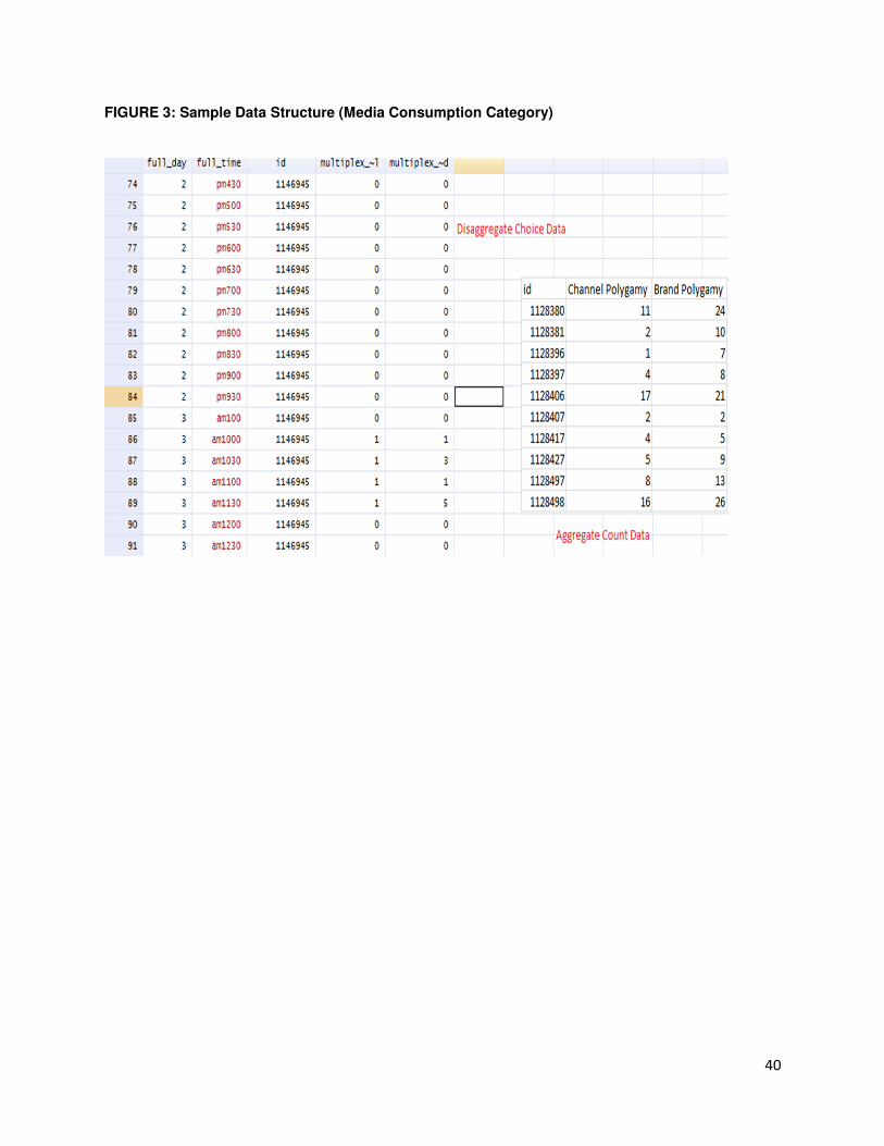
during any half-hour slot in the observation window. A sample data structure is presented in

Figure 5. For each respondent, we also have selected demographic information including age,

gender, household income, household size, and location information such as whether the

respondent is from an urban or rural area.

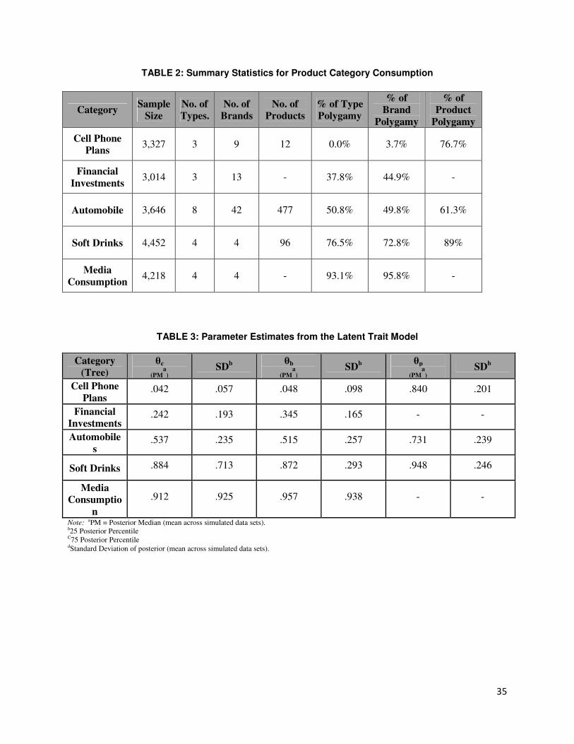
Figure 3 provides a snapshot of our data structure and Table 2 reports detailed descriptive

statistics for each product category. In the Cell Phone Plan category, almost zero percent of

consumers hold multiple types of plans, which is sensible because consumers rarely belong to

both an individual plan and a family plan. Polygamy happens more at the brand level and

product/service level (e.g., ring tones, caller IDs, etc.). Note that Financial Investment is a

4 The Media Consumption category is also pre-tested for “disparateness” with other product categories.

24

special category because information on brands and products are confidential. Nevertheless,

respondents report detailed investment sub-types/formats. For instance, fixed income includes

six formats: treasury bills, savings bonds, U.S. government bonds, municipal bonds, money

markets and corporate bonds. Equity includes three formats: company stocks, common stocks

and equity mutual funds. Others include four formats: other securities (e.g., futures and

derivatives), investment collectibles, international investments, and trust funds. Specifically, 37.8

percent of the 3,014 respondents hold multiple types of financial investments, with an average of

2.17 types. 44.9 percent of the respondents hold multiple sub-types/formats, with an average of

3.06. Clearly, there is a considerable group of single-type investors exhibiting polygamy for

different investment formats. Furthermore, we observe significant variation in polygamy across

product categories (trees), and across tree levels. For example, in the Soft Drinks category, there

are four major brands (Coco-Cola, Pepsi, Dr. Pepper and other brands) as in Dubé (2004) and 96

products/SKUs (23 Coco-Cola products, 20 Pepsi, 27 Dr. Pepper and 26 other brands). 76.5

percent of all 4,452 consumers purchase multiple types within the last seven days, with an

average of 2.42 types, 72.8 percent purchase multiple brands with an average of 2.79, and 89

percent purchase multiple products with an average of 7.69. In a nutshell, summary statistics

suggest that this data is sparse with large variations across categories (trees) and across decision

stages (tree levels). It is also sensible and reflects reality (that less polygamy happens for specialty

retailing products such as Cell Phone Plans, and more so for convenience products such as Soft

Drinks).

5. RESULTS

5.1 Model Selection and Goodness-of-Fit Measures

The deviance information criterion (DIC) is a Bayesian analogue of information

measures such as Akaike’s information criterion in that it comprises a term quantifying lack of

25

model fit and a term penalizing model complexity. The latter term, pD, is of interest in its own

right in that it is interpreted as the effective number of parameters. It is smaller than the actual

number of parameters to the extent to which the model parameters are constrained by

dependencies in the data or the prior. DIC can be computed on the basis of the output from the

Gibbs sampler. A point estimate of the parameter estimates θt is also required, and I used the

maximum likelihood estimates from separate analyses conducted for each individual t. The

model with the smallest DIC value strikes the best compromise between fit and complexity in the

metric defined by DIC. I will report DIC in Section 6 where I compare the latent trait approach

with the latent class approach.

5.2 Parameter Estimates

We obtain parameter estimates for each individual across all product categories (except for

media) and summarize them in Table 3. Table 3 shows the posterior percentiles for the parameters

(on the probability scale) and the posterior medians of the Probit-transformed parameters. The rows

present the product categories or subtrees, whereas the columns present the latent trait parameter θ’s

at different levels of the tree. A high θ (close to 1) denotes a high level of polygamy. Several aspects

of Table 3 are noteworthy. First, the posterior medians are able to reproduce the underlying

population means with little bias. Second, there are variations of the magnitude of polygamy across

tree levels, as well as across trees (product categories). Third, the relatively high standard deviations

suggest evidence for large individual differences in the impact of polygamy. Let us take three real

data records for illustration purposes: ID 1227670 is a young female from Los Angeles with all of her

parameters close to 1 (e.g., 0.5, 0.7, 0.8, 0.7, 0.9,…). This suggests that she is a “Polygamist” that

would love to enjoy offers of multiple products, brands and types. Managers should label her as a

desirable candidate for cross-selling and attempt to provide a large assortment for her selection. In

contrast, ID 1162260 is a senior male from New York City with low parameter estimates (e.g., 0.0,

26

0.1, 0.2, 0.1, 0.3,… ). He is a “Monogamist” that exhibits high inertia in purchase patterns across

consumption scenarios. Managers may want to avoid going through expensive cross-selling efforts

but rather deepen a strong long-term relationship with him with just one type of product or service.

Most consumers are like ID 1357204, who is being a “Wanderer” that is polygamous in some

situations, but not in others (e.g., 0.1, 0.3, 0.5, 0.8, 0.9, …). Our individual-level results on latent

traits not only offer an empirical-based, theory-grounded process for understanding individual

variations in cross-category decisions, but also provide a new basis for segmentation and profiling to

generate important managerial insights on coordinating across categories and across different types

of customers, as discussed in Section 3.6.

5.3 Model Comparison: Latent Trait versus Latent Class

We now compare the results from the latent-trait model with the results from the latent-

class MPT model. The latent-class version of the multinomial processing tree is given as follows:

pkjt = pkj(θt), where θt is the vector of the S parameter values by person t. Allowing for different

parameters for each person t, the vector of person-wise category counts (n11t, . . . , n1J1t , . . . ,

nK1t, .. .,nKJKt )’ is still modeled by a vector-valued random variable N that follows a product-

multinomial distribution

�( � =!�|��)= ∏ #$ %�&�'(…&��(*∏ [�� (��),-�� ]&��(/0�� , (16)

Let the model parameters follow a distribution with probability measure µ, then

�( = !)= X�( = !|Y)ZG(Y), (17)

where �( = !|Y)is given by the right side of Equation 16, in which the fixed values θt are

replaced by the variable of integration, η, and nt is replaced by n. Therefore, for T consumers, we

have:

�(( �, … , ;) = (!�, … , !�))= ∏ {;�� X�( � = !�|Y)ZG(Y)}, (18)

27

Let µ be distributed over a finite number C of fixed parameter vectors θ1, . . . , θC. If λc =

µ({θc}) is the size of class c, the model equation simplifies to:

�(( �, … , ;) = (!�, … , !�))= ∏ {;�� ∑ W]�( � = !�|�])^]�� }, (19)

This means that each consumer t is assumed to belong to one of the C latent classes of

proportional sizes λc. In a latent-class multinomial model, the category counts jointly follow a

mixture of product-multinomial distributions, and each category count considered individually

follows a mixture of binomial distributions. Furthermore, it is well known that mixtures of

binomial distributions with parameters pc and N and mixture coefficients λc are identified if and

only if N >= 2C − 1. A simple EM-algorithm can then be devised for the maximum-likelihood

estimation of latent-class multinomial models.

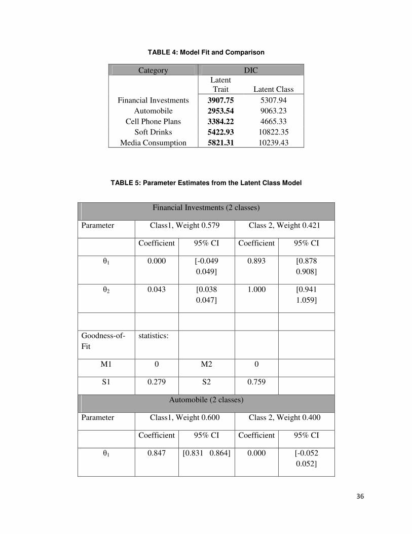
Table 4 shows the model fit statistics for both the latent-trait model and the latent-class

model. Smaller DIC values suggest that the proposed model outperforms the latent class model

significantly. Following Klauer (2006), two test statistics, termed M1 and M2, are considered for

mean structure testing, and another two test statistics, termed S1 and S2, for variance-covariance

structure testing. All four statistics are asymptotically distributed as χ2 when the degrees of

freedom are larger than zero. Table 5 shows the detailed results from the latent class model.

Parameter estimates for the Cell Phone Plans and Media Consumption category are not identified

in the latent class framework because the probability is trivially close to zero (or one) so that

there is not enough variation in the data for the model to distinguish multiple segments. In

addition, not surprisingly, all the other categories seem to have two distinct classes: the

polygamous class, and the single class. While we observe significant differences across tree

levels and across trees, there are quite a number of places where the latent-class approach is not

able to accurately capture the coefficients to reflect the true population mean (as indicated by the

28

zero values), indicating a poor job of capturing underlying distribution with the discrete

representation of consumer heterogeneity.

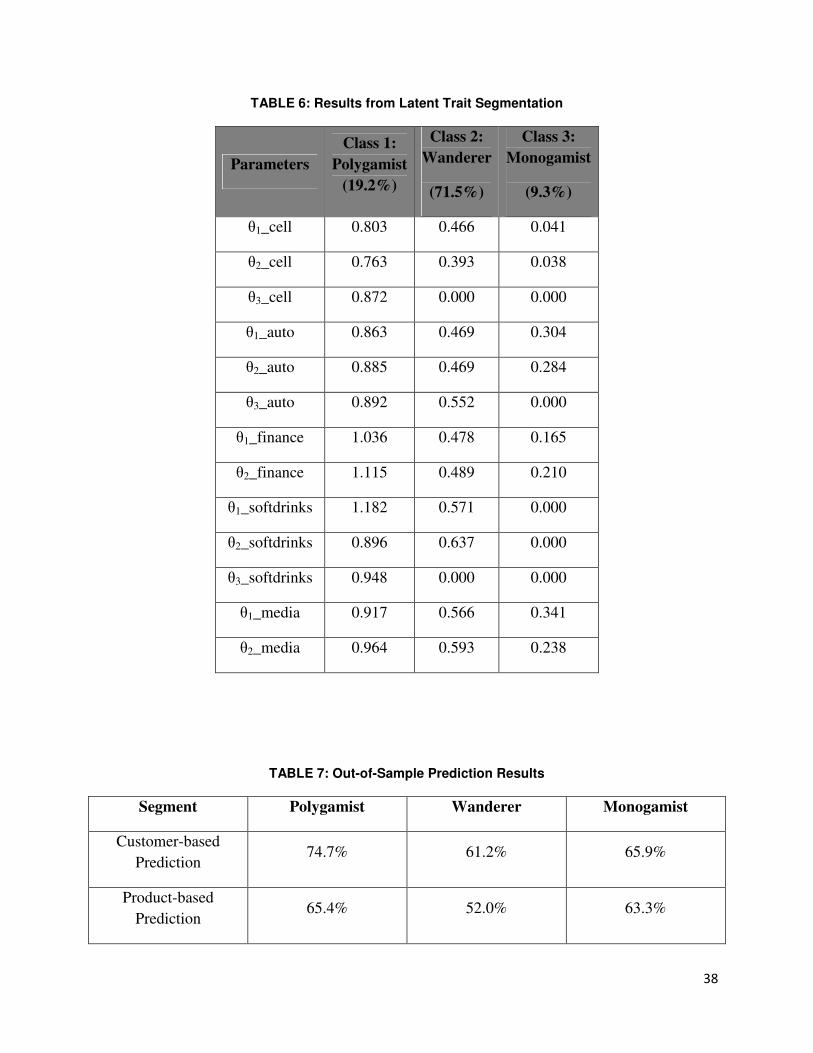
6. SEGMENTATION ANALYSIS

We conducted a finite mixture analysis to segment the consumers based on the collection

of individual θ parameters (θc, θb, θp) across categories, with θ being free to vary between (0,1).

Such continuous representation of consumer heterogeneity allows one to achieve value-based

segmentation where consumers are grouped based on their decision processes rather than binary

observed behavior, 0 or 1. It both provides richer theoretical support and better empirical fit

with continuous distribution. Table 6 summarizes the segmentation results. The three segments

“Polygamist”, “Monogamist” and “Wanderer” roughly each represent 20 percent, 10 percent

and 70 percent of the data respectively. Profile analysis shows group differences are significant.

As illustrated in the previous example in Section 5.2, the Polygamist segment shows high θs

across decision tree stages and categories, whereas the Monogamists show the opposite. The θs

for the Wanderer segment lie in between.

Next, we perform two types of out-of-sample predictions: customer-based and

product/category-based. For the customer-based prediction, the idea is to find customers that

behave similarly and use their parameters to predict the decisions of the holdout sample (15

percent). For product/category-based prediction, the assumption is that customers may exhibit

similar behavior across multiple categories (Ainslie and Rossi 1998). For example, if a customer

is price sensitive in the toothbrush category, then he may be sensitive to the toothpaste category,

or even the clothing category. Specifically, we use parameters from three of the five categories

to predict outcomes of the other two categories and report the average hit rates. Table 7 shows

hit rate by segment using both types of prediction. In summary, while the latent trait model is

29

not designed for prediction (but rather for assessing the underlying processes), the hit rates still

seem reasonable (more than 60 percent), although it is much harder to predict decisions of the

Wanderer segment as compared to the Polygamist and the Monogamist segments which exhibit

more consistent behavior across categories. In addition, customer-based prediction yields better

accuracy than product/category-based prediction. This finding relates back to the intuition that

getting at the “why consumers did it” by looking at the underlying processes provides greater

conceptual and empirical support as compared to the “what consumers did” question in the

traditional behavioral segmentation approach.

7. DISCUSSION AND CONCLUSION

Much of marketing has focused on a consumer’s choices and preferences in individual

product categories or a set of closely related product categories. The reality is that consumers

shop around a globe of categories that are much more diverse and complex than the traditionally

defined “market basket”. This research takes a first step in modeling a complete picture of

consumer decision problems by examining consumption across seemingly disparate product

categories to advance understanding in both dimensions of customer behavior: the breadth of

their consumption portfolio and the depth of their latent decision processes. While traditional

research on multi-category choice models and latent class suffer from data and modeling

limitations that prohibit deeper investigation of the underlying process that governs consumer

decision making, this research empirically examines consumer choices across seemingly

disparate product categories using a latent trait hierarchical multinomial processing tree model.

In doing so, this paper contributes to the consumer decision literature in three ways: 1)

theoretically, the latent-trait approach provides rich support in examining the high level

processes; 2) methodologically, the relative merits of models with continuous versus discrete

representations of consumer heterogeneity are discussed; and 3) substantively, new insights on

30

value-based targeting and profiling are presented with respect to managing across seemingly

disparate product categories.

The power of the latent trait model lies in its ability to infer and assess the impact of

underlying processes using behavioral data without necessarily augmenting survey or

experiments on consumer attitudes. Segmentation and prediction analysis suggests that the

approach of categorizing consumers as collections of latent process parameters provides better

theoretical and empirical support for value/process based segmentation and targeting exercise.

The idea of modeling individual latent processes is not bound by a particular context, but

is applicable to a broader phenomenon that is generally manifested across a wide range of

settings and situations. It would be especially intriguing to study the impact of latent processes

in the online world where firms may have access to large-scale behavioral data across categories

and situations. Future research can look at how firms can improve current recommendation

systems based on inferred consumer preferences across categories, and how brand constellations

are formed in social media (e.g., a consumer may “like” many seemingly unrelated brands on

Facebook).

31

REFERENCES

Ainslie, A. and P.E. Rossi (1998), “Similarities in Choice Behavior Across Multiple Categories,”

Marketing Science, 17(2), 91-106.

Andrews, R. L., A. Ainslie, and I. S. Currim (2002), “An Empirical Comparison of Logit Choice

Models with Discrete Versus Continuous Representations of Heterogeneity,” Journal of

Marketing Research, 39 (4), 479-487.

Andrews, R. L., A. Ansari, and I. S. Currim (2002), “Hierarchical Bayes vs. Finite Mixture

Conjoint Analysis Models: A Comparison of Fit, Prediction, and Partworth Recovery,” Journal

of Marketing Research, 39 (1), 87-98.

Ansari, A., M.Vanhuele and M. Zemborain(2008), “Heterogeneous Multinomial Processing Tree

Models,” Working paper, Columbia University, New York.

Balasubramanian, S. and W. A. Kamakura (1989), “Measuring Consumer Attitudes Towards the

Marketplace with Tailored Interviews,” Journal of Marketing Research, 26(3), 311-26.

Bawa.K., S.S. Srinivasan and R. K. Srivastava (1997), “Coupon Attractiveness and Coupon

Proneness: A Framework for Modeling Coupon Redemption,” Journal of Marketing Research,

34(4), 517-525.

Batchelder, W.H., and D.M. Riefer (1999), “Theoretical and Empirical Review of Multinomial

Processing Tree Modeling,” Psychonomic Bulletin & Review, 6(1), 57–86.

Bell, D.R. and J.M. Lattin (1998), “Shopping Behavior and Consumer Preferences for Store

Price Format: Why Large Basket Shoppers Prefer EDLP,” Marketing Science, 17, 1, 66-88.

Berry, S. T. (1994), "Estimating Discrete-Choice Models of Product Differentiation," RAND

Journal of Economics, 25(2), 242-262.

Bettman, J. (1979), An Information Processing Theory of Consumer Choice, Reading, MA:

Addison-Wesley Publishing Company.

Bucklin, R. E. and Gupta, S. (1992), “Brand Choice, Purchase Incidence, and Segmentation: An

Integrated Modeling Approach,” Journal of Marketing Research, 29(2), 201-215.

Berns G.S., J.D. Cohen, and M.A. Mintun (1997), “Brain Regions Responsive to Novelty in the

Absence of Awareness,” Science, 276(53), 1272-1275

Chung, J. and V.R. Rao (2003), “A General Choice Model for Bundles with Multiple-Category

Products: Application to Market Segmentation and Optimal Pricing for Bundles,” Journal of

Marketing Research, 40 (2), 115–130.

32

Coombs, C. H. (1964), A Theory of Data. New York: John Wiley & Sons.

DeSarbo, W., W. A. Kamakura and M. Wedel (2004) “Applications of Multivariate Latent

Variable Models in Marketing,” in Advances in Marketing Research and Modeling: The

Academic and Industry Impact of Paul E. Green, Boston, MA: Kluwer, 43-67.

DeSarbo, W., W. A. Kamakura, M. Wedel (2006), “Latent Structure Regression,” in Handbook

of Marketing Research, Thousand Oaks, CA: Sage Publications, 394-417.

Dubé, J.-P. (2004), “Multiple Discreteness and Product Differentiation: Demand for Carbonated

Soft Drinks,” Marketing Science, 23(1), 66–81.

Gelman, A. and J. Hill (2007), Data Analysis Using Regression and Multilevel/Hierarchical

Models. New York: Cambridge University Press.

Guadagni, P. M., J. D. C. Little (1983), “A Logit Model of Brand Choice Calibrated on Scanner

Data,” Marketing Science, 2(3), 203–238.

Hedgcock W., Rao A. R. (2009), “Trade-off Aversion as an Explanation for the Attraction Effect:

A Functional Magnetic Resonance Imaging Study. Journal Marketing Research, 46(1), 1–13.

Heilman, C. and D. Bowman (2002), “Segmenting Consumers Using Multiple-Category

Purchasing Data,” International Journal of Research in Marketing, 19 (3), 225–52.

Hu, X. and W.H. Batchelder (1994), “The Statistical Analysis of General Processing Tree

Models with the EM Algorithm,” Psychometrika, 59(1), 21–47.

Kahn, B.E., M.U. Kalwani, and D.G. Morrison (1986), ``Measuring Variety Seeking and

Reinforcement Behaviors Using Panel Data,’’ Journal of Marketing Research, 23(2), 89-100.

Kamakura, W.A. and G. J. Russell (1989), “A Probabilistic Choice Model for Market

Segmentation and Elasticity Structure,” Journal of Marketing Research, 26(4), 379-390.

Kamakura, W.A., Sridhar R. and R. K. Srivastava (1991), “Applying Latent Trait Analysis in the

Evaluation of Prospects for Cross-Selling of Financial Services,” International Journal of

Research in Marketing, 8(4), 329-349.

Kim, J., G.M. Allenby and P. E. Rossi (2002), “Modeling Consumer Demand for Variety,”

Marketing Science, 21(3), 223-228.

Klauer, K.C. (2006), “Hierarchical Multinomial Processing Tree Models: a Latent-Class

Approach,” Psychometrika, 71(1), 1–31.

Klauer, K.C. (2010), “Hierarchical Multinomial Processing Tree Models: a Latent-Trait

Approach,” Psychometrika, 75(1), 70–98.

33

Langeheine, R. and J. Rost (1988), Latent Trait and Latent Class Models, New York: Plenum.

Lord, F. M. and M. R. Novick (1968), Statistical Theories of Mental Test Scores, Reading, MA:

Addison-Wesley.

McFadden, D. (1980), “Economic Models for Probabilistic Choice Among Products,” Journal of

Business, 53(3), 513-529.

Manchanda, P., A. Ansari and S. Gupta (1999), “The Shopping Basket: A Model for

Multicategory Purchase Incidence Decisions,” Marketing Science, 18(2), 95-114.

McGuire W.J. (1976), “Psychological Factors Influencing Consumer Choice,” in Selected

Aspects of Consumer Behavior, Washington University Press, 319 – 360.

Mehta, N. (2007), “Investigating Consumers’ Purchase Incidence and Brand Choice Decisions

across Multiple Product Categories: A Theoretical and Empirical Analysis”. Marketing Science.

26(2), 196–217.

Seetharaman, P.B., A. Ainslie and P.K. Chintagunta (1999), “Investigating Household State

Dependence Effects Across Categories,” Journal of Marketing Research, 36(4), 488-500.

Tversky, A. (1977), “Features of Similarity,” Psychological Review, 84(4), 327-352.

Wedel, M. and W. A. Kamakura (2000) Market Segmentation: Conceptual Methodological

Foundations, Second Edition. Boston: Kluwer Academic Publishers.

Wedel, M., W.A Kamakura, N. Arora, A. Bemmaor, J. Chiang, T. Elrod, R. Johnson, P. Lenk, S.

Neslin, and C. S. Poulsen (1999), “Discrete and Continuous Representations of Unobserved

Heterogeneity in Choice Modeling,” Marketing Letters, 10 (3), 219–32.

Weller, J., I. Levin, B. Shiv, and A. Bechara (2011), “The Effects of Insula Damage on Decision

Making for Risky Gains and Losses, Social Neuroscience, Forthcoming.

34

TA

BL

E 1

: N

ota

tio

ns

an

d V

ari

ab

les f

or

the L

ate

nt

Tra

it M

od

el

35

TABLE 2: Summary Statistics for Product Category Consumption

Category Sample

Size

No. of

Types.

No. of

Brands

No. of

Products

% of Type

Polygamy

% of

Brand

Polygamy

% of

Product

Polygamy

Cell Phone

Plans 3,327 3 9 12 0.0% 3.7% 76.7%

Financial

Investments 3,014 3 13 - 37.8% 44.9% -

Automobile 3,646 8 42 477 50.8% 49.8% 61.3%

Soft Drinks 4,452 4 4 96 76.5% 72.8% 89%

Media

Consumption 4,218 4 4 - 93.1% 95.8% -

TABLE 3: Parameter Estimates from the Latent Trait Model

Category

(Tree)

θc

(PM

a

) SD

b

θb

(PM

a

) SD

b

θp

(PM

a

) SD

b

Cell Phone

Plans .042 .057 .048 .098 .840 .201

Financial

Investments .242 .193 .345 .165 - -

Automobile

s .537 .235 .515 .257 .731 .239

Soft Drinks .884 .713 .872 .293 .948 .246

Media

Consumptio

n

.912 .925 .957 .938 - -

Note: aPM = Posterior Median (mean across simulated data sets). b25 Posterior Percentile C75 Posterior Percentile dStandard Deviation of posterior (mean across simulated data sets).

36

TABLE 4: Model Fit and Comparison

Category DIC

Latent

Trait Latent Class

Financial Investments 3907.75 5307.94

Automobile 2953.54 9063.23

Cell Phone Plans 3384.22 4665.33

Soft Drinks 5422.93 10822.35

Media Consumption 5821.31 10239.43

TABLE 5: Parameter Estimates from the Latent Class Model

Financial Investments (2 classes)

Parameter Class1, Weight 0.579 Class 2, Weight 0.421

Coefficient 95% CI Coefficient 95% CI

θ1 0.000 [-0.049

0.049]

0.893 [0.878

0.908]

θ2 0.043 [0.038

0.047]

1.000 [0.941

1.059]

Goodness-of-

Fit

statistics:

M1 0 M2 0

S1 0.279 S2 0.759

Automobile (2 classes)



θ1 0.847 [0.831 0.864] 0.000 [-0.052

0.052]

37

θ2 0.830 [0.813 0.847] 0.000 [-0.052

0.052]

θ3 1.000 [0.957 1.043] 0.034 [0.019 0.05]

Goodness-of-

Fit

M1 0 M2 0.000

S1 0.774 S2 1.508

Soft Drinks (2 classes)



θ1 0.885 [0.87 0.9] 0.422 [0.378

0.466]

θ2 0.982 [0.957

1.007]

0.000 [-0.108

0.108]

θ3 1.000 [0.958

1.042]

0.575 [0.525

0.624]

Goodness-of-

Fit

M1 0 M2 0.002

S1 0.149 S2 0.832

Cell Phone Plans (Not Enough Variations to Distinguish Multiple Segments)

Media Consumption (Not Enough Variations to Distinguish Multiple

Segments)

38

TABLE 6: Results from Latent Trait Segmentation

Parameters

Class 1:

Polygamist

(19.2%)

Class 2:

Wanderer

(71.5%)

Class 3:

Monogamist

(9.3%)

θ1_cell 0.803 0.466 0.041

θ2_cell 0.763 0.393 0.038

θ3_cell 0.872 0.000 0.000

θ1_auto 0.863 0.469 0.304

θ2_auto 0.885 0.469 0.284

θ3_auto 0.892 0.552 0.000

θ1_finance 1.036 0.478 0.165

θ2_finance 1.115 0.489 0.210

θ1_softdrinks 1.182 0.571 0.000

θ2_softdrinks 0.896 0.637 0.000

θ3_softdrinks 0.948 0.000 0.000

θ1_media 0.917 0.566 0.341

θ2_media 0.964 0.593 0.238

TABLE 7: Out-of-Sample Prediction Results

Segment Polygamist Wanderer Monogamist

Customer-based

Prediction 74.7% 61.2% 65.9%

Product-based

Prediction 65.4% 52.0% 63.3%

39

FIGURE 1: Multinomial Process Tree Representation of the Latent Trait Model

FIGURE 2: Multinomial Process Tree Representation of the Latent Trait Model with Augmented

Data

Product Category

Multiple Channels/Types

Multiple Brands Multiple Products

Single Brand Single Product

Single Channel/Type



Product Category

Multiple Channels/Types



Single Channel/Type



θc

θb

θp

1-θc

θb θp

1-θb

1-θb

1-θp

1-θp

P(Z1>0)

P(Z2>0) P(Z3>0)

P(Z1≤0)

P(Z2≤0)

P(Z3≤0)

P(Z2≤0)

P(Z3≤0)

P(Z2>0)

P(Z3>0)

40

FIGURE 3: Sample Data Structure (Media Consumption Category)

No. 029/2020/MKT Consumer Choices Across Seemingly Disparate ...

Documents

Transcript of No. 029/2020/MKT Consumer Choices Across Seemingly Disparate ...