New formulation for compressive strength of CFRP confined concrete cylinders using linear genetic...

ORIGINAL ARTICLE

New formulation for compressive strength of CFRP confinedconcrete cylinders using linear genetic programming

Amir Hossein Gandomi • Amir Hossein Alavi •

Mohammad Ghasem Sahab

Received: 12 January 2009 / Accepted: 14 October 2009 / Published online: 30 October 2009

� RILEM 2009

Abstract This paper proposes a new approach for

the formulation of compressive strength of carbon

fiber reinforced plastic (CFRP) confined concrete

cylinders using a promising variant of genetic

programming (GP) namely, linear genetic program-

ming (LGP). The LGP-based models are constructed

using two different sets of input data. The first set of

inputs comprises diameter of concrete cylinder,

unconfined concrete strength, tensile strength of

CFRP laminate and total thickness of utilized CFRP

layers. The second set includes unconfined concrete

strength and ultimate confinement pressure which are

the most widely used parameters in the CFRP

confinement existing models. The models are devel-

oped based on experimental results collected from the

available literature. The results demonstrate that the

LGP-based formulas are able to predict the ultimate

compressive strength of concrete cylinders with an

acceptable level of accuracy. The LGP results are

also compared with several CFRP confinement

models presented in the literature and found to be

more accurate in nearly all of the cases. Moreover,

the formulas evolved by LGP are quite short and

simple and seem to be practical for use. A subsequent

parametric study is also carried out and the trends of

the results have been confirmed via some previous

laboratory studies.

Keywords CFRP confinement �Linear genetic programming � Formulation �Concrete compressive strength

1 Introduction

Concrete as a frictional material is considerably

sensitive to hydrostatic pressure. Lateral stresses have

advantageous effects on the concrete strength and

deformation. This means when concrete is uniaxially

loaded and can not dilate laterally, it exhibits

increased strength and axial deformation capacity

indicated as confinement. Concrete confinement can

be generally provided through transverse reinforce-

ment in the form of spirals, circular hoops or

rectangular ties, or by encasing the concrete columns

into steel tubes that act as permanent formwork [1].

Fiber reinforced polymers (FRPs) are also employed

for confinement of concrete columns. Compared to

A. H. Gandomi (&)

The Highest Prestige Scientific and Professional National

Foundation, National Elites Foundation, Tehran, Iran

e-mail: [email protected]

A. H. Alavi

College of Civil Engineering, Iran University of Science

& Technology (IUST), Tehran, Iran


M. G. Sahab

College of Civil Engineering, Tafresh University, Tafresh,

Iran


Materials and Structures (2010) 43:963–983

DOI 10.1617/s11527-009-9559-y

steel [2], FRPs present several advantages such as

continuous confining action to the entire cross-

section, easiness and speed of application, no change

in the shape and size of the strengthened elements

and corrosive resistance [1]. Typical response of

FRP-confined concrete is shown in Fig. 1, where

normalized axial stress is plotted against axial,

lateral, and volumetric strains. The stress is normal-

ized with respect to the unconfined strength of

concrete core. The figure shows that both axial and

lateral responses are bi-linear with a transition zone at

or near the peak strength of unconfined concrete core.

The volumetric response shows a similar transition

toward volume expansion. However, as soon as the

jacket takes over, volumetric response undergoes

another transition which reverses the dilation trend

and results in volume compaction. This behavior is

shown to be remarkably different from plain concrete

and steel-confined concrete [3]. Carbon fiber rein-

forced plastic (CFRP) is one of the main types of FRP

composites. The advantages of CFRP comprise anti-

corrosion, easy cutting and construction, as well as

high strength to weight ratio and high elastic

modulus. These features caused widely using of

CFRP in the retrofitting and strengthening of rein-

forced concrete structures as one of the most

successfully transferred technologies to the civil

engineering industry for over 50 years. The illustra-

tive figure of CFRP confining concrete cylinder can

be seen in Fig. 2.

Several investigations have been conducted about

the effect of CFRP confinement on the strength and

deformation capacity of concrete columns. On the

basis of these researches, a number of empirical and

theoretical models are proposed [1]. In spite of the

extensive research in this field, there are some

significant limitations such as specific loading system

and conditions and the need for calibration of several

involving parameters on the application of these

empirical models. These limitations, suggest the

necessity of developing more comprehensive math-

ematical models for assessing the behaviour of CFRP

confined concrete columns.

Genetic programming (GP) [4, 5] is a developing

subarea of evolutionary algorithms inspired from

Darwin’s evolution theory. GP may generally be defined

as a supervised machine learning technique that

searches a program space instead of a data space [5].

Fig. 1 Typical response of

FRP-confined concrete [3]

Fig. 2 The illustrative figure of CFRP confining concrete

cylinder

964 Materials and Structures (2010) 43:963–983

In recent years, a particular subset of GP with a linear

structure similar to the DNA molecule in biological

genomes namely, linear genetic programming (LGP)

[6] has emerged. LGP is a machine learning approach

that evolves the programs of an imperative language

or machine language instead of the traditional tree-

based GP [4] expressions of a functional program-

ming language. LGP has significant advantages over

other modeling approaches [6, 7]. There has been just

some little scientific effort directed at applying LGP

to civil engineering tasks such as behavior appraisal

of steel semi-rigid joints [8], performance character-

istics modeling of stabilized soil [9], and soil

liquefaction assessment [10].

The main purpose of this paper is to utilize the LGP

technique to obtain formulas for the determination of

compressive strength of CFRP wrapped concrete

cylinders. A comparison between the proposed

formulations results, as well as 15 existing models

found in the literature, is performed. A reliable

database including previously published compressive

strength of CFRP wrapped concrete cylinder test

results is utilized to develop generic models.

2 Review of previous studies

The characteristic response of confined concrete

includes three distinct regions of un-cracked elastic

deformations, crack formation and propagation, and

plastic deformations. It is generally assumed that

concrete behaves like an elastic-perfectly plastic

material after reaching its maximum strength capac-

ity, and that the failure surface is fixed in the stress

space. Constitutive models for concrete should be

concerned with pressure sensitivity, path dependence,

Table 1 Different models for strength enhancement of FRP confined concrete cylinders

ID Authors Expression

1 Fardis and Khalili [18]f 0cc

f 0co¼ 1þ 3:7 pu

f 0co

� �0:85

2 Mander et al. [19]f 0cc

f 0co¼ 2:254

ffiffiffiffiffiffiffiffiffiffiffiffiffiffiffiffiffiffi1þ 7:94pu

f 0co

q� 2pu

f 0co� 1:254

3 Miyauchi et al. [11]f 0cc

f 0co¼ 1þ 3:485 pu

f 0co

� �

4 Kono et al. [12]f 0cc

f 0co¼ 1þ 0:0572Pu

5 Samaan et al. [20]f 0cc

f 0co¼ 1þ 0:6p0:7

u

6 Lam and Teng [21]f 0cc

f 0co¼ 1þ 2 pu

f 0co

� �

7 Toutanji [22]f 0cc

f 0co¼ 1þ 3:5 pu

f 0co

� �0:85

8 Saafi et al. [23]f 0cc

f 0co¼ 1þ 2:2 pu

f 0co

� �0:84

9 Spoelstra and Monti [24]f 0cc

f 0co¼ 0:2þ 3

ffiffiffiffipu

f 0co

q

10 Karbhari and Gao [25]f 0cc

f 0co¼ 1þ 2:1 pu

f 0co

� �0:87

11 Richart et al. [26]f 0cc

f 0co¼ 1þ 4:1 pu

f 0co

� �

12 Berthet et al. [27]

f 0cc

f 0co

¼ 1þ K1

pu

f 0co

� �;

K1 ¼ 3:45 20� f 0co� 50 MPa

K1 ¼ 0:95 f 0co

� ��1=450 � f 0co� 200 MPa

(

13 Vintzileou and Panagiotidou [28]f 0cc

f 0co¼ 1þ 2:8 pu

f 0co

� �

14 Xiao and Wu [29]f 0cc

f 0co¼ 1:1þ 4:1� 0:75

f 02co

El

� �pu

f 0co

15 Li et al. (L-L Model) [30]f 0cc

f 0co¼ 1þ tan 45� � /

2

� �pu

f 0co

� �

/ ¼ 36� þ 1�f 0co

35

� �� 45�

f0co: Compressive strength of unconfined concrete cylinder; f0cc: Ultimate compressive strength of confined concrete cylinder; Pu:

Ultimate confinement pressure Pu ¼ El:ef ¼2t:f 0f

D

� �; El: Lateral modulus; ef: Ultimate tensile strain of FRP laminate; f0f: Ultimate

tensile strength of FRP layer; t: Thickness of FRP layer; D: Diameter of concrete cylinder

Materials and Structures (2010) 43:963–983 965

stiffness degradation and cyclic response. The exist-

ing plasticity models range from nonlinear elasticity,

endochronic plasticity, classical plasticity, and multi-

laminate or micro-plane plasticity to bounding surface

plasticity. Many of these models, however, are only

suitable in a specific application and loading system

for which they are devised and may give unrealistic

results in other cases. Also, some of these models

require several parameters to be calibrated based on

experimental results [3]. Considerable experimental

research has been performed on the behavior of CFRP

confined concrete columns [11–17]. Numerous stud-

ies have concentrated on assessing the strength

enhancement of CFRP wrapped concrete cylinders

in the literature. Some of the most important models in

this field (Eqs. 1 to 15) have been shown in Table 1.

Cevik and Guzelbey [31] presented an application

of neural networks (NN) for the modeling of

compressive strength of CFRP confined concrete

cylinders. Moreover, they obtained the explicit for-

mulation of the compressive strength using the NN

model with 4 neurons in input layer and 15 neurons in

middle layer. Since some of the models in the

literature such as the second formula of Karbhari and

Gao [25] and the modified L-L model [30] require

additional details, they are not used in the compar-

ative study. In recent decade, different models for the

compressive strength of concrete cylinders after FRP

confinement have been proposed [27–31]. The rela-

tive differences between the general forms of the

recently proposed models [27, 29–31] and the older

ones pursue one to challenge for obtaining more

accurate models with newer general forms.

3 Genetic programming

GP is one of the branches of evolutionary algorithms

(EA) that creates computer programs to solve a

problem using the principle of Darwinian natural

selection [32]. GP was introduced by Koza [4] as an

extension of the genetic algorithms, in which pro-

grams are represented as tree structures and expressed

in the functional programming language LISP [4]. GP

has successfully been applied to various kinds of the

civil engineering problems [33–37]. A comprehen-

sive description of GP can be found in Refs. [4]

and [5].

3.1 Linear genetic programming

LGP is a subset of GP that has emerged recently.

Comparing LGP to the traditional Koza’s tree-based

GP, there are some main differences. Linear genetic

programs (LGPs) have graph-based functional struc-

tures and evolve in an imperative programming

language C/C?? [38] and machine code [39] rather

than in expressions of a functional programming

language like LISP [40]. Unlike tree-based GP,

structurally noneffective codes coexist with effective

codes in LGPs.

Noneffective code in genetic programs which is

referred to as ‘‘intron’’, represents instructions

without any influence on the program behavior.

Structural introns act as a protection that reduces the

effect of variation on the effective code. The introns

allow variations to remain neutral in terms of fitness

change [6]. Because of the imperative program

structure in LGP, these noneffective instructions can

be identified efficiently. This allows the correspond-

ing effective instructions to be extracted from a

program during runtime. Since, only effective pro-

grams are executed, evaluation can be accelerated

significantly (see Fig. 3).

The instructions from imperative languages are

restricted to operations that accept a minimum

number of constants or memory variables, called

Fig. 3 Elimination of

noneffective code in LGP.

Only effective programs are

executed [6]


registers (r), and assign the result to a destination

register, e.g., r0: = r1 ? 1. A part of a linear genetic

program in C code is represented as follows [6]:

void LGP (double r[5])

{…r[0] = r[5] ? 70;

r[5] = r[0] - 50;

if (r[1] [ 0)

if (r[5] [ 2)

r[4] = r[2] * r[1];

r[2] = r[5] ? r[4];

r[0] = sin(r[2]);

}

where register r[0] holds the final program output.

LGPs can be converted into a functional representa-

tion by successive replacements of variables starting

with the last effective instruction [7]. Automatic

Induction of Machine code by Genetic Programming

(AIMGP) is a particular form of LGP. AIMGP

induces binary machine code directly without any

interpreting steps that results in a significant speedup

in execution compared to interpreting GP systems.

This LGP approach searches for the computer

program and the constants at the same time. The

evolved program is a sequence of binary machine

instructions [39].

The machine-code-based, LGP uses the following

steps to evolve a computer program that predicts the

target output from a data file of inputs and outputs

[6]:

I. Initializing a population of randomly generated

programs.

II. Running a Tournament. In this step four programs

are selected from the population randomly. They

are compared and based on fitness, two programs

are picked as the winners and two as the losers.

III. Transforming the winner programs. After that,

two winner programs are copied and transformed

probabilistically as follows:

• Parts of the winner programs are exchanged with

each other to create two new programs (cross-

over); and/or

• Each of the tournament winners are changed

randomly to create two new programs (mutation).

IV. Replacing the loser programs in the tournament

with the transformed winner programs. The

winners of the tournament remain without

change.

V. Repeating steps two through four until conver-

gence. A program defines the output of the

algorithm that simulates the behavior of the

problem to an arbitrary degree of accuracy.

A brief description of basic parameters, used to

direct the search for a linear genetic program, is

explained below.

3.1.1 Population size

The number of programs in the population that LGP

will evolve are set by the population size. The proper

population size depends on the number of possible

solutions and complexity of the problem.

3.1.2 Crossover

Crossover transforms programs in the population and

exchanges sequences of instructions between two

tournament winners. Two offsprings are the outcomes

of this exchange that are inserted in place of the

loser programs in the tournament. Crossover occurs

between instruction blocks and it can be either

homologous or non-homologous. Reproducing natu-

ral evolution is more closely in homologous cross-

over as a novel approach than traditional crossover.

Figure 4 demonstrates the two-point linear cross-

over used in LGP for recombining two tournament

winners. As shown, a segment of random position and

arbitrary length is selected in each of the two parents

and exchanged. If one of the two children would

exceed the maximum length, crossover is aborted and

restarted with exchanging equally sized segments [6].

Fig. 4 Crossover in LGP [6]


3.1.3 Mutation

The mutation operator is used to transform some

randomly selected programs with a small mutation

probability to prevent premature convergence. Three

different types of mutation in LGP are block muta-

tion, instruction mutation and data mutation.

3.1.4 Demes

Based on the EA, the population of individual

solutions may be subdivided into multiple subpopu-

lations that migration of individuals among these

subpopulations causes evolution to occur in the

population. This mechanism was described by biol-

ogists as the island model. Demes are semi-isolated

subpopulations that in comparison to a single popu-

lation of equal size, evolution proceeds faster in

them. The percentage of individuals allowed to

migrate from a deme into another deme during each

generation is limited. Demes are widely used in the

field of EA and GP. The number of them is related to

the way that the population of programs is divided.

3.1.5 Fitness function

The fitness function is a criterion for the evaluation of

the goodness of each individual computer program.

The fitness values are used to determine which

evolved programs survive and reproduce. To evaluate

the fitness of an evolved program, the average of the

squared raw errors is calculated.

3.1.6 Function and terminal sets

The Function and terminal sets are important param-

eters of LGP. The function set for a run may include

the operators such as addition, subtraction, square

root, absolute value and logarithm while the terminal

set comprises of the variables and constants of the

evolving programs.

4 Model development

The main objective of this paper is to explore the

feasibility of using the LGP approach for the

formulation of compressive strength (f0cc) of CFRP

confined concrete cylinders. An experimental

database has been gathered for strength enhancement

of CFRP wrapped concrete cylinders from the

literature. The database contains 101 specimens

obtained from seven separate studies. The complete

list of the data is presented in Table 6 of the

Appendix. The ranges of different input and output

parameters involved in the model development are

given in Table 2.

For the analysis, the data sets are divided into

training and testing subsets (10 data sets were used

for testing and the rest for training). For the LGP-

based models, a computer software called Discipulus

[41] is used. This software works on the basis of the

AIMGP approach. Two LGP-based models (Model I

and Model II) are considered for the assessment of

compressive strength using two different sets of input

data. For each models of I and II, two formulas of

compressive strength of the confined concrete cylin-

der have been obtained. The first function set consists

of nearly all functions (addition, subtraction, division,

multiplication, square root, sine, cosine and tangent)

and the other includes just addition, subtraction,

division, and multiplication in order to obtain short

and very simple formulas. In addition to the men-

tioned function sets, logarithmic function has also

been considered in the LGP predictive models. Since

the best obtained formula considering this form of

function was complex and inaccurate, it has not been

presented here.

The details of developing Model I and Model II

are discussed in the following subsections. Various

LGP involved parameters are population size, muta-

tion type and rate (block mutation rate, instruction

mutation rate, and data mutation rate), crossover type

and rate, function set, number of demes and program

size. The parameter selection will affect the gener-

alization capability of the LGP-based models. For the

development of models, the LGP parameters are

selected based on some previously suggested values

[42] and also after a trial and error approach. The

parameter settings are shown in Table 3. In order to

evaluate the capabilities of the LGP models, the

correlation coefficient (R) and mean absolute percent

error (MAPE) are used.

4.1 Development of Model I

The existing FRP confinement models take into

account the unconfined compressive strength and the


ultimate confinement pressure as the main influencing

parameters. The main goal of developing Model I is

to obtain the explicit formulation of the ultimate

strength of concrete cylinders after CFRP confine-

ment (f0cc) by considering the influencing variables

given as follows:

f 0cc ¼ f D; t; f 0f ; f0co

� �ð16Þ

The four input variables to build the model are

listed below:

• diameter of the concrete cylinder (D)

• thickness of the CFRP layer (t)

• ultimate tensile strength of the CFRP laminate

(f0f)• unconfined ultimate concrete strength (f0co)

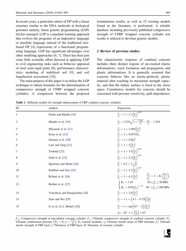
The first two inputs are geometrical parameters

(Fig. 5) and others are mechanical properties. The

database, presented in Table 6, is used to build Model

I. All specimens used in the database have a length

(L) to diameter (D) ratio of 2. The parameter settings

of Model I are shown in Table 3.

4.1.1 Explicit formulation of compressive strength,

Model I

Formulation of f0cc in terms of the independent

variables, D, t, f0f and f0co, for the best results by the

LGP algorithm are as given below:

f 0cc;I:1 ðMPaÞ ¼ffiffiffiffiffiffiffiffiffiffiffiffiffiffiffiffiffiffiffiffiffiffiffiffiffiffiffiffiffiffiffiffiffiffiffiffiffiffiffiffiffiffiffiffiffiffiffiffiffiffiffiffiffiffiffiffiffiffiffiffiffiffiffiffiffiffiffiffiffiffiffiffiffiffiffiffiffiffiffiffiffiffiffiffiffiffiffiffiffiffiffiffiffiffiffiffiffiffiffiffiffiffiffiffiffiffiffiffi2 cos f 0f :t: sin

sin2ðcos2ðf 0co þ D:t=2ÞÞ2

þ 3f 0co

2þ t

� �� sþ f 0co

ð17Þ

f 0cc;I:2 ðMPaÞ ¼ D

4011

�0:57t � D:f 0f ðð3:6f 0co � 58:7tÞ

�10�8Þ4 þ 11:6 f 0co=100�

ð18Þ

The functions generated for the best results by

LGP to use in the compressive strength prediction

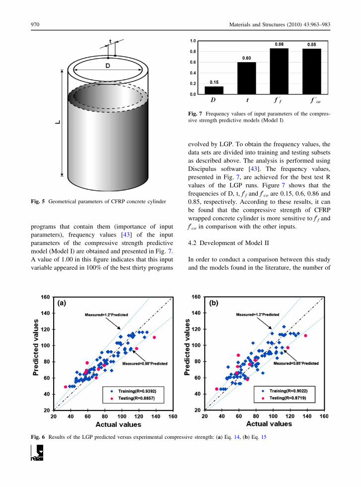
include the effects of all parameters. Comparisons of

the LGP predicted versus experimental compressive

strength of CFRP wrapped concrete cylinder for

Eqs. 17 and 18 are shown in Fig. 6a, b.

In order to evaluate how many times each input

parameters contributes to the fitness of the LGP

Table 2 Ranges of the

parameters in databaseParameters Range

Diameter of the concrete cylinder (mm) 100–153

Thickness of CFRP layer (mm) 0.11–5.04

Ultimate tensile strength of the CFRP laminate (MPa) 1100–3820

Unconfined ultimate concrete strength (MPa) 19.40–82.13

Ultimate confinement pressure (MPa) 3.44–38.38

Confined ultimate concrete strength (MPa) 33.8–137.9

Table 3 Parameter settings

for the LGP modelsParameter Settings

f0cc, I.1, f0cc, II.1 f0cc, I.2, f0cc, II.2

Function set ?, -, *, /, H, sin, cos, tan ?, -, *, /

Population size 10000–25000 10000–25000

Maximum program size 256 256

Initial program size 80 80

Crossover rate (%) 50, 95 50, 95

Homologous crossover (%) 95 95

Mutation rate (%) 90 90

Block mutation rate (%) 30 30

Instruction mutation rate (%) 30 30

Data mutation rate (%) 40 40

Number of demes 20 20


programs that contain them (importance of input

parameters), frequency values [43] of the input

parameters of the compressive strength predictive

model (Model I) are obtained and presented in Fig. 7.

A value of 1.00 in this figure indicates that this input

variable appeared in 100% of the best thirty programs

evolved by LGP. To obtain the frequency values, the

data sets are divided into training and testing subsets

as described above. The analysis is performed using

Discipulus software [43]. The frequency values,

presented in Fig. 7, are achieved for the best test R

values of the LGP runs. Figure 7 shows that the

frequencies of D, t, f0f and f0co are 0.15, 0.6, 0.86 and

0.85, respectively. According to these results, it can

be found that the compressive strength of CFRP

wrapped concrete cylinder is more sensitive to f0f and

f0co in comparison with the other inputs.

4.2 Development of Model II

In order to conduct a comparison between this study

and the models found in the literature, the number of

Fig. 5 Geometrical parameters of CFRP concrete cylinder

Fig. 6 Results of the LGP predicted versus experimental compressive strength: (a) Eq. 14, (b) Eq. 15

Fig. 7 Frequency values of input parameters of the compres-

sive strength predictive models (Model I)


inputs to build Model II is reduced to two para-

meters. These parameters are the most widely used

parameters in the existing FRP confinement models.

Hence, the formulation of the strength of concrete

cylinders after CFRP confinement as function of

variables will be as follows:

f 0cc ¼ f Pu; f0co

� �ð19Þ

in which the two inputs to build the models are:

• unconfined ultimate concrete strength (f0co)

• ultimate confinement pressure (Pu)

As indicated in Table 1, Pu is a function of the

diameter of the concrete cylinder (D), the thickness of

the CFRP layer (t), and the ultimate strength of the

CFRP layer (f0f) [24]. Therefore, Model II includes

the already mentioned parameters in implicit form.

The parameter settings of Model II are as shown in

Table 3.

4.2.1 Explicit formulation of compressive strength,

Model II

For Model II, f0co and Pu are considered in the

formulation process as the input parameters. The

prediction equations for the best test R values by the

LGP algorithm are given in Eqs. 20 and 21.

f 0cc;II:1 MPað Þ ¼ 7f 0co

18

40cos

ffiffiffi2p

180

ffiffiffiffiffiffiffiffiffiffiffiffiffiffiffiffiffiffiffiffiffiffiffiffiffiffiffiffiffiffiffiffiffiffiffiffiffiffiffiffiffiffiffiffiffiffiffiffiffiffiffiffiffiffiffiffiffiffiffiffiffiffiffiffiffi90 f 0co � cos 2sin

f 02co

2025

� �8 !

þ f 02co

vuut!þ Pu

!

ð20Þ

f 0cc; II:2 MPað Þ ¼ 7

180pu:f

0co þ

40 f 0co

1þ f 0co

90

� �2

0B@

1CA ð21Þ

Comparisons of the LGP predicted versus exper-

imental compressive strength of CFRP wrapped

concrete cylinder for Eqs. 20 and 21 are shown in

Fig. 8a, b.

Similar to Model I, to obtain the frequency

values, the data sets are divided into training (91

data) and testing (10 data) subsets. Frequency values

of input parameters of Model II for the best test R

values of the LGP runs are presented in Fig. 9. It

can be seen from this figure that that the frequencies

of f0co and Pu are 0.55 and 0.51, respectively.

According to these results, it can be found that

the compressive strength of CFRP wrapped concrete

cylinder is more sensitive to f0co in comparison

with Pu.

Fig. 8 Results of the LGP predicted versus experimental compressive strength: (a) Eq. 17, (b) Eq. 18


5 Comparison of CFRP confinement models

The available experimental database is used for

training and testing the LGP-based models. Four

formulas for the compressive strength are obtained

and given in Eqs. 17, 18, 20 and 21. As mentioned

previously, R and MAPE are selected as the target

error parameters to evaluate the performance of the

proposed LGP and other models. A comparison of the

ratio between the predicted compressive strength

values by LGP, the models found in the literature,

and experimental values are shown in Fig. 10a–q.

Performance statistics of the LGP-based formulas and

the other existing models are summarized in Tables 4

and 5.

Comparing the performance of the LGP-based

formulas, it can be seen that Eq. 17 has the best

performance on the training and whole of data. For

the testing data, Eq. 20 has produced better results

followed by Eqs. 17, 18 and 21. Overall perfor-

mance of the LGP models indicates that the

formulas developed using the first function set, as

presented in Table 3, have performed better than

those using the second set of functions as the input

parameters.

When comparison of the overall performance of

the LGP-based formulae with those found in the

literature is taken into consideration, it can be seen

that the best performance is obtained by the NN

model. Comparing the results of the proposed LGP

models with 15 different FRP confinement models,

the LGP-based formulas are found to be more

accurate. In this case, Eq. 4, proposed by Kono

et al. [12], has a slightly better R value than Eq. 21

of Model II. Considering the MAPE values, it can

be seen that Eq. 21 outperforms Eq. 4. In spite of

the better performance of the NN model, the

equation proposed in that study for estimating the

strength enhancement of CFRP wrapped concrete

cylinders is too complex and has long expressions.

On the other hand, the LGP prediction equations are

short and can be used for practical applications.

Details of the NN formulation are shown in

Appendix.

Besides, Eq. 18 evolved by LGP can be expressed

similar to the form of other formulas in Table 1 as

follows:

f 0cc

f 0co

¼ 7 Pu

180þ 1:5

1þ f 0co

90

� �2ð22Þ

This form of equation indicates that the ratio of

f0cc to f0co is more sensitive to Pu in comparison with

f0co. Another agreement for this debate is Eq. 4

which uses only Pu for the determination of the ratio

of f0cc to f0co (as shown in Table 1) and has produced

the best results compared to the other existing

formulas.

6 Parametric study

For further verification of the LGP models, a

parametric study is performed in this study. The

main goal is to find the effect of each parameter,

presented in Table 2, on the values of compression

strength of CFRP wrapped concrete cylinders. Fig-

ures 11a–d and 12a, b present the predicted values of

the strength of concrete cylinders after CFRP con-

finement as a function of each parameter for Model I

and Model II, respectively. The tendency of the

prediction to the variations of the geometrical

parameters (D, t), and the other mechanical properties

(f0f, f0co and Pu) can be determined according to these

figures.

The results of parametric study for Eqs. 17 and

18, presented in Fig. 11b–d, indicate that the

compressive strength continuously increases due to

increasing t, f0f and f0co and slightly decreases due to

increasing D. It is well known that, by inhibiting

lateral expansion of concrete, its strength and

ductility improve significantly [3, 44]. According

Fig. 9 Frequency values of input parameters of the compres-

sive strength predictive models (Model II)


to poisson’s effect, for a given value of axial

compression stress, applied on FRP confined con-

crete cylinders, lateral expansion changes depend

on elastic modulus and so tensile strength of

FRP materials. For this reason, there is a direct

relationship between the compressive strength of

CFRP confined concrete cylinders and the tensile

strength of CFRP materials. One can conclude from

Fig. 10 A comparison of the ratio between the predicted and the experimental f0cc values using different methods


Fig. 11a that the strength enhancement is not

sensitive to the changes in the values of D. This

can be explained according to the frequency values

for Model I, presented in Fig. 7. Figure 7 indicates

that the strength of CFRP wrapped concrete cylinder

is less sensitive to D compared to the other inputs.

Moreover, the insensitivity of compressive strength

to the changes of D may probably be due to that the

database is poor representative on the range of D.

Considering the results of parametric analysis for

Eqs. 20 and 21, as shown in Fig. 12a, b, it can be

seen that the strength of concrete cylinders after

CFRP confinement continuously increases due to

increasing f0co and Pu. The results of parametric

study are in close agreement with those reported by

other researchers [24, 27, 29, 30, 45].

7 Conclusions and future directions

In this research, a promising variant of GP namely,

LGP was employed to assess the complex behavior of

CFRP confined concrete cylinders. The main focus of

this study is to propose new formulas for determining

the compressive strength enhancement of CFRP

wrapped concrete cylinder as a function of various

influencing parameters. A reliable database including

previously published ultimate strength of concrete

cylinders after CFRP confinement test results was

used for developing the models. Four formulas

of compressive strength were obtained by means of

LGP. In order to evaluate the sensitivity of strength of

concrete cylinders due to variation of the influencing

parameters, a parametric study was also conducted.

The results of the parametric study were confirmed

with the results of experimental studies presented by

other researchers. The results indicate that the

developed correlations are robust and can be used

with confidence. The LGP formulation results were

also compared with the experimental results and

several CFRP confinement models found in the

literature. It was observed that the proposed LGP

models give reliable estimates of the ultimate

strength of concrete cylinders after CFRP confine-

ment. The results demonstrated that, in nearly all

cases, the formulas created by LGP outperform the

models found in the literature. In addition to the

Table 4 Statistical parameters of the LGP models

Models Training Testing

R MAPE R MAPE

LGP, Eq. 17 0.9392 6.62 0.8857 13.19

LGP, Eq. 18 0.9022 7.96 0.8719 13.51

LGP, Eq. 20 0.9016 7.66 0.8961 11.01

LGP, Eq. 21 0.8781 8.74 0.8646 13.43

Table 5 Overall performance of the formulas for the com-

pressive strength prediction

Model R MAPE

NN 0.982 3.02

Eq. 1 0.752 24.04

Eq. 2 0.871 18.19

Eq. 3 0.704 16.91

Eq. 4 0.884 11.34

Eq. 5 0.847 10.12

Eq. 6 0.833 11.09

Eq. 7 0.769 21.62

Eq. 8 0.851 10.11

Eq. 9 0.812 11.81

Eq. 10 0.702 16.28

Eq. 11 0.659 23.16

Eq. 12 0.854 9.8

Eq. 13 0.763 12.86

Eq. 14 0.23 29.43

Eq. 15 0.791 26.5

LGP, Eq. 17 0.929 7.27

LGP, Eq. 18 0.894 7.45

LGP, Eq. 20 0.898 7.1

LGP, Eq. 21 0.882 9.21


acceptable accuracy, the LGP-based prediction equa-

tions are quite short and simple and seem to be

practical for use.

Further research can be focused on both the

problem domain and the computing one. As more

data become available, including those for other types

of FRP, the same models can be improved to make

more accurate predictions for a wider range. Also,

more work needs to be conducted for specimens with

squared sections. LGP is quite robust in nonlinear

relationships modeling. However, the underlying

assumption that the input parameters are reliable is

not always the case. Sine fuzzy logic can provide a

systematic method to deal with imprecise and

Fig. 11 Parametric analysis of f0cc in the LGP models (Eqs. 17 and 18)

Fig. 12 Parametric analysis of f0cc in the LGP models (Eqs. 20 and 21)


incomplete information, the process of developing a

hybrid fuzzy-LGP model for such problems can be a

suitable topic for further studies.

Acknowledgment The journal reviewers are thanked for

their constructive comments that helped improve this paper.

Appendix

Details of the explicit formulation of the NN model

for the determination of strength enhancement of

CFRP wrapped concrete cylinders [31] (see Table 6):

f 0cc;NNðMPaÞ¼150� 2

1þe�2W�1

� �

W¼0:63� 2

1þe�2U1�1

� �þ0:74� 2

1þe�2U2�1

� ��3:16� 2

1þe�2U3�1

� ��2:62� 2

1þe�2U4�1

� �

�0:68� 2

1þe�2U5�1

� �þ1:16� 2

1þe�2U6�1

� ��1:36� 2

1þe�2U7�1

� �þ0:61� 2

1þe�2U8�1

� �

þ0:83� 2

1þe�2U9�1

� ��0:52� 2

1þe�2U10�1

� ��0:61� 2

1þe�2U11�1

� ��2:57� 2

1þe�2U12�1

� �

þ1:60� 2

1þe�2U13�1

� �þ1:84� 2

1þe�2U14�1

� ��3:77� 2

1þe�2U15�1

� �þ0:25

U1 ¼ ð0:024� DÞ þ ð0:59� tÞ þ ð0:0004� Ef Þ þ ð0:037� f 0coÞ þ 14:02

U2 ¼ ð0:0217� DÞ þ ð1:56� tÞ þ ð�0:0003� Ef Þ þ ð0:0346� f 0coÞ þ 4:42

U3 ¼ ð�0:07� DÞ þ ð�0:1� tÞ þ ð�0:00013� Ef Þ þ ð0:073� f 0coÞ þ 16:12

U4 ¼ ð0:058� DÞ þ ð�0:96� tÞ þ ð�0:0028� Ef Þ þ ð�0:041� f 0coÞ þ 1:42

U5 ¼ ð0:061� DÞ þ ð�0:138� tÞ þ ð�0:0006� Ef Þ þ ð�0:06� f 0coÞ � 4:02

U6 ¼ ð�0:0639� DÞ þ ð�0:6017� tÞ þ ð�0:0014� Ef Þ þ ð�0:0327� f 0coÞ þ 15:32

U7 ¼ ð�0:0365� DÞ þ ð�0:4598� tÞ þ ð0:0004� Ef Þ þ ð0:0691� f 0coÞ þ 2:07

U8 ¼ ð�0:0684� DÞ þ ð0:1734� tÞ þ ð0:0006� Ef Þ þ ð�0:0381� f 0coÞ þ 9:33

U9 ¼ ð0:044� DÞ þ ð0:2966� tÞ þ ð0:0008� Ef Þ þ ð0:0736� f 0coÞ � 6:82

U10 ¼ ð0:0559� DÞ þ ð1:3957� tÞ þ ð0:0004� Ef Þ þ ð0:016� f 0coÞ � 10:58

U11 ¼ ð0:0434� DÞ þ ð�0:7968� tÞ þ ð0:0014� Ef Þ þ ð�0:0164� f 0coÞ þ 3:41

U12 ¼ ð�0:0309� DÞ þ ð�1:0127� tÞ þ ð�0:0014� Ef Þ þ ð�0:0326� f 0coÞ þ 6:09

U13 ¼ ð�0:0638� DÞ þ ð0:7750� tÞ þ ð0:0003� Ef Þ þ ð0:0633� f 0coÞ þ 1:34

U14 ¼ ð0:092� DÞ þ ð�0:6339� tÞ þ ð0:0007� Ef Þ þ ð�0:0032� f 0coÞ � 2:86

U15 ¼ ð�0:0288� DÞ þ ð�0:1202� tÞ þ ð0:0028� Ef Þ þ ð0:0137� f 0coÞ � 5:91


Table 6 Experimental database and comparative analysis of experimental and other models results

Ref. D(mm)

t(mm)

f0f(MPa)

f0co

(MPa)

Pu

(MPa)

fccTest(MPa)

NN/

test

Eq. 1/

test

Eq. 2/

test

Eq. 3/

test

Eq. 4/

test

Eq. 5/

test

Eq. 6/

test

[11] 150 0.11 3481 45.2 5.2 59.4 1.01 1.2 1.23 1.06 0.99 1.08 0.94

[11] 150 0.22 3481 45.2 10.08 79.4 0.99 1.15 1.18 1.02 0.9 0.95 0.82

[11] 150 0.11 3481 31.2 5.04 52.4 0.99 1.06 1.08 0.93 0.77 0.95 0.79

[11] 150 0.22 3481 31.2 10.14 67.4 1 1.12 1.1 1 0.73 0.92 0.76

[11] 150 0.33 3481 31.2 15.31 81.7 1 1.15 1.05 1.03 0.72 0.88 0.76

[11] 100 0.11 3481 51.9 7.7 75.2 0.98 1.18 1.23 1.05 0.99 1.02 0.89

[11] 100 0.22 3481 51.9 15.15 104.6 1.02 1.14 1.13 1.01 0.93 0.88 0.79

[11] 100 0.11 3481 33.7 7.57 69.6 1.06 0.98 1 0.87 0.69 0.84 0.7

[11] 100 0.22 3481 33.7 15.39 88 1 1.1 1.02 0.98 0.72 0.84 0.73

[11] 150 0.11 3481 45.2 5.2 59.4 1.01 1.2 1.23 1.06 0.99 1.08 0.94

[12] 100 0.167 3820 34.3 12.77 57.4 1.03 1.55 1.48 1.37 1.04 1.22 1.04

[12] 100 0.167 3820 34.3 12.85 64.9 0.91 1.37 1.31 1.21 0.92 1.08 0.92

[12] 100 0.167 3820 32.3 12.85 58.2 0.97 1.48 1.42 1.33 0.96 1.17 1

[12] 100 0.167 3820 32.3 12.77 61.8 0.91 1.4 1.34 1.25 0.91 1.1 0.94

[12] 100 0.167 3820 32.3 12.67 57.7 0.98 1.49 1.43 1.34 0.97 1.18 1

[12] 100 0.334 3820 32.3 27.69 61.8 1.18 2.23 1.8 2.09 1.37 1.55 1.42

[12] 100 0.334 3820 32.3 35.55 80.2 0.91 2.11 1.7 1.97 1.29 1.46 1.29

[12] 100 0.334 3820 32.3 16.4 58.2 1.25 1.62 1.31 1.51 0.99 1.13 1.12

[12] 100 0.501 3820 32.3 38.33 86.9 1.05 1.96 1.36 1.91 1.19 1.26 1.25

[12] 100 0.501 3820 32.3 38.27 90.1 1.01 1.89 1.31 1.84 1.14 1.21 1.21

[12] 100 0.167 3820 34.8 12.8 57.8 1.03 1.54 1.49 1.38 1.04 1.22 1.04

[12] 100 0.167 3820 34.8 12.67 55.6 1.07 1.6 1.55 1.43 1.08 1.27 1.08

[12] 100 0.167 3820 34.8 12.66 50.7 1.17 1.75 1.7 1.57 1.18 1.39 1.19

[12] 100 0.334 3820 34.8 25.4 82.7 0.97 1.61 1.33 1.49 1.03 1.12 1.04

[12] 100 0.334 3820 34.8 25.46 81.4 0.99 1.64 1.35 1.51 1.05 1.14 1.05

[12] 100 0.501 3820 34.8 38.38 103.3 1.01 1.69 1.2 1.63 1.07 1.08 1.08

[12] 100 0.501 3820 34.8 38.24 110.1 0.94 1.59 1.13 1.53 1.01 1.02 1.01

[13] 150 0.117 2600 34.9 4.08 46.1 1 1.2 1.25 1.07 0.93 1.1 0.93

[13] 150 0.235 1100 34.9 3.44 45.8 1.01 1.15 1.19 1.03 0.91 1.08 0.91

[14] 153 0.36 2275 19.4 10.77 33.8 0.98 1.85 1.65 1.68 0.93 1.51 1.21

[14] 153 0.66 2275 19.4 19.71 46.4 1.01 1.99 1.47 1.91 0.89 1.46 1.27

[14] 153 0.9 2275 19.4 26.87 62.6 1 1.82 1.17 1.8 0.79 1.27 1.17

[14] 153 1.08 2275 19.4 32.2 75.7 0.97 1.72 1 1.74 0.73 1.16 1.11

[14] 153 1.25 2275 19.4 37.32 80.2 1.02 1.81 0.97 1.86 0.76 1.19 1.17

[14] 153 0.36 2275 49 10.68 59.1 1.01 1.66 1.69 1.46 1.33 1.36 1.19

[14] 153 0.66 2275 49 19.77 76.5 1.03 1.72 1.64 1.53 1.36 1.27 1.16

[14] 153 0.9 2275 49 26.85 98.8 0.97 1.59 1.42 1.44 1.26 1.1 1.04

[14] 153 1.08 2275 49 32.3 112.7 1.01 1.56 1.33 1.43 1.24 1.04 1.01

[14] 100 0.6 1265 42 15.21 73.5 0.97 1.45 1.4 1.29 1.07 1.12 0.99

[15] 100 0.6 1265 42 15.21 73.5 0.97 1.45 1.4 1.29 1.07 1.12 0.99

[15] 100 0.6 1265 42 15.15 67.62 1.06 1.58 1.52 1.4 1.16 1.22 1.07

[15] 150 1.26 230 43 3.82 47.3 1 1.33 1.38 1.19 1.11 1.24 1.07

[15] 150 2.52 230 43 7.76 58.91 1 1.35 1.39 1.19 1.05 1.16 0.99

[15] 150 3.78 230 43 11.66 70.95 1 1.33 1.33 1.18 1.01 1.08 0.93


Table 6 continued

Ref. D(mm)

t(mm)

f0f(MPa)

f0co

(MPa)

Pu

(MPa)

fccTest(MPa)

NN/

test

Eq. 1/

test

Eq. 2/

test

Eq. 3/

test

Eq. 4/

test

Eq. 5/

test

Eq. 6/

test

[15] 150 5.04 230 43 15.46 74.39 1 1.47 1.42 1.3 1.09 1.13 0.99

[16] 100 0.35 1520 32 10.63 54 0.95 1.44 1.41 1.27 0.95 1.17 0.99

[16] 100 0.35 1520 32 10.69 48 1.07 1.62 1.58 1.43 1.07 1.32 1.11

[16] 100 0.35 1520 32 10.63 54 0.95 1.44 1.41 1.27 0.95 1.17 0.99

[16] 100 0.35 1520 32 10.61 50 1.03 1.56 1.52 1.38 1.03 1.27 1.06

[16] 100 0.16 3790 37 12.2 60 0.99 1.49 1.47 1.33 1.05 1.19 1.02

[16] 100 0.16 3790 37 12.15 62 0.96 1.44 1.41 1.28 1.01 1.15 0.99

[16] 100 0.16 3790 37 12.13 59 1.01 1.52 1.49 1.35 1.07 1.21 1.04

[16] 100 0.16 3790 37 12.11 57 1.05 1.57 1.54 1.4 1.1 1.25 1.07

[17] 150 0.169 2024 25.15 4.63 44.13 0.97 1.06 1.09 0.93 0.72 0.97 0.78

[17] 150 0.169 2024 25.15 4.61 41.56 1.04 1.12 1.15 0.99 0.76 1.02 0.83

[17] 150 0.169 2024 25.15 4.55 38.75 1.11 1.2 1.23 1.06 0.82 1.1 0.88

[17] 150 0.338 2024 25.15 9.11 60.09 0.93 1.07 1.03 0.94 0.64 0.89 0.72

[17] 150 0.338 2024 25.15 9.14 55.93 1 1.15 1.11 1.02 0.69 0.96 0.78

[17] 150 0.338 2024 25.15 9.19 61.61 0.91 1.04 1 0.92 0.62 0.87 0.71

[17] 150 0.507 2024 25.15 13.64 67 1.04 1.2 1.07 1.08 0.67 0.94 0.78

[17] 150 0.507 2024 25.15 13.72 67.27 1.04 1.2 1.07 1.08 0.67 0.93 0.78

[17] 150 0.507 2024 25.15 13.72 70.18 1 1.14 1.02 1.03 0.64 0.89 0.75

[17] 150 0.169 2024 47.44 4.64 72.26 0.91 0.98 1.03 0.89 0.83 0.9 0.79

[17] 150 0.169 2024 47.44 4.61 64.4 1.02 1.1 1.15 0.99 0.93 1 0.88

[17] 150 0.169 2024 47.44 4.57 66.19 0.99 1.07 1.12 0.96 0.9 0.98 0.85

[17] 150 0.338 2024 47.44 9.12 82.36 1.02 1.09 1.11 0.96 0.87 0.92 0.8

[17] 150 0.338 2024 47.44 9.12 82.35 1.02 1.09 1.11 0.96 0.87 0.92 0.8

[17] 150 0.338 2024 47.44 9.08 79.11 1.06 1.14 1.16 1 0.91 0.95 0.83

[17] 150 0.507 2024 47.44 13.79 96.29 0.99 1.12 1.11 0.99 0.88 0.88 0.78

[17] 150 0.507 2024 47.44 13.74 95.22 1.01 1.13 1.13 1 0.89 0.89 0.79

[17] 150 0.507 2024 47.44 13.77 103.9 0.92 1.04 1.03 0.92 0.81 0.82 0.72

[17] 150 0.169 2024 51.84 4.62 78.65 0.94 0.96 1 0.86 0.83 0.88 0.78

[17] 150 0.169 2024 51.84 4.54 79.18 0.93 0.95 0.99 0.86 0.82 0.87 0.77

[17] 150 0.169 2024 51.84 4.57 72.76 1.01 1.04 1.08 0.94 0.9 0.95 0.84

[17] 150 0.338 2024 51.84 9.23 95.4 0.98 0.99 1.03 0.88 0.83 0.84 0.74

[17] 150 0.338 2024 51.84 9.16 90.3 1.04 1.05 1.09 0.94 0.87 0.89 0.78

[17] 150 0.338 2024 51.84 9.02 90.65 1.03 1.05 1.09 0.93 0.87 0.88 0.77

[17] 150 0.507 2024 51.84 13.77 110.5 0.97 1.02 1.02 0.89 0.84 0.81 0.72

[17] 150 0.507 2024 51.84 13.64 103.6 1.03 1.09 1.09 0.95 0.89 0.86 0.76

[17] 150 0.507 2024 51.84 13.65 117.2 0.91 0.96 0.96 0.84 0.79 0.76 0.68

[17] 150 0.845 2024 51.84 22.78 112.6 1.07 1.3 1.22 1.17 1.06 0.94 0.87

[17] 150 0.845 2024 51.84 22.87 126.6 0.95 1.16 1.08 1.04 0.94 0.83 0.77

[17] 150 0.845 2024 51.84 22.67 137.9 0.87 1.06 0.99 0.95 0.87 0.76 0.7

[17] 150 0.169 2024 70.48 4.53 87.29 0.98 1.09 1.1 0.98 1.02 1.01 0.91

[17] 150 0.169 2024 70.48 4.53 84.03 1.02 1.14 1.15 1.02 1.06 1.05 0.95

[17] 150 0.169 2024 70.48 4.53 83.22 1.03 1.15 1.16 1.02 1.07 1.06 0.96

[17] 150 0.338 2024 70.48 9.19 94.06 1.04 1.23 1.28 1.09 1.14 1.05 0.94

[17] 150 0.338 2024 70.48 9.14 98.13 1 1.18 1.22 1.05 1.09 1.01 0.9


Table 6 continued

Ref. D(mm)

t(mm)

f0f(MPa)

f0co

(MPa)

Pu

(MPa)

fccTest(MPa)

NN/

test

Eq. 1/

test

Eq. 2/

test

Eq. 3/

test

Eq. 4/

test

Eq. 5/

test

Eq. 6/

test

[17] 150 0.338 2024 70.48 9.22 107.2 0.91 1.08 1.12 0.96 1 0.92 0.83

[17] 150 0.507 2024 70.48 13.7 114.1 0.98 1.17 1.2 1.03 1.1 0.95 0.86

[17] 150 0.507 2024 70.48 13.63 108 1.03 1.24 1.27 1.09 1.17 1 0.9

[17] 150 0.507 2024 70.48 13.48 110.3 1.01 1.21 1.23 1.06 1.14 0.98 0.88

[17] 150 0.169 2024 82.13 4.75 94.08 1 1.15 1.2 1.06 1.11 1.06 0.97

[17] 150 0.169 2024 82.13 5.2 97.6 0.96 1.13 1.18 1.04 1.09 1.04 0.95

[17] 150 0.169 2024 82.13 4.98 95.83 0.98 1.14 1.19 1.05 1.1 1.05 0.96

[17] 150 0.338 2024 82.13 10.15 97.43 1.07 1.36 1.4 1.2 1.32 1.17 1.05

[17] 150 0.338 2024 82.13 9.14 98.85 1.05 1.3 1.34 1.15 1.27 1.12 1.02

[17] 150 0.338 2024 82.13 9.92 98.24 1.06 1.34 1.39 1.19 1.31 1.16 1.04

[17] 150 0.507 2024 82.13 13.59 124.2 0.99 1.19 1.23 1.05 1.18 0.96 0.88

[17] 150 0.507 2024 82.13 13.76 129.5 0.95 1.13 1.18 1.01 1.13 0.92 0.85

[17] 150 0.507 2024 82.13 13.42 120.3 1.08 1.22 1.27 1.08 1.21 0.99 0.91

Bold sets are test

sets

Std.

Dev.

0.06 0.28 0.2 0.29 0.18 0.17 0.16

Mean 1 1.33 1.25 1.2 0.98 1.06 0.94

Ref. Eq. 7/

test

Eq. 8/

test

Eq. 9/

test

Eq. 10/

test

Eq. 11/

test

Eq. 12/

test

Eq. 13/

test

Eq. 14/

test

Eq. 15/

test

Eq. 17/

test

Eq. 18/

test

Eq. 20/

test

Eq. 21/

test

[11] 1.17 1.03 0.91 1.06 1.12 1 0.88 0.80 1.09 1.16 1.12 1.14 1.1

[11] 1.14 0.93 0.93 1.01 1.09 0.9 1.00 0.86 1.17 0.96 0.95 0.96 0.93

[11] 1.03 0.88 0.83 0.93 0.99 0.85 0.94 0.84 1.13 1.12 1.03 0.94 0.94

[11] 1.09 0.86 0.89 0.98 1.08 0.84 1.03 0.97 1.26 1.04 0.92 0.82 0.83

[11] 1.11 0.84 0.88 1.03 1.15 0.81 1.05 1.05 1.37 0.96 0.85 0.75 0.76

[11] 1.17 1 0.94 1.05 1.11 0.97 0.94 0.77 1.11 1.04 0.99 1.19 1.01

[11] 1.12 0.89 0.91 1.01 1.09 0.86 1.02 0.86 1.22 0.87 0.8 1 0.87

[11] 0.97 0.79 0.79 0.86 0.93 0.77 1.00 0.80 1.18 0.87 0.83 0.8 0.8

[11] 1.06 0.81 0.85 0.99 1.1 0.78 1.05 0.98 1.36 0.79 0.75 0.75 0.75

[11] 1.17 1.03 0.91 1.06 1.12 1 0.88 0.80 1.09 1.16 1.12 1.14 1.1

[12] 1.5 1.17 1.21 1.37 1.51 1.13 1.03 1.32 1.29 1.06 1.11 1.11 1.11

[12] 1.32 1.03 1.07 1.21 1.34 1 1.04 1.16 1.30 0.94 0.98 0.98 0.98

[12] 1.45 1.12 1.17 1.32 1.46 1.08 1.04 1.30 1.30 1.02 1.05 1.04 1.04

[12] 1.36 1.06 1.1 1.24 1.37 1.02 1.04 1.23 1.29 0.96 0.99 0.98 0.98

[12] 1.46 1.13 1.17 1.32 1.46 1.09 1.04 1.31 1.29 1.03 1.06 1.04 1.05

[12] 2.15 1.56 1.59 2.07 2.36 1.49 1.02 2.19 1.51 1.13 1.2 1.28 1.28

[12] 2.02 1.47 1.5 1.93 2.22 1.33 1.02 2.07 1.51 0.87 0.92 1.11 1.11

[12] 1.56 1.13 1.16 1.53 1.71 1.19 1.03 1.59 1.51 1.2 1.27 1.11 1.12

[12] 1.88 1.32 1.29 1.89 2.18 1.28 0.98 2.08 1.65 0.92 1 1.06 1.07

[12] 1.81 1.27 1.24 1.82 2.1 1.23 0.98 2.00 1.65 0.89 0.96 1.02 1.03

[12] 1.51 1.18 1.22 1.37 1.51 1.14 1.03 1.32 1.28 1.12 1.11 1.11 1.11

[12] 1.56 1.22 1.27 1.41 1.56 1.18 1.04 1.37 1.28 1.16 1.15 1.15 1.16

[12] 1.71 1.34 1.39 1.55 1.71 1.29 1.04 1.50 1.28 1.27 1.27 1.27 1.27

[12] 1.55 1.13 1.16 1.48 1.68 1.09 1.03 1.54 1.49 0.94 0.94 0.98 0.99

[12] 1.57 1.15 1.18 1.51 1.71 1.11 1.03 1.57 1.49 0.96 0.95 1 1


Table 6 continued

Ref. Eq. 7/

test

Eq. 8/

test

Eq. 9/

test

Eq. 10/

test

Eq. 11/

test

Eq. 12/

test

Eq. 13/

test

Eq. 14/

test

Eq. 15/

test

Eq. 17/

test

Eq. 18/

test

Eq. 20/

test

Eq. 21/

test

[12] 1.61 1.14 1.13 1.62 1.86 1.11 0.99 1.75 1.63 0.92 0.87 0.96 0.96

[12] 1.52 1.07 1.06 1.51 1.74 1.04 0.99 1.64 1.63 0.86 0.82 0.9 0.9

[13] 1.19 1.04 0.94 1.06 1.12 1.01 0.90 0.96 1.08 1.25 1.27 1.14 1.14

[13] 1.14 1.01 0.88 1.02 1.07 0.98 0.87 1.11 1.06 1.2 1.3 1.13 1.13

[14] 1.78 1.34 1.39 1.67 1.88 1.29 1.04 1.70 1.40 1.45 1.37 1.08 1.09

[14] 1.91 1.35 1.35 1.88 2.16 1.31 1.00 2.04 1.60 1.29 1.28 0.93 0.94

[14] 1.73 1.2 1.15 1.79 2.07 1.17 0.96 1.97 1.73 1.12 1.12 0.77 0.78

[14] 1.64 1.12 1.04 1.72 2 1.09 0.93 1.92 1.79 0.97 1.03 0.69 0.7

[14] 1.72 1.16 1.05 1.85 2.15 1.14 0.91 2.08 1.85 1 1.06 0.7 0.71

[14] 1.63 1.34 1.33 1.45 1.57 1.29 0.99 0.82 1.17 1.33 1.49 1.46 1.34

[14] 1.67 1.29 1.34 1.53 1.7 1.24 1.04 1.11 1.32 1.19 1.35 1.36 1.26

[14] 1.54 1.15 1.2 1.43 1.61 1.11 1.04 1.16 1.40 1.02 1.16 1.19 1.11

[14] 1.5 1.11 1.15 1.42 1.61 1.07 1.04 1.21 1.45 1.02 1.09 1.13 1.07

[14] 1.41 1.1 1.14 1.29 1.42 1.07 1.04 1.20 1.29 0.99 1.1 1.08 1.07

[15] 1.41 1.1 1.14 1.29 1.42 1.07 1.04 1.20 1.29 0.99 1.1 1.08 1.07

[15] 1.53 1.2 1.24 1.39 1.54 1.16 1.03 1.30 1.28 1.08 1.19 1.17 1.16

[15] 1.32 1.17 1 1.19 1.24 1.14 0.85 0.84 1.06 1.42 1.55 1.31 1.29

[15] 1.32 1.11 1.08 1.18 1.27 1.08 0.97 0.94 1.14 1.17 1.34 1.17 1.14

[15] 1.3 1.05 1.07 1.17 1.28 1.02 1.02 1.01 1.22 1.16 1.19 1.06 1.04

[15] 1.43 1.12 1.16 1.29 1.43 1.08 1.04 1.17 1.28 1.14 1.21 1.1 1.08

[16] 1.4 1.1 1.14 1.27 1.4 1.06 1.04 1.16 1.27 1.04 1.12 1.06 1.06

[16] 1.58 1.24 1.28 1.44 1.58 1.2 1.03 1.30 1.27 1.18 1.26 1.19 1.2

[16] 1.4 1.1 1.14 1.27 1.4 1.06 1.04 1.16 1.27 1.04 1.12 1.06 1.06

[16] 1.52 1.2 1.23 1.37 1.51 1.15 1.03 1.25 1.26 1.13 1.21 1.14 1.15

[16] 1.46 1.15 1.19 1.32 1.45 1.11 1.03 1.23 1.26 1.11 1.1 1.12 1.11

[16] 1.41 1.11 1.14 1.27 1.4 1.07 1.03 1.18 1.26 1.08 1.07 1.08 1.08

[16] 1.49 1.17 1.21 1.34 1.47 1.13 1.03 1.25 1.26 1.13 1.12 1.13 1.13

[16] 1.54 1.21 1.25 1.38 1.52 1.17 1.03 1.29 1.26 1.17 1.16 1.17 1.17

[17] 1.04 0.87 0.84 0.93 1 0.84 0.97 0.87 1.15 1.12 1.04 0.91 0.92

[17] 1.1 0.92 0.89 0.99 1.06 0.89 0.97 0.92 1.15 1.19 1.11 0.97 0.98

[17] 1.18 0.99 0.96 1.05 1.13 0.96 0.97 0.99 1.14 1.28 1.19 1.04 1.05

[17] 1.03 0.81 0.84 0.94 1.04 0.78 1.04 0.94 1.28 0.97 0.88 0.74 0.75

[17] 1.11 0.87 0.9 1.01 1.12 0.84 1.03 1.02 1.29 1.04 0.94 0.8 0.81

[17] 1.01 0.79 0.82 0.92 1.02 0.76 1.04 0.92 1.29 0.95 0.85 0.73 0.73

[17] 1.16 0.87 0.9 1.08 1.21 0.84 1.03 1.13 1.39 0.96 0.88 0.73 0.74

[17] 1.15 0.87 0.9 1.08 1.21 0.83 1.03 1.12 1.39 0.95 0.88 0.73 0.74

[17] 1.1 0.83 0.86 1.03 1.16 0.8 1.04 1.07 1.40 0.91 0.84 0.7 0.71

[17] 0.98 0.87 0.76 0.88 0.92 0.85 0.87 0.58 1.06 0.98 1.06 0.98 0.92

[17] 1.1 0.97 0.84 0.98 1.03 0.94 0.87 0.65 1.06 1.1 1.19 1.1 1.03

[17] 1.07 0.94 0.82 0.96 1 0.92 0.87 0.63 1.06 1.07 1.16 1.07 1

[17] 1.07 0.89 0.87 0.96 1.03 0.86 0.98 0.73 1.16 1 1.02 0.96 0.91

[17] 1.07 0.89 0.87 0.96 1.03 0.86 0.98 0.73 1.16 1 1.02 0.96 0.91

[17] 1.11 0.93 0.9 1 1.07 0.9 0.97 0.76 1.15 1.04 1.07 1 0.94

[17] 1.09 0.88 0.89 0.99 1.08 0.84 1.01 0.83 1.23 0.94 0.95 0.91 0.86


References

1. Lorenzis LA (2001) Comparative study of models on

confinement of concrete cylinders with FRP composites.

PhD thesis, Division for Building Technology, Chalmers

University of Technology, Sweden

2. Fardis MN, Khalili H (1982) FRP-encased concrete as a

structural material. Mag Concrete Res 34(121):191–202

3. Mirmiran A, Zagers K, Yuan W (2000) Nonlinear finite

element modeling of concrete confined by fiber compos-

ites. Finite Elem Anal Des 35:79–96

4. Koza JR (1992) Genetic programming: on the program-

ming of computers by means of natural selection. MIT

Press, Cambridge, Mass

5. Banzhaf W, Nordin P, Keller R, Francone F (1998) Genetic

programming–an introduction. On the automatic evolution

Table 6 continued

Ref. Eq. 7/

test

Eq. 8/

test

Eq. 9/

test

Eq. 10/

test

Eq. 11/

test

Eq. 12/

test

Eq. 13/

test

Eq. 14/

test

Eq. 15/

test

Eq. 17/

test

Eq. 18/

test

Eq. 20/

test

Eq. 21/

test

[17] 1.11 0.88 0.9 1 1.09 0.85 1.02 0.83 1.24 0.95 0.96 0.92 0.87

[17] 1.01 0.81 0.83 0.91 1 0.78 1.02 0.77 1.23 0.88 0.88 0.85 0.8

[17] 0.96 0.85 0.72 0.87 0.9 0.83 0.85 0.52 1.06 0.96 1.04 1.06 0.89

[17] 0.95 0.84 0.72 0.86 0.89 0.82 0.86 0.52 1.06 0.96 1.03 1.05 0.88

[17] 1.04 0.92 0.79 0.93 0.97 0.9 0.86 0.56 1.05 1.04 1.12 1.14 0.96

[17] 0.99 0.83 0.8 0.89 0.94 0.8 0.96 0.63 1.13 0.91 0.94 0.97 0.83

[17] 1.04 0.87 0.85 0.93 0.99 0.85 0.98 0.67 1.14 0.96 0.99 1.02 0.88

[17] 1.04 0.87 0.84 0.92 0.98 0.84 0.97 0.66 1.13 0.96 0.99 1.02 0.87

[17] 0.99 0.8 0.81 0.91 0.98 0.77 1.01 0.71 1.23 0.87 0.88 0.92 0.8

[17] 1.06 0.85 0.86 0.97 1.04 0.82 1.01 0.76 1.22 0.93 0.94 0.98 0.85

[17] 0.94 0.76 0.77 0.85 0.92 0.73 1.01 0.67 1.21 0.82 0.83 0.87 0.75

[17] 1.26 0.97 1.01 1.18 1.29 0.94 1.04 1.03 1.33 0.98 1 1.07 0.95

[17] 1.12 0.86 0.9 1.05 1.15 0.83 1.05 0.92 1.34 0.87 0.89 0.95 0.84

[17] 1.03 0.79 0.82 0.96 1.05 0.76 1.04 0.84 1.33 0.8 0.81 0.87 0.77

[17] 1.06 0.97 0.75 0.98 1.02 0.96 0.77 0.41 1.05 1.06 1.07 0.98 0.92

[17] 1.11 1.01 0.79 1.02 1.06 1 0.78 0.43 1.05 1.1 1.11 1.02 0.96

[17] 1.12 1.02 0.79 1.03 1.07 1 0.77 0.43 1.05 1.11 1.12 1.03 0.97

[17] 1.22 1.05 0.96 1.07 1.15 1.02 0.91 0.54 1.10 1.1 1.1 1.05 0.99

[17] 1.16 1 0.92 1.02 1.1 0.98 0.92 0.52 1.10 1.05 1.05 1 0.95

[17] 1.06 0.92 0.84 0.94 1.01 0.89 0.91 0.48 1.10 0.96 0.96 0.92 0.87

[17] 1.14 0.95 0.93 1.01 1.11 0.93 0.98 0.61 1.17 0.98 0.99 0.97 0.92

[17] 1.21 1.01 0.99 1.07 1.17 0.98 0.98 0.65 1.16 1.04 1.05 1.03 0.98

[17] 1.18 0.98 0.96 1.04 1.14 0.95 0.98 0.63 1.16 1.02 1.03 1 0.95

[17] 1.16 1.06 0.82 1.03 1.08 1.03 0.77 0.18 1.02 1.1 0.95 0.97 0.9

[17] 1.14 1.04 0.81 1.01 1.06 1.01 0.78 0.18 1.02 1.06 0.92 0.95 0.88

[17] 1.15 1.05 0.81 1.02 1.07 1.02 0.77 0.18 1.02 1.08 0.94 0.96 0.89

[17] 1.34 1.17 1.04 1.17 1.27 1.13 0.89 0.44 1.09 1.14 1.05 1.11 1.05

[17] 1.28 1.12 1 1.12 1.21 1.09 0.89 0.42 1.08 1.12 1.04 1.06 1

[17] 1.32 1.16 1.03 1.15 1.25 1.12 0.89 0.44 1.08 1.13 1.04 1.1 1.03

[17] 1.18 0.99 0.95 1.01 1.11 0.96 0.96 0.48 1.12 0.94 0.92 0.96 0.91

[17] 1.12 0.95 0.91 0.97 1.07 0.92 0.96 0.46 1.13 0.9 0.88 0.93 0.88

[17] 1.21 1.02 0.98 1.03 1.14 0.98 0.96 0.49 1.12 0.97 0.95 0.99 0.94

Bold sets

are test

sets

0.27 0.16 0.19 0.28 0.35 0.16 0.08 0.46 0.18 0.13 0.15 0.15 0.14

1.29 1.03 1.01 1.19 1.31 1 0.97 1.00 1.25 1.03 1.04 1 0.96


of computer programs and its application. Dpunkt/Morgan

Kaufmann, Heidelberg/San Francisco

6. Brameier M, Banzhaf W (2007) Linear genetic program-

ming. Springer Science?Business Media, LLC, New York

7. Oltean M, Grosan C (2003) A comparison of several linear

genetic programming techniques. Adv Complex Syst

14(4):1–29

8. Gandomi AH, Alavi AH, Kazemi S, Alinia MM (2009)

Behavior appraisal of steel semi-rigid joints using Linear

Genetic Programming. J Constr Steel Res 65(8–9):1738–

1750

9. Alavi AH, Heshmati AAR, Gandomi AH, Askarinejad A,

Mirjalili M (2008) Utilisation of computational intelli-

gence techniques for stabilised soil. In: Papadrakakis M,

Topping BHV (eds) Proceedings of the 6th international

conference on engineering computational technology.

Civil-Comp Press, Paper 175, Edinburgh, Scotland

10. Alavi AH, Gandomi AH (2009) Energy-based numerical

correlations for soil liquefaction assessment. Comput

Geotech. doi:10.1016/j.compgeo.2009.08.003

11. Miyauchi K, Nishibayashi S, Inoue S (1997) Estimation of

strengthening effects with carbon fiber sheet for concrete

column. In: Proceedings of the 3rd international sympo-

sium (FRPRCS-3) on non-metallic (FRP) reinforcement

for concrete structures, vol 1. Sapporo, Japan, pp 217–224

12. Kono S, Inazumi M, Kaku T (1998) Evaluation of confining

effects of CFRP sheets on reinforced concrete members. In:

Proceedings of the 2nd international conference on com-

posites in infrastructure ICCI’98, pp 343–355

13. Matthys S, Taerwe L, Audenaert K (1999) Tests on axially

loaded concrete columns confined by fiber reinforced

polymer sheet wrapping. In: Proceedings of the 4th inter-

national symposium on fiber reinforced polymer rein-

forcement for reinforced concrete structures, pp 217–228

14. Shahawy M, Mirmiran A, Beitelmann T (2000) Tests and

modeling of carbon-wrapped concrete columns. Compos

Part B Eng 31:471–480

15. Rochette P, Labossiere P (2000) Axial testing of rectan-

gular column models confined with composites. J Compos

Const ASCE 4(3):129–136

16. Micelli F, Myers JJ, Murthy S (2001) Effect of environ-

mental cycles on concrete cylinders confined with FRP. In:

Proceedings of the CCC international conference on

composites in construction. Porto, Portugal

17. Rousakis T (2001) Experimental investigation of concrete

cylinders confined by carbon FRP sheets, under monotonic

and cyclic axial compressive load. Research Report.

Chalmers University of Technology, Goteborg, Sweden

18. Fardis MN, Khalili H (1981) Concrete encased in fiber-

glass-reinforced plastic. ACI J 8(6):440–446

19. Mander JB, Priestley MJN, Park R (1988) Theoretical

stress–strain model for confined concrete. J Struct Eng

114(8):1804–1849

20. Samaan M, Mirmiram A, Shahawy M (1998) Model of

concrete confined by fiber composites. J Struct Eng

124(9):1025–1031

21. Lam L, Teng JG (2001) Strength models for circular

concrete columns confined by FRP composites. In: Bur-

goyne CJ (ed) Proceedings of the international conference

on fibre reinforced plastics for reinforced concrete struc-

tures. London, pp 835–844

22. Toutanji H (1999) Stress–strain characteristics of concrete

columns externally confined with advanced fiber composite

sheets. ACI Mater J 96(3):397–404

23. Saafi M, Toutanji HA, Li Z (1999) Behavior of concrete

columns confined with fiber reinforced polymer tubes. ACI

Mater J 96(4):500–509

24. Spoelstra MR, Monti G (1999) FRP-confined concrete

model. J Compos Const 3(3):143–150

25. Karbhari VM, Gao Y (1997) Composite jacketed concrete

under uniaxial compression verification of simple design

equation. J Mater Civil Eng 9(4):185–193

26. Richart FE, Brandtzaeg A, Brown RL (1928) A study of

the failure of concrete under combined compressive

stresses. Bulletin No. 185, University of Illinois, Engi-

neering Experimental Station, Urbana, IL

27. Berthet JF, Ferrier E, Hamelin P (2006) Compressive

behavior of concrete externally confined by composite

jackets, Part B: modeling. Construct Build Mater 20:338–

347

28. Vintzileou E, Panagiotidou E (2008) An empirical model

for predicting the mechanical properties of FRP-confined

concrete. Construct Build Mater 22:841–854

29. Xiao Y, Wu H (2000) Compressive behavior of concrete

confined by carbon fiber composite jackets. J Mater Civil

Eng 12(2):139–146

30. Li Y, Lin C, Sung Y (2003) A constitutive model for

concrete confined with carbon fiber reinforced plastics.

Mech Mater 35:603–619

31. Cevik A, Guzelbey IH (2008) Neural network modeling of

strength enhancement for CFRP confined concrete cylin-

ders. Build Environ 43:751–763

32. Back T (1996) Evolutionary algorithms in theory and

practice: evolution strategies, evolutionary programming,

genetic algorithms. Adv Complex Syst 14(4):1–29

33. Ashour AF, Alvarez LF, Toropov VV (2003) Empirical

modelling of shear strength of RC deep beams by genetic

programming. Comput Struct 81:331–338

34. Baykasoglu A, Dereli T, Tanıs S (2004) Prediction of

cement strength using soft computing techniques. Cem

Concr Res 34(4):2083–2090

35. Gesoglu M, Guneyisi E (2007) Prediction of load-carrying

capacity by soft computing techniques. Mater Struct

40:939–951

36. Alavi AH, Gandomi AH, Sahab MG, Gandomi M (2009)

Multi expression programming: a new approach to for-

mulation of soil classification. Eng Comput. doi:10.1007/

s00366-009-0140-7

37. Cevik A, Cabalar AF (2009) Modelling damping ratio and

shear modulus of sand–mica mixtures using genetic pro-

gramming. Expert Syst Appl 36(4):7749–7757

38. Brameier M, Kantschik W, Dittrich P, Banzhaf W (1998)

SYSGP – A C?? library of different GP variants. Tech-

nical Report [CI-98/48]. Collaborative Research Center

531, University of Dortmund, Germany

39. Nordin PJ (1994) A compiling genetic programming sys-

tem that directly manipulates the machine code (Chapter

14). In: Kenneth E, Kinnear Jr (ed) Proceedings of the

international conference on advances in genetic program-

ming. MIT Press, USA, pp 311–331

40. Gandomi AH, Alavi AH, Sadat Hosseini SS (2008) A

discussion on ‘‘Genetic programming for retrieving


http://dx.doi.org/10.1016/j.compgeo.2009.08.003

http://dx.doi.org/10.1007/s00366-009-0140-7

http://dx.doi.org/10.1007/s00366-009-0140-7

missing information in wave records along the west coast

of India’’. Appl Ocean Res 30(4):338–339

41. Francone F (2004) DiscipulusTM owner’s manual, version

4.0. Register Machine Learning Technologies

42. Feldt R, Nordin P (2000) Using factorial experiments to

evaluate the effect of genetic programming parameters.

Proceedings of the EuroGP 2000, LNCS 1802, pp 271–282

43. Francone F (2000) DiscipulusTM owner’s manual, version

3.0. Register Machine Learning Technologies

44. Rousakis TC, Karabinis AI, Kiousis PD, Tepfers R (2008)

Analytical modelling of plastic behaviour of uniformly

FRP confined concrete members. Compos Part B 39(7–

8):1104–1113

45. Park TW, Na UJ, Feng MQ (2008) Compressive behavior

of concrete cylinders confined by narrow strips of CFRP

with spacing. Compos Part B 39(7–8):1093–1103


New formulation for compressive strength of CFRP confined concrete cylinders using linear genetic...

Documents

Transcript of New formulation for compressive strength of CFRP confined concrete cylinders using linear genetic...